BIOST 536 Lecture 14 1 Lecture 14 – Stratified Models Outline Description of stratified models Exact and approximate conditional likelihood Comparison to standard logistic regression models Comparison to Mantel-Haenszel Stratification m ay be done after the fact M any casesand controlsin the sam e stratum (no longer 1 case m atched to m controls) U nderlying m odelstill: logit(P log(P P X X X ji ji ji ji1 ji2 jik ) /( )) ... 1 1 2 j k for the j th stratum , i th person in thatstratum Stratified conditionalm odel: “R em ove” 1 2 , ,..., J from the m odel C an be com pared to the standard logistic regression m odelto see ifthe coefficientsare sim ilar D on’thave to think very hard abouthow to m odelthe confounder, butdo need to be consciousofthe num ber ofstrata (every stratum hasto have atleastone case or the entire stratum islost)

BIOST 536 Lecture 14 1 Lecture 14 – Stratified Models Outline Description of stratified models Exact and approximate conditional likelihood Comparison.
Dec 20, 2015
Welcome message from author
This document is posted to help you gain knowledge. Please leave a comment to let me know what you think about it! Share it to your friends and learn new things together.
Transcript
BIOST 536 Lecture 14 1
Lecture 14 – Stratified Models Outline
Description of stratified models Exact and approximate conditional likelihood Comparison to standard logistic regression models Comparison to Mantel-Haenszel
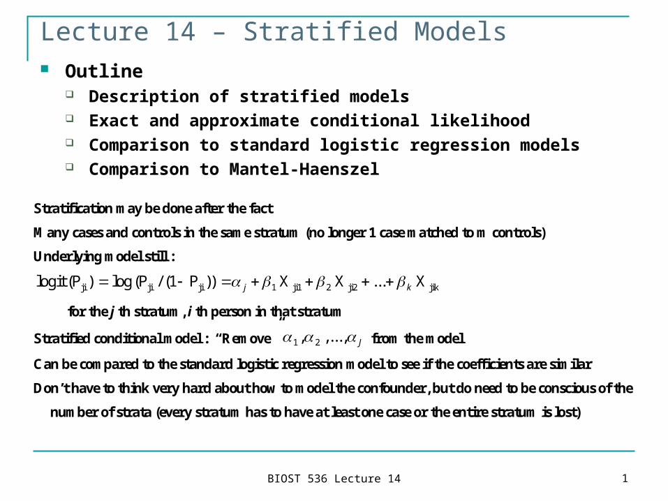
Stratification may be done after the fact
Many cases and controls in the same stratum (no longer 1 case matched to m controls)
Underlying model still :
logit (P log (P P X X Xji ji ji ji1 ji2 jik) / ( )) ... 1 1 2 j k
for the j th stratum, i th person in that stratum
Stratified conditional model : “Remove” 1 2, ,..., J from the model
Can be compared to the standard logistic regression model to see if the coefficients are similar
Don’t have to think very hard about how to model the confounder, but do need to be conscious of the
number of strata (every stratum has to have at least one case or the entire stratum is lost)

BIOST 536 Lecture 14 2
Leisure world data Suppose they stratified on 5-year age groups post hoc, rather
than forming matched sets
Multiple cases and controls in each stratum Need a minimum of one case and one control per stratum Cases are compared to only controls within their stratum and
the results accumulated over all strata
stratum outcome Age age group gall estrogen 1 1 74 70-74 0 1 1 0 75 70-74 1 0 1 0 72 70-74 0 0 1 1 74 70-74 1 0 1 0 75 70-74 0 1 2 1 67 65-69 0 1 2 0 67 65-69 1 1 2 1 68 65-69 0 0 2 0 67 65-69 1 1 2 1 65 65-69 0 0 2 1 67 65-69 1 1 2 0 68 65-69 0 1
BIOST 536 Lecture 14 3
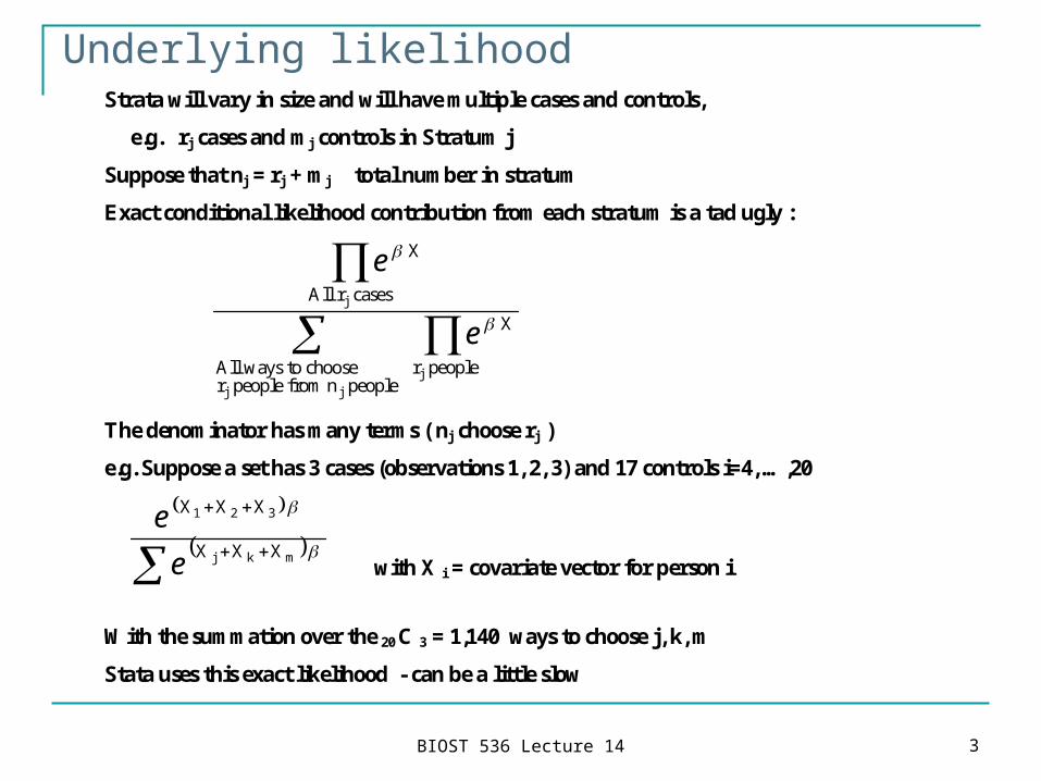
Underlying likelihoodStrata will vary in size and will have multiple cases and controls,
e.g. rj cases and mj controls in Stratum j
Suppose that nj = rj + mj total number in stratum
Exact conditional likelihood contribution from each stratum is a tad ugly :
e
e
X
All r cases
X
r peopleAll ways to chooser people from n people
j
j
j j
The denominator has many terms ( nj choose rj )
e.g. Suppose a set has 3 cases (observations 1, 2, 3) and 17 controls i=4, …,20
XXX
XXX
mkj
321
e
e
with X i = covariate vector for person i
With the summation over the 20 C 3 = 1,140 ways to choose j, k, m
Stata uses this exact likelihood - can be a little slow
BIOST 536 Lecture 14 4
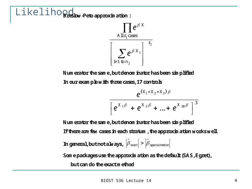
LikelihoodBreslow-Peto approximation :
e
e
X
All r cases
X
i=1 to n
rj
i
j
j
Numerator the same, but denominator has been simplified
In our example with three cases, 17 controls
1 2 3
1 2 20
X X X
3X X X...
e
e e e
Numerator the same, but denominator has been simplified
If there are few cases in each stratum, the approximation works well
In general, but not always, exact approximation
Some packages use the approximation as the default (SAS, Egret),
but can do the exact method
BIOST 536 Lecture 14 5
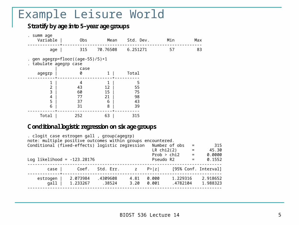
Example Leisure WorldStratify by age into 5–year age groups . summ age Variable | Obs Mean Std. Dev. Min Max -------------+-------------------------------------------------------- age | 315 70.76508 6.251271 57 83 . gen agegrp=floor((age-55)/5)+1 . tabulate agegrp case | case agegrp | 0 1 | Total -----------+----------------------+---------- 1 | 4 1 | 5 2 | 43 12 | 55 3 | 60 15 | 75 4 | 77 21 | 98 5 | 37 6 | 43 6 | 31 8 | 39 -----------+----------------------+---------- Total | 252 63 | 315
Conditional logistic regression on six age groups . clogit case estrogen gall , group(agegrp) note: multiple positive outcomes within groups encountered. Conditional (fixed-effects) logistic regression Number of obs = 315 LR chi2(2) = 45.30 Prob > chi2 = 0.0000 Log likelihood = -123.28176 Pseudo R2 = 0.1552 ------------------------------------------------------------------------------ case | Coef. Std. Err. z P>|z| [95% Conf. Interval] -------------+---------------------------------------------------------------- estrogen | 2.073984 .4309608 4.81 0.000 1.229316 2.918652 gall | 1.233267 .38524 3.20 0.001 .4782104 1.988323 ------------------------------------------------------------------------------

BIOST 536 Lecture 14 6
Example Leisure World. clogit, or Conditional (fixed-effects) logistic regression Number of obs = 315 LR chi2(2) = 45.30 Prob > chi2 = 0.0000 Log likelihood = -123.28176 Pseudo R2 = 0.1552 ------------------------------------------------------------------------------ case | Odds Ratio Std. Err. z P>|z| [95% Conf. Interval] -------------+---------------------------------------------------------------- estrogen | 7.956459 3.428922 4.81 0.000 3.418892 18.51631 gall | 3.432425 1.322307 3.20 0.001 1.613185 7.303279 ------------------------------------------------------------------------------
Compare to original matched sets analysis . clogit case estrogen gall , group(set) Conditional (fixed-effects) logistic regression Number of obs = 315 LR chi2(2) = 45.05 Prob > chi2 = 0.0000 Log likelihood = -78.871308 Pseudo R2 = 0.2221 ------------------------------------------------------------------------------ case | Coef. Std. Err. z P>|z| [95% Conf. Interval] -------------+---------------------------------------------------------------- estrogen | 2.114785 .4397942 4.81 0.000 1.252804 2.976766 gall | 1.274654 .4108678 3.10 0.002 .4693683 2.079941 ------------------------------------------------------------------------------ . clogit, or Conditional (fixed-effects) logistic regression Number of obs = 315 LR chi2(2) = 45.05 Prob > chi2 = 0.0000 Log likelihood = -78.871308 Pseudo R2 = 0.2221 ------------------------------------------------------------------------------ case | Odds Ratio Std. Err. z P>|z| [95% Conf. Interval] -------------+---------------------------------------------------------------- estrogen | 8.287802 3.644927 4.81 0.000 3.500144 19.62424 gall | 3.577465 1.469865 3.10 0.002 1.598984 8.003994 ------------------------------------------------------------------------------

BIOST 536 Lecture 14 7
Alcohol/tobacco exampleCompare the unconditional model to the exact and approximate conditional models . list in 1/10 +----------------------------+ | age alc tob cc | |----------------------------| 1. | 35-44 40-79 10-19 0 | 2. | 35-44 0-39 0-9 0 | 3. | 35-44 120+ 0-9 1 | 4. | 25-34 40-79 0-9 0 | 5. | 35-44 0-39 0-9 0 | 6. | 35-44 40-79 30+ 0 | 7. | 35-44 0-39 20-29 0 | 8. | 35-44 0-39 0-9 0 | 9. | 35-44 0-39 10-19 0 | 10. | 25-34 0-39 10-19 0 | +----------------------------+
First fit an unconditional analysis . xi: logistic cc i.age alc tob i.age _Iage_1-6 (naturally coded; _Iage_1 omitted) Logistic regression Number of obs = 975 LR chi2(7) = 276.83 Prob > chi2 = 0.0000 Log likelihood = -356.32774 Pseudo R2 = 0.2798 ------------------------------------------------------------------------------ cc | Odds Ratio Std. Err. z P>|z| [95% Conf. Interval] -------------+---------------------------------------------------------------- _Iage_2 | 5.909744 6.426261 1.63 0.102 .7014092 49.79273 _Iage_3 | 33.46817 34.99045 3.36 0.001 4.312349 259.7467 _Iage_4 | 58.15342 60.6019 3.90 0.000 7.542841 448.3484 _Iage_5 | 98.41494 103.5183 4.36 0.000 12.52333 773.3965 _Iage_6 | 98.71308 108.572 4.18 0.000 11.433 852.2935 alc | 2.908565 .3051819 10.18 0.000 2.367915 3.572657 tob | 1.552015 .1493572 4.57 0.000 1.285231 1.874178 ------------------------------------------------------------------------------
BIOST 536 Lecture 14 8
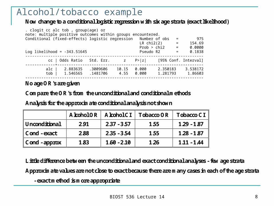
Alcohol/tobacco exampleNow change to a conditional logistic regression with six age strata (exact likelihood) . clogit cc alc tob , group(age) or note: multiple positive outcomes within groups encountered. Conditional (fixed-effects) logistic regression Number of obs = 975 LR chi2(2) = 154.69 Prob > chi2 = 0.0000 Log likelihood = -343.51645 Pseudo R2 = 0.1838 ------------------------------------------------------------------------------ cc | Odds Ratio Std. Err. z P>|z| [95% Conf. Interval] -------------+---------------------------------------------------------------- alc | 2.883635 .3009606 10.15 0.000 2.350183 3.538172 tob | 1.546565 .1481706 4.55 0.000 1.281793 1.86603 ------------------------------------------------------------------------------
No age OR's are given
Compare the OR's from the unconditional and conditional methods
Analysis for the approximate conditional analysis not shown
Alcohol OR Alcohol CI Tobacco OR Tobacco CI
Unconditional 2.91 2.37 - 3.57 1.55 1.29 - 1.87
Cond - exact 2.88 2.35 - 3.54 1.55 1.28 - 1.87
Cond - approx 1.83 1.60 - 2.10 1.26 1.11 - 1.44
Little difference between the unconditional and exact conditional analyses - few age strata
Approximate values are not close to exact because there are many cases in each of the age strata
- exact method is more appropriate

BIOST 536 Lecture 14 9
Alcohol/tobacco example
Effect modification
Consider effect modification of the tobacco effect by age after fitting group linear terms
for tobacco and alcohol
1 6 1 2logit (p) ( 1) ... ( 6)age age tob alc with 1 6, ..., conditioned out
versus
1 6 1 2
3 4 5 6 7
logit (p) ( 1) ... ( 6)
*( 2) *( 3) *( 4) *( 5) *( 6)
age age tob alc
tob age tob age tob age tob age tob age
with 1 6, ..., conditioned out
Perform a likelihood ratio test to determine if the association of tobacco use and disease is constant
over age group . est store A

BIOST 536 Lecture 14 10
Alcohol/tobacco example. xi: clogit cc alc tob i.age*tob, group(age) i.age _Iage_1-6 (naturally coded; _Iage_1 omitted) i.age*tob _IageXtob_# (coded as above) note: tob dropped because of collinearity note: multiple positive outcomes within groups encountered. note: _Iage_2 omitted because of no within-group variance. note: _Iage_3 omitted because of no within-group variance. Etc Conditional (fixed-effects) logistic regression Number of obs = 975 LR chi2(7) = 157.59 Prob > chi2 = 0.0000 Log likelihood = -342.0694 Pseudo R2 = 0.1872 ------------------------------------------------------------------------------ cc | Coef. Std. Err. z P>|z| [95% Conf. Interval] -------------+---------------------------------------------------------------- alc | 1.068209 .1053501 10.14 0.000 .8617269 1.274692 tob | -.1220555 .8373177 -0.15 0.884 -1.763168 1.519057 _IageXtob_2 | .4033857 .9070478 0.44 0.657 -1.374395 2.181167 _IageXtob_3 | .6426227 .856762 0.75 0.453 -1.0366 2.321845 _IageXtob_4 | .6927818 .8530814 0.81 0.417 -.979227 2.364791 _IageXtob_5 | .3139141 .8673739 0.36 0.717 -1.386108 2.013936 _IageXtob_6 | .4352042 .9089803 0.48 0.632 -1.346365 2.216773 ------------------------------------------------------------------------------ . lrtest . A Likelihood-ratio test LR chi2(5) = 2.89 (Assumption: A nested in .) Prob > chi2 = 0.7163
No evidence of effect modification of age on the tobacco effect
Now check for effect modification by age on the alcohol effect
BIOST 536 Lecture 14 11
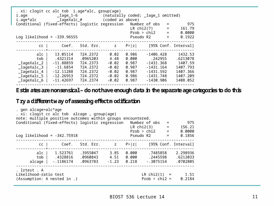
. xi: clogit cc alc tob i.age*alc, group(age) i.age _Iage_1-6 (naturally coded; _Iage_1 omitted) i.age*alc _IageXalc_# (coded as above) Conditional (fixed-effects) logistic regression Number of obs = 975 LR chi2(7) = 161.79 Prob > chi2 = 0.0000 Log likelihood = -339.96555 Pseudo R2 = 0.1922 ------------------------------------------------------------------------------ cc | Coef. Std. Err. z P>|z| [95% Conf. Interval] -------------+---------------------------------------------------------------- alc | 13.05114 724.2372 0.02 0.986 -1406.428 1432.53 tob | .4321314 .0965203 4.48 0.000 .242955 .6213078 _IageXalc_2 | -11.88859 724.2373 -0.02 0.987 -1431.368 1407.59 _IageXalc_3 | -11.6854 724.2372 -0.02 0.987 -1431.164 1407.793 _IageXalc_4 | -12.11288 724.2372 -0.02 0.987 -1431.592 1407.366 _IageXalc_5 | -12.26953 724.2372 -0.02 0.986 -1431.748 1407.209 _IageXalc_6 | -11.42697 724.2374 -0.02 0.987 -1430.906 1408.052 ------------------------------------------------------------------------------
Estimates are nonsensical – do not have enough data in the separate age categories to do this
Try a different way of assessing effect modification . gen alcage=alc*age . xi: clogit cc alc tob alcage , group(age) note: multiple positive outcomes within groups encountered. Conditional (fixed-effects) logistic regression Number of obs = 975 LR chi2(3) = 156.21 Prob > chi2 = 0.0000 Log likelihood = -342.75918 Pseudo R2 = 0.1856 ------------------------------------------------------------------------------ cc | Coef. Std. Err. z P>|z| [95% Conf. Interval] -------------+---------------------------------------------------------------- alc | 1.523761 .3955047 3.85 0.000 .7485858 2.298936 tob | .4328816 .0960843 4.51 0.000 .2445598 .6212033 alcage | -.1186174 .0963783 -1.23 0.218 -.3075154 .0702805 ------------------------------------------------------------------------------ . lrtest . A Likelihood-ratio test LR chi2(1) = 1.51 (Assumption: A nested in .) Prob > chi2 = 0.2184

BIOST 536 Lecture 14 12
Alcohol/tobacco example
No evidence of effect modification of age on the tobacco effect using the model
1 6 1 2 3logit (p) ( 1) ... ( 6) *age age tob alc tob age
This is a simpler form of effect modification that assumes the log OR for tobacco
changes linearly with age group
Interaction terms can be modeled in a simpler way than main effects, but not vice-versa
Test whether alcohol and tobacco interact . gen alctob=alc*tob . xi: clogit cc alc tob alctob , group(age) or Conditional (fixed-effects) logistic regression Number of obs = 975 LR chi2(3) = 155.78 Prob > chi2 = 0.0000 Log likelihood = -342.97434 Pseudo R2 = 0.1851 ------------------------------------------------------------------------------ cc | Odds Ratio Std. Err. z P>|z| [95% Conf. Interval] -------------+---------------------------------------------------------------- alc | 3.521209 .7743686 5.72 0.000 2.288229 5.418565 tob | 1.929266 .4469089 2.84 0.005 1.225219 3.037879 alctob | .9031615 .0875702 -1.05 0.293 .7468497 1.092189 ------------------------------------------------------------------------------ . lrtest . A Likelihood-ratio test LR chi2(1) = 1.08 (Assumption: A nested in .) Prob > chi2 = 0.2978
No evidence of an interaction between the two grouped linear variables
BIOST 536 Lecture 14 13
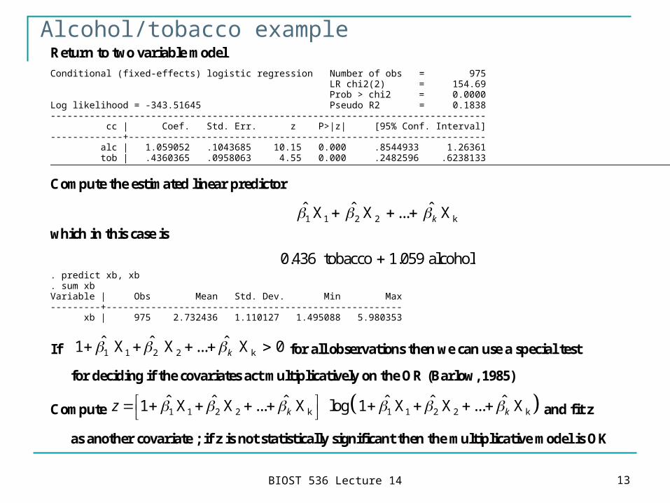
Alcohol/tobacco exampleReturn to two variable model Conditional (fixed-effects) logistic regression Number of obs = 975 LR chi2(2) = 154.69 Prob > chi2 = 0.0000 Log likelihood = -343.51645 Pseudo R2 = 0.1838 ------------------------------------------------------------------------------ cc | Coef. Std. Err. z P>|z| [95% Conf. Interval] -------------+---------------------------------------------------------------- alc | 1.059052 .1043685 10.15 0.000 .8544933 1.26361 tob | .4360365 .0958063 4.55 0.000 .2482596 .6238133
Compute the estimated linear predictor
1 1 2 2 kˆ ˆ ˆX X ... Xk
which in this case is
0.436 tobacco 1.059 alcohol . predict xb, xb . sum xb Variable | Obs Mean Std. Dev. Min Max ---------+----------------------------------------------------- xb | 975 2.732436 1.110127 1.495088 5.980353
If 1 1 2 2 kˆ ˆ ˆ1 X X ... X 0k for all observations then we can use a special test
for deciding if the covariates act multiplicatively on the OR (Barlow, 1985)
Compute 1 1 2 2 k 1 1 2 2 kˆ ˆ ˆ ˆ ˆ ˆ1 X X ... X log 1 X X ... Xk kz and fit z
as another covariate ; if z is not statistically significant then the multiplicative model is OK
BIOST 536 Lecture 14 14
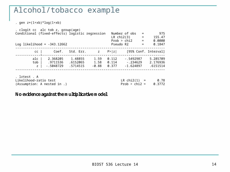
Alcohol/tobacco example. gen z=(1+xb)*log(1+xb) . clogit cc alc tob z, group(age) Conditional (fixed-effects) logistic regression Number of obs = 975 LR chi2(3) = 155.47 Prob > chi2 = 0.0000 Log likelihood = -343.12662 Pseudo R2 = 0.1847 ------------------------------------------------------------------------------ cc | Coef. Std. Err. z P>|z| [95% Conf. Interval] -------------+---------------------------------------------------------------- alc | 2.368205 1.48855 1.59 0.112 -.5492987 5.285709 tob | .9711536 .6152065 1.58 0.114 -.234629 2.176936 z | -.5048729 .5714515 -0.88 0.377 -1.624897 .6151514 ------------------------------------------------------------------------------ . lrtest . A Likelihood-ratio test LR chi2(1) = 0.78 (Assumption: A nested in .) Prob > chi2 = 0.3772
No evidence against the multiplicative model
BIOST 536 Lecture 14 15
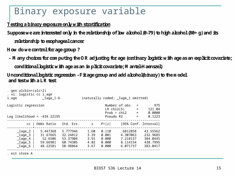
Binary exposure variableTesting a binary exposure only with stratification
Suppose we are interested only in the relationship of low alcohol (0-79) to high alcohol (80+ g) and its
relationship to esophageal cancer
How do we control for age group ?
- Many choices for computing the OR adjusting for age (ordinary logistic with age as an explicit covariate;
conditional logistic with age as an implicit covariate; Mantel-Haenszel)
Unconditional logistic regression - Fit age group and add alcohol(binary) to the model and test with a LR test . gen alcbin=(alc>2) . xi: logistic cc i.age i.age _Iage_1-6 (naturally coded; _Iage_1 omitted) Logistic regression Number of obs = 975 LR chi2(5) = 121.04 Prob > chi2 = 0.0000 Log likelihood = -434.22195 Pseudo R2 = 0.1223 ------------------------------------------------------------------------------ cc | Odds Ratio Std. Err. z P>|z| [95% Conf. Interval] -------------+---------------------------------------------------------------- _Iage_2 | 5.447368 5.777946 1.60 0.110 .6812858 43.55562 _Iage_3 | 31.67665 32.24812 3.39 0.001 4.307063 232.9685 _Iage_4 | 52.6506 53.37904 3.91 0.000 7.218137 384.0445 _Iage_5 | 59.66981 60.74305 4.02 0.000 8.114154 438.7995 _Iage_6 | 48.22581 50.98864 3.67 0.000 6.071737 383.0417 ------------------------------------------------------------------------------ . est store A
BIOST 536 Lecture 14 16
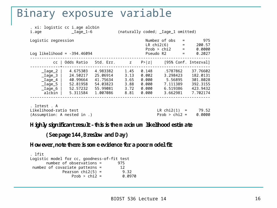
Binary exposure variable. xi: logistic cc i.age alcbin i.age _Iage_1-6 (naturally coded; _Iage_1 omitted) Logistic regression Number of obs = 975 LR chi2(6) = 200.57 Prob > chi2 = 0.0000 Log likelihood = -394.46094 Pseudo R2 = 0.2027 ------------------------------------------------------------------------------ cc | Odds Ratio Std. Err. z P>|z| [95% Conf. Interval] -------------+---------------------------------------------------------------- _Iage_2 | 4.675303 4.983382 1.45 0.148 .5787862 37.76602 _Iage_3 | 24.50217 25.06914 3.13 0.002 3.298423 182.0131 _Iage_4 | 40.99664 41.75634 3.65 0.000 5.56895 301.8028 _Iage_5 | 52.81958 54.03823 3.88 0.000 7.111389 392.3155 _Iage_6 | 52.57232 55.99081 3.72 0.000 6.519386 423.9432 alcbin | 5.311584 1.007086 8.81 0.000 3.662981 7.702174 ------------------------------------------------------------------------------ . lrtest . A Likelihood-ratio test LR chi2(1) = 79.52 (Assumption: A nested in .) Prob > chi2 = 0.0000
Highly significant result - this is the maximum likelihood estimate
( See page 144, Breslow and Day)
However, note there is some evidence for a poor model fit . lfit Logistic model for cc, goodness-of-fit test number of observations = 975 number of covariate patterns = 12 Pearson chi2(5) = 9.32 Prob > chi2 = 0.0970

BIOST 536 Lecture 14 17
Now try conditional logistic regression . clogit cc alcbin, group(age) or note: multiple positive outcomes within groups encountered. Conditional (fixed-effects) logistic regression Number of obs = 975 LR chi2(1) = 79.01 Prob > chi2 = 0.0000 Log likelihood = -381.35643 Pseudo R2 = 0.0939 ------------------------------------------------------------------------------ cc | Odds Ratio Std. Err. z P>|z| [95% Conf. Interval] -------------+---------------------------------------------------------------- alcbin | 5.250918 .9913914 8.78 0.000 3.626815 7.6023 ------------------------------------------------------------------------------
Pretty close to the unconditional estimate - the conditional estimate will also
be very close to the Mantel-Haenszel estimate . mhodds cc alcbin age Mantel-Haenszel estimate of the odds ratio Comparing alcbin==1 vs. alcbin==0, controlling for age ---------------------------------------------------------------- Odds Ratio chi2(1) P>chi2 [95% Conf. Interval] ---------------------------------------------------------------- 5.157623 85.01 0.0000 3.494918 7.611359 ---------------------------------------------------------------- Consider another binary exposure variable (0-9 cigarettes versus more) . gen tobbin=(tob>1) if tob~=. . tabulate tobbin cc | cc tobbin | 0 1 | Total -----------+----------------------+---------- 0 | 447 78 | 525 1 | 328 122 | 450 -----------+----------------------+---------- Total | 775 200 | 975
BIOST 536 Lecture 14 18
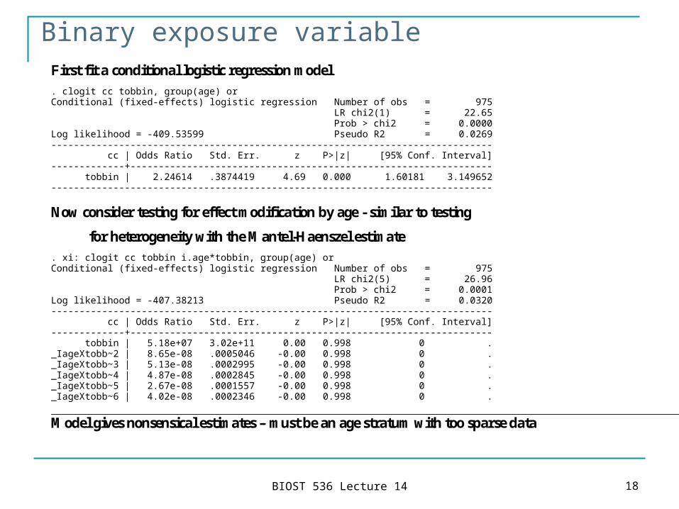
Binary exposure variableFirst fit a conditional logistic regression model . clogit cc tobbin, group(age) or Conditional (fixed-effects) logistic regression Number of obs = 975 LR chi2(1) = 22.65 Prob > chi2 = 0.0000 Log likelihood = -409.53599 Pseudo R2 = 0.0269 ------------------------------------------------------------------------------ cc | Odds Ratio Std. Err. z P>|z| [95% Conf. Interval] -------------+---------------------------------------------------------------- tobbin | 2.24614 .3874419 4.69 0.000 1.60181 3.149652 ------------------------------------------------------------------------------
Now consider testing for effect modification by age - similar to testing
for heterogeneity with the Mantel-Haenszel estimate . xi: clogit cc tobbin i.age*tobbin, group(age) or Conditional (fixed-effects) logistic regression Number of obs = 975 LR chi2(5) = 26.96 Prob > chi2 = 0.0001 Log likelihood = -407.38213 Pseudo R2 = 0.0320 ------------------------------------------------------------------------------ cc | Odds Ratio Std. Err. z P>|z| [95% Conf. Interval] -------------+---------------------------------------------------------------- tobbin | 5.18e+07 3.02e+11 0.00 0.998 0 . _IageXtobb~2 | 8.65e-08 .0005046 -0.00 0.998 0 . _IageXtobb~3 | 5.13e-08 .0002995 -0.00 0.998 0 . _IageXtobb~4 | 4.87e-08 .0002845 -0.00 0.998 0 . _IageXtobb~5 | 2.67e-08 .0001557 -0.00 0.998 0 . _IageXtobb~6 | 4.02e-08 .0002346 -0.00 0.998 0 .
Model gives nonsensical estimates – must be an age stratum with too sparse data
BIOST 536 Lecture 14 19
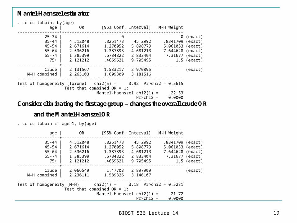
Mantel-Haenszel estimator . cc cc tobbin, by(age) age | OR [95% Conf. Interval] M-H Weight -----------------+------------------------------------------------- 25-34 | . 0 . 0 (exact) 35-44 | 4.512048 .8251473 45.2992 .8341709 (exact) 45-54 | 2.671614 1.270052 5.808779 5.061033 (exact) 55-64 | 2.536216 1.387893 4.681213 7.644628 (exact) 65-74 | 1.385399 .6734822 2.833404 7.31677 (exact) 75+ | 2.121212 .4669621 9.705495 1.5 (exact) -----------------+------------------------------------------------- Crude | 2.131567 1.533217 2.970895 (exact) M-H combined | 2.263103 1.609809 3.181516 ------------------------------------------------------------------- Test of homogeneity (Tarone) chi2(5) = 3.92 Pr>chi2 = 0.5615 Test that combined OR = 1: Mantel-Haenszel chi2(1) = 22.53 Pr>chi2 = 0.0000
Consider eliminating the first age group – changes the overall crude OR
and the Mantel-Haenszel OR . cc cc tobbin if age>1, by(age) age | OR [95% Conf. Interval] M-H Weight -----------------+------------------------------------------------- 35-44 | 4.512048 .8251473 45.2992 .8341709 (exact) 45-54 | 2.671614 1.270052 5.808779 5.061033 (exact) 55-64 | 2.536216 1.387893 4.681213 7.644628 (exact) 65-74 | 1.385399 .6734822 2.833404 7.31677 (exact) 75+ | 2.121212 .4669621 9.705495 1.5 (exact) -----------------+------------------------------------------------- Crude | 2.066549 1.47703 2.897909 (exact) M-H combined | 2.236111 1.589326 3.146107 ------------------------------------------------------------------- Test of homogeneity (M-H) chi2(4) = 3.18 Pr>chi2 = 0.5281 Test that combined OR = 1: Mantel-Haenszel chi2(1) = 21.72 Pr>chi2 = 0.0000

BIOST 536 Lecture 14 20
Eliminate the first age group in the conditional logistic regression and
check for interaction . clogit cc tobbin if age>1, group(age) or Conditional (fixed-effects) logistic regression Number of obs = 859 LR chi2(1) = 21.84 Prob > chi2 = 0.0000 Log likelihood = -405.1876 Pseudo R2 = 0.0262 ------------------------------------------------------------------------------ cc | Odds Ratio Std. Err. z P>|z| [95% Conf. Interval] -------------+---------------------------------------------------------------- tobbin | 2.219142 .3838213 4.61 0.000 1.581109 3.114643 ------------------------------------------------------------------------------ . est store A . xi: clogit cc tobbin i.age*tobbin if age>1, group(age) or Conditional (fixed-effects) logistic regression Number of obs = 859 LR chi2(5) = 25.11 Prob > chi2 = 0.0001 Log likelihood = -403.55349 Pseudo R2 = 0.0302 ------------------------------------------------------------------------------ cc | Odds Ratio Std. Err. z P>|z| [95% Conf. Interval] -------------+---------------------------------------------------------------- tobbin | 1.382556 .4672329 0.96 0.338 .712886 2.681298 _IageXtobb~2 | 3.24064 2.854645 1.33 0.182 .576523 18.21566 _IageXtobb~3 | 1.923551 .9431359 1.33 0.182 .7357855 5.028705 _IageXtobb~4 | 1.827305 .8127669 1.36 0.175 .7641966 4.369351 _IageXtobb~6 | 1.507227 1.12128 0.55 0.581 .3507032 6.477652 ------------------------------------------------------------------------------ . lrtest . A Likelihood-ratio test LR chi2(4) = 3.27 (Assumption: A nested in .) Prob > chi2 = 0.5140
Test of interaction is testing homogeneity of the OR across age strata -
similar to M-H result above
BIOST 536 Lecture 14 21
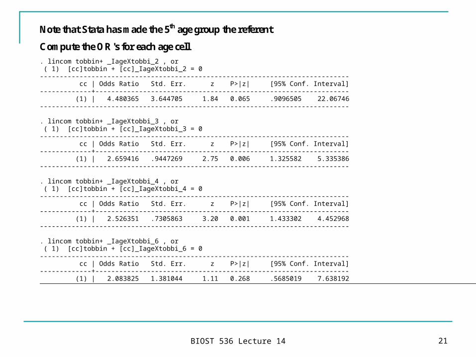
Note that Stata has made the 5th age group the referent
Compute the OR's for each age cell . lincom tobbin+ _IageXtobbi_2 , or ( 1) [cc]tobbin + [cc]_IageXtobbi_2 = 0 ------------------------------------------------------------------------------ cc | Odds Ratio Std. Err. z P>|z| [95% Conf. Interval] -------------+---------------------------------------------------------------- (1) | 4.480365 3.644705 1.84 0.065 .9096505 22.06746 ------------------------------------------------------------------------------ . lincom tobbin+ _IageXtobbi_3 , or ( 1) [cc]tobbin + [cc]_IageXtobbi_3 = 0 ------------------------------------------------------------------------------ cc | Odds Ratio Std. Err. z P>|z| [95% Conf. Interval] -------------+---------------------------------------------------------------- (1) | 2.659416 .9447269 2.75 0.006 1.325582 5.335386 ------------------------------------------------------------------------------ . lincom tobbin+ _IageXtobbi_4 , or ( 1) [cc]tobbin + [cc]_IageXtobbi_4 = 0 ------------------------------------------------------------------------------ cc | Odds Ratio Std. Err. z P>|z| [95% Conf. Interval] -------------+---------------------------------------------------------------- (1) | 2.526351 .7305863 3.20 0.001 1.433302 4.452968 ------------------------------------------------------------------------------ . lincom tobbin+ _IageXtobbi_6 , or ( 1) [cc]tobbin + [cc]_IageXtobbi_6 = 0 ------------------------------------------------------------------------------ cc | Odds Ratio Std. Err. z P>|z| [95% Conf. Interval] -------------+---------------------------------------------------------------- (1) | 2.083825 1.381044 1.11 0.268 .5685019 7.638192
BIOST 536 Lecture 14 22
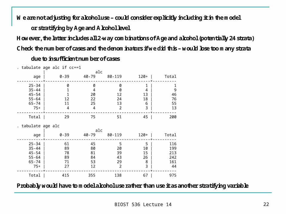
We are not adjusting for alcohol use – could consider explicitly including it in the model
or stratifying by Age and Alcohol level
However, the latter includes all 2-way combinations of Age and alcohol (potentially 24 strata)
Check the number of cases and the denominators if we did this – would lose too many strata
due to insufficient number of cases . tabulate age alc if cc==1 | alc age | 0-39 40-79 80-119 120+ | Total -----------+--------------------------------------------+---------- 25-34 | 0 0 0 1 | 1 35-44 | 1 4 0 4 | 9 45-54 | 1 20 12 13 | 46 55-64 | 12 22 24 18 | 76 65-74 | 11 25 13 6 | 55 75+ | 4 4 2 3 | 13 -----------+--------------------------------------------+---------- Total | 29 75 51 45 | 200 . tabulate age alc | alc age | 0-39 40-79 80-119 120+ | Total -----------+--------------------------------------------+---------- 25-34 | 61 45 5 5 | 116 35-44 | 89 80 20 10 | 199 45-54 | 78 81 39 15 | 213 55-64 | 89 84 43 26 | 242 65-74 | 71 53 29 8 | 161 75+ | 27 12 2 3 | 44 -----------+--------------------------------------------+---------- Total | 415 355 138 67 | 975
Probably would have to model alcohol use rather than use it as another stratifying variable
BIOST 536 Lecture 14 23
Example
Data on condom use collected as part of a nationwide survey of males ages 19-39
Sample was stratified such that low income groups and minorities were oversampled
Sampling fractions not included here, but can be accomodated by Stata using pweights
(precision can be enhanced by appropriate weighting)
Below we use data on men with multiple "current" partners, but only use the first partner
here so that each male appears only once
Outcome: condom used for the prevention of disease
Covariates:
Have information on male's age, race, and education and same information on the first female partner
Male age both continuous and grouped (19-24, 25-29, 30-34, 35-39)
Female age both continuous and grouped (<24, 25-29, 30-34, 35+)
Education by number of years completed and categorized into three tertiles (low, medium, high)
BIOST 536 Lecture 14 24
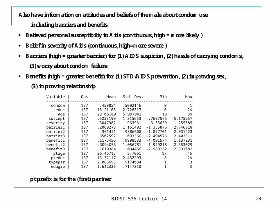
Also have information on attitudes and beliefs of the male about condom use
including barriers and benefits
Believed personal susceptibilty to Aids (continuous, high = more likely )
Belief in severity of Aids (continuous, high=more severe )
Barriers (high = greater barrier) for (1) AIDS suspicion, (2) hassle of carrying condoms,
(3) worry about condom failure
Benefits (high = greater benefit) for (1) STD/AIDS prevention, (2) improving sex,
(3) improving relationship
Variable | Obs Mean Std. Dev. Min Max ---------+----------------------------------------------------- condom | 137 .459854 .5002146 0 1 educ | 137 13.21168 2.726317 6 24 age | 137 28.05109 5.997942 19 39 suscept | 137 .5258199 1.315653 -.7697575 5.175257 severity | 137 .3047982 .963961 -3.35639 1.255085 barrier1 | 137 .2069278 1.161492 -1.355876 2.746918 barrier2 | 137 -.301471 .9886608 -1.877701 2.031423 barrier3 | 137 .3502592 1.093366 -2.494576 2.403311 benefit1 | 137 .1175456 .9908533 -4.091574 1.137231 benefit2 | 137 -.3094053 1.056781 -1.949218 2.353029 benefit3 | 137 .1619384 1.034456 -2.989232 2.331082 ptage | 137 26.46715 5.7061 17 45 pteduc | 137 13.32117 2.452293 8 24 typepar | 137 2.065693 .5174084 1 3 edugrp | 137 1.642336 .7147318 1 3
pt prefix is for the (first) partner
BIOST 536 Lecture 14 25
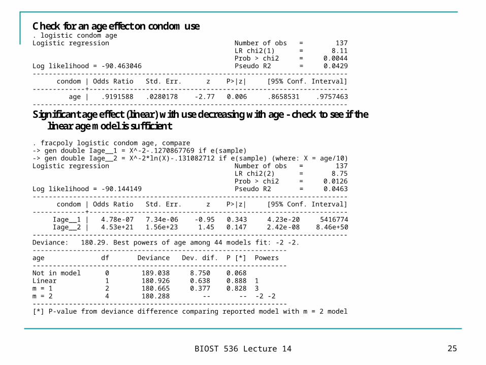
Check for an age effect on condom use . logistic condom age Logistic regression Number of obs = 137 LR chi2(1) = 8.11 Prob > chi2 = 0.0044 Log likelihood = -90.463046 Pseudo R2 = 0.0429 ------------------------------------------------------------------------------ condom | Odds Ratio Std. Err. z P>|z| [95% Conf. Interval] -------------+---------------------------------------------------------------- age | .9191588 .0280178 -2.77 0.006 .8658531 .9757463 ------------------------------------------------------------------------------
Significant age effect (linear) with use decreasing with age - check to see if the linear age model is sufficient
. fracpoly logistic condom age, compare -> gen double Iage__1 = X^-2-.1270867769 if e(sample) -> gen double Iage__2 = X^-2*ln(X)-.131082712 if e(sample) (where: X = age/10) Logistic regression Number of obs = 137 LR chi2(2) = 8.75 Prob > chi2 = 0.0126 Log likelihood = -90.144149 Pseudo R2 = 0.0463 ------------------------------------------------------------------------------ condom | Odds Ratio Std. Err. z P>|z| [95% Conf. Interval] -------------+---------------------------------------------------------------- Iage__1 | 4.78e-07 7.34e-06 -0.95 0.343 4.23e-20 5416774 Iage__2 | 4.53e+21 1.56e+23 1.45 0.147 2.42e-08 8.46e+50 ------------------------------------------------------------------------------ Deviance: 180.29. Best powers of age among 44 models fit: -2 -2. --------------------------------------------------------------- age df Deviance Dev. dif. P [*] Powers --------------------------------------------------------------- Not in model 0 189.038 8.750 0.068 Linear 1 180.926 0.638 0.888 1 m = 1 2 180.665 0.377 0.828 3 m = 2 4 180.288 -- -- -2 -2 --------------------------------------------------------------- [*] P-value from deviance difference comparing reported model with m = 2 model

BIOST 536 Lecture 14 26
Linear age term seems sufficient; check survey variables . logistic condom age suscept Logistic regression Number of obs = 137 LR chi2(2) = 9.46 Prob > chi2 = 0.0088 Log likelihood = -89.786959 Pseudo R2 = 0.0501 ------------------------------------------------------------------------------ condom | Odds Ratio Std. Err. z P>|z| [95% Conf. Interval] -------------+---------------------------------------------------------------- age | .9207313 .0281974 -2.70 0.007 .8670913 .9776895 suscept | .8528191 .117933 -1.15 0.250 .6503507 1.11832
The more susceptible to AIDS - the less likely to use condoms (!!) . logistic condom age severity Logistic regression Number of obs = 137 LR chi2(2) = 10.52 Prob > chi2 = 0.0052 Log likelihood = -89.259015 Pseudo R2 = 0.0557 ------------------------------------------------------------------------------ condom | Odds Ratio Std. Err. z P>|z| [95% Conf. Interval] -------------+---------------------------------------------------------------- age | .924917 .0284517 -2.54 0.011 .8708004 .9823968 severity | .7475505 .1430667 -1.52 0.128 .5137325 1.087787 ------------------------------------------------------------------------------
The greater the belief that AIDS is severe - the less likely to use condoms (!!) . logistic condom age barrier1 barrier2 barrier3 Logistic regression Number of obs = 137 LR chi2(4) = 10.74 Prob > chi2 = 0.0296 Log likelihood = -89.148431 Pseudo R2 = 0.0568 ------------------------------------------------------------------------------ condom | Odds Ratio Std. Err. z P>|z| [95% Conf. Interval] -------------+---------------------------------------------------------------- age | .9188923 .0283186 -2.74 0.006 .865032 .9761062 barrier1 | .7901184 .1295718 -1.44 0.151 .5729324 1.089635 barrier2 | 1.149433 .2147997 0.75 0.456 .7969219 1.657874 barrier3 | .9401959 .1583129 -0.37 0.714 .6759127 1.307814 ------------------------------------------------------------------------------
None of the barriers appears to affect condom use
BIOST 536 Lecture 14 27
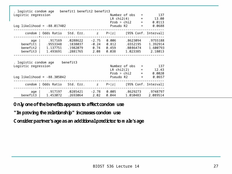
. logistic condom age benefit1 benefit2 benefit3 Logistic regression Number of obs = 137 LR chi2(4) = 13.00 Prob > chi2 = 0.0113 Log likelihood = -88.017402 Pseudo R2 = 0.0688 ------------------------------------------------------------------------------ condom | Odds Ratio Std. Err. z P>|z| [95% Conf. Interval] -------------+---------------------------------------------------------------- age | .917169 .0288622 -2.75 0.006 .8623094 .9755188 benefit1 | .9553348 .1838037 -0.24 0.812 .6552195 1.392914 benefit2 | 1.137751 .1982079 0.74 0.459 .8086474 1.600793 benefit3 | 1.493691 .2881765 2.08 0.038 1.023385 2.18013 ------------------------------------------------------------------------------ . logistic condom age benefit3 Logistic regression Number of obs = 137 LR chi2(2) = 12.43 Prob > chi2 = 0.0020 Log likelihood = -88.305042 Pseudo R2 = 0.0657 ------------------------------------------------------------------------------ condom | Odds Ratio Std. Err. z P>|z| [95% Conf. Interval] -------------+---------------------------------------------------------------- age | .917197 .0285421 -2.78 0.005 .8629273 .9748797 benefit3 | 1.453072 .2693064 2.02 0.044 1.010483 2.089514
Only one of the benefits appears to affect condom use
"Improving the relationship" increases condom use
Consider partner's age as an additional predictor to male’s age
BIOST 536 Lecture 14 28
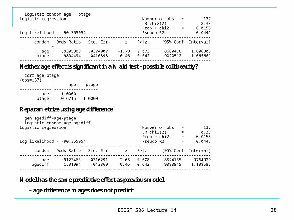
. logistic condom age ptage Logistic regression Number of obs = 137 LR chi2(2) = 8.33 Prob > chi2 = 0.0155 Log likelihood = -90.355054 Pseudo R2 = 0.0441 ------------------------------------------------------------------------------ condom | Odds Ratio Std. Err. z P>|z| [95% Conf. Interval] -------------+---------------------------------------------------------------- age | .9305389 .0374007 -1.79 0.073 .8600478 1.006808 ptage | .9804494 .0416898 -0.46 0.642 .9020512 1.065661 ------------------------------------------------------------------------------
Neither age effect is significant in a Wald test - possible collinearity? . corr age ptage (obs=137) | age ptage -------------+------------------ age | 1.0000 ptage | 0.6715 1.0000
Reparametrize using age difference . gen agediff=age-ptage . logistic condom age agediff Logistic regression Number of obs = 137 LR chi2(2) = 8.33 Prob > chi2 = 0.0155 Log likelihood = -90.355054 Pseudo R2 = 0.0441 ------------------------------------------------------------------------------ condom | Odds Ratio Std. Err. z P>|z| [95% Conf. Interval] -------------+---------------------------------------------------------------- age | .9123463 .0316291 -2.65 0.008 .8524135 .9764929 agediff | 1.01994 .043369 0.46 0.642 .9383845 1.108585 ------------------------------------------------------------------------------
Model has the same predictive effect as previous model
– age difference in ages does not predict
BIOST 536 Lecture 14 29
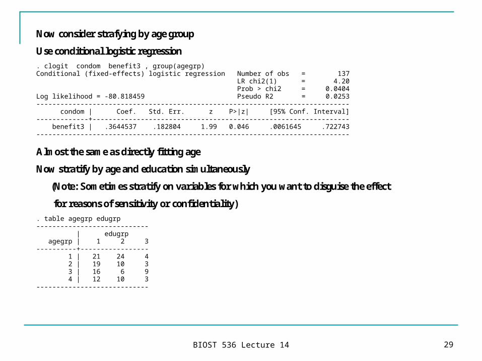
Now consider strafying by age group
Use conditional logistic regression . clogit condom benefit3 , group(agegrp) Conditional (fixed-effects) logistic regression Number of obs = 137 LR chi2(1) = 4.20 Prob > chi2 = 0.0404 Log likelihood = -80.818459 Pseudo R2 = 0.0253 ------------------------------------------------------------------------------ condom | Coef. Std. Err. z P>|z| [95% Conf. Interval] -------------+---------------------------------------------------------------- benefit3 | .3644537 .182804 1.99 0.046 .0061645 .722743 ------------------------------------------------------------------------------
Almost the same as directly fitting age
Now stratify by age and education simultaneously
(Note: Sometimes stratify on variables for which you want to disguise the effect
for reasons of sensitivity or confidentiality) . table agegrp edugrp ---------------------------- | edugrp agegrp | 1 2 3 ----------+----------------- 1 | 21 24 4 2 | 19 10 3 3 | 16 6 9 4 | 12 10 3 ----------------------------

BIOST 536 Lecture 14 30
. gen ageeduc=3*(agegrp-1)+edugrp . table ageeduc condom ---------------------- | condom ageeduc | 0 1 ----------+----------- 1 | 11 10 2 | 10 14 3 | 1 3 4 | 11 8 5 | 2 8 6 | 2 1 7 | 11 5 8 | 3 3 9 | 4 5 10 | 9 3 11 | 7 3 12 | 3 ----------------------
Ageeduc = 12 will drop out since no members use condoms . clogit condom benefit3 , group(ageeduc) note: 1 group (3 obs) dropped because of all positive or all negative outcomes. Conditional (fixed-effects) logistic regression Number of obs = 134 LR chi2(1) = 3.06 Prob > chi2 = 0.0803 Log likelihood = -69.653107 Pseudo R2 = 0.0215 ------------------------------------------------------------------------------ condom | Coef. Std. Err. z P>|z| [95% Conf. Interval] -------------+---------------------------------------------------------------- benefit3 | .3190356 .1864274 1.71 0.087 -.0463554 .6844266 ------------------------------------------------------------------------------
Slightly reduced OR for benefit3 - now technically ns; Strata are too small
In this case the unconditional analysis might be preferred since the age effect is of scientific interest
Related Documents