BIOST 536 Lecture 1 1 Lecture 1 - Introduction Overview of course Focus is on binary outcomes Some ordinal outcomes considered Simple examples Definitions.

BIOST 536 Lecture 1 1

Lecture 1 - Introduction

Overview of course Focus is on binary outcomes Some ordinal outcomes considered

Simple examples Definitions Hypothetical example Framingham example


Binary outcome data Outcome variable Y

Response to treatment: Success versus failure Outcome of screening or diagnostic test:

Positive versus negative Disease prevalence at a specific time or age:

Present versus absent Disease incidence in a time interval ( 0 , t ) where t may be

a predefined single time point and all outcomes are assessed; otherwise consider survival models

Dichotimization of a continuous variable: High blood pressure (SBP ≥ 140) Overweight (BMI ≥ 30) Low birthweight ( < 2500 grams )

Case (disease) versus Control (no disease) { Using outcome in an imprecise sense }


Covariates Vector of variables called “X”

Randomized treatment Exposure ( Exposed = 1 versus Unexposed = 0 ) Degree of exposure (continuous; ordinal) Demographic variables: age, race, gender Baseline characteristics; propensity score

Scientific variable of interest (usually treatment or exposure)

Other “control” variables Precision variables Confounders or potential confounders Effect modifiers

≥≥


Example 1Prostate cancer (Hosmer & Lemeshow, 1.6.3)

Y = 1 if the tumor penetrates capsule; 0 if no penetration X = Gleason score, age, race, rectal exam, PSA, volume

Could decide if there is any association of Gleason score with capsule penetration

Could decide if there is an ordinal association of Gleason score with outcome

May want to adjust for age, race, PSA etc or determine if they modify the association

YGleason score

2-5 6 7 8-9

0 64 101 55 7

1 6 38 73 36


Example 2

Low birthweight determinant (Hosmer & Lemeshow, 1.6.2)

Y = low birthweight (< 2500 grams) X = mother’s age, weight, smoking, number of

prenatal visits, etc Not dichotomizing birthweight may be more

powerful, but we may have a particular interest in this definition of low birthweight

Is the goal to discover new, possibly mutable, risk factors for LBW? (Scientific hypothesis testing/hypothesis generation)

Goal may be to predict LBW from known risk factors (empirical models with validation)


Example 3

Framingham Prediction of coronary heart disease

Y = CHD within a prescribed time window X = age, gender, blood pressure, serum

cholesterol, smoking, etc Framingham cohort is followed with regular exams

and updated risk factors If the goal is to predict 10 year CHD risk?

How do we handle dropouts and deaths due to other causes < 10 years?

Do we use the updated risk factors in the prediction model?

May prefer true cohort methods (survival analysis) or time-matched case-control studies


Example 4

Leprosy case-control study (Clayton & Hills 18.1) Y = 1 if leprosy case; 0 otherwise X = age, presence/absence of BCG scar BCG was a vaccine against tuberculosis; but may

protect against leprosy as well Stratified case-control data

Leprosy cases Healthy controls

Age BCG scar No BCG scar BCG scar No BCG scar

0-4 1 1 7,593 11,719

5-9 11 14 7,143 10,184

10-14 28 22 5,611 7,561

15-19 16 28 2,208 8,117

20-24 20 19 2,438 5,588

25-29 36 11 4,356 1,625

30-34 47 6 5,245 1,234


Definitions Time or age of disease occurrence T Incidence rate at time t (or age t)

Numerator is probability that a person without disease at time t gets disease in the next small interval of time

Incidence rates theoretically can change continuously in time

Often assume that the incidence rates are piecewise constant over a longer duration

0

Pr( ( , ) | )( ) lim

t

T t t t T tt

t

# of new incident casesˆPerson-time in years

0.0

1.0

2.0

3.0

4In

cide

nce

ra

te

0 5 10 15 20Years

Actual incidence rate over time

0.0

1.0

2.0

3.0

4In

cide

nce

ra

te

0 5 10 15 20Years

Actual

Assumed constant over 20 years

Actual incidence rate versus assumed

0.0

1.0

2.0

3.0

4In

cide

nce

ra

te

0 5 10 15 20Years

ActualAssumed constant over 20 years

Assumed constant over 10 years

Actual incidence rate versus assumed


Definitions Incidence rate ratio at time t (or age t) for individuals in Group

1 (exposed) versus Group 0 (unexposed)

Often assume that the IRR is constant, i.e. does not depend on time even if the incidence rate ratios do

Incidence rates can be modeled and compared with Poisson regression models

Poisson and binomial models are similar when the event rate is low, but the variances differ

1

0

( )( )

( )

tIRR t

t

1

0

( )

( )

tIRR

t


Definitions - continued Risk of disease by time t (or age t) starting at time 0

Cumulative risk over the time interval assuming no competing risks

“Disease prevalence” if competing risks

Risk of disease within a time interval

Risk ratio at time t (or age t) for individuals in Group 1 (exposed) versus Group 0 (unexposed) As time increases probabilities increase for common diseases Risk ratio is usually not constant over time

Risk difference at time t (or age t)

0 0

( ) ( ) 1 exp ( ) ( )t t

P t P T t s ds s ds

1

0

( )( )

( )

P tRR t

P t

1 0( ) ( ) ( )RD t P t P t

0 1[ , )t t t

0 1 0( ) ( [ , ) | )P t P T t t T t

( ) ( | alive)P t P T t


Cohort model 2 x 2 Table Cohort study design

Assemble two disease-free groups: n 1 Exposed and n 0 Unexposed individuals

Follow both groups for exactly the same period of time and measure occurrence of disease (Y=1 disease; Y=0 if no disease)

Then let r 1 = Exposed with disease and r 0 = Unexposed with disease

0 0 0( , )r Binom n p1 1 1( , )r Binom n p

1 Pr ( 1| 1) disease risk for exposedp Y X

0 Pr ( 1| 0) disease risk for unexposedp Y X


Measures of Association for 2 x 2 Tables

Risk difference Excess risk model Measures absolute effect of exposure

Risk ratio Measures relative effect of exposure Ratio is constrained by p0

If p0 = 0.50 then max RR = 2.0

If p0 is small thenlittle range restriction

1 0RD p p

1 0RR p p

05

10

15

20

Ma

xim

al v

alue

of R

R0 .2 .4 .6 .8 1

Probability of Y=1 for unexposed


Measures of Association for 2 x 2 Tables - continued Odds ratio

Measures relative effect of exposure Not constrained Can switch rows and columns and get the

same OR or 1/OR if transposed Natural parameter for statistical inference

Logistic regression models log odds ratio Asymptotic p-values and CI’s work well even in

small to moderate sample sizes OR approximates the RR for outcomes with

low probability

1 0 0 11 1OR p p p p

0 log ( )OR OR

0 11 1 1p p


Statistical Inference

Null hypothesis Theoretically equivalent, but not mathematically,

equivalent tests Estimation

1 0 0 1p p RD RR OR

i i ip r n 1i iq p

X=1 X=0 Total

Y=1 r 1 = a r 0 = b a+b

Y=0 n 1 - r 1 = c n 0 - r 0 = d c+d

Total n 1 n 0 N

1 01 0

1 0

ˆ ˆr r a b

RD p pn n a c b d

1 1 0 0

3 31 0

ˆ ˆ ˆ ˆp q p q ac bdSE RD

n n a c b d


Estimation of Risk Ratio

1 0ˆ ˆlog log log log loga ba b

RR p pa c b d a c b d

01

1 1 0 0

ˆˆlog

ˆ ˆqq c d

SE RRp n p n a a c b b d

1 2

ˆ ˆ ˆ ˆ100(1 )% for ( ) designated ( , )L UCI is z SE

For RR work on the unrestricted log scale then back transform

ˆˆ ˆfor RR is based on ( , ) where log(RR)ULCI e e

Note: RR for modeling Y=1 ≠ (1/RR) for modeling Y=0


Odds Ratio Estimation

1 0

0 1

ˆ ˆlog log log

ˆ ˆ

p q a dOR

p q bc

1 1 1 1 0 0 0 0

1 1 1 1 1 1 1 1Woolf log

ˆ ˆ ˆ ˆSE OR

p n q n p n q n a b c d

1 2

ˆ ˆ ˆ ˆ100(1 )% for ( ) designated ( , )L UCI is z SE

For OR work on the unrestricted log scale then back transform

ˆˆ ˆfor OR or RR is based on ( , ) where log(OR)ULCI e e

Note: OR for modeling Y=1 = (1/OR) for modeling Y=0


Simple Hypothetical Example: Prospective Study Randomized study with n=50 in each group

Estimation

Technically would be a statistically significant difference

Exposed Unexposed Total

Y=1 19 10 29

Y=0 31 40 71

Total 50 50 100

1 0

19 10ˆ ˆ 0.38 0.20 0.18

50 50

a bRD p p

a c b d

1 1 0 0

3 3 3 31 0

ˆ ˆ ˆ ˆ 19*31 10*400.08895

50 50

p q p q ac bdSE RD

n n a c b d

95% for RD 0.18 1.96 *0.08895 (0.006,0.354)CI


Simple Hypothetical Example continued

Technically would not be statistically significant

1 0ˆ ˆlog log log 0.38 log 0.20 0.6419RR p p

1

0

ˆ1.9

ˆ

pRR

p

01

1 1 0 0

ˆˆlog 0.3356

ˆ ˆqq c d

SE RRp n p n a a c b b d

95% for log RR 0.6419 1.96*0.3356 ( 0.0158,1.30)CI

0.0158 1.3095% for RR ( , ) (0.94,3.67)CI e e


Simple Hypothetical Example continued

There are alternative CI calculations for OR Technically would not be statistically significant

1 0

0 1

ˆ ˆ 19*402.45

ˆ ˆ 10*31

p q a dOR

p q bc

log log 2.4516 0.8967OR 1 1 1 1log 0.4581

19 10 31 40SE OR

95% for log OR 0.8967 1.96*0.4581 ( 0.001,1.795)CI

0.001 1.79595% for OR ( , ) (0.999,6.02)CI e e


Stata Epitab commands . csi 19 10 31 40, or

| Exposed Unexposed | Total

-----------------+------------------------+------------

Cases | 19 10 | 29

Noncases | 31 40 | 71

-----------------+------------------------+------------

Total | 50 50 | 100

| |

Risk | .38 .2 | .29

| |

| Point estimate | [95% Conf. Interval]

|------------------------+------------------------

Risk difference | .18 | .0056623 .3543377

Risk ratio | 1.9 | .9842037 3.66794

Attr. frac. ex. | .4736842 | -.0160498 .7273674

Attr. frac. pop | .3103448 |

Odds ratio | 2.451613 | 1.010396 5.933827 (Cornfield)

+-------------------------------------------------

chi2(1) = 3.93 Pr>chi2 = 0.0473


. csi 19 10 31 40, or woolf

| Point estimate | [95% Conf. Interval]

|------------------------+------------------------

Risk difference | .18 | .0056623 .3543377

Risk ratio | 1.9 | .9842037 3.66794

Attr. frac. ex. | .4736842 | -.0160498 .7273674

Attr. frac. pop | .3103448 |

Odds ratio | 2.451613 | .9988145 6.017539 (Woolf)

+-------------------------------------------------

chi2(1) = 3.93 Pr>chi2 = 0.0473

. csi 19 10 31 40, or exact

1-sided Fisher's exact P = 0.0385

2-sided Fisher's exact P = 0.0769

Using Woolf’s estimator for the SE gives a non-significant OR as does Fisher’s exact test

Standard chi-square test (“score test”) and Cornfield SE give significant results

Use logistic regression


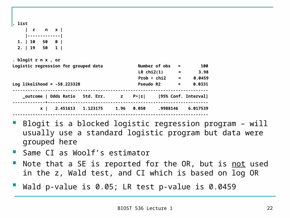
. list

| r n x |

|-------------|

1. | 10 50 0 |

2. | 19 50 1 |

. blogit r n x , or

Logistic regression for grouped data Number of obs = 100

LR chi2(1) = 3.98

Prob > chi2 = 0.0459

Log likelihood = -58.223328 Pseudo R2 = 0.0331

------------------------------------------------------------------------------

_outcome | Odds Ratio Std. Err. z P>|z| [95% Conf. Interval]

-------------+----------------------------------------------------------------

x | 2.451613 1.123175 1.96 0.050 .9988146 6.017539

------------------------------------------------------------------------------

Blogit is a blocked logistic regression program – will usually use a standard logistic program but data were grouped here

Same CI as Woolf’s estimator Note that a SE is reported for the OR, but is not used in the z, Wald

test, and CI which is based on log OR

Wald p-value is 0.05; LR test p-value is 0.0459


Framingham study

5209 individuals identified in 1948 in Framingham, MA

Biennial exams for blood pressure, serum cholesterol, weight

Endpoints include occurrence of coronary heart disease (CHD) and deaths due to

CHD including sudden death (MI) Cerebrovascular accident (CVA) Cancer (CA) Other causes


Framingham study

Stimulus for developing the method of logistic regression

Too many potential covariates to have tables of all combinations

Simultaneous consideration of several variables Could have continuous variables; not necessary to

categorize continuous covariates Linear discriminant analysis first used;

later logistic regression Linear discriminant analysis and logistic regression

can be mathematically equivalent LDA requires normality of covariates, but logistic

regression does not


Framingham data analysis. use "H:\Biostat\Biost536\Fall2007\data\Datasets\framfull.dta", clear

. summ

Variable | Obs Mean Std. Dev. Min Max

-------------+--------------------------------------------------------

lexam | 5209 14.03532 3.449479 2 16

surv | 5209 .3822231 .4859773 0 1

cause | 5209 1.563064 2.368246 0 9

cexam | 5209 2.561912 4.739291 0 16

chd | 5209 .1161451 .3204296 0 1

-------------+--------------------------------------------------------

cva | 5209 .0725667 .2594489 0 1

ca | 5209 .1034748 .3046072 0 1

oth | 5209 .2660779 .4419479 0 1

sex | 5209 1.551545 .4973837 1 2

age | 5209 44.06873 8.574954 28 62

-------------+--------------------------------------------------------

ht | 5203 64.81318 3.582707 51.5 76.5

wt | 5203 153.0867 28.91543 67 300

sc1 | 3172 221.2393 45.01786 96 503

sc2 | 4583 228.1778 44.81669 115 568

dbp | 5209 85.35861 12.97309 50 160

-------------+--------------------------------------------------------

sbp | 5209 136.9096 23.7396 82 300

mrw | 5203 119.9575 19.9834 67 268

smok | 5173 9.366518 12.03145 0 60


Framingham data analysis. • Restrict attention to males age 40+ with known values of Restrict attention to males age 40+ with known values of

serum cholesterol, smoking, and relative weight with no serum cholesterol, smoking, and relative weight with no evidence of CHD at first exam evidence of CHD at first exam . drop if sex>1 | age < 40 | sc1>1000 | smok > 1000 | mrw > 1000 | cexam==1(4299 observations deleted)

• Note that Stata treats missing values as large numbers so will Note that Stata treats missing values as large numbers so will eliminate observations above the cutoff value of 1000 ; better to eliminate observations above the cutoff value of 1000 ; better to just specify nonmissing values just specify nonmissing values . drop if sex>1 | age < 40 | sc1==. | smok==. | mrw ==. | cexam==1(4299 observations deleted)

•Leaves 910 observations for analysis; create grouped variables Leaves 910 observations for analysis; create grouped variables for SBP, cholesterol, and agefor SBP, cholesterol, and age. gen bpg=sbp. recode bpg min/126=1 127/146=2 147/166=3 167/max=4. gen scg=sc1. recode scg min/199=1 200/219=2 220/259=3 260/max=4. gen agp=age. recode agp 40/44=1 45/49=2 50/54=3 55/59=4 60/max=5


.

• Compare levels of CHD risk by grouped variablesCompare levels of CHD risk by grouped variables

. tab chd agp | agp chd | 1 2 3 4 5 | Total-----------+-------------------------------------------------------+---------- 0 | 226 174 153 138 41 | 732 1 | 41 35 48 38 16 | 178 -----------+-------------------------------------------------------+---------- Total | 267 209 201 176 57 | 910 . tabodds chd agp, or--------------------------------------------------------------------------- agp | Odds Ratio chi2 P>chi2 [95% Conf. Interval]-------------+------------------------------------------------------------- 1 | 1.000000 . . . . 2 | 1.108775 0.17 0.6813 0.677180 1.815443 3 | 1.729316 5.40 0.0201 1.083224 2.760771 4 | 1.517851 2.81 0.0938 0.928364 2.481647 5 | 2.151101 5.22 0.0223 1.097236 4.217174---------------------------------------------------------------------------Test of homogeneity (equal odds): chi2(4) = 9.51 Pr>chi2 = 0.0495Score test for trend of odds: chi2(1) = 7.55 Pr>chi2 = 0.0060

•Overall significant association of age with CHD risk that Overall significant association of age with CHD risk that appears to increase with age appears to increase with age


.

. tab chd bpg | bpg chd | 1 2 3 4 | Total-----------+--------------------------------------------+---------- 0 | 213 302 140 77 | 732 1 | 32 63 42 41 | 178 -----------+--------------------------------------------+---------- Total | 245 365 182 118 | 910

. tabodds chd bpg, or--------------------------------------------------------------------------- bpg | Odds Ratio chi2 P>chi2 [95% Conf. Interval]-------------+------------------------------------------------------------- 1 | 1.000000 . . . . 2 | 1.388555 1.96 0.1612 0.875422 2.202465 3 | 1.996875 7.29 0.0069 1.196801 3.331807 4 | 3.544237 23.25 0.0000 2.046106 6.139278---------------------------------------------------------------------------Test of homogeneity (equal odds): chi2(3) = 26.50 Pr>chi2 = 0.0000Score test for trend of odds: chi2(1) = 24.79 Pr>chi2 = 0.0000

Overall significant association of SBP with CHD risk that Overall significant association of SBP with CHD risk that appears to increase with SBP; most of the heterogeneity is appears to increase with SBP; most of the heterogeneity is explained by the trendexplained by the trend


.

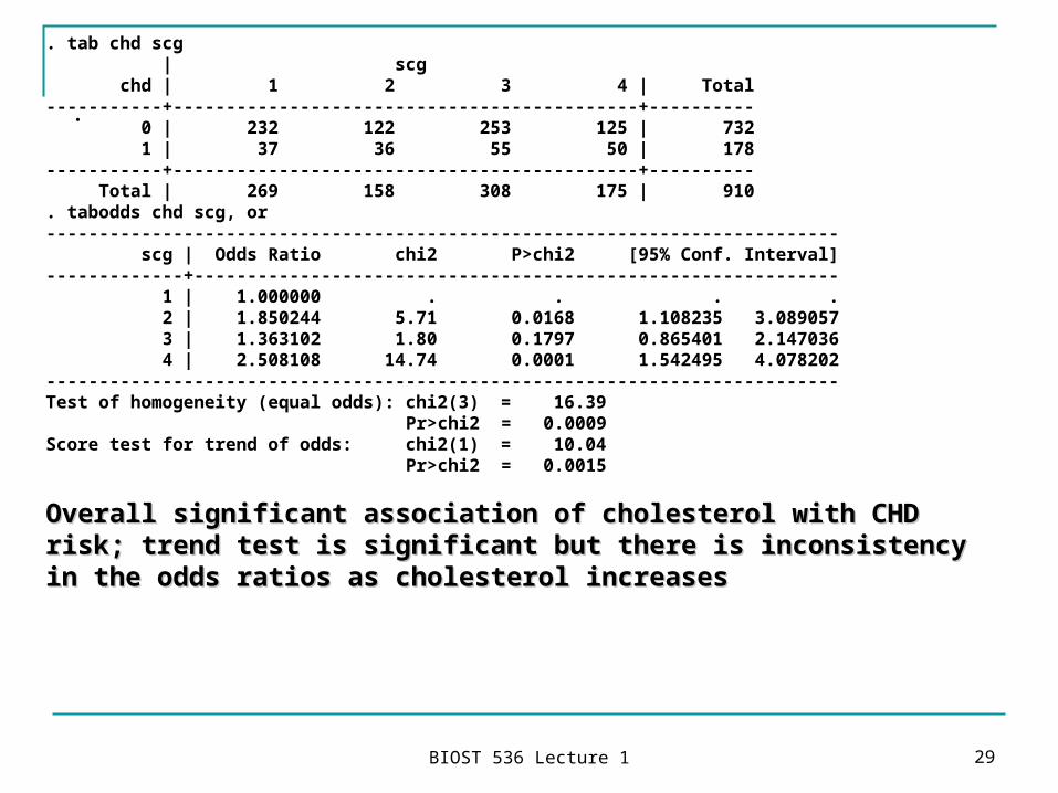
. tab chd scg | scg chd | 1 2 3 4 | Total-----------+--------------------------------------------+---------- 0 | 232 122 253 125 | 732 1 | 37 36 55 50 | 178 -----------+--------------------------------------------+---------- Total | 269 158 308 175 | 910 . tabodds chd scg, or--------------------------------------------------------------------------- scg | Odds Ratio chi2 P>chi2 [95% Conf. Interval]-------------+------------------------------------------------------------- 1 | 1.000000 . . . . 2 | 1.850244 5.71 0.0168 1.108235 3.089057 3 | 1.363102 1.80 0.1797 0.865401 2.147036 4 | 2.508108 14.74 0.0001 1.542495 4.078202---------------------------------------------------------------------------Test of homogeneity (equal odds): chi2(3) = 16.39 Pr>chi2 = 0.0009Score test for trend of odds: chi2(1) = 10.04 Pr>chi2 = 0.0015

Overall significant association of cholesterol with CHD risk; Overall significant association of cholesterol with CHD risk; trend test is significant but there is inconsistency in the odds trend test is significant but there is inconsistency in the odds ratios as cholesterol increasesratios as cholesterol increases


Course Overview Summary

Primarily interested in binary outcomes 2 x 2 table (Case status x Exposed/Unexposed) 2 x K table (Case status x Level of exposure) Stratified 2 x 2 tables (Case status x Exposure

controlling for confounder) Case status x scientific variable(s) of interest

controlling for other covariates Statistical methods

Hypothesis testing (Wald, score, and likelihood ratio tests, permutation tests for small samples)

Parameter estimation and CI’s (usually odds ratios) Stratification (implicitly controlling for confounders) Explicitly modeling confounders

BIOST 536 Lecture 1 1 Lecture 1 - Introduction Overview of course Focus is on binary outcomes Some ordinal outcomes considered Simple examples Definitions.

Documents

association y gleason

mothers age

grams case disease

validation slide

updated risk factors

grams x

penetration x

definition of low birthweight