BIFURCATION ANALYSIS OF THE FLOW PATTERNS IN TWO-DIMENSIONAL RAYLEIGH–BÉNARD CONVECTION

June 23, 2012 16:8 WSPC/S0218-1274 1230018

International Journal of Bifurcation and Chaos, Vol. 22, No. 5 (2012) 1230018 (15 pages)c© World Scientific Publishing CompanyDOI: 10.1142/S0218127412300182

BIFURCATION ANALYSIS OF THE FLOWPATTERNS IN TWO-DIMENSIONALRAYLEIGH–BENARD CONVECTION

SUPRIYO PAUL∗ and MAHENDRA K. VERMADepartment of Physics, Indian Institute of Technology,

Kanpur 208 016, India

PANKAJ WAHI and SANDEEP K. REDDYDepartment of Mechanical Engineering,

Indian Institute of Technology,Kanpur 208 016, India

KRISHNA KUMARDepartment of Physics and Meteorology,

Indian Institute of Technology,Kharagpur 721 302, India

Received January 22, 2011; Revised May 9, 2011

We investigate the origin of various convective patterns for Prandtl number P = 6.8 (for waterat room temperature) using bifurcation diagrams that are constructed using direct numericalsimulations (DNS) of Rayleigh–Benard convection (RBC). Several complex flow patterns result-ing from normal bifurcations as well as various instances of “crises” have been observed inthe DNS. “Crises” play vital roles in determining various convective flow patterns. After a tran-sition of conduction state to convective roll states, we observe time-periodic and quasiperiodicrolls through Hopf and Neimark–Sacker bifurcations at r � 80 and r � 500 respectively (wherer is the normalized Rayleigh number). The system becomes chaotic at r � 750, and the size ofthe chaotic attractor increases at r � 840 through an “attractor-merging crisis” which resultsin traveling chaotic rolls. For 846 ≤ r ≤ 849, stable fixed points and a chaotic attractor coexistas a result of an inverse subcritical Hopf bifurcation. Subsequently the chaotic attractor dis-appears through a “boundary crisis” and only stable fixed points remain. These fixed pointslater become periodic and chaotic through another set of bifurcations which ultimately leads toturbulence. As a function of Rayleigh number, |W101| ∼ (r − 1)0.62 and |θ101| ∼ (r − 1)−0.34

(velocity and temperature Fourier coefficient for (1, 0, 1) mode). However the Nusselt numberscales as (r − 1)0.33.

Keywords : Buoyancy-driven instabilities; chaos in fluid dynamics; direct numerical simulations.

1. Introduction

Rayleigh–Benard convection (RBC), an idealizedversion of thermal convection, is studied for under-standing pattern-forming instabilities, chaos, and

turbulence in atmosphere, astrophysics, crystalgrowth, etc. [Chandrasekhar, 1961; Busse, 1985;Bhattacharjee, 1987; Manneville, 2004; Ahlerset al., 2009]. In RBC, a layer of fluid, confined

∗Present address: Computational Fluid Dynamics Team, Scientific and Engineering Application Group, Centre for Develop-ment of Advanced Computing, Pune 411 007, India.

1230018-1

Int.

J. B

ifur

catio

n C

haos

201

2.22

. Dow

nloa

ded

from

ww

w.w

orld

scie

ntif

ic.c

omby

IN

DIA

N I

NST

ITU

TE

OF

TE

CH

NO

LO

GY

KH

AR

AG

PUR

on

09/2

2/14

. For

per

sona

l use

onl

y.

June 23, 2012 16:8 WSPC/S0218-1274 1230018

S. Paul et al.

between two thermally conducting plates, is heatedfrom below. The flow dynamics in RBC is governedby two nondimensional parameters: Prandtl num-ber P and Rayleigh number R. P is the ratio of thekinematic viscosity ν and the thermal diffusivity κ.Rayleigh number R = αgβd4/νκ, is the ratio ofbuoyancy and the dissipative terms, where α is thethermal expansion coefficient, g is the accelerationdue to gravity, β is the imposed temperature gradi-ent in the fluid, and d is the separation betweenthe plates. Increasing the temperature differenceacross the plates increases the Rayleigh number.Convection starts (primary instability) at the crit-ical Rayleigh number Rc that has been foundto be independent of the Prandtl number. Thenumerical value of Rc is approximately 1708 forno-slip boundary conditions, and 657.5 for free-slipboundary conditions [Chandrasekhar, 1961; Busse,1985].

The sequence of bifurcations and routes tochaos in the RBC system depend critically onthe Prandtl number. Low Prandtl number (P � 1,low-P) convection shows complex bifurcation sce-nario involving three-dimensional flow patternswhich asymptotically converge to zero Prandtlnumber (P = 0, zero-P) case as P is lowered.For low-P and zero-P convection, the inertialterm u · ∇u is significant and it generates verticalvorticity. Consequently the flow pattern becomesthree-dimensional, and oscillatory waves along thehorizontal axes are generated just near the onset ofconvection. For large-P (P > 1) convection, how-ever, vertical vorticity is absent near the onsetand two-dimensional (2D) rolls survive till largeRayleigh numbers [Chandrasekhar, 1961; Schlutteret al., 1965]. This feature of large-P convec-tion makes 2D simulations quite relevant for thisregime.

Krishnamurti [1970a, 1970b] carried out exten-sive convection experiments on fluids of differentPrandtl numbers (0.025 ≤ P ≤ 8500) and studiedvarious convective states such as two-dimensional,time-periodic, and chaotic rolls, and turbulentstructures. Gollub and Benson [1980] performedRBC experiments on water for P = 2.5 and 5.0(varied by changing the mean temperature) andaspect ratios Γ = 2.4 and 3.5. They observed avariety of convective states and several routes tochaos. For Γ = 3.5 and P = 5.0, they found aquasiperiodic state at the reduced Rayleigh num-ber r = R/Rc � 32 and subsequent phase locking

at r � 44.4. The flow became chaotic at aroundr � 46, thus exhibiting a quasiperiodic route tochaos. Gollub and Benson [1980] also observed aperiod-doubling route to chaos for Γ = 3.5 andP = 2.5, and a quasiperiodic route to chaos withthree frequencies (Ruelle–Takens) for Γ = 2.4 andP = 5.0. Intermittent chaos too was observed intheir experiments. Maurer and Libchaber [1979]observed quasiperiodic and frequency-locking routeto chaos in helium (P ∼ 0.7). Experiments of Giglioet al. [1981] on the convection of water (P ∼ 7)showed a period-doubling route to chaos. Bergeet al. [1980] observed intermittency in their RBCexperiments on silicon oil (P ∼ 100). Libchaberet al. [1982, 1983] studied convection in mercury(P ∼ 0.02) in the presence of an applied mean mag-netic field and observed generation of chaos throughperiod doubling and quasiperiodic routes.

Direct numerical simulations (DNS) are usedextensively to study convection. Curry et al. [1984]performed DNS in three dimensions for a P = 10fluid under free-slip boundary conditions. Theyreported steady convection till r � 40, after which alimit cycle is observed till r � 45. Subsequently theyreported quasiperiodicity (r � 45–55), phase lock-ing (r � 55–65), and chaos (r ≥ 65). Yahata [2000]observed a similar route to chaos in his DNS forP = 5, Γx = 3.5 and Γy = 2. Mukutmoni and Yang[1993] performed DNS for convection in a rectangu-lar enclosure with insulated side walls and found aperiod-two state, but a quasiperiodic route to chaos.Nishikawa and Yahata [1996] and Yahata [2000] per-formed direct numerical simulations of RBC for thesetup similar to Gollub and Benson’s [1980] exper-iments and observed quasiperiodic route to chaos.Yahata [2000] also observed frequency locking. Gelf-gat [1999] numerically studied the effects of theaspect ratio on the critical Rayleigh number andthe instability modes.

Three-dimensional DNS are quite expensivecomputationally, so a large number of two-dimensional DNS have been performed. Mooreand Weiss [1973] simulated for P = 6.8 using afinite-difference method under free-slip boundaryconditions and reported that the Nusselt numberNu ∝ r1/3 for 5 ≤ r ≤ P 1.5, and Nu ∝ r0.365 forhigher Rayleigh numbers. McLaughlin and Orszag[1982] simulated RBC in air (P = 0.71) withno-slip boundary conditions and observed periodic,quasiperiodic, and chaotic states for Rayleigh num-bers between 6500 and 25 000. Curry et al. [1984]

1230018-2

Int.

J. B

ifur

catio

n C

haos

201

2.22

. Dow

nloa

ded

from

ww

w.w

orld

scie

ntif

ic.c

omby

IN

DIA

N I

NST

ITU

TE

OF

TE

CH

NO

LO

GY

KH

AR

AG

PUR

on

09/2

2/14

. For

per

sona

l use

onl

y.

June 23, 2012 16:8 WSPC/S0218-1274 1230018

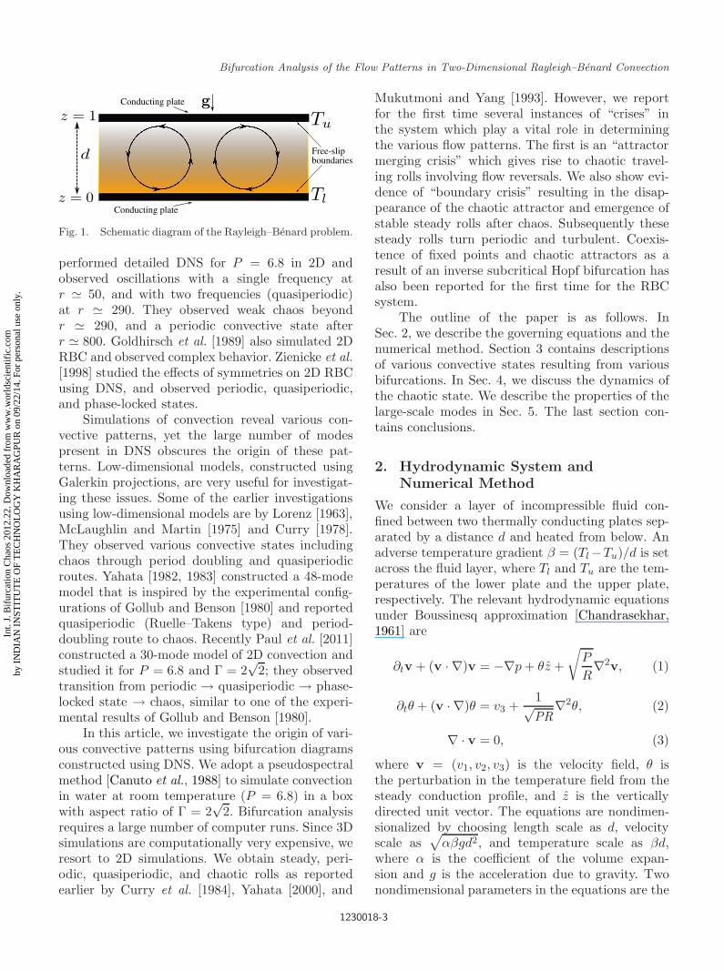
Bifurcation Analysis of the Flow Patterns in Two-Dimensional Rayleigh–Benard Convection

Conducting plate

Conducting plate

Free-slipboundaries

Fig. 1. Schematic diagram of the Rayleigh–Benard problem.

performed detailed DNS for P = 6.8 in 2D andobserved oscillations with a single frequency atr � 50, and with two frequencies (quasiperiodic)at r � 290. They observed weak chaos beyondr � 290, and a periodic convective state afterr � 800. Goldhirsch et al. [1989] also simulated 2DRBC and observed complex behavior. Zienicke et al.[1998] studied the effects of symmetries on 2D RBCusing DNS, and observed periodic, quasiperiodic,and phase-locked states.

Simulations of convection reveal various con-vective patterns, yet the large number of modespresent in DNS obscures the origin of these pat-terns. Low-dimensional models, constructed usingGalerkin projections, are very useful for investigat-ing these issues. Some of the earlier investigationsusing low-dimensional models are by Lorenz [1963],McLaughlin and Martin [1975] and Curry [1978].They observed various convective states includingchaos through period doubling and quasiperiodicroutes. Yahata [1982, 1983] constructed a 48-modemodel that is inspired by the experimental config-urations of Gollub and Benson [1980] and reportedquasiperiodic (Ruelle–Takens type) and period-doubling route to chaos. Recently Paul et al. [2011]constructed a 30-mode model of 2D convection andstudied it for P = 6.8 and Γ = 2

√2; they observed

transition from periodic → quasiperiodic → phase-locked state → chaos, similar to one of the experi-mental results of Gollub and Benson [1980].

In this article, we investigate the origin of vari-ous convective patterns using bifurcation diagramsconstructed using DNS. We adopt a pseudospectralmethod [Canuto et al., 1988] to simulate convectionin water at room temperature (P = 6.8) in a boxwith aspect ratio of Γ = 2

√2. Bifurcation analysis

requires a large number of computer runs. Since 3Dsimulations are computationally very expensive, weresort to 2D simulations. We obtain steady, peri-odic, quasiperiodic, and chaotic rolls as reportedearlier by Curry et al. [1984], Yahata [2000], and

Mukutmoni and Yang [1993]. However, we reportfor the first time several instances of “crises” inthe system which play a vital role in determiningthe various flow patterns. The first is an “attractormerging crisis” which gives rise to chaotic travel-ing rolls involving flow reversals. We also show evi-dence of “boundary crisis” resulting in the disap-pearance of the chaotic attractor and emergence ofstable steady rolls after chaos. Subsequently thesesteady rolls turn periodic and turbulent. Coexis-tence of fixed points and chaotic attractors as aresult of an inverse subcritical Hopf bifurcation hasalso been reported for the first time for the RBCsystem.

The outline of the paper is as follows. InSec. 2, we describe the governing equations and thenumerical method. Section 3 contains descriptionsof various convective states resulting from variousbifurcations. In Sec. 4, we discuss the dynamics ofthe chaotic state. We describe the properties of thelarge-scale modes in Sec. 5. The last section con-tains conclusions.

2. Hydrodynamic System andNumerical Method

We consider a layer of incompressible fluid con-fined between two thermally conducting plates sep-arated by a distance d and heated from below. Anadverse temperature gradient β = (Tl −Tu)/d is setacross the fluid layer, where Tl and Tu are the tem-peratures of the lower plate and the upper plate,respectively. The relevant hydrodynamic equationsunder Boussinesq approximation [Chandrasekhar,1961] are

∂tv + (v · ∇)v = −∇p + θz +

√P

R∇2v, (1)

∂tθ + (v · ∇)θ = v3 +1√PR

∇2θ, (2)

∇ · v = 0, (3)

where v = (v1, v2, v3) is the velocity field, θ isthe perturbation in the temperature field from thesteady conduction profile, and z is the verticallydirected unit vector. The equations are nondimen-sionalized by choosing length scale as d, velocityscale as

√αβgd2, and temperature scale as βd,

where α is the coefficient of the volume expan-sion and g is the acceleration due to gravity. Twonondimensional parameters in the equations are the

1230018-3

Int.

J. B

ifur

catio

n C

haos

201

2.22

. Dow

nloa

ded

from

ww

w.w

orld

scie

ntif

ic.c

omby

IN

DIA

N I

NST

ITU

TE

OF

TE

CH

NO

LO

GY

KH

AR

AG

PUR

on

09/2

2/14

. For

per

sona

l use

onl

y.

June 23, 2012 16:8 WSPC/S0218-1274 1230018

S. Paul et al.

Rayleigh number, R = αgβd4/νκ and the Prandtlnumber, P = ν/κ, where ν and κ are the kine-matic viscosity and the thermal diffusivity of thefluid, respectively. In the following we will alsouse the reduced Rayleigh number, r = R/Rc as aparameter.

The top and bottom boundaries are consideredto be stress free and perfectly conducting:

v3 = ∂zv1 = ∂zv2 = θ = 0, at z = 0, 1. (4)

We assume periodic boundary conditions along thehorizontal direction (x-direction). The boundaryconditions chosen here are ideal. However, theyallow us to choose Fourier and sin or cos basis func-tions in our DNS. This makes computation simplerand easier to formulate. This also helps us to getinsights into the convective flow patterns.

The above set of equations (1)–(3) are solvednumerically using a pseudospectral method [Canutoet al., 1988] in two dimensions (2D) under the aboveboundary conditions [Eq. (4)]. We use Fourier basisfunctions for representation along the x-direction,and sin or cos functions for representation alongthe z-direction. The two-dimensional rolls formedin the system are assumed to be parallel to the y-axis. Therefore the velocity component along they-direction (v2) is zero. The expansion of the veloc-ity and temperature fields in terms of the chosenbasis functions are:

v1(x, z, t) =∑m,n

2Um0n(t) exp(imkcx) cos(nπz),

v2(x, z, t) = 0,

v3(x, z, t) =∑m,n

2Wm0n(t) exp(imkcx) sin(nπz),

θ(x, z, t) =∑m,n

2θm0n(t) exp(imkcx) sin(nπz),

(5)

where kc = π/√

2 [Chandrasekhar, 1961].Our simulations are performed in a two-

dimensional box with aspect ratio (ratio of thewidth to the height), Γ = 2

√2. Various grid res-

olutions, 64 × 64, 128 × 128, 256 × 256, 512 × 512have been used for the simulations. Our runs aredealiased using 2/3 rule. Time stepping is car-ried out using the fourth-order Runge–Kutta (RK4)method with CFL scheme for choosing dt (dt =∆x/

√20Eu, where ∆x is the grid size and Eu is

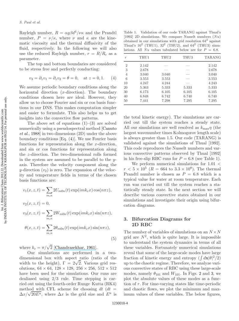
Table 1. Validation of our code TARANG against Thual’s[1992] 2D simulations. We compare Nusselt numbers (Nu)obtained in our simulations with grid resolution 642 againstThual’s 162 (THU1), 322 (THU2), and 642 (THU3) simu-lations. All Nu values tabulated below are for P = 6.8.

r THU1 THU2 THU3 TARANG

2 2.142 — — 2.1423 2.678 — — 2.6784 3.040 3.040 — 3.0406 3.553 3.553 — 3.553

10 4.247 4.244 — 4.24320 5.363 5.333 5.333 5.33330 6.173 6.105 6.105 6.10540 6.848 6.742 6.740 6.74050 7.441 7.298 7.295 7.295

the total kinetic energy). The simulations are car-ried out till the system reaches a steady state.All our simulations are well resolved as kmaxη (thelargest wavenumber times Kolmogorov length scale)is always greater than 1.5. Our code (TARANG) isvalidated against the simulations of Thual [1992].This code reproduces the Nusselt numbers and var-ious convective patterns observed by Thual [1992]in his free-slip RBC runs for P = 6.8 (see Table 1).

We perform numerical simulations for 1.01 <r < 5 × 105 (R = 664 to 3.3 × 108). The thermalPrandtl number is chosen as P = 6.8 which is atypical value for water at room temperature. Eachrun was carried out till the system reaches a sta-tistically steady state. In the next section we willdescribe various convective states obtained in oursimulations and investigate their origin using bifur-cation diagrams.

3. Bifurcation Diagrams for2D RBC

The number of variables of simulations on an N×Ngrid are N2, which is quite large. It is impossibleto understand the system dynamics in terms of allthese variables. Fortunately numerical simulationsreveal that some of the large-scale modes have largefraction of kinetic energy and entropy (

∫dx|θ|2/2)

up to the chaotic regime. Therefore, we analyze vari-ous convective states of RBC using these large-scalemodes, namely θ101 and W101. In Figs. 2 and 3, weplot the absolute values of these modes as a func-tion of r. For time-varying states like time-periodicand chaotic flows, we plot the minimum and max-imum values of these variables. The below figures,

1230018-4

Int.

J. B

ifur

catio

n C

haos

201

2.22

. Dow

nloa

ded

from

ww

w.w

orld

scie

ntif

ic.c

omby

IN

DIA

N I

NST

ITU

TE

OF

TE

CH

NO

LO

GY

KH

AR

AG

PUR

on

09/2

2/14

. For

per

sona

l use

onl

y.

June 23, 2012 16:8 WSPC/S0218-1274 1230018

Bifurcation Analysis of the Flow Patterns in Two-Dimensional Rayleigh–Benard Convection

0 200 400 600 800 1000 1200 1400 16000

0.02

0.04

0.06

0.08

0.1

|θ10

1|

r

844 846 848 850 8520.0134

0.0166

0.015

0 5 100.06

0.08

0.1

0.12

Fixed pointPeriodicQuasiperiodicChaotic

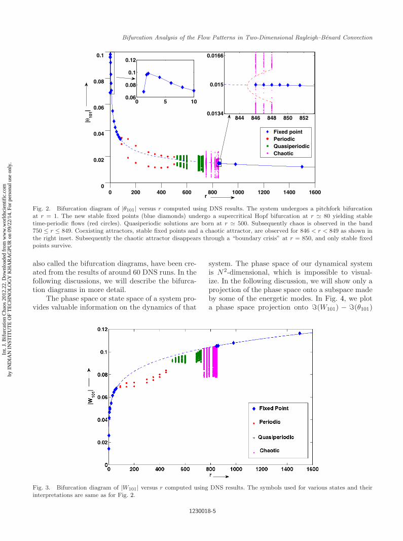
Fig. 2. Bifurcation diagram of |θ101| versus r computed using DNS results. The system undergoes a pitchfork bifurcationat r = 1. The new stable fixed points (blue diamonds) undergo a supercritical Hopf bifurcation at r � 80 yielding stabletime-periodic flows (red circles). Quasiperiodic solutions are born at r � 500. Subsequently chaos is observed in the band750 ≤ r ≤ 849. Coexisting attractors, stable fixed points and a chaotic attractor, are observed for 846 < r < 849 as shown inthe right inset. Subsequently the chaotic attractor disappears through a “boundary crisis” at r = 850, and only stable fixedpoints survive.

also called the bifurcation diagrams, have been cre-ated from the results of around 60 DNS runs. In thefollowing discussions, we will describe the bifurca-tion diagrams in more detail.

The phase space or state space of a system pro-vides valuable information on the dynamics of that

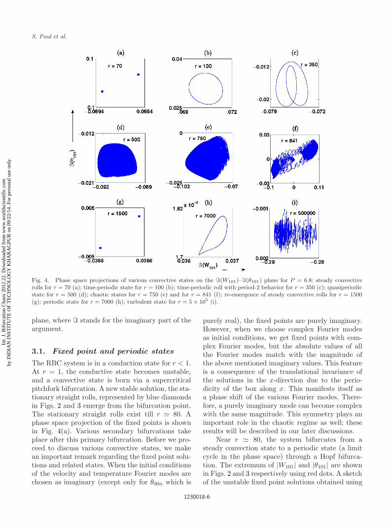
system. The phase space of our dynamical systemis N2-dimensional, which is impossible to visual-ize. In the following discussion, we will show only aprojection of the phase space onto a subspace madeby some of the energetic modes. In Fig. 4, we plota phase space projection onto (W101) − (θ101)

Fig. 3. Bifurcation diagram of |W101| versus r computed using DNS results. The symbols used for various states and theirinterpretations are same as for Fig. 2.

1230018-5

Int.

J. B

ifur

catio

n C

haos

201

2.22

. Dow

nloa

ded

from

ww

w.w

orld

scie

ntif

ic.c

omby

IN

DIA

N I

NST

ITU

TE

OF

TE

CH

NO

LO

GY

KH

AR

AG

PUR

on

09/2

2/14

. For

per

sona

l use

onl

y.

June 23, 2012 16:8 WSPC/S0218-1274 1230018

S. Paul et al.

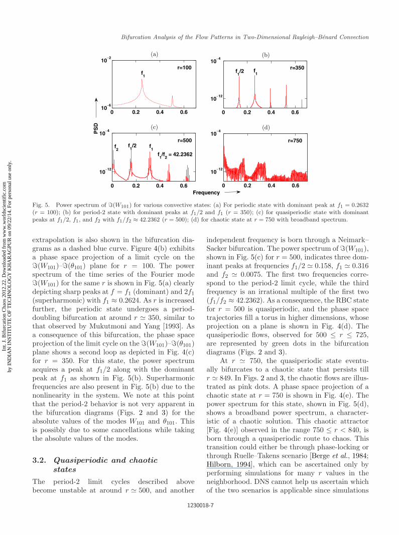
Fig. 4. Phase space projections of various convective states on the �(W101)–�(θ101) plane for P = 6.8: steady convectiverolls for r = 70 (a); time-periodic state for r = 100 (b); time-periodic roll with period-2 behavior for r = 350 (c); quasiperiodicstate for r = 500 (d); chaotic states for r = 750 (e) and for r = 841 (f); re-emergence of steady convective rolls for r = 1500(g); periodic state for r = 7000 (h); turbulent state for r = 5 × 105 (i).

plane, where stands for the imaginary part of theargument.

3.1. Fixed point and periodic states

The RBC system is in a conduction state for r < 1.At r = 1, the conductive state becomes unstable,and a convective state is born via a supercriticalpitchfork bifurcation. A new stable solution, the sta-tionary straight rolls, represented by blue diamondsin Figs. 2 and 3 emerge from the bifurcation point.The stationary straight rolls exist till r � 80. Aphase space projection of the fixed points is shownin Fig. 4(a). Various secondary bifurcations takeplace after this primary bifurcation. Before we pro-ceed to discuss various convective states, we makean important remark regarding the fixed point solu-tions and related states. When the initial conditionsof the velocity and temperature Fourier modes arechosen as imaginary (except only for θ00n which is

purely real), the fixed points are purely imaginary.However, when we choose complex Fourier modesas initial conditions, we get fixed points with com-plex Fourier modes, but the absolute values of allthe Fourier modes match with the magnitude ofthe above mentioned imaginary values. This featureis a consequence of the translational invariance ofthe solutions in the x-direction due to the perio-dicity of the box along x. This manifests itself asa phase shift of the various Fourier modes. There-fore, a purely imaginary mode can become complexwith the same magnitude. This symmetry plays animportant role in the chaotic regime as well; theseresults will be described in our later discussions.

Near r � 80, the system bifurcates from asteady convection state to a periodic state (a limitcycle in the phase space) through a Hopf bifurca-tion. The extremum of |W101| and |θ101| are shownin Figs. 2 and 3 respectively using red dots. A sketchof the unstable fixed point solutions obtained using

1230018-6

Int.

J. B

ifur

catio

n C

haos

201

2.22

. Dow

nloa

ded

from

ww

w.w

orld

scie

ntif

ic.c

omby

IN

DIA

N I

NST

ITU

TE

OF

TE

CH

NO

LO

GY

KH

AR

AG

PUR

on

09/2

2/14

. For

per

sona

l use

onl

y.

June 23, 2012 16:8 WSPC/S0218-1274 1230018

Bifurcation Analysis of the Flow Patterns in Two-Dimensional Rayleigh–Benard Convection

0 0.2 0.4 0.610

−6

10−2

PS

D

0 0.2 0.4 0.6

10−12

10−4

0 0.2 0.4 0.6

10−12

10−4

Frequency0 0.2 0.4 0.6

10−12

10−4

f1

r=100 r=350

r=500 r=750

f1f

1/2

f1/2 f

1f2

f1/f

2 = 42.2362

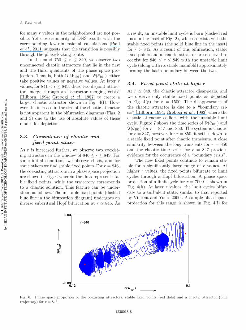
Fig. 5. Power spectrum of �(W101) for various convective states: (a) For periodic state with dominant peak at f1 = 0.2632(r = 100); (b) for period-2 state with dominant peaks at f1/2 and f1 (r = 350); (c) for quasiperiodic state with dominantpeaks at f1/2, f1, and f2 with f1/f2 ≈ 42.2362 (r = 500); (d) for chaotic state at r = 750 with broadband spectrum.

extrapolation is also shown in the bifurcation dia-grams as a dashed blue curve. Figure 4(b) exhibitsa phase space projection of a limit cycle on the(W101)–(θ101) plane for r = 100. The powerspectrum of the time series of the Fourier mode(W101) for the same r is shown in Fig. 5(a) clearlydepicting sharp peaks at f = f1 (dominant) and 2f1

(superharmonic) with f1 ≈ 0.2624. As r is increasedfurther, the periodic state undergoes a period-doubling bifurcation at around r � 350, similar tothat observed by Mukutmoni and Yang [1993]. Asa consequence of this bifurcation, the phase spaceprojection of the limit cycle on the (W101)–(θ101)plane shows a second loop as depicted in Fig. 4(c)for r = 350. For this state, the power spectrumacquires a peak at f1/2 along with the dominantpeak at f1 as shown in Fig. 5(b). Superharmonicfrequencies are also present in Fig. 5(b) due to thenonlinearity in the system. We note at this pointthat the period-2 behavior is not very apparent inthe bifurcation diagrams (Figs. 2 and 3) for theabsolute values of the modes W101 and θ101. Thisis possibly due to some cancellations while takingthe absolute values of the modes.

3.2. Quasiperiodic and chaoticstates

The period-2 limit cycles described abovebecome unstable at around r � 500, and another

independent frequency is born through a Neimark–Sacker bifurcation. The power spectrum of (W101),shown in Fig. 5(c) for r = 500, indicates three dom-inant peaks at frequencies f1/2 � 0.158, f1 � 0.316and f2 � 0.0075. The first two frequencies corre-spond to the period-2 limit cycle, while the thirdfrequency is an irrational multiple of the first two(f1/f2 ≈ 42.2362). As a consequence, the RBC statefor r = 500 is quasiperiodic, and the phase spacetrajectories fill a torus in higher dimensions, whoseprojection on a plane is shown in Fig. 4(d). Thequasiperiodic flows, observed for 500 ≤ r ≤ 725,are represented by green dots in the bifurcationdiagrams (Figs. 2 and 3).

At r � 750, the quasiperiodic state eventu-ally bifurcates to a chaotic state that persists tillr � 849. In Figs. 2 and 3, the chaotic flows are illus-trated as pink dots. A phase space projection of achaotic state at r = 750 is shown in Fig. 4(e). Thepower spectrum for this state, shown in Fig. 5(d),shows a broadband power spectrum, a character-istic of a chaotic solution. This chaotic attractor[Fig. 4(e)] observed in the range 750 ≤ r < 840, isborn through a quasiperiodic route to chaos. Thistransition could either be through phase-locking orthrough Ruelle–Takens scenario [Berge et al., 1984;Hilborn, 1994], which can be ascertained only byperforming simulations for many r values in theneighborhood. DNS cannot help us ascertain whichof the two scenarios is applicable since simulations

1230018-7

Int.

J. B

ifur

catio

n C

haos

201

2.22

. Dow

nloa

ded

from

ww

w.w

orld

scie

ntif

ic.c

omby

IN

DIA

N I

NST

ITU

TE

OF

TE

CH

NO

LO

GY

KH

AR

AG

PUR

on

09/2

2/14

. For

per

sona

l use

onl

y.

June 23, 2012 16:8 WSPC/S0218-1274 1230018

S. Paul et al.

for many r values in the neighborhood are not pos-sible. Yet close similarity of DNS results with thecorresponding low-dimensional calculations [Paulet al., 2011] suggests that the transition is possiblythrough the phase-locking route.

In the band 750 ≤ r ≤ 840, we observe twounconnected chaotic attractors that lie in the firstand the third quadrants of the phase space pro-jection. That is, both (W101) and (θ101) eithertake positive values or negative values. At later rvalues, for 841 < r ≤ 849, these two disjoint attrac-tors merge through an “attractor merging crisis”[Hilborn, 1994; Grebogi et al., 1987] to create alarger chaotic attractor shown in Fig. 4(f). How-ever the increase in the size of the chaotic attractoris not apparent in the bifurcation diagrams (Figs. 2and 3) due to the use of absolute values of thesemodes for depiction.

3.3. Coexistence of chaotic andfixed point states

As r is increased further, we observe two coexist-ing attractors in the window of 846 ≤ r ≤ 849. Forsome initial conditions we observe chaos, and forsome others we find stable fixed points. For r = 846,the coexisting attractors in a phase space projectionare shown in Fig. 6 wherein the dots represent sta-ble fixed points, while the trajectory correspondsto a chaotic solution. This feature can be under-stood as follows. The unstable fixed points (dashedblue line in the bifurcation diagram) undergoes aninverse subcritical Hopf bifurcation at r � 845. As

a result, an unstable limit cycle is born (dashed redlines in the inset of Fig. 2), which coexists with thestable fixed points (the solid blue line in the inset)for r > 845. As a result of this bifurcation, stablefixed points and a chaotic attractor are observed tocoexist for 846 ≤ r ≤ 849 with the unstable limitcycle (along with its stable manifold) approximatelyforming the basin boundary between the two.

3.4. Fixed point state at high r

At r � 849, the chaotic attractor disappears, andwe observe only stable fixed points as depictedin Fig. 4(g) for r = 1500. The disappearance ofthe chaotic attractor is due to a “boundary cri-sis” [Hilborn, 1994; Grebogi et al., 1983] where thechaotic attractor collides with the unstable limitcycle. Figure 7 shows the time series of �(θ101) and(θ101) for r = 847 and 850. The system is chaoticfor r = 847, however, for r = 850, it settles down toa stable fixed point after chaotic transients. A closesimilarity between the long transients for r = 850and the chaotic time series for r = 847 providesevidence for the occurrence of a “boundary crisis”.

The new fixed points continue to remain sta-ble for a significantly large range of r values. Athigher r values, the fixed points bifurcate to limitcycles through a Hopf bifurcation. A phase spaceprojection of a limit cycle for r = 7000 is shown inFig. 4(h). At later r values, the limit cycles bifur-cate to a turbulent state, similar to that reportedby Vincent and Yuen [2000]. A sample phase spaceprojection for this range is shown in Fig. 4(i) for

−0.12 0.1−0.03

0.03

ℑ(θ

101)

ℑ(W101

)

r=846

Fig. 6. Phase space projection of the coexisting attractors, stable fixed points (red dots) and a chaotic attractor (bluetrajectory) for r = 846.

1230018-8

Int.

J. B

ifur

catio

n C

haos

201

2.22

. Dow

nloa

ded

from

ww

w.w

orld

scie

ntif

ic.c

omby

IN

DIA

N I

NST

ITU

TE

OF

TE

CH

NO

LO

GY

KH

AR

AG

PUR

on

09/2

2/14

. For

per

sona

l use

onl

y.

June 23, 2012 16:8 WSPC/S0218-1274 1230018

Bifurcation Analysis of the Flow Patterns in Two-Dimensional Rayleigh–Benard Convection

1.2 1.4 1.6 1.8

x 105

−0.025

−0.02

−0.015

−0.01

−0.005

0

0.005

0.01

0.015

0.02

0.025

t

ℜ(θ

101),

ℑ(θ

101)

1 1.2 1.4 1.6 1.8

x 105

−0.025

−0.02

−0.015

−0.01

−0.005

0

0.005

0.01

0.015

0.02

0.025ℜ(θ

101)

ℑ(θ101

)

ℜ(θ101

)

ℑ(θ101

)

r = 847 r = 850

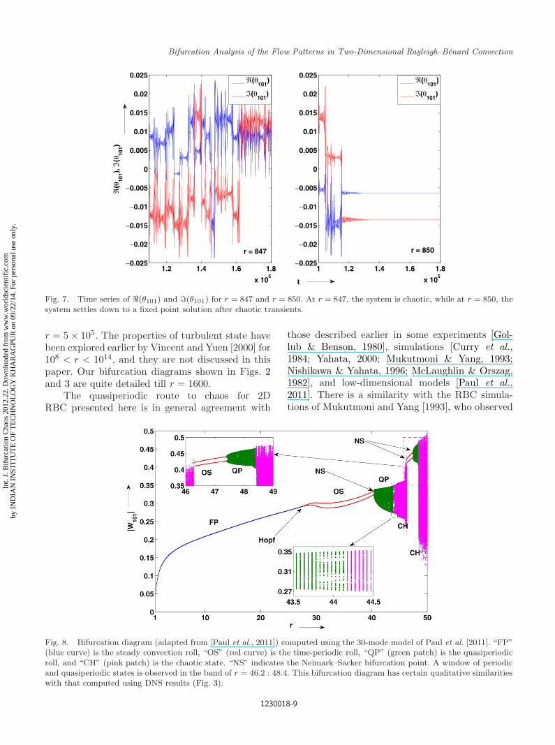
Fig. 7. Time series of �(θ101) and �(θ101) for r = 847 and r = 850. At r = 847, the system is chaotic, while at r = 850, thesystem settles down to a fixed point solution after chaotic transients.

r = 5 × 105. The properties of turbulent state havebeen explored earlier by Vincent and Yuen [2000] for108 < r < 1014, and they are not discussed in thispaper. Our bifurcation diagrams shown in Figs. 2and 3 are quite detailed till r = 1600.

The quasiperiodic route to chaos for 2DRBC presented here is in general agreement with

those described earlier in some experiments [Gol-lub & Benson, 1980], simulations [Curry et al.,1984; Yahata, 2000; Mukutmoni & Yang, 1993;Nishikawa & Yahata, 1996; McLaughlin & Orszag,1982], and low-dimensional models [Paul et al.,2011]. There is a similarity with the RBC simula-tions of Mukutmoni and Yang [1993], who observed

Fig. 8. Bifurcation diagram (adapted from [Paul et al., 2011]) computed using the 30-mode model of Paul et al. [2011]. “FP”(blue curve) is the steady convection roll, “OS” (red curve) is the time-periodic roll, “QP” (green patch) is the quasiperiodicroll, and “CH” (pink patch) is the chaotic state. “NS” indicates the Neimark–Sacker bifurcation point. A window of periodicand quasiperiodic states is observed in the band of r = 46.2 : 48.4. This bifurcation diagram has certain qualitative similaritieswith that computed using DNS results (Fig. 3).

1230018-9

Int.

J. B

ifur

catio

n C

haos

201

2.22

. Dow

nloa

ded

from

ww

w.w

orld

scie

ntif

ic.c

omby

IN

DIA

N I

NST

ITU

TE

OF

TE

CH

NO

LO

GY

KH

AR

AG

PUR

on

09/2

2/14

. For

per

sona

l use

onl

y.

June 23, 2012 16:8 WSPC/S0218-1274 1230018

S. Paul et al.

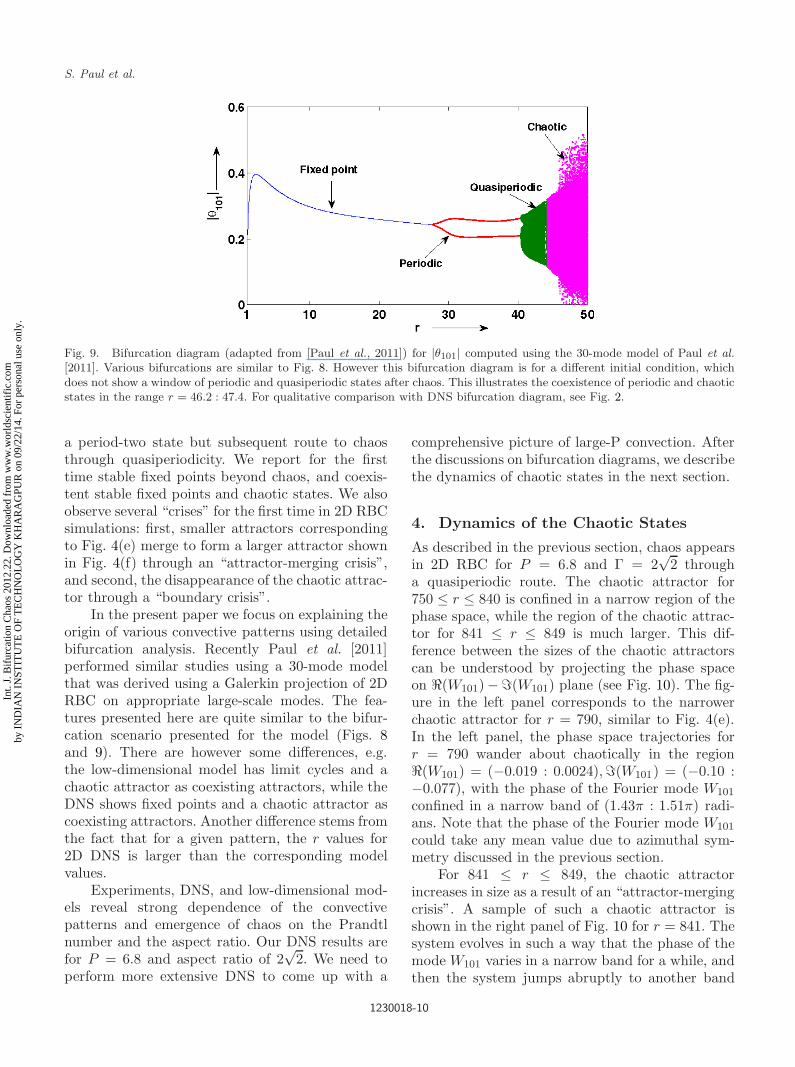
Fig. 9. Bifurcation diagram (adapted from [Paul et al., 2011]) for |θ101| computed using the 30-mode model of Paul et al.[2011]. Various bifurcations are similar to Fig. 8. However this bifurcation diagram is for a different initial condition, whichdoes not show a window of periodic and quasiperiodic states after chaos. This illustrates the coexistence of periodic and chaoticstates in the range r = 46.2 : 47.4. For qualitative comparison with DNS bifurcation diagram, see Fig. 2.

a period-two state but subsequent route to chaosthrough quasiperiodicity. We report for the firsttime stable fixed points beyond chaos, and coexis-tent stable fixed points and chaotic states. We alsoobserve several “crises” for the first time in 2D RBCsimulations: first, smaller attractors correspondingto Fig. 4(e) merge to form a larger attractor shownin Fig. 4(f) through an “attractor-merging crisis”,and second, the disappearance of the chaotic attrac-tor through a “boundary crisis”.

In the present paper we focus on explaining theorigin of various convective patterns using detailedbifurcation analysis. Recently Paul et al. [2011]performed similar studies using a 30-mode modelthat was derived using a Galerkin projection of 2DRBC on appropriate large-scale modes. The fea-tures presented here are quite similar to the bifur-cation scenario presented for the model (Figs. 8and 9). There are however some differences, e.g.the low-dimensional model has limit cycles and achaotic attractor as coexisting attractors, while theDNS shows fixed points and a chaotic attractor ascoexisting attractors. Another difference stems fromthe fact that for a given pattern, the r values for2D DNS is larger than the corresponding modelvalues.

Experiments, DNS, and low-dimensional mod-els reveal strong dependence of the convectivepatterns and emergence of chaos on the Prandtlnumber and the aspect ratio. Our DNS results arefor P = 6.8 and aspect ratio of 2

√2. We need to

perform more extensive DNS to come up with a

comprehensive picture of large-P convection. Afterthe discussions on bifurcation diagrams, we describethe dynamics of chaotic states in the next section.

4. Dynamics of the Chaotic States

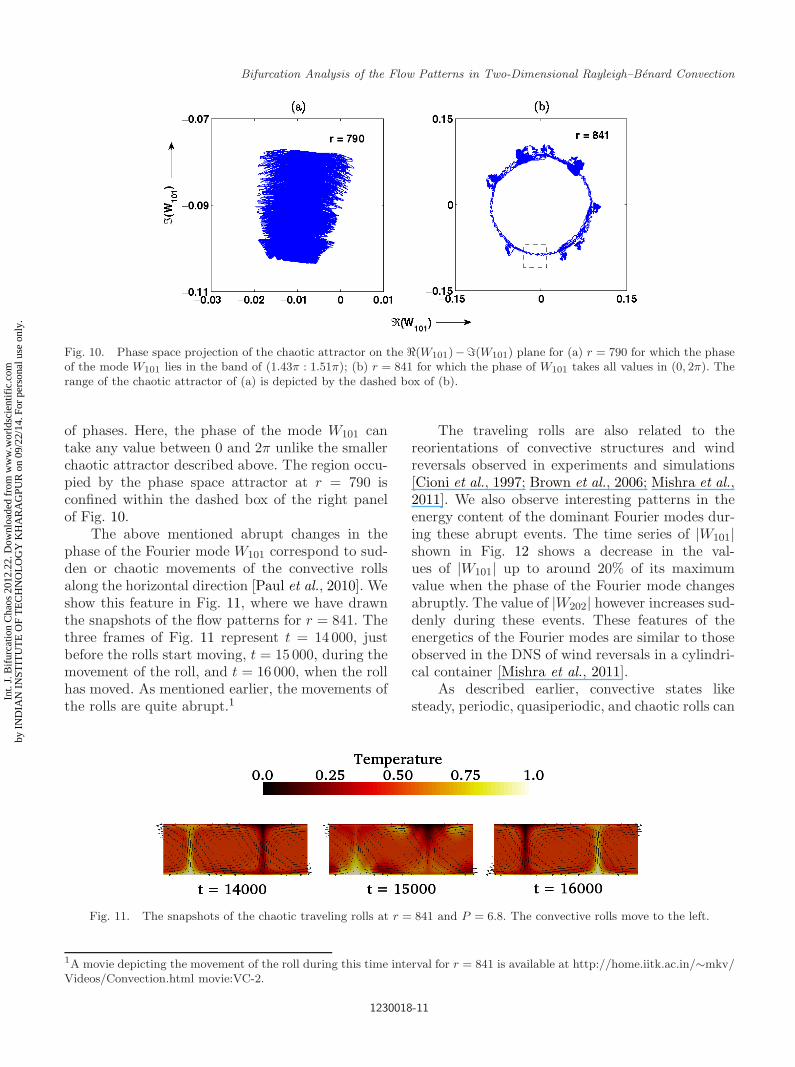
As described in the previous section, chaos appearsin 2D RBC for P = 6.8 and Γ = 2

√2 through

a quasiperiodic route. The chaotic attractor for750 ≤ r ≤ 840 is confined in a narrow region of thephase space, while the region of the chaotic attrac-tor for 841 ≤ r ≤ 849 is much larger. This dif-ference between the sizes of the chaotic attractorscan be understood by projecting the phase spaceon �(W101)−(W101) plane (see Fig. 10). The fig-ure in the left panel corresponds to the narrowerchaotic attractor for r = 790, similar to Fig. 4(e).In the left panel, the phase space trajectories forr = 790 wander about chaotically in the region�(W101) = (−0.019 : 0.0024),(W101) = (−0.10 :−0.077), with the phase of the Fourier mode W101

confined in a narrow band of (1.43π : 1.51π) radi-ans. Note that the phase of the Fourier mode W101

could take any mean value due to azimuthal sym-metry discussed in the previous section.

For 841 ≤ r ≤ 849, the chaotic attractorincreases in size as a result of an “attractor-mergingcrisis”. A sample of such a chaotic attractor isshown in the right panel of Fig. 10 for r = 841. Thesystem evolves in such a way that the phase of themode W101 varies in a narrow band for a while, andthen the system jumps abruptly to another band

1230018-10

Int.

J. B

ifur

catio

n C

haos

201

2.22

. Dow

nloa

ded

from

ww

w.w

orld

scie

ntif

ic.c

omby

IN

DIA

N I

NST

ITU

TE

OF

TE

CH

NO

LO

GY

KH

AR

AG

PUR

on

09/2

2/14

. For

per

sona

l use

onl

y.

June 23, 2012 16:8 WSPC/S0218-1274 1230018

Bifurcation Analysis of the Flow Patterns in Two-Dimensional Rayleigh–Benard Convection

Fig. 10. Phase space projection of the chaotic attractor on the �(W101)−�(W101) plane for (a) r = 790 for which the phaseof the mode W101 lies in the band of (1.43π : 1.51π); (b) r = 841 for which the phase of W101 takes all values in (0, 2π). Therange of the chaotic attractor of (a) is depicted by the dashed box of (b).

of phases. Here, the phase of the mode W101 cantake any value between 0 and 2π unlike the smallerchaotic attractor described above. The region occu-pied by the phase space attractor at r = 790 isconfined within the dashed box of the right panelof Fig. 10.

The above mentioned abrupt changes in thephase of the Fourier mode W101 correspond to sud-den or chaotic movements of the convective rollsalong the horizontal direction [Paul et al., 2010]. Weshow this feature in Fig. 11, where we have drawnthe snapshots of the flow patterns for r = 841. Thethree frames of Fig. 11 represent t = 14000, justbefore the rolls start moving, t = 15000, during themovement of the roll, and t = 16000, when the rollhas moved. As mentioned earlier, the movements ofthe rolls are quite abrupt.1

The traveling rolls are also related to thereorientations of convective structures and windreversals observed in experiments and simulations[Cioni et al., 1997; Brown et al., 2006; Mishra et al.,2011]. We also observe interesting patterns in theenergy content of the dominant Fourier modes dur-ing these abrupt events. The time series of |W101|shown in Fig. 12 shows a decrease in the val-ues of |W101| up to around 20% of its maximumvalue when the phase of the Fourier mode changesabruptly. The value of |W202| however increases sud-denly during these events. These features of theenergetics of the Fourier modes are similar to thoseobserved in the DNS of wind reversals in a cylindri-cal container [Mishra et al., 2011].

As described earlier, convective states likesteady, periodic, quasiperiodic, and chaotic rolls can

Fig. 11. The snapshots of the chaotic traveling rolls at r = 841 and P = 6.8. The convective rolls move to the left.

1A movie depicting the movement of the roll during this time interval for r = 841 is available at http://home.iitk.ac.in/∼mkv/Videos/Convection.html movie:VC-2.

1230018-11

Int.

J. B

ifur

catio

n C

haos

201

2.22

. Dow

nloa

ded

from

ww

w.w

orld

scie

ntif

ic.c

omby

IN

DIA

N I

NST

ITU

TE

OF

TE

CH

NO

LO

GY

KH

AR

AG

PUR

on

09/2

2/14

. For

per

sona

l use

onl

y.

June 23, 2012 16:8 WSPC/S0218-1274 1230018

S. Paul et al.

5.6 5.8 6 6.2 6.4 6.6 6.8

x 104

0

0.02

0.04

0.06

0.08

0.1

t

|W10

1|, |W

202|

|W101

|

|W202

|

r = 841

Fig. 12. Time series of |W101| and |W202| modes for r = 841. |W101| value decreases sharply, while |W202| rises when thephase of W101 changes abruptly.

be conveniently described using the large scale orsmall wavenumber Fourier modes. Variation of themagnitudes of these Fourier modes with r followssome interesting patterns that will be described inthe next section.

5. Properties of the Large-ScaleModes

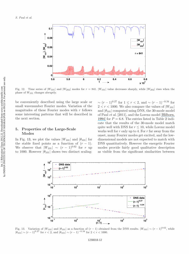
In Fig. 13, we plot the values |W101| and |θ101| forthe stable fixed points as a function of (r − 1).We observe that |W101| ∼ (r − 1)0.62 for r upto 1000. However |θ101| shows two distinct scaling:

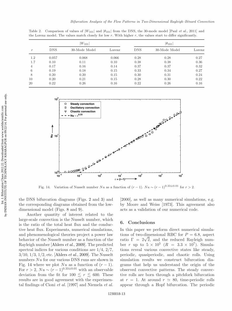
∼ (r − 1)0.27 for 1 ≤ r < 2, and ∼ (r − 1)−0.34 for2 < r < 1000. We also compare the values of |W101|and |θ101| computed using DNS, the 30-mode modelof Paul et al. [2011], and the Lorenz model [Hilborn,1994] for P = 6.8. The entries listed in Table 2 indi-cate that the results of the 30-mode model matchquite well with DNS for r ≤ 10, while Lorenz modelworks well for r only up to 4. For r far away from theonset, many Fourier modes get excited, and the low-dimensional models are not expected to match withDNS quantitatively. However the energetic Fouriermodes provide fairly good qualitative descriptionas visible from the significant similarities between

10−1

100

101

102

103

100

10−2

102

104

|W10

1|

10−1

100

101

102

103

10−2

10−1

100

(r−1)

|θ10

1|

DNS data

(r−1)0.27

(r−1)− 0.34

DNS data

(r−1)0.62

Fig. 13. Variation of |W101| and |θ101| as a function of (r − 1) obtained from the DNS results. |W101| ∼ (r − 1)0.62, while|θ101| ∼ (r − 1)0.27 for r < 2, and |θ101| ∼ (r − 1)−0.34 for 2 < r < 1000.

1230018-12

Int.

J. B

ifur

catio

n C

haos

201

2.22

. Dow

nloa

ded

from

ww

w.w

orld

scie

ntif

ic.c

omby

IN

DIA

N I

NST

ITU

TE

OF

TE

CH

NO

LO

GY

KH

AR

AG

PUR

on

09/2

2/14

. For

per

sona

l use

onl

y.

June 23, 2012 16:8 WSPC/S0218-1274 1230018

Bifurcation Analysis of the Flow Patterns in Two-Dimensional Rayleigh–Benard Convection

Table 2. Comparison of values of |W101| and |θ101| from the DNS, the 30-mode model [Paul et al., 2011] andthe Lorenz model. The values match closely for low r. With higher r, the values start to differ significantly.

|W101| |θ101|r DNS 30-Mode Model Lorenz DNS 30-Mode Model Lorenz

1.2 0.057 0.068 0.066 0.28 0.28 0.271.7 0.10 0.11 0.10 0.38 0.38 0.364 0.17 0.16 0.14 0.37 0.37 0.326 0.19 0.18 0.15 0.33 0.34 0.278 0.20 0.20 0.15 0.30 0.31 0.24

10 0.20 0.21 0.15 0.28 0.30 0.2220 0.22 0.26 0.16 0.22 0.26 0.16

10−2

10−1

100

101

102

103

104

100

101

102

ε = (r−1)

Nu

Steady convectionOscillatory convectionChaotic convection

Nu ~ ε0.33

Fig. 14. Variation of Nusselt number Nu as a function of (r − 1). Nu ∼ (r − 1)0.33±0.01 for r > 2.

the DNS bifurcation diagrams (Figs. 2 and 3) andthe corresponding diagrams obtained from the low-dimensional model (Figs. 8 and 9).

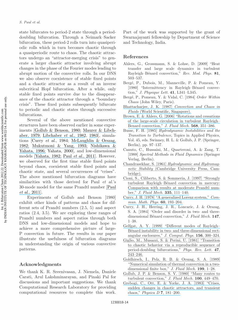
Another quantity of interest related to thelarge-scale convection is the Nusselt number, whichis the ratio of the total heat flux and the conduc-tive heat flux. Experiments, numerical simulations,and phenomenological theories project a power lawbehavior of the Nusselt number as a function of theRayleigh number [Ahlers et al., 2009]. The predictedspectral indices for various conditions are 1/4, 2/7,3/10, 1/3, 1/2, etc. [Ahlers et al., 2009]. The Nusseltnumbers Nu for our various DNS runs are shown inFig. 14 where we plot Nu as a function of (r − 1).For r > 2, Nu ∼ (r − 1)0.33±0.01 with an observabledeviation from the fit for 100 � r � 600. Theseresults are in good agreement with the experimen-tal findings of Cioni et al. [1997] and Niemela et al.

[2000], as well as many numerical simulations, e.g.by Moore and Weiss [1973]. This agreement alsoacts as a validation of our numerical code.

6. Conclusions

In this paper we perform direct numerical simula-tions of two-dimensional RBC for P = 6.8, aspectratio Γ = 2

√2, and the reduced Rayleigh num-

ber r up to 5 × 105 (R = 3.3 × 107). Simula-tions reveal various convective states like steady,periodic, quasiperiodic, and chaotic rolls. Usingsimulation results we construct bifurcation dia-grams that help us understand the origin of theobserved convective patterns. The steady convec-tive rolls are born through a pitchfork bifurcationat r = 1. At around r � 80, time-periodic rollsappear through a Hopf bifurcation. The periodic

1230018-13

Int.

J. B

ifur

catio

n C

haos

201

2.22

. Dow

nloa

ded

from

ww

w.w

orld

scie

ntif

ic.c

omby

IN

DIA

N I

NST

ITU

TE

OF

TE

CH

NO

LO

GY

KH

AR

AG

PUR

on

09/2

2/14

. For

per

sona

l use

onl

y.

June 23, 2012 16:8 WSPC/S0218-1274 1230018

S. Paul et al.

state bifurcates to period-2 state through a period-doubling bifurcation. Through a Neimark–Sackerbifurcation, these period-2 rolls turn into quasiperi-odic rolls which in turn becomes chaotic througha quasiperiodic route to chaos. The chaotic attrac-tors undergo an “attractor-merging crisis” to gen-erate a larger chaotic attractor involving abruptchanges in the phase of the Fourier modes leading toabrupt motion of the convective rolls. In our DNSwe also observe coexistence of stable fixed pointsand a chaotic attractor as a result of an inversesubcritical Hopf bifurcation. After a while, onlystable fixed points survive due to the disappear-ance of the chaotic attractor through a “boundarycrisis”. These fixed points subsequently bifurcateto periodic and chaotic states through successivebifurcations.

Several of the above mentioned convectivestructures have been observed earlier in some exper-iments [Gollub & Benson, 1980; Maurer & Libch-aber, 1979; Libchaber et al., 1982, 1983], simula-tions [Curry et al., 1984; McLaughlin & Orszag,1982; Mukutmoni & Yang, 1993; Nishikawa &Yahata, 1996; Yahata, 2000], and low-dimensionalmodels [Yahata, 1982; Paul et al., 2011]. However,we observed for the first time stable fixed pointsbeyond chaos, coexistent stable fixed points andchaotic state, and several occurrences of “crises”.The above mentioned bifurcation diagrams havesimilarities with those derived for Paul et al.’s30-mode model for the same Prandtl number [Paulet al., 2011].

Experiments of Gollub and Benson [1980]exhibit other kinds of patterns and chaos for dif-ferent sets of Prandtl numbers (2.5, 5) and aspectratios (2.4, 3.5). We are exploring these ranges ofPrandtl numbers and aspect ratios through bothDNS and low-dimensional models and hope toachieve a more comprehensive picture of large-P convection in future. The results in our paperillustrate the usefulness of bifurcation diagramsin understanding the origin of various convectivepatterns.

Acknowledgments

We thank K. R. Sreenivasan, J. Niemela, DanieleCarati, Arul Lakshminarayan, and Pinaki Pal fordiscussions and important suggestions. We thankComputational Research Laboratory for providingcomputational resources to complete this work.

Part of the work was supported by the grant ofSwarnajayanti fellowship by Department of Scienceand Technology, India.

References

Ahlers, G., Grossmann, S. & Lohse, D. [2009] “Heattransfer and large scale dynamics in turbulentRayleigh–Benard convection,” Rev. Mod. Phys. 81,503–537.

Berge, P., Dubois, M., Manneville, P. & Pomeau, Y.[1980] “Intermittency in Rayleigh–Benard convec-tion,” J. Physique Lett. 41, L341–L345.

Berge, P., Pomeau, Y. & Vidal, C. [1984] Order WithinChaos (John Wiley, Paris).

Bhattacharjee, J. K. [1987] Convection and Chaos inFluids (World Scientific, Singapore).

Brown, E. & Ahlers, G. [2006] “Rotations and cessationsof the large-scale circulation in turbulent Rayleigh–Benard convection,” J. Fluid Mech. 568, 351–386.

Busse, F. H. [1985] Hydrodynamic Instabilities and theTransition to Turbulence, Topics in Applied Physics,Vol. 45, eds. Swinney, H. L. & Gollub, J. P. (Springer,Berlin), pp. 97–137.

Canuto, C., Hussaini, M., Quarteroni, A. & Zang, T.[1988] Spectral Methods in Fluid Dynamics (SpringerVerlag, Berlin).

Chandrasekhar, S. [1961] Hydrodynamic and Hydromag-netic Stability (Cambridge University Press, Cam-bridge).

Cioni, S., Ciliberto, S. & Sommeria, J. [1997] “Stronglyturbulent Rayleigh–Benard convection in mercury:Comparison with results at moderate Prandtl num-ber,” J. Fluid Mech. 335, 111–140.

Curry, J. H. [1978] “A generalized Lorenz system,” Com-mun. Math. Phys. 60, 193–204.

Curry, J. H., Herring, J. R., Loncaric, J. & Orszag,S. A. [1984] “Order and disorder in two- and three-dimensional Benard convection,” J. Fluid Mech. 147,1–38.

Gelfgat, A. Y. [1999] “Different modes of Rayleigh–Benard instability in two- and three-dimensional rect-angular enclosures,” J. Comput. Phys. 156, 300–324.

Giglio, M., Musazzi, S. & Perini, U. [1981] “Transitionto chaotic behavior via a reproducible sequence ofperiod-doubling bifurcations,” Phys. Rev. Lett. 47,243–246.

Goldhirsch, I., Pelz, R. B. & Orszag, S. A. [1989]“Numerical simulation of thermal convection in a two-dimensional finite box,” J. Fluid Mech. 199, 1–28.

Gollub, J. P. & Benson, S. V. [1980] “Many routes toturbulent convection,” J. Fluid Mech. 100, 449–470.

Grebogi, C., Ott, E. & Yorke, J. A. [1983] “Crises,sudden changes in chaotic attractors, and transientchaos,” Physica D 7, 181–200.

1230018-14

Int.

J. B

ifur

catio

n C

haos

201

2.22

. Dow

nloa

ded

from

ww

w.w

orld

scie

ntif

ic.c

omby

IN

DIA

N I

NST

ITU

TE

OF

TE

CH

NO

LO

GY

KH

AR

AG

PUR

on

09/2

2/14

. For

per

sona

l use

onl

y.

June 23, 2012 16:8 WSPC/S0218-1274 1230018

Bifurcation Analysis of the Flow Patterns in Two-Dimensional Rayleigh–Benard Convection

Grebogi, C., Ott, E., Romeiras, F. & Yorke, J. A. [1987]“Critical exponents for crisis-induced intermittency,”Phys. Rev. A 36, 5365–5380.

Hilborn, R. C. [1994] Chaos and Nonlinear Dynamics :An Introduction for Scientists and Engineers (OxfordUniversity Press, Oxford).

Krishnamurti, R. [1970a] “On the transition to turbu-lent convection. Part 1. The transition from two- tothree-dimensional flow,” J. Fluid Mech. 42, 295–307.

Krishnamurti, R. [1970b] “On the transition to turbulentconvection. Part 2. The transition to time-dependentflow,” J. Fluid Mech. 42, 309–320.

Libchaber, A., Laroche, C. & Fauve, S. [1982] “Perioddoubling cascade in mercury, a quantitative measure-ment,” J. Physique Lett. 43, L211–L216.

Libchaber, A., Fauve, S. & Laroche, C. [1983] “Two-parameter study of the routes to chaos,” Physica D7, 73–84.

Lorenz, E. N. [1963] “Deterministic nonperiodic flow,”J. Atmos. Sci. 20, 130–141.

Manneville, P. [2004] Instabilities, Chaos and Turbulence(Imperial College Press, London).

Maurer, J. & Libchaber, A. [1979] “Rayleigh–Benardexperiment in liquid helium; frequency locking andthe onset of turbulence,” J. Physique Lett. 40,419–423.

McLaughlin, J. B. & Martin, P. C. [1975] “Transitionto turbulence in a statistically stressed fluid system,”Phys. Rev. A 12, 186–203.

McLaughlin, J. B. & Orszag, S. A. [1982] “Transitionfrom periodic to chaotic thermal convection,” J. FluidMech. 122, 123–142.

Mishra, P. K., De, A., Verma, M. K. & Eswaran, V.[2011] “Dynamics of reorientations and reversals oflarge scale flow in Rayleigh–Benard convection,” J.Fluid Mech. 668, 480–499.

Moore, D. R. & Weiss, N. O. [1973] “Two-dimensionalRayleigh–Benard convection,” J. Fluid Mech. 58,289–312.

Mukutmoni, D. & Yang, K. T. [1993] “Rayleigh–Benardconvection in a small aspect ratio enclosure. II: Bifur-cation to chaos,” J. Heat Transf. 115, 367–376.

Nimela, J. J. [2000] “Turbulent convection at very highRayleigh numbers,” Nature 404, 837–840.

Nishikawa, S. & Yahata, H. [1996] “Evolution of theRayleigh–Benard convection in a rectangular box,”J. Phys. Soc. Jpn. 65, 935–944.

Paul, S., Kumar, K., Verma, M. K., Carati, D.,De, A. & Eswaran, V. [2010] “Chaotic traveling rollsin Rayleigh–Benard convection,” Pramana 74, 75–82.

Paul, S., Wahi, P. & Verma, M. K. [2011] “Bifurcationsand chaos in large-Prandtl number Rayleigh–Benardconvection,” Int. J. Nonlin. Mech. 46, 772–781.

Schlutter, A., Lortz, D. & Busse, F. H. [1965] “Onthe stability of steady finite amplitude convection,”J. Fluid Mech. 23, 129–144.

Thual, O. [1992] “Zero-Prandtl-number convection,”J. Fluid Mech. 240, 229–258.

Vincent, A. P. & Yuen, D. A. [2000] “Transition to turbu-lent thermal convection beyond Ra = 1010 detectedin numerical simulations,” Phys. Rev. E 61, 5241–5246.

Yahata, H. [1982] “Transition to turbulence in theRayleigh–Benard convection,” Progr. Theoret. Phys.68, 1070–1081.

Yahata, H. [1983] “Period-doubling cascade in theRayleigh–Benard convection,” Progr. Theoret. Phys.69, 1802–1805.

Yahata, H. [2000] “Transition to chaos in the Rayleigh–Benard convection: Classical phenomenology andapplications,” J. Phys. Soc. Jpn. 69, 1384–1388.

Zienicke, E., Seehafer, N. & Feudel, F. [1998] “Bifur-cations in two-dimensional Rayleigh–Benard convec-tion,” Phys. Rev. E 57, 428–435.

1230018-15

Int.

J. B

ifur

catio

n C

haos

201

2.22

. Dow

nloa

ded

from

ww

w.w

orld

scie

ntif

ic.c

omby

IN

DIA

N I

NST

ITU

TE

OF

TE

CH

NO

LO

GY

KH

AR

AG

PUR

on

09/2

2/14

. For

per

sona

l use

onl

y.