Small-Scale Properties of Turbulent Rayleigh-Bénard Convection

ANRV400-FL42-15 ARI 13 November 2009 14:9

Small-Scale Properties ofTurbulent Rayleigh-BenardConvectionDetlef Lohse1 and Ke-Qing Xia2

1Physics of Fluids Group, Department of Science and Technology, J.M. Burgers Center forFluid Dynamics, and Impact-Institute, University of Twente, 7500 AE Enschede,The Netherlands; email: [email protected] of Physics, The Chinese University of Hong Kong, Shatin, Hong Kong, China;email: [email protected]

Annu. Rev. Fluid Mech. 2010. 42:335–64

First published online as a Review in Advance onSeptember 2, 2009

The Annual Review of Fluid Mechanics is online atfluid.annualreviews.org

This article’s doi:10.1146/annurev.fluid.010908.165152

Copyright c© 2010 by Annual Reviews.All rights reserved

0066-4189/10/0115-0335$20.00

Key Words

thermal convection, turbulence, structure functions, Bolgiano scaling

AbstractThe properties of the structure functions and other small-scale quantities inturbulent Rayleigh-Benard convection are reviewed, from an experimental,theoretical, and numerical point of view. In particular, we address the ques-tion of whether, and if so where in the flow, the so-called Bolgiano-Obukhovscaling exists, i.e., Sθ (r) ∼ r2/5 for the second-order temperature structurefunction and Su(r) ∼ r6/5 for the second-order velocity structure function.Apart from the anisotropy and inhomogeneity of the flow, insufficiently highRayleigh numbers, and intermittency corrections (which all hinder the iden-tification of such a potential regime), there are also reasons, as a matter ofprinciple, why such a scaling regime may be limited to at most a decade,namely the lack of clear scale separation between the Bolgiano length scaleLB and the height of the cell.

335

Ann

u. R

ev. F

luid

Mec

h. 2

010.

42:3

35-3

64. D

ownl

oade

d fr

om a

rjou

rnal

s.an

nual

revi

ews.

org

by P

rof.

Ke-

Qin

g X

ia o

n 12

/28/

09. F

or p

erso

nal u

se o

nly.

ANRV400-FL42-15 ARI 13 November 2009 14:9

1. INTRODUCTION

Thermally driven turbulence is of tremendous importance to various areas of science, technology,and the environment and in the geophysical and astrophysical context. For flow in the atmosphere,thermal convection (e.g., see Hartmann et al. 2001) is relevant both on smaller length scales andtimescales for weather predictions and on larger scales for climate calculations. In the ocean(e.g., see Marshall & Schott 1999), thermohaline convection (Rahmstorf 2000) is a main drivingmechanism of deep-ocean circulation. Thermally driven convection takes place both in Earth’souter core (see, e.g., Cardin & Olson 1994) and in its mantle (see, e.g., McKenzie et al. 1974).

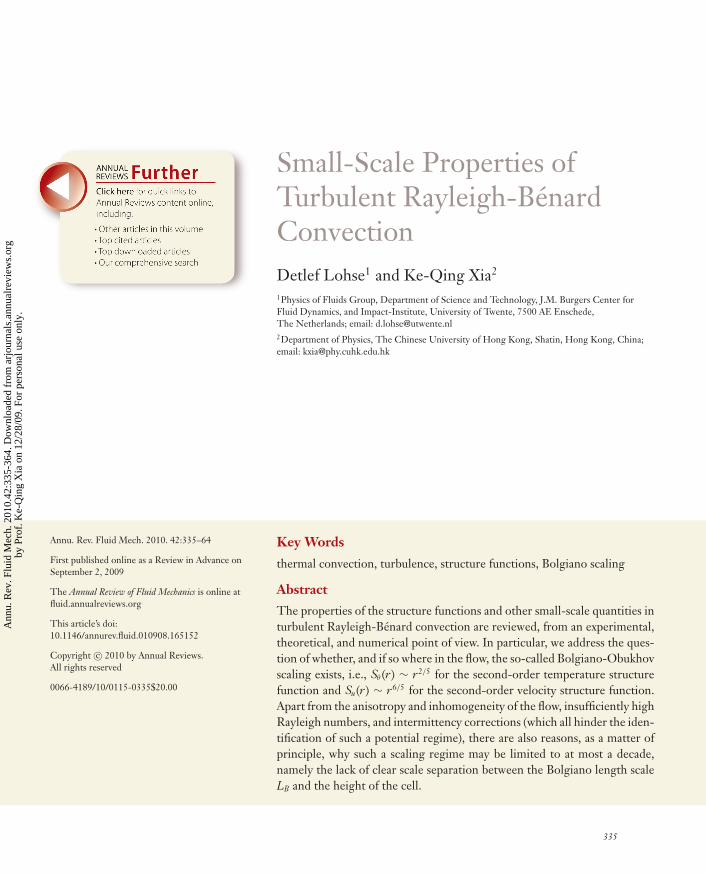
The idealized system of thermally driven turbulence is turbulent Rayleigh-Benard (RB)convection—a fluid in a box of height L strongly heated from below and cooled from above.This system may even be considered as a raw model for turbulent flow in general. It is notonly a mathematically well-defined problem, in principle given by the Boussinesq equations (seeSection 2) and the appropriate boundary conditions for the velocity field u(x, t) and the temper-ature field θ (x, t), but it can also be straightforwardly realized experimentally. Figure 1 shows ashadowgraph image of turbulent thermal convection in an aspect-ratio-one cylindrical cell, to-gether with two instantaneous two-dimensional (2D) velocity field snapshots, taken with particleimage velocimetry (PIV).

In contrast, the theoretical concept of homogeneous and isotropic turbulence (e.g., seeBatchelor 1953, Frisch 1995, Kolmogorov 1941, Monin & Yaglom 1975, Pope 2000) is muchharder to realize in a laboratory. Nonetheless, most theoretical (Frisch 1995; e.g., for a morerecent review, see Falkovich et al. 2001) and numerical (recently reviewed in Ishihara et al. 2009)work on the (small scale) scaling of structure functions (SFs) and energy spectra focused on

0.0 2.5 1.10.0

Velocity (cm s–1) Velocity (cm s–1)

Figure 1(Middle panel ) Shadowgraph image of turbulent thermal convection in an aspect-ratio-one cylindrical cell (Ra = 6.8 × 108, Pr = 596).The thermal plumes in the image play important roles in the small-scale properties of the system’s velocity and temperature fields. (Leftand right panels) Instantaneous high-resolution 2D velocity field measured in the sidewall (left panel ) and central regions (right panel )marked by the red rectangle and blue square in the shadowgraph, respectively. Because of the large disparity in the number of plumes,these two regions exhibit different scaling properties of velocity and temperature fields, as found by Sun et al. (2006). Shadowgraphtaken from Xi et al. 2004, PIV taken from Zhou et al. 2008.

336 Lohse · Xia

Ann

u. R

ev. F

luid

Mec

h. 2

010.

42:3

35-3

64. D

ownl

oade

d fr

om a

rjou

rnal

s.an

nual

revi

ews.

org

by P

rof.

Ke-

Qin

g X

ia o

n 12

/28/

09. F

or p

erso

nal u

se o

nly.

ANRV400-FL42-15 ARI 13 November 2009 14:9

homogeneous, isotropic turbulence, comparing these results with laboratory and field measure-ments for which the conditions of homogeneity and isotropy were only approximately fulfilled.In their Annual Review of Fluid Mechanics article, Sreenivasan & Antonia (1997) describe the phe-nomenology of this small-scale turbulence. In the inertial range, the second-order velocity SFSu(r) = 〈(u(x + r) − u(x))2〉x,t is basically found to scale with the Kolmogorov (1941) scaling∼r2/3, in short called K41, apart from small intermittency corrections, which are found to be re-markably universal (Arneodo et al. 1996). K41 follows from pure dimensional analysis, assumingthat in the inertial range, apart from the scale r itself, the only relevant parameter is the meanenergy dissipation rate εu , giving

Su(r) ∼ (εur)2/3. (1)

Obukhov (1949) and Corrsin (1951) generalized Kolmogorov’s argument to the fluctuations of apassive scalar θ (x, t), giving

Sθ (r) ∼ εθ ε−1/3u r2/3 (2)

for the second-order SF Sθ (r) = 〈(θ (x + r) − θ (x))2〉x,t of θ (x, t). Here εθ is its dissipation rate.Again, apart from small intermittency corrections, Equation 2 is in reasonable agreement with theexperimental data (see Warhaft 2000).

In analogy to K41, pure dimensional analysis can also be done for RB turbulence. Assuming thatnext to the scale r, the only relevant parameters are the mean thermal dissipation rate εθ and theproduct of the thermal expansion coefficient β and gravity g, one obtains the so-called Bolgiano-Obukhov scaling (BO59), which was first suggested for stably stratified convection (Bolgiano 1959,Obukhov 1959). It reads

Su(r) ∼ ε2/5θ (βg)4/5r6/5, (3)

Sθ (r) ∼ ε4/5θ (βg)−2/5r2/5. (4)

According to the same dimensional argument, the mixed SF between temperature and verticalvelocity Sθu3 (r) = 〈(θ (x + r) − θ (x))(u3(x + r) − u3(x)〉x,t should scale as

Sθu3 (r) ∼ ε3/5θ (βg)1/5r4/5. (5)

When comparing Equations 1 and 3, on one hand, or Equations 2 and 4, on the other hand, onecan read off the so-called Bolgiano length LB as crossover scale, with

LB = ε5/4u ε

−3/4θ (βg)−3/2. (6)

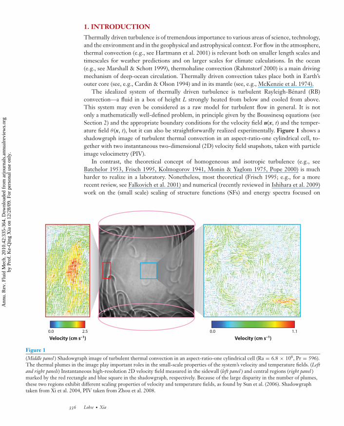
For LB � r � L, one expects BO59 scaling, whereas for η � r � LB one still expects K41scaling (see Figure 2). (Here, the height L of the cell is identified with the outer length scaleand η = ν3/4/ε1/4 is the Kolmogorov length, i.e., the inner length scale.) However, the scaling assketched in Figure 2 has hitherto not been identified in experimental or in numerical data, neitherfor the SFs nor in the respective Fourier transforms, for which BO59 would mean Eu(k) ∼ k−11/5

for the energy spectrum and Eθ (k) ∼ k−7/5 for the thermal spectrum.In this article we review the experimental and numerical attempts to at least partly identify

BO59 scaling. Owing to space limitations, we do not strive to review all aspects of the problemthat may be called small-scale. For example, we do not discuss the extraction and characterizationof individual thermal plumes (Ching et al. 2004b, Funfschilling et al. 2008, Julien et al. 1999,Puthenveettil & Arakeri 2005, Shishkina & Wagner 2008, Zhou & Xia 2002, Zhou et al. 2007)and studies of the energy and thermal dissipation rates (Benzi et al. 1998, Ching & Kwok 2000,He & Tong 2009, He et al. 2007, Kaczorowski & Wagner 2009, Kerr 2001, Shishkina & Wagner2006, Verzicco & Camussi 2003), nor do we review the small-scale properties in 2D turbulent

www.annualreviews.org • Turbulent Rayleigh-Benard Convection 337

Ann

u. R

ev. F

luid

Mec

h. 2

010.

42:3

35-3

64. D

ownl

oade

d fr

om a

rjou

rnal

s.an

nual

revi

ews.

org

by P

rof.

Ke-

Qin

g X

ia o

n 12

/28/

09. F

or p

erso

nal u

se o

nly.

ANRV400-FL42-15 ARI 13 November 2009 14:9

0 5 10

log

(Su(

r)),

lo

g(S

θ(r)

)

log(r/η)

–20

–15

–10

–5

0

2

2/3

2/5

6/5

10η

LB

L

Figure 2Sketch of the second-order velocity (blue curve) and temperature ( purple curve) structure functions, as theyfollow from BO59 dimensional analysis: LB = 106η and L = 1011η are assumed, and there is a crossover at10η (e.g., see Effinger & Grossmann 1987) between the viscous subrange and the inertial subrange. For10η < r < LB, the BO59-type dimensional analysis gives K41 scaling (Equations 1 and 2), and for LB < r < Lit gives BO59 scaling (Equations 3 and 4). Such pronounced scaling as sketched here has hitherto never beenobserved.

thermal convection (Celani et al. 2001, 2002; Zhang & Wu 2005; Zhang et al. 2005) and thosein the Lagrangian frame (Gasteuil et al. 2007, Schumacher 2008). Rather, we focus on the issueregarding the existence of BO59 and how the properties of an active scalar as a small-scale quantitycompare with those of a passive scalar in convective flows. Section 2 presents numerical data onthe Bolgiano scale LB (which turns out to be the crucial quantity) and demonstrates that the BO59dimensional argument is too simplistic. We then point out further difficulties, both practical andas a matter of principle, in identifying BO59 scaling: the inhomogeneity and anisotropy of theflow and intermittency. Section 3 presents experimental and numerical data on the SFs, whereasSection 4 compares the flow characteristics of an active scalar, such as temperature in RB convec-tion, with that of a passive scalar.

The review aims to give an update on the statistics of small-scale quantities in RB convectionto the status as described in Siggia (1994). An update on large-scale quantities and in particularon how the Nusselt number (Nu) and the Reynolds number (Re) depend on the Rayleigh number(Ra) and the Prandtl number (Pr) has already been given by Ahlers et al. (2009). Along with Ra,Pr, and the shape of the cell, the other control parameter of the system is the aspect ratio �; herewe focus on � ∼ 1.

2. BOLGIANO LENGTH SCALE AND DIFFICULTIESIN REALIZING BO59 SCALING

2.1. Bolgiano Length Scale

The first step in judging whether BO59 scaling is possible is to determine the Bolgiano lengthLB from Equation 6. Assuming spatial homogeneity, one can do this based on rigorous relations,within the approximations of the Boussinesq equation (see, e.g., Shraiman & Siggia 1990),

εu ≡ 〈ν(∂i u j (x, t))2〉V,t = ν3

L4(Nu − 1)RaPr−2, (7)

338 Lohse · Xia

Ann

u. R

ev. F

luid

Mec

h. 2

010.

42:3

35-3

64. D

ownl

oade

d fr

om a

rjou

rnal

s.an

nual

revi

ews.

org

by P

rof.

Ke-

Qin

g X

ia o

n 12

/28/

09. F

or p

erso

nal u

se o

nly.

ANRV400-FL42-15 ARI 13 November 2009 14:9

εθ ≡ 〈κ(∂iθ (x, t))2〉V,t = κ�2

L2Nu, (8)

for the volume and time-averaged kinetic and thermal dissipation rates, respectively. Here Ra =βg�L3/(νκ) and Pr = ν/κ are the Rayleigh and Prandtl numbers, with � the applied temperaturedifference, and ν and κ the kinematic viscosity and the thermal diffusivity, respectively. For Nu �1, these relations imply

LB/L ≈ Nu1/2/(PrRa)1/4. (9)

Assuming the large-Ra power law Nu ∼ Ra1/3, which follows from Grossmann & Lohse’s (2000)theory and is consistent with the experimental data of Niemela et al. (2000), Nikolaenko et al.(2005), and Niemela & Sreenivasan (2006), one obtains

LB/L ∼ Ra−1/12Pr−1/4, (10)

giving hope that at least for very large Ra and large Pr a separation of scales between LB and Lmay arise.

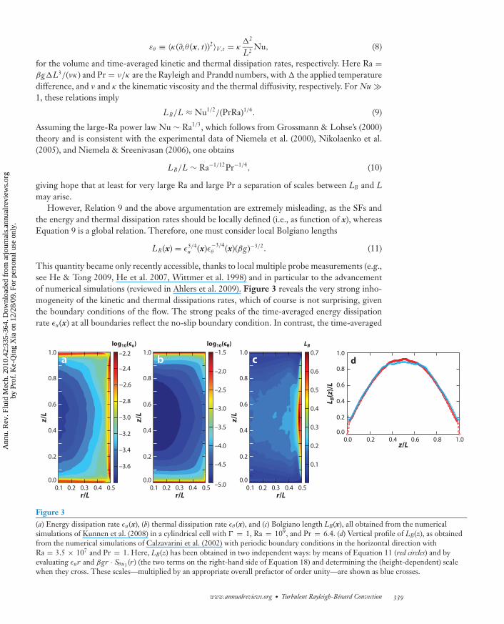
However, Relation 9 and the above argumentation are extremely misleading, as the SFs andthe energy and thermal dissipation rates should be locally defined (i.e., as function of x), whereasEquation 9 is a global relation. Therefore, one must consider local Bolgiano lengths

LB (x) = ε5/4u (x)ε−3/4

θ (x)(βg)−3/2. (11)

This quantity became only recently accessible, thanks to local multiple probe measurements (e.g.,see He & Tong 2009, He et al. 2007, Wittmer et al. 1998) and in particular to the advancementof numerical simulations (reviewed in Ahlers et al. 2009). Figure 3 reveals the very strong inho-mogeneity of the kinetic and thermal dissipations rates, which of course is not surprising, giventhe boundary conditions of the flow. The strong peaks of the time-averaged energy dissipationrate εu(x) at all boundaries reflect the no-slip boundary condition. In contrast, the time-averaged

–5.0

–4.5

–4.0

–3.5

–3.0

–2.5

–2.0

–1.5

0.1

0.2

0.3

0.4

0.5

0.6

0.7

0.1 0.2 0.3 0.4 0.50.1 0.2 0.3 0.4 0.50.1 0.2 0.3 0.4 0.50.0

0.2

0.4

0.6

0.8

1.0

–3.6

–3.4

–3.2

–3.0

–2.8

−2.6

–2.4

–2.2

log10(єθ) LBlog10(єu)

0.0

0.2

0.4

0.6

0.8

1.0

0.0 0.2 0.4 0.6 0.8 1.0

L B(z

)/L

r/Lr/L

z/L

0.0

0.2

0.4

0.6

0.8

1.0

z/L

0.0

0.2

0.4

0.6

0.8

1.0

z/L

r/L

z/L

a ba b c d

Figure 3(a) Energy dissipation rate εu(x), (b) thermal dissipation rate εθ (x), and (c) Bolgiano length LB(x), all obtained from the numericalsimulations of Kunnen et al. (2008) in a cylindrical cell with � = 1, Ra = 109, and Pr = 6.4. (d) Vertical profile of LB(z), as obtainedfrom the numerical simulations of Calzavarini et al. (2002) with periodic boundary conditions in the horizontal direction withRa = 3.5 × 107 and Pr = 1. Here, LB(z) has been obtained in two independent ways: by means of Equation 11 (red circles) and byevaluating εur and βgr · Sθu3 (r) (the two terms on the right-hand side of Equation 18) and determining the (height-dependent) scalewhen they cross. These scales—multiplied by an appropriate overall prefactor of order unity—are shown as blue crosses.

www.annualreviews.org • Turbulent Rayleigh-Benard Convection 339

Ann

u. R

ev. F

luid

Mec

h. 2

010.

42:3

35-3

64. D

ownl

oade

d fr

om a

rjou

rnal

s.an

nual

revi

ews.

org

by P

rof.

Ke-

Qin

g X

ia o

n 12

/28/

09. F

or p

erso

nal u

se o

nly.

ANRV400-FL42-15 ARI 13 November 2009 14:9

thermal dissipation rate εθ (x) is only peaked at the top and at the bottom wall, where there arestrong temperature gradients—at the sidewall there is no peak because of the adiabatic sidewallboundary conditions. The resulting local Bolgiano length (Equation 11) is shown in Figure 3c,again reflecting this strong inhomogeneity. Except close to the plates, where LB/L ≈ 0.1, theBolgiano length scale is not really separated from the outer length scale L. This result was foundearlier in Benzi et al.’s (1998) and, with better precision, Calzavarini et al.’s (2002) simulations,which assume periodic boundary conditions in the horizontal direction: In the bulk of the flow,LB is the same order of magnitude as the height of the cell (see Figure 3d ) and no BO59 can beexpected. According to these numerical findings, the best chance to observe BO59 is close to theupper and lower plates. Consistent with this finding, in homogeneous RB convection—convectionwith an imposed vertical temperature gradient and periodic boundary conditions also in the ver-tical direction (see also Calzavarini et al. 2005, 2006; Lohse & Toschi 2003) so that no boundarylayers can develop—Biferale et al. (2003) find LB ∼ L and correspondingly no BO59 scaling at all.The corresponding SFs, including their subleading corrections, are discussed in Section 3.5.

From the global relation (Equation 10), one may expect that the separation of scales willimprove for larger Ra, but again the global argument is misleading. When fitting the numericalvalues for LB(x) between 0.1 < r/L < 0.4 at half-height in the regime 108 ≤ Ra ≤ 1010, Kunnenet al. (2008) obtained the relation LB (x in bulk)/L = 0.024 Ra0.107±0.016 with a positive power-lawexponent, suggesting that for larger Ra, what would be a potentially small regime of BO59 scalingwill vanish altogether. This indeed is found in the experiments of Sun et al. (2006) and Kunnenet al. (2008) (and numerical simulations as well for the latter; see Section 3).

We try to rationalize the positive power-law exponent in LB (x in bulk)/L = 0.024 Ra0.107±0.016.When we take the bulk estimates of the Grossmann-Lohse theory, εu ∼ U3/L and εθ ∼ U�2/L,we obtain LB (x in bulk)/L ∼ Re3 Pr3/2 /Ra3/2. For regime Iu of Grossmann & Lohse’s (2000, 2001,2002, 2004) theory, where one has Re ∼ Ra1/2Pr−5/6, this would imply LB (x in bulk)/L ∼ Pr−1;for regime IVu with Re ∼ Ra4/9Pr−2/3, it would imply LB (x in bulk)/L ∼ Ra−1/6 Pr−1/2. Neithergives a positive power-law exponent with Ra, for which we therefore do not have any explanation.

2.2. Cascade Picture

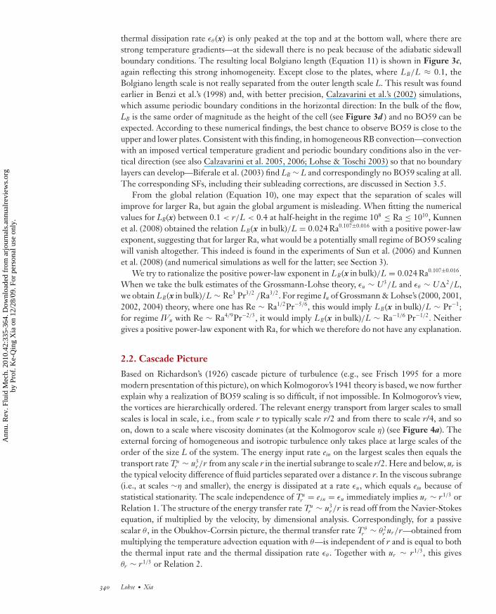
Based on Richardson’s (1926) cascade picture of turbulence (e.g., see Frisch 1995 for a moremodern presentation of this picture), on which Kolmogorov’s 1941 theory is based, we now furtherexplain why a realization of BO59 scaling is so difficult, if not impossible. In Kolmogorov’s view,the vortices are hierarchically ordered. The relevant energy transport from larger scales to smallscales is local in scale, i.e., from scale r to typically scale r/2 and from there to scale r/4, and soon, down to a scale where viscosity dominates (at the Kolmogorov scale η) (see Figure 4a). Theexternal forcing of homogeneous and isotropic turbulence only takes place at large scales of theorder of the size L of the system. The energy input rate ein on the largest scales then equals thetransport rate Tu

r ∼ u3r /r from any scale r in the inertial subrange to scale r/2. Here and below, ur is

the typical velocity difference of fluid particles separated over a distance r. In the viscous subrange(i.e., at scales ∼η and smaller), the energy is dissipated at a rate εu , which equals ein because ofstatistical stationarity. The scale independence of Tu

r = ein = εu immediately implies ur ∼ r1/3 orRelation 1. The structure of the energy transfer rate Tu

r ∼ u3r /r is read off from the Navier-Stokes

equation, if multiplied by the velocity, by dimensional analysis. Correspondingly, for a passivescalar θ , in the Obukhov-Corrsin picture, the thermal transfer rate T θ

r ∼ θ2r ur/r—obtained from

multiplying the temperature advection equation with θ—is independent of r and is equal to boththe thermal input rate and the thermal dissipation rate εθ . Together with ur ∼ r1/3, this givesθr ∼ r1/3 or Relation 2.

340 Lohse · Xia

Ann

u. R

ev. F

luid

Mec

h. 2

010.

42:3

35-3

64. D

ownl

oade

d fr

om a

rjou

rnal

s.an

nual

revi

ews.

org

by P

rof.

Ke-

Qin

g X

ia o

n 12

/28/

09. F

or p

erso

nal u

se o

nly.

ANRV400-FL42-15 ARI 13 November 2009 14:9

βgθrur

Tur

u3r

r

βgθrur

Tur

u3r

r

euin

єuєu

a b

K41 balance

B059balance

Thermal plumeinput

≅

K41balance

≅

Figure 4(a) Sketch of the Richardson cascade for homogeneous isotropic turbulence. The K41 balance results in theK41 scaling ur ∼ r1/3. (b) Attempted sketch of the situation in Rayleigh-Benard flow: On one hand, thermalplumes drive the large-scale convection roll. On the other hand, the buoyancy term βgθr ur , whose rdependency is not a priori known, supplies kinetic energy on scale r. Both the K41 and the BO59 balancesare shown. If the cascade is downscale, the energy transfer term Tu

r transports the sum of all energies thathave been put into the various scales from L to r down the cascade.

What changes for an active scalar θ , i.e., in RB convection, where the underlying equations arenow the Oberbeck-Boussinesq equations (Landau & Lifshitz 1987)

∂tui + u j ∂ j ui = −∂i p + ν∂2j ui + βgδi3θ, (12)

∂tθ + u j ∂ j θ = κ∂2j θ, (13)

together with the incompressibility conditions ∂i ui = 0? [Here p(x, t) is kinematic pressure;scaling-wise the corresponding term ∂i p has the same structure as the advection term u j ∂ j ui .]The thermal balance does not change; i.e., T θ

r ∼ θ2r ur/r ∼ εθ remains scale-independent. The

situation is rather different for the kinetic balance. On one hand, a large-scale convection rolldevelops, which was first described by Krishnamurti & Howard (1981). It is fed and driven by thesmall-scale thermal plumes detaching from the boundary layers, as nicely sketched by Kadanoff(2001). This implies an interaction that is scale-wise nonlocal. On the other hand, the large-scaleconvection roll decays to smaller vortices, so energy is also transported from the large scales towardthe small scales. We try to sketch the situation in Figure 4b.

If one wanted to obtain BO59 scaling within the cascade picture, the balance βgθr ur ∼ Tur ∼

u3r /r would be required for all scales in the inertial subrange for the energy equation. Indeed, from

this balance, together with above thermal balance T θr ∼ εθ , one immediately obtains BO59 scaling.

However, this would imply that Tu2r � Tu

r , as on scale r the energy gain from larger scales wouldbe required to be neglible as compared to the energy input through buoyancy βgθr ur on scale r. Ittherefore would imply that βgθr ur � βgθ2r u2r for all scale r in the inertial range. Employing the

www.annualreviews.org • Turbulent Rayleigh-Benard Convection 341

Ann

u. R

ev. F

luid

Mec

h. 2

010.

42:3

35-3

64. D

ownl

oade

d fr

om a

rjou

rnal

s.an

nual

revi

ews.

org

by P

rof.

Ke-

Qin

g X

ia o

n 12

/28/

09. F

or p

erso

nal u

se o

nly.

ANRV400-FL42-15 ARI 13 November 2009 14:9

framework of Effinger & Grossmann’s (1987) mean field theory, Procaccia & Zeitak (1989, 1990)made these assumptions, obtaining BO59 scaling. Similarly, in the framework of shell models (e.g.,see Biferale 2003), such balances were also implemented by Brandenburg (1992), Ching & Cheng(2008), Ching & Ko (2008), and Ching et al. (2008a,b), again giving BO59 scaling. Grossmann &L’vov (1993) discuss these balances in Fourier space.

However, within the cascade picture, it is impossible to fulfill the conditions Tu2r � Tu

r andβgθr ur � βgθ2r u2r over many scales r in the inertial range. Instead, the energy input throughbuoyancy from the outer length scale L down to the length scale r will accumulate, and the relevantbalance on scale r is

Tur ∼ u3

r /r ∼r ′=L∑

r ′=r

βgθr ′ ur ′ . (14)

When assuming some power-law scaling for θr ur with some positive exponent—e.g.,with 4/5 as suggested by the BO59 scaling relation (Equation 5) itself—the sum∑r ′=L

r ′=r βgθr ′ ur ′ ∼ L4/5 + (L/2)4/5 + (L/4)4/5 + · · · + r4/5 in this balance is then a quickly converg-ing geometric series because r � L. In particular, it quickly becomes independent of r, resulting inK41 scaling. This illustrates the paradoxical nature of the BO59 scaling. Within the framework ofthe reduced wave vector set approximation (see Eggers & Grossmann 1991, Grossmann & Lohse1992a), Grossmann & Lohse (1991) indeed found the balance (Equation 14) to dynamically es-tablish, giving basically K41 scaling and LB ∼ L. Only when locally injecting, with decreasingscale, an increasing amount of kinetic energy into the cascade—somehow mimicking the kineticdriving of the plumes detaching from the boundary layers—were Grossmann & Lohse (1992b)able to achieve a scaling less steep than K41 for θ r—but for ur , no scaling steeper than K41 couldbe achieved.

2.3. Further Obstacles in Identifying BO59 Scaling

Apart from the inhomogeneity of the flow and the unavoidable limited separation of the lengthscales between LB and L, there are further obstacles in identifying BO59 scaling. As pointed out byLohse (1994), a clear identification of the, at most, short BO59 regime (as shown above) is furthercomplicated by the proximity of the exponents for the BO59 scaling and for the scaling in shearflows. Moreover, because of the large-scale convection roll, there is considerable shear in the RBflow field, making it strongly nonhomogeneous and anisotropic. Either from dimensional analysis(Grossmann et al. 1994, Kuznetsov & L’vov 1981, Lohse 1994, Lohse & Muller-Groeling 1996,Lumley 1967, Tennekes & Lumley 1972) or from a more systematic SO(3) decomposition of thevelocity field (e.g., see Arad et al. 1998, 1999a,b; von der Heydt et al. 2001; and Biferale & Procaccia2005 for a recent review), one obtains for shear flow either dominantly or subdominantly

Su(r) ∼ ε2/3u L−2/3

s r4/3, (15)

Sθ (r) ∼ εθ ε−1/3u L1/3

s r1/3, (16)

where Ls ∼ ε1/2u /s 3/2 is the shear length scale and s the typical shear rate. In Fourier space, the cor-

responding spectra for the kinetic energy and the thermal fluctuations are Eu(k) ∼ ε2/3u L−2/3

s k−7/3

and Eθ (k) ∼ εθ ε−1/3u L1/3

s k−4/3, respectively. We note that this type of scaling has been observedin various shear flows, although often only as an anisotropic correction to the (isotropic) K41scaling. Experimental and numerical examples for the kinetic energy spectrum include Arad et al.1998, Biferale & Toschi 2001, Biferale et al. 2002b, Kurien & Sreenivasan 2000, and Saddoughi& Veeravalli 1994—for a review, we again refer the reader to Biferale & Procaccia (2005)—andSreenivasan (1991) gives an example for the temperature fluctuation spectrum. Indeed, close to

342 Lohse · Xia

Ann

u. R

ev. F

luid

Mec

h. 2

010.

42:3

35-3

64. D

ownl

oade

d fr

om a

rjou

rnal

s.an

nual

revi

ews.

org

by P

rof.

Ke-

Qin

g X

ia o

n 12

/28/

09. F

or p

erso

nal u

se o

nly.

ANRV400-FL42-15 ARI 13 November 2009 14:9

the top and bottom plates, Kunnen et al. (2008, their figure 18) find a shear spectrum Su(r) ∼ r4/3

for the second-order SF of the vertical velocity.A proper analysis of the flow properties clearly requires one to disentangle the shear effects

and thermal effects, with the help of the SO(3) decompositions, as has been attempted for RBturbulence (Biferale et al. 2003, Rincon 2006). For the longitudinal p-th order velocity SF S (p)

u (r) =〈(u(x + r) − u(x)) · r/r)p 〉x,t , the SO(3) decomposition reads

S (p)u (r) =

∞∑

j=0

m= j∑

m=− j

S (p)jm (r)Yjm(r/r), (17)

where Yjm(r/r) is the spherical harmonics (see Biferale & Procaccia 2005). The projections S (p)jm

on the different anisotropic sectors are expected to scale with an m-independent exponent, S (p)jm ∼

rζj

u (p). Yakhot (1992) has generalized the von Karman–Howarth equation (see Monin & Yaglom1975) to the case of thermally driven turbulence, obtaining

S(3)u (r) ∼ εr + βgrez · Sθu3 (r). (18)

Here ez is the unit vector in the vertical direction, and for simplicity we have suppressed thetensorial structure. The first term on the right-hand side is isotropic ( j = 0), whereas in thesecond term, the j = 1 factor βgrez couples to Sθu3 (r) with its j = 1, 3, . . . contributions, givingprojections on all sectors j = 0, 1, 2, . . . . Biferale et al. (2003) point out that the dimensionalisotropic balance in the j = 0 sector reads S(3), j=0

u (r) ∼ εr + βgrezS j=1θu3

(r), with the second termbeing subdominant, implying K41-type scaling, whereas in the anisotropic sectors j > 0, oneobtains

S (3), ju (r) ∼ βgrezS j−1

θu3(r). (19)

Relation 19 reveals that it is the anisotropic contribution of the third-order velocity SF that,according to the BO59 dimensional argument, should balance the buoyancy term. In Section 3.5,we report Biferale et al.’s (2003) numerical results on homogeneous RB convection, showing thatRelation 19 does not hold. The clean SO(3) analysis of Biferale et al. (2003) was possible onlybecause the authors restricted themselves to the kind of artificial case of homogeneous RB flow,i.e., the case with an imposed vertical temperature gradient, but without any walls. In real RB flow,walls are present, and close to the walls, the SO(3) analysis must be replaced by an SO(2) analysis,as done by Biferale et al. (2002b) for shear flow. We do not further discuss this complication here.

Apart from the SO(3) decomposition [or close to walls, SO(2)], another helpful tool for dataanalysis may be the property of extended self-similarity (ESS), as first found by Benzi et al.(1993). The method, plotting (logarithms of) SFs of different orders p against each other andnot against the scale r, is usually effective in revealing mutual scaling relations and in partic-ular intermittency. In the context of RB convection, it has first been applied by Benzi et al.(1994) and later by Cioni et al. (1995), Ching (2000), Zhou & Xia (2001), Skrbek et al. (2002),Ching et al. (2003b), and Kunnen et al. (2008). Independent of the scaling of the second-ordervelocity SF (K41, BO59, shear flow scaling), dimensional scaling implies S (p)

u (r) ∼ (S (2)u (r))p/2.

However, even for homogeneous and isotropic flows, there are major deviations from this di-mensional scaling—the so-called intermittency corrections (see Frisch 1995, Ishihara et al. 2009,Sreenivasan & Antonia 1997 for reviews). Such intermittency corrections are also present in RBflow for both the velocity and the temperature SFs (see Berschadskii et al. 2004; Ching 2000;Ching & Cheng 2008; Ching et al. 2003b, 2008a; Sun et al. 2006; Zhang & Wu 2005). Disen-tangling the anisotropic effects and intermittency effects (Biferale & Toschi 2001, Biferale et al.2002a, Toschi et al. 1999) and effects from the buoyancy-driven mechanism remains a majorchallenge.

www.annualreviews.org • Turbulent Rayleigh-Benard Convection 343

Ann

u. R

ev. F

luid

Mec

h. 2

010.

42:3

35-3

64. D

ownl

oade

d fr

om a

rjou

rnal

s.an

nual

revi

ews.

org

by P

rof.

Ke-

Qin

g X

ia o

n 12

/28/

09. F

or p

erso

nal u

se o

nly.

ANRV400-FL42-15 ARI 13 November 2009 14:9

We would like to stress that even if the above-mentioned complications (e.g., shear, intermit-tency) were overcome, the intrinsic difficulties of the BO59 scaling as discussed in Section 2.2 stillremain.

3. TEMPERATURE AND VELOCITY SPECTRAAND STRUCTURE FUNCTIONS

3.1. Overview of Main Experimental Methods

Above we discuss the theoretical difficulties in detecting BO59 scaling, namely anisotropy, in-homogeneity, intermittency, and the lack of a wide inertial range that can provide a sufficientseparation of the relevant length scales (η, LB, Ls, and L). However, in addition there is also alack of suitable experimental techniques for direct and high-resolution simultaneous multipointmeasurements of the velocity and temperature fields.

By far most experimental studies on temperature and velocity fluctuations employ only pointmeasurements, resulting in temperature and velocity time series acquired at a single point in theconvection cell. At best, such measurements are performed at several locations in the flow. Thebasic methods at hand are thermometry or bolometry for the temperature time series and laterlaser Doppler velocimetry (LDV) for the velocity time series. To connect the time-domain resultsto the theoretical predictions made for the spatial domain, investigators invoke Taylor’s (1938)frozen-flow hypothesis, either explicitly or implicitly. The validity of this hypothesis requires thatturbulent velocity fluctuations are much smaller than the mean flow velocity. However, the meanvelocity is approximately zero in the central region of the convection cell and is comparable to theroot-mean-square (rms) velocity near the sidewall and plate regions (Qiu et al. 2000, Sun et al.2005, Xia et al. 2003). Therefore, the condition for the Taylor hypothesis is often not met inturbulent RB convection, and its applicability to the system is at best doubtful. Nonetheless, wediscuss results from such point measurements in Sections 3.2 and 3.3.

Only recently, with the maturing of PIV (see Adrian 1991) and other similar techniques for thefull velocity field measurement, have the experimental limitations of single-point measurementsbecome less of a problem. We discuss the results of recent PIV measurements of the velocity fieldin RB convection in Section 3.4. Finally, the numerical results on temperature and velocity spectraand SFs are reviewed in Section 3.5. Here, the full spatial information is available, but Ra is limited.

3.2. Time-Domain Measurements

The first systematic measurements in turbulent RB convection by Libchaber and coworkers(Castaing et al. 1989, Heslot et al. 1987, Procaccia et al. 1991, Sano et al. 1989, Wu et al. 1990)were restricted to temperature time series, from which temperature frequency power spectra wereobtained through Fourier transformation. These temperature power spectra, and also those basedon later temperature time-series measurements at Pr ≈ 0.7 and larger, display a scaling exponentaround −1.3 ± 0.1 (e.g., Procaccia et al. 1991) to −1.4 (e.g., Wu et al. 1990), similar to the BO59value −7/5 (but also similar to the shear spectrum value −4/3). In contrast, low-Pr liquid metals(such as mercury, Pr ≈ 0.025) show more complicated behavior, depending on the value of Ra.We first discuss experiments made in fluids with Pr ≥ 0.7.

Libchaber and coworkers’ early experiments (Castaing et al. 1989, Heslot et al. 1987, Procacciaet al. 1991, Sano et al. 1989, Wu et al. 1990; reviewed in Siggia 1994) used low-temperature heliumgas as the working fluid and measured temperature frequency power spectra with miniaturizedsemiconductor bolometers placed inside the convection cell. Wu et al.’s (1990) experiments were

344 Lohse · Xia

Ann

u. R

ev. F

luid

Mec

h. 2

010.

42:3

35-3

64. D

ownl

oade

d fr

om a

rjou

rnal

s.an

nual

revi

ews.

org

by P

rof.

Ke-

Qin

g X

ia o

n 12

/28/

09. F

or p

erso

nal u

se o

nly.

ANRV400-FL42-15 ARI 13 November 2009 14:9

made in a � = 0.5 cylindrical cell with Ra spanning from 7 × 106 to 4 × 1014. Their mainresult is that up to1 at least Ra = 7 × 1010, the temperature power spectra exhibit a universalshape characterized by a power-law range in the low-frequency region and an exponential decayin the high-frequency tails, which is characteristic of dissipation range behavior. All power spectracan be collapsed onto a single curve by a simple rescaling of power density and frequency, i.e.,shifts in log-log plot. A slope of −1.4 was observed in the low-frequency power-law region, andthe authors noted that the scaling range increases with increasing Ra, starting from Ra ∼ 108,where the scaling range is almost zero. Interestingly, Wu et al. (1990) did not take the findingof the exponent −1.4 in the temperature power spectra as indicative of the existence of BO59scaling; rather they seem to regard this as a mere coincidence. Instead, their main message is thata kind of universality may exist in the cascades of turbulent fluctuations in the dissipative regionof thermal turbulence. Wu et al. (1990) suggested that this may represent a generalization ofKolmogorov’s picture of turbulence; i.e., a lack of universality in the original Kolmogorov spiritmay be restored by a proper multifractal transformation, which is referred to as a multifractaluniversality (Frisch 1995). In their experiment, Wu et al. measured temperature at the cell center,where the convective flow may be regarded as homogeneous but the mean flow is essentially zero,and the authors themselves point out that Taylor’s frozen-flow hypothesis is not believed to beapplicable. We shall take the same view when discussing below the other experiments conductedunder similar circumstances.

Whereas Wu et al. (1990) focused primarily on whether the temperature power spectra hasa universal shape, Chilla et al. (1993) studied both the shape and the scaling properties of thepower spectra and SFs of the temperature field. Their experiment was carried out in a rectangularcell using water as the convecting fluid, with Pr ≈ 4 and Ra between 106 and 4 × 108. The 2Dtemperature field was measured using a laser sweeping technique in which the deflection of thelaser beam is proportional to the local temperature gradient averaged along the beam path (Rubioet al. 1989). The temperature was then reconstructed by integrating the measured temperaturegradient. Because the measured temperature gradient was integrated along the optical path of thelaser beam, this technique required that the flow field be mainly 2D. These authors also used athermocouple placed inside the fluid to measure the local temperature. Their results show thatwave-number power spectra of the temperature from the laser sweeping method and the frequencypower spectra measured by the thermocouple have similar shape. In fact these two types of spectralargely overlap when normalized properly. The authors suggest that this coincidence may betaken as an indirect verification of Taylor’s frozen-flow hypothesis (actually a modified version ofit because it involved averaged quantities), although they also conceded that it did not constitute arigorous proof of the hypothesis. Using the spatially averaged temperature field, they also studiedlow-order SFs. In a later study, Cioni et al. (1995), employing ESS, found consistency of Chillaet al.’s (1993) results with BO59.

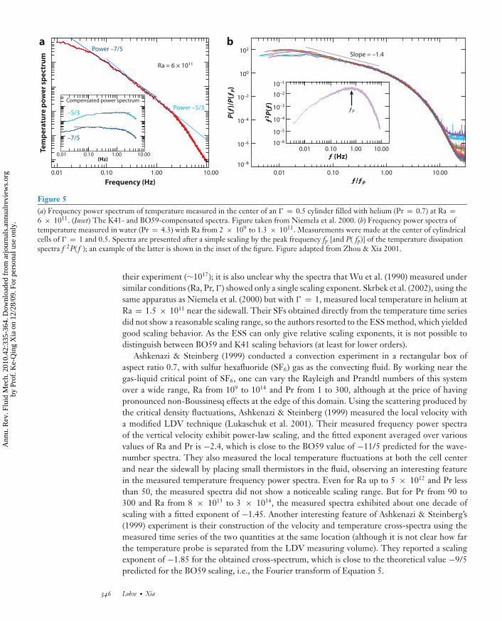
Several later studies focused primarily on the scaling of the power spectra. For example, in ahelium gas experiment, Niemela et al. (2000) reported observing both BO59- and K41-type scalingin the frequency power spectrum obtained from measured temperature time series. However, asseen from Figure 5a, for both regimes the scaling range is less than a decade, and it is not knownwhether the power spectrum remains the same shape at the high end of Ra that was reached in

1The transition at Ra ≈ 7 × 1010, which Wu et al. (1990) and later Procaccia et al. (1991) found in various quantities—including the temperature spectra themselves—has consistently been interpreted to be caused by temperature-fluctuationaveraging effects around the bolometer (Grossmann & Lohse 1993). Although already Siggia (1994) favors Grossmann &Lohse (1993)’s interpretation, it has not been strictly proven. Due to space limitations, we do not further discuss this issue inthis review.

www.annualreviews.org • Turbulent Rayleigh-Benard Convection 345

Ann

u. R

ev. F

luid

Mec

h. 2

010.

42:3

35-3

64. D

ownl

oade

d fr

om a

rjou

rnal

s.an

nual

revi

ews.

org

by P

rof.

Ke-

Qin

g X

ia o

n 12

/28/

09. F

or p

erso

nal u

se o

nly.

ANRV400-FL42-15 ARI 13 November 2009 14:9

Compensated power spectrum

Ra = 6 × 1011

Te

mp

era

ture

po

we

r sp

ec

tru

m

Frequency (Hz)

P(ƒ)

/P(ƒ

P)

ƒ/ƒP

(Hz) ƒ (Hz)

ƒP

ƒ2P(

ƒ)

102

100

10–2

10–4

10–6

10–8

0.01 0.10 1.00 10.00

Slope = –1.4

0.10 1.00 10.00

10–1

10–2

10–4

10–6

10–3

10–5

0.01 0.10 1.00 10.00

0.01 0.10 1.00 10.00

Power –5/3

Power –7/5

–5/3

–7/5

0.01

a b

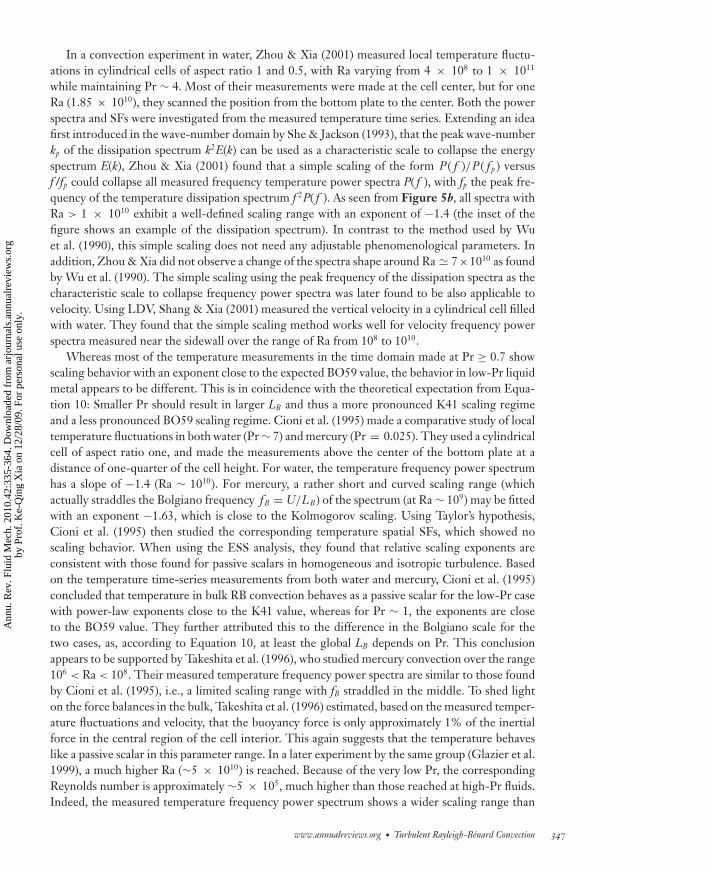
Figure 5(a) Frequency power spectrum of temperature measured in the center of an � = 0.5 cylinder filled with helium (Pr = 0.7) at Ra =6 × 1011. (Inset) The K41- and BO59-compensated spectra. Figure taken from Niemela et al. 2000. (b) Frequency power spectra oftemperature measured in water (Pr = 4.3) with Ra from 2 × 109 to 1.3 × 1011. Measurements were made at the center of cylindricalcells of � = 1 and 0.5. Spectra are presented after a simple scaling by the peak frequency fp [and P( fp)] of the temperature dissipationspectra f 2P( f ); an example of the latter is shown in the inset of the figure. Figure adapted from Zhou & Xia 2001.

their experiment (∼1017); it is also unclear why the spectra that Wu et al. (1990) measured undersimilar conditions (Ra, Pr, �) showed only a single scaling exponent. Skrbek et al. (2002), using thesame apparatus as Niemela et al. (2000) but with � = 1, measured local temperature in helium atRa = 1.5 × 1011 near the sidewall. Their SFs obtained directly from the temperature time seriesdid not show a reasonable scaling range, so the authors resorted to the ESS method, which yieldedgood scaling behavior. As the ESS can only give relative scaling exponents, it is not possible todistinguish between BO59 and K41 scaling behaviors (at least for lower orders).

Ashkenazi & Steinberg (1999) conducted a convection experiment in a rectangular box ofaspect ratio 0.7, with sulfur hexafluoride (SF6) gas as the convecting fluid. By working near thegas-liquid critical point of SF6, one can vary the Rayleigh and Prandtl numbers of this systemover a wide range, Ra from 109 to 1014 and Pr from 1 to 300, although at the price of havingpronounced non-Boussinesq effects at the edge of this domain. Using the scattering produced bythe critical density fluctuations, Ashkenazi & Steinberg (1999) measured the local velocity witha modified LDV technique (Lukaschuk et al. 2001). Their measured frequency power spectraof the vertical velocity exhibit power-law scaling, and the fitted exponent averaged over variousvalues of Ra and Pr is −2.4, which is close to the BO59 value of −11/5 predicted for the wave-number spectra. They also measured the local temperature fluctuations at both the cell centerand near the sidewall by placing small thermistors in the fluid, observing an interesting featurein the measured temperature frequency power spectra. Even for Ra up to 5 × 1012 and Pr lessthan 50, the measured spectra did not show a noticeable scaling range. But for Pr from 90 to300 and Ra from 8 × 1013 to 3 × 1014, the measured spectra exhibited about one decade ofscaling with a fitted exponent of −1.45. Another interesting feature of Ashkenazi & Steinberg’s(1999) experiment is their construction of the velocity and temperature cross-spectra using themeasured time series of the two quantities at the same location (although it is not clear how farthe temperature probe is separated from the LDV measuring volume). They reported a scalingexponent of −1.85 for the obtained cross-spectrum, which is close to the theoretical value −9/5predicted for the BO59 scaling, i.e., the Fourier transform of Equation 5.

346 Lohse · Xia

Ann

u. R

ev. F

luid

Mec

h. 2

010.

42:3

35-3

64. D

ownl

oade

d fr

om a

rjou

rnal

s.an

nual

revi

ews.

org

by P

rof.

Ke-

Qin

g X

ia o

n 12

/28/

09. F

or p

erso

nal u

se o

nly.

ANRV400-FL42-15 ARI 13 November 2009 14:9

In a convection experiment in water, Zhou & Xia (2001) measured local temperature fluctu-ations in cylindrical cells of aspect ratio 1 and 0.5, with Ra varying from 4 × 108 to 1 × 1011

while maintaining Pr ∼ 4. Most of their measurements were made at the cell center, but for oneRa (1.85 × 1010), they scanned the position from the bottom plate to the center. Both the powerspectra and SFs were investigated from the measured temperature time series. Extending an ideafirst introduced in the wave-number domain by She & Jackson (1993), that the peak wave-numberkp of the dissipation spectrum k2E(k) can be used as a characteristic scale to collapse the energyspectrum E(k), Zhou & Xia (2001) found that a simple scaling of the form P ( f )/P ( f p ) versusf /fp could collapse all measured frequency temperature power spectra P( f ), with fp the peak fre-quency of the temperature dissipation spectrum f 2P( f ). As seen from Figure 5b, all spectra withRa > 1 × 1010 exhibit a well-defined scaling range with an exponent of −1.4 (the inset of thefigure shows an example of the dissipation spectrum). In contrast to the method used by Wuet al. (1990), this simple scaling does not need any adjustable phenomenological parameters. Inaddition, Zhou & Xia did not observe a change of the spectra shape around Ra 7×1010 as foundby Wu et al. (1990). The simple scaling using the peak frequency of the dissipation spectra as thecharacteristic scale to collapse frequency power spectra was later found to be also applicable tovelocity. Using LDV, Shang & Xia (2001) measured the vertical velocity in a cylindrical cell filledwith water. They found that the simple scaling method works well for velocity frequency powerspectra measured near the sidewall over the range of Ra from 108 to 1010.

Whereas most of the temperature measurements in the time domain made at Pr ≥ 0.7 showscaling behavior with an exponent close to the expected BO59 value, the behavior in low-Pr liquidmetal appears to be different. This is in coincidence with the theoretical expectation from Equa-tion 10: Smaller Pr should result in larger LB and thus a more pronounced K41 scaling regimeand a less pronounced BO59 scaling regime. Cioni et al. (1995) made a comparative study of localtemperature fluctuations in both water (Pr ∼ 7) and mercury (Pr = 0.025). They used a cylindricalcell of aspect ratio one, and made the measurements above the center of the bottom plate at adistance of one-quarter of the cell height. For water, the temperature frequency power spectrumhas a slope of −1.4 (Ra ∼ 1010). For mercury, a rather short and curved scaling range (whichactually straddles the Bolgiano frequency fB = U/LB ) of the spectrum (at Ra ∼ 109) may be fittedwith an exponent −1.63, which is close to the Kolmogorov scaling. Using Taylor’s hypothesis,Cioni et al. (1995) then studied the corresponding temperature spatial SFs, which showed noscaling behavior. When using the ESS analysis, they found that relative scaling exponents areconsistent with those found for passive scalars in homogeneous and isotropic turbulence. Basedon the temperature time-series measurements from both water and mercury, Cioni et al. (1995)concluded that temperature in bulk RB convection behaves as a passive scalar for the low-Pr casewith power-law exponents close to the K41 value, whereas for Pr ∼ 1, the exponents are closeto the BO59 value. They further attributed this to the difference in the Bolgiano scale for thetwo cases, as, according to Equation 10, at least the global LB depends on Pr. This conclusionappears to be supported by Takeshita et al. (1996), who studied mercury convection over the range106 < Ra < 108. Their measured temperature frequency power spectra are similar to those foundby Cioni et al. (1995), i.e., a limited scaling range with fB straddled in the middle. To shed lighton the force balances in the bulk, Takeshita et al. (1996) estimated, based on the measured temper-ature fluctuations and velocity, that the buoyancy force is only approximately 1% of the inertialforce in the central region of the cell interior. This again suggests that the temperature behaveslike a passive scalar in this parameter range. In a later experiment by the same group (Glazier et al.1999), a much higher Ra (∼5 × 1010) is reached. Because of the very low Pr, the correspondingReynolds number is approximately ∼5 × 105, much higher than those reached at high-Pr fluids.Indeed, the measured temperature frequency power spectrum shows a wider scaling range than

www.annualreviews.org • Turbulent Rayleigh-Benard Convection 347

Ann

u. R

ev. F

luid

Mec

h. 2

010.

42:3

35-3

64. D

ownl

oade

d fr

om a

rjou

rnal

s.an

nual

revi

ews.

org

by P

rof.

Ke-

Qin

g X

ia o

n 12

/28/

09. F

or p

erso

nal u

se o

nly.

ANRV400-FL42-15 ARI 13 November 2009 14:9

previous cases, and the estimated fB is well above the noise cutoff frequency. But even in this case,the fitted exponent (−1.47) still differs from the BO59 prediction.

Although extremely important for the BO59 scaling, the force balance relation βgθr ur ∼ u3r /r

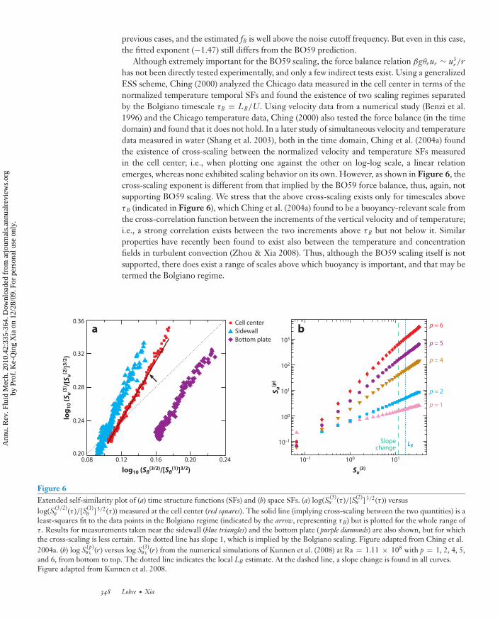
has not been directly tested experimentally, and only a few indirect tests exist. Using a generalizedESS scheme, Ching (2000) analyzed the Chicago data measured in the cell center in terms of thenormalized temperature temporal SFs and found the existence of two scaling regimes separatedby the Bolgiano timescale τB = LB/U. Using velocity data from a numerical study (Benzi et al.1996) and the Chicago temperature data, Ching (2000) also tested the force balance (in the timedomain) and found that it does not hold. In a later study of simultaneous velocity and temperaturedata measured in water (Shang et al. 2003), both in the time domain, Ching et al. (2004a) foundthe existence of cross-scaling between the normalized velocity and temperature SFs measuredin the cell center; i.e., when plotting one against the other on log-log scale, a linear relationemerges, whereas none exhibited scaling behavior on its own. However, as shown in Figure 6, thecross-scaling exponent is different from that implied by the BO59 force balance, thus, again, notsupporting BO59 scaling. We stress that the above cross-scaling exists only for timescales aboveτB (indicated in Figure 6), which Ching et al. (2004a) found to be a buoyancy-relevant scale fromthe cross-correlation function between the increments of the vertical velocity and of temperature;i.e., a strong correlation exists between the two increments above τB but not below it. Similarproperties have recently been found to exist also between the temperature and concentrationfields in turbulent convection (Zhou & Xia 2008). Thus, although the BO59 scaling itself is notsupported, there does exist a range of scales above which buoyancy is important, and that may betermed the Bolgiano regime.

SidewallBottom plate

0.08 0.12 0.16 0.20 0.240.20

0.24

0.28

0.32

0.36

100 10110–1

log10 (Sθ(3/2)/[Sθ

(1)]3/2)

log

10 (

S u(3

) /[S u

(2) ]3

/2)

a b103

102

101

100

10–1

S u(p

)

Su(3)

Cell center

p = 1

p = 2

p = 4

p = 5

p = 6

LΒSlope

change

Figure 6Extended self-similarity plot of (a) time structure functions (SFs) and (b) space SFs. (a) log(S (3)

u (τ )/[S(2)u ] 3/2(τ )) versus

log(S (3/2)θ (τ )/[S(1)

θ ] 3/2(τ )) measured at the cell center (red squares). The solid line (implying cross-scaling between the two quantities) is aleast-squares fit to the data points in the Bolgiano regime (indicated by the arrow, representing τB) but is plotted for the whole range ofτ . Results for measurements taken near the sidewall (blue triangles) and the bottom plate ( purple diamonds) are also shown, but for whichthe cross-scaling is less certain. The dotted line has slope 1, which is implied by the Bolgiano scaling. Figure adapted from Ching et al.2004a. (b) log S (p)

u3 (r) versus log S (3)u3 (r) from the numerical simulations of Kunnen et al. (2008) at Ra = 1.11 × 108 with p = 1, 2, 4, 5,

and 6, from bottom to top. The dotted line indicates the local LB estimate. At the dashed line, a slope change is found in all curves.Figure adapted from Kunnen et al. 2008.

348 Lohse · Xia

Ann

u. R

ev. F

luid

Mec

h. 2

010.

42:3

35-3

64. D

ownl

oade

d fr

om a

rjou

rnal

s.an

nual

revi

ews.

org

by P

rof.

Ke-

Qin

g X

ia o

n 12

/28/

09. F

or p

erso

nal u

se o

nly.

ANRV400-FL42-15 ARI 13 November 2009 14:9

3.3. Converting Time-Domain Data into Space-DomainData Using Local Taylor Hypothesis

As mentioned above, because of the absence of a sufficiently large mean flow, the conditions forTaylor’s frozen-flow hypothesis are not satisfied in most parts of the convection cell. This in turnraises serious questions regarding the interpretation of results from time-domain measurements.However, as the direct real-space measurement techniques such as PIV cannot be used conve-niently in fluids such as gas and liquid metal, time-domain measurement will continue to play animportant role. It is therefore highly desirable to be able to connect time or frequency domain datawith spatial domain theoretical predictions in a meaningful way. The standard Taylor hypothesisassumes that velocity time series can be converted into spatial series according to v(x = Ut) ≡ v(t),where the mean flow velocity U should be much larger than the rms velocity. When this conditionis not met, the so-called local Taylor hypothesis may be used (e.g., see Tennekes & Lumley 1972).Sun et al. (2006) recently applied one such method, introduced by Pinton & Labbe (1994), to tur-bulent RB convection. By assuming that small-scale structures in the inertial range are advected bylarge eddies at the integral scale, Pinton & Labbe (1994) propose that the velocity v(x) at locationx should be related to the velocity v(t) by x = ∫ t

0 v(τ )dτ , where v(τ ) is a local running average ofv(t) over the integral timescale Tint, v(τ ) = T−1

int

∫ τ+Tint/2τ−Tint/2 v(t)dt.

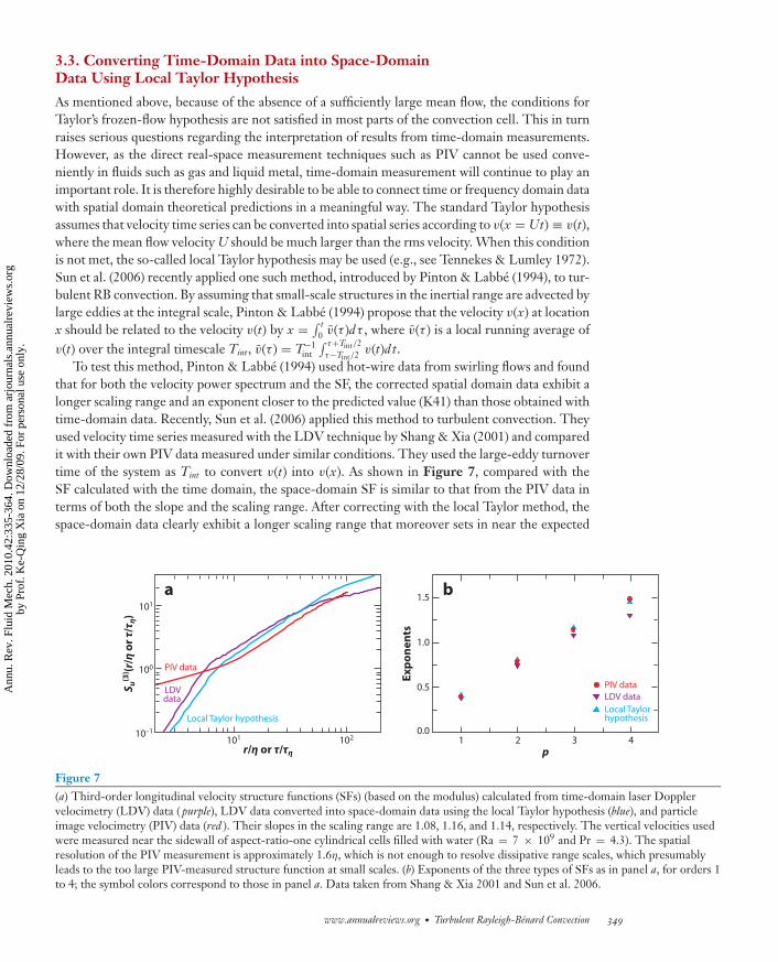
To test this method, Pinton & Labbe (1994) used hot-wire data from swirling flows and foundthat for both the velocity power spectrum and the SF, the corrected spatial domain data exhibit alonger scaling range and an exponent closer to the predicted value (K41) than those obtained withtime-domain data. Recently, Sun et al. (2006) applied this method to turbulent convection. Theyused velocity time series measured with the LDV technique by Shang & Xia (2001) and comparedit with their own PIV data measured under similar conditions. They used the large-eddy turnovertime of the system as Tint to convert v(t) into v(x). As shown in Figure 7, compared with theSF calculated with the time domain, the space-domain SF is similar to that from the PIV data interms of both the slope and the scaling range. After correcting with the local Taylor method, thespace-domain data clearly exhibit a longer scaling range that moreover sets in near the expected

101 102

1.5

1.0

0.5

0.0

a b

1 2 3 4

Ex

po

ne

nts

S u(3

) (r/η

or

τ/τ η

)

r/η or τ/τη

101

100

10–1

p

Local Taylor hypothesis

LDVdata

PIV data

Local Taylorhypothesis

LDV dataPIV data

Figure 7(a) Third-order longitudinal velocity structure functions (SFs) (based on the modulus) calculated from time-domain laser Dopplervelocimetry (LDV) data ( purple), LDV data converted into space-domain data using the local Taylor hypothesis (blue), and particleimage velocimetry (PIV) data (red ). Their slopes in the scaling range are 1.08, 1.16, and 1.14, respectively. The vertical velocities usedwere measured near the sidewall of aspect-ratio-one cylindrical cells filled with water (Ra = 7 × 109 and Pr = 4.3). The spatialresolution of the PIV measurement is approximately 1.6η, which is not enough to resolve dissipative range scales, which presumablyleads to the too large PIV-measured structure function at small scales. (b) Exponents of the three types of SFs as in panel a, for orders 1to 4; the symbol colors correspond to those in panel a. Data taken from Shang & Xia 2001 and Sun et al. 2006.

www.annualreviews.org • Turbulent Rayleigh-Benard Convection 349

Ann

u. R

ev. F

luid

Mec

h. 2

010.

42:3

35-3

64. D

ownl

oade

d fr

om a

rjou

rnal

s.an

nual

revi

ews.

org

by P

rof.

Ke-

Qin

g X

ia o

n 12

/28/

09. F

or p

erso

nal u

se o

nly.

ANRV400-FL42-15 ARI 13 November 2009 14:9

scale r ≈ 10η. The difference between the time-domain and space-domain SFs becomes larger atlarger-order p, and thus with increasing order of the SF, the correction becomes more important.It is clear from these results that corrections to the time-domain data can be quite significant evenin the presence of a relatively strong mean flow (the LDV data were measured near the sidewallof the convection cell, where the large-scale flow mean velocity v = 11.7 mm s−1 and the rmsvelocity vrms = 6.5 mm s−1). Clearly the local Taylor hypothesis can be used to effectively converttime-domain velocity series into spatial series in situations in which the usual condition for theconventional Taylor hypothesis is not satisfied; i.e., the mean flow either is absent or is comparableto the rms velocity. However, without velocity data, this method cannot be applied to convert thetemperature time series, which is more readily available and can be more conveniently measuredin thermal convection. Therefore, it is highly desirable to directly study SF, which indeed has beendone in recent years thanks to the developments in PIV.

3.4. Space-Domain Measurements

To our knowledge, the first spatial-domain measurements of velocity differences in turbulent ther-mal convection were made by Tong & Shen (1992). Using the technique of homodyne photon-correlation spectroscopy, they measured velocity differences of particle pairs in a scattering volumeof linear dimension r in an aspect-ratio-one cylindrical cell filled with water. Their results showthat ur ∼ r0.6 over about a decade of r and for 5 × 107 ≤ Ra ≤ 1010. Thus, their results appear toagree with the BO59 prediction for the first-order velocity SF. However, they should be interpretedwith caution. The measured photon-correlation function records differences in the Doppler shiftsof all particle pairs in the scattering volume of size �, with separations from zero up to � (� variedin the experiment and was taken as r). Therefore, the measured ur is essentially an integration ofvelocity differences of particles with separations from 0 to r. Another space-domain measurementof the velocity field was made in mercury by Mashiko et al. (2004). Using the same apparatus asGlazier et al. (1999), the authors measured the vertical velocity profile along the cylindrical axisof the cell by the technique of ultrasonic velocimetry. Their wave-number energy spectrum atRa = 5 × 1010 (at the cell center) showed about a decade of power-law behavior with an ex-ponent consistent with the BO59 value of −11/5. They also computed the velocity SFs andfound that the second-order SF compensated by r6/5 showed a very small scaling range con-sistent with BO59. We note that Mashiko et al. (2004) used a mode decomposition method toseparate the slow dynamics related to the mean flow and the fast dynamics related to the tur-bulent cascades and that in the calculation of their energy spectra and SFs, mean flow and sev-eral low-order modes were subtracted. It is thus clear that, although both Tong & Shen (1992)and Mashiko et al. (2004) found some evidence for BO59-like scaling, no direct spatial veloc-ity SFs have been measured. Additionally, no direct spatial temperature SFs have been mea-sured in the studies discussed above. Obviously, both velocity and temperature should be in thesame class of scaling behavior (either K41, BO59, or shear-flow scaling), over the same range ofscales, and under the same conditions if we are to agree on an acceptable and convincing cascadedynamics.

In an attempt to determine the cascades of both temperature and velocity variances in turbulentthermal convection, Sun et al. (2006) made high-resolution multipoint measurements of both thevelocity and the temperature fields in water, using a cylindrical cell of aspect ratio one (Ra ≈1.0 × 1010 and Pr = 4.3). Using PIV and the multi-thermistor-probe technique, these authorsmeasured the 2D velocity field and the temperature difference along the vertical direction, fromwhich they obtained the real-space longitudinal and transverse SFs for both the horizontal andvertical velocity components and spatial temperature SFs, respectively. The spatial resolutions

350 Lohse · Xia

Ann

u. R

ev. F

luid

Mec

h. 2

010.

42:3

35-3

64. D

ownl

oade

d fr

om a

rjou

rnal

s.an

nual

revi

ews.

org

by P

rof.

Ke-

Qin

g X

ia o

n 12

/28/

09. F

or p

erso

nal u

se o

nly.

ANRV400-FL42-15 ARI 13 November 2009 14:9

p = 1

S u(p

) (r)/

rp/3

S θ(p

) (r)/

rp/3

S u(p

) , co

mp

en

sate

d

r (mm) r (mm) r (mm)100 101

104

103

102

101

100

10–1

105

104

103

102

101

100

10–1

100

10–2

10–1

100 101 100 102101

LB

a b c

BO59SFs

K41SFsScaling range Scaling range

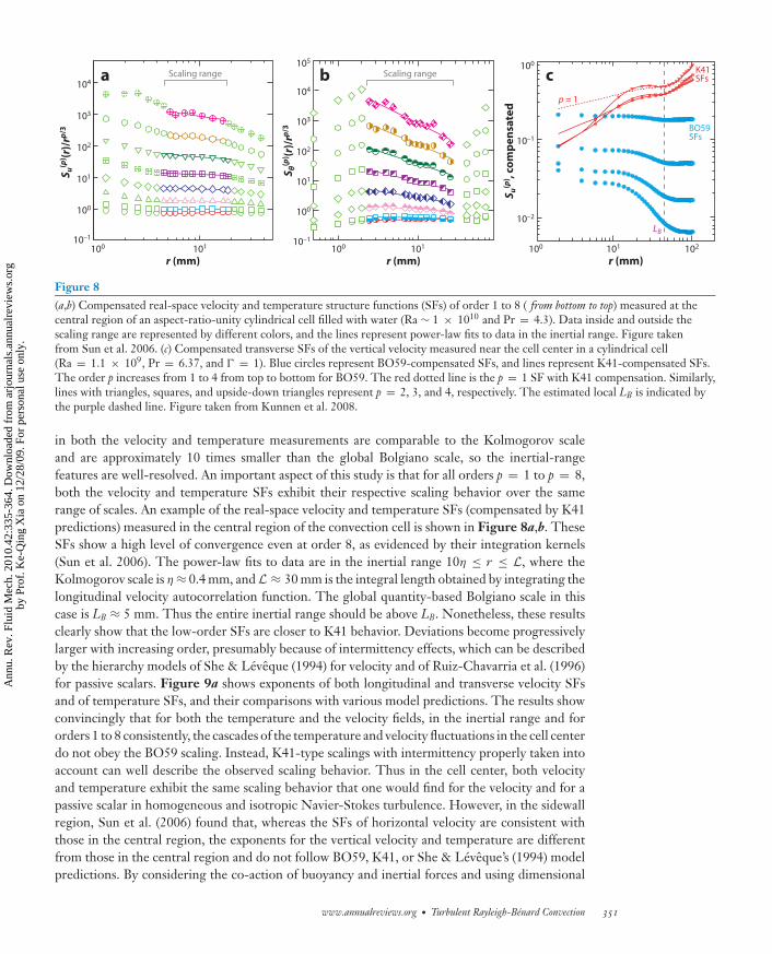
Figure 8(a,b) Compensated real-space velocity and temperature structure functions (SFs) of order 1 to 8 ( from bottom to top) measured at thecentral region of an aspect-ratio-unity cylindrical cell filled with water (Ra ∼ 1 × 1010 and Pr = 4.3). Data inside and outside thescaling range are represented by different colors, and the lines represent power-law fits to data in the inertial range. Figure takenfrom Sun et al. 2006. (c) Compensated transverse SFs of the vertical velocity measured near the cell center in a cylindrical cell(Ra = 1.1 × 109, Pr = 6.37, and � = 1). Blue circles represent BO59-compensated SFs, and lines represent K41-compensated SFs.The order p increases from 1 to 4 from top to bottom for BO59. The red dotted line is the p = 1 SF with K41 compensation. Similarly,lines with triangles, squares, and upside-down triangles represent p = 2, 3, and 4, respectively. The estimated local LB is indicated bythe purple dashed line. Figure taken from Kunnen et al. 2008.

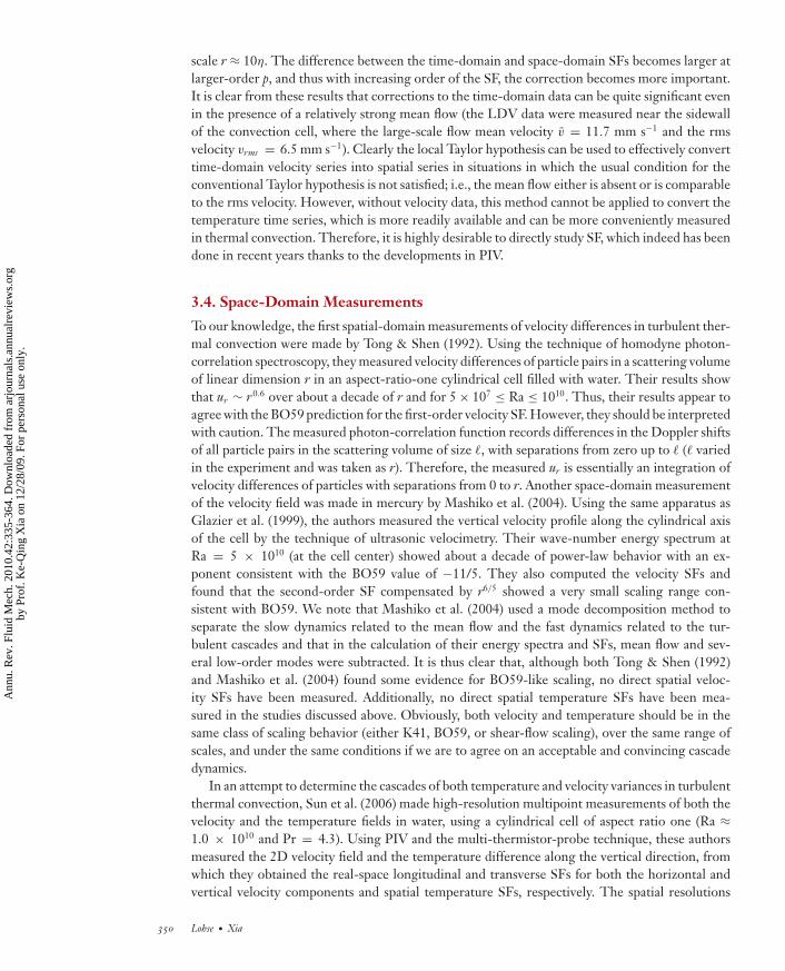
in both the velocity and temperature measurements are comparable to the Kolmogorov scaleand are approximately 10 times smaller than the global Bolgiano scale, so the inertial-rangefeatures are well-resolved. An important aspect of this study is that for all orders p = 1 to p = 8,both the velocity and temperature SFs exhibit their respective scaling behavior over the samerange of scales. An example of the real-space velocity and temperature SFs (compensated by K41predictions) measured in the central region of the convection cell is shown in Figure 8a,b. TheseSFs show a high level of convergence even at order 8, as evidenced by their integration kernels(Sun et al. 2006). The power-law fits to data are in the inertial range 10η ≤ r ≤ L, where theKolmogorov scale is η ≈ 0.4 mm, andL ≈ 30 mm is the integral length obtained by integrating thelongitudinal velocity autocorrelation function. The global quantity-based Bolgiano scale in thiscase is LB ≈ 5 mm. Thus the entire inertial range should be above LB. Nonetheless, these resultsclearly show that the low-order SFs are closer to K41 behavior. Deviations become progressivelylarger with increasing order, presumably because of intermittency effects, which can be describedby the hierarchy models of She & Leveque (1994) for velocity and of Ruiz-Chavarria et al. (1996)for passive scalars. Figure 9a shows exponents of both longitudinal and transverse velocity SFsand of temperature SFs, and their comparisons with various model predictions. The results showconvincingly that for both the temperature and the velocity fields, in the inertial range and fororders 1 to 8 consistently, the cascades of the temperature and velocity fluctuations in the cell centerdo not obey the BO59 scaling. Instead, K41-type scalings with intermittency properly taken intoaccount can well describe the observed scaling behavior. Thus in the cell center, both velocityand temperature exhibit the same scaling behavior that one would find for the velocity and for apassive scalar in homogeneous and isotropic Navier-Stokes turbulence. However, in the sidewallregion, Sun et al. (2006) found that, whereas the SFs of horizontal velocity are consistent withthose in the central region, the exponents for the vertical velocity and temperature are differentfrom those in the central region and do not follow BO59, K41, or She & Leveque’s (1994) modelpredictions. By considering the co-action of buoyancy and inertial forces and using dimensional

www.annualreviews.org • Turbulent Rayleigh-Benard Convection 351

Ann

u. R

ev. F

luid

Mec

h. 2

010.

42:3

35-3

64. D

ownl

oade

d fr

om a

rjou

rnal

s.an

nual

revi

ews.

org

by P

rof.

Ke-

Qin

g X

ia o

n 12

/28/

09. F

or p

erso

nal u

se o

nly.

ANRV400-FL42-15 ARI 13 November 2009 14:9

Str

uc

ture

fu

nc

tio

n e

xp

on

en

ts

0.500.420.330.250.160.080

2.0

1.5

1.0

0.5

0.0

3.0

2.5

2.0

1.5

1.0

0.5

0.00 1 2 3 4 5 6 7 8 9

z/L

BO59 (velocity)BO59 (temperature)K41SL94RCBC96ζp

L,w

ζpT,u

ζpθ

ζ3u

ζ3θ

9/5

1

3/5

p

a b

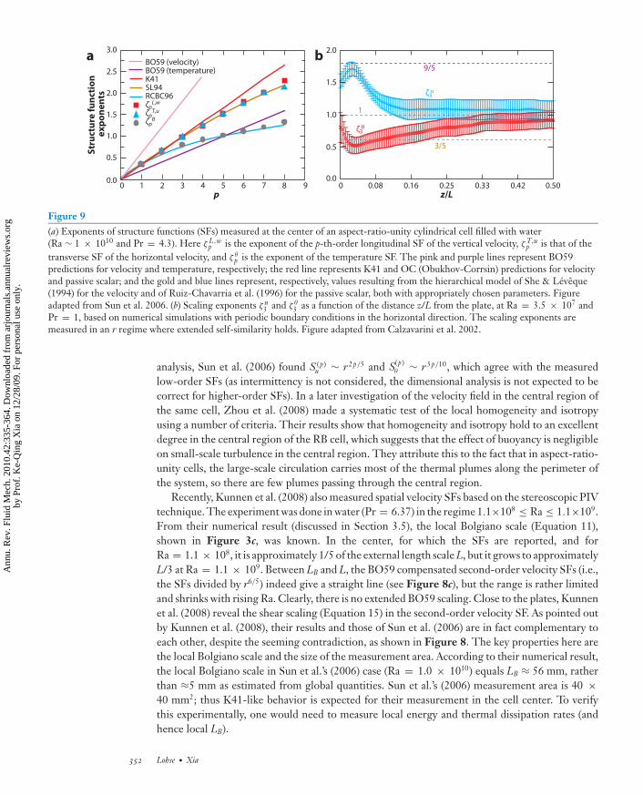
Figure 9(a) Exponents of structure functions (SFs) measured at the center of an aspect-ratio-unity cylindrical cell filled with water(Ra ∼ 1 × 1010 and Pr = 4.3). Here ζ L,w

p is the exponent of the p-th-order longitudinal SF of the vertical velocity, ζ T,up is that of the

transverse SF of the horizontal velocity, and ζ θp is the exponent of the temperature SF. The pink and purple lines represent BO59

predictions for velocity and temperature, respectively; the red line represents K41 and OC (Obukhov-Corrsin) predictions for velocityand passive scalar; and the gold and blue lines represent, respectively, values resulting from the hierarchical model of She & Leveque(1994) for the velocity and of Ruiz-Chavarria et al. (1996) for the passive scalar, both with appropriately chosen parameters. Figureadapted from Sun et al. 2006. (b) Scaling exponents ζ u

3 and ζ θ3 as a function of the distance z/L from the plate, at Ra = 3.5 × 107 and

Pr = 1, based on numerical simulations with periodic boundary conditions in the horizontal direction. The scaling exponents aremeasured in an r regime where extended self-similarity holds. Figure adapted from Calzavarini et al. 2002.

analysis, Sun et al. (2006) found S (p)u ∼ r2p/5 and S(p)

θ ∼ r3p/10, which agree with the measuredlow-order SFs (as intermittency is not considered, the dimensional analysis is not expected to becorrect for higher-order SFs). In a later investigation of the velocity field in the central region ofthe same cell, Zhou et al. (2008) made a systematic test of the local homogeneity and isotropyusing a number of criteria. Their results show that homogeneity and isotropy hold to an excellentdegree in the central region of the RB cell, which suggests that the effect of buoyancy is negligibleon small-scale turbulence in the central region. They attribute this to the fact that in aspect-ratio-unity cells, the large-scale circulation carries most of the thermal plumes along the perimeter ofthe system, so there are few plumes passing through the central region.

Recently, Kunnen et al. (2008) also measured spatial velocity SFs based on the stereoscopic PIVtechnique. The experiment was done in water (Pr = 6.37) in the regime 1.1×108 ≤ Ra ≤ 1.1×109.From their numerical result (discussed in Section 3.5), the local Bolgiano scale (Equation 11),shown in Figure 3c, was known. In the center, for which the SFs are reported, and forRa = 1.1 × 108, it is approximately 1/5 of the external length scale L, but it grows to approximatelyL/3 at Ra = 1.1 × 109. Between LB and L, the BO59 compensated second-order velocity SFs (i.e.,the SFs divided by r6/5) indeed give a straight line (see Figure 8c), but the range is rather limitedand shrinks with rising Ra. Clearly, there is no extended BO59 scaling. Close to the plates, Kunnenet al. (2008) reveal the shear scaling (Equation 15) in the second-order velocity SF. As pointed outby Kunnen et al. (2008), their results and those of Sun et al. (2006) are in fact complementary toeach other, despite the seeming contradiction, as shown in Figure 8. The key properties here arethe local Bolgiano scale and the size of the measurement area. According to their numerical result,the local Bolgiano scale in Sun et al.’s (2006) case (Ra = 1.0 × 1010) equals LB ≈ 56 mm, ratherthan ≈5 mm as estimated from global quantities. Sun et al.’s (2006) measurement area is 40 ×40 mm2; thus K41-like behavior is expected for their measurement in the cell center. To verifythis experimentally, one would need to measure local energy and thermal dissipation rates (andhence local LB).

352 Lohse · Xia

Ann

u. R

ev. F

luid

Mec

h. 2

010.

42:3

35-3

64. D

ownl

oade

d fr

om a

rjou

rnal

s.an

nual

revi

ews.

org

by P

rof.

Ke-

Qin

g X

ia o

n 12

/28/

09. F

or p

erso

nal u

se o

nly.

ANRV400-FL42-15 ARI 13 November 2009 14:9

Kunnen et al. (2008) also applied ESS, plotting the p-th order velocity SF against S(3)u ; the

relative scaling exponent is called ξ p, defined by S (p)u (r) ∼ (S(3)

u (r))ξp . Two regimes can be identified(see Figure 6b): For r ≤ LB/2, the relative exponents ξ p resemble the ones one would expect forintermittency-corrected K41 scaling and that are well described by She & Leveque’s (1994) model(e.g., ξ 6 = 1.78). For r ≥ LB/2, the ξ p are smaller and Ra-dependent, however, with an errorbar within the range of what has been found by Toschi et al. (1999) for the ξ p in channel-flowturbulence (e.g., ξ 6 = 1.44).

Zhou et al. (2008) measured the velocity circulation SFs in the central region of the RB sys-tem. Their result shows that the circulation SFs also exhibit K41-like behavior, but they aremore sensitive to local anisotropy than the velocity field itself. These results give further sup-port to Sun et al.’s (2006) findings that in the central region of the RB system, K41-like ratherthan BO59-like dynamics prevails. Putting together results from these two studies, we see theemergence of a consistent picture regarding the cascades of turbulent velocity and temperaturefluctuations; i.e., for the directly measured SFs, no BO59-like behavior is observed in turbulent RBconvection.

3.5. Structure Functions and Spectra From Numerical Simulations

The tremendous advantage of numerical simulations of RB flow is that in principle all data areavailable. However, due to computational costs, only limited Ra and Pr can be achieved, and onlyin the past 15 years or so have turbulent 3D RB simulations become possible. For a more detaileddiscussion, we refer the reader to the review by Ahlers et al. (2009).

Kerr (1996) provides one of the first numerical simulations for really turbulent RB convection,achieving Ra = 2 × 107 at Pr = 0.7 with periodic boundary conditions at the sidewalls. He findsabout one decade of K41-type scaling Eu(k) ∼ k−5/3 and less steep scaling for the temperaturespectrum, consistent with Eθ (k) ∼ k−1, both inconsistent with the BO59 picture.

Calzavarini et al. (2002) provide a numerical simulation in a similar Ra and Pr regime with aLattice-Boltzmann scheme. The SFs do not scale. However, some scaling regimes can be identifiedin ESS plots of the SFs against each other. When measuring the local scaling exponents ζ (p)

u andζ

(p)θ in the respective SFs for that ESS scaling regime as a function of the distance z from the

plates, they obtain values consistent with K41 scaling in the bulk, where LB (z) ∼ L, and valuesconsistent with BO59 scaling close to the plates, where LB (z) ≈ 0.2L (see Figure 9b for the localscaling exponents and Figure 3c for the corresponding local Bolgiano scale).

Camussi & Verzicco (1998) provide temperature and velocity frequency spectra for RB flowin mercury at � = 1/2 and Pr = 0.022 and for 5 × 104 ≤ Ra ≤ 106, based on their numericalsimulations. To allow for a one-to-one comparison, they calculated the spectra from velocityand temperature time series taken at the cell center and close to the cell wall. No indicationof BO59 scaling was reported. Moreover, Camussi & Verzicco (2004) employed numerical timeseries to calculate spectra and SFs Su(τ ) and Sθ (τ ), but now for Pr = 0.7 and for Ra up to 2 ×1011. The temperature frequency spectrum showed a power-law exponent close to −5/3 (K41)in the center and close to −7/5 (BO59) at mid-height close to the sidewall, where Sθ (τ ) showedthe corresponding slope 2/5. Depending on the position and velocity component, the velocityfrequency spectrum showed either a slope close to −5/3, or even a less steep slope (smallermodulus of slope)—in fact similar to the value −7/5 of the temperature frequency spectrum—butclearly no indication of BO59 scaling. Rincon (2006) performed numerical simulations at Ra =106, Pr = 1, and � = 5, employing the SO(3) analysis to properly treat isotropic and anisotropicprojections of the SF tensor. However, the Rayleigh number in these simulations is too small toreveal any scaling, and the focus of the paper is on energy balances resulting from the Boussinesq

www.annualreviews.org • Turbulent Rayleigh-Benard Convection 353

Ann

u. R

ev. F

luid

Mec

h. 2

010.

42:3

35-3

64. D

ownl

oade

d fr

om a

rjou

rnal

s.an

nual

revi

ews.

org

by P

rof.

Ke-

Qin

g X

ia o

n 12

/28/

09. F

or p

erso

nal u

se o

nly.

ANRV400-FL42-15 ARI 13 November 2009 14:9

equations. The paper again stresses the importance of disentangling anisotropy, inhomogeneity,and buoyancy effects.

The hitherto most complete numerical calculations of real-space velocity and temperatureSFs were performed by Kunnen et al. (2008). For the velocity SFs in the center of the cell, theyfound similar results as those obtained from their stereoscopical PIV measurements, including therelative ESS scaling exponents. In particular, with increasing Ra, the BO59 regime becomes evenless limited, which is consistent with the trend in the local Bolgiano length. In the small regimebeyond r > LB (less than half a decade even for the best case Ra = 108), the BO59-compensatedtemperature spectra are more horizontal than the K41-compensated ones, although both showan unexplained increase at the very large scales, r ≈ L. With increasing Ra, this regime becomeseven smaller.

All the numerical simulations reported above in this subsection are for the flow in real cells withno-slip boundary conditions, at least at the top and bottom walls, leading to inhomogeneities in theflow. As discussed in Section 2.3, the inhomogeneities can be avoided in the so-called homogeneousRB flow. Biferale et al. (2003) applied the SO(3) decomposition for this type of flow. They notonly found K41 scaling (with the standard intermittency corrections) in the isotropic j = 0 sector,but they also found no evidence for BO59 scaling in the subleading, anisotropic j = 1 sector:The BO59 dimensional scaling relation (Equation 19) for j = 1 clearly is not fulfilled. Instead,the anisotropic fluctuations in the RB system are anomalous and universal, with similar relativescaling exponents as in random Kolmogorov flow or in other types of shear flows (Toschi et al.1999).

4. SMALL-SCALE MIXING OF ACTIVE AND PASSIVE SCALARS

In Grossmann & Lohse’s (2000, 2001, 2002, 2004) theory, the kinetic energy and thermal dis-sipation rates have been decomposed into boundary layer and bulk contributions, and a laminarPrandtl-Blasius boundary layer, in a time-averaged sense, has been assumed. This theory can suc-cessfully describe and predict Nu and Re’s dependency on Ra and Pr (e.g., see the recent reviewin Ahlers et al. 2009). In a recent high-resolution measurement of the properties of the velocityboundary layer, Sun et al. (2008) have found that, despite the intermittent emission of plumes, theBlasius-type laminar boundary condition is indeed a good approximation, in a time-averaged sense,both in terms of its scaling and its various dynamic properties. In the Prandtl-Blasius boundary-layer theory, temperature is treated as a passive scalar, but because of buoyancy, in the inertial rangeand above the Bolgiano scale, temperature behaves as an active scalar. One naturally wonders whatwould be the properties of the temperature field at these small scales. Specifically, how does thetemperature as an active scalar compare with a passive scalar under the same conditions?

4.1. Small-Scale Anisotropy of the Temperature Field

The persistence of nonzero skewness of the scalar derivatives is a hallmark of passive scalar mixing,as it invalidates the local isotropy assumption of the classical Kolmogorov-Obukhov-Corrsintheory of passive scalars (Sreenivasan 1991). The nonzero skewness is believed to result from sharpfronts or gradients of the scalar. By examining the skewness Sθ ≡ S(θ ) ≡ 〈(θ −〈θ〉)3〉/〈(θ −〈θ〉)2〉3/2

of the temperature and the skewness S∂tθ ≡ S(∂tθ ) of its time derivative in thermal convection,Belmonte & Libchaber (1996) studied the small-scale mixing properties of the temperature field,in particular the question of active versus passive. Their experiment was conducted in a cubiccell of aspect ratio one filled with pressurized gas (helium, nitrogen, or sulfur hexafluoride) atroom temperature and spanned a range of Ra from 2 × 107 to 1 × 1011 with Pr = 0.7. Sharp

354 Lohse · Xia

Ann

u. R

ev. F

luid

Mec

h. 2

010.

42:3

35-3

64. D

ownl

oade

d fr

om a

rjou

rnal

s.an

nual

revi

ews.

org

by P

rof.

Ke-

Qin

g X

ia o

n 12

/28/

09. F

or p

erso

nal u

se o

nly.

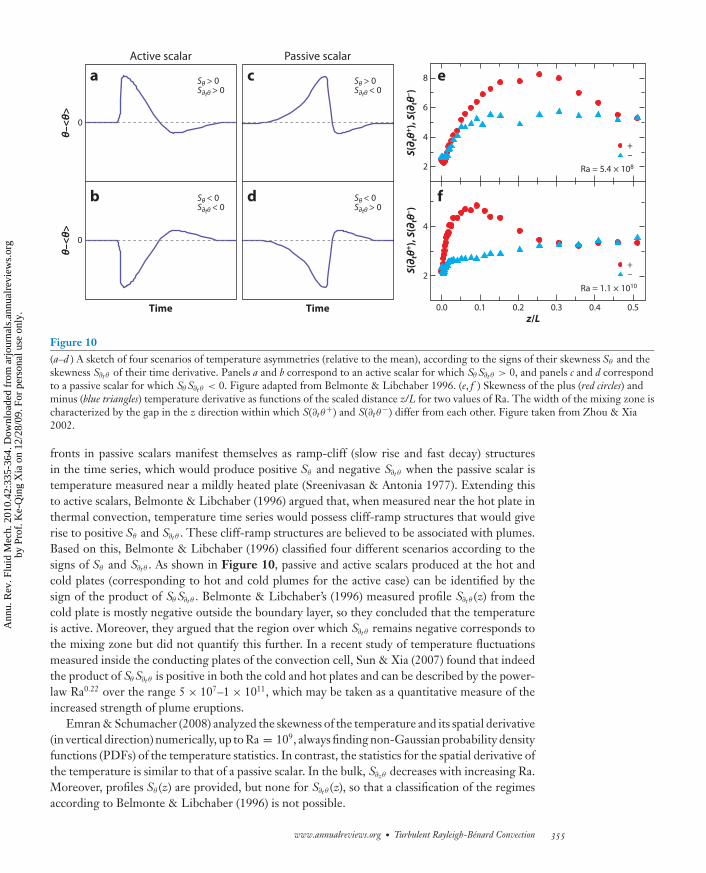
ANRV400-FL42-15 ARI 13 November 2009 14:9

+–

+–

Active scalar

b

a e

f

c

d

Passive scalar

z/L0.0 0.1 0.2 0.3 0.4 0.5

Ra = 5.4 × 108

Ra = 1.1 × 1010

Sθ > 0S∂tθ < 0

Sθ < 0S∂tθ > 0

θ–<

θ>θ–

<θ>

Sθ > 0S∂tθ > 0

Sθ < 0S∂tθ < 0

S(∂ t

θ+),

S(∂

tθ–)

S(∂ t

θ+),

S(∂

tθ–)

Time

0

2

4

6

8

2

4

Time

0

Figure 10(a–d ) A sketch of four scenarios of temperature asymmetries (relative to the mean), according to the signs of their skewness Sθ and theskewness S∂tθ of their time derivative. Panels a and b correspond to an active scalar for which Sθ S∂tθ > 0, and panels c and d correspondto a passive scalar for which Sθ S∂tθ < 0. Figure adapted from Belmonte & Libchaber 1996. (e, f ) Skewness of the plus (red circles) andminus (blue triangles) temperature derivative as functions of the scaled distance z/L for two values of Ra. The width of the mixing zone ischaracterized by the gap in the z direction within which S(∂tθ

+) and S(∂tθ−) differ from each other. Figure taken from Zhou & Xia

2002.

fronts in passive scalars manifest themselves as ramp-cliff (slow rise and fast decay) structuresin the time series, which would produce positive Sθ and negative S∂tθ when the passive scalar istemperature measured near a mildly heated plate (Sreenivasan & Antonia 1977). Extending thisto active scalars, Belmonte & Libchaber (1996) argued that, when measured near the hot plate inthermal convection, temperature time series would possess cliff-ramp structures that would giverise to positive Sθ and S∂tθ . These cliff-ramp structures are believed to be associated with plumes.Based on this, Belmonte & Libchaber (1996) classified four different scenarios according to thesigns of Sθ and S∂tθ . As shown in Figure 10, passive and active scalars produced at the hot andcold plates (corresponding to hot and cold plumes for the active case) can be identified by thesign of the product of Sθ S∂tθ . Belmonte & Libchaber’s (1996) measured profile S∂tθ (z) from thecold plate is mostly negative outside the boundary layer, so they concluded that the temperatureis active. Moreover, they argued that the region over which S∂tθ remains negative corresponds tothe mixing zone but did not quantify this further. In a recent study of temperature fluctuationsmeasured inside the conducting plates of the convection cell, Sun & Xia (2007) found that indeedthe product of Sθ S∂tθ is positive in both the cold and hot plates and can be described by the power-law Ra0.22 over the range 5 × 107–1 × 1011, which may be taken as a quantitative measure of theincreased strength of plume eruptions.

Emran & Schumacher (2008) analyzed the skewness of the temperature and its spatial derivative(in vertical direction) numerically, up to Ra = 109, always finding non-Gaussian probability densityfunctions (PDFs) of the temperature statistics. In contrast, the statistics for the spatial derivative ofthe temperature is similar to that of a passive scalar. In the bulk, S∂zθ decreases with increasing Ra.Moreover, profiles Sθ (z) are provided, but none for S∂tθ (z), so that a classification of the regimesaccording to Belmonte & Libchaber (1996) is not possible.

www.annualreviews.org • Turbulent Rayleigh-Benard Convection 355

Ann

u. R

ev. F

luid

Mec

h. 2

010.

42:3

35-3

64. D

ownl

oade

d fr

om a

rjou

rnal

s.an

nual

revi

ews.

org

by P

rof.

Ke-

Qin

g X

ia o

n 12

/28/

09. F

or p

erso

nal u

se o

nly.

ANRV400-FL42-15 ARI 13 November 2009 14:9

In a somewhat different approach, Zhou & Xia (2002) studied the skewness of the so-called plusand minus temperature increments θ±

τ = (|θτ |±θτ )/2, where θτ = θ (t+τ )−θ (t) is the temperatureincrement over a time interval τ . [Plus and minus increments were first used in the study of rampstructures in the velocity field in Navier-Stokes turbulence (Vainshtein & Sreenivasan 1994) andlater in the context of the temperature field by Aivalis et al. (2004).] When a (hot) plume passesthrough a temperature probe, it would produce a spike with a steep rising edge (due to its cap) anda relatively gentle falling edge (due to its tail) in the measured time series. The plus and minustemperature increments thus capture, respectively, the slope of the rising and falling edges for τ

smaller than the size of a plume (in the time domain). Therefore, in regions where hot plumesdominate over cold ones, θ+

τ would be expected to be larger than θ−τ , and vice versa in regions

where cold plumes dominate. Indeed, Zhou & Xia found that for τ < τB = LB/U, the skewnessS(θ+

τ ) > S(θ−τ ) in regions where hot plumes dominate. This also suggests that the cap thickness (in

time domain) of a typical plume should be smaller than τB but larger than τ η. For τ > τB, featuressmaller than the corresponding scale are averaged out, resulting in the same values for the plusand minus skewness. Zhou & Xia (2002) also found that S(∂tθ

+) and S(∂tθ−) are the same in the

boundary layer and central regions of the cell but differ in regions where plumes dominate, whichis shown in the right panel of Figure 10 for two values of Ra. The width (in the z direction) ofthe region in which the two quantities differ shrinks as Ra increases, which in fact has a scalingexponent as that predicted for the width of the mixing zone (Castaing et al. 1989). The mixingzone plays an important role in the Chicago model for hard turbulence (Castaing et al. 1989),and the plus and minus skewness provides a useful definition for its quantitative characterization.Recently, it has been found that quantities such as the profile of vorticity fluctuations (Zhou et al.2007) and skewness of spatial temperature gradient and local thermal dissipation rate (He & Tong2009) can all be used to characterize the mixing zone.

4.2. Comparative Studies of Active and Passive Scalars

A fascinating property of passive scalars is the saturation of the scaling exponent of their high-order SFs; i.e., the exponent ζ θ

p approaches a constant ζ θ∞ for large enough order p. The saturation

is believed to be related to the ramp-cliff structures (or fronts) in the scalar (Celani et al. 2000,Moisy et al. 2001). With the temperature time series in thermal convection found to exhibit cliff-ramp structures (Belmonte & Libchaber 1996, Zhou & Xia 2002), it is natural to ask whether thetemperature field as an active scalar would possess the saturation property. In a 2D numerical studyof thermal convection, Celani et al. (2001) found that the temperature indeed exhibits saturationphenomenon. Experimentally, Zhou & Xia (2002) measured long time records (consisting of 1.2 ×108 data points, corresponding to 37,000 large-eddy turnover times) of local temperature both nearthe sidewall region and at the center in an aspect-ratio-one cylindrical cell filled with water (Ra =1.8 × 1010, Pr = 4). As the high-order moments are dominated by large temperature excursions,the saturation of the SF exponent is equivalent to the scaled PDF r−ζ θ∞ P (θr ) becoming independentof r for inertial range values of θr � θrms . Because high-order SFs are very sensitive to the far tailsof the PDF, collapsing of the scaled PDF is a statistically more reliable test of the saturation (Celaniet al. 2000, 2001). By examining both the scaled PDF τ−ζ θ∞ P (δτ ) of temperature increments overvarying timescales in the inertial range and the cumulated probability

∫ ∞θτ

P (δτ )dδτ , Zhou & Xiafound evidence for the saturation of the temperature SFs near the sidewalls, but not at the cellcenter. Because plumes are abundant at the sidewall but scarce in the center, this finding suggeststhat the saturation is caused by the presence of plumes. As mentioned in Section 3.2, Skrbek et al.(2002) analyzed temperature time series measured in helium (Ra = 1.5 × 1011), also near thesidewall, using the ESS method. They find no saturation of the ESS (relative) scaling exponents

356 Lohse · Xia

Ann

u. R

ev. F

luid

Mec

h. 2

010.

42:3

35-3

64. D

ownl

oade

d fr

om a

rjou

rnal

s.an

nual

revi

ews.

org

by P

rof.

Ke-

Qin

g X

ia o

n 12

/28/

09. F

or p

erso

nal u

se o

nly.

ANRV400-FL42-15 ARI 13 November 2009 14:9

TemperatureConcentration

0.1 0.3 0.5 0.7

p = 4

p = 2

Ex

po

ne

nts

a b c1.0

0.8

0.6

0.4

0.2

0.0

102

101

100

10–1

10–4

10–3

10–2

102

101

100

10–1

10–4

10–3

10–2

10–5

–10 –5 0 5 10

P(C

τ/C

rms)

P(θ τ

/θrm

s)

Cτ/Crms θτ/θrms

–10 –5 0 5 10

r

Figure 11(a) Local scaling exponents of temperature (circles) and concentration (triangles) structure functions for orders 2 and 4, from 2Dsimulations made at Ra = 107. Figure taken from Celani et al. 2002. (b,c) Probability density functions of concentration andtemperature increments normalized by their standard deviations for four time intervals ( from top to bottom): τ /τB = 0.05, 0.15, 1, and10. The curves have been shifted vertically for clarity, and the gray dashed curve indicates a Gaussian distribution of variance 1.Measurements were made near the sidewall, at mid-height, of a rectangular cell filled with water (Ra = 1.2 × 1010 and Pr = 5.3).Figure taken from Zhou & Xia 2008.

ξ θp with increasing order, up to p = 16. However, from that result it cannot be concluded that the

scaling exponents ζ θp of the temperature SFs do not saturate either.

A fruitful way to investigate the temperature field with respect to the question of whether itbehaves more as an active or more as a passive scalar in thermal convection would be to makea direct comparative study with a real passive scalar (such as the concentration of a disperseddye) under the same conditions. Such an approach has been taken mostly in numerical studies.Celani et al. (2002) investigated the scaling properties of both the temperature and a passive scalargoverned by the Boussinesq equations in a 2D numerical study and found that the two scalar fieldshave the same even-order SF exponents, as shown in Figure 11. They conjectured that this maybe attributed to the existence of so-called statistically preserved structures in the temperature field,as is the case for passive scalars. In a shell model study of thermal convection, Ching et al. (2002,2003a) found numerical evidence that the equivalence of even-order statistics of active and passivescalars can indeed be understood from the presence of statistically preserved structures.

On the experimental side, there exist only a few comparative studies of active and passivescalars advected by the same flow. Using liquid crystal imaging and planar laser-induced fluo-rescence techniques, Gluckman et al. (1993) studied the geometric properties of isothermal andisoconcentration contours in turbulent convection in water (Ra ∼ 107–108). They found thatthe isoconcentration contours show a limited fractal scaling range. In contrast, the isotherms donot exhibit fractal scaling, which does not support Procaccia et al.’s (1991) suggestion that thetemperature field appears fractal above a certain scale. Conversely, the local curvature of both theisoconcentration and isothermal contours possesses a stretched exponential PDF with asymmetrictails. By injecting a fluorescent dye into a rectangular cell filled with water, Zhou & Xia (2008)made simultaneous and separate measurements of the local temperature, using a small thermistor,and dye-concentration fluctuations, using laser-induced fluorescence, in close proximity (near thesidewall at mid-height). They showed that although the two scalars are advected by the sameturbulent flow, the quantities themselves and their small-scale increments distribute differently.Below τB, the temperature behaves as a passive scalar, and above τB it behaves as an active scalar,where it also possesses a higher level of intermittency as compared with the passive scalar (dye con-centration). Figure 11b,c plots the PDF of concentration and temperature increments over severaltime intervals, respectively. The PDFs of temperature increments change from non-Gaussian insmall scales to near Gaussian in large scales, whereas those of concentration increments remain

www.annualreviews.org • Turbulent Rayleigh-Benard Convection 357

Ann

u. R

ev. F

luid

Mec

h. 2

010.

42:3

35-3

64. D

ownl

oade

d fr

om a

rjou

rnal

s.an

nual

revi

ews.

org

by P

rof.

Ke-

Qin

g X

ia o

n 12

/28/

09. F

or p

erso

nal u

se o

nly.

ANRV400-FL42-15 ARI 13 November 2009 14:9

non-Gaussian for all scales investigated; i.e., as τ changes from small to large scales, the shapesof the concentration-increment PDFs are more similar among themselves than those of the tem-perature, and hence the passive scalar is less intermittent than the active one. The finding thatan active scalar is more intermittent than a passive one is consistent with the saturation of the SFexponent for the temperature. The saturation exponent ζ θ

∞ is found to be 0.8 for an active scalarfrom experiment (Zhou & Xia 2002) and 2D simulations (Celani et al. 2001) and 1.45 for a passivescalar measured in a swirling flow (Moisy et al. 2001). This suggests that ζ θ

∞ deviates more fromthe dimensional predictions for active scalars than passive ones, implying that the active scalaris more intermittent. As a possible future experiment, the saturation of both active and passivescalars advected by the same flow should be measured.

As a closing remark, we point out that many of the studies reviewed in this section are madein the time domain; therefore, they also face the question regarding the validity of the Taylorhypothesis, and one should always bear this in mind when interpreting the results and connectingthem to theoretical predictions.

5. CONCLUSIONS AND OUTLOOK

The discussions in this review reflect that the issue regarding the nature of cascades of the velocityand temperature fluctuations in turbulent thermal convection is not fully settled. On one hand,both temperature and temperature gradient PDFs and their skewnesses and force balances onlarge scales carry the feature of an active scalar, pronouncedly different from those of a passivescalar like a concentration field. On the other hand, BO59 scaling has not been found over a largerange of scales and many hints point toward the sketch of Figure 2 being unrealistic. Accordingto Kunnen et al. (2008), as the Ra dependency of the local Bolgiano scale LB(x) is an increasingfunction of Ra—at least in the center of the cell, where the effect of anisotropy and shear issmallest—future attempts to find BO59 scaling should be made with lower Ra and higher Pr toincrease the potential BO59 range, if it exists at all. This, of course, strongly limits the possibleinertial scaling regime, again revealing the conflict of requirements for extended BO59 scaling:This fundamental obstacle—the lack of separation of length scales between L and LB—appears toplace conflicting demands on the control parameters of the system, and an extended BO59 scalingregime therefore may never be achieved.

Ultimately, a true test of the Bolgiano argument should consist of observing K41-like scaling,for both velocity and temperature, below LB. In contrast, above LB, one should observe BO59-like scaling, again for both velocity and temperature, just as sketched in Figure 2. Because theKolmogorov scale and the local Bolgiano scale have opposite dependency on Ra, this meansthat simultaneous observation of K41 and BO59 scalings at the same location is unlikely, if notimpossible. In light of this, several different approaches may yield fruitful results. The first oneis to select an appropriate range of Ra and Pr, and suitable system size and aspect ratio, and lookfor different scalings in different regions of the convection cell; for example, BO59-like scalingnear the boundary layer and K41-like scaling in the cell center. The second approach is to lookfor different scalings in the same location of the cell by tuning the local LB to be either largeror smaller than the experimentally accessible scale, which could be achieved by using differentworking fluids, for example. Attempts along the line of the first approach have been made bySun et al. (2006) and Kunnen et al. (2008), whereas the second type of approach has not beenattempted in a systematic way. A third approach may be to use cells of wider aspect ratio, � � 1,to allow for a large length scale at least in the horizontal direction and for a possible separationof scales between LB and �L. For any of these efforts, it will in addition be helpful to employthe SO(3) decomposition of the flow to better disentangle scaling corrections due to shear and

358 Lohse · Xia

Ann

u. R

ev. F

luid

Mec

h. 2

010.

42:3

35-3

64. D

ownl

oade

d fr

om a

rjou

rnal

s.an

nual

revi

ews.

org

by P

rof.

Ke-

Qin

g X

ia o

n 12

/28/

09. F

or p

erso

nal u

se o

nly.

ANRV400-FL42-15 ARI 13 November 2009 14:9

scaling corrections due to buoyancy. Also for future studies, a quantitative test of the force balancerelation βgθr ur ∼ u3

r /r in direct spatial measurements of the velocity and temperature fields willneed to be made—as done in Calzavarini et al. (2002) for numerical simulations (see Figure 3d).

As pointed out in Section 1, the RB system may be ideal to study turbulence as it is experi-mentally accessible and as the governing equations and boundary conditions are exactly known.However, thanks to the richness of its dynamics, it clearly is not the easiest system to study cleanand extended scaling regimes of SFs over a large range of scales.

DISCLOSURE STATEMENT

The authors are not aware of any affiliations, memberships, funding, or financial holdings thatmight be perceived as affecting the objectivity of this review.

ACKNOWLEDGMENTS

We thank all our colleagues and collaborators on this subject for various discussions over the past20 years. We have learned tremendously from them and enjoy and appreciate the joint researchefforts to better understand turbulent thermal convection. D.L. acknowledges FOM for the con-tinuous support and K.Q.X. the Hong Kong Research Grants Council (grant nos. CUHK 403806and 403807).

LITERATURE CITED

Adrian RJ. 1991. Particle-imaging techniques for experimental fluid mechanics. Annu. Rev. Fluid Mech. 23:261–304

Ahlers G, Grossmann S, Lohse D. 2009. Heat transfer and large scale dynamics in turbulent Rayleigh-Benardconvection. Rev. Mod. Phys. 81:503–37

Aivalis KG, Schumacher J, Sreenivasan KR. 2004. Sign-symmetry of temperature structure functions. Phys.Rev. E 69:066315

Arad I, Biferale L, Mazzitelli I, Procaccia I. 1999a. Disentangling scaling properties in anisotropic and inho-mogeneous turbulence. Phys. Rev. Lett. 82:5040–43

Arad I, Dhruva B, Kurien S, L’vov VS, Procaccia I, Sreenivasan KR. 1998. Extraction of anisotropic contri-butions in turbulent flows. Phys. Rev. Lett. 81:5330–33

Arad I, L’vov V, Procaccia I. 1999b. Correlation functions in isotropic and anisotropic turbulence: the role ofthe symmetry group. Phys. Rev. E 61:6753–65

Arneodo A, Baudet C, Belin F, Benzi R, Castaing B, et al. 1996. Structure functions in turbulence, in variousflow configurations, at Reynolds number between 30 and 5000, using extended self-similarity. Europhys.Lett. 34:411–16

Ashkenazi S, Steinberg V. 1999. Spectra and statistics of velocity and temperature fluctuations in turbulentconvection. Phys. Rev. Lett. 83:4760–63

Batchelor GK. 1953. The Theory of Homogeneous Turbulence. Cambridge, UK: Cambridge Univ. PressBelmonte A, Libchaber A. 1996. Thermal signature of plumes in turbulent convection: the skewness of the

derivative. Phys. Rev. E 53:4893–98Benzi R, Biferale L, Ciliberto S, Struglia MV, Tripiccione R. 1996. Generalized scaling in fully developed

turbulence. Phys. D 96:162–81Benzi R, Ciliberto S, Tripiccione R, Baudet C, Massaioli F, Succi S. 1993. Extended self-similarity in turbulent

flows. Phys. Rev. E 48:R29–32Benzi R, Tripiccione R, Massaioli F, Succi S, Ciliberto S. 1994. On the scaling of the velocity and temperature

structure functions in Rayleigh-Benard convection. Europhys. Lett. 25:341–46Benzi R, Toschi F, Tripiccione R. 1998. On the heat transfer in the Rayleigh-Benard system. J. Stat. Phys.

93:901–18

www.annualreviews.org • Turbulent Rayleigh-Benard Convection 359

Ann

u. R

ev. F

luid

Mec

h. 2

010.

42:3

35-3

64. D

ownl

oade

d fr

om a

rjou

rnal

s.an

nual

revi

ews.

org

by P

rof.

Ke-

Qin

g X

ia o

n 12

/28/

09. F

or p

erso

nal u

se o

nly.

ANRV400-FL42-15 ARI 13 November 2009 14:9

Berschadskii A, Niemela JJ, Praskovsky A, Sreenivasan KR. 2004. Clusterization and intermittency of tem-perature fluctuations in turbulent convection. Phys. Rev. E 69:056314

Biferale L. 2003. Shell models of energy cascade in turbulence. Annu. Rev. Fluid Mech. 35:441–68Biferale L, Calzavarini E, Toschi F, Tripiccione R. 2003. Universality of anisotropic fluctuations from numer-

ical simulations of turbulent flows. Europhys. Lett. 64:461–67Biferale L, Daumont I, Lanotte A, Toschi F. 2002a. Anomalous and dimensional scaling in anisotorpic turbu-

lence. Phys. Rev. E 66:056306Biferale L, Lohse D, Mazzitelli I, Toschi F. 2002b. Probing structures in channel flow through SO(3) and

SO(2) decomposition. J. Fluid Mech. 452:39–59Biferale L, Procaccia I. 2005. Anisotropy in turbulent flows and in turbulent transport. Phys. Rep. 414:43–164Biferale L, Toschi F. 2001. Anisotropies in homogeneous turbulence: hierarchy of scaling exponents and

intermittency of the anisotropic sectors. Phys. Rev. Lett. 86:4831–34Bolgiano R. 1959. Turbulent spectra in a stably stratified atmosphere. J. Geophys. Res. 64:2226–29Brandenburg A. 1992. Energy spectra in a model for convective turbulence. Phys. Rev. Lett. 69:605–8Calzavarini E, Doering CR, Gibbon JD, Lohse D, Tanabe A, Toschi F. 2006. Exponentially growing solutions

of homogeneous Rayleigh-Benard flow. Phys. Rev. E 73:R035301Calzavarini E, Lohse D, Toschi F, Tripiccione R. 2005. Rayleigh and Prandtl number scaling in the bulk of

Rayleigh-Benard turbulence. Phys. Fluids 17:055107Calzavarini E, Toschi F, Tripiccione R. 2002. Evidences of Bolgiano-Obhukhov scaling in three-dimensional

Rayleigh-Benard convection. Phys. Rev. E 66:016304Camussi R, Verzicco R. 1998. Convective turbulence in mercury: scaling laws and spectra. Phys. Fluids 10:516–

27Camussi R, Verzicco R. 2004. Temporal statistics in high Rayleigh number convective turbulence. Eur. J.

Mech. B Fluids 23:427–42Cardin P, Olson P. 1994. Chaotic thermal convection in a rapidly rotating spherical shell: consequences for

flow in the outer core. Phys. Earth Planet. Inter. 82:235–59Castaing B, Gunaratne G, Heslot F, Kadanoff L, Libchaber A, et al. 1989. Scaling of hard thermal turbulence

in Rayleigh-Benard convection. J. Fluid Mech. 204:1–30Celani A, Lanotte A, Mazzino A, Vergassola M. 2000. Universality and saturation of intermittency in passive

scalar turbulence. Phys. Rev. Lett. 84:2385–88Celani A, Matsumoto T, Mazzino A, Vergassola M. 2002. Scaling and universality in turbulent convection.

Phys. Rev. Lett. 88:054503Celani A, Mazzino A, Vergassola M. 2001. Thermal plume turbulence. Phys. Fluids 13:2133–35Chilla F, Ciliberto S, Innocenti C, Pampaloni E. 1993. Boundary layer and scaling properties in turbulent

thermal convection. Il Nuovo Cim. D 15:1229–49Ching ESC. 2000. Intermittency of temperature field in turbulent convection. Phys. Rev. E 61:R33–36Ching ESC, Cheng WC. 2008. Anomalous scaling and refined similarity of an active scalar in a shell model

of homogeneous turbulent convection. Phys. Rev. E 77:015303Ching ESC, Chui KW, Shang XD, Qiu XL, Tong P, Xia KQ. 2004a. Velocity and temperature cross-scaling

in turbulent thermal convection. J. Turbul. 5:27Ching ESC, Cohen Y, Gilbert T, Procaccia I. 2002. Statistically preserved structures and anomalous scaling

in turbulent active scalar advection. Europhys. Lett. 60:369–75Ching ESC, Cohen Y, Gilbert T, Procaccia I. 2003a. Active and passive fields in turbulent transport: the role

of statistically preserved structures. Phys. Rev. E 67:016304Ching ESC, Guo H, Cheng WC. 2008a. Understanding the different scaling behavior in various shell models

proposed for turbulent thermal convection. Phys. D 237:2009–14Ching ESC, Guo H, Lo TS. 2008b. Refined similarity hypotheses in shell models of homogeneous turbulence

and turbulent convection. Phys. Rev. E 78:026303Ching ESC, Guo H, Shang XD, Tong P, Xia KQ. 2004b. Extraction of plumes in turbulent thermal convection.

Phys. Rev. Lett. 93:124501Ching ESC, Ko TC. 2008. Ultimate-state scaling in a shell model for homogeneous turbulent convection.

Phys. Rev. E 78:036309

360 Lohse · Xia

Ann

u. R

ev. F

luid

Mec

h. 2

010.

42:3

35-3

64. D

ownl

oade

d fr

om a

rjou

rnal

s.an

nual

revi

ews.

org

by P

rof.

Ke-

Qin

g X

ia o

n 12

/28/

09. F

or p

erso

nal u

se o

nly.

ANRV400-FL42-15 ARI 13 November 2009 14:9

Ching ESC, Kwok CY. 2000. Statistics of local temperature dissipation in high Rayleigh number convection.Phys. Rev. E 62:R7587–90

Ching ESC, Leung CK, Qiu XL, Tong P. 2003b. Intermittency of velocity fluctuations in turbulent thermalconvection. Phys. Rev. E 68:026307

Cioni S, Ciliberto S, Sommeria J. 1995. Temperature structure functions in turbulent convection at low Prandtlnumber. Europhys. Lett. 32:413–18

Corrsin S. 1951. On the spectrum of isotropic temperature fluctuations in anisotropic turbulence. J. Appl.Phys. 22:469–73

Effinger H, Grossmann S. 1987. Static structure function of turbulent flow from the Navier-Stokes equation.Z. Phys. B 66:289–304

Eggers J, Grossmann S. 1991. Does deterministic chaos imply intermittency in fully-developed turbulence?Phys. Fluids A 3:1958–68

Emran MS, Schumacher J. 2008. Fine-scale statistics of temperature and its derivatives in convective turbu-lence. J. Fluid Mech. 611:13–34

Falkovich G, Gawe↪dzki K, Vergassola M. 2001. Particles and fields in fluid turbulence. Rev. Mod. Phys. 73:913–75

Frisch U. 1995. Turbulence. Cambridge, UK: Cambridge Univ. PressFunfschilling D, Brown E, Ahlers G. 2008. Torsional oscillations of the large-scale circulation in turbulent

Rayleigh-Benard convection. J. Fluid Mech. 607:119–39Gasteuil Y, Shew WL, Gibert M, Chilla F, Castaing B, Pinton JF. 2007. Lagrangian temperature, velocity,

and local heat flux measurement in Rayleigh-Benard convection. Phys. Rev. Lett. 99:234302Glazier JA, Segawa T, Naert A, Sano M. 1999. Evidence against ultrahard thermal turbulence at very high

Rayleigh numbers. Nature 398:307–10Gluckman BJ, Willaime H, Gollub J. 1993. Geometry of isothermal and isoconcentration surfaces in thermal

turbulence. Phys. Fluids A 5:647–61Grossmann S, Lohse D. 1991. Fourier-Weierstrass mode analysis for thermally driven turbulence. Phys. Rev.

Lett. 67:445–48Grossmann S, Lohse D. 1992a. Intermittency in Navier-Stokes dynamics. Z. Phys. B 89:11–19Grossmann S, Lohse D. 1992b. Scaling in hard turbulent Rayleigh-Benard flow. Phys. Rev. A 46:903–17Grossmann S, Lohse D. 1993. Characteristic scales in Rayleigh-Benard convection. Phys. Lett. A 173:58–62Grossmann S, Lohse D. 2000. Scaling in thermal convection: a unifying view. J. Fluid. Mech. 407:27–56Grossmann S, Lohse D. 2001. Thermal convection for large Prandtl number. Phys. Rev. Lett. 86:3316–19Grossmann S, Lohse D. 2002. Prandtl and Rayleigh number dependence of the Reynolds number in turbulent

thermal convection. Phys. Rev. E 66:016305Grossmann S, Lohse D. 2004. Fluctuations in turbulent Rayleigh-Benard convection: the role of plumes. Phys.

Fluids 16:4462–72Grossmann S, Lohse D, L’vov V, Procaccia I. 1994. Finite size corrections to scaling in high Reynolds number

turbulence. Phys. Rev. Lett. 73:432–35Grossmann S, L’vov VS. 1993. Crossover of spectral scaling in thermal turbulence. Phys. Rev. E 47:4161–68Hartmann DL, Moy LA, Fu Q. 2001. Tropical convection and the energy balance at the top of the atmosphere.

J. Clim. 14:4495–511He X, Tong P. 2009. Measurements of the thermal dissipation field in turbulent Rayleigh-Benard convection.

Phys. Rev. E 79:026306He X, Tong P, Xia KQ. 2007. Measured thermal dissipation field in turbulent Rayleigh-Benard convection.

Phys. Rev. Lett. 98:144501Heslot F, Castaing B, Libchaber A. 1987. Transition to turbulence in helium gas. Phys. Rev. A 36:5870–73Ishihara T, Gotoh T, Kaneda Y. 2009. Study of high-Reynolds number isotropic turbulence by direct numerical

simulation. Annu. Rev. Fluid Mech. 41:165–80Julien K, Legg S, McWilliams J, Werne J. 1999. Plumes in rotating convection. Part 1. Ensemble statistics

and dynamical balances. J. Fluid Mech. 391:151–87Kaczorowski M, Wagner C. 2009. Analysis of the thermal plumes in turbulent Rayleigh-Benard convection

based on well-resolved numerical simulations. J. Fluid Mech. 618:89–112

www.annualreviews.org • Turbulent Rayleigh-Benard Convection 361

Ann

u. R

ev. F

luid

Mec

h. 2

010.

42:3

35-3

64. D

ownl

oade

d fr

om a

rjou

rnal

s.an

nual

revi

ews.

org

by P

rof.

Ke-

Qin

g X

ia o

n 12

/28/

09. F

or p

erso

nal u

se o

nly.

ANRV400-FL42-15 ARI 13 November 2009 14:9

Kadanoff LP. 2001. Turbulent heat flow: structures and scaling. Phys. Today 54(8):34–39Kerr R. 1996. Rayleigh number scaling in numerical convection. J. Fluid Mech. 310:139–79Kerr RM. 2001. Energy budget in Rayleigh-Benard convection. Phys. Rev. Lett. 87:244502Kolmogorov AN. 1941. The local structure of turbulence in imcompressible viscous fluid for very large

Reynolds numbers. Dokl. Akad. Nauk. SSSR 30:299–303Krishnamurti R, Howard LN. 1981. Large scale flow generation in turbulent convection. Proc. Natl. Acad. Sci.

USA 78:1981–85Kunnen RPJ, Clercx HJH, Geurts BJ, Bokhoven LJA, Akkermans RAD, Verzicco R. 2008. A numerical and

experimental investigation of structure function scaling in turbulent Rayleigh-Benard convection. Phys.Rev. E 77:016302

Kurien S, Sreenivasan KR. 2000. Anisotropic scaling contributions to high-order structure functions in high-Reynolds-number turbulence. Phys. Rev. E 62:2206–12

Kuznetsov EA, L’vov VS. 1981. On developed hydrodynamic turbulence spectra. Phys. D 2:203–17Landau LD, Lifshitz EM. 1987. Fluid Mechanics. Oxford: PergamonLohse D. 1994. Temperature spectra in shear flow and thermal convection. Phys. Lett. A 196:70–75Lohse D, Muller-Groeling A. 1996. Anisotropy and scaling corrections in turbulence. Phys. Rev. E 54:395–405Lohse D, Toschi F. 2003. The ultimate state of thermal convection. Phys. Rev. Lett. 90:034502Lukaschuk S, Ashkenazi S, Lebedev V, Steinberg V. 2001. New light scattering technique based on phase

time derivative correlation function. Europhys. Lett. 56(6):808–14Lumley JL. 1967. Similarity and turbulent energy spectrum. Phys. Fluids 10:855–58Marshall J, Schott F. 1999. Open-ocean convection: observations, theory, and models. Rev. Geophys. 37:1–64Mashiko T, Tsuji Y, Mizuno T, Sano M. 2004. Instantaneous measurement of velocity fields in developed

thermal turbulence in mercury. Phys. Rev. E 69:036306McKenzie DP, Roberts JM, Weiss NO. 1974. Convection in the Earth’s mantle: towards a numerical simula-

tion. J. Fluid Mech. 62:465–538Moisy F, Willaime H, Andersen J, Tabeling P. 2001. Passive scalar intermittency in low temperature helium

flows. Phys. Rev. Lett. 86:4827–30Monin AS, Yaglom AM. 1975. Statistical Fluid Mechanics. Cambridge, MA: MIT PressNiemela J, Skrbek L, Sreenivasan KR, Donnelly R. 2000. Turbulent convection at very high Rayleigh numbers.

Nature 404:837–40Niemela J, Sreenivasan KR. 2006. The use of cryogenic helium for classical turbulence: promises and hurdles.

J. Low Temp. Phys. 143:163–212Nikolaenko A, Brown E, Funfschilling D, Ahlers G. 2005. Heat transport by turbulent Rayleigh-Benard

convection in cylindrical cells with aspect ratio one and less. J. Fluid Mech. 523:251–60Obukhov AM. 1949. Structure of the temperature field in a turbulent flow. Izv. Akad. Nauk. SSSR Ser. Geog.

Geofiz. 13:58–69Obukhov AM. 1959. On the influence of Archimedean forces on the structure of the temperature field in a

turbulent flow. Dokl. Akad. Nauk. SSR 125:1246–48Pinton JF, Labbe R. 1994. Correction to the Taylor hypothesis in swirling flows. J. Phys. II France 4:1461–68Pope SB. 2000. Turbulent Flow. Cambridge, UK: Cambridge Univ. PressProcaccia I, Ching ESC, Constantin P, Kadanoff LP, Libchaber A, Wu XZ. 1991. Transition to convective

turbulence: the role of thermal plumes. Phys. Rev. A 44:8091–102Procaccia I, Zeitak R. 1989. Scaling nonisotropic convective turbulence. Phys. Rev. Lett. 62:2128–31Procaccia I, Zeitak R. 1990. Scaling exponents in thermally driven turbulence. Phys. Rev. A 42:821–30Puthenveettil BA, Arakeri JH. 2005. Plume structure in high-Rayleigh-number convection. J. Fluid Mech.

542:217–49Qiu XL, Yao SH, Tong P. 2000. Large-scale coherent rotation and oscillation in turbulent thermal convection.

Phys. Rev. E 61:R6075–78Rahmstorf S. 2000. The thermohaline ocean circulation: a system with dangerous thresholds? Clim. Change

46:247–56Richardson LF. 1926. Atmospheric diffusion shown on a distance-neighbor graph. Proc. R. Soc. Lond. Ser. A

110:709–37

362 Lohse · Xia

Ann

u. R

ev. F

luid

Mec

h. 2

010.

42:3

35-3

64. D

ownl

oade

d fr

om a

rjou

rnal

s.an

nual

revi

ews.

org

by P

rof.

Ke-

Qin

g X

ia o

n 12

/28/

09. F

or p

erso

nal u

se o

nly.

ANRV400-FL42-15 ARI 13 November 2009 14:9

Rincon F. 2006. Anisotropy, inhomogeneity and inertial-range scalings in turbulent convection. J. Fluid Mech.563:43–69

Rubio MA, Bigazzi P, Albavetti L, Ciliberto S. 1989. Spatio-temporal regimes in Rayleigh-Benard convectionin a small rectangular cell. J. Fluid Mech. 209:309–34

Ruiz-Chavarria G, Baudet C, Ciliberto S. 1996. Scaling laws and dissipation scale of a passive scalar in fullydeveloped turbulence. Phys. D 99:369–80

Saddoughi SG, Veeravalli SV. 1994. Local isotropy in turbulent boundary layers at high Reynolds number.J. Fluid Mech. 268:333–72

Sano M, Wu XZ, Libchaber A. 1989. Turbulence in helium-gas free-convection. Phys. Rev. A 40:6421–30Schumacher J. 2008. Lagrangian dispersion and heat transport in convective turbulence. Phys. Rev. Lett.

100:134502Shang XD, Xia KQ. 2001. Scaling of the velocity power spectra in turbulent thermal convection. Phys. Rev. E

64:065301Shang XD, Qiu XL, Tong P, Xia KQ. 2003. Measured local heat transport in turbulent Rayleigh-Benard

convection. Phys. Rev. Lett. 90:074501She ZS, Jackson E. 1993. On the universal form of energy spectra in fully developed turbulence. Phys. Fluids

A 5:1526–28She ZS, Leveque E. 1994. Universal scaling laws in fully developed turbulence. Phys. Rev. Lett. 72:336–39Shishkina O, Wagner C. 2006. Analysis of thermal dissipation rates in turbulent Rayleigh-Benard convection.

J. Fluid Mech. 546:51–60Shishkina O, Wagner C. 2008. Analysis of sheetlike thermal plumes in turbulent Rayleigh-Benard convection.

J. Fluid Mech. 599:383–404Shraiman BI, Siggia ED. 1990. Heat transport in high-Rayleigh number convection. Phys. Rev. A 42:3650–53Siggia ED. 1994. High Rayleigh number convection. Annu. Rev. Fluid Mech. 26:137–68Skrbek L, Niemela JJ, Sreenivasan KR, Donnelly RJ. 2002. Temperature structure functions in the Bolgiano

regime of thermal convection. Phys. Rev. E 66:036303Sreenivasan KR. 1991. On local isotropy of passive scalars in turbulent shear flows. Proc. R. Soc. Lond. A

434:165–82Sreenivasan KR, Antonia RA. 1977. Skewness of temperature derivatives in turbulent shear flows. Phys. Fluids

20:1986–88Sreenivasan KR, Antonia RA. 1997. The phenomenology of small-scale turbulence. Annu. Rev. Fluid Mech.

29:435–72Sun C, Cheung YH, Xia KQ. 2008. Experimental studies of the viscous boundary layer properties in turbulent

Rayleigh-Benard convection. J. Fluid Mech. 605:79–113Sun C, Xia KQ. 2007. Multi-point local temperature measurements inside the conducting plates in turbulent

thermal convection. J. Fluid Mech. 570:479–89Sun C, Xia KQ, Tong P. 2005. Three-dimensional flow structures and dynamics of turbulent thermal con-

vection in a cylindrical cell. Phys. Rev. E 72:026302Sun C, Zhou Q, Xia KQ. 2006. Cascades of velocity and temperature fluctuations in buoyancy-driven thermal

turbulence. Phys. Rev. Lett. 97:144504Takeshita T, Segawa T, Glazier JA, Sano M. 1996. Thermal turbulence in mercury. Phys. Rev. Lett. 76:1465–68Taylor GI. 1938. The spectrum of turbulence. Proc. R. Soc. Lond. A 164:476–90Tennekes H, Lumley JL. 1972. A First Course in Turbulence. Cambridge, MA: MIT PressTong P, Shen Y. 1992. Relative velocity fluctuations in turbulent Rayleigh-Benard convection. Phys. Rev. Lett.

69:2066–69Toschi F, Amati G, Succi S, Benzi R, Piva R. 1999. Intermittency and structure functions in channel flow

turbulence. Phys. Rev. Lett. 82:5044–47Vainshtein S, Sreenivasan K. 1994. Kolmogorov’s 4/5 law and intermittency in turbulence. Phys. Rev. Lett.

73:3085–88Verzicco R, Camussi R. 2003. Numerical experiments on strongly turbulent thermal convection in a slender

cylindrical cell. J. Fluid Mech. 477:19–49von der Heydt A, Grossman S, Lohse D. 2001. Scaling exponents in anisotropic turbulence from the Navier-

Stokes equations. J. Fluid Mech. 440:381–90

www.annualreviews.org • Turbulent Rayleigh-Benard Convection 363

Ann

u. R

ev. F

luid

Mec

h. 2

010.

42:3

35-3

64. D

ownl

oade

d fr

om a

rjou

rnal

s.an

nual

revi

ews.

org

by P

rof.

Ke-

Qin

g X

ia o

n 12

/28/

09. F

or p

erso

nal u

se o

nly.

ANRV400-FL42-15 ARI 13 November 2009 14:9

Warhaft Z. 2000. Passive scalars in turbulent flows. Annu. Rev. Fluid Mech. 32:203–40Wittmer KS, Devenport WJ, Zsoldos JS. 1998. A four-sensor hot-wire probe system for three-component

velocity measurement. Exp. Fluids 24:416–23Wu XZ, Kadanoff L, Libchaber A, Sano M. 1990. Frequency power spectrum of temperature-fluctuation in

free convection. Phys. Rev. Lett. 64:2140–43Xi HD, Lam S, Xia KQ. 2004. From laminar plumes to organized flows: the onset of large-scale circulation

in turbulent thermal convection. J. Fluid Mech. 503:47–56Xia KQ, Sun C, Zhou SQ. 2003. Particle image velocimetry measurement of the velocity field in turbulent

thermal convection. Phys. Rev. E 68:066303Yakhot V. 1992. 4/5 Kolmogorov law for statistically staionary turbulence: application to high Rayleigh number

Benard convection. Phys. Rev. Lett. 69:769–71Zhang J, Wu XL. 2005. Velocity intermittency in a buoyancy subrange in a two-dimensional soap film con-

vection experiment. Phys. Rev. Lett. 94:234501Zhang J, Wu XL, Xia KQ. 2005. Density fluctuations in strongly stratified two-dimensional turbulence. Phys.

Rev. Lett. 94:174503Zhou Q, Sun C, Xia KQ. 2007. Morphological evolution of thermal plumes in turbulent Rayleigh-Benard

convection. Phys. Rev. Lett. 98:074501Zhou Q, Sun C, Xia KQ. 2008. Experimental investigation of homogeneity, isotropy, and circulation of the

velocity field in buoyancy-driven turbulence. J. Fluid Mech. 598:361–72Zhou Q, Xia KQ. 2008. Comparative experimental study of local mixing of active and passive scalars in

turbulent thermal convection. Phys. Rev. E 77:056312Zhou SQ, Xia KQ. 2001. Scaling properties of the temperature field in convective turbulence. Phys. Rev. Lett.

87:064501Zhou SQ, Xia KQ. 2002. Plume statistics in thermal turbulence: mixing of an active scalar. Phys. Rev. Lett.

89:184502

364 Lohse · Xia

Ann

u. R

ev. F

luid

Mec

h. 2

010.

42:3

35-3

64. D

ownl

oade

d fr

om a

rjou

rnal

s.an

nual

revi

ews.

org

by P

rof.

Ke-

Qin

g X

ia o

n 12

/28/

09. F

or p

erso

nal u

se o

nly.