University of Central Florida University of Central Florida STARS STARS Electronic Theses and Dissertations, 2020- 2020 Bias and Sensitivity of Nonlinear Models for Seismic Response of Bias and Sensitivity of Nonlinear Models for Seismic Response of Ordinary Standard Bridges Ordinary Standard Bridges Andres Rodriguez Caballero University of Central Florida Part of the Civil Engineering Commons Find similar works at: https://stars.library.ucf.edu/etd2020 University of Central Florida Libraries http://library.ucf.edu This Masters Thesis (Open Access) is brought to you for free and open access by STARS. It has been accepted for inclusion in Electronic Theses and Dissertations, 2020- by an authorized administrator of STARS. For more information, please contact [email protected]. STARS Citation STARS Citation Rodriguez Caballero, Andres, "Bias and Sensitivity of Nonlinear Models for Seismic Response of Ordinary Standard Bridges" (2020). Electronic Theses and Dissertations, 2020-. 405. https://stars.library.ucf.edu/etd2020/405

Welcome message from author
This document is posted to help you gain knowledge. Please leave a comment to let me know what you think about it! Share it to your friends and learn new things together.
Transcript

University of Central Florida University of Central Florida
STARS STARS
Electronic Theses and Dissertations, 2020-
2020
Bias and Sensitivity of Nonlinear Models for Seismic Response of Bias and Sensitivity of Nonlinear Models for Seismic Response of
Ordinary Standard Bridges Ordinary Standard Bridges
Andres Rodriguez Caballero University of Central Florida
Part of the Civil Engineering Commons
Find similar works at: https://stars.library.ucf.edu/etd2020
University of Central Florida Libraries http://library.ucf.edu
This Masters Thesis (Open Access) is brought to you for free and open access by STARS. It has been accepted for
inclusion in Electronic Theses and Dissertations, 2020- by an authorized administrator of STARS. For more
information, please contact [email protected].
STARS Citation STARS Citation Rodriguez Caballero, Andres, "Bias and Sensitivity of Nonlinear Models for Seismic Response of Ordinary Standard Bridges" (2020). Electronic Theses and Dissertations, 2020-. 405. https://stars.library.ucf.edu/etd2020/405

BIAS AND SENSITIVITY OF NONLINEAR MODELS FOR SEISMIC RESPONSE OFORDINARY STANDARD BRIDGES.
by
ANDRES F. RODRIGUEZB.S. Universidad del Norte, 2004
A thesis submitted in partial fulfilment of the requirementsfor the degree of Master of Science
in the Department of Civil, Environmental, and Construction Engineeringin the College of Engineering and Computer Science
at the University of Central FloridaOrlando, Florida
Fall Term2020
Major Professor: Kevin Mackie

c© 2020 Andres F. Rodriguez
ii
ABSTRACT
The implementation of nonlinear structural analysis under large deformation demands has
enabled more realistic response prediction in comparison with the classical linear approaches.
However, the sensitivity to modeling assumptions, element and material formulations, implemen-
tations, and parameter selection may lead to unreliable results. While previous works have led to
a better understanding of how to best model nonlinear static responses of bridge components and
systems, the introduction of dynamic loads and the corresponding material hysteresis presents an
additional source of variability in the nonlinear responses. The current research involves the anal-
ysis of two ordinary standard bridges in California under seismic load in SAP2000 and OpenSees
after a calibration phase to standardize the material, section, and element-level nonlinear static
responses. The bridges were defined using simplified steel and concrete constitutive models in
concentrated plasticity elements, with common unloading-reloading rules, damping, and mass.
Analyses showed that minor differences in the material constitutive models did not impact agree-
ment of drift, base shear, and curvature time histories. The column hinge and abutment non-
linear characterization clearly dominated the dynamic response variability of the bridge models.
The bias analysis of the nonlinear model concluded that both software agreed after improving the
hinge length and the inclusion of gaps in the abutments. The same SAP2000 models were used
to analyze the sensitivity of the most representative nonlinear parameters in the columns, super-
structure, and abutments, as well as sensitivity to the hysteresis behavior of the concrete and the
reinforcement steel. The prediction of the sensitivity was obtained applying the finite difference
method, perturbing each parameter forward and backward by a coefficient of variation. The results
obtained indicate that the selected bridges have a strong sensitivity in the longitudinal direction
to the hysteretic assumptions and to small variations in parameters such as steel yield strength,
superstructure Young’s modulus, and abutment strength, while the displacement response in the
transversal direction seems to be insensitive.
iii

ACKNOWLEDGMENTS
There are several people I would like to thank for assisting me in the process of completing
this thesis. First and foremost, I would like to thank my advisor Dr. Kevin Mackie for his guidance
and patience. I am extremely grateful for the opportunity to work with him and his advice has been
instrumental in the completion of this thesis. I would like to extend my thanks the other members
of my thesis committee: Dr. Luis G. Arboleda-Monsalve and Dr. Georgios Apostolakis for their
support. I would also like to thank Rocio Cajar, Jaime Mercado, and Anyella Barbosa for their
support and encouragement during this research.
Portions of the work presenting in this thesis are based on a study sponsored by the Califor-
nia Department of Transportation under contract #65A0559. The views and findings reported here
are those of the authors alone. The contents do not necessarily reflect the official views or policies
of the State of California or the Federal Highway Administration. This study does not constitute a
standard, specification, or regulation.
iv
TABLE OF CONTENTS
LIST OF FIGURES . . . . . . . . . . . . . . . . . . . . . . . . . . . . . . . . . . . . . . viii
LIST OF TABLES . . . . . . . . . . . . . . . . . . . . . . . . . . . . . . . . . . . . . . . xiv
CHAPTER 1: INTRODUCTION . . . . . . . . . . . . . . . . . . . . . . . . . . . . . . . 1
1.1 Background . . . . . . . . . . . . . . . . . . . . . . . . . . . . . . . . . . . . . . 3
1.1.1 Previous Research on Bridges . . . . . . . . . . . . . . . . . . . . . . . . 4
1.1.2 Bridge sensitivity analysis . . . . . . . . . . . . . . . . . . . . . . . . . . 4
1.1.3 Approximation methods in sensitivity analysis . . . . . . . . . . . . . . . 6
1.1.3.1 Finite difference method (FDM) . . . . . . . . . . . . . . . . . 6
1.1.3.2 Direct differentiation method (DDM) . . . . . . . . . . . . . . . 7
1.2 Research Objectives . . . . . . . . . . . . . . . . . . . . . . . . . . . . . . . . . . 8
1.3 Thesis Outline . . . . . . . . . . . . . . . . . . . . . . . . . . . . . . . . . . . . . 9
CHAPTER 2: TIME HISTORY ANALYSIS OF BRIDGES INCORPORATING NONLIN-
EAR ELEMENTS. . . . . . . . . . . . . . . . . . . . . . . . . . . . . . . . 11
2.1 Benchmark column models . . . . . . . . . . . . . . . . . . . . . . . . . . . . . . 11
2.1.1 Reinforced concrete constitutive models . . . . . . . . . . . . . . . . . . . 11
2.1.2 Response comparison of nonlinear column models . . . . . . . . . . . . . 13
2.2 Benchmark bridge models . . . . . . . . . . . . . . . . . . . . . . . . . . . . . . 14
2.2.1 Ordinary standard bridge description . . . . . . . . . . . . . . . . . . . . . 15
2.2.1.1 SAP2000 bridge model implementation . . . . . . . . . . . . . 17
2.2.1.2 OpenSees bridge model implementation . . . . . . . . . . . . . 19
2.2.2 Bridge model modifications . . . . . . . . . . . . . . . . . . . . . . . . . 21
2.2.3 Nonlinear time history analysis . . . . . . . . . . . . . . . . . . . . . . . 23
v

2.3 Results for Bridge models with Roller Abutments . . . . . . . . . . . . . . . . . . 25
2.3.1 OSB1-S . . . . . . . . . . . . . . . . . . . . . . . . . . . . . . . . . . . . 25
2.3.2 OSB2-S . . . . . . . . . . . . . . . . . . . . . . . . . . . . . . . . . . . . 27
2.4 Results for nonlinear link-gap abutment models . . . . . . . . . . . . . . . . . . . 27
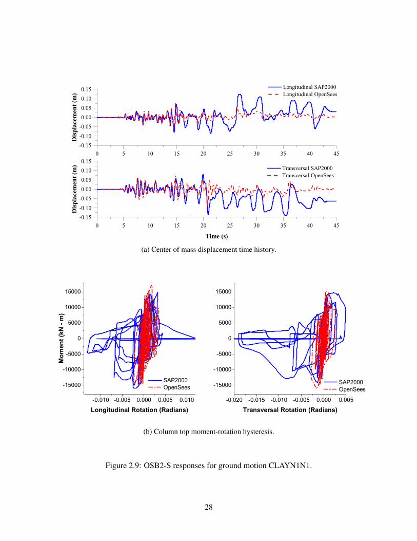
2.4.1 OSB1-O . . . . . . . . . . . . . . . . . . . . . . . . . . . . . . . . . . . 27
2.4.2 OSB2-O . . . . . . . . . . . . . . . . . . . . . . . . . . . . . . . . . . . 29
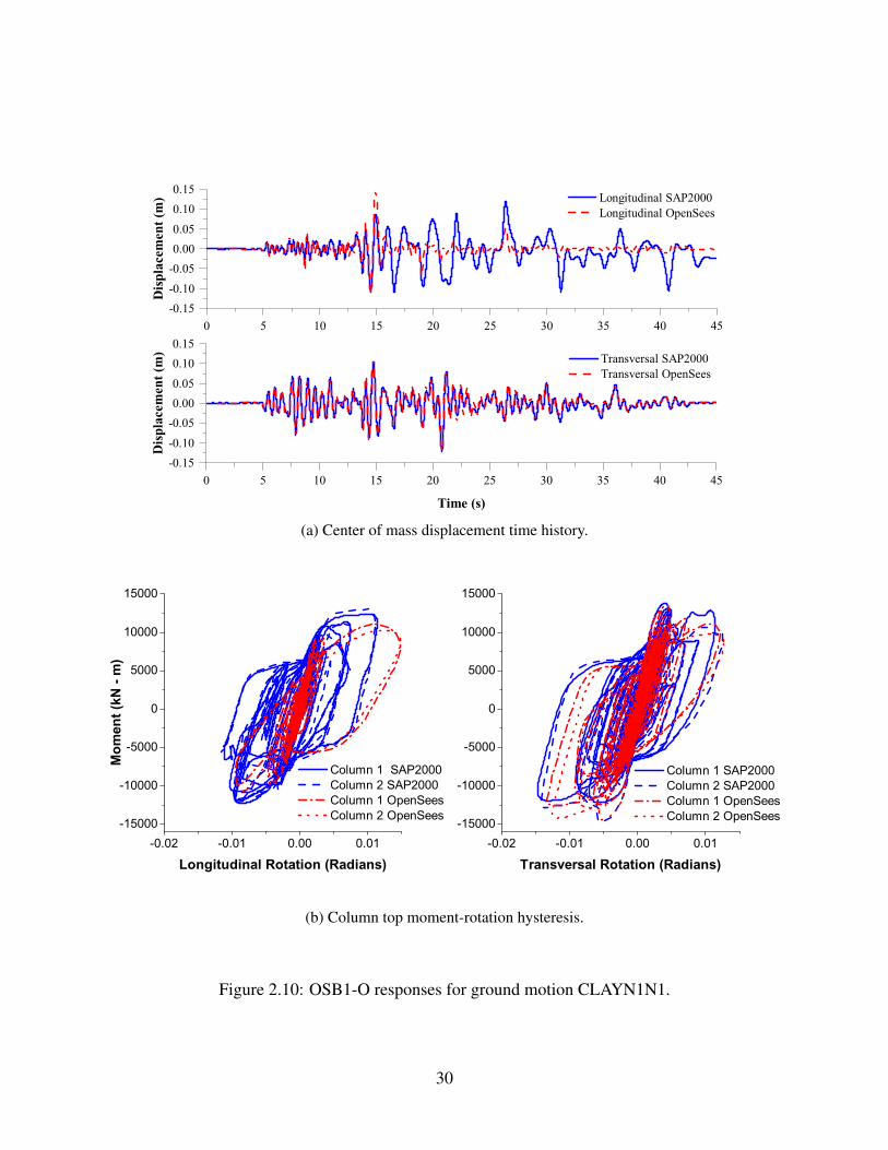
2.4.3 OSB1-MO . . . . . . . . . . . . . . . . . . . . . . . . . . . . . . . . . . 31
2.4.4 OSB2-MO . . . . . . . . . . . . . . . . . . . . . . . . . . . . . . . . . . 33
2.5 Summary and Discussion . . . . . . . . . . . . . . . . . . . . . . . . . . . . . . . 33
CHAPTER 3: NONLINEAR RESPONSE HISTORY SENSITIVITY ANALYSIS OF TYP-
ICAL HIGHWAY BRIDGES. . . . . . . . . . . . . . . . . . . . . . . . . . 44
3.1 Bridge sensitivity analysis . . . . . . . . . . . . . . . . . . . . . . . . . . . . . . 44
3.1.1 Parameters . . . . . . . . . . . . . . . . . . . . . . . . . . . . . . . . . . 44
3.1.2 Static analysis . . . . . . . . . . . . . . . . . . . . . . . . . . . . . . . . 45
3.1.3 Nonlinear time history analysis . . . . . . . . . . . . . . . . . . . . . . . 47
3.1.4 Response sensitivity analysis of OSB1-MO . . . . . . . . . . . . . . . . . 47
3.1.5 Response sensitivity analysis of OSB2-MO . . . . . . . . . . . . . . . . . 50
3.2 Sensitivity Analysis summary . . . . . . . . . . . . . . . . . . . . . . . . . . . . 55
CHAPTER 4: HYSTERETIC BEHAVIORS AND THEIR IMPACT IN THE RESPONSES 56
4.1 Ground motions . . . . . . . . . . . . . . . . . . . . . . . . . . . . . . . . . . . . 56
4.2 Linear responses . . . . . . . . . . . . . . . . . . . . . . . . . . . . . . . . . . . 57
4.3 Single degree of freedom constitutive models . . . . . . . . . . . . . . . . . . . . 57
4.4 Constant ductility response spectrum . . . . . . . . . . . . . . . . . . . . . . . . . 57
4.5 Predictions based on constant ductility response spectrum . . . . . . . . . . . . . . 58
4.6 Single degree of freedom peak values . . . . . . . . . . . . . . . . . . . . . . . . 60
vi

4.7 Benchmark column . . . . . . . . . . . . . . . . . . . . . . . . . . . . . . . . . . 65
4.8 Fast Fourier Transform Analysis . . . . . . . . . . . . . . . . . . . . . . . . . . . 70
4.9 Summary and Discussion . . . . . . . . . . . . . . . . . . . . . . . . . . . . . . . 77
CHAPTER 5: CONCLUSIONS . . . . . . . . . . . . . . . . . . . . . . . . . . . . . . . 80
APPENDIX A: OSB1-S PUSHOVER ANALYSIS . . . . . . . . . . . . . . . . . . . . . . 84
APPENDIX B: GROUND MOTIONS . . . . . . . . . . . . . . . . . . . . . . . . . . . . 86
APPENDIX C: CENTER OF MASS DISPLACEMENTS . . . . . . . . . . . . . . . . . . 89
APPENDIX D: CONSTANT DUCTILITY RESPONSE SPECTRUM . . . . . . . . . . . 98
LIST OF REFERENCES . . . . . . . . . . . . . . . . . . . . . . . . . . . . . . . . . . . 109
vii

LIST OF FIGURES
2.1 Unconfined and confined concrete cyclic stress-strain response for OSB1. . . 13
2.2 Steel cyclic stress-strain response. . . . . . . . . . . . . . . . . . . . . . . . 13
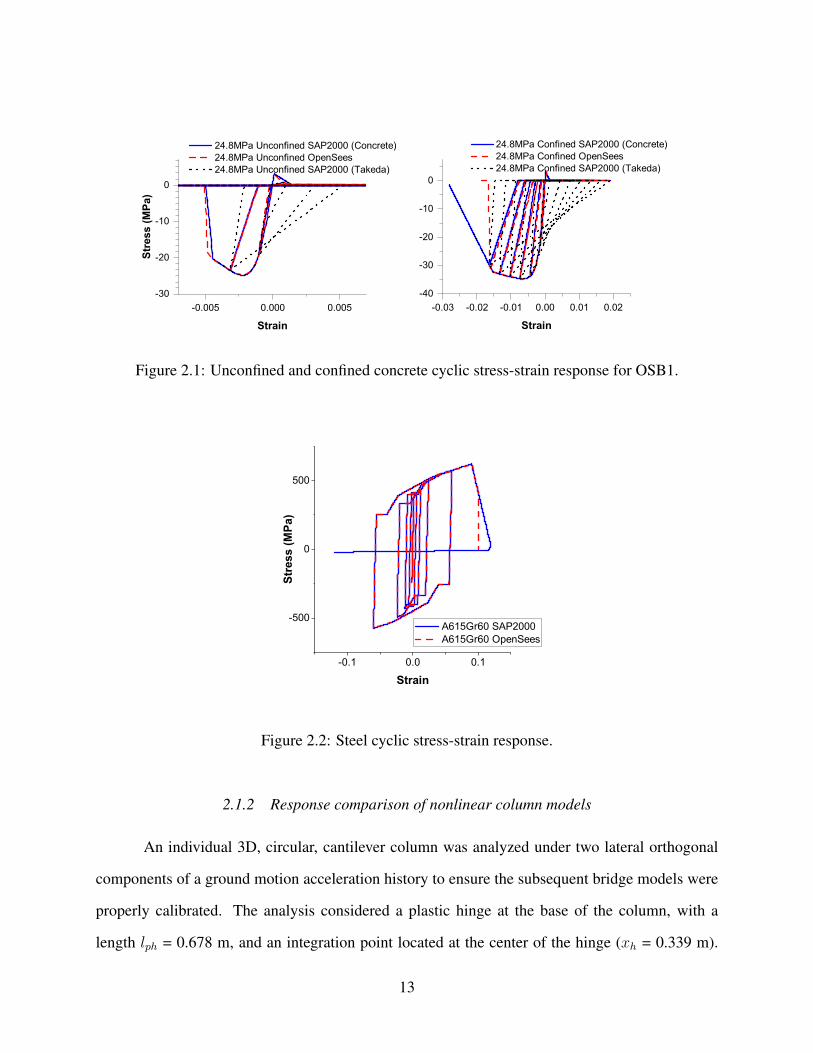
2.3 Benchmark Reinforced concrete column CP3 behavior comparison. . . . . . 15
2.4 Schematic of OSB1 and OSB2 geometry and column cross section. . . . . . . 17
2.5 Abutment resultant load-displacement relationship in SAP2000. . . . . . . . 20
2.6 OSB reinforced concrete column. . . . . . . . . . . . . . . . . . . . . . . . . 22
2.7 Load vs displacement pushover comparison for OSB models. . . . . . . . . . 24
2.8 OSB1-S responses for ground motion CLAYN1N1. . . . . . . . . . . . . . . 26
2.9 OSB2-S responses for ground motion CLAYN1N1. . . . . . . . . . . . . . . 28
2.10 OSB1-O responses for ground motion CLAYN1N1. . . . . . . . . . . . . . . 30
2.11 OSB2-O responses for ground motion CLAYN1N1. . . . . . . . . . . . . . . 32
2.12 OSB1-MS responses for ground motion CLAYN1N1. . . . . . . . . . . . . . 34
2.13 OSB1-MO responses for ground motion CLAYN1N1. . . . . . . . . . . . . . 35
2.14 OSB1-MS and OSB1-MO column top moment-rotation responses for ground
motion CLAYN1N1. . . . . . . . . . . . . . . . . . . . . . . . . . . . . . . 36
2.15 OSB2-MS responses for ground motion CLAYN1N1. . . . . . . . . . . . . . 37
2.16 OSB2-MS column top and bottom moment-rotation responses for ground
motion CLAYN1N1. . . . . . . . . . . . . . . . . . . . . . . . . . . . . . . 38
2.17 OSB2-MO responses for ground motion CLAYN1N1. . . . . . . . . . . . . . 39
2.18 OSB2-MO column top and bottom moment-rotation responses for ground
motion CLAYN1N1. . . . . . . . . . . . . . . . . . . . . . . . . . . . . . . 40
3.1 OSB-MS static sensitivity analysis for longitudinal axis. . . . . . . . . . . . 46
3.2 OSB1-MO Sensitivity response for hysteresis type. . . . . . . . . . . . . . . 49
viii
3.3 OSB1-MO Properties Sensitivity. . . . . . . . . . . . . . . . . . . . . . . . . 51
3.4 OSB2-MO Sensitivity response for hysteresis type. . . . . . . . . . . . . . . 53
3.5 OSB2-MO Properties Sensitivity. . . . . . . . . . . . . . . . . . . . . . . . . 54
4.1 SDOF Material definition for µ = 1, 2, 4, 8, and 10 under CLAYN1N1000
ground motions, and Tn = 0.9s: a) Elastoplasticity; b) Softening. . . . . . . . 58
4.2 Constant-ductility response spectrum for elastoplastic systems and CLAY1N1000
ground motion; µ = 1, 2, 4, 8, and 10; ζ = 1%. . . . . . . . . . . . . . . . . . 59
4.3 SDOF response spectrum with µ=2 under CLAYN1N1000 ground motion
for different hysteretic rules. . . . . . . . . . . . . . . . . . . . . . . . . . . 61
4.4 SDOF response spectrum with µ=2 under CLAYN1N1090 ground motion
for different hysteretic rules. . . . . . . . . . . . . . . . . . . . . . . . . . . 61
4.5 SDOF response spectrum with µ=2 under ROCKN1N1000 ground motion
for different hysteretic rules. . . . . . . . . . . . . . . . . . . . . . . . . . . 62
4.6 SDOF response spectrum with µ=2 under SANDN1N1000 ground motion
for different hysteretic rules. . . . . . . . . . . . . . . . . . . . . . . . . . . 62
4.7 Fiber hysteretic analysis for SDOF system under CLAYN1N1000 ground
motion: a) Elastoplastic model µ=2; b) Elastoplastic model µ=8. . . . . . . . 64
4.8 PDFs for Elastoplasticity SDOF with µ=2: a) Excluding Concrete and Elastic
hysteretic rules; b) Including all hysteretic rules. . . . . . . . . . . . . . . . . 65
4.9 PDFs with normalized peak displacement for Elastoplasticity SDOF with
µ=2: a) Excluding Concrete and Elastic hysteretic rules; b) Including all
hysteretic rules. . . . . . . . . . . . . . . . . . . . . . . . . . . . . . . . . . 66
4.10 PDFs for Elastoplasticity SDOF with µ=8: a) Excluding Concrete and Elastic
hysteretic rules; b) Including all hysteretic rules. . . . . . . . . . . . . . . . . 67
ix

4.11 PDFs with normalized peak displacement for Elastoplasticity SDOF with
µ=8: a) Excluding Concrete and Elastic hysteretic rules; b) Including all
hysteretic rules. . . . . . . . . . . . . . . . . . . . . . . . . . . . . . . . . . 68
4.12 Column response spectrum with µ=2.64 under CLAYN1N1000 ground mo-
tion for different hysteretic rules. . . . . . . . . . . . . . . . . . . . . . . . . 69
4.13 PDFs for elastoplasticity column with µ=2.64: a) Excluding Concrete and
Elastic hysteretic rules; b) Including all hysteretic rules. . . . . . . . . . . . . 71
4.14 PDFs with normalized peak displacement for Elastoplasticity column with
µ=2.64: a) Excluding Concrete and Elastic hysteretic rules; b) Including all
hysteretic rules. . . . . . . . . . . . . . . . . . . . . . . . . . . . . . . . . . 71
4.15 FFT ground motion power spectrum for CLAYN1N1000, CLAYN1N1090,
ROCKN1N1000, and SANDN1N1000 . . . . . . . . . . . . . . . . . . . . . 72
4.16 FFT ground motion power spectrum for elastoplastic SDOF with µ=2 and
different hysteretic rules . . . . . . . . . . . . . . . . . . . . . . . . . . . . . 73
4.17 Transfer functions for elastoplastic SDOF with µ=2 under CLAYN1N1000
ground motion. . . . . . . . . . . . . . . . . . . . . . . . . . . . . . . . . . 74
4.18 Transfer functions for elastoplastic SDOF with µ=8 under CLAYN1N1000
ground motion. . . . . . . . . . . . . . . . . . . . . . . . . . . . . . . . . . 75
4.19 Transfer functions for softening SDOF with µ=2 under CLAYN1N1000 ground
motion. . . . . . . . . . . . . . . . . . . . . . . . . . . . . . . . . . . . . . 76
4.20 Normalized area and normalized displacement relationship for all SDOF sys-
tems: a) All hysteretic rules; b) Excluding Concrete hysteretic rule. . . . . . . 78
4.21 Normalized area and normalized displacement relationship for SDOF sys-
tems with µ=2 and excluding Concrete hysteretic rule. . . . . . . . . . . . . . 79
x
A.1 OSB1-S Pushover analysis using concrete constitutive model dropping to
zero stress at crushing in SAP2000 . . . . . . . . . . . . . . . . . . . . . . . 85
B.1 CLAYN1N1 Recorded Ground Motion. . . . . . . . . . . . . . . . . . . . . 87
B.2 ROCKN1N1 Recorded Ground Motion. . . . . . . . . . . . . . . . . . . . . 87
B.3 SANDN1N1 Recorded Ground Motion. . . . . . . . . . . . . . . . . . . . . 88
C.1 OSB1-S center of mass displacement time history for ROCKN1N1 recorded
ground motion. . . . . . . . . . . . . . . . . . . . . . . . . . . . . . . . . . 90
C.2 OSB1-S center of mass displacement time history for SANDN1N1 recorded
ground motion. . . . . . . . . . . . . . . . . . . . . . . . . . . . . . . . . . 90
C.3 OSB2-S center of mass displacement time history for ROCKN1N1 recorded
ground motion. . . . . . . . . . . . . . . . . . . . . . . . . . . . . . . . . . 91
C.4 OSB2-S center of mass displacement time history for SANDN1N1 recorded
ground motion. . . . . . . . . . . . . . . . . . . . . . . . . . . . . . . . . . 91
C.5 OSB1-O center of mass displacement time history for ROCKN1N1 recorded
ground motion. . . . . . . . . . . . . . . . . . . . . . . . . . . . . . . . . . 92
C.6 OSB1-O center of mass displacement time history for SANDN1N1 recorded
ground motion. . . . . . . . . . . . . . . . . . . . . . . . . . . . . . . . . . 92
C.7 OSB2-O center of mass displacement time history for ROCKN1N1 recorded
ground motion. . . . . . . . . . . . . . . . . . . . . . . . . . . . . . . . . . 93
C.8 OSB2-O center of mass displacement time history for SANDN1N1 recorded
ground motion. . . . . . . . . . . . . . . . . . . . . . . . . . . . . . . . . . 93
C.9 OSB1-MS center of mass displacement time history for ROCKN1N1 recorded
ground motion. . . . . . . . . . . . . . . . . . . . . . . . . . . . . . . . . . 94
C.10 OSB1-MS center of mass displacement time history for SANDN1N1 recorded
ground motion. . . . . . . . . . . . . . . . . . . . . . . . . . . . . . . . . . 94
xi

C.11 OSB2-MS center of mass displacement time history for ROCKN1N1 recorded
ground motion. . . . . . . . . . . . . . . . . . . . . . . . . . . . . . . . . . 95
C.12 OSB2-MS center of mass displacement time history for SANDN1N1 recorded
ground motion. . . . . . . . . . . . . . . . . . . . . . . . . . . . . . . . . . 95
C.13 OSB1-MO center of mass displacement time history for ROCKN1N1 recorded
ground motion. . . . . . . . . . . . . . . . . . . . . . . . . . . . . . . . . . 96
C.14 OSB1-MO center of mass displacement time history for SANDN1N1 recorded
ground motion. . . . . . . . . . . . . . . . . . . . . . . . . . . . . . . . . . 96
C.15 OSB2-MO center of mass displacement time history for ROCKN1N1 recorded
ground motion. . . . . . . . . . . . . . . . . . . . . . . . . . . . . . . . . . 97
C.16 OSB2-MO center of mass displacement time history for SANDN1N1 recorded
ground motion. . . . . . . . . . . . . . . . . . . . . . . . . . . . . . . . . . 97
D.1 Normalized strength vs ductility factor and reduction factor for Tn = 0.1s and
0.2s under CLAYN1N1000 ground motion. . . . . . . . . . . . . . . . . . . 99
D.2 Normalized strength vs ductility factor and reduction factor for Tn = 0.3s and
0.4s under CLAYN1N1000 ground motion. . . . . . . . . . . . . . . . . . . 100
D.3 Normalized strength vs ductility factor and reduction factor for Tn = 0.5s and
0.6s under CLAYN1N1000 ground motion. . . . . . . . . . . . . . . . . . . 101
D.4 Normalized strength vs ductility factor and reduction factor for Tn = 0.7s and
0.75s under CLAYN1N1000 ground motion. . . . . . . . . . . . . . . . . . . 102
D.5 Normalized strength vs ductility factor and reduction factor for Tn = 0.8s and
0.9s under CLAYN1N1000 ground motion. . . . . . . . . . . . . . . . . . . 103
D.6 Normalized strength vs ductility factor and reduction factor for Tn = 1.0s and
1.25s under CLAYN1N1000 ground motion. . . . . . . . . . . . . . . . . . . 104
xii
D.7 Normalized strength vs ductility factor and reduction factor for Tn = 1.5s and
1.75s under CLAYN1N1000 ground motion. . . . . . . . . . . . . . . . . . . 105
D.8 Normalized strength vs ductility factor and reduction factor for Tn = 2.0s and
2.5s under CLAYN1N1000 ground motion. . . . . . . . . . . . . . . . . . . 106
D.9 Normalized strength vs ductility factor and reduction factor for Tn = 3.0s and
4.0s under CLAYN1N1000 ground motion. . . . . . . . . . . . . . . . . . . 107
D.10 Normalized strength vs ductility factor and reduction factor for Tn = 5.0s and
10.0s under CLAYN1N1000 ground motion. . . . . . . . . . . . . . . . . . . 108
xiii

LIST OF TABLES
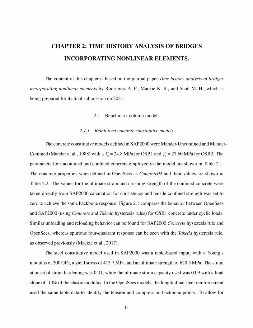
2.1 Concrete model parameters for SAP2000. . . . . . . . . . . . . . . . . . . . 12
2.2 Concrete04 material properties employed in columns. . . . . . . . . . . . . . 12
2.3 Benchmark bridge definitions . . . . . . . . . . . . . . . . . . . . . . . . . . 16
2.4 Superstructure material and section properties. . . . . . . . . . . . . . . . . . 19
2.5 Ground motion acceleration time history properties. . . . . . . . . . . . . . . 25
2.6 Longitudinal peak displacement values . . . . . . . . . . . . . . . . . . . . . 42
2.7 Transversal peak displacement values . . . . . . . . . . . . . . . . . . . . . 42
2.8 Longitudinal peak displacement bias factors . . . . . . . . . . . . . . . . . . 43
2.9 Transversal peak displacement bias factors . . . . . . . . . . . . . . . . . . . 43
3.1 Parameters considered for the sensitivity analysis. . . . . . . . . . . . . . . . 45
3.2 Peak sensitivity results for static analysis. . . . . . . . . . . . . . . . . . . . 46
3.3 OSB1-MO peak sensitivity results for hysteresis type. . . . . . . . . . . . . . 48
3.4 OSB1-MO peak sensitivity results for bridge nonlinear parameters. . . . . . . 50
3.5 OSB2-MO Peak sensitivity results for hysteresis type. . . . . . . . . . . . . . 52
3.6 OSB2-MO peak sensitivity results for bridge nonlinear parameters. . . . . . . 55
4.1 Ground motion acceleration time history properties. . . . . . . . . . . . . . . 56
4.2 Prediction bias for elastoplasticity systems under CLAYN1N1000 ground
motion and Kinematic hysteretic rule . . . . . . . . . . . . . . . . . . . . . . 59
4.3 Elastoplastic SDOF model peak displacements for µ = 2 and Tn = 0.9s . . . . 60
4.4 Elastoplastic SDOF model peak displacements for µ = 8 and Tn = 0.9s . . . . 63
4.5 Softening SDOF model peak displacements for µ = 2 and Tn = 0.9s . . . . . 63
4.6 Mean value and standard deviation for Elastoplastic and Softening systems
under different ground motions and considering all hysteretic rules. . . . . . . 65
xiv

4.7 Mean value and standard deviation for Elastoplastic and Softening systems
under different ground motions excluding Concrete and Elastic hysteretic rules. 66
4.8 Peak displacement and prediction bias for benchmark column with a µ = 2.64
and under CLAYN1N1000 ground motion. . . . . . . . . . . . . . . . . . . . 70
xv
CHAPTER 1: INTRODUCTION
Poor seismic performance of older bridges is often attributable to the design philosophy at
the time of construction. Numerous historical events have led to improvements in design criteria
and evolution of codes and guidelines. In the United States, many design philosophy changes oc-
curred after damage during the 1971 San Fernando earthquake where, for example, the Newhall
Pass interchange collapsed (Fung et al., 1971). The 1989 Loma Prieta earthquake caused nearly
$6.5 billion damage in bridge structures, including the signature 50 ft span of San Francisco -
Oakland bridge and more than a mile of elevated road way on I-880 (EERI, 1989). Two bridges
retrofitted after 1971 San Fernando collapsed and 39 highway bridges experienced structural dam-
age in the 1994 Northridge earthquake. The most important collapses occurred in the Gavin
Canyon Bridge and an elevated portion of the Los Angeles I-10 (Bolin & Stanford, 2006).
After the Hyogoken-Nanbu (Kobe) 1995 earthquake in Japan, several lessons were learned
about shear detailing and longitudinal bar continuity. Design criteria and assumptions about
recorded seismic coefficients were improved, particularly given the similarity between several
Japanese and central-southeastern US bridges (steel girders and concrete columns) (NIST, 1996,
pp. 163-191). Recent earthquakes such as Maule (Chile) in 2010 illustrated performance of retrofits
for foundation bearing capacity, anchors and stopper mechanisms at bearings, seat support length
and the strength of the prestressed concrete girder (Kawashima et al., 2011). As a result, important
changes were incorporated into the bridge design criteria, such as reductions to overpass skew, in-
creases in seat width, the use of multi-rotational instead of rocker-type bearings, distance to hinges
from columns, the use of spiral reinforcement to confine the longitudinal rebars, and the increase
of reinforcement in the column-deck connection (Khan, 2015).
While bridges are often treated as simple structural systems for analysis and design, com-
plex responses may occur in the two primary load paths (bents and abutments) under large seismic
loads. In addition, the structural simplicity that they possess seems to generate a greater sensitivity
1

to errors during design and construction process (Priestly et al., 1996). The implementation of
nonlinear methods in the analysis of bridges exposed to dynamic loads has provided more accurate
response in comparison with the traditional linear approaches. A summary of common element for-
mulations and implementations in nonlinear static analysis of typical reinforced concrete bridges
was recently reported by Mackie and Scott (2019). Beyond standard concentrated and distributed
plasticity approaches for columns, recommendations were made on making sure response differ-
ences were due to the formulation and not the software-specific implementation - two items that
are commonly confused.
The study further develops previous models of two Caltrans ordinary bridges evaluating
different kinds of responses, such as nonlinear time history analysis and moment-rotation column
reactions, when seismic loads are applied (Mackie et al., 2017), and the sensitivity of the nonlin-
ear time history response after a slightly perturbation of the basic nonlinear constitutive materials
and the hysteresis behavior. The calibration of the nonlinear static responses of the constitutive
models for abutments and columns between two different software (SAP2000 and OpenSees) was
an important step to reduce sources of uncertainty when comparing dynamic responses. A simple
boundary condition, which consisted of a roller abutment at the end of the superstructure, was
used to concentrate nonlinear response in the columns. After obtaining an adequate agreement in
the column nonlinear behavior, the abutment impact on hysteresis was studied by replacing the
roller abutment with an abutment model comprised of gap-link elements. The numerical models
presented in the current study are based on SAP2000 (version 21.0.2 Build 1491) and OpenSees
(version 2.6.4), employing the same finite element formulations for the column and abutment non-
linearities to better identify the sources of discrepancies in the responses.
2
1.1 Background
Nonlinear time history studies on bridges have been evolving alongside the nonlinear
analysis tools. Modeling of bridge collapse mechanisms and retrofit for bridges after the 1994
Northridge used DRAIN-3DX (Fenves & Ellery, 1998). A bridge in the Egnatia motorway in
northern Greece was seismically analyzed to study the responses using Ruaumoko 3D for non-
linear analysis (Kappos & Dimitrakopoulos, 2005). Follow up studies on other as-built structures
were conducted as nonlinear analysis tools for bridges matured in OpenSees (Kunnath, 2007)
that started to identify component vulnerabilities through nonlinear dynamic modeling (Nielson
& DesRoches, 2007). Explicit soil-structure-interaction modeling was included in bridge models
of the Humboldt Bay bridge by Zhang, et al. (2004) and the I-880 viaduct (Jeremic et al., 2004),
concluding that the SSI effects can be detrimental depending on the seismic loading. The link
between nonlinear behavior in bridges after seismic events and damage and decision making in a
performance-based context was conducted by Mackie and Stojadinovic (2003). A seismic analysis
of the Meloland road overcrossing was conducted using a multiplatform approach that analyzed
the structural model of the bridge built in Zeus-NL and the soil-structure interaction modeled in
OpenSees (Kwon & Elnashai, 2008).
The link between nonlinear behavior in concrete bridges after seismic events and damage
and decision making in a performance-based context was conducted by (Mackie, 2008) and (Niel-
son & DesRoches, 2007), amongst others. Although many studies followed on the seismic perfor-
mance of typical concrete bridges that included distributions of parameters and the corresponding
component/system fragilities, few formal model sensitivity studies have been conducted the impact
of modeling parameters on seismic response prediction. However, recent studies have established
guidelines for modeling the nonlinear time history response of ordinary standard bridges and in-
vestigated variability of peak responses to modeling parameters and software implementations. In
addition, recommendations for modeling were made in different commercially or freely available
3
software that aimed to eliminate or quantify differences that arose from software implementations
(Aviram et al., 2008; Mackie & Scott, 2019).
1.1.1 Previous Research on Bridges
The recent guidelines all investigated the role of boundary conditions on the time history
responses, specifically the different assumptions for abutment models. While some studies based
their analyses on the nonlinear behavior of gap-link abutments (Omrani et al., 2015), others imple-
mented models to establish practical recommendations for the nonlinear analysis in commercial
software like SAP2000 and OpenSees (Aviram et al., 2008). Mackie, et al. (2017) studied the non-
linear time history analysis (NTHA) of Caltrans bridges by separating the effects of the abutment
assumptions and a simplified roller condition using OpenSees and CSiBridge software.
Realistic seismic response prediction of bridges requires the use of nonlinear analysis meth-
ods (Pinto & Franchin, 2010), which can be divided into static (using a pushover load pattern) and
dynamic (hysteresis response under acceleration input) analysis. However, the degree of complex-
ity inherent in the nonlinear models increases the computational effort necessary for the analyses,
as well the difficulty in the interpretation of the results. In addition, the large number of parameters,
choice of numerical methods, software implementations, and element or material formulations in-
volved in a nonlinear analysis lead to potentially larger uncertainty in the responses. While past
work has shown that nonlinear static responses can be standardized between software implemen-
tations if consistent modeling choices are made (Mackie & Scott, 2019), the causes of nonlinear
dynamic response bias have not previously been isolated as due to formulation or implementation
(Aviram et al., 2008).
1.1.2 Bridge sensitivity analysis
A rational method to evaluate the damages and losses in highway bridges was developed
by Mackie and Stojadinovic (2005). The bridge fragilities obtained help future designers to predict
4

the amount of losses in bridges after a seismic event, based on the bridge parameters sensitivity.
A finite element response sensitivity analysis was conducted by Zona, Barbato, and Conte (2006)
to study the importance and the effects of different material parameters, using the direct differ-
entiation method and forward finite difference method. Several investigations such as Pan et al.
(2010) and Sullivan and Nielson (2010) have been focused to analyze the sensitivity on steel struc-
ture bridges. On the other hand, some authors addressed the sensitivity analysis in different way.
This is the case of Zhao, Vasheghani-Farahani and Burdette (2011), who analyzed the sensitivity
response of the bridges considering the soil-structure interaction under different backfilling con-
ditions at the abutments and Ghotbi (2014), who studied the fragility curves sensitivity of skewed
bridges under seismic loads with different types of soils. A reliable computational tool is very im-
portant to reduce time and errors during a sensitivity analysis. Thus, some studies like Haukaas and
Der Kiureghian (2007) were conducted to obtain a freely library of software codes for OpenSees
to analysis the response sensibility of the bridge structures.
The approach method to be used to predict the sensitivity of bridges will vary depending
on the conditions, computational tool capacity, and the objective of the analysis. Therefore, sev-
eral authors like Kleiber (1997) and Jurado et al (2011) dedicated their researches to explore the
best method to obtain an optimal design. Regarding to the sensitivity analysis of bridges nonlin-
ear finite element models, the most used approaches involve different theories such as the finite
difference method, direct differentiation method, complex perturbation method, and the adjoint
structure method. The finite difference method represents the simplest way to analyze the sensitiv-
ity in bridges under seismic loads, where after obtaining a mean response, the analysis is repeated
perturbing the parameters object to study. The sensitivity is obtained by a simple differentiation
between the original and the modified values response. Even though is a very simplistic method,
it involves a huge computational effort and some errors could be induced due to round-off and
effect of perturbation size on the nonlinear system. A more accurate result can be obtained using
the direct differentiation method, which uses analytical differentiation based on the equations that
5

govern the finite element responses and the constitutive responses of the elements involved in the
bridge model. On the other hand, the sensitivity analysis could be performed using the complex
perturbation method by computing the responses using a complex algebra and reanalyzing each
parameter in the finite element model (Mackie et al., 2017). Finally, the adjoint structure method
is very useful to obtain the sensitivity response on bridges, but without a correct application in
situations that involve path-dependent conditions the direct differentiation method appears to be
usually more accurate (Kleiber et al., 1997).
1.1.3 Approximation methods in sensitivity analysis
There are a variety of theories or methods which could predict with a reasonable accurate
the sensitivity of the bridge to changes in the main parameters that conform the model. The method
to be chosen usually will depend on the objective of the analysis and the capacity of the computa-
tional tool. The most common approaches to establish the sensitivity for nonlinear finite element
models include the finite difference method (FDM), the direct differentiation method (DDM), com-
plex perturbation method (CPM), and adjoint structure method (ASM). Because the computational
tools to be used in the current research only require the FDM and DDM to achieve the research
objectives, the other methods will not be described.
1.1.3.1 Finite difference method (FDM)
The FDM probably represents the simplest technique to estimate the bridge sensitivity. In
the method, it is necessary to obtain the value u(x) as the original response without perturbation
and then repeat the entire calculation for a perturbed value x+∆x to obtain u(x+∆x). Therefore,
the first-order forward-difference approximation ∆u/∆x to the derivative du/dx can be expressed
as
∆u/∆x = (u(x+ ∆x)− u(x))/∆x (1.1)
6
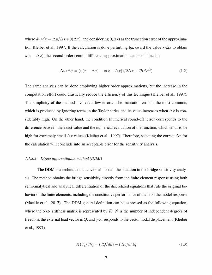
where du/dx = ∆u/∆x+0(∆x), and considering 0(∆x) as the truncation error of the approxima-
tion Kleiber et al., 1997. If the calculation is done perturbing backward the value x-∆x to obtain
u(x−∆x), the second-order central difference approximation can be obtained as
∆u/∆x = (u(x+ ∆x)− u(x−∆x))/2∆x+O(∆x2) (1.2)
The same analysis can be done employing higher order approximations, but the increase in the
computation effort could drastically reduce the efficiency of this technique (Kleiber et al., 1997).
The simplicity of the method involves a few errors. The truncation error is the most common,
which is produced by ignoring terms in the Taylor series and its value increases when ∆x is con-
siderably high. On the other hand, the condition (numerical round-off) error corresponds to the
difference between the exact value and the numerical evaluation of the function, which tends to be
high for extremely small ∆x values (Kleiber et al., 1997). Therefore, selecting the correct ∆x for
the calculation will conclude into an acceptable error for the sensitivity analysis.
1.1.3.2 Direct differentiation method (DDM)
The DDM is a technique that covers almost all the situation in the bridge sensitivity analy-
sis. The method obtains the bridge sensitivity directly from the finite element response using both
semi-analytical and analytical differentiation of the discretized equations that rule the original be-
havior of the finite elements, including the constitutive performance of them on the model response
(Mackie et al., 2017). The DDM general definition can be expressed as the following equation,
where the NxN stiffness matrix is represented by K, N is the number of independent degrees of
freedom, the external load vector isQ, and q corresponds to the vector nodal displacement (Kleiber
et al., 1997).
K(dq/dh) = (dQ/dh)− (dK/dh)q (1.3)
7

This simple expression of the DDM is used to estimate the sensitivity on static linear cases
and can be easily adapted to be used in a variety different cases such as nonlinear quasi-static
problems, inelastic systems, and nonlinear dynamic, and others situation (Kleiber et al., 1997).
The method computes the sensitivity for all the parameters while the deterministic analysis is
performed achieved by considering the load vectors substituted forward and backward with the
corresponding factorized dynamic tangent stiffness matrix in each calculation, contrasting with
the FDM which requires to calculate the responses again after perturbing the parameters. The
described process concludes in a perturbed response in the same order of accuracy than the mean
response (Mackie et al., 2017), removing the condition error due to round-off and the loose of high
orders terms.
1.2 Research Objectives
The study further wants to analyze the behavior of two Caltrans bridges under static and
dynamic loads, by evaluating different kinds of responses, such as nonlinear time history analy-
sis and moment-rotation column reactions, when seismic loads are applied, and the sensitivity of
the nonlinear time history response after a slightly perturbation of the basic nonlinear constitutive
materials and the hysteresis behavior. Additionally, the research will study the different hysteretic
behavior and their impact in the nonlinear time history response on single degree of freedom sys-
tems. The research should achieve this objective by completing the following tasks:
• Developing and analysis of benchmark columns concrete constitutive models.
• Time history analysis of two Caltrans bridges incorporating nonlinear elements under dy-
namic loads using SAP2000 and OpenSees softwares.
• Elaborate modifications on the bridge models for a better agreement between softwares.
• Compare the results achieved with the improvements done.
8

• Establish the parameter to be perturbed to perform a sensitivity analysis.
• Using the modified bridge models, develop a nonlinear response history sensitivity analysis
under static and dynamic loads.
• Develop single degree of freedom systems for linear elastic, elastoplastic, and softening
backbones to construct a constant-ductility response spectrum.
• Hysteretic behaviors analysis and their impact in the nonlinear time history response on the
single degree of freedom systems developed.
1.3 Thesis Outline
This thesis is organized into four different chapters as listed:
Chapter 1 consists of the introduction, which includes the most relevant historical events
that led to improvements in the bridges design and analysis criteria, different software implemen-
tations on bridge retrofits and typical situations, materials and element formulations on bridge
models, previous researches conducted to analyze the sensitivity of bridges, and the most com-
mon numerical methods employed to estimate the sensitivity of typical bridges. This chapter also
includes the research objectives and the specific tasks required to achieve them.
Chapter 2 develops previous models of two Caltrans ordinary standard bridges, evaluating
different kinds of responses, such as nonlinear time history analysis and moment-rotation column
reactions, when seismic loads are applied (Mackie et al., 2017). The column responses were
analyzed using a simplified bridge model, which consisted in a simple roller abutment at the end
of the superstructure. After obtaining an adequate agreement in the column nonlinear behavior
for SAP2000 and OpenSees models, the abutment hysteresis was studied by replacing the roller
abutment with the original bridge consideration. The numerical models presented in the current
study are based on SAP2000 (version 21.0.2 Build 1491) and OpenSees (version 2.6.4), employing
9

the same finite element formulations for the column and abutment nonlinearities to better identify
the sources of discrepancies in the responses.
Chapter 3 evaluates the sensitivity of the nonlinear time history response using the same
bridge models developed in the previous chapter. Sensitivities were obtained using the finite dif-
ference method, using a slightly perturbation of the basic nonlinear constitutive materials and the
hysteresis behaviors. Using SAP2000 (version 21.0.2 Built 1491), the sensitivity analysis was
performance by the implementation of the finite central difference method.
Chapter 4 studies the effects of the hysteretic considerations on the responses of differ-
ent single degree of freedom (SDOF) systems under ground motions. The analysis was done by
the study of a constant-ductility response spectrum under an specific ground motion, probability
density functions, and fast Fourier transformation.
10
CHAPTER 2: TIME HISTORY ANALYSIS OF BRIDGES
INCORPORATING NONLINEAR ELEMENTS.
The content of this chapter is based on the journal paper Time history analysis of bridges
incorporating nonlinear elements by Rodriguez A. F., Mackie K. R., and Scott M. H., which is
being prepared for its final submission on 2021.
2.1 Benchmark column models
2.1.1 Reinforced concrete constitutive models
The concrete constitutive models defined in SAP2000 were Mander-Unconfined and Mander-
Confined (Mander et al., 1988) with a f ′c = 24.8 MPa for OSB1 and f ′c = 27.60 MPa for OSB2. The
parameters for unconfined and confined concrete employed in the model are shown in Table 2.1.
The concrete properties were defined in OpenSees as Concrete04 and their values are shown in
Table 2.2. The values for the ultimate strain and crushing strength of the confined concrete were
taken directly from SAP2000 calculation for consistency and tensile confined strength was set to
zero to achieve the same backbone response. Figure 2.1 compares the behavior between OpenSees
and SAP2000 (using Concrete and Takeda hysteresis rules) for OSB1 concrete under cyclic loads.
Similar unloading and reloading behavior can be found for SAP2000 Concrete hysteresis rule and
OpenSees, whereas spurious four-quadrant response can be seen with the Takeda hysteresis rule,
as observed previously (Mackie et al., 2017).
The steel constitutive model used in SAP2000 was a table-based input, with a Young’s
modulus of 200 GPa, a yield stress of 413.7 MPa, and an ultimate strength of 620.5 MPa. The strain
at onset of strain hardening was 0.01, while the ultimate strain capacity used was 0.09 with a final
slope of -10% of the elastic modulus. In the OpenSees models, the longitudinal steel reinforcement
used the same table data to identify the tension and compression backbone points. To allow for
11
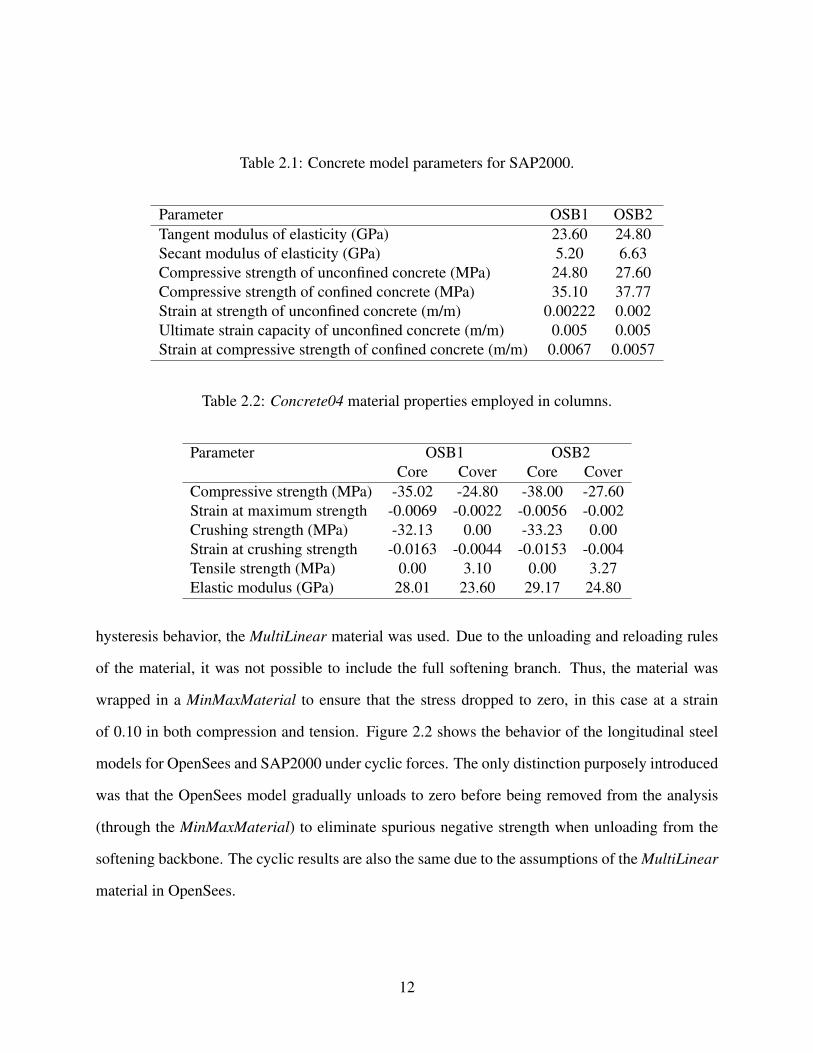
Table 2.1: Concrete model parameters for SAP2000.
Parameter OSB1 OSB2Tangent modulus of elasticity (GPa) 23.60 24.80Secant modulus of elasticity (GPa) 5.20 6.63Compressive strength of unconfined concrete (MPa) 24.80 27.60Compressive strength of confined concrete (MPa) 35.10 37.77Strain at strength of unconfined concrete (m/m) 0.00222 0.002Ultimate strain capacity of unconfined concrete (m/m) 0.005 0.005Strain at compressive strength of confined concrete (m/m) 0.0067 0.0057
Table 2.2: Concrete04 material properties employed in columns.
Parameter OSB1 OSB2Core Cover Core Cover
Compressive strength (MPa) -35.02 -24.80 -38.00 -27.60Strain at maximum strength -0.0069 -0.0022 -0.0056 -0.002Crushing strength (MPa) -32.13 0.00 -33.23 0.00Strain at crushing strength -0.0163 -0.0044 -0.0153 -0.004Tensile strength (MPa) 0.00 3.10 0.00 3.27Elastic modulus (GPa) 28.01 23.60 29.17 24.80
hysteresis behavior, the MultiLinear material was used. Due to the unloading and reloading rules
of the material, it was not possible to include the full softening branch. Thus, the material was
wrapped in a MinMaxMaterial to ensure that the stress dropped to zero, in this case at a strain
of 0.10 in both compression and tension. Figure 2.2 shows the behavior of the longitudinal steel
models for OpenSees and SAP2000 under cyclic forces. The only distinction purposely introduced
was that the OpenSees model gradually unloads to zero before being removed from the analysis
(through the MinMaxMaterial) to eliminate spurious negative strength when unloading from the
softening backbone. The cyclic results are also the same due to the assumptions of the MultiLinear
material in OpenSees.
12
-0.03 -0.02 -0.01 0.00 0.01 0.02-40
-30
-20
-10
0
Strain
24.8MPa Confined SAP2000 (Concrete) 24.8MPa Confined OpenSees 24.8MPa Confined SAP2000 (Takeda)
-0.005 0.000 0.005-30
-20
-10
0
Strain
24.8MPa Unconfined SAP2000 (Concrete) 24.8MPa Unconfined OpenSees 24.8MPa Unconfined SAP2000 (Takeda)
Stre
ss (M
Pa)
Figure 2.1: Unconfined and confined concrete cyclic stress-strain response for OSB1.
-0.1 0.0 0.1
-500
0
500
Stre
ss (M
Pa)
Strain
A615Gr60 SAP2000 A615Gr60 OpenSees
Figure 2.2: Steel cyclic stress-strain response.
2.1.2 Response comparison of nonlinear column models
An individual 3D, circular, cantilever column was analyzed under two lateral orthogonal
components of a ground motion acceleration history to ensure the subsequent bridge models were
properly calibrated. The analysis considered a plastic hinge at the base of the column, with a
length lph = 0.678 m, and an integration point located at the center of the hinge (xh = 0.339 m).
13
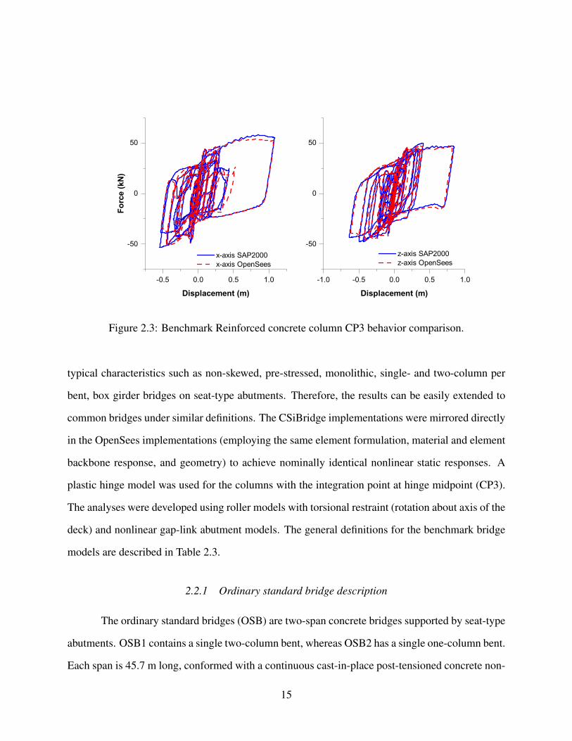
The effective moment of inertia of the column was 0.60Ig to assume an appropriated softening of
the cracked elastic properties. The values assumed were taken according to the CP3 case (Mackie
& Scott, 2019). Similar values can be obtained using ACI-318 (ACI, 2014), Caltrans Seismic
Design Criteria (Caltrans, 2013), and Paulay and Priestly (1992), where the recommended effective
inertias are 0.70Ig, 0.53Ig, and 0.50−0.70Ig, respectively. The column used to calibrate the models
had a diameter of 0.51 m, with 8 #8 Grade 50 longitudinal reinforcement, and #8 transverse spiral
reinforcement spaced at 0.025 m (which correspond to the properties of OSB1). The circular
concrete cross section was discretized into 100 and 40 fiber layers in the tangential and radial
directions.
A vertical load of P = -267.5 KN was applied at the top of the column. The orthogonal
lateral ground motions imposed were CLAYN1N1000 and CLAYN1N1090 synthetic accelerations
(Lu et al., 2015) for x-axis and z-axis respectively. No damping and P-Delta effects were consid-
ered in the dynamic analysis, and the time integration method used was Hilber-Hughes-Taylor with
γ = 0.5, β = 0.25, and α = 0. Comparisons between SAP2000 and OpenSees implementations of
the CP3 benchmark column under dynamic load are shown in Figure 2.3.
The results shown in the figure concluded that SAP2000 CP3 model has a similar behavior
than OpenSees, with small differences in the force peaks values. The response shapes are almost
the same for both software, showing identical slopes during the ground motion.
2.2 Benchmark bridge models
Two previously calibrated three-dimensional (3D) bridge models under static pushover
loads and and considering a concentrated plasticity (CP) approach (Mackie & Scott, 2019) are
extended in this investigation to include dynamic time history response under ground motion
excitation. The bridge models were originally developed by Caltrans and modeled in CSiB-
ridge/SAP2000, denoted as ordinary standard bridges (OSBs) 1 and 2. The models represent bridge
14
-0.5 0.0 0.5 1.0
-50
0
50
x-axis SAP2000 x-axis OpenSees
Forc
e (k
N)
Displacement (m)-1.0 -0.5 0.0 0.5 1.0
-50
0
50
z-axis SAP2000 z-axis OpenSees
Displacement (m)
Figure 2.3: Benchmark Reinforced concrete column CP3 behavior comparison.
typical characteristics such as non-skewed, pre-stressed, monolithic, single- and two-column per
bent, box girder bridges on seat-type abutments. Therefore, the results can be easily extended to
common bridges under similar definitions. The CSiBridge implementations were mirrored directly
in the OpenSees implementations (employing the same element formulation, material and element
backbone response, and geometry) to achieve nominally identical nonlinear static responses. A
plastic hinge model was used for the columns with the integration point at hinge midpoint (CP3).
The analyses were developed using roller models with torsional restraint (rotation about axis of the
deck) and nonlinear gap-link abutment models. The general definitions for the benchmark bridge
models are described in Table 2.3.
2.2.1 Ordinary standard bridge description
The ordinary standard bridges (OSB) are two-span concrete bridges supported by seat-type
abutments. OSB1 contains a single two-column bent, whereas OSB2 has a single one-column bent.
Each span is 45.7 m long, conformed with a continuous cast-in-place post-tensioned concrete non-
15
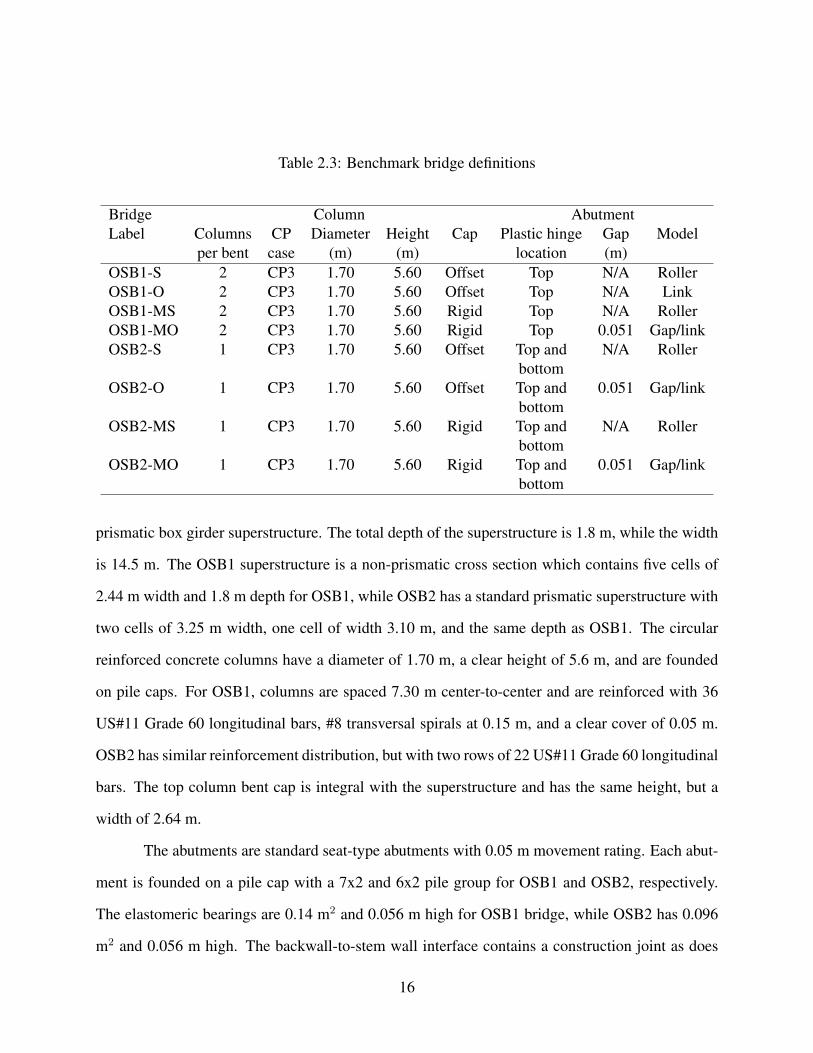
Table 2.3: Benchmark bridge definitions
Bridge Column AbutmentLabel Columns CP Diameter Height Cap Plastic hinge Gap Model
per bent case (m) (m) location (m)OSB1-S 2 CP3 1.70 5.60 Offset Top N/A RollerOSB1-O 2 CP3 1.70 5.60 Offset Top N/A LinkOSB1-MS 2 CP3 1.70 5.60 Rigid Top N/A RollerOSB1-MO 2 CP3 1.70 5.60 Rigid Top 0.051 Gap/linkOSB2-S 1 CP3 1.70 5.60 Offset Top and N/A Roller
bottomOSB2-O 1 CP3 1.70 5.60 Offset Top and 0.051 Gap/link
bottomOSB2-MS 1 CP3 1.70 5.60 Rigid Top and N/A Roller
bottomOSB2-MO 1 CP3 1.70 5.60 Rigid Top and 0.051 Gap/link
bottom
prismatic box girder superstructure. The total depth of the superstructure is 1.8 m, while the width
is 14.5 m. The OSB1 superstructure is a non-prismatic cross section which contains five cells of
2.44 m width and 1.8 m depth for OSB1, while OSB2 has a standard prismatic superstructure with
two cells of 3.25 m width, one cell of width 3.10 m, and the same depth as OSB1. The circular
reinforced concrete columns have a diameter of 1.70 m, a clear height of 5.6 m, and are founded
on pile caps. For OSB1, columns are spaced 7.30 m center-to-center and are reinforced with 36
US#11 Grade 60 longitudinal bars, #8 transversal spirals at 0.15 m, and a clear cover of 0.05 m.
OSB2 has similar reinforcement distribution, but with two rows of 22 US#11 Grade 60 longitudinal
bars. The top column bent cap is integral with the superstructure and has the same height, but a
width of 2.64 m.
The abutments are standard seat-type abutments with 0.05 m movement rating. Each abut-
ment is founded on a pile cap with a 7x2 and 6x2 pile group for OSB1 and OSB2, respectively.
The elastomeric bearings are 0.14 m2 and 0.056 m high for OSB1 bridge, while OSB2 has 0.096
m2 and 0.056 m high. The backwall-to-stem wall interface contains a construction joint as does
16

Figure 2.4: Schematic of OSB1 and OSB2 geometry and column cross section.
the exterior shear key-to-stem wall interface. The end diaphragm is also integral with the super-
structure and has 0.91 m width. The material properties were f ′c = 24.8 MPa for the bent pile cap
and f ′c = 27.6 MPa for the superstructure. Figure 2.4 shows a schematic representation of OSB1
geometry with its column cross section.
2.2.1.1 SAP2000 bridge model implementation
Previously developed by Caltrans (2013), no changes were made to the OSB1-O and OSB2-
O SAP2000 models. The center of mass in these models is located 6.1 m above the column bases.
A 0.85 m long rigid element was created at the top of each column, increasing its moment of inertia
with a multiplier of 3. The OSB2-O model incorporated an additional rigid element at the bottom
of the column, with the same characteristics as the top. The rigid element included a frame hinge
17

type Fiber P-M2-M3 (CSI, 2017) in the center and for OSB1-O model it was offset 0.45 m from
the deck. The offset was modeled considering a rigid zone factor of 0.5. The moment of inertia of
the remaining column was reduced in both directions by a factor of 0.35 and no frame hinge was
considered. The superstructure concrete was defined with an elastic modulus of 23.60 GPa and a
non-prismatic cross section. The elastic properties are described in Table 2.4.
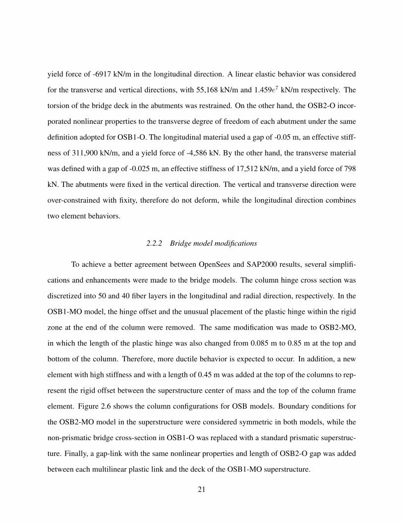
For OSB1-O, a single multilinear plastic link element (CSI, 2017) was used to define
the nonlinear properties of the longitudinal degree of freedom at each abutment. The force-
deformation relation was elastic-plastic with a yield force of -6917 kN and a yield displacement
of -0.0152 m, following a kinematic hysteresis rule. The effective stiffness for the linear analysis
in the longitudinal and transverse directions were 453,754 kN/m and 55,165 kN/m respectively,
while the vertical direction had an effective stiffness of 1.459×10⁷ kN/m.
Two link elements in series defined the OSB2-O abutments. The first link element consisted
of a gap link with nonlinear properties in the longitudinal axis connected to the deck end node.
The effective stiffness for the linear analysis case was 3.50×10⁷ kN/m, while the gap length and
the stiffness for the nonlinear analysis were -0.051 m and 175.13×10⁴ kN/m respectively. The
deck left end node had restraints in the transverse and vertical directions, as well as all rotational
degrees of freedom. However, the right end node was only restrained in the translational degrees of
freedom. The second link element consisted of a multilinear plastic link with nonlinear properties
in the longitudinal degree of freedom, located between the gap link and the supports. With an
elastoplastic nonlinear force-deformation relation, the link had a yield displacement of -0.015 m
and a yield force of -4586 kN in the longitudinal directions, but the remaining degrees of freedom
were restrained. Figure 2.5 shows the resultant load-displacement relationship for OSB1-O and
OSB2-O abutments.
18
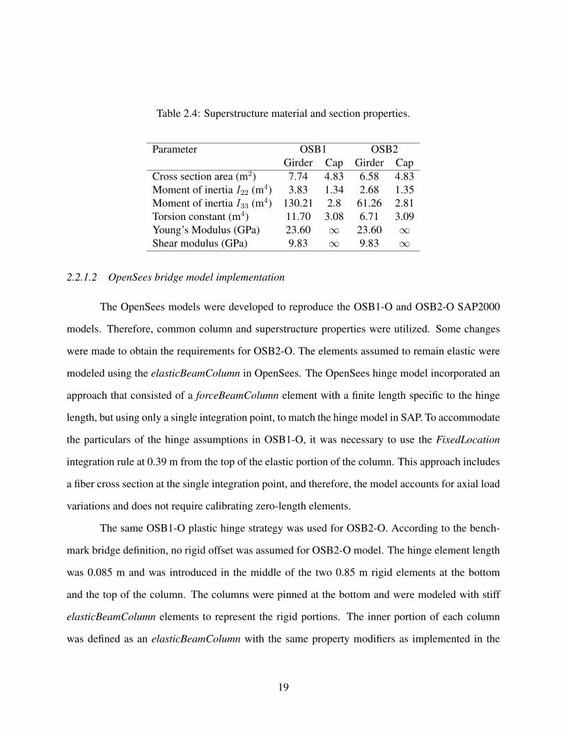
Table 2.4: Superstructure material and section properties.
Parameter OSB1 OSB2Girder Cap Girder Cap
Cross section area (m2) 7.74 4.83 6.58 4.83Moment of inertia I22 (m4) 3.83 1.34 2.68 1.35Moment of inertia I33 (m4) 130.21 2.8 61.26 2.81Torsion constant (m4) 11.70 3.08 6.71 3.09Young’s Modulus (GPa) 23.60 ∞ 23.60 ∞Shear modulus (GPa) 9.83 ∞ 9.83 ∞
2.2.1.2 OpenSees bridge model implementation
The OpenSees models were developed to reproduce the OSB1-O and OSB2-O SAP2000
models. Therefore, common column and superstructure properties were utilized. Some changes
were made to obtain the requirements for OSB2-O. The elements assumed to remain elastic were
modeled using the elasticBeamColumn in OpenSees. The OpenSees hinge model incorporated an
approach that consisted of a forceBeamColumn element with a finite length specific to the hinge
length, but using only a single integration point, to match the hinge model in SAP. To accommodate
the particulars of the hinge assumptions in OSB1-O, it was necessary to use the FixedLocation
integration rule at 0.39 m from the top of the elastic portion of the column. This approach includes
a fiber cross section at the single integration point, and therefore, the model accounts for axial load
variations and does not require calibrating zero-length elements.
The same OSB1-O plastic hinge strategy was used for OSB2-O. According to the bench-
mark bridge definition, no rigid offset was assumed for OSB2-O model. The hinge element length
was 0.085 m and was introduced in the middle of the two 0.85 m rigid elements at the bottom
and the top of the column. The columns were pinned at the bottom and were modeled with stiff
elasticBeamColumn elements to represent the rigid portions. The inner portion of each column
was defined as an elasticBeamColumn with the same property modifiers as implemented in the
19

-0.04 -0.02 0.00 0.02 0.04
-8000
-6000
-4000
-2000
0 Longitudinal
Reac
tion
Forc
e (k
N)
-0.4 -0.2 0.0 0.2 0.4
-50000
0
50000
Transverse
Displacement (m)-0.2 -0.1 0.0 0.1 0.2
-2x10⁷
-1x10⁷
0
1x10⁷
2x10⁷ Vertical
(a) OSB1
-0.04 -0.02 0.00 0.02 0.04
-4000
-2000
0
Longitudinal
Reac
tion
Forc
e (k
N)
-0.04 -0.02 0.00 0.02 0.04
-50000
0
50000
Transverse
Displacement (m)-0.04 -0.02 0.00 0.02 0.04
-2x10⁷
-1x10⁷
0
1x10⁷
2x10⁷ Vertical
(b) OSB2
Figure 2.5: Abutment resultant load-displacement relationship in SAP2000.
SAP2000 models. The fiber cross section discretization was created to match SAP2000 with in-
dividual core concrete, cover concrete, and longitudinal reinforcing steel constitutive models. The
concrete columns properties were defined with OpenSees Concrete04 and their values are shown
in Table 2.2.
The OSB1-O nonlinear properties for the abutments were defined as a compression-only
ElasticPPGap material, with a gap of 0.0m, an effective stiffness equals to 453,754 kN/m, and a
20
yield force of -6917 kN/m in the longitudinal direction. A linear elastic behavior was considered
for the transverse and vertical directions, with 55,168 kN/m and 1.459e7 kN/m respectively. The
torsion of the bridge deck in the abutments was restrained. On the other hand, the OSB2-O incor-
porated nonlinear properties to the transverse degree of freedom of each abutment under the same
definition adopted for OSB1-O. The longitudinal material used a gap of -0.05 m, an effective stiff-
ness of 311,900 kN/m, and a yield force of -4,586 kN. By the other hand, the transverse material
was defined with a gap of -0.025 m, an effective stiffness of 17,512 kN/m, and a yield force of 798
kN. The abutments were fixed in the vertical direction. The vertical and transverse direction were
over-constrained with fixity, therefore do not deform, while the longitudinal direction combines
two element behaviors.
2.2.2 Bridge model modifications
To achieve a better agreement between OpenSees and SAP2000 results, several simplifi-
cations and enhancements were made to the bridge models. The column hinge cross section was
discretized into 50 and 40 fiber layers in the longitudinal and radial direction, respectively. In the
OSB1-MO model, the hinge offset and the unusual placement of the plastic hinge within the rigid
zone at the end of the column were removed. The same modification was made to OSB2-MO,
in which the length of the plastic hinge was also changed from 0.085 m to 0.85 m at the top and
bottom of the column. Therefore, more ductile behavior is expected to occur. In addition, a new
element with high stiffness and with a length of 0.45 m was added at the top of the columns to rep-
resent the rigid offset between the superstructure center of mass and the top of the column frame
element. Figure 2.6 shows the column configurations for OSB models. Boundary conditions for
the OSB2-MO model in the superstructure were considered symmetric in both models, while the
non-prismatic bridge cross-section in OSB1-O was replaced with a standard prismatic superstruc-
ture. Finally, a gap-link with the same nonlinear properties and length of OSB2-O gap was added
between each multilinear plastic link and the deck of the OSB1-MO superstructure.
21

Figure 2.6: OSB reinforced concrete column.
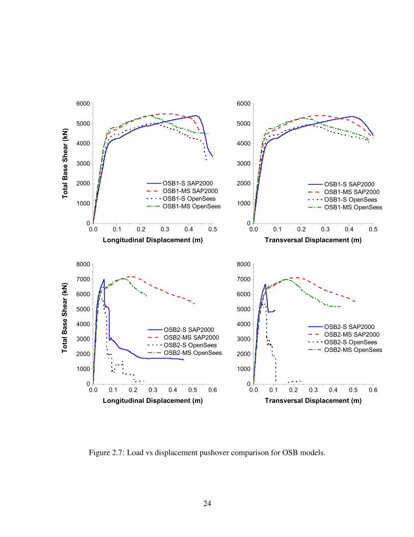
The nonlinear static response was analyzed adopting the simple roller abutment case to iso-
late the bent and column from the abutment contribution. A single 445 kN lateral load was applied
at the center of mass of the bridges in the longitudinal and transversal direction independently to
monitor bridge responses. The comparative pushover curves obtained for the models are illustrated
in Figure 2.7. Due to the roller abutments, the total base shear is the same as the column/bent shear.
Similar result were obtained in previous studies for OSB1-S and OSB2-S (Mackie et al., 2017) and
the differences in the responses were attributed to the non-prismatic cross section (in OSB1), hinge
definition (rigid offset plus rigid zone factor), and the concrete constitutive models. The improve-
ments done over the models concluded in more ductile responses for OSB2-MS, while OSB1-MS
increased its shear resistance. Even though both SAP2000 and OpenSees models had similar initial
stiffness and yield points, the pushover responses in OpenSees described a stiffer and larger yield
force. The improvements done over the models had a small impact on OSB1 static response, while
the changes in OSB2 hinge length affected considerably the bridge reaction to pushover loads.
The early softening in the OpenSees pushover responses remained, concluding that the difference
between models is produced at the material constitutive level. Another analysis was performed
22
using the same definition as OpenSees for the concrete constitutive model (dropping to zero stress
at the end of the backbone) in the SAP2000 models, concluding that the difference is produced
by the limitation on the crushing strain of the confined concrete in compression for the OpenSees
constitutive model. Figure A.1 in the annex shows the pushover plot for OSB1-S using concrete
constitutive model dropping to zero stress at the end of the backbone in SAP2000.
2.2.3 Nonlinear time history analysis
The nonlinear time history analysis was performed using CLAYN1N1, ROCKN1N1, and
SANDN1N1 ground motion acceleration, which correspond to different types of soil, and were
taken from a set of 50 ground motions provided by Caltrans for a previous research (Lu et al.,
2015). The analysis was driven to compare the responses of the bridges after the application of
two lateral orthogonal components of excitation along the longitudinal and transverse direction,
therefore, only the input motions with two components were considered for this study. The strong
motion duration was obtained based on the standard Arias 5-95 bounds (Mackie et al., 2017).
The corresponding ground motion acceleration properties components are shown in Table 2.5.
Due to the large demand presented by the ground motion CLAYN1N1, it was selected to show
individual representative time history responses in the research. The dynamic analysis was done
considering an equivalent viscous damping ratio of 5% at periods of 1.2 and 0.7 seconds for OSB1
and 0.889 and 0.692 for OSB2. The corresponding Rayleigh mass proportional coefficients were
0.3307 and 0.3974 for OSB1 and OSB2 respectively, while the stiffness proportional coefficients
were 7.036e−3 s for OSB1 and 6.193e−3 s for OSB2. The time integration scheme employed was
Hilber-Hughes-Taylor method, considering γ = 0.5, β = 0.25, and α = 0. OpenSees used the same
values directly for the analysis, with an initial stiffness used the stiffness-proportional values.
23
0.0 0.1 0.2 0.3 0.4 0.5 0.60
1000
2000
3000
4000
5000
6000
7000
8000
OSB2-S SAP2000 OSB2-MS SAP2000 OSB2-S OpenSees OSB2-MS OpenSees
Longitudinal Displacement (m)0.0 0.1 0.2 0.3 0.4 0.5 0.6
0
1000
2000
3000
4000
5000
6000
7000
8000
OSB2-S SAP2000 OSB2-MS SAP2000 OSB2-S OpenSees OSB2-MS OpenSees
Transversal Displacement (m)
0.0 0.1 0.2 0.3 0.4 0.50
1000
2000
3000
4000
5000
6000
OSB1-S SAP2000 OSB1-MS SAP2000 OSB1-S OpenSees OSB1-MS OpenSees
Tota
l Bas
e Sh
ear (
kN)
Longitudinal Displacement (m)
Tota
l Bas
e Sh
ear (
kN)
0.0 0.1 0.2 0.3 0.4 0.50
1000
2000
3000
4000
5000
6000
OSB1-S SAP2000 OSB1-MS SAP2000 OSB1-S OpenSees OSB1-MS OpenSees
Transversal Displacement (m)
Figure 2.7: Load vs displacement pushover comparison for OSB models.
24

Table 2.5: Ground motion acceleration time history properties.
Component Direction in model SMD (s) PGA (g) PGV (cm/s) PGD (cm)CLAYN1N1000 Long. 30.4 0.706 108 95.9CLAYN1N1090 Tran. 29.1 0.788 104 57.7ROCKN1N1000 Long. 15.0 0.399 59.2 25.7ROCKN1N1090 Tran. 13.2 0.576 77.9 44.8SANDN1N1000 Long. 37.0 0.784 86.3 33.3SANDN1N1090 Tran. 36.3 0.812 67.9 30.7
2.3 Results for Bridge models with Roller Abutments
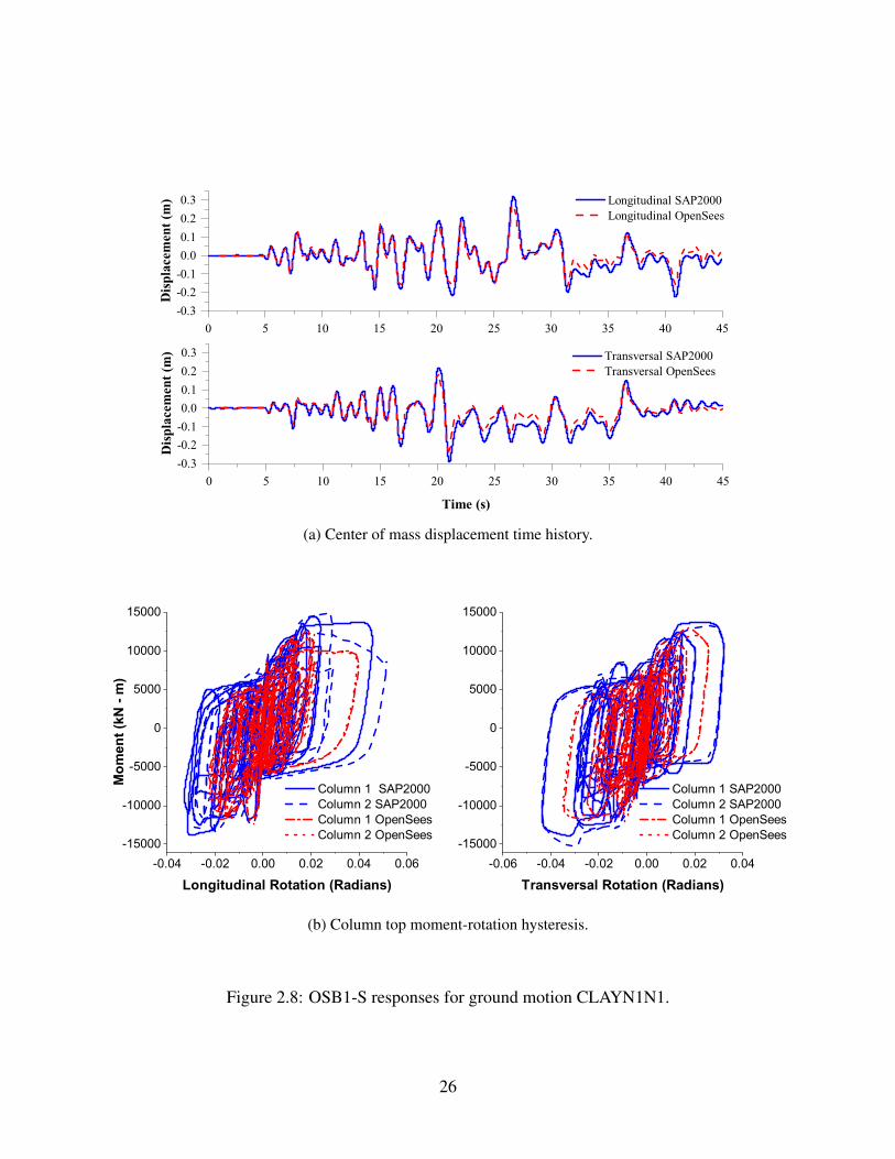
2.3.1 OSB1-S
The displacement time history responses for OSB1-S at the center of mass of the bent in the
longitudinal and transverse directions are shown in Figure 2.8a, respectively. The results obtained
for longitudinal and transverse displacements in SAP2000 were close to the response reached by
OpenSees, particularly the phasing. The peak displacement magnitudes differ by 17% and 21%
for the longitudinal and transverse directions respectively, the larger values obtained in SAP2000.
The variations in the inelastic peak displacement are consistent with the discrepancies found in the
concrete constitutive models related to the differences in the hystertic rule considerations for both
software.
In the SAP2000 responses, the changes in the elastic peaks had a larger residual displace-
ment in both the longitudinal and transverse responses.
The moment-rotation response at the top of the two columns are shown in Figure 2.8b.
The roller abutment hysteresis results illustrate an increase in the plastic curvature for both models
under similar bending moments compared with original abutment models. The response obtained
for the OpenSees models softens in agreement with the concrete constitutive model presented
previously, while SAP2000 response showed a continued ductility near the peak. Even though both
models had similar behavior, OpenSees model dissipates near 40% more energy than SAP2000’s.
25
0 5 10 15 20 25 30 35 40 45-0.3-0.2-0.10.00.10.20.3 Longitudinal SAP2000
Longitudinal OpenSees
Disp
lace
men
t (m
)
0 5 10 15 20 25 30 35 40 45-0.3-0.2-0.10.00.10.20.3 Transversal SAP2000
Transversal OpenSees
Disp
lace
men
t (m
)
Time (s)
(a) Center of mass displacement time history.
-0.04 -0.02 0.00 0.02 0.04 0.06-15000
-10000
-5000
0
5000
10000
15000
-0.06 -0.04 -0.02 0.00 0.02 0.04-15000
-10000
-5000
0
5000
10000
15000
Mom
ent (
kN -
m)
Longitudinal Rotation (Radians)
Column 1 SAP2000 Column 2 SAP2000 Column 1 OpenSees Column 2 OpenSees
Transversal Rotation (Radians)
Column 1 SAP2000 Column 2 SAP2000 Column 1 OpenSees Column 2 OpenSees
(b) Column top moment-rotation hysteresis.
Figure 2.8: OSB1-S responses for ground motion CLAYN1N1.
26
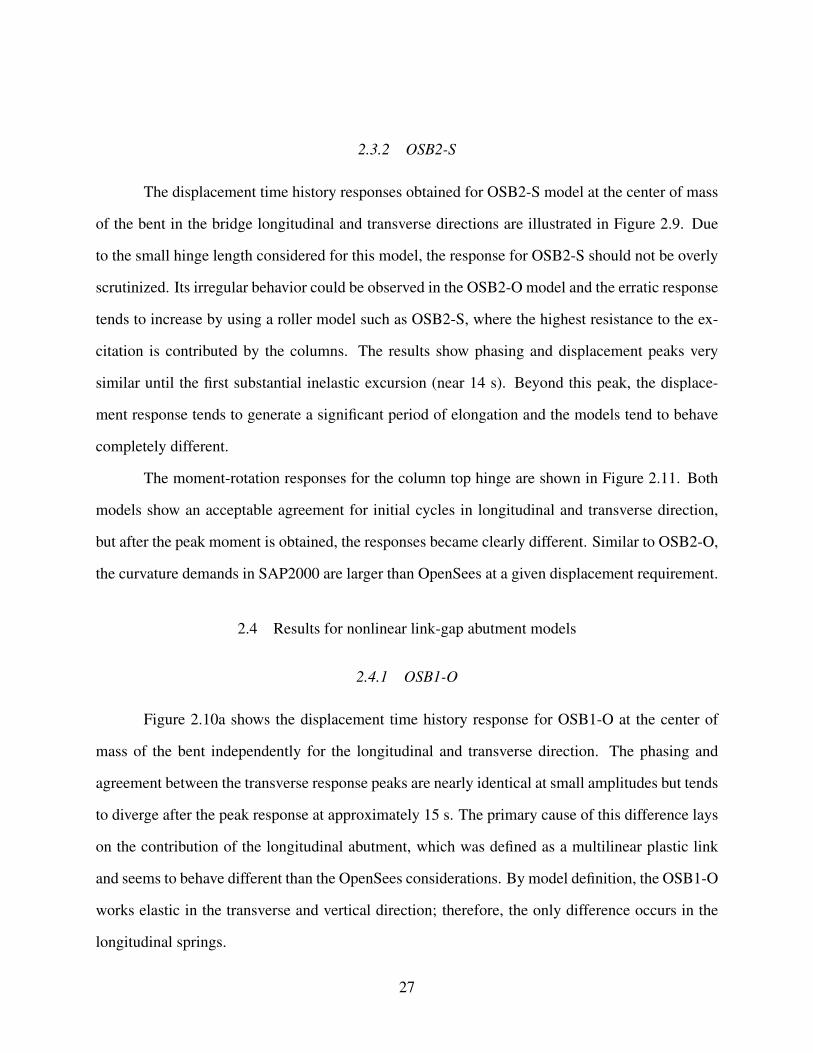
2.3.2 OSB2-S
The displacement time history responses obtained for OSB2-S model at the center of mass
of the bent in the bridge longitudinal and transverse directions are illustrated in Figure 2.9. Due
to the small hinge length considered for this model, the response for OSB2-S should not be overly
scrutinized. Its irregular behavior could be observed in the OSB2-O model and the erratic response
tends to increase by using a roller model such as OSB2-S, where the highest resistance to the ex-
citation is contributed by the columns. The results show phasing and displacement peaks very
similar until the first substantial inelastic excursion (near 14 s). Beyond this peak, the displace-
ment response tends to generate a significant period of elongation and the models tend to behave
completely different.
The moment-rotation responses for the column top hinge are shown in Figure 2.11. Both
models show an acceptable agreement for initial cycles in longitudinal and transverse direction,
but after the peak moment is obtained, the responses became clearly different. Similar to OSB2-O,
the curvature demands in SAP2000 are larger than OpenSees at a given displacement requirement.
2.4 Results for nonlinear link-gap abutment models
2.4.1 OSB1-O
Figure 2.10a shows the displacement time history response for OSB1-O at the center of
mass of the bent independently for the longitudinal and transverse direction. The phasing and
agreement between the transverse response peaks are nearly identical at small amplitudes but tends
to diverge after the peak response at approximately 15 s. The primary cause of this difference lays
on the contribution of the longitudinal abutment, which was defined as a multilinear plastic link
and seems to behave different than the OpenSees considerations. By model definition, the OSB1-O
works elastic in the transverse and vertical direction; therefore, the only difference occurs in the
longitudinal springs.
27
0 5 10 15 20 25 30 35 40 45-0.15-0.10-0.050.000.050.100.15 Longitudinal SAP2000
Longitudinal OpenSees
Disp
lace
men
t (m
)
0 5 10 15 20 25 30 35 40 45-0.15-0.10-0.050.000.050.100.15
Transversal SAP2000 Transversal OpenSees
Disp
lace
men
t (m
)
Time (s)
(a) Center of mass displacement time history.
-0.010 -0.005 0.000 0.005 0.010
-15000
-10000
-5000
0
5000
10000
15000
-0.020 -0.015 -0.010 -0.005 0.000 0.005
-15000
-10000
-5000
0
5000
10000
15000
Mom
ent (
kN -
m)
Longitudinal Rotation (Radians)
SAP2000 OpenSees
Transversal Rotation (Radians)
SAP2000 OpenSees
(b) Column top moment-rotation hysteresis.
Figure 2.9: OSB2-S responses for ground motion CLAYN1N1.
28

The moment vs rotation responses at the top of the two bent columns are shown by sep-
arately for longitudinal and transverse directions in Figure 2.10b. The sign of the moment and
rotation were calibrated to be the same as the displacement, therefore, a peak positive displace-
ment has a corresponding peak positive rotation. The results obtained show a close agreement
between SAP2000 and OpenSees on the transverse displacement responses, while the longitudinal
presents a substantial energy dissipation beyond the peak different than OpenSees prediction.
2.4.2 OSB2-O
The displacement time history responses for OSB2-O at the center of mass of the bent in
the longitudinal and transverse directions are shown in Figure 2.9 separately. Due to the small
hinge length assumed for this model, the stiffness was higher than the expected and the bridge
presented a brittle behavior at displacement demands that are small. Therefore, the frequency
content of the OSB2-O time history results for the ground motion was higher. This characteristic
can be observed particularly in the transverse direction, where the abutments do not represent an
important contribution in the resisting forces compared with the column. The results obtained
for the transverse response show a significantly difference between SAP2000 and OpenSees for
the peak displacement magnitude (near 50%), while the longitudinal response matches until the
first substantial inelastic peak displacement. Beyond this peak the displacement response tends
to generate a significant period of elongation. The reason for a change in the frequency content
could be due to changes on the integrator during time history analysis or changes in the concrete
constitutive models.
The moment-rotation responses obtained in the top column hinge are shown in Figure 2.11.
Similar to OSB1-O, the sign of the moment and rotation were calibrated to be the same as the dis-
placement. The shape and energy dissipated in the longitudinal response are similar for SAP2000
and OpenSees, until the peak value is obtained in about 14 seconds. After the peak is reached,
the response for both models is noticeable different, with a softening in the reloading stiffness of
29
0 5 10 15 20 25 30 35 40 45-0.15-0.10-0.050.000.050.100.15
Longitudinal SAP2000 Longitudinal OpenSees
Disp
lace
men
t (m
)
0 5 10 15 20 25 30 35 40 45-0.15-0.10-0.050.000.050.100.15
Transversal SAP2000 Transversal OpenSees
Disp
lace
men
t (m
)
Time (s)
(a) Center of mass displacement time history.
-0.02 -0.01 0.00 0.01-15000
-10000
-5000
0
5000
10000
15000
-0.02 -0.01 0.00 0.01-15000
-10000
-5000
0
5000
10000
15000
Mom
ent (
kN -
m)
Longitudinal Rotation (Radians)
Column 1 SAP2000 Column 2 SAP2000 Column 1 OpenSees Column 2 OpenSees
Transversal Rotation (Radians)
Column 1 SAP2000 Column 2 SAP2000 Column 1 OpenSees Column 2 OpenSees
(b) Column top moment-rotation hysteresis.
Figure 2.10: OSB1-O responses for ground motion CLAYN1N1.
30

the SAP2000 at a smaller rotation demand than the OpenSees response. The transverse displace-
ments, and hence rotations, remain mostly in the elastic range. The peak displacement achieved
for SAP2000 is close to the first yield. Rotational inertia may contribute to slightly larger trans-
verse curvature demands in SAP2000 than OpenSees. Because of the small hinge length in OSB2,
performing numerical simulations may be extremely complex, concluding in an increase in the
rotation demands for SAP2000.
2.4.3 OSB1-MO
The displacement time history responses generated for the OSB1-MO model at the center
of mass of the bent are presented individually for the longitudinal and transverse direction in Fig-
ure 2.12. The longitudinal and transverse displacement show excellent agreement throughout the
nonlinear time history analysis, specially the phasing and peaks values. The peak values difference
between models is almost neglected for both directions. However, a small offset can be found in
the longitudinal response after 30 s. The improvements done over the model concluded in a better
nonlinear behavior and the responses were very similar in both programs.
The analysis results for the OSB-MO abutment model are illustrated in Figure 2.14. The
hysteresis behavior of both models is almost identical. The overall difference between OpenSees
and SAP2000 in the curvature was lower than 10%, while the bending moment was negligible.
These results are in accordance with the response obtained in the displacement time history analy-
sis and provided an excellent agreement between SAP2000 and OpenSees. A similar result can be
found in the base shear vs displacement analysis done at the top of the columns, where the offset
between both programs was considerable small. The maximum difference obtained in the base
shear was near 10%, while the displacement was almost 0%. The results illustrated in Figure 2.13
clearly demonstrate that OpenSees and SAP2000 had an excellent agreement in the OSB1-MO
abutment model. The figures show that the bias presented between OpenSees and Sap2000 in the
OSB1-O responses was corrected with the use of gaps in the corners of the deck. Therefore, the
31

0 5 10 15 20 25 30 35 40 45-0.10
-0.05
0.00
0.05
0.10 Longitudinal SAP2000 Longitudinal OpenSees
Disp
lace
men
t (m
)
0 5 10 15 20 25 30 35 40 45
-0.04
-0.02
0.00
0.02
0.04 Transversal SAP2000 Transversal OpenSees
Disp
lace
men
t (m
)
Time (s)
(a) Center of mass displacement time history.
-0.006 -0.004 -0.002 0.000 0.002 0.004-20000
-15000
-10000
-5000
0
5000
10000
15000
20000
-0.0004 -0.0002 0.0000 0.0002 0.0004-6000
-4000
-2000
0
2000
4000
6000
Mom
ent (
kN -
m)
Longitudinal Rotation (Radians)
SAP2000 OpenSees
Transversal Rotation (Radians)
SAP2000 OpenSees
(b) Column top moment-rotation hysteresis.
Figure 2.11: OSB2-O responses for ground motion CLAYN1N1.
32

main cause of variance in the responses between models could be attributed to the assumptions on
the abutments for both OpenSees and Sap2000, rather than the consideration of the hysteretic rule.
2.4.4 OSB2-MO
The analysis done over the displacement time history of the OSB2-MO model are displayed
in Figure 2.15. The phasing and peaks magnitudes for both models were almost identical, with a
peak offset lower than 8% in the longitudinal direction. The difference between models for the peak
value in the transverse direction was almost neglected. The modifications made over the OSB2-O
models produced a better nonlinear behavior and the responses had an excellent agreement for both
programs.
Similar to the other models, a moment vs rotation analysis was done over the OSB2-MO
model. The analysis was performance for the top and the bottom hinges. In the longitudinal
direction the results were very close, but small differences were found in the transverse response.
However, the models presented an excellent agreement for phasing and peaks values. The results
are illustrated in Figures 2.16 and 2.18 for OSB2-MS and OSB2-MO models, respectively.
For the OSB2-MO, the analysis was extended to the base shear vs displacement response.
The results obtained were in concordance with the previous ones achieved for the displacement
time history. Even small differences were found, the variation in the peak values between both
models was lower than the 10%. The phasing was almost identical for both models, but a difference
in the slope was registered in the transversal direction for the roller model. However, the models
presented almost identical shapes, which can be observed in Figure 2.17.
2.5 Summary and Discussion
The Tables 2.6 and 2.7 summarize the peak values obtained in SAP2000 for all models
developed in the current study after applying different ground motion combinations (Mackie et al.,
33

0 5 10 15 20 25 30 35 40 45-0.3-0.2-0.10.00.10.20.3
Transversal SAP2000 Transversal OpenSees
Disp
lace
men
t (m
)
Time (s)
0 5 10 15 20 25 30 35 40 45-0.3-0.2-0.10.00.10.20.3
Longitudinal SAP2000 Longitudinal OpenSees
Disp
lace
men
t (m
)
(a) Center of mass displacement time history
-0.2 -0.1 0.0 0.1 0.2 0.3
-4000
-3000
-2000
-1000
0
1000
2000
3000
4000
-0.3 -0.2 -0.1 0.0 0.1 0.2 0.3
-4000
-3000
-2000
-1000
0
1000
2000
3000
4000
Base
She
ar (k
N)
Longitudinal Displacement (m)
Column 1 SAP2000 Column 2 SAP2000 Column 1 OpenSees Column 2 OpenSees
Transversal Displacement (m)
Column 1 SAP2000 Column 2 SAP2000 Column 1 OpenSees Column 2 OpenSees
(b) Base Shear vs Displacement at the top of the column
Figure 2.12: OSB1-MS responses for ground motion CLAYN1N1.
34
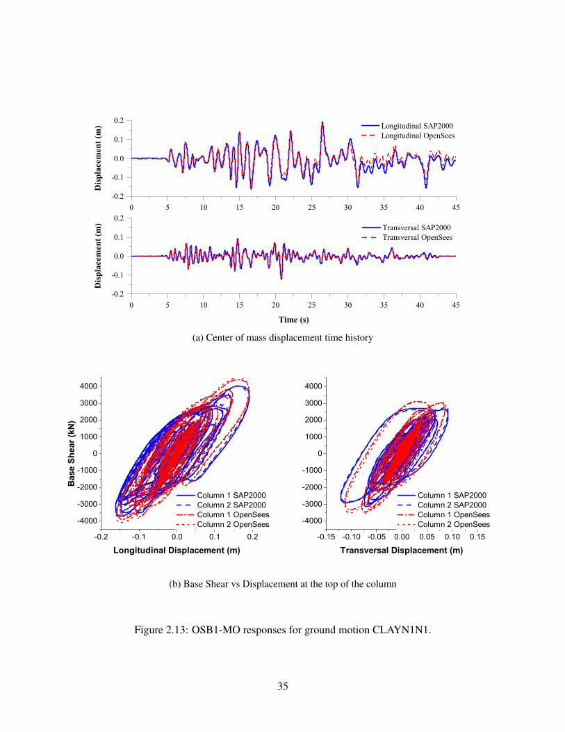
0 5 10 15 20 25 30 35 40 45-0.2
-0.1
0.0
0.1
0.2 Transversal SAP2000 Transversal OpenSees
Disp
lace
men
t (m
)
Time (s)
0 5 10 15 20 25 30 35 40 45-0.2
-0.1
0.0
0.1
0.2 Longitudinal SAP2000 Longitudinal OpenSees
Disp
lace
men
t (m
)
(a) Center of mass displacement time history
-0.2 -0.1 0.0 0.1 0.2
-4000
-3000
-2000
-1000
0
1000
2000
3000
4000
-0.15 -0.10 -0.05 0.00 0.05 0.10 0.15
-4000
-3000
-2000
-1000
0
1000
2000
3000
4000
Base
She
ar (k
N)
Longitudinal Displacement (m)
Column 1 SAP2000 Column 2 SAP2000 Column 1 OpenSees Column 2 OpenSees
Transversal Displacement (m)
Column 1 SAP2000 Column 2 SAP2000 Column 1 OpenSees Column 2 OpenSees
(b) Base Shear vs Displacement at the top of the column
Figure 2.13: OSB1-MO responses for ground motion CLAYN1N1.
35
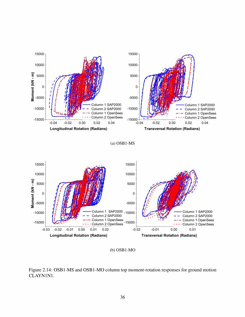
-0.04 -0.02 0.00 0.02 0.04-15000
-10000
-5000
0
5000
10000
15000
-0.04 -0.02 0.00 0.02 0.04-15000
-10000
-5000
0
5000
10000
15000
Mom
ent (
kN -
m)
Longitudinal Rotation (Radians)
Column 1 SAP2000 Column 2 SAP2000 Column 1 OpenSees Column 2 OpenSees
Transversal Rotation (Radians)
Column 1 SAP2000 Column 2 SAP2000 Column 1 OpenSees Column 2 OpenSees
(a) OSB1-MS
-0.03 -0.02 -0.01 0.00 0.01 0.02
-15000
-10000
-5000
0
5000
10000
15000
-0.02 -0.01 0.00 0.01
-15000
-10000
-5000
0
5000
10000
15000
Mom
ent (
kN -
m)
Longitudinal Rotation (Radians)
Column 1 SAP2000 Column 2 SAP2000 Column 1 OpenSees Column 2 OpenSees
Transversal Rotation (Radians)
Column 1 SAP2000 Column 2 SAP2000 Column 1 OpenSees Column 2 OpenSees
(b) OSB1-MO
Figure 2.14: OSB1-MS and OSB1-MO column top moment-rotation responses for ground motionCLAYN1N1.
36

0 5 10 15 20 25 30 35 40 45-0.15-0.10-0.050.000.050.100.15
Longitudinal SAP2000 Longitudinal OpenSees
Disp
lace
men
t (m
)
0 5 10 15 20 25 30 35 40 45-0.15-0.10-0.050.000.050.100.15 Transversal SAP2000
Transversal OpenSees
Disp
lace
men
t (m
)
Time (s)
(a) Center of mass displacement time history
-0.10 -0.05 0.00 0.05 0.10-10000
-8000
-6000
-4000
-2000
0
2000
4000
6000
8000
10000
Base
She
ar (k
N)
Longitudinal Displacement (m)
SAP2000 OpenSees
-0.2 -0.1 0.0 0.1 0.2-10000
-8000
-6000
-4000
-2000
0
2000
4000
6000
8000
10000
Transversal Displacement (m)
SAP2000 OpenSees
(b) Base shear vs displacement at the top of the column
Figure 2.15: OSB2-MS responses for ground motion CLAYN1N1.
37
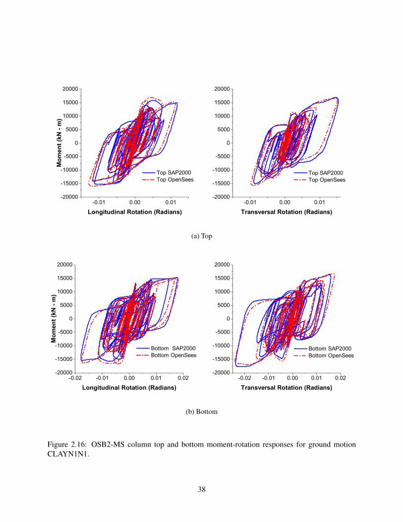
-0.01 0.00 0.01-20000
-15000
-10000
-5000
0
5000
10000
15000
20000
-0.01 0.00 0.01-20000
-15000
-10000
-5000
0
5000
10000
15000
20000
Mom
ent (
kN -
m)
Longitudinal Rotation (Radians)
Top SAP2000 Top OpenSees
Transversal Rotation (Radians)
Top SAP2000 Top OpenSees
(a) Top
-0.02 -0.01 0.00 0.01 0.02-20000
-15000
-10000
-5000
0
5000
10000
15000
20000
-0.02 -0.01 0.00 0.01 0.02-20000
-15000
-10000
-5000
0
5000
10000
15000
20000
Mom
ent (
kN -
m)
Longitudinal Rotation (Radians)
Bottom SAP2000 Bottom OpenSees
Transversal Rotation (Radians)
Bottom SAP2000 Bottom OpenSees
(b) Bottom
Figure 2.16: OSB2-MS column top and bottom moment-rotation responses for ground motionCLAYN1N1.
38

0 5 10 15 20 25 30 35 40 45-0.10
-0.05
0.00
0.05
0.10 Longitudinal SAP2000 Longitudinal OpenSees
Disp
lace
men
t (m
)
0 5 10 15 20 25 30 35 40 45-0.02
-0.01
0.00
0.01
0.02 Transversal SAP2000 Transversal OpenSees
Disp
lace
men
t (m
)
Time (s)
(a) Center of mass displacement time history
-0.1 0.0 0.1-10000
-8000
-6000
-4000
-2000
0
2000
4000
6000
8000
10000
12000
Base
She
ar (k
N)
Longitudinal Displacement (m)
SAP2000 OpenSees
-0.02 -0.01 0.00 0.01 0.02-2000
-1500
-1000
-500
0
500
1000
1500
2000
2500
3000
Transversal Displacement (m)
SAP2000 OpenSees
(b) Base shear vs displacement at the top of the column
Figure 2.17: OSB2-MO responses for ground motion CLAYN1N1.
39

-0.010 -0.005 0.000 0.005-20000
-15000
-10000
-5000
0
5000
10000
15000
20000
-0.0002 0.0000 0.0002-1500
-1000
-500
0
500
1000
Mom
ent (
kN -
m)
Longitudinal Rotation (Radians)
Top SAP2000 Top OpenSees
Transversal Rotation (Radians)
Top SAP2000 Top OpenSees
(a) Top
-0.01 0.00 0.01
-20000
-15000
-10000
-5000
0
5000
10000
15000
20000
-0.001 0.000 0.001-7500
-5000
-2500
0
2500
5000
7500
Mom
ent (
kN -
m)
Longitudinal Rotation (Radians)
Bottom SAP2000 Bottom OpenSees
Transversal Rotation (Radians)
Bottom SAP2000 Bottom OpenSees
(b) Bottom
Figure 2.18: OSB2-MO column top and bottom moment-rotation responses for ground motionCLAYN1N1.
40

2017). The modifications done over the OSB1 models increased the columns stiffness, conclud-
ing in less deformations for OSB1-MS. However, the abutment modifications added elasticity to
the model, providing more displacement to OSB1-MO. On the other hand, OSB2-MO peak dis-
placements were very close to OSB2-O values. The results achieved after improving OSB1-O and
OSB2-O models determined a better agreement between both OpenSees and SAP2000, reducing
the peak response variation under different ground motions.
After analyzing and comparing the different responses obtained using the roller and the
abutment models, the study shows a small bias developed by the difference in the hysteresis rule
for the concrete in columns assumed for both softwares. This variance is illustrated in the results
achieved by the roller models, where the abutments are not affecting the responses. While compar-
ing the OSB1-O models, the analysis reflects a high bias which was totally removed after adding
gaps in the corners of the deck for OSB1-MO models. Therefore, the link used in OpenSees has a
similar behavior than the composite abutment improved in OSB1’s SAP2000 model. On the other
hand, OSB2-S models had a huge bias which was corrected after modifying the hinge length in
the OSB2-MS models. Since both SAP2000 and OpenSees OSB2 models considered gaps in the
corners of the deck, no bias was induced by the abutment considerations.
The values were compared using the bias factor formulation used by Aviram (2008) for
short bridges and the ratios are illustrated in the Tables 2.8 and 2.9. The NTHA bias factors were
obtained normalizing the SAP2000 peak displacement by the corresponding OpenSees values,
concluding in a better agreement than Aviram’s factors for bridges under high hazard seismic
levels and applying a pair-wise comparison and averaging method (Aviram et al., 2008).
41
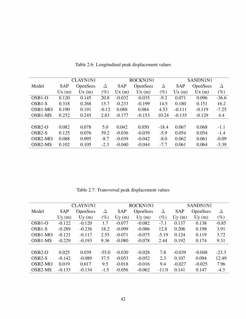
Table 2.6: Longitudinal peak displacement values
CLAYN1N1 ROCKN1N1 SANDN1N1Model SAP OpenSees ∆ SAP OpenSees ∆ SAP OpenSees ∆
Ux (m) Ux (m) (%) Ux (m) Ux (m) (%) Ux (m) Ux (m) (%)OSB1-O 0.120 0.145 20.8 -0.032 -0.035 -9.2 0.071 0.096 -36.6OSB1-S 0.318 0.268 15.7 -0.233 -0.199 14.5 0.180 0.151 16.2OSB1-MO 0.190 0.191 -0.12 0.088 0.084 4.53 -0.111 -0.119 -7.25OSB1-MS 0.252 0.245 2.83 -0.177 -0.153 10.24 -0.135 -0.129 4.4
OSB2-O 0.082 0.078 5.0 0.042 0.050 -18.4 0.067 0.068 -1.1OSB2-S 0.125 0.076 39.2 -0.036 -0.039 -5.9 0.054 0.054 -1.4OSB2-MO 0.088 0.095 -8.7 -0.039 -0.042 -8.0 0.062 0.061 -0.09OSB2-MS 0.102 0.105 -2.3 -0.040 -0.044 -7.7 0.061 0.064 -3.39
Table 2.7: Transversal peak displacement values
CLAYN1N1 ROCKN1N1 SANDN1N1Model SAP OpenSees ∆ SAP OpenSees ∆ SAP OpenSees ∆
Uy (m) Uy (m) (%) Uy (m) Uy (m) (%) Uy (m) Uy (m) (%)OSB1-O -0.122 -0.120 1.7 -0.077 -0.082 -7.1 0.137 0.138 -0.85OSB1-S -0.289 -0.236 18.2 -0.099 -0.086 12.8 0.206 0.198 3.91OSB1-MO -0.121 -0.117 2.55 -0.071 -0.075 -5.19 0.124 0.119 3.72OSB1-MS -0.229 -0.193 9.36 -0.080 -0.078 2.44 0.192 0.174 9.31
OSB2-O 0.025 0.039 -55.0 -0.030 -0.028 7.8 -0.039 -0.048 -23.3OSB2-S -0.142 -0.089 37.5 -0.053 -0.052 2.3 0.107 0.094 12.49OSB2-MO 0.019 0.017 9.5 -0.018 -0.016 9.4 -0.027 -0.025 7.96OSB2-MS -0.133 -0.134 -1.5 -0.056 -0.062 -11.0 0.141 0.147 -4.3
42

Table 2.8: Longitudinal peak displacement bias factors
NTHA Bias Factor Aviram Bias FactorModel CLAYN1N1 ROCKN1N1 SANDN1N1 High Hazard LevelOSB1-O 1.21 1.09 1.37OSB1-S 0.84 0.86 0.84 1.20OSB1-MO 1.00 0.95 1.07OSB1-MS 0.97 0.90 0.96
OSB2-O 0.95 1.18 1.01OSB2-S 0.61 1.06 1.01 1.20OSB2-MO 1.09 1.08 1.00OSB2-MS 1.02 1.08 1.03
Table 2.9: Transversal peak displacement bias factors
NTHA Bias Factor Aviram Bias FactorModel CLAYN1N1 ROCKN1N1 SANDN1N1 High Hazard LevelOSB1-O 0.98 1.07 1.01OSB1-S 0.82 0.87 0.96 1.20OSB1-MO 0.97 1.06 0.95OSB1-MS 0.81 0.96 0.91
OSB2-O 1.55 0.92 1.23OSB2-S 0.63 0.98 0.88 1.20OSB2-MO 0.91 0.91 0.92OSB2-MS 1.02 1.11 1.04
43

CHAPTER 3: NONLINEAR RESPONSE HISTORY SENSITIVITY
ANALYSIS OF TYPICAL HIGHWAY BRIDGES.
The content of the current chapter is based on the journal paper Nonlinear response history
sensitivity analysis of typical highway bridges by Rodriguez A. F., Mackie K. R., and Scott M. H.,
which is being prepared for its submission.
3.1 Bridge sensitivity analysis
The models under analysis contemplated the specifications provided by Caltrans and the
improvement obtained in chapter 2 (OSB1-MO and OSB2-MO). The analysis was developed us-
ing the original abutment models to reflect field real condition. The analysis was focused to the
static and dynamic response of the bridges with nonlinear elements. The sensitivity analysis was
developed using the FDM, which computes a deterministic bridge response and compares it with
the behavior after perturbing a specific value. Therefore, the calculations were done considering
the change in the responses of the properties forward and backward compared with the original
value and applying the second-order central difference theory over the results obtained. On the
other hand, the change in the hysteresis type assumption would represent only one final response
in the nonlinear time history analysis, which means that the hysteresis type sensitivity analysis must
be obtained using the first-order forward finite difference method between the original condition
and the new consideration.
3.1.1 Parameters
To establish an accurate result, the sensitivity analysis included the bridges most relevant
parameters, which could strongly affect the response of the nonlinear time history. Different ∆θ
were assumed as coefficient of variation of the parameters, affecting the properties forward and
44
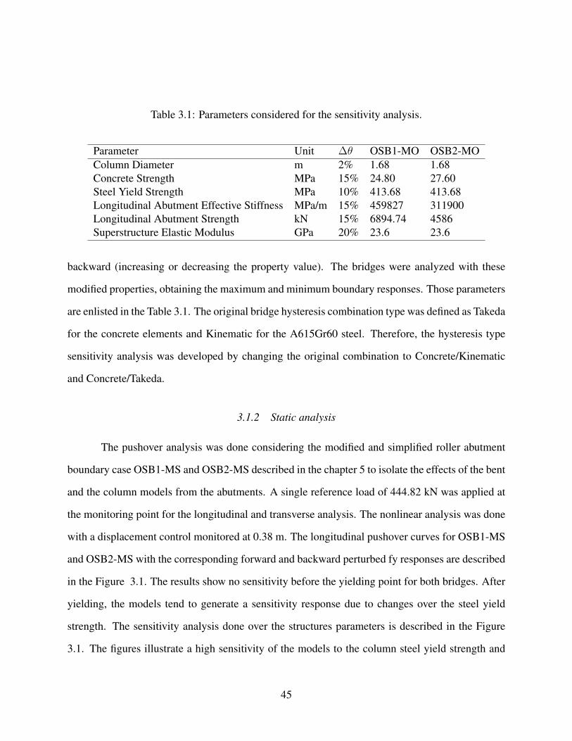
Table 3.1: Parameters considered for the sensitivity analysis.
Parameter Unit ∆θ OSB1-MO OSB2-MOColumn Diameter m 2% 1.68 1.68Concrete Strength MPa 15% 24.80 27.60Steel Yield Strength MPa 10% 413.68 413.68Longitudinal Abutment Effective Stiffness MPa/m 15% 459827 311900Longitudinal Abutment Strength kN 15% 6894.74 4586Superstructure Elastic Modulus GPa 20% 23.6 23.6
backward (increasing or decreasing the property value). The bridges were analyzed with these
modified properties, obtaining the maximum and minimum boundary responses. Those parameters
are enlisted in the Table 3.1. The original bridge hysteresis combination type was defined as Takeda
for the concrete elements and Kinematic for the A615Gr60 steel. Therefore, the hysteresis type
sensitivity analysis was developed by changing the original combination to Concrete/Kinematic
and Concrete/Takeda.
3.1.2 Static analysis
The pushover analysis was done considering the modified and simplified roller abutment
boundary case OSB1-MS and OSB2-MS described in the chapter 5 to isolate the effects of the bent
and the column models from the abutments. A single reference load of 444.82 kN was applied at
the monitoring point for the longitudinal and transverse analysis. The nonlinear analysis was done
with a displacement control monitored at 0.38 m. The longitudinal pushover curves for OSB1-MS
and OSB2-MS with the corresponding forward and backward perturbed fy responses are described
in the Figure 3.1. The results show no sensitivity before the yielding point for both bridges. After
yielding, the models tend to generate a sensitivity response due to changes over the steel yield
strength. The sensitivity analysis done over the structures parameters is described in the Figure
3.1. The figures illustrate a high sensitivity of the models to the column steel yield strength and
45
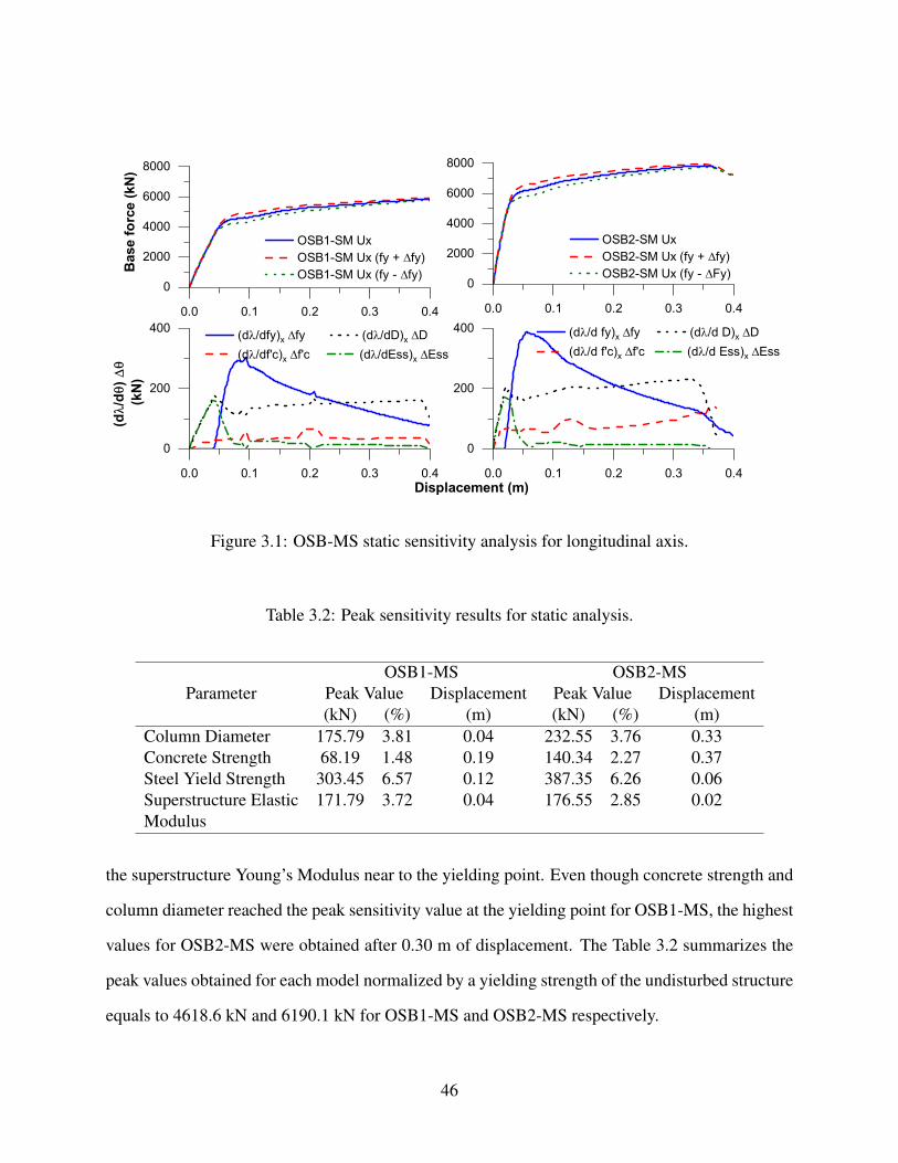
0.0 0.1 0.2 0.3 0.4
0
2000
4000
6000
8000
OSB1-SM Ux OSB1-SM Ux (fy + Dfy) OSB1-SM Ux (fy - Dfy)Ba
se fo
rce
(kN)
0.0 0.1 0.2 0.3 0.4
0
2000
4000
6000
8000
OSB2-SM Ux OSB2-SM Ux (fy + Dfy) OSB2-SM Ux (fy - DFy)
0.0 0.1 0.2 0.3 0.4
0
200
400 (dl/dfy)x Dfy (dl/dD)x DD (dl/df'c)x Df'c (dl/dEss)x DEss
(dl/
dq) D
q (k
N)
Displacement (m)0.0 0.1 0.2 0.3 0.4
0
200
400 (dl/d fy)x Dfy (dl/d D)x DD (dl/d f'c)x Df'c (dl/d Ess)x DEss
Figure 3.1: OSB-MS static sensitivity analysis for longitudinal axis.
Table 3.2: Peak sensitivity results for static analysis.
OSB1-MS OSB2-MSParameter Peak Value Displacement Peak Value Displacement
(kN) (%) (m) (kN) (%) (m)Column Diameter 175.79 3.81 0.04 232.55 3.76 0.33Concrete Strength 68.19 1.48 0.19 140.34 2.27 0.37Steel Yield Strength 303.45 6.57 0.12 387.35 6.26 0.06Superstructure Elastic 171.79 3.72 0.04 176.55 2.85 0.02Modulus
the superstructure Young’s Modulus near to the yielding point. Even though concrete strength and
column diameter reached the peak sensitivity value at the yielding point for OSB1-MS, the highest
values for OSB2-MS were obtained after 0.30 m of displacement. The Table 3.2 summarizes the
peak values obtained for each model normalized by a yielding strength of the undisturbed structure
equals to 4618.6 kN and 6190.1 kN for OSB1-MS and OSB2-MS respectively.
46
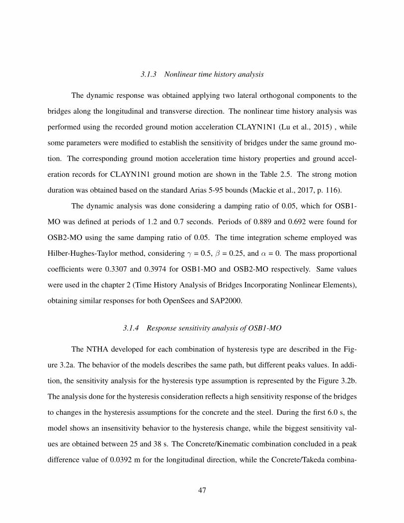
3.1.3 Nonlinear time history analysis
The dynamic response was obtained applying two lateral orthogonal components to the
bridges along the longitudinal and transverse direction. The nonlinear time history analysis was
performed using the recorded ground motion acceleration CLAYN1N1 (Lu et al., 2015) , while
some parameters were modified to establish the sensitivity of bridges under the same ground mo-
tion. The corresponding ground motion acceleration time history properties and ground accel-
eration records for CLAYN1N1 ground motion are shown in the Table 2.5. The strong motion
duration was obtained based on the standard Arias 5-95 bounds (Mackie et al., 2017, p. 116).
The dynamic analysis was done considering a damping ratio of 0.05, which for OSB1-
MO was defined at periods of 1.2 and 0.7 seconds. Periods of 0.889 and 0.692 were found for
OSB2-MO using the same damping ratio of 0.05. The time integration scheme employed was
Hilber-Hughes-Taylor method, considering γ = 0.5, β = 0.25, and α = 0. The mass proportional
coefficients were 0.3307 and 0.3974 for OSB1-MO and OSB2-MO respectively. Same values
were used in the chapter 2 (Time History Analysis of Bridges Incorporating Nonlinear Elements),
obtaining similar responses for both OpenSees and SAP2000.
3.1.4 Response sensitivity analysis of OSB1-MO
The NTHA developed for each combination of hysteresis type are described in the Fig-
ure 3.2a. The behavior of the models describes the same path, but different peaks values. In addi-
tion, the sensitivity analysis for the hysteresis type assumption is represented by the Figure 3.2b.
The analysis done for the hysteresis consideration reflects a high sensitivity response of the bridges
to changes in the hysteresis assumptions for the concrete and the steel. During the first 6.0 s, the
model shows an insensitivity behavior to the hysteresis change, while the biggest sensitivity val-
ues are obtained between 25 and 38 s. The Concrete/Kinematic combination concluded in a peak
difference value of 0.0392 m for the longitudinal direction, while the Concrete/Takeda combina-
47

Table 3.3: OSB1-MO peak sensitivity results for hysteresis type.
Hysteresis type Longitudinal Transversal∆u (m) ∆u (%) t (sec) ∆u (m) ∆u (%) t (sec)
Concrete/Kinematic -0.0392 20.3 41.73 -0.0039 3.3 31.28Concrete/Takeda 0.0803 41.5 27.52 0.0214 17.7 21.75
tion had a peak difference of 0.0803 m, representing a 20.3% and 41.5% of the original NTHA
peak value respectively. The sensitivity of the deck displacement to the hysteresis changes in the
transversal direction is lower than the longitudinal, but still important when the changes in the
steel reinforcement hysteresis behavior are considered. The peak values obtained in the sensitivity
analysis for the hysteresis cases are illustrated in the Table 3.3. It is important to note that the
Concrete hysteresis type was recently incorporated in the newest SAP2000 versions. Before this,
the software only considered Takeda, Kinematic, and Elastic hysteresis types for the nonlinear
analysis.
The sensitivity analysis done by central difference method concluded that the chosen non-
linear parameters have an important incidence in the longitudinal displacement of the superstruc-
ture. The Figure 3.3 describes the displacement sensitivity to the modification of each parame-
ter under the seismic load by separately. The bridge response shows an unsensitive behavior to
changes in the parameters during the first seconds of the seismic load. After 5 seconds, the col-
umn and superstructure parameters describe sensitive responses while the abutment considerations
reflect changes after 7 seconds. The most sensitive responses are obtained between 24 and 40
seconds for the column and superstructure parameters, while the peak sensitive response for the
abutment are found between 14 to 26 seconds. The perturbation done over the steel yield strength
generated a peak difference of -0.0272m in the center of mass displacement, while the longitudi-
nal abutment strength variation induced a maximum variation of -0.0146m, representing a 14.1%
and 7.5% of the peak displacement of the original NTHA response respectively. In the transversal
48
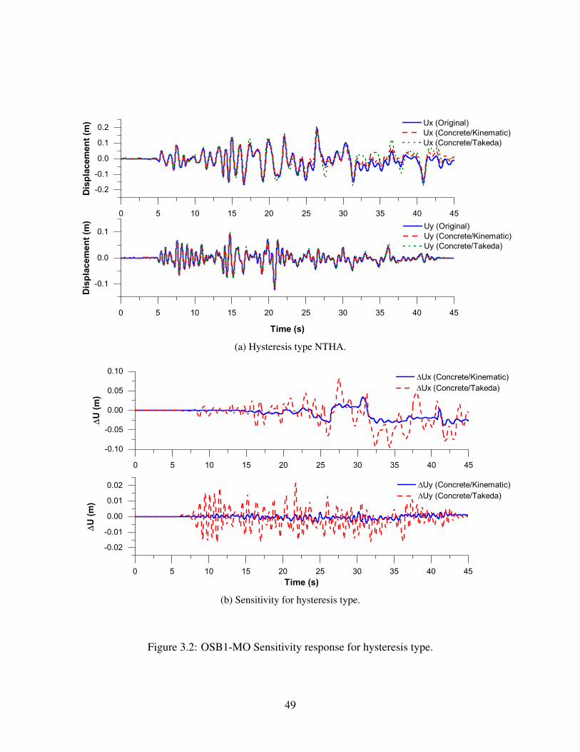
0 5 10 15 20 25 30 35 40 45
-0.1
0.0
0.1 Uy (Original) Uy (Concrete/Kinematic) Uy (Concrete/Takeda)
Disp
lace
men
t (m
)
Time (s)
0 5 10 15 20 25 30 35 40 45
-0.2
-0.1
0.0
0.1
0.2 Ux (Original) Ux (Concrete/Kinematic) Ux (Concrete/Takeda)
Disp
lace
men
t (m
)
(a) Hysteresis type NTHA.
0 5 10 15 20 25 30 35 40 45
-0.02
-0.01
0.00
0.01
0.02 DUy (Concrete/Kinematic) DUy (Concrete/Takeda)
Time (s)
DU
(m)
0 5 10 15 20 25 30 35 40 45
-0.10
-0.05
0.00
0.05
0.10 DUx (Concrete/Kinematic) DUx (Concrete/Takeda)
DU
(m)
(b) Sensitivity for hysteresis type.
Figure 3.2: OSB1-MO Sensitivity response for hysteresis type.
49

Table 3.4: OSB1-MO peak sensitivity results for bridge nonlinear parameters.
Hysteresis type Longitudinal Transversal∆u (m) ∆u (%) t (sec) ∆u (m) ∆u (%) t (sec)
Column Diameter 0.0181 9.3 31.3 -0.0073 6.0 10.98Concrete Strength 0.0137 7.1 24.16 0.0038 3.1 15.25Steel Yield Strength -0.0272 14.1 36.96 0.0042 3.4 15.33Longitudinal Abutment -0.0072 3.7 8.38 0.0074 0.6 9.13Effective StiffnessLongitudinal Abutment -0.0146 7.5 26.67 0.0022 1.8 16.07StrengthSuperstructure Elastic -0.0250 12.9 31.61 -0.0028 2.3 20.11Modulus
direction, the sensitivity results are very low, with a small incidence in the deck displacement. The
peak values obtained in the sensitivity analysis are shown in the Table 3.4.
3.1.5 Response sensitivity analysis of OSB2-MO
OSB2-MO model was analyzed under the same criteria used for OSB1-MO. The Fig-
ure 3.4a describes the original NTHA compared with each hysteresis type combination. The
Figure 3.4b illustrates the sensitivity analysis done over changes in the concrete and steel rein-
forcement hysteresis type assumptions. A high sensitivity response of the bridge to modifications
in the hysteresis behavior was found during the analysis. The model shows an insensitive behav-
ior during the first 7.5 seconds. The highest sensitivity values are developed between 15 to 32
seconds in the longitudinal direction. The Concrete/Kinematic combination concluded in a peak
difference value of 0.0058m in the longitudinal direction representing a 6.6% of the NTHA maxi-
mum value. On the other hand, the Concrete/Takeda combination registered higher values, with a
peak difference of 0.0282m and a 32.3% of the original NTHA peak displacement. The transversal
direction describes fewer sensitive responses in the center of mass displacement due to changes
in the hysteresis type consideration. It is noted that the bridge is very sensitive to changes in the
50

0 5 10 15 20 25 30 35 40 45
-0.004
-0.002
0.000
0.002
0.004 (du/dfy)y Dfy (du/df'c)y Df'c
Time (s)
(du/
dq) D
q(m
)
0 5 10 15 20 25 30 35 40 45
-0.03-0.02-0.010.000.010.020.03
(du/dfy)x Dfy (du/df'c)x Df'c
(du/
dq) D
q (m
)
(a) Structure Sensitivity.
0 5 10 15 20 25 30 35 40 45
-0.002
0.000
0.002 (du/d fyGap)y DfyGap (du/d kGap)y DkGap
Time (s)
(du/
dq) D
q(m
)
0 5 10 15 20 25 30 35 40 45
-0.01
0.00
0.01 (du/d fyGap)x DfyGap (du/d kGap)x DkGap
(du/
dq) D
q (m
)
(b) Abutment Sensitivity.
Figure 3.3: OSB1-MO Properties Sensitivity.
51

Table 3.5: OSB2-MO Peak sensitivity results for hysteresis type.
Hysteresis type Longitudinal Transversal∆u (m) ∆u (%) t (sec) ∆u (m) ∆u (%) t (sec)
Concrete/Kinematic 0.0058 6.6 22.80 0.0002 1.2 16.48Concrete/Takeda 0.0282 32.3 27.37 0.001 5.0 16.43
steel reinforcement hysteresis type assumptions, while changes in the concrete nonlinear behavior
have less impact in the displacement response. Table 3.5 summarize the maximum values achieved
during the sensitivity analysis for the hysteresis types.
The Figure 3.5 describes the displacement sensitivity to the modification of each parameter
under the seismic load by separately. The model describes an insensitive response to changes in
the columns and superstructure parameters during the first 5 seconds of the imposed seismic load,
while changes in the displacement values start to appear after 13 seconds when we modify the
abutment parameters. The bridge showed a highly sensitive response in the longitudinal direction
between 14 to 16 seconds when the columns, superstructure, and abutment parameters are mod-
ified. The changes done over the concrete strength concluded in a peak difference of -0.0082m
which represents a 7.2% of the maximum displacement obtained in the original NTHA. After per-
turbing the longitudinal abutment strength, the peak difference obtained in the deck longitudinal
displacement was -0.001452m, which is near to a 5.9% of the maximum peak displacement of the
bridge center of mass in the unperturbed model. On the other hand, the bridge shows an insensitive
behavior in the transversal direction, resulting in a low variation of the displacement, except for
the superstructure elastic modulus, which seems to be very sensitive to changes. Table 3.6 contains
the peak values obtained during the analysis.
52

0 5 10 15 20 25 30 35 40 45
-0.02
0.00
0.02 Uy (Original) Uy (Concrete/Kinematic) Uy (Concrete/Takeda)
Disp
lace
men
t (m
)
Time (s)
0 5 10 15 20 25 30 35 40 45
-0.10
-0.05
0.00
0.05
0.10 Ux (Original) Ux (Concrete/Kinematic) Ux (Concrete/Takeda)
Disp
lace
men
t (m
)
(a) Hysteresis type NTHA.
0 5 10 15 20 25 30 35 40 45
-0.0010
-0.0005
0.0000
0.0005
0.0010 DUy (Concrete/Kinematic) DUy (Concrete/Takeda)
Time (s)
DU
(m)
0 5 10 15 20 25 30 35 40 45
-0.04
-0.02
0.00
0.02
0.04 DUx (Concrete/Kinematic) DUx (Concrete/Takeda)
DU
(m)
(b) Sensitivity for hysteresis type.
Figure 3.4: OSB2-MO Sensitivity response for hysteresis type.
53
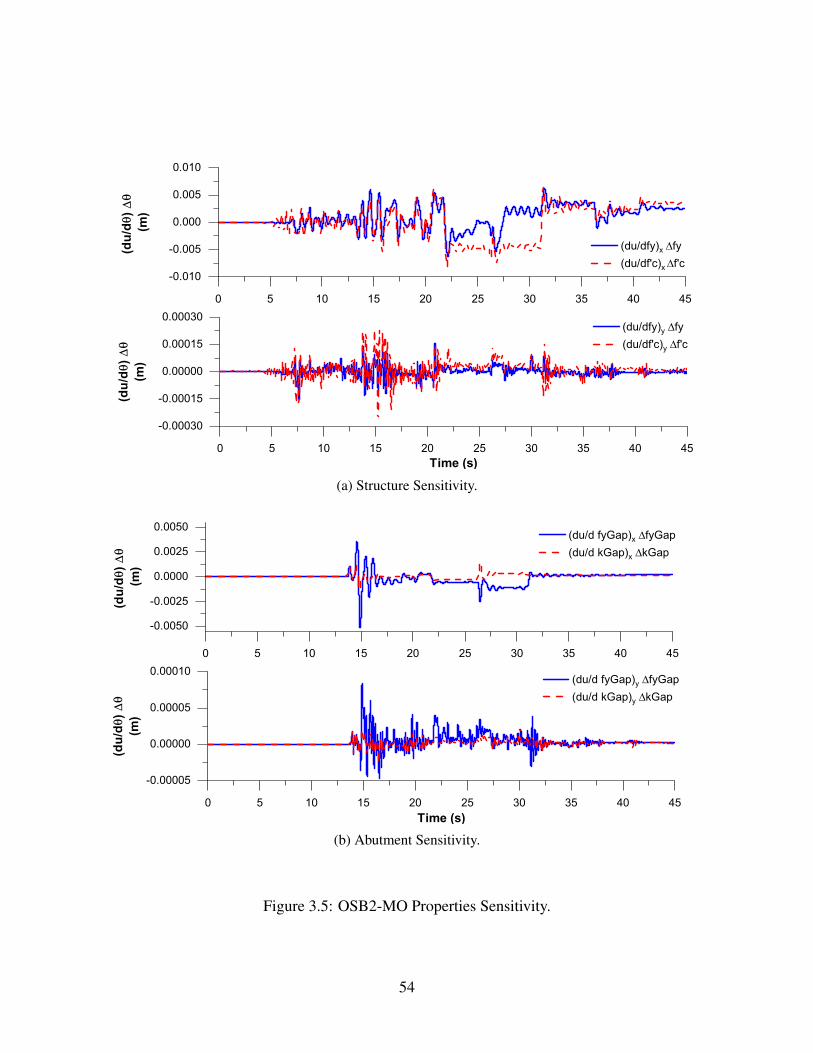
0 5 10 15 20 25 30 35 40 45
-0.00030
-0.00015
0.00000
0.00015
0.00030 (du/dfy)y Dfy (du/df'c)y Df'c
Time (s)
(du/
dq) D
q(m
)
0 5 10 15 20 25 30 35 40 45
-0.010
-0.005
0.000
0.005
0.010
(du/dfy)x Dfy (du/df'c)x Df'c
(du/
dq) D
q (m
)
(a) Structure Sensitivity.
0 5 10 15 20 25 30 35 40 45
-0.00005
0.00000
0.00005
0.00010 (du/d fyGap)y DfyGap (du/d kGap)y DkGap
Time (s)
(du/
dq) D
q(m
)
0 5 10 15 20 25 30 35 40 45
-0.0050
-0.0025
0.0000
0.0025
0.0050 (du/d fyGap)x DfyGap (du/d kGap)x DkGap
(du/
dq) D
q (m
)
(b) Abutment Sensitivity.
Figure 3.5: OSB2-MO Properties Sensitivity.
54
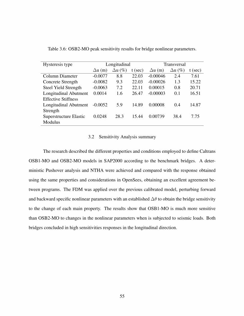
Table 3.6: OSB2-MO peak sensitivity results for bridge nonlinear parameters.
Hysteresis type Longitudinal Transversal∆u (m) ∆u (%) t (sec) ∆u (m) ∆u (%) t (sec)
Column Diameter -0.0077 8.8 22.03 -0.00046 2.4 7.61Concrete Strength -0.0082 9.3 22.03 -0.00026 1.3 15.22Steel Yield Strength -0.0063 7.2 22.11 0.00015 0.8 20.71Longitudinal Abutment 0.0014 1.6 26.47 -0.00003 0.1 16.51Effective StiffnessLongitudinal Abutment -0.0052 5.9 14.89 0.00008 0.4 14.87StrengthSuperstructure Elastic 0.0248 28.3 15.44 0.00739 38.4 7.75Modulus
3.2 Sensitivity Analysis summary
The research described the different properties and conditions employed to define Caltrans
OSB1-MO and OSB2-MO models in SAP2000 according to the benchmark bridges. A deter-
ministic Pushover analysis and NTHA were achieved and compared with the response obtained
using the same properties and considerations in OpenSees, obtaining an excellent agreement be-
tween programs. The FDM was applied over the previous calibrated model, perturbing forward
and backward specific nonlinear parameters with an established ∆θ to obtain the bridge sensitivity
to the change of each main property. The results show that OSB1-MO is much more sensitive
than OSB2-MO to changes in the nonlinear parameters when is subjected to seismic loads. Both
bridges concluded in high sensitivities responses in the longitudinal direction.
55
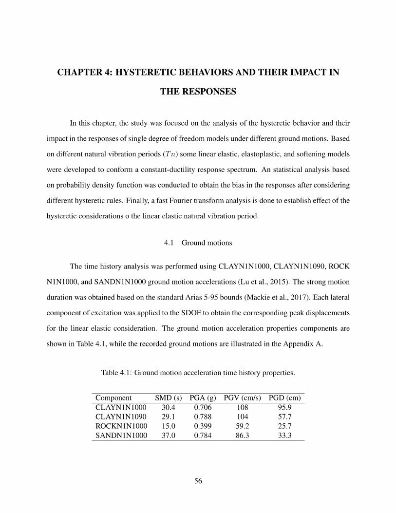
CHAPTER 4: HYSTERETIC BEHAVIORS AND THEIR IMPACT IN
THE RESPONSES
In this chapter, the study was focused on the analysis of the hysteretic behavior and their
impact in the responses of single degree of freedom models under different ground motions. Based
on different natural vibration periods (Tn) some linear elastic, elastoplastic, and softening models
were developed to conform a constant-ductility response spectrum. An statistical analysis based
on probability density function was conducted to obtain the bias in the responses after considering
different hysteretic rules. Finally, a fast Fourier transform analysis is done to establish effect of the
hysteretic considerations o the linear elastic natural vibration period.
4.1 Ground motions
The time history analysis was performed using CLAYN1N1000, CLAYN1N1090, ROCK
N1N1000, and SANDN1N1000 ground motion accelerations (Lu et al., 2015). The strong motion
duration was obtained based on the standard Arias 5-95 bounds (Mackie et al., 2017). Each lateral
component of excitation was applied to the SDOF to obtain the corresponding peak displacements
for the linear elastic consideration. The ground motion acceleration properties components are
shown in Table 4.1, while the recorded ground motions are illustrated in the Appendix A.
Table 4.1: Ground motion acceleration time history properties.
Component SMD (s) PGA (g) PGV (cm/s) PGD (cm)CLAYN1N1000 30.4 0.706 108 95.9CLAYN1N1090 29.1 0.788 104 57.7ROCKN1N1000 15.0 0.399 59.2 25.7SANDN1N1000 37.0 0.784 86.3 33.3
56

4.2 Linear responses
An elastic model was defined to compare the peak deformation caused by the earthquake
ground motions and the maximum response obtained on an elastoplaticity SDOF system under the
same excitation. The stiffness (k) were obtained considering a constant mass of 175.12 kN-s2/m
(1 kip-s2/in) and natural periods (Tn) between 0.10 s and 10.00 s using the equation for periodic
motion. The damping was assumed equals to 1%.
The responses obtained for the linear elastic systems under CLAYN1N1000 ground motion
are described in the Figure 4.2 for different values of Tn and stiffness (k). Values were obtained
using Newmark iteration method, considering β and γ coefficients equals to 0.25 and 0.5, respec-
tively.
4.3 Single degree of freedom constitutive models
Using the linear elastic responses, the elastoplastic and softening SDOF systems were con-
formed for different ductility factors, natural periods, and stiffness. The SDOF models were de-
fined with the same stiffness during the initial loading path obtained for the linear elastic models.
The same mass and damping used to define the linear elastic systems were assumed for both,
elastoplastic and softening model. Therefore, under small oscillations, all the models had the same
natural vibration period Tn. The Figure 4.1 illustrates the SDOF models for Tn = 0.9 s and µ = 1,
2, 4, 8, and 10 under specific ground motion.
4.4 Constant ductility response spectrum
A response spectrum was done based on the elastoplastic systems previously described for
specified levels of ductility factor, using a ζ = 1%, under CLAYN1N1000 ground motion, and
Kinematic hysteretic rule. For different values of Tn, the exact response u(t) of the linear elastic
systems were obtained. Using those values, the peak deformations (uo) and the peak force (fo)
57

-200 -100 0 100 200-6000
-4000
-2000
0
2000
4000
6000
m =1 m =2 m =4 m =8 m =10
-50 0 50-6000
-4000
-2000
0
2000
4000
6000
Stre
ss (M
Pa)
Strain (m/m)a) b)
Figure 4.1: SDOF Material definition for µ = 1, 2, 4, 8, and 10 under CLAYN1N1000 groundmotions, and Tn = 0.9s: a) Elastoplasticity; b) Softening.
were achieved for each case. The same values were obtained for the corresponding yielding forces
associated to different ductility factors (Chopra, 2012). The Figure 4.2 shows the constant ductility
response spectrum obtained. The Appendix C contains the normalized strength (fy′) vs ductility
factor µ and reduction factor (Ry) plots used to achieve the response spectrum.
4.5 Predictions based on constant ductility response spectrum
Using the constant ductility response spectrum described in The Figure 4.2, some responses
were predicted for different values of natural vibration periods and were compared with their cor-
responding SDOF system under the same hysteretic behavior. The analysis done describes a bias
under 10% for 0.3s ≤ Tn ≤ 4.0s and 1 ≤ µ ≤ 4, while the bias for ranges outside of these bound-
aries tends to be over 20%. The Table 4.2 describes the resulting bias for different periods under
CLAYN1N1000 ground motion and kinematic hysteretic rule.
58

0 2 4 6 8 10
0.0
0.5
1.0
1.5
2.0
2.5
3.0
3.5
4.0
Um (m
)
Tn (sec)
m = 1 m = 2 m = 4 m = 8 m = 10
Figure 4.2: Constant-ductility response spectrum for elastoplastic systems and CLAY1N1000ground motion; µ = 1, 2, 4, 8, and 10; ζ = 1%.
Table 4.2: Prediction bias for elastoplasticity systems under CLAYN1N1000 ground motion andKinematic hysteretic rule
µ Tn (s)0.20 0.50 0.75 1.00 2.00 3.00 4.00 5.00
1 0.00% 0.00% 0.00% 0.00% 0.00% 0.00% 0.00% 0.00%2 -10.7% -3.1% -1.2% -1.1% -1.2% 8.6% 0.6% -21.7%4 -10.2% -9.2% 1.3% 0.6% 9.8% -7.1% 37.4% -21.1%8 21.0% 18.1% -5.3% 10.8% -0.2% 0.9% -17.0% 7.2%10 67.1% 30.3% -1.1% 15.9% 5.0% -18.1% 10.1% 17.2%
59
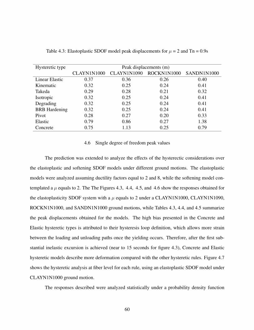
Table 4.3: Elastoplastic SDOF model peak displacements for µ = 2 and Tn = 0.9s
Hysteretic type Peak displacements (m)CLAYN1N1000 CLAYN1N1090 ROCKN1N1000 SANDN1N1000
Linear Elastic 0.37 0.36 0.26 0.40Kinematic 0.32 0.25 0.24 0.41Takeda 0.29 0.28 0.21 0.32Isotropic 0.32 0.25 0.24 0.41Degrading 0.32 0.25 0.24 0.41BRB Hardening 0.32 0.25 0.24 0.41Pivot 0.28 0.27 0.20 0.33Elastic 0.79 0.86 0.27 1.38Concrete 0.75 1.13 0.25 0.79
4.6 Single degree of freedom peak values
The prediction was extended to analyze the effects of the hysterectic considerations over
the elastoplastic and softening SDOF models under different ground motions. The elastoplastic
models were analyzed assuming ductility factors equal to 2 and 8, while the softening model con-
templated a µ equals to 2. The The Figures 4.3, 4.4, 4.5, and 4.6 show the responses obtained for
the elastoplasticity SDOF system with a µ equals to 2 under a CLAYN1N1000, CLAYN1N1090,
ROCKN1N1000, and SANDN1N1000 ground motions, while Tables 4.3, 4.4, and 4.5 summarize
the peak displacements obtained for the models. The high bias presented in the Concrete and
Elastic hysteretic types is attributed to their hysteresis loop definition, which allows more strain
between the loading and unloading paths once the yielding occurs. Therefore, after the first sub-
stantial inelastic excursion is achieved (near to 15 seconds for figure 4.3), Concrete and Elastic
hysteretic models describe more deformation compared with the other hysteretic rules. Figure 4.7
shows the hysteretic analysis at fiber level for each rule, using an elastoplastic SDOF model under
CLAYN1N1000 ground motion.
The responses described were analyzed statistically under a probability density function
60

Figure 4.3: SDOF response spectrum with µ=2 under CLAYN1N1000 ground motion for differenthysteretic rules.
Figure 4.4: SDOF response spectrum with µ=2 under CLAYN1N1090 ground motion for differenthysteretic rules.
61
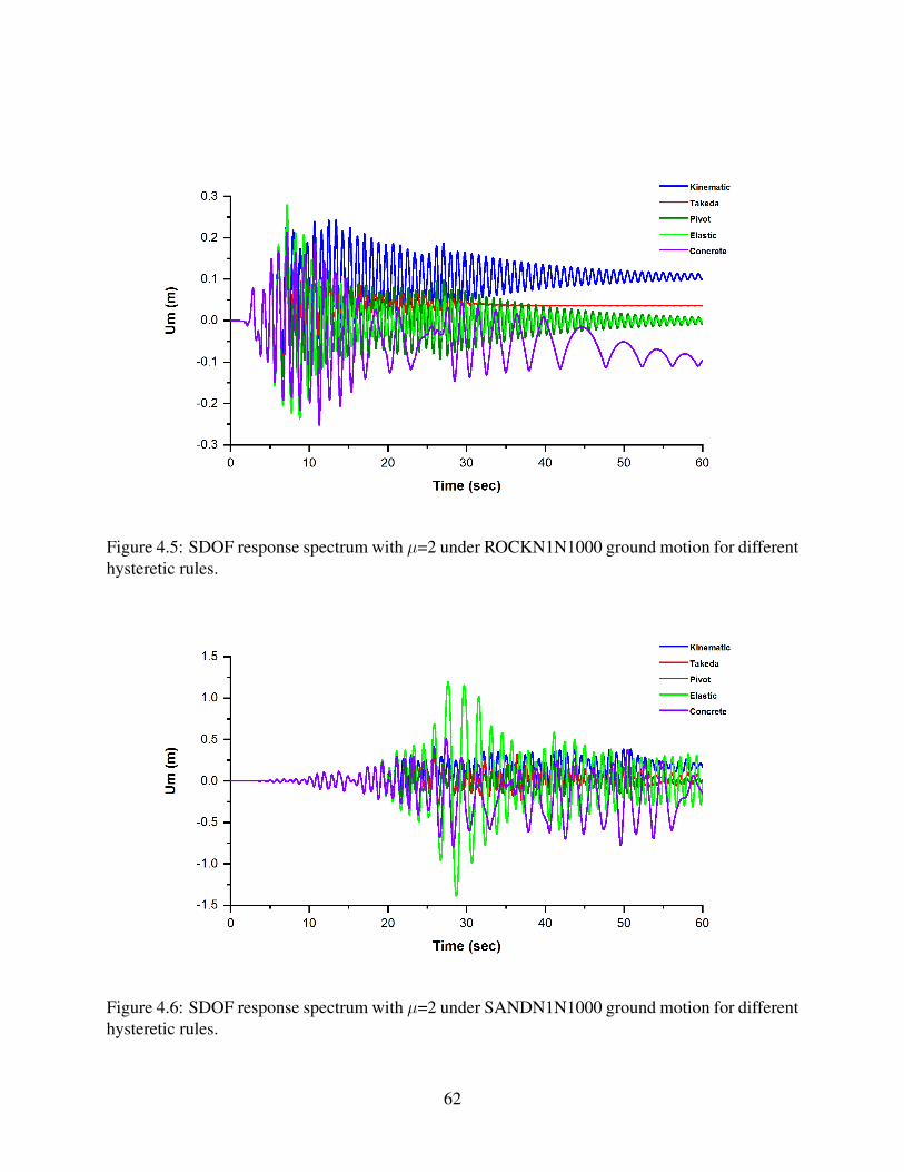
Figure 4.5: SDOF response spectrum with µ=2 under ROCKN1N1000 ground motion for differenthysteretic rules.
Figure 4.6: SDOF response spectrum with µ=2 under SANDN1N1000 ground motion for differenthysteretic rules.
62
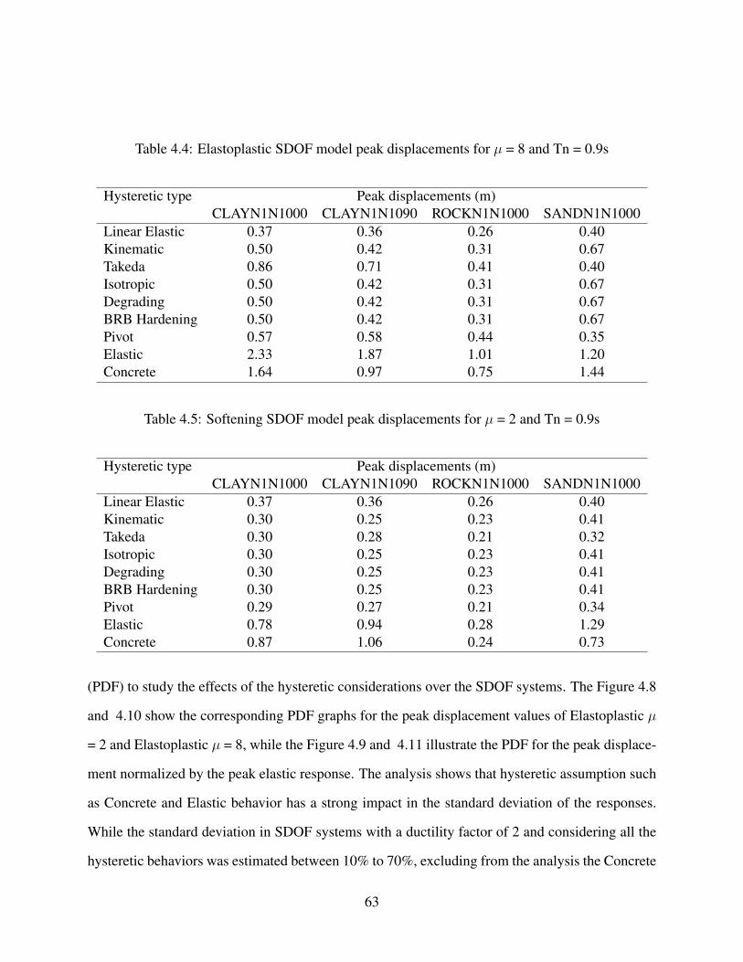
Table 4.4: Elastoplastic SDOF model peak displacements for µ = 8 and Tn = 0.9s
Hysteretic type Peak displacements (m)CLAYN1N1000 CLAYN1N1090 ROCKN1N1000 SANDN1N1000
Linear Elastic 0.37 0.36 0.26 0.40Kinematic 0.50 0.42 0.31 0.67Takeda 0.86 0.71 0.41 0.40Isotropic 0.50 0.42 0.31 0.67Degrading 0.50 0.42 0.31 0.67BRB Hardening 0.50 0.42 0.31 0.67Pivot 0.57 0.58 0.44 0.35Elastic 2.33 1.87 1.01 1.20Concrete 1.64 0.97 0.75 1.44
Table 4.5: Softening SDOF model peak displacements for µ = 2 and Tn = 0.9s
Hysteretic type Peak displacements (m)CLAYN1N1000 CLAYN1N1090 ROCKN1N1000 SANDN1N1000
Linear Elastic 0.37 0.36 0.26 0.40Kinematic 0.30 0.25 0.23 0.41Takeda 0.30 0.28 0.21 0.32Isotropic 0.30 0.25 0.23 0.41Degrading 0.30 0.25 0.23 0.41BRB Hardening 0.30 0.25 0.23 0.41Pivot 0.29 0.27 0.21 0.34Elastic 0.78 0.94 0.28 1.29Concrete 0.87 1.06 0.24 0.73
(PDF) to study the effects of the hysteretic considerations over the SDOF systems. The Figure 4.8
and 4.10 show the corresponding PDF graphs for the peak displacement values of Elastoplastic µ
= 2 and Elastoplastic µ = 8, while the Figure 4.9 and 4.11 illustrate the PDF for the peak displace-
ment normalized by the peak elastic response. The analysis shows that hysteretic assumption such
as Concrete and Elastic behavior has a strong impact in the standard deviation of the responses.
While the standard deviation in SDOF systems with a ductility factor of 2 and considering all the
hysteretic behaviors was estimated between 10% to 70%, excluding from the analysis the Concrete
63
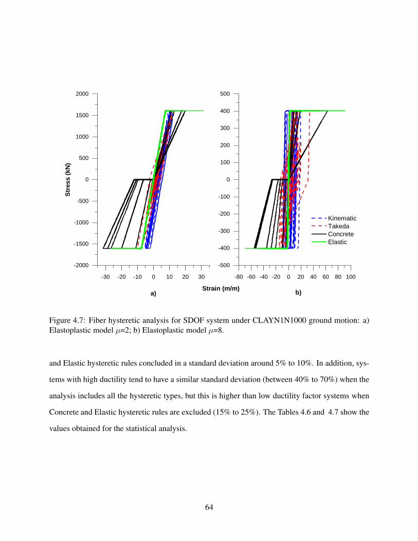
- 3 0 - 2 0 - 1 0 0 1 0 2 0 3 0- 2 0 0 0
- 1 5 0 0
- 1 0 0 0
- 5 0 0
0
5 0 0
1 0 0 0
1 5 0 0
2 0 0 0
Stres
s (kN
)
S t r a i n ( m / m )a ) b )- 8 0 - 6 0 - 4 0 - 2 0 0 2 0 4 0 6 0 8 0 1 0 0
- 5 0 0
- 4 0 0
- 3 0 0
- 2 0 0
- 1 0 0
0
1 0 0
2 0 0
3 0 0
4 0 0
5 0 0
K i n e m a t i c T a k e d a C o n c r e t e E l a s t i c
Figure 4.7: Fiber hysteretic analysis for SDOF system under CLAYN1N1000 ground motion: a)Elastoplastic model µ=2; b) Elastoplastic model µ=8.
and Elastic hysteretic rules concluded in a standard deviation around 5% to 10%. In addition, sys-
tems with high ductility tend to have a similar standard deviation (between 40% to 70%) when the
analysis includes all the hysteretic types, but this is higher than low ductility factor systems when
Concrete and Elastic hysteretic rules are excluded (15% to 25%). The Tables 4.6 and 4.7 show the
values obtained for the statistical analysis.
64
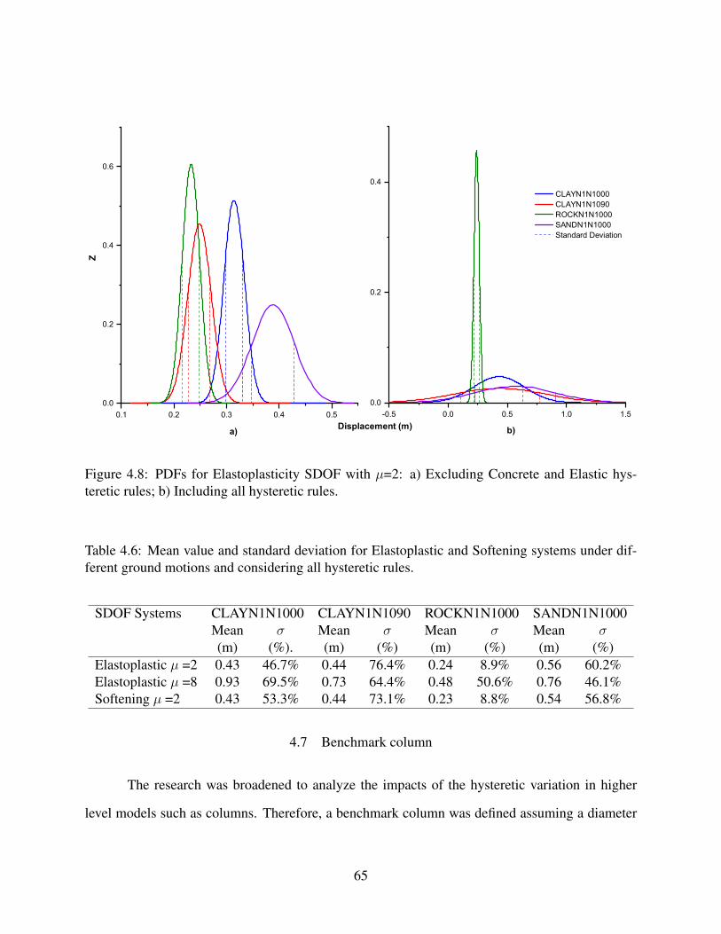
0.1 0.2 0.3 0.4 0.50.0
0.2
0.4
0.6
-0.5 0.0 0.5 1.0 1.50.0
0.2
0.4
Z
CLAYN1N1000 CLAYN1N1090 ROCKN1N1000 SANDN1N1000 Standard Deviation
Displacement (m)a) b)
Figure 4.8: PDFs for Elastoplasticity SDOF with µ=2: a) Excluding Concrete and Elastic hys-teretic rules; b) Including all hysteretic rules.
Table 4.6: Mean value and standard deviation for Elastoplastic and Softening systems under dif-ferent ground motions and considering all hysteretic rules.
SDOF Systems CLAYN1N1000 CLAYN1N1090 ROCKN1N1000 SANDN1N1000Mean σ Mean σ Mean σ Mean σ(m) (%). (m) (%) (m) (%) (m) (%)
Elastoplastic µ =2 0.43 46.7% 0.44 76.4% 0.24 8.9% 0.56 60.2%Elastoplastic µ =8 0.93 69.5% 0.73 64.4% 0.48 50.6% 0.76 46.1%Softening µ =2 0.43 53.3% 0.44 73.1% 0.23 8.8% 0.54 56.8%
4.7 Benchmark column
The research was broadened to analyze the impacts of the hysteretic variation in higher
level models such as columns. Therefore, a benchmark column was defined assuming a diameter
65

0.4 0.6 0.8 1.0 1.2 1.40.0
0.2
0.4
0.6
-1.0 -0.5 0.0 0.5 1.0 1.5 2.0 2.5 3.0 3.5 4.00.0
0.2
0.4
Z
CLAYN1N1000 CLAYN1N1090 ROCKN1N1000 SANDN1N1000 Standard Deviation
Normalized Displacements (m/m)a) b)
Figure 4.9: PDFs with normalized peak displacement for Elastoplasticity SDOF with µ=2: a)Excluding Concrete and Elastic hysteretic rules; b) Including all hysteretic rules.
Table 4.7: Mean value and standard deviation for Elastoplastic and Softening systems under dif-ferent ground motions excluding Concrete and Elastic hysteretic rules.
SDOF Systems CLAYN1N1000 CLAYN1N1090 ROCKN1N1000 SANDN1N1000Mean σ Mean σ Mean σ Mean σ(m) (%). (m) (%) (m) (%) (m) (%)
Elastoplastic µ =2 0.31 5.2% 0.25 8.1% 0.23 6.9% 0.39 10.4%Elastoplastic µ =8 0.57 22.6% 0.50 22.1% 0.35 15.5% 0.57 24.7%Softening µ =2 0.30 1.7% 0.26 6.0% 0.22 4.4% 0.38 9.8%
of 0.50 m and a high of 6.10m. The analysis considered a plastic hinge at the base of the column,
with a length lph = 0.678 m, and an integration point located at the center of the hinge (xh =
0.339 m). The effective moment of inertia of the column was 0.60Ig to assume an appropriated
softening of the cracked elastic properties. The values assumed were taken according to the CP3
66
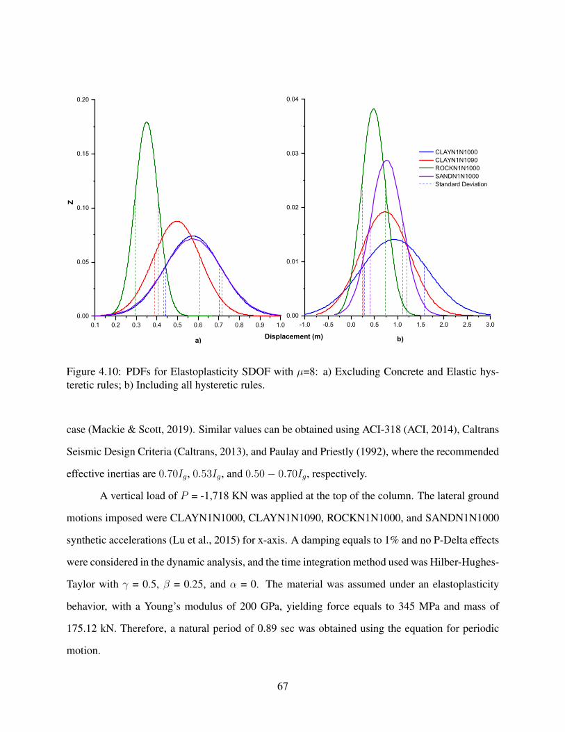
0.1 0.2 0.3 0.4 0.5 0.6 0.7 0.8 0.9 1.00.00
0.05
0.10
0.15
0.20
-1.0 -0.5 0.0 0.5 1.0 1.5 2.0 2.5 3.00.00
0.01
0.02
0.03
0.04
Z
CLAYN1N1000 CLAYN1N1090 ROCKN1N1000 SANDN1N1000 Standard Deviation
Displacement (m)a) b)
Figure 4.10: PDFs for Elastoplasticity SDOF with µ=8: a) Excluding Concrete and Elastic hys-teretic rules; b) Including all hysteretic rules.
case (Mackie & Scott, 2019). Similar values can be obtained using ACI-318 (ACI, 2014), Caltrans
Seismic Design Criteria (Caltrans, 2013), and Paulay and Priestly (1992), where the recommended
effective inertias are 0.70Ig, 0.53Ig, and 0.50− 0.70Ig, respectively.
A vertical load of P = -1,718 KN was applied at the top of the column. The lateral ground
motions imposed were CLAYN1N1000, CLAYN1N1090, ROCKN1N1000, and SANDN1N1000
synthetic accelerations (Lu et al., 2015) for x-axis. A damping equals to 1% and no P-Delta effects
were considered in the dynamic analysis, and the time integration method used was Hilber-Hughes-
Taylor with γ = 0.5, β = 0.25, and α = 0. The material was assumed under an elastoplasticity
behavior, with a Young’s modulus of 200 GPa, yielding force equals to 345 MPa and mass of
175.12 kN. Therefore, a natural period of 0.89 sec was obtained using the equation for periodic
motion.
67

0.5 1.0 1.5 2.0 2.5 3.00.00
0.05
0.10
0.15
0.20
-2 0 2 4 6 80.00
0.01
0.02
0.03
0.04
Z
CLAYN1N1000 CLAYN1N1090 ROCKN1N1000 SANDN1N1000 Standard Deviation
Normalized Displacements (m/m)a) b)
Figure 4.11: PDFs with normalized peak displacement for Elastoplasticity SDOF with µ=8: a)Excluding Concrete and Elastic hysteretic rules; b) Including all hysteretic rules.
The column was analyzed assuming the same hysteretic rules used for the SDOF analysis.
The peak displacement obtained for each hysteretic rule under CLAYN1N1000 ground motion are
described in the Table 4.8. The values were compared with the predicted peak displacement using
the response spectrum obtained before, with Tn = 0.89 sec and µ =2.64. This ductility factor was
calculated based on the elastic peak displacement of the column (u0), the elastic peak force (f0 =
ku0), the elastic peak moment (My = f0h), the yielding strength of the system (fysys = My/S),
and the yielding strength of the material (fymat = 345 MPa). The Figure 4.12 shows the column’s
responses for different hysteretic rules under CLAYN1N1000 ground motion, while the Table 4.8
illustrates the bias obtained with the predicted value. A high bias was achieved in the prediction of
the peak displacement values for Concrete and Elastic hyteretic rules (near 60%), while the other
hysteretic case concluded in a bias under 15%. Therefore, the assumptions done over the hysteretic
68

0 10 20 30 40 50 60-0.8
-0.6
-0.4
-0.2
0.0
0.2
0.4
0.6
0.8
Um (m
)
Time (sec)
Kinematic
Takeda
Pivot
Elastic
Concrete
Figure 4.12: Column response spectrum with µ=2.64 under CLAYN1N1000 ground motion fordifferent hysteretic rules.
rules have an important effect over the column responses when comparing the results obtained with
common hysteretic considerations such as Concrete and Kinematic or Takeda.
The column’s peak displacements were analyzed statistically under a probability density
function (PDF) to study the incidence of the hysteretic considerations over the systems. The Fig-
ure 4.13 shows the corresponding PDF graphs for the peak displacement values of the column,
while the Figure 4.14 illustrates the PDF for the peak displacement normalized by the peak elastic
response. The analysis shows that similar results as SDOF systems, where hysteretic assumptions
such as Concrete and Elastic behavior have a strong impact in the standard deviation of the re-
sponses. While the standard deviation in column with a ductility factor of 2 and considering all the
hysteretic behaviors had a huge variation (between 10% to 110%), excluding Concrete and Elastic
hysteretic rules from the analysis concluded in standard deviations between 4% and 13%. PDF’s
analysis describes the same conclusions obtained during the column peak displacement predic-
69

Table 4.8: Peak displacement and prediction bias for benchmark column with a µ = 2.64 and underCLAYN1N1000 ground motion.
Hysteretic Rule Um (m) Um Prediction (m) Bias (%)Kinematic 0.239 0.245 -2.74%Takeda 0.283 0.245 13.31%Isotropic 0.239 0.245 -2.74%Degrading 0.239 0.245 -2.74%BRB Hardening 0.239 0.245 -2.74%Pivot 0.257 0.245 4.78%Elastic 0.613 0.245 60.00%Concrete 0.755 0.245 67.55%
tions, where the hysteretic assumption has an important effect on the responses when considering
a Concrete or Elastic hysteretic rules instead of Takeda, Kinematic, or Pivot.
4.8 Fast Fourier Transform Analysis
The Fast Fourier Transform (FFT) and Transfer function (TF) of the acceleration responses
of the SDOF and column were analyzed under different ground motions and hysteretic rules.
Therefore, the impact on the behavior of the systems was studied after converting the responses
to their representation in the frequency domain. The FFT and TF analysis of the SDOF time his-
tory can describe the different hysteretic behaviors of the systems and the impact in the responses.
FFT is only applicable to time history response of linear systems. For the nonlinear responses
considered, it was assumed that response was approximately stationary when averaged over the
complete time history of response, and therefore only appropriate for cases of small ductility such
as µ=2. Therefore, it is not representative for nonlinear models with high ductility factors, such
as µ=8, which is used in just an approximate sense to establish if there is any trends. The Fig-
ure 4.15 and 4.16 illustrate the FFT power spectrum for the ground motions used and the FFT
power spectrum for the elastoplastic SDOF considering µ=2, respectively.
70
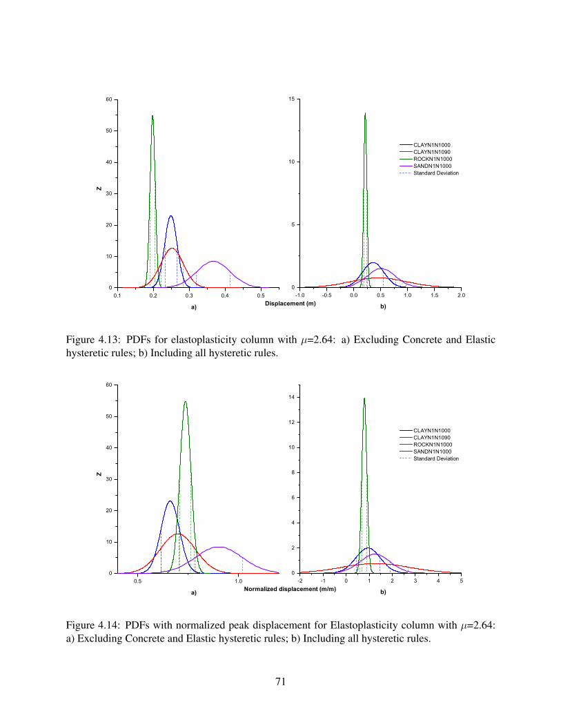
0.1 0.2 0.3 0.4 0.50
10
20
30
40
50
60
-1.0 -0.5 0.0 0.5 1.0 1.5 2.00
5
10
15Z
CLAYN1N1000 CLAYN1N1090 ROCKN1N1000 SANDN1N1000 Standard Deviation
Displacement (m)a) b)
Figure 4.13: PDFs for elastoplasticity column with µ=2.64: a) Excluding Concrete and Elastichysteretic rules; b) Including all hysteretic rules.
0.5 1.00
10
20
30
40
50
60
-2 -1 0 1 2 3 4 50
2
4
6
8
10
12
14
Z
CLAYN1N1000 CLAYN1N1090 ROCKN1N1000 SANDN1N1000 Standard Deviation
Normalized displacement (m/m)a) b)
Figure 4.14: PDFs with normalized peak displacement for Elastoplasticity column with µ=2.64:a) Excluding Concrete and Elastic hysteretic rules; b) Including all hysteretic rules.
71

0 1 20
1
2
3
4 C L A Y N 1 N 1 0 0 0
0 1 20
1
2C L A Y N 1 N 1 0 9 0
0 1 20 . 0
0 . 2
0 . 4
0 . 6 R O C K N 1 N 1 0 0 0FF
T Mag
nitud
e
F F T F r e q u e n c y ( H z )0 1 2
0
2
4 S A N D N 1 N 1 0 0 0
Figure 4.15: FFT ground motion power spectrum for CLAYN1N1000, CLAYN1N1090,ROCKN1N1000, and SANDN1N1000
The Figure 4.17 to 4.19 show the transfer function and natural period analysis done over
the acceleration responses of the SDOF systems under CLAYN1N1000 ground motion. Similar
results were obtained for the elastoplastic and softening materials under the same ductility factor.
The analysis shows important variations in the linear elastic natural period when Concrete and
Elastic hysteretic rules are assumed. This variations tend to increase for high values of ductility
factor such as µ=8. Therefore, the effects of the hysteretic behavior over the systems tend to
increase when high ductility factors are considered and the impact of material nonlinear backbone
consideration is very small when the same ductility factor is assumed.
72
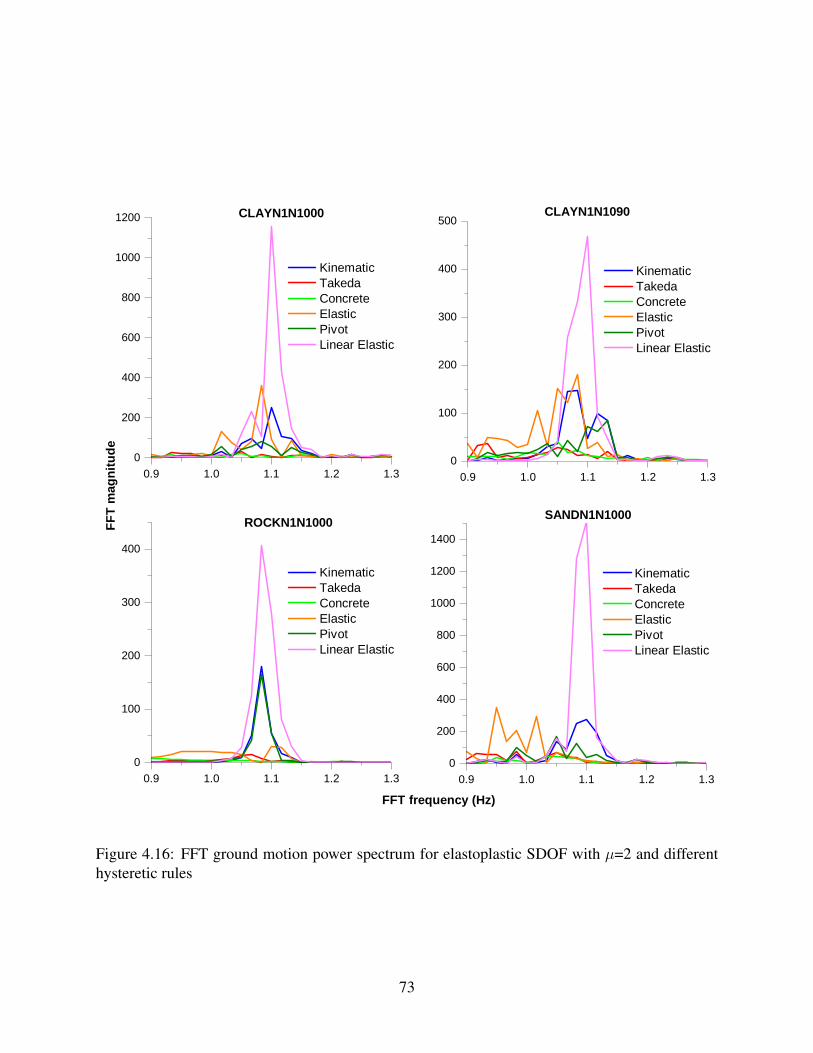
0 . 9 1 . 0 1 . 1 1 . 2 1 . 30
2 0 0
4 0 0
6 0 0
8 0 0
1 0 0 0
1 2 0 0
FFT m
agnit
ude
K i n e m a t i c T a k e d a C o n c r e t e E l a s t i c P i v o t L i n e a r E l a s t i c
F F T f r e q u e n c y ( H z )
0 . 9 1 . 0 1 . 1 1 . 2 1 . 30
1 0 0
2 0 0
3 0 0
4 0 0
5 0 0
K i n e m a t i c T a k e d a C o n c r e t e E l a s t i c P i v o t L i n e a r E l a s t i c
0 . 9 1 . 0 1 . 1 1 . 2 1 . 30
1 0 0
2 0 0
3 0 0
4 0 0 K i n e m a t i c T a k e d a C o n c r e t e E l a s t i c P i v o t L i n e a r E l a s t i c
0 . 9 1 . 0 1 . 1 1 . 2 1 . 30
2 0 0
4 0 0
6 0 0
8 0 0
1 0 0 0
1 2 0 0
1 4 0 0
K i n e m a t i c T a k e d a C o n c r e t e E l a s t i c P i v o t L i n e a r E l a s t i c
C L A Y N 1 N 1 0 0 0 C L A Y N 1 N 1 0 9 0
R O C K N 1 N 1 0 0 0 S A N D N 1 N 1 0 0 0
Figure 4.16: FFT ground motion power spectrum for elastoplastic SDOF with µ=2 and differenthysteretic rules
73
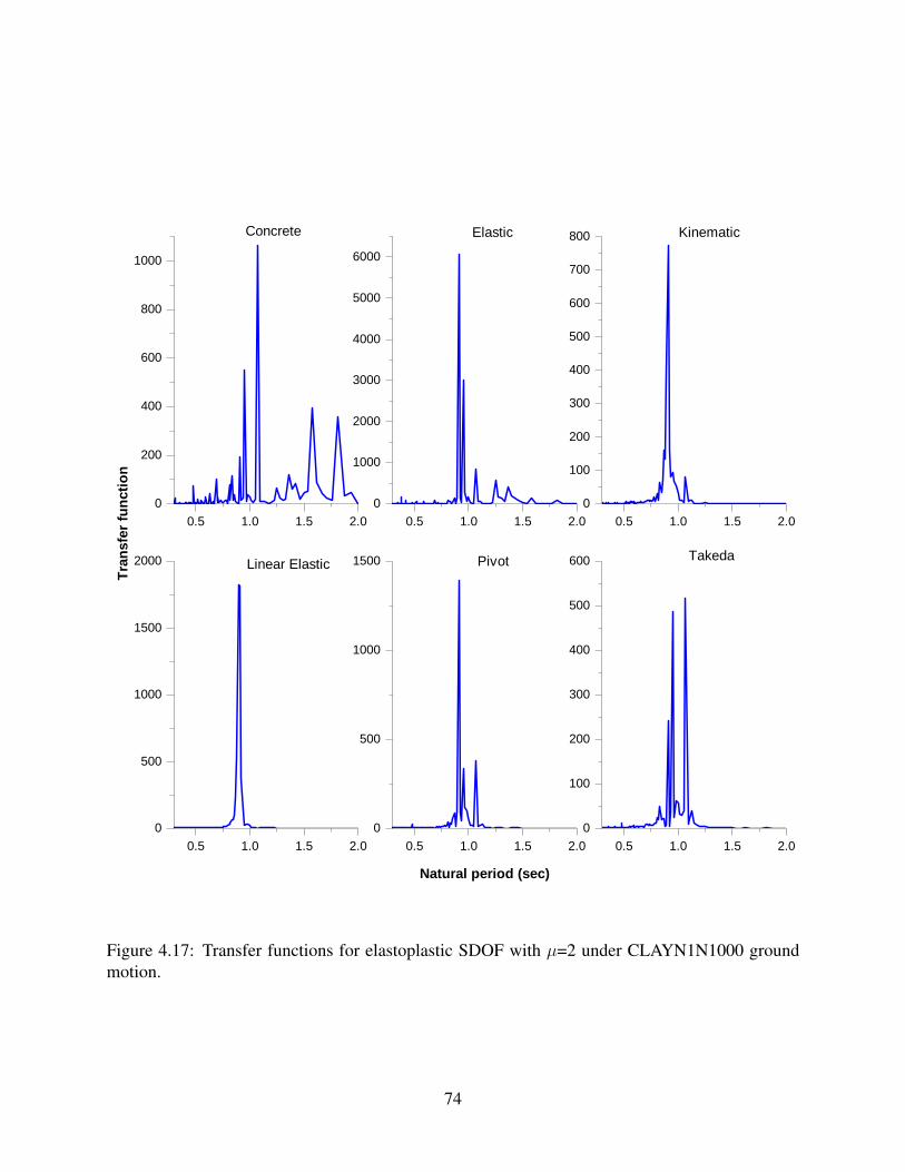
0 . 5 1 . 0 1 . 5 2 . 00
2 0 0
4 0 0
6 0 0
8 0 0
1 0 0 0C o n c r e t e
0 . 5 1 . 0 1 . 5 2 . 00
1 0 0 0
2 0 0 0
3 0 0 0
4 0 0 0
5 0 0 0
6 0 0 0 E l a s t i c
0 . 5 1 . 0 1 . 5 2 . 00
1 0 0
2 0 0
3 0 0
4 0 0
5 0 0
6 0 0
7 0 0
8 0 0 K i n e m a t i c
0 . 5 1 . 0 1 . 5 2 . 00
5 0 0
1 0 0 0
1 5 0 0
2 0 0 0 L i n e a r E l a s t i cTrans
fer fu
nctio
n
0 . 5 1 . 0 1 . 5 2 . 00
5 0 0
1 0 0 0
1 5 0 0 P i v o t
N a t u r a l p e r i o d ( s e c )0 . 5 1 . 0 1 . 5 2 . 0
0
1 0 0
2 0 0
3 0 0
4 0 0
5 0 0
6 0 0 T a k e d a
Figure 4.17: Transfer functions for elastoplastic SDOF with µ=2 under CLAYN1N1000 groundmotion.
74

0 . 5 1 . 0 1 . 5 2 . 00
1 0
2 0
3 0
4 0
5 0 C o n c r e t e
0 . 5 1 . 0 1 . 5 2 . 00
5 0
1 0 0
1 5 0
2 0 0
2 5 0
3 0 0 E l a s t i c
0 . 5 1 . 0 1 . 5 2 . 00
5 0
1 0 0
1 5 0
2 0 0 K i n e m a t i c
0 . 5 1 . 0 1 . 5 2 . 00
5 0 0
1 0 0 0
1 5 0 0
2 0 0 0 L i n e a r E l a s t i cTrans
fer fu
nctio
n
0 . 5 1 . 0 1 . 5 2 . 00
5 0
1 0 0
1 5 0P i v o t
N a t u r a l p e r i o d ( s e c )0 . 5 1 . 0 1 . 5 2 . 0
0
2 0
4 0
6 0
8 0
1 0 0 T a k e d a
Figure 4.18: Transfer functions for elastoplastic SDOF with µ=8 under CLAYN1N1000 groundmotion.
75
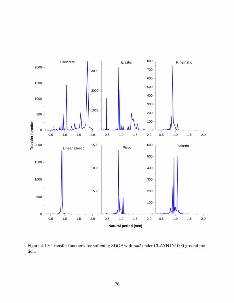
0 . 5 1 . 0 1 . 5 2 . 00
5 0 0
1 0 0 0
1 5 0 0
2 0 0 0C o n c r e t e
0 . 5 1 . 0 1 . 5 2 . 00
1 0 0 0
2 0 0 0
3 0 0 0
E l a s t i c
0 . 5 1 . 0 1 . 5 2 . 00
1 0 0
2 0 0
3 0 0
4 0 0
5 0 0
6 0 0
7 0 0
8 0 0 K i n e m a t i c
0 . 5 1 . 0 1 . 5 2 . 00
5 0 0
1 0 0 0
1 5 0 0
2 0 0 0 L i n e a r E l a s t i cTrans
fer fu
nctio
n
0 . 5 1 . 0 1 . 5 2 . 00
5 0 0
1 0 0 0
1 5 0 0 P i v o t
N a t u r a l p e r i o d ( s e c )0 . 5 1 . 0 1 . 5 2 . 0
0
1 0 0
2 0 0
3 0 0
4 0 0
5 0 0
6 0 0 T a k e d a
Figure 4.19: Transfer functions for softening SDOF with µ=2 under CLAYN1N1000 ground mo-tion.
76
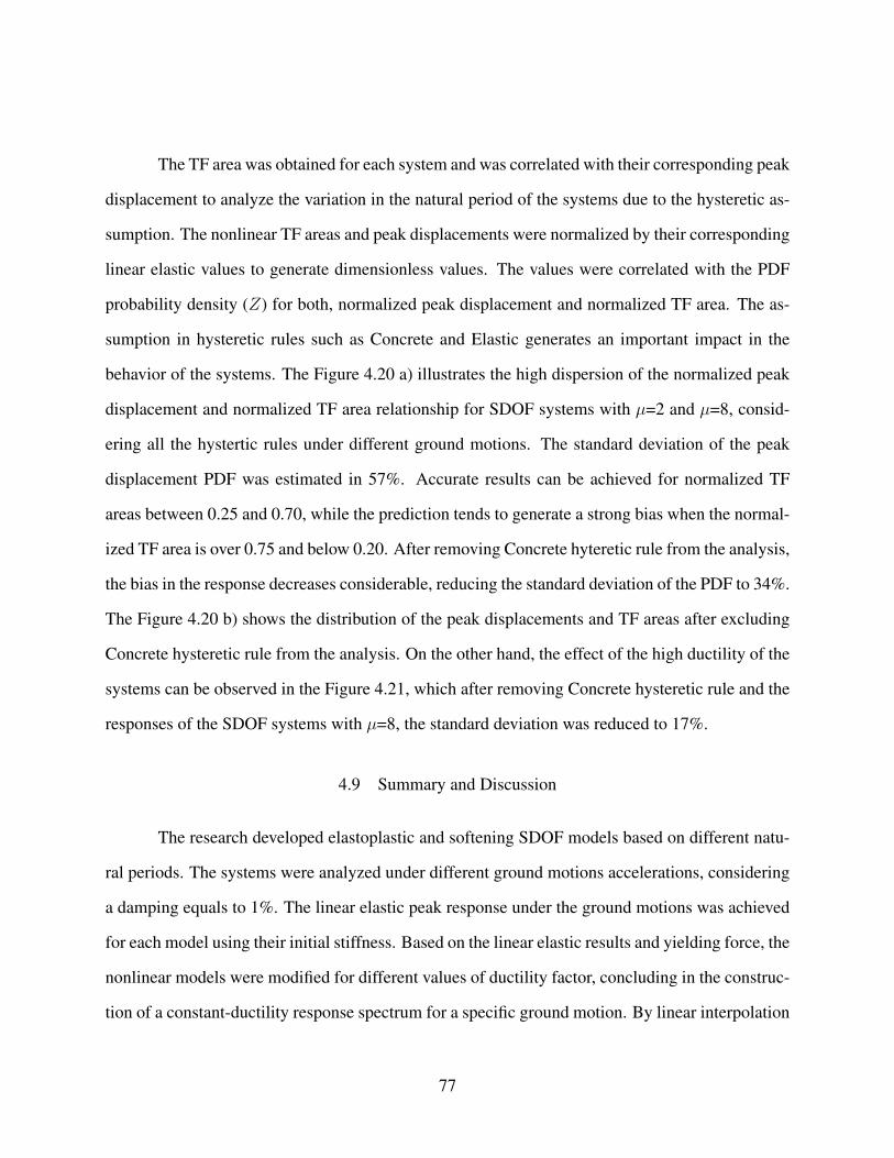
The TF area was obtained for each system and was correlated with their corresponding peak
displacement to analyze the variation in the natural period of the systems due to the hysteretic as-
sumption. The nonlinear TF areas and peak displacements were normalized by their corresponding
linear elastic values to generate dimensionless values. The values were correlated with the PDF
probability density (Z) for both, normalized peak displacement and normalized TF area. The as-
sumption in hysteretic rules such as Concrete and Elastic generates an important impact in the
behavior of the systems. The Figure 4.20 a) illustrates the high dispersion of the normalized peak
displacement and normalized TF area relationship for SDOF systems with µ=2 and µ=8, consid-
ering all the hystertic rules under different ground motions. The standard deviation of the peak
displacement PDF was estimated in 57%. Accurate results can be achieved for normalized TF
areas between 0.25 and 0.70, while the prediction tends to generate a strong bias when the normal-
ized TF area is over 0.75 and below 0.20. After removing Concrete hyteretic rule from the analysis,
the bias in the response decreases considerable, reducing the standard deviation of the PDF to 34%.
The Figure 4.20 b) shows the distribution of the peak displacements and TF areas after excluding
Concrete hysteretic rule from the analysis. On the other hand, the effect of the high ductility of the
systems can be observed in the Figure 4.21, which after removing Concrete hysteretic rule and the
responses of the SDOF systems with µ=8, the standard deviation was reduced to 17%.
4.9 Summary and Discussion
The research developed elastoplastic and softening SDOF models based on different natu-
ral periods. The systems were analyzed under different ground motions accelerations, considering
a damping equals to 1%. The linear elastic peak response under the ground motions was achieved
for each model using their initial stiffness. Based on the linear elastic results and yielding force, the
nonlinear models were modified for different values of ductility factor, concluding in the construc-
tion of a constant-ductility response spectrum for a specific ground motion. By linear interpolation
77

a)
b)
0
1
2
3
4
5
6
7
8
9
10
0
0.5
1
1.5
2
2.5
3
3.5
4
4.5
5
-0.5 0 0.5 1 1.5 2
Z A
rea
No
rma
lize
d d
isp
lac
em
en
t
Normalized area
0 1 2 3 4 5Z Displacement
0
1
2
3
4
5
6
7
8
9
10
0
0.5
1
1.5
2
2.5
3
3.5
4
4.5
5
-0.5 0 0.5 1 1.5 2
Z A
rea
No
rma
lize
d d
isp
lac
em
en
t
Normalized area
0 1 2 3 4 5
Z Displacement
Figure 4.20: Normalized area and normalized displacement relationship for all SDOF systems: a)All hysteretic rules; b) Excluding Concrete hysteretic rule.
78
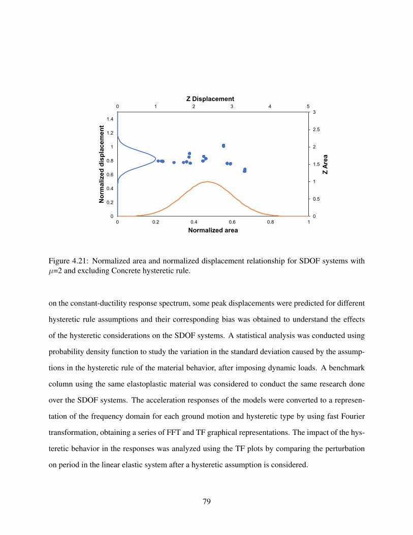
0
0.5
1
1.5
2
2.5
3
0
0.2
0.4
0.6
0.8
1
1.2
1.4
0 0.2 0.4 0.6 0.8 1
Z A
rea
No
rma
lize
d d
isp
lac
em
en
t
Normalized area
0 1 2 3 4 5
Z Displacement
Figure 4.21: Normalized area and normalized displacement relationship for SDOF systems withµ=2 and excluding Concrete hysteretic rule.
on the constant-ductility response spectrum, some peak displacements were predicted for different
hysteretic rule assumptions and their corresponding bias was obtained to understand the effects
of the hysteretic considerations on the SDOF systems. A statistical analysis was conducted using
probability density function to study the variation in the standard deviation caused by the assump-
tions in the hysteretic rule of the material behavior, after imposing dynamic loads. A benchmark
column using the same elastoplastic material was considered to conduct the same research done
over the SDOF systems. The acceleration responses of the models were converted to a represen-
tation of the frequency domain for each ground motion and hysteretic type by using fast Fourier
transformation, obtaining a series of FFT and TF graphical representations. The impact of the hys-
teretic behavior in the responses was analyzed using the TF plots by comparing the perturbation
on period in the linear elastic system after a hysteretic assumption is considered.
79

CHAPTER 5: CONCLUSIONS
The research demonstrated the constitutive models, element formulations, and modeling
parameters necessary to achieve comparable nonlinear dynamic behavior of two OSBs in OpenSees
and SAP2000. During the calibration process, both software showed close results for steel con-
stitutive model under dynamic loads. The hysteresis type considered for SAP2000 in the model
was Kinematic. On the other hand, concrete behavior had a different shape under Takeda hys-
teresis type (which was considered for SAP2000 models). An additional comparison was done
using Concrete hysteresis type for SAP2000 concrete constitutive model and the results obtained
were similar than OpenSees’ concrete model. Concrete hysteresis type started to be available in
SAP2000 recent versions. Thus, the Caltrans models only considered Takeda hysteresis type. The
model was also calibrated using columns constitutive models. The values assumed were taken
according to the concentrated plasticity case 3, CP3 (Mackie & Scott, 2019). The results obtained
for SAP2000 and OpenSees described excellent agreement in phasing and peaks values, even the
concrete constitutive model had disagreements in shape.
In the first bridge nonlinear analysis, OpenSees models were adapted to match Caltrans
files, while SAP2000 remained the same. The results obtained for OSB1-O concluded in an ac-
ceptable agreement between both programs, while OSB2-O presented several differences due to
issues in the hinge length considerations. A roller abutment analysis (S models) was developed
to determinate the root of the differences between programs, confirming that OSB2-O incongru-
ences were due to the inadvertent hinge length choice, while OSB1-O discrepancies were related
to the concrete constitutive models and the nonlinear behavior of the abutments in the longitudinal
direction.
The second bridge nonlinear analysis was focused to improve the issues found in Caltrans
models. Important modifications were done over the elements of the columns in the models and
the OSB2-O hinge length was improved to a more realistic one. The nonlinear time history anal-
80

ysis concluded in an excellent agreement between SAP2000 and OpenSees. Shape, phasing, and
peaks values were almost identical for OSB1-MO and OSB2-MO. The improvement done over the
models induced a more accurate response after applying dynamics loads to the Caltrans bridges.
The results achieved with SAP2000 and OpenSees were almost the same, however concrete ma-
terial constitutive model had several differences in its nonlinear dynamic behavior. The hinge, the
fiber discretization in the hinge cross section, and the abutments nonlinear characterization clearly
defined the main dynamic behavior of the bridge models.
The FDM was applied over the previous calibrated model, perturbing forward and back-
ward specific nonlinear parameters with an established ∆θ to obtain the bridge sensitivity to the
change of each main property. The results show that OSB1-MO is much more sensitive than OSB2-
MO to changes in the nonlinear parameters when is subjected to seismic loads. Both bridges
concluded in high sensitivities responses in the longitudinal direction. Parameters such as steel
yield strength for the column reinforcement and longitudinal abutment strength for the links have
the highest sensitivities values for OSB1-MO, while the concrete strength in columns and the su-
perstructure elastic modulus describe the most relevant perturbation in the displacement response
for OSB2-MO. The displacement response in the transversal direction seems to be insensitive to
changes for both bridges, except for the superstructure elastic modulus in OSB2-MO, which shows
a high impact in the bridge response after its perturbation.
In addition, the bridge sensitivity to the hysteresis governing rule for concrete and rein-
forcement steel was analyzed. The deterministic response was obtained using the SAP2000 default
hysteretic types (Takeda for concrete and Kinematic for steel). The change in the hysteresis behav-
ior of the materials concluded in high sensitivity responses. The analysis concluded that OSB1-MO
is much more sensitive that OSB2-MO to changes in the hysteresis rules assumption, especially
in the steel reinforcement when is changed from Kinematic to Takeda. It is important to note that
changing the concrete hysteresis rule from Takeda to Concrete generate in both bridges (specially
OSB1-MO) an important perturbation in displacement of the deck and the Concrete hysteretic rule
81

was not available in the SAP2000 old versions. Therefore, a change in the concrete hysteretic
assumption to a more realistic behavior could not be done until the latest SAP2000 versions.
The impact of the different hysteretic consideration over the responses of the SDOF systems
under specific ground motion was demonstrated in the current study. The peak response predictions
bias for Concrete and Elastic hysteretic rules was very high compared with the other hysteretic
behaviors. Therefore, the hysteretic assumption will strongly affect the estimation of the peak
displacement in SDOF systems. The research achieved similar conclusion after analyzing the
results obtained in the probability density function. The PDF figures described steep slopes and
small standard deviation when the Concrete and Elastic hysteretic rules were excluded from the
analysis, while the values tend to be dispersed when the calculations included all the hysteretic
behavior. The hysteretic effect on the responses tends to be higher when the ductility factor is
increased. This is the case of the analysis done over the elastoplastic material with µ = 8 and
the comparison with the same material assuming a µ =2. The increment in the standard deviation
is considerable when the ductility factor is changed from 2 to 8. On the other hand, the impact
of material nonlinear backbone consideration (elastoplastic vs softening) is very small when the
same ductility factor is assumed for them. The results achieved for both, elastoplastic and softening
material using µ =2 where very similar. The TF analysis was focused to study the perturbations on
the average peak displacement over the time history after applying ground motion accelerations,
assuming a stationary response and considering different hysteretic rules. The TF plots showed
an important variation in the behavior of the SDOF systems when Concrete and Elastic hysteretic
rules are assumed, while the perturbation was small for the remaining hysteretic types. Similar to
the PDF analysis, the perturbation tends to increase for high values of ductility factor such as µ=8.
The bias and the standard deviation were considerably reduced after excluding the high ductility
systems and Concrete hysteretic rule responses from the PDF analysis. Therefore, the responses in
a SDOF system are highly affected by the hysteretic assumption and the ductility factor.
A similar nonlinear time history analysis and sensitivity study could be extended to dif-
82

ferent Caltrans ordinary standard bridges, such as OSB3 and OSB4. Also, the sensitivity analysis
could be extended to compare the results with different softwares and the variation using the di-
rect differentiation method. Finally, the bias analysis can be broadened to composite materials
implemented in different type of structures such as concrete reinforced columns and bridges.
83

APPENDIX A: OSB1-S PUSHOVER ANALYSIS
84
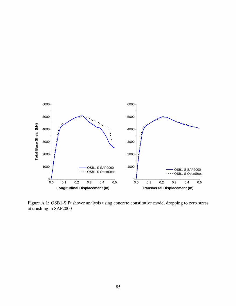
0 . 0 0 . 1 0 . 2 0 . 3 0 . 4 0 . 50
1 0 0 0
2 0 0 0
3 0 0 0
4 0 0 0
5 0 0 0
6 0 0 0
O S B 1 - S S A P 2 0 0 0 O S B 1 - S O p e n S e e s
Total
Base
Shea
r (kN)
L o n g i t u d i n a l D i s p l a c e m e n t ( m )0 . 0 0 . 1 0 . 2 0 . 3 0 . 4 0 . 50
1 0 0 0
2 0 0 0
3 0 0 0
4 0 0 0
5 0 0 0
6 0 0 0
O S B 1 - S S A P 2 0 0 0 O S B 1 - S O p e n S e e s
T r a n s v e r s a l D i s p l a c e m e n t ( m )
Figure A.1: OSB1-S Pushover analysis using concrete constitutive model dropping to zero stressat crushing in SAP2000
85

APPENDIX B: GROUND MOTIONS
86
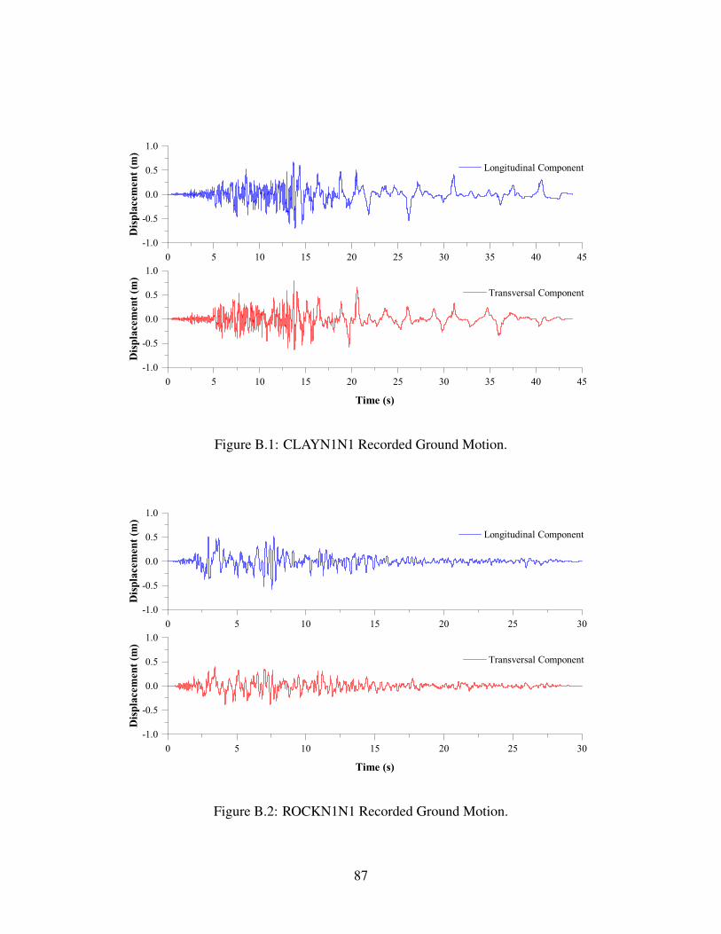
0 5 10 15 20 25 30 35 40 45-1.0
-0.5
0.0
0.5
1.0
Transversal Component
Disp
lace
men
t (m
)
Time (s)
0 5 10 15 20 25 30 35 40 45-1.0
-0.5
0.0
0.5
1.0
Longitudinal Component
Disp
lace
men
t (m
)
Figure B.1: CLAYN1N1 Recorded Ground Motion.
0 5 10 15 20 25 30-1.0
-0.5
0.0
0.5
1.0
Transversal Component
Disp
lace
men
t (m
)
Time (s)
0 5 10 15 20 25 30-1.0
-0.5
0.0
0.5
1.0
Longitudinal Component
Disp
lace
men
t (m
)
Figure B.2: ROCKN1N1 Recorded Ground Motion.
87

0 5 10 15 20 25 30 35 40 45 50 55 60-1.0
-0.5
0.0
0.5
1.0
Transversal Component
Disp
lace
men
t (m
)
Time (s)
0 5 10 15 20 25 30 35 40 45 50 55 60-1.0
-0.5
0.0
0.5
1.0
Longitudinal Component
Disp
lace
men
t (m
)
Figure B.3: SANDN1N1 Recorded Ground Motion.
88

APPENDIX C: CENTER OF MASS DISPLACEMENTS
89

0 5 10 15 20 25 30
-0.2
-0.1
0.0
0.1
Transversal SAP2000 Transversal OpenSeesD
ispla
cem
ent (
m)
Time (s)
0 5 10 15 20 25 30
-0.2
-0.1
0.0
0.1
Longitudinal SAP2000 Longitudinal OpenSeesD
ispla
cem
ent (
m)
Figure C.1: OSB1-S center of mass displacement time history for ROCKN1N1 recorded groundmotion.
0 5 10 15 20 25 30 35 40 45 50 55 60-0.2
-0.1
0.0
0.1
0.2
Transversal SAP2000 Transversal OpenSeesD
ispla
cem
ent (
m)
Time (s)
0 5 10 15 20 25 30 35 40 45 50 55 60-0.2
-0.1
0.0
0.1
0.2
Longitudinal SAP2000 Longitudinal OpenSeesD
ispla
cem
ent (
m)
Figure C.2: OSB1-S center of mass displacement time history for SANDN1N1 recorded groundmotion.
90

0 5 10 15 20 25 30
-0.05
0.00
0.05
Transversal SAP2000 Transversal OpenSeesD
ispla
cem
ent (
m)
Time (s)
0 5 10 15 20 25 30
-0.05
0.00
0.05
Longitudinal SAP2000 Longitudinal OpenSeesD
ispla
cem
ent (
m)
Figure C.3: OSB2-S center of mass displacement time history for ROCKN1N1 recorded groundmotion.
0 5 10 15 20 25 30 35 40 45 50 55 60-0.10
-0.05
0.00
0.05
0.10
Transversal SAP2000 Transversal OpenSeesD
ispla
cem
ent (
m)
Time (s)
0 5 10 15 20 25 30 35 40 45 50 55 60-0.10
-0.05
0.00
0.05
0.10
Longitudinal SAP2000 Longitudinal OpenSeesD
ispla
cem
ent (
m)
Figure C.4: OSB2-S center of mass displacement time history for SANDN1N1 recorded groundmotion.
91
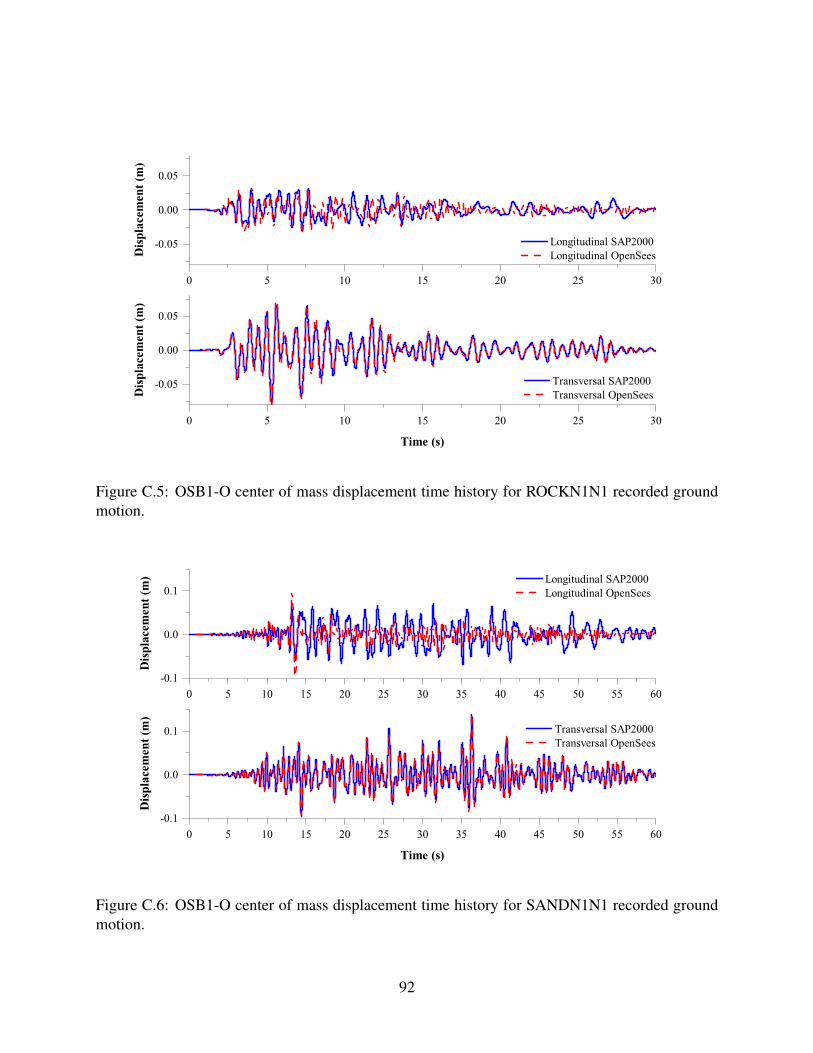
0 5 10 15 20 25 30
-0.05
0.00
0.05
Transversal SAP2000 Transversal OpenSeesD
ispla
cem
ent (
m)
Time (s)
0 5 10 15 20 25 30
-0.05
0.00
0.05
Longitudinal SAP2000 Longitudinal OpenSeesD
ispla
cem
ent (
m)
Figure C.5: OSB1-O center of mass displacement time history for ROCKN1N1 recorded groundmotion.
0 5 10 15 20 25 30 35 40 45 50 55 60-0.1
0.0
0.1 Transversal SAP2000 Transversal OpenSees
Disp
lace
men
t (m
)
Time (s)
0 5 10 15 20 25 30 35 40 45 50 55 60-0.1
0.0
0.1 Longitudinal SAP2000 Longitudinal OpenSees
Disp
lace
men
t (m
)
Figure C.6: OSB1-O center of mass displacement time history for SANDN1N1 recorded groundmotion.
92

0 5 10 15 20 25 30-0.05
0.00
0.05
Transversal SAP2000 Transversal OpenSees
Disp
lace
men
t (m
)
Time (s)
0 5 10 15 20 25 30-0.05
0.00
0.05 Longitudinal SAP2000 Longitudinal OpenSees
Disp
lace
men
t (m
)
Figure C.7: OSB2-O center of mass displacement time history for ROCKN1N1 recorded groundmotion.
0 5 10 15 20 25 30 35 40 45 50 55 60-0.05
0.00
0.05 Transversal SAP2000 Transversal OpenSees
Disp
lace
men
t (m
)
Time (s)
0 5 10 15 20 25 30 35 40 45 50 55 60-0.05
0.00
0.05 Longitudinal SAP2000 Longitudinal OpenSees
Disp
lace
men
t (m
)
Figure C.8: OSB2-O center of mass displacement time history for SANDN1N1 recorded groundmotion.
93
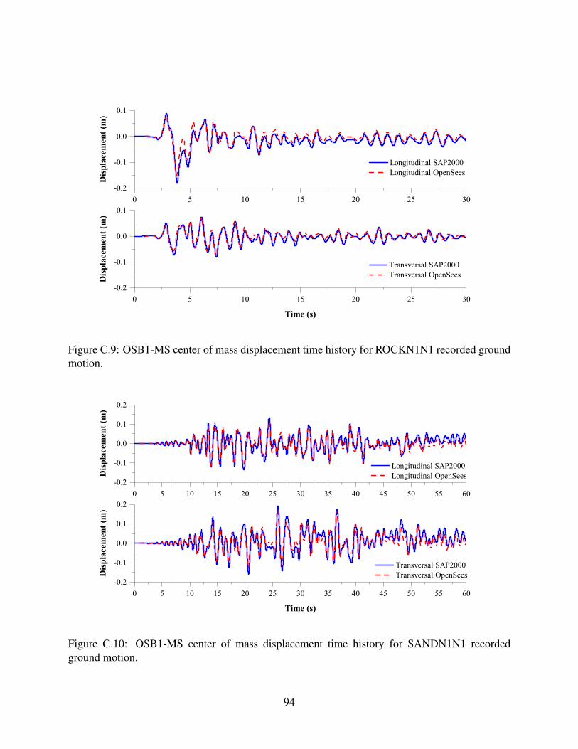
0 5 10 15 20 25 30-0.2
-0.1
0.0
0.1
Transversal SAP2000 Transversal OpenSeesD
ispla
cem
ent (
m)
Time (s)
0 5 10 15 20 25 30-0.2
-0.1
0.0
0.1
Longitudinal SAP2000 Longitudinal OpenSees
Disp
lace
men
t (m
)
Figure C.9: OSB1-MS center of mass displacement time history for ROCKN1N1 recorded groundmotion.
0 5 10 15 20 25 30 35 40 45 50 55 60-0.2
-0.1
0.0
0.1
0.2
Transversal SAP2000 Transversal OpenSeesD
ispla
cem
ent (
m)
Time (s)
0 5 10 15 20 25 30 35 40 45 50 55 60-0.2
-0.1
0.0
0.1
0.2
Longitudinal SAP2000 Longitudinal OpenSeesD
ispla
cem
ent (
m)
Figure C.10: OSB1-MS center of mass displacement time history for SANDN1N1 recordedground motion.
94

0 5 10 15 20 25 30
-0.05
0.00
0.05
Transversal SAP2000 Transversal OpenSeesD
ispla
cem
ent (
m)
Time (s)
0 5 10 15 20 25 30
-0.05
0.00
0.05
Longitudinal SAP2000 Longitudinal OpenSeesD
ispla
cem
ent (
m)
Figure C.11: OSB2-MS center of mass displacement time history for ROCKN1N1 recordedground motion.
0 5 10 15 20 25 30 35 40 45 50 55 60-0.10
-0.05
0.00
0.05
0.10
0.15 Transversal SAP2000 Transversal OpenSees
Disp
lace
men
t (m
)
Time (s)
0 5 10 15 20 25 30 35 40 45 50 55 60-0.10
-0.05
0.00
0.05
0.10
0.15 Longitudinal SAP2000 Longitudinal OpenSees
Disp
lace
men
t (m
)
Figure C.12: OSB2-MS center of mass displacement time history for SANDN1N1 recordedground motion.
95
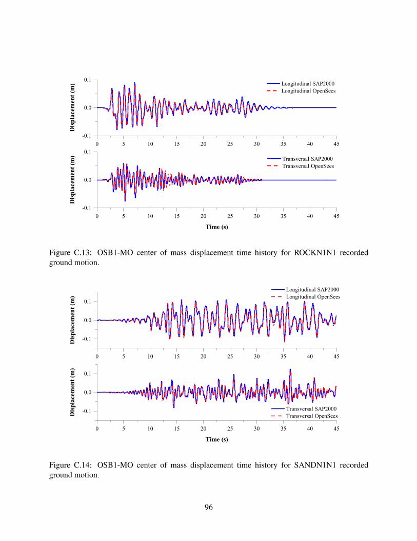
0 5 10 15 20 25 30 35 40 45-0.1
0.0
0.1 Transversal SAP2000 Transversal OpenSees
Disp
lace
men
t (m
)
Time (s)
0 5 10 15 20 25 30 35 40 45-0.1
0.0
0.1 Longitudinal SAP2000 Longitudinal OpenSees
Disp
lace
men
t (m
)
Figure C.13: OSB1-MO center of mass displacement time history for ROCKN1N1 recordedground motion.
0 5 10 15 20 25 30 35 40 45
-0.1
0.0
0.1
Transversal SAP2000 Transversal OpenSeesD
ispla
cem
ent (
m)
Time (s)
0 5 10 15 20 25 30 35 40 45
-0.1
0.0
0.1
Longitudinal SAP2000 Longitudinal OpenSees
Disp
lace
men
t (m
)
Figure C.14: OSB1-MO center of mass displacement time history for SANDN1N1 recordedground motion.
96
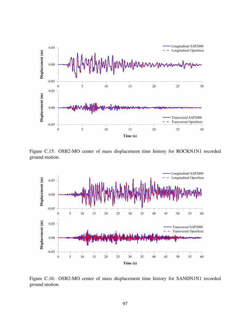
0 5 10 15 20 25 30-0.05
0.00
0.05
Transversal SAP2000 Transversal OpenSeesD
ispla
cem
ent (
m)
Time (s)
0 5 10 15 20 25 30-0.05
0.00
0.05 Longitudinal SAP2000 Longitudinal OpenSees
Disp
lace
men
t (m
)
Figure C.15: OSB2-MO center of mass displacement time history for ROCKN1N1 recordedground motion.
0 5 10 15 20 25 30 35 40 45 50 55 60-0.05
0.00
0.05 Transversal SAP2000 Transversal OpenSees
Disp
lace
men
t (m
)
Time (s)
0 5 10 15 20 25 30 35 40 45 50 55 60-0.05
0.00
0.05
Longitudinal SAP2000 Longitudinal OpenSees
Disp
lace
men
t (m
)
Figure C.16: OSB2-MO center of mass displacement time history for SANDN1N1 recordedground motion.
97

APPENDIX D: CONSTANT DUCTILITY RESPONSE SPECTRUM
98
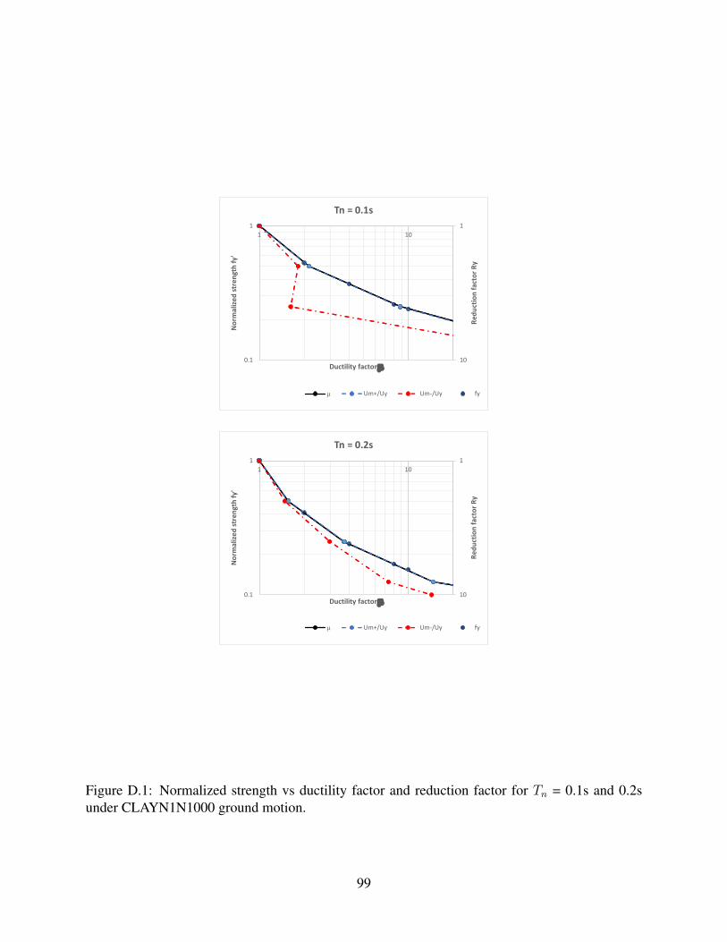
1
100.1
11 10
Redu
ctio
n fa
ctor
Ry
Nor
mal
ized
str
engt
h fy
'
Ductility factor m
Tn = 0.1s
m Um+/Uy Um-/Uy fy
1
100.1
11 10
Redu
ctio
n fa
ctor
Ry
Nor
mal
ized
str
engt
h fy
'
Ductility factor m
Tn = 0.2s
m Um+/Uy Um-/Uy fy
Figure D.1: Normalized strength vs ductility factor and reduction factor for Tn = 0.1s and 0.2sunder CLAYN1N1000 ground motion.
99

1
100.1
11 10
Redu
ctio
n fa
ctor
Ry
Nor
mal
ized
str
engt
h fy
'
Ductility factor m
Tn = 0.3s
m Um+/Uy Um-/Uy fy
1
100.1
11 10
Redu
ctio
n fa
ctor
Ry
Nor
mal
ized
str
engt
h fy
'
Ductility factor m
Tn = 0.4s
m Um+/Uy Um-/Uy fy
Figure D.2: Normalized strength vs ductility factor and reduction factor for Tn = 0.3s and 0.4sunder CLAYN1N1000 ground motion.
100
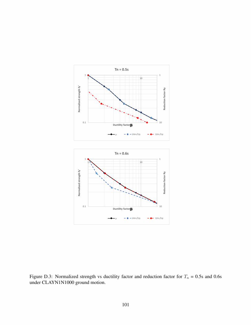
1
100.1
11 10
Redu
ctio
n fa
ctor
Ry
Nor
mal
ized
str
engt
h fy
'
Ductility factor m
Tn = 0.5s
m Um+/Uy Um-/Uy
1
100.1
11 10
Redu
ctio
n fa
ctor
Ry
Nor
mal
ized
str
engt
h fy
'
Ductility factor m
Tn = 0.6s
m Um+/Uy Um-/Uy
Figure D.3: Normalized strength vs ductility factor and reduction factor for Tn = 0.5s and 0.6sunder CLAYN1N1000 ground motion.
101
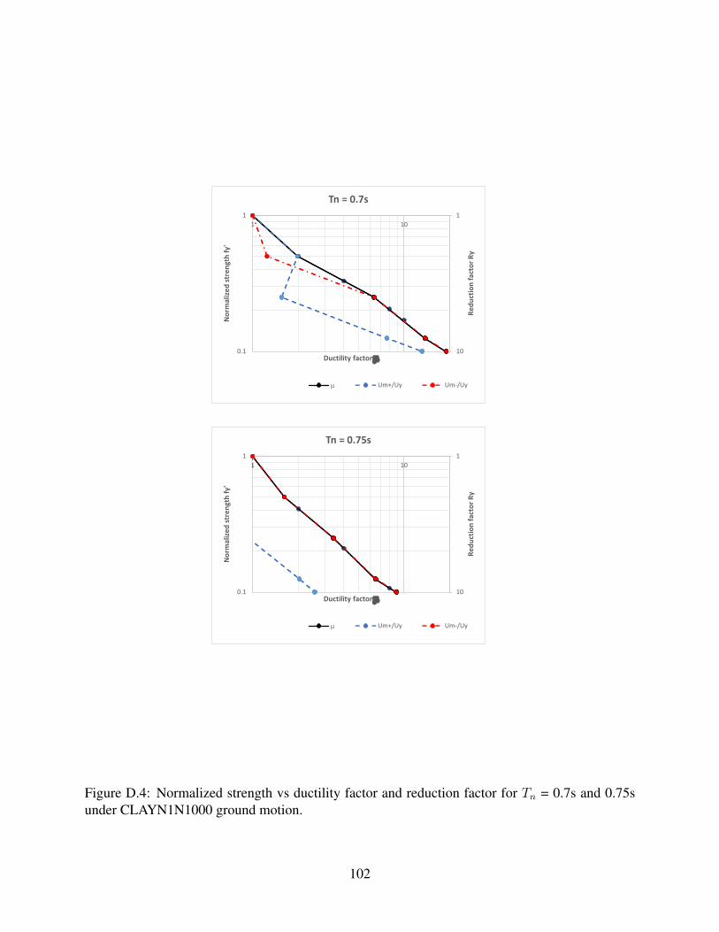
1
100.1
11 10
Redu
ctio
n fa
ctor
Ry
Nor
mal
ized
str
engt
h fy
'
Ductility factor m
Tn = 0.7s
m Um+/Uy Um-/Uy
1
100.1
11 10
Redu
ctio
n fa
ctor
Ry
Nor
mal
ized
str
engt
h fy
'
Ductility factor m
Tn = 0.75s
m Um+/Uy Um-/Uy
Figure D.4: Normalized strength vs ductility factor and reduction factor for Tn = 0.7s and 0.75sunder CLAYN1N1000 ground motion.
102
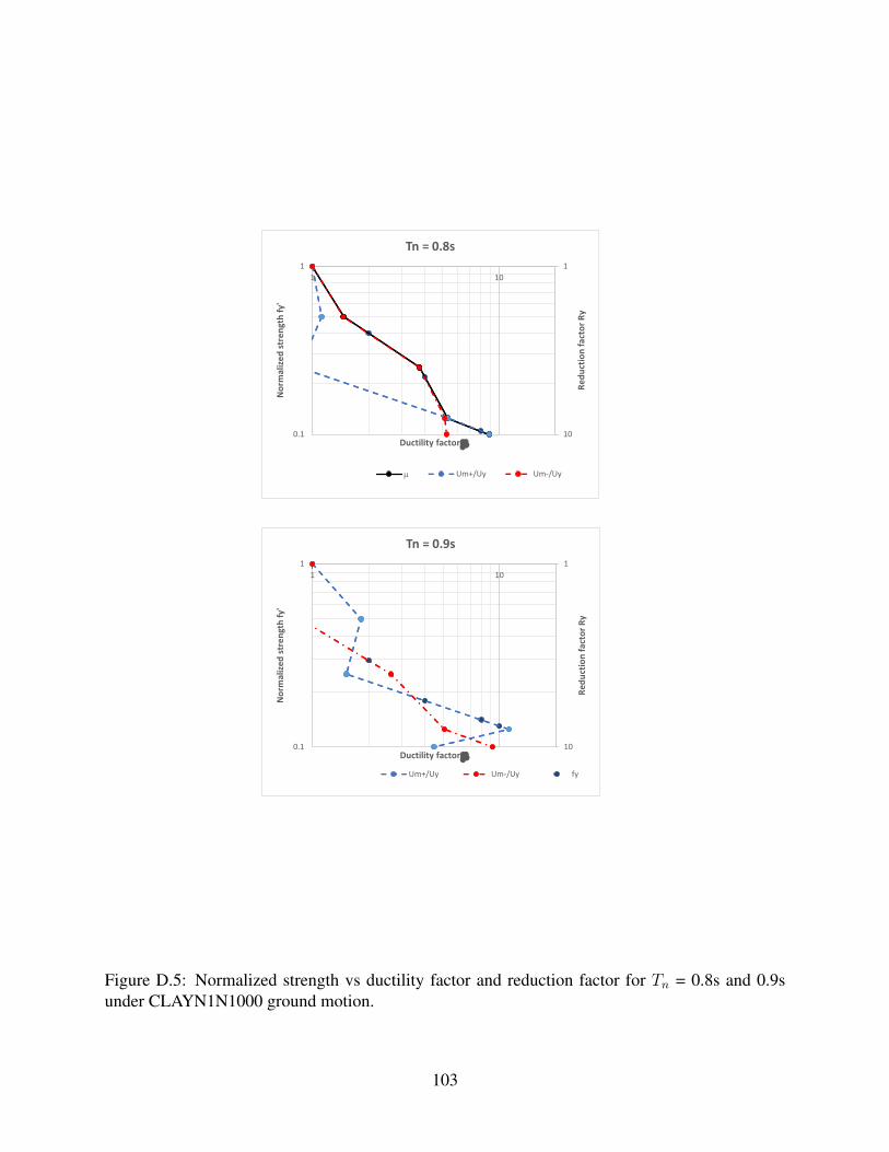
1
100.1
11 10
Redu
ctio
n fa
ctor
Ry
Nor
mal
ized
str
engt
h fy
'
Ductility factor m
Tn = 0.8s
m Um+/Uy Um-/Uy
1
100.1
11 10
Redu
ctio
n fa
ctor
Ry
Nor
mal
ized
str
engt
h fy
'
Ductility factor m
Tn = 0.9s
Um+/Uy Um-/Uy fy
Figure D.5: Normalized strength vs ductility factor and reduction factor for Tn = 0.8s and 0.9sunder CLAYN1N1000 ground motion.
103

1
100.1
11 10
Redu
ctio
n fa
ctor
Ry
Nor
mal
ized
str
engt
h fy
'
Ductility factor m
Tn = 1.0s
m Um+/Uy Um-/Uy
1
100.1
11 10
Redu
ctio
n fa
ctor
Ry
Nor
mal
ized
str
engt
h fy
'
Ductility factor m
Tn = 1.25s
m Um+/Uy Um-/Uy
Figure D.6: Normalized strength vs ductility factor and reduction factor for Tn = 1.0s and 1.25sunder CLAYN1N1000 ground motion.
104

1
100.1
11 10
Redu
ctio
n fa
ctor
Ry
Nor
mal
ized
str
engt
h fy
'
Ductility factor m
Tn = 1.5s
m Um+/Uy Um-/Uy
1
100.1
11 10
Redu
ctio
n fa
ctor
Ry
Nor
mal
ized
str
engt
h fy
'
Ductility factor m
Tn = 1.75s
m Um+/Uy Um-/Uy
Figure D.7: Normalized strength vs ductility factor and reduction factor for Tn = 1.5s and 1.75sunder CLAYN1N1000 ground motion.
105
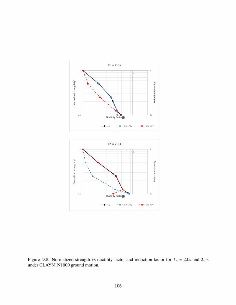
1
100.1
11 10
Redu
ctio
n fa
ctor
Ry
Nor
mal
ized
str
engt
h fy
'
Ductility factor m
Tn = 2.0s
m Um+/Uy Um-/Uy
1
100.1
11 10
Redu
ctio
n fa
ctor
Ry
Nor
mal
ized
str
engt
h fy
'
Ductility factor m
Tn = 2.5s
m Um+/Uy Um-/Uy
Figure D.8: Normalized strength vs ductility factor and reduction factor for Tn = 2.0s and 2.5sunder CLAYN1N1000 ground motion.
106

1
100.1
11 10
Redu
ctio
n fa
ctor
Ry
Nor
mal
ized
str
engt
h fy
'
Ductility factor m
Tn = 3.0s
m Um+/Uy Um-/Uy
1
100.1
11 10
Redu
ctio
n fa
ctor
Ry
Nor
mal
ized
str
engt
h fy
'
Ductility factor m
Tn = 4.0s
m Um+/Uy Um-/Uy
Figure D.9: Normalized strength vs ductility factor and reduction factor for Tn = 3.0s and 4.0sunder CLAYN1N1000 ground motion.
107

1
100.1
11 10
Redu
ctio
n fa
ctor
Ry
Nor
mal
ized
str
engt
h fy
'
Ductility factor m
Tn = 5.0s
m Um+/Uy Um-/Uy
1
100.1
11 10
Redu
ctio
n fa
ctor
Ry
Nor
mal
ized
str
engt
h fy
'
Ductility factor m
Tn = 10.0s
m Um+/Uy Um-/Uy
Figure D.10: Normalized strength vs ductility factor and reduction factor for Tn = 5.0s and 10.0sunder CLAYN1N1000 ground motion.
108
LIST OF REFERENCES
Aviram, A., Mackie, K., & Stojadinovic, B. (2008). Guidelines of Nonlinear Analysis of Bridge
Structures in California (tech. rep. August). Pacific Earthquake Engineering Research Cen-
ter, University of Berkely. Berkeley, California.
Bolin, R., & Stanford, L. (2006). The Northridge earthquake: Vulnerability and disaster. https:
//doi.org/10.4324/9780203028070
Chopra, A. K. (2012). DYNAMICS OF STRUCTURES Theory and Applications to Earthquake
Engineering (W. J. Hall, Ed.; Fourth Edi). Berkeley, California, Pearson.
CSI. (2017). CSI analysis reference manual for SAP2000, ETAPS, SAFE, and CSIBridge. Berkeley,
California, Computer & Structures, Inc.
EERI. (1989). The Loma Prieta earthquake of October 17, 1989. Earthquakes & Volcanoes (USGS),
21(6), 216–237.
Fenves, G. L., & Ellery, M. (1998). Behavior and failure analysis of a multiple-frame highway
bridge in the 1994 Northridge earthquake (tech. rep.). Pacific Earthquake Engineering Re-
search Center, University of California. Berkeley, California.
Fung, G. G., Lebeau, E., Klein, J., Belverder, & Goldschmidt, A. (1971). Field investigation of
bridge damage in the San Fernando earthquake. Sacramento, California, California De-
partment of Transportation, bridge department, division of highways.
Ghotbi, A. R. (2014). Performance-based seismic assessment of skewed bridges with and without
considering soil-foundation interaction effects for various site classes. Earthquake Engi-
neering and Engineering Vibration, 13(3), 357–373. https://doi.org/10.1007/s11803-014-
0248-7
Haukaas, T., & Der Kiureghian, A. (2007). Methods and Object-Oriented Software for FE Reliabil-
ity and Sensitivity Analysis with Application to a Bridge Structure. Journal of Computing
109

in Civil Engineering, 21(3), 151–163. https://doi.org/10.1061/(ASCE)0887-3801(2007)21:
3(151)
Jeremic, B., Kunnath, S., & Xiong, F. (2004). Influence of soil-foundation-structure interaction
on seismic response of the I-880 viaduct. Engineering Structures, 26(3), 391–402. https:
//doi.org/10.1016/j.engstruct.2003.10.011
Jurado, J.A., Hernadez, S., Nieto, F., & Mosquera, A. (2011). Bridge aeroeslasticity, sensitivity
analysis and optimal desing. Billerica, MA, USA, WIT Press.
Kappos, A. J., & Dimitrakopoulos, E. (2005). Analysis and assessment of a seismically isolated
bridge. WIT Transactions on the Built Environment, 81, 625–635. https://doi.org/10.2495/
978-1-84564-672-1/13
Kawashima, K., Unjoh, S., Hoshikuma, J. I., & Kosa, K. (2011). Damage of bridges due to the
2010 Maule, Chile, earthquake. Journal of Earthquake Engineering, 15(7), 1036–1068.
https://doi.org/10.1080/13632469.2011.575531
Khan, M. A. (2015). Accelerated bridge construction, best practices and techniques. Waltham,
MA, USA, Butterworth-Heinemann.
Kleiber, M., Antunez, H., Hien, T. D., & Kowalczyk, P. (1997). Parameter sensitivity in nonlinear
mechanics. Theory and finite element computations. New York, John Wiley & Sons, Inc.
https://doi.org/10.1016/s0997-7538(99)80031-x
Kunnath, S. K. (2007). Application of the PEER PBEE methodology to the I-880 viaduct. (tech.
rep.). Pacific Earthquake Engineering Research Center, University of California. Berkeley,
California.
Kwon, O. S., & Elnashai, A. S. (2008). Seismic analysis of meloland road overcrossing using mul-
tiplatform simulation software including SSI. Journal of Structural Engineering, 134(4),
651–660. https://doi.org/10.1061/(ASCE)0733-9445(2008)134:4(651)
110

Lu, J., Elgamal, A., & Mackie, K. R. (2015). Parametric Study of Ordinary Standard Bridges
using OpenSees and CSiBridge (tech. rep. No. 2). California Department of Transportation,
University of California. La Jolla, California.
Mackie, K. R. (2008). Integrated Probabilistic Performance-Based Evaluation of Benchmark Rein-
forced Concrete Bridges. Pacific Earthquake Engineering Research Center, (PEER Report
2007/09).
Mackie, K. R., & Scott, M. H. (2019). Implementation of Nonlinear Elements for Seismic Re-
sponse Analysis of Bridges. Practice Periodical on Structural Design and Construction,
24(3), 1–14. https://doi.org/10.1061/(ASCE)SC.1943-5576.0000420
Mackie, K. R., Scott, M. H., Johnsohn, K., Al-Ramahee, M., & Steijlen, M. (2017). Nonlinear
Time History Analysis of Ordinary Standard Bridges (tech. rep.). California Department of
Transportation (Caltrans). Sacramento, California. https://rosap.ntl.bts.gov/view/dot/37382
Mackie, K. R., & Stojadinovic, B. (2003). Seismic demands for performance based design of
bridges (tech. rep. August). Pacific Earthquake Engineering Research Center, University
of California. Berkeley, California.
Mackie, K. R., & Stojadinovic, B. (2005). Fragility basis for California highway overpass brige
seismic decision making (tech. rep. June). Pacific Earthquake Engineering Research Center,
University of California. Berkeley, California.
Mander, J., Priestley, M., & Park, R. (1988). Theoretical stress-strain model for confined concrete.
Journal of Structural Engineering. Journal of Structural Engineering, 114(8): 1804–1826.
Nielson, B. G., & DesRoches, R. (2007). Analytical seismic fragility curves for typical bridges
in the central and southeastern United States. Earthquake Spectra, 23(3), 615–633. https:
//doi.org/10.1193/1.2756815
NIST. (1996). The January 17, 1995 Hyogoken-Nanbu (Kobe) earthquake. Performance of struc-
tures, lifelines, and fire protection systems. NIST SP 901 (tech. rep.). National Institute of
Standards and Technology. Gaithersburg, MD.
111

Omrani, R., Mobasher, B., Liang, X., Gunay, S., Mosalam, K. M., Zareian, F., & Taciroglu, E.
(2015). Guidelines for Nonlinear Seismic Analysis of Ordinary Bridges: Version 2.0 (tech.
rep. December). California Department of Transportation (Caltrans). Sacramento, Califor-
nia. https://doi.org/10.13140/RG.2.1.4946.6648
Pan, Y., Agrawal, A. K., Ghosn, M., & Alampalli, S. (2010). Seismic Fragility of Multispan Sim-
ply Supported Steel Highway Bridges in New York State. I: Bridge Modeling, Paramet-
ric Analysis, and Retrofit Design. Journal of Bridge Engineering, 15(5), 448–461. https:
//doi.org/10.1061/(ASCE)BE.1943-5592.0000085
Pinto, P. E., & Franchin, P. (2010). Open Issues in the Seismic Design and Assessment of Bridges,
In Geotechnical, earthquake engineering in europe (vol. 17). Rome, Italy, Springer. https:
//doi.org/10.1007/978-90-481-9544-2 13
Priestly, N. M. J., Seible, F., & Calvi, G. M. (1996). Seismic Design and Retrofit of Bridges. New
York, John Wiley & Sons, Inc.
Sullivan, I., & Nielson, B. G. (2010). Sensitivity Analysis of Seismic Fragility Curves for Skewed
Multi-Span Simply Supported Steel Girder Bridges, In Structures congress 2010, Reston,
VA, American Society of Civil Engineers. https://doi.org/10.1061/41131(370)19
Zhang, Y., Acero, G., Conte, J., Yang, Z., & Elgamal, A. (2004). Seismic Reliability Assessment
of a Bridge Ground System. 13th World Conference on Earthquake Engineering, Paper No.
2978.
Zhao, Q., Vasheghani-Farahani, R., & Burdette, E. G. (2011). Seismic Analysis of Integral Abut-
ment Bridges Including Soil-Structure Interaction, In Structures congress 2011, Reston,
VA, American Society of Civil Engineers. https://doi.org/10.1061/41171(401)26
Zona, A., Barbato, M., & Conte, J. P. (2006). Finite element response sensitivity analysis of con-
tinuous steel-concrete composite girders. Steel and Composite Structures, 6(3), 183–202.
https://doi.org/10.12989/scs.2006.6.3.183
112
Related Documents