Contrast Sensitivity Is Enhanced by Expansive Nonlinear Processing in the Lateral Geniculate Nucleus

1

Contrast sensitivity is enhanced by expansive nonlinear processing in the LGN

Thang Duong and Ralph D. Freeman

Group in Vision Science, School of Optometry, and Helen Wills Neuroscience Institute

University of California, Berkeley

Berkeley, California 94720-2020

Running head: Expansive nonlinearity in LGN

Contact Information:

Ralph D. Freeman

360 Minor Hall

University of California, Berkeley

Berkeley, CA 94720-2020

Email: [email protected]

Page 1 of 26 Articles in PresS. J Neurophysiol (October 24, 2007). doi:10.1152/jn.00873.2007

Copyright © 2007 by the American Physiological Society.

2

Abstract

The firing rates of neurons in the central visual pathway vary with stimulus strength, but

not necessarily in a linear manner. In the contrast domain, the neural response function

for cells in the primary visual cortex is characterized by expansive and compressive

nonlinearities at low and high contrasts, respectively. A compressive nonlinearity at high

contrast is also found for early visual pathway neurons in the LGN. This mechanism

affects processing in the visual cortex. A fundamentally related issue is the possibility of

an expansive nonlinearity at low contrast in LGN. To examine this possibility, we have

obtained contrast-response data for a population of LGN neurons. We find for most cells

that the best fit function requires an expansive component. Additionally, we have

measured the responses of LGN neurons to m-sequence white noise and examine the

static relationship between a linear prediction and actual spike rate. We find that this

static relationship is well-fit by an expansive nonlinear power law with average exponent

of 1.58. These results demonstrate that neurons in early visual pathways exhibit

expansive nonlinear responses at low contrasts. While this thalamic expansive

nonlinearity has been largely ignored in models of early visual processing, it may have

important consequences because it potentially affects the interpretation of a variety of

visual functions.

Page 2 of 26

3

Introduction

The standard Weiner system consisting of a linear component followed by a static

nonlinearity has been used extensively as a functional model for neurons in the retina,

LGN, and primary visual cortex (Nykamp and Ringach 2002). This model is accurate for

neurons in the retina and LGN, although other nonlinearities exist (Chichilnisky 2001;

Victor 1987; Victor and Shapley 1979). Specifically, in the LGN and retina, a contrast

gain control mechanism decreases the neuronal response gain with increasing stimulus

contrast. This provides high sensitivity for small changes of stimulus contrast over a wide

range. A recent model proposes that the underlying mechanism for contrast gain control

in LGN neurons is a suppressive region within the receptive field (Bonin et al. 2005).

This model consists of three components: a linear classical receptive field, a nonlinear

suppressive field, and a response rectification. The nonlinear suppressive field serves to

compute local contrast of the stimulus. This local contrast then decreases the linear

receptive field gain by divisive normalization. A final linear threshold function converts

this signal to a positive spike rate.

In this suppressive field model, as stimulus contrast increases, the local contrast within

the suppressive field also increases, which decreases the response gain. This decrease in

gain causes a saturation of response with increasing stimulus contrast. An assumption of

this model is that the static nonlinear component is simply a linear rectifying function.

This is of primary significance because it implies an approximately linear response at low

Page 3 of 26

4

contrast levels where the suppressive field is minimally activated. If in fact there is a

clear nonlinearity at low contrasts, this addition can improve the predictive power of the

suppressive field model, and it also could have implications for the interpretation of

visual function at low contrasts.

We have examined this issue by obtaining contrast response functions from extra-cellular

recordings of neurons in the cat’s LGN. We fit the data with a Naka-Rushton function

(Naka and Rushton 1966). Results show significant expansive nonlinearities at low

contrasts. Additionally, we have measured directly the static nonlinear function by

comparing a linear prediction with actual spike responses. The linear predictions are

generated from spatiotemporal receptive fields obtained via m-sequence stimulation.

Static nonlinear functions for the majority of neurons of our sample exhibit power-law

nonlinearities with a mean exponent of 1.58. These results show a clear expansive

nonlinear component in LGN neurons for low contrast visual stimuli. It is likely that this

has important consequences for basic response properties of cortical neurons.

Methods

Physiological Preparation

All procedures complied with the National Institutes of Health Guide for the Care and

Use of Laboratory Animals. Extracellular recordings are made using epoxy coated

tungsten microelectrodes in the LGN of anaesthetized and paralyzed mature cats. Cats

are initially anaesthetized with isofluorane (1-4%). After catheterization, a continuous

infusion is given of a combination of fentanyl citrate (10µg kg-1hr-1) and thiopental

Page 4 of 26

5

sodium (6mg kg-1hr-1). Bolus injections of thiopental sodium are given as required

during surgery. After a tracheal cannula is positioned, isofluorane is discontinued, and

the animal is artificially ventilated with a mixture of 25% O2 and 75% N2O. Respiration

rate is manually adjusted to maintain an end-tidal CO2 of 34-38mmHg. Body

temperature is maintained at 38 oC with a closed-loop controlled heating pad. A

craniotomy is performed over the LGN, and the dura is resected and covered with agar

and wax to form a closed chamber. After completion of all surgical procedures,

continuous injection of fentanyl citrate is discontinued, and thiopental sodium

concentration is lowered gradually to a level at which the cat is stabilized for one hour or

more. The level of anesthetic used is determined individually for each cat. The range

used is 1.0-3.0 mg kg-1hr-1 and a typical level is 1.5mg kg-1hr-1. Once a stabilized

anesthetic level is reached, it is kept constant throughout the experiment. To minimize

eye movements during visual tests, animals are immobilized with pancuronium bromide

(0.2 mg kg-1hr-1). EEG, ECG, heart rate, temperature, end-tidal CO2, and intra-tracheal

pressure are monitored for the entire duration of the experiment. Contact lenses are used

which are opaque except for a central 4mm diameter window to create an artificial pupil.

To focus the eyes on the stimulation screen, opthalmoscopic refraction is used to

determine appropriate lens power.

Electrode penetrations are made perpendicular to the cortical surface at approximately

Horsley-Clarke coordinates A6L9. Electrodes are then advanced until visually

responsive cells with LGN response characteristics are found (typically around 12mm

below the cortical surface). Recordings were made from all layers of the LGN.

Page 5 of 26

6

Extracellular Recording

Single units are isolated in real-time by the shape of their spike waveforms using custom

software. An initial estimate of the tuning parameters is made qualitatively by computer-

controlled manipulation of drifting sinusoidal gratings. The spatial extent of visual

stimulation is kept larger than the receptive field size. Temporal frequency tuning curves

are measured with drifting sinusoidal gratings at 50% contrast. Spatial frequency and

contrast tuning curves are measured at optimal temporal frequencies determined for each

cell, typically between 4 and 15 cycles per second.

Visual Stimulation

Visual patterns consisting of sinusoidal gratings or noise patterns are presented on a large

CRT at a frame rate of 75 Hz. The 47.8 cm diameter CRT is positioned at an optical

distance of 41.8 cm in front of the cat’s eyes, and is split so that each half of the display

stimulates left or right eye. Luminance from the CRT is calibrated for a linear range with

maximum and minimum values of 90cd/m2 and 0.1cd/m2, respectively.

Data Analysis

For contrast tuning data, the first harmonic (F1 component) is used for analysis. All data

fitting is done by minimizing the sum squared error using fminsearch in Matlab (The

MathWorks; MA), which implements the Nelder-Mead nonlinear minimization

algorithm. For m-sequence analysis, spikes are first binned with a window of one m-

Page 6 of 26

7

sequence frame (typically about 13ms). Reverse correlation is done using the fast m-

transform method (Reid et al. 1997; Sutter 1991), and the first order kernel is extracted

from m-transformed data. Estimation of the static nonlinearity is done by comparing the

linear prediction to the actual spike response. Linear predictions are generated by

convolving the linear spatiotemporal receptive fields with the m-sequence stimulus.

Details of this analysis are given elsewhere (Anzai et al. 1999a; Chichilnisky 2001).

Results

To evaluate contrast tuning, we collected complete data for 168 LGN neurons. Visual

stimulation via m-sequence tests was run on 250 LGN cells. These two populations of

LGN neurons are partially overlapping. Additionally, we tested 96 simple cells in area

17 with m-sequence stimulation.

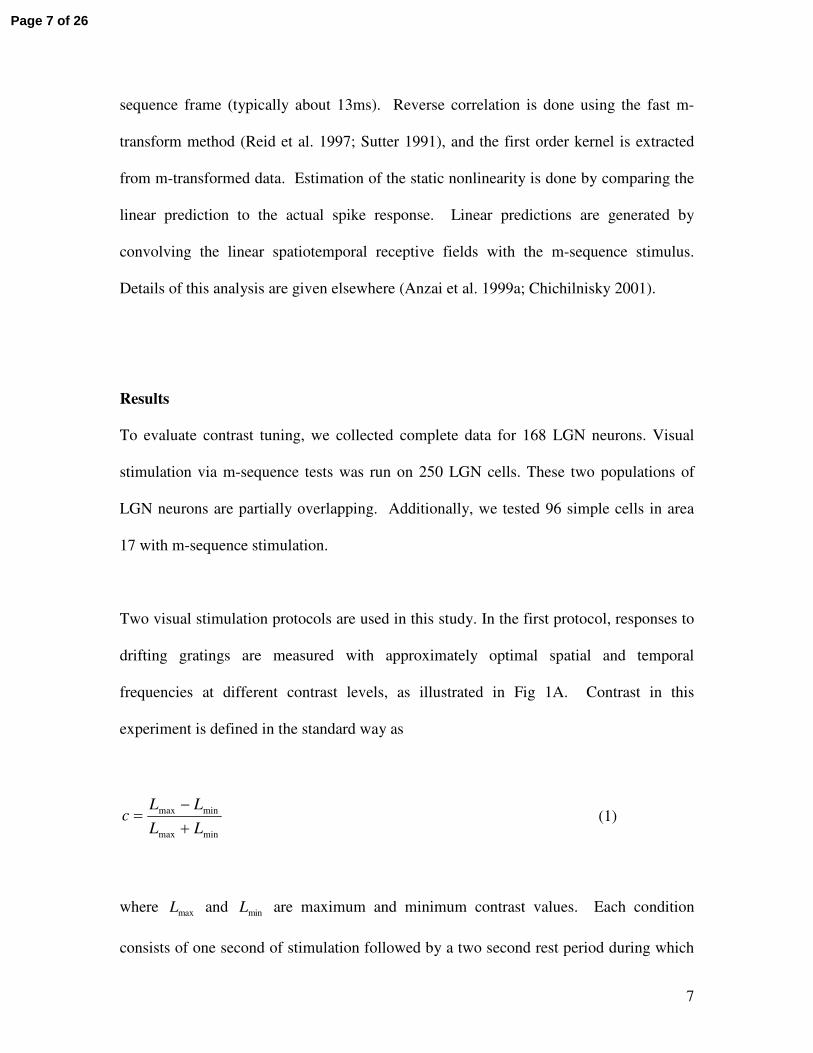
Two visual stimulation protocols are used in this study. In the first protocol, responses to

drifting gratings are measured with approximately optimal spatial and temporal

frequencies at different contrast levels, as illustrated in Fig 1A. Contrast in this

experiment is defined in the standard way as

minmax

minmax

LL

LLc

+−

= (1)

where maxL and minL are maximum and minimum contrast values. Each condition

consists of one second of stimulation followed by a two second rest period during which

Page 7 of 26

8

the screen is blank and is displayed at the mean luminance level. This protocol was run

on 168 cells. The second protocol is a standard binary m-sequence stimulation procedure

(Anzai et al. 1999a, b; Reid et al. 1997). Briefly, the stimulus field is split into a grid of

either 8x8 or 16x16 elements centered on the receptive field. For cortical neurons, the

dominant eye is stimulated. Luminance of individual grid elements is modulated at 75

Hz following a 14-bit binary m-sequence. An inverse repeat stimulation is always used

(Reid et al. 1997; Sutter 1991), and multiple repetitions are presented per neuron as

needed based on the signal-to-noise ratio of the response. The modulation is at 100%

contrast so that each grid element can have a luminance of either 0.1cd/m2 or 90cd/m2.

Spatiotemporal receptive fields are calculated using the fast m-transform (Reid et al.

1997; Sutter 1991). Figure 1C illustrates this stimulus. For both visual stimulation

protocols, gratings or white noise patterns larger than the receptive field sizes were used.

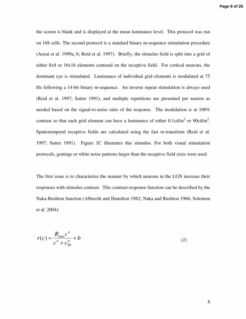
The first issue is to characterize the manner by which neurons in the LGN increase their

responses with stimulus contrast. This contrast-response function can be described by the

Naka-Rushton function (Albrecht and Hamilton 1982; Naka and Rushton 1966; Solomon

et al. 2004):

bcc

cRcr

nn

n

++

=50

max)( (2)

Page 8 of 26

9

Where )(cr is the neural response at contrast c; n , maxR , 50c , and b , are free parameters.

For 1>n , this function is expansive at low contrast levels and compressive at high

contrasts with an inflection point at

ni n

ncc

1

150 +

−= , 1>n (3)

so that )(cr exhibits an expansive nonlinearity for contrasts less than ic and a saturation

nonlinearity for contrasts larger than ic . Figure 1 B, D illustrates this point. Figure 1B

shows the Naka-Rushton function (solid curve) and, at low contrasts, the best fit power-

law function (dashed curve) given by:

baccr n +=)( (4)

where a ,b , and n are free parameters. The dotted curve shows an example Naka-

Rushton fit without the expansive component. Details of this function are given in

equation (5) below. Filled and unfilled arrows denote 50c and ic , respectively. A

comparison of n for equations (2) and (4) shows that the best fit power-law exponent n

(y-axis) is lower than that of the corresponding Naka-Rushton value (x-axis) as shown in

Fig 1D. The data points here (open circles) are calculated by fitting equation (4) to the

Naka-Rushton functions with various values of n . The best fit exponents in equation (4)

Page 9 of 26

10

are then plotted on the y-axis. The x=y unity solid line here is clearly above the data

points.

Recent studies and models assume that contrast-response data for LGN neurons follow

the Naka-Rushton function with n=1 (Bonin et al. 2005; Li et al. 2006; Priebe and Ferster

2006). This assumption means that the contrast-response function of LGN neurons does

not exhibit an expansive component. It implies that LGN neurons undergo saturation at

all contrast levels above firing threshold. However, our measurements, as described

below, are at odds with this assumption. They demonstrate that LGN neurons exhibit

expansive power-law nonlinearities when stimulated with low contrast gratings. To

quantify this observation, we have measured the neural responses to gratings at different

contrasts for our population of LGN neurons and we calculate the best-fit Naka-Rushton

function to these data. Figure 2A, B, and C show the best fits for n , 50c , and ic ,

respectively, for 168 LGN cells. The mean and SEM values for n , 50c , and ic are

2.47±0.162, 68.89±5.45, and 27.42±2.01, respectively. The medians for n , 50c , and ic

are 2.03, 38.87, and 17.72, respectively, and the modes are 1.758, 27.51, and 13.91,

respectively. Mean values are indicated by unfilled arrows above the histograms. Note

that these distributions are non-normal.

To test whether an expansive nonlinearity is necessary to describe the contrast-response

function, we also fit a modified Naka-Rushton function to the data. This modified

function has no expansive component and is given by the following equation:

Page 10 of 26

11

bcc

cRcr

nn+

+=

50

max)( (5)

where the exponent in the numerator of the Naka-Rushton function is removed. Note that

for the common case when the exponent of both the numerator and denominator is set to

one, the fit is equal or worse than that with equation (5). A plot of example functions

from equations (2), (4), and (5) is given in Figure 1B (solid, dashed, and dotted,

respectively). Figure 2 D-F shows the contrast response data and best fit Naka-Rushton

functions for three representative LGN neurons. The dashed and solid lines denote best

fit functions with (equation 2) and without (equation 5) expansive nonlinearity,

respectively. Clearly, for these cells, the data are better described with the expansive

nonlinear component than without. The differences in fits may have substantial

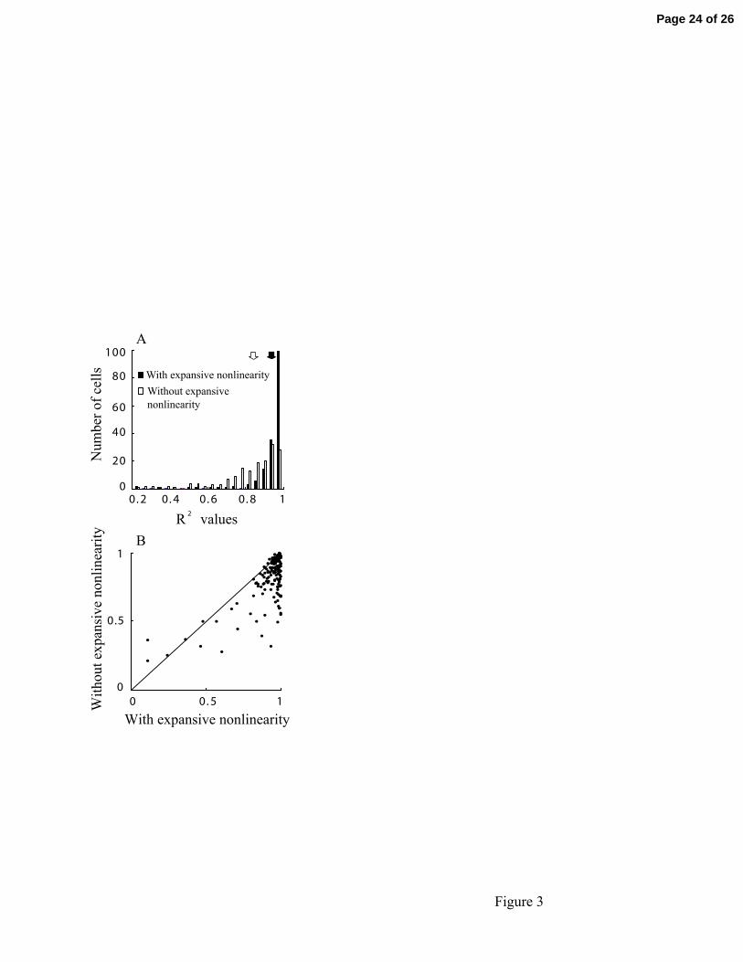
consequences as considered below. We quantify this relationship further in Figure 3. For

each cell, R2 values are calculated using the best fit function with and without expansive

nonlinearity. Figure 3A shows the R2 values of the fit with and without the expansive

component. Mean and SEM with and without expansive nonlinearity are 0.9233±0.0110

and 0.8191±0.0130, respectively. Mean values are indicated by unfilled and filled arrows,

respectively. Of the two histograms, the one with expansive nonlinearity is more clearly

weighted toward an R2 value of 1. Figure 3B shows a scatter plot of R2 values for our

population of 156 neurons which compares results with and without an expansive

nonlinearity. The scatter plot is also weighted extensively toward the expansive

nonlinearity side of the y=x line. Considered together, the data in Fig 3 show clearly that

an expansive nonlinearity provides a better explanation for the data.

Page 11 of 26

12

Presumably for stimulation with low contrast gratings, the effect of contrast gain control

is minimal, and expansive nonlinearity is due entirely to static nonlinearity. To examine

this possibility, we have measured the static nonlinearity for 250 LGN neurons by

comparing a linear prediction and actual spike response levels. The linear prediction is

generated from the spatiotemporal receptive field via m-sequence stimulation (see

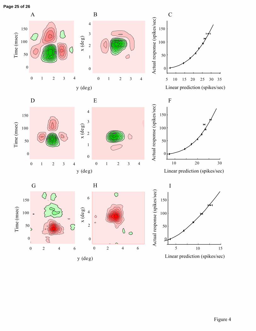
Methods). Figure 4 shows linear spatiotemporal receptive fields (A, B, D, E, G, and H)

and static nonlinearities (C, F, and I) for three representative LGN neurons. Space-time

(Fig 4A, D, and G) and x-y space (Fig 4B, E, and I) contour plots are shown. Green and

red represent bright and dark excitatory responses, respectively. Greater color saturation

represents higher response rate, and each contour line denotes a region of equal response

level. For all three cells in Fig.4, the relationship between actual response and linear

prediction follows a power law function with exponents of 3.03 (Fig 4A, B, and C), 2.64

(Fig 4D, E, and F), and 1.50 (Fig 4G, H, and I). For static nonlinearity plots given in Fig

4C, F, and I, the y-axis denotes actual response to m-sequence stimulation binned at one

m-sequence frame window (13ms) and averaged across all repetitions. For each actual

response value, linear prediction varies through the course of the m-sequence stimulation.

The x-axis denotes the average linear prediction for each corresponding actual response.

Error bars denote SEM of the prediction for each corresponding actual response.

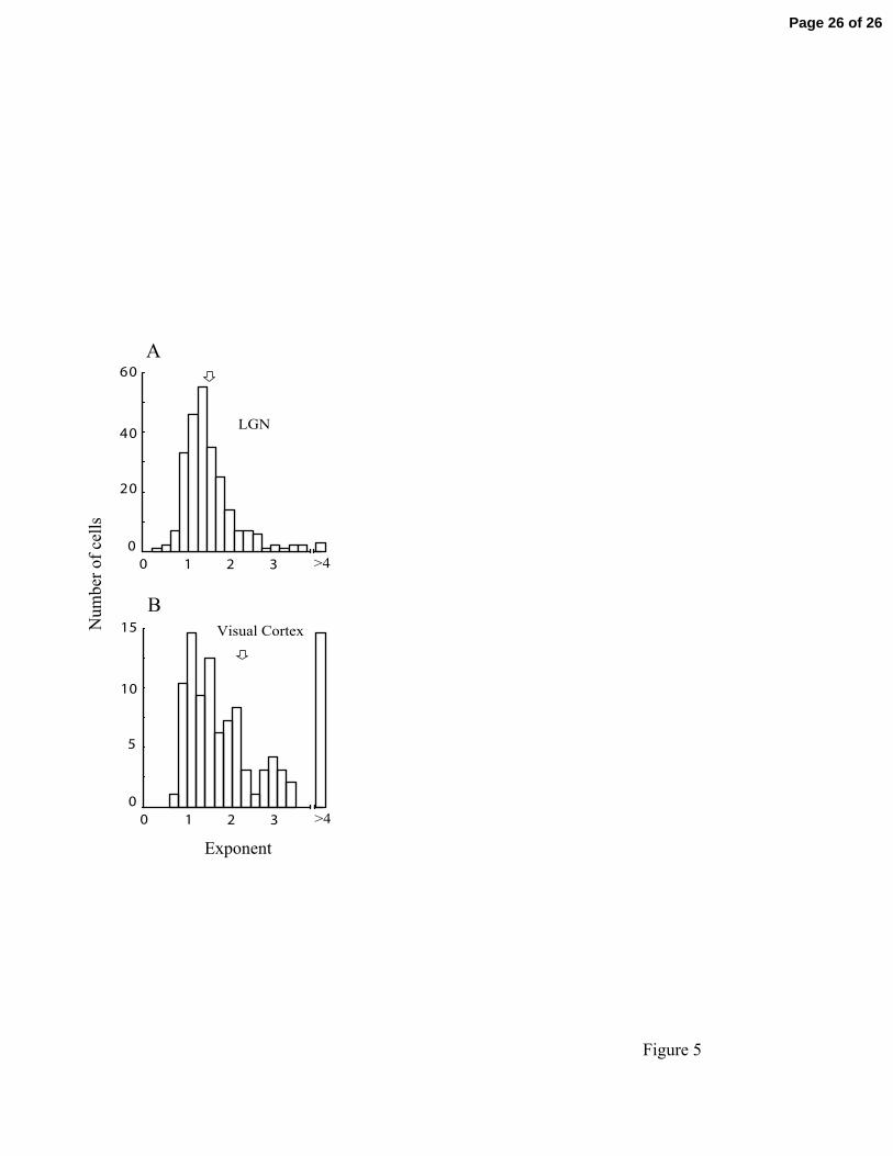
We calculated the best fit parameters to equation (4). Figure 5A shows the histogram of

best fit exponents for the LGN. The mean and SEM of the exponents across this

Page 12 of 26

13

population is 1.580 ±0.004, and the median and mode are 1.408 and 1.319, respectively.

The mean is indicated by the open arrow in Fig 5A.

A direct comparison of the value of n for a static nonlinear power law versus the Naka-

Rushton contrast response function is difficult to make since other nonlinearities such as

those imposed by a suppressive non-classical receptive field may play a role in

dissociating these two values (Bonin et al. 2006, 2005; Chander and Chichilnisky 2001).

However, the data in Figure 1D show that a mean power law exponent of 1.58

approximates an n larger than 2 in the Naka-Rushton function. Therefore, our results for

both analysis approaches are consistent and show that LGN neurons exhibit an expansive

nonlinearity at low stimulus contrast. The consistency between these two methods

suggests that a static power law nonlinearity as estimated by m-sequence stimulation

contributes substantially to expansive nonlinearity in the contrast tuning data.

Finally, for comparison to data from visual cortex, we show the exponent distribution for

an expansive static nonlinearity for 160 cortical neurons in Fig 5B. This distribution has

a mean (open arrow) and SEM of 2.4±0.2 which is higher than that for the LGN

population. Note that many neurons in the cortical population have large exponents (>4).

This reflects more pronounced expansive nonlinearities in visual cortex as compared with

LGN.

Discussion

Nonlinearities exist in various forms at various stages of the early visual pathway. In

retinal ganglion and LGN neurons, a gain control mechanism introduces distinct

Page 13 of 26

14

nonlinear response properties. First, a response phase advance is observed with

increasing stimulus contrast. Second, the transfer characteristics and response gain are

altered with stimulus contrast (Sclar 1987; Victor 1987). These properties also exist in

the primary visual cortex and are attributed to a divisive normalization mechanism

(Carandini and Heeger 1994; Carandini et al. 1997). Additionally, neurons in the primary

visual cortex also exhibit a power law expansive nonlinearity when stimulated at low

contrasts (Albrecht and Geisler 1991; Carandini 2004; DeAngelis et al. 1993; Gardner et

al. 1999; Miller and Troyer 2002).

Models of visual processing in the LGN and visual cortex have largely ignored any

thalamic expansive nonlinearity (Bonin et al. 2005; Li et al. 2006; Priebe and Ferster

2006). In the current study, we show that neurons in the LGN also exhibit a power law

expansive nonlinearity when activated by low contrast visual stimuli. This expansive

nonlinearity is likely to be the origin of expansive nonlinearity in membrane potentials of

cortical neurons when stimulated at low contrasts (Ahmed et al. 1997; Contreras and

Palmer 2003). We suggest therefore that expansive nonlinearity in the visual pathway

originates early and is enhanced at various stages.

While our measurements were made in LGN, the origin of expansive nonlinearities is

probably in the retina. However, we should point out that direct neural input is not the

only way to produce an expansive nonlinearity. It can also be produced as a by-product of

neural noise. Random fluctuations in the membrane potential can make sub-threshold

responses “visible” in the presence of a threshold spiking mechanism, which can cause

Page 14 of 26

15

spike responses near threshold to simulate an expansive nonlinearity (Miller and Troyer

2002). Given these factors, it is possible that an expansive nonlinearity originates in the

retina and gradually increases in magnitude as transmission progresses in a feed-forward

manner along the visual pathway. Our data for LGN and visual cortex are consistent with

this hypothesis.

The existence of a low contrast expansive nonlinearity is not consistent with recent feed-

forward models of cross orientation suppression in the primary visual cortex. In these

models, response saturation with increasing contrast in LGN is thought to underlie cross

orientation suppression in primary visual cortex (Li et al. 2006; Priebe and Ferster 2006).

For this to be true, the level of contrast saturation must match that of cross orientation

suppression at all contrast levels. We show here that, on average, the contrast response

function is expansive for contrasts below 27% (see Figure 2C). This would cause cross-

orientation facilitation, not suppression, in the visual cortex. However, cross orientation

suppression is present in the visual cortex even with gratings at contrasts below 27%

(DeAngelis et al. 1992; Freeman et al. 2002; Li et al. 2006). Therefore, at low stimulus

contrast, another mechanism must be involved in cross orientation suppression (Li et al.

2006).

Finally, it is relevant to consider possible consequences of a low contrast expansive non-

linearity. In general, an expansive non-linearity should contribute to a sharpening of

tuning curves for different stimulus dimensions. This would occur via an increase in the

slope of response functions so that small changes in the stimulus would generate

Page 15 of 26

16

relatively large changes in spike rates of neurons. This could apply to spatial frequency

selectivity. It could also be relevant to orientation since tuning properties of orientation

and spatial frequency of neurons in the visual cortex are related (Webster et al. 1990) . In

a similar fashion, an expansive non-linearity at low contrast levels could increase contrast

sensitivity via steeper slopes in contrast tuning functions. This would also yield low

thresholds or high contrast sensitivities. This accentuation of sensitivity could be highly

significant in a practical sense since most visual performance occurs in a relatively low

contrast environment (Mante et al. 2005).

Acknowledgment

This work was supported by research and core grants (EY01175 and EY03176) from the

National Eye Institute.

References

Ahmed B, Allison JD, Douglas RJ, and Martin KA. An intracellular study of the

contrast-dependence of neuronal activity in cat visual cortex. Cereb Cortex 7: 559-570,

1997.

Albrecht DG and Geisler WS. Motion selectivity and the contrast-response function of

simple cells in the visual cortex. Vis Neurosci 7: 531-546, 1991.

Albrecht DG and Hamilton DB. Striate cortex of monkey and cat: contrast response

function. J Neurophysiol 48: 217-237, 1982.

Page 16 of 26

17

Anzai A, Ohzawa I, and Freeman RD. Neural mechanisms for processing binocular

information I. Simple cells. J Neurophysiol 82: 891-908, 1999a.

Anzai A, Ohzawa I, and Freeman RD. Neural mechanisms for processing binocular

information II. Complex cells. J Neurophysiol 82: 909-924, 1999b.

Bonin V, Mante V, and Carandini M. The statistical computation underlying contrast

gain control. J Neurosci 26: 6346-6353, 2006.

Bonin V, Mante V, and Carandini M. The suppressive field of neurons in lateral

geniculate nucleus. J Neurosci 25: 10844-10856, 2005.

Carandini M. Amplification of trial-to-trial response variability by neurons in visual

cortex. PLoS Biol 2: E264, 2004.

Carandini M and Heeger DJ. Summation and division by neurons in primate visual

cortex. Science 264: 1333-1336, 1994.

Carandini M, Heeger DJ, and Movshon JA. Linearity and normalization in simple

cells of the macaque primary visual cortex. J Neurosci 17: 8621-8644, 1997.

Chander D and Chichilnisky EJ. Adaptation to temporal contrast in primate and

salamander retina. J Neurosci 21: 9904-9916, 2001.

Chichilnisky EJ. A simple white noise analysis of neuronal light responses. Network 12:

199-213, 2001.

Contreras D and Palmer L. Response to contrast of electrophysiologically defined cell

classes in primary visual cortex. J Neurosci 23: 6936-6945, 2003.

DeAngelis GC, Ohzawa I, and Freeman RD. Spatiotemporal organization of simple-

cell receptive fields in the cat's striate cortex. II. Linearity of temporal and spatial

summation. J Neurophysiol 69: 1118-1135, 1993.

Page 17 of 26

18

DeAngelis GC, Robson JG, Ohzawa I, and Freeman RD. Organization of suppression

in receptive fields of neurons in cat visual cortex. J Neurophysiol 68: 144-163, 1992.

Freeman TC, Durand S, Kiper DC, and Carandini M. Suppression without inhibition

in visual cortex. Neuron 35: 759-771, 2002.

Gardner JL, Anzai A, Ohzawa I, and Freeman RD. Linear and nonlinear contributions

to orientation tuning of simple cells in the cat's striate cortex. Vis Neurosci 16: 1115-

1121, 1999.

Li B, Thompson JK, Duong T, Peterson MR, and Freeman RD. Origins of cross-

orientation suppression in the visual cortex. J Neurophysiol 96: 1755-1764, 2006.

Mante V, Frazor RA, Bonin V, Geisler WS, and Carandini M. Independence of

luminance and contrast in natural scenes and in the early visual system. Nat Neurosci 8:

1690-1697, 2005.

Miller KD and Troyer TW. Neural noise can explain expansive, power-law

nonlinearities in neural response functions. J Neurophysiol 87: 653-659, 2002.

Naka KI and Rushton WA. S-potentials from luminosity units in the retina of fish

(Cyprinidae). J Physiol 185: 587-599, 1966.

Nykamp DQ and Ringach DL. Full identification of a linear-nonlinear system via cross-

correlation analysis. J Vis 2: 1-11, 2002.

Priebe NJ and Ferster D. Mechanisms underlying cross-orientation suppression in cat

visual cortex. Nat Neurosci 9: 552-561, 2006.

Reid RC, Victor JD, and Shapley RM. The use of m-sequences in the analysis of visual

neurons: linear receptive field properties. Vis Neurosci 14: 1015-1027, 1997.

Page 18 of 26

19

Sclar G. Expression of "retinal" contrast gain control by neurons of the cat's lateral

geniculate nucleus. Exp Brain Res 66: 589-596, 1987.

Solomon SG, Peirce JW, Dhruv NT, and Lennie P. Profound contrast adaptation early

in the visual pathway. Neuron 42: 155-162, 2004.

Sutter EE. The Fast m-Transform: A Fast Computation of Cross-Correlations with

Binary m-Sequences. SIAM J Comput 20: 686-694, 1991.

Victor JD. The dynamics of the cat retinal X cell centre. J Physiol 386: 219-246, 1987.

Victor JD and Shapley RM. Receptive field mechanisms of cat X and Y retinal

ganglion cells. J Gen Physiol 74: 275-298, 1979.

Webster MA, De Valois KK, and Switkes E. Orientation and spatial-frequency

discrimination for luminance and chromatic gratings. J Opt Soc Am A 7: 1034-1049,

1990.

Figure Legends

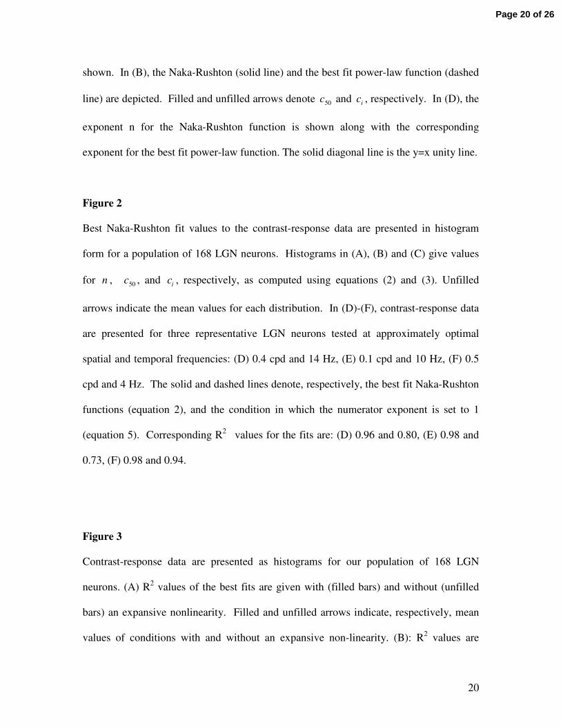
Figure 1

Visual stimulation paradigm is illustrated in (A) and (C). In (A), the contrast tuning

sequence is shown. Contrast levels between 0 and 100% are presented randomly for a 1

second duration followed by a 2 second rest period. In (C), the m-sequence stimulation

paradigm is depicted. In this case, the luminance of 8x8 or 16x16 grid elements is

modulated following a binary m-sequence. In (B) and (D), Naka-Rushton functions with

(solid) and without (dotted) expansive nonlinearity, and power-law functions (dashed) are

Page 19 of 26

20

shown. In (B), the Naka-Rushton (solid line) and the best fit power-law function (dashed

line) are depicted. Filled and unfilled arrows denote 50c and ic , respectively. In (D), the

exponent n for the Naka-Rushton function is shown along with the corresponding

exponent for the best fit power-law function. The solid diagonal line is the y=x unity line.

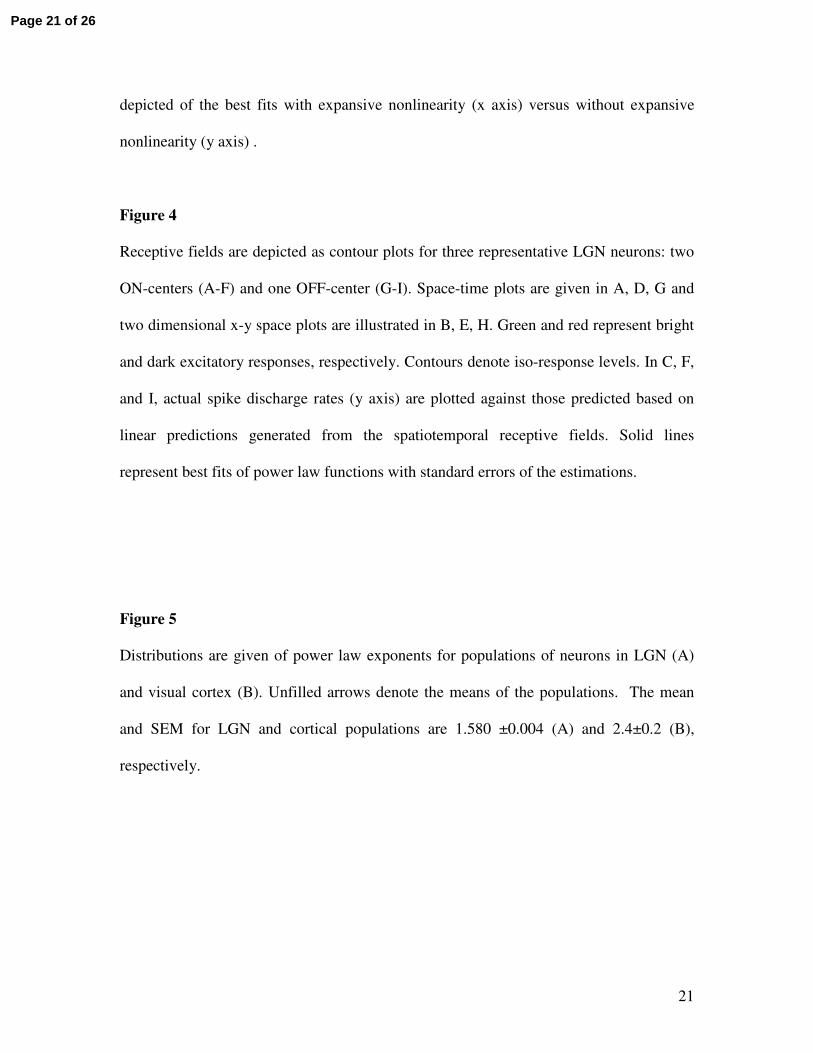
Figure 2

Best Naka-Rushton fit values to the contrast-response data are presented in histogram

form for a population of 168 LGN neurons. Histograms in (A), (B) and (C) give values

for n , 50c , and ic , respectively, as computed using equations (2) and (3). Unfilled

arrows indicate the mean values for each distribution. In (D)-(F), contrast-response data

are presented for three representative LGN neurons tested at approximately optimal

spatial and temporal frequencies: (D) 0.4 cpd and 14 Hz, (E) 0.1 cpd and 10 Hz, (F) 0.5

cpd and 4 Hz. The solid and dashed lines denote, respectively, the best fit Naka-Rushton

functions (equation 2), and the condition in which the numerator exponent is set to 1

(equation 5). Corresponding R2 values for the fits are: (D) 0.96 and 0.80, (E) 0.98 and

0.73, (F) 0.98 and 0.94.

Figure 3

Contrast-response data are presented as histograms for our population of 168 LGN

neurons. (A) R2 values of the best fits are given with (filled bars) and without (unfilled

bars) an expansive nonlinearity. Filled and unfilled arrows indicate, respectively, mean

values of conditions with and without an expansive non-linearity. (B): R2 values are

Page 20 of 26

21

depicted of the best fits with expansive nonlinearity (x axis) versus without expansive

nonlinearity (y axis) .

Figure 4

Receptive fields are depicted as contour plots for three representative LGN neurons: two

ON-centers (A-F) and one OFF-center (G-I). Space-time plots are given in A, D, G and

two dimensional x-y space plots are illustrated in B, E, H. Green and red represent bright

and dark excitatory responses, respectively. Contours denote iso-response levels. In C, F,

and I, actual spike discharge rates (y axis) are plotted against those predicted based on

linear predictions generated from the spatiotemporal receptive fields. Solid lines

represent best fits of power law functions with standard errors of the estimations.

Figure 5

Distributions are given of power law exponents for populations of neurons in LGN (A)

and visual cortex (B). Unfilled arrows denote the means of the populations. The mean

and SEM for LGN and cortical populations are 1.580 ±0.004 (A) and 2.4±0.2 (B),

respectively.

Page 21 of 26

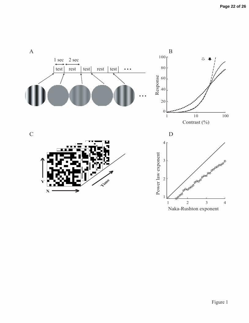
Figure 1

A B

Time

1 10 1000

20

40

60

80

100

Contrast (%)

Res

pons

e

C

Naka-Rushton exponent1 2 3 4

1

2

3

4

Pow

er la

w e

xpon

ent

D

X

Y

test rest test

1 sec 2 sec

...test

...

rest

Page 22 of 26

Figure 2

50 100 150 2000

C values (%)50

BA

2 4 6 80

20

40

60

80

0

Num

ber o

f cel

ls

n values50 100 150 2000

0

20

40

60

80

C values (%)i

C

0

20

40

60

80

D FE

Contrast (%)

0

jb253x3505,5,0

1 10 100

5

15

10

0

5

10

15

20

25 jb253x4106,3,0

1 10 1001 10 1000

5

10

15

20jb253x0710,2,0

Res

pons

e (s

pike

s/se

c)Page 23 of 26

0. 2 0. 4 0. 6 0. 8 10

20

40

60

80

100

R values2

Num

ber o

f cel

ls

0 0. 5 10

0.5

1

With

out e

xpan

sive

non

linea

rity

With expansive nonlinearity

With expansive nonlinearityWithout expansive nonlinearity

Figure 3

A

B

Page 24 of 26

0

50

100

150

y (deg)

5 10 15 20 25 30 35

0

50

100

150

Linear prediction (spikes/sec)

Act

ual r

espo

nse

(spi

kes/

sec)

0 1 2 3 40 1 2 3 4

0

1

2

3

4

Tim

e (m

sec)

A B C

Figure 4

0 1 2 3 4 0 1 2 3 4 10 20 30

0

50

100

150

0

1

2

3

4

Linear prediction (spikes/sec)

Act

ual r

espo

nse

(spi

kes/

sec)

y (deg)

Tim

e (m

sec)

D E F

0

50

100

150

x (d

eg)

x (d

eg)

0 2 4 6

Tim

e (m

sec)

0

50

100

150

0 2 4 6

0

2

4

6

y (deg)

x (d

eg)

G H

5 10 15

0

50

100

150

Linear prediction (spikes/sec)

Act

ual r

espo

nse

(spi

kes/

sec)

I

Page 25 of 26

0 1 2 3 >40

20

40

60

Figure 5

Num

ber o

f cel

ls

LGN

Visual Cortex

A

B

0 1 2 3 >40

5

10

15

Exponent

Page 26 of 26