DELINEATING THE SOURCE, GEOCHEMICAL SINKS AND AQUEOUS MOBILISATION PROCESSES OF NATURALLY OCCURRING ARSENIC IN A COASTAL SANDY AQUIFER Stuarts Point, New South Wales, Australia. Bethany Megan O’Shea A thesis submitted in fulfillment of the requirements for the degree of Doctor of Philosophy School of Biological, Earth & Environmental Sciences Faculty of Science University of New South Wales Sydney, Australia August 2006

Welcome message from author
This document is posted to help you gain knowledge. Please leave a comment to let me know what you think about it! Share it to your friends and learn new things together.
Transcript
DELINEATING THE SOURCE,
GEOCHEMICAL SINKS AND AQUEOUS
MOBILISATION PROCESSES OF
NATURALLY OCCURRING ARSENIC IN A
COASTAL SANDY AQUIFER
Stuarts Point, New South Wales, Australia.
Bethany Megan O’Shea
A thesis submitted in fulfillmentof the requirements for the degree of
Doctor of Philosophy
School of Biological, Earth & Environmental Sciences Faculty of Science
University of New South Wales Sydney, Australia
August 2006
PLEASE TYPE
Surname or Family name: O'SHEA
THE UNIVERSITY OF NEW SOUTH WALES Thesis/Dissertation Sheet
First name: BETHANY Other name/s: MEGAN
Abbreviation for degree as given in the University calendar: PhD
School: BIOLOGICAL, EARTH & ENVIRONMENTAL SCIENCES Faculty: SCIENCE
Title: DELINEATING THE SOURCE, GEOCHEMICAL SINKS AND AQUEOUS MOBILISATION PROCESSES OF NATURALLY OCCURRING ARSENIC IN A COASTAL SANDY AQUIFER, STUARTS POINT, NEW SOUTH WALES, AUSTRALIA
Abstract 350 words maximum: (PLEASE TYPE)
Elevated arsenic concentrations have been reported in a drinking water and irrigation-supply aquifer of Stuarts Point, New South Wales, Australia. Arsenic occurrence in such aquifers is potentially a major issue due to their common use for high yield domestic and irrigation water supplies. Ten multi-level piezometers
were installed to depths of approximately 30 m in the sand and clay aquifer. Sediment samples were collected at specific depths during drilling and analysed for chemical and mineralogical composition, grain size characteristics, potential for arsenic release from solid phase and detailed microscopic features. From this data, a full geomorphic reconstruction allowed the determination of source provenance for the aquifer sediments. The model proposed herein provides evidence that the bulk of the aquifer was deposited under
intermittent fluvial and estuarine conditions; and that all sediments derive from the regional arsenicmineralised hinterland. More than 200 groundwater samples were collected and analysed for over 50
variables. The heterogeneity of the aquifer sediments causes redox stratification to occur, which in turn governs arsenic mobility in the groundwater. The bulk of the aquifer is composed of fluvial sand deposits
undergoing reductive dissolution of iron oxides. Arsenic adsorbed to iron oxide minerals is released during dissolution but re-adsorbs to other iron oxides present in this part of the aquifer. The deeper, more
reducing fluvial sand and estuarine clay groundwaters have undergone complete reductive dissolution of iron oxides resulting in the subsequent mobilisation of arsenic into groundwater. Some of this arsenic has
been incorporated into iron sulfide mineral precipitates, forming current arsenian pyrite sinks within the aquifer. The extraction of groundwater from the aquifer for irrigation and drinking water supply induces seawater intrusion of arsenic-rich estuarine water, bringing further dissolved arsenic into the aquifer. A greater understanding of the source, sinks and mobilisation of arsenic in this aquifer contributes to our
broad understanding of arsenic in the environment; and allows aquifer specific management procedures and research recommendations to be made. Any coastal or unconsolidated aquifer that has sediments
derived from mineralised provenances should consider monitoring for arsenic, and other potentially toxic trace elements, in their groundwater systems.
Declaration relating to disposition of project thesis/dissertation
I hereby grant to the University of New South Wales or its agents the right to archive and to make available my thesis or dissertation in whole or in part in the University libraries in all forms of media, now or here after known, subject to the provisions of the Copyright Act 1968. I retain all property rights, such as patent rights. I also retain the right to use in future works (such as articles or books) all or part of this thesis or dissertation.
I also authorise University Microfilms to use the 350 word abstract of my thesis in Dissertation Abstracts International (this is applicable to doctoral theses only).
Witness
22 1oBjo b ··············~-~- .......................... .
Date ............... . 4.J .. Q .. :~-!.-.~.~'~ .................... .
Signature
J,) ([) jLQ_ .,) . . ...... ~ .. ~ ............................................ .
The University recognises that there may be exceptional circumstances requiring restrictions on copying or conditions on use. Requests for restriction for a period of up to 2 years must be made in writing. Requests for a longer period of restriction may be considered in exceptional circumstances and require the approval of the Dean of Graduate Research.
FOR OFFICE USE ONLY Date of completion of requirements for Award:
THIS SHEET IS TO BE GLUED TO THE INSIDE FRONT COVER OF THE THESIS

COPYRIGHT STATEMENT
'I hereby grant the University of New South Wales or its agents the right to archive and to make available my thesis or dissertation in whole or part in the University libraries in all forms of media, now or here after known, subject to the provisions of the Copyright Act 1968. I retain all proprietary rights, such as patent rights. I also retain the right to use in future works (such as articles or books) all or part ofthis thesis or dissertation. I also authorise University Microfilms to use the 350 word abstract of my thesis in Dissertation Abstract International (this is applicable to doctoral theses only). I have either used no substantial portions of copyright material in my thesis or I have obtained permission to use copyright material; where permission has not been granted I have applied/will apply for a partial restriction of the digital copy of my thesis or dissertation.'
Signed ........ 4.:.S::? . .' ......................................................... .
Date . . . . . . . ?.. .~/ 9.. !? . .! C?.~ ............................................. .
AUTHENTICITY STATEMENT
'I certify that the Library deposit digital copy is a direct equivalent of the final officially approved version of my thesis. No emendation of content has occurred and if there are any minor variations in formatting, they are the result of the conversion to digital format.'
Signed
Date ...... ??:./~~.~~
ORIGINALITY STATEMENT
'I hereby declare that this submission is my own work and to the best of my knowledge it contains no materials previously published or written by another person, or substantial proportions of material which have been accepted for the award of any other degree or diploma at UNSW or any other educational institution, except where due acknowledgement is made in the thesis. Any contribution made to the research by others, with whom I have worked at UNSW or elsewhere, is explicitly acknowledged in the thesis. I also declare that the intellectual content of this thesis is the product of my own work, except to the extent that assistance from others in the project's design and conception or in style, presentation and linguistic expression is acknowledged.'
Signed
Date ......... ~.~/.c. .'6./? (o ................................. .
O’Shea (2006) Page i
ABSTRACT
Elevated arsenic concentrations have been reported in a drinking water and irrigation-
supply aquifer of Stuarts Point, New South Wales, Australia. Coastal areas are often
heavily populated, making groundwater a valuable resource. Arsenic occurrence in such
aquifers is potentially a major issue due to their common use for high yield domestic
and irrigation water supplies. This study was initiated in response to community anxiety
over arsenic in their water supply aquifer; and concern for the potential occurrence of
elevated arsenic in other coastal sandy aquifers.
The source of arsenic deduced from preliminary studies was proposed as being derived
from acid sulfate soil material and sorption of arsenic onto marine clays during sea level
transgressions in the Quaternary period. The evidence presented herein suggests an
alternative source; the arsenic in this aquifer is predominantly derived from regional
and/or bedrock geology.
Ten multi-level piezometers were installed to depths of approximately 30 m in the sand
and clay aquifer. Sediment samples were collected at specific depths during drilling and
analysed for chemical and mineralogical composition, grain size characteristics,
potential for arsenic release from solid phase and detailed microscopic features. From
this data, a full geomorphic reconstruction allowed the determination of source
provenance for the aquifer sediments. Previous geomorphic models have suggested the
aquifer is largely comprised of barrier sands derived from off-shore. The model
proposed herein provides evidence that the bulk of the aquifer was deposited under
intermittent fluvial and estuarine conditions; and that all sediments derive from the
regional arsenic-mineralised hinterland. The wet climate of the Pleistocene and
Holocene promoted weathering in the upper catchment, which weathered natural
stibnite deposits containing arsenic and antimony to form iron oxides. These oxides
were present in colloidal forms and as coatings on sediment grains, which were
transported downstream and deposited to form the current aquifer matrix.
Abstract
O’Shea (2006) Page ii
More than 200 groundwater samples were collected and analysed for over 50 variables.
Statistical methods were employed in conjunction with hydrochemical interpretative
techniques to determine the geochemical processes active in the groundwater system.
Natural and anthropogenic effects contribute to arsenic mobilisation. The heterogeneity
of the aquifer sediments causes redox stratification to occur, which in turn governs
arsenic mobility in the groundwater. Shallow groundwaters are exposed to nitrate input
from the ground surface, which contributes to the oxidative release of discrete arsenian
pyrite phases. The bulk of the aquifer is composed of fluvial sand deposits undergoing
reductive dissolution of iron oxides. Arsenic adsorbed to iron oxide minerals is released
during dissolution but re-adsorbs to other iron oxides present in this part of the aquifer.
The deeper, more reducing fluvial sand and estuarine clay groundwaters have
undergone complete reductive dissolution of iron oxides resulting in the subsequent
mobilisation of arsenic into groundwater. Some of this arsenic has been incorporated
into iron sulfide mineral precipitates, forming current arsenian pyrite sinks within the
aquifer. Mineralised bedrock groundwaters contribute arsenic to the overlying
weathered bedrock clays. The extraction of groundwater from the aquifer for irrigation
and drinking water supply induces seawater intrusion of arsenic-rich estuarine water,
bringing further dissolved arsenic into the aquifer.
Previous arsenic mobilisation processes were proposed to be dominated by the
dissolution of aluminium hydroxides and release of adsorbed As(V) or concurrently via
pH-influenced desorption of arsenic enriched iron oxides; and the leaching of the
aquifer’s sandy-clayey matrix by groundwaters rich in HCO3- and of high pH. The
detailed hydrochemical interpretation provided herein suggests these are minor arsenic
control mechanisms. Instead, the reductive dissolution of iron oxides and precipitation
of iron sulfide minerals has been shown to dominate arsenic mobilisation and
retardation at Stuarts Point.
A greater understanding of the source, sinks and mobilisation of arsenic in this aquifer
contributes to our broad understanding of arsenic in the environment; and allows aquifer
specific management procedures and research recommendations to be made. In
addition, the findings of this study are similar to geochemical processes proposed by
some authors for arsenic release in Bangladesh. The suggestion that groundwater

Abstract
O’Shea (2006) Page iii
arsenic occurrence has implications for the management of coastal aquifers remains, but
not solely due to the presence of acid sulfate soils or exposure of these coastal
sediments to Quaternary sea level fluctuations. Rather, any coastal or unconsolidated
aquifer that has sediments derived from mineralised provenances should consider
monitoring for arsenic, and other potentially toxic trace elements, in their groundwater
systems.

O’Shea (2006) Page iv
ACKNOWLEDGEMENTS
It is good to have an end to journey towards, but it is the journey that matters, in the end.
– Ursula Le Guin
There are many who have supported me during my journey towards a PhD. Some have
been there from the first step, while others have endured the final leg of the journey.
Each of you have helped in your own special way, and for this, I thank you.
I would like to acknowledge my supervisor Jerzy Jankowski who inspired my interest in
hydrogeochemistry and Jesmond Sammut who provided both advice and
encouragement. The day to day trials and successes were experienced by those present
in room 515 of the School of BEES – Sarah Groves, John Wischusen, Jessica Northey,
Maria Dubikova, Emma Haradasa and Karina Morgan. Our many conversations – both
hydrochemical and ‘tangent-related’ – were excellent stress relievers (in addition to
coffee and chocolate). Our combined quest for knowledge saw us endlessly searching
through journal papers and text books to find ‘the right answer’ even when there may
not have been one. I have learnt a great deal from these brainstorming sessions.
To those that helped me in the field or lab – Kavita Gosavi, Dorothy Yu, Irene
Wainwright, Lange Jorstad, James Smith, Phillip Crisp, Maree Emmett, Paul Simpson,
Barry Searle – your help is greatly appreciated. And to those who stood on the outside
looking in – my family and friends. Thankyou for your cooking (Mum and Alana),
outrageous yet funny technical suggestions (Dad), constant asking of when my ‘book’
will be finished (everyone single person I know!!), nights on the town (Melbourne girls,
Coogee boys) and the combined support, nagging and encouragement from Jim.
To all those who have contributed to the development of my scientific curiosity, I hope
this thesis inspires you all. But most of all…..
Happy Reading !!
O’Shea (2006) Page v
TABLE OF CONTENTS
Abstract i Acknowledgements iv Table of Contents v List of Figures xi List of Tables xv Abbreviations xvii
1 INTRODUCTION 1 1.1 PROJECT INCEPTION 1
1.2 RESEARCH AIMS 3
1.3 HYPOTHESES 3
1.4 SIGNIFICANCE OF THIS RESEARCH 4
1.5 STUDY APPROACH 6
1.6 THESIS STRUCTURE 6
2 THE STUARTS POINT STUDY AREA 9 2.1 LOCATION AND ENVIRONMENTAL CONDITIONS 9
2.2 THE MACLEAY RIVER CATCHMENT 9
2.2.1 Regional Geology 12
2.2.2 The Macleay Fluvial-Deltaic Floodplain 15
2.3 DEPOSITION OF THE STUARTS POINT AQUIFER 15
2.3.1 Previous Geomorphic Models 15
2.3.2 Bedrock Geology 19
2.3.2.1 Lithology and Structure 19
2.3.2.2 Mineralisation 22
2.3.3 Hydrogeology 25
2.4 PREVIOUS INVESTIGATIONS 28
3 ARSENIC LITERATURE REVIEW 31 3.1 GENERAL PROPERTIES OF ARSENIC 31
3.1.1 Periodicity 31
3.1.2 Toxicity 33
3.1.3 Arsenic Production and Use 34
3.2 SOURCES OF ARSENIC IN THE ENVIRONMENT 35
3.2.1 Natural Occurrences 36
3.2.2 Anthropogenic Sources 37
Table of Contents
O’Shea (2006) Page vi
3.2.3 Concentrations in the Environment 39
3.2.3.1 Rocks 42
3.2.3.2 Soils 42
3.2.3.3 Sediments 42
3.2.3.4 Water 42
3.2.3.5 Air 43
3.3 AQUEOUS ARSENIC CHEMISTRY 44
3.4 IMMOBILISATION OF ARSENIC: SOLID PHASE RETARDATION 47
3.4.1 Properties of Sorbent Materials 47
3.4.1.1 Surface Area 47
3.4.1.2 Surface Charge 47
3.4.2 Surface Sorption 49
3.4.2.1 Surface Complexation 49
3.4.2.2 Permanent Versus Variable Surface Charge 51
3.4.3 Arsenic Retention in the Solid Phase 52
3.4.3.1 Solid Phase Arsenic Formation 52
3.4.3.2 Surface Reactions Affecting Arsenic Mobility 56
3.4.3.2.1Surface Complexation (Adsorption) 56
3.4.3.2.2Surface Precipitates 65
3.4.3.2.3Competitive Anion Exchange 65
3.5 MOBILISATION OF ARSENIC: THE GEOCHEMICAL TRIGGERS 67
3.5.1 Changes to Aqueous pH 67
3.5.2 Shifts in Aqueous Redox Potential 68
3.5.3 Influence of, and Interaction with, the Surrounding Solution 70
3.5.4 Colloidal Transport 72
3.6 NATURALLY OCCURRING GROUNDWATER ARSENIC 72
3.6.1 Geochemical Controls 74
3.6.1.1 Oxidising Environments 74
3.6.1.2 Arid Oxidising Environments 75
3.6.1.3 Reducing Conditions 76
3.6.1.4 Combined Oxidising and Reducing Conditions 77
3.6.2 Geological And Depositional Influences 78
3.6.2.1 Geothermal Systems 78
3.6.2.2 Volcanic Sediments 78
3.6.2.3 Alluvial and Deltaic Sediments 79
3.6.2.4 Consolidated Sediments 79
Table of Contents
O’Shea (2006) Page vii
3.6.2.5 Lacustrine Environments 80
3.6.2.6 Glacial Drift 81
3.6.2.7 Aeolian Loess Deposits 82
3.6.2.8 Zone of Water Table Fluctuation 82
3.6.2.9 Coastal Sand Dunes 83
3.6.3 Arsenic In Australia 84
3.7 ARSENIC GEOCHEMICAL SUMMARY 84
4 METHODOLOGY 86 4.1 CONSTRUCTION & INSTALLATION OF SAMPLING NETWORK 86
4.1.1 Multi-Level Piezometer Design 86
4.1.2 Drilling 86
4.2 SEDIMENT AND GROUNDWATER SAMPLING 88
4.2.1 Sediment Sampling, Storage and Preparation Methods 88
4.2.2 Groundwater Sampling, Preservation & Storage Methods 88
4.3 AQUEOUS CHEMICAL ANALYSES 89
4.3.1 General Parameters 89
4.3.2 Unstable Chemical Species 90
4.3.3 Major Ions 90
4.3.4 Minor Elements 91
4.3.5 Arsenic Speciation 92
4.4 SOLID PHASE ANALYSES 93
4.4.1 Electron Microscopy 93
4.4.1.1 Sample Preparation 93
4.4.1.2 SEM-EDS 93
4.4.1.3 Electron Microprobe-WDS 94
4.4.1.4 Internal QA/QC Procedures 94
4.4.2 Grain Size Analysis 95
4.4.3 Sequential Extractions 97
4.4.4 XRD 97
4.4.5 XRF 97
4.4.6 Loss On Ignition (LOI) 100
4.5 STATISTICAL ANALYSES 100
4.5.1 Data Screening 100
4.5.1.1 Assessment of Normality 100
4.5.1.2 Standardization 101
Table of Contents
O’Shea (2006) Page viii
4.5.1.3 Censored Data 102
4.5.2 Descriptive Statistics 103
4.5.3 Multi-Variate Statistical Analyses 104
4.5.3.1 Cluster Analysis 104
4.5.3.2 Principal Components Analysis (PCA) 104
4.5.4 Statistical Correlation 105
5 ORIGINAL SOURCE OF ARSENIC TO THE AQUIFER 106 5.1 HYPOTHESES 106
5.2 INVESTIGATIVE RESULTS AND INTERPRETATION 109
5.2.1 Aquifer Lithology 109
5.2.2 Aquifer Depositional Conditions 120
5.2.2.1 Differentiating between Beach Sand & Fluvial Sand 120
5.2.2.2 The Onset of Estuarine Conditions 122
5.2.2.3 Weathered Bedrock 126
5.2.3 Aquifer (Sediment) Chemistry 128
5.2.4 Aquifer Facies Definition 128
5.2.4.1 Statistical Procedures 128
5.2.4.2 Development of Aquifer Cross Sections 132
5.2.5 Determining Source Provenance for the Aquifer Facies 137
5.2.5.1 Origin of the Sands 137
5.2.5.2 Selection of a Hinterland Indicator Element 139
5.2.6 Aquifer Geomorphology 142
5.2.6.1 Linking the Stuarts Point Facies to Surrounding
Depositional Environments 142
5.2.6.2 Proposed Geomorphic Model for the Stuarts Point
Aquifer 143
5.3 DISCUSSION ON EACH PROPOSED ARSENIC SOURCE
HYPOTHESIS 146
5.3.1 Anthropogenic Sources 146
5.3.1.1 Agricultural Practices 147
5.3.1.2 Historical Mining 148
5.3.1.3 Town (Anthropogenic) By-Products 148
5.3.2 A Regional Geologic Source? 150
5.3.3 Input from As-rich Holocene Sea Level Rise 152
5.3.4 A Note on Arsenic and Acid Sulfate Soils / Pyrite 157
Table of Contents
O’Shea (2006) Page ix
5.3.5 Direct Bedrock Contribution 158
5.4 A COMPARISON TO ARSENIC SOURCES IN OTHER NATURALLY
ELEVATED ARSENIC ENVIRONMENTS 160
5.5 CHAPTER SUMMARY 162
6 IDENTIFICATION OF CURRENT ARSENIC SINKS 164 6.1 AQUIFER MINERALOGY AND PHYSICAL PROPERTIES 165
6.2 HOW MUCH ARSENIC IS IN THE AQUIFER MATRIX ? 167
6.2.1 Arsenic-Bearing Minerals 174
6.2.2 Are there any Distinctive Correlations? 175
6.3 EXAMINATION OF KNOWN ARSENIC SCAVENGING MATERIALS IN
RELATION TO THE STUARTS POINT AQUIFER MATRIX 181
6.3.1 Adsorption to Oxyhydroxides 181
6.3.2 Association with Pyrite 188
6.3.3 Incorporation into Clay Minerals 194
6.3.4 Sorption on Organic Matter 196
6.3.5 Association with Calcite 197
6.3.6 Anion Competition 198
6.4 CHAPTER SUMMARY: IDENTIFICATION OF CONTROLLING SINKS
IN THE AQUIFER 198
7 ARSENIC MOBILISATION IN THE AQUIFER 201 7.1 GENERAL AQUIFER CONDITIONS 201
7.1.1 Major Hydrochemical Processes 201
7.2 ARSENIC GEOCHEMICAL PROCESSES 207
7.2.1 Arsenic Distribution and Speciation 207
7.2.2 Identification of Arsenic Mobilisation Processes 211
7.2.2.1 Shallow Groundwaters 212
7.2.2.2 Barrier Sand Groundwaters 220
7.2.2.3 Fluvial Sand Groundwaters 223
7.2.2.4 Fluvial Sand / Estuarine Clay Groundwaters 231
7.2.2.5 Bedrock Clay Groundwaters 236
7.2.2.6 Seawater Intrusion Groundwaters 237
7.3 CHAPTER SUMMARY 241

Table of Contents
O’Shea (2006) Page x
8 CONCLUSIONS AND RECOMMENDATIONS 243 8.1 THE PROBLEM 243
8.2 PROPOSED ARSENIC GEOCHEMICAL MODEL FOR THE STUARTS
POINT AQUIFER 243
8.3 CONCLUSIONS 246
8.4 RECOMMENDATIONS 248
8.4.1 Aquifer Specific (Stuarts Point) 248
8.4.2 Other Research Recommendations 251
REFERENCES 254
APPENDICES A PUBLICATIONS
B1 SEDIMENT CHEMISTRY
B2 GROUNDWATER CHEMISTRY
B3 GRAIN SIZE ANALYSIS
B4 BORE LOGS
B5 IRON OXIDE CONVERSIONS
B6 SEQUENTIAL EXTRACTION RESULTS
B7 STATISTICAL RESULTS
B8 GEOCHEMICAL MODELLING RESULTS
C1 PHOTOGRAPHS
O’Shea (2006) Page xi
LIST OF FIGURES
Figure 1.1 Thesis Structure………………………………………………….…….....8Figure 2.1 Location of the Stuarts Point sand aquifer (contained within the dotted
lines). Multi-level piezometers used in this study are also shown…..…..10Figure 2.2 Boundaries of the Macleay River Catchment. Stuarts Point is located on
the northeastern margin of the catchment where floodplain deposits dominate (NSW EPA, 2005)………………………………………….....11
Figure 2.3 Extent of the New England Fold Belt and its adjacent basin margins (modified from Palfreyman, 1984 and Leitch, 1974)……………….…..12
Figure 2.4 Geological subdivision of the southern NEFB. Stuarts Point is situated on the Nambucca Block (modified from Gilligan et al., 1992)……………13
Figure 2.5 Generalised section of a dual barrier system (Roy and Thom, 1981)…..16Figure 2.6 Pre-Pleistocene and current Holocene coastlines on the NSW mid-north
coast (Hails, 1968)……………………………………………………....17Figure 2.7 The Stuarts Point aquifer denoted by Eddie (2000) as an inner barrier
beach/dune sand – ‘sp’ (extracted and modified from Eddie, 2000)……18Figure 2.8 Various bedrock lithologies proposed for Stuarts Point. The Stuarts Point
aquifer is contained within the dotted area……………………………...20Figure 2.9 Coastal granitoid belt forming Mt Yarrahapinni (modified from Gilligan
et al., 1992)………………………………………………………..…….23Figure 2.10 Zones of mineralisation surrounding Mt Yarrahapinni (modified from
Gilligan et al., 1992). Numbers refer to recognised mineral deposits described in Gilligan et al. (1992). 772-774 are disseminated/vein Mo deposits……………………………………………………………….…24
Figure 2.11 Groundwater contour map (mAHD) for the Stuarts Point sand aquifer…………………………………………………………………..26
Figure 2.12 Regional arsenic distribution reported by Smith et al.(2000).The Stuarts Point aquifer and multi-level piezometers installed for this study are marked…………………………………………………………………..29
Figure 3.1 Eh-pH diagram for the As-O2-S-H2O system at 25ºC and 1 bar pressure (Bissen and Frimmel, 2003)…………………………………..…………45
Figure 3.2 Deprotonation of (a) As(III) and (b) As(V) species over different pH ranges (Smedley and Kinniburgh, 2002)………………………………..46
Figure 3.3 Mechanisms of sorption at the mineral/water interface. (a) adsorption of an ion via formation of an outer-sphere complex; (b) loss of hydration water and formation of an inner-sphere complex; (c) lattice diffusion and isomorphic substitution within the mineral lattice; (d) rapid lateral diffusion and formation either of a surface polymer or (e) adsorption on a ledge which maximizes the number of bonds to the atom; (f) upon particle growth surface polymers end up embedded in the lattice structure; and (g) the adsorbed ion can diffuse back into solution either as a result of dynamic equilibrium or as a product of surface reactions (from Charlet and Manceau, 1993; as cited in Sparks, 2003)…………………………..49
Figure 3.4 (a) Inner-sphere complex formation and (b) Outer-sphere complex formation (taken from Sposito, 1984; as cited in Sparks, 2003)…….….50
Figure 3.5 Arsenic adsorption on HFO for a) As(V) and b) As(III) according to ionic strength (I), Fe and As concentrations given (after Dzombak and Morel,
List of Figures
O’Shea (2006) Page xii
1990). Solid line is optimal fit, dashed line is an estimate using sorption constants……………………………………………………………….59
Figure 3.6 As(III)substitution for the carbonate ion on the calcite surface as suggested by Cheng et al. (1999)………………..…………………….64
Figure 3.7 Natural arsenic distribution in aquifers globally (Smedley and Kinniburgh, 2002). Some mining and geothermal sources are also noted………….73
Figure 4.1 Schematic of the multi-level design used at Stuarts Point……………..87Figure 5.1 Borelog for ML1………………………………………………………110Figure 5.2 Borelog for ML2………………………………………….…………...111Figure 5.3 Borelog for ML3………………………………………………………112Figure 5.4 Borelog for ML4………………………………………………………113Figure 5.5 Borelog for ML5………………………………………………………114Figure 5.6 Borelog for ML6………………………………………………………115Figure 5.7 Borelog for ML7………………………………………………………116Figure 5.8 Borelog for ML8………………………………………………………117Figure 5.9 Borelog for ML9………………………………………………………118Figure 5.10 Borelog for ML10…………………………………………………….119Figure 5.11 Moment skewness versus moment standard deviation to differentiate
beach and river sands from the Stuarts Point aquifer (method adapted from Friedman, 1960). Numbers represent depth below ground surface for respective multi-levels……………………………………………122
Figure 5.12 Proposed bedrock units at Stuarts Point. The Stuarts Point aquifer is contained within the dotted area. Approximate bedrock contours (based on drilling evidence) are shown at 5m depth intervals……………….127
Figure 5.13 The HCA dendrogram on sediment chemistry successfully delineated the proposed facies units…………………………………………………131
Figure 5.14 Cross Section A to A'. See text for discussion……………………….133Figure 5.15 Cross section B to B'. See text for discussion………………………..134Figure 5.16 Cross Section C to C'. See text for discussion……………………….135Figure 5.17 Cross section D to D'. See text for discussion………………………136Figure 5.18 Ternary diagram of the Stuarts Point sediments showing a recycled
orogen for most aquifer sediments. Boundaries for tectonic fields are from Dickinson and Suczek (1979), Dickinson et al. (1983), and Ingersoll and Suczek (1979) (Q=quartz, F=feldspar, L=lithics)………………138
Figure 5.19 Indicative types of mineralisation occurring within the Macleay River catchment (information obtained from Gilligan et al., 1992)……….140
Figure 5.20 Proposed geomorphic model for the deposition of the Stuarts Point aquifer. ……………………………………………………………….145
Figure 5.21 Potential anthropogenic arsenic sources in the Stuarts Point aquifer...146Figure 5.22 Sb versus As concentrations in the aquifer matrix. The “beach barrier
deposits” contain the most Sb and the least As, showing Sb is more immobile than As……………………………………………………..151
Figure 5.23 Vertical solid phase arsenic concentrations reported herein. Arsenic peaks with “fluvial sand/estuarine clay” units due to their higher adsorption capacity……………………………………………………………….156
Figure 5.24 As and Mo groundwater concentrations with depth in ML9 (left) and ML6 (right). Note the simultaneous increase in both elements as depth increases and weathered phyllite bedrock is penetrated at 20 mbgs in

List of Figures
O’Shea (2006) Page xiii
ML9. Contrasting, ML6 shows no distinct correlation between the two elements……………………………………………………………159
Figure 5.25 Development of an arsenic affected aquifer in Taiwan. Slate debris, deposited via fluvial and long-shore processes, is the source of the arsenic (Yu et al., 2000)……………………………………………161
Figure 6.1 SEM photomicrographs of typical grains observed for each geomorphic facies in the Stuarts Point aquifer. (a) beach barrier sand (b) fluvial sand (c) fluvial sand/estuarine clay and (d) bedrock clay. Spectral plots coincide with the white spectral boxes outlined in each photomicrograph……………………………………………………166
Figure 6.2 XRD spectrum for a fluvial sand/estuarine clay at ML7/27. Quartz dominates with minor amounts of illite, kaolinite, feldspar and pyrite identified……………………………………………………………174
Figure 6.3 As versus fine fraction component (silts and clays) in the aquifer sediments. The clayey units report the highest As concentrations yet no good correlation exists to support As association with just the fine fraction………………………………………………………………180
Figure 6.4 Detailed analysis of particles within oxidised bedrock clay (ML10/26.8) with some fluvial influence. Potential iron oxide minerals, as proposed by atomic ratios, are (a) goethite (b) ferrihydrite aggregate on goethite surface (c) amorphous iron oxide on goethite surface………………186
Figure 6.5 Small agregate observed on a “fluvial sand / estuarine clay” sample. Clay and quartz are suspected however the presence of sulfur may indicate discrete sulfide mineral presence……………………………………189
Figure 6.6 Electron microprobe back scattered image of a shell fragment with a pyrite cluster, as determined by the quantitative analysis…………...191
Figure 6.7 Back scattered electron image of a quartz grain with an arsenic containing pyrite cluster occurring on it…………………………………………193
Figure 6.8 A coating on a grain in sample ML10/26.8 under electron microprobe (a) optical image (b) back scattered electron image. Scale identical……194
Figure 6.9 Line scan output chart and identified mineral compositions…………195Figure 6.10 Coffee rock SEM photomicrograph………………………………….196Figure 6.11 Portion of shell material identified as calcite with minor trace element
impurities……………………………………………………………..197Figure 6.12 Summary of As geochemical sinks proposed herein for the heterogenous
Stuarts Point aquifer………………………………………………….200Figure 7.1 Piper diagram showing lithological and geochemical influences on major
ion groundwater composition. The log of ML1 is shown to illustrate how groundwater varies vertically down the profile………………………202
Figure 7.2 Saturation Indices for calcite with the various water groups separately graphed………………………………………………………………..203
Figure 7.3 Ca+Mg+Sr versus HCO3- to indicate calcite dissolution. The excess
cations over HCO3- in the seawater intrusion samples is a result of
mixing and cation exchange processes………………………………..204Figure 7.4 Na+ versus Cl- shows seawater intrusion and mixing groundwaters plot
on the seawater line (a). Other groundwaters (red box in {A} enlarged) are less influenced (b) by seawater composition……………………...205
List of Figures
O’Shea (2006) Page xiv
Figure 7.5 (a) Reverse ion exchange dominates the seawater intrusion samples whereas (b) the shallow groundwaters, barrier sands and fluvial sand and clay are subjected to both normal and reverse ion exchange processes.206
Figure 7.6 Stuarts Point groundwater samples plotted on a generalised Eh-pH diagram for the As-O2-H2O system at 25ºC and 1 bar total pressure....210
Figure 7.7 Vertical distribution of dissolved arsenic for ML1 to ML5. Statistically defined water groups are noted on each graph………………………..213
Figure 7.8 Vertical distribution of dissolved arsenic for ML6 to ML10. Statistically defined water groups are noted on each graph………………………..214
Figure 7.9 (a) Na+ versus Cl- (b) As Tot versus SO42- (c) Fe2+ versus SO4
2- and (d) AsTot versus Fe2+ concentrations in shallow groundwaters…………..215
Figure 7.10 (a) arsenic versus ammonium in the shallow groundwaters, and (b) iron versus ammonium in the shallow groundwaters………………………216
Figure 7.11 Plot of dissolved Al variation with depth for ML2. Statistical groundwater groups are noted also……………………………………218
Figure 7.12 Saturation Indices of various aluminium oxide minerals (boehmite, diaspore and gibbsite) for the shallow groundwaters………………….219
Figure 7.13 AsTot versus (a) Cl- (b) EC (c) TDS and (d) Li+ in the shallow groundwaters…………………………………………………………..220
Figure 7.14 (a) Iron versus arsenic (b) sulfate versus arsenic (c) arsenic versus ammonium and (d) iron versus ammonium in the barrier sand groundwaters…………………………………………………………..221
Figure 7.15 (a) Fe versus HCO3- (b) As versus HCO3
- (c) As versus Fe and (d) As versus Eh for the fluvial sand groundwaters…………………………..225
Figure 7.16 (a) As versus pH (b) PO43- versus As (c) As versus Mo (d) As versus Cr
(e) As versus V (f) As versus U for the fluvial sand groundwaters…...229Figure 7.17 As versus Sr in the fluvial sand groundwaters of Stuarts Point……….230Figure 7.18 Saturation indices for pyrite in the fluvial sand / estuarine clay
groundwaters. Ninety three percent of these waters are oversaturated.233Figure 7.19 Constituents required for pyrite formation (Appelo & Postma, 1999)..232Figure 7.20 AsTot, Na+, Cl- and EC variation with depth for ML1…………………237Figure 7.21 Arsenic versus chloride (a) arsenic versus sulfate (b) in the seawater
intrusion groundwaters………………………………………………...238Figure 7.22 The Macleay River exhibits increased arsenic concentrations
downgradient of the Hillgrove antimony mines (Ashley et al., 2003)...240Figure 8.1 Arsenic source and mobilisation model proposed for Stuarts Point…..245
O’Shea (2006) Page xv
LIST OF TABLES
Table 1.1 Tasks executed in this thesis and new data generated as a result.................... 7Table 2.1 Geological History of the NEFB. .................................................................. 14Table 3.1 Common Physico-Chemical Properties of Arsenic (adapted from Carmalt
and Norman, 1998; Moeller et al., 1989; Reimann and de Caritat, 1998). ... 32Table 3.2 Past and present uses of arsenical compounds (adapted from Nriagu &
Azcue, 1990; Bissen and Frimmel, 2003; WHO, 1992). .............................. 34Table 3.3 Common naturally occurring arsenic bearing minerals and their
occurrence in the environment (adapted from Smedley and Kinniburgh, 2002; Palache et al., 1949). ........................................................................... 36
Table 3.4 Reported arsenic concentrations in various media. ....................................... 40Table 3.5 Dissociation constants for protonated arsenite and arsenate. ........................ 44Table 3.6 Measured or estimated surface areas and surface site densities for
different geological materials (table adapted from Langmuir, 1997)............ 48Table 3.7 CEC’s of different geologic materials measured at pH 7. Absent,
negligible or slight pH dependencies indicate the material obtains its CEC primarily via isomorphous substitution. Strong dependencies indicate the surface charge results from adsorption at the mineral surface (table adapted from Langmuir, 1997)...................................................................... 51
Table 3.8 pH concentrations required for optimum arsenic sorption conditions onto different iron oxides. ..................................................................................... 58
Table 3.9 Surface complexation reactions for arsenate and arsenite on HFO (data derived from Dzombak and Morel, 1990)..................................................... 58
Table 3.10 Changes to redox equilibrium in natural waters and how this may affect arsenic mobilisation....................................................................................... 69
Table 3.11 Common colloids and their PZC (vanLoon and Duffy, 2000)...................... 72Table 4.1 Depth and screened intervals for the multi-levels used in this study. Note
that a screened interval of 5-30 indicates that a groundwater sample was collected at metre increments between 5 m depth and 30 m depth, unless otherwise noted.............................................................................................. 88
Table 4.2 Calculation of various grain size parameters using different methods.......... 96Table 4.3 Mean RPD values between calculations by the graphical and moment
measures methods.......................................................................................... 96Table 4.4 Step-by-step sequential extraction scheme utilised herein............................ 98Table 4.5 Commonly applied sequential extraction techniques and their associated
advantages/disadvantages.............................................................................. 99Table 5.1 Techniques used herein to dismiss or support potential arsenic sources to
the Stuarts Point aquifer, and the location of results provided within this thesis. ........................................................................................................... 107
Table 5.2 Mollusc species identified within the Stuarts Point aquifer. General depth of the mollusc fossil localities and their preferred habitats are also shown.124
Table 5.3 Common mollusc species and their environmental habitats identified in the sediments of the Stuarts Point aquifer. .................................................. 125
Table 5.4 Element means in the Stuarts Point aquifer sediments, as determined herein by XRF (n=36). ................................................................................ 129
Table 5.5 Mean Sb concentration for each of the proposed aquifer facies at Stuarts Point............................................................................................................. 141
List of Tables
O’Shea (2006) Page xvi
Table 5.6 Summary of eustatic changes in sea level and comparative depositional environments between the Bengal Delta Plain and the Stuarts Point aquifer.......................................................................................................... 154
Table 5.7 Potential arsenic sources to the Stuarts Point aquifer and the supporting/opposing evidence associated with each suggested source....... 163
Table 6.1 Elemental mean and ranges (mg kg-1) reported herein for the Stuarts Point aquifer sediments and their comparison to natural background concentrations for different matrices (full Stuarts Point data set provided in Appendix B1). ......................................................................................... 169
Table 6.2 Calculation of EF's for comparison to other coastal environments............. 171Table 6.3 EF Categories devised by Sutherland (2000). ............................................. 173Table 6.4 Pearsons correlations between solid phase arsenic and trace/major
element concentrations reported for the Stuarts Point geomorphic facies. Extremely strong correlations are highlighted in black, very strong correlations in grey, and strong correlations are bolded. Additional X-Y plots for selected correlations with arsenic are located in Appendix B9. ... 176
Table 6.5 Indicative amount of iron and aluminium present as oxides in the Stuarts Point matrix. ................................................................................................ 184
Table 7.1 Mean concentrations of general parameters and major ions in each groundwater type identified at Stuarts Point (mg L-1 unless stated). .......... 203
Table 7.2 Average chemical composition for each water group. Traces in ug L-1 and majors in mg L-1. ......................................................................................... 208
Table 7.3 Descriptive statistics for dissolved arsenic concentrations in each lithologically or hydrochemically dominated water group (ug L-1). ........... 209
Table 7.4 Proposed mobilisation processes (tested herein) from identified arsenic sinks at Stuarts Point and their influence on arsenic concentrations in groundwater................................................................................................. 212
Table 7.5 Mean and range for Stuarts Point LOI concentrations. Organic matter contents can be no higher than LOI............................................................. 226

O’Shea (2006) Page xvii
ABBREVIATIONS
statistical mean g L-1 micrograms per litre ‰ per mille ABS Australian Bureau of Statistics AHD Australian Height Datum (in metres) ANSTO Australian Nuclear Science and Technology Organisation APHA American Public Health Association ARMCANZ Agricultural Resource & Management Council of Australia & New
ZealandASS Acid Sulfate Soils BDP Bengal Delta Plain DDT dichlorodiphenyltrichloroethane (pesticide) DIPNR Department of Infrastructure, Planning and Natural Resources DL Detection Limit DLWC Department of Land and Water Conservation EC Electrical Conductivity EPA Environmental Protection Authority (E)XAFS (Extended) X-ray absorption fine structure spectroscopy GSA Grain Size Analysis HCA Hierarchial Cluster Analysis HFO Hydrous Ferric Oxide KMC K-Means Clustering LOI Loss on Ignition mbgs metres below ground surface mg L-1 milligrams per litre ML Multi-Level (piezometer) na not analysed nd not detected NHMRC National Health and Medical Research Council NSW New South Wales PC Principal Component PCA Principal Components Analysis ppm parts per million PVC polyvinyl chloride PWD Public Works Department SI Saturation Index TEM Transmission Electron Microscopy UNSW University of New South Wales WHO World Health Organisation WRC Water Resources Commission
O’Shea (2006) Page 1
1 INTRODUCTION
1.1 PROJECT INCEPTION
In 1995, the coastal Tomago Sandbed aquifer of eastern Australia underwent a
groundwater study to investigate the impact of heavy mineral sand mining on the
aquifer water quality (Coffey et al., 1996). A finding of this study concluded that
elevated levels of arsenic may be associated with the oxidation of marine pyrite during
lowering of the water table for mining associated activities. The presence of numerous
sand aquifers along coastal eastern Australia, which are stratigraphically similar to the
Tomago Sandbeds, raised concern over the quality of water presently being used for
domestic, stock, irrigation, town water and industrial activity along the eastern
Australian coastline.
To address these concerns, the New South Wales (NSW) State Government organised a
Taskforce comprising officers from the Environment Protection Authority (EPA);
Department of Infrastructure, Planning and Natural Resources (DIPNR – formerly the
Department of Land and Water Conservation, DLWC); Department of Minerals, Energy
and Health; the Hunter Water Corporation; and the Port Stephens Shire Council; to
investigate the occurrence of arsenic in coastal sand aquifers in NSW. Four hundred
and thirty three groundwater samples were collected from bores located within aquifers
spanning the entire length of the NSW coastline.
Thirty four samples returned arsenic concentrations above the Australian Drinking
Water Guidelines of 7 g L-1 As (NHMRC and ARMCANZ, 1996). Of these 34
samples reporting elevated arsenic, only three samples exceeded the World Health
Organisation (WHO) limit of 50 g L-1 As. The highest reported arsenic concentration
was 80 g L-1 from the town water supply bore at Stuarts Point, located on the mid-
North coast of NSW (Piscopo, 1996). Stuarts Point was thus given priority for further
investigation based on its use of groundwater for human consumption.
Chapter 1 - Introduction
O’Shea (2006) Page 2
Subsequently, in 1999 representatives from the University of New South Wales
(UNSW) visited Stuarts Point to inform residents of a regional groundwater study to be
implemented in the Stuarts Point sandy aquifer. This regional study focussed on the
following issues:
the impact of overextraction of groundwater for irrigation supplies;
the impact of Acid Sulfate Soils (ASS) and decreased water quality on
groundwater dependent ecosystems;
potential contamination issues arising from septic tanks, hillside runoff and
irrigation practices;
the regional impact of arsenic on the groundwater supply; and
potential for seawater intrusion into the freshwater aquifer following the re-
flooding of the Yarrahapinni Wetland upon opening of the tidal floodgates.
Results from this regional study can be found in Northey (2001) and Jankowski et al.
(2002). Seawater intrusion processes are discussed in Simpson (2004).
Above all else, the Stuarts Point community were especially concerned with the
elevated levels of arsenic present in their drinking water supply. Concurrently,
thousands of kilometres away in Bangladesh, news was emerging of what is now
referred to as the worst natural mass poisoning in history. Millions of Bangladeshi’s are
estimated to be at risk of arsenic poisoning from ingesting drinking water from an
aquifer with arsenic concentrations up to 200 times the WHO limit (Pearce, 1995). With
each passing moment, more people in Bangladesh were being diagnosed with arsenic
related illnesses, consequently causing social, economic and health implications for the
developing country. As time progressed, the occurrence of arsenic in groundwater of
other countries began to emerge. It seemed prudent to address the situation at Stuarts
Point as soon as possible. Thus, a study was established to examine solely, and in detail,
the occurrence of arsenic in the Stuarts Point groundwater environment. This detailed
study eventuated in a four-year research project. The results are provided within this
thesis.

Chapter 1 - Introduction
O’Shea (2006) Page 3
1.2 RESEARCH AIMS In order to understand the occurrence and distribution of arsenic within the Stuarts Point
aquifer, three main aims have been deduced for this study:
1. To identify potential sources of arsenic in the aquifer, specifically determining
whether the arsenic is naturally elevated or anthropogenically influenced;
2. To delineate the current geochemical sinks of arsenic within the aquifer matrix;
and
3. To assess and determine the hydrogeochemical processes contributing to arsenic
transport and retardation (i.e., mobilisation) within the aquifer.
Establishing the source of arsenic within the aquifer matrix requires the detailed
examination of aquifer depositional conditions. Thus, a minor aim of this research is to
propose a thorough geomorphic evolution of the Stuarts Point aquifer using the data
generated during this study. Knowledge on local bedrock geology will also be updated.
1.3 HYPOTHESES
Addressing each of the three main aims, the following theories are hypothesised:
What is the Source of Arsenic in the Aquifer?
In the absence of any strong supporting evidence for anthropogenic contamination
sources in the study area, the presence of arsenic in the aquifer is hypothesised to be
naturally occurring. Four arsenic source theories are probable:
1. Arsenic has been contributed to the aquifer matrix via deposition of regionally
eroded geological units containing arsenic mineralisation;
2. Arsenic is derived from remnant seawater trapped in marine clay units deposited
during eustatic changes of sea level in the Quaternary (Smith et al., 2006);
3. The oxidation of arsenian pyrite present in ASS material contributes dissolved
arsenic to the groundwater (Smith et al., 2006); and/or
4. The underlying bedrock contains arsenic, which is being contributed to the aquifer
via upwards vertical leakage of groundwater (Smith et al., 2003).
Chapter 1 - Introduction
O’Shea (2006) Page 4
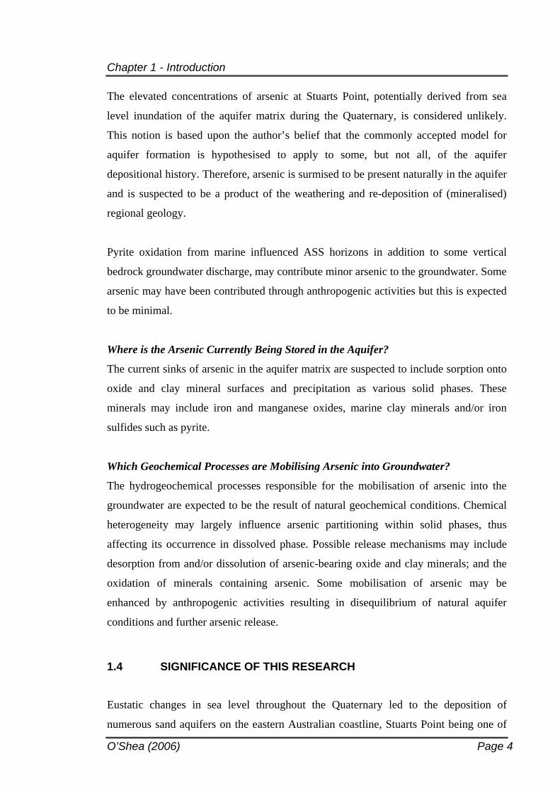
The elevated concentrations of arsenic at Stuarts Point, potentially derived from sea
level inundation of the aquifer matrix during the Quaternary, is considered unlikely.
This notion is based upon the author’s belief that the commonly accepted model for
aquifer formation is hypothesised to apply to some, but not all, of the aquifer
depositional history. Therefore, arsenic is surmised to be present naturally in the aquifer
and is suspected to be a product of the weathering and re-deposition of (mineralised)
regional geology.
Pyrite oxidation from marine influenced ASS horizons in addition to some vertical
bedrock groundwater discharge, may contribute minor arsenic to the groundwater. Some
arsenic may have been contributed through anthropogenic activities but this is expected
to be minimal.
Where is the Arsenic Currently Being Stored in the Aquifer?
The current sinks of arsenic in the aquifer matrix are suspected to include sorption onto
oxide and clay mineral surfaces and precipitation as various solid phases. These
minerals may include iron and manganese oxides, marine clay minerals and/or iron
sulfides such as pyrite.
Which Geochemical Processes are Mobilising Arsenic into Groundwater?
The hydrogeochemical processes responsible for the mobilisation of arsenic into the
groundwater are expected to be the result of natural geochemical conditions. Chemical
heterogeneity may largely influence arsenic partitioning within solid phases, thus
affecting its occurrence in dissolved phase. Possible release mechanisms may include
desorption from and/or dissolution of arsenic-bearing oxide and clay minerals; and the
oxidation of minerals containing arsenic. Some mobilisation of arsenic may be
enhanced by anthropogenic activities resulting in disequilibrium of natural aquifer
conditions and further arsenic release.
1.4 SIGNIFICANCE OF THIS RESEARCH
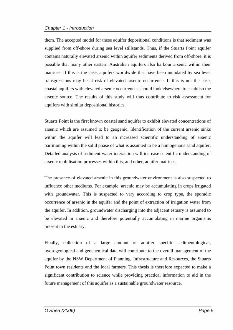
Eustatic changes in sea level throughout the Quaternary led to the deposition of
numerous sand aquifers on the eastern Australian coastline, Stuarts Point being one of
Chapter 1 - Introduction
O’Shea (2006) Page 5
them. The accepted model for these aquifer depositional conditions is that sediment was
supplied from off-shore during sea level stillstands. Thus, if the Stuarts Point aquifer
contains naturally elevated arsenic within aquifer sediments derived from off-shore, it is
possible that many other eastern Australian aquifers also harbour arsenic within their
matrices. If this is the case, aquifers worldwide that have been inundated by sea level
transgressions may be at risk of elevated arsenic occurrence. If this is not the case,
coastal aquifers with elevated arsenic occurrences should look elsewhere to establish the
arsenic source. The results of this study will thus contribute to risk assessment for
aquifers with similar depositional histories.
Stuarts Point is the first known coastal sand aquifer to exhibit elevated concentrations of
arsenic which are assumed to be geogenic. Identification of the current arsenic sinks
within the aquifer will lead to an increased scientific understanding of arsenic
partitioning within the solid phase of what is assumed to be a homogenous sand aquifer.
Detailed analysis of sediment-water interaction will increase scientific understanding of
arsenic mobilisation processes within this, and other, aquifer matrices.
The presence of elevated arsenic in this groundwater environment is also suspected to
influence other mediums. For example, arsenic may be accumulating in crops irrigated
with groundwater. This is suspected to vary according to crop type, the sporadic
occurrence of arsenic in the aquifer and the point of extraction of irrigation water from
the aquifer. In addition, groundwater discharging into the adjacent estuary is assumed to
be elevated in arsenic and therefore potentially accumulating in marine organisms
present in the estuary.
Finally, collection of a large amount of aquifer specific sedimentological,
hydrogeological and geochemical data will contribute to the overall management of the
aquifer by the NSW Department of Planning, Infrastructure and Resources, the Stuarts
Point town residents and the local farmers. This thesis is therefore expected to make a
significant contribution to science while providing practical information to aid in the
future management of this aquifer as a sustainable groundwater resource.
Chapter 1 - Introduction
O’Shea (2006) Page 6
1.5 STUDY APPROACH
To investigate the main aims (and subsequently reject or accept the proposed
hypotheses) the tasks listed in Table 1.1 were executed. This list also differentiates
between existing knowledge previously available for incorporation in this investigation
and information that has been generated as part of this study.
1.6 THESIS STRUCTURE
The structure of this thesis is outlined in Figure 1.1. This introduction establishes a
summary of the problem to date and the need for its resolution. An overview of the site
location and geological knowledge available to date is provided in Chapter 2. The
literature review (Chapter 3) examines all aspects of arsenic chemistry relevant to its
occurrence in the environment and provides the reader with sufficient background
knowledge to critically assess the processes proposed herein. Chapter 4 outlines the
methods of analysis used within. An appreciable effort has been made to keep this thesis
clear and concise, with a strong focus on addressing the main aims, which form the bulk
sections of this thesis – Chapters 4 through 6 – covering arsenic sources, sinks and
mobilisation, respectively. Finally, Chapter 8 provides conclusions to the proposed
hypotheses, recommendations for the future management of the aquifer and any further
geochemical research that may be required. Supporting data are contained within the
appendices.

Tab
le 1
.1 T
asks
exe
cute
d in
this
thes
is a
nd n
ew d
ata
gene
rate
d as
a r
esul
t. Ta
skEx
isiti
ng In
form
atio
n D
ata
Gen
erat
ed H
erei
n D
eter
min
e re
lativ
e in
puts
(if
any)
from
ant
hrop
ogen
ic
arse
nic
sour
ces
His
toric
al re
cord
s –
spor
adic
and
in
com
plet
e; a
necd
otal
evi
denc
e A
sses
smen
t of a
ny re
cord
s pe
rtain
ing
to th
e us
e of
ars
enic
-co
ntai
ning
che
mic
als
in th
e vi
cini
ty o
f Stu
arts
Poi
nt –
liai
son
with
N
SW
Agr
icul
ture
, EP
A, L
and
& P
rope
rty In
form
atio
n, K
emps
ey
Shi
re C
ounc
il, lo
cal h
isto
rians
, Rut
ile Z
inc
Min
ing
Co.
& c
urre
nt
user
s of
the
land
E
stab
lish
pote
ntia
l for
ar
seni
c co
ntrib
utio
n fro
m
bedr
ock
geol
ogy
Lim
ited
and
cont
rast
ing
info
rmat
ion
avai
labl
e on
bed
rock
ge
olog
y; d
epth
and
lith
olog
y un
know
n
Ret
rieva
l of h
isto
rical
geo
logi
cal r
ecor
ds w
hich
hav
e be
en o
mitt
ed
from
the
mos
t rec
ent b
edro
ck g
eolo
gica
l stu
dies
; int
erse
ctio
n of
be
droc
k fro
m d
rillin
g pr
ovid
ed in
form
atio
n on
dep
th a
nd li
thol
ogy,
w
hich
sub
sequ
ently
sug
gest
ed a
faul
t exi
sts
in b
edro
ck w
hich
has
be
en o
verlo
oked
in re
cent
stu
dies
; exa
min
atio
n of
gro
undw
ater
co
mpo
sitio
n to
sup
port
or d
ism
iss
poss
ible
pre
senc
e of
faul
t E
stab
lish
pote
ntia
l for
ar
seni
c co
ntrib
utio
n fro
m
regi
onal
geo
logy
Det
aile
d ge
olog
ical
des
crip
tion
of
regi
onal
geo
logy
Reg
iona
l geo
mor
phic
mod
el
prop
osed
but
not
Stu
arts
Poi
nt
spec
ific
Lith
olog
ical
logg
ing
of a
quife
r sed
imen
ts to
dep
ths
grea
ter t
han
ever
sam
pled
bef
ore;
sed
imen
tolo
gica
l met
hods
and
sta
tistic
al
anal
ysis
of s
edim
ent c
hem
istry
ena
ble
aco
mpr
ehen
sive
geo
mor
phic
mod
el to
be
deve
lope
d fo
r dep
ositi
on
of th
e S
tuar
ts P
oint
aqu
ifer
Exa
min
atio
n of
cur
rent
ar
seni
c si
nks
in th
e aq
uife
r m
atrix
Nil
X-ra
y D
iffra
ctio
n; S
cann
ing
Ele
ctro
n M
icro
prob
e; S
X50
Ele
ctro
n M
icro
prob
e; S
eque
ntia
l Ext
ract
ions
; X-ra
y Fl
uore
scen
ce; S
tatis
tical
A
naly
ses;
bor
ehol
e pr
ofile
s A
sses
smen
t of g
roun
dwat
er
cond
ition
s su
itabl
e fo
r the
m
obili
satio
n of
ars
enic
Pre
limin
ary
stud
ies
sugg
estin
g ar
seni
c m
obili
satio
n pr
oces
ses
are
geoc
hem
ical
ly c
ompl
ex
Sta
tistic
al a
naly
sis
of m
ore
than
200
gro
undw
ater
sam
ples
from
10
mul
ti-le
vel p
iezo
met
ers
with
met
re d
epth
incr
emen
t sam
plin
g po
ints
; ana
lysi
s of
geo
chem
ical
cor
rela
tions
bet
wee
n ar
seni
c an
d m
ore
than
50
elem
ents
in a
queo
us p
hase
; ass
essm
ent o
f ge
oche
mic
al s
uita
bilit
y fo
r rel
ease
from
iden
tifie
d ar
seni
c si
nks
in
the
aqui
fer;
geoc
hem
ical
mod
ellin
g to
sup
port
prop
osed
m
obili
satio
n pr
oces
ses;
ass
essm
ent o
f cur
rent
pro
cess
es a
ffect
ing
arse
nic
pres
ence
and
mob
ility
in th
e aq
uife
r In
fluen
ce o
f ars
enic
in th
e su
rroun
ding
env
ironm
ent
Nil
Indi
catio
n of
ars
enic
acc
umul
atio
n in
cro
ps; a
nd in
fluen
ce o
f ar
seni
c in
the
adja
cent
est
uary
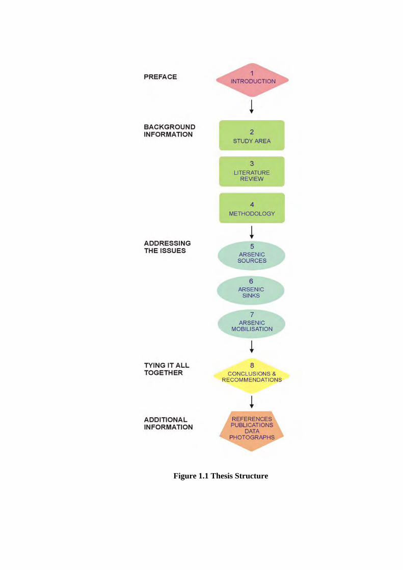
Figure 1.1 Thesis Structure
O’Shea (2006) Page 9
2 THE STUARTS POINT STUDY AREA
2.1 LOCATION AND ENVIRONMENTAL CONDITIONS1
Stuarts Point is located on the NSW mid-north coast (Figure 2.1), approximately 400
km north of Sydney, Australia (lat. 30º S, long. 153º E). The region is exposed to a
temperate climate with average maximum summer temperatures of 27º C in February
and average minimum winter temperatures of 11º C in July (Bureau of Meterology,
2005). Higher rainfall is received in summer than in winter, with maximum March
rainfall (average 194 mm - Bureau of Meteorology, 2005) generating excellent
conditions for extensive groundwater recharge via these increased precipitation rates.
Climate can vary, however, as observed during the course of this four year investigation
which saw floods, El Nino-induced bushfires and extreme drought plague much of the
region.
2.2 THE MACLEAY RIVER CATCHMENT
The Stuarts Point aquifer is positioned on the northeastern margin of the Macleay River
catchment, which covers approximately 11,450 km2. The catchment consists mainly of
floodplain deposits downstream of Kempsey, the region’s largest town (Figure 2.2).
Upstream of Kempsey, the rocky terrain of the New England Fold Belt characterises the
regional landscape.
The dominance of the floodplain in the surrounding region keeps topographic gradients
at Stuarts Point to a minimum, resulting in heights generally <5 m Australian Height
Datum (AHD). The Yarrahapinni Mountain rises approximately 495 m to the immediate
northwest of the Stuarts Point township (Figure 2.1).
1 A selection of site photographs can be viewed in Appendix C.
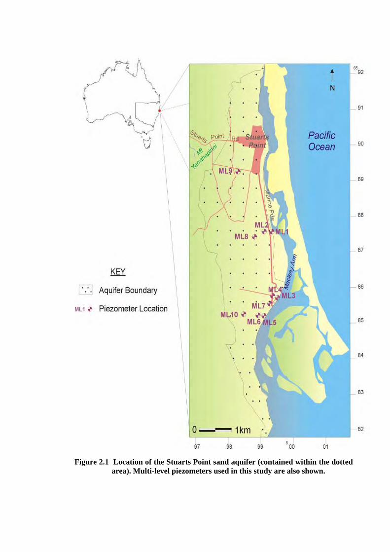
Figure 2.1 Location of the Stuarts Point sand aquifer (contained within the dotted area). Multi-level piezometers used in this study are also shown.

Figu
re h
as b
een
rem
oved
due
to C
opyr
ight
Agr
eem
ents
Figu
re 2
.2
Bou
ndar
ies
of t
he M
acle
ay R
iver
Cat
chm
ent.
Stua
rts
Poin
t is
loc
ated
on
the
nort
heas
tern
mar
gin
of t
he c
atch
men
t w
here
flood
plai
n de
posi
ts d
omin
ate
(NSW
EPA
, 200
5).
Chapter 2 – Study Area
O’Shea (2006) Page 12
The lower reaches of the mountain are used for banana, strawberry and macadamia
plantations while the upper reaches consist of wet sclerophyll forest. Much of the low-
lying land to the south of the township consists of heathland, sporadic residential lots
and agricultural crops including potatoes, stone fruits and avocadoes. The Macleay
River estuary located adjacent to Stuarts Point is used extensively for recreational
activities and commercial fishing, prawning and oyster production.
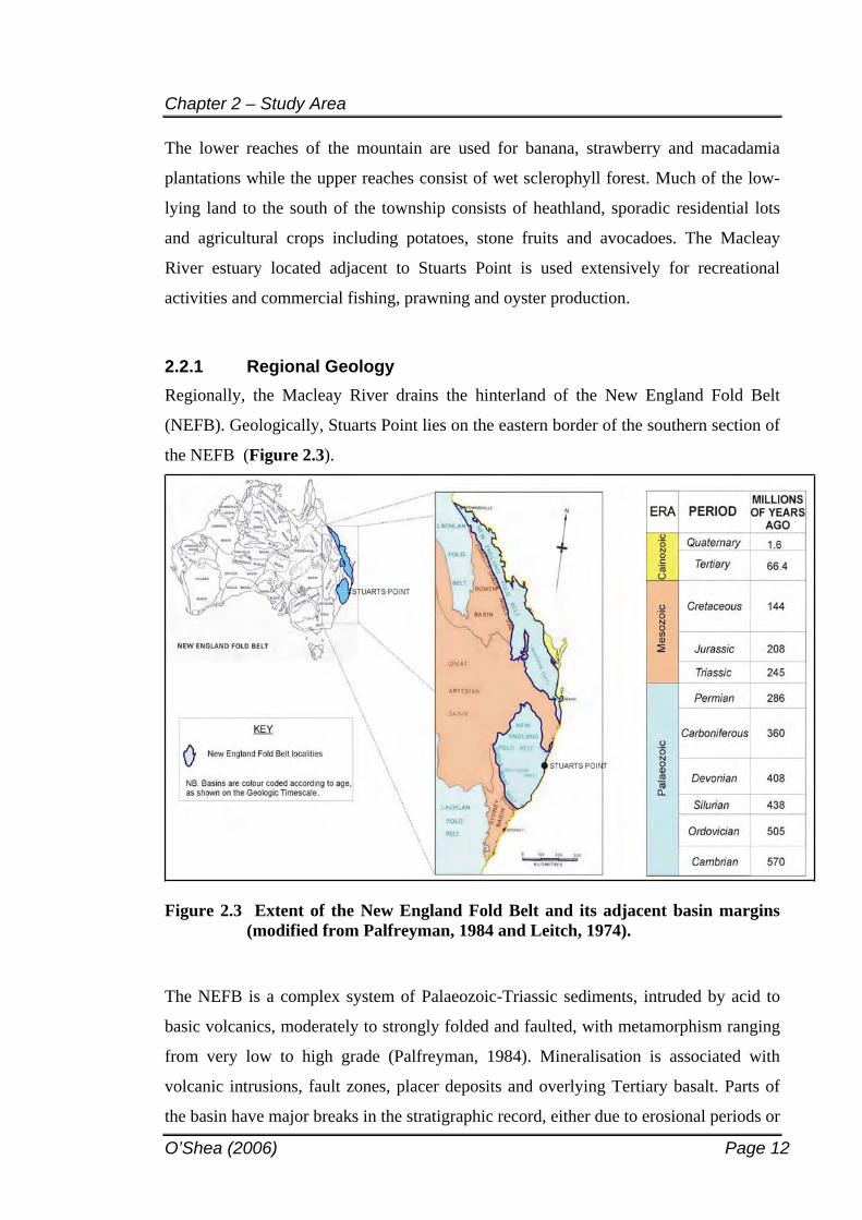
2.2.1 Regional Geology Regionally, the Macleay River drains the hinterland of the New England Fold Belt
(NEFB). Geologically, Stuarts Point lies on the eastern border of the southern section of
the NEFB (Figure 2.3).
Figure 2.3 Extent of the New England Fold Belt and its adjacent basin margins (modified from Palfreyman, 1984 and Leitch, 1974).
The NEFB is a complex system of Palaeozoic-Triassic sediments, intruded by acid to
basic volcanics, moderately to strongly folded and faulted, with metamorphism ranging
from very low to high grade (Palfreyman, 1984). Mineralisation is associated with
volcanic intrusions, fault zones, placer deposits and overlying Tertiary basalt. Parts of
the basin have major breaks in the stratigraphic record, either due to erosional periods or
Chapter 2 – Study Area
O’Shea (2006) Page 13
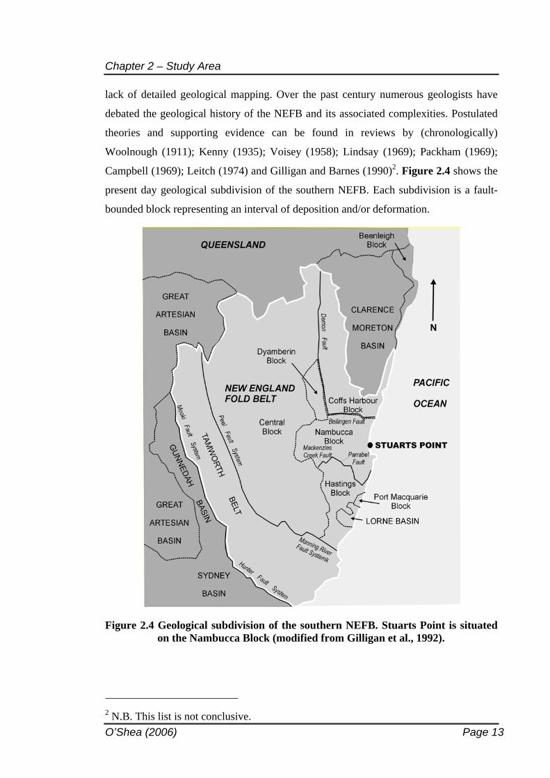
lack of detailed geological mapping. Over the past century numerous geologists have
debated the geological history of the NEFB and its associated complexities. Postulated
theories and supporting evidence can be found in reviews by (chronologically)
Woolnough (1911); Kenny (1935); Voisey (1958); Lindsay (1969); Packham (1969);
Campbell (1969); Leitch (1974) and Gilligan and Barnes (1990)2. Figure 2.4 shows the
present day geological subdivision of the southern NEFB. Each subdivision is a fault-
bounded block representing an interval of deposition and/or deformation.
Figure 2.4 Geological subdivision of the southern NEFB. Stuarts Point is situated on the Nambucca Block (modified from Gilligan et al., 1992).
2 N.B. This list is not conclusive.
Chapter 2 – Study Area
O’Shea (2006) Page 14
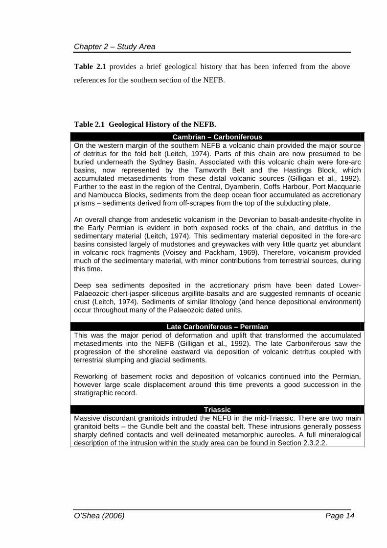
Table 2.1 provides a brief geological history that has been inferred from the above
references for the southern section of the NEFB.
Table 2.1 Geological History of the NEFB. Cambrian – Carboniferous
On the western margin of the southern NEFB a volcanic chain provided the major source of detritus for the fold belt (Leitch, 1974). Parts of this chain are now presumed to be buried underneath the Sydney Basin. Associated with this volcanic chain were fore-arc basins, now represented by the Tamworth Belt and the Hastings Block, which accumulated metasediments from these distal volcanic sources (Gilligan et al., 1992). Further to the east in the region of the Central, Dyamberin, Coffs Harbour, Port Macquarie and Nambucca Blocks, sediments from the deep ocean floor accumulated as accretionary prisms – sediments derived from off-scrapes from the top of the subducting plate.
An overall change from andesetic volcanism in the Devonian to basalt-andesite-rhyolite in the Early Permian is evident in both exposed rocks of the chain, and detritus in the sedimentary material (Leitch, 1974). This sedimentary material deposited in the fore-arc basins consisted largely of mudstones and greywackes with very little quartz yet abundant in volcanic rock fragments (Voisey and Packham, 1969). Therefore, volcanism provided much of the sedimentary material, with minor contributions from terrestrial sources, during this time.
Deep sea sediments deposited in the accretionary prism have been dated Lower-Palaeozoic chert-jasper-siliceous argillite-basalts and are suggested remnants of oceanic crust (Leitch, 1974). Sediments of similar lithology (and hence depositional environment) occur throughout many of the Palaeozoic dated units.
Late Carboniferous – Permian This was the major period of deformation and uplift that transformed the accumulated metasediments into the NEFB (Gilligan et al., 1992). The late Carboniferous saw the progression of the shoreline eastward via deposition of volcanic detritus coupled with terrestrial slumping and glacial sediments.
Reworking of basement rocks and deposition of volcanics continued into the Permian, however large scale displacement around this time prevents a good succession in the stratigraphic record.
TriassicMassive discordant granitoids intruded the NEFB in the mid-Triassic. There are two main granitoid belts – the Gundle belt and the coastal belt. These intrusions generally possess sharply defined contacts and well delineated metamorphic aureoles. A full mineralogical description of the intrusion within the study area can be found in Section 2.3.2.2.
Chapter 2 – Study Area
O’Shea (2006) Page 15
2.2.2 The Macleay Fluvial-Deltaic Floodplain
The floodplain consists of a variety of soils and sediments deposited during eustatic
changes in sea level during the Quarternary. Sediments consist of alluvial terraces
(Walker, 1970), back barrier swamp deposits, beach barrier sands (Hails, 1968),
estuarine muds and silty clay sequences (Eddie, 2000). Soil development is highly
dependent on sediment type and can vary from sandy podzolized soils to organic
topsoils with high ASS potential (Haskins et al., 2000). Aboriginal shell middens have
been identified in the area and are considered to be of archaeological significance
(Sullivan and Hughes, 1978).
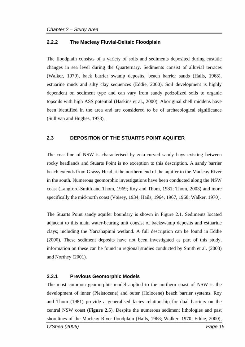
2.3 DEPOSITION OF THE STUARTS POINT AQUIFER
The coastline of NSW is characterised by zeta-curved sandy bays existing between
rocky headlands and Stuarts Point is no exception to this description. A sandy barrier
beach extends from Grassy Head at the northern end of the aquifer to the Macleay River
in the south. Numerous geomorphic investigations have been conducted along the NSW
coast (Langford-Smith and Thom, 1969; Roy and Thom, 1981; Thom, 2003) and more
specifically the mid-north coast (Voisey, 1934; Hails, 1964, 1967, 1968; Walker, 1970).
The Stuarts Point sandy aquifer boundary is shown in Figure 2.1. Sediments located
adjacent to this main water-bearing unit consist of backswamp deposits and estuarine
clays; including the Yarrahapinni wetland. A full description can be found in Eddie
(2000). These sediment deposits have not been investigated as part of this study,
information on these can be found in regional studies conducted by Smith et al. (2003)
and Northey (2001).
2.3.1 Previous Geomorphic Models The most common geomorphic model applied to the northern coast of NSW is the
development of inner (Pleistocene) and outer (Holocene) beach barrier systems. Roy
and Thom (1981) provide a generalised facies relationship for dual barriers on the
central NSW coast (Figure 2.5). Despite the numerous sediment lithologies and past
shorelines of the Macleay River floodplain (Hails, 1968; Walker, 1970; Eddie, 2000),
Chapter 2 – Study Area
O’Shea (2006) Page 16
the aquifer investigated herein focuses on a sandy water-bearing unit generally
described as a coastal barrier. It is this stratigraphy which is commonly adopted by
investigators in the area (Eddie, 2000; Smith et al., 2003; 2006).
Figure has been removed due to Copyright Agreements
Figure 2.5 Generalised section of a dual barrier system (Roy and Thom, 1981).
Hoyt (1966) proposes the dual barrier system primarily develops due to submergence of
dune or beach ridges adjacent to pre existing shorelines; that is, sediment is derived
from off-shore and is pushed on-shore during stillstands. Prior to this deposition,
however, existed a pre-Pleistocene shoreline present inland of the current coastline. This
former shoreline is illustrated nicely in Hails’ (1968) existing geomorphic model for the
region shown in Figure 2.6. This figure shows the former Pleistocene shoreline and
headlands at Hat Head and Smoky Cape were once offshore islands and have since been
joined to the coastline by deposition of a dual barrier system.

Chapter 2 – Study Area
O’Shea (2006) Page 17
Figure has been removed due to Copyright Agreements
Figure 2.6 Pre-Pleistocene and current Holocene coastlines on the NSW mid-north coast (Hails, 1968).
Eddie (2000) classified the Stuarts Point aquifer as an inner barrier unconsolidated
siliceous beach and dune sand, denoted by ‘sp’ on the extract of his soil landscape map
presented in (Figure 2.7).
Chapter 2 – Study Area
O’Shea (2006) Page 18
Figure has been removed due to Copyright Agreements
Figure 2.7 The Stuarts Point aquifer (outlined) denoted by Eddie (2000) as an inner barrier beach/dune sand – ‘sp’ (extracted and modified from Eddie, 2000).
Hails (1968) described the area simply as ‘abandoned beach ridges’ in contrast to actual
inner and outer barrier systems. He does state that deflection of the Macleay River most
probably occurred during formation of the outer barrier which is thus assumed to be
positioned on the eastern (seaward) side of the Macleay Arm and thus not within the
limits of the Stuarts Point aquifer investigated herein. The outer Holocene barrier is also
quartzose and contains abundant shell material. The outer Holocene barrier has formed
in the last 7,000 years during which time there has been a constant and plentiful onshore
supply of sand (Hails, 1968).
In terms of groundwater environments elevated in dissolved arsenic, a quartz-rich sand
barrier deposit constructed from sediment supplied from offshore proved to be a unique
and alarming occurrence of such natural contamination; thus sparking the need for this
research. This commonly accepted dual barrier geomorphic model for the deposition of
the Stuarts Point aquifer will be assessed in Chapter 5 – Original Source of Arsenic to
the Aquifer.
Chapter 2 – Study Area
O’Shea (2006) Page 19
2.3.2 Bedrock Geology
2.3.2.1 Lithology and Structure The underlying bedrock has been deduced as belonging to the NEFB, however, a review
of previous literature relating to the Stuarts Point (site specific) geology indicates
inconsistent theories on the likely bedrock lithology present beneath the unconsolidated
aquifer. Kenny (1935) explains the likely cause of these inconsistencies in his
geological reconnaissance of the north coastal region.
“In common with neighbouring tracts of country practically the whole of the
area traversed is heavily timbered. Rock outcrops are masked by a cover of scrub,
grass, and waste material to the extent that favourable exposures are restricted
almost wholly to sections along the sea-coast to road and railway cuttings, to
gullies in the upper reaches of stream systems, and to mine workings. For these
reasons it has been found impracticable to trace geological boundaries save in a
very general sense and no attempt at any detailed interpretation of structural
relationships and stratigraphical succession has been made.” (pg 85)
The inaccessible terrain surrounding Stuarts Point has therefore made ground truthing
and subsequent geological mapping difficult. Geological boundaries presented herein
may have been inferred from the limited data available and should thus be interpreted
with caution.
Figure 2.8 shows several possible bedrock lithologies proposed by various geologists.
The earliest account was conducted by Voisey (1950). A possible fault, termed the
‘Kempsey Area Fault’, was indicated to extend from the bedrock outcrops west of
Stuarts Point, trending in an easterly direction towards the coast and dissecting the
Stuarts Point study area. The Kempsey Area Fault was hypothesised to dissect northern
lower Palaeozoic slates and phyllites from southern upper Palaeozoic micaceous
mudstones of the Warbro (Permian) stage of the Macleay series. According to Voisey
(1950), these upper Palaeozoic sediments have been lowered relative to the northern
lower Palaeozoic sediments; and were already folded when the Kempsey Area Fault
occurred late in the Upper Palaeozoic orogeny.
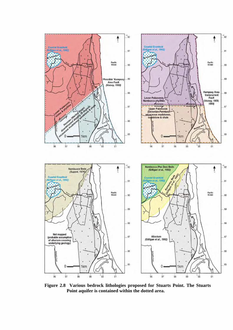
Figure 2.8 Various bedrock lithologies proposed for Stuarts Point. The Stuarts Point aquifer is contained within the dotted area.
Chapter 2 – Study Area
O’Shea (2006) Page 21
Voisey (1958) again suggested the presence of the Kempsey Area Fault, described as a
transcurrent fault, once again separating Permian sediments in the south from lower
Palaeozoic sediments in the north. Several years later Voisey and Packham (1969)
provided a review of the New England Region. The same theories were postulated
except that the lower Palaeozoic sediments north of the Kempsey Area Fault were re-
named the Nambucca Phyllites.
Suppel (1974) made no mention of the Kempsey Area Fault. Figure 2.8 marks the
boundary proposed by Suppel for the Nambucca Beds, consisting of slate, phyllite,
schistose, sandstone and schistose conglomerate of probable Permian age. No reason
was given as to the difference in proposed boundaries for the Nambucca Beds
previously described by Voisey and Packham (1969). It is thought that the boundary
was simply inferred, but could not be clearly identified due to the presence of alluvium
covering accessible outcrops.
Similarly, Gilligan et al. (1992) provided a metallogenic map of the Nambucca Block
without any indication of a fault occurring in the Stuarts Point area. The area where
Suppel’s (1974) Nambucca Beds were postulated to occur were divided into Nambucca
(Pee Dee) and Kempsey Beds by Gilligan et al. (1992). The Kempsey Beds were in turn
described as consisting of lithic sandstone, mudstone, pebbly sandstone and minor
conglomerate of late Carboniferous to early Permian age and most probably correspond
to Leitch’s (1974) Kempsey Beds. Leitch (1974) had previously provided an account of
regional geology in the Nambucca Block. While no approximate boundaries were
inferred for the Stuarts Point area, the Kempsey Beds were thought to overlie the
Nambucca (Pee Dee) Beds in the southeast of the Nambucca Block (i.e., the northwest
corner of Stuarts Point). Leitch (1974) described the Kempsey Beds as consisting of
interbedded lithic sandstone and siltstone with occasional conglomerate horizons. Both
sandstones and siltstones were indicated to potentially be pyritic; many of them showing
evidence of organic reworking. The Pee Dee Beds were described by Leitch (1974) to
be dominated by cleaved siltstone. All rocks were deposited in a marine environment
with terrigenous sediment contributions.
Chapter 2 – Study Area
O’Shea (2006) Page 22
In their review of the geology of Stuarts Point, Smith et al. (2003) concluded from the
above evidence that the unconsolidated aquifer sediments must overlie the Kempsey
Beds. They also stated that the upper reaches of the catchment were characterised by the
early Permian Pee Dee Beds of slaty siltstone, lithic sandstone and minor diamictite.
Gilligan et al.’s (1992) boundary for the Pee Dee Beds does not extend as far southeast
to the Stuarts Point aquifer, however drilling evidence obtained herein, in addition to the
location of a slate/phyllite quarry at Stuarts Point, indicates the Nambucca (Pee Dee)
Beds may in fact underlie the northern part of the Stuarts Point aquifer.
Smith et al. (2003), Gilligan et al. (1992) and Suppel (1974) made no reference to
Voisey’s previous papers (1950; 1958) in which the Kempsey Area Fault was listed as a
principal structural feature. It seems that the possibility of this Kempsey Area Fault
being present has been neglected in the most recent geological literature without any
plausible explanation of its omission. The terrain surrounding Stuarts Point has been
noted by many authors as being harsh and inaccessible. If the fault is present, the
unconsolidated deposits of the Stuarts Point aquifer cover it. Combined with the
inaccessible terrain, this fault may exist but to date has not been accurately mapped. In
addition, many of the later geological investigations were conducted on a regional scale
rather than a site specific scale and therefore attention to an inconspicuous fault at
Stuarts Point may have been overlooked.
2.3.2.2 MineralisationThe Nambucca Block contains a coastal granitoid belt extending approximately 40 km
in length and 10 km wide and comprising small discrete granitic intrusions (Gilligan et
al., 1992). In the vicinity of Stuarts Point an adamellite granitoid intrusion forms Mt
Yarrahapinni in the northwest of the study area (Figure 2.9).
Substantial mineralisation occurs within the granitic intrusion and contact aureole
forming Mt Yarrahapinni. The intrusion and associated aureole span approximately 1.5
km by 2.5 km and are located to the southwest of a larger intrusion (Suppel and Hobbs,
1977). Mineralisation is directly associated with the granitic intrusions which are
located in complexly deformed low grade metasediments of the Nambucca Block
(Suppel and Hobbs, 1977). Deposits are present in both the granitic and
Chapter 2 – Study Area
O’Shea (2006) Page 23
metasedimentary rocks – the phyllites and slates of the Nambucca (Pee Dee) Beds.
Further description of mineralised deposits are discussed below and are largely
summarised from Gilligan et al. (1992).
Figure has been removed due to Copyright Agreements
Figure 2.9 Coastal granitoid belt forming Mt Yarrahapinni (modified from Gilligan et al., 1992).
Molybdenite is sparsely disseminated throughout the adamellite and therefore is the
dominant exploited form of mineralisation present at Mt Yarrahapinni, with three
deposits having previously been mined. Deposits of tungsten, silver, base metals (Pb,
Zn) and gold occur in and around the Yarrahapinni adamellite. Mineralisation grades
from an outward zoning molybdenum zone (I), to a silver-lead zone (II) and finally to a
silver-arsenic zone (III). On the Stuarts Point side of Mt Yarrahapinni these mapped
zones are incomplete, indicating the lack of accurate geological mapping specific to the
area (Figure 2.10).
Chapter 2 – Study Area
O’Shea (2006) Page 24
Figure has been removed due to Copyright Agreements
Figure 2.10 Zones of mineralisation surrounding Mt Yarrahapinni (modified from Gilligan et al., 1992). Numbers refer to recognised mineral deposits described in Gilligan et al. (1992). 772-774 are disseminated/vein Mo deposits.
The exact extent of the intrusion remains uncertain. Air borne geophysics was thus
obtained to aid in the interpretation of the extent of the adamellite intrusion forming Mt
Yarrahapinni. However, the quality of this data was poor and very little processing
could be conducted. An anomaly was detected in the vicinity of the Stuarts Point
aquifer, however, the poor data quality prevented further analysis or identification of the
anomaly. It should be assumed that the granitoid intrusion may extend underneath the
Stuarts Point aquifer further than previously mapped by Gilligan et al. (1992).
Mineralisation occurs primarily as (Gilligan et al., 1992):
disseminated - particularly Mo with associated chalcopyrite, pyrite and pyrrhotite;
joint-controlled sheeted veins - quartz-molybdenite-scheelite veinlets hosted by the
adamellite;
Chapter 2 – Study Area
O’Shea (2006) Page 25
fracture-controlled quartz veins - discrete molybdenite-quartz veins within the
adamellite and associated hornfels, with disseminated or sporadically associated Ag-
As-Zn sulfides; and
fracture-controlled siliceous sulfide veins - joint controlled parallel vein system of
high-grade Ag-Pb-Zn mineralisation hosted by the hornfels.
In a geochemical survey of the Yarrahapinni - Way Way State Forest area, Suppel and
Hobbs (1977) found arsenic stream sediment concentrations were high, widespread and
frequently associated with anomalous molybdenum and copper zones. They further
state,
“the results indicate that arsenic is associated with the granitic intrusions” (pg
43).
In addition, Kenny (1935) noted,
“narrow veins of quartzose material, together with sulfides of lead, zinc, iron and
arsenic, the last-mentioned predominating, are developed along joints in
claystones close to the granite contact” (pg 86).
Arsenic is therefore undoubtedly associated with rocks located in close proximity to and
potentially underneath the Stuarts Point aquifer.
2.3.3 Hydrogeology The township extracts groundwater from a designated borefield to supply its 781
residents (Australian Bureau of Statistics, 2001) in addition to localised extraction for
agricultural irrigation. Domestic groundwater is treated to remove arsenic, however
most irrigation water is extracted via on-farm spearpoint bores and applied to crops
untreated.
Groundwater levels were measured in May 2001 and indicate a general flow direction
from Mt Yarrahapinni in the northwest, flowing south-southeast through the sand
aquifer and discharging into the Macleay Arm (Figure 2.11).
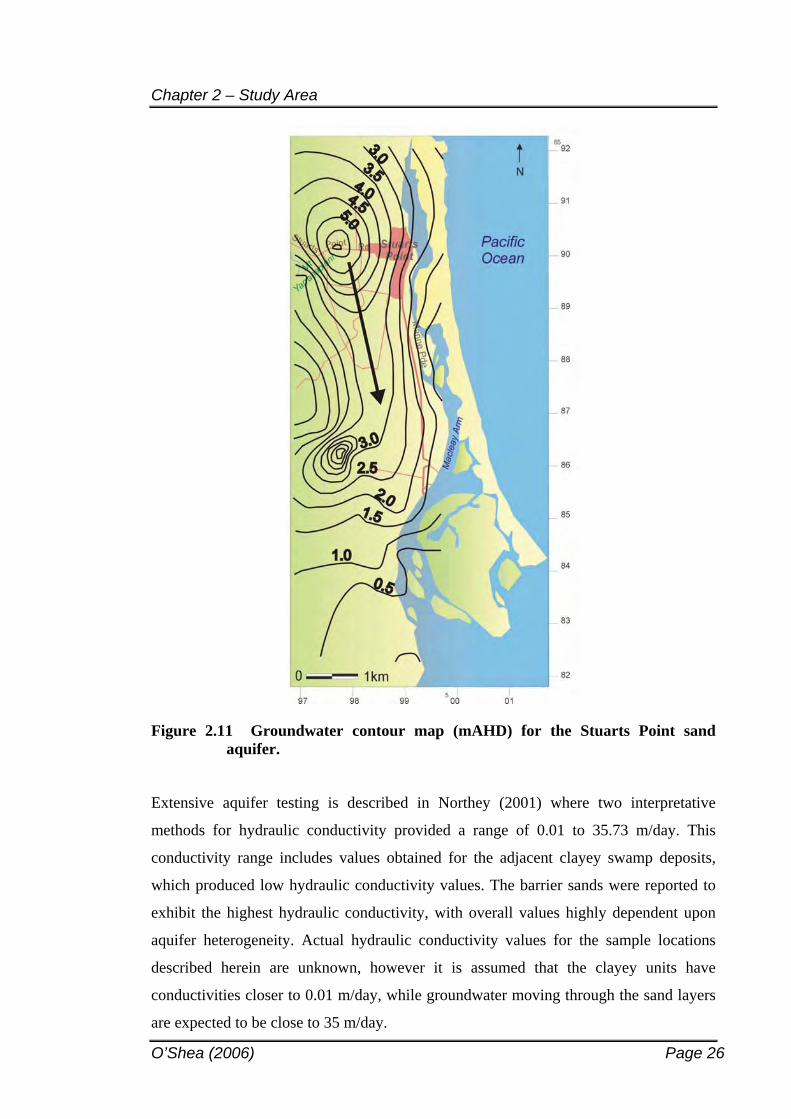
Chapter 2 – Study Area
O’Shea (2006) Page 26
Figure 2.11 Groundwater contour map (mAHD) for the Stuarts Point sand aquifer.
Extensive aquifer testing is described in Northey (2001) where two interpretative
methods for hydraulic conductivity provided a range of 0.01 to 35.73 m/day. This
conductivity range includes values obtained for the adjacent clayey swamp deposits,
which produced low hydraulic conductivity values. The barrier sands were reported to
exhibit the highest hydraulic conductivity, with overall values highly dependent upon
aquifer heterogeneity. Actual hydraulic conductivity values for the sample locations
described herein are unknown, however it is assumed that the clayey units have
conductivities closer to 0.01 m/day, while groundwater moving through the sand layers
are expected to be close to 35 m/day.
Chapter 2 – Study Area
O’Shea (2006) Page 27
Recharge to the aquifer is assumed to be dominated by diffuse precipitation and
potential recharge from bedrock groundwaters below the sandy aquifer. Isotopic
investigations conducted by Smith et al. (2003) suggest Yarrahapinni bedrock
groundwaters have endured a process of isotopic fractionation due to orographic
precipitation and the altitude effect described by Bortolami et al. (1979). They thus
exhibit 18O and 2H values of –5.2 and –26.3‰ respectively. In contrast, previous
work by Smith et al. (2001) appear to have mistakenly suggested that recharge
groundwater associated with the Yarrahapinni fractured (bed)rock system exhibits 18O
and 2H values up to approximately –7.3 and –44.2‰ respectively. Northey (2001)
graphed the same data according to lithological units in the study area and found that
Holocene sands plotted in this latter region (as opposed to bedrock waters only) and that
Holocene/Pleistocene sands and alluvial clays all plotted within the first stated range.
Additionally, the presence of the 500m high Mt Yarrahapinni is considered too low to
be affected by the altitude effect. For these reasons, the isotopic data is deemed
unreliable in the interpretation of bedrock discharge to the overlying unconsolidated
aquifer. Further isotopic investigations are known to be underway in the aquifer, but at
the time of writing this thesis these results had not yet been made publicly available.
The assumed discharge areas are the adjacent wetlands and Macleay River Arm estuary.
Water level data loggers examined by Smith et al. (2001) show the sandy aquifer
responds to rainfall events with a short time lag evident between precipitation events
and an observed rise in groundwater levels. Given the sandy nature of the aquifer
matrix, short response times to groundwater recharge can be expected. The close
proximity of the aquifer to the coastline may also induce diurnal variations in
groundwater levels influenced by the daily movement of tides. During extreme weather
conditions, such as floods and drought, both of which were observed during the course
of this investigation, the aquifer may respond accordingly. Indeed, a decline in
groundwater levels of approximately 1 m was observed between winter and summer. In
the summer, increased groundwater extraction for town and irrigation supplies may
provide a change in the flow conditions observed in Figure 2.11. While temporal
changes were not investigated during this study, it is important to realise that a change
in groundwater flow conditions will influence solute transport pathways. Bearing this in
Chapter 2 – Study Area
O’Shea (2006) Page 28
mind, the interpretations presented herein represent solute transport occurring under the
conditions observed during the sampling period.
2.4 PREVIOUS INVESTIGATIONS
Piscopo’s (1996) Taskforce report provided a baseline investigation for arsenic
occurrence within the Stuarts Point aquifer. Piscopo proposed there was sufficient
evidence to suggest that elevated levels of arsenic along the coast were:
localised, yet variable;
associated with disturbed coastal dune sands where pyrite was present;
below irrigation and stock guidelines;
predominantly below 50 g L-1 As;
potentially linked to acid sulfate soils; yet
insufficient evidence was found to determine a relationship between groundwater
abstraction and elevated arsenic concentrations.
It also raised further questions. Why was arsenic elevated at Stuarts Point and not in
other coastal aquifers? What is the definite source of the arsenic? Who, if anyone, is to
blame? How is it getting into the groundwater, and where is it going? What can we do
to minimise, or avoid, further arsenic contamination in this and other aquifers?
The horizontal distribution of arsenic at Stuarts Point was investigated by Smith et al.
(2000). This investigation sampled groundwater from wells installed in nearby Mt
Yarrahapinni (assumed bedrock), the inner Pleistocene Barrier, clay and swamp
deposits adjacent to the Stuarts Point sandy aquifer and the aquifer itself (Figure 2.12).
Arsenic was reported up to 70 g L-1 in wells installed at various depths and in different
stratigraphic facies, indicating a non-localised and sporadic occurrence of arsenic in the
local environment. Follow-up vertical studies of As distribution in the high yielding
sandy aquifer reported concentrations of up to 330 g L-1 (Smith et al., 2003).
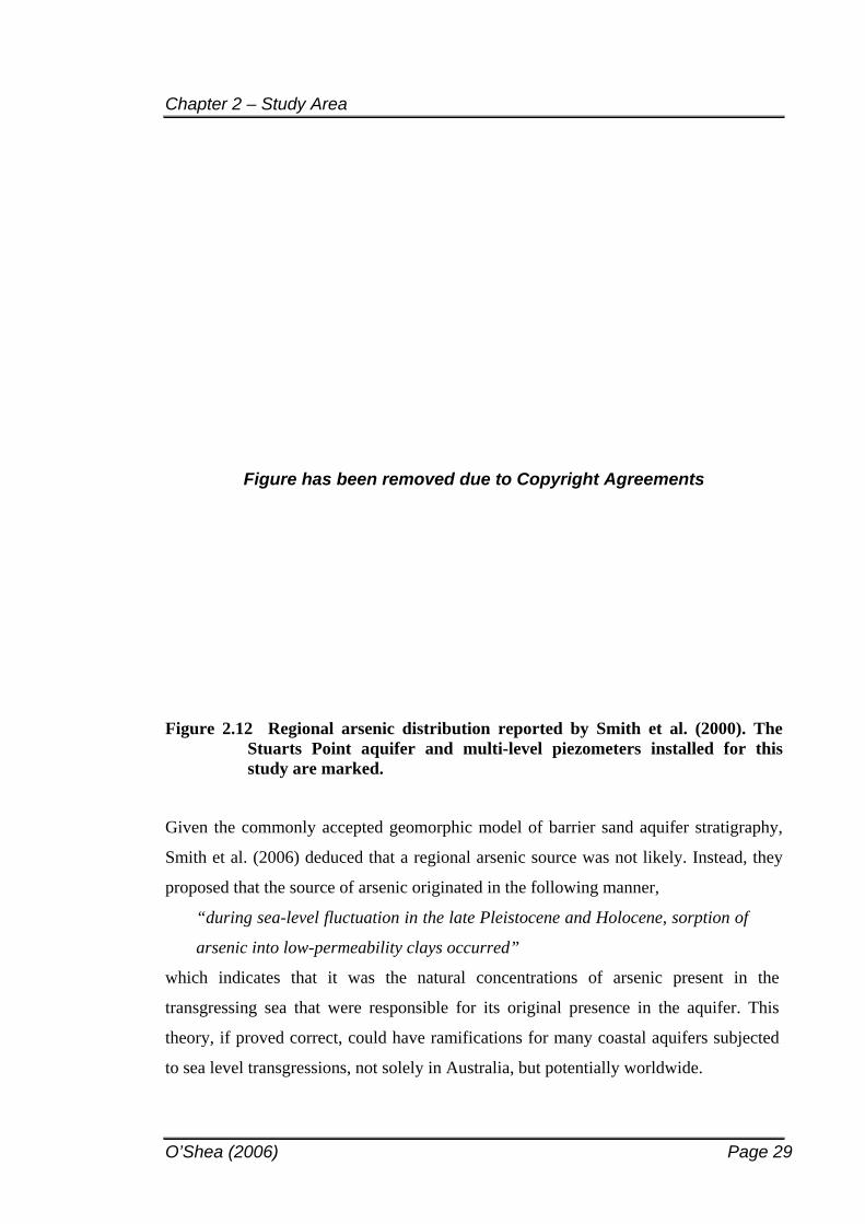
Chapter 2 – Study Area
O’Shea (2006) Page 29
Figure has been removed due to Copyright Agreements
Figure 2.12 Regional arsenic distribution reported by Smith et al. (2000). The Stuarts Point aquifer and multi-level piezometers installed for this study are marked.
Given the commonly accepted geomorphic model of barrier sand aquifer stratigraphy,
Smith et al. (2006) deduced that a regional arsenic source was not likely. Instead, they
proposed that the source of arsenic originated in the following manner,
“during sea-level fluctuation in the late Pleistocene and Holocene, sorption of
arsenic into low-permeability clays occurred”
which indicates that it was the natural concentrations of arsenic present in the
transgressing sea that were responsible for its original presence in the aquifer. This
theory, if proved correct, could have ramifications for many coastal aquifers subjected
to sea level transgressions, not solely in Australia, but potentially worldwide.
Chapter 2 – Study Area
O’Shea (2006) Page 30
Smith et al. (2003) also examined the aquifer groundwater composition and suggested
two principle geochemical processes contributing to arsenic mobilisation in the aquifer.
Arsenic reached concentrations of 85 g L-1 at a depth of 10-11 m and was suggested to
be
“present due to either the dissolution of Al hydroxides and release of adsorbed
As(V)… or concurrently via pH-influenced desorption of As enriched Fe oxides”
(pg 1490).
The greatest arsenic peak (337 g L-1) occurred at a depth of 25 m and was proposed to
be derived from
“leaching of the aquifer’s sandy-clayey matrix by groundwaters rich in HCO3-
and of high pH” (pg 1493).
More thorough investigations continued and included speciation of arsenic in aqueous
phase, but the method used was later found to be questionable during the course of the
investigations herein. Limited solid phase data were available to accurately determine
the source or sink of arsenic in the aquifer matrix. Therefore, assumptions governing
arsenic mobility could only be postulated based on the available aqueous data, with the
conclusions suggesting several plausible geochemical processes were governing arsenic
mobility in the aquifer. No definite arsenic source, sink or dominating mobilisation
process could be identified and sufficiently supported with the limited data available at
that time. The culmination of Smith’s research (Smith, 2005) recommends further
examination is required to better understand the arsenic geochemical cycle at Stuarts
Point. This investigation aims to fill that gap.
To date, no further published material has been found relating to the Stuarts Point
hydrogeochemical environment.
O’Shea (2006) Page 31
3 ARSENIC LITERATURE REVIEW
In the last decade there has been a dramatic increase in the number of studies
investigating arsenic in the environment. Much of this can be attributed to the discovery
of elevated levels of arsenic in domestic groundwater supplies throughout the world,
with particular respect to the arsenic crisis in Bangladesh. The severity of the problem
in Bangladesh has led to an increased amount of international scientific research being
conducted on arsenic toxicity, mobility, occurrence, chemical behaviour, cycling and
bioaccumulation. As such, a number of recent reviews on arsenic in the environment
have been provided by Welch et al. (2000); Smedley and Kinniburgh (2002); Welch and
Stollenwerk (2003); and Naidu et al. (2006); in addition to an entire Applied
Geochemistry journal volume (Volume 18, 2003) devoted solely to arsenic
geochemistry. Further to these recent reviews, earlier publications by Ferguson and
Gavis (1972) and Cullen and Reimer (1989) provide a solid basis on the theoretical
chemistry of arsenic in the environment.
Given the amount of published literature on this current affair, this review will focus on
topics considered by the author as appropriate background information on arsenic issues
most relevant to this study. Where possible, references for further reading will be
provided on elements that are less critical to this investigation and are therefore only
briefly discussed herein.
3.1 GENERAL PROPERTIES OF ARSENIC
3.1.1 Periodicity Arsenic belongs to Group 15 of the Periodic Table which comprises N, P, As, Sb and
Bi. The properties of these elements vary as the group is descended, with N and P
classified as non-metals; As and Sb as metalloids; and Bi being the only metal present
within the group. Group 15 is one of the few groups to exhibit the full range of element
chemistries – from non-metal to metalloid to metal – in a single group (Carmalt and
Norman, 1998).
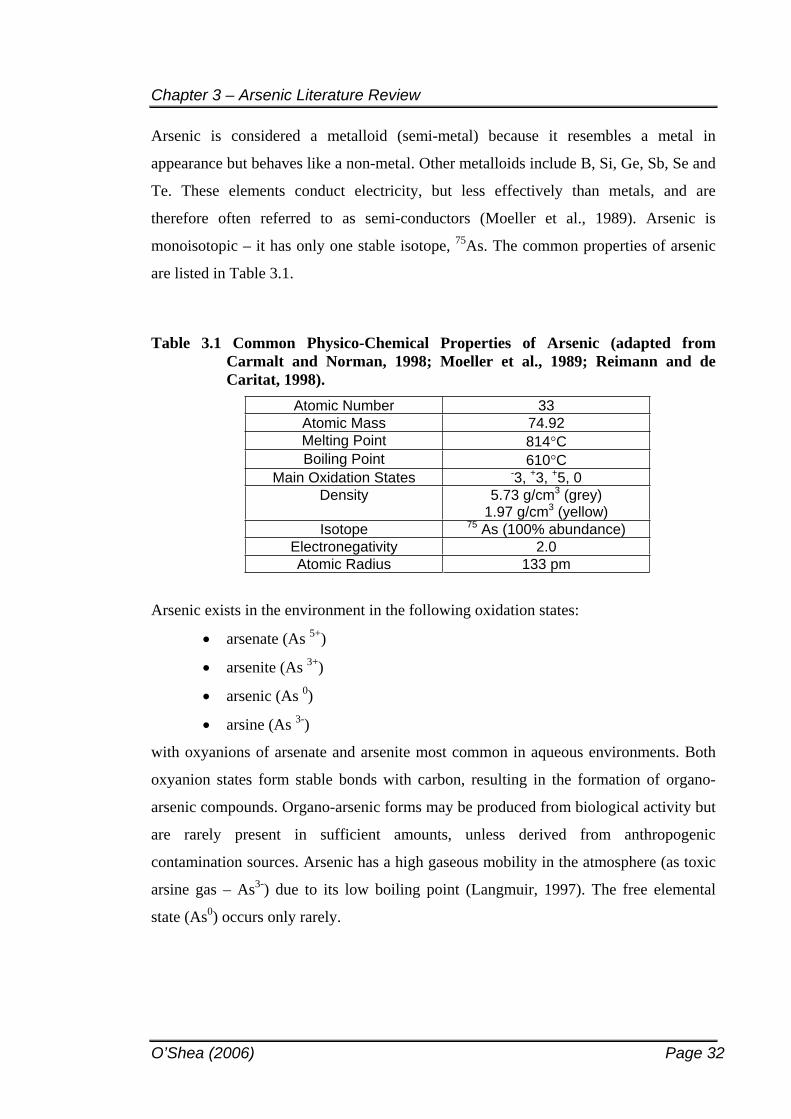
Chapter 3 – Arsenic Literature Review
O’Shea (2006) Page 32
Arsenic is considered a metalloid (semi-metal) because it resembles a metal in
appearance but behaves like a non-metal. Other metalloids include B, Si, Ge, Sb, Se and
Te. These elements conduct electricity, but less effectively than metals, and are
therefore often referred to as semi-conductors (Moeller et al., 1989). Arsenic is
monoisotopic – it has only one stable isotope, 75As. The common properties of arsenic
are listed in Table 3.1.
Table 3.1 Common Physico-Chemical Properties of Arsenic (adapted from Carmalt and Norman, 1998; Moeller et al., 1989; Reimann and de Caritat, 1998).
Atomic Number 33 Atomic Mass 74.92 Melting Point 814 CBoiling Point 610 C
Main Oxidation States -3, +3, +5, 0 Density 5.73 g/cm3 (grey)
1.97 g/cm3 (yellow) Isotope 75 As (100% abundance)
Electronegativity 2.0 Atomic Radius 133 pm
Arsenic exists in the environment in the following oxidation states:
arsenate (As 5+)
arsenite (As 3+)
arsenic (As 0)
arsine (As 3-)
with oxyanions of arsenate and arsenite most common in aqueous environments. Both
oxyanion states form stable bonds with carbon, resulting in the formation of organo-
arsenic compounds. Organo-arsenic forms may be produced from biological activity but
are rarely present in sufficient amounts, unless derived from anthropogenic
contamination sources. Arsenic has a high gaseous mobility in the atmosphere (as toxic
arsine gas – As3-) due to its low boiling point (Langmuir, 1997). The free elemental
state (As0) occurs only rarely.
Chapter 3 – Arsenic Literature Review
O’Shea (2006) Page 33
3.1.2 Toxicity Arsenic is considered an essential element and is routinely found in the body, however
many arsenic compounds are toxic. Akin to heavy metals, the toxicity of arsenic largely
depends on its chemical form, with toxicity decreasing in the order: arsine > arsenite >
arsenate > monomethylarsonic acid (MMA) > dimethylarsinic acid (DMA) (Jain and
Ali, 2000).
Arsine gas is the most toxic compound and if readily inhaled may cause lung cancer
(Bissen and Frimmel, 2003). Arsenite is resorbed faster into biological systems than
arsenate and hence is considered to be 60 times more toxic (Ferguson and Gavis, 1972).
Both oxidation states inhibit the energy-linked functions of the mitochondria (Bissen
and Frimmel, 2003). In addition, arsenic compounds block cell and tissue respiration,
can paralyse smooth muscle and cause numerous small haemorrhages (DMR, 1995).
Organo- arsenic compounds are least toxic to humans because the methylation of
arsenic reduces the affinity of the compound for tissue (Vahter and Marafante, 1988).
Arsenic is carcinogenic and may cause lung, bladder, liver, renal and skin cancers
(Bissen and Frimmel, 2003). A dose of 100 mg As2O3 can cause chronic arsenic
poisoning with 130 mg As2O3 considered fatal (DMR, 1995). Chronic symptoms
include fatigue, gastritis, anorexia and hair loss; with long term exposure producing
hyperkeratosis (thickening of the skin), cardiovascular diseases, disturbances in the
peripheral vascular and nervous systems, circulatory disorders and liver and kidney
disorders. Arsenic is deposited in hair, nail, bones and skin; and is readily excreted
through urine after three to four days. The body can detoxify (to an extent) arsenic
compounds by methylation to reduce its affinity for human tissue (Pontius et al., 1994).
Humans accustomed to arsenic ingestion have been shown to withstand greater amounts
of arsenic intake than those who are not accustomed to its presence within the body
(Morton and Dunnette, 1994). There is an increased amount of research being
conducted on the epidemiology of arsenic (Aguirre-Banuelos et al., 2004; Lu et al.,
2004) with particular reference to spatial distribution between arsenic health impacts
and consumption of arsenic-rich groundwater (Mandal and Biswas, 2004; Rahman et
al., 2005).
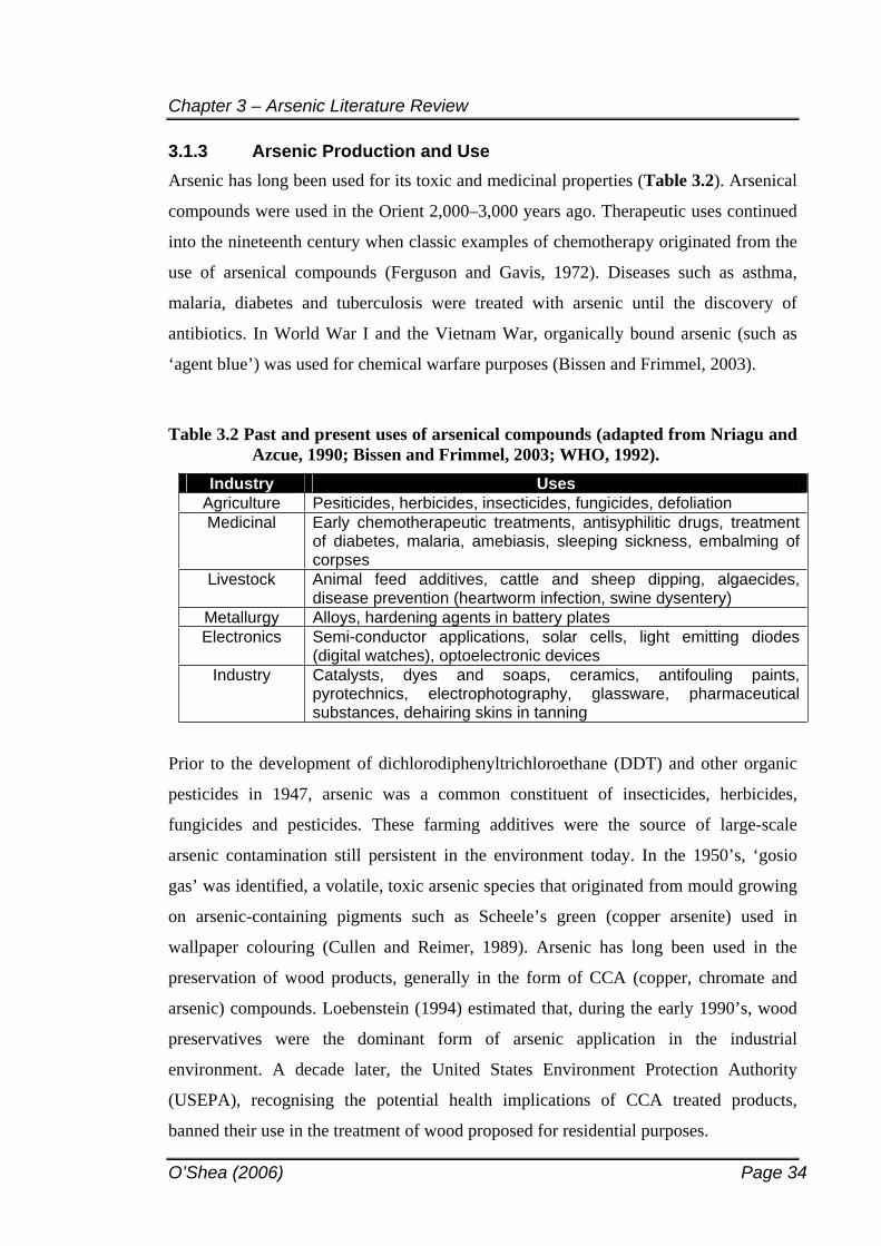
Chapter 3 – Arsenic Literature Review
O’Shea (2006) Page 34
3.1.3 Arsenic Production and Use Arsenic has long been used for its toxic and medicinal properties (Table 3.2). Arsenical
compounds were used in the Orient 2,000–3,000 years ago. Therapeutic uses continued
into the nineteenth century when classic examples of chemotherapy originated from the
use of arsenical compounds (Ferguson and Gavis, 1972). Diseases such as asthma,
malaria, diabetes and tuberculosis were treated with arsenic until the discovery of
antibiotics. In World War I and the Vietnam War, organically bound arsenic (such as
‘agent blue’) was used for chemical warfare purposes (Bissen and Frimmel, 2003).
Table 3.2 Past and present uses of arsenical compounds (adapted from Nriagu and Azcue, 1990; Bissen and Frimmel, 2003; WHO, 1992).
Industry UsesAgriculture Pesiticides, herbicides, insecticides, fungicides, defoliation Medicinal Early chemotherapeutic treatments, antisyphilitic drugs, treatment
of diabetes, malaria, amebiasis, sleeping sickness, embalming of corpses
Livestock Animal feed additives, cattle and sheep dipping, algaecides, disease prevention (heartworm infection, swine dysentery)
Metallurgy Alloys, hardening agents in battery plates Electronics Semi-conductor applications, solar cells, light emitting diodes
(digital watches), optoelectronic devices Industry Catalysts, dyes and soaps, ceramics, antifouling paints,
pyrotechnics, electrophotography, glassware, pharmaceutical substances, dehairing skins in tanning
Prior to the development of dichlorodiphenyltrichloroethane (DDT) and other organic
pesticides in 1947, arsenic was a common constituent of insecticides, herbicides,
fungicides and pesticides. These farming additives were the source of large-scale
arsenic contamination still persistent in the environment today. In the 1950’s, ‘gosio
gas’ was identified, a volatile, toxic arsenic species that originated from mould growing
on arsenic-containing pigments such as Scheele’s green (copper arsenite) used in
wallpaper colouring (Cullen and Reimer, 1989). Arsenic has long been used in the
preservation of wood products, generally in the form of CCA (copper, chromate and
arsenic) compounds. Loebenstein (1994) estimated that, during the early 1990’s, wood
preservatives were the dominant form of arsenic application in the industrial
environment. A decade later, the United States Environment Protection Authority
(USEPA), recognising the potential health implications of CCA treated products,
banned their use in the treatment of wood proposed for residential purposes.
Chapter 3 – Arsenic Literature Review
O’Shea (2006) Page 35
Its description as a human carcinogen has prompted the recent reduction of arsenic use
in favour of less persistent and less toxic synthetic organic compounds. Nevertheless,
arsenic production has occurred for more than a century. The estimated amount of
arsenic derived from anthropogenic uses doubles that of naturally occurring arsenic
(ANZECC, 2000). The majority of anthropogenically produced arsenic comes as a by-
product from the smelting of metallic ores. Mines worked solely for arsenic are rare. In
fact, the Bolidan copper smelter in Sweden produces enough arsenic as a by-product to
supply the world’s entire demand (DMR, 1995). Han et al. (2003) provide a thorough
review of global industrial-age arsenic accumulation and production in the environment.
They calculated that in the year 2000, anthropogenic arsenic input into the world arable
surface was 2.18 mg arsenic kg-1, which is 1.2 times the abundance in the lithosphere.
Major anthropogenic arsenic sources were estimated to follow the order: As mining
production > As generated from coal > As generated from petroleum.
According to records held by the New South Wales Department of Mineral Resources
(DMR, 1995) arsenic production in Australia has been limited:
Prior to 1912 – small tonnages of ore were produced in South Australia and New
South Wales.
1916 to 1936 – major production occurred in several states for ‘prickly pear poison’
which was required in Queensland. All previous supplies had been shipped to
England during World War I. The New England region of NSW (encompassing
Stuarts Point) was an important mining area during this time.
1935 to 1949 – the market price for arsenic was low; the Wiluna mine in Western
Australia was the only Australian mine producing arsenic during this time.
Post 1952 – arsenic has not been produced in Australian mines since this time.
In NSW, arsenic ores have been recovered at eight main centres, with the New England
geological region accounting for 85% of the state’s production (DMR, 1995).
3.2 SOURCES OF ARSENIC IN THE ENVIRONMENT
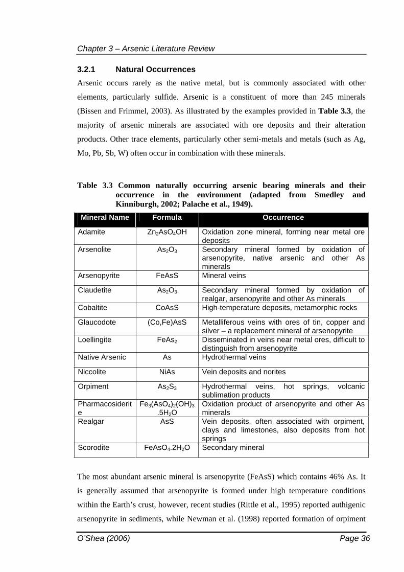
Chapter 3 – Arsenic Literature Review
O’Shea (2006) Page 36
3.2.1 Natural Occurrences Arsenic occurs rarely as the native metal, but is commonly associated with other
elements, particularly sulfide. Arsenic is a constituent of more than 245 minerals
(Bissen and Frimmel, 2003). As illustrated by the examples provided in Table 3.3, the
majority of arsenic minerals are associated with ore deposits and their alteration
products. Other trace elements, particularly other semi-metals and metals (such as Ag,
Mo, Pb, Sb, W) often occur in combination with these minerals.
Table 3.3 Common naturally occurring arsenic bearing minerals and their occurrence in the environment (adapted from Smedley and Kinniburgh, 2002; Palache et al., 1949).
Mineral Name Formula Occurrence
Adamite Zn2AsO4OH Oxidation zone mineral, forming near metal ore deposits
Arsenolite As2O3 Secondary mineral formed by oxidation of arsenopyrite, native arsenic and other As minerals
Arsenopyrite FeAsS Mineral veins
Claudetite As2O3 Secondary mineral formed by oxidation of realgar, arsenopyrite and other As minerals
Cobaltite CoAsS High-temperature deposits, metamorphic rocks
Glaucodote (Co,Fe)AsS Metalliferous veins with ores of tin, copper and silver – a replacement mineral of arsenopyrite
Loellingite FeAs2 Disseminated in veins near metal ores, difficult to distinguish from arsenopyrite
Native Arsenic As Hydrothermal veins
Niccolite NiAs Vein deposits and norites
Orpiment As2S3 Hydrothermal veins, hot springs, volcanic sublimation products
Pharmacosiderite
Fe3(AsO4)2(OH)3.5H2O
Oxidation product of arsenopyrite and other As minerals
Realgar AsS Vein deposits, often associated with orpiment, clays and limestones, also deposits from hot springs
Scorodite FeAsO4.2H2O Secondary mineral
The most abundant arsenic mineral is arsenopyrite (FeAsS) which contains 46% As. It
is generally assumed that arsenopyrite is formed under high temperature conditions
within the Earth’s crust, however, recent studies (Rittle et al., 1995) reported authigenic
arsenopyrite in sediments, while Newman et al. (1998) reported formation of orpiment
Chapter 3 – Arsenic Literature Review
O’Shea (2006) Page 37
by microbial precipitation. Arsenic rich pyrite – Fe(S,As)2 – rather than arsenopyrite, is
likely to be the most important source of As in ore zones (Nordstrom, 2000). Arsenic
rich pyrite (called arsenian pyrite hereafter) is also suspected to be a constituent of acid
sulfate soil material.
In addition to arsenic mineral occurrences, volcanic eruptions; cycling from the oceans
(sea spray); wind erosion; low temperature volatilisation; and the burning of wood
through natural forest fires can also contribute arsenic naturally to the environment.
3.2.2 Anthropogenic Sources Section 3.1.3 discussed both former and current anthropogenic uses of arsenic.
Therefore, human production and use of arsenic and its compounds can lead to an
increased load of this element in the environment. Failure to adequately contain
arsenical compounds during or after their use may lead to mobilisation of arsenic into
environmental substrates. For example, the application of arsenic-containing
pesticides/herbicides to the pedosphere increases its mobilisation potential to underlying
groundwater, which may subsequently discharge to rivers or oceans, and become
available for bioaccumulation or methylation by marine organisms, eventually to be
recycled back to the pedosphere via precipitation. Its high mobility in the environment
ensures many substrates are affected by arsenic contamination.
Significant quantities of arsenic can be found in pesticides, insecticides, herbicides and
fertilizers. Mirlean et al., (2003) found that bioavailable arsenic in estuarine sediments
accounted for 80% of total arsenic and was derived from atmospheric contamination by
a fertilizer factory. Bioavailable forms can easily be transported into surface or
groundwater. Similarly, direct application of pesticides, insecticides and herbicides to
the land surface can enable infiltration of arsenic and other metals to groundwater,
unless plant uptake or surface run-off re-directs arsenic towards other substrates.
Mariner et al. (1996) investigated a groundwater plume derived from a
pesticide/herbicide chemical plant travelling towards the shores of Commencement Bay
in Washington. Chemical wastes from the plant had been placed in unlined pits,
generating an arsenic plume exceeding 250 mg L-1 As.
Chapter 3 – Arsenic Literature Review
O’Shea (2006) Page 38
Arsenic is highly dispersed into the atmosphere through metal smelting processes and
the burning of fossil fuels. The burning of crude oil also contributes arsenic to the
atmosphere, to a lesser extent (Han et al., 2003). Fly ash from power plants may leach
arsenic into the surrounding soil and groundwater (Wallschlager et al., 2005). Mine
tailings can produce conditions suitable for arsenic mobilisation and transport in
aqueous environments. The most common arsenic associated ores are sulfides. Acid
mine drainage (AMD) results from extensive oxidation of Fe sulfide minerals and many
solid phase arsenic partitioning studies are conducted on the products of Fe sulfide
oxidation. One extreme case of AMD exists at Iron Mountain in the USA where pH
values are negative in AMD waters and arsenic concentrations reach the mg L-1 range
(Nordstrom et al., 2000).
Arsenopyrite and arsenian pyrite are often associated with ores of other metals, such as
Sn (Williams, 1997 as cited in Smedley and Kinniburgh, 2002); Au (Carrillo-Chavez et
al., 2000; Bodenan et al., 2004); Pb-Zn-Ag (Mok and Wai, 1990); Cu-W (Jung et al.,
2002); and Sb (Ashley et al., 2003; Mok and Wai, 1990). For example, arsenic derived
from stibnite deposits in the upper reaches of the Macleay River catchment has been
shown to contaminate both river water and stream sediments downgradient of the
Hillgrove stibnite mine (Ashley et al., 2003). In the Hetao Area of China, arsenic
concentrations in groundwater are also attibuted to downstream migration from mining
of metal sulfides and correspond to incidences of arsenic poisoning in local residents
(Zhang et al., 2002).
A less commonly documented occurrence of arsenic is its release after sand mining. The
same geochemical principles apply; arsenic is suggested to be released from the
oxidation of iron sulfides most likely present as pyrite in ASS. This suggestion was
made for the Tomago Sand aquifer (Coffey et al., 1996) located to the south of Stuarts
Point and was an instrumental finding leading to the inception of this project.
Other anthropogenic arsenic inputs include the disposal of industrial waste, leaching
from sheep dips and former tannery sites and contamination from CCA treated wood
products. CCA pressure treated wood has been widely used to preserve wood and
prevent decay by fungi, mould and termites. Children’s playgrounds, wooden decks and
Chapter 3 – Arsenic Literature Review
O’Shea (2006) Page 39
utility poles are commonly constructed with CCA treated wood. Arsenic and Cu are
used as insecticides while Cr is added to fix As and Cu to the wood cellulose (Dawson
et al., 1991). Soil sampled close to CCA treated wood is normally high in As and
decreases with depth and spatial distance from the structure (see Chirenje et al., 2003
for an example). However, Chirenje et al. (2003) noted that this pattern only occurred in
new structures and suggested that soils surrounding older structures may have been
weathered and leached over time. This may increase the risk of arsenic entering local
groundwater resources.
Industrial anthropogenic activities may allow arsenic to enter groundwater via
atmospheric deposition, infiltration, streambed deposition and subsequent groundwater
recharge, or as direct contaminant sources to groundwater via spills or buried wastes.
Tanneries commonly use arsenic in the tanning process and may result in dissolved
arsenic plumes beneath the former/current tannery site. One such site has been
investigated by the author herein, situated in the Botany Sands aquifer of metropolitan
Sydney. Dissolved arsenic concentrations reach mg L-1 level and respond to rainfall
events in a pulsating manner (GHD, 2002). Davis et al. (1994) studied a highly reducing
groundwater environment downgradient of a historical tannery in Massachusetts.
Conditions were so reducing that DOC levels were extremely high (>100 mg L-1) from
hide breakdown, leading to reduction of As(V) to As(III) and subsequent methylation to
MMAA and DMAA. Sekhar et al. (2003) found arsenic in groundwater downgradient of
buried veterinary chemicals in India. Armienta et al. (1997) reported concentrations of
dissolved arsenic up to 1.097 mg L-1 in groundwater of the Zimapan Valley in Mexico.
Contribution via percolation of smelter fumes during the 1940’s was considered as a
potential arsenic source. In an extreme case of arsenic contamination, Jarmersted et al.
(1998) reported dissolved arsenic up to 100 mg L-1 downgradient of a sulfuric acid
production plant where arsenic and several other metals were present as by-products of
the sulfide ore roasting process.
3.2.3 Concentrations in the Environment Arsenic ranks 20th in abundance of elements within the Earth’s crust (NRC, 1977).
Table 3.4 indicates the variation in concentrations between natural versus anthropogenic
activities. A number of substrate examples have been provided in a series of different
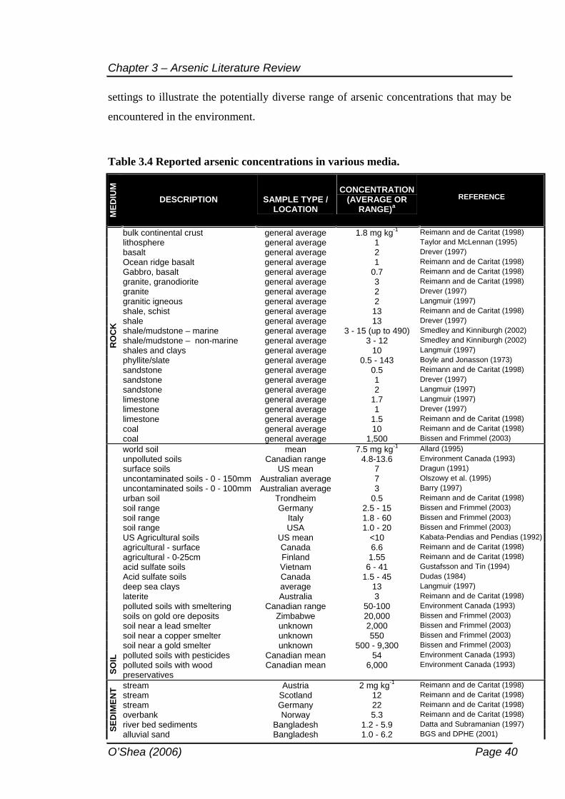
Chapter 3 – Arsenic Literature Review
O’Shea (2006) Page 40
settings to illustrate the potentially diverse range of arsenic concentrations that may be
encountered in the environment.
Table 3.4 Reported arsenic concentrations in various media.
MED
IUM
DESCRIPTION SAMPLE TYPE / LOCATION
CONCENTRATION (AVERAGE OR
RANGE)aREFERENCE
bulk continental crust general average 1.8 mg kg-1 Reimann and de Caritat (1998) lithosphere general average 1 Taylor and McLennan (1995) basalt general average 2 Drever (1997) Ocean ridge basalt general average 1 Reimann and de Caritat (1998) Gabbro, basalt general average 0.7 Reimann and de Caritat (1998) granite, granodiorite general average 3 Reimann and de Caritat (1998) granite general average 2 Drever (1997) granitic igneous general average 2 Langmuir (1997) shale, schist general average 13 Reimann and de Caritat (1998) shale general average 13 Drever (1997) shale/mudstone – marine general average 3 - 15 (up to 490) Smedley and Kinniburgh (2002) shale/mudstone – non-marine general average 3 - 12 Smedley and Kinniburgh (2002) shales and clays general average 10 Langmuir (1997) phyllite/slate general average 0.5 - 143 Boyle and Jonasson (1973) sandstone general average 0.5 Reimann and de Caritat (1998) sandstone general average 1 Drever (1997) sandstone general average 2 Langmuir (1997) limestone general average 1.7 Langmuir (1997) limestone general average 1 Drever (1997) limestone general average 1.5 Reimann and de Caritat (1998) coal general average 10 Reimann and de Caritat (1998)
RO
CK
coal general average 1,500 Bissen and Frimmel (2003) world soil mean 7.5 mg kg-1 Allard (1995) unpolluted soils Canadian range 4.8-13.6 Environment Canada (1993) surface soils US mean 7 Dragun (1991) uncontaminated soils - 0 - 150mm Australian average 7 Olszowy et al. (1995) uncontaminated soils - 0 - 100mm Australian average 3 Barry (1997) urban soil Trondheim 0.5 Reimann and de Caritat (1998) soil range Germany 2.5 - 15 Bissen and Frimmel (2003) soil range Italy 1.8 - 60 Bissen and Frimmel (2003) soil range USA 1.0 - 20 Bissen and Frimmel (2003) US Agricultural soils US mean <10 Kabata-Pendias and Pendias (1992)agricultural - surface Canada 6.6 Reimann and de Caritat (1998) agricultural - 0-25cm Finland 1.55 Reimann and de Caritat (1998) acid sulfate soils Vietnam 6 - 41 Gustafsson and Tin (1994) Acid sulfate soils Canada 1.5 - 45 Dudas (1984) deep sea clays average 13 Langmuir (1997) laterite Australia 3 Reimann and de Caritat (1998) polluted soils with smeltering Canadian range 50-100 Environment Canada (1993) soils on gold ore deposits Zimbabwe 20,000 Bissen and Frimmel (2003) soil near a lead smelter unknown 2,000 Bissen and Frimmel (2003) soil near a copper smelter unknown 550 Bissen and Frimmel (2003) soil near a gold smelter unknown 500 - 9,300 Bissen and Frimmel (2003) polluted soils with pesticides Canadian mean 54 Environment Canada (1993)
SOIL
polluted soils with wood preservatives
Canadian mean 6,000 Environment Canada (1993)
stream Austria 2 mg kg-1 Reimann and de Caritat (1998) stream Scotland 12 Reimann and de Caritat (1998) stream Germany 22 Reimann and de Caritat (1998) overbank Norway 5.3 Reimann and de Caritat (1998) river bed sediments Bangladesh 1.2 - 5.9 Datta and Subramanian (1997) SE
DIM
ENT
alluvial sand Bangladesh 1.0 - 6.2 BGS and DPHE (2001)
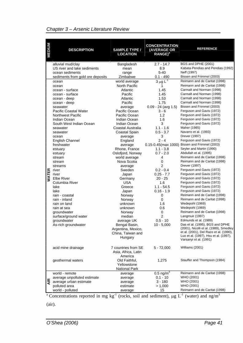
Chapter 3 – Arsenic Literature Review
O’Shea (2006) Page 41
MED
IUM
DESCRIPTION SAMPLE TYPE / LOCATION
CONCENTRATION (AVERAGE OR
RANGE)aREFERENCE
alluvial mud/clay Bangladesh 2.7 - 14.7 BGS and DPHE (2001) US river and lake sediments mean 8.9 Kabata-Pendias and Pendias (1992)ocean sediments range 5-40 Neff (1997) sediments from gold ore deposits Zimbabwe 0.1 - 490 Bissen and Frimmel (2003) ocean world average 3 g L-1 Reimann and de Caritat (1998) ocean North Pacific 1 Reimann and de Caritat (1998) ocean - surface Atlantic 1.45 Carmalt and Norman (1998) ocean - surface Pacific 1.45 Carmalt and Norman (1998) ocean - deep Atlantic 1.53 Carmalt and Norman (1998) ocean - deep Pacific 1.75 Carmalt and Norman (1998) seawater average 0.09 - 24 (avg 1.5) Bissen and Frimmel (2003) Pacific Coastal Water Pacific Ocean 3 - 6 Ferguson and Gavis (1972) Northwest Pacific Pacific Ocean 1.2 Ferguson and Gavis (1972) Indian Ocean Indian Ocean 1.6 Ferguson and Gavis (1972) South West Indian Ocean Indian Ocean 3 Ferguson and Gavis (1972) seawater Coastal Australia 1.1 - 1.6 Maher (1985) seawater Coastal Spain 0.5 - 3.7 Navarro et al. (1993) ocean average 3 Drever (1997) English Channel England 2 - 4 Ferguson and Gavis (1972) freshwater average 0.15-0.45(max 1000) Bissen and Frimmel (2003) estuary Rhone, France 1.1 - 3.8 Seyler and Martin (1990) estuary Oslofjord, Norway 0.7 - 2.0 Abdullah et al. (1995) stream world average 4 Reimann and de Caritat (1998) stream Nova Scotia 0 Reimann and de Caritat (1998) streams average 2 Drever (1997) river Sweden 0.2 - 0.4 Ferguson and Gavis (1972) river Japan 0.25 - 7.7 Ferguson and Gavis (1972) Elbe River Germany 20 - 25 Ferguson and Gavis (1972) Columbia River USA 1.6 Ferguson and Gavis (1972) lake Greece 1.1 - 54.5 Ferguson and Gavis (1972) lake Japan 0.16 - 1.9 Ferguson and Gavis (1972) rain - coastal Norway 0 Reimann and de Caritat (1998) rain - inland Norway 0 Reimann and de Caritat (1998) rain on land unknown 1.6 Wedepohl (1969) rain at sea unknown 0.6 Wedepohl (1969) groundwater Norway 0 Reimann and de Caritat (1998) surface/ground water median 2 Langmuir (1997) groundwater average UK 0.5 - 10 Edmunds et al. (1989) As-rich groundwater Bengal Basin,
Argentina, Mexico, China, Taiwan and
Hungary
10 - 5,000 Das et al. (1995), BGS and DPHE (2001), Nicolli et al. (1989), Smedley et al. (2001), Del Razo et al. (1990), Luo et al. (1997), Hsu et al. (1997), Varsanyi et al. (1991)
acid mine drainage 7 countries from SE
Asia, Africa, Latin America
5 - 72,000 Williams (2001)
WA
TER
geothermal waters Old Faithful, Yellowstone
National Park
1,275 Stauffer and Thompson (1984)
world - remote average 0.5 ng/m3 Reimann and de Caritat (1998) average unpolluted estimate average 0.1 - 10 WHO (2001) average urban estimate average 3 - 180 WHO (2001) polluted area estimate > 1,000 WHO (2001) A
IR
world - polluted average 15 Reimann and de Caritat (1998) a Concentrations reported in mg kg-1 (rocks, soil and sediment), g L-1 (water) and ng/m3
(air).
Chapter 3 – Arsenic Literature Review
O’Shea (2006) Page 42
3.2.3.1 RocksArsenic concentrations in igneous rocks are generally low (less than 2 mg kg-1 As).
Metamorphic rocks tend to reflect concentrations present in their igneous and
sedimentary predecessors, with average concentrations from Table 3.4 also indicating
less than 2 mg kg-1 As. Pelitic rocks derived from metamorphosed and non-
metamorphosed argillaceous rocks (shales, phyllites, slates) report slightly higher
averages of around 13 mg kg-1 As, but can reach much higher levels depending on their
depositional environment. Concentrations in sedimentary rocks vary due to major
constituents, sediment provenance and particle size. Sandstones, dominated by quartz
and feldspars, contain lower average arsenic concentrations (1-2 mg kg-1 As) than shales
(13 mg kg-1 As) which exhibit more clay, organic matter, oxide and sulfide minerals.
Coal can reach concentrations higher than 1,500 mg kg-1 As depending on the amount
of impurities present.
3.2.3.2 SoilsConcentrations of arsenic in soil will vary depending on parent material, grain size, soil
constituents, proximity to mineralised zones and anthropogenic influence. Values
shown in Table 3.4 range from 0.5 – 60 mg kg-1 As for suspected unpolluted soils; less
than 10 mg kg-1 As for agricultural soils; up to 45 mg kg-1 As in acid sulfate soils; and
excessively high concentrations in soils suspected of being anthropogenically
contaminated.
3.2.3.3 SedimentsSediment constituents play a vital role in determining arsenic concentrations. There is
no significant difference between sediments and rock concentrations containing the
same major constituents. Clays, muds and sediments high in oxides and sulfides will
retain more arsenic than sands and carbonates. Increased concentrations may occur due
to mineralised zones and anthropogenic sources.
3.2.3.4 WaterOcean waters typically average ca. 3 g L-1 As in the dominant form of As(V). This
figure applies to estuarine waters also, but may vary slightly due to salinity and redox
Chapter 3 – Arsenic Literature Review
O’Shea (2006) Page 43
gradients. Fresh water in rivers and streams are slightly lower (around 1 g L-1 As) but
are highly influenced by drainage areas, baseflow and point contamination sources such
as processing plants located on riverbanks. Rivers draining As-poor bedrock will have
lower As concentrations in their waters (less than 1 g L-1 As) compared to rivers
draining As-rich bedrock or geothermal areas. Nimick et al. (1998) found up to 370 g
L-1 As in the Madison River as a result of geothermal inputs from the Yellowstone
geothermal system. Lake water As concentrations can be influenced by stratification,
evaporation and seasonal effects. Changes in redox gradients with depth can lead to
stratification of lakes and influence on arsenic species available for sorption onto iron
oxides. Azcue and Nriagu (1995) studied arsenic distribution in lake waters from
Ontario and found that seasonal biological activity in the lake accounted for differences
in arsenic species distribution in summer months. Closed basins can account for high
evaporation rates and elevated arsenic levels in some lakes. Rain water arsenic
concentrations are typically below 1.5 g L-1 but may differ slightly between oceanic
and terrestrial precipitation localities.
Background As concentrations in groundwater are greatly influenced by the
composition of the aquifer matrix. Natural concentrations are reported in the range 0 –
5,000 g L-1 in the literature, but typically occur as less than 10 g L-1 as provided by
Edmunds et al. (1989) for the UK, and Welch et al. (2000) for the USA. Arsenic-rich
groundwaters are widely dispersed throughout the world and often occur as a result of
natural processes. Mining, agricultural and industrially influenced arsenic groundwaters
can exhibit very high arsenic concentrations (in the mg L-1 range) but tend to be more
localised than the naturally occurring systems.
3.2.3.5 AirAtmospheric arsenic concentrations are typically in the order of a few nanograms per
cubic metre. Elevated levels are largely influenced by proximity to industrial emitting
infrastructure such as smelters and fossil fuel power plants, or volcanic activity. Much
of the atmospheric arsenic is particulate and is cycled back to the lithosphere through
wet and dry deposition.
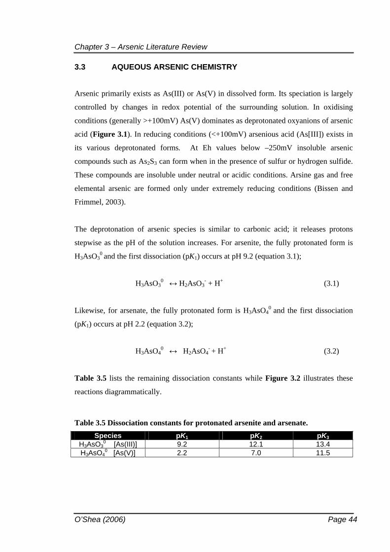
Chapter 3 – Arsenic Literature Review
O’Shea (2006) Page 44
3.3 AQUEOUS ARSENIC CHEMISTRY
Arsenic primarily exists as As(III) or As(V) in dissolved form. Its speciation is largely
controlled by changes in redox potential of the surrounding solution. In oxidising
conditions (generally >+100mV) As(V) dominates as deprotonated oxyanions of arsenic
acid (Figure 3.1). In reducing conditions (<+100mV) arsenious acid (As[III]) exists in
its various deprotonated forms. At Eh values below –250mV insoluble arsenic
compounds such as As2S3 can form when in the presence of sulfur or hydrogen sulfide.
These compounds are insoluble under neutral or acidic conditions. Arsine gas and free
elemental arsenic are formed only under extremely reducing conditions (Bissen and
Frimmel, 2003).
The deprotonation of arsenic species is similar to carbonic acid; it releases protons
stepwise as the pH of the solution increases. For arsenite, the fully protonated form is
H3AsO30 and the first dissociation (pK1) occurs at pH 9.2 (equation 3.1);
H3AsO30 H2AsO3
- + H+ (3.1)
Likewise, for arsenate, the fully protonated form is H3AsO40 and the first dissociation
(pK1) occurs at pH 2.2 (equation 3.2);
H3AsO40 H2AsO4
- + H+ (3.2)
Table 3.5 lists the remaining dissociation constants while Figure 3.2 illustrates these
reactions diagrammatically.
Table 3.5 Dissociation constants for protonated arsenite and arsenate. Species pK1 pK2 pK3
H3AsO30 [As(III)] 9.2 12.1 13.4
H3AsO40 [As(V)] 2.2 7.0 11.5
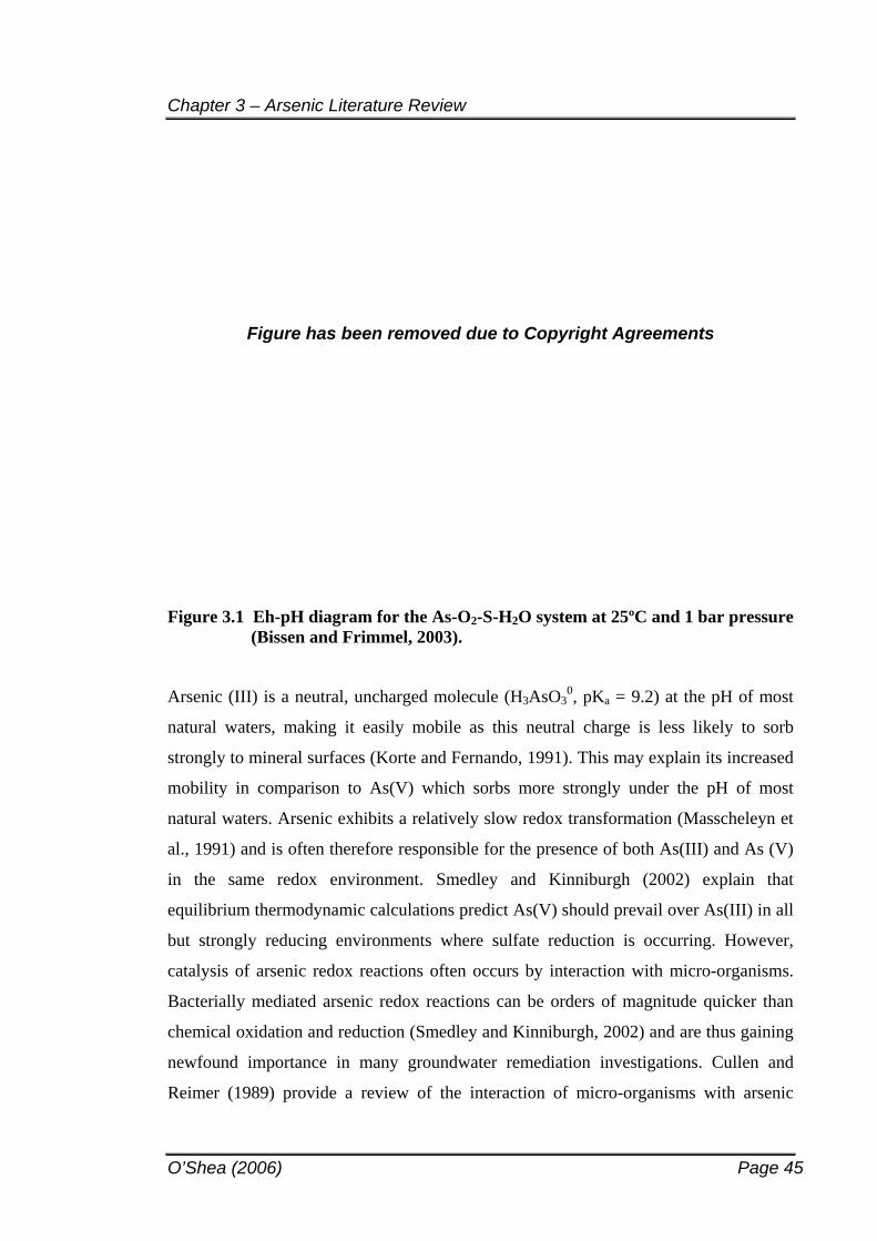
Chapter 3 – Arsenic Literature Review
O’Shea (2006) Page 45
Figure has been removed due to Copyright Agreements
Figure 3.1 Eh-pH diagram for the As-O2-S-H2O system at 25ºC and 1 bar pressure (Bissen and Frimmel, 2003).
Arsenic (III) is a neutral, uncharged molecule (H3AsO30, pKa = 9.2) at the pH of most
natural waters, making it easily mobile as this neutral charge is less likely to sorb
strongly to mineral surfaces (Korte and Fernando, 1991). This may explain its increased
mobility in comparison to As(V) which sorbs more strongly under the pH of most
natural waters. Arsenic exhibits a relatively slow redox transformation (Masscheleyn et
al., 1991) and is often therefore responsible for the presence of both As(III) and As (V)
in the same redox environment. Smedley and Kinniburgh (2002) explain that
equilibrium thermodynamic calculations predict As(V) should prevail over As(III) in all
but strongly reducing environments where sulfate reduction is occurring. However,
catalysis of arsenic redox reactions often occurs by interaction with micro-organisms.
Bacterially mediated arsenic redox reactions can be orders of magnitude quicker than
chemical oxidation and reduction (Smedley and Kinniburgh, 2002) and are thus gaining
newfound importance in many groundwater remediation investigations. Cullen and
Reimer (1989) provide a review of the interaction of micro-organisms with arsenic
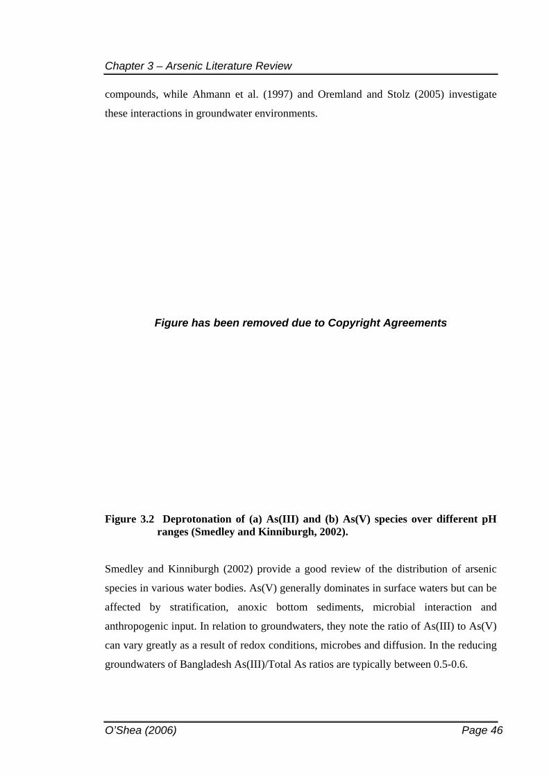
Chapter 3 – Arsenic Literature Review
O’Shea (2006) Page 46
compounds, while Ahmann et al. (1997) and Oremland and Stolz (2005) investigate
these interactions in groundwater environments.
Figure has been removed due to Copyright Agreements
Figure 3.2 Deprotonation of (a) As(III) and (b) As(V) species over different pH ranges (Smedley and Kinniburgh, 2002).
Smedley and Kinniburgh (2002) provide a good review of the distribution of arsenic
species in various water bodies. As(V) generally dominates in surface waters but can be
affected by stratification, anoxic bottom sediments, microbial interaction and
anthropogenic input. In relation to groundwaters, they note the ratio of As(III) to As(V)
can vary greatly as a result of redox conditions, microbes and diffusion. In the reducing
groundwaters of Bangladesh As(III)/Total As ratios are typically between 0.5-0.6.
Chapter 3 – Arsenic Literature Review
O’Shea (2006) Page 47
3.4 IMMOBILISATION OF ARSENIC: SOLID PHASE RETARDATION
Arsenic (and other trace elements) associated with the solid phase may be present in a
variety of different chemical forms – precipitated as a mineral phase; adsorbed onto a
mineral surface; incorporated within the crystal structure of a mineral or partitioned into
organic matter. A general term applied to all of these processes is sorption, and a brief
review of these mechanisms is provided below. A more specific discussion on
documented arsenic sorption phenomena follows which examines experiments proven
to constrain arsenic mobility and retain it in the solid phase.
3.4.1 Properties of Sorbent Materials
3.4.1.1 Surface Area Solid materials in aquifers can act as sorbents, with strength of sorption dependent on
both the mineralogy and the surface area of the solid. Larger surface areas sorb more,
making smaller grain size fractions (such as clays) responsible for much of the sorption
in aquifers. However, oxide or organic coatings on the coarser (i.e., larger) sand grains
can also sorb material. Therefore, the content of clay, type of clay, amount of organic
matter present and surface coatings can all contribute to sorption capacity in sediments.
3.4.1.2 Surface charge Concurrently, an increase in surface area of a mineral also increases its surface charge
(number of charged sites per unit area, commonly referred to as surface site density)
which are both directly proportional to the sorptive properties of a particular mineral
(Table 3.6). Clay minerals exhibit high surface areas in comparison to oxides of iron,
manganese and aluminium; however, oxides are characterised by high surface site
densities increasing the likelihood of sorption.
A mineral surface can exhibit two types of surface charge – permanent or variable.
Permanent surface charge arises from the isomorphic substitution of lower valence
cations in the crystal lattice of minerals. For example, Al3+ replaces Si4+ in the
tetrahedral layer and Mg2+ replaces Al3+ in the octahedral layer of clay minerals and
zeolites resulting in a net negative charge. An excess of O2- bonds creates this negative
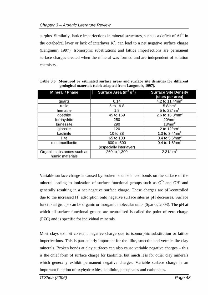
Chapter 3 – Arsenic Literature Review
O’Shea (2006) Page 48
surplus. Similarly, lattice imperfections in mineral structures, such as a deficit of Al3+ in
the octahedral layer or lack of interlayer K+, can lead to a net negative surface charge
(Langmuir, 1997). Isomorphic substitutions and lattice imperfections are permanent
surface charges created when the mineral was formed and are independent of solution
chemistry.
Table 3.6 Measured or estimated surface areas and surface site densities for different geological materials (table adapted from Langmuir, 1997).
Mineral / Phase Surface Area (m2 g-1) Surface Site Density (sites per area)
quartz 0.14 4.2 to 11.4/nm2
rutile 5 to 19.8 5.8/nm2
hematite 1.8 5 to 22/nm2
goethite 45 to 169 2.6 to 16.8/nm2
ferrihydrite 250 20/nm2
birnessite 290 18/nm2
gibbsite 120 2 to 12/nm2
kaolinite 10 to 38 1.3 to 3.4/nm2
illite 65 to 100 0.4 to 5.6/nm2
montmorillonite 600 to 800 (especially interlayer)
0.4 to 1.6/nm2
Organic substances such as humic materials
260 to 1,300 2.31/nm2
Variable surface charge is caused by broken or unbalanced bonds on the surface of the
mineral leading to ionization of surface functional groups such as O2- and OH- and
generally resulting in a net negative surface charge. These charges are pH-controlled
due to the increased H+ adsorption onto negative surface sites as pH decreases. Surface
functional groups can be organic or inorganic molecular units (Sparks, 2003). The pH at
which all surface functional groups are neutralised is called the point of zero charge
(PZC) and is specific for individual minerals.
Most clays exhibit constant negative charge due to isomorphic substitution or lattice
imperfections. This is particularly important for the illite, smectite and vermiculite clay
minerals. Broken bonds at clay surfaces can also cause variable negative charges – this
is the chief form of surface charge for kaolinite, but much less for other clay minerals
which generally exhibit permanent negative charges. Variable surface charge is an
important function of oxyhydroxides, kaolinite, phosphates and carbonates.
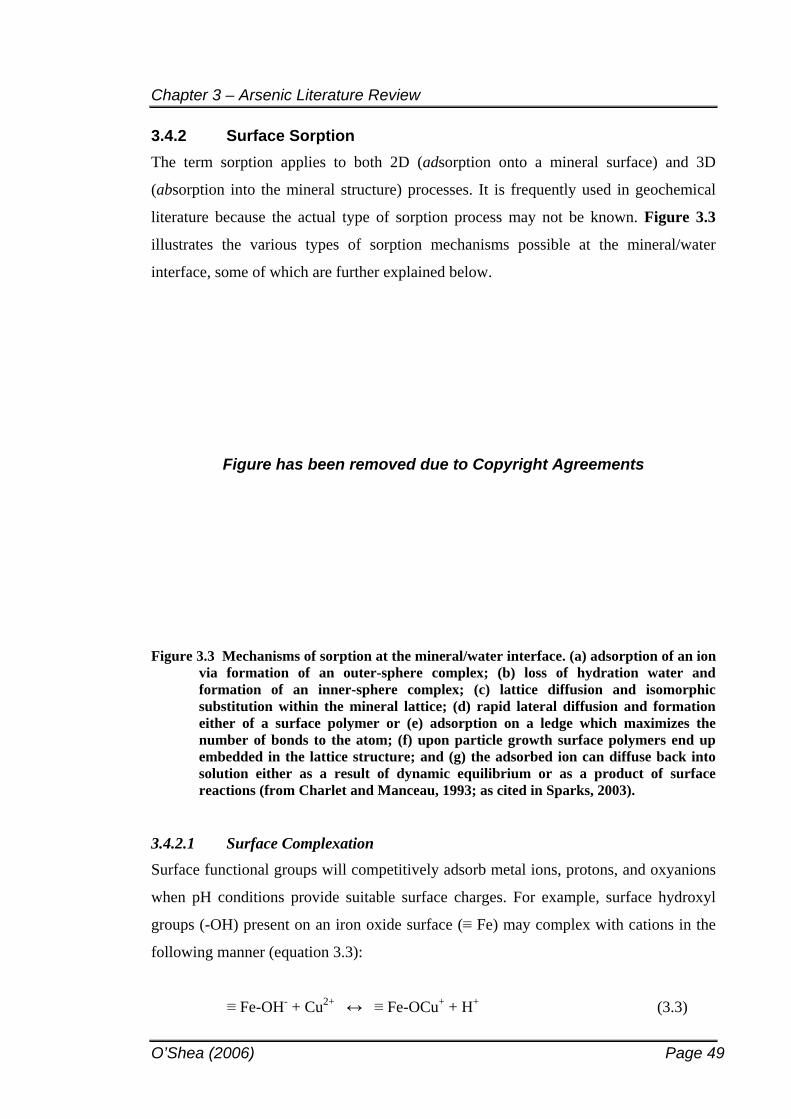
Chapter 3 – Arsenic Literature Review
O’Shea (2006) Page 49
3.4.2 Surface Sorption The term sorption applies to both 2D (adsorption onto a mineral surface) and 3D
(absorption into the mineral structure) processes. It is frequently used in geochemical
literature because the actual type of sorption process may not be known. Figure 3.3
illustrates the various types of sorption mechanisms possible at the mineral/water
interface, some of which are further explained below.
Figure has been removed due to Copyright Agreements
Figure 3.3 Mechanisms of sorption at the mineral/water interface. (a) adsorption of an ion via formation of an outer-sphere complex; (b) loss of hydration water and formation of an inner-sphere complex; (c) lattice diffusion and isomorphic substitution within the mineral lattice; (d) rapid lateral diffusion and formation either of a surface polymer or (e) adsorption on a ledge which maximizes the number of bonds to the atom; (f) upon particle growth surface polymers end up embedded in the lattice structure; and (g) the adsorbed ion can diffuse back into solution either as a result of dynamic equilibrium or as a product of surface reactions (from Charlet and Manceau, 1993; as cited in Sparks, 2003).
3.4.2.1 Surface Complexation Surface functional groups will competitively adsorb metal ions, protons, and oxyanions
when pH conditions provide suitable surface charges. For example, surface hydroxyl
groups (-OH) present on an iron oxide surface ( Fe) may complex with cations in the
following manner (equation 3.3):
Fe-OH- + Cu2+ Fe-OCu+ + H+ (3.3)
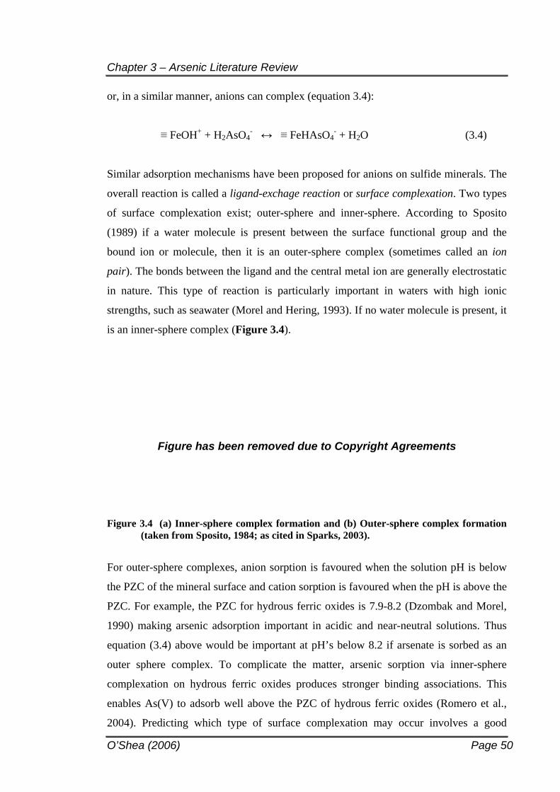
Chapter 3 – Arsenic Literature Review
O’Shea (2006) Page 50
or, in a similar manner, anions can complex (equation 3.4):
FeOH+ + H2AsO4- FeHAsO4
- + H2O (3.4)
Similar adsorption mechanisms have been proposed for anions on sulfide minerals. The
overall reaction is called a ligand-exchage reaction or surface complexation. Two types
of surface complexation exist; outer-sphere and inner-sphere. According to Sposito
(1989) if a water molecule is present between the surface functional group and the
bound ion or molecule, then it is an outer-sphere complex (sometimes called an ion
pair). The bonds between the ligand and the central metal ion are generally electrostatic
in nature. This type of reaction is particularly important in waters with high ionic
strengths, such as seawater (Morel and Hering, 1993). If no water molecule is present, it
is an inner-sphere complex (Figure 3.4).
Figure has been removed due to Copyright Agreements
Figure 3.4 (a) Inner-sphere complex formation and (b) Outer-sphere complex formation (taken from Sposito, 1984; as cited in Sparks, 2003).
For outer-sphere complexes, anion sorption is favoured when the solution pH is below
the PZC of the mineral surface and cation sorption is favoured when the pH is above the
PZC. For example, the PZC for hydrous ferric oxides is 7.9-8.2 (Dzombak and Morel,
1990) making arsenic adsorption important in acidic and near-neutral solutions. Thus
equation (3.4) above would be important at pH’s below 8.2 if arsenate is sorbed as an
outer sphere complex. To complicate the matter, arsenic sorption via inner-sphere
complexation on hydrous ferric oxides produces stronger binding associations. This
enables As(V) to adsorb well above the PZC of hydrous ferric oxides (Romero et al.,
2004). Predicting which type of surface complexation may occur involves a good
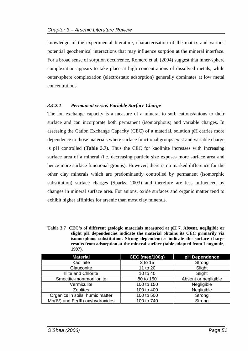
Chapter 3 – Arsenic Literature Review
O’Shea (2006) Page 51
knowledge of the experimental literature, characterisation of the matrix and various
potential geochemical interactions that may influence sorption at the mineral interface.
For a broad sense of sorption occurrence, Romero et al. (2004) suggest that inner-sphere
complexation appears to take place at high concentrations of dissolved metals, while
outer-sphere complexation (electrostatic adsorption) generally dominates at low metal
concentrations.
3.4.2.2 Permanent versus Variable Surface ChargeThe ion exchange capacity is a measure of a mineral to sorb cations/anions to their
surface and can incorporate both permanent (isomorphous) and variable charges. In
assessing the Cation Exchange Capacity (CEC) of a material, solution pH carries more
dependence to those materials where surface functional groups exist and variable charge
is pH controlled (Table 3.7). Thus the CEC for kaolinite increases with increasing
surface area of a mineral (i.e. decreasing particle size exposes more surface area and
hence more surface functional groups). However, there is no marked difference for the
other clay minerals which are predominantly controlled by permanent (isomorphic
substitution) surface charges (Sparks, 2003) and therefore are less influenced by
changes in mineral surface area. For anions, oxide surfaces and organic matter tend to
exhibit higher affinities for arsenic than most clay minerals.
Table 3.7 CEC’s of different geologic materials measured at pH 7. Absent, negligible or slight pH dependencies indicate the material obtains its CEC primarily via isomorphous substitution. Strong dependencies indicate the surface charge results from adsorption at the mineral surface (table adapted from Langmuir, 1997).
Material CEC (meq/100g) pH Dependence Kaolinite 3 to 15 Strong
Glauconite 11 to 20 Slight Illite and Chlorite 10 to 40 Slight
Smectite-montmorillonite 80 to 150 Absent or negligible Vermiculite 100 to 150 Negligible
Zeolites 100 to 400 Negligible Organics in soils, humic matter 100 to 500 Strong
Mn(IV) and Fe(III) oxyhydroxides 100 to 740 Strong
Chapter 3 – Arsenic Literature Review
O’Shea (2006) Page 52
So, when the pH of the surrounding solution is high the surface carries a net negative
charge and is conducive to cation exchange. When the pH of the surrounding solution is
low the surface carries a net positive charge providing conditions suitable for anion
exchange. This process may play an important part in this study given that arsenic forms
negative oxyanions in solution which will be attracted to net positive surface charges.
Clays with high CEC’s can remove various cations from solution and retain them in the
solid phase.
3.4.3 Arsenic Retention in the Solid Phase Having reviewed the processes responsible for ion sorption we now focus on the
behaviour of potential sorbents available for arsenic retardation at Stuarts Point. The
heterogeneity of the aquifer matrix is conducive to many different arsenic
immobilisation processes, including mineral precipitation as well as sorption; with both
processes influenced by the surrounding water chemistry. The dominant arsenic-specific
immobilisation processes are presented here.
3.4.3.1 Solid Phase Arsenic FormationArsenic bearing minerals have previously been discussed and their distribution is a
product of well documented ore genesis processes. Geological mapping and
geochemical tracing techniques can identify zones of arsenic minerals and its elemental
occurrence in association with various other mineral deposits. Geochemical conditions
must be suitable for ore genesis, with shallow unconsolidated sandy aquifers (such as
Stuarts Point) rarely providing these conditions for arsenic mineral precipitation.
Precipitation of arsenic minerals occurs when geochemical conditions are suitable and
sufficient concentrations of respective elements are present in dissolved form.
Numerous theoretical and experimental studies exist on the precipitation of arsenic with
various elements, notably sulfides and metal arsenates (Wagemann, 1978; Crecelius et
al., 1986) including calcium and magnesium (Raposo et al., 2004). Saturation of the
aqueous solution with respect to mineral solubility will promote precipitation.
Geochemical modelling codes generally contain thermodynamic databases that are
incorporated into many studies and designed to assess the plausibility of arsenic mineral
precipitation. These databases should be thoroughly reviewed before use so as to
Chapter 3 – Arsenic Literature Review
O’Shea (2006) Page 53
include the most recent thermodynamic data applicable to the system being modeled.
Failure to do this can result in unrealistic results, as was the case adopted by Crecelius
et al. (1986) who found barium arsenate was oversaturated in the solution being
modeled. They attributed this to an error in the thermodynamic data as there was no
geological occurrence of the material and dissolved barium would have been
analytically undetectable. An investigation by Planer-Friedrich et al. (2001) using an
updated Saturation Index (SI) for BaHAsO4.H2O (rather than Ba2[AsO4]2) produced
results which suggested barium arsenate may precipitate but only at higher barium
concentrations (up to 170 g L-1) than those used in their study. They thus attributed the
negative arsenic and barium correlation to differences in geological settings. To solve
the thermodynamic question regarding barium arsenate stability in natural waters, Zhu
et al. (2005) conducted specific experimental investigations to conclude that barium
arsenate was unlikely to form under natural conditions in water. Their updated
thermodynamic data should be included in all geochemical databases so as to avoid
misconceived results.
Perhaps a mechanism of more recently examined arsenic mineral association in
groundwater resource investigations is that of its association with pyrite. Pyrite is
formed when water containing iron and sulfate, in the presence of organic matter,
crystallises to form secondary iron sulfides (Fitzpatrick et al., 1996). Sulfate reducing
bacteria, such as Desulfovibrio desulfuricans, use sulfur as an electron sink during the
oxidation of organic matter, reducing sulfate to sulfide which then combines with
ferrous iron under anaerobic environments (Fitzpatrick et al., 1996). This process can
occur in both marine and non-marine environments. Coastal pyrite is often associated
with acid sulfate soil formation. Authigenic pyrite is common where marine incursion
has occurred in the sediments, such as marine shales (Craw and Chappell, 1999). Recent
studies in Australia (Fitzpatrick et al., 1996) have identified pyrite formation under
inland dryland salinisation processes, whereby saline sulfate groundwater combines
with iron and organic matter to produce suitable pyritization conditions. Pyritization in
salt marsh sediments can be rapid; in other sedimentary environments the process is
relatively slow as amorphous iron monosulfides (FeS) react with elemental sulfur (S0) to
form pyrite (Berner, 1970).
Chapter 3 – Arsenic Literature Review
O’Shea (2006) Page 54
Early research on the association of arsenic with pyrite includes a study of marine pyrite
capture of arsenic in the Laurentian Trough of Canada (Belzile and Lebel, 1986). Iron
extracted from the targeted pyrite fraction during sediment extraction procedures
produced a correlation of 0.981 with arsenic also extracted from this phase. This early
work suggested that arsenic may be present within the lattice sites of pyrite. Research
on acid sulfate soil by-products generated further interest in the association of arsenic
with pyrite. In 1984 and 1987 Dudas studied the relationship between arsenic and pyrite
in acid sulfate soils. He found that although pyrite was already known to be a carrier of
arsenic, containing as much as 5,600 mg kg-1 As (Boyle and Jonasson, 1973), there was
no information on the arsenic chemistry of ASS. Gustaffson and Tin (1994) confirmed
Dudas’ earlier correlative work and also suggested that arsenic is predominantly
redistributed in iron oxide phases after oxidation of arsenic-rich pyrite. Still no
definitive studies had been produced on the detailed mechanisms of arsenic formation
with pyrite.
Belzile (1988) examined the fate of arsenic in estuarine and coastal offshore sediments,
finding that the formation of pyrite greatly affected the distribution of arsenic. He once
again proposed that arsenic was included into the lattice sites of pyrite, in a constant
Fe/As ratio of 1000. Previous Fe/As ratios were established by Boyle and Jonasson
(1973) to range from 290 to 4,660 in rocks containing pyrite. Belzile’s (1988) constant
Fe/As ratio could reflect the maximum arsenic retention capacity for the framboidal
pyrites he examined, but may not be reproduced in the same ratio in other environments.
Much of the work following these earlier studies focussed on contaminated sediments
and the association of arsenic with various selectively extracted soil fractions, with the
pyrite fraction often specifically examined (Gruebel et al., 1988; Lacal et al., 2003; La
Force et al., 2000; Moore et al., 1988; Van Herreweghe et al., 2003; Wenzel et al.,
2001). While this work has been important in deciphering the correlation between
arsenic and iron sulfide phases it has not been successful in delineating specific sorption
mechanisms between arsenic and pyrite.
By the 1990’s it became commonly accepted that arsenic is isomorphically substituted
(sometimes called solid-solution) for reduced sulfur in the pyrite structure (Presser and

Chapter 3 – Arsenic Literature Review
O’Shea (2006) Page 55
Swain, 1990; Nesbitt et al., 1995; Strawn et al., 2002). The most recent studies are now
examining these mechanisms via the use of spectroscopic methods in order to determine
arsenic local structure and oxidation state. Savage et al. (2000) used electron
microprobe, transmission electron microscope and extended X-ray absorption fine-
structure spectroscopy (EXAFS) to indicate that As substitutes for S in pyrite,
producing a mineral commonly referred to as arsenian pyrite. Their detailed studies of
mine tailings on a molecular level indicated that the amount and spatial arrangement of
arsenic substitution for sulfur can lead to enhanced weathering of arsenian pyrite in
comparison to pure pyrite phases. Zacharias et al. (2004) concurrently confirmed this
most recent work by providing electron microscope quantitative analyses of pyrites
from a granitoid intrusion in Prague. The atomic percentages of Fe, S and As indicated
an arsenic association with pyrite via sulfur substitution – Fe(AsxS1-x).
The common relationship between the presence of dissolved arsenic and sulfide
minerals in anoxic environments led Bostick and Fendorf (2003) to examine in detail
the mechanisms by which sulfide minerals sequestered arsenic under such conditions.
At pH levels above 2-3 iron sulfide minerals are negatively charged (Bebie et al., 1998).
In contrast to arsenic adsorption onto iron oxides (which is low at high pH levels),
arsenite sorption on pyrite and troilite (FeS) increased at higher pH. The authors
proposed that strong, inner-sphere complexes sorbed the arsenite to the iron sulfides,
rather than outer sphere complexation mechanisms. In contrast to isomorphic
substitution, they also suggested the formation of an intermediate surface precipitate
with a structure resembling arsenopyrite (FeAsS). Initially, arsenite was reduced to an
FeAsS-like precipitate on both FeS and FeS2. The corresponding oxidation of Fe(II) and
sulfide was detected but low amounts were observed in dissolved phase. Bostick and
Fendorf (2003) subsequently proposed the following reaction (equation 3.5) for arsenic
surface precipitation on iron sulfides:
3FeS + As(OH)3 FeS2 + FeAsS + Fe(OH)3 (3.5)
This reaction supports the association of arsenic and pyrite observed via the numerous
selective extraction techniques found in the scientific literature. In both sorption and
surface precipitate cases an insoluble arsenic-bound sulfide phase is formed that is
Chapter 3 – Arsenic Literature Review
O’Shea (2006) Page 56
effective in immobilising arsenic in reducing sulfidic environments. Oxidation of these
phases are predicted to release arsenic species from their sorbed sulfides, similar to the
reductive dissolution of iron oxide phases releasing arsenic into dissolved phase.
Follow-up studies conducted by Bostick et al. (2004) confirmed that sorption reactions
on sulfide minerals in anoxic environments are the initial step in arsenic sequestration
processes. Precipitation of an FeAsS phase on sulfide minerals, specifically pyrite,
eventually led to conversion of a more stable arsenic sulfide mineral (As2S3) in sulfidic,
reducing environments.
3.4.3.2 Surface Reactions Affecting Arsenic Mobility Arsenic sorption to solid phases is a complex mechanism currently receiving an
increased amount of research attention. Experimental studies using pure mineral phases
and high powered microscopic techniques are providing valuable information for
geochemists, material scientists, environmental scientists and pedologists alike. Using
the data obtained through these theoretical investigations, predictions regarding arsenic
retardation in heterogenous matrices can be made.
Arsenic sorption in such highly composite settings can be controlled by mineral type,
crystallinity, surface features and properties of the surrounding solution. A number of
arsenic mineral sorption studies are reviewed in order to show the wide range of
potential conditions suitable for arsenic surface sorption in the environment.
3.4.3.2.1 SURFACE COMPLEXATION (ADSORPTION)
Lin and Puls (2003) found the following order of decreasing arsenic affinity on various
minerals: iron hydroxides > clays > feldspars. This illustrates the complexity of arsenic
adsorption onto various mineral substrates which are discussed independently below.
Chapter 3 – Arsenic Literature Review
O’Shea (2006) Page 57
Oxyhydroxides1
Common oxides of Fe, Al, Mn and silica are widely dispersed in nature as fine particles
and surface coatings. They have an excellent ability to sorb cations and anions to their
surface thereby decreasing the mobility of many trace elements in the environment.
Given the high affinity of Fe-oxides for arsenic adsorption much work has focussed on
them, however similar results have also been reported for other oxides.
Both crystalline and amorphous iron oxide forms have hydroxylated surfaces allowing
surface adsorption processes to occur (Dudas, 1987). The amount of arsenic sorbed to
an iron oxide surface, however, is dependent on both arsenic speciation and mineral
crystallinity. Iron oxides initially form poorly crystalline (amorphous2) phases with high
surface areas which undergo transformation over time to more crystalline phases such as
goethite, hematite or magnetite (Dixit and Hering, 2003). With the advent of
crystallisation comes a loss in specific surface area, however, Dixit and Hering (2003)
found that the transformation of HFO to goethite did not decrease the affinity of the
sorbed phase for arsenic. Nevertheless, reduction in surface size and site density during
crystallisation may increase the mobilisation of any surface-bound arsenic.
Arsenic adsorption is more highly dependent on its oxidation state than on pH in the
range of 5.5-7.5 (Raven et al., 1998). Several studies have been conducted on the
adsorption of arsenic to ferrihydrite (Raven et al., 1998; Jain et al., 1999; Appelo et al.,
2002); goethite (Grafe et al., 2001); and hematite (Redman et al., 2002). Results of these
investigations vary according to experimental conditions. The general consensus for
optimum arsenic adsorption onto ferrihydrite and goethite under different pH conditions
is summarised in Table 3.8.
1 The term ‘oxyhydroxide’ will be used herein to collectively describe the terms hydroxide, oxide and oxyhydroxide, unless specifically stated. 2 Iron (hydr) oxides, hydrous ferric oxides (HFO) or hydroxylated iron oxides will generally be termed as amorphous or specified as ferrihydrite herein.
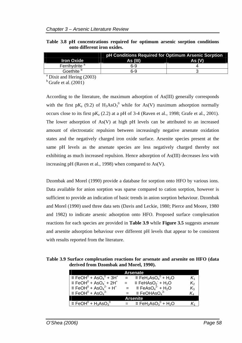
Chapter 3 – Arsenic Literature Review
O’Shea (2006) Page 58
Table 3.8 pH concentrations required for optimum arsenic sorption conditions onto different iron oxides.
pH Conditions Required for Optimum Arsenic Sorption Iron Oxide As (III) As (V)
Ferrihydrite a 6-9 4 Goethite b 6-9 3
a Dixit and Hering (2003) b Grafe et al. (2001)
According to the literature, the maximum adsorption of As(III) generally corresponds
with the first pKa (9.2) of H3AsO30 while for As(V) maximum adsorption normally
occurs close to its first pKa (2.2) at a pH of 3-4 (Raven et al., 1998; Grafe et al., 2001).
The lower adsorption of As(V) at high pH levels can be attributed to an increased
amount of electrostatic repulsion between increasingly negative arsenate oxidation
states and the negatively charged iron oxide surface. Arsenite species present at the
same pH levels as the arsenate species are less negatively charged thereby not
exhibiting as much increased repulsion. Hence adsorption of As(III) decreases less with
increasing pH (Raven et al., 1998) when compared to As(V).
Dzombak and Morel (1990) provide a database for sorption onto HFO by various ions.
Data available for anion sorption was sparse compared to cation sorption, however is
sufficient to provide an indication of basic trends in anion sorption behaviour. Dzombak
and Morel (1990) used three data sets (Davis and Leckie, 1980; Pierce and Moore, 1980
and 1982) to indicate arsenic adsorption onto HFO. Proposed surface complexation
reactions for each species are provided in Table 3.9 while Figure 3.5 suggests arsenate
and arsenite adsorption behaviour over different pH levels that appear to be consistent
with results reported from the literature.
Table 3.9 Surface complexation reactions for arsenate and arsenite on HFO (data derived from Dzombak and Morel, 1990).
Arsenate FeOH0 + AsO4
0 + 3H+ = FeH2AsO40 + H2O K1
FeOH0 + AsO4- + 2H+ = FeHAsO2
- + H2O K2 FeOH0 + AsO4
2- + H+ = FeAsO42- + H2O K3
FeOH0 + AsO43- = FeOHAsO4
3- K4Arsenite
FeOH0 + H3AsO30 = FeH2AsO3
0 + H2O K1
Chapter 3 – Arsenic Literature Review
O’Shea (2006) Page 59
By reference to the above cited literature, inner-sphere complexation has been proposed
for the dominant arsenic sorption mechanism onto metal oxides via displacement of a
hydroxyl group on the oxide surface. Sherman and Randall (2003) agreed that evidence
for inner-sphere complexation of arsenic is sufficient but that the nature of the surface
complexes remains controversial. Consistent with sorption mechanisms for iron oxides,
both aluminium and manganese oxides produce inner-sphere surface complexation
reactions with arsenic thereby reducing its mobility under suitable aqueous geochemical
conditions.
Figure has been removed due to Copyright Agreements
Figure 3.5 Arsenic adsorption on HFO for a) As(V) and b) As(III) according to ionic strength (I), Fe and As concentrations given (after Dzombak and Morel, 1990). Solid line is optimal fit, dashed line is an estimate using sorption constants.
Clay Minerals
As noted previously, the clay mineral type, surface charge and surface area, in addition
to the presence of any other trace elements, may all influence arsenic sorption onto clay
mineral surfaces. While many studies have been conducted on arsenic affinity for iron
oxide adsorption, clay mineral adsorption has been studied significantly less despite
their abundance in aquifer sediments, soils and particulate matter. Two predominant
experimental studies on arsenic sorption with clay minerals are frequently cited in
arsenic geochemical reviews.
Lin and Puls (2000) investigated adsorption, desorption and oxidation of arsenic
affected by clay minerals and aging. Six different clay minerals were utilised in their
study; halloysite, two different kaolinites, illite, an illite/montmorillonite mix and
Chapter 3 – Arsenic Literature Review
O’Shea (2006) Page 60
chlorite. Arsenic (V) exhibited higher adsorption affinity than As(III) for all the clay
minerals studied. This adsorption affinity was influenced by pH; As(V) adsorption
decreased at pH 7.5 (compared to experimental pH’s of 5.5 and 6.5) while As(III)
increased at pH 7.5. This difference can be attributed to the pKa values of arsenic acid
(H3AsO4 – As[V]) ranging from 2.2 to 11.5 in comparison to arsenous acid (H3AsO3 –
As[III]) ranging from 9.2 to 13.4. Therefore, at pH 5.5 to 7.5 the positively charged
particle edges would be more conducive to the lower pKa values assigned to the As(V)
protonated species (2.2 – 11.5) over the As(III) species.
Desorption of both As(III) and As(V) decreased over time, indicating aging could
hinder the desorption of arsenic. Two theories were presented to explain this
phenomena:
1. Arsenic adsorbed onto external clay surfaces may diffuse into internal pores; and
2. Loss of hydration water.
Both theories contribute to the strengthened bonding of arsenic with the clay mineral
and promoting less desorption of arsenic. Aging over time also allowed oxidation of
As(III) to take place resulting in significant amounts of surface-bound As(V). Oxidation
effects are important due to the increased affinity of As(V) for surface sites over the
more mobile and toxic As(III) species. The mechanism of oxidation is not well
understood but may be due to the presence of other elements within the clay mineral
structure.
Individually, each clay mineral exhibited different sorption characteristics. The illites
and montmorillonites are 2:1 layer clays whose negative surface charge is largely
controlled by isomorphic substitution in the lattice. Positive surface charges for anion
adsorption can be generated by protonation on broken Al-OH bonds exposed at the
particle surface. Chlorite exhibits similar features. In contrast, the kaolinites and
halloysite are 1:1 layer clays and do not demonstrate extensive isomorphic substitution
– broken edge effects are thus more important for these minerals.
The illite and mixed illite/montmorillonite in Lin and Puls’ (2000) study had moderate
arsenic adsorption and subsequently moderate desorption. The exposed Al-OH edge
groups were postulated to control these results and hence influence arsenic sorption with
Chapter 3 – Arsenic Literature Review
O’Shea (2006) Page 61
changes in pH (because variable surface charges are pH controlled). Kaolinite,
theoretically predicted to sorb and desorb more arsenic than these clays, produced
similar sorption/desorption results. The authors attributed this anomaly to the fine-
grained nature of the illite and montmorillonite samples used in the experiment which
may have been prone to increased surface reactivity.
Halloysite displayed the greatest adsorption - nearly 100% - of As(V). Changes in pH
had little effect on adsorption to halloysite indicating the potential formation of a
hydroxy-arsenate interlayer within the clay mineral structure. Chlorite also retained
arsenic well and was little influenced by pH. Its rich iron content may suggest arsenic
sorption onto iron oxide contained within its structure.
Manning and Goldberg (1997) conducted laboratory experiments on clay minerals to
determine:
a) the influence of pH and ionic strength (I) on As(III) adsorption;
b) differences between As(III) and As(V) adsorption;
c) stability of As(III) adsorbed onto clay mineral surfaces; and
d) to describe As(III) and As(V) adsorption envelopes using surface complexation
modelling.
They found that ionic strength had little effect on As(III) adsorption providing
macroscopic evidence for inner-sphere complexation. However, pH had a profound
influence on adsorption capability. All four materials (kaolinite, montmorillonite, illite
and synthetic amorphous Al(OH)3) exhibited low As(III) adsorption at low pH and
maximum As(III) adsorption between pH 7.5 and pH 9.5. This value is only slightly
above the first H3AsO30 pKa value of 9.2 and coincides with the point of zero charge
(PZC) for amorphous Al(OH)3. This suggests that Al-OH functional groups are highly
pH dependent and conducive to As(III) adsorption in preference to the SiO4 tetrahedra
predominant in the clay minerals utilised. Given this prediction, kaolinite, with its
dominant surface hydroxyl variable charge is expected to adsorb more As(III) than illite
which is controlled by permanent isomorphic substitution and minor surface edge ( Al-
OH and Al-OH2+) functional groups. The results were unexpected – illite adsorbed
Chapter 3 – Arsenic Literature Review
O’Shea (2006) Page 62
more As(III) than kaolinite, and was postulated to be a result of the higher surface area
of illites, also noted by Lin and Puls (2000).
Desorption experiments (simulating mobilisation of arsenic) revealed significant
oxidation of As(III) to surface-bound As(V) had occurred. As(III) was stable in solution
at pH 4-9 but oxidation occurred at or above pH 9.2. Manning and Goldberg (1997)
suspected that the presence of MnO2 in the clays may have contributed to oxidation,
which in turn promotes more strongly bound arsenic in solid phase.
As(V) desorption was greatest at high pH, but not all arsenic was extractable. For
example, at pH 7 montmorillonite, kaolinite and illite desorbed As(V) at 80%, 66% and
33% respectively. Above pH 8.5 montmorillonite and kaolinite desorption was almost
100%, whereas illite retained more than 50% of its sorbed arsenic. The outcome of their
experiments suggested both pH and mineralogy were critical factors in controlling
arsenic adsorption to clay mineral surfaces.
Influence of Organic Matter
The presence of organic matter, both in solid and aqueous forms, can influence arsenic
sorption onto mineral surfaces. Organic matter often exhibits high surface areas and
great affinities for surface sorption. Humic substances act as good accumulators of
metal-humate complexes. Mukhopadhyay and Sanyal (2004) devised stability constants
for arsenic-humic/fulvic complexes that were considered stable. This was also
investigated by Saada et al. (2003) who found that at pH 7 humic substances adsorbed
onto kaolinite had a significant impact on arsenic adsorption. Redman et al. (2002)
found that the formation of aqueous complexes of arsenic and natural organic matter
dramatically reduced the amount of arsenic sorption onto hematite and displaced
already sorbed arsenic (III and V). Thus, the decomposition of organic matter can
release arsenic into solution (Belzile, 1988).
Additionally, the decomposition of other minerals by indirect organic matter influence
can affect arsenic mobility. The reductive dissolution of iron oxides catalysed by
organic matter oxidation is a prime example. Reduction of Fe(III) oxides may be
minimal if organic carbon contents are low, therefore producing an environment
Chapter 3 – Arsenic Literature Review
O’Shea (2006) Page 63
favouring crystallisation (Willett and Walker, 1982). This is because organic matter acts
as a reductant, converting Fe(III) to Fe(II) and therefore inhibiting oxide formation, in
addition to inhibiting crystallisation (Schwertmann et al., 1968). If it is not present then
oxide formation and crystallisation will occur more easily. Willett and Walker (1982)
observed this process in the Shoalhaven River floodplain where cores in close proximity
to each other exhibited different iron oxide contents and degrees of crystallinity
correlating with organic matter presence. Crystallisation of iron oxides can enhance
arsenic release due to a reduction in surface area available for arsenic sorption. Thus the
presence of organic matter can directly and indirectly influence arsenic sorption
processes.
Carbonates
Arsenic incorporation within carbonate mineral structures has received little research
attention despite the ubiquitous nature of carbonate materials in the environment.
Arsenic partitioning on calcite surfaces is applicable to this investigation due to the
presence of calcite (shells) within the aquifer matrix. Cheng et al. (1999) provide one of
the few macroscopic investigations of arsenic association with calcite surfaces. Their X-
ray standing wave study concluded that the arsenite ion occupies the carbonate lattice
site of the calcite surface (Figure 3.6).
Actual bonding mechanisms remain unclear, however the authors suggest As(III) is
incorporated within the calcite lattice either at or near the surface (as opposed to ion
exchange reactions) potentially by a dissolution-reprecipitation mechanism.
Incorporation via an outer-sphere complex could suggest arsenic adsorption in alkaline
environments given that the PZC of calcite ranges from 7-10.8 (Romero et al., 2004).
Goldberg and Glaubig (1988) observed a maximum surface adsorption of As on calcite
at around pH 10. Subsequently, Romero et al. (2004) conducted batch experiments on
carbonate-rich aquifer material from Zimapan, Mexico, and found arsenic adsorption
was greatest (97%) at pH 10.5. These results indicate that arsenic adsorption onto
calcite is likely to exert a major control on dissolved arsenic concentrations in the
groundwater. Goethite was also found to influence arsenic sorption in this study,
however, calcite sorption was found to dominate by using a combination of
experimental (determination of PZC; batch experiments; pH dependent sorption) and
Chapter 3 – Arsenic Literature Review
O’Shea (2006) Page 64
geochemical modeling (MINTEQA2) techniques. The high affinity of arsenic for the
carbonate-rich aquifer material was suggested to be utilised as a remediation option by
allowing deeper contaminated groundwaters to flow through shallow carbonate-rich
material in order to decrease dissolved arsenic concentrations.
Figure has been removed due to Copyright Agreements
Figure 3.6 As(III) substitution for the carbonate ion on the calcite surface as suggested by Cheng et al. (1999).
Sulfides other than Iron
Arsenic association with iron sulfides has been touched briefly upon in the discussion
on arsenian pyrite. Other sulfides, however, possess the potential for anion retardation
via surface complexation mechanisms. Bostick et al., (2003) studied arsenite adsorption
on the more stable sulfide ores found in anoxic environments; galena (PbS) and
sphalerite (ZnS). They found a distinct difference between arsenic adsorption on
sulfides when compared to arsenic adsorption processes postulated for iron oxide
surfaces. The main notable difference was an increase in As(III) adsorption with
increasing pH on PbS and ZnS. This is in direct contrast to arsenic-oxide adsorption
which is greatest at circumneutral pH and lowest at high pH. These results suggest
arsenic adsorption on sulfide minerals does not occur via ligand-exchange mechanisms.
Bostick et al. (2003) also ruled out isomorphic susbstitution with Pb or S. Instead they
proposed the formation of an inner-sphere multinuclear arsenic thiosulfide complex on
the surface of PbS and ZnS.
Chapter 3 – Arsenic Literature Review
O’Shea (2006) Page 65
3.4.3.2.2 SURFACE PRECIPITATES
Surface precipitates were briefly mentioned in the discussion on arsenic association
with pyrite. As surface coverage of adsorbed anions increases, three dimensional
surface precipitates can form (Sparks, 2003). The formation of metal hydroxide surface
precipitates may be an important mechanism for retaining metals in the solid phase,
thereby limiting transport and bioavailability. Surface precipitation may take place at
high As(III) activity (Bostick et al., 2003). In sulfidic, reducing environments
precipitation of arsenic sulfides such as orpiment (As2S3) have been proposed for
mechanisms of arsenic retention (Sadiq, 1990). Bostick et al. (2003) conducted
laboratory experiments and concluded it was unlikely for arsenic sulfide precipitation to
occur on galena and sphalerite but did emphasize the need for additional research
involving such reactions.
3.4.3.2.3 COMPETITIVE ANION EXCHANGE
The mobility, bioavailability and toxicity of arsenic may be influenced by the
competitive interaction of other anions. Various minerals are affected differently and the
concentrations and speciation of competitive anions can also influence potential for
arsenic sorption. Common competing anions include SO42-, PO4
3-, CO32- and Cl-.
Perhaps the most commonly studied competitive anion with arsenic is PO43-, probably
due to its application via fertilizer use increasing its potential to be present in
groundwater systems. Competitive ligand exchange generally occurs between H2PO4-
and HPO42- and arsenate ions (Manning and Goldberg, 1997).
Aside from fertilizer use, Belzile (1988) suggested anion exchange processes were
responsible for occurrence of dissolved arsenic in porewaters of offshore sediments.
Phosphate was suggested to replace arsenic in pyrite (equation 3.6) maintaining
dissolved arsenic concentrations while depleting dissolved phosphate in the porewaters:
PO43- + As-FeS2 As5+ + PO4-FeS2 (3.6)
Chapter 3 – Arsenic Literature Review
O’Shea (2006) Page 66
Goh and Lim (2004) studied anion competition with arsenic sorption on a bulk tropical
soil sample as opposed to singular or synthetic minerals. They found that SO42- rarely
affected As(V) adsorption capacity but could compete with As(III) for sorption sites.
Phosphate had a more profound effect on sorption capacity for both As(III) and As(V),
which may be attributed to its higher negative charge. Goh and Lim (2004) suggested
two possible reactions for PO43- on surface sites; strong inner-sphere complexation
and/or accumulation or precipitation of PO43- providing electrostatic repulsion on the
mineral surface. Both would reduce arsenic sorption and increase its mobilisation into
groundwater.
Both As(III) and As(V) adsorption onto goethite is reduced in the presence of dissolved
organic matter (Grafe et al., 2001). Dissolved organic matter (DOM), such as humic or
fulvic acids, form stable complexes with mineral surfaces (Kaiser et al., 1997) thereby
blocking arsenic sorption sites on iron oxides, alumina, kaolinite or quartz (Grafe et al.,
2001). This has recently been supported by Bauer and Blodau (2005) who confirmed
competition between arsenic and organic anions for sorption sites on synthetic iron
oxides and natural soils and sediments. Therefore DOM may contribute to increasing
the mobility and potential bioavailability of arsenic via competitive anion exchange
mechanisms.
Appelo et al. (2002) examined ferrihydrite sorption capacity and found that carbonate
present in common soil and groundwater concentrations significantly replaced arsenic
on sorption sites. This has been further confirmed by Anawar et al. (2004) who
conducted batch experiments that showed bicarbonate solutions were effective in
releasing arsenic from iron and manganese oxyhydroxides. The formation of arseno-
carbonate complexes; As(CO3)2-, As(CO3)(OH)2- and AsCO3
+, which are stable in water,
were earlier predicted by Kim et al. (2000).
Manning and Goldberg (1996) found that molybdate (MoO42-) inhibited As(V)
adsorption onto oxide minerals only at pH levels below 4. Similarly, Ronngren et al.
(1994) suggested sulfide may inhibit As(III) adsorption onto mineral surfaces due to
competition for surface sites. In general agreement with the studies cited above, Goh
Chapter 3 – Arsenic Literature Review
O’Shea (2006) Page 67
and Lim (2005) found the ability of anions to mobilise arsenic from a fine soil followed
the order PO43- >> CO3
2- > SO42- and Cl-.
3.5 MOBILISATION OF ARSENIC: THE GEOCHEMICAL TRIGGERS
The aqueous distribution of many trace elements is often dominated by solution pH;
redox potential; composition and interaction with the surrounding solution; and surface
reactions on solid particles (both colloids and in-situ matrices). This current section
explains geochemical conditions required for the mobilisation of arsenic. Colloidal
interactions are included here as many colloids pass through a 0.45 m filter (utilised
herein) and are thus included in the ‘dissolved’ analyses; their fractionation cannot be
determined otherwise with the use of the sampling methods employed herein (see
Appendix A for sampling methodology).
3.5.1 Changes to Aqueous pH As noted in the previous section, solution pH influences the adsorption of both As(III)
and As(V). At slightly acidic to neutral pH values commonly encountered in most
natural waters, arsenic is strongly adsorbed by oxide minerals. As the pH approaches 9
desorption of arsenic can occur as mineral surfaces become increasingly negatively
charged, repelling the As oxyanion. Smedley and Kinniburgh (2002) attribute
desorption at high pH as being one of the most likely mechanisms for high arsenic
groundwaters under oxidising conditions. Many authors (see Robertson, 1994) note a
positive correlation between dissolved arsenic concentrations and pH in predominantly
oxidising conditions. The oxyanions of Se, Cr, Mo and V generally correlate positively
with pH and As under these conditions, indicating similar pH-influenced mechanisms
governing their mobility.
Changes in aqueous pH may also influence mineral solubility. Based on the literature
reviewed for carbonate minerals, uncertainty remains over the association of arsenic
with minerals such as calcite, siderite and dolomite; but the inclusion of arsenic in the
calcite structure discussed previously indicates possible release of arsenic upon calcite
dissolution (equation 3.7).
Chapter 3 – Arsenic Literature Review
O’Shea (2006) Page 68
2Ca(As,CO3) + 4H+ 2Ca2+ + As +2CO2 + 2H2O (3.7)
3.5.2 Shifts in Aqueous Redox Potential Following general redox trends in natural systems, several stages of the redox cycle can
influence arsenic mobilisation processes. These are described in (Table 3.10) with
specific examples of arsenic release or retardation processes provided in response to
changes in aqueous Eh.
Dissolved O2 is consumed first while dissolved CO2 increases via the decomposition of
organic matter. Arsenic bound to organic matter may be released upon its degradation,
such as arsenic associated with coffee rock in shallow groundwaters where oxygen is
present. The oxidation of arsenic-bearing minerals by oxygen can also release arsenic
into dissolved phase, particularly arsenic associated with sulfide minerals like arsenian
pyrite. The oxidation of sulfides, however, is not an efficient mechanism for arsenic
release into groundwater due to its rapid adsorption onto iron oxide by-products
commonly formed upon sulfide oxidation.
When oxygen is consumed nitrate becomes the dominant electron donor and can be
reduced by oxidising arsenian pyrite. Manganese reduction generally follows,
increasing dissolved Mn2+ concentrations. Arsenic sorbed onto Mn oxides may be
released as a consequence. Iron oxides are similarly reduced increasing dissolved Fe2+
in solution. In strongly reducing conditions, Fe(III) on the surface of iron oxides reduces
to Fe(II), which lowers the overall net positive charge of the oxide producing weaker
electrostatic bonds between sorbed anions and the oxide surface, leading to desorption
of the anion. Iron oxide dissolution occurs under strongly acid and strongly reducing
conditions. The actual dissolution of iron oxides will release both labile and non-labile
arsenic (and any other bound trace elements) into solution as the mineral structure
completely breaks down.

Tab
le 3
.10
Cha
nges
to r
edox
equ
ilibr
ium
in n
atur
al w
ater
s and
how
this
may
aff
ect a
rsen
ic m
obili
satio
n.
Indi
cativ
eEh
Elec
tron
Acc
epto
rEx
ampl
e Pr
oces
s R
elea
sing
A
rsen
icEq
uatio
nEx
ampl
eR
efer
ence
Slig
htly
oxid
isin
gC
onsu
mpt
ion
of o
xyge
n
Dec
ompo
sitio
n of
org
anic
mat
ter
and
rele
ase
of b
ound
ars
enic
Oxi
datio
n of
ars
enia
n py
rite,
w
ith a
dsor
ptio
n on
to ir
on o
xide
by-
prod
ucts
Hum
ic a
cid
As
+ 2O
2 + H
+
2CO
2 + 2
H2O
+ A
s (aq
)
Fe(A
s,S
) 2 +
15/4
O2 +
7/2
H2O
Fe(O
H) 3
As
+SO
42-+
4H+
Muk
hopa
dhya
yan
d S
anya
l (20
04)
Kim
et a
l. (2
002)
Slig
htly
redu
cing
Nitr
ate
redu
ctio
nN
itrat
e re
duct
ion
by p
yrite
oxi
datio
n8F
e(A
s,S
) 2 +
13N
O3- +
25H
2O +
10H
+
8Fe2+
+ 8
HA
sO42-
+ 8
SO
42- +
13N
H4+
App
elo
and
Pos
tma
(199
9)
Slig
htly
redu
cing
Man
gane
sere
duct
ion
Man
gane
se o
xide
redu
ctio
n an
d re
leas
e of
sor
bed
arse
nic
MnO
2H
AsO
2 + 2
H+
H3A
sO4(
aq) +
Mn2+
Cha
illou
et a
l. (2
003)
Red
ucin
gIro
nre
duct
ion
Iron
redu
ctio
n on
oxi
de s
urfa
ces
chan
ges
net c
harg
e le
adin
g to
ar
seni
c de
sorp
tion
Iron
oxid
e re
duct
ive
diss
olut
ion
and
rele
ase
of s
orbe
d ar
seni
c ca
taly
sed
by o
rgan
ic m
atte
r deg
rada
tion
FeA
sO4- +
2e- +
5H
+
Fe2+
+ H
3AsO
3 + H
2O
8FeO
OH
As
+ C
H3C
OO
H +
14H
2CO
38F
e2+ +
16H
CO
3- +12
H2O
+ A
s (aq
)
Nic
kson
et a
l. (2
000)
Nic
kson
et a
l. (2
000)
Red
ucin
g A
rsen
ate
redu
ctio
nA
s(V
) red
uctio
n to
As(
III) a
nd
chan
ge in
sor
ptio
n pr
oper
ties
AsO
43- +
2H
+ + 2
e- A
sO33-
+ H
2OB
ose
and
Sha
rma
(200
2)S
trong
lyre
duci
ngS
ulfa
tere
duct
ion
Pre
cipi
tatio
n of
inso
lubl
e su
lfide
s an
d im
mob
ilisa
tion
of a
rsen
ic
Fe2O
3 + 4
SO
42- +
8C
H2O
+ 1
/2O
2 + A
s (aq
)2F
e(A
s,S
) 2 +
8H
CO
3- + 4
H2O
Zhen
g et
al.
(200
4)
Chapter 3 – Arsenic Literature Review
O’Shea (2006) Page 70
The full reaction process of reductive dissolution of iron oxides remains unclear,
however, it is generally responsible for the high amounts of Fe(II) in reducing waters
(0.1 – 30 mg L-1). Smedley and Kinniburgh (2002) state that it does not appear to be
responsible for all dissolved arsenic in arsenic-rich reducing groundwaters. These
strongly reducing conditions are often brought about by rapid sediment burial and can
be dependent on the organic content of the sediments, which drives the redox reaction.
Arsenic release by reduction of iron oxides due to the decomposition of organic matter
has been linked to the release of arsenic in some groundwater environments (McArthur
et al., 2004).
Reduction of As(V) to its less strongly sorbed counterpart As(III) may increase the
mobility of arsenic in the environment via decreased affinity for surface adsorption.
Redman et al. (2002) and more recently Bauer and Blodau (2005), found that DOM is
capable of reducing arsenate and oxidising arsenite; both redox changes having an effect
on arsenic mobility. Arsenite oxidation can also be catalysed by dissolved manganese.
Next sulfate is converted to S2- which subsequently reacts with any dissolved Fe2+ to
form insoluble precipitates which may sequester arsenic. Sulfide is normally the
limiting ion for iron sulfide mineral formation, which leads to an excess of dissolved
Fe2+ over dissolved S2-. This is particularly important in low sulfate environments.
Changes in Eh equilibrium described in Table 3.10 can thus lead to the dominance of
one mechanism over another, or conditions can be reversed and redox cycling may be
observed whereby arsenic is repeatedly mobilised and immobilised as the Eh conditions
change. An indication of a change in redox potential occurring in sediments can be
demonstrated by a colour change from red/brown/orange (oxidising conditions) to
grey/green/blue (reducing conditions). Additionally, many of these processes are
mediated by biological reactions rather than simple chemical reactions alone.
3.5.3 Influence of, and Interaction with, the Surrounding Solution The immobilisation of As via competitive anion exchange (Section 3.4.3.2.3) can
generally be reversed to mobilise As into solution once again. This has previously been
Chapter 3 – Arsenic Literature Review
O’Shea (2006) Page 71
explained, therefore discussion moves onto aqueous complexation mechanisms.
Complex formation is defined loosely by Morel and Hering (1993) as,
“the reversible reaction of two dissolved species to form a third one” (pg 319)
and generally takes place between metals of one charge and ions of the opposite charge
in aqueous solution. The ion bonding to the metal is termed a ligand. Common ligands
include Cl-, Fl-, Br-, NO3-, CO3
2-, SO42-, NH3, S2-, PO4
3- and a variety of organic
molecules with suitable surface charges. Complexation can inhibit arsenic adsorption
thereby enhancing its mobility in aqueous environments.
Cullen and Reimer (1989) reviewed detailed calculations of the equilibrium speciation
of numerous trace elements and found that, unlike other elements, few aqueous arsenic
complexes form with typical water constituents. Arsenic-fluoride complexes were
possibly suggested at high fluoride concentrations, and in seawater arsenate may pair
with magnesium and calcium. Apart from these they concluded that the range of water-
soluble arsenic complexes was limited. More recent research has revealed the formation
of stable As(III) sulfide solution complexes which have been postulated to enhance the
mobility of As(III) by maintaining it in a soluble form (Helz et al., 1995; Rochette et al.,
2000). Such complexes include AsO(SH)2- in slightly sulfidic solutions. Bostick et al.
(2003) considered that the thioarsenite trimer As3S3(SH)3 in higher sulfide activities
may be a plausible complex present in their experimental results.
The formation of aqueous complexes of arsenic with DOM has recently been examined
by Saada et al. (2003) and found to increase arsenic mobility in waters containing
DOM. Wetland soils, which often contain DOM at slightly higher than normal
concentrations, have shown an increase in arsenic mobility in the presence of high DOC
concentrations (Kalbitz and Wennrich, 1998).
The formation of aqueous complexes is also important when examining the
bioavailability of metals. Some metals are much less toxic when strongly complexed to
organic ligands compared to when present as free ions or hydroxylated (Drever, 1997).
Others are more conducive to plant uptake when complexed, such as cadmium
complexed with chloride.
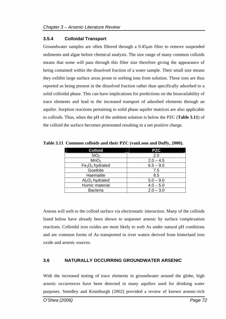
Chapter 3 – Arsenic Literature Review
O’Shea (2006) Page 72
3.5.4 Colloidal Transport Groundwater samples are often filtered through a 0.45 m filter to remove suspended
sediments and algae before chemical analysis. The size range of many common colloids
means that some will pass through this filter size therefore giving the appearance of
being contained within the dissolved fraction of a water sample. Their small size means
they exhibit large surface areas prone to sorbing ions from solution. These ions are thus
reported as being present in the dissolved fraction rather than specifically adsorbed to a
solid colloidal phase. This can have implications for predictions on the bioavailability of
trace elements and lead to the increased transport of adsorbed elements through an
aquifer. Sorption reactions pertaining to solid phase aquifer matrices are also applicable
to colloids. Thus, when the pH of the ambient solution is below the PZC (Table 3.11) of
the colloid the surface becomes protonated resulting in a net positive charge.
Table 3.11 Common colloids and their PZC (vanLoon and Duffy, 2000). Colloid PZC
SiO2 2.0 MnO2 2.0 – 4.5
Fe2O3 hydrated 6.5 – 9.0 Goethite 7.5
Haematite 8.5 Al2O3 hydrated 5.0 – 9.0 Humic material 4.0 – 5.0
Bacteria 2.0 – 3.0
Anions will sorb to the colloid surface via electrostatic interaction. Many of the colloids
listed below have already been shown to sequester arsenic by surface complexation
reactions. Colloidal iron oxides are most likely to sorb As under natural pH conditions
and are common forms of As transported in river waters derived from hinterland iron
oxide and arsenic sources.
3.6 NATURALLY OCCURRING GROUNDWATER ARSENIC
With the increased testing of trace elements in groundwater around the globe, high
arsenic occurrences have been detected in many aquifers used for drinking water
purposes. Smedley and Kinniburgh (2002) provided a review of known arsenic-rich
Chapter 3 – Arsenic Literature Review
O’Shea (2006) Page 73
aquifers and their status, current to several years ago, producing the global distribution
diagram shown in Figure 3.7. Conditions producing these elevated arsenic
concentrations are further reviewed and built on with current literature below. In
particular, the status of arsenic in the Australian environment is discussed in light of its
previous omission in worldwide occurrences.
Figure has been removed due to Copyright Agreements
Figure 3.7 Natural arsenic distribution in aquifers globally (Smedley and Kinniburgh, 2002). Some mining and geothermal sources are also noted.
Naturally occurring arsenic-enriched aquifers are common throughout many countries
but they are not ubiquitous. Elevated arsenic in groundwater is related to specific
geochemical conditions and the past and present hydrogeology of the aquifer. A variety
of case studies from different countries, geochemical conditions, and past depositional
environments, are presented to indicate the heterogeneity and widespread global
occurrence of elevated arsenic in groundwater.
Chapter 3 – Arsenic Literature Review
O’Shea (2006) Page 74
3.6.1 Geochemical Controls
3.6.1.1 Oxidising Environments Oxidising conditions are generally conducive to As(V) domination in aqueous
environments. The common association of arsenic with many sulfide minerals means
that oxidising conditions in groundwater elevated in arsenic is often derived from the
oxidation of such minerals. The sporadic occurrence of arsenic in the oxidising
conditions of the Goose River basin in Maine has been investigated by Sidle et al.
(2001); Sidle (2002, 2003) and Sidle and Fischer (2003). Arsenic is predominantly
present as As(V) in both H2AsO4- and HAsO4
2- states. The slightly oxidising conditions
present in the aquifer (median dissolved oxygen [DO] 8.1 mg L-1) promotes oxidation of
arsenian pyrite along fractured zones in the igneous and metamorphic bedrock. Sidle et
al. (2001) suggest these arsenian pyrites are the probable source of arsenic
concentrations in groundwater. This suggestion is supported by analysis of 34S and 18OSO4
/18OH2O (Sidle, 2002) isotopes which indicate SO42- presence with elevated As in
solution may be characteristic of arsenian pyrite oxidation in the fractured flow systems.
In the confined part of the central Oklahoma aquifer dissolved arsenic concentrations
reach 110 g L-1 under oxidising conditions (Schlottmann and Breit, 1992). As(V) was
determined to be present and strongly dependent on pH. The authors found that the
highest reported arsenic concentrations were only observed at pH values above 8.5 and
could be attributed to desorption from abundant iron oxides present in the aquifer.
An unusual occurrence of arsenic release in an oxidising environment occurs in a
confined aquifer in eastern Wisconsin. The fully saturated nature of deeper
groundwaters or confined aquifers often leads to reducing conditions where sulfide
mineral oxidation does not readily occur. The Fox River Valley, however, reports
arsenic up to 12,000 g L-1 where DO is typically less than 0.5 mg L-1 (Schreiber et al.,
2000). Sulfur isotopic signatures suggest oxidation of arsenian sulfide as the source of
arsenic to groundwater. Four potential oxidant sources were suggested (regional
recharge, vertical leakage, borehole and dewatering), however, interaction between
oxygen in the borehole and the arsenian pyrite horizon was implied as the probable
oxidant source.
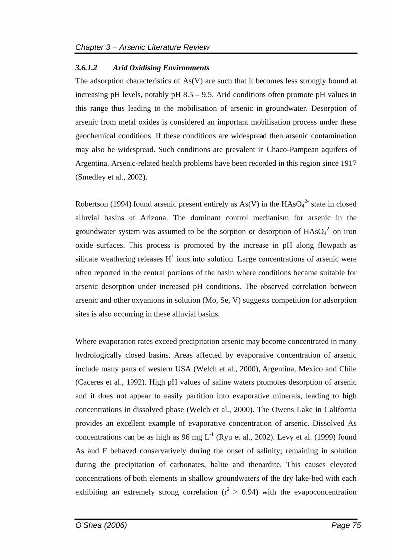
Chapter 3 – Arsenic Literature Review
O’Shea (2006) Page 75
3.6.1.2 Arid Oxidising Environments The adsorption characteristics of As(V) are such that it becomes less strongly bound at
increasing pH levels, notably pH 8.5 – 9.5. Arid conditions often promote pH values in
this range thus leading to the mobilisation of arsenic in groundwater. Desorption of
arsenic from metal oxides is considered an important mobilisation process under these
geochemical conditions. If these conditions are widespread then arsenic contamination
may also be widespread. Such conditions are prevalent in Chaco-Pampean aquifers of
Argentina. Arsenic-related health problems have been recorded in this region since 1917
(Smedley et al., 2002).
Robertson (1994) found arsenic present entirely as As(V) in the HAsO42- state in closed
alluvial basins of Arizona. The dominant control mechanism for arsenic in the
groundwater system was assumed to be the sorption or desorption of HAsO42- on iron
oxide surfaces. This process is promoted by the increase in pH along flowpath as
silicate weathering releases H+ ions into solution. Large concentrations of arsenic were
often reported in the central portions of the basin where conditions became suitable for
arsenic desorption under increased pH conditions. The observed correlation between
arsenic and other oxyanions in solution (Mo, Se, V) suggests competition for adsorption
sites is also occurring in these alluvial basins.
Where evaporation rates exceed precipitation arsenic may become concentrated in many
hydrologically closed basins. Areas affected by evaporative concentration of arsenic
include many parts of western USA (Welch et al., 2000), Argentina, Mexico and Chile
(Caceres et al., 1992). High pH values of saline waters promotes desorption of arsenic
and it does not appear to easily partition into evaporative minerals, leading to high
concentrations in dissolved phase (Welch et al., 2000). The Owens Lake in California
provides an excellent example of evaporative concentration of arsenic. Dissolved As
concentrations can be as high as 96 mg L-1 (Ryu et al., 2002). Levy et al. (1999) found
As and F behaved conservatively during the onset of salinity; remaining in solution
during the precipitation of carbonates, halite and thenardite. This causes elevated
concentrations of both elements in shallow groundwaters of the dry lake-bed with each
exhibiting an extremely strong correlation (r2 > 0.94) with the evapoconcentration
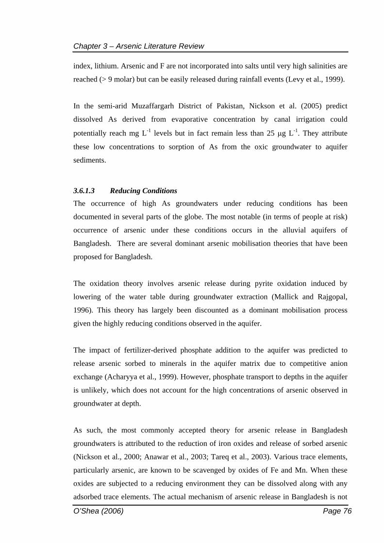
Chapter 3 – Arsenic Literature Review
O’Shea (2006) Page 76
index, lithium. Arsenic and F are not incorporated into salts until very high salinities are
reached (> 9 molar) but can be easily released during rainfall events (Levy et al., 1999).
In the semi-arid Muzaffargarh District of Pakistan, Nickson et al. (2005) predict
dissolved As derived from evaporative concentration by canal irrigation could
potentially reach mg L-1 levels but in fact remain less than 25 g L-1. They attribute
these low concentrations to sorption of As from the oxic groundwater to aquifer
sediments.
3.6.1.3 Reducing Conditions The occurrence of high As groundwaters under reducing conditions has been
documented in several parts of the globe. The most notable (in terms of people at risk)
occurrence of arsenic under these conditions occurs in the alluvial aquifers of
Bangladesh. There are several dominant arsenic mobilisation theories that have been
proposed for Bangladesh.
The oxidation theory involves arsenic release during pyrite oxidation induced by
lowering of the water table during groundwater extraction (Mallick and Rajgopal,
1996). This theory has largely been discounted as a dominant mobilisation process
given the highly reducing conditions observed in the aquifer.
The impact of fertilizer-derived phosphate addition to the aquifer was predicted to
release arsenic sorbed to minerals in the aquifer matrix due to competitive anion
exchange (Acharyya et al., 1999). However, phosphate transport to depths in the aquifer
is unlikely, which does not account for the high concentrations of arsenic observed in
groundwater at depth.
As such, the most commonly accepted theory for arsenic release in Bangladesh
groundwaters is attributed to the reduction of iron oxides and release of sorbed arsenic
(Nickson et al., 2000; Anawar et al., 2003; Tareq et al., 2003). Various trace elements,
particularly arsenic, are known to be scavenged by oxides of Fe and Mn. When these
oxides are subjected to a reducing environment they can be dissolved along with any
adsorbed trace elements. The actual mechanism of arsenic release in Bangladesh is not
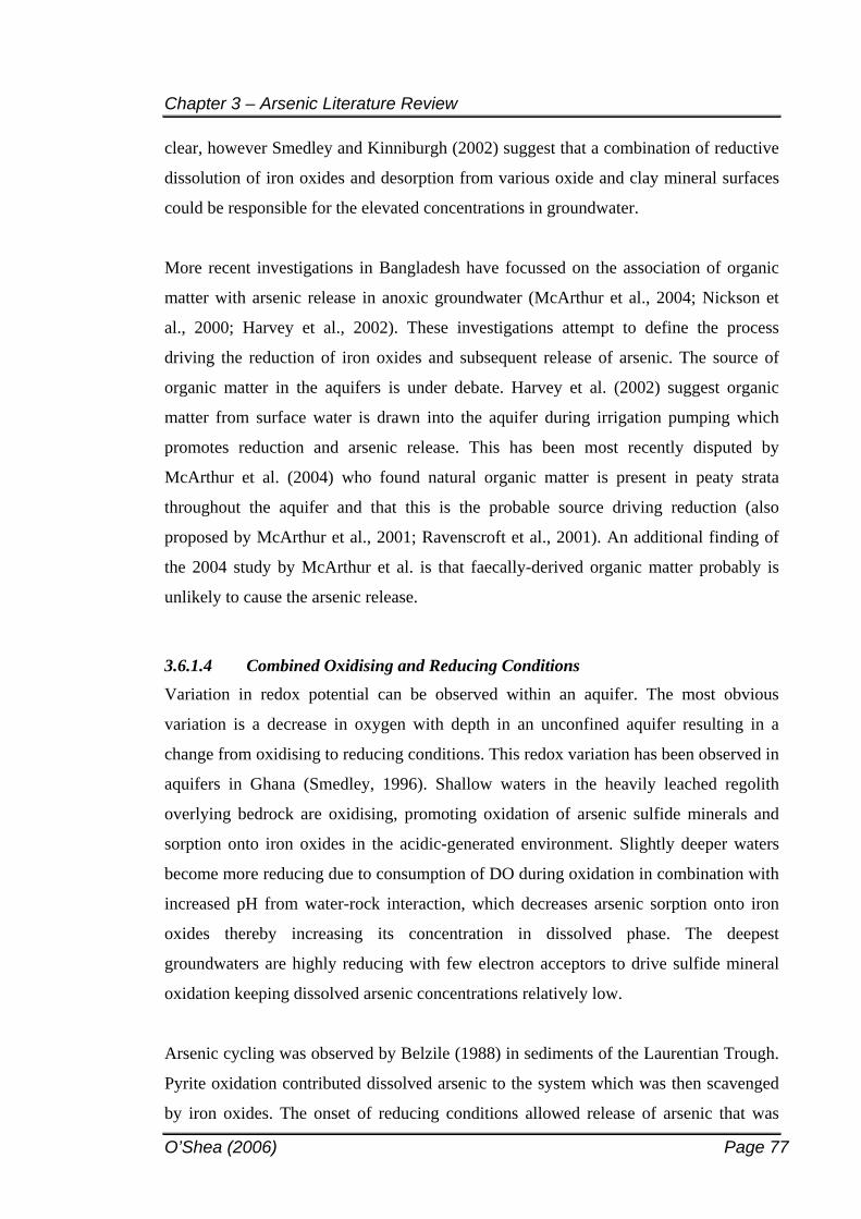
Chapter 3 – Arsenic Literature Review
O’Shea (2006) Page 77
clear, however Smedley and Kinniburgh (2002) suggest that a combination of reductive
dissolution of iron oxides and desorption from various oxide and clay mineral surfaces
could be responsible for the elevated concentrations in groundwater.
More recent investigations in Bangladesh have focussed on the association of organic
matter with arsenic release in anoxic groundwater (McArthur et al., 2004; Nickson et
al., 2000; Harvey et al., 2002). These investigations attempt to define the process
driving the reduction of iron oxides and subsequent release of arsenic. The source of
organic matter in the aquifers is under debate. Harvey et al. (2002) suggest organic
matter from surface water is drawn into the aquifer during irrigation pumping which
promotes reduction and arsenic release. This has been most recently disputed by
McArthur et al. (2004) who found natural organic matter is present in peaty strata
throughout the aquifer and that this is the probable source driving reduction (also
proposed by McArthur et al., 2001; Ravenscroft et al., 2001). An additional finding of
the 2004 study by McArthur et al. is that faecally-derived organic matter probably is
unlikely to cause the arsenic release.
3.6.1.4 Combined Oxidising and Reducing Conditions Variation in redox potential can be observed within an aquifer. The most obvious
variation is a decrease in oxygen with depth in an unconfined aquifer resulting in a
change from oxidising to reducing conditions. This redox variation has been observed in
aquifers in Ghana (Smedley, 1996). Shallow waters in the heavily leached regolith
overlying bedrock are oxidising, promoting oxidation of arsenic sulfide minerals and
sorption onto iron oxides in the acidic-generated environment. Slightly deeper waters
become more reducing due to consumption of DO during oxidation in combination with
increased pH from water-rock interaction, which decreases arsenic sorption onto iron
oxides thereby increasing its concentration in dissolved phase. The deepest
groundwaters are highly reducing with few electron acceptors to drive sulfide mineral
oxidation keeping dissolved arsenic concentrations relatively low.
Arsenic cycling was observed by Belzile (1988) in sediments of the Laurentian Trough.
Pyrite oxidation contributed dissolved arsenic to the system which was then scavenged
by iron oxides. The onset of reducing conditions allowed release of arsenic that was
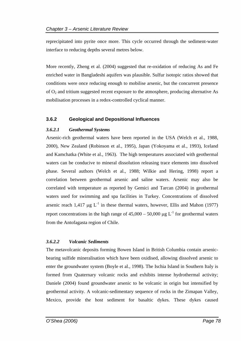
Chapter 3 – Arsenic Literature Review
O’Shea (2006) Page 78
reprecipitated into pyrite once more. This cycle occurred through the sediment-water
interface to reducing depths several metres below.
More recently, Zheng et al. (2004) suggested that re-oxidation of reducing As and Fe
enriched water in Bangladeshi aquifers was plausible. Sulfur isotopic ratios showed that
conditions were once reducing enough to mobilise arsenic, but the concurrent presence
of O2 and tritium suggested recent exposure to the atmosphere, producing alternative As
mobilisation processes in a redox-controlled cyclical manner.
3.6.2 Geological and Depositional Influences
3.6.2.1 Geothermal Systems Arsenic-rich geothermal waters have been reported in the USA (Welch et al., 1988,
2000), New Zealand (Robinson et al., 1995), Japan (Yokoyama et al., 1993), Iceland
and Kamchatka (White et al., 1963). The high temperatures associated with geothermal
waters can be conducive to mineral dissolution releasing trace elements into dissolved
phase. Several authors (Welch et al., 1988; Wilkie and Hering, 1998) report a
correlation between geothermal arsenic and saline waters. Arsenic may also be
correlated with temperature as reported by Gemici and Tarcan (2004) in geothermal
waters used for swimming and spa facilities in Turkey. Concentrations of dissolved
arsenic reach 1,417 g L-1 in these thermal waters, however, Ellis and Mahon (1977)
report concentrations in the high range of 45,000 – 50,000 g L-1 for geothermal waters
from the Antofagasta region of Chile.
3.6.2.2 Volcanic Sediments The metavolcanic deposits forming Bowen Island in British Columbia contain arsenic-
bearing sulfide mineralisation which have been oxidised, allowing dissolved arsenic to
enter the groundwater system (Boyle et al., 1998). The Ischia Island in Southern Italy is
formed from Quaternary volcanic rocks and exhibits intense hydrothermal activity;
Daniele (2004) found groundwater arsenic to be volcanic in origin but intensified by
geothermal activity. A volcanic-sedimentary sequence of rocks in the Zimapan Valley,
Mexico, provide the host sediment for basaltic dykes. These dykes caused
Chapter 3 – Arsenic Literature Review
O’Shea (2006) Page 79
metamorphism during emplacement, forming arsenic sulfides (Rodriguez et al., 2004)
which have subsequently caused elevated arsenic in the groundwater.
3.6.2.3 Alluvial and Deltaic Sediments Unconsolidated aquifers can cover large areas, often in heavily populated coastal zones,
and are capable of storing good quality groundwater resources. It is unfortunate then
that many of these productive aquifers are prone to natural arsenic contamination. The
most severe case, in terms of population exposed to arsenic rich groundwater, has
previously been discussed (Bangladesh). The Bengal Delta Plain consists of Holocene
alluvium derived from the Himalayan and Indo-Burman range and exhibiting dissolved
arsenic concentrations up to 2,500 g L-1 in the aquifer (BGS and DPHE, 2001). The
Red River Delta in northern Vietnam has only recently (1998) discovered arsenic up to
3,050 g L-1 in its groundwater (Berg et al., 2003). The similarity of geology and
groundwater composition between the Bengal Delta and the Red River Basin were
predicted, and confirmed, to exhibit elevated arsenic concentrations in the alluvial
aquifers surrounding Hanoi (Berg et al., 2001). Additionally in Nepal, alluvial aquifers
contain up to 409 g L-1 of dissolved arsenic (Bhattacharya et al., 2003).
3.6.2.4 Consolidated Sediments The incidence of arsenic contamination in unconsolidated sediments is perhaps more
pronounced given their capacity to provide large quantities of water to many people. In
spite of their less frequent use for domestic water supplies globally, consolidated
aquifers are important resources and can be heavily exploited for their groundwater.
Like the unconsolidated aquifers, these water resources have not been left untouched by
natural arsenic contamination. Examples are provided below for sandstone, limestone
and shale consolidated aquifers.
In an area where no obvious source of arsenic occurs, the Triassic Keuper Sandstone
aquifer in northern Bavaria exhibits arsenic concentrations up to 150 g L-1. Heinrichs
and Udluft (1999) found the arsenic was related to the geology and lithofacies of the
aquifer. Terrestrially derived sediments of fluvial origin were responsible for arsenic
concentrations in comparison to adjacent marine beds that contained no arsenic. In a
Chapter 3 – Arsenic Literature Review
O’Shea (2006) Page 80
separate study on arsenic occurrence in a sandstone aquifer of the Fox River Valley,
Thornburg and Sahai (2004) found that where discrete zones of arsenic rich sulfides
were lacking within the aquifer matrix, arsenic was present as disseminated veins,
grains and nodules. These discrete sulfides were found to influence groundwater arsenic
concentrations sporadically throughout the sandstone and dolomite aquifer.
The mining town of Zimapan, Mexico, is well known for its base-metal sulfide
mineralisation which intrudes domestic water supply limestone aquifers. Arsenic
concentrations reach more than 1 mg L-1 in the most polluted drinking water wells
installed in carbonate-rich aquifer material (Romero et al., 2004). The arsenic present in
this limestone aquifer is directly related to a nearby mineralised source rather than
dominated by aquifer lithology. Limestone aquifers generally do not contain naturally
elevated arsenic (see Al-Awadi et al., 2003, for an example of a limestone aquifer
without elevated arsenic) unless some association with a proximal arsenic source is
recognised.
Examples pertaining to shale aquifers are rare, potentially due to their low water holding
capacity and subsequent rejection for domestic yield requirements. Chen et al. (1994)
linked the occurrence of blackfoot disease with arsenic concentrations in groundwater
extracted from sands, muds and shale in Taiwan. However, the characterisation of
arsenic distribution in this aquifer remains poorly understood. Average arsenic
concentrations in shale rock assays are generally higher than other rock types indicating
groundwater in shale aquifers may be influenced by elevated As. More research is
needed to fully characterise the association between shale aquifers and arsenic
occurrence.
3.6.2.5 Lacustrine Environments Shallow groundwater in the Carson Desert, Nevada consists of elevated arsenic and
uranium concentrations controlled by evaporation, adsorption and redox processes
(Welch and Lico, 1998). The aquifer formation consists of deep-lake sediments, lake-
bed deposits and alluvium but is largely controlled chemically by the above processes.
The authors postulated it may be a modern analog of non-marine closed basins
producing U-ore deposits in New Mexico.
Chapter 3 – Arsenic Literature Review
O’Shea (2006) Page 81
The Huhhot Basin, Inner Mongolia, while also of (fluvio)lacustrine origin is dominated
by anaerobic conditions with elevated organic acids in addition to elevated arsenic
(Smedley et al., 2001). The reducing conditions were considered similar to those
observed in Bangladesh groundwaters. Association between arsenic and organic acid
was suggested to be a product of the highly reducing conditions or potential competition
between sorbing anions. Once again, geochemical conditions rather than
sedimentological controls influence arsenic occurrence in this fluviolacustrine
environment.
3.6.2.6 Glacial Drift The erosion of arsenic-bearing rocks by glacial processes can result in complex arsenic
distributions in groundwater related to the heterogenous nature of glacial aquifer
deposits. A deep glacial drift aquifer consisting of sand and gravel is the primary
groundwater drinking source in the lower Illinois River Basin (Warner, 2001). As part
of the USGS National Water Quality Assessment Program, arsenic concentrations were
investigated and found to be positively correlated with barium and chloride. A
subsequent increase in concentrations of these analytes along the flowpath indicates
arsenic may be derived from the underlying pyrite-containing bedrock, which
discharges into the glacial drift aquifer through localised structural features (Warner,
2001). Given the common occurrence of glacial drift aquifers overlying shale and coal
bedrock in the Midwest, in combination with the complex geochemistry of arsenic
resulting in variable distribution throughout the aquifer, arsenic is considered a health
concern for the entire Midwest region of the United States.
Szramek et al. (2004) also note the complexity associated with arsenic geochemistry in
glacial drift aquifers as a product of past glacial history, erosion, deposition and aquifer
recharge rate fluctuations. Different watersheds exhibited variation in arsenic
concentrations attributable to aquifer heterogeneity and consistent with groundwater
residence times. That is, less permeable aquifers reported higher arsenic concentrations.
The original source of arsenic is derived from the erosion and oxidation of arsenopyrite
during glacial processes.
Chapter 3 – Arsenic Literature Review
O’Shea (2006) Page 82
In addition to providing valuable groundwater resources, glacial processes can deposit
low permeability till forming confining units/aquitards. These tills are capable of
retarding dissolved solutes like arsenic, thereby removing it from solution (Yan et al.,
2000). Overall, glacial drift aquifers can provide complex arsenic occurrences related to
aquifer heterogeneity, which may include geochemical processes conducive to the
addition and removal of arsenic to/from the groundwater resource.
3.6.2.7 Aeolian Loess Deposits In contrast to glacial aquifer deposits, aquifers composed of loess are lithologically
homogenous. Therefore, variation in groundwater chemistry can be attributable to
hydrochemical differences rather than lithological controls. The La Pampa Province of
central Argentina has significant groundwater problems due to high concentrations of
various oxyanions, including arsenic (Bundschuh et al., 2004; Farias et al., 2003;
Smedley et al., 1998, 2002). The source of arsenic is thought to be derived from the
weathering of primary silicate minerals contained within fine-grained loess and ash
deposits forming the main exploited aquifers of the region (Smedley et al., 1998).
Geochemical processes are the controlling factors in arsenic mobilisation and are
characterised by arid oxidising conditions. In addition, slow groundwater flow rates
through the fine-grained material have enabled the accumulation of arsenic within the
aquifer and decreased its opportunity for removal via aquifer flushing (Smedley et al.,
2002).
3.6.2.8 Zone of Water Table Fluctuation The vertical movement of the water table can lead to chemical changes in the
unsaturated and shallow saturated zone. For example, eustatic changes in sea level can
enable flocculation and precipitation of humus leaching through aquifer materials
leading to impregnation of layers often referred to as coffee rock, waterloo rock, coastal
sandrock or indurated sand. The presence of these organic layers can influence arsenic
mobilisation via competitive anion exchange with dissolved organic matter or reduction
of oxides in the presence of organic matter subsequently releasing arsenic into solution
(Nickson et al., 2000).
Chapter 3 – Arsenic Literature Review
O’Shea (2006) Page 83
The oxidation of pyrite is a common occurrence leading to the development of ASS in
low-lying coastal areas. Oxidation often occurs as a product of vertical movement of the
water table. Arsenian pyrite oxidation can contribute dissolved arsenic to the
groundwater system if it is not sequestered by other processes. Iron oxide phases
commonly form as by products of pyrite oxidation and are excellent scavengers of
arsenic. Dudas (1984) found that iron oxides were favoured as arsenic scavengers over
the inclusion of arsenate for sulfate in the jarosite (FeSO4) structure; another commonly
formed pyrite oxidation by-product. Arsenic correlation with ASS may be a problem for
many coastal areas (O’Shea and Jankowski, 2001). Appleyard et al. (2004) found that
water table decline in a coastal suburb of Perth, Australia, led to the oxidation of
sulfidic peat soils resulting in widespread acidification and contamination of
groundwater by arsenic.
Some geochemical processes may be enhanced at the zone of water table fluctuation.
Smedley et al. (2002) noted more arsenic release at the water table compared to greater
depths in the aquifer studied. No correlations existed to indicate evaporation, and as
such, desorption from metal oxides and silicate reactions were suggested as the
controlling arsenic mobilisation factors. Water table fluctuations under irrigated
agricultural land can alter natural hydrodynamics and chemical processes. Northey et al.
(in press) observed this phenomenon in relation to major ion chemistry, however trace
elements may also be influenced. Repeated application of fertilizer can induce ion
exchange reactions, complexation processes and influence arsenic uptake by crops.
3.6.2.9 Coastal Sand Dunes It is clear by reviewing the literature that naturally elevated arsenic in groundwater is
found under many variable aquifer geochemical and depositional conditions. Despite
the many occurrences of elevated arsenic groundwaters, the coastal sand dune
environment rarely receives much attention, but is of utmost importance at Stuarts Point
where they form part of the main water bearing zone. A study conducted by Tesoriero et
al. (2004) examines water quality in a similar geomorphic setting as Stuarts Point,
however it fails to address arsenic occurrence. Appleyard et al.’s (2004) study of arsenic
occurrence in coastal sand dunes in Perth is attributed to ASS oxidation. Thus, arsenic
distribution in this coastal environment is controlled by a dominant and identifiable
Chapter 3 – Arsenic Literature Review
O’Shea (2006) Page 84
geochemical process, differing from the variable conditions observed in the Stuarts
Point sandy aquifer which does not contain large amounts of distinct ASS horizons
(although they are present in close proximity to the sandy aquifer). The seemingly
homogenous sands derived from sediment movement onshore to form the Stuarts Point
aquifer is a unique and potentially unidentified environment for naturally high-As
groundwaters. A thorough search of scientific research databases provided no studies on
arsenic occurrence from any other coastal sand dune environment.
3.6.3 Arsenic in Australia There have been few studies on natural arsenic occurrences in the Australian
environment. Smith et al. (2003a) provide an overview of arsenic in Australia, stating
that,
“By far the most common source of elevated As concentrations in the Australian
environment are attributable to anthropogenic activities.” (pg 235)
Limited groundwater studies have been conducted and generally target past mining
activities. It appears that the Stuarts Point aquifer may be the first Australian
groundwater environment to receive research attention due to natural arsenic
occurrence. Subsequently, members of the same research group, the UNSW
Groundwater Group, have since noted elevated arsenic elsewhere in Australia. McLean
and Jankowski (2001) studied an inland alluvial aquifer used extensively for crop
irrigation in Australia and found it to contain approximately 70 g L-1 dissolved arsenic
from an unknown but presumably natural source. Morgan (2005) also noted elevated
arsenic concentrations in deep saline groundwaters responsible for producing extensive
dryland salinity in western NSW. Additionally, Groves (in prep.) and Gosavi (2004)
note arsenic is ubiquitous in ASS environments on the southeast Queensland coast, a
point also confirmed in coastal Perth by Appleyard (2004).
3.7 ARSENIC GEOCHEMICAL SUMMARY
Both Australian and coastal sand environments are little investigated in relation to
arsenic occurrence in groundwater and drinking water supplies. This literature review
has provided background information on the ubiquitous occurrence of arsenic in the
Chapter 3 – Arsenic Literature Review
O’Shea (2006) Page 85
environment and the complexities involved in determining arsenic geochemical cycles.
Potential sources of arsenic in the Stuarts Point aquifer may include anthropogenic
contamination, sorption to aquifer materials during sea level transgressions and/or
erosion and deposition of regional mineral deposits. Sorbent materials contained within
the aquifer include clays, oxyhydroxides, calcite; and potential sinks like mineral
precipitates and arsenian pyrite. The mobilisation of arsenic from these sinks will vary
according to solution pH, Eh and composition. This chapter, summarising theoretical
information in conjunction with recent arsenic geochemical case studies from current
literature sources, provides sufficient background information required to make a
reliable assessment of arsenic source, retardation and mobilisation within the Stuarts
Point aquifer.
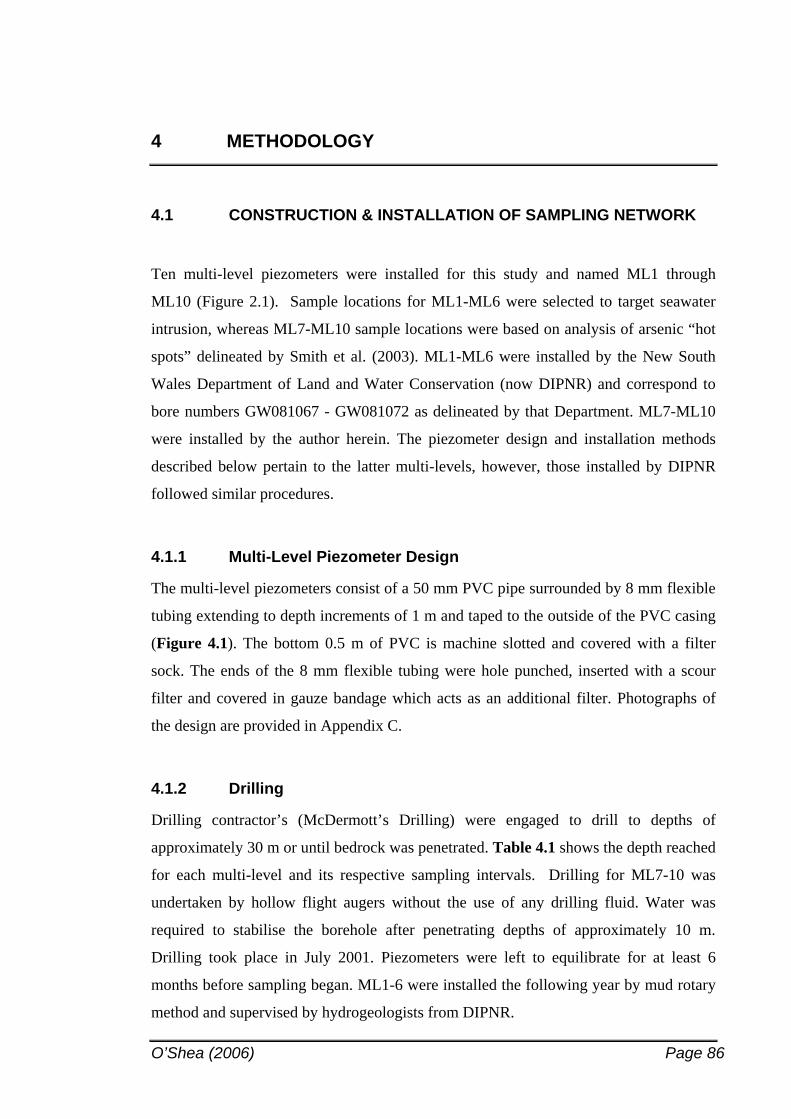
O’Shea (2006) Page 86
4 METHODOLOGY
4.1 CONSTRUCTION & INSTALLATION OF SAMPLING NETWORK
Ten multi-level piezometers were installed for this study and named ML1 through
ML10 (Figure 2.1). Sample locations for ML1-ML6 were selected to target seawater
intrusion, whereas ML7-ML10 sample locations were based on analysis of arsenic “hot
spots” delineated by Smith et al. (2003). ML1-ML6 were installed by the New South
Wales Department of Land and Water Conservation (now DIPNR) and correspond to
bore numbers GW081067 - GW081072 as delineated by that Department. ML7-ML10
were installed by the author herein. The piezometer design and installation methods
described below pertain to the latter multi-levels, however, those installed by DIPNR
followed similar procedures.
4.1.1 Multi-Level Piezometer Design
The multi-level piezometers consist of a 50 mm PVC pipe surrounded by 8 mm flexible
tubing extending to depth increments of 1 m and taped to the outside of the PVC casing
(Figure 4.1). The bottom 0.5 m of PVC is machine slotted and covered with a filter
sock. The ends of the 8 mm flexible tubing were hole punched, inserted with a scour
filter and covered in gauze bandage which acts as an additional filter. Photographs of
the design are provided in Appendix C.
4.1.2 Drilling
Drilling contractor’s (McDermott’s Drilling) were engaged to drill to depths of
approximately 30 m or until bedrock was penetrated. Table 4.1 shows the depth reached
for each multi-level and its respective sampling intervals. Drilling for ML7-10 was
undertaken by hollow flight augers without the use of any drilling fluid. Water was
required to stabilise the borehole after penetrating depths of approximately 10 m.
Drilling took place in July 2001. Piezometers were left to equilibrate for at least 6
months before sampling began. ML1-6 were installed the following year by mud rotary
method and supervised by hydrogeologists from DIPNR.
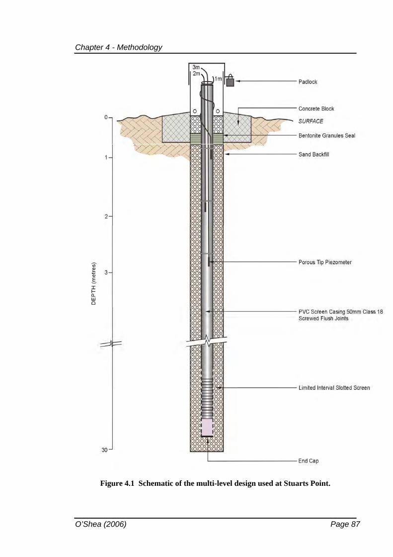
Chapter 4 - Methodology
O’Shea (2006) Page 87
Figure 4.1 Schematic of the multi-level design used at Stuarts Point.
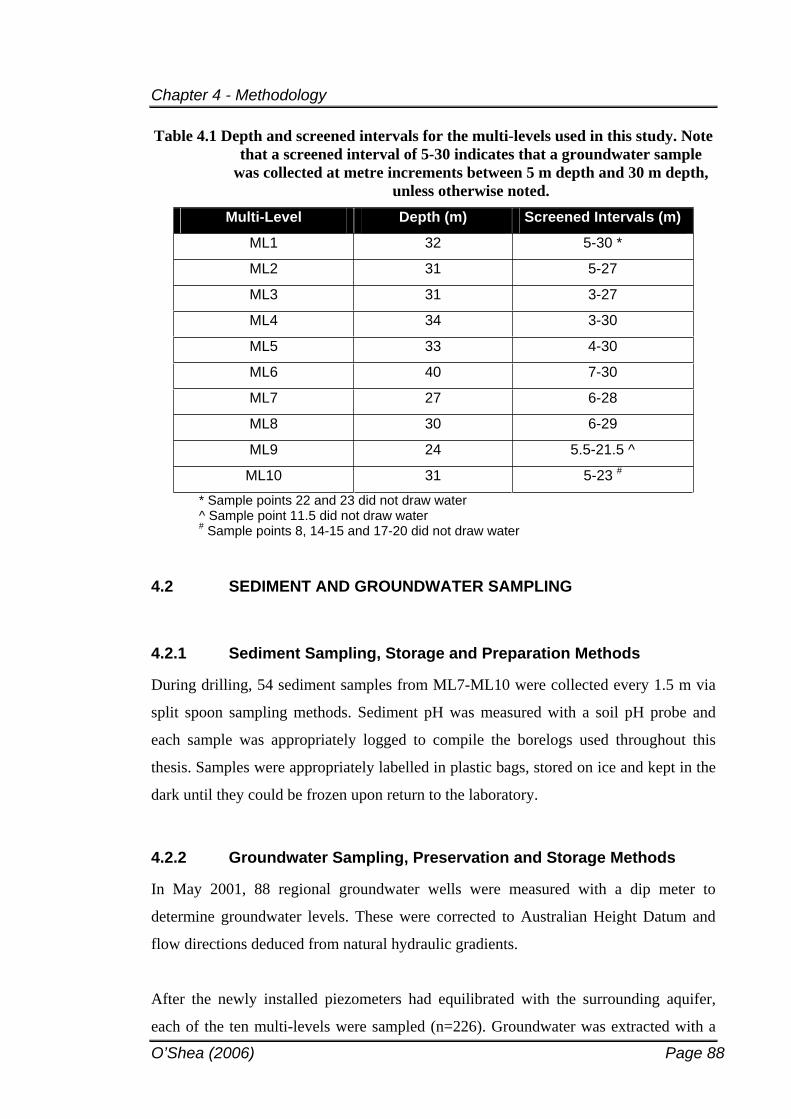
Chapter 4 - Methodology
O’Shea (2006) Page 88
Table 4.1 Depth and screened intervals for the multi-levels used in this study. Note that a screened interval of 5-30 indicates that a groundwater sample
was collected at metre increments between 5 m depth and 30 m depth, unless otherwise noted.
Multi-Level Depth (m) Screened Intervals (m)
ML1 32 5-30 *
ML2 31 5-27
ML3 31 3-27
ML4 34 3-30
ML5 33 4-30
ML6 40 7-30
ML7 27 6-28
ML8 30 6-29
ML9 24 5.5-21.5 ^
ML10 31 5-23 #
* Sample points 22 and 23 did not draw water ^ Sample point 11.5 did not draw water
# Sample points 8, 14-15 and 17-20 did not draw water
4.2 SEDIMENT AND GROUNDWATER SAMPLING
4.2.1 Sediment Sampling, Storage and Preparation Methods
During drilling, 54 sediment samples from ML7-ML10 were collected every 1.5 m via
split spoon sampling methods. Sediment pH was measured with a soil pH probe and
each sample was appropriately logged to compile the borelogs used throughout this
thesis. Samples were appropriately labelled in plastic bags, stored on ice and kept in the
dark until they could be frozen upon return to the laboratory.
4.2.2 Groundwater Sampling, Preservation and Storage Methods
In May 2001, 88 regional groundwater wells were measured with a dip meter to
determine groundwater levels. These were corrected to Australian Height Datum and
flow directions deduced from natural hydraulic gradients.
After the newly installed piezometers had equilibrated with the surrounding aquifer,
each of the ten multi-levels were sampled (n=226). Groundwater was extracted with a
Chapter 4 - Methodology
O’Shea (2006) Page 89
Peristaltic GeoPumpTM attached to each 8 mm sample tube. Each sample point was
purged to remove standing water and allow groundwater representative of the aquifer to
be sampled. Sampling began after general parameters (temperature, pH and EC) had
stablised to within +/-5% of the previously measured reading. Each sample was field-
filtered to enable measurement of ‘dissolved’ species; dissolved being defined as those
substances that will pass through a 0.45 m MilliporeTM cellulose acetate membrane
filter. However, it is noted that colloids can range from 0.01 to 10 m in diameter
(Sposito, 1989), with Gschwend and Reynolds (1987) reporting colloid particles of
intermediate diameter – 0.1 m to 1.0 m – as being the most mobile particles in a
sandy medium. This was taken into account during the interpretation procedure.
Each sample was placed into acid washed plastic containers after rinsing first with the
actual groundwater to be sampled. Care was taken to minimise exposure of the sample
to the atmosphere, which may induce chemical changes prior to sample preservation.
Concentrated analytical grade nitric acid (10 drops of 32M nitric acid) was used to
preserve samples to eliminate precipitation and adsorption occurring within the matrix.
All groundwater samples were labelled accordingly and kept in chilled, dark, eskies
until transferred to refrigerators. Routine duplicates and blanks were submitted with the
samples to assess quality control procedures.
4.3 AQUEOUS CHEMICAL ANALYSES
4.3.1 General Parameters
Eight Orion meters (two for each parameter) were used to measure Eh, EC, temperature,
pH and DO. The average of the two readings is reported within. Probes were kept in de-
ionised water between samples and thoroughly washed to prevent cross-contamination.
Each meter was calibrated before going into the field and re-calibrated if the reported
measurements were more than +/-5% of the other meter. EC readings were measured
with a Model 122 conductivity cell and calibrated by checking measurements against
freshly prepared KCl standards ranging from 0.0005 to 0.2M. This follows the
calibration method for conductivity meters provided in APHA (1992). DO was
measured with a Model 820 oxygen meter, while pH and Eh were measured with a
Chapter 4 - Methodology
O’Shea (2006) Page 90
Model 290A portable pH/concentration meter. pH meters were calibrated every day
using standard buffer solutions of pH 4.01, 7.00 and 10.01. A platinum redox electrode
was used to measure Eh after being calibrated against standard Zobell’s solution
(Nordstrom, 1997; Zobell, 1946).
4.3.2 Unstable Chemical Species
Redox sensitive parameters were measured at the time of sampling with a field-portable
Hach Spectrophotometer. Ferrous iron was measured using the 1,10 Phenanthroline
Method (Hach 8146) adapted from APHA (1992); sulfide was measured by the
Methylene Blue method (Hach 8131) adapted from APHA (1992); ammonium was
measured by the Nessler method (Hach 8038) adapted from APHA (1992); nitrate was
measured by the Cadmium Reduction method (Hach 8039); and phosphate the Reactive
Phosphorous method (Hach 8048) adapted from APHA (1992).
Additionally, field titrations were carried out at the piezometer head. The carbonate
species (bicarbonate and/or carbonate) were determined by field titration using 0.01M
or 0.1M HCl against methyl orange and bromocresol green indicators (APHA, 1992).
Carbon dioxide was measured in a similar manner against 0.025M NaOH with
phenolphthalein indictor (APHA, 1992). Each titration was performed twice and the
average of the two results was taken. All equipment was washed in nitric acid and
rinsed with both de-ionised water and sample water prior to use.
4.3.3 Major Ions
Major cations (Na+, K+, Ca2+ and Mg2+) were analysed by ICP-AES in the School of
Biological, Earth and Environmental Sciences at the University of New South Wales.
The machine was calibrated for the range of EC’s encountered and repeated
measurements were preformed on both samples and blanks (one blank for every ten
samples to account for machine drift) to monitor integrity of the analytical results.
Argentometric determination of chloride was ascertained by tritrating 0.01M AgNO3
against 10% potassium chromate indicator (APHA, 1992).
Chapter 4 - Methodology
O’Shea (2006) Page 91
An overall check of precision and accuracy of the chemical analyses was conducted by
calculating charge balance errors (CBE’s) for the major ions to assess the
electroneutrality of each solution. CBE’s were calculated according to the following
equation:
CBE % = ( cations – anions) x 100
( cations + anions)
CBE’s not within +/-5% (Freeze and Cherry, 1979) were re-analysed for all major ions.
4.3.4 Minor Elements
Metals and trace elements (including arsenic) were analysed by ICP-MS in the School
of Chemical Sciences at the University of New South Wales. The same calibration and
quality control procedures described for the ICP-AES were applied by the laboratory
technician during the ICP-MS analyses. A commonly known problem involved in
analysing arsenic by ICP-MS is potential interference from chloride. The argon plasma
may form argon chloride, which has the same atomic mass (75) as arsenic. This
interference can raise reported arsenic concentrations by 1 g L-1 for every 100 mg L-1
of chloride present. Given the relatively fresh and low chloride concentrations of most
groundwaters at Stuarts Point this was initially not deemed a problem. However,
additional sampling of the seawater intrusion groundwaters and estuarine waters meant
this interference needed to be addressed. Corrections may be applied using the chlorine
isotope ratio but arsenic concentrations may remain inaccurate at the g L-1 level.
Therefore, the problem was addressed by calibrating the ICP-MS against a ‘seawater’
solution containing 19,000 mg L-1 Cl-. This ‘seawater’ solution was subsequently spiked
with arsenic concentrations ranging from 1 g L-1 - 1,000 g L-1 As (also selenium and
chromium as an additional check), diluted 100 times, and used to calibrate the machine
before analysis. For comparison, saline groundwaters from the adjacent wetland
previously analysed on the same ICP-MS and by the same technician reported no
concentrations of arsenic, thereby dismissing the increased arsenic bias in saline water
samples.
Chapter 4 - Methodology
O’Shea (2006) Page 92
4.3.5 Arsenic Speciation
The original arsenic speciation method employed was also utilised by Smith et al.
(2003). The author herein conducted the analyses for both studies, but later found them
to be questionable due to chemical instability and concern over the accuracy of the
original method - APHA Method 3500-As B (20th ed., 1998). Custom made glassware
enabled a larger groundwater sample to be analysed and ensured equipment was robust
to sustain field conditions. After preparing spiked arsenic solutions in the laboratory, a
calibration curve was constructed which enabled the field-measured arsenic
concentrations to be determined. This laboratory work was initally conducted at the
Australian Nuclear Science and Technology Organisation under Dr Maree Emmett. The
following list is the step-by-step procedure carried out during As(III) analysis in the
field at Stuarts Point:
1. Place 400 mL of sample in glass jar and place onto magnetic stirrer.
2. Grease reaction vessel, place all stoppers in holes, add custom made absorber tube.
3. Add 5 mL of acetate buffer to sample by pipette.
4. Place 10 g of 3 mm glass beads into absorber tube (making sure lead acetate wool is
in the mouth of the absorber tube).
5. Record absorbance of DTC solution (as a blank) at 520 nm in the
spectrophotometer.
6. Add 20 mL of DTC solution from a glass syringe into absorber tube.
7. Connect and adjust nitrogen gas flow into reaction vessel to 60 mL per minute,
making sure gas is bubbling through DTC solution.
8. Fill a 60 mL plastic syringe with 30 mL of sodium borohydride and connect to the
nitrogen gas line.
9. Start stopwatch.
10. Slowly (over 2-5 minutes) add the sodium borohydride to the groundwater sample.
11. Leave to develop over 20 minutes.
12. At 20 minutes, redissolve any crystals in the absorber tube by pulling one of the
glass stoppers in and out, releasing pressure in the glass cylinder.
13. Place DTC solution into spectrophotometer cell and measure the absorbance at
520nm.
14. Determine As(III) concentration off previously prepared absorbance curve.
Chapter 4 - Methodology
O’Shea (2006) Page 93
4.4 SOLID PHASE ANALYSES
4.4.1 Electron Microscopy
All electron microscope work was undertaken by the author (with the assistance of Mr
Barry Searle) at the Electron Microscope Unit (EMU) within the University of New
South Wales (UNSW). The following section details sample preparation procedures and
instrument particulars, and is largely drawn from the in-house manual compiled for
EMU users at UNSW (Munroe and Stevens-Kalceff, 2002).
4.4.1.1 Sample Preparation
Fifteen samples were analysed via Scanning Electron Microscope – Energy Dispersive
x-ray Spectrometer (SEM-EDS). Each sample was mounted on an aluminium stub 2.5
cm in diameter, by adherence to double-sided carbon tape. The samples were then
placed in a sputter coater and coated with a thin layer of carbon to make them
electrically conductive. Carbon was chosen as the coating element as other metallic
coats (such as Au, Pt or Cr) may interfere with the chemical analysis.
For samples necessitating more accurate chemical analysis (n=10), the electron
microprobe equipped with a Wavelength Dispersive x-ray Spectrometer (WDS)
required samples to be embedded in a resin for polishing. A cross sectional sample was
thus prepared by Mr Rad Flossman in the School of Biological, Earth and
Environmental Sciences at UNSW. These samples were processed so as to be optically
flat, before coating with carbon to provide a path for the probe current to flow to the
earth.
4.4.1.2 SEM-EDS
SEM analysis was conducted on a Hitachi S4500 Field Emission SEM (1996), with
high resolution (1.5 nanometers), a tilting stage, Robinson Back-Scatter Detector,
Oxford Cathodoluminescence Detector (MonoCL2/ISIS) and a Link ISIS 200
Microanalysis System for chemical determination. The accelerating voltage was set at
20kV throughout the analysis process. Spectra were analysed by comparing the energies
of the observed peaks with characteristic peak energies of the elements. Care was taken
Chapter 4 - Methodology
O’Shea (2006) Page 94
with elements that had overlapping peaks, such as arsenic and lead; several peaks were
examined in order to identify the correct element spectra produced.
4.4.1.3 Electron Microprobe-WDS
The electron microprobe consists of a SEM with several WDS interfaces, giving it the
advantage of a more accurate and sensitive chemical analysis than the standard SEM-
EDS analysis. However, the WDS detector can only detect one element at a time,
whereas the EDS can semi-quantitate several elements at a time. Thus, the WDS is a
more powerful tool but is both costly and timely in its analysis.
A Cameca SX50 electron microprobe employing four WDS’s and one EDS was utilised
to produce a line scan over a grain with an identified coating layer. Several individual
points were also analysed quantitatively. Characteristic x-rays generated by elements
within the sample are diffracted by a suitable analysing crystal and measured in counts
per second by the gas flow proportional detectors.
4.4.1.4 Internal QA/QC Procedures
Both instruments are calibrated with Standard Reference Materials for the various
elements analysed. The S4500 uses Guide E1508-98 Standard Guide for Quantitative
Analysis by Energy-Dispersive Spectroscopy; while the SX50 employs the data
reduction matrix correction procedure based on the methods of Pouchou and Pichoir
(1985).
Various steps in the SX50 calibration process were carried out by the technical officer
in charge of the instrument (Mr Barry Searle). This required manual entry of calibration
criteria such as background positions, counting time, background slope and the
analytical line. The acquisition parameters used during calibration (including crystals
used and interferences accounted for) may be supplied on request.
Detection limits for the SX50 may be affected by random errors such as calibration
uncertainty, peak and background counting time, system stability, profile slope,
uncertainty in any overlap corrections, the accelerating voltage, the beam current, the
Chapter 4 - Methodology
O’Shea (2006) Page 95
line used to measure the element and the composition of both the sample and the
standards. The peak counts must exceed three times the standard deviation of the
background to give a 95% probability that a peak may be present. Only those elements
adhering to this criteria were given a reported concentration value; all others were
reported as 0%. The detection limits for the SX50 are generally set at 0.01% (100ppm)
except for As which was set at 0.02%. This compares with the S4500 which has
detection limits of 0.2%.
4.4.2 Grain Size Analysis
Nineteen samples were selected for grain size analysis (GSA). The sand and granule
fractions were targeted during the GSA procedure in order to differentiate beach sands
from river sands. Approximately 50-100 g of split sample was first wet-sieved through a
63 m (0.063 mm) sized sieve to remove the silt and clay fractions. These two fractions
are therefore reported together as a percentage of each respective sample. The
remaining sand and granule fractions were oven dried and sieved through a set of 8-inch
diameter sieves at ½ phi ( ) intervals and placed on an electronic shaker for 5 minutes.
Each respective size fraction was weighed to 0.01 g.
Histograms and cumulative frequency curves were generated for the grain size results.
An arithmetic scale was used for cumulative frequency. The parameters of mean grain
size, skewness and standard deviation (sorting) were determined using the graphical
formulae of Folk and Ward (1957) with grain size measured in . As an alternative, they
were also calculated using the method of moments (as cited in Tucker, 1991). Formulae
for both methods are presented in Table 4.2. A comparison between the results of each
method are shown by the mean relative percent difference (RPD) calculated for each
parameter (Table 4.3). These calculations are provided in Appendix B3.
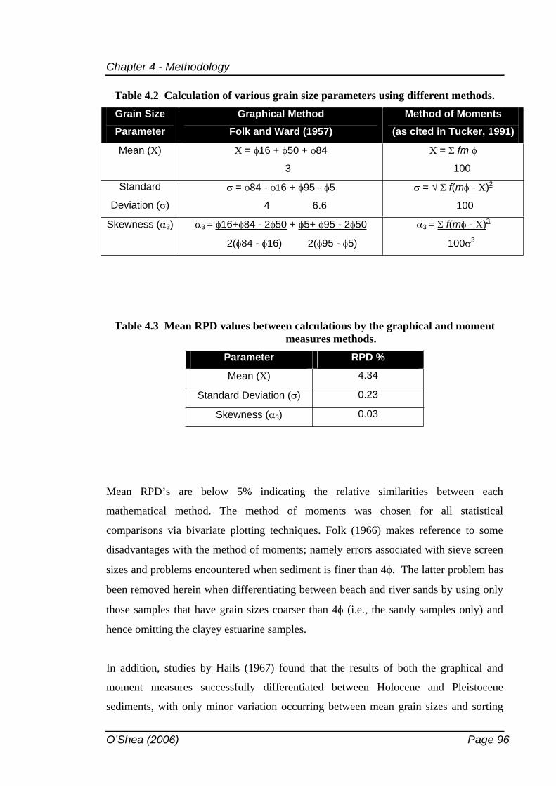
Chapter 4 - Methodology
O’Shea (2006) Page 96
Table 4.2 Calculation of various grain size parameters using different methods. Grain Size Parameter
Graphical Method Folk and Ward (1957)
Method of Moments (as cited in Tucker, 1991)
Mean ( ) = 16 + 50 + 84
3
= fm
100
Standard
Deviation ( )
= 84 - 16 + 95 - 5
4 6.6
= f(m - )2
100
Skewness ( 3) 3 = 16+ 84 - 2 50 + 5+ 95 - 2 50
2( 84 - 16) 2( 95 - 5)
3 = f(m - )3
100 3
Table 4.3 Mean RPD values between calculations by the graphical and moment measures methods.
Parameter RPD %
Mean ( ) 4.34
Standard Deviation ( ) 0.23
Skewness ( 3) 0.03
Mean RPD’s are below 5% indicating the relative similarities between each
mathematical method. The method of moments was chosen for all statistical
comparisons via bivariate plotting techniques. Folk (1966) makes reference to some
disadvantages with the method of moments; namely errors associated with sieve screen
sizes and problems encountered when sediment is finer than 4 . The latter problem has
been removed herein when differentiating between beach and river sands by using only
those samples that have grain sizes coarser than 4 (i.e., the sandy samples only) and
hence omitting the clayey estuarine samples.
In addition, studies by Hails (1967) found that the results of both the graphical and
moment measures successfully differentiated between Holocene and Pleistocene
sediments, with only minor variation occurring between mean grain sizes and sorting
Chapter 4 - Methodology
O’Shea (2006) Page 97
values. Thus the selection of one mathematical technique over the other is insignificant
to the final result in this instance.
4.4.3 Sequential Extractions
A modified (cation/anion) sequential extraction technique (Table 4.4) was applied to
specifically target arsenic pools in the sediments. This procedure was chosen based on a
literature review of sequential extraction schemes.
Table 4.1 lists references cited and common advantages/disadvantages for each targeted
fraction. Due to the disputable nature of such extraction techniques, only five samples
were chosen for this procedure. Each sample was significantly different to the other
(brown sand, green sand and clay, orange/red clay, coffee rock and farm topsoil), and
were chosen for analysis as a preliminary screening tool leading to further analytical
techniques.
4.4.4 XRD
XRD analysis was carried out on a Philips PW1140 Diffractometer located in the
School of Biological, Earth and Environmental Sciences at the University of New South
Wales. Sediments were first oven-dried and ground to pass a 2 mm sieve. Semi-
quantitative mineral analysis was aided with XPLOT software providing a database of
representative XRD mineral peaks that were visually matched to the resulting analytical
spectra.
4.4.5 XRF
Both major and minor elements were analysed in samples on a Philips PW2400 XRF
with a 102 position sample changer by Ms Irene Wainwright in the School of
Biological, Earth and Environmental Sciences at the University of New South Wales.
Sample preparation involved mechanical grinding of sediments prior to construction of
‘pellets’ for trace element analysis and ‘glass plates’ for major elements.
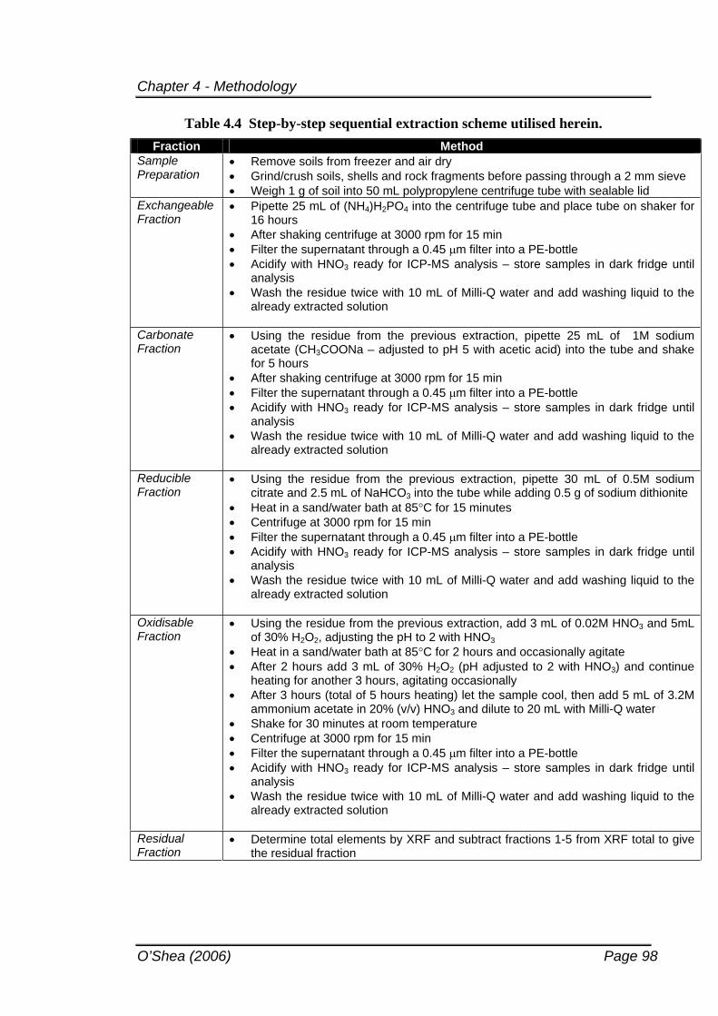
Chapter 4 - Methodology
O’Shea (2006) Page 98
Table 4.4 Step-by-step sequential extraction scheme utilised herein.Fraction Method
SamplePreparation
Remove soils from freezer and air dry Grind/crush soils, shells and rock fragments before passing through a 2 mm sieve Weigh 1 g of soil into 50 mL polypropylene centrifuge tube with sealable lid
Exchangeable Fraction
Pipette 25 mL of (NH4)H2PO4 into the centrifuge tube and place tube on shaker for 16 hours
After shaking centrifuge at 3000 rpm for 15 min Filter the supernatant through a 0.45 m filter into a PE-bottle Acidify with HNO3 ready for ICP-MS analysis – store samples in dark fridge until
analysis Wash the residue twice with 10 mL of Milli-Q water and add washing liquid to the
already extracted solution
Carbonate Fraction
Using the residue from the previous extraction, pipette 25 mL of 1M sodium acetate (CH3COONa – adjusted to pH 5 with acetic acid) into the tube and shake for 5 hours
After shaking centrifuge at 3000 rpm for 15 min Filter the supernatant through a 0.45 m filter into a PE-bottle Acidify with HNO3 ready for ICP-MS analysis – store samples in dark fridge until
analysis Wash the residue twice with 10 mL of Milli-Q water and add washing liquid to the
already extracted solution
Reducible Fraction
Using the residue from the previous extraction, pipette 30 mL of 0.5M sodium citrate and 2.5 mL of NaHCO3 into the tube while adding 0.5 g of sodium dithionite
Heat in a sand/water bath at 85 C for 15 minutes Centrifuge at 3000 rpm for 15 min Filter the supernatant through a 0.45 m filter into a PE-bottle Acidify with HNO3 ready for ICP-MS analysis – store samples in dark fridge until
analysis Wash the residue twice with 10 mL of Milli-Q water and add washing liquid to the
already extracted solution
Oxidisable Fraction
Using the residue from the previous extraction, add 3 mL of 0.02M HNO3 and 5mL of 30% H2O2, adjusting the pH to 2 with HNO3
Heat in a sand/water bath at 85 C for 2 hours and occasionally agitate After 2 hours add 3 mL of 30% H2O2 (pH adjusted to 2 with HNO3) and continue
heating for another 3 hours, agitating occasionally After 3 hours (total of 5 hours heating) let the sample cool, then add 5 mL of 3.2M
ammonium acetate in 20% (v/v) HNO3 and dilute to 20 mL with Milli-Q water Shake for 30 minutes at room temperature Centrifuge at 3000 rpm for 15 min Filter the supernatant through a 0.45 m filter into a PE-bottle Acidify with HNO3 ready for ICP-MS analysis – store samples in dark fridge until
analysis Wash the residue twice with 10 mL of Milli-Q water and add washing liquid to the
already extracted solution
Residual Fraction
Determine total elements by XRF and subtract fractions 1-5 from XRF total to give the residual fraction

Tab
le 4
.5 C
omm
only
app
lied
sequ
entia
l ext
ract
ion
tech
niqu
es a
nd th
eir
asso
ciat
ed a
dvan
tage
s/di
sadv
anta
ges.
Ta
rget
edFr
actio
nC
omm
only
Use
d Ex
trac
tion
Che
mic
als
Adv
anta
ges
/ Dis
adva
ntag
es
Cite
d In
Exc
hang
eabl
eFr
actio
nA
mm
oniu
m o
r sod
ium
ace
tate
Mag
nesi
um c
hlor
ide
May
als
o at
tack
car
bona
tes
Ace
tate
com
plex
es w
ith c
alci
um
Chl
orid
e m
ay in
terfe
re w
ith IC
P-M
S
Tess
ier e
t al.
(197
9); C
ai e
t al.
(200
2)
Tess
ier e
t al.
(197
9)
Car
bona
teFr
actio
nS
odiu
m a
ceta
te o
r ace
tic a
cid
Low
er p
H v
alue
s pa
rtial
ly a
ttack
Fe
& M
n ox
ides
Doe
s no
t affe
ct s
ilica
tes,
sul
fides
or o
rgan
ic m
atte
r
Tess
ier e
t al.
(197
9); L
a Fo
rce
et a
l. (2
000)
Wen
zel (
2001
)
Red
ucib
leFr
actio
nS
odiu
m d
ithio
nite
citr
ate
Hyd
roxy
lam
ine
hydr
ochl
orid
e
Sub
stan
tial p
reci
pita
tion
of tr
ace
met
als
with
inso
lubl
e su
lfide
s fro
m d
ispr
opor
tiona
tion
of d
ithio
nite
, whi
ch is
als
o hi
ghly
con
tam
inat
ed w
ith z
inc
Chl
orid
e m
ay in
terfe
re w
ith IC
P-M
S
Tess
ier e
t al.
(197
9); G
leyz
es e
t al
. (20
02a)
Tess
ier e
t al.
(197
9)
Oxi
disa
ble
Frac
tion
Hyd
roge
n pe
roxi
de in
aci
dic
med
ium
Con
cent
rate
d ni
tric
or
hydr
ochl
oric
or p
erch
loric
aci
d
May
not
oxi
dise
all
form
s of
org
anic
mat
ter,
also
ext
ract
s so
me
sulfi
de m
iner
als
Als
o at
tack
s so
me
silic
ate
latti
ces
in a
dditi
on to
pot
entia
l ch
lorid
e in
terfe
renc
e w
ith IC
P-M
S
Tess
ier e
t al.
(197
9); G
leyz
es e
t al
. (20
02a)
Tess
ier e
t al.
(197
9)
Res
idua
lFr
actio
nH
F or
nitr
ic a
cid
or p
erch
loric
ac
id
XR
F
HF
high
ly to
xic
and
pote
ntia
l chl
orid
e in
terfe
renc
e
Muc
h sa
fer t
han
usin
g H
F
Tess
ier e
t al.
(197
9)
Stu
mm
eyer
et a
l. (2
002)
Chapter 4 - Methodology
O’Shea (2006) Page 100
4.4.6 Loss On Ignition (LOI)
LOI was determined as part of the XRF analytical process and can be used as an
indication of the amount of organic matter in the sample - roughly 40-60% LOI may be
organic carbon (Bengtsson and Enell, 1986). Such a method has been used by Welch
and Lico (1998) to determine arsenic and uranium occurrence in shallow groundwater.
However, given the amount of carbonates, sulfides and potential hydration minerals in
these sediments, the use of LOI as an indicator of organic matter content is not
considered plausible here.
4.5 STATISTICAL ANALYSES
The following statistical methods were applied by the author herein in a separate
hydrogeochemical study (O’Shea and Jankowski, 2006).
4.5.1 Data Screening
4.5.1.1 Assessment Of Normality
Prior to commencing statistical analyses, the data set should be assessed for normality
and completeness of data. Results of the data screening process determines if the data is
suitable for statistical tests in raw form, or if it requires manipulation to achieve more
accurate results from the statistical procedures employed. The data screening process for
the Stuarts Point chemical data is described below. Major ions and trace elements were
assessed independently due to large compositional differences.
Data producing a bell shaped frequency distribution, with values clustered around a
central point and the frequency of occurrence declining away from this point, are said to
be normally distributed (Davis, 1986). It is often assumed that variables are normally
distributed, and many statistical tests are based on this assumption. PCA is an exception
to this rule as it is based solely on eigenanalysis of the correlation/covariance matrix
(Meglin, 1991). However, HCA assumes the data is either normal or log-normal (Guler
et al., 2002), therefore an assessment of normality was required before HCA could be
undertaken.
Chapter 4 - Methodology
O’Shea (2006) Page 101
Histograms produced in SPSS showed that the major ion groundwater data from Stuarts
Point are positively skewed. Most naturally occurring element distributions follow this
pattern (Miesch, 1976). An assessment of normality for the major ions indicated that
neither the raw nor log10-transformed data appeared to approximate normality. Based on
these results, the major ion groundwater data was left in raw form for the statistical
analyses. In contrast, the trace element groundwater data showed a closer approximation
to normality after log10-transformation. There are advantages and disadvantages to
transformating data sets. Dreher (2003) debated the use of transformation techniques on
positively skewed data due to the possibility of information – specifically anomalies –
to become lost. Guler and Thyne (2003) responded to Dreher’s comment by stating that
transformation is required to produce maximum results from parametric (normal)
statistical methods. Given debate in this subject, the raw trace element data was used for
PCA (which does not require the assumption of normality) and the log10-transformed
data was used for HCA (which does require the assumption of normality). When both
data sets were combined transformed data was used; as was the case for the sediment
samples.
4.5.1.2 Standardization
In order for each variable to have an equal weight in the statistical analyses, the data can
be standardized to a range of –3 to +3 standard deviations, centred about a mean of zero
(Guler et al., 2002). Dreher (2003) disputed the use of standardization, saying it shifts
the relationships between the ions and neglects information derived from relative
abundances, such as supply and demand on the air, soil, unsaturated and saturated
zones. Guler and Thyne (2003) responded to this comment saying they used
standardization to avoid misclassifications arising from the inappropriate weighting of
parameters with large magnitudes. A number of other authors have standardized their
geochemical data (Farnham et al., 2000; Ruiz et al., 1990; Swanson et al., 2001).
Standardization is necessary when data varies over wide ranges, as is the case with
concentrations of major ions and trace elements in both the Stuarts Point groundwater
and sediment data sets. Standardization was employed herein to ensure each analyte was
equally weighted during the statistical analyses.
Chapter 4 - Methodology
O’Shea (2006) Page 102
4.5.1.3 Censored Data
Robust statistical techniques achieve the most reliable results when a full (i.e.,
complete) data set is used. However, as is often the case in geochemical investigations,
the Stuarts Point data set contains ‘censored’ values. Values reported as “less than” or
“greater than” a censor point are known as censored or qualified values (Sanford et al.,
1993). The censor point for these investigations is the analytical detection limit (DL) for
each variable (analyte). Several analytes reported concentrations at or below the
analytical DL and were thus assigned a value of “less-than” the DL. Such censored data
can complicate all subsequent statistical analyses (Farnham et al., 2002) and therefore
consideration should be given to replacing the censored data with uncensored values.
Sanford et al. (1993) showed the importance of treating censored data as opposed to
ignoring it. They discuss the importance of replacing censored values, to prevent
misguided statistical results.
A number of techniques are available for replacing censored data values, depending on
the size of the data set and the number of censored values present. Perhaps the most
common method is replacement of the less-than values with ¾ times the lower DL and
the greater-than values with 4/3 times the upper DL (VanTrump and Miesch, 1977).
Similar to this, replacement with half the DL is the current method supported by the
New South Wales Environmental Protection Authority (NSW EPA, 1995) for the
assessment of contaminated sites. Additionally, replacement with zero or the DL are
also common substitution values. Seyhan et al. (1985) settled on substitution with the
DL stating that this has an insignificant effect on the Q-mode classification results of
principle components, cluster and discriminant analysis. However, Farnham et al.
(2002) showed that substitution with half the detection limit (DL/2) gave superior
results when compared to the DL or zero. Significant deterioration of the performance
of all substitution methods occurred when the number of less-than values exceeded
25%. Sanford et al. (1993) proposed that for a small proportion of substitutions, a
replacement factor of 0.55 is preferable to using ¾ the DL.
An alternative approach is to use the actual reported concentration produced by the
analytical instrument, even if it is below the DL. Many chemists won’t report these less-
Chapter 4 - Methodology
O’Shea (2006) Page 103
than values stating they are unreliable. However, studies have shown that these
‘unreliable’ values can more effectively detect trends than censored data (Gilliom et al.,
1984). These values were used for the Stuarts Point sediment concentrations reported by
the XRF.
More precise methods are available for determining descriptive statistical values (such
as mean and variance) but are not commonly used for multivariate techniques. These
methods involve estimating the mean of the (normally distributed) censored data set and
using this estimated mean as a replacement value. Further information on these
statistical procedures can be found in Farnham et al. (2002), Sanford et al. (1993) and
Singh and Nocerino (2002).
An assessment of the raw major ion groundwater data showed three values for
potassium were reported as being below the analytical DL (<0.16 mg L-1). Given the
low frequency of replacement required (less than 2% of the data), a replacement value
of half the detection limit (DL/2 - 0.08 mg L-1) was used for the three censored
potassium values. This method follows that used by Farnham et al. (2002) and the NSW
EPA (1995). This value was also extremely close to using a replacement factor of 0.55
as recommended by Sanford et al. (1993), which would yield a value of 0.088 mg L-1.
Replacement with DL/2 was also selected for the trace element data set. This method
was selected based on Farnham et al.’s (2002) assessment of the performance and
deterioration of replacement values. Given the deterioration of substitution methods
when increasing amounts of censored values are present, elements with more than 30%
replacements required were removed from the statistical analyses. The same approach
was taken by Critto et al. (2003) who removed those parameters showing low frequency
of detection from their statistical analysis.
4.5.2 Descriptive Statistics
Prior to subjecting the Stuarts Point data to multivariate statistical manipulation, an
analysis of descriptive statistics was conducted. Descriptive statistics provide an
indication of abundance and elemental outliers. All statistical analyses were performed
using the software package SPSS Version 12.01.
Chapter 4 - Methodology
O’Shea (2006) Page 104
4.5.3 Multi-Variate Statistical Analyses
4.5.3.1 Cluster Analysis
Hierarchial Cluster Analysis was performed on all sediment and groundwater samples.
Q-mode HCA classified each case (sample), measured by variable (element or ion) into
statistically defined groups. Ward’s (1963) linkage method was chosen to iteratively
link nearby points of similarity. Euclidean distance measure assessed the similarity
combined with linkage. R-mode HCA was useful in establishing relationships between
the variables (analytes) rather than the cases (samples) as is the situation in Q-mode
HCA. A dendrogram was produced for each cluster analysis undertaken. In most cases,
the phenon line was set at an Euclidean distance of five to identify clusters of most
similarity.
4.5.3.2 Principal Components Analysis (PCA)
A second geostatistical tool was used on the Stuarts Point data – Principal Components
Analysis. PCA is a mathematical technique used for reducing data and deciphering
patterns within large data sets (Hull, 1984; Joliffe, 1986; Stetzenbach et al., 1999; and
Wold et al., 1987). Principal Components (PC’s) are based on eigenanalysis of the
correlation or covariance matrix, therefore data does not need to be normally distributed
(Meglin, 1991). PCA was thus conducted on raw standardized data using the
correlation matrix. PC’s are the result of strong correlations between variables. PC’s
may result from the correlation of suites of variables (such as marine elements)
representing the same geological origin or geochemical source. The first PC is that
component which has the greatest possible variance, the second PC has the second
greatest variance, and so on. All PC’s are uncorrelated (ie, orthogonal) to one another
(Stetzenbach et al., 2001). Eigenvalues describe the amount of variance explained by
each PC, and thus decrease with each successive PC extracted. Eigenvectors (or PC
loadings) indicate the relative contribution each element makes to that PC score. The
larger the score - in absolute value - the stronger the influence of that element (Webster,
2001). While PCA was utilised as a pre-screening device for the hydrochemical
interpretation, the best statistical results were provided by HCA and thus the results of
the PCA are not included within.

Chapter 4 - Methodology
O’Shea (2006) Page 105
4.5.4 Statistical Correlation
Most geochemical data are positively skewed. As such, Spearmans correlations are
often used in geochemical correlation. However, Pearsons correlations are better suited
to normal data. Since the Stuarts Point data has been log10-transformed to better
approximate normality, Pearsons correlation technique is most appropriate. Pearsons
correlations were calculated in SPSS. All r2 values provided on graphs, tables and in the
text, are correlations performed in SPSS, not Excel.
O’Shea (2006) Page 106
5 ORIGINAL SOURCE OF ARSENIC TO THE AQUIFER
5.1 HYPOTHESES
Five arsenic source theories are hypothesised:
1. Arsenic is present in the aquifer as a by-product of anthropogenic activities;
2. Arsenic has been contributed to the aquifer matrix via deposition of regionally
eroded geological units containing arsenic mineralisation;
3. Arsenic is derived from remnant seawater trapped in marine clay units deposited
during eustatic changes of sea level in the Quaternary (Smith et al., 2006);
4. The oxidation of arsenian pyrite present in ASS material contributes dissolved
arsenic to the groundwater (Smith et al., 2006); and/or
5. The underlying bedrock contains arsenic, which is being contributed to the aquifer
via upwards vertical leakage of groundwater (Smith et al., 2003).
This chapter discusses the validity of each hypothesis and determines which one is most
likely to be the dominant arsenic source in the aquifer. A number of investigative
techniques have been utilised herein in the assessment of each potential arsenic source.
Table 5.1 lists each proposed source, and the work completed herein, in order to assess
the validity of each source.
This chapter is structured as follows:
the results of investigative techniques are provided first;
followed by a discussion of each potential arsenic source and the evidence
collected both for, and against, each hypothesis;
the chapter concludes with a comparison to known arsenic sources in other
elevated arsenic environments; and finally
a summary of the findings presented in this chapter.

Tab
le 5
.1 T
echn
ique
s us
ed h
erei
n to
dis
mis
s or
sup
port
pot
entia
l ars
enic
sou
rces
to th
e St
uart
s Po
int a
quife
r, a
nd th
e lo
catio
n of
res
ults
pr
ovid
ed w
ithin
this
thes
is.
Pote
ntia
lA
rsen
ic S
ourc
e Sp
ecifi
c Q
uest
ion(
s) to
be
addr
esse
d he
rein
Inve
stig
ativ
e Te
chni
ques
Lo
catio
n of
Dat
a
Ant
hrop
ogen
ic
arse
nic
Has
ant
hrop
ogen
ic c
onta
min
atio
n oc
curr
ed?
Lite
ratu
re re
view
of g
over
nmen
t rec
ords
; ane
cdot
al
evid
ence
; pa
st m
inin
g hi
stor
y; in
terv
iew
s w
ith p
rese
nt
resi
dent
s
Ana
lysi
s of
gro
undw
ater
dat
a (s
uppo
rting
evi
denc
e)
Inte
grat
ed in
to d
iscu
ssio
n in
Sec
tion
5.3.
1
Gro
undw
ater
dat
a di
scus
sed
fully
in
Cha
pter
7
Reg
iona
l geo
logi
c so
urce
W
as th
e S
tuar
ts P
oint
aqu
ifer d
epos
ited
by o
nsho
re s
edim
ent m
ovem
ent,
as
prev
ious
ly p
ropo
sed,
or d
oes
it ha
ve
sign
ifica
nt fl
uvia
l inf
luen
ce?
If th
e aq
uife
r has
bee
n de
posi
ted
by
fluvi
al e
rosi
on o
f the
hin
terla
nd, i
s th
ere
regi
onal
ars
enic
min
eral
isat
ion
pres
ent?
Com
pila
tion
of b
orel
ogs
from
dril
ling
Sed
imen
t gra
in s
ize
anal
yses
to d
eter
min
e if
fluvi
al
sedi
men
tatio
n ha
s oc
curr
ed
Mol
lusc
iden
tific
atio
n to
sho
w s
peci
fic p
arts
of t
he
aqui
fer w
ere
depo
site
d un
der h
abita
t con
ditio
ns
suita
ble
for c
erta
in m
ollu
sc s
peci
es
Dev
elop
men
t of a
quife
r cro
ss s
ectio
ns
Det
erm
inin
g so
urce
pro
vena
nce
for t
he a
quife
r se
dim
ents
Dev
elop
men
t of a
n aq
uife
r spe
cific
geo
mor
phic
mod
el
Rev
iew
of r
egio
nal m
iner
alis
atio
n
Sec
tion
5.2.
1
Sec
tion
5.2.
2.1
Spe
cies
iden
tific
atio
n di
scus
sed
in
Sec
tion
5.2.
2.2
; loc
atio
ns o
f spe
cies
pr
ovid
ed o
n bo
relo
gs in
Sec
tion
5.2.
1
Sec
tion
5.2.
4.2
Sec
tion
5.2.
5
Sec
tion
5.2.
6
Sec
tion
5.2.
5.2

Pote
ntia
lA
rsen
ic S
ourc
e Sp
ecifi
c Q
uest
ion(
s) to
be
addr
esse
d he
rein
Inve
stig
ativ
e Te
chni
ques
Lo
catio
n of
Dat
a
Can
a li
nk b
e m
ade
betw
een
regi
onal
ar
seni
c an
d th
e pr
esen
ce o
f ars
enic
at
Stu
arts
Poi
nt?
Sta
tistic
al c
lust
erin
g of
sed
imen
t che
mis
try
Sel
ectio
n of
a h
inte
rland
indi
cato
r ele
men
t to
corr
elat
e aq
uife
r sed
imen
ts w
ith a
regi
onal
sou
rce
prov
enan
ce
Sed
imen
t che
mis
try re
sults
pro
vide
d in
Sec
tion
5.2.
3; s
tatis
tical
resu
lts
disc
usse
d in
Sec
tion
5.2.
4.1.
Sec
tion
5.2.
5.2
Rem
nant
se
awat
er
Did
sea
wat
er tr
ansg
ress
ove
r the
S
tuar
ts P
oint
aqu
ifer?
Do
the
curr
ent a
quife
r sed
imen
ts h
old
any
clue
s in
dica
ting
a pa
st o
rigin
from
se
awat
er?
Geo
mor
phic
reco
nstru
ctio
n of
the
Stu
arts
Poi
nt a
quife
r
Ana
lysi
s of
ars
enic
con
cent
ratio
n pe
aks
in s
edim
ents
an
d th
e di
strib
utio
n of
est
uarin
e cl
ay u
nits
Sec
tion
5.2.
6
Ars
enic
che
mis
try p
rovi
ded
in
Sec
tion
5.2.
3; c
orre
latio
n w
ith
bore
logs
(est
uarin
e cl
ay u
nits
) di
scus
sed
in S
ectio
n 5.
3.3
AS
S a
ssoc
iatio
n Is
ther
e an
y as
soci
atio
n w
ith A
SS
ho
rizon
s an
d ar
seni
c?
Is th
ere
any
asso
ciat
ion
with
pyr
ite a
nd
arse
nic?
Obs
erva
tion
of A
SS
hor
izon
s
SE
M u
sed
to id
entif
y py
rite
Bor
elog
s in
Sec
tion
5.2.
1; d
iscu
ssio
n in
Sec
tion
5.3.
4
Res
ults
pre
sent
ed in
Cha
pter
61
Dire
ct b
edro
ck
cont
ribut
ion
Is a
rsen
ic p
rese
nt in
the
bedr
ock?
Is a
rsen
ic b
eing
con
tribu
ted
to th
e un
cons
olid
ated
aqu
ifer v
ia d
isch
arge
fro
m th
e be
droc
k aq
uife
r bel
ow?
Rev
iew
of l
itera
ture
and
ana
lysi
s of
bed
rock
en
coun
tere
d du
ring
drill
ing
Inve
stig
atio
n of
sta
tistic
al c
orre
latio
n be
twee
n ar
seni
c an
d tra
ce e
lem
ents
in g
roun
dwat
er s
ampl
ed c
lose
to
bedr
ock
Sec
tion
5.2.
2.3
Ver
tical
gra
ph o
f an
indi
cato
r ele
men
t pr
ovid
ed in
Fig
ure
5.24
; gro
undw
ater
da
ta p
rovi
ded
in C
hapt
er 7
; sta
tistic
al
corr
elat
ion
betw
een
arse
nic
and
trace
ele
men
ts in
gro
undw
ater
pr
ovid
ed in
App
endi
x B
6
1 N.B
. Thi
s ch
apte
r dea
ls s
peci
fical
ly w
ith th
e th
eory
that
ars
enic
may
be
asso
ciat
ed w
ith d
istin
ct A
SS
hor
izon
s; C
hapt
er 6
dis
cuss
es th
e as
soci
atio
n be
twee
n ar
seni
c an
d th
e m
iner
al p
yrite
.
Chapter 5 – Original Source of Arsenic to the Aquifer
O’Shea (2006) Page 109
5.2 INVESTIGATIVE RESULTS AND INTERPRETATION
The aquifer matrix was determined to be the key medium to investigate both arsenic
source and current sinks (Chapter 6). The natural (geogenic) arsenic sources proposed
for the Stuarts Point aquifer are a direct result of the aquifer’s depositional history. To
date, some regional geologic and geomorphic surveys have been extended to encompass
Stuarts point (Roy and Thom, 1981; Hails, 1968), however, no aquifer-specific
geomorphic studies have been conducted. Data collected during this study allows the
first comprehensive geomorphic model to be developed for Stuarts Point.
5.2.1 Aquifer Lithology
To enable a complete geomorphic reconstruction, the installation of ten multi-level
piezometers ranging in depth from 24 – 40 metres below ground surface (mbgs)
allowed detailed logging of the aquifer sediments to be recorded. Six boreholes (ML1-
ML6) were installed and logged by the NSW DLWC to monitor seawater intrusion,
while the remaining four boreholes (ML7-ML10) were completed by the author
specifically for this study (see Chapter 4 for full drilling methodology). All ten
piezometers have been utilised in this investigation. The location of these multi-levels is
shown on the map provided in Chapter 2 (Figure 2.1).
Sediments were visually logged by collecting a sample every 1.5 m during drilling.
Individual borelogs are shown in Figure 5.1 through Figure 5.10.
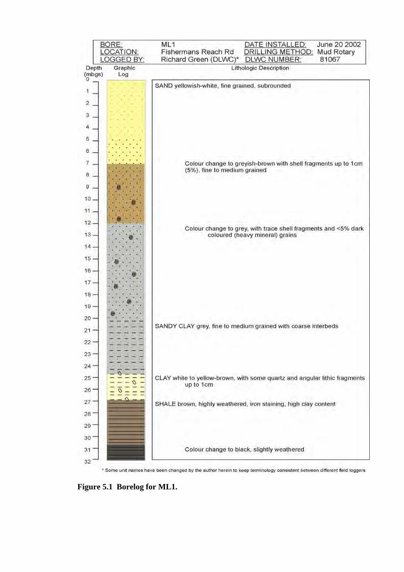
Figure 5.1 Borelog for ML1.
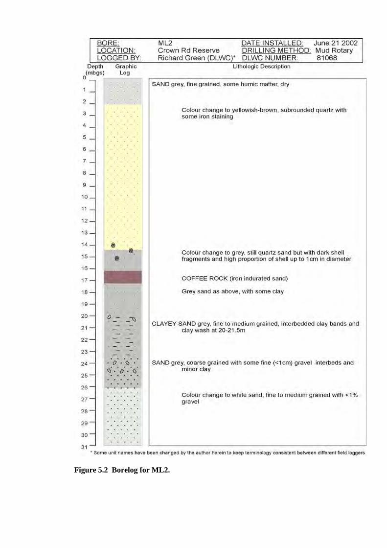
Figure 5.2 Borelog for ML2.
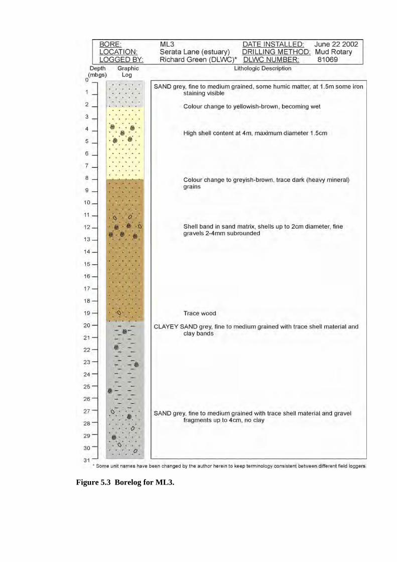
Figure 5.3 Borelog for ML3.
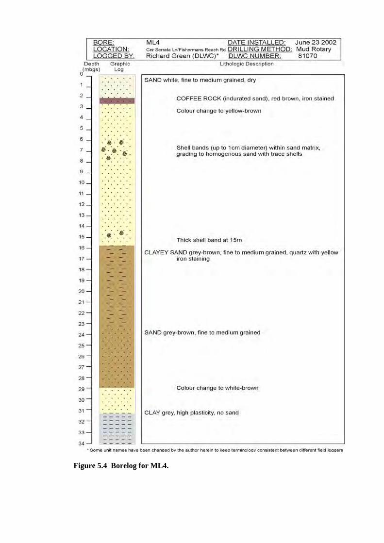
Figure 5.4 Borelog for ML4.
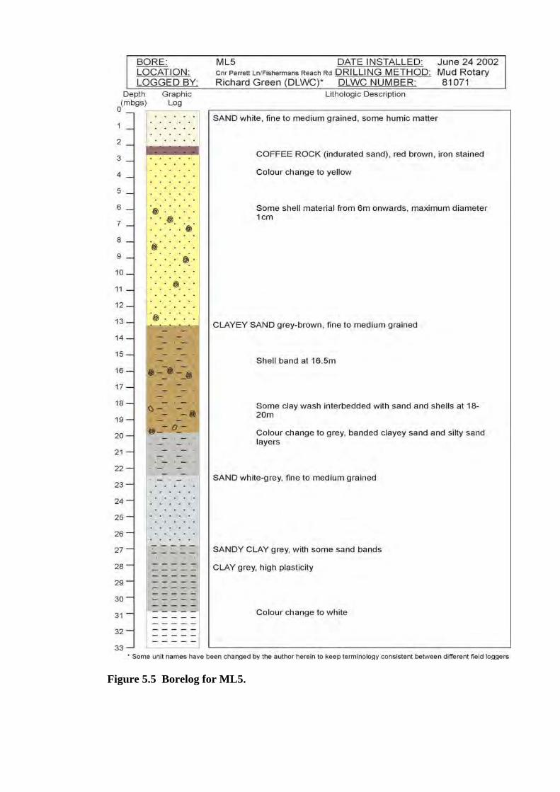
Figure 5.5 Borelog for ML5.
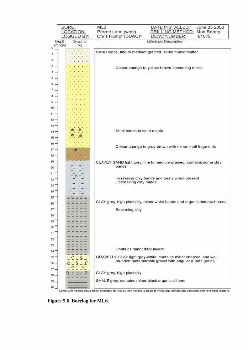
Figure 5.6 Borelog for ML6.
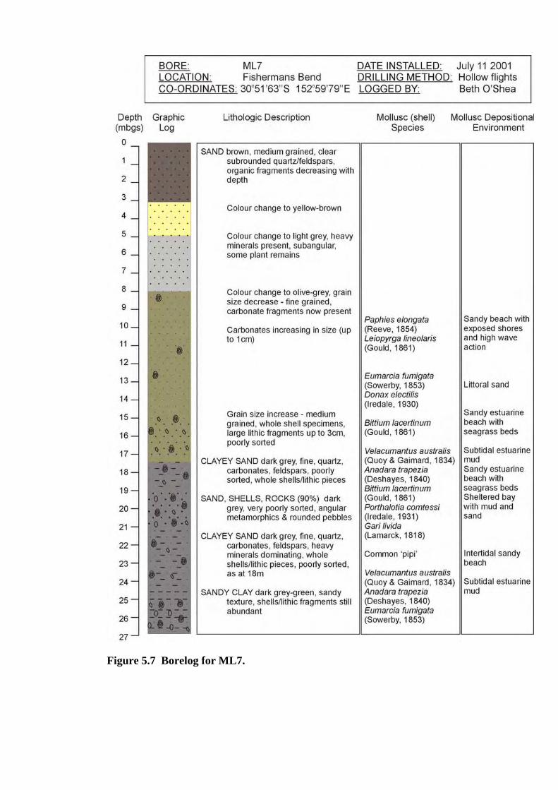
Figure 5.7 Borelog for ML7.
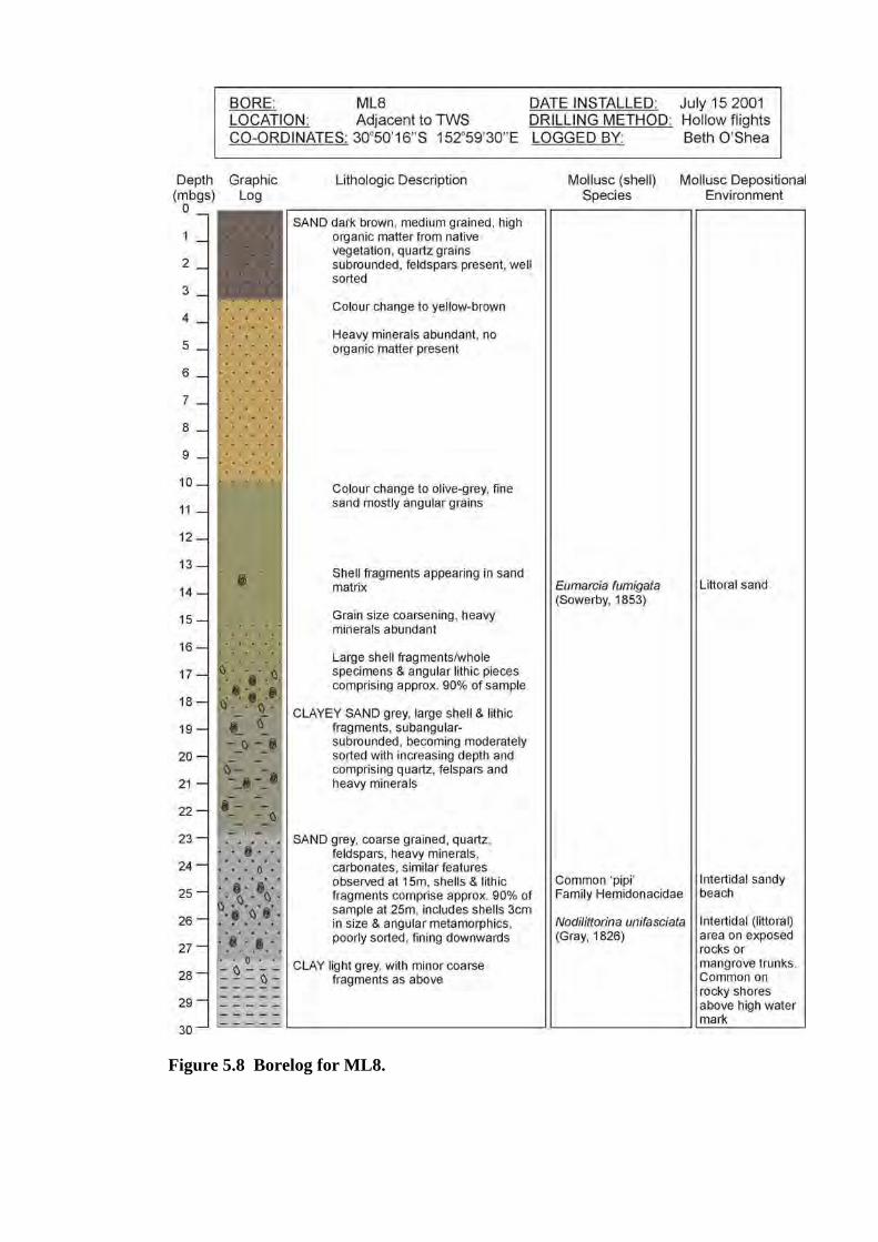
Figure 5.8 Borelog for ML8.
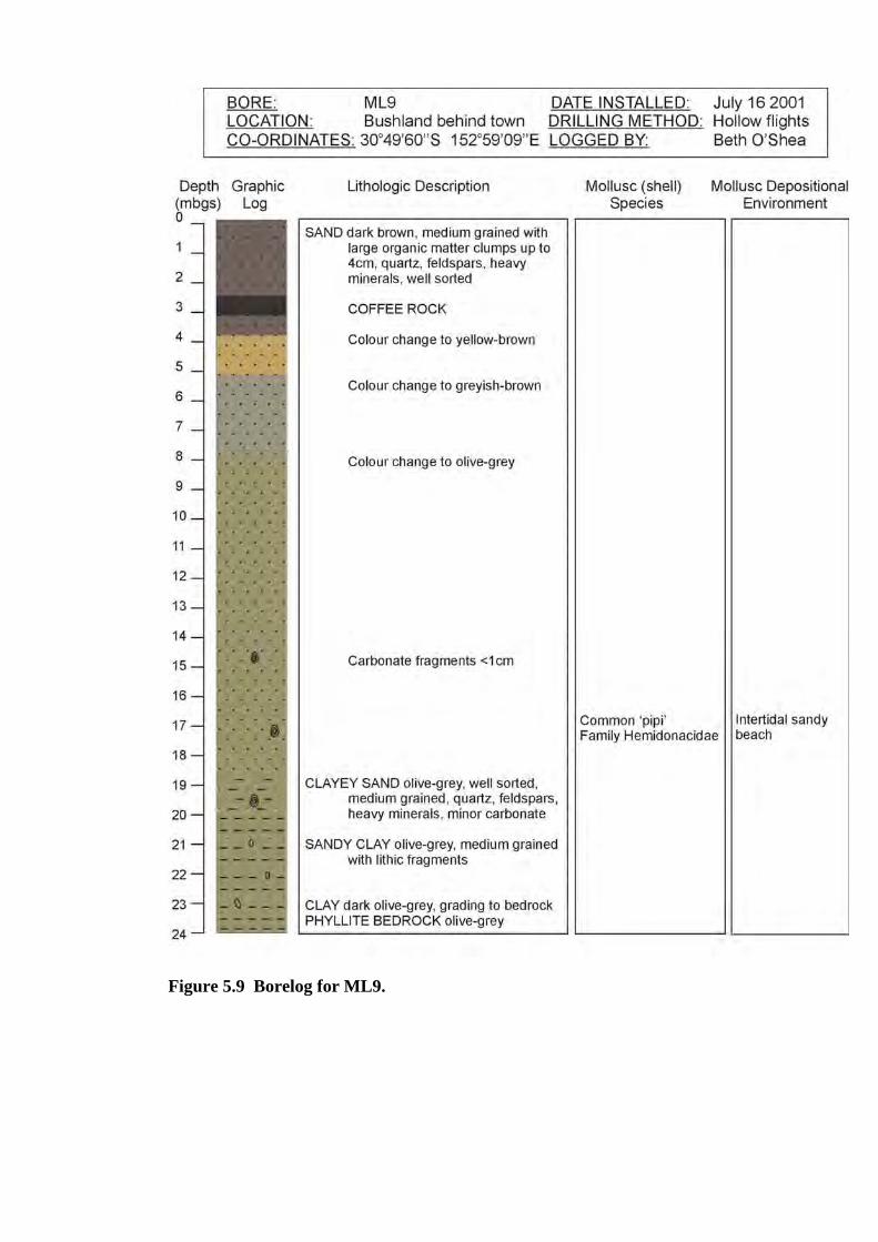
Figure 5.9 Borelog for ML9.
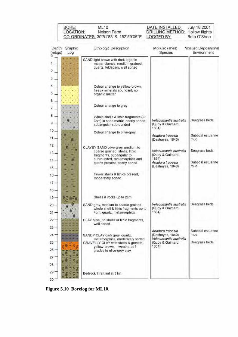
Figure 5.10 Borelog for ML10.
Chapter 5 – Original Source of Arsenic to the Aquifer
O’Shea (2006) Page 132
Various sediment facies were observed during drilling:
An organic topsoil layer consisting of natural vegetative litter or domestic lawn
seed was present at all borehole locations;
Sand was penetrated below the organic soil layer. The sand ranged in colour
from dark brown (influenced by organic matter) to yellow, through to olive grey,
with increasing depth. The shallow brown and yellow sands were generally of
uniform sorting and fine to medium grained; quartz dominant. Some indurated
‘coffee rock’ was periodically observed where old water table fluctuations have
occurred, cementing organic matter with the sand grains. Sands olive grey in
colour and present at mid-depths in the aquifer often exhibited a fining upwards
grain size pattern and sometimes contained large lithic fragments; both angular
and round in shape.
Clay material was observed at mid to deeper depths in the aquifer. Sand units
became clayey and mollusc shells are often present. Rocks and pebbles are
sometimes interspersed with clay units. Highly plastic olive grey clay units are
encountered towards the base of the aquifer. Many boreholes are terminated in
weathered bedrock resembling phyllite or shale.
5.2.2 Aquifer Depositional Conditions
5.2.2.1 Differentiating between beach sand and fluvial sand
The sands encountered in the shallow section of the aquifer exhibited homogeneity in
both grain size and colour; typical of the barrier sand system of the NSW coastline
(Hails, 1967). Sediment beneath these proposed beach barrier sands changes into
coarser, poorly sorted sediments characteristic of fluvial depositional conditions. These
sediment differences are particularly noticeable in Figure 5.10. The first 8 m of sand are
uniformly sorted and composed mainly of quartz. Below 8 m, the sands become
increasingly poorly sorted, with large lithic fragments often present. These large
fragments are often indicative of flood deposits. By observing these changes in the field,
one can hypothesise that the shallow uniform sediments were deposited under a
different energy regime than the deeper non-uniform sediments.
Chapter 5 – Original Source of Arsenic to the Aquifer
O’Shea (2006) Page 133
However, a facies change observed in the field is not considered sufficient to
differentiate between fluvial and barrier depositional conditions. Some common grain
size parameters are often used by sedimentologists to aid in the differentiation of sands
from different environments, such as dune versus river sands. An example of one such
study is presented in Friedman (1961), who studied sands from recent dune, beach and
river environments with the aim of determining if certain mineralogical or textural
characteristics were diagnostic of particular depositional environments. His findings
(relevant to this study) include:
Dune and beach sands can almost completely be differentiated by a bivariate plot of
mean grain size and the third moment (skewness).
Both dune and river sands are generally positively skewed, however dune sands
tend to be better sorted than river sands.
Likewise, beach sands tend to be better sorted than river sands.
For all the sands studied by Friedman (1961), skewness reflects the environment of
deposition and is not affected by the mineralogy of the sample.
Bivariate plots of these grain parameters can thus indicate environments of deposition,
as utilised in studies by Hails (1967) and Smith (2005). The sands collected from the
aquifer were thus separated from clay samples and subjected to grain size analysis.
Grain parameters of skewness and standard deviation (sorting) were calculated by two
methods; the full methodology is described in Chapter 4. Results of these calculations
and a comparison between the two methods can be found in Appendix B3.
A plot of moment skewness versus moment standard deviation (Figure 5.11) identified
samples derived from beach processes (generally sands present at the surface ranging to
a depth of 10 mbgs) and those sands more likely to be a product of fluvial transport
mechanisms (sands from approximately 10 to 15 mbgs and another coarser layer
existing at around 20m depth). They have been termed ‘beach’ and ‘river’ sands on the
following graph.
Those sands designated as river sands on the graph often contain pebble sized lithic
fragments within the sand matrix. These units also exhibit a fining upwards sequence,
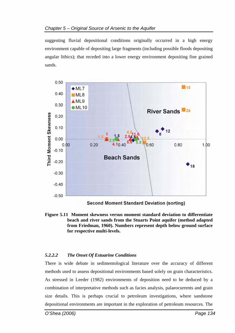
Chapter 5 – Original Source of Arsenic to the Aquifer
O’Shea (2006) Page 134
suggesting fluvial depositional conditions originally occurred in a high energy
environment capable of depositing large fragments (including possible floods depositing
angular lithics); that receded into a lower energy environment depositing fine grained
sands.
Figure 5.11 Moment skewness versus moment standard deviation to differentiate beach and river sands from the Stuarts Point aquifer (method adapted from Friedman, 1960). Numbers represent depth below ground surface for respective multi-levels.
5.2.2.2 The Onset Of Estuarine Conditions
There is wide debate in sedimentological literature over the accuracy of different
methods used to assess depositional environments based solely on grain characteristics.
As stressed in Leeder (1982) environments of deposition need to be deduced by a
combination of interpretative methods such as facies analysis, palaeocurrents and grain
size details. This is perhaps crucial to petroleum investigations, where sandstone
depositional environments are important in the exploration of petroleum resources. The
Chapter 5 – Original Source of Arsenic to the Aquifer
O’Shea (2006) Page 135
sediments of the Stuarts Point aquifer are unconsolidated and the study area is smaller
than most conventional petroleum investigations, however, a combination of
interpretative methods have been employed to satisfy any uncertainty present with the
use of a singular technique for deducing the depositional environment of the aquifer.
Thus far, analysis of the sand units has deduced that both barrier and fluvial
depositional conditions have contributed to the formation of the Stuarts Point aquifer.
The presence of clay units interbedded with sandy facies indicates an additional change.
Below the olive-grey fluvial sands (generally at an approximate depth of 18-20 m in
most boreholes) a gradual transition into a clayey sand is observed. The dual presence
of sand and clay suggests the high energy depositional environment of the fluvial and
beach sands was preceded by a lower energy depositional environment of mixed sand
and clay, and at deeper depths, solely clays. Such lower energy coastal environments
can include back-swamp lagoons, intertidal zones and estuaries. A technique was thus
sought to determine the environmental conditions that these clayey sand and
homogenous clay units had endured during deposition.
Numerous mollusc (shell) species were collected during drilling. Table 5.2 lists each
species identified herein, their location within the aquifer and their inferred habitat.
Depth ranges for mollusc occurrence within the aquifer have been provided in the table
below, however the cross sections in Figures 5.1-5.10 show the actual depths of each
identified fossil mollusc for each separate borehole.
The presence of various species at specific depths in the aquifer can suggest the likely
habitat endured by that mollusc and thus the depositional conditions occurring when the
surrounding sediments were deposited. Note that no molluscs were identified at depths
< 10 m in the aquifer; the same sands that have previously been identified as beach
barrier deposits. Therefore, the absence of mollusc species (particularly estuarine
species) in the shallow barrier sands supports the designation of shallow sediments
being deposited by onshore movement of sand in a high energy environment (i.e., beach
barrier formation).
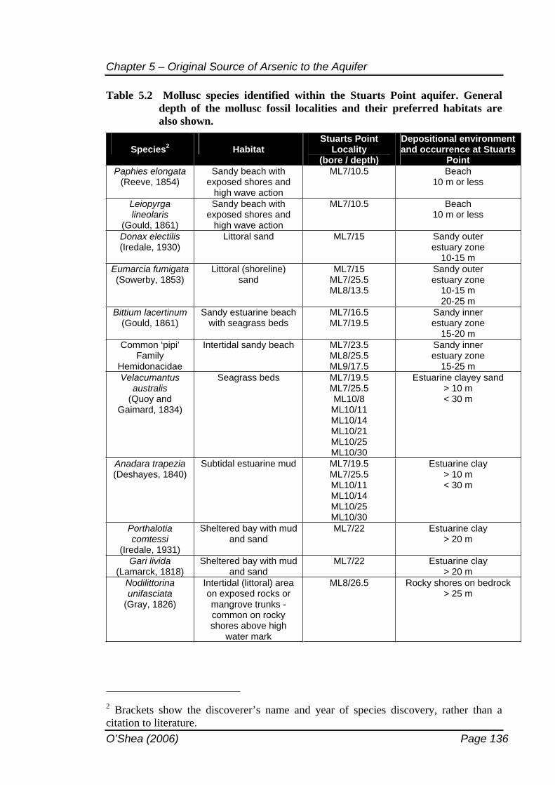
Chapter 5 – Original Source of Arsenic to the Aquifer
O’Shea (2006) Page 136
Table 5.2 Mollusc species identified within the Stuarts Point aquifer. General depth of the mollusc fossil localities and their preferred habitats are also shown.
Species2 Habitat Stuarts Point
Locality (bore / depth)
Depositional environment and occurrence at Stuarts
PointPaphies elongata
(Reeve, 1854) Sandy beach with
exposed shores and high wave action
ML7/10.5 Beach10 m or less
Leiopyrga lineolaris
(Gould, 1861)
Sandy beach with exposed shores and
high wave action
ML7/10.5 Beach 10 m or less
Donax electilis (Iredale, 1930)
Littoral sand ML7/15 Sandy outer estuary zone
10-15 m Eumarcia fumigata(Sowerby, 1853)
Littoral (shoreline) sand
ML7/15ML7/25.5ML8/13.5
Sandy outer estuary zone
10-15 m 20-25 m
Bittium lacertinum (Gould, 1861)
Sandy estuarine beach with seagrass beds
ML7/16.5ML7/19.5
Sandy inner estuary zone
15-20 m Common ‘pipi’
FamilyHemidonacidae
Intertidal sandy beach ML7/23.5 ML8/25.5ML9/17.5
Sandy inner estuary zone
15-25 m Velacumantus
australis(Quoy and
Gaimard, 1834)
Seagrass beds ML7/19.5 ML7/25.5ML10/8ML10/11ML10/14ML10/21ML10/25ML10/30
Estuarine clayey sand > 10 m< 30 m
Anadara trapezia (Deshayes, 1840)
Subtidal estuarine mud ML7/19.5 ML7/25.5ML10/11ML10/14ML10/25ML10/30
Estuarine clay > 10 m< 30 m
Porthalotiacomtessi
(Iredale, 1931)
Sheltered bay with mud and sand
ML7/22 Estuarine clay > 20 m
Gari livida (Lamarck, 1818)
Sheltered bay with mud and sand
ML7/22 Estuarine clay > 20 m
Nodilittorina unifasciata
(Gray, 1826)
Intertidal (littoral) area on exposed rocks or mangrove trunks -common on rocky shores above high
water mark
ML8/26.5 Rocky shores on bedrock > 25 m
2 Brackets show the discoverer’s name and year of species discovery, rather than a citation to literature.
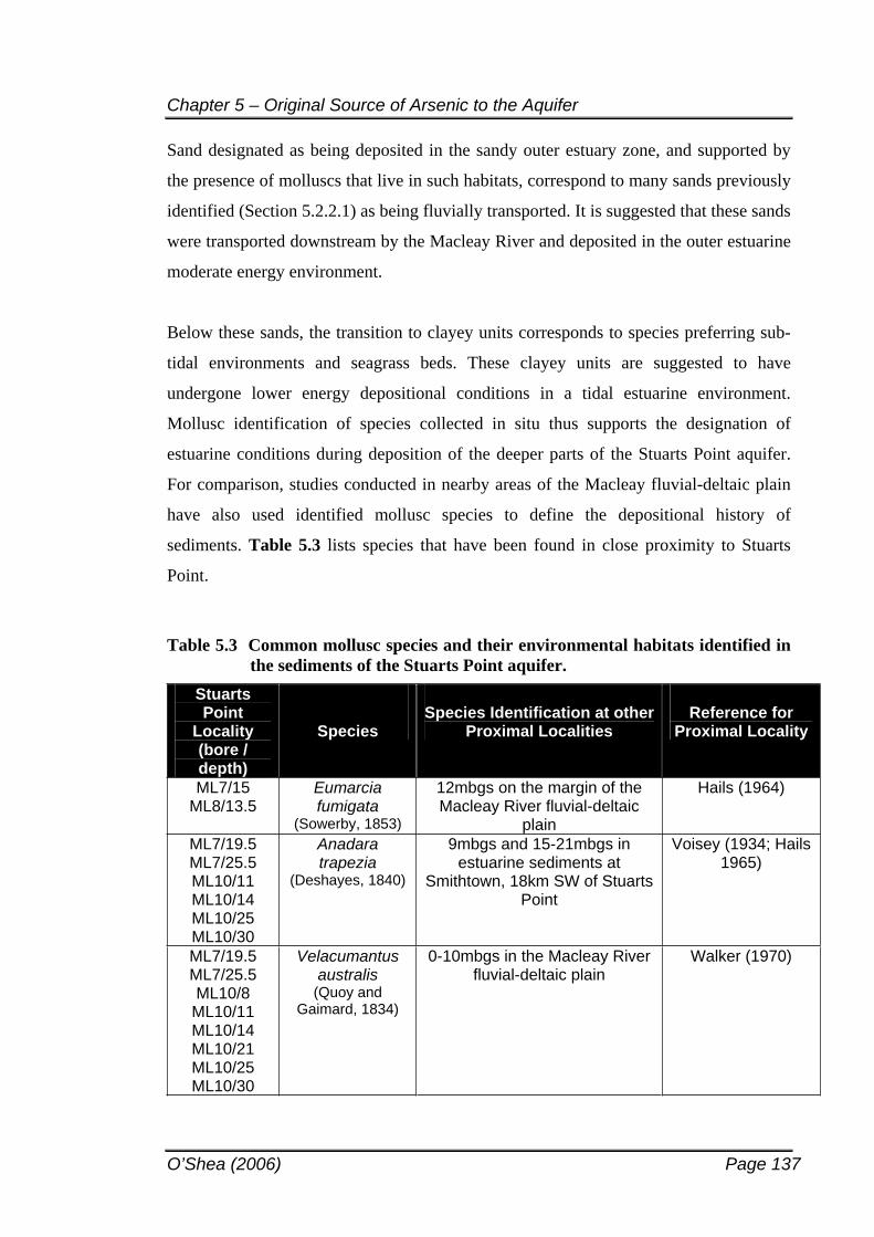
Chapter 5 – Original Source of Arsenic to the Aquifer
O’Shea (2006) Page 137
Sand designated as being deposited in the sandy outer estuary zone, and supported by
the presence of molluscs that live in such habitats, correspond to many sands previously
identified (Section 5.2.2.1) as being fluvially transported. It is suggested that these sands
were transported downstream by the Macleay River and deposited in the outer estuarine
moderate energy environment.
Below these sands, the transition to clayey units corresponds to species preferring sub-
tidal environments and seagrass beds. These clayey units are suggested to have
undergone lower energy depositional conditions in a tidal estuarine environment.
Mollusc identification of species collected in situ thus supports the designation of
estuarine conditions during deposition of the deeper parts of the Stuarts Point aquifer.
For comparison, studies conducted in nearby areas of the Macleay fluvial-deltaic plain
have also used identified mollusc species to define the depositional history of
sediments. Table 5.3 lists species that have been found in close proximity to Stuarts
Point.
Table 5.3 Common mollusc species and their environmental habitats identified in the sediments of the Stuarts Point aquifer.
StuartsPoint
Locality (bore / depth)
SpeciesSpecies Identification at other
Proximal LocalitiesReference for
Proximal Locality
ML7/15ML8/13.5
Eumarcia fumigata
(Sowerby, 1853)
12mbgs on the margin of the Macleay River fluvial-deltaic
plain
Hails (1964)
ML7/19.5ML7/25.5ML10/11ML10/14ML10/25ML10/30
Anadaratrapezia
(Deshayes, 1840)
9mbgs and 15-21mbgs in estuarine sediments at
Smithtown, 18km SW of Stuarts Point
Voisey (1934; Hails 1965)
ML7/19.5ML7/25.5ML10/8
ML10/11ML10/14ML10/21ML10/25ML10/30
Velacumantus australis
(Quoy and Gaimard, 1834)
0-10mbgs in the Macleay River fluvial-deltaic plain
Walker (1970)
Chapter 5 – Original Source of Arsenic to the Aquifer
O’Shea (2006) Page 138
For example, Walker (1970) identified a nearby estuarine unit that he termed the
Gladstone unit, which is suggested to have been deposited in the greater Stuarts Point
region as part of the Macleay fluvial-deltaic plain. Within this unit, Velacumantus
australis, a common mollusc living in seagrass beds, was used to designate the
sediments as being estuarine in origin. The same species was identified at Stuarts Point.
Clayey units within the Stuarts Point aquifer containing Velacumantus australis were
also designated as being deposited in an estuary. Further comparison to these local
studies will be made in Section 5.2.6.1 when all the evidence herein has been presented
and a new geomorphic model for the Stuarts Point aquifer has been proposed.
5.2.2.3 Weathered Bedrock
Several bores (ML1, ML6, ML9 and ML10) encountered hard rock refusal during
drilling and were terminated in suspected bedrock. ML9 encountered phyllite whereas
the remaining bores penetrated shale. The review of bedrock data presented in Chapter 2
(Section 2.3.2) shows inconsistent theories relating to the bedrock lithology at Stuarts
Point. From the compilation and review of this data, in addition to borelog analysis
presented here, bedrock for the Stuarts Point area has been deduced for this study and
shown in Figure 5.12. As with most other geological mapping investigations carried out
in this area, these boundaries are simply inferred until more accurate data is obtained.
The northern part of the aquifer is underlain by Lower Palaeozoic Nambucca (Pee Dee)
Beds consisting of slate and phyllite and intruded by the Yarrahappinni coastal
granitoid. These beds were intersected at the base of ML9, which encountered phyllite.
The overlying Kempsey Beds extend from immediately south of the Stuarts Point
township to approximately 9436-2-N EUNGAI 001 885 and consist of mudstone.
Bedrock was not encountered within this area and so lithology is proposed based on the
literature review.
South of this approximate grid reference, bores penetrated shale bedrock. There are two
main possibilities for this change in lithology. The Kempsey Area transcurrent fault
diagonally separates the mudstone of the Lower Palaeozoic Kempsey Beds from the
Upper Palaeozoic (Permian) shale of the Macleay Series; or, contact metamorphism
associated with the granitoid intrusion does not extend this far south, leaving the shale
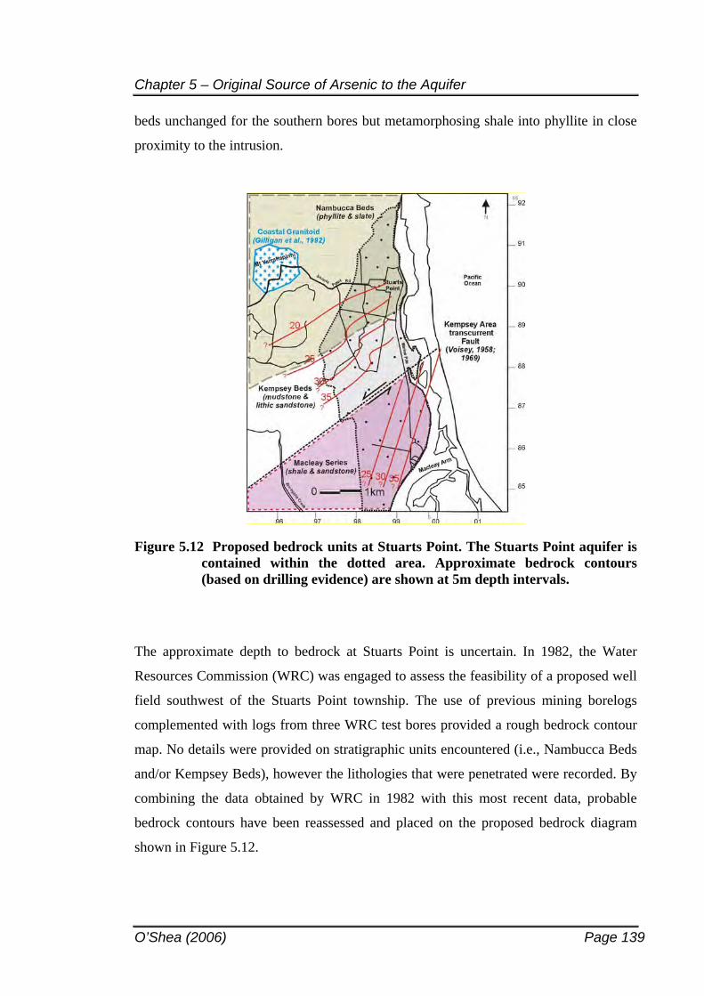
Chapter 5 – Original Source of Arsenic to the Aquifer
O’Shea (2006) Page 139
beds unchanged for the southern bores but metamorphosing shale into phyllite in close
proximity to the intrusion.
Figure 5.12 Proposed bedrock units at Stuarts Point. The Stuarts Point aquifer is contained within the dotted area. Approximate bedrock contours (based on drilling evidence) are shown at 5m depth intervals.
The approximate depth to bedrock at Stuarts Point is uncertain. In 1982, the Water
Resources Commission (WRC) was engaged to assess the feasibility of a proposed well
field southwest of the Stuarts Point township. The use of previous mining borelogs
complemented with logs from three WRC test bores provided a rough bedrock contour
map. No details were provided on stratigraphic units encountered (i.e., Nambucca Beds
and/or Kempsey Beds), however the lithologies that were penetrated were recorded. By
combining the data obtained by WRC in 1982 with this most recent data, probable
bedrock contours have been reassessed and placed on the proposed bedrock diagram
shown in Figure 5.12.
Chapter 5 – Original Source of Arsenic to the Aquifer
O’Shea (2006) Page 140
Depth to bedrock can give an indication of aquifer thickness. Bedrock refusal was first
encountered at 22 mbgs (ML9) close to Mt Yarrahappinni. It is assumed the aquifer
shallows as it progresses northward toward the mountain. The deepest bore used in this
study, ML6, encountered bedrock at 40 mbgs and is located in the southern section of
the aquifer. Anecdotal evidence suggests bores drilled in the centre of the aquifer extend
past 40 m depth before encountering bedrock.
Combined with the uncertainty of bedrock structure and lithology, the actual thickness
of the Stuarts Point aquifer is suggested to range from shallow (a few metres thick near
Mt Yarrahappinni) to deep (perhaps up to 60 m depth in the centre of the aquifer) and
moderate (30-40 m deep in the southern sections of the aquifer). Where drilling
encountered weathered bedrock and clay, no mollusc fossils or mixed sand facies were
encountered, thus differing to the estuarine-deposited clays. More than often, the
bedrock clays were the same colour as bedrock and contained fragments of weathered
rock, distinguishing them from estuarine clay deposits.
5.2.3 Aquifer (Sediment) Chemistry
A full examination of aquifer composition was conducted during the course of these
investigations. Thirty-six sediment samples from multi-levels ML7-ML10 were
analysed for total element content every 3-4 m depth by XRF. Table 5.4 shows mean
concentrations of major and trace elements in the Stuarts Point sediments. Full results
are provided in Appendix B1.
5.2.4 Aquifer Facies Definition
5.2.4.1 Statistical Procedures
Statistical analyses were conducted on sediment chemistry to ascertain if solid phase
chemistry could indicate source provenance or aquifer depositional variability. Thirty-
six sediment samples were subjected to Hierarchial Cluster Analysis (HCA), clustered
according to total element XRF compositional similarities observed between samples.
In total, 33 elements were involved in the statistical analysis. Appendix B1 lists the full
chemical data set. Two dominant clusters (Clusters 1 and 2) with sub-groups (1A and
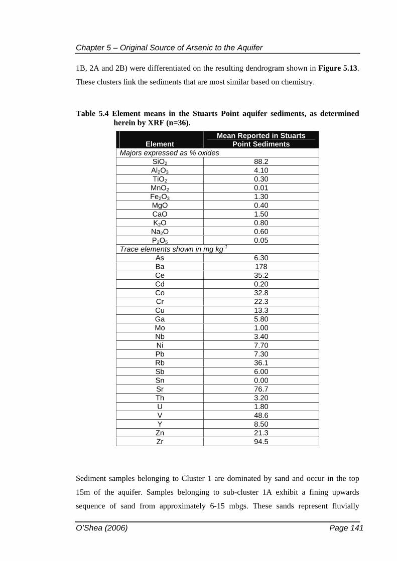
Chapter 5 – Original Source of Arsenic to the Aquifer
O’Shea (2006) Page 141
1B, 2A and 2B) were differentiated on the resulting dendrogram shown in Figure 5.13.
These clusters link the sediments that are most similar based on chemistry.
Table 5.4 Element means in the Stuarts Point aquifer sediments, as determined herein by XRF (n=36).
ElementMean Reported in Stuarts
Point Sediments Majors expressed as % oxides
SiO2 88.2 Al2O3 4.10 TiO2 0.30
MnO2 0.01 Fe2O3 1.30 MgO 0.40 CaO 1.50 K2O 0.80
Na2O 0.60 P2O5 0.05
Trace elements shown in mg kg-1
As 6.30 Ba 178 Ce 35.2 Cd 0.20 Co 32.8 Cr 22.3 Cu 13.3 Ga 5.80 Mo 1.00 Nb 3.40 Ni 7.70 Pb 7.30 Rb 36.1 Sb 6.00 Sn 0.00 Sr 76.7 Th 3.20 U 1.80 V 48.6 Y 8.50 Zn 21.3 Zr 94.5
Sediment samples belonging to Cluster 1 are dominated by sand and occur in the top
15m of the aquifer. Samples belonging to sub-cluster 1A exhibit a fining upwards
sequence of sand from approximately 6-15 mbgs. These sands represent fluvially
Chapter 5 – Original Source of Arsenic to the Aquifer
O’Shea (2006) Page 142
transported sediments and correspond with the statistically defined river sands from
Figure 5.11. Lenses of these “fluvial sands” also occur at various other depths in the
aquifer representing the ever-changing course of the Macleay River. Sands in sub-
cluster 1B are fine to medium grained homogenous sands existing from the surface to
approximately 6 mbgs. These sands have been deposited via onshore sediment supply
and correspond to the statistically defined “beach barrier deposits”.
Sediments belonging to Cluster 2 are a mix of sand, silt and clay. Sub-cluster 2A
sediments contain the highest amount of clay material and represent clays encountered
towards the base of the bore. These clays are therefore deemed to be a product of
bedrock weathering and thus are statistically grouped together based on their
mineralogical and textural composition and the weathering effects of the underlying
bedrock. Sub-cluster 2B represents sands that are influenced by both fluvial processes
but also contain some clay, thus being termed “fluvial sand/estuarine clay” sequences.
These sediments exist from 15 mbgs to the “bedrock clays” at the base of the bore.
The results of the statistical clustering show that the “fluvial sands” and “beach barrier
deposits” are closely related (Euclidean distance of 7); while the “bedrock clays” and
“fluvial sand/estuarine clay” facies are also similarly related to one another (Euclidean
distance of 7). Note that two populations exist within sub-group 2B, which effectively
separates the fluvial sands and estuarine clays of ML7 from the same proposed facies in
other bores. This is likely a product of the close proximity of ML7 to the current
estuary, thereby exposing ML7 to more recent geomorphic activity. Given that
sediment chemical composition can be largely based on grain size parameters (i.e., clays
and silts provide more surface area for element sorption than sands) it is postulated that
assignment to each cluster group may be highly influenced by chemical differences
induced by grain size characteristics, rather than being representative of their source
environment. However, the statistical analyses have successfully aided in the
differentiation of facies within the aquifer, particularly when supported by the results
presented so far, as discussed in the next section.
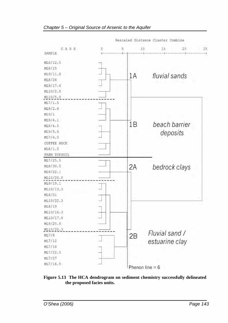
Chapter 5 – Original Source of Arsenic to the Aquifer
O’Shea (2006) Page 143
Figure 5.13 The HCA dendrogram on sediment chemistry successfully delineated the proposed facies units.
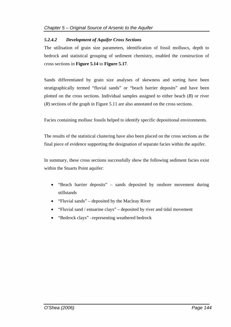
Chapter 5 – Original Source of Arsenic to the Aquifer
O’Shea (2006) Page 144
5.2.4.2 Development of Aquifer Cross Sections
The utilisation of grain size parameters, identification of fossil molluscs, depth to
bedrock and statistical grouping of sediment chemistry, enabled the construction of
cross sections in Figure 5.14 to Figure 5.17.
Sands differentiated by grain size analyses of skewness and sorting have been
stratigraphically termed “fluvial sands” or “beach barrier deposits” and have been
plotted on the cross sections. Individual samples assigned to either beach (B) or river
(R) sections of the graph in Figure 5.11 are also annotated on the cross sections.
Facies containing mollusc fossils helped to identify specific depositional environments.
The results of the statistical clustering have also been placed on the cross sections as the
final piece of evidence supporting the designation of separate facies within the aquifer.
In summary, these cross sections successfully show the following sediment facies exist
within the Stuarts Point aquifer:
“Beach barrier deposits” – sands deposited by onshore movement during
stillstands
“Fluvial sands” – deposited by the Macleay River
“Fluvial sand / estuarine clays” – deposited by river and tidal movement
“Bedrock clays” –representing weathered bedrock
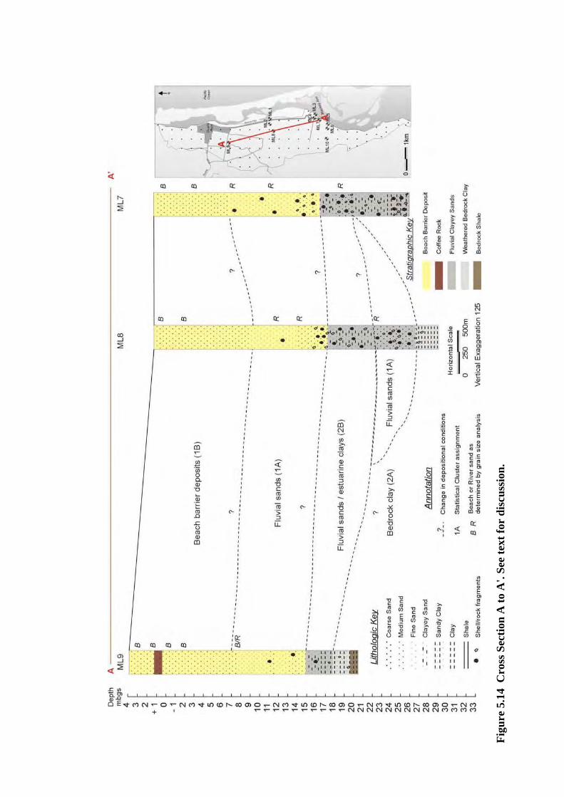
Figu
re 5
.14
Cro
ss S
ectio
n A
to A
'. Se
e te
xt fo
r di
scus
sion
.
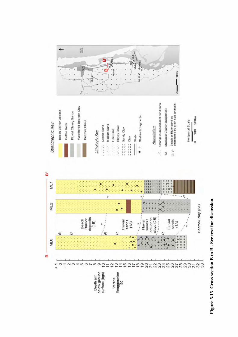
Figu
re 5
.15
Cro
ss se
ctio
n B
to B
'. Se
e te
xt fo
r di
scus
sion
.
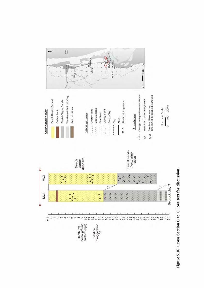
Figu
re 5
.16
Cro
ss S
ectio
n C
to C
'. Se
e te
xt fo
r di
scus
sion
.
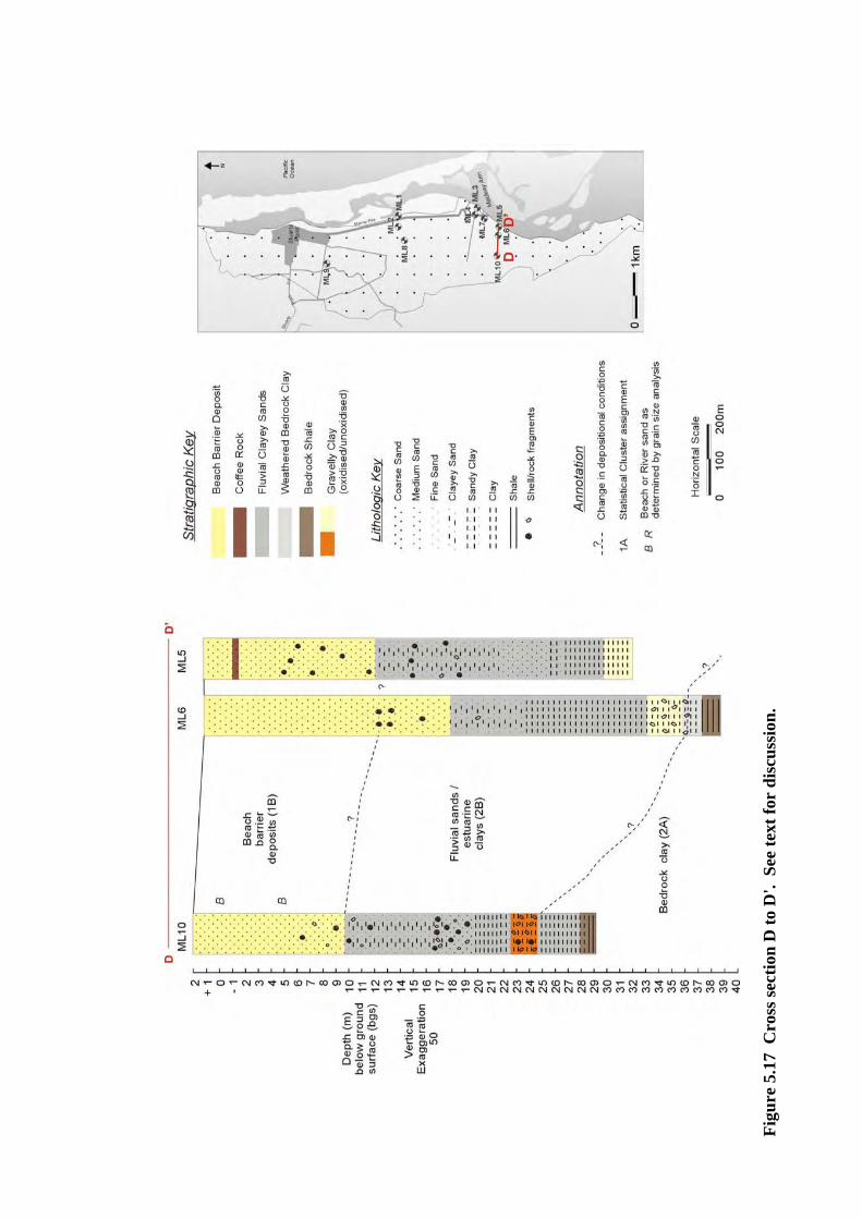
Figu
re 5
.17
Cro
ss se
ctio
n D
to D
'. S
ee te
xt fo
r di
scus
sion
.
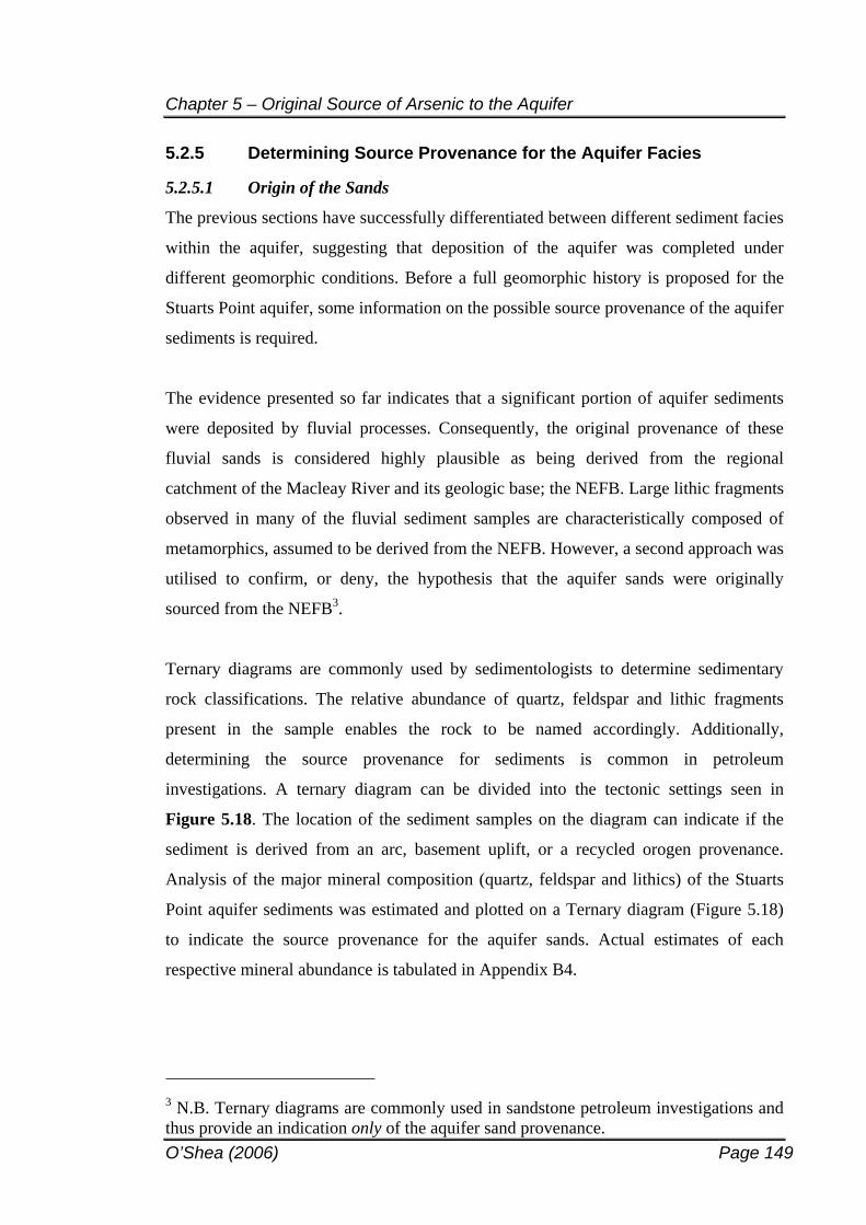
Chapter 5 – Original Source of Arsenic to the Aquifer
O’Shea (2006) Page 149
5.2.5 Determining Source Provenance for the Aquifer Facies
5.2.5.1 Origin of the Sands
The previous sections have successfully differentiated between different sediment facies
within the aquifer, suggesting that deposition of the aquifer was completed under
different geomorphic conditions. Before a full geomorphic history is proposed for the
Stuarts Point aquifer, some information on the possible source provenance of the aquifer
sediments is required.
The evidence presented so far indicates that a significant portion of aquifer sediments
were deposited by fluvial processes. Consequently, the original provenance of these
fluvial sands is considered highly plausible as being derived from the regional
catchment of the Macleay River and its geologic base; the NEFB. Large lithic fragments
observed in many of the fluvial sediment samples are characteristically composed of
metamorphics, assumed to be derived from the NEFB. However, a second approach was
utilised to confirm, or deny, the hypothesis that the aquifer sands were originally
sourced from the NEFB3.
Ternary diagrams are commonly used by sedimentologists to determine sedimentary
rock classifications. The relative abundance of quartz, feldspar and lithic fragments
present in the sample enables the rock to be named accordingly. Additionally,
determining the source provenance for sediments is common in petroleum
investigations. A ternary diagram can be divided into the tectonic settings seen in
Figure 5.18. The location of the sediment samples on the diagram can indicate if the
sediment is derived from an arc, basement uplift, or a recycled orogen provenance.
Analysis of the major mineral composition (quartz, feldspar and lithics) of the Stuarts
Point aquifer sediments was estimated and plotted on a Ternary diagram (Figure 5.18)
to indicate the source provenance for the aquifer sands. Actual estimates of each
respective mineral abundance is tabulated in Appendix B4.
3 N.B. Ternary diagrams are commonly used in sandstone petroleum investigations and thus provide an indication only of the aquifer sand provenance.
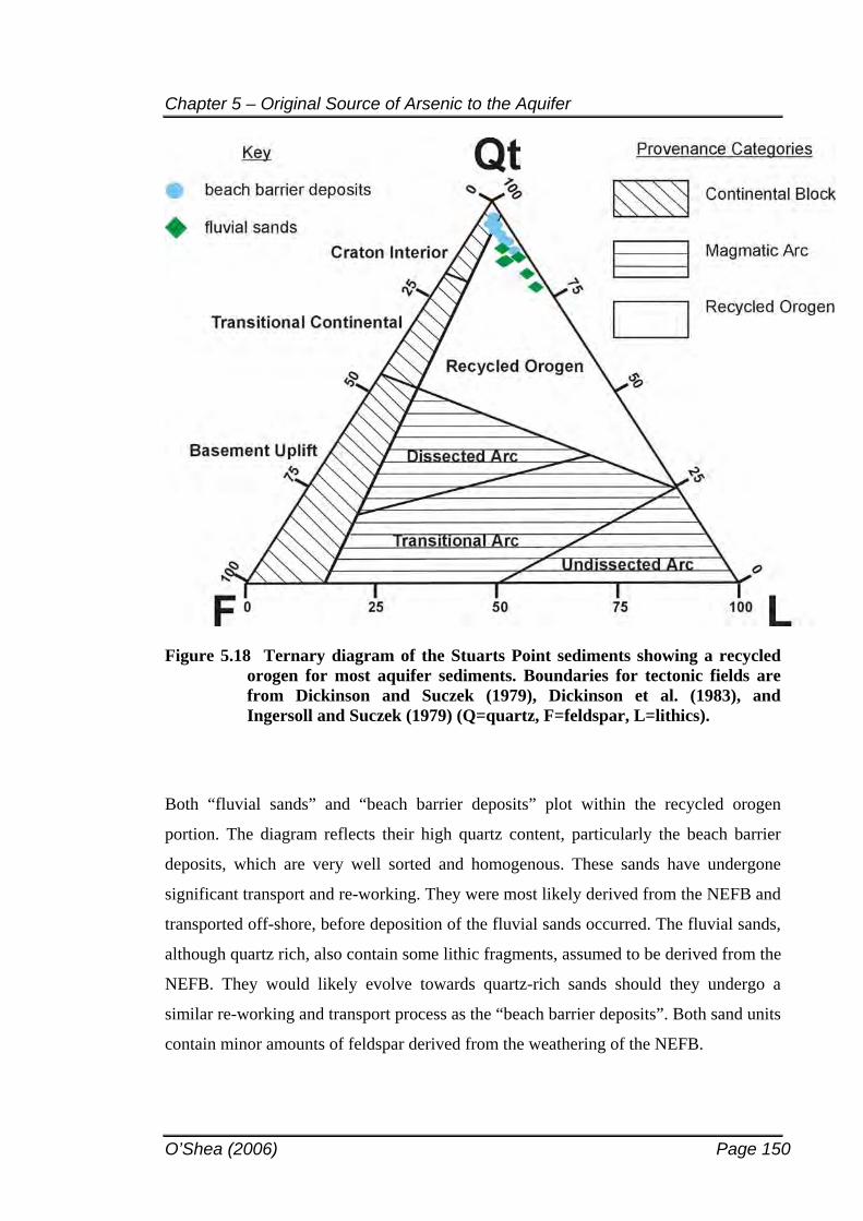
Chapter 5 – Original Source of Arsenic to the Aquifer
O’Shea (2006) Page 150
Figure 5.18 Ternary diagram of the Stuarts Point sediments showing a recycled orogen for most aquifer sediments. Boundaries for tectonic fields are from Dickinson and Suczek (1979), Dickinson et al. (1983), and Ingersoll and Suczek (1979) (Q=quartz, F=feldspar, L=lithics).
Both “fluvial sands” and “beach barrier deposits” plot within the recycled orogen
portion. The diagram reflects their high quartz content, particularly the beach barrier
deposits, which are very well sorted and homogenous. These sands have undergone
significant transport and re-working. They were most likely derived from the NEFB and
transported off-shore, before deposition of the fluvial sands occurred. The fluvial sands,
although quartz rich, also contain some lithic fragments, assumed to be derived from the
NEFB. They would likely evolve towards quartz-rich sands should they undergo a
similar re-working and transport process as the “beach barrier deposits”. Both sand units
contain minor amounts of feldspar derived from the weathering of the NEFB.
Chapter 5 – Original Source of Arsenic to the Aquifer
O’Shea (2006) Page 151
5.2.5.2 Selection of a Hinterland Indicator Element
To ascertain a better indicator of source provenance the regional mineralisation has been
examined. The aim of this section is to select an element that is abundant in the upper
reaches of the Macleay river, in addition to being capable of fluvial transport by the
river, deposition within the aquifer sediments, and being retained within the aquifer
matrix. Such an element can then act as an ‘indicator’ of a NEFB provenance for the
aquifer sediments. Trace elements associated with rare ore deposits, may act as potential
NEFB hinterland indicators.
Given its geological complexity, the NEFB contains a wide variety of mineralisation,
each type capable of contributing trace elements to the aquifer composition:
The accretionary prism sediments associated with subduction related complexes
in the mid-Palaeozoic era, carried with them syngenetic mineralisation and the
source for later epigenetic mineralisation, particularly gold and antimony veins
(Gilligan and Barnes, 1990).
After a period of intense folding and faulting, mid-Triassic granites intruded
parts of the NEFB to produce gold, molybdenum, bismuth and tungsten deposits
(Suppel, 1974) and minor elements associated with these granitic intrusions and
their contact aureoles.
Tertiary volcanism produced sapphires.
Placer deposits of tin, gold, sapphires and diamonds formed in the Tertiary and
Quaternary, with the Quaternary also producing heavy mineral sand deposits
along the eastern coastline.
A large river draining this mineralised hinterland can deposit sediment in its lower
reaches characterised by a geological signature of its prior incision pathway. The
Macleay River is the second largest river on the NSW north coast. Figure 5.19 shows
the various mineral deposits, hence potential hinterland indicators, located in the upper
Macleay River catchment.
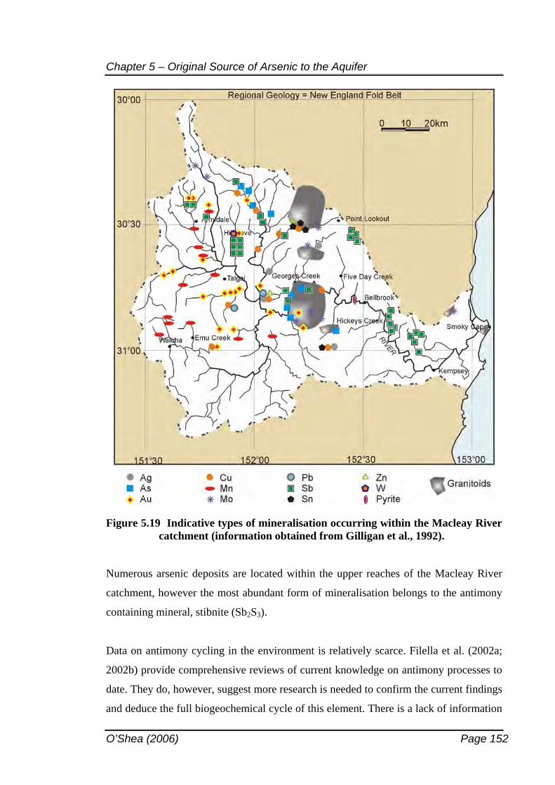
Chapter 5 – Original Source of Arsenic to the Aquifer
O’Shea (2006) Page 152
Figure 5.19 Indicative types of mineralisation occurring within the Macleay River catchment (information obtained from Gilligan et al., 1992).
Numerous arsenic deposits are located within the upper reaches of the Macleay River
catchment, however the most abundant form of mineralisation belongs to the antimony
containing mineral, stibnite (Sb2S3).
Data on antimony cycling in the environment is relatively scarce. Filella et al. (2002a;
2002b) provide comprehensive reviews of current knowledge on antimony processes to
date. They do, however, suggest more research is needed to confirm the current findings
and deduce the full biogeochemical cycle of this element. There is a lack of information
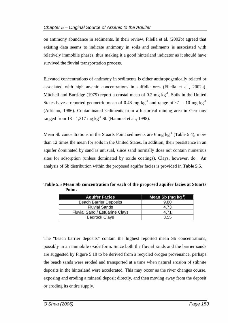
Chapter 5 – Original Source of Arsenic to the Aquifer
O’Shea (2006) Page 153
on antimony abundance in sediments. In their review, Filella et al. (2002b) agreed that
existing data seems to indicate antimony in soils and sediments is associated with
relatively immobile phases, thus making it a good hinterland indicator as it should have
survived the fluvial transportation process.
Elevated concentrations of antimony in sediments is either anthropogenically related or
associated with high arsenic concentrations in sulfidic ores (Filella et al., 2002a).
Mitchell and Burridge (1979) report a crustal mean of 0.2 mg kg-1. Soils in the United
States have a reported geometric mean of 0.48 mg kg-1 and range of <1 – 10 mg kg-1
(Adriano, 1986). Contaminated sediments from a historical mining area in Germany
ranged from 13 - 1,317 mg kg-1 Sb (Hammel et al., 1998).
Mean Sb concentrations in the Stuarts Point sediments are 6 mg kg-1 (Table 5.4), more
than 12 times the mean for soils in the United States. In addition, their persistence in an
aquifer dominated by sand is unusual, since sand normally does not contain numerous
sites for adsorption (unless dominated by oxide coatings). Clays, however, do. An
analysis of Sb distribution within the proposed aquifer facies is provided in Table 5.5.
Table 5.5 Mean Sb concentration for each of the proposed aquifer facies at Stuarts Point.
Aquifer Facies Mean Sb (mg kg-1)Beach Barrier Deposits 9.80
Fluvial Sands 4.73 Fluvial Sand / Estuarine Clays 4.71
Bedrock Clays 3.55
The “beach barrier deposits” contain the highest reported mean Sb concentrations,
possibly in an immobile oxide form. Since both the fluvial sands and the barrier sands
are suggested by Figure 5.18 to be derived from a recycled orogen provenance, perhaps
the beach sands were eroded and transported at a time when natural erosion of stibnite
deposits in the hinterland were accelerated. This may occur as the river changes course,
exposing and eroding a mineral deposit directly, and then moving away from the deposit
or eroding its entire supply.
Chapter 5 – Original Source of Arsenic to the Aquifer
O’Shea (2006) Page 154
The “fluvial sands” and “fluvial sand / estuarine clays” contain similar Sb
concentrations, showing the fluvial depositional conditions were intermittent with
estuarine conditions. The “bedrock clays” at Stuarts Point exhibit low concentrations of
Sb due to their genesis from in-situ bedrock which is unlikely to contain stibnite
deposits. In summary, the high concentrations of Sb in the aquifer sediments,
particularly fluvial sands and beach sands derived from the same provenance, suggests
that the majority of sediments in the Stuarts Point aquifer have been derived from
erosion of the NEFB mineralised hinterland.
5.2.6 Aquifer Geomorphology
Initially, the author supported the classification of the Stuarts Point sediments as a dual
barrier system, proposing the model of Roy and Thom (1981) could be applicable to
Stuarts Point (O’Shea and Jankowski, 2002). Strong evidence now suggests that the
majority of aquifer sediments have been sourced from the hinterland. The designation of
appropriate stratigraphic units in the Stuarts Point aquifer has been successful and in
addition, these units correspond with research conducted by other scientists in nearby
localities.
5.2.6.1 Linking the Stuarts Point facies to surrounding depositional environments
The Macleay River drains hilly tablelands upstream of Kempsey at which point it
broadens into a wide fluvial-deltaic flood plain termed the Lower Macleay valley. The
Stuarts Point aquifer forms part of this floodplain.
Walker (1970) examined exposed soil terraces upstream of Kempsey and linked several
terraces to buried floodplain deposits downstream, confirming the input of fluvial
sedimentation within the Lower Macleay floodplain / Stuarts Point aquifer. An analysis
of Walker’s (1970) floodplain stratigraphy provided the following comparisons to the
Stuarts Point sediments (from oldest to youngest):
The older clays found at the base of most bores and termed “bedrock clays” herein,
are comparable to Walker’s stiff sands and clays and basal clay occurring towards
the bottom of the floodplain profile. Walker (1970) could not successfully link this
unit to upstream soil terraces, and additionally, none of the bores examined in his
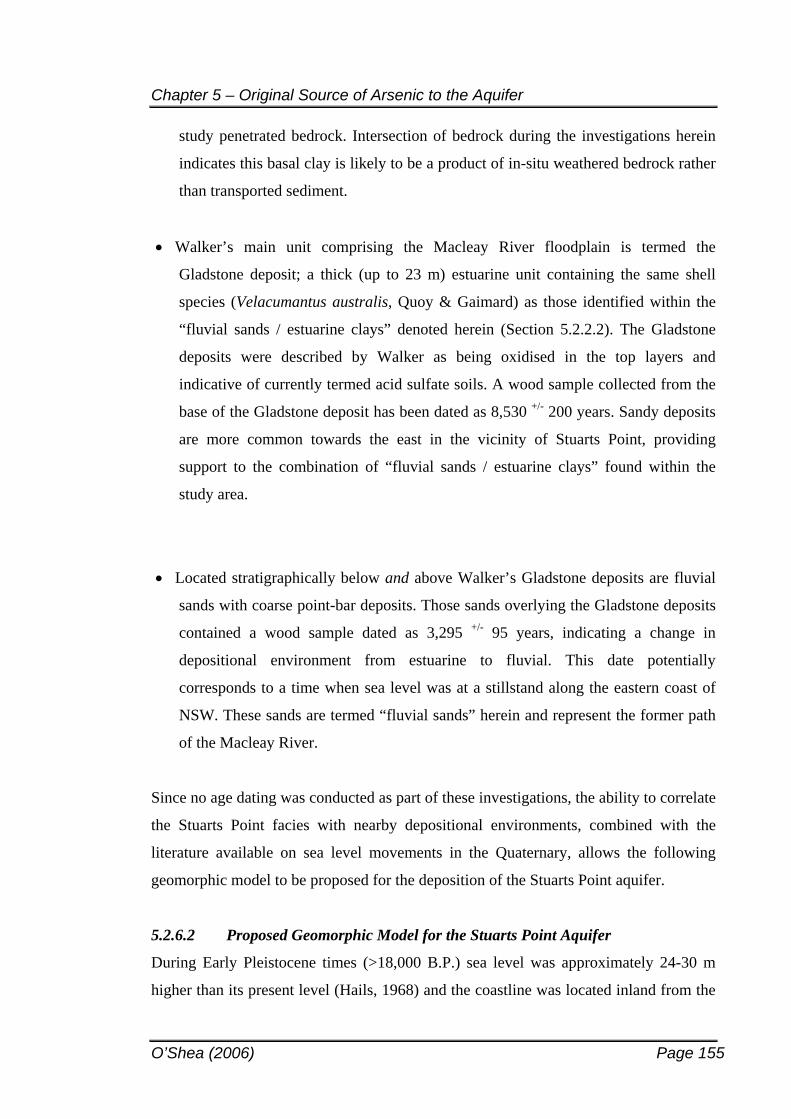
Chapter 5 – Original Source of Arsenic to the Aquifer
O’Shea (2006) Page 155
study penetrated bedrock. Intersection of bedrock during the investigations herein
indicates this basal clay is likely to be a product of in-situ weathered bedrock rather
than transported sediment.
Walker’s main unit comprising the Macleay River floodplain is termed the
Gladstone deposit; a thick (up to 23 m) estuarine unit containing the same shell
species (Velacumantus australis, Quoy & Gaimard) as those identified within the
“fluvial sands / estuarine clays” denoted herein (Section 5.2.2.2). The Gladstone
deposits were described by Walker as being oxidised in the top layers and
indicative of currently termed acid sulfate soils. A wood sample collected from the
base of the Gladstone deposit has been dated as 8,530 +/- 200 years. Sandy deposits
are more common towards the east in the vicinity of Stuarts Point, providing
support to the combination of “fluvial sands / estuarine clays” found within the
study area.
Located stratigraphically below and above Walker’s Gladstone deposits are fluvial
sands with coarse point-bar deposits. Those sands overlying the Gladstone deposits
contained a wood sample dated as 3,295 +/- 95 years, indicating a change in
depositional environment from estuarine to fluvial. This date potentially
corresponds to a time when sea level was at a stillstand along the eastern coast of
NSW. These sands are termed “fluvial sands” herein and represent the former path
of the Macleay River.
Since no age dating was conducted as part of these investigations, the ability to correlate
the Stuarts Point facies with nearby depositional environments, combined with the
literature available on sea level movements in the Quaternary, allows the following
geomorphic model to be proposed for the deposition of the Stuarts Point aquifer.
5.2.6.2 Proposed Geomorphic Model for the Stuarts Point Aquifer
During Early Pleistocene times (>18,000 B.P.) sea level was approximately 24-30 m
higher than its present level (Hails, 1968) and the coastline was located inland from the
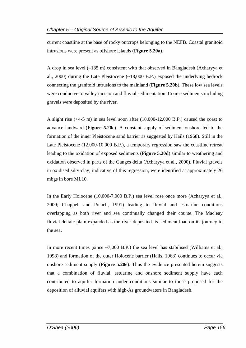
Chapter 5 – Original Source of Arsenic to the Aquifer
O’Shea (2006) Page 156
current coastline at the base of rocky outcrops belonging to the NEFB. Coastal granitoid
intrusions were present as offshore islands (Figure 5.20a).
A drop in sea level (–135 m) consistent with that observed in Bangladesh (Acharyya et
al., 2000) during the Late Pleistocene (~18,000 B.P.) exposed the underlying bedrock
connecting the granitoid intrusions to the mainland (Figure 5.20b). These low sea levels
were conducive to valley incision and fluvial sedimentation. Coarse sediments including
gravels were deposited by the river.
A slight rise (+4-5 m) in sea level soon after (18,000-12,000 B.P.) caused the coast to
advance landward (Figure 5.20c). A constant supply of sediment onshore led to the
formation of the inner Pleistocene sand barrier as suggested by Hails (1968). Still in the
Late Pleistocene (12,000-10,000 B.P.), a temporary regression saw the coastline retreat
leading to the oxidation of exposed sediments (Figure 5.20d) similar to weathering and
oxidation observed in parts of the Ganges delta (Acharyya et al., 2000). Fluvial gravels
in oxidised silty-clay, indicative of this regression, were identified at approximately 26
mbgs in bore ML10.
In the Early Holocene (10,000-7,000 B.P.) sea level rose once more (Acharyya et al.,
2000; Chappell and Polach, 1991) leading to fluvial and estuarine conditions
overlapping as both river and sea continually changed their course. The Macleay
fluvial-deltaic plain expanded as the river deposited its sediment load on its journey to
the sea.
In more recent times (since ~7,000 B.P.) the sea level has stabilised (Williams et al.,
1998) and formation of the outer Holocene barrier (Hails, 1968) continues to occur via
onshore sediment supply (Figure 5.20e). Thus the evidence presented herein suggests
that a combination of fluvial, estuarine and onshore sediment supply have each
contributed to aquifer formation under conditions similar to those proposed for the
deposition of alluvial aquifers with high-As groundwaters in Bangladesh.
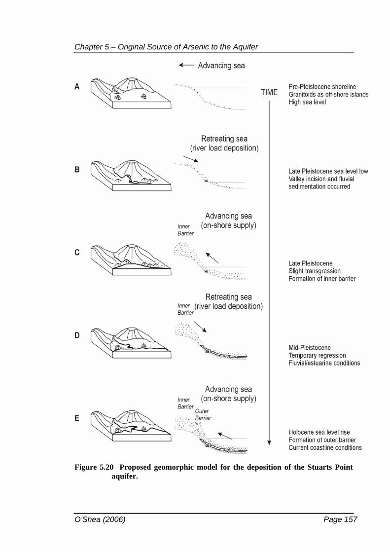
Chapter 5 – Original Source of Arsenic to the Aquifer
O’Shea (2006) Page 157
Figure 5.20 Proposed geomorphic model for the deposition of the Stuarts Point aquifer.
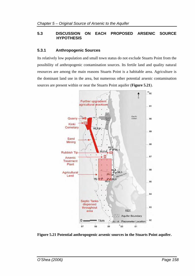
Chapter 5 – Original Source of Arsenic to the Aquifer
O’Shea (2006) Page 158
5.3 DISCUSSION ON EACH PROPOSED ARSENIC SOURCE HYPOTHESIS
5.3.1 Anthropogenic Sources
Its relatively low population and small town status do not exclude Stuarts Point from the
possibility of anthropogenic contamination sources. Its fertile land and quality natural
resources are among the main reasons Stuarts Point is a habitable area. Agriculture is
the dominant land use in the area, but numerous other potential arsenic contamination
sources are present within or near the Stuarts Point aquifer (Figure 5.21).
Figure 5.21 Potential anthropogenic arsenic sources in the Stuarts Point aquifer.
Chapter 5 – Original Source of Arsenic to the Aquifer
O’Shea (2006) Page 159
5.3.1.1 Agricultural Practices
Aldarman et al. (1984) provided a folk history of Yarrahapinni and Stuarts Point, which
is briefly drawn upon here to examine potential past arsenic contamination practices.
Early settlement industries at Stuarts Point included timber milling, sea transport and
fishing before dairy farming became common in the late 1800’s. By 1984 beef cattle
had replaced dairy farming. In 1920 the first banana plantations were established and
continue to be a dominant land use today. Other crops previously grown have included
asparagus, watermelon, corn, pumpkin and beans. Current crops include potatoes, stone
fruits, avocados and macadamias.
Both cattle and crop farming practices have the potential to provide sources of arsenic to
the environment. A common form of cattle tick eradication involved the use of arsenic
dipping solutions which were common on the NSW mid-north coast from 1895 until
replacement with DDT in 1955 (Maganov et al., 2000). Studies by Kimber et al. (2002)
of former cattle dip sites in NSW showed no signficant transport or redeposition of
arsenic had occurred at the sites studied (n=28). Sandy soils exhibited groundwater with
elevated arsenic concentrations, however, these declined sharply with increased distance
(ca. 20 m) from the dip sites studied. NSW Agriculture retains records of former cattle
dip sites located throughout the State and does not posses any documentation of such
sites being present at Stuarts Point.
Arsenical herbicides and pesticides, such as sodium arsenite, have been widely used in
the past and continue to be used around the world today. No documentation on the types
of pesticides/herbicides previously used at Stuarts Point is available, however
application is assumed to have occurred, particularly on banana plantations. Arsenic
may or may not have been an active ingredient in the pesticides/ herbicides used.
Fertilizers applied to assist crop growth can contain up to 6,200 mg kg-1 of arsenic
depending on fertilizer type (eg. micronutrient, phosphate) and manufacturer
(Woltering, 2004). An inventory of all fertilizer types used at Stuarts Point is not
available but the use of Muriate of Potash (potassium chloride) has been confirmed. In a
study investigating trace element concentrations in this type of fertilizer Robarge et al.
Chapter 5 – Original Source of Arsenic to the Aquifer
O’Shea (2006) Page 160
(2004) reported arsenic concentrations less than detection limit (0.3 mg kg-1) for all
samples analysed (n=8).
The application of fertilizers, pesticides and herbicides has the potential to be diffuse
sources of arsenic contamination within the aquifer. Some degree of traceability would
be expected in the hydrochemical data and may aid in the identification of any diffuse
arsenic sources in the aquifer. No such patterns have been identified during these
investigations.
5.3.1.2 Historical Mining
The east coast of Australia contains valuable heavy mineral sand resources (rutile,
zircon, monazite) and Stuarts Point is no exception. In the 1970’s localised mining
occurred to the southwest of the township upgradient of all multi-levels sampled for this
study. Separation processes between heavy mineral fractions and other grains is
normally based on physical separation methods, dismissing the use of any chemicals
during the mining process and reducing the production of contaminated by-products.
Sand mining occurring within the Tomago Sandbeds on the mid-NSW coast south of
Stuarts Point (Newcastle) has been tentatively linked to arsenic release into the
groundwater environment via the oxidation of arsenic-rich pyrite. In contrast to Stuarts
Point, groundwater in the Tomago Sandbeds contains elevated levels of iron indicative
of pyrite oxidation which decreases away from the mined area (Binnings et al., 2001).
No such impact is evident downgradient of the mined area at Stuarts Point.
A small unoperational (?) quarry located in a hillside cutting west of the township is
presumed to supply slate and phyllite for use in tiling and decorative construction and is
not considered to impact the quality of the groundwater.
5.3.1.3 Town (Anthropogenic) By-Products
Kinki Cemetery has been irregularly used since 1877 and has significant European
Heritage value (NSW DPWS, 1998). In a study examining inorganic soil contamination
from cemetery leachate, Spongberg and Becks (2000) found statistical differences
existed between arsenic concentrations in soils at a (different) cemetery site (1 to 20 m
from the nearest grave) compared to soils tested off the cemetery site. The elevated
Chapter 5 – Original Source of Arsenic to the Aquifer
O’Shea (2006) Page 161
arsenic concentrations – up to 8.06 mg kg-1 – were suggested to be a product of previous
embalming practices and/or coffin wood preservatives. Nearby graves dated back to the
mid-late 1800’s in an era when arsenic was commonly being used in the preservation
process. Operation of Kinki Cemetery since 1877 lends support to the possibility of
embalming fluids being a potential source of arsenic to the Stuarts Point environment.
The use of arsenic in embalming fluids was apparently stopped in 1910 (Dent, 2002).
Prior to this, the use of such embalming fluids was minor in Australia (Dent, pers.
comm., 2004).
The limited studies conducted on contaminants leaching from cemeteries (Dent, 2002;
Spongberg and Becks, 2000) indicate arsenic leaching from embalming fluids and/or
treated coffins may be localised to within the cemetery proximity, however further
information is required to confidently support these conclusions, and notably, soil and
groundwater conditions vary between cemetery sites. The potential for Kinki Cemetery
to contribute widespread arsenic contamination within the Stuarts Point aquifer is
therefore considered unlikely.
Prior to the installation of a reticulated water supply at Stuarts Point in 1985, concern
was raised over the impact of septic discharge contaminating spearpoints utilised as
domestic water supplies (NSW DPWS, 1998). In 1999 DLWC informed local residents
that uncertainty still remained over the impact of septic tanks on the local groundwater
system. A study was initiated to examine the effects of both the local rubbish tip and
septic tank systems on the groundwater environment, but to date has not been released.
Investigations conducted herein do not show any relationship between these potential
contaminant sources and arsenic distribution throughout the aquifer, thus dismissing
their probability as arsenic sources within the aquifer.
The treatment plant recently installed to remove arsenic from the town water supply is
obviously not the original source of arsenic and stringent controls are in place to contain
the arsenic rich by-products produced during the treatment process, so as to ensure
further contamination does not occur.
Chapter 5 – Original Source of Arsenic to the Aquifer
O’Shea (2006) Page 162
The NSW Environmental Protection Authority (EPA) maintains a Contaminated Sites
Register throughout NSW. The database includes all sites that have been deemed
contaminated regardless of remedial measures that may have since been implemented.
There were no listings for Stuarts Point, Mt Yarrahapinni, Clybucca or Fishermans
Reach on the Contaminated Sites Register as of late 2004.
5.3.2 A Regional geologic source?
In the absence of any notable anthropogenic arsenic source, the focus turns to natural, or
‘geogenic’ sources. Past investigations (Section 2.4) have largely based their source
hypotheses on the previously accepted geomorphic model for the aquifer. Since the
commonly accepted geomorphic model for the aquifer was based on barrier
development from onshore sediment transport (Section 2.3), the possibility of arsenic
being derived from the hinterland has not been fully examined.
Section 5.1 now proposes that a significant amount of the aquifer has, in fact, been
derived from erosion of the hinterland. The presence of elevated Sb in the aquifer
sediments, supplied from erosion of abundant stibnite deposits in the NEFB hinterland,
supports this hypothesis. Of more notable consideration is that natural stibnite deposits
can contain more than 5,000 mg kg-1 arsenic in solid solution, in addition to its common
association with arsenopyrite and arsenian pyrite (Ashley et al., 2003).
A geochemical study into the environmental mobility of Sb and As from mesothermal
stibnite deposits in a high energy stream environment undergoing accelerated natural
erosion, was conducted by Ashley et al. (2003) in the upper reaches of the Macleay
River catchment (Hillgrove – see Figure 5.19). They found that significant levels of Sb
and As had been contributed to the Macleay River system through both mining
activities and natural processes. It is noted that the Stuarts Point sediments contain up
to 14 mg kg-1 of Sb (Section 5.2.5.2; Appendix B1) and are thus considered Sb-rich.
These concentrations are comparable to As concentrations, which are also up to 14 mg
kg-1 (Chapter 6; Appendix B1) thus both elements are considered to be elevated in these
sediments. It is possible the two elements may exhibit similar properties given their
proximal locations in the periodic table, however, the relative immobile nature of Sb is
expected to override any non-geochemical relationship.
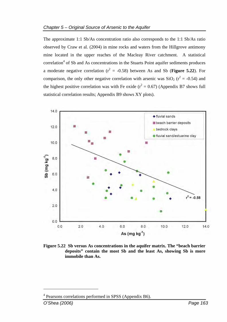
Chapter 5 – Original Source of Arsenic to the Aquifer
O’Shea (2006) Page 163
The approximate 1:1 Sb/As concentration ratio also corresponds to the 1:1 Sb/As ratio
observed by Craw et al. (2004) in mine rocks and waters from the Hillgrove antimony
mine located in the upper reaches of the Macleay River catchment. A statistical
correlation4 of Sb and As concentrations in the Stuarts Point aquifer sediments produces
a moderate negative correlation (r2 = -0.58) between As and Sb (Figure 5.22). For
comparison, the only other negative correlation with arsenic was SiO2 (r2 = -0.54) and
the highest positive correlation was with Fe oxide (r2 = 0.67) (Appendix B7 shows full
statistical correlation results; Appendix B9 shows XY plots).
Figure 5.22 Sb versus As concentrations in the aquifer matrix. The “beach barrier deposits” contain the most Sb and the least As, showing Sb is more immobile than As.
4 Pearsons correlations performed in SPSS (Appendix B6).
Chapter 5 – Original Source of Arsenic to the Aquifer
O’Shea (2006) Page 164
The predicted 1:1 ratio (observed upstream at the minesite) has potentially been altered
during erosion, transport and the subsequent onset of geochemical conditions in the
aquifer. A positive correlation of 1 could be expected if both elements behaved
conservatively during transport. Hammel et al. (1998) found that antimony in sediments
derived from geogenic sources is mostly immobile. The moderate negative correlation
indicates Sb is less mobile than As which may contribute to the onset of dissolved As
concentrations in the groundwater.
An independent and concurrent study examining Sb and As enrichment in the surface
deposits of the Macleay floodplain assumes a predominant source of both Sb and As
from upstream dispersion (Tighe et al., 2005). While their calculated Sb and As
enrichment in the top 10 cm of floodplain soil agrees well with estimates lost from
upstream mining areas (Ashley and Graham, 2000), results reported herein show this
enrichment extends to depths of more than 20 m when sediments were deposited prior
to mining activities. Discussions with these researchers (Tighe, pers. comm., 2005)
reveal that preliminary work conducted by the University of New England indicates
shallow soil Sb enrichment has most likely occurred after commencement of mining at
Hillgrove; but that Sb concentrations at depth in these floodplain deposits may be a
product of natural erosion prior to mining. These combined results indicate the natural
erosion of Sb and As has potentially been occurring for several thousand years.
It is therefore proposed that the source of arsenic within the aquifer may be of regional
geological origin, primarily stemming from the erosion of hinterland stibnite deposits.
The original mode of transport for arsenic may be as a sorbed constituent, or
alternatively, present in dissolved form. After deposition of the aquifer sediments,
antimony is retained by the solid phase whereas arsenic is prone to mobilisation. This
causes the negative correlation between the two elements. It is suggested that antimony
is retained in the sediments in an immobile oxide form, however further work is
required to confirm or deny this hypothesis.
5.3.3 Input from As-rich Holocene Sea Level Rise
Smith et al. (2006) suggested the Stuarts Point groundwater was elevated in arsenic due
to adsorption onto clays during sea level fluctuations in the late Pleistocene and
Chapter 5 – Original Source of Arsenic to the Aquifer
O’Shea (2006) Page 165
Holocene (Section 2.4). They support their theory by reference to several studies
(Acharyya et al., 2000; Khan et al., 2000; Manning and Goldberg, 1997; and Lin and
Puls, 2000).
The first two studies indicate a correlation between arsenic and Bangladeshi sediments
subjected to Holocene sea level fluctuations. It appears that Smith et al. (2006) are
suggesting that since the Stuarts Point aquifer has also endured sea level movements in
the Holocene, then the transgressing sea must be the source of arsenic in both aquifers.
Indeed, the Stuarts Point aquifer has potentially been subjected to the same eustatic
movements in sea level as the Bengal Delta Plain5.
Table 5.6 compares the two alluvial aquifers with respect to sea level change and
sediment depositional environment.
One critical difference is observed between marine transgressions occurring in
Bangladesh when compared to Stuarts Point. Khan et al. (2001a) stated;
“The major source of arsenic in the Quaternary sediments of the Bengal Delta is
inferred to have derived from arsenic-rich aqueous solution due to marine
transgression.” (pg 57)
In other publications (Khan et al., 2000; 2001b) the arsenic-rich aqueous solution is
described as seawater transgressing over volcanic ash deposits rich in arsenic, thereby
concentrating it within the transgressing seawater. As sea levels later regressed, the
arsenic was retained by iron and manganese oxyhydroxides present within the fine-
grained aquifer sediments. The critical difference is that no such arsenic-rich deposits
have been identified at Stuarts Point.
5 Hails (1968) states that while eustatic events during the Quaternary were likely to be worldwide, comparison between different hemispheres must be made with caution due to the common lack of evidence of former shorelines in some coastal regions.
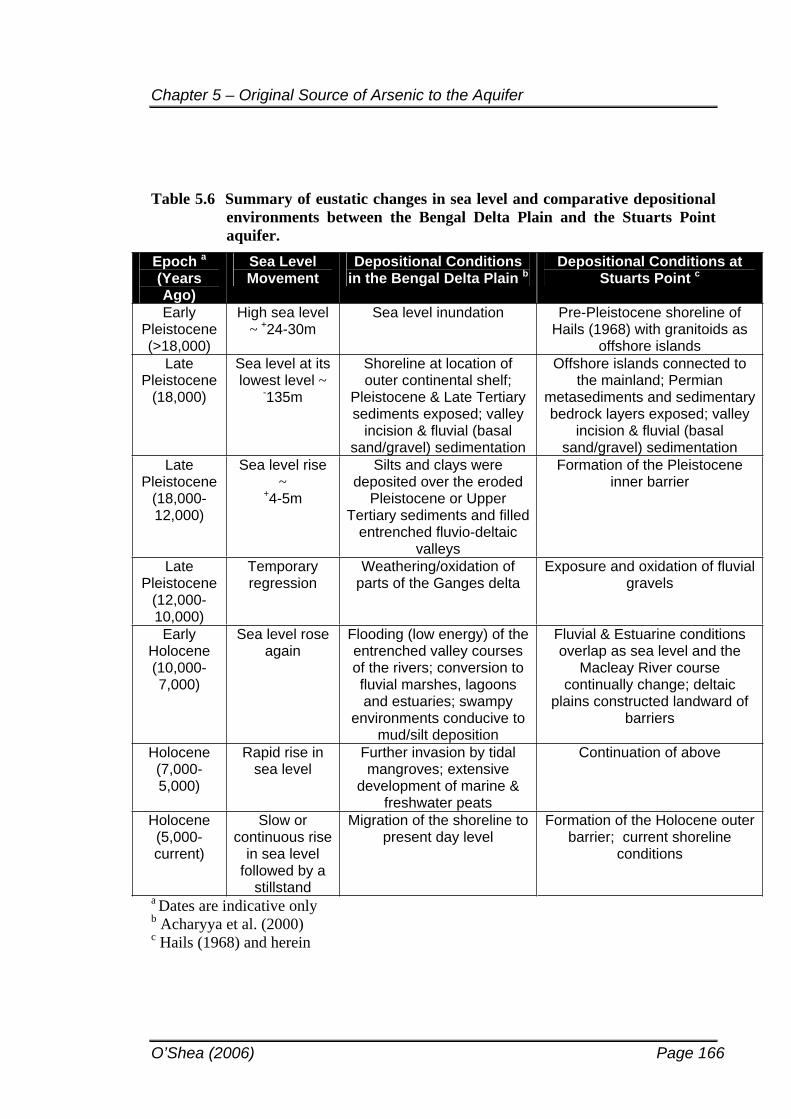
Chapter 5 – Original Source of Arsenic to the Aquifer
O’Shea (2006) Page 166
Table 5.6 Summary of eustatic changes in sea level and comparative depositional environments between the Bengal Delta Plain and the Stuarts Point aquifer.
Epoch a
(YearsAgo)
Sea Level Movement
Depositional Conditions in the Bengal Delta Plain b
Depositional Conditions at Stuarts Point c
EarlyPleistocene (>18,000)
High sea level ~ +24-30m
Sea level inundation Pre-Pleistocene shoreline of Hails (1968) with granitoids as
offshore islands Late
Pleistocene(18,000)
Sea level at its lowest level ~
-135m
Shoreline at location of outer continental shelf;
Pleistocene & Late Tertiary sediments exposed; valley
incision & fluvial (basal sand/gravel) sedimentation
Offshore islands connected to the mainland; Permian
metasediments and sedimentary bedrock layers exposed; valley
incision & fluvial (basal sand/gravel) sedimentation
LatePleistocene
(18,000-12,000)
Sea level rise ~
+4-5m
Silts and clays were deposited over the eroded
Pleistocene or Upper Tertiary sediments and filled
entrenched fluvio-deltaic valleys
Formation of the Pleistocene inner barrier
LatePleistocene
(12,000-10,000)
Temporaryregression
Weathering/oxidation of parts of the Ganges delta
Exposure and oxidation of fluvial gravels
EarlyHolocene(10,000-7,000)
Sea level rose again
Flooding (low energy) of the entrenched valley courses of the rivers; conversion to fluvial marshes, lagoons and estuaries; swampy
environments conducive to mud/silt deposition
Fluvial & Estuarine conditions overlap as sea level and the
Macleay River course continually change; deltaic
plains constructed landward of barriers
Holocene(7,000-5,000)
Rapid rise in sea level
Further invasion by tidal mangroves; extensive
development of marine & freshwater peats
Continuation of above
Holocene(5,000-current)
Slow or continuous rise
in sea level followed by a
stillstand
Migration of the shoreline to present day level
Formation of the Holocene outer barrier; current shoreline
conditions
a Dates are indicative only b Acharyya et al. (2000)c Hails (1968) and herein
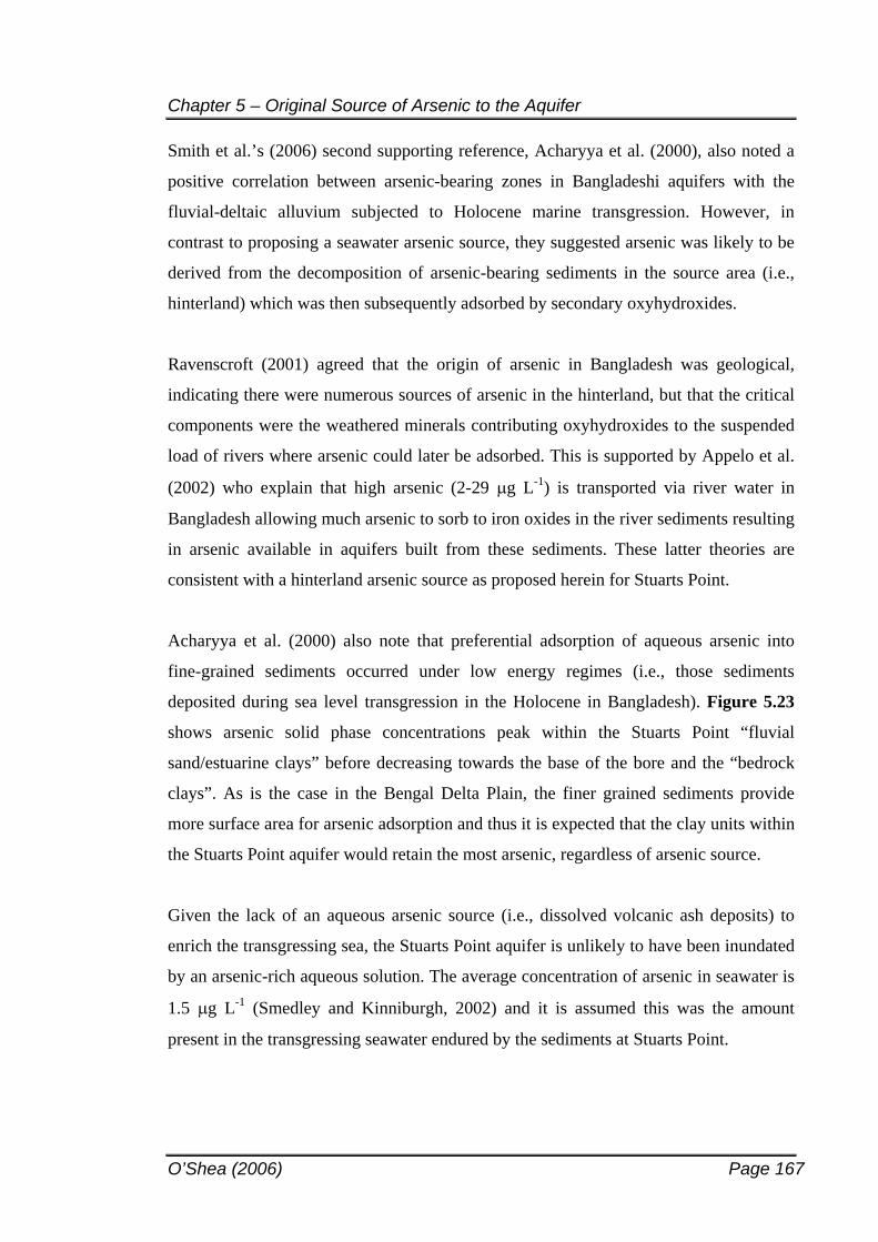
Chapter 5 – Original Source of Arsenic to the Aquifer
O’Shea (2006) Page 167
Smith et al.’s (2006) second supporting reference, Acharyya et al. (2000), also noted a
positive correlation between arsenic-bearing zones in Bangladeshi aquifers with the
fluvial-deltaic alluvium subjected to Holocene marine transgression. However, in
contrast to proposing a seawater arsenic source, they suggested arsenic was likely to be
derived from the decomposition of arsenic-bearing sediments in the source area (i.e.,
hinterland) which was then subsequently adsorbed by secondary oxyhydroxides.
Ravenscroft (2001) agreed that the origin of arsenic in Bangladesh was geological,
indicating there were numerous sources of arsenic in the hinterland, but that the critical
components were the weathered minerals contributing oxyhydroxides to the suspended
load of rivers where arsenic could later be adsorbed. This is supported by Appelo et al.
(2002) who explain that high arsenic (2-29 g L-1) is transported via river water in
Bangladesh allowing much arsenic to sorb to iron oxides in the river sediments resulting
in arsenic available in aquifers built from these sediments. These latter theories are
consistent with a hinterland arsenic source as proposed herein for Stuarts Point.
Acharyya et al. (2000) also note that preferential adsorption of aqueous arsenic into
fine-grained sediments occurred under low energy regimes (i.e., those sediments
deposited during sea level transgression in the Holocene in Bangladesh). Figure 5.23
shows arsenic solid phase concentrations peak within the Stuarts Point “fluvial
sand/estuarine clays” before decreasing towards the base of the bore and the “bedrock
clays”. As is the case in the Bengal Delta Plain, the finer grained sediments provide
more surface area for arsenic adsorption and thus it is expected that the clay units within
the Stuarts Point aquifer would retain the most arsenic, regardless of arsenic source.
Given the lack of an aqueous arsenic source (i.e., dissolved volcanic ash deposits) to
enrich the transgressing sea, the Stuarts Point aquifer is unlikely to have been inundated
by an arsenic-rich aqueous solution. The average concentration of arsenic in seawater is
1.5 g L-1 (Smedley and Kinniburgh, 2002) and it is assumed this was the amount
present in the transgressing seawater endured by the sediments at Stuarts Point.
Chapter 5 – Original Source of Arsenic to the Aquifer
O’Shea (2006) Page 168
Figure 5.23 Vertical solid phase arsenic concentrations reported herein. Arsenic peaks with “fluvial sand/estuarine clay” units due to their higher adsorption capacity.
Khan et al.’s (2001a) reason for rejection of arsenic contribution by hinterland erosion
in Bangladesh was based on the non-proportional amount of opaque minerals present
within the alluvium that indicated arsenic was not derived from parent arsenic bearing
minerals. This theory was in turn examined at Stuarts Point. Common opaque minerals
include iron oxides, sulfides and heavy minerals such as ilmenite. Oxides and sulfides
have been identified in the aquifer and are discussed further in Chapter 6. Oxides are not
excellent indicators of hinterland contribution due to exposure and formation
(oxidation) upon the lowering of sea level in the Pleistocene. Concurrently, sulfides
(e.g. pyrite) are also questionable as hinterland indicators due to possible authigenic
precipitation of pyrite after sediment deposition. Heavy minerals have previously been
mined in close proximity to the Stuarts Point study area and their genesis is attributed to
wave action during the building of coastal sand barriers, with their original source
provenance terrigenous (Roy, 1999). The immediate source of the NSW east coast
heavy mineral sands seems to be the Mesozoic sediments of the Sydney, Clarence and
Moreton Basins (Thorp and McDonald, 2001), however sands on the mid-north coast of
NSW - close to Stuarts Point – are attributed to a New England Granite source (Wallis
and Oakes, 1990). Therefore, the use of heavy opaque minerals potentially supports
hinterland derived aquifer sediments for Stuarts Point. This has further been supported
by use of the indicator element, antimony.
Chapter 5 – Original Source of Arsenic to the Aquifer
O’Shea (2006) Page 169
The latter two studies cited by Smith et al. (2006) examine the experimental aspects of
arsenic adsorption onto clays, confirming clay ability to sequester arsenic, rather than
the potential for arsenic origination from transgressing seawater. As is demonstrated by
the arsenic concentration peaks in the “fluvial sand/estuarine clay” unit (Figure 5.23),
fine-grained sediments possess higher surface areas for elemental adsorption and
therefore this accounts for the increased arsenic concentrations in these units when
compared to the “fluvial sands” and “beach barrier deposits”. It is important to note that
arsenic concentrations peak in the (mixed) clayey sand units as opposed to the high
plasticity estuarine clays containing little or no sand content. This demonstrates the
importance of fluvially derived sediments correlating with the highest arsenic
concentrations and therefore supports the contribution of arsenic from erosion of the
hinterland.
Based on these findings, it seems prudent to dismiss the feasibility of arsenic within the
Stuarts Point aquifer being derived from the past inundation of the aquifer sediments by
seawater.
5.3.4 A note on arsenic and acid sulfate soils / pyrite
The source of arsenic deduced from preliminary studies by Smith et al. (2003; 2006)
was also proposed as being derived from ASS material. The literature review outlined
the common association of arsenic with pyrite via substitution mechanisms (Section
3.4.3.1), and as such, ASS material containing pyrite may be a potential source of
arsenic to the Stuarts Point groundwater system. Within the sandy aquifer investigated
herein, no distinct ASS formations were identified, however, adjacent clayey deposits in
the wetland show visible signs (surface scalds) of ASS formation and exposure. If
arsenic is sourced solely from theses ASS horizons, the distribution would be governed
by the presence of ASS. No such correlation has been observed herein.
The terminology describing the association of arsenic and pyrite can have double
meaning. If ASS horizons are disturbed and release arsenic into the groundwater
system, then pyrite can be considered as an arsenic source. If arsenic is present in the
groundwater system during in-situ precipitation of pyrite, then it may be considered a
current arsenic sink. Distinguishing between the two processes may not be possible.
Chapter 5 – Original Source of Arsenic to the Aquifer
O’Shea (2006) Page 170
Discrete, micron sized, clusters of pyrite were observed in the aquifer matrix (Chapter
6). For the purpose of this investigation, arsenian pyrite is identified as a current arsenic
sink. This will be supported and discussed further in subsequent chapters.
5.3.5 Direct Bedrock Contribution
Groundwater discharge from consolidated bedrock into the overlying alluvial aquifer
has the potential to transport dissolved arsenic into the Stuarts Point sandy aquifer.
Bedrock lithology and groundwater flow dynamics thus become an important part of the
arsenic source determination process.
Section 2.3.2 identified arsenic as a probable trace element associated with mineralised
bedrock. Drilling for these investigations encountered metamorphosed sediments in
close proximity to the granitoid intrusion of Mt Yarrahappinni (ML9; Figure 5.9). It is
thus hypothesised that in the northern portion of the aquifer, metamorphosed bedrock
directly below the sand aquifer, may contribute localised arsenic to the system. In order
to explore this hypothesis as a potential arsenic source, a hydraulic link needs to be
identified between the bedrock and the unconsolidated aquifer. Since very little physical
hydrogeology is known regarding groundwater movement in the aquifer, chemical
methods of investigation need to be utilised to establish any connection between
bedrock and unconsolidated sediments.
Recognised mineral deposits most likely to affect groundwater chemistry are the
molybdenum deposits and associated outward zoning of metal sulfides discussed in
Chapter 2. Bore ML9, which penetrated phyllite bedrock of the Nambucca (Pee Dee)
Beds exhibits a localised increase in both arsenic and molybdenum with increasing
depth in the aquifer (Figure 5.24).
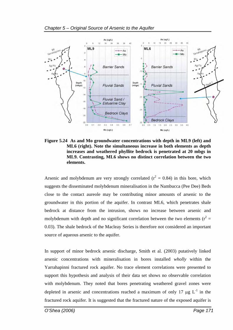
Chapter 5 – Original Source of Arsenic to the Aquifer
O’Shea (2006) Page 171
Figure 5.24 As and Mo groundwater concentrations with depth in ML9 (left) and ML6 (right). Note the simultaneous increase in both elements as depth increases and weathered phyllite bedrock is penetrated at 20 mbgs in ML9. Contrasting, ML6 shows no distinct correlation between the two elements.
Arsenic and molybdenum are very strongly correlated (r2 = 0.84) in this bore, which
suggests the disseminated molybdenum mineralisation in the Nambucca (Pee Dee) Beds
close to the contact aureole may be contributing minor amounts of arsenic to the
groundwater in this portion of the aquifer. In contrast ML6, which penetrates shale
bedrock at distance from the intrusion, shows no increase between arsenic and
molybdenum with depth and no significant correlation between the two elements (r2 =
0.03). The shale bedrock of the Macleay Series is therefore not considered an important
source of aqueous arsenic to the aquifer.
In support of minor bedrock arsenic discharge, Smith et al. (2003) putatively linked
arsenic concentrations with mineralisation in bores installed wholly within the
Yarrahapinni fractured rock aquifer. No trace element correlations were presented to
support this hypothesis and analysis of their data set shows no observable correlation
with molybdenum. They noted that bores penetrating weathered gravel zones were
depleted in arsenic and concentrations reached a maximum of only 17 g L-1 in the
fractured rock aquifer. It is suggested that the fractured nature of the exposed aquifer is
Chapter 5 – Original Source of Arsenic to the Aquifer
O’Shea (2006) Page 172
conducive to geochemical reactions promoting arsenic mobilisation and therefore
dissolved arsenic contribution to the sandy aquifer through bedrock fractures is
expected to be minimal.
Given the fractured nature of the bedrock, however, it is possible that discharge of
bedrock groundwater into the sandy aquifer may occur through such structures. The
presence of a fault could allow groundwater to act as a conduit and discharge arsenic
rich water into the aquifer above. This theory would suggest the original source of
arsenic is in an aqueous form. Uncertainty regarding the presence and location of the
Kempsey Fault (Section 2.3.2) means potential groundwater discharge through this zone
cannot be specifically addressed. The aqueous groundwater data shows no indication of
groundwater mixing at depth in the locations sampled during this study.
The potentially localised arsenic bedrock source in the northern portion of the aquifer
(underlain by the Nambucca [Pee Dee] Beds) is not considered to be a dominating
origin of arsenic in the aquifer, given the widespread occurrence of arsenic in the
aquifer. Additionally, there is no reliable isotopic evidence (Section 2.3.3) to support
groundwater discharge from the bedrock, it is only hypothetically assumed.
5.4 A COMPARISON TO ARSENIC SOURCES IN OTHER NATURALLY ELEVATED ARSENIC ENVIRONMENTS
The reconstruction of the aquifer’s depositional history suggests the dominance of a
regionally derived arsenic source via the weathering and re-deposition of mineralised
deposits from the Macleay River hinterland. Several other studies (excluding
Bangladesh) have deduced arsenic from a hinterland source. Yu et al. (2000) conducted
a combined geochemical, mineralogical and sedimentological investigation to determine
the source and distribution of arsenic along the coastline of southwestern Taiwan. The
depositional environment of the arsenic contaminated aquifer is almost identical with
the geomorphic development at Stuarts Point; rivers deposited load resulting in the
formation of an advancing alluvial plain with lagoonal and barrier environments and the
current coastline processes observed today (Figure 5.25). Slate was determined to be
the source rock for the arsenic, originating in the Central Mountain range of Taiwan and
Chapter 5 – Original Source of Arsenic to the Aquifer
O’Shea (2006) Page 173
transported via two rivers (Hsilou Chi in the north and Kauping Chi in the south) and
deposited to the study area by long-shore currents.
Figure has been removed due to Copyright Agreements
Figure 5.25 Development of an arsenic affected aquifer in Taiwan. Slate debris, deposited via fluvial and long-shore processes, is the source of the arsenic (Yu et al., 2000).
A less common occurrence of arsenic in groundwater has been investigated in a
sandstone drinking water aquifer in Bavaria (Heinrichs and Udluft, 1999). The Keuper
Sandstone aquifer is characterised by shallow marine basin facies (estuarine, deltaic)
and terrestrial facies (fluvial) divided by a 20 km transitional zone between these two
facies types. Arsenic concentrations in groundwater were notably higher in the
terrestrial facies – up to 120 g L-1 - as compared to groundwaters from marine facies
which ranged from only < 1-4 g L-1 As. Similar patterns were observed with As
concentrations in the aquifer rock material. Terrestrial facies deposited under fluvial-
marine environments were deduced as source rocks for the arsenic in comparison to
marine beds that contain no arsenic. The degree of arsenic contamination within the
Keuper Sandstone aquifer is directly related to the distribution of these two facies.
Chapter 5 – Original Source of Arsenic to the Aquifer
O’Shea (2006) Page 174
5.5 CHAPTER SUMMARY
Examination of both anthropogenic and geogenic sources of arsenic to the Stuarts Point
aquifer has yielded five major arsenic source possibilities:
1. Arsenic derived from one or more anthropogenic activities;
2. Arsenic contributed via fluvial erosion of the NEFB hinterland and subsequent
deposition;
3. Arsenic captured and retained by aquifer sediments during past changes in sea level;
4. The oxidation and release of arsenian pyrite present in ASS material; and/or
5. Aqueous arsenic contributed via upwards vertical bedrock / fault conduit discharge.
The absence of distinct contaminant plumes emanating from potential anthropogenic
sources dismisses the dominance of a human-induced arsenic source. However, diffuse
application of fertilizers and/or pesticides may have contributed to minor amounts of
arsenic in the aquifer. The review conducted herein proposes a predominantly geogenic
source of arsenic in the aquifer, with strong support for a regionally derived arsenic
source via erosion of the mineralised hinterland and subsequent deposition of these
sediments to form the current aquifer sediments. The use of Sb as a hinterland indicator
element supports the designation of a regionally derived arsenic source for the Stuarts
Point aquifer. In addition, localised discharge of groundwater from arsenic-mineralised
bedrock may occur in the northern portion of the aquifer. The contribution of arsenic
from past sea level transgressions is considered unlikely as the dominant source of
arsenic at Stuarts Point.
Table 5.7 provides evidence both for, and against, each potential arsenic source at
Stuarts Point.
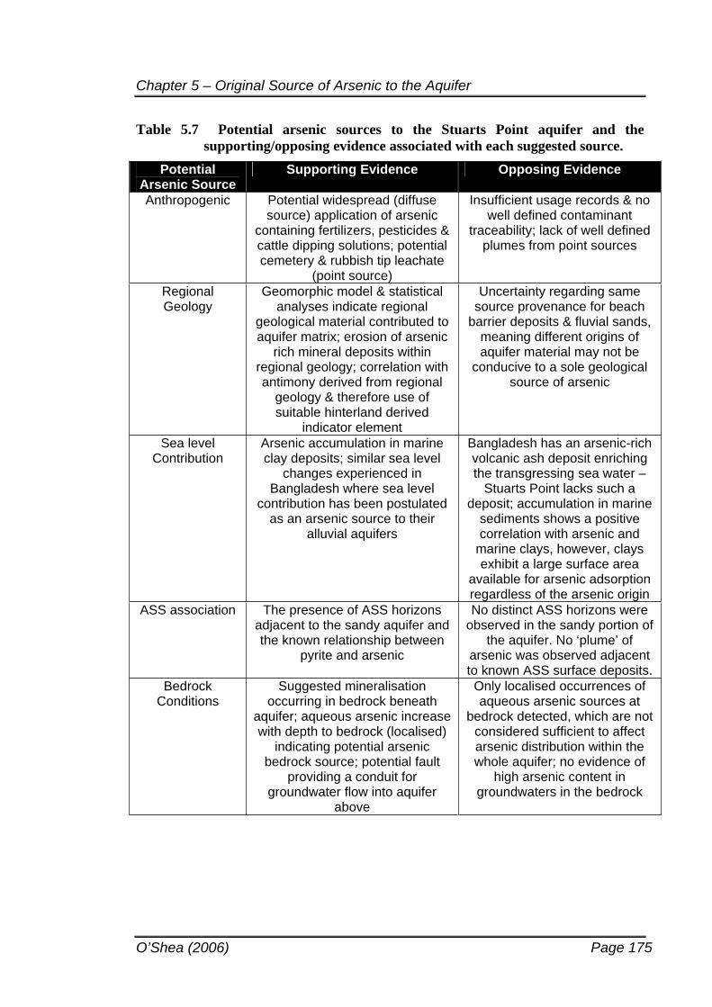
Chapter 5 – Original Source of Arsenic to the Aquifer
O’Shea (2006) Page 175
Table 5.7 Potential arsenic sources to the Stuarts Point aquifer and the supporting/opposing evidence associated with each suggested source.
PotentialArsenic Source
Supporting Evidence Opposing Evidence
Anthropogenic Potential widespread (diffuse source) application of arsenic
containing fertilizers, pesticides & cattle dipping solutions; potential cemetery & rubbish tip leachate
(point source)
Insufficient usage records & no well defined contaminant
traceability; lack of well defined plumes from point sources
RegionalGeology
Geomorphic model & statistical analyses indicate regional
geological material contributed to aquifer matrix; erosion of arsenic
rich mineral deposits within regional geology; correlation with antimony derived from regional
geology & therefore use of suitable hinterland derived
indicator element
Uncertainty regarding same source provenance for beach
barrier deposits & fluvial sands, meaning different origins of aquifer material may not be
conducive to a sole geological source of arsenic
Sea level Contribution
Arsenic accumulation in marine clay deposits; similar sea level
changes experienced in Bangladesh where sea level
contribution has been postulated as an arsenic source to their
alluvial aquifers
Bangladesh has an arsenic-rich volcanic ash deposit enriching the transgressing sea water –
Stuarts Point lacks such a deposit; accumulation in marine
sediments shows a positive correlation with arsenic and
marine clays, however, clays exhibit a large surface area
available for arsenic adsorption regardless of the arsenic origin
ASS association The presence of ASS horizons adjacent to the sandy aquifer and the known relationship between
pyrite and arsenic
No distinct ASS horizons were observed in the sandy portion of
the aquifer. No ‘plume’ of arsenic was observed adjacent to known ASS surface deposits.
BedrockConditions
Suggested mineralisation occurring in bedrock beneath
aquifer; aqueous arsenic increase with depth to bedrock (localised)
indicating potential arsenic bedrock source; potential fault
providing a conduit for groundwater flow into aquifer
above
Only localised occurrences of aqueous arsenic sources at
bedrock detected, which are not considered sufficient to affect arsenic distribution within the whole aquifer; no evidence of
high arsenic content in groundwaters in the bedrock
O’Shea (2006) Page 164
6 IDENTIFICATION OF CURRENT ARSENIC SINKS
The aquifer matrix was investigated in Chapter 5 to determine the likely source of
arsenic. This chapter explores the matrix in more detail, focussing on where the arsenic
is currently ‘being held’ in the aquifer (i.e., current arsenic sinks). Geochemically,
arsenic is influenced by many parameters (e.g. redox potential, pH, composition of the
surrounding solution) frequently making it mobile under natural aquifer conditions and
sensitive to slight changes in the geochemical environment. An understanding of the
chemical forms of solid phase arsenic present in the aquifer is critical to determining its
potential for transport in the groundwater system.
The chapter is structured as follows:
Section 6.1 builds on the sediment descriptions provided in Section 5.2 by
examining the aquifer mineralogy at the micron scale;
Section 6.2 deals with the sediment chemistry, particularly the occurrence of
arsenic, and any relationships observable between arsenic and other elements in
the matrix;
Section 6.3 examines the likely sinks of arsenic present in the aquifer, as
detailed in the literature review of Chapter 3. The following potential sinks are
examined:
o Adsorption to oxyhydroxides
o Association with pyrite
o Incorporation into clay minerals
o Sorption on organic matter
o Association with calcite
o Anion competition
For clarity and flow of discussion, results and interpretation are included in each
respective section.
Chapter 6 – Identification of Current Arsenic Sinks
O’Shea (2006) Page 165
6.1 AQUIFER MINERALOGY AND PHYSICAL PROPERTIES
The aquifer has been established as an unconsolidated deposit dominated by sand and
clay (Section 5.2). In summary, medium to coarse grained sand dominates the upper
part of the aquifer above fine sands of fluvial origin, estuarine clays and in-situ
weathered bedrock. Quartz dominates over minor feldspar and lithics. Gravel sized
fragments of lithic material (metamorphic in origin, sometimes up to 3cm in length) and
carbonates (often up to 80% in shell lenses) are sporadic throughout the aquifer and
representative of changes in depositional conditions. The sands form the main water-
bearing zone of the aquifer and are readily recharged by precipitation. Zones of water
table fluctuation are conducive to impregnation of organic material and form a
discontinuous lens of coffee rock (indurated sand) capable of reducing infiltration and
leading to the development of localised perched water tables.
Detailed analysis of the sediment matrix was undertaken on a Hitachi S4500 Field
Emission Scanning Electron Microscope (SEM) fitted with an ISIS Energy Dispersive
x-ray Spectrometer (EDS). Atomic ratios are semi-quantitative and normalised to 100%.
The full electron microprobe methodology is outlined in Chapter 4. Of the 36 collected
sediments, samples were divided into the geomorphic facies developed in Section 5.2.
After several samples from each facies had been examined under the SEM, a
photomicrograph of typical sediment grains observed within each facies was selected
and is shown in Figure 6.1.
The ‘beach barrier sand” unit has previously been visually identified as quartz rich
(Section 5.2). Individual grains semi-quantitatively analysed by the SEM are composed
of silica and oxygen, with a normalised Si/O ratio of 0.5 indicative of quartz (Figure
6.1a). No other elements were detected despite the irregular morphology observed on
the grain surface. These irregularities are thought to represent amorphous quartz
overgrowth structures.
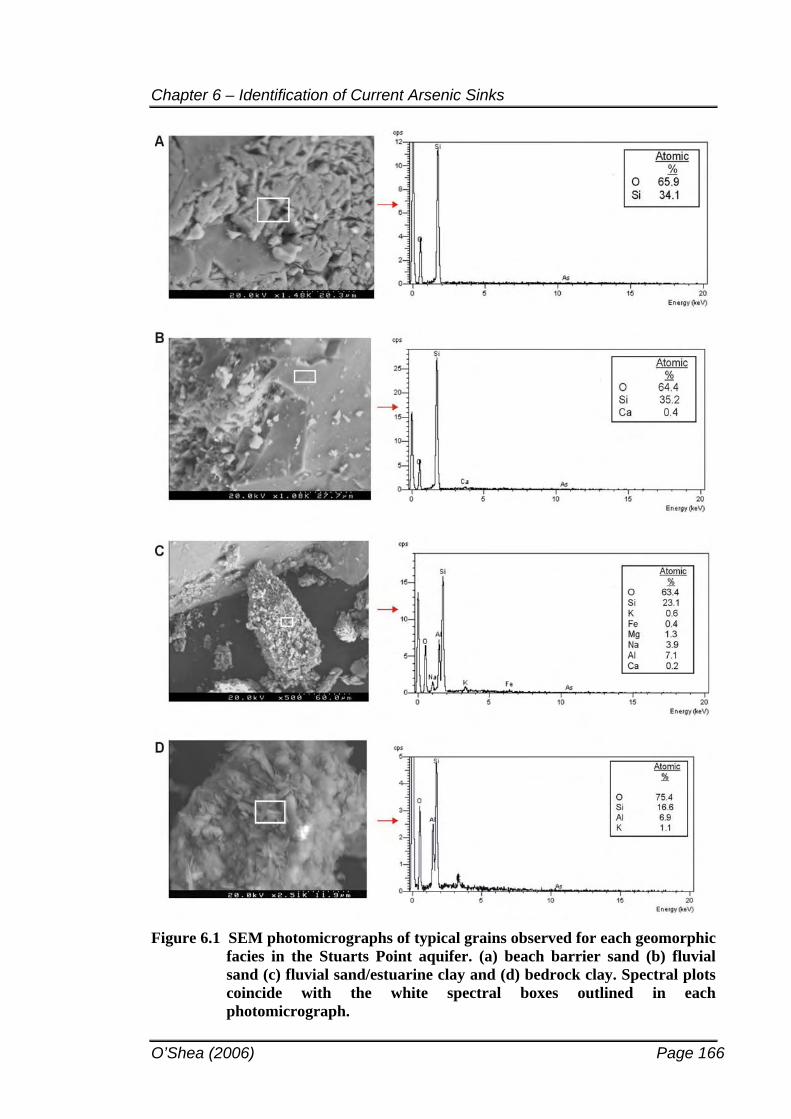
Chapter 6 – Identification of Current Arsenic Sinks
O’Shea (2006) Page 166
Figure 6.1 SEM photomicrographs of typical grains observed for each geomorphic facies in the Stuarts Point aquifer. (a) beach barrier sand (b) fluvial sand (c) fluvial sand/estuarine clay and (d) bedrock clay. Spectral plots coincide with the white spectral boxes outlined in each photomicrograph.
Chapter 6 – Identification of Current Arsenic Sinks
O’Shea (2006) Page 167
The “fluvial sand” sample is an olive-grey medium-fine grained sand (Section 5.2),
composed of quartz with a small proportion of calcium most likely due to the presence
of shell material within this unit (Figure 6.1b). The presence of shell material (i.e.,
molluscs) within a fluvial unit is not unusual given the proximity of the aquifer to the
coast and the transitional nature of the aquifer within a small scale (i.e., on a metre
scale). Some overlapping of beach and fluvial sands is probable. Additionally, some
Australian molluscs (e.g. Alathyria jacksoni) live in freshwater. The small white
aggregates bound to the surface of the grain were also composed of quartz with minor
calcium.
The underlying “fluvial sand / estuarine clay” unit is finer grained, with particles
varying from approximately 10-300 m in the clayey sand (as observed under SEM).
This decrease in particle size has an influence on its major composition (Figure 6.1c).
Quartz is suspected to remain dominant, however a reduction in the Si/O ratio to 0.36
and the presence of other elements (K, Al, Mg, Na, Fe, Ca) indicates the potential
presence of clay minerals and oxides.
The heterogenous mix of mineral grains such as quartz, which is visible under standard
laboratory microscopes, with a variety of potential clay minerals and oxides, does not
allow identification of any specific minerals via atomic ratios reported by the SEM.
Surface structures can be seen on the larger particles even at a high magnification of
x100 in these sediments. Their semi-quantitative analysis indicates a similar
composition to the surface of the grain.
High levels of O and Si in conjunction with Al and K indicate the presence of a clay
mineral in the bedrock clay unit (Figure 6.1d). The atomic ratios for Si/O (0.2) and K/Al
(0.2) are close to illite composition. Bulk arsenic concentrations were below detection
limit for the SEM. The location of the arsenic peak is shown to indicate its absence.
6.2 HOW MUCH ARSENIC IS IN THE AQUIFER MATRIX ?
Arsenic-rich groundwaters are not frequently associated with arsenic-rich host matrices.
It is common for arsenic concentrations in sediments to be in the range of normal crustal
Chapter 6 – Identification of Current Arsenic Sinks
O’Shea (2006) Page 168
abundance; 1-20 mg kg-1 As. Such is the case for Stuarts Point. Arsenic concentrations
in the aquifer matrix range from 1.4 to 14.0 mg kg-1 with a mean concentration of 6.3
mg kg-1 (n = 36).
Similar concentrations have been observed in Bangladeshi sediments where arsenic
concentrations were reported to range from 0.4 to 10.3 mg kg-1 (n = 21) for three
spatially distant districts (BGS and DPHE, 2001). This relationship between low solid
phase arsenic and high aqueous arsenic concentrations was noted by Smedley and
Kinniburgh (2002) who suggested it appeared to be the rule rather than the exception
and may be a characteristic responsible for previously delaying the identification of high
arsenic groundwaters in many regions.
The use of mean elemental concentrations in a heterogeneous aquifer, however, can bias
interpretation. Clays can sequester considerably higher concentrations of trace elements
when compared to the values reported for sandstones. This variation can be expected
between the different geomorphic facies in the Stuarts Point aquifer.
To determine element anomalies for the various geomorphic facies identified at Stuarts
Point, sediment enrichment factors (EF’s) were calculated. Comparison of sediment
element concentrations to similar sedimentary environments can indicate possible
enrichment of specific metals and trace elements relative to their sediment lithology. A
common method of assessing this phenomenon is via the calculation of EF’s.
Table 6.1 lists the 22 trace elements analysed herein and their reported means in the
Stuarts Point aquifer sediments. Background mean element concentrations for various
rock and sediment types have been provided for indicative comparison. These
background concentrations highlight potential element anomalies in the Stuarts Point
sediments, as compared to natural element concentrations for various aquifer matrices.
For instance, mean Sb concentrations at Stuarts Point are 6 mg kg-1 while all other
average values are reported at or below 1.5 mg kg-1.
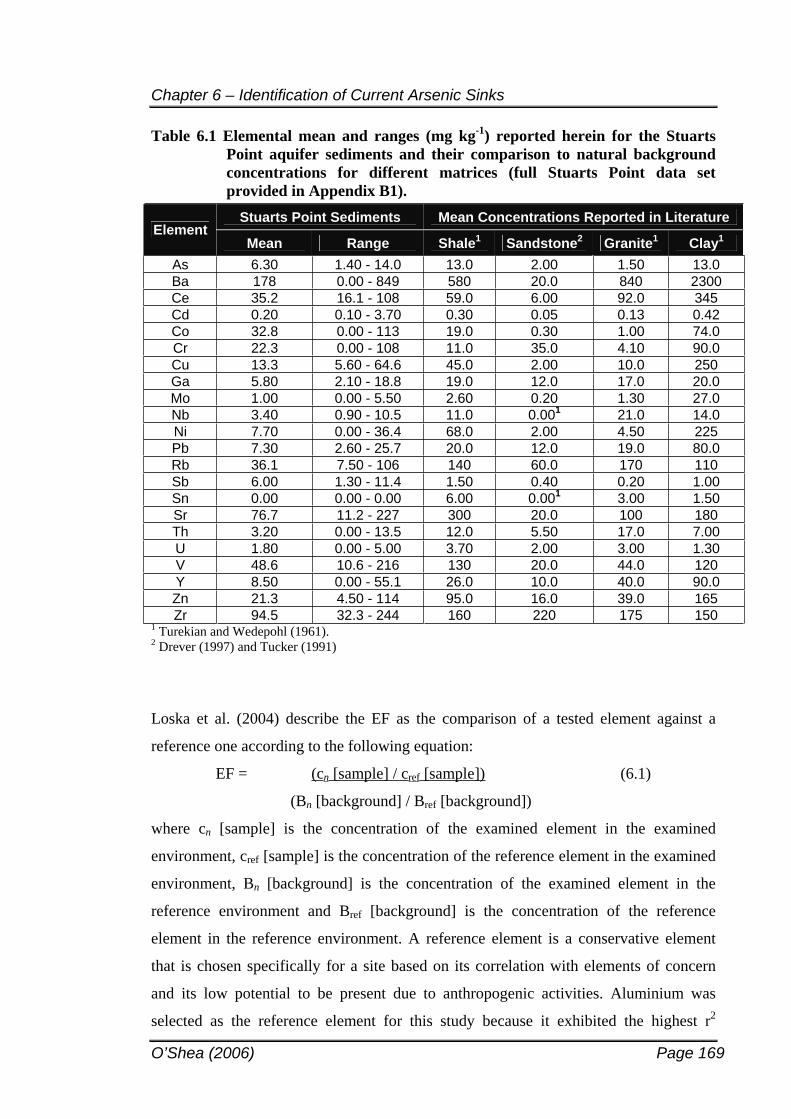
Chapter 6 – Identification of Current Arsenic Sinks
O’Shea (2006) Page 169
Table 6.1 Elemental mean and ranges (mg kg-1) reported herein for the Stuarts Point aquifer sediments and their comparison to natural background concentrations for different matrices (full Stuarts Point data set provided in Appendix B1).
Stuarts Point Sediments Mean Concentrations Reported in Literature Element
Mean Range Shale1 Sandstone2 Granite1 Clay1
As 6.30 1.40 - 14.0 13.0 2.00 1.50 13.0Ba 178 0.00 - 849 580 20.0 840 2300Ce 35.2 16.1 - 108 59.0 6.00 92.0 345Cd 0.20 0.10 - 3.70 0.30 0.05 0.13 0.42Co 32.8 0.00 - 113 19.0 0.30 1.00 74.0Cr 22.3 0.00 - 108 11.0 35.0 4.10 90.0Cu 13.3 5.60 - 64.6 45.0 2.00 10.0 250Ga 5.80 2.10 - 18.8 19.0 12.0 17.0 20.0Mo 1.00 0.00 - 5.50 2.60 0.20 1.30 27.0Nb 3.40 0.90 - 10.5 11.0 0.001 21.0 14.0Ni 7.70 0.00 - 36.4 68.0 2.00 4.50 225Pb 7.30 2.60 - 25.7 20.0 12.0 19.0 80.0Rb 36.1 7.50 - 106 140 60.0 170 110Sb 6.00 1.30 - 11.4 1.50 0.40 0.20 1.00Sn 0.00 0.00 - 0.00 6.00 0.001 3.00 1.50Sr 76.7 11.2 - 227 300 20.0 100 180Th 3.20 0.00 - 13.5 12.0 5.50 17.0 7.00U 1.80 0.00 - 5.00 3.70 2.00 3.00 1.30V 48.6 10.6 - 216 130 20.0 44.0 120Y 8.50 0.00 - 55.1 26.0 10.0 40.0 90.0Zn 21.3 4.50 - 114 95.0 16.0 39.0 165Zr 94.5 32.3 - 244 160 220 175 150
1 Turekian and Wedepohl (1961). 2 Drever (1997) and Tucker (1991)
Loska et al. (2004) describe the EF as the comparison of a tested element against a
reference one according to the following equation:
EF = (cn [sample] / cref [sample]) (6.1)
(Bn [background] / Bref [background])
where cn [sample] is the concentration of the examined element in the examined
environment, cref [sample] is the concentration of the reference element in the examined
environment, Bn [background] is the concentration of the examined element in the
reference environment and Bref [background] is the concentration of the reference
element in the reference environment. A reference element is a conservative element
that is chosen specifically for a site based on its correlation with elements of concern
and its low potential to be present due to anthropogenic activities. Aluminium was
selected as the reference element for this study because it exhibited the highest r2
Chapter 6 – Identification of Current Arsenic Sinks
O’Shea (2006) Page 170
correlation with the majority of trace elements (Appendix B7). Similarly, Liaghati et al.
(2003) chose aluminium as the reference element for a coastal plain catchment in
nearby Queensland, Australia. For comparison of this environment to the Stuarts Point
coastal environment it is advantageous if the reference element is the same.
Of particular interest to the Stuarts Point study, is the proposed derivation of aquifer
sediments from regionally eroded geology abundant with various types of
mineralisation. To ascertain whether the Stuarts Point sediments are unusually elevated
in some trace elements, comparison to a similar coastal or geomorphological unit is
required. EF’s were thus calculated using mean elemental concentrations of average
sandstones (for the “beach barrier sands” and “fluvial sands”), mean elemental
concentrations of average clays (for the “bedrock clays”) and mean concentrations of
pre-industrial estuarine sediments reported for a coastal environment in Queensland
(Preda and Cox, 2002) for the “fluvial sand / estuarine clays” at Stuarts Point (Table
6.2).
The comparison to Queensland estuarine clays is particularly important. One of the
initial arsenic source theories proposed by previous investigators (Smith, 2006; Section
2.4) is that arsenic is contained within the Stuarts Point aquifer due to inundation of the
aquifer by sea level rise in the Quaternary. If this source theory is correct, then the entire
east coast of Australia (which was subjected to the same sea level movements) may be
at risk of elevated arsenic. Additionally, the first paragraph of this thesis (Section 1.1)
explains that the discovery of arsenic in an aquifer south of Stuarts Point may lead to
concern for arsenic to be present in other coastal sand aquifers of eastern Australia. It
was these results that led to the inception of this project. Therefore, Queensland
provides an excellent example of a background environment, given its coastal location
and the same sea level movements as endured at Stuarts Point.
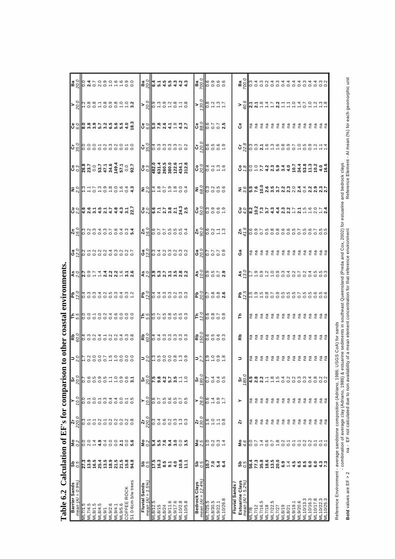
Bar
rier
San
dsS
bM
oZr
YS
rU
Rb
ThP
bA
sG
aZn
Cu
Ni
Co
Cr
Ce
VB
am
ean
(Al =
0.9
%)
0.5
0.2
220.
010
.020
.02.
060
.05.
512
.02.
012
.016
.02.
02.
00.
335
.06.
020
.020
.0M
L7/1
.527
.30.
00.
30.
00.
71.
70.
40.
00.
42.
70.
20.
34.
61.
326
.80.
08.
01.
20.
0M
L7/4
.513
.92.
00.
10.
10.
60.
20.
30.
00.
30.
90.
10.
22.
61.
123
.70.
03.
80.
82.
4M
L8/1
.516
.51.
40.
10.
00.
50.
00.
20.
10.
31.
70.
20.
33.
10.
70.
00.
03.
90.
80.
7M
L8/4
.525
.44.
90.
20.
10.
90.
00.
40.
00.
41.
40.
20.
44.
51.
353
.70.
15.
71.
12.
0M
L9/1
13.5
0.4
0.1
0.3
0.5
0.7
0.1
0.2
0.2
2.4
0.2
0.3
2.1
0.9
47.1
0.2
3.2
0.8
0.9
ML9
/2.6
18.9
0.0
0.2
0.4
1.1
1.5
0.2
0.4
0.5
2.2
0.4
0.7
4.7
1.8
34.6
0.3
6.5
0.9
1.0
ML9
/4.1
21.5
0.0
0.2
0.4
1.0
1.0
0.2
0.6
0.3
2.2
0.3
0.6
4.8
0.0
149.
40.
25.
60.
81.
6M
L9/5
.621
.52.
10.
20.
00.
90.
00.
40.
00.
41.
60.
20.
44.
31.
657
.10.
05.
51.
01.
6C
OFF
EE
RO
CK
15.8
0.0
0.2
0.1
0.6
0.0
0.3
0.0
0.3
3.1
0.2
0.3
3.1
0.4
0.0
0.1
4.0
1.0
0.9
S1
0-6c
m b
/w tr
ees
94.8
5.6
0.8
0.5
3.1
0.0
0.8
0.0
1.2
2.6
0.7
5.4
22.7
4.3
92.7
0.0
18.3
3.2
0.0
Fluv
ial S
ands
Sb
Mo
ZrY
Sr
UR
bTh
Pb
As
Ga
ZnC
uN
iC
oC
rC
eV
Ba
mea
n (A
l = 1
.5%
)0.
50.
222
0.0
10.0
20.0
2.0
60.0
5.5
12.0
2.0
12.0
16.0
2.0
2.0
0.3
35.0
6.0
20.0
20.0
ML8
/12.
517
.55.
40.
30.
67.
51.
30.
40.
50.
43.
90.
30.
66.
61.
448
2.0
0.4
5.0
0.9
6.4
ML8
/15
16.3
5.5
0.4
0.7
9.8
0.5
0.4
0.7
0.4
5.3
0.4
0.7
7.1
1.8
631.
40.
37.
81.
35.
1M
L8/2
48.
57.
60.
60.
54.
20.
00.
30.
50.
32.
70.
20.
72.
70.
726
0.5
0.3
2.6
0.9
4.5
ML9
/11.
69.
19.
40.
20.
65.
70.
00.
30.
80.
33.
10.
30.
53.
81.
938
0.0
0.3
4.1
1.2
5.5
ML9
/17.
64.
03.
00.
30.
53.
50.
80.
30.
50.
23.
50.
20.
52.
11.
812
2.6
0.3
1.8
0.8
4.3
ML1
0/2.
810
.80.
01.
30.
71.
11.
30.
30.
50.
32.
80.
30.
524
.30.
043
4.1
0.7
4.3
1.1
4.2
ML1
0/5.
811
.13.
50.
30.
51.
00.
90.
30.
30.
32.
20.
20.
42.
50.
431
2.8
0.2
2.7
0.8
4.3
Bed
rock
Cla
ysS
bM
oZr
YS
rU
Rb
ThP
bA
sG
aZn
Cu
Ni
Co
Cr
Ce
VB
am
ean
(Al =
12.
4%)
0.5
2.5
130.
028
.018
0.0
2.7
150.
012
.020
.010
.020
.090
.050
.068
.020
.012
0.0
88.0
130.
070
0.0
ML7
/25.
510
.71.
01.
60.
60.
71.
90.
60.
60.
70.
90.
70.
60.
30.
30.
40.
60.
60.
80.
6M
L8/3
0.5
7.0
0.2
1.0
1.4
0.4
1.0
0.5
0.8
0.8
0.5
0.7
0.2
0.9
0.2
0.1
0.5
0.7
1.2
0.9
ML9
/22.
15.
40.
31.
10.
90.
40.
90.
60.
70.
80.
70.
71.
10.
60.
51.
30.
60.
71.
30.
6M
L10/
26.8
6.4
1.4
0.8
1.7
0.5
1.8
0.3
0.8
2.6
2.9
0.9
1.3
1.9
0.6
1.6
1.9
2.5
1.7
0.6
Fluv
ial S
ands
/ E
stua
rine
Cla
ysS
bM
oZr
YS
rU
Rb
ThP
bA
sG
aZn
Cu
Ni
Co
Cr
Ce
VB
am
ean
(Al =
5.2
%)
0.5
4.6
180.
012
.513
.041
.64.
03.
61.
822
.840
.670
0.0
ML7
/856
.40.
0na
na4.
5na
nana
1.5
1.7
na0.
68.
25.
50.
00.
3na
2.1
0.3
ML7
/12
77.3
0.7
nana
2.8
nana
na1.
91.
9na
0.9
10.2
7.6
1.0
0.3
na2.
10.
4M
L7/1
6.5
35.8
1.4
nana
2.2
nana
na1.
50.
9na
0.7
7.3
10.0
7.7
2.1
na1.
80.
3M
L7/1
818
.60.
6na
na1.
1na
nana
0.8
1.2
na0.
53.
72.
64.
21.
6na
1.4
0.2
ML7
/22.
513
.50.
7na
na1.
8na
nana
0.7
1.0
na0.
84.
33.
52.
31.
3na
1.7
0.4
ML7
/27
20.0
1.8
nana
1.5
nana
na0.
90.
9na
0.8
4.4
3.7
5.9
1.6
na2.
20.
3M
L8/1
96.
90.
2na
na0.
4na
nana
0.5
0.3
na0.
62.
32.
23.
40.
8na
1.1
0.4
ML8
/21
1.4
0.1
nana
0.2
nana
na0.
50.
4na
0.6
2.2
2.3
4.0
0.9
na1.
10.
4M
L9/1
9.1
4.5
0.1
nana
0.2
nana
na0.
50.
2na
0.5
1.7
2.0
10.7
0.7
na1.
00.
4M
L9/2
0.6
6.5
0.1
nana
0.3
nana
na0.
70.
7na
0.7
2.1
2.4
34.4
1.0
na1.
40.
4M
L10/
13.3
8.5
0.2
nana
0.3
nana
na0.
50.
2na
0.5
1.5
0.4
53.8
0.5
na0.
70.
3M
L10/
16.3
6.0
0.2
nana
0.4
nana
na0.
50.
4na
0.6
1.6
2.2
11.3
0.9
na1.
00.
4M
L10/
17.8
6.0
0.1
nana
0.8
nana
na0.
60.
5na
0.7
2.0
2.9
10.2
1.2
na1.
20.
4M
L10/
22.3
4.3
0.1
nana
0.2
nana
na0.
50.
5na
0.5
1.7
2.3
4.0
1.1
na1.
30.
3M
L10/
25.3
7.3
0.1
nana
0.2
nana
na0.
60.
3na
0.5
2.4
2.7
16.6
1.4
na1.
80.
2
Ref
eren
ce E
nviro
nmen
t - a
vera
ge s
ands
tone
com
posi
tion
(Adr
iano
, 198
6; U
SG
S C
oA) f
or s
ands
- com
bina
tion
of a
vera
ge c
lay
(Adr
iano
, 198
6) &
est
uarin
e se
dim
ents
in s
outh
east
Que
ensl
and
(Pre
da a
nd C
ox, 2
002)
for e
stua
rine
and
bedr
ock
clay
sB
old
valu
es a
re E
F >
2na
- E
F no
t cal
cula
ted
due
to n
on a
vaila
bilit
y of
a m
ean
elem
ent c
once
ntra
tion
for t
hat r
efer
ence
env
ironm
ent
Ref
eren
ce E
lem
ent -
Al m
ean
(%) f
or e
ach
geom
orph
ic u
nit
Tab
le 6
.2 C
alcu
latio
n of
EF'
s for
com
pari
son
to o
ther
coa
stal
env
iron
men
ts.
Chapter 6 – Identification of Current Arsenic Sinks
O’Shea (2006) Page 172
If arsenic is in fact derived from the sea, then both the Queensland sediments and the
Stuarts Point sediments may have similar arsenic compositions. This was not found to
be the case. Arsenic was higher in the Stuarts Point sediments. Other trace elements
provided similar results. These elevated trace elements can be found in the hinterland of
the Macleay River, thus providing evidence that the arsenic at Stuarts Point is derived
from the hinterland, not sea level transgressions during the Quaternary.
Another possible reference environment could have been selected for the estuarine
clays; the Stuarts Point bedrock clays. However, the bedrock clays are influenced by
mineralisation in the bedrock below. Therefore, they would bias the results. For the
most part (except the few bedrock clay samples), the aquifer clays are not derived from
weathering of the bedrock. The clays are the result of estuarine processes. The
Queensland background material were once again excellent references due to their
estuarine nature – deposited in a manner most similar to the estuarine clays found at
Stuarts Point. It is for these reasons that the bedrock clays would be deemed
inappropriate for comparison to the estuarine clays within the aquifer.
According to Sutherland’s (2000) five categories based on the enrichment factor (Table
6.3) the following enrichments occur within the Stuarts Point aquifer matrix:
1. Moderately to extremely highly enriched in antimony in all (bar one) sediment
samples. This uniform enrichment (across all depth intervals, rather than surface
samples only) dismisses the possibility of antimony as an anthropogenic
contaminant and supports the proposal of antimony derivation from regional erosion
of stibnite deposits in the upper reaches of the Macleay River catchment;
2. Extremely highly enriched in cobalt in all sands contained within the aquifer. The Bn
[background] concentration for Co in sandstones has been listed as 0.3 mg kg-1
which may be considered low, however even when this value is raised to a crustal
abundance of 20 mg kg-1 (Bowen, 1979) it remains significantly enriched,
particularly in the “fluvial sands”. Cobalt is commonly associated with Ag, Ni, Pb,
Cu and Fe ores, but most abundant in sulfide ores (Adriano, 1986). Therefore cobalt
Chapter 6 – Identification of Current Arsenic Sinks
O’Shea (2006) Page 173
can also be considered an indicator of hinterland erosion and depositional processes;
and
3. Enriched to various degrees in As, Mo, Cu, Ce, Ni and Sr throughout the aquifer.
Arsenic, Mo and Cu mineralisation all occur in the NEFB, while the majority of Ni
minerals are sulfides or arsenides. Strontium can be associated with granite or shell
material and Ce may be the product of monazite (i.e., heavy mineral sands) present
in the aquifer.
Table 6.3 EF Categories devised by Sutherland (2000). EF Value EF Category
< 2 Deficiency to minimal enrichment 2 –5 Moderate enrichment
5 – 20 Significant enrichment 20 – 40 Very high enrichment
> 40 Extremely high enrichment
The enrichment of arsenic is particularly noted for all “fluvial sand” samples, in
comparison to no enrichment observed in the “fluvial sand / estuarine clay” unit1. This
may be an indication of arsenic enrichment via fluvial processes. Copper, Co and Ba are
enriched in a similar way, suggesting possible element relationships or the same source
provenance.
The enrichment of elements indicative of mineralisation in both the “beach barrier
sands” and the “fluvial sands” suggests these sediments are derived from a regional
geologic source in comparison to local anthropogenic inputs. Thus, the use of EF’s
supports the derivation of arsenic and other trace elements (particularly Sb) from
regional geology.
1 This is of course a direct response to the higher element concentration used for the reference environment value but which takes into account the higher surface area for arsenic sorption for clays, in comparison to sands.
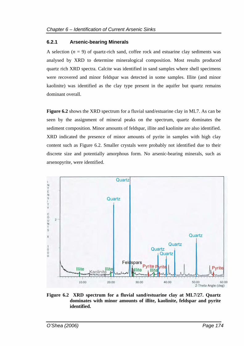
Chapter 6 – Identification of Current Arsenic Sinks
O’Shea (2006) Page 174
6.2.1 Arsenic-bearing Minerals
A selection (n = 9) of quartz-rich sand, coffee rock and estuarine clay sediments was
analysed by XRD to determine mineralogical composition. Most results produced
quartz rich XRD spectra. Calcite was identified in sand samples where shell specimens
were recovered and minor feldspar was detected in some samples. Illite (and minor
kaolinite) was identified as the clay type present in the aquifer but quartz remains
dominant overall.
Figure 6.2 shows the XRD spectrum for a fluvial sand/estuarine clay in ML7. As can be
seen by the assignment of mineral peaks on the spectrum, quartz dominates the
sediment composition. Minor amounts of feldspar, illite and kaolinite are also identified.
XRD indicated the presence of minor amounts of pyrite in samples with high clay
content such as Figure 6.2. Smaller crystals were probably not identified due to their
discrete size and potentially amorphous form. No arsenic-bearing minerals, such as
arsenopyrite, were identified.
Figure 6.2 XRD spectrum for a fluvial sand/estuarine clay at ML7/27. Quartz dominates with minor amounts of illite, kaolinite, feldspar and pyrite identified.
Chapter 6 – Identification of Current Arsenic Sinks
O’Shea (2006) Page 175
6.2.2 Are there any distinctive physical or geochemical correlations ?
Arsenic geochemistry is complex. Often concentrations in solid phase can be
representative of original arsenic sources, and those that have been redistributed through
various sorption, precipitation and dissolution mechanisms.
For example, arsenian pyrite may oxidise and release arsenic into solution, with iron
oxide by-products scavenging this released arsenic and retaining it in solid form.
Changes to iron oxide morphology, solution pH and Eh, or addition of competing ions
can release arsenic into solution once again. The slow redox transformation of arsenic,
aquifer heterogeneity and anthropogenic use of the aquifer may leave arsenic re-
distributed in different forms throughout the aquifer. Therefore, the correlation between
arsenic and other element concentrations in the solid phase may only be indicative of
potential geochemical sinks in different parts of the aquifer. By statistically clustering
aquifer sediments into more homogenous geomorphic units, aquifer heterogeneity is
somewhat addressed. Examination of arsenic occurrence in each of these units can then
be independently assessed.
Pearsons correlations (Appendix B7) were calculated to evaluate arsenic geochemical
relationships in each facies (Table 6.4). For the purpose of discussion, the following
terminology applies herein:
r2 = 0.91 to 0.99 extremely strong correlation
r2 = 0.81 to 0.90 very strong correlation
r2 = 0.61 to 0.80 strong correlation
r2 = 0.41 to 0.60 moderate correlation
r2 = 0.31 to 0.40 weak correlation
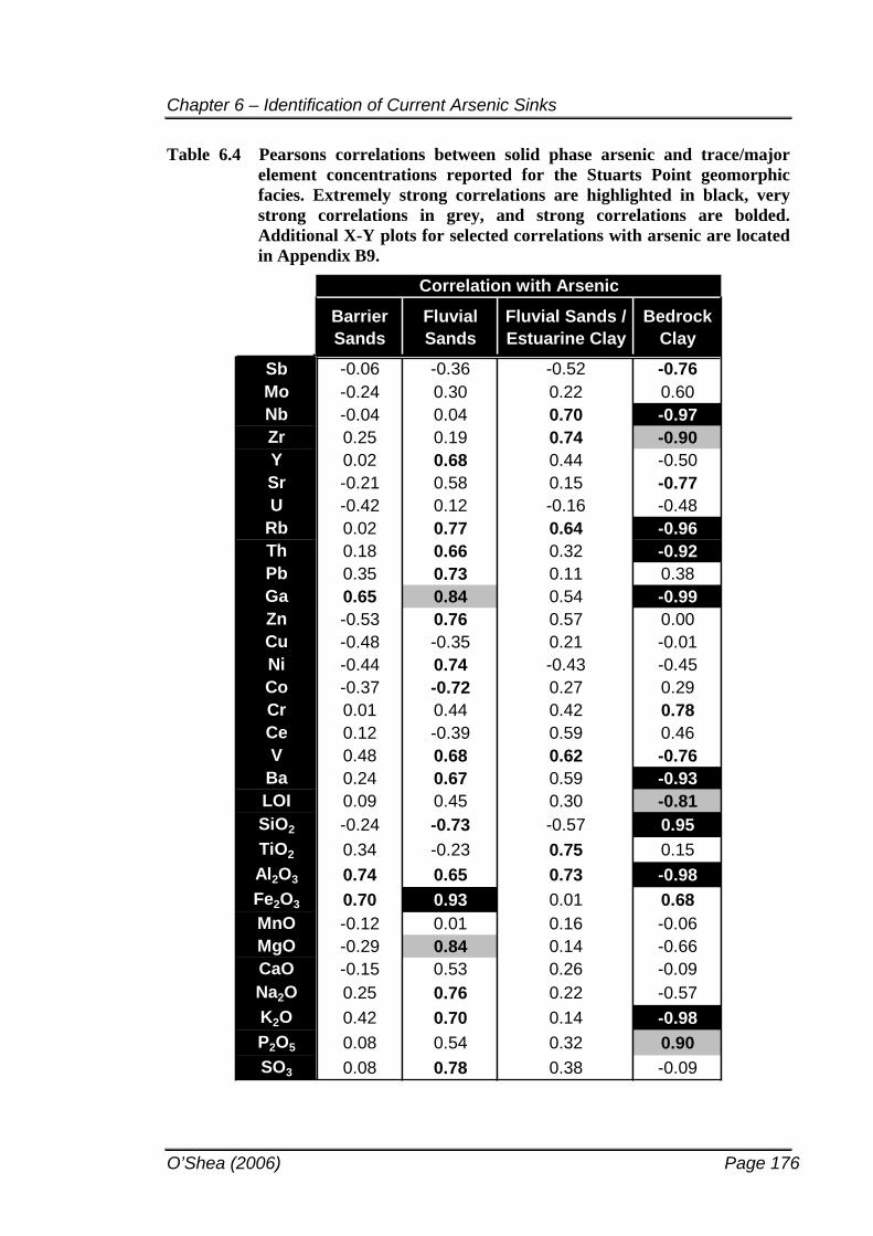
Chapter 6 – Identification of Current Arsenic Sinks
O’Shea (2006) Page 176
Table 6.4 Pearsons correlations between solid phase arsenic and trace/major element concentrations reported for the Stuarts Point geomorphic facies. Extremely strong correlations are highlighted in black, very strong correlations in grey, and strong correlations are bolded. Additional X-Y plots for selected correlations with arsenic are located in Appendix B9.
Barrier Sands
Fluvial Sands
Fluvial Sands / Estuarine Clay
BedrockClay
Sb -0.06 -0.36 -0.52 -0.76Mo -0.24 0.30 0.22 0.60Nb -0.04 0.04 0.70 -0.97Zr 0.25 0.19 0.74 -0.90Y 0.02 0.68 0.44 -0.50Sr -0.21 0.58 0.15 -0.77U -0.42 0.12 -0.16 -0.48
Rb 0.02 0.77 0.64 -0.96Th 0.18 0.66 0.32 -0.92Pb 0.35 0.73 0.11 0.38Ga 0.65 0.84 0.54 -0.99Zn -0.53 0.76 0.57 0.00Cu -0.48 -0.35 0.21 -0.01Ni -0.44 0.74 -0.43 -0.45Co -0.37 -0.72 0.27 0.29Cr 0.01 0.44 0.42 0.78Ce 0.12 -0.39 0.59 0.46V 0.48 0.68 0.62 -0.76
Ba 0.24 0.67 0.59 -0.93LOI 0.09 0.45 0.30 -0.81SiO2 -0.24 -0.73 -0.57 0.95TiO2 0.34 -0.23 0.75 0.15Al2O3 0.74 0.65 0.73 -0.98Fe2O3 0.70 0.93 0.01 0.68MnO -0.12 0.01 0.16 -0.06MgO -0.29 0.84 0.14 -0.66CaO -0.15 0.53 0.26 -0.09Na2O 0.25 0.76 0.22 -0.57K2O 0.42 0.70 0.14 -0.98P2O5 0.08 0.54 0.32 0.90SO3 0.08 0.78 0.38 -0.09
Correlation with Arsenic
Chapter 6 – Identification of Current Arsenic Sinks
O’Shea (2006) Page 177
The identification of average arsenic concentrations (i.e., low background
concentrations) in the aquifer sediments at Stuarts Point supports the hypothesis that
arsenic is naturally derived rather than anthropogenically induced. Frequently associated
with naturally occurring arsenic are the elements iron, aluminium and manganese
(representing silicates, oxyhydroxides or sulfides); various trace elements derived from
ore deposits (molybdenum and antimony have previously been shown to be allied with
arsenic regionally); species of sulfur (commonly delineating a pyrite association); loss
on ignition (LOI) indicating potential arsenic association with organic matter; fine grain
size correlation with elevated arsenic concentrations indicating silts and clays
potentially immobilising arsenic; and phosphate or bicarbonate ions dueling for the
same aquifer sorption sites as arsenic. Thus, a correlation between arsenic and one or
more of these elements or parameters could identify the presence of particular solid
phase arsenic sinks.
Examining these correlations in order of oldest sediments to youngest, the in-situ
“bedrock clays” exhibit the greatest element correlation with arsenic. Niobium and Th
are often hosted by Ti-oxides (Lopez et al., 2005); Rb and Ba have been associated with
sorption on clays (Eylem et al., 1990; Kleven and Alstad, 1996; Lopez et al., 2005); Ga
is generally associated with clays of granite source (Burton et al., 1959) while LOI,
Al2O3 and K2O5 may be direct representations of clay mineral occurrence. Thus, the
high negative r2 values reported with arsenic for Nb, Rb, Th, Ga, Ba, LOI, Al2O3 and
K2O5 are suggested to indicate a non-association with a potassium clay likely to be illite.
In other words, arsenic is not associated with the weathered bedrock clays. The
remaining correlation with arsenic for the “bedrock clays” are extremely strong for SiO2
(r2 = 0.95) and very strong for P2O5 (r2 = 0.90). This suggests a relationship between
arsenic and the quartz fraction perhaps partially coated with iron oxide (r2 = 0.68) which
is also sorbing phosphorous.
The “fluvial sand / estuarine clays” exhibit a strong positive correlation between arsenic
and Nb, Zr, Rb, V, TiO2 and Al2O3 which is in contrast to that previously observed for
the bedrock clays. Plausible explanations could include the presence of a different clay
mineral with different sorptive properties, however this is unlikely as XRD has
identified illite in both geomorphic units. Alternatively, the heterogenous mix of sands
Chapter 6 – Identification of Current Arsenic Sinks
O’Shea (2006) Page 178
and clays in this unit may influence the statistical results. It is interesting to note that
arsenic and iron are not correlated (r2 = 0.01) for this geomorphic unit.
A better correlation with iron is observed for the “fluvial sands”. In contrast to the
absence of an iron oxide and arsenic correlation in the underlying sediments, an
extremely strong positive (r2 = 0.93) correlation exists for As and iron in the sands of
purely fluvial origin. In addition, the strong positive correlations with clay indicative
elements and SO3, with a strong negative SiO2 (r2 = -0.73) correlation suggests that iron
oxide, clay and sulfur mineral coatings may be dominating the fluvially transported
quartz grains which are sorbing arsenic to their outer edges.
Arsenic association with elements in the “beach barrier sands” results in strong
correlations for both Al2O3 (r2 = 0.74) and Fe2O3 (r2 = 0.70). Clay dominance or sulfur
association is not indicated therefore suggesting arsenic association with oxide grain
coatings in this highly re-worked homogenous sand unit. Alternatively, association with
coffee rock may explain the aluminium association in the absence of other clay
indicators. A correlation with LOI is not expected in the “beach barrier sands” as coffee
rock is sporadic and localised and generally organic matter contents are low throughout
the unit.
A moderate negative correlation (r2 = -0.58) has previously been proposed between
arsenic and antimony for all sediments (bulk statistical result) regardless of their
geomorphic origin. This correlation is proposed to be indicative of arsenic and antimony
being derived from the same source with arsenic being mobilised after deposition while
antimony is retained in the solid phase. When each geomorphic unit is assessed
independently the correlation between the two elements is almost non-existent in the
surface sediments (r2 = -0.06 for the “beach barrier sands”) yet increases with depth,
reporting a strong negative (r2 = -0.76) correlation in the “bedrock clay” unit. The
barrier sands deposited in the top portion of the aquifer are depositionally youngest, yet
have been derived from the NEFB, deposited offshore and re-distributed onshore as
barrier sands. They were most likely eroded from the NEFB earlier than the underlying
fluvial sediments. Their extensive re-working has altered the original Sb-As signature
resulting in low statistical correlation. This signature remains recognisable in the
Chapter 6 – Identification of Current Arsenic Sinks
O’Shea (2006) Page 179
underlying sediments that have not been extensively re-worked, particularly the bedrock
clays which may contribute Sb from in-situ weathering of the granitoid influenced
bedrock. Arsenic-rich pyrites in a mineralised granitoid intrusion investigated by
Zacharias et al. (2004) also found the pyrites and associated arsenopyrites to be enriched
in antimony. The metasediments surrounding the contact aureole of Mt Yarrahapinni
have been described as pyritic (Leitch, 1974).
The association of arsenic with molybdenum was discussed in relation to bedrock
contribution of arsenic to the aquifer. Molybdenum is present in disseminated form in
the northern part of the bedrock aquifer where arsenic has also been associated with
these mineral deposits. This association of As and Mo with depth is confirmed via the
moderate positive correlation (r2 = 0.60) observed between the two elements in the
“bedrock clays” compared to no statistically significant correlation observed for the
other geomorphic units.
Manganese oxides exhibit a high affinity for arsenic sorption (although to a lesser extent
than iron oxides) and have been suggested as arsenic sorbents for many
hydrogeochemical studies (Mucci et al., 2003; Chaillou et al., 2003). Coupled with the
low concentrations of Mn in the Stuarts Point aquifer matrix (up to 0.04%), no
statistical correlation was observed with arsenic in the solid phase thereby reducing the
likelihood of Mn oxides as a potential arsenic sink.
Arsenic inclusion into the calcite structure was documented in the literature review. A
moderate positive (r2 = 0.53) correlation between As and Ca was observed in the shell
dominated “fluvial sand” unit potentially suggesting an arsenic-calcite association at
localised depths. This correlation is similar to that between arsenic and phosphorous for
the same geomorphic unit indicating phosphate inclusion into the calcite lattice as a
possible simultaneous geochemical process. Dual anion interaction is also expected
between phosphate and arsenic in the “bedrock clays” where sorption is dominated by
iron oxides. This is supported by the very strong correlation (r2 = 0.90) between As and
P2O5 in this unit.
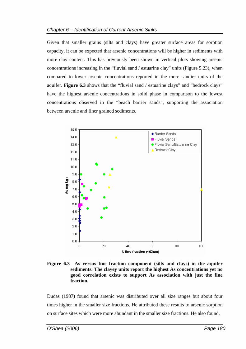
Chapter 6 – Identification of Current Arsenic Sinks
O’Shea (2006) Page 180
Given that smaller grains (silts and clays) have greater surface areas for sorption
capacity, it can be expected that arsenic concentrations will be higher in sediments with
more clay content. This has previously been shown in vertical plots showing arsenic
concentrations increasing in the “fluvial sand / estuarine clay” units (Figure 5.23), when
compared to lower arsenic concentrations reported in the more sandier units of the
aquifer. Figure 6.3 shows that the “fluvial sand / estuarine clays” and “bedrock clays”
have the highest arsenic concentrations in solid phase in comparison to the lowest
concentrations observed in the “beach barrier sands”, supporting the association
between arsenic and finer grained sediments.
Figure 6.3 As versus fine fraction component (silts and clays) in the aquifer sediments. The clayey units report the highest As concentrations yet no good correlation exists to support As association with just the fine fraction.
Dudas (1987) found that arsenic was distributed over all size ranges but about four
times higher in the smaller size fractions. He attributed these results to arsenic sorption
on surface sites which were more abundant in the smaller size fractions. He also found,
Chapter 6 – Identification of Current Arsenic Sinks
O’Shea (2006) Page 181
“The broad partitioning of As among size separates suggests the element was
adsorbed onto iron oxide-coated mineral surfaces rather than occurring in a
discrete mineral or as an inorganic precipitate.” (pg 327)
The lack of correlation throughout the Stuarts Point aquifer between arsenic and the
amount of fine grained material can be explained by grain coatings present in all
geomorphic units contributing to arsenic distribution, rather than the singular
dominance of arsenic sorption onto clays.
These statistical correlations indicate numerous controls on arsenic distribution in the
solid phase and therefore support the assumption that arsenic immobilisation factors are
geochemically complex. Further solid phase analysis was thus conducted to assess each
of the main arsenic sinks prior to analysis of aqueous geochemical conditions.
6.3 EXAMINATION OF KNOWN ARSENIC SCAVENGING MATERIALS IN RELATION TO THE STUARTS POINT AQUIFER MATRIX
The statistical element correlations indicate certain geochemical controls on arsenic
distribution, however their likelihood of arsenic retardation cannot be confirmed until
their presence in the aquifer is established. The literature review outlined various
experimental studies on arsenic sorption phenomena for different minerals. Each of
these potential sinks, and their likelihood of retarding arsenic at Stuarts Point, is
discussed below.
6.3.1 Adsorption to Oxyhydroxides
Smedley and Kinniburgh (2002) state;
“Fe oxides are probably the most important adsorbents in sandy aquifers because
of their greater abundance and the strong binding affinity” (page 534).
The good statistical correlation between arsenic and iron in units of the aquifer solid
phase indicates arsenic sorption may be occurring onto iron oxides. Two important
questions supporting this potential theory remain unanswered:
1. Are iron oxides present in the aquifer?
Chapter 6 – Identification of Current Arsenic Sinks
O’Shea (2006) Page 182
2. Do aqueous geochemical conditions support sorption of arsenic to iron oxides?
(Chapter 7)
A common method for assessing arsenic fractionation in sediments is via selective
extraction methods where specific fractions of the soil are targeted by chemical
extractants and arsenic association with each fraction is quantified. There are distinct
advantages and disadvantages in using these analytical methods. The advantages
include obtaining an indication on the relative mobility of elements in comparison to a
total elemental analysis that does not indicate the potential for element transport through
the matrix. The disadvantages lie mostly with the complexities involved in the chemical
extractants used and the analytical methods employed. For example, errors can be
introduced in the sample drying stage (Farrah and Pickering, 1993); due to incomplete
dissolution of a targeted fraction (La Force and Fendorf, 2000; Gleyzes et al., 2002b);
redistribution of trace elements due to precipitation with extracting chemicals (Shuman,
1982); not to mention contamination of extraction solutions, variabilities in reaction
times and lack of quality control (Gleyzes et al., 2002a). Given these disadvantages,
some authors question the validity of using selective extraction techniques while others
recognise their shortfalls and assess the results accordingly.
There are numerous studies utilising selective extractions, each one different depending
on the nature of the matrix and the particular phases being targeted. Often they are
employed in studies on contaminated sediments and sludges (Carlsson et al., 2002; Bird
et al., 2003; La Force et al., 2000) where contaminants are present in high
concentrations and results can be verified to some extent via SEM analyses confirming
the extractant solution has removed the targeted fractions. Variations to sequential
extractions need to be made when the elements of concern are anionic rather than
cationic because sorption behaviour differs with pH. In addition, arsenic is sensitive to
changes in redox and some extractant chemicals can induce oxidation, which may
influence arsenic associations in the solid phase. Subsequently, several specific schemes
have been proposed especially for arsenic (Keon et al., 2001; van Herreweghe et al.,
2003; Wenzel et al., 2001).
Chapter 6 – Identification of Current Arsenic Sinks
O’Shea (2006) Page 183
Another problem encountered with selective extractions is their applicability to natural
sediments. As mentioned, arsenic concentrations in sediments can be low in areas where
high arsenic groundwaters exist. Dudas (1987) used extractant chemicals commonly
performed on arsenic contaminated sediments but produced no effective results in his
natural sediments. This may be a major drawback for assessing arsenic fractionation in
sediments of naturally high arsenic groundwaters.
Sequential extractants were trialled herein in the hope they might produce reasonable
results (O’Shea and Jankowski, 2003). An arsenic specific scheme was employed
utilising extractant chemicals from several studies, their advantages and disadvantages
noted in Chapter 4. Five specific pools were targeted:
Exchangeable – arsenic sorbed to mineral surfaces that can be released by changes
in solution pH or competition with phosphate;
Carbonate bound – arsenic incorporated into the lattice sites of calcite which are
acido-soluble;
Reducible – arsenic associated with amorphous and/or crystalline oxyhydroxides of
iron and aluminium;
Oxidisable – arsenic associated with organic matter and partial sulfide oxidation;
and
Residual – arsenic bound in the residual mineral phase such as in silicate lattice sites
and therefore not prone to mobilisation.
As found by Dudas (1987), the naturally low levels of arsenic in the Stuarts Point
matrix were not sufficient for chemical extraction, thereby reporting no detectable
arsenic in the extracting solutions. This is due in part to the large dilution factors applied
to enable the chemical extractants to be analysed via ICP-MS; and limitations with
laboratory equipment being small enough to fit into the available water bath and
centrifuge, which subsequently led to small sediment to aqueous extraction ratios. In
addition, precipitation reactions between phases is strongly suspected given that
phosphate, which had previously been used as an extractant chemical and was therefore
present at significant concentrations, decreased to levels below detection when the
reducible phase was targeted, indicating redistribution as an insoluble phase. Given that
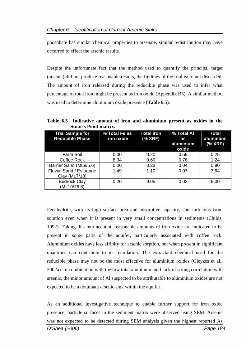
Chapter 6 – Identification of Current Arsenic Sinks
O’Shea (2006) Page 184
phosphate has similar chemical properties to arsenate, similar redistribution may have
occurred to effect the arsenic results.
Despite the unfortunate fact that the method used to quantify the principal target
(arsenic) did not produce reasonable results, the findings of the trial were not discarded.
The amount of iron released during the reducible phase was used to infer what
percentage of total iron might be present as iron oxide (Appendix B5). A similar method
was used to determine aluminium oxide presence (Table 6.5).
Table 6.5 Indicative amount of iron and aluminium present as oxides in the Stuarts Point matrix.
Trial Sample for Reducible Phase
% Total Fe as iron oxide
Total iron(% XRF)
% Total Al as
aluminiumoxide
Totalaluminium
(% XRF)
Farm Soil 0.00 0.20 0.59 0.25Coffee Rock 8.34 0.60 0.78 1.24
Barrier Sand (ML9/5.6) 0.00 0.23 0.04 0.90Fluvial Sand / Estuarine
Clay (ML7/18) 1.49 1.10 0.07 3.64
Bedrock Clay (ML10/26.8)
0.20 9.05 0.03 6.00
Ferrihydrite, with its high surface area and adsorptive capacity, can sorb ions from
solution even when it is present in very small concentrations in sediments (Childs,
1992). Taking this into account, reasonable amounts of iron oxide are indicated to be
present in some parts of the aquifer, particularly associated with coffee rock.
Aluminium oxides have less affinity for arsenic sorption, but when present in significant
quantities can contribute to its retardation. The extractant chemical used for the
reducible phase may not be the most effective for aluminium oxides (Gleyzes et al.,
2002a). In combination with the low total aluminium and lack of strong correlation with
arsenic, the minor amount of Al suspected to be attributable to aluminium oxides are not
expected to be a dominant arsenic sink within the aquifer.
As an additional investigative technique to enable further support for iron oxide
presence, particle surfaces in the sediment matrix were observed using SEM. Arsenic
was not expected to be detected during SEM analysis given the highest reported As
Chapter 6 – Identification of Current Arsenic Sinks
O’Shea (2006) Page 185
concentration (14 mg kg-1) by XRF was well below the As detection limit for the SEM
(approximately 50 mg kg-1). Thus, the aim of using the SEM was to identify
morphological irregularities at the particle surface and semi-quantitatively analyse the
particle surface composition. Once individual particles and/or mineral precipitates have
been semi-quantitated, their ability to scavenge and/or contribute arsenic to the system
can be critically assessed2.
Minor amounts of iron were detected by SEM in samples throughout the aquifer,
particularly in the coffee rock and clayey samples. Atomic ratio calculations generally
did not distinguish discrete iron oxide phases, more likely indicating iron association
with the clay mineral structure and/or minor oxide presence. However, the bedrock at
the base of ML10 was notably different to other samples. Arsenic concentration
reported by XRF was 14 mg kg-1, the highest reported for all samples analysed. This
sample exhibited a distinctive bright orange colour and contained lithic fragments up to
3 mm in size. It is assumed to represent weathered bedrock at the base of the sandy
aquifer containing some fluvially deposited river gravels. It is hypothesised that the
ubiquitous olive grey clays existing in other places throughout the aquifer are under
reducing conditions, and that ML10/26.8 has undergone oxidation when the sea
regressed during the Pleistocene.
Upon first examination the clay component of this sample was logged as a potential
oxidised iron sulfate such as jarosite. The arsenic was thought to be present as a re-
distributed phase associated with jarosite or other oxidation products, which is what
gave this sample its distinctive colour and elevated arsenic concentrations. SEM was
expected to identify jarosite and confirm this hypothesis. Detailed analysis of the
sample was undertaken (Figure 6.4). The position of the arsenic peak is labelled on
each spectra to indicate its potential presence. The first point semi-quantitated was
chosen to represent the bulk particle surface (i.e. the smooth, unaltered grain surface).
2 The semi-quantitative SEM-EDS analysis, coupled with atomic ratios influenced by variable numbers of hydrated ions, enforces the inexact nature of the spectral analysis and the importance of assessing approximate element/atomic percentages only.
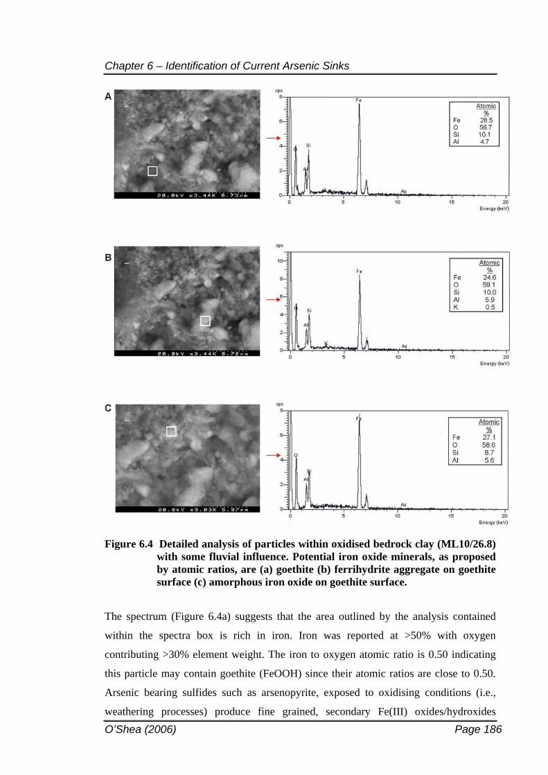
Chapter 6 – Identification of Current Arsenic Sinks
O’Shea (2006) Page 186
Figure 6.4 Detailed analysis of particles within oxidised bedrock clay (ML10/26.8) with some fluvial influence. Potential iron oxide minerals, as proposed by atomic ratios, are (a) goethite (b) ferrihydrite aggregate on goethite surface (c) amorphous iron oxide on goethite surface.
The spectrum (Figure 6.4a) suggests that the area outlined by the analysis contained
within the spectra box is rich in iron. Iron was reported at >50% with oxygen
contributing >30% element weight. The iron to oxygen atomic ratio is 0.50 indicating
this particle may contain goethite (FeOOH) since their atomic ratios are close to 0.50.
Arsenic bearing sulfides such as arsenopyrite, exposed to oxidising conditions (i.e.,
weathering processes) produce fine grained, secondary Fe(III) oxides/hydroxides
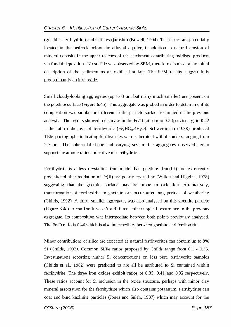
Chapter 6 – Identification of Current Arsenic Sinks
O’Shea (2006) Page 187
(goethite, ferrihydrite) and sulfates (jarosite) (Bowell, 1994). These ores are potentially
located in the bedrock below the alluvial aquifer, in addition to natural erosion of
mineral deposits in the upper reaches of the catchment contributing oxidised products
via fluvial deposition. No sulfide was observed by SEM, therefore dismissing the initial
description of the sediment as an oxidised sulfate. The SEM results suggest it is
predominantly an iron oxide.
Small cloudy-looking aggregates (up to 8 m but many much smaller) are present on
the goethite surface (Figure 6.4b). This aggregate was probed in order to determine if its
composition was similar or different to the particle surface examined in the previous
analysis. The results showed a decrease in the Fe/O ratio from 0.5 (previously) to 0.42
– the ratio indicative of ferrihydrite (Fe5HO8.4H2O). Schwertmann (1988) produced
TEM photographs indicating ferrihydrites were spheroidal with diameters ranging from
2-7 nm. The spheroidal shape and varying size of the aggregates observed herein
support the atomic ratios indicative of ferrihydrite.
Ferrihydrite is a less crystalline iron oxide than goethite. Iron(III) oxides recently
precipitated after oxidation of Fe(II) are poorly crystalline (Willett and Higgins, 1978)
suggesting that the goethite surface may be prone to oxidation. Alternatively,
transformation of ferrihydrite to goethite can occur after long periods of weathering
(Childs, 1992). A third, smaller aggregate, was also analysed on this goethite particle
(Figure 6.4c) to confirm it wasn’t a different mineralogical occurrence to the previous
aggregate. Its composition was intermediate between both points previously analysed.
The Fe/O ratio is 0.46 which is also intermediary between goethite and ferrihydrite.
Minor contributions of silica are expected as natural ferrihydrites can contain up to 9%
Si (Childs, 1992). Common Si/Fe ratios proposed by Childs range from 0.1 - 0.35.
Investigations reporting higher Si concentrations on less pure ferrihydrite samples
(Childs et al., 1982) were predicted to not all be attributed to Si contained within
ferrihydrite. The three iron oxides exhibit ratios of 0.35, 0.41 and 0.32 respectively.
These ratios account for Si inclusion in the oxide structure, perhaps with minor clay
mineral association for the ferrihydrite which also contains potassium. Ferrihydrite can
coat and bind kaolinite particles (Jones and Saleh, 1987) which may account for the
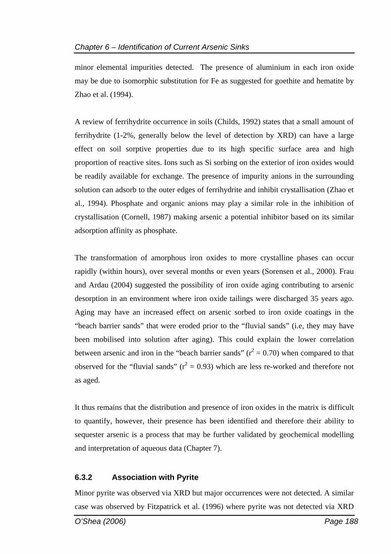
Chapter 6 – Identification of Current Arsenic Sinks
O’Shea (2006) Page 188
minor elemental impurities detected. The presence of aluminium in each iron oxide
may be due to isomorphic substitution for Fe as suggested for goethite and hematite by
Zhao et al. (1994).
A review of ferrihydrite occurrence in soils (Childs, 1992) states that a small amount of
ferrihydrite (1-2%, generally below the level of detection by XRD) can have a large
effect on soil sorptive properties due to its high specific surface area and high
proportion of reactive sites. Ions such as Si sorbing on the exterior of iron oxides would
be readily available for exchange. The presence of impurity anions in the surrounding
solution can adsorb to the outer edges of ferrihydrite and inhibit crystallisation (Zhao et
al., 1994). Phosphate and organic anions may play a similar role in the inhibition of
crystallisation (Cornell, 1987) making arsenic a potential inhibitor based on its similar
adsorption affinity as phosphate.
The transformation of amorphous iron oxides to more crystalline phases can occur
rapidly (within hours), over several months or even years (Sorensen et al., 2000). Frau
and Ardau (2004) suggested the possibility of iron oxide aging contributing to arsenic
desorption in an environment where iron oxide tailings were discharged 35 years ago.
Aging may have an increased effect on arsenic sorbed to iron oxide coatings in the
“beach barrier sands” that were eroded prior to the “fluvial sands” (i.e, they may have
been mobilised into solution after aging). This could explain the lower correlation
between arsenic and iron in the “beach barrier sands” (r2 = 0.70) when compared to that
observed for the “fluvial sands” (r2 = 0.93) which are less re-worked and therefore not
as aged.
It thus remains that the distribution and presence of iron oxides in the matrix is difficult
to quantify, however, their presence has been identified and therefore their ability to
sequester arsenic is a process that may be further validated by geochemical modelling
and interpretation of aqueous data (Chapter 7).
6.3.2 Association with Pyrite
Minor pyrite was observed via XRD but major occurrences were not detected. A similar
case was observed by Fitzpatrick et al. (1996) where pyrite was not detected via XRD
Chapter 6 – Identification of Current Arsenic Sinks
O’Shea (2006) Page 189
but was later found under high powered microscope. SEM analysis of a “fluvial sand /
estuarine clay” sample located close to the estuary was conducted (ML7/18). Shell
material is abundant in this area, although this sample is predominantly a poorly sorted
fine-grained sandy olive clay containing both smooth and angular shaped pebbles. It
contains 10.4 mg kg-1. As in the sediment, while groundwater As was reported at 26 g
L-1 and 16 g L-1 over a one year interval between sampling events. The composition is
largely quartz (Si, O) with clay (Al, Mg, K, Fe, Ti) also potentially dominating. Various
surface aggregates were examined and generally found to be representative of the
remainder of the particle, with the exception of one analysis. A small spherical
aggregate (Figure 6.5) contained the elements noted above with the addition of sulfur
and an increase in iron. This implies that a sulfide mineral may be present sporadically
in the aquifer, however, no other SEM-EDX analyses reported sulfide.
Figure 6.5 Small agregate observed on a “fluvial sand / estuarine clay” sample. Clay and quartz are suspected however the presence of sulfur may indicate discrete sulfide mineral presence.
Further analysis of the potential for discrete sulfide mineral presence in the aquifer was
warranted. A separate “fluvial sand / estuarine clay” sample (ML7/12) was examined by
SX50 electron microprobe. Like sample ML7/18 this sediment is an olive grey sand
containing both lithic and shell fragments. Quantitative analysis of a shell fragment
produced atomic ratios indicative of calcite (Ca/O 0.32) with minor association of Fe
and Mg potentially via inclusion or sorption (Figure 6.6). A small bright cluster was
observed on a portion of the shell material. A quantitative analysis of this cluster
reported it was predominantly Fe and S, which suggested it was an iron sulfide,
potentially pyrite. The Fe/S ratio (which was previously 1.17 on the shell material) is
Chapter 6 – Identification of Current Arsenic Sinks
O’Shea (2006) Page 190
reported as 0.66 for this cluster, which is closer to the ratio for pyrite (0.5). The Fe
presumed to be substituting in the CaCO3 matrix is most likely contributing to this ratio,
thereby keeping it above the 0.5 ratio of pyrite. Arsenic is reported at 0.14%,
significantly above its DL of 0.02% and surprisingly high given its bulk XRF
concentration of only 5.8 mg kg-1. It is likely that arsenic has been included into the
pyrite crystal lattice by substitution of sulfur, which may also contribute to keeping the
Fe/S ratio above that indicative of pure pyrite. The presence of 0.14% Pb may indicate
cation association with pyrite by a sorption mechanism.
For comparison, electron microprobe analyses of arsenian pyrite in a gold mining
district of California produced an average As content between 0 and 0.09 wt.% for a
sample reporting a bulk concentration of 10 mg kg-1 (Savage et al., 2000). In addition,
up to 0.33 wt.% Pb was also reported in the arsenian pyrites of the region, with the trace
elements Zn, Mn, Sb, Se, Cu, Bi, Co, Ag and Au all generally reported below 0.1 wt.%.
Further, Thornburg and Sahai (2004) identified arsenian pyrite occurring as
disseminated grains, veins and nodules in sandstone of the Fox River Valley, Eastern
Wisconsin. Concentrations of arsenic in disseminated pyrite are comparable to those
reported herein – generally <1 wt%. The pyrite was initially formed due to migration of
ore forming Mississippi Valley type fluids.
To be consistent with the above cited literature, the presence of Pb in the Stuarts Point
arsenian pyrite may indicate formation in close proximity to a mineralised source in
comparison to authigenic precipitation in-situ. This will be further discussed during
analysis of pyrite formation in the arsenic mobilisation chapter.
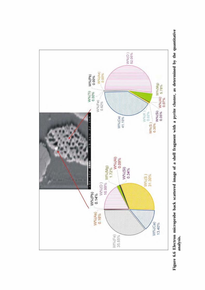
Figu
re 6
.6 E
lect
ron
mic
ropr
obe
back
sca
tter
ed i
mag
e of
a s
hell
frag
men
t w
ith a
pyr
ite c
lust
er,
as d
eter
min
ed b
y th
e qu
antit
ativ
ean
alys
is.
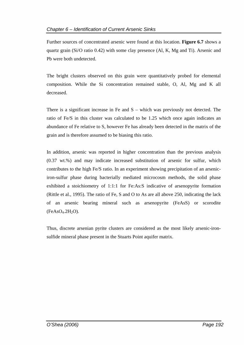
Chapter 6 – Identification of Current Arsenic Sinks
O’Shea (2006) Page 192
Further sources of concentrated arsenic were found at this location. Figure 6.7 shows a
quartz grain (Si/O ratio 0.42) with some clay presence (Al, K, Mg and Ti). Arsenic and
Pb were both undetected.
The bright clusters observed on this grain were quantitatively probed for elemental
composition. While the Si concentration remained stable, O, Al, Mg and K all
decreased.
There is a significant increase in Fe and S – which was previously not detected. The
ratio of Fe/S in this cluster was calculated to be 1.25 which once again indicates an
abundance of Fe relative to S, however Fe has already been detected in the matrix of the
grain and is therefore assumed to be biasing this ratio.
In addition, arsenic was reported in higher concentration than the previous analysis
(0.37 wt.%) and may indicate increased substitution of arsenic for sulfur, which
contributes to the high Fe/S ratio. In an experiment showing precipitation of an arsenic-
iron-sulfur phase during bacterially mediated microcosm methods, the solid phase
exhibited a stoichiometry of 1:1:1 for Fe:As:S indicative of arsenopyrite formation
(Rittle et al., 1995). The ratio of Fe, S and O to As are all above 250, indicating the lack
of an arsenic bearing mineral such as arsenopyrite (FeAsS) or scorodite
(FeAsO4.2H2O).
Thus, discrete arsenian pyrite clusters are considered as the most likely arsenic-iron-
sulfide mineral phase present in the Stuarts Point aquifer matrix.
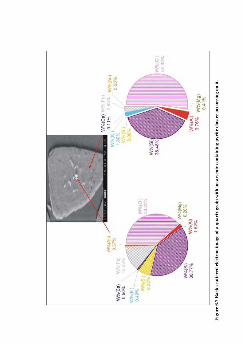
Figu
re 6
.7 B
ack
scat
tere
d el
ectr
on im
age
of a
qua
rtz
grai
n w
ith a
n ar
seni
c co
ntai
ning
pyr
ite c
lust
er o
ccur
ring
on
it.
Chapter 6 – Identification of Current Arsenic Sinks
O’Shea (2006) Page 194
6.3.3 Incorporation into clay minerals
A negative correlation observed between arsenic and clay-representative elements
suggests arsenic at Stuarts Point may not be associated with bedrock clay minerals.
Theoretically, however, it may be possible and should be investigated accordingly in the
event that the statistical correlations are not representative of true conditions. The
identification of illite was made via XRD and electron microprobe analysis. Through
both optical illumination and back scattered electron imaging, a coating was identified
on a selected grain in the matrix (Figure 6.8).
A
B
Figure 6.8 A coating on a grain in sample ML10/26.8 under electron microprobe (a) optical image (b) back scattered electron image. Scale identical.
A line scan was conducted to ascertain the compositional differences between coating
and grain. Eleven elements were chosen for the analysis: O, Mg, Al, Si, S, K, Ca, Ti, Fe,
Pb and As. Figure 6.9 shows the location of the line scan on the optical image and the
output graph to show changes in composition between coating and grain. Calculation of
atomic ratios indicate that the grain is composed of quartz (Si/O is predominantly 0.5)
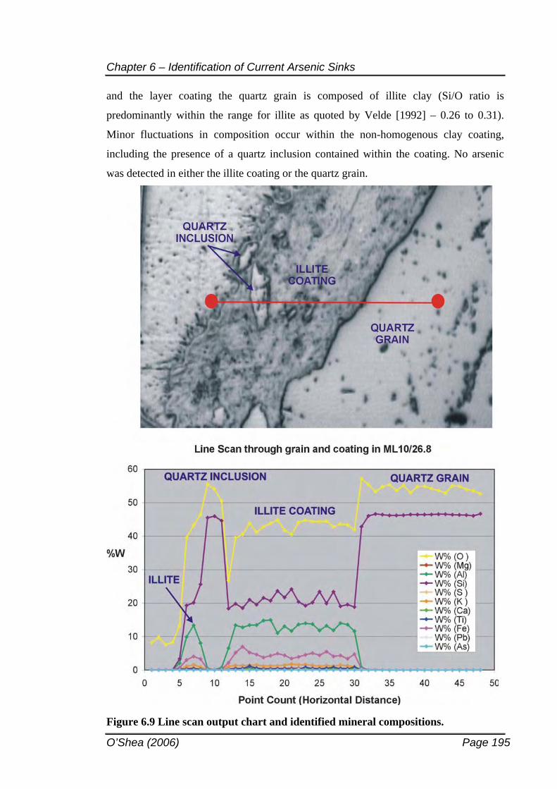
Chapter 6 – Identification of Current Arsenic Sinks
O’Shea (2006) Page 195
and the layer coating the quartz grain is composed of illite clay (Si/O ratio is
predominantly within the range for illite as quoted by Velde [1992] – 0.26 to 0.31).
Minor fluctuations in composition occur within the non-homogenous clay coating,
including the presence of a quartz inclusion contained within the coating. No arsenic
was detected in either the illite coating or the quartz grain.
Figure 6.9 Line scan output chart and identified mineral compositions.
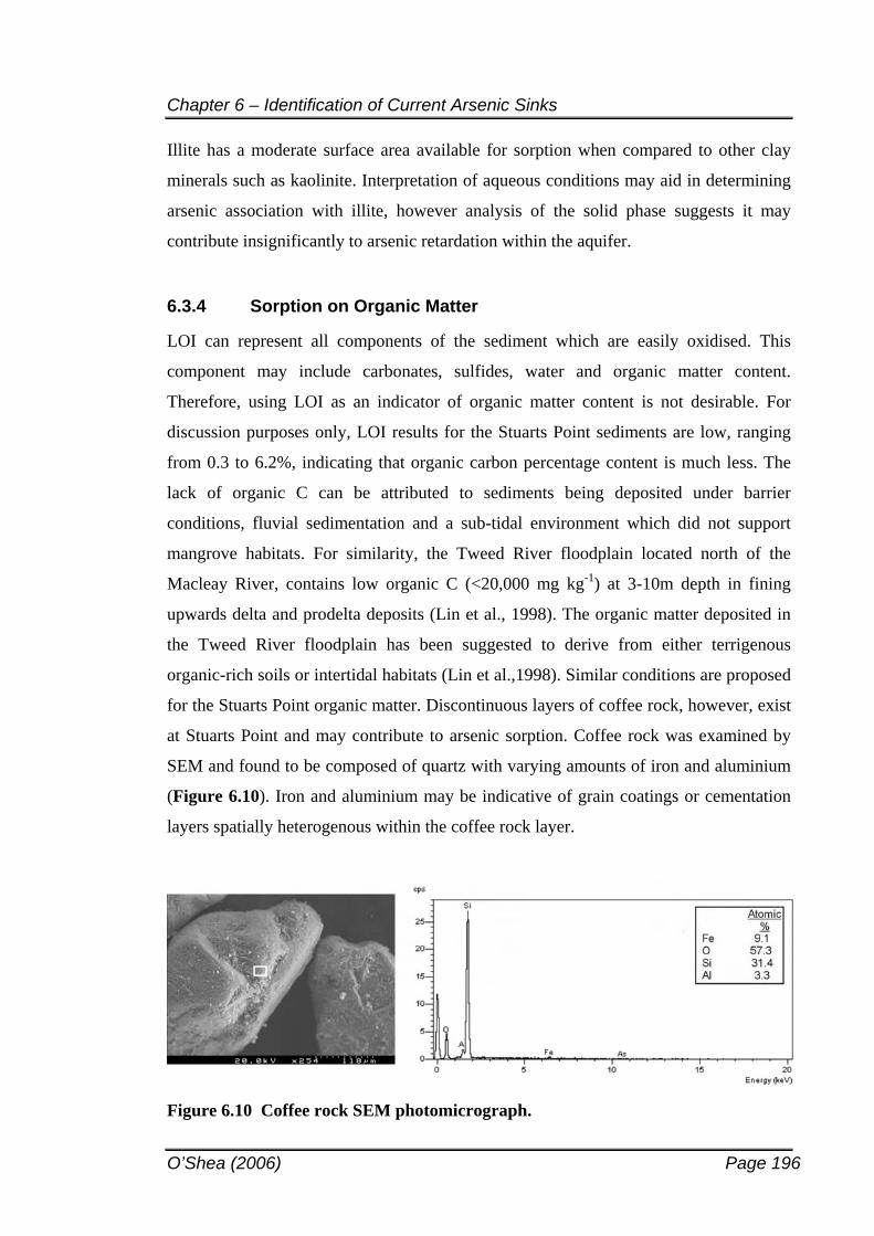
Chapter 6 – Identification of Current Arsenic Sinks
O’Shea (2006) Page 196
Illite has a moderate surface area available for sorption when compared to other clay
minerals such as kaolinite. Interpretation of aqueous conditions may aid in determining
arsenic association with illite, however analysis of the solid phase suggests it may
contribute insignificantly to arsenic retardation within the aquifer.
6.3.4 Sorption on Organic Matter
LOI can represent all components of the sediment which are easily oxidised. This
component may include carbonates, sulfides, water and organic matter content.
Therefore, using LOI as an indicator of organic matter content is not desirable. For
discussion purposes only, LOI results for the Stuarts Point sediments are low, ranging
from 0.3 to 6.2%, indicating that organic carbon percentage content is much less. The
lack of organic C can be attributed to sediments being deposited under barrier
conditions, fluvial sedimentation and a sub-tidal environment which did not support
mangrove habitats. For similarity, the Tweed River floodplain located north of the
Macleay River, contains low organic C (<20,000 mg kg-1) at 3-10m depth in fining
upwards delta and prodelta deposits (Lin et al., 1998). The organic matter deposited in
the Tweed River floodplain has been suggested to derive from either terrigenous
organic-rich soils or intertidal habitats (Lin et al.,1998). Similar conditions are proposed
for the Stuarts Point organic matter. Discontinuous layers of coffee rock, however, exist
at Stuarts Point and may contribute to arsenic sorption. Coffee rock was examined by
SEM and found to be composed of quartz with varying amounts of iron and aluminium
(Figure 6.10). Iron and aluminium may be indicative of grain coatings or cementation
layers spatially heterogenous within the coffee rock layer.
Figure 6.10 Coffee rock SEM photomicrograph.
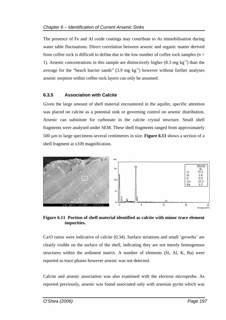
Chapter 6 – Identification of Current Arsenic Sinks
O’Shea (2006) Page 197
The presence of Fe and Al oxide coatings may contribute to As immobilisation during
water table fluctuations. Direct correlation between arsenic and organic matter derived
from coffee rock is difficult to define due to the low number of coffee rock samples (n =
1). Arsenic concentrations in this sample are distinctively higher (8.3 mg kg-1) than the
average for the “beach barrier sands” (3.9 mg kg-1) however without further analyses
arsenic sorption within coffee rock layers can only be assumed.
6.3.5 Association with Calcite
Given the large amount of shell material encountered in the aquifer, specific attention
was placed on calcite as a potential sink or governing control on arsenic distribution.
Arsenic can substitute for carbonate in the calcite crystal structure. Small shell
fragments were analysed under SEM. These shell fragments ranged from approximately
500 m to large specimens several centimetres in size. Figure 6.11 shows a section of a
shell fragment at x100 magnification.
Figure 6.11 Portion of shell material identified as calcite with minor trace element impurities.
Ca/O ratios were indicative of calcite (0.34). Surface striations and small ‘growths’ are
clearly visible on the surface of the shell, indicating they are not merely homogenous
structures within the sediment matrix. A number of elements (Si, Al, K, Ba) were
reported as trace phases however arsenic was not detected.
Calcite and arsenic association was also examined with the electron microprobe. As
reported previously, arsenic was found associated only with arsenian pyrite which was
Chapter 6 – Identification of Current Arsenic Sinks
O’Shea (2006) Page 198
precipitated onto the calcite structure rather than isomorphically bound within the
calcite mineral.
6.3.6 Anion competition
Competitive adsorption between arsenic and phosphate has been suggested as a
probable process in the “bedrock clays”. A very strong correlation exists between
arsenic and phosphorous in this group and no other. Both the highest reported As and
P2O5 concentrations occur in the oxidised bedrock clay supporting potential anion
sorption onto iron oxides. The coffee rock sample contains similar ratios of arsenic and
P2O5 and therefore may also exhibit competitive sorption between the two anions. These
processes are further addressed in Chapter 7.
6.4 CHAPTER SUMMARY: IDENTIFICATION OF CONTROLLING SINKS IN THE AQUIFER
Theoretical and laboratory studies are useful in determining potential controlling sinks
present within the Stuarts Point aquifer based on their presence or absence, as discussed
above. Unfortunately, as Goh and Lim (2004) note, few studies have been conducted on
soils and sediments as a whole, which often contain a mixture of minerals and
geochemical reactions operating in disequilibrium. Each plausible arsenic sink has been
examined in relation to the Stuarts Point aquifer. Identification of some sinks have been
made, however direct evidence of arsenic association is not available for each one.
Given the characterisation of the aquifer matrix provided herein, the suggested arsenic
sources and sinks to be tested in the mobilisation chapter are (Figure 6.12):
Arsenic and phosphate are both sorbed onto iron oxide surfaces in the “bedrock
clays”. Illite is present but is considered a potentially minor arsenic sink, if at all.
Arsenic may be contributed to the depths of the aquifer via bedrock discharge
through mineralised zones or as a product of released arsenic after fluvial
transportation of gravels present within some clays at depth;
Fluvial and marine conditions exist intermittently hereafter, contributing arsenic
from the hinterland via deposition of arsenic sorbed onto iron oxides. Persistent
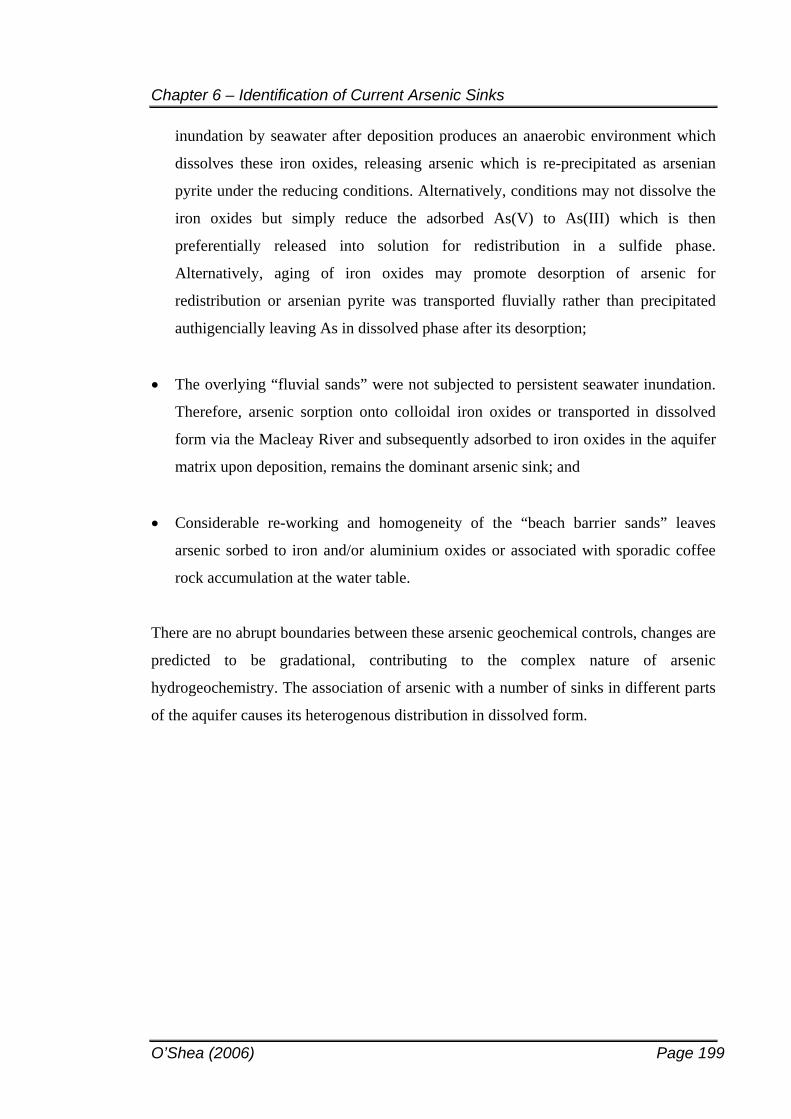
Chapter 6 – Identification of Current Arsenic Sinks
O’Shea (2006) Page 199
inundation by seawater after deposition produces an anaerobic environment which
dissolves these iron oxides, releasing arsenic which is re-precipitated as arsenian
pyrite under the reducing conditions. Alternatively, conditions may not dissolve the
iron oxides but simply reduce the adsorbed As(V) to As(III) which is then
preferentially released into solution for redistribution in a sulfide phase.
Alternatively, aging of iron oxides may promote desorption of arsenic for
redistribution or arsenian pyrite was transported fluvially rather than precipitated
authigencially leaving As in dissolved phase after its desorption;
The overlying “fluvial sands” were not subjected to persistent seawater inundation.
Therefore, arsenic sorption onto colloidal iron oxides or transported in dissolved
form via the Macleay River and subsequently adsorbed to iron oxides in the aquifer
matrix upon deposition, remains the dominant arsenic sink; and
Considerable re-working and homogeneity of the “beach barrier sands” leaves
arsenic sorbed to iron and/or aluminium oxides or associated with sporadic coffee
rock accumulation at the water table.
There are no abrupt boundaries between these arsenic geochemical controls, changes are
predicted to be gradational, contributing to the complex nature of arsenic
hydrogeochemistry. The association of arsenic with a number of sinks in different parts
of the aquifer causes its heterogenous distribution in dissolved form.
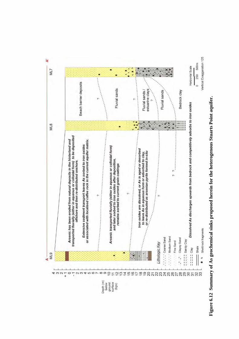
Figu
re 6
.12
Sum
mar
y of
As g
eoch
emic
al si
nks p
ropo
sed
here
in fo
r th
e he
tero
geno
us S
tuar
ts P
oint
aqu
ifer.
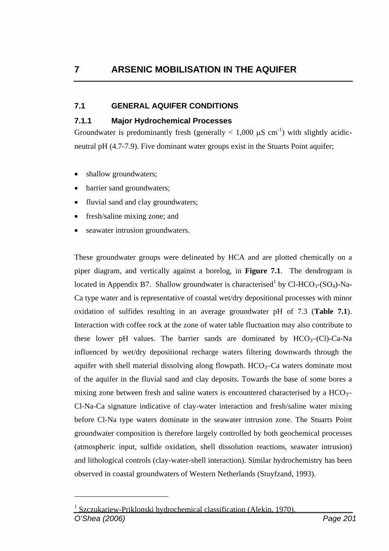
O’Shea (2006) Page 201
7 ARSENIC MOBILISATION IN THE AQUIFER
7.1 GENERAL AQUIFER CONDITIONS
7.1.1 Major Hydrochemical Processes Groundwater is predominantly fresh (generally < 1,000 S cm-1) with slightly acidic-
neutral pH (4.7-7.9). Five dominant water groups exist in the Stuarts Point aquifer;
shallow groundwaters;
barrier sand groundwaters;
fluvial sand and clay groundwaters;
fresh/saline mixing zone; and
seawater intrusion groundwaters.
These groundwater groups were delineated by HCA and are plotted chemically on a
piper diagram, and vertically against a borelog, in Figure 7.1. The dendrogram is
located in Appendix B7. Shallow groundwater is characterised1 by Cl-HCO3-(SO4)-Na-
Ca type water and is representative of coastal wet/dry depositional processes with minor
oxidation of sulfides resulting in an average groundwater pH of 7.3 (Table 7.1).
Interaction with coffee rock at the zone of water table fluctuation may also contribute to
these lower pH values. The barrier sands are dominated by HCO3–(Cl)-Ca-Na
influenced by wet/dry depositional recharge waters filtering downwards through the
aquifer with shell material dissolving along flowpath. HCO3–Ca waters dominate most
of the aquifer in the fluvial sand and clay deposits. Towards the base of some bores a
mixing zone between fresh and saline waters is encountered characterised by a HCO3–
Cl-Na-Ca signature indicative of clay-water interaction and fresh/saline water mixing
before Cl-Na type waters dominate in the seawater intrusion zone. The Stuarts Point
groundwater composition is therefore largely controlled by both geochemical processes
(atmospheric input, sulfide oxidation, shell dissolution reactions, seawater intrusion)
and lithological controls (clay-water-shell interaction). Similar hydrochemistry has been
observed in coastal groundwaters of Western Netherlands (Stuyfzand, 1993).
1 Szczukariew-Priklonski hydrochemical classification (Alekin, 1970).
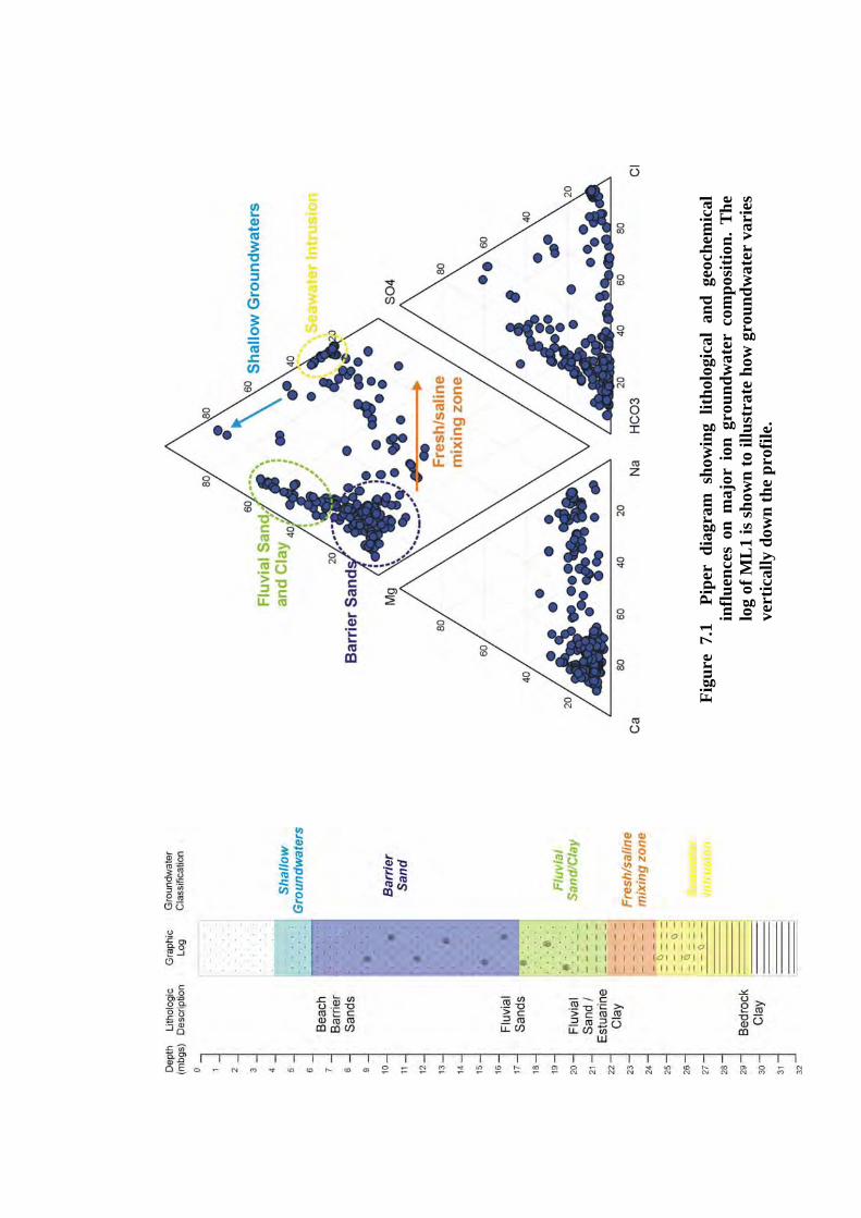
Figu
re 7
.1
Pipe
r di
agra
m s
how
ing
litho
logi
cal
and
geoc
hem
ical
in
fluen
ces
on m
ajor
ion
gro
undw
ater
com
posi
tion.
The
lo
g of
ML
1 is
show
n to
illu
stra
te h
ow g
roun
dwat
er v
arie
s ve
rtic
ally
dow
n th
e pr
ofile
.
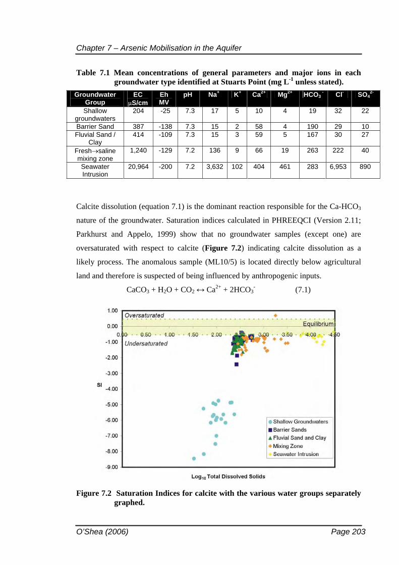
Chapter 7 – Arsenic Mobilisation in the Aquifer
O’Shea (2006) Page 203
Table 7.1 Mean concentrations of general parameters and major ions in each groundwater type identified at Stuarts Point (mg L-1 unless stated).
Groundwater Group
ECS/cm
EhMV
pH Na+ K+ Ca2+ Mg2+ HCO3- Cl- SO4
2-
Shallowgroundwaters
204 -25 7.3 17 5 10 4 19 32 22
Barrier Sand 387 -138 7.3 15 2 58 4 190 29 10 Fluvial Sand /
Clay 414 -109 7.3 15 3 59 5 167 30 27
Fresh saline mixing zone
1,240 -129 7.2 136 9 66 19 263 222 40
Seawater Intrusion
20,964 -200 7.2 3,632 102 404 461 283 6,953 890
Calcite dissolution (equation 7.1) is the dominant reaction responsible for the Ca-HCO3
nature of the groundwater. Saturation indices calculated in PHREEQCI (Version 2.11;
Parkhurst and Appelo, 1999) show that no groundwater samples (except one) are
oversaturated with respect to calcite (Figure 7.2) indicating calcite dissolution as a
likely process. The anomalous sample (ML10/5) is located directly below agricultural
land and therefore is suspected of being influenced by anthropogenic inputs.
CaCO3 + H2O + CO2 Ca2+ + 2HCO3- (7.1)
Figure 7.2 Saturation Indices for calcite with the various water groups separately graphed.
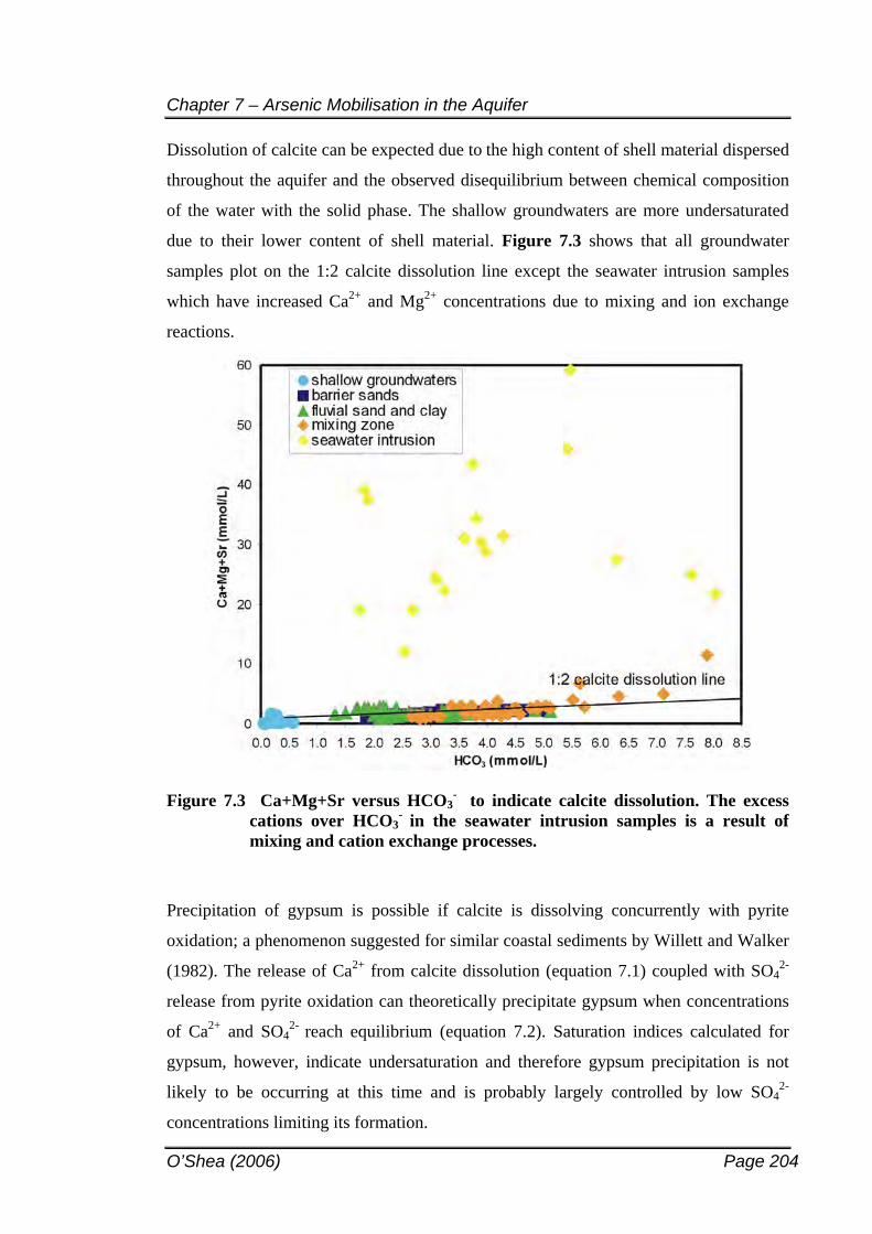
Chapter 7 – Arsenic Mobilisation in the Aquifer
O’Shea (2006) Page 204
Dissolution of calcite can be expected due to the high content of shell material dispersed
throughout the aquifer and the observed disequilibrium between chemical composition
of the water with the solid phase. The shallow groundwaters are more undersaturated
due to their lower content of shell material. Figure 7.3 shows that all groundwater
samples plot on the 1:2 calcite dissolution line except the seawater intrusion samples
which have increased Ca2+ and Mg2+ concentrations due to mixing and ion exchange
reactions.
Figure 7.3 Ca+Mg+Sr versus HCO3- to indicate calcite dissolution. The excess
cations over HCO3- in the seawater intrusion samples is a result of
mixing and cation exchange processes.
Precipitation of gypsum is possible if calcite is dissolving concurrently with pyrite
oxidation; a phenomenon suggested for similar coastal sediments by Willett and Walker
(1982). The release of Ca2+ from calcite dissolution (equation 7.1) coupled with SO42-
release from pyrite oxidation can theoretically precipitate gypsum when concentrations
of Ca2+ and SO42- reach equilibrium (equation 7.2). Saturation indices calculated for
gypsum, however, indicate undersaturation and therefore gypsum precipitation is not
likely to be occurring at this time and is probably largely controlled by low SO42-
concentrations limiting its formation.
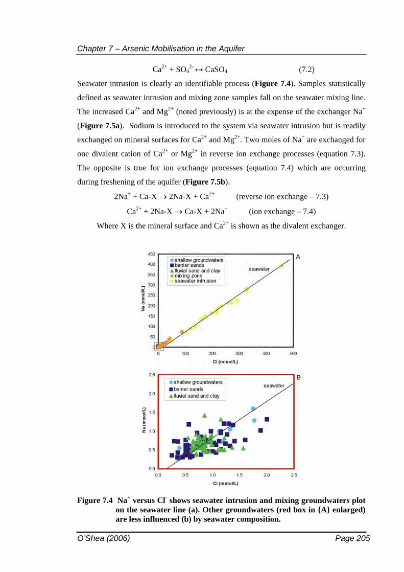
Chapter 7 – Arsenic Mobilisation in the Aquifer
O’Shea (2006) Page 205
Ca2+ + SO42- CaSO4 (7.2)
Seawater intrusion is clearly an identifiable process (Figure 7.4). Samples statistically
defined as seawater intrusion and mixing zone samples fall on the seawater mixing line.
The increased Ca2+ and Mg2+ (noted previously) is at the expense of the exchanger Na+
(Figure 7.5a). Sodium is introduced to the system via seawater intrusion but is readily
exchanged on mineral surfaces for Ca2+ and Mg2+. Two moles of Na+ are exchanged for
one divalent cation of Ca2+ or Mg2+ in reverse ion exchange processes (equation 7.3).
The opposite is true for ion exchange processes (equation 7.4) which are occurring
during freshening of the aquifer (Figure 7.5b).
2Na+ + Ca-X 2Na-X + Ca2+ (reverse ion exchange – 7.3)
Ca2+ + 2Na-X Ca-X + 2Na+ (ion exchange – 7.4)
Where X is the mineral surface and Ca2+ is shown as the divalent exchanger.
Figure 7.4 Na+ versus Cl- shows seawater intrusion and mixing groundwaters plot on the seawater line (a). Other groundwaters (red box in {A} enlarged) are less influenced (b) by seawater composition.
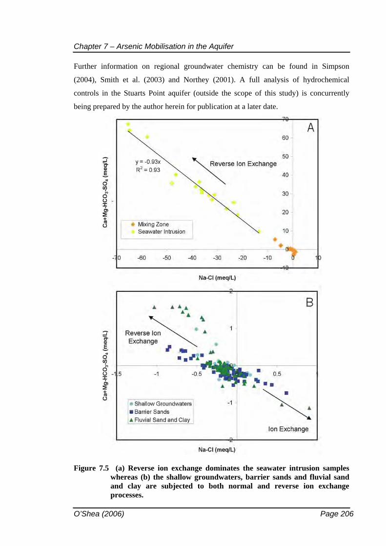
Chapter 7 – Arsenic Mobilisation in the Aquifer
O’Shea (2006) Page 206
Further information on regional groundwater chemistry can be found in Simpson
(2004), Smith et al. (2003) and Northey (2001). A full analysis of hydrochemical
controls in the Stuarts Point aquifer (outside the scope of this study) is concurrently
being prepared by the author herein for publication at a later date.
Figure 7.5 (a) Reverse ion exchange dominates the seawater intrusion samples whereas (b) the shallow groundwaters, barrier sands and fluvial sand and clay are subjected to both normal and reverse ion exchange processes.
Chapter 7 – Arsenic Mobilisation in the Aquifer
O’Shea (2006) Page 207
7.2 ARSENIC GEOCHEMICAL PROCESSES
The contribution of arsenic by both lithological (e.g. arsenic sinks) and hydrochemical
(e.g. seawater intrusion) processes requires independent investigation. Therefore,
assessment of arsenic hydrogeochemistry will be conducted on six different
groundwater groups:
Shallow groundwater influenced by marine aerosol precipitation and water table
fluctuations (Group 1);
The high yielding sands of both barrier (Group 2) and fluvial (Group 3) origin,
differentiated based on transportation/weathering history;
The mixed fluvial sand / estuarine clay unit (Group 4);
Deep groundwaters from weathered bedrock clays (Group 5); and
Groundwaters affected by seawater intrusion (Group 6).
Groups 1 and 6 will deal with hydrochemical processes whereas groups 2-5 will assess
the plausibility of the arsenic sinks proposed in Chapter 6. Note that these groups differ
slightly from the HCA classified groundwater groups discussed above. The sands of
barrier and fluvial origin have been separated to account for arsenic variation due to
depositional differences; and the saline/fresh mixing zone has been included in the
seawater intrusion group to assess the overall arsenic relationship with seawater. The
average chemical composition for each of these ‘arsenic’ water groups is shown in
Table 7.2.
7.2.1 Arsenic Distribution and Speciation Dissolved arsenic concentrations range from 0.19 g L-1 to 83.69 g L-1 with mean
concentrations for each water group listed in Table 7.3. The previously high
concentrations (>330 g L-1) reported by Smith et al. (2003) indicate heterogeneity of
arsenic occurrence in the aquifer.

Table 7.2 Average chemical composition for each water group. Traces in g L-1
and majors in mg L-1.
shallow groundwaters
barrier sands
fluvial sands
fluvial sand/ estuarine
clay
bedrock clay
seawater intrusion
Ag 0.1 3.2 20.6 4.3 26.3 0.2Al 266.3 57.4 28.9 48.8 4.4 76.3As 6.4 4.8 10.9 10.7 43.3 39.5Ba 34.6 17.5 11.4 28.2 15.4 215.4Be 0.1 0.0 0.0 0.0 0.0 0.0B 0.0 17.0 19.5 122.4 49.5 0.0
Cd 0.0 1.6 23.5 11.7 0.0 3.9Ce 30.4 0.4 0.2 0.1 0.0 0.2Co 0.4 0.1 0.1 0.1 0.0 1.0Cr 2.0 2.0 1.5 1.4 1.2 3.8Cs 0.0 0.0 0.0 0.0 0.0 0.2Cu 0.0 0.2 0.0 1.3 0.0 2.8Dy 1.7 0.1 0.0 0.0 0.0 0.0Er 0.8 0.0 0.0 0.0 0.0 0.0Eu 0.7 0.0 0.0 0.0 0.0 0.0Ga 0.7 0.4 0.3 0.8 0.5 3.9Gd 3.1 0.1 0.0 0.0 0.0 0.0Ge 0.2 0.0 0.0 0.1 0.0 0.0Hg 0.0 0.2 0.3 4.7 0.0 0.0Ho 0.3 0.0 0.0 0.0 0.0 0.0La 21.3 0.2 0.1 0.1 0.0 0.1Li 1.8 1.1 1.0 5.8 2.1 89.4Lu 0.1 0.0 0.0 0.0 0.0 0.0Mn 24.1 84.4 46.7 60.9 28.8 1245.7Mo 0.1 1.6 0.3 0.9 0.7 1.5Nb 0.2 0.1 0.1 0.1 0.0 0.0Nd 20.2 0.3 0.1 0.1 0.0 0.1Ni 1.0 1.6 1.2 1.4 1.7 11.6P 30.5 83.3 112.4 139.6 44.9 172.1
Pb 3.2 5.1 4.3 3.0 10.4 1.9Pr 3.8 0.1 0.0 0.0 0.0 0.0Rb 10.1 4.0 3.1 3.5 2.2 32.2Sb 0.0 0.5 0.0 0.0 0.0 0.0Sc 1.4 1.2 1.6 2.1 2.6 3.5Se 0.5 0.4 0.4 2.0 0.4 42.4Sm 3.2 0.1 0.0 0.0 0.0 0.0Sn 0.0 0.3 0.2 1.7 0.0 0.1Sr 56.7 535.9 410.0 472.3 324.9 6901.4Ta 0.1 0.1 0.1 0.1 0.0 0.0Tb 0.3 0.0 0.0 0.0 0.0 0.0Th 0.1 0.0 0.0 0.0 0.0 0.0U 0.0 0.2 0.1 0.5 0.2 0.1V 1.4 1.9 1.2 1.1 0.0 23.6W 0.2 0.1 0.1 0.1 0.1 0.1Y 7.1 0.4 0.2 0.1 0.1 0.1
Yb 0.5 0.0 0.0 0.0 0.0 0.0Zn 30.3 2.1 4.1 2.0 1.2 5.4Zr 0.2 0.4 0.4 0.2 0.3 0.3
Sulfide 0.6 0.1 0.1 0.4 0.0 1.2Total Fe 1.6 1.3 1.2 0.7 0.0 11.8
Ca2+ 9.6 72.6 58.5 54.9 47.3 417.8Mg2+ 3.6 6.3 3.7 11.3 4.8 479.1Na+ 17.1 15.5 16.6 73.9 31.5 3752.9K+ 5.1 2.7 1.9 5.5 2.5 105.0
HCO3- 19.3 207.3 196.1 200.4 204.1 270.1
Cl- 31.7 31.9 29.5 120.8 33.2 7193.6SO4
2- 22.2 38.5 8.1 25.0 5.7 929.5PO4
3- 0.3 0.4 0.4 0.4 0.3 0.8EC 207.8 473.0 390.5 719.4 405.5 20042.2Eh -14.4 -122.7 -137.5 -111.7 -74.0 -243.3DO 1.0 0.5 0.6 0.7 0.7 0.1
Temp 20.9 20.9 21.2 21.6 21.2 20.5pH 5.3 7.3 7.4 7.3 7.5 7.1
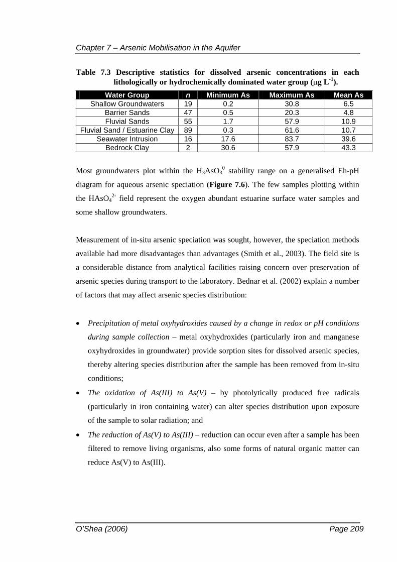
Chapter 7 – Arsenic Mobilisation in the Aquifer
O’Shea (2006) Page 209
Table 7.3 Descriptive statistics for dissolved arsenic concentrations in each lithologically or hydrochemically dominated water group ( g L-1).
Water Group n Minimum As Maximum As Mean As Shallow Groundwaters 19 0.2 30.8 6.5
Barrier Sands 47 0.5 20.3 4.8 Fluvial Sands 55 1.7 57.9 10.9
Fluvial Sand / Estuarine Clay 89 0.3 61.6 10.7 Seawater Intrusion 16 17.6 83.7 39.6
Bedrock Clay 2 30.6 57.9 43.3
Most groundwaters plot within the H3AsO30 stability range on a generalised Eh-pH
diagram for aqueous arsenic speciation (Figure 7.6). The few samples plotting within
the HAsO42- field represent the oxygen abundant estuarine surface water samples and
some shallow groundwaters.
Measurement of in-situ arsenic speciation was sought, however, the speciation methods
available had more disadvantages than advantages (Smith et al., 2003). The field site is
a considerable distance from analytical facilities raising concern over preservation of
arsenic species during transport to the laboratory. Bednar et al. (2002) explain a number
of factors that may affect arsenic species distribution:
Precipitation of metal oxyhydroxides caused by a change in redox or pH conditions
during sample collection – metal oxyhydroxides (particularly iron and manganese
oxyhydroxides in groundwater) provide sorption sites for dissolved arsenic species,
thereby altering species distribution after the sample has been removed from in-situ
conditions;
The oxidation of As(III) to As(V) – by photolytically produced free radicals
(particularly in iron containing water) can alter species distribution upon exposure
of the sample to solar radiation; and
The reduction of As(V) to As(III) – reduction can occur even after a sample has been
filtered to remove living organisms, also some forms of natural organic matter can
reduce As(V) to As(III).
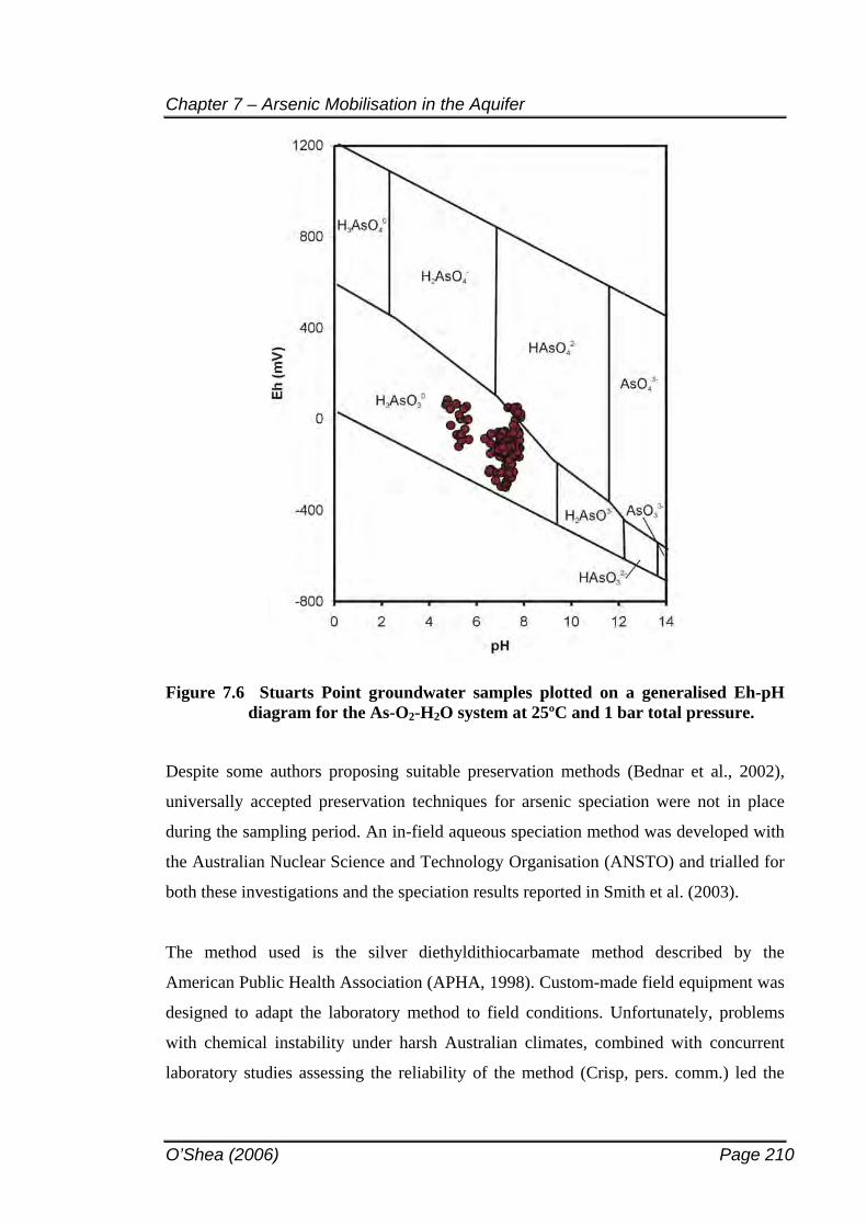
Chapter 7 – Arsenic Mobilisation in the Aquifer
O’Shea (2006) Page 210
Figure 7.6 Stuarts Point groundwater samples plotted on a generalised Eh-pH diagram for the As-O2-H2O system at 25ºC and 1 bar total pressure.
Despite some authors proposing suitable preservation methods (Bednar et al., 2002),
universally accepted preservation techniques for arsenic speciation were not in place
during the sampling period. An in-field aqueous speciation method was developed with
the Australian Nuclear Science and Technology Organisation (ANSTO) and trialled for
both these investigations and the speciation results reported in Smith et al. (2003).
The method used is the silver diethyldithiocarbamate method described by the
American Public Health Association (APHA, 1998). Custom-made field equipment was
designed to adapt the laboratory method to field conditions. Unfortunately, problems
with chemical instability under harsh Australian climates, combined with concurrent
laboratory studies assessing the reliability of the method (Crisp, pers. comm.) led the
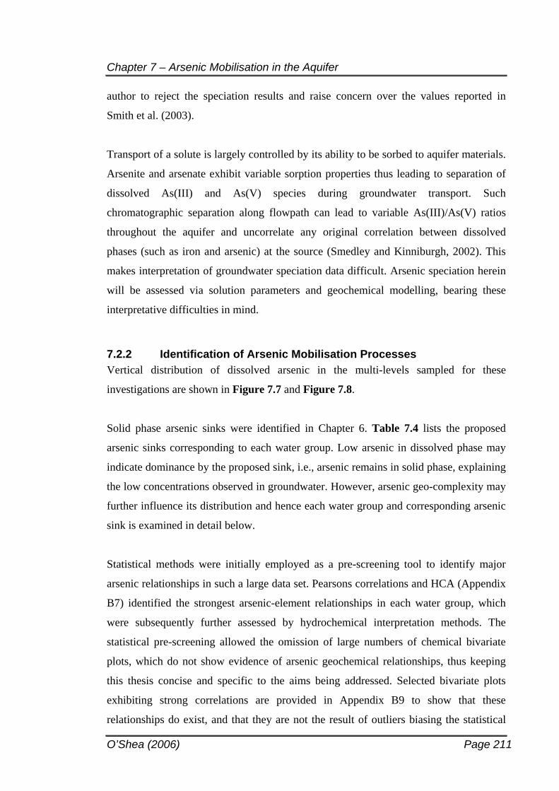
Chapter 7 – Arsenic Mobilisation in the Aquifer
O’Shea (2006) Page 211
author to reject the speciation results and raise concern over the values reported in
Smith et al. (2003).
Transport of a solute is largely controlled by its ability to be sorbed to aquifer materials.
Arsenite and arsenate exhibit variable sorption properties thus leading to separation of
dissolved As(III) and As(V) species during groundwater transport. Such
chromatographic separation along flowpath can lead to variable As(III)/As(V) ratios
throughout the aquifer and uncorrelate any original correlation between dissolved
phases (such as iron and arsenic) at the source (Smedley and Kinniburgh, 2002). This
makes interpretation of groundwater speciation data difficult. Arsenic speciation herein
will be assessed via solution parameters and geochemical modelling, bearing these
interpretative difficulties in mind.
7.2.2 Identification of Arsenic Mobilisation Processes Vertical distribution of dissolved arsenic in the multi-levels sampled for these
investigations are shown in Figure 7.7 and Figure 7.8.
Solid phase arsenic sinks were identified in Chapter 6. Table 7.4 lists the proposed
arsenic sinks corresponding to each water group. Low arsenic in dissolved phase may
indicate dominance by the proposed sink, i.e., arsenic remains in solid phase, explaining
the low concentrations observed in groundwater. However, arsenic geo-complexity may
further influence its distribution and hence each water group and corresponding arsenic
sink is examined in detail below.
Statistical methods were initially employed as a pre-screening tool to identify major
arsenic relationships in such a large data set. Pearsons correlations and HCA (Appendix
B7) identified the strongest arsenic-element relationships in each water group, which
were subsequently further assessed by hydrochemical interpretation methods. The
statistical pre-screening allowed the omission of large numbers of chemical bivariate
plots, which do not show evidence of arsenic geochemical relationships, thus keeping
this thesis concise and specific to the aims being addressed. Selected bivariate plots
exhibiting strong correlations are provided in Appendix B9 to show that these
relationships do exist, and that they are not the result of outliers biasing the statistical

Chapter 7 – Arsenic Mobilisation in the Aquifer
O’Shea (2006) Page 212
result. It should also be noted that a lack of correlation may sometimes be the most
interesting result, such as the lack of correlation between iron and arsenic in the solid
phase of the fluvial sand/estuarine clays (Table 6.4). Calculation of saturation indices
(SI’s) and arsenic speciation was conducted in PHREEQCI. The results for each
separate water group are provided in Appendix B8.
Table 7.4 Proposed mobilisation processes (tested herein) from identified arsenic sinks at Stuarts Point and their influence on arsenic concentrations in groundwater.
Stuarts Point Water Group
Proposed Mobilisation Process from Solid Phase Arsenic Sink
Influence on Dissolved As
Concentrations Shallow
Groundwaters Oxidation of discrete arsenian pyrite and/or
coffee rock at the zone of water table fluctuation
Moderate localised effects
Barrier Sands Potential reductive dissolution or desorption from iron oxide coatings on sand grains
Extremely low concentrations
Fluvial Sands Reductive dissolution from iron oxide coatings on sand grains
Low to moderate concentrations
Fluvial Sand/ Estuarine Clay
Complete reductive dissolution of iron oxides; potential desorption from clays
High
Bedrock Clay Desorption from clay minerals and/or iron oxides
Moderate
SeawaterIntrusion
Suggested aqueous source of arsenic-rich estuarine water into the aquifer
Highest observed concentrations
7.2.2.1 Shallow Groundwaters The shallow groundwaters are characterised by a Cl-SO4-Na signature indicating
contribution by marine dry and wet deposition (Figure 7.9a). The low average pH of
the shallow groundwaters ( pH (shallow groundwaters) = 7.3) suggests iron sulfide oxidation
(equation 7.5) reactions may be contributing acidity, Fe2+ and SO42- in this zone of
groundwater fluctuation (Figure 7.9b, c and d).
FeS2 + 15/4O2 + 7/2H2O Fe(OH)3 + 2SO42- + 4H+ (7.5)
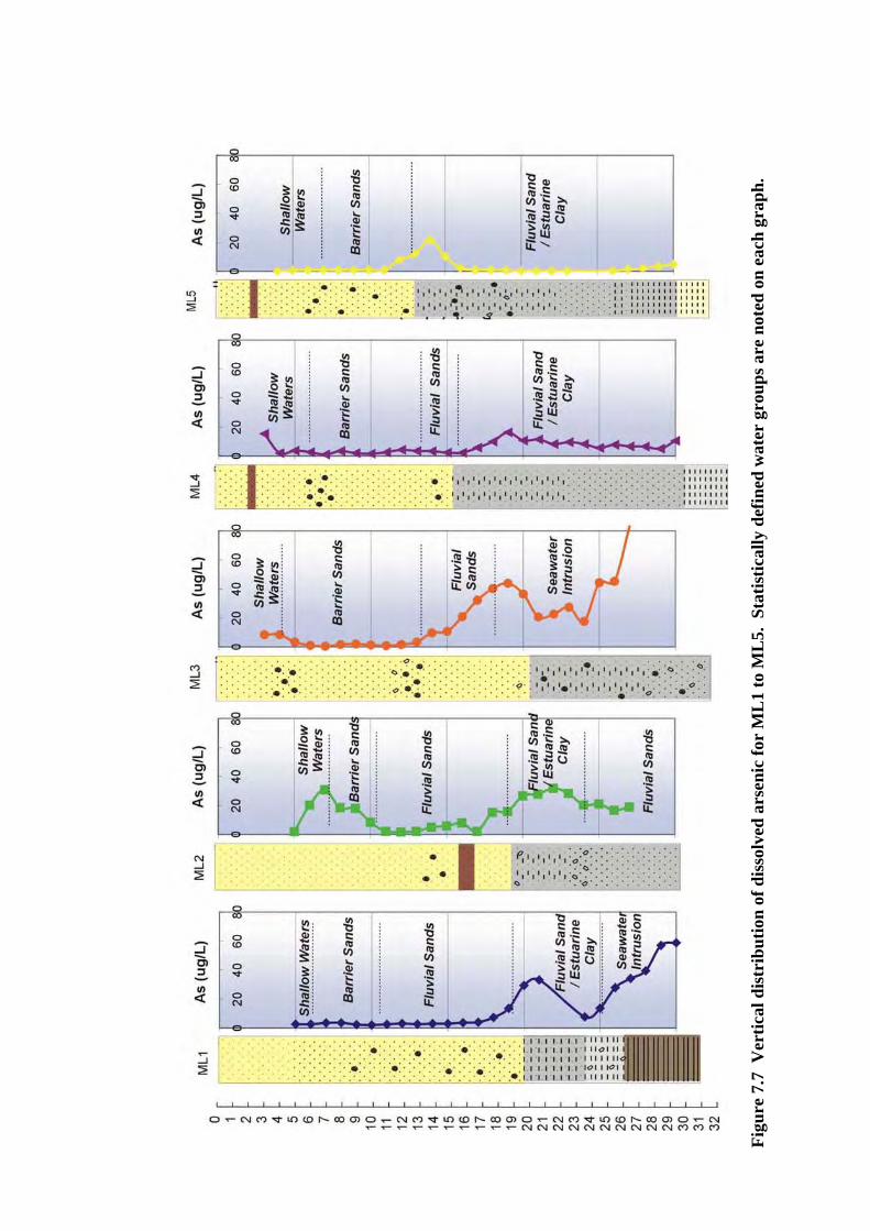
Figu
re 7
.7 V
ertic
al d
istr
ibut
ion
of d
isso
lved
ars
enic
for
ML
1 to
ML
5. S
tatis
tical
ly d
efin
ed w
ater
gro
ups a
re n
oted
on
each
gra
ph.
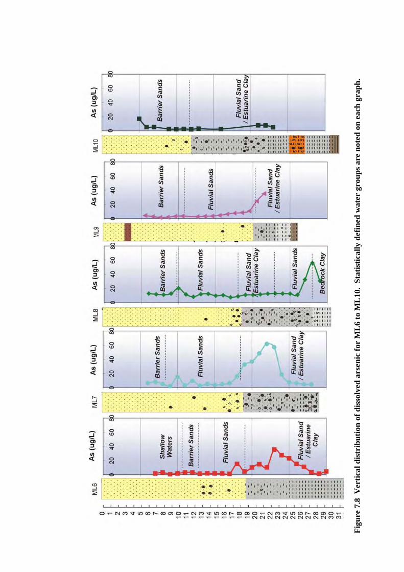
Figu
re 7
.8 V
ertic
al d
istr
ibut
ion
of d
isso
lved
ars
enic
for
ML
6 to
ML
10.
Stat
istic
ally
def
ined
wat
er g
roup
s are
not
ed o
n ea
ch g
raph
.
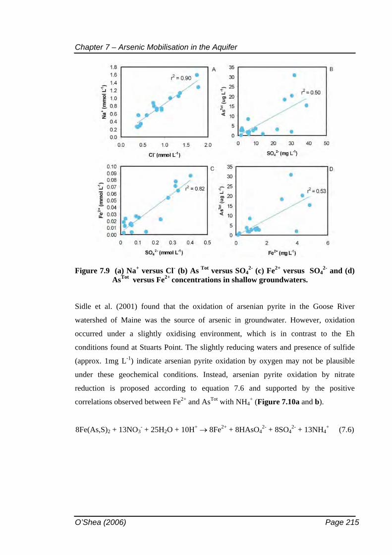
Chapter 7 – Arsenic Mobilisation in the Aquifer
O’Shea (2006) Page 215
Figure 7.9 (a) Na+ versus Cl- (b) As Tot versus SO42- (c) Fe2+ versus SO4
2- and (d) AsTot versus Fe2+ concentrations in shallow groundwaters.
Sidle et al. (2001) found that the oxidation of arsenian pyrite in the Goose River
watershed of Maine was the source of arsenic in groundwater. However, oxidation
occurred under a slightly oxidising environment, which is in contrast to the Eh
conditions found at Stuarts Point. The slightly reducing waters and presence of sulfide
(approx. 1mg L-1) indicate arsenian pyrite oxidation by oxygen may not be plausible
under these geochemical conditions. Instead, arsenian pyrite oxidation by nitrate
reduction is proposed according to equation 7.6 and supported by the positive
correlations observed between Fe2+ and AsTot with NH4+ (Figure 7.10a and b).
8Fe(As,S)2 + 13NO3- + 25H2O + 10H+ 8Fe2+ + 8HAsO4
2- + 8SO42- + 13NH4
+ (7.6)
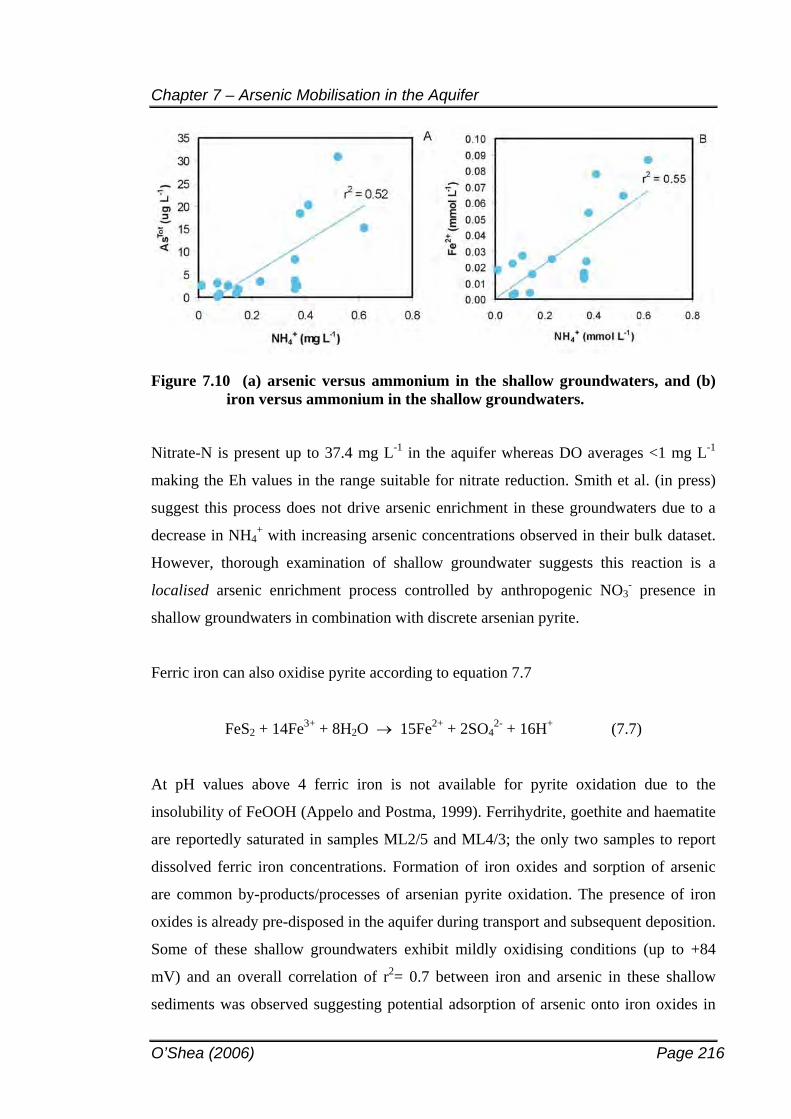
Chapter 7 – Arsenic Mobilisation in the Aquifer
O’Shea (2006) Page 216
Figure 7.10 (a) arsenic versus ammonium in the shallow groundwaters, and (b) iron versus ammonium in the shallow groundwaters.
Nitrate-N is present up to 37.4 mg L-1 in the aquifer whereas DO averages <1 mg L-1
making the Eh values in the range suitable for nitrate reduction. Smith et al. (in press)
suggest this process does not drive arsenic enrichment in these groundwaters due to a
decrease in NH4+ with increasing arsenic concentrations observed in their bulk dataset.
However, thorough examination of shallow groundwater suggests this reaction is a
localised arsenic enrichment process controlled by anthropogenic NO3- presence in
shallow groundwaters in combination with discrete arsenian pyrite.
Ferric iron can also oxidise pyrite according to equation 7.7
FeS2 + 14Fe3+ + 8H2O 15Fe2+ + 2SO42- + 16H+ (7.7)
At pH values above 4 ferric iron is not available for pyrite oxidation due to the
insolubility of FeOOH (Appelo and Postma, 1999). Ferrihydrite, goethite and haematite
are reportedly saturated in samples ML2/5 and ML4/3; the only two samples to report
dissolved ferric iron concentrations. Formation of iron oxides and sorption of arsenic
are common by-products/processes of arsenian pyrite oxidation. The presence of iron
oxides is already pre-disposed in the aquifer during transport and subsequent deposition.
Some of these shallow groundwaters exhibit mildly oxidising conditions (up to +84
mV) and an overall correlation of r2= 0.7 between iron and arsenic in these shallow
sediments was observed suggesting potential adsorption of arsenic onto iron oxides in
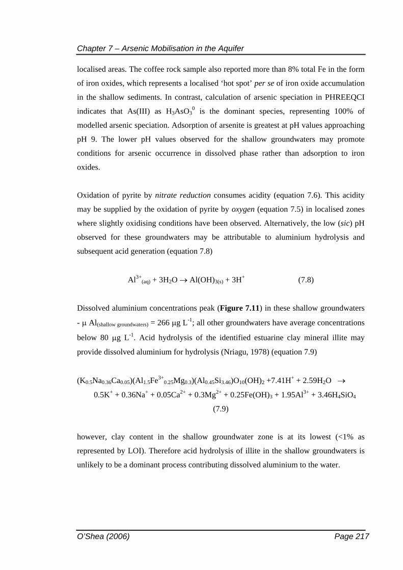
Chapter 7 – Arsenic Mobilisation in the Aquifer
O’Shea (2006) Page 217
localised areas. The coffee rock sample also reported more than 8% total Fe in the form
of iron oxides, which represents a localised ‘hot spot’ per se of iron oxide accumulation
in the shallow sediments. In contrast, calculation of arsenic speciation in PHREEQCI
indicates that As(III) as H3AsO30 is the dominant species, representing 100% of
modelled arsenic speciation. Adsorption of arsenite is greatest at pH values approaching
pH 9. The lower pH values observed for the shallow groundwaters may promote
conditions for arsenic occurrence in dissolved phase rather than adsorption to iron
oxides.
Oxidation of pyrite by nitrate reduction consumes acidity (equation 7.6). This acidity
may be supplied by the oxidation of pyrite by oxygen (equation 7.5) in localised zones
where slightly oxidising conditions have been observed. Alternatively, the low (sic) pH
observed for these groundwaters may be attributable to aluminium hydrolysis and
subsequent acid generation (equation 7.8)
Al3+(aq) + 3H2O Al(OH)3(s) + 3H+ (7.8)
Dissolved aluminium concentrations peak (Figure 7.11) in these shallow groundwaters
- Al(shallow groundwaters) = 266 g L-1; all other groundwaters have average concentrations
below 80 g L-1. Acid hydrolysis of the identified estuarine clay mineral illite may
provide dissolved aluminium for hydrolysis (Nriagu, 1978) (equation 7.9)
(K0.5Na0.36Ca0.05)(Al1.5Fe3+0.25Mg0.3)(Al0.45Si3.46)O10(OH)2 +7.41H+ + 2.59H2O
0.5K+ + 0.36Na+ + 0.05Ca2+ + 0.3Mg2+ + 0.25Fe(OH)3 + 1.95Al3+ + 3.46H4SiO4
(7.9)
however, clay content in the shallow groundwater zone is at its lowest (<1% as
represented by LOI). Therefore acid hydrolysis of illite in the shallow groundwaters is
unlikely to be a dominant process contributing dissolved aluminium to the water.
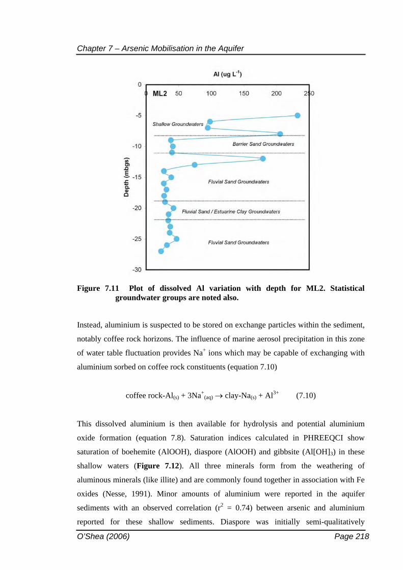
Chapter 7 – Arsenic Mobilisation in the Aquifer
O’Shea (2006) Page 218
Figure 7.11 Plot of dissolved Al variation with depth for ML2. Statistical groundwater groups are noted also.
Instead, aluminium is suspected to be stored on exchange particles within the sediment,
notably coffee rock horizons. The influence of marine aerosol precipitation in this zone
of water table fluctuation provides Na+ ions which may be capable of exchanging with
aluminium sorbed on coffee rock constituents (equation 7.10)
coffee rock-Al(s) + 3Na+(aq) clay-Na(s) + Al3+ (7.10)
This dissolved aluminium is then available for hydrolysis and potential aluminium
oxide formation (equation 7.8). Saturation indices calculated in PHREEQCI show
saturation of boehemite (AlOOH), diaspore (AlOOH) and gibbsite (Al[OH]3) in these
shallow waters (Figure 7.12). All three minerals form from the weathering of
aluminous minerals (like illite) and are commonly found together in association with Fe
oxides (Nesse, 1991). Minor amounts of aluminium were reported in the aquifer
sediments with an observed correlation (r2 = 0.74) between arsenic and aluminium
reported for these shallow sediments. Diaspore was initially semi-qualitatively
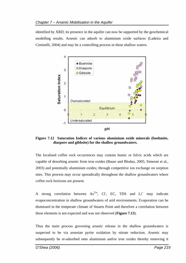
Chapter 7 – Arsenic Mobilisation in the Aquifer
O’Shea (2006) Page 219
identified by XRD; its presence in the aquifer can now be supported by the geochemical
modelling results. Arsenic can adsorb to aluminium oxide surfaces (Ladeira and
Ciminelli, 2004) and may be a controlling process in these shallow waters.
Figure 7.12 Saturation Indices of various aluminium oxide minerals (boehmite, diaspore and gibbsite) for the shallow groundwaters.
The localised coffee rock occurrences may contain humic or fulvic acids which are
capable of desorbing arsenic from iron oxides (Bauer and Blodau, 2005; Simeoni et al.,
2003) and potentially aluminium oxides; through competitive ion exchange on sorption
sites. This process may occur sporadically throughout the shallow groundwaters where
coffee rock horizons are present.
A strong correlation between AsTot, Cl-, EC, TDS and Li+ may indicate
evapoconcentration in shallow groundwaters of arid environments. Evaporation can be
dismissed in the temperate climate of Stuarts Point and therefore a correlation between
these elements is not expected and was not observed (Figure 7.13).
Thus the main process governing arsenic release in the shallow groundwaters is
suspected to be via arsenian pyrite oxidation by nitrate reduction. Arsenic may
subsequently be re-adsorbed onto aluminium and/or iron oxides thereby removing it
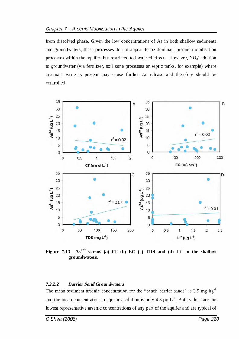
Chapter 7 – Arsenic Mobilisation in the Aquifer
O’Shea (2006) Page 220
from dissolved phase. Given the low concentrations of As in both shallow sediments
and groundwaters, these processes do not appear to be dominant arsenic mobilisation
processes within the aquifer, but restricted to localised effects. However, NO3- addition
to groundwater (via fertilizer, soil zone processes or septic tanks, for example) where
arsenian pyrite is present may cause further As release and therefore should be
controlled.
Figure 7.13 AsTot versus (a) Cl- (b) EC (c) TDS and (d) Li+ in the shallow groundwaters.
7.2.2.2 Barrier Sand Groundwaters The mean sediment arsenic concentration for the “beach barrier sands” is 3.9 mg kg-1
and the mean concentration in aqueous solution is only 4.8 g L-1. Both values are the
lowest representative arsenic concentrations of any part of the aquifer and are typical of
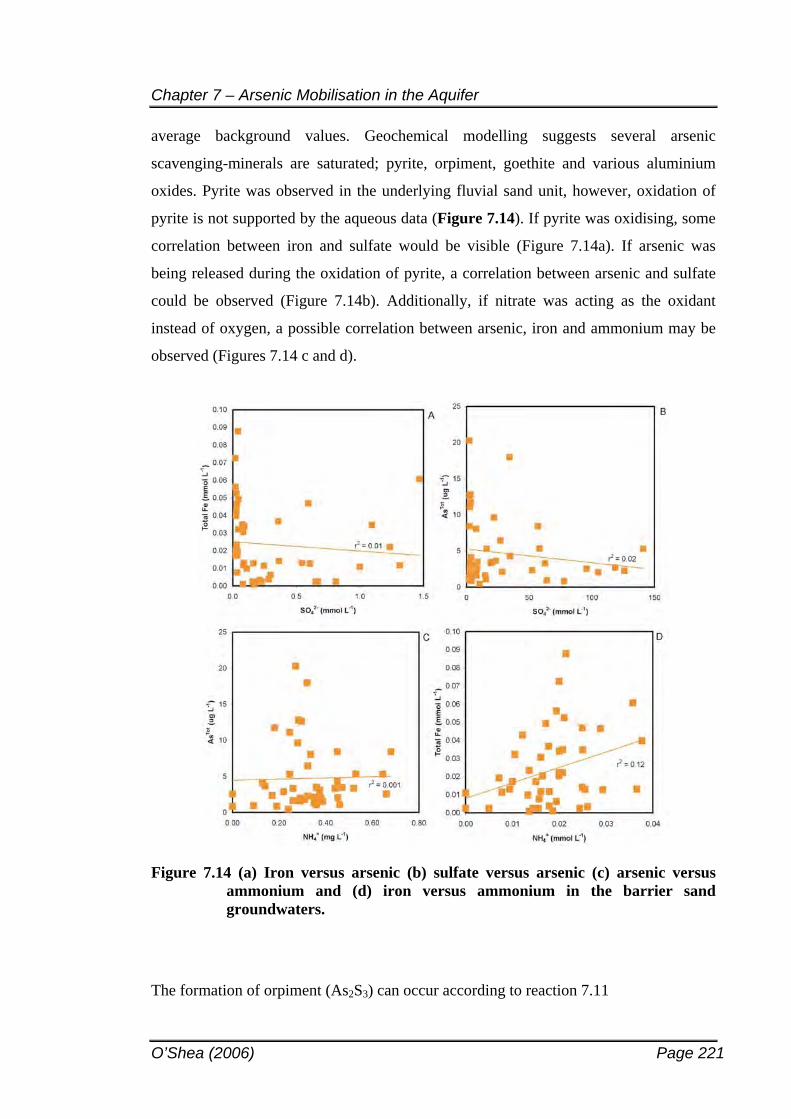
Chapter 7 – Arsenic Mobilisation in the Aquifer
O’Shea (2006) Page 221
average background values. Geochemical modelling suggests several arsenic
scavenging-minerals are saturated; pyrite, orpiment, goethite and various aluminium
oxides. Pyrite was observed in the underlying fluvial sand unit, however, oxidation of
pyrite is not supported by the aqueous data (Figure 7.14). If pyrite was oxidising, some
correlation between iron and sulfate would be visible (Figure 7.14a). If arsenic was
being released during the oxidation of pyrite, a correlation between arsenic and sulfate
could be observed (Figure 7.14b). Additionally, if nitrate was acting as the oxidant
instead of oxygen, a possible correlation between arsenic, iron and ammonium may be
observed (Figures 7.14 c and d).
Figure 7.14 (a) Iron versus arsenic (b) sulfate versus arsenic (c) arsenic versus ammonium and (d) iron versus ammonium in the barrier sand groundwaters.
The formation of orpiment (As2S3) can occur according to reaction 7.11
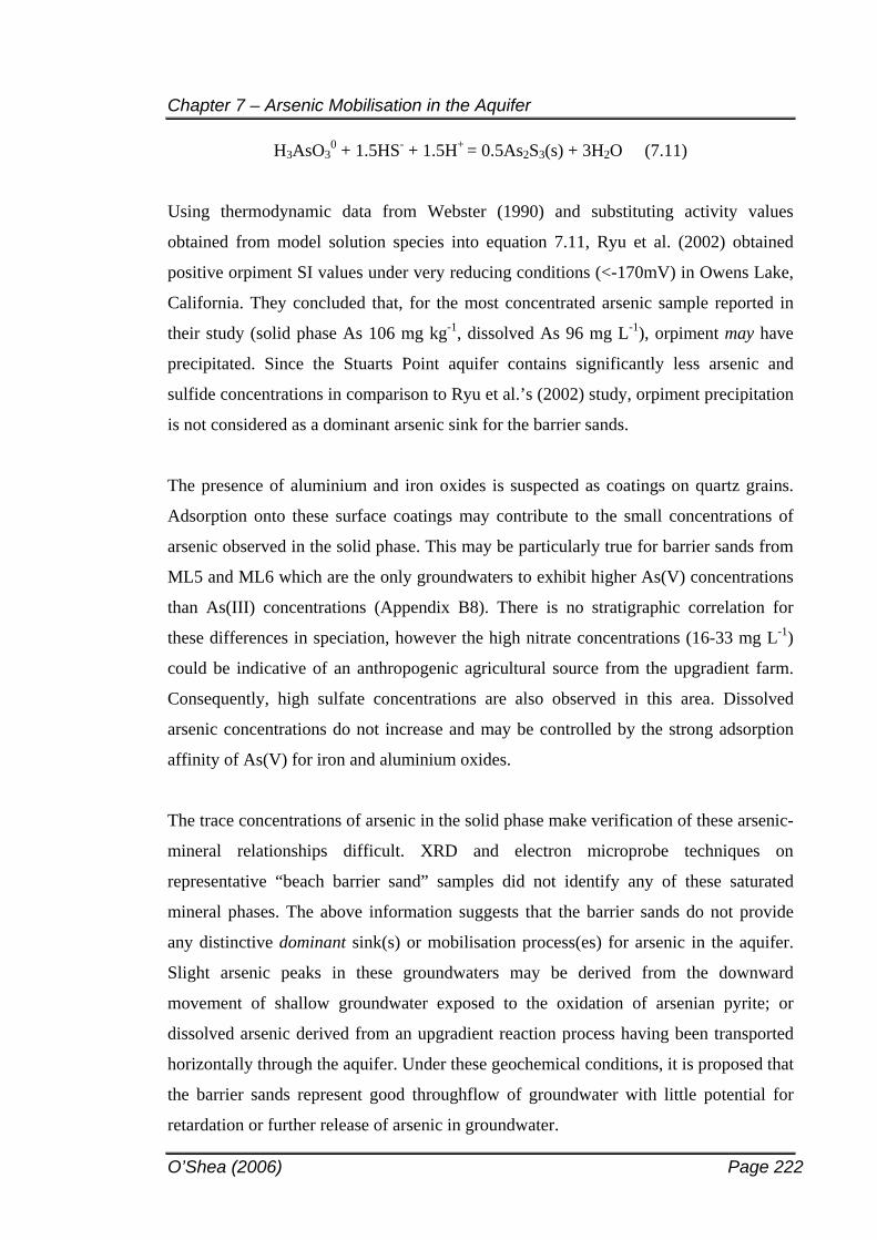
Chapter 7 – Arsenic Mobilisation in the Aquifer
O’Shea (2006) Page 222
H3AsO30 + 1.5HS- + 1.5H+ = 0.5As2S3(s) + 3H2O (7.11)
Using thermodynamic data from Webster (1990) and substituting activity values
obtained from model solution species into equation 7.11, Ryu et al. (2002) obtained
positive orpiment SI values under very reducing conditions (<-170mV) in Owens Lake,
California. They concluded that, for the most concentrated arsenic sample reported in
their study (solid phase As 106 mg kg-1, dissolved As 96 mg L-1), orpiment may have
precipitated. Since the Stuarts Point aquifer contains significantly less arsenic and
sulfide concentrations in comparison to Ryu et al.’s (2002) study, orpiment precipitation
is not considered as a dominant arsenic sink for the barrier sands.
The presence of aluminium and iron oxides is suspected as coatings on quartz grains.
Adsorption onto these surface coatings may contribute to the small concentrations of
arsenic observed in the solid phase. This may be particularly true for barrier sands from
ML5 and ML6 which are the only groundwaters to exhibit higher As(V) concentrations
than As(III) concentrations (Appendix B8). There is no stratigraphic correlation for
these differences in speciation, however the high nitrate concentrations (16-33 mg L-1)
could be indicative of an anthropogenic agricultural source from the upgradient farm.
Consequently, high sulfate concentrations are also observed in this area. Dissolved
arsenic concentrations do not increase and may be controlled by the strong adsorption
affinity of As(V) for iron and aluminium oxides.
The trace concentrations of arsenic in the solid phase make verification of these arsenic-
mineral relationships difficult. XRD and electron microprobe techniques on
representative “beach barrier sand” samples did not identify any of these saturated
mineral phases. The above information suggests that the barrier sands do not provide
any distinctive dominant sink(s) or mobilisation process(es) for arsenic in the aquifer.
Slight arsenic peaks in these groundwaters may be derived from the downward
movement of shallow groundwater exposed to the oxidation of arsenian pyrite; or
dissolved arsenic derived from an upgradient reaction process having been transported
horizontally through the aquifer. Under these geochemical conditions, it is proposed that
the barrier sands represent good throughflow of groundwater with little potential for
retardation or further release of arsenic in groundwater.
Chapter 7 – Arsenic Mobilisation in the Aquifer
O’Shea (2006) Page 223
7.2.2.3 Fluvial Sand Groundwaters An extremely strong correlation (r2 = 0.93) was observed between arsenic and total iron
in the “fluvial sand” sediments, thus leading the investigation towards the possibility of
arsenic sorption processes with iron oxides. Tareq et al. (2003) observed the opposite; a
very weak relationship between arsenic and total iron in Bangladeshi sediments was
attributed to the potential presence of insoluble Fe-silicates and minerals rather than Fe-
(hydr)oxides. However, they did report a good correlation (r2 = 0.68) between arsenic
and easily reducible iron in the sediments, indicating that arsenic may be associated
primarily with the amorphous iron oxide phase.
The excellent correlation between total iron and arsenic at Stuarts Point may indicate
dominance of iron oxide minerals rather than insoluble iron minerals. Oxides, rather
than any other iron-bearing minerals, were examined initially due to the orange-brown
colour of these sands which is often associated with their presence. Saturation Indices
calculated for the fluvial sand groundwaters indicate spatially variable saturation of
several iron oxide minerals; ferrihydrite, hematite, goethite, ferrosic hydroxide
(Fe3[OH]8)2 and lepidocrocite (FeOOH). Concentrations of dissolved ferric iron range
from 0 - 1.94 mg L-1 Fe3+ however ferrous iron concentrations are consistently higher
(up to 4.25 mg L-1 Fe2+) owing to the reducing nature of these waters (Eh (fluvial sand
groundwaters) range is –62 to –207 mV). Reductive dissolution of iron oxides and release of
bound arsenic has been proposed by several authors as the dominant mechanism of
arsenic release in Bangladeshi groundwaters (McArthur et al., 2004; Ravenscroft et al.,
2001; Nickson et al., 2000; Anawar et al., 2003; Tareq et al., 2003). The reaction is
catalysed by natural organic matter (equation 7.12),
8FeOOH + CH3COOH + 14H2CO3 8Fe2+ + 16HCO3- + 12H2O (7.12)
which promotes dissolution of the iron oxide and the subsequent release of any sorbed
arsenic. Differentiating between reductive dissolution and desorption from iron oxides
can be ambiguous under in-situ conditions. In a laboratory study by Guo et al. (1997)
arsenic was rapidly released after reductive dissolution of iron oxides suggesting it was
2 Langmuir (1997) reports that the infrequent identification of ferrosic hydroxide in nature may imply that the tabulated free energy of the phase is too negative.
Chapter 7 – Arsenic Mobilisation in the Aquifer
O’Shea (2006) Page 224
dissolution rather than desorption governing arsenic mobility or that they occurred
simultaneously. Without such laboratory studies on the natural aquifer matrix, the
feasibility of iron oxide dissolution and/or desorption processes is best assessed by
examining solution pH, arsenic speciation and the relationship between Fe, HCO3- and
As concentrations in groundwater.
A good correlation between dissolved iron and bicarbonate in groundwater might be
expected if iron oxide dissolution is occurring (Figure 7.15a). Both ions, however, are
involved in other common geochemical reaction processes (e.g. silicate weathering, iron
sulfide precipitation) which may affect their concentrations in dissolved phase thereby
altering the expected relationship between the two ions. Iron oxides in the form of
ferrihydrite and goethite were both observed via SEM. A correlation between As and
HCO3- could also indicate arsenic release from iron oxide dissolution, however, the
addition of considerable amounts of HCO3- from calcite dissolution is one process
expected to mask this potential correlation (Figure 7.15b). Focussing instead on a
potential correlation between iron and arsenic (Figure 7.15c) does not provide any
additional clarity on the likelihood of iron oxide dissolution dominating arsenic
mobilisation. Both elements are highly susceptible to redistribution in separate mineral
phases thus altering any original correlation between the two elements. However, one
explanation is presented. Where total Fe concentrations are >0.03 mmol L-1 they are in
good correlation with HCO3- concentrations (Figure 7.15a) suggesting iron oxide
dissolution and potential arsenic release for these samples, yet Figure 7.15c indicates
arsenic concentrations are subsequently lower in these samples (i.e., As concentrations
are lowest when total iron concentrations are highest). This suggests that arsenic may be
re-adsorbed to freshly exposed iron oxide surfaces that have recently been dissolved, or
to other iron oxides in the aquifer which have not yet been dissolved. Arsenic
adsorption processes are considered to be rapid (Goh and Lim, 2004). The presence of
brown sediments in this unit supports the residence of iron oxides that have not yet been
dissolved; as does the optimum Eh range shown in Figure 7.15d. Arsenic
concentrations are highest from –50 to –150 mV before the onset of more reducing
conditions. These Eh conditions are more likely to be sulfate reducing waters and hence
conducive to arsenian pyrite formation, which will be further discussed shortly.
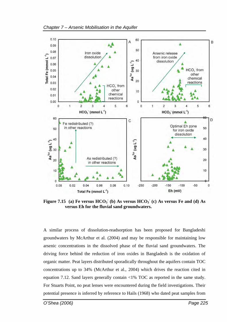
Chapter 7 – Arsenic Mobilisation in the Aquifer
O’Shea (2006) Page 225
Figure 7.15 (a) Fe versus HCO3- (b) As versus HCO3
- (c) As versus Fe and (d) As versus Eh for the fluvial sand groundwaters.
A similar process of dissolution-readsorption has been proposed for Bangladeshi
groundwaters by McArthur et al. (2004) and may be responsible for maintaining low
arsenic concentrations in the dissolved phase of the fluvial sand groundwaters. The
driving force behind the reduction of iron oxides in Bangladesh is the oxidation of
organic matter. Peat layers distributed sporadically throughout the aquifers contain TOC
concentrations up to 34% (McArthur et al., 2004) which drives the reaction cited in
equation 7.12. Sand layers generally contain <1% TOC as reported in the same study.
For Stuarts Point, no peat lenses were encountered during the field investigations. Their
potential presence is inferred by reference to Hails (1968) who dated peat samples from
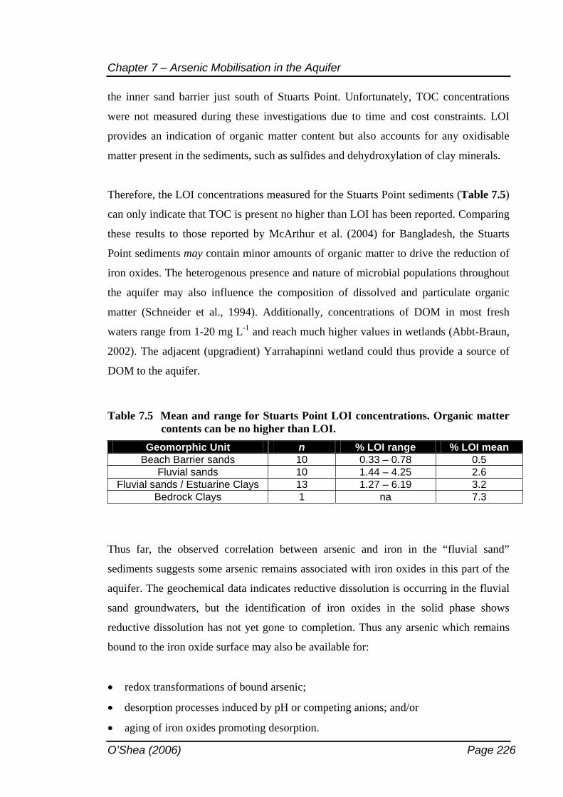
Chapter 7 – Arsenic Mobilisation in the Aquifer
O’Shea (2006) Page 226
the inner sand barrier just south of Stuarts Point. Unfortunately, TOC concentrations
were not measured during these investigations due to time and cost constraints. LOI
provides an indication of organic matter content but also accounts for any oxidisable
matter present in the sediments, such as sulfides and dehydroxylation of clay minerals.
Therefore, the LOI concentrations measured for the Stuarts Point sediments (Table 7.5)
can only indicate that TOC is present no higher than LOI has been reported. Comparing
these results to those reported by McArthur et al. (2004) for Bangladesh, the Stuarts
Point sediments may contain minor amounts of organic matter to drive the reduction of
iron oxides. The heterogenous presence and nature of microbial populations throughout
the aquifer may also influence the composition of dissolved and particulate organic
matter (Schneider et al., 1994). Additionally, concentrations of DOM in most fresh
waters range from 1-20 mg L-1 and reach much higher values in wetlands (Abbt-Braun,
2002). The adjacent (upgradient) Yarrahapinni wetland could thus provide a source of
DOM to the aquifer.
Table 7.5 Mean and range for Stuarts Point LOI concentrations. Organic matter contents can be no higher than LOI.
Geomorphic Unit n % LOI range % LOI mean Beach Barrier sands 10 0.33 – 0.78 0.5
Fluvial sands 10 1.44 – 4.25 2.6 Fluvial sands / Estuarine Clays 13 1.27 – 6.19 3.2
Bedrock Clays 1 na 7.3
Thus far, the observed correlation between arsenic and iron in the “fluvial sand”
sediments suggests some arsenic remains associated with iron oxides in this part of the
aquifer. The geochemical data indicates reductive dissolution is occurring in the fluvial
sand groundwaters, but the identification of iron oxides in the solid phase shows
reductive dissolution has not yet gone to completion. Thus any arsenic which remains
bound to the iron oxide surface may also be available for:
redox transformations of bound arsenic;
desorption processes induced by pH or competing anions; and/or
aging of iron oxides promoting desorption.
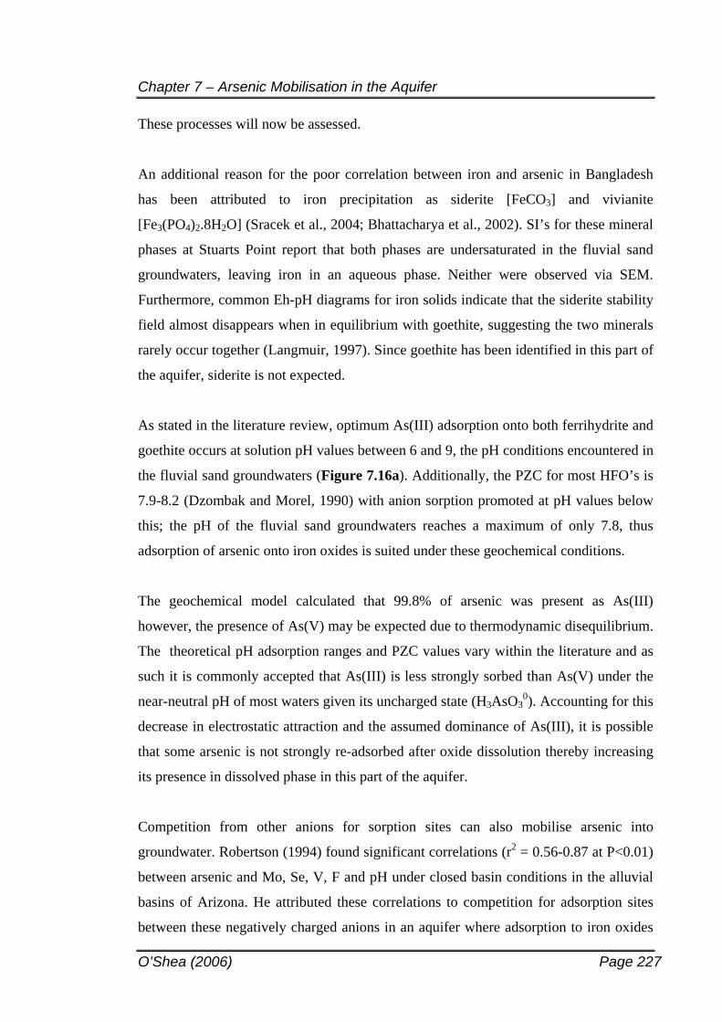
Chapter 7 – Arsenic Mobilisation in the Aquifer
O’Shea (2006) Page 227
These processes will now be assessed.
An additional reason for the poor correlation between iron and arsenic in Bangladesh
has been attributed to iron precipitation as siderite [FeCO3] and vivianite
[Fe3(PO4)2.8H2O] (Sracek et al., 2004; Bhattacharya et al., 2002). SI’s for these mineral
phases at Stuarts Point report that both phases are undersaturated in the fluvial sand
groundwaters, leaving iron in an aqueous phase. Neither were observed via SEM.
Furthermore, common Eh-pH diagrams for iron solids indicate that the siderite stability
field almost disappears when in equilibrium with goethite, suggesting the two minerals
rarely occur together (Langmuir, 1997). Since goethite has been identified in this part of
the aquifer, siderite is not expected.
As stated in the literature review, optimum As(III) adsorption onto both ferrihydrite and
goethite occurs at solution pH values between 6 and 9, the pH conditions encountered in
the fluvial sand groundwaters (Figure 7.16a). Additionally, the PZC for most HFO’s is
7.9-8.2 (Dzombak and Morel, 1990) with anion sorption promoted at pH values below
this; the pH of the fluvial sand groundwaters reaches a maximum of only 7.8, thus
adsorption of arsenic onto iron oxides is suited under these geochemical conditions.
The geochemical model calculated that 99.8% of arsenic was present as As(III)
however, the presence of As(V) may be expected due to thermodynamic disequilibrium.
The theoretical pH adsorption ranges and PZC values vary within the literature and as
such it is commonly accepted that As(III) is less strongly sorbed than As(V) under the
near-neutral pH of most waters given its uncharged state (H3AsO30). Accounting for this
decrease in electrostatic attraction and the assumed dominance of As(III), it is possible
that some arsenic is not strongly re-adsorbed after oxide dissolution thereby increasing
its presence in dissolved phase in this part of the aquifer.
Competition from other anions for sorption sites can also mobilise arsenic into
groundwater. Robertson (1994) found significant correlations (r2 = 0.56-0.87 at P<0.01)
between arsenic and Mo, Se, V, F and pH under closed basin conditions in the alluvial
basins of Arizona. He attributed these correlations to competition for adsorption sites
between these negatively charged anions in an aquifer where adsorption to iron oxides
Chapter 7 – Arsenic Mobilisation in the Aquifer
O’Shea (2006) Page 228
was the dominant arsenic control. However, instead of replacing anions on adsorption
sites, the positive correlations observed by Robertson (1994) indicate that the chemical
similarity of these anions allowed them to be controlled (i.e., adsorbed) in a similar
manner. If adsorption sites become full, a negative correlation may be observed as
anions begin replacing other sorbed anions and releasing them into dissolved phase.
Phosphate is often examined due to its high negative charge and common occurrence in
groundwaters. Smith et al. (2002) found that PO43- presence significantly decreased
As(V) adsorption onto soils containing low amounts of Fe oxides, similar to the Stuarts
Point Fe oxide abundance. With As(V) concentrations assumed to be negligible in the
fluvial sand groundwaters, the effect of PO43- competition with As(III) is of more
concern. Goh and Lim (2004) found that PO43- had a more profound effect on sorption
capacity of both As(III) and As(V), when compared to the sorption competition from
other anions.
The poor correlation observed between arsenic and PO43- (Figure 7.16b) does not
support extensive competitive exchange between these two anions. Molybdenum and
arsenic concentrations exhibit a better correlation (Figure 7.16c) indicative of potential
for adsorption to the same sites, rather than competitive exchange processes. Indeed,
molybdate (MoO42-) has been found to inhibit arsenic adsorption onto mineral surfaces
(Manning and Goldberg, 1996). However, this relationship is expected to stem from the
surrounding molybdenite mineralisation, which has previously been shown to exhibit
arsenic as an associated element. Other common anions (Cr, V and U - Figure 7.16d-f)
show no apparent relationship with dissolved arsenic concentrations dismissing the
dominance of competitive interaction between arsenic and other anions.
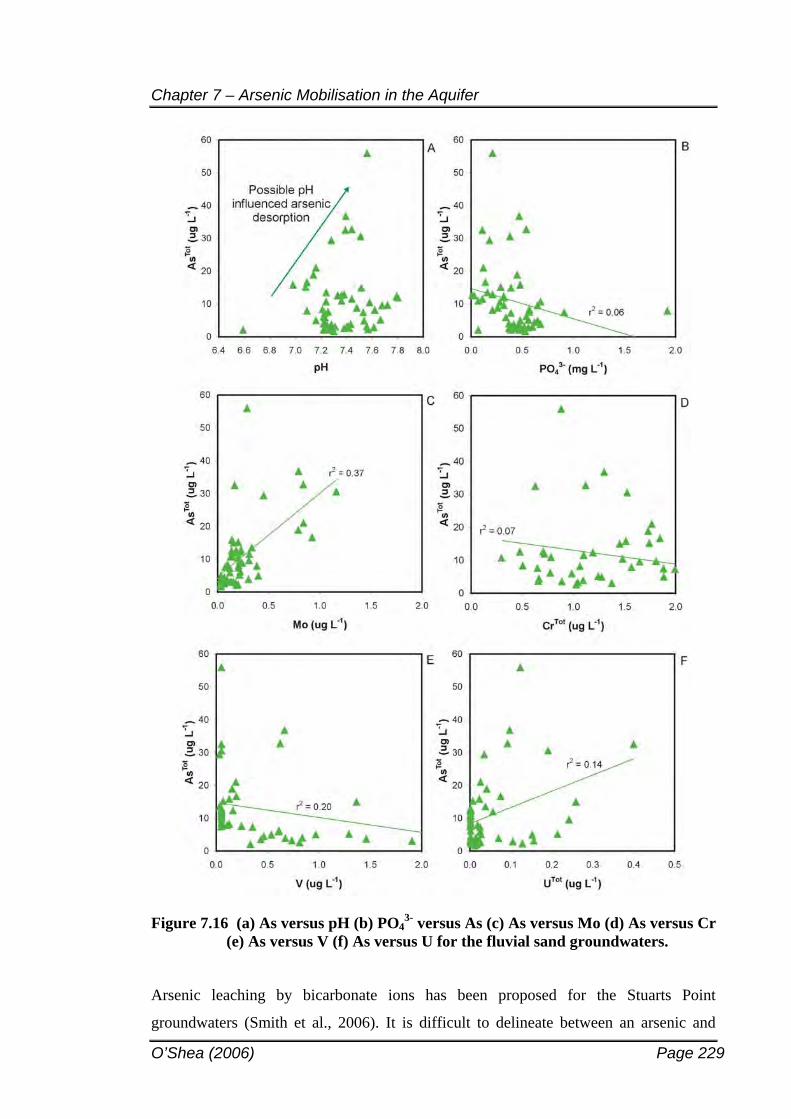
Chapter 7 – Arsenic Mobilisation in the Aquifer
O’Shea (2006) Page 229
Figure 7.16 (a) As versus pH (b) PO43- versus As (c) As versus Mo (d) As versus Cr
(e) As versus V (f) As versus U for the fluvial sand groundwaters.
Arsenic leaching by bicarbonate ions has been proposed for the Stuarts Point
groundwaters (Smith et al., 2006). It is difficult to delineate between an arsenic and
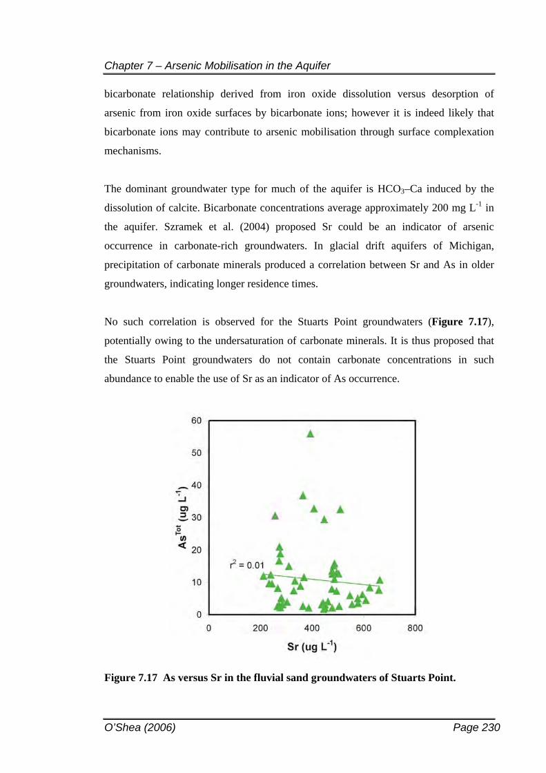
Chapter 7 – Arsenic Mobilisation in the Aquifer
O’Shea (2006) Page 230
bicarbonate relationship derived from iron oxide dissolution versus desorption of
arsenic from iron oxide surfaces by bicarbonate ions; however it is indeed likely that
bicarbonate ions may contribute to arsenic mobilisation through surface complexation
mechanisms.
The dominant groundwater type for much of the aquifer is HCO3–Ca induced by the
dissolution of calcite. Bicarbonate concentrations average approximately 200 mg L-1 in
the aquifer. Szramek et al. (2004) proposed Sr could be an indicator of arsenic
occurrence in carbonate-rich groundwaters. In glacial drift aquifers of Michigan,
precipitation of carbonate minerals produced a correlation between Sr and As in older
groundwaters, indicating longer residence times.
No such correlation is observed for the Stuarts Point groundwaters (Figure 7.17),
potentially owing to the undersaturation of carbonate minerals. It is thus proposed that
the Stuarts Point groundwaters do not contain carbonate concentrations in such
abundance to enable the use of Sr as an indicator of As occurrence.
Figure 7.17 As versus Sr in the fluvial sand groundwaters of Stuarts Point.
Chapter 7 – Arsenic Mobilisation in the Aquifer
O’Shea (2006) Page 231
Both aging of iron oxides and changes to the speciation of sorbed arsenic can promote
desorption. The aging of iron oxides leads to a loss in surface area when crystallisation
occurs (Frau and Ardau, 2004) and thus a loss in specific sorption sites. The
identification of both amorphous and crystalline iron oxides via SEM indicates iron
oxide crystallisation is a potential arsenic release mechanism in the aquifer. In addition,
with the onset of reducing conditions, any surface bound arsenic present as As(V) due
to redox disequilibrium, may be reduced to As(III) and subsequently mobilised.
Additionally, the formation of arsenian pyrite (solid phase arsenic and sulfur correlation
reported as r2 = 0.78 for the “fluvial sands”) may be occurring and will be discussed in
detail below. These processes are expected to contribute minor amounts of arsenic to the
fluvial sand groundwater and be overshadowed by the dominance of arsenic release
from reductive iron dissolution.
7.2.2.4 Fluvial Sand / Estuarine Clay Groundwaters The transition from “fluvial sand” to “fluvial sand / estuarine clay” is marked by a
change in sediment colour from orange/brown/red to olive green/grey. Often this change
in sediment colour is due to the disappearance of iron oxide minerals, which are
characteristically orange/brown/red. It can also be associated with a concurrent change
in redox potential from oxidising to reducing. The fluvial sand / estuarine clay
groundwaters show an increase in measured aqueous Eh ranging from –53 to –235 mV.
These geochemical conditions promote the complete dissolution of iron oxides, thereby
removing the potential for arsenic re-adsorption to fresh iron oxide surfaces. The
extremely strong correlation between iron and arsenic (r2 = 0.93) observed in the
overlying “fluvial sand” sediments is non-existent for the “fluvial sand / estuarine clay”
unit (r2 = 0.01). With the removal of iron oxide minerals for re-adsorption, arsenic
should remain in dissolved phase.
This process was observed by McArthur et al. (2004) for Bangladeshi groundwaters and
sediments. Where arsenic concentrations were >50 g L-1 reduction had gone to
completion and the sediments changed from brown to grey in colour. An increase in
dissolved arsenic in the fluvial sand / estuarine clay zone is noted for many of the
vertical profiles shown in Figure 7.7 and Figure 7.8. The average arsenic concentration
Chapter 7 – Arsenic Mobilisation in the Aquifer
O’Shea (2006) Page 232
is 12.4 g L-1 but ranges from 0.3 – 61.9 g L-1. This is only a minor increase in
dissolved arsenic. However, sediment concentrations average 8 mg kg-1 which is also an
increase from 6.6 mg kg-1 As observed in the overlying “fluvial sand” unit. It appears
that an additional arsenic sink may be controlling arsenic distribution in this part of the
aquifer.
The presence of dissolved arsenic (0.30 – 61.9 g L-1), ferrous iron (0.14 – 3.88 mg L-
1), sulfide (0.0 – 2.85 mg L-1), reducing conditions (-53 to –235 mV) and the
identification of arsenian pyrite in this groundwater zone directs the interpretation
towards the likelihood of iron-(arsenic)-sulfide mineral formation and its resulting
stability under these geochemical conditions. The following questions are raised in this
discussion:
Are conditions currently suitable for arsenian pyrite formation in-situ? Alternatively,
Have conditions in the past been suitable for arsenian pyrite formation in-situ? Or,
Has the arsenian pyrite been transported from its original place of formation, i.e.
associated with mineralisation in the upper catchment?
Substantial evidence supporting either the first or second questions will confirm the role
of arsenian pyrite as a sink for arsenic, while confirmation of the third point would
consider it as a source of arsenic to the aquifer.
Geochemical modelling results indicate that pyrite is currently oversaturated in 93% of
the fluvial sand / estuarine clay groundwaters (Figure 7.18). With the presence of
dissolved arsenic already explained via the recent release from iron oxide dissolution,
arsenic may indeed be present in the groundwater for isomorphic substitution of sulfur
in the pyrite lattice. The formation of pyrite can be a complex process; Langmuir (1997)
notes that it does not simply precipitate directly from solution, rather it forms from the
successive sulfidation of a series of metastable Fe(II) sulfides. Schoonen and Barnes
(1991a; 1991b) list these sulfide sequences in more detail. Figure 7.19 shows
generalised pathways of pyrite formation, also described in equation 7.13
4SO42- + Fe2O3 + 8CH2O 2FeS2 + 8HCO3
- + 4H2O (7.13)
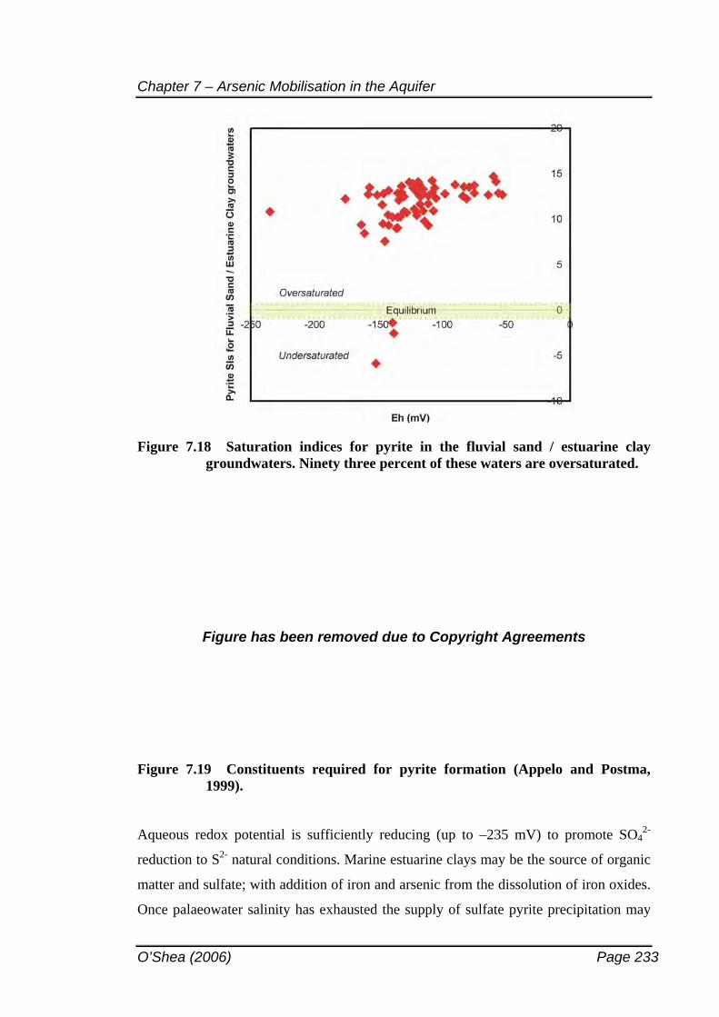
Chapter 7 – Arsenic Mobilisation in the Aquifer
O’Shea (2006) Page 233
Figure 7.18 Saturation indices for pyrite in the fluvial sand / estuarine clay groundwaters. Ninety three percent of these waters are oversaturated.
Figure has been removed due to Copyright Agreements
Figure 7.19 Constituents required for pyrite formation (Appelo and Postma, 1999).
Aqueous redox potential is sufficiently reducing (up to –235 mV) to promote SO42-
reduction to S2- natural conditions. Marine estuarine clays may be the source of organic
matter and sulfate; with addition of iron and arsenic from the dissolution of iron oxides.
Once palaeowater salinity has exhausted the supply of sulfate pyrite precipitation may
Chapter 7 – Arsenic Mobilisation in the Aquifer
O’Shea (2006) Page 234
be limited. As suggested in Figure 7.19 this process is bacterially mediated and is the
subject of much current research (Oremland and Stolz, 2005).
With the establishment that current geochemical conditions may be suitable for arsenian
pyrite formation, the possibility of past conditions forming pyrite (i.e., seawater
inundation of the aquifer during transgressions) do not need to be addressed in order to
define the likelihood of an in-situ formation of an arsenic sink. An alternate possibility
is the arsenian pyrite with its associated lead (and other potentially unknown trace
elements) could have formed in close proximity to a mineralised source in the upper
catchment and been transported by fluvial processes for later deposition. Detrital sulfide
minerals do not usually persist in the environment during erosion and transportation due
to oxidation processes. Craw and Chappell (1999) provide an example where such
detrital sulfide grains do persist – as a result of rapid erosion and transport providing
chemically immature sediments faster than oxidation can occur. In their investigation,
sediments are locally derived from arsenopyrite/pyrite metasediments within a few
hundred metres of their source; the Hyde-Macraes Shear Zone in New Zealand.
However, the length of transport via the Macleay River is in the order of kilometres, and
as such, preservation of discrete sulfide minerals over long distances is not likely at
Stuarts Point. Lead has also been identified associated with pyrite of acid sulfate soils
north of Stuarts Point (Smith and Melville, 2004), where source provenance (and thus
mineralisation) differs. In addition, the formation of arsenian pyrite on shell fragments
supports its designation as an in-situ arsenic sink, rather than source, for the Stuarts
Point aquifer.
Arsenic sorption and precipitation reactions on pyrite (in comparison to isomorphic
substitution) could also be occurring. Orpiment SI’s were calculated to be oversaturated
for the fluvial sand / estuarine clay groundwaters. The formation of an intermediate
iron-arsenic-sulfide precipitate on pyrite was observed by Bostick et al. (2004) and may
eventually lead to conversion of orpiment on the pyrite mineral surface. Molecular
studies of arsenic association with iron sulfide minerals is an emerging research area.
During the course of these investigations many different theories were produced,
including a recent study (O’Day et al., 2004) which provides spectroscopic evidences
that arsenic does not substitute for iron or sulfur in these minerals at the molecular scale.
Chapter 7 – Arsenic Mobilisation in the Aquifer
O’Shea (2006) Page 235
The most that can be concluded at this stage is that arsenic is associated with iron
sulfide minerals at Stuarts Point, however, association via isomorphic substitution or
surface sorption/precipitation reactions cannot be differentiated. Detailed microscopic
investigations were not conducted as part of this study, but would provide beneficial
information on the association of arsenic with these mineral phases.
The highly reducing conditions are responsible for 99.9% of modelled arsenic species
being present as As(III). The speciation of arsenic (H3AsO30) is not conducive to strong
bonding to oxides and a lack of iron oxide minerals in this part of the aquifer decreases
the amount of re-adsorption of dissolved arsenic to any iron oxides remaining in the
aquifer matrix. Aluminium oxides may provide suitable sorption sites for some arsenic.
They exhibit an r2 value of 0.73 with arsenic in these sediments and modelling indicates
saturation of gibbsite and diaspore.
Additionally, the presence of illite may be conducive to arsenic adsorption. The
literature review noted the decrease in sorption affinity of As(III) compared to As(V)
but studies cited indicated illite (identified herein) was capable of both As(III) and (V)
sorption due to its high surface area. Maximum As(III) adsorption was found by
Manning and Goldberg (1997) to occur between pH 7.5 and 9.5 – the pH for these
groundwaters ranges from 6.6 to 7.8 and the highest dissolved arsenic concentrations
reported for these waters are at pH levels below this maximum adsorption range.
Therefore, some arsenic sorption onto illite may be occurring in the higher (sic) pH
waters. Less arsenic is expected to desorb over time due to diffusion of arsenic into the
lattice and strengthening of surface bonds.
The onset of estuarine conditions deposited many shell specimens in the sediments. The
association of arsenic with calcite was examined in Chapter 6 (sinks) finding no
apparent relationship via solid phase analytical techniques. The minor concentrations of
arsenic in solid phase did not identify any arsenic minerals via XRD; reported no
arsenic incorporated into calcite analysed by SEM and produced no appreciable arsenic
desorption via calcite digestion methods. Regardless, the sorption affinity of arsenic for
calcite has been documented in the literature. Given that all measured groundwater pH
values are below the PZC for calcite (approximately pH 10) it is plausible that arsenic
Chapter 7 – Arsenic Mobilisation in the Aquifer
O’Shea (2006) Page 236
adsorption to calcite surfaces may be occurring. This process, however, is assumed to
have a negligible (if any) effect on dissolved arsenic concentrations throughout the
aquifer.
7.2.2.5 Bedrock Clay Groundwaters Only two sample points directly sampled groundwater from bedrock clay.
Concentrations of arsenic were highest (31 and 56 g L-1), however, no firm
conclusions can be made without a more representative data set. The decrease in Eh to –
74mV may indicate recharge from more oxidised bedrock groundwaters below.
Molybdenum derived from mineralisation has previously been discussed, and
additionally, concentrations of Ag (26 ug L-1) and Pb (10.4 g L-1) above natural
background concentrations and ecological guidelines3 confirms the theory that bedrock
groundwaters may contribute some arsenic to the unconsolidated aquifer. Other studies
have inferred arsenic contribution from bedrock; Warner (2001) found that arsenic and
chloride were positively correlated in groundwaters of the Lower Illinois River basin in
a manner similar to that observed between As and Mo for Stuarts Point. She concluded
that this correlation provided evidence of arsenic derivation from the underlying
bedrock.
The Pearsons correlations for arsenic in the solid phase bedrock clays were
predominantly negative with clay containing elements indicating a non-association with
arsenic and clay in the solid phase. However, only four sediment samples representing
these clays were analysed. This small sub-population may not be representative of all
bedrock clays and it is suspected that one sample, containing abundant iron oxides,
overshadowed the resulting statistics. Therefore it is proposed that groundwater with
arsenic derived from mineralised bedrock is discharging into the unconsolidated aquifer
where some dissolved arsenic may become adsorbed to illite or iron oxides depending
on their presence or absence at the discharge point. The modelled speciation indicated
dominance of As(III) therefore these processes are expected to be similar as those
described above.
3 ANZECC (2000) trigger values for freshwater (to ensure 95% species protection): Ag 0.05 g L-1 and Pb 3.4 g L-1.
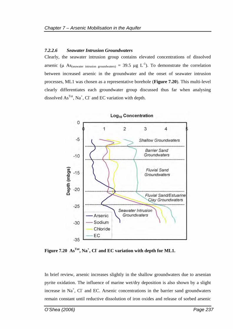
Chapter 7 – Arsenic Mobilisation in the Aquifer
O’Shea (2006) Page 237
7.2.2.6 Seawater Intrusion GroundwatersClearly, the seawater intrusion group contains elevated concentrations of dissolved
arsenic ( As(seawater intrusion groundwaters) = 39.5 g L-1). To demonstrate the correlation
between increased arsenic in the groundwater and the onset of seawater intrusion
processes, ML1 was chosen as a representative borehole (Figure 7.20). This multi-level
clearly differentiates each groundwater group discussed thus far when analysing
dissolved AsTot, Na+, Cl- and EC variation with depth.
Figure 7.20 AsTot, Na+, Cl- and EC variation with depth for ML1.
In brief review, arsenic increases slightly in the shallow groundwaters due to arsenian
pyrite oxidation. The influence of marine wet/dry deposition is also shown by a slight
increase in Na+, Cl- and EC. Arsenic concentrations in the barrier sand groundwaters
remain constant until reductive dissolution of iron oxides and release of sorbed arsenic
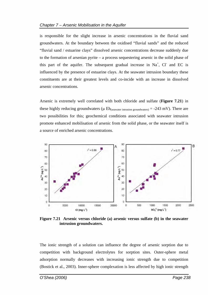
Chapter 7 – Arsenic Mobilisation in the Aquifer
O’Shea (2006) Page 238
is responsible for the slight increase in arsenic concentrations in the fluvial sand
groundwaters. At the boundary between the oxidised “fluvial sands” and the reduced
“fluvial sand / estuarine clays” dissolved arsenic concentrations decrease suddenly due
to the formation of arsenian pyrite – a process sequestering arsenic in the solid phase of
this part of the aquifer. The subsequent gradual increase in Na+, Cl- and EC is
influenced by the presence of estuarine clays. At the seawater intrusion boundary these
constituents are at their greatest levels and co-incide with an increase in dissolved
arsenic concentrations.
Arsenic is extremely well correlated with both chloride and sulfate (Figure 7.21) in
these highly reducing groundwaters ( Eh(seawater intrusion groundwaters) = -243 mV). There are
two possibilities for this; geochemical conditions associated with seawater intrusion
promote enhanced mobilisation of arsenic from the solid phase, or the seawater itself is
a source of enriched arsenic concentrations.
Figure 7.21 Arsenic versus chloride (a) arsenic versus sulfate (b) in the seawater intrusion groundwaters.
The ionic strength of a solution can influence the degree of arsenic sorption due to
competition with background electrolytes for sorption sites. Outer-sphere metal
adsorption normally decreases with increasing ionic strength due to competition
(Bostick et al., 2003). Inner-sphere complexation is less affected by high ionic strength
Chapter 7 – Arsenic Mobilisation in the Aquifer
O’Shea (2006) Page 239
and has been proposed as the dominant sorption mechanism between metal oxides
(Sherman and Randell, 2003) and many clay minerals (Manning and Goldberg, 1997).
Thus, the increased ionic strength due to seawater intrusion should not largely promote
As desorption in the aquifer. Additionally, iron oxide minerals are no longer dominant
in the reducing sediments and thus do not supply considerable sites for arsenic sorption
or desorption. This suggests that the change in geochemical conditions due to seawater
intrusion does not create an environment suited to increased arsenic release from the
aquifer matrix.
In fact, seawater intrusion conditions may actually promote some immobilisation of
arsenic in the aquifer. In a geochemical study of processes at the freshwater/seawater
interface in a shallow sandy aquifer in Denmark, Andersen et al. (2001) noted the
dominant redox process was sulfate reduction followed by methanogenesis. In the
seawater intrusion zone at Stuarts Point, the reduction of sulfate ( 2,196 mg L-1) to
sulfide ( 6.3 mg L-1) in the presence of dissolved Fe2+ ( 79.5 mg L-1) is conducive to
iron sulfide mineral formation and the possible sequestration of arsenic; a process
observed in the overlying fluvial sand / estuarine clay groundwaters. Strongly reducing
conditions and the oversaturation of iron sulfide minerals in the seawater intrusion
groundwaters supports these processes. The presence of ferrous iron, sulfide, arsenic
and organic matter in the absence of oxygen, is likely to increase the potential for
arsenian pyrite precipitation thereby removing arsenic from the dissolved phase. These
processes combine to indicate that seawater intrusion may actually immobilise dissolved
arsenic present in the aquifer. Therefore, seawater intrusion is not suspected to enhance
arsenic release into the groundwater. Instead, it is predicted to be an additional source
of arsenic to the Stuarts Point groundwater.
However, the decreased in dissolved arsenic due to arsenian pyrite formation observed
in the fluvial sand / estuarine clay groundwaters in Figure 7.20 is not apparent in the
seawater intrusion groundwaters. Instead, dissolved arsenic begins to increase with
increasing depth, suggesting an additional source of arsenic to the aquifer.
The adjacent Macleay River Estuary contains arsenic concentrations ranging from 23 –
79 g L-1 with a mean of 57 g L-1 (n = 15) which is significantly higher than the
Chapter 7 – Arsenic Mobilisation in the Aquifer
O’Shea (2006) Page 240
groundwaters. Ashley et al. (2003) document the contribution of arsenic to the Macleay
River by oxidation of arsenic-rich stibnite deposits in the upper catchment (Figure 7.22)
while Tighe et al. (2004) note the contribution of arsenic via flood deposition (from the
same stibnite source) in the Macleay floodplain. It is proposed that dissolved arsenic is
being contributed to the aquifer via seawater intrusion of arsenic-enriched estuarine
water, however this requires further research4.
Figure has been removed due to Copyright Agreements
Figure 7.22 The Macleay River exhibits increased arsenic concentrations downgradient of the Hillgrove antimony mines (Ashley et al., 2003).
When this arsenic-rich seawater enters the aquifer, the highly reducing conditions
present in this part of the aquifer are sufficient to reduce As(V) estuarine surface waters
to As(III). All modelled arsenic is present as As(III) which further reduces the
likelihood of strong arsenic sorption by mineral surfaces. Likewise, the complexation of
4 Research is currently being conducted by the UNSW Groundwater Group to assess
Chapter 7 – Arsenic Mobilisation in the Aquifer
O’Shea (2006) Page 241
arsenic in the seawater intrusion groundwaters is not expected to be a dominant reaction
since it is As(V) which is most strongly complexed with Ca2+ and Mg2+ in seawater
(Cullen and Reimer, 1989).
The combined effects of arsenic speciation, lack of iron oxide minerals and arsenic
behaviour in seawater are predicted to promote arsenic occurrence in dissolved phase.
Additionally, the formation of arsenian pyrite may be kinetically slow or have a limiting
component preventing further precipitation and arsenic sequestration. It is for these
reasons that arsenic in the seawater intrusion groundwaters is considered an additional
source of this toxic element to the aquifer.
7.3 CHAPTER SUMMARY
Dissolved arsenic varies in the Stuarts Point coastal aquifer due to a combination of
both lithological and geochemical processes. The heterogeneity of the aquifer sediments
causes redox stratification to occur, which in turn governs arsenic mobility in the
groundwater. Desorption, re-sorption and precipitation of arsenic occurs within the bulk
of the aquifer and is a consequence of changes in redox conditions. Bose and Sharma
(2002) proposed that,
“substantial (arsenic) mobilization is thought to occur under shifting redox
conditions” (pg 4917)
which appears applicable to the Stuarts Point groundwaters as it experiences changes to
redox conditions with increasing depth.
Natural and anthropogenic effects contribute to arsenic mobilisation processes. Natural
effects include water table fluctuation inducing geochemical changes in the shallow
system and aquifer heterogeneity contributing to changes in aqueous equilibrium.
Anthropogenic nitrate addition at the ground surface increases arsenic mobilisation in
shallow groundwaters. Seawater intrusion contributes further dissolved arsenic to the
groundwater system from arsenic-enriched estuarine water potentially derived from the
upstream erosion of arsenic-bearing mineral deposits and related mine tailings.
arsenic distribution in the Macleay Estuary and surface-groundwater processes.
Chapter 7 – Arsenic Mobilisation in the Aquifer
O’Shea (2006) Page 242
The previous mobilisation processes proposed by Smith et al. (2003) have been
superceded by the more detailed analyses contained herein. The two principle processes
listed by Smith et al. (i.e., dissolution of Al hydroxides and release of adsorbed As(V)
or concurrently via pH-influenced desorption of As enriched Fe oxides; and the leaching
of the aquifer’s sandy-clayey matrix by groundwaters rich in HCO3- and of high pH) are
suggested as minor arsenic control mechanisms. Instead, the reductive dissolution of
iron oxides and precipitation of iron sulfide minerals has been shown to dominate
arsenic mobilisation at Stuarts Point.
O’Shea (2006) Page 243
8 CONCLUSIONS AND RECOMMENDATIONS
8.1 THE PROBLEM
Elevated arsenic has been identified at Stuarts on the mid-north coast of NSW. Stuarts
Point is a small coastal town located on the floodplain of the Macleay River and home
to several hundred local residents and farmers. Concern was raised over the presence of
such high concentrations in a drinking water supply aquifer. This study investigated the
source, geochemical sinks and aqueous mobilisation processes governing arsenic
distribution in the aquifer. Arsenic occurrence in a sandy aquifer was considered
unusual, since no source of geogenic arsenic was obvious, and few aquifers of this
nature had previously been investigated for arsenic. The findings of this research are
thus unique, and are presented below.
8.2 PROPOSED ARSENIC GEOCHEMICAL MODEL FOR THE STUARTS POINT AQUIFER
Figure 8.1 shows the major processes and inter-relationships, as proposed herein, for
the occurrence and mobilisation of arsenic within the Stuarts Point aquifer. This model
is described below.
Mineralised bedrock groundwaters contribute arsenic to the overlying weathered
bedrock clays.
The wet climate of the Pleistocene and Holocene promotes weathering in the
upper Macleay River catchment.
Natural stibnite deposits containing arsenic and antimony are weathered to form
iron oxides.
These oxides are present in colloidal forms and as coatings on sediment grains,
which are transported downstream and deposited to form the aquifer matrix.
Chapter 8 – Conclusions and Recommendations
O’Shea (2006) Page 244
Groundwater residence time, depositional history and age of the sediments
enables redox stratification to occur in the aquifer.
The deeper, more reducing fluvial sand and estuarine clay groundwaters have
undergone complete reductive dissolution of iron oxides resulting in the
subsequent mobilisation of arsenic into groundwater.
Some of this arsenic has been incorporated into iron sulfide mineral precipitates,
forming current arsenian pyrite sinks within the aquifer.
The fluvial sand sediments above have not completed reduction of all iron
oxides within the sediments, causing re-adsorption of arsenic to the remaining
iron oxide surfaces. This helps to maintain low arsenic concentrations in the
groundwater.
Conditions are not suitably reducing enough in the overlying barrier sands to
promote abundant iron oxide dissolution, which is responsible for the
background arsenic concentrations observed in this part of the aquifer.
Shallow groundwaters are exposed to nitrate input from the ground surface and
the presence of organic matter in the form of coffee rock lenses. Nitrate
contributes to the oxidative release of discrete arsenian pyrite phases while
DOM potentially influences sorption of arsenic to oxide surfaces.
The current extraction of groundwater from the aquifer induces seawater
intrusion of arsenic-rich estuarine water, bringing further dissolved arsenic into
the aquifer.
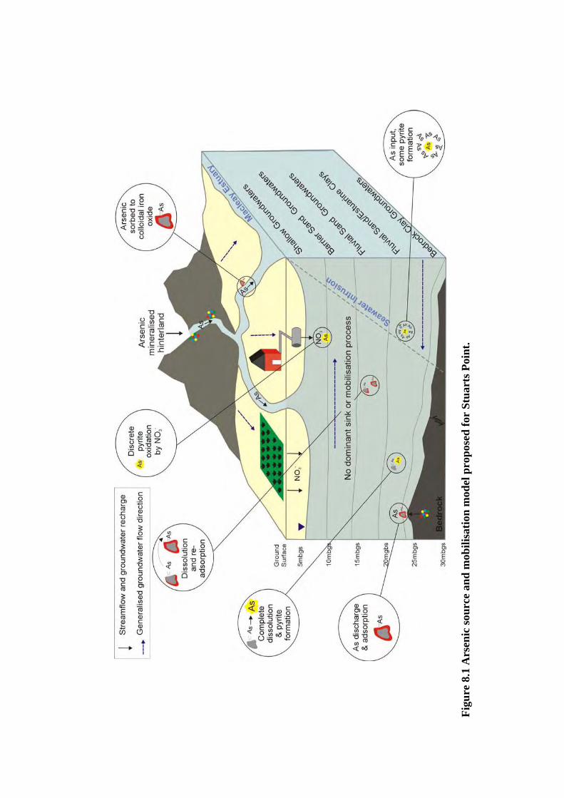
Figu
re 8
.1 A
rsen
ic so
urce
and
mob
ilisa
tion
mod
el p
ropo
sed
for
Stua
rts P
oint
.
Chapter 8 – Conclusions and Recommendations
O’Shea (2006) Page 246
8.3 CONCLUSIONS
The main conclusions, addressing the proposed hypotheses from Chapter 1, are listed in
below:
1. Where is the arsenic coming from ?
Arsenic is derived from regional erosion of As-rich stibnite deposits that
have been fluvially transported and deposited to form sediments of the
Stuarts Point aquifer. Some minor arsenic is locally contributed from
mineralised bedrock sources.
2. What form is it taking in the aquifer matrix ?
Arsenic sorbed to iron oxides during fluvial transport now form part of
the aquifer matrix. Disseminated arsenian pyrite grains have been
identified within the aquifer matrix and are suspected of forming after
deposition of the aquifer. During their formation they sequestered
dissolved arsenic into their crystal structure. The presence of minor
aluminium oxide, humic matter and illite clays are suspected of retarding
arsenic under suitable, localised, geochemical conditions.
3. How is it being released into groundwater ?
Geochemical conditions, dominated by changes in the redox state of
groundwaters, produces several arsenic release and retardation
mechanisms in the aquifer. Processes include the oxidation of arsenian
pyrite in the shallow system; reductive dissolution of iron oxides;
desorption from mineral surfaces; and the introduction of increased
arsenic concentrations via arsenic-enriched seawater intrusion.
These findings make a solid contribution to the science and management of arsenic
geochemistry in the following manner:
Chapter 8 – Conclusions and Recommendations
O’Shea (2006) Page 247
Previously proposed arsenic sources for this aquifer differ from those discussed
herein. The source of arsenic has been successfully deduced and supported with
sufficient evidence. The derivation of a natural arsenic source reduces any potential
blame for anthropogenic introduction concerning its initial presence in this aquifer.
Prior to these investigations, the geochemical processes responsible for arsenic
distribution in the Stuarts Point aquifer (both solid and aqueous forms) could only
be postulated from the limited aqueous data available. Complex arsenic geochemical
processes have been delineated in great detail herein, and confirmed and/or
dismissed with a more robust geochemical data set.
A greater understanding of the source, retardation and mobilisation of arsenic in this
aquifer contributes to our broad understanding of arsenic in the environment; and
allows aquifer specific management procedures and research recommendations to be
made.
Previous studies suggesting arsenic in the Stuarts Point aquifer is derived from
adsorption to clays during sea level rise have been questioned. The contribution of
arsenic onto oxide and clay surfaces from seawater during marine transgressions has
been proposed for Bangladesh, however the absence of an arsenic-rich volcanic ash
deposit over which the Bangladeshi sea transgressed reduces the plausibility of this
theory occurring at Stuarts Point.
The suggestion that groundwater arsenic occurrence has implications for the
management of Australian coastal aquifers remains, but not solely due to the presence
of ASS or exposure of these coastal sediments to Quaternary sea level fluctuations.
Rather, any coastal or unconsolidated aquifer that has sediments derived from
mineralised provenances should consider monitoring for arsenic, and other potentially
toxic trace elements, in their groundwater systems.
Chapter 8 – Conclusions and Recommendations
O’Shea (2006) Page 248
8.4 RECOMMENDATIONS
8.4.1 Aquifer Specific (Stuarts Point)
A number of unanswered points have been raised during the course of this research.
Some of these are listed here to provide guidance on possible mitigating measures for
reducing the arsenic impact at Stuarts Point. They should not be relied upon as a
complete solution to the arsenic problem and should only be implemented if required,
after further consideration and investigation.
Management of aquifer redox equilibria – minimising anthropogenic additions
Oxidation of arsenian pyrite by nitrate reduction has been identified as a potential
arsenic mobilisation process in the aquifer. Arsenian pyrite may be oxidised by other
reductants (such as oxygen), however, nitrate addition to groundwater, particularly
shallow waters, should be minimised to reduce arsenic release. Examination of nitrate
inputs to the aquifer should include contributions from fertilizers (e.g. manure),
degrading (landfill) waste and septic tanks.
The addition of organic matter may also enhance the reductive dissolution of iron
oxides and the subsequent release of arsenic into the groundwater. Anthropogenic
organic matter input may include human and animal organic wastes; mulching or
fertilizer input; and leachate from landfills. Changes in redox equilibria brought on by
such examples should be minimised.
Examining the redox driver
Analysis of Total Organic Carbon (TOC) in the Stuarts Point aquifer sediments would
provide a better indication of processes driving the reduction of iron oxides and release
of arsenic into groundwater. Likewise, the identification of peat lenses in the aquifer
may provide information on areas where enhanced iron reduction and arsenic release
may occur. Further in-situ studies on the mobilisation of arsenic in this aquifer would
benefit other aquifers experiencing similar geochemical conditions, and provide further
management options for the aquifer. Experiments such as the injection of molasses,
nitrate and low arsenic water by Harvey et al. (2002) would allow more detailed
examination of the redox driver within the Stuarts Point aquifer.
Chapter 8 – Conclusions and Recommendations
O’Shea (2006) Page 249
Impacts on the environment
Although not reported herein, crops irrigated with untreated groundwater may be at risk
of trace element accumulation. Regular testing of vegetation should be maintained. The
detection of dissolved arsenic at elevated concentrations in the estuary requires further
research; delineation of the actual source (potentially from an upstream mining area)
should be identified from both a mitigation and possibly a legal viewpoint. In the
interim, measures should be in place to ensure protection of the environment,
particularly marine organisms which may bioaccumulate arsenic. Consumption of
organisms from the estuary by humans should be avoided unless given the all clear.
Seawater intrusion into the freshwater aquifer should be effectively managed to
minimise further arsenic input to the groundwater.
Groundwater extraction
The identification of discrete arsenian pyrite phases within the aquifer matrix warrants
further investigation into the effects of oxidation on arsenic release into groundwater.
Thornburg and Sahai (2004) noted that arsenic concentrations in groundwater affected
by discrete arsenian pyrite phases peaked after one hour of pumping or exposure to air
during laboratory investigations. Pyrite was presumed to be oxidised during this time,
releasing arsenic prior to the formation of surface iron oxide precipitates which
subsequently re-sorbed arsenic species, thereby lowering concentrations in dissolved
phase. These findings may have implications for groundwater extraction from the
Stuarts Point aquifer. Arsenic concentrations during well pumping should be monitored
to assess changes in dissolved arsenic concentrations. If arsenic decreases over a
specified pumping time, groundwater extracted for domestic and irrigation use may be
of a more suitable quality if it is pumped before consumption / application.
Alternatively, this may act as a relatively inexpensive pre-treatment mechanism leading
to a reduction in chemical treatment currently being utilised by local council. Therefore,
a simple pump test measuring arsenic concentrations during pumping could provide
improved management options for the aquifer.
Temporal uncertainties
Investigations herein and those reported in Smith et al. (2003) indicate that arsenic is
highly variable in the groundwater at Stuarts Point. Sidle (2002) found that arsenic
Chapter 8 – Conclusions and Recommendations
O’Shea (2006) Page 250
concentrations in the Goose River basin in Maine derived from the oxidation of arsenian
pyrite were highly variable over a two year sampling period. No specific temporal
investigations have been carried out at Stuarts Point and as such it should be recognised
that arsenic concentrations in groundwater may be prone to variation in both spatial
distribution and observed concentration ranges. For a better understanding of such
processes temporal studies would be beneficial.
Formation of discrete mineral phases capable of retarding arsenic mobility
Geochemical modelling outputs often produced results indicating conditions were
suitable for formation of arsenic minerals, or minerals capable of capturing arsenic from
solution. The presence of trace amounts of arsenic in the solid phase makes verification
of these potential minerals difficult. More detailed studies of the solid phase of the
aquifer matrix may enable discrete micron-sized arsenic bearing and/or ‘capturing’
minerals to be confirmed or dismissed. The potential presence of such small mineral
phases in a predominantly sandy medium may have implications for trace element
mobility in high yielding unconsolidated aquifers.
Analysis of antimony occurrence in the aquifer matrix
Antimony geochemistry, in general, is lacking in the literature. The few articles that are
available on antimony occurrence and chemistry suggest it is present in a solid
immobile phase. The elevated levels of antimony present in the Stuarts Point aquifer
matrix were thus attributed to an unknown solid antimony phase. Research on the
aquifer matrix, perhaps high resolution microscopy such as EXAFS, would confirm or
deny the presence of such antimony phase. In addition, further research on antimony
geochemistry would greatly benefit the small amount of research that is currently
available.
Further geomorphic work
Dating of sediments and shells may provide more information on the age of sediments
at their deposition. This would help to better define the geomorphic history of the
aquifer and extrapolate these findings to sea level changes elsewhere.
Chapter 8 – Conclusions and Recommendations
O’Shea (2006) Page 251
8.4.2 Other Research Recommendations
Advances in the science of arsenic geochemistry can be beneficial in predicting its
mobilisation/retardation at Stuarts Point. The following list provides examples of
technical research that may further aid in the interpretation of arsenic geochemical
processes in this, and other, aquifers. Some general conclusions drawn herein (not
necessarily arsenic-related) are also mentioned as their findings may be applicable to
other aquifers.
Advancement in the micron scale investigation of arsenic partitioning in solid solution
Much of the current arsenic research deals with its behaviour at the mineral surface.
Further increased knowledge of arsenic partitioning in various mineral phases (i.e.,
specific bonding mechanisms); mineral stability; and the effects of other system
components (ionic strength, competitive anions, speciation, aging) can improve
predictions on its likely mobilisation and bioavailability in the environment.
Application of theoretical knowledge to natural aquifer sediments
The investigations noted above are generally conducted on synthetic materials under
controlled laboratory conditions. This is essential to our understanding of the underlying
mechanisms but is not representative of true aquifer conditions. Different studies yield
different results, as can synthetic materials versus natural ones. For example, aquifer
sediments contain numerous minerals all potentially contributing to the sorption of
arsenic. The combined analysis of surface titrations to determine bulk PZC of an
aquifer’s clay and sand fractions, with batch experiments to characterise how each
fraction sorbs arsenic, would allow better judgement to be made regarding arsenic
sorption properties (i.e., outer-sphere versus inner-sphere complexation). In turn, this
would allow more confident predictions to be made about the dominant mechanism of
arsenic sorption in the aquifer and its likely potential for mobilisation. As such,
concurrent laboratory investigations with actual aquifer sediments would be particularly
beneficial prior to geochemical modelling or remediation trials. Research such as this
would help to improve the overall discipline of geochemistry.
Potential for arsenic occurrence in other coastal aquifers of NSW
Chapter 8 – Conclusions and Recommendations
O’Shea (2006) Page 252
The original report identifying elevated arsenic in the Stuarts Point aquifer (Piscopo,
1996) also identified dissolved arsenic concentrations in other coastal aquifers of NSW.
Stuarts Point was given priority for further investigation due to use of its groundwater
for human consumption. Deduction of a hinterland derived arsenic source for the Stuarts
Point aquifer could have implications for other unconsolidated aquifers deposited by the
Macleay River fluvial depositional environment. Additionally, other large river systems
present in NSW, such as the Manning River, may have had the potential to erode
hinterland arsenic sources and thus deposit aquifers conducive to arsenic mobilisation.
Alternatively, pyrite formation in the presence of arsenic (whether it be a natural or
anthropogenic source) followed by oxidation can lead to elevated arsenic in both coastal
and inland groundwaters. Investigation of other fluvially deposited aquifer sediments of
the Macleay River is recommended, followed by examination of fluvially deposited
coastal sediments derived from other river systems, especially if a hinterland arsenic
source is suspected. Additionally, the potential for arsenic incorporation into sulfide
minerals followed by oxidation, should be incorporated into risk assessment procedures.
Association of trace elements with pyrite and acid sulfate soils
The association of trace elements with pyrite was documented in the literature review.
In the Goose River Basin of Maine, a groundwater environment where arsenic is
proposed to originate from the oxidation of arsenian pyrite, analysis of pyrites in the
area reported up to 1.93% As; 0.02% Cu; 0.08% Pb; 0.01% Bi; 0.06% Ag; 0.34%
Co; 0.09% Ni; 0.03% Au and 0.02% Sb (Sidle et al., 2001). Unfortunately, their
relative concentrations in groundwater were not reported.
The inclusion of arsenic into the pyrite structure is well documented, however the
association of other trace elements has been given much less attention. Investigations
into trace element associations with pyrite formed under different environments may aid
in predicting the risks associated with pyrite oxidation. For example, pyrite at Stuarts
Point was found to contain both arsenic and lead, possibly as a result of their presence
in the sediments derived from a mineralised provenance. However, lead and copper has
been shown to be scavenged by iron monosulfide formation in sediments of the Tweed
Chapter 8 – Conclusions and Recommendations
O’Shea (2006) Page 253
River floodplain (Smith and Melville, 2004) indicating that provenance may not play an
important role in the association of trace elements with iron sulfide minerals.
Additionally, saline sulfidic soils developed under dryland salinity conditions inland
(Fitzpatrick et al., 1996) may also contain trace elements incorporated in their crystal
structure. The association of trace elements with pyrite should be the focus of additional
research, particularly in relation to their potential environmental impact and health risk
upon oxidation of ASS.
Mechanisms of pyrite oxidation by nitrate reduction
While pyrite oxidation by nitrate reduction is often cited as a potential arsenic
mobilisation mechanism, few reports of its occurrence in the environment have been
made. Data for the shallow groundwaters of the Stuarts Point aquifer indicate this
reaction may be occurring. Inputs of nitrate from anthropogenic activities such as
farming, may lead to pyrite oxidation in shallow groundwaters. This may be of
increased significance to acid sulfate soil environments where land is often used for
farming or settlement, potentially increasing the likelihood of nitrate addition to the
subsurface.
Heterogeneity in coastal groundwaters – source provenance and redox stratification
Groundwater drawn from ‘clean’ aquifer sands should not automatically be assumed as
‘safe’ for drinking and irrigation water supply. Although sparsely populated, with no
major source of contamination and producing water from ‘clean’ aquifer sands; the
Stuarts Point groundwater contains arsenic, and some other elevated elements, as a
product of its source provenance. Heterogeneity in aquifer conditions (such as changes
in redox) can cause these elements to be elevated in different areas of the aquifer.
Groundwater in similar environments being used for domestic or irrigation water supply
should be thoroughly investigated, addressing chemical and sediment heterogeneity,
before its use can be regarded as safe. The importance of detailed vertical studies to
show aquifer heterogeneity is particularly emphasised.
REFERENCES
Abbt-Braun, G. 2002. Huminstoffe-Vorkommen, Charakterisierung und Reaktionen. Wasser-und Geotechnologie, 1, 41-49.
Abdullah, M.I., Shiyu, Z. and Mosgren, K. 1995. Arsenic and selenium species in the oxic and anoxic waters of the Oslofjord, Norway. Marine Pollution Bulletin, 31,116-126.
Acharyya, S.K., Chakraborty, P., Lahiri, S., Raymahashay, B.C., Guha, S. and Bhowmik, A. 1999. Arsenic poisoning in the Ganges delta. Nature, 401, 545.
Acharyya, S.K., Lahiri, S., Raymahashay, B.C. and Bhowmik, A. 2000. Arsenic toxicity of groundwater in parts of the Bengal basin in India and Bangladesh: the role of Quaternary stratigraphy and Holocene sea-level fluctuation. EnvironmentalGeology, 39 (10), 1127-1137.
Adriano, D.C. 1986. Trace Elements in the Terrestrial Environment. Springer-Verlag, New York.
Aguirre-Banuelos, P. Escudero-Lourdes, C., Carrizales, L., Diaz-Barriga, F. and Perez-Urizar, J. 2004. Effect of acute exposure to arsenic on formalin-induced nociception and tramadol-mediated antinociception in mice. Proceedings of West Pharmacological Society, 47, 113-116.
Ahmann D., Krumholz L.R., Hemond H.F., Lovley D.R. and Morel F.M.M. 1997. Microbial mobilization of arsenic from sediments of the Aberjona watershed. Environmental Science and Technology, 31 (10), 2923-2930.
Al-Awadi, E., Mukhopadhyay, A., Akber, A. and Hadi, K. 2003. Distribution of selected trace constituents in the ground water of Kuwait. Advances in Environmental Research, 7, 367-380.
Aldarman, F., Blanco, J., Buckley, J., Donnelly, G., Evans, M., Irving, N., Parkhouse, T., and Robertson, V. 1984. A Folk of History of Yarrahapinni and Stuarts Point.
Alekin, O.A. 1970. Principles of Hydrochemistry. Hydromet. Izdat. Allard, B. 1995. Groundwater. In: Salbu, B., Steinnes, E. (eds) Trace elements in
natural waters. CRC, Boca Raton, Florida. American Public Health Association (APHA), 1992. Standard methods for the
Examination of Water and Wastewater (18th ed.). APHA-AWWA-WET, Washington, USA.
American Public Health Association (APHA), 1998. Standard methods for the Examination of Water and Wastewater (20th ed.). APHA-AWWA-WET, Washington, USA.
Anawar, H.M., Akai, J. and Sakugawa, H. 2004. Mobilization of arsenic from subsurface sediments by effect of bicarbonate ions in groundwater. Chemosphere,54, 753-762.
Anawar, H.M., Akai, J., Komaki, K., Terao, H., Yoshioka, T., Ishizuka, T., Safiullah, S. and Kato, K. 2003. Geochemical occurrences of arsenic in groundwater of Bangladesh: sources and mobilisation processses. Journal of Geochemical Exploration, 77, 109-131.
Andersen, M.S., Larsen,F. and Postma, D. 2001. Pyrite oxidation in unsaturated aquifer sediments. Reaction stoichiometry and rate of oxidation. Environmental Science and Technology, 35, 4074-4079.
ANZECC (2000). Australian and New Zealand Environment and Conservation Council and Agriculture and Resource Management Council of Australia and New
O’Shea (2006) Page 254
References
Zealand. Australian and New Zealand Guidelines for Fresh and Marine Water Quality: Volume 2. Aquatic Ecosystems – Rationale and Background Information. National Water Quality Management Strategy, Paper No. 4, October 2000.
Appelo, C.A.J. and Postma, D. 1999. Geochemistry, Groundwater and Pollution.Balkema, Rotterdam.
Appelo, C.A.J., Van Der Weiden, M.J.J., Tournassat, C. and Charlet, L. 2002. Surface complexation of ferrous iron and carbonate on ferrihydrite and the mobilisation of arsenic. Environmental Science and Technology, 36, 3096-3103.
Appleyard, S., Wong, S., Willis-Jones, B., Angeloni, J. and Watkins, R. 2004. Groundwater acidification caused by urban development in Perth, Western Australia: source, distribution, and implications for management. Australian Journal of Soil Research, 42, 579-585.
Armienta, M.A., Rodriguez, R., Aguayo, A., Ceniceros, N., Villasenor, G. and Cruz, O. 1997. Arsenic contamination of groundwater at Zimapan, Mexico. HydrogeologyJournal, 5 (2), 39-46.
Ashley, P. and B. Graham. 2000. Heavy metal loadings in the Macleay River Catchment, northeastern New South Wales, 15th Australian Geological Convention, Geological Society of Australia, Sydney.
Ashley, P.M., Craw, D., Graham, B.P. and Chappell, D.A. 2003. Environmental mobility of antimony around mesothermal stibnite deposits, New South Wales, Australia and southern New Zealand. Journal of Geochemical Exploration 77, 1-14.
Australian Bureau of Statistics (ABS) 2001. Census of Population and Housing (Stuarts Point). www.kempseyshirecouncil.gov.nsw.au Accessed 8.3.05
Azcue, J.M. and Nriagu, J.O. 1995. Impact of abandoned mine tailing on the arsenic concentrations in Moira Lake, Ontario. Journal of Geochemical Exploration, 52,81-89.
Barry, G.A. 1997. Total heavy metal status of horticultural soils in Queensland. Final report to Horticultural Research and Development Corporation on Project BG404. Queensland Department of Natural Resources, Brisbane.
Bauer, M. and Blodau, C. 2006. Mobilisation of arsenic by dissolved organic matter from iron oxides, soils and sediments. Science of the Total Environment, 354 (2-3), 179-190.
Bebie, J., Schoonen, M.A.A., Fuhrmann, M. and Strongin, D.R. 1998. Surface charge development on transition metal sulfides: An electrokinetic study. Geochimica et Cosmochimica Acta, 62, 633-642.
Bednar, A.J., Garbarino, J.R., Burkhardt, M.R., Ranville, J.F. and Wildeman. 2002. Field and laboratory arsenic speciation methods and their application to natural-water analysis. Water Research, 38, 355-364.
Belzile, N. and Lebel, J. 1986. Capture of arsenic by pyrite in near-shore marine sediments. Chemical Geology, 54, 279-281.
Belzile,N. 1988. The fate of arsenic in sediments of the Laurentian Trough. Geochimicaet Cosmochimica Acta, 52, 2293-2302.
Bengtsson, L. and Enell, M. 1986. Chemical Analysis. In: Berglund, B.E. (Ed.) Handbook of Holocene Palaeoecology and Palaeohydrology. John Wiley & Sons, New York.
Berg, M., Tran, H.C., Nguyen, T.C., Pham, H.V., Schertenleib, R. and Giger, W. 2001. Arsenic contamination of groundwater and drinking water in Vietnam: A human health threat. Environmental Science and Technology, 35 (13), 2621-2626.
Berg, M., Tran, H.C., Pham, K.T., Pham, H.V., Schertenleib, R. and Giger, W. 2003. Arsenic pollution of water resources in Vietnam – A plea for early mitigation
O’Shea (2006) Page 255
References
actions. In: Gobran, G.R. and Lepp, N. (eds) 7th International Conference on the BioGeochemistry of Trace Elements, Volume 2 Symposia, June 15-19 Uppsala, Sweden, 8-9.
Berner, R.A. 1970. Sedimentary pyrite formation. American Journal of Science, 268, 1-23.
BGS and DPHE. 2001. Arsenic contamination of groundwater in Bangladesh. In: Kinniburgh, D.G., Smedley, P.L. (eds.), British Geological Survey (Technical Report, WC/00/19. 4 Volumes). British Geological Survey, Keyworth.
Bhattacharya, P., Jacks, G., Ahmed, K.M., Khan, A.A. and Routh, J. 2002. Arsenic in groundwater of the Bengal Delta Plain aquifers in Bangladesh. Bulletin of Environmental Contaminant Toxicology, 69, 538-545.
Bhattacharya, P., Tandukar, N., Mukherjee, A.B., Valero, A.A. and Jacks, G. 2003. Redox chemistry of arsenic in groundwaters of Terai Belt of Nepal. In: Gobran, G.R. and Lepp, N. (eds) 7th International Conference on the BioGeochemistry of Trace Elements, Volume 2 Symposia, June 15-19 Uppsala, Sweden, 10-11.
Binnings, P., Raidu, R. and Hettipathirana, T. 2001. Oxidation of an unconfined aquifer. Arsenic in the Asia-Pacific Region Workshop, “Managing Arsenic for our Future”. 20-23 November 2001, Adelaide, Australia, 34-5.
Bird, G., Brewer, P.A., Macklin, M.G., Balteanu, D., Driga, B., Serban, M. and Zaharia, S. 2003. The solid state partitioning of contaminant metals and As in river channel sediments of the mining affected Tisa drainage basin, northwestern Romania and eastern Hungary. Applied Geochemistry, 18, 1583-1595.
Bissen, M. and Frimmel, F.H. 2003. Arsenic – a Review. Part 1: Occurrence, Toxicity, Speciation, Mobility. Acta Hydrochimica Hydrobiologica, 31 (1), 9-18.
Bodenan, F., Baranger, P., Piantone, P., Lassin, A., Azaroual, M., Gaucher, E.and Braibant, G. 2004. Arsenic behaviour in gold-ore mill tailings, Massif Central, France: hydroGeochemical study and investigation of in situ redox signatures. Applied Geochemistry 19, 1785-1800.
Bortolami,G.C., Ricci, B., Susella, G.F. and Zuppi, G.M. 1979. Isotope hydrology of the Val Corsaglia, Maritime Alps, Piedmont, Italy. In: Isotope Hydrology 1978, Vol I, IAEA Symposium 228, June 1978, Germany, 327-350.
Bose, P. and Sharma, A. 2002. Role of iron in controlling speciation and mobilization of arsenic in subsurface environment. Water Research, 36, 4916-4926.
Bostick, B.C. and Fendorf, S. 2003. Arsenite sorption on troilite (FeS) and pyrite (FeS2). Geochimica et Cosmochimica Acta, 67(5), 909-921.
Bostick, B.C., Chen, C. and Fendorf, S. 2004. Arsenite retention mechanisms within estuarine sediments of Pescadero, CA. Environmental Science and Technology,38, 3299-3304.
Bostick, B.C., Fendorf, S. and Manning, B.A. 2003. Arsenite adsorption on galena (PbS) and sphalerite (ZnS). Geochimica et Cosmochimica Acta, 67 (5), 895-907.
Bowell, R.J. 1994. Sorption of arsenic by iron oxides and hydroxides in soils. Applied Geochemistry, 9, 279-286.
Bowen, H.J.M. 1979. Environmental Chemistry of the Elements. Academic Press, New York.
Boyle, D.R., Turner, R.J.W. and Hall, G.E.M. 1998. Anomalous arsenic concentrations in groundwaters of an island community, Bowen Island, British Columbia. Environmental Geochemistry and Health, 20, 199-212.
Boyle, R.W. and Jonasson, I.R. 1973. The Geochemistry of arsenic and its use as an indicator element in Geochemical prospecting. J. Geochemical Exploration, 2,252-296.
O’Shea (2006) Page 256
References
Bundschuh, J., Farias, B., Marin, R., Storniolo, A., Bhattacharya, P., Cortes, J., Bonorino, G. and Albouy, R. 2004. Groundwater arsenic in the Chaco-Pampean Plain, Argentina: case study from Robles county, Santiago del Estero Province. Applied Geochemistry, 19, 231-243.
Bureau of Meteorology Website (BOM) 2005. Climate averages for SouthWest Rocks. www.bom.gov.au/climate/averages/tables Accessed 8.3.05
Burton, J.D., F. Culkin and J. P. Riley. 1959. The abundances of gallium and germanium in terrestrial materials. Geochimica et Cosmochimica Acta, 16, 151-180.
Caceres, L., Gruttner, E., Contreras, R. 1992. Water recycling in arid regions-Chilean case. Ambio, 21, 138-144.
Cai, Y., Cabrera, J.C., Georgiadis, M. and Jayachandran, K. 2002. Assessment of arsenic mobility in the soils of some golf courses in South Florida. Science of the Total Environment, 291, 123-134.
Campbell, K.S.W. 1969. Carboniferous System, New England Region. In: Packham, G.H. (ed) 1969. The Geology of New South Wales. Journal of the Geological Society of Australia, 16 (1), 245-261.
Carlsson, E., Thunberg, J., Ohlander, B. and Holmstrom, H. 2002. Sequential extraction of sulfide-rich tailings remediated by the application of till cover, Kristineberg mine, northern Sweden. Science of the Total Environmental, 299, 207-226.
Carmalt, C.J. and Norman, N.C. 1998. Arsenic, antimony and bismuth: some general properties and aspects of periodicity. In: Norman, N.C. (ed) Chemistry of Arsenic, Antimony and Bismuth (1st edition). Blackie Academic & Professional, London, New York.
Carrillo-Chavez, A., Drever, J.I. and Martinez, M. 2000. Arsenic content and groundwater Geochemistry of the San Antonio-El Triunfo, Carrizal and Los Planes aquifers in southernmost Baja California, Mexico. Environmental Geology,39 (11), 1295-1303.
Chaillou, G., Schafer, J., Anschutz, P., Lavaux, G. and Blanc, G. 2003. The behaviour of arsenic in muddy sediments of The Bay of Biscay (France). Geochimica et Cosmochimica Acta, 67, 2993-3003.
Chappell, J. and Polach, H. 1991. Post-glacial sea-level rise from a coral record at Huon Peninsula, Papua New Guinea. Nature, 349, 147-149.
Charlet, L. and Manceau, A. 1993. Structure, formation, and reactivity of hydrous oxide particles: Insights from x-ray absorption spectroscopy. In: J. Buffle and A.P. vanLeeuwen (Eds.). Environmental Particles. Lewis Publishers, Boca Raton, FL, 117-164.
Chen, S-L., Dzeng, S.R., Yang, M-H., Chiu, K-H., Shieh, G-M. and Chien, M.W. 1994. Arsenic species in groundwaters of the blackfoot disease area, Taiwan. Environmental Science and Technology, 28, 877-881.
Cheng, L., Fenter, P., Sturchio, N.C., Zhong, Z. and Bedzyk, M.J. 1999. X-ray standing wave study of arsenite incorporation at the calcite surface. Geochimica et Cosmochimica Acta, 63 (19/20), 3153-3157.
Childs, C.W. 1992. Ferrihydrite: A review of structure, properties and occurrence in relation to soils. Z. Pflanzenernahr. Bodenk., 155, 441-448.
Childs, C.W., Downes, C.J. and Wells, N. 1982. Hydrous iron oxide minerals with short range order deposited in a spring/stream system, Tongariro National Park, New Zealand. Australian Journal of Soil Research, 20, 119-129.
O’Shea (2006) Page 257
References
Chirenje, T., Ma, L.Q., Clark, C. and Reeves, M. 2003. Cu, Cr and As distribution in soils adjacent to pressure-treated decks, fences and poles. EnvironmentalPollution, 124, 407-417.
Coffey Partners International, Australian Nuclear Science and Technology Organisation (ANSTO), Sinclair Knight Merz and Econsearch. 1996. Data Review and Assessment of Hydrogeological and Hydrochemical Impacts on Heavy Mineral Mining on the Tomago Sandbeds, Newcastle, NSW.
Cornell, R.M. 1987. Comparison and classification of the effects of simple ions and molecules upon the transformation of ferrihdyrite into more crystalline products. Z. Pflanzenernahr. Bodenk., 150, 304-307.
Craw, D. and Chappell, D.A. 1999. Evolution of sulphide mineral occurrences of an incipient nonmarine sedimentary basin, New Zealand. Sedimentary Geology, 129,37-50.
Craw, D., Wilson, N. and Ashley, P.M. 2004. Geochemical controls on the environmental mobility of Sb and As at mesothermal antimony and gold deposits. Applied Earth Science (Transactions Institute of Mining and Metallurgy B), 113,B3-B10.
Crecelius, E.A., Bloom, N.S., Cowan, C.E. and Jenne, E.A. 1986. Speciation of selenium and arsenic in natural waters and sediments: arsenic speciation. Electric Power Research Institute, Vol. 2, EA-4641, Project 2020-2.
Crisp, P. (personal communication, 2002) School of Chemical Engineering and Industrial Chemistry, University of New South Wales.
Critto, A., Carlon, C. and Marcomini, A. 2003. Characterization of contaminated soil and groundwater surrounding an illegal landfill (S. Giuliano, Venice, Italy) by principal component analysis and kriging. Environmental Pollution, 122, 235-244.
Cullen, W.R. and Reimer, K.J. 1989. Arsenic speciation in the environment. ChemicalReview, 89, 713-764.
Daniele, L. 2004. Distribution of arsenic and other minor trace elements in the groundwater of Ischia Island (southern Italy). Environmental Geology, 46, 96-103.
Das, D. Chatterjee, A., Mandal, B.K., Samanta, G., Chakraborti, D. and Chanda, B. 1995. Arsenic in ground-water in 6 districts of West Bengal, India – the biggest arsenic calamity in the world. 2. Arsenic concentration in drinking-water, hair, nails, urine, skin-scale and liver-tissue, biopsy of the affected people. Analyst,120, 917-924.
Datta, D.K. and Subramanian, V. 1997. Texture and mineralogy of sediments from the Ganges-Brahmaputra-Meghna river system in the Bengal basin, Bangladesh and their environmental implications. Environmental Geology 30, 181- 188.
Davis, A., Kempton J.H. and Nicholson, A. 1994. Groundwater transport of arsenic and chromium at a historical tannery, Woburn, Massachusetts, USA. AppliedGeochemistry, 9, 569-582.
Davis, J.A. and Leckie, J.O. 1980. Surface ionization and complexation at the oxide/water interface. 3. Adsorption of anions. Journal of Colloid and Interface Science, 74(1), 32-43.
Davis, J.C. 1986. Statistics and data analysis in geology, 2nd edn. Wiley, New York. Dawson, B.S.W., Parker, G.F., Cowan, F.J. and Hong, S.O. 1991. Inter-laboratory
determination of copper, chromium, and arsenic in timber treated with wood preservative. Analyst, 116, 339-346.
Del Razo, L.M., Arellano, M.A. and Cebrian, M.E. 1990. The oxidation states of arsenic in well-water from a chronic arsenicism area of northern Mexico. EnviromentalPollution 64, 143-153.
O’Shea (2006) Page 258
References
Dent, B.B. 2002. The Hydrogeological Context of Cemetery Operations and Planning in Australia. PhD Thesis (unpublished), University of Technology, Sydney.
Dent, B.B. 2004. Personal Communication. Dickinson, W.R. and Suczek. C.A. 1979. Plate tectonics and sandstone compositions.
American Association of Petroleum Geologists, Bulletin, 63, 2164-2182. Dickinson, W.R., Beard, L.S., Brakenridge, G.R., Erjavec, J.L., Ferguson, R.C., Inman,
K.F., Knepp, R.A., Lindberg, F.A., and Ryberg, P.T. 1983. Provenance of North American Phanerozoic sandstones in relation to tectonic setting. GeologicalSociety of America, Bulletin, 94, 222-235.
Dixit, S. and Hering, J.G. 2003. Comparison of arsenic(V) and arsenic (III) sorption onto iron oxide minerals: implications for arsenic mobility. EnvironmentalScience and Technology, 37, 4182-4189.
DMR, 1995. Arsenic. MinFact, 22, March 1995, Department of Mineral Resources (DMR), St Leonards, New South Wales.
Dragun, J. and Chiasson. 1991. Elements in North American Soils. Hazardous Materials Control Resources Institute, Greenbelt, MD.
Dreher, T. 2003. Comment on Guler, C., Thyne, G.D., McCray, J.E. and Turner, A.K. 2002. Evaluation of graphical and multivariate statistical methods for classification of water chemistry data, in Hydrogeology Journal, 10, 455-474. Hydrogeology Journal, 11, 605-606.
Drever, J.I. 1997. The Geochemistry of Natural Waters: surface and groundwater environments. 3rd edition. Prentice-Hall, New Jersey.
Dudas, M.J. 1984. Enriched levels of arsenic in post-active acid sulfate soils in Alberta. Soil Science Soc. Am. J., 48, 1451-1452.
Dudas, M.J. 1987. Accumulation of native arsenic in acid sulphate soils in Alberta. Can.J. Soil Science, 67, 317-331.
Dzombak, D.A. and Morel, F.M.M. 1990. Surface Complexation Modeling: Hydrous Ferric Oxide. John Wiley, New York.
Eddie, M.W. 2000. Soil Landscapes of the Macksville and Nambucca 1:100 000 Sheets.Department of Land and Water Conservation, Sydney.
Edmunds, W.M. Cook, J.M., Kinniburgh, D.G. Miles, D.L. and Trafford, J.M. 1989. Trace-element occurrence in British Groundwaters. Res. Report SD/89/3, British Geological Survey, Keyworth.
Ellis, A.J. and Mahon, W.A.J. 1977. Chemistry and Geothermal Systems. Academic Press, New York.
Environment Canada. 1993. Priority substances list assessment report: arsenic and its compounds. Environment Canada.
Eylem, C., H. N. Erten and H. Göktürk. 1990. Sorption-desorption behaviour of barium on clays. Journal of Environmental Radioactivity, 11 (2), 183-200.
Farias, S.S., Casa, V.A., Vazquez, C., Ferpozzi, L., Pucci, G.N. and Cohen, I.M. 2003. Natural contamination with arsenic and other trace elements in ground waters of Argentine Pampean Plain. The Science of the Total Environment, 309, 187-199.
Farnham, I.M., Stetzenbach, K.J., Singh, A.K. and Johannesson, K.H. 2000. Deciphering groundwater flow systems in Oasis Valley, Nevada, using trace element chemistry, multivariate statistics, and geographical information system. Mathematical Geology, 32 (8), 943-968.
Farrah, H. and Pickering, W.F. 1993. Chem. Speciation Bioavailability, 5 (3), 81. Fendorf, S.E., Eick, M.J., Grossl, P. and Sparks, D.L. 1997. Arsenate and chromate
retention mechanisms on goethite. 1. Surface structure. Environmental Science
O’Shea (2006) Page 259

References
and Technology 31, 315-320.
Ferguson, J.F. and Gavis, J. 1972. A review of the arsenic cycle in natural waters. Water Research, 6, 1259-1274.
Filella, M., Belzile, N. and Chen, Y-W. 2002a. Antimony in the environment: a review focused on natural waters. I. Occurrence. Earth Science Reviews, 57 (1-2), 125-176.
Filella, M., Belzile, N. and Chen, Y-W. 2002b. Antimony in the environment: a review focused on natural waters. II. Relevant solution chemistry. Earth Science Reviews,59, 265-285.
Fitzpatrick, R.W., Fritsch, E. and Self, P.G. 1996. Interpretation of soil features produced by ancient and modern processes in degraded landscapes: V. Development of saline sulfidic features in non-tidal seepage areas. Geoderma, 69,1-29.
Folk, R.L. 1966. A review of grain-size parameters. Sedimentology, 6, 73-93. Folk, R.L. and Ward, W.C. 1957. Brazos River bar: A study in the significance of grain
size parameters. Journal of Sedimentary Petrology, 27, 3-27. Frau, F. and Ardau, C. 2004. Mineralogical controls on arsenic mobility in the Baccu
Locci stream catchment (Sardinia, Italy) affected by past mining. MineralogicalMagazine, 68 (1), 15-30.
Freeze, R.A. and Cherry, J.A. 1979. Groundwater. Prentice-Hall, Inc., Englewood Cliffs, New Jersey.
Friedman, G.M. 1961. The distinction between dune, beach and river sands from their textural characteristics. Journal of Sedimentary Petrology, 31, 514-529.
Gemici, U. and Tarcan, G. 2004. Hydrogeological and hydroGeochemical features of the Heybeli Spa, Afyon, Turkey: Arsenic and the other contaminants in the thermal waters. Bull. Environmental Contamination and Toxicology, 72, 1107-1114.
GHD, 2002. Bi-Annual Groundwater Monitoring Report, Lord Street Botany.Gilligan, L.B. and Barnes, R.G. 1990. New England Fold Belt, New South Wales –
regional geology and mineralisation. In: Hughes, F.E. (ed) Geology of the Mineral Deposits of Australia and Papua New Guinea, 1417-1423. The Australasian Institute of Mining and Metallurgy: Melbourne.
Gilligan, L.B., J.W. Brownlow, R.G. Cameron and H.F. Henley. 1992. Dorrigo-Coffs Harbour 1:250 000 Metallogenic Map SH/56-10, SH/56-11: Metallogenic Study and Mineral Deposit Data Sheets. New South Wales Geological Survey, Sydney.
Gilliom, R.J., Hirsch, R.M. and Gilroy, E.J. 1984. Effects of censoring trace-level water-quality data on trend-detection capability. Environmental Science and Technology, 18, 530-535.
Gleyzes, C., Tellier, S. and Astruc, M. 2002a. Fractionation studies of trace elements in contaminated soils and sediments: a review of sequential extraction procedures. Trends in Analytical Chemistry, 21 (6 and 7), 451-467.
Gleyzes, C., Tellier, S. and Astruc, M. 2002b. Sequential extraction procedures for the characterisation of the fractionation of elements in industrially-contaminated soils. In: Ph. Quevauviller (ed.) Methodologies for Soil and Sediment Fractionation Studies. Royal Society of Chemistry, Cambridge, 67-97.
Goh, K-H. and Lim, T-T. 2004. Geochemistry of inorganic arsenic and selenium in a tropical soil: effect of reaction time, pH, and competitive anions on arsenic and selenium adsorption. Chemosphere, 55, 849-859.
O’Shea (2006) Page 260
References
Goh, K-H. and Lim, T-T. 2005. Arsenic fractionation in a fine soil fraction and influence of various anions on its mobility in the subsurface environment. Applied Geochemistry, 20, 229-239.
Goldberg, S. and Glaubig, R.A. 1988. Anion sorption on a calcareous, montmorillonitic soil - Arsenic. Soil Science Am. J., 52, 1297-1300.
Gosavi, K. 2004. Metal Distribution in Sediments, Waters and Biota of Aquaculture Ponds, Pimpama, Queensland. PhD Thesis, University of New South Wales, Sydney Australia.
Grafe, M., Eick. M.J. and Grossl, P.R. 2001. Adsorption of arsenate (V) and arsenite (III) on goethite in the presence and absence of dissolved organic carbon. SoilScience Society of America Journal, 65, 1680-1687.
Gruebel, K.A., Davis, J.A. and Leckie, J.O. 1988. The feasibility of using sequential extraction techniques for arsenic and selenium in soils and sediments. Soil Science Society of America Journal, 52, 390-397.
Gschwend, P.M. and Reynolds, M.D. 1987. Monodisperse ferrous phosphate colloids in an anoxic groundwater plume. Journal of Contaminant Hydrology, 1, 309-327.
Guler, C. and Thyne, G.D. 2003. Reply to Comment by T.Dreher to Guler, C., Thyne, G.D., McCray, J.E. and Turner, A.K. 2002. Evaluation of graphical and multivariate statistical methods for classification of water chemistry data, in Hydrogeology Journal, 10, 455-474. Hydrogeology Journal, 11, 607-608.
Guler, C., Thyne, G.D., McCray, J.E. and Turner, A.K. 2002. Evaluation of graphical and multivariate statistical methods for classification of water chemistry data. Hydrogeology Journal, 10, 455-474.
Guo, T.Z., DeLaune, R.D. and Patrick, W.H. 1997. The influence of sediment redox chemistry on chemically active forms of arsenic, cadmium, chromium, and zinc in estuarine sediment. Environmental International 23, 305-316.
Gustafsson, J.P. and Tin, N.T. 1994. Arsenic and selenium in some Vietnamese acid sulphate soils. The Science of the Total Environment, 151, 153-158.
Hach, 1993. DR/2000 Spectrophotometer handbook – Procedures manual. Hach. Hails, J.R. 1964. A reappraisal of the nature and occurrence of heavy mineral deposits
along parts of the East Australian coast. Australian Journal of Science, 27 (1), 22-23.
Hails, J.R. 1965. The geomorphic history of the Macleay deltaic plain. Australian Journal of Science, 27 (7), 214-215.
Hails, J.R. 1967. Significance of statistical parameters for distinguishing sedimentary environments in New South Wales, Australia. Journal of Sedimentary Petrology,37 (4), 1059-1069.
Hails, J.R. 1968. The late Quaternary history of part of the Mid-North Coast, New South Wales, Australia. Transactions of the Institute of British Geography, 44,133-149.
Hammel, W., Steubing, L. and Debus, R. 1998. Assessment of the ecotoxic potential of soil contaminants by using a soil-algae test. Ecotoxicology and Environmental Safety, 40, 173-176.
Han, F.X., Su, Y., Monts, D.L., Plodinec, M.J., Banin, A. and Triplett, G.E. 2003. Assessment of global industrial-age anthropogenic arsenic contamination. Naturwissenschaften, 90 (9), 395-401.
Harvey, C.F., Swartz, C.H., Badruzzaman, A.B.M., Keon-Blute, N., Yu, W., All, M.A., Jay, J., Beckie, R., Niedan, V., Brabander, D., Oates, P.M., Ashfaque, K.N., Isl.am, S., Hemond, H.F. and Ahmed, M.F. 2002. Arsenic mobility and groundwater extraction in Bangladesh. Science, 298, 1602-1606.
O’Shea (2006) Page 261
References
Haskins, P., Pelosi, G. and Murphy, P. 2000. Yarrahapinni Wetland Water Quality Monitoring. Manly Hydraulic Laboratory, Australia.
Heinrichs, G. and Udluft, P. 1999. Natural arsenic in Triassic rocks: A source of drinking-water contamination in Bavaria, Germany. Hydrogeology Journal, 7,468-476.
Helz, G.R., Tossell, J.A., Charnock, J.M., Pattrick, R.A.D., Vaughan, D.J. and Garner, C.D. 1995. Oligomerization in As (III) sulfide solutions: Theoretical constraints and spectroscopic evidence. Geochimica et Cosmochimica Acta, 59(22), 4591-4604.
Hoyt, J.H. 1966. Barrier island formation (abstract) Geology Society of AmericaProgramme for Annual Meeting, 99.
Hsu, K.H., Froines, J.R. and Chen, C-J. 1997. Studies of arsenic ingestion from drinking water in northeastern Taiwan: chemical speciation and urinary metabolites. In: Abernathy, C.O., Calderon, R.L. and Chappell, W.R. (eds.), Arsenic Exposure and Health Effects. Chapman Hall, London.
Hull, L.C. 1984. Geochemistry of groundwater in the Sacromento Valley, CA. U.S. Geological Survey Professional Paper, 1401-B.
Ingersoll, R.V. and Suczek, C.A. 1979. Petrology and provenance of Neogene sand from Nicobar and Bengal fans, DSDP Sites 211 and 218. Journal of Sedimentary Petrology, 49, 1217-1228.
Jain, A., Raven, K.P. and Loeppert, R.H. 1999. Arsenite and arsenate adsorption on ferrihydrite: surface charge reduction and net OH- release stoichiometry. Environmental Science and Technology, 33, 1179-1184.
Jain, C.K. and Ali, I. 2000. Arsenic: occurrence, toxicity and speciation techniques. Water Research, 34 (17), 4304-4312.
Jankowski, J., Smith, J. V. S. and Northey, J., 2002. Yarrahapinni Wetland restoration, integrated acid sulphate soil, aquifer and groundwater dependent ecosystem monitoring program. Final Report for the Coasts and Clean Seas. Project No 99058. Technical Report No 3/02.
Jarmersted, C.S., Maiwald, U., Pekdeger, A. and Schafmeister, M.T. 1998. HydroGeochemical investigations on arsenic contamination of a shallow aquifer. In: Arehart and Hulston (eds) Water-Rock Interaction, Balkema, Rotterdam.
Joliffe, I.T. 1986. Principal Component Analysis. Springer, Berlin. Jones, A.A. and Saleh, A.M. 1987. A study of the thickness of ferrihydrite coatings on
kaolinite. Mineralogical Magazine, 51, 87-92. Juillot, F., Ildefonse, P.H., Morin, G., Calas, G., Karsabiec, D. and Benedetti, M. 1999.
Remobilisation of arsenic from buried wastes at an industrial site: mineralogical and Geochemical control. Applied Geochemistry, 14, 1031-1048.
Jung, M.C., Thornton, I. and Chon, H-T. 2002. Arsenic, Sb and Bi contamination of soils, plants, waters and sediments in the vicinity of the Dalsung Cu-W mine in Korea. Science Total Environmental, 295, 81-89.
Kabata-Pendias, A. and Pendias, H. 1992. Trace elements in soils and plants. Lewis, Boca Raton, Fla.
Kaiser, K., Guggenberger, G. and Zech, W. 1997. Dissolved organic matter sorption on subsoils and minerals studied by 13C-NMR and DRIFT spectroscopy. European Journal of Soil Science, 48, 301-310.
Kalbitz, K. and Wennrich. R. 1998. Mobilization of heavy metals and arsenic in polluted wetland soils and its dependance on dissolved organic matter. Science of the Total Environment, 209, 27-39.
O’Shea (2006) Page 262
References
Kenny, E.J. 1935. Geological reconaissance of the North coastal region. Dept. Mines Annual Report, 1935, 85-6.
Keon, N.E., Swartz, C.H., Brabander, D.J., Harvey, C. and Hemond, H.F. 2001. Validation of an arsenic sequential extraction method for evaluating mobility in sediments. Environmental Science and Technology, 35, 2778-2784.
Khan, A.A., Akhter, S.H. and Alam, S.M.M. 2000. Evidence of Holocene transgression, dolomitization and the source of arsenic in the Bengal delta. In: Mohamed and Hosani, A. (eds) Geoengineering in Arid Lands. Balkema, Rotterdam.
Khan, A.A., Akhter, S.H., Hasan, M.A., Ahmed, K.M. and Imam, B. 2001a. Etiology of arsenic in groundwater of Bengal Delta Plain – Constraints from geological evidences. In: Jacks, G., Bhattacharya, P. and Khan, A.A. (eds) Groundwater Arsenic Contamination in the Bengal Delta Plain of Bangladesh. Proceedings of the KTH-Dhaka University Seminar, University of Dhaka, Bangladesh, February 7-8, 1999. KTH Special Publication, Trita-Ami Report 3084.
Khan, A.A., Alam, S.M.M. and Akhter, S.H. 2001b. Role of clay in preventing arsenic dispersion in the Ganges delta of Bangladesh. In: Adachi, K. and Fukue, M. (eds) Proceedings of the International Symposium on Suction, Swelling, Permeability and Structure of Clays, 11-13 January, Is-Shizuoka, Japan.
Khan, A.A., Hoque, M.A., Ali, M. and Hasan, M.A. 2003. Morpho-tectonic depression and early holocene land-ocean interaction vis-à-vis trace metals adsorption in sediment and groundwater contamination – a case study from the Bengal delta, Bangladesh. J. Phys. IV France, 107, 691-694.
Kim, M-J., Nriagu, J. and Haack, S. 2000. Carbonate ions and arsenic dissolution by groundwater. Environmental Science and Technology 34, 3094-3100.
Kimber, S.W.L., Sizemore, D.J. and Slavich, P.G. 2002. Is there evidence of arsenic movement at cattle tick dip sites? Australian Journal of Soil Research, 40, 1103-1114.
Kleven, R. and Alstad, J. 1996. Interaction of alkali, alkaline-earth and sulphate ions with clay minerals and sedimentary rocks. Journal of Petroleum Science and Engineering, 15, (2-4), 181-200.
Korte, N.E. and Fernando, Q. 1991. Critical Reviews in Environmental Control, 21, 1-39.
La Force, M.J. and Fendorf, S. 2000. Solid-Phase Iron Characterization During Common Selective Sequential Extractions. Soil Science Society of America Journal, 64, 1608-1615.
La Force, M.J., Hansel, C.M. and Fendorf, S. 2000. Arsenic speciation, seasonal transformations, and co-distribution with iron in a mine waste-influenced palustrine emergent wetland. Environmental Science and Technology, 34, 3937-3943.
Lacal, J., da Silva, M.P., Garcia, R., Sevilla, M.T., Procopio, J.R. and Hernandez, L. 2003. Study of fractionation and potential mobility of metal in sludge from pyrite mining and affected river sediments: changes in mobility over time and use of artificial ageing as a tool in environmental impact assessment. EnvironmentalPollution, 124, 291-305.
Ladeira, A.C.Q. and Ciminelli, V.S.T. 2004. Adsorption and desorption of arsenic on an oxisol and its constituents. Water Research, 38, 2087-2094.
Langford-Smith, T. and Thom, B.G. 1969. Coastal morphology of New South Wales. Journal of the Geological Society of Australia, 16, 572-580.
Langmuir, D. 1997. Aqueous Environmental Geochemistry. Prentice-Hall, New Jersey, USA.
O’Shea (2006) Page 263
References
Leeder, M.R. 1982. Sedimentology, process and product. Chapman and Hall, London. Leitch, E.C. 1974. The geological development of the southern part of the New England
Fold Belt. Journal of the Geological Society of Australia, 21 (2), 133-156.Levy, D.B., Schramke, J.A., Esposito, K.J., Erickson, T.A. and Moore, J.C. 1999. The
shallow ground water chemistry of arsenic, fluorine, and major elements: Eastern Owens Lake, California. Applied Geochemistry, 14, 53-65.
Liaghati, T., Preda, M. and Cox, M. 2003. Heavy metal distribution and controlling factors within coastal plain sediments, Bells Creek catchment, southeast Queensland, Australia. Environment International, 29, 935-948.
Lin, C., Melville, M.D., White, I., Wilson, B.P. and Yu, D. 1998. Sedimentary environment and acid potential of the pyritic sediments in a sand barrier estuarine system, eastern Australia. Geochemical Journal, 32, 91-101.
Lin, Z. and Puls, R.W. 2000. Adsorption, desorption and oxidation of arsenic affected by clay minerals and aging process. Environmental Geology, 39 (7), 753-759.
Lin, Z. and Puls, R.W. 2003. Potential indicators for the assessment of arsenic natural attenuation in the subsurface. Advances in Environmental Research, 7(4), 825-834.
Lindsay, J.F. 1969. Stratigraphy and structure of the Palaeozoic sediments of the Lower Macleay region, north-eastern New South Wales. Journal and Proceedings, Royal Society of New South Wales, 102, 41-55.
Loebenstein, J.R. 1994. The materials flow of arsenic in the United States. US Bureau of Mines Information.
Lopez, J.M.G., Bauluz, B., Fernandez-Nieto, C. and Oliete, A.Y. 2005. Factors controlling the trace-element distribution in fine-grained rocks: the Albian kaolinite-rich deposits of the Oliete Basin (NE Spain). Chemical Geology, 214, 1-19.
Loska, K., Wiechula, D. and Korus, I. 2004. Metal contamination of farming soils affected by industry. Environment International, 30, 159-165.
Lu, M., Wang, H., Li, XF., Lu, X., Cullen, W.R., Arnold, L.L., Cohen, S.M. and Le, XC.2004. Evidence of hemoglobin binding to arsenic as a basis for the accumulation ofarsenic in rat blood. Chemical Research in Toxicology, 17(12), 1733-42.
Luo. Z.D., Zhang, Y.M., Ma, L., Zhang, G.Y., He, X., Wilson, R., Byrd, D.M., Griffiths, J.G., Lai, S., He, L., Grumski, K. and Lamm, S.H. 1997. Chronic arsenicism and cancer in Inner Mongolia – consequences of well-water arsenic levels greater than 50 g/L. In: Abernathy, C.O., Calderon, R.L. and Chappell, W.R. (eds.), Arsenic Exposure and Health Effects. Chapman Hall, London.
Maganov, P., Jones, N., Kelley, E., Knight, E. and Lewis, A. 2000. Chapter 4: Land. In: Weston, B., Williams, D. and Johnson, R. (eds) New South Wales State of the Environment Report, 2000. Environment Protection Authority, NSW, Australia.
Maher, W.A. 1985. Arsenic in coastal waters of South Australia. Water Res. 19, 933-934.
Mallick, S. and Rajgopal, N.R. 1996. Groundwater development in the arsenic-affected alluvial belt of West Bengal – some questions. Current Science 70, 956-958.
Mandal, N.K. and Biswas, R. 2004. A study on arsenical dermatosis in rural community of West Bengal Indian Journal of Public Health, 48(1), 30-3.
Manning, B.A. and Goldberg, S. 1996. Modeling competitive adsorption of arsenate with phosphate and molybdate on oxide minerals. Soil Science Society of America Journal, 60, 121-131.
O’Shea (2006) Page 264
References
Manning, B.A. and Goldberg, S.G. 1997. Adsorption and stability of arsenic(III) at the clay mineral-water interface. Environmental Science and Technology, 31, 2005-2011.
Mariner, P.E., Holzmer, F.J., Jackson, R.E., Meinardus, H.W. and Wolf, F.G. 1996. Effects of high pH on arsenic mobility in a shallow sandy aquifer and on aquifer permeability along the adjacent shoreline, Commencement Bay Superfund Site, Tacoma, Washington. Environmental Science and Technology, 30, 1645-1651.
Masscheleyn, P.H., Delaune, R.D. and Patrick, W.H. 1991. Arsenic and selenium chemistry as affected by sediment redox potential and pH. Journal of Environmental Quality, 20 (3), 522-527.
McArthur, J.M., Banerjee, D.M, Hudson-Edwards, K.A., Mishra, R., Purohit, R., Ravenscroft, P., Cronin, A., Howarth, R.J., Chatterjee, A., Talukder, T., Lowry, D., Houghton, S. and Chadha, D.K. 2004. Natural organic matter in sedimentary basins and its relation to arsenic in anoxic ground water: the example of West Bengal and its worldwide implications. Applied Geochemistry, 19, 1255-1293.
McArthur, J.M., Ravenscroft, P., Safiullah, S. and Thirlwall, M.F. 2001. Arsenic in groundwater: testing pollution mechanisms for sedimentary aquifers in Bangladesh. Water Resources Research, 37, 109-117.
McLean, W. and Jankowski, J. 2001. The occurrence of arsenic in an alluvial aquifer system, northern New South Wales. In: Arsenic in the Asia-Pacific Region: Managing Arsenic for our Future, Book of Abstracts, 20-23 November, Adelaide, Australia, 21-23.
Meglin, R.R. 1991. Examining large databases: a chemometric approach using principle components analysis. Journal of Chemometrics, 5, 163-179.
Miesch, A.T. 1976. Geochemical survey of Missouri – methods of sampling, laboratory analysis and statistical reduction of data. US Geological Survey Professional Paper 954-A.
Mirlean, N., Andrus, V.E., Baisch, P., Griep, G. and Casartelli M.R. 2003. Arsenic pollution in Patos Lagoon estuarine sediments, Brazil. Marine Pollution Bulletin,46, 1480-1484.
Mitchell, R.L. and Burridge, J.C. 1979. Philosophical Transactions of the Royal Society (London) B288, 15-24. Moeller, T., Bailar, J.C.Jr., Kleinberg, J., Guss, C.O., Castellion, M.E. and Metz, C.
1989. Chemistry with Inorganic Qualitative Analysis (3rd ed.). Harcourt Brace Jovanovich Publishers and its subsidiary, Academic Press, USA.
Mok, W-M. and Wai, C.M. 1990. Distribution and mobilization of arsenic and antimony species in the Coeur D’Alene River, Idaho. Environmental Science and Technology, 24, 102-108.
Moore, J.N., Ficklin, W.H. and Johns, C. 1988. Partitioning of arsenic and metals in reducing sulfidic sediments. Environmental Science and Technology, 22, 432-437.
Morel, F.M.M. and Hering, J.G. 1993. Principles and Applications of Aquatic Chemistry. John Wiley & Sons, United States.
Morgan, K. 2005. Dryland Salinity in Spicers Creek Catchment, NSW, Australia. PhD Thesis, University of New South Wales, Sydney Australia (unpublished).
Morton, W.E. and Dunnette, D.A. 1994. Health effects of environmental arsenic. In: Nriagu, J.O. (ed) 1994. Arsenic in the Environment. Part II. Human Health and Ecosystem Effects. Wiley, New York, 17-34.
Mucci, A., Boudreau, B. and Guignard, C. 2003. Diagenetic mobility of trace elements in sediments covered by a flash flood deposit: Mn, Fe and As. AppliedGeochemistry, 18, 1011-1026.
O’Shea (2006) Page 265
References
Mukhopadhyay, D. and Sanyal, S.K. 2004. Complexation and release isotherm of arsenic in arsenic-humic/fulvic equilibrium study. Australian Journal of Soil Research, 42, 815-824.
Munroe, P. and Stevens-Kalceff, M. 2002. Elements of Electron Microscopy. The University of New South Wales, Electron Microscope Unit, 14 August 2002.
Naidu, R., Smith, E., Owens, G., Bhattacharya, P. and Nadebaum, P. 2006. ManagingArsenic in the Environment. From Soil to Human Health. CSIRO Publishing, Melbourne, Australia.
Navarro, M., Sanchez, M., Lopez, H. and Lopez, M.C. 1993. Arsenic contamination levels in waters, soils, and sludges in southeast Spain. Bulletin of Environmental Contamination and Toxicology 50, 356-362.
Neff, J.M. 1997. Ecotoxicology of arsenic in the marine environment. EnvironmentalToxicology and Chemistry, 16, 917-927.
Nesbitt, H.W., Muir, I.J. and Pratt, A.R. 1995. Oxidation of arsenopyrite by air and air-saturated, distilled water, and implications for mechanism of oxidation. Geochimica et Cosmochimica Acta, 59, 1773-1786.
Nesse, W.D. 1991. Introduction to Optical Mineralogy (2nd edition). Oxford University Press, New York.
Newman, D.K, Ahmann, D. and Morel, F.M.M. 1998. A brief review of microbial arsenate respiration. Geomicrobiology, 15, 255-268.
NHMRC & ARMCANZ. 1996. Australian Drinking Water Guidelines. National Health and Medical Research Council & Agriculture and Resources Management Council of Australia and New Zealand (NHMRC). National Water Quality Management Strategy, Canberra.
Nickson, R.T., McArthur, J.M., Burgess, W.C., Ahmed, K.M., Ravenscroft, P. and Rahman, M. 1998. Arsenic poisoning of Bangladesh groundwater. Nature, 395,338.
Nickson, R.T., McArthur, J.M., Ravenscroft, P., Burgess, W.G. and Ahmed, K.M. 2000. Mechanism of arsenic release to groundwater, Bangladesh and West Bengal. Applied Geochemistry, 15, 403-413.
Nickson, R.T., McArthur, J.M., Shrestha, B., Kyaw-Myint, T.O. and Lowry, D. 2005. Arsenic and other drinking water quality issues, Muzaffargarh District, Pakistan. Applied Geochemistry, 20, 55-68.
Nicolli, H.B., Suriano, J.M., Peral, M.A.G., Ferpozzi, L.H. and Baleani, O.A. 1989. Groundwater contamination with arsenic and other trace-elements in an area of the Pampa, province of Cordoba, Argentina. Environmental Geology Water Science 14, 3-16.
Nimick, D.A., Moore, J.N., Dalby, C.E. and Savka, M.W. 1998. The fate of geothermal arsenic in the Madison and Missouri Rivers, Montana and Wyoming. Water Resources Research, 34, 3051-3067.
Nordstrom, D.K. 1997. Thermochemical redox equilibria of Zobell’s solution. Geochimica et Cosmochimica Acta, 41, 1835-1841.
Nordstrom, D.K. 2000. An overview of arsenic mass poisoning in Bangladesh and West Baengal, India. In: Young, C. (Ed.), Minor Elements 2000: Processing and Environmental Aspects of As, Sb, Se, Te, and Bi. Society for Mining, Metallurgy and Exploration, 21-30.
Nordstrom, D.K., Alpers, C.N., Ptacek C.J. and Blowes, D.W. 2000. Negative pH and extremely acidic mine waters from Iron Mountain, California, Environmental Science and Technology 34, 254–258.
O’Shea (2006) Page 266
References
Northey, J. 2001. A Hydrological and HydroGeochemical Investigation of Stuarts Point Aquifer System, NSW, Following the Re-Introduction of Tidal Exchange into Yarrahapinni Wetland. Honours Thesis (unpublished), University of New South Wales, Australia.
NRC (National Research Council), 1977. Arsenic. National Academy of Sciences, Washington, DC.
Nriagu, J.O. 1978. Dissolved silica in pore waters of Lake Ontario, Erie and Superior sediments. Limnology and Oceanography, 23, 53-67.
Nriagu, J.O. and Azcue, J.M. 1990. Environmental sources of arsenic in food. Adv. Environmental Science and Technology, 23, 103-127.
NSW DPWS, 1998. New South Wales Department of Public Works and Services. Stuarts Point Water Supply Upgrading Water Treatment Plant and Duplication of Pipeline to Fishermans Reach. Review of Environmental Factors. Report MHL959, October 1998.
NSW EPA, 2005. New South Wales Environment Protection Authority. Remote Sensing and GIS division. www.epa.nsw.gov.au/ieo/Macleay/map Accessed 9.3.05
NSW EPA. 1995. Contaminated Sites: Sampling Design Guidelines. New South Wales Environment Protection Authority.
O’Day, P.A., Vlassopoulos, D., Root, R. and Rivera, N. 2004. The influence of sulfur and iron on dissolved arsenic concentrations in the shallow subsurface under changing redox conditions. PNAS, 101 (38), 13703-13708.
O’Shea, B. and Jankowski, J. 2001. The correlation between arsenic, pyrite and marine clays in a coastal aquifer. In: Arsenic in the Asia-Pacific Region: Managing Arsenic for our Future, Book of Abstracts, 20-23 November, Adelaide, Australia, 36-38.
O’Shea, B. and Jankowski, J. 2002. Anthropogenic and geomorphic factors contributing to arsenic distribution in a coastal aquifer, New South Wales, Australia. In:Bocanegra, E., Martinez, D. and Massone, H. (Eds) Proceedings of the XXXII IAH & VI ALHSUD Congress, Groundwater and Human Development, October 21-25, Mar del Plata, Argentina, 860-868.
O’Shea, B. and Jankowski, J. 2003. The use of solid phase selective extraction techniques to support groundwater chemical data from a coastal aquifer affected by elevated arsenic concentrations. 7th International Conference on the BioGeochemistry of Trace Elements, June 15-19, Uppsala, Sweden, Volume 1, Scientific Programs II, 43-44.
Olszowy, H., Torr, P. and Imray, P. 1995. Trace element concentration in soils from rural and urban areas of Australia. Contaminated Sites Monograph Series 4. South Australian Health Commission, Adelaide.
Oremland, R.S. and Stolz, J.S. 2005. Arsenic, microbes and contaminated aquifers.Trends in Microbiology, 13(2), 45-49.
Packham, G.H. (ed) 1969. The Geology of New South Wales. Journal of the Geological Society of Australia, 16 (1), 265-270.
Palache, C. Berman, H. and Frandel, C. 1949. The System of Mineralogy of J.D. Dana and E.S. Dana. Wiley, New York.
Palfreyman, W.D. 1984. Guide to the Geology of Australia. Bureau of Mineral Resources Bulletin 181. Australian Government Publishing Service, Canberra.
Parkhurst, D.L. and Appelo, C.A.J. 1999. User’s guide to PHREEQC (Version 2)-A computer program for speciation, batch-reaction, one-dimensional transport, and inverse Geochemical calculations: U.S. Geological Survey Water-Resources Investigations Report 99-4259.
O’Shea (2006) Page 267
References
Pearce, F. 1995. Death and the Devil’s Water. New Scientist, 16th September 1995, 14-15.
Pierce, M.L. and Moore, C.B. 1980. Adsorption of arsenite on amorphous iron hydroxide from dilute aqueous solution. Environmental Science and Technology,14, 214-216.
Pierce, M.L. and Moore, C.B. 1982. Adsorption of arsenite and arsenate on amorphous iron hydroxide. Water Research, 16 (7), 1247-1253.
Piscopo, G. 1996. Arsenic Occurrence in Bores in Coastal Sands. Technical Report TS96.044, Department of Land and Water Conservation, NSW, Australia, August 1996.
Planer-Friedrich, B., Armienta, M.A. and Merkel, B.J. 2001. Origin of arsenic in the groundwater of the Rioverde basin, Mexico. Environmental Geology, 40, 1290-1298.
Pontius, F. W., Brown, K.G., and Chen, C.J. 1994. Health implications of arsenic in drinking water. J. Am. Water Works Assoc., 86, 52-63.
Pouchou, J. L. and F. Pichoir, 1985. F(rZ) Procedure for Improved Quantitative Microanalysis. In: Microbeam Analysis. J. T. Armstrong (Ed.), San Francisco Press, Inc., San Francisco, California, USA, p.104.
Preda, M. and Cox, M.E. 2002. Trace metal occurrence and distribution in sediments and mangroves, Pumicestone region, southeast Queensland, Australia. Environment International, 28, 433-449.
Presser, T.S. and Swain, W.C. 1990. Geochemical evidence for Se mobilisation by the weathering of pyritic shale, San Joaquin Valley, California, U.S.A. Applied Geochemistry, 5, 703-717.
Rahman, M.M., Sengupta, M.K., Ahamed, S., Chowdhury, U.K., Lodh, D., Hossain, A., Das, B., Roy, N., Saha, K.C., Palit, S.K. and Chakraborti, D. 2005. Arsenic contamination of groundwater and its health impact on residents in a village in West Bengal, India. Bulletin World Health Organ, 83(1), 49-57.
Raposo, J.C., Zuloaga, O., Olazabal, M.A. and Madariaga, J.M. 2004. Study of the precipitation equilibria of arsenate anion with calcium and magnesium in sodium perchlorate at 25 C. Applied Geochemistry, 19, 855-862.
Raven, K.P., Jain, A. and Loeppert, R.H. 1998. Arenite and arsenate adsorption on ferrihydrite: kinetics, equilibrium, and adsorption envelopes. Environmental Science and Technology, 32, 344-349.
Ravenscroft, P. 2001. Distribution of groundwater arsenic in Bangladesh related to geology. In: Jacks, G., Bhattacharya, P. and Khan, A.A. (eds) GroundwaterArsenic Contamination in the Bengal Delta Plain of Bangladesh. Proceedings of the KTH-Dhaka University Seminar, University of Dhaka, Bangladesh, February 7-8, 1999. KTH Special Publication, Trita-Ami Report 3084.
Ravenscroft, P., McAurthur, J.M. and Hoque, B.A. 2001. Geochemical and palaeohydrological controls on pollution of groundwater by arsenic. In: Chappell, W.R., Abernathy, C.O. and Calderon, R.L. (eds) Arsenic Exposure and Health Effects IV. Elsevier, Oxford, 53-77.
Redman, A.D., Macalady, D.OL. and Ahmann, D. 2002. Natural organic matter affects arsenic speciation and sorption onto hematite. Environmental Science and Technology, 36, 2889-2896.
Reimann, C. and de Caritat, P. 1998. Chemical Elements in the Environment. Springer-Verlag, Berlin, Heidelberg.
Rittle, K.A., Drever, J.I. and Colberg, P.J.S. 1995. Precipitation of arsenic during bacterial sulfate reduction. Geomicrobiology Journal, 13, 1-11.
O’Shea (2006) Page 268
References
Robarge, W.P., Boos, D. and Proctor, C. 2004. Determination of trace metal content of fertilizer source materials produced in North America. In: Hall, W.L. and Robarge, W.P. (eds) 2004. Environmental Impact of Fertilizer on Soil and Water.American Chemical Society Symposium Series 872. Washington, D.C. 277p.
Robertson, F.N. 1994. Arsenic in ground-water under oxidizing conditions, south-west United States. Environmental Geochemistry and Health, 11 (3-4), 171-185.
Robinson, B., Outred, H., Brooks, R. and Kirkman, J. 1995. The distribution and fate of arsenic in the Waikato River System, North Island, New Zealand. ChemicalSpeciation and Bioavailability, 7, 89-96.
Rochette, E.A., Bostick, B.C., Li, G. and Fendorf, S. 2000. Kinetics of arsenate reduction by dissolved sulfide. Environmental Science and Technology, 34(22),4714 – 4720.
Rodriguez, R., Ramos, J.A. and Armienta, A. 2004. Groundwater arsenic variations: the role of local geology and rainfall. Applied Geochemistry, 19, 245-250.
Romero, F.M., Armienta, M.A. and Carrillo-Chavez, A. 2004. Arsenic sorption by carbonate-rich aquifer material, a control on arsenic mobility at Zimapan, Mexico. Environmental Contamination and Toxicology, 47, 1-13.
Ronngren, L., Sjoberg, S., Sun, Z.-X. and Forsling, W. 1994. Surface reactions in aqueous metal sulfide systems. 5. The complexation of sulfide ions at the ZnS-H2O and PbS-H2O interfaces. Journal of Colloid Interference Science, 162, 227-235.
Roy, P.S. 1999. Heavy mineral beach placers in southeastern Australia: Their nature and genesis. Economic Geology, 94, 567-588.
Roy, P.S. and B.G. Thom. 1981. Late Quaternary marine deposition in New South Wales and southern Queensland – an evolutionary model. Journal of the Geological Society of Australia, 28, 471-489.
Ruiz, F., Gomis, V. and Blasco, P. 1990. Application of factor analysis to the hydroGeochemical study of a coastal aquifer. Journal of Hydrology, 119, 169-177.
Ryu, J-H., Gao, S., Dahlgren, R.A. and Zierenberg, R.A. 2002. Arsenic distribution, speciation and solubility in shallow groundwater of Owens Dry Lake, California. Geochimica et Cosmochimica Acta, 66 (17), 2981-2994.
Saada, A., Breeze, D., Crouzet, C., Cornu, S. and Baranger, P. 2003. Adsorption f arsenic (V) on kaolinite and on kaolinite-humic acid complexes. Role of humic acid nitrogen groups. Chemosphere, 51, 757-763.
Sadiq, M. 1990. Arsenic chemistry in marine environments: A comparison between theoretical and field observations. Mar. Chem., 31, 285-297
Sanford, R.F., Pierson, C.T. and Crovelli, R.A. 1993. An objective replacement method for censored Geochemical data. Mathematical Geology, 25 (1), 59-80.
Savage, K.S., Tingle, T.N., O’Day, P.A., Waychunas, G.A. and Bird, D.K. 2000. Arsenic speciation in pyrite and secondary weathering phases, Mother Lode Gold district, Tuolumne County, California. Applied Geochemistry, 15, 1219-1244.
Scaini, M.J., Bancroft, G.M., Lorimer, J.W. and Maddox, L.M. 1995. The interaction of aqueous silver species with sulfur-containing minerals as studied by XPS, AES, SEM and electrochemistry. Geochimica et Cosmochimica Acta, 59, 2733-2747.
Schlottmann, J.L. and Breit, G.N. 1992. Mobilization of As and U in the Cnetral Oklahoma aquifer, USA. In: Y.K. Kharaka and A.S. Maest (eds) Proceedings of the 7th International Symposium on Water-Rock Interaction, Park City, Utah, 13-18 July 1992. Balkema, Rotterdam, 835-838.
O’Shea (2006) Page 269
References
Schneider, R.P., Chadwick, B.R., Pembrey, R., Jankowski, J. and Acworth, I. 1994. Retention of the gram-negative bacterium SW8 on surfaces under conditions relevant to the subsurface environment: effects of conditioning films and substratum nature. Microbial Ecology, 14, 243-254.
Schoonen, M.A.A. and Barnes, H.L. 1991a. Reactions forming pyrite and marcasite from solution: II. Via FeS precursors below 100 C. Geochimica et Cosmochimica Acta, 55, 1505-1514.
Schoonen, M.A.A. and Barnes, H.L. 1991b. Mechanism of pyrite and marcasite formation from solution: III. Hydrothermal processes. Geochimica et Cosmochimica Acta, 55, 3491-3504.
Schreiber, M., Gotkowitz, M., Simo, J. and Frieberg, P. 2000. Stratigraphic and Geochemical controls on naturally occurring arsenic in groundwater, eastern Wisconsin, USA. Hydrogeology Journal, 8, 161-176.
Schwertmann, U. 1988. Some properties of soil and synthetic iron oxides. In: Stucki, J.W., Goodman, B.A. and Schwertmann, U. (eds). Iron in Soils and Clay Minerals. Reidel, Dordrecht, 203-250.
Schwertmann, U., Fischer, W.R. and Papendorf, H. 1968. The influence of organic compounds on the formation of iron oxides. Transactions of 9th International Congress on Soil Science (Adelaide), Vol. I, 645-55.
Sekhar, K.C., Chary, N.S., Kamala, C.T., Rao, J.V., Balaram, V. and Anjaneyulu, Y. 2003. Risk assessment and pathway study of arsenic in industrially contaminated sites of Hyderabad: a case study. Environment International, 1053, 1-11.
Seyhan, E. 1981. Introduction to Multivariate Statistical Analysis in Hydrogeology.Free University, Institute of Earth Sciences, Amsterdam.
Seyhan, E., Van de Griend, A.A. and Engelen, G.B. 1985. Multivariate analysis and interpretation of the hydrochemistry of a dolomitic reef aquifer, northern Italy. Water Resources Research, 21 (7), 1010-1024.
Seyler, P. and Martin, J.M. 1990. Distribution of arsenite and total dissolved arsenic in major French estuaries: dependence on bioGeochemical processes and anthropogenic inputs. Marine Chemistry 29, 277-294.
Sherman, D.M. and Randall, S.R. 2003. Surface complexation of arsenic(V) to iron(III) (hydr)oxides: structural mechanism from ab initio molecular geometries and EXAFS spectroscopy. Geochimica et Cosmochimica Acta, 67 (22), 4223-4230.
Sherman, D.M. and Randall, S.R. 2003. Surface complexation of arsenic (V) to iron (II) hydroxides: structural mechanism from ab initio molecular geometries and EXAFS spectroscopy. Geochimica et Cosmochimica Acta, 67, 4223-4230.
Shuman, L.M. 1982. Soil Science Soc. Am. J., 46, 1099. Sidle, W.C. 2002. 18OSO4 and 18OH2O as prospective indicators of elevated arsenic in the
Goose River ground-watershed, Maine. Environmental Geology, 42, 350-359. Sidle, W.C. 2003. Identifying discharge zones of arsenic in the Goose River Basin,
Maine. Journal of the American Water Resources Association, 39 (5), 1067-1077. Sidle, W.C. and Fischer, R.A. 2003. Detection of 3H and 85Kr in groundwater from
arsenic-bearing crystalline bedrock of the Goose River basin, Maine. Environmental Geology, 44 (7), 781-789.
Sidle, W.C., Wotten, B. and Murphy, E. 2001. Provenance of geogenic arsenic in the Goose River basin, Maine, USA. Environmental Geology, 41, 62-73.
Simeoni, M.A., Batts, B.D. and McRae, C. 2003. Effect of groundwater fulvic acid on the adsorption of arsenate by ferrihydrite and gibbsite. Applied Geochemistry, 18,1507-1515.
O’Shea (2006) Page 270
References
Simpson, P. 2004. Arsenic Distribution within a coastal aquifer and the effects of Seawater Intrusion. Masters Thesis. University of New South Wales, Australia (unpublished).
Singh, A. and Nocerino, J. 2002. Robust estimation of mean and variance using environmental data sets with below detection limit observations. Chemometrics and Intelligent Laboratory Systems, 60, 69-86.
Smedley, P.L. 1996. Arsenic in rural groundwater in Ghana. Journal of African Earth Sciences, 22 (4), 459-470.
Smedley, P.L. and Kinniburgh, D.G. 2002. A review of the source, behaviour and distribution of arsenic in natural waters. Applied Geochemistry, 17, 517-568.
Smedley, P.L., Nicolli, H.B., Barros, A.J. and Tullio, J.O. 1998. Origin and mobility of arsenic in groundwater from the Pampean Plain, Argentina. In: Arehart & Hulston (eds) Water-Rock Interaction, Balkema, Rotterdam, 275-278.
Smedley, P.L., Nicolli, H.B., Macdonald, D.M.J., Barros, A.J. and Tullio, J.O. 2002. HydroGeochemistry of arsenic and other inorganic constituents in groundwaters from La Pampa, Argentina. Applied Geochemistry, 17, 259-284.
Smedley, P.L., Zhang, M., Zhang, G. and Luo, Z. 2001. Arsenic and other redox-sensitive elements in groundwater from the Huhhot Basin, Inner Mongolia. In: Cidu, R. (ed.) Water-Rock Interaction 2001. 1, Swets & Zeitlinger, Lisse, 581-584.
Smedley, P.L., Zhang, M., Zhang, G. and Luo, Z. 2003. Mobilisation of arsenic and other trace elements in fluviolacustrine aquifers of the Huhhot Basin, Inner Mongolia. Applied Geochemistry, 18, 1453-1477.
Smith, E., Naidu, R. and Alston, A.M. 2002. Chemistry of inorganic arsenic in soils: II. Effect of phosphorus, sodium, and calcium on arsenic sorption. Journal of Environmental Quality, 31, 557-563.
Smith, E., Smith, J., Smith, L., Biswas, T., Correll, R. and Naidu, R. 2003a. Arsenic in Australian environment: an overview. Journal of Environmental Science and Health, Part A – Toxic/Hazardous Substances & Environmental Engineering,A38 (1), 223-239.
Smith, J. and Melville, M.D. 2004. Iron monosulfide formation and oxidation in drain-bottom sediments of an acid sulfate soil environment. Applied Geochemistry, 19,1837-1853.
Smith, J.V.S. 2005. Inorganic hydroGeochemistry, hydrogeology and geology of the Stuarts Point aquifer system: a process analysis of the natural occurrences of enriched As(III) and As(V) in an Australian coastal groundwater system. PhD Thesis, University of New South Wales, Australia. (unpublished).
Smith, J.V.S., Jankowski, J. and Acworth, I. 2001. HydroGeochemical, isotopic and hydrogeological investigations of a proposed coastal wetland restoration: Yarrahapinni Wetland, Northern New South Wales, Australia. Proceedings of the International Association of Hydrogeologists XXXIth Congress. Munich, Germany 9-15 September, 2001.
Smith, J.V.S., Jankowski, J. and Sammut, J. 2000. Arsenic and acidity in a groundwater system affected by acid sulfate soils, Stuarts Point, Australia. Proceedings of the International Association of Hydrogeologists, XXXth Congress, Cape Town, 26 Nov – 1 Dec.
Smith, J.V.S., Jankowski, J. and Sammut, J. 2003. Vertical distribution of As(III) and As(V) in a coastal sandy aquifer: factors controlling the concentration and speciation of arsenic in the Stuarts Point groundwater system, Northern New South Wales, Australia. Applied Geochemistry 18, 1479-1496.
O’Shea (2006) Page 271
References
Smith, J.V.S., Jankowski, J. and Sammut, J. 2006. Natural occurrences of inorganic arsenic in the Australian coastal groundwater environment: Implications for water quality in Australian coastal communities. In: Naidu, R., Smith, E., Smith, L., Smith, J. (eds.). Managing Arsenic in the Environment: From Soil to Human Health. CSIRO Publishing, Melbourne, Australia.
Sorensen, M.A., Stackpoole, M.M., Frenkel, A.I., Bordia, R.K., Korshin, G.V. and Christensen, T.H. 2000. Aging of iron (hydr)oxides by heat treatment and effects on heavy metal binding. Environmental Science and Technology, 34, 3991-4000.
Sparks, D.L. 1996. Soil Science Society of America Book Series: 5. Methods of Soil Analysis, Part 3 – Chemical Methods. Soil Science Society of America, USA.
Sparks, D.L. 2003. Environmental Soil Chemistry (2nd edition). Elsevier Science, USA. Spongberg, A.L. and Becks, P.M. 2000. Inorganic soil contamination from cemetery
leachate. Water, Air and Soil Pollution, 117, 313-327. Sposito, G. 1989. The Chemistry of Soils. Oxford University Press. New York. Sracek, O., Bhattacharya, P., Jacks, G., Gustafsson, J-P. and von Bromssen, M. 2004.
Behavior of arsenic and Geochemical modeling of arsenic enrichment in aqueous environments, Applied Geochemistry, 19, 169-180.
Stauffer, R.E. and Thompson, J.M. 1984. Geochimica et Cosmochimica Acta, 48, 2547. Stetzenbach, K.J., Farnham, I.M., Hodge, V.F., Johannesson, K.H. 1999. Using
multivariate statistical analysis of groundwater major cation and trace element concentrations to evaluate groundwater flow in a regional aquifer. HydrologicalProcess. 13, 2655-2697.
Stetzenbach, K.J., Hodge, V.F., Guo, C., Farnham, I.M. and Johannesson, K.H. 2001. Geochemical and statistical evidence of deep carbonate groundwater within overlying volcanic rock aquifers/aquitards of southern Nevada, USA. Journal of Hydrology, 243, 254-271.
Strawn, D., Doner, H., Zavarin, M. and McHugo, S. 2002. Microscale investigation into the Geochemistry of arsenic, selenium, and iron in soil developed in pyritic shale materials. Geoderma, 108, 237-257.
Stummeyer, J., Marchig, v. and Knabe, W. 2002. The composition of suspended matter from Ganges-Brahmaputra sediment dispersal system during low sediment transport season. Chemical Geology, 185, 125-147.
Stuyfzand P.J. 1993. Hydrochemistry and Hydrology of the Coastal Dune area of the Western Netherlands. KIWA N.V. Research & Consultancy Division, Nieuwegein, The Netherlands. Also published as thesis Vrije Universiteit Amsterdam, 1993. ISBN 90-74741-01-0
Sullivan, M.E. and Hughes, P.J. 1978. A survey of the Stuarts Point shell midden complex, Macleay River, New South Wales. A report to the National Parks and Wildlife Service of NSW.
Suppel, D.W. 1974. Nambucca Block. In: Markham, N.L. and Basden, H. (eds) The Mineral Deposits of New South Wales. Department of Mines, Geological Survey of New South Wales.
Suppel, D.W. and Hobbs, J.J. 1977. Mineralization in and Geochemical survey of the Yarrahapinni-Way Way State Forest area, Macksville, NSW. Geological Survey of New South Wales, Report No. GS 1977/124.
Sutherland, R.A. 2000. Bed sediment-associated trace metals in an urban stream, Oahu, Hawaii. Environmental Geology, 39, 611-627.
Swanson, S.K., Bahr, J.M., Schwar, M.T. and Potter, K.W. 2001. Two-way cluster analysis of Geochemical data to constrain spring source waters. ChemicalGeology, 179, 73-91.
O’Shea (2006) Page 272

References
Szramek, K., Walter, L.M. and McCall, P. 2004. Arsenic mobility in groundwater/surface water systems in carbonate-rich Pleistocene glacial drift aquifers (Michigan). Applied Geochemistry, 19, 1137-1155.
Tareq, S.M., Safiullah, S.,Anawar, H.M., Rahman, M.M. and Ishizuka, T. 2003. Arsenic pollution in groundwater: a self-organizing complex Geochemical process in the deltaic sedimentary environment, Bangladesh. Science of the Total Environmental, 313, 213-226.
Taylor, S.R. and McLennan, S.M. 1995. The Geochemical evolution of continental crust. Reviews in Geophysics, 33, 241-265.
Tesoriero, A.J., Spruill, T.B. and Eimers, J.L. 2004. Geochemistry of shallow ground water in coastal plain environments in the southeastern United States: implications for aquifer susceptibility. Applied Geochemistry, 19, 1471-1482.
Tessier, A., Campbell, P.G.C. and Bisson, M. 1979. Sequential extraction procedure for the speciation of particulate trace metals. Analytical Chemistry, 51(7), 844-850.
Thom, B. 2003. The World’s Coasts. Coastal Council of New South Wales, Kluwer online-reference works, accessed 13/07/04.
Thornburg, K. and Sahai, N. 2004. Arsenic occurrence, mobility and retardation in sandstone and dolomite formations of the Fox River Valley, Eastern Wisconsin. Environmental Science and Technology, 38, 5087-5094.
Thorp, C. and McDonald, J. An Overview of the Mineral Sands Industry. Minex 2001, 22 March, Australia.
Tighe, M., Ashley, P., Lockwood, P. and Wilson, S. 2005. Soil, water, and pasture enrichment of antimony and arsenic within a coastal floodplain system. ScienceTotal Environmental, 347 (1-3), 175-186.
Tucker, M.E. 1991. Sedimentary Petrology (2nd edition). Blackwell Science, Oxford. Turekian, K.K. and Wedepohl, K.H. 1961. Distribution of the Elements in some major
units of the Earth's crust. Geological Society of America Bulletin, 72, 175-192. Vahter, M. and Marafante, E. 1988. In vivo methylation and detoxification of arsenic.
In: Craig, P.J. and Glockliy, F. (eds) 1988. The Biological Alkylation of Heavy Elements. Royal Society of Chemistry, London, 105-119.
Van Herreweghe, S., Swennen, R., Vandecasteele, C. and Cappuyns, V. 2003. Solid phase speciation of arsenic by sequential extraction in standard reference materials and industrially contaminated soil samples. Environmental Pollution,122, 323-342.
VanLoon, G.W. and Duffy, S.J. 2000. Environmental Chemistry. A global perspective.Oxford University Press, New York.
VanTrump, G.Jr. and Miesch, A.T. 1977. The US Geological Survey RASS-STATPAC System for management and statistical reduction of Geochemical data. Computer Geoscience, 3, 475-88.
Varsanyi, I., Fodre, Z. and Bartha, A. 1991. Arsenic in drinking water and mortality in the southern Great Plain, Hungary. Environmental Geochemistry and Health 13,14-22.
Velde, B. 1992. Introduction to Clay Minerals. Chapman and Hall, London. Voisey, A.H. 1934. The physiography of the middle north coast district of New South
Wales. Journal of the Royal Society of New South Wales, 68, 88-103. Voisey, A.H. 1936. The upper Paleozoic rocks around Yessabah, near Kempsey, New
South Wales. Journal of the Royal Society of New South Wales, 70, 183-204. Voisey, A.H. 1950. The Permian rocks of the Manning-Macleay Province, New South
Wales. Journal of the Royal Society of New South Wales, 84, 64-70.
O’Shea (2006) Page 273
References
Voisey, A.H. 1958. Tectonic evolution of North-Eastern New South Wales, Australia.Journal of the Royal Society of New South Wales, 92 (4), 191-203.
Voisey, A.H. and Packham, G.H. 1969. Permian System, New England Region. In: Packham, G.H. (ed) 1969. The Geology of New South Wales. Journal of the Geological Society of Australia, 16 (1), 265-270.
Wagemann, R. 1978. Some theoretical aspects of stability and solubility of inorganic arsenic in the freshwater environment. Water Resources, 12, 139-145.
Walker, P.H. 1970. Depositional and soil history along the Lower Macleay River, New South Wales. Journal of the Geological Society of Australia, 16 (2), 683-696.
Walker, P.H. 1972. Seasonal and stratigraphic controls in coastal floodplain soils. Australian Journal of Soil Research, 10, 127-142.
Wallis, D.S. and Oakes, G.M. 1990. Heavy mineral sands in eastern Australia. In: Hughes, F.E. (ed) Geology of the Mineral Deposits of Australia and Papua New Guinea, 1599-1608. The Australasian Institute of Mining and Metallurgy: Melbourne.
Wallschlager, D., London, J., Ferrarello, C.N., Hennings, B.G., Hensel, B.R., Ladwig, K.J. 2005. Leaching of trace elements and their species from coal combustion by-products during management and storage. In: Proceedings of the 8th International Conference on the BioGeochemistry of Trace Elements, Adelaide, Australia, 3-7 April 2005. CSIRO Land and Water Publishing, Australia.
Ward, J.H. 1963. Hierarchial grouping to optimize an objective function. Journal of the American Statistical Association, 58 (301), 236-244.
Warner, K.L. 2001. Arsenic in glacial drift aquifers and the implication for drinking water – Lower Illinois river Basin. Ground Water, 39 (3), 433-442.
Webster, J.G. 1990. The solubility of As2S3 and speciation of As in dilute and sulphide-bearing fluids at 25 and 90ºC. Geochimica et Cosmochimica Acta 54,1009-1017.
Webster, R. 2001. Statistics to support soil research and their presentation. EuropeanJournal of Soil Science, 52, 331-340.
Wedepohl, K.H. 1969. Handbook of Geochemistry. Springer-Verlag, Berlin, Heidelberg, New York.
Welch, A.H. and Lico, M.S. 1998. Factors controlling As and U in shallow ground water, southern Carson Desert, Nevada. Applied Geochemistry, 13 (4), 521-539.
Welch, A.H. and Stollenwerk, K.G. (Eds) 2003. Arsenic in Ground Water. Geochemistry and Occurrence. Kluwer Academic Publishers, United States of America.
Welch, A.H., Lico, M.S. and Hughes, J.L. 1988. Arsenic in ground-water of the Western United States. Ground Water, 26, 333-347.
Welch, A.H., Westjohn, D.B., Helsel, D.R. and Wanty, R.B. 2000. Arsenic in ground water of the United States: occurrence and Geochemistry. Ground Water, 38, 589-604.
Wenzel, W.W., Kirchbaumer, N., Prohaska, T., Stingeder, G., Lombi, E. and Adriano, D.C. 2001. Arsenic fractionation in soils using an improved sequential extraction procedure. Analytica Chimica Acta, 436, 309-323.
White, D.E., Hem, J.D. and Waring, G.A. 1963. Chapter F. Chemical composition of sub-surface waters. In: M. Fleischer (Ed.) Data of Geochemistry, 6th ed. US Geology Survey Professional Paper 440-F.
WHO, 1992. Inorganic arsenic compounds other than arsine health and safety guide. Health and Saftey Guide No. 70, World Health Organisation, Geneva.
O’Shea (2006) Page 274
References
WHO, 2001. Environmental Health Criteria 224: Arsenic compounds 2nd edition.World Health Organisation, Geneva.
Wilkie, J.A. and Hering, J.G. 1998. Rapid oxidation of geothermal arsenic(III) in streamwaters of the eastern Sierra Nevada. Environmental Science and Technology, 32, 657-662.
Willett, I.R. and Higgins, M.L. 1978. Phosphate sorption by reduced and reoxidized rice soils. Australian Journal of Soil Research, 16, 319-26.
Willett, I.R. and Walker, P.H. 1982. Soil morphology and distribution of iron and sulfur fractions in a coastal flood plain toposequence. Aust. J. Soil Res., 20, 283-94.
Williams, M. 1997. Mining-Related Arsenic Hazards: Thailand Case Study. Summary Report. Brit. Geology Surv. Tech. Rep., WC/97/49.
Williams, M. 2001. Arsenic in mine waters: an international study. Environmental Geology 40, 267-278.
Williams, M., Dunkerley D., De Deckker, P., Kershaw, P. and Chappell, J. 1998. Quaternary Environments (2nd edition). Oxford University Press, New York.
Wold, S., Esbensen, K., Geladi, P. 1987. Principal Component Analysis. ChemometricsIntelligent Labratory Systems 2, 37-52.
Woltering, D.M. 2004. Health risk assessment for metals in inorganic fertilizers: Development and use in risk management. In: Hall, W.L. and Robarge, W.P. (eds) 2004. Environmental Impact of Fertilizer on Soil and Water. American Chemical Society Symposium Series 872. Washington, D.C. 277p.
Woolnough, W.G. 1911. Preliminary note on the geology of the Kempsey district. Journal of the Royal Society of New South Wales, 45, 159-168.
WRC (Water Resources Commission). 1982. Stuarts Point Town Water Supply. Report No. WS.1751/1.
Yan, X-P., Kerrich, R. and Hendry, J. 2000. Distribution of arsenic(III), arsenic(V) and total inorganic arsenic in porewaters from a thick till and clay-rich aquitard sequence, Saskatchewan, Canada. Geochimica et Cosmochimica Acta, 62 (15), 2637-2648.
Yokoyama, T., Takahashi, Y. and Tarutani, T. 1993. Simultaneous determination of arsenic and arsenious acids in geothermal water. Chemical Geology, 103, 103-111.
Yu, K-H., Chang, M-C., Yen, F-S. and Tsai, S-C. 2000. On the arsenic distribution along the coastline area of southeastern Taiwan. In: Geertman, R.M. (Ed.) 8th
World Salt Symposium, May 7-11 2000, 601-605. Zacharias, J., Fryda, J., Paterova, B. and Mihaljevic, M. 2004. Arsenopyrite and As-
bearing pyrite from the Roudny deposit, Bohemian Massif. MineralogicalMagazine, 68, 31-46.
Zhang, H., Ma, D. and Hu, X. 2002. Arsenic pollution in groundwater from Hetao Area, China. Environmental Geology, 41, 638-643.
Zhao, J., Huggins, F.E., Feng, Z. and Huffman, G.P. 1994. Ferrihydrite: surface structure and its effects on phase transformation. Clays and Clay Minerals, 42 (6), 737-746.
Zheng, Y., Stute, M. van Geen, A., Gavrieli, I., Dhar, R., Simpson, H.J., Schlosser, P. and Ahmed, K.M. 2004. Redox control of arsenic mobilization in Bangladesh groundwater. Applied Geochemistry, 19, 201-214.
Zhu, Y., Zhang, X., Xil, Q., Chen, Y., Wang, D., Liang, Y. and Lu, J. 2005. Solubility and stability of barium arsenate and barium hydrogen arsenate at 25ºC. Journal of Hazardous Materials, 120, 37-44.
O’Shea (2006) Page 275

References
Zobell, C.E. 1946. Studies of the redox potential of marine sediments. Bulletin of the American Association of Petroleum Geologists (AAPG), 30 (4), 477-513.
O’Shea (2006) Page 276

APPENDIX A
Publications
O’Shea (2006) Page A-1
PUBLICATIONS RESULTING FROM THIS THESIS
Conference Abstracts and Papers (* peer reviewed) O’Shea, B., Smith, J.V.S. and Jankowski, J. 2001. The correlation between arsenic,
pyrite and marine clays in a coastal aquifer. Arsenic in the Asia-Pacific Region
Workshop, Nov 20-23, Adelaide, Australia, 36-38.*
O’Shea, B. and Jankowski, J. 2002a. Irrigation conflicts in a coastal aquifer – risks from
natural arsenic cycling. Irrigation Australia, May 20-23, Sydney, Australia.
O’Shea, B. and Jankowski, J. 2002b. Natural arsenic in a coastal aquifer: implications
for water quality management in Australian coastal zones. 27th Hydrology and Water
Resources Symposium, May 20-23, Melbourne, Australia, 117.*
O’Shea, B. and Jankowski, J. 2002c. Anthropogenic and geomorphic factors
contributing to arsenic distribution in a coastal aquifer, New South Wales, Australia.
XXXII IAH & VI ALHSUD Congress, Groundwater and Human Development,
October 21-25, Mar del Plata, Argentina, 110-116.*
O’Shea, B. and Jankowski, J. 2003. The use of solid phase selective extraction
techniques to support groundwater chemical data from a coastal aquifer affected by
elevated arsenic concentrations. 7th International Conference on the Biogeochemistry
of Trace Elements, June 15-19, Uppsala, Sweden, Volume 1, Scientific Programs II,
43-44.*
O’Shea, B. and Jankowski, J. 2004. Uncovering the source and distribution of elevated
arsenic in a coastal aquifer: Clues from the aquifer matrix. Inaugural Hydrogeology
Conference, December 1-3, Melbourne, Australia.
O’Shea, B. and Jankowski, J. 2005. Arsenic cycling in a Coastal Aquifer: Uncovering
the Source, Sinks and Mobilisation Processes. 8th International Conference on the
Biogeochemistry of Trace Elements, April 3-7, Adelaide, Australia.*
O’Shea, B. and Jankowski, J. 2005. Arsenic distribution in a coastal aquifer affected by
seawater intrusion. Geological Society of America Annual Meeting, 16-19 October,
Salt Lake City, Utah, USA. Abstracts with Programs, 37, (7), 170. *
O’Shea, B. and Jankowski, J. 2006. Naturally elevated arsenic and other trace elements
in a sand aquifer of eastern Australia. 41st Annual Meeting of the Northeastern
Section, The Geological Society of America, March 20-22, Camp Hill/Harrisburg,
Pennsylvania, USA. Abstracts with Programs, 38, (2), 88. *
O’Shea (2006) Page A-2
O’Shea, B., Clark, G. and Jankowski, J. 2006. A comparison of arsenic occurrence and
geochemistry in two coastal groundwater environments. 16th Annual V.M.
Goldschmidt Conference, 27 Aug – 1 Sept, Melbourne, Australia.
Book Contributions O’Shea, B. and Jankowski, J. 2006. Geogenic arsenic in an Australian sedimentary
aquifer: risk awareness for aquifers in Latin American countries. Proceedings from
the International Congress on Natural Arsenic in Groundwaters of Latin American
Countries, 20-22 June, Mexico City, Mexico. Balkema, Rotterdam.
Journal Articles O’Shea, B., Jankowski, J. and Sammut, J. (accepted July 2006) The Source of Naturally
Occurring Arsenic in a Coastal Sand Aquifer Of Eastern Australia. Science of the
Total Environment (special arsenic issue).
Arsenic in the Asia-Pacific Region Workshop Adelaide 2001
The Correlation between Arsenic, Pyrite and Marine Claysin a Coastal Aquifer
B. O’Shea, J.V.S. Smith and J. Jankowski
University of New South Wales, UNSW Sydney NSW 2052, AUSTRALIA
INTRODUCTIONPrevious studies of the Stuarts Point coastal sands aquifer, in northern New South Wales, have found elevated levels of arsenic in the coastal groundwater system (Smith et al., 2000; Smith et al., 2001). The two most important uses of this aquifer are; drinking water supply for the Stuarts Point township, and use of the groundwater for irrigation of local crops. In Australia, the National Health and Medical Research Council recommends an arsenic threshold of 7 g/L in drinking water (NHMRC, 1996). The Stuarts Point coastal aquifer has exceeded this limit by a factor of close to 50, with arsenic levels in the aquifer being above 330 g/L (Smith et al., 2001). Two possible hydrogeochemical processes that are responsible for arsenic release into groundwater are oxidation of arsenic enriched pyrite and pH influenced desorption from Al-OH sites on marine clays. The purpose of this current research is to complete extended investigations into the vertical solid phase distribution of arsenic in coastal sand aquifer matrices that could be responsible for the high levels already found in the local groundwater system.
RESULTS AND DISCUSSION Figure 1 shows the stratigraphic column constructed from data and samples obtained during drilling. A plot of arsenic concentration (mg/kg) with depth is also presented. Other dominant ions found in the nitric acid extract include Ca, Fe, S, Al, Mg, Na and K. Results of the XRD analysis showed that quartz was the dominate mineral, with illite the major clay mineral and pyrite present at depth. Arsenic concentrations ranged from 0.05–5.30 mg/kg in the acid extracts. Since world averages for arsenic in soil are around 5mg/kg, these results are not unusually high. The reason for studying the solid phase arsenic source lies in the fact that high levels of arsenic are known to be in the groundwater, and that high pH hinders arsenic adsorption onto clay minerals. Figure 1 shows the stratigraphy encountered several shell layers recording soil pH ranges of 8–9, and high Ca values in the acid extracts. These sediment characteristics indicate that arsenic may already be mobilised into the groundwater system. Two main processes for arsenic release into the Stuarts Point coastal aquifer are presented below.
Arsenic and Marine Clays Figure 1 shows arsenic increases in the profile in association with layers exhibiting higher clay contents (depths of 18m and 22.5-27m). The XRD analysis identified the major clay mineral as illite. During the Holocene when these clays were deposited, arsenic from the sea contributed to arsenic in the sediments. The arsenic is adsorbed onto Al-OH functional groups at particle edge sites of these illitic clays (Lin and Puls, 2000; Manning and Goldberg, 1997). A rise in pH due to the high content of shell material present in the aquifer is expected to have hindered adsorption and hence already mobilised arsenic into solution.
Arsenic and Pyrite During the Holocene, sea level rose and inundated the land. Sulfate in the seawater mixed with land sediments containing iron and organic matter, producing large amounts of iron
36
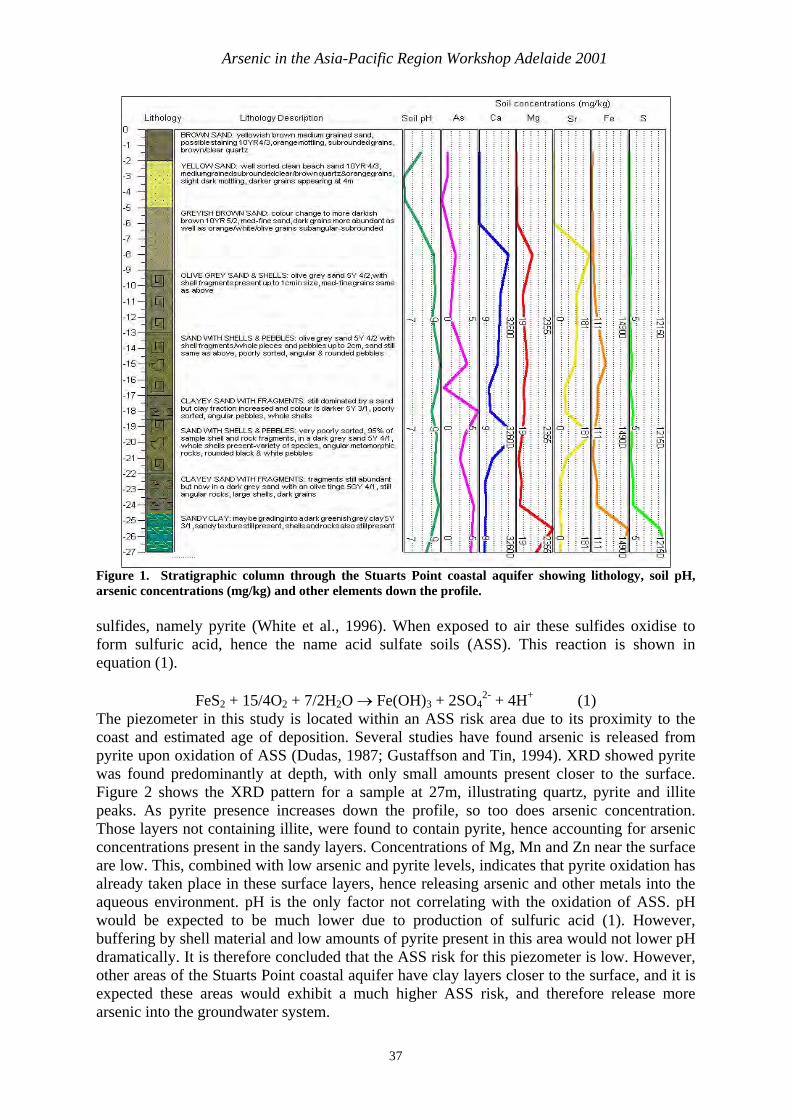
Arsenic in the Asia-Pacific Region Workshop Adelaide 2001
Figure 1. Stratigraphic column through the Stuarts Point coastal aquifer showing lithology, soil pH, arsenic concentrations (mg/kg) and other elements down the profile.
sulfides, namely pyrite (White et al., 1996). When exposed to air these sulfides oxidise to form sulfuric acid, hence the name acid sulfate soils (ASS). This reaction is shown in equation (1).
FeS2 + 15/4O2 + 7/2H2O Fe(OH)3 + 2SO42- + 4H+ (1)
The piezometer in this study is located within an ASS risk area due to its proximity to the coast and estimated age of deposition. Several studies have found arsenic is released from pyrite upon oxidation of ASS (Dudas, 1987; Gustaffson and Tin, 1994). XRD showed pyrite was found predominantly at depth, with only small amounts present closer to the surface. Figure 2 shows the XRD pattern for a sample at 27m, illustrating quartz, pyrite and illite peaks. As pyrite presence increases down the profile, so too does arsenic concentration. Those layers not containing illite, were found to contain pyrite, hence accounting for arsenic concentrations present in the sandy layers. Concentrations of Mg, Mn and Zn near the surface are low. This, combined with low arsenic and pyrite levels, indicates that pyrite oxidation has already taken place in these surface layers, hence releasing arsenic and other metals into the aqueous environment. pH is the only factor not correlating with the oxidation of ASS. pH would be expected to be much lower due to production of sulfuric acid (1). However, buffering by shell material and low amounts of pyrite present in this area would not lower pH dramatically. It is therefore concluded that the ASS risk for this piezometer is low. However, other areas of the Stuarts Point coastal aquifer have clay layers closer to the surface, and it is expected these areas would exhibit a much higher ASS risk, and therefore release more arsenic into the groundwater system.
37
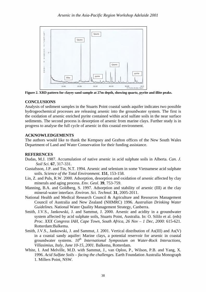
Arsenic in the Asia-Pacific Region Workshop Adelaide 2001
Figure 2. XRD pattern for clayey sand sample at 27m depth, showing quartz, pyrite and illite peaks.
Quartz
Illitepyrite
Quartz
Quartz
pyrite
CONCLUSIONS Analysis of sediment samples in the Stuarts Point coastal sands aquifer indicates two possible hydrogeochemical processes are releasing arsenic into the groundwater system. The first is the oxidation of arsenic enriched pyrite contained within acid sulfate soils in the near surface sediments. The second process is desorption of arsenic from marine clays. Further study is in progress to analyse the full cycle of arsenic in this coastal environment.
ACKNOWLEDGEMENTS The authors would like to thank the Kempsey and Grafton offices of the New South Wales Department of Land and Water Conservation for their funding assistance.
REFERENCES Dudas, M.J. 1987. Accumulation of native arsenic in acid sulphate soils in Alberta. Can. J.
Soil Sci. 67, 317-331. Gustafsson, J.P. and Tin, N.T. 1994. Arsenic and selenium in some Vietnamese acid sulphate
soils. Science of the Total Environment. 151, 153-158. Lin, Z. and Puls, R.W. 2000. Adsorption, desorption and oxidation of arsenic affected by clay
minerals and aging process. Env. Geol. 39, 753-759. Manning, B.A. and Goldberg, S. 1997. Adsorption and stability of arsenic (III) at the clay
mineral-water interface. Environ. Sci. Technol. 31, 2005-2011. National Health and Medical Research Council & Agriculture and Resources Management
Council of Australia and New Zealand (NHMRC) 1996. Australian Drinking Water Guidelines. National Water Quality Management Strategy, Canberra.
Smith, J.V.S., Jankowski, J. and Sammut, J. 2000. Arsenic and acidity in a groundwater system affected by acid sulphate soils, Stuarts Point, Australia. In: O. Sililo et al. (eds) Proc. XXX Congress IAH, Cape Town, South Africa, 26 Nov – 1 Dec, 2000: 615-621. Rotterdam:Balkema.
Smith, J.V.S., Jankowski, J. and Sammut, J. 2001. Vertical distribution of As(III) and As(V) in a coastal sandy aquifer: Marine clays, a potential reservoir for arsenic in coastal groundwater systems. 10th International Symposium on Water-Rock Interactions, Villasimius, Italy, June 10-15, 2001. Balkema, Rotterdam.
White, I. And Melville, M.D. with Sammut, J., van Oploo, P., Wilson, P.B. and Yang, X. 1996. Acid Sulfate Soils – facing the challenges. Earth Foundation Australia Monograph 1. Millers Point, NSW.
38
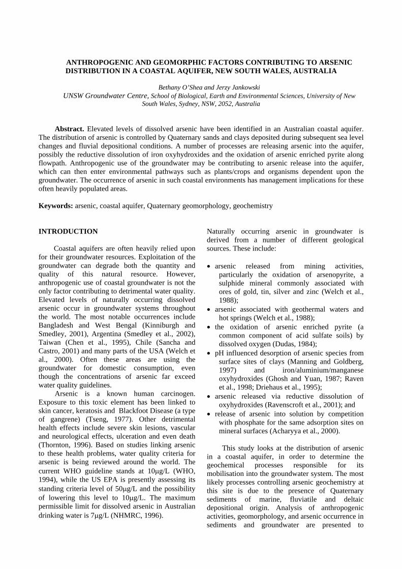
ANTHROPOGENIC AND GEOMORPHIC FACTORS CONTRIBUTING TO ARSENIC DISTRIBUTION IN A COASTAL AQUIFER, NEW SOUTH WALES, AUSTRALIA
Bethany O’Shea and Jerzy Jankowski UNSW Groundwater Centre, School of Biological, Earth and Environmental Sciences, University of New
South Wales, Sydney, NSW, 2052, Australia
Abstract. Elevated levels of dissolved arsenic have been identified in an Australian coastal aquifer. The distribution of arsenic is controlled by Quaternary sands and clays deposited during subsequent sea level changes and fluvial depositional conditions. A number of processes are releasing arsenic into the aquifer, possibly the reductive dissolution of iron oxyhydroxides and the oxidation of arsenic enriched pyrite along flowpath. Anthropogenic use of the groundwater may be contributing to arsenic release into the aquifer, which can then enter environmental pathways such as plants/crops and organisms dependent upon the groundwater. The occurrence of arsenic in such coastal environments has management implications for these often heavily populated areas.
Keywords: arsenic, coastal aquifer, Quaternary geomorphology, geochemistry
INTRODUCTION
Coastal aquifers are often heavily relied upon for their groundwater resources. Exploitation of the groundwater can degrade both the quantity and quality of this natural resource. However, anthropogenic use of coastal groundwater is not the only factor contributing to detrimental water quality. Elevated levels of naturally occurring dissolved arsenic occur in groundwater systems throughout the world. The most notable occurrences include Bangladesh and West Bengal (Kinniburgh and Smedley, 2001), Argentina (Smedley et al., 2002), Taiwan (Chen et al., 1995), Chile (Sancha and Castro, 2001) and many parts of the USA (Welch et al., 2000). Often these areas are using the groundwater for domestic consumption, even though the concentrations of arsenic far exceed water quality guidelines.
Arsenic is a known human carcinogen. Exposure to this toxic element has been linked to skin cancer, keratosis and Blackfoot Disease (a type of gangrene) (Tseng, 1977). Other detrimental health effects include severe skin lesions, vascular and neurological effects, ulceration and even death (Thornton, 1996). Based on studies linking arsenic to these health problems, water quality criteria for arsenic is being reviewed around the world. The current WHO guideline stands at 10 g/L (WHO, 1994), while the US EPA is presently assessing its standing criteria level of 50 g/L and the possibility of lowering this level to 10 g/L. The maximum permissible limit for dissolved arsenic in Australian drinking water is 7 g/L (NHMRC, 1996).
Naturally occurring arsenic in groundwater is derived from a number of different geological sources. These include:
arsenic released from mining activities, particularly the oxidation of arsenopyrite, a sulphide mineral commonly associated with ores of gold, tin, silver and zinc (Welch et al., 1988);
arsenic associated with geothermal waters and hot springs (Welch et al., 1988);
the oxidation of arsenic enriched pyrite (a common component of acid sulfate soils) by dissolved oxygen (Dudas, 1984);
pH influenced desorption of arsenic species from surface sites of clays (Manning and Goldberg, 1997) and iron/aluminium/manganese oxyhydroxides (Ghosh and Yuan, 1987; Raven et al., 1998; Driehaus et al., 1995);
arsenic released via reductive dissolution of oxyhydroxides (Ravenscroft et al., 2001); and
release of arsenic into solution by competition with phosphate for the same adsorption sites on mineral surfaces (Acharyya et al., 2000).
This study looks at the distribution of arsenic in a coastal aquifer, in order to determine the geochemical processes responsible for its mobilisation into the groundwater system. The most likely processes controlling arsenic geochemistry at this site is due to the presence of Quaternary sediments of marine, fluviatile and deltaic depositional origin. Analysis of anthropogenic activities, geomorphology, and arsenic occurrence in sediments and groundwater are presented to
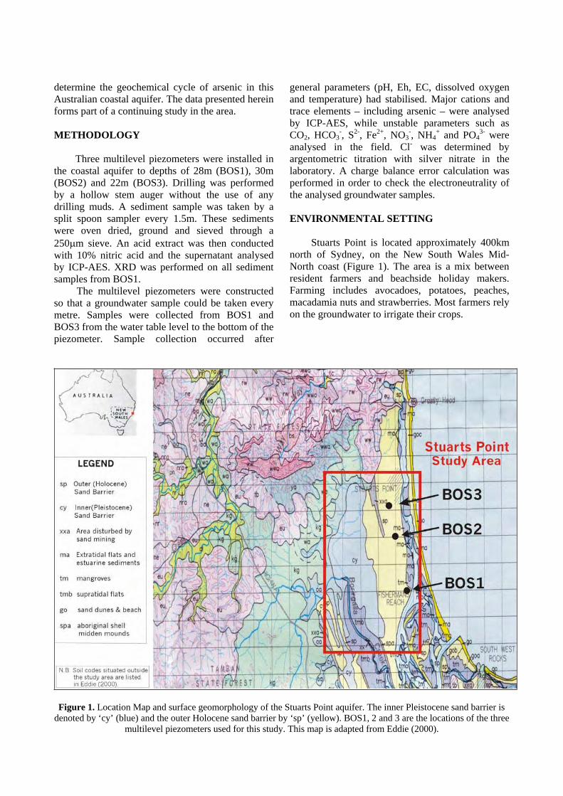
determine the geochemical cycle of arsenic in this Australian coastal aquifer. The data presented herein forms part of a continuing study in the area.
METHODOLOGY
Three multilevel piezometers were installed in the coastal aquifer to depths of 28m (BOS1), 30m (BOS2) and 22m (BOS3). Drilling was performed by a hollow stem auger without the use of any drilling muds. A sediment sample was taken by a split spoon sampler every 1.5m. These sediments were oven dried, ground and sieved through a 250 m sieve. An acid extract was then conducted with 10% nitric acid and the supernatant analysed by ICP-AES. XRD was performed on all sediment samples from BOS1.
The multilevel piezometers were constructed so that a groundwater sample could be taken every metre. Samples were collected from BOS1 and BOS3 from the water table level to the bottom of the piezometer. Sample collection occurred after
general parameters (pH, Eh, EC, dissolved oxygen and temperature) had stabilised. Major cations and trace elements – including arsenic – were analysed by ICP-AES, while unstable parameters such as CO2, HCO3
-, S2-, Fe2+, NO3-, NH4
+ and PO43- were
analysed in the field. Cl- was determined by argentometric titration with silver nitrate in the laboratory. A charge balance error calculation was performed in order to check the electroneutrality of the analysed groundwater samples.
ENVIRONMENTAL SETTING
Stuarts Point is located approximately 400km north of Sydney, on the New South Wales Mid-North coast (Figure 1). The area is a mix between resident farmers and beachside holiday makers. Farming includes avocadoes, potatoes, peaches, macadamia nuts and strawberries. Most farmers rely on the groundwater to irrigate their crops.
Figure 1. Location Map and surface geomorphology of the Stuarts Point aquifer. The inner Pleistocene sand barrier is denoted by ‘cy’ (blue) and the outer Holocene sand barrier by ‘sp’ (yellow). BOS1, 2 and 3 are the locations of the three
multilevel piezometers used for this study. This map is adapted from Eddie (2000).
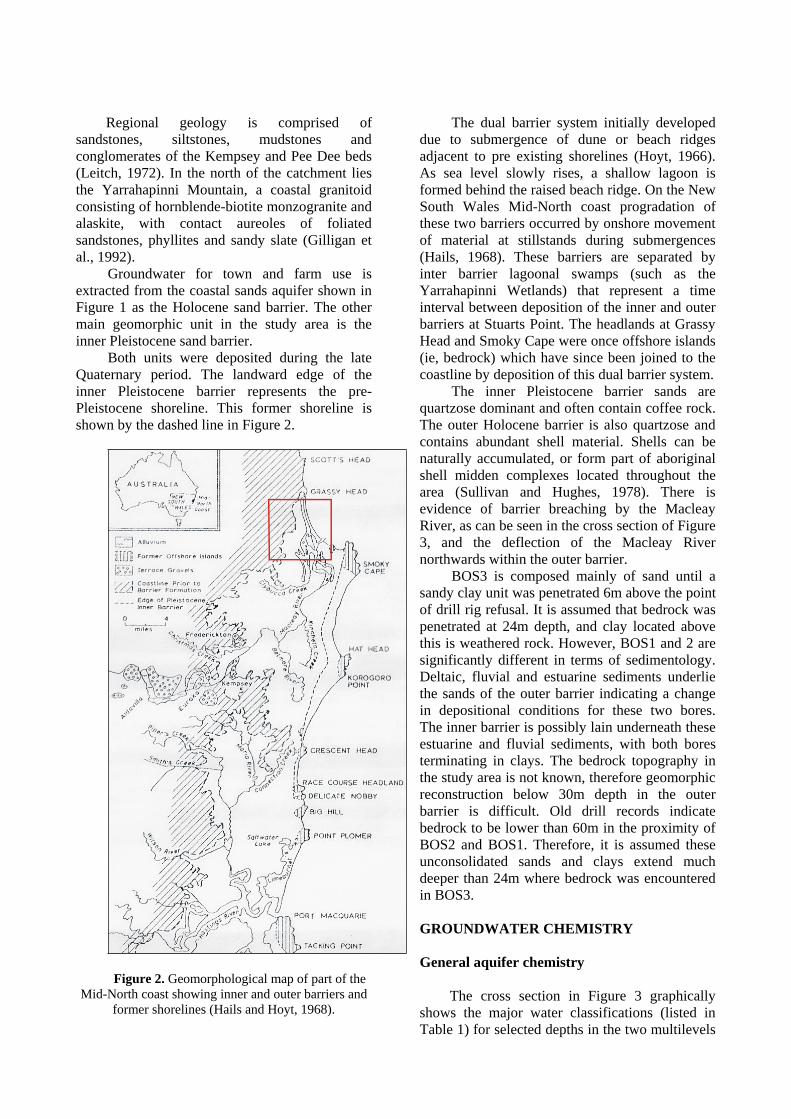
Regional geology is comprised of sandstones, siltstones, mudstones and conglomerates of the Kempsey and Pee Dee beds(Leitch, 1972). In the north of the catchment lies the Yarrahapinni Mountain, a coastal granitoid consisting of hornblende-biotite monzogranite and alaskite, with contact aureoles of foliated sandstones, phyllites and sandy slate (Gilligan et al., 1992).
Groundwater for town and farm use is extracted from the coastal sands aquifer shown in Figure 1 as the Holocene sand barrier. The other main geomorphic unit in the study area is the inner Pleistocene sand barrier.
Both units were deposited during the late Quaternary period. The landward edge of the inner Pleistocene barrier represents the pre-Pleistocene shoreline. This former shoreline is shown by the dashed line in Figure 2.
Figure 2. Geomorphological map of part of the Mid-North coast showing inner and outer barriers and
former shorelines (Hails and Hoyt, 1968).
The dual barrier system initially developed due to submergence of dune or beach ridges adjacent to pre existing shorelines (Hoyt, 1966). As sea level slowly rises, a shallow lagoon is formed behind the raised beach ridge. On the New South Wales Mid-North coast progradation of these two barriers occurred by onshore movement of material at stillstands during submergences (Hails, 1968). These barriers are separated by inter barrier lagoonal swamps (such as the Yarrahapinni Wetlands) that represent a time interval between deposition of the inner and outer barriers at Stuarts Point. The headlands at Grassy Head and Smoky Cape were once offshore islands (ie, bedrock) which have since been joined to the coastline by deposition of this dual barrier system.
The inner Pleistocene barrier sands are quartzose dominant and often contain coffee rock. The outer Holocene barrier is also quartzose and contains abundant shell material. Shells can be naturally accumulated, or form part of aboriginal shell midden complexes located throughout the area (Sullivan and Hughes, 1978). There is evidence of barrier breaching by the Macleay River, as can be seen in the cross section of Figure 3, and the deflection of the Macleay River northwards within the outer barrier.
BOS3 is composed mainly of sand until a sandy clay unit was penetrated 6m above the point of drill rig refusal. It is assumed that bedrock was penetrated at 24m depth, and clay located above this is weathered rock. However, BOS1 and 2 are significantly different in terms of sedimentology. Deltaic, fluvial and estuarine sediments underlie the sands of the outer barrier indicating a change in depositional conditions for these two bores. The inner barrier is possibly lain underneath these estuarine and fluvial sediments, with both bores terminating in clays. The bedrock topography in the study area is not known, therefore geomorphic reconstruction below 30m depth in the outer barrier is difficult. Old drill records indicate bedrock to be lower than 60m in the proximity of BOS2 and BOS1. Therefore, it is assumed these unconsolidated sands and clays extend much deeper than 24m where bedrock was encountered in BOS3.
GROUNDWATER CHEMISTRY
General aquifer chemistry
The cross section in Figure 3 graphically shows the major water classifications (listed in Table 1) for selected depths in the two multilevels
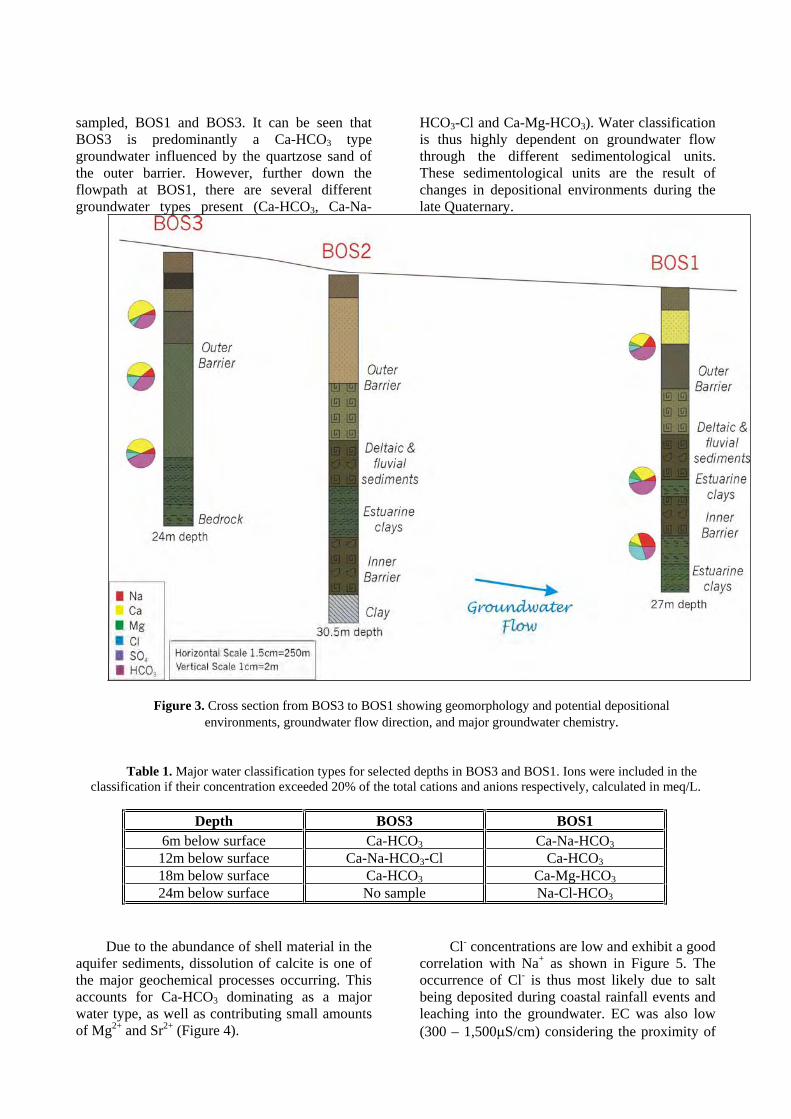
sampled, BOS1 and BOS3. It can be seen that BOS3 is predominantly a Ca-HCO3 type groundwater influenced by the quartzose sand of the outer barrier. However, further down the flowpath at BOS1, there are several different groundwater types present (Ca-HCO3, Ca-Na-
HCO3-Cl and Ca-Mg-HCO3). Water classification is thus highly dependent on groundwater flow through the different sedimentological units. These sedimentological units are the result of changes in depositional environments during the late Quaternary.
Figure 3. Cross section from BOS3 to BOS1 showing geomorphology and potential depositional environments, groundwater flow direction, and major groundwater chemistry.
Table 1. Major water classification types for selected depths in BOS3 and BOS1. Ions were included in the classification if their concentration exceeded 20% of the total cations and anions respectively, calculated in meq/L.
Depth BOS3 BOS16m below surface Ca-HCO3 Ca-Na-HCO3
12m below surface Ca-Na-HCO3-Cl Ca-HCO3
18m below surface Ca-HCO3 Ca-Mg-HCO3
24m below surface No sample Na-Cl-HCO3
Due to the abundance of shell material in the aquifer sediments, dissolution of calcite is one of the major geochemical processes occurring. This accounts for Ca-HCO3 dominating as a major water type, as well as contributing small amounts of Mg2+ and Sr2+ (Figure 4).
Cl- concentrations are low and exhibit a good correlation with Na+ as shown in Figure 5. The occurrence of Cl- is thus most likely due to salt being deposited during coastal rainfall events and leaching into the groundwater. EC was also low (300 – 1,500 S/cm) considering the proximity of
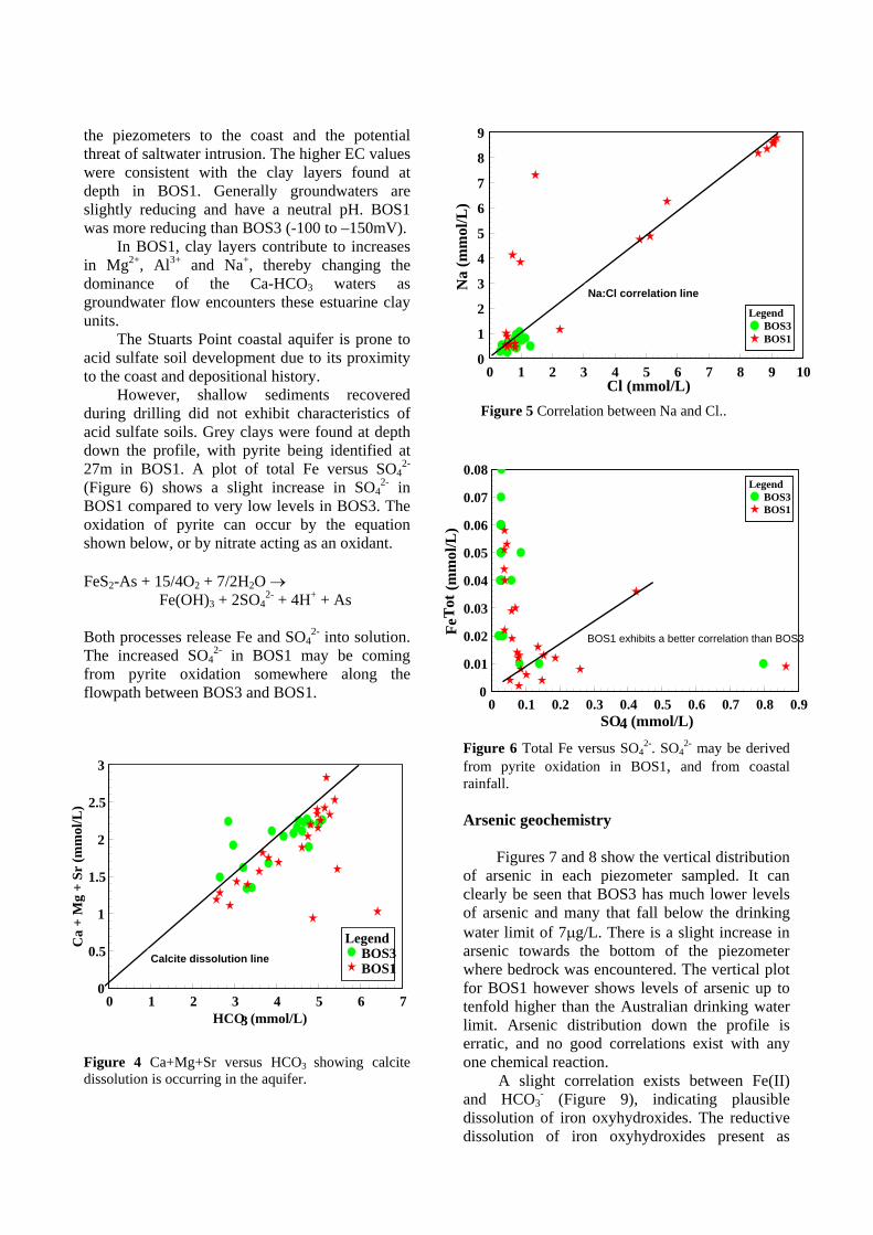
the piezometers to the coast and the potential threat of saltwater intrusion. The higher EC values were consistent with the clay layers found at depth in BOS1. Generally groundwaters are slightly reducing and have a neutral pH. BOS1 was more reducing than BOS3 (-100 to –150mV).
0 1 2 3 4 5 6 7 8 9 10Cl (mmol/L)
0
1
2
3
4
5
6
7
8
9
Na
(mm
ol/L
)
LegendBOS3BOS1
Na:Cl correlation line
In BOS1, clay layers contribute to increases in Mg2+, Al3+ and Na+, thereby changing the dominance of the Ca-HCO3 waters as groundwater flow encounters these estuarine clay units.
The Stuarts Point coastal aquifer is prone to acid sulfate soil development due to its proximity to the coast and depositional history.
However, shallow sediments recovered during drilling did not exhibit characteristics of acid sulfate soils. Grey clays were found at depth down the profile, with pyrite being identified at 27m in BOS1. A plot of total Fe versus SO4
2-
(Figure 6) shows a slight increase in SO42- in
BOS1 compared to very low levels in BOS3. The oxidation of pyrite can occur by the equation shown below, or by nitrate acting as an oxidant.
FeS2-As + 15/4O2 + 7/2H2O Fe(OH)3 + 2SO4
2- + 4H+ + As
Both processes release Fe and SO42- into solution.
The increased SO42- in BOS1 may be coming
from pyrite oxidation somewhere along the flowpath between BOS3 and BOS1.
Figure 4 Ca+Mg+Sr versus HCO3 showing calcite dissolution is occurring in the aquifer.
Figure 5 Correlation between Na and Cl..
0 0.1 0.2 0.3 0.4 0.5 0.6 0.7 0.8 0.9SO4 (mmol/L)
0
0.01
0.02
0.03
0.04
0.05
0.06
0.07
0.08Fe
Tot
(mm
ol/L
)
LegendBOS3BOS1
BOS1 exhibits a better correlation than BOS3
Figure 6 Total Fe versus SO42-. SO4
2- may be derived from pyrite oxidation in BOS1, and from coastal rainfall.
0 1 2 3 4 5 6 7HCO3 (mmol/L)
0
0.5
1
1.5
2
2.5
3
Ca
+M
g+
Sr(m
mol
/L)
LegendBOS3BOS1
Calcite dissolution line
Arsenic geochemistry
Figures 7 and 8 show the vertical distribution of arsenic in each piezometer sampled. It can clearly be seen that BOS3 has much lower levels of arsenic and many that fall below the drinking water limit of 7 g/L. There is a slight increase in arsenic towards the bottom of the piezometer where bedrock was encountered. The vertical plot for BOS1 however shows levels of arsenic up to tenfold higher than the Australian drinking water limit. Arsenic distribution down the profile is erratic, and no good correlations exist with any one chemical reaction.
A slight correlation exists between Fe(II) and HCO3
- (Figure 9), indicating plausible dissolution of iron oxyhydroxides. The reductive dissolution of iron oxyhydroxides present as
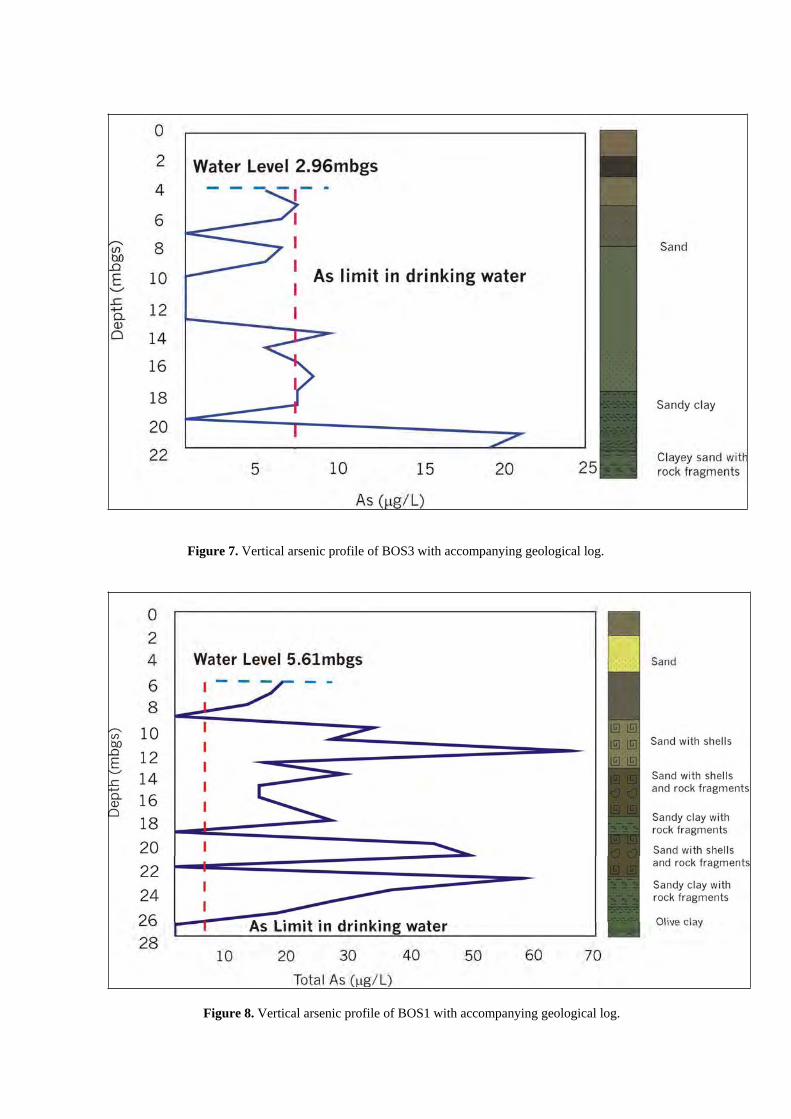
Figure 7. Vertical arsenic profile of BOS3 with accompanying geological log.
Figure 8. Vertical arsenic profile of BOS1 with accompanying geological log.
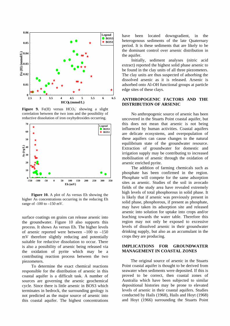
Figure 9. Fe(II) versus HCO3- showing a slight
correlation between the two ions and the possibility of reductive dissolution of iron oxyhydroxides occurring.
Figure 10. A plot of As versus Eh showing the higher As concentrations occurring in the reducing Eh range of -100 to –150 mV.
surface coatings on grains can release arsenic into the groundwater. Figure 10 also supports this process. It shows As versus Eh. The higher levels of arsenic reported were between –100 to –150 mV therefore slightly reducing and potentially suitable for reductive dissolution to occur. There is also a possibility of arsenic being released via the oxidation of pyrite which may be a contributing reaction process between the two piezometers.
To determine the exact chemical reactions responsible for the distribution of arsenic in this coastal aquifer is a difficult task. A number of sources are governing the arsenic geochemical cycle. Since there is little arsenic in BOS3 which terminates in bedrock, the surrounding geology is not predicted as the major source of arsenic into this coastal aquifer. The highest concentrations
have been located downgradient, in the heterogenous sediments of the late Quaternary period. It is these sediments that are likely to be the dominant control over arsenic distribution in the aquifer.
2.5 3 3.5 4 4.5 5 5.5 6 6.5HCO3 (mmol/L)
0
0.01
0.02
0.03
0.04
0.05
0.06
Fe(I
I)(m
mol
/L)
LegendBOS3BOS1
Initially, sediment analyses (nitric acid extract) reported the highest solid phase arsenic to be found in the clay units of all three piezometers. The clay units are thus suspected of adsorbing the dissolved arsenic as it is released. Arsenic is adsorbed onto Al-OH functional groups at particle edge sites of these clays.
ANTHROPOGENIC FACTORS AND THE DISTRIBUTION OF ARSENIC
No anthropogenic source of arsenic has been uncovered in the Stuarts Point coastal aquifer, but this does not mean that arsenic is not being influenced by human activities. Coastal aquifers are delicate ecosystems, and overpopulation of these aquifers can cause changes to the natural equilibrium state of the groundwater resource. Extraction of groundwater for domestic and irrigation supply may be contributing to increased mobilisation of arsenic through the oxidation of arsenic enriched pyrite.
-150 -100 -50 0 50 100 150 200 250 300 350Eh (mV)
0
10
20
30
40
50
60
70
As(
g/L
)
LegendBOS3BOS1
The addition of farming chemicals such as phosphate has been confirmed in the region. Phosphate will compete for the same adsorption sites as arsenic. Studies of the soil in avocado fields of the study area have revealed extremely high levels of total phosphorous in solid phase. It is likely that if arsenic was previously present in solid phase, phosphorous, if present as phosphate, may have taken its adsorption site and released arsenic into solution for uptake into crops and/or leaching towards the water table. Therefore this region may not only be exposed to excessive levels of dissolved arsenic in their groundwater drinking supply, but also as an accumulant in the crops they are producing.
IMPLICATIONS FOR GROUNDWATER MANAGEMENT IN COASTAL ZONES
The original source of arsenic in the Stuarts Point coastal aquifer is thought to be derived from seawater when sediments were deposited. If this is proved to be correct, then coastal zones of Australia which have been subjected to similar depositional histories may be prone to elevated levels of arsenic in their coastal aquifers. Studies conducted by Hails (1968), Hails and Hoyt (1968) and Hoyt (1966) surrounding the Stuarts Point
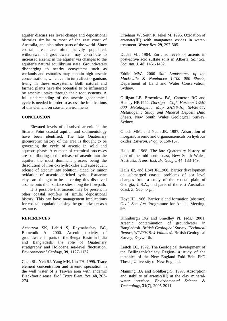
aquifer discuss sea level change and depositional histories similar to most of the east coast of Australia, and also other parts of the world. Since coastal areas are often heavily populated, withdrawal of groundwater may contribute to increased arsenic in the aquifer via changes to the aquifer’s natural equilibrium state. Groundwaters discharging to nearby ecosystems such as wetlands and estuaries may contain high arsenic concentrations, which can in turn affect organisms living in these ecosystems. Both natural and farmed plants have the potential to be influenced by arsenic uptake through their root systems. A full understanding of the arsenic geochemical cycle is needed in order to assess the implications of this element on coastal environments.
CONCLUSION
Elevated levels of dissolved arsenic in the Stuarts Point coastal aquifer and sedimentology have been identified. The late Quaternary geomorphic history of the area is thought to be governing the cycle of arsenic in solid and aqueous phase. A number of chemical processes are contributing to the release of arsenic into the aquifer, the most dominant process being the dissolution of iron oxyhydroxides and subsequent release of arsenic into solution, aided by minor oxidation of arsenic enriched pyrite. Estuarine clays are thought to be adsorbing this dissolved arsenic onto their surface sites along the flowpath.
It is possible that arsenic may be present in other coastal aquifers of similar depositional history. This can have management implications for coastal populations using the groundwater as a resource.
REFERENCES
Acharyya SK, Lahiri S, Raymahashay BC, Bhowmik A. 2000. Arsenic toxicity of groundwater in parts of the Bengal Basin in India and Bangladesh: the role of Quaternary stratigraphy and Holocene sea-level fluctuation. Environmental Geology, 39, 1127-1137.
Chen SL, Yeh SJ, Yang MH, Lin TH. 1995. Trace element concentration and arsenic speciation in the well water of a Taiwan area with endemic Blackfoot disease. Biol. Trace Elem. Res. 48, 263-274.
Driehaus W, Seith R, Jekel M. 1995. Oxidation of arsenate(III) with manganese oxides in water-treatment. Water Res. 29, 297-305.
Dudas MJ. 1984. Enriched levels of arsenic in post-active acid sulfate soils in Alberta. Soil Sci. Soc. Am. J. 48, 1451-1452.
Eddie MW. 2000 Soil Landscapes of the Macksville & Nambucca 1:100 000 Sheets,Department of Land and Water Conservation, Sydney.
Gilligan LB, Brownlow JW,. Cameron RG and Henley HF.1992. Dorrigo – Coffs Harbour 1:250 000 Metallogenic Map SH/56-10, SH/56-11: Metallogenic Study and Mineral Deposit Data Sheets. New South Wales Geological Survey, Sydney.
Ghosh MM, and Yuan JR. 1987. Adsorption of inorganic arsenic and organoarsenicals on hydrous oxides. Environ. Prog. 6, 150-157.
Hails JR. 1968. The late Quaternary history of part of the mid-north coast, New South Wales, Australia. Trans. Inst. Br. Geogr., 44, 133-149.
Hails JR, and Hoyt JR.1968. Barrier development on submerged coasts; problems of sea level changes from a study of the coastal plain of Georgia, U.S.A., and parts of the east Australian coast. Z. Geomorph.
Hoyt JH. 1966. Barrier island formation (abstract) Geol. Soc. Am. Programme for Annual Meeting, 99.
Kinniburgh DG and Smedley PL (eds.) 2001. Arsenic contamination of groundwater in Bangladesh. British Geological Survey (Technical Report, WC/00/19. 4 Volumes). British Geological Survey, Keyworth.
Leitch EC. 1972. The Geological development of the Bellinger-Macleay Region- a study of the tectonics of the New England Fold Belt. PhD Thesis, University of New England.
Manning BA and Goldberg S. 1997. Adsorption and stability of arsenic(III) at the clay mineral-water interface. Environmental Science & Technology, 31(7), 2005-2011.
National Health and Medical Research Council (NHMRC) & Agriculture and Resources Management Council of Australia and New Zealand. 1996. Australian Drinking Water Guidelines. National Water Quality Management Strategy, Canberra.
Raven KP, Jain A, Loeppert RH. 1998 Arsenite and arsenate adsorption on ferrihydrite: kinetics, equilibrium, and adsorption envelopes. Environ. Sci. Technol. 32, 344-349.
Ravenscroft P, McArthur JM and Hoque BA. 2001. Geochemical and palaeohydrological controls on pollution of groundwater by arsenic. In: Chapell WR, Abernathy CO, Calderon RL. (eds) Arsenic Exposure and Health Effects IV. Elsevier, Amsterdam, 20p.
Sancha AM and Castro ML. 2001 Arsenic in Latin America: occurrence, exposure, health effects and remediation. In: Chapell WR, Abernathy CO, Calderon RL. (eds) Arsenic Exposure and Health Effects IV. Elsevier, Amsterdam, 87-96.
Smedley PL, Nicolli HB, Macdonald DMJ, Barros AJ, Tullio JO. 2002 Hydrogeochemistry of arsenic and other inorganic constituents in groundwaters from La Pampa, Argentina. Appl.Geochem. 17, 259-284.
Sullivan ME and Hughes PJ. 1978. A survey of the Stuarts Point shell midden complex, Macleay River, New South Wales. A report to the National Parks and Wildlife Service of NSW.
Thornton I. 1996. Sources and pathways of arsenic in the geochemical environment: health implications. In: Appleton JD, Fuge R and McCall GJH. (eds), Environmental Geochemistry and Health, Geological Society Special Publication No. 113, 153-161.
Tseng WP. 1977. Effects of dose-response relationships on skin cancer and Blackfoot Disease with arsenic. Environmental Health Perspectives, 19, 109-119.
Welch AH, Lico MS and Hughes JL. 1988. Arsenic in ground water of the western United States. Ground Water, 26(3) 333-347.
Welch AH, Westhohn DB, Helsel DR and Wanty RB. 2000. Arsenic in ground water of the United States: occurrence and geochemistry. Ground Water, 38(4), 589-604.
World Health Organisation (WHO). 1994. Recommendations, second ed., Guidelines for Drinking Water Quality, 1, Geneva.
NATURAL ARSENIC IN A COASTAL AQUIFER: IMPLICATIONS FOR WATER QUALITY MANAGEMENT IN AUSTRALIAN
COASTAL ZONES
Bethany O’Shea1and Jerzy Jankowski21PhD Research Student, UNSW Groundwater Centre, Sydney, NSW, Australia 2052
2Senior Lecturer, UNSW Groundwater Centre, Sydney, NSW, Australia 2052
Abstract
Arsenic concentrations in excess of Australian Drinking Water Guidelines have been found in a coastal aquifer at Stuarts Point on the Mid-North coast of New South Wales, Australia. Groundwater from this aquifer is used for a variety of purposes including domestic and town water supplies, and irrigation of local crops. Sediment and groundwater were analysed from a 27m deep multilevel piezometer. Results of this study indicate that arsenic is derived from several sources. The oxidation of pyrite present as coatings on sediment grains by both dissolved oxygen and nitrate is suggested by water chemistry and soil extract results. Reductive dissolution of iron oxyhydroxide coatings could also contribute arsenic to the system, but these coatings have not yet been identified in the system. pH influenced adsorption/desorption of arsenic on surface sites of clays is probable, and is being investigated further. Arsenic and element profiles with depth indicate a combination of various sources are contributing arsenic to the groundwater system at different depths in the profile. Arsenic in this aquifer is derived from a natural source. Other coastal areas with similar depositional histories should be aware of the possibility of elevated arsenic in their groundwater systems, and incorporate this into their management plans.
Key Words: arsenic, coastal aquifers, pyrite, desorption, iron oxyhydroxides
Introduction
Elevated levels of dissolved arsenic have been found in groundwater in various parts of the world. The most notable occurrences include West Bengal and Bangladesh, Hungary, Taiwan, China, Chile, Argentina and many parts of the USA. Millions of people are being exposed to arsenic by consumption of groundwater used for domestic supplies. Exposure to arsenic can cause skin lesions, kerotosis, cancer, ulceration, gangrene and ultimately death.
Natural arsenic in groundwater is derived from a number of different geological sources. These include:
arsenic released from mining activities, particularly the oxidation of arsenopyrite, a sulphide mineral commonly associated with ores of gold, tin, silver and zinc
arsenic associated with geothermal waters and hot springs
the oxidation of arsenic enriched pyrite (a common component of acid sulfate soils) by dissolved oxygen or other oxidants, such as nitrate
pH influenced desorption of arsenic species from surface sites of clays and iron and aluminium oxyhydroxides
arsenic released via reductive dissolution of iron oxyhydroxides, and
release of arsenic into solution by competition with phosphate and bicarbonate for the same adsorption sites on mineral surfaces.
The purpose of this study was to determine possible sources and release mechanisms of natural arsenic in an Australian coastal aquifer. Once these sources and mechanisms have been identified an assessment of arsenic occurrences in other coastal zones can be made.
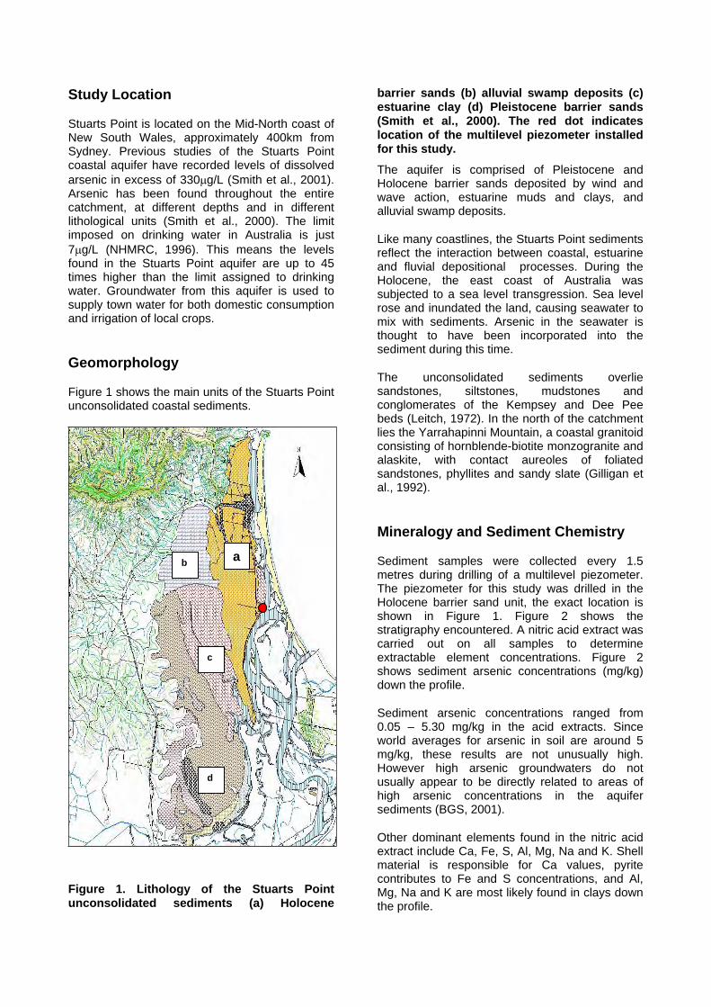
Study Location
Stuarts Point is located on the Mid-North coast of New South Wales, approximately 400km from Sydney. Previous studies of the Stuarts Point coastal aquifer have recorded levels of dissolved arsenic in excess of 330 g/L (Smith et al., 2001). Arsenic has been found throughout the entire catchment, at different depths and in different lithological units (Smith et al., 2000). The limit imposed on drinking water in Australia is just 7 g/L (NHMRC, 1996). This means the levels found in the Stuarts Point aquifer are up to 45 times higher than the limit assigned to drinking water. Groundwater from this aquifer is used to supply town water for both domestic consumption and irrigation of local crops.
Geomorphology
Figure 1 shows the main units of the Stuarts Point unconsolidated coastal sediments.
Figure 1. Lithology of the Stuarts Point unconsolidated sediments (a) Holocene
barrier sands (b) alluvial swamp deposits (c) estuarine clay (d) Pleistocene barrier sands (Smith et al., 2000). The red dot indicates location of the multilevel piezometer installed for this study.
The aquifer is comprised of Pleistocene and Holocene barrier sands deposited by wind and wave action, estuarine muds and clays, and alluvial swamp deposits.
Like many coastlines, the Stuarts Point sediments reflect the interaction between coastal, estuarine and fluvial depositional processes. During the Holocene, the east coast of Australia was subjected to a sea level transgression. Sea level rose and inundated the land, causing seawater to mix with sediments. Arsenic in the seawater is thought to have been incorporated into the sediment during this time.
The unconsolidated sediments overlie sandstones, siltstones, mudstones and conglomerates of the Kempsey and Dee Pee beds (Leitch, 1972). In the north of the catchment lies the Yarrahapinni Mountain, a coastal granitoid consisting of hornblende-biotite monzogranite and alaskite, with contact aureoles of foliated sandstones, phyllites and sandy slate (Gilligan et al., 1992).
Mineralogy and Sediment Chemistry a Sediment samples were collected every 1.5
metres during drilling of a multilevel piezometer. The piezometer for this study was drilled in the Holocene barrier sand unit, the exact location is shown in Figure 1. Figure 2 shows the stratigraphy encountered. A nitric acid extract was carried out on all samples to determine extractable element concentrations. Figure 2 shows sediment arsenic concentrations (mg/kg) down the profile.
b
c
Sediment arsenic concentrations ranged from 0.05 – 5.30 mg/kg in the acid extracts. Since world averages for arsenic in soil are around 5 mg/kg, these results are not unusually high. However high arsenic groundwaters do not usually appear to be directly related to areas of high arsenic concentrations in the aquifer sediments (BGS, 2001).
d
Other dominant elements found in the nitric acid extract include Ca, Fe, S, Al, Mg, Na and K. Shell material is responsible for Ca values, pyrite contributes to Fe and S concentrations, and Al, Mg, Na and K are most likely found in clays down the profile.
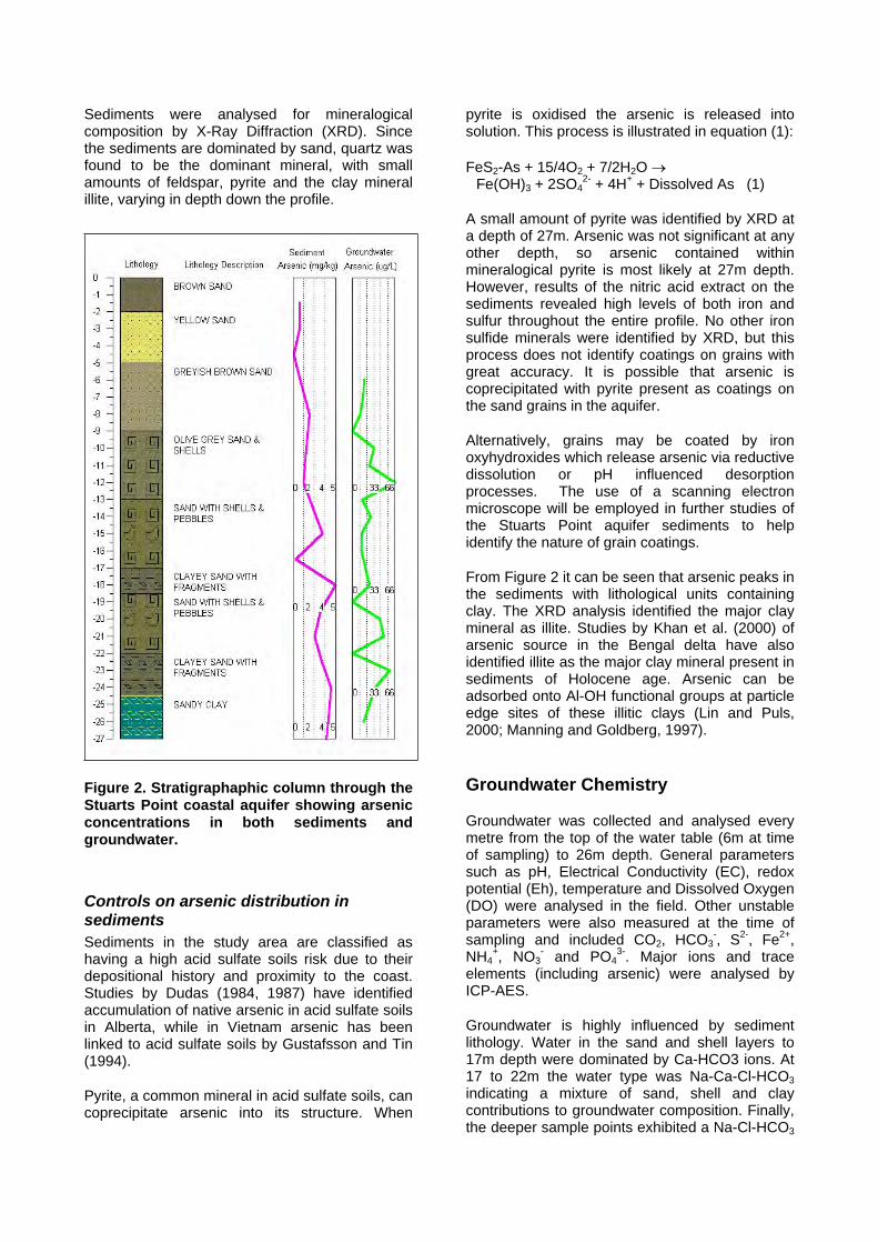
Sediments were analysed for mineralogical composition by X-Ray Diffraction (XRD). Since the sediments are dominated by sand, quartz was found to be the dominant mineral, with small amounts of feldspar, pyrite and the clay mineral illite, varying in depth down the profile.
Figure 2. Stratigraphaphic column through the Stuarts Point coastal aquifer showing arsenic concentrations in both sediments and groundwater.
Controls on arsenic distribution in sedimentsSediments in the study area are classified as having a high acid sulfate soils risk due to their depositional history and proximity to the coast. Studies by Dudas (1984, 1987) have identified accumulation of native arsenic in acid sulfate soils in Alberta, while in Vietnam arsenic has been linked to acid sulfate soils by Gustafsson and Tin (1994).
Pyrite, a common mineral in acid sulfate soils, can coprecipitate arsenic into its structure. When
pyrite is oxidised the arsenic is released into solution. This process is illustrated in equation (1):
FeS2-As + 15/4O2 + 7/2H2OFe(OH)3 + 2SO4
2- + 4H+ + Dissolved As (1)
A small amount of pyrite was identified by XRD at a depth of 27m. Arsenic was not significant at any other depth, so arsenic contained within mineralogical pyrite is most likely at 27m depth. However, results of the nitric acid extract on the sediments revealed high levels of both iron and sulfur throughout the entire profile. No other iron sulfide minerals were identified by XRD, but this process does not identify coatings on grains with great accuracy. It is possible that arsenic is coprecipitated with pyrite present as coatings on the sand grains in the aquifer.
Alternatively, grains may be coated by iron oxyhydroxides which release arsenic via reductive dissolution or pH influenced desorption processes. The use of a scanning electron microscope will be employed in further studies of the Stuarts Point aquifer sediments to help identify the nature of grain coatings.
From Figure 2 it can be seen that arsenic peaks in the sediments with lithological units containing clay. The XRD analysis identified the major clay mineral as illite. Studies by Khan et al. (2000) of arsenic source in the Bengal delta have also identified illite as the major clay mineral present in sediments of Holocene age. Arsenic can be adsorbed onto Al-OH functional groups at particle edge sites of these illitic clays (Lin and Puls, 2000; Manning and Goldberg, 1997).
Groundwater Chemistry
Groundwater was collected and analysed every metre from the top of the water table (6m at time of sampling) to 26m depth. General parameters such as pH, Electrical Conductivity (EC), redox potential (Eh), temperature and Dissolved Oxygen (DO) were analysed in the field. Other unstable parameters were also measured at the time of sampling and included CO2, HCO3
-, S2-, Fe2+,NH4
+, NO3- and PO4
3-. Major ions and trace elements (including arsenic) were analysed by ICP-AES.
Groundwater is highly influenced by sediment lithology. Water in the sand and shell layers to 17m depth were dominated by Ca-HCO3 ions. At 17 to 22m the water type was Na-Ca-Cl-HCO3indicating a mixture of sand, shell and clay contributions to groundwater composition. Finally, the deeper sample points exhibited a Na-Cl-HCO3
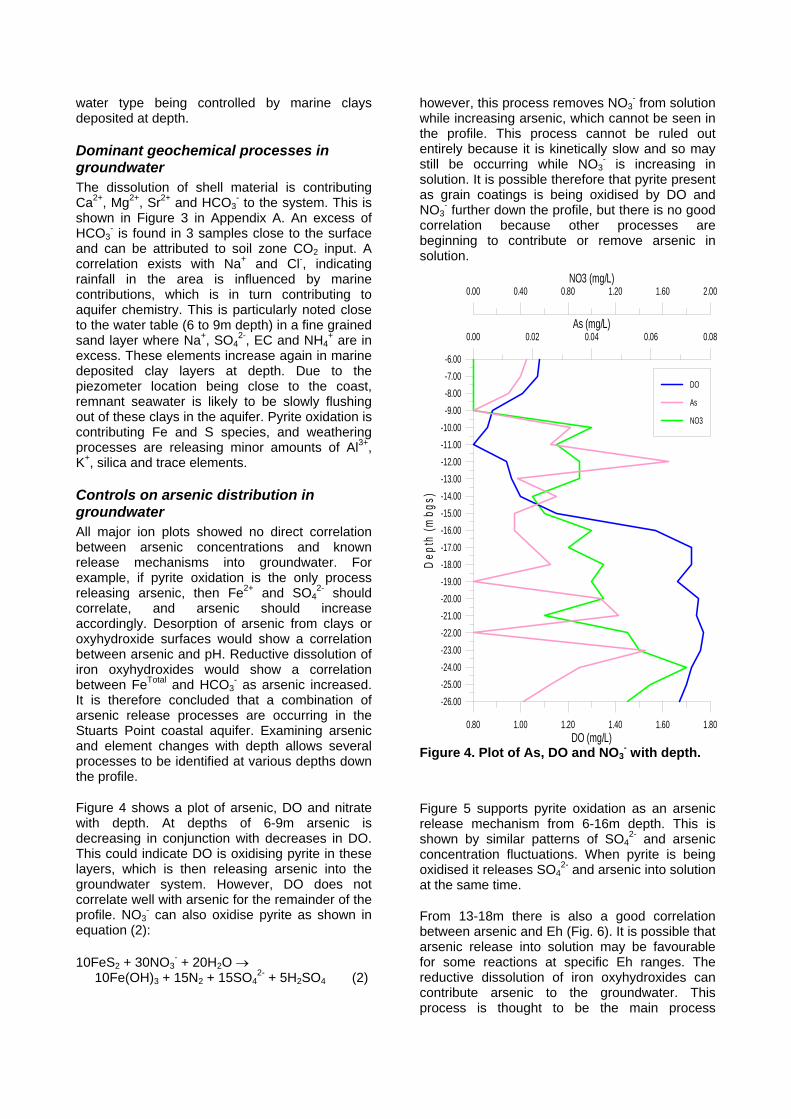
water type being controlled by marine clays deposited at depth.
Dominant geochemical processes in groundwaterThe dissolution of shell material is contributing Ca2+, Mg2+, Sr2+ and HCO3
- to the system. This is shown in Figure 3 in Appendix A. An excess of HCO3
- is found in 3 samples close to the surface and can be attributed to soil zone CO2 input. A correlation exists with Na+ and Cl-, indicating rainfall in the area is influenced by marine contributions, which is in turn contributing to aquifer chemistry. This is particularly noted close to the water table (6 to 9m depth) in a fine grained sand layer where Na+, SO4
2-, EC and NH4+ are in
excess. These elements increase again in marine deposited clay layers at depth. Due to the piezometer location being close to the coast, remnant seawater is likely to be slowly flushing out of these clays in the aquifer. Pyrite oxidation is contributing Fe and S species, and weathering processes are releasing minor amounts of Al3+,K+, silica and trace elements.
Controls on arsenic distribution in groundwaterAll major ion plots showed no direct correlation between arsenic concentrations and known release mechanisms into groundwater. For example, if pyrite oxidation is the only process releasing arsenic, then Fe2+ and SO4
2- should correlate, and arsenic should increase accordingly. Desorption of arsenic from clays or oxyhydroxide surfaces would show a correlation between arsenic and pH. Reductive dissolution of iron oxyhydroxides would show a correlation between FeTotal and HCO3
- as arsenic increased. It is therefore concluded that a combination of arsenic release processes are occurring in the Stuarts Point coastal aquifer. Examining arsenic and element changes with depth allows several processes to be identified at various depths down the profile.
Figure 4 shows a plot of arsenic, DO and nitrate with depth. At depths of 6-9m arsenic is decreasing in conjunction with decreases in DO. This could indicate DO is oxidising pyrite in these layers, which is then releasing arsenic into the groundwater system. However, DO does not correlate well with arsenic for the remainder of the profile. NO3
- can also oxidise pyrite as shown in equation (2):
10FeS2 + 30NO3- + 20H2O
10Fe(OH)3 + 15N2 + 15SO42- + 5H2SO4 (2)
however, this process removes NO3- from solution
while increasing arsenic, which cannot be seen in the profile. This process cannot be ruled out entirely because it is kinetically slow and so may still be occurring while NO3
- is increasing in solution. It is possible therefore that pyrite present as grain coatings is being oxidised by DO and NO3
- further down the profile, but there is no good correlation because other processes are beginning to contribute or remove arsenic in solution.
Figure 4. Plot of As, DO and NO3- with depth.
0.80 1.00 1.20 1.40 1.60 1.80DO (mg/L)
-26.00-25.00-24.00-23.00-22.00-21.00-20.00-19.00-18.00-17.00-16.00-15.00-14.00-13.00-12.00-11.00-10.00-9.00-8.00-7.00-6.00
Dep
th (m
bgs)
0.00 0.02 0.04 0.06 0.08As (mg/L)
0.00 0.40 0.80 1.20 1.60 2.00NO3 (mg/L)
DO
As
NO3
Figure 5 supports pyrite oxidation as an arsenic release mechanism from 6-16m depth. This is shown by similar patterns of SO4
2- and arsenic concentration fluctuations. When pyrite is being oxidised it releases SO4
2- and arsenic into solution at the same time.
From 13-18m there is also a good correlation between arsenic and Eh (Fig. 6). It is possible that arsenic release into solution may be favourable for some reactions at specific Eh ranges. The reductive dissolution of iron oxyhydroxides can contribute arsenic to the groundwater. This process is thought to be the main process
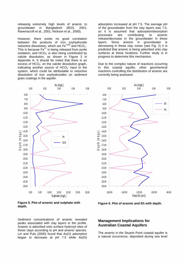
releasing extremely high levels of arsenic to groundwater in Bangladesh (BGS, 2001; Ravenscroft et al., 2001; Nickson et al., 2000).
However, there exists no good correlation between the products of iron oxyhydroxide reductive dissolution, which are FeTotal and HCO3
-.This is because Fe2+ is being released from pyrite oxidation, and HCO3
- is also being contributed by calcite dissolution, as shown in Figure 3 in Appendix A. It should be noted that there is an excess of HCO3
- on the calcite dissolution graph, indicating another source of HCO3
- input to the system, which could be attributable to reductive dissolution of iron oxyhydroxides on sediment grain coatings in the aquifer.
Figure 5. Plot of arsenic and sulphate with depth.
Sediment concentrations of arsenic revealed peaks associated with clay layers in the profile. Arsenic is adsorbed onto surface hydroxyl sites of these clays according to pH and arsenic species. Lin and Puls (2000) found that As(V) adsorption began to decrease at pH 7.5 while As(III)
adsorption increased at pH 7.5. The average pH of the groundwater from the clay layers was 7.5, so it is assumed that adsorption/desorption processes are contributing to arsenic release/decrease in the groundwater in these layers. Since arsenic in groundwater is decreasing in these clay zones (see Fig. 2) it is predicted that arsenic is being adsorbed onto clay surfaces at these locations. Further study is in progress to determine this mechanism.
Due to the complex nature of reactions occurring in this coastal aquifer, other geochemical reactions controlling the distribution of arsenic are currently being assessed.
-160.00 -140.00 -120.00 -100.00 -80.00Field Eh (mV)
-26.00-25.00-24.00-23.00-22.00-21.00-20.00-19.00-18.00-17.00-16.00-15.00-14.00-13.00-12.00-11.00-10.00-9.00-8.00-7.00-6.00
Dep
th (m
bgs)
0.00 0.02 0.04 0.06 0.08As (mg/L)
Eh
As
0.00 5.00 10.00 15.00 20.00 25.00 30.00Sulphate (mg/L)
-26.00-25.00-24.00-23.00-22.00-21.00-20.00-19.00-18.00-17.00-16.00-15.00-14.00-13.00-12.00-11.00-10.00
-9.00-8.00-7.00-6.00
Dep
th (m
bgs)
0.00 0.02 0.04 0.06 0.08As (mg/L)
As
SO4
Figure 6. Plot of arsenic and Eh with depth.
Management Implications for Australian Coastal Aquifers
The arsenic in the Stuarts Point coastal aquifer is a natural occurrence, deposited during sea level
rise in the Holocene. Similar sediments were deposited along the entire east coast of Australia during this time. It is possible then, that other coastal zones have elevated levels of natural arsenic in their groundwater systems. It is already known that arsenic can be associated with acid sulfate soils, and these soils are widespread in Eastern Australian coastlines. Fluctuations in water levels of aquifers due to extraction for irrigation, construction and drinking water can lead to oxidation of these sediments and release of arsenic. Introduction of phosphate to the system through anthropogenic activities could also release arsenic into groundwater. Levels of dissolved arsenic need to be measured in similar coastal zones and management practices to treat or control dissolved arsenic in coastal aquifers be put into place.
Conclusion
Natural arsenic was deposited in sediments at Stuarts Point during sea level rise in the Holocene. This arsenic is now being released into the groundwater system. There are several processes responsible for arsenic mobilisation in this coastal aquifer.
The oxidation of arsenic enriched pyrite by DO or NO3
-, reductive dissolution of iron oxyhydroxide coatings on sediment grains, and pH influenced desorption from surface sites of clays are thought to be the main processes controlling arsenic in this coastal aquifer.
Due to the complex nature of reactions occurring in the Stuarts Point groundwater system, further studies are in progress to determine the full cycle of arsenic in this environment.
Acknowledgements
The authors would like to thank the Grafton office of the New South Wales Department of Land and Water Conservation for their financial contribution to this study.
References
British Geological Survey (BGS) (2001) “Arsenic contamination of groundwater in Bangladesh. Volume 2: Final report”. BGS Technical Report WC/00/19.
Dudas, M.J. (1984) Enriched levels of arsenic in post-active acid sulfate soils in Alberta. Soil Sci. Soc. Am. J. 48: 1451-1452.
Dudas, M.J. (1987) Accumulation of native arsenic in acid sulfate soils in Alberta. Can. J. Soil Sci. 67: 317-331.
Eddie, M.W. (2000) Soil Landscapes of the Macksville & Nambucca 1:100 000 Sheets, Department of Land and Water Conservation, Sydney.
Gustafsson, J.P. and N.T. Tin (1994) Arsenic and selenium in some Vietnamese acid sulphate soils. Science of the Total Environment 151: 153-158.
Gilligan, L.B., J.W. Brownlow, R.G. Cameron & H.F. Henley (1992) Dorrigo – Coffs Harbour 1: 250 000 Metallogenic Map SH/56-10, SH/56-11: Metallogenic Study and Mineral Deposit Data Sheets. New South Wales Geological Survey, Sydney.
Khan, A.A., S.H. Akhter and S.M.M. Alam (2000) Evidence of Holocene trangression, dolomitization and the source of arsenic in the Bengal delta. Proceedings of the First International Conference on geotechnical, Geoenvironmental Engineering and Management in Arid Areas (GEO2000), November 4-7, 2000. A.A. Balkema Publishers, Rotterdam, Netherlands.
Leitch, E.C. (1972) The Geological development of the Bellinger-Macleay Region- a study of the tectonics of the New England Fold Belt. PhD.Thesis, University of New England.
Lin, Z. and R.W. Puls (2000) Adsorption, desorption and oxidation of arsenic affected by clay minerals and aging process. Env. Geol. 39,753-759.
Manning, B.A. and S. Goldberg (1997) Adsorption and stability of arsenic (III) at the clay mineral-water interface. Environ. Sci, Technol. 31, 2005-2011.
National Health and Medical Research Council & Agriculture and Resources Management Council of Australia and New Zealand (NHMRC) (1996) Australian Drinking Water Guidelines. National Water Quality Management Strategy, Canberra.
Nickson, R.T., J.M. McArthur, P.Ravenscroft, W.G. Burgess and K.M. Ahmed (2000) Mechanism of arsenic release to groundwater, Bangladesh and West Bengal. AppliedGeochemistry 15: 403-413.
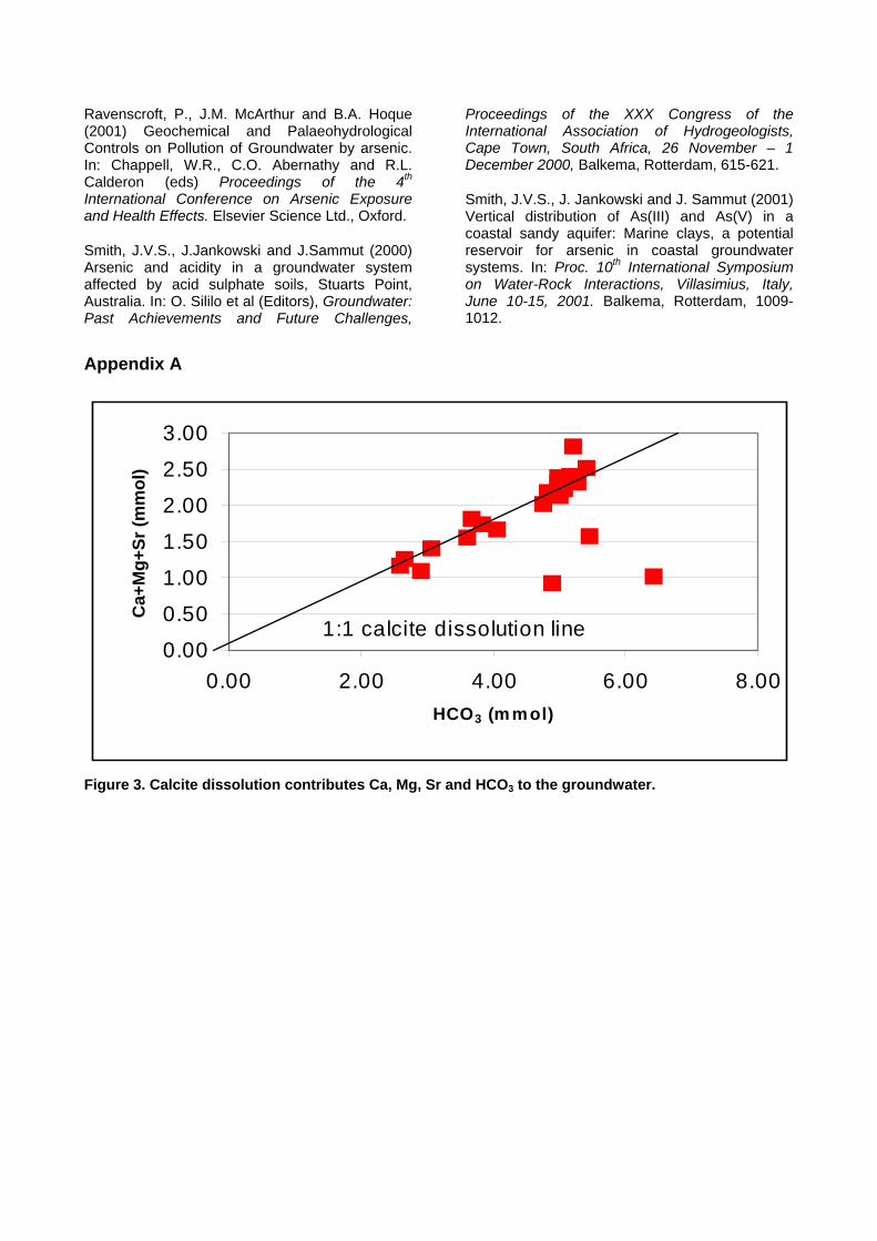
Ravenscroft, P., J.M. McArthur and B.A. Hoque (2001) Geochemical and Palaeohydrological Controls on Pollution of Groundwater by arsenic. In: Chappell, W.R., C.O. Abernathy and R.L. Calderon (eds) Proceedings of the 4th
International Conference on Arsenic Exposure and Health Effects. Elsevier Science Ltd., Oxford.
Smith, J.V.S., J.Jankowski and J.Sammut (2000) Arsenic and acidity in a groundwater system affected by acid sulphate soils, Stuarts Point, Australia. In: O. Sililo et al (Editors), Groundwater:Past Achievements and Future Challenges,
Proceedings of the XXX Congress of the International Association of Hydrogeologists,Cape Town, South Africa, 26 November – 1 December 2000, Balkema, Rotterdam, 615-621.
Smith, J.V.S., J. Jankowski and J. Sammut (2001) Vertical distribution of As(III) and As(V) in a coastal sandy aquifer: Marine clays, a potential reservoir for arsenic in coastal groundwater systems. In: Proc. 10th International Symposium on Water-Rock Interactions, Villasimius, Italy, June 10-15, 2001. Balkema, Rotterdam, 1009-1012.
Appendix A
0.00
0.50
1.00
1.50
2.00
2.50
3.00
0.00 2.00 4.00 6.00 8.00HCO3 (m mol)
Ca+
Mg+
Sr (m
mol
)
1:1 calcite dissolution line
Figure 3. Calcite dissolution contributes Ca, Mg, Sr and HCO3 to the groundwater.
Authors Biographies
Bethany O’Shea is a PhD research student at the University of New South Wales Groundwater Centre. Her research involves determining the source, release and transport of natural arsenic in a coastal aquifer. Arsenic speciation and cycling in both sediments and groundwater is also a major component of her PhD project. Bethany has a First Class Honours degree in Earth and Environmental Science, and has worked for International Mining Consultants and the NSW Department of Mineral Resources during her undergraduate years. She is currently employed as hydrogeologist in the Sydney office of Egis Consulting Australia Pty Limited.
Postal Address: School of Geology, University of New South Wales, UNSW SYDNEY NSW 2052
E-mail: [email protected]
Jerzy Jankowski has a BSc in hydrology, an MSc in hydrology/hydrochemistry and a Ph.D. in hydrogeology/hydrogeochemistry, all from the University of Wroclaw, Poland. He has more than 20 years research experience in countries including Poland, Czechoslovakia, Bulgaria and Australia. He is author/co-author of over 100 research papers, chapters in books and conference proceedings. Areas of special research expertise include: water-rock interaction in different rock type environments, contamination of surface waters and groundwaters, chemical evolution of groundwaters in the arid zone, groundwater-sea water and groundwater-surface water interactions, dryland salinisation processes and hydrochemical and isotopic studies including environmental isotopes and hydrogeochemical modelling.
Postal Address: School of Geology, University of New South Wales, UNSW SYDNEY NSW 2052
E-mail: [email protected]
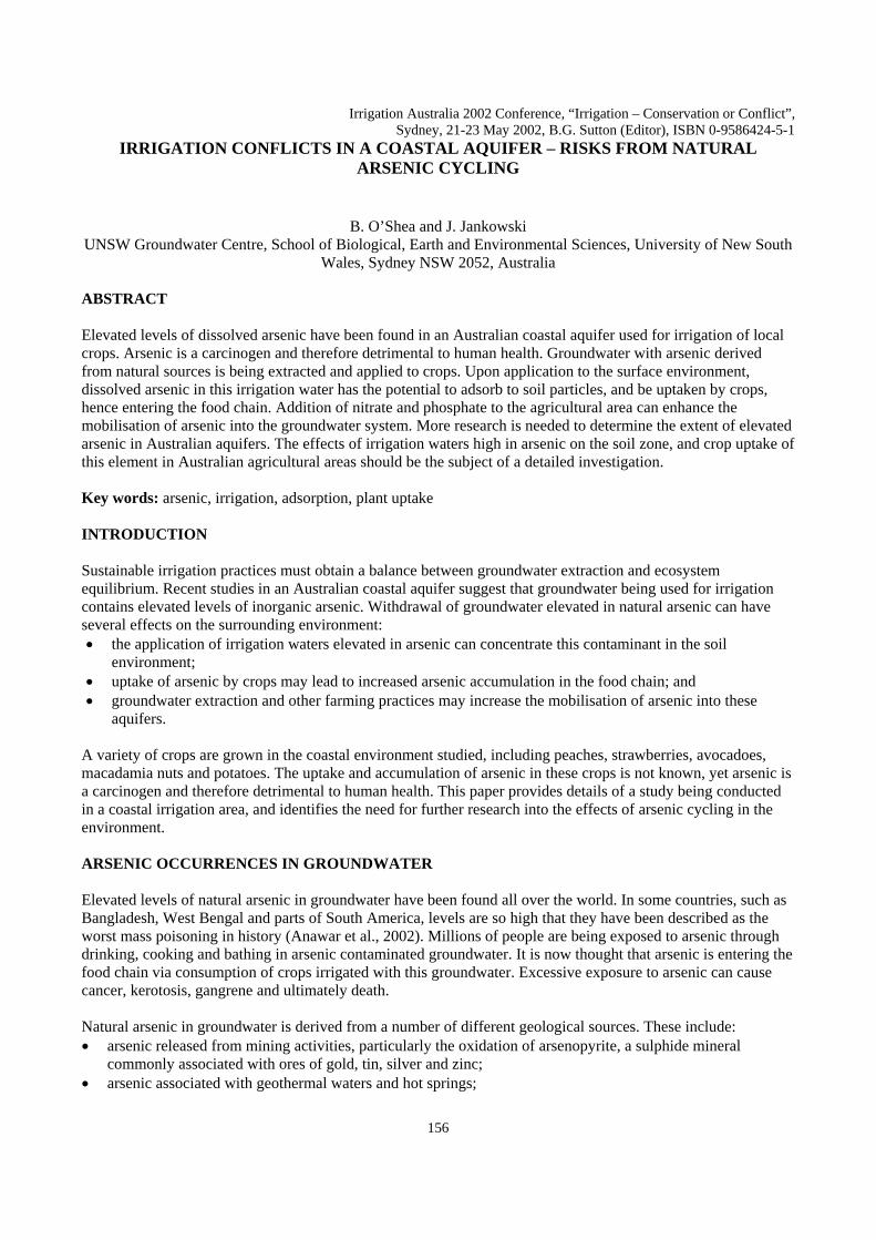
Irrigation Australia 2002 Conference, “Irrigation – Conservation or Conflict”, Sydney, 21-23 May 2002, B.G. Sutton (Editor), ISBN 0-9586424-5-1
IRRIGATION CONFLICTS IN A COASTAL AQUIFER – RISKS FROM NATURAL ARSENIC CYCLING
B. O’Shea and J. Jankowski UNSW Groundwater Centre, School of Biological, Earth and Environmental Sciences, University of New South
Wales, Sydney NSW 2052, Australia
ABSTRACT
Elevated levels of dissolved arsenic have been found in an Australian coastal aquifer used for irrigation of local crops. Arsenic is a carcinogen and therefore detrimental to human health. Groundwater with arsenic derived from natural sources is being extracted and applied to crops. Upon application to the surface environment, dissolved arsenic in this irrigation water has the potential to adsorb to soil particles, and be uptaken by crops, hence entering the food chain. Addition of nitrate and phosphate to the agricultural area can enhance the mobilisation of arsenic into the groundwater system. More research is needed to determine the extent of elevated arsenic in Australian aquifers. The effects of irrigation waters high in arsenic on the soil zone, and crop uptake of this element in Australian agricultural areas should be the subject of a detailed investigation.
Key words: arsenic, irrigation, adsorption, plant uptake
INTRODUCTION
Sustainable irrigation practices must obtain a balance between groundwater extraction and ecosystem equilibrium. Recent studies in an Australian coastal aquifer suggest that groundwater being used for irrigationcontains elevated levels of inorganic arsenic. Withdrawal of groundwater elevated in natural arsenic can have several effects on the surrounding environment:
the application of irrigation waters elevated in arsenic can concentrate this contaminant in the soil environment; uptake of arsenic by crops may lead to increased arsenic accumulation in the food chain; and groundwater extraction and other farming practices may increase the mobilisation of arsenic into these aquifers.
A variety of crops are grown in the coastal environment studied, including peaches, strawberries, avocadoes, macadamia nuts and potatoes. The uptake and accumulation of arsenic in these crops is not known, yet arsenic is a carcinogen and therefore detrimental to human health. This paper provides details of a study being conducted in a coastal irrigation area, and identifies the need for further research into the effects of arsenic cycling in the environment.
ARSENIC OCCURRENCES IN GROUNDWATER
Elevated levels of natural arsenic in groundwater have been found all over the world. In some countries, such as Bangladesh, West Bengal and parts of South America, levels are so high that they have been described as the worst mass poisoning in history (Anawar et al., 2002). Millions of people are being exposed to arsenic through drinking, cooking and bathing in arsenic contaminated groundwater. It is now thought that arsenic is entering the food chain via consumption of crops irrigated with this groundwater. Excessive exposure to arsenic can cause cancer, kerotosis, gangrene and ultimately death.
Natural arsenic in groundwater is derived from a number of different geological sources. These include: arsenic released from mining activities, particularly the oxidation of arsenopyrite, a sulphide mineral commonly associated with ores of gold, tin, silver and zinc; arsenic associated with geothermal waters and hot springs;
156
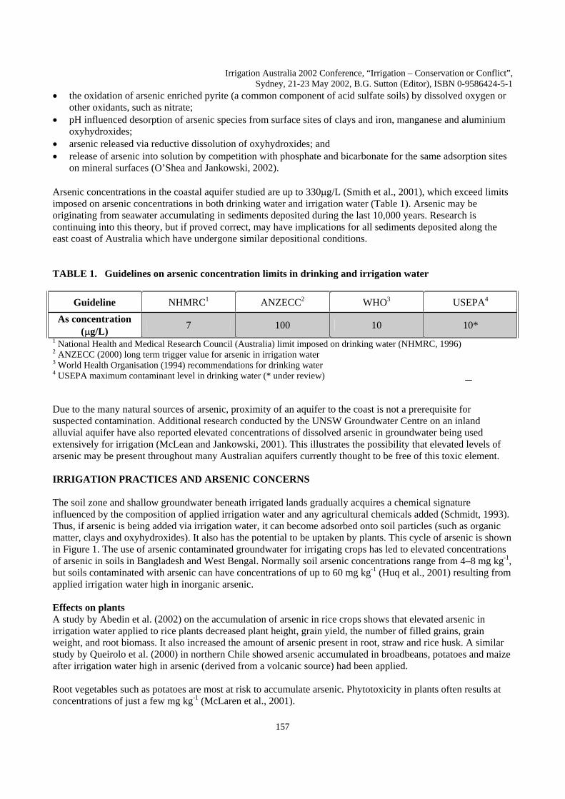
Irrigation Australia 2002 Conference, “Irrigation – Conservation or Conflict”, Sydney, 21-23 May 2002, B.G. Sutton (Editor), ISBN 0-9586424-5-1
the oxidation of arsenic enriched pyrite (a common component of acid sulfate soils) by dissolved oxygen or other oxidants, such as nitrate; pH influenced desorption of arsenic species from surface sites of clays and iron, manganese and aluminium oxyhydroxides; arsenic released via reductive dissolution of oxyhydroxides; and release of arsenic into solution by competition with phosphate and bicarbonate for the same adsorption sites on mineral surfaces (O’Shea and Jankowski, 2002).
Arsenic concentrations in the coastal aquifer studied are up to 330 g/L (Smith et al., 2001), which exceed limits imposed on arsenic concentrations in both drinking water and irrigation water (Table 1). Arsenic may be originating from seawater accumulating in sediments deposited during the last 10,000 years. Research is continuing into this theory, but if proved correct, may have implications for all sediments deposited along the east coast of Australia which have undergone similar depositional conditions.
TABLE 1. Guidelines on arsenic concentration limits in drinking and irrigation water
Guideline NHMRC1 ANZECC2 WHO3 USEPA4
As concentration ( g/L) 7 100 10 10*
1 National Health and Medical Research Council (Australia) limit imposed on drinking water (NHMRC, 1996) 2 ANZECC (2000) long term trigger value for arsenic in irrigation water 3 World Health Organisation (1994) recommendations for drinking water 4 USEPA maximum contaminant level in drinking water (* under review)
Due to the many natural sources of arsenic, proximity of an aquifer to the coast is not a prerequisite for suspected contamination. Additional research conducted by the UNSW Groundwater Centre on an inland alluvial aquifer have also reported elevated concentrations of dissolved arsenic in groundwater being used extensively for irrigation (McLean and Jankowski, 2001). This illustrates the possibility that elevated levels of arsenic may be present throughout many Australian aquifers currently thought to be free of this toxic element.
IRRIGATION PRACTICES AND ARSENIC CONCERNS
The soil zone and shallow groundwater beneath irrigated lands gradually acquires a chemical signature influenced by the composition of applied irrigation water and any agricultural chemicals added (Schmidt, 1993). Thus, if arsenic is being added via irrigation water, it can become adsorbed onto soil particles (such as organic matter, clays and oxyhydroxides). It also has the potential to be uptaken by plants. This cycle of arsenic is shown in Figure 1. The use of arsenic contaminated groundwater for irrigating crops has led to elevated concentrations of arsenic in soils in Bangladesh and West Bengal. Normally soil arsenic concentrations range from 4–8 mg kg-1,but soils contaminated with arsenic can have concentrations of up to 60 mg kg-1 (Huq et al., 2001) resulting from applied irrigation water high in inorganic arsenic.
Effects on plants A study by Abedin et al. (2002) on the accumulation of arsenic in rice crops shows that elevated arsenic in irrigation water applied to rice plants decreased plant height, grain yield, the number of filled grains, grain weight, and root biomass. It also increased the amount of arsenic present in root, straw and rice husk. A similar study by Queirolo et al. (2000) in northern Chile showed arsenic accumulated in broadbeans, potatoes and maize after irrigation water high in arsenic (derived from a volcanic source) had been applied.
Root vegetables such as potatoes are most at risk to accumulate arsenic. Phytotoxicity in plants often results at concentrations of just a few mg kg-1 (McLaren et al., 2001).
157
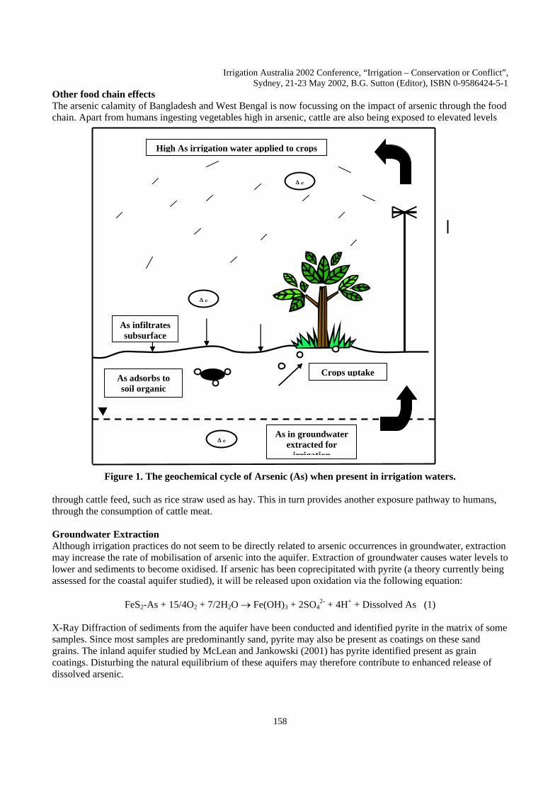
Irrigation Australia 2002 Conference, “Irrigation – Conservation or Conflict”, Sydney, 21-23 May 2002, B.G. Sutton (Editor), ISBN 0-9586424-5-1
Other food chain effects The arsenic calamity of Bangladesh and West Bengal is now focussing on the impact of arsenic through the food chain. Apart from humans ingesting vegetables high in arsenic, cattle are also being exposed to elevated levels
As
As
AsAs in groundwater
extracted for irrigation
High As irrigation water applied to crops
As adsorbs to soil organic
Crops uptake
As infiltrates subsurface
Figure 1. The geochemical cycle of Arsenic (As) when present in irrigation waters.
through cattle feed, such as rice straw used as hay. This in turn provides another exposure pathway to humans, through the consumption of cattle meat.
Groundwater Extraction Although irrigation practices do not seem to be directly related to arsenic occurrences in groundwater, extraction may increase the rate of mobilisation of arsenic into the aquifer. Extraction of groundwater causes water levels to lower and sediments to become oxidised. If arsenic has been coprecipitated with pyrite (a theory currently being assessed for the coastal aquifer studied), it will be released upon oxidation via the following equation:
FeS2-As + 15/4O2 + 7/2H2O Fe(OH)3 + 2SO42- + 4H+ + Dissolved As (1)
X-Ray Diffraction of sediments from the aquifer have been conducted and identified pyrite in the matrix of some samples. Since most samples are predominantly sand, pyrite may also be present as coatings on these sand grains. The inland aquifer studied by McLean and Jankowski (2001) has pyrite identified present as grain coatings. Disturbing the natural equilibrium of these aquifers may therefore contribute to enhanced release of dissolved arsenic.
158

Irrigation Australia 2002 Conference, “Irrigation – Conservation or Conflict”, Sydney, 21-23 May 2002, B.G. Sutton (Editor), ISBN 0-9586424-5-1
Addition of agricultural chemicals Nitrate also has the potential to oxidise pyrite, according to equation 2 below:
10FeS2-As + 30NO3- + 20H2O 10Fe(OH)3 + 15N2 + 15SO4
2- + 5H2SO4 + Dissolved As (2)
The addition of ammonium nitrate has been confirmed in the coastal aquifer under consideration, however there is insufficient evidence to state that nitrate levels are directly responsible for the amount of arsenic present in dissolved phase. Preliminary groundwater results indicate that there are several processes governing arsenic occurrence in dissolved phase, with pyrite oxidation by nitrate being one of the processes possible (O’Shea and Jankowski, 2002).
Phosphate is another agricultural chemical that can influence the mobility of arsenic in solution. Phosphate and arsenate (the oxidised form of arsenic) have similar physicochemical characteristics, and compete directly for the same adsorption sites on mineral surfaces. When the two species are present at equal concentrations, phosphate will outcompete arsenate for adsorption sites (Abedin et al., 2002). Thus addition of phosphate to the soil environment can re-mobilise arsenic into solution, which will then leach down towards the water table, or increase availability of arsenic in the soil water to be uptaken by plants.
Selenium in the USA Another ion with similar properties to arsenate, is the oxidised form of selenium. In the United States, the National Irrigation Water Quality Program was set up in order to determine whether problems of selenium in irrigation drainwater were adversely affecting the health of humans, fish and wildlife. The source of selenium, like arsenic, was determined to be natural, accumulating in sediments of Cretaceous age from large amounts of volcanism during this period. Selenium has been commonly found at elevated concentrations in water, bottom sediment and biota (Presser et al., 1994; Feltz et al., 1991). In several areas, evaporative concentration of applied irrigation water and drainage of this water to wetlands, canals, streams, and lakes appeared to be responsible for elevated concentrations of selenium (Engberg and Sylvester, 1993).
These studies show the significance of the effects toxic elements can have when cycled through the ecosystem. Arsenic has the potential to effect humans and biota in a similar way to selenium, through the mismanagement of irrigation waters elevated in dissolved arsenic.
RECOMMENDATIONS FOR FURTHER RESEARCH
The recent discovery of high arsenic concentrations in groundwaters of West Bengal and Bangladesh have prompted authorities worldwide to re-evaluate the levels of arsenic in groundwater used for irrigation and drinking water supplies. In Australia, it is unknown as to how many aquifers contain elevated levels of arsenic. Those that do contain arsenic, need to be analysed in detail to assess the cycle of arsenic in solid and aqueous phase. Speciation in waters, sediments and biota would provide details not only on occurrence of different arsenic species, but also on toxicity of this element. Inorganic forms of arsenic are much more toxic than organic forms.
Where groundwater high in arsenic is being used for irrigation, studies need to be conducted to assess the influence of extraction, nitrate and phosphate addition on arsenic cycling. Uptake by crops needs to be further researched, and regular testing for arsenic levels in crops (particularly root vegetables) should be implemented. Treatment of irrigation water prior to application would help to prevent accumulation of arsenic in the food chain.
CONCLUSION
Elevated levels of arsenic, a known carcinogen, have been found in a coastal and inland aquifer of Australia. Both aquifers are extensively used for irrigation of local crops. The source of arsenic is expected to be natural, and hence could be widespread over many parts of Australia with similar geomorphic/geologic depositional
159
Irrigation Australia 2002 Conference, “Irrigation – Conservation or Conflict”, Sydney, 21-23 May 2002, B.G. Sutton (Editor), ISBN 0-9586424-5-1
histories. Irrigation water high in arsenic which is applied to soils and crops can be cycled into these surface environments. Arsenic has the potential to adsorb onto soil particles, and be uptaken by crops, therefore entering the food chain.
This paper outlines the need for extensive research to be undertaken by the irrigation industry, to determine the impacts of natural arsenic contamination on water, soil and crops in Australian agricultural areas.
REFERENCES
Abedin, M.D.J., Cresser, M.S., Meharg, A.A., Feldmann, J. and Cotter-Howells, J. (2002) Arsenic accumulation and metabolism in rice (Oryza Sativa L.), Environmental Science & Technology, 36, 962-968.
Anawar, H.M., Akai, J., Mostofa, K.M.G., Safiullah, S. and Tareq, S.M. (2002) Arsenic poisoning in groundwater: Health risk and geochemical sources in Bangladesh, Environment International, 27, 597-604.
ANZECC, (2000) Australian & New Zealand Guidelines for Fresh and Marine Water Quality, Volume 3 Primary Industries – Rationale and Background. Australia & New Zealand Environment & Conservation Council.
Engberg, R.A. and Sylvester, M.A. (1993) Concentrations, distribution, and sources of selenium from irrigated lands in Western United States, Journal of Irrigation and Drainage Engineering, 119, 522-536.
Feltz, H.R., Sylvester, M.A. and Engberg, R.A. (1991) Reconnaissance investigations of the effects of irrigation drainage on water quality, bottom sediment, and biota in the Western United States, in Mallard, G.E. and Aronson, D.A. [eds] Proceedings of the U.S. Geological Survey Toxic Substance Hydrology Program, Monterey, Calif., March 11-15, 1991: U.S. Geological Survey Water-Resources Investigations Report 91-4034, 319-323.
Huq, S.M.I., Ahmed, K.M., Sultana, N. and Naidu, R. (2001) Extensive arsenic contamination in groundwater and soils of Bangladesh, Arsenic in the Asia-Pacific Region Workshop Adelaide, November 20-23, 2001.
McLaren, R.G., Megharaj, M. and Naidu, R. (2001) Fate of arsenic in the soil environment, Arsenic in the Asia-Pacific Region Workshop Adelaide, November 20-23, 2001.
McLean, W. and Jankowski, J. (2001) The occurrence of arsenic in an alluvial aquifer system, Northern New South Wales, Arsenic in the Asia-Pacific Region Workshop Adelaide, November 20-23, 2001.
National Health and Medical Research Council & Agriculture and Resources Management Council of Australia and New Zealand (NHMRC) (1996) Australian Drinking Water Guidelines, National Water Quality Management Strategy, Canberra.
O’Shea, B. and Jankowski, J. (2002) Natural arsenic in a coastal aquifer: Implications for water quality management in Australian coastal zones, Proceedings of the 27th Hydrology and Water Resources Symposium, Melbourne, May 20-23, 2002.
Presser, T.S., Sylvester, M.A. and Low, W.H. (1994) Bioaccumulation of selenium from natural geologic sources in Western States and its potential consequences, Environmental Management, 18, 423-436.
Queirolo, F., Stegen, S., Restovic, M., Paz, M., Ostapczuk, P., Schwuger, M.J. and Munoz, L. (2000) Total arsenic, lead, and cadmium levels in vegetables cultivated at the Andean villages of northern Chile, The Science of the Total Environment, 255, 75-84.
Schmidt, K.D. (1993) Hydrogeologic factors affecting mobility of trace inorganic constituents, Journal of Irrigation and Drainage Engineering, 119, 600-612.
Smith, J.V.S., Jankowski, J. and Sammut, J. (2001) Vertical distribution of As(III) and As(V) in a coastal sandy aquifer: Marine clays, a potential reservoir for arsenic in coastal groundwater systems, Proceedings of the 10th International Symposium on Water-Rock Interactions, Villasimius, Italy, June 10-15, 2001, 1009-1012.
World Health Organisation (WHO) (1994) Recommendations, second ed., Guidelines for Drinking Water Quality, 1, Geneva.
160
SP5o – Chemical Speciation and Modeling
43
The use of solid phase selective extraction techniques to support groundwater chemical data from a coastal aquifer affected by elevated arsenic concentrations
Bethany O’Shea1 and Jerzy Jankowski School of Biological, Earth and Environmental Sciences
University of New South Wales, Sydney NSW, Australia 2052
1PhD Research Student, [email protected]
INTRODUCTIONThe mobility of arsenic in the Stuarts Point coastal aquifer is a critical element in the
determination of the aquifer’s arsenic geochemical cycle. The ease with which arsenic can be released, transported and redistributed through the aquifer has effects on both the anthropogenic use and the environmental receptors of this groundwater resource. Aquifer groundwater chemistry is complex and suggests several geochemical processes may be controlling arsenic distribution.
Sequential extractions have been carried out on sediments collected from the aquifer. The aim of these extractions was to determine sources and/or sinks of arsenic in the aquifer matrix, and their potential to release arsenic in dissolved form, for transport and redistribution throughout the aquifer. A thorough understanding of the solid phase arsenic geochemistry obtained through sequential extraction analyses can then be used to assess groundwater chemical processes contributing to arsenic transport in the aquifer.
STUDY LOCATION AND GROUNDWATER USE The Stuarts Point coastal aquifer is located approximately 400km north of Sydney, Australia.
The aquifer is extensively used for both domestic town water supplies and for the irrigation of local crops. Elevated levels of dissolved arsenic in the groundwater system (>300 g/L) prompted the installation of an arsenic treatment plant. Residents are now provided with drinking water containing <7 g/L of arsenic, the limit set in the Australian Drinking Water Guidelines (NHMRC, 1996).
Groundwater used for the irrigation of local crops (potatoes, avocadoes, stone fruits), however, remains untreated. Some concerns exist over the potential uptake and accumulation of arsenic in these crops. Oyster beds farmed for human consumption in the nearby Macleay estuary are also possibly at risk. Potential discharge of high arsenic groundwater into the estuary may lead to accumulation of this element in the oysters.
This study forms part of a three year project to determine the source, mobilisation, transport and sink(s) of arsenic in this coastal aquifer. The expected benefits of this project include:
a thorough understanding of the arsenic geochemical cycle in the aquifer;assessment of the current management of the aquifer as an important water resource; effects of applying arsenic contaminated irrigation water to local crops; andawareness of potential arsenic impacts on surrounding groundwater dependent ecosystems.
POTENTIAL SOURCES AND/OR SINKS OF ARSENIC IN THE STUARTS POINT COASTAL AQUIFER
There are several possible sources and sinks of arsenic in this coastal aquifer, including, but not necessarily limited to:
SP5o – Chemical Speciation and Modeling
44
Loosely bound to mineral surfaces – Arsenic may be attached to mineral surfaces, and subsequently released due to changes in pH or competition with other oxyanions for surface sorption sites. Oxide minerals and oxyhydroxide grain coatings present in the aquifer are suspected of sorbing labile arsenic. Clay deposits of marine/estuarine origin may also be sorbing arsenic to their outer edges. The abundance of shell material (calcite) in these coastal sediments is another potential contributor to the sorption of arsenic. Co-precipitated within the mineral structure – Iron and manganese oxides may dissolve under aquifer reducing conditions, releasing non-labile arsenic into solution. In contrast, sulphide minerals which are oxidised (such as pyrite contained within acid sulphate soils of this coastal zone) can also release arsenic. Sourced from surrounding mineralised bedrock - Nearby bedrock outcrops (suspected to form part of the basement beneath the aquifer) consist of adamellite granitic intrusions with associated zones of mineralisation, grading from molybdenum to silver-arsenic deposits (Gilligan et al., 1992). The contribution of groundwater flow to the Stuarts Point coastal aquifer from this mineralised bedrock is not well understood, but is considered a potential source of arsenic input to the coastal aquifer. In addition, the aquifer contains dispersed lithic fragments. These lithic fragments have been transported to the coast via ancient river systems originating in the upper reaches of the catchment, and thus are a potential source of arsenic within the aquifer matrix.
SOLID PHASE SEQUENTIAL EXTRACTIONS A sequential extraction technique specific for arsenic has been applied to aquifer sediments.
Fractions were chosen in order to target the potential sources and/or sinks of arsenic identified above: arsenic loosely bound to mineral surfaces; arsenic associated with calcite; arsenic contained within the reducible fraction, ie. iron and manganese oxyhydroxides; arsenic associated with oxidisable materials such as sulphide minerals and organic matter; and the residual mineral fraction.
CONCLUSIONS The results of these sequential extractions will be presented at the conference, with discussion
on the advantages and disadvantages of using these analytical techniques in the determination of the arsenic geochemical cycle. Information obtained from the solid phase arsenic geochemistry will be used to support complex groundwater chemical data. In particular, arsenic mobility in this system is a major concern, and thus was addressed via these analytical techniques, to assess the availability of this toxic element to oysters, crops, humans, and other receptors in the surrounding environment.
REFERENCES Gilligan, L.B., J.W. Brownlow, R.G. and H.F. Henley. 1992. Dorrigo-Coffs Harbour 1:250 000
Metallogenic Map SH/56-10, SH/56-11: Metallogenic Study and Mineral Deposit Data Sheets. New South Wales Geological Survey, Sydney.
National Health and Medical Research Council (NHMRC) & Agriculture and Resources Management Council of Australia and New Zealand. 1996. Australian Drinking Water Guidelines. National Water Quality Management Strategy, Canberra.
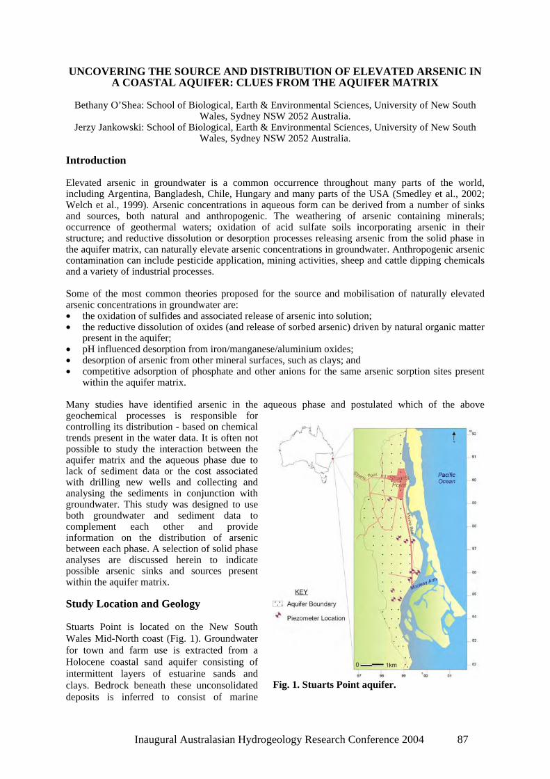
UNCOVERING THE SOURCE AND DISTRIBUTION OF ELEVATED ARSENIC IN A COASTAL AQUIFER: CLUES FROM THE AQUIFER MATRIX
Bethany O’Shea: School of Biological, Earth & Environmental Sciences, University of New South Wales, Sydney NSW 2052 Australia.
Jerzy Jankowski: School of Biological, Earth & Environmental Sciences, University of New South Wales, Sydney NSW 2052 Australia.
Introduction
Elevated arsenic in groundwater is a common occurrence throughout many parts of the world, including Argentina, Bangladesh, Chile, Hungary and many parts of the USA (Smedley et al., 2002; Welch et al., 1999). Arsenic concentrations in aqueous form can be derived from a number of sinks and sources, both natural and anthropogenic. The weathering of arsenic containing minerals; occurrence of geothermal waters; oxidation of acid sulfate soils incorporating arsenic in their structure; and reductive dissolution or desorption processes releasing arsenic from the solid phase in the aquifer matrix, can naturally elevate arsenic concentrations in groundwater. Anthropogenic arsenic contamination can include pesticide application, mining activities, sheep and cattle dipping chemicals and a variety of industrial processes.
Some of the most common theories proposed for the source and mobilisation of naturally elevated arsenic concentrations in groundwater are:
the oxidation of sulfides and associated release of arsenic into solution; the reductive dissolution of oxides (and release of sorbed arsenic) driven by natural organic matter present in the aquifer; pH influenced desorption from iron/manganese/aluminium oxides; desorption of arsenic from other mineral surfaces, such as clays; and competitive adsorption of phosphate and other anions for the same arsenic sorption sites present within the aquifer matrix.
Many studies have identified arsenic in the aqueous phase and postulated which of the above geochemical processes is responsible for controlling its distribution - based on chemical trends present in the water data. It is often not possible to study the interaction between the aquifer matrix and the aqueous phase due to lack of sediment data or the cost associated with drilling new wells and collecting and analysing the sediments in conjunction with groundwater. This study was designed to use both groundwater and sediment data to complement each other and provide information on the distribution of arsenic between each phase. A selection of solid phase analyses are discussed herein to indicate possible arsenic sinks and sources present within the aquifer matrix.
Fig. 1. Stuarts Point aquifer.
Study Location and Geology
Stuarts Point is located on the New South Wales Mid-North coast (Fig. 1). Groundwater for town and farm use is extracted from a Holocene coastal sand aquifer consisting of intermittent layers of estuarine sands and clays. Bedrock beneath these unconsolidated deposits is inferred to consist of marine
Inaugural Australasian Hydrogeology Research Conference 2004 87
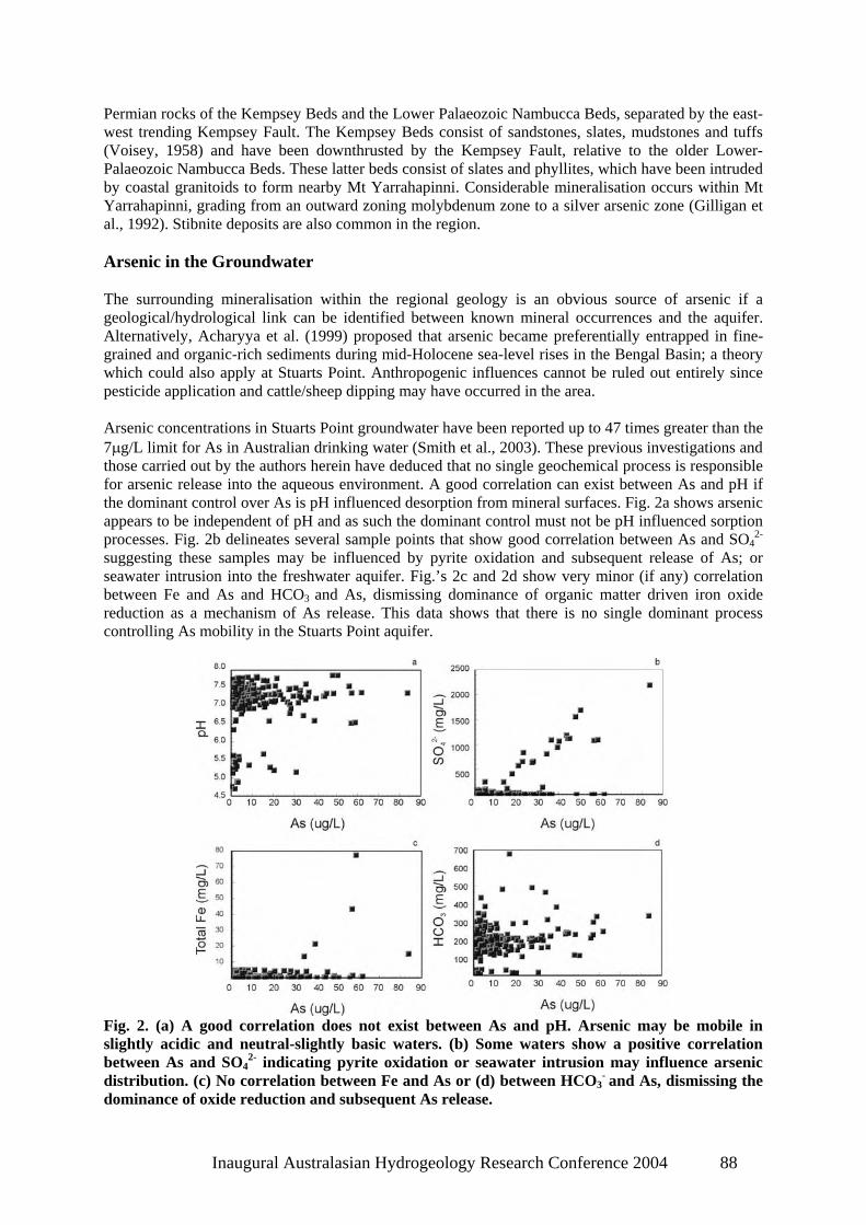
Permian rocks of the Kempsey Beds and the Lower Palaeozoic Nambucca Beds, separated by the east-west trending Kempsey Fault. The Kempsey Beds consist of sandstones, slates, mudstones and tuffs (Voisey, 1958) and have been downthrusted by the Kempsey Fault, relative to the older Lower-Palaeozoic Nambucca Beds. These latter beds consist of slates and phyllites, which have been intruded by coastal granitoids to form nearby Mt Yarrahapinni. Considerable mineralisation occurs within Mt Yarrahapinni, grading from an outward zoning molybdenum zone to a silver arsenic zone (Gilligan et al., 1992). Stibnite deposits are also common in the region.
Arsenic in the Groundwater
The surrounding mineralisation within the regional geology is an obvious source of arsenic if a geological/hydrological link can be identified between known mineral occurrences and the aquifer. Alternatively, Acharyya et al. (1999) proposed that arsenic became preferentially entrapped in fine-grained and organic-rich sediments during mid-Holocene sea-level rises in the Bengal Basin; a theory which could also apply at Stuarts Point. Anthropogenic influences cannot be ruled out entirely since pesticide application and cattle/sheep dipping may have occurred in the area.
Arsenic concentrations in Stuarts Point groundwater have been reported up to 47 times greater than the 7 g/L limit for As in Australian drinking water (Smith et al., 2003). These previous investigations and those carried out by the authors herein have deduced that no single geochemical process is responsible for arsenic release into the aqueous environment. A good correlation can exist between As and pH if the dominant control over As is pH influenced desorption from mineral surfaces. Fig. 2a shows arsenic appears to be independent of pH and as such the dominant control must not be pH influenced sorption processes. Fig. 2b delineates several sample points that show good correlation between As and SO4
2-
suggesting these samples may be influenced by pyrite oxidation and subsequent release of As; or seawater intrusion into the freshwater aquifer. Fig.’s 2c and 2d show very minor (if any) correlation between Fe and As and HCO3 and As, dismissing dominance of organic matter driven iron oxide reduction as a mechanism of As release. This data shows that there is no single dominant process controlling As mobility in the Stuarts Point aquifer.
Fig. 2. (a) A good correlation does not exist between As and pH. Arsenic may be mobile in slightly acidic and neutral-slightly basic waters. (b) Some waters show a positive correlation between As and SO4
2- indicating pyrite oxidation or seawater intrusion may influence arsenic distribution. (c) No correlation between Fe and As or (d) between HCO3
- and As, dismissing the dominance of oxide reduction and subsequent As release.
Inaugural Australasian Hydrogeology Research Conference 2004 88
Arsenic in Solid Phase
Given the uncertainty regarding controls on As distribution suggested from water data alone, it was necessary to analyse the solid phase of the aquifer matrix to determine sources and sinks of As. Sequential extraction procedures, XRF, XRD, statistical analysis and SEM techniques were used to ascertain whether or not postulated sinks were present in the aquifer matrix. Targeted sinks included:
the presence and identification of specific clay types in the matrix and their potential to adsorb As onto their outer edges; any specific As mineral phases such as scorodite, arsenopyrite or barium arsenate; correlations between As and other elements in the solid phase; influence of shell material on the sequestration of As; the presence of pyrite and its ability to incorporate As into its crystal structure; and the presence of iron/aluminium/manganese oxides and oxyhydroxides and their ability to sorb As.
Analysis of the solid phase enabled correlations to be made between various trace elements present in the matrix, leading to a hypothesised source of arsenic for the aquifer. Further high powered microscopic analysis identified potential sinks of arsenic redistributed throughout the matrix. Water chemistry was used to ascertain which chemical processes are currently active in the aquifer and therefore which processes are controlling As mobility. Due to the large amount of graphics generated during this analysis process the results will not be incorporated within this abstract, rather they will be presented at the conference where further discussion can warrant their importance.
Conclusion
Arsenic has been identified at elevated concentrations in a coastal aquifer. Investigations were initiated to determine whether the As was naturally occurring or anthropogenically induced. Results from groundwater sampling alone were inconclusive and suggested many geochemical processes were controlling As distribution in the aquifer. A thorough analysis of the solid phase of the aquifer matrix has provided a possible source for the As in the aquifer, in addition to identifying current geochemical sinks present within the aquifer. This integrated approach to the investigation has allowed a better understanding of As geochemical processes to be determined and stresses the importance of considering the solid phase component of any groundwater study.
References
Acharyya SK, Lahiri S, Raymahashay BC, Bhowmik A (1999) Arsenic toxicity of groundwater in parts of the Bengal basin in India and Bangladesh: the role of Quaternary stratigraphy and Holocene sea-level fluctuation. Environmental Geology 39:1127-1137.
Gilligan LB, Brownlow JW, Cameron RG, Henley HF (1992) Dorrigo-Coffs Harbour 1:250 000 Metallogenic Map SH/56-10, SH/56-11: Metallogenic Study and Mineral Deposit Data Sheets. New South Wales Geological Survey, Sydney.
Smedley PL, Nicolli HB, Macdonald DMJ, Barros AJ, Tullio JO (2002) Hydrogeochemistry of arsenic and other inorganic constituents in groundwaters from La Pampa, Argentina. Appl. Geochem. 17:259-284.
Smith JVS, Jankowski J, Sammut J (2003) Vertical distribution of As(III) and As(V) in a coastal sandy aquifer: factors controlling the concentration and speciation of arsenic in the Stuarts Point groundwater system, Northern New South Wales, Australia. Appl. Geochem. 18:1479-1496.
Voisey AH (1958) Tectonic evolution of North-Eastern New South Wales, Australia. Journal of the Royal Society of New South Wales, 92: 191-203.
Welch AH, Helsel DR, Focazio MJ, Watkins SA (1999) Arsenic in ground water supplies of the United States. In: Chappell WR, Abernathy CO, Calderon RL (Eds.), Arsenic Exposure and Health Effects. Elsevier, Amsterdam, 9-17.
Inaugural Australasian Hydrogeology Research Conference 2004 89
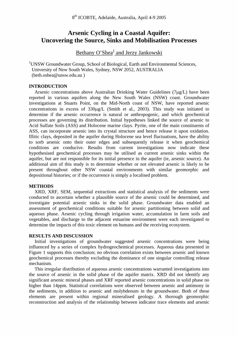
8th ICOBTE, Adelaide, Australia, April 4-9 2005
Arsenic Cycling in a Coastal Aquifer: Uncovering the Source, Sinks and Mobilisation Processes
Bethany O’Shea1 and Jerzy Jankowski1UNSW Groundwater Group, School of Biological, Earth and Environmental Sciences,
University of New South Wales, Sydney, NSW 2052, AUSTRALIA ([email protected] )
INTRODUCTIONArsenic concentrations above Australian Drinking Water Guidelines (7 g/L) have been
reported in various aquifers along the New South Wales (NSW) coast. Groundwater investigations at Stuarts Point, on the Mid-North coast of NSW, have reported arsenic concentrations in excess of 330 g/L (Smith et al., 2003). This study was initiated to determine if the arsenic occurrence is natural or anthropogenic, and which geochemical processes are governing its distribution. Initial hypotheses linked the source of arsenic to Acid Sulfate Soils (ASS) and Holocene marine clays. Pyrite, one of the main constituents of ASS, can incorporate arsenic into its crystal structure and hence release it upon oxidation. Illitic clays, deposited in the aquifer during Holocene sea level fluctuations, have the ability to sorb arsenic onto their outer edges and subsequently release it when geochemical conditions are conducive. Results from current investigations now indicate these hypothesised geochemical processes may be utilised as current arsenic sinks within the aquifer, but are not responsible for its initial presence in the aquifer (ie, arsenic source). An additional aim of this study is to determine whether or not elevated arsenic is likely to be present throughout other NSW coastal environments with similar geomorphic and depositional histories; or if the occurrence is simply a localised problem.
METHODSXRD, XRF, SEM, sequential extractions and statistical analysis of the sediments were
conducted to ascertain whether a plausible source of the arsenic could be determined, and investigate potential arsenic sinks in the solid phase. Groundwater data enabled an assessment of geochemical conditions suitable for arsenic partitioning between solid and aqueous phase. Arsenic cycling through irrigation water, accumulation in farm soils and vegetables, and discharge to the adjacent estuarine environment were each investigated to determine the impacts of this toxic element on humans and the receiving ecosystem.
RESULTS AND DISCUSSION Initial investigations of groundwater suggested arsenic concentrations were being
influenced by a series of complex hydrogeochemical processes. Aqueous data presented in Figure 1 supports this conclusion; no obvious correlation exists between arsenic and known geochemical processes thereby excluding the dominance of one singular controlling release mechanism.
This irregular distribution of aqueous arsenic concentrations warranted investigations into the source of arsenic in the solid phase of the aquifer matrix. XRD did not identify any significant arsenic mineral phases and XRF reported arsenic concentrations in solid phase no higher than 14ppm. Statistical correlations were observed between arsenic and antimony in the sediments, in addition to arsenic and molybdenum in the groundwater. Both of these elements are present within regional mineralised geology. A thorough geomorphic reconstruction and analysis of the relationship between indicator trace elements and arsenic
8th ICOBTE, Adelaide, Australia, April 4-9 2005
suggest the original provenance of arsenic in the aquifer is likely to be derived from local and/or regional stratigraphy. Regional geologic influences are hypothesised to be associated with fluvially transported sediments now forming parts of the aquifer matrix. For example, stibnite deposits located in the upper catchment of the Macleay River have oxidised and contributed dissolved antimony and arsenic to the Macleay River (Ashley et al., 2003), illustrating the past and present potential for contribution of trace elements to the aquifer matrix via river processes. Alternatively, an in-situ upwards vertical gradient may be contributing arsenic and trace elements from the underlying mineralised bedrock to the unconsolidated aquifer above.
Fig. 1. (a) A good correlation does not exist between As and pH, indicating pH influenced desorption processes are not dominant. Arsenic may be mobile in slightly acidic and neutral-slightly basic waters. (b) Some waters show a positive correlation between As and SO4
2- indicating pyrite oxidation or seawater intrusion may influence arsenic distribution in these samples. (c) No correlation between Fe and As dismissing the dominance of an oxide reduction and subsequent As release mechanism.
While the source of arsenic is still being hypothesised, current sinks within the aquifer matrix have successfully been identified. Arsenic-rich pyrite, iron oxyhydroxides and illitic clay coatings on aquifer particles suggest several arsenic sinks exist in the aquifer, each contributing to arsenic occurrence and its variable distribution. This explains the poor relationships observed in the aqueous data presented in Figure 1. Investigations are currently under way to determine the aqueous conditions conducive to arsenic mobilisation within the groundwater and whether anthropogenic activities are enhancing its release from solid phase.
CONCLUSIONS Arsenic is therefore suggested to be naturally derived from local and/or regional geology.
Its mobility in this drinking water aquifer is controlled by several geochemical processes, as identified by SEM and aqueous chemical interpretation methods. Arsenic cycling through irrigation water does not cause accumulation of this element in soils or vegetables, however potential arsenic discharge to the adjacent estuary is of concern to local oyster production. The source of arsenic in this coastal environment is thought to be localised according to geology, however, given its ubiquitous nature, arsenic should not be ignored in other NSW coastal environments and therefore should be investigated accordingly.
REFERENCES Smith, J.V.S., Jankowski, J. and Sammut, J. (2003) Vertical distribution of As(III) and As(V)
in a coastal sandy aquifer: factors controlling the concentration and speciation of arsenic in the Stuarts Point groundwater system, Northern New South Wales, Australia. Appl.Geochem. 18:1479-1496.
Ashley, P.M., Craw, D., Graham, B.P. and Chappell, D.A. (2003) Environmental mobility of antimony around mesothermal stibnite deposits, New South Wales, Australia and southern New Zealand. J. Geochem. Expl. 77:1-14.

NATURALLY ELEVATED ARSENIC AND OTHER TRACE ELEMENTS IN A SAND AQUIFER OF EASTERN AUSTRALIA
O’SHEA, Bethany. Department of Geology, Dickinson College, PO Box 1773, Carlisle, PA 17013, [email protected] and JANKOWSKI, Jerzy. School of Biological, Earth & Environmental Sciences, University of New South Wales, Sydney 2052, Australia.
Aquifers comprised of unconsolidated sediments can be valuable resources due to their high groundwater yields. Much of eastern coastal Australia contains sand aquifers that are heavily exploited for drinking water and irrigation. Unless specifically targeted, many trace elements and metals have not been part of routine analyte suites in groundwater risk assessments in past decades. The recent widespread occurrence of arsenic in many sedimentary aquifers of the world prompted the analysis of dissolved arsenic in a drinking water supply aquifer at Stuarts Point, 600 km north of Sydney. Arsenic has been reported above the Australian drinking water limit of 7 g L-1 in 49% of groundwater samples analyzed. A detailed hydrochemical characterization of the aquifer revealed the source of arsenic to be natural, weathered from a mineralized arsenic-bearing stibnite (Sb2S3) deposit in the hinterland and transported downstream by fluvial processes.
Also reported above drinking water guidelines in this seemingly ‘pristine’ and low contaminant risk environment were Cd, Hg, Mn, Pb and Se. However, spatial distribution is not widespread like dissolved arsenic distribution. Multivariate statistical analyses have linked these elevated elemental occurrences to specific zones in the aquifer. Such zones include shallow groundwater subjected to pyrite oxidation, groundwater flowing through fluvially deposited sediments or mineralized weathered bedrock clays, and groundwater impacted by seawater intrusion processes. Variation in chemical heterogeneity, particularly redox conditions and groundwater-matrix interaction, govern the sporadic distribution of these elevated elements.
These results can aid in determining optimal depths of groundwater withdrawal for various uses in the Stuarts Point aquifer. For example, Cd occurs in elevated concentrations at approximately 10 m below the ground surface. Bores installed primarily for irrigation of potato crops should therefore target shallow groundwater (less than 10 m) in order to reduce the possibility for Cd accumulation in potatoes. Distinct groundwater zones occur within a very limited depth (30 meters) in this aquifer, illustrating the importance of considering chemical heterogeneity in groundwater risk assessments for all aquifer matrices.
A comparison of arsenic occurrence and geochemistry in two coastal
groundwater environments B.M. O’SHEA1, G. CLARK1 AND J. JANKOWSKI2
1 Department of Geology, Dickinson College, Pennsylvania, USA; [email protected]; [email protected]
2 School of Biological, Earth & Environmental Science, University of New South Wales, Australia; [email protected]
Arsenic occurrence and geochemistry in two distinctly different coastal aquifers has been investigated. The first, an unconsolidated sand and clay aquifer of eastern Australia, has been compared to groundwater composition contained within sand and gravel surficial deposits and bedrock of coastal Maine, USA. Both studies investigate the presence of natural arsenic in groundwater being used for potable supply. The Australian aquifer, located in northern New South Wales, has been investigated in detail [1]. Dissolved arsenic concentrations are greater than 300 g L-1. Arsenic bearing stibnite deposits in the upper catchment have been fluvially eroded and transported over time to deposit an aquifer lithology elevated in arsenic. Current groundwater conditions are suitable for both arsenic mobilisation and immobilisation processes, producing a cyclic control on arsenic distribution. The redox state of the groundwater largely controls arsenic distribution. Reductive dissolution of iron oxyhydroxides releases arsenic into shallow parts of the aquifer (0-20m depth). As redox conditions become more anoxic with depth, the reductive dissolution of iron oxyhydroxides approaches completion and correlates with increased arsenic concentrations in groundwater. At depths of 25-30m, seawater intrusion draws increased sulfate concentrations into the fresh water aquifer and promotes reduction of sulfate and the subsequent precipitation of iron sulfides. Geochemical modeling and redox conditions support this hypothesis. Arsenic concentrations in groundwater signficantly decrease as iron sulfide minerals incorporate the arsenic into their mineral structure. Arsenian pyrite has been identified with an Electron Microprobe. In comparison, the sporadic occurrence of arsenic in coastal Maine is proposed to derive from the oxidation of arsenical pyrite in fractured igneous and metamorphic bedrock of mid-coastal Maine [2]. Investigations continue in an extended area of coastal Maine to complement the work conducted by [2] and allow a detailed geochemical comparison to be conducted on two distinctly different coastal aquifers bearing similar aqueous geochemical signatures and associated health risk problems. References [1] O’Shea B.M. (2006) PhD Thesis. University of NSW. Australia. [2] Sidle W.C., Wotten B., Murphy E. (2001) Env.Geol. 41, 62-73.
Geogenic arsenic in an Australian sedimentary aquifer: risk awareness for aquifers in Latin American countries
B. O’Shea Department of Geology, Dickinson College, Carlisle PA, USA
J. Jankowski School of Biological, Earth and Environmental Sciences, The University of New South Wales, Sydney NSW, Australia
ABSTRACT: Arsenic concentrations in a coastal sandy aquifer used extensively for drinking water and irrigation supply have been reported at more than 45 times the permissable limit in Australian drinking water. The presence of arsenic in the Stuarts Point aquifer was surprising due to its assumed deposition by on-shore sediment supply and thus lack of an obvious arsenic source. Development of an aquifer-specific geomorphic model now suggests that arsenic has been derived from regional erosion of arsenic-rich stibnite deposits. The heterogeneity of the sedimentary aquifer causes groundwater redox conditions to control arsenic mobilisation via re-ductive dissolution of iron oxyhydroxides and precipitation of arsenian pyrite. The valuable les-sons learned from an Australian sedimentary aquifer where arsenic occurrence is complex, should be utilised in the assessment and identification of potential arsenic-rich groundwaters of Latin America.
1 INTRODUCTION
In the last decade there has been a dramatic increase in the number of studies investigating arse-nic in groundwater. Much of this can be attributed to the discovery of elevated arsenic in domes-tic groundwater supplies in Bangladesh (Nickson et al., 2000; Harvey et al., 2005). The in-creased awareness of the ubiquitous nature of arsenic in the environment led other countries to focus on the occurrence of arsenic in their groundwater. Elevated arsenic has since been found in groundwater of Australia (Smith et al., 2003; 2006, O’Shea et al., 2006), Taiwan (Chen et al., 1994), Vietnam (Berg et al., 2003) and many parts of the USA (Schreiber et al., 2000; Welch et al., 2000; Sidle et al., 2001). In recent years, the occurrence of arsenic in aquifers of Latin American countries has become increasingly apparent (Smedley et al., 2002; Bundschuh et al., 2004; Bhattacharya et al., 2006; Romero et al., 2004).
The effects of ingesting arsenic-rich groundwater can be devastating both physically and so-cially. Physical effects include various cancers (Bissen and Frimel, 2003), skin lesions, gangrene and other clinical symptoms like joint pain, chronic cough and abdominal pain (Khalequzzaman et al., 2005). Unfortunately, many people who depend on arsenic-rich groundwater supplies also live in rural areas where basic necessities are unsatisfied and incidences of poverty can be high, such as the Chaco-Pampean Plain of Argentina (Bundschuh et al., 2004).
In contrast, the Stuarts Point aquifer of eastern Australia supports small coastal communities where the standard of living is more than satisfactory. Dissolved arsenic has been reported by Smith et al. (2003) at concentrations as high as 337 g/L, more than 45 times the acceptable drinking water limit of 7 g/L As (NHMRC, 1996). As such, groundwater in this aquifer is now being treated to remove dissolved arsenic prior to human consumption.
The purpose of this study is to provide an outline of the investigation conducted at Stuarts Point. Arsenic sources, sinks and controls on mobilization into groundwater have been exam-ined in detail (O’Shea, 2006) and are described herein. By examining the geochemical controls
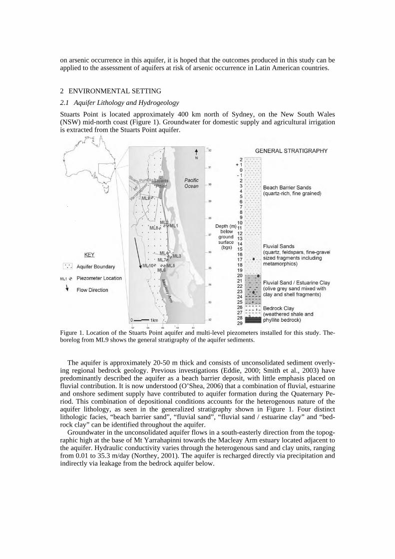
on arsenic occurrence in this aquifer, it is hoped that the outcomes produced in this study can be applied to the assessment of aquifers at risk of arsenic occurrence in Latin American countries.
2 ENVIRONMENTAL SETTING 2.1 Aquifer Lithology and Hydrogeology Stuarts Point is located approximately 400 km north of Sydney, on the New South Wales (NSW) mid-north coast (Figure 1). Groundwater for domestic supply and agricultural irrigation is extracted from the Stuarts Point aquifer.
Figure 1. Location of the Stuarts Point aquifer and multi-level piezometers installed for this study. The-borelog from ML9 shows the general stratigraphy of the aquifer sediments.
The aquifer is approximately 20-50 m thick and consists of unconsolidated sediment overly-ing regional bedrock geology. Previous investigations (Eddie, 2000; Smith et al., 2003) have predominantly described the aquifer as a beach barrier deposit, with little emphasis placed on fluvial contribution. It is now understood (O’Shea, 2006) that a combination of fluvial, estuarine and onshore sediment supply have contributed to aquifer formation during the Quaternary Pe-riod. This combination of depositional conditions accounts for the heterogenous nature of the aquifer lithology, as seen in the generalized stratigraphy shown in Figure 1. Four distinct lithologic facies, “beach barrier sand”, “fluvial sand”, “fluvial sand / estuarine clay” and “bed-rock clay” can be identified throughout the aquifer.
Groundwater in the unconsolidated aquifer flows in a south-easterly direction from the topog-raphic high at the base of Mt Yarrahapinni towards the Macleay Arm estuary located adjacent to the aquifer. Hydraulic conductivity varies through the heterogenous sand and clay units, ranging from 0.01 to 35.3 m/day (Northey, 2001). The aquifer is recharged directly via precipitation and indirectly via leakage from the bedrock aquifer below.
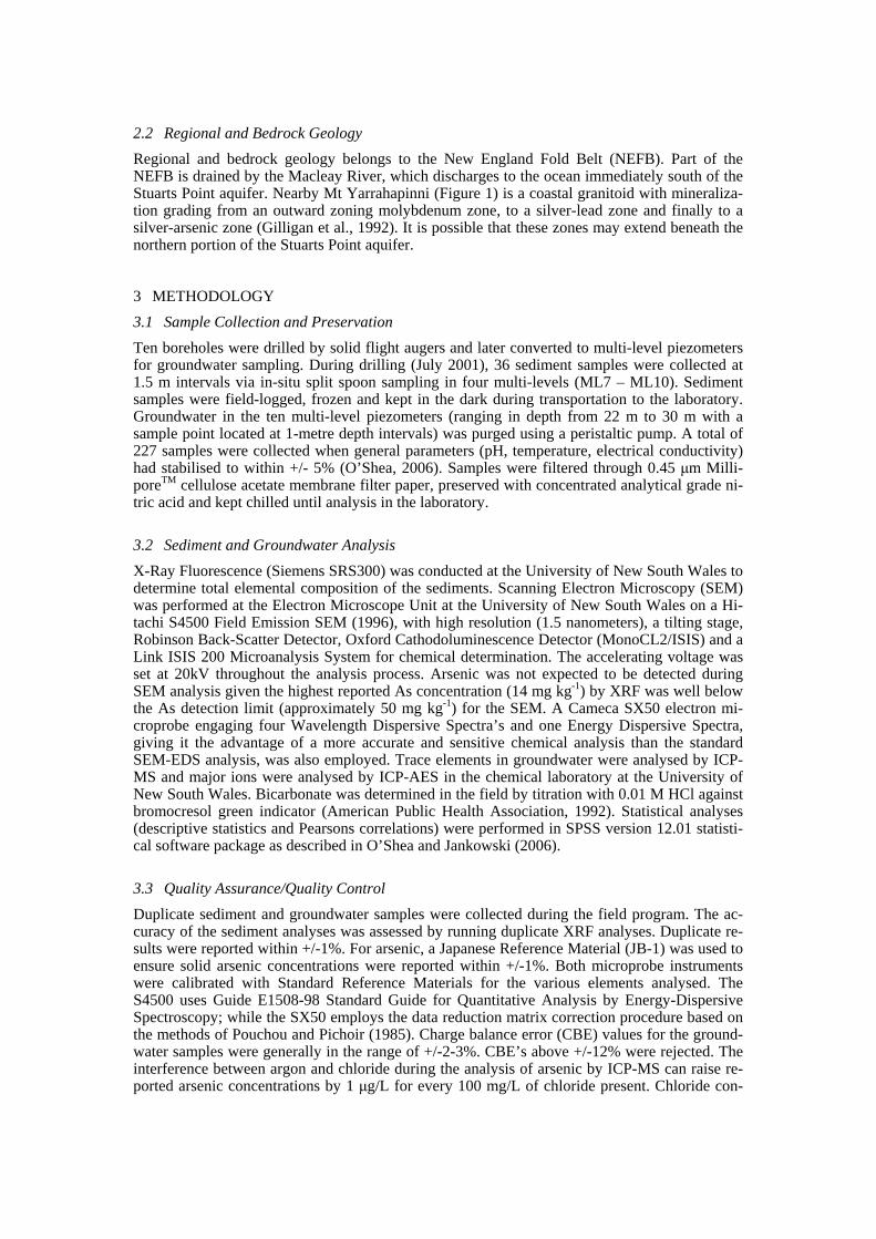
2.2 Regional and Bedrock Geology Regional and bedrock geology belongs to the New England Fold Belt (NEFB). Part of the NEFB is drained by the Macleay River, which discharges to the ocean immediately south of the Stuarts Point aquifer. Nearby Mt Yarrahapinni (Figure 1) is a coastal granitoid with mineraliza-tion grading from an outward zoning molybdenum zone, to a silver-lead zone and finally to a silver-arsenic zone (Gilligan et al., 1992). It is possible that these zones may extend beneath the northern portion of the Stuarts Point aquifer.
3 METHODOLOGY3.1 Sample Collection and Preservation Ten boreholes were drilled by solid flight augers and later converted to multi-level piezometers for groundwater sampling. During drilling (July 2001), 36 sediment samples were collected at 1.5 m intervals via in-situ split spoon sampling in four multi-levels (ML7 – ML10). Sediment samples were field-logged, frozen and kept in the dark during transportation to the laboratory. Groundwater in the ten multi-level piezometers (ranging in depth from 22 m to 30 m with a sample point located at 1-metre depth intervals) was purged using a peristaltic pump. A total of 227 samples were collected when general parameters (pH, temperature, electrical conductivity) had stabilised to within +/- 5% (O’Shea, 2006). Samples were filtered through 0.45 m Milli-poreTM cellulose acetate membrane filter paper, preserved with concentrated analytical grade ni-tric acid and kept chilled until analysis in the laboratory.
3.2 Sediment and Groundwater Analysis X-Ray Fluorescence (Siemens SRS300) was conducted at the University of New South Wales to determine total elemental composition of the sediments. Scanning Electron Microscopy (SEM) was performed at the Electron Microscope Unit at the University of New South Wales on a Hi-tachi S4500 Field Emission SEM (1996), with high resolution (1.5 nanometers), a tilting stage, Robinson Back-Scatter Detector, Oxford Cathodoluminescence Detector (MonoCL2/ISIS) and a Link ISIS 200 Microanalysis System for chemical determination. The accelerating voltage was set at 20kV throughout the analysis process. Arsenic was not expected to be detected during SEM analysis given the highest reported As concentration (14 mg kg-1) by XRF was well below the As detection limit (approximately 50 mg kg-1) for the SEM. A Cameca SX50 electron mi-croprobe engaging four Wavelength Dispersive Spectra’s and one Energy Dispersive Spectra, giving it the advantage of a more accurate and sensitive chemical analysis than the standard SEM-EDS analysis, was also employed. Trace elements in groundwater were analysed by ICP-MS and major ions were analysed by ICP-AES in the chemical laboratory at the University of New South Wales. Bicarbonate was determined in the field by titration with 0.01 M HCl against bromocresol green indicator (American Public Health Association, 1992). Statistical analyses (descriptive statistics and Pearsons correlations) were performed in SPSS version 12.01 statisti-cal software package as described in O’Shea and Jankowski (2006).
3.3 Quality Assurance/Quality Control Duplicate sediment and groundwater samples were collected during the field program. The ac-curacy of the sediment analyses was assessed by running duplicate XRF analyses. Duplicate re-sults were reported within +/-1%. For arsenic, a Japanese Reference Material (JB-1) was used to ensure solid arsenic concentrations were reported within +/-1%. Both microprobe instruments were calibrated with Standard Reference Materials for the various elements analysed. The S4500 uses Guide E1508-98 Standard Guide for Quantitative Analysis by Energy-Dispersive Spectroscopy; while the SX50 employs the data reduction matrix correction procedure based on the methods of Pouchou and Pichoir (1985). Charge balance error (CBE) values for the ground-water samples were generally in the range of +/-2-3%. CBE’s above +/-12% were rejected. The interference between argon and chloride during the analysis of arsenic by ICP-MS can raise re-ported arsenic concentrations by 1 g/L for every 100 mg/L of chloride present. Chloride con-
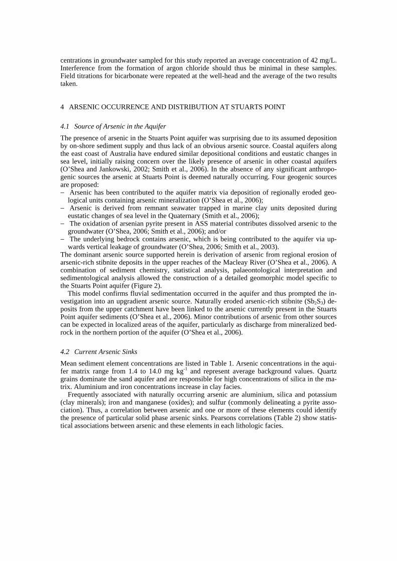
centrations in groundwater sampled for this study reported an average concentration of 42 mg/L. Interference from the formation of argon chloride should thus be minimal in these samples. Field titrations for bicarbonate were repeated at the well-head and the average of the two results taken.
4 ARSENIC OCCURRENCE AND DISTRIBUTION AT STUARTS POINT
4.1 Source of Arsenic in the Aquifer The presence of arsenic in the Stuarts Point aquifer was surprising due to its assumed deposition by on-shore sediment supply and thus lack of an obvious arsenic source. Coastal aquifers along the east coast of Australia have endured similar depositional conditions and eustatic changes in sea level, initially raising concern over the likely presence of arsenic in other coastal aquifers (O’Shea and Jankowski, 2002; Smith et al., 2006). In the absence of any significant anthropo-genic sources the arsenic at Stuarts Point is deemed naturally occurring. Four geogenic sources are proposed:
Arsenic has been contributed to the aquifer matrix via deposition of regionally eroded geo-logical units containing arsenic mineralization (O’Shea et al., 2006); Arsenic is derived from remnant seawater trapped in marine clay units deposited during eustatic changes of sea level in the Quaternary (Smith et al., 2006); The oxidation of arsenian pyrite present in ASS material contributes dissolved arsenic to the groundwater (O’Shea, 2006; Smith et al., 2006); and/or The underlying bedrock contains arsenic, which is being contributed to the aquifer via up-wards vertical leakage of groundwater (O’Shea, 2006; Smith et al., 2003).
The dominant arsenic source supported herein is derivation of arsenic from regional erosion of arsenic-rich stibnite deposits in the upper reaches of the Macleay River (O’Shea et al., 2006). A combination of sediment chemistry, statistical analysis, palaeontological interpretation and sedimentological analysis allowed the construction of a detailed geomorphic model specific to the Stuarts Point aquifer (Figure 2).
This model confirms fluvial sedimentation occurred in the aquifer and thus prompted the in-vestigation into an upgradient arsenic source. Naturally eroded arsenic-rich stibnite (Sb2S3) de-posits from the upper catchment have been linked to the arsenic currently present in the Stuarts Point aquifer sediments (O’Shea et al., 2006). Minor contributions of arsenic from other sources can be expected in localized areas of the aquifer, particularly as discharge from mineralized bed-rock in the northern portion of the aquifer (O’Shea et al., 2006).
4.2 Current Arsenic Sinks Mean sediment element concentrations are listed in Table 1. Arsenic concentrations in the aqui-fer matrix range from 1.4 to 14.0 mg kg-1 and represent average background values. Quartz grains dominate the sand aquifer and are responsible for high concentrations of silica in the ma-trix. Aluminium and iron concentrations increase in clay facies.
Frequently associated with naturally occurring arsenic are aluminium, silica and potassium (clay minerals); iron and manganese (oxides); and sulfur (commonly delineating a pyrite asso-ciation). Thus, a correlation between arsenic and one or more of these elements could identify the presence of particular solid phase arsenic sinks. Pearsons correlations (Table 2) show statis-tical associations between arsenic and these elements in each lithologic facies.
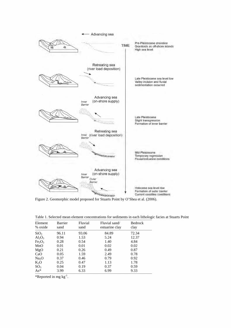
Figure 2. Geomorphic model proposed for Stuarts Point by O’Shea et al. (2006).
Table 1. Selected mean element concentrations for sediments in each lithologi_____________________________________________________________________________ c facies at Stuarts PointElement Barrier Fluvial Fluvial sand/ Bedrock % oxide sand sand estuarine clay clay _____________________________________________________________________________SiO2 96.11 93.06 84.89 72.34 Al2O3 0.94 1.53 5.24 12.37 Fe2O3 0.28 0.54 1.40 4.84 MnO 0.01 0.01 0.02 0.02 MgO 0.21 0.26 0.49 0.87 CaO 0.05 1.59 2.49 0.78 Na2O 0.37 0.46 0.79 0.92 K2O 0.25 0.47 1.13 1.78 SO3 0.04 0.19 0.37 0.59 As* 3.99 6.33 6.99 9.33 _____________________________________________________________________________*Reported in mg kg-1.
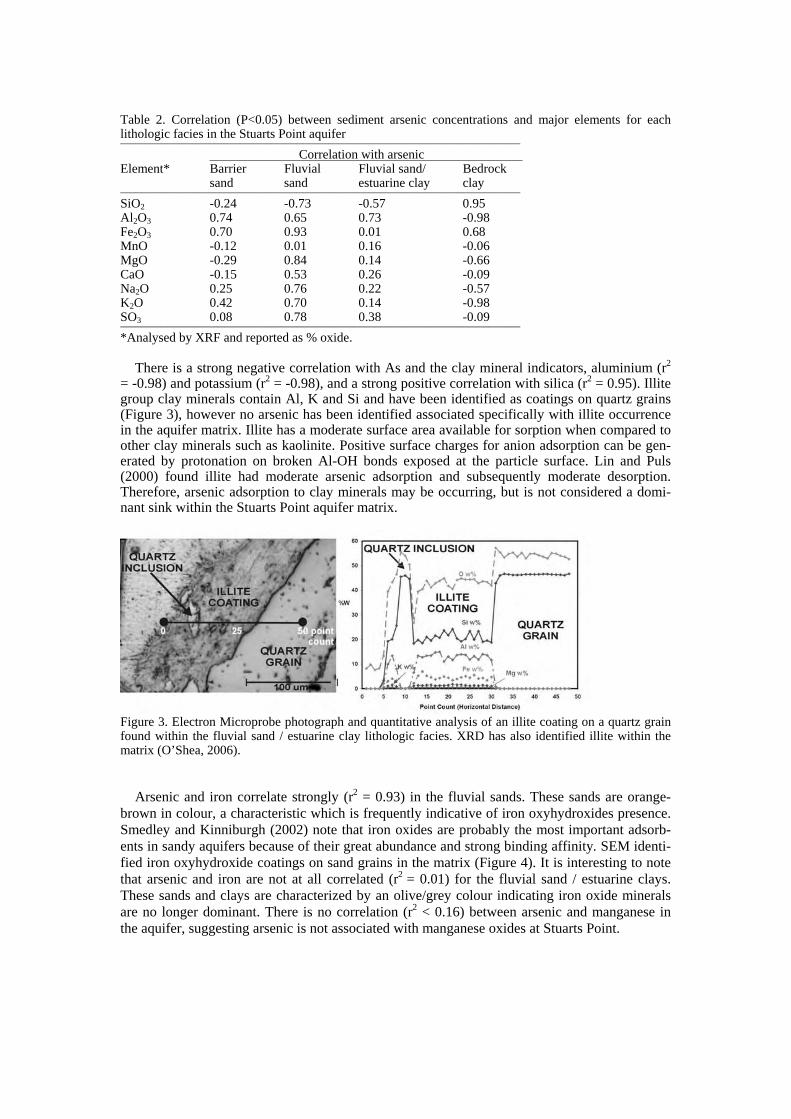
Table 2. Correlation (P<0.05) between sediment arsenic concentrations and major elements for each lithologic facies in the Stuarts Point aquifer _____________________________________________________________________________
Correlation with arsenic Element* Barrier Fluvial Fluvial sand/ Bedrock sand sand estuarine clay clay _____________________________________________________________________________SiO2 -0.24 -0.73 -0.57 0.95 Al2O3 0.74 0.65 0.73 -0.98 Fe2O3 0.70 0.93 0.01 0.68 MnO -0.12 0.01 0.16 -0.06 MgO -0.29 0.84 0.14 -0.66 CaO -0.15 0.53 0.26 -0.09 Na2O 0.25 0.76 0.22 -0.57 K2O 0.42 0.70 0.14 -0.98 SO3 0.08 0.78 0.38 -0.09 _____________________________________________________________________________*Analysed by XRF and reported as % oxide.
There is a strong negative correlation with As and the clay mineral indicators, aluminium (r2
= -0.98) and potassium (r2 = -0.98), and a strong positive correlation with silica (r2 = 0.95). Illite group clay minerals contain Al, K and Si and have been identified as coatings on quartz grains (Figure 3), however no arsenic has been identified associated specifically with illite occurrence in the aquifer matrix. Illite has a moderate surface area available for sorption when compared to other clay minerals such as kaolinite. Positive surface charges for anion adsorption can be gen-erated by protonation on broken Al-OH bonds exposed at the particle surface. Lin and Puls (2000) found illite had moderate arsenic adsorption and subsequently moderate desorption. Therefore, arsenic adsorption to clay minerals may be occurring, but is not considered a domi-nant sink within the Stuarts Point aquifer matrix.
Figure 3. Electron Microprobe photograph and quantitative analysis of an illite coating on a quartz grain found within the fluvial sand / estuarine clay lithologic facies. XRD has also identified illite within the matrix (O’Shea, 2006).
Arsenic and iron correlate strongly (r2 = 0.93) in the fluvial sands. These sands are orange-brown in colour, a characteristic which is frequently indicative of iron oxyhydroxides presence. Smedley and Kinniburgh (2002) note that iron oxides are probably the most important adsorb-ents in sandy aquifers because of their great abundance and strong binding affinity. SEM identi-fied iron oxyhydroxide coatings on sand grains in the matrix (Figure 4). It is interesting to note that arsenic and iron are not at all correlated (r2 = 0.01) for the fluvial sand / estuarine clays. These sands and clays are characterized by an olive/grey colour indicating iron oxide minerals are no longer dominant. There is no correlation (r2 < 0.16) between arsenic and manganese in the aquifer, suggesting arsenic is not associated with manganese oxides at Stuarts Point.
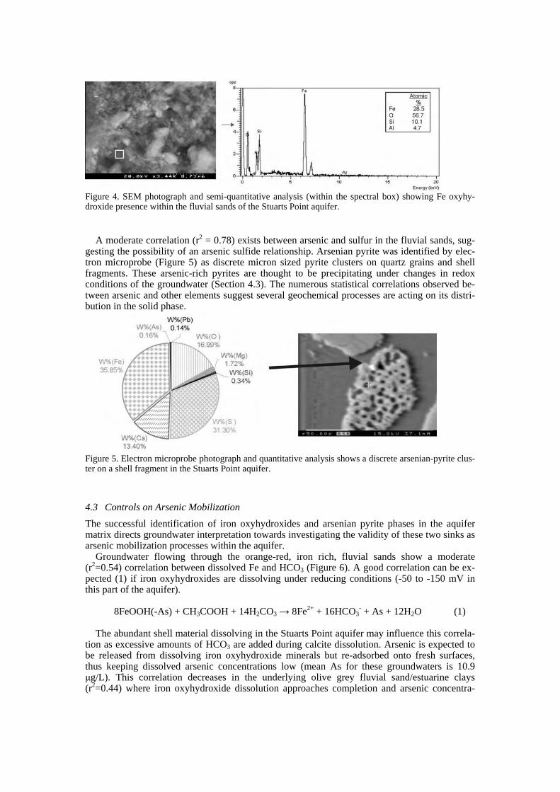
Figure 4. SEM photograph and semi-quantitative analysis (within the spectral box) showing Fe oxyhy-droxide presence within the fluvial sands of the Stuarts Point aquifer.
A moderate correlation (r2 = 0.78) exists between arsenic and sulfur in the fluvial sands, sug-gesting the possibility of an arsenic sulfide relationship. Arsenian pyrite was identified by elec-tron microprobe (Figure 5) as discrete micron sized pyrite clusters on quartz grains and shell fragments. These arsenic-rich pyrites are thought to be precipitating under changes in redox conditions of the groundwater (Section 4.3). The numerous statistical correlations observed be-tween arsenic and other elements suggest several geochemical processes are acting on its distri-bution in the solid phase.
Figure 5. Electron microprobe photograph and quantitative analysis shows a discrete arsenian-pyrite clus-ter on a shell fragment in the Stuarts Point aquifer.
4.3 Controls on Arsenic MobilizationThe successful identification of iron oxyhydroxides and arsenian pyrite phases in the aquifer matrix directs groundwater interpretation towards investigating the validity of these two sinks as arsenic mobilization processes within the aquifer.
Groundwater flowing through the orange-red, iron rich, fluvial sands show a moderate (r2=0.54) correlation between dissolved Fe and HCO3 (Figure 6). A good correlation can be ex-pected (1) if iron oxyhydroxides are dissolving under reducing conditions (-50 to -150 mV in this part of the aquifer).
8FeOOH(-As) + CH3COOH + 14H2CO3 8Fe2+ + 16HCO3- + As + 12H2O (1)
The abundant shell material dissolving in the Stuarts Point aquifer may influence this correla-tion as excessive amounts of HCO3 are added during calcite dissolution. Arsenic is expected to be released from dissolving iron oxyhydroxide minerals but re-adsorbed onto fresh surfaces, thus keeping dissolved arsenic concentrations low (mean As for these groundwaters is 10.9
g/L). This correlation decreases in the underlying olive grey fluvial sand/estuarine clays (r2=0.44) where iron oxyhydroxide dissolution approaches completion and arsenic concentra-
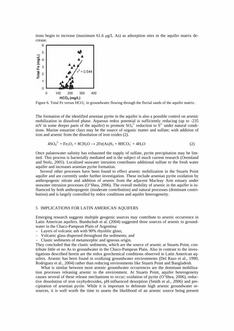
tions begin to increase (maximum 61.6 g/L As) as adsorption sites in the aquifer matrix de-crease.
Figure 6. Total Fe versus HCO3- in groundwater flowing through the fluvial sands of the aquifer matrix.
The formation of the identified arsenian pyrite in the aquifer is also a possible control on arsenic mobilization in dissolved phase. Aqueous redox potential is sufficiently reducing (up to -235 mV in some deeper parts of the aquifer) to promote SO4
2- reduction to S2- under natural condi-tions. Marine estuarine clays may be the source of organic matter and sulfate; with addition of iron and arsenic from the dissolution of iron oxides (2).
4SO42- + Fe2O3 + 8CH2O 2Fe(As)S2 + 8HCO3
- + 4H2O (2)
Once palaeowater salinity has exhausted the supply of sulfate, pyrite precipitation may be lim-ited. This process is bacterially mediated and is the subject of much current research (Oremland and Stolz, 2005). Localized seawater intrusion contributes additional sulfate to the fresh water aquifer and increases arsenian pyrite formation.
Several other processes have been found to effect arsenic mobilization in the Stuarts Point aquifer and are currently under further investigation. These include arsenian pyrite oxidation by anthropogenic nitrate and addition of arsenic from the adjacent Macleay Arm estuary under seawater intrusion processes (O’Shea, 2006). The overall mobility of arsenic in the aquifer is in-fluenced by both anthropogenic (moderate contribution) and natural processes (dominant contri-bution) and is largely controlled by redox conditions and aquifer heterogeneity.
5 IMPLICATIONS FOR LATIN AMERICAN AQUIFERS
Emerging research suggests multiple geogenic sources may contribute to arsenic occurrence in Latin American aquifers. Bundschuh et al. (2004) suggested three sources of arsenic to ground-water in the Chaco-Pampean Plain of Argentina:
Layers of volcanic ash with 90% rhyolitic glass; Volcanic glass dispersed throughout the sediments; and Clastic sediments of metamorphic and igneous origin.
They concluded that the clastic sediments, which are the source of arsenic at Stuarts Point, con-tribute little or no As to groundwater in the Chaco-Pampean Plain. Also in contrast to the inves-tigations described herein are the redox geochemical conditions observed in Latin American aq-uifers. Arsenic has been found in oxidizing groundwater environments (Del Razo et al., 1990; Rodriguez et al., 2004) rather than reducing environments like Stuarts Point and Bangladesh.
What is similar between most arsenic groundwater occurrences are the dominant mobiliza-tion processes releasing arsenic to the environment. At Stuarts Point, aquifer heterogeneity causes several of these release mechanisms to occur; oxidation of pyrite (O’Shea, 2006), reduc-tive dissolution of iron oxyhydroxides, pH-influenced desorption (Smith et al., 2006) and pre-cipitation of arsenian pyrite. While it is important to delineate high arsenic groundwater re-sources, it is well worth the time to assess the likelihood of an arsenic source being present
within the aquifer matrix. Developing a set of ‘arsenic source risk factors’ according to aquifer depositional history and lithology, may indicate areas at high risk of arsenic contamination prior to fieldwork, which can then be targeted in groundwater surveys. The lessons learned from a small coastal sedimentary aquifer in Australia should be utilised in the assessment and identifi-cation of potential arsenic-rich groundwaters of Latin America.
6 CONCLUSIONS
At Stuarts Point, mobilisation of arsenic occurs when iron oxide surfaces coating sediment grains are dissolved under reducing conditions, releasing their adsorbed arsenic into the groundwater. Increased reducing conditions develop with depth in the aquifer, as do concentra-tions of arsenic. Anoxic conditions in the aquifer develop due to decreased influx of oxidized rainwater, water-sediment interaction and increased flux of organic matter. Progression of the geochemical conditions into a strongly reducing environment promotes precipitation of arsenic into iron sulfides, with sulfate being supplied by seawater intrusion into the aquifer due to ex-cessive exploitation of the groundwater resource. This removes arsenic from the groundwater and incorporates it into a solid phase sink, preventing further migration of dissolved arsenic.
The low risk of anthropogenic arsenic input in combination with the accepted geomorphic model for the Stuarts Point aquifer indicated the aquifer was not expected to contain elevated concentrations of dissolved arsenic in the matrix. Characterisation of the arsenic geochemistry of the Stuarts Point aquifer can be applied as a potential risk assessment tool for fluvial and coastal aquifers of Latin America. A geomorphic approach to aquifer characterisation and iden-tification of potential arsenic sources may indicate Latin American aquifers that could be sus-ceptible to elevated arsenic concentrations. In addition, an assessment of hydrogeochemical conditions to determine the probability of arsenic mobilisation in the aquifer, can aid in the placement of potentially ‘safe’ wells for human consumption of groundwater. Heterogeneity of the aquifer chemical conditions and anthropogenic use of the aquifer should also be considered in the determination of low arsenic groundwater environments.
7 ACKNOWLEDGEMENTS
The authors would like to thank the New South Wales Department of Infrastructure, Planning and Natural Resources for financial assistance with this study. Field and laboratory assistance was provided by Sarah Groves, John Wischusen, Irene Wainwright and Dorothy Yu.
REFERENCESAmerican Public Health Association, 1992. Standard methods for the Examination of Water and Waste-
water (18th ed.). APHA-AWWA-WET, Washington, USA. Berg, M., Tran, H.C., Pham, K.T., Pham, H.V., Schertenleib, R. and Giger, W. 2003. Arsenic pollution of
water resources in Vietnam – A plea for early mitigation actions. In: Gobran, G.R. and Lepp, N. (eds) 7th International Conference on the Biogeochemistry of Trace Elements, Volume 2 Symposia, June 15-19 Uppsala, Sweden, 8-9.
Bhattacharya, P., Claesson, M., Bundschuh, J., Sracek, O., Fagerberg, J., Jacks, G., Martin, R.A., Storniolo, A.D.R., Thir, J.M. 2006. Distribution and mobility of arsenic in the Rio Dulce alluvial aqui-fers in Santiago del Estero Province, Argentina. Sci Tot Env, 358: 97-120.
Bissen, M. and Frimmel, F.H. 2003. Arsenic – a Review. Part 1: Occurrence, Toxicity, Speciation, Mobil-ity. Acta Hydrochim. Hydrobiol., 31(1): 9-18.
Bundschuh, J., Farias, B., Marin, R., Storniolo, A., Bhattacharya, P., Cortes, J., Bonorino, G. and Albouy, R. 2004. Groundwater arsenic in the Chaco-Pampean Plain, Argentina: case study from Robles county, Santiago del Estero Province. Applied Geochemistry, 19: 231-243.
Chen, S-L., Dzeng, S.R., Yang, M-H., Chiu, K-H., Shieh, G-M. and Chien, M.W. 1994. Arsenic species in groundwaters of the blackfoot disease area, Taiwan. Environ. Sci. Technol., 28: 877-881.
Del Razo, L.M., Arellano, M.A. and Cebrian, M.E. 1990. The oxidation states of arsenic in well-water from a chronic arsenicism area of northern Mexico. Enviro. Pollut. 64: 143-153.
Eddie, M.W. 2000. Soil Landscapes of the Macksville and Nambucca 1:100 000 Sheets. Department of Land and Water Conservation, Sydney.
Gilligan, L.B., J.W. Brownlow, R.G. Cameron and H.F. Henley. 1992. Dorrigo-Coffs Harbour 1:250 000 Metallogenic Map SH/56-10, SH/56-11: Metallogenic Study and Mineral Deposit Data Sheets. New South Wales Geological Survey, Sydney.
Harvey, C.F., Swartz, D.H., Badruzzaman, A.B.M., Keon-Blute, N., Yu, W., Ali, M.A., Jay, J., Beckie, R., Niedan, V., Brabander, D., Oates, P.M., Ashfaque, K.N., Islam, S., Hemond, H.F., Ahmed, M.F. 2005. Groundwater arsenic contamination on the Ganges Delta: biogeochemistry, hydrology, human perturbations, and human suffering on a large scale. C.R. Geoscience, 337: 285-296.
Khalequzzaman, Md., Farugue, F.S., Mitra, A.K. 2005. Assessment of arsenic contamination of ground-water and health problems in Bangladesh. International Journal of Environmental Research and Pub-lic Health, 2(2): 204-213.
Lin, Z. and Puls, R.W. 2000. Adsorption, desorption and oxidation of arsenic affected by clay minerals and aging process. Environmental Geology, 39(7): 753-759.
NHMRC, 1996. Australian Drinking Water Guidelines. National Health and Medical Research Council (NHMRC) & Agriculture and Resources Management Council of Australia and New Zealand (ARMCANZ). National Water Quality Management Strategy, Canberra.
Nickson, R.T., McArthur, J.M., Ravenscroft, P., Burgess, W.G. and Ahmed, K.M. 2000. Mechanism of arsenic release to groundwater, Bangladesh and West Bengal. Appl. Geochem., 15: 403-413.
Northey, J. 2001. A Hydrological and Hydrogeochemical Investigation of Stuarts Point Aquifer System, NSW, Following the Re-Introduction of Tidal Exchange into Yarrahapinni Wetland. Honours Thesis (unpublished), University of New South Wales, Australia.
O’Shea B. 2006. Delineating the source, geochemical sinks and aqueous mobilisation processes of natu-rally occurring arsenic in a coastal sandy aquifer, Stuarts Point, New South Wales, Australia. PhD Thesis (unpublished), University of New South Wales, Australia.
O’Shea, B. and Jankowski, J. 2002. Anthropogenic and geomorphic factors contributing to arsenic distri-bution in a coastal aquifer, New South Wales, Australia. In: Bocanegra, E., Martinez, D. and Massone, H. (Eds) Proceedings of the XXXII IAH & VI ALHSUD Congress, Groundwater and Human Develop-ment, October 21-25, Mar del Plata, Argentina: 860-868.
O’Shea, B. Jankowski, J. 2006. Determining subtle hydrochemical anomalies using multivariate statistics: an example from the Great Artesian Basin, Australia. Hydrological Processes in press, publication ex-pected May 2006.
O’Shea, B., Jankowski, J. and Sammut, J. 2006. The source of naturally occurring arsenic in a coastal sand aquifer of eastern Australia. Sci Tot Env, in review.
Oremland, R.S. and Stolz, J.S. 2005. Arsenic, microbes and contaminated aquifers. Trends in Microbiol-ogy, 13(2): 45-49.
Pouchou, J. L. and F. Pichoir, 1985. F(rZ) Procedure for Improved Quantitative Microanalysis. In: Mi-crobeam Analysis. J. T. Armstrong (Ed.), San Francisco Press, Inc., San Francisco, California, USA, p.104.
Rodriguez, R., Ramos, J.A. and Armienta, A. 2004. Groundwater arsenic variations: the role of local ge-ology and rainfall. Applied Geochemistry, 19: 245-250.
Romero, F.M., Armienta, M.A. and Carrillo-Chavez, A. 2004. Arsenic sorption by carbonate-rich aquifer material, a control on arsenic mobility at Zimapan, Mexico. Environmental Contamination and Toxi-cology, 47: 1-13.
Schreiber, M., Gotkowitz, M., Simo, J. and Frieberg, P. 2000. Stratigraphic and geochemical controls on naturally occurring arsenic in groundwater, eastern Wisconsin, USA. Hydrogeology Journal, 8: 161-176.
Sidle, W.C., Wotten, B. and Murphy, E. 2001. Provenance of geogenic arsenic in the Goose River basin, Maine, USA. Environmental Geology, 41: 62-73.
Smedley, P.L. and Kinniburgh, D.G. 2002. A review of the source, behaviour and distribution of arsenic in natural waters. Applied Geochemistry, 17: 517-568.
Smedley, P.L., Nicolli, H.B., Macdonald, D.M.J., Barros, A.J. and Tullio, J.O. 2002. Hydrogeochemistry of arsenic and other inorganic constituents in groundwaters from La Pampa, Argentina. Applied Geo-chemistry, 17: 259-284.
Smith, J.V.S., Jankowski, J. and Sammut, J. 2006. Natural occurrences of inorganic arsenic in the Austra-lian coastal groundwater environment: Implications for water quality in Australian coastal communi-ties. In: Naidu, R., Smith, E., Smith, L., Smith, J. (eds.). Managing Arsenic in the Environment: From Soil to Human Health. CSIRO Publishing, Melbourne, Australia.
Smith, J.V.S., Jankowski, J. and Sammut, J. 2003. Vertical distribution of As(III) and As(V) in a coastal sandy aquifer: factors controlling the concentration and speciation of arsenic in the Stuarts Point groundwater system, Northern New South Wales, Australia. Appl. Geochem. 18: 1479-1496.
Welch, A.H., Westjohn, D.B., Helsel, D.R. and Wanty, R.B. 2000. Arsenic in ground water of the United States: occurrence and geochemistry. Ground Water, 38: 589-604.
APPENDIX B
Raw Data
B1 Sediment Chemistry
B2 Groundwater Chemistry
B3 Grain Size Analysis
B4 Sediment Mineral Composition
B5 Iron Oxide Conversions
B6 Sequential Extraction Results
B7 Statistical Results
B8 Geochemical Modelling Results
B9 Selected X-Y plots
(for sediments & groundwater)
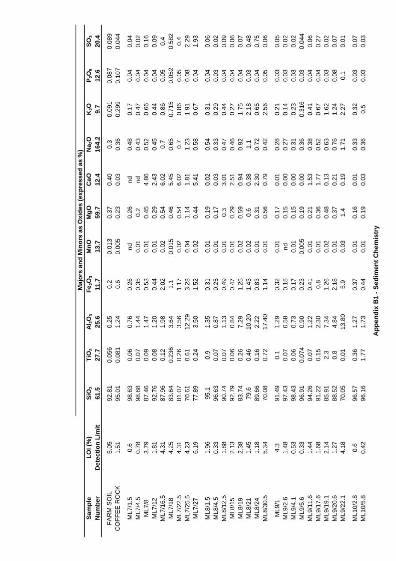
Sam
ple
LOI (
%)
SiO
2Ti
O2
Al 2O
3Fe
2O3
MnO
MgO
CaO
Na 2
OK
2OP 2
O5
SO3
Num
ber
Det
ectio
n Li
mit
61.5
27.7
25.6
11.7
13.7
59.7
12.4
164.
29.
712
.620
.4
FAR
M S
OIL
5.05
92.8
10.
056
0.25
0.2
0.01
30.
370.
400.
30.
091
0.08
70.
089
CO
FFE
E R
OC
K1.
5195
.01
0.08
11.
240.
60.
005
0.23
0.03
0.36
0.29
90.
107
0.04
4
ML7
/1.5
0.6
98.6
30.
060.
760.
26nd
0.26
nd0.
480.
170.
040.
04M
L7/4
.50.
7898
.68
0.07
1.44
0.35
0.01
0.2
nd0.
430.
470.
040.
02M
L7/8
3.79
87.4
60.
091.
470.
530.
010.
454.
860.
520.
660.
040.
16M
L7/1
21.
8192
.76
0.08
1.20
0.44
0.01
0.29
2.43
0.45
0.44
0.04
0.09
ML7
/16.
54.
3187
.96
0.12
1.98
2.02
0.02
0.54
6.02
0.7
0.86
0.05
0.4
ML7
/18
4.25
83.6
40.
236
3.64
1.1
0.01
50.
465.
450.
650.
715
0.05
20.
582
ML7
/22.
54.
3181
.07
0.26
3.56
1.17
0.02
0.54
6.02
0.7
0.86
0.05
0.4
ML7
/25.
54.
2370
.61
0.61
12.2
93.
280.
041.
141.
811.
231.
910.
082.
29M
L7/2
76.
1977
.89
0.24
3.50
1.52
0.02
0.44
5.41
0.58
0.67
0.04
1.93
ML8
/1.5
1.96
95.1
0.9
1.35
0.31
0.01
0.19
0.02
0.54
0.31
0.04
0.06
ML8
/4.5
0.33
96.6
30.
070.
870.
250.
010.
170.
030.
330.
290.
030.
02M
L8/1
2.5
1.88
90.7
40.
071.
130.
490.
010.
33.
010.
470.
440.
040.
09M
L8/1
52.
1392
.79
0.06
0.84
0.47
0.01
0.29
2.51
0.46
0.27
0.04
0.06
ML8
/19
2.38
83.7
40.
267.
291.
250.
020.
590.
940.
921.
750.
040.
07M
L8/2
11.
4579
.60.
4610
.20
1.43
0.02
0.6
0.38
1.1
2.18
0.03
0.48
ML8
/24
1.18
89.6
60.
162.
220.
830.
010.
312.
300.
720.
650.
040.
75M
L8/3
0.5
5.34
70.0
80.
7217
.40
1.14
0.01
0.56
0.79
0.42
2.56
0.05
0.06
ML9
/14.
391
.49
0.1
1.29
0.32
0.01
0.17
0.01
0.28
0.21
0.03
0.05
ML9
/2.6
1.48
97.4
30.
070.
580.
15nd
0.15
0.00
0.27
0.14
0.03
0.02
ML9
/4.1
0.53
98.4
30.
060.
730.
170.
010.
150.
000.
310.
230.
030.
02M
L9/5
.60.
3396
.91
0.07
40.
900.
230.
005
0.19
0.00
0.36
0.31
60.
030.
044
ML9
/11.
61.
4494
.26
0.07
1.22
0.41
0.01
0.21
1.53
0.38
0.41
0.04
0.06
ML9
/17.
61.
6891
.22
0.15
2.30
0.8
0.01
0.36
1.77
0.52
0.67
0.04
0.27
ML9
/19.
12.
1485
.91
2.3
7.34
1.26
0.02
0.48
0.13
0.63
1.62
0.03
0.02
ML9
/20.
61.
2788
.52
0.8
4.84
2.18
0.01
0.37
0.21
0.76
1.24
0.08
0.07
ML9
/22.
14.
1870
.05
0.01
13.8
05.
90.
031.
40.
191.
712.
270.
10.
01
ML1
0/2.
80.
696
.57
0.36
1.27
0.37
0.01
0.16
0.01
0.33
0.32
0.03
0.07
ML1
0/5.
80.
4296
.16
1.77
1.73
0.44
0.01
0.19
0.03
0.36
0.5
0.03
0.03
Maj
ors
and
Min
ors
as O
xide
s (e
xpre
ssed
as
%)
App
endi
x B
1 - S
edim
ent C
hem
istr
y
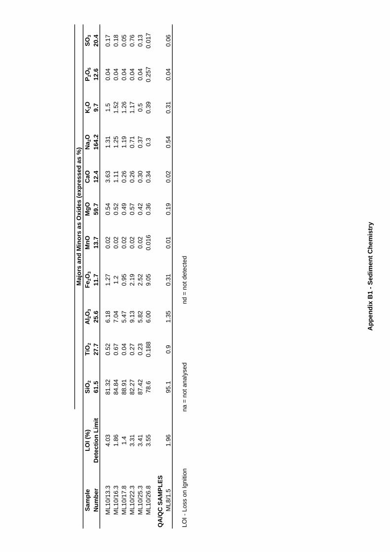
Sam
ple
LOI (
%)
SiO
2Ti
O2
Al 2O
3Fe
2O3
MnO
MgO
CaO
Na 2
OK
2OP 2
O5
SO3
Num
ber
Det
ectio
n Li
mit
61.5
27.7
25.6
11.7
13.7
59.7
12.4
164.
29.
712
.620
.4
Maj
ors
and
Min
ors
as O
xide
s (e
xpre
ssed
as
%)
ML1
0/13
.34.
0381
.32
0.52
6.18
1.27
0.02
0.54
3.63
1.31
1.5
0.04
0.17
ML1
0/16
.31.
8684
.84
0.67
7.04
1.2
0.02
0.52
1.11
1.25
1.52
0.04
0.18
ML1
0/17
.81.
488
.91
0.04
5.47
0.95
0.02
0.49
0.26
1.19
1.26
0.04
0.05
ML1
0/22
.33.
3182
.27
0.27
9.13
2.19
0.02
0.57
0.26
0.71
1.17
0.04
0.76
ML1
0/25
.33.
4187
.42
0.23
5.82
2.52
0.02
0.42
0.30
0.37
0.5
0.04
0.13
ML1
0/26
.83.
5578
.60.
188
6.00
9.05
0.01
60.
360.
340.
30.
390.
257
0.01
7
QA
/QC
SA
MPL
ESM
L8/1
.51.
9695
.10.
91.
350.
310.
010.
190.
020.
540.
310.
040.
06
LOI -
Los
s on
Igni
tion
na =
not
ana
lyse
dnd
= n
ot d
etec
ted
App
endi
x B
1 - S
edim
ent C
hem
istr
y
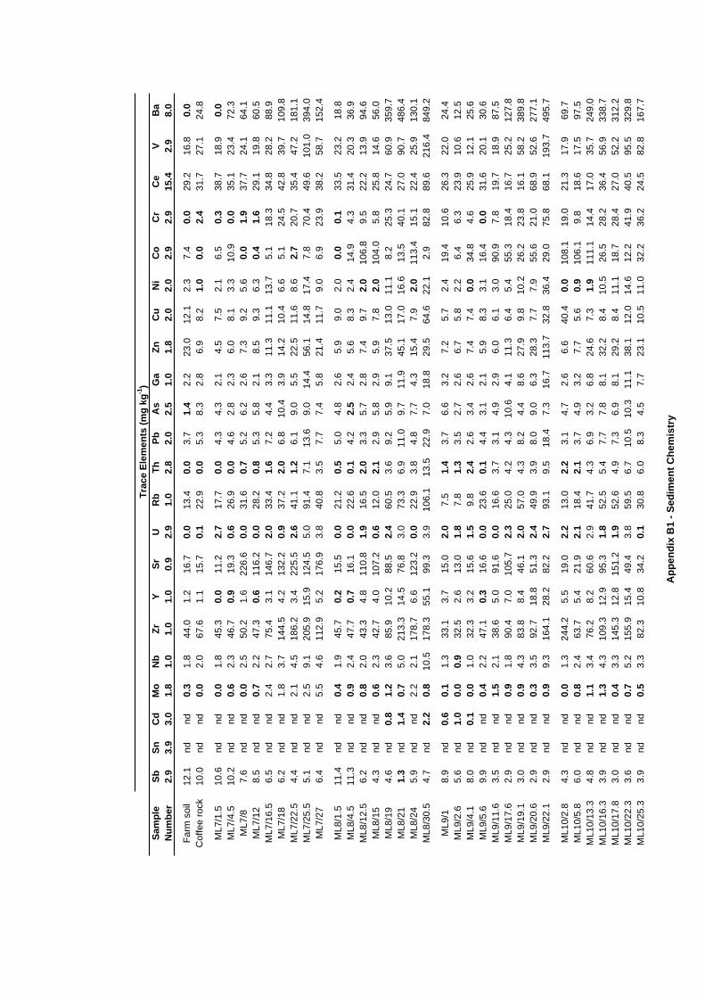
Sam
ple
SbSn
Cd
Mo
Nb
ZrY
SrU
Rb
ThPb
As
Ga
ZnC
uN
iC
oC
rC
eV
Ba
Num
ber
2.9
3.9
3.0
1.8
1.0
1.0
1.0
0.9
2.9
1.0
2.8
2.0
2.5
1.0
1.8
2.0
2.0
2.9
2.9
15.4
2.9
8.0
Farm
soi
l12
.1nd
nd0.
31.
844
.01.
216
.70.
013
.40.
03.
71.
42.
223
.012
.12.
37.
40.
029
.216
.80.
0C
offe
e ro
ck10
.0nd
nd0.
02.
067
.61.
115
.70.
122
.90.
05.
38.
32.
86.
98.
21.
00.
02.
431
.727
.124
.8
ML7
/1.5
10.6
ndnd
0.0
1.8
45.3
0.0
11.2
2.7
17.7
0.0
4.3
4.3
2.1
4.5
7.5
2.1
6.5
0.3
38.7
18.9
0.0
ML7
/4.5
10.2
ndnd
0.6
2.3
46.7
0.9
19.3
0.6
26.9
0.0
4.6
2.8
2.3
6.0
8.1
3.3
10.9
0.0
35.1
23.4
72.3
ML7
/87.
6nd
nd0.
02.
550
.21.
622
6.6
0.0
31.6
0.7
5.2
6.2
2.6
7.3
9.2
5.6
0.0
1.9
37.7
24.1
64.1
ML7
/12
8.5
ndnd
0.7
2.2
47.3
0.6
116.
20.
028
.20.
85.
35.
82.
18.
59.
36.
30.
41.
629
.119
.860
.5M
L7/1
6.5
6.5
ndnd
2.4
2.7
75.4
3.1
146.
72.
033
.41.
67.
24.
43.
311
.311
.113
.75.
118
.334
.828
.288
.9M
L7/1
86.
2nd
nd1.
83.
714
4.5
4.2
132.
20.
937
.22.
06.
810
.43.
914
.210
.46.
65.
124
.542
.839
.710
9.8
ML7
/22.
54.
4nd
nd2.
14.
518
6.2
3.4
225.
52.
641
.11.
26.
19.
05.
522
.511
.68.
62.
720
.735
.447
.218
1.1
ML7
/25.
55.
1nd
nd2.
59.
120
5.9
15.9
124.
55.
091
.47.
113
.69.
014
.456
.114
.817
.47.
870
.449
.610
1.0
394.
0M
L7/2
76.
4nd
nd5.
54.
611
2.9
5.2
176.
93.
840
.83.
57.
77.
45.
821
.411
.79.
06.
923
.938
.258
.715
2.4
ML8
/1.5
11.4
ndnd
0.4
1.9
45.7
0.2
15.5
0.0
21.2
0.5
5.0
4.8
2.6
5.9
9.0
2.0
0.0
0.1
33.5
23.2
18.8
ML8
/4.5
11.3
ndnd
0.9
2.4
47.7
0.7
16.1
0.0
22.6
0.1
4.2
2.5
2.4
5.6
8.3
2.4
14.9
4.3
31.4
20.3
36.9
ML8
/12.
56.
2nd
nd0.
82.
043
.34.
811
0.8
1.9
16.5
2.0
3.3
5.7
2.8
7.4
9.7
2.0
106.
89.
522
.213
.994
.6M
L8/1
54.
3nd
nd0.
62.
342
.74.
010
7.2
0.6
12.0
2.1
2.9
5.8
2.9
5.9
7.8
2.0
104.
05.
825
.814
.656
.0M
L8/1
94.
6nd
0.8
1.2
3.6
85.9
10.2
88.5
2.4
60.5
3.6
9.2
5.9
9.1
37.5
13.0
11.1
8.2
25.3
24.7
60.9
359.
7M
L8/2
11.
3nd
1.4
0.7
5.0
213.
314
.576
.83.
073
.36.
911
.09.
711
.945
.117
.016
.613
.540
.127
.090
.748
6.4
ML8
/24
5.9
ndnd
2.2
2.1
178.
76.
612
3.2
0.0
22.9
3.8
4.8
7.7
4.3
15.4
7.9
2.0
113.
415
.122
.425
.913
0.1
ML8
/30.
54.
7nd
2.2
0.8
10.5
178.
355
.199
.33.
910
6.1
13.5
22.9
7.0
18.8
29.5
64.6
22.1
2.9
82.8
89.6
216.
484
9.2
ML9
/18.
9nd
0.6
0.1
1.3
33.1
3.7
15.0
2.0
7.5
1.4
3.7
6.6
3.2
7.2
5.7
2.4
19.4
10.6
26.3
22.0
24.4
ML9
/2.6
5.6
nd1.
00.
00.
932
.52.
613
.01.
87.
81.
33.
52.
72.
66.
75.
82.
26.
46.
323
.910
.612
.5M
L9/4
.18.
0nd
0.1
0.0
1.0
32.3
3.2
15.6
1.5
9.8
2.4
2.6
3.4
2.6
7.4
7.4
0.0
34.8
4.6
25.9
12.1
25.6
ML9
/5.6
9.9
ndnd
0.4
2.2
47.1
0.3
16.6
0.0
23.6
0.1
4.4
3.1
2.1
5.9
8.3
3.1
16.4
0.0
31.6
20.1
30.6
ML9
/11.
63.
5nd
nd1.
52.
138
.65.
091
.60.
016
.63.
73.
14.
92.
96.
06.
13.
090
.97.
819
.718
.987
.5M
L9/1
7.6
2.9
ndnd
0.9
1.8
90.4
7.0
105.
72.
325
.04.
24.
310
.64.
111
.36.
45.
455
.318
.416
.725
.212
7.8
ML9
/19.
13.
0nd
nd0.
94.
383
.88.
446
.12.
057
.04.
38.
24.
48.
627
.99.
810
.226
.223
.816
.158
.238
9.8
ML9
/20.
62.
9nd
nd0.
33.
592
.718
.851
.32.
449
.93.
98.
09.
06.
328
.37.
77.
955
.621
.068
.952
.627
7.1
ML9
/22.
12.
9nd
nd0.
99.
316
4.1
28.2
82.2
2.7
93.1
9.5
18.4
7.3
16.7
113.
732
.836
.429
.075
.868
.119
3.7
495.
7
ML1
0/2.
84.
3nd
nd0.
01.
324
4.2
5.5
19.0
2.2
13.0
2.2
3.1
4.7
2.6
6.6
40.4
0.0
108.
119
.021
.317
.969
.7M
L10/
5.8
6.0
ndnd
0.8
2.4
63.7
5.4
21.9
2.1
18.4
2.1
3.7
4.9
3.2
7.7
5.6
0.9
106.
19.
818
.617
.597
.5M
L10/
13.3
4.8
ndnd
1.1
3.4
76.2
8.2
60.6
2.9
41.7
4.3
6.9
3.2
6.8
24.6
7.3
1.9
111.
114
.417
.035
.724
9.0
ML1
0/16
.33.
9nd
nd1.
34.
310
9.3
12.9
95.3
1.8
52.5
5.4
7.7
7.8
8.1
32.2
8.4
10.5
26.5
28.2
36.4
56.9
338.
7M
L10/
17.8
3.0
ndnd
0.4
3.3
145.
312
.815
1.2
1.9
52.6
4.9
7.3
6.9
8.1
29.2
8.4
11.1
18.7
28.4
27.0
52.2
312.
2M
L10/
22.3
3.6
ndnd
0.7
5.2
155.
915
.449
.43.
859
.56.
710
.510
.311
.138
.112
.014
.612
.241
.940
.595
.532
9.8
ML1
0/25
.33.
9nd
nd0.
53.
382
.310
.834
.20.
130
.86.
08.
34.
57.
723
.110
.511
.032
.236
.224
.582
.816
7.7
Trac
e El
emen
ts (m
g kg
-1)
App
endi
x B
1 - S
edim
ent C
hem
istr
y
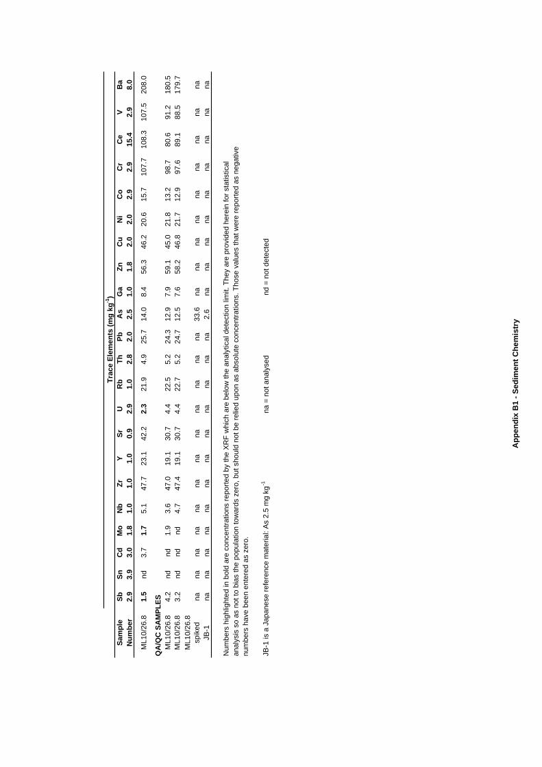
Sam
ple
SbSn
Cd
Mo
Nb
ZrY
SrU
Rb
ThPb
As
Ga
ZnC
uN
iC
oC
rC
eV
Ba
Num
ber
2.9
3.9
3.0
1.8
1.0
1.0
1.0
0.9
2.9
1.0
2.8
2.0
2.5
1.0
1.8
2.0
2.0
2.9
2.9
15.4
2.9
8.0
Trac
e El
emen
ts (m
g kg
-1)
ML1
0/26
.81.
5nd
3.7
1.7
5.1
47.7
23.1
42.2
2.3
21.9
4.9
25.7
14.0
8.4
56.3
46.2
20.6
15.7
107.
710
8.3
107.
520
8.0
QA
/QC
SA
MPL
ESM
L10/
26.8
4.2
ndnd
1.9
3.6
47.0
19.1
30.7
4.4
22.5
5.2
24.3
12.9
7.9
59.1
45.0
21.8
13.2
98.7
80.6
91.2
180.
5M
L10/
26.8
3.2
ndnd
nd4.
747
.419
.130
.74.
422
.75.
224
.712
.57.
658
.246
.821
.712
.997
.689
.188
.517
9.7
ML1
0/26
.8sp
iked
nana
nana
nana
nana
nana
nana
33.6
nana
nana
nana
nana
naJB
-1na
nana
nana
nana
nana
nana
na2.
6na
nana
nana
nana
nana
Num
bers
hig
hlig
hted
in b
old
are
conc
entra
tions
repo
rted
by th
e X
RF
whi
ch a
re b
elow
the
anal
ytic
al d
etec
tion
limit.
The
y ar
e pr
ovid
ed h
erei
n fo
r sta
tistic
al
anal
ysis
so
as n
ot to
bia
s th
e po
pula
tion
tow
ards
zer
o, b
ut s
houl
d no
t be
relie
d up
on a
s ab
solu
te c
once
ntra
tions
. Tho
se v
alue
s th
at w
ere
repo
rted
as n
egat
ive
num
bers
hav
e be
en e
nter
ed a
s ze
ro.
JB-1
is a
Jap
anes
e re
fere
nce
mat
eria
l: A
s 2.
5 m
g kg
-1na
= n
ot a
naly
sed
nd =
not
det
ecte
d
App
endi
x B
1 - S
edim
ent C
hem
istr
y
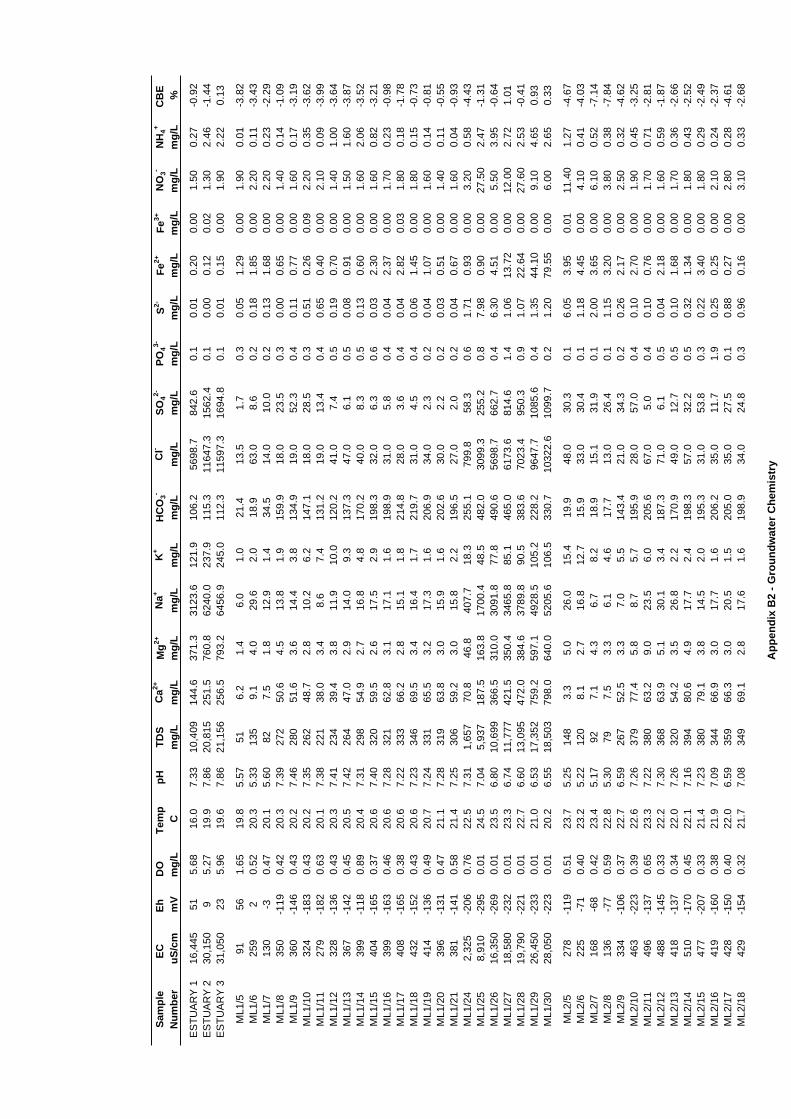
Sam
ple
EC
Eh
D
O
Tem
p pH
TDS
Ca2+
Mg2+
Na+
K+
HC
O3-
Cl-
SO42-
PO43-
S2-Fe
2+Fe
3+N
O3-
NH
4+C
BE
Num
ber
uS/c
mm
Vm
g/L
Cm
g/L
mg/
Lm
g/L
mg/
Lm
g/L
mg/
Lm
g/L
mg/
Lm
g/L
mg/
Lm
g/L
mg/
Lm
g/L
mg/
L%
ES
TUA
RY
116
,445
515.
6816
.07.
3310
,409
144.
637
1.3
3123
.612
1.9
106.
256
98.7
842.
60.
10.
010.
200.
001.
500.
27-0
.92
ES
TUA
RY
230
,150
95.
2719
.97.
8620
,815
251.
576
0.8
6240
.023
7.9
115.
311
647.
315
62.4
0.1
0.00
0.12
0.02
1.30
2.46
-1.4
4E
STU
AR
Y 3
31,0
5023
5.96
19.6
7.86
21,1
5625
6.5
793.
264
56.9
245.
011
2.3
1159
7.3
1694
.80.
10.
010.
150.
001.
902.
220.
13
ML1
/591
561.
6519
.85.
5751
6.2
1.4
6.0
1.0
21.4
13.5
1.7
0.3
0.05
1.29
0.00
1.90
0.01
-3.8
2M
L1/6
259
20.
5220
.35.
3313
59.
14.
029
.62.
018
.963
.08.
60.
20.
181.
850.
002.
200.
11-3
.43
ML1
/713
0-3
0.47
20.1
5.60
827.
51.
812
.91.
434
.514
.010
.00.
20.
131.
680.
002.
200.
23-2
.29
ML1
/835
0-1
190.
4220
.37.
3927
250
.64.
513
.81.
915
9.9
18.0
23.5
0.3
0.00
0.65
0.00
1.40
0.14
-1.0
9M
L1/9
360
-146
0.43
20.2
7.46
280
51.6
3.6
14.4
3.8
134.
919
.052
.30.
40.
110.
770.
001.
600.
17-3
.19
ML1
/10
324
-183
0.43
20.2
7.35
262
48.7
2.8
10.2
6.2
147.
118
.028
.50.
30.
510.
260.
092.
200.
35-3
.62
ML1
/11
279
-182
0.63
20.1
7.38
221
38.0
3.4
8.6
7.4
131.
219
.013
.40.
40.
650.
400.
002.
100.
09-3
.99
ML1
/12
328
-136
0.43
20.3
7.41
234
39.4
3.8
11.9
10.0
120.
241
.07.
40.
50.
190.
700.
001.
401.
00-3
.64
ML1
/13
367
-142
0.45
20.5
7.42
264
47.0
2.9
14.0
9.3
137.
347
.06.
10.
50.
080.
910.
001.
501.
60-3
.87
ML1
/14
399
-118
0.89
20.4
7.31
298
54.9
2.7
16.8
4.8
170.
240
.08.
30.
50.
130.
600.
001.
602.
06-3
.52
ML1
/15
404
-165
0.37
20.6
7.40
320
59.5
2.6
17.5
2.9
198.
332
.06.
30.
60.
032.
300.
001.
600.
82-3
.21
ML1
/16
399
-163
0.46
20.6
7.28
321
62.8
3.1
17.1
1.6
198.
931
.05.
80.
40.
042.
370.
001.
700.
23-0
.98
ML1
/17
408
-165
0.38
20.6
7.22
333
66.2
2.8
15.1
1.8
214.
828
.03.
60.
40.
042.
820.
031.
800.
18-1
.78
ML1
/18
432
-152
0.43
20.6
7.23
346
69.5
3.4
16.4
1.7
219.
731
.04.
50.
40.
061.
450.
001.
800.
15-0
.73
ML1
/19
414
-136
0.49
20.7
7.24
331
65.5
3.2
17.3
1.6
206.
934
.02.
30.
20.
041.
070.
001.
600.
14-0
.81
ML1
/20
396
-131
0.47
21.1
7.28
319
63.8
3.0
15.9
1.6
202.
630
.02.
20.
20.
030.
510.
001.
400.
11-0
.55
ML1
/21
381
-141
0.58
21.4
7.25
306
59.2
3.0
15.8
2.2
196.
527
.02.
00.
20.
040.
670.
001.
600.
04-0
.93
ML1
/24
2,32
5-2
060.
7622
.57.
311,
657
70.8
46.8
407.
718
.325
5.1
799.
858
.30.
61.
710.
930.
003.
200.
58-4
.43
ML1
/25
8,91
0-2
950.
0124
.57.
045,
937
187.
516
3.8
1700
.448
.548
2.0
3099
.325
5.2
0.8
7.98
0.90
0.00
27.5
02.
47-1
.31
ML1
/26
16,3
50-2
690.
0123
.56.
8010
,699
366.
531
0.0
3091
.877
.849
0.6
5698
.766
2.7
0.4
6.30
4.51
0.00
5.50
3.95
-0.6
4M
L1/2
718
,580
-232
0.01
23.3
6.74
11,7
7742
1.5
350.
434
65.8
85.1
465.
061
73.6
814.
61.
41.
0613
.72
0.00
12.0
02.
721.
01M
L1/2
819
,790
-221
0.01
22.7
6.60
13,0
9547
2.0
384.
637
89.8
90.5
383.
670
23.4
950.
30.
91.
0722
.64
0.00
27.6
02.
53-0
.41
ML1
/29
26,4
50-2
330.
0121
.06.
5317
,352
759.
259
7.1
4928
.510
5.2
228.
296
47.7
1085
.60.
41.
3544
.10
0.00
9.10
4.65
0.93
ML1
/30
28,0
50-2
230.
0120
.26.
5518
,503
798.
064
0.0
5205
.610
6.5
330.
710
322.
610
99.7
0.2
1.20
79.5
50.
006.
002.
650.
33
ML2
/527
8-1
190.
5123
.75.
2514
83.
35.
026
.015
.419
.948
.030
.30.
16.
053.
950.
0111
.40
1.27
-4.6
7M
L2/6
225
-71
0.40
23.2
5.22
120
8.1
2.7
16.8
12.7
15.9
33.0
30.4
0.1
1.18
4.45
0.00
4.10
0.41
-4.0
3M
L2/7
168
-68
0.42
23.4
5.17
927.
14.
36.
78.
218
.915
.131
.90.
12.
003.
650.
006.
100.
52-7
.14
ML2
/813
6-7
70.
5922
.85.
3079
7.5
3.3
6.1
4.6
17.7
13.0
26.4
0.1
1.15
3.20
0.00
3.80
0.38
-7.8
4M
L2/9
334
-106
0.37
22.7
6.59
267
52.5
3.3
7.0
5.5
143.
421
.034
.30.
20.
262.
170.
002.
500.
32-4
.62
ML2
/10
463
-223
0.39
22.6
7.26
379
77.4
5.8
8.7
5.7
195.
928
.057
.00.
40.
102.
700.
001.
900.
45-3
.25
ML2
/11
496
-137
0.65
23.3
7.22
380
63.2
9.0
23.5
6.0
205.
667
.05.
00.
40.
100.
760.
001.
700.
71-2
.81
ML2
/12
488
-145
0.33
22.2
7.30
368
63.9
5.1
30.1
3.4
187.
371
.06.
10.
50.
042.
180.
001.
600.
59-1
.87
ML2
/13
418
-137
0.34
22.0
7.26
320
54.2
3.5
26.8
2.2
170.
949
.012
.70.
50.
101.
680.
001.
700.
36-2
.66
ML2
/14
510
-170
0.45
22.1
7.16
394
80.6
4.9
17.7
2.4
198.
357
.032
.20.
50.
321.
340.
001.
800.
43-2
.52
ML2
/15
477
-207
0.33
21.4
7.23
380
79.1
3.8
14.5
2.0
195.
331
.053
.80.
30.
223.
400.
001.
800.
29-2
.49
ML2
/16
419
-160
0.38
21.9
7.09
344
66.9
3.0
17.7
1.6
206.
235
.011
.71.
90.
250.
250.
002.
100.
24-2
.37
ML2
/17
428
-150
0.40
22.0
6.59
359
66.3
3.0
20.5
1.5
205.
035
.027
.50.
10.
880.
270.
002.
800.
28-4
.61
ML2
/18
429
-154
0.32
21.7
7.08
349
69.1
2.8
17.6
1.6
198.
934
.024
.80.
30.
960.
160.
003.
100.
33-2
.68
App
endi
x B
2 - G
roun
dwat
er C
hem
istr
y
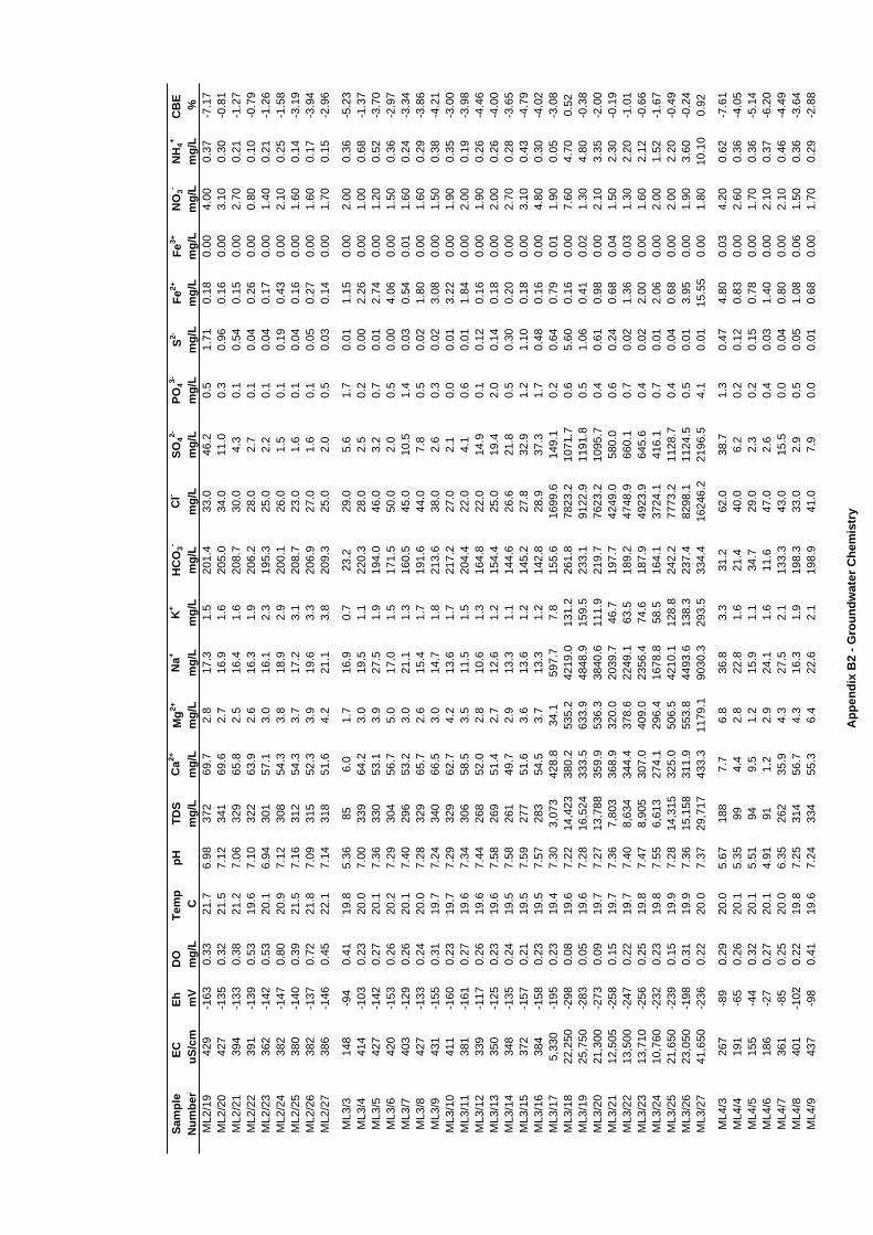
Sam
ple
EC
Eh
D
O
Tem
p pH
TDS
Ca2+
Mg2+
Na+
K+
HC
O3-
Cl-
SO42-
PO43-
S2-Fe
2+Fe
3+N
O3-
NH
4+C
BE
Num
ber
uS/c
mm
Vm
g/L
Cm
g/L
mg/
Lm
g/L
mg/
Lm
g/L
mg/
Lm
g/L
mg/
Lm
g/L
mg/
Lm
g/L
mg/
Lm
g/L
mg/
L%
ML2
/19
429
-163
0.33
21.7
6.98
372
69.7
2.8
17.3
1.5
201.
433
.046
.20.
51.
710.
180.
004.
000.
37-7
.17
ML2
/20
427
-135
0.32
21.5
7.12
341
69.6
2.7
16.9
1.6
205.
034
.011
.00.
30.
960.
160.
003.
100.
30-0
.81
ML2
/21
394
-133
0.38
21.2
7.06
329
65.8
2.5
16.4
1.6
208.
730
.04.
30.
10.
540.
150.
002.
700.
21-1
.27
ML2
/22
391
-139
0.53
19.6
7.10
322
63.9
2.6
16.3
1.9
206.
228
.02.
70.
10.
040.
260.
000.
800.
10-0
.79
ML2
/23
362
-142
0.53
20.1
6.94
301
57.1
3.0
16.1
2.3
195.
325
.02.
20.
10.
040.
170.
001.
400.
21-1
.26
ML2
/24
382
-147
0.80
20.9
7.12
308
54.3
3.8
18.9
2.9
200.
126
.01.
50.
10.
190.
430.
002.
100.
25-1
.58
ML2
/25
380
-140
0.39
21.5
7.16
312
54.3
3.7
17.2
3.1
208.
723
.01.
60.
10.
040.
160.
001.
600.
14-3
.19
ML2
/26
382
-137
0.72
21.8
7.09
315
52.3
3.9
19.6
3.3
206.
927
.01.
60.
10.
050.
270.
001.
600.
17-3
.94
ML2
/27
386
-146
0.45
22.1
7.14
318
51.6
4.2
21.1
3.8
209.
325
.02.
00.
50.
030.
140.
001.
700.
15-2
.96
ML3
/314
8-9
40.
4119
.85.
3685
6.0
1.7
16.9
0.7
23.2
29.0
5.6
1.7
0.01
1.15
0.00
2.00
0.36
-5.2
3M
L3/4
414
-103
0.23
20.0
7.00
339
64.2
3.0
19.5
1.1
220.
328
.02.
50.
20.
002.
260.
001.
000.
68-1
.37
ML3
/542
7-1
420.
2720
.17.
3633
053
.13.
927
.51.
919
4.0
46.0
3.2
0.7
0.01
2.74
0.00
1.20
0.52
-3.7
0M
L3/6
420
-153
0.26
20.2
7.29
304
56.7
5.0
17.0
1.5
171.
550
.02.
00.
50.
004.
060.
001.
500.
36-2
.97
ML3
/740
3-1
290.
2620
.17.
4029
653
.23.
021
.11.
316
0.5
45.0
10.5
1.4
0.03
0.54
0.01
1.60
0.24
-3.3
4M
L3/8
427
-133
0.24
20.0
7.28
329
65.7
2.6
15.4
1.7
191.
644
.07.
80.
50.
021.
800.
001.
600.
29-3
.86
ML3
/943
1-1
550.
3119
.77.
2434
066
.53.
014
.71.
821
3.6
38.0
2.6
0.3
0.02
3.08
0.00
1.50
0.38
-4.2
1M
L3/1
041
1-1
600.
2319
.77.
2932
962
.74.
213
.61.
721
7.2
27.0
2.1
0.0
0.01
3.22
0.00
1.90
0.35
-3.0
0M
L3/1
138
1-1
610.
2719
.67.
3430
658
.53.
511
.51.
520
4.4
22.0
4.1
0.6
0.01
1.84
0.00
2.00
0.19
-3.9
8M
L3/1
233
9-1
170.
2619
.67.
4426
852
.02.
810
.61.
316
4.8
22.0
14.9
0.1
0.12
0.16
0.00
1.90
0.26
-4.4
6M
L3/1
335
0-1
250.
2319
.67.
5826
951
.42.
712
.61.
215
4.4
25.0
19.4
2.0
0.14
0.18
0.00
2.00
0.26
-4.0
0M
L3/1
434
8-1
350.
2419
.57.
5826
149
.72.
913
.31.
114
4.6
26.6
21.8
0.5
0.30
0.20
0.00
2.70
0.28
-3.6
5M
L3/1
537
2-1
570.
2119
.57.
5927
751
.63.
613
.61.
214
5.2
27.8
32.9
1.2
1.10
0.18
0.00
3.10
0.43
-4.7
9M
L3/1
638
4-1
580.
2319
.57.
5728
354
.53.
713
.31.
214
2.8
28.9
37.3
1.7
0.48
0.16
0.00
4.80
0.30
-4.0
2M
L3/1
75,
330
-195
0.23
19.4
7.30
3,07
342
8.8
34.1
597.
77.
815
5.6
1699
.614
9.1
0.2
0.64
0.79
0.01
1.90
0.05
-3.0
8M
L3/1
822
,250
-298
0.08
19.6
7.22
14,4
2338
0.2
535.
242
19.0
131.
226
1.8
7823
.210
71.7
0.6
5.60
0.16
0.00
7.60
4.70
0.52
ML3
/19
25,7
50-2
830.
0519
.67.
2816
,524
333.
563
3.9
4848
.915
9.5
233.
191
22.9
1191
.80.
51.
060.
410.
021.
304.
80-0
.38
ML3
/20
21,3
00-2
730.
0919
.77.
2713
,788
359.
953
6.3
3840
.611
1.9
219.
776
23.2
1095
.70.
40.
610.
980.
002.
103.
35-2
.00
ML3
/21
12,5
05-2
580.
1519
.77.
367,
803
368.
932
0.0
2039
.746
.719
7.7
4249
.058
0.0
0.6
0.24
0.68
0.04
1.50
2.30
-0.1
9M
L3/2
213
,500
-247
0.22
19.7
7.40
8,63
434
4.4
378.
622
49.1
63.5
189.
247
48.9
660.
10.
70.
021.
360.
031.
302.
20-1
.01
ML3
/23
13,7
10-2
560.
2519
.87.
478,
905
307.
040
9.0
2356
.474
.618
7.9
4923
.964
5.6
0.4
0.02
2.00
0.00
1.60
2.12
-0.6
6M
L3/2
410
,760
-232
0.23
19.8
7.55
6,61
327
4.1
296.
416
78.8
58.5
164.
137
24.1
416.
10.
70.
012.
060.
002.
001.
52-1
.67
ML3
/25
21,6
50-2
390.
1519
.97.
2814
,315
325.
050
6.5
4210
.112
8.8
242.
277
73.2
1128
.70.
40.
040.
680.
002.
002.
20-0
.49
ML3
/26
23,0
50-1
980.
3119
.97.
3615
,158
311.
955
3.8
4493
.613
8.3
237.
482
98.1
1124
.50.
50.
013.
950.
001.
903.
60-0
.24
ML3
/27
41,6
50-2
360.
2220
.07.
3729
,717
433.
311
79.1
9030
.329
3.5
334.
416
246.
221
96.5
4.1
0.01
15.5
50.
001.
8010
.10
0.92
ML4
/326
7-8
90.
2920
.05.
6718
87.
76.
836
.83.
331
.262
.038
.71.
30.
474.
800.
034.
200.
62-7
.61
ML4
/419
1-6
50.
2620
.15.
3599
4.4
2.8
22.8
1.6
21.4
40.0
6.2
0.2
0.12
0.83
0.00
2.60
0.36
-4.0
5M
L4/5
155
-44
0.32
20.1
5.51
949.
51.
215
.91.
134
.729
.02.
30.
20.
150.
780.
001.
700.
36-5
.14
ML4
/618
6-2
70.
2720
.14.
9191
1.2
2.9
24.1
1.6
11.6
47.0
2.6
0.4
0.03
1.40
0.00
2.10
0.37
-6.2
0M
L4/7
361
-85
0.25
20.0
6.35
262
35.9
4.3
27.5
2.1
133.
343
.015
.50.
00.
040.
800.
002.
100.
46-4
.49
ML4
/840
1-1
020.
2219
.87.
2531
456
.74.
316
.31.
919
8.3
33.0
2.9
0.5
0.05
1.08
0.06
1.50
0.36
-3.6
4M
L4/9
437
-98
0.41
19.6
7.24
334
55.3
6.4
22.6
2.1
198.
941
.07.
90.
00.
010.
680.
001.
700.
29-2
.88
App
endi
x B
2 - G
roun
dwat
er C
hem
istr
y
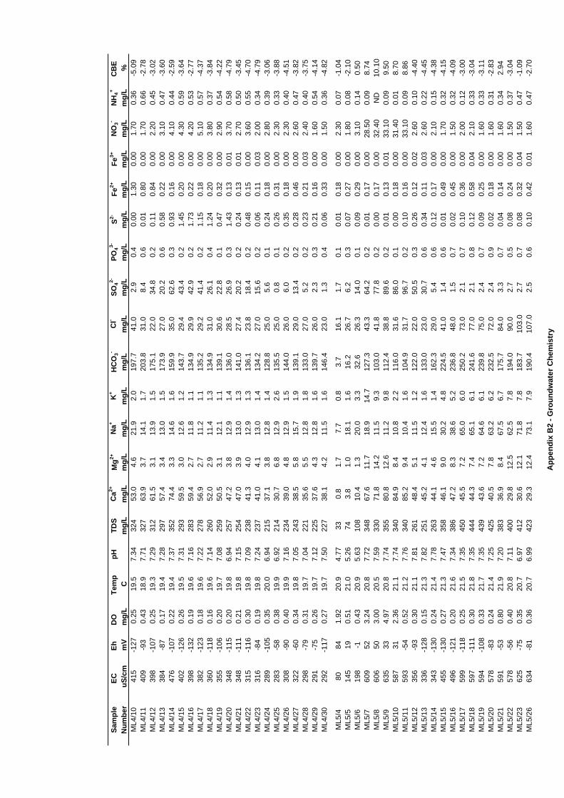
Sam
ple
EC
Eh
D
O
Tem
p pH
TDS
Ca2+
Mg2+
Na+
K+
HC
O3-
Cl-
SO42-
PO43-
S2-Fe
2+Fe
3+N
O3-
NH
4+C
BE
Num
ber
uS/c
mm
Vm
g/L
Cm
g/L
mg/
Lm
g/L
mg/
Lm
g/L
mg/
Lm
g/L
mg/
Lm
g/L
mg/
Lm
g/L
mg/
Lm
g/L
mg/
L%
ML4
/10
415
-127
0.25
19.5
7.34
324
53.0
4.6
21.9
2.0
197.
741
.02.
90.
40.
001.
300.
001.
700.
36-5
.09
ML4
/11
409
-93
0.43
18.9
7.71
327
63.9
3.7
14.1
1.7
203.
831
.08.
40.
60.
010.
800.
001.
700.
66-2
.78
ML4
/12
398
-107
0.25
19.3
7.29
312
61.5
3.1
13.9
1.5
175.
122
.034
.80.
20.
110.
840.
002.
200.
45-3
.02
ML4
/13
384
-87
0.17
19.4
7.28
297
57.4
3.4
13.0
1.5
173.
927
.020
.20.
60.
580.
220.
003.
100.
47-3
.60
ML4
/14
476
-107
0.22
19.4
7.37
352
74.4
3.3
14.6
1.6
159.
935
.062
.60.
30.
930.
160.
004.
100.
44-2
.59
ML4
/15
402
-126
0.26
19.5
7.31
293
59.5
3.0
12.6
1.2
143.
729
.443
.40.
21.
450.
200.
004.
300.
59-3
.64
ML4
/16
398
-132
0.19
19.6
7.16
283
59.4
2.7
11.8
1.1
134.
929
.942
.90.
21.
730.
220.
004.
200.
53-2
.77
ML4
/17
382
-123
0.18
19.6
7.22
278
56.9
2.7
11.2
1.1
135.
229
.241
.40.
21.
150.
180.
005.
100.
57-4
.37
ML4
/18
360
-118
0.16
19.6
7.14
260
52.0
2.9
11.4
1.3
134.
931
.026
.10.
41.
240.
200.
003.
800.
37-3
.84
ML4
/19
355
-106
0.20
19.7
7.08
259
50.5
3.1
12.1
1.1
139.
130
.622
.80.
10.
470.
320.
002.
900.
54-4
.22
ML4
/20
348
-115
0.20
19.8
6.94
257
47.2
3.8
12.9
1.4
136.
028
.526
.90.
31.
430.
130.
013.
700.
58-4
.79
ML4
/21
348
-111
0.21
19.8
7.15
254
47.0
3.9
13.0
1.3
141.
027
.420
.20.
20.
240.
130.
012.
700.
50-3
.45
ML4
/22
315
-116
0.30
19.8
7.09
238
41.3
4.0
12.9
1.3
136.
123
.818
.40.
20.
480.
150.
003.
600.
55-4
.70
ML4
/23
316
-84
0.19
19.8
7.24
237
41.0
4.1
13.0
1.4
134.
227
.015
.60.
20.
060.
110.
032.
000.
34-4
.79
ML4
/24
289
-105
0.35
20.0
6.94
215
37.1
3.8
12.8
1.4
128.
825
.05.
60.
10.
240.
180.
002.
800.
39-3
.06
ML4
/25
283
-58
0.38
19.9
6.92
214
30.7
6.8
12.9
2.6
135.
525
.00.
80.
10.
260.
310.
002.
300.
33-3
.88
ML4
/26
308
-90
0.40
19.9
7.16
234
39.0
4.8
12.9
1.5
144.
026
.06.
00.
20.
350.
180.
002.
300.
40-4
.51
ML4
/27
322
-60
0.34
19.8
7.05
243
38.5
5.8
15.7
1.9
139.
129
.013
.40.
20.
280.
460.
002.
600.
47-3
.82
ML4
/28
298
-79
0.31
19.7
7.04
221
35.6
5.5
12.8
1.8
133.
027
.05.
20.
20.
230.
210.
032.
400.
40-3
.75
ML4
/29
291
-75
0.26
19.7
7.12
225
37.6
4.3
12.8
1.6
139.
726
.02.
30.
30.
210.
160.
001.
600.
54-4
.14
ML4
/30
292
-117
0.27
19.7
7.50
227
38.1
4.2
11.5
1.6
146.
423
.01.
30.
40.
060.
330.
001.
500.
36-4
.82
ML5
/480
841.
9220
.94.
7733
0.8
1.7
7.7
0.8
3.7
16.1
1.7
0.1
0.01
0.18
0.00
2.30
0.07
-1.0
4M
L5/5
145
190.
5121
.05.
2674
3.8
1.0
18.1
1.6
16.2
26.7
6.2
0.3
0.07
0.27
0.00
1.80
0.08
-2.1
0M
L5/6
198
-10.
4320
.95.
6310
810
.41.
320
.03.
332
.626
.314
.00.
10.
090.
290.
003.
100.
140.
50M
L5/7
609
523.
2420
.87.
7234
867
.611
.718
.914
.712
7.3
43.3
64.2
0.2
0.01
0.17
0.00
28.5
00.
098.
74M
L5/8
606
503.
0020
.57.
5933
071
.814
.211
.59.
310
3.0
41.8
77.8
0.2
0.00
0.17
0.00
32.4
0N
D10
.10
ML5
/963
533
4.97
20.8
7.74
355
80.8
12.6
11.2
9.8
112.
438
.889
.60.
20.
010.
130.
0133
.10
0.09
9.50
ML5
/10
587
312.
3621
.17.
7434
084
.98.
410
.82.
211
6.0
31.6
86.0
0.1
0.00
0.18
0.00
31.4
00.
018.
70M
L5/1
159
3-5
40.
5221
.27.
7634
085
.29.
410
.41.
610
4.9
31.7
96.7
0.2
0.10
0.16
0.00
33.1
00.
098.
86M
L5/1
235
6-9
30.
3021
.17.
8126
148
.45.
111
.51.
212
2.0
22.0
50.5
0.3
0.26
0.12
0.02
2.60
0.10
-4.4
0M
L5/1
333
6-1
280.
1521
.37.
8225
145
.24.
112
.41.
613
3.0
23.0
30.7
0.6
0.34
0.11
0.03
2.60
0.22
-4.4
5M
L5/1
434
3-1
300.
2421
.47.
7826
344
.14.
615
.51.
416
2.3
29.0
5.4
0.6
0.12
0.17
0.00
2.10
0.15
-4.3
8M
L5/1
545
5-1
300.
2721
.37.
4735
846
.19.
030
.24.
822
4.5
41.0
1.4
0.6
0.01
0.49
0.00
1.70
0.32
-4.1
5M
L5/1
649
6-1
210.
2021
.67.
3438
647
.28.
338
.65.
223
6.8
48.0
1.5
0.7
0.02
0.45
0.00
1.50
0.32
-4.0
9M
L5/1
759
9-1
180.
2521
.57.
3545
045
.57.
265
.06.
025
0.2
73.0
2.1
0.7
0.10
0.36
0.00
2.00
0.12
-3.0
0M
L5/1
859
7-1
110.
3021
.87.
3544
444
.37.
465
.16.
124
1.6
77.0
2.1
0.8
0.12
0.58
0.04
2.10
0.33
-3.0
4M
L5/1
959
4-1
080.
3321
.77.
3543
943
.67.
264
.66.
123
9.8
75.0
2.4
0.7
0.09
0.25
0.00
1.60
0.33
-3.1
1M
L5/2
057
8-8
30.
2421
.47.
2542
540
.57.
863
.26.
223
2.5
72.0
2.4
0.9
0.02
0.18
0.00
1.60
0.31
-2.8
3M
L5/2
159
1-5
30.
8021
.97.
2038
336
.98.
467
.56.
717
5.7
84.0
3.3
0.7
0.04
0.14
0.00
1.60
0.34
2.94
ML5
/22
578
-56
0.40
20.8
7.11
400
29.8
12.5
62.5
7.8
194.
090
.02.
70.
50.
080.
240.
001.
500.
37-3
.04
ML5
/23
625
-75
0.35
20.7
6.97
412
30.6
12.1
71.8
7.8
183.
710
3.0
2.7
0.7
0.08
0.32
0.04
1.50
0.47
-1.0
9M
L5/2
663
4-8
10.
3620
.76.
9942
329
.312
.473
.17.
919
0.4
107.
02.
50.
60.
100.
420.
011.
600.
47-2
.70
App
endi
x B
2 - G
roun
dwat
er C
hem
istr
y
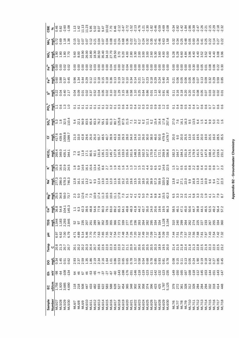
Sam
ple
EC
Eh
D
O
Tem
p pH
TDS
Ca2+
Mg2+
Na+
K+
HC
O3-
Cl-
SO42-
PO43-
S2-Fe
2+Fe
3+N
O3-
NH
4+C
BE
Num
ber
uS/c
mm
Vm
g/L
Cm
g/L
mg/
Lm
g/L
mg/
Lm
g/L
mg/
Lm
g/L
mg/
Lm
g/L
mg/
Lm
g/L
mg/
Lm
g/L
mg/
L%
ML5
/27
1,75
6-9
80.
3420
.86.
971,
044
36.8
25.5
277.
315
.326
5.4
417.
65.
31.
10.
220.
600.
001.
900.
720.
46M
L5/2
81,
920
-64
1.45
21.3
6.62
1,18
354
.834
.828
6.0
16.6
349.
043
9.9
1.8
0.6
0.04
3.88
0.00
1.80
0.69
0.82
ML5
/29
3,68
5-1
080.
5120
.77.
002,
293
104.
159
.057
8.3
22.9
435.
110
59.8
32.5
1.3
0.40
0.37
0.02
1.80
1.18
-2.6
0M
L5/3
04,
690
-134
0.62
20.7
6.79
2,84
514
5.3
73.7
746.
324
.534
4.1
1399
.711
0.4
1.0
2.17
0.45
0.02
7.70
1.38
-1.0
8
ML6
/711
864
2.93
20.1
4.71
521.
12.
312
.81.
87.
321
.05.
40.
10.
040.
960.
005.
600.
151.
13M
L6/8
218
462.
3720
.24.
8997
6.3
5.0
16.1
5.9
8.5
33.0
22.1
0.1
0.09
1.34
0.00
8.00
0.07
1.42
ML6
/950
867
2.59
20.2
5.14
235
42.3
12.6
16.1
14.6
11.8
42.8
94.9
0.1
0.01
0.44
0.00
33.9
00.
0711
.13
ML6
/10
447
461.
3520
.35.
4620
739
.57.
513
.216
.117
.129
.683
.50.
10.
020.
290.
0026
.00
0.07
11.2
3M
L6/1
143
3-5
31.
8620
.47.
7025
148
.87.
38.
715
.680
.525
.065
.40.
10.
370.
120.
0216
.80
0.12
5.95
ML6
/12
482
-65
2.19
20.7
7.79
289
54.6
10.9
9.3
13.4
92.1
25.0
83.3
0.1
0.52
0.11
0.03
18.3
00.
215.
02M
L6/1
369
3-3
2.34
20.6
7.63
387
77.9
17.4
12.4
15.4
131.
855
.776
.20.
10.
040.
180.
0030
.50
0.04
8.07
ML6
/14
622
-37
2.16
22.6
7.65
352
80.3
11.3
13.0
8.6
135.
148
.555
.10.
10.
050.
150.
0035
.40
0.07
9.47
ML6
/15
583
-27
1.64
22.0
7.55
328
79.1
10.5
11.8
2.7
122.
340
.760
.60.
20.
020.
180.
0034
.10
0.04
10.0
2M
L6/1
658
8-6
71.
0122
.37.
4235
583
.010
.612
.01.
914
5.7
39.9
61.3
0.2
0.10
0.36
0.04
27.7
00.
087.
70M
L6/1
762
8-6
00.
8622
.67.
5436
689
.211
.111
.61.
912
7.8
43.3
80.7
0.1
0.02
0.13
0.01
29.5
00.
018.
46M
L6/1
852
7-1
430.
5322
.07.
7237
365
.317
.810
.62.
611
6.5
33.8
125.
80.
31.
290.
190.
003.
700.
24-2
.12
ML6
/19
454
-198
0.65
21.2
7.48
339
64.1
7.3
15.2
1.6
133.
029
.387
.50.
63.
150.
120.
025.
200.
68-3
.47
ML6
/20
365
-176
0.65
21.1
7.34
277
49.8
5.1
15.0
1.4
155.
628
.021
.50.
41.
660.
100.
044.
000.
36-2
.72
ML6
/21
348
-151
0.78
20.9
7.26
276
48.3
4.2
19.6
1.3
161.
634
.07.
10.
30.
580.
340.
002.
800.
22-1
.52
ML6
/22
302
-146
1.12
20.7
7.20
236
41.8
4.1
13.5
1.2
148.
324
.03.
20.
41.
100.
140.
003.
300.
27-2
.13
ML6
/23
343
-118
0.58
20.6
7.62
263
44.2
4.3
16.0
1.5
159.
931
.06.
20.
20.
250.
210.
002.
000.
17-4
.76
ML6
/24
358
-119
0.54
20.5
7.49
264
43.7
5.0
18.0
2.3
162.
326
.06.
20.
30.
640.
170.
003.
000.
24-1
.21
ML6
/25
374
-123
0.68
20.5
7.32
282
35.0
7.9
26.0
4.4
167.
230
.011
.10.
30.
860.
230.
003.
000.
32-2
.30
ML6
/26
396
-111
0.78
20.5
7.09
295
24.0
9.4
39.9
6.0
170.
938
.06.
20.
50.
010.
180.
002.
600.
35-1
.82
ML6
/27
423
-142
0.85
20.3
7.17
334
20.6
9.8
57.3
6.5
177.
646
.015
.40.
91.
130.
290.
005.
300.
41-0
.46
ML6
/28
425
-132
0.93
18.9
6.94
334
19.6
9.4
59.9
6.3
172.
150
.016
.40.
61.
400.
240.
003.
600.
46-0
.59
ML6
/29
1,78
7-1
230.
8119
.57.
091,
128
19.5
15.5
320.
014
.625
9.9
479.
917
.81.
20.
910.
400.
004.
000.
63-4
.69
ML6
/30
5,12
5-2
350.
7820
.07.
033,
194
86.3
42.3
968.
222
.533
6.8
1479
.725
7.4
0.5
2.85
3.34
0.00
0.00
1.58
-2.0
8
ML7
/637
9-1
490.
0821
.47.
4431
058
.56.
513
.81.
518
2.3
20.0
27.0
0.1
0.11
0.21
0.00
5.28
0.32
-0.3
4M
L7/7
272
-150
0.15
21.5
7.51
240
46.1
3.3
8.1
0.7
164.
79.
07.
60.
40.
160.
060.
005.
280.
34-2
.82
ML7
/836
1-1
650.
1121
.87.
7929
947
.13.
227
.10.
518
4.3
20.0
16.1
0.8
0.18
0.05
0.00
6.60
0.25
-1.4
2M
L7/9
328
-167
0.13
22.4
7.57
264
45.0
2.5
22.0
0.5
151.
925
.516
.30.
50.
200.
060.
004.
840.
48-1
.84
ML7
/10
312
-168
0.05
21.8
7.52
262
50.6
3.1
9.9
0.8
174.
513
.09.
50.
40.
200.
050.
003.
960.
05-2
.86
ML7
/11
328
-118
0.24
21.3
7.56
274
44.7
5.8
16.8
2.2
179.
910
.513
.50.
40.
150.
060.
304.
400.
00-0
.39
ML7
/12
284
-112
1.90
22.8
7.68
225
39.8
3.3
13.3
0.8
141.
519
.56.
40.
70.
080.
070.
004.
400.
34-2
.47
ML7
/13
284
-145
0.19
22.5
7.61
227
44.1
2.0
11.6
0.4
147.
020
.01.
50.
60.
050.
130.
053.
520.
41-2
.26
ML7
/14
294
-153
0.18
21.9
7.67
233
46.5
1.9
10.9
0.3
147.
619
.06.
40.
60.
070.
090.
013.
520.
25-2
.21
ML7
/15
332
-144
0.42
22.3
7.43
267
52.5
4.1
9.6
0.9
168.
420
.59.
90.
70.
030.
320.
084.
400.
22-2
.15
ML7
/16
318
-151
0.27
22.0
7.54
255
49.2
3.7
9.4
0.9
170.
216
.05.
00.
70.
020.
290.
064.
400.
14-2
.29
ML7
/17
414
-143
0.85
22.5
7.42
334
56.4
7.9
17.2
1.7
219.
628
.52.
00.
60.
020.
590.
223.
080.
27-2
.18
ML7
/18
448
-147
0.45
23.2
7.32
360
57.2
8.7
22.3
2.3
231.
235
.51.
60.
60.
010.
850.
303.
960.
22-2
.32
App
endi
x B
2 - G
roun
dwat
er C
hem
istr
y
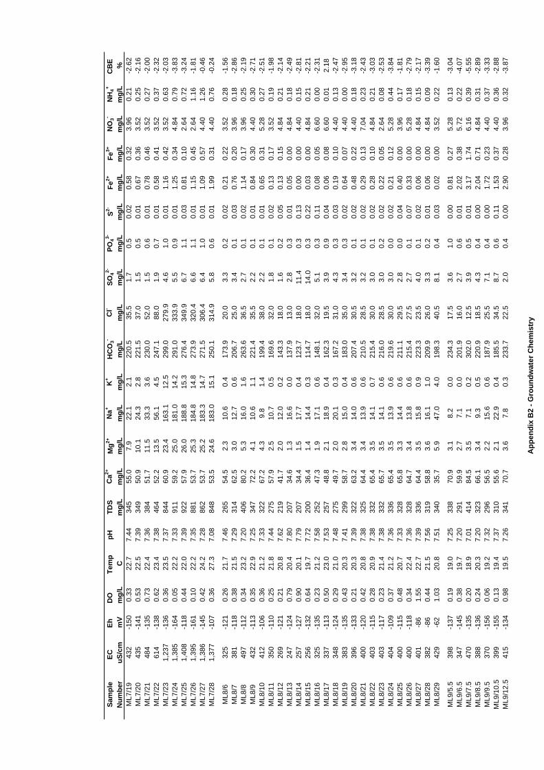
Sam
ple
EC
Eh
D
O
Tem
p pH
TDS
Ca2+
Mg2+
Na+
K+
HC
O3-
Cl-
SO42-
PO43-
S2-Fe
2+Fe
3+N
O3-
NH
4+C
BE
Num
ber
uS/c
mm
Vm
g/L
Cm
g/L
mg/
Lm
g/L
mg/
Lm
g/L
mg/
Lm
g/L
mg/
Lm
g/L
mg/
Lm
g/L
mg/
Lm
g/L
mg/
L%
ML7
/19
432
-150
0.33
22.7
7.44
345
55.0
7.9
22.1
2.1
220.
535
.51.
70.
50.
020.
580.
323.
960.
21-2
.62
ML7
/20
435
-141
0.53
22.5
7.39
349
50.9
10.1
24.3
2.8
221.
537
.01.
50.
50.
010.
670.
363.
520.
25-2
.16
ML7
/21
484
-135
0.73
22.4
7.36
384
51.7
11.5
33.3
3.6
230.
052
.01.
50.
60.
010.
780.
463.
520.
27-2
.00
ML7
/22
614
-138
0.62
23.4
7.38
464
52.2
13.5
56.1
4.5
247.
188
.01.
90.
70.
010.
580.
413.
520.
37-2
.32
ML7
/23
1,23
7-1
360.
3623
.57.
3784
460
.923
.416
3.1
12.5
299.
027
9.9
4.6
1.0
0.01
1.16
0.42
3.52
0.63
-2.0
3M
L7/2
41,
385
-164
0.05
22.2
7.33
911
59.2
25.0
181.
014
.229
1.0
333.
95.
50.
90.
011.
250.
344.
840.
79-3
.83
ML7
/25
1,40
8-1
180.
4422
.07.
3992
257
.926
.018
8.8
15.3
276.
434
9.9
6.7
1.1
0.03
0.81
0.10
2.64
0.72
-3.2
4M
L7/2
61,
395
-161
0.10
22.2
7.35
881
53.7
25.3
184.
814
.827
3.9
320.
46.
61.
10.
011.
150.
452.
641.
16-1
.81
ML7
/27
1,38
6-1
450.
4224
.27.
2886
253
.725
.218
3.3
14.7
271.
530
6.4
6.4
1.0
0.01
1.09
0.57
4.40
1.26
-0.4
6M
L7/2
81,
377
-107
0.36
27.3
7.08
848
53.5
24.6
183.
015
.125
0.1
314.
95.
80.
60.
011.
990.
314.
400.
76-0
.24
ML8
/632
5-1
210.
2621
.77.
4626
554
.52.
310
.60.
417
3.9
20.0
3.3
0.2
0.02
0.21
0.22
3.52
0.28
-1.5
6M
L8/7
381
-118
0.38
21.5
7.29
314
62.5
3.0
12.7
0.6
206.
725
.03.
40.
10.
030.
760.
203.
960.
18-2
.86
ML8
/849
7-1
120.
3423
.27.
2040
680
.25.
316
.01.
626
3.6
36.5
2.7
0.1
0.02
1.14
0.17
3.96
0.25
-2.1
9M
L8/9
432
-113
0.35
22.9
7.25
347
72.2
4.1
10.6
1.1
221.
435
.52.
20.
10.
010.
840.
304.
400.
30-2
.71
ML8
/10
412
-106
0.36
21.2
7.33
322
67.2
4.3
9.8
1.4
199.
438
.02.
20.
10.
010.
650.
315.
280.
27-2
.51
ML8
/11
350
-110
0.25
21.8
7.44
275
57.9
2.5
10.7
0.5
169.
632
.01.
80.
10.
020.
130.
173.
520.
19-1
.98
ML8
/12
269
-121
0.21
20.8
7.62
219
41.7
2.0
12.0
0.2
143.
318
.01.
60.
20.
050.
130.
154.
840.
21-2
.14
ML8
/13
247
-124
0.79
20.4
7.80
207
34.6
1.3
16.6
0.0
137.
913
.02.
80.
30.
010.
050.
004.
840.
18-2
.49
ML8
/14
257
-127
0.90
20.1
7.79
207
34.4
1.5
17.7
0.4
123.
718
.011
.40.
30.
130.
000.
004.
400.
15-2
.81
ML8
/15
256
-132
0.64
19.7
7.72
200
36.4
1.4
14.4
0.3
114.
718
.014
.00.
30.
220.
030.
004.
840.
21-2
.21
ML8
/16
325
-135
0.23
21.2
7.58
252
47.3
1.9
17.1
0.6
148.
132
.05.
10.
30.
110.
080.
056.
600.
00-2
.31
ML8
/17
337
-113
0.50
23.0
7.53
257
48.8
2.1
18.9
0.4
162.
319
.53.
90.
90.
040.
060.
086.
600.
012.
18M
L8/1
834
8-1
240.
2921
.07.
4827
549
.72.
020
.10.
316
7.2
31.0
4.3
0.3
0.03
0.19
0.10
4.40
0.13
-2.4
7M
L8/1
938
3-1
350.
4320
.37.
4129
958
.72.
815
.00.
418
3.0
35.0
3.4
0.3
0.02
0.64
0.07
4.40
0.00
-2.9
5M
L8/2
039
6-1
330.
2120
.37.
3932
263
.23.
414
.00.
620
7.4
30.5
3.2
0.1
0.02
0.48
0.22
4.40
0.18
-3.1
8M
L8/2
140
0-1
200.
4220
.87.
3832
564
.43.
413
.90.
621
0.5
28.5
3.2
0.1
0.02
0.29
0.13
7.04
0.23
-2.4
3M
L8/2
240
3-1
150.
2820
.97.
3833
265
.43.
514
.10.
721
5.4
30.0
3.0
0.1
0.02
0.28
0.10
4.84
0.21
-3.0
3M
L8/2
340
3-1
170.
2321
.47.
3833
265
.73.
514
.10.
621
6.0
28.5
3.0
0.2
0.02
0.22
0.05
2.64
0.08
-2.5
3M
L8/2
440
4-1
090.
3721
.27.
3633
665
.43.
513
.90.
621
9.6
30.0
3.0
0.0
0.02
0.21
0.12
5.28
0.44
-3.8
4M
L8/2
540
0-1
150.
4820
.77.
3332
865
.83.
314
.40.
621
1.1
29.5
2.8
0.0
0.04
0.40
0.00
3.96
0.17
-1.8
1M
L8/2
640
0-1
180.
3422
.47.
3632
864
.73.
413
.80.
621
5.4
27.5
2.7
0.1
0.07
0.33
0.00
5.28
0.18
-2.7
9M
L8/2
740
1-8
61.
5522
.77.
3933
664
.43.
515
.80.
922
3.3
23.5
4.0
0.1
0.02
0.06
0.00
4.84
0.15
-2.1
7M
L8/2
838
2-8
60.
4421
.57.
5631
958
.83.
616
.11.
020
9.9
26.0
3.3
0.2
0.01
0.06
0.00
4.84
0.09
-3.3
9M
L8/2
942
9-6
21.
0320
.87.
5134
035
.75.
947
.04.
019
8.3
40.5
8.1
0.4
0.03
0.02
0.00
3.52
0.22
-1.6
0
ML9
/5.5
398
-137
0.19
19.0
7.25
338
70.9
3.1
8.2
0.0
234.
317
.53.
61.
00.
000.
810.
275.
280.
13-3
.04
ML9
/6.5
347
-145
0.38
19.7
7.20
291
59.9
2.7
7.1
0.0
201.
916
.02.
70.
60.
012.
020.
385.
720.
22-4
.07
ML9
/7.5
470
-135
0.20
18.9
7.01
414
84.5
3.5
7.1
0.2
302.
012
.53.
90.
50.
013.
171.
746.
160.
39-5
.55
ML9
/8.5
388
-136
0.24
20.3
7.20
323
66.1
3.4
9.3
0.5
220.
918
.54.
30.
40.
002.
040.
714.
840.
31-2
.89
ML9
/9.5
370
-156
0.06
19.2
7.32
296
56.5
2.2
15.6
0.6
187.
925
.57.
10.
40.
001.
720.
234.
400.
37-3
.33
ML9
/10.
539
9-1
550.
1319
.47.
3731
055
.62.
122
.90.
418
5.5
34.5
8.7
0.6
0.11
1.53
0.37
4.40
0.36
-2.8
8M
L9/1
2.5
415
-134
0.98
19.5
7.26
341
70.7
3.6
7.8
0.3
233.
722
.52.
00.
40.
002.
900.
283.
960.
32-3
.87
App
endi
x B
2 - G
roun
dwat
er C
hem
istr
y
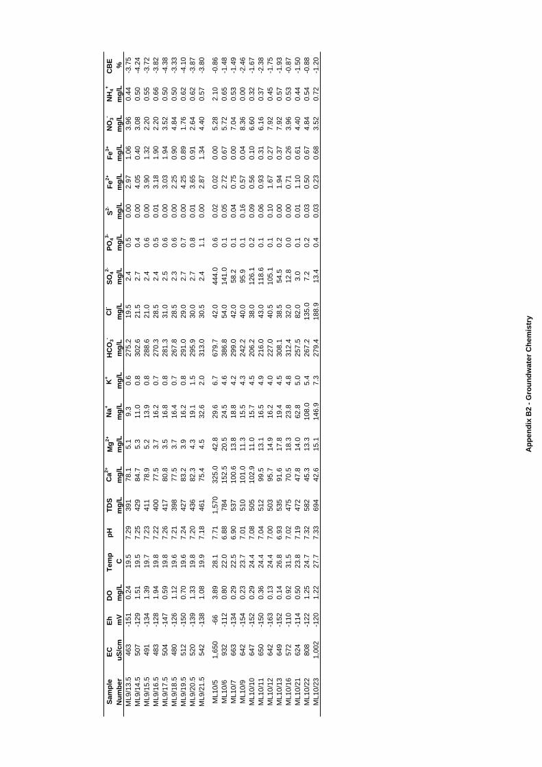
Sam
ple
EC
Eh
D
O
Tem
p pH
TDS
Ca2+
Mg2+
Na+
K+
HC
O3-
Cl-
SO42-
PO43-
S2-Fe
2+Fe
3+N
O3-
NH
4+C
BE
Num
ber
uS/c
mm
Vm
g/L
Cm
g/L
mg/
Lm
g/L
mg/
Lm
g/L
mg/
Lm
g/L
mg/
Lm
g/L
mg/
Lm
g/L
mg/
Lm
g/L
mg/
L%
ML9
/13.
546
3-1
510.
2419
.57.
2939
178
.15.
19.
30.
627
5.2
19.5
2.4
0.5
0.00
2.97
1.06
3.96
0.44
-3.7
5M
L9/1
4.5
507
-129
1.51
19.5
7.25
429
84.7
5.3
11.0
0.8
302.
621
.52.
70.
40.
004.
050.
403.
080.
50-4
.24
ML9
/15.
549
1-1
341.
3919
.77.
2341
178
.95.
213
.90.
828
8.6
21.0
2.4
0.6
0.00
3.90
1.32
2.20
0.55
-3.7
2M
L9/1
6.5
483
-128
1.94
19.8
7.22
400
77.5
3.7
16.2
0.7
270.
328
.52.
40.
50.
013.
181.
902.
200.
66-3
.82
ML9
/17.
550
4-1
470.
5919
.87.
2641
780
.83.
516
.80.
828
1.3
31.0
2.5
0.6
0.00
3.03
1.94
3.52
0.50
-4.3
8M
L9/1
8.5
480
-126
1.12
19.6
7.21
398
77.5
3.7
16.4
0.7
267.
828
.52.
30.
60.
002.
250.
904.
840.
50-3
.33
ML9
/19.
551
2-1
500.
7019
.67.
2442
783
.23.
916
.20.
829
1.0
29.0
2.7
0.7
0.00
4.25
0.89
1.76
0.62
-4.1
0M
L9/2
0.5
520
-139
1.33
19.8
7.20
436
82.3
4.3
19.1
1.5
295.
930
.02.
70.
80.
013.
650.
912.
640.
62-3
.87
ML9
/21.
554
2-1
381.
0819
.97.
1846
175
.44.
532
.62.
031
3.0
30.5
2.4
1.1
0.00
2.87
1.34
4.40
0.57
-3.8
0
ML1
0/5
1,65
0-6
63.
8928
.17.
711,
570
325.
042
.829
.66.
767
9.7
42.0
444.
00.
60.
020.
020.
005.
282.
10-0
.86
ML1
0/6
932
-112
0.80
22.0
6.88
784
152.
520
.524
.54.
638
6.8
54.0
141.
00.
10.
052.
720.
675.
720.
65-1
.48
ML1
0/7
663
-134
0.29
22.5
6.90
537
100.
613
.818
.84.
229
9.0
42.0
58.2
0.1
0.04
0.75
0.00
7.04
0.53
-1.4
9M
L10/
964
2-1
540.
2323
.77.
0151
010
1.0
11.3
15.5
4.3
242.
240
.095
.90.
10.
160.
570.
048.
360.
00-2
.46
ML1
0/10
647
-152
0.29
24.4
7.08
505
102.
911
.015
.74.
520
6.2
38.0
126.
10.
20.
090.
560.
106.
600.
32-1
.67
ML1
0/11
650
-150
0.36
24.4
7.04
512
99.5
13.1
16.5
4.9
216.
043
.011
8.6
0.1
0.06
0.93
0.31
6.16
0.37
-2.3
8M
L10/
1264
2-1
630.
1324
.47.
0050
395
.714
.916
.24.
022
7.0
40.5
105.
10.
10.
101.
670.
277.
920.
45-1
.75
ML1
0/13
649
-152
0.14
26.8
6.93
535
91.6
17.8
19.4
4.5
308.
138
.554
.50.
20.
001.
940.
377.
920.
57-1
.93
ML1
0/16
572
-110
0.92
31.5
7.02
475
70.5
18.3
23.8
4.8
312.
432
.012
.80.
00.
000.
710.
263.
960.
53-0
.87
ML1
0/21
624
-114
0.50
23.8
7.19
472
47.8
14.0
62.8
5.0
257.
582
.03.
00.
10.
011.
100.
614.
400.
44-1
.50
ML1
0/22
808
-122
1.25
24.7
7.32
582
45.3
13.3
108.
05.
426
7.2
135.
07.
20.
20.
030.
500.
674.
840.
54-0
.88
ML1
0/23
1,00
2-1
201.
2227
.77.
3369
442
.615
.114
6.9
7.3
279.
418
8.9
13.4
0.4
0.03
0.23
0.68
3.52
0.72
-1.2
0
App
endi
x B
2 - G
roun
dwat
er C
hem
istr
y
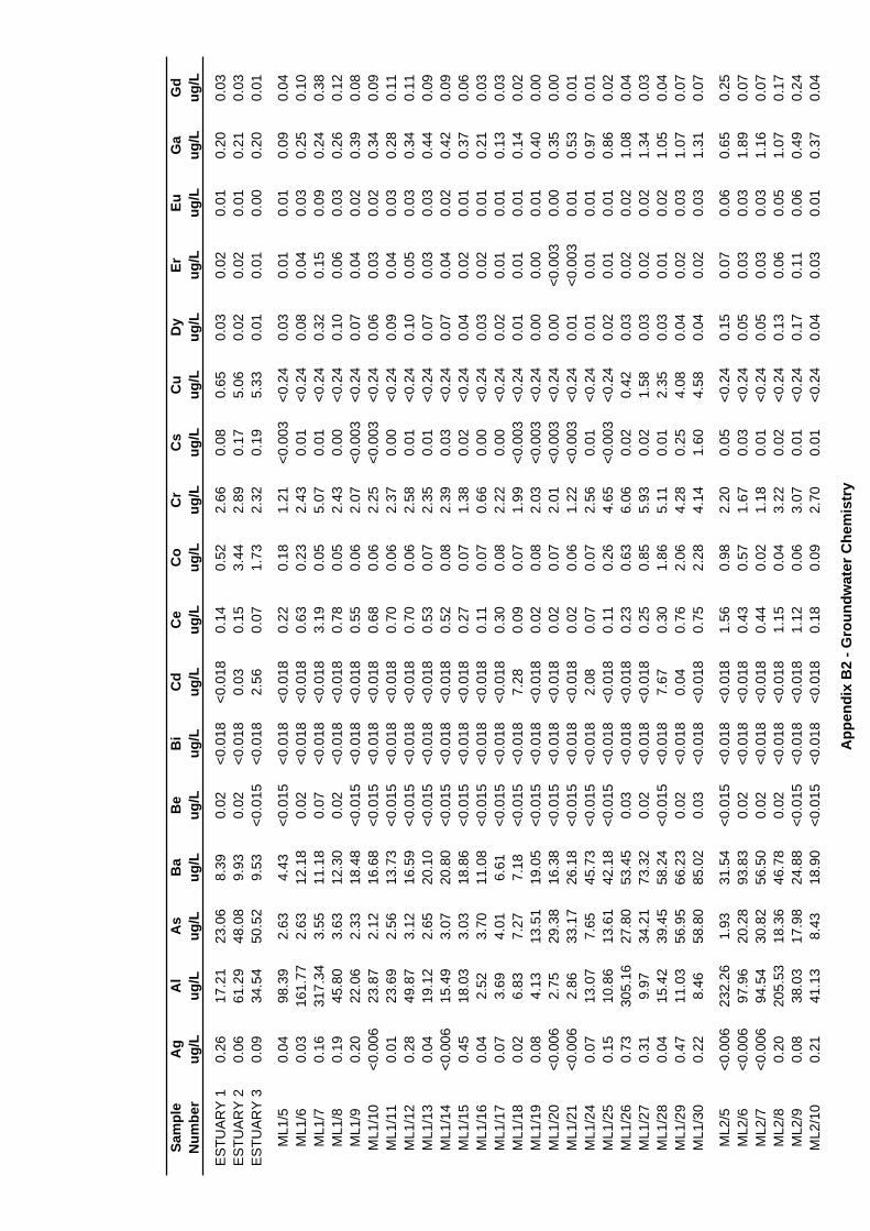
Sam
ple
Ag
Al
As
Ba
Be
Bi
Cd
Ce
Co
Cr
Cs
Cu
Dy
ErEu
Ga
Gd
Num
ber
ug/L
ug/L
ug/L
ug/L
ug/L
ug/L
ug/L
ug/L
ug/L
ug/L
ug/L
ug/L
ug/L
ug/L
ug/L
ug/L
ug/L
ES
TUA
RY
10.
2617
.21
23.0
68.
390.
02<0
.018
<0.0
180.
140.
522.
660.
080.
650.
030.
020.
010.
200.
03E
STU
AR
Y 2
0.06
61.2
948
.08
9.93
0.02
<0.0
180.
030.
153.
442.
890.
175.
060.
020.
020.
010.
210.
03E
STU
AR
Y 3
0.09
34.5
450
.52
9.53
<0.0
15<0
.018
2.56
0.07
1.73
2.32
0.19
5.33
0.01
0.01
0.00
0.20
0.01
ML1
/50.
0498
.39
2.63
4.43
<0.0
15<0
.018
<0.0
180.
220.
181.
21<0
.003
<0.2
40.
030.
010.
010.
090.
04M
L1/6
0.03
161.
772.
6312
.18
0.02
<0.0
18<0
.018
0.63
0.23
2.43
0.01
<0.2
40.
080.
040.
030.
250.
10M
L1/7
0.16
317.
343.
5511
.18
0.07
<0.0
18<0
.018
3.19
0.05
5.07
0.01
<0.2
40.
320.
150.
090.
240.
38M
L1/8
0.19
45.8
03.
6312
.30
0.02
<0.0
18<0
.018
0.78
0.05
2.43
0.00
<0.2
40.
100.
060.
030.
260.
12M
L1/9
0.20
22.0
62.
3318
.48
<0.0
15<0
.018
<0.0
180.
550.
062.
07<0
.003
<0.2
40.
070.
040.
020.
390.
08M
L1/1
0<0
.006
23.8
72.
1216
.68
<0.0
15<0
.018
<0.0
180.
680.
062.
25<0
.003
<0.2
40.
060.
030.
020.
340.
09M
L1/1
10.
0123
.69
2.56
13.7
3<0
.015
<0.0
18<0
.018
0.70
0.06
2.37
0.00
<0.2
40.
090.
040.
030.
280.
11M
L1/1
20.
2849
.87
3.12
16.5
9<0
.015
<0.0
18<0
.018
0.70
0.06
2.58
0.01
<0.2
40.
100.
050.
030.
340.
11M
L1/1
30.
0419
.12
2.65
20.1
0<0
.015
<0.0
18<0
.018
0.53
0.07
2.35
0.01
<0.2
40.
070.
030.
030.
440.
09M
L1/1
4<0
.006
15.4
93.
0720
.80
<0.0
15<0
.018
<0.0
180.
520.
082.
390.
03<0
.24
0.07
0.04
0.02
0.42
0.09
ML1
/15
0.45
18.0
33.
0318
.86
<0.0
15<0
.018
<0.0
180.
270.
071.
380.
02<0
.24
0.04
0.02
0.01
0.37
0.06
ML1
/16
0.04
2.52
3.70
11.0
8<0
.015
<0.0
18<0
.018
0.11
0.07
0.66
0.00
<0.2
40.
030.
020.
010.
210.
03M
L1/1
70.
073.
694.
016.
61<0
.015
<0.0
18<0
.018
0.30
0.08
2.22
0.00
<0.2
40.
020.
010.
010.
130.
03M
L1/1
80.
026.
837.
277.
18<0
.015
<0.0
187.
280.
090.
071.
99<0
.003
<0.2
40.
010.
010.
010.
140.
02M
L1/1
90.
084.
1313
.51
19.0
5<0
.015
<0.0
18<0
.018
0.02
0.08
2.03
<0.0
03<0
.24
0.00
0.00
0.01
0.40
0.00
ML1
/20
<0.0
062.
7529
.38
16.3
8<0
.015
<0.0
18<0
.018
0.02
0.07
2.01
<0.0
03<0
.24
0.00
<0.0
030.
000.
350.
00M
L1/2
1<0
.006
2.86
33.1
726
.18
<0.0
15<0
.018
<0.0
180.
020.
061.
22<0
.003
<0.2
40.
01<0
.003
0.01
0.53
0.01
ML1
/24
0.07
13.0
77.
6545
.73
<0.0
15<0
.018
2.08
0.07
0.07
2.56
0.01
<0.2
40.
010.
010.
010.
970.
01M
L1/2
50.
1510
.86
13.6
142
.18
<0.0
15<0
.018
<0.0
180.
110.
264.
65<0
.003
<0.2
40.
020.
010.
010.
860.
02M
L1/2
60.
7330
5.16
27.8
053
.45
0.03
<0.0
18<0
.018
0.23
0.63
6.06
0.02
0.42
0.03
0.02
0.02
1.08
0.04
ML1
/27
0.31
9.97
34.2
173
.32
0.02
<0.0
18<0
.018
0.25
0.85
5.93
0.02
1.58
0.03
0.02
0.02
1.34
0.03
ML1
/28
0.04
15.4
239
.45
58.2
4<0
.015
<0.0
187.
670.
301.
865.
110.
012.
350.
030.
010.
021.
050.
04M
L1/2
90.
4711
.03
56.9
566
.23
0.02
<0.0
180.
040.
762.
064.
280.
254.
080.
040.
020.
031.
070.
07M
L1/3
00.
228.
4658
.80
85.0
20.
03<0
.018
<0.0
180.
752.
284.
141.
604.
580.
040.
020.
031.
310.
07
ML2
/5<0
.006
232.
261.
9331
.54
<0.0
15<0
.018
<0.0
181.
560.
982.
200.
05<0
.24
0.15
0.07
0.06
0.65
0.25
ML2
/6<0
.006
97.9
620
.28
93.8
30.
02<0
.018
<0.0
180.
430.
571.
670.
03<0
.24
0.05
0.03
0.03
1.89
0.07
ML2
/7<0
.006
94.5
430
.82
56.5
00.
02<0
.018
<0.0
180.
440.
021.
180.
01<0
.24
0.05
0.03
0.03
1.16
0.07
ML2
/80.
2020
5.53
18.3
646
.78
0.02
<0.0
18<0
.018
1.15
0.04
3.22
0.02
<0.2
40.
130.
060.
051.
070.
17M
L2/9
0.08
38.0
317
.98
24.8
8<0
.015
<0.0
18<0
.018
1.12
0.06
3.07
0.01
<0.2
40.
170.
110.
060.
490.
24M
L2/1
00.
2141
.13
8.43
18.9
0<0
.015
<0.0
18<0
.018
0.18
0.09
2.70
0.01
<0.2
40.
040.
030.
010.
370.
04
App
endi
x B
2 - G
roun
dwat
er C
hem
istr
y
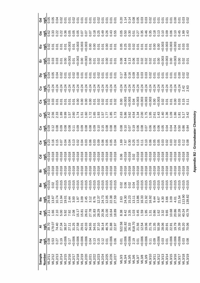
Sam
ple
Ag
Al
As
Ba
Be
Bi
Cd
Ce
Co
Cr
Cs
Cu
Dy
ErEu
Ga
Gd
Num
ber
ug/L
ug/L
ug/L
ug/L
ug/L
ug/L
ug/L
ug/L
ug/L
ug/L
ug/L
ug/L
ug/L
ug/L
ug/L
ug/L
ug/L
ML2
/11
0.08
39.7
02.
1129
.68
<0.0
15<0
.018
<0.0
180.
230.
092.
420.
02<0
.24
0.04
0.03
0.02
0.62
0.05
ML2
/12
0.53
179.
071.
6613
.67
0.02
<0.0
18<0
.018
0.16
0.12
2.56
0.03
<0.2
40.
050.
030.
010.
330.
05M
L2/1
30.
2774
.40
2.10
10.7
4<0
.015
<0.0
18<0
.018
0.15
0.08
2.33
0.01
<0.2
40.
040.
030.
010.
220.
04M
L2/1
40.
1927
.34
5.00
11.9
4<0
.015
<0.0
18<0
.018
0.07
0.09
1.89
0.01
<0.2
40.
020.
010.
010.
220.
02M
L2/1
5<0
.006
38.5
75.
9219
.01
<0.0
15<0
.018
<0.0
180.
040.
080.
990.
01<0
.24
0.01
0.00
0.01
0.36
0.01
ML2
/16
0.17
27.1
17.
922.
44<0
.015
<0.0
18<0
.018
0.04
0.08
1.57
0.01
<0.2
40.
01<0
.003
<0.0
030.
050.
01M
L2/1
7<0
.006
31.2
52.
083.
00<0
.015
<0.0
18<0
.018
0.13
0.11
2.60
0.01
<0.2
40.
020.
010.
010.
050.
02M
L2/1
8<0
.006
27.5
815
.17
1.97
<0.0
15<0
.018
<0.0
180.
020.
091.
740.
00<0
.24
0.00
<0.0
03<0
.003
0.05
0.01
ML2
/19
<0.0
0629
.01
15.8
13.
09<0
.015
<0.0
18<0
.018
0.04
0.09
1.51
0.00
<0.2
40.
010.
00<0
.003
0.07
0.01
ML2
/20
<0.0
0642
.03
26.6
12.
45<0
.015
<0.0
18<0
.018
0.03
0.08
1.60
0.00
<0.2
40.
01<0
.003
<0.0
030.
070.
01M
L2/2
10.
0434
.55
27.7
83.
12<0
.015
<0.0
18<0
.018
0.06
0.08
1.72
0.00
<0.2
40.
010.
000.
000.
070.
01M
L2/2
20.
1334
.01
31.8
38.
76<0
.015
<0.0
18<0
.018
0.03
0.09
1.65
0.01
<0.2
40.
010.
010.
000.
180.
01M
L2/2
30.
1537
.10
28.2
912
.37
<0.0
15<0
.018
<0.0
180.
090.
101.
930.
02<0
.24
0.02
0.02
0.01
0.25
0.02
ML2
/24
0.12
36.1
420
.36
24.7
3<0
.015
<0.0
18<0
.018
0.06
0.15
1.57
0.02
<0.2
40.
010.
010.
010.
490.
01M
L2/2
50.
0146
.76
21.0
012
.05
<0.0
15<0
.018
<0.0
180.
050.
081.
770.
01<0
.24
0.01
0.00
0.00
0.26
0.01
ML2
/26
<0.0
0631
.88
16.6
422
.38
<0.0
15<0
.018
<0.0
180.
050.
081.
850.
01<0
.24
0.01
0.01
0.01
0.43
0.01
ML2
/27
0.06
22.9
718
.89
27.5
9<0
.015
<0.0
18<0
.018
0.04
0.08
1.73
0.02
<0.2
40.
010.
010.
010.
550.
01
ML3
/30.
0152
2.58
8.38
2.63
0.02
<0.0
180.
061.
690.
082.
630.
00<0
.24
0.17
0.08
0.05
0.05
0.20
ML3
/4<0
.006
181.
828.
4224
.30
0.06
<0.0
18<0
.018
7.67
0.10
5.86
<0.0
03<0
.24
0.84
0.44
0.25
0.50
1.14
ML3
/5<0
.006
26.3
33.
3515
.23
0.02
<0.0
18<0
.018
0.30
0.07
3.62
<0.0
03<0
.24
0.16
0.13
0.03
0.30
0.14
ML3
/62.
1981
8.70
1.03
13.1
10.
04<0
.018
0.02
0.25
0.19
4.54
0.04
<0.2
40.
090.
060.
020.
510.
08M
L3/7
0.01
21.5
60.
4513
.86
<0.0
15<0
.018
<0.0
180.
150.
061.
34<0
.003
<0.2
40.
040.
030.
010.
270.
05M
L3/8
<0.0
0612
.54
1.59
16.3
3<0
.015
<0.0
18<0
.018
0.11
0.08
2.00
<0.0
03<0
.24
0.03
0.02
0.01
0.35
0.03
ML3
/9<0
.006
19.0
61.
9521
.92
<0.0
15<0
.018
<0.0
180.
100.
071.
75<0
.003
<0.2
40.
030.
020.
010.
460.
03M
L3/1
00.
1121
.76
1.31
16.9
2<0
.015
<0.0
18<0
.018
0.06
0.06
1.95
<0.0
03<0
.24
0.02
0.02
0.01
0.35
0.02
ML3
/11
0.09
11.3
50.
869.
44<0
.015
<0.0
18<0
.018
0.05
0.06
2.61
0.00
<0.2
40.
010.
010.
000.
180.
01M
L3/1
2<0
.006
50.3
91.
626.
67<0
.015
<0.0
18<0
.018
0.05
0.06
1.43
<0.0
03<0
.24
0.01
0.00
0.00
0.13
0.01
ML3
/13
0.03
28.0
63.
324.
30<0
.015
<0.0
18<0
.018
0.03
0.05
1.40
0.02
<0.2
40.
01<0
.003
<0.0
030.
100.
01M
L3/1
40.
0120
.91
9.65
3.66
<0.0
15<0
.018
<0.0
180.
020.
041.
360.
01<0
.24
0.01
<0.0
03<0
.003
0.09
0.01
ML3
/15
<0.0
0622
.91
10.6
83.
09<0
.015
<0.0
18<0
.018
0.03
0.04
1.09
0.01
<0.2
40.
010.
00<0
.003
0.06
0.01
ML3
/16
<0.0
0619
.79
20.8
64.
01<0
.015
<0.0
18<0
.018
0.02
0.04
1.86
0.00
<0.2
40.
01<0
.003
<0.0
030.
100.
00M
L3/1
7<0
.006
15.3
932
.28
21.5
4<0
.015
<0.0
18<0
.018
0.03
0.50
1.81
0.03
<0.2
40.
000.
000.
010.
450.
01M
L3/1
80.
0355
.20
40.2
411
3.90
<0.0
15<0
.018
<0.0
180.
120.
865.
170.
152.
420.
020.
020.
031.
990.
03M
L3/1
90.
0870
.06
43.7
913
9.82
<0.0
15<0
.018
<0.0
180.
080.
843.
420.
112.
630.
020.
010.
032.
430.
02
App
endi
x B
2 - G
roun
dwat
er C
hem
istr
y
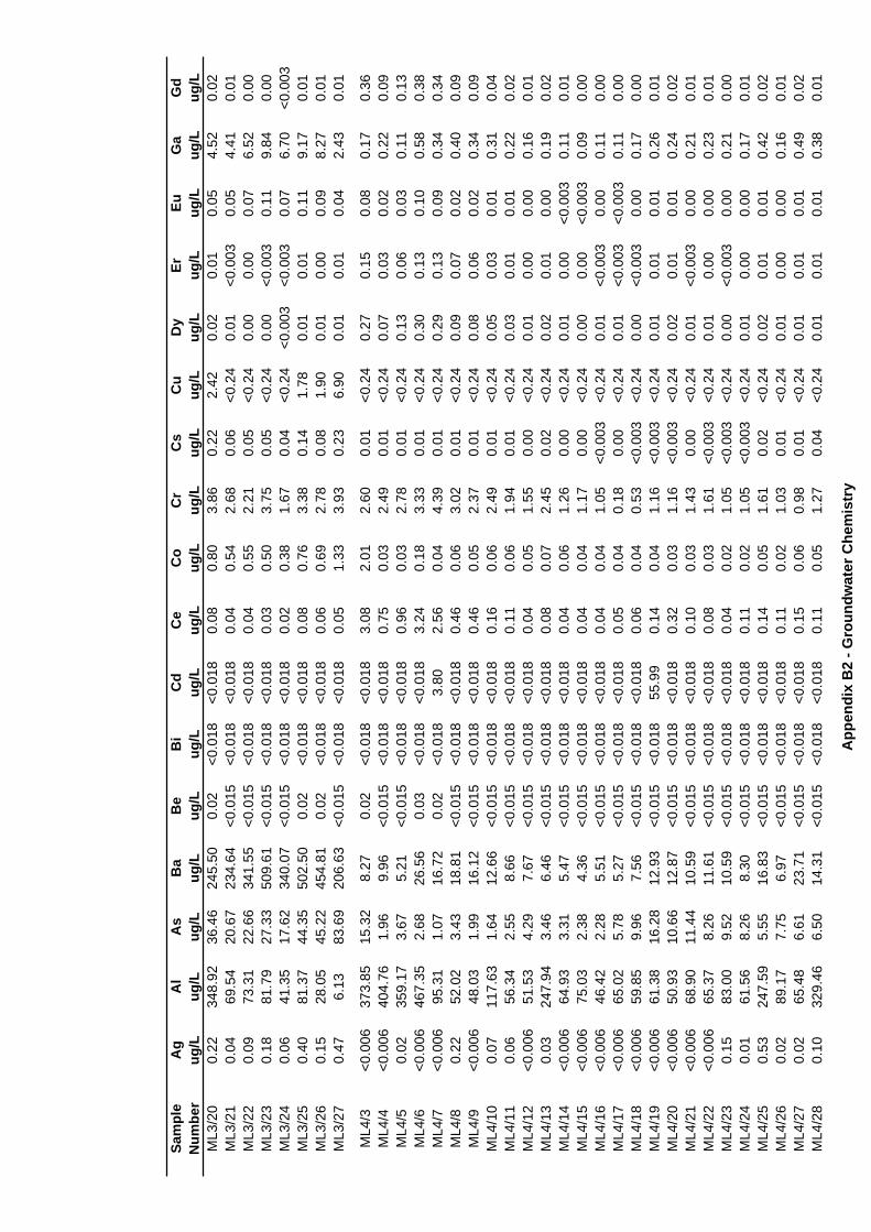
Sam
ple
Ag
Al
As
Ba
Be
Bi
Cd
Ce
Co
Cr
Cs
Cu
Dy
ErEu
Ga
Gd
Num
ber
ug/L
ug/L
ug/L
ug/L
ug/L
ug/L
ug/L
ug/L
ug/L
ug/L
ug/L
ug/L
ug/L
ug/L
ug/L
ug/L
ug/L
ML3
/20
0.22
348.
9236
.46
245.
500.
02<0
.018
<0.0
180.
080.
803.
860.
222.
420.
020.
010.
054.
520.
02M
L3/2
10.
0469
.54
20.6
723
4.64
<0.0
15<0
.018
<0.0
180.
040.
542.
680.
06<0
.24
0.01
<0.0
030.
054.
410.
01M
L3/2
20.
0973
.31
22.6
634
1.55
<0.0
15<0
.018
<0.0
180.
040.
552.
210.
05<0
.24
0.00
0.00
0.07
6.52
0.00
ML3
/23
0.18
81.7
927
.33
509.
61<0
.015
<0.0
18<0
.018
0.03
0.50
3.75
0.05
<0.2
40.
00<0
.003
0.11
9.84
0.00
ML3
/24
0.06
41.3
517
.62
340.
07<0
.015
<0.0
18<0
.018
0.02
0.38
1.67
0.04
<0.2
4<0
.003
<0.0
030.
076.
70<0
.003
ML3
/25
0.40
81.3
744
.35
502.
500.
02<0
.018
<0.0
180.
080.
763.
380.
141.
780.
010.
010.
119.
170.
01M
L3/2
60.
1528
.05
45.2
245
4.81
0.02
<0.0
18<0
.018
0.06
0.69
2.78
0.08
1.90
0.01
0.00
0.09
8.27
0.01
ML3
/27
0.47
6.13
83.6
920
6.63
<0.0
15<0
.018
<0.0
180.
051.
333.
930.
236.
900.
010.
010.
042.
430.
01
ML4
/3<0
.006
373.
8515
.32
8.27
0.02
<0.0
18<0
.018
3.08
2.01
2.60
0.01
<0.2
40.
270.
150.
080.
170.
36M
L4/4
<0.0
0640
4.76
1.96
9.96
<0.0
15<0
.018
<0.0
180.
750.
032.
490.
01<0
.24
0.07
0.03
0.02
0.22
0.09
ML4
/50.
0235
9.17
3.67
5.21
<0.0
15<0
.018
<0.0
180.
960.
032.
780.
01<0
.24
0.13
0.06
0.03
0.11
0.13
ML4
/6<0
.006
467.
352.
6826
.56
0.03
<0.0
18<0
.018
3.24
0.18
3.33
0.01
<0.2
40.
300.
130.
100.
580.
38M
L4/7
<0.0
0695
.31
1.07
16.7
20.
02<0
.018
3.80
2.56
0.04
4.39
0.01
<0.2
40.
290.
130.
090.
340.
34M
L4/8
0.22
52.0
23.
4318
.81
<0.0
15<0
.018
<0.0
180.
460.
063.
020.
01<0
.24
0.09
0.07
0.02
0.40
0.09
ML4
/9<0
.006
48.0
31.
9916
.12
<0.0
15<0
.018
<0.0
180.
460.
052.
370.
01<0
.24
0.08
0.06
0.02
0.34
0.09
ML4
/10
0.07
117.
631.
6412
.66
<0.0
15<0
.018
<0.0
180.
160.
062.
490.
01<0
.24
0.05
0.03
0.01
0.31
0.04
ML4
/11
0.06
56.3
42.
558.
66<0
.015
<0.0
18<0
.018
0.11
0.06
1.94
0.01
<0.2
40.
030.
010.
010.
220.
02M
L4/1
2<0
.006
51.5
34.
297.
67<0
.015
<0.0
18<0
.018
0.04
0.05
1.55
0.00
<0.2
40.
010.
000.
000.
160.
01M
L4/1
30.
0324
7.94
3.46
6.46
<0.0
15<0
.018
<0.0
180.
080.
072.
450.
02<0
.24
0.02
0.01
0.00
0.19
0.02
ML4
/14
<0.0
0664
.93
3.31
5.47
<0.0
15<0
.018
<0.0
180.
040.
061.
260.
00<0
.24
0.01
0.00
<0.0
030.
110.
01M
L4/1
5<0
.006
75.0
32.
384.
36<0
.015
<0.0
18<0
.018
0.04
0.04
1.17
0.00
<0.2
40.
000.
00<0
.003
0.09
0.00
ML4
/16
<0.0
0646
.42
2.28
5.51
<0.0
15<0
.018
<0.0
180.
040.
041.
05<0
.003
<0.2
40.
01<0
.003
0.00
0.11
0.00
ML4
/17
<0.0
0665
.02
5.78
5.27
<0.0
15<0
.018
<0.0
180.
050.
040.
180.
00<0
.24
0.01
<0.0
03<0
.003
0.11
0.00
ML4
/18
<0.0
0659
.85
9.96
7.56
<0.0
15<0
.018
<0.0
180.
060.
040.
53<0
.003
<0.2
40.
00<0
.003
0.00
0.17
0.00
ML4
/19
<0.0
0661
.38
16.2
812
.93
<0.0
15<0
.018
55.9
90.
140.
041.
16<0
.003
<0.2
40.
010.
010.
010.
260.
01M
L4/2
0<0
.006
50.9
310
.66
12.8
7<0
.015
<0.0
18<0
.018
0.32
0.03
1.16
<0.0
03<0
.24
0.02
0.01
0.01
0.24
0.02
ML4
/21
<0.0
0668
.90
11.4
410
.59
<0.0
15<0
.018
<0.0
180.
100.
031.
430.
00<0
.24
0.01
<0.0
030.
000.
210.
01M
L4/2
2<0
.006
65.3
78.
2611
.61
<0.0
15<0
.018
<0.0
180.
080.
031.
61<0
.003
<0.2
40.
010.
000.
000.
230.
01M
L4/2
30.
1583
.00
9.52
10.5
9<0
.015
<0.0
18<0
.018
0.04
0.02
1.05
<0.0
03<0
.24
0.00
<0.0
030.
000.
210.
00M
L4/2
40.
0161
.56
8.26
8.30
<0.0
15<0
.018
<0.0
180.
110.
021.
05<0
.003
<0.2
40.
010.
000.
000.
170.
01M
L4/2
50.
5324
7.59
5.55
16.8
3<0
.015
<0.0
18<0
.018
0.14
0.05
1.61
0.02
<0.2
40.
020.
010.
010.
420.
02M
L4/2
60.
0289
.17
7.75
6.97
<0.0
15<0
.018
<0.0
180.
110.
021.
030.
01<0
.24
0.01
0.00
0.00
0.16
0.01
ML4
/27
0.02
65.4
86.
6123
.71
<0.0
15<0
.018
<0.0
180.
150.
060.
980.
01<0
.24
0.01
0.01
0.01
0.49
0.02
ML4
/28
0.10
329.
466.
5014
.31
<0.0
15<0
.018
<0.0
180.
110.
051.
270.
04<0
.24
0.01
0.01
0.01
0.38
0.01
App
endi
x B
2 - G
roun
dwat
er C
hem
istr
y
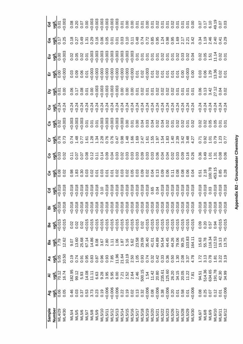
Sam
ple
Ag
Al
As
Ba
Be
Bi
Cd
Ce
Co
Cr
Cs
Cu
Dy
ErEu
Ga
Gd
Num
ber
ug/L
ug/L
ug/L
ug/L
ug/L
ug/L
ug/L
ug/L
ug/L
ug/L
ug/L
ug/L
ug/L
ug/L
ug/L
ug/L
ug/L
ML4
/29
0.06
70.1
25.
057.
79<0
.015
<0.0
18<0
.018
0.08
0.03
0.76
0.02
<0.2
40.
010.
000.
000.
170.
01M
L4/3
00.
0516
.74
10.5
012
.62
<0.0
15<0
.018
<0.0
180.
020.
020.
73<0
.003
<0.2
40.
00<0
.003
<0.0
030.
25<0
.003
ML5
/40.
4618
2.95
0.19
9.07
0.02
<0.0
18<0
.018
0.98
0.11
0.74
<0.0
03<0
.24
0.06
0.03
0.02
0.18
0.08
ML5
/50.
0399
.12
0.74
13.6
00.
02<0
.018
<0.0
181.
830.
071.
48<0
.003
<0.2
40.
170.
090.
050.
270.
20M
L5/6
0.37
5.93
0.91
25.6
80.
02<0
.018
<0.0
180.
300.
070.
77<0
.003
<0.2
40.
080.
060.
020.
490.
07M
L5/7
0.53
14.0
80.
9567
.14
<0.0
15<0
.018
<0.0
180.
030.
081.
610.
01<0
.24
0.01
0.01
0.01
1.31
0.00
ML5
/83.
7311
.11
0.83
14.8
6<0
.015
<0.0
18<0
.018
0.02
0.12
1.28
0.01
<0.2
40.
00<0
.003
<0.0
030.
29<0
.003
ML5
/90.
236.
630.
878.
08<0
.015
<0.0
18<0
.018
0.01
0.11
1.34
0.01
<0.2
4<0
.003
<0.0
03<0
.003
0.16
<0.0
03M
L5/1
00.
199.
280.
963.
67<0
.015
<0.0
180.
100.
030.
142.
28<0
.003
<0.2
4<0
.003
<0.0
03<0
.003
0.06
<0.0
03M
L5/1
1<0
.006
3.95
0.93
2.80
<0.0
15<0
.018
<0.0
180.
010.
090.
76<0
.003
<0.2
4<0
.003
<0.0
03<0
.003
0.05
<0.0
03M
L5/1
2<0
.006
5.95
7.85
1.11
<0.0
15<0
.018
<0.0
180.
010.
040.
76<0
.003
<0.2
4<0
.003
<0.0
03<0
.003
0.01
<0.0
03M
L5/1
3<0
.006
6.00
11.9
61.
06<0
.015
<0.0
18<0
.018
0.02
0.03
0.47
<0.0
03<0
.24
<0.0
03<0
.003
<0.0
030.
01<0
.003
ML5
/14
0.22
7.21
21.6
41.
87<0
.015
<0.0
18<0
.018
0.03
0.02
0.98
<0.0
03<0
.24
0.00
<0.0
03<0
.003
0.03
0.01
ML5
/15
0.19
2.52
10.1
95.
16<0
.015
<0.0
18<0
.018
0.02
0.03
1.48
0.00
<0.2
40.
00<0
.003
<0.0
030.
100.
00M
L5/1
60.
022.
642.
505.
62<0
.015
<0.0
18<0
.018
0.05
0.03
1.66
0.01
<0.2
40.
00<0
.003
<0.0
030.
110.
00M
L5/1
70.
132.
461.
0523
.58
<0.0
15<0
.018
<0.0
180.
030.
031.
690.
00<0
.24
0.01
0.01
0.01
0.48
0.01
ML5
/18
0.32
500.
150.
9329
.09
0.02
<0.0
18<0
.018
0.09
0.09
2.47
0.04
<0.2
40.
020.
020.
010.
740.
01M
L5/1
9<0
.006
1.54
0.74
35.4
0<0
.015
<0.0
18<0
.018
0.02
0.03
1.61
0.03
<0.2
40.
01<0
.003
0.01
0.72
0.00
ML5
/20
0.08
11.4
20.
3241
.01
<0.0
15<0
.018
0.65
0.04
0.03
1.55
0.04
<0.2
40.
010.
010.
010.
850.
01M
L5/2
1<0
.006
20.8
00.
4244
.89
<0.0
15<0
.018
0.04
0.13
0.06
1.97
0.02
<0.2
40.
020.
020.
010.
950.
02M
L5/2
20.
3823
5.61
0.33
54.5
4<0
.015
<0.0
18<0
.018
0.09
0.04
1.54
0.04
<0.2
40.
020.
010.
021.
240.
01M
L5/2
3<0
.006
125.
600.
3644
.45
<0.0
15<0
.018
<0.0
180.
060.
041.
830.
02<0
.24
0.02
0.01
0.01
0.98
0.01
ML5
/26
0.20
26.2
00.
5044
.26
<0.0
15<0
.018
<0.0
180.
110.
021.
400.
01<0
.24
0.02
0.01
0.01
0.95
0.02
ML5
/27
0.01
34.1
51.
3079
.06
<0.0
15<0
.018
<0.0
180.
080.
032.
390.
02<0
.24
0.01
0.01
0.02
1.69
0.01
ML5
/28
0.58
20.0
52.
0899
.25
<0.0
15<0
.018
<0.0
180.
080.
093.
420.
02<0
.24
0.01
0.00
0.03
2.17
0.01
ML5
/29
0.01
11.2
23.
3710
3.83
<0.0
15<0
.018
<0.0
180.
060.
163.
480.
01<0
.24
0.01
<0.0
030.
022.
210.
01M
L5/3
0<0
.006
7.81
4.78
164.
11<0
.015
<0.0
18<0
.018
0.04
0.26
4.27
0.02
<0.2
40.
010.
000.
043.
420.
00
ML6
/70.
0894
.51
1.72
15.6
30.
09<0
.018
<0.0
180.
510.
360.
710.
02<0
.24
0.06
0.03
0.02
0.34
0.07
ML6
/80.
2551
4.36
3.13
55.7
80.
20<0
.018
<0.0
182.
180.
490.
920.
02<0
.24
0.13
0.06
0.05
1.19
0.17
ML6
/90.
0763
4.65
0.78
116.
340.
57<0
.018
0.03
100.
781.
011.
010.
05<0
.24
3.42
1.29
1.51
2.46
6.10
ML6
/10
0.12
191.
781.
8111
2.53
0.94
<0.0
18<0
.018
453.
151.
310.
790.
05<0
.24
27.1
213
.36
11.1
42.
4049
.19
ML6
/11
0.01
42.3
03.
2219
.13
<0.0
15<0
.018
<0.0
180.
850.
081.
230.
01<0
.24
0.04
0.02
0.02
0.41
0.07
ML6
/12
<0.0
0634
.99
3.19
13.7
5<0
.015
<0.0
18<0
.018
0.28
0.06
0.77
0.01
<0.2
40.
020.
010.
010.
290.
03
App
endi
x B
2 - G
roun
dwat
er C
hem
istr
y
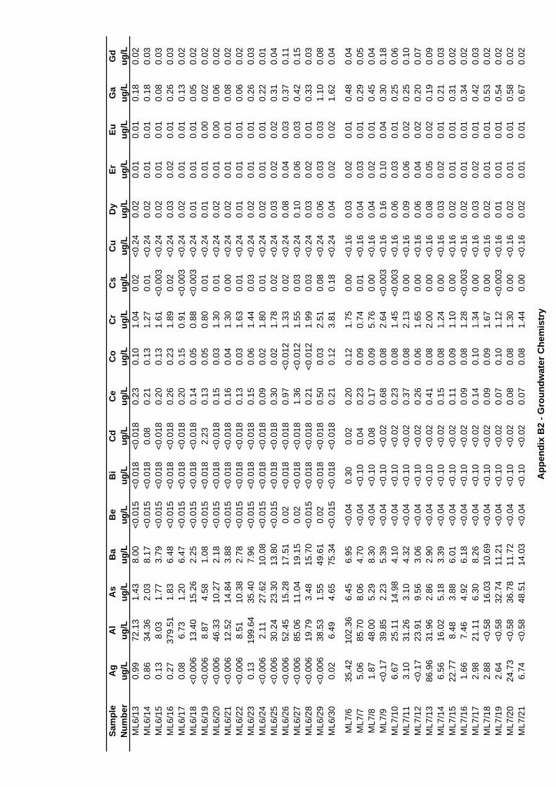
Sam
ple
Ag
Al
As
Ba
Be
Bi
Cd
Ce
Co
Cr
Cs
Cu
Dy
ErEu
Ga
Gd
Num
ber
ug/L
ug/L
ug/L
ug/L
ug/L
ug/L
ug/L
ug/L
ug/L
ug/L
ug/L
ug/L
ug/L
ug/L
ug/L
ug/L
ug/L
ML6
/13
0.99
72.1
31.
438.
00<0
.015
<0.0
18<0
.018
0.23
0.10
1.04
0.02
<0.2
40.
020.
010.
010.
180.
02M
L6/1
40.
8634
.36
2.03
8.17
<0.0
15<0
.018
0.08
0.21
0.13
1.27
0.01
<0.2
40.
020.
010.
010.
180.
03M
L6/1
50.
138.
031.
773.
79<0
.015
<0.0
18<0
.018
0.20
0.13
1.61
<0.0
03<0
.24
0.02
0.01
0.01
0.08
0.03
ML6
/16
0.27
379.
511.
836.
48<0
.015
<0.0
18<0
.018
0.26
0.23
1.89
0.02
<0.2
40.
030.
020.
010.
260.
03M
L6/1
70.
086.
731.
206.
47<0
.015
<0.0
18<0
.018
0.20
0.15
0.91
<0.0
03<0
.24
0.02
0.01
0.01
0.13
0.02
ML6
/18
<0.0
0613
.40
15.2
62.
25<0
.015
<0.0
18<0
.018
0.14
0.05
0.88
<0.0
03<0
.24
0.01
0.01
0.01
0.05
0.02
ML6
/19
<0.0
068.
874.
581.
08<0
.015
<0.0
182.
230.
130.
050.
800.
01<0
.24
0.01
0.01
0.00
0.02
0.02
ML6
/20
<0.0
0646
.33
10.2
72.
18<0
.015
<0.0
18<0
.018
0.15
0.03
1.30
0.01
<0.2
40.
020.
010.
000.
060.
02M
L6/2
1<0
.006
12.5
214
.84
3.88
<0.0
15<0
.018
<0.0
180.
160.
041.
300.
00<0
.24
0.02
0.01
0.01
0.08
0.02
ML6
/22
<0.0
068.
5110
.38
2.78
<0.0
15<0
.018
<0.0
180.
130.
031.
630.
01<0
.24
0.01
0.01
0.01
0.06
0.02
ML6
/23
0.13
199.
6435
.40
7.96
<0.0
15<0
.018
<0.0
180.
150.
061.
440.
03<0
.24
0.02
0.01
0.01
0.26
0.03
ML6
/24
<0.0
062.
1127
.62
10.0
8<0
.015
<0.0
18<0
.018
0.09
0.02
1.80
0.01
<0.2
40.
020.
010.
010.
220.
01M
L6/2
5<0
.006
30.2
423
.30
13.8
0<0
.015
<0.0
18<0
.018
0.30
0.02
1.78
0.02
<0.2
40.
030.
020.
020.
310.
04M
L6/2
6<0
.006
52.4
515
.28
17.5
10.
02<0
.018
<0.0
180.
97<0
.012
1.33
0.02
<0.2
40.
080.
040.
030.
370.
11M
L6/2
7<0
.006
85.0
611
.04
19.1
50.
02<0
.018
<0.0
181.
36<0
.012
1.55
0.03
<0.2
40.
100.
060.
030.
420.
15M
L6/2
8<0
.006
19.7
93.
4815
.70
<0.0
15<0
.018
<0.0
180.
21<0
.012
1.99
0.03
<0.2
40.
030.
020.
010.
330.
03M
L6/2
9<0
.006
38.5
31.
5549
.61
0.02
<0.0
18<0
.018
0.50
0.03
2.51
0.08
<0.2
40.
060.
030.
031.
100.
08M
L6/3
00.
026.
494.
6575
.34
<0.0
15<0
.018
<0.0
180.
210.
123.
810.
18<0
.24
0.04
0.02
0.02
1.62
0.04
ML7
/635
.42
102.
366.
456.
95<0
.04
0.30
0.02
0.20
0.12
1.75
0.00
<0.1
60.
030.
020.
010.
480.
04M
L7/7
5.06
85.7
08.
064.
70<0
.04
<0.1
00.
040.
230.
090.
740.
01<0
.16
0.04
0.03
0.01
0.29
0.05
ML7
/81.
8748
.00
5.29
8.30
<0.0
4<0
.10
0.08
0.17
0.09
5.76
0.00
<0.1
60.
040.
020.
010.
450.
04M
L7/9
<0.1
739
.85
2.23
5.39
<0.0
4<0
.10
<0.0
20.
680.
082.
64<0
.003
<0.1
60.
160.
100.
040.
300.
18M
L7/1
06.
6725
.11
14.9
84.
10<0
.04
<0.1
0<0
.02
0.23
0.08
1.45
<0.0
03<0
.16
0.06
0.03
0.01
0.25
0.06
ML7
/11
3.10
31.2
63.
104.
32<0
.04
<0.1
0<0
.02
0.37
0.08
2.13
0.00
<0.1
60.
090.
060.
020.
250.
10M
L7/1
2<0
.17
23.9
19.
563.
06<0
.04
<0.1
0<0
.02
0.26
0.06
1.65
0.00
<0.1
60.
060.
040.
020.
200.
07M
L7/1
386
.96
31.9
62.
862.
90<0
.04
<0.1
0<0
.02
0.41
0.08
2.00
0.00
<0.1
60.
080.
050.
020.
190.
09M
L7/1
46.
5616
.02
5.18
3.39
<0.0
4<0
.10
<0.0
20.
150.
081.
240.
00<0
.16
0.03
0.02
0.01
0.21
0.03
ML7
/15
22.7
78.
483.
886.
01<0
.04
<0.1
0<0
.02
0.11
0.09
1.10
0.00
<0.1
60.
020.
010.
010.
310.
02M
L7/1
61.
667.
464.
926.
18<0
.04
<0.1
0<0
.02
0.09
0.08
1.28
<0.0
03<0
.16
0.02
0.01
0.01
0.34
0.02
ML7
/17
2.98
21.1
16.
308.
26<0
.04
<0.1
0<0
.02
0.14
0.10
1.34
0.00
<0.1
60.
030.
020.
010.
420.
03M
L7/1
82.
88<0
.58
16.0
310
.69
<0.0
4<0
.10
<0.0
20.
090.
091.
670.
00<0
.16
0.02
0.01
0.01
0.53
0.02
ML7
/19
2.64
<0.5
832
.74
11.2
1<0
.04
<0.1
0<0
.02
0.07
0.10
1.12
<0.0
03<0
.16
0.01
0.01
0.01
0.54
0.02
ML7
/20
24.7
3<0
.58
36.7
811
.72
<0.0
4<0
.10
<0.0
20.
080.
081.
300.
00<0
.16
0.02
0.01
0.01
0.58
0.02
ML7
/21
6.74
<0.5
848
.51
14.0
3<0
.04
<0.1
0<0
.02
0.07
0.08
1.44
0.00
<0.1
60.
020.
010.
010.
670.
02
App
endi
x B
2 - G
roun
dwat
er C
hem
istr
y
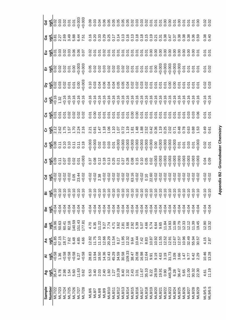
Sam
ple
Ag
Al
As
Ba
Be
Bi
Cd
Ce
Co
Cr
Cs
Cu
Dy
ErEu
Ga
Gd
Num
ber
ug/L
ug/L
ug/L
ug/L
ug/L
ug/L
ug/L
ug/L
ug/L
ug/L
ug/L
ug/L
ug/L
ug/L
ug/L
ug/L
ug/L
ML7
/22
35.4
7<0
.58
61.8
516
.96
<0.0
4<0
.10
<0.0
20.
090.
082.
120.
01<0
.16
0.02
0.02
0.01
0.81
0.02
ML7
/23
6.78
1.36
57.1
550
.63
<0.0
4<0
.10
<0.0
20.
110.
112.
620.
011.
320.
030.
020.
032.
270.
03M
L7/2
42.
98<0
.58
18.7
760
.41
<0.0
4<0
.10
<0.0
20.
070.
101.
750.
01<0
.16
0.02
0.02
0.02
2.69
0.02
ML7
/25
1.54
<0.5
87.
6282
.18
<0.0
4<0
.10
<0.0
20.
030.
101.
570.
02<0
.16
0.01
0.01
0.03
3.49
0.01
ML7
/26
5.60
<0.5
86.
4814
0.59
<0.0
4<0
.10
0.05
0.02
0.11
1.70
0.02
<0.1
60.
010.
000.
065.
880.
01M
L7/2
711
.63
6.27
4.85
151.
43<0
.04
<0.1
023
.44
0.01
0.11
2.24
0.02
<0.1
60.
00<0
.003
0.06
6.44
<0.0
03M
L7/2
80.
62<0
.58
4.66
177.
81<0
.04
<0.1
0<0
.02
<0.0
030.
182.
160.
02<0
.16
<0.0
03<0
.003
0.07
7.51
<0.0
03
ML8
/66.
5328
.83
12.8
24.
70<0
.04
<0.1
0<0
.02
0.37
<0.0
032.
210.
01<0
.16
0.10
0.05
0.02
0.16
0.09
ML8
/73.
4013
.94
11.7
56.
35<0
.04
<0.1
0<0
.02
0.08
<0.0
030.
810.
00<0
.16
0.03
0.02
0.01
0.20
0.03
ML8
/82.
0318
.50
11.1
011
.22
<0.0
4<0
.10
2.38
0.12
0.02
1.47
0.01
<0.1
60.
040.
020.
010.
330.
04M
L8/9
2.40
14.3
612
.66
9.27
<0.0
4<0
.10
<0.0
20.
180.
031.
180.
01<0
.16
0.06
0.03
0.02
0.29
0.06
ML8
/10
1.60
12.4
320
.29
7.74
<0.0
4<0
.10
<0.0
20.
130.
031.
060.
01<0
.16
0.04
0.02
0.01
0.25
0.05
ML8
/11
1.27
45.2
911
.54
4.71
<0.0
4<0
.10
<0.0
20.
250.
011.
100.
01<0
.16
0.04
0.02
0.01
0.17
0.05
ML8
/12
10.2
834
.59
8.17
3.62
<0.0
4<0
.10
<0.0
20.
21<0
.003
1.07
0.01
<0.1
60.
050.
030.
010.
140.
05M
L8/1
38.
4030
.58
11.9
52.
81<0
.04
<0.1
0<0
.02
0.27
<0.0
030.
720.
01<0
.16
0.05
0.02
0.01
0.13
0.05
ML8
/14
2.32
109.
3312
.32
3.66
<0.0
4<0
.10
<0.0
20.
28<0
.003
1.19
0.01
<0.1
60.
040.
020.
010.
160.
05M
L8/1
52.
4338
.47
9.64
2.92
<0.0
4<0
.10
63.1
60.
08<0
.003
1.81
0.00
<0.1
60.
020.
010.
010.
130.
02M
L8/1
63.
0126
.08
10.4
45.
39<0
.04
<0.1
0<0
.02
0.15
<0.0
031.
480.
00<0
.16
0.02
0.01
0.01
0.18
0.03
ML8
/17
11.6
716
.98
7.42
5.07
<0.0
4<0
.10
<0.0
20.
10<0
.003
1.88
0.01
<0.1
60.
030.
010.
010.
180.
03M
L8/1
835
.10
12.6
48.
834.
66<0
.04
<0.1
00.
100.
05<0
.003
2.52
0.01
<0.1
60.
020.
010.
010.
150.
02M
L8/1
96.
229.
9110
.87
5.74
<0.0
4<0
.10
22.6
00.
02<0
.003
0.42
0.01
<0.1
60.
010.
010.
000.
190.
01M
L8/2
028
.59
9.19
10.9
26.
64<0
.04
<0.1
0<0
.02
<0.0
030.
000.
360.
01<0
.16
0.01
0.00
0.00
0.21
0.01
ML8
/21
19.9
14.
6311
.55
9.65
<0.0
4<0
.10
<0.0
2<0
.003
<0.0
031.
190.
01<0
.16
0.01
<0.0
030.
000.
310.
01M
L8/2
20.
903.
1912
.52
11.8
4<0
.04
<0.1
0<0
.02
<0.0
03<0
.003
0.25
0.01
<0.1
60.
01<0
.003
0.00
0.38
0.00
ML8
/23
445.
3831
.73
12.9
114
.93
<0.0
4<0
.10
<0.0
2<0
.003
<0.0
032.
020.
01<0
.16
0.00
<0.0
030.
000.
470.
00M
L8/2
46.
283.
0912
.67
11.9
9<0
.04
<0.1
0<0
.02
<0.0
03<0
.003
0.71
0.01
<0.1
60.
00<0
.003
0.00
0.37
0.01
ML8
/25
36.4
73.
6612
.57
12.7
9<0
.04
<0.1
0<0
.02
<0.0
030.
010.
480.
01<0
.16
0.01
<0.0
030.
000.
380.
00M
L8/2
65.
651.
4710
.96
12.3
3<0
.04
<0.1
0<0
.02
<0.0
030.
010.
780.
01<0
.16
0.01
0.01
0.00
0.38
0.01
ML8
/27
21.0
09.
7732
.49
12.1
2<0
.04
<0.1
0<0
.02
<0.0
030.
030.
630.
03<0
.16
0.01
0.01
0.00
0.38
0.01
ML8
/28
30.3
26.
4255
.94
11.3
9<0
.04
<0.1
0<0
.02
<0.0
030.
010.
880.
03<0
.16
0.01
0.01
0.00
0.36
0.01
ML8
/29
22.3
02.
2930
.57
19.4
5<0
.04
<0.1
0<0
.02
<0.0
03<0
.003
1.53
0.06
<0.1
60.
010.
010.
010.
590.
00
ML9
/5.5
4.61
10.4
64.
1512
.90
<0.0
4<0
.10
<0.0
20.
040.
020.
490.
01<0
.16
0.02
0.01
0.01
0.38
0.02
ML9
/6.5
11.1
913
.28
2.87
13.3
2<0
.04
<0.1
0<0
.02
0.09
0.01
0.61
0.01
<0.1
60.
030.
020.
010.
400.
02
App
endi
x B
2 - G
roun
dwat
er C
hem
istr
y
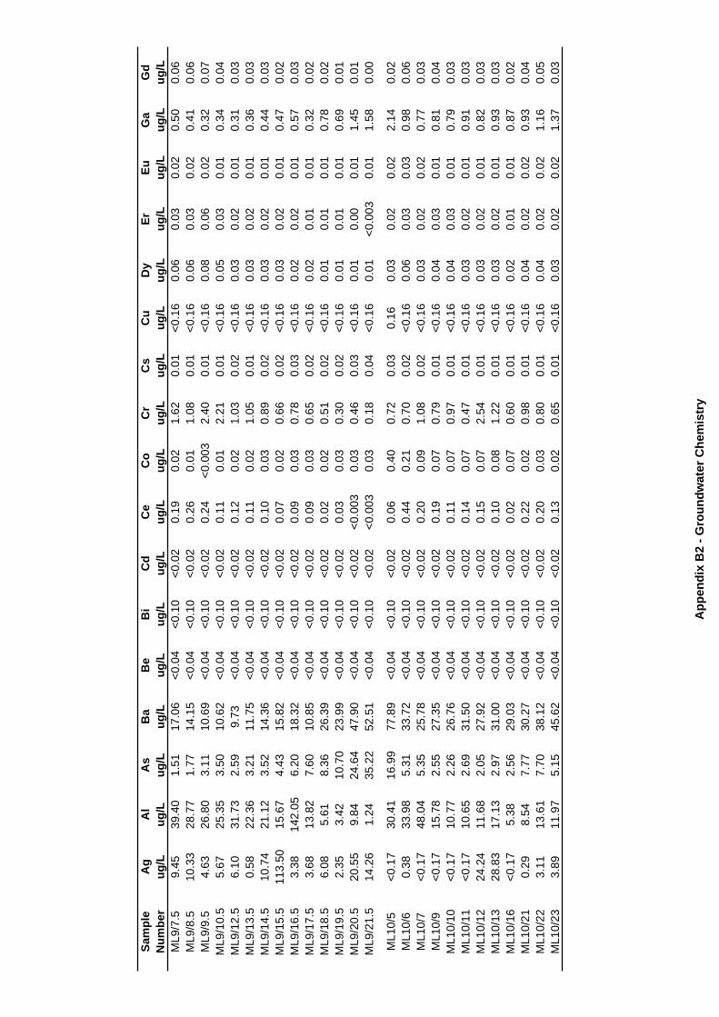
Sam
ple
Ag
Al
As
Ba
Be
Bi
Cd
Ce
Co
Cr
Cs
Cu
Dy
ErEu
Ga
Gd
Num
ber
ug/L
ug/L
ug/L
ug/L
ug/L
ug/L
ug/L
ug/L
ug/L
ug/L
ug/L
ug/L
ug/L
ug/L
ug/L
ug/L
ug/L
ML9
/7.5
9.45
39.4
01.
5117
.06
<0.0
4<0
.10
<0.0
20.
190.
021.
620.
01<0
.16
0.06
0.03
0.02
0.50
0.06
ML9
/8.5
10.3
328
.77
1.77
14.1
5<0
.04
<0.1
0<0
.02
0.26
0.01
1.08
0.01
<0.1
60.
060.
030.
020.
410.
06M
L9/9
.54.
6326
.80
3.11
10.6
9<0
.04
<0.1
0<0
.02
0.24
<0.0
032.
400.
01<0
.16
0.08
0.06
0.02
0.32
0.07
ML9
/10.
55.
6725
.35
3.50
10.6
2<0
.04
<0.1
0<0
.02
0.11
0.01
2.21
0.01
<0.1
60.
050.
030.
010.
340.
04M
L9/1
2.5
6.10
31.7
32.
599.
73<0
.04
<0.1
0<0
.02
0.12
0.02
1.03
0.02
<0.1
60.
030.
020.
010.
310.
03M
L9/1
3.5
0.58
22.3
63.
2111
.75
<0.0
4<0
.10
<0.0
20.
110.
021.
050.
01<0
.16
0.03
0.02
0.01
0.36
0.03
ML9
/14.
510
.74
21.1
23.
5214
.36
<0.0
4<0
.10
<0.0
20.
100.
030.
890.
02<0
.16
0.03
0.02
0.01
0.44
0.03
ML9
/15.
511
3.50
15.6
74.
4315
.82
<0.0
4<0
.10
<0.0
20.
070.
020.
660.
02<0
.16
0.03
0.02
0.01
0.47
0.02
ML9
/16.
53.
3814
2.05
6.20
18.3
2<0
.04
<0.1
0<0
.02
0.09
0.03
0.78
0.03
<0.1
60.
020.
020.
010.
570.
03M
L9/1
7.5
3.68
13.8
27.
6010
.85
<0.0
4<0
.10
<0.0
20.
090.
030.
650.
02<0
.16
0.02
0.01
0.01
0.32
0.02
ML9
/18.
56.
085.
618.
3626
.39
<0.0
4<0
.10
<0.0
20.
020.
020.
510.
02<0
.16
0.01
0.01
0.01
0.78
0.02
ML9
/19.
52.
353.
4210
.70
23.9
9<0
.04
<0.1
0<0
.02
0.03
0.03
0.30
0.02
<0.1
60.
010.
010.
010.
690.
01M
L9/2
0.5
20.5
59.
8424
.64
47.9
0<0
.04
<0.1
0<0
.02
<0.0
030.
030.
460.
03<0
.16
0.01
0.00
0.01
1.45
0.01
ML9
/21.
514
.26
1.24
35.2
252
.51
<0.0
4<0
.10
<0.0
2<0
.003
0.03
0.18
0.04
<0.1
60.
01<0
.003
0.01
1.58
0.00
ML1
0/5
<0.1
730
.41
16.9
977
.89
<0.0
4<0
.10
<0.0
20.
060.
400.
720.
030.
160.
030.
020.
022.
140.
02M
L10/
60.
3833
.98
5.31
33.7
2<0
.04
<0.1
0<0
.02
0.44
0.21
0.70
0.02
<0.1
60.
060.
030.
030.
980.
06M
L10/
7<0
.17
48.0
45.
3525
.78
<0.0
4<0
.10
<0.0
20.
200.
091.
080.
02<0
.16
0.03
0.02
0.02
0.77
0.03
ML1
0/9
<0.1
715
.78
2.55
27.3
5<0
.04
<0.1
0<0
.02
0.19
0.07
0.79
0.01
<0.1
60.
040.
030.
010.
810.
04M
L10/
10<0
.17
10.7
72.
2626
.76
<0.0
4<0
.10
<0.0
20.
110.
070.
970.
01<0
.16
0.04
0.03
0.01
0.79
0.03
ML1
0/11
<0.1
710
.65
2.69
31.5
0<0
.04
<0.1
0<0
.02
0.14
0.07
0.47
0.01
<0.1
60.
030.
020.
010.
910.
03M
L10/
1224
.24
11.6
82.
0527
.92
<0.0
4<0
.10
<0.0
20.
150.
072.
540.
01<0
.16
0.03
0.02
0.01
0.82
0.03
ML1
0/13
28.8
317
.13
2.97
31.0
0<0
.04
<0.1
0<0
.02
0.10
0.08
1.22
0.01
<0.1
60.
030.
020.
010.
930.
03M
L10/
16<0
.17
5.38
2.56
29.0
3<0
.04
<0.1
0<0
.02
0.02
0.07
0.60
0.01
<0.1
60.
020.
010.
010.
870.
02M
L10/
210.
298.
547.
7730
.27
<0.0
4<0
.10
<0.0
20.
220.
020.
980.
01<0
.16
0.04
0.02
0.02
0.93
0.04
ML1
0/22
3.11
13.6
17.
7038
.12
<0.0
4<0
.10
<0.0
20.
200.
030.
800.
01<0
.16
0.04
0.02
0.02
1.16
0.05
ML1
0/23
3.89
11.9
75.
1545
.62
<0.0
4<0
.10
<0.0
20.
130.
020.
650.
01<0
.16
0.03
0.02
0.02
1.37
0.03
App
endi
x B
2 - G
roun
dwat
er C
hem
istr
y
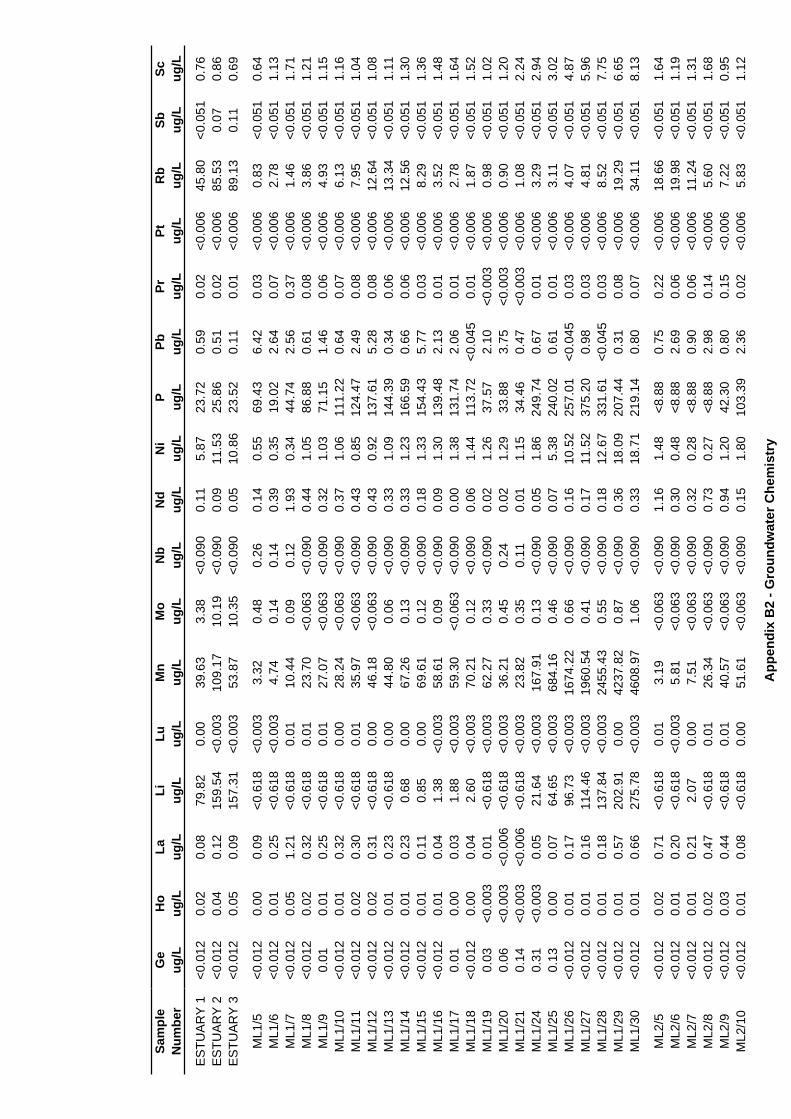
Sam
ple
Num
ber
ES
TUA
RY
1E
STU
AR
Y 2
ES
TUA
RY
3
ML1
/5M
L1/6
ML1
/7M
L1/8
ML1
/9M
L1/1
0M
L1/1
1M
L1/1
2M
L1/1
3M
L1/1
4M
L1/1
5M
L1/1
6M
L1/1
7M
L1/1
8M
L1/1
9M
L1/2
0M
L1/2
1M
L1/2
4M
L1/2
5M
L1/2
6M
L1/2
7M
L1/2
8M
L1/2
9M
L1/3
0
ML2
/5M
L2/6
ML2
/7M
L2/8
ML2
/9M
L2/1
0
Ge
Ho
LaLi
LuM
nM
oN
bN
dN
iP
PbPr
PtR
bSb
Scug
/Lug
/Lug
/Lug
/Lug
/Lug
/Lug
/Lug
/Lug
/Lug
/Lug
/Lug
/Lug
/Lug
/Lug
/Lug
/Lug
/L
<0.0
120.
020.
0879
.82
0.00
39.6
33.
38<0
.090
0.11
5.87
23.7
20.
590.
02<0
.006
45.8
0<0
.051
0.76
<0.0
120.
040.
1215
9.54
<0.0
0310
9.17
10.1
9<0
.090
0.09
11.5
325
.86
0.51
0.02
<0.0
0685
.53
0.07
0.86
<0.0
120.
050.
0915
7.31
<0.0
0353
.87
10.3
5<0
.090
0.05
10.8
623
.52
0.11
0.01
<0.0
0689
.13
0.11
0.69
<0.0
120.
000.
09<0
.618
<0.0
033.
320.
480.
260.
140.
5569
.43
6.42
0.03
<0.0
060.
83<0
.051
0.64
<0.0
120.
010.
25<0
.618
<0.0
034.
740.
140.
140.
390.
3519
.02
2.64
0.07
<0.0
062.
78<0
.051
1.13
<0.0
120.
051.
21<0
.618
0.01
10.4
40.
090.
121.
930.
3444
.74
2.56
0.37
<0.0
061.
46<0
.051
1.71
<0.0
120.
020.
32<0
.618
0.01
23.7
0<0
.063
<0.0
900.
441.
0586
.88
0.61
0.08
<0.0
063.
86<0
.051
1.21
0.01
0.01
0.25
<0.6
180.
0127
.07
<0.0
63<0
.090
0.32
1.03
71.1
51.
460.
06<0
.006
4.93
<0.0
511.
15<0
.012
0.01
0.32
<0.6
180.
0028
.24
<0.0
63<0
.090
0.37
1.06
111.
220.
640.
07<0
.006
6.13
<0.0
511.
16<0
.012
0.02
0.30
<0.6
180.
0135
.97
<0.0
63<0
.090
0.43
0.85
124.
472.
490.
08<0
.006
7.95
<0.0
511.
04<0
.012
0.02
0.31
<0.6
180.
0046
.18
<0.0
63<0
.090
0.43
0.92
137.
615.
280.
08<0
.006
12.6
4<0
.051
1.08
<0.0
120.
010.
23<0
.618
0.00
44.8
00.
06<0
.090
0.33
1.09
144.
390.
340.
06<0
.006
13.3
4<0
.051
1.11
<0.0
120.
010.
230.
680.
0067
.26
0.13
<0.0
900.
331.
2316
6.59
0.66
0.06
<0.0
0612
.56
<0.0
511.
30<0
.012
0.01
0.11
0.85
0.00
69.6
10.
12<0
.090
0.18
1.33
154.
435.
770.
03<0
.006
8.29
<0.0
511.
36<0
.012
0.01
0.04
1.38
<0.0
0358
.61
0.09
<0.0
900.
091.
3013
9.48
2.13
0.01
<0.0
063.
52<0
.051
1.48
0.01
0.00
0.03
1.88
<0.0
0359
.30
<0.0
63<0
.090
0.00
1.38
131.
742.
060.
01<0
.006
2.78
<0.0
511.
64<0
.012
0.00
0.04
2.60
<0.0
0370
.21
0.12
<0.0
900.
061.
4411
3.72
<0.0
450.
01<0
.006
1.87
<0.0
511.
520.
03<0
.003
0.01
<0.6
18<0
.003
62.2
70.
33<0
.090
0.02
1.26
37.5
72.
10<0
.003
<0.0
060.
98<0
.051
1.02
0.06
<0.0
03<0
.006
<0.6
18<0
.003
36.2
10.
450.
240.
021.
2933
.88
3.75
<0.0
03<0
.006
0.90
<0.0
511.
200.
14<0
.003
<0.0
06<0
.618
<0.0
0323
.82
0.35
0.11
0.01
1.15
34.4
60.
47<0
.003
<0.0
061.
08<0
.051
2.24
0.31
<0.0
030.
0521
.64
<0.0
0316
7.91
0.13
<0.0
900.
051.
8624
9.74
0.67
0.01
<0.0
063.
29<0
.051
2.94
0.13
0.00
0.07
64.6
5<0
.003
684.
160.
46<0
.090
0.07
5.38
240.
020.
610.
01<0
.006
3.11
<0.0
513.
02<0
.012
0.01
0.17
96.7
3<0
.003
1674
.22
0.66
<0.0
900.
1610
.52
257.
01<0
.045
0.03
<0.0
064.
07<0
.051
4.87
<0.0
120.
010.
1611
4.46
<0.0
0319
60.5
40.
41<0
.090
0.17
11.5
237
5.20
0.98
0.03
<0.0
064.
81<0
.051
5.96
<0.0
120.
010.
1813
7.84
<0.0
0324
55.4
30.
55<0
.090
0.18
12.6
733
1.61
<0.0
450.
03<0
.006
8.52
<0.0
517.
75<0
.012
0.01
0.57
202.
910.
0042
37.8
20.
87<0
.090
0.36
18.0
920
7.44
0.31
0.08
<0.0
0619
.29
<0.0
516.
65<0
.012
0.01
0.66
275.
78<0
.003
4608
.97
1.06
<0.0
900.
3318
.71
219.
140.
800.
07<0
.006
34.1
1<0
.051
8.13
<0.0
120.
020.
71<0
.618
0.01
3.19
<0.0
63<0
.090
1.16
1.48
<8.8
80.
750.
22<0
.006
18.6
6<0
.051
1.64
<0.0
120.
010.
20<0
.618
<0.0
035.
81<0
.063
<0.0
900.
300.
48<8
.88
2.69
0.06
<0.0
0619
.98
<0.0
511.
19<0
.012
0.01
0.21
2.07
0.00
7.51
<0.0
63<0
.090
0.32
0.28
<8.8
80.
900.
06<0
.006
11.2
4<0
.051
1.31
<0.0
120.
020.
47<0
.618
0.01
26.3
4<0
.063
<0.0
900.
730.
27<8
.88
2.98
0.14
<0.0
065.
60<0
.051
1.68
<0.0
120.
030.
44<0
.618
0.01
40.5
7<0
.063
<0.0
900.
941.
2042
.30
0.80
0.15
<0.0
067.
22<0
.051
0.95
<0.0
120.
010.
08<0
.618
0.00
51.6
1<0
.063
<0.0
900.
151.
8010
3.39
2.36
0.02
<0.0
065.
83<0
.051
1.12
App
endi
x B
2 - G
roun
dwat
er C
hem
istr
y
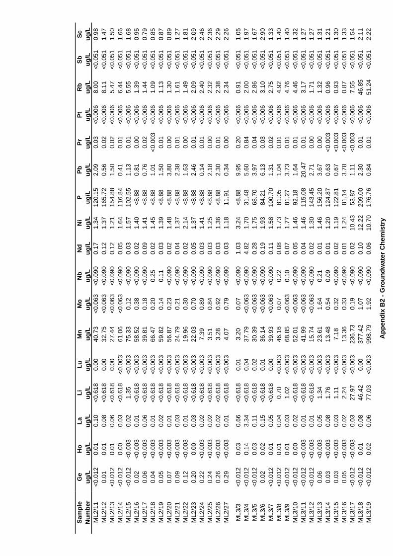
Sam
ple
Num
ber
ML2
/11
ML2
/12
ML2
/13
ML2
/14
ML2
/15
ML2
/16
ML2
/17
ML2
/18
ML2
/19
ML2
/20
ML2
/21
ML2
/22
ML2
/23
ML2
/24
ML2
/25
ML2
/26
ML2
/27
ML3
/3M
L3/4
ML3
/5M
L3/6
ML3
/7M
L3/8
ML3
/9M
L3/1
0M
L3/1
1M
L3/1
2M
L3/1
3M
L3/1
4M
L3/1
5M
L3/1
6M
L3/1
7M
L3/1
8M
L3/1
9
Ge
Ho
LaLi
LuM
nM
oN
bN
dN
iP
PbPr
PtR
bSb
Scug
/Lug
/Lug
/Lug
/Lug
/Lug
/Lug
/Lug
/Lug
/Lug
/Lug
/Lug
/Lug
/Lug
/Lug
/Lug
/Lug
/L<0
.012
0.01
0.10
<0.6
180.
0040
.73
<0.0
63<0
.090
0.17
1.34
120.
152.
090.
03<0
.006
8.00
<0.0
510.
980.
010.
010.
08<0
.618
0.00
32.7
5<0
.063
<0.0
900.
121.
3716
5.72
0.56
0.02
<0.0
068.
11<0
.051
1.47
<0.0
120.
010.
06<0
.618
0.00
27.4
4<0
.063
<0.0
900.
121.
2115
4.88
1.50
0.02
<0.0
065.
47<0
.051
1.50
<0.0
120.
000.
03<0
.618
<0.0
0361
.06
<0.0
63<0
.090
0.05
1.64
116.
840.
410.
01<0
.006
6.44
<0.0
511.
66<0
.012
<0.0
030.
021.
35<0
.003
75.3
30.
12<0
.090
0.03
1.57
102.
551.
130.
01<0
.006
5.55
<0.0
511.
680.
02<0
.003
0.01
<0.6
18<0
.003
58.5
20.
38<0
.090
0.02
1.40
<8.8
80.
810.
00<0
.006
1.39
<0.0
510.
950.
06<0
.003
0.06
<0.6
18<0
.003
39.8
10.
18<0
.090
0.09
1.41
<8.8
80.
760.
02<0
.006
1.44
<0.0
510.
790.
04<0
.003
0.01
<0.6
18<0
.003
66.4
70.
200.
250.
021.
45<8
.88
1.01
<0.0
03<0
.006
1.09
<0.0
510.
850.
05<0
.003
0.02
<0.6
18<0
.003
59.8
20.
140.
110.
031.
39<8
.88
1.50
0.01
<0.0
061.
13<0
.051
0.87
0.07
<0.0
030.
01<0
.618
<0.0
0356
.87
0.23
<0.0
900.
021.
48<8
.88
3.80
0.00
<0.0
061.
30<0
.051
0.89
0.09
<0.0
030.
03<0
.618
<0.0
0324
.79
0.21
<0.0
900.
041.
37<8
.88
2.38
0.01
<0.0
061.
61<0
.051
1.27
0.12
<0.0
030.
01<0
.618
<0.0
0319
.96
0.30
<0.0
900.
022.
14<8
.88
1.63
0.00
<0.0
061.
49<0
.051
1.81
0.20
0.00
0.03
<0.6
18<0
.003
22.0
30.
70<0
.090
0.05
1.37
<8.8
82.
460.
01<0
.006
2.09
<0.0
512.
090.
22<0
.003
0.02
<0.6
18<0
.003
7.39
0.89
<0.0
900.
031.
41<8
.88
0.14
0.01
<0.0
062.
40<0
.051
2.46
0.24
<0.0
030.
02<0
.618
<0.0
033.
510.
84<0
.090
0.03
1.25
<8.8
82.
180.
00<0
.006
2.32
<0.0
512.
360.
26<0
.003
0.02
<0.6
18<0
.003
3.28
0.92
<0.0
900.
031.
36<8
.88
2.30
0.01
<0.0
062.
38<0
.051
2.29
0.29
<0.0
030.
01<0
.618
<0.0
034.
070.
79<0
.090
0.03
1.18
11.9
10.
340.
00<0
.006
2.34
<0.0
512.
26
<0.0
120.
030.
66<0
.618
0.01
3.20
0.07
<0.0
901.
033.
24<8
.88
9.95
0.20
<0.0
060.
91<0
.051
1.05
<0.0
120.
143.
34<0
.618
0.04
37.7
9<0
.063
<0.0
904.
821.
7031
.48
5.60
0.84
<0.0
062.
00<0
.051
1.97
<0.0
120.
030.
11<0
.618
0.02
30.3
9<0
.063
<0.0
900.
281.
7568
.70
3.97
0.04
<0.0
062.
86<0
.051
1.67
0.02
0.02
0.15
<0.6
180.
0136
.14
<0.0
63<0
.090
0.19
1.93
84.2
16.
130.
03<0
.006
3.10
<0.0
512.
90<0
.012
0.01
0.05
<0.6
180.
0039
.93
<0.0
63<0
.090
0.11
1.58
100.
701.
310.
02<0
.006
2.75
<0.0
511.
33<0
.012
0.01
0.04
0.70
<0.0
0346
.16
0.07
0.22
0.08
1.73
81.0
51.
040.
01<0
.006
4.92
<0.0
511.
40<0
.012
0.01
0.03
1.02
<0.0
0368
.85
<0.0
630.
100.
071.
7781
.27
3.73
0.01
<0.0
064.
76<0
.051
1.40
<0.0
120.
000.
02<0
.618
<0.0
0352
.01
<0.0
63<0
.090
0.05
1.46
92.1
81.
640.
01<0
.006
4.46
<0.0
511.
32<0
.012
<0.0
030.
01<0
.618
<0.0
0341
.99
<0.0
63<0
.090
0.04
1.46
115.
0820
.47
0.01
<0.0
063.
17<0
.051
1.27
<0.0
12<0
.003
0.01
<0.6
18<0
.003
15.7
4<0
.063
<0.0
900.
021.
3014
3.45
2.71
0.00
<0.0
061.
71<0
.051
1.27
0.06
<0.0
030.
051.
34<0
.003
23.6
11.
640.
210.
011.
4615
6.20
3.67
0.00
<0.0
061.
32<0
.051
1.31
0.03
<0.0
030.
081.
76<0
.003
13.4
80.
540.
090.
011.
2012
4.87
0.63
<0.0
03<0
.006
0.96
<0.0
511.
210.
03<0
.003
0.03
1.11
<0.0
037.
180.
32<0
.090
0.02
1.19
122.
810.
67<0
.003
<0.0
060.
93<0
.051
1.30
0.05
<0.0
030.
022.
24<0
.003
13.3
60.
33<0
.090
0.01
1.24
81.1
43.
78<0
.003
<0.0
060.
87<0
.051
1.33
<0.0
12<0
.003
0.03
27.9
7<0
.003
236.
730.
19<0
.090
0.02
10.4
353
.87
1.11
<0.0
03<0
.006
7.55
<0.0
511.
54<0
.012
0.01
0.08
46.4
20.
0037
7.42
1.07
<0.0
900.
1012
.22
209.
002.
300.
01<0
.006
46.8
5<0
.051
2.11
<0.0
120.
020.
0677
.03
<0.0
0399
8.79
1.92
<0.0
900.
0610
.70
176.
760.
840.
01<0
.006
51.2
4<0
.051
2.22
App
endi
x B
2 - G
roun
dwat
er C
hem
istr
y
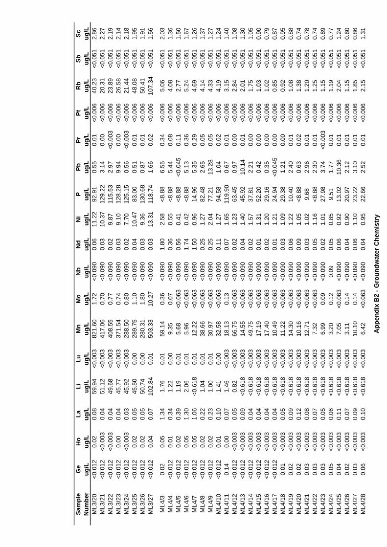
Sam
ple
Num
ber
ML3
/20
ML3
/21
ML3
/22
ML3
/23
ML3
/24
ML3
/25
ML3
/26
ML3
/27
ML4
/3M
L4/4
ML4
/5M
L4/6
ML4
/7M
L4/8
ML4
/9M
L4/1
0M
L4/1
1M
L4/1
2M
L4/1
3M
L4/1
4M
L4/1
5M
L4/1
6M
L4/1
7M
L4/1
8M
L4/1
9M
L4/2
0M
L4/2
1M
L4/2
2M
L4/2
3M
L4/2
4M
L4/2
5M
L4/2
6M
L4/2
7M
L4/2
8
Ge
Ho
LaLi
LuM
nM
oN
bN
dN
iP
PbPr
PtR
bSb
Scug
/Lug
/Lug
/Lug
/Lug
/Lug
/Lug
/Lug
/Lug
/Lug
/Lug
/Lug
/Lug
/Lug
/Lug
/Lug
/Lug
/L<0
.012
0.02
0.08
59.9
4<0
.003
821.
601.
72<0
.090
0.06
11.2
292
.91
0.55
0.01
<0.0
0640
.23
<0.0
512.
86<0
.012
<0.0
030.
0451
.12
<0.0
0341
7.06
0.70
<0.0
900.
0310
.37
129.
223.
140.
00<0
.006
20.3
1<0
.051
2.27
<0.0
12<0
.003
0.04
49.6
8<0
.003
408.
550.
77<0
.090
0.02
9.87
115.
532.
97<0
.003
<0.0
0623
.89
<0.0
512.
19<0
.012
0.00
0.04
45.7
7<0
.003
371.
540.
74<0
.090
0.03
9.10
128.
289.
940.
00<0
.006
26.5
8<0
.051
2.14
<0.0
12<0
.003
0.03
45.9
2<0
.003
288.
500.
80<0
.090
0.02
7.70
125.
150.
56<0
.003
<0.0
0621
.44
<0.0
512.
18<0
.012
0.02
0.05
45.5
00.
0028
9.75
1.10
<0.0
900.
0410
.47
83.0
00.
510.
01<0
.006
48.0
8<0
.051
1.95
<0.0
120.
020.
0550
.74
0.00
280.
311.
80<0
.090
0.03
9.36
130.
680.
870.
01<0
.006
50.4
1<0
.051
1.91
<0.0
120.
040.
0710
2.84
0.01
503.
3310
.27
<0.0
900.
0313
.31
118.
741.
660.
02<0
.006
107.
34<0
.051
1.56
0.02
0.05
1.34
1.76
0.01
59.1
40.
36<0
.090
1.80
2.58
<8.8
86.
550.
34<0
.006
5.06
<0.0
512.
03<0
.012
0.01
0.34
1.22
0.00
9.35
0.07
<0.0
900.
360.
55<8
.88
5.44
0.08
<0.0
064.
08<0
.051
1.36
<0.0
120.
020.
391.
190.
015.
68<0
.063
<0.0
900.
560.
41<8
.88
<0.0
450.
11<0
.006
2.77
<0.0
511.
50<0
.012
0.05
1.30
2.06
0.01
5.96
<0.0
63<0
.090
1.74
0.42
<8.8
85.
130.
36<0
.006
5.24
<0.0
511.
67<0
.012
0.05
1.06
<0.6
180.
0112
.22
<0.0
63<0
.090
1.50
0.96
14.9
65.
350.
29<0
.006
4.69
<0.0
511.
26<0
.012
0.02
0.22
1.04
0.01
38.6
6<0
.063
<0.0
900.
251.
2782
.48
2.65
0.05
<0.0
064.
14<0
.051
1.37
<0.0
120.
020.
231.
000.
0130
.97
<0.0
63<0
.090
0.25
2.04
77.2
113
.28
0.05
<0.0
064.
33<0
.051
1.27
<0.0
120.
010.
101.
410.
0032
.58
<0.0
63<0
.090
0.11
1.27
94.5
81.
040.
02<0
.006
4.19
<0.0
511.
240.
140.
000.
071.
46<0
.003
18.1
30.
13<0
.090
0.07
1.65
119.
900.
670.
01<0
.006
3.15
<0.0
511.
40<0
.012
<0.0
030.
050.
82<0
.003
66.7
5<0
.063
<0.0
900.
021.
2363
.45
0.97
0.00
<0.0
062.
84<0
.051
1.08
<0.0
12<0
.003
0.09
<0.6
18<0
.003
14.5
5<0
.063
<0.0
900.
041.
4045
.92
10.1
40.
01<0
.006
2.01
<0.0
511.
30<0
.012
<0.0
030.
04<0
.618
<0.0
0349
.75
<0.0
63<0
.090
0.02
1.57
37.8
12.
210.
00<0
.006
1.75
<0.0
511.
05<0
.012
<0.0
030.
04<0
.618
<0.0
0317
.19
<0.0
63<0
.090
0.01
1.31
52.2
00.
420.
00<0
.006
1.03
<0.0
510.
90<0
.012
<0.0
030.
04<0
.618
<0.0
0317
.40
<0.0
63<0
.090
0.02
1.20
29.1
60.
350.
00<0
.006
1.02
<0.0
510.
79<0
.012
<0.0
030.
04<0
.618
<0.0
0310
.49
<0.0
63<0
.090
0.01
1.21
24.9
4<0
.045
0.00
<0.0
060.
85<0
.051
0.87
0.01
<0.0
030.
05<0
.618
<0.0
0311
.22
<0.0
63<0
.090
0.03
1.09
29.3
81.
210.
00<0
.006
0.92
<0.0
510.
950.
02<0
.003
0.09
<0.6
18<0
.003
14.3
0<0
.063
<0.0
900.
061.
2210
.40
2.40
0.01
<0.0
061.
08<0
.051
0.88
0.02
<0.0
030.
12<0
.618
<0.0
0310
.16
<0.0
63<0
.090
0.09
1.05
<8.8
80.
630.
02<0
.006
1.38
<0.0
510.
740.
03<0
.003
0.08
<0.6
18<0
.003
12.7
1<0
.063
<0.0
900.
031.
029.
682.
960.
01<0
.006
1.20
<0.0
510.
780.
03<0
.003
0.07
<0.6
18<0
.003
7.32
<0.0
63<0
.090
0.05
1.16
<8.8
82.
300.
01<0
.006
1.25
<0.0
510.
740.
03<0
.003
0.05
<0.6
18<0
.003
6.99
0.09
<0.0
900.
021.
0127
.98
3.74
<0.0
03<0
.006
1.15
<0.0
510.
890.
05<0
.003
0.06
<0.6
18<0
.003
3.20
0.12
0.09
0.05
0.85
9.51
1.77
0.01
<0.0
061.
19<0
.051
0.77
0.04
<0.0
030.
11<0
.618
<0.0
037.
05<0
.063
<0.0
900.
060.
9213
.02
10.3
60.
01<0
.006
2.04
<0.0
511.
240.
02<0
.003
0.07
<0.6
18<0
.003
3.11
0.14
<0.0
900.
040.
9020
.97
2.12
0.01
<0.0
061.
15<0
.051
0.80
0.03
<0.0
030.
09<0
.618
<0.0
0310
.10
0.14
<0.0
900.
061.
1023
.22
3.10
0.01
<0.0
061.
85<0
.051
0.86
0.06
<0.0
030.
10<0
.618
<0.0
036.
42<0
.063
<0.0
900.
040.
9522
.66
2.52
0.01
<0.0
062.
15<0
.051
1.31
App
endi
x B
2 - G
roun
dwat
er C
hem
istr
y
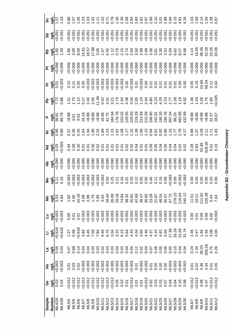
Sam
ple
Num
ber
ML4
/29
ML4
/30
ML5
/4M
L5/5
ML5
/6M
L5/7
ML5
/8M
L5/9
ML5
/10
ML5
/11
ML5
/12
ML5
/13
ML5
/14
ML5
/15
ML5
/16
ML5
/17
ML5
/18
ML5
/19
ML5
/20
ML5
/21
ML5
/22
ML5
/23
ML5
/26
ML5
/27
ML5
/28
ML5
/29
ML5
/30
ML6
/7M
L6/8
ML6
/9M
L6/1
0M
L6/1
1M
L6/1
2
Ge
Ho
LaLi
LuM
nM
oN
bN
dN
iP
PbPr
PtR
bSb
Scug
/Lug
/Lug
/Lug
/Lug
/Lug
/Lug
/Lug
/Lug
/Lug
/Lug
/Lug
/Lug
/Lug
/Lug
/Lug
/Lug
/L0.
03<0
.003
0.06
<0.6
18<0
.003
3.53
0.11
<0.0
900.
030.
9538
.91
7.72
0.01
<0.0
061.
60<0
.051
1.07
0.04
<0.0
030.
03<0
.618
<0.0
034.
840.
16<0
.090
<0.0
030.
8989
.79
0.86
<0.0
03<0
.006
1.28
<0.0
511.
33
<0.0
120.
010.
471.
270.
001.
82<0
.063
<0.0
900.
440.
37<8
.88
1.01
0.10
<0.0
061.
86<0
.051
0.86
<0.0
120.
030.
680.
680.
014.
56<0
.063
<0.0
901.
080.
369.
611.
700.
21<0
.006
3.09
<0.0
511.
07<0
.012
0.02
0.14
<0.6
180.
0110
.16
<0.0
63<0
.090
0.30
0.45
9.52
1.12
0.05
<0.0
068.
09<0
.051
1.06
<0.0
12<0
.003
0.04
4.84
<0.0
034.
08<0
.063
<0.0
900.
011.
6416
.18
5.27
0.00
<0.0
0624
.81
<0.0
511.
24<0
.012
<0.0
030.
046.
45<0
.003
3.99
<0.0
63<0
.090
0.01
1.94
<8.8
82.
40<0
.003
<0.0
0618
.57
<0.0
511.
03<0
.012
<0.0
030.
037.
56<0
.003
1.79
<0.0
63<0
.090
0.00
1.90
<8.8
82.
00<0
.003
<0.0
0617
.88
<0.0
511.
02<0
.012
<0.0
030.
037.
84<0
.003
2.90
<0.0
63<0
.090
0.02
2.26
<8.8
811
.46
<0.0
03<0
.006
3.06
<0.0
511.
11<0
.012
<0.0
030.
029.
40<0
.003
3.53
<0.0
63<0
.090
0.01
1.89
18.0
80.
42<0
.003
<0.0
061.
57<0
.051
1.02
<0.0
12<0
.003
0.03
6.75
<0.0
0328
.44
0.50
<0.0
900.
011.
2442
.75
4.01
<0.0
03<0
.006
0.45
<0.0
510.
71<0
.012
<0.0
030.
033.
04<0
.003
26.0
90.
25<0
.090
0.01
1.15
184.
943.
21<0
.003
<0.0
061.
12<0
.051
0.78
0.05
<0.0
030.
043.
23<0
.003
29.1
80.
21<0
.090
0.01
1.02
176.
781.
74<0
.003
<0.0
060.
79<0
.051
1.30
0.02
<0.0
030.
036.
15<0
.003
74.8
40.
16<0
.090
0.01
1.08
153.
021.
62<0
.003
<0.0
062.
15<0
.051
2.30
0.01
<0.0
030.
045.
64<0
.003
38.3
20.
31<0
.090
0.02
1.17
129.
554.
380.
00<0
.006
2.74
<0.0
512.
68<0
.012
<0.0
030.
044.
33<0
.003
45.8
10.
33<0
.090
0.02
1.15
225.
933.
04<0
.003
<0.0
062.
94<0
.051
2.84
0.01
0.01
0.11
4.04
<0.0
0342
.69
0.12
<0.0
900.
041.
3921
9.28
2.95
0.01
<0.0
063.
50<0
.051
3.60
0.01
<0.0
030.
023.
65<0
.003
38.4
70.
55<0
.090
0.01
1.06
214.
591.
24<0
.003
<0.0
062.
99<0
.051
2.82
<0.0
12<0
.003
0.04
4.40
<0.0
0336
.82
0.50
<0.0
900.
011.
1021
5.59
2.44
0.00
<0.0
062.
99<0
.051
2.97
0.02
0.01
0.07
4.37
<0.0
0323
.28
0.46
<0.0
900.
060.
9419
6.80
4.80
0.01
<0.0
063.
36<0
.051
2.89
0.03
0.00
0.08
4.15
<0.0
0321
.87
0.11
<0.0
900.
050.
9115
2.81
3.23
0.01
<0.0
063.
81<0
.051
3.10
0.03
0.00
0.05
4.82
<0.0
0348
.54
0.16
<0.0
900.
040.
9219
0.30
4.29
0.01
<0.0
063.
30<0
.051
3.01
0.07
0.00
0.06
5.59
<0.0
0356
.57
0.09
<0.0
900.
050.
8619
0.76
2.23
0.01
<0.0
063.
52<0
.051
2.88
0.04
<0.0
030.
0517
.39
<0.0
0367
.73
<0.0
63<0
.090
0.04
1.15
397.
541.
770.
01<0
.006
5.59
<0.0
513.
940.
04<0
.003
0.10
26.2
9<0
.003
278.
230.
09<0
.090
0.04
1.77
98.2
92.
390.
01<0
.006
6.62
<0.0
515.
150.
19<0
.003
0.04
31.6
5<0
.003
116.
64<0
.063
<0.0
900.
022.
7948
2.85
1.19
0.00
<0.0
068.
27<0
.051
4.81
0.08
<0.0
030.
0431
.74
<0.0
0324
0.12
<0.0
63<0
.090
0.02
4.27
432.
894.
920.
00<0
.006
8.68
<0.0
514.
26
<0.0
120.
010.
242.
460.
0011
.51
0.00
<0.0
900.
280.
88<8
.88
1.36
0.05
<0.0
064.
14<0
.051
1.03
<0.0
120.
021.
342.
470.
0118
.21
0.00
<0.0
900.
831.
07<8
.88
1.43
0.19
<0.0
0616
.05
<0.0
511.
590.
080.
4636
.03
1.84
0.09
111.
620.
00<0
.090
52.4
93.
29<8
.88
3.28
10.6
6<0
.006
38.4
6<0
.051
2.14
0.47
4.34
359.
262.
460.
9915
5.38
0.00
<0.0
9031
8.18
2.11
<8.8
81.
7558
.24
<0.0
0642
.28
<0.0
511.
59<0
.012
0.01
0.75
3.08
0.00
6.44
0.24
<0.0
900.
521.
7132
.37
1.85
0.12
<0.0
0623
.26
<0.0
511.
08<0
.012
0.00
0.26
4.00
<0.0
037.
640.
00<0
.090
0.19
1.45
28.6
7<0
.045
0.04
<0.0
0620
.06
<0.0
510.
87
App
endi
x B
2 - G
roun
dwat
er C
hem
istr
y
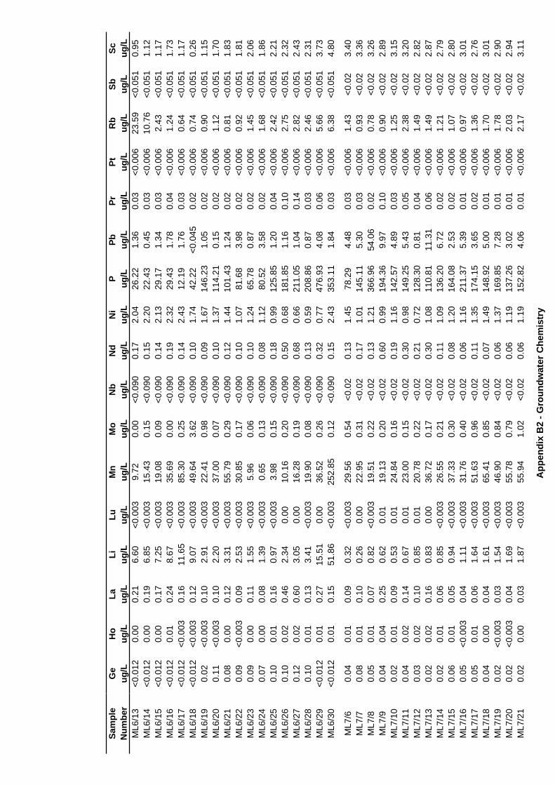
Sam
ple
Num
ber
ML6
/13
ML6
/14
ML6
/15
ML6
/16
ML6
/17
ML6
/18
ML6
/19
ML6
/20
ML6
/21
ML6
/22
ML6
/23
ML6
/24
ML6
/25
ML6
/26
ML6
/27
ML6
/28
ML6
/29
ML6
/30
ML7
/6M
L7/7
ML7
/8M
L7/9
ML7
/10
ML7
/11
ML7
/12
ML7
/13
ML7
/14
ML7
/15
ML7
/16
ML7
/17
ML7
/18
ML7
/19
ML7
/20
ML7
/21
Ge
Ho
LaLi
LuM
nM
oN
bN
dN
iP
PbPr
PtR
bSb
Scug
/Lug
/Lug
/Lug
/Lug
/Lug
/Lug
/Lug
/Lug
/Lug
/Lug
/Lug
/Lug
/Lug
/Lug
/Lug
/Lug
/L<0
.012
0.00
0.21
6.60
<0.0
039.
720.
00<0
.090
0.17
2.04
26.2
21.
360.
03<0
.006
23.5
9<0
.051
0.95
<0.0
120.
000.
196.
85<0
.003
15.4
30.
15<0
.090
0.15
2.20
22.4
30.
450.
03<0
.006
10.7
6<0
.051
1.12
<0.0
120.
000.
177.
25<0
.003
19.0
80.
09<0
.090
0.14
2.13
29.1
71.
340.
03<0
.006
2.43
<0.0
511.
17<0
.012
0.01
0.24
8.67
<0.0
0335
.69
0.00
<0.0
900.
192.
3229
.43
1.78
0.04
<0.0
061.
24<0
.051
1.73
<0.0
12<0
.003
0.16
11.6
5<0
.003
85.3
00.
25<0
.090
0.14
2.43
12.1
91.
760.
03<0
.006
0.64
<0.0
511.
17<0
.012
<0.0
030.
129.
07<0
.003
49.6
43.
62<0
.090
0.10
1.74
42.2
2<0
.045
0.02
<0.0
060.
74<0
.051
0.26
0.02
<0.0
030.
102.
91<0
.003
22.4
10.
98<0
.090
0.09
1.67
146.
231.
050.
02<0
.006
0.90
<0.0
511.
150.
11<0
.003
0.10
2.20
<0.0
0337
.00
0.07
<0.0
900.
101.
3711
4.21
0.15
0.02
<0.0
061.
12<0
.051
1.70
0.08
0.00
0.12
3.31
<0.0
0355
.79
0.29
<0.0
900.
121.
4410
1.43
1.24
0.02
<0.0
060.
81<0
.051
1.83
0.09
<0.0
030.
092.
53<0
.003
30.8
50.
17<0
.090
0.10
1.07
81.6
83.
980.
02<0
.006
0.92
<0.0
511.
810.
090.
000.
111.
55<0
.003
5.96
0.06
<0.0
900.
101.
2465
.78
0.87
0.02
<0.0
061.
45<0
.051
2.06
0.07
0.00
0.08
1.39
<0.0
030.
650.
13<0
.090
0.08
1.12
80.5
23.
580.
02<0
.006
1.68
<0.0
511.
860.
100.
010.
160.
97<0
.003
3.98
0.15
<0.0
900.
180.
9912
5.85
1.20
0.04
<0.0
062.
42<0
.051
2.21
0.10
0.02
0.46
2.34
0.00
10.1
60.
20<0
.090
0.50
0.68
181.
851.
160.
10<0
.006
2.75
<0.0
512.
320.
120.
020.
603.
050.
0016
.28
0.19
<0.0
900.
680.
6621
1.05
1.04
0.14
<0.0
062.
82<0
.051
2.43
0.10
0.01
0.13
3.41
<0.0
0319
.90
0.08
<0.0
900.
130.
5920
8.86
0.87
0.03
<0.0
062.
46<0
.051
2.31
<0.0
120.
010.
2715
.51
0.00
36.5
20.
26<0
.090
0.32
0.77
476.
934.
080.
06<0
.006
5.66
<0.0
513.
73<0
.012
0.01
0.15
51.8
6<0
.003
252.
850.
12<0
.090
0.15
2.43
353.
111.
840.
03<0
.006
6.38
<0.0
514.
80
0.04
0.01
0.09
0.32
<0.0
0329
.56
0.54
<0.0
20.
131.
4578
.29
4.48
0.03
<0.0
061.
43<0
.02
3.40
0.08
0.01
0.10
0.26
0.00
22.9
50.
31<0
.02
0.17
1.01
145.
115.
300.
03<0
.006
0.93
<0.0
23.
360.
050.
010.
070.
82<0
.003
19.5
10.
22<0
.02
0.13
1.21
366.
9654
.06
0.02
<0.0
060.
78<0
.02
3.26
0.04
0.04
0.25
0.62
0.01
19.1
30.
20<0
.02
0.60
0.99
194.
369.
970.
10<0
.006
0.90
<0.0
22.
890.
020.
010.
090.
530.
0124
.84
0.16
<0.0
20.
191.
1614
2.57
4.89
0.03
<0.0
061.
25<0
.02
3.15
0.04
0.02
0.14
0.67
0.01
23.0
00.
15<0
.02
0.30
0.98
149.
255.
430.
05<0
.006
2.38
<0.0
23.
200.
030.
020.
100.
850.
0120
.78
0.22
<0.0
20.
210.
7212
8.30
0.81
0.04
<0.0
061.
49<0
.02
2.82
0.02
0.02
0.16
0.83
0.00
36.7
20.
17<0
.02
0.30
1.08
110.
8111
.31
0.06
<0.0
061.
49<0
.02
2.87
0.02
0.01
0.06
0.85
<0.0
0326
.55
0.21
<0.0
20.
111.
0913
6.20
6.72
0.02
<0.0
061.
21<0
.02
2.79
0.06
0.01
0.05
0.94
<0.0
0337
.33
0.30
<0.0
20.
081.
2016
4.08
2.53
0.02
<0.0
061.
07<0
.02
2.80
0.05
<0.0
030.
041.
11<0
.003
31.7
60.
40<0
.02
0.06
1.16
211.
375.
390.
01<0
.006
0.97
<0.0
23.
010.
050.
010.
061.
64<0
.003
51.6
30.
96<0
.02
0.11
1.35
174.
153.
650.
02<0
.006
1.36
<0.0
22.
760.
040.
000.
041.
61<0
.003
65.4
10.
85<0
.02
0.07
1.49
148.
925.
000.
01<0
.006
1.70
<0.0
23.
010.
02<0
.003
0.03
1.54
<0.0
0346
.90
0.84
<0.0
20.
061.
3716
9.85
7.28
0.01
<0.0
061.
78<0
.02
2.90
0.02
<0.0
030.
041.
69<0
.003
55.7
80.
79<0
.02
0.06
1.19
137.
263.
020.
01<0
.006
2.03
<0.0
22.
940.
020.
000.
031.
87<0
.003
55.9
41.
02<0
.02
0.06
1.19
152.
824.
060.
01<0
.006
2.17
<0.0
23.
11
App
endi
x B
2 - G
roun
dwat
er C
hem
istr
y
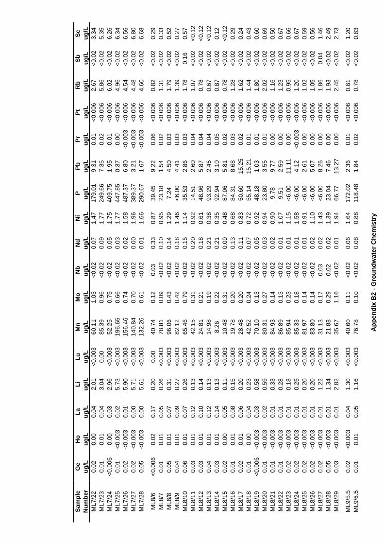
Sam
ple
Num
ber
ML7
/22
ML7
/23
ML7
/24
ML7
/25
ML7
/26
ML7
/27
ML7
/28
ML8
/6M
L8/7
ML8
/8M
L8/9
ML8
/10
ML8
/11
ML8
/12
ML8
/13
ML8
/14
ML8
/15
ML8
/16
ML8
/17
ML8
/18
ML8
/19
ML8
/20
ML8
/21
ML8
/22
ML8
/23
ML8
/24
ML8
/25
ML8
/26
ML8
/27
ML8
/28
ML8
/29
ML9
/5.5
ML9
/6.5
Ge
Ho
LaLi
LuM
nM
oN
bN
dN
iP
PbPr
PtR
bSb
Scug
/Lug
/Lug
/Lug
/Lug
/Lug
/Lug
/Lug
/Lug
/Lug
/Lug
/Lug
/Lug
/Lug
/Lug
/Lug
/Lug
/L0.
020.
000.
042.
01<0
.003
60.1
11.
03<0
.02
0.07
1.47
179.
019.
310.
01<0
.006
2.67
<0.0
23.
340.
010.
010.
043.
040.
0085
.39
0.96
<0.0
20.
091.
7724
9.66
7.35
0.02
<0.0
065.
86<0
.02
5.35
<0.0
060.
000.
032.
96<0
.003
52.2
50.
75<0
.02
0.05
1.75
409.
751.
950.
01<0
.006
6.02
<0.0
26.
260.
01<0
.003
0.02
5.73
<0.0
0319
6.65
0.66
<0.0
20.
031.
7744
7.85
0.37
0.00
<0.0
064.
96<0
.02
6.34
0.02
<0.0
030.
015.
90<0
.003
156.
460.
74<0
.02
0.02
1.58
487.
376.
80<0
.003
<0.0
064.
54<0
.02
6.56
0.02
<0.0
030.
005.
71<0
.003
140.
840.
70<0
.02
0.00
1.96
389.
373.
21<0
.003
<0.0
064.
48<0
.02
6.80
0.05
<0.0
030.
005.
61<0
.003
132.
260.
61<0
.02
0.01
1.66
290.
671.
67<0
.003
<0.0
064.
60<0
.02
6.68
<0.0
060.
020.
170.
200.
0040
.74
0.12
0.03
0.33
0.87
39.4
59.
220.
06<0
.006
0.82
<0.0
20.
290.
010.
010.
050.
26<0
.003
78.8
10.
09<0
.02
0.10
0.95
23.1
81.
540.
02<0
.006
1.31
<0.0
20.
330.
050.
010.
070.
31<0
.003
96.0
60.
43<0
.02
0.14
1.29
7.24
4.50
0.03
<0.0
061.
79<0
.02
0.52
0.04
0.01
0.09
0.27
<0.0
0382
.12
0.42
<0.0
20.
181.
46<6
.00
4.41
0.03
<0.0
061.
39<0
.02
0.27
0.06
0.01
0.07
0.26
<0.0
0365
.46
0.79
<0.0
20.
151.
1435
.53
2.86
0.03
<0.0
061.
780.
160.
570.
030.
010.
120.
13<0
.003
42.1
50.
31<0
.02
0.20
0.92
14.5
12.
600.
04<0
.006
1.07
<0.0
2<0
.12
0.03
0.01
0.10
0.14
<0.0
0324
.81
0.21
<0.0
20.
180.
6148
.96
5.87
0.04
<0.0
060.
78<0
.02
<0.1
20.
040.
010.
120.
13<0
.003
14.9
80.
19<0
.02
0.21
0.38
93.2
92.
450.
04<0
.006
0.67
<0.0
2<0
.12
0.03
0.01
0.14
0.13
<0.0
038.
260.
22<0
.02
0.21
0.35
92.9
43.
100.
05<0
.006
0.87
<0.0
20.
120.
020.
000.
050.
11<0
.003
10.4
80.
31<0
.02
0.09
0.48
87.0
65.
810.
02<0
.006
0.78
<0.0
2<0
.12
0.01
0.01
0.08
0.15
<0.0
0319
.78
0.20
<0.0
20.
130.
6884
.31
8.68
0.03
<0.0
061.
28<0
.02
0.29
0.02
0.01
0.06
0.20
<0.0
0328
.48
0.20
<0.0
20.
110.
8350
.60
15.2
50.
02<0
.006
1.62
<0.0
20.
240.
010.
000.
040.
23<0
.003
42.5
20.
24<0
.02
0.07
0.72
55.1
415
.21
0.01
<0.0
061.
44<0
.02
0.43
<0.0
06<0
.003
0.03
0.58
<0.0
0370
.10
0.13
<0.0
20.
050.
9248
.18
1.03
0.01
<0.0
061.
80<0
.02
0.60
0.01
<0.0
030.
020.
59<0
.003
80.3
10.
27<0
.02
0.03
0.94
23.8
03.
550.
01<0
.006
2.02
<0.0
20.
690.
01<0
.003
0.01
0.33
<0.0
0384
.93
0.14
<0.0
20.
020.
909.
789.
770.
00<0
.006
1.16
<0.0
20.
500.
01<0
.003
0.01
0.28
<0.0
0386
.89
0.13
<0.0
20.
011.
079.
512.
590.
00<0
.006
1.23
<0.0
20.
670.
02<0
.003
0.01
0.18
<0.0
0385
.94
0.23
<0.0
20.
011.
15<6
.00
11.1
10.
00<0
.006
0.95
<0.0
20.
660.
02<0
.003
0.01
0.25
<0.0
0385
.33
0.18
<0.0
20.
011.
58<6
.00
4.12
<0.0
03<0
.006
1.20
<0.0
20.
670.
02<0
.003
0.01
0.20
<0.0
0381
.97
0.14
<0.0
20.
010.
91<6
.00
2.61
0.00
<0.0
061.
02<0
.02
0.59
0.02
<0.0
030.
010.
20<0
.003
83.8
00.
14<0
.02
0.02
1.10
<6.0
05.
070.
00<0
.006
1.05
<0.0
20.
560.
02<0
.003
0.01
1.22
<0.0
0331
.13
0.17
0.03
0.02
1.43
<6.0
08.
260.
00<0
.006
1.86
0.04
1.46
0.05
<0.0
030.
011.
34<0
.003
21.8
80.
290.
020.
021.
3923
.04
7.46
0.00
<0.0
061.
93<0
.02
2.49
0.03
<0.0
030.
012.
82<0
.003
35.6
71.
16<0
.02
0.01
1.94
66.7
713
.27
0.00
<0.0
062.
45<0
.02
2.73
0.02
<0.0
030.
041.
30<0
.003
40.6
00.
11<0
.02
0.06
1.64
172.
022.
360.
01<0
.006
0.61
<0.0
21.
200.
010.
010.
051.
16<0
.003
76.7
80.
10<0
.02
0.08
0.88
118.
481.
840.
02<0
.006
0.78
<0.0
20.
83
App
endi
x B
2 - G
roun
dwat
er C
hem
istr
y
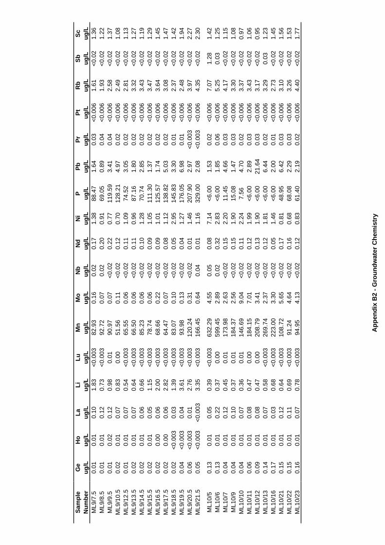
Sam
ple
Num
ber
ML9
/7.5
ML9
/8.5
ML9
/9.5
ML9
/10.
5M
L9/1
2.5
ML9
/13.
5M
L9/1
4.5
ML9
/15.
5M
L9/1
6.5
ML9
/17.
5M
L9/1
8.5
ML9
/19.
5M
L9/2
0.5
ML9
/21.
5
ML1
0/5
ML1
0/6
ML1
0/7
ML1
0/9
ML1
0/10
ML1
0/11
ML1
0/12
ML1
0/13
ML1
0/16
ML1
0/21
ML1
0/22
ML1
0/23
Ge
Ho
LaLi
LuM
nM
oN
bN
dN
iP
PbPr
PtR
bSb
Scug
/Lug
/Lug
/Lug
/Lug
/Lug
/Lug
/Lug
/Lug
/Lug
/Lug
/Lug
/Lug
/Lug
/Lug
/Lug
/Lug
/L0.
010.
010.
101.
83<0
.003
82.9
30.
160.
020.
171.
3888
.47
1.64
0.03
<0.0
061.
61<0
.02
1.36
0.01
0.01
0.12
0.73
<0.0
0392
.72
0.07
0.02
0.20
0.91
69.0
50.
890.
04<0
.006
1.93
<0.0
21.
220.
010.
020.
120.
980.
0190
.97
0.07
<0.0
20.
220.
7711
9.59
3.41
0.04
<0.0
062.
58<0
.02
1.37
0.02
0.01
0.07
0.83
0.00
51.5
60.
11<0
.02
0.12
0.70
128.
214.
970.
02<0
.006
2.49
<0.0
21.
080.
010.
010.
070.
54<0
.003
65.5
50.
06<0
.02
0.11
1.09
74.5
23.
050.
02<0
.006
2.81
<0.0
21.
130.
020.
010.
070.
64<0
.003
66.5
00.
06<0
.02
0.11
0.96
87.1
61.
800.
02<0
.006
3.32
<0.0
21.
270.
020.
010.
060.
66<0
.003
85.2
30.
06<0
.02
0.10
1.28
70.7
42.
850.
02<0
.006
3.43
<0.0
21.
190.
020.
010.
051.
15<0
.003
78.7
40.
06<0
.02
0.09
1.05
111.
301.
370.
02<0
.006
3.47
<0.0
21.
290.
020.
000.
062.
00<0
.003
68.6
60.
22<0
.02
0.09
1.01
125.
571.
740.
02<0
.006
3.64
<0.0
21.
450.
020.
000.
062.
82<0
.003
64.4
70.
07<0
.02
0.08
1.12
138.
825.
030.
02<0
.006
3.08
<0.0
21.
470.
02<0
.003
0.03
1.39
<0.0
0383
.07
0.10
<0.0
20.
052.
9514
5.83
3.30
0.01
<0.0
062.
37<0
.02
1.42
0.04
<0.0
030.
043.
61<0
.003
93.9
80.
13<0
.02
0.04
1.27
176.
056.
980.
01<0
.006
2.48
<0.0
21.
940.
06<0
.003
0.01
2.76
<0.0
0312
0.24
0.31
<0.0
20.
011.
4620
7.90
2.97
<0.0
03<0
.006
3.97
<0.0
22.
270.
05<0
.003
<0.0
033.
35<0
.003
166.
450.
640.
040.
011.
1632
9.00
2.08
<0.0
03<0
.006
4.35
<0.0
22.
30
0.13
0.01
0.05
0.39
<0.0
0363
2.29
4.55
0.05
0.08
7.14
<6.0
01.
530.
02<0
.006
7.07
1.28
1.42
0.13
0.01
0.22
0.37
0.00
599.
452.
890.
020.
322.
83<6
.00
1.85
0.06
<0.0
065.
250.
031.
250.
040.
010.
120.
450.
0117
3.98
2.63
<0.0
20.
152.
2011
.45
4.66
0.03
<0.0
064.
17<0
.02
1.15
0.04
0.01
0.10
0.37
0.01
184.
372.
56<0
.02
0.15
1.90
15.0
81.
470.
03<0
.006
3.30
<0.0
21.
080.
040.
010.
070.
360.
0114
6.69
9.04
<0.0
20.
112.
247.
564.
700.
02<0
.006
3.37
<0.0
20.
970.
060.
010.
080.
470.
0018
4.15
7.01
<0.0
20.
121.
99<6
.00
2.89
0.03
<0.0
063.
43<0
.02
1.06
0.09
0.01
0.08
0.47
0.00
208.
793.
41<0
.02
0.13
1.90
<6.0
021
.64
0.03
<0.0
063.
17<0
.02
0.95
0.14
0.01
0.07
0.58
<0.0
0326
9.74
2.37
<0.0
20.
121.
81<6
.00
6.44
0.02
<0.0
063.
290.
031.
230.
170.
010.
030.
68<0
.003
223.
003.
30<0
.02
0.05
1.46
<6.0
02.
000.
01<0
.006
2.73
<0.0
21.
450.
150.
010.
120.
64<0
.003
108.
725.
65<0
.02
0.17
0.81
48.9
56.
420.
03<0
.006
3.10
<0.0
21.
560.
150.
010.
110.
69<0
.003
91.2
44.
64<0
.02
0.16
0.68
68.0
82.
290.
03<0
.006
3.26
<0.0
21.
530.
160.
010.
070.
78<0
.003
94.9
54.
13<0
.02
0.12
0.83
61.4
02.
190.
02<0
.006
4.40
<0.0
21.
77
App
endi
x B
2 - G
roun
dwat
er C
hem
istr
y
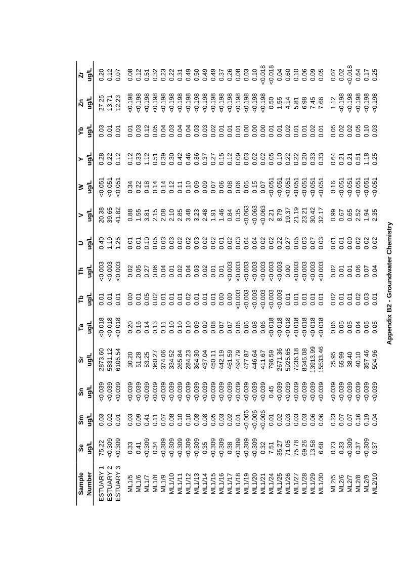
Sam
ple
Num
ber
ES
TUA
RY
1E
STU
AR
Y 2
ES
TUA
RY
3
ML1
/5M
L1/6
ML1
/7M
L1/8
ML1
/9M
L1/1
0M
L1/1
1M
L1/1
2M
L1/1
3M
L1/1
4M
L1/1
5M
L1/1
6M
L1/1
7M
L1/1
8M
L1/1
9M
L1/2
0M
L1/2
1M
L1/2
4M
L1/2
5M
L1/2
6M
L1/2
7M
L1/2
8M
L1/2
9M
L1/3
0
ML2
/5M
L2/6
ML2
/7M
L2/8
ML2
/9M
L2/1
0
SeSm
SnSr
TaTb
ThU
VW
YYb
ZnZr
ug/L
ug/L
ug/L
ug/L
ug/L
ug/L
ug/L
ug/L
ug/L
ug/L
ug/L
ug/L
ug/L
ug/L
75.2
20.
03<0
.039
2873
.60
<0.0
180.
01<0
.003
0.40
20.3
8<0
.051
0.28
0.03
27.2
50.
20<0
.309
0.02
<0.0
3958
31.1
2<0
.018
0.01
<0.0
031.
1939
.65
<0.0
510.
220.
0113
.71
0.12
<0.3
090.
01<0
.039
6105
.54
<0.0
180.
01<0
.003
1.25
41.8
2<0
.051
0.12
0.01
12.2
30.
07
0.33
0.03
<0.0
3930
.20
0.20
0.00
0.02
0.01
0.88
0.34
0.12
0.01
<0.1
980.
080.
410.
09<0
.039
51.2
80.
160.
010.
050.
011.
550.
220.
330.
03<0
.198
0.12
<0.3
090.
41<0
.039
53.2
50.
140.
050.
270.
103.
810.
181.
120.
12<0
.198
0.51
0.34
0.11
<0.0
3936
0.27
0.13
0.02
0.06
0.05
2.15
0.14
0.51
0.05
<0.1
980.
32<0
.309
0.07
<0.0
3937
4.06
0.11
0.01
0.04
0.03
2.08
0.14
0.39
0.04
<0.1
980.
23<0
.309
0.08
<0.0
3933
4.52
0.10
0.01
0.01
0.03
2.10
0.12
0.30
0.03
<0.1
980.
22<0
.309
0.10
<0.0
3926
5.84
0.10
0.01
0.02
0.02
2.85
0.11
0.42
0.04
<0.1
980.
31<0
.309
0.10
<0.0
3928
4.23
0.10
0.02
0.04
0.02
3.48
0.10
0.46
0.04
<0.1
980.
49<0
.309
0.08
<0.0
3936
4.30
0.09
0.01
0.03
0.03
3.23
0.09
0.36
0.03
<0.1
980.
500.
350.
08<0
.039
437.
040.
090.
010.
020.
022.
480.
090.
370.
03<0
.198
0.49
<0.3
090.
05<0
.039
450.
110.
080.
010.
010.
021.
910.
070.
270.
02<0
.198
0.49
<0.3
090.
03<0
.039
442.
190.
070.
000.
010.
011.
460.
060.
150.
01<0
.198
0.37
0.38
0.02
<0.0
3946
1.59
0.07
0.00
<0.0
030.
020.
840.
080.
120.
01<0
.198
0.26
<0.3
090.
01<0
.039
494.
790.
06<0
.003
<0.0
030.
030.
350.
060.
090.
01<0
.198
0.08
<0.3
09<0
.006
<0.0
3947
7.87
0.06
<0.0
03<0
.003
0.04
<0.0
630.
050.
030.
00<0
.198
0.03
<0.3
09<0
.006
<0.0
3944
6.64
0.08
<0.0
03<0
.003
0.04
<0.0
630.
150.
020.
00<0
.198
0.10
0.32
<0.0
06<0
.039
411.
670.
06<0
.003
<0.0
030.
02<0
.063
0.07
0.02
0.00
<0.1
98<0
.018
7.51
0.01
0.45
796.
59<0
.018
<0.0
03<0
.003
0.02
2.21
<0.0
510.
050.
010.
50<0
.018
35.2
70.
02<0
.039
2671
.36
<0.0
18<0
.003
<0.0
030.
228.
79<0
.051
0.10
0.01
1.55
0.04
71.0
50.
03<0
.039
5925
.65
<0.0
180.
010.
000.
2719
.37
<0.0
510.
220.
024.
140.
6075
.78
0.03
<0.0
3972
36.1
8<0
.018
0.01
<0.0
030.
0521
.19
<0.0
510.
220.
015.
810.
1069
.26
0.03
<0.0
3983
45.0
8<0
.018
0.01
<0.0
030.
0323
.21
<0.0
510.
200.
016.
980.
0613
.58
0.06
<0.0
3913
913.
99<0
.018
0.01
<0.0
030.
0730
.42
<0.0
510.
330.
027.
450.
096.
680.
06<0
.039
1553
3.46
<0.0
180.
01<0
.003
0.03
32.1
7<0
.051
0.33
0.01
7.66
0.05
0.73
0.23
<0.0
3925
.95
0.06
0.02
0.02
0.01
0.99
0.16
0.64
0.05
1.12
0.07
0.33
0.07
<0.0
3965
.99
0.05
0.01
0.01
0.01
0.67
<0.0
510.
210.
02<0
.198
0.02
<0.3
090.
07<0
.039
38.4
00.
050.
010.
010.
000.
65<0
.051
0.21
0.02
<0.1
98<0
.018
0.37
0.16
<0.0
3940
.10
0.04
0.02
0.06
0.02
2.52
<0.0
510.
510.
05<0
.198
0.64
<0.3
090.
19<0
.039
357.
460.
050.
030.
070.
021.
94<0
.051
1.18
0.10
<0.1
980.
170.
370.
04<0
.039
504.
960.
050.
010.
040.
022.
35<0
.051
0.25
0.03
<0.1
980.
25
App
endi
x B
2 - G
roun
dwat
er C
hem
istr
y
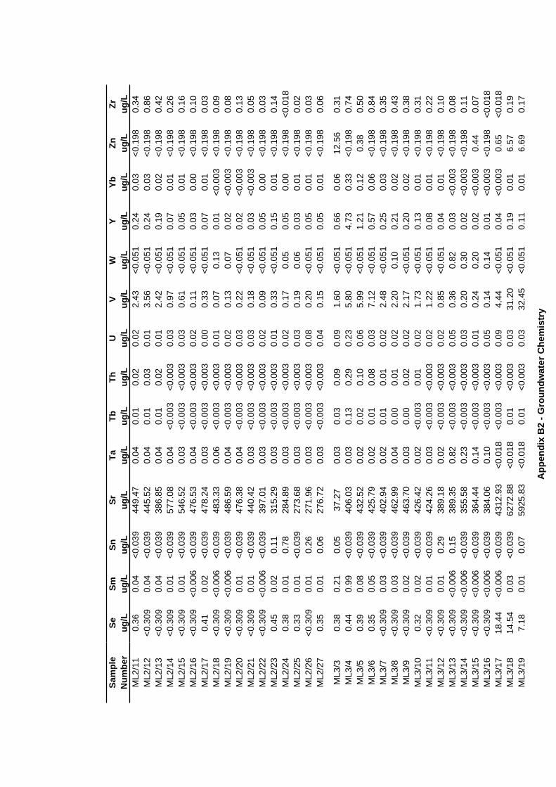
Sam
ple
Num
ber
ML2
/11
ML2
/12
ML2
/13
ML2
/14
ML2
/15
ML2
/16
ML2
/17
ML2
/18
ML2
/19
ML2
/20
ML2
/21
ML2
/22
ML2
/23
ML2
/24
ML2
/25
ML2
/26
ML2
/27
ML3
/3M
L3/4
ML3
/5M
L3/6
ML3
/7M
L3/8
ML3
/9M
L3/1
0M
L3/1
1M
L3/1
2M
L3/1
3M
L3/1
4M
L3/1
5M
L3/1
6M
L3/1
7M
L3/1
8M
L3/1
9
SeSm
SnSr
TaTb
ThU
VW
YYb
ZnZr
ug/L
ug/L
ug/L
ug/L
ug/L
ug/L
ug/L
ug/L
ug/L
ug/L
ug/L
ug/L
ug/L
ug/L
0.36
0.04
<0.0
3944
9.47
0.04
0.01
0.02
0.02
2.43
<0.0
510.
240.
03<0
.198
0.34
<0.3
090.
04<0
.039
445.
520.
040.
010.
030.
013.
56<0
.051
0.24
0.03
<0.1
980.
86<0
.309
0.04
<0.0
3938
6.85
0.04
0.01
0.02
0.01
2.42
<0.0
510.
190.
02<0
.198
0.42
<0.3
090.
01<0
.039
577.
080.
04<0
.003
<0.0
030.
030.
97<0
.051
0.07
0.01
<0.1
980.
26<0
.309
0.01
<0.0
3954
6.52
0.03
<0.0
03<0
.003
0.03
0.61
<0.0
510.
050.
01<0
.198
0.16
<0.3
09<0
.006
<0.0
3947
6.53
0.04
<0.0
03<0
.003
0.02
0.11
<0.0
510.
030.
00<0
.198
0.10
0.41
0.02
<0.0
3947
8.24
0.03
<0.0
03<0
.003
0.00
0.33
<0.0
510.
070.
01<0
.198
0.03
<0.3
09<0
.006
<0.0
3948
3.33
0.06
<0.0
03<0
.003
0.01
0.07
0.13
0.01
<0.0
03<0
.198
0.09
<0.3
09<0
.006
<0.0
3948
6.59
0.04
<0.0
03<0
.003
0.02
0.13
0.07
0.02
<0.0
03<0
.198
0.08
<0.3
090.
01<0
.039
476.
380.
04<0
.003
<0.0
030.
030.
22<0
.051
0.02
<0.0
03<0
.198
0.13
<0.3
090.
01<0
.039
440.
420.
03<0
.003
<0.0
030.
030.
18<0
.051
0.03
<0.0
03<0
.198
0.05
<0.3
09<0
.006
<0.0
3939
7.01
0.03
<0.0
03<0
.003
0.02
0.09
<0.0
510.
050.
00<0
.198
0.03
0.45
0.02
0.11
315.
290.
03<0
.003
<0.0
030.
010.
33<0
.051
0.15
0.01
<0.1
980.
140.
380.
010.
7828
4.89
0.03
<0.0
03<0
.003
0.02
0.17
0.05
0.05
0.00
<0.1
98<0
.018
0.33
0.01
<0.0
3927
3.68
0.03
<0.0
03<0
.003
0.03
0.19
0.06
0.03
0.01
<0.1
980.
02<0
.309
0.01
0.26
271.
960.
03<0
.003
<0.0
030.
080.
20<0
.051
0.05
0.01
<0.1
980.
030.
350.
010.
0627
6.72
0.03
<0.0
03<0
.003
0.04
0.15
<0.0
510.
050.
01<0
.198
0.06
0.38
0.21
0.05
37.2
70.
030.
030.
090.
091.
60<0
.051
0.66
0.06
12.5
60.
310.
440.
99<0
.039
406.
030.
030.
130.
290.
235.
80<0
.051
4.73
0.33
<0.1
980.
740.
390.
08<0
.039
432.
520.
020.
020.
100.
065.
99<0
.051
1.21
0.12
0.38
0.50
0.35
0.05
<0.0
3942
5.79
0.02
0.01
0.08
0.03
7.12
<0.0
510.
570.
06<0
.198
0.84
<0.3
090.
03<0
.039
402.
940.
020.
010.
010.
022.
48<0
.051
0.25
0.03
<0.1
980.
35<0
.309
0.03
<0.0
3946
2.99
0.04
0.00
0.01
0.02
2.20
0.10
0.21
0.02
<0.1
980.
43<0
.309
0.02
<0.0
3946
3.70
0.03
0.00
0.02
0.02
2.17
<0.0
510.
200.
02<0
.198
0.38
0.32
0.02
<0.0
3942
6.42
0.02
<0.0
030.
010.
021.
73<0
.051
0.13
0.01
<0.1
980.
31<0
.309
0.01
<0.0
3942
4.26
0.03
<0.0
03<0
.003
0.02
1.22
<0.0
510.
080.
01<0
.198
0.22
<0.3
090.
010.
2938
9.18
0.02
<0.0
03<0
.003
0.02
0.85
<0.0
510.
040.
01<0
.198
0.10
<0.3
09<0
.006
0.15
389.
350.
82<0
.003
<0.0
030.
050.
360.
820.
03<0
.003
<0.1
980.
08<0
.309
<0.0
06<0
.039
355.
580.
23<0
.003
<0.0
030.
030.
200.
300.
02<0
.003
<0.1
980.
11<0
.309
<0.0
06<0
.039
364.
440.
14<0
.003
<0.0
030.
010.
240.
200.
02<0
.003
0.44
0.07
<0.3
09<0
.006
<0.0
3938
4.06
0.10
<0.0
03<0
.003
0.05
0.14
0.14
0.01
<0.0
03<0
.198
<0.0
1818
.44
<0.0
06<0
.039
4312
.93
<0.0
18<0
.003
<0.0
030.
094.
44<0
.051
0.04
<0.0
030.
65<0
.018
14.5
40.
03<0
.039
6272
.88
<0.0
180.
01<0
.003
0.03
31.2
0<0
.051
0.19
0.01
6.57
0.19
7.18
0.01
0.07
5925
.83
<0.0
180.
01<0
.003
0.03
32.4
5<0
.051
0.11
0.01
6.69
0.17
App
endi
x B
2 - G
roun
dwat
er C
hem
istr
y
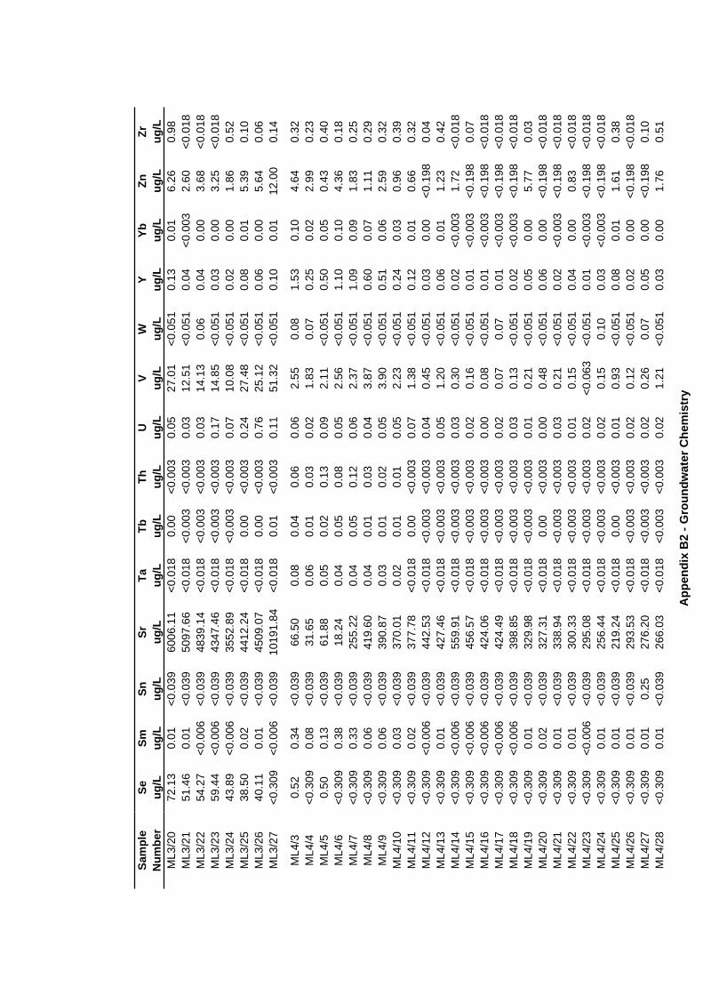
Sam
ple
Num
ber
ML3
/20
ML3
/21
ML3
/22
ML3
/23
ML3
/24
ML3
/25
ML3
/26
ML3
/27
ML4
/3M
L4/4
ML4
/5M
L4/6
ML4
/7M
L4/8
ML4
/9M
L4/1
0M
L4/1
1M
L4/1
2M
L4/1
3M
L4/1
4M
L4/1
5M
L4/1
6M
L4/1
7M
L4/1
8M
L4/1
9M
L4/2
0M
L4/2
1M
L4/2
2M
L4/2
3M
L4/2
4M
L4/2
5M
L4/2
6M
L4/2
7M
L4/2
8
SeSm
SnSr
TaTb
ThU
VW
YYb
ZnZr
ug/L
ug/L
ug/L
ug/L
ug/L
ug/L
ug/L
ug/L
ug/L
ug/L
ug/L
ug/L
ug/L
ug/L
72.1
30.
01<0
.039
6006
.11
<0.0
180.
00<0
.003
0.05
27.0
1<0
.051
0.13
0.01
6.26
0.98
51.4
60.
01<0
.039
5097
.66
<0.0
18<0
.003
<0.0
030.
0312
.51
<0.0
510.
04<0
.003
2.60
<0.0
1854
.27
<0.0
06<0
.039
4839
.14
<0.0
18<0
.003
<0.0
030.
0314
.13
0.06
0.04
0.00
3.68
<0.0
1859
.44
<0.0
06<0
.039
4347
.46
<0.0
18<0
.003
<0.0
030.
1714
.85
<0.0
510.
030.
003.
25<0
.018
43.8
9<0
.006
<0.0
3935
52.8
9<0
.018
<0.0
03<0
.003
0.07
10.0
8<0
.051
0.02
0.00
1.86
0.52
38.5
00.
02<0
.039
4412
.24
<0.0
180.
00<0
.003
0.24
27.4
8<0
.051
0.08
0.01
5.39
0.10
40.1
10.
01<0
.039
4509
.07
<0.0
180.
00<0
.003
0.76
25.1
2<0
.051
0.06
0.00
5.64
0.06
<0.3
09<0
.006
<0.0
3910
191.
84<0
.018
0.01
<0.0
030.
1151
.32
<0.0
510.
100.
0112
.00
0.14
0.52
0.34
<0.0
3966
.50
0.08
0.04
0.06
0.06
2.55
0.08
1.53
0.10
4.64
0.32
<0.3
090.
08<0
.039
31.6
50.
060.
010.
030.
021.
830.
070.
250.
022.
990.
230.
500.
13<0
.039
61.8
80.
050.
020.
130.
092.
11<0
.051
0.50
0.05
0.43
0.40
<0.3
090.
38<0
.039
18.2
40.
040.
050.
080.
052.
56<0
.051
1.10
0.10
4.36
0.18
<0.3
090.
33<0
.039
255.
220.
040.
050.
120.
062.
37<0
.051
1.09
0.09
1.83
0.25
<0.3
090.
06<0
.039
419.
600.
040.
010.
030.
043.
87<0
.051
0.60
0.07
1.11
0.29
<0.3
090.
06<0
.039
390.
870.
030.
010.
020.
053.
90<0
.051
0.51
0.06
2.59
0.32
<0.3
090.
03<0
.039
370.
010.
020.
010.
010.
052.
23<0
.051
0.24
0.03
0.96
0.39
<0.3
090.
02<0
.039
377.
78<0
.018
0.00
<0.0
030.
071.
38<0
.051
0.12
0.01
0.66
0.32
<0.3
09<0
.006
<0.0
3944
2.53
<0.0
18<0
.003
<0.0
030.
040.
45<0
.051
0.03
0.00
<0.1
980.
04<0
.309
0.01
<0.0
3942
7.46
<0.0
18<0
.003
<0.0
030.
051.
20<0
.051
0.06
0.01
1.23
0.42
<0.3
09<0
.006
<0.0
3955
9.91
<0.0
18<0
.003
<0.0
030.
030.
30<0
.051
0.02
<0.0
031.
72<0
.018
<0.3
09<0
.006
<0.0
3945
6.57
<0.0
18<0
.003
<0.0
030.
020.
16<0
.051
0.01
<0.0
03<0
.198
0.07
<0.3
09<0
.006
<0.0
3942
4.06
<0.0
18<0
.003
<0.0
030.
000.
08<0
.051
0.01
<0.0
03<0
.198
<0.0
18<0
.309
<0.0
06<0
.039
424.
49<0
.018
<0.0
03<0
.003
0.02
0.07
0.07
0.01
<0.0
03<0
.198
<0.0
18<0
.309
<0.0
06<0
.039
398.
85<0
.018
<0.0
03<0
.003
0.03
0.13
<0.0
510.
02<0
.003
<0.1
98<0
.018
<0.3
090.
01<0
.039
329.
98<0
.018
<0.0
03<0
.003
0.01
0.21
<0.0
510.
050.
005.
770.
03<0
.309
0.02
<0.0
3932
7.31
<0.0
180.
00<0
.003
0.00
0.48
<0.0
510.
060.
00<0
.198
<0.0
18<0
.309
0.01
<0.0
3933
8.94
<0.0
18<0
.003
<0.0
030.
030.
21<0
.051
0.02
<0.0
03<0
.198
<0.0
18<0
.309
0.01
<0.0
3930
0.33
<0.0
18<0
.003
<0.0
030.
010.
15<0
.051
0.04
0.00
0.83
<0.0
18<0
.309
<0.0
06<0
.039
295.
08<0
.018
<0.0
03<0
.003
0.02
<0.0
63<0
.051
0.01
<0.0
03<0
.198
<0.0
18<0
.309
0.01
<0.0
3925
6.44
<0.0
18<0
.003
<0.0
030.
020.
150.
100.
03<0
.003
<0.1
98<0
.018
<0.3
090.
01<0
.039
219.
24<0
.018
0.00
<0.0
030.
010.
93<0
.051
0.08
0.01
1.61
0.38
<0.3
090.
01<0
.039
293.
53<0
.018
<0.0
03<0
.003
0.02
0.12
<0.0
510.
020.
00<0
.198
<0.0
18<0
.309
0.01
0.25
276.
20<0
.018
<0.0
03<0
.003
0.02
0.26
0.07
0.05
0.00
<0.1
980.
10<0
.309
0.01
<0.0
3926
6.03
<0.0
18<0
.003
<0.0
030.
021.
21<0
.051
0.03
0.00
1.76
0.51
App
endi
x B
2 - G
roun
dwat
er C
hem
istr
y
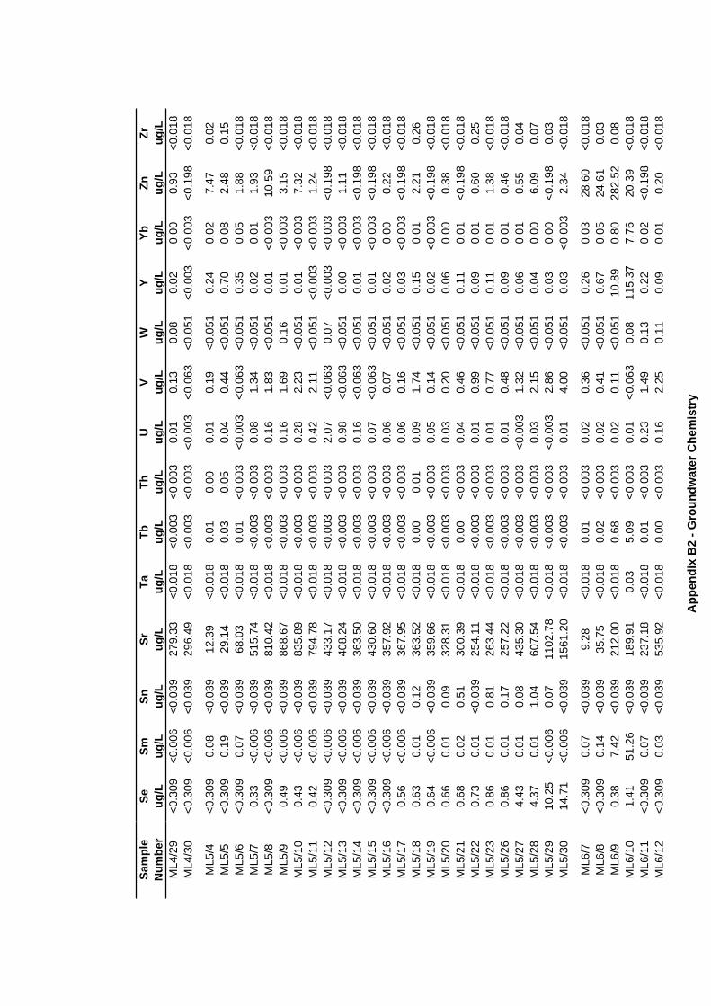
Sam
ple
Num
ber
ML4
/29
ML4
/30
ML5
/4M
L5/5
ML5
/6M
L5/7
ML5
/8M
L5/9
ML5
/10
ML5
/11
ML5
/12
ML5
/13
ML5
/14
ML5
/15
ML5
/16
ML5
/17
ML5
/18
ML5
/19
ML5
/20
ML5
/21
ML5
/22
ML5
/23
ML5
/26
ML5
/27
ML5
/28
ML5
/29
ML5
/30
ML6
/7M
L6/8
ML6
/9M
L6/1
0M
L6/1
1M
L6/1
2
SeSm
SnSr
TaTb
ThU
VW
YYb
ZnZr
ug/L
ug/L
ug/L
ug/L
ug/L
ug/L
ug/L
ug/L
ug/L
ug/L
ug/L
ug/L
ug/L
ug/L
<0.3
09<0
.006
<0.0
3927
9.33
<0.0
18<0
.003
<0.0
030.
010.
130.
080.
020.
000.
93<0
.018
<0.3
09<0
.006
<0.0
3929
6.49
<0.0
18<0
.003
<0.0
03<0
.003
<0.0
63<0
.051
<0.0
03<0
.003
<0.1
98<0
.018
<0.3
090.
08<0
.039
12.3
9<0
.018
0.01
0.00
0.01
0.19
<0.0
510.
240.
027.
470.
02<0
.309
0.19
<0.0
3929
.14
<0.0
180.
030.
050.
040.
44<0
.051
0.70
0.08
2.48
0.15
<0.3
090.
07<0
.039
68.0
3<0
.018
0.01
<0.0
03<0
.003
<0.0
63<0
.051
0.35
0.05
1.88
<0.0
180.
33<0
.006
<0.0
3951
5.74
<0.0
18<0
.003
<0.0
030.
081.
34<0
.051
0.02
0.01
1.93
<0.0
18<0
.309
<0.0
06<0
.039
810.
42<0
.018
<0.0
03<0
.003
0.16
1.83
<0.0
510.
01<0
.003
10.5
9<0
.018
0.49
<0.0
06<0
.039
868.
67<0
.018
<0.0
03<0
.003
0.16
1.69
0.16
0.01
<0.0
033.
15<0
.018
0.43
<0.0
06<0
.039
835.
89<0
.018
<0.0
03<0
.003
0.28
2.23
<0.0
510.
01<0
.003
7.32
<0.0
180.
42<0
.006
<0.0
3979
4.78
<0.0
18<0
.003
<0.0
030.
422.
11<0
.051
<0.0
03<0
.003
1.24
<0.0
18<0
.309
<0.0
06<0
.039
433.
17<0
.018
<0.0
03<0
.003
2.07
<0.0
630.
07<0
.003
<0.0
03<0
.198
<0.0
18<0
.309
<0.0
06<0
.039
408.
24<0
.018
<0.0
03<0
.003
0.98
<0.0
63<0
.051
0.00
<0.0
031.
11<0
.018
<0.3
09<0
.006
<0.0
3936
3.50
<0.0
18<0
.003
<0.0
030.
16<0
.063
<0.0
510.
01<0
.003
<0.1
98<0
.018
<0.3
09<0
.006
<0.0
3943
0.60
<0.0
18<0
.003
<0.0
030.
07<0
.063
<0.0
510.
01<0
.003
<0.1
98<0
.018
<0.3
09<0
.006
<0.0
3935
7.92
<0.0
18<0
.003
<0.0
030.
060.
07<0
.051
0.02
0.00
0.22
<0.0
180.
56<0
.006
<0.0
3936
7.95
<0.0
18<0
.003
<0.0
030.
060.
16<0
.051
0.03
<0.0
03<0
.198
<0.0
180.
630.
010.
1236
3.52
<0.0
180.
000.
010.
091.
74<0
.051
0.15
0.01
2.21
0.26
0.64
<0.0
06<0
.039
359.
66<0
.018
<0.0
03<0
.003
0.05
0.14
<0.0
510.
02<0
.003
<0.1
98<0
.018
0.66
0.01
0.09
328.
31<0
.018
<0.0
03<0
.003
0.03
0.20
<0.0
510.
060.
000.
38<0
.018
0.68
0.02
0.51
300.
39<0
.018
0.00
<0.0
030.
040.
46<0
.051
0.11
0.01
<0.1
98<0
.018
0.73
0.01
<0.0
3925
4.11
<0.0
18<0
.003
<0.0
030.
010.
99<0
.051
0.09
0.01
0.60
0.25
0.86
0.01
0.81
263.
44<0
.018
<0.0
03<0
.003
0.01
0.77
<0.0
510.
110.
011.
38<0
.018
0.86
0.01
0.17
257.
22<0
.018
<0.0
03<0
.003
0.01
0.48
<0.0
510.
090.
010.
46<0
.018
4.43
0.01
0.08
435.
30<0
.018
<0.0
03<0
.003
<0.0
031.
32<0
.051
0.06
0.01
0.55
0.04
4.37
0.01
1.04
607.
54<0
.018
<0.0
03<0
.003
0.03
2.15
<0.0
510.
040.
006.
090.
0710
.25
<0.0
060.
0711
02.7
8<0
.018
<0.0
03<0
.003
<0.0
032.
86<0
.051
0.03
0.00
<0.1
980.
0314
.71
<0.0
06<0
.039
1561
.20
<0.0
18<0
.003
<0.0
030.
014.
00<0
.051
0.03
<0.0
032.
34<0
.018
<0.3
090.
07<0
.039
9.28
<0.0
180.
01<0
.003
0.02
0.36
<0.0
510.
260.
0328
.60
<0.0
18<0
.309
0.14
<0.0
3935
.75
<0.0
180.
02<0
.003
0.02
0.41
<0.0
510.
670.
0524
.61
0.03
0.38
7.42
<0.0
3921
2.00
<0.0
180.
68<0
.003
0.02
0.11
<0.0
5110
.89
0.80
282.
520.
081.
4151
.26
<0.0
3918
9.91
0.03
5.09
<0.0
030.
01<0
.063
0.08
115.
377.
7620
.39
<0.0
18<0
.309
0.07
<0.0
3923
7.18
<0.0
180.
01<0
.003
0.23
1.49
0.13
0.22
0.02
<0.1
98<0
.018
<0.3
090.
03<0
.039
535.
92<0
.018
0.00
<0.0
030.
162.
250.
110.
090.
010.
20<0
.018
App
endi
x B
2 - G
roun
dwat
er C
hem
istr
y
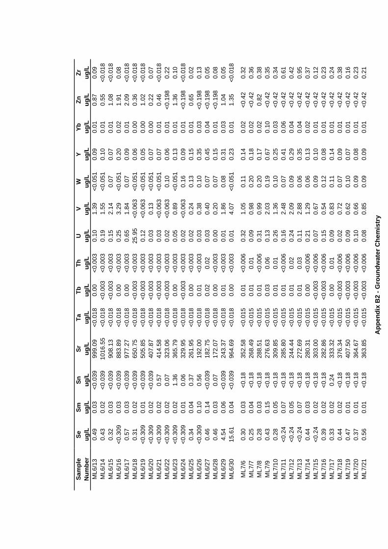
Sam
ple
Num
ber
ML6
/13
ML6
/14
ML6
/15
ML6
/16
ML6
/17
ML6
/18
ML6
/19
ML6
/20
ML6
/21
ML6
/22
ML6
/23
ML6
/24
ML6
/25
ML6
/26
ML6
/27
ML6
/28
ML6
/29
ML6
/30
ML7
/6M
L7/7
ML7
/8M
L7/9
ML7
/10
ML7
/11
ML7
/12
ML7
/13
ML7
/14
ML7
/15
ML7
/16
ML7
/17
ML7
/18
ML7
/19
ML7
/20
ML7
/21
SeSm
SnSr
TaTb
ThU
VW
YYb
ZnZr
ug/L
ug/L
ug/L
ug/L
ug/L
ug/L
ug/L
ug/L
ug/L
ug/L
ug/L
ug/L
ug/L
ug/L
0.49
0.03
<0.0
3999
9.09
<0.0
180.
00<0
.003
0.10
1.39
<0.0
510.
090.
010.
870.
090.
430.
02<0
.039
1016
.55
<0.0
18<0
.003
<0.0
030.
191.
55<0
.051
0.10
0.01
0.55
<0.0
180.
320.
03<0
.039
908.
13<0
.018
<0.0
03<0
.003
0.15
2.14
0.07
0.07
0.01
1.08
<0.0
18<0
.309
0.03
<0.0
3988
3.89
<0.0
180.
00<0
.003
0.25
3.29
<0.0
510.
200.
021.
910.
080.
570.
03<0
.039
977.
27<0
.018
0.00
<0.0
030.
651.
840.
070.
090.
012.
09<0
.018
0.31
0.02
<0.0
3965
0.75
<0.0
18<0
.003
<0.0
0325
.95
<0.0
63<0
.051
0.06
0.00
0.36
<0.0
18<0
.309
0.01
<0.0
3950
5.85
<0.0
18<0
.003
<0.0
030.
12<0
.063
<0.0
510.
050.
001.
02<0
.018
<0.3
090.
02<0
.039
407.
87<0
.018
<0.0
03<0
.003
0.03
0.13
<0.0
510.
070.
000.
220.
07<0
.309
0.02
0.57
414.
58<0
.018
<0.0
03<0
.003
0.03
<0.0
63<0
.051
0.07
0.01
0.46
<0.0
18<0
.309
0.02
0.07
323.
06<0
.018
<0.0
03<0
.003
0.02
<0.0
630.
100.
060.
01<0
.198
0.22
<0.3
090.
021.
3636
5.79
<0.0
180.
00<0
.003
0.05
0.89
<0.0
510.
130.
011.
360.
10<0
.309
0.01
0.06
329.
95<0
.018
<0.0
03<0
.003
0.02
<0.0
630.
160.
090.
01<0
.198
<0.0
180.
340.
040.
3726
1.95
<0.0
180.
00<0
.003
0.02
0.24
0.13
0.15
0.01
0.65
0.02
<0.3
090.
100.
5619
2.00
<0.0
180.
01<0
.003
0.03
0.38
0.10
0.35
0.03
<0.1
980.
130.
460.
14<0
.039
182.
75<0
.018
0.02
0.02
0.03
0.40
0.07
0.45
0.04
<0.1
980.
050.
460.
030.
0717
2.07
<0.0
180.
00<0
.003
0.00
0.20
0.07
0.15
0.01
<0.1
980.
084.
540.
06<0
.039
243.
37<0
.018
0.01
<0.0
030.
011.
860.
080.
310.
031.
040.
0515
.61
0.04
<0.0
3996
4.69
<0.0
180.
00<0
.003
0.01
4.07
<0.0
510.
230.
011.
35<0
.018
0.30
0.03
<0.1
835
2.58
<0.0
150.
01<0
.006
0.32
1.05
0.11
0.14
0.02
<0.4
20.
320.
250.
04<0
.18
268.
49<0
.015
0.01
0.01
0.09
0.98
0.20
0.18
0.02
<0.4
20.
360.
280.
03<0
.18
288.
51<0
.015
0.01
<0.0
060.
310.
990.
200.
170.
020.
820.
380.
430.
15<0
.18
276.
63<0
.015
0.03
0.06
0.13
2.03
0.19
0.67
0.10
<0.4
20.
350.
280.
05<0
.18
309.
85<0
.015
0.01
0.01
0.26
1.36
0.10
0.25
0.03
<0.4
20.
34<0
.24
0.07
<0.1
828
5.80
<0.0
150.
01<0
.006
0.16
2.48
0.07
0.41
0.06
<0.4
20.
61<0
.24
0.05
<0.1
824
4.44
<0.0
150.
010.
020.
242.
090.
090.
290.
04<0
.42
0.42
<0.2
40.
07<0
.18
272.
69<0
.015
0.01
0.03
0.11
2.88
0.06
0.35
0.04
<0.4
20.
950.
440.
03<0
.18
280.
31<0
.015
0.00
<0.0
060.
211.
290.
060.
130.
02<0
.42
0.37
<0.2
40.
02<0
.18
303.
00<0
.015
<0.0
03<0
.006
0.07
0.67
0.09
0.10
0.01
<0.4
20.
120.
390.
02<0
.18
282.
86<0
.015
<0.0
03<0
.006
0.15
0.54
0.12
0.08
0.01
<0.4
20.
230.
330.
020.
2433
3.32
<0.0
150.
000.
010.
090.
830.
110.
140.
01<0
.42
0.24
0.44
0.02
<0.1
837
6.34
<0.0
15<0
.003
<0.0
060.
020.
720.
070.
090.
01<0
.42
0.38
0.47
0.01
<0.1
840
7.50
<0.0
15<0
.003
<0.0
060.
090.
620.
100.
070.
01<0
.42
0.16
0.37
0.01
<0.1
836
4.67
<0.0
15<0
.003
<0.0
060.
100.
660.
090.
080.
01<0
.42
0.23
0.56
0.01
<0.1
836
3.85
<0.0
15<0
.003
<0.0
060.
080.
850.
090.
090.
01<0
.42
0.21
App
endi
x B
2 - G
roun
dwat
er C
hem
istr
y
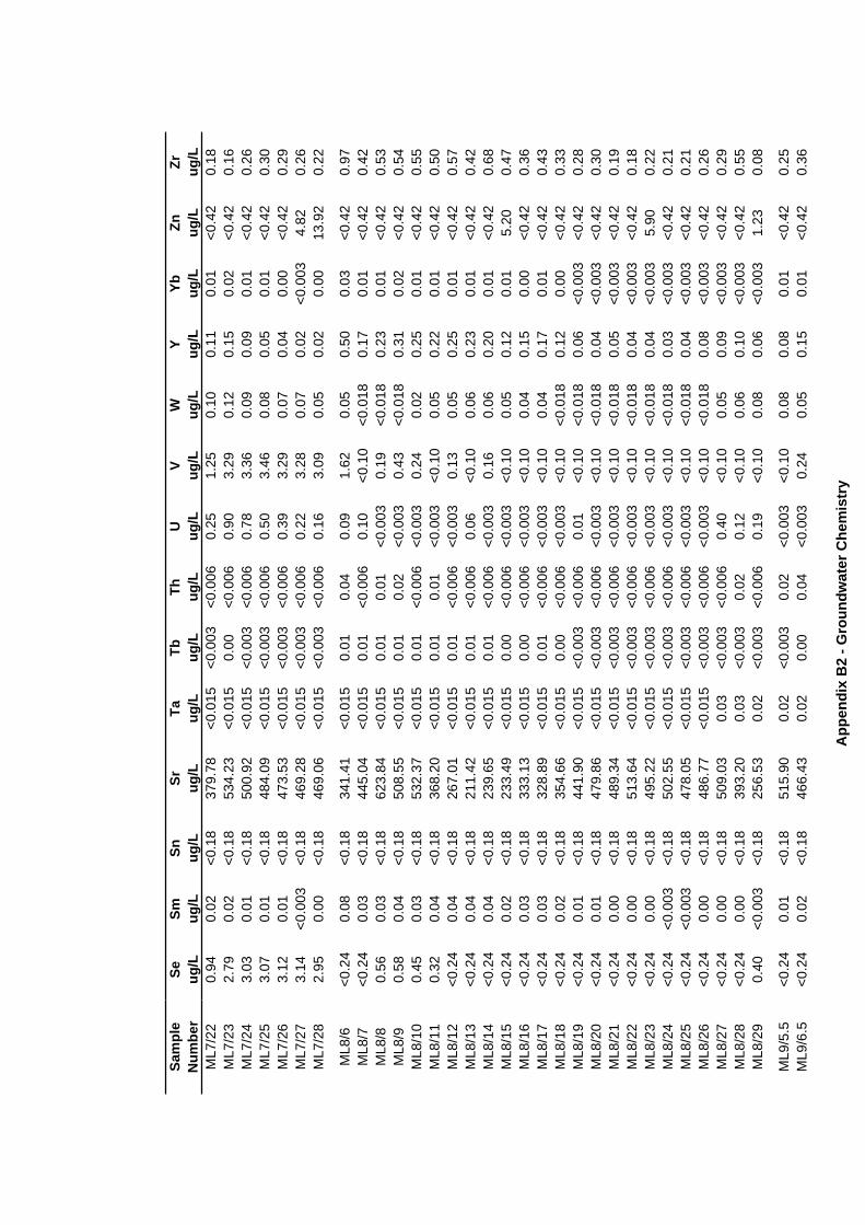
Sam
ple
Num
ber
ML7
/22
ML7
/23
ML7
/24
ML7
/25
ML7
/26
ML7
/27
ML7
/28
ML8
/6M
L8/7
ML8
/8M
L8/9
ML8
/10
ML8
/11
ML8
/12
ML8
/13
ML8
/14
ML8
/15
ML8
/16
ML8
/17
ML8
/18
ML8
/19
ML8
/20
ML8
/21
ML8
/22
ML8
/23
ML8
/24
ML8
/25
ML8
/26
ML8
/27
ML8
/28
ML8
/29
ML9
/5.5
ML9
/6.5
SeSm
SnSr
TaTb
ThU
VW
YYb
ZnZr
ug/L
ug/L
ug/L
ug/L
ug/L
ug/L
ug/L
ug/L
ug/L
ug/L
ug/L
ug/L
ug/L
ug/L
0.94
0.02
<0.1
837
9.78
<0.0
15<0
.003
<0.0
060.
251.
250.
100.
110.
01<0
.42
0.18
2.79
0.02
<0.1
853
4.23
<0.0
150.
00<0
.006
0.90
3.29
0.12
0.15
0.02
<0.4
20.
163.
030.
01<0
.18
500.
92<0
.015
<0.0
03<0
.006
0.78
3.36
0.09
0.09
0.01
<0.4
20.
263.
070.
01<0
.18
484.
09<0
.015
<0.0
03<0
.006
0.50
3.46
0.08
0.05
0.01
<0.4
20.
303.
120.
01<0
.18
473.
53<0
.015
<0.0
03<0
.006
0.39
3.29
0.07
0.04
0.00
<0.4
20.
293.
14<0
.003
<0.1
846
9.28
<0.0
15<0
.003
<0.0
060.
223.
280.
070.
02<0
.003
4.82
0.26
2.95
0.00
<0.1
846
9.06
<0.0
15<0
.003
<0.0
060.
163.
090.
050.
020.
0013
.92
0.22
<0.2
40.
08<0
.18
341.
41<0
.015
0.01
0.04
0.09
1.62
0.05
0.50
0.03
<0.4
20.
97<0
.24
0.03
<0.1
844
5.04
<0.0
150.
01<0
.006
0.10
<0.1
0<0
.018
0.17
0.01
<0.4
20.
420.
560.
03<0
.18
623.
84<0
.015
0.01
0.01
<0.0
030.
19<0
.018
0.23
0.01
<0.4
20.
530.
580.
04<0
.18
508.
55<0
.015
0.01
0.02
<0.0
030.
43<0
.018
0.31
0.02
<0.4
20.
540.
450.
03<0
.18
532.
37<0
.015
0.01
<0.0
06<0
.003
0.24
0.02
0.25
0.01
<0.4
20.
550.
320.
04<0
.18
368.
20<0
.015
0.01
0.01
<0.0
03<0
.10
0.05
0.22
0.01
<0.4
20.
50<0
.24
0.04
<0.1
826
7.01
<0.0
150.
01<0
.006
<0.0
030.
130.
050.
250.
01<0
.42
0.57
<0.2
40.
04<0
.18
211.
42<0
.015
0.01
<0.0
060.
06<0
.10
0.06
0.23
0.01
<0.4
20.
42<0
.24
0.04
<0.1
823
9.65
<0.0
150.
01<0
.006
<0.0
030.
160.
060.
200.
01<0
.42
0.68
<0.2
40.
02<0
.18
233.
49<0
.015
0.00
<0.0
06<0
.003
<0.1
00.
050.
120.
015.
200.
47<0
.24
0.03
<0.1
833
3.13
<0.0
150.
00<0
.006
<0.0
03<0
.10
0.04
0.15
0.00
<0.4
20.
36<0
.24
0.03
<0.1
832
8.89
<0.0
150.
01<0
.006
<0.0
03<0
.10
0.04
0.17
0.01
<0.4
20.
43<0
.24
0.02
<0.1
835
4.66
<0.0
150.
00<0
.006
<0.0
03<0
.10
<0.0
180.
120.
00<0
.42
0.33
<0.2
40.
01<0
.18
441.
90<0
.015
<0.0
03<0
.006
0.01
<0.1
0<0
.018
0.06
<0.0
03<0
.42
0.28
<0.2
40.
01<0
.18
479.
86<0
.015
<0.0
03<0
.006
<0.0
03<0
.10
<0.0
180.
04<0
.003
<0.4
20.
30<0
.24
0.00
<0.1
848
9.34
<0.0
15<0
.003
<0.0
06<0
.003
<0.1
0<0
.018
0.05
<0.0
03<0
.42
0.19
<0.2
40.
00<0
.18
513.
64<0
.015
<0.0
03<0
.006
<0.0
03<0
.10
<0.0
180.
04<0
.003
<0.4
20.
18<0
.24
0.00
<0.1
849
5.22
<0.0
15<0
.003
<0.0
06<0
.003
<0.1
0<0
.018
0.04
<0.0
035.
900.
22<0
.24
<0.0
03<0
.18
502.
55<0
.015
<0.0
03<0
.006
<0.0
03<0
.10
<0.0
180.
03<0
.003
<0.4
20.
21<0
.24
<0.0
03<0
.18
478.
05<0
.015
<0.0
03<0
.006
<0.0
03<0
.10
<0.0
180.
04<0
.003
<0.4
20.
21<0
.24
0.00
<0.1
848
6.77
<0.0
15<0
.003
<0.0
06<0
.003
<0.1
0<0
.018
0.08
<0.0
03<0
.42
0.26
<0.2
40.
00<0
.18
509.
030.
03<0
.003
<0.0
060.
40<0
.10
0.05
0.09
<0.0
03<0
.42
0.29
<0.2
40.
00<0
.18
393.
200.
03<0
.003
0.02
0.12
<0.1
00.
060.
10<0
.003
<0.4
20.
550.
40<0
.003
<0.1
825
6.53
0.02
<0.0
03<0
.006
0.19
<0.1
00.
080.
06<0
.003
1.23
0.08
<0.2
40.
01<0
.18
515.
900.
02<0
.003
0.02
<0.0
03<0
.10
0.08
0.08
0.01
<0.4
20.
25<0
.24
0.02
<0.1
846
6.43
0.02
0.00
0.04
<0.0
030.
240.
050.
150.
01<0
.42
0.36
App
endi
x B
2 - G
roun
dwat
er C
hem
istr
y
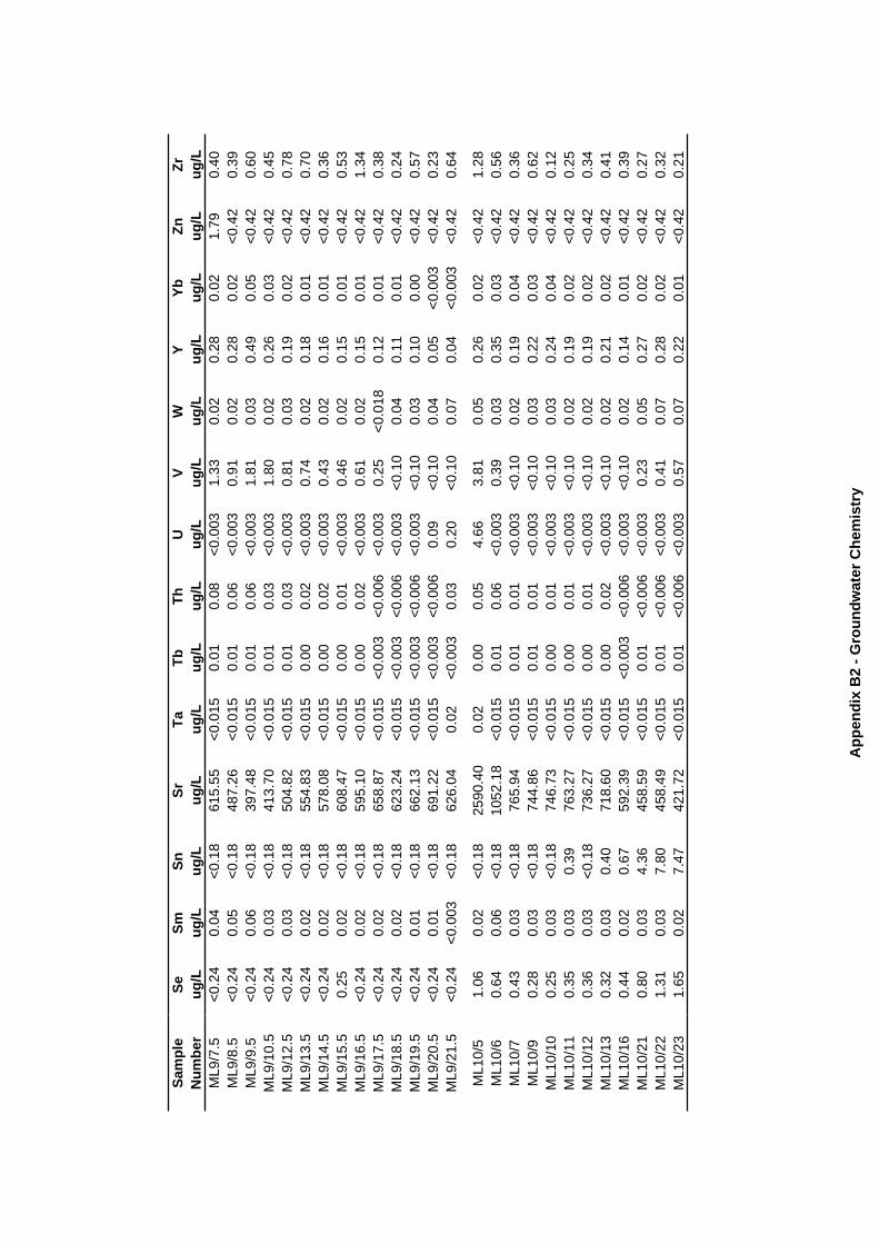
Sam
ple
Num
ber
ML9
/7.5
ML9
/8.5
ML9
/9.5
ML9
/10.
5M
L9/1
2.5
ML9
/13.
5M
L9/1
4.5
ML9
/15.
5M
L9/1
6.5
ML9
/17.
5M
L9/1
8.5
ML9
/19.
5M
L9/2
0.5
ML9
/21.
5
ML1
0/5
ML1
0/6
ML1
0/7
ML1
0/9
ML1
0/10
ML1
0/11
ML1
0/12
ML1
0/13
ML1
0/16
ML1
0/21
ML1
0/22
ML1
0/23
SeSm
SnSr
TaTb
ThU
VW
YYb
ZnZr
ug/L
ug/L
ug/L
ug/L
ug/L
ug/L
ug/L
ug/L
ug/L
ug/L
ug/L
ug/L
ug/L
ug/L
<0.2
40.
04<0
.18
615.
55<0
.015
0.01
0.08
<0.0
031.
330.
020.
280.
021.
790.
40<0
.24
0.05
<0.1
848
7.26
<0.0
150.
010.
06<0
.003
0.91
0.02
0.28
0.02
<0.4
20.
39<0
.24
0.06
<0.1
839
7.48
<0.0
150.
010.
06<0
.003
1.81
0.03
0.49
0.05
<0.4
20.
60<0
.24
0.03
<0.1
841
3.70
<0.0
150.
010.
03<0
.003
1.80
0.02
0.26
0.03
<0.4
20.
45<0
.24
0.03
<0.1
850
4.82
<0.0
150.
010.
03<0
.003
0.81
0.03
0.19
0.02
<0.4
20.
78<0
.24
0.02
<0.1
855
4.83
<0.0
150.
000.
02<0
.003
0.74
0.02
0.18
0.01
<0.4
20.
70<0
.24
0.02
<0.1
857
8.08
<0.0
150.
000.
02<0
.003
0.43
0.02
0.16
0.01
<0.4
20.
360.
250.
02<0
.18
608.
47<0
.015
0.00
0.01
<0.0
030.
460.
020.
150.
01<0
.42
0.53
<0.2
40.
02<0
.18
595.
10<0
.015
0.00
0.02
<0.0
030.
610.
020.
150.
01<0
.42
1.34
<0.2
40.
02<0
.18
658.
87<0
.015
<0.0
03<0
.006
<0.0
030.
25<0
.018
0.12
0.01
<0.4
20.
38<0
.24
0.02
<0.1
862
3.24
<0.0
15<0
.003
<0.0
06<0
.003
<0.1
00.
040.
110.
01<0
.42
0.24
<0.2
40.
01<0
.18
662.
13<0
.015
<0.0
03<0
.006
<0.0
03<0
.10
0.03
0.10
0.00
<0.4
20.
57<0
.24
0.01
<0.1
869
1.22
<0.0
15<0
.003
<0.0
060.
09<0
.10
0.04
0.05
<0.0
03<0
.42
0.23
<0.2
4<0
.003
<0.1
862
6.04
0.02
<0.0
030.
030.
20<0
.10
0.07
0.04
<0.0
03<0
.42
0.64
1.06
0.02
<0.1
825
90.4
00.
020.
000.
054.
663.
810.
050.
260.
02<0
.42
1.28
0.64
0.06
<0.1
810
52.1
8<0
.015
0.01
0.06
<0.0
030.
390.
030.
350.
03<0
.42
0.56
0.43
0.03
<0.1
876
5.94
<0.0
150.
010.
01<0
.003
<0.1
00.
020.
190.
04<0
.42
0.36
0.28
0.03
<0.1
874
4.86
<0.0
150.
010.
01<0
.003
<0.1
00.
030.
220.
03<0
.42
0.62
0.25
0.03
<0.1
874
6.73
<0.0
150.
000.
01<0
.003
<0.1
00.
030.
240.
04<0
.42
0.12
0.35
0.03
0.39
763.
27<0
.015
0.00
0.01
<0.0
03<0
.10
0.02
0.19
0.02
<0.4
20.
250.
360.
03<0
.18
736.
27<0
.015
0.00
0.01
<0.0
03<0
.10
0.02
0.19
0.02
<0.4
20.
340.
320.
030.
4071
8.60
<0.0
150.
000.
02<0
.003
<0.1
00.
020.
210.
02<0
.42
0.41
0.44
0.02
0.67
592.
39<0
.015
<0.0
03<0
.006
<0.0
03<0
.10
0.02
0.14
0.01
<0.4
20.
390.
800.
034.
3645
8.59
<0.0
150.
01<0
.006
<0.0
030.
230.
050.
270.
02<0
.42
0.27
1.31
0.03
7.80
458.
49<0
.015
0.01
<0.0
06<0
.003
0.41
0.07
0.28
0.02
<0.4
20.
321.
650.
027.
4742
1.72
<0.0
150.
01<0
.006
<0.0
030.
570.
070.
220.
01<0
.42
0.21
App
endi
x B
2 - G
roun
dwat
er C
hem
istr
y
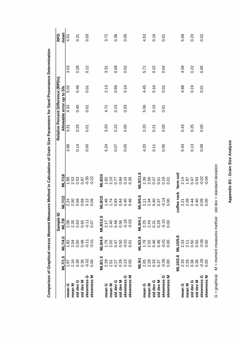
Com
paris
on o
f Gra
phic
al v
ersu
s M
omen
t Mea
sure
s M
etho
d in
Cal
cula
tion
of G
rain
Siz
e Pa
ram
eter
s fo
r San
d Pr
oven
ance
Det
erm
inat
ion
Sam
ple
IDR
elat
ive
Perc
ent D
iffer
ence
(RPD
s)A
llow
able
err
or u
p to
5%
RPD
ML7
/1.5
ML7
/4.5
ML7
/8M
L7/1
2M
L7/1
8m
ean
mea
n G
1.97
1.82
2.08
2.24
1.88
3.88
3.31
4.33
5.02
3.53
4.01
mea
n M
2.16
2.04
2.35
2.50
2.53
std
dev
G0.
380.
500.
630.
680.
530.
140.
250.
400.
460.
280.
31st
d de
v M
0.36
0.48
0.65
0.69
0.87
skew
ness
G-0
.02
-0.1
1-0
.11
0.12
-0.3
50.
000.
010.
010.
010.
120.
03sk
ewne
ss M
0.00
-0.0
10.
070.
09-0
.22
ML8
/1.5
ML8
/4.5
ML8
/12.
5M
L8/1
5M
L8/2
4m
ean
G2.
291.
792.
171.
461.
825.
243.
204.
712.
133.
313.
72m
ean
M2.
512.
022.
401.
742.
10st
d de
v G
0.27
0.47
0.48
0.83
0.77
0.07
0.22
0.23
0.69
0.59
0.36
std
dev
M0.
290.
500.
560.
840.
84sk
ewne
ss G
0.23
-0.0
1-0
.18
0.40
0.15
0.05
0.00
0.03
0.16
0.02
0.05
skew
ness
M0.
000.
01-0
.03
0.46
0.26
ML9
/1M
L9/2
.6M
L9/4
.1M
L9/5
.6M
L9/1
1.6
mea
n G
2.05
1.79
2.25
2.11
2.39
4.20
3.20
5.06
4.45
5.71
4.53
mea
n M
2.28
2.02
2.43
2.34
2.55
std
dev
G0.
330.
460.
310.
400.
470.
110.
210.
100.
160.
220.
16st
d de
v M
0.37
0.46
0.29
0.37
0.51
skew
ness
G-0
.05
-0.0
1-0
.10
-0.1
40.
190.
000.
000.
010.
020.
040.
01sk
ewne
ss M
0.00
0.00
0.00
0.00
0.01
ML1
0/2.
8M
L10/
5.8
coffe
e ro
ckfa
rm s
oil
mea
n G
2.33
2.33
2.21
2.14
5.43
5.43
4.88
4.58
5.08
mea
n M
2.26
2.11
2.09
1.97
std
dev
G0.
360.
500.
440.
470.
130.
250.
190.
220.
20st
d de
v M
0.36
0.50
0.40
0.54
skew
ness
G-0
.28
-0.0
60.
09-0
.02
0.08
0.00
0.01
0.00
0.02
skew
ness
M0.
000.
000.
00-0
.04
G =
gra
phic
al
M =
mom
ent m
easu
res
met
hod
st
d de
v =
stan
dard
dev
iatio
n
App
endi
x B
3 - G
rain
Siz
e A
naly
sis

Estimate of mineral composition for ternary diagram
Sample IDFeldspar
%Quartz
% Lithics
%ML7/1.5 4 96 0ML7/12 4 82 6ML7/18 5 85 5ML7/4.5 8 89 3ML7/8 2 90 5ML8/1.5 3 97 0ML8/12.6 7 83 4ML8/15 10 75 10ML8/24 6 77 9ML8/4.5 6 89 5ML9/1 5 94 1ML9/11.6 5 90 4ML9/2.6 5 93 2ML9/4.1 3 93 4ML9/5.6 3 92 5ML10/2.8 4 93 3ML10/5.8 10 92 8
Appendix B4 - Ternary Diagram
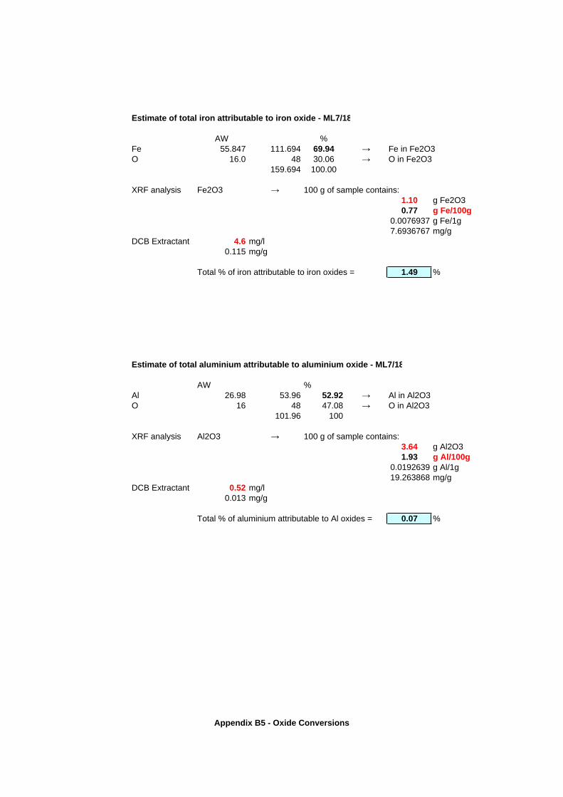
Estimate of total iron attributable to iron oxide - ML7/18
AW %Fe 55.847 111.694 69.94 Fe in Fe2O3O 16.0 48 30.06 O in Fe2O3
159.694 100.00
XRF analysis Fe2O3 100 g of sample contains: 1.10 g Fe2O30.77 g Fe/100g
0.0076937 g Fe/1g7.6936767 mg/g
DCB Extractant 4.6 mg/l0.115 mg/g
Total % of iron attributable to iron oxides = 1.49 %
Estimate of total aluminium attributable to aluminium oxide - ML7/18
AW %Al 26.98 53.96 52.92 Al in Al2O3O 16 48 47.08 O in Al2O3
101.96 100
XRF analysis Al2O3 100 g of sample contains: 3.64 g Al2O31.93 g Al/100g
0.0192639 g Al/1g19.263868 mg/g
DCB Extractant 0.52 mg/l0.013 mg/g
Total % of aluminium attributable to Al oxides = 0.07 %
Appendix B5 - Oxide Conversions
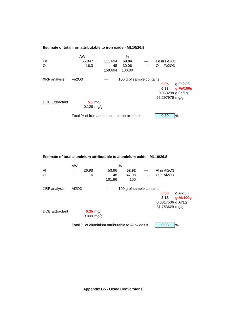
Estimate of total iron attributable to iron oxide - ML10/26.8
AW %Fe 55.847 111.694 69.94 Fe in Fe2O3O 16.0 48 30.06 O in Fe2O3
159.694 100.00
XRF analysis Fe2O3 100 g of sample contains: 9.05 g Fe2O36.33 g Fe/100g
0.063298 g Fe/1g63.297976 mg/g
DCB Extractant 5.1 mg/l0.128 mg/g
Total % of iron attributable to iron oxides = 0.20 %
Estimate of total aluminium attributable to aluminium oxide - ML10/26.8
AW %Al 26.98 53.96 52.92 Al in Al2O3O 16 48 47.08 O in Al2O3
101.96 100
XRF analysis Al2O3 100 g of sample contains: 6.00 g Al2O33.18 g Al/100g
0.0317536 g Al/1g31.753629 mg/g
DCB Extractant 0.35 mg/l0.009 mg/g
Total % of aluminium attributable to Al oxides = 0.03 %
Appendix B5 - Oxide Conversions

Estimate of total iron attributable to iron oxide - ML9/5.6
AW %Fe 55.847 111.694 69.94 Fe in Fe2O3O 16.0 48 30.06 O in Fe2O3
159.694 100.00
XRF analysis Fe2O3 100 g of sample contains: 0.23 g Fe2O30.16 g Fe/100g
0.0016087 g Fe/1g1.6086778 mg/g
DCB Extractant 0 mg/l0.000 mg/g
Total % of iron attributable to iron oxides = 0.00 %
Estimate of total aluminium attributable to aluminium oxide - ML9/5.6
AW %Al 26.98 53.96 52.92 Al in Al2O3O 16 48 47.08 O in Al2O3
101.96 100
XRF analysis Al2O3 100 g of sample contains: 0.90 g Al2O30.48 g Al/100g
0.004763 g Al/1g4.7630443 mg/g
DCB Extractant 0.07 mg/l0.002 mg/g
Total % of aluminium attributable to Al oxides = 0.04 %
Appendix B5 - Oxide Conversions
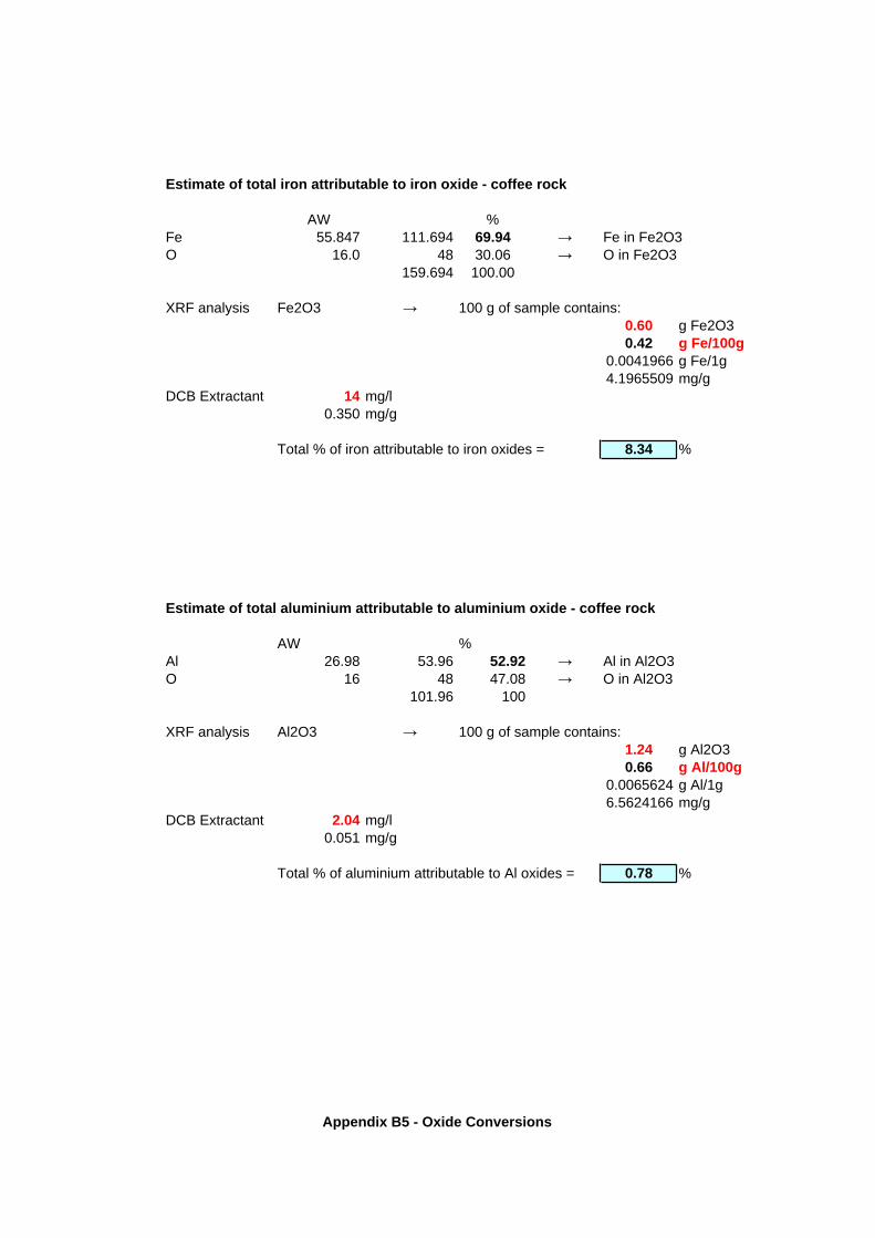
Estimate of total iron attributable to iron oxide - coffee rock
AW %Fe 55.847 111.694 69.94 Fe in Fe2O3O 16.0 48 30.06 O in Fe2O3
159.694 100.00
XRF analysis Fe2O3 100 g of sample contains: 0.60 g Fe2O30.42 g Fe/100g
0.0041966 g Fe/1g4.1965509 mg/g
DCB Extractant 14 mg/l0.350 mg/g
Total % of iron attributable to iron oxides = 8.34 %
Estimate of total aluminium attributable to aluminium oxide - coffee rock
AW %Al 26.98 53.96 52.92 Al in Al2O3O 16 48 47.08 O in Al2O3
101.96 100
XRF analysis Al2O3 100 g of sample contains: 1.24 g Al2O30.66 g Al/100g
0.0065624 g Al/1g6.5624166 mg/g
DCB Extractant 2.04 mg/l0.051 mg/g
Total % of aluminium attributable to Al oxides = 0.78 %
Appendix B5 - Oxide Conversions
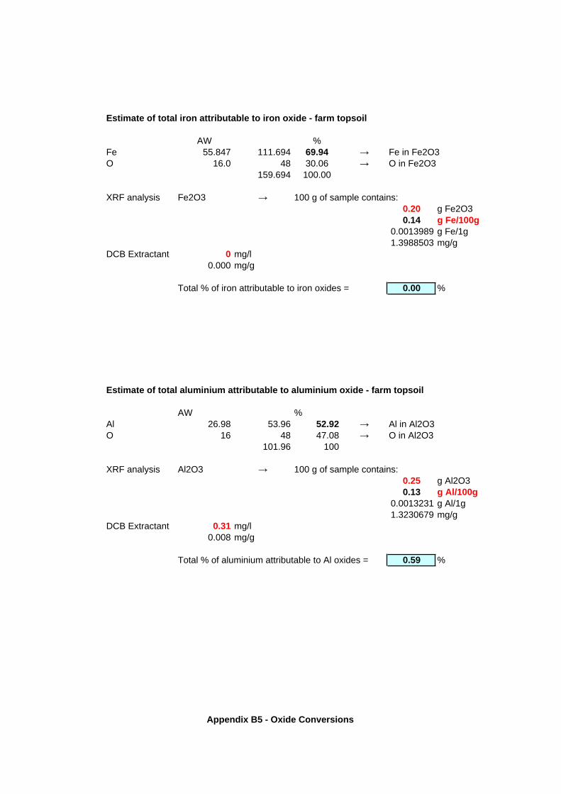
Estimate of total iron attributable to iron oxide - farm topsoil
AW %Fe 55.847 111.694 69.94 Fe in Fe2O3O 16.0 48 30.06 O in Fe2O3
159.694 100.00
XRF analysis Fe2O3 100 g of sample contains: 0.20 g Fe2O30.14 g Fe/100g
0.0013989 g Fe/1g1.3988503 mg/g
DCB Extractant 0 mg/l0.000 mg/g
Total % of iron attributable to iron oxides = 0.00 %
Estimate of total aluminium attributable to aluminium oxide - farm topsoil
AW %Al 26.98 53.96 52.92 Al in Al2O3O 16 48 47.08 O in Al2O3
101.96 100
XRF analysis Al2O3 100 g of sample contains: 0.25 g Al2O30.13 g Al/100g
0.0013231 g Al/1g1.3230679 mg/g
DCB Extractant 0.31 mg/l0.008 mg/g
Total % of aluminium attributable to Al oxides = 0.59 %
Appendix B5 - Oxide Conversions
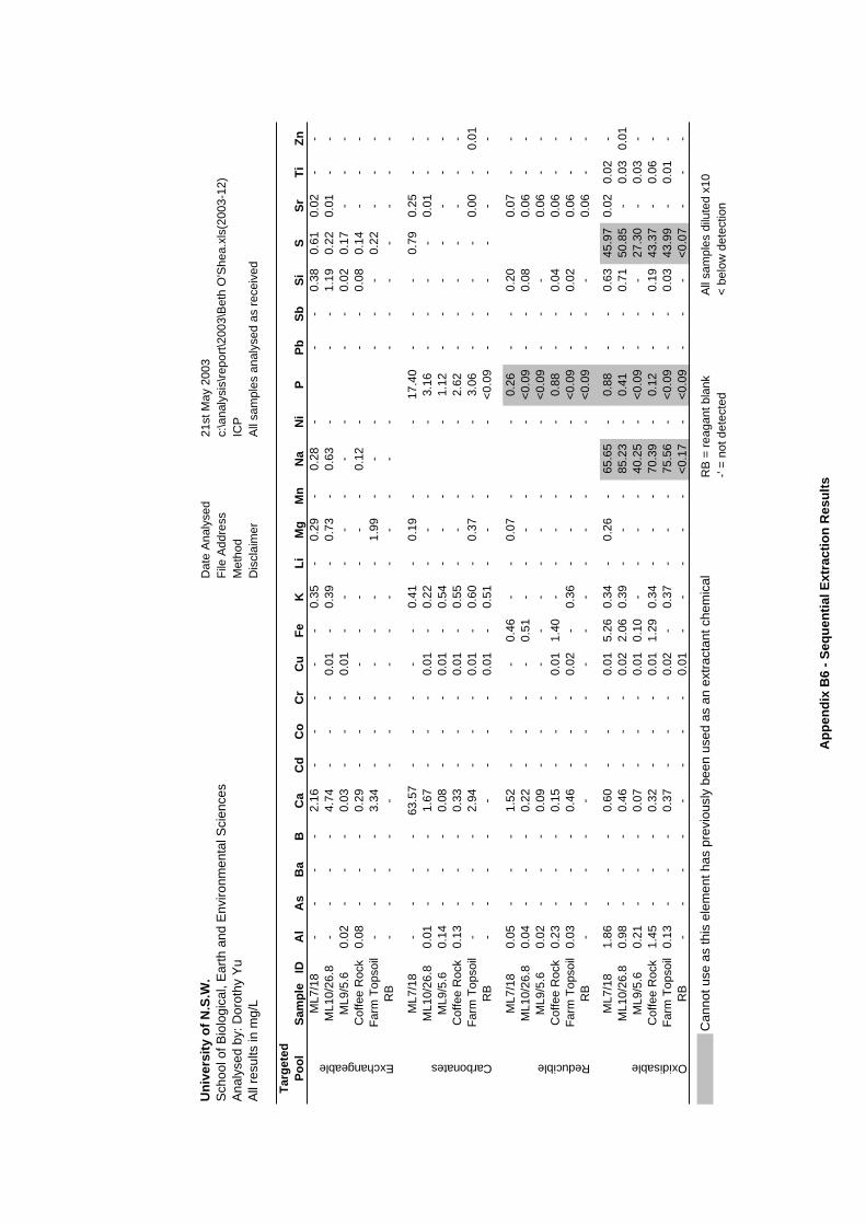
Uni
vers
ity o
f N.S
.W.
Dat
e A
naly
sed
21st
May
200
3S
choo
l of B
iolo
gica
l, E
arth
and
Env
ironm
enta
l Sci
ence
sFi
le A
ddre
ssc:
\ana
lysi
s\re
port\
2003
\Bet
h O
'She
a.xl
s(20
03-1
2)A
naly
sed
by: D
orot
hy Y
uM
etho
dIC
PA
ll re
sults
in m
g/L
Dis
clai
mer
All
sam
ples
ana
lyse
d as
rece
ived
Targ
eted
Pool
Sam
ple
ID
Al
As
Ba
BC
aC
dC
oC
rC
uFe
KLi
Mg
Mn
Na
Ni
PPb
SbSi
SSr
TiZn
Exchangeable
ML7
/18
--
--
2.16
--
--
-0.
35-
0.29
-0.
28-
--
0.38
0.61
0.02
--
ML1
0/26
.8-
--
-4.
74-
--
0.01
-0.
39-
0.73
-0.
63-
--
1.19
0.22
0.01
--
ML9
/5.6
0.02
--
-0.
03-
--
0.01
--
--
--
--
-0.
020.
17-
--
Cof
fee
Roc
k0.
08-
--
0.29
--
--
--
--
-0.
12-
--
0.08
0.14
--
-Fa
rm T
opso
il-
--
-3.
34-
--
--
--
1.99
--
--
--
0.22
--
-R
B-
--
--
--
--
--
--
--
--
--
--
--
Carbonates
ML7
/18
--
--
63.5
7-
--
--
0.41
-0.
19-
-17
.40
--
-0.
790.
25-
-M
L10/
26.8
0.01
--
-1.
67-
--
0.01
-0.
22-
--
-3.
16-
--
-0.
01-
-M
L9/5
.60.
14-
--
0.08
--
-0.
01-
0.54
--
--
1.12
--
--
--
-C
offe
e R
ock
0.13
--
-0.
33-
--
0.01
-0.
55-
--
-2.
62-
--
--
--
Farm
Top
soil
--
--
2.94
--
-0.
01-
0.60
-0.
37-
-3.
06-
--
-0.
00-
0.01
RB
--
--
--
--
0.01
-0.
51-
--
-<0
.09
--
--
--
-
Reducible
ML7
/18
0.05
--
-1.
52-
--
-0.
46-
-0.
07-
-0.
26-
-0.
200.
07-
-M
L10/
26.8
0.04
--
-0.
22-
--
-0.
51-
--
--
<0.0
9-
-0.
080.
06-
-M
L9/5
.60.
02-
--
0.09
--
--
--
--
--
<0.0
9-
--
0.06
--
Cof
fee
Roc
k0.
23-
--
0.15
--
-0.
011.
40-
--
--
0.88
--
0.04
0.06
--
Farm
Top
soil
0.03
--
-0.
46-
--
0.02
-0.
36-
--
-<0
.09
--
0.02
0.06
--
RB
--
--
--
--
--
--
--
-<0
.09
--
-0.
06-
-
Oxidisable
ML7
/18
1.86
--
-0.
60-
--
0.01
5.26
0.34
-0.
26-
65.6
5-
0.88
--
0.63
45.9
70.
020.
02-
ML1
0/26
.80.
98-
--
0.46
--
-0.
022.
060.
39-
--
85.2
3-
0.41
--
0.71
50.8
5-
0.03
0.01
ML9
/5.6
0.21
--
-0.
07-
--
0.01
0.10
--
--
40.2
5-
<0.0
9-
--
27.3
0-
0.03
-C
offe
e R
ock
1.45
--
-0.
32-
--
0.01
1.29
0.34
--
-70
.39
-0.
12-
-0.
1943
.37
-0.
06-
Farm
Top
soil
0.13
--
-0.
37-
--
0.02
-0.
37-
--
75.5
6-
<0.0
9-
-0.
0343
.99
-0.
01-
RB
--
--
--
--
0.01
--
--
-<0
.17
-<0
.09
--
-<0
.07
--
-
Can
not u
se a
s th
is e
lem
ent h
as p
revi
ousl
y be
en u
sed
as a
n ex
tract
ant c
hem
ical
RB
= re
agan
t bla
nkA
ll sa
mpl
es d
ilute
d x1
0-'
= no
t det
ecte
d<
belo
w d
etec
tion
App
endi
x B
6 - S
eque
ntia
l Ext
ract
ion
Res
ults
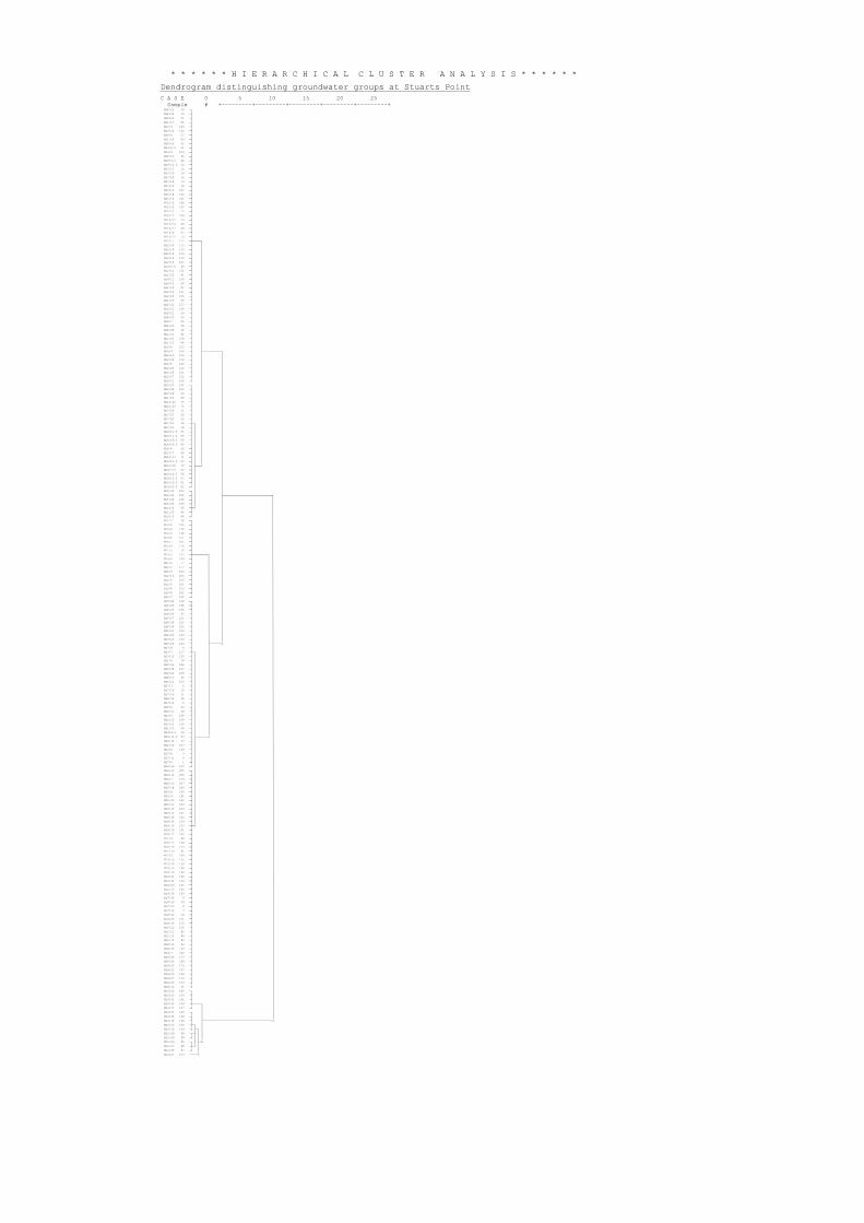
* * * * * * H I E R A R C H I C A L C L U S T E R A N A L Y S I S * * * * * *
Dendrogram distinguishing groundwater groups at Stuarts Point
C A S E 0 5 10 15 20 25 Sample # +---------+---------+---------+---------+---------+ ML8/22 40 òø ML8/26 44 òú ML8/23 41 òú ML1/17 88 òú ML3/9 129 òú ML3/10 130 òú ML8/9 27 òú ML1/18 89 òú ML8/24 42 òú ML9/8.5 51 òú ML3/4 124 òú ML8/27 45 òú ML9/5.5 48 òú ML9/12.5 54 òú ML7/17 12 òú ML7/19 14 òú ML7/20 15 òú ML7/18 13 òú ML7/21 16 òú ML5/15 187 òú ML5/18 190 òú ML5/19 191 òú ML5/16 188 òú ML5/20 192 òú ML7/22 17 òú ML5/17 189 òú ML10/21 73 òú ML10/10 68 òú ML10/11 69 òú ML10/9 67 òú ML10/12 70 òú ML2/17 112 òôòòòòòø ML2/18 113 òú ó ML2/19 114 òú ó ML2/14 109 òú ó ML2/15 110 òú ó ML2/10 105 òú ó ML9/6.5 49 òú ó ML3/11 131 òú ó ML1/20 91 òú ó ML4/11 156 òú ó ML8/10 28 òú ó ML1/16 87 òú ó ML2/16 111 òú ó ML2/20 115 òú ó ML1/19 90 òú ó ML2/22 117 òú ó ML2/21 116 òú ó ML8/21 39 òú ó ML8/25 43 òú ó ML8/7 25 òú ó ML8/20 38 òú ó ML8/28 46 òú ó ML1/21 92 òú ó ML2/23 118 òú ó ML1/15 86 òú ó ML4/8 153 òú ó ML4/9 154 òú ùòòòòòòòòòòòø ML4/10 155 òú ó ó ML2/24 119 òú ó ó ML3/5 125 òú ó ó ML2/25 120 òú ó ó ML2/26 121 òú ó ó ML2/27 122 òú ó ó ML2/11 106 ò÷ ó ó ML5/27 197 òø ó ó ML6/29 223 òú ó ó ML7/28 23 òú ó ó ML1/24 93 òú ó ó ML10/22 74 òú ó ó ML10/23 75 òú ó ó ML7/26 21 òú ó ó ML7/27 22 òú ó ó ML7/25 20 òú ó ó ML7/23 18 òôòø ó ó ML7/24 19 òú ó ó ó ML9/13.5 55 òú ó ó ó ML9/17.5 59 òú ó ó ó ML9/16.5 58 òú ó ó ó ML9/18.5 60 òú ó ó ó ML8/8 26 òú ó ó ó ML10/7 66 òú ó ó ó ML10/13 71 òú ó ó ó ML9/21.5 63 òú ó ó ó ML10/16 72 òú ùòòò÷ ó ML9/7.5 50 òú ó ó ML9/14.5 56 òú ó ó ML9/15.5 57 òú ó ó ML9/19.5 61 òú ó ó ML9/20.5 62 ò÷ ó ó ML5/30 200 òø ó ó ML6/30 224 òú ó ùòòòòòòòòòòòòòòòòòòòòòòòòòòòòòø ML5/28 198 òú ó ó ó ML5/29 199 òú ó ó ó ML10/6 65 òôò÷ ó ó ML1/25 94 òú ó ó ML10/5 64 ò÷ ó ó ML1/7 78 òø ó ó ML4/5 150 òú ó ó ML5/6 178 òú ó ó ML4/3 148 òú ó ó ML4/6 151 òú ó ó ML6/7 201 òú ó ó ML5/4 176 òú ó ó ML1/5 76 òú ó ó ML3/3 123 òôòòòòòòòòòø ó ó ML4/4 149 òú ó ó ó ML1/6 77 òú ó ó ó ML5/5 177 òú ó ó ó ML6/9 203 òú ó ó ó ML6/10 204 òú ó ó ó ML2/5 100 òú ó ó ó ML2/6 101 òú ó ó ó ML2/8 103 òú ó ó ó ML6/8 202 òú ó ó ó ML2/7 102 ò÷ ó ó ó ML5/22 194 òø ó ó ó ML5/26 196 òú ó ó ó ML5/23 195 òú ó ó ó ML8/29 47 òú ó ó ó ML6/27 221 òú ó ó ó ML6/28 222 òú ó ó ó ML6/26 220 òú ó ó ó ML5/21 193 òú ó ó ó ML6/25 219 òú ó ó ó ML3/13 133 òú ó ó ó ML6/20 214 òú ùòòòòòòò÷ ó ML7/9 4 òú ó ó ML3/7 127 òôòø ó ó ML3/12 132 òú ó ó ó ML1/8 79 òú ó ó ó ML5/14 186 òú ó ó ó ML6/23 217 òú ó ó ó ML6/24 218 òú ó ó ó ML8/17 35 òú ó ó ó ML6/21 215 òú ó ó ó ML7/7 2 òú ó ó ó ML7/15 10 òú ó ó ó ML7/16 11 òú ó ó ó ML8/18 36 òú ó ó ó ML7/10 5 òú ó ó ó ML8/6 24 òú ó ó ó ML8/11 29 òú ó ó ó ML3/6 126 òú ó ó ó ML2/13 108 òú ó ó ó ML4/13 158 òú ó ó ó ML1/14 85 òú ó ó ó ML9/9.5 52 òú ó ó ó ML9/10.5 53 òú ùòòòòòòò÷ ó ML8/19 37 òú ó ó ML2/12 107 òú ó ó ML3/8 128 òú ó ó ML7/8 3 òú ó ó ML7/11 6 òú ó ó ML7/6 1 òú ó ó ML4/12 157 ò÷ ó ó ML6/11 205 òø ó ó ML6/12 206 òú ó ó ML5/7 179 òú ó ó ML6/13 207 òú ó ó ML6/14 208 òú ó ó ML5/8 180 òú ó ó ML5/9 181 òú ó ó ML5/10 182 òú ó ó ML5/11 183 òú ó ó ML6/15 209 òú ó ó ML6/17 211 òú ó ó ML6/18 212 òú ó ó ML4/14 159 òú ó ó ML6/16 210 òôò÷ ó ML4/16 161 òú ó ML4/17 162 òú ó ML1/9 80 òú ó ML5/12 184 òú ó ML6/19 213 òú ó ML1/10 81 òú ó ML2/9 104 òú ó ML3/15 135 òú ó ML3/16 136 òú ó ML4/15 160 òú ó ML4/19 164 òú ó ML4/21 166 òú ó ML3/14 134 òú ó ML4/20 165 òú ó ML5/13 185 òú ó ML4/18 163 òú ó ML7/14 9 òú ó ML8/16 34 òú ó ML7/13 8 òú ó ML7/12 7 òú ó ML8/12 30 òú ó ML4/26 171 òú ó ML4/30 175 òú ó ML6/22 216 òú ó ML1/11 82 òú ó ML1/13 84 òú ó ML1/12 83 òú ó ML8/14 32 òú ó ML8/15 33 òú ó ML4/7 152 òú ó ML4/28 173 òú ó ML4/24 169 òú ó ML4/25 170 òú ó ML4/22 167 òú ó ML4/23 168 òú ó ML4/27 172 òú ó ML4/29 174 òú ó ML8/13 31 ò÷ ó ML3/22 142 òø ó ML3/23 143 òú ó ML3/21 141 òú ó ML3/24 144 òôòòòòòø ó ML3/17 137 ò÷ ó ó ML3/25 145 òø ó ó ML3/26 146 òú ó ó ML3/18 138 òú ùòòòòòòòòòòòòòòòòòòòòòòòòòòòòòòòòòòòòòòòòò÷ ML3/20 140 òôòø ó ML3/19 139 ò÷ ùòø ó ML1/29 98 òûòú ó ó ML1/30 99 ò÷ ó ó ó ML1/26 95 òø ó ùò÷ ML1/27 96 òôò÷ ó ML1/28 97 ò÷ ó ML3/27 147 òòòòò÷
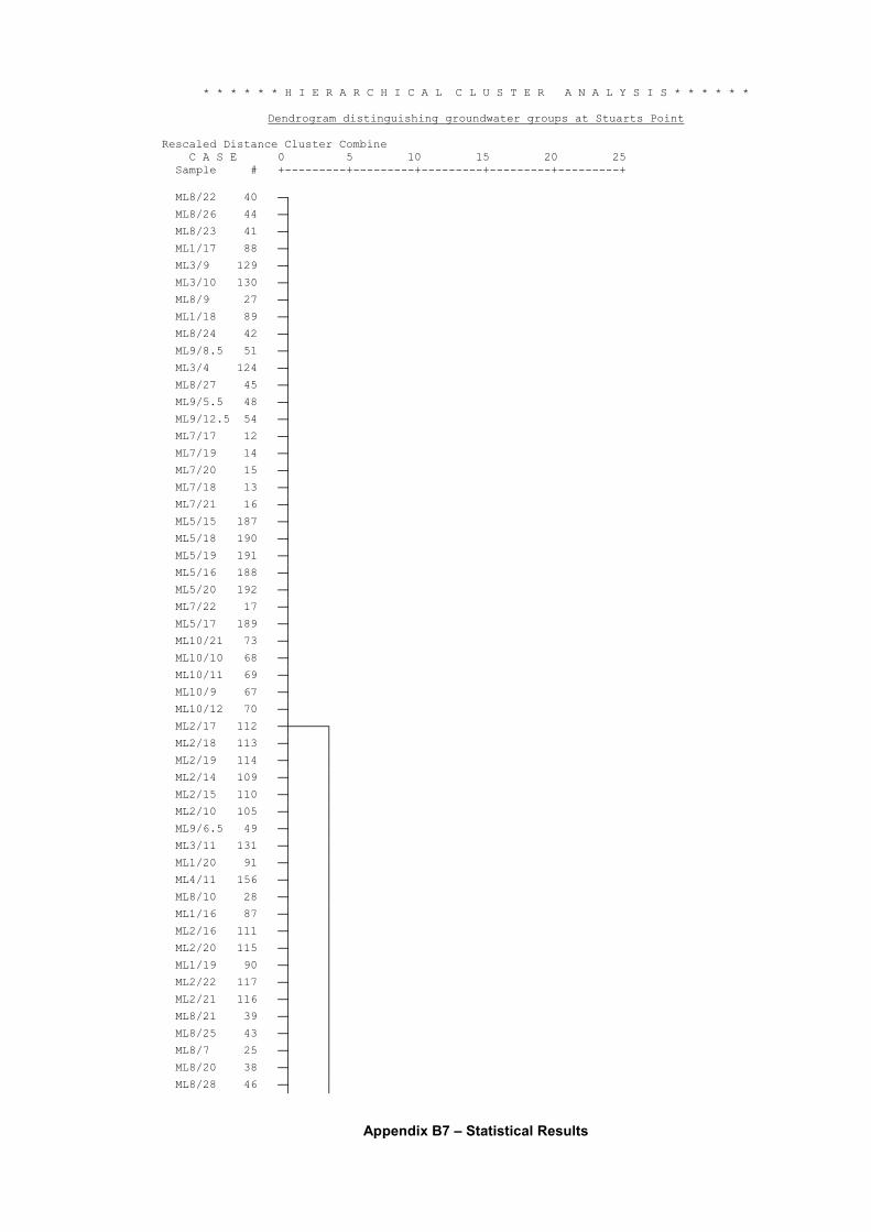
Appendix B7 – Statistical Results
* * * * * * H I E R A R C H I C A L C L U S T E R A N A L Y S I S * * * * * *
Dendrogram distinguishing groundwater groups at Stuarts Point
Rescaled Distance Cluster Combine C A S E 0 5 10 15 20 25 Sample # +---------+---------+---------+---------+---------+ ML8/22 40 òø ML8/26 44 òú ML8/23 41 òú ML1/17 88 òú ML3/9 129 òú ML3/10 130 òú ML8/9 27 òú ML1/18 89 òú ML8/24 42 òú ML9/8.5 51 òú ML3/4 124 òú ML8/27 45 òú ML9/5.5 48 òú ML9/12.5 54 òú ML7/17 12 òú ML7/19 14 òú ML7/20 15 òú ML7/18 13 òú ML7/21 16 òú ML5/15 187 òú ML5/18 190 òú ML5/19 191 òú ML5/16 188 òú ML5/20 192 òú ML7/22 17 òú ML5/17 189 òú ML10/21 73 òú ML10/10 68 òú ML10/11 69 òú ML10/9 67 òú ML10/12 70 òú ML2/17 112 òôòòòòòø ML2/18 113 òú ó ML2/19 114 òú ó ML2/14 109 òú ó ML2/15 110 òú ó ML2/10 105 òú ó ML9/6.5 49 òú ó ML3/11 131 òú ó ML1/20 91 òú ó ML4/11 156 òú ó ML8/10 28 òú ó ML1/16 87 òú ó ML2/16 111 òú ó ML2/20 115 òú ó ML1/19 90 òú ó ML2/22 117 òú ó ML2/21 116 òú ó ML8/21 39 òú ó ML8/25 43 òú ó ML8/7 25 òú ó ML8/20 38 òú ó ML8/28 46 òú ó
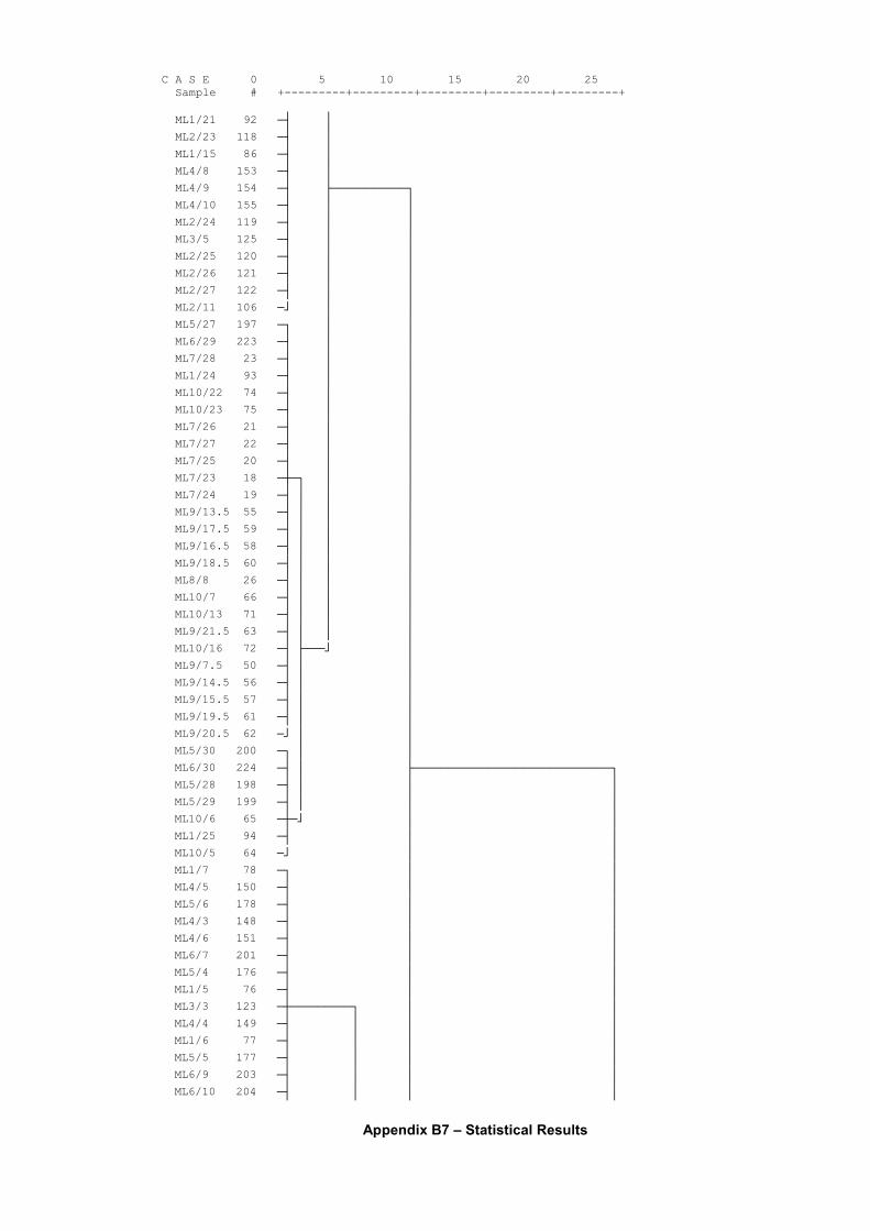
Appendix B7 – Statistical Results
C A S E 0 5 10 15 20 25 Sample # +---------+---------+---------+---------+---------+ ML1/21 92 òú ó ML2/23 118 òú ó ML1/15 86 òú ó ML4/8 153 òú ó ML4/9 154 òú ùòòòòòòòòòòòø ML4/10 155 òú ó ó ML2/24 119 òú ó ó ML3/5 125 òú ó ó ML2/25 120 òú ó ó ML2/26 121 òú ó ó ML2/27 122 òú ó ó ML2/11 106 ò÷ ó ó ML5/27 197 òø ó ó ML6/29 223 òú ó ó ML7/28 23 òú ó ó ML1/24 93 òú ó ó ML10/22 74 òú ó ó ML10/23 75 òú ó ó ML7/26 21 òú ó ó ML7/27 22 òú ó ó ML7/25 20 òú ó ó ML7/23 18 òôòø ó ó ML7/24 19 òú ó ó ó ML9/13.5 55 òú ó ó ó ML9/17.5 59 òú ó ó ó ML9/16.5 58 òú ó ó ó ML9/18.5 60 òú ó ó ó ML8/8 26 òú ó ó ó ML10/7 66 òú ó ó ó ML10/13 71 òú ó ó ó ML9/21.5 63 òú ó ó ó ML10/16 72 òú ùòòò÷ ó ML9/7.5 50 òú ó ó ML9/14.5 56 òú ó ó ML9/15.5 57 òú ó ó ML9/19.5 61 òú ó ó ML9/20.5 62 ò÷ ó ó ML5/30 200 òø ó ó ML6/30 224 òú ó ùòòòòòòòòòòòòòòòòòòòòòòòòòòòòòø ML5/28 198 òú ó ó ó ML5/29 199 òú ó ó ó ML10/6 65 òôò÷ ó ó ML1/25 94 òú ó ó ML10/5 64 ò÷ ó ó ML1/7 78 òø ó ó ML4/5 150 òú ó ó ML5/6 178 òú ó ó ML4/3 148 òú ó ó ML4/6 151 òú ó ó ML6/7 201 òú ó ó ML5/4 176 òú ó ó ML1/5 76 òú ó ó ML3/3 123 òôòòòòòòòòòø ó ó ML4/4 149 òú ó ó ó ML1/6 77 òú ó ó ó ML5/5 177 òú ó ó ó ML6/9 203 òú ó ó ó ML6/10 204 òú ó ó ó
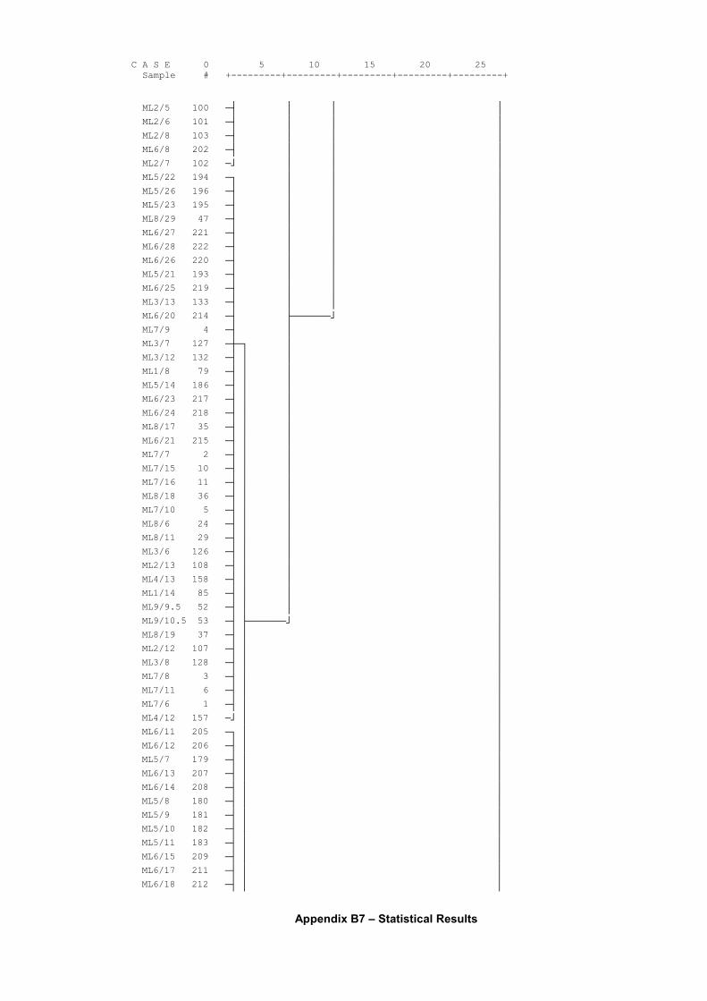
Appendix B7 – Statistical Results
C A S E 0 5 10 15 20 25 Sample # +---------+---------+---------+---------+---------+ ML2/5 100 òú ó ó ó ML2/6 101 òú ó ó ó ML2/8 103 òú ó ó ó ML6/8 202 òú ó ó ó ML2/7 102 ò÷ ó ó ó ML5/22 194 òø ó ó ó ML5/26 196 òú ó ó ó ML5/23 195 òú ó ó ó ML8/29 47 òú ó ó ó ML6/27 221 òú ó ó ó ML6/28 222 òú ó ó ó ML6/26 220 òú ó ó ó ML5/21 193 òú ó ó ó ML6/25 219 òú ó ó ó ML3/13 133 òú ó ó ó ML6/20 214 òú ùòòòòòòò÷ ó ML7/9 4 òú ó ó ML3/7 127 òôòø ó ó ML3/12 132 òú ó ó ó ML1/8 79 òú ó ó ó ML5/14 186 òú ó ó ó ML6/23 217 òú ó ó ó ML6/24 218 òú ó ó ó ML8/17 35 òú ó ó ó ML6/21 215 òú ó ó ó ML7/7 2 òú ó ó ó ML7/15 10 òú ó ó ó ML7/16 11 òú ó ó ó ML8/18 36 òú ó ó ó ML7/10 5 òú ó ó ó ML8/6 24 òú ó ó ó ML8/11 29 òú ó ó ó ML3/6 126 òú ó ó ó ML2/13 108 òú ó ó ó ML4/13 158 òú ó ó ó ML1/14 85 òú ó ó ó ML9/9.5 52 òú ó ó ó ML9/10.5 53 òú ùòòòòòòò÷ ó ML8/19 37 òú ó ó ML2/12 107 òú ó ó ML3/8 128 òú ó ó ML7/8 3 òú ó ó ML7/11 6 òú ó ó ML7/6 1 òú ó ó ML4/12 157 ò÷ ó ó ML6/11 205 òø ó ó ML6/12 206 òú ó ó ML5/7 179 òú ó ó ML6/13 207 òú ó ó ML6/14 208 òú ó ó ML5/8 180 òú ó ó ML5/9 181 òú ó ó ML5/10 182 òú ó ó ML5/11 183 òú ó ó ML6/15 209 òú ó ó ML6/17 211 òú ó ó ML6/18 212 òú ó ó
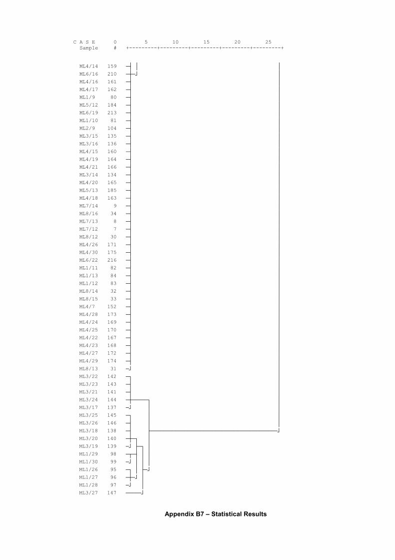
Appendix B7 – Statistical Results
C A S E 0 5 10 15 20 25 Sample # +---------+---------+---------+---------+---------+ ML4/14 159 òú ó ó ML6/16 210 òôò÷ ó ML4/16 161 òú ó ML4/17 162 òú ó ML1/9 80 òú ó ML5/12 184 òú ó ML6/19 213 òú ó ML1/10 81 òú ó ML2/9 104 òú ó ML3/15 135 òú ó ML3/16 136 òú ó ML4/15 160 òú ó ML4/19 164 òú ó ML4/21 166 òú ó ML3/14 134 òú ó ML4/20 165 òú ó ML5/13 185 òú ó ML4/18 163 òú ó ML7/14 9 òú ó ML8/16 34 òú ó ML7/13 8 òú ó ML7/12 7 òú ó ML8/12 30 òú ó ML4/26 171 òú ó ML4/30 175 òú ó ML6/22 216 òú ó ML1/11 82 òú ó ML1/13 84 òú ó ML1/12 83 òú ó ML8/14 32 òú ó ML8/15 33 òú ó ML4/7 152 òú ó ML4/28 173 òú ó ML4/24 169 òú ó ML4/25 170 òú ó ML4/22 167 òú ó ML4/23 168 òú ó ML4/27 172 òú ó ML4/29 174 òú ó ML8/13 31 ò÷ ó ML3/22 142 òø ó ML3/23 143 òú ó ML3/21 141 òú ó ML3/24 144 òôòòòòòø ó ML3/17 137 ò÷ ó ó ML3/25 145 òø ó ó ML3/26 146 òú ó ó ML3/18 138 òú ùòòòòòòòòòòòòòòòòòòòòòòòòòòòòòòòòòòòòòòòòò÷ ML3/20 140 òôòø ó ML3/19 139 ò÷ ùòø ó ML1/29 98 òûòú ó ó ML1/30 99 ò÷ ó ó ó ML1/26 95 òø ó ùò÷ ML1/27 96 òôò÷ ó ML1/28 97 ò÷ ó ML3/27 147 òòòòò÷
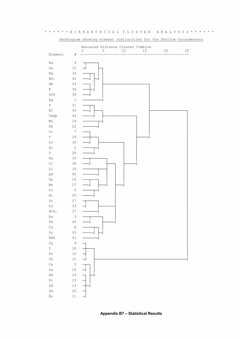
Appendix B7 – Statistical Results
* * * * * * H I E R A R C H I C A L C L U S T E R A N A L Y S I S * * * * * *
Dendrogram showing element similarities for the Shallow Groundwaters
Rescaled Distance Cluster Combine 0 5 10 15 20 25
Element # +---------+---------+---------+---------+---------+ Ba 4 òûòòòòòø Ga 12 ò÷ ùòø Ng 34 òòòûòø ó ó NO3 42 òòò÷ ùò÷ ó Rb 24 òòòø ó ùòòòòòòòòòòòòòòòòòòòòòø K 36 òòòôò÷ ó ó SO4 39 òòò÷ ó ó Ag 1 òòòòòòòòò÷ ó P 21 òòòûòø ó EC 43 òòò÷ ùòòòø ùòòòòòòòòòòòòòòòòòø Temp 44 òòòòò÷ ùòòòòòòòòòòòòòòòø ó ó Mo 18 òòòòòòòûò÷ ó ó ó Pb 22 òòòòòòò÷ ó ó ó Cr 7 òòòø ó ó ó V 29 òòòôòòòø ùòòòòò÷ ó Zr 32 òòò÷ ùòòòòòòòòòòòø ó ó Al 2 òòòòòûò÷ ó ó ó U 28 òòòòò÷ ó ó ó Na 35 òòòûòòòòòòòø ó ó ó Cl 38 òòò÷ ùòòòø ùòòòòò÷ ó Li 16 òòòòòòòûòòòú ó ó ó pH 45 òòòòòòò÷ ó ó ó ó Ge 14 òòòûòòòø ó ó ó ó Mn 17 òòò÷ ùòòò÷ ùòòò÷ ó Co 6 òòòòòûò÷ ó ó Ni 20 òòòòò÷ ó ó Sr 27 òûòòòòòø ó ó Ca 33 ò÷ ùòòòòòòòú ó HCO3 37 òòòòòòò÷ ó ó As 3 òòòûòòòòòø ó ó Fe 40 òòò÷ ùòòòòò÷ ó Cs 8 òòòòòûòø ó ó Sc 25 òòòòò÷ ùò÷ ó NH4 41 òòòòòòò÷ ó Dy 9 òø ó Y 30 òôòòòø ó Er 10 òú ó ó Yb 31 ò÷ ùòòòòòòòòòòòòòòòòòòòòòòòòòòòòòòòòòòòòòòòòòòò÷ Ce 5 òûòø ó La 15 ò÷ ó ó Nd 19 òø ùò÷ Pr 23 òú ó Gd 13 òôò÷ Sm 26 òú Eu 11 ò÷
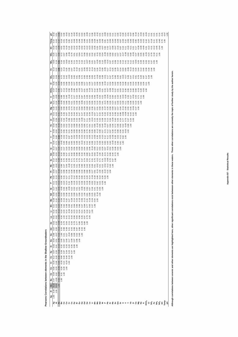
Pear
sons
Cor
rela
tions
bet
wee
n el
emen
ts in
the
Shal
low
Gro
undw
ater
s
Ag
Al
As
Ba
Ce
Co
Cr
Cs
Dy
ErEu
Ga
Gd
Ge
LaLi
Mn
Mo
Nd
Ni
PPb
PrR
bSc
SmSr
UV
YYb
ZrC
aM
gN
aK
HC
O3
Cl
SO4
FeN
H4
NO
3EC
Tem
ppH
Ag1.
00-0
.30
-0.2
20.
47-0
.04
0.06
-0.3
40.
12-0
.07
-0.0
2-0
.04
0.48
-0.0
7-0
.02
0.02
0.16
0.21
-0.2
8-0
.05
-0.2
7-0
.11
0.02
-0.0
40.
350.
14-0
.06
-0.1
4-0
.44
-0.3
9-0
.05
-0.0
4-0
.40
-0.2
10.
18-0
.21
0.29
-0.3
7-0
.26
0.22
-0.1
4-0
.03
0.25
-0.3
40.
10-0
.32
Al
1.00
0.13
-0.0
90.
620.
200.
480.
400.
500.
410.
51-0
.07
0.55
0.32
0.62
0.35
0.22
0.10
0.53
0.42
-0.2
50.
130.
57-0
.02
0.52
0.53
0.07
0.71
0.60
0.50
0.38
0.59
0.03
0.43
0.16
-0.0
5-0
.14
0.29
0.04
0.22
0.19
0.17
-0.1
5-0
.42
0.51
As
1.00
0.15
-0.2
0-0
.06
0.44
0.32
-0.1
6-0
.13
-0.0
50.
16-0
.14
-0.0
8-0
.20
-0.1
20.
220.
19-0
.16
-0.0
1-0
.13
0.14
-0.1
80.
110.
28-0
.13
0.24
0.04
0.54
-0.1
3-0
.15
0.21
0.31
0.23
-0.0
80.
290.
46-0
.04
0.40
0.86
0.51
0.00
-0.0
90.
100.
36B
a1.
000.
310.
28-0
.26
0.66
0.28
0.32
0.45
1.00
0.33
0.29
0.34
0.19
0.46
-0.5
60.
33-0
.05
-0.3
50.
000.
330.
900.
450.
330.
31-0
.45
-0.3
60.
290.
29-0
.41
0.28
0.60
-0.0
50.
88-0
.27
0.09
0.72
0.23
0.16
0.72
-0.5
1-0
.16
0.03
Ce
1.00
0.39
0.15
0.40
0.97
0.94
0.97
0.31
0.98
0.79
1.00
0.33
0.62
-0.1
50.
990.
55-0
.24
0.15
0.99
0.37
0.70
0.98
0.47
0.45
-0.0
20.
960.
920.
340.
360.
580.
260.
29-0
.12
0.35
0.44
-0.1
30.
040.
57-0
.18
-0.5
10.
08C
o1.
00-0
.20
0.44
0.34
0.33
0.40
0.27
0.39
0.54
0.41
0.14
0.36
0.20
0.38
0.66
-0.1
40.
270.
380.
440.
260.
370.
160.
08-0
.15
0.40
0.32
-0.1
60.
070.
600.
460.
46-0
.23
0.58
0.42
0.25
-0.0
30.
56-0
.19
-0.2
6-0
.02
Cr
1.00
0.18
0.23
0.20
0.17
-0.2
40.
21-0
.11
0.10
-0.3
40.
000.
270.
16-0
.09
0.15
0.11
0.16
-0.2
80.
450.
210.
180.
610.
870.
210.
190.
860.
14-0
.01
0.28
-0.1
80.
580.
18-0
.03
0.48
0.52
-0.3
60.
190.
060.
02C
s1.
000.
370.
350.
490.
680.
430.
340.
430.
240.
51-0
.28
0.40
0.22
-0.3
8-0
.12
0.39
0.72
0.71
0.42
0.26
0.05
0.20
0.38
0.32
0.02
0.25
0.74
0.21
0.74
-0.0
60.
340.
640.
570.
450.
70-0
.52
-0.3
10.
18D
y1.
000.
990.
970.
280.
990.
780.
960.
230.
64-0
.14
0.99
0.53
-0.1
80.
120.
980.
350.
730.
990.
560.
45-0
.02
0.99
0.98
0.39
0.44
0.52
0.33
0.27
0.06
0.37
0.45
-0.1
00.
110.
51-0
.12
-0.4
8-0
.02
Er1.
000.
960.
320.
970.
770.
930.
220.
66-0
.20
0.97
0.51
-0.2
30.
090.
960.
410.
750.
980.
580.
38-0
.09
0.99
0.99
0.33
0.45
0.51
0.38
0.32
0.09
0.39
0.51
-0.1
00.
180.
51-0
.15
-0.4
9-0
.05
Eu1.
000.
450.
990.
800.
960.
240.
66-0
.19
0.99
0.52
-0.2
30.
160.
980.
490.
750.
990.
580.
32-0
.04
0.96
0.94
0.28
0.47
0.64
0.26
0.44
-0.0
20.
350.
580.
010.
130.
64-0
.18
-0.4
60.
03G
a1.
000.
330.
290.
350.
210.
47-0
.56
0.34
-0.0
6-0
.36
0.00
0.33
0.90
0.47
0.34
0.30
-0.4
3-0
.33
0.29
0.29
-0.3
90.
270.
60-0
.06
0.87
-0.2
70.
080.
720.
240.
160.
72-0
.52
-0.1
60.
03G
d1.
000.
800.
970.
240.
64-0
.13
1.00
0.55
-0.2
00.
150.
990.
400.
741.
000.
540.
41-0
.01
0.98
0.95
0.37
0.43
0.59
0.31
0.34
0.01
0.37
0.50
-0.0
50.
110.
58-0
.15
-0.4
80.
00G
e1.
000.
790.
340.
770.
150.
810.
64-0
.18
0.20
0.80
0.43
0.53
0.80
0.64
0.14
-0.2
20.
790.
740.
110.
540.
680.
230.
390.
000.
370.
56-0
.05
-0.0
70.
65-0
.22
-0.4
1-0
.09
La1.
000.
370.
63-0
.18
0.98
0.57
-0.2
80.
140.
990.
420.
710.
970.
460.
42-0
.05
0.96
0.91
0.29
0.34
0.62
0.26
0.32
-0.1
60.
350.
46-0
.12
0.05
0.61
-0.2
3-0
.54
0.11
Li1.
000.
37-0
.24
0.25
0.18
-0.5
2-0
.16
0.27
0.30
0.31
0.24
-0.1
80.
08-0
.12
0.26
0.21
-0.2
4-0
.24
0.36
0.05
0.06
-0.4
70.
170.
03-0
.14
0.01
0.32
-0.6
3-0
.58
0.38
Mn
1.00
0.04
0.63
0.41
-0.2
20.
180.
610.
510.
700.
630.
590.
12-0
.09
0.68
0.66
0.15
0.57
0.67
0.16
0.46
0.12
0.22
0.70
0.20
0.07
0.61
-0.3
5-0
.28
-0.0
2M
o1.
00-0
.16
0.19
0.62
0.46
-0.1
5-0
.52
-0.2
1-0
.16
0.12
0.19
0.39
-0.1
2-0
.19
0.35
0.17
0.01
0.10
-0.3
50.
400.
09-0
.16
0.26
-0.2
9-0
.31
0.53
0.45
-0.3
2N
d1.
000.
55-0
.21
0.14
1.00
0.41
0.71
1.00
0.54
0.39
-0.0
50.
980.
950.
330.
420.
580.
280.
34-0
.03
0.35
0.50
-0.1
00.
090.
59-0
.16
-0.4
90.
01N
i1.
00-0
.30
0.30
0.55
0.22
0.31
0.54
0.29
0.30
-0.1
00.
570.
490.
080.
260.
500.
410.
220.
010.
480.
380.
090.
100.
54-0
.07
-0.5
60.
32P
1.00
0.20
-0.2
2-0
.54
-0.4
2-0
.21
0.07
0.00
0.12
-0.2
1-0
.18
0.16
0.16
-0.3
7-0
.21
-0.3
60.
34-0
.34
-0.3
1-0
.05
-0.5
8-0
.39
0.82
0.81
-0.6
9Pb
1.00
0.15
-0.1
2-0
.06
0.14
-0.0
10.
050.
120.
120.
070.
13-0
.01
0.26
0.08
-0.0
4-0
.07
0.11
0.17
0.17
-0.1
50.
030.
320.
190.
02Pr
1.00
0.40
0.70
0.99
0.52
0.40
-0.0
50.
970.
940.
340.
400.
580.
260.
33-0
.06
0.34
0.47
-0.1
10.
070.
58-0
.17
-0.5
00.
03R
b1.
000.
570.
400.
39-0
.39
-0.3
80.
380.
36-0
.39
0.34
0.69
0.23
0.94
-0.1
60.
380.
790.
250.
310.
82-0
.66
-0.4
40.
11Sc
1.00
0.73
0.48
0.34
0.28
0.76
0.72
0.40
0.38
0.67
0.41
0.51
0.22
0.43
0.65
0.39
0.58
0.51
-0.4
7-0
.49
0.12
Sm1.
000.
540.
40-0
.02
0.98
0.96
0.35
0.42
0.57
0.30
0.34
0.01
0.36
0.49
-0.0
70.
130.
57-0
.15
-0.4
90.
00Sr
1.00
0.01
-0.1
10.
560.
550.
240.
960.
400.
230.
440.
530.
280.
610.
140.
040.
370.
07-0
.07
-0.2
2U
1.00
0.62
0.44
0.42
0.77
-0.0
6-0
.11
0.28
-0.4
30.
140.
18-0
.24
0.03
0.13
-0.2
70.
10-0
.30
0.28
V1.
00-0
.03
-0.0
90.
75-0
.09
0.00
0.11
-0.2
60.
360.
08-0
.17
0.60
0.41
-0.3
90.
110.
100.
24Y
1.00
0.98
0.37
0.44
0.55
0.38
0.30
0.06
0.41
0.49
-0.0
60.
120.
53-0
.15
-0.5
0-0
.01
Yb1.
000.
340.
430.
450.
360.
270.
100.
350.
47-0
.13
0.12
0.48
-0.1
1-0
.46
-0.0
7Zr
1.00
0.22
-0.0
40.
20-0
.33
0.48
0.14
-0.1
10.
190.
21-0
.33
0.21
-0.0
30.
06C
a1.
000.
370.
100.
430.
580.
160.
610.
20-0
.04
0.37
0.17
0.06
-0.1
8M
g1.
000.
250.
71-0
.15
0.48
0.76
0.44
0.25
0.82
-0.3
9-0
.30
0.14
Na
1.00
0.11
0.28
0.92
0.20
0.13
0.39
0.05
-0.0
9-0
.40
-0.0
4K
1.00
-0.0
20.
260.
870.
450.
330.
82-0
.49
-0.2
20.
03H
CO
31.
000.
110.
170.
390.
33-0
.25
0.31
0.18
-0.2
9C
l1.
000.
280.
180.
320.
23-0
.22
-0.4
70.
11SO
41.
000.
460.
370.
78-0
.31
-0.1
80.
01Fe
1.00
0.55
0.18
-0.1
20.
110.
21N
H4
1.00
0.11
-0.4
5-0
.42
0.31
NO
31.
00-0
.44
-0.4
00.
10EC
1.00
0.70
-0.4
1Te
mp
1.00
-0.5
7pH
1.00
Alth
ough
cor
rela
tions
bet
wee
n ar
seni
c an
d ot
her e
lem
ents
are
hig
hlig
hted
her
e, o
ther
sig
nific
ant c
orre
latio
ns e
xist
bet
wee
en o
ther
ele
men
ts in
thes
e w
ater
s. T
hese
oth
er c
orre
latio
ns a
re c
urre
ntly
the
topi
c of
furt
her s
tudy
by
the
auth
or h
erei
n.
App
endi
x B
7 - S
tatis
tical
Res
ults
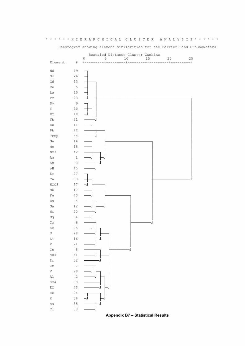
Appendix B7 – Statistical Results
* * * * * * H I E R A R C H I C A L C L U S T E R A N A L Y S I S * * * * * *
Dendrogram showing element similarities for the Barrier Sand Groundwaters
Rescaled Distance Cluster Combine 0 5 10 15 20 25
Element # +---------+---------+---------+---------+---------+ Nd 19 òø Sm 26 òú Gd 13 òôòòòø Ce 5 òú ó La 15 òú ó Pr 23 ò÷ ùòòòòòòòòòòòòòòòòòòòòòòòòòòòòòòòòòòòòòòòòòòòø Dy 9 òø ó ó Y 30 òôòø ó ó Er 10 ò÷ ó ó ó Yb 31 òòòôò÷ ó Eu 11 òòò÷ ó Pb 22 òòòòòûòòòø ó Temp 44 òòòòò÷ ó ó Ge 14 òòòø ùòòòòòòòòòòòòòòòòòòòòòø ó Mo 18 òòòú ó ó ó NO3 42 òòòôòòòø ó ó ó Ag 1 òòò÷ ùò÷ ó ó As 3 òòòòòûò÷ ó ó pH 45 òòòòò÷ ó ó Sr 27 òø ó ó Ca 33 òôòø ùòòòòòòòòòòòòòòòòò÷ HCO3 37 ò÷ ùòòòòòø ó Mn 17 òòòú ó ó Fe 40 òòò÷ ùòòòòòòòòòòòø ó Ba 4 òòòûòø ó ó ó Ga 12 òòò÷ ùòòò÷ ó ó Ni 20 òòòûò÷ ó ó Mg 34 òòò÷ ó ó Co 6 òòòûòø ùòòòòòòòòò÷ Sc 25 òòò÷ ùòø ó U 28 òòòòò÷ ùòòòø ó Li 16 òòòòòûò÷ ó ó P 21 òòòòò÷ ó ó Cs 8 òòòòòûòø ùòòòòòòòòò÷ NH4 41 òòòòò÷ ùòòòú Zr 32 òòòòòòò÷ ó Cr 7 òòòûòø ó V 29 òòò÷ ùòø ó Al 2 òòòòò÷ ùòø ó SO4 39 òòòòòòòú ó ó EC 43 òòòòòòò÷ ùò÷ Rb 24 òûòòòòòø ó K 36 ò÷ ùò÷ Na 35 òòòòòûò÷ Cl 38 òòòòò÷
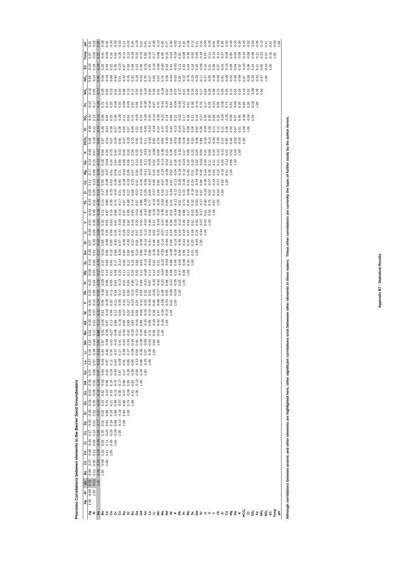
Pear
sons
Cor
rela
tions
bet
wee
n el
emen
ts in
the
Bar
rier S
and
Gro
undw
ater
s
AgAl
AsB
aC
eC
oC
rC
sD
yEr
EuG
aG
dG
eLa
LiM
nM
oN
dN
iP
PbPr
Rb
ScSm
SrU
VY
YbZr
Ca
Mg
Na
KH
CO
3C
lSO
4Fe
NH
4N
O3
ECTe
mp
pHAg
1.00
-0.0
80.
39-0
.39
-0.3
7-0
.48
-0.4
80.
27-0
.30
-0.3
0-0
.31
-0.0
2-0
.36
0.70
-0.2
70.
160.
150.
58-0
.30
-0.2
8-0
.01
0.29
-0.2
5-0
.58
-0.1
5-0
.35
0.07
-0.2
8-0
.51
-0.3
4-0
.43
0.29
0.14
-0.1
7-0
.22
-0.6
50.
28-0
.45
-0.4
1-0
.13
-0.1
60.
69-0
.33
0.07
0.31
Al1.
00-0
.21
-0.1
10.
560.
130.
590.
140.
510.
520.
35-0
.09
0.55
-0.0
80.
57-0
.39
-0.4
4-0
.27
0.52
-0.0
7-0
.14
0.08
0.54
0.04
0.00
0.51
-0.2
60.
090.
380.
490.
510.
29-0
.23
0.08
0.14
0.07
-0.2
80.
120.
15-0
.17
0.05
-0.2
40.
18-0
.09
-0.0
2As
1.00
-0.2
6-0
.22
-0.2
9-0
.40
0.16
-0.1
7-0
.27
-0.0
2-0
.10
-0.1
80.
47-0
.12
-0.1
20.
040.
62-0
.11
-0.3
2-0
.24
0.09
-0.0
6-0
.37
-0.4
0-0
.17
-0.0
2-0
.06
-0.6
0-0
.16
-0.3
60.
130.
03-0
.20
-0.1
2-0
.22
0.05
-0.2
4-0
.11
-0.2
9-0
.12
0.45
-0.2
60.
250.
35B
a1.
00-0
.08
0.33
0.04
0.35
0.01
0.02
0.24
0.82
-0.0
2-0
.54
-0.0
40.
400.
57-0
.52
-0.0
60.
610.
09-0
.38
-0.0
90.
720.
37-0
.03
0.65
-0.0
50.
310.
110.
14-0
.17
0.55
0.53
0.18
0.55
0.47
0.48
0.08
0.72
0.39
-0.5
60.
26-0
.41
-0.3
9C
e1.
000.
210.
71-0
.22
0.91
0.86
0.75
-0.2
20.
96-0
.32
0.97
-0.4
0-0
.46
-0.3
50.
97-0
.14
-0.2
80.
020.
960.
140.
000.
96-0
.48
0.26
0.55
0.87
0.80
0.04
-0.4
8-0
.07
-0.0
40.
26-0
.52
-0.0
10.
26-0
.21
0.02
-0.3
40.
33-0
.09
0.10
Co
1.00
0.36
-0.2
00.
160.
190.
210.
330.
19-0
.24
0.11
0.16
-0.0
1-0
.27
0.13
0.58
0.20
-0.1
10.
090.
510.
650.
190.
000.
590.
630.
160.
39-0
.25
0.03
0.51
0.24
0.70
-0.0
70.
360.
320.
200.
23-0
.60
0.22
0.16
-0.2
5C
r1.
00-0
.29
0.68
0.68
0.49
-0.1
10.
70-0
.43
0.63
-0.3
7-0
.42
-0.4
80.
660.
12-0
.11
0.18
0.61
0.28
0.17
0.69
-0.3
50.
350.
670.
680.
74-0
.02
-0.3
50.
090.
240.
42-0
.44
0.27
0.36
-0.0
80.
01-0
.44
0.25
0.05
-0.2
0C
s1.
00-0
.13
-0.1
6-0
.07
0.36
-0.1
70.
07-0
.09
0.17
0.41
0.01
-0.1
60.
04-0
.05
-0.1
7-0
.13
0.25
-0.1
4-0
.20
0.47
-0.4
7-0
.16
-0.1
0-0
.17
0.31
0.40
0.21
0.06
-0.0
10.
400.
28-0
.29
0.30
0.34
0.01
-0.2
4-0
.26
-0.0
3D
y1.
000.
940.
86-0
.07
0.96
-0.2
70.
91-0
.30
-0.3
2-0
.34
0.95
-0.0
7-0
.31
0.04
0.91
0.11
0.05
0.94
-0.3
60.
280.
560.
970.
870.
20-0
.39
-0.0
20.
080.
20-0
.37
0.05
0.11
-0.0
90.
08-0
.32
0.37
-0.1
20.
12Er
1.00
0.74
-0.0
60.
93-0
.28
0.85
-0.2
7-0
.30
-0.4
20.
890.
02-0
.27
0.06
0.84
0.11
0.12
0.90
-0.3
00.
230.
620.
950.
880.
22-0
.33
0.05
0.06
0.18
-0.2
90.
070.
04-0
.03
0.10
-0.3
50.
33-0
.13
-0.0
2Eu
1.00
0.22
0.82
-0.2
80.
80-0
.09
-0.1
8-0
.28
0.82
0.04
-0.2
3-0
.11
0.80
0.20
0.15
0.82
-0.2
20.
310.
430.
830.
740.
08-0
.25
0.07
0.11
0.28
-0.2
50.
090.
150.
020.
12-0
.31
0.39
-0.1
80.
20G
a1.
00-0
.13
-0.0
6-0
.13
0.59
0.54
-0.1
4-0
.16
0.56
0.24
-0.2
0-0
.17
0.42
0.56
-0.1
40.
560.
070.
20-0
.01
0.07
-0.0
70.
520.
550.
130.
330.
560.
22-0
.03
0.56
0.35
-0.2
00.
13-0
.31
-0.1
9G
d1.
00-0
.29
0.96
-0.3
5-0
.38
-0.3
40.
98-0
.04
-0.3
20.
030.
940.
120.
030.
98-0
.38
0.23
0.54
0.95
0.86
0.13
-0.4
0-0
.04
0.03
0.23
-0.4
20.
050.
16-0
.14
0.05
-0.3
20.
36-0
.10
0.12
Ge
1.00
-0.2
50.
07-0
.09
0.80
-0.2
5-0
.33
-0.0
10.
32-0
.21
-0.6
8-0
.10
-0.3
2-0
.14
-0.1
2-0
.52
-0.3
3-0
.38
0.20
-0.0
6-0
.11
-0.1
1-0
.53
0.11
-0.4
5-0
.28
-0.3
8-0
.20
0.78
-0.2
60.
280.
41La
1.00
-0.3
5-0
.42
-0.3
10.
98-0
.15
-0.3
00.
010.
970.
11-0
.04
0.96
-0.4
10.
160.
440.
880.
770.
09-0
.42
-0.0
7-0
.05
0.20
-0.4
5-0
.03
0.20
-0.1
90.
04-0
.27
0.35
-0.1
90.
17Li
1.00
0.54
0.06
-0.3
90.
380.
46-0
.05
-0.4
00.
130.
62-0
.36
0.48
0.02
0.11
-0.2
9-0
.10
-0.0
70.
490.
240.
02-0
.08
0.60
-0.0
4-0
.14
0.47
0.20
0.04
-0.1
6-0
.17
-0.0
5M
n1.
00-0
.01
-0.4
20.
47-0
.08
-0.2
7-0
.42
0.31
0.22
-0.4
00.
84-0
.31
-0.0
4-0
.26
-0.2
60.
090.
820.
35-0
.20
0.09
0.76
0.23
-0.3
60.
760.
31-0
.07
-0.0
6-0
.08
-0.1
3M
o1.
00-0
.30
-0.3
4-0
.08
0.28
-0.2
5-0
.64
-0.2
2-0
.35
-0.1
4-0
.07
-0.5
7-0
.40
-0.5
00.
19-0
.07
-0.2
9-0
.13
-0.4
60.
04-0
.37
-0.2
1-0
.43
-0.1
90.
75-0
.40
0.39
0.45
Nd
1.00
-0.1
5-0
.33
0.05
0.98
0.09
-0.0
40.
98-0
.44
0.21
0.46
0.92
0.80
0.11
-0.4
5-0
.09
-0.0
20.
20-0
.46
-0.0
30.
18-0
.20
0.02
-0.2
60.
33-0
.10
0.17
Ni
1.00
0.02
-0.0
6-0
.21
0.39
0.58
-0.0
80.
590.
180.
360.
010.
21-0
.24
0.62
0.62
0.07
0.38
0.49
0.43
0.00
0.64
0.26
-0.4
40.
12-0
.01
-0.4
2P
1.00
-0.0
4-0
.35
0.15
0.49
-0.3
0-0
.10
0.26
0.16
-0.3
4-0
.11
-0.1
2-0
.11
-0.0
40.
160.
05-0
.03
-0.1
30.
22-0
.04
0.03
-0.0
2-0
.03
-0.2
4-0
.02
Pb1.
000.
05-0
.47
-0.0
50.
04-0
.30
0.10
-0.1
20.
060.
010.
13-0
.25
-0.1
90.
15-0
.32
-0.0
6-0
.20
-0.2
2-0
.30
-0.2
70.
35-0
.11
0.32
0.12
Pr1.
000.
06-0
.08
0.95
-0.4
40.
190.
400.
880.
740.
10-0
.46
-0.1
0-0
.04
0.17
-0.4
6-0
.07
0.17
-0.2
30.
01-0
.22
0.33
-0.0
80.
20R
b1.
000.
330.
140.
330.
070.
540.
170.
25-0
.09
0.22
0.45
0.22
0.85
0.06
0.58
0.28
0.51
0.30
-0.7
60.
24-0
.30
-0.3
6Sc
1.00
0.01
0.20
0.49
0.61
0.03
0.32
-0.1
80.
240.
510.
100.
330.
260.
080.
210.
380.
16-0
.25
0.14
-0.0
2-0
.12
Sm1.
00-0
.43
0.25
0.52
0.93
0.83
0.10
-0.4
4-0
.09
0.02
0.25
-0.4
60.
020.
19-0
.15
0.04
-0.3
20.
33-0
.08
0.11
Sr1.
00-0
.44
-0.0
7-0
.27
-0.2
70.
070.
960.
49-0
.02
0.09
0.88
0.36
-0.2
70.
760.
27-0
.17
-0.0
6-0
.19
-0.3
1U
1.00
0.43
0.21
0.40
-0.1
9-0
.36
0.14
0.24
0.31
-0.3
2-0
.05
0.35
-0.1
70.
04-0
.27
0.15
0.25
-0.0
3V
1.00
0.55
0.75
0.02
-0.0
70.
360.
110.
56-0
.14
0.28
0.30
0.26
0.29
-0.6
50.
31-0
.11
-0.2
8Y
1.00
0.87
0.22
-0.3
20.
000.
110.
24-0
.30
0.12
0.05
-0.0
10.
09-0
.38
0.39
-0.1
30.
03Yb
1.00
0.04
-0.2
70.
150.
110.
33-0
.30
0.12
0.26
0.05
0.23
-0.4
80.
37-0
.12
-0.0
9Zr
1.00
0.02
-0.1
60.
20-0
.21
0.15
0.11
-0.5
4-0
.06
0.05
0.04
-0.0
1-0
.07
0.19
Ca
1.00
0.51
-0.1
10.
020.
900.
26-0
.25
0.74
0.25
-0.0
9-0
.15
-0.0
9-0
.32
Mg
1.00
0.08
0.52
0.48
0.32
0.09
0.51
0.12
-0.3
20.
090.
00-0
.43
Na
1.00
0.23
-0.0
20.
570.
07-0
.05
0.01
-0.3
00.
04-0
.03
-0.1
0K
1.00
-0.1
50.
510.
450.
260.
16-0
.69
0.32
-0.0
9-0
.30
HC
O3
1.00
0.09
-0.4
60.
650.
180.
07-0
.20
-0.1
0-0
.25
Cl
1.00
-0.0
40.
390.
32-0
.59
0.06
-0.0
8-0
.32
SO4
1.00
-0.2
0-0
.08
-0.2
00.
15-0
.08
-0.0
3Fe
1.00
0.36
-0.4
10.
11-0
.21
-0.3
5N
H4
1.00
-0.3
70.
05-0
.22
-0.1
3N
O3
1.00
-0.4
20.
220.
41EC
1.00
-0.3
10.
22Te
mp
1.00
-0.0
5pH
1.00
Alth
ough
cor
rela
tions
bet
wee
n ar
seni
c an
d ot
her e
lem
ents
are
hig
hlig
hted
her
e, o
ther
sig
nific
ant c
orre
latio
ns e
xist
bet
wee
en o
ther
ele
men
ts in
thes
e w
ater
s. T
hese
oth
er c
orre
latio
ns a
re c
urre
ntly
the
topi
c of
furt
her s
tudy
by
the
auth
or h
erei
n.
App
endi
x B
7 - S
tatis
tical
Res
ults
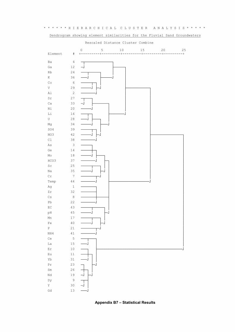
Appendix B7 – Statistical Results
* * * * * * H I E R A R C H I C A L C L U S T E R A N A L Y S I S * * * * *
Dendrogram showing element similarities for the Fluvial Sand Groundwaters
Rescaled Distance Cluster Combine
0 5 10 15 20 25 Element # +---------+---------+---------+---------+---------+ Ba 4 òûòòòòòòòòòòòòòø Ga 12 ò÷ ùòòòòòø Rb 24 òòòûòòòòòø ó ó K 36 òòò÷ ùòòòòò÷ ó Co 6 òòòòòûòø ó ó V 29 òòòòò÷ ùò÷ ùòòòòòòòòòòòø Al 2 òòòòòòò÷ ó ó Sr 27 òûòòòø ó ó Ca 33 ò÷ ùòòòòòòòø ó ó Ni 20 òòòòò÷ ó ó ó Li 16 òòòûòø ùòòòòòòò÷ ó U 28 òòò÷ ùòòòø ó ó Mg 34 òòòòò÷ ùòòò÷ ó SO4 39 òòòòòûòø ó ó NO3 42 òòòòò÷ ùò÷ ùòòòòòòòòòòòòòòòø Cl 38 òòòòòòò÷ ó ó As 3 òòòòòø ó ó Ge 14 òòòòòôòø ó ó Mo 18 òòòòò÷ ùòòòø ó ó HCO3 37 òòòòòòò÷ ùòø ó ó Sc 25 òòòòòûòòòø ó ó ó ó Na 35 òòòòò÷ ùò÷ ó ó ó Cr 7 òòòòòòòûò÷ ó ó ó Temp 44 òòòòòòò÷ ùòòòòòòòòòòòòòòòòòòò÷ ó Ag 1 òòòòòòòø ó ó Zr 32 òòòòòòòú ó ó Cs 8 òòòòòòòôòòòòòú ó Pb 22 òòòòòòò÷ ó ó EC 43 òòòòòûòòòòòø ó ó pH 45 òòòòò÷ ùò÷ ó Mn 17 òòòòòûòòòø ó ó Fe 40 òòòòò÷ ùò÷ ó P 21 òòòòòòòûò÷ ó NH4 41 òòòòòòò÷ ó Ce 5 òòòûòòòø ó La 15 òòò÷ ó ó Er 10 òòòø ùòòòòòòòòòòòòòòòòòòòòòòòòòòòòòòòòòòòòòòòòò÷ Eu 11 òòòôòø ó Yb 31 òòò÷ ó ó Pr 23 òø ùò÷ Sm 26 òôòø ó Nd 19 ò÷ ùò÷ Dy 9 òûòú Y 30 ò÷ ó Gd 13 òòò÷

Pear
sons
Cor
rela
tions
bet
wee
n el
emen
ts in
the
Fluv
ial S
and
Gro
undw
ater
s
Ag
Al
As
Ba
Ce
Co
Cr
Cs
Dy
ErEu
Ga
Gd
Ge
LaLi
Mn
Mo
Nd
Ni
PPb
PrR
bSc
SmSr
UV
YYb
ZrC
aM
gN
aK
HC
O3
Cl
SO4
FeN
H4
NO
3EC
Tem
ppH
Ag
1.00
-0.2
90.
160.
19-0
.56
-0.6
1-0
.33
0.42
-0.0
6-0
.01
-0.0
70.
30-0
.16
-0.1
0-0
.25
0.01
0.37
0.05
-0.1
6-0
.03
-0.1
40.
35-0
.17
0.09
-0.1
9-0
.18
0.23
-0.2
0-0
.21
0.10
-0.2
00.
440.
180.
030.
19-0
.28
0.22
0.17
-0.1
70.
04-0
.21
0.24
0.15
0.09
0.32
Al
1.00
-0.2
00.
040.
560.
370.
240.
110.
380.
260.
180.
050.
390.
060.
51-0
.25
-0.3
1-0
.40
0.42
-0.0
2-0
.17
-0.1
30.
390.
10-0
.04
0.39
-0.2
5-0
.06
0.48
0.25
0.28
0.00
-0.2
1-0
.04
-0.3
40.
12-0
.31
-0.1
10.
23-0
.17
0.21
-0.0
4-0
.07
-0.1
90.
10A
s1.
000.
03-0
.41
-0.3
8-0
.17
0.15
-0.2
0-0
.23
-0.1
70.
09-0
.16
0.65
-0.4
5-0
.35
0.21
0.58
-0.2
5-0
.16
-0.0
20.
04-0
.30
-0.4
80.
18-0
.26
-0.0
5-0
.11
-0.6
4-0
.12
-0.3
90.
230.
10-0
.33
0.33
-0.3
80.
53-0
.30
-0.5
50.
050.
23-0
.53
-0.0
80.
060.
31B
a1.
000.
060.
03-0
.08
0.39
0.35
0.37
0.52
0.97
0.20
0.23
0.09
-0.1
9-0
.09
-0.1
30.
20-0
.09
-0.2
10.
140.
200.
520.
290.
27-0
.27
-0.2
2-0
.02
0.46
0.38
0.12
-0.1
70.
020.
210.
34-0
.14
-0.0
3-0
.32
0.31
-0.0
50.
040.
11-0
.14
-0.1
1C
e1.
000.
650.
31-0
.10
0.67
0.67
0.66
-0.0
20.
730.
030.
850.
15-0
.24
-0.3
20.
780.
060.
00-0
.28
0.82
0.34
0.09
0.80
-0.3
50.
110.
380.
560.
72-0
.35
-0.3
50.
14-0
.21
0.47
-0.6
70.
040.
35-0
.05
-0.0
10.
130.
02-0
.07
-0.1
3C
o1.
000.
33-0
.14
0.30
0.34
0.40
-0.0
80.
360.
050.
420.
29-0
.26
-0.1
90.
360.
41-0
.10
-0.3
00.
370.
340.
350.
390.
030.
410.
500.
200.
48-0
.36
0.04
0.27
-0.1
80.
61-0
.36
0.11
0.40
-0.0
3-0
.01
0.20
0.01
0.05
-0.3
4C
r1.
00-0
.08
0.06
0.16
0.11
-0.1
00.
190.
140.
08-0
.04
-0.1
8-0
.04
0.12
0.17
-0.1
00.
180.
110.
050.
220.
16-0
.08
0.00
0.36
0.15
0.23
0.03
-0.0
2-0
.01
0.14
0.18
0.05
0.09
-0.0
5-0
.04
0.01
-0.1
6-0
.02
0.24
-0.1
3C
s1.
000.
320.
340.
270.
480.
230.
330.
090.
09-0
.02
0.23
0.17
0.15
-0.0
20.
220.
160.
360.
330.
160.
01-0
.03
0.05
0.40
0.18
0.44
0.07
0.21
0.26
0.18
0.12
0.07
-0.2
3-0
.02
-0.0
40.
10-0
.02
0.24
0.16
Dy
1.00
0.84
0.76
0.36
0.89
0.16
0.71
0.02
0.09
-0.1
70.
82-0
.01
-0.1
0-0
.09
0.84
0.40
0.11
0.85
-0.3
8-0
.12
0.17
0.89
0.79
0.11
-0.3
2-0
.06
0.00
0.24
-0.5
4-0
.03
0.11
0.07
0.00
0.14
0.03
0.14
-0.0
3Er
1.00
0.85
0.35
0.82
0.11
0.71
0.17
0.03
-0.1
50.
810.
08-0
.10
-0.0
70.
840.
460.
190.
84-0
.37
0.03
0.17
0.86
0.82
0.08
-0.3
30.
100.
060.
36-0
.57
0.06
0.10
0.05
-0.1
60.
200.
100.
16-0
.03
Eu1.
000.
470.
730.
190.
670.
220.
05-0
.07
0.75
0.08
-0.0
3-0
.13
0.79
0.49
0.23
0.82
-0.3
10.
060.
110.
780.
81-0
.02
-0.2
80.
160.
130.
46-0
.54
0.13
0.08
0.18
-0.0
70.
200.
08-0
.02
-0.0
9G
a1.
000.
210.
240.
05-0
.22
-0.0
1-0
.11
0.19
-0.0
9-0
.21
0.17
0.19
0.47
0.26
0.25
-0.2
2-0
.27
-0.0
30.
500.
330.
26-0
.12
-0.0
10.
230.
23-0
.06
0.01
-0.3
60.
32-0
.05
0.05
0.10
-0.0
9-0
.03
Gd
1.00
0.20
0.74
0.06
0.11
-0.1
10.
850.
02-0
.10
-0.1
00.
870.
340.
080.
89-0
.35
-0.0
50.
170.
860.
770.
09-0
.30
-0.0
3-0
.09
0.23
-0.5
4-0
.07
0.12
0.09
-0.0
20.
11-0
.03
0.19
-0.0
7G
e1.
00-0
.08
-0.3
4-0
.01
0.47
0.08
-0.0
7-0
.16
0.10
0.06
-0.1
90.
450.
13-0
.27
-0.2
5-0
.37
0.19
0.05
0.13
-0.0
6-0
.25
0.35
-0.0
70.
23-0
.29
-0.5
20.
070.
26-0
.48
-0.1
40.
220.
04La
1.00
0.30
-0.1
6-0
.35
0.82
0.08
-0.0
2-0
.18
0.86
0.42
-0.0
40.
78-0
.28
0.10
0.33
0.61
0.69
-0.3
1-0
.34
0.29
-0.2
90.
43-0
.76
0.10
0.45
-0.1
8-0
.06
0.36
0.01
-0.1
1-0
.02
Li1.
00-0
.01
0.03
0.12
0.52
0.37
-0.1
70.
180.
360.
230.
140.
410.
740.
310.
020.
19-0
.27
0.22
0.73
-0.0
20.
51-0
.19
0.46
0.46
-0.1
2-0
.32
0.58
0.13
0.00
-0.0
8M
n1.
000.
230.
030.
110.
140.
05-0
.02
-0.2
2-0
.14
0.01
0.26
-0.1
2-0
.38
0.21
-0.0
30.
420.
30-0
.18
0.26
-0.3
50.
310.
19-0
.15
0.45
0.01
-0.1
0-0
.01
0.22
0.21
Mo
1.00
-0.1
70.
080.
10-0
.02
-0.2
2-0
.32
0.17
-0.1
80.
030.
20-0
.49
-0.1
0-0
.24
0.06
0.14
-0.0
40.
38-0
.12
0.38
-0.0
8-0
.33
-0.0
20.
04-0
.34
-0.0
60.
320.
08N
d1.
000.
04-0
.14
-0.1
30.
910.
350.
000.
88-0
.34
0.02
0.15
0.81
0.77
-0.1
0-0
.33
0.11
-0.1
00.
31-0
.65
0.07
0.25
-0.0
6-0
.10
0.25
0.06
0.08
-0.0
2N
i1.
00-0
.05
-0.1
10.
030.
250.
210.
020.
730.
490.
380.
030.
08-0
.17
0.74
0.62
-0.1
60.
420.
200.
440.
47-0
.21
-0.2
00.
52-0
.19
0.15
-0.1
9P
1.00
-0.1
1-0
.09
-0.1
00.
27-0
.07
0.06
0.28
-0.0
8-0
.13
-0.0
40.
08-0
.02
0.07
0.14
-0.0
60.
16-0
.03
-0.0
40.
310.
18-0
.22
-0.0
4-0
.11
0.05
Pb1.
00-0
.15
-0.0
10.
05-0
.15
-0.0
8-0
.17
-0.1
00.
01-0
.05
0.32
-0.0
7-0
.12
0.18
-0.2
00.
12-0
.07
-0.2
9-0
.02
-0.0
7-0
.05
-0.1
30.
14-0
.13
Pr1.
000.
410.
020.
93-0
.32
0.02
0.23
0.79
0.78
-0.1
0-0
.34
0.16
-0.1
40.
35-0
.65
0.06
0.23
0.04
-0.0
90.
270.
030.
06-0
.04
Rb
1.00
0.20
0.42
-0.0
10.
150.
430.
430.
53-0
.09
-0.0
30.
420.
000.
80-0
.40
0.29
0.24
0.02
-0.2
70.
510.
170.
03-0
.23
Sc1.
000.
09-0
.13
0.20
0.07
0.16
0.27
0.03
-0.0
40.
040.
490.
360.
150.
00-0
.34
0.13
0.05
-0.2
00.
030.
19-0
.07
Sm1.
00-0
.34
0.01
0.23
0.82
0.83
-0.0
2-0
.32
0.10
-0.0
90.
34-0
.59
0.02
0.14
0.11
-0.1
00.
190.
020.
06-0
.09
Sr1.
000.
310.
19-0
.32
-0.3
4-0
.03
0.93
0.55
-0.2
20.
040.
520.
470.
33-0
.01
-0.2
20.
50-0
.14
0.01
0.00
U1.
000.
26-0
.13
0.03
-0.2
60.
180.
57-0
.07
0.43
-0.0
80.
200.
41-0
.22
-0.1
90.
290.
05-0
.06
-0.1
3V
1.00
0.10
0.27
-0.0
30.
120.
38-0
.34
0.41
-0.1
80.
240.
44-0
.12
-0.1
10.
43-0
.01
-0.0
4-0
.13
Y1.
000.
780.
25-0
.25
-0.0
40.
120.
23-0
.42
0.06
-0.0
40.
19-0
.09
0.13
0.04
0.24
0.02
Yb1.
00-0
.01
-0.3
20.
09-0
.01
0.47
-0.5
90.
040.
100.
10-0
.14
0.20
0.07
0.14
-0.2
0Zr
1.00
0.04
-0.3
60.
20-0
.44
0.36
-0.1
0-0
.45
0.39
0.05
-0.2
4-0
.08
0.25
0.18
Ca
1.00
0.40
-0.1
6-0
.01
0.64
0.33
0.20
0.05
-0.1
30.
34-0
.25
0.05
-0.0
3M
g1.
00-0
.18
0.64
-0.0
60.
510.
43-0
.23
-0.2
50.
660.
05-0
.13
-0.0
5N
a1.
000.
030.
300.
29-0
.49
0.24
0.12
-0.3
80.
280.
180.
30K
1.00
-0.3
70.
350.
34-0
.19
-0.1
50.
430.
19-0
.02
-0.2
1H
CO
31.
000.
06-0
.45
0.27
0.17
-0.3
5-0
.14
0.13
0.28
Cl
1.00
0.28
-0.0
3-0
.32
0.49
0.30
-0.0
50.
18SO
41.
00-0
.49
-0.1
20.
670.
04-0
.14
-0.1
7Fe
1.00
0.06
-0.3
5-0
.01
-0.0
50.
03N
H4
1.00
-0.4
4-0
.17
-0.0
70.
20N
O3
1.00
0.06
-0.0
8-0
.18
EC1.
000.
030.
49Te
mp
1.00
-0.1
3pH
1.00
Alth
ough
cor
rela
tions
bet
wee
n ar
seni
c an
d ot
her e
lem
ents
are
hig
hlig
hted
her
e, o
ther
sig
nific
ant c
orre
latio
ns e
xist
bet
wee
en o
ther
ele
men
ts in
thes
e w
ater
s. T
hese
oth
er c
orre
latio
ns a
re c
urre
ntly
the
topi
c of
furt
her s
tudy
by
the
auth
or h
erei
n.
App
endi
x B
7 - S
tatis
tical
Res
ults
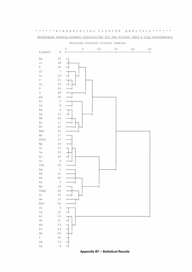
Appendix B7 – Statistical Results
* * * * * * H I E R A R C H I C A L C L U S T E R A N A L Y S I S * * * * * *
Dendrogram showing element similarities for the Fluvial Sand & Clay Groundwaters
Rescaled Distance Cluster Combine 0 5 10 15 20 25 Element # +---------+---------+---------+---------+---------+ Na 35 òø Cl 38 òôòòòòòø K 36 ò÷ ùòòòø Cr 7 òûòòòø ó ó Li 16 ò÷ ùò÷ ó P 21 òûòø ó ùòòòø Sc 25 ò÷ ùò÷ ó ó V 29 òòò÷ ó ó U 28 òòòûòòòòòòò÷ ó pH 45 òòò÷ ùòòòòòòòòòòòòòø Al 2 òòòûòòòòòø ó ó Cs 8 òòò÷ ó ó ó Ba 4 òûòø ó ó ó Ga 12 ò÷ ó ùòòòòò÷ ó Rb 24 òòòôòø ó ó Eu 11 òòò÷ ùòø ó ó EC 43 òòòòò÷ ùò÷ ó NH4 41 òòòòòòò÷ ùòòòòòòòòòòòòòòòòòòòø Mn 17 òòòø ó ó HCO3 37 òòòú ó ó Mg 34 òòòú ó ó Sr 27 òø ùòø ó ó Ca 33 òôòú ó ó ó Ni 20 ò÷ ó ùòòòòòòòòòòòòòø ó ó Co 6 òòò÷ ó ó ó ó SO4 39 òòòòò÷ ó ó ó Ag 1 òòòòòø ùòòòòòòòòò÷ ó Pb 22 òòòòòú ó ó Fe 40 òòòòòôòòòø ó ó As 3 òòòòò÷ ó ó ó Mo 18 òòòø ùòòòòòòòòò÷ ó Temp 44 òòòôòòòø ó ó Zr 32 òòò÷ ùò÷ ó Ge 14 òòòòòûò÷ ó NO3 42 òòòòò÷ ó Ce 5 òûòòòø ó La 15 ò÷ ó ó Er 10 òûòø ùòòòòòòòòòòòòòòòòòòòòòòòòòòòòòòòòòòòòòòòòòòò÷ Yb 31 ò÷ ó ó Nd 19 òø ùò÷ Pr 23 òú ó Sm 26 òôò÷ Y 30 òú Gd 13 òú Dy 9 ò÷
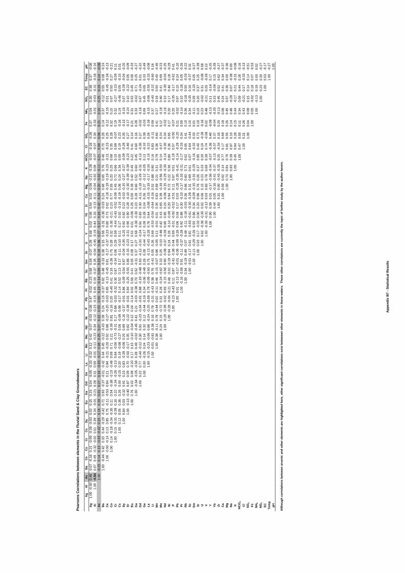
Pear
sons
Cor
rela
tions
bet
wee
n el
emen
ts in
the
Fluv
ial S
and
& C
lay
Gro
undw
ater
s
Ag
Al
As
Ba
Ce
Co
Cr
Cs
Dy
ErEu
Ga
Gd
Ge
LaLi
Mn
Mo
Nd
Ni
PPb
PrR
bSc
SmSr
UV
YYb
ZrC
aM
gN
aK
HC
O3
Cl
SO4
FeN
H4
NO
3EC
Tem
ppH
Ag
1.00
-0.5
00.
46-0
.07
-0.1
60.
21-0
.09
-0.3
9-0
.03
0.02
0.15
0.23
0.04
-0.0
5-0
.33
-0.3
20.
120.
42-0
.07
-0.0
3-0
.08
0.47
-0.0
2-0
.23
0.08
0.04
-0.0
70.
280.
080.
020.
060.
540.
02-0
.09
-0.2
1-0
.28
-0.0
3-0
.16
-0.2
60.
370.
040.
300.
380.
37-0
.06
Al
1.00
-0.5
40.
070.
49-0
.32
-0.0
20.
510.
390.
34-0
.01
-0.2
10.
280.
310.
59-0
.01
-0.1
1-0
.23
0.34
-0.1
2-0
.23
-0.1
50.
450.
19-0
.37
0.35
-0.0
4-0
.45
-0.1
90.
440.
33-0
.15
-0.1
1-0
.04
-0.0
20.
08-0
.07
-0.0
70.
30-0
.33
-0.0
1-0
.03
-0.3
1-0
.18
-0.1
0A
s1.
00-0
.25
0.14
0.13
-0.0
3-0
.42
0.15
0.16
0.19
0.01
0.27
0.16
-0.0
3-0
.17
0.08
0.25
0.27
0.22
0.03
0.00
0.23
-0.1
40.
090.
230.
190.
380.
270.
170.
240.
420.
240.
20-0
.02
-0.1
10.
210.
000.
060.
210.
100.
250.
190.
14-0
.08
Ba
1.00
-0.4
40.
420.
330.
44-0
.29
-0.4
20.
710.
93-0
.37
-0.0
1-0
.42
0.44
0.45
-0.2
2-0
.43
0.39
0.24
-0.1
6-0
.37
0.82
0.48
-0.3
30.
380.
150.
56-0
.31
-0.3
6-0
.03
0.24
0.66
0.65
0.76
0.46
0.70
0.26
0.14
0.37
-0.1
20.
550.
08-0
.24
Ce
1.00
-0.5
0-0
.14
0.13
0.85
0.75
-0.1
1-0
.53
0.84
0.21
0.94
-0.2
1-0
.26
0.02
0.88
-0.2
7-0
.20
-0.0
30.
85-0
.13
-0.4
50.
81-0
.17
-0.3
7-0
.23
0.80
0.73
0.02
-0.1
8-0
.19
-0.1
9-0
.23
-0.2
1-0
.23
0.25
-0.1
2-0
.15
0.01
-0.4
5-0
.34
-0.1
3C
o1.
000.
14-0
.18
-0.3
4-0
.35
0.11
0.54
-0.3
8-0
.10
-0.4
80.
090.
710.
21-0
.39
0.81
-0.1
60.
20-0
.40
0.41
0.16
-0.3
60.
750.
280.
32-0
.30
-0.2
10.
230.
770.
550.
200.
250.
680.
350.
280.
320.
150.
070.
500.
27-0
.21
Cr
1.00
0.15
-0.3
1-0
.39
0.16
0.22
-0.3
4-0
.26
-0.1
30.
84-0
.06
-0.7
3-0
.31
0.17
0.68
-0.0
3-0
.32
0.30
0.67
-0.3
40.
060.
290.
59-0
.44
-0.4
3-0
.52
-0.0
90.
450.
720.
660.
100.
69-0
.07
0.19
0.32
-0.2
7-0
.23
-0.5
90.
11C
s1.
000.
120.
050.
360.
260.
00-0
.15
0.20
0.19
-0.0
8-0
.27
0.06
-0.0
90.
08-0
.17
0.14
0.52
0.13
0.17
-0.1
1-0
.10
0.11
0.17
0.02
-0.1
6-0
.19
0.06
0.24
0.34
0.00
0.19
0.23
-0.1
60.
19-0
.46
0.05
-0.1
50.
01D
y1.
000.
840.
03-0
.32
0.91
0.23
0.83
-0.3
9-0
.08
0.25
0.89
-0.1
6-0
.37
-0.0
10.
86-0
.09
-0.5
40.
87-0
.04
-0.3
5-0
.25
0.92
0.82
0.23
-0.0
3-0
.15
-0.2
7-0
.27
-0.0
9-0
.28
0.35
-0.1
3-0
.15
0.07
-0.2
9-0
.04
-0.2
0Er
1.00
-0.1
3-0
.40
0.87
0.09
0.70
-0.5
0-0
.17
0.35
0.82
-0.2
2-0
.38
-0.0
10.
84-0
.25
-0.5
50.
86-0
.15
-0.2
3-0
.31
0.90
0.90
0.28
-0.1
0-0
.30
-0.3
9-0
.39
-0.2
3-0
.40
0.27
-0.1
7-0
.24
0.10
-0.2
20.
05-0
.09
Eu1.
000.
760.
020.
08-0
.20
0.17
0.15
-0.1
0-0
.04
0.12
0.24
-0.1
40.
020.
560.
410.
050.
080.
170.
510.
01-0
.06
0.26
0.00
0.39
0.40
0.45
0.22
0.41
0.14
0.21
0.31
0.03
0.45
0.06
-0.3
3G
a1.
00-0
.34
-0.0
5-0
.58
0.28
0.49
-0.0
2-0
.45
0.41
0.21
-0.0
3-0
.38
0.70
0.52
-0.3
10.
370.
270.
58-0
.30
-0.3
00.
230.
280.
600.
520.
600.
450.
600.
160.
280.
33-0
.02
0.71
0.25
-0.2
7G
d1.
000.
220.
77-0
.40
-0.1
20.
300.
91-0
.23
-0.3
4-0
.01
0.88
-0.1
9-0
.48
0.93
-0.1
2-0
.31
-0.2
40.
910.
830.
30-0
.11
-0.1
8-0
.29
-0.3
1-0
.13
-0.3
00.
27-0
.02
-0.1
60.
07-0
.24
0.01
-0.2
2G
e1.
000.
20-0
.26
0.24
0.14
0.32
0.12
-0.4
4-0
.19
0.34
-0.0
6-0
.48
0.26
0.28
-0.4
4-0
.17
0.28
0.28
0.24
0.26
0.27
-0.1
2-0
.05
0.13
-0.1
00.
39-0
.03
0.09
0.45
0.05
0.33
-0.4
9La
1.00
-0.1
5-0
.23
-0.0
60.
86-0
.24
-0.2
5-0
.09
0.79
-0.0
9-0
.50
0.75
-0.1
3-0
.43
-0.2
80.
760.
64-0
.08
-0.1
5-0
.19
-0.1
7-0
.20
-0.1
5-0
.22
0.26
-0.1
8-0
.15
-0.0
6-0
.55
-0.3
3-0
.08
Li1.
00-0
.01
-0.8
1-0
.38
0.10
0.78
-0.3
1-0
.43
0.38
0.76
-0.4
10.
050.
260.
69-0
.53
-0.5
4-0
.64
-0.1
60.
520.
880.
800.
160.
83-0
.11
0.09
0.37
-0.4
0-0
.22
-0.6
00.
16M
n1.
000.
38-0
.11
0.78
-0.4
40.
02-0
.11
0.46
-0.1
5-0
.07
0.86
-0.0
50.
11-0
.01
0.01
0.35
0.83
0.69
0.21
0.31
0.79
0.36
0.60
0.41
0.17
0.18
0.50
0.40
-0.4
6M
o1.
000.
240.
15-0
.72
0.31
0.26
-0.2
4-0
.62
0.33
0.25
-0.1
0-0
.48
0.42
0.43
0.65
0.39
-0.1
9-0
.56
-0.5
00.
14-0
.47
0.24
0.12
-0.1
80.
400.
410.
69-0
.23
Nd
1.00
-0.2
0-0
.39
-0.0
20.
93-0
.15
-0.5
60.
90-0
.08
-0.3
7-0
.28
0.90
0.85
0.24
-0.0
6-0
.15
-0.2
9-0
.30
-0.1
4-0
.30
0.34
-0.0
2-0
.16
0.10
-0.3
0-0
.03
-0.2
5N
i1.
00-0
.28
-0.0
4-0
.21
0.48
-0.0
1-0
.19
0.94
0.24
0.26
-0.1
4-0
.09
0.20
0.94
0.72
0.22
0.36
0.80
0.36
0.65
0.17
0.20
0.17
0.40
0.18
-0.2
9P
1.00
-0.2
3-0
.43
0.11
0.87
-0.4
1-0
.38
0.44
0.69
-0.5
1-0
.50
-0.5
2-0
.51
0.11
0.67
0.51
-0.1
90.
57-0
.50
-0.0
70.
20-0
.35
-0.1
7-0
.62
0.41
Pb1.
000.
01-0
.13
-0.1
7-0
.01
-0.0
6-0
.09
-0.2
60.
060.
040.
170.
03-0
.28
-0.3
5-0
.41
-0.1
4-0
.29
-0.2
00.
21-0
.02
0.07
0.10
0.24
-0.1
0Pr
1.00
-0.1
6-0
.56
0.91
-0.1
1-0
.37
-0.2
80.
920.
880.
30-0
.10
-0.1
7-0
.33
-0.3
1-0
.17
-0.3
30.
340.
00-0
.14
0.10
-0.2
60.
05-0
.26
Rb
1.00
0.34
-0.1
90.
490.
070.
48-0
.11
-0.1
8-0
.03
0.36
0.66
0.60
0.71
0.62
0.65
0.41
0.10
0.36
-0.1
80.
50-0
.03
-0.2
2Sc
1.00
-0.5
1-0
.17
0.61
0.81
-0.6
3-0
.61
-0.3
0-0
.28
0.31
0.69
0.61
0.07
0.64
-0.4
40.
150.
34-0
.35
0.16
-0.3
70.
31Sm
1.00
-0.1
1-0
.29
-0.2
60.
930.
860.
34-0
.09
-0.1
5-0
.31
-0.2
9-0
.16
-0.3
20.
330.
01-0
.11
0.09
-0.2
00.
05-0
.27
Sr1.
000.
030.
17-0
.02
0.00
0.20
0.96
0.76
0.26
0.37
0.85
0.40
0.73
0.19
0.19
0.20
0.37
0.25
-0.3
9U
1.00
0.62
-0.3
6-0
.30
0.02
0.06
0.15
0.23
0.23
0.20
0.19
-0.2
8-0
.16
0.23
-0.0
20.
31-0
.08
0.58
V1.
00-0
.30
-0.3
1-0
.12
0.03
0.60
0.78
0.69
0.39
0.74
-0.0
90.
020.
48-0
.21
0.25
-0.2
90.
22Y
1.00
0.90
0.39
0.01
-0.1
7-0
.36
-0.3
4-0
.07
-0.3
60.
40-0
.09
-0.1
30.
11-0
.14
0.17
-0.2
5Yb
1.00
0.44
0.05
-0.1
6-0
.41
-0.3
7-0
.13
-0.3
70.
37-0
.04
-0.2
00.
23-0
.09
0.15
-0.2
8Zr
1.00
0.31
0.00
-0.4
3-0
.35
0.25
-0.3
40.
160.
20-0
.13
0.45
0.52
0.62
-0.2
7C
a1.
000.
590.
020.
140.
770.
170.
690.
180.
080.
240.
410.
34-0
.37
Mg
1.00
0.73
0.81
0.76
0.81
0.55
0.26
0.45
0.07
0.36
0.00
-0.3
6N
a1.
000.
930.
390.
970.
100.
140.
46-0
.28
0.07
-0.3
80.
00K
1.00
0.45
0.94
0.28
0.15
0.44
-0.1
70.
21-0
.31
-0.0
8H
CO
31.
000.
470.
500.
110.
340.
090.
440.
26-0
.16
Cl
1.00
0.21
0.26
0.43
-0.2
10.
17-0
.33
-0.1
3SO
41.
000.
040.
080.
150.
140.
14-0
.51
Fe1.
000.
05-0
.02
0.18
0.07
-0.5
3N
H4
1.00
-0.1
30.
190.
000.
02N
O3
1.00
0.23
0.30
-0.2
7EC
1.00
0.53
-0.1
7Te
mp
1.00
-0.2
7pH
1.00
Alth
ough
cor
rela
tions
bet
wee
n ar
seni
c an
d ot
her e
lem
ents
are
hig
hlig
hted
her
e, o
ther
sig
nific
ant c
orre
latio
ns e
xist
bet
wee
en o
ther
ele
men
ts in
thes
e w
ater
s. T
hese
oth
er c
orre
latio
ns a
re c
urre
ntly
the
topi
c of
furt
her s
tudy
by
the
auth
or h
erei
n.
App
endi
x B
7 - S
tatis
tical
Res
ults
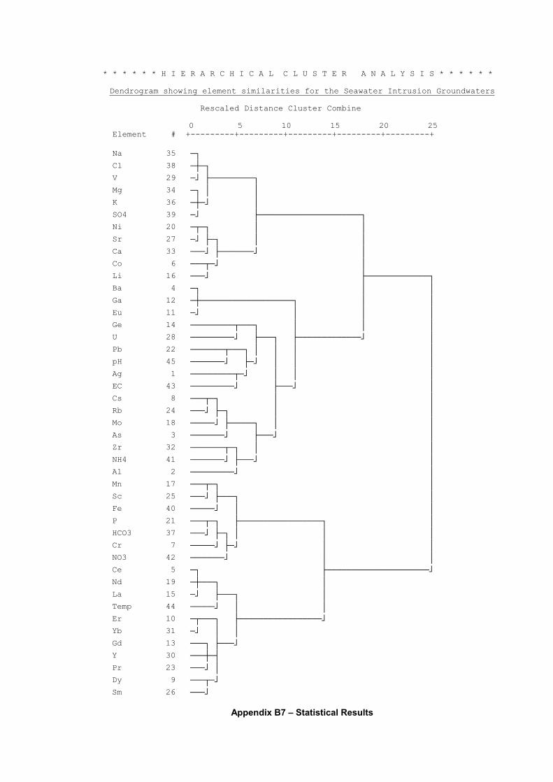
Appendix B7 – Statistical Results
* * * * * * H I E R A R C H I C A L C L U S T E R A N A L Y S I S * * * * * *
Dendrogram showing element similarities for the Seawater Intrusion Groundwaters
Rescaled Distance Cluster Combine 0 5 10 15 20 25 Element # +---------+---------+---------+---------+---------+ Na 35 òø Cl 38 òôòø V 29 ò÷ ùòòòòòòòòòø Mg 34 òø ó ó K 36 òôò÷ ó SO4 39 ò÷ ùòòòòòòòòòòòòòòòòòòòòòø Ni 20 òûòø ó ó Sr 27 ò÷ ùòø ó ó Ca 33 òòò÷ ùòòòòòòò÷ ó Co 6 òòòûò÷ ó Li 16 òòò÷ ùòòòòòòòòòòòòòø Ba 4 òø ó ó Ga 12 òôòòòòòòòòòòòòòòòòòòòø ó ó Eu 11 ò÷ ó ó ó Ge 14 òòòòòòòòòûòòòø ó ó ó U 28 òòòòòòòòò÷ ùòòòø ùòòòòòòòòòòòòò÷ ó Pb 22 òòòòòòòûòòòø ó ó ó ó pH 45 òòòòòòò÷ ùò÷ ó ó ó Ag 1 òòòòòòòòòûò÷ ó ó ó EC 43 òòòòòòòòò÷ ùòòò÷ ó Cs 8 òòòûòø ó ó Rb 24 òòò÷ ùòø ó ó Mo 18 òòòòò÷ ùòòòòòø ó ó As 3 òòòòòòò÷ ùòòò÷ ó Zr 32 òòòòòòòûòø ó ó NH4 41 òòòòòòò÷ ùòòò÷ ó Al 2 òòòòòòòòò÷ ó Mn 17 òòòûòø ó Sc 25 òòò÷ ùòòòø ó Fe 40 òòòòò÷ ó ó P 21 òòòûòø ùòòòòòòòòòòòòòòòòòø ó HCO3 37 òòò÷ ùòø ó ó ó Cr 7 òòòòò÷ ùò÷ ó ó NO3 42 òòòòòòò÷ ó ó Ce 5 òø ùòòòòòòòòòòòòòòòòòòòòò÷ Nd 19 òôòòòø ó La 15 ò÷ ùòòòø ó Temp 44 òòòòò÷ ó ó Er 10 òûòòòø ùòòòòòòòòòòòòòòòòò÷ Yb 31 ò÷ ó ó Gd 13 òòòø ùòòò÷ Y 30 òòòôòú Pr 23 òòò÷ ó Dy 9 òòòûò÷ Sm 26 òòò÷
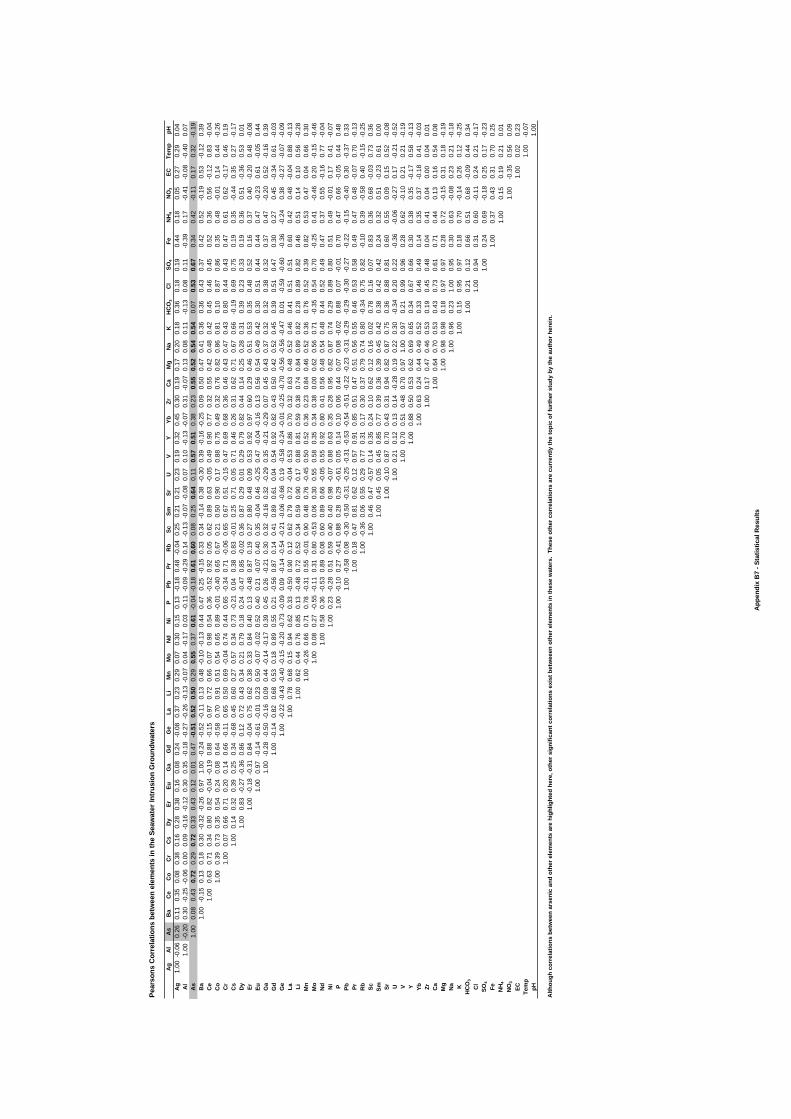
Pear
sons
Cor
rela
tions
bet
wee
n el
emen
ts in
the
Seaw
ater
Intr
usio
n G
roun
dwat
ers
Ag
Al
As
Ba
Ce
Co
Cr
Cs
Dy
ErEu
Ga
Gd
Ge
LaLi
Mn
Mo
Nd
Ni
PPb
PrR
bSc
SmSr
UV
YYb
ZrC
aM
gN
aK
HC
O3
Cl
SO4
FeN
H4
NO
3EC
Tem
ppH
Ag
1.00
-0.0
60.
260.
110.
350.
080.
380.
160.
280.
380.
160.
080.
24-0
.08
0.37
0.23
0.29
0.07
0.30
0.15
0.13
-0.1
80.
48-0
.04
0.25
0.21
0.21
0.23
0.19
0.32
0.45
0.30
0.19
0.17
0.20
0.18
0.36
0.18
0.19
0.44
0.18
0.05
0.27
0.29
0.04
Al
1.00
-0.2
00.
30-0
.25
-0.0
60.
000.
09-0
.16
-0.1
20.
300.
35-0
.18
-0.2
7-0
.26
-0.1
3-0
.07
0.04
-0.1
70.
03-0
.11
-0.0
9-0
.29
0.14
-0.1
3-0
.07
-0.0
80.
070.
10-0
.13
-0.0
70.
31-0
.07
0.13
0.08
0.11
-0.1
30.
080.
11-0
.39
0.17
-0.4
1-0
.08
-0.4
00.
07A
s1.
000.
080.
430.
720.
290.
720.
330.
430.
120.
010.
47-0
.51
0.52
0.50
0.29
0.55
0.37
0.61
-0.0
4-0
.18
0.61
0.60
0.08
0.25
0.64
0.11
0.57
0.51
0.38
0.23
0.55
0.52
0.54
0.54
0.07
0.53
0.67
0.34
0.42
-0.1
10.
170.
32-0
.19
Ba
1.00
-0.1
50.
130.
180.
30-0
.32
-0.2
60.
971.
00-0
.24
-0.5
2-0
.11
0.13
0.48
-0.1
0-0
.13
0.44
0.47
0.25
-0.1
50.
330.
34-0
.14
0.38
-0.3
00.
39-0
.16
-0.2
50.
090.
500.
470.
410.
360.
360.
430.
370.
420.
52-0
.19
0.53
-0.1
20.
39C
e1.
000.
630.
710.
340.
800.
82-0
.04
-0.1
90.
88-0
.15
0.97
0.72
0.66
0.07
0.98
0.54
0.36
-0.5
20.
920.
050.
620.
890.
63-0
.05
0.49
0.90
0.77
0.32
0.55
0.42
0.48
0.42
0.45
0.46
0.45
0.52
0.36
0.56
-0.1
20.
83-0
.04
Co
1.00
0.39
0.73
0.35
0.54
0.24
0.08
0.64
-0.5
80.
700.
910.
510.
540.
650.
89-0
.01
-0.4
00.
650.
670.
210.
500.
900.
170.
880.
750.
490.
320.
760.
820.
860.
810.
100.
870.
860.
350.
48-0
.01
0.14
0.44
-0.2
6C
r1.
000.
070.
660.
710.
200.
140.
66-0
.11
0.65
0.50
0.69
-0.0
40.
740.
440.
65-0
.34
0.71
-0.0
60.
650.
670.
51-0
.15
0.47
0.69
0.68
0.36
0.46
0.43
0.47
0.43
0.80
0.44
0.43
0.47
0.61
0.62
-0.1
70.
460.
19C
s1.
000.
140.
320.
390.
250.
34-0
.68
0.45
0.60
0.27
0.57
0.34
0.73
-0.2
10.
040.
380.
83-0
.01
0.25
0.71
0.05
0.71
0.46
0.26
0.31
0.62
0.71
0.67
0.66
-0.1
90.
690.
750.
190.
35-0
.44
0.35
0.27
-0.1
7D
y1.
000.
83-0
.27
-0.3
60.
860.
120.
720.
430.
340.
210.
790.
180.
24-0
.47
0.85
-0.0
20.
360.
870.
290.
010.
290.
790.
820.
440.
140.
250.
280.
310.
390.
230.
330.
190.
360.
51-0
.36
0.53
0.01
Er1.
00-0
.18
-0.3
10.
84-0
.04
0.75
0.62
0.38
0.33
0.84
0.40
0.13
-0.4
80.
870.
190.
270.
800.
480.
090.
530.
920.
970.
600.
290.
460.
510.
530.
350.
480.
520.
160.
370.
40-0
.20
0.48
-0.0
8Eu
1.00
0.97
-0.1
4-0
.61
-0.0
10.
230.
50-0
.07
-0.0
20.
520.
400.
21-0
.07
0.40
0.35
-0.0
40.
46-0
.25
0.47
-0.0
4-0
.16
0.13
0.56
0.54
0.49
0.42
0.30
0.51
0.44
0.44
0.47
-0.2
30.
61-0
.05
0.44
Ga
1.00
-0.2
8-0
.50
-0.1
60.
090.
44-0
.14
-0.1
70.
390.
450.
26-0
.21
0.30
0.32
-0.1
60.
32-0
.29
0.35
-0.2
1-0
.29
0.07
0.45
0.43
0.37
0.32
0.32
0.38
0.32
0.37
0.47
-0.2
00.
52-0
.16
0.39
Gd
1.00
-0.1
40.
820.
680.
530.
180.
890.
550.
21-0
.56
0.87
0.14
0.41
0.89
0.61
0.04
0.54
0.92
0.82
0.43
0.50
0.42
0.52
0.45
0.39
0.51
0.47
0.30
0.27
0.45
-0.3
40.
61-0
.03
Ge
1.00
-0.2
2-0
.43
-0.4
0-0
.15
-0.2
0-0
.73
-0.0
90.
09-0
.14
-0.5
4-0
.21
-0.0
6-0
.66
0.19
-0.5
8-0
.24
-0.0
1-0
.25
-0.7
0-0
.56
-0.5
6-0
.47
0.01
-0.5
9-0
.60
-0.3
6-0
.24
0.38
-0.2
7-0
.07
-0.0
9La
1.00
0.78
0.68
0.15
0.94
0.62
0.33
-0.5
00.
900.
120.
620.
790.
72-0
.04
0.53
0.86
0.70
0.32
0.63
0.48
0.52
0.46
0.41
0.51
0.51
0.60
0.42
0.48
-0.0
40.
88-0
.13
Li1.
000.
620.
440.
760.
850.
13-0
.48
0.72
0.52
0.34
0.59
0.90
0.17
0.88
0.81
0.59
0.38
0.74
0.84
0.89
0.82
0.28
0.89
0.82
0.46
0.51
0.14
0.10
0.56
-0.2
8M
n1.
00-0
.26
0.66
0.71
0.78
-0.3
10.
55-0
.01
0.90
0.48
0.76
-0.4
50.
500.
520.
360.
230.
840.
460.
520.
360.
760.
520.
390.
820.
530.
470.
040.
660.
30M
o1.
000.
080.
27-0
.55
-0.1
10.
310.
80-0
.53
0.06
0.30
0.55
0.58
0.35
0.34
0.38
0.00
0.62
0.56
0.71
-0.3
50.
540.
70-0
.25
0.41
-0.4
60.
20-0
.15
-0.4
6N
d1.
000.
580.
36-0
.53
0.89
0.08
0.60
0.89
0.66
-0.0
50.
550.
920.
800.
410.
560.
480.
540.
480.
440.
520.
490.
470.
370.
55-0
.16
0.77
-0.0
4N
i1.
000.
23-0
.28
0.51
0.59
0.40
0.40
0.98
-0.0
70.
880.
630.
350.
280.
950.
820.
870.
740.
290.
890.
800.
510.
49-0
.01
0.17
0.41
-0.0
7P
1.00
-0.1
00.
27-0
.41
0.88
0.28
0.29
-0.6
10.
050.
140.
100.
060.
440.
070.
08-0
.02
0.88
0.07
-0.0
10.
700.
470.
66-0
.05
0.44
0.48
Pb1.
00-0
.58
0.08
-0.3
0-0
.50
-0.3
1-0
.25
-0.3
1-0
.53
-0.5
4-0
.51
-0.2
2-0
.23
-0.3
1-0
.29
-0.2
9-0
.30
-0.2
7-0
.22
-0.1
5-0
.40
0.30
-0.3
70.
33Pr
1.00
0.18
0.47
0.81
0.62
0.12
0.57
0.91
0.85
0.51
0.47
0.51
0.56
0.55
0.46
0.53
0.58
0.49
0.47
0.48
-0.0
70.
70-0
.13
Rb
1.00
-0.3
60.
060.
550.
290.
770.
310.
170.
300.
370.
790.
740.
80-0
.34
0.75
0.82
-0.1
00.
39-0
.58
0.40
-0.1
5-0
.25
Sc1.
000.
460.
47-0
.57
0.14
0.35
0.24
0.10
0.62
0.12
0.16
0.02
0.78
0.16
0.07
0.83
0.36
0.68
-0.0
30.
730.
36Sm
1.00
0.45
0.05
0.45
0.85
0.77
0.39
0.36
0.39
0.45
0.42
0.38
0.42
0.42
0.24
0.32
0.51
-0.2
30.
610.
00Sr
1.00
-0.1
00.
870.
700.
430.
310.
940.
820.
870.
750.
360.
880.
810.
600.
550.
090.
150.
52-0
.08
U1.
000.
210.
120.
130.
14-0
.28
0.19
0.22
0.30
-0.3
40.
200.
22-0
.36
-0.0
6-0
.27
0.17
-0.2
1-0
.52
V1.
000.
700.
510.
480.
700.
971.
000.
970.
210.
990.
960.
280.
62-0
.10
0.21
0.21
-0.1
9Y
1.00
0.88
0.50
0.53
0.62
0.69
0.65
0.34
0.67
0.66
0.30
0.38
0.35
-0.1
70.
58-0
.13
Yb1.
000.
630.
240.
440.
490.
520.
330.
460.
490.
140.
350.
37-0
.18
0.41
-0.0
3Zr
1.00
0.17
0.47
0.46
0.53
0.19
0.45
0.48
0.04
0.41
0.04
0.00
0.04
0.01
Ca
1.00
0.64
0.70
0.53
0.43
0.73
0.61
0.71
0.44
0.13
0.16
0.54
0.08
Mg
1.00
0.98
0.98
0.18
0.97
0.97
0.28
0.72
-0.1
50.
310.
18-0
.19
Na
1.00
0.96
0.23
1.00
0.95
0.30
0.63
-0.0
80.
230.
21-0
.18
K1.
000.
150.
950.
970.
180.
70-0
.14
0.26
0.12
-0.2
5H
CO
31.
000.
210.
120.
660.
510.
68-0
.09
0.44
0.34
Cl
1.00
0.94
0.31
0.60
-0.1
10.
240.
21-0
.17
SO4
1.00
0.24
0.69
-0.1
80.
250.
17-0
.23
Fe1.
000.
370.
430.
310.
700.
25N
H4
1.00
0.15
0.19
0.21
0.01
NO
31.
00-0
.35
0.56
0.09
EC1.
000.
020.
23Te
mp
1.00
-0.0
7pH
1.00
Alth
ough
cor
rela
tions
bet
wee
n ar
seni
c an
d ot
her e
lem
ents
are
hig
hlig
hted
her
e, o
ther
sig
nific
ant c
orre
latio
ns e
xist
bet
wee
en o
ther
ele
men
ts in
thes
e w
ater
s. T
hese
oth
er c
orre
latio
ns a
re c
urre
ntly
the
topi
c of
furt
her s
tudy
by
the
auth
or h
erei
n.
App
endi
x B
7 - S
tatis
tical
Res
ults
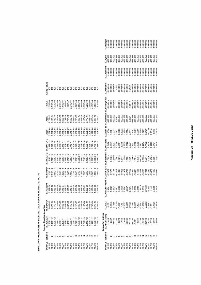
SHA
LLO
W G
RO
UN
DW
ATE
RS
SELE
CTE
D G
EOC
HEM
ICA
L M
OD
ELLI
NG
OU
TPU
T
Arsenic
Species
Molalities
SAM
PLE
solu
tion
m_H
2AsO
3-m
_H2A
sO4-
m_H
3AsO
3m
_H3A
sO4
m_H
AsO
3-2
m_H
AsO
4-2
As(
III)
As(
V)To
t As
As(
III)/Tot
As
ML1/5
15.70E-
122.
64E-
123.
52E-
081.
13E-
151.71E-
181.
17E-
133.
52E-
082.75E-
123.
52E-
0810
0ML1/6
23.42E-
121.
07E-
143.
51E-
087.
81E-
186.
50E-
192.
94E-
163.
51E-
081.
10E-
143.
51E-
0810
0ML1/7
38.39E-
125.47E-
144.73E-
082.
18E-
172.79E-
182.
67E-
154.73E-
085.74E-
144.73E-
0810
0ML2/5
42.39E-
124.
11E-
182.
57E-
083.71E-21
4.47E-
199.72E-20
2.58E-
084.21E-
182.
58E-
0810
0ML2/6
52.28E-
111.
07E-
152.71E-
071.
04E-
183.
81E-
182.30E-
172.71E-
071.
09E-
152.71E-
0710
0ML2/7
63.
10E-
111.
66E-
154.
11E-
071.
82E-
184.
60E-
183.
14E-
174.
11E-
071.
69E-
154.
11E-
0710
0ML2/8
72.43E-
117.
54E-
162.45E-
076.
12E-
194.
65E-
181.
90E-
172.45E-
077.74E-
162.45E-
0710
0ML3/3
81.
1 3E-
111.
65E-
171.
12E-
071.
14E-20
2.15E-
184.
65E-
191.
12E-
071.70E-
171.
12E-
0710
0ML4/3
94.36E-
114.41E-
162.
04E-
071.45E-
191.
85E-
172.74E-
172.
04E-
074.
68E-
162.
04E-
0710
0ML4/4
102.
62E-
124.30E-
172.
61E-
083.
02E-20
5.00E-
191.20E-
182.
61E-
084.42E-
172.
61E-
0810
0ML4/5
117.
07E-
121.21E-
154.
90E-
085.
94E-
191.
93E-
184.
84E-
174.
90E-
081.26E-
154.
90E-
0810
0ML4/6
121.30E-
125.36E-
173.
58E-
081.
04E-
199.
00E-20
5.42E-
193.
58E-
085.42E-
173.
58E-
0810
0ML5/4
136.78E-
141.46E-
142.
54E-
094.
00E-
173.34E-21
1.02E-
162.
54E-
091.47E-
142.
54E-
0910
0ML5/5
148.31E-
131.
15E-
149.
93E-
091.
02E-
171.31E-
192.
56E-
169.
93E-
091.
18E-
149.
93E-
0910
0ML5/6
152.41E-
123.
58E-
141.22E-
081.33E-
179.
10E-
191.
92E-
151.22E-
083.77E-
141.22E-
0810
0ML6/7
165.24E-
131.
03E-
142.30E-
083.20E-
172.23E-20
6.42E-
172.30E-
081.
04E-
142.30E-
0810
0ML6/8
171.47E-
121.78E-
144.
17E-
083.
60E-
179.
99E-20
1.77E-
164.
17E-
081.
80E-
144.
17E-
0810
0ML6/9
186.
82E-
131.37E-
131.
05E-
081.
50E-
169.30E-20
2.73E-
151.
05E-
081.40E-
131.
05E-
0810
0ML6/1
019
3.28E-
125.
88E-
132.42E-
083.
10E-
169.
14E-
192.38E-
142.42E-
086.
12E-
132.42E-
0810
0
Satu
ration Indices
SAM
PLE
solu
tion
si_A
l(OH
)3(a
m)
si_A
l2O
3si
_Al4
(OH
)10S
O4
si_A
lOH
SO4
si_Boe
hmite
si_D
iaspor
esi
_Gib
bsite
si_Goe
thite
si_F
errih
ydrit
esi
_Hem
atite
si_Orp
imen
tsi
_Pyr
itesi
_Rea
lgar
ML1/5
1-1
.101
9-0
.37
1.4941
-2.7
057
1.09
932.
8498
1.45
56-9
99.9
99-9
99.9
99-9
99.9
99-9
99.9
99-9
99.9
99-9
99.9
99ML1/6
2-1
.2547
-0.6
643
1.8927
-1.7477
0.94
862.
6947
1.29
81-9
99.9
99-9
99.9
99-9
99.9
99-9
99.9
99-9
99.9
99-9
99.9
99ML1/7
3-0
.553
60.7334
4.3124
-1.4717
1.64
893.39
672.
0011
-999
.999
-999
.999
-999
.999
-999
.999
-999
.999
-999
.999
ML2/5
4-1
.128
8-0
.337
92.
1933
-1.145
91.
0881
2.8044
1.3922
2.5321
-0.177
87.45
82-9
99.9
99-9
99.9
99-9
99.9
99ML2/6
5-1
.5874
-1.2
661
0.5625
-1.4
996
0.6275
2.34
810.
9382
-999
.999
-999
.999
-999
.999
-999
.999
-999
.999
-999
.999
ML2/7
6-1
.701
5-1
.49
0.17
98-1
.5003
0.5141
2.233
0.8222
-999
.999
-999
.999
-999
.999
-999
.999
-999
.999
-999
.999
ML2/8
7-1
.103
9-0
.3077
2.3943
-1.1
977
1.10
942.
8335
1.42
55-9
99.9
99-9
99.9
99-9
99.9
99-9
99.9
99-9
99.9
99-9
99.9
99ML3/3
8-0
.699
10.43
564.
037
-1.3712
1.5021
3.2526
1.85
84-9
99.9
99-9
99.9
99-9
99.9
99-9
99.9
99-9
99.9
99-9
99.9
99ML4/3
9-0
.4414
0.95
575.
1817
-0.9
593
1.76
073.
5094
2.1143
3.2931
0.5548
8.9628
-999
.999
-999
.999
-999
.999
ML4/4
10-0
.815
60.20
933.
5444
-1.4
535
1.38
683.
1347
1.73
91-9
99.9
99-9
99.9
99-9
99.9
99-9
99.9
99-9
99.9
99-9
99.9
99ML4/5
11-0
.611
0.61
863.
6085
-2.0
033
1.59
143.33
931.
9437
-999
.999
-999
.999
-999
.999
-999
.999
-999
.999
-999
.999
ML4/6
12-1
.624
1-1
.4077
0.81
58-1
.756
60.
5783
2.32
620.
9306
-999
.999
-999
.999
-999
.999
-999
.999
-999
.999
-999
.999
ML5/4
13-2
.2763
-2.6
943
-1.8
915
-2.346
1-0
.070
61.
6702
0.27
09-9
99.9
99-9
99.9
99-9
99.9
99-9
99.9
99-9
99.9
99-9
99.9
99ML5/5
14-1
.520
5-1
.180
50.
6815
-2.0203
0.68
562.42
541.
0257
-999
.999
-999
.999
-999
.999
-999
.999
-999
.999
-999
.999
ML5/6
15-2
.2043
-2.5
502
-2.4324
-3.1
031
0.00
141.7422
0.3429
-999
.999
-999
.999
-999
.999
-999
.999
-999
.999
-999
.999
ML6/7
16-2
.8284
-3.8
163
-3.2
63-2
.222
5-0
.626
1.12
18-0
.273
8-9
99.9
99-9
99.9
99-9
99.9
99-9
99.9
99-9
99.9
99-9
99.9
99ML6/8
17-1
.771
9-1
.701
11.
141
-0.9
677
0.43
092.
1779
0.78
18-9
99.9
99-9
99.9
99-9
99.9
99-9
99.9
99-9
99.9
99-9
99.9
99ML6/9
18-1
.3077
-0.772
63.
0385
-0.4
629
0.89
512.
6421
1.24
6-9
99.9
99-9
99.9
99-9
99.9
99-9
99.9
99-9
99.9
99-9
99.9
99ML6/1
019
-1.0
988
-0.3
526
3.1739
-0.933
91.
1044
2.85
051.4539
-999
.999
-999
.999
-999
.999
-999
.999
-999
.999
-999
.999
App
endi
x B8
- PH
REE
QC
Out
put
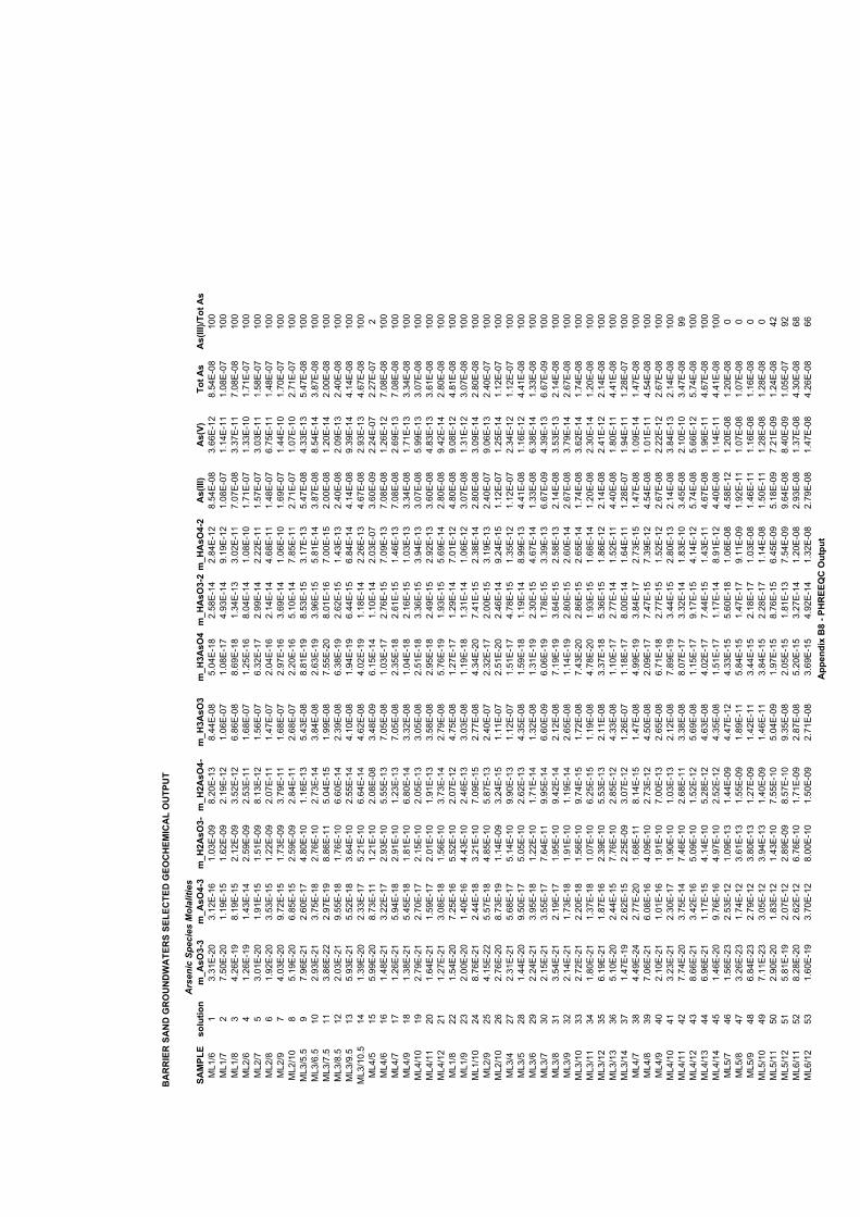
BA
RR
IER
SA
ND
GR
OU
ND
WA
TER
S SE
LEC
TED
GEO
CH
EMIC
AL
OU
TPU
T
Arsenic
Species
Molalities
SAM
PLE
solu
tion
m_A
sO3-
3m
_AsO
4-3
m_H
2AsO
3-m
_H2A
sO4-
m_H
3AsO
3m
_H3A
sO4
m_H
AsO
3-2
m_H
AsO
4-2
As(
III)
As(
V)To
t As
As(
III)/Tot
As
ML1/6
13.31E-20
3.12E-
161.
03E-
098.20E-
138.44E-
085.
04E-
182.
58E-
142.
84E-
128.
54E-
083.
66E-
128.
54E-
0810
0ML1/7
27.
50E-20
1.19E-
151.
62E-
092.
19E-
121.
06E-
071.
08E-
174.
93E-
149.
19E-
121.
08E-
071.
14E-
111.
08E-
0710
0ML 1/8
34.26E-
198.
19E-
152.
12E-
093.
52E-
126.
86E-
088.
69E-
181.34E-
133.
02E-
117.
07E-
083.37E-
117.
08E-
0810
0ML2/6
41.26E-
191.43E-
142.
59E-
092.
53E-
111.
68E-
071.25E-
168.
04E-
141.
08E-
101.71E-
071.33E-
101.71E-
0710
0ML2/7
53.
01E-20
1.91E-
151.
51E-
098.
13E-
121.
56E-
076.32E-
172.
99E-
142.22E-
111.
57E-
073.
03E-
111.
58E-
0710
0ML2/8
61.
92E-20
3.53E-
151.22E-
092.
07E-
111.47E-
072.
04E-
162.
14E-
144.
68E-
111.48E-
076.75E-
111.48E-
0710
0ML2/9
74.
03E-20
9.72E-
151.73E-
093.79E-
111.
68E-
072.
97E-
163.
69E-
141.
06E-
101.
69E-
071.44E-
101.70E-
0710
0ML2/1
08
5.19E-20
6.85E-
152.
59E-
092.
84E-
112.
68E-
072.20E-
165.
10E-
147.
85E-
112.71E-
071.
07E-
102.71E-
0710
0ML3/5
.59
7.96E-21
2.60E-
174.
80E-
101.
16E-
135.43E-
088.
81E-
198.
53E-
153.
17E-
135.47E-
084.33E-
135.47E-
0810
0ML3/6
.510
2.93E-21
3.75E-
182.76E-
102.73E-
143.
84E-
082.
63E-
193.
96E-
155.
81E-
143.
87E-
088.
54E-
143.
87E-
0810
0ML3/7
.511
3.86E-22
2.97E-
198.
86E-
115.
04E-
151.
99E-
087.
55E-20
8.01E-
167.
00E-
152.
00E-
081.20E-
142.
00E-
0810
0ML3/8
.512
2.03E-21
9.55E-
181.76E-
106.
60E-
142.39E-
086.38E-
192.
62E-
151.43E-
132.40E-
082.
09E-
132.40E-
0810
0ML3/9
.513
5.93E-21
5.52E-
183.
64E-
102.
55E-
144.
10E-
081.
94E-
196.44E-
156.
84E-
144.
14E-
089.39E-
144.
14E-
0810
0ML3/1
0.5
141.39E-20
2.33E-
175.21E-
106.
64E-
144.
62E-
084.
02E-
191.
18E-
142.26E-
134.
67E-
082.
93E-
134.
67E-
0810
0ML4/ 5
155.
99E-20
8.73E-
111.21E-
102.
08E-
083.48E-
096.
15E-
141.
10E-
142.
03E-
073.
60E-
092.24E-
072.27E-
072
ML4/6
161.48E-21
3.22E-
172.
93E-
105.
55E-
137.
05E-
081.
03E-
172.76E-
157.
09E-
137.
08E-
081.26E-
127.
08E-
0810
0ML4/7
1 71.26E-21
5.94E-
182.
91E-
101.23E-
137.
05E-
082.35E-
182.
61E-
151.46E-
137.
08E-
082.
69E-
137.
08E-
0810
0ML4/9
181.38E-21
5.45E-
181.
81E-
106.
80E-
143.32E-
081.
04E-
182.
16E-
151.
03E-
133.34E-
081.71E-
133.34E-
0810
0ML4/1
019
2.79E-21
2.70E-
172.
15E-
102.
05E-
133.
05E-
082.
51E-
183.36E-
153.
94E-
133.
07E-
085.
99E-
133.
07E-
0810
0ML4/1
120
1.64E-21
1.59E-
172.
01E-
101.
91E-
133.
58E-
082.
95E-
182.49E-
152.
92E-
133.
60E-
084.
83E-
133.
61E-
0810
0ML4/12
211.27E-21
3.08E-
181.
56E-
103.73E-
142.79E-
085.76E-
191.
9 3E-
155.
69E-
142.
80E-
089.42E-
142.
80E-
0810
0ML1/8
221.
54E-20
7.25E-
165.
52E-
102.
07E-
124.75E-
081.27E-
171.29E-
147.
01E-
124.
80E-
089.
08E-
124.
81E-
0810
0ML1/9
232.
00E-20
1.40E-
164.43E-
102.46E-
133.
03E-
081.
19E-
181.31E-
141.
06E-
123.
07E-
081.31E-
123.
07E-
0810
0ML1/1
024
8.76E-21
2.44E-
183.21E-
107.
09E-
152.77E-
084.34E-20
7.41E-
152.38E-
142.
80E-
083.
09E-
142.
80E-
0810
0ML2/9
254.
15E-22
5.57E-
184.
85E-
105.
87E-
132.40E-
072.32E-
172.
00E-
153.
19E-
132.40E-
079.
06E-
132.40E-
0710
0ML2/1
026
2.76E-20
8 .73E-
191.
14E-
093.24E-
151.
11E-
072.
51E-20
2.46E-
149.24E-
151.
12E-
071.25E-
141.
12E-
0710
0ML3/4
272.31E-21
5.68E-
175.
14E-
109.
90E-
131.
12E-
071.
51E-
174.78E-
151.35E-
121.
12E-
072.34E-
121.
12E-
0710
0ML3/5
281.44E-2 0
9.50E-
175.
05E-
102.
62E-
134.35E-
081.
59E-
181.
19E-
148.
99E-
134.41E-
081.
16E-
124.41E-
0810
0ML3/6
292.24E-21
3.95E-
181.22E-
101.71E-
141.32E-
081.31E-
192.30E-
154.
67E-
141.33E-
086.38E-
141.33E-
0810
0ML3/7
302.
15E-21
3.55E-
177.
64E-
119.
95E-
146.
60E-
096.
06E-
191.78E-
153.39E-
136.
67E-
094.39E-
136.
67E-
0910
0ML3/8
313.
54E-21
2.19E-
171.
95E-
109.42E-
142.
12E-
087.
19E-
193.
64E-
152.
58E-
132.
14E-
083.
53E-
132.
14E-
0810
0ML3/9
322.
14E-21
1 .73E-
181.
91E-
101.
19E-
142.
65E-
081.
14E-
192.
80E-
152.
60E-
142.
67E-
083.79E-
142.
67E-
0810
0ML3/1
033
2.72E-21
2.20E-
181.
56E-
109.74E-
151.72E-
087.43E-20
2.86E-
152.
65E-
141.74E-
083.
62E-
141.74E-
0810
0ML3/1
134
1.80E-21
1.37E-
181.
07E-
106.25E-
151.
19E-
084.78E-20
1.93E-
151.
68E-
141.20E-
082.30E-
141.20E-
0810
0ML3/ 12
356.
19E-21
1.87E-
162.39E-
105.
53E-
132.
11E-
083.37E-
185.36E-
151.
86E-
122.
14E-
082.41E-
122.
14E-
0810
0ML3/13
365.
10E-20
2.44E-
157.76E-
102.
85E-
124.33E-
081.
10E-
172.77E-
141.
52E-
114.40E-
081.
80E-
114.41E-
0810
0ML3/14
371.47E-
192.
62E-
152.25E-
093.
07E-
121.26E-
071.
18E-
178.
00E-
141.
64E-
111.28E-
071.
94E-
111.28E-
0710
0ML4/7
384.49E-24
2.77E-20
1.68E-
118.
14E-
151.47E-
084.
99E-
193.
84E-
172.73E-
151.47E-
081.
09E-
141.47E-
0810
0ML4/8
397.
06E-21
6.08E-
164.
09E-
102.73E-
124.
50E-
082.
09E-
177.47E-
157.39E-
124.
54E-
081.
01E-
114.
54E-
0810
0ML4/9
402.
10E-21
1.01E-
161.
91E-
107.
00E-
132.
65E-
086.71E-
182.77E-
151.
52E-
122.
67E-
082.22E-
122.
67E-
0810
0ML4/1
041
3.23E-21
2.30E-
171.
90E-
101.
0 3E-
132.
12E-
087.
89E-
193.44E-
152.
80E-
132.
14E-
083.
84E-
132.
14E-
0810
0ML4/1
142
7.74E-20
3.75E-
147.46E-
102.
68E-
113.38E-
088.
07E-
173.32E-
141.
83E-
103.45E-
082.
10E-
103.47E-
0899
ML4/12
438.
66E-21
3.42E-
165.
09E-
101.
52E-
125.
69E-
081.
15E-
179.
17E-
154.
14E-
125.74E-
085.
66E-
125.74E-
0810
0ML4/13
446.
96E-21
1.17E-
154.
14E-
105.28E-
124.
63E-
084.
02E-
177.44E-
151.43E-
114.
67E-
081.
96E-
114.
67E-
0810
0ML4/14
451.46E-20
9.76E-
164.
97E-
102.
52E-
124.35E-
081.
51E-
171.
17E-
148.
91E-
124.40E-
081.
1 4E-
114.41E-
0810
0ML5/7
461.
56E-23
2.53E-
121.
09E-
131.44E-
094.47E-
124.33E-
155.
60E-
181.
06E-
084.
58E-
121.20E-
081.20E-
080
ML5/8
473.26E-23
1.74E-
123.
61E-
131.
55E-
091.
89E-
115.
84E-
151.47E-
179.
11E-
091.
92E-
111.
07E-
081.
07E-
080
ML5/9
486.
84E-23
2.79E-
123.
80E-
131.27E-
091.42E-
113.44E-
152.
18E-
171.
03E-
081.46E-
111.
16E-
081.
16E-
080
ML5/1
049
7.11E-23
3.05E-
123.
94E-
131.40E-
091.46E-
113.
84E-
152.28E-
171.
14E-
081.
50E-
111.28E-
081.28E-
080
ML5/1
150
2.90E-20
1.83E-
121.43E-
107.
55E-
105.
04E-
091.
97E-
158.76E-
156.45E-
095.
18E-
097 .21E-
091.24E-
0842
ML5/12
515.
81E-
192.
07E-
122.
89E-
098.
57E-
109.35E-
082.
05E-
151.
81E-
137.
54E-
099.
64E-
088.40E-
091.
05E-
0792
ML6/1
152
8.28E-20
2.62E-
126.76E-
101.71E-
092.
87E-
085.20E-
153.27E-
141.20E-
082.
93E-
081.37E-
084.30E-
0868
ML6/12
531.
60E-
193.70E-
128.
00E-
101.
50E-
092.71E-
083.
69E-
154.
92E-
141.32E-
082.79E-
081.47E-
084.26E-
0866
App
endi
x B8
- PH
REE
QC
Out
put
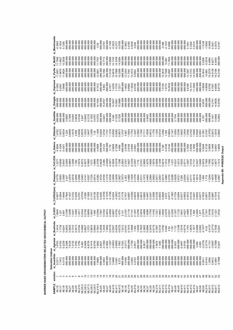
BA
RR
IER
SA
ND
GR
OU
ND
WA
TER
S SE
LEC
TED
GEO
CH
EMIC
AL
OU
TPU
T
Satu
ration Indices
SAM
PLE
solu
tion
si_A
cant
hite
si_A
gmet
alsi
_Boe
hmite
si_Cr2
O3
si_Cr(
OH
)3(a
m)
si_D
iaspor
esi
_FeCr2
O4
si_G
alen
asi
_Gib
bsite
si_Goe
thite
si_Gre
igite
si_Orp
imen
tsi
_Pyr
itesi
_MoS
2si
_Mac
kina
wite
ML1/6
19.23
111.
6763
1.34
141.
8844
0.5677
3.0778
1.3277
4.36
941.
6762
-999
.999
-999
.999
8.18
5511
.285
111
.756
8-0
.3683
ML1/7
27.
1912
0.41
631.
1738
1.32
10.2844
2.90
930.
6936
4.1549
1.5072
-999
.999
-999
.999
9.20
9111
.967
911
.6927
-0.1
634
ML1/8
36.
5179
0.2239
0.6241
3.69
11.4649
2.35
693.
6547
5.43
510.
9534
-999
.999
-999
.999
7.90
6811
.9624
10.2
638
0.12
58ML2/6
4-9
99.9
998.23
880.
6933
2.31
890.78
042.427
2.02
65-9
99.9
991.
024
5.96
83-9
99.9
99-9
99.9
99-9
99.9
99-9
99.9
99-9
99.9
99ML2/7
5-9
99.9
997.
8129
0.5625
1.03
960.
1437
2.2979
0.88
64-9
99.9
990.
8958
5.74
89-9
99.9
99-9
99.9
99-9
99.9
99-9
99.9
99-9
99.9
99ML2/8
6-9
99.9
997.2735
0.73
121.4341
0.31
522.45
181.32
88-9
99.9
991.
0419
5.63
64-9
99.9
99-9
99.9
99-9
99.9
99-9
99.9
99-9
99.9
99ML2/9
7-9
99.9
997.37
820.
5413
1.43
650.32
092.2645
1.392
-999
.999
0.85
65.
9636
-999
.999
-999
.999
-999
.999
-999
.999
-999
.999
ML2/1
08
-999
.999
7.17
950.
5184
1.30
110.27
912.25
661.
0574
-999
.999
0.85
585.
9148
-999
.999
-999
.999
-999
.999
-999
.999
-999
.999
ML3/5
.59
-999
.999
8.483
0.49
060.
5344
-0.0704
2.24
830.2672
-999
.999
0.8578
5.847
-999
.999
-999
.999
-999
.999
-999
.999
-999
.999
ML3/6
.510
-999
.999
9.04
660.
6627
0.51
89-0
.089
2.4141
0.4977
-999
.999
1.02
035.
9042
-999
.999
-999
.999
-999
.999
-999
.999
-999
.999
ML3/7
.511
-999
.999
8.8729
1.2721
0.88
590.
1069
3.03
070.
5965
-999
.999
1.64
076.3132
-999
.999
-999
.999
-999
.999
-999
.999
-999
.999
ML3/8
.512
-999
.999
8.74
140.
9874
1.0647
0.1747
2.7335
1.073
-999
.999
1.33
696.
1652
-999
.999
-999
.999
-999
.999
-999
.999
-999
.999
ML3/9
.513
-999
.999
8.67
590.
8955
1.90
90.
6138
2.65
141.
9866
-999
.999
1.26
5.67
87-9
99.9
99-9
99.9
99-9
99.9
99-9
99.9
99-9
99.9
99ML3/1
0.5
147.
8969
1.08
920.7841
2.03
940.
6759
2.53
822.27
094.49
081.
1458
6.07
5316
.1034
8.15
1212
.085
111
.7767
0.55
ML4/5
15-9
99.9
994.
8521
0.2938
1.7947
0.4226
1.9724
0.9426
-999
.999
0.54
04-9
99.9
99-9
99.9
99-9
99.9
99-9
99.9
99-9
99.9
99-9
99.9
99ML4/6
164.
9463
-0.7284
1.2435
0.01
64-0
.375
62.
9746
-0.4
863.
6123
1.57
025.
9241
15.9707
8.893
12.1494
13.7713
-0.0
161
ML4/7
17-9
99.9
996.36
921.39
520.4674
-0.1
576
3.12
19-0
.506
9-9
99.9
991.71
51-9
99.9
99-9
99.9
99-9
99.9
99-9
99.9
99-9
99.9
99-9
99.9
99ML4/9
183.21
05-1
.1257
0.8176
0.45
95-0
.179
62.
5338
-0.3
871
3.17
81.
1216
-999
.999
-999
.999
8.7071
11.0
126
14.9
089
-0.176
9ML4/1
019
3.48
98-0
.9053
0.55
070.
8907
0.02
542.26
090.26
083.
9958
0.84
565.34
614
.0637
7.4229
10.6
616
14.1742
-0.3
523
ML4/1
120
3.43
81-0
.9592
0.6334
0.07
52-0
.3823
2.3436
-0.531
63.72
990.
9282
5.7325
15.0
841
7.73
1610
.796
814
.376
9-0
.273
1ML4/12
218.273
1.79
030.
6725
1.47
510.3176
2.3827
1.12
864.
666
0.9673
5.7328
15.0
886
7.32
1110
.328
914
.5364
-0.076
9ML1/8
22-9
99.9
996.73
531.
0212
2.15
10.7178
2.7673
2.06
03-9
99.9
991.37
07-9
99.9
99-9
99.9
99-9
99.9
99-9
99.9
99-9
99.9
99-9
99.9
99ML1/9
234.
9168
-0.5717
0.61
612.21
970.7537
2.363
2.37
613.
9799
0.967
-999
.999
-999
.999
7.46
0212
.2403
-999
.999
0.38
03ML1/1
024
-999
.999
-999
.999
0.74
152.
1116
0.69
972.48
851.
5927
2.81
061.
0924
-999
.999
-999
.999
9.69
8411
.708
1-9
99.9
990.47
65ML2/9
253.
0362
-1.779
51.45
890.71
01-0
.0392
3.1839
-0.3332
2.62
851.77
63-9
99.9
99-9
99.9
9911
.6052
12.3472
-999
.999
0.0039
ML2/1
026
4.4723
0.65
111.
002
2.12
070.
6676
2.7279
2.53
013.
9361
1.32
07-9
99.9
99-9
99.9
998.47
959.
5563
-999
.999
0.63
6ML3/4
27-9
99.9
99-9
99.9
991.
9356
2.07
850.
6862
3.6844
1.71
6-9
99.9
992.28
92-9
99.9
99-9
99.9
99-9
99.9
99-9
99.9
99-9
99.9
99-9
99.9
99ML3/5
28-9
99.9
99-9
99.9
990.7832
2.49
160.
8912
2.53
113.
0161
-999
.999
1.13
54-9
99.9
99-9
99.9
99-9
99.9
99-9
99.9
99-9
99.9
99-9
99.9
99ML3/6
29-9
99.9
998.
0817
2.36
022.48
890.
8883
4.1072
2.98
93-9
99.9
992.71
11-9
99.9
99-9
99.9
99-9
99.9
99-9
99.9
99-9
99.9
99-9
99.9
99ML3/7
30-9
99.9
99-9
99.9
990.
6984
1.60
860.44
972.44
621.4276
-999
.999
1.05
064.4945
-999
.999
-999
.999
-999
.999
-999
.999
-999
.999
ML3/8
31-9
99.9
99-9
99.9
990.
5476
1 .77
550.
5347
2.29
641.
9068
-999
.999
0.90
12-9
99.9
99-9
99.9
99-9
99.9
99-9
99.9
99-9
99.9
99-9
99.9
99ML3/9
32-9
99.9
99-9
99.9
990.
8179
1.41
650.35
982.
5693
1.5679
-999
.999
1.17
55-9
99.9
99-9
99.9
99-9
99.9
99-9
99.9
99-9
99.9
99-9
99.9
99ML3/1
033
-999
.999
7.0676
0.79
571.7221
0.5126
2.5471
2.09
59-9
99.9
991.
1534
-999
.999
-999
.999
-999
.999
-999
.999
-999
.999
-999
.999
ML3/1
134
-999
.999
7.12
850.
5134
1.9943
0.65
032.26
572.
1248
-999
.999
0.8724
-999
.999
-999
.999
-999
.999
-999
.999
-999
.999
-999
.999
ML3/12
35-9
99.9
99-9
99.9
991.
0792
1.65
940.4828
2.83
150.
9274
4.18
51.43
82-9
99.9
99-9
99.9
997.
5139
12.3
616
-999
.999
-0.3
96ML3/13
36-9
99.9
99-9
99.9
990.
646
2.0378
0.672
2.39
831.75
124.4749
1.00
5-9
99.9
99-9
99.9
997.
6774
12.7
008
10.8
91- 0
.1037
ML3/14
37-9
99.9
99-9
99.9
990.
522.
0341
0.67
172.2732
1.77
693.2144
0.88
04-9
99.9
99-9
99.9
9910
.0532
13.2
897
11.7
604
0.40
66ML4/7
38-9
99.9
99-9
99.9
991.78
10.3326
-0.1
867
3.52
98-1
.672
-999
.999
2.1347
-999
.999
-999
.999
-999
.999
-999
.999
-999
.999
-999
.999
ML4/8
39-9
99.9
996.3031
1.172
2.1247
0.7124
2.9226
2.0331
-999
.999
1.52
835.
1744
-999
.999
-999
.999
-999
.999
-999
.999
-999
.999
ML4/9
40-9
99.9
99-9
99.9
991.21
981.7125
0.50
942.
9721
1.20
13-9
99.9
991.
5788
-999
.999
-999
.999
-999
.999
-999
.999
-999
.999
-999
.999
ML4/1
041
-999
.999
6.44
971.
5318
1.9541
0.63
173.28
51.
9252
-999
.999
1.8922
-999
.999
-999
.999
-999
.999
-999
.999
-999
.999
-999
.999
ML4/1
142
-999
.999
5.9745
0.87
192.4527
0.89
032.
6304
2.97
11-9
99.9
991.24
04-9
99.9
99-9
99.9
99-9
99.9
99-9
99.9
99-9
99.9
99-9
99.9
99ML4/12
43-9
99.9
99-9
99.9
991.
1761
1.49
890.4072
2.93
111.25
073.70
841.
5392
-999
.999
-999
.999
8.61
8613
.1907
-999
.999
0.1641
ML4/13
44-9
99.9
99-9
99.9
991.
8576
1.9144
0.6134
3.61
171.
0724
3.9336
2.21
93-9
99.9
99-9
99.9
9910
.7413
14.7372
-999
.999
0.33
92ML4/ 14
45-9
99.9
99-9
99.9
991.
1877
1.56
90.44
072.
9418
0.7131
3.16
561.
5494
-999
.999
-999
.999
11.0
064
14.5354
-999
.999
0.43
14ML5/7
46-9
99.9
993.
956
0.20
992.34
930.
8093
1.95
152.2427
-999
.999
0.5526
-999
.999
-999
.999
-999
.999
-999
.999
-999
.999
-999
.999
ML5/8
47-9
99.9
994.
955
0.20
821.
977
0.6277
1.9526
1.64
66-9
99.9
990.
5551
-999
.999
-999
.999
-999
.999
-999
.999
-999
.999
-999
.999
ML5/9
486.
5611
-2.273
9-0
.1577
2.2579
0.7635
1.584
2.0974
5.5048
0.18
514.78
16.
5576
-3.9
629
15.3
814
0.03
08-1
.514
8ML5/1
049
6.6143
-2.071
9-0
.02
2.7341
0.9971
1.71
92.73
656.3139
0.31
87-9
99.9
99-9
99.9
99-4
.865
614
.883
-0.5
518
-1.6
562
ML5/1
150
1.29
94-4
.113
1-0
.4137
1.81
080.
5339
1.3244
1.79
953.
5859
-0.0763
-999
.999
-999
.999
5.07
5615
.257
95.49
94-0
.046
8ML5/12
510.
8012
-3.9397
-0.271
51.
9133
0.58
671.4675
1.92
154.
1949
0.0673
5.14
5114
.274
18.75
5714
.813
88.
6271
0.3521
ML6/1
152
0.38
91-4
.758
80.7036
2.1221
0.70
182.44
881.
8477
3.64
811.
0518
5.04
8414
.863
68.
6095
16.2
184
8.04
040.35
15ML6/12
53-4
.758
80.
5241
0.5241
1.87
020.
5713
2.26
671.72
131.
6606
0.86
835.29
5315
.6783
8.67
1916
.2154
-999
.999
0.51
91A
ppen
dix
B8
- PH
REE
QC
Out
put
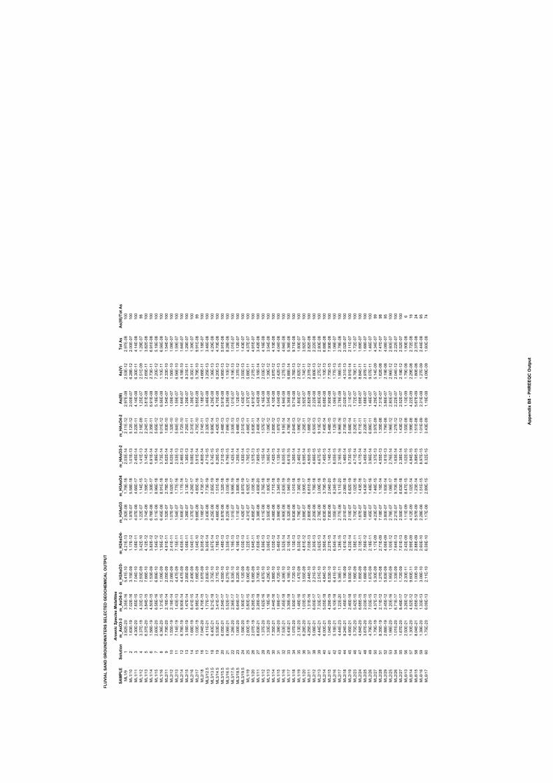
FLU
VIA
L SA
ND
GR
OU
ND
WA
TER
S SE
LEC
TED
GEO
CH
EMIC
AL
OU
TPU
T
Arsenic
Species
Molalities
SAM
PLE
Solu
tion
m_A
sO3-
3m
_AsO
4-3
m_H
2AsO
3-m
_H2A
sO4-
m_H
3AsO
3m
_H3A
sO4
m_H
AsO
3-2
m_H
AsO
4-2
As(
III)
As(
V)To
t As
As(
III)/Tot
As
ML1/9
13.
82E-20
3.35E-
165.41E-
104.21E-
132.
92E-
081.79E-
182.
03E-
142.
11E-
122.
97E-
082.
53E-
122.
97E-
0810
0ML1/1
02
1.63E-
197.
02E-
163.
15E-
091.
17E-
121.
97E-
075.
58E-
181.
01E-
135.
12E-
122.
00E-
076.28E-
122.
00E-
0710
0ML1/1
13
4.30E-20
7.85E-
157.
04E-
101.
08E-
114.
07E-
084.
66E-
172.45E-
145.22E-
114.
14E-
086.30E-
114.
14E-
0810
0ML1/12
43.37E-
194.33E-
132.
93E-
093.42E-
101.22E-
071.
14E-
151.41E-
132.
16E-
091.25E-
072.
51E-
091.28E-
0798
ML1/13
56.37E-2 0
3.84E-
157.
66E-
104.
12E-
123.74E-
081.
59E-
173.
14E-
142.24E-
113.
81E-
082.
65E-
113.
82E-
0810
0ML1/14
61.
56E-
194.
50E-
151.
53E-
093.
82E-
126.76E-
081.30E-
176.
91E-
142.35E-
116.
91E-
082.73E-
116.
91E-
0810
0ML1/1
57
2.60E-20
6.58E-
166.
89E-
101.
54E-
125.
11E-
088.
96E-
181.
89E-
145.
65E-
125.
18E-
087.20E-
125.
18E-
0810
0ML1/1
68
6.36E-20
1.31E-
151.
09E-
091.
95E-
126.45E-
088.
91E-
183.73E-
149.
01E-
126.
56E-
081.
10E-
116.
56E-
0810
0ML2/1
19
7.79E-20
2.16E-
142.
05E-
094.
91E-
111.
52E-
072.78E-
165.
62E-
141.
83E-
101.
54E-
072.33E-
101.
5 4E-
0710
0ML2/12
101.
55E-
192.
19E-
142.
08E-
092.41E-
111.
07E-
079.
02E-
178.
02E-
141.32E-
101.
09E-
071.
56E-
101.
09E-
0710
0ML2/13
117.
14E-
191.43E-
134.47E-
097.
15E-
111.
54E-
071.77E-
162.
53E-
135.
84E-
101.
59E-
076.
56E-
101.
59E-
0710
0ML2/14
126.78E-
198.
90E-
144.47E-
094.
63E-
111.
60E-
071.
17E-
162.46E-
133.72E-
101.
64E-
074.
18E-
101.
64E-
0710
0ML2/1
513
3.16E-
191.47E-
142.
95E-
091.
06E-
111.26E-
073.
13E-
171.36E-
137.25E-
111.29E-
078.31E-
111.29E-
0710
0ML2/1
614
1.68E-
198.41E-
152.49E-
091.
0 4E-
111.37E-
074.26E-
179.
08E-
145.31E-
111.39E-
076.35E-
111.39E-
0710
0ML2/17
151.
03E-
196.
98E-
141.
68E-
091.
04E-
109.
68E-
084.
85E-
165.
91E-
144.75E-
109.
85E-
085.79E-
109.
91E-
0899
ML2/1
816
7.04E-20
4.70E-
151.
67E-
099.20E-
121.
16E-
074.73E-
174.
80E-
143.74E-
111.
18E-
074.
66E-
111.
18E-
0710
0ML3/12.
517
4.11E-21
1.77E-
172.
83E-
109.30E-
143.43E-
087.73E-
194.71E-
152.32E-
133.46E-
083.25E-
133.46E-
0810
0ML3/13.
518
6.40E-21
8.21E-
183.75E-
103.
67E-
144.25E-
082.
85E-
196.74E-
159.
89E-
144.29E-
081.36E-
134.29E-
0810
0ML3/14.
519
5.53E-21
3.41E-
173.77E-
101.78E-
134.
66E-
081.
51E-
186.26E-
154.42E-
134.70E-
086.20E-
134.70E-
0810
0ML3/1
5.5
206.
05E-21
2.54E-
174.
55E-
101.48E-
135.
87E-
081.32E-
187.21E-
153.48E-
135.
91E-
084.
95E-
135.
91E-
0810
0ML3/ 1
6.5
218.
06E-21
5.52E-
176.27E-
103.33E-
138.22E-
083.
03E-
189.79E-
157.
69E-
138.28E-
081.
10E-
128.28E-
0810
0ML3/17.
522
1.28E-20
2.36E-
178.33E-
101.
19E-
131.
01E-
079.
99E-
191.42E-
143.
00E-
131.
01E-
074.
19E-
131.
01E-
0710
0ML3/1
8.5
231.
00E-20
6.6 4E-
178.22E-
104.
19E-
131.
11E-
073.
89E-
181.25E-
149.48E-
131.
12E-
071.37E-
121.
12E-
0710
0ML3/1
9.5
241.
59E-20
1.90E-
171.
12E-
091.
03E-
131.42E-
078.
97E-
191.
83E-
142.
51E-
131.43E-
073.
55E-
131.43E-
0710
0ML1/1
925
2.60E-
195.
80E-
156.
06E-
091.22E-
114.31E-
076.
92E-
171.76E-
134.
66E-
114.37E-
075.
88E-
114.37E-
0710
0ML1/2
026
2.07E-
196.26E-
156.
08E-
091.
64E-
114.
85E-
071.
03E-
161.
57E-
135.
63E-
114.
91E-
077.27E-
114.
91E-
0710
0ML1/1
127
8.63E-21
2.26E-
183.70E-
107.
63E-
153.38E-
084.
93E-20
7.95E-
152.40E-
143.42E-
083.
16E-
143.42E-
0810
0ML 1/12
281.37E-20
1.62E-
164.
87E-
104.
59E-
134.
11E-
082.76E-
181.
15E-
141.
57E-
124.
16E-
082.
03E-
124.
16E-
0810
0ML 1/13
291.33E-20
1.18E-
164.29E-
103.
06E-
133.
50E-
081.
80E-
181.
06E-
141.
09E-
123.
54E-
081.39E-
123.
54E-
0810
0ML1/14
307.35E-21
2.44E-
163.
86E-
101.
03E-
124.
06E-
087.71E-
187.42E-
152.
85E-
124.
10E-
083.
87E-
124.
10E-
0810
0ML1/1
531
1.39E-20
1.99E-
174.72E-
105.46E-
143.
99E-
083.34E-
191.
13E-
141.
87E-
134.
04E-
082.42E-
134.
04E-
0810
0ML1/1
632
7.53E-21
7.45E-
184.39E-
103.
52E-
144.
90E-
082.
83E-
198.
00E-
159.
18E-
144.
94E-
081.27E-
134.
94E-
0810
0ML1/17
335.43E-21
3.39E-
184.
16E-
102.
10E-
145.32E-
081.
9 4E-
196.
61E-
154.78E-
145.36E-
086.
88E-
145.36E-
0810
0ML1/1
834
1.07E-20
1.93E-
177.72E-
101.
13E-
139.
63E-
081.
01E-
181.26E-
142.
64E-
139.71E-
083.76E-
139.71E-
0810
0ML1/1
935
2.13E-20
1.48E-
161.47E-
098.33E-
131.79E-
077.36E-
182.46E-
141.
99E-
121.
80E-
072.
82E-
121.
80E-
0710
0ML1/2
036
6.28E-20
1.03E-
153.
55E-
094.
81E-
123.
89E-
073.
90E-
176.
59E-
141.25E-
113.
92E-
071.74E-
113.
92E-
0710
0ML2/1
137
4.25E-21
1.31E-
162.44E-
107.
03E-
132.
80E-
086.
61E-
184.
50E-
151.
66E-
122.
82E-
082.37E-
122.
82E-
0810
0ML2/12
385.
08E-21
6.00E-
172.21E-
102.30E-
132.20E-
081.78E-
184.
66E-
156.
50E-
132.22E-
088.
80E-
132.22E-
0810
0ML2/13
394.44E-21
7.33E-
172.
51E-
103.
62E-
132.78E-
083.
09E-
184.
67E-
159.
10E-
132.
80E-
081.27E-
122.
80E-
0810
0ML2/14
406.
00E-21
5.05E-
184.
84E-
103.
56E-
146.
63E-
083.79E-
197.45E-
157.40E-
146.
68E-
081.
10E-
136.
68E-
0810
0ML2/1
541
1.04E-20
4.29E-
196.
53E-
102.27E-
157.
83E-
082.
04E-20
1.14E-
145.48E-
157.
90E-
087.75E-
157.
90E-
0810
0ML2/ 1
642
5.18E-21
6.10E-
186.41E-
106.
54E-
141.
05E-
078.24E-
198.
05E-
151.
12E-
131.
06E-
071.77E-
131.
06E-
0710
0ML2/17
434.44E-23
1.22E-20
5.38E-
111.28E-
152.77E-
085.
11E-20
2.16E-
166.
96E-
162.78E-
081.
98E-
152.78E-
0810
0ML2/ 1
844
9.24E-21
1.45E-
171.
19E-
091.
61E-
132.
01E-
072.
06E-
181.46E-
142.70E-
132.
02E-
074.31E-
132.
02E-
0710
0ML2/1
945
4.95E-21
2.46E-
189.
93E-
104.23E-
142.
10E-
076.
82E-
199.73E-
155.
68E-
142.
11E-
079.
91E-
142.
11E-
0710
0ML2/23
465.75E-20
5.42E-
151.
98E-
091.
58E-
111.70E-
071.
02E-
164.71E-
145.20E-
111.72E-
076.78E-
111.72E-
0710
0ML2/24
474.
84E-20
6.68E-
151.
85E-
092.
13E-
111.
67E-
071.43E-
164.
17E-
146.71E-
111.
69E-
078.
84E-
111.
69E-
0710
0ML2/2
548
3.67E-20
2.03E-
151.
68E-
097.
56E-
121.
66E-
075.43E-
173.45E-
142.22E-
111.
68E-
072.
97E-
111.
68E-
0710
0ML2/2
649
4.79E-20
7.03E-
151.
67E-
092.
18E-
111.45E-
071.48E-
163.
96E-
146.
89E-
111.46E-
079.
07E-
111.46E-
0710
0ML2/27
501.79E-
194.37E-
135.30E-
091.
17E-
094.23E-
077.46E-
151.37E-
133.
97E-
094.29E-
075.
14E-
094.34E-
0799
ML2/2
851
8.35E-
192.
11E-
121.27E-
082.71E-
097.
18E-
071.
16E-
144.
55E-
131.35E-
087.31E-
071.
62E-
087.47E-
0798
ML2/2
952
2.88E-
192.45E-
125.
83E-
094.
06E-
093.
80E-
071.
93E-
141.
81E-
131.79E-
083.
86E-
072.
19E-
084.
08E-
0795
ML2/2
553
1.98E-20
1.2 0E-
161.
95E-
091.
00E-
122.78E-
071.
08E-
172.76E-
141.
96E-
122.
80E-
072.
96E-
122.
80E-
0710
0ML2/2
654
1.01E-20
6.71E-
171.33E-
097.
64E-
132.21E-
079.70E-
181.
6 3E-
141.27E-
122.22E-
072.
04E-
122.22E-
0710
0ML2/27
551.
67E-20
8.49E-
171.72E-
097.
61E-
132.
50E-
078.
63E-
182.38E-
141.43E-
122.
52E-
072.
19E-
122.
52E-
0710
0ML6/13
562.
50E-21
3.26E-
122.30E-
112.43E-
091.
11E-
098.47E-
151.
02E-
151.
55E-
081.
13E-
091.79E-
081.
90E-
086
ML 6/14
571.30E-20
4.52E-
129.
60E-
112.
99E-
094.
12E-
091.
02E-
144.
84E-
151.
99E-
084.22E-
092.29E-
082.72E-
0816
ML6/1
558
8.04E-21
2.65E-
121.
00E-
102.
88E-
095.
57E-
091.23E-
143.
89E-
151.
51E-
085.
67E-
091.
80E-
082.37E-
0824
ML6/1
659
1.39E-20
1.33E-
133.
08E-
102.
60E-
102.28E-
081.
51E-
158.
97E-
151.
01E-
092.31E-
081.27E-
092.44E-
0895
ML6/17
601.75E-20
6.09E-
132.
11E-
106.
59E-
101.
17E-
082.
89E-
158.32E-
153.43E-
091.
19E-
084.
09E-
091.
60E-
0874
App
endi
x B8
- PH
REE
QC
Out
put
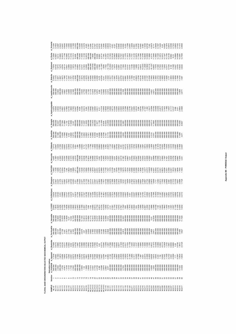
FLU
VIA
L SA
ND
GR
OU
ND
WA
TER
S SE
LEC
TED
GEO
CH
EMIC
AL
OU
TPU
T
Satu
ration Indices
SAM
PLE
Solu
tion
si_F
e3(O
H)8
si_A
gmet
alsi
_Boe
hmite
si_F
errih
ydrit
esi
_Hem
atite
si_Cr2
O3
si_Cr(
OH
)3(a
m)
si_D
iaspor
esi
_FeCr2
O4
si_H
ercy
nite
si_G
ibbs
itesi
_Goe
thite
si_Gre
igite
si_H
ydro
xyla
patit
esi
_Lep
idocro
cite
si_S
ider
itesi
_Orp
imen
tsi
_Pyr
itesi
_Viv
iani
teML1/9
1-9
99.9
99-1
.107
80.74
99-9
99.9
99-9
99.9
992.
6262
0.9234
2.4775
1.94
624.
658
1.07
13-9
99.9
99-9
99.9
995.3575
-999
.999
-2.0452
7.7679
11.2
509
-3.1244
ML1/1
02
-999
.999
0.85
830.
6173
-999
.999
-999
.999
1.99
160.
6152
2.35
011.
1036
4.18
870.
9467
-999
.999
-999
.999
4.9526
-999
.999
-2.121
99.
6193
10.9
921
-3.7
603
ML1/1
13
2.30
52-0
.1564
0.68
653.41
0714
.660
52.3829
0.81
842.4237
1.62
854.464
1.0226
6.13
8815
.3227
4.9034
5.3922
-1.9
971
7.8772
12.6
13-3
.3987
ML1/12
4-9
99.9
99-1
.6674
0.4135
-999
.999
-999
.999
2.42
960.
819
2.1376
2.07
544.30
830.72
95-9
99.9
99-9
99.9
995.
1505
- 999
.999
-1.8
657
7.5279
12.6
682
-2.9443
ML1/13
51.27
552.
5468
0.61
042.71
5613
.257
62.47
620.
8468
2.3371
2.2524
4.8344
0.93
045.4346
10.7264
4.8921
4.6443
-1.6473
4.87
6410
.451
9-2
.409
1ML1/14
6-0
.091
11.
0932
0.2777
2.037
11.9
068
2.1329
0.6843
2.00
971.
8148
4.07
870.
6057
4.76
0611
.0864
5.4631
3.9921
-1.7
692
6.81
1411
.114
9-2
.624
5ML1/1
57
1.41
091.
9219
0.20
892.7677
13.3
639
1.6038
0.4137
1.9373
1.383
4.03
560.
5315
5.48
8211
.732
4.78
654.70
52-1
.4114
5.8421
10.5
8 45
-1.4362
ML1/1
68
1.5134
1.04
950.
0642
2.71
9213
.27
1.92
620.
5794
1.79
531.
8624
3.90
540.39
095.442
10.8763
5.51
654.
6698
-1.336
15.38
9910
.277
6-1
.0582
ML2/1
19
1.71
660.20
910.
942
3.0841
14.0
021.
6048
0.42
182.
6749
0.98
65.
1073
1.27
145.
8084
11.649
81.
8663
5.0436
-1.7
971
6.6024
11.2
105
-4.6
985
ML2/12
102.3022
0.9274
0.6876
3.14
5214
.134
91.
8846
0.577
2.42
931.
5868
4.92
621.
0304
5.8772
13.247
3.72
635.
1489
-1.6783
7.2674
12.1
013
-3.1
069
ML2/13
11-9
99.9
992.25
680.47
58-9
99.9
99-9
99.9
991.
8422
0.56
192.22
11.47
114.43
190.
824
-999
.999
-999
.999
5.04
07-9
99.9
99-1
.924
83.
1539
9.30
99-3
.332
5ML2/14
12-9
99.9
99-0
.068
1.04
67-9
99.9
99-9
99.9
992.2543
0.7726
2.7946
-999
.999
-999
.999
1.39
9-9
99.9
99-9
99.9
994.
9288
-999
.999
-999
.999
8.58
54-9
99.9
99-9
99.9
99ML2/1
513
-999
.999
-0.0
805
0.67
09-9
99.9
99-9
99.9
992.4846
0.8939
2.4223
1.67
934.3928
1.0 2
86-9
99.9
99-9
99.9
994.
629
-999
.999
-2.337
69.
1076
12.4
836
-4.3
026
ML2/1
614
0.96
550.2734
0.58
892.
6476
13.1354
2.10
680.
6819
2.3271
1.5246
4.44
180.
9263
5.37
6513
.3454
4.4335
4.6335
-1.9273
8.4741
11.940
8-3
.4294
ML2/17
151.
0 30.
9978
0.39
862.
8713
.5612
2.2831
0.7427
2.12
091.
5754
3.9236
0.712
5.58
5211
.2297
3.64
134.77
69-2
.029
56.
1603
11.2
148
-4.337
8ML2/1
816
1.5846
1.9821
0.3726
2.85
9713
.561
92.3744
0.81
882.
1124
1.95
844.
1766
0.7127
5.59
0211
.200
53.494
4.8546
-1.6
079
6.30
0610
.921
9-2
.925
ML3/12.
517
2.8428
8.4845
0.9935
3.0549
13.9
684
1.09
90.2042
2.74
671.33
586.
0814
1.3539
5.7971
-999
.999
3.3342
5.11
65-0
.5607
-999
.999
-999
.999
0.15
67ML3/13.
518
4.10
147.78
580.
8182
3.65
6315
.1712
1.164
0.23
672.
5714
1.45
655.78
651.
1786
6.39
85-9
99.9
993.
8082
5.7179
-0.4
606
-999
.999
-999
.999
0.33
94ML3/14.
519
3.2321
8.2245
0.8238
3.19
6314
.2512
0.93
850.
1239
2.5771
1.28
185.
8486
1.1842
5.93
84-13.3433
3.44
875.2579
-0.3352
-13.
8164
-1.9
096
0.41
19ML3/1
5.5
204.
1752
9.75
980.70
833.7042
15.2
648
0.65
1 3-0
.022
82.45
970.
9507
5.5722
1.06
596.4448
-999
.999
3.82
625.75
68-0
.386
9-9
99.9
99-9
99.9
990.73
07ML3/1
6.5
214.3726
1.89
691.
6705
3.85
9215
.5737
0.7748
0.0374
3.42
110.
9761
7.3979
2.02
696.
599
11.9
071
3.94
115.
9074
-0.5
095
4.6944
9.93
980.
5725
ML3/17.
522
4 .49
92.44
820.
633.
8998
15.6
549
0.69
14-0
.0043
2.38
050.
9379
5.362
0.98
636.
6396
11.1
198
4.31
15.
948
-0.479
4.1846
8.95
820.
6722
ML3/1
8.5
233.
5396
7.9327
0.2773
3.51
8214
.893
90.37
55-0
.159
12.
0296
0.39
694.4329
0.63
636.25
96-13.
1065
4.10
185.
5753
-0.6783
-13.
1391
-2.2714
0.2345
ML3/1
9.5
243.
9075
3.22
990.
0394
3.53
8414
.9344
-0.032
5-0
.363
11.79
170.31
634.2845
0.39
846.27
986.
9339
4.56
095.
5956
-0.341
1.82
957.
1483
1.24
58ML1/1
925
2.88
011.
184
-1.3
093
3.3876
14.5
996
1.64
560.42
850.41
561.71
061.2824
-0.9
926.
1051
12.644
54.
8638
5.3076
-1.0333
7.1932
10.3
947
-0.6
835
ML1/2
026
2.877
8.39
63-1
.260
13.3928
14.6
121.
6774
0.4474
0.46
661.70
071.34
07-0
.940
16.
1118
-13.29
594.
1859
5.32
15-1
.0222
-12.
1154
-2.4
129
-0.8
035
ML1/1
127
- 999
.999
-2.148
0.75
99-9
99.9
99-9
99.9
992.
101
0.69
592.
5078
1.7279
5.00
021.
1122
-999
.999
-999
.999
3.5626
-999
.999
-1.5417
10.2
503
12.1
003
-1.5727
ML1/12
28-9
99.9
99-0
.875
81.
0508
-999
.999
-999
.999
2.23
810.76
142.79
692.21
085.
9265
1.40
04-9
99.9
99-9
99.9
993.
8773
-999
.999
-1.2703
8.70
5312
.914
8-0
.601
ML1/13
29-9
99.9
99-1
.2942
0.61
93-9
99.9
99-9
99.9
992.
1793
0.72
892.3636
2.293
5.203
0.96
61-9
99.9
99-9
99.9
994.30
56-9
99.9
99-1
.090
17.3574
12.0
823
- 0.227
ML1/14
30-9
99.9
99-2
.9557
0.62
53-9
99.9
99-9
99.9
991.
9702
0.62
592.37
061.
6 704
4.8024
0.9735
-999
.999
-999
.999
4.23
54-9
99.9
99-1
.307
88.3924
12.8
669
-0.9702
ML1/1
531
-999
.999
0.5846
0.6077
-999
.999
-999
.999
1.67
530.47
542.35
122.
1498
5.54
010.
9532
-999
.999
-999
.999
4.6833
-999
.999
-0.5
577
6.36
9110
.8933
0.90
66ML1/1
632
-999
.999
-0.4
935
-0.142
5-9
99.9
99-9
99.9
990.7941
0.0348
1.60
091.
0408
3.81
180.203
-999
.999
-999
.999
4.0625
-999
.999
-0.675
56.
9164
10.7
521
0.5336
ML1/17
330.7233
-0.2404
0.0726
2.09
1212
.029
11.7249
0.50
021.
8161
1.9275
4.19
810.41
814.
8248
12.2
891
3.7829
4.1038
-0.633
17.
1694
10.629
10.
5395
ML1/1
834
- 999
.999
-1.0
933
0.33
17-9
99.9
99-9
99.9
991.
652
0.4637
2.07
511.
5819
4.4434
0.6772
-999
.999
-999
.999
3.73
98-9
99.9
99-0
.906
18.
1524
11.127
6-0
.433
ML1/1
935
-999
.999
-0.7
074
0.1033
-999
.999
-999
.999
1.6949
0.4836
1.84
591.
5234
3.8847
0.4475
-999
.999
-999
.999
2.26
84-9
99.9
99-1
.044
98.3141
11.3413
-1.729
8ML1/2
036
-999
.999
-2.1364
-0.1
156
-999
.999
-999
.999
1.78
190.
521
1.6234
1.3932
3.227
0.2232
-999
.999
-999
.999
2.31
95-9
99.9
99-1
.3204
8.41
8111
.026
9-2
.648
1ML2/1
137
-999
.999
-1.2
665
1.0425
-999
.999
-999
.999
1.89
540.
5443
2.7622
1.65
665.
6783
1.35
18-9
99.9
99-9
99.9
993.
5507
-999
.999
-1.1
909
7.31
8911
.772
1-1
.262
8ML2/12
38-9
99.9
990.
1511
1.6522
-999
.999
-999
.999
2.0649
0.64
573.38
152.38
567.4645
1.97
62-9
99.9
99-9
99.9
994.36
65-9
99.9
99-0
.705
6.00
6811
.414
50.
5831
ML2/13
39-9
99.9
99-0
.6482
1.3137
-999
.999
-999
.999
1.904
0.56
833.
0447
2.03
066.
5947
1.64
03-9
99.9
99-9
99.9
993.
8316
-999
.999
-0.8
923
7.49
8912
.267
90.
1556
ML2/ 14
40-9
99.9
99-0
.736
90.
9592
-999
.999
-999
.999
1.5028
0.36
622.
6894
1.3034
5.55
921.2846
-999
.999
-999
.999
3.59
8-9
99.9
99-1
.074
89.
9173
11.736
5-0
.8187
ML2/1
541
-999
.999
-1.6
871.
0644
-999
.999
-999
.999
1.05
850.
1547
2.80
071.3636
6.27
871.39
91-9
99.9
99-9
99.9
993.
6744
-999
.999
-0.6
134
9.4972
10.7
046
0.43
93ML2/1
642
-999
.999
-0.831
1.02
06-9
99.9
99-9
99.9
991.20
090.21
832.7526
0.1526
4.8344
1.34
87-9
99.9
99-9
99.9
99-1
.2282
-999
.999
-1.834
610
.2333
11.0
199
-5.8
93ML2/17
43-9
99.9
99-3
.0073
1.3646
-999
.999
-999
.999
0.4847
-0.1413
3.09
57-1
.5417
4.5437
1.69
13-9
99.9
99-9
99.9
99-4
.132
1-9
99.9
99-2
.4384
11.2
909
10.8
6 46
-7.4
036
ML2/1
844
-999
.999
-3.3
085
1.03
86-9
99.9
99-9
99.9
991.25
940.25
062.7724
-0.070
14.
5906
1.36
93-9
99.9
99-9
99.9
99-1
.262
-999
.999
-2.1
167
12.5
802
12.0
959
-6.6782
ML2/1
945
-999
.999
-3.4
005
1.13
52-9
99.9
99-9
99.9
990.
9144
0.07
812.
8689
-0.640
54.
5583
1.46
59-9
99.9
99-9
99.9
99-1
.8417
-999
.999
-2.2
538
13.5
116
11.9
666
-7.045
ML2/23
460.
6558
9.80
580.
8512
2.48
5912
.81
1.99
860.
6248
2.5875
1.45
855.
007
1.18
595.2133
-19.
9713
-0.2
994
4.4631
-1.5463
-16.
1337
-4.3
174
-5.5
979
ML2/24
471.3222
1.0572
-0.1373
2.84
1113
.522
61.
0368
0.14
691.
6009
0.4241
2.95
890.20
015.
5701
11.0
826
-0.4
162
4.8271
-1.5
863
6.6833
11.040
6-5
.717
ML2/2
548
-999
.999
1.65
5 4-0
.025
6-9
99.9
99-9
99.9
990.
6189
-0.0
544
1.717
0.20
033.37
980.31
86-9
99.9
99-9
99.9
99-0
.559
9-9
99.9
99-1
.3642
7.7578
11.6
662
-4.9
608
ML2/2
649
-999
.999
0.44
8-0
.4892
-999
.999
-999
.999
1.16
90.
1948
1.23
830.
8179
2.50
85-0
.167
9-9
99.9
99-9
99.9
99-0
.405
6-9
99.9
99-1
.3753
8.1826
12.1
539
-5.1
067
ML2/27
50-9
99.9
991.
194
0.29
63-9
99.9
99-9
99.9
991.
0461
0.12
872.
0212
0.03
013.4127
0.6136
-999
.999
-999
.999
-0.2
617
-999
.999
-2.0
626
6.7933
11.0
974
-7.244
5ML2/2
851
-999
.999
2.04
62-0
.0112
-999
.999
-999
.999
1.6248
0.43
641.7243
0.8875
3.0844
0.3222
- 999
.999
-999
.999
3.0076
-999
.999
-1.9263
5.15
0510
.2472
-5.0
5ML2/2
952
-999
.999
0.73
02-0
.3924
-999
.999
-999
.999
1.9842
0.62
671.34
920.
6298
1.70
97-0
.049
6-9
99.9
99-9
99.9
993.
1403
-999
.999
-2.4
932
7.33
5312
.1347
-5.6387
ML2/2
553
-999
.999
-1.743
91.21
02-9
99.9
99-9
99.9
991.44
540.34
672.
9456
0.3431
5.1621
1.5435
-999
.999
-999
.999
-1.1
982
-999
.999
-1.926
58.70
1710
.1784
-6.1
879
ML2/2
654
-999
.999
-2.2
102
1.09
51-9
99.9
99-9
99.9
991.34
80.2933
2.82
80.34
895.
0333
1.4245
-999
.999
-999
.999
-1.640
1-9
99.9
99-1
.777
8.7345
10.4
148
-5.6
974
ML2/27
55-9
99.9
99-0
.623
0.90
63-9
99.9
99-9
99.9
991.40
910.31
932.
6365
0.24
014.4836
1.23
16-9
99.9
99-9
99.9
99-0
.111
1-9
99.9
99-1
.9953
8.14
99.
5982
-5.549
8ML6/13
56-9
99.9
99-2
.006
60.
9885
-999
.999
-999
.999
1.83
970.
5575
2.73
191.
5919
5.57
941.3339
-999
.999
-999
.999
3.5127
-999
.999
-1.6
859
3.10
6816
.03
-3.7403
ML6/14
57-9
99.9
99-1
.71
0.59
-999
.999
-999
.999
2.11
690.
6656
2.31
591.
9497
4.84
960.
908 7
-999
.999
-999
.999
3.59
6-9
99.9
99-1
.683
84.
0427
14.9
684
-3.9
805
ML6/1
558
-999
.999
-2.2
597
0.0726
-999
.999
-999
.999
2.1229
0.6778
1.8037
1.80
563.
6687
0.39
93-9
99.9
99-9
99.9
993.47
1-9
99.9
99-1
.759
53.
5753
14.438
9-3
.7332
ML6/1
659
0.7323
-1.9
044
1.86
122.44
8312
.7252
2.0249
0.6 242
3.58
961.7642
7.30
052.
1838
5.16
8813
.4282
2.98
024.38
58-1
.5154
6.9232
14.3
081
-3.141
5ML6/17
60-0
.500
5-1
.8033
-0.0
129
1.9527
11.730
91.
6202
0.4173
1.7129
1.16
033.35
10.30
574.
671
8.65
572.46
693.
8771
-1.8
973.
6242
12.7
939
-4.9
959
App
endi
x B8
- PH
REE
QC
Out
put
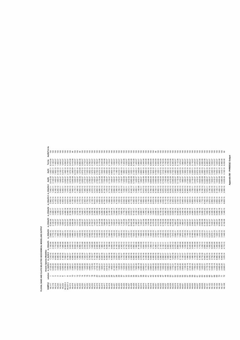
FLU
VIA
L SA
ND
AN
D C
LAYS
SEL
ECTE
D G
EOC
HEM
ICA
L M
OD
ELLI
NG
OU
TPU
T
Arsenic
Species
Molalities
SAM
PLE
solu
tion
m_A
sO3-
3m
_AsO
4-3
m_H
2AsO
3-m
_H2A
sO4-
m_H
3AsO
3m
_H3A
sO4
m_H
AsO
3-2
m_H
AsO
4-2
As(
III)
As(
V)To
t As
As(
III)/Tot
As
ML1/17
14.
12E-20
1.21E-
151.
10E-
092.
88E-
128.30E-
081.72E-
172.
99E-
141.
04E-
118.41E-
081.33E-
118.41E-
0810
0ML1/1
82
6.09E-20
1.35E-
152.32E-
094.77E-
122.
12E-
073.
56E-
175.27E-
141.40E-
112.
14E-
071.
88E-
112.
14E-
0710
0ML2/1
93
5.12E-20
6.65E-
161.71E-
091.77E-
121.43E-
071.
06E-
174.
12E-
146.
18E-
121.45E-
077.
95E-
121.45E-
0710
0ML2/2
04
4.56E-20
6.48E-
161.
65E-
091.
86E-
121.44E-
071.
16E-
173.
81E-
146.25E-
121.46E-
078.
12E-
121.46E-
0710
0ML2/2
15
4.82E-20
2.47E-
151.74E-
097.29E-
121.
52E-
074.
67E-
174.
03E-
142.40E-
111.
54E-
073.
13E-
111.
54E-
0710
0ML2/22
65.29E-20
4.18E-
151.
89E-
091.23E-
111.
65E-
077.
87E-
174.40E-
144.
05E-
111.
67E-
075.27E-
111.
67E-
0710
0ML3/2
0.5
72.78E-20
7.06E-
172.36E-
094.
66E-
133.27E-
074.48E-
183.
51E-
141.
03E-
123.29E-
071.49E-
123.29E-
0710
0ML3/2
1.5
83.
56E-20
9.73E-
173.25E-
096.
93E-
134.
67E-
076.
96E-
184.
67E-
141.47E-
124.70E-
072.
16E-
124.70E-
0710
0ML4/13
91.39E-21
2.89E-
172.
04E-
104.
69E-
133.
95E-
088.79E-
182.35E-
156.
05E-
133.
97E-
081.
07E-
123.
97E-
0810
0ML4/1
610
3.38E-21
4.90E-
142.45E-
104.
96E-
103.26E-
087.
93E-
154.
13E-
157.
84E-
103.29E-
081.28E-
093.41E-
0896
ML4/2
111
1.44E-20
3.22E-
158.
63E-
101.
84E-
111.
03E-
071.
84E-
161.
55E-
144.
17E-
111.
04E-
076.
01E-
111.
04E-
0710
0ML4/22
124.23E-20
1.56E-
141.20E-
094.40E-
111.
01E-
073.27E-
163.
10E-
141.39E-
101.
03E-
071.
83E-
101.
03E-
0710
0ML4/23
134.48E-20
1.26E-
138.
98E-
102.
93E-
106.
67E-
082.
19E-
152.77E-
149.
80E-
106.76E-
081.27E-
096.
88E-
0898
ML2/2
014
2.06E-20
1.50E-
162.27E-
091.40E-
123.
53E-
071.
64E-
173.
01E-
142.
57E-
123.
55E-
073.
97E-
123.
55E-
0710
0ML2/2
115
1.33E-20
7.32E-
172.
04E-
099.36E-
133.
69E-
071.26E-
172.30E-
141.48E-
123.71E-
072.41E-
123.71E-
0710
0ML2/22
161.
64E-20
2.37E-
172.41E-
092.
67E-
134.22E-
073.23E-
182.75E-
144.
56E-
134.25E-
077.23E-
134.25E-
0710
0ML2/23
174.
98E-21
3.76E-
181.
51E-
098.
96E-
143.76E-
071.
58E-
181.21E-
141.
05E-
133.78E-
071.
95E-
133.78E-
0710
0ML2/24
181.37E-20
2.72E-
171.
69E-
092.75E-
132.70E-
073.23E-
182.
13E-
144.
91E-
132.72E-
077.
67E-
132.72E-
0710
0ML3/1
519
1.57E-
195.
11E-
162.45E-
096.
10E-
131.40E-
072.39E-
188.
61E-
143.21E-
121.43E-
073.
82E-
121.43E-
0710
0ML3/1
620
2.73E-
197.38E-
164.
59E-
099.49E-
132.74E-
073.
88E-
181.
55E-
134.
80E-
122.78E-
075.75E-
122.78E-
0710
0ML4/1
521
5.30E-21
5.20E-
172.
90E-
102.
18E-
133.
14E-
081.
62E-
185.42E-
156.
09E-
133.
17E-
088.27E-
133.
17E-
0810
0ML4/1
622
1.82E-21
6.02E-
181.
98E-
105.
04E-
143.
02E-
085.29E-
192.
63E-
159.
97E-
143.
04E-
081.
50E-
133.
04E-
0810
0ML4/17
236.
91E-21
6.30E-
175.76E-
104.
03E-
137.
66E-
083.
69E-
188.73E-
159.
13E-
137.72E-
081.32E-
127.72E-
0810
0ML4/1
824
6.61E-21
6.03E-
178.23E-
105.77E-
131.32E-
076.38E-
181.
03E-
141.
07E-
121.33E-
071.
65E-
121.33E-
0710
0ML4/1
925
7.16E-21
1.33E-
161.
18E-
091.
68E-
122.
16E-
072.
14E-
171.28E-
142.71E-
122.
17E-
074.40E-
122.
17E-
0710
0ML4/2
026
1.80E-21
9.34E-
185.
60E-
102.26E-
131.42E-
073.
97E-
184.43E-
152.
64E-
131.42E-
074.
90E-
131.42E-
0710
0ML4/2
127
8.14E-21
1.53E-
169.72E-
101.42E-
121.
52E-
071.
54E-
171.24E-
142.
69E-
121.
53E-
074.
11E-
121.
53E-
0710
0ML4/22
283.78E-21
3.57E-
176.
10E-
104.47E-
131.
10E-
075.
59E-
186.72E-
157.29E-
131.
10E-
071.
18E-
121.
10E-
0710
0ML4/23
291.22E-20
2.89E-
159.
90E-
101.
82E-
111.26E-
071.
61E-
161.
54E-
144.
19E-
111.27E-
076.
01E-
111.27E-
0710
0ML4/24
301.32E-21
1.70E-
174.34E-
104.39E-
131.
10E-
077.
80E-
183.37E-
155.
00E-
131.
10E-
079.38E-
131.
10E-
0710
0ML4/2
531
7.53E-22
3.31E-
162.77E-
109.48E-
127.37E-
081.77E-
162.
03E-
151.
03E-
117.40E-
081.
98E-
117.40E-
0810
0ML4/2
632
5.69E-21
5.99E-
166.72E-
105.
53E-
121.
03E-
075.
90E-
178.
68E-
151.
05E-
111.
03E-
071.
60E-
111.
03E-
0710
0ML4/27
332.30E-21
1.44E-
154.45E-
102.
16E-
118.77E-
082.
95E-
164.48E-
153.21E-
118.
81E-
085.36E-
118.
82E-
0810
0ML4/2
834
2.02E-21
2.58E-
164.25E-
104.20E-
128.
64E-
085.
91E-
174.
11E-
156.
04E-
128.
68E-
081.
02E-
118.
68E-
0810
0ML4/2
935
2.70E-21
6.89E-
163.
96E-
107.
82E-
126.70E-
089.
15E-
174.
59E-
151.35E-
116.74E-
082.
13E-
116.74E-
0810
0ML4/3
036
7.65E-20
4.28E-
151.
96E-
098.45E-
121.38E-
074.
13E-
175.44E-
143.49E-
111.40E-
074.34E-
111.40E-
0710
0ML5/14
371.38E-
182.
99E-
138.
10E-
091.48E-
102.79E-
073.
82E-
164.71E-
131.
19E-
092.
87E-
071.34E-
092.
89E-
0710
0ML5/1
538
8.36E-20
4.07E-
151.
91E-
097.
82E-
121.34E-
074.
09E-
175.
58E-
143.
17E-
111.36E-
073.
96E-
111.36E-
0710
0ML5/1
639
8.89E-21
5.73E-
163.
55E-
101.
95E-
123.31E-
081.38E-
177.
83E-
155.
91E-
123.34E-
087.
86E-
123.34E-
0810
0ML5/17
404.
17E-21
3.33E-
161.
52E-
101.
03E-
121.38E-
087.
07E-
183.49E-
153.26E-
121.40E-
084.29E-
121.40E-
0810
0ML5/1
841
3.85E-21
6.45E-
161.37E-
101.
98E-
121.23E-
081.36E-
173.
19E-
156.27E-
121.24E-
088.24E-
121.25E-
0810
0ML5/1
942
2.98E-21
5.90E-
161.
08E-
101.
83E-
129.74E-
091.26E-
172.49E-
155.78E-
129.
85E-
097.
61E-
129.
85E-
0910
0ML5/2
043
6.24E-22
4.46E-
163.71E-
112.24E-
124.27E-
091.
93E-
176.
67E-
165.
58E-
124.30E-
097.
82E-
124.31E-
0910
0ML5/2
144
5.98E-22
4.87E-
154.28E-
113.
02E-
115.41E-
092.
93E-
167.
02E-
166.73E-
115.46E-
099.75E-
115.
55E-
0998
ML5/22
452.29E-22
4.90E-
162.71E-
114.75E-
124.41E-
095.
62E-
173.45E-
168.
56E-
124.43E-
091.33E-
114.45E-
0910
0ML5/23
469.45E-23
2.28E-
172.
10E-
114.
13E-
134.72E-
096.73E-
181.
94E-
165.44E-
134.74E-
099.
57E-
134.74E-
0910
0ML5/2
647
1.55E-22
2.58E-
173.
13E-
114.25E-
136.70E-
096.
61E-
183.
03E-
165.
87E-
136.73E-
091.
01E-
126.73E-
0910
0ML5/27
486.
00E-22
2.56E-
178.20E-
112.
86E-
131.73E-
084.39E-
189.
11E-
164.
52E-
131.74E-
087.38E-
131.74E-
0810
0ML5/2
849
9.98E-23
1.68E-
176.
06E-
118.
58E-
132.78E-
082.
93E-
173.
17E-
166.25E-
132.78E-
081.48E-
122.78E-
0810
0ML5/2
950
3.88E-21
8.16E-
172.46E-
104.21E-
134.48E-
085.
52E-
183.70E-
159.
03E-
134.
51E-
081.32E-
124.
51E-
0810
0ML5/3
051
1.77E-21
1.87E-
182.23E-
101.
91E-
146.37E-
083.
92E-
192.30E-
152.
81E-
146.39E-
084.73E-
146.39E-
0810
0ML6/1
852
9.06E-
197.
85E-
145.27E-
093.
98E-
111.
98E-
071.
15E-
163.
00E-
133.
06E-
102.
03E-
073.46E-
102.
04E-
0710
0ML6/1
953
4.41E-20
1.01E-
178.
86E-
101.70E-
146.
02E-
088.
56E-20
2.72E-
147.28E-
146.
11E-
088.
98E-
146.
11E-
0810
0ML6/2
054
3.26E-20
2.11E-
171.42E-
097.
66E-
141.36E-
075.42E-
193.
01E-
142.28E-
131.37E-
073.
04E-
131.37E-
0710
0ML6/2
155
2.60E-20
7.13E-
171.
69E-
093.
81E-
131.
96E-
073.24E-
182.
94E-
149.37E-
131.
98E-
071.32E-
121.
98E-
0710
0ML6/22
561.
14E-20
3.22E-
171.
03E-
092.36E-
131.37E-
072.29E-
181.
52E-
145.
00E-
131.39E-
077.36E-
131.39E-
0710
0ML6/23
576.
91E-
191.
08E-
139.
01E-
091.
14E-
104.
63E-
074.25E-
163.
50E-
136.36E-
104.72E-
077.
51E-
104.73E-
0710
0ML6/24
582.
19E-
191.
62E-
145.22E-
093.
10E-
113.
63E-
071.
55E-
161.
50E-
131.28E-
103.
69E-
071.
59E-
103.
69E-
0710
0ML6/2
559
5.82E-20
1.49E-
153.
00E-
096.
18E-
123.
08E-
074.
56E-
175.
85E-
141.73E-
113.
11E-
072.35E-
113.
11E-
0710
0ML6/2
660
7.76E-21
1.73E-
161.
16E-
092.
08E-
122.
03E-
072.
62E-
171.33E-
143.43E-
122.
04E-
075.
52E-
122.
04E-
0710
0ML6/27
611.
00E-20
2.47E-
171.
01E-
091.
98E-
131.46E-
072.
05E-
181.40E-
143.
99E-
131.47E-
075.
97E-
131.47E-
0710
0ML6/2
862
5.44E-22
4.19E-
191.77E-
101.
01E-
144.
63E-
081.75E-
191.36E-
151.
19E-
144.
64E-
082.20E-
144.
64E-
0810
0ML6/2
963
1.43E-21
6.71E-
181.23E-
104.42E-
142.
06E-
085.
06E-
191.71E-
159.
19E-
142.
08E-
081.36E-
132.
08E-
0810
0ML6/3
064
8.82E-21
6.84E-21
3.69E-
102.25E-
176.
19E-
082.
61E-22
6.54E-
155.
84E-
176.22E-
088.
09E-
176.22E-
0810
0ML1/2
165
2.17E-
198.
19E-
157.36E-
092.47E-
116.40E-
071.
69E-
161.76E-
137.
87E-
116.48E-
071.
03E-
106.48E-
0710
0ML1/22
664.
10E-
192.
61E-
141.
05E-
086.22E-
118.
15E-
074.
00E-
162.
87E-
132.
19E-
108.25E-
072.
81E-
108.26E-
0710
0ML1/23
675.
06E-
193.75E-
149.
87E-
096.
87E-
117.
53E-
074.34E-
162.
98E-
132.
65E-
107.
63E-
073.34E-
107.
63E-
0710
0ML1/24
681.
15E-
193.78E-
162.
84E-
098.23E-
132.48E-
075.
59E-
187.
52E-
142.
93E-
122.
51E-
073.75E-
122.
51E-
0710
0ML1/2
569
6.64E-20
8.96E-
151.29E-
091.
52E-
111.
00E-
079.
09E-
173.
85E-
146.
12E-
111.
02E-
077.
64E-
111.
02E-
0710
0ML1/2
670
4.46E-20
1.94E-
161.
02E-
093.
91E-
138.
55E-
082.
54E-
182.
82E-
141.45E-
128.
65E-
081.
84E-
128.
65E-
0810
0ML1/27
712.45E-20
8.94E-
166.
90E-
102.45E-
126.41E-
081.
95E-
171.74E-
147.
65E-
126.48E-
081.
01E-
116.48E-
0810
0ML1/2
872
8.59E-21
1.67E-
144.71E-
101.
04E-
106.
15E-
081.34E-
158.
60E-
152.
09E-
106.20E-
083.
13E-
106.23E-
0899
App
endi
x B8
- PH
REE
QC
Out
put
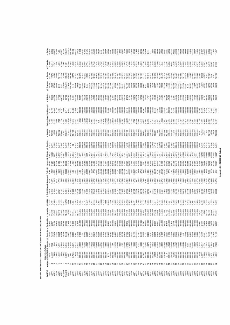
FLU
VIA
L SA
ND
AN
D C
LAYS
SEL
ECTE
D G
EOC
HEM
ICA
L M
OD
ELLI
NG
OU
TPU
T
Satu
ration Indices
SAM
PLE
solu
tion
si_F
e3(O
H)8
si_A
gmet
alsi
_Boe
hmite
si_F
errih
ydrit
esi
_Hem
atite
si_Cr2
O3
si_Cr(
OH
)3(a
msi
_Dia
spor
esi_
FeCr2
O4si
_Her
cyni
tsi_
Gib
bsite
si_Goe
thite
si_Gre
igite
_Hydro
xyla
pati_
Lepi
docroc
itsi
_Sid
erite
si_Orp
imen
tsi
_Pyr
itesi
_Viv
iani
tesi
_Sul
fur
ML1/17
12.477
1.197
0.61
133.
1953
14.2
171
1.7478
0.4826
2.33
81.76
65.
0783
0.93
135.
9143
12.1
054
4.84
685.
1241
-1.0
535.7025
10.470
6-0
.693
6-1
.792
5ML1/1
82
2.55
021.
598
-1.2
135
3.28
0414
.379
91.77
910.4877
0.5071
1.79
891.42
57-0
.902
85.
9941
10.9
657
4.18
965.
1786
-0.9
673
5.45
989.4976
-0.6
114
-2.3
989
ML2/1
93
1.54
551.
8309
0.34
642.
6184
13.0
867
0.65
85-0
.0284
2.0925
0.58
614.4726
0.69
65.3543
9.99
053.2372
4.6443
-1.1374
5.7546
10.2
19-1
.707
1-1
.863
9ML2/2
04
2.33
622.3948
0.33
093.
0976
14.0452
0.4771
-0.1
191
2.077
0.23
684.2738
0.68
055.
8335
11.0
947
2.347
5.1235
-1.2337
5.9935
10.248
-2.7
691
-1.745
5ML2/2
15
1.6133
1.99
610.
0301
2.87
8713
.601
91.
5155
0.3924
1.77
181.
0618
3.45
530.3729
5.61
0710
.3702
1.18
14.
8824
-1.449
85.
935
10.4
115
-4.221
5-1
.321
ML2/22
61.36
860.3846
-0.134
2.76
8413
.3803
0.1673
-0.2
832
1.60
68-0
.2963
3.11
650.2075
5.49
9710
.844
11.
1756
4.7677
-1.4
535
6.523
10.9
124
-4.2
939
-0.9
803
ML3/2
0.5
73.
6908
8.2638
0.52
983.
5168
14.8
889
0.2731
-0.2
134
2.28
040.4774
5.11
950.
8861
6.25
66-1
0.59
114.
5453
5.56
5-0
.446
6-1
0.46
94-1
.3954
1.082
-8.120
6ML3/2
1.5
83.
8472
8.81
55-0
.3572
3.67
0615
.195
6-0
.574
1-0
.638
61.3925
-0.5
068
3.2078
-0.0
022
6.40
97-9
99.9
994.
8929
5.7144
-0.5463
-999
.999
-999
.999
1.13
64-9
99.9
99ML4/13
91.48
58.
8365
0.8478
3.14
8214
.078
0.794
-0.0
585
2.5374
0.5132
5.224
1.11
135.
8348
-17.
6922
-2.270
54.
8912
-0.934
6-17.43
57-5
.8847
-4.2
593
-10.2526
ML4/1
610
1.02
915.45
590.
1345
3.2273
14.1
883
0.557
-0.2452
1.7847
0.2974
3.78
860.33
815.
8795
-999
.999
-2.037
54.7731
-1.1363
-999
.999
-999
.999
-5.0
948
-999
.999
ML4/2
111
2.75
050.3374
0.38
583.49
0814
.7944
1.06
640.
1223
2.10
110.
954.484
0.68
856.2
10.4
177
1.59
155.3628
-0.9
644.
146
9.7774
-1.6
599
-1.7402
ML4/22
122.
9269
0.57
140.442
3.6724
15.148
11.
1683
0.15
972.
1496
0.99
14.
5297
0.7329
6.3747
13.5
623
2.47
825.
5054
-1.1
579
6.1739
11.1
023
-2.1
137
-1.0
135
ML4/23
132.
5149
0.45
560.29
053.76
9415
.311
11.
0846
0.0735
1.9724
0.7147
4.0145
0.5423
6.44
9413
.0793
2.1922
5.4741
-1.441
15.
1432
10.7202
-3.237
8-0
.912
8ML2/2
014
-999
.999
-3.6382
1.1937
-999
.999
-999
.999
1.26
640.2572
2.92
920.
014.
9751
1.5271
-999
.999
-999
.999
-1.0
035
-999
.999
-2.0
577
13.038
112
.8577
-6.5
586
-0.1
802
ML2/2
115
-999
.999
-2.1
886
1.16
1-9
99.9
99-9
99.9
991.
1921
0.2246
2.89
91-0
.1812
4.7948
1.49
84-9
99.9
99-9
99.9
99-1
.393
9-9
99.9
99-2
.103
812
.505
512
.3033
-6.6
647
-0.434
5ML2/22
16-9
99.9
99-0
.293
61.
1445
-999
.999
-999
.999
1.17
570.24
12.
8968
0.05
555.
0256
1.5035
-999
.999
-999
.999
-1.2
629
-999
.999
-1.832
89.47
1110
.2232
-5.7
937
-1.7
545
ML2/23
17-9
99.9
99-0
.0847
1.2828
-999
.999
-999
.999
0.98
170.
1363
3.03
06-0
.609
54.
8278
1.63
5-9
99.9
99-9
99.9
99-2
.310
5-9
99.9
99-2
.2112
9.324
9.33
01-6
.774
1-2
.1494
ML2/24
18-9
99.9
99-1
.007
51.
1405
-999
.999
-999
.999
1.2345
0.25
042.
8813
0.44
575.34
041.48
19-9
99.9
99-9
99.9
99-1
.4342
-999
.999
-1.575
610
.842
811
.5827
-5.037
5-1
.2827
ML3/1
519
-999
.999
-3.4
682
0.56
8-9
99.9
99-9
99.9
991.7977
0.5535
2.32
121.3529
4.54
880.
9284
-999
.999
-999
.999
4.98
03-9
99.9
99-1
.7494
11.8242
13.4
809
-2.5
029
-0.2787
ML3/1
620
-999
.999
-2.9
615
0.52
19-9
99.9
99-9
99.9
992.21
920.7643
2.27
521.77
554.4578
0.8823
-999
.999
-999
.999
4.42
64-9
99.9
99-1
.737
611
.386
812
.722
1-2
.798
5-0
.698
6ML4/1
521
-999
.999
-3.9
889
1.3274
-999
.999
-999
.999
1.30
980.30
953.
0806
0.32
145.
524
1.6877
-999
.999
-999
.999
2.76
83-9
99.9
99-2
.0394
11.4
958
14.0
639
-3.9
157
0.5246
ML4/1
622
-999
.999
-3.8
974
1.23
54-9
99.9
99-9
99.9
990.
9034
0.1048
2.9877
-0.347
15.
0773
1.5945
-999
.999
-999
.999
1.26
-999
.999
-2.1
992
11.944
913
.629
5-4
.725
80.
1937
ML4/17
23-9
99.9
99-3
.871
11.33
64-9
99.9
99-9
99.9
99-0
.496
1-0
.594
93.
0887
-1.6432
5.3826
1.69
54-9
99.9
99-9
99.9
991.29
06-9
99.9
99-2
.146
912
.1354
13.7
615
-4.7387
0.42
8ML4/1
824
-999
.999
-3.9384
1.3621
-999
.999
-999
.999
0.2728
-0.2
105
3.1144
-0.9763
5.3321
1.72
11-9
99.9
99-9
99.9
990.
9756
-999
.999
-2.1783
12.841
813
.8144
-4.631
60.
5055
ML4/1
925
-999
.999
-3.5
835
1.4149
-999
.999
-999
.999
0.83
10.
0671
3.16
63-0
.248
15.
607
1.7726
-999
.999
-999
.999
-0.7383
-999
.999
-1.9467
12.0
183
13.4364
-4.8492
0.37
67ML4/2
026
-2.7
19-3
.950
11.42
081.32
0610
.496
60.
5249
-0.0
875
3.17
13-1
.2884
4.8838
1.7771
4.06
0415
.759
5-2
.754
93.36
88-2
.5787
13.375
613
.2773
-7.376
0.37
95ML4/2
127
-1.821
5-3
.259
11.4143
1.51
9810
.894
91.
174
0.237
3.1648
-0.1402
5.36
991.77
064.25
9613
.1227
-0.5
853.
568
-2.238
810
.784
612
.5693
-5.844
10.
056
ML4/22
28-9
99.9
99-3
.47
1.43
58-9
99.9
99-9
99.9
991.
1503
0.22
523.
1863
-0.225
65.35
121.7921
-999
.999
-999
.999
-2.1
512
-999
.999
-2.2
6311
.5114
12.8
806
-6.5
018
0.0925
ML4/23
29-0
.579
6-1
.470
51.42
662.
0814
12.0
181
1.09
920.
1996
3.1771
-0.0
962
5.5134
1.7829
4.82
1211
.870
91.
0265
4.12
96-2
.2184
8.7528
12.5412
-4.837
80.
5325
ML4/24
30-9
99.9
99-2
.8344
1.50
56-9
99.9
99-9
99.9
990.4575
-0.1243
3.2544
-1.1
025.30
591.
8592
-999
.999
-999
.999
-2.122
1-9
99.9
99-2
.3523
10.7
865
12.3
043
-5.9
555
-0.0
534
ML4/2
531
-999
.999
-1.820
12.
1215
-999
.999
-999
.999
0.7845
0.04
083.
8712
-0.579
56.7338
2.47
65-9
99.9
99-9
99.9
99-2
.223
6-9
99.9
99-2
.114
810
.567
914
.138
8-5
.026
81.
5409
ML4/2
632
-999
.999
-2.9
61.
5191
-999
.999
-999
.999
0.91
990.
1085
3.26
88-0
.2164
5.75
681.
8741
-999
.999
-999
.999
0.16
82-9
99.9
99-2
.061
510
.917
113
.787
1-4
.6673
0.94
12ML4/27
33-9
99.9
99-3
.3232
1.4637
-999
.999
-999
.999
0.63
52-0
.0324
3.2142
-0.322
85.
825
1.82
-999
.999
-999
.999
-0.3
662
-999
.999
-1.8
018
10.6
933
14.7
022
-3.6
974
1.7043
ML4/2
834
-1.0
606
-2.1
815
2.1739
1.89
1611
.639
50.
8332
0.06
823.
9253
-0.478
6.8927
2.53
154.
6322
14.049
5-0
.5533
3.9442
-2.1
612
10.440
913
.5237
-4.7
175
0.95
65ML4/2
935
-999
.999
-2.4
661
1.4474
-999
.999
-999
.999
0.5672
-0.0
648
3.19
88-0
.699
95.4838
1.80
5-9
99.9
99-9
99.9
990.71
93-9
99.9
99-2
.163
9.99
8613
.7202
-4.3
588
1.1826
ML4/3
036
-999
.999
-1.4
543
0.5122
-999
.999
-999
.999
1.29
650.29
982.2637
1.1047
4.68
90.
8699
-999
.999
-999
.999
3.7328
-999
.999
-1.4
096
8.16
0412
.491
1-1
.677
5-0
.299
6ML5/14
37-9
99.9
99-1
.052
6-0
.1663
-999
.999
-999
.999
2.10
610.
6785
1.57
012.25
893.
665
0.16
84-9
99.9
99-9
99.9
996.
129
-999
.999
-1.3
516
8.68
1412
.992
1-1
.359
8-0
.072
8ML5/1
538
-999
.999
-0.0
095
-0.329
5-9
99.9
99-9
99.9
991.
8988
0.57
641.4077
1.87
813.
1656
0.00
65-9
99.9
99-9
99.9
994.49
94-9
99.9
99-1
.0884
5.80
8510
.702
6-0
.9123
-1.446
ML5/1
639
-999
.999
-1.1
84-0
.1993
-999
.999
-999
.999
1.75
050.4976
1.53
531.44
593.
1404
0.1328
-999
.999
-999
.999
3.69
96-9
99.9
99-1
.2404
5.1328
10.836
1-1
.500
6-1
.2017
ML5/17
40-9
99.9
99-1
.303
6-0
.238
6-9
99.9
99-9
99.9
991.77
570.
5118
1.49
691.37
532.
9667
0.0948
-999
.999
-999
.999
4.3443
-999
.999
-1.3
196
6.80
8612
.4757
-1.321
8-0
.2792
ML5/1
841
0.73
87-1
.138
2.0629
2.3748
12.5
835
2.1177
0.67
823.79
581.
9397
7.79
2.3923
5.09
9114
.040
14.253
4.3343
-1.122
86.
9467
13.1
153
-0.726
60.
0649
ML5/1
942
-999
.999
-3.072
1-0
.4447
-999
.999
-999
.999
1.744
0.4929
1.28
91.
1975
2.40
69-0
.114
-999
.999
-999
.999
4.20
68-9
99.9
99-1
.4907
6.363
12.5
877
-1.826
60.
0302
ML5/2
043
-999
.999
-1.3
074
0.52
02-9
99.9
99-9
99.9
991.
5006
0.37
572.25
660.
5994
3.984
0.8549
-999
.999
-999
.999
3.57
68-9
99.9
99-1
.757
3.89
9911
.6917
-2.4
983
0.064
ML5/2
144
-999
.999
-3.530
50.
8126
-999
.999
-999
.999
1.6244
0.43
2.5445
0.54
044.3826
1.14
06-9
99.9
99-9
99.9
993.
0172
-999
.999
-2.0342
4.8473
12.9
511
-3.029
51.27
1ML5/22
45-9
99.9
99-1
.619
61.
9604
-999
.999
-999
.999
1.1771
0.2232
3.7021
0.08
946.
6819
2.3032
-999
.999
-999
.999
1.72
17-9
99.9
99-1
.877
66.
1019
13.5
606
-2.8
182
1.38
06ML5/23
46-0
.9612
-3.3
593
1.7871
1.9838
11.8
132
1.01
110.
1417
3.52
96-0
.241
66.
1711
2.13
124.71
6612
.529
11.2841
3.99
19-1
.946
86.4877
12.6
876
-2.6
825
0.56
13ML5/2
647
-1.970
6-1
.5364
1.0931
1.40
0510
.646
80.
8275
0.04
992.
8357
-0.2
684.
9402
1.4372
4.1334
11.8
681.3032
3.40
87-1
.790
57.
0532
12.8
588
-2.2
699
0.48
84ML5/27
48-9
99.9
99-3
.093
11.2048
-999
.999
-999
.999
1.1731
0.22
092.
9464
0.0924
5.1779
1.5474
-999
.999
-999
.999
2.0477
-999
.999
-1.6357
8.80
6912
.879
5-1
.676
10.
1864
ML5/2
849
-999
.999
-0.7
582
1.1339
-999
.999
-999
.999
0.64
05-0
.053
12.
8712
-0.3
145
5.15
861.46
98-9
99.9
99-9
99.9
99-1
.030
8-9
99.9
99-1
.149
17.35
0512
.247
8-1
.640
10.
0636
ML5/2
950
-1.7
083
-3.032
80.
6837
1.6739
11.1
948
1.45
940.36
522.42
620.
0797
3.8376
1.0274
4.4072
14.3
589
3.91
013.
6825
-1.7
6610
.375
912
.787
8-2
.7102
0.1447
ML5/3
051
-2.576
-3.7
818
0.63
971.4644
10.7762
1.06
050.
1656
2.3822
-0.7
678
3.30
120.
9833
4.1978
16.7
585
3.06
543.4731
-2.1
564
13.132
12.6724
-3.5
605
-0.3387
ML6/1
852
-999
.999
-4.044
50.
1331
-999
.999
-999
.999
1.9021
0.5673
1.8642
1.7779
3.9828
0.45
98-9
99.9
99-9
99.9
994.2072
-999
.999
-1.7482
11.4
553
14.237
5-3
.4533
0.43
94ML6/1
953
-0.6
029
-3.527
80.2077
2.1624
12.1
652
1.3633
0.31
021.
9458
0.183
3.08
110.
5451
4.89
1417
.929
54.
9105
4.14
84-2
.486
12.3752
12.078
9-4
.477
-1.3332
ML6/2
054
-0.231
6-3
.374
61.
0598
2.3441
12.529
51.
5238
0.392
2.79
880.3372
4.77
981.39
865.
0738
17.6
163.
6898
4.3345
-2.2
8512
.588
612
.2187
-4.1
509
-1.0253
ML6/2
155
-999
.999
-3.1347
0.56
61-9
99.9
99-9
99.9
991.36
130.3138
2.30
680.7228
4.34
170.
9075
-999
.999
-999
.999
3.12
14-9
99.9
99-1
.6404
11.7267
12.6467
-2.3
075
-0.7
557
ML6/22
56-9
99.9
99-3
.5262
0.45
13-9
99.9
99-9
99.9
991.444
0.35
822.
1939
0.25
133.
5595
0.79
55-9
99.9
99-9
99.9
992.3375
-999
.999
-2.1724
12.4
073
12.8
093
-3.9
164
-0.373
8ML6/23
57-9
99.9
99-1
.771
91.4525
-999
.999
-999
.999
2.13
180.7036
3.19
592.
0103
6.6336
1.7979
-999
.999
-999
.999
4.1227
-999
.999
-1.449
910
.6904
13.7
993
-2.3277
0.46
64ML6/24
58-9
99.9
99-3
.814
8-0
.4-9
99.9
99-9
99.9
992.
0846
0.68
151.3443
1.56
922.
5354
-0.0
532
-999
.999
-999
.999
3.7543
-999
.999
-1.7
108
11.9
978
14.1
115
-2.8
549
0.6643
ML6/2
559
-999
.999
-3.8273
0.90
67-9
99.9
99-9
99.9
991.73
930.
5089
2.65
10.
9938
4.91
861.2535
-999
.999
-999
.999
3.0175
-999
.999
-1.770
912
.5897
13.9
116
-2.5
661
0.44
94ML6/2
660
-999
.999
-1.636
1.33
16-9
99.9
99-9
99.9
991.
0112
0.1448
3.07
59-0
.2343
5.26
861.
6785
-999
.999
-999
.999
1.54
08-9
99.9
99-2
.057
86.
159
9.30
64-2
.983
8-1
.6333
ML6/27
61-9
99.9
99-3
.538
1.48
18-9
99.9
99-9
99.9
991.30
070.2926
3.2279
0.31
945.
8346
1.83
14-9
99.9
99-9
99.9
991.75
09-9
99.9
99-1
.840
112
.5997
13.142
-2.2
862
-0.3
08ML6/2
862
-999
.999
-3.573
11.
0071
-999
.999
-999
.999
0.95
010.
139
2.76
56-0
.6417
4.2841
1.37
56-9
99.9
99-9
99.9
990.35
63-9
99.9
99-2
.2224
12.524
812
.948
1-3
.217
5-0
.2332
ML6/2
963
-999
.999
-3.6397
1.18
69-9
99.9
99-9
99.9
991.4274
0.36
812.
9401
0.3026
5.10
671.
5471
-999
.999
-999
.999
1.5625
-999
.999
-1.742
110
.877
13.4377
-1.7783
0.11
97ML6/3
064
-999
.999
-1.425
80.4242
-999
.999
-999
.999
1.50
950.40
072.
1729
0.93
14.
1247
0.7771
-999
.999
-999
.999
2.88
08-9
99.9
99-1
.082
812
.9337
10.826
8-0
.5727
-3.3
93ML1/2
165
3.0149
2.2735
-1.223
93.46
6314
.76
1.6836
0.452
0.5037
1.6837
1.39
06-0
.902
56.
186
9.51
94.
1146
5.39
94-0
.9922
5.1546
9.0347
-0.649
8-2
.438
5ML1/22
662.
8479
8.3447
-1.279
93.47
1414
.759
82.
1003
0.64
530.43
892.
0641
1.23
54-0
.971
96.
1836
-13.
5052
4.39
965.36
08-1
.0613
-11.
9875
-2.5
575
-0.8
856
-8.1
871
ML1/23
673.
0346
2.27
61-0
.583
13.4624
14.741
2.232
0.70
941.
1349
2.4146
2.8474
-0.276
56.
1739
9.27
124.
6839
5.3476
-0.7
674.
8652
8.9877
-0.037
1-2
.498
9ML1/24
682.74
821.79
16-1
.215
13.29
1814
.413
51.7475
0.48
680.
5143
1.80
181.4637
-0.8
912
6.0132
11.8
144.
9989
5.2338
-0.8262
6.2936
9.382
0.32
85-2
.8043
ML1/2
569
1.6839
0.34
02-1
.258
82.7938
13.4
197
1.75
140.49
180.4722
1.70
91.28
08-0
.9323
5.51
6812
.117
95.3028
4.7446
-0.9
875
6.5775
11.6
521
-0.040
6-0
.7982
ML1/2
670
3.02
512.
5428
-1.232
83.4272
14.6
844
1.7673
0.49
670.49
661.
8276
1.4343
-0.9
089
6.14
869.
9509
5.1378
5.36
92-0
.863
83.7639
8.43
80.43
82-3
.2193
ML1/27
712.
8845
3.05
50.
1524
3.5329
14.8747
1.9227
0.5443
1.8643
1.9121
4.12
050.44
986.23
917.76
194.
5185
5.3877
-0.936
81.
5602
7.56
10.
0125
-3.328
ML1/2
872
1.83
13-0
.199
9-1
.113
63.20
6414
.1894
1.5976
0.33
580.
5718
1.61
541.
5967
-0.8
567
5.88
9412
.058
63.
1987
4.92
81-0
.874
14.
9013
10.9
155
0.0576
-1.0
57
App
endi
x B8
- PH
REE
QC
Out
put
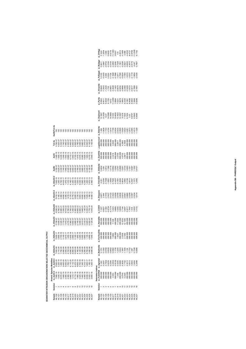
SEA
WA
TER
INTR
USI
ON
GR
OU
ND
WA
TER
S SE
LEC
TED
GEO
CH
EMIC
AL
OU
TPU
T
Arsenic
Species
Molalities
Sam
ple
Solu
tion
m_A
sO3-
3m
_AsO
4-3
m_H
2AsO
3-m
_H2A
sO4-
m_H
3AsO
3m
_H3A
sO4
m_H
AsO
3-2
m_H
AsO
4-2
As(
III)
As(
V)To
t As
As(
III)/Tot
As
ML1/2
61
1.59E-
192.
65E-20
1.93E-
093.
02E-
173.73E-
074.
63E-22
5.01E-
141.
00E-
163.75E-
071.30E-
163.75E-
0710
0ML1/27
21.
63E-
193.32E-
192.
11E-
093.
99E-
164.
60E-
076.79E-21
5.16E-
141.25E-
154.
62E-
071.
65E-
154.
62E-
0710
0ML1/2
83
8.87E-20
1.49E-
191.79E-
092.70E-
165.32E-
076.
08E-21
3.38E-
146.74E-
165.33E-
079.44E-
165.33E-
0710
0ML1/2
94
1.59E-
192.
65E-20
2.28E-
093.
14E-
177.71E-
077.22E-22
4.60E-
148.
91E-
177.74E-
071.20E-
167.74E-
0710
0ML1/3
05
2.08E-
195.
00E-20
2.45E-
094.
67E-
177.
97E-
079.
91E-22
5.30E-
141.47E-
167.
99E-
071.
94E-
167.
99E-
0710
0ML3/17
64.39E-
191.76E-
174.74E-
091.45E-
144.27E-
078.78E-20
1.61E-
137.41E-
144.32E-
078.
86E-
144.32E-
0710
0ML3/1
87
5.88E-
186.
11E-20
6.89E-
095.
50E-
185.38E-
072.78E-23
5.17E-
136.
16E-
175.45E-
076.71E-
175.45E-
0710
0ML3/1
98
1.41E-
176.
11E-
198.
98E-
092.
98E-
175.
85E-
071.25E-22
8.77E-
134.35E-
165.
94E-
074.
65E-
165.
94E-
0710
0ML3/2
09
6.71E-
186.47E-
196.
92E-
095.
16E-
174.
86E-
072.36E-22
5.62E-
136.22E-
164.
93E-
076.74E-
164.
93E-
0710
0ML3/2
110
1.98E-
189.
60E-
194.
16E-
091.
56E-
162.74E-
076.
85E-22
2.72E-
131.
52E-
152.78E-
071.
67E-
152.78E-
0710
0ML3/22
113.
52E-
184.70E-
185.
12E-
095.28E-
163.
00E-
072.
06E-21
3.94E-
136.
03E-
153.
05E-
076.
57E-
153.
05E-
0710
0ML3/23
127.46E-
187.34E-
187.32E-
095.
59E-
163.
61E-
071.
84E-21
6.80E-
137.
69E-
153.
68E-
078.26E-
153.
68E-
0710
0ML3/24
134.
58E-
184.31E-
175.28E-
093.
86E-
152.31E-
071.
14E-20
4.84E-
135.23E-
142.37E-
075.
62E-
142.37E-
0710
0ML3/2
514
9.63E-
181.
60E-
178.76E-
091.
13E-
155.
92E-
075.
03E-21
7.52E-
131.43E-
146.
00E-
071.
55E-
146.
00E-
0710
0ML3/2
615
2.02E-
171.
16E-
151.
09E-
084.
89E-
146.
02E-
071.77E-
191.
19E-
127.
87E-
136.
13E-
078.37E-
136.
13E-
0710
0ML3/27
163.
90E-
161.30E-
152.
69E-
087.
04E-
151.
12E-
061.
81E-20
6.40E-
122.46E-
131.
15E-
062.
54E-
131.
15E-
0610
0
Satu
ration Indices
Sam
ple
Solu
tion
si_F
e3(O
H)8
si_A
gmet
alsi
_Boe
hmite
si_F
errih
ydrit
esi
_Hem
atite
si_Cr2
O3
si_D
iaspor
esi
_FeCr2
O4
si_G
ibbs
itesi
_Goe
thite
i_Le
pido
croc
itsi
_Sid
erite
si_Orp
imen
tsi
_Pyr
itesi
_Viv
iani
tesi
_FeS
(ppt
)si
_Rea
lgar
si_C
H4(
g)ML1/2
61
-999
.999
0.14
612.
1791
-999
.999
-999
.999
1.10
073.
8971
-0.0
512.4834
-999
.999
-999
.999
-1.4
8415
.1807
9.2843
-2.8
845
0.31
030.
0811
3.1624
ML1/27
2-9
99.9
990.20
570.72
92-9
99.9
99-9
99.9
990.
8327
2.44
90.
0764
1.03
6-9
99.9
99-9
99.9
99-1
.063
813
.252
89.40
11-1
.2003
-0.0
025
-1.0
997
-1.3
504
ML1/2
83
-999
.999
-0.7
602
0.97
68-9
99.9
99-9
99.9
990.
1 464
2.70
18-0
.756
61.29
12-9
99.9
99-9
99.9
99-1
.1723
13.67
9.4939
-1.2
526
-0.0
66-0
.9754
-1.5
66ML1/2
94
-999
.999
0.6229
0.8028
-999
.999
-999
.999
-0.6754
2.5427
-1.6
851
1.13
89-9
99.9
99-9
99.9
99-1
.4194
14.638
89.
1783
-1.7
020.
0024
-0.3
164
0.6428
ML1/3
05
-999
.999
0.23
940.
6652
-999
.999
-999
.999
-0.7774
2.4122
-1.5
693
1.01
18-9
99.9
99-9
99.9
99-1
.0314
14.5
809
9.672
-0.9
851
0.1726
-0.5
154
-0.6
176
ML3/17
6-0
.953
-2.2
933
0.59
821.
5882
11.038
1.4323
2.3523
0.7928
0.95
944.33
183.
6549
-1.7
199
12.5
5511
.239
9-3
.464
8-0
.184
8-2
.4993
-11.
1365
ML3/1
87
-999
.999
-0.8
129
1.1735
-999
.999
-999
.999
1.69
852.
9258
-0.4
507
1.52
92-9
99.9
99-9
99.9
99-3
.0034
15.4
635
7.89
94-7
.1403
-0.7
896
0.3249
3.6327
ML3/1
98
-1.436
0.42
051.2245
1.83
0711
.5304
1.42
922.
9768
-0.146
11.
5797
4.57
593.
8917
-2.5433
13.1
823
7.5221
-5.8
579
-1.0
011
-0.732
81.
04ML3/2
09
-999
.999
0.99
691.
9324
-999
.999
-999
.999
1.60
693.
6838
0.49
082.28
69-9
99.9
99-9
99.9
99-2
.092
912
.3597
7.8678
-4.9254
-0.7
595
-1.1
951
-0.2
614
ML3/2
110
0.0745
0.3635
1.16
972.23
0912
.3233
1.7144
2.92
120.
8614
1.52
574.
9732
4.28
53-1
.9324
10.578
7.98
02-3
.966
6-0
.9224
-2.223
6-3
.166
9ML3/22
110.2325
1.71
521.
1546
2.13
9212
.140
61.
6097
2.90
611.
0983
1.51
044.
8817
4.1938
-1.6
523
7.1825
6.4446
-3.236
5-1
.7393
-3.5
621
-4.9
88ML3/23
12-9
99.9
992.30
131.
136
-999
.999
-999
.999
2.22
172.
8865
2.01
081.49
03-9
99.9
99-9
99.9
99-1
.426
16.74
046.
1891
-2.542
9-1
.6374
-3.6
033
-4.4332
ML3/24
13-9
99.9
991.
6013
0.77
52-9
99.9
99-9
99.9
991.7642
2.52
581.
8414
1.13
01-9
99.9
99-9
99.9
99-1
.2573
5.53
6.90
88-1
.8723
-1.6237
-4.5
615
-8.4737
ML3/2
514
-999
.999
1.9543
1.287
-999
.999
-999
.999
1.51
63.
0367
0.25
971.
6387
-999
.999
-999
.999
-2.2
065
8.87
976.48
52-5
.5017
-2.1
118
-2.9
179
-4.976
9ML3/2
615
-999
.999
1.54
040.7538
-999
.999
-999
.999
1.52
022.
5034
1.1572
1.10
52-9
99.9
99-9
99.9
99-1
.401
56.
5945
7.3846
-2.7
689
-1.9
854
-4.447
-11.2248
ML3/27
16-9
99.9
992.24
980.
0686
-999
.999
-999
.999
1.4133
1.8174
1.24
650.41
51-9
99.9
99-9
99.9
99-1
.132
86.40
845.
8298
-2.7
851
-2.033
5-3
.7857
-6.1
162
App
endi
x B8
- PH
REE
QC
Out
put
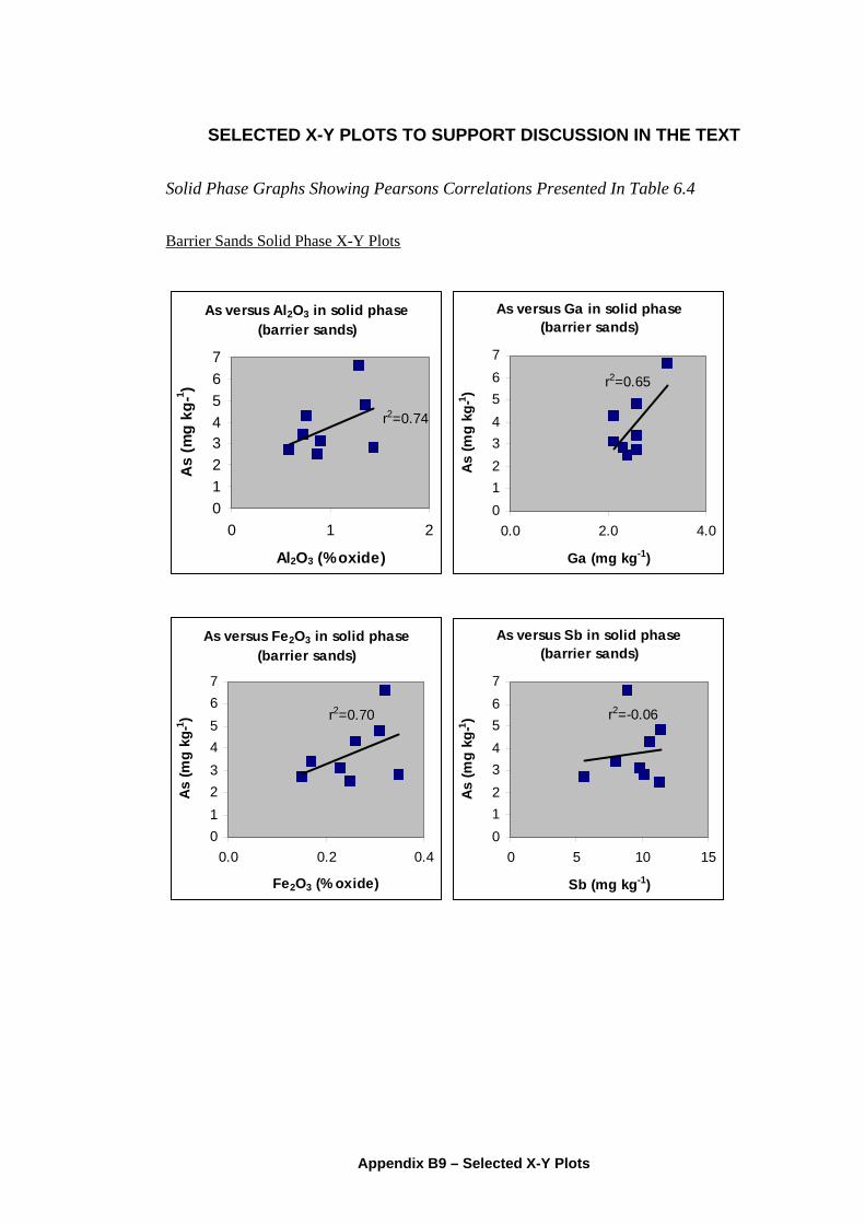
SELECTED X-Y PLOTS TO SUPPORT DISCUSSION IN THE TEXT
Solid Phase Graphs Showing Pearsons Correlations Presented In Table 6.4
Barrier Sands Solid Phase X-Y Plots
As versus Al2O3 in solid phase (barrier sands)
01234567
0 1 2
As versus Ga in solid phase (barrier sands)
01234567
0.0 2.0 4.0
Ga (mg kg-1)
As (m
g kg
-1 )
r2=0.65
Al2O3 (% oxide)
As
(mg
kg-1 )
r2=0.74
As versus Fe2O3 in solid phase (barrier sands)
01234567
0.0 0.2 0.4
Fe2O3 (% oxide)
As
(mg
kg-1 ) r2=0.70
As versus Sb in solid phase (barrier sands)
01234567
0 5 10 15
Sb (mg kg-1)
As (m
g kg
-1 ) r2=-0.06
Appendix B9 – Selected X-Y Plots
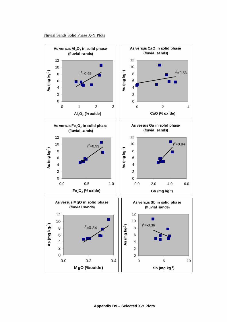
Fluvial Sands Solid Phase X-Y Plots
As versus Al2O3 in solid phase (fluvial sands)
0
2
4
6
8
10
12
0 1 2 3
Al2O3 (% oxide)
As
(mg
kg-1 )
As versus CaO in solid phase (fluvial sands)
0
2
4
6
8
10
12
0 2 4
CaO (% oxide)
As (m
g kg
-1 )
r2=0.53r2=0.65
As versus Fe2O3 in solid phase (fluvial sands)
0
2
4
6
8
10
12
0.0 0.5 1.0
Fe2O3 (% oxide)
As (m
g kg
-1 )
As versus Ga in solid phase (fluvial sands)
0
2
4
6
8
10
12
0.0 2.0 4.0 6.0
Ga (mg kg-1)
As (m
g kg
-1 )
r2=0.84r2=0.93
As versus MgO in solid phase (fluvial sands)
0
2
46
8
10
12
0.0 0.2 0.4
MgO (% oxide)
As
(mg
kg-1 )
As versus Sb in solid phase (fluvial sands)
0
2
4
6
8
10
12
0 5 10
Sb (mg kg-1)
As (m
g kg
-1 ) r2=-0.36r2=0.84
Appendix B9 – Selected X-Y Plots
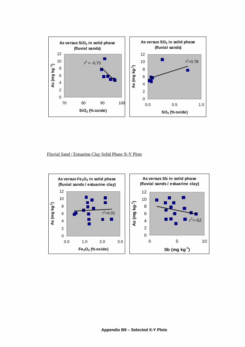
As versus SiO2 in solid phase (fluvial sands)
0
2
4
6
8
10
12
70 80 90 100
SiO2 (% oxide)
As
(mg
kg -1
) r2 = -0.73
As versus SO3 in solid phase (fluvial sands)
0
2
4
6
8
10
12
0.0 0.5 1.0
SO3 (% oxide)
As (m
g kg
-1 )
r2=0.78
Fluvial Sand / Estuarine Clay Solid Phase X-Y Plots
As versus Fe2O3 in solid phase (fluvial sands / estuarine clay)
0
2
4
6
8
10
12
0.0 1.0 2.0 3.0
Fe2O3 (% oxide)
As (m
g kg
-1 )
r2=0.01
As versus Sb in solid phase (fluvial sands / estuarine clay)
0
24
6
810
12
0 5
Sb (mg kg-1)
As
(mg
kg-1 )
10
r2=-52
Appendix B9 – Selected X-Y Plots
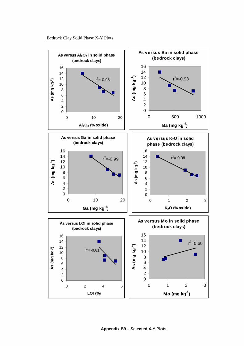
Bedrock Clay Solid Phase X-Y Plots
As versus Al2O3 in solid phase (bedrock clays)
02468
10121416
0 10 20
Al2O3 (% oxide)
As (m
g kg
-1 )As versus Ba in solid phase
(bedrock clays)
02468
10121416
0 500 1000
Ba (mg kg-1)
As
(mg
kg-1 )
r2=-0.93r2=-0.98
As versus Ga in solid phase (bedrock clays)
02468
10121416
0 10 20
Ga (mg kg-1)
As
(mg
kg-1 ) r2=-0.99
As versus K2O in solid phase (bedrock clays)
02468
10121416
0 1 2 3
K2O (% oxide)
As (m
g kg
-1 )
r2=-0.98
As versus LOI in solid phase (bedrock clays)
02468
10121416
0 2 4 6
LOI (%)
As (m
g kg
-1 )
As versus Mo in solid phase (bedrock clays)
02468
10121416
0 1 2 3
Mo (mg kg-1)
As
(mg
kg-1 ) r2=0.60
r2=-0.81
Appendix B9 – Selected X-Y Plots
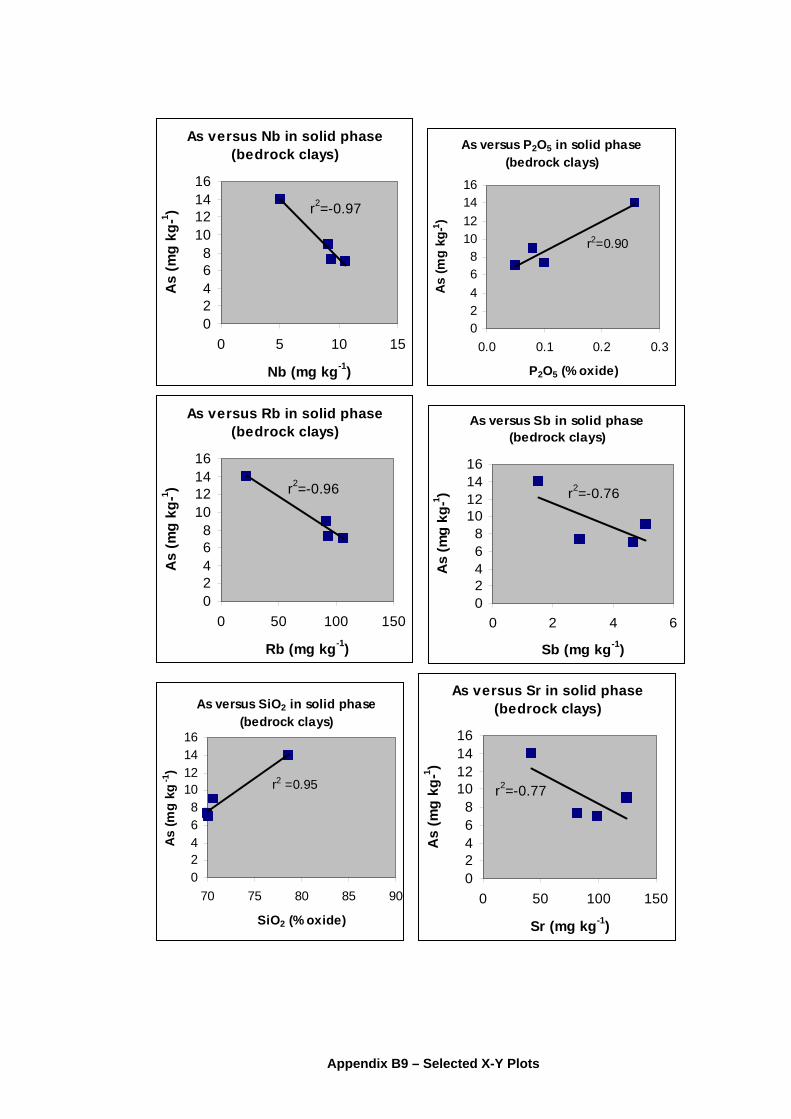
As versus Nb in solid phase (bedrock clays)
02468
10121416
0 5 10 15
Nb (mg kg-1)
As
(mg
kg-1 ) r2=-0.97
As versus P2O5 in solid phase (bedrock clays)
02468
10121416
0.0 0.1 0.2 0.3
P2O5 (% oxide)
As (m
g kg
-1 )
r2=0.90
As versus Rb in solid phase (bedrock clays)
02468
10121416
0 50 100 150
Rb (mg kg-1)
As
(mg
kg-1 ) r2=-0.96
As versus Sb in solid phase (bedrock clays)
02468
10121416
0 2 4
Sb (mg kg-1)
As
(mg
kg-1 )
6
r2=-0.76
As versus SiO2 in solid phase (bedrock clays)
02468
10121416
70 75 80 85 90
SiO2 (% oxide)
As (m
g kg
-1)
r2 =0.95
As versus Sr in solid phase (bedrock clays)
02468
10121416
0 50 100 150
Sr (mg kg-1)
As
(mg
kg-1 )
r2=-0.77
Appendix B9 – Selected X-Y Plots
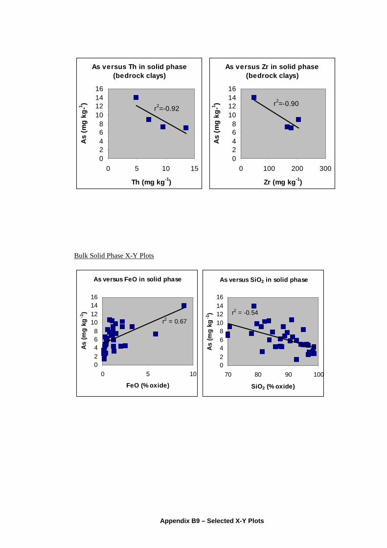
As versus Th in solid phase (bedrock clays)
02468
10121416
0 5 10 15
Th (mg kg-1)
As
(mg
kg-1 )
r2=-0.92
As versus Zr in solid phase (bedrock clays)
02468
10121416
0 100 200 300
Zr (mg kg-1)
As
(mg
kg-1 ) r2=-0.90
Bulk Solid Phase X-Y Plots
As versus FeO in solid phase
02468
10121416
0 5 10
As versus SiO2 in solid phase
02468
10121416
70 80 90 100
SiO2 (% oxide)
As (m
g kg
-1) r2 = -0.54
FeO (% oxide)
As (m
g kg
-1)
r2 = 0.67
Appendix B9 – Selected X-Y Plots

APPENDIX C
Photographs
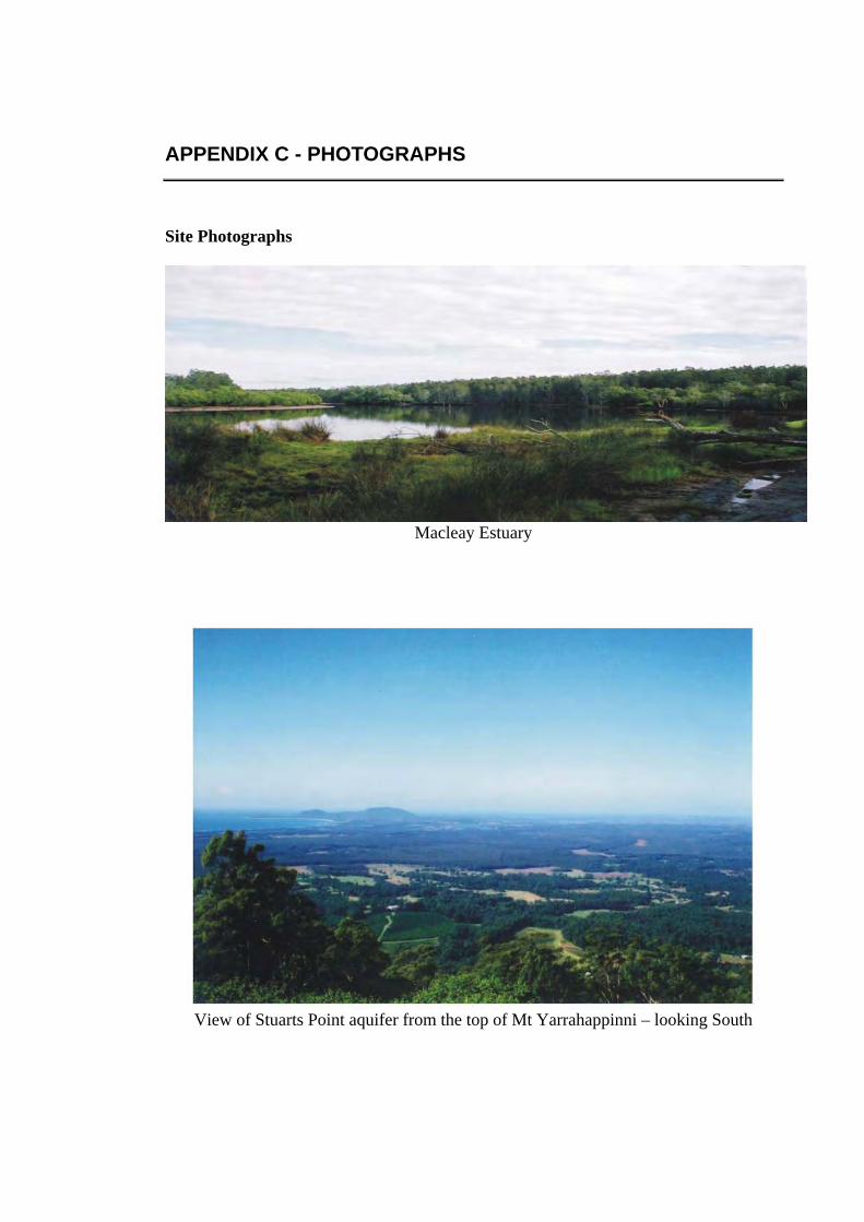
APPENDIX C - PHOTOGRAPHS
Site Photographs
Macleay Estuary
View of Stuarts Point aquifer from the top of Mt Yarrahappinni – looking South
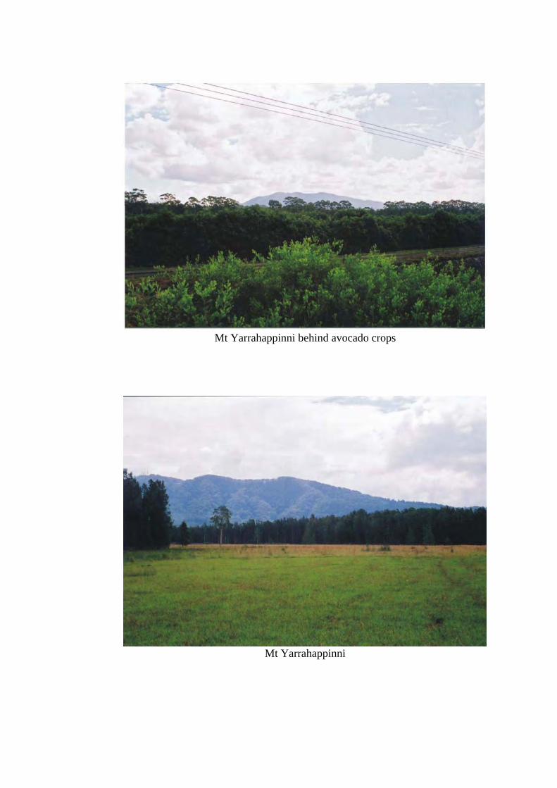
Mt Yarrahappinni behind avocado crops
Mt Yarrahappinni
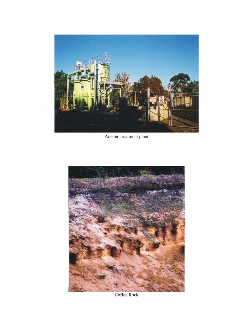
Arsenic treatment plant
Coffee Rock
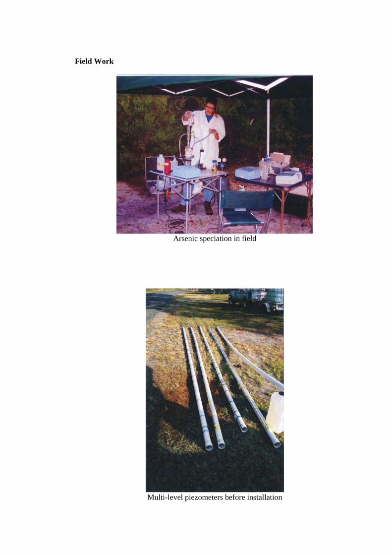
Field Work
Arsenic speciation in field
Multi-level piezometers before installation
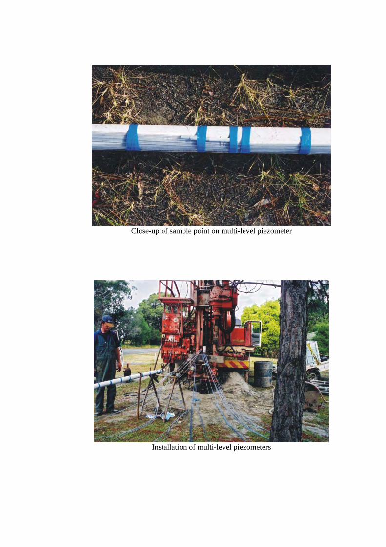
Close-up of sample point on multi-level piezometer
Installation of multi-level piezometers
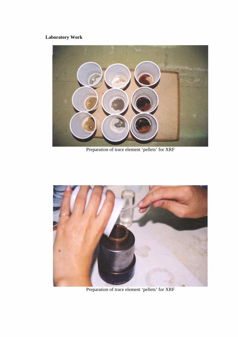
Laboratory Work
Preparation of trace element ‘pellets’ for XRF
Preparation of trace element ‘pellets’ for XRF
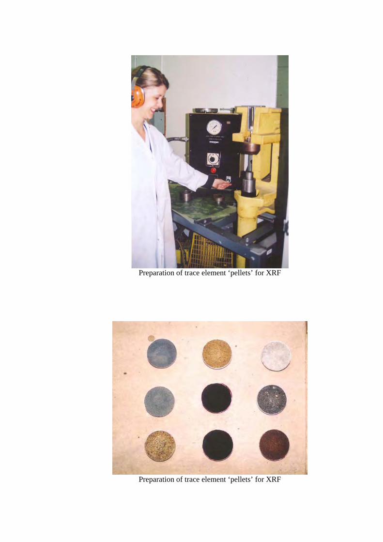
Preparation of trace element ‘pellets’ for XRF
Preparation of trace element ‘pellets’ for XRF
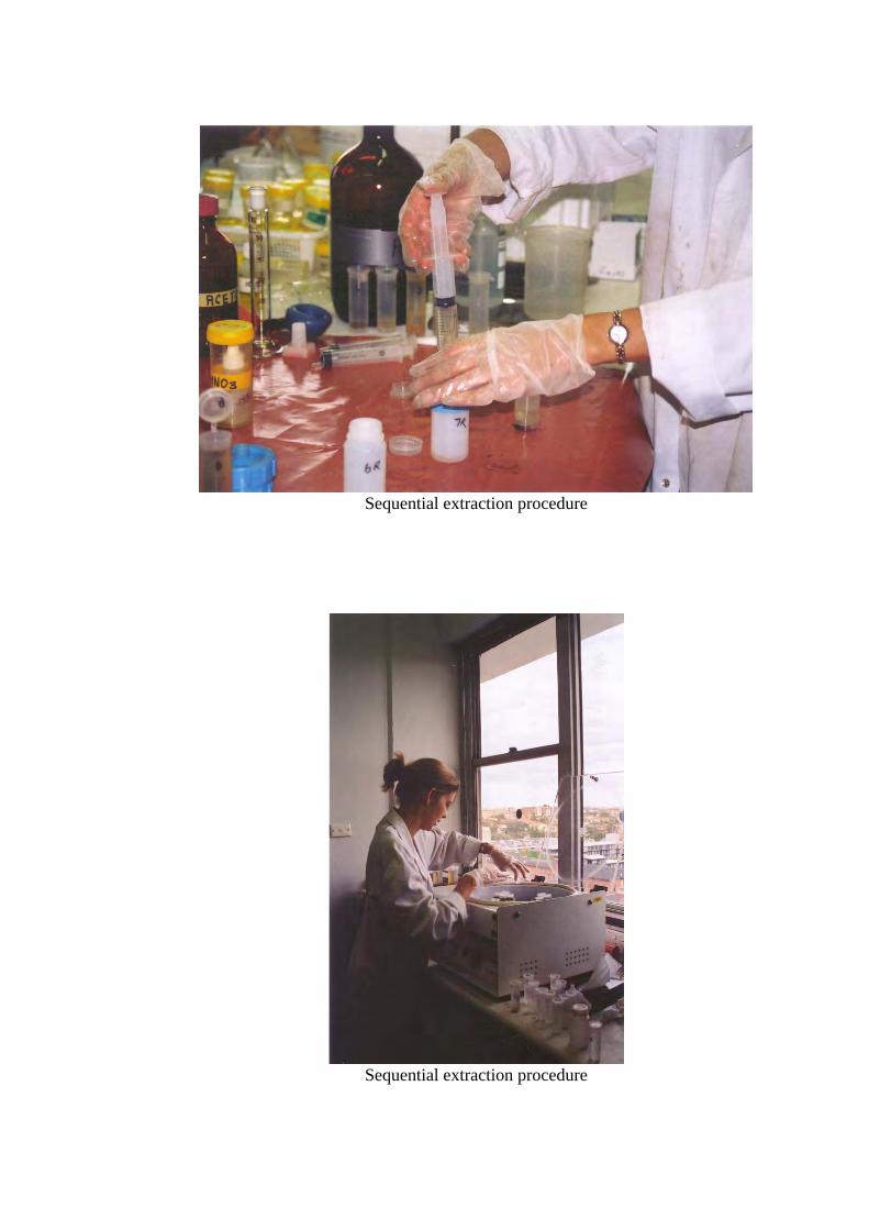
Sequential extraction procedure
Sequential extraction procedure
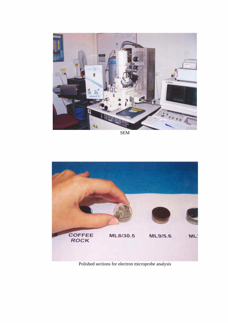
SEM
Polished sections for electron microprobe analysis
Related Documents