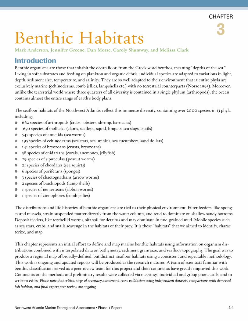
Northwest Atlantic Marine Ecoregional Assessment • Phase 1 Report 3-1 Introduction Benthic organisms are those that inhabit the ocean floor; from the Greek word benthos, meaning “depths of the sea.” Living in soft substrates and feeding on plankton and organic debris, individual species are adapted to variations in light, depth, sediment size, temperature, and salinity. They are so well adapted to their environment that 15 entire phyla are exclusively marine (echinoderms, comb jellies, lampshells etc.) with no terrestrial counterparts (Norse 1993). Moreover, unlike the terrestrial world where three quarters of all diversity is contained in a single phylum (arthropods), the ocean contains almost the entire range of earth’s body plans. The seafloor habitats of the Northwest Atlantic reflect this immense diversity, containing over 2000 species in 13 phyla including: • 662 species of arthropods (crabs, lobsters, shrimp, barnacles) • 650 species of mollusks (clams, scallops, squid, limpets, sea slugs, snails) • 547 species of annelids (sea worms) • 195 species of echinoderms (sea stars, sea urchins, sea cucumbers, sand dollars) • 141 species of bryozoans (crusts, bryozoans) • 58 species of cnidarians (corals, anemones, jellyfish) • 29 species of sipunculas (peanut worms) • 21 species of chordates (sea squirts) • 6 species of poriferans (sponges) • 3 species of chaetognathans (arrow worms) • 2 species of brachiopods (lamp shells) • 1 species of nemerteans (ribbon worms) • 1 species of ctenophores (comb jellies) The distributions and life histories of benthic organisms are tied to their physical environment. Filter feeders, like spong- es and mussels, strain suspended matter directly from the water column, and tend to dominate on shallow sandy bottoms. Deposit feeders, like terebellid worms, sift soil for detritus and may dominate in fine-grained mud. Mobile species such as sea stars, crabs, and snails scavenge in the habitats of their prey. It is these “habitats” that we aimed to identify, charac - terize, and map. This chapter represents an initial effort to define and map marine benthic habitats using information on organism dis- tributions combined with interpolated data on bathymetry, sediment grain size, and seafloor topography. The goal was to produce a regional map of broadly-defined, but distinct, seafloor habitats using a consistent and repeatable methodology. This work is ongoing and updated reports will be produced as the research matures. A team of scientists familiar with benthic classification served as a peer review team for this project and their comments have greatly improved this work. Comments on the methods and preliminary results were collected via meetings, individual and group phone calls, and in written edits. Please note that critical steps of accuracy assessment, cross-validation using independent datasets, comparisons with demersal fish habitat, and final expert peer review are ongoing Benthic Habitats Mark Anderson, Jennifer Greene, Dan Morse, Caroly Shumway, and Melissa Clark CHAPTER 3

Welcome message from author
This document is posted to help you gain knowledge. Please leave a comment to let me know what you think about it! Share it to your friends and learn new things together.
Transcript
Northwest Atlantic Marine Ecoregional Assessment • Phase 1 Report 3-1
IntroductionBenthic organisms are those that inhabit the ocean floor; from the Greek word benthos, meaning “depths of the sea.” Living in soft substrates and feeding on plankton and organic debris, individual species are adapted to variations in light, depth, sediment size, temperature, and salinity. They are so well adapted to their environment that 15 entire phyla are exclusively marine (echinoderms, comb jellies, lampshells etc.) with no terrestrial counterparts (Norse 1993). Moreover, unlike the terrestrial world where three quarters of all diversity is contained in a single phylum (arthropods), the ocean contains almost the entire range of earth’s body plans.
The seafloor habitats of the Northwest Atlantic reflect this immense diversity, containing over 2000 species in 13 phyla including:• 662 species of arthropods (crabs, lobsters, shrimp, barnacles)• 650 species of mollusks (clams, scallops, squid, limpets, sea slugs, snails)• 547 species of annelids (sea worms) • 195 species of echinoderms (sea stars, sea urchins, sea cucumbers, sand dollars)• 141 species of bryozoans (crusts, bryozoans)• 58 species of cnidarians (corals, anemones, jellyfish)• 29 species of sipunculas (peanut worms)• 21 species of chordates (sea squirts)• 6 species of poriferans (sponges) • 3 species of chaetognathans (arrow worms) • 2 species of brachiopods (lamp shells)• 1 species of nemerteans (ribbon worms)• 1 species of ctenophores (comb jellies) The distributions and life histories of benthic organisms are tied to their physical environment. Filter feeders, like spong-es and mussels, strain suspended matter directly from the water column, and tend to dominate on shallow sandy bottoms. Deposit feeders, like terebellid worms, sift soil for detritus and may dominate in fine-grained mud. Mobile species such as sea stars, crabs, and snails scavenge in the habitats of their prey. It is these “habitats” that we aimed to identify, charac-terize, and map.
This chapter represents an initial effort to define and map marine benthic habitats using information on organism dis-tributions combined with interpolated data on bathymetry, sediment grain size, and seafloor topography. The goal was to produce a regional map of broadly-defined, but distinct, seafloor habitats using a consistent and repeatable methodology. This work is ongoing and updated reports will be produced as the research matures. A team of scientists familiar with benthic classification served as a peer review team for this project and their comments have greatly improved this work. Comments on the methods and preliminary results were collected via meetings, individual and group phone calls, and in written edits. Please note that critical steps of accuracy assessment, cross-validation using independent datasets, comparisons with demersal fish habitat, and final expert peer review are ongoing
Benthic HabitatsMarkAnderson,JenniferGreene,DanMorse,CarolyShumway,andMelissaClark
CHAPTER
3

Northwest Atlantic Marine Ecoregional Assessment • Phase 1 Report 3-�
Chapter 3 - Benthic Habitats
Technical Teams MembersMark Anderson, Ph.D., The Nature Conservancy, Eastern DivisionMatthew Arsenault, United States Geological SurveyMelissa Clark, The Nature Conservancy, Eastern DivisionZach Ferdana, The Nature Conservancy, Global Marine InitiativeKathryn Ford, Ph.D., Massachusetts Division of Marine FisheriesJennifer Greene, The Nature Conservancy, Eastern DivisionRay Grizzle, Ph.D., University of New HampshireLes Kaufman, Ph.D., Boston UniversityCaroly Shumway, Ph.D., Boston UniversityPage Valentine, Ph.D., United States Geological Survey
Definition of Target HabitatsThe goal of this work was to identify all of the benthic habitat types in the Northwest Atlantic and map their ex-tent. We defined a benthic habitat as a group of organisms repeatedly found together within a specific environmental setting. For example, silt flats in shallow water typified by a specific suite of amphipods, clams, whelks and snails is one habitat, while steep canyons in deep water inhabited by hard corals is another. Conservation of these habitats is necessary to protect the full diversity of species that inhabit the seafloor, and to maintain the ecosystem func-tions of benthic communities.
MethodsTo design a conservation plan for benthic diversity in the Northwest Atlantic, it is essential to have some under-standing of the extent and location of various benthic hab-itats (e.g. a map). Fortunately, the challenge of mapping seafloor habitats has produced an extensive body of re-search (see Kostylev et al. 2001; Green et al. 2005; Auster 2006; World Wildlife Fund 2006; Todd and Greene 2008). In addition, comprehensive seafloor classification schemes have been proposed by many authors (see Dethier 1992; Brown 1993, European Environmental Agency 1999; Greene et al. 1999; Allee et al. 2000; Brown 2002; Conner et al 2004; Davies et al. 2004; Greene et al. 2005; Madden et al. 2009; Valentine et al. 2005; Kutcher 2006; and see reviews in National Estuarine Research Reserve System 2000 and Lund and Wilbur 2007).
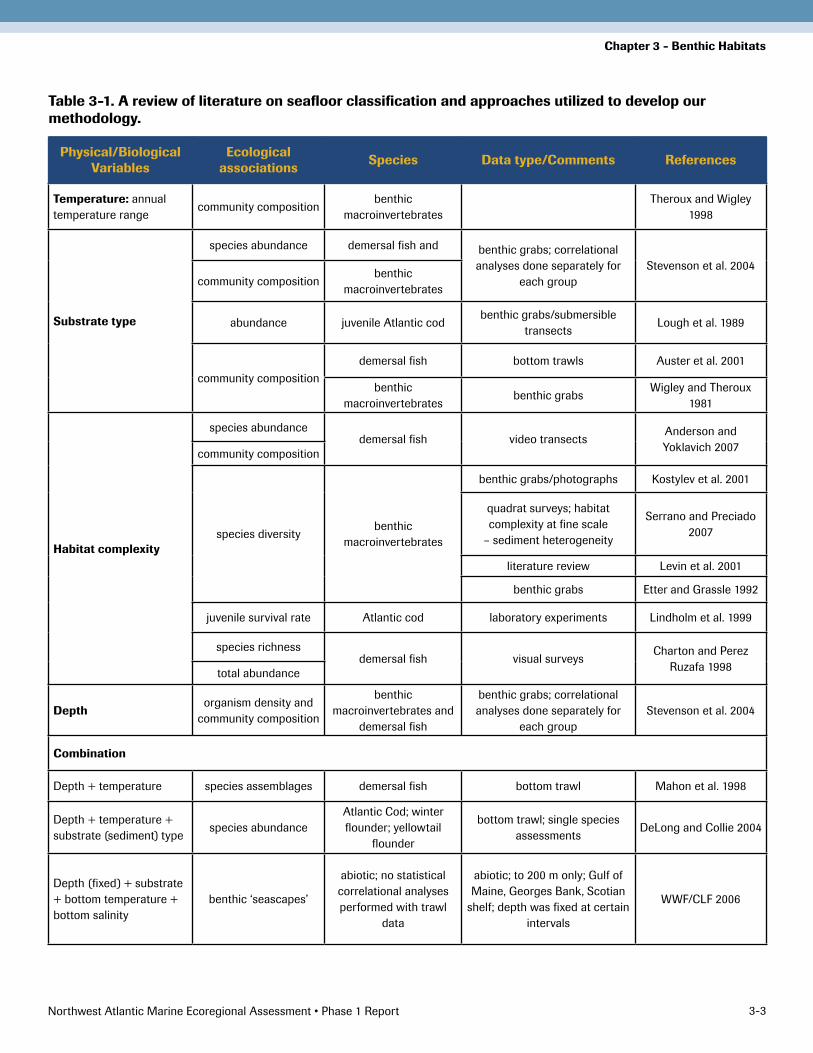
Initially, we reviewed the literature on seafloor classifi-cation, and examined the variety of approaches already utilized in order to develop our methodology (Table 3-1). Many of the existing schemes base their classifications on physical factors such as bathymetry, sediment grain size, sediment texture, salinity, bottom temperature, and topographic features. This is logical as there is ample evi-dence that benthic distribution patterns are associated with many of these variables. For example, temperature is correlated with the community composition of benthic macroinvertebrates (Theroux and Wigley 1998); substrate type is correlated with community composition and abun-dance of both the invertebrates and demersal fish (Auster et al. 2001; Stevenson et al. 2004); habitat complexity is correlated with species composition, diversity, and richness (Etter and Grassle 1992; Kostylev et al. 2001; Serrano and Preciado 2007, reviews in Levin et al. 2001); and depth is correlated with abundance, richness, and community com-position (Stevenson et al. 2004).
The approach presented here builds on existing schemes both explicitly and implicitly, and results can be readily compared to them. However, the goal of this assessment was to produce a map of broadly-defined benthic habitats in the Northwest Atlantic using readily available informa-tion. Therefore, a new classification system for benthic systems in general is not proposed here.
Northwest Atlantic Marine Ecoregional Assessment • Phase 1 Report 3-3
Chapter 3 - Benthic Habitats
Table 3-1. A review of literature on seafloor classification and approaches utilized to develop our methodology.
Physical/Biological Variables
Ecological associations Species Data type/Comments References
Temperature: annual temperature range
community compositionbenthic
macroinvertebratesTheroux and Wigley
1998
Substrate type
species abundance demersal fish and benthic grabs; correlational analyses done separately for
each groupStevenson et al. �004
community compositionbenthic
macroinvertebrates
abundance juvenile Atlantic codbenthic grabs/submersible
transectsLough et al. 1989
community compositiondemersal fish bottom trawls Auster et al. �001
benthic macroinvertebrates
benthic grabsWigley and Theroux
1981
Habitat complexity
species abundancedemersal fish video transects
Anderson and Yoklavich �007community composition
species diversitybenthic
macroinvertebrates
benthic grabs/photographs Kostylev et al. �001
quadrat surveys; habitat complexity at fine scale
– sediment heterogeneity
Serrano and Preciado �007
literature review Levin et al. �001
benthic grabs Etter and Grassle 199�
juvenile survival rate Atlantic cod laboratory experiments Lindholm et al. 1999
species richnessdemersal fish visual surveys
Charton and Perez Ruzafa 1998total abundance
Depthorganism density and
community composition
benthic macroinvertebrates and
demersal fish
benthic grabs; correlational analyses done separately for
each groupStevenson et al. �004
Combination
Depth + temperature species assemblages demersal fish bottom trawl Mahon et al. 1998
Depth + temperature + substrate (sediment) type
species abundanceAtlantic Cod; winter flounder; yellowtail
flounder
bottom trawl; single species assessments
DeLong and Collie �004
Depth (fixed) + substrate + bottom temperature + bottom salinity
benthic ‘seascapes’
abiotic; no statistical correlational analyses performed with trawl
data
abiotic; to �00 m only; Gulf of Maine, Georges Bank, Scotian
shelf; depth was fixed at certain intervals
WWF/CLF �006

Northwest Atlantic Marine Ecoregional Assessment • Phase 1 Report
Chapter 3 - Benthic Habitats
3-4
Biological Factors: Benthic Organisms The map of benthic habitats presented here is based on the distribution and abundance of benthic organisms in the Northwest Atlantic. The knowledge of these spe-cies and their distributions comes largely from seafloor grab samples described below. In the analysis of this data, groups of species with shared distribution patterns were identified, then thresholds in the physical factors were identified that correlated with those patterns. Specifically, three basic steps were followed: 1) quantitative analysis of the grab samples to identify distinct and reoccurring assemblages of benthic organisms, 2) recursive partition-ing to relate the species assemblages to physical factors (bathymetry, sediment types, and seabed topographic forms), and 3) mapping the habitats based on the statisti-cal relationships between the organism groups and the distribution of the physical factors. Although organism distributions were used to identify meaningful thresholds and cutoffs in the physical variables, the final habitat maps are composed solely of combinations of enduring physical factors and are thus closely related to the maps and clas-sification schemes proposed by others.
This study was made possible by access to over forty years of benthic sampling data by the National Marine Fisheries Service’s (NMFS) Northeast Fisheries Science Center (NEFSC). The NEFSC conducted a quantitative survey of macrobenthic invertebrate fauna from the mid 1950s to the early 1990s across the region (Figure 3-1, Table 3-2). Each year, samples of the seafloor were systematically tak-en during 25+ individual cruises by five or more research vessels using benthic grab samplers designed to collect 0.1 to 0.6m2 of benthic sediments. In total, over 22,000 sam-ples were collected. Organisms collected in each sample were sorted and identified to species, genus, or family, and information on the sediment sizes, depth, and other asso-ciated features were recorded for each sample. A thorough discussion of the sampling methodology, gear types, his-tory, and an analysis of the benthic dataset, including the distribution and ecology of the organisms, can be found in the publications of Wigley and Theroux (1981 and 1998). Recently, new video and remote sensing technologies have arisen to directly assess the seafloor and supplement the sample data (Kostylev et al. 2001). In future iterations of the assessment, we hope to integrate data collected using these new methods.
Table 3-1 (continued). A review of literature on seafloor classification and approaches utilized to develop our methodology.
Physical/Biological Variables
Ecological associations Species Data type/Comments References
Principal Component Analysis
PC1: SST, thermal gradients, stratification, chlorophyll
species abundance and richness
pelagic (nekton) and benthic
bottom trawl; research survey trawls; bongo nets (for nekton); principal components combine
physical and biological variables
Fogarty and Keith �007
PC�: depth, primary production, chlorophyll, zooplankton, biomass, benthic biomass
PC3: substrate type, nekton species richness
PC4: nekton biomass
PC5: benthic biomass
PC6: nekton species richnes

Northwest Atlantic Marine Ecoregional Assessment • Phase 1 Report 3-5
Chapter 3 - Benthic Habitats
Figure 3-1. Distribution of the 11,132 benthic grab samples.

Northwest Atlantic Marine Ecoregional Assessment • Phase 1 Report 3-6
Chapter 3 - Benthic Habitats
Figure 3-2. Geography of the region showing the three subregions.

Northwest Atlantic Marine Ecoregional Assessment • Phase 1 Report 3-7
Chapter 3 - Benthic Habitats
Classification Methods Classification analysis began with the entire 22,481 sea-floor samples taken between 1881 and 1992. However, only about half of the samples contained information on the full composition or the sample identified to species, and it is that subset of 11,132 samples that is used in this analysis. Initially, two separate classifications were created - one based on genera and one based on species as a way of including more samples in the analysis. However, because the species level classification showed a stronger relation-ship with the physical factors, this level of taxonomy was used. Organisms in the samples that were identified only to family or order were omitted from the dataset, as were fish, plants, egg masses, and organic debris.
Separate classifications were created for each of the three subregions: the Gulf of Maine, Southern New England, and the Mid-Atlantic Bight (Figure 3-2). For each, samples with similar species composition and abundance were grouped together using hierarchical cluster analysis (PCORD, McCune and Grace 2002). This technique starts with pairwise contrasts of every sample combination then aggregates the pairs most similar in species composi-tion into a cluster. Next, it repeats the pairwise contrasts, treating the clusters as if they were single samples, and joins the next most similar sample to the existing clusters. The process is repeated until all samples are assigned to one of the many clusters. For our analysis, the Sorenson
similarity index and the flexible beta linkage technique with Beta set at 25 was used as the basis for measuring similarity (McCune and Grace 2002). After grouping the samples, indicator species analysis was used to iden-tify those species that were faithful and exclusive to each organism group (Dufrene and Legrande 1997). Lastly, Monte Carlo tests of significance were run for each spe-cies relative to the organism groups to identify diagnostic species for each group using the criterion of a p-value less than or equal to 0.10 (90% probability). The number of sets of clusters (testing 10 to 40) was determined by see-ing which amount gave the lowest average p-value. The test concluded that 20-22 organism groups for each subre-gion yielded the lowest p-value.
Physical Factors: Bathymetry, Substrate and Seabed Forms To understand how the benthic invertebrate community distributions related to the distribution of physical fac-tors, a spatially comprehensive data layer for each factor of interest was developed. Four aspects of seafloor structure were used: bathymetry, sediment grain size, topographic forms, and habitat complexity. These factors were cho-sen as they are both correlated with the distribution and abundance of benthic organisms (Table 3-1) and are rela-tively stable over time and space. Variables that fluctuate markedly over time were purposely avoided, such as temperature and salinity. Data on each physical factor
Table 3-2. Distribution of the benthic grab samples by decade and subregion.
Decade Gulf of Maine Southern New England Mid-Atlantic Outside of
region Grand Total
Pre-1950 38 33 � 1 74
1950s �,150 660 61 164 3,035
1960s 4,146 �,693 857 669 8,365
1970s 188 3,770 1,166 4 5,1�8
1980s 637 3,681 1,535 1 5,854
1990s �5 �5
Total 7,159 10,837 3,646 839 ��,481
Northwest Atlantic Marine Ecoregional Assessment • Phase 1 Report 3-8
Chapter 3 - Benthic Habitats
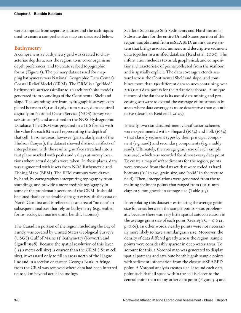
were compiled from separate sources and the techniques used to create a comprehensive map are discussed below.
Bathymetry A comprehensive bathymetry grid was created to char-acterize depths across the region, to uncover organisms’ depth preferences, and to create seabed topographic forms (Figure 3). The primary dataset used for map-ping bathymetry was National Geographic Data Center’s Coastal Relief Model (CRM). The CRM is a “gridded” bathymetric surface (similar to an architect’s site model) generated from soundings of the Continental Shelf and slope. The soundings are from hydrographic surveys com-pleted between 1851 and 1965, from survey data acquired digitally on National Ocean Service (NOS) survey ves-sels since 1965, and are stored in the NOS Hydrographic Database.
The CRM was prepared in a GIS format with
the value for each 82m cell representing the depth of that cell. In some areas, however (particularly east of the Hudson Canyon), the dataset showed distinct artifacts of interpolation, with the resulting surface stretched into a taut plane marked with peaks and valleys at survey loca-tions where actual depths were taken. In these places, data was augmented with insets from NOS Bathymetric and Fishing Maps (BFM). The BFM contours were drawn by hand, by cartographers interpreting topography from soundings, and provide a more credible topography in some of the problematic sections of the CRM. It should be noted that a considerable data gap exists off the coast of North Carolina and is reflected as an area of “no data” in subsequent analyses that rely on bathymetry (e.g., seabed forms, ecological marine units, benthic habitats).
The Canadian portion of the region, including the Bay of Fundy, was covered by United States Geological Survey’s (USGS) Gulf of Maine 15’ Bathymetry (Roworth and Signell 1998). Because the spatial resolution of this layer (~350 meter cell size) is coarser than the CRM (~82 m cell size), it was used only to fill in areas north of the Hague line and in a section of eastern Georges Bank. A fringe from the CRM was removed where data had been inferred up to 9 km beyond actual soundings.
Seafloor Substrates: Soft Sediments and Hard BottomsSubstrate data for the entire United States portion of the region was obtained from usSEABED, an innovative sys-tem that brings assorted numeric and descriptive sediment data together in a unified database (Reid et al. 2005). The information includes textural, geophysical, and composi-tional characteristic of points collected from the seafloor, and is spatially explicit. The data coverage extends sea-ward across the Continental Shelf and slope, and com-bines more than 150 different data sources containing over 200,000 data points for the Atlantic seaboard. A unique feature of the database is its use of data mining and pro-cessing software to extend the coverage of information in areas where data coverage is more descriptive than quanti-tative (details in Reid et al. 2005).
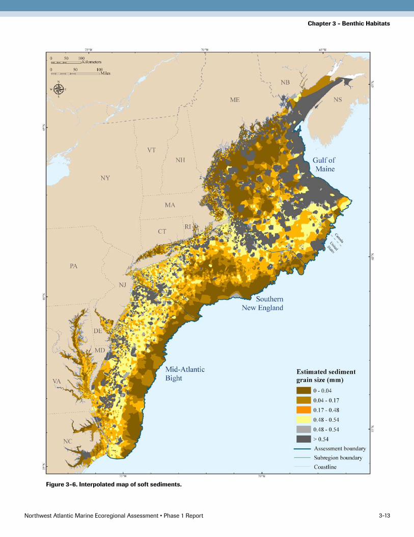
Initially, two standard sediment classification schemes were experimented with - Shepard (1954) and Folk (1954) - that classify sediment types by their principal compo-nent (e.g. sand) and secondary components (e.g. muddy sand). Ultimately, the average grain size of each sample was used, which was recorded for almost every data point. To create a map of soft sediments for the region, points were removed from the dataset that were coded as hard bottoms (“0” in ave. grain size, and “solid” in the texture field). Then, interpolations were generated from the re-maining sediment points that ranged from 0.001 mm clays to 9 mm gravels in average size (Table 3-3).
Interpolating this dataset - estimating the average grain size for areas between the sample points - was problem-atic because there was very little spatial autocorrelation in the average grain size of each point (Gearey’s C = 0.034, p<0.01). In other words, nearby points were not necessar-ily more likely to have a similar grain size. Moreover, the density of data differed greatly across the region: sample points were considerably sparser in deep water areas. To account for this, a Voronoi map was generated to display spatial patterns and attribute benthic grab sample points with sediment information from the closest usSEABED point. A Voronoi analysis creates a cell around each data point such that all space within the cell is closer to the central point than to any other data point (Figure 3-4 and
Northwest Atlantic Marine Ecoregional Assessment • Phase 1 Report 3-9
Chapter 3 - Benthic Habitats
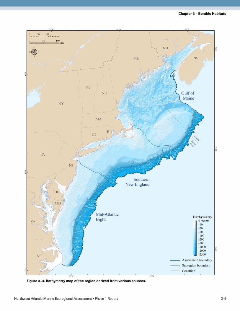
Figure 3-3. Bathymetry map of the region derived from various sources.

Northwest Atlantic Marine Ecoregional Assessment • Phase 1 Report 3-10
Chapter 3 - Benthic Habitats
3-5). Next, the explanatory power of the closest sediment point in differentiating among the organism groups was tested using the partitioning methods described below. This allowed comparison of the various interpolation techniques by contrasting the results with the results of the closest point attributes and measuring the improve-ment, or lack of improvement, in explanatory power. In addition, the correlation between each interpolation method and the raw Voronoi output was determined, as-suming that results that were highly uncorrelated with the Voronoi map were probably distorting the data.
After considerable experimentation, the following inter-polation parameters were used: ordinary kriging, spherical semivariogram, variable search radius type using three points with no maximum distance, and output cell size of 500 meters. This method had the strongest correlation with the Voronoi map, and had the highest explanatory power for differentiating the organism groups. Moreover, kriging provides consistent results across areas that have been sparsely and densely sampled. Visually, the krig-ing interpolation resembled the Voronoi map, but with smoother surfaces and more realistic looking shapes (Figure 3-6).
A separate dataset of hard bottom locations was created from the points coded as “solid” in the usSeabed dataset. The dataset was supplemented by adding points coded as “solid” from the NMFS bottom trawl survey (see Chapter 5 for description of this database). Thus, the final sediment map consisted of the interpolated soft sediment points overlaid with the hard bottom locations (Figure 3-7).
Soft sediment diversity was mapped at a 10 km scale by superimposing a 10 km unit around each map cell and cal-culating the number of grain size classes within the unit’s area. Each cell was scored with the results creating a visu-ally seamless surface (Figure 3-8). Ideally, mapping sedi-ment diversity helps identify ecotonal benthic areas, the tran-sition area between two different habitats, where which demersal fish are known to favor (Kaufman, personal communication). However, these results were sensitive to the huge variations in data density across the region and were not used in the predictive models.
Seabed Topographic Forms This region is characterized by a complexity of banks, ba-sins, ledges, shoals, trenches, and channels in the north, shoals and deltas to the south, and deep canyons along the
Table 3-3. Grain size and sediment class names (Wentworth 1922).
Grain Size (mm) Class Grain Size (mm) Class
0 0.001 Fine clay 0.�5 0.5 Medium sand
0.001 0.00� Medium clay 0.5 1 Coarse sand
0.00� 0.004 Coarse clay 1 � Very coarse sand
0.004 0.008 Very fine silt � 4 Very fine pebbles (granules)
0.008 0.016 Fine silt 4 8 Fine pebbles
0.016 0.031 Medium silt 8 16 Medium pebbles
0.031 0.063 Coarse silt 16 3� Coarse pebbles
0.063 0.1�5 Very fine sand 3� 86 Very coarse pebbles to cobbles
0.1�5 0.�5 Fine sand

Northwest Atlantic Marine Ecoregional Assessment • Phase 1 Report 3-11
Chapter 3 - Benthic Habitats
Figure 3-4. Voronoi map of the usSEABED database, showing the distance between samples.

Northwest Atlantic Marine Ecoregional Assessment • Phase 1 Report 3-1�
Chapter 3 - Benthic Habitats
Figure 3-5. Voronoi map of the usSEABED database, showing sediment grain size.
Northwest Atlantic Marine Ecoregional Assessment • Phase 1 Report 3-13
Chapter 3 - Benthic Habitats
Figure 3-6. Interpolated map of soft sediments.

Northwest Atlantic Marine Ecoregional Assessment • Phase 1 Report 3-14
Chapter 3 - Benthic Habitats
Figure 3-7. Hard bottom points overlaid on the soft sediment interpolation.

Northwest Atlantic Marine Ecoregional Assessment • Phase 1 Report 3-15
Chapter 3 - Benthic Habitats
Figure 3-8. Map of sediment diversity using a 10 k focal window.

Northwest Atlantic Marine Ecoregional Assessment • Phase 1 Report 3-16
Chapter 3 - Benthic Habitats
Continental Shelf (Figure 3-2). These features have a large influence on oceanic processes, and on the distribution of benthic habitats. With this in mind, the seabed form data layer was developed to characterize seafloor topography in a systematic and categorical way, relevant to the scale of benthic habitats. The units that emerge from this analysis, from high flats to depressions, represent depositional and erosional environments that typically differ in fluvial pro-cesses, sediments, and organism composition (Wigley and Theroux 1981).
Seabed topographic forms were created from relative posi-tion and degree of slope of each seafloor cell. Seabed posi-tion (or topographic position) describes the topography of the area surrounding a particular 82 m cell. Calculations were based on the methods of Fels and Zobel (1995) that evaluate the elevation differences between any cell and the surrounding cells within a specified distance. For example, if the model cell is, on average, higher than the surround-ing cells, then it is considered to be closer to the ridge top (a more positive seabed position value). Conversely, if the model cell is, on average, lower than the surrounding cells then it is considered closer to the slope bottom (a more negative seabed position value). The relative position value is the mean of the distance-weighted elevation differences between a given point and all other model points within a specified search radius. The search radius was set at 100 cells after examining the effects of various radii. Position was grouped into six classes that were later simplified to three classes:
1) Very low Low 2) Low Low 3) Lower mid Mid 4) Upper mid Mid 5) High High 6) Very high High
The following diagrams illustrate the seabed position index values along slopes:
The second element of the seabed forms, degree of slope, was used to differentiate between steep canyons and flat depressions. Slope was calculated as the difference in el-evation between two neighboring raster cells, expressed in degrees. After examining the distribution of slopes across the region, slopes were grouped according to the following thresholds:
1) 0° - 0.015° Level flat 2) 0.015° - 0.05° Flat 3) 0.05° - 0.8° Gentle slope 4) 0.8° - 8.0° Slope 6) >8.0° Steep slope (includes canyons)
The cutoffs might be misleading if interpreted too lit-erally, For example, there are very few locations on the Continental Shelf with slopes in the category >8° and most of these correspond to canyon walls reported as 35-45° slope by divers. The discrepancies are due to the cell size (82 m) of the analysis unit that averages slope over a larger area.
Ridge: seabed position = positive value
Sideslope: seabed position = 0
Slope Bottom: seabed position = negative value
Flat: seabed position = 0

Northwest Atlantic Marine Ecoregional Assessment • Phase 1 Report 3-17
Chapter 3 - Benthic Habitats
Slope and relative position were combined to create 30 possible seabed forms ranging from high flat banks to low level bottoms to steep canyons. Initially, all 30 types were used in the analysis of organism relationships, but results suggested that they could be simplified while maintain-ing, or improving, their explanatory power. Therefore, the analysis was simplified into the following six categories: 1) depression, 2) mid flat, 3) high flat, 4) low slope, 5) high slope,6) sideslope, and 7) steep (Table 3-4).
Small errors in the bathymetry grid were bypassed by identifying very small-scale variations in depth. Generalization tools were used to clean up small scale variations in the dataset. This eliminated thousands of “dimples” present in the CRM bathymetry without having to edit the original grid.
Each individual cell was assigned to a unique seabed form and often groups of forms cluster to define a larger scale topographic unit such as Jeffreys Ledge or Georges Bank (Figure 3-9). Depressions and mid position flats repre-sent the broad plains common in Southern New England, steep areas identify the canyons of the continental slope, and highest position sideslopes occur on the cusp of the shelf-slope break.
Habitat Complexity: Standard Deviation of the SlopeIn addition to the categorical analysis of topography for the seabed forms, habitat complexity was assessed using the standard deviation of slope. Using the bathymetry grid, “floating window” analyses of the standard deviation of the slope were conducted within a 500 m, 1 km, and 10 km search radii. To calculate the standard deviation of the slope, the slope for each cell was calculated using the GIS slope command (3 x 3 cell neighborhood). Next, the range was divided into ten equal interval classes and the mean and standard deviation of the cells within each search ra-dius were calculated (Figure 3-10). The search radius mat-ters because the importance of any given spatial feature depends on its size relative to the species of interest. The 1 km analysis had the greatest explanatory power for differ-entiating between the benthic organism groups. Linking the Organisms to Physical Factors Recursive partitioning (JMP software package) was used to uncover relationships between benthic communities and the physical environment. Recursive partitioning is a statistical method that creates decision trees to clas-sify members of a common population (the classification types) based on a set of dependent variables (the physical
Table 3-4. Seabed forms showing position and slope combinations. For example, code 11 = Very low + Level flat = Low flat.
Slope
Level flat Flat Gentle slope Slope Steep slope
Pos
itio
n
Very low depression depression low slope low slope steep
Low depression depression low slope low slope steep
Lower mid mid flat mid flat sideslope sideslope steep
Upper mid mid flat mid flat sideslope sideslope steep
High high flat high flat high slope high slope steep
Very high high flat high flat high slope high slope steep

Northwest Atlantic Marine Ecoregional Assessment • Phase 1 Report 3-18
Chapter 3 - Benthic Habitats
Figure 3-9. Map of the seabed topographic forms.

Northwest Atlantic Marine Ecoregional Assessment • Phase 1 Report 3-19
Chapter 3 - Benthic Habitats
Figure 3-10. Map of standard deviation of slope using a 1 k focal window.

Northwest Atlantic Marine Ecoregional Assessment • Phase 1 Report 3-�0
Chapter 3 - Benthic Habitats
variables). The analysis required each benthic grab sample to be attributed with the benthic community type that it belonged to, overlaid on the standardized base maps, and attributed with the information on depth, sediment grain size and seabed form appropriate to the point (Table 3-5).
Regression trees were first built using all variables col-lectively to identify the variables driving organism dif-ferences. Each analysis was run separately by subregion because initial data exploration revealed that the relation-ships between the species and the physical factors differed markedly among subregions.
After examining the variable contributions collectively, individual regression trees were built for depth, grain size, and seabed forms to identify critical thresholds that separated sets of organism groups from each other (see Appendix 3-1). In recursive partitioning, these cuts are identified by exhaustively searching all possible cuts and choosing the one that best separates the dataset into non-overlapping subsets. For example, the first run of the organism groups on the bathymetry data separated the deep water samples from the shallow water samples while identifying the exact depth that most cleanly separated the two sets.
Statistical significance was determined for each variable in each organism group using chi-squared tests. This method compares the observed distribution of each benthic or-ganism group across each physical variable against the distribution expected from a random pattern. A variable
and threshold was considered to be significant if it had a p-value less that 0.01 (less than a 99% probability that this pattern could have occurred by chance -Appendix 3-1).
Results Based on the bathymetry dataset, the region varied in depth from 0 m at the coast to -2400 m along the shelf boundary, reaching a maximum of -2740 m at the deepest part. Critical depth thresholds for benthic organisms and habitats differed among the three subregions and are dis-cussed under the organism classification. The three subre-gions also differed in physical structure, with the Gulf of Maine being made up of a moderately deep basin (-150 to -300 m), a distinctive shallower bank (-35 to -80 m), and a small portion of the deep slope. In contrast, the Mid-Atlantic Bight has extensive shallow water shoals (0 to -35 m), an extensive moderate depth plain (-35 to -80 m), and a large proportion of steeply sloping deep habitat along the Continental Shelf. The Southern New England region is similar in most ways to the Mid-Atlantic Bight.
The sediment maps show a seafloor dominated by coarse to fine sand with large pockets of silt in the Southern New England region, deep regions in the Gulf of Maine and along the Continental Slope. Large pockets of gravels are concentrated on the tip of Georges Bank, the eastern edge of Nantucket Shoals, around the Hudson Canyon, and in various other deep and shallow patches. Hard bottom points are concentrated near the Maine shoreline and offshore are loosely correlated with the gravel areas (Figure 3-7).
Table 3-5. Example of information for sample point #22254, a grab sample from the Mid-Atlantic Bight subregion classified in organism group 505. We calculated these metrics for each of the 11,132 grab sample points.
Sample IDOrganism
GroupSubregion Bathymetry (m)
Sediment Grain Size
(mm)Position Slope
Seabed Form
STD_Slope_1K
���54 505 Mid-Atlantic Bight -996.6� 0.143 Low Steep Canyon 0.8

Northwest Atlantic Marine Ecoregional Assessment • Phase 1 Report 3-�1
Chapter 3 - Benthic Habitats
Organism ClassificationFor each subregion, we provide a summary of the char-acteristic species and their indicator values (Appendix 3-2). This table gives diagnostic species for each organism group and shows its distribution across all the organisms groups. The mean indicator value and the probability of this distribution being random chance is calculated for each species in the group that it is most closely associated with. Most species don’t have a common name; Gosner (1979), Weiss (1995) and Pollock (1998) were used to add them where available. Often, these are common names for the family or genus, not the species. Relationship of the organism groups to the physical factorsAcross all subregions, depth was the most important explanatory variable, followed by grain size, and then seabed forms. Seabed forms were less important in the Mid-Atlantic Bight than the other regions. Standard de-viation of depth was somewhat important in Southern New England, but not in the other regions. Basic relation-ships between each organism group and its characteristic physical setting are described below. Charts giving the distribution of the organism groups across each physical factor class, a chi-squared test for significance, and the class where this group is most likely to be found are given in Appendix 3-1. Tables of key physical factor values that correspond to ecological thresholds separating the distri-bution of one benthic habitat from another are provided in the subregion results (Table 3-6, 3-7, 3-8).
Benthic Habitat Types and Ecological Marine Units The benthic habitat types identified for each subregion are presented in the following section of this document. Because the final results are a product of several steps, e.g. the macrofauna classification; the identification of relationships between the organism groups and the factors of depth, grain size and topography; and the mapping of benthic environments, the results and details on each step are provided separately in the appendices.
Two separate, but closely related final maps were created. The Ecological Marine Units (EMU) represent all three-way combinations of depth, sediment grain size, and sea-bed forms based on the ecological thresholds revealed by the benthic-organism relationships (Figure 3-11, 3-12, 3-13, 3-14). Benthic Habitats are EMUs clustered into groups that contain the same species assemblage (Figure 3-15). The two terms are not synonymous, but they are based on the same information, and thus, represent two perspec-tives on the seafloor. Essentially, the EMU maps show the full diversity of physical factor combinations, regardless of whether a specific habitat type was identified for the com-bination. The benthic habitat map shows only the combi-nations of factors, or groups of combinations, for which a benthic organism group was identified. It should be noted that the numbers of the EMUs and benthic habitats were derived from the statistical relationships and is completely arbitrary.
The Benthic Habitat map is simpler because a single organism group typically occurs across several EMUs, although in some instances a single EMU is synonymous with a single organism group. For example, in the Mid-Atlantic Bight, EMU 1101 (silty depression centers in water less than 15 m) is synonymous with organism group 768, a community identified by a specific set of amphi-pods, brittle stars, clams, whelks, and snails. More typical are organism groups that occur across several closely relat-ed EMUs such as Southern New England organism group 25. It ranges across both high position and mid position flats, very shallow to shallow water ranging in depth from 0-23 m, and medium to coarse sand. This community of shimmyworms, glass shrimp, hermit crabs, and surf clams is thus found across a small range of EMUs, and the habi-tat is mapped as the set of EMUs that define it.

Northwest Atlantic Marine Ecoregional Assessment • Phase 1 Report 3-��
Chapter 3 - Benthic Habitats
Figure 3-11. Ecological Marine Units of the Northwest Atlantic region. Scale 1:7,250.000

Northwest Atlantic Marine Ecoregional Assessment • Phase 1 Report 3-�3
Chapter 3 - Benthic Habitats
Figure 3-12. Gulf of Maine Ecological Marine Units. Scale 1:2,900,00

Northwest Atlantic Marine Ecoregional Assessment • Phase 1 Report 3-�4
Chapter 3 - Benthic Habitats
Figure 3-13. Southern New England Ecological Marine Units. Scale 1:2,600,000

Northwest Atlantic Marine Ecoregional Assessment • Phase 1 Report 3-�5
Chapter 3 - Benthic Habitats
Figure 3-14. Mid-Atlantic Bight Ecological Marine Units. Scale 1:3,210,600

Northwest Atlantic Marine Ecoregional Assessment • Phase 1 Report 3-�6
Chapter 3 - Benthic Habitats
Figure 3-15. Benthic habitats of the Northwest Atlantic region.

Northwest Atlantic Marine Ecoregional Assessment • Phase 1 Report 3-�7
Chapter 3 - Benthic Habitats
Figure 3-15. Benthic Habitats Legend
UnitStates
65∞W
70∞W
70∞W
75∞W
75∞W
45∞N
40∞N
35∞N
GOM_9/133/183/1451
GOM_*4
GOM_1
GOM_1028
GOM_1078
GOM_12
GOM_1451
GOM_18
GOM_183
GOM_2
GOM_2367
GOM_24
GOM_24/1028
GOM_247
GOM_5
GOM_557
GOM_7
GOM_72
GOM_72/8/87
GOM_8
GOM_9
GOM_91
MAB_0
MAB_1
MAB_1223
MAB_2
MAB_216
MAB_218
MAB_219
MAB_229
MAB_25
MAB_301
MAB_306
MAB_32
MAB_38
MAB_384
MAB_395
MAB_4
MAB_44
MAB_505
MAB_520
MAB_592
MAB_64
MAB_7
MAB_768
MAB_84
MAB_87
SNE _0
SNE _1
SNE _109
SNE _11
SNE _113
SNE _200
SNE _223
SNE _230/229
SNE _24
SNE _25
SNE _2537
SNE _3
SNE _316
SNE _317
SNE _36
SNE _372
SNE _381
SNE _387
SNE _390
SNE _437
SNE _6
SNE _66
SNE _82
SNE _873
SNE _949

Northwest Atlantic Marine Ecoregional Assessment • Phase 1 Report 3-�8
Chapter 3 - Benthic Habitats
Description of Benthic HabitatsNote: This section is arranged by subregion and benthic habitats are displayed from shallow to deep water habitats based on the average depth of each benthic habitat.
Gulf of Maine
Figure 3-16. Average depth and range of each benthic habitat type in the Gulf of Maine subregion. Lines represent two standard deviations above and below the mean. Habitat types with the same depths often differ from each other by sediment grain size or topographic location. Habitats with very large depth ranges are widespread associations unrelated to, or weakly correlated with, depth.
Benthic Habitat Types: Gulf of Maine
Dep
th (
met
ers
belo
w s
ea le
vel)
050
100150200250300350400450500550600650700750800850900950
10001050110011501200125013001350140014501500
BH:557
BH:236
BH:145
BH:1078
BH:1028
BH:183
BH:133
BH:91
BH:9
BH:24
BH:1
BH:139
BH:2
BH:4
BH:247
BH:7
BH:18
BH:87
BH:72
BH:8
BH:5
BH:103
BH:12
Table 3-6. Physical factor values that correspond to ecological thresholds in the Gulf of Maine subregion.
Bathymetry (m) Sediment Grain Size (mm) Seabed Form
0-4� 0-0.04 (mud and silt) Depression
4�-61 0.04-0.17 (very fine sand) Mid Flat
61-70 0.17-0.36 (fine sand) High Flat
70-84 0.36 -0.54 (sand) Low Slope
84-101 >=0.54 (coarse sand and gravel) Sideslope
101 - 143 Steep
143 -�33
>=�33
Northwest Atlantic Marine Ecoregional Assessment • Phase 1 Report 3-�9
Chapter 3 - Benthic Habitats
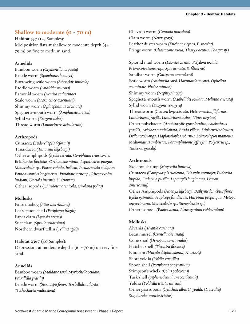
Shallow to moderate (0 - 70 m)Habitat 557 (125 Samples):Mid position flats at shallow to moderate depth (42 - 79 m) on fine to medium sand.
AnnelidsBamboo worm (Clymenella torquata)Bristle worm (Spiophanes bombyx)Burrowing scale worm (Sthenelais limicola)Paddle worm (Anaitides mucosa)Paraonid worm (Acmira catherinae)Scale worm (Harmothoe extenuata)Shimmy worm (Aglaophamus circinata)Spaghetti-mouth worm (Ampharete arctica)Syllid worm (Exogone hebes)Thread worm (Lumbrineris acicularum)
ArthropodsCumacea (Eudorellopsis deformis)Tanaidacea (Tanaissus lilljeborgi)Other amphipods (Byblis serrata, Corophium crassicorne, Ericthonius fasciatus, Orchomene minut, Leptocheirus pinguis, Monoculodes sp., Phoxocephalus holbolli, Pseudunciola obliquua, Parahaustorius longimerus , Protohaustorius sp., Rhepoxynius hudsoni, Unciola inermis, U. irrorata)Other isopods (Chiridotea arenicola, Cirolana polita)
MollusksFalse quahog (Pitar morrhuana)Lea’s spoon shell (Periploma fragile)Paper clam (Lyonsia arenos)Surf clam (Spisula solidissima)Northern dwarf tellin (Tellina agilis)
Habitat 2367 (40 Samples):Depressions at moderate depths (61 - 70 m) on very fine sand.
AnnelidsBamboo worm (Maldane sarsi, Myriochelle oculata, Praxillella gracilis)Bristle worm (Sternaspis fossor, Terebellides atlantis, Trochochaeta multisetosa)
Chevron worm (Goniada maculata)Clam worm (Nereis grayi)Feather duster worm (Euchone elegans, E. incolor)Fringe worm (Chaetozone setosa, Tharyx acutus, Tharyx sp.)
Spionid mud worm (Laonice cirrata, Polydora socialis, Prionospio steenstrupi, Spio armata, S. filicornis)Sandbar worm (Gattyana amondseni)Scale worm (Antinoella sarsi, Hartmania moorei, Ophelina acuminate, Pholoe minuta)Shimmy worm (Nephtys incisa)Spaghetti-mouth worm (Asabellides oculata, Melinna cristata)Syllid worm (Exogone verugera)Threadworm (Cossura longocirrata, Heteromastus filiformis, Lumbrineris fragilis, Lumbrineris hebes, Ninoe nigripes)Other polychaetes (Ancistrosyllis groenlandica, Anobothrus gracilis , Aricidea quadrilobata, Brada villosa, Diplocirrus hirsutus, Drilonereis longa, Haploscoloplos robustus, Leitoscoloplos mamosus, Mediomastus ambisetae, Paramphinome jeffreysii, Polycirrus sp., Tauberia gracilis)
ArthropodsSkeleton shrimp (Mayerella limicola)Cumacea (Campylaspis rubicund, Diastylis cornuifer, Eudorella hispida, Eudorella pusilla, Leptostylis longimana, Leucon americanus)Other Amphipods (Anonyx liljeborgi, Bathymedon obtusifrons, Byblis gaimardi, Haploops fundiensis, Harpinia propinqua, Metopa angustimana, Monoculodes sp., Stenopleustes sp.)Other isopods (Edotea acuta, Pleurogonium rubicundum)
MollusksAlvania (Alvania carinata)Bean mussel (Crenella decussata)Cone snail (Oenopota concinnulus)Hatchet shell (Thyasira flexuosa)Nutclam (Nucula delphinodonta, N. tenuis)Short yoldia (Yoldia sapotilla)Spoon shell (Periploma papyratium)Stimpson’s whelk (Colus pubescens)Tusk shell (Siphonodentalium occidentale)Yoldia (Yoldiella iris, Y. sanesia)Other gastropods (Cylichna alba, C. gouldi, C. occulta)Scaphander punctostriatus)

Northwest Atlantic Marine Ecoregional Assessment • Phase 1 Report 3-30
Chapter 3 - Benthic Habitats
CnidariansBurrowing anemone (Edwardsia elegans)Twelve-tentacle burrowing anemone (Halcampa duodecimcirrata)
EchinodermsMud star (Ctenodiscus crispatus)Sea cucumber (Molpadia oolitica)
BryozoansHippodiplosia propinqua
PhoronidsHorseshoe worm (Phoronis architecta)
SipunculidsTube worm (Phascolion strombi)
Habitat 1451 (127 Samples):Mid-position flats at shallow to moderate depths (42 - 101 m) on fine sand.
ArthropodsAtlantic rock crab (Cancer irroratus)Hairy hermit crab (Pagurus arcuatus)Lady crab (Ovalipes ocellatus)
MollusksAtlantic razor (Siliqua costata)Dog whelk (Nassarius trivittatus)Spotted northern moon-shell (Lunatia triseriata)Common northern moon snail (Euspira heros)Paper clam (Lyonsia hyalina)Stimpson’s whelk (Colus stimpsoni)
CnidariansColonial anemone (Epizoanthus americanus)
EchinodermsCommon sand dollar (Echinarachnius parma)Slender-armed star (Leptasterias tenera)
Habitat 1078 (305 Samples):Mid-position flats on at moderate depths (61 - 101 m) on fine sand.
No diagnostic species, depauperate samples with occasional sea scallop (Placopecten magellanicus) Habitat 1028 (67 Samples):Mid-position flats at moderate depths (61 - 101 m) on fine sand.
Arthropods American lobster (Homarus americanus)
MollusksIceland scallop (Chlamys islandica)Sea scallop (Placopecten magellanicus)Other gastropods (Stilifer stimpsoni)
Habitat 183 (136 Samples):Mid-position flats in shallow to moderate depths (42 - 101 m) on fine sand.
No diagnostic species, samples largely empty – some Northern shortfin squid (Illex illecebrosus)
Moderate Depths (70 - 233 m)Habitat 133 (61 Samples):Mid-position flats at moderate depths (70 - 101 m) on fine sand.
AnnelidsClam worm (Nereis pelagica)Feather duster worm (Chone infundibuliformis)Thread worm (Lumbrinerides acuta)Spionid mud worm (Scolelepis squamata)Paraonid worm (Acmira cerruti)Shimmy worm (Nephtys bucera)Syllid worm (Streptosyllis arenae)Threadworm (Notomastus latericeus)
ArthropodsFairy shrimp (Erythrops erythrophthalma)
Northwest Atlantic Marine Ecoregional Assessment • Phase 1 Report 3-31
Chapter 3 - Benthic Habitats
Cumacea (Pseudoleptocuma minor)Other amphipods (Pontogeneia inermis)
MollusksSea butterfly (Thecosomata spp.)
ChaetognathaArrow worm (Chaetognatha sp.)
Habitat 91 (307 Samples):Mid-position flats at moderate depths (42 to 83 m) on fine to medium sand.
ArthropodsAtlantic rock crab (Cancer irroratus)Acadian hermit crab (Pagurus acadianus)Cumacea (Lamprops quadriplicata, Pseudoleptocuma minor)Krill (Thysanoessa inermis, T. longicaudata)Mysid shrimp (Mysidopsis bigelowi, Neomysis americana)Skeleton shrimp (Caprella linearis)Sand shrimp (Crangon septemspinosa)Sea spider (Nymphon rubrum)Striped barnacle (Balanus hameri)Other amphipods (Ampelisca agassizi, A. macrocephala, Calliopius laeviusculus, Casco bigelowi , Ericthonius diffor-mis, Haustorius arenarius, Hippomedon serratus, Melita sp., Monoculodes sp., Orchomene pinguis, Parahaustorius longimerus, Parathemisto bispinosa, P. compressa, Photis dentate, Podoceropsis nitida, Pontogeneia inermis, Protomedeia fasciata, Psammonyx terranovae, Rhepoxynius epistomus, Tmetonyx cicada, Unciola inermis)Other isopods (Chiridotea arenicola, Chiridotea tuftsi, Cirolana concharum, Edotea triloba, Politolana polita)MollusksAtlantic razor (Siliqua costata)Chestnut astarte (Astarte castanea)Convex slipper shell (Crepidula plana)Dog welk (Nassarius trivittatus)Northern moon shell (Lunatia triseriata)Pearly top snail (Margarites groenlandicus)
CnidariansNorthern red anemone (Urticina felina)
EchinodermsDwarf brittlestar (Amphipholis squamata)
BryozoansLacy crusts (Electra pilosa)
ChaetognathaArrow worm (Chaetognatha sp.)
Habitat 9 (219 Samples):High and mid-postion flats at moderate depth (42 - 101 m) on fine to medium sand.
AnnelidsBeard worm (Pogonophora sp.)Mosaic worm (Nothria conchylega)
ArthropodsAcadian hermit crab (Pagurus acadianus)
MollusksConvex slipper shell (Crepidula plana)Jingle shell (Anomia simplex)
EchinodermsGreen sea urchin (Strongylocentrotus droebachiensis)Northern sea star (Asterias vulgaris)Spiny sun star (Crossaster papposus)
Habitat 12 (56 Samples):Steep slopes and flats at depths over 69 m, on fine to medium sand.
ArthropodsSand shrimp (Crangon septemspinosa)Other amphipods (Diastylis quadrispinosa, D. sculpta)
MollusksBean mussel (Crenella glandula)Black Clam (Arctica islandica)
Northwest Atlantic Marine Ecoregional Assessment • Phase 1 Report 3-3�
Chapter 3 - Benthic Habitats
Cone snail (Oenopota harpularia)Hatchet shell (Thyasira equalis, T. trisinuata)Northern moon snail (Euspira immaculata)Paper bubble (Philine quadrata)Rusty axinopsid (Mendicula ferruginosa)Solitary glassy bubble (Retusa obtusa)Top snail (Solariella obscura)
Bryozoans and ProtozoansTessarodoma gracilisForaminiferida
EchinodermsDwarf brittle star (Axiognathus squamatus)Sea cucumber (Stereoderma unisemita)
Habitat 24 (139 Samples):Mid-position flats at moderate depths (70 - 101 m) on silt to fine sand.
ArthropodsMysid shrimp (Pseudomma affine)Cumacea (Petalosarsia declivis, Lamprops quadriplicata)
Habitat 1 (153 Samples):High flats and slopes at any depth on silt, fine sand or sand.
ArthropodsBristled longbeak shrimp (Dichelopandalus leptocerus)
MollusksNorthern shorfin squid (Illex illecebrosus)
EchinodermsBasket star (Gorgonocephalus eucnemis)
*Habitat 139 (90 Samples):Various seabed postions in moderately shallow water (42 - 70 m) on fine to medium to coarse sand. Not a habitat type, but listed here for completeness.
No diagnostic species, samples largely empty – some squid (Sepioidea)
Habitat 2 (116 Samples):Flats and slopes at moderate depth (70 - 233 m) on very coarse sand or pebbles.
ArthropodsSpiny lebbeid (Lebbeus groenlandicus)Aesop shrimp (Pandalus montagui)Sars shimp (Sabinea sarsii)
*Habitat 4 (791 Samples):Any seabed form at any depth and any substrate. Not a habitat type, but included in this list for completeness.
Apparently poor samples, no diagnostic species, samples mostly krill (Euphausia krohni)
Habitat 247 (62 Samples):Depressions and high flats in moderate to deep water (101 - 233 m) on silt and mud.
ArthropodsPink glass shrimp (Pasiphaea multidentata)Northern shrimp (Pandalus borealis)Other decapods (Geryon quinquedens)
Habitat 7: (157 samples)Depressions, and high flats and slopes, in deep water (143 - 233 m) mostly on silt and fine sand, but substrate is variable.
AnnelidsPlumed worm (Onuphis opalina)Sea mouse (Laetmonice filicornis)
ArthropodsArctic eualid (Eualus fabricii)Friendly blade shrimp (Spirontocaris liljeborgii)Hermit crab (Pagurus pubescens)Norwegian shrimp (Pontophilus norvegicus)Parrot shrimp (Spirontocaris spinus)Polar lebbeid (Lebbeus polaris)Pycnogonum (Pycnogonum littorale)Sea spider (Nymphon grossipes, Nymphon longitarse, Nymphon

Northwest Atlantic Marine Ecoregional Assessment • Phase 1 Report 3-33
Chapter 3 - Benthic Habitats
macrum, Nymphon stroemi)Other amphipods (Epimeria loricata, Haploops tubicola, Stegocephalus inflatus)Other decopods (Stereomastis sculpta)
MollusksArctic rock borer (Hiatella arctica)Ark shell (Bathyarca pectunculoides)Bean mussel (Crenella pectinula)Broad yoldia (Yoldia thraciaeformis)Chalky macoma (Macoma calcarea)Astarte (Astarte elliptica, A. subequilatera, A. undata)Chiton-like mullusk (Amphineura sp.)Cone snail (Pleurotomella packardi)Cup-and-saucer limpet (Crucibulum striatum)Dipperclam (Cuspidaria fraterna, C. glacialis)Dove shell (Anachis haliaecti)Duckfoot snail (Aporrhais occidentalis)Heart clam (Cyclocardia borealis)Jingle shell (Anomia aculeata)Keyhole limpet (Puncturella noachina)Little cockle (Cerastoderma pinnulatum)Moon snail (Natica clausa)Mussel (Musculus discors, M. niger)Northern moon shell (Lunatia pallida)Nutclam (Nuculana pernula)Nutmeg snail (Admete couthouyi)Occidental tuskshell (Antalis occidentale)Offshore octopus (Bathypolypus arcticus)Pearly top snail (Margarites costalis)Stimpson’s whelk (Colus pygmaeus)Ten-ridged whelk (Neptunea decemcostata)Top shell (Calliostoma occidentale)Turret snail (Tachyrhynchus erosus)Velvet snail (Velutina laevigata)Waved whelk (Buccinum undatum)Wentletraps (Epitonium greenlandicum)Yoldia (Yoldiella lucida)Other bivalves (Cyclopecten pustulosus)
Brachipods and BryozoansLamp shell (Brachiopoda)Other bryozoan (Bugula sp., Caberea ellisii, Idmonea atlantica)
ChordatesCactus sea squirt (Boltenia ovifera)
CnidariansSea feather (Pennatula aculeata)Soft coral (Alcyonacea spp.)
EchinodermsBlood star (Henricia sanguinoleata)Brittle star (Ophiocten sericeum, Ophiura sarsi, Amphiura otteri, Ophiopholis amphiuridae)Cushion star (Leptychaster arcticus)Hairy sea cucumber (Havelockia scabra)Margined sea star (Psilaster andromeda)Orange-footed cucumber (Cucumaria planci)Psolus cucumber (Psolus phantapus)Scarlet psolus cucumber (Psolus fabricii)Sea urchin (Brisaster fragilis)Sun star (Lophaster furcifer)Other sea stars (Diplopteraster multiples, Poraniomorpha hispida)Sea lilies (Crinoidea sp.)
Habitat 18 (204 Samples):High flats at moderate to deep depths (over 101 m) on silt to fine sand.
AnnelidsBristle worm (Trochochaeta carica)Clam worm (Ceratocephale loveni)Thread worm (Abyssoninoe winsnesae, Lumbrineris magalhaensis)Plumed worm (Onuphis opalina)Others polychaetes (Paramphinome pulchella)
ArthropodsHorned krill shrimp (Meganyctiphanes norvegica)Cumacea (Eudorella truncatula)Other amphipods (Tmetonyx cicada)Other decapods (Calocaris templemanni, Stereomastis sculpta)Other isopods (Politolana impressa)
Northwest Atlantic Marine Ecoregional Assessment • Phase 1 Report 3-34
Chapter 3 - Benthic Habitats
MollusksAlvania (Alvania pelagica)Baltic macoma (Macoma baltica)Broad yoldia (Yoldia thraciaeformis)Cone snail (Oenopota exarata)Conrad’s thracia (Thracia myopsis)Dipperclam (Cuspidaria parva)Hatchet shell (Thyasira equalis, T. gouldii, T. pygmaea, T. trisinuata)Mussel (Dacrydium vitreum)Nutclam (Nucula proxima)Softshell Clam (Mya arenaria)Tusk shells (Polyschides rushii)Yoldia (Yoldia regularis)
EchinodermsBrittle star (Ophiocten sericeum, Ophiura robusta)
Habitat 87 (132 Samples):Depressions and high flats at moderate depths (101 - 233 m) on silt and mud.
ArthropodsSevenline shrimp (Sabinea septemcarinata)Prawn (Sergestes arcticus)
Echinoderms Mud star (Ctenodiscus porcell)
Deep 143 - 233 mHabitat 72 (152 Samples):Depressions and high flats at deep depths (143 - 233 m) on silt and mud.
ArthropodsShrimp (Pandalus propinquus)Others amphipods (Epimeria loricata)
Habitat 8 (266 Samples):Depressions and side slopes in deep water (143 - 233 m) on silt and mud.
AnnelidsBristle worm (Trochochaeta carica)
Clam worm (Ceratocephale loveni)Thread worm (Abyssoninoe winsnesae, Lumbrineris magalhaensis)Plumed worm (Onuphis opalina)Other polychaetes (Paramphinome pulchella)
ArthropodsHorned krill shrimp (Meganyctiphanes norvegica)Other decopods (Stereomastis sculpta)
MollusksAlvania (Alvania pelagica)Broad yoldia (Yoldia thraciaeformis)Conrad’s thracia (Thracia myopsis)Dipper clam (Cuspidaria parva)Hatchet shell (Thyasira equalism, T. gouldii, T. pygmaea, T. trisinuata)Mussel (Dacrydium vitreum)Nutclam (Nucula proxima)Softshell Clam (Mya arenaria)Tusk shells (Polyschides rushii)Yoldia (Yoldia regularis)
EchinodermsBrittle star (Ophiocten sericeum)
Habitat 5 (130 Samples):Depressions, high flats and slopes in deep water (101 - 233 m) on silt, fine sand and sand.
AnnelidsSea mouse (Aphrodita hastata)
ArthropodsShrimp (Pandalus propinquus)
Habitat 103 (42 Samples):High slopes, steep slopes and depressions in deep water (over 233 m) on silt and fine sand.
ArthropodsPrawn (Sergestes arcticus)Pink glass shrimp (Pasiphaea multidentata)

Northwest Atlantic Marine Ecoregional Assessment • Phase 1 Report 3-35
Chapter 3 - Benthic Habitats
Southern New England
Table 3-7. Physical factor values that correspond to ecological thresholds in the Southern New England subregion.
Bathymetry (m) Sediment Grain Size (mm) Seabed Form
0-9 0-0.03 (mud and silt) Depression
9-�3 0.03- 0.16 (very fine sand) Mid Flat
�3-31 0.16-0.34 (fine sand) High Flat
31-44 0.34 -0.36 (sand) Low Slope
44-76 >=0.36 (medium and coarse sand) Sideslope
76-139 Steep
>=139
Figure 3-17. Average depth and range of each benthic habitat type in the Southern New England subregion. Lines represent two standard deviations above and below the mean. Habitat types with the same depths often differ from each other by sediment grain size or topographic location. Habitats with very large depth ranges are widespread associations unrelated to, or weakly correlated with, depth.
Benthic Habitat Types: Southern New England
Dep
th (
met
ers
belo
w s
ea le
vel)
050
100150200250300350400450500550600650700750800850900950
10001050110011501200125013001350140014501500
BH:109
BH:200
BH:25
BH:390
BH:316
BH:230
BH:873
BH:229
BH:2537
BH:113
BH:36
BH:372
BH:317
BH:223
BH:381
BH:82
BH:949
BH:66
BH:3BH:11
BH:437
BH:6
BH:1
BH:387
Northwest Atlantic Marine Ecoregional Assessment • Phase 1 Report 3-36
Chapter 3 - Benthic Habitats
Shallow (0 - 31 m)Habitat 109 (134 Samples):Depressions in very shallow water (0 - 23 m) mostly on medium to coarse sand but occasionally on silt.
AnnelidsOthers polychaetes (Maldanopsis elongate, Sigambra tentaculata)Bamboo worm (Euclymene collaris, Owenia fusiformis)Blood worm (Glycera americana)Burrowing scale worm (Sthenelais boa)Clam worm (Neathes succinea)Spionid mud worm (Polydora ligni, Spio filicornis, Streblospio benedicti)Orbiniid worm (Scoloplos acutus)Paddle worm (Eteone heteropoda, Eumida sanguinea)Spaghetti-mouth worm (Ampharete arctica, Melinna cristata)Syllid worm (Exogone dispar)Terebellid worm (Polycirrus medusa)Thread worm (Heteromastus filiformis)
ArthropodsBay barnicle (Balanus improvisus)Longwrist hermit crab (Pagurus longicarpus)Other amphipods (Ampelisca abdita, Corophium bonelli, Corophium insidiosum, Microdeutopus gryllotalpa, Unciola serrata)
MollusksChanneled barrel-bubble (Acteocina canaliculata)Common razor clam (Ensis directus)Slipper shell (Crepidula convex, C. fornicata)Dog welk (Nassarius trivittatus)False anglewing (Petricola pholadiformis)File yoldia (Yoldia limatula)Gould’s pandora (Pandora gouldiana)Hard-shelled clam (Venus gallina)Little surf clam (Mulinia lateralis)Northern quahog (Mercenaria mercenaria)Paper clam (Lyonsia hyalina)Pyramid snail (Turbonilla elegantula)Softshell clam (Mya arenaria)White baby ear (Sinum perspectivum)Other bivalves (Mysella planulata)
Habitat 200 (163 Samples):Depressions at very shallow to moderate depths (0 – 44 m) on very fine to medium sand. AnnelidsSludge worm (Peloscolex gabriellae)
MollusksPitted baby-bubble (Acteon punctostriatus)
Habitat 25 (492 Samples):Flats and side slopes in very shallow to shallow water (0 - 23 m) on fine to coarse sand.
AnnelidsBlood worm (Hemipodus roseus)Mageloni worm (Magelona rosea)Spionid mud worm (Scolelepis squamata)Shimmy worm (Nephtys bucera)Other polychaetes (Pisione remota)
ArthropodsGlass shrimp (Leptochelia savignyi)Hermit crab (Pagurus politus)Cumacea (Leptocuma minor)Tanaidacea (Leptognathia caeca)Other isopods (Chiridotea arenicola)Other amphipods (Acanthohaustorius millsi, A. similis, Ampelisca verrilli, Parahaustorius attenuatus, P. longimerus, Protohaustorius sp.)
MollusksSurf clam (Spisula solidissima)
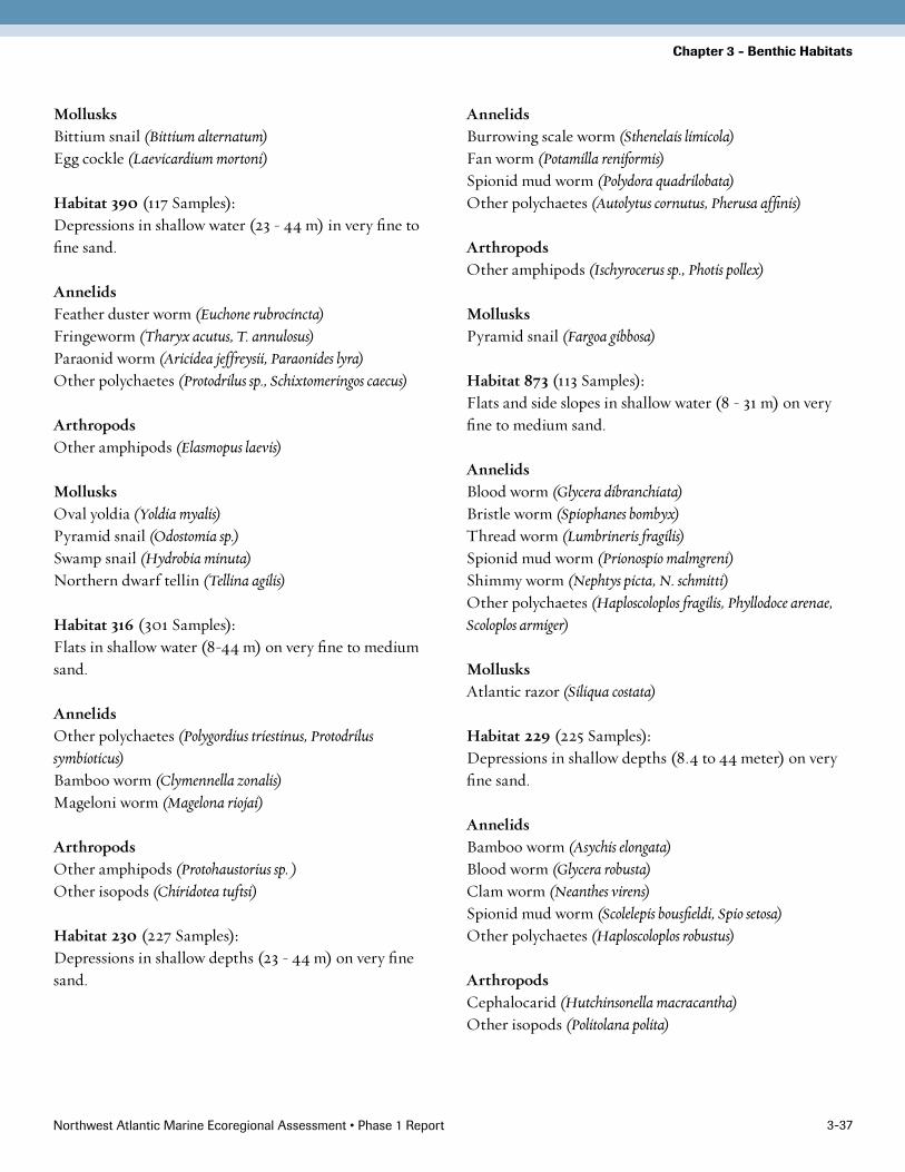
Habitat 36 (61 Samples):Depressions and high flats in very shallow to moderate depths (0 – 75 m) on medium to coarse sand.
ArthropodsGreen crab (Carcinus maenas)Portly spider crab (Libinia emarginata)
Northwest Atlantic Marine Ecoregional Assessment • Phase 1 Report 3-37
Chapter 3 - Benthic Habitats
MollusksBittium snail (Bittium alternatum)Egg cockle (Laevicardium mortoni)
Habitat 390 (117 Samples):Depressions in shallow water (23 - 44 m) in very fine to fine sand.
AnnelidsFeather duster worm (Euchone rubrocincta)Fringeworm (Tharyx acutus, T. annulosus)Paraonid worm (Aricidea jeffreysii, Paraonides lyra)Other polychaetes (Protodrilus sp., Schixtomeringos caecus)
ArthropodsOther amphipods (Elasmopus laevis)
MollusksOval yoldia (Yoldia myalis)Pyramid snail (Odostomia sp.)Swamp snail (Hydrobia minuta)Northern dwarf tellin (Tellina agilis)
Habitat 316 (301 Samples):Flats in shallow water (8-44 m) on very fine to medium sand.
AnnelidsOther polychaetes (Polygordius triestinus, Protodrilus symbioticus)Bamboo worm (Clymennella zonalis)Mageloni worm (Magelona riojai)
ArthropodsOther amphipods (Protohaustorius sp. )Other isopods (Chiridotea tuftsi)
Habitat 230 (227 Samples):Depressions in shallow depths (23 - 44 m) on very fine sand.
AnnelidsBurrowing scale worm (Sthenelais limicola)Fan worm (Potamilla reniformis)Spionid mud worm (Polydora quadrilobata)Other polychaetes (Autolytus cornutus, Pherusa affinis)
ArthropodsOther amphipods (Ischyrocerus sp., Photis pollex)
MollusksPyramid snail (Fargoa gibbosa)
Habitat 873 (113 Samples):Flats and side slopes in shallow water (8 - 31 m) on very fine to medium sand.
AnnelidsBlood worm (Glycera dibranchiata)Bristle worm (Spiophanes bombyx)Thread worm (Lumbrineris fragilis)Spionid mud worm (Prionospio malmgreni)Shimmy worm (Nephtys picta, N. schmitti)Other polychaetes (Haploscoloplos fragilis, Phyllodoce arenae, Scoloplos armiger)
MollusksAtlantic razor (Siliqua costata)
Habitat 229 (225 Samples):Depressions in shallow depths (8.4 to 44 meter) on very fine sand.
AnnelidsBamboo worm (Asychis elongata)Blood worm (Glycera robusta)Clam worm (Neanthes virens)Spionid mud worm (Scolelepis bousfieldi, Spio setosa)Other polychaetes (Haploscoloplos robustus)
ArthropodsCephalocarid (Hutchinsonella macracantha)Other isopods (Politolana polita)

Northwest Atlantic Marine Ecoregional Assessment • Phase 1 Report 3-38
Chapter 3 - Benthic Habitats
MollusksBlack Clam (Arctica islandica)Conrad’s thracia (Thracia sp.)False Quahog (Pitar morrhuana)Little Cockle (Cerastoderma pinnulatum)Nutclam (Nucula proxima)Pyramid snail (Turbonilla sp.)Other gastropods (Acteocina oryza)
CnidariansLined anemone (Edwardsia sipunculoides)
EchinodermsRat tailed cucumber (Caudina arenata)
Habitat 2537 (37 Samples):Depressions and high flats in shallow water (23 - 31 m) on very fine to fine sand.
AnnelidsClam worm (Nereis zonata)Hesion worm (Microphthalmus sczelkowii)Paddle worm (Eteone flava)Plumed worm (Diopatra cuprea)Thread worm (Capitella capitata)
ArthropodsAtlantic rock crab (Cancer irroratus)Lady Crab (Ovalipes ocellatus)Other amphipods (Melita nitida)
Habitat 36 (61 Samples):Depressions and high flats in very shallow to moderate depths (0 – 75 m) on medium to coarse sand.
ArthropodsGreen crab (Carcinus maenas)Portly spider crab (Libinia emarginata)
MollusksBittium snail (Bittium alternatum)Egg cockle (Laevicardium mortoni)
Moderate Depths (31 - 76 m)Habitat 113 (314 Samples):Depressions and mid-position flats at moderate depths (23 - 44 m) on very fine sand.
AnnelidsPaddle worm (Parougia caeca)Paraonid worm (Paraonis fulgens)Spaghetti-mouth worm (Asabellides oculata)Other polychaetes (Paranaitis speciosa)
ArthropodsOther amphipods (Dulichia monocantha)
Habitat 372 (125 Samples):Depressions and los slopes at moderate depths (44 – 75 m) on very fine sand.
AnnelidsFeather duster worm (Euchone incolor)Fringe worm (Tharyx dorsobranchialis, T. marioni)Thread worm (Cossura longocirrata, Lumbrineris hebes, Ninoe nigripes)Spionid mud worm (Polydora socialis, Prionospio steenstrupi)Paddle worm (Eteone lacteal, E. longa)Paraonid worm (Acmira catherinae, Aricidea quadrilobata, Tauberia gracilis)Scale worm (Hartmania moorei, Pholoe minuta)Shimmy worm (Nephtys incisa)Other polychaetes (Apistobranchus typicus, Drilonereis longa, Mediomastus ambiesetae, Polycirrus sp.)
ArthropodsCumacea (Campylaspis affinis, Campylaspis rubicund, Diastylis abbreviate, D. cornuifer, Jassa falcata, Leptostylis longimana)Other amphipods (Argissa hamatipes, Metopa angustimana, Photis macrocoxa, Stenopleustes )Other isopods (Edotea acuta)

Northwest Atlantic Marine Ecoregional Assessment • Phase 1 Report 3-39
Chapter 3 - Benthic Habitats
MollusksAlvania (Alvania carinata)Nutclam (Nucula delphinodonta)Short yoldia (Yoldia sapotilla)
EchinodermsBurrowing anemone (Edwardsia elegans)Twelve-tentacle burrowing anemone (Halcampa duodecimcirrata)
PhoronidsHorseshoe worm (Phoronis architecta)
Habitat 317 (190 Samples):Mid-position flats at moderate depths (31 - 75 m) on fine to medium sand.
AnnelidsBamboo worm (Clymenura dispar, Euclymene zonalis)Burrowing scale worm (Sigalion areicola)Chevron worm (Goniadella gracilis)Feather duster worm (Euchone elegans)Fringe worm (Caulleriella killariensis, Chaetozone setosa)Thread worm (Lumbrinerides acuta, Lumbrineris acicularum)Orbiniid worm (Orbinia swani, Scoloplos acmeceps)Paraonid worm (Aricidea wassi, Cirrophoris brevicirratus, C. furcatus, Paraonis pygoenigmatica)Sandbar worm (Ophelia denticulata)Scale worm (Harmothoe extenuata)Shimmy worm (Aglaophamus circinata)Spionid mud worm (Polydora caulleryi)Syllid worm (Exogone hebes, Sphaeroyllis erinaceus, Streptosyllis arenae, Syllides sp.)Other polychaetes (Drilonereis magna)
ArthropodsAcadian hermit crab (Pagurus acadianus)Lysianisid shrimp (Hippomedon serratus)Sand shrimp (Crangon septemspinosa)Cumacea (Petalosarsia declivis)Tanaidacea (Tanaissus lilljeborgi)Other amphipods (Acanthohaustorius spinosus , Byblis serrata,
Corophium crassicorne, Pseudunciola obliquua, Phoxocephalus holbolli, Protomedeia fasciata, Monoculodes sp., Rhepoxynius hudsoni, Siphonoecetes sp., Unciola inermis)Other isopods (Cirolana polita)
MollusksChestnut astarte (Astarte castanea)Northern moon shell (Lunatia triseriata)Northern moonsnail (Euspira immaculata)Paper clam (Lyonsia arenos)Pearly top snail (Margarites groenlandicus)Stimpson’s whelk (Colus pygmaeus)Top snail (Solariella obscura) EchinodermsCommon sand dollar (Echinarachnius parma)
Habitat 223 (98 Samples):Mid-position flats and depressions at moderate depths (44 - 75 m) on fine to medium sand.
AnnelidsBristle worm (Spiophanes kroeyeri)Terebellid worm (Polycirrus eximius)
ArthropodsCumacea (Eudorella emarginata, E. truncatula, Eudorellopsis deformis)Other amphipods (Ampelisca macrocephala, A. vadorum, Dyopedos porrectus, Ericthonius rubricornis, Leptocheirus pinguis, Orchomella pinguis, Rhepoxynius epistomus, Unciola irrorata)Other decapods (Stereomastis sculpta)Other isopods (Idotea balthica)
MollusksBean mussel (Crenella pectinula)Hatchet shell (Thyasira gouldii)Mussel (Musculus niger)Pyramid snail (Turbonilla interrupta)Other gastropods (Cylichma gouldi, C. alba)
Northwest Atlantic Marine Ecoregional Assessment • Phase 1 Report 3-40
Chapter 3 - Benthic Habitats
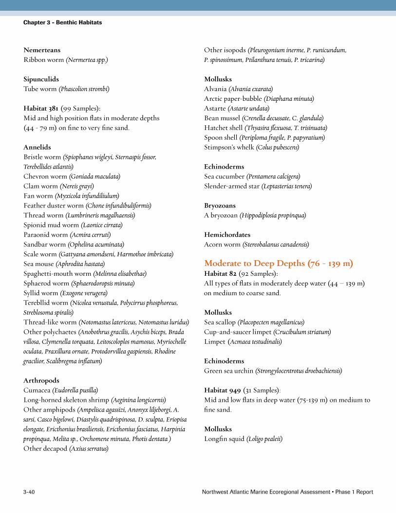
NemerteansRibbon worm (Nermertea spp.)
SipunculidsTube worm (Phascolion strombi)
Habitat 381 (99 Samples):Mid and high position flats in moderate depths (44 - 79 m) on fine to very fine sand.
AnnelidsBristle worm (Spiophanes wigleyi, Sternaspis fossor, Terebellides atlantis)Chevron worm (Goniada maculata)Clam worm (Nereis grayi)Fan worm (Myxicola infundiliulum)Feather duster worm (Chone infundibuliformis)Thread worm (Lumbrineris magalhaensis)Spionid mud worm (Laonice cirrata)Paraonid worm (Acmira cerruti)Sandbar worm (Ophelina acuminata)Scale worm (Gattyana amondseni, Harmothoe imbricata)Sea mouse (Aphrodita hastata)Spaghetti-mouth worm (Melinna elisabethae)Sphaerod worm (Sphaerodoropsis minuta)Syllid worm (Exogone verugera)Terebllid worm (Nicolea venustula, Polycirrus phosphoreus, Streblosoma spiralis)Thread-like worm (Notomastus latericeus, Notomastus luridus)Other polychaetes (Anobothrus gracilis, Asychis biceps, Brada villosa, Clymenella torquata, Leitoscoloplos mamosus, Myriochelle oculata, Praxillura ornate, Protodorvillea gaspiensis, Rhodine gracilior, Scalibregma inflatum)
ArthropodsCumacea (Eudorella pusilla)Long-horned skeleton shrimp (Aeginina longicornis)Other amphipods (Ampelisca agassizi, Anonyx liljeborgi, A. sarsi, Casco bigelowi, Diastylis quadrispinosa, D. sculpta, Eriopisa elongate, Ericthonius brasiliensis, Ericthonius fasciatus, Harpinia propinqua, Melita sp., Orchomene minuta, Photis dentata )Other decapod (Axius serratus)
Other isopods (Pleurogonium inerme, P. runicundum, P. spinossimum, Ptilanthura tenuis, P. tricarina)
MollusksAlvania (Alvania exarata)Arctic paper-bubble (Diaphana minuta)Astarte (Astarte undata)Bean mussel (Crenella decussate, C. glandula)Hatchet shell (Thyasira flexuosa, T. trisinuata)Spoon shell (Periploma fragile, P. papyratium)Stimpson’s whelk (Colus pubescens)
EchinodermsSea cucumber (Pentamera calcigera)Slender-armed star (Leptasterias tenera)
BryozoansA bryozoan (Hippodiplosia propinqua)
HemichordatesAcorn worm (Stereobalanus canadensis)
Moderate to Deep Depths (76 - 139 m)Habitat 82 (92 Samples):All types of flats in moderately deep water (44 – 139 m) on medium to coarse sand.
MollusksSea scallop (Placopecten magellanicus)Cup-and-saucer limpet (Crucibulum striatum)Limpet (Acmaea testudinalis)
EchinodermsGreen sea urchin (Strongylocentrotus droebachiensis)
Habitat 949 (31 Samples):Mid and low flats in deep water (75-139 m) on medium to fine sand.
MollusksLongfin squid (Loligo pealeii)

Northwest Atlantic Marine Ecoregional Assessment • Phase 1 Report 3-41
Chapter 3 - Benthic Habitats
Habitat 66 (121 Samples):Hihg flats and slopes in moderately deep water (75 - 139 m) on very fine to fine sand.
AnnelidsBamboo worm (Paralacydonia paradoxa)Fringe worm (Tharyx tesselata)Hesion worm (Gyptis vittata)Thread worm (Lumbrineris brevipes)Shimmy worm (Aglaophamus minusculus)
EchinodermsDwarf brittlestar (Amphipholis squamata)
CnidariansSlender sea pen (Stylatula elegans)
*Habitat 3 (78 Samples):Flats and slopes at moderate to very deep depths (average 128 m, min 44 m) on fine to very fine sand.
No diagnostic species, samples largely empty except for deep sea Spirula squid (Sepioidea). Not a benthic habitat type, but listed here for completeness.
Habitat 11 (78 Samples):High slopes, canyons, flats in deep water (60 – 485 m) on medium to fine sand.
ArthropodsShrimp (Pontophilus brevirostris)Arthropods (Pycnogonum littorale)Bristled longbeak shrimp (Dichelopandalus leptocerus)Deepwater humpback shrimp (Solenocera necopina)Friendly blade shrimp (Spirontocaris liljeborgii)Hermit crab (Catapagurus sharreri)Krill (Thysanoessa longicaudata)Parrot shrimp (Spirontocaris spinus)Rose shrimp (Parapenaeus politus)Sand shrimp (Crangon septemspinosa)Shrimp (Palicus gracilis)Slender tube makers (Ericthonius difformis)Squat lobsters (Munida valida)
Striped barnacle (Balanus hameri)Other amphipods (Monoculodes spp., Tiron acanthurus)
MollusksBobtail squid (Rossia tenera)Iceland cockle (Clinocardium ciliatum)Iceland scallop (Chlamys islandica)Offshore octopus (Bathypolypus arcticus)Rock borer clam (Panomya arctica)
CnidariansBadge sea star (Porania insignis)Blood star (Henricia sanguinoleata)Margined sea star (Astropecten americana)Northern sea star (Asterias vulgaris)
Habitat 437 (34 Samples):High flats and slopes in deep to very deep water (75 - 200 m) on fine sand.
ArthropodsAmerican Lobster (Homarus americanus)Jonah Crab (Cancer borealis)Swimming crab (Bathynectes superba)Other decapods (Geryon quinquedens)
MollusksNorthern shortfin squid (Illex illecebrosus)Longfin squid (Loligo pealeii)
EchinodermsMargined sea stars (Astropecten cingulatus)
Habitat 6 (105 Samples):High slopes and flats at moderate to deep depths (44 - 139 m) on coarse to fine sand.
ArthropdodaAesop shrimp (Pandalus montagui)Arctic lyre crab (Hyas coarctatus)Hermit crab (Pagurus pubescens)

Northwest Atlantic Marine Ecoregional Assessment • Phase 1 Report 3-4�
Chapter 3 - Benthic Habitats
MollusksChiton-like mullusk (Amphineura spp.)Arctic rock borer (Hiatella arctica)Jingle shell (Anomia simplex)Mussel (Musculus discors)
EchinodermsDaisy brittle star(Ophiopholis amphiuridae)Green sea urchin (Strongylocentrotus droebachiensis)
*Habitat 1 (627 Samples):Variable settings in a wide range of depths on fine to coarse sand. A very mixed set of samples with many un-identified species and few commonalities. Not a benthic habitat type, but listed here for completeness.
Deep to Very Deep (> 139 m)Habitat 387 (29 Samples):High slopes and flats in very deep water (>139 m) on fine sand.
AnnelidsBeard worm (Siboglinum ekmani)Plumed worm (Onuphis opalina)Fairy shrimp (Erythrops erythrophthalma)Cumacea (Eudorella hispida)
MolluksArk shell (Bathyarca pectunculoides)Chestnut Astarte (Astarte subequilatera)Nutclam (Nuculana acuta)Occidental Tuskshell (Antalis occidentale)Rusty Axinopsid (Mendicula ferruginosa)Other bivalves (Lucina filosa)
EchinodermsSea butterfly (Thecosomata )Burrowing brittle star (Amphioplus macilentus, Amphilimna olivacea)
HemichordatesAcorn worm (Enteropneusta )
NemotodaRound worm (Nematoda )
ProtozoansForaminiferida
SipunculidsPeanut worm (Golfingia catharinae, Onchnesoma steenstrupi

Northwest Atlantic Marine Ecoregional Assessment • Phase 1 Report 3-43
Chapter 3 - Benthic Habitats
Mid-Atlantic Bight
Table 3-8. Physical factor values that correspond to ecological thresholds in the Mid-Atlantic Bight subregion.
Bathymetry (m) Sediment Grain Size (mm) Seabed Form
0-15 0-0.18 (silt and very fine sand Depression
15-�� 0.18-0.35 (fine sand) Mid Flat
��-45 0.35-0.36 (sand) High Flat
45-48 0.36 -0.48 (sand) Low Slope
48-8� >=0.48 (coarse sand) Sideslope
8�-95 Steep
95-59�
>59�
Figure 3-18. Average depth and range of each benthic habitat type in the Mid-Atlantic Bight subregion. Lines represent two standard deviations above and below the mean. Habitat types with the same depths often differ from each other by sediment grain size or topographic location. Habitats with very large depth ranges are widespread associations often unrelated to, or only weakly correlated with, depth.
050
100150200250300350400450500550600650700750800850900950
10001050110011501200125013001350140014501500
Benthic Habitat Types: Mid-Atlantic Bight
Dep
th (
met
ers
belo
w s
ea le
vel)
BH:768
BH:64
BH:87
BH:38
BH:1
BH:7
BH:2
BH:32
BH:4
BH:25
BH:233
BH:592
BH:306
BH:395
BH:218
BH:520
BH:84
BH:1223
BH:219
BH:44
BH:229
BH:216
BH:384
BH:505

Northwest Atlantic Marine Ecoregional Assessment • Phase 1 Report 3-44
Chapter 3 - Benthic Habitats
Very Shallow (0 – 22 m)Habitat 768 (22 Samples):Depressions in very shallow water (0 - 15 m) on silt to fine sand.
ArthropodsMysid shrimp (Neomysis americana)Other amphipods (Ampelisca abdita)
MollusksElongated macoma (Macoma tenta)Tellin clam (Tellina sybaritica)Channeled whelk (Busycon canaliculatum)Cone snail (Kurtziella cerina)Dove shell (Mitrella lunata)Pyramid snail (Odostomia winkleyi)Solitary glassy bubble (Retusa canaliculata)Wentletraps (Epitonium rupicola)
EchinodermsBurrowing brittle star (Micropholis atra)
Habitat 64 (62 Samples):Depressions and mid-position flats in shallow water (15 and 22 m) on medium sand.
AnnelidsBlood worm (Hemipodus roseus)Fringe worm (Tharyx sp.)Hesion worm (Microphthalmus sczelkowii)Thread worm (Lumbrineris acicularum)Paddle worm (Hesionura augeneri)Paraonid worm (Acmira catherinae, A. cerruti)Sandbar worm (Ophelia denticulata)Spaghetti-mouth worm (Ampharete arctica)Syllid worm (Brania wellfleetensis, Streptosyllis pettiboneae, S. websteri, Syllides longicirrata)Other polychaetes (Pisione remota)
ArthropodsSharp-tailed cumacean (Oxyurostylis smithi)Other isopods (Chiridotea arenicola)
MollusksBlue mussel (Mytilus edulis)Dove shell (Anachis lafresnayi)Eastern aligena (Aligena elevata)
Habitat 87 (20 Samples):Depressions and high flats in shallow water (15 - 22 m) on medium sand.
AnnelidsBurrowing scale worm (Sigalion areicola)Fringe worm (Caulleriella killariensis)Mageloni worm (Magelona riojai)Spionid mud worm (Scolelepis squamata, Dispio uncinata, Polydora caulleryi)Sphaerod worm (Sphaerodoropsis corrugata)Syllid worm (Streptosyllis varians)
ArthropodsGlass shrimp (Leptochelia savignyi)Gammarid amphipods (Acanthohaustorius bousfieli, A.intermedius, A. Similis)Other amphipods (Bathyporeia quoddyensis, B. parkeri, B. quoddyensis, Parahaustorius attenuates, Synchelidium americanum)Tanaidacea (Tanaissus lilljeborgi)Other isopods (Chiridotea tuftsi)
EchinodermsSand dollar (Encope emarginata)
MollusksAtlantic razor (Siliqua costata)Gould’s pandora (Pandora trilineata)Lea’s spoon shell (Periploma leanum)Pandora (Pandora trilineata)Surf clam (Spisula solidissima)Margin shells (Dentimargo eburneolus)
Habitat 38 (95 Samples):Depressions in water shallow (15 - 22 m) on medium to coarse sand.

Northwest Atlantic Marine Ecoregional Assessment • Phase 1 Report 3-45
Chapter 3 - Benthic Habitats
AnnelidsBamboo worm (Owenia fusiformis)Chevron worm (Glycinde solitaria)Orbiniid worm (Scoloplos rubra)Paddle worm (Eteone heteropoda, Eteone lactea)Plumed worm (Diopatra cuprea)Shimmy worm (Nephtys picta)Spionid mud worm (Paraprionospio pinnata, Polydora ligni, Prionospio pygmaea, Scolelepis bousfieldi, Spio pettiboneae, S. se-tosa)Thread worm (Notomastus hemipodus, N. luridus)
ArthropodsOlivepit porcelain crab (Euceramus praelongus)Pea crab (Pinnixa sayana)Other amphipods (Corophium tuberculatum, Parametopella cypris)
MollusksArctic paper-bubble (Diaphana minuta)Common razor clam (Ensis directus)Pandora (Pandora bushiana)Margin shells (Marginella virginiana)Miniature moonsnail (Tectonatica pusilla)Pitted baby-bubble (Acteon punctostriatus)Pyramid snail (Odostomia sp., Turbonilla interrupta)Solitary glassy-bubble (Haminoea solitaria)Northern dwarf tellin (Tellina agilis)Other gastropods (Acteocina oryza)
HemichordatesAcorn worm (Stereobalanus canadensis)
Shallow (22 - 45 m)Habitat 1(109 Samples):Depressions and mid-position flats, shallow to moderate depth (0 - 45 m) on coarse to fine sand.
AnnelidsShimmy worm (Nephtys bucera)
Arthropods Other amphipods (Protohaustorius deichmannae, Acanthohaustorius spinosus,A. shoemakeri)
MollusksAstarte (Astarte borealis)Lunate crassinella (Crassinella lunulata)
ChordatesLancelet (Branchiostoma virginiae)
Habitat 7 (83 Samples):Mid-position flats and depressions in shallow water (25 - 45 m) on medium to coarse substrate.
AnnelidsBlood worm (Hemipodus armatus)Fringe worm (Tharyx acutus, T. Annulosus)Hesion worm (Microphthalmus aberrans)Thread worm (Lumbrineris coccinea, L.fragilis)Spionid mud worm (Prionospio malmgreni, Spio filicornis)Paraonid worm (Aricidea jeffreysii, Paraonides lyra)Syllid worm (Eusyllis blomstrandi, Syllis cornuta)Other polychaetes (Protodrilus symbioticus)
ArthropodsTanaidacea (Leptognathia caeca)
CnidariansFrilled anemone (Metridium senile)
EchinodermsCommon sea star (Asterias forbesi)
Habitat 2 (58 Samples):Flat depressions at shallow to moderate depth (0 - 45 m) in medium sand.
AnnelidsBamboo worm (Asychis elongata)Burrowing scale worm (Sthenelais boa)Chevron worm (Goniada norvegica, G. carolinae)

Northwest Atlantic Marine Ecoregional Assessment • Phase 1 Report 3-46
Chapter 3 - Benthic Habitats
Flabelliger worm (Pherusa affinis)Fringe worm (Tharyx dorsobranchialis, T. marioni)Spionid mud worm (Polydora quadrilobata, Streblospio benedicti)Paddle worm (Eteone longa, Paranaitis speciosa)Paraonid worm (Tauberia gracilis)Shimmy worm (Nephtys incisa)Spaghetti-mouth worm (Asabellides oculata)Thread-like worm (Cossura longocirrata)Threadworm (Capitella capitata)
ArthropodsAmphipod (Dulichia monocantha, Photis macrocoxa)
CnidariansBurrowing anemone (Edwardsia elegans)Sea cucumber (Pentamera calcigera)
MollusksDog welk (Nassarius trivittatus)False quahog (Pitar morrhuana)File yoldia (Yoldia limatula)Hard-shelled clam (Venus gallina)Nutclam (Nucula annulata, N. proxima)Short yoldia (Yoldia sapotilla)
PhoronidsHoreshoe worm (Phoronis architecta)
Habitat 32 (52 Samples):Mid-position flats at shallow to moderate depths (22 - 45 m) on medium sand.
ArthropodsAtlantic rock crab (Cancer irroratus)Longnose spider crab (Libinia dubia)
MollusksCommon northern moon snail (Euspira heros)Northern moon shell (Lunatia triseriata)Astarte (Astarte quadrans)Blood ark (Anadara ovalis)
EchinodermsCommon sand dollar (Echinarachnius parma)
Habitat 4 (128 Samples):Mid-position flats in shallow water (25 - 45 m) on coarse to medium sand.
AnnelidsBamboo worm (Clymennella zonalis)Chevron worm (Goniadella gracilis)Thread worm (Lumbrinerides acuta)Syllid worm (Streptosyllis arenae)Other polychaetes (Polygordius triestinus)
ArthropodsOther amphipods (Parahaustorius longimerus)Other isopods (Cirolana polita, Chiridotea coeca)
MollusksChestnut astarte (Astarte castanea)
Moderate depth (45 - 82 m)Habitat 25 (46 Samples):Depressions at moderate depths (15 - 82 m) on fine to coarse sand.
AnnelidsBamboo worm (Myriochelle heeri)Bristle worm (Spiophanes bombyx, S. missionensis)Mageloni worm (Magelona rosea)Spionid mud worm (Scolelepis sp.)Orbiniid worm (Orbinia swani)Shimmy worm (Nephtys schmitti)Other polychaetes (Novaquesta trifurcata)
ArthropodsMysid shrimp (Neomysis Americana)
MollusksMoon snail (Natica clausa)
CnidariansLined anemone (Edwardsia sipunculoides)
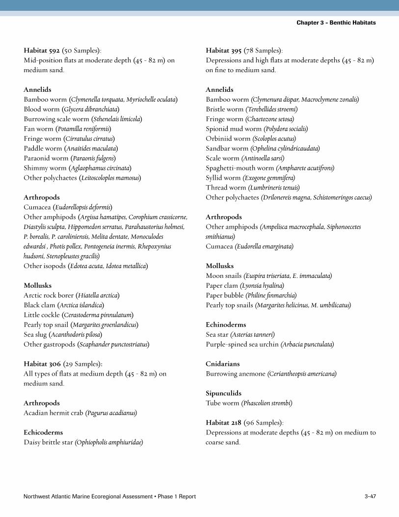
Northwest Atlantic Marine Ecoregional Assessment • Phase 1 Report 3-47
Chapter 3 - Benthic Habitats
Habitat 592 (50 Samples):Mid-position flats at moderate depth (45 - 82 m) on medium sand.
AnnelidsBamboo worm (Clymenella torquata, Myriochelle oculata)Blood worm (Glycera dibranchiata)Burrowing scale worm (Sthenelais limicola)Fan worm (Potamilla reniformis)Fringe worm (Cirratulus cirratus)Paddle worm (Anaitides maculata)Paraonid worm (Paraonis fulgens)Shimmy worm (Aglaophamus circinata)Other polychaetes (Leitoscoloplos mamosus)
ArthropodsCumacea (Eudorellopsis deformis)Other amphipods (Argissa hamatipes, Corophium crassicorne, Diastylis sculpta, Hippomedon serratus, Parahaustorius holmesi, P. borealis, P. caroliniensis, Melita dentate, Monoculodes edwardsi , Photis pollex, Pontogeneia inermis, Rhepoxynius hudsoni, Stenopleustes gracilis)Other isopods (Edotea acuta, Idotea metallica)
MollusksArctic rock borer (Hiatella arctica)Black clam (Arctica islandica)Little cockle (Cerastoderma pinnulatum)Pearly top snail (Margarites groenlandicus)Sea slug (Acanthodoris pilosa)Other gastropods (Scaphander punctostriatus)
Habitat 306 (29 Samples):All types of flats at medium depth (45 - 82 m) on medium sand.
ArthropodsAcadian hermit crab (Pagurus acadianus)
EchicodermsDaisy brittle star (Ophiopholis amphiuridae)
Habitat 395 (78 Samples):Depressions and high flats at moderate depths (45 - 82 m) on fine to medium sand.
AnnelidsBamboo worm (Clymenura dispar, Macroclymene zonalis)Bristle worm (Terebellides stroemi)Fringe worm (Chaetozone setosa)Spionid mud worm (Polydora socialis)Orbiniid worm (Scoloplos acutus)Sandbar worm (Ophelina cylindricaudata)Scale worm (Antinoella sarsi)Spaghetti-mouth worm (Ampharete acutifrons)Syllid worm (Exogone gemmifera)Thread worm (Lumbrineris tenuis)Other polychaetes (Drilonereis magna, Schistomeringos caecus)
ArthropodsOther amphipods (Ampelisca macrocephala, Siphonoecetes smithianus)Cumacea (Eudorella emarginata)
MollusksMoon snails (Euspira triseriata, E. immaculata)Paper clam (Lyonsia hyalina)Paper bubble (Philine finmarchia)Pearly top snails (Margarites helicinus, M. umbilicatus)
EchinodermsSea star (Asterias tanneri)Purple-spined sea urchin (Arbacia punctulata)
CnidariansBurrowing anemone (Ceriantheopsis americana)
SipunculidsTube worm (Phascolion strombi)
Habitat 218 (96 Samples):Depressions at moderate depths (45 - 82 m) on medium to coarse sand.

Northwest Atlantic Marine Ecoregional Assessment • Phase 1 Report 3-48
Chapter 3 - Benthic Habitats
AnnelidsBamboo worm (Praxillura ornata)Clam worm (Nereis grayi)Feather duster worm (Euchone incolor)Flabelliger worm (Brada villosa, Diplocirrus hirsutus, Pherusa aspera)Thread worm (Lumbrineris hebes, Ninoe nigripes, Lumbrineris hebes)Paddle worm (Eulalia bilineata)Paraonid worm (Cirrophorus lyriformis)Scale worm (Harmothoe extenuata)Sea mouse (Aphrodita hastata)Sphaerod worm (Sphaerodoridium claparedi, S. minuta)Syllid worm (Typosyllis alternata)Terebellid worm (Nicolea venustula,Polycirrus sp.)Other polychaetes (Drilonereis longa, Meiodorvillea minuta, Scalibregma inflatum)
ArthropodsCumacea (Petalosarsia declivis, Campylaspis affinis)Other amphipods (Ampelisca vadorum, Anonyx sarsi, Casco bigelowi, Leptocheirus pinguis, Orchomella minuta, O. pinguis)Other isopods (Janira alta, Pleurogonium inerme)
MollusksBean mussel (Crenella decussata)Conrad’s thracia (Thracia morrisoni)Mussel (Musculus discors)Nutclam (Nucula delphinodonta)Alvania (Alvania carinata)Stimpson’s whelk (Colus pubescens)Striate aclis (Aclis striata)
CnidariansTwelve-tentacle burrowing anemone (Halcampa duodecimcirrata)
520 (31 Samples):Mid position flats and depressions at moderate depths (45 - 82) on mostly coarse to occsasionaly fine sand.
AnnelidsBamboo worm (Rhodine gracilior, R. Loveni)Bristleworm (Spiophanes wigleyi, Terebellides atlantis)Chevron worm (Goniada brunnea, G.maculata, Ophioglycera gigantea)Clam worm (Nereis zonata)Fan worm (Myxicola infundiliulum)Feather duster worm (Euchone elegans)Fringe worm (Dodecaceria corallii)Thread worm (Lumbrineris brevipes)Spionid mud worm (Laonice cirrata, Minuspio cirrifera, Polydora giardi, Prionospio steenstrupi)Orbiniid worm (Scoloplos armiger)Paddle worm (Anaitides mucosa, Eumida sanguinea, Mystides boreali, Notophyllum foliosum)Paraonid worm (Aricidea belgicae, Cirrophorus furcatus)Parchment worm (Spiochaetopterus oculatus)Sandbar worm (Ophelina acuminata)Scale worm (Arcteobia anticostiensis, Gattyana nutti, Gattyana sp. Harmothoe imbricate, Pholoe minuta)Spaghetti-mouth worm (Amphicteis gunneri, Melinna cristata, M.elisabethae)Syllid worm (Exogone verugera, Sphaerosyllis erinaceus, Typosyllis tegulum)Terebellid worm (Eupolymnia nebulosa, Polycirrus eximius, P. Medusa, Streblosoma spiralis)Threadworm (Notomastus latericeus)Other polychaetes (Aberranta enigmatica)
ArthropodLong-horned skeleton shrimp (Aeginina longicornis)Cumacea (Eudorella pusilla)Other amphipods (Eriopisa elongate, Anonyx liljeborgi, Ampelisca agassizi, Diastylis quadrispinosa, Ericthonius fasciatus, Harpinia propinqua, Photis dentata, Phoxocephalus holbolli, Unciola irrorata)Other decapods (Axius serratus)
MollusksAstarte (Astarte undata)Hatchet shell (Thyasira flexuosa)Heart clam (Cyclocardia borealis)

Northwest Atlantic Marine Ecoregional Assessment • Phase 1 Report 3-49
Chapter 3 - Benthic Habitats
Spoon shell (Periploma fragile, P. Papyratium)Mussel (Dacrydium vitreum)Pyramid snail (Odistomia sulcosa)Risso (Boreocingula castanea)Other bivalves (Lucina filosa, Mysella planulata)
EchinodermsSea star (Asterias rathbuni)Dwarf brittlestar (Amphipholis squamata)Margined sea star (Astropecten irregularis)
BryozoansA bryozoan (Hippodiplosia propinqua)
SipunculidsPeanut worm (Themiste alutacea)
Habitat 84 (104 Samples):All types of flats at moderate depth (22 - 82 m) on fine to medium sand.
AnnelidsBeardworm (Siboglinum bayer, Diplobrachia ii, Oligobrachia floridana)Marphysa worm (Marphysa belli)Paddle worm (Anaitides arenae)Sandbar worm (Ophelina aulogaster)
ArthropodsCumacea (Eudorella truncatula, Pseudoleptocuma minor)Other decapods (Calocaris macandreae)Other amphipods (Ampelisca verrilli, Byblis serrata, Lembos Webster,Rhepoxynius epistomus)
EchinodermsHeart sea urchin (Echinocardium cordatum)Sea urchin (Brisaster fragilis)Burrowing brittle star (Amphioplus macilentus)
MollusksCross-hatched lucine (Divaricella quadrisulcata)Bean mussel (Crenella pectinula)Astarte (Astarte elliptica)
Gould’s pandora (Pandora gouldiana)Hard-shelled clam (Chione latilirata)Hatchet shell (Thyasira trisinuata)Lucine clam (Lucinoma blakeanum)Nutclam (Nuculana acuta)Dove shell (Mitrella dissimilis)Margin shells (Marginella roscida)Pyramid snail (Turbonilla areolata)Pyramid snail (Turbonilla rathbuni)Ribbed moelleria (Moelleria costulata)Wentletraps (Epitonium dallianum)Other bivalves (Cyclopecten nanus)Other gastropods (Granulina ovuformis)
Deep (82 - 592 m)Habitat 1223 (35 Samples):High flats in moderately deep water (82 - 95 m) on medium sand.
AnnelidsBamboo worm (Clymenura borealis, Euclymene zonalis)Blood worm (Glycera robusta)Eunice worm (Eunice norvegica)Fan worm (Manayunkia aestuarina)Feather duster worm (Chone infundibuliformis, Fabricia sabella)Thread worm (Lumbrineris magalhaensis)Spionid mud worm (Malacoceros indicus, Polydora barbilla, P. concharum)Opal worm (Arabella iricolor, Arabella mutans)Orbiniid worm (Scoloplos acmeceps)Paraonid worm (Acmira lopezi, Aricidea wassi, Paraonis pygoenigmatica)Plumed worm (Onuphis opalina, O. pallidula)Sandbar worm (Travisia parva)Shimmy worm (Aglaophamus igalis, Nephtys squamosa)Syllid worm (Exogone dispar, E.hebes, E.naidina)Tube worm (Hydroides dianthus)Other polychaetes (Drilonereis caulleryi, Protodorvillea gaspiensis)

Northwest Atlantic Marine Ecoregional Assessment • Phase 1 Report 3-50
Chapter 3 - Benthic Habitats
ArthropodsOther amphipods (Idunella bowenae, Jerbarnia Americana, Rhachotropis inflate, Unciola serrata)Other isopods (Apanthura magnifica, Ptilanthura tricarina)
MollusksBean mussel (Crenella glandula)Eastern beaded chiton (Chaetopleura apiculata)Heart clam (Pleuromeris tridentata)Striate scallop (Palliolum striatum)Other bivalves (Cumingia tellinoides, Diplodonta punctata, Mysella grippi)Other gastropods (Cocculina beani)
CnidariansBurrowing anemone (Haloclava producta)Twelve-tentacle parasitic anemone (Peachia parasitica)
EchinodermsMargined sea stars (Astropecten articulatus)
Habitat 219 (44 Samples):High flats at moderate depths (45 - 82 m) on coarse to fine sand.
ArthropodsPrawn (Sergestes robustus)
MollusksBroad yoldia (Yoldia thraciaeformis)Sea scallop (Placopecten magellanicus)Jingle shell (Anomia simplex)Longfin squid (Loligo pealeii)Duckfoot snail (Aporrhais occidentalis)
EchidodermsMud star (Ctenodiscus porcell)
Habitat 44 (82 Samples):Depressions and mid-position flats mostly very shallow (0 - 22m), but occasionally very deep on fine to coarse sand.
ArthropodsPrawn (Sergestes arcticus)Jonah crab (Cancer borealis)Other isopods (Chiridotea nigrescens)
MollusksAmethyst gemclam (Gemma gemma)Baltic macoma (Macoma baltica)Little surf clam (Mulinia lateralis)
EchinodermsNorthern sea star (Asterias vulgaris)
Habitat 229 (57 Samples):High flats and depressions at shallow to deep depths (22 - 592 m) on a fine to medium sand.
ArthropodsJonah crab (Cancer borealis)
EchinodermsCommon sea star (Asterias forbesi)Northern sea star (Asterias vulgaris)Green sea urchin (Strongylocentrotus droebachiensis)
CnidariansAnemone (Actiniaria spp.)
Habitat 216 (41 Samples):High slopes in deep water (95 - 592 m) on medium to fine sand.
ArthropodsAmerican lobster (Homarus americanus)Bristled longbeak shrimp (Dichelopandalus leptocerus)Fairy shrimp (Bathymysis renocullata)Friendly blade shrimp (Spirontocaris liljeborgii)Hermit crab (Pagurus politus)Norwegian shrimp (Pontophilus norvegicus)Rose shrimp (Parapenaeus politus)Shrimp (Palicus gracilis)Squat lobsters (Munida iris, M. valida)Other decapods (Nematocarcinus ensifer, Scyllarus depressus)

Northwest Atlantic Marine Ecoregional Assessment • Phase 1 Report 3-51
Chapter 3 - Benthic Habitats
EchinodermsMargined sea stars (Astropecten americana)Sea urchin (Genocidaris maculata)
CnidariansSea feather (Pennatula aculeata)
CephalopodsBobtail squid (Rossia glaucopis)Offshore octopus (Bathypolypus arcticus)Squid (Sepioidea)
Habitat 384 (14 Samples):High slopes and canyons in deep water (95 - 592 m) on any substrate.
AnnelidsScale worm (Alentiana aurantiaca)
ArthropodsFlorida lobsterette (Nephropsis aculeata)Royal red shrimp (Pleoticus robustus)Prawn (Sergestes arcticus)Swimming crab (Bathynectes superba)
Very Deep (> 592 m)Habitat 505 (51 Samples):Slopes and canyons in very deep water (>592 m) on silt and mud.
AnnelidsBeardworms (Pogonophora sp., Siboglinum angustum, S.ekmani, S. holmei, S. pholidotum, Diplobrachia similis)
MollusksDipperclams (Cuspidaria glacialis, Cuspidaria parva)Hatchet shells (Thyasira elliptica, T. equalis, T. gouldii)Limops (Limopsis affinis, L. minuta)Nutclams (Nucula tenuis, Nuculana carpenteri)Rusty axinopsid (Mendicula ferruginosa)Small-ear fileclam (Limatula subauriculata)Alvania (Alvania brychia)Cone snails (Mangelia bandella, Oenopota bicarinata, O. ovalis)
Dove shell (Anachis haliaecti, Mitrella pura)Sea snail (Cylichna alba)Small sea snail (Balcis stenostoma)Whelks (Colus pygmaeus, C. obesus, C. pygmaeus)Wentletraps (Epitonium pandion)Chiton-like mullusk (Amphineura sp.)Occidental tuskshell (Antalis occidentale)Tusk shell (Dentalium meridionale)Other bivalves (Malletia obtuse, Saturnia subovata)
EchinodermsHairy sea cucmber (Havelockia scabra)Rat-tailed cucumber (Caudina arenata)Brittle star (Ophiomusium lymani)Burrowing brittle star (Amphiura otteri)
CnidariansSoft coral (Alcyonacea)Stony corals (Zoantharia)
SipunculidsA sipuculid worm (Golfingia catharinae, G. minuta)A tube worm (Sipunculus norvegicus)
Habitat 301 (34 Samples):Any seabed form at moderate to deep depths (45 -592) on any substrate.
MollusksGould’s pandora (Pandora gouldiana)Other bivalves (Lucina filosa)
CnidariansCalcareous coral (Madreporaria spp.)
ProtozoansForaminiferida

Northwest Atlantic Marine Ecoregional Assessment • Phase 1 Report 3-5�
Chapter 3 - Benthic Habitats
DiscussionIn the Gulf of Maine/Georges Bank/Scotian Shelf re-gion, World Wildlife Fund and the Conservation Law Foundation conducted an earlier analysis of the seafloor, resulting in “seascapes,” a concept similar to EMUs (World Wildlife Fund and Conservation Law Foundation 2006). In their approach, they used fixed depth, bottom temperature and salinity, and sediment type to define a seascape. Our approach was influenced by their work, with some differences. This analysis extends to the entire
Northwest Atlantic region and depth and sediment classes were not pre-assigned, but as described above, the cluster analysis of grab samples was used to determine the eco-logically relevant splits. Seabed forms were also correlated with the benthic invertebrate assemblages. In addition, temperature and salinity were explored as variables, but not used in this analysis. The assumption was that these two factors may not be geographically stable over long time periods, especially in light of climate change, and the goal was to understand the importance of enduring physi-cal places on benthic habitats.
The thresholds used to define depth, grain size, and sea-bed forms for the EMUs were extracted directly from
the organism data. This step was important in ensuring that the EMUs represent truly different environments as perceived by the benthic macrofauna. Moreover, this ap-proach allowed us to sidestep the problem of determining which of the many proposed physical factor classifications is best for a given region. Finding the most important physical thresholds for each organism group in order to determine a meaningful number of EMUs to which we could link a clear organism group or set of groups was an important part of this process. The results presented
here range from 108 to 168 EMUs per subregion with correspond-ingly different thresholds for each subregion. Because this approach used the actual types and amounts of seafloor structures, the results are not generalizable to other regions. In other words, the patterns uncovered are ecological, not physiological, and presumably somewhat different rela-tionships between depth and grain-size and benthic assemblages would be observed in other regions.
The use of habitat complexity as a metric for separating among examples of the same habitat type is still be-ing explored. The complexity of a habitat can affect whether an animal survives predation. It also affects
the number of available niches. To date, habitat complex-ity has been shown to be correlated with a number of biological variables, including species richness, diversity, abundance, and community composition. Other variables under consideration for distinguishing and prioritizing among examples of the same habitat type include: con-firmed rare species such as corals, diversity (phyla to spe-cies), size of the feature, intactness relative to human uses, and confirmed importance from other sources. As it will not be possible to conserve all examples of every benthic habitat type, these metrics are intended to help focus con-servation on the most critical examples of each type.
© S
BN
MS

Northwest Atlantic Marine Ecoregional Assessment • Phase 1 Report 3-53
Chapter 3 - Benthic Habitats
Future Research: Demersal Fish HabitatsWe will apply this methodology to demersal fish data col-lected over 40 years in the NMFS bottom trawl surveys. At this point, the proof-of concept analysis has been initi-ated for demersal fish using data from one year (2005), but the statistical analysis necessary to solidly connect the organism groups with the physical factors have not been performed. However, initial results look promising and a draft of the fish-based habitats will be completed in 2010.
Human InteractionsBenthic habitats are vulnerable to a wide variety of human activities that disturb the physical structure of seafloor sediments or alter the composition of the community. In shallow environments, soft sediment habi-tats are susceptible to the effects of shore-line hardening and dredging for marinas and navigation. In deeper subtidal habitats, biological resource harvest, particularly trawling in mud and sand, and overfish-ing affect habitat structure (Gulf of Maine Council 2005).
Commercial fishing is one of the most stud-ied human impacts on the marine benthic environment. Bottom contact nets and dredge fisheries disturb benthic habitats as gear is dragged across the seafloor. Experimental studies suggest that up to 20% of the variability in the macrofauna composition of some benthic communities might be attributed to fish-ing effects. Overall effects include a decrease in the total number of species and individuals, as well as decreases in the density of several functional groups including de-posit feeders, echinoderms, long-lived surface dwellers, and large epifauna (Thrush et al. 1998; Gaspar 2009). Moreover, diversity of the very small “meiofauna,” the major contributor to benthic production, also decreases
after trawling because of direct mortality or displacement, changes in sediment structure and geochemistry, and al-terations in the abundance of predators or competitors. (Schratzberger and Jennings 2002). As these changes are identifiable over broad spatial scales, they are likely to have important ramifications for the development of sustainable fisheries that depend on productive benthic communities.
There is a need to document commercial and recreational fishing efforts on the communities mapped in this chap-ter, as well as the sensitivities and recovery rates of each habitat type. It may be important to address regulatory efforts pertaining to specific habitat types. For example, vulnerable habitats, such as eelgrass and cold water cor-als, might be protected through regulations that designate some of these areas as off-limits to bottom tending gear. Other areas, like mud, gravel and cobble, which are much more widespread, could be subjected to rotational closures (Gulf of Maine Council 2005).

Northwest Atlantic Marine Ecoregional Assessment • Phase 1 Report 3-54
Chapter 3 - Benthic Habitats
LITERATURE CITED Allee, R. J., M. Detheir, D. Brown, L. Deegan, R. G. Ford, T. F. Hourigan, J. Maragos, C. Schoch, K. Sealey, R. Twilley, M. P. Weinstein and M. Yoklavich. 2000. Marine and estuarine ecosystem and habitat classification. NOAA Technical Memorandum. NMFS-F/SPO-43.
Anderson, T. J. and M. M. Yoklavich. 2007. Multiscale habitat associations of deepwater demersal fishes off central California. Fishery Bulletin. 105:168-179.
Auster, P. J. 2006. Linking Seafloor Habitat Mapping Protocols to Management and Policy Needs. Funding application to US Environmental Protection Agency.
Auster, P. J., K. Joy and P. C. Valentine. 2001. Fish species and community distributions as proxies for seafloor habitat distributions: the Stellwagen Bank National Marine Sanctuary example (Northwest Atlantic, Gulf of Maine). Environmental Biology of Fishes 60:331-346.
Brown, B. 1993. A Classification System of Marine and Estuarine Habitats in Maine: An Ecosystem Approach to Habitats. Maine Natural Areas Program. Department of Economic and Community Development. 51 pp. Augusta, ME.
Brown, S.K. 2002. Our living Oceans Benthic Habitat Classification System. NOAA NMFS Office of Science and Technology.
Charton, J. A. and A. Perez Ruzafa. 1998. Correlation between habitat structure and a rocky reef fish assemblage in the southwest Mediterranean. Marine Ecology. 19:111-128.
Connor, D. W., J. Allen, N. Golding, K. Howell, L. Lieberknecht, K. Northen, and J. Reker. 2004. The national marine habitat classification for Britain and Ireland, version 04.05. Joint Nature Conservation Committee. http://www.jncc.gov.uk/pdf/04_05_introduction.pdf .
Danovaro, R., C. Gambi, A. Dell’Anno, C. Corinaldesi, S. Fraschetti, A. Vanreusel, M. Vincx, and A. J. Gooday. 2008. Exponetial decline of deep-sea ecosystem functioning linked to benthic biodiversity loss. Current Biology. 18(1): 1-8.
Davies, C., D. Moss, and M. O. Hill. 2004. EUNIS Habitat Classification. European Environment Agency.
DeLong, A. K. and J. S. Collie. 2004. Defining Essential Fish Habitat: A Model-Based Approach. Rhode Island Sea Grant, Narragansett, R.I.
Dethier, M. N. 1992. Classifying marine and estuarine natural communities: an alternative to the Cowardin system. Natural Areas Journal. 12(2): 90-100.
Divins, D. L., and D. Metzger. NGDC Coastal Relief Model. Accessed 2008. http://www.ngdc.noaa.gov/mgg/coastal/coastal.html.

Northwest Atlantic Marine Ecoregional Assessment • Phase 1 Report 3-55
Chapter 3 - Benthic Habitats
Dufrene, M. and P. Legendre. 1997. Species assemblages and indicator species: the need for a flexible asymmetrical approach. Ecolological Monographs. 67(3): 345-366.
Etter, R. J., and J. F. Grassle. 1992. Patterns of species diversity in the deep sea as a function of sediment particle size diversity. Nature. 360: 576-578.
European Environment Agency. 1999. European Topic Centre on Nature Conservation. Work Programme: Task 4.3 EUNIS Habitat Classification, Draft Final Report. 209 pp. http://www.searchmesh.net/.
Fels, J. and R. Zobel. 1995. Landscape position and classifying landtype mapping for statewide DRASTIC map-ping Project. North Carolina State University. Technical Report. VEL.95.1 to the North Carolina Department of Environment, Health, and Natural Resources, Division of Environmental Management.
Fogarty, M. J. and C. Keith. 2007. Delineation of Regional Ecosystem Units on the U.S. Northeast Continental Shelf. Northeast Fisheries Science Center, National Marine Fisheries Service, Woods Hole, MA.
Folk, R. L., 1954. The distinction between grain size and mineral composition in sedimentary rock nomenclature. Journal of Geology. 62 (4): 344-359.
Gaspar, M. B., Carvalho, S., Constantino, R., Tata-Regala, J., Cúrdia, J., and Monteiro, C. C. 2009. Can we infer dredge fishing effort from macrobenthic community structure? ICES Journal of Marine Science 66: 2121–2132.
Gosner, K. L. 1979. A field guide to the Atlantic seashore. Houghton Mifflin, Boston, MA. 329 pp.
Greene, H. G., J. J. Bizzarro, J. E. Tilden, H. L. Lopez, and M. D. Erdey. 2005. The benefits and pitfalls of geographic information systems in marine benthic habitat mapping. Pages 34-46, in Wright, D. J. and Scholz, A. J., eds. Place Matters. Oregon State University Press, Portland, OR.
Greene, H. G., M. M. Yoklavich, R. M. Starr, V. M. O’Connell, W. W. Wakefield, D. E. Sullivan, J. E. McRea Jr., and G. M. Caillet. 1999. A classification scheme for deep seafloor habitats. Oceanologica Acta. 22: 663-678.
Gulf of Maine Council on the Environment. 2005. Workshop Proceedings: Marine Habitats in the Gulf of Maine. Online publication. http://www.gulfofmaine.org/council/publications/marine-habitat-workshop-proceedings.pdf.
Kostylev, V. E, B. J. Todd, G. B. Fader, R. C. Courtney, G. D. M. Cameron, and R.A. Pickrill. 2001. Benthic habitat mapping on the Scotian Shelf based on multibeam bathymetry, surficial geology and sea floor photographs. Marine Ecology Progress Series. 219: 121-137.
Kutcher, T. E. 2006. A comparison of functionality between two coastal classification schemes developed within the National Oceanic and Atmospheric Administration. Report to NOAA/NOS/OCRM. Silver Spring, MD. 5 pp.

Northwest Atlantic Marine Ecoregional Assessment • Phase 1 Report 3-56
Chapter 3 - Benthic Habitats
Levin, L. A., R. J. Etter, M. A. Rex, A. J. Gooday, C. R. Smith, J. Pineda, C. T. Stuart, R. R. Hessler, and D. Pawson. 2001. Environmental influences on regional deep-sea species diversity. Annual Review of Ecology, Evolution, and Systematics. 32: 51-93.
Lindholm, J. B., P. J. Auster, and L. S. Kaufman. 1999. Habitat-mediated survivorship of juvenile (0-year) Atlantic cod Gadus morhua. Marine Ecology Progress Series. 180: 247-255.
Lough, R. G., P. C. Valentine, D. C. Potter, P. J. Auditore, G. R. Bolz, J. D. Neilson, and R. I. Perry. 1989. Ecology and distribution of juvenile cod and haddock in relation to sediment type and bottom currents on eastern Georges Bank. Marine Ecology Progress Series. 56: 1-12.
Lund, K. and A. R. Wilbur. 2007. Habitat Feasibility study of coastal and marine environments in Massachusetts. Massachusetts Office of Coastal Zone Management. Boston, MA. 31 pp.
Madden, C. J., K. Goodin, R. J. Allee, G. Cicchetti, C. Moses, M. Finkbeiner, and D. Bamford. 2009. Coastal and Marine Ecological Classification Standard. NOAA and NatureServe. 107 pp.
Mahon, R., S. K. Brown, K. C. T. Zwanenburg, D. B. Atkinson, K. R. Buja, L. Clafin, G. D. Howell, M. E. Monaco, R. N. O’Boyle, and M. Sinclair. 1998. Assemblages and biogeography of demersal fishes of the east coast of North America. Canadian Journal of Fisheries and Aquatic Sciences. 55: 1704-1738.
McCune, B. and J. B Grace. 2002. Analysis of Ecological Communities. MjM software design. Oregon USA. 300 pp. www.pcord.com.
NERRS (National Estuarine Research Reserve System). 2000. Evaluations of marine and estuarine ecosystem and habitat classification. NOAA Technical Memorandum. NMFS-F/SPO-43.
National Ocean Service, Office of Coast Survey, US Bathymetric & Fishing Maps. Accessed 2008. http://www.ngdc.noaa.gov/mgg/bathymetry/.
Norse, E. A. 1993. Global marine biological diversity. Center for Marine Conservation. Island Press, Washington, D.C. 383 pp.
Pollock, L. W. 1998. A Practical Guide to the Marine Annimals of Northeast North America. Rutgers University Press. New Brunswick, NJ.
Reid, J. M., J. A. Reid, C. J. Jenkins, M. E. Hastings, S. J. Williams, and L. J. Poppe. 2005. usSEABED: Atlantic coast offshore surficial sediment data release: U.S. Geological Survey Data Series 118, version 1.0. http://pubs.usgs.gov/ds/2005/118/.
Roworth, E. and R. Signell. 1998. Construction of a Digital Bathymetry for the Gulf of Maine. U.S.Geological Survey Publications. of98-901. http://pubs.usgs.gov/of/1998/of98-801/bathy/.

Northwest Atlantic Marine Ecoregional Assessment • Phase 1 Report 3-57
Chapter 3 - Benthic Habitats
Schratzberger, M., and S. Jennings. 2002. Impacts of chronic trawling disturbance on meiofaunal communities. Marine Biology. 141: 991-1000.
Serrano, A., and I. Preciado. 2007. Environmental factors structuring polychaete communities in shallow rocky habitats: role of physical stress versus habitat complexity. Helgoland Marine Research. 61: 17-29.
Shepard, F. P. 1954. Nomenclature based on sand-silt-clay ratios. Journal of Sedimentary Petrology. 24: 151-158.
Stevenson D., L. Chiarella, D. Stephan, R. Reid, K. Wilhelm, J. McCarthy and M. Pentony. 2004. Characterization of the fishing practices and marine benthic ecosystems of the northeast US shelf, and an evaluation of the potential effects of fishing on essential habitat. NOAA Technical Memorandum. NMFS NE 181. 179 pp.
Theroux, R. B. and R. L. Wigley. 1998. Quantitative composition and distribution of the macrobenthic invertebrate fauna of the continental shelf ecosystems of the northeastern United States. NOAA Technical Report. NMFS 140. 240 pp.
Thrush, S. F., J. E. Hewitt, V. J. Cummings, P. K. Dayton, M. Cryer, S. J. Turner, G. A. Funnell, R. G. Budd, C. J Milburn, and M. R. Wilkinson. 1998. Disturbance of the marine benthic habitat by commercial fishing: Impacts at the scale of the fishery. Ecological Applications. (8)3: 866-879.
Todd, B. J. and H. G. Greene. 2008. Mapping the Seafloor for Habitat Characterization. Geological Association of Canada. 327 pp.
Valentine, P. C., B. J. Todd, and V. E. Kostylev. 2005. Classification of marine sublittoral habitats, with application to the northeastern North America region. American Fisheries Society Symposium 41:183-200. Available at: http://woodshole.er.usgs.gov/project-pages/stellwagen/index.html. 31.
Weiss, H. M. 1995. Marine animals of Southern New England and New York. State geological and natural history survey of Connecticut. Connecticut Department of Environmental Protection. Bulletin 115.
Wentworth, C. K. 1922. A scale of grade and class terms for clastic sediments. Journal of Geology. 30: 377–392.
Wigley, R. L. and R. B. Theroux. 1981. Atlantic continental shelf and slope of the United States-Macrobenthic invertebrate fauna of the Middle Atlantic Bight region-Faunal composition and quantitative distribution. Dept. of Interior, Geological Survey. Prof. Paper 529-N.
World Wildlife Fund and Conservation Law Foundation. 2006. Marine Ecosystem Conservation for New England and Maritime Canada: a Science-Based Approach to Identifying Priority Areas for Conservation. Conservation Law Foundation, Boston, MA and WWF-Canada, Halifax, Nova Scotia.

Northwest Atlantic Marine Ecoregional Assessment • Phase 1 Report 3-58
Chapter 3 - Benthic Habitats
APPENDIX 1
Distribution of benthic habitats in each subregion across each physical factor (depth, sediment grain size, and seabed forms). A p-value of <0.01 for the chi-square test indicates that the observed distribu-tion is significantly different than expected if the habitat was randomly distributed.

Northwest Atlantic Marine Ecoregional Assessment • Phase 1 Report 3-59
Chapter 3 - Benthic Habitats
Gul
f of
Mai
ne
Ben
thic
H
abit
at
(Cod
e)
Dep
th (
m)
Sed
imen
t G
rain
Siz
e (m
m)
Sea
bed
Form
s
0-42
42-61
61-70
70-84
84-101
101-143
143-233
>=233
p-value
0-0.04 (mud and silt)
0.04-0.17 (very fine sand)
0.17-0.36 (fine sand)
0.36-0.54 (sand)
>=0.54 (coarse sand and gravel)
p-value
Depression
Mid Flat
High Flat
Low Slope
High Slope
Sideslope/Steep**
p-value
13�
%16
%�%
46%
5%0.
0016
%69
%15
%0.
0063
%37
%0.
05
�8%
18%
47%
�8%
0.00
41%
38%
�1%
0.00
90%
5%5%
0.03
*41%
11%
�3%
51%
14%
0.00
19%
68%
13%
0.00
53%
47%
0.00
537
%63
%0%
0.00
15%
67%
18%
0.00
35%
30%
��%
13%
0.�4
71�
%15
%8%
66%
0.00
39%
33%
14%
15%
0.00
55%
3�%
1�%
0.04
810
0%0.
0089
%8%
3%0.
0093
%3%
4%0.
00
919
%19
%4�
%�1
%0.
0089
%11
%0.
0088
%1�
%0.
00
1���
%44
%11
%4%
�0%
0.00
85%
16%
0.00
56%
9%35
%0.
00
1814
%56
%30
%0.
0134
%55
%11
%0.
0010
0%0.
00
�43%
35%
6�%
0.00
7%87
%7%
0.00
100%
0%0.
00
7�1%
99%
0.00
96%
4%0.
0078
%��
%0.
03
871�
%88
%0.
0095
%5%
0.00
80%
�0%
0.00
9134
%41
%�1
%4%
0.00
89%
11%
0.00
100%
0.00
103
100%
0.00
50%
49%
�%0.
0047
%49
%4%
0.04
133
3%75
%��
%0.
0097
%3%
0.00
100%
0.00
*139
44%
11%
39%
5%0.
0086
%14
%0.
0048
%1�
%3�
%8%
0.00
183
1�%
17%
41%
30%
0.00
9�%
8%0.
0088
%1�
%0.
00
�47
9%3�
%59
%0.
009�
%9%
0.00
45%
49%
6%0.
15
557
3%57
%39
%�%
0.00
7�%
�9%
0.00
100%
0.00
10�8
15%
�7%
59%
0.00
87%
13%
0.00
95%
6%0.
00
*107
816
%50
%35
%0.
0097
%3%
0.00
100%
0.00
1451
�4%
18%
48%
10%
0.00
90%
10%
0.00
100%
0.00
�367
100%
0.00
5%95
%0.
0010
0%0.
00
*App
aren
tly p
oor
sam
ples
, few
spe
cies
, no
diag
nost
ics.
Not
a h
abita
t typ
e, b
ut in
clud
ed h
ere
for
com
plet
enes
s.
**G
roup
s w
ere
com
bine
d du
e to
few
sam
plin
g po
ints
.

Northwest Atlantic Marine Ecoregional Assessment • Phase 1 Report 3-60
Chapter 3 - Benthic Habitats
Sou
ther
n N
ew
Engl
and
Ben
thic
H
abit
at
(Cod
e)
Dep
th (
m)
Sed
imen
t G
rain
Siz
e (m
m)
Sea
bed
Form
s
0-9
9-23
23-31
31-44
44-76
76-139
>=139
p-value
0-0.03 (mud and silt)
0.03-0.16 (very fine sand)
0.16-0.34 (fine sand)
0.34-0.36 (sand)
>=0.36 (medium and coarse sand)
p-value
Depression
Mid Flat
High Flat
Low Slope
High Slope
Sideslope/Steep**
p-value
*178
%��
%0.
0018
%34
%48
%0.
004�
%�7
%30
%1%
0.00
378
%��
%0.
0058
%4�
%0.
001�
%4�
%47
%0.
00
6�4
%63
%13
%0.
0014
%16
%71
%0.
0018
%30
%5�
%0.
01
11�4
%6�
%15
%0.
00�1
%79
%0.
00�8
%�9
%40
%3%
0.00
�5�7
%60
%14
%0.
003%
�5%
7�%
0.00
60%
17%
�4%
0.00
3665
%17
%6%
1�%
0.00
�7%
73%
0.00
50%
41%
9%0.
00
6610
0%0.
0070
%30
%0.
0051
%31
%18
%0.
00
8�81
%19
%0.
007%
48%
45%
0.00
�1%
54%
�5%
0.00
109
63%
�4%
14%
0.00
�9%
71%
0.00
100%
0.00
113
98%
�%0.
0010
0%0.
0067
%33
%1%
0.00
�00
71%
7%11
%11
%0.
0047
%16
%38
%0.
0010
0%0.
00
��3
4%4%
9�%
0%0.
004�
%58
%0.
0013
%87
%0.
00
��9
1�%
79%
9%0.
0010
0%0.
0010
0%0.
00
�30
9�%
8%0.
0010
0%0.
0099
%1%
0.00
316
41%
59%
0.00
34%
48%
18%
0.00
69%
11%
�0%
0.00
317
9%66
%�6
%0.
0068
%33
%0.
0010
0%0.
00
37�
3�%
10%
58%
0.00
100%
0.00
88%
1�%
0.00
381
99%
1%0.
0018
%83
%0.
0079
%�1
%0.
00
387
14%
86%
0.00
1%99
%0.
004�
%58
%0.
00
390
8%80
%1�
%0.
0085
%15
%0.
0094
%7%
0.00
437
77%
�3%
0.00
5%95
%0.
0041
%59
%0.
00
873
9%90
%0%
0.00
49%
�9%
��%
0.00
5�%
4%33
%11
%0.
00
949
100%
0.00
�5%
75%
0.00
89%
11%
0.00
�537
90%
10%
0.00
55%
45%
0.00
81%
19%
0.00
*App
aren
tly p
oor
sam
ples
, few
spe
cies
, no
diag
nost
ics.
Not
a h
abita
t typ
e, b
ut in
clud
ed h
ere
for
com
plet
enes
s.
**G
roup
s w
ere
com
bine
d du
e to
few
sam
plin
g po
ints
.
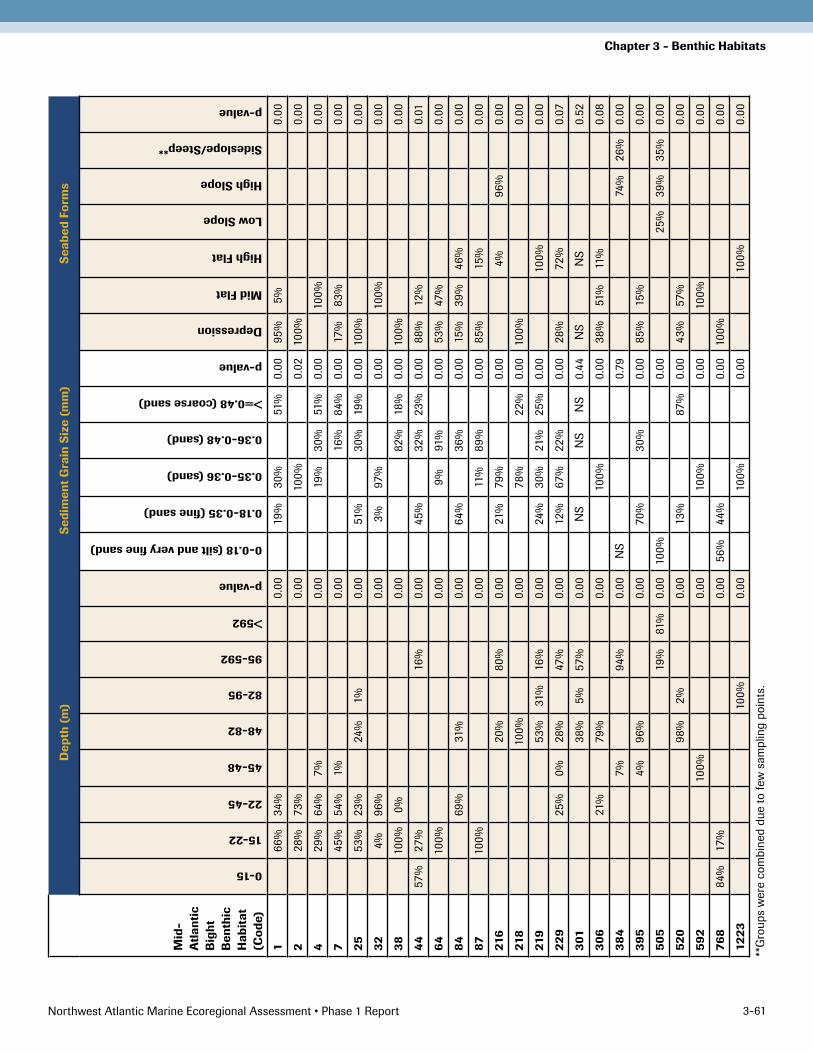
Northwest Atlantic Marine Ecoregional Assessment • Phase 1 Report 3-61
Chapter 3 - Benthic Habitats
Mid
-A
tlan
tic
Big
ht
Ben
thic
H
abit
at
(Cod
e)
Dep
th (
m)
Sed
imen
t G
rain
Siz
e (m
m)
Sea
bed
Form
s
0-15
15-22
22-45
45-48
48-82
82-95
95-592
>592
p-value
0-0.18 (silt and very fine sand)
0.18-0.35 (fine sand)
0.35-0.36 (sand)
0.36-0.48 (sand)
>=0.48 (coarse sand)
p-value
Depression
Mid Flat
High Flat
Low Slope
High Slope
Sideslope/Steep**
p-value
166
%34
%0.
0019
%30
%51
%0.
0095
%5%
0.00
2�8
%73
%0.
0010
0%0.
0�10
0%0.
00
4�9
%64
%7%
0.00
19%
30%
51%
0.00
100%
0.00
745
%54
%1%
0.00
16%
84%
0.00
17%
83%
0.00
2553
%�3
%�4
%1%
0.00
51%
30%
19%
0.00
100%
0.00
324%
96%
0.00
3%97
%0.
0010
0%0.
00
3810
0%0%
0.00
8�%
18%
0.00
100%
0.00
44
57%
�7%
16%
0.00
45%
3�%
�3%
0.00
88%
1�%
0.01
6410
0%0.
009%
91%
0.00
53%
47%
0.00
8469
%31
%0.
0064
%36
%0.
0015
%39
%46
%0.
00
8710
0%0.
0011
%89
%0.
0085
%15
%0.
00
216
�0%
80%
0.00
�1%
79%
0.00
4%96
%0.
00
218
100%
0.00
78%
��%
0.00
100%
0.00
219
53%
31%
16%
0.00
�4%
30%
�1%
�5%
0.00
100%
0.00
229
�5%
0%�8
%47
%0.
001�
%67
%��
%0.
00�8
%7�
%0.
07
301
38%
5%57
%0.
00N
SN
SN
S0.
44N
SN
S0.
5�
306
�1%
79%
0.00
100%
0.00
38%
51%
11%
0.08
384
7%94
%0.
00N
S0.
7974
%�6
%0.
00
395
4%96
%0.
0070
%30
%0.
0085
%15
%0.
00
505
19%
81%
0.00
100%
0.00
�5%
39%
35%
0.00
520
98%
�%0.
0013
%87
%0.
0043
%57
%0.
00
592
100%
0.00
100%
0.00
100%
0.00
768
84%
17%
0.00
56%
44%
0.00
100%
0.00
1223
100%
0.00
100%
0.00
100%
0.00
**G
roup
s w
ere
com
bine
d du
e to
few
sam
plin
g po
ints
.
Related Documents