Bayesian Statistics for Genetics Lecture 4: Linear Regression

Bayesian Statistics for Genetics

Lecture 4: Linear Regression

Ken Rice

Swiss Institute in Statistical Genetics

September, 2017

Regression models: overview

How does an outcome Y vary as a function of x = {x1, . . . , xp}?

• What are the effect sizes?

• What is the effect of x1, in observations that have the same

x2, x3, ...xp (a.k.a. “keeping these covariates constant”)?

• Can we predict Y as a function of x?

These questions can be assessed via a regression model p(y|x).

4.1

Regression models: overview

Parameters in a regression model can be estimated from data:

y1 x1,1 · · · x1,p... ... ...yn xn,1 · · · xn,p

The data are often expressed in matrix/vector form:

y =

y1...yn

XXX =

x1...xn

=

x1,1 · · · x1,p... ...

xn,1 · · · xn,p

4.2

FTO example: design

FTO gene is hypothesized to be involved in growth and obesity.

Experimental design:

• 10 fto+ /− mice

• 10 fto− /− mice

• Mice are sacrificed at the end of 1-5 weeks of age.

• Two mice in each group are sacrificed at each age.

4.3

FTO example: data

●

● ●

● ●

●

●

●

●●

●

●

●

●

●

●

●

●

●

●

1 2 3 4 5

510

1520

25

age (weeks)

wei

ght (

g)

●

●

fto−/−fto+/−

4.4

FTO example: analysis

• y = weight

• xg = indicator of fto heterozygote ∈ {0,1} = number of “+”

alleles

• xa = age in weeks ∈ {1,2,3,4,5}

How can we estimate p(y|xg, xa)?

Cell means model:

genotype age−/− θ0,1 θ0,2 θ0,3 θ0,4 θ0,5+/− θ1,1 θ1,2 θ1,3 θ1,4 θ1,5

Problem: 10 parameters – only two observations per cell

4.5

Linear regression

Solution: Assume smoothness as a function of age. For each

group,

y = α0 + α1xa + ε.

This is a linear regression model. Linearity means “linear in

the parameters”, i.e. several covariates, each multiplied by

corresponding α, and added.

A more complex model might assume e.g.

y = α0 + α1xa + α2x2a + α3x

3a + ε,

– but this is still a linear regression model, even with age2, age3

terms.

4.6

Multiple linear regression

With enough variables, we can describe the regressions for both

groups simultaneously:

Yi = β1xi,1 + β2xi,2 + β3xi,3 + β4xi,4 + εi , where

xi,1 = 1 for each subject i

xi,2 = 0 if subject i is homozygous, 1 if heterozygous

xi,3 = age of subject i

xi,4 = xi,2 × xi,3

Note that under this model,

E[Y |x, ] = β1 + β3 × age if x2 = 0, and

E[Y |x ] = (β1 + β2) + (β3 + β4)× age if x2 = 1.

4.7

Multiple linear regression

For graphical thinkers...

●

● ●

● ●

●

●

●

●●

●

●

●

●

●

●

●

●

●

●

510

1520

25w

eigh

t

β3 = 0 β4 = 0

●

● ●

● ●

●

●

●

●●

●

●

●

●

●

●

●

●

●

●

β2 = 0 β4 = 0

●

● ●

● ●

●

●

●

●●

●

●

●

●

●

●

●

●

●

●

1 2 3 4 5

510

1520

25

age

wei

ght

β4 = 0

●

● ●

● ●

●

●

●

●●

●

●

●

●

●

●

●

●

●

●

1 2 3 4 5age

4.8

Normal linear regression

How does each Yi vary around its mean E[Yi|βββ,xi ], ?

Yi = βββTxi + εi

ε1, . . . , εn ∼ i.i.d. normal(0, σ2).

This assumption of Normal errors specifies the likelihood:

p(y1, . . . , yn|x1, . . .xn,βββ, σ2) =

n∏i=1

p(yi|xi,βββ, σ2)

= (2πσ2)−n/2exp{−1

2σ2

n∑i=1

(yi − βββTxi)2}.

Note: in large(r) sample sizes, analysis is “robust” to the

Normality assumption—but here we rely on the mean being

linear in the x’s, and on the εi’s variance being constant with

respect to x.

4.9

Matrix form

• Let y be the n-dimensional column vector (y1, . . . , yn)T ;

• Let XXX be the n× p matrix whose ith row is xi

Then the normal regression model is that

y|XXX,βββ, σ2 ∼ multivariate normal (XXXβββ, σ2I),

where I is the p× p identity matrix and

XXXβββ =

x1 →x2 →

...xn →

β1

...βp

=

β1x1,1 + · · ·+ βpx1,p...

β1xn,1 + · · ·+ βpxn,p

=

EY1|βββ,x1...

EYn|βββ,xn

.

4.10

Ordinary least squares estimation

What values of βββ are consistent with our data y,XXX?

Recall

p(y1, . . . , yn|x1, . . .xn,βββ, σ2) = (2πσ2)−n/2exp{−

1

2σ2

n∑i=1

(yi−βββTxi)2}.

This is big when SSR(βββ) =∑

(yi − βββTxi)2 is small – where we

define

SSR(βββ) =n∑i=1

(yi − βββTxi)2 = (y −XXXβββ)T (y −XXXβββ)

= yTy − 2βββTXXXTy + βββTXXXTXXXβββ .

What value of βββ makes this the smallest, i.e. gives fitted values

closest to the outcomes y1, y2, ...yn?

4.11

OLS: with calculus

‘Recall’ that...

1. a minimum of a function g(z) occurs at a value z such thatddzg(z) = 0;

2. the derivative of g(z) = az is a and the derivative of g(z) =bz2 is 2bz.

Doing this for SSR...

d

dβββSSR(βββ) =

d

dβββ

(yTy − 2βββTXXXTy + βββTXXXTXXXβββ

)= −2XXXTy + 2XXXTXXXβββ ,

and sod

dβββSSR(βββ) = 0 ⇔ −2XXXTy + 2XXXTXXXβββ = 0

⇔ XXXTXXXβββ = XXXTy

⇔ βββ = (XXXTXXX)−1XXXTy .

β̂ββols = (XXXTXXX)−1XXXTy is the Ordinary Least Squares (OLS)estimator of βββ.

4.12

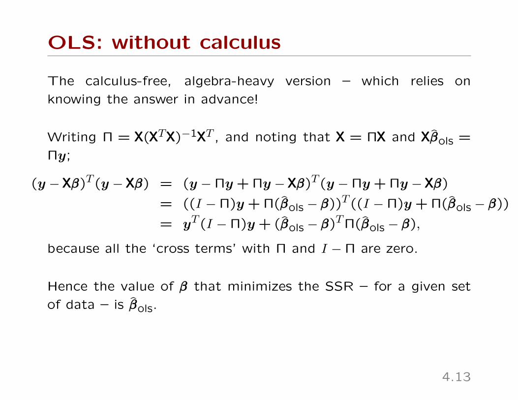
OLS: without calculus

The calculus-free, algebra-heavy version – which relies on

knowing the answer in advance!

Writing Π = XXX(XXXTXXX)−1XXXT , and noting that XXX = ΠXXX and XXXβ̂ββols =

Πy;

(y −XXXβββ)T (y −XXXβββ) = (y −Πy + Πy −XXXβββ)T (y −Πy + Πy −XXXβββ)

= ((I −Π)y + Π(β̂ββols − βββ))T ((I −Π)y + Π(β̂ββols − βββ))

= yT (I −Π)y + (β̂ββols − βββ)TΠ(β̂ββols − βββ),

because all the ‘cross terms’ with Π and I −Π are zero.

Hence the value of βββ that minimizes the SSR – for a given set

of data – is β̂ββols.

4.13

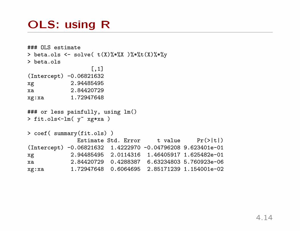
OLS: using R

### OLS estimate> beta.ols <- solve( t(X)%*%X )%*%t(X)%*%y> beta.ols

[,1](Intercept) -0.06821632xg 2.94485495xa 2.84420729xg:xa 1.72947648

### or less painfully, using lm()> fit.ols<-lm( y~ xg*xa )

> coef( summary(fit.ols) )Estimate Std. Error t value Pr(>|t|)

(Intercept) -0.06821632 1.4222970 -0.04796208 9.623401e-01xg 2.94485495 2.0114316 1.46405917 1.625482e-01xa 2.84420729 0.4288387 6.63234803 5.760923e-06xg:xa 1.72947648 0.6064695 2.85171239 1.154001e-02

4.14

OLS: using R

●

● ●

● ●

●

●

●

●●

●

●

●

●

●

●

●

●

●

●

1 2 3 4 5age

wei

ght

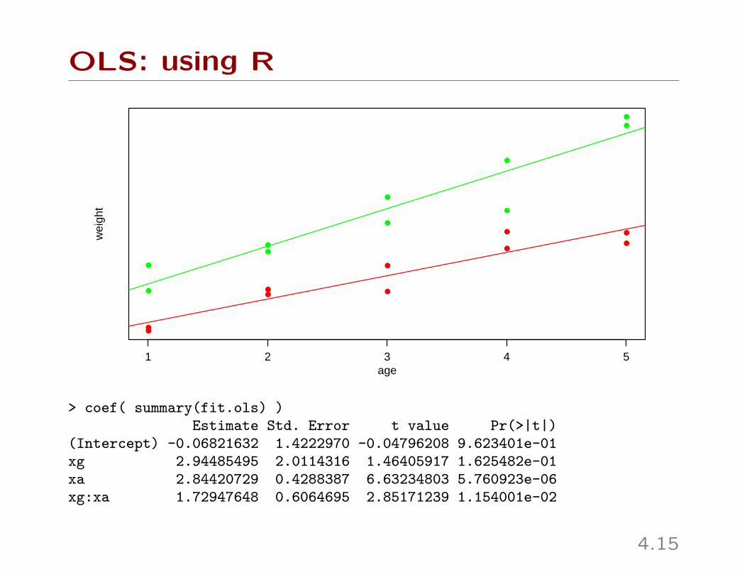
> coef( summary(fit.ols) )Estimate Std. Error t value Pr(>|t|)

(Intercept) -0.06821632 1.4222970 -0.04796208 9.623401e-01xg 2.94485495 2.0114316 1.46405917 1.625482e-01xa 2.84420729 0.4288387 6.63234803 5.760923e-06xg:xa 1.72947648 0.6064695 2.85171239 1.154001e-02

4.15

Bayesian inference for regression models

yi = β1xi,1 + · · ·+ βpxi,p + εi

Motivation:

• Incorporating prior information

• Posterior probability statements: P[βj > 0|y,XXX ]

• OLS tends to overfit when p is large, Bayes’ use of prior

tends to make it more conservative – as we’ll see

• Model selection and averaging (more later)

4.16

Prior and posterior distribution

prior βββ ∼ mvn(βββ0,Σ0)sampling model y ∼ mvn(XXXβββ, σ2I)posterior βββ|y,XXX ∼ mvn(βββn,Σn)

where

Σn = Varβββ|y,XXX, σ2 = (Σ−10 +XXXTXXX/σ2)−1

βββn = Eβββ|y,XXX, σ2 = (Σ−10 +XXXTXXX/σ2)−1(Σ−1

0 βββ0 +XXXTy/σ2).

Notice:

• If Σ−10 � XXXTXXX/σ2, then βββn ≈ β̂ββols

• If Σ−10 � XXXTXXX/σ2, then βββn ≈ βββ0

4.17

The g-prior

How to pick βββ0,Σ0? A classical suggestion (Zellner, 1986) usesthe g-prior:

βββ ∼ mvn(0, gσ2(XXXTXXX)−1)

Idea: The variance of the OLS estimate β̂ββols is

Varβ̂ββols = σ2(XXXTXXX)−1 =σ2

n(XXXTXXX/n)−1

This is (roughly) the uncertainty in βββ from n observations.

Varβββgprior = gσ2(XXXTXXX)−1 =σ2

n/g(XXXTXXX/n)−1

The g-prior can roughly be viewed as the uncertainty from n/g

observations.

For example, g = n means the prior has the same amount of infoas 1 observation – so (roughly!) not much, in a large study.

4.18

Posterior distributions under the g-prior

After some algebra, it turns out that

{βββ|y,XXX, σ2} ∼ mvn(βββn,Σn),

where Σn = Var[βββ|y,XXX, σ2 ] =g

g + 1σ2(XXXTXXX)−1

βββn = E[βββ|y,XXX, σ2 ] =g

g + 1(XXXTXXX)−1XXXTy

Notes:

• The posterior mean estimate βββn is simply gg+1β̂ββols.

• The posterior variance of βββ is simply gg+1Varβ̂ββols.

• g shrinks the coefficients towards 0 and can prevent overfit-

ting to the data

• If g = n, then as n increases, inference approximates that

using β̂ββols.

4.19

Monte Carlo simulation

What about the error variance σ2? It’s rarely known exactly, so

more realistic to allow for uncertainty with a prior...

prior 1/σ2 ∼ gamma(ν0/2, ν0σ20/2)

sampling model y ∼ mvn(XXXβββ, σ2I)posterior 1/σ2|y,XXX ∼ gamma([ν0 + n]/2, [ν0σ

20 + SSRg]/2)

where SSRg is somewhat complicated.

Simulating the joint posterior distribution:

joint distribution p(σ2,βββ|y,XXX) = p(σ2|y,XXX)× p(βββ|y,XXX, σ2)simulation {σ2,βββ} ∼ p(σ2,βββ|y,XXX) ⇔ σ2 ∼ p(σ2|y,XXX),βββ ∼ p(βββ|y,XXX, σ2)

To simulate {σ2,βββ} ∼ p(σ2,βββ|y,XXX),

• First simulate σ2 from p(σ2|y,XXX)

• Use this σ2 to simulate βββ from p(βββ|y,XXX, σ2)

Repeat 1000’s of times to obtain MC samples: {σ2,βββ}(1), . . . , {σ2,βββ}(S).

4.20

FTO example: Bayes

Priors:

1/σ2 ∼ gamma(1/2,3.678/2)

βββ|σ2 ∼ mvn(0, g × σ2(XXXTXXX)−1)

Posteriors:

{1/σ2|y,XXX} ∼ gamma((1 + 20)/2, (3.678 + 251.775)/2)

{βββ|y,XXX, σ2} ∼ mvn(.952× β̂ββols, .952× σ2(XXXTXXX)−1)

where

(XXXTXXX)−1 =

0.55 −0.55 −0.15 0.15−0.55 1.10 0.15 −0.30−0.15 0.15 0.05 −0.05

0.15 −0.30 −0.05 0.10

β̂ββols =

−0.0682.9452.8441.729

4.21

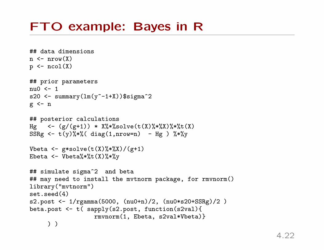
FTO example: Bayes in R

## data dimensionsn <- nrow(X)p <- ncol(X)

## prior parametersnu0 <- 1s20 <- summary(lm(y~-1+X))$sigma^2g <- n

## posterior calculationsHg <- (g/(g+1)) * X%*%solve(t(X)%*%X)%*%t(X)SSRg <- t(y)%*%( diag(1,nrow=n) - Hg ) %*%y

Vbeta <- g*solve(t(X)%*%X)/(g+1)Ebeta <- Vbeta%*%t(X)%*%y

## simulate sigma^2 and beta## may need to install the mvtnorm package, for rmvnorm()library("mvtnorm")set.seed(4)s2.post <- 1/rgamma(5000, (nu0+n)/2, (nu0*s20+SSRg)/2 )beta.post <- t( sapply(s2.post, function(s2val){

rmvnorm(1, Ebeta, s2val*Vbeta)}) )

4.22

FTO example: Bayes in R

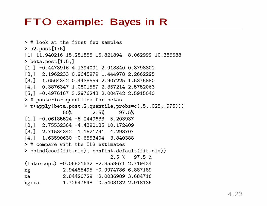
> # look at the first few samples> s2.post[1:5][1] 11.940216 15.281855 15.821894 8.062999 10.385588> beta.post[1:5,][1,] -0.4473916 4.1394091 2.918340 0.8798302[2,] 2.1962233 0.9645979 1.444978 2.2662295[3,] 1.6564342 0.4438559 2.907225 1.5375880[4,] 0.3876347 1.0801567 2.357214 2.5752063[5,] -0.4976167 3.2976243 2.004742 2.5915040> # posterior quantiles for betas> t(apply(beta.post,2,quantile,probs=c(.5,.025,.975)))

50% 2.5% 97.5%[1,] -0.06185524 -5.2449633 5.203937[2,] 2.75532364 -4.4390185 10.172409[3,] 2.71534342 1.1521791 4.293707[4,] 1.63590630 -0.6553404 3.840388> # compare with the OLS estimates> cbind(coef(fit.ols), confint.default(fit.ols))

2.5 % 97.5 %(Intercept) -0.06821632 -2.8558671 2.719434xg 2.94485495 -0.9974786 6.887189xa 2.84420729 2.0036989 3.684716xg:xa 1.72947648 0.5408182 2.918135

4.23

FTO example: Bayes in R

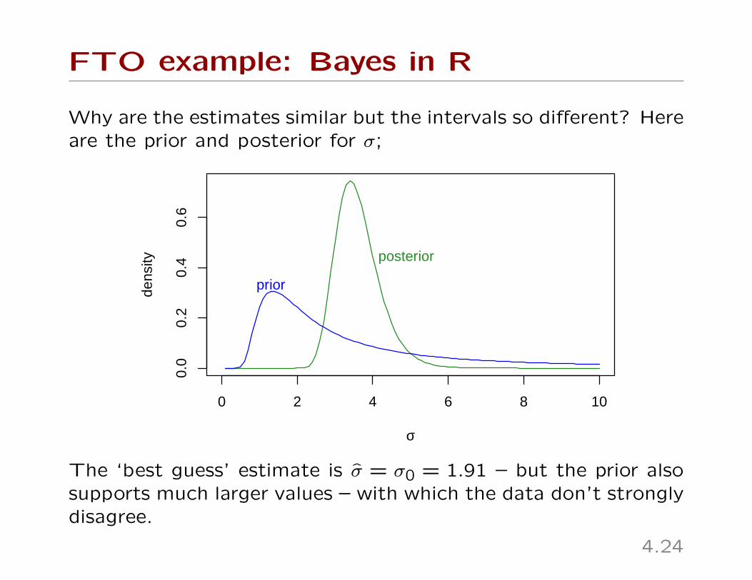
Why are the estimates similar but the intervals so different? Hereare the prior and posterior for σ;

0 2 4 6 8 10

0.0

0.2

0.4

0.6

σ

dens

ity

prior

posterior

The ‘best guess’ estimate is σ̂ = σ0 = 1.91 – but the prior alsosupports much larger values – with which the data don’t stronglydisagree.

4.24

FTO example: Bayes in R

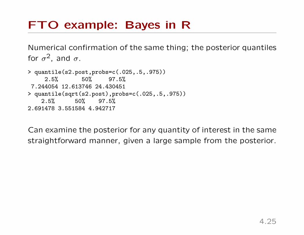
Numerical confirmation of the same thing; the posterior quantiles

for σ2, and σ.

> quantile(s2.post,probs=c(.025,.5,.975))2.5% 50% 97.5%

7.244054 12.613746 24.430451> quantile(sqrt(s2.post),probs=c(.025,.5,.975))

2.5% 50% 97.5%2.691478 3.551584 4.942717

Can examine the posterior for any quantity of interest in the same

straightforward manner, given a large sample from the posterior.

4.25

Posterior distributions

−10 0 10 20

0.00

0.02

0.04

0.06

0.08

0.10

β2

−4 −2 0 2 4 6 8

0.00

0.05

0.10

0.15

0.20

0.25

0.30

0.35

β4

−10 −5 0 5 10 15

−2

02

46

β2

β 4

4.26

Summarizing the genetic effect

Genetic effect = E[ y|age,+/− ]− E[ y|age,−/− ]

= [(β1 + β2) + (β3 + β4)× age]− [β1 + β3 × age]

= β2 + β4 × age

1 2 3 4 5

05

1015

age

β 2+

β 4ag

e

4.27

Numerical approximations

The Monte Carlo method is important for Bayesian work;

● ●

●

●

●

●

●

● ●

●

●

●

●

●

●

●

●

●

●

●

●

●

●

● ●

●

●●

●●

●

●

●

●●

●

●

●

●

●

●

●

●

●

●

●

●

●

●●

●●

●

●

●

●

●

●

● ●

●

●

●

●

●●

●

●

●

●

Large sample (points) to estimate posterior (contours)

θθ1

θθ 2

With a large sample from some distribution – i.e. the posterior

– we can approximate any property of that distribution. It does

not matter if how we get the sample.

4.28

Numerical approximations

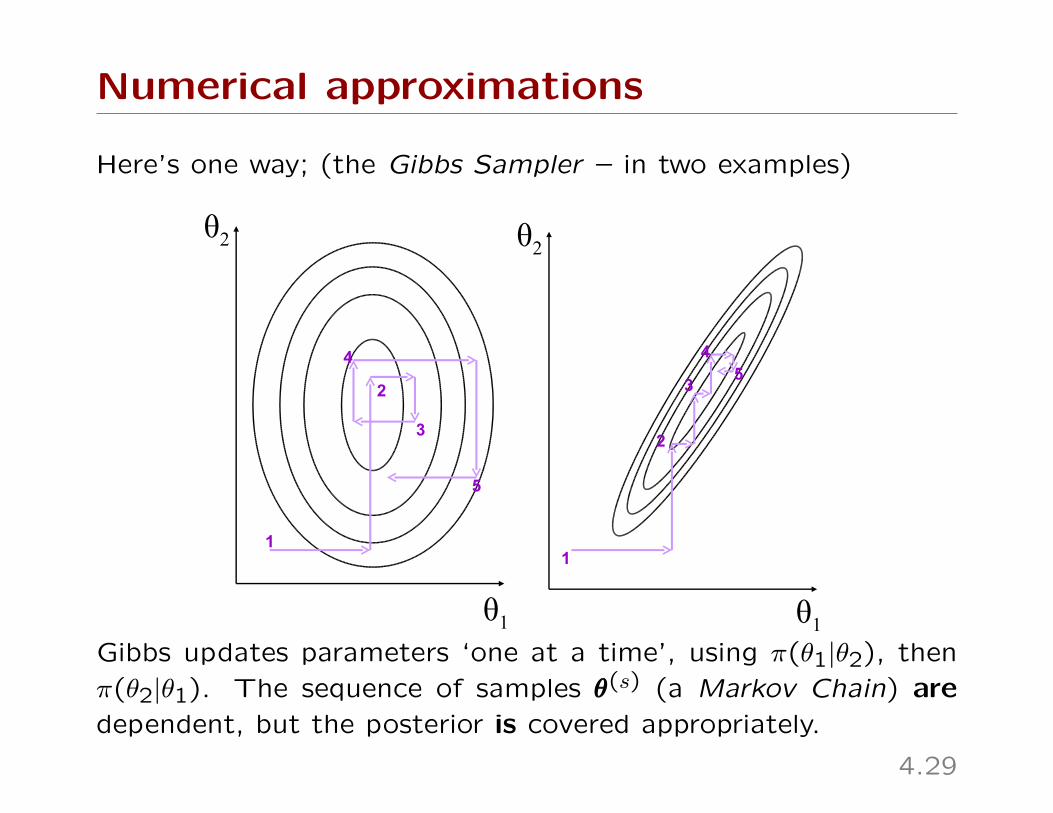
Here’s one way; (the Gibbs Sampler – in two examples)

θ1 θ1

θ2 θ2

1

3

4

5

1

2

3

45

2

Gibbs updates parameters ‘one at a time’, using π(θ1|θ2), then

π(θ2|θ1). The sequence of samples θθθ(s) (a Markov Chain) are

dependent, but the posterior is covered appropriately.

4.29

Numerical approximations

Algebra for the same thing; the posterior is

π(θ1, θ2|Y) ∝ f(Y|θ1, θ2)× π(θ1, θ2),

and is usually intractable. But it is equivalent to

π(θ1, θ2|Y) = p(θ2|Y)× p(θ1|θ2,Y),

and conditional p(θ1|θ2,Y) may be more readily-available.

Gibbs uses just the conditionals, iterating between these steps:

θ(s)1 ∼ p(θ1|θ

(s−1)2 ,Y)

θ(s)2 ∼ p(θ2|θ

(s)1 ,Y)

to produce the sequence

(θ(0)1 , θ

(0)2 ), (θ(1)

1 , θ(1)2 ), ..., (θ(s)

1 , θ(s)2 ), ...

• If the run is long enough (s→∞), this sequence is a samplefrom π(θ1, θ2|Y), no matter where you started• For more parameters, update each θk in turn, then start again

4.30

MCMC: with Stan

Stan does all these

steps for us;

• Specify a model, including priors, and tell Stan what the data

are

• Stan writes code to sample from the posterior, by ‘walking

around’ – actually it runs the No U-Turn Sampler, a more

• Stan runs this code, and reports back all the samples

• The rstan package lets you run chains from R

• Some modeling limitations – no discrete parameters – but

becoming very popular; works well with some models where

other software would struggle

• Requires declarations (like C++) – unlike R – so models

require a bit more typing...

4.31

MCMC: with Stan

A first attempt at the FTO example, running Stan from within

R;

cat(file="FTOexample.stan", "data {

int n; //the number of observationsint p; //the number of columns in the model matrixreal y[n]; //the responsematrix[n,p] X; //the model matrixreal g; // Zellner scale factorvector[p] mu; // Zellner prior mean (all zeros)matrix[p,p] XtXinv; // information matrixreal sigma; // std dev’n, assumed known

}parameters {

vector[p] beta; //the regression parameters}transformed parameters {

vector[n] linpred;cov_matrix[p] Sigma;linpred = X*beta;for (j in 1:p){

for (k in 1:p){

4.32

MCMC: with Stan

Sigma[j,k] = g*sigma^2*XtXinv[j,k];}

}}model {

beta ~ multi_normal(mu, Sigma);y ~ normal(linpred, sigma);

}")

# do the MCMC, store the resultslibrary("rstan")stan1 <- stan(file = "FTOexample.stan", data = list(

n=n,p=p, y=y, X=X, g=n, mu=rep(0,p), XtXinv=solve(crossprod(X)),sigma=sqrt(s20)), iter = 100000, chains = 1, pars="beta")

• Most of the work involves writing a model file (though our

‘model’ is only two lines!)

• We use 100,000 iterations – which takes only a few seconds

4.33

MCMC: with Stan

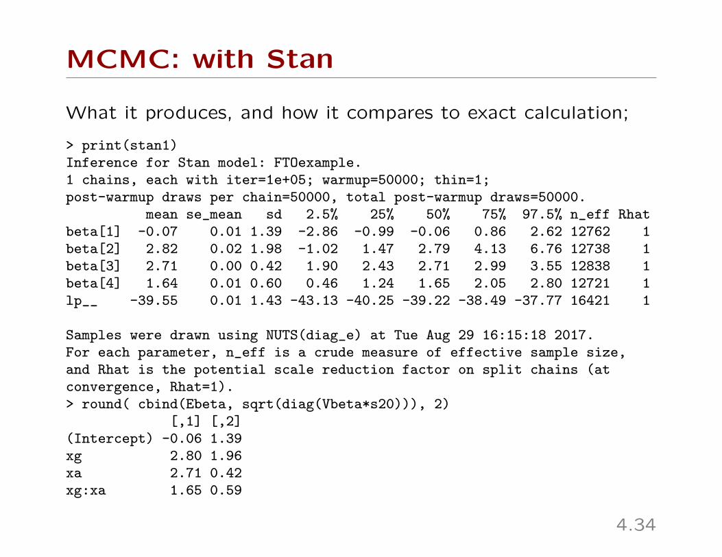
What it produces, and how it compares to exact calculation;

> print(stan1)Inference for Stan model: FTOexample.1 chains, each with iter=1e+05; warmup=50000; thin=1;post-warmup draws per chain=50000, total post-warmup draws=50000.

mean se_mean sd 2.5% 25% 50% 75% 97.5% n_eff Rhatbeta[1] -0.07 0.01 1.39 -2.86 -0.99 -0.06 0.86 2.62 12762 1beta[2] 2.82 0.02 1.98 -1.02 1.47 2.79 4.13 6.76 12738 1beta[3] 2.71 0.00 0.42 1.90 2.43 2.71 2.99 3.55 12838 1beta[4] 1.64 0.01 0.60 0.46 1.24 1.65 2.05 2.80 12721 1lp__ -39.55 0.01 1.43 -43.13 -40.25 -39.22 -38.49 -37.77 16421 1

Samples were drawn using NUTS(diag_e) at Tue Aug 29 16:15:18 2017.For each parameter, n_eff is a crude measure of effective sample size,and Rhat is the potential scale reduction factor on split chains (atconvergence, Rhat=1).> round( cbind(Ebeta, sqrt(diag(Vbeta*s20))), 2)

[,1] [,2](Intercept) -0.06 1.39xg 2.80 1.96xa 2.71 0.42xg:xa 1.65 0.59

4.34

MCMC: with Stan

Now the full version, with the inverse-gamma prior on σ2;

cat(file="FTOexample.stan", "data {

int n; //the number of observationsint p; //the number of columns in the model matrixreal y[n]; //the responsematrix[n,p] X; //the model matrixreal g; // Zellner scale factorvector[p] mu; // Zellner prior mean (all zeros)matrix[p,p] XtXinv; // information matrix

}parameters {

vector[p] beta; //the regression parametersreal invsigma2; //the standard deviation

}transformed parameters {

vector[n] linpred;cov_matrix[p] Sigma;real sigma;linpred = X*beta;sigma = 1/sqrt(invsigma2);for (j in 1:p){

4.35

MCMC: with Stan

for (k in 1:p){Sigma[j,k] = g*sigma^2*XtXinv[j,k];}

}}model {

beta ~ multi_normal(mu, Sigma);y ~ normal(linpred, sigma);invsigma2 ~ gamma(0.5, 1.839);

}")

# do the MCMC, store the resultslibrary("rstan")stan2 <- stan(file = "FTOexample.stan",data = list(n=n,p=p, y=y, X=X, g=n, mu=rep(0,p), XtXinv=solve(crossprod(X)) ),iter = 100000, chains = 1, pars=c("beta","sigma"))

4.36

MCMC: with Stan

And comparing the output again;

> print(stan2)Inference for Stan model: FTOexample.1 chains, each with iter=1e+05; warmup=50000; thin=1;post-warmup draws per chain=50000, total post-warmup draws=50000.

mean se_mean sd 2.5% 25% 50% 75% 97.5% n_eff Rhatbeta[1] -0.09 0.02 2.66 -5.32 -1.85 -0.08 1.65 5.13 15022 1beta[2] 2.84 0.03 3.73 -4.46 0.38 2.84 5.29 10.25 14829 1beta[3] 2.72 0.01 0.80 1.14 2.19 2.71 3.25 4.29 15065 1beta[4] 1.64 0.01 1.12 -0.60 0.90 1.63 2.38 3.85 14780 1sigma 3.62 0.00 0.59 2.69 3.20 3.55 3.95 4.97 18325 1lp__ -42.49 0.01 1.65 -46.59 -43.34 -42.15 -41.27 -40.32 15016 1

> round(t(apply( cbind(beta.post, sqrt(s2.post)), 2,+ function(x){c(m=mean(x), sd=sd(x), quantile(x, c(0.025, 0.5, 0.975)))})), 2)

m sd 2.5% 50% 97.5%[1,] -0.05 2.57 -5.14 -0.04 5.07[2,] 2.77 3.62 -4.38 2.76 9.90[3,] 2.70 0.77 1.17 2.70 4.23[4,] 1.66 1.09 -0.50 1.66 3.83[5,] 3.50 0.54 2.63 3.43 4.74

4.37

MCMC: with Stan

To see where the the ‘chain’ went...

> traceplot(stan2)

4.38

MCMC: summary so far

• Stan - and other similar software - may look like overkill for

this ‘conjugate’ problem, but Stan can provide posteriors for

almost any model

• The ‘modeling’ language is modeled on R

• Users do have to decide how long a chain to run, and how

long to ‘burn in’ for at the start of the chain. These are not

easy to answer! We’ll see some diagnostics in later sessions

4.39

Bonus: what if the model’s wrong?

Different types of violation—in decreasing order of how much

they typically matter in practice

• Just have the wrong data (!) i.e. not the data you claim to

have

• Observations are not independent, e.g. repeated measures

on same mouse over time

• Mean model is incorrect

• Error terms do not have constant variance

• Error terms are not Normally distributed

4.40

Wrong model: dependent outcomes

• Observations from the same mouse are more likely to be

similar than those from different mice (even if they have

same age and genotype)

• SBP from subjects (even with same age, genotype etc) in

the same family are more likely to be similar than those in

different familes – perhaps unmeasured common diet?

• Spatial and temporal relationships also tend to induce

correlation

If the pattern of relationship is known, can allow for it – typically

in “random effects modes” – see later session.

If not, treat results with caution! Precision is likely over-stated.

4.41

Wrong model: mean model

Even when the scientific background is highly informative aboutthe variables of interest (e.g. we want to know about theassociation of Y with x1, adjusting for x2, x3...) there is rarelystrong information about the form of the model

• Does mean weight increase with age? age2? age3?• Could the effect of genotype also change non-linearly with

age?

Including quadratic terms is a common approach – but quadraticsare sensitive to the tails. Instead, including “spline” representa-tions of covariates allows the model to capture many patterns.

Including interaction terms (as we did with xi,2 × xi,3) lets onecovariate’s effect vary with another.

(Deciding which covariates to use is addressed in the ModelChoice session.)

4.42

Wrong model: non-constant variance

This is plausible in many situations; perhaps e.g. young miceare harder to measure, i.e. more variables. Or perhaps the FTOvariant affects weight regulation — again, more variance.

• Having different variances at different covariate values isknown as heteroskedasticity• Unaddressed, it can result in over- or under-statement of

precision

The most obvious approach is to model the variance, i.e.

Yi = βββTxi + εi,

εi ∼ Normal(0, σ2i ),

where σi depends on covariates, e.g. σhomozy and σheterozy forthe two genotypes.

Of course, these parameters need priors. Constraining variancesto be positive also makes choosing a model difficult in practice.

4.43

Robust standard errors (in Bayes)

In linear regression, some robustness to model-misspecification

and/or non-constant variance is available – but it relies on

interest in linear ‘trends’. Formally, we can define parameter

θθθ = argmin Ex[(Ey[y|x]−XXXtθθθ

)2],

i.e. the straight line that best-captures random-sampling, in a

least-squares sense.

• This ‘trend’ can capture important features in how the mean

y varies at different x

• Fitting extremely flexible Bayesian models, we get a posterior

for θθθ

• The posterior mean approaches β̂ββols, in large samples

• The posterior variance approaches the ‘robust’ sandwich

estimate, in large samples (details in Szpiro et al, 2011)

4.44

Robust standard errors (in Bayes)

The OLS estimator can be written as β̂ββols = (XXXTXXX)−1XXXTy =∑ni=1 ciyi, for appropriate ci.

True variance Var[ β̂ ] =∑ni=1 c

2i Var[Yi ]

Robust estimate V̂arR[ β̂ ] =∑ni=1 c

2i e

2i

Model-based estimate V̂arM [ β̂ ] = Mean(e2i )∑ni=1 c

2i ,

where ei = yi − xTi β̂ββols, the residuals from fitting a linear model.

Non-Bayesian sandwich estimates are available through R’s

sandwich package – much quicker than Bayes with a very-

flexible model. For correlated outcomes, see the GEE package

for generalizations.

4.45

Wrong model: Non-Normality

This is not a big problem for learning about population param-

eters;

• The variance statements/estimates we just saw don’t rely on

Normality

• The central limit theorem means that β̂ββ ends up Normal

anyway, in large samples

• In small samples, expect to have limited power to detect

non-Normality

• ... except, perhaps, for extreme outliers (data errors?)

For prediction – where we assume that outcomes do follow a

Normal distibution – this assumption is more important.

4.46

Summary

• Linear regressions are of great applied interest

• Corresponding models are easy to fit, particularly with

judicious prior choices

• Assumptions are made — but a well-chosen linear regression

usually tells us something of interest, even if the assump-

tions are (mildly) incorrect

4.47