Bayesian quantile regression

BAYESIAN QUANTILE REGRESSION

Tony LancasterSung Jae Jun

THE INSTITUTE FOR FISCAL STUDIESDEPARTMENT OF ECONOMICS, UCL

cemmap working paper CWP05/06

Bayesian Quantile RegressionTony Lancaster1 and Sung Jae Jun

Brown UniversityDecember 2005

1. Introduction:Recent work by Schennach(2005) has opened the way to a Bayesian treat-

ment of quantile regression. Her method, called Bayesian exponentially tiltedempirical likelihood (BETEL), provides a likelihood for data y subject only to aset of m moment conditions of the form Eg(y, θ) = 0 where θ is a k dimensionalparameter of interest and k may be smaller, equal to or larger than m. Themethod may be thought of as construction of a likelihood supported on the ndata points that is minimally informative, in the sense of maximum entropy,subject to the moment conditions. Specifically the probabilities {pi} attachedto the n data points are chosen to solve

maxpΣni=1 − pi log pi subject to Σni=1pi = 1 and Σni=1pig(yi, θ) = 0 (1)

The solutions of this problem, well known in the maximum entropy litera-ture, e.g. Jaynes(2003, p.357), take the form

pi(θ) =exp{λ(θ)0g(yi, θ)}

Σnj=1 exp{λ(θ)0g(yi, θ)}(2)

where m vector λ, dependent on θ, satisfies

λ(θ) = argminηn−1Σni=1 exp{η0g(yi, θ)}. (3)

The {λi} are the Lagrange multipliers corresponding to the m constraints inthe problem (1). For every θ (3) is a convex minimization problem and compu-tationally straightforward.The resulting likelihood for i.i.d data is Πni=1pi(θ) and this may be combined

with a prior density on θ to yield the posterior density

p(θ|Y ) = p(θ)Πni=1pi(θ) (4)

on a support such that 0 is in the convex hull of the g(yi, θ).In this paper we explore the application of this method to the case where

the moments g(yi, θ) correspond to those of quantiles or quantile regressionfunctions.

We first consider the quantiles of a random variable and give an explicitform for the posterior distributions and a comparison with the Bayesian boot-strap posterior. We then consider posterior distributions for quantile regres-sion functions. Finally we consider the model studied by Chernozhukov and

1Correspondence to first author, Department of Economics, Brown University, ProvidenceRI 02912; [email protected]

1

Hansen(2004) of quantile regression with endogenous regressors. We show thatthe Schennach approach leads to an alternative way to do inference about struc-tural quantile functions than that proposed by these authors. For each class ofmodels we consider how to construct marginal posterior densities.

2. Quantiles:Consider first Bayesian inference about quantiles. The τ 0th quantile θτ sat-

isfies the moment restriction E(g) = 0 where

g = 1(y ≤ θτ )− τ

where 1(.) is the indicator function. Given a random sample of size n and for anyθ in [min y,max y) the Lagrange multiplier λ solving the problem (3) satisfiesthe equation

Σni=1gieλgi = 0

with solution

eλ(θ) =τn0

(1− τ)n1where n1 = ](yi ≤ θτ ) and n0 = n− n1.

Substituting this solution into the expression for the posterior density (4) andassuming a uniform prior gives

p(θτ |y) ∝ φn1

nn11 nn00

, φ =τ

1− τ. (5)

This is a piecewise constant density supported on [min(yi),max(yi)).The density (5) may be sampled as follows. There are n − 1 pieces, if the

observations are all distinct, forming a partition of the interval from min(yi) tomax(yi). Sample each piece according to its probabilitity. If the sampled pieceis bounded by y(j) and y(j+1) sample a random variable uniformly distributedon this interval.Figure 1 shows the posterior density of the median from a random sample

of size n = 40 using a uniform prior. The step function (red) is (5) and thecontinuous curve (blue) is the posterior density corresponding to a doubleexponential density of the form

f(y|θ) ∝ exp{−|y − θ|}.

The vertical line shows the sample median. Both curves have been normalizedto integrate to one. Posterior distributions are always piecewise constant, as inthe figure. Highest posterior density intervals with (possibly approximate) 95%etc. probability content are straightforward to construct.3. Comparison with the Bayesian Bootstrap:The Bayesian bootstrap of Rubin(1981) takes the data to be iid multinomial

with probabilities {pi}. An improper Dirichlet prior on these probabilities leads

2

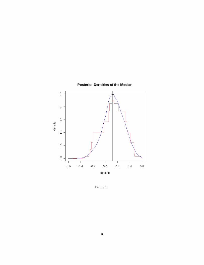
Figure 1:

3

to a Dirichlet posterior that assigns positive probability only to the distinctsample observations and in this respect is similar to BETEL. Paremeters suchas quantiles that can be expressed as functionals of the data distribution haveposterior distributions that can be calculated by repeatedly simulating from theposterior distribution of the {pi} and calculating the parameter of interest. AsChamberlain and Imbens(2003) point out, the posterior distribution of quantileregression parameters can be simulated by repeatedly solving the problem

θ = argmintΣni=1cτ (Viyi − t0Vixi), {Vi} ∼ iid E(1). (6)

Here cτ is the check function defined by cτ (u) = 2u(τ − I(u < 0)). Thisproblem may be solved using Koenker’s quantile regression R function rq(y~x,tau, weights=..) by letting the weights be n unit exponentials.To compare the Bayesian bootstrap and BETEL (uniform prior) posteriors

we consider inference about the median — τ = 0.5 — using a sample n = 500standard normal variates. To get the BB posterior we solved the problem (6)10,000 times and drew the histogram of the realizations. This is shown in figure(2). Note the sparsity of the Bayeian bootstrap distribution which reflects thefact that there were only 162 distinct realizations among the 10,000 draws eventhough the sample size was 500. This arises because the criterion function in (6)is a piecewise linear function with knots at the data points so solutions of theproblem will always lie at one of the data points2. Hence there can be at mostn points of support for the Bayesian bootstrap distribution and with n = 500most of these will have probability so low that they will not occur in a sample of10,000 realizations. By contrast, the BETEL distibution, shown in red, providespositive probability density over the relevant interval.3

It seems that the Bayesian bootstrap provides a less appealing posterior thanSchennach’s method in this application. This is in addition to to its other wellknown drawbacks.4. Regression Quantiles:The τ 0th quantile regression is such that

Pr(Y ≤ α(τ) + β(τ)X|X) = τ

and so satisfies the moment conditions

E(1(Y ≤ α(τ) + β(τ)X)− τ |X) = 0E(X1(Y ≤ α(τ) + β(τ)X)− τ |X) = 0

If we now define

g1i = 1(yi ≤ α+ βxi)− τ

and g2i = xi(1(yi ≤ α+ βxi)− τ)

2This assumes that if there is a flat section at the minimum the solution is chosen as oneof the two data points between which the function is flat.

3These BB realizations were computed in R according to the program g <- rexp(n); g <-g/sum(g); coef(rq(y ~1, weights = g)). The sample median was 0.078.

4

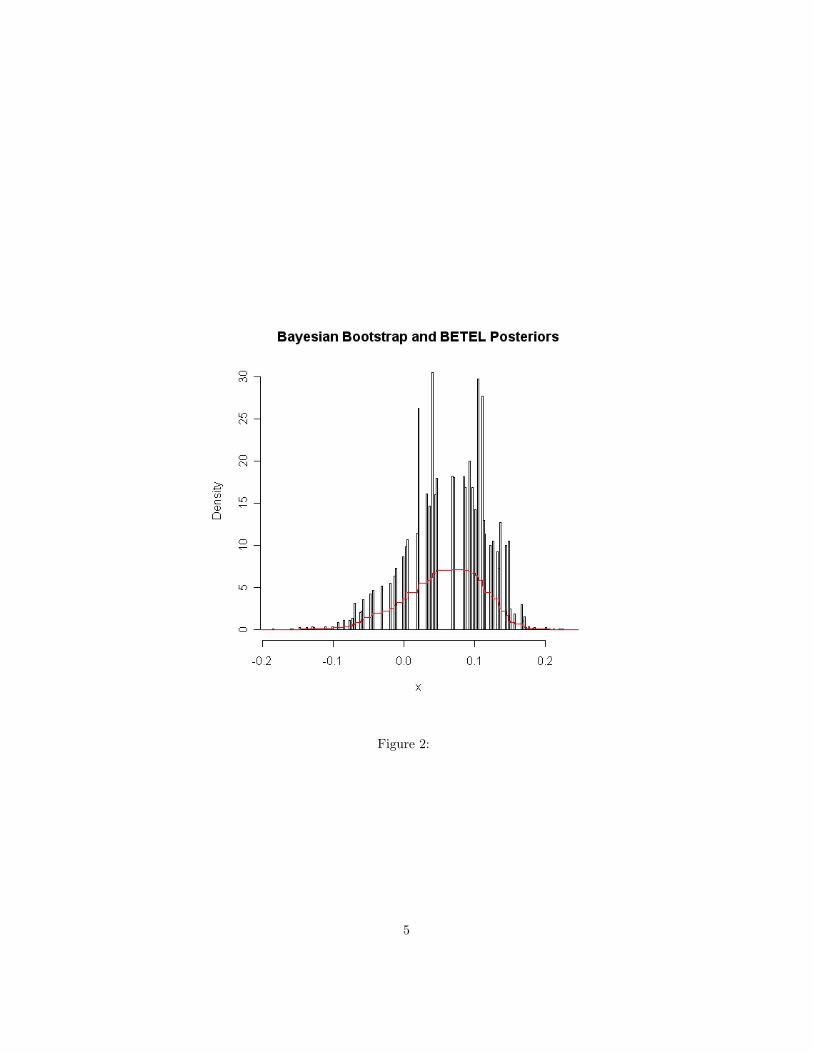
Figure 2:

5

we may compute the Lagrange multipliers λ1 and λ2 by

λ = argminηΣni=1 exp{η1g1i + η2g2i}

and then calculate the posterior density according to (2).Figure 3 plots the joint posterior density of α(0.5) and β(0.5) from a sample

of n = 111 observations and under a uniform prior. The data are Graddy’s(1995)fish market observations with Y as log quantity traded and X as log price. Toconstruct figure 3 the density was evaluated on a 100× 100 grid of α,β values.As the figure shows the density consists of adjoining flat surfaces. The marginaldensities of α and β may be calculated by summing this grid across rows oracross columns. Figure (4) shows the marginal density of the price elasticity ofdemand at the 0.5 quantile found in this way. The quantile regression estimateof β(0.5) using the R program previously mentioned was −0.414 which can beseen to be close to the marginal posterior mode.4. Quantiles With Endogenous Covariates.Quantile regression applied to the observations on price and quantity neglects

the simultaneity of these variables when the market is in equilibrium. This canbe surmounted by use of instrumental variables.Recall that if the τ 0th quantile is denoted α(τ) then we can represent our

random variable as

Y = α(U), U ∼ Uniform(0, 1), α(.) strictly increasing,

sincePr(Y ≤ α(τ)) = Pr(α(U) ≤ α(τ)) = Pr(U ≤ τ) = τ .

and so α(τ) is the quantile function.Similarly, a regression quantile can be represented by

Y = α(U)+β(U)X, U |X ∼ Uniform(0, 1), α(τ)+β(τ)X strictly increasing in τ .

with τ 0th conditional quantile equal to α(τ) + β(τ)X.Following Chernozhukov and Hansen(2004) consider the model

Y = D0α(U) +X 0β(U), U |X,Z ∼ Uniform(0, 1)

in whichD is statistically dependent on U, D0α(τ)+X 0β(τ) is strictly increasingin τ , and Z is a set of instrumental variables that are independent of U butstatistically dependent on D. Then D0α(τ) +X 0β(τ) is the τ 0th quantile of Yconditional on X,Z. That is,

Pr(Y ≤ D0α(τ) +X 0β(τ)|X,Z) = τ (7)

The expressionD0α(τ) +X 0β(τ)

4This was computed using rq(Q~P) in R, where Q and P are logarithms of quantity andprice.

6

Figure 3:

7

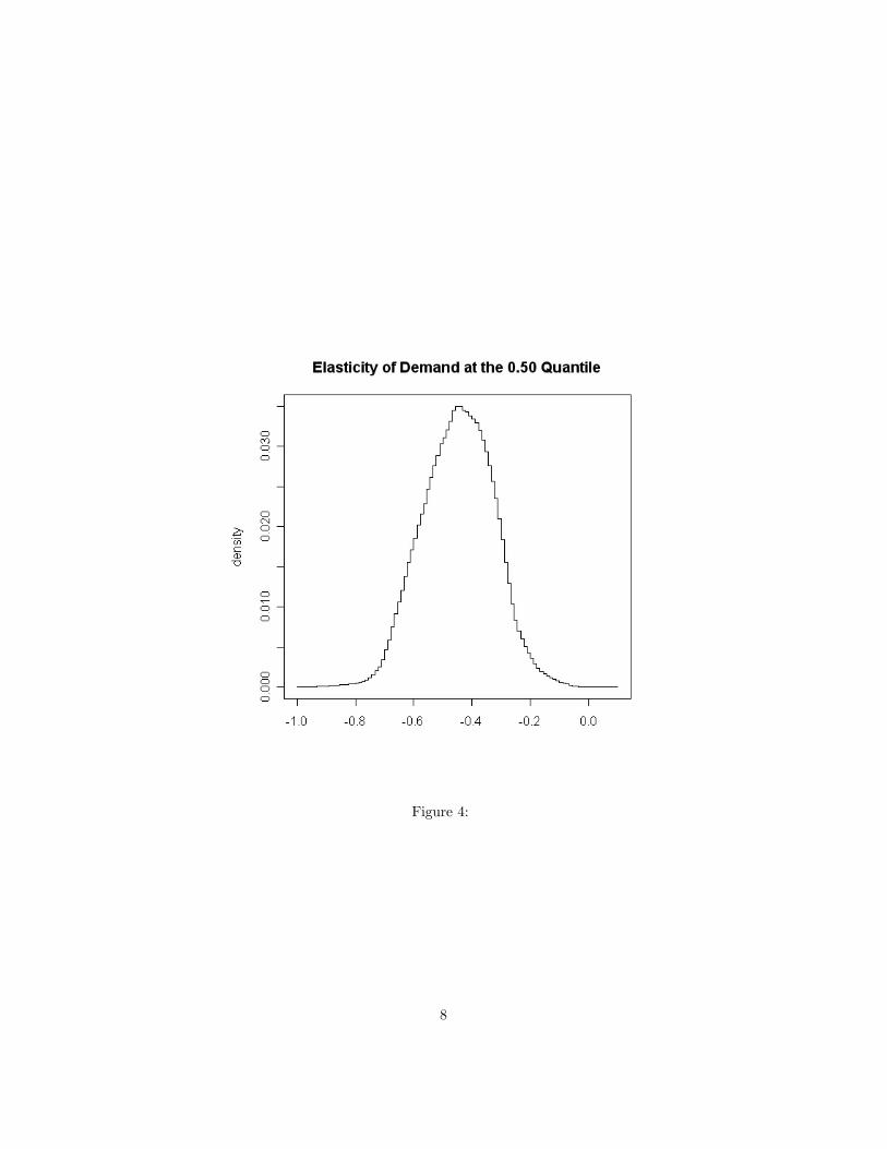
Figure 4:

8

is what Chernozhukov and Hansen refer to as the structural quantile function.The fact (6) then leads to conditional moments of which the simplest are of theform

X 0i(1(yi ≤ D0

iα(τ) +X0iβ(τ))− τ)

Z0i(1(yi ≤ D0iα(τ) +X

0iβ(τ))− τ)

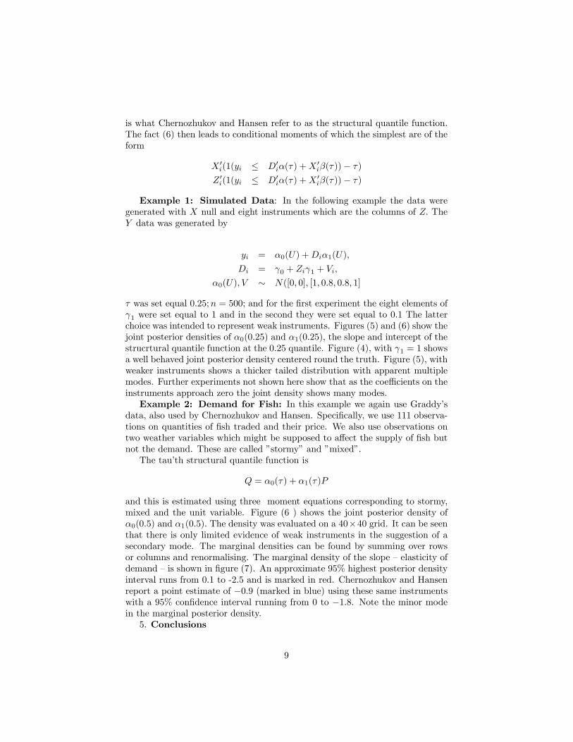
Example 1: Simulated Data: In the following example the data weregenerated with X null and eight instruments which are the columns of Z. TheY data was generated by

yi = α0(U) +Diα1(U),

Di = γ0 + Ziγ1 + Vi,

α0(U), V ∼ N([0, 0], [1, 0.8, 0.8, 1]

τ was set equal 0.25;n = 500; and for the first experiment the eight elements ofγ1 were set equal to 1 and in the second they were set equal to 0.1 The latterchoice was intended to represent weak instruments. Figures (5) and (6) show thejoint posterior densities of α0(0.25) and α1(0.25), the slope and intercept of thestrucrtural quantile function at the 0.25 quantile. Figure (4), with γ1 = 1 showsa well behaved joint posterior density centered round the truth. Figure (5), withweaker instruments shows a thicker tailed distribution with apparent multiplemodes. Further experiments not shown here show that as the coefficients on theinstruments approach zero the joint density shows many modes.Example 2: Demand for Fish: In this example we again use Graddy’s

data, also used by Chernozhukov and Hansen. Specifically, we use 111 observa-tions on quantities of fish traded and their price. We also use observations ontwo weather variables which might be supposed to affect the supply of fish butnot the demand. These are called ”stormy” and ”mixed”.The tau’th structural quantile function is

Q = α0(τ) + α1(τ)P

and this is estimated using three moment equations corresponding to stormy,mixed and the unit variable. Figure (6 ) shows the joint posterior density ofα0(0.5) and α1(0.5). The density was evaluated on a 40×40 grid. It can be seenthat there is only limited evidence of weak instruments in the suggestion of asecondary mode. The marginal densities can be found by summing over rowsor columns and renormalising. The marginal density of the slope — elasticity ofdemand — is shown in figure (7). An approximate 95% highest posterior densityinterval runs from 0.1 to -2.5 and is marked in red. Chernozhukov and Hansenreport a point estimate of −0.9 (marked in blue) using these same instrumentswith a 95% confidence interval running from 0 to −1.8. Note the minor modein the marginal posterior density.5. Conclusions

9

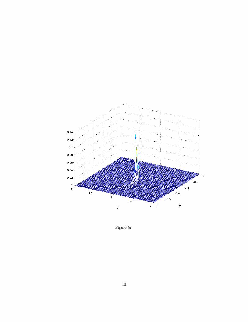
Figure 5:

10

Figure 6:

11

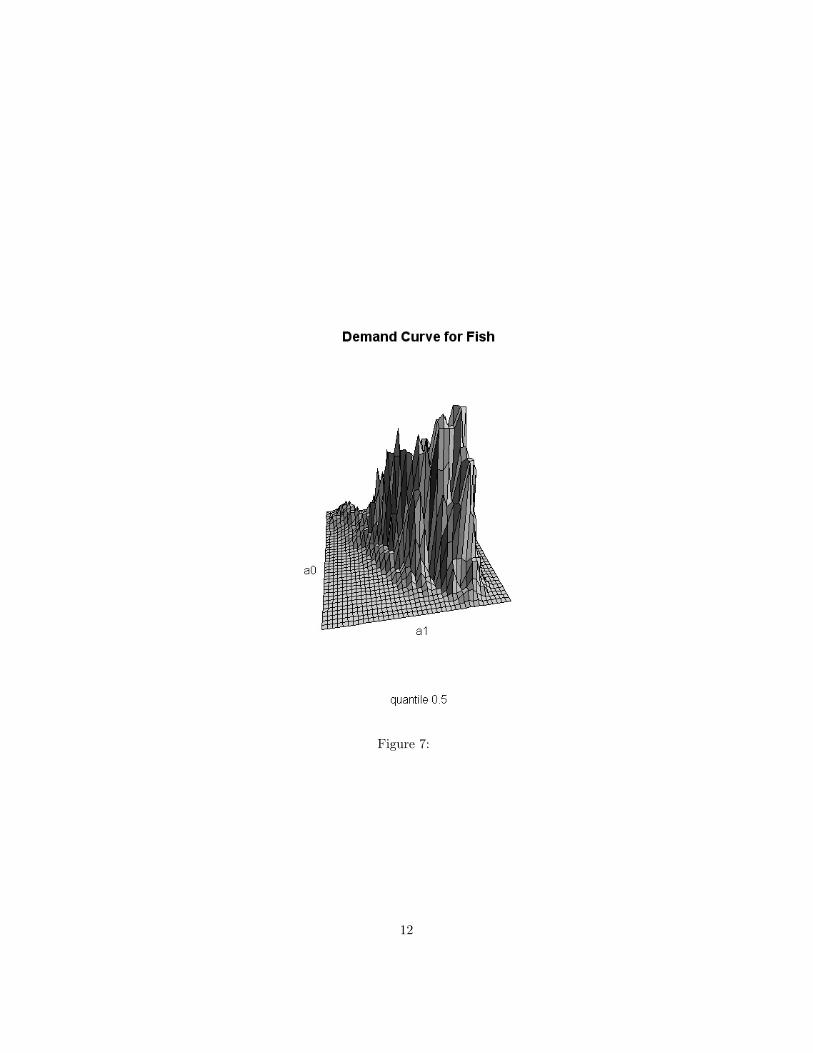
Figure 7:

12

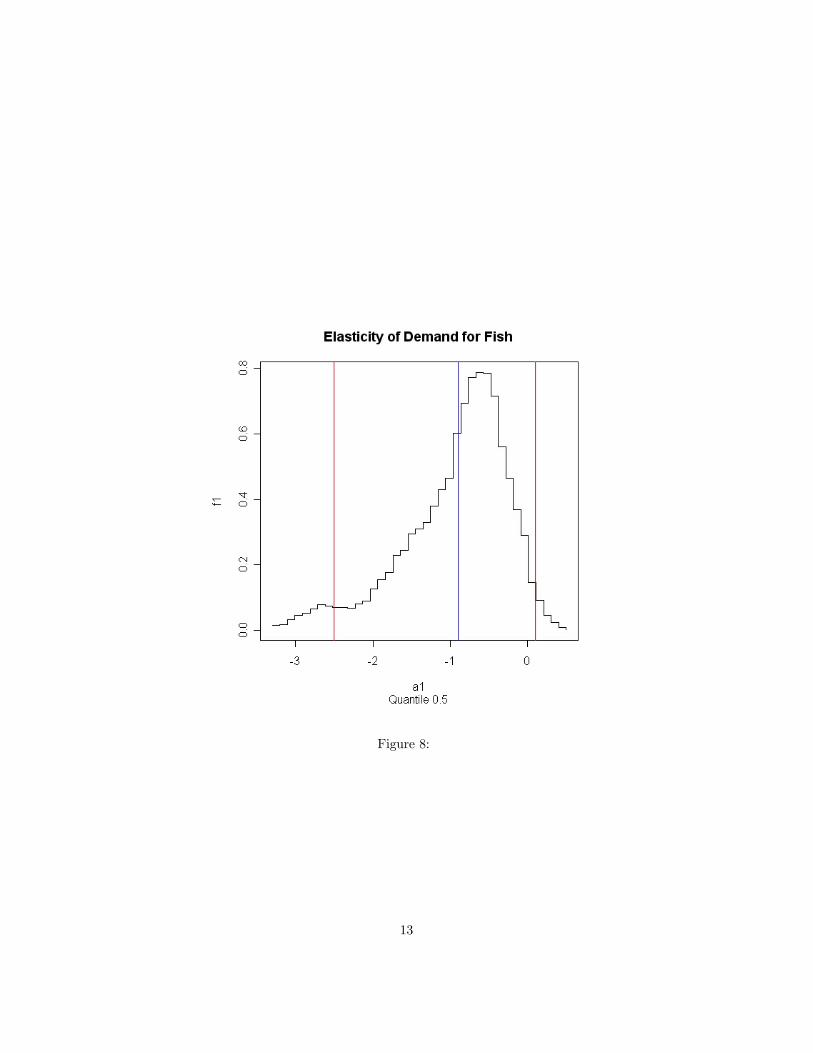
Figure 8:

13

Schennach’s method represents a way of doing Bayesian inference aboutquantile regression models without using a potentially restrictive parametriclikelihood. When the number of parameters of interest is small, as in the il-lustrations used in this paper, marginal posterior distributions can be easilyevaluated by evaluating the joint posterior density on a grid, summing over theunwanted dimensions and renormalizing if necessary. When the dimensionalityof the parameter of interest is larger it is likely to be preferable to use MCMCmethods. In initial experiments not reported here we have used a Metropo-lis/Hasting sampler with a proposal distribution formed from an overdispersedversion of the asymptotic multivariate normal posterior density. This appears tobe satisfactory except when identification is very weak and the posterior densityhas multiple modes. Results on this point will be given in future versions of thispaper.

14

References

Chamberlain, G. and G. W. Imbens Nonparametric applications of Bayesianinference, Journal of Business and Economic Statistics, 2003, 21, 1, 12-18.Chernozhukov, V. and C. Hansen Instrumental variable quantile regression,

unpublished ms, version of December 2004.Graddy, K. Testing for imperfect competition in the Fulton fish market, Rand

Journal of Economics, 1995 26(1),75-92.Jaynes, E. T. Probability theory:the logic of science Cambridge University

Press 2003.Rubin, D. The Bayesian bootstrap, The Annals of Statistics, 1981, 9, 130-

134.Schennach, S. M. Bayesian exponentially tilted empirical likelihood, Bio-

metrika 2005 92 (1), 31-46.

15