Hindawi Publishing Corporation Mathematical Problems in Engineering Volume 2012, Article ID 329489, 18 pages doi:10.1155/2012/329489 Research Article Bayesian Analysis of the Survival Function and Failure Rate of Weibull Distribution with Censored Data Chris Bambey Guure 1 and Noor Akma Ibrahim 1, 2 1 Institute for Mathematical Research, Universiti Putra Malaysia, 43400 Serdang, Selangor, Malaysia 2 Department of Mathematics, Universiti Putra Malaysia, 43400 Serdang, Selangor, Malaysia Correspondence should be addressed to Chris Bambey Guure, [email protected] Received 17 August 2012; Accepted 18 September 2012 Academic Editor: Carlo Cattani Copyright q 2012 C. B. Guure and N. A. Ibrahim. This is an open access article distributed under the Creative Commons Attribution License, which permits unrestricted use, distribution, and reproduction in any medium, provided the original work is properly cited. The survival function of the Weibull distribution determines the probability that a unit or an individual will survive beyond a certain specified time while the failure rate is the rate at which a randomly selected individual known to be alive at time t − 1 will die at time t. The classical approach for estimating the survival function and the failure rate is the maximum likelihood method. In this study, we strive to determine the best method, by comparing the classical maximum likelihood against the Bayesian estimators using an informative prior and a proposed data-dependent prior known as generalised noninformative prior. The Bayesian estimation is considered under three loss functions. Due to the complexity in dealing with the integrals using the Bayesian estimator, Lindley’s approximation procedure is employed to reduce the ratio of the integrals. For the purpose of comparison, the mean squared error MSE and the absolute bias are obtained. This study is conducted via simulation by utilising different sample sizes. We observed from the study that the generalised prior we assumed performed better than the others under linear exponential loss function with respect to MSE and under general entropy loss function with respect to absolute bias. 1. Introduction As a result of the adaptability in fitting time-to-failure of a very widespread multiplicity to multifaceted mechanisms, the Weibull distribution has assumed the centre stage especially in the field of life-testing and reliability/survival analysis. It has shown to be very useful for modelling and analysing life time data in medical, biological and engineering sciences, Lawless 1. Much of the attractiveness of the Weibull distribution is due to the wide variety of shapes it can assume by altering its parameters. Censoring is a feature that is recurrent in lifetime and reliability data analysis, it occurs when exact lifetimes or run-outs can only be collected for a portion of the inspection units.

Welcome message from author
This document is posted to help you gain knowledge. Please leave a comment to let me know what you think about it! Share it to your friends and learn new things together.
Transcript

Hindawi Publishing CorporationMathematical Problems in EngineeringVolume 2012, Article ID 329489, 18 pagesdoi:10.1155/2012/329489
Research ArticleBayesian Analysis of the SurvivalFunction and Failure Rate of WeibullDistribution with Censored Data
Chris Bambey Guure1 and Noor Akma Ibrahim1, 2
1 Institute for Mathematical Research, Universiti Putra Malaysia, 43400 Serdang, Selangor, Malaysia2 Department of Mathematics, Universiti Putra Malaysia, 43400 Serdang, Selangor, Malaysia
Correspondence should be addressed to Chris Bambey Guure, [email protected]
Received 17 August 2012; Accepted 18 September 2012
Academic Editor: Carlo Cattani
Copyright q 2012 C. B. Guure and N. A. Ibrahim. This is an open access article distributed underthe Creative Commons Attribution License, which permits unrestricted use, distribution, andreproduction in any medium, provided the original work is properly cited.
The survival function of the Weibull distribution determines the probability that a unit or anindividual will survive beyond a certain specified time while the failure rate is the rate at which arandomly selected individual known to be alive at time (t − 1) will die at time (t). The classicalapproach for estimating the survival function and the failure rate is the maximum likelihoodmethod. In this study, we strive to determine the best method, by comparing the classicalmaximum likelihood against the Bayesian estimators using an informative prior and a proposeddata-dependent prior known as generalised noninformative prior. The Bayesian estimation isconsidered under three loss functions. Due to the complexity in dealing with the integrals usingthe Bayesian estimator, Lindley’s approximation procedure is employed to reduce the ratio of theintegrals. For the purpose of comparison, the mean squared error (MSE) and the absolute bias areobtained. This study is conducted via simulation by utilising different sample sizes. We observedfrom the study that the generalised prior we assumed performed better than the others underlinear exponential loss function with respect to MSE and under general entropy loss function withrespect to absolute bias.
1. Introduction
As a result of the adaptability in fitting time-to-failure of a very widespread multiplicity tomultifaceted mechanisms, the Weibull distribution has assumed the centre stage especiallyin the field of life-testing and reliability/survival analysis. It has shown to be very usefulfor modelling and analysing life time data in medical, biological and engineering sciences,Lawless [1]. Much of the attractiveness of the Weibull distribution is due to the wide varietyof shapes it can assume by altering its parameters.
Censoring is a feature that is recurrent in lifetime and reliability data analysis, it occurswhen exact lifetimes or run-outs can only be collected for a portion of the inspection units.

2 Mathematical Problems in Engineering
According to Rinne [2], “A data sample is said to be censored when, either by accidentor design, the value of the variables under investigation is unobserved for some of the itemsin the sample.”
Maximum likelihood estimator (MLE) is quiet efficient and very popular both inliterature and practice. Bayesian approach has been employed for estimating parameters.Some research have been done to compare MLE and that of the Bayesian approach inestimating the survival function and the parameters of the Weibull distribution. Sinha[3] determined the Bayes estimates of the reliability function and the hazard rate ofthe Weibull failure time distribution by employing squared error loss function, Abdel-Wahid and Winterbottom [4] studied the approximate Bayesian estimates for the Weibullreliability function and hazard rate from censored data by employing a new methodthat has the potential of reducing the number of terms in Lindley procedure, and AlOmari and Ibrahim [5] conducted a study on Bayesian survival estimator for Weibulldistribution with censored data using squared error loss function with Jeffreys prior amongstothers.
Guure et al. [6] applied Bayesian estimation, for the two-parameter Weibulldistribution using extension of Jeffreys’ prior information with three loss functions, Syuan-Rong and Shuo-Jye [7] considered Bayesian estimation and prediction for Weibull modelwith progressive censoring. Other recent papers employing different models can be seen inCattani and Ciancio [8], Wang et al. [9], Cattani [10, 11]. Similar work can be seen in Guptaand Kundu [12] Zellner [13], Al-Aboud [14], Al-Athari [15], Cattani et al. [16] Pandey et al.[17], and a work on generalized exponential distribution: Bayesian estimations, Kundu andGupta [18]which is somehow similar to the Weibull distribution.
The aim of this paper is twofold. First is to consider the maximum likelihood estimatorof the survival function and the failure rate. In order to obtain the estimate of the survivalfunction and the failure rate, we first need the MLE of the Weibull two parameters underconsideration here. It is observed that the MLE cannot be obtained in analytical form, wetherefore assumed the Newton-Raphson method to compute the MLE, and the methodworks quite well.
The second aim of this paper is to consider the Bayesian approach for the survivalfunction and the failure rate. It is remarkable that most of the Bayesian inference procedureshave been developed with the usual squared error loss function, which is symmetricaland associates equal importance to the losses due to overestimation and underestimationof equal magnitude according to Vasile et al. [19]. However, such applications may berestrictive in most situations of practical importance. For example, in the estimation of thefailure rate, an overestimation is usually much more serious than an underestimation. Inthis case, the use of a symmetric loss function might be inappropriate as stated by Basu andEbrahimi [20]. In this paper, we obtain the Bayes estimates under the LINEX loss function,general entropy loss function, and squared error loss function using Lindley’s approximationtechnique via simulation study with informative prior and a generalised noninformativeprior.
The rest of the paper is arranged as follows: Section 2 contains the derivative ofthe parameters based on which the survival function and the failure rate are determinedunder maximum likelihood estimator, Section 3 is the Bayesian estimation approach. This isfollowed by simulation study in Section 4. Results and discussion are in Sections 5 and 6 isthe conclusion.

Mathematical Problems in Engineering 3
2. Maximum Likelihood Estimation
Let (ti, . . . , tn) be the set of n random lifetimes with respect to the Weibull distribution with αand β as the parameters, where α is the scale parameter and β the shape parameter.
The probability density function (pdf), the cumulative distribution function (cdf), andthe survival function S(·) of Weibull are given, respectively, as
f(t;α, β
)=
β
α
(t
α
)β−1exp
[
−(t
α
)β]
∀t > 0,
F(t;α, β
)= 1 − exp
[
−(t
α
)β]
,
S(t;α, β
)= exp
[
−(t
α
)β]
.
(2.1)
The likelihood function is
L(ti;α, β, δ
)=
n∏
i=1
[f(ti, α, β
)]δi[s(ti, α, β
)]1−δi , (2.2)
where δi = 1 is the failure time and δi = 0 is for censored observations. S(·) is the survivalfunction.
The log-likelihood function of (2.2) is
� =n∑
i=1
[
δi[ln(β) − β ln(α) +
(β − 1
)ln(ti)
] −(tiα
)β]
. (2.3)
We differentiate (2.3) with respect to the unknown parameters and equal the resultingequation to zero as follows:
∂�
∂α= −β
∑ni=1 δiα
+β∑n
i=1 (ti/α)β
α= 0,
∂�
∂β=∑n
i=1 δiβ
−n∑
i=1
δi ln(α) +n∑
i=1
δi ln(ti) −n∑
i=1
(tiα
)β
ln(tiα
)= 0.
(2.4)
The maximum likelihood estimator of α is
αML =
⎛
⎝∑n
i=1 (ti)β
∑ni=1 δi
⎞
⎠
1/β
. (2.5)
The shape parameter β is obtained by the method of Newton-Raphson since it cannot besolved analytically.
4 Mathematical Problems in Engineering
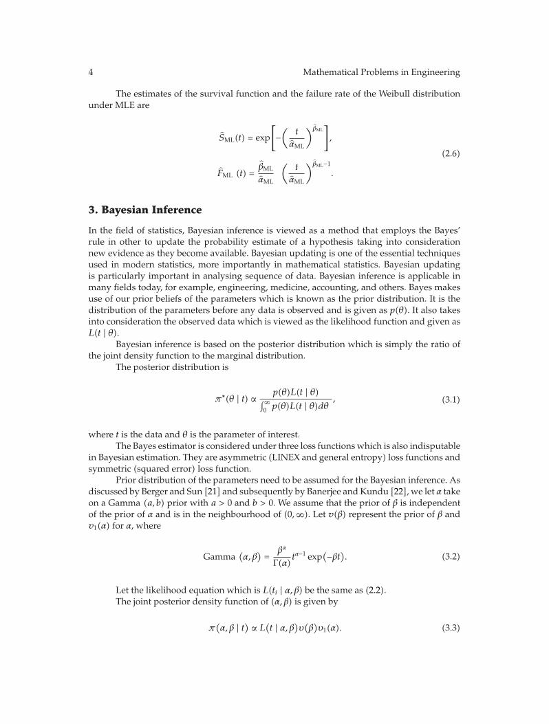
The estimates of the survival function and the failure rate of the Weibull distributionunder MLE are
SML(t) = exp
[
−(
t
αML
)βML]
,
FML (t) =βML
αML
(t
αML
)βML−1.
(2.6)
3. Bayesian Inference
In the field of statistics, Bayesian inference is viewed as a method that employs the Bayes’rule in other to update the probability estimate of a hypothesis taking into considerationnew evidence as they become available. Bayesian updating is one of the essential techniquesused in modern statistics, more importantly in mathematical statistics. Bayesian updatingis particularly important in analysing sequence of data. Bayesian inference is applicable inmany fields today, for example, engineering, medicine, accounting, and others. Bayes makesuse of our prior beliefs of the parameters which is known as the prior distribution. It is thedistribution of the parameters before any data is observed and is given as p(θ). It also takesinto consideration the observed data which is viewed as the likelihood function and given asL(t | θ).
Bayesian inference is based on the posterior distribution which is simply the ratio ofthe joint density function to the marginal distribution.
The posterior distribution is
π∗(θ | t) ∝ p(θ)L(t | θ)∫∞0 p(θ)L(t | θ)dθ , (3.1)
where t is the data and θ is the parameter of interest.The Bayes estimator is considered under three loss functions which is also indisputable
in Bayesian estimation. They are asymmetric (LINEX and general entropy) loss functions andsymmetric (squared error) loss function.
Prior distribution of the parameters need to be assumed for the Bayesian inference. Asdiscussed by Berger and Sun [21] and subsequently by Banerjee and Kundu [22], we let α takeon a Gamma (a, b) prior with a > 0 and b > 0. We assume that the prior of β is independentof the prior of α and is in the neighbourhood of (0,∞). Let v(β) represent the prior of β andv1(α) for α, where
Gamma(α, β
)=
βα
Γ(α)tα−1 exp
(−βt). (3.2)
Let the likelihood equation which is L(ti | α, β) be the same as (2.2).The joint posterior density function of (α, β) is given by
π(α, β | t) ∝ L
(t | α, β)υ(β)υ1(α). (3.3)

Mathematical Problems in Engineering 5
The posterior probability density function of α and β given the data (t1, t2, . . . , tn)is obtained by dividing the joint posterior density function over the marginal distributionfunction as
π∗(α, β | t) = L(t | α, β)v(β)v1(α)
∫∫∞0 L(t | α, β)v(β)v1(α)dαdβ
. (3.4)
3.1. Generalised Noninformative Prior
Our proposition of the generalised noninformative prior for the parameters α and β is givensuch that
v2(α, β
)=
(1
αβ
)a
, a > 0. (3.5)
We are assuming there is no or little knowledge on the parameters being estimated, where αand β are the estimates from maximum likelihood with respect to the available data obtainedby the researcher and a is a constant that can assume any value in order to minimise the prioreffect on the posterior distribution. We refer to this approach as the data-dependent prior andit is more or less an empirical or objective Bayes prior. This is an interesting new developingtheory of objective priors and, while data dependent, it does not involve an inappropriatedouble use of the data, Berger [23], unless the sample size is fairly small. The generalisednoninformative prior must not be misconstrued to imply a joint prior for the two parametersWeibull distribution. In other words, the scale and shape parameters are independent a priori.
The likelihood function from (2.2) is
L(ti | α, β
)=
n∏
i=1
{(β
α
)(tiα
)β−1exp
[
−(tiα
)β]}δi{
exp
[
−(tiα
)β]}1−δi
. (3.6)
With Bayes theorem the joint posterior distribution of the parameters α and β is
π(α, β | t) ∝ L
(t | α, β)v2
(α, β
),
= kv2(α, β
) n∏
i=1
{(β
α
)(tiα
)β−1exp
[
−(tiα
)β]}δi{
exp
[
−(tiα
)β]}1−δi
,(3.7)
where k is the normalizing constant that makes π a proper pdf.The posterior density function is obtained by using (3.4).
3.2. Linear Exponential Loss Function
This loss function according to Soliman et al. [24] rises approximately exponentially on oneside of zero and approximately linearly on the other side.

6 Mathematical Problems in Engineering
The posterior expectation of the LINEX loss function according to Zellner [13] is
Eθ
[L(θ − θ
)]∝ exp
(cθ)Eθ
[exp(−cθ)] − c
[θ − Eθ(θ)
]− 1, (3.8)
with Eθ(·) denoting the posterior expectation with respect to the posterior density of θ.Therefore, the Bayes estimator of θ, which is denoted by θBL under LINEX loss function isthe value of θ which minimizes (3.8) and is
θBL = −1cln{Eθ
[exp(−cθ)]}, (3.9)
provided that Eθ[exp(−cθ)] exist and is finite.The posterior density of the survival function and the failure rate under this loss
function are given as
S(t)BL = E
{
exp
[
−c exp[
−(tiα
)β]]
| t}
=
∫∫∞0 v(β)v1(α) exp
[−c exp
[−(ti/α)β
]]L(ti | α, β
)dαdβ
∫∫∞0 v(β)v1(α)L
(ti | α, β
)dαdβ
,
F(t)BL = E
{[
−c exp(β
α
)(t
α
)β−1]
| t}
=
∫∫∞0 v(β)v1(α) exp
[−c(β/α)(t/α)β−1
]L(ti | α, β
)dαdβ
∫∫∞0 v(β)v1(α)L
(ti | α, β
)dαdβ
.
(3.10)
It can be observed that (3.10) contain ratio of integrals which cannot be obtainedanalytically and as a result we make use of Lindley approximation procedure to evaluatethe integrals involved.
3.3. Lindley Approximation
A prior of β need to be specified here so as to calculate the approximate Bayes estimates of αand β. Having specified a prior for α as Gamma (a, b), it is similarly assumed that v(β) alsotakes on a Gamma (c, d) prior.
Lindley [25] proposed a ratio of integral of the form
∫ω(θ) exp{L(θ)}dθ∫v(θ) exp{L(θ)}dθ , (3.11)

Mathematical Problems in Engineering 7
where L(θ) is the log-likelihood and ω(θ), v(θ) are arbitrary functions of θ. Assuming thatv(θ) is the prior distribution for θ and ω(θ) = u(θ) · v(θ) with u(θ) being some function ofinterest.
The posterior expectation according to Sinha [3] is
E{u(θ) | t} =
∫v(θ) exp
{L(θ) + ρ(θ)
}d(θ)
∫exp
{L(θ) + ρ(θ)
}d(θ)
, (3.12)
where ρ(θ) = log{v(θ)}.This can be approximated asymptotically by
E{u(θ) | x} =
⎡
⎣u +12
∑
i
∑
j
(uij + 2ui · ρj
) · σij +12
∑
i
∑
j
∑
k
∑
l
Lijk · σij · σkl · ul
⎤
⎦, (3.13)
where i, j, k, l = 1, 2, . . . , n; θ = (θ1, θ2, . . . , θm).Taking the two parameters into consideration, (3.13) reduces to
θ = u +12[(u11σ11) + (u22σ22)] + u1ρ1σ11 + u2ρ2σ22 +
12
[(L30u1σ
211
)+(L03u2σ
222
)], (3.14)
where L is the log-likelihood equation in (2.3).Taking the survival function, where
u = exp
{
−c exp[
−(t
α
)β]}
, q = exp
[
−(t
α
)β]
,
u1 =∂u
∂α= c
(β
α
)(−tα
)β
qu,
(3.15)
u11 =∂2u
∂α2= −c
(β2
α2
)[
−(t
α
)β]
qu − c
(β
α2
)[
−(t
α
)β]
qu
− c
(β2
α2
)[
−(t
α
)β]2qu + c2
(β2
α2
)[
−(t
α
)β]2q2u.
(3.16)
In a similar approach u2 = ∂u/∂β and u22 = ∂2u/∂β2 can be obtained.
8 Mathematical Problems in Engineering
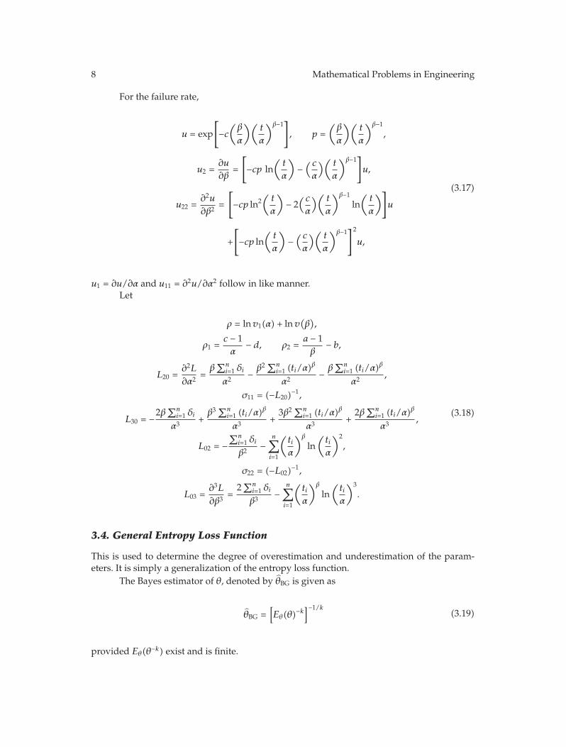
For the failure rate,
u = exp
[
−c(β
α
)(t
α
)β−1]
, p =(β
α
)(t
α
)β−1,
u2 =∂u
∂β=
[
−cp ln(t
α
)−( cα
)( t
α
)β−1]
u,
u22 =∂2u
∂β2=
[
−cp ln2(t
α
)− 2( cα
)( t
α
)β−1ln(t
α
)]
u
+
[
−cp ln(t
α
)−( cα
)( t
α
)β−1]2u,
(3.17)
u1 = ∂u/∂α and u11 = ∂2u/∂α2 follow in like manner.Let
ρ = lnv1(α) + lnv(β),
ρ1 =c − 1α
− d, ρ2 =a − 1β
− b,
L20 =∂2L
∂α2=
β∑n
i=1 δi
α2− β2
∑ni=1 (ti/α)
β
α2− β
∑ni=1 (ti/α)
β
α2,
σ11 = (−L20)−1,
L30 = −2β∑n
i=1 δi
α3+β3∑n
i=1 (ti/α)β
α3+3β2
∑ni=1 (ti/α)
β
α3+2β∑n
i=1 (ti/α)β
α3,
L02 = −∑n
i=1 δi
β2−
n∑
i=1
(tiα
)β
ln(tiα
)2
,
σ22 = (−L02)−1,
L03 =∂3L
∂β3=
2∑n
i=1 δi
β3−
n∑
i=1
(tiα
)β
ln(tiα
)3
.
(3.18)
3.4. General Entropy Loss Function
This is used to determine the degree of overestimation and underestimation of the param-eters. It is simply a generalization of the entropy loss function.
The Bayes estimator of θ, denoted by θBG is given as
θBG =[Eθ(θ)
−k]−1/k
(3.19)
provided Eθ(θ−k) exist and is finite.

Mathematical Problems in Engineering 9
The posterior density function of the survival function and the failure rate undergeneral entropy loss are given, respectively, as
S(t)BG = E
⎧⎨
⎩
[
exp
[
−(t
α
)β]]−k
| t⎫⎬
⎭
=
∫∫∞0 v(β)v1(α)
[exp
[−(t/α)β
]]−kL(ti | α, β
)dαdβ
∫∫∞0 v(β)v1(α)L
(ti | α, β
)dαdβ
,
F(t)BG = E
⎧⎨
⎩
[(β
α
)(t
α
)β−1]−k| t⎫⎬
⎭
=
∫∫∞0 v(β)v1(α)
[(β/α
)(t/α)β−1
]−kL(ti | α, β
)dαdβ
∫∫∞0 v(β)v1(α)L
(ti | α, β
)dαdβ
.
(3.20)
By making use of Lindley procedure as in (3.14), where u1, u11, and u2, u22 represent the firstand second derivatives of the survival function and the failure rate, the following equationsare obtained:
u =
{
exp
[
−(t
α
)β]}−k
, e =
[
−(t
α
)β]
,
u1 =∂u
∂α= uk
(β
α
)e,
u11 =∂2u
∂α2= uk2
(β2
α2
)
e2 − k
(β2
α2
)
eu − k
(β
α2
)eu.
(3.21)
Hence, u2 = ∂u/∂β and u22 = ∂2u/∂β2 follows.For the failure rate,
u =
[(β
α
)(t
α
)β−1]−k, r =
(t
α
)β−1,
u1 =∂u
∂α= −uk
[−(β/α2 )r − (β − 1)(β/α2 )r
]α
βr,
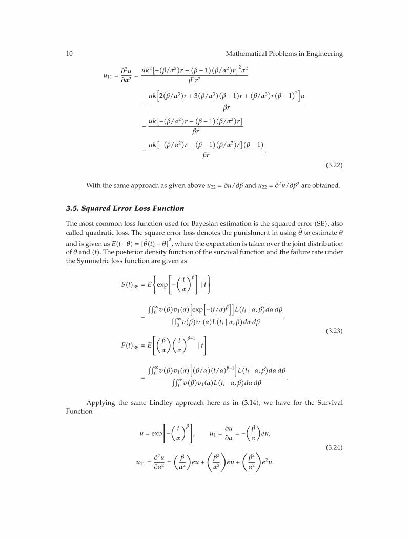
10 Mathematical Problems in Engineering
u11 =∂2u
∂α2=
uk2[−(β/α2)r − (β − 1)(β/α2)r
]2α2
β2r2
−uk[2(β/α3)r + 3
(β/α3)(β − 1
)r +
(β/α3)r
(β − 1
)2]α
βr
− uk[−(β/α2)r − (β − 1
)(β/α2)r
]
βr
− uk[−(β/α2)r − (β − 1
)(β/α2)r
](β − 1
)
βr.
(3.22)
With the same approach as given above u22 = ∂u/∂β and u22 = ∂2u/∂β2 are obtained.
3.5. Squared Error Loss Function
The most common loss function used for Bayesian estimation is the squared error (SE), alsocalled quadratic loss. The square error loss denotes the punishment in using θ to estimate θ
and is given as E(t | θ) = [θ(t) − θ]2, where the expectation is taken over the joint distribution
of θ and (t). The posterior density function of the survival function and the failure rate underthe Symmetric loss function are given as
S(t)BS = E
{
exp
[
−(t
α
)β]
| t}
=
∫∫∞0 v(β)v1(α)
[exp
[−(t/α)β
]]L(ti | α, β
)dαdβ
∫∫∞0 v(β)v1(α)L
(ti | α, β
)dαdβ
,
F(t)BS = E
[(β
α
)(t
α
)β−1| t]
=
∫∫∞0 v(β)v1(α)
[(β/α
)(t/α)β−1
]L(ti | α, β
)dαdβ
∫∫∞0 v(β)v1(α)L
(ti | α, β
)dαdβ
.
(3.23)
Applying the same Lindley approach here as in (3.14), we have for the SurvivalFunction
u = exp
[
−(t
α
)β]
, u1 =∂u
∂α= −
(β
α
)eu,
u11 =∂2u
∂α2=(
β
α2
)eu +
(β2
α2
)
eu +
(β2
α2
)
e2u.
(3.24)

Mathematical Problems in Engineering 11
In a similar approach u2 = ∂u/∂β and u22 = ∂2u/∂β2 can be obtained.For the Failure Rate,
u =(β
α
)(t
α
)β−1, d = ln
(t
α
),
u2 =∂u
∂β=(1α
)r + ud, u22 =
∂2u
∂β2=(2α
)rd2 + ud.
(3.25)
u1 = ∂u/∂α and u11 = ∂2u/∂α2 follow in like manner.With respect to the generalised noninformative prior, the same procedures as above
are also employed but ρ = lnv1(α) + lnv(β) is substituted by ρ = ln[v2(α, β)].
4. Simulation Study
We have considered in this simulation study a sample size of n = 25, 50 and 100, which isrepresentative of small, moderate, and large data sets. The following steps were employed togenerate the data.
A lifetime T is generated from the sample sizes indicated above from the Weibulldistribution which represents failure of the product or unit. The values of the assumed actualparameters of theWeibull distributionwere taken to be α = 0.5 and 1.5 and that of β = 0.8 and1.2. The same sample size is generated from the uniform distribution for the censored timeC with (0, b), where the value of b depends solely on the proportion of the observations thatare censored. In our study, we consider the percentage of censoring to be 30. T = min(T,C)is taken as the minimum of the failure time and the censored time of the observed time T ,where
T =
{δi = 1, if X ≤ C,
δi = 0, if X > C.(4.1)
To compute the Bayes estimates, an assumption is made such that α and β take,respectively, Gamma (a, b) and Gamma (c, d) priors. We set the hyperparameters to zero,that is, a = b = c = d = 0 in order to obtain noninformative priors. Note that at this point,the priors become nonproper but the results do not have any significant difference with theimplementation of proper priors as stated by Banerjee and Kundu [22].
The values for the loss parameters of both the LINEX and general entropy were c =k = ± 1 and ±2. For problems on how to choose the loss parameter values, see Calabria andPulcini [26]. We have also considered the generalised noninformative prior to be a = 3 and 5without loss of generality. These were iterated (R) 1000 times. The mean squared error andthe absolute bias values are determined and presented below for the purpose of comparison.Consider the following:
MSE(θ)=
∑Rr=1
(θr − θ
)2
R − 1, Abs. Bias
(θ)=
∑Rr=1
∣∣∣θr − θ∣∣∣
R − 1.
(4.2)

12 Mathematical Problems in Engineering
Table 1:MSEs and Abs. Biases (in parenthesis) for the survival function S(t).
nα = 0.5 α = 1.5
β = 0.8 β = 1.2 β = 0.8 β = 1.2
25
ML 0.01577 (0.09892) 0.01613 (0.10131) 0.01644 (0.10076) 0.01635 (0.10273)
BS 0.01581 (0.09909) 0.01618 (0.10149) 0.01648 (0.10092) 0.01639 (0.10290)
BL (c = 1) 0.01681 (0.10213) 0.01731 (0.10556) 0.01564 (0.09971) 0.01707 (0.10299)
BL (c = −1) 0.01613 (0.10035) 0.01732 (0.10361) 0.01625 (0.10014) 0.01687 (0.10428)
BL (c = 2) 0.01604 (0.09968) 0.01742 (0.10428) 0.01629 (0.10079) 0.01711 (0.10437)
BL (c = −2) 0.01623 (0.10091) 0.01753 (0.10573) 0.01578 (0.09839) 0.01708 (0.10266)
BG (k = 1) 0.01568 (0.09809) 0.01770 (0.10566) 0.01520 (0.09737) 0.01667 (0.10269)
BG (k = −1) 0.01565 (0.09855) 0.01774 (0.10563) 0.01565 (0.09976) 0.01721 (0.10453)
BG (k = 2) 0.01495 (0.09495) 0.01613 (0.10047) 0.01549 (0.09792) 0.01722 (0.10326)
BG (k = −2) 0.01589 (0.09983) 0.01686 (0.10303) 0.01549 (0.09711) 0.01812 (0.10809)
50
ML 0.01179 (0.08736) 0.01370 (0.09561) 0.01155 (0.08619) 0.01274 (0.09169)
BS 0.01180 (0.08741) 0.01371 (0.09566) 0.01156 (0.08624) 0.01276 (0.09174)
BL (c = 1) 0.01160 (0.08666) 0.01354 (0.09606) 0.01164 (0.08681) 0.01299 (0.09248)
BL (c = −1) 0.01137 (0.08563) 0.01246 (0.09134) 0.01144 (0.08683) 0.01299 (0.09263)
BL (c = 2) 0.01180 (0.08794) 0.01275 (0.09056) 0.01199 (0.08865) 0.01282 (0.09201)
BL (c = −2) 0.01192 (0.08840) 0.01353 (0.09489) 0.01197 (0.08823) 0.01239 (0.09009)
BG (k = 1) 0.01179 (0.08768) 0.01312 (0.09299) 0.01139 (0.08609) 0.01263 (0.09120)
BG (k = −1) 0.01799 (0.08722) 0.01259 (0.09168) 0.01109 (0.08408) 0.01274 (0.09257)
BG (k = 2) 0.01143 (0.08651) 0.01320 (0.09432) 0.01136 (0.08635) 0.01273 (0.09260)
BG (k = −2) 0.01159 (0.08686) 0.01229 (0.09049) 0.01133 (0.08472) 0.01306 (0.09325)
100
ML 0.00969 (0.08234) 0.01108 (0.08929) 0.00915 (0.07937) 0.01119 (0.08962)
BS 0.00969 (0.08235) 0.01108 (0.08931) 0.00715 (0.07938) 0.01119 (0.08963)
BL (c = 1) 0.00953 (0.08105) 0.01109 (0.08969) 0.00932 (0.08059) 0.01136 (0.09084)
BL (c = −1) 0.00938 (0.08148) 0.01062 (0.08779) 0.00952 (0.08159) 0.01056 (0.08705)
BL (c = 2) 0.00945 (0.08189) 0.01087 (0.08877) 0.00746 (0.08212) 0.01067 (0.08779)
BL (c = −2) 0.00970 (0.08226) 0.01111 (0.08950) 0.00943 (0.08102) 0.01078 (0.08804)
BG (k = 1) 0.00951 (0.08202) 0.01132 (0.09110) 0.00916 (0.07991) 0.01124 (0.09032)
BG (k = −1) 0.00958 (0.08190) 0.01085 (0.08838) 0.00933 (0.08117) 0.01071 (0.08810)
BG (k = 2) 0.00905 (0.07915) 0.01118 (0.08959) 0.00845 (0.08126) 0.01068 (0.08739)
BG (k = −2) 0.00893 (0.07912) 0.01071 (0.08751) 0.00946 (0.08176) 0.01124 (0.09051)
ML: maximum likelihood, BG: general entropy loss function, BL: LINEX loss function, BS: squared error loss function.
5. Results and Discussion
From Tables 1 and 3, the most dominant estimator that had the smallest mean squared error isthe Bayesian under linear exponential loss function(LINEX). This happened with generalisednoninformative prior except at n = 50 with α = 1.5 and β = 1.2 that we observed that thenoninformative gamma prior gave the smallestMSE. This was followed closely by the generalentropy loss function (GELF) with the noninformative gamma prior. What is remarkable isthat the smallest absolute bias values occurred mostly with the generalised noninformativeprior. GELFwas slightly ahead of LINEX but both were better than SELF and that of theMLE.
Mathematical Problems in Engineering 13
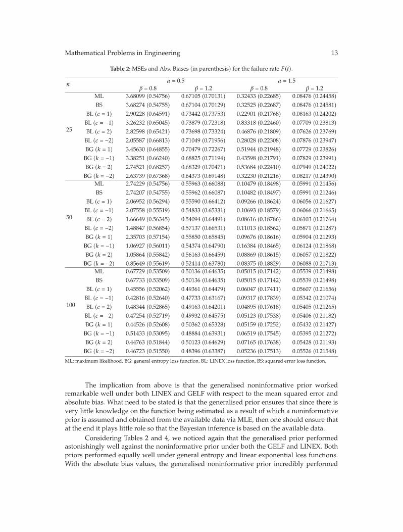
Table 2: MSEs and Abs. Biases (in parenthesis) for the failure rate F(t).
nα = 0.5 α = 1.5
β = 0.8 β = 1.2 β = 0.8 β = 1.2
25
ML 3.68099 (0.54756) 0.67105 (0.70131) 0.32433 (0.22685) 0.08476 (0.24458)
BS 3.68274 (0.54755) 0.67104 (0.70129) 0.32525 (0.22687) 0.08476 (0.24581)
BL (c = 1) 2.90228 (0.64591) 0.73442 (0.73753) 0.22901 (0.21768) 0.08163 (0.24202)
BL (c = −1) 3.26232 (0.65045) 0.73879 (0.72318) 0.83318 (0.22460) 0.07709 (0.23813)
BL (c = 2) 2.82598 (0.65421) 0.73698 (0.73324) 0.46876 (0.21809) 0.07626 (0.23769)
BL (c = −2) 2.05587 (0.66813) 0.71049 (0.71956) 0.28028 (0.22308) 0.07876 (0.23947)
BG (k = 1) 3.45630 (0.64855) 0.70479 (0.72267) 0.51944 (0.21948) 0.07729 (0.23826)
BG (k = −1) 3.38251 (0.66240) 0.68825 (0.71194) 0.43598 (0.21791) 0.07829 (0.23991)
BG (k = 2) 2.74521 (0.68257) 0.68329 (0.70471) 0.53684 (0.22410) 0.07949 (0.24022)
BG (k = −2) 2.63739 (0.67368) 0.64373 (0.69148) 0.32230 (0.21216) 0.08217 (0.24390)
50
ML 2.74229 (0.54756) 0.55963 (0.66088) 0.10479 (0.18498) 0.05991 (0.21456)
BS 2.74207 (0.54755) 0.55962 (0.66087) 0.10482 (0.18497) 0.05991 (0.21246)
BL (c = 1) 2.06952 (0.56294) 0.55590 (0.66412) 0.09266 (0.18624) 0.06056 (0.21627)
BL (c = −1) 2.07558 (0.55519) 0.54833 (0.65331) 0.10693 (0.18579) 0.06066 (0.21665)
BL (c = 2) 1.66649 (0.56345) 0.54094 (0.64491) 0.08616 (0.18786) 0.06103 (0.21764)
BL (c = −2) 1.48847 (0.56854) 0.57137 (0.66531) 0.11013 (0.18562) 0.05871 (0.21287)
BG (k = 1) 2.35703 (0.57154) 0.55850 (0.65845) 0.09676 (0.18616) 0.05904 (0.21293)
BG (k = −1) 1.06927 (0.56011) 0.54374 (0.64790) 0.16384 (0.18465) 0.06124 (0.21868)
BG (k = 2) 1.05864 (0.55842) 0.56163 (0.66459) 0.08869 (0.18615) 0.06057 (0.21822)
BG (k = −2) 0.85649 (0.55619) 0.52414 (0.63780) 0.08375 (0.18829) 0.06088 (0.21713)
100
ML 0.67729 (0.53509) 0.50136 (0.64635) 0.05015 (0.17142) 0.05539 (0.21498)
BS 0.67733 (0.53509) 0.50136 (0.64635) 0.05015 (0.17142) 0.05539 (0.21498)
BL (c = 1) 0.45556 (0.52062) 0.49361 (0.64479) 0.06047 (0.17411) 0.05607 (0.21656)
BL (c = −1) 0.42816 (0.52640) 0.47733 (0.63167) 0.09317 (0.17839) 0.05342 (0.21074)
BL (c = 2) 0.48344 (0.52865) 0.49163 (0.64201) 0.04895 (0.17618) 0.05405 (0.21265)
BL (c = −2) 0.47254 (0.52719) 0.49932 (0.64575) 0.05123 (0.17538) 0.05406 (0.21182)
BG (k = 1) 0.44526 (0.52608) 0.50362 (0.65328) 0.05159 (0.17252) 0.05432 (0.21427)
BG (k = −1) 0.51433 (0.53095) 0.48884 (0.63931) 0.06519 (0.17545) 0.05395 (0.21272)
BG (k = 2) 0.44763 (0.51844) 0.50123 (0.64629) 0.07165 (0.17638) 0.05428 (0.21193)
BG (k = −2) 0.46723 (0.51550) 0.48396 (0.63387) 0.05236 (0.17513) 0.05526 (0.21548)
ML: maximum likelihood, BG: general entropy loss function, BL: LINEX loss function, BS: squared error loss function.
The implication from above is that the generalised noninformative prior workedremarkable well under both LINEX and GELF with respect to the mean squared error andabsolute bias. What need to be stated is that the generalised prior ensures that since there isvery little knowledge on the function being estimated as a result of which a noninformativeprior is assumed and obtained from the available data via MLE, then one should ensure thatat the end it plays little role so that the Bayesian inference is based on the available data.
Considering Tables 2 and 4, we noticed again that the generalised prior performedastonishingly well against the noninformative prior under both the GELF and LINEX. Bothpriors performed equally well under general entropy and linear exponential loss functions.With the absolute bias values, the generalised noninformative prior incredibly performed

14 Mathematical Problems in Engineering
Table 3: MSEs and Abs. Biases (in parenthesis) for the survival function S(t) using GNP.
α = 0.5 α = 1.5n β = 0.8 β = 1.2 β = 0.8 β = 1.2
a = 5, [3] a = 5, [3]
25
BS 0.01671 (0.10237) 0.01731 (0.10550) 0.01553 (0.09804) 0.01740 (0.10389)[0.01528 (0.09853)] [0.01733 (0.10441)] [0.01632 (0.10123)] [0.01861 (0.10795)]
BL (c = 1) 0.01736 (0.01025) 0.01608 (0.10052) 0.01531 (0.09805) 0.01694 (0.10227)[0.01559 (0.09876)] [0.01726 (0.10385)] [0.01585 (0.09796)] [0.01755 (0.10476)]
BL (c = −1) 0.01756 (0.10315) 0.01655 (0.10308) 0.01614 (0.10075) 0.01748 (0.10470)[0.01544 (0.09803)] [0.01806 (0.10735)] [0.01680 (0.10254)] [0.01727 (0.10453)]
BL (c = 2) 0.01797 (0.10635) 0.01649 (0.10116) 0.01467 (0.09588) 0.01718 (0.10317)[0.01716 (0.10194)] [0.01806 (0.10617)] [0.01506 (0.09667)] [0.01793 (0.10640)]
BL (c = −2) 0.01756 (0.10499) 0.01637 (0.10090) 0.01571 (0.09796) 0.01748 (0.10551)[0.01554 (0.09817)] [0.01732 (0.10397)] [0.01602 (0.10003)] [0.01857 (0.10914)]
BG (k = 1) 0.01645 (0.10157) 0.01659 (0.10271) 0.01587 (0.09919) 0.01719 (0.10355)[0.01519 (0.09767)] [0.01741 (0.10468)] [0.01649 (0.10107)] [0.01782 (0.10583)]
BG (k = −1) 0.01660 (0.10067) 0.01734 (0.10515) 0.01621 (0.09978) 0.01808 (0.10817)[0.01554 (0.09757)] [0.01609 (0.10096)] [0.01539 (0.09644)] [0.01793 (0.10731)]
BG (k = 2) 0.01794 (0.10643) 0.01773 (0.10477) 0.01653 (0.10009) 0.01688 (0.10393)[0.01551 (0.09821)] [0.01690 (0.10249)] [0.01518 (0.09757)] [0.01667 (0.10306)]
BG (k = −2) 0.01623 (0.10158) 0.01730 (0.10519) 0.01562 (0.09759) 0.01748 (0.10465)[0.01654 (0.10175)] [0.01773 (0.10552)] [0.01636 (0.10043)] [0.01822 (0.10797)]
50
BS 0.01178 (0.08765) 0.01299 (0.09209) 0.01174 (0.08754) 0.01312 (0.09343)[0.01163 (0.08629)] [0.01255 (0.09154)] [0.01163 (0.08679)] [0.01272 (0.09223)]
BL (c = 1) 0.01092 (0.08456) 0.01259 (0.09203) 0.01134 (0.08587) 0.01276 (0.09198)[0.01128 (0.08459)] [0.01284 (0.09326)] [0.01181 (0.08617)] [0.01289 (0.09290)]
BL (c = −1) 0.01201 (0.08874) 0.01266 (0.09119) 0.01149 (0.08649) 0.01270 (0.09149)[0.01118 (0.08561)] [0.01274 (0.09196)] [0.01126 (0.08554)] [0.01251 (0.09036)]
BL (c = 2) 0.01126 (0.08480) 0.01288 (0.09267) 0.01164 (0.08756) 0.01307 (0.09326)[0.01149 (0.08640)] [0.01261 (0.09249)] [0.01106 (0.08521)] [0.01335 (0.09481)]
BL (c = −2) 0.01119 (0.08567) 0.01304 (0.09343) 0.01135 (0.08484) 0.01299 (0.09379)[0.01158 (0.08676)] [0.01234 (0.09038)] [0.01209 (0.08853)] [0.01310 (0.09310)]
BG (k = 1) 0.01109 (0.08496) 0.01322 (0.09375) 0.01137 (0.08565) 0.01309 (0.09474)[0.01111 (0.08467)] [0.01287 (0.09549)] [0.01176 (0.08690)] [0.01279 (0.09197)]
BG (k = −1) 0.01187 (0.08821) 0.01365 (0.09533) 0.01191 (0.08832) 0.01263 (0.09130)[0.01147 (0.08608)] [0.01289 (0.09229)] [0.01126 (0.08621)] [0.01298 (0.09259)]
BG (k = 2) 0.01135 (0.08535) 0.01307 (0.09349) 0.01126 (0.08878) 0.01361 (0.09489)[0.01197 (0.08815)] [0.01257 (0.09113)] [0.01145 (0.08588)] [0.01251 (0.09138)]
BG (k = −2) 0.01199 (0.08802) 0.01325 (0.09363) 0.01232 (0.08958) 0.01259 (0.09138)[0.01166 (0.08674)] [0.01299 (0.09296)] [0.01138 (0.08564)] [0.01302 (0.09359)]
BS 0.00967 (0.08273) 0.01069 (0.08780) 0.00935 (0.08153) 0.01107 (0.08928)[0.00936 (0.08143)] [0.01087 (0.08831)] [0.00929 (0.08039)] [0.01084 (0.08928)]
BL (c = 1) 0.00984 (0.08327) 0.01084 (0.08875) 0.00867 (0.07797) 0.01061 (0.08743)[0.00961 (0.08267)] [0.01090 (0.08894)] [0.00969 (0.08240)] [0.01093 (0.08894)]
100BL (c = −1) 0.00951 (0.08128) 0.01051 (0.08688) 0.00975 (0.08276) 0.01119 (0.08929)
[0.00925 (0.08078)] [0.01043 (0.08648)] [0.00963 (0.08201)] [0.01110 (0.08923)]
BL (c = 2) 0.00937 (0.08062) 0.01064 (0.08733) 0.00929 (0.08096) 0.01105 (0.08896)[0.00973 (0.08233)] [0.01101 (0.08887)] [0.00969 (0.08302)] [0.01118 (0.09015)]

Mathematical Problems in Engineering 15
Table 3: Continued.
α = 0.5 α = 1.5n β = 0.8 β = 1.2 β = 0.8 β = 1.2
a = 5, [3] a = 5, [3]
BL (c = −2) 0.00952 (0.08184) 0.01098 (0.08906) 0.00966 (0.08244) 0.01087 (0.08856)
[0.00994 (0.08372)] [0.01102 (0.08887)] [0.00938 (0.08141)] [0.01094 (0.08877)]
BG (k = 1) 0.00895 (0.07874) 0.01091 (0.08838) 0.00946 (0.08088) 0.01059 (0.08729)
[0.00926 (0.08019)] [0.01093 (0.08855)] [0.00955 (0.08214)] [0.01108 (0.08918)]
BG (k = −1) 0.00914 (0.08047) 0.01093 (0.08833) 0.00956 (0.08156) 0.01078 (0.08802)
[0.00897 (0.07956)] [0.01091 (0.08844)] [0.00985 (0.08260)] [0.01001 (0.08491)]
BG (k = 2) 0.00929 (0.08071) 0.01106 (0.08889) 0.00921 (0.07979) 0.01142 (0.09069)
[0.00963 (0.08220)] [0.01111 (0.08947)] [0.00975 (0.08284)] [0.01092 (0.08865)]
BG (k = −2) 0.00936 (0.08122) 0.01128 (0.09042) 0.00990 (0.08379) 0.01111 (0.08941)
[0.00961 (0.08213)] [0.01072 (0.08811)] [0.00947 (0.08152)] [0.01132 (0.09072)]
GNP: generalised nonInformative prior, BG: general entropy loss function, BL: LINEX loss function, BS: squared error lossfunction.
better under LINEX loss function but was almost equal with the noninformative prior underthe general entropy loss function.
To obtain the MSE values for each estimated value, the MSE is calculated for each ofthe one thousand estimated values of the survival function and the failure rate that is, from1 to 1000. At the end, we obtain the average of the MSE, values. Our aim is to find out howclose the estimated values of the estimators are to the true value. The absolute bias valuesare obtained in like manner and of course from the same simulated values as that of theMSE.
6. Conclusion
In this study, we consider the point estimation of the Weibull distribution based on rightcensoring through simulation. MLE and Bayes estimators are applied to estimate the survivalfunction and the failure rate of this lifetime distribution. The Bayes estimators are obtainedusing linear exponential, general entropy, and squared error loss functions.We also employedthe Bayesian noninformative prior approach in estimating survival function and the failurerate. In order to reduce the complicated integrals that are in the posterior distributionwhich cannot explicitly be obtained in close form, we employed the Lindley approximationprocedure to calculate the Bayes estimators.
Another point worth noting is that we assumed an informative prior for the scaleparameter and the shape parameter which led us into obtaining an improper prior. We alsomade a proposition for a generalised noninformative prior.
From the results and discussions above, it is evident that the proposed generalisednoninformative prior performed quite well than the noninformative gamma prior. In all thecases, the Bayesian estimator using the generalised noninformative prior under the linearexponential loss function overall performed better than the other estimators and underthe other different loss functions with respect to the mean squared error. It has also beenobserved that the smallest absolute bias values occurred predominantly with the generalised

16 Mathematical Problems in Engineering
Table 4: MSEs and Abs. Biases (in parenthesis) for the failure rate F(t) using GNP.
α = 0.5 α = 1.5n β = 0.8 β = 1.2 β = 0.8 β = 1.2
a = 5, [3] a = 5, [3]
25
BS 1.60882 (0.60581) 0.75601 (0.74247) 0.26918 (0.22161) 0.08242 (0.24192)[3.50808 (0.66123)] [0.70983 (0.72011)] [0.21814 (0.22270)] [0.08227 (0.24568)]
BL (c = 1) 3.10223 (0.66497) 0.66435 (0.70130) 0.24086 (0.21740) 0.07698 (0.23560)[0.97145 (0.64334)] [0.73049 (0.73445)] [0.46015 (0.22941)] [0.08183 (0.24475)]
BL (c = −1) 5.07183 (0.70026) 0.72658 (0.71728) 0.17702 (0.22059) 0.07997 (0.24249)[1.89290 (0.65885)] [0.72855 (0.73625)] [0.28853 (0.22911)] [0.07864 (0.23852)]
BL (c = 2) 2.57595 (0.67277) 0.70089 (0.71957) 0.19602 (0.21443) 0.08062 (0.24190)[1.42447 (0.65551)] [0.73245 (0.73581)] [0.26676 (0.22149)] [0.08261 (0.24604)]
BL (c = −2) 2.47065 (0.68677) 0.68712 (0.70818) 0.29206 (0.22263) 0.07838 (0.24087)[2.90974 (0.65568)] [0.69822 (0.71461)] [0.31298 (0.23181)] [0.08179 (0.24609)]
BG (k = 1) 5.09142 (0.63923) 0.68482 (0.71454) 0.32629 (0.21537) 0.07963 (0.24117)[1.59876 (0.64264)] [0.71224 (0.72443)] [0.39187 (0.22194)] [0.08104 (0.24269)]
BG (k = −1) 1.11653 (0.60663) 0.73329 (0.72535) 0.28561 (0.21867) 0.07938 (0.24085)[2.05799 (0.65800)] [0.67003 (0.70302)] [0.28235 (0.28235)] [0.07783 (0.24017)]
BG (k = 2) 3.26989 (0.63433) 0.70409 (0.72102) 0.14943 (0.21824) 0.08079 (0.24219)[3.59616 (0.65300)] [0.70879 (0.71412)] [0.20827 (0.22005)] [0.08084 (0.24227)]
BG (k = −2) 1.56123 (0.63166) 0.68200 (0.71084) 0.22126 (0.21289) 0.07983 (0.24229)[1.82844 (0.64736)] [0.71757 (0.72167)] [0.16709 (0.21693)] [0.07978 (0.24356)]
50
BS 0.99284 (0.55903) 0.53895 (0.64125) 0.21602 (0.18856) 0.06088 (0.21759)[1.20392 (0.55531)] [0.53767 (0.64578)] [0.23509 (0.18781)] [0.05879 (0.21411)]
BL (c = 1) 0.85858 (0.55004) 0.54626 (0.65313) 0.21497 (0.18676) 0.06021 (0.21590)[0.84299 (0.54806)] [0.54644 (0.65612)] [0.18170 (0.18565)] [0.06051 (0.21811)]
BL (c = −1) 0.90621 (0.56868) 0.55652 (0.65539) 0.17717 (0.18777) 0.06052 (0.21565)[0.70963 (0.54405)] [0.53659 (0.64556)] [0.19359 (0.18475)] [0.06063 (0.21566)]
BL (c = 2) 0.84116 (0.54422) 0.55124 (0.65304) 0.19584 (0.18896) 0.06132 (0.21808)[1.05227 (0.55656)] [0.55016 (0.65747)] [0.19113 (0.18416)] [0.06118 (0.21996)]
BL (c = −2) 0.83699 (0.55410) 0.54021 (0.64881) 0.19281 (0.18479) 0.06111 (0.21948)[0.87199 (0.55693)] [0.52738 (0.63962)] [0.18451 (0.18884)] [0.06072 (0.21715)]
BG (k = 1) 1.08699 (0.55039) 0.55381 (0.65826) 0.17302 (0.18223) 0.06119 (0.21882)[0.95041 (0.55106)] [0.54985 (0.65467)] [0.24233 (0.18548)] [0.06097 (0.21819)]
BG (k = −1) 1.12507 (0.55889) 0.55956 (0.66129) 0.25057 (0.19005) 0.06023 (0.21461)[1.01425 (0.55157)] [0.55221 (0.65488)] [0.11878 (0.18655)] [0.06018 (0.21560)]
BG (k = 2) 1.17354 (0.55312) 0.57334 (0.67120) 0.17699 (0.18661) 0.06244 (0.22011)[1.00135 (0.56841)] [0.54657 (0.64917)] [0.10609 (0.18484)] [0.05985 (0.21521)]
BG (k = −2) 1.18804 (0.56841) 0.56341 (0.66432) 0.13249 (0.18605) 0.06024 (0.21510)[1.15358 (0.55573)] [0.54699 (0.65363)] [0.14781 (0.18359)] [0.06057 (0.21754)]
BS 0.66670 (0.53230) 0.48857 (0.63609) 0.05482 (0.17604) 0.05524 (0.21483)[0.44568 (0.52663)] [0.49065 (0.64062)] [0.06864 (0.17410)] [0.05323 (0.21001)]
BL (c = 1) 0.47245 (0.53712) 0.48375 (0.63740) 0.04677 (0.16927) 0.05397 (0.21152)[0.48126 (0.52985)] [0.49223 (0.64333)] [0.06145 (0.17697)] [0.05467 (0.21400)]
100BL (c = −1) 0.50560 (0.52798) 0.48800 (0.63826) 0.06408 (0.17864) 0.05512 (0.21358)
[0.48709 (0.52132)] [0.47258 (0.62645)] [0.06531 (0.17577)] [0.05552 (0.21507)]
BL (c = 2) 0.44645 (0.52047) 0.48540 (0.63612) 0.06605 (0.17422) 0.05524 (0.21454)[0.80817 (0.52984)] [0.48774 (0.63795)] [0.06651 (0.17786)] [0.05648 (0.21780)]

Mathematical Problems in Engineering 17
Table 4: Continued.
α = 0.5 α = 1.5n β = 0.8 β = 1.2 β = 0.8 β = 1.2
a = 5, [3] a = 5, [3]
BL (c = −2) 0.50473 (0.52856) 0.49342 (0.64368) 0.05039 (0.17666) 0.05434 (0.21327)[0.52768 (0.53450)] [0.49421 (0.64037)] [0.07692 (0.17494)] [0.05561 (0.21493)]
BG (k = 1) 0.44440 (0.51305) 0.49572 (0.64148) 0.07150 (0.17498) 0.05361 (0.21112)[0.59699 (0.52223)] [0.49308 (0.64049)] [0.05309 (0.17608)] [0.05444 (0.21287)]
BG (k = −1) 0.49145 (0.52292) 0.49925 (0.64372) 0.05013 (0.17478) 0.05340 (0.21109)[0.46108 (0.52107)] [0.49309 (0.63951)] [0.04829 (0.17618)] [0.05185 (0.20729)]
BG (k = 2) 0.50315 (0.52624) 0.50124 (0.64500) 0.05319 (0.17324) 0.05761 (0.22003)[0.45561 (0.52818)] [0.49235 (0.64167)] [0.05073 (0.17732)] [0.05492 (0.21381)]
BG (k = −2) 0.55240 (0.52938) 0.51051 (0.65583) 0.04795 (0.17732) 0.05482 (0.21406)[0.42269 (0.52581)] [0.48926 (0.63954)] [0.06453 (0.17769)] [0.05630 (0.21743)]
GNP: generalised noninformative prior, BG: general entropy loss function, BL: LINEX loss function, BS: squared error lossfunction.
noninformative prior under general entropy loss function for both the survival function andthe failure rate.
Acknowledgments
The authors would like to thank the anonymous referees for their suggestions and comments.The first author would like to personally thank the Editor, Professor Carlo Cattani, for hisencouragement and suggestions.
References
[1] J. F. Lawless, Statistical Models and Methods for Lifetime Data, John Wiley & Sons, New York, NY, USA,1982.
[2] H. Rinne, The Weibull Distribution, CRC Press, Taylor and Francis Group LLC, New York, NY, USA,2009.
[3] S. K. Sinha, “Bayes estimation of the reliability function and hazard rate of a weibull failure timedistribution,” Tranbajos De Estadistica, vol. 1, pp. 47–56, 1986.
[4] A. A. Abdel-Wahid andA.Winterbottom, “Approximate Bayesian estimates for theWeibull reliabilityfunction and hazard rate from censored data,” Journal of Statistical Planning and Inference, vol. 16, no.3, pp. 277–283, 1987.
[5] M. A. Al Omari and N. A. Ibrahim, “Bayesian survival estimation estimation for weibull distributionwith censored data,” Journal of Applied Sciences, vol. 11, pp. 393–396, 2011.
[6] C. B. Guure, N. A. Ibrahim, and A. M. Al Omari, “Bayesian estimation of two-parameter weibulldistribution using extension of Jeffreys’ prior information with three loss functions,” MathematicalProblems in Engineering, vol. 2012, Article ID 589640, 13 pages, 2012.
[7] H. Syuan-Rong and W. Shuo-Jye, “Bayesian estimation and prediction for weibull model withprogressive censoring,” Journal of Statistical Computation and Simulation, pp. 1–14, 2011.
[8] C. Cattani and A. Ciancio, “Separable transition density in the hybrid model for tumor-immunesystem competition,” Computational andMathematical Methods inMedicine, vol. 2012, Article ID 610124,6 pages, 2012.
[9] X. Wang, M. Xia, C. Huiwen, Y. Gao, and C. Cattani, “Hidden-markov-models-based dynamic handgesture recognition,”Mathematical Problems in Engineering, vol. 2012, Article ID 986134, 11 pages, 2012.
[10] C. Cattani, “On the existence of wavelet symmetries in archaea DNA,” Computational andMathematicalMethods in Medicine, vol. 2012, Article ID 673934, 21 pages, 2012.
[11] C. Cattani, “Fractional calculus and shannonwavelet,”Mathematical Problems in Engineering, vol. 2012,Article ID 502812, 26 pages, 2012.
[12] R. D. Gupta and D. Kundu, “Generalized exponential distribution: different method of estimations,”Journal of Statistical Computation and Simulation, vol. 69, no. 4, pp. 315–337, 2001.
18 Mathematical Problems in Engineering
[13] A. Zellner, “Bayesian estimation and prediction using asymmetric loss functions,” Journal of theAmerican Statistical Association, vol. 81, no. 394, pp. 446–451, 1986.
[14] F. M. Al-Aboud, “Bayesian estimations for the extreme value distribution using progressive censoreddata and asymmetric loss,” International Mathematical Forum, vol. 4, no. 33–36, pp. 1603–1622, 2009.
[15] F. M. Al-Athari, “Parameter estimation for the double-pareto distribution,” Journal of Mathematics andStatistics, vol. 7, no. 4, pp. 289–294, 2011.
[16] C. Cattani, G. Pierro, and G. Altieri, “Entropy and multifractality for the myeloma multiple TET 2gene,”Mathematical Problems in Engineering, vol. 2012, Article ID 193761, 14 pages, 2012.
[17] B. N. Pandey, N. Dwividi, and B. Pulastya, “Comparison between Bayesian and maximum likelihoodestimation of the scale parameter in weibull distribution with known shape under linex lossfunction,” Journal of Scientific Research, vol. 55, pp. 163–172, 2011.
[18] D. Kundu and R. D. Gupta, “Generalized exponential distribution: bayesian estimations,” Computa-tional Statistics & Data Analysis, vol. 52, no. 4, pp. 1873–1883, 2008.
[19] P. Vasile, P. Eugeine, and C. Alina, “Bayes estimators of modified-Weibull distribution parametersusing Lindley’s approximation,” WSEAS Transactions on Mathematics, vol. 9, no. 7, pp. 539–549, 2010.
[20] A. P. Basu and N. Ebrahimi, “Bayesian approach to life testing and reliability estimation usingasymmetric loss function,” Journal of Statistical Planning and Inference, vol. 29, no. 1-2, pp. 21–31, 1991.
[21] J. O. Berger and D. C. Sun, “Bayesian analysis for the poly-Weibull distribution,” Journal of theAmerican Statistical Association, vol. 88, no. 424, pp. 1412–1418, 1993.
[22] A. Banerjee and D. Kundu, “Inference based on type-II hybrid censored data from a weibulldistribution,” IEEE Transactions on Reliability, vol. 57, no. 2, pp. 369–378, 2008.
[23] J. O. Berger, “The case for objective Bayesian analysis,” Bayesian Analysis, vol. 1, no. 3, pp. 385–402,2006.
[24] A. A. Soliman, A. H. Abd Ellah, and S. B. Ryan, “Comparison of estimates using record statistics fromweibull model: bayesian and non-Bayesian approaches,” Computational Statistics & Data Analysis, vol.51, pp. 2065–2077, 2006.
[25] D. V. Lindley, “Approximate Bayesian methods,” Trabajos Estadist, vol. 31, pp. 223–237, 1980.[26] R. Calabria and G. Pulcini, “Point estimation under asymmetric loss functions for left-truncated
exponential samples,” Communications in Statistics. Theory and Methods, vol. 25, no. 3, pp. 585–600,1996.
Related Documents


![Semiparametric Bayesian Analysis of Censored Linear ...sinha/research/SMMR_2015_Final_versi… · Previously, Muller¨ and Roeder [15] used a nonparametric Bayesian approach for handling](https://static.cupdf.com/doc/110x72/5f4ddd4f4ba54845583df83e/semiparametric-bayesian-analysis-of-censored-linear-sinharesearchsmmr2015finalversi.jpg)


