AUTOMATIC DIAGNOSIS OF VOLTAGE DISTURBANCES IN POWER DISTRIBUTION NETWORKS Víctor Augusto BARRERA NÚÑEZ Dipòsit legal: GI-902-2012 http://hdl.handle.net/10803/80944 ADVERTIMENT: L'accés als continguts d'aquesta tesi doctoral i la seva utilització ha de respectar els drets de la persona autora. Pot ser utilitzada per a consulta o estudi personal, així com en activitats o materials d'investigació i docència en els termes establerts a l'art. 32 del Text Refós de la Llei de Propietat Intel·lectual (RDL 1/1996). Per altres utilitzacions es requereix l'autorització prèvia i expressa de la persona autora. En qualsevol cas, en la utilització dels seus continguts caldrà indicar de forma clara el nom i cognoms de la persona autora i el títol de la tesi doctoral. No s'autoritza la seva reproducció o altres formes d'explotació efectuades amb finalitats de lucre ni la seva comunicació pública des d'un lloc aliè al servei TDX. Tampoc s'autoritza la presentació del seu contingut en una finestra o marc aliè a TDX (framing). Aquesta reserva de drets afecta tant als continguts de la tesi com als seus resums i índexs.

Welcome message from author
This document is posted to help you gain knowledge. Please leave a comment to let me know what you think about it! Share it to your friends and learn new things together.
Transcript
AUTOMATIC DIAGNOSIS OF VOLTAGE DISTURBANCES IN POWER DISTRIBUTION
NETWORKS
Víctor Augusto BARRERA NÚÑEZ
Dipòsit legal: GI-902-2012 http://hdl.handle.net/10803/80944
ADVERTIMENT: L'accés als continguts d'aquesta tesi doctoral i la seva utilització ha de respectar els drets de la persona autora. Pot ser utilitzada per a consulta o estudi personal, així com en activitats o materials d'investigació i docència en els termes establerts a l'art. 32 del Text Refós de la Llei de Propietat Intel·lectual (RDL 1/1996). Per altres utilitzacions es requereix l'autorització prèvia i expressa de la persona autora. En qualsevol cas, en la utilització dels seus continguts caldrà indicar de forma clara el nom i cognoms de la persona autora i el títol de la tesi doctoral. No s'autoritza la seva reproducció o altres formes d'explotació efectuades amb finalitats de lucre ni la seva comunicació pública des d'un lloc aliè al servei TDX. Tampoc s'autoritza la presentació del seu contingut en una finestra o marc aliè a TDX (framing). Aquesta reserva de drets afecta tant als continguts de la tesi com als seus resums i índexs.
Automatic Diagnosis of Voltage
Disturbances in Power
Distribution Networks
Victor Augusto Barrera Nunez
Doctoral Programme in Technology
Universitat de Girona
PhD Thesis
February 2012
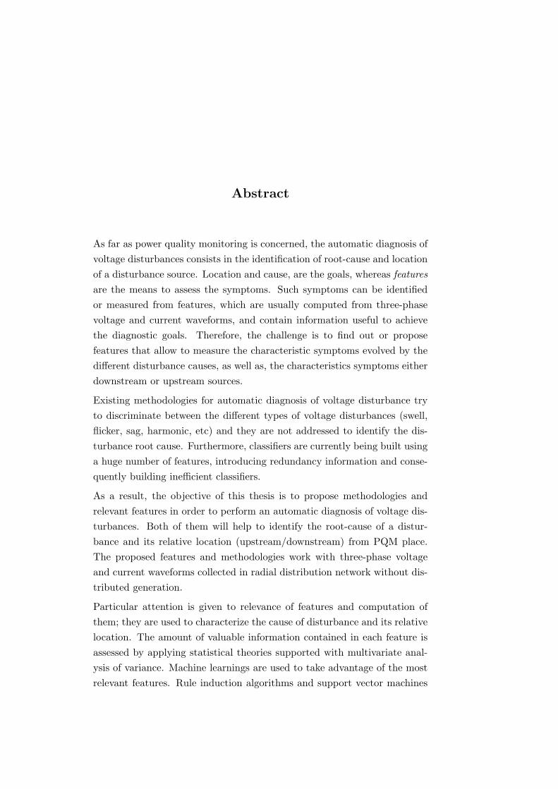
Abstract
As far as power quality monitoring is concerned, the automatic diagnosis ofvoltage disturbances consists in the identification of root-cause and locationof a disturbance source. Location and cause, are the goals, whereas featuresare the means to assess the symptoms. Such symptoms can be identifiedor measured from features, which are usually computed from three-phasevoltage and current waveforms, and contain information useful to achievethe diagnostic goals. Therefore, the challenge is to find out or proposefeatures that allow to measure the characteristic symptoms evolved by thedifferent disturbance causes, as well as, the characteristics symptoms eitherdownstream or upstream sources.
Existing methodologies for automatic diagnosis of voltage disturbance tryto discriminate between the different types of voltage disturbances (swell,flicker, sag, harmonic, etc) and they are not addressed to identify the dis-turbance root cause. Furthermore, classifiers are currently being built usinga huge number of features, introducing redundancy information and conse-quently building inefficient classifiers.
As a result, the objective of this thesis is to propose methodologies andrelevant features in order to perform an automatic diagnosis of voltage dis-turbances. Both of them will help to identify the root-cause of a distur-bance and its relative location (upstream/downstream) from PQM place.The proposed features and methodologies work with three-phase voltageand current waveforms collected in radial distribution network without dis-tributed generation.
Particular attention is given to relevance of features and computation ofthem; they are used to characterize the cause of disturbance and its relativelocation. The amount of valuable information contained in each feature isassessed by applying statistical theories supported with multivariate anal-ysis of variance. Machine learnings are used to take advantage of the mostrelevant features. Rule induction algorithms and support vector machines
are used to build methodologies for disturbance diagnosis. Feature extrac-tion process is addressed by comparing existing waveform segmentation al-gorithms. Furthermore, a segmentation algorithm is also proposed in thisthesis.
The upstream or downstream location of the source of a disturbance is ad-dressed statistically analyzing and comparing features used by existing algo-rithms. The objective is to identify the most relevant features. As a resultof combining the features used by existing algorithms, a relative locationalgorithm is obtained with better location performance. The algorithms arecompared through an approach based on specificity and sensitivity statis-tics. Fault pinpoint location problem is not addressed in this thesis becauseof lack of information about network configuration and impedances.
The most common disturbance causes are divided into two categories, in-ternal and external. Internal causes are those due to network normal op-eration actions, such as transformer energization, induction motor starting,large-load and capacitor switchings. Conversely, external causes are thoseexternal factors to the network involving short-circuits, such as animalsand tree branches getting in touch with overhead networks, undergroundcable failures, lightning-induced events, insulator breakdowns, among oth-ers. Both categories of disturbance causes are independently analyzed andcharacterized. Relevant features are conceived based on electrical principlesand assuming hypothesis on the analyzed phenomena. Features based onwaveforms as well as weather conditions are also taken into account.
The proposed methodologies and features are tested using real-world andsynthetic waveforms. The behavior of features and classification resultsof the methodologies show that proposed features and methodologies canbe used in a framework for automatic diagnosis of voltage disturbancescollected in distribution networks. The diagnostic results can be used forsupporting power network operation, maintenance and planning.
Keywords: cause identification, fault characterization, machine learning,multivariate analysis of variance, power quality monitoring, source relativelocation, waveform segmentation.

iv
To my parents, Rosy and Victor. To my fiancee, Sheila. To my futurechildren.
Acknowledgements
I firstly would like to thank Joaquim Melendez and Sergio Herraiz for theirguidance throughout my PhD studies. I am deeply grateful for their dis-cussions about power quality issues and long hours structuring and writingjournal and conference papers.
My sincere thanks to Math Bollen, Irene Yu-Hua Gu and Surya Santosofor welcoming me as guest researcher in Chalmers University of Technologyand The University of Texas. I will be forever grateful for the opportunitygiven by them.
I want also thanks to Jorge Sanchez and Surya Santoso for the providedreal-world waveforms. This research would not have been possible withoutthe valuable information provided by both.
I am grateful to professors Gabriel Ordonez and Gilberto Carrillo for theircooperation in the research project between Universidad Industrial de San-tander (Colombia) and Universitat de Girona. I am also grateful to degreestudents I was advising during this project, their contributions were impor-tant to this research.
To the members of eXiT research group for the time I share with all ofthem during the doctoral studies.
To my parents for their continuously encouragement words.
To Sheila for her love and patience during the long time period I spentwriting this thesis manuscript.
This research was fully funded by the Spanish Ministry of Education andScience (MEC) under the project Diagnostico de Redes de DistribucionElectrica Basada en Casos y Modelos” (reference DPI2006-09370) and grantnumber FPI (BES-2007-14942). The financial support is also gratefully ac-knowledged.
Contents
List of Figures ix
List of Tables xiii
List of Acronyms xiv
1 Introduction 1
1.1 Voltage disturbances in power distribution networks . . . . . . . . . . . 2
1.2 Motivation of the work . . . . . . . . . . . . . . . . . . . . . . . . . . . . 3
1.3 Automatic diagnosis of voltage disturbances . . . . . . . . . . . . . . . . 5
1.4 Outline of the thesis . . . . . . . . . . . . . . . . . . . . . . . . . . . . . 6
1.5 Data collection . . . . . . . . . . . . . . . . . . . . . . . . . . . . . . . . 7
1.6 List of publications . . . . . . . . . . . . . . . . . . . . . . . . . . . . . . 8
1.7 Contributions of the thesis . . . . . . . . . . . . . . . . . . . . . . . . . . 10
2 Automatic Diagnosis of Voltage Sags in Power Distribution Networks 13
2.1 Introduction . . . . . . . . . . . . . . . . . . . . . . . . . . . . . . . . . . 13
2.1.1 Causes of voltage sag disturbances . . . . . . . . . . . . . . . . . 15
2.1.2 Relative and pinpoint location of a sag source . . . . . . . . . . . 16
2.1.3 Organization of the chapter . . . . . . . . . . . . . . . . . . . . . 17
2.2 Artificial intelligence for power quality diagnosis . . . . . . . . . . . . . 18
2.3 Framework for automatic diagnosis of voltage sags . . . . . . . . . . . . 20
2.3.1 Three-phase voltage and current waveforms . . . . . . . . . . . . 21
2.3.2 Waveform segmentation . . . . . . . . . . . . . . . . . . . . . . . 21
2.3.3 Feature extraction . . . . . . . . . . . . . . . . . . . . . . . . . . 23
2.3.3.1 Features related to relative location of sag source . . . . 23
iii
CONTENTS
2.3.3.2 Features related to voltage sag causes . . . . . . . . . . 26
2.3.3.3 Features related to pinpoint location of sag source . . . 32
2.3.4 Fault location . . . . . . . . . . . . . . . . . . . . . . . . . . . . . 32
2.3.4.1 Fault relative location . . . . . . . . . . . . . . . . . . . 32
2.3.4.2 Fault pinpoint location . . . . . . . . . . . . . . . . . . 34
2.3.5 Cause identification . . . . . . . . . . . . . . . . . . . . . . . . . 34
2.3.5.1 Internal cause rules . . . . . . . . . . . . . . . . . . . . 35
2.3.5.2 External cause rules . . . . . . . . . . . . . . . . . . . . 36
2.4 Conclusions . . . . . . . . . . . . . . . . . . . . . . . . . . . . . . . . . . 39
3 Waveform Segmentation of Voltage Disturbances 41
3.1 Introduction . . . . . . . . . . . . . . . . . . . . . . . . . . . . . . . . . . 41
3.1.1 Existing waveforms segmentation algorithms . . . . . . . . . . . 43
3.1.2 Organization of the chapter . . . . . . . . . . . . . . . . . . . . . 43
3.2 Kalman filter . . . . . . . . . . . . . . . . . . . . . . . . . . . . . . . . . 44
3.3 Tensor analysis . . . . . . . . . . . . . . . . . . . . . . . . . . . . . . . . 46
3.4 Waveform segmentation algorithms . . . . . . . . . . . . . . . . . . . . . 47
3.4.1 Algorithms based on Kalman filter . . . . . . . . . . . . . . . . . 47
3.4.1.1 Residual model . . . . . . . . . . . . . . . . . . . . . . . 48
3.4.1.2 Second order harmonic components . . . . . . . . . . . 49
3.4.2 Segmentation algorithm based on Tensor theory . . . . . . . . . 51
3.4.2.1 Tensor theory applied to waveform segmentation . . . . 51
3.4.2.2 Tensor-WSA index . . . . . . . . . . . . . . . . . . . . 52
3.5 Influence of remaining voltage and fault insertion angle on segmentation
results . . . . . . . . . . . . . . . . . . . . . . . . . . . . . . . . . . . . . 53
3.5.1 Tests for different remaining voltage magnitudes . . . . . . . . . 54
3.5.2 Tests for different fault insertion phase angles . . . . . . . . . . . 56
3.6 Algorithm performance analysis . . . . . . . . . . . . . . . . . . . . . . . 57
3.6.1 Analysis of segmentation errors . . . . . . . . . . . . . . . . . . . 59
3.6.2 Analysis of the cumulative distribution of segmentation errors . . 60
3.6.3 Analysis of the not conclusive segmentations . . . . . . . . . . . 60
3.7 Conclusions . . . . . . . . . . . . . . . . . . . . . . . . . . . . . . . . . . 61
iv
CONTENTS
4 Relative Location of Voltage Sag Sources 63
4.1 Introduction . . . . . . . . . . . . . . . . . . . . . . . . . . . . . . . . . . 63
4.1.1 Existing algorithms for sag source location . . . . . . . . . . . . 64
4.1.2 Organisation of the chapter . . . . . . . . . . . . . . . . . . . . . 65
4.2 Data description . . . . . . . . . . . . . . . . . . . . . . . . . . . . . . . 66
4.3 Definition and results of the fault relative location algorithms . . . . . . 66
4.3.1 Slope of system trajectory (SST) . . . . . . . . . . . . . . . . . . 67
4.3.2 Real current component (RCC) . . . . . . . . . . . . . . . . . . . 69
4.3.3 Distance relay (DR) . . . . . . . . . . . . . . . . . . . . . . . . . 70
4.3.4 Resistance sign (RS) . . . . . . . . . . . . . . . . . . . . . . . . . 72
4.3.5 Phase change in sequence current (PCSC) . . . . . . . . . . . . . 74
4.4 Feature analysis . . . . . . . . . . . . . . . . . . . . . . . . . . . . . . . . 77
4.4.1 Outlier correction . . . . . . . . . . . . . . . . . . . . . . . . . . 78
4.4.2 Descriptive statistical analysis . . . . . . . . . . . . . . . . . . . . 78
4.4.3 Multivariate analysis of variance - MANOVA . . . . . . . . . . . 78
4.5 Combination of features to improve sag source location . . . . . . . . . . 80
4.5.1 Experimentation and results . . . . . . . . . . . . . . . . . . . . 80
4.5.2 Interpretation of the extracted rules . . . . . . . . . . . . . . . . 81
4.6 Comparison of algorithms . . . . . . . . . . . . . . . . . . . . . . . . . . 81
4.6.1 Comparison . . . . . . . . . . . . . . . . . . . . . . . . . . . . . . 82
4.6.1.1 Scenario with all sag events . . . . . . . . . . . . . . . . 85
4.6.1.2 Scenario with single-phase sag events . . . . . . . . . . 86
4.6.1.3 Scenario with phase-to-phase sag events . . . . . . . . . 86
4.6.2 Misclassified voltage sags . . . . . . . . . . . . . . . . . . . . . . 86
4.7 Conclusions . . . . . . . . . . . . . . . . . . . . . . . . . . . . . . . . . . 88
5 Internal Causes of Voltage Disturbances: Relevant Features and Clas-sification Methodology 89
5.1 Introduction . . . . . . . . . . . . . . . . . . . . . . . . . . . . . . . . . . 89
5.1.1 Voltage disturbances according to their RMS voltage sequence
shape . . . . . . . . . . . . . . . . . . . . . . . . . . . . . . . . . 90
5.1.2 Organization of the chapter . . . . . . . . . . . . . . . . . . . . . 92
5.2 Data description . . . . . . . . . . . . . . . . . . . . . . . . . . . . . . . 92
v
CONTENTS
5.2.1 Synthetic waveforms . . . . . . . . . . . . . . . . . . . . . . . . . 93
5.2.2 Field measurements . . . . . . . . . . . . . . . . . . . . . . . . . 94
5.3 Feature description . . . . . . . . . . . . . . . . . . . . . . . . . . . . . . 94
5.3.1 Features characterizing load/capacitor switching disturbances: Step-
changes . . . . . . . . . . . . . . . . . . . . . . . . . . . . . . . . 94
5.3.1.1 Change in voltage and current shift angle (φpost-φpre) . 95
5.3.1.2 Active and reactive powers (P , Q) . . . . . . . . . . . . 96
5.3.2 Features characterizing motor and transformer disturbances: Non-
rectangular RMS shape . . . . . . . . . . . . . . . . . . . . . . . 97
5.3.2.1 Maximum neutral voltage and current ratios (Vn, In) . 98
5.3.2.2 Magnitude of the second order harmonic current (|I2|) . 98
5.3.2.3 Transformer waveform coefficient (TWC) . . . . . . . . 100
5.3.3 Features characterizing short-circuits disturbances: Rectangular
RMS shape . . . . . . . . . . . . . . . . . . . . . . . . . . . . . . 105
5.3.3.1 Magnitude of the zero sequence current (I0) . . . . . . 105
5.3.3.2 Loss-of-voltage angles – θv1, θv2 . . . . . . . . . . . . . 107
5.3.3.3 Gain-of-current angles – θc1, θc2 . . . . . . . . . . . . . 109
5.3.3.4 Fault type index – FTI . . . . . . . . . . . . . . . . . . 109
5.3.4 Features characterizing the different RMS voltage shapes . . . . 113
5.3.4.1 Number of non-stationary stages (NE) . . . . . . . . . 113
5.3.4.2 Transformer waveform coefficient (TWC) . . . . . . . . 113
5.4 Feature analysis . . . . . . . . . . . . . . . . . . . . . . . . . . . . . . . . 115
5.5 Internal cause identification of voltage disturbances . . . . . . . . . . . . 115
5.5.1 Description of the proposed methodology . . . . . . . . . . . . . 115
5.5.2 Results of the rule-based classification methodology . . . . . . . 117
5.6 Conclusion . . . . . . . . . . . . . . . . . . . . . . . . . . . . . . . . . . 119
6 External Causes of Voltage Sags: Relevant Features and ClassificationMethodology 121
6.1 Introduction . . . . . . . . . . . . . . . . . . . . . . . . . . . . . . . . . . 121
6.1.1 Existing methodologies for external cause identification . . . . . 122
6.1.2 Organization of the chapter . . . . . . . . . . . . . . . . . . . . . 123
6.2 Data description . . . . . . . . . . . . . . . . . . . . . . . . . . . . . . . 123
vi
CONTENTS
6.3 Features description . . . . . . . . . . . . . . . . . . . . . . . . . . . . . 124
6.3.1 Features based on time stamp . . . . . . . . . . . . . . . . . . . . 124
6.3.1.1 Date of occurrence(day): . . . . . . . . . . . . . . . . . 124
6.3.1.2 Time of occurrence (hour): . . . . . . . . . . . . . . . . 124
6.3.2 Features based on waveforms . . . . . . . . . . . . . . . . . . . . 126
6.3.2.1 Maximum change of voltage magnitude (4V and 4Vn) 126
6.3.2.2 Maximum change of current magnitude (4I and 4In) 126
6.3.2.3 Maximum zero sequence voltage (V0) . . . . . . . . . . 128
6.3.2.4 Maximum Zero Sequence Current (I0) . . . . . . . . . . 128
6.3.2.5 Maximum arc voltage (Varc) . . . . . . . . . . . . . . . 129
6.3.2.6 Fault insertion phase angle (FIPA) . . . . . . . . . . . 130
6.4 Feature analysis . . . . . . . . . . . . . . . . . . . . . . . . . . . . . . . . 131
6.4.1 Descriptive analysis . . . . . . . . . . . . . . . . . . . . . . . . . 132
6.4.2 Multivariate analysis of variance - MANOVA . . . . . . . . . . . 133
6.4.3 Rule extraction with CN2 induction algorithm . . . . . . . . . . 134
6.4.4 Interpretation of extracted rules . . . . . . . . . . . . . . . . . . 135
6.5 External cause identification of voltage sags . . . . . . . . . . . . . . . . 137
6.5.1 Description of the proposed methodology . . . . . . . . . . . . . 139
6.5.2 Results of the rule-based classification methodology . . . . . . . 141
6.6 Conclusion . . . . . . . . . . . . . . . . . . . . . . . . . . . . . . . . . . 144
7 Conclusions 147
7.1 Conclusions . . . . . . . . . . . . . . . . . . . . . . . . . . . . . . . . . . 147
7.2 Future work . . . . . . . . . . . . . . . . . . . . . . . . . . . . . . . . . . 150
References 153
Appendices 161
A Confusion Matrix and Performance Statistics 163
B CN2 Rule Induction Algorithm 165
vii

CONTENTS
viii
List of Figures
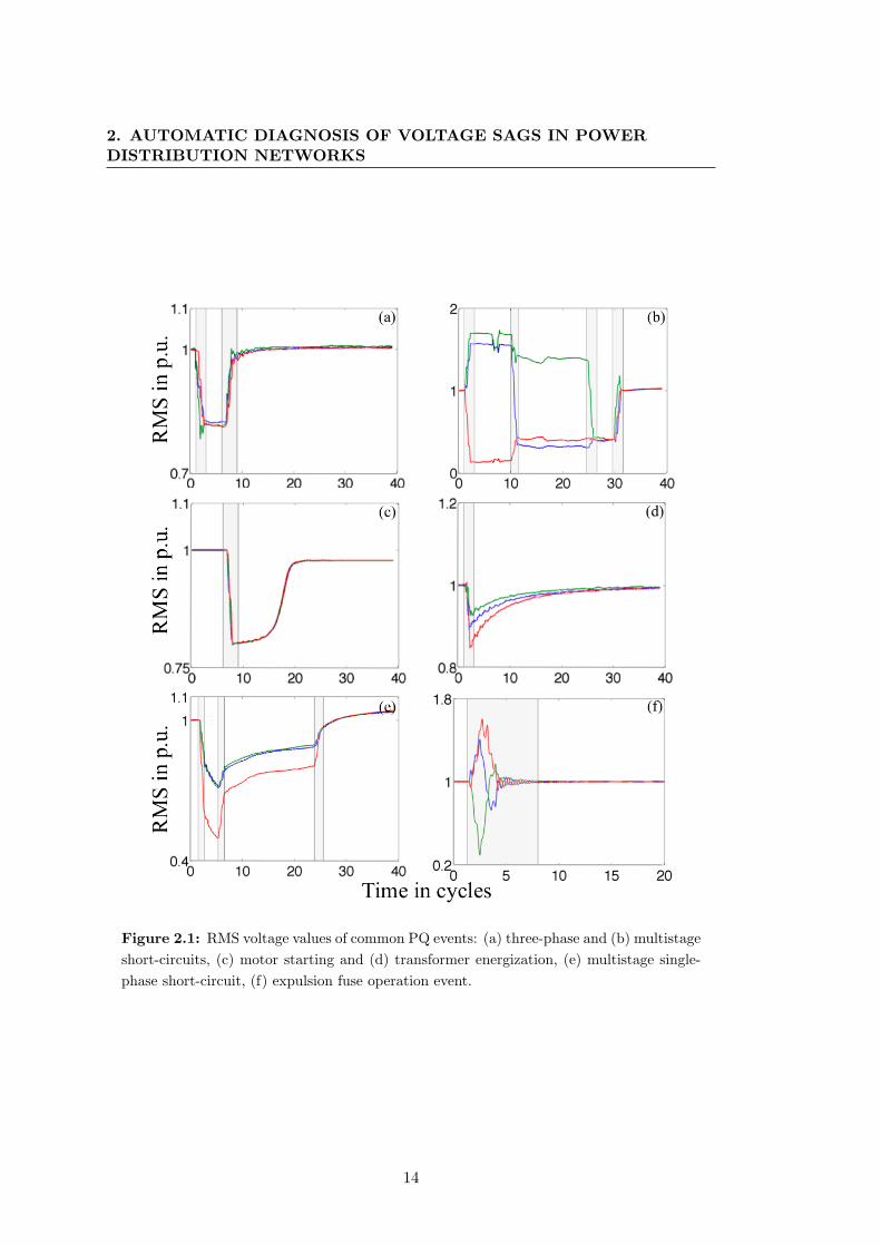
2.1 RMS voltage values of common PQ events: (a) three-phase and (b) multistage short-
circuits, (c) motor starting and (d) transformer energization, (e) multistage single-phase
short-circuit, (f) expulsion fuse operation event. . . . . . . . . . . . . . . . . . . . . . . . 14
2.2 Internal and external causes of sags in distribution networks. . . . . . . . . . . . . . . . 16
2.3 Voltage sag source relative location problem. . . . . . . . . . . . . . . . . . . . . . . . . 16
2.4 Example of an upstream (top) and downstream (bottom) voltage sag disturbance. . . . 17
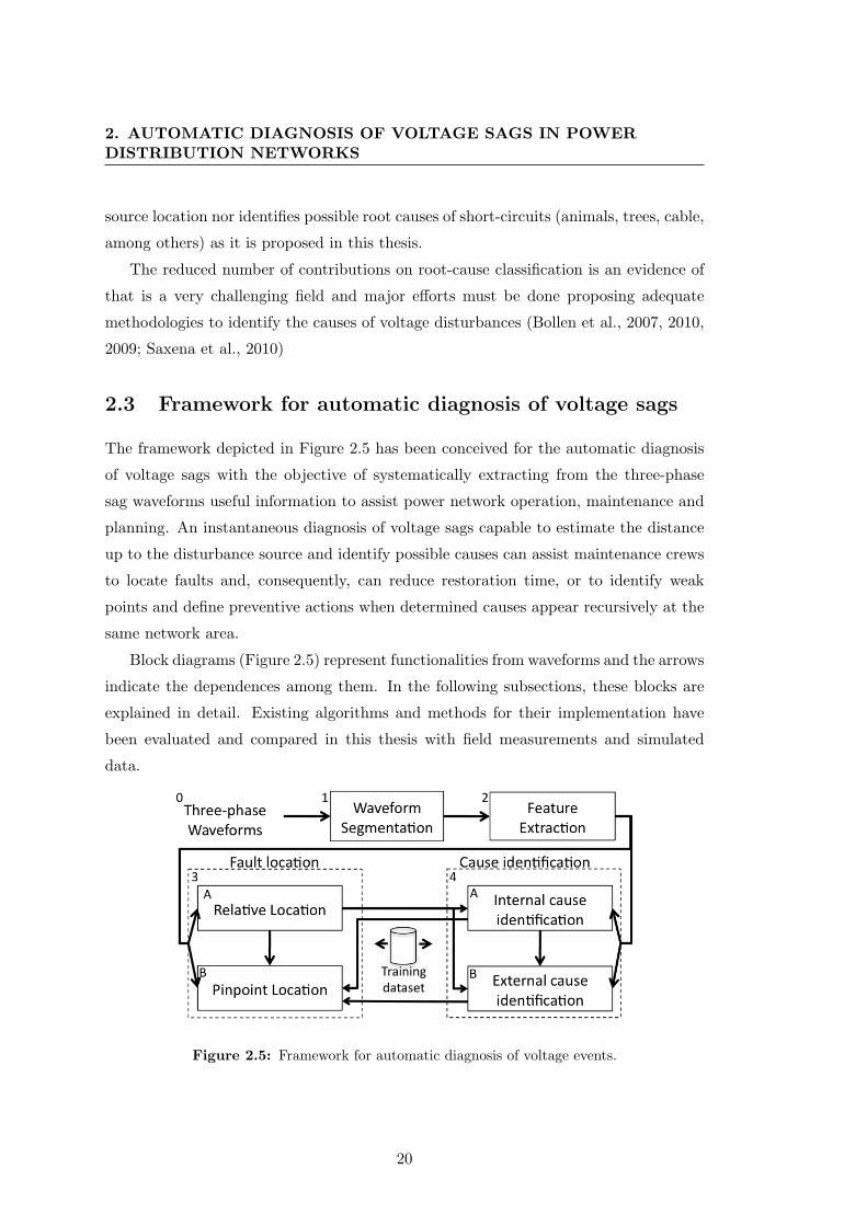
2.5 Framework for automatic diagnosis of voltage events. . . . . . . . . . . . . . . . . . . . . 20
2.6 Power distribution network without distributed generation . . . . . . . . . . . . . . . . . 21
2.7 Features according to waveform segmentation stages. . . . . . . . . . . . . . . . . . . . . 24
2.8 Second order current (dotted curve) and neutral voltage (dash curve) throughout a
transformer saturation event. . . . . . . . . . . . . . . . . . . . . . . . . . . . . . . . . . 27
2.9 Computation of fault insertion phase angle (FIPA) and the maximum change of voltage
magnitude (∆V ). . . . . . . . . . . . . . . . . . . . . . . . . . . . . . . . . . . . . . . . . 29
2.10 Voltage magnitude of the zero sequence component (V0) in a highly unbalanced event
due to an underground cable failure. . . . . . . . . . . . . . . . . . . . . . . . . . . . . . 30
2.11 Arc voltage (Varc) during a voltage disturbance due to a cable failure. Varc is only valid
in fault stage instants. . . . . . . . . . . . . . . . . . . . . . . . . . . . . . . . . . . . . . 31
2.12 Voltage waveforms due to an underground cable failure (top) and an animal contact
disturbance (bottom). . . . . . . . . . . . . . . . . . . . . . . . . . . . . . . . . . . . . . 35
2.13 Feature relevance. Date: day of the year. Time: hour of the day. Features are listed in
Fig. 2.7 and Section 2.3.3.2. . . . . . . . . . . . . . . . . . . . . . . . . . . . . . . . . . . 37
3.1 RMS phase-voltage sequence values and non-stationary stages of the 40 recorded PQ
events: (1-10) single-stage and (11-20) multistage short-circuits, (21-30) fuse operation
and (31-40) transformer saturation events. . . . . . . . . . . . . . . . . . . . . . . . . . . 42
3.2 Instantaneous power tensor (left) and its deformation (right). . . . . . . . . . . . . . . . 46
3.3 Isotropic- (1st row), deviation- (2nd row) and antisymmetric-tensors (3rd row) during
prefault, fault and postfault instants in a single-stage voltage sag event. . . . . . . . . . 47
3.4 Waveform segmentation of a synthetic single-phase voltage sag. (a) Instantaneous and
RMS signal values. (b) Residual-WSA, (c) Harmonic-WSA and (d) Tensor-WSA results. 50
3.5 Detection index for each segmentation algorithm and voltage residual magnitudes. Ver-
tical dotted lines are the true starting and ending transition samples. . . . . . . . . . . . 55
3.6 Detection errors for different remaining voltage magnitudes from the faulted phase of
the 40 collected disturbances. . . . . . . . . . . . . . . . . . . . . . . . . . . . . . . . . . 56
ix
LIST OF FIGURES
3.7 Detection errors for each fault insertion phase angle and segmentation algorithm. Syn-
thetic (top) and collected waveforms (bottom). . . . . . . . . . . . . . . . . . . . . . . . 57
3.8 Error cumulative distribution for each waveform segmentation algorithm. . . . . . . . . 61
4.1 Magnitude of voltage sags vs. duration . . . . . . . . . . . . . . . . . . . . . . . . . . . . 67
4.2 Slope of system trajectory algorithm results. Downstream sag events (circles) are de-
picted in the first 228 positions of the horizontal axis. . . . . . . . . . . . . . . . . . . . 69
4.3 Real current component algorithm results. The downstream sag events (circles) are
depicted in the first 228 positions of the horizontal axis. . . . . . . . . . . . . . . . . . . 70
4.4 Distance relay algorithm results. Sags are classified as downstream sags if Zratio < 1
and ∠Zsag > 0. . . . . . . . . . . . . . . . . . . . . . . . . . . . . . . . . . . . . . . . . . 71
4.5 Resistance sign algorithm results. Voltages sags are classified as downstream sags if
Rex < 0 and Rey < 0. . . . . . . . . . . . . . . . . . . . . . . . . . . . . . . . . . . . . . 74
4.6 Simplified resistance sign algorithm results. Voltage sags are classified as downstream
sags if Re < 0. . . . . . . . . . . . . . . . . . . . . . . . . . . . . . . . . . . . . . . . . . 75
4.7 Phasor diagram of the network shown in Figure 2.3 . . . . . . . . . . . . . . . . . . . . . 76
4.8 Phase change in sequence current algorithm results. Downstream sag events (circles)
must be inside the shaded bottom left region (4φ < 0). . . . . . . . . . . . . . . . . . . 77
4.9 Combination of PCSC and RS algorithms. Upstream sag events (crosses) have to be
inside the cube. . . . . . . . . . . . . . . . . . . . . . . . . . . . . . . . . . . . . . . . . . 82
4.10 FPR vs TPR. Single-phase and phase-to-phase sag events . . . . . . . . . . . . . . . . . 84
4.11 FPR vs TPR. Single-phase sag events only. . . . . . . . . . . . . . . . . . . . . . . . . . 84
4.12 FPR vs TPR. Phase-to-phase sag events only. . . . . . . . . . . . . . . . . . . . . . . . . 85
5.1 Root causes of disturbances according to their RMS voltage sequence shape. . . . . . . . 90
5.2 Step changes in voltage: (a) Capacitor energization, (b) load connection and (c) load
disconnection. . . . . . . . . . . . . . . . . . . . . . . . . . . . . . . . . . . . . . . . . . . 91
5.3 Change in power factor angle. Difference between postfault and preafault power factor
angle . . . . . . . . . . . . . . . . . . . . . . . . . . . . . . . . . . . . . . . . . . . . . . . 95
5.4 Prefault and postfault active/reactive power in step change events . . . . . . . . . . . . 96
5.5 RMS voltage waveforms of motor-starting disturbances with low (ID=2) and high (ID=14)
inertia in Figure 5.9. . . . . . . . . . . . . . . . . . . . . . . . . . . . . . . . . . . . . . . 97
5.6 Maximum neutral current and voltage ratios during motor and transformer events (non-
rectangular shape) . . . . . . . . . . . . . . . . . . . . . . . . . . . . . . . . . . . . . . . 99
5.7 Magnitude of 2-order current component in each non-rectangular event . . . . . . . . . . 100
5.8 RMS voltage waveform of a transformer-saturation disturbance. Ideal triangle and co-
efficient for TWC computation . . . . . . . . . . . . . . . . . . . . . . . . . . . . . . . . 101
5.9 Transformer waveform coefficient (TWC) of each motor and transformer event. . . . . . 103
5.10 RMS voltage waveforms of the disturbance with ID=41 in Figure 5.9. Transformer
saturation followed by a protection operation. . . . . . . . . . . . . . . . . . . . . . . . . 104
5.11 Zero sequence current of each rectangular event. Three-phase-to-ground disturbances
correspond to asymmetrical three-phase voltage sags. . . . . . . . . . . . . . . . . . . . . 106
5.12 Loss-of-voltage triangle in per unit of the maximum loss-of-voltage value (Lmax = 1).
The triangle corresponds to the outer triangle. . . . . . . . . . . . . . . . . . . . . . . . 107
5.13 Loss-of-voltage triangle of the transformer saturation plotted in Figure 5.10. . . . . . . . 108
x
LIST OF FIGURES
5.14 FTIv (crosses) and FTIc (circles) of each disturbance waveform. . . . . . . . . . . . . . 110
5.15 Loss-of-voltage angles θv1 and θv2. . . . . . . . . . . . . . . . . . . . . . . . . . . . . . . 111
5.16 RMS voltage waveforms of the short-circuit disturbances with ID=1 (single-phase) and
ID=12 (double-phase to ground) in Figure 5.15. . . . . . . . . . . . . . . . . . . . . . . . 112
5.17 Number of non-stationary stages during the event for all root causes. . . . . . . . . . . . 114
5.18 TWC values for each disturbance waveform. . . . . . . . . . . . . . . . . . . . . . . . . 114
5.19 Rule-based framework for identification of short-circuits and internal root causes. . . . . 117
5.20 Classification results of the rule-based framework for root cause identification. . . . . . . 118
6.1 Histogram of the date of occurrence of the events. . . . . . . . . . . . . . . . . . . . . . 125
6.2 Histogram of the events according to time of the day. . . . . . . . . . . . . . . . . . . . . 125
6.3 Histograms of the maximum change of voltage magnitude (4V ). . . . . . . . . . . . . . 127
6.4 Histogram of the maximum change of the neutral voltage magnitude (4Vn). . . . . . . . 127
6.5 Histograms of the maximum zero-sequence voltage (V0). . . . . . . . . . . . . . . . . . . 128
6.6 Histograms of the maximum zero sequence current (I0). . . . . . . . . . . . . . . . . . . 129
6.7 Histogram of the maximum arc voltage during the event. . . . . . . . . . . . . . . . . . 130
6.8 Histogram of the absolute value of fault insertion phase angle. . . . . . . . . . . . . . . . 131
6.9 Quality of the cause effect for each feature. . . . . . . . . . . . . . . . . . . . . . . . . . 134
6.10 Extracted rule for identifying animal contact events [(Varc > 0.319) & (6 < Time 6 14)
& (56, 25◦ 6 FIPA 6 137.813◦)→ Animalcontact]. Most of animal contact events are
inside the blue shaded region. . . . . . . . . . . . . . . . . . . . . . . . . . . . . . . . . . 136
6.11 Extracted rule for identifying single-phase lightning-induced events [(Varc 6 0, 319) &
(T ime 6 9) & (I0 6 1, 057) → Lightning − induced]. Most of ligthning-induced events
are inside the green shaded region. . . . . . . . . . . . . . . . . . . . . . . . . . . . . . . 137
6.12 Extracted rule for identifying single-phase tree-contact events [(V0 6 0, 249) & (Date >
241) & (Varc 6 0, 664)→ Tree− contact]. Most of tree contact events are inside the red
shaded region. . . . . . . . . . . . . . . . . . . . . . . . . . . . . . . . . . . . . . . . . . . 138
6.13 Extracted rule for identifying cable fault events [(4V > 0, 278) & (V0 > 0, 242) &
(FIPA 6 112, 5◦)→ Cablefault]. Most of cable fault events are inside the black shaded
region. . . . . . . . . . . . . . . . . . . . . . . . . . . . . . . . . . . . . . . . . . . . . . . 139
6.14 Classification methodology for power quality events based on fault cause identification. . 140
A.1 FPR versus TPR. . . . . . . . . . . . . . . . . . . . . . . . . . . . . . . . . . . . . . . . . 164
xi

LIST OF FIGURES
xii
List of Tables
2.1 Applications of artificial intelligence techniques on power quality diagnosis . . . . . . . . 18
2.2 Decision rules used by existing relative location algorithms . . . . . . . . . . . . . . . . . 33
2.3 Source relative location results for voltage sags in Figure 2.4. . . . . . . . . . . . . . . . 33
2.4 Extracted rules for diagnosing the internal cause of sags . . . . . . . . . . . . . . . . . . 36
2.5 Extracted rules for diagnosing the external cause of voltage sags . . . . . . . . . . . . . 38
3.1 Waveform segmentation results according to each algorithm and collected disturbance:
Samples difference between true and detected transition instants (128 samples = 1 cycle). 58
4.1 Relative location algorithms used in this analysis . . . . . . . . . . . . . . . . . . . . . . 65
4.2 Voltage sag events gathered and used in the analysis . . . . . . . . . . . . . . . . . . . . 66
4.3 Qualitative performance of each feature . . . . . . . . . . . . . . . . . . . . . . . . . . . 76
4.4 Feature descriptive statistics . . . . . . . . . . . . . . . . . . . . . . . . . . . . . . . . . . 79
4.5 Quality of the source relative location effect over the feature . . . . . . . . . . . . . . . . 79
4.6 Extracted rule set using CN2 induction algorithm . . . . . . . . . . . . . . . . . . . . . . 81
4.7 Confusion matrix and classification rates for each algorithm . . . . . . . . . . . . . . . . 83
4.8 Voltage sags misclassified using PCSC algorithm . . . . . . . . . . . . . . . . . . . . . . 87
5.1 Voltage disturbances used in the characterization of internal causes . . . . . . . . . . . . 93
5.2 Features according to each root cause of power quality events . . . . . . . . . . . . . . . 116
6.1 Power quality events used in the analysis . . . . . . . . . . . . . . . . . . . . . . . . . . 123
6.2 Feature descriptive statistics . . . . . . . . . . . . . . . . . . . . . . . . . . . . . . . . . . 133
6.3 Extracted rule set using CN2 induction algorithm . . . . . . . . . . . . . . . . . . . . . . 135
6.4 Result of the methodology according to each approach . . . . . . . . . . . . . . . . . . . 142
6.5 Comparison of the rule-based framework results . . . . . . . . . . . . . . . . . . . . . . . 143
A.1 Confusion matrix . . . . . . . . . . . . . . . . . . . . . . . . . . . . . . . . . . . . . . . . 163
xiii
LIST OF TABLES
List of
Acronyms
4φ Difference in phase angle between
fault and steady-state current.
4I Maximum change of the current mag-
nitude
4In Maximum change of the neutral cur-
rent magnitude
4V Maximum change of the voltage mag-
nitude
4Vn Maximum change of the neutral volt-
age magnitude
FIPA Fault Insertion Phase Angle
FTI Fault-Type Index for identifying type
of the faults
I0 Maximum zero sequence current
Iss Steady-state current.
Re Resistance obtained from the rotat-
ing transformation to Rex and Rey
expressions (Eq. 4.8 and Eq. 4.9).
Rex Equivalent resistance computed from
imaginary parts of voltage samples.
Rey Equivalent resistance computed from
imaginary parts of voltage samples.
TWC Transformer Waveform Coefficient
V0 Maximum zero sequence voltage
Varc Maximum arc voltage throughout
the disturbance
Zratio Impedance ratio between Zsag and
Zss magnitudes.
Zsag Impedance seen during a voltage sag.
Zss Impedance seen in steady state.
CN2 CN2 rule induction algorithm
DR Distance Relay algorithm
FFT Fast Fourier Transform
FN False Negative
FP False Positive
FPR False Positive Rate
MANOVA Multivariate Analysis of Variance
PCSC Phase Change in Sequence Current
algorithm
PQM Power Quality Monitoring device
RCC Real Current Component
RMS Root Mean Square
RS Resistance Sign algorithm
sRS Simplified Resistance Sign algorithm
SST Slope of System Trajectory
SVM Support Vector Machine
TN True Negative
TP True Positive
TPR True Positive Rate
xiv
1
Introduction
This thesis proposes a framework for automatic diagnosis of voltage disturbances. A
voltage disturbance is a deviation in magnitude or frequency of the waveform regard-
ing its nominal values. Voltage disturbances are generated during energy generation,
transmission and distribution processes. Both, external agents interacting with the
power network and common actions of power components are the causes of voltage
disturbances. According to their duration, voltage disturbances can be classified as:
transients, short duration and long duration variations. This thesis mainly focuses
on the study of short duration variations; particularly in voltage sags (1 cycle to 1
or 3 minutes according to different international standards) recorded in distribution
networks.
The automatic diagnosis of disturbances is the set of tasks oriented to locate the
source origin and to identify the causes of such disturbances. It includes the combina-
tion of signal processing tools, power system principles and data mining techniques to
extract significant information for diagnosis purposes from waveforms. The idea is to
propose a methodology to systematically analyse a voltage sag and infer information
related with its source origin and causes.
Physical phenomena involved in the apparition of disturbances are analysed to pro-
pose relevant features of the event waveform useful for diagnosis. Short-circuits induced
by animal or tree contacts, atmospheric phenomena or commutation of large loads and
transformer energizing are examples of common causes of voltage disturbances. Signal
processing methods are used to obtain the RMS sequence and determine stationary and
non-stationary stages of a disturbance to facilitate the extraction of these features. Dif-
1
1. INTRODUCTION
ferent sets of disturbances, characterised by this vector of features, or attributes, have
been analysed using a data mining approach to select the most relevant attributes and
their dependencies with causes and origin of the disturbances. The work has performed
mainly with real-world waveforms, which origin and causes is previously known, and
complemented with synthetic data when real one was not available.
Nowadays, automatic diagnosis of disturbances has special interest due to the im-
pact of voltage sags on sensitive loads, industrial productive processes and the existence
of standards and regulatory frameworks. This has motivated electrical facilities and
research institutions to develop power quality monitoring campaigns and surveys to
establish a power quality baseline and defining assessment strategies. As consequence,
large databases of power quality events have been generated. This work takes advantage
of several power quality databases containing waveforms of voltage sags and synthetic
induction motor and switching events. The necessity to develop a systematic procedure
to analyze them has motivated this work.
1.1 Voltage disturbances in power distribution networks
The term disturbance or event is commonly used to describe significant and sudden
deviations of voltage from its established waveform. When a fault takes place, changes
in shape, magnitude and frequency of the waveform are expected. These changes can be
associated with the physical phenomena causing the event. Throughout the event the
disturbance waveform experiences several non-stationary and stationary stages. Both,
normal operation of network components and short-circuits can be the cause of voltage
disturbances in distribution networks. Common causes of voltage disturbances due
to normal operation actions are: transformer energization, starting of large induction
motors, large-load and capacitor-bank switching events. On the other hand, causes of
short-circuits are usually failures in underground cables, animals/tree-branches getting
touch with overhead lines, pneumatic drills and shovel accidents.
Since operation actions carried out on power components cause the apparition of
disturbances (transformer energizing, motor starting, capacitor banks and large load
switching, etc.), these are considered in this work as internal root-causes of voltage
disturbances. Conversely, the causes of short-circuits are called external root-causes
because they are beyond the control of the electrical facility.
2
1.2 Motivation of the work
According to the source location, disturbances are classified as downstream or up-
stream with respect to the measurement point, being the origin of a downstream dis-
turbance located in the power flow direction whereas an upstream one is in opposite
direction.
1.2 Motivation of the work
The necessity to better know how power networks are performed and to understand how
they behave in front of specific situations has motivated the installation of power quality
monitors and other sensing equipments in the distribution networks. The tendency to
increase observability of the power network, in part motivated by the necessity to adapt
their management towards the Smart Grid concept (distributed generation, electric
vehicle, flexible networks, etc.), and in part due to the necessity to assure certain levels
of power quality, is another factor that is influencing the existence of increasing large
data bases of power quality events.
Power quality events are asynchronous information that reports instantaneous changes
in the network, consequently a fast diagnosis of every event can report relevant infor-
mation about how the network is behaving and at the same time the information can
be used to assist maintenance and power restoration. Continuous monitoring of events
collected in a single point could be focused on discovering recurrent faults or predicting
failures. Finally, multipoint monitoring campaigns can facilitate power quality assess-
ment and when combining with meteorological and geo-positioned information the use
of data mining and knowledge discovery can contribute to more challenging goals.
This thesis aims to contribute to define a methodology to automatically diagnose
voltage disturbances, in particular voltage sags. Disturbance diagnosis can be under-
stood as a classification problem where a disturbance has to be associated with a class.
Different classes correspond to different origins (upstream/downstream) and different
root causes (transformer, animal, tree, cable, etc). The majority of existing works for
automatic classification of voltage disturbances reported in the literature have been
oriented to discriminate among different types of disturbances (sag, swell, flicker, har-
monic, etc) instead of identifying its source location and root cause (Bollen et al., 2007,
2009; McGranaghan and Santoso, 2007; Saxena et al., 2010).
3
1. INTRODUCTION
On the other hand, it has observed that many works addressing the disturbance
classification problem using different artificial intelligent techniques; their classifiers are
trained by using a great amount of features without previously performing a suitable
selection of the best or relevant features, so, classifiers are being trained with sets of
features containing redundancy information, or lack of it, (Gunal et al., 2009; Peng
et al., 2004; Saxena et al., 2010). This work proposes a systematic procedure to extract
relevant features according to classification / diagnosis goal and an evaluation of this
relevance.
The benefits of diagnosing power quality disturbances (root-cause identification and
source location) are also noticeable since it can contribute to decrease power quality sup-
ply indexes related to duration and frequency of interruptions. Interruption duration
indexes will decrease because during a permanent fault from the captured three-phase
voltage and current waveforms, the fault root-cause can be identified and time can
be saved as consequence of a faster power supply restoration. Interruption frequency
indexes can also benefit from an early detection of failures or the identification of re-
current auto-extinguished faults, for instance, faults induced by tree contacts during
windy days. Reclosers generally do not operate during recurrent faults as they self
clear, so an early diagnosis can prevent from future failures in that point.
The need for methodologies and tools for optimal use of power quality waveforms is
highlighted in a number of publications (Bollen et al., 2010, 2009; McGranaghan and
Santoso, 2007; Styvaktakis., 2002; Styvaktakis et al., 2002). So, the work is carried out
along the following objectives:
• The understanding of physical phenomenon occurred when internal and external
root causes induce voltage disturbances on radial distribution networks.
• The selection and suitable computation of relevant features containing valuable
information about possible root-cause and relative location of the disturbance
source.
• The conception of a conceptual framework for an automatic diagnosis of voltage
sags making use of relevant features extracted from three-phase voltage/current
waveforms.
4
1.3 Automatic diagnosis of voltage disturbances
The thesis mainly focuses on diagnosis of voltage sags and it has been performed
with data collected in power networks without distributed generation.
Information about power network configuration is not considered and the thesis
only focuses on the information contained in the recorded waveforms. So, fault location
problem is reduced to relative location (upstream/downstream) and distance estimation
to the fault has not been considered in this study.
1.3 Automatic diagnosis of voltage disturbances
Automatic diagnosis of disturbances has been defined as the set of tasks to locate
disturbance origin and identify its root cause. In the following paragraphs the main
steps for automatic diagnosis are enumerated and serves as guide of the document
content:
• Waveform segmentation: This is the estimation of stationary and non-satationary
stages in a disturbance waveform. This is necessary because there are features re-
quiring to be computed during stationary stages and other during non-stationary
ones.
• Feature extraction: Calculation of required features according to diagnostic ob-
jectives (location and cause identification). Relevance of theses features according
to the diagnosis goals must be analysed and the most relevant must be selected.
• Source relative location: This step proposes the classification of a voltage sag
according to its origin upstream or downstream from measurement point. The
origin of a disturbance is needed because the pinpoint location and possible cause
can only be estimated for downstream disturbances.
• Cause identification: It has to be identied the disturbance root cause if its source
is located downstream. In this work, the root cause is obtained using a pre-
trained classier with the set of relevant features selected in previous step. The
training dataset is conformed by disturbance waveforms whose source location or
root-cause is previously known.
5
1. INTRODUCTION
• Source pinpoint location: This is the estimation of the distance from the mea-
surement place up to the disturbance location. This task would apply only for
downstream disturbances.
Root cause of upstream voltage disturbances cannot be identied because their wave-
forms do not contain information about fault impedance; thus, their source pinpoint
location neither can be estimated. Classiers must be built making use of relevant fea-
tures since it allows improving classication performance. As was mentioned before,
the last step (Source pinpoint location) is out of the thesis scope since it is related to
distance estimation and author does not have information about network configuration
neither line impedances.
1.4 Outline of the thesis
This thesis document is organized in seven chapters. This first chapter corresponds to
the introduction and contains fundamentals of the thesis. Content of others chapters
is the following:
• Chapter 2 - Automatic diagnosis of voltage sags collected in power
distribution networks: Conception of a framework for voltage sag diagnosing
is described in this chapter. It presents a set of significant features, that can be
used for diagnosis purposes, and the general procedure to identify affected phases,
locate origin of disturbances (upstream/downstream) and determine possible root
causes (motor, transformer, underground cable failure, tree branch, animal and
lightning-induced events).
• Chapter 3 - Waveform segmentation of voltage disturbances: The chap-
ter analyses and compares existing segmentation algorithms and proposes a new
one inspired on the Tensor theory. All of them have been assessed according to
different scenarios considering events caused by different root causes.
• Chapter 4 - Relative location of voltage sag source: Algorithms for relative
location of the voltage sag origin are compared. Six different algorithms have been
included in the test, and relevance of their features is analyzed using multivariate
analysis of variance (MANOVA). New classification rules are proposed based on
6
1.5 Data collection
the application of a machine learning algorithm (CN2) to the features involved
in the analysed algorithms.
• Chapter 5 - Internal causes of voltage disturbances - Relevant features
and classification methodology: It addresses the problem of extracting sig-
nificant features to determine internal causes (produced by network operation
actions) of voltage disturbances. The analysis includes voltage disturbances due
to power transformers, induction motors, switch of capacitor-bank or large-load.
The proposed feature set is then used for building and test a rule-based classifier
to discriminate among these internal causes.
• Chapter 6 - External causes of voltage disturbances - Relevant features
and classification methodology: This chapter aims determining relevant fea-
tures in voltage and current waveforms of a voltage sag to automatically identify
its external cause. In particular, it focuses on voltage sags caused by external
factors such as animals, tree contacts, lightning-induced events and failures on
underground cables. Collected disturbances characterised by these features are
used to obtain classification rules capable to discriminate among these external
causes.
• Chapter 7 - Conclusions and future works: Main conclusions and contri-
butions of this thesis are emphasized in this chapter.
1.5 Data collection
Field measurements used in this thesis have been collected in American and Eu-
ropean distribution networks:
– Catalan distribution network: Disturbance waveforms were collected in 25kV
radial distribution circuits by PQMs installed at secondary side of power
transformers. Details about this data are given in Section 4.2.
– Several electrical facilities at northeastern american region: Electric Power
Research Institute (EPRI) collects the power quality data from several Amer-
ican electrical facilities. Waveforms were captured at 12,47kV radial distri-
7
1. INTRODUCTION
bution networks during a PQ survey carried out from 2002 to 2006. Details
about EPRI data in Section 6.2.
Synthetic waveforms used in Chapter 5 were simulated for four different power
networks. They were modelled using Analysis Transient Program (ATP). More
details about simulated data can be found in Section 5.2.
1.6 List of publications
The following subsection list the main contributions of this thesis based on the
publications in journals and conferences.
• Journals
1. V. Barrera, J. Melendez, S. Kulkarni, S. Santoso. Feature Analysis and Automatic Clas-
sification of Short-Circuit Faults Resulting from External Causes, European Transactions
on Electrical Power (ETEP), DOI: 10.1002/etep.674, January, 2012., (Barrera et al., 2012).
2. V. Barrera, J. Melendez, S. Herraiz. Waveform Segmentation for Intelligent Monitoring
of Power Events, Electric Power Systems Research (EPSR). Manuscript id: EPSR-D-11-
00655. Submitted in August 2011. Paper in second review , (Barrera et al., 2011b).
3. V. Barrera, R. Velandia, F. Hernandez, H. Vargas, J. Melendez. Relevant Attributes for
Voltage Event Diagnosis in Power Distribution Networks, Revista Iberoamericana de Au-
tomatica e Informatica Industrial. Manuscript 11077-28049-1-SM, submitted in November
2010. On printing process, (Barrera et al., 2010d).
4. V. Barrera, J. Melendez, S. Herraiz. Evaluation of Fault Relative Location Algorithms
Using Voltage Sag Data Collected at 25-kV Substations, Special Issue on Power Qual-
ity, European Transactions on Electrical Power (ETEP), DOI 10.1002/etep.393, October,
2009, (Barrera et al., 2009a).
• Conferences
1. V. Barrera, A. Pavas, J. Melendez. Power quality assessment of the Bogota distribution
network focused on voltage sags analysis, International Conference on Innovative Smart
Grid Technologies Europe 2011 (ISGT) , IEEE PES, Manchester-England, paper number
159, 6-9 December 2011, (Barrera et al., 2011d).
2. V. Barrera, J. Melendez, S. Herraiz, A. Ferreira, A. Munoz. Analysis of the influence
of weather factors on outages in Spanish distribution networks, International Conference
on Innovative Smart Grid Technologies Europe 2011 (ISGT) , IEEE PES, Manchester-
England, paper number 269, 6-9 December 2011, (Barrera et al., 2011c).
8
1.6 List of publications
3. V. Barrera, J. Melendez, S. Herraiz. Feature analysis for voltage disturbances resulting
from external causes, 21st International Conference on Electricity Distribution (CIRED),
Frankfurt-Germany, paper number 1151, 5-7 June 2011, (Barrera et al., 2011a).
4. V. Barrera, I. Yu-Hua Gu, M. H.J Bollen, J. Melendez. Feature Characterization of
Power Quality Events According to Their Underlying Causes, 14th IEEE International
Conference on Harmonics and Quality of Power (ICHQP), September 26-29, 2010, Berg-
amo, Italy, (Barrera et al., 2010a).
5. V. Barrera, S. Kulkarni, S. Santoso, J. Melendez. SVM-Based Classification Methodology
for Overhead Distribution Fault Events, 14th IEEE International Conference on Harmonics
and Quality of Power (ICHQP), September 26-29, 2010, Bergamo, Italy, (Barrera et al.,
2010c).
6. V. Barrera, S. Kulkarni, S. Santoso, J. Melendez. Feature Analysis and Classification
Methodology for Overhead Distribution Fault Events, IEEE Power & Energy Society, 2010
General Meeting, July 25-29, 2010, Minneapolis, Minnesota, USA, (Barrera et al., 2010b).
7. J. Jagua, V. Barrera, G. Carrillo, J. Melendez. Waveform Segmentation Based On
Tensor Analysis, IEEE Andean Conference, Exhibition and Industry Forum (IEEE AN-
DESCON), September 15-17, 2010, Colombia, (Jagua et al., 2010).
8. S. Ortiz, H.Torres, V. Barrera, C. Duarte, G. Ordonez, S. Herraiz. Analysis of Voltage
Events Segmentation Using Kalman Filter and Wavelet Transform, IEEE Andean Con-
ference, Exhibition and Industry Forum (IEEE ANDESCON), September 15-17, 2010,
Colombia, (Ortiz et al., 2010).
9. V. Barrera, J. Melendez, S. Herraiz, J. Sanchez. A New Sag Source Relative Location
Algorithm Based On The Sequence Current Magnitude, Simposio Internacional sobre la
Calidad de la Energıa Electrica SICEL09, Bogota, Colombia, August 4-6, 2009, (Barrera
et al., 2009b).
10. S. Ortiz, A. Torres, V. Barrera, C. Duarte, G. Ordonez, S. Herraiz. Estrategias para la
Segmentacion de Huecos de Tension con Componentes de Alta Frecuencia, Simposio In-
ternacional sobre la Calidad de la Energıa Electrica SICEL09, Bogota, Colombia, August
4-6, 2009, (Ortiz et al., 2009).
11. J. Blanco, J. Jagua, L. Jaimes, V. Barrera, J. Melendez. Metodologıa para el Diagnostico
de la Causa de Huecos de Tension , Simposio Internacional sobre la Calidad de la Energıa
Electrica SICEL09, Bogota, Colombia, August 4-6, 2009, (Blanco et al., 2009a).
12. V. Barrera, B. Lopez, J. Melendez, J. Sanchez. Voltage Sag Source Location From
Extracted Rules Using Subgroup Discovery, Frontiers in Artificial Intelligence and Appli-
cations, Edited by Teresa Alsinet, Josep Puyol-Gruart, Carme Torras, Vol. 128, p.p.:
225-235, ISBN 978-1-58603-925-7, October 2008, (Barrera et al., 2008b).
13. V. Barrera, X. Berjaga, J. Melendez, S. Herraiz, J. Sanchez and M. Castro. Two New
Methods for Voltage Sag Source Location, ICHQP 2008 - 13th International Conference on
Harmonics & Quality of Power 28th September 1st October, Australia, 2008, (Barrera
et al., 2008a).
14. V. Barrera, J. Melendez, S. Herraiz, J. Sanchez. Unusual Voltage Sag Event Detection
in Power Systems, 2008 IEEE/PES Transmission and Distribution Conference and Ex-
9
1. INTRODUCTION
position: Latin America, Bogota, Colombia, August 13th to 15th, 2008, (Barrera Nunez
et al., 2008).
15. V. Barrera, J. Melendez, S. Herraiz. A Survey on Voltage Sag Events in Power Systems,
IEEE/PES Transmission and Distribution Conference and Exposition: Latin America,
Bogota, Colombia, August 13th to 15th, 2008, (Barrera et al., 2008c).
16. J. Melendez, X. Berjaga, S. Herraiz, V. Barrera, J. Sanchez and M. Castro. Classification
of sags according to their origin based on the waveform similarity, IEEE/PES Transmission
and Distribution Conference and Exposition: Latin America, Bogota, Colombia - August
13th to 15th, 2008, (Melendez et al., 2008).
As an additional contribution, throughout the development of this thesis four
bachelor degree thesis were developed between Universitat de Girona and Uni-
versidad Industrial de Santander (Colombia). Similarly, part of the findings of
this thesis has been approved to be included in the report of the CIGRE1 working
group C4.112 ”Guidelines for power quality monitoring - measurements locations,
processing and presentation of data”.
1.7 Contributions of the thesis
The findings obtained in this thesis show that is possible from three-phase wave-
forms to automatically identify the relative location of a disturbance source, as
well as its possible root cause. The main contributions of the work are:
1. A framework for automatic diagnosis of voltage sags is conceived. It is able
to identify the source relative location and possible cause of this kind of
disturbances (Barrera et al., 2008c, 2011 (Submitted).
2. The main mathematical/statistical tools, algorithms and artificial intelli-
gence techniques applied for diagnosis of voltage disturbances are identified
and applied (Barrera et al., 2008c, 2011 (Submitted).
3. Existing waveform segmentation algorithms are compared by varying sev-
eral parameters of the waveforms and algorithms. Their advantages and
disadvantages are elucidated (Barrera et al., 2011b; Jagua et al., 2010; Ortiz
et al., 2010).
1International Council of Large Power Systems
10
1.7 Contributions of the thesis
4. A waveform segmentation algorithm is proposed. It is based on Tensor
analysis and is compared with the existing ones (Barrera et al., 2011b).
5. Three feature sets are statistically analyzed. Two of them are proposed in
this thesis and contain useful information about external and internal causes
of sags. The third set contains information about the relative location of sag
source. Latter set has not been proposed by author, it is conformed with
the features used by existing relative location algorithms. Especial attention
is given to extraction and relevance of features. Statistics and multivariate
analysis of variance are used to assess their relevance (Barrera et al., 2009a,
2010a,b,c,d, 2011a,c, 2012).
6. The information contained in feature sets has been exploited by building
classification frameworks based on decision rules and support vector ma-
chines (Barrera et al., 2010a,c, 2012).
7. Existing algorithms for relative location of sag source are compared with
single- and double-phase short-circuits. Their advantages and drawbacks
according to each fault type are identified through an analysis based on
specificity and sensitivity statistics (Barrera et al., 2008a, 2009a; Melendez
et al., 2008).
8. It is proposed and tested a methodology able to identify the internal cause
of voltage disturbances. It is based on decision rules and the proposed fea-
ture set for internal causes. The five identifiable internal causes are: power
transformer, induction motor, capacitor switching and large-load connection
or disconnection (Barrera et al., 2010a).
9. Unlike the aforementioned methodology, it is proposed a second one that is
able to identify the external disturbance cause: animal contact, tree con-
tact, lightning-induced and underground cable failure (Barrera et al., 2010b,
2012).
11
1. INTRODUCTION
12
2
Automatic Diagnosis of Voltage
Sags in Power Distribution
Networks
2.1 Introduction
A framework for a systematic analysis of voltage sags is presented in this chapter.
The objective is to automatically extract information from sag waveforms in order
to identify possible root causes and location of its source. The framework combines
electrical principles and data mining concepts to perform the information extraction in
an automatic way.
Voltage sag is an electromagnetic disturbance characterised by a reduction on the
voltage magnitude due to a sudden variation of the network operation conditions. Du-
ration and magnitude are commonly used to characterize voltage sags. However, the
shape of voltage and current waveforms of two voltage sags with same duration and
magnitude can be extremely different (see as example Figure 2.1a-and-c or b-and-e).
Shape depends on many factors such as root cause, source location, affected phases or
protection operation, among others. Common causes of voltage sags are short-circuits
(Figure 2.1 a, b and e), induction motors starting (Figure 2.1c), transformer energizing
(Figure 2.1d) or fuse operation (Figure 2.1f).
All voltage sags start and end with a steady-state stage, but the evolution be-
tween those stages can be diverse resulting in different number of stationary and non-
13
2. AUTOMATIC DIAGNOSIS OF VOLTAGE SAGS IN POWERDISTRIBUTION NETWORKS
Figure 2.1: RMS voltage values of common PQ events: (a) three-phase and (b) multistageshort-circuits, (c) motor starting and (d) transformer energization, (e) multistage single-phase short-circuit, (f) expulsion fuse operation event.
14
2.1 Introduction
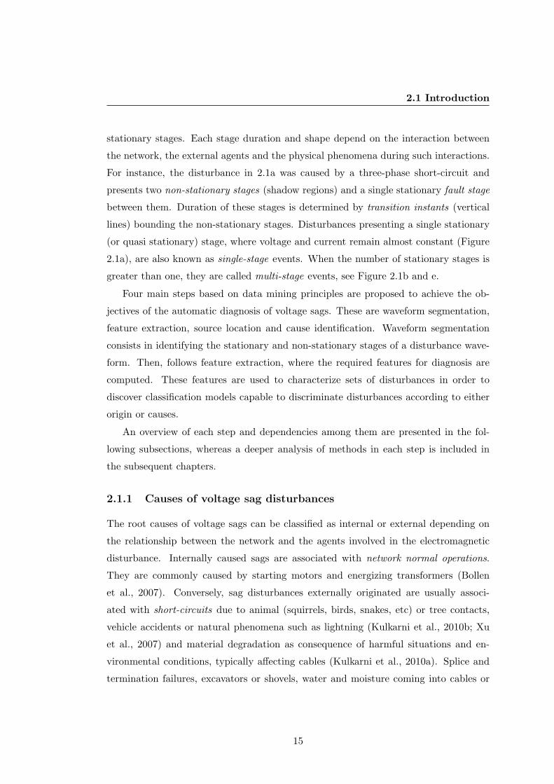
stationary stages. Each stage duration and shape depend on the interaction between
the network, the external agents and the physical phenomena during such interactions.
For instance, the disturbance in 2.1a was caused by a three-phase short-circuit and
presents two non-stationary stages (shadow regions) and a single stationary fault stage
between them. Duration of these stages is determined by transition instants (vertical
lines) bounding the non-stationary stages. Disturbances presenting a single stationary
(or quasi stationary) stage, where voltage and current remain almost constant (Figure
2.1a), are also known as single-stage events. When the number of stationary stages is
greater than one, they are called multi-stage events, see Figure 2.1b and e.
Four main steps based on data mining principles are proposed to achieve the ob-
jectives of the automatic diagnosis of voltage sags. These are waveform segmentation,
feature extraction, source location and cause identification. Waveform segmentation
consists in identifying the stationary and non-stationary stages of a disturbance wave-
form. Then, follows feature extraction, where the required features for diagnosis are
computed. These features are used to characterize sets of disturbances in order to
discover classification models capable to discriminate disturbances according to either
origin or causes.
An overview of each step and dependencies among them are presented in the fol-
lowing subsections, whereas a deeper analysis of methods in each step is included in
the subsequent chapters.
2.1.1 Causes of voltage sag disturbances
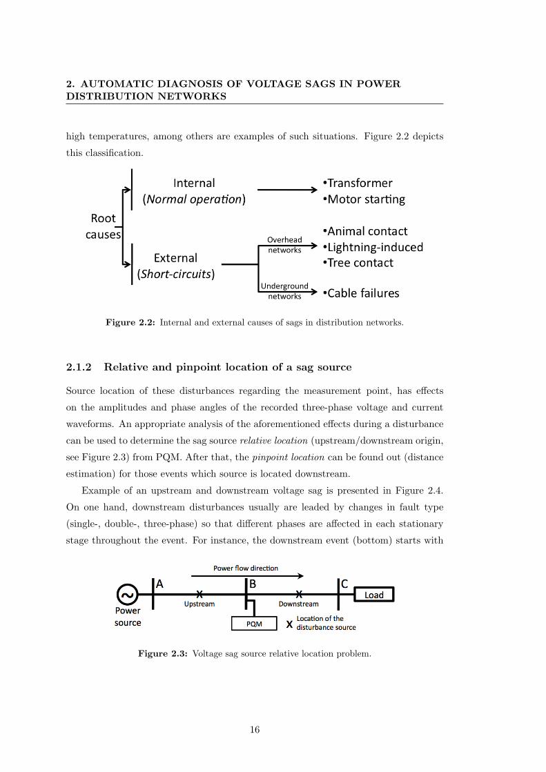
The root causes of voltage sags can be classified as internal or external depending on
the relationship between the network and the agents involved in the electromagnetic
disturbance. Internally caused sags are associated with network normal operations.
They are commonly caused by starting motors and energizing transformers (Bollen
et al., 2007). Conversely, sag disturbances externally originated are usually associ-
ated with short-circuits due to animal (squirrels, birds, snakes, etc) or tree contacts,
vehicle accidents or natural phenomena such as lightning (Kulkarni et al., 2010b; Xu
et al., 2007) and material degradation as consequence of harmful situations and en-
vironmental conditions, typically affecting cables (Kulkarni et al., 2010a). Splice and
termination failures, excavators or shovels, water and moisture coming into cables or
15
2. AUTOMATIC DIAGNOSIS OF VOLTAGE SAGS IN POWERDISTRIBUTION NETWORKS
high temperatures, among others are examples of such situations. Figure 2.2 depicts
this classification.
Figure 2.2: Internal and external causes of sags in distribution networks.
2.1.2 Relative and pinpoint location of a sag source
Source location of these disturbances regarding the measurement point, has effects
on the amplitudes and phase angles of the recorded three-phase voltage and current
waveforms. An appropriate analysis of the aforementioned effects during a disturbance
can be used to determine the sag source relative location (upstream/downstream origin,
see Figure 2.3) from PQM. After that, the pinpoint location can be found out (distance
estimation) for those events which source is located downstream.
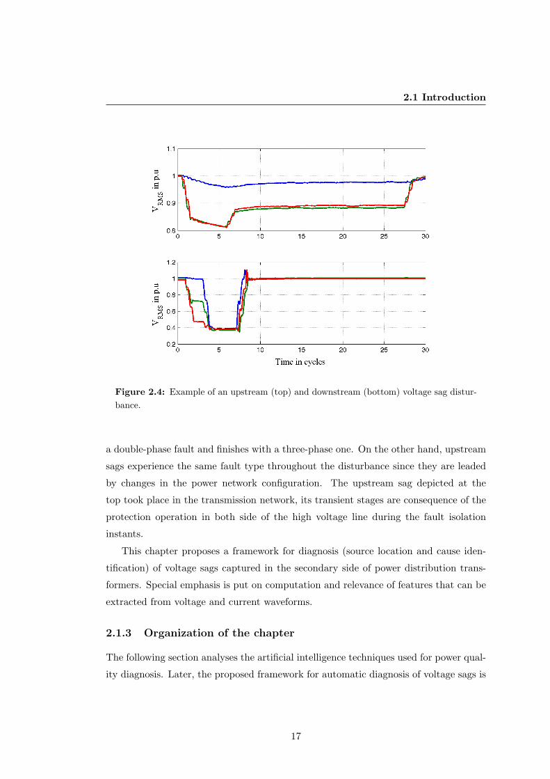
Example of an upstream and downstream voltage sag is presented in Figure 2.4.
On one hand, downstream disturbances usually are leaded by changes in fault type
(single-, double-, three-phase) so that different phases are affected in each stationary
stage throughout the event. For instance, the downstream event (bottom) starts with
Figure 2.3: Voltage sag source relative location problem.
16
2.1 Introduction
Figure 2.4: Example of an upstream (top) and downstream (bottom) voltage sag distur-bance.
a double-phase fault and finishes with a three-phase one. On the other hand, upstream
sags experience the same fault type throughout the disturbance since they are leaded
by changes in the power network configuration. The upstream sag depicted at the
top took place in the transmission network, its transient stages are consequence of the
protection operation in both side of the high voltage line during the fault isolation
instants.
This chapter proposes a framework for diagnosis (source location and cause iden-
tification) of voltage sags captured in the secondary side of power distribution trans-
formers. Special emphasis is put on computation and relevance of features that can be
extracted from voltage and current waveforms.
2.1.3 Organization of the chapter
The following section analyses the artificial intelligence techniques used for power qual-
ity diagnosis. Later, the proposed framework for automatic diagnosis of voltage sags is
17
2. AUTOMATIC DIAGNOSIS OF VOLTAGE SAGS IN POWERDISTRIBUTION NETWORKS
described and some guidelines for building it are given. Finally, the relevant conclusions
of the chapter will be elucidated and discussed.
2.2 Artificial intelligence for power quality diagnosis
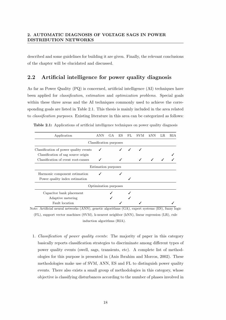
As far as Power Quality (PQ) is concerned, artificial intelligence (AI) techniques have
been applied for classification, estimation and optimization problems. Special goals
within these three areas and the AI techniques commonly used to achieve the corre-
sponding goals are listed in Table 2.1. This thesis is mainly included in the area related
to classification purposes. Existing literature in this area can be categorized as follows:
Table 2.1: Applications of artificial intelligence techniques on power quality diagnosis
Application ANN GA ES FL SVM kNN LR RIA
Classification purposes
Classification of power quality events 3 3 3 3
Classification of sag source origin 3
Classification of event root-causes 3 3 3 3 3 3
Estimation purposes
Harmonic component estimation 3 3
Power quality index estimation 3
Optimization purposes
Capacitor bank placement 3 3
Adaptive metering 3 3
Fault location 3 3 3
Note: Artificial neural networks (ANN), genetic algorithms (GA), expert systems (ES), fuzzy logic
(FL), support vector machines (SVM), k-nearest neighbor (kNN), linear regression (LR), rule
induction algorithms (RIA).
1. Classification of power quality events: The majority of paper in this category
basically reports classification strategies to discriminate among different types of
power quality events (swell, sags, transients, etc). A complete list of method-
ologies for this purpose is presented in (Anis Ibrahim and Morcos, 2002). These
methodologies make use of SVM, ANN, ES and FL to distinguish power quality
events. There also exists a small group of methodologies in this category, whose
objective is classifying disturbances according to the number of phases involved in
18
2.2 Artificial intelligence for power quality diagnosis
the events (single-, double-, three-phase, -to-ground, etc) (Axelberg et al., 2007;
Bollen, 2000, 2003; Djokic et al., 2005; Parsons et al., 2000; Yaleinkaya et al.,
1998). Six phase algorithm, symmetrical component theory (Bollen, 2003) and
decision trees (Das, 1998) are also used to identify the disturbance fault type
according to the phases involved in a fault.
2. Classification of sag source origin: These algorithms classify voltage sags accord-
ing to their source origin, upstream or downstream from recording place. Decision
rules and statistical models have been used to discriminate between the two pos-
sible origins (Hamzah N, 2004; Khosravi et al., 2008; Khosravi A, 2009; Li et al.,
2003; Pradhan and Routray, 2005; Pradhan et al., 2007; Tayjasanant et al., 2005).
These algorithms are extensively tested in Chapter 4.
3. Classification of event root causes: This category includes methodologies that al-
low discriminating among the different root causes of voltage disturbances. They
take advantage of different machine learning approaches (SVM, LR, kNN, ANN
and RIA) mainly trained with contextual features as hour, season, protection
operation or type of line. Only few contributions found in the literature focuses
on identifying disturbances according to external root causes as animals, trees
and lightning (Ahn et al., 2004; Cai et al., 2010a,b; Peng et al., 2004; Styvaktakis
et al., 2002; Xu and Chow, 2006; Xu et al., 2007) and only the contribution pre-
sented in (Styvaktakis et al., 2002) analyses the use of features extracted from
waveforms to perform this classification.
This work proposes a new framework for automatically classify disturbances ac-
cording to categories 2 and 3. Even thought, it only exists few contributions about
root-cause classification, the expert system presented in (Styvaktakis et al., 2002) is
the most relevant work in this area. This expert system uses the voltage waveforms to
discriminate among disturbances caused by transformers, induction motors or short-
circuits. The methodology consists in estimating the number of non-stationary stages
(waveform segmentation) throughout the disturbance. After that, a rule-based clas-
sification module assesses some additional voltage waveform characteristics in order
to refine the root cause classification. This expert-system does not take advantage
of information contained in current waveforms and neither estimates the disturbance
19
2. AUTOMATIC DIAGNOSIS OF VOLTAGE SAGS IN POWERDISTRIBUTION NETWORKS
source location nor identifies possible root causes of short-circuits (animals, trees, cable,
among others) as it is proposed in this thesis.
The reduced number of contributions on root-cause classification is an evidence of
that is a very challenging field and major efforts must be done proposing adequate
methodologies to identify the causes of voltage disturbances (Bollen et al., 2007, 2010,
2009; Saxena et al., 2010)
2.3 Framework for automatic diagnosis of voltage sags
The framework depicted in Figure 2.5 has been conceived for the automatic diagnosis
of voltage sags with the objective of systematically extracting from the three-phase
sag waveforms useful information to assist power network operation, maintenance and
planning. An instantaneous diagnosis of voltage sags capable to estimate the distance
up to the disturbance source and identify possible causes can assist maintenance crews
to locate faults and, consequently, can reduce restoration time, or to identify weak
points and define preventive actions when determined causes appear recursively at the
same network area.
Block diagrams (Figure 2.5) represent functionalities from waveforms and the arrows
indicate the dependences among them. In the following subsections, these blocks are
explained in detail. Existing algorithms and methods for their implementation have
been evaluated and compared in this thesis with field measurements and simulated
data.
Figure 2.5: Framework for automatic diagnosis of voltage events.
20
2.3 Framework for automatic diagnosis of voltage sags
Only the root-causes of downstream voltage sags can be diagnosed since their cap-
tured waveforms contain information about the fault impedance. This is represented
through the arrow from relative-location block to internal/external cause identifica-
tion blocks. Similarly, the identified internal or external sag root-cause is useful for
fault pinpoint location purposes (see incoming arrows in pinpoint location block). The
importance of sag cause in fault pinpoint location is given later in Section 2.3.4.
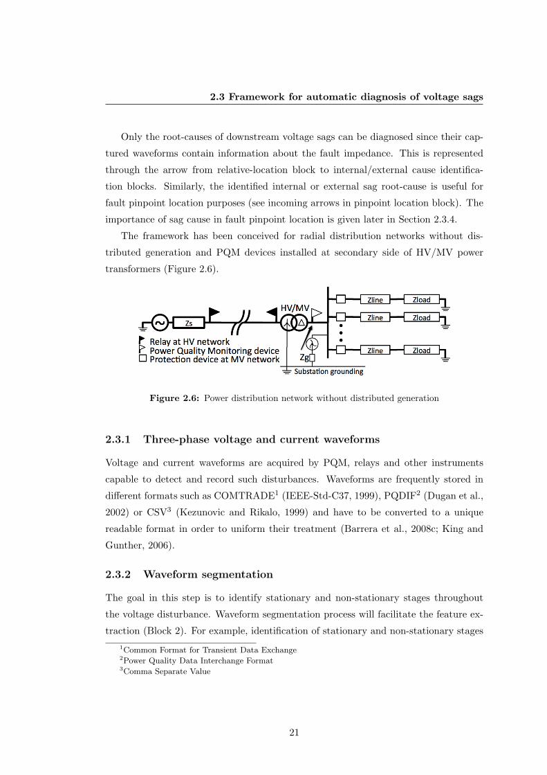
The framework has been conceived for radial distribution networks without dis-
tributed generation and PQM devices installed at secondary side of HV/MV power
transformers (Figure 2.6).
Figure 2.6: Power distribution network without distributed generation
2.3.1 Three-phase voltage and current waveforms
Voltage and current waveforms are acquired by PQM, relays and other instruments
capable to detect and record such disturbances. Waveforms are frequently stored in
different formats such as COMTRADE1 (IEEE-Std-C37, 1999), PQDIF2 (Dugan et al.,
2002) or CSV3 (Kezunovic and Rikalo, 1999) and have to be converted to a unique
readable format in order to uniform their treatment (Barrera et al., 2008c; King and
Gunther, 2006).
2.3.2 Waveform segmentation
The goal in this step is to identify stationary and non-stationary stages throughout
the voltage disturbance. Waveform segmentation process will facilitate the feature ex-
traction (Block 2). For example, identification of stationary and non-stationary stages1Common Format for Transient Data Exchange2Power Quality Data Interchange Format3Comma Separate Value
21
2. AUTOMATIC DIAGNOSIS OF VOLTAGE SAGS IN POWERDISTRIBUTION NETWORKS
allows making correctly use of FFT1 and Wavelet based methods. Waveform segmen-
tation also allows identifying disturbances with duration lower than one cycle, which
must be discarded from diagnosis process. Several Waveform Segmentation Algorithms
(WSA) can be applied for this purpose:
1. Algorithm based on residual model (Residual-WSA): It makes use of the differ-
ence between Kalman filter estimation and voltage disturbance to detect non-
stationary stages, which are detected when a mismatch between signal and model
overpass a threshold (Bollen, 2000; Bollen et al., 2007, 2009).
2. Algorithm based on even harmonic components (Harmonic-WSA): It takes advan-
tage of the fact that even harmonics flow during non-stationary stages. Kalman
filter algorithm (Ortiz et al., 2010) estimates the 2nd-order harmonic component
from waveform and its presence is used to detect the transition instants.
3. Algorithm based on Tensor theory (Tensor-WSA): The algorithm (Jagua et al.,
2010; Ustariz et al., 2010) analyzes the rotation angle of the instantaneous power
tensor to detect sudden variations that correspond to those instants when the
voltage or current experience sudden changes.
4. Algorithm based on RMS sequences (RMS-WSA): It explores first-order deriva-
tives of RMS sequence to detect sudden changes (Bollen et al., 2007, 2009). This
algorithm is only recommended to be used when only the RMS waveform is avail-
able.
Chapter 3 assesses the performance of these algorithms with respect to different
causes. They are applied to 40 voltage disturbances leaded by single-stage and multi-
stage short-circuits, expulsion fuse operation and transformer saturation events. The
following relevant results are presented in Chapter 3:
• Residual-WSA and Harmonic-WSA introduce large errors with disturbances whose
fault has been inserted around zero-crossing instant.
• Harmonic-WSA is the most accurate for segmenting fuse operation disturbances.
• Tensor-WSA is the fastest and simplest.
• The remaining voltage magnitude does not affect the performance of algorithms.1Fast Fourier Transforms
22
2.3 Framework for automatic diagnosis of voltage sags
2.3.3 Feature extraction
Block 2 is dedicated to process the waveform after segmentation in order to obtain fea-
tures for diagnostic goal. A selection of features is listed in Figure 2.7. They have been
basically grouped according to their usefulness for sag source location and cause iden-
tification. Figure 2.7 indicates the necessity of specific stationary and non-stationary
stages (output of Waveform Segmentation block) for feature computation.
For instance, the algorithm proposed in (Li et al., 2003) for estimating the relative
location of a sag source computes its feature (Slope[I, |V cos(θ − α)|]) during the first
non-stationary and fault stages, thus, this feature is obtained from voltage and current
samples between beginning and ending instants of first non-stationary and fault stages
in a single-stage sag event, respectively (Figure 2.7).
On the other hand, there are three groups of impedance-based features for fault
pinpoint location purposes, those requiring steady-state and fault stages (Group A in
Figure 2.7) (D. Novosel, 1998; Das, 1998; Girgis et al., 1993; M. Saha, 2002; Sachdev,
1988; Srinivasan, 1989), those requiring only fault stages as the features used in War-
rington and Choi methods (Group B in Figure 2.7) (Choi et al., 2004; Warrington,
1968) and those requiring the three first stages as the feature used by Zhu method (Jun
Zhu; Lubkeman, 1997).
Features listed in Figure 2.7 are described in following subsections organized ac-
cording to the diagnostic goal. All of them are highly sensitive to their corresponding
goal (location or cause).
2.3.3.1 Features related to relative location of sag source
The features described in this diagnostic goal take advantage of energy flow direction,
ratios and residuals between steady-state and fault stage of electric parameters to iden-
tify the direction of the sag source location. These features will be analyzed in detail
in Chapter 4.
• Disturbance energy –∫pfault(t) (Parsons et al., 2000): This feature makes ref-
erence to the energy demanded by the fault impedance leading the sag event.
The energy flow direction of the fault impedance indicates the disturbance source
relative location. This feature is computed by integrating the three-phase distur-
bance power defined as psag(t)− pss(t), where pss and psag are the instantaneous
23
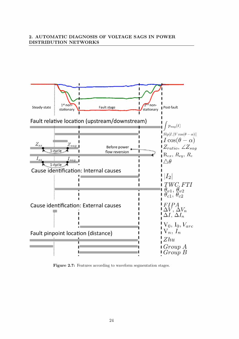
2. AUTOMATIC DIAGNOSIS OF VOLTAGE SAGS IN POWERDISTRIBUTION NETWORKS
Figure 2.7: Features according to waveform segmentation stages.
24
2.3 Framework for automatic diagnosis of voltage sags
powers during steady-state and sag stages (fault and both non-stationary stages),
respectively.
• Slope of the system trajectory – Slope[I, |V cos(θ − α)|] (Li et al., 2003): This
feature is based on the fact that the slope of line fitting the samples |V cos(θ −α)| and I at the measurement location are not the same for a downstream and
upstream sag. |V cos(θ−α)| is the product of voltage magnitude and power factor
samples, where θ and α are the voltage and current phase angles. I corresponds to
the current magnitude samples. The slope must be computed using the samples
contained in the time instant depicted in Figure 2.7.
• Real current component – I cos(θ − α) (Hamzah N, 2004): It corresponds to the
product of the RMS current and power factor angle at the beginning of the first
non-stationary stage of the sag event.
• Magnitude and angle of the impedance during the sag – Zratio, ∠Zsag (Pradhan
and Routray, 2005): Zratio is the ratio of sag impedance (Zsag) to steady state
impedance (Zss). ∠Zsag is the phase angle of the impedance during sag. In order
to compute Zratio and ∠Zsag, it has to be accomplished that Zss and Zsag are
delayed one cycle and Zsag is computed in a cycle contained in the first non-
stationary stage as is shown in Figure 2.7.
• Sign of the real part of the estimated impedance – RX , RY , Re (Tayjasanant
et al., 2005): The equivalent resistance during a voltage sag can be obtained
evaluating two different equations called RX and RY . Both of them basically
differ in that RX is a function of the real part of voltage samples (VX), whereas
RY of the imaginary part (VY ). Voltage and current samples used for computing
RX and RY must only include samples before the reversion of the power flow.
It is expected that RX and RY take negative signs for a downstream voltage sag,
and positive signs for an upstream one. Applying a rotating transformation to
RX and RY expressions an unique resistance Re can also be obtained, so that Retakes positive sign for upstream voltage sags.
• Phase change in sequence current - 4φ (Pradhan et al., 2007): This feature
uses the difference in phase angle between the fault-stage (Isag) and steady-state
25
2. AUTOMATIC DIAGNOSIS OF VOLTAGE SAGS IN POWERDISTRIBUTION NETWORKS
positive-sequence component of the current (Iss). Iss and Isag have to follow the
same delay requirements as Zss and Zsag features, respectively (Figure 2.7).
2.3.3.2 Features related to voltage sag causes
The features in this diagnostic goal will be separately described according to the dif-
ferent types of root causes (external or internal).
Internal causes
These features take advantage of harmonic-component flow, RMS sequence shape and
unbalance grade of the voltage/current waveform to characterize internal root-causes
of voltage disturbances. Most of them are computed from the beginning up to to end
of the sag disturbance (Figure 2.7). These features are deeply defined and analyzed in
Chapter 5.
• Second order harmonic current – |I2|(Ahn et al., 2004; Barrera et al., 2010a;
Bollen et al., 2007). |I2| is relatively large when a transformer is energized or
when a transformer voltage suddenly change. This effect is due to the core flux
saturation in the three transformer wings. Figure 2.8 depicts the maximum |I2|value at each instant during a transformer saturation event. It can be seen that
|I2| takes values close to 60% of the prefault current.
• Transformer waveform coefficient – TWC: This feature is conceived from the tri-
angular trend of transformer events. It measures the tendency from RMS voltage
sequence values (Barrera et al., 2010a). In order to do so, TWC includes three
coefficients that work with the ideal triangle bounding the RMS sequence. The
expressions for coefficient computation will be explained in detail in Chapter 5.
TWC takes values close to zero under short circuits because of their rectangular
trend, and values close to unity under transformer events due to their triangular-
ity. Disturbance caused by small motor starting have relatively high TWC values
because their RMS voltage sequences tend to be in triangular shape. This is due
to their motor inertia parameters causing a fast start-up, consequently, the RMS
voltage sequence experiences a strong triangular shape.
26
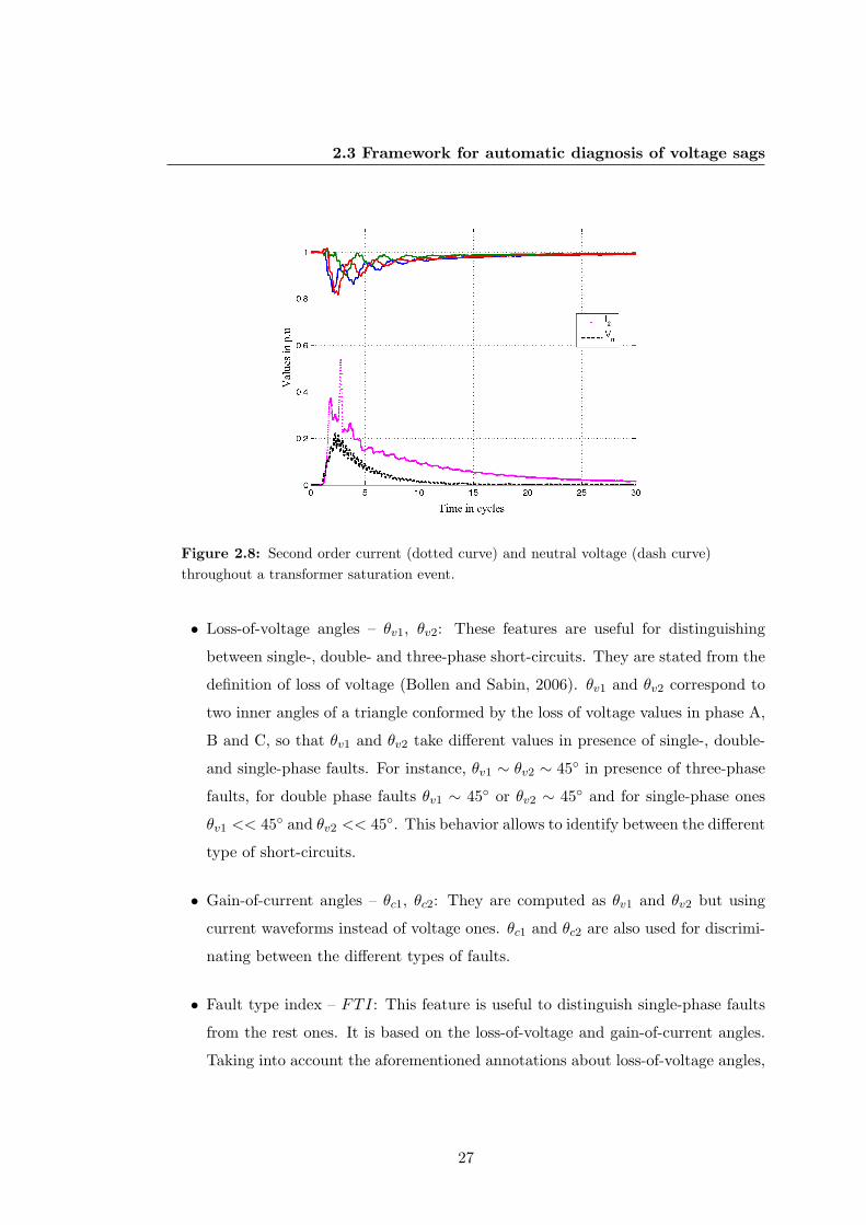
2.3 Framework for automatic diagnosis of voltage sags
Figure 2.8: Second order current (dotted curve) and neutral voltage (dash curve)throughout a transformer saturation event.
• Loss-of-voltage angles – θv1, θv2: These features are useful for distinguishing
between single-, double- and three-phase short-circuits. They are stated from the
definition of loss of voltage (Bollen and Sabin, 2006). θv1 and θv2 correspond to
two inner angles of a triangle conformed by the loss of voltage values in phase A,
B and C, so that θv1 and θv2 take different values in presence of single-, double-
and single-phase faults. For instance, θv1 ∼ θv2 ∼ 45◦ in presence of three-phase
faults, for double phase faults θv1 ∼ 45◦ or θv2 ∼ 45◦ and for single-phase ones
θv1 << 45◦ and θv2 << 45◦. This behavior allows to identify between the different
type of short-circuits.
• Gain-of-current angles – θc1, θc2: They are computed as θv1 and θv2 but using
current waveforms instead of voltage ones. θc1 and θc2 are also used for discrimi-
nating between the different types of faults.
• Fault type index – FTI: This feature is useful to distinguish single-phase faults
from the rest ones. It is based on the loss-of-voltage and gain-of-current angles.
Taking into account the aforementioned annotations about loss-of-voltage angles,
27
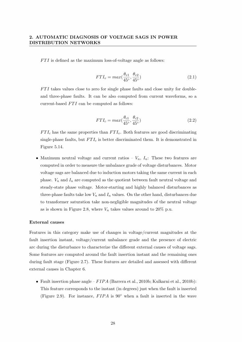
2. AUTOMATIC DIAGNOSIS OF VOLTAGE SAGS IN POWERDISTRIBUTION NETWORKS
FTI is defined as the maximum loss-of-voltage angle as follows:
FTIv = max(θv145◦
,θv245◦
) (2.1)
FTI takes values close to zero for single phase faults and close unity for double-
and three-phase faults. It can be also computed from current waveforms, so a
current-based FTI can be computed as follows:
FTIc = max(θc145◦
,θc245◦
) (2.2)
FTIc has the same properties than FTIv. Both features are good discriminating
single-phase faults, but FTIc is better discriminated them. It is demonstrated in
Figure 5.14.
• Maximum neutral voltage and current ratios – Vn, In: These two features are
computed in order to measure the unbalance grade of voltage disturbances. Motor
voltage sags are balanced due to induction motors taking the same current in each
phase. Vn and In are computed as the quotient between fault neutral voltage and
steady-state phase voltage. Motor-starting and highly balanced disturbances as
three-phase faults take low Vn and In values. On the other hand, disturbances due
to transformer saturation take non-negligible magnitudes of the neutral voltage
as is shown in Figure 2.8, where Vn takes values around to 20% p.u.
External causes
Features in this category make use of changes in voltage/current magnitudes at the
fault insertion instant, voltage/current unbalance grade and the presence of electric
arc during the disturbance to characterize the different external causes of voltage sags.
Some features are computed around the fault insertion instant and the remaining ones
during fault stage (Figure 2.7). These features are detailed and assessed with different
external causes in Chapter 6.
• Fault insertion phase angle – FIPA (Barrera et al., 2010b; Kulkarni et al., 2010b):
This feature corresponds to the instant (in degrees) just when the fault is inserted
(Figure 2.9). For instance, FIPA is 90◦ when a fault is inserted in the wave
28
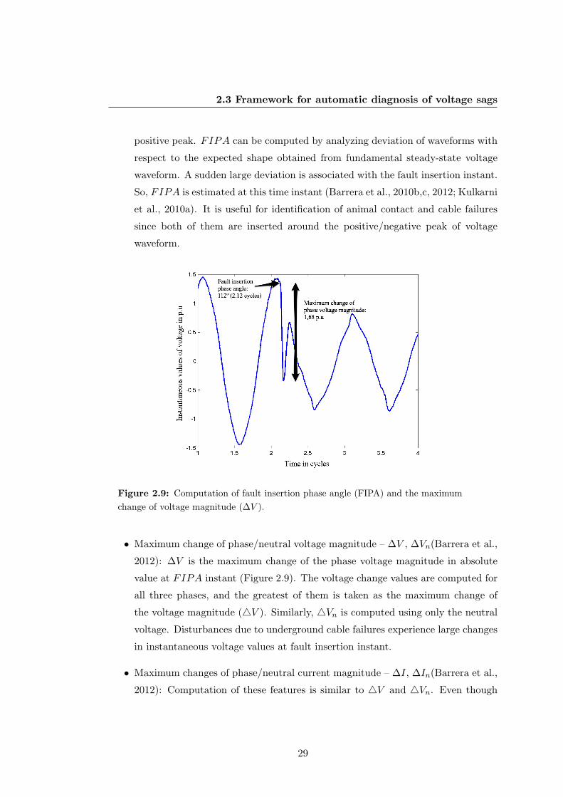
2.3 Framework for automatic diagnosis of voltage sags
positive peak. FIPA can be computed by analyzing deviation of waveforms with
respect to the expected shape obtained from fundamental steady-state voltage
waveform. A sudden large deviation is associated with the fault insertion instant.
So, FIPA is estimated at this time instant (Barrera et al., 2010b,c, 2012; Kulkarni
et al., 2010a). It is useful for identification of animal contact and cable failures
since both of them are inserted around the positive/negative peak of voltage
waveform.
Figure 2.9: Computation of fault insertion phase angle (FIPA) and the maximumchange of voltage magnitude (∆V ).
• Maximum change of phase/neutral voltage magnitude – ∆V , ∆Vn(Barrera et al.,
2012): ∆V is the maximum change of the phase voltage magnitude in absolute
value at FIPA instant (Figure 2.9). The voltage change values are computed for
all three phases, and the greatest of them is taken as the maximum change of
the voltage magnitude (4V ). Similarly, 4Vn is computed using only the neutral
voltage. Disturbances due to underground cable failures experience large changes
in instantaneous voltage values at fault insertion instant.
• Maximum changes of phase/neutral current magnitude – ∆I, ∆In(Barrera et al.,
2012): Computation of these features is similar to 4V and 4Vn. Even though
29
2. AUTOMATIC DIAGNOSIS OF VOLTAGE SAGS IN POWERDISTRIBUTION NETWORKS
4I and 4In can discriminate cable faults from other external causes, 4V and
4Vn are better at describing this cause.
• Maximum zero sequence voltage magnitude – V0 (Barrera et al., 2012): It is
perceived as an indicator of the degree of unbalance. That is, highly unbalanced
events will present high zero-sequence voltage values. V0 is computed during the
fault stage from the three-phase voltage waveform. Underground cable failures
are usually due to single phase faults, so voltage and current waveforms contain
high zero sequence components. For instance, the cable-caused event shown in
Figure 2.10 has a V0 around to 93% of the prefault voltage.
Figure 2.10: Voltage magnitude of the zero sequence component (V0) in a highlyunbalanced event due to an underground cable failure.
• Maximum zero sequence current magnitude – I0: This feature is adequate to
distinguish single-phase faults from two- and three-phase faults. For instance, it
reveals that animal contacts and cable faults usually affect a single phase (high I0values), whereas lightning-induced and tree-contact events can affect either one
or two phases because of the most of them have low I0 values.
• Maximum arc voltage – Varc (Djuric et al., 1999; Kulkarni et al., 2010b): This
feature was conceived from the hypothesis that some faults present an electric
30
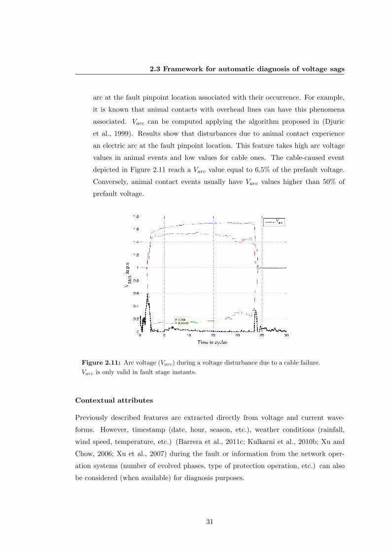
2.3 Framework for automatic diagnosis of voltage sags
arc at the fault pinpoint location associated with their occurrence. For example,
it is known that animal contacts with overhead lines can have this phenomena
associated. Varc can be computed applying the algorithm proposed in (Djuric
et al., 1999). Results show that disturbances due to animal contact experience
an electric arc at the fault pinpoint location. This feature takes high arc voltage
values in animal events and low values for cable ones. The cable-caused event
depicted in Figure 2.11 reach a Varc value equal to 6,5% of the prefault voltage.
Conversely, animal contact events usually have Varc values higher than 50% of
prefault voltage.
Figure 2.11: Arc voltage (Varc) during a voltage disturbance due to a cable failure.Varc is only valid in fault stage instants.
Contextual attributes
Previously described features are extracted directly from voltage and current wave-
forms. However, timestamp (date, hour, season, etc.), weather conditions (rainfall,
wind speed, temperature, etc.) (Barrera et al., 2011c; Kulkarni et al., 2010b; Xu and
Chow, 2006; Xu et al., 2007) during the fault or information from the network oper-
ation systems (number of evolved phases, type of protection operation, etc.) can also
be considered (when available) for diagnosis purposes.
31
2. AUTOMATIC DIAGNOSIS OF VOLTAGE SAGS IN POWERDISTRIBUTION NETWORKS
2.3.3.3 Features related to pinpoint location of sag source
Features for pinpoint location purposes basically correspond to the impedance seen
from PQM place. Estimated impedance includes the line, load and fault impedance.
According to feature computation step, there are three groups of algorithms, those
computing their features using the three first stages, those using steady-state- and
fault-stages and those using only fault stage. Several pinpoint location algorithms are
tested in (Mora-Florez et al., 2008) and stages were features must be computed are also
analyzed. Evaluation and comparison of pinpoint location methods are out of thesis
scope.
2.3.4 Fault location
The goal of this block is locating the direction of sag source a registered sag event. This
task is split into two steps: relative and pinpoint location. Relative location (source
direction) implies determining the origin upstream or downstream of sag sources from
the measurement place. This classification is necessary because pinpoint location algo-
rithms and classifiers for internal cause identification require downstream disturbances
in order to perform a distance estimation and root-cause, respectively.
2.3.4.1 Fault relative location
Seven different methods based on electric laws have been revised and compared in
(Barrera et al., 2009a; Chouhy, 2007). They are: disturbance power and energy (DPE)
(Parsons et al., 2000), slope of system trajectory (SST) (Li et al., 2003), real current
component (RCC) (Hamzah N, 2004), distance relay (DR) (Pradhan and Routray,
2005), resistance (RS) and simplified resistance sign (sRS) (Tayjasanant et al., 2005),
and phase change in sequence current (PCSC) (Pradhan et al., 2007). All of these
algorithms follow the same principle that consists of evaluating an IF-THEN decision
rule with logical conditions applied to one or several features described in Section
2.3.3.1. Decision rules have been summarized in Table 2.2. The first four methods
(Table 2.2) are suitable for both, meshed and radial networks, whereas the last three
(RS, sRS and PCSC) only apply to radial ones.
32
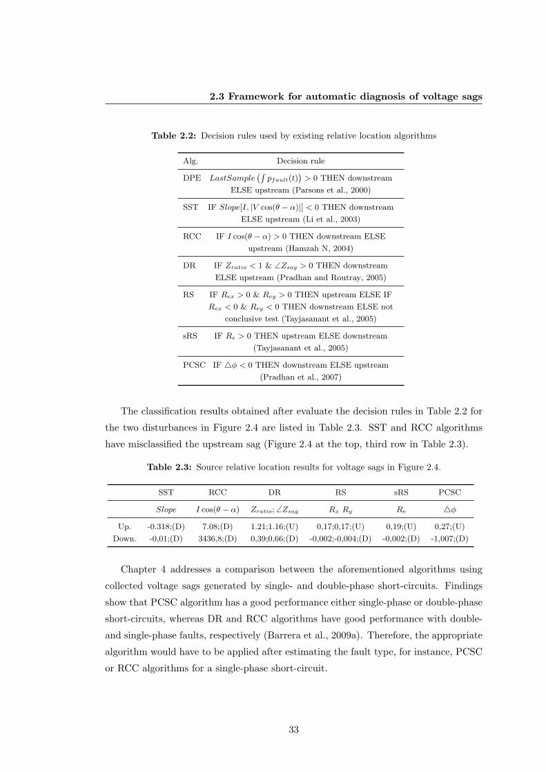
2.3 Framework for automatic diagnosis of voltage sags
Table 2.2: Decision rules used by existing relative location algorithms
Alg. Decision rule
DPE LastSample`Rpfault(t)
´> 0 THEN downstream
ELSE upstream (Parsons et al., 2000)
SST IF Slope[I, |V cos(θ − α)|] < 0 THEN downstream
ELSE upstream (Li et al., 2003)
RCC IF I cos(θ − α) > 0 THEN downstream ELSE
upstream (Hamzah N, 2004)
DR IF Zratio < 1 & ∠Zsag > 0 THEN downstream
ELSE upstream (Pradhan and Routray, 2005)
RS IF Rex > 0 & Rey > 0 THEN upstream ELSE IF
Rex < 0 & Rey < 0 THEN downstream ELSE not
conclusive test (Tayjasanant et al., 2005)
sRS IF Re > 0 THEN upstream ELSE downstream
(Tayjasanant et al., 2005)
PCSC IF 4φ < 0 THEN downstream ELSE upstream
(Pradhan et al., 2007)
The classification results obtained after evaluate the decision rules in Table 2.2 for
the two disturbances in Figure 2.4 are listed in Table 2.3. SST and RCC algorithms
have misclassified the upstream sag (Figure 2.4 at the top, third row in Table 2.3).
Table 2.3: Source relative location results for voltage sags in Figure 2.4.
SST RCC DR RS sRS PCSC
Slope I cos(θ − α) Zratio; ∠Zsag Rx Ry Re 4φ
Up. -0.318;(D) 7.08;(D) 1.21;1.16;(U) 0,17;0,17;(U) 0,19;(U) 0,27;(U)
Down. -0,01;(D) 3436,8;(D) 0,39;0,66;(D) -0,002;-0,004;(D) -0,002;(D) -1,007;(D)
Chapter 4 addresses a comparison between the aforementioned algorithms using
collected voltage sags generated by single- and double-phase short-circuits. Findings
show that PCSC algorithm has a good performance either single-phase or double-phase
short-circuits, whereas DR and RCC algorithms have good performance with double-
and single-phase faults, respectively (Barrera et al., 2009a). Therefore, the appropriate
algorithm would have to be applied after estimating the fault type, for instance, PCSC
or RCC algorithms for a single-phase short-circuit.
33
2. AUTOMATIC DIAGNOSIS OF VOLTAGE SAGS IN POWERDISTRIBUTION NETWORKS
2.3.4.2 Fault pinpoint location
Once a voltage sag origin has been located downstream, the next diagnosis goal is to
estimate the distance up to the fault location (Block-3B). In this case, only pinpoint
location of single-stage and multistage short-circuits require attention (external causes
in Fig. 2.2).
A variety of algorithms for fault location in distribution networks can be found
in the literature. A previous work of the authors compares and summarizes main
aspects of 10 impedance based methods (Mora-Florez et al., 2008). This work extends
capabilities of those algorithms by taking advantage of the identified root-cause in Block
4. When root-causes are known this knowledge can be used to reduce estimation errors
and multiple estimation problem. This is the case of faults involving arc voltage, i.e.
animal or tree caused disturbances (Barrera et al., 2010b,c, 2012), where transient peaks
usually appear close to zero-crossing instants, in voltage sags generated by failures in
underground cables, see Figure 2.12 at the top (Barrera et al., 2012; Kulkarni et al.,
2010a). If these peaks are not properly filtered they introduce large errors resulting in
impedance values larger than real one.
The arc voltage magnitude take values around 10% of steady-state voltage during
the animal contact disturbance presented in Figure 2.12 at the bottom (arc voltage is
only valid during fault stage). Arc voltage can also reach values even greater than 70%
(Barrera et al., 2010b,c, 2012).
On the other hand, the multi-estimation problem can also be reduced when in-
formation about causes can be associated with typologies of line sections (overhead/
underground) or with specific geographic areas (urban/forest). So, applying these sim-
ple heuristic rules the multi-estimation problem can be reduced in many cases.
Multistage disturbances also play an important role in fault distance estimation
because the same fault location can be estimated with different methods at different
stages providing certain redundancy to validate the distance estimated.
2.3.5 Cause identification
Inputs of this block are the features computed during feature extraction step (Block
2) and the downstream disturbances (single-stage or multistage) identified in relative
location step (Block 3A).
34
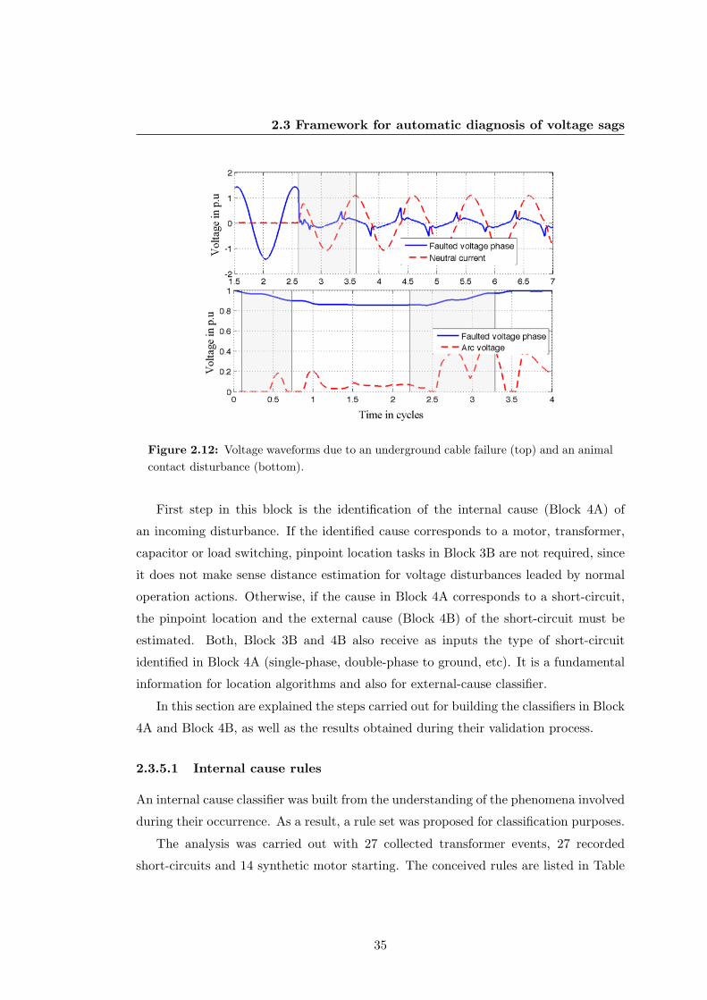
2.3 Framework for automatic diagnosis of voltage sags
Figure 2.12: Voltage waveforms due to an underground cable failure (top) and an animalcontact disturbance (bottom).
First step in this block is the identification of the internal cause (Block 4A) of
an incoming disturbance. If the identified cause corresponds to a motor, transformer,
capacitor or load switching, pinpoint location tasks in Block 3B are not required, since
it does not make sense distance estimation for voltage disturbances leaded by normal
operation actions. Otherwise, if the cause in Block 4A corresponds to a short-circuit,
the pinpoint location and the external cause (Block 4B) of the short-circuit must be
estimated. Both, Block 3B and 4B also receive as inputs the type of short-circuit
identified in Block 4A (single-phase, double-phase to ground, etc). It is a fundamental
information for location algorithms and also for external-cause classifier.
In this section are explained the steps carried out for building the classifiers in Block
4A and Block 4B, as well as the results obtained during their validation process.
2.3.5.1 Internal cause rules
An internal cause classifier was built from the understanding of the phenomena involved
during their occurrence. As a result, a rule set was proposed for classification purposes.
The analysis was carried out with 27 collected transformer events, 27 recorded
short-circuits and 14 synthetic motor starting. The conceived rules are listed in Table
35
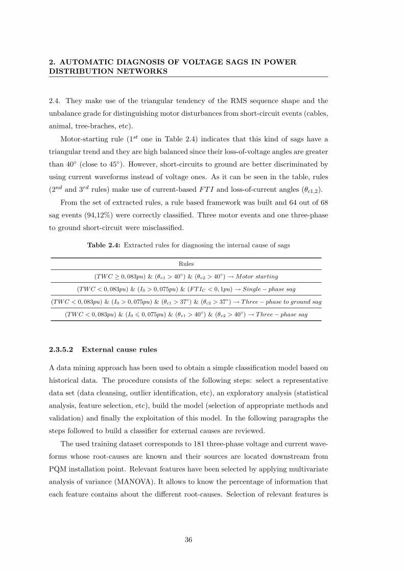
2. AUTOMATIC DIAGNOSIS OF VOLTAGE SAGS IN POWERDISTRIBUTION NETWORKS
2.4. They make use of the triangular tendency of the RMS sequence shape and the
unbalance grade for distinguishing motor disturbances from short-circuit events (cables,
animal, tree-braches, etc).
Motor-starting rule (1st one in Table 2.4) indicates that this kind of sags have a
triangular trend and they are high balanced since their loss-of-voltage angles are greater
than 40◦ (close to 45◦). However, short-circuits to ground are better discriminated by
using current waveforms instead of voltage ones. As it can be seen in the table, rules
(2nd and 3rd rules) make use of current-based FTI and loss-of-current angles (θc1,2).
From the set of extracted rules, a rule based framework was built and 64 out of 68
sag events (94,12%) were correctly classified. Three motor events and one three-phase
to ground short-circuit were misclassified.
Table 2.4: Extracted rules for diagnosing the internal cause of sags
Rules
(TWC ≥ 0, 083pu) & (θv1 > 40◦) & (θv2 > 40◦) →Motor starting
(TWC < 0, 083pu) & (I0 > 0, 075pu) & (FTIC < 0, 1pu) → Single− phase sag
(TWC < 0, 083pu) & (I0 > 0, 075pu) & (θc1 > 37◦) & (θc2 > 37◦) → Three− phase to ground sag
(TWC < 0, 083pu) & (I0 6 0, 075pu) & (θv1 > 40◦) & (θv2 > 40◦) → Three− phase sag
2.3.5.2 External cause rules
A data mining approach has been used to obtain a simple classification model based on
historical data. The procedure consists of the following steps: select a representative
data set (data cleansing, outlier identification, etc), an exploratory analysis (statistical
analysis, feature selection, etc), build the model (selection of appropriate methods and
validation) and finally the exploitation of this model. In the following paragraphs the
steps followed to build a classifier for external causes are reviewed.
The used training dataset corresponds to 181 three-phase voltage and current wave-
forms whose root-causes are known and their sources are located downstream from
PQM installation point. Relevant features have been selected by applying multivariate
analysis of variance (MANOVA). It allows to know the percentage of information that
each feature contains about the different root-causes. Selection of relevant features is
36
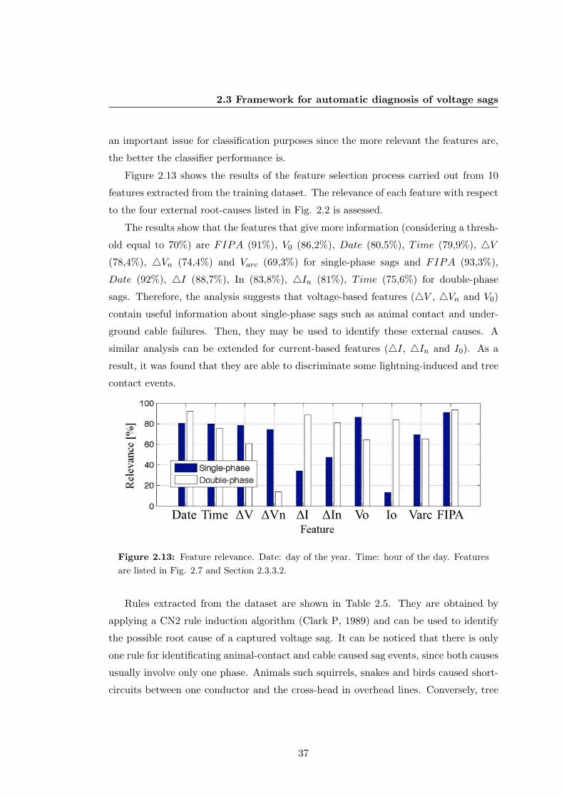
2.3 Framework for automatic diagnosis of voltage sags
an important issue for classification purposes since the more relevant the features are,
the better the classifier performance is.
Figure 2.13 shows the results of the feature selection process carried out from 10
features extracted from the training dataset. The relevance of each feature with respect
to the four external root-causes listed in Fig. 2.2 is assessed.
The results show that the features that give more information (considering a thresh-
old equal to 70%) are FIPA (91%), V0 (86,2%), Date (80,5%), Time (79,9%), 4V(78,4%), 4Vn (74,4%) and Varc (69,3%) for single-phase sags and FIPA (93,3%),
Date (92%), 4I (88,7%), In (83,8%), 4In (81%), Time (75,6%) for double-phase
sags. Therefore, the analysis suggests that voltage-based features (4V , 4Vn and V0)
contain useful information about single-phase sags such as animal contact and under-
ground cable failures. Then, they may be used to identify these external causes. A
similar analysis can be extended for current-based features (4I, 4In and I0). As a
result, it was found that they are able to discriminate some lightning-induced and tree
contact events.
Figure 2.13: Feature relevance. Date: day of the year. Time: hour of the day. Featuresare listed in Fig. 2.7 and Section 2.3.3.2.
Rules extracted from the dataset are shown in Table 2.5. They are obtained by
applying a CN2 rule induction algorithm (Clark P, 1989) and can be used to identify
the possible root cause of a captured voltage sag. It can be noticed that there is only
one rule for identificating animal-contact and cable caused sag events, since both causes
usually involve only one phase. Animals such squirrels, snakes and birds caused short-
circuits between one conductor and the cross-head in overhead lines. Conversely, tree
37
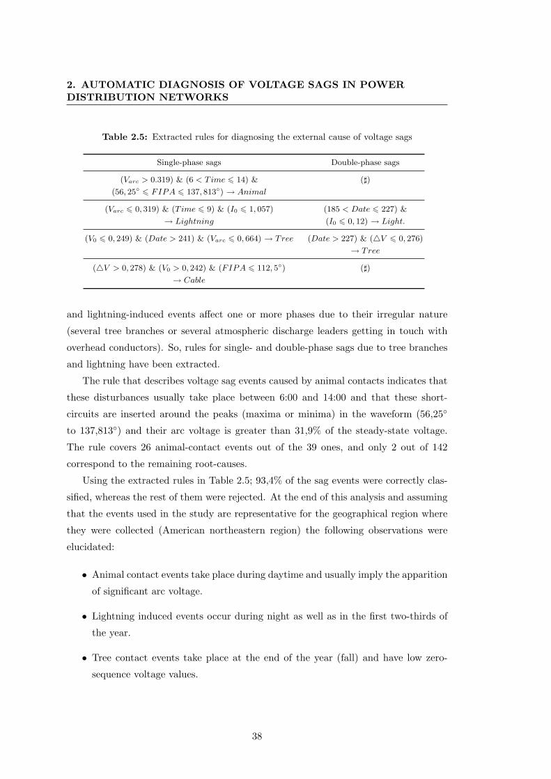
2. AUTOMATIC DIAGNOSIS OF VOLTAGE SAGS IN POWERDISTRIBUTION NETWORKS
Table 2.5: Extracted rules for diagnosing the external cause of voltage sags
Single-phase sags Double-phase sags
(Varc > 0.319) & (6 < Time 6 14) &
(56, 25◦ 6 FIPA 6 137, 813◦) → Animal
(])
(Varc 6 0, 319) & (T ime 6 9) & (I0 6 1, 057)
→ Lightning
(185 < Date 6 227) &
(I0 6 0, 12) → Light.
(V0 6 0, 249) & (Date > 241) & (Varc 6 0, 664) → Tree (Date > 227) & (4V 6 0, 276)
→ Tree
(4V > 0, 278) & (V0 > 0, 242) & (FIPA 6 112, 5◦)
→ Cable
(])
and lightning-induced events affect one or more phases due to their irregular nature
(several tree branches or several atmospheric discharge leaders getting in touch with
overhead conductors). So, rules for single- and double-phase sags due to tree branches
and lightning have been extracted.
The rule that describes voltage sag events caused by animal contacts indicates that
these disturbances usually take place between 6:00 and 14:00 and that these short-
circuits are inserted around the peaks (maxima or minima) in the waveform (56,25◦
to 137,813◦) and their arc voltage is greater than 31,9% of the steady-state voltage.
The rule covers 26 animal-contact events out of the 39 ones, and only 2 out of 142
correspond to the remaining root-causes.
Using the extracted rules in Table 2.5; 93,4% of the sag events were correctly clas-
sified, whereas the rest of them were rejected. At the end of this analysis and assuming
that the events used in the study are representative for the geographical region where
they were collected (American northeastern region) the following observations were
elucidated:
• Animal contact events take place during daytime and usually imply the apparition
of significant arc voltage.
• Lightning induced events occur during night as well as in the first two-thirds of
the year.
• Tree contact events take place at the end of the year (fall) and have low zero-
sequence voltage values.
38
2.4 Conclusions
• Cable fault events have substantial phase voltage changes and high zero-sequence
voltage components.
2.4 Conclusions
The main research objectives related to analysis of voltage sag events were identified.
With few exceptions, most papers propose methodologies to discriminate between dif-
ferent power quality disturbances and do not propose methodologies to determine the
root cause of voltage disturbances.
Useful steps have been given to build a framework for automatic diagnosis of voltage
sags collected in distribution networks. Each step has been described and the used
mathematical and statistical tools have been identified. Likewise, several algorithms
prone to be used in each step have also been compared with real-world and synthetic
waveforms. Their corresponding advantages and drawbacks have been elucidated and
discussed.
Several features have been proposed according to the different diagnostic goals (sag
source location and cause identification). Especial attention has been given to feature
computation regarding the waveform segmentation results. The relevance of proposed
features has been assessed using field measurements and applying a multivariate sta-
tistical analysis. Additionally, benefits of the proposed features have been discussed
through several classification examples.
It is very important to select relevant features before building a classifier instead of
using a great amount of them. This will allow to reduce redundancy of information and
build more efficient classifiers. Multivariate statistical theory must be used to recognize
relevant features from an initial feature set.
39
2. AUTOMATIC DIAGNOSIS OF VOLTAGE SAGS IN POWERDISTRIBUTION NETWORKS
40
3
Waveform Segmentation of
Voltage Disturbances
3.1 Introduction
As it has been introduced in the previous chapters, waveform segmentation is the
process of dividing a disturbance waveform through time to identify non-stationary
and stationary stages. It can also be treated as a detection problem where the instants
when each stage starts and ends must be accurately found (Styvaktakis., 2002). Similar
problem is studied in the context of fault detection, speech recognition or in biomedical
signal processing (Bollen et al., 2007).
In this thesis waveform segmentation has been presented as a pre-processing task
of the diagnosis process, required to identify periods of the waveform where compute
relevant features with minimal estimation error (Block 2 in Figure 2.5).
Three waveform segmentation algorithms are evaluated in this chapter using 20
synthetic and 40 real-world waveforms recorded in the Catalan distribution network.
These are depicted in Figure 3.1 One of these algorithms is inspired on the Tensor
theory and constitutes one original contribution of this thesis. The performance of
these algorithms is assessed in terms of capacity to correctly identify transition instants
when voltage sags are generated by different root causes. Results show that each
algorithm has advantages and drawbacks with respect to different root causes and
disturbance parameters, such as fault insertion angle and remaining voltage magnitude
of disturbances.
41
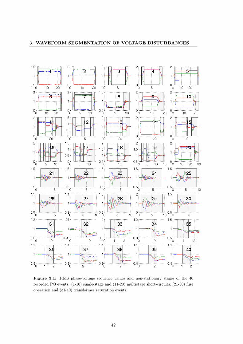
3. WAVEFORM SEGMENTATION OF VOLTAGE DISTURBANCES
Figure 3.1: RMS phase-voltage sequence values and non-stationary stages of the 40recorded PQ events: (1-10) single-stage and (11-20) multistage short-circuits, (21-30) fuseoperation and (31-40) transformer saturation events.
42
3.1 Introduction
3.1.1 Existing waveforms segmentation algorithms
Three main segmentation strategies are described in the literature: the first one cor-
respond to the algorithms that use RMS voltage, or current sequences, (Bollen et al.,
2007, 2009) and detect sudden variations on them; the second one groups the algo-
rithms based on the comparison between the instantaneous waveform and a theoretical
one (Le et al., 2010; Styvaktakis., 2002); and a third one is based on the analysis of
geometric properties of tensor (Jagua et al., 2010; Ustariz et al., 2010).
Algorithms in the first family usually explore first-order derivatives of RMS se-
quence values to detect these sudden changes. The basic idea in the second group
resides on the analysis of residuals (difference between expected and real values) and a
common strategy consists in the use of Kalman filters. Two different algorithms of this
group have been analysed in this work. One uses directly the residual to identify the
transition instants, whereas the other one takes advantage of the existence of second
order harmonic components during those non-stationary stages. The last group makes
use of geometric analysis of instantaneous power tensor to detect sudden changes in
the instantaneous values and considers the three phase waveforms as whole.
Algorithms based on RMS sequence have not been included in the comparison
because they introduced a delay (one or half cycle depending on the RMS method
used) and their use is only recommended when the instantaneous waveform does not
exist (Bollen et al., 2007, 2009).
3.1.2 Organization of the chapter
Kalman filter and Tensor theory fundamentals are given in Section 3.2 and Section 3.3,
respectively. Then, the segmentation algorithms under study are described and evalu-
ated with synthetic data in Section 3.4. A more precise study about their performance
with respect to the influence of remaining voltage magnitude and fault insertion angle
is analyzed in Section 3.5. Thereafter, performance of each algorithm is analyzed and
discussed in Section 3.6 with a set of disturbances generated by short-circuits, trans-
former saturation and fuse operation. Finally, conclusions are summarized in the last
section.
43
3. WAVEFORM SEGMENTATION OF VOLTAGE DISTURBANCES
3.2 Kalman filter
Kalman filter uses a state-space modeling to estimate signals from noisy measurement.
In case of power networks, a suitable model consists of a fundamental frequency signal
containing N harmonic components (Styvaktakis., 2002):
z(t) =N∑n=1
An(t) cos(nw0t+ θn(t)) (3.1)
Where w0 = 2πf0 and f0 is the fundamental frequency. In Eq. 3.1 the phasor
An∠θn for each harmonic component is the parameter to be estimated. Kalman filtering
theory assumes a system model (Eq. 3.2) and a measurement model (Eq. 3.3) with
the following equations:
xk = φk−1xk−1 + wk−1 (3.2)
zk = Hkxk + vk (3.3)
Where zk is the sampled measurement of z(t) at time instant k. xk is the state
variable vector of size 2×N and determines the filter order:
xk = [Re(A1,k∠θ1,k), Im(A1,k∠θ1,k), ...,Re(AN,k∠θN,k), Im(AN,k∠θN,k)]T
(3.4)
φk is the diagonal transition matrix of size 2×N defined as φk = diag[M1, ...,MN ]
with
Mn =[
cos(nw04t) − sin(nw04t)sin(nw04t) cos(nw04t)
](3.5)
wk is the modelling noise and is defined as follows:
Qk = E[wkwTk ] = σ2qI (3.6)
vk is the measurement noise and it is assumed to be a zero mean white noise sequence
with known covariance σ2v and uncorrelated to wk.
44
3.2 Kalman filter
The measurement matrix Hk that connects the measurements zk with the state
vector xk is:
Hk = [1 0 ... 1 0]T (3.7)
Once suitable error covariances (Qk and σ2v) have been selected, the procedures for
Kalman filter estimation (from Eq. 3.8 to Eq. 3.10 ) and updating (Eq. 3.11 and Eq.
3.12) are started.
The predicted values of the state x−k , the error covariance matrix P−k and the
Kalman gain are as follows:
x−k = φk−1xk−1 (3.8)
P−k = φk−1Pk−1φTk−1 +Qk−1 (3.9)
Kk = P−k Hk
(HTk P−k Hk + σ2
v
)−1(3.10)
The updated estimate xk and its corresponding updated covariance matrix Pk are
given by:
xk = x−k +Kk
(zk −HT
k x−k
)(3.11)
Pk = (I −KkHTk )P−k (3.12)
Once xk is obtained, from the xk elements (Eq. 3.4) the magnitude of the frequency
component n at time instant k can be calculated as:
An,k =√Re(An,k∠θn,k)2 + Im(An,k∠θn,k)2 (3.13)
45
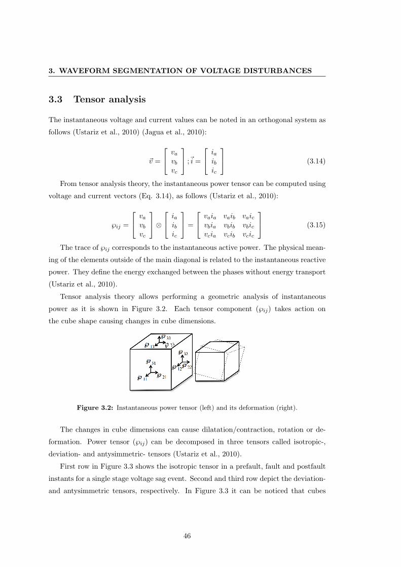
3. WAVEFORM SEGMENTATION OF VOLTAGE DISTURBANCES
3.3 Tensor analysis
The instantaneous voltage and current values can be noted in an orthogonal system as
follows (Ustariz et al., 2010) (Jagua et al., 2010):
~v =
vavbvc
;~i =
iaibic
(3.14)
From tensor analysis theory, the instantaneous power tensor can be computed using
voltage and current vectors (Eq. 3.14), as follows (Ustariz et al., 2010):
℘ij =
vavbvc
⊗ iaibic
=
vaia vaib vaicvbia vbib vbicvcia vcib vcic
(3.15)
The trace of ℘ij corresponds to the instantaneous active power. The physical mean-
ing of the elements outside of the main diagonal is related to the instantaneous reactive
power. They define the energy exchanged between the phases without energy transport
(Ustariz et al., 2010).
Tensor analysis theory allows performing a geometric analysis of instantaneous
power as it is shown in Figure 3.2. Each tensor component (℘ij) takes action on
the cube shape causing changes in cube dimensions.
Figure 3.2: Instantaneous power tensor (left) and its deformation (right).
The changes in cube dimensions can cause dilatation/contraction, rotation or de-
formation. Power tensor (℘ij) can be decomposed in three tensors called isotropic-,
deviation- and antysimmetric- tensors (Ustariz et al., 2010).
First row in Figure 3.3 shows the isotropic tensor in a prefault, fault and postfault
instants for a single stage voltage sag event. Second and third row depict the deviation-
and antysimmetric tensors, respectively. In Figure 3.3 it can be noticed that cubes
46
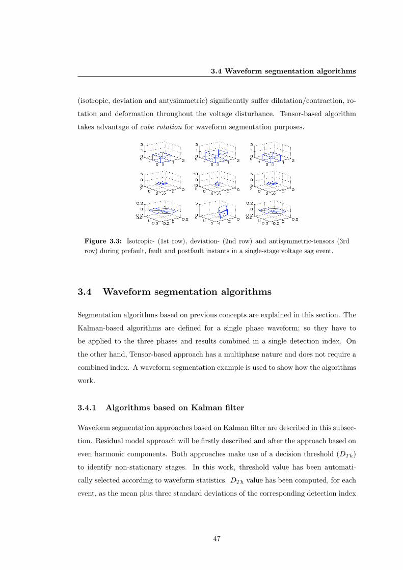
3.4 Waveform segmentation algorithms
(isotropic, deviation and antysimmetric) significantly suffer dilatation/contraction, ro-
tation and deformation throughout the voltage disturbance. Tensor-based algorithm
takes advantage of cube rotation for waveform segmentation purposes.
Figure 3.3: Isotropic- (1st row), deviation- (2nd row) and antisymmetric-tensors (3rdrow) during prefault, fault and postfault instants in a single-stage voltage sag event.
3.4 Waveform segmentation algorithms
Segmentation algorithms based on previous concepts are explained in this section. The
Kalman-based algorithms are defined for a single phase waveform; so they have to
be applied to the three phases and results combined in a single detection index. On
the other hand, Tensor-based approach has a multiphase nature and does not require a
combined index. A waveform segmentation example is used to show how the algorithms
work.
3.4.1 Algorithms based on Kalman filter
Waveform segmentation approaches based on Kalman filter are described in this subsec-
tion. Residual model approach will be firstly described and after the approach based on
even harmonic components. Both approaches make use of a decision threshold (DTh)
to identify non-stationary stages. In this work, threshold value has been automati-
cally selected according to waveform statistics. DTh value has been computed, for each
event, as the mean plus three standard deviations of the corresponding detection index
47
3. WAVEFORM SEGMENTATION OF VOLTAGE DISTURBANCES
(DI) sequence as follows:
DTh = mean(DI) + 3× std(DI) (3.16)
3.4.1.1 Residual model
The Waveform Segmentation Algorithm (WSA) based on residual model (Residual-
WSA) makes use of the difference between real signal, z, and Kalman filter estimation,
zkalman, in order to detect deviations corresponding to non-stationary stages in the
waveform. When a mismatch between signal and model exists, a non-stationary stage
is detected. The deviation between the two waveforms is analyzed by means of a
detection index (DI), that is computed individually for the three phases i using a
w-length sliding window as follows (Bollen et al., 2007; Styvaktakis., 2002):
DIi(n) =
1w
n+w/2∑i=n−w/2
[z(i)− zkalman(i)]
2
(3.17)
The detection index representing the three-phase waveform is obtained by consid-
ering the maximum value of individual indexes using Eq. 3.18 (Bollen et al., 2007;
Styvaktakis., 2002):
DI(n) = max[DIa(n), DIb(n), DIc(n)] (3.18)
In this work a 7-order Kalman filter has been implemented using the following
parameters:
• Initial covariance matrix (Pk): It is recommended that the diagonal elements take
values equal to 0,05 pu2. This value is proposed in (Perez, 2006; Styvaktakis.,
2002).
• Noise variance (σ2v): A constant value equal to 10−5 pu2 has been selected. A
small value means low measurement error.
• State variable covariance matrix (Q): Also the value proposed in (Perez, 2006;
Styvaktakis., 2002) has been selected (0,05 pu2).
48
3.4 Waveform segmentation algorithms
A 7-order Kalman filter was selected by the two following reasons; on one hand,
the harmonic components higher than 7-order have negligible voltage magnitudes in
comparison with 1- to 7-order components in the collected waveforms; and on the
other hand, the computational cost of higher order filters was excessive, for instance
20-order, and the reached accuracy regarding a 7-order filter was insignificantly. A
7-order filter allowed reducing the computational cost five times approximately.
In addition, a signal smoothing process using a half cycle filter has been carried
out before applying Kalman filter. The smoothing process allows reducing the signal
noise and, consequently, the number of detected false transition instants is significantly
reduced.
Figure 3.4a shows the instantaneous and RMS values of a synthetic single-phase
sag with magnitude 0.1p.u. The shadow region corresponds to the true non-stationary
stage of the waveform. This synthetic waveform will be used for analyzing segmentation
algorithms.
Figure 3.4b represents segmentation results obtained after Residual-WSA was ap-
plied to the waveform depicted in Figure 3.4a. The shadow region corresponds to the
detected non-stationary stage. The two transition instants have been detected using
the automatically computed threshold according to Eq. 3.16, it has taken a value equal
to 3% (horizontal dotted line in Figure 3.4b).
3.4.1.2 Second order harmonic components
The algorithm takes advantage of the apparition of second order harmonic components
(Harmonic-WSA) flowing during non-stationary stages. In this algorithm, 2nd-order
component is estimated in each phase of the waveform by applying Kalman filter. The
detection index is calculated as follows:
DI(n) = max[Aa2(n), Ab2(n), Ac2(n)] (3.19)
Where Ai2 is the estimation of the magnitude of second-order component in phase
i using Eq. 3.13 given by Kalman filter. The 2nd-order harmonic was selected be-
cause it usually experiences the highest voltage magnitude throughout non-stationary
stages. Any other even harmonic can be taken, but the higher its order, the worst its
performance detecting non-stationary ones.
49
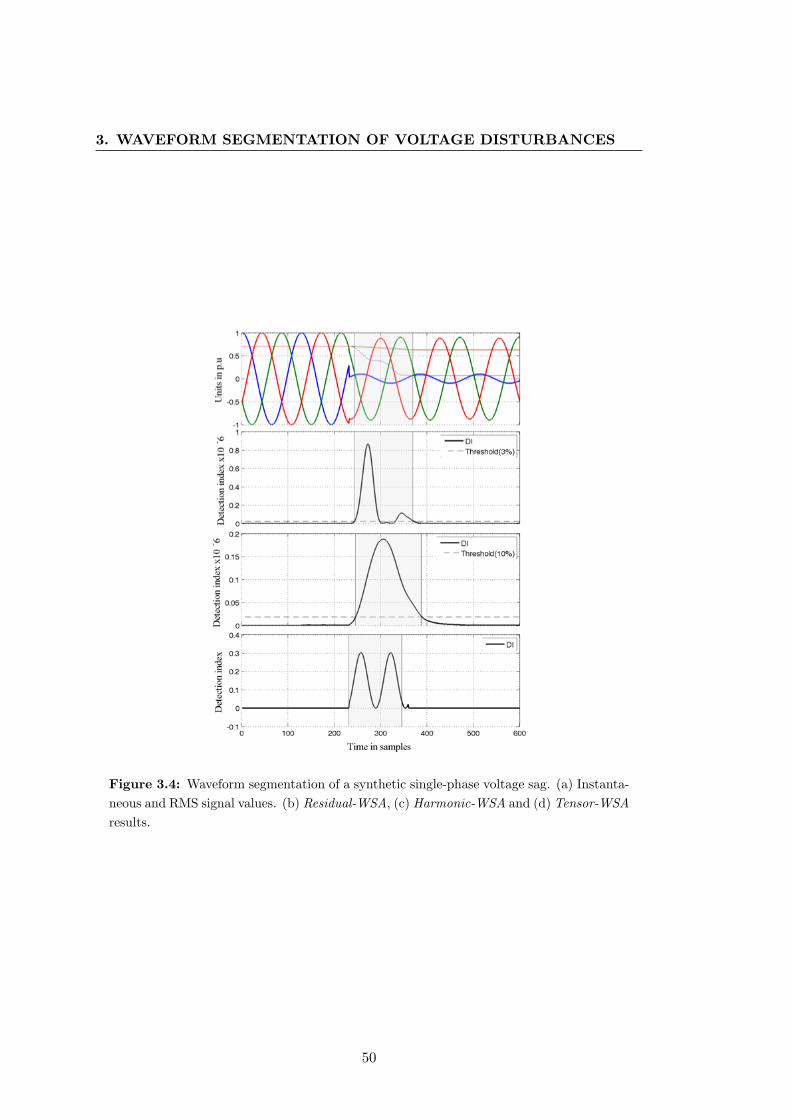
3. WAVEFORM SEGMENTATION OF VOLTAGE DISTURBANCES
Figure 3.4: Waveform segmentation of a synthetic single-phase voltage sag. (a) Instanta-neous and RMS signal values. (b) Residual-WSA, (c) Harmonic-WSA and (d) Tensor-WSAresults.
50
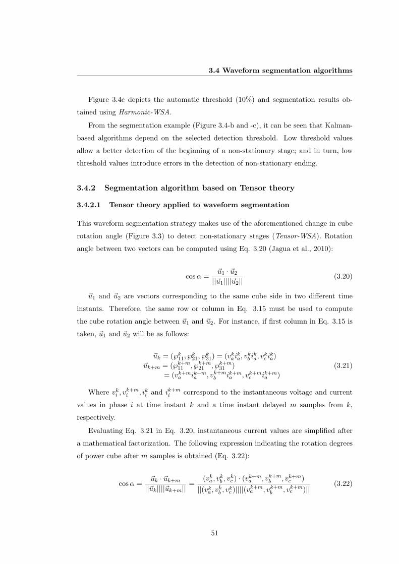
3.4 Waveform segmentation algorithms
Figure 3.4c depicts the automatic threshold (10%) and segmentation results ob-
tained using Harmonic-WSA.
From the segmentation example (Figure 3.4-b and -c), it can be seen that Kalman-
based algorithms depend on the selected detection threshold. Low threshold values
allow a better detection of the beginning of a non-stationary stage; and in turn, low
threshold values introduce errors in the detection of non-stationary ending.
3.4.2 Segmentation algorithm based on Tensor theory
3.4.2.1 Tensor theory applied to waveform segmentation
This waveform segmentation strategy makes use of the aforementioned change in cube
rotation angle (Figure 3.3) to detect non-stationary stages (Tensor-WSA). Rotation
angle between two vectors can be computed using Eq. 3.20 (Jagua et al., 2010):
cosα =~u1 · ~u2
||~u1||||~u2||(3.20)
~u1 and ~u2 are vectors corresponding to the same cube side in two different time
instants. Therefore, the same row or column in Eq. 3.15 must be used to compute
the cube rotation angle between ~u1 and ~u2. For instance, if first column in Eq. 3.15 is
taken, ~u1 and ~u2 will be as follows:
~uk = (℘k11, ℘k21, ℘
k31) = (vkai
ka, v
kb ika, v
kc ika)
~uk+m = (℘k+m11 , ℘k+m21 , ℘k+m31 )= (vk+ma ik+ma , vk+mb ik+ma , vk+mc ik+ma )
(3.21)
Where vki , vk+mi , iki and ik+mi correspond to the instantaneous voltage and current
values in phase i at time instant k and a time instant delayed m samples from k,
respectively.
Evaluating Eq. 3.21 in Eq. 3.20, instantaneous current values are simplified after
a mathematical factorization. The following expression indicating the rotation degrees
of power cube after m samples is obtained (Eq. 3.22):
cosα =~uk · ~uk+m||~uk||||~uk+m||
=(vka , v
kb , v
kc ) · (vk+ma , vk+mb , vk+mc )
||(vka , vkb , vkc )||||(vk+ma , vk+mb , vk+mc )||(3.22)
51
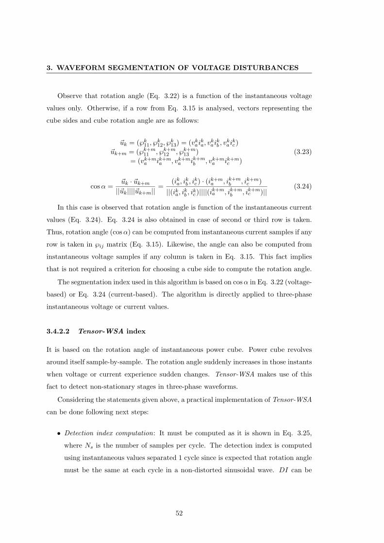
3. WAVEFORM SEGMENTATION OF VOLTAGE DISTURBANCES
Observe that rotation angle (Eq. 3.22) is a function of the instantaneous voltage
values only. Otherwise, if a row from Eq. 3.15 is analysed, vectors representing the
cube sides and cube rotation angle are as follows:
~uk = (℘k11, ℘k12, ℘
k13) = (vkai
ka, v
kaikb , v
kaikc )
~uk+m = (℘k+m11 , ℘k+m12 , ℘k+m13 )= (vk+ma ik+ma , vk+ma ik+mb , vk+ma ik+mc )
(3.23)
cosα =~uk · ~uk+m||~uk||||~uk+m||
=(ika, i
kb , i
kc ) · (ik+ma , ik+mb , ik+mc )
||(ika, ikb , ikc )||||(ik+ma , ik+mb , ik+mc )||
(3.24)
In this case is observed that rotation angle is function of the instantaneous current
values (Eq. 3.24). Eq. 3.24 is also obtained in case of second or third row is taken.
Thus, rotation angle (cosα) can be computed from instantaneous current samples if any
row is taken in ℘ij matrix (Eq. 3.15). Likewise, the angle can also be computed from
instantaneous voltage samples if any column is taken in Eq. 3.15. This fact implies
that is not required a criterion for choosing a cube side to compute the rotation angle.
The segmentation index used in this algorithm is based on cosα in Eq. 3.22 (voltage-
based) or Eq. 3.24 (current-based). The algorithm is directly applied to three-phase
instantaneous voltage or current values.
3.4.2.2 Tensor-WSA index
It is based on the rotation angle of instantaneous power cube. Power cube revolves
around itself sample-by-sample. The rotation angle suddenly increases in those instants
when voltage or current experience sudden changes. Tensor-WSA makes use of this
fact to detect non-stationary stages in three-phase waveforms.
Considering the statements given above, a practical implementation of Tensor-WSA
can be done following next steps:
• Detection index computation: It must be computed as it is shown in Eq. 3.25,
where Ns is the number of samples per cycle. The detection index is computed
using instantaneous values separated 1 cycle since is expected that rotation angle
must be the same at each cycle in a non-distorted sinusoidal wave. DI can be
52
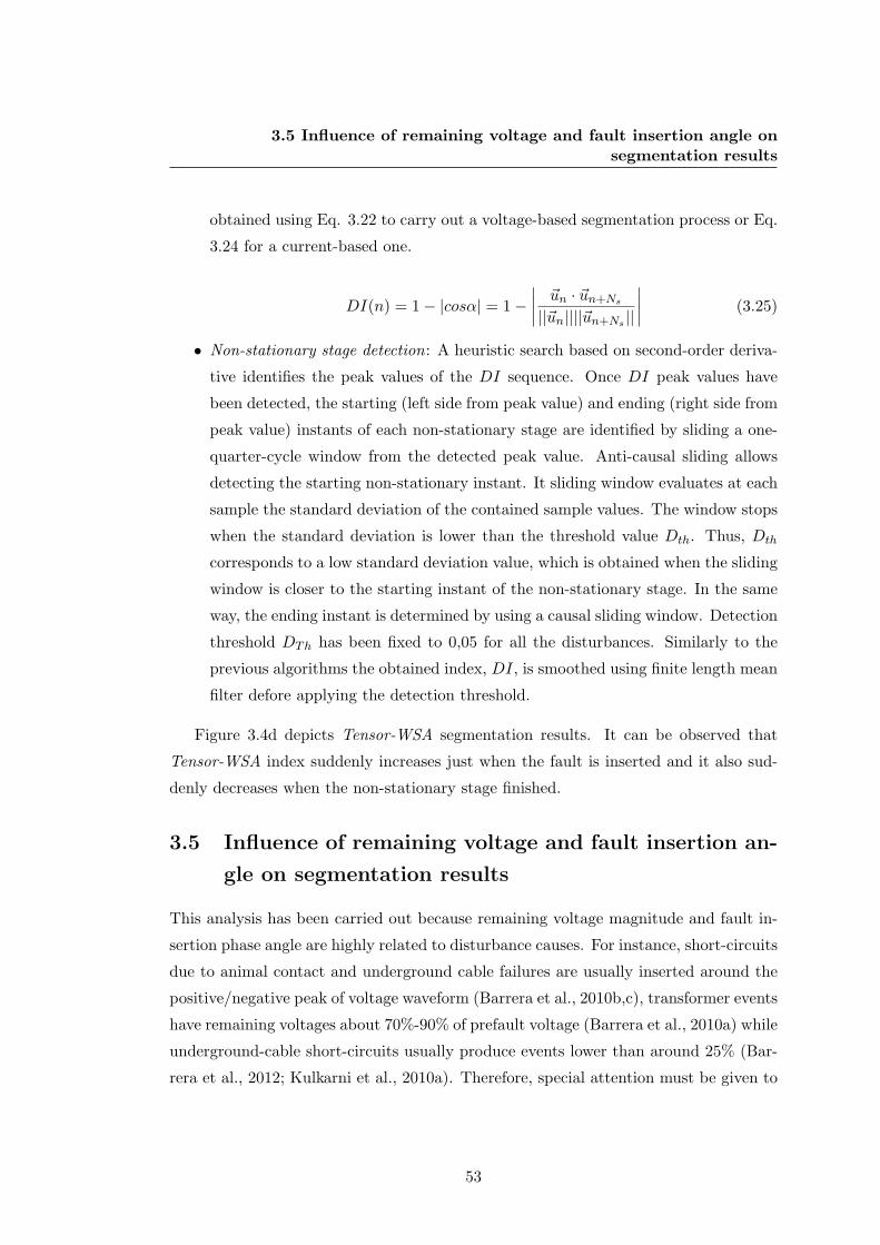
3.5 Influence of remaining voltage and fault insertion angle onsegmentation results
obtained using Eq. 3.22 to carry out a voltage-based segmentation process or Eq.
3.24 for a current-based one.
DI(n) = 1− |cosα| = 1−∣∣∣∣ ~un · ~un+Ns
||~un||||~un+Ns ||
∣∣∣∣ (3.25)
• Non-stationary stage detection: A heuristic search based on second-order deriva-
tive identifies the peak values of the DI sequence. Once DI peak values have
been detected, the starting (left side from peak value) and ending (right side from
peak value) instants of each non-stationary stage are identified by sliding a one-
quarter-cycle window from the detected peak value. Anti-causal sliding allows
detecting the starting non-stationary instant. It sliding window evaluates at each
sample the standard deviation of the contained sample values. The window stops
when the standard deviation is lower than the threshold value Dth. Thus, Dth
corresponds to a low standard deviation value, which is obtained when the sliding
window is closer to the starting instant of the non-stationary stage. In the same
way, the ending instant is determined by using a causal sliding window. Detection
threshold DTh has been fixed to 0,05 for all the disturbances. Similarly to the
previous algorithms the obtained index, DI, is smoothed using finite length mean
filter defore applying the detection threshold.
Figure 3.4d depicts Tensor-WSA segmentation results. It can be observed that
Tensor-WSA index suddenly increases just when the fault is inserted and it also sud-
denly decreases when the non-stationary stage finished.
3.5 Influence of remaining voltage and fault insertion an-
gle on segmentation results
This analysis has been carried out because remaining voltage magnitude and fault in-
sertion phase angle are highly related to disturbance causes. For instance, short-circuits
due to animal contact and underground cable failures are usually inserted around the
positive/negative peak of voltage waveform (Barrera et al., 2010b,c), transformer events
have remaining voltages about 70%-90% of prefault voltage (Barrera et al., 2010a) while
underground-cable short-circuits usually produce events lower than around 25% (Bar-
rera et al., 2012; Kulkarni et al., 2010a). Therefore, special attention must be given to
53
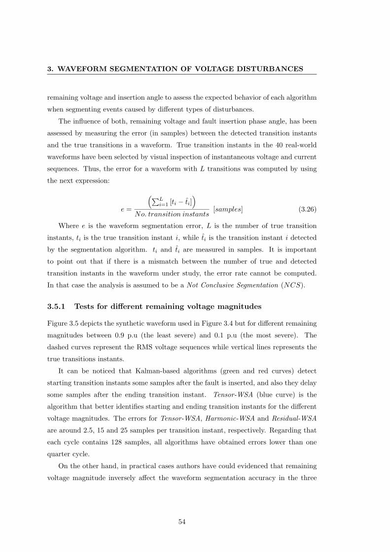
3. WAVEFORM SEGMENTATION OF VOLTAGE DISTURBANCES
remaining voltage and insertion angle to assess the expected behavior of each algorithm
when segmenting events caused by different types of disturbances.
The influence of both, remaining voltage and fault insertion phase angle, has been
assessed by measuring the error (in samples) between the detected transition instants
and the true transitions in a waveform. True transition instants in the 40 real-world
waveforms have been selected by visual inspection of instantaneous voltage and current
sequences. Thus, the error for a waveform with L transitions was computed by using
the next expression:
e =
(∑Li=1 [ti − ti]
)No. transition instants
[samples] (3.26)
Where e is the waveform segmentation error, L is the number of true transition
instants, ti is the true transition instant i, while ti is the transition instant i detected
by the segmentation algorithm. ti and ti are measured in samples. It is important
to point out that if there is a mismatch between the number of true and detected
transition instants in the waveform under study, the error rate cannot be computed.
In that case the analysis is assumed to be a Not Conclusive Segmentation (NCS).
3.5.1 Tests for different remaining voltage magnitudes
Figure 3.5 depicts the synthetic waveform used in Figure 3.4 but for different remaining
magnitudes between 0.9 p.u (the least severe) and 0.1 p.u (the most severe). The
dashed curves represent the RMS voltage sequences while vertical lines represents the
true transitions instants.
It can be noticed that Kalman-based algorithms (green and red curves) detect
starting transition instants some samples after the fault is inserted, and also they delay
some samples after the ending transition instant. Tensor-WSA (blue curve) is the
algorithm that better identifies starting and ending transition instants for the different
voltage magnitudes. The errors for Tensor-WSA, Harmonic-WSA and Residual-WSA
are around 2.5, 15 and 25 samples per transition instant, respectively. Regarding that
each cycle contains 128 samples, all algorithms have obtained errors lower than one
quarter cycle.
On the other hand, in practical cases authors have could evidenced that remaining
voltage magnitude inversely affect the waveform segmentation accuracy in the three
54
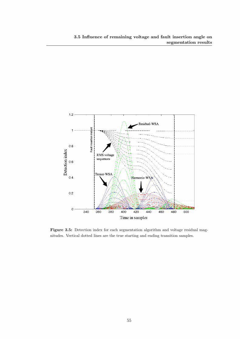
3.5 Influence of remaining voltage and fault insertion angle onsegmentation results
Figure 3.5: Detection index for each segmentation algorithm and voltage residual mag-nitudes. Vertical dotted lines are the true starting and ending transition samples.
55
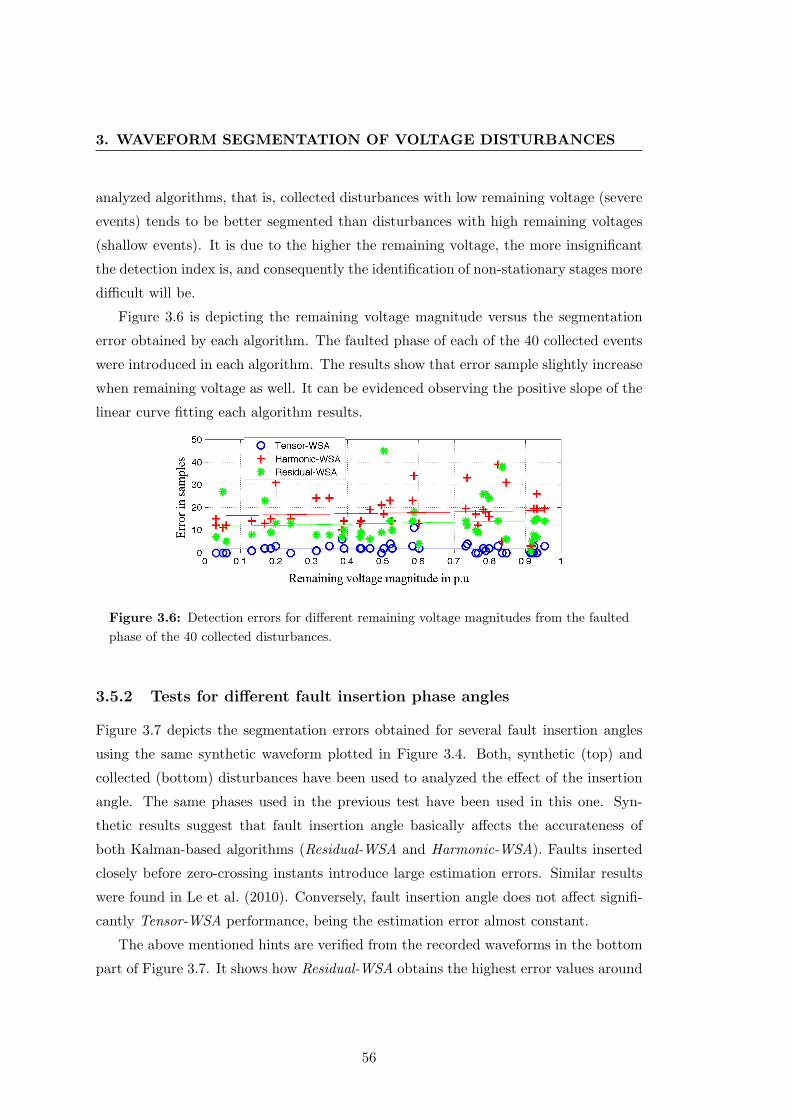
3. WAVEFORM SEGMENTATION OF VOLTAGE DISTURBANCES
analyzed algorithms, that is, collected disturbances with low remaining voltage (severe
events) tends to be better segmented than disturbances with high remaining voltages
(shallow events). It is due to the higher the remaining voltage, the more insignificant
the detection index is, and consequently the identification of non-stationary stages more
difficult will be.
Figure 3.6 is depicting the remaining voltage magnitude versus the segmentation
error obtained by each algorithm. The faulted phase of each of the 40 collected events
were introduced in each algorithm. The results show that error sample slightly increase
when remaining voltage as well. It can be evidenced observing the positive slope of the
linear curve fitting each algorithm results.
Figure 3.6: Detection errors for different remaining voltage magnitudes from the faultedphase of the 40 collected disturbances.
3.5.2 Tests for different fault insertion phase angles
Figure 3.7 depicts the segmentation errors obtained for several fault insertion angles
using the same synthetic waveform plotted in Figure 3.4. Both, synthetic (top) and
collected (bottom) disturbances have been used to analyzed the effect of the insertion
angle. The same phases used in the previous test have been used in this one. Syn-
thetic results suggest that fault insertion angle basically affects the accurateness of
both Kalman-based algorithms (Residual-WSA and Harmonic-WSA). Faults inserted
closely before zero-crossing instants introduce large estimation errors. Similar results
were found in Le et al. (2010). Conversely, fault insertion angle does not affect signifi-
cantly Tensor-WSA performance, being the estimation error almost constant.
The above mentioned hints are verified from the recorded waveforms in the bottom
part of Figure 3.7. It shows how Residual-WSA obtains the highest error values around
56
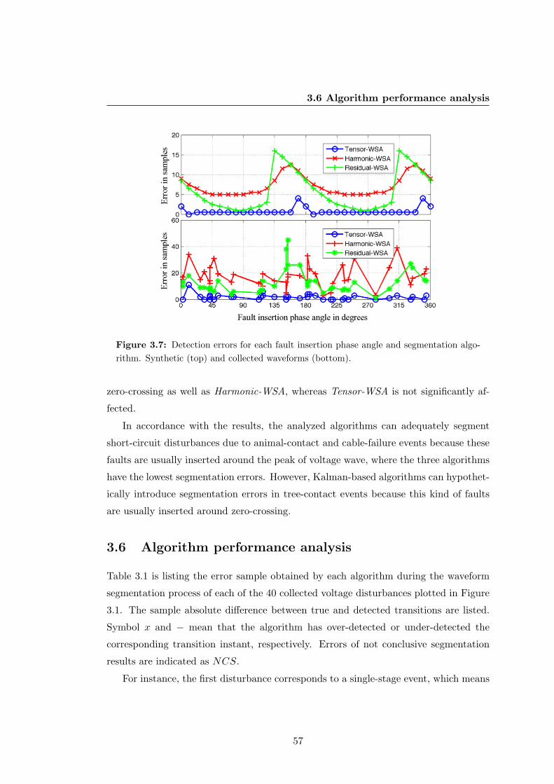
3.6 Algorithm performance analysis
Figure 3.7: Detection errors for each fault insertion phase angle and segmentation algo-rithm. Synthetic (top) and collected waveforms (bottom).
zero-crossing as well as Harmonic-WSA, whereas Tensor-WSA is not significantly af-
fected.
In accordance with the results, the analyzed algorithms can adequately segment
short-circuit disturbances due to animal-contact and cable-failure events because these
faults are usually inserted around the peak of voltage wave, where the three algorithms
have the lowest segmentation errors. However, Kalman-based algorithms can hypothet-
ically introduce segmentation errors in tree-contact events because this kind of faults
are usually inserted around zero-crossing.
3.6 Algorithm performance analysis
Table 3.1 is listing the error sample obtained by each algorithm during the waveform
segmentation process of each of the 40 collected voltage disturbances plotted in Figure
3.1. The sample absolute difference between true and detected transitions are listed.
Symbol x and − mean that the algorithm has over-detected or under-detected the
corresponding transition instant, respectively. Errors of not conclusive segmentation
results are indicated as NCS.
For instance, the first disturbance corresponds to a single-stage event, which means
57
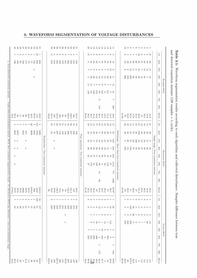
3. WAVEFORM SEGMENTATION OF VOLTAGE DISTURBANCES
Tab
le3.1:
Waveform
segmentation
resultsaccording
toeach
algorithmand
collecteddisturbance:
Samples
differencebetw
eentrue
anddetected
transitioninstants
(128sam
ples=
1cycle).
Resid
ual-W
SA
Harm
onic
-WSA
Tenso
r-W
SA
1st
2nd
3rd
4th
5th
6th
7th
8th
Erro
r1st
2nd
3rd
4th
5th
6th
7th
8th
Erro
r1st
2nd
3rd
4th
5th
6th
7th
8th
Erro
r
Sin
gle
stage:
Four
transitio
nin
stants
127
32
13
15
21,8
21
39
830
24,5
11
312
4,3
28
34
14
715,8
13
23
17
22
18,8
35
320
7,8
34
24
12
25
16,3
10
38
18
40
26,5
05
31
2,3
46
31
716
15
12
40
13
37
25,5
13
21
1,8
516
34
13
28
22,8
21
532
16
36
151,3
811
67
8
67
29
624
16,5
13
40
100
35
47
01
15
1,8
75
29
11
26
17,8
11
37
22
37
26,8
129
66
324,8
84
12
12
222
62,5
13
16
21
194
61
1139
8282
107,5
95
39
8159
52,8
18
24
26
54
30,5
03
3242
62
10
816
8280
78
24
38
9185
64
13
1270
68,8
31,9
347,5
928,9
1
Multista
ge:
More
than
four
transitio
nin
stants
11
413
811
13
31
7390
59,6
15
25
416
504
933
1114
771
1492
NC
S*
126
––
56
1534
NC
S
12
624
12
39
43
14,7
12
41
27
710
27
20,7
110
4119
18
23,8
13
743
633
7211
51,2
23
28
18
15
19
119
37
25
57
2303
54
14
727
715
811
12,5
16
32
14
18
21
39
23,3
22
614
00
4
15
643
615
17
121
34,7
13
64
12
30
25
424,7
25
21
12
204
37,7
16
96
444
350
6119
30,1
25
910
24
13
38
14
42
21,9
212
16
33
1175
25,4
17
823
414
5215
44,8
17
16
13
30
11
165
42
18
154
1226
48,5
18
634
428
7169
41,3
13
30
939
57
94
40,3
14
16
1202
35,8
19
234
436
14
94
30,7
13
15
13
83
19
172
52,5
28
19
7241
44,7
20
17
67
411
138
30,5
33
24
18
28
22
27
25,3
66
––
7235
NC
S
35,0
131,9
734,2
Fuse
opera
tion:
Tw
otra
nsitio
nin
stants
21
7196
101,5
19
120
69,5
2254
128
22
4316
160
16
238
127
1373
187
23
9270
139,5
26
217
121,5
7309
158
24
7392
199,5
16
289
152,5
1409
205
25
3181
92
13
143
78
1446
xx
NC
S
26
9179
94
31
135
83
1241
121
27
6358
182
27
118
72,5
1611
306
28
8303
155,5
20
257
138,5
1454
227,5
29
6318
162
11
75
xx
NC
S1
899
450
30
11
272
141,5
34
45
39,5
4362
183
142,6
98
218,4
Tra
nsfo
rmer:
Tw
otra
nsitio
nin
stants
31
1204
102,5
23289
1645,5
52
157
104,5
32
23
209
116
131
4763
2447
125
61
93
33
1142
xx
NC
S3
1801
902
159
30
34
477
40,5
28
3609
1818,5
157
29
35
679
42,5
7–
NC
S3
01,5
36
1171
86
0971
xx
NC
S2
81
41,5
37
3109
56
74161
2084
115
8
38
220
11
2–
NC
S1
39
20
39
7169
88
43972
xx
NC
S1
18
9,5
40
1190
95,5
43631
xx
xx
NC
S7
34
20,5
70,9
1779,4
35,8
x:
Over-d
ete
cte
dtra
nsitio
nin
stant,
-:U
nder-d
ete
cte
dtra
nsitio
nin
stant,
NC
S:N
ot
conclu
sive
segm
enta
tion
resu
lt.(*
)H
arm
onic
-WSA
has
dete
cte
d1
extra
non-sta
tionary
stage.
58
3.6 Algorithm performance analysis
that contains 2 non-stationary stages or 4 transition instants (1st, 2nd, 3rd and 4th),
see Fig. 3.1-1. These four transitions where estimated by Residual-WSA with absolute
difference equal to 27, 32, 13 and 15 samples regarding the corresponding true transition
instant sample, respectively. Likewise, Residual-WSA has over-detected 2 more non-
existing transition instants in the disturbance number 33, whereas Tensor-WSA has
under-detected the 3rd and 4th transition instant in the disturbance number 11 and
20. Similar analysis can be carried out for Harmonic-WSA and the rest of disturbances.
3.6.1 Analysis of segmentation errors
Segmentation errors listed in Table 3.1 have been computed using Eq. 3.26. The
following behaviours can be highlighted from them:
• The events produced by fuse operation are the most difficult to segment. The
three algorithms give the largest segmentation errors in samples for this type of
disturbance (142,8; 98 and 218,4 samples/transition for Residual-WSA, Harmonic-
WSA and Tensor-WSA, respectively).
• Residual-WSA has the lower rate of non conclusive segmentations (NCS). Only
in one event the number of estimated transition instants have been mismatched.
Tensor-WSA and Harmonic-WSA have obtained 3 and 7 NCS events, respec-
tively.
• Harmonic-WSA is the best segmenting expulsion fuse operation events. It has
been obtained an average error of 0,77 cycles/transition while the use of Tensor-
WSA and Residual-WSA leads to an average error of 1,48 and 1,12; respectively.
It is the best one because high frequency oscillations appear just after the fuse
extinguishes the fault impedance; see Figure 3.1-21 to 3.1-30. These RMS volt-
age oscillations are consequence of the electromagnetic interaction of the line
equivalent inductance and the high equivalent capacitance, since the collected
waveforms have been recorded in mainly underground distribution circuits. This
underdumped response in RMS voltage follows an asymmetrical decreasing. It
asymmetry is due to the apparition of second-order harmonic components, which
keep flowing up to the electromagnetic interaction has finished. Residual-WSA
and Tensor-WSA are not able to track these components up to the end of RMS
voltage oscillations.
59
3. WAVEFORM SEGMENTATION OF VOLTAGE DISTURBANCES
• Harmonic-WSA is not suitable for transformer event segmentation. It gives a
large segmentation error equal to 13,9 cycles/transition. Its poor performance
is due to the frequency oscillations experienced by voltage waveforms during the
transformer core saturation. These oscillacions cause detection or under-detection
of non-existing or existing transition instants, respectively. For instance, events
from number 35 to 40.
• The heuristic search used by Tensor-WSA was not able to identify the detection-
index peak corresponding to the second non-stationary stage in the events number
11 and 20. As a result, Tensor-WSA has 2 not conclusive segmentation corre-
sponding to multistage disturbances.
From a computation complexity point of view, Tensor-WSA- and Harmonic-WSA
are faster. They consume 20% and 35% of the time taken by the Residual-WSA algo-
rithm.
3.6.2 Analysis of the cumulative distribution of segmentation errors
The performance of the different algorithms can be assessed from the error cumulative
distribution curve plotted in Figure 3.8. In accordance with the cumulative curve;
47,22% of the collected events that have been segmented by using Tensor-WSA have
segmentation errors lower than 0,25 cycle/transition or 32 samples/transition, while
for the rest of the algorithms only 33,3% of the collected disturbances have obtained
the same error rate. Tensor-WSA has achieved segmentation errors lower than 187
samples/transition (or 1,46 cycles/transition) in 90% of the analyzed disturbances.
The area over the curve can be considered as a performance indicator of the algo-
rithm. The lower the area over the error cumulative curve, the better the algorithm
performance. Tensor-WSA has obtained the lowest area (0.495), while Harmonic-WSA
and Residual-WSA have taken 2.208 and 0.529, respectively. Consequently, Tensor-
WSA and Residual-WSA can be considered as the algorithms with the best segmenta-
tion performance.
3.6.3 Analysis of the not conclusive segmentations
Residual-WSA has achieved the best NCS rate with only one rejected transformer
event. In the event number 33, Residual-WSA has estimated one extra non-existing
60
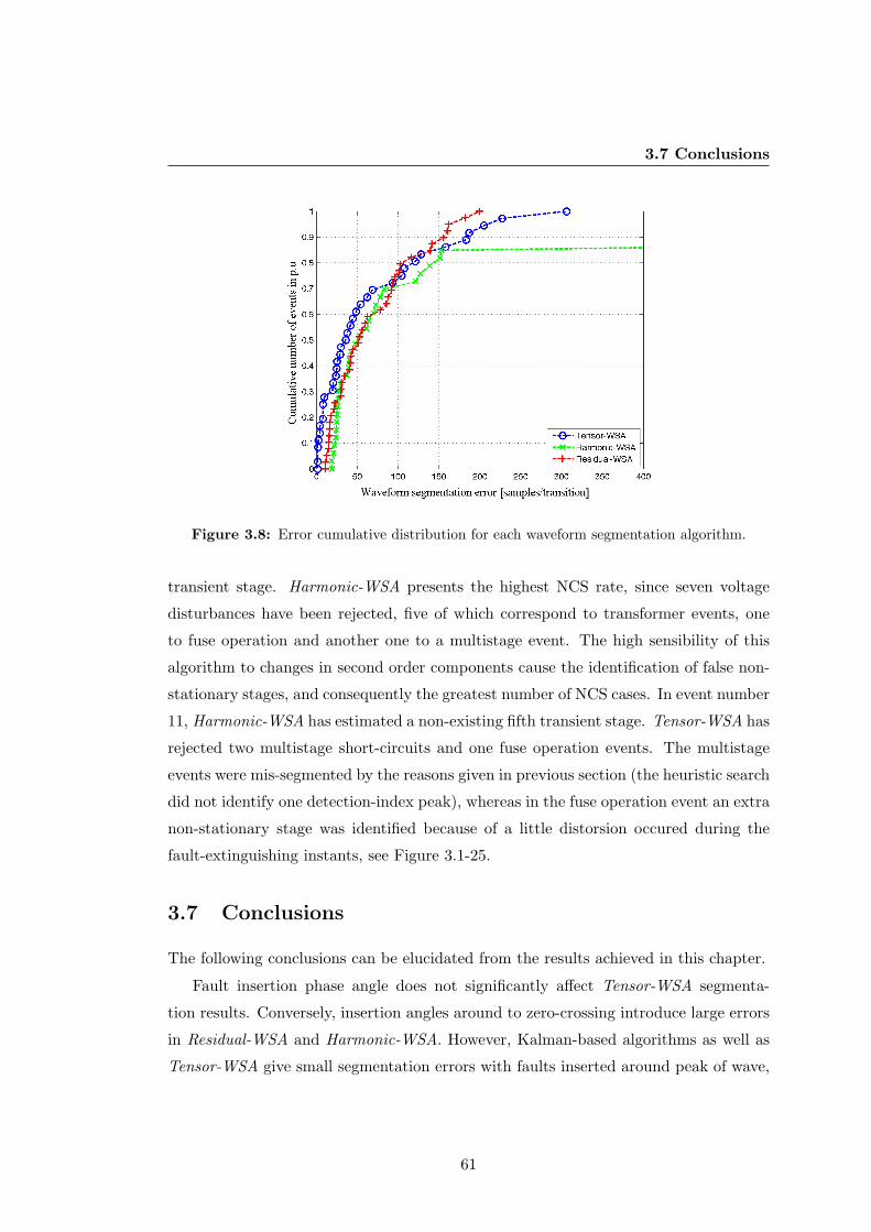
3.7 Conclusions
Figure 3.8: Error cumulative distribution for each waveform segmentation algorithm.
transient stage. Harmonic-WSA presents the highest NCS rate, since seven voltage
disturbances have been rejected, five of which correspond to transformer events, one
to fuse operation and another one to a multistage event. The high sensibility of this
algorithm to changes in second order components cause the identification of false non-
stationary stages, and consequently the greatest number of NCS cases. In event number
11, Harmonic-WSA has estimated a non-existing fifth transient stage. Tensor-WSA has
rejected two multistage short-circuits and one fuse operation events. The multistage
events were mis-segmented by the reasons given in previous section (the heuristic search
did not identify one detection-index peak), whereas in the fuse operation event an extra
non-stationary stage was identified because of a little distorsion occured during the
fault-extinguishing instants, see Figure 3.1-25.
3.7 Conclusions
The following conclusions can be elucidated from the results achieved in this chapter.
Fault insertion phase angle does not significantly affect Tensor-WSA segmenta-
tion results. Conversely, insertion angles around to zero-crossing introduce large errors
in Residual-WSA and Harmonic-WSA. However, Kalman-based algorithms as well as
Tensor-WSA give small segmentation errors with faults inserted around peak of wave,
61
3. WAVEFORM SEGMENTATION OF VOLTAGE DISTURBANCES
such as: single-stage and multistage short-circuit faults inserted around the peak of
the voltage waveform. So, it is expected that animal contact and underground cable
failures be adequately segmented by the three algorithms, whereas those faults with
insertion angles around zero-crossing, such as tree-contact, lightning induced and in-
sulator breakdowns, among other, will be better segmented by Tensor-WSA since it is
not affected by the fault insertion angle.
Unlike fault insertion phase angle, the remaining voltage magnitude does not sig-
nificantly affect the performance of any segmentation algorithm. However, voltage
disturbances with shallow voltage magnitudes can reduce the accurateness estimating
the starting and ending instants of non-stationary stages.
Harmonic-WSA is not suitable for the segmentation of transformer events because
2nd-order harmonic components keep flowing several cycles after the transformer non-
stationary stage. Thus, the Harmonic-WSA misestimates the ending transition instant
suggesting a longer non-stationary stage. Harmonic-WSA has also proved to be the
most accurate with fuse operation disturbances.
Tensor-WSA and Harmonic-WSA are faster than Residual-WSA because they do
not require computing residuals. Additionally, Tensor-WSA neither requires index
combination as the remaining algorithms, accordingly, it has been the algorithm with
the lowest time consumption during test performed in this work.
The overall segmentation results have suggested the algorithm based on Tensor the-
ory (Tensor-WSA) as the algorithm with the best segmentation performance, because
it has achieved the best performance indexes in comparison with the rest ones.
Feature extraction must be carried out after waveform segmentation. Several fea-
tures will be presented in subsequent chapters and their computation is also described.
Some of them were briefly described in Chapter 2 (Section 2.3.3). Features containing
information about relative location, internal and external root causes are addressed
and deeply analyzed in Chapters 4, 5 and 6, respectively. In order to computed them,
different strategies are used in each stage during the feature extraction step.
62
4
Relative Location of Voltage Sag
Sources
4.1 Introduction
This chapter focuses on the relative location (upstream or downstream) of sag source
collected in distribution networks. A downstream source is located in power flow di-
rection from the measurement point, whereas an upstream one is located in oppo-
site direction Figure 2.3 and Figure 2.4. Fault distance estimation algorithms and
cause identification methodologies can be only applied to those events generated in
downstream direction, since downstream waveforms contain information about fault
impedance. Then, relative location step precedes the cause classification task (Chapter
5) in the proposed disturbance diagnosis framework.
Six source location algorithms recently proposed in the literature are analyzed and
compared in this chapter. All of them are based on features extracted from distur-
bance waveforms before and during the fault insertion instant. Simple decision rules
are applied on these features to determine the sag relative location. The relevance
of features with respect to the sag origin (upstream/downstream) has been analyzed
and also the performance of the algorithms is evaluated with field measurements. The
obtained results show that some algorithms have better performance with single-phase
and other ones with double-phase short-circuits. Furthermore, it is founded an algo-
rithm with better performance than existing ones. It is conceived as the combination of
two existing algorithms and is supported on the automatic extraction of decision rules.
63
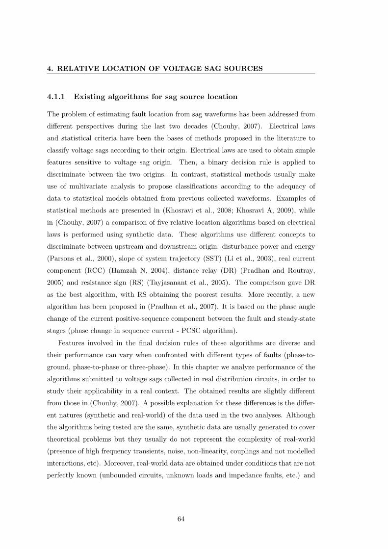
4. RELATIVE LOCATION OF VOLTAGE SAG SOURCES
4.1.1 Existing algorithms for sag source location
The problem of estimating fault location from sag waveforms has been addressed from
different perspectives during the last two decades (Chouhy, 2007). Electrical laws
and statistical criteria have been the bases of methods proposed in the literature to
classify voltage sags according to their origin. Electrical laws are used to obtain simple
features sensitive to voltage sag origin. Then, a binary decision rule is applied to
discriminate between the two origins. In contrast, statistical methods usually make
use of multivariate analysis to propose classifications according to the adequacy of
data to statistical models obtained from previous collected waveforms. Examples of
statistical methods are presented in (Khosravi et al., 2008; Khosravi A, 2009), while
in (Chouhy, 2007) a comparison of five relative location algorithms based on electrical
laws is performed using synthetic data. These algorithms use different concepts to
discriminate between upstream and downstream origin: disturbance power and energy
(Parsons et al., 2000), slope of system trajectory (SST) (Li et al., 2003), real current
component (RCC) (Hamzah N, 2004), distance relay (DR) (Pradhan and Routray,
2005) and resistance sign (RS) (Tayjasanant et al., 2005). The comparison gave DR
as the best algorithm, with RS obtaining the poorest results. More recently, a new
algorithm has been proposed in (Pradhan et al., 2007). It is based on the phase angle
change of the current positive-sequence component between the fault and steady-state
stages (phase change in sequence current - PCSC algorithm).
Features involved in the final decision rules of these algorithms are diverse and
their performance can vary when confronted with different types of faults (phase-to-
ground, phase-to-phase or three-phase). In this chapter we analyze performance of the
algorithms submitted to voltage sags collected in real distribution circuits, in order to
study their applicability in a real context. The obtained results are slightly different
from those in (Chouhy, 2007). A possible explanation for these differences is the differ-
ent natures (synthetic and real-world) of the data used in the two analyses. Although
the algorithms being tested are the same, synthetic data are usually generated to cover
theoretical problems but they usually do not represent the complexity of real-world
(presence of high frequency transients, noise, non-linearity, couplings and not modelled
interactions, etc). Moreover, real-world data are obtained under conditions that are not
perfectly known (unbounded circuits, unknown loads and impedance faults, etc.) and
64
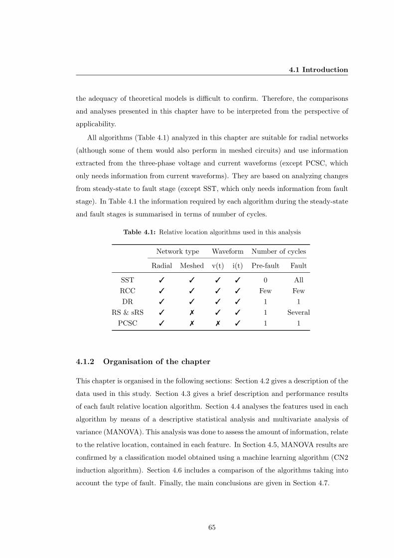
4.1 Introduction
the adequacy of theoretical models is difficult to confirm. Therefore, the comparisons
and analyses presented in this chapter have to be interpreted from the perspective of
applicability.
All algorithms (Table 4.1) analyzed in this chapter are suitable for radial networks
(although some of them would also perform in meshed circuits) and use information
extracted from the three-phase voltage and current waveforms (except PCSC, which
only needs information from current waveforms). They are based on analyzing changes
from steady-state to fault stage (except SST, which only needs information from fault
stage). In Table 4.1 the information required by each algorithm during the steady-state
and fault stages is summarised in terms of number of cycles.
Table 4.1: Relative location algorithms used in this analysis
Network type Waveform Number of cycles
Radial Meshed v(t) i(t) Pre-fault Fault
SST 3 3 3 3 0 AllRCC 3 3 3 3 Few FewDR 3 3 3 3 1 1
RS & sRS 3 7 3 3 1 SeveralPCSC 3 7 7 3 1 1
4.1.2 Organisation of the chapter
This chapter is organised in the following sections: Section 4.2 gives a description of the
data used in this study. Section 4.3 gives a brief description and performance results
of each fault relative location algorithm. Section 4.4 analyses the features used in each
algorithm by means of a descriptive statistical analysis and multivariate analysis of
variance (MANOVA). This analysis was done to assess the amount of information, relate
to the relative location, contained in each feature. In Section 4.5, MANOVA results are
confirmed by a classification model obtained using a machine learning algorithm (CN2
induction algorithm). Section 4.6 includes a comparison of the algorithms taking into
account the type of fault. Finally, the main conclusions are given in Section 4.7.
65
4. RELATIVE LOCATION OF VOLTAGE SAG SOURCES
4.2 Data description
A set of voltage sags, previously classified as upstream and downstream (Table 4.2),
collected by power quality monitors installed in the secondary side of HV/MV trans-
formers of radial distribution networks (25-kV) in the northeast of Spain, have been
used in this study. The data set is well balanced (228 downstream and 243 upstream
records) and waveforms were sampled at 128 samples per cycle (50Hz) and they contain
40 cycles/period.
Table 4.2: Voltage sag events gathered and used in the analysis
Single-phase Phase-to-phase Total
Downstream 118 120 228Upstream 92 151 243
Total 210 261 471
Figure 4.1 depicts voltage sag magnitudes versus duration. It can be observed that
the use of duration and magnitude as discriminant features for classification will result
in a very bad performance. Although the most part of upstream sag events last between
3 and 10 cycles, and the majority of downstream sags have magnitude lower than 60%,
these simple rules are not reliable enough. This behaviour is quite normal because
faults generated in distribution networks (downstream) are in general longer and more
serious than faults generated in transmission networks (upstream).
4.3 Definition and results of the fault relative location
algorithms
A brief description of the previously introduced algorithms is included in this section,
with special attention being paid to the features used to define the decision rule that
represents each algorithm. Their performance is also analyzed, and the relevance of
features for source location is qualitatively analyzed.
66
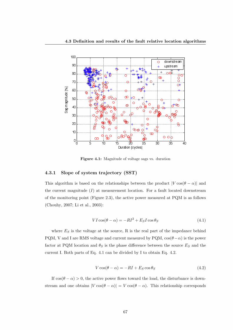
4.3 Definition and results of the fault relative location algorithms
Figure 4.1: Magnitude of voltage sags vs. duration
4.3.1 Slope of system trajectory (SST)
This algorithm is based on the relationships between the product |V cos(θ − α)| and
the current magnitude (I) at measurement location. For a fault located downstream
of the monitoring point (Figure 2.3), the active power measured at PQM is as follows
(Chouhy, 2007; Li et al., 2003):
V I cos(θ − α) = −RI2 + ESI cos θS (4.1)
where ES is the voltage at the source, R is the real part of the impedance behind
PQM, V and I are RMS voltage and current measured by PQM, cos(θ−α) is the power
factor at PQM location and θS is the phase difference between the source ES and the
current I. Both parts of Eq. 4.1 can be divided by I to obtain Eq. 4.2.
V cos(θ − α) = −RI + ES cos θS (4.2)
If cos(θ − α) > 0, the active power flows toward the load, the disturbance is down-
stream and one obtains |V cos(θ − α)| = V cos(θ − α). This relationship corresponds
67
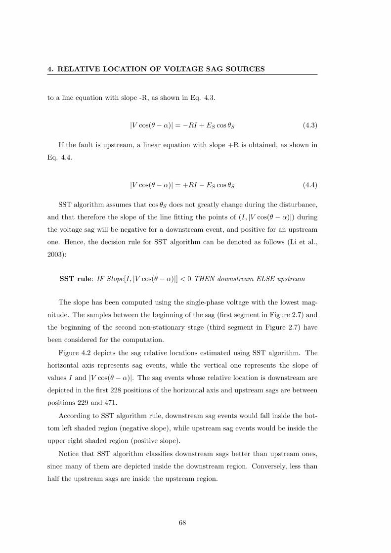
4. RELATIVE LOCATION OF VOLTAGE SAG SOURCES
to a line equation with slope -R, as shown in Eq. 4.3.
|V cos(θ − α)| = −RI + ES cos θS (4.3)
If the fault is upstream, a linear equation with slope +R is obtained, as shown in
Eq. 4.4.
|V cos(θ − α)| = +RI − ES cos θS (4.4)
SST algorithm assumes that cos θS does not greatly change during the disturbance,
and that therefore the slope of the line fitting the points of (I, |V cos(θ − α)|) during
the voltage sag will be negative for a downstream event, and positive for an upstream
one. Hence, the decision rule for SST algorithm can be denoted as follows (Li et al.,
2003):
SST rule: IF Slope[I, |V cos(θ − α)|] < 0 THEN downstream ELSE upstream
The slope has been computed using the single-phase voltage with the lowest mag-
nitude. The samples between the beginning of the sag (first segment in Figure 2.7) and
the beginning of the second non-stationary stage (third segment in Figure 2.7) have
been considered for the computation.
Figure 4.2 depicts the sag relative locations estimated using SST algorithm. The
horizontal axis represents sag events, while the vertical one represents the slope of
values I and |V cos(θ − α)|. The sag events whose relative location is downstream are
depicted in the first 228 positions of the horizontal axis and upstream sags are between
positions 229 and 471.
According to SST algorithm rule, downstream sag events would fall inside the bot-
tom left shaded region (negative slope), while upstream sag events would be inside the
upper right shaded region (positive slope).
Notice that SST algorithm classifies downstream sags better than upstream ones,
since many of them are depicted inside the downstream region. Conversely, less than
half the upstream sags are inside the upstream region.
68
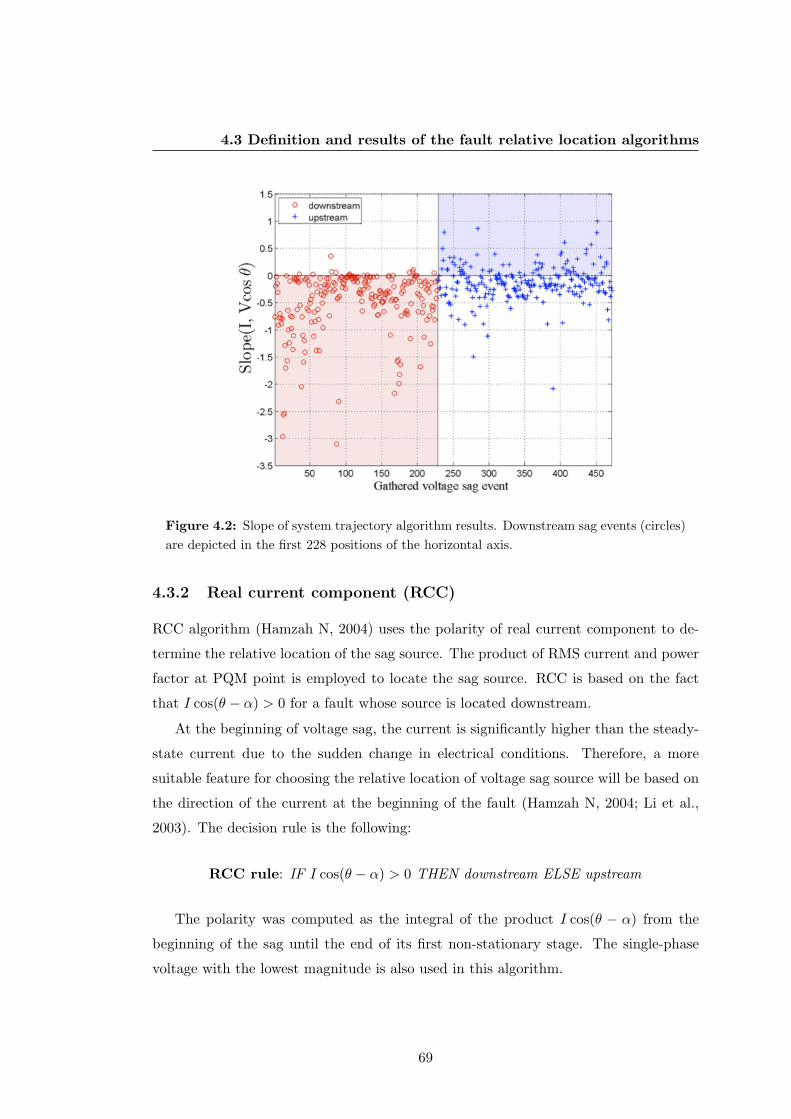
4.3 Definition and results of the fault relative location algorithms
Figure 4.2: Slope of system trajectory algorithm results. Downstream sag events (circles)are depicted in the first 228 positions of the horizontal axis.
4.3.2 Real current component (RCC)
RCC algorithm (Hamzah N, 2004) uses the polarity of real current component to de-
termine the relative location of the sag source. The product of RMS current and power
factor at PQM point is employed to locate the sag source. RCC is based on the fact
that I cos(θ − α) > 0 for a fault whose source is located downstream.
At the beginning of voltage sag, the current is significantly higher than the steady-
state current due to the sudden change in electrical conditions. Therefore, a more
suitable feature for choosing the relative location of voltage sag source will be based on
the direction of the current at the beginning of the fault (Hamzah N, 2004; Li et al.,
2003). The decision rule is the following:
RCC rule: IF I cos(θ − α) > 0 THEN downstream ELSE upstream
The polarity was computed as the integral of the product I cos(θ − α) from the
beginning of the sag until the end of its first non-stationary stage. The single-phase
voltage with the lowest magnitude is also used in this algorithm.
69
4. RELATIVE LOCATION OF VOLTAGE SAG SOURCES
RCC rule indicates that downstream sag events have to be depicted in the upper
left shaded region (I cos(θ−α) > 0), whereas upstream sag events will be in the bottom
right shaded region (I cos(θ − α) < 0) (Figure 4.3 ).
Results are similar to those obtained with SST algorithm (downstream sags are
classified better than upstream sags). But the feature used in RCC algorithm, I cos(θ−
α), has more variability than SST feature, Slope[I, |V cos(θ − α)|].
Figure 4.3: Real current component algorithm results. The downstream sag events(circles) are depicted in the first 228 positions of the horizontal axis.
4.3.3 Distance relay (DR)
This algorithm is based on the principle that the magnitude and angle of impedances
before and after the sag event clearly indicates the relative location of sag source with
respect to PQM point (Pradhan and Routray, 2005). For this purpose, DR algorithm
uses distance relay information (phases involved, impedances, etc). For a downstream
fault in the network shown in Figure 2.3, the impedance seen at PQM point will be:
ZPQM =V ∠θI∠α
= Z ′ +4Z (4.5)
70
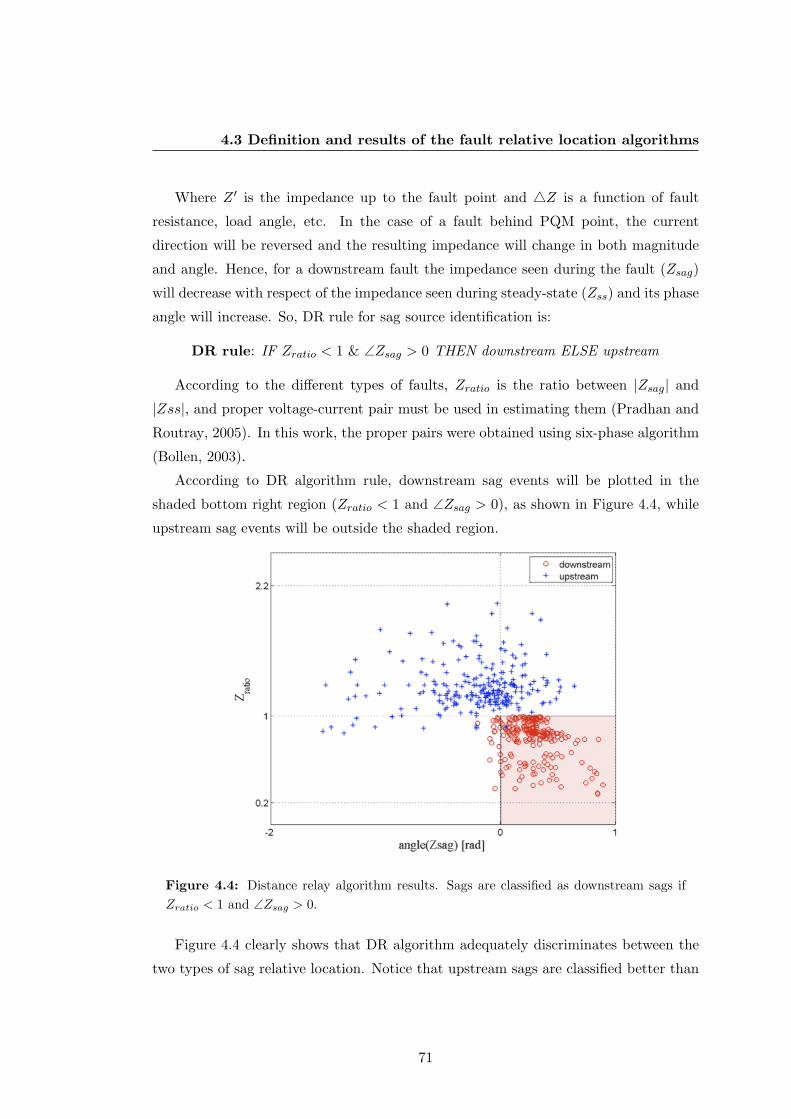
4.3 Definition and results of the fault relative location algorithms
Where Z ′ is the impedance up to the fault point and 4Z is a function of fault
resistance, load angle, etc. In the case of a fault behind PQM point, the current
direction will be reversed and the resulting impedance will change in both magnitude
and angle. Hence, for a downstream fault the impedance seen during the fault (Zsag)
will decrease with respect of the impedance seen during steady-state (Zss) and its phase
angle will increase. So, DR rule for sag source identification is:
DR rule: IF Zratio < 1 & ∠Zsag > 0 THEN downstream ELSE upstream
According to the different types of faults, Zratio is the ratio between |Zsag| and
|Zss|, and proper voltage-current pair must be used in estimating them (Pradhan and
Routray, 2005). In this work, the proper pairs were obtained using six-phase algorithm
(Bollen, 2003).
According to DR algorithm rule, downstream sag events will be plotted in the
shaded bottom right region (Zratio < 1 and ∠Zsag > 0), as shown in Figure 4.4, while
upstream sag events will be outside the shaded region.
Figure 4.4: Distance relay algorithm results. Sags are classified as downstream sags ifZratio < 1 and ∠Zsag > 0.
Figure 4.4 clearly shows that DR algorithm adequately discriminates between the
two types of sag relative location. Notice that upstream sags are classified better than
71
4. RELATIVE LOCATION OF VOLTAGE SAG SOURCES
downstream sags. Only 1 upstream sag was misclassified while 24 downstream sags
were considered as upstream.
In fact, it can be seen that Zratio is able to discriminate between upstream and
downstream sags without ∠Zsag because most of upstream sags have Zratio values
greater than 1, while downstream sags have values lower than 1. Conversely, the
majority of downstream sags and a reasonable number of upstream sags have ∠Zsag
greater than zero, meaning that ∠Zsag is not as good as Zratio to discriminate between
both origins. Nevertheless, DR algorithm gives better results when both features are
considered in the rules.
4.3.4 Resistance sign (RS)
This algorithm is based on the principle of estimating the equivalent impedance of the
non-disturbance side by utilising the voltage and current changes caused by the distur-
bance (Tayjasanant et al., 2005). A sign of the real part of the estimated impedance
can reveal if the sag event is from upstream or downstream.
For a downstream fault from PQM point in Figure 2.3 the voltage is as follows:
V = ES − IZ (4.6)
where V and I are the voltage and current at PQM point and Z is the impedance
behind PQM point. In order to improve impedance estimation, authors propose utilis-
ing multiple voltage and current cycles and solve the equation using least-squares (LS)
method. Eq. 4.6 can be written as a function of real and imaginary parts as follows:
VX + jVY = (ESX + ESY )− (IX + jIY )(R+ jX) (4.7)
where X and Y represent real and imaginary parts of each variable respectively.
If n steady-state and fault cycles of (V, I) data are measured during the sag event,
the equivalent impedance (R + jX) can then be found using the LS method. This
means that equivalent impedance can be computed through two expressions, the first
(Eq. 4.8) based on the real part of voltage values, and the second (Eq. 4.9) on the
72
4.3 Definition and results of the fault relative location algorithms
imaginary part.
RXESX
=
IX(1) IY (1) 1. . .. . .. . .
IX(n) IY (n) 1
⊕
×
VX(1)...
VX(n)
(4.8)
and
RXESY
=
IY (1) IX(1) 1. . .. . .. . .
IY (n) IX(n) 1
⊕
×
VY (1)...
VY (n)
(4.9)
where symbol ⊕ indicates the pseudo-inverse of matrix. The number of cycles n
is determined by the power flow, so voltages and currents used in Eq. 4.8 and Eq.
4.9 must only include values before the reversion of power flow. Authors claim that if
the fault is located downstream, the equivalent resistance (R) will be negative in both
equations Eq. 4.8 and Eq. 4.9. Conversely, if both signs are positive, the sag source
is upstream. If the signs are different (opposite), the test is not conclusive. Then, RS
rule is as follows:
RS rule: IF Rex > 0 & Rey > 0 THEN upstream ELSE IF Rex < 0 & Rey < 0
THEN downstream ELSE not conclusive test
Where Rex and Rey represent equivalent resistance R based on real (Eq. 4.8) and
imaginary (Eq. 4.9) parts of the voltage respectively.
RS algorithm rule indicates that downstream sag events will be depicted in the
bottom left shaded region (Rex < 0 and Rey < 0), whereas the upstream sag events
will be depicted in the upper right shaded region (Rex > 0 and Rey > 0), Figure 4.5.
Most upstream sag events (242) were correctly classified (Figure 4.5). Only one
was confused and classified as a downstream event. Hence, Rex and Rey are able to
discriminate between sag events whose relative location is upstream. However, while
a reasonable percentage of downstream sags (155) was correctly identified, others (32)
were classified as Not Conclusive Test (NCT) because of resistance signs was differ-
ent. In (Chouhy, 2007) similar results (excessive NTC outputs) were obtained for RS
algorithm using synthetic data.
73
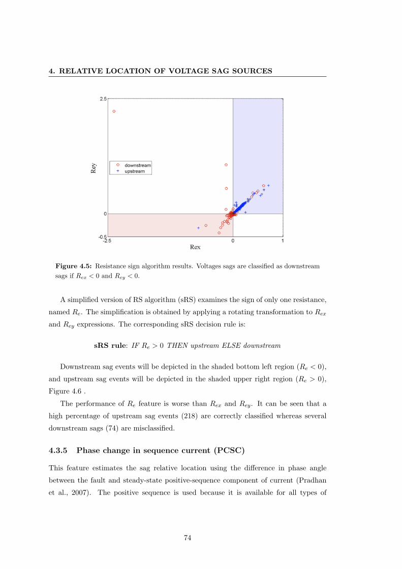
4. RELATIVE LOCATION OF VOLTAGE SAG SOURCES
Figure 4.5: Resistance sign algorithm results. Voltages sags are classified as downstreamsags if Rex < 0 and Rey < 0.
A simplified version of RS algorithm (sRS) examines the sign of only one resistance,
named Re. The simplification is obtained by applying a rotating transformation to Rexand Rey expressions. The corresponding sRS decision rule is:
sRS rule: IF Re > 0 THEN upstream ELSE downstream
Downstream sag events will be depicted in the shaded bottom left region (Re < 0),
and upstream sag events will be depicted in the shaded upper right region (Re > 0),
Figure 4.6 .
The performance of Re feature is worse than Rex and Rey. It can be seen that a
high percentage of upstream sag events (218) are correctly classified whereas several
downstream sags (74) are misclassified.
4.3.5 Phase change in sequence current (PCSC)
This feature estimates the sag relative location using the difference in phase angle
between the fault and steady-state positive-sequence component of current (Pradhan
et al., 2007). The positive sequence is used because it is available for all types of
74
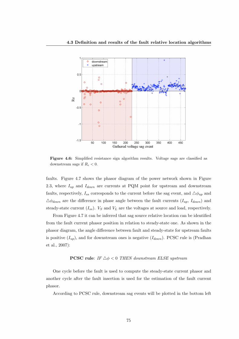
4.3 Definition and results of the fault relative location algorithms
Figure 4.6: Simplified resistance sign algorithm results. Voltage sags are classified asdownstream sags if Re < 0.
faults. Figure 4.7 shows the phasor diagram of the power network shown in Figure
2.3, where Iup and Idown are currents at PQM point for upstream and downstream
faults, respectively, Iss corresponds to the current before the sag event, and 4φup and
4φdown are the difference in phase angle between the fault currents (Iup, Idown) and
steady-state current (Iss). VS and VL are the voltages at source and load, respectively.
From Figure 4.7 it can be inferred that sag source relative location can be identified
from the fault current phasor position in relation to steady-state one. As shown in the
phasor diagram, the angle difference between fault and steady-state for upstream faults
is positive (Iup), and for downstream ones is negative (Idown). PCSC rule is (Pradhan
et al., 2007):
PCSC rule: IF 4φ < 0 THEN downstream ELSE upstream
One cycle before the fault is used to compute the steady-state current phasor and
another cycle after the fault insertion is used for the estimation of the fault current
phasor.
According to PCSC rule, downstream sag events will be plotted in the bottom left
75
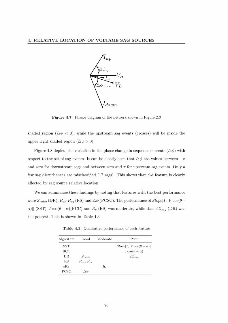
4. RELATIVE LOCATION OF VOLTAGE SAG SOURCES
Figure 4.7: Phasor diagram of the network shown in Figure 2.3
shaded region (4φ < 0), while the upstream sag events (crosses) will be inside the
upper right shaded region (4φ > 0).
Figure 4.8 depicts the variation in the phase change in sequence currents (4φ) with
respect to the set of sag events. It can be clearly seen that 4φ has values between −π
and zero for downstream sags and between zero and π for upstream sag events. Only a
few sag disturbances are misclassified (17 sags). This shows that 4φ feature is clearly
affected by sag source relative location.
We can summarise these findings by noting that features with the best performance
were Zratio (DR),Rex-Rey (RS) and4φ (PCSC). The performance of Slope[I, |V cos(θ−
α)|] (SST), I cos(θ−α)(RCC) and Re (RS) was moderate, while that ∠Zsag (DR) was
the poorest. This is shown in Table 4.3.
Table 4.3: Qualitative performance of each feature
Algorithm Good Moderate Poor
SST Slope[I, |V cos(θ − α)|]RCC I cos(θ − α)
DR Zratio ∠Zsag
RS Rex, Rey
sRS Re
PCSC 4φ
76
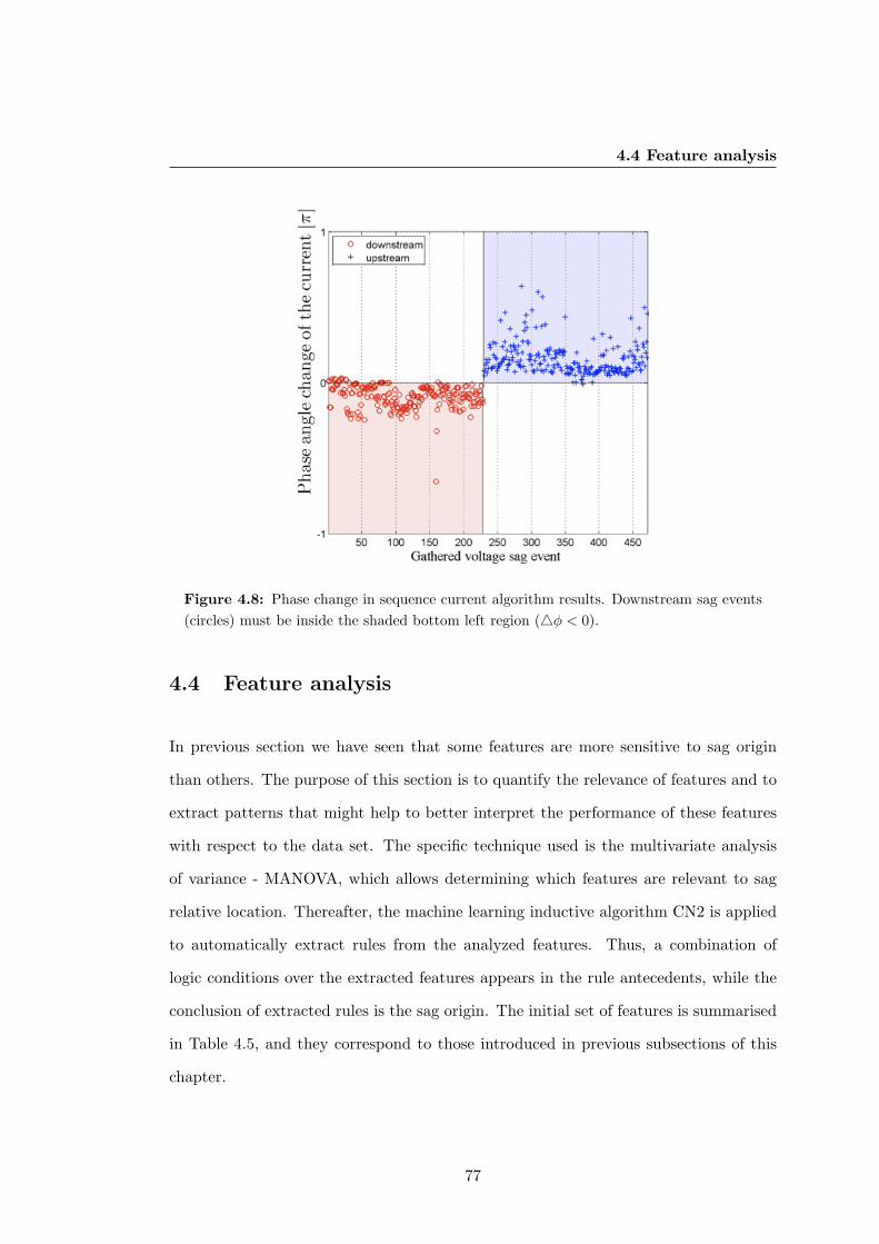
4.4 Feature analysis
Figure 4.8: Phase change in sequence current algorithm results. Downstream sag events(circles) must be inside the shaded bottom left region (4φ < 0).
4.4 Feature analysis
In previous section we have seen that some features are more sensitive to sag origin
than others. The purpose of this section is to quantify the relevance of features and to
extract patterns that might help to better interpret the performance of these features
with respect to the data set. The specific technique used is the multivariate analysis
of variance - MANOVA, which allows determining which features are relevant to sag
relative location. Thereafter, the machine learning inductive algorithm CN2 is applied
to automatically extract rules from the analyzed features. Thus, a combination of
logic conditions over the extracted features appears in the rule antecedents, while the
conclusion of extracted rules is the sag origin. The initial set of features is summarised
in Table 4.5, and they correspond to those introduced in previous subsections of this
chapter.
77
4. RELATIVE LOCATION OF VOLTAGE SAG SOURCES
4.4.1 Outlier correction
Since inductive algorithms are sensitive to outliers, an analysis was performed to detect
them and to avoid systematic mistakes due to them. As a result, the furthest voltage
sag events from the mean of each feature were modified. Therefore, outlier sags were
not excluded. They were corrected with a confidence interval of 95%. It consists of
replacing 5% of the highest (2,5%) and lowest (2,5%) values for each feature by the mean
value of the corresponding feature. Based on the amount of upstream and downstream
voltage sags (Table 4.2), the six highest and six lowest values for each feature were
replaced. Outlier correction was performed on both class (upstream and downstream).
After this outlier correction, the whole set of sags described by the selected features
were used as input for CN2 algorithm.
4.4.2 Descriptive statistical analysis
In Table 4.4 the mean, µ, and standard deviation, σ, of each feature in each class are
listed (data with corrected outliers).
Analysis of the mean and standard deviation values of each features and class, shows
that Slope[I, |V cos(θ − α)|], I cos(θ − α) and ∠Zsag features are overlap for upstream
and downstream sags. For instance, taking I cos(θ− α) feature, the mean value minus
one standard deviation of downstream class is equal to -38,7, while the mean value plus
one standard deviation of upstream class is equal to 21.69. Hence, although the centres
of classes are not close, with only one standard deviation they overlap. As a result, the
aforementioned features obtain a low performance (Table 4.3). The other features are
not overlapped.
4.4.3 Multivariate analysis of variance - MANOVA
The main purpose of MANOVA is to explore how independent variables influence the
patterning of response in dependent variables. Thus, MANOVA allows the following
question to be answered: what is the importance of each feature for source relative
location? From this, it can be determined the influence grade of source location in each
feature. The sag source relative location (upstream or downstream sag) was used as
independent variable and Slope[I, |V cos(θ−α)|], I cos(θ−α), Zratio, ∠Zsag, Rex, Rey,
Re and 4φ features were used as dependent variables.
78
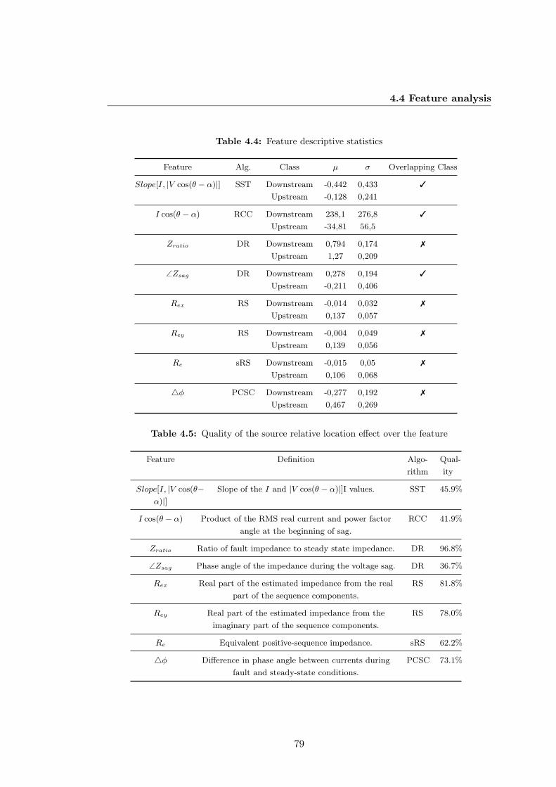
4.4 Feature analysis
Table 4.4: Feature descriptive statistics
Feature Alg. Class µ σ Overlapping Class
Slope[I, |V cos(θ − α)|] SST Downstream -0,442 0,433 3
Upstream -0,128 0,241
I cos(θ − α) RCC Downstream 238,1 276,8 3
Upstream -34,81 56,5
Zratio DR Downstream 0,794 0,174 7
Upstream 1,27 0,209
∠Zsag DR Downstream 0,278 0,194 3
Upstream -0,211 0,406
Rex RS Downstream -0,014 0,032 7
Upstream 0,137 0,057
Rey RS Downstream -0,004 0,049 7
Upstream 0,139 0,056
Re sRS Downstream -0,015 0,05 7
Upstream 0,106 0,068
4φ PCSC Downstream -0,277 0,192 7
Upstream 0,467 0,269
Table 4.5: Quality of the source relative location effect over the feature
Feature Definition Algo-
rithm
Qual-
ity
Slope[I, |V cos(θ−α)|]
Slope of the I and |V cos(θ − α)|]I values. SST 45.9%
I cos(θ − α) Product of the RMS real current and power factor
angle at the beginning of sag.
RCC 41.9%
Zratio Ratio of fault impedance to steady state impedance. DR 96.8%
∠Zsag Phase angle of the impedance during the voltage sag. DR 36.7%
Rex Real part of the estimated impedance from the real
part of the sequence components.
RS 81.8%
Rey Real part of the estimated impedance from the
imaginary part of the sequence components.
RS 78.0%
Re Equivalent positive-sequence impedance. sRS 62.2%
4φ Difference in phase angle between currents during
fault and steady-state conditions.
PCSC 73.1%
79
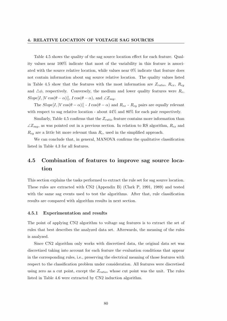
4. RELATIVE LOCATION OF VOLTAGE SAG SOURCES
Table 4.5 shows the quality of the sag source location effect for each feature. Qual-
ity values near 100% indicate that most of the variability in this feature is associ-
ated with the source relative location, while values near 0% indicate that feature does
not contain information about sag source relative location. The quality values listed
in Table 4.5 show that the features with the most information are Zratio, Rex, Reyand 4φ, respectively. Conversely, the medium and lower quality features were Re,
Slope[I, |V cos(θ − α)|], I cos(θ − α), and ∠Zsag.
The Slope[I, |V cos(θ − α)|] - I cos(θ − α) and Rex - Rey pairs are equally relevant
with respect to sag relative location - about 44% and 80% for each pair respectively.
Similarly, Table 4.5 confirms that the Zratio feature contains more information than
∠Zsag, as was pointed out in a previous section. In relation to RS algorithm, Rex and
Rey are a little bit more relevant than Re, used in the simplified approach.
We can conclude that, in general, MANOVA confirms the qualitative classification
listed in Table 4.3 for all features.
4.5 Combination of features to improve sag source loca-
tion
This section explains the tasks performed to extract the rule set for sag source location.
These rules are extracted with CN2 (Appendix B) (Clark P, 1991, 1989) and tested
with the same sag events used to test the algorithms. After that, rule classification
results are compared with algorithm results in next section.
4.5.1 Experimentation and results
The point of applying CN2 algorithm to voltage sag features is to extract the set of
rules that best describes the analyzed data set. Afterwards, the meaning of the rules
is analyzed.
Since CN2 algorithm only works with discretised data, the original data set was
discretized taking into account for each feature the evaluation conditions that appear
in the corresponding rules, i.e., preserving the electrical meaning of those features with
respect to the classification problem under consideration. All features were discretised
using zero as a cut point, except the Zratio, whose cut point was the unit. The rules
listed in Table 4.6 were extracted by CN2 induction algorithm.
80
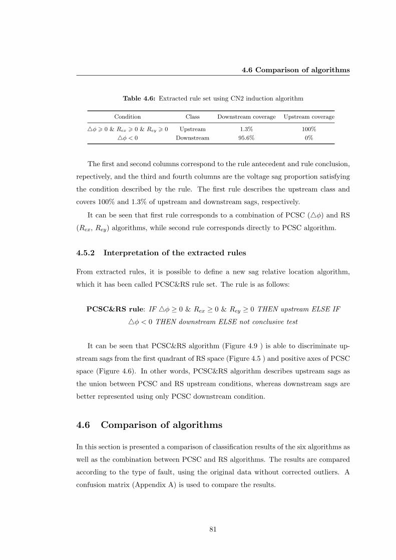
4.6 Comparison of algorithms
Table 4.6: Extracted rule set using CN2 induction algorithm
Condition Class Downstream coverage Upstream coverage
4φ > 0 & Rex > 0 & Rey > 0 Upstream 1.3% 100%
4φ < 0 Downstream 95.6% 0%
The first and second columns correspond to the rule antecedent and rule conclusion,
repectively, and the third and fourth columns are the voltage sag proportion satisfying
the condition described by the rule. The first rule describes the upstream class and
covers 100% and 1.3% of upstream and downstream sags, respectively.
It can be seen that first rule corresponds to a combination of PCSC (4φ) and RS
(Rex, Rey) algorithms, while second rule corresponds directly to PCSC algorithm.
4.5.2 Interpretation of the extracted rules
From extracted rules, it is possible to define a new sag relative location algorithm,
which it has been called PCSC&RS rule set. The rule is as follows:
PCSC&RS rule: IF 4φ ≥ 0 & Rex ≥ 0 & Rey ≥ 0 THEN upstream ELSE IF
4φ < 0 THEN downstream ELSE not conclusive test
It can be seen that PCSC&RS algorithm (Figure 4.9 ) is able to discriminate up-
stream sags from the first quadrant of RS space (Figure 4.5 ) and positive axes of PCSC
space (Figure 4.6). In other words, PCSC&RS algorithm describes upstream sags as
the union between PCSC and RS upstream conditions, whereas downstream sags are
better represented using only PCSC downstream condition.
4.6 Comparison of algorithms
In this section is presented a comparison of classification results of the six algorithms as
well as the combination between PCSC and RS algorithms. The results are compared
according to the type of fault, using the original data without corrected outliers. A
confusion matrix (Appendix A) is used to compare the results.
81
4. RELATIVE LOCATION OF VOLTAGE SAG SOURCES
Figure 4.9: Combination of PCSC and RS algorithms. Upstream sag events (crosses)have to be inside the cube.
4.6.1 Comparison
Figure 4.10 shows the FPR and TPR indices for each algorithm and both asymmetrical
fault types (single-phase and phase-to-phase), while Figure 4.11 and Figure 4.12 show
the same indices separately computed for single-phase and phase-to-phase fault types
respectively. Downstream origin has been selected as reference class.
In Table 4.7 the confusion matrices and values taken for the indices in each algorithm
and scenario are listed. The number of sags classified as not conclusive test (NCT) and
the error and classification rates in percentage terms (Hit%) are also listed.
Another classifier called Voting has been added to these figures. The Voting clas-
sifier gives the sag source location using a democratic combination of results coming
from the six algorithms described in Section IV. Its output will be upstream if four
of the six algorithms give upstream as a result, with a similar condition applying for
a downstream estimation. In other cases (where the majority is lower than four) the
estimation will be marked as not conclusive test (NCT).
FPR and TPR indices obtained with PCSC&RS rule set are equal to PCSC indices.
The differences between both are seen in FN and TN indices (Table 4.7).
82
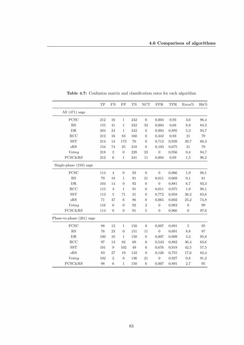
4.6 Comparison of algorithms
Table 4.7: Confusion matrix and classification rates for each algorithm
TP FN FP TN NCT FPR TPR Error% Hit%
All (471) sags
PCSC 212 16 1 242 0 0,004 0,93 3,6 96,4
RS 155 41 1 242 32 0,004 0,68 8,9 84,3
DR 204 24 1 242 0 0,004 0,895 5,3 94,7
RCC 212 16 83 160 0 0,342 0,93 21 79
SST 214 14 173 70 0 0,712 0,939 39,7 60,3
sRS 154 74 25 218 0 0,103 0,675 21 79
Voting 218 2 0 228 23 0 0,956 0,4 94,7
PCSC&RS 212 6 1 241 11 0,004 0,93 1,5 96,2
Single-phase (210) sags
PCSC 114 4 0 92 0 0 0,966 1,9 98,1
RS 79 18 1 91 21 0,011 0,669 9,1 81
DR 104 14 0 92 0 0 0,881 6,7 93,3
RCC 115 3 1 91 0 0,011 0,975 1,9 98,1
SST 113 5 71 21 0 0,772 0,958 36,2 63,8
sRS 71 47 6 86 0 0,065 0,602 25,2 74,8
Voting 116 0 0 92 2 0 0,983 0 99
PCSC&RS 114 0 0 91 5 0 0,966 0 97,6
Phase-to-phase (261) sags
PCSC 98 12 1 150 0 0,007 0,891 5 95
RS 76 23 0 151 11 0 0,691 8,8 87
DR 100 10 1 150 0 0,007 0,909 4,2 95,8
RCC 97 13 82 69 0 0,543 0,882 36,4 63,6
SST 101 9 102 49 0 0,676 0,918 42,5 57,5
sRS 83 27 19 132 0 0,126 0,755 17,6 82,4
Voting 102 2 0 136 21 0 0,927 0,8 91,2
PCSC&RS 98 6 1 150 6 0,007 0,891 2,7 95
83
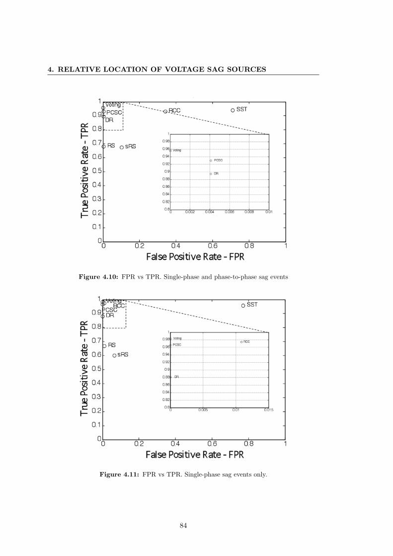
4. RELATIVE LOCATION OF VOLTAGE SAG SOURCES
Figure 4.10: FPR vs TPR. Single-phase and phase-to-phase sag events
Figure 4.11: FPR vs TPR. Single-phase sag events only.
84
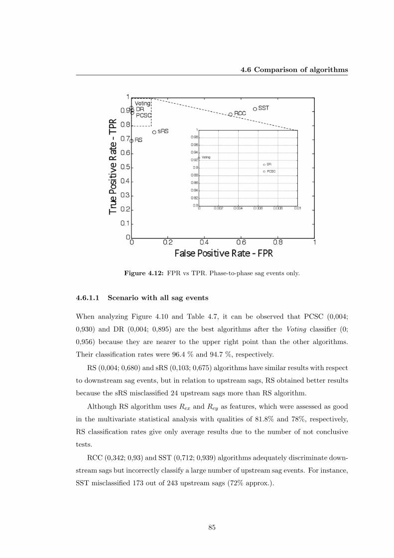
4.6 Comparison of algorithms
Figure 4.12: FPR vs TPR. Phase-to-phase sag events only.
4.6.1.1 Scenario with all sag events
When analyzing Figure 4.10 and Table 4.7, it can be observed that PCSC (0,004;
0,930) and DR (0,004; 0,895) are the best algorithms after the Voting classifier (0;
0,956) because they are nearer to the upper right point than the other algorithms.
Their classification rates were 96.4 % and 94.7 %, respectively.
RS (0,004; 0,680) and sRS (0,103; 0,675) algorithms have similar results with respect
to downstream sag events, but in relation to upstream sags, RS obtained better results
because the sRS misclassified 24 upstream sags more than RS algorithm.
Although RS algorithm uses Rex and Rey as features, which were assessed as good
in the multivariate statistical analysis with qualities of 81.8% and 78%, respectively,
RS classification rates give only average results due to the number of not conclusive
tests.
RCC (0,342; 0,93) and SST (0,712; 0,939) algorithms adequately discriminate down-
stream sags but incorrectly classify a large number of upstream sag events. For instance,
SST misclassified 173 out of 243 upstream sags (72% approx.).
85
4. RELATIVE LOCATION OF VOLTAGE SAG SOURCES
4.6.1.2 Scenario with single-phase sag events
In this scenario (Figure 4.11 ), it can be seen that RCC (0,011; 0,975) algorithm is able
to correctly discriminate the sags whose cause is a single-phase fault, even a little bit
better than PCSC algorithm (0; 0,966), because RCC is the nearest to the (0, 1) point
after the Voting classifier. The other algorithms plot around the same zone in Figure
4.10 .
With single-phase faults, SST algorithm still has a low classification rate. In this
scenario, 71 out of 92 single-phase upstream sags were misclassified (77% approx.).
4.6.1.3 Scenario with phase-to-phase sag events
In Figure 4.12 , it can be observed that DR algorithm (0.007; 0,909) is a little better at
determining phase-to-phase sags than PCSC (0.007; 0,891), and that the sRS algorithm
(0.126; 0,755) is slightly better than RS (0; 0,691). It should be noted that RCC
algorithm classification rate is low with sag events caused by phase-to-phase faults.
SST algorithm does not improve its classification rate in this scenario.
Although PCSC&RS classification indices are the same as those of PCSC algorithm,
PCSC&RS has a lower percentage of error (1,5%) than PCSC algorithm (3,6%), because
PCSC&RS is able to distinguish sags that cannot be classified. The combination of
both methods increases the reliability of PCSC&RS rule. PCSC&RS algorithm is more
reliable than RS and PCSC in terms of success ratios. For instance, PCSC misclassified
11 downstream sags but PCSC&RS was able to classify the same 11 sags as NCT.
4.6.2 Misclassified voltage sags
Based on the previous results, the sag events incorrectly classified by PCSC and
PCSC&RS have been analyzed.
The features used by PCSC and PCSC&RS are listed in Table 4.8 for the 17 voltage
sags misclassified by PCSC algorithm. The real class of each one is shown in the column
labelled Class. A cross (7) indicates that the sag was incorrectly classified, and NCT
indicates that the event was classified as a Not Conclusive Test.
PCSC algorithm classified 16 downstream sags as upstream and one upstream sag
as a downstream event. For downstream sags, 4φ should be lower than zero (4φ < 0),
and greater than zero (4φ > 0) for upstream events, but it can be clearly seen that for
86
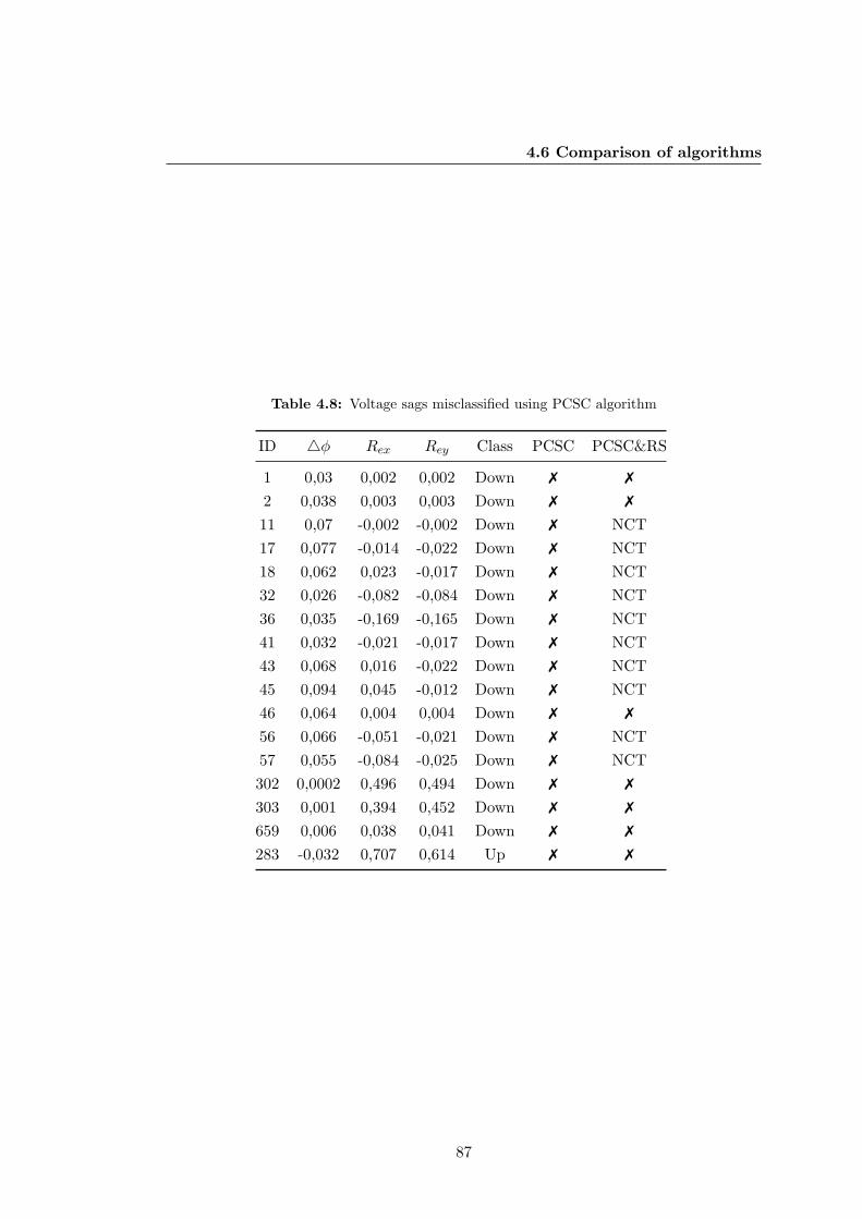
4.6 Comparison of algorithms
Table 4.8: Voltage sags misclassified using PCSC algorithm
ID 4φ Rex Rey Class PCSC PCSC&RS
1 0,03 0,002 0,002 Down 7 7
2 0,038 0,003 0,003 Down 7 7
11 0,07 -0,002 -0,002 Down 7 NCT17 0,077 -0,014 -0,022 Down 7 NCT18 0,062 0,023 -0,017 Down 7 NCT32 0,026 -0,082 -0,084 Down 7 NCT36 0,035 -0,169 -0,165 Down 7 NCT41 0,032 -0,021 -0,017 Down 7 NCT43 0,068 0,016 -0,022 Down 7 NCT45 0,094 0,045 -0,012 Down 7 NCT46 0,064 0,004 0,004 Down 7 7
56 0,066 -0,051 -0,021 Down 7 NCT57 0,055 -0,084 -0,025 Down 7 NCT302 0,0002 0,496 0,494 Down 7 7
303 0,001 0,394 0,452 Down 7 7
659 0,006 0,038 0,041 Down 7 7
283 -0,032 0,707 0,614 Up 7 7
87
4. RELATIVE LOCATION OF VOLTAGE SAG SOURCES
all 17 sags 4φ feature is very close to zero. All of them have been misclassified by a
few hundredths and thousandths of radian units of 4φ feature.
Likewise, PCSC&RS rule set behaves the same with this group of sags, since with
most of them the Rex and Rey features are very close to zero too. Consequently,
PCSC&RS rule set misclassified some sags and others were classified as NCT.
4.7 Conclusions
An evaluation of six algorithms for voltage sag source relative location has been per-
formed. Their used rules and features have been qualitatively and statistically analyzed.
The relative fault location of voltage sags caused by single-phase faults have been
correctly estimated using PCSC and RCC algorithms, which obtained the highest clas-
sification rates for this type of fault. Likewise, PCSC and DR algorithms can correctly
estimate the direction of voltage sag caused by phase-to-phase faults. In any fault
relative location scheme, the appropriate algorithm would have to be applied after
estimating the type of fault.
The multivariate analysis of variance (MANOVA) and CN2 rule induction algorithm
have been used to quantify the relevance of features and extract patterns from a huge
amount of data. Validation and comparative results have been presented in ROC space
as an extension of confusion matrices, and reveal that similar results can be obtained
by observing electrical laws and data mining principles.
A more reliable estimation of sag source has been obtained by combining PCSC
and RS algorithms.
88
5
Internal Causes of Voltage
Disturbances: Relevant Features
and Classification Methodology
5.1 Introduction
This chapter addresses the automatic identification of the internal cause leading a volt-
age disturbance. Motors and transformers generate voltage sags during starting and
energization/saturation, respectively. Capacitor-bank and large-load switchings also
generate voltage disturbances during actions for voltage regulation and load redistri-
bution. Since all of them are network intrinsic components, they are considered in this
work as internal causes of voltage disturbances (Figure 5.1). They distinguish from
other disturbances generated by external causes interacting with the power network
resulting from short-circuits due to animals, tree contacts or failures in underground
cables, among others.
In this chapter, short-circuits disturbances are only considered to find out patterns
that allow to discriminate between internal an external causes of voltage disturbances.
In the analysis, short-circuits are grouped according to the number of involved phases
(single-, double-, three-phase) instead of their root cause (animal, tree, etc). Therefore,
the methodology proposed in this chapter is able to identify when a disturbance is being
leaded by a motor starting, transformer saturation, capacitor bank energization, load
connection, load disconnection or a short-circuit.
89
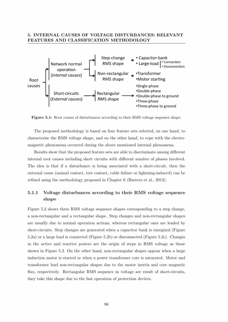
5. INTERNAL CAUSES OF VOLTAGE DISTURBANCES: RELEVANTFEATURES AND CLASSIFICATION METHODOLOGY
Figure 5.1: Root causes of disturbances according to their RMS voltage sequence shape.
The proposed methodology is based on four feature sets selected, on one hand, to
characterise the RMS voltage shape, and on the other hand, to cope with the electro-
magnetic phenomena occurred during the above mentioned internal phenomena.
Results show that the proposed feature sets are able to discriminate among different
internal root causes including short circuits with different number of phases involved.
The idea is that if a disturbance is being associated with a short-circuit, then the
external cause (animal contact, tree contact, cable failure or lightning-induced) can be
refined using the methodology proposed in Chapter 6 (Barrera et al., 2012).
5.1.1 Voltage disturbances according to their RMS voltage sequence
shape
Figure 5.2 shows three RMS voltage sequence shapes corresponding to a step change,
a non-rectangular and a rectangular shape. Step changes and non-rectangular shapes
are usually due to normal operation actions, whereas rectangular ones are leaded by
short-circuits. Step changes are generated when a capacitor bank is energized (Figure
5.2a) or a large load is connected (Figure 5.2b) or disconnected (Figure 5.2c). Changes
in the active and reactive powers are the origin of steps in RMS voltage as those
shown in Figure 5.2. On the other hand, non-rectangular shapes appear when a large
induction motor is started or when a power transformer core is saturated. Motor and
transformer lead non-rectangular shapes due to the motor inertia and core magnetic
flux, respectively. Rectangular RMS sequence in voltage are result of short-circuits,
they take this shape due to the fast operation of protection devices.
90
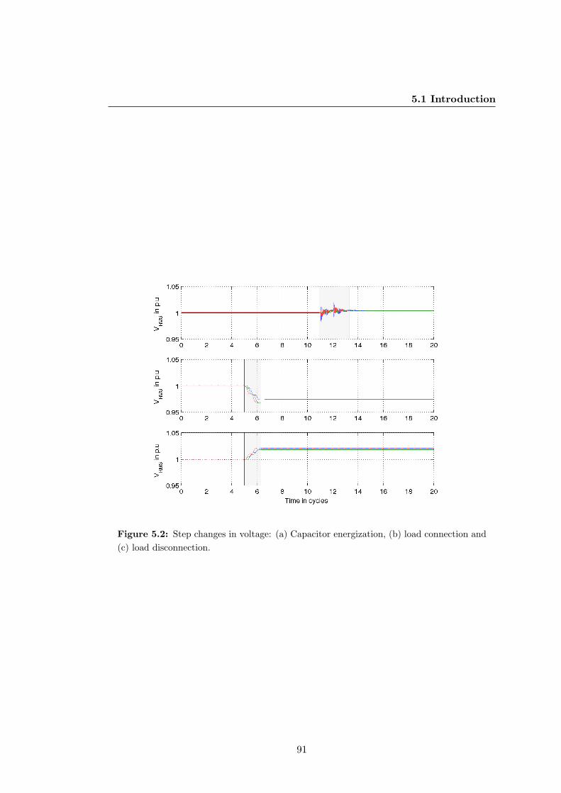
5.1 Introduction
Figure 5.2: Step changes in voltage: (a) Capacitor energization, (b) load connection and(c) load disconnection.
91
5. INTERNAL CAUSES OF VOLTAGE DISTURBANCES: RELEVANTFEATURES AND CLASSIFICATION METHODOLOGY
The problem of internal cause identification in this chapter is addressed basically
taking advantage of the RMS voltage shape. So, the first step is to establish a classifi-
cation of the shape of a disturbance. After that, a new classification will focus on the
root cause identification. The feature sets proposed for classification in this chapter are
as follows:
1. RMS-shape feature set : Two features able to distinguish between the three RMS
shapes: step change, non-rectangular and rectangular.
2. Step-change feature set : Capacitor bank energizing, load connection or load dis-
connection can be discriminated from the three features contained in this subset.
3. Non-rectangular feature set : Transformer saturation and motor starting distur-
bances are adequately distinguished with the three features included in this set.
4. Rectangular feature set : This set contains four features for discriminating between
single-phase, double-phase (to ground) and three-phase (to ground) short-circuits.
Hence, the first feature set is used in the RMS shape identification (first group),
and the remaining sets are used to identify the corresponding cause from the pre-
identified RMS shape. From the aforementioned four feature sets, an effective classifi-
cation method can be built for automatically identifying the root cause of disturbances.
5.1.2 Organization of the chapter
This chapter is organized as follows: in Section 5.2, a brief description of the used
waveforms is given. The four feature sets are presented and their contained features
are described and analyzed in Section 5.3. Later, a feature analysis is carried out in
Section 5.4. After that, a rule-based classification method for identifying internal root
causes is proposed and tested in Section 5.5. Finally, relevant conclusions are given in
last section.
5.2 Data description
The study was carried out using a combination of synthetic and field measurements. On
one hand, disturbances due to motor starting, capacitor switching and load switching
92
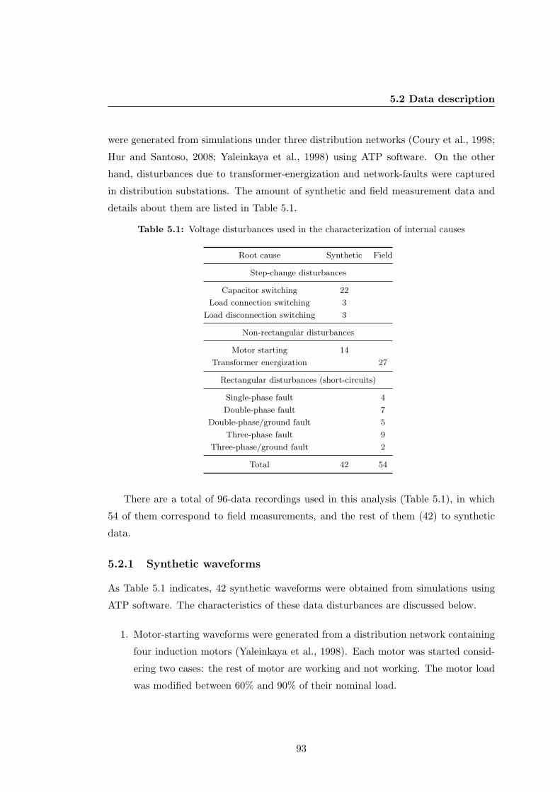
5.2 Data description
were generated from simulations under three distribution networks (Coury et al., 1998;
Hur and Santoso, 2008; Yaleinkaya et al., 1998) using ATP software. On the other
hand, disturbances due to transformer-energization and network-faults were captured
in distribution substations. The amount of synthetic and field measurement data and
details about them are listed in Table 5.1.
Table 5.1: Voltage disturbances used in the characterization of internal causes
Root cause Synthetic Field
Step-change disturbances
Capacitor switching 22
Load connection switching 3
Load disconnection switching 3
Non-rectangular disturbances
Motor starting 14
Transformer energization 27
Rectangular disturbances (short-circuits)
Single-phase fault 4
Double-phase fault 7
Double-phase/ground fault 5
Three-phase fault 9
Three-phase/ground fault 2
Total 42 54
There are a total of 96-data recordings used in this analysis (Table 5.1), in which
54 of them correspond to field measurements, and the rest of them (42) to synthetic
data.
5.2.1 Synthetic waveforms
As Table 5.1 indicates, 42 synthetic waveforms were obtained from simulations using
ATP software. The characteristics of these data disturbances are discussed below.
1. Motor-starting waveforms were generated from a distribution network containing
four induction motors (Yaleinkaya et al., 1998). Each motor was started consid-
ering two cases: the rest of motor are working and not working. The motor load
was modified between 60% and 90% of their nominal load.
93
5. INTERNAL CAUSES OF VOLTAGE DISTURBANCES: RELEVANTFEATURES AND CLASSIFICATION METHODOLOGY
2. Capacitor-switching waveforms were simulated using two distribution networks
presented in (Coury et al., 1998; Hur and Santoso, 2008). First one corresponds
to an IEEE test case, and second one corresponds to a network of an American
electric utility. Normal switching and back-to-back switching were generated in
both simulated networks. Additionally, capacitor banks were located and ener-
gized in different buses to obtain different dumping factors as consequence of the
distance between capacitor bank and monitoring device.
3. Waveforms related to load switching were obtained from the IEEE 37 node feeder.
Load connection/disconnection switching was simulated throughout the network
(Kersting, 2001).
5.2.2 Field measurements
A set of 54 voltage and current waveforms were collected at the medium voltage side
of different HV/MV substations (25-kV). 27 of them were due to transformer energiza-
tion and the rest were due to short-circuits. The current and voltage waveforms were
sampled at 128 samples per cycle (50 Hz) and contain 40 cycles.
5.3 Feature description
In this subsection are explained and analyzed the four aforemetioned feature sets.
Firstly are addressed the three feature sets (No. 2, 3 and 4) able to discriminate
between the causes sharing a same RMS shape, and after that, the feature set (No. 1)
able to discriminate between the different RMS shapes.
5.3.1 Features characterizing load/capacitor switching disturbances:
Step-changes
Since capacitor bank de-energizing leads to a drop in voltage without any noticeable
transient (Santoso et al., 2001), they have not been included in this analysis. When a
load connection/disconnection switching, or a capacitor bank energization occurs, the
substation feeder experiences changes in active/reactive powers, power factor and RMS
voltage. The reactive power injected by a capacitor bank leads to a slight rise in voltage,
since it compensates the reactive power demanded by network load. Connection of a
94
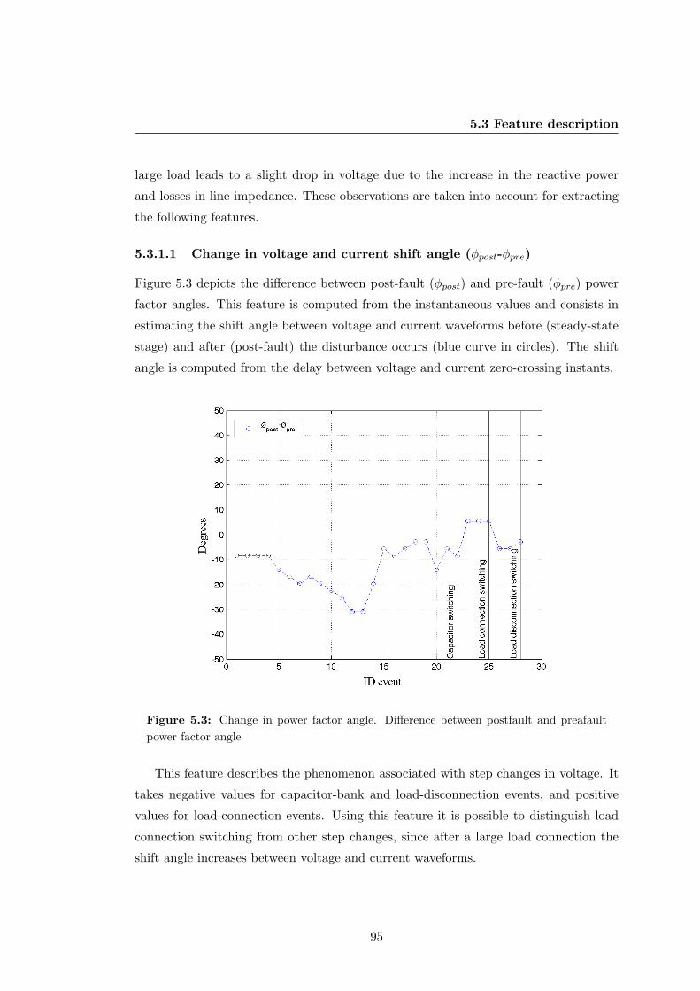
5.3 Feature description
large load leads to a slight drop in voltage due to the increase in the reactive power
and losses in line impedance. These observations are taken into account for extracting
the following features.
5.3.1.1 Change in voltage and current shift angle (φpost-φpre)
Figure 5.3 depicts the difference between post-fault (φpost) and pre-fault (φpre) power
factor angles. This feature is computed from the instantaneous values and consists in
estimating the shift angle between voltage and current waveforms before (steady-state
stage) and after (post-fault) the disturbance occurs (blue curve in circles). The shift
angle is computed from the delay between voltage and current zero-crossing instants.
Figure 5.3: Change in power factor angle. Difference between postfault and preafaultpower factor angle
This feature describes the phenomenon associated with step changes in voltage. It
takes negative values for capacitor-bank and load-disconnection events, and positive
values for load-connection events. Using this feature it is possible to distinguish load
connection switching from other step changes, since after a large load connection the
shift angle increases between voltage and current waveforms.
95
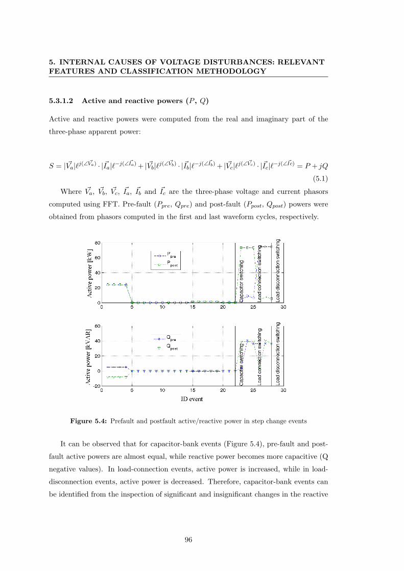
5. INTERNAL CAUSES OF VOLTAGE DISTURBANCES: RELEVANTFEATURES AND CLASSIFICATION METHODOLOGY
5.3.1.2 Active and reactive powers (P , Q)
Active and reactive powers were computed from the real and imaginary part of the
three-phase apparent power:
S = | ~Va|`j(∠~Va) · |~Ia|`−j(∠
~Ia) + | ~Vb|`j(∠~Vb) · |~Ib|`−j(∠
~Ib) + | ~Vc|`j(∠~Vc) · |~Ic|`−j(∠
~Ic) = P + jQ
(5.1)
Where ~Va, ~Vb, ~Vc, ~Ia, ~Ib and ~Ic are the three-phase voltage and current phasors
computed using FFT. Pre-fault (Ppre, Qpre) and post-fault (Ppost, Qpost) powers were
obtained from phasors computed in the first and last waveform cycles, respectively.
Figure 5.4: Prefault and postfault active/reactive power in step change events
It can be observed that for capacitor-bank events (Figure 5.4), pre-fault and post-
fault active powers are almost equal, while reactive power becomes more capacitive (Q
negative values). In load-connection events, active power is increased, while in load-
disconnection events, active power is decreased. Therefore, capacitor-bank events can
be identified from the inspection of significant and insignificant changes in the reactive
96
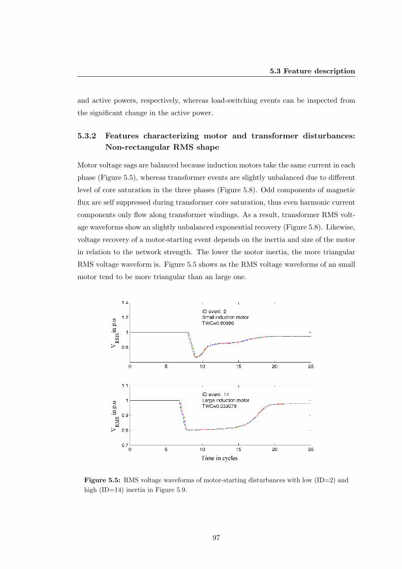
5.3 Feature description
and active powers, respectively, whereas load-switching events can be inspected from
the significant change in the active power.
5.3.2 Features characterizing motor and transformer disturbances:
Non-rectangular RMS shape
Motor voltage sags are balanced because induction motors take the same current in each
phase (Figure 5.5), whereas transformer events are slightly unbalanced due to different
level of core saturation in the three phases (Figure 5.8). Odd components of magnetic
flux are self suppressed during transformer core saturation, thus even harmonic current
components only flow along transformer windings. As a result, transformer RMS volt-
age waveforms show an slightly unbalanced exponential recovery (Figure 5.8). Likewise,
voltage recovery of a motor-starting event depends on the inertia and size of the motor
in relation to the network strength. The lower the motor inertia, the more triangular
RMS voltage waveform is. Figure 5.5 shows as the RMS voltage waveforms of an small
motor tend to be more triangular than an large one.
Figure 5.5: RMS voltage waveforms of motor-starting disturbances with low (ID=2) andhigh (ID=14) inertia in Figure 5.9.
97
5. INTERNAL CAUSES OF VOLTAGE DISTURBANCES: RELEVANTFEATURES AND CLASSIFICATION METHODOLOGY
From these hypotheses, features that described the unbalance grade, the shape of the
RMS voltage sequence and the even current harmonics can be defined to characterize
such disturbances.
5.3.2.1 Maximum neutral voltage and current ratios (Vn, In)
These two features are computed in order to measure the unbalance grade of non-
rectagular events. Vn is taken as the maximum value during fault stage as follows:
Vn = |−→Va +
−→Vb +
−→Vc| (5.2)
−→Va,−→Vb,−→Vc are the phase voltage phasors calculated by making use of FFT with a
1-cycle window. Vn is computed at each fault-stage sample and the maximum of them
is taken as the feature value. Likewise, In is computed evaluating Eq. 5.2 by using
current phasors instead of voltage ones. Vn and In are depicted in Figure 5.6 in per
unit of prefault phase voltage and current values, respectively.
Unlike motor disturbances, those due to transformer energizing present significant
increments in neutral current during the event (Figure 5.6). This increment directly
depends on the difference in the saturation level of the transformer phases. Hence,
the higher the difference, the higher the neutral current is. This is only valid in wye-
grounded networks (Figure 2.6); otherwise no neutral current and voltage are available.
Respect to the performance of both features, the neutral current ratio (In) should
be used to better distinguish between both root causes rather than neutral voltage ratio
(Vn), since In presents more variability than Vn. In Figure 5.6 it can also be observed
that some transformer events (ID=16, 20, 21, 25, 34, 39 at the top) have neutral current
close to zero. This is due to a small difference in saturation level of the transformer
windings.
5.3.2.2 Magnitude of the second order harmonic current (|I2|)
|I2| is computed as the maximum value of the second harmonic current magnitude
during fault-stage using FFT. Figure 5.7 depicts the second order current harmonic in
per unit of the fundamental current component. As expected, |I2| takes higher values
during transformer events than motor ones. Then, |I2| may adequately distinguish
between both types of non-rectangular events.
98
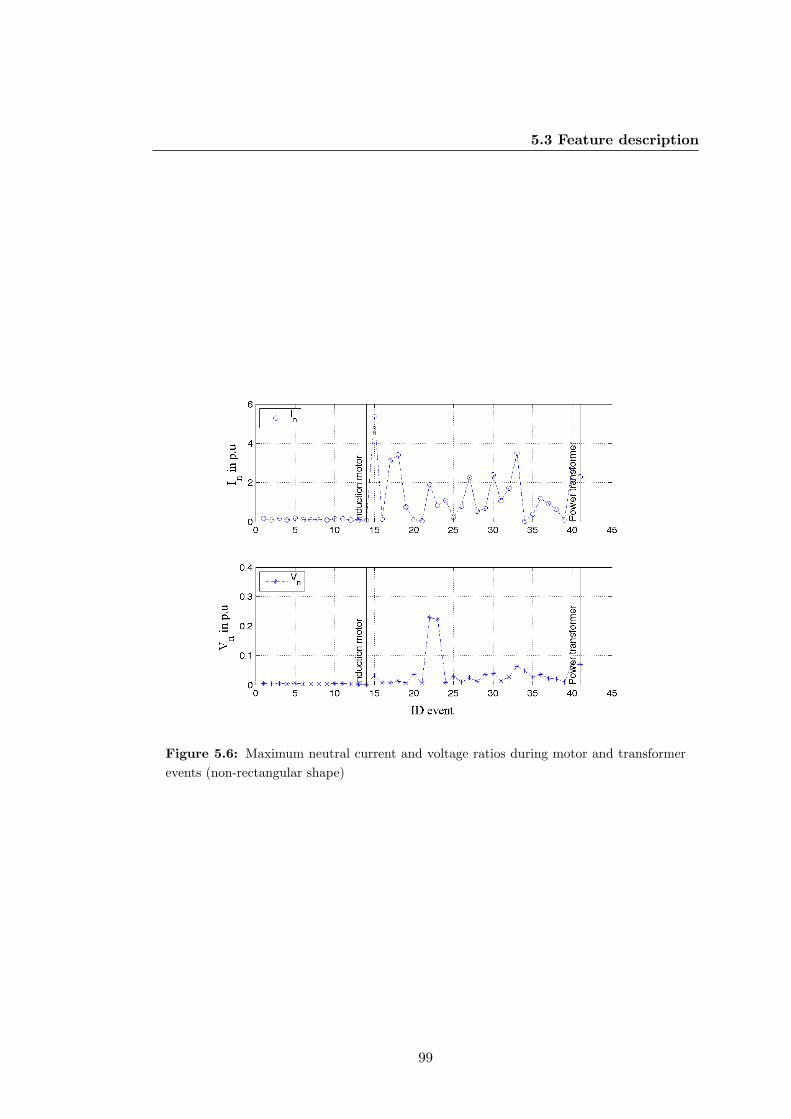
5.3 Feature description
Figure 5.6: Maximum neutral current and voltage ratios during motor and transformerevents (non-rectangular shape)
99
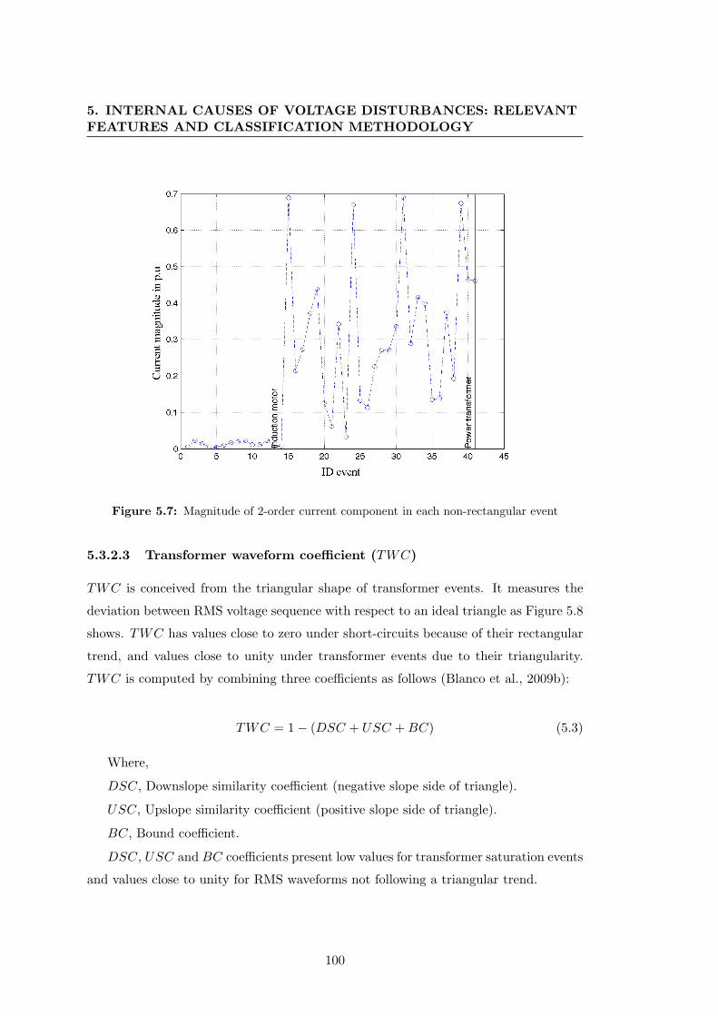
5. INTERNAL CAUSES OF VOLTAGE DISTURBANCES: RELEVANTFEATURES AND CLASSIFICATION METHODOLOGY
Figure 5.7: Magnitude of 2-order current component in each non-rectangular event
5.3.2.3 Transformer waveform coefficient (TWC)
TWC is conceived from the triangular shape of transformer events. It measures the
deviation between RMS voltage sequence with respect to an ideal triangle as Figure 5.8
shows. TWC has values close to zero under short-circuits because of their rectangular
trend, and values close to unity under transformer events due to their triangularity.
TWC is computed by combining three coefficients as follows (Blanco et al., 2009b):
TWC = 1− (DSC + USC +BC) (5.3)
Where,
DSC, Downslope similarity coefficient (negative slope side of triangle).
USC, Upslope similarity coefficient (positive slope side of triangle).
BC, Bound coefficient.
DSC, USC and BC coefficients present low values for transformer saturation events
and values close to unity for RMS waveforms not following a triangular trend.
100
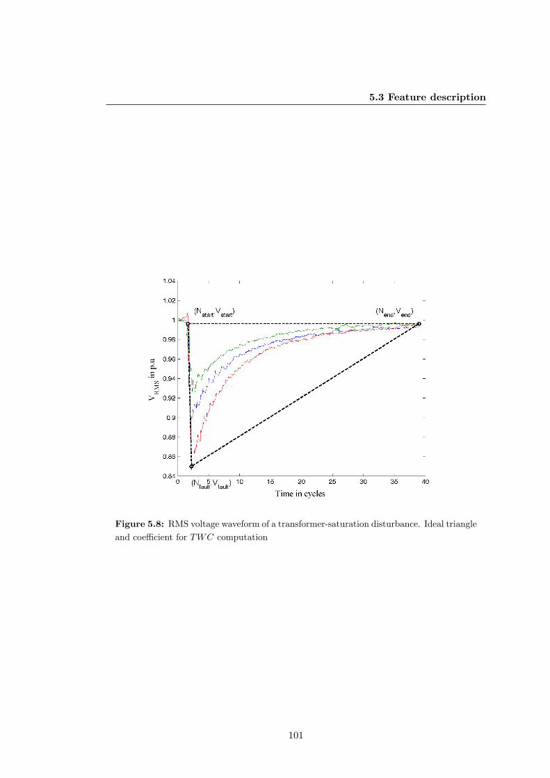
5.3 Feature description
Figure 5.8: RMS voltage waveform of a transformer-saturation disturbance. Ideal triangleand coefficient for TWC computation
101
5. INTERNAL CAUSES OF VOLTAGE DISTURBANCES: RELEVANTFEATURES AND CLASSIFICATION METHODOLOGY
DSC and USC coefficients measure the deviation between RMS voltage sequence
with the negative and positive slope of triangle sides, respectively. In the following
equations DSC coefficient is declared:
DSC =σ(lDownA , lDownB , lDownC )
lNSS(5.4)
lDownphase =Nfault∑i=Nstart
√(Nfault −Nstart)2 + (Vphase [i+ 1]− Vphase [i])2 (5.5)
lNSS =√
(Nfault −Nstart)2 + (Vfault − Vstart)2 (5.6)
Where,
lDownA,B,C , Length of RMS voltage signal in each phase at the beginning of the event.
lNSS , Distance of a line between the samples (Nstart, Vstart) and (Nfault, Vfault).
NSS stands for Negative Slope Side.
Nstart, Sample where the event start.
Vstart, Voltage magnitude at Nstart.
Nfault, Sample where voltage magnitude is minimum.
Vfault, Voltage magnitude at Nfault.
Similar expressions are defined to compute USC feature using the corresponding
parameters related to the positive slope triangle side, that is, lPSS , Nfault and Nend.
PSS stands for Positive Slope Side.
The BC coefficient measures the number of disturbance points outside of triangle
area.
Figure 5.9 shows the TWC values associated with motor and transformer events.
It can be seen that transformer-energizing events have the highest TWC values due to
their triangular shape in RMS voltage sequence. The last transformer event has the
lowest TWC value because this event corresponds to a transformer saturation followed
by a protection operation, thus, its exponential recovery is abruptly truncated by the
fast protection operation, and consequently its RMS shape is not completely triangular,
see Figure 5.10.
Some motor-starting events have relatively high TWC values because their RMS
voltage sequences tend to have a triangular shape. This is due to their low inertia
parameters causing a fast start-up (event ID=2, TWC=0,81), and consequently, the
102
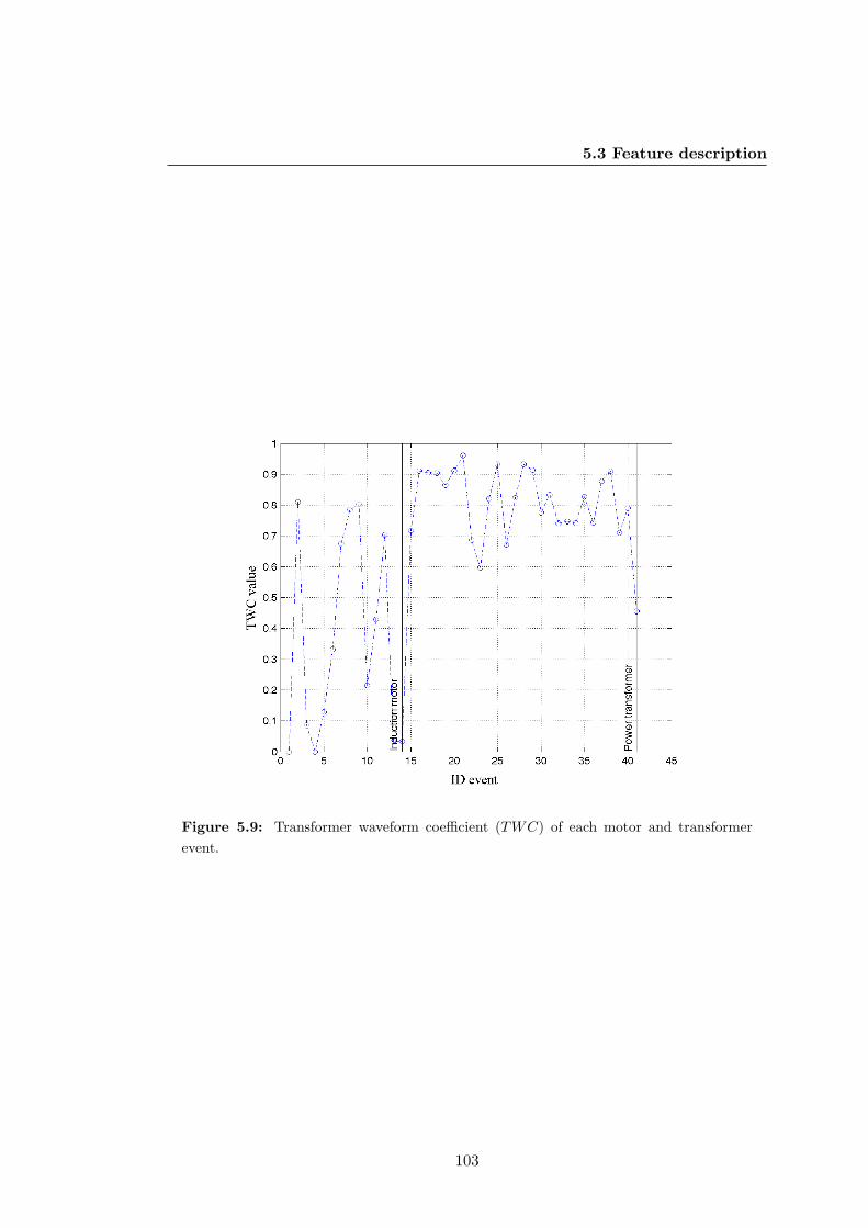
5.3 Feature description
Figure 5.9: Transformer waveform coefficient (TWC) of each motor and transformerevent.
103
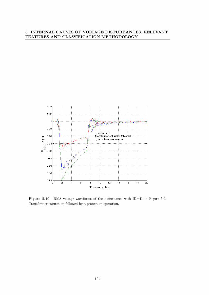
5. INTERNAL CAUSES OF VOLTAGE DISTURBANCES: RELEVANTFEATURES AND CLASSIFICATION METHODOLOGY
Figure 5.10: RMS voltage waveforms of the disturbance with ID=41 in Figure 5.9.Transformer saturation followed by a protection operation.
104
5.3 Feature description
RMS voltage sequence experiences a strong triangular shape, see Figure 5.5a. Similarly,
an RMS voltage sequence caused by a high-inertia motor is presented in Figure 5.5b,
it does not follow a triangular shape which is verified with its low TWC value equal to
0,0033.
TWC feature is capable to discriminate those non-rectangular events whose RMS
voltage sequences tend to be in triangular shape. Transformer events and motor fast
starting can be distinguished.
5.3.3 Features characterizing short-circuits disturbances: Rectangu-
lar RMS shape
Disturbances with rectangular RMS shape usually correspond to short-circuits (e.g.,
animal/tree contact, cable failure, shovel, and excavators and many others (Barrera
et al., 2010b,c; Kulkarni et al., 2010b)). These disturbances can present different af-
fectations according to the phases involved in the short-circuit, that is, single-phase,
double-phase, double-phase-to-ground, three-phase, and three-phase-to-ground voltage
events.
Short-circuits disturbances have a rectangular RMS shape because they are usually
generated by low fault impedances, which causes a very fast operation of protection
relays. As a result, RMS voltage sequence has a strong rectangular shape in the instants
just after the fault insertion and fault extinguishing.
Efficient features related to short-circuits should be able to distinguish grounded
faults from ungrounded ones, and to obtain the number of faulted phases affected during
the disturbance.
5.3.3.1 Magnitude of the zero sequence current (I0)
I0 is defined for identifying ground faults and is computed during fault-stage instants
in the same way that Vn and In in Eq. 5.2 as follows (Fortescue, 1918):
I0 =13|−→Ia +
−→Ib +
−→Ic | (5.7)
When a ground fault happens, the zero sequence current significantly increases,
except with symmetrical three-phase-to-ground faults. In that situation I0 is close to
zero.
105
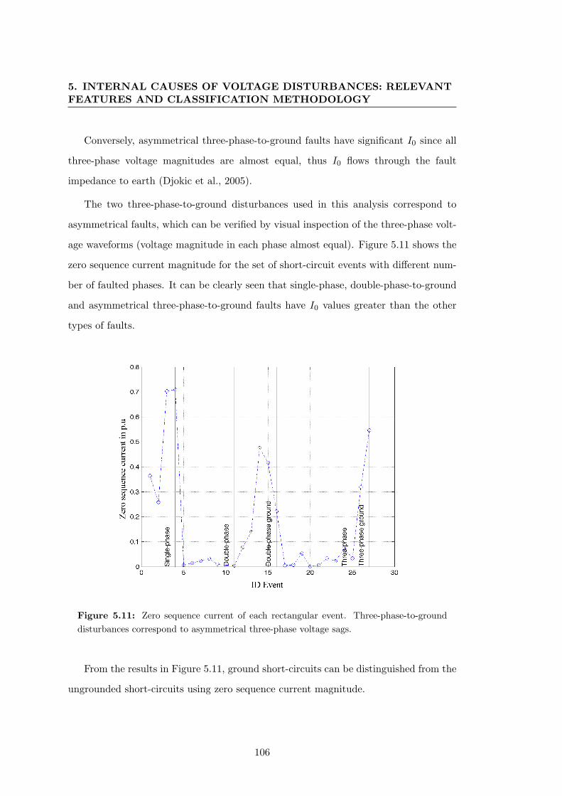
5. INTERNAL CAUSES OF VOLTAGE DISTURBANCES: RELEVANTFEATURES AND CLASSIFICATION METHODOLOGY
Conversely, asymmetrical three-phase-to-ground faults have significant I0 since all
three-phase voltage magnitudes are almost equal, thus I0 flows through the fault
impedance to earth (Djokic et al., 2005).
The two three-phase-to-ground disturbances used in this analysis correspond to
asymmetrical faults, which can be verified by visual inspection of the three-phase volt-
age waveforms (voltage magnitude in each phase almost equal). Figure 5.11 shows the
zero sequence current magnitude for the set of short-circuit events with different num-
ber of faulted phases. It can be clearly seen that single-phase, double-phase-to-ground
and asymmetrical three-phase-to-ground faults have I0 values greater than the other
types of faults.
Figure 5.11: Zero sequence current of each rectangular event. Three-phase-to-grounddisturbances correspond to asymmetrical three-phase voltage sags.
From the results in Figure 5.11, ground short-circuits can be distinguished from the
ungrounded short-circuits using zero sequence current magnitude.
106
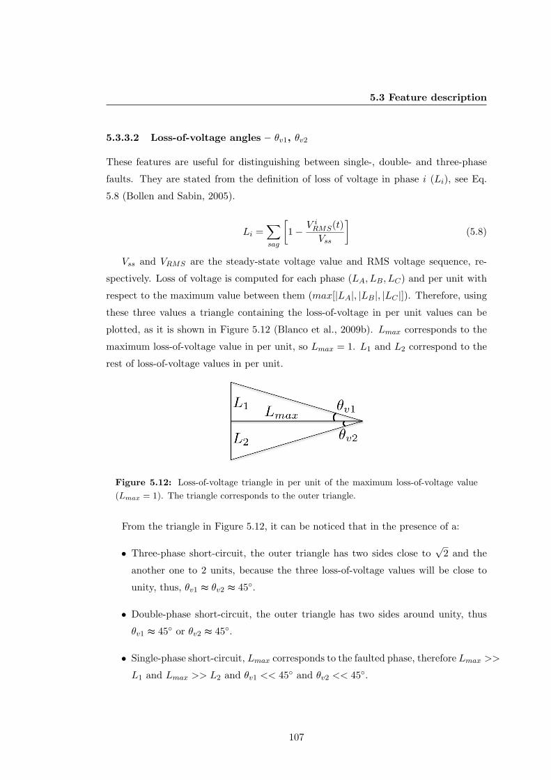
5.3 Feature description
5.3.3.2 Loss-of-voltage angles – θv1, θv2
These features are useful for distinguishing between single-, double- and three-phase
faults. They are stated from the definition of loss of voltage in phase i (Li), see Eq.
5.8 (Bollen and Sabin, 2005).
Li =∑sag
[1−
V iRMS(t)Vss
](5.8)
Vss and VRMS are the steady-state voltage value and RMS voltage sequence, re-
spectively. Loss of voltage is computed for each phase (LA, LB, LC) and per unit with
respect to the maximum value between them (max[|LA|, |LB|, |LC |]). Therefore, using
these three values a triangle containing the loss-of-voltage in per unit values can be
plotted, as it is shown in Figure 5.12 (Blanco et al., 2009b). Lmax corresponds to the
maximum loss-of-voltage value in per unit, so Lmax = 1. L1 and L2 correspond to the
rest of loss-of-voltage values in per unit.
Figure 5.12: Loss-of-voltage triangle in per unit of the maximum loss-of-voltage value(Lmax = 1). The triangle corresponds to the outer triangle.
From the triangle in Figure 5.12, it can be noticed that in the presence of a:
• Three-phase short-circuit, the outer triangle has two sides close to√
2 and the
another one to 2 units, because the three loss-of-voltage values will be close to
unity, thus, θv1 ≈ θv2 ≈ 45◦.
• Double-phase short-circuit, the outer triangle has two sides around unity, thus
θv1 ≈ 45◦ or θv2 ≈ 45◦.
• Single-phase short-circuit, Lmax corresponds to the faulted phase, therefore Lmax >>
L1 and Lmax >> L2 and θv1 << 45◦ and θv2 << 45◦.
107
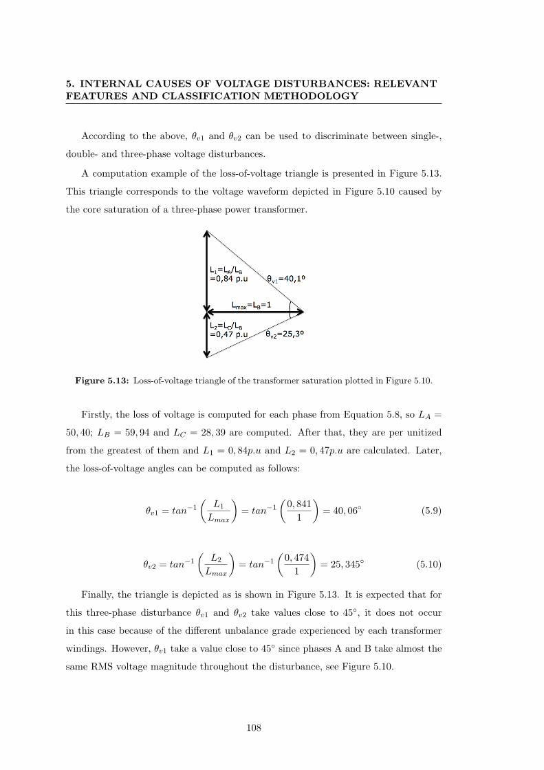
5. INTERNAL CAUSES OF VOLTAGE DISTURBANCES: RELEVANTFEATURES AND CLASSIFICATION METHODOLOGY
According to the above, θv1 and θv2 can be used to discriminate between single-,
double- and three-phase voltage disturbances.
A computation example of the loss-of-voltage triangle is presented in Figure 5.13.
This triangle corresponds to the voltage waveform depicted in Figure 5.10 caused by
the core saturation of a three-phase power transformer.
Figure 5.13: Loss-of-voltage triangle of the transformer saturation plotted in Figure 5.10.
Firstly, the loss of voltage is computed for each phase from Equation 5.8, so LA =
50, 40; LB = 59, 94 and LC = 28, 39 are computed. After that, they are per unitized
from the greatest of them and L1 = 0, 84p.u and L2 = 0, 47p.u are calculated. Later,
the loss-of-voltage angles can be computed as follows:
θv1 = tan−1
(L1
Lmax
)= tan−1
(0, 841
1
)= 40, 06◦ (5.9)
θv2 = tan−1
(L2
Lmax
)= tan−1
(0, 474
1
)= 25, 345◦ (5.10)
Finally, the triangle is depicted as is shown in Figure 5.13. It is expected that for
this three-phase disturbance θv1 and θv2 take values close to 45◦, it does not occur
in this case because of the different unbalance grade experienced by each transformer
windings. However, θv1 take a value close to 45◦ since phases A and B take almost the
same RMS voltage magnitude throughout the disturbance, see Figure 5.10.
108
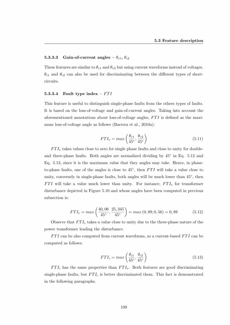
5.3 Feature description
5.3.3.3 Gain-of-current angles – θc1, θc2
These features are similar to θv1 and θv2 but using current waveforms instead of voltages.
θc1 and θc2 can also be used for discriminating between the different types of short-
circuits.
5.3.3.4 Fault type index – FTI
This feature is useful to distinguish single-phase faults from the others types of faults.
It is based on the loss-of-voltage and gain-of-current angles. Taking into account the
aforementioned annotations about loss-of-voltage angles, FTI is defined as the maxi-
mum loss-of-voltage angle as follows (Barrera et al., 2010a):
FTIv = max
(θv145◦
,θv245◦
)(5.11)
FTIv takes values close to zero for single phase faults and close to unity for double-
and three-phase faults. Both angles are normalized dividing by 45◦ in Eq. 5.12 and
Eq. 5.13, since it is the maximum value that they angles may take. Hence, in phase-
to-phase faults, one of the angles is close to 45◦, then FTI will take a value close to
unity, conversely in single-phase faults, both angles will be much lower than 45◦, then
FTI will take a value much lower than unity. For instance, FTIv for transformer
disturbance depicted in Figure 5.10 and whose angles have been computed in previous
subsection is:
FTIv = max
(40, 0645◦
,25, 345
45◦
)= max (0, 89; 0, 56) = 0, 89 (5.12)
Observe that FTIv takes a value close to unity due to the three-phase nature of the
power transformer leading the disturbance.
FTI can be also computed from current waveforms, so a current-based FTI can be
computed as follows:
FTIc = max
(θc145◦
,θc245◦
)(5.13)
FTIc has the same properties than FTIv. Both features are good discriminating
single-phase faults, but FTIc is better discriminated them. This fact is demonstrated
in the following paragraphs.
109
5. INTERNAL CAUSES OF VOLTAGE DISTURBANCES: RELEVANTFEATURES AND CLASSIFICATION METHODOLOGY
Figure 5.14 shows FTI computed from voltage and current waveforms. It can be
seen that in FTIv curve (crosses), a single-phase short-circuit has values close to zero;
double-phase and double-phase-to-ground short-circuits take values around 0.4 to 0.8,
and the highest values with both types of three-phase are around unity. This implies
that FTIv is able to discriminate between the three types of faults. Conversely, using
the current waveform, FTIc (circles) is possible to discriminate single-phase faults from
the others.
Figure 5.14: FTIv (crosses) and FTIc (circles) of each disturbance waveform.
On the other hand, double-phase and three-phase short-circuits can be well discrim-
inated observing θv1 and θv2, or θc1 and θc2, respectively.
From θv1, θv2, θc1 and θc2 values the following behaviors are observed:
1. All of them take values close to 45◦ (between 40◦ to 45◦) in presence of three-phase
short-circuits.
2. At least one of them takes values close to 45◦ (around 30◦) in presence of double-
phase short-circuits.
110
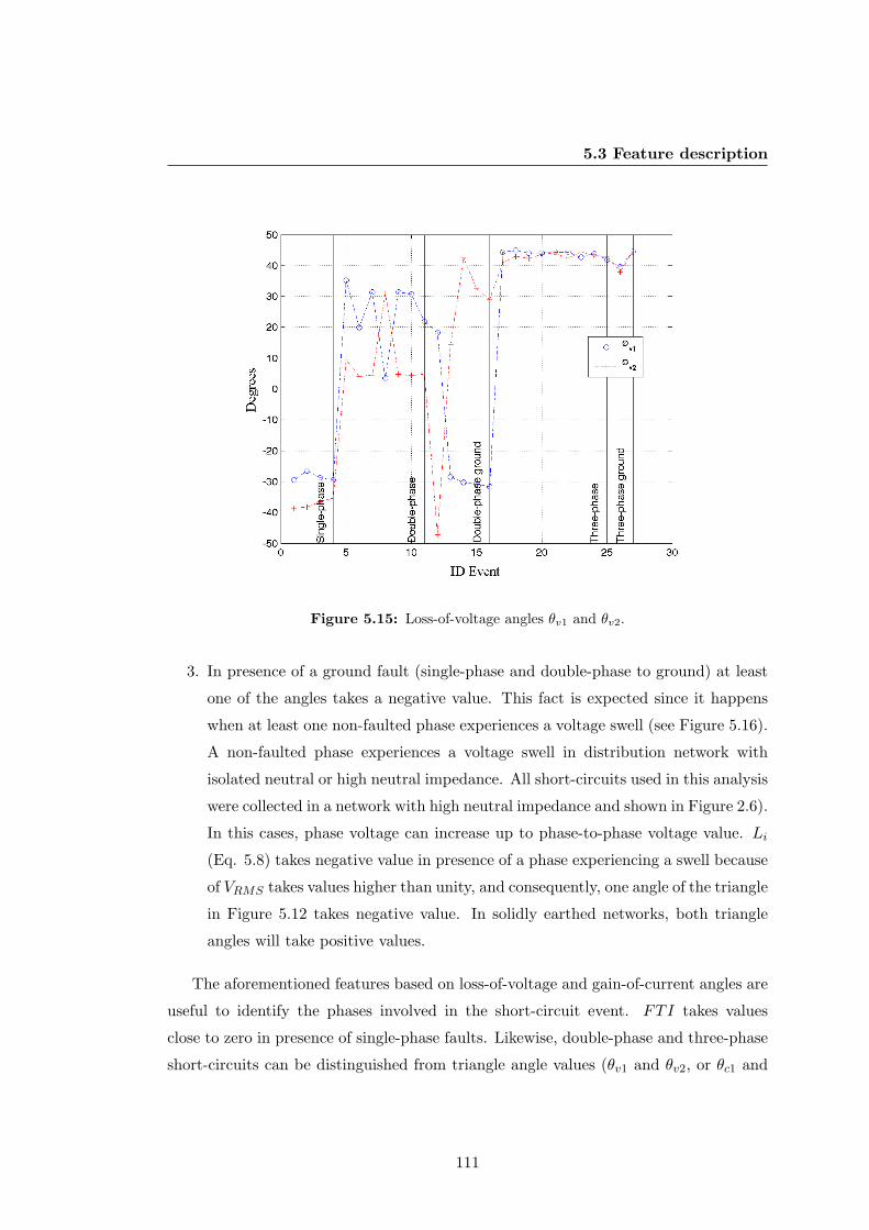
5.3 Feature description
Figure 5.15: Loss-of-voltage angles θv1 and θv2.
3. In presence of a ground fault (single-phase and double-phase to ground) at least
one of the angles takes a negative value. This fact is expected since it happens
when at least one non-faulted phase experiences a voltage swell (see Figure 5.16).
A non-faulted phase experiences a voltage swell in distribution network with
isolated neutral or high neutral impedance. All short-circuits used in this analysis
were collected in a network with high neutral impedance and shown in Figure 2.6).
In this cases, phase voltage can increase up to phase-to-phase voltage value. Li
(Eq. 5.8) takes negative value in presence of a phase experiencing a swell because
of VRMS takes values higher than unity, and consequently, one angle of the triangle
in Figure 5.12 takes negative value. In solidly earthed networks, both triangle
angles will take positive values.
The aforementioned features based on loss-of-voltage and gain-of-current angles are
useful to identify the phases involved in the short-circuit event. FTI takes values
close to zero in presence of single-phase faults. Likewise, double-phase and three-phase
short-circuits can be distinguished from triangle angle values (θv1 and θv2, or θc1 and
111
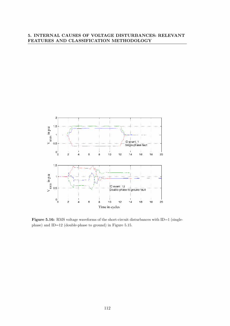
5. INTERNAL CAUSES OF VOLTAGE DISTURBANCES: RELEVANTFEATURES AND CLASSIFICATION METHODOLOGY
Figure 5.16: RMS voltage waveforms of the short-circuit disturbances with ID=1 (single-phase) and ID=12 (double-phase to ground) in Figure 5.15.
112
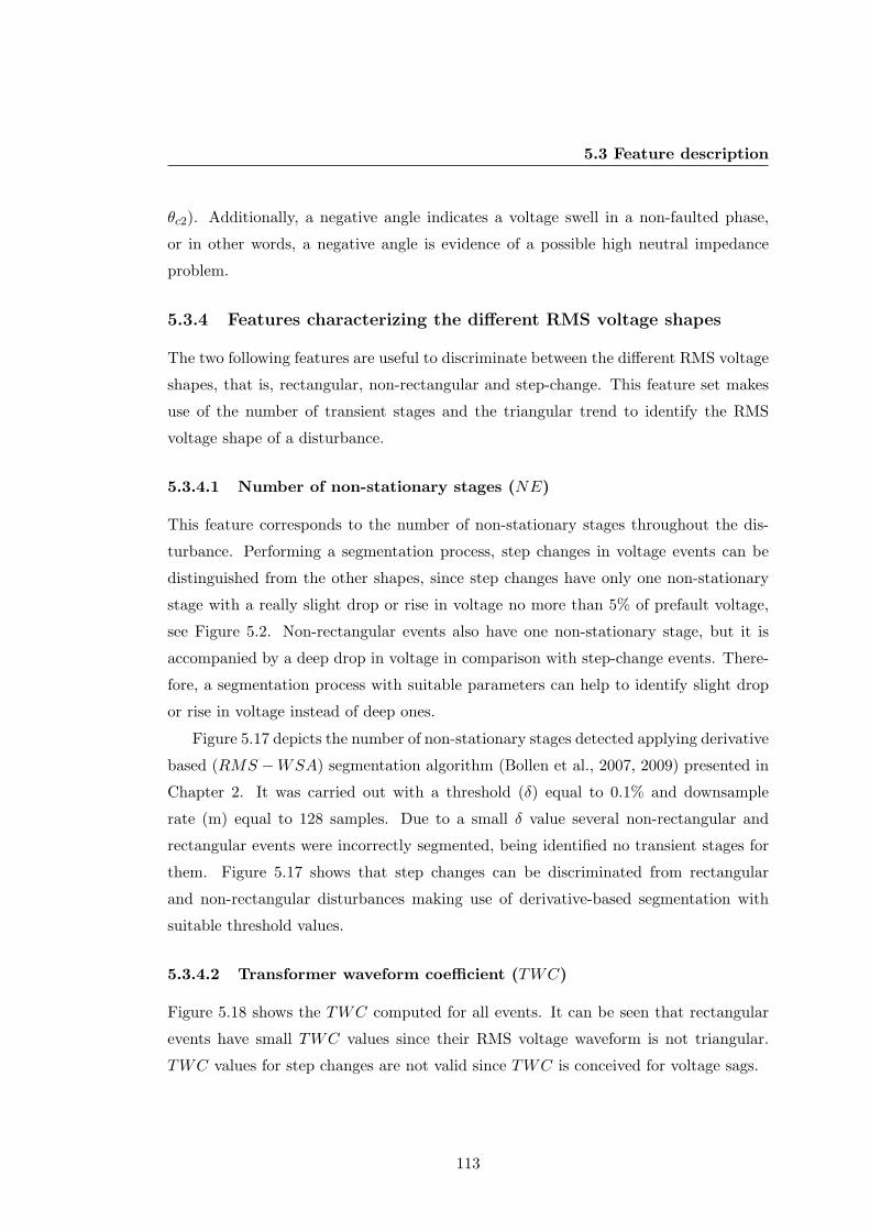
5.3 Feature description
θc2). Additionally, a negative angle indicates a voltage swell in a non-faulted phase,
or in other words, a negative angle is evidence of a possible high neutral impedance
problem.
5.3.4 Features characterizing the different RMS voltage shapes
The two following features are useful to discriminate between the different RMS voltage
shapes, that is, rectangular, non-rectangular and step-change. This feature set makes
use of the number of transient stages and the triangular trend to identify the RMS
voltage shape of a disturbance.
5.3.4.1 Number of non-stationary stages (NE)
This feature corresponds to the number of non-stationary stages throughout the dis-
turbance. Performing a segmentation process, step changes in voltage events can be
distinguished from the other shapes, since step changes have only one non-stationary
stage with a really slight drop or rise in voltage no more than 5% of prefault voltage,
see Figure 5.2. Non-rectangular events also have one non-stationary stage, but it is
accompanied by a deep drop in voltage in comparison with step-change events. There-
fore, a segmentation process with suitable parameters can help to identify slight drop
or rise in voltage instead of deep ones.
Figure 5.17 depicts the number of non-stationary stages detected applying derivative
based (RMS −WSA) segmentation algorithm (Bollen et al., 2007, 2009) presented in
Chapter 2. It was carried out with a threshold (δ) equal to 0.1% and downsample
rate (m) equal to 128 samples. Due to a small δ value several non-rectangular and
rectangular events were incorrectly segmented, being identified no transient stages for
them. Figure 5.17 shows that step changes can be discriminated from rectangular
and non-rectangular disturbances making use of derivative-based segmentation with
suitable threshold values.
5.3.4.2 Transformer waveform coefficient (TWC)
Figure 5.18 shows the TWC computed for all events. It can be seen that rectangular
events have small TWC values since their RMS voltage waveform is not triangular.
TWC values for step changes are not valid since TWC is conceived for voltage sags.
113
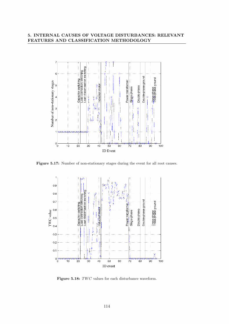
5. INTERNAL CAUSES OF VOLTAGE DISTURBANCES: RELEVANTFEATURES AND CLASSIFICATION METHODOLOGY
Figure 5.17: Number of non-stationary stages during the event for all root causes.
Figure 5.18: TWC values for each disturbance waveform.
114
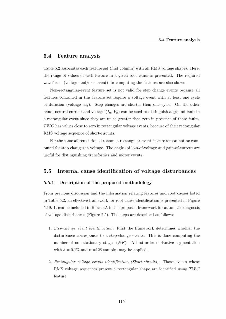
5.4 Feature analysis
5.4 Feature analysis
Table 5.2 associates each feature set (first column) with all RMS voltage shapes. Here,
the range of values of each feature in a given root cause is presented. The required
waveforms (voltage and/or current) for computing the features are also shown.
Non-rectangular-event feature set is not valid for step change events because all
features contained in this feature set require a voltage event with at least one cycle
of duration (voltage sag). Step changes are shorter than one cycle. On the other
hand, neutral current and voltage (In, Vn) can be used to distinguish a ground fault in
a rectangular event since they are much greater than zero in presence of these faults.
TWC has values close to zero in rectangular voltage events, because of their rectangular
RMS voltage sequence of short-circuits.
For the same aforementioned reason, a rectangular-event feature set cannot be com-
puted for step changes in voltage. The angles of loss-of-voltage and gain-of-current are
useful for distinguishing transformer and motor events.
5.5 Internal cause identification of voltage disturbances
5.5.1 Description of the proposed methodology
From previous discussion and the information relating features and root causes listed
in Table 5.2, an effective framework for root cause identification is presented in Figure
5.19. It can be included in Block 4A in the proposed framework for automatic diagnosis
of voltage disturbances (Figure 2.5). The steps are described as follows:
1. Step-change event identification: First the framework determines whether the
disturbance corresponds to a step-change events. This is done computing the
number of non-stationary stages (NE). A first-order derivative segmentation
with δ = 0.1% and m=128 samples may be applied.
2. Rectangular voltage events identification (Short-circuits): Those events whose
RMS voltage sequences present a rectangular shape are identified using TWC
feature.
115

5. INTERNAL CAUSES OF VOLTAGE DISTURBANCES: RELEVANTFEATURES AND CLASSIFICATION METHODOLOGY
Tab
le5.2:
Featuresaccording
toeach
rootcause
ofpow
erquality
events
Intern
alca
uses
(norm
alopera
tion
actio
ns)
Extern
alca
uses
(short-circu
its)
Step
-change
shape
Non-recta
ngula
rsh
ape
Recta
ngula
rsh
ape
Fea
u-
res
iv
Cap.
LC
SLD
SM
STra
nsf.
1-P
g2-P
2-P
g3-P
3-P
g
φpost -
φpre
33
<0
>0
<0
>0
--
--
--
--
--
--
Step
change
P3
3P
post
≈P
pre
Ppost>
Ppre
Ppost<
Ppre
Ppost>
Ppre
Ppost>P
pre
--
--
--
--
--
Q3
3Q
post<
Qpre
--
--
--
--
--
--
--
--
--
Non
In
3N
.VN
.VN
.V≈
0>
0>>
0≈
0>>
0≈
0>>
0
rectangula
rVn
N.V
N.V
N.V
≈0
>0
>>
0≈
0>>
0≈
0>>
0
RM
S|I
2 |3
N.V
N.V
N.V
≈0
>0
--
--
--
--
--
shape
TWC
N.V
N.V
N.V
0<
TWC<
1
≈1
≈0
≈0
≈0
≈0
≈0
I0
3N
.VN
.VN
.V≈
0>
0>>
0≈
0>>
0≈
0>>
0
Recta
ngula
r
RM
Ssh
ape
θv1,θ
v2
N.V
N.V
N.V
θv1
≈θv2
≈45◦
θv1<
45◦
and
θv2<
45◦
θv1<<
45◦
and
θv2<<
45◦
θv1
≈45◦
or
θv2
≈45◦
θv1
≈45◦
or
θv2
≈45◦
θv1
≈θv2
≈45◦
θv1
≈θv2
≈45◦
θc1,θ
c2
3N
.VN
.VN
.Vθc1
≈θc2
≈45◦
θc1<
45◦
and
θc2<
45◦
θc1<<
45◦
and
θc2<<
45◦
θc1
≈45◦
or
θc2
≈45◦
θc1
≈45◦
or
θc2
≈45◦
θc1
≈θc2
≈45◦
θc1
≈θc2
≈45◦
FTI
33
N.V
N.V
N.V
≈1
<1
<<
1≈
1≈
1≈
1≈
1
LC
S/LD
S:Load
connectio
n/disco
nnectio
nsw
itchin
g;M
S:M
oto
rsta
rting;N
.V:N
ot
valid
.
116
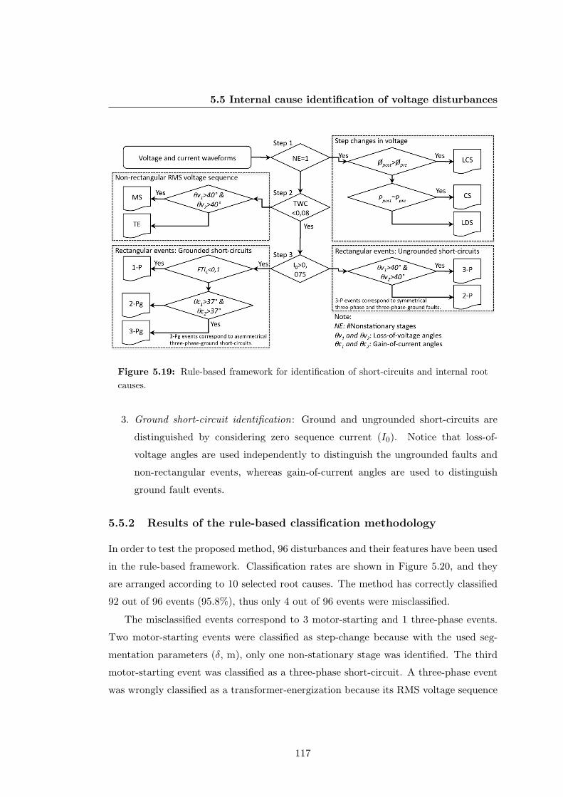
5.5 Internal cause identification of voltage disturbances
Figure 5.19: Rule-based framework for identification of short-circuits and internal rootcauses.
3. Ground short-circuit identification: Ground and ungrounded short-circuits are
distinguished by considering zero sequence current (I0). Notice that loss-of-
voltage angles are used independently to distinguish the ungrounded faults and
non-rectangular events, whereas gain-of-current angles are used to distinguish
ground fault events.
5.5.2 Results of the rule-based classification methodology
In order to test the proposed method, 96 disturbances and their features have been used
in the rule-based framework. Classification rates are shown in Figure 5.20, and they
are arranged according to 10 selected root causes. The method has correctly classified
92 out of 96 events (95.8%), thus only 4 out of 96 events were misclassified.
The misclassified events correspond to 3 motor-starting and 1 three-phase events.
Two motor-starting events were classified as step-change because with the used seg-
mentation parameters (δ, m), only one non-stationary stage was identified. The third
motor-starting event was classified as a three-phase short-circuit. A three-phase event
was wrongly classified as a transformer-energization because its RMS voltage sequence
117
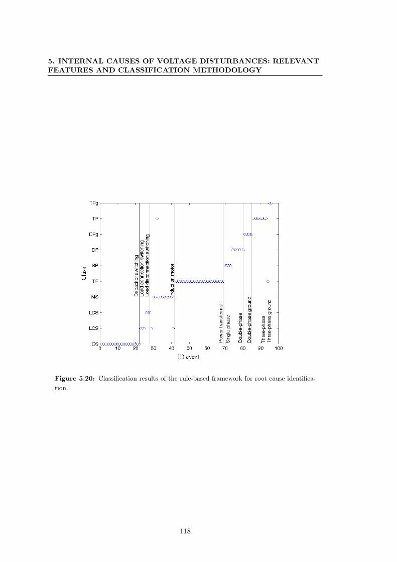
5. INTERNAL CAUSES OF VOLTAGE DISTURBANCES: RELEVANTFEATURES AND CLASSIFICATION METHODOLOGY
Figure 5.20: Classification results of the rule-based framework for root cause identifica-tion.
118
5.6 Conclusion
tends to look triangular due to its short duration.
5.6 Conclusion
The study performed for this chapter has shown that step changes (capacitor-bank and
large-load switchings) may be distinguished from changes in the angle between voltage
and current waveforms, as well as changes in active and reactive powers. Step changes
may also be distinguished from other causes by performing a segmentation based on a
first-order derivative with δ = 0.1% and m=128 samples.
Non-rectangular events (motor and transformer) may be discriminated using neutral
current ratio and second order current harmonic. Also, they can be distinguished from
the rest of root causes using the triangular waveform coefficient (TWC), which measures
the similarity of the RMS voltage shape with a triangle.
Rectangular events may be distinguished using zero sequence current, the angles of
loss-of-voltage and gain-of-current triangles.
It is possible to discriminate short-circuits from the rest of causes using the analyzed
features. Therefore, the proposed rule-based classification may be used to determine
the root causes of events due to external causes. This methodology will be used in next
chapter to previously identify disturbances due to internal causes, so that those clas-
sified as short-circuits are inputs to the methodology for external cause identification
proposed in subsequent chapter.
119

5. INTERNAL CAUSES OF VOLTAGE DISTURBANCES: RELEVANTFEATURES AND CLASSIFICATION METHODOLOGY
120
6
External Causes of Voltage Sags:
Relevant Features and
Classification Methodology
6.1 Introduction
This chapter addresses the automatic classification of disturbances according to exter-
nal causes. A good performance in identifying external causes can be used to reduce
uncertainty during pinpoint location, with the consequent reduction of time restora-
tion and improvement of continuity indices. For instance, a disturbance diagnosed as a
short-circuit and with an estimated distance to the fault of 5km (from the substation
where the disturbance has been registered) can match with multiple points in a radial
network, but if we are capable to assign this waveform to a class of sags generated by
tree contacts probably this multiple estimation can be reduced significantly observing
green areas at that distance.
This chapter explores the use of an inductive learning algorithm to deduce classi-
fication rules capable to discriminate among different external causes. This algorithm
requires the use of a labelled dataset to be trained. Thus, a set of disturbances char-
acterised by a feature set and label according to external causes is required. In this
work four main groups of external causes have been identified according to common
causes reported by electrical utilities: animal contact, tree contact, lightning-induced
or underground cable failures. The relevant features proposed in this chapter to dis-
121
6. EXTERNAL CAUSES OF VOLTAGE SAGS: RELEVANT FEATURESAND CLASSIFICATION METHODOLOGY
criminate the different external root-causes are: voltage/current changes in magnitude,
zero sequence components, fault insertion phase angle and arc voltage.
These features are described in this chapter and their significance is statistically
analysed according to the external causes. A data set of 181 voltage sags originated by
short-circuits, registered in distribution substations and documented by several electri-
cal utilities (including root causes) have been used in the analysis. Results of applying
this methodology to obtain classification rules could be used as part of a global frame-
work (Chapter 2, Block 4B in Figure 2.5) for the automatic diagnosis of voltage sags
in the region where the training data set have been collected.
6.1.1 Existing methodologies for external cause identification
In the literature, there is a short number of works addressing the classification of voltage
sags according to external causes and major efforts have been focus on obtaining associ-
ation rules between causes and relevant features of waveforms, supported by statistical
or probabilistic criteria. In that direction, (Xu and Chow, 2006) proposes the use of
logistic regression and Bayesian networks to define flow charts for the identification of
animal and tree causes. A recent work (Cai et al., 2010a) analyses the performance
of different machine learning approaches (SVM, linear regression, nearest neighbour,
recognition theory and neural network) to discriminate between faults caused by an-
imals and trees using six input features. Results show that all these algorithms give
similar results when the proper decision thresholds are selected. An improvement of
fuzzy classification rules to deal with imbalanced data set is used to discriminate faults
caused by trees, animals, and lightning in (Xu et al., 2007), while the use of rough set
theory is proposed in (Peng et al., 2004) to diagnose faults. The relevance of input
features is evident in these algorithms and has motivated the use of feature selection
strategies (Peng et al., 2004) to focus on significant ones avoiding the use of redundant
or irrelevant information. Common features used in those works consider contextual
information related to time (season, occurrence hour, daytime, night time, etc.), pro-
tection operation (number of affected phases, activation of protective systems) and type
of lines (underground/overhead). This justifies the use of statistical criteria to obtain
discriminant rules.
The approach presented in this chapter differs from these previous works mainly
in the idea of using information contained in the waveform instead of contextual in-
122
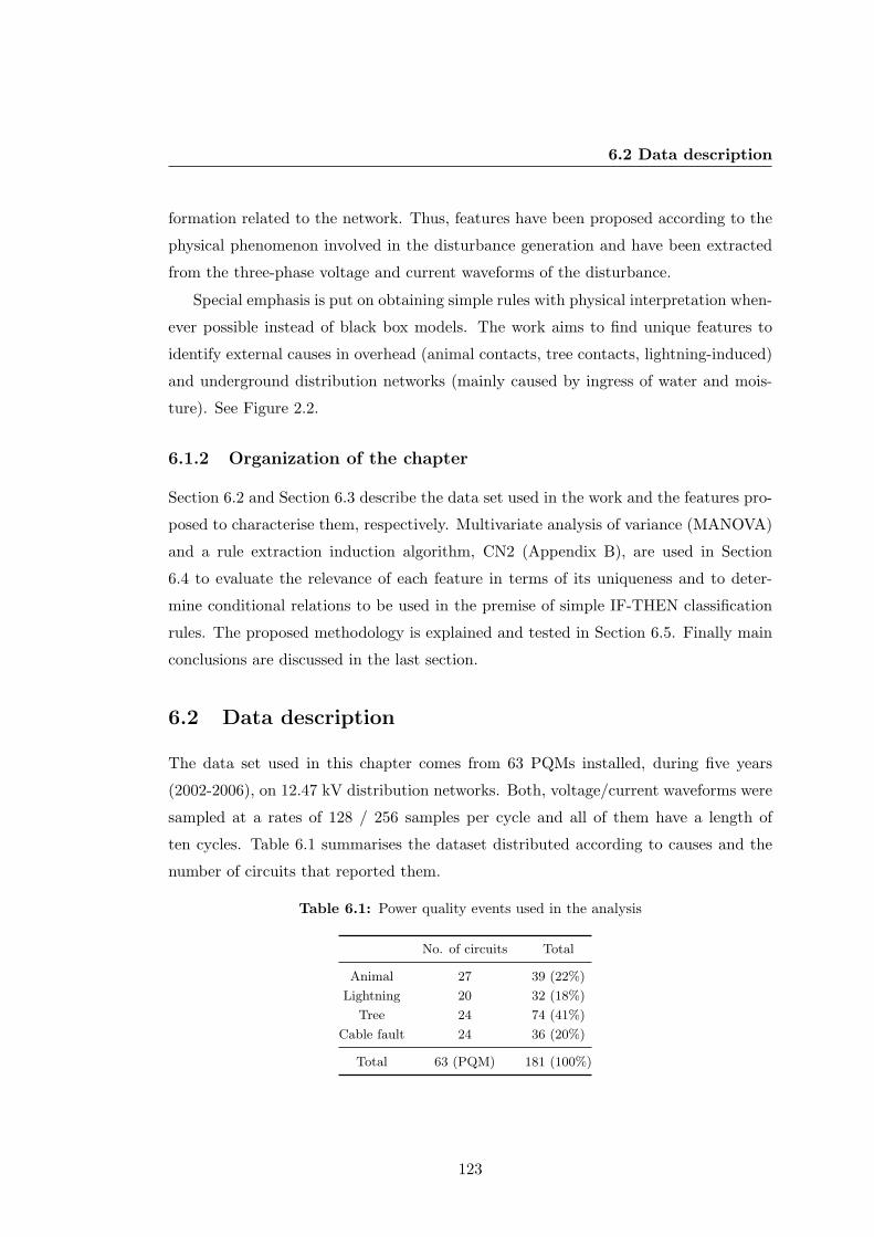
6.2 Data description
formation related to the network. Thus, features have been proposed according to the
physical phenomenon involved in the disturbance generation and have been extracted
from the three-phase voltage and current waveforms of the disturbance.
Special emphasis is put on obtaining simple rules with physical interpretation when-
ever possible instead of black box models. The work aims to find unique features to
identify external causes in overhead (animal contacts, tree contacts, lightning-induced)
and underground distribution networks (mainly caused by ingress of water and mois-
ture). See Figure 2.2.
6.1.2 Organization of the chapter
Section 6.2 and Section 6.3 describe the data set used in the work and the features pro-
posed to characterise them, respectively. Multivariate analysis of variance (MANOVA)
and a rule extraction induction algorithm, CN2 (Appendix B), are used in Section
6.4 to evaluate the relevance of each feature in terms of its uniqueness and to deter-
mine conditional relations to be used in the premise of simple IF-THEN classification
rules. The proposed methodology is explained and tested in Section 6.5. Finally main
conclusions are discussed in the last section.
6.2 Data description
The data set used in this chapter comes from 63 PQMs installed, during five years
(2002-2006), on 12.47 kV distribution networks. Both, voltage/current waveforms were
sampled at a rates of 128 / 256 samples per cycle and all of them have a length of
ten cycles. Table 6.1 summarises the dataset distributed according to causes and the
number of circuits that reported them.
Table 6.1: Power quality events used in the analysis
No. of circuits Total
Animal 27 39 (22%)
Lightning 20 32 (18%)
Tree 24 74 (41%)
Cable fault 24 36 (20%)
Total 63 (PQM) 181 (100%)
123
6. EXTERNAL CAUSES OF VOLTAGE SAGS: RELEVANT FEATURESAND CLASSIFICATION METHODOLOGY
From table, it is observed that causes occur more or less uniformly distributed in the
same number of circuits (approximately the same cause is common to around twenty
out of sixty three circuits) showing their representativeness despite the total amount of
events used in the study is only 181 and the benefit of dealing with all together instead
of performing individualised analysis for each circuit.
6.3 Features description
This section describes ten features used to represent the disturbances as a vector.
Features have been selected according to the phenomena involved in these external
causes and their capacities to discriminate between different external causes of short-
circuits. Two main groups of features are distinguished, those related to timestamp
and those extracted from current and voltage waveforms.
6.3.1 Features based on time stamp
The occurrence time of faults can play an important role in the automatic classification
of the external cause of a short-circuit as previous work demonstrated (Cai et al., 2010a;
Xu and Chow, 2006; Xu et al., 2007). This is because external factors such weather,
animal habits, seasonality or insolation, are highly correlated with occurrence date and
hour of faults.
6.3.1.1 Date of occurrence(day):
The distribution of occurrence dates of the set of events under study (Figure 6.1) reveals
that most animal contact and cable fault events occurred during spring and summer.
Likewise, a majority of lightning induced events occurred during summer, when storms
with thunder and lightning are common in the region where disturbances were collected.
On the other hand, most of tree contact events occurred during fall season.
6.3.1.2 Time of occurrence (hour):
The dependence of events with respect to their occurrence time is depicted in Figure
6.2. The majority of animal contact and cable fault events took place during daytime;
whereas lightning induced events occurred mainly during night. On the other hand,
tree contact events are spread out in time.
124
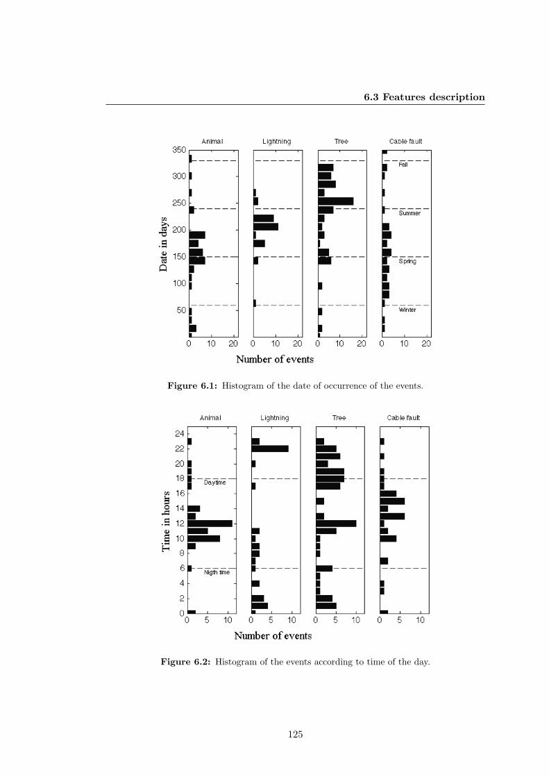
6.3 Features description
Figure 6.1: Histogram of the date of occurrence of the events.
Figure 6.2: Histogram of the events according to time of the day.
125
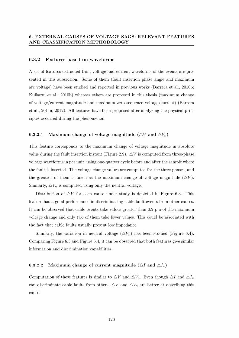
6. EXTERNAL CAUSES OF VOLTAGE SAGS: RELEVANT FEATURESAND CLASSIFICATION METHODOLOGY
6.3.2 Features based on waveforms
A set of features extracted from voltage and current waveforms of the events are pre-
sented in this subsection. Some of them (fault insertion phase angle and maximum
arc voltage) have been studied and reported in previous works (Barrera et al., 2010b;
Kulkarni et al., 2010b) whereas others are proposed in this thesis (maximum change
of voltage/current magnitude and maximum zero sequence voltage/current) (Barrera
et al., 2011a, 2012). All features have been proposed after analyzing the physical prin-
ciples occurred during the phenomenon.
6.3.2.1 Maximum change of voltage magnitude (4V and 4Vn)
This feature corresponds to the maximum change of voltage magnitude in absolute
value during the fault insertion instant (Figure 2.9). 4V is computed from three-phase
voltage waveforms in per unit, using one-quarter cycle before and after the sample where
the fault is inserted. The voltage change values are computed for the three phases, and
the greatest of them is taken as the maximum change of voltage magnitude (4V ).
Similarly, 4Vn is computed using only the neutral voltage.
Distribution of 4V for each cause under study is depicted in Figure 6.3. This
feature has a good performance in discriminating cable fault events from other causes.
It can be observed that cable events take values greater than 0.2 p.u of the maximum
voltage change and only two of them take lower values. This could be associated with
the fact that cable faults usually present low impedance.
Similarly, the variation in neutral voltage (4Vn) has been studied (Figure 6.4).
Comparing Figure 6.3 and Figure 6.4, it can be observed that both features give similar
information and discrimination capabilities.
6.3.2.2 Maximum change of current magnitude (4I and 4In)
Computation of these features is similar to 4V and 4Vn. Even though 4I and 4Incan discriminate cable faults from others, 4V and 4Vn are better at describing this
cause.
126
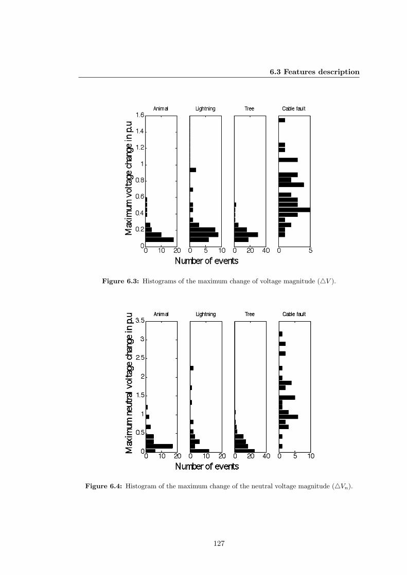
6.3 Features description
Figure 6.3: Histograms of the maximum change of voltage magnitude (4V ).
Figure 6.4: Histogram of the maximum change of the neutral voltage magnitude (4Vn).
127
6. EXTERNAL CAUSES OF VOLTAGE SAGS: RELEVANT FEATURESAND CLASSIFICATION METHODOLOGY
6.3.2.3 Maximum zero sequence voltage (V0)
It is perceived as an indicator of unbalance degree in the network. That is, highly
unbalanced events will present high zero-sequence voltage values (Figure 2.9). V0 is
computed after segmentation during fault-stage instants (Figure 2.7) applying Eq. 5.7
but using voltage phasors instead of current ones (Fortescue, 1918).
The results shown in Figure 6.5 demonstrate that cable faults present greater unbal-
ance (high V0 values). This observation is in agreement with the fact that short-circuits
in underground cables are usually single-phase ones.
Figure 6.5: Histograms of the maximum zero-sequence voltage (V0).
6.3.2.4 Maximum Zero Sequence Current (I0)
As zero sequence voltage, I0 is also perceived as an indicator of unbalance degree. It is
also computed during fault stage and applying Eq. 5.7 (Fortescue, 1918).
This feature is adequate to distinguish single-phase faults from two- and three-phase
ones. Figure 6.6 shows that events with high I0 values correspond to single-phase faults,
while events with low I0 values correspond to double-phase and double-phase-ground
faults (in the data set there are no three-phase faults documented). This reveals the
128
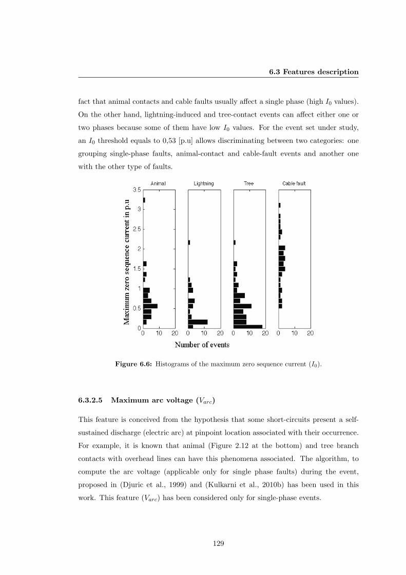
6.3 Features description
fact that animal contacts and cable faults usually affect a single phase (high I0 values).
On the other hand, lightning-induced and tree-contact events can affect either one or
two phases because some of them have low I0 values. For the event set under study,
an I0 threshold equals to 0,53 [p.u] allows discriminating between two categories: one
grouping single-phase faults, animal-contact and cable-fault events and another one
with the other type of faults.
Figure 6.6: Histograms of the maximum zero sequence current (I0).
6.3.2.5 Maximum arc voltage (Varc)
This feature is conceived from the hypothesis that some short-circuits present a self-
sustained discharge (electric arc) at pinpoint location associated with their occurrence.
For example, it is known that animal (Figure 2.12 at the bottom) and tree branch
contacts with overhead lines can have this phenomena associated. The algorithm, to
compute the arc voltage (applicable only for single phase faults) during the event,
proposed in (Djuric et al., 1999) and (Kulkarni et al., 2010b) has been used in this
work. This feature (Varc) has been considered only for single-phase events.
129
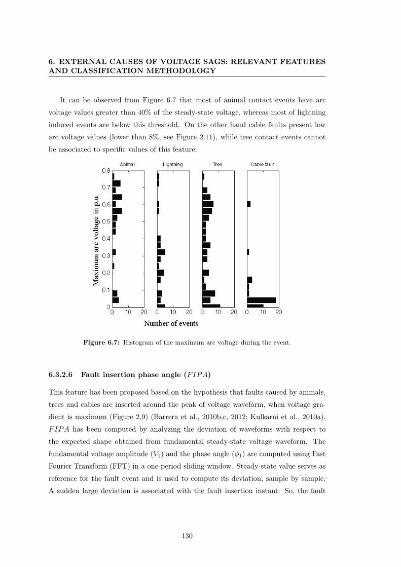
6. EXTERNAL CAUSES OF VOLTAGE SAGS: RELEVANT FEATURESAND CLASSIFICATION METHODOLOGY
It can be observed from Figure 6.7 that most of animal contact events have arc
voltage values greater than 40% of the steady-state voltage, whereas most of lightning
induced events are below this threshold. On the other hand cable faults present low
arc voltage values (lower than 8%, see Figure 2.11), while tree contact events cannot
be associated to specific values of this feature.
Figure 6.7: Histogram of the maximum arc voltage during the event.
6.3.2.6 Fault insertion phase angle (FIPA)
This feature has been proposed based on the hypothesis that faults caused by animals,
trees and cables are inserted around the peak of voltage waveform, when voltage gra-
dient is maximum (Figure 2.9) (Barrera et al., 2010b,c, 2012; Kulkarni et al., 2010a).
FIPA has been computed by analyzing the deviation of waveforms with respect to
the expected shape obtained from fundamental steady-state voltage waveform. The
fundamental voltage amplitude (V1) and the phase angle (φ1) are computed using Fast
Fourier Transform (FFT) in a one-period sliding-window. Steady-state value serves as
reference for the fault event and is used to compute its deviation, sample by sample.
A sudden large deviation is associated with the fault insertion instant. So, the fault
130
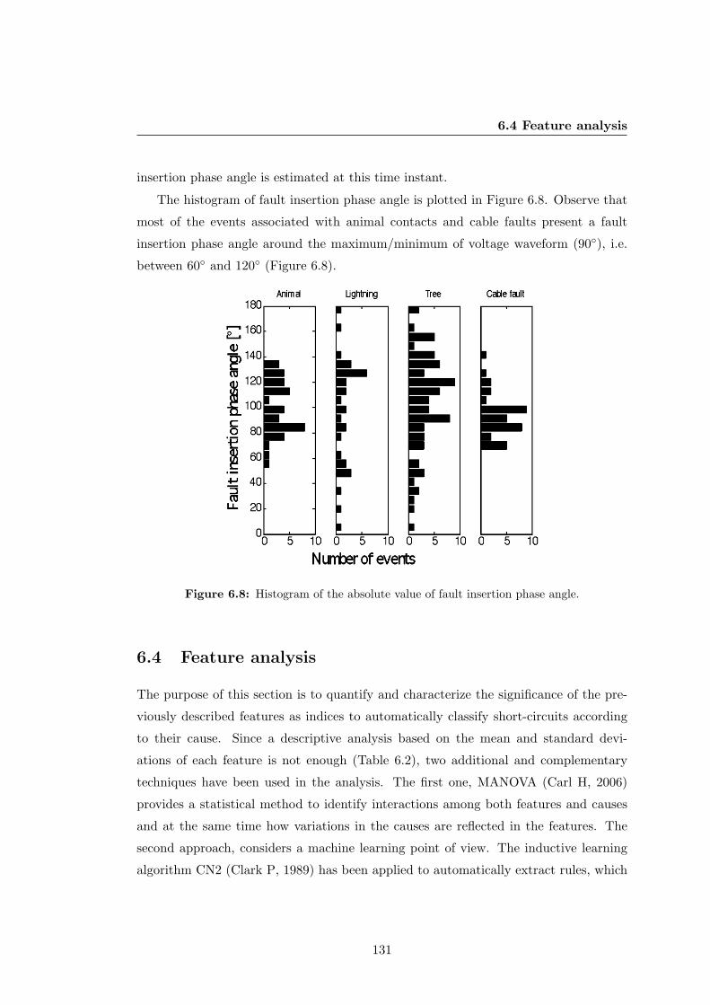
6.4 Feature analysis
insertion phase angle is estimated at this time instant.
The histogram of fault insertion phase angle is plotted in Figure 6.8. Observe that
most of the events associated with animal contacts and cable faults present a fault
insertion phase angle around the maximum/minimum of voltage waveform (90◦), i.e.
between 60◦ and 120◦ (Figure 6.8).
Figure 6.8: Histogram of the absolute value of fault insertion phase angle.
6.4 Feature analysis
The purpose of this section is to quantify and characterize the significance of the pre-
viously described features as indices to automatically classify short-circuits according
to their cause. Since a descriptive analysis based on the mean and standard devi-
ations of each feature is not enough (Table 6.2), two additional and complementary
techniques have been used in the analysis. The first one, MANOVA (Carl H, 2006)
provides a statistical method to identify interactions among both features and causes
and at the same time how variations in the causes are reflected in the features. The
second approach, considers a machine learning point of view. The inductive learning
algorithm CN2 (Clark P, 1989) has been applied to automatically extract rules, which
131
6. EXTERNAL CAUSES OF VOLTAGE SAGS: RELEVANT FEATURESAND CLASSIFICATION METHODOLOGY
describe the causes according to the values of features obtained from events. As a
result, representative ranges of values for relevant features are obtained for each cause.
6.4.1 Descriptive analysis
In this subsection are analyzed the mean and standard deviation of each feature ac-
cording to the different studied causes. The analysis is carried out splitting the features
according to their nature (time- or waveform-based).
1. Features based on time stamp: From the analysis of histograms of the Date (Fig-
ure 6.1) and Table 6.2 it can be affirmed that most of animal contact events take
place in the second and third trimester (µ=153,4 / σ=74,4), lightning induced
events in summer (µ=203,8 / σ=37,5), and finally tree contact events between
summer and fall (µ=224,4 / σ=77,8). On the other hand, Time feature (Figure
6.2 and Table 6.2) reveals that animal contacts (µ=11,7 / σ=4,2) and cable fault
events (µ=12,6 / σ=5,2) take place around noon, whereas the other causes do
not show this relationship.
2. Features based on waveforms: 4V and4Vn values are in general greater for cable
faults than for the other causes. A similar behavior is found with the features
corresponding to maximum changes in phase and neutral current (4I and 4In)
but with less discriminative capacity (there exists an overlapping between cable
and tree faults). Cable faults also present distributions of V0 and I0 features
centered in higher values than the other causes. V0 mean is around four times
larger than the others, indicating a major unbalance in those faults. Io was also
independently computed for single- and double-phase faults. It can be noticed
that double-phase events have lower I0 mean and standard deviation values than
single-phase events (Table 6.2). Double-phase faults caused by animals and cables
are not available in the used database, thus I0 cannot be computed for this fault
type (Table 6.2).
Arc voltage (Figure 6.7) for animal contact usually takes values over 0,45 p.u
whereas in cable events the values are very low (Varc < 0, 15p.u). Values for
lightning and tree events are spread along the range 0-0,8 p.u. FIPA statistics
indicate that most of animal contact and cable fault events occur around the
peak of voltage waveform (mean value 99,3◦ and 93,7◦ respectively with standard
132

6.4 Feature analysis
deviation; 21,02◦ and 16,6◦; respectively), Table 6.2. Other causes present larger
standard deviations (41,5◦ and 37,9◦ respectively) which means that faults due to
these causes are inserted with independence of the instantaneous voltage values.
Table 6.2: Feature descriptive statistics
Cause Animal Lightning Tree Cable
Feature µ/σ µ/σ µ/σ µ/σ
Date (day) 153,4/74,4 203,8/37,5 224,4/77,8 166,5/84,3
T ime (hour) 11,7/4,2 11,8/8,8 13,6/6,8 12,6/5,2
4V 0,2/0,1 0,3/0,2 0,2/0,1 0,7/0,3
4Vn 0,3/0,3 0,4/0,6 0,2/0,2 1,5/0,7
4I 0,4/0,1 0,4/0,1 0,4/0,1 0,7/1,3
4In 0,6/0,2 0,5/0,2 0,4/0,2 0,9/1,3
V0 0,1/0,1 0,1/0,1 0,1/0,1 0,4/0,1
I0 0,7/0,6 0,5/0,5 0,5/0,5 1,7/0,6
I0 (1-phase) 0,7/0,6 0,7/0,5 0,7/0,4 1,7/0,6
I0 (2-phase) – 0,1//0,01 0,1/0,04 –
Varc 0,5/0,2 0,2/0,2 0,3/0,2 0,1/0,1
Varc (1-phase) 0,5/0,2 0,2/0,2 0,4/0,3 0,1/0,1
FIPA (*) 99,3/21,02 97,6/41,5 104,6/37,9 93,7/16,6
FIPA: Fault insertion phase angle.
6.4.2 Multivariate analysis of variance - MANOVA
The main purpose of MANOVA (Carl H, 2006) is to explore how causes (independent
variables) influence the pattern of response in the features under study (dependent
variables). MANOVA determines the influence of the event cause (animal, lightning,
tree and cable fault) in each feature (Date and Time of occurrence, 4V , 4Vn, 4I,
4In, V0, I0, FIPA, Varc).
Figure 6.9 shows the quality of the cause-effect relationship for each feature. Quality
values near 100% indicate that most of the variability in the feature is associated with
the event cause. While, values near 0% indicate that the feature does not contain any
information about the event cause. The quality values depicted in Figure 6.9 show
that features with more information (quality greater than 70%) are FIPA (91%), V0
(86,2%), Date (80,5%), Time (79,9%), 4V (78,4%), 4Vn (74,4%) and Varc (69,3%)
for single-phase events and FIPA (93,3%), Date (92%), 4I (88,7%), I0(83,8%), 4In
133
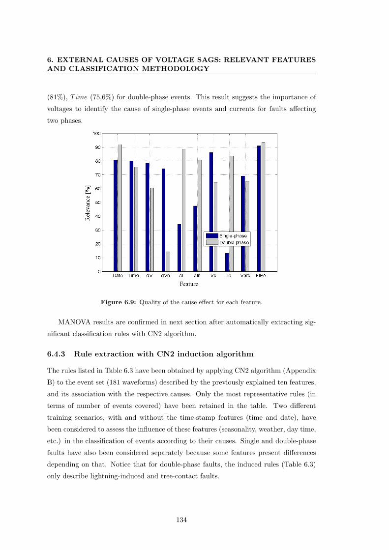
6. EXTERNAL CAUSES OF VOLTAGE SAGS: RELEVANT FEATURESAND CLASSIFICATION METHODOLOGY
(81%), Time (75,6%) for double-phase events. This result suggests the importance of
voltages to identify the cause of single-phase events and currents for faults affecting
two phases.
Figure 6.9: Quality of the cause effect for each feature.
MANOVA results are confirmed in next section after automatically extracting sig-
nificant classification rules with CN2 algorithm.
6.4.3 Rule extraction with CN2 induction algorithm
The rules listed in Table 6.3 have been obtained by applying CN2 algorithm (Appendix
B) to the event set (181 waveforms) described by the previously explained ten features,
and its association with the respective causes. Only the most representative rules (in
terms of number of events covered) have been retained in the table. Two different
training scenarios, with and without the time-stamp features (time and date), have
been considered to assess the influence of these features (seasonality, weather, day time,
etc.) in the classification of events according to their causes. Single and double-phase
faults have also been considered separately because some features present differences
depending on that. Notice that for double-phase faults, the induced rules (Table 6.3)
only describe lightning-induced and tree-contact faults.
134
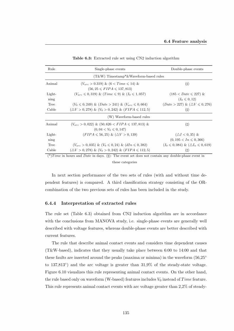
6.4 Feature analysis
Table 6.3: Extracted rule set using CN2 induction algorithm
Rule Single-phase events Double-phase events
(T&W) Timestamp*&Waveform-based rules
Animal (Varc > 0.319) & (6 < Time 6 14) &
(56, 25 6 FIPA 6 137, 813)
(])
Light-
ning
(Varc 6 0, 319) & (T ime 6 9) & (I0 6 1, 057) (185 < Date 6 227) &
(I0 6 0, 12)
Tree (V0 6 0, 249) & (Date > 241) & (Varc 6 0, 664) (Date > 227) & (4V 6 0, 276)
Cable (4V > 0, 278) & (V0 > 0, 242) & (FIPA 6 112, 5) (])
(W) Waveform-based rules
Animal (Varc > 0, 022) & (50, 626 < FIPA 6 137, 813) &
(0, 04 < V0 6 0, 147)
(])
Light-
ning
(FIPA 6 56, 25) & (4V > 0, 139) (4I < 0, 35) &
(0, 195 < In 6 0, 366)
Tree (Varc > 0, 035) & (V0 6 0, 24) & (dIn 6 0, 382) (I0 6 0, 084) & (4In 6 0, 619)
Cable (4V > 0, 278) & (V0 > 0, 242) & (FIPA 6 112, 5) (])
(*)T ime in hours and Date in days. (]): The event set does not contain any double-phase event in
these categories
In next section performance of the two sets of rules (with and without time de-
pendent features) is compared. A third classification strategy consisting of the OR-
combination of the two previous sets of rules has been included in the study.
6.4.4 Interpretation of extracted rules
The rule set (Table 6.3) obtained from CN2 induction algorithm are in accordance
with the conclusions from MANOVA study, i.e. single-phase events are generally well
described with voltage features, whereas double-phase events are better described with
current features.
The rule that describe animal contact events and considers time dependent causes
(T&W-based), indicates that they usually take place between 6:00 to 14:00 and that
these faults are inserted around the peaks (maxima or minima) in the waveform (56,25◦
to 137,813◦) and the arc voltage is greater than 31,9% of the steady-state voltage.
Figure 6.10 visualizes this rule representing animal contact events. On the other hand,
the rule based only on waveform (W-based) features includes V0 instead of Time feature.
This rule represents animal contact events with arc voltage greater than 2,2% of steady-
135
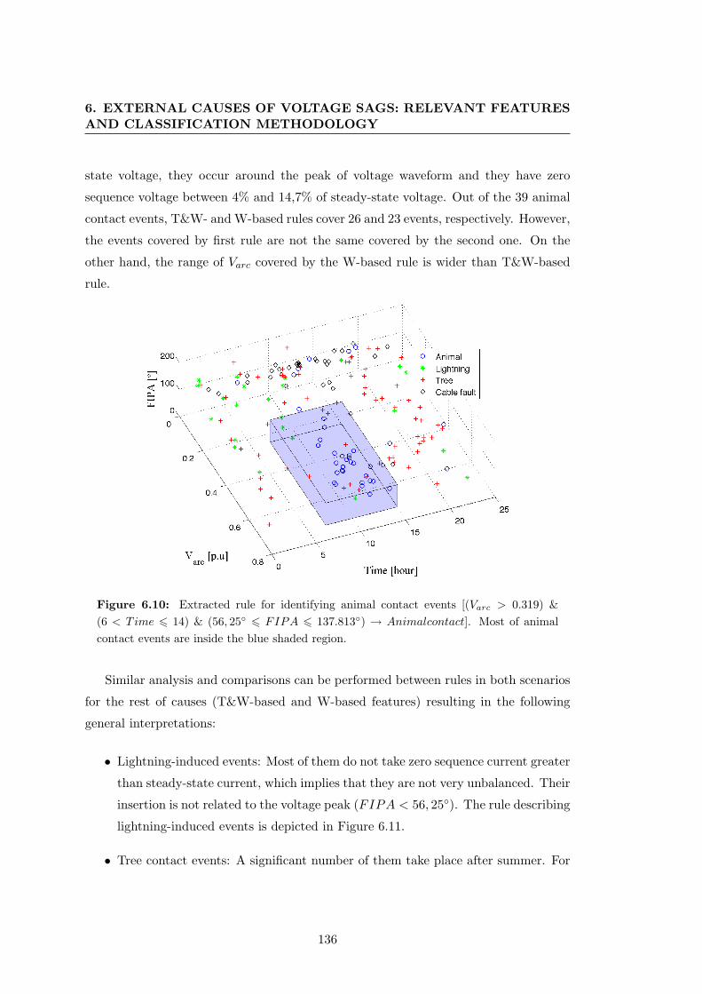
6. EXTERNAL CAUSES OF VOLTAGE SAGS: RELEVANT FEATURESAND CLASSIFICATION METHODOLOGY
state voltage, they occur around the peak of voltage waveform and they have zero
sequence voltage between 4% and 14,7% of steady-state voltage. Out of the 39 animal
contact events, T&W- and W-based rules cover 26 and 23 events, respectively. However,
the events covered by first rule are not the same covered by the second one. On the
other hand, the range of Varc covered by the W-based rule is wider than T&W-based
rule.
Figure 6.10: Extracted rule for identifying animal contact events [(Varc > 0.319) &(6 < Time 6 14) & (56, 25◦ 6 FIPA 6 137.813◦) → Animalcontact]. Most of animalcontact events are inside the blue shaded region.
Similar analysis and comparisons can be performed between rules in both scenarios
for the rest of causes (T&W-based and W-based features) resulting in the following
general interpretations:
• Lightning-induced events: Most of them do not take zero sequence current greater
than steady-state current, which implies that they are not very unbalanced. Their
insertion is not related to the voltage peak (FIPA < 56, 25◦). The rule describing
lightning-induced events is depicted in Figure 6.11.
• Tree contact events: A significant number of them take place after summer. For
136
6.5 External cause identification of voltage sags
Figure 6.11: Extracted rule for identifying single-phase lightning-induced events [(Varc 6
0, 319) & (Time 6 9) & (I0 6 1, 057)→ Lightning − induced]. Most of ligthning-inducedevents are inside the green shaded region.
single-phase animal events, the zero sequence voltage (Vo) is lower than about
25%, see rule space for single-phase events in Figure 6.12.
• Cable failures: Their occurrence does not depend on the date and time. Almost
all of them have a large change in voltage magnitude (4V ) and zero sequence
voltage (V0) and these faults are inserted around the peak of voltage wave. The
rule describing cable failures is plotted in Figure 6.13.
6.5 External cause identification of voltage sags
In this section we revise the proposed method for classification of short-circuits accord-
ing to their external causes. It makes use of the set of rules extracted by CN2 algorithm
and selected in previous section. Three different strategies have been considered de-
pending on the use of rules concerning time dependent features. The first one includes
rules with time dependent features, the second one uses only rules involving features
extracted from waveform with independence of the date and time of occurrence, and
137
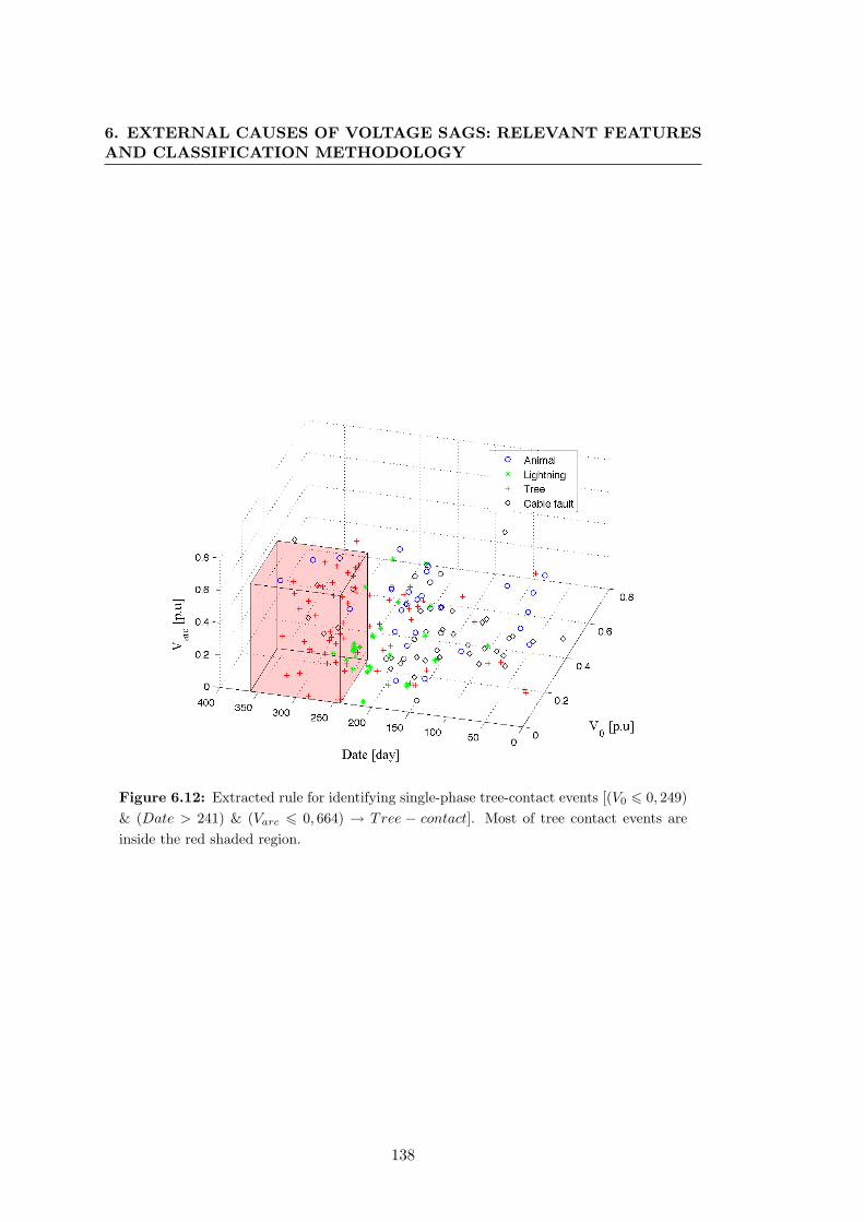
6. EXTERNAL CAUSES OF VOLTAGE SAGS: RELEVANT FEATURESAND CLASSIFICATION METHODOLOGY
Figure 6.12: Extracted rule for identifying single-phase tree-contact events [(V0 6 0, 249)& (Date > 241) & (Varc 6 0, 664) → Tree − contact]. Most of tree contact events areinside the red shaded region.
138
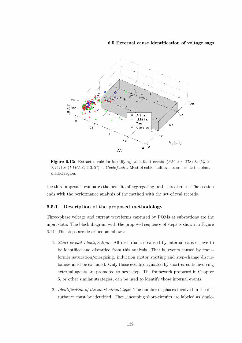
6.5 External cause identification of voltage sags
Figure 6.13: Extracted rule for identifying cable fault events [(4V > 0, 278) & (V0 >
0, 242) & (FIPA 6 112, 5◦)→ Cablefault]. Most of cable fault events are inside the blackshaded region.
the third approach evaluates the benefits of aggregating both sets of rules. The section
ends with the performance analysis of the method with the set of real records.
6.5.1 Description of the proposed methodology
Three-phase voltage and current waveforms captured by PQMs at substations are the
input data. The block diagram with the proposed sequence of steps is shown in Figure
6.14. The steps are described as follows:
1. Short-circuit identification: All disturbances caused by internal causes have to
be identified and discarded from this analysis. That is, events caused by trans-
former saturation/energizing, induction motor starting and step-change distur-
bances must be excluded. Only those events originated by short-circuits involving
external agents are promoted to next step. The framework proposed in Chapter
5, or other similar strategies, can be used to identify those internal events.
2. Identification of the short-circuit type: The number of phases involved in the dis-
turbance must be identified. Then, incoming short-circuits are labeled as single-
139
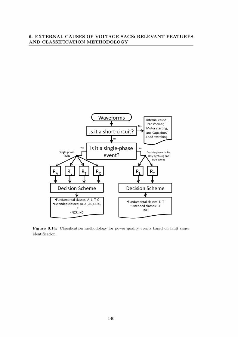
6. EXTERNAL CAUSES OF VOLTAGE SAGS: RELEVANT FEATURESAND CLASSIFICATION METHODOLOGY
Figure 6.14: Classification methodology for power quality events based on fault causeidentification.
140
6.5 External cause identification of voltage sags
or double-phase.
3. Evaluation of rules: The corresponding rules listed in Table 6.3 are evaluated
according to the number of phases involved in the short-circuit disturbance.
4. Decision making scheme: For single-phase short-circuits, when the evaluation
of rules set concludes a single class, it is classified according to it: animal (A),
lightning (L), tree (T) or cable (C). However, when the event matches different
rules concluding two different causes, it is assigned to extended imprecise classes
defined by the combination of two possible causes: AL, AT, AC, LT, LC or TC.
This means that the event cause could be both. Otherwise, the event is classified
as inconclusive, and the output labeled as Not conclusive result (NCR), when
three or more possible causes are identified and the event is Not classified (NC)
when no rules are fired. Similarly, double-phase events are classified as L, T, LT
or NC. Observe that NCR does not exist for double-phase events.
6.5.2 Results of the rule-based classification methodology
Zero sequence current magnitude (I0) has been used to identify the number of phases
(single-, double-phase) involved in the disturbance. All events whose I0 greater than
202 [A] were assumed as single-phase short-circuits. FTI, θv1, θv2, θc1, θc2 features
(Chapter 5) have not been used to estimate the short-circuit type because authors
did not have access to waveforms when this methodology was tested. A confidential
agreement between the provider and authors avoided the use of waveforms outside of
installations of the provider.
Date and Time features have been obtained directly from record time-stamp. The
rest of features have been calculated according to the procedures previously described
in Section 6.3.
Three different approaches have been considered for evaluation of rules. The first
approach uses rules based on timestamp and waveform features (T&W). The second
approach only makes use of waveform-based features (W) while the third one combines
results of both previous sets of rules using a logical OR. This allows analyzing the
influence of time in specific causes and its significance to infer an automatic diagnose
of the root-cause of a short-circuit.
141
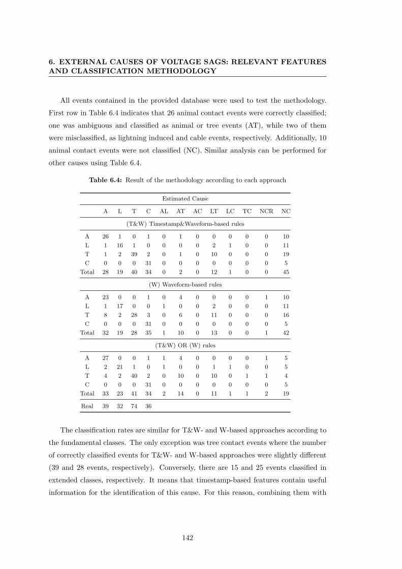
6. EXTERNAL CAUSES OF VOLTAGE SAGS: RELEVANT FEATURESAND CLASSIFICATION METHODOLOGY
All events contained in the provided database were used to test the methodology.
First row in Table 6.4 indicates that 26 animal contact events were correctly classified;
one was ambiguous and classified as animal or tree events (AT), while two of them
were misclassified, as lightning induced and cable events, respectively. Additionally, 10
animal contact events were not classified (NC). Similar analysis can be performed for
other causes using Table 6.4.
Table 6.4: Result of the methodology according to each approach
Estimated Cause
A L T C AL AT AC LT LC TC NCR NC
(T&W) Timestamp&Waveform-based rules
A 26 1 0 1 0 1 0 0 0 0 0 10
L 1 16 1 0 0 0 0 2 1 0 0 11
T 1 2 39 2 0 1 0 10 0 0 0 19
C 0 0 0 31 0 0 0 0 0 0 0 5
Total 28 19 40 34 0 2 0 12 1 0 0 45
(W) Waveform-based rules
A 23 0 0 1 0 4 0 0 0 0 1 10
L 1 17 0 0 1 0 0 2 0 0 0 11
T 8 2 28 3 0 6 0 11 0 0 0 16
C 0 0 0 31 0 0 0 0 0 0 0 5
Total 32 19 28 35 1 10 0 13 0 0 1 42
(T&W) OR (W) rules
A 27 0 0 1 1 4 0 0 0 0 1 5
L 2 21 1 0 1 0 0 1 1 0 0 5
T 4 2 40 2 0 10 0 10 0 1 1 4
C 0 0 0 31 0 0 0 0 0 0 0 5
Total 33 23 41 34 2 14 0 11 1 1 2 19
Real 39 32 74 36
The classification rates are similar for T&W- and W-based approaches according to
the fundamental classes. The only exception was tree contact events where the number
of correctly classified events for T&W- and W-based approaches were slightly different
(39 and 28 events, respectively). Conversely, there are 15 and 25 events classified in
extended classes, respectively. It means that timestamp-based features contain useful
information for the identification of this cause. For this reason, combining them with
142
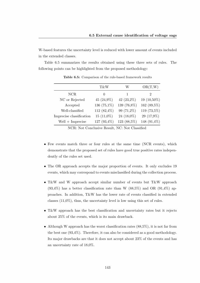
6.5 External cause identification of voltage sags
W-based features the uncertainty level is reduced with lower amount of events included
in the extended classes.
Table 6.5 summarizes the results obtained using these three sets of rules. The
following points can be highlighted from the proposed methodology:
Table 6.5: Comparison of the rule-based framework results
T&W W OR(T,W)
NCR 0 1 2NC or Rejected 45 (24,9%) 42 (23,2%) 19 (10,50%)
Accepted 136 (75,1%) 139 (76,8%) 162 (89,5%)Well-classified 112 (82,4%) 99 (71,2%) 119 (73,5%)
Imprecise classification 15 (11,0%) 24 (18,0%) 29 (17,9%)Well + Imprecise 127 (93,4%) 123 (88,5%) 148 (91,4%)
NCR: Not Conclusive Result, NC: Not Classified
• Few events match three or four rules at the same time (NCR events), which
demonstrate that the proposed set of rules have good true positive rates indepen-
dently of the rules set used.
• The OR approach accepts the major proportion of events. It only excludes 19
events, which may correspond to events misclassified during the collection process.
• T&W and W approach accept similar number of events but T&W approach
(93,4%) has a better classification rate than W (88,5%) and OR (91,4%) ap-
proaches. In addition, T&W has the lower rate of events classified in extended
classes (11,0%), thus, the uncertainty level is low using this set of rules.
• T&W approach has the best classification and uncertainty rates but it rejects
about 25% of the events, which is its main drawback.
• Although W approach has the worst classification rates (88,5%), it is not far from
the best one (93,4%). Therefore, it can also be considered as a good methodology.
Its major drawbacks are that it does not accept about 23% of the events and has
an uncertainty rate of 18,0%.
143
6. EXTERNAL CAUSES OF VOLTAGE SAGS: RELEVANT FEATURESAND CLASSIFICATION METHODOLOGY
• OR approach has a good classification rate (91,4%) and the lowest rejected rate
(10,5%). Its main drawback is a high uncertainty rate (17,9%).
In general, the three approaches have a good performance. The selection of one or
other approach could be influenced by the existence of time dependent faults (season
and day time) associated with specific causes. Hence, for the data set under study, the
first approach (T&W-based) gives the best performance, but results can be different
for other regions with different weather conditions. The second approach (W-based)
has the advantage that it uses features extracted only from the event waveform.
Finally, it worth to remark that records used in this work were associated manually
with cause labels by the utility operators after an accurate analysis of short-circuits;
but, it is possible that some events could be wrongly labeled. For example, lightning
events are difficult to be inspected visually and sometimes these associations are made
because of the event coincidences in time with storms or rainy days. However, this does
not strictly imply that lightning was the real cause of the said event.
6.6 Conclusion
It has been proposed a methodological approach for the automatic identification of
fault causes produced by external factors based on simple features that are extracted
from voltage disturbances recorded in distribution networks. Ten features, related to
underlying physical phenomena between external factors and the power line during the
fault, have been analyzed. The performance of these features is presented for a given set
of events in a way that it can be easily reproduced by other sets of events. A descriptive
analysis of features, for each cause, has been combined with MANOVA and the use of
CN2 to automatically extract rules covering the maximum number of instances in the
data set. Consistency of results given by the three approaches reinforces the confidence
on this analysis of the features and also on the representativeness of the data set despite
the number of events not being significantly large.
CN2 induction algorithm has been used to extract a representative set of rules
capable of classifying the events, described by these features, into four main causes:
animal contact, tree contact, lightning-induced and cable failures. So, assuming that
the events used in the study are representative of the geographical region where they
were collected, the following observations can be added to the previous analysis:
144
6.6 Conclusion
• Voltage events resulting from external causes are highly influenced by weather
conditions.
• Animal contact events take place during daytime and usually imply the apparition
of significant arc voltage.
• Lightning induced events occur during night as well as in the first two-thirds of
the year.
• Tree contact events take place at the end of the year (fall) and have low zero-
sequence voltage values.
• Cable fault events have substantial phase voltage changes and high zero-sequence
voltage components.
From the study it can affirm that influence of weather on the apparition of short-
circuits induced by external causes is high and further work has to be done to better
describe these relationships. Unfortunately, in this work it did not have access to
weather data (wind speed, temperature, raining or geographical coordinates of lightings
among others) during the faults reported in the data set.
145
6. EXTERNAL CAUSES OF VOLTAGE SAGS: RELEVANT FEATURESAND CLASSIFICATION METHODOLOGY
146
7
Conclusions
This chapter summarizes the conclusions obtained as a result of this research. The
relevant conclusions are highlighted and discussed, as well as several ideas for future
work are proposed.
7.1 Conclusions
The aim of this thesis is to propose relevant features for characterizing voltage distur-
bances collected in radial distribution networks as well as to propose methodologies for
their automatic diagnosis.
The problem of voltage disturbance diagnosis was basically formulated as a classi-
fication problem where disturbances, characterized by significant features, have to be
assigned to classes associated with different root-causes and relative location. Due to
the availability of collected waveforms and the increasing tendency to install power
quality monitors, the proposed solution follows a data mining approach. As a result,
this thesis contributes to propose significant features for the characterization of wave-
forms, according to each diagnosis goal (relative location of disturbance origin and root
cause identification). The use of inductive learning algorithms to obtain classification
rules based on in the proposed features and their further exploitation for diagnosis
constitutes other significant contributions of this thesis.
Section 2.1.1 and 2.1.2, proposes a categorization of voltage disturbances according
to their root causes and their source relative location. Normal operation actions over
power network components were considered as internal causes of disturbances, such as
147
7. CONCLUSIONS
motor starting, transformer energizing/saturation, capacitor-bank switching, large-load
connection and disconnection. On the other hand, factors that generate short-circuits
and are beyond the control of electrical facilities, such as animal contact, tree contact,
lightning-induced and underground cable failures were considered as external causes of
disturbances. Regarding the source relative location, disturbances can be categorized
as upstream or downstream with respect to the PQM meter.
The aforementioned categorization allows working with three different feature sets
that contain information about internal causes, external causes and relative location
of the disturbance source, respectively. Concerning the sets related to internal and
external causes, features were conceived understanding the phenomenon associated
with each cause, whereas features in the set related to relative location were obtained
from the analysis and evaluation of different algorithms found in the literature.
Especial attention was given to feature extraction and selection of the three feature
sets. The process was supported with a waveform segmentation analysis (Chapter
3 ) that estimates the beginning and ending samples of stationary and non-stationary
stages throughout the disturbance. These estimations allow selecting the cycles or time
instants where compute these features in order to reduce estimation error.
Waveform segmentation findings suggested that an algorithm based on the changes
of rotation angle of the instantaneous power tensor (Tensor-WSA) is the one that per-
forms better when compared with those based on Kalman filters. First, Tensor-WSA
obtained the best segmentation performance in all tested scenarios (Chapter 3 ). Sec-
ondly, Kalman-based segmentation algorithms are sensitive to fault insertion instant,
so that their performance is highly affected by faults inserted around zero-crossing
instants. Finally, the study revealed that Harmonic-WSA is suitable for segmenting
disturbances due to fuse operation events, whereas Residual-WSA has a good global
performance and the lowest not-conclusive segmentation rate.
Both, location- and cause-based features were statistically analyzed in order to
assess the amount of information contained in each feature (Chapter 4 and Chapter
6 ). The statistical analysis was done making use of multivariate analysis of variance
(MANOVA).
Relevant location-based features were identified during the statistical analysis (Sec-
tion 4.4.3). After this, CN2 rule induction algorithm was used to extract decision rules
148
7.1 Conclusions
for describing the upstream and downstream voltage disturbances (Section 4.5). Ac-
cordingly, a new decision algorithm that combines most of the location-based relevant
features was proposed. It was called PCSC&RS since it combines the features used
by Phase Change in Sequence Current (PCSC) and Resistance Sign (RS) algorithms.
Likewise, decision rules combining cause-based features were also extracted and they
were included within the methodology for identifying the disturbance external cause
proposed in Chapter 6.
Source relative location of voltage disturbances should be estimated applying PCSC
algorithm because its feature has demonstrated to be highly sensitive to the source
relative location of disturbances (Chapter 4 ). Similarly, features used by Real Current
Component (RCC) and Distance Relay (DR) algorithms are also sensitive to source
relative location of single-phase and double phase faults, respectively.
Capacitor and load switchings can be discriminated from the rest of internal causes
carrying out a derivative-based segmentation with suitable thresholds (Chapter 5 ). On
the other hand, motor and transformer disturbances can be discriminated mainly by
neutral current and second order current harmonics (Section 5.3.2). Consequently,
short-circuits can be discriminated from the above mentioned internal causes by apply-
ing a derivative-based segmentation followed by the measure of the triangular shape of
the RMS waveform (Figure 5.19). The different types of short-circuits (single-, double-,
three-phase) can be distinguished analyzing the angles of loss-of-voltage and gain-of-
current triangles (Section 5.3.3.2 and 5.3.3.3).
In a framework for diagnosis of disturbance causes, the possibility that a disturbance
is being leaded by an internal cause has to be evaluated before the evaluating the
possibility of external causes, since internal causes as motor starting, capacitor/load
switching or transformer energizing have a well-known electrical models that allow a
theoretical analysis of the phenomenon, whereas the models of external factors are
partially unknown when they occur and usually they are time variant and involve
unknown parameters. Consequently, disturbances generated by external causes do not
follow a characteristic waveform shape. Thus, assumptions and hypothesis are needed
in order to propose significant features with discriminant properties.
On the other hand, animal contact and cable failures usually involve one phase.
However, some cable failures start affecting one phase and finish affecting two or three
149
7. CONCLUSIONS
phases as a consequence of evolutive discharges between phases. Conversely, tree con-
tact and lightning-induced events either affect one, two or three phase due to their
irregular nature. In this thesis only tree and lightning events affecting one and two
phases were analyzed due to the availability of data. High and low arc voltage values
are experienced by animal and cable disturbances, respectively.
From the analysis of timestamp also some conclusion can be derived. Disturbances
due to animals and lightning usually occur during daytime and night, respectively.
Cable and tree contact events have high and low zero sequence voltage components.
At the end and middle year the apparition of tree contact and lightning-induced events
usually increases, respectively. All aforementioned hints are valid to the region where
disturbances have been recorded (northeastern American region). Waveforms recorded
in other regions could be analyzed following the methodology presented in this thesis.
7.2 Future work
From the achieved results of the research, new research challenges are elucidated in this
section in order to complement the thesis contributions.
More knowledge about the recorded waveforms will allow extracting more infor-
mation in an automatic way. Knowledge about environmental factors (wind speed,
temperature, rainfall level, vegetation, etc.) can be incorporated in the diagnosis of
disturbances leaded by external causes (short-circuits). Environmental information is
useful for this purpose because short-circuits are highly influenced by environmental
factors. Combining these information with knowledge coming from recorded waveforms
(features) and network configuration (grounding system, transformer connection, pro-
tection scheme, etc.) a better diagnosis framework for short-circuits will be obtained.
Hence, analysis oriented to find out how to combine all these information require more
efforts.
Additional work is also needed to validate the proposed framework making use of
disturbance waveforms recorded in different geographical regions. Then, the general-
ization capacity of the proposed rule sets would be really assessed and, if it is necessary,
new rule sets can be proposed for diagnosis of disturbances collected in new geographical
regions.
150

7.2 Future work
In consequence, other research field of interest is to propose a set of cause-based fea-
tures conceived for radial and meshed networks with distributed generation. Similarly,
the comparison of relative location algorithms using disturbances collected in networks
with the previously mentioned characteristics.
Another problem that requires attention is that arc voltage can only be computed
for single-phase faults. For this reason, in this work arc voltage was only included in
rules describing single-phase disturbances. Mathematical expressions for computing arc
voltages in case of double- and three-phase faults could be studied.
The problem of automatic diagnosis of voltage disturbances is not completely solved.
More efforts are required to find more robust classifiers allowing better classifications of
the different disturbance root causes. Furthermore, different classifiers structures shall
be tested, as well as their performance and robustness shall be assessed using a large
and representative sample of disturbances.
151

7. CONCLUSIONS
152
References
Seon-Ju Ahn, Dong-Jun Won, D-Yop Chung, and Seung-U Moon. Determination of the relative location
of voltage sag source according to event cause. In Power Engineering Society General Meeting, 2004.
IEEE, pages 620 – 625 Vol.1, june 2004. doi: 10.1109/PES.2004.1372880. 19, 26
W.R. Anis Ibrahim and M.M. Morcos. Artificial intelligence and advanced mathematical tools for
power quality applications: a survey. Power Delivery, IEEE Transactions on, 17(2):668 –673, apr
2002. ISSN 0885-8977. doi: 10.1109/61.997958. 18
Peter G. V. Axelberg, Irene Yu-Hua Gu, , and Math H. J. Bollen. Support vector machine for classifi-
cation of voltage disturbances. Power Delivery, IEEE Transactions on, 22(3):1297–1303, July 2007.
19
V. Barrera, X. Berjaga Moliner, J. Melendez Frigola, S. Herraiz Jaramillo, J. Sanchez, and M. Castro.
Two methods for voltage sag source location. In Harmonics and Quality of Power, 2008. ICHQP
2008. 13th International Conference on, pages 1 –6, 28 2008-oct. 1 2008a. doi: 10.1109/ICHQP.
2008.4668849. 9, 11
V. Barrera, B. Lopez, J. Melendez, and J. Sanchez. Voltage sag source location from extracted rules
using subgroup discovery. In Josep Puyol-Gruart Teresa Alsinet and Carme Torras, editors, Frontiers
in Artificial Intelligence and Applications, volume 128 of ISBN 978-1-58603-925-7, pages 225–235.
IOS Press, October 2008b. 9, 165
V. Barrera, J. Melendez Frigola, and S. Herraiz Jaramillo. A survey on voltage sag events in
power systems. In Transmission and Distribution Conference and Exposition: Latin America, 2008
IEEE/PES, pages 1 –3, aug. 2008c. doi: 10.1109/TDC-LA.2008.4641774. 10, 21
V. Barrera, J. Melendez, S. Herraiz, and J. Sanchez. Evaluation of fault relative location algorithms
using voltage sag data collected at 25-kv substations. European Transactions on Electrical Power
(ETEP), 20(1):34–51, DOI: 10.1002/etep.393, January 2009a. 8, 11, 32, 33
V. Barrera, J. Melendez, S. Herraiz, and J. Sanchez. A new sag source relative location algorithm
based on the sequence current magnitude. In Simposio Internacional sobre la Calidad de la Energia
Electrica (SICEL), Bogota, Colombia, August 2009b. 9
V. Barrera, I.Y. Gu, M.H.J. Bollen, and J. Melendez. Feature characterization of power quality events
according to their underlying causes. In Harmonics and Quality of Power (ICHQP), 2010 14th
International Conference on, pages 1 –8, sept. 2010a. doi: 10.1109/ICHQP.2010.5625496. 9, 11, 26,
53, 109
153
REFERENCES
V. Barrera, S. Kulkarni, S. Santoso, and J. Melendez. Feature analysis and classification methodology
for overhead distribution fault events. In Power and Energy Society General Meeting, 2010 IEEE,
pages 1 –8, july 2010b. doi: 10.1109/PES.2010.5589270. 9, 11, 28, 29, 34, 53, 105, 126, 130
V. Barrera, S. Kulkarni, S. Santoso, and J. Melendez. Svm-based classification methodology for over-
head distribution fault events. In Harmonics and Quality of Power (ICHQP), 2010 14th International
Conference on, pages 1 –6, sept. 2010c. doi: 10.1109/ICHQP.2010.5625497. 9, 11, 29, 34, 53, 105,
130
V. Barrera, R. Velandia, F. Hernandez, H. Vargas, and J. Melendez. Relevant attributes for voltage
event diagnosis in power distribution networks. Revista Iberoamericana de Automatica e Informatica
Industrial, –(Manuscript no. 11077-28049-1-SM), 2010d. 8, 11
V. Barrera, J. Melendez, and S. Herraiz. Feature analysis for voltage disturbances resulting from
external causes. In 21st International Conference on Electricity Distribution, Frankfurt, June 2011a.
CIRED. 9, 11, 126
V. Barrera, J. Melendez, and S. Herraiz. Waveform segmentation for intelligent monitoring of power
events. Electric Power Systems Research, (Manuscript id: EPSR-D-11-00655), 2011b. 8, 10, 11
V. Barrera, J. Melendez, S. Herraiz, A. Ferreira, and A. Munoz. Analysis of the influence of weather
factors on outages in spanish distribution networks. In International Conference on Innovative Smart
Grid Technologies Europe 2011 (ISGT), number 269 in -. Power Engineering Society, 6-9 December
2011c. 8, 11, 31
V. Barrera, A. Pavas, and J. Melendez. Power quality assessment of the bogota distribution network
focused on voltage sags analysis. In International Conference on Innovative Smart Grid Technologies
Europe 2011 (ISGT), number 159 in -, Manchester, 6-9 December 2011d. Power Engineering Society.
8
V. Barrera, J. Melendez, and S. Herraiz. Automatic diagnosis of voltage sags collected in power
distribution networks. Electric Power Systems Research, 2011 (Submitted). 10
Victor Barrera, Joaquim Melendez, Saurabh Kulkarni, and Surya Santoso. Feature analysis and au-
tomatic classification of short-circuit faults resulting from external causes. European Transactions
on Electrical Power, page 10.1002/etep.674, 2012. ISSN 1546-3109. doi: 10.1002/etep.674. URL
http://dx.doi.org/10.1002/etep.674. 8, 11, 29, 30, 34, 53, 90, 126, 130
V. Barrera Nunez, J. Melendez Frigola, S. Herraiz Jaramillo, and J. Sanchez Losada. Unusual voltage
sag event detection in power systems. In Transmission and Distribution Conference and Exposition:
Latin America, 2008 IEEE/PES, pages 1 –5, aug. 2008. doi: 10.1109/TDC-LA.2008.4641821. 10
J. Blanco, J. Jagua, L. Jaimes, V. Barrera, and J. Melendez. Metodologia para el diagnostico de
la causa de huecos de tension. In Simposio Internacional sobre la Calidad de la Energia Electrica
(SICEL), Bogota, Colombia, August 2009a. 9
J. Blanco, J. Jagua, and L. Jaimes. V. Barrera. Diagnosis of the Underlying Cause of Voltage Events:
Fault characterization. Degree thesis. Bucaramanga, Colombia, 2009b. 100, 107
154
REFERENCES
M. Bollen. Understanding Power Quality Problems: Voltages Sags and Interruptions. IEEE Press, New
York, 2000. 19, 22
M. Bollen, I Gu, P. Axelberg, and E. Styvaktakis. Classification of underlying causes of power quality
disturbances: deterministic versus statistical methods. EURASIP Journal on Advances in Signal
Processing, ID 79747:17 pages, 2007. 3, 15, 20, 22, 26, 41, 43, 48, 113
M. H. J. Bollen, P. Ribeiro, I. Y. H. Gu, and C. A. Duque. Trends, challenges and opportunities in power
quality research. European Transactions on Electrical Power (ETEP), 20(doi: 10.1002/etep.370):
3–18, 2010. 4, 20
M.H.J. Bollen. Algorithms for characterizing measured three-phase unbalanced voltage dips. Power
Delivery, IEEE Transactions on, 18(3):937 – 944, july 2003. ISSN 0885-8977. doi: 10.1109/TPWRD.
2003.813879. 19, 71
M.H.J. Bollen and D.D. Sabin. International coordination for voltage sag indices. In Power Engineering
Society General Meeting, 2005. IEEE, pages 2217 – 2222 Vol. 3, june 2005. doi: 10.1109/PES.2005.
1489164. 107
M.H.J. Bollen and D.D. Sabin. International coordination for voltage sag indices. In Transmission
and Distribution Conference and Exhibition, 2005/2006 IEEE PES, pages 229 –234, may 2006. doi:
10.1109/TDC.2006.1668492. 27
M.H.J. Bollen, I.Y.H. Gu, S. Santoso, M.F. Mcgranaghan, P.A. Crossley, M.V. Ribeiro, and P.F.
Ribeiro. Bridging the gap between signal and power. Signal Processing Magazine, IEEE, 26(4):
12–31, July 2009. 3, 4, 20, 22, 43, 113
Yixin Cai, Mo-Yuen Chow, Wenbin Lu, and Lexin Li. Evaluation of distribution fault diagnosis algo-
rithms using roc curves. In Power and Energy Society General Meeting, 2010 IEEE, pages 1 –6, july
2010a. doi: 10.1109/PES.2010.5588154. 19, 122, 124
Yixin Cai, Mo-Yuen Chow, Wenbin Lu, and Lexin Li. Statistical feature selection from massive data
in distribution fault diagnosis. Power Systems, IEEE Transactions on, 25(2):642 –648, may 2010b.
ISSN 0885-8950. doi: 10.1109/TPWRS.2009.2036924. 19
Olejnik S Carl H. Applied MANOVA and discriminant analysis 2d ed. Wiley-Interscience, 2006. 131,
133
Myeon-Song Choi, Seung-Jae Lee, Duck-Su Lee, and Bo-Gun Jin. A new fault location algorithm using
direct circuit analysis for distribution systems. Power Delivery, IEEE Transactions on, 19(1):35–41,
January 2004. 23
Chouhy. Voltage sags: single event characterisation, system performance and source location. PhD
thesis, Chalmers University of Technology, 2007. 32, 64, 67, 73
Boswell R. Clark P. Rule induction with cn2: Some recent improvements. In In Y Kodratoff, editor,
Machine Learning — EWSL-91, Berlin, 1991. Springer-Verlag. 80, 165
Niblett T. Clark P. The cn2 induction algorithm. Machine Learning Journal, 3(4):261–283, 1989. 37,
80, 131, 165
155
REFERENCES
D.V. Coury, C.J. dos Santos, and M.C. Tavares. Transient analysis resulting from shunt capacitor
switching in an actual electrical distribution system. In Harmonics And Quality of Power, 1998.
Proceedings. 8th International Conference on, volume 1, pages 292 –297 vol.1, oct 1998. doi: 10.
1109/ICHQP.1998.759902. 93, 94
J. Myllymaki D. Novosel, D. Hart. System for locating faults and estimating fault resistance in distri-
bution networks with tapped loads. US Patent number 5.839.093, 1998. 23
R. Das. Determining the locations of faults in distribution systems. PhD thesis, University of
Saskatchewan, Saskatoon, Canada, 1998. 19, 23
S.Z. Djokic, J.V. Milanovic, D.J. Chapman, and M.F. McGranaghan. Shortfalls of existing methods
for classification and presentation of voltage reduction events. Power Delivery, IEEE Transactions
on, 20(2):1640 – 1649, april 2005. ISSN 0885-8977. doi: 10.1109/TPWRD.2004.833880. 19, 106
M.B. Djuric, Z.M. Radojevic, and V.V. Terzija. Time domain solution of fault distance estimation and
arcing faults detection on overhead lines. Power Delivery, IEEE Transactions on, 14(1):60 –67, jan
1999. ISSN 0885-8977. doi: 10.1109/61.736683. 30, 31, 129
R. Dugan, M. McGranaghan, S. Santoso, and H. Wayne. Electrical Power Systems Quality. McGraw
Hill, United Kingdom, second edition edition, 2002. 21
C. L. Fortescue. Method of symmetrical co-ordinates applied to the solution of polyphase networks.
American Institute of Electrical Engineers, Transactions of the, XXXVII(2):1027 –1140, july 1918.
ISSN 0096-3860. doi: 10.1109/T-AIEE.1918.4765570. 105, 128
A. Girgis, C. Fallon, and D. Lubkeman. A fault location technique for rural distribution feeders.
Industry Applications, IEEE Transactions on, 29(6):1170 – 1175, November 1993. 23
Serkan Gunal, Omer Nezih Gerek, Dogan Gokhan Ece, and Rifat Edizkan. The search for optimal
feature set in power quality event classification. Expert Systems with Applications, 36(7):10266 –
10273, 2009. ISSN 0957-4174. doi: 10.1016/j.eswa.2009.01.051. URL http://www.sciencedirect.
com/science/article/pii/S0957417409000980. 4
Hussain A. Hamzah N, Mohamed A. A new approach to locate the voltage sag source using real current
component. Electric Power Systems Research, 72:113–123, 2004. 19, 25, 32, 33, 64, 69
Kyeon Hur and S. Santoso. On two fundamental signatures for determining the relative location of
switched capacitor banks. Power Delivery, IEEE Transactions on, 23(2):1105 –1112, april 2008.
ISSN 0885-8977. doi: 10.1109/TPWRD.2008.917669. 93, 94
IEEE-Std-C37. Ieee standard common format for transient data exchange (comtrade) for power systems.
IEEE Std C37.111-1999, page i, 1999. doi: 10.1109/IEEESTD.1999.90571. 21
J. Jagua, V. Barrera, G. Carrillo, and J. Melendez. Waveform segmentation based on tensor analysis.
In ANDESCON, 2010 IEEE, pages 1 –7, sept. 2010. doi: 10.1109/ANDESCON.2010.5633225. 9,
10, 22, 43, 46, 51
A.A.; Jun Zhu; Lubkeman, D.L.; Girgis. Automated fault location and diagnosis on electric power
distribution feeders. Power Delivery, IEEE Transactions on, 12(2):801 – 809, April 1997. 23
156
REFERENCES
W.H. Kersting. Radial distribution test feeders. In Power Engineering Society Winter Meeting, 2001.
IEEE, volume 2, pages 908 –912 vol.2, 2001. doi: 10.1109/PESW.2001.916993. 94
M. Kezunovic and I. Rikalo. Automating the analysis of faults and power quality. Computer Applications
in Power, IEEE, 12(1):46 –50, January 1999. ISSN 0895-0156. doi: 10.1109/67.738319. 21
A Khosravi, J Melendez, J Colomer, and J Sanchez. Multiway principal component analysis (mpca) for
up/downstream class of voltage sags gathered in distribution substation. Advances of Computational
Intelligence in Industrial Systems, 116:297–312, 2008. 19, 64
Colomer J. Khosravi A, Melendez J. Sags classification of sags gathered in distribution substations
based on multiway principal component analysis. European Political Science Review, 79:144–151,
2009. 19, 64
J.A. King and E.W. Gunther. Comtrade / pqdif conversion. In Transmission and Distribution Con-
ference and Exhibition, 2005/2006 IEEE PES, pages 359 –364, may 2006. doi: 10.1109/TDC.2006.
1668518. 21
S. Kulkarni, A.J. Allen, S. Chopra, S. Santoso, and T.A. Short. Waveform characteristics of under-
ground cable failures. In Power and Energy Society General Meeting, 2010 IEEE, pages 1 –8, july
2010a. doi: 10.1109/PES.2010.5590158. 15, 29, 34, 53, 130
Saurabh Kulkarni, Duehee Lee, Alicia J. Allen, Surya Santoso, and Thomas A. Short. Waveform
characterization of animal contact, tree contact, and lightning induced faults. In Power and Energy
Society General Meeting, 2010 IEEE, pages 1 –7, july 2010b. doi: 10.1109/PES.2010.5590214. 15,
28, 30, 31, 105, 126, 129
C.D. Le, I.Y.H. Gu, and M.H.J. Bollen. Joint causal and anti-causal segmentation and location of
transitions in power disturbances. In PES, editor, Power and Energy Society General Meeting, 2010
IEEE, pages 1–6. Power Engineering Society, July 2010. 43, 56
C. Li, T. Tayjasanant, W. Xu, and X. Liu. Method for voltage-sag-source detection by investigating
slope of the system trajectory. Generation, Transmission and Distribution, IEE Proceedings-, 150
(3):367 – 372, may 2003. ISSN 1350-2360. doi: 10.1049/ip-gtd:20030214. 19, 23, 25, 32, 33, 64, 67,
68, 69
E. Rosolowski M. Saha. Method and device of fault location for distribution networks. US Patent
number 6.483.435, 2002. 23
Mark F. McGranaghan and Surya Santoso. Challenges and trends in analyses of electric power quality
measurement data. EURASIP Journal on Advances in Signal Processing, 2007(57985,):5 pages,
November 2007. 3, 4
J. Melendez, X. Berjaga, S. Herraiz, V. Barrera, J. Sanchez, and M. Castro. Classification of
sags according to their origin based on the waveform similarity. In Transmission and Distribu-
tion Conference and Exposition: Latin America, 2008 IEEE/PES, pages 1 –6, aug. 2008. doi:
10.1109/TDC-LA.2008.4641819. 10, 11
157
REFERENCES
J. Mora-Florez, J. Melendez, and G.Carrillo-Caicedo. Comparison of impedance based fault location
methods for power distribution systems. Electric Power Systems Research, 78(4):657 – 666, 2008.
32, 34
L.S. Ortiz, H. Torres S, V. Barrera, C. Duarte, G. Ordonez, and S. Herraiz. Analysis of the voltage
event segmentation using kalman filter and wavelet transform. In ANDESCON, 2010 IEEE, pages
1 –6, sept. 2010. doi: 10.1109/ANDESCON.2010.5630052. 9, 10, 22
S. Ortiz, A. Torres, V. Barrera, C. Duarte, G. Ordonez, and S. Herraiz. Estrategias para la segmentacion
de huecos de tension con componentes de alta frecuencia. In Simposio Internacional sobre la Calidad
de la Energia Electrica (SICEL), Bogota, Colombia, August 2009. 9
A.C. Parsons, W.M. Grady, E.J. Powers, and J.C. Soward. A direction finder for power quality distur-
bances based upon disturbance power and energy. Power Delivery, IEEE Transactions on, 15(3):
1081 –1086, jul 2000. ISSN 0885-8977. doi: 10.1109/61.871378. 19, 23, 32, 33, 64
J.-T. Peng, C.F. Chien, and T.L.B. Tseng. Rough set theory for data mining for fault diagnosis on
distribution feeder. Generation, Transmission and Distribution, IEE Proceedings-, 151(6):689 – 697,
nov. 2004. ISSN 1350-2360. doi: 10.1049/ip-gtd:20040917. 4, 19, 122
E. Perez. Nuevo metodo de deteccion y analisis en tiempo real de eventos en la tension de suministro de
energıa electrica empleando un modelo combinado Wavelet-filtro de Kalman extendido. PhD thesis,
Cantabria University, 2006. 48
A.K. Pradhan and A. Routray. Applying distance relay for voltage sag source detection. Power Delivery,
IEEE Transactions on, 20(1):529 – 531, jan 2005. ISSN 0885-8977. doi: 10.1109/TPWRD.2004.
839741(410)2. 19, 25, 32, 33, 64, 70, 71
A.K. Pradhan, A. Routray, and S. Madhan Gudipalli. Fault direction estimation in radial distribution
system using phase change in sequence current. Power Delivery, IEEE Transactions on, 22(4):2065
–2071, oct. 2007. ISSN 0885-8977. doi: 10.1109/TPWRD.2007.905340. 19, 25, 32, 33, 64, 74, 75
Braatz RD. Russell EL, Chiang LH. Data-Driven Methods for Fault Detection and Diagnosis in Chem-
ical Processes. Springer-Verlog, London, Berlin, Heidelberg, New York, 2000. 163
R.; Sachdev, M.S.; Agarwal. A technique for estimating transmission line fault locations from digital
impedance relay measurements. Power Delivery, IEEE Transactions on, 3(1):121 – 129, January
1988. 23
S. Santoso, J.D. Lamoree, and M.F. McGranaghan. Signature analysis to track capacitor switching per-
formance. In Transmission and Distribution Conference and Exposition, 2001 IEEE/PES, volume 1,
pages 259 –263 vol.1, 2001. doi: 10.1109/TDC.2001.971244. 94
D. Saxena, K.S. Verma, and S.N. Singh. Power quality event classification: an overview and key issues.
International Journal of Engineering, Science and Technology, 2(3):186–199, 2010. 3, 4, 20
A.; Srinivasan, K.; St.-Jacques. A new fault location algorithm for radial transmission lines with loads.
Power Delivery, IEEE Transactions on, 4(3):1676 – 1682, July 1989. 23
158
REFERENCES
E. Styvaktakis. Automating Power Quality Analysis. PhD thesis, Chalmers University of Technilogy,
Gothemborg, Sweden, 2002. 4, 41, 43, 44, 48
E. Styvaktakis, M.H.J. Bollen, and I.Y.H. Gu. Expert system for classification and analysis of power
system events. Power Delivery, IEEE Transactions on, 17(2):423 –428, apr 2002. ISSN 0885-8977.
doi: 10.1109/61.997911. 4, 19
T. Tayjasanant, Chun Li, and W. Xu. A resistance sign-based method for voltage sag source detection.
Power Delivery, IEEE Transactions on, 20(4):2544 – 2551, oct. 2005. ISSN 0885-8977. doi: 10.1109/
TPWRD.2005.852341. 19, 25, 32, 33, 64, 72
A.J. Ustariz, E.A. Canoa, and H.E. Tacca. Tensor analysis of the instantaneous power in electrical
networks. Electric Power Systems Research, 80(7):788–798, July 2010. 22, 43, 46
A. Warrington. Protective relays, their theory and practice, volume 2. Chapman and Hall, London,
1968. 23
L. Xu and Mo-Yuen Chow. A classification approach for power distribution systems fault cause iden-
tification. Power Systems, IEEE Transactions on, 21(1):53 – 60, feb. 2006. ISSN 0885-8950. doi:
10.1109/TPWRS.2005.861981. 19, 31, 122, 124
L. Xu, M.-Y. Chow, and L. S. Taylor. Power distribution fault cause identification with imbalanced data
using the data mining-based fuzzy classification e-algorithm. Power Systems, IEEE Transactions
on, 22(1):164 –171, feb. 2007. ISSN 0885-8950. doi: 10.1109/TPWRS.2006.888990. 15, 19, 31, 122,
124
G. Yaleinkaya, M.H.J. Bollen, and P.A. Crossley. Characterization of voltage sags in industrial distri-
bution systems. Industry Applications, IEEE Transactions on, 34(4):682 –688, jul/aug 1998. ISSN
0093-9994. doi: 10.1109/28.703958. 19, 93
159

REFERENCES
160

Appendices
161

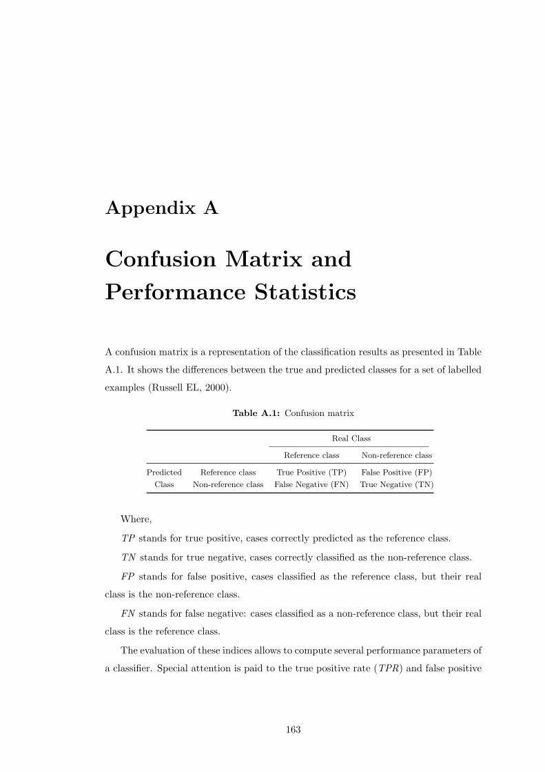
Appendix A
Confusion Matrix and
Performance Statistics
A confusion matrix is a representation of the classification results as presented in Table
A.1. It shows the differences between the true and predicted classes for a set of labelled
examples (Russell EL, 2000).
Table A.1: Confusion matrix
Real Class
Reference class Non-reference class
Predicted Reference class True Positive (TP) False Positive (FP)
Class Non-reference class False Negative (FN) True Negative (TN)
Where,
TP stands for true positive, cases correctly predicted as the reference class.
TN stands for true negative, cases correctly classified as the non-reference class.
FP stands for false positive, cases classified as the reference class, but their real
class is the non-reference class.
FN stands for false negative: cases classified as a non-reference class, but their real
class is the reference class.
The evaluation of these indices allows to compute several performance parameters of
a classifier. Special attention is paid to the true positive rate (TPR) and false positive
163
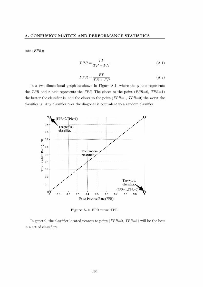
A. CONFUSION MATRIX AND PERFORMANCE STATISTICS
rate (FPR):
TPR =TP
TP + FN(A.1)
FPR =FP
TN + FP(A.2)
In a two-dimensional graph as shown in Figure A.1, where the y axis represents
the TPR and x axis represents the FPR. The closer to the point (FPR=0, TPR=1)
the better the classifier is, and the closer to the point (FPR=1, TPR=0) the worst the
classifier is. Any classifier over the diagonal is equivalent to a random classifier.
Figure A.1: FPR versus TPR.
In general, the classifier located nearest to point (FPR=0, TPR=1) will be the best
in a set of classifiers.
164
Appendix B
CN2 Rule Induction Algorithm
CN2 is a rule extraction algorithm that induces an ordered list of classification rules
from a set of labelled observations (Clark P, 1991, 1989). The rules are in the form
Condi → Classj , where the property of interest is Classj that appears in the rule con-
sequent, and the condition Condi is a conjunction of the features selected from training
observations. CN2 works as an iterative process; each iteration forms a condition cov-
ering a large number of observations of a single Classj and a few observations of other
classes. Having found a good Condi, CN2 removes those observations it covers from
the training set and adds the rule If < Condi > THEN Classj to the end of the rule
list. This process iterates until no more satisfactory conditions can be found. The main
CN2 parameters are as follows:
1. Examples to cover : the percentage of examples to cover.
2. Beam width: the number of best rules that are, in each step, further specialised.
Other rules are discarded.
3. Evaluation function: CN2 has three evaluation functions - Entropy, Laplacian and
WRAcc 1 (Barrera et al., 2008b). During search heuristic, CN2 must evaluate the
rules it finds to decide which is the best. In order to do so, it uses the evaluation
function (Clark P, 1991, 1989).
In this study good results were obtained making use of WRAcc function, a number
of example to cover around 80-95% of the examples in a class and a beam width equal
to 5.1Weighted Relative Accuracy - WRAcc
165
B. CN2 RULE INDUCTION ALGORITHM
CN2 was selected as rule induction algorithm by the following three reasons:
• It is able to accurately classify new cases in presence of noise.
• It induces rules as short as possible.
• Its computation time required for rule generation is linearly proportional to the
sample size.
The above characteristics allow to apply CN2 algorithm to a variety of real-world
situations. It was implemented using Orange data mining software available online.
166
Related Documents