Automated Mapping of Convective Clouds (AMCC ...

Automated Mapping of Convective Clouds (AMCC) Thermodynamical, Microphysical,and CCN Properties from SNPP/VIIRS Satellite Data

ZHIGUO YUE,a,b DANIEL ROSENFELD,c GUIHUA LIU,a JIN DAI,a XING YU,a YANNIAN ZHU,a

EYAL HASHIMSHONI,c XIAOHONG XU,a YING HUI,a AND OLIVER LAUERd

aMeteorological Institute of Shaanxi Province, Xi’an, ChinabOffice of Weather Modification of Shaanxi Province, Xi’an, China

c Institute of Earth Sciences, Hebrew University of Jerusalem, Jerusalem, IsraeldMultiphase Chemistry Department, Max Planck Institute for Chemistry, Mainz, Germany

(Manuscript received 7 June 2018, in final form 19 January 2019)

ABSTRACT

The advent of the Visible Infrared Imager Radiometer Suite (VIIRS) on board the Suomi NPP (SNPP)

satellite made it possible to retrieve a new class of convective cloud properties and the aerosols that they

ingest. An automated mapping system of retrieval of some properties of convective cloud fields over large

areas at the scale of satellite coverage was developed and is presented here. The system is named Automated

Mapping of Convective Clouds (AMCC). The input is level-1 VIIRS data and meteorological gridded data.

AMCC identifies the cloudy pixels of convective elements; retrieves for each pixel its temperature T and

cloud drop effective radius re; calculates cloud-base temperature Tb based on the warmest cloudy pixels;

calculates cloud-base height Hb and pressure Pb based on Tb and meteorological data; calculates cloud-base

updraft Wb based on Hb; calculates cloud-base adiabatic cloud drop concentrations Nd,a based on the T–rerelationship, Tb, and Pb; calculates cloud-base maximum vapor supersaturation S based on Nd,a andWb; and

definesNd,a/1.3 as the cloud condensation nuclei (CCN) concentrationNCCN at that S. The results are gridded

36 km 3 36 km data points at nadir, which are sufficiently large to capture the properties of a field of con-

vective clouds and also sufficiently small to capture aerosol and dynamic perturbations at this scale, such as

urban and land-use features. The results of AMCC are instrumental in observing spatial covariability in

clouds and CCN properties and for obtaining insights from such observations for natural and man-made

causes. AMCC-generated maps are also useful for applications from numerical weather forecasting to

climate models.

1. Introduction

Satellite retrievals are the only practical way of ob-

serving clouds and aerosol properties on regional and

global scales. Recently Rosenfeld et al. (2016) was able

to use such satellite retrievals to provide estimation of

cloud condensation nuclei (CCN) concentration NCCN

from satellite measurements. In this study we take the

next step and present a method for application of the

CCN retrievals for mapping large areas. The main part

of this paper presents the method of CCNmapping. The

introduction prepares the background by reviewing the

physical basis for CCN retrieval.

Aerosols affect clouds mainly by their CCN activity,

which influences cloud drop number concentrations and

albedo, which in turn is followed by a cascade of ad-

justment processes that can either buffer or amplify the

primary effect on cloud radiative properties (Stevens

and Feingold 2009). Therefore, much of the science of

atmospheric chemistry and aerosols has been devoted to

ways by which aerosol size and composition determine

their CCN and ice nucleating particle activity (Andreae

and Rosenfeld 2008). Satellite observation retrievals are

the only practical way to quantify the effective radiative

forcing by aerosol cloud interactions at a global scale.

Aerosol optical-depth retrieval near clouds is plagued

by artifacts (Várnai and Marshak 2009) and ambiguity

(Quaas et al. 2010), and it is only crudely related to

CCN (Andreae 2009). Even if AOD could be retrieved

accurately, it would likely be poorly correlated with the

actual CCN that affects clouds (Stier 2016). Furthermore,

aerosol effects on cloud composition are entangled with

meteorological conditions, mainly as manifested by updraftCorresponding author: Daniel Rosenfeld, daniel.rosenfeld@

mail.huji.ac.il

APRIL 2019 YUE ET AL . 887

DOI: 10.1175/JAMC-D-18-0144.1

� 2019 American Meteorological Society. For information regarding reuse of this content and general copyright information, consult the AMS CopyrightPolicy (www.ametsoc.org/PUBSReuseLicenses).

Unauthenticated | Downloaded 03/24/22 11:42 AM UTC

speeds. Without simultaneously retrieving both cloud

active aerosols and cloud-base updrafts Wb, it is im-

possible to disentangle and extract the net aerosol ef-

fects. To make matters worse, the ability to retrieveWb

via satellite has been nonexistent until our very recent

studies (Zheng and Rosenfeld 2015; Zheng et al.

2015, 2016).

Cloud pixel temperature–cloud drop effective radius,

or T–re, relationships were first constructed by Rosenfeld

and Lensky (1998) for inferring the microstructure and

precipitation forming processes of convective clouds.

The T–re relationships are used to retrieve glaciation

temperature Tg of convective clouds (Rosenfeld et al.

2011; Yuan et al. 2010) and the depth of precipitation

initiation. This depthD14 is the height within the cloud

at which the retrieved re reaches 14mm—the point

above which the probability of precipitation increases

(Freud et al. 2008; Freud and Rosenfeld 2012;

Rosenfeld 1999; Rosenfeld and Gutman 1994; Zhu

et al. 2015). The observed brightness temperature at

the top of this layer is T14. The depth of precipitation

initiation D14 may also be related to convective storm

severity (Rosenfeld et al. 2008a). As a result of the

previously mentioned studies, it is now possible to use

VIIRS for retrieving a set of convective cloud products

that include Tb, Hb, Wb, S, Nd,a, NCCN, T14, D14, Ttop,

Htop, Tcon, Tr, Tmix, and Tg (see the definitions of all

parameters in Table 1).

Although retrieved cloud microphysical properties

have been realized by using theVisible Infrared Imaging

Radiometer Suite (VIIRS) 375-m data of the Suomi

National Polar-Orbiting Partnership (SNPP) spacecraft

(Rosenfeld et al. 2014a,b, 2016), the selection of the

analyzed convective cloud clusters in an area of interest

was done manually by an interactive software package.

But the process is tedious and time-consuming, and it is

impractical to retrieve large-scale data of VIIRS. The

motivation of this paper is to introduce an automated

system that may lead to operational retrieval and map-

ping of the properties of these convective clouds at re-

gional to global scales. This retrieval system will be

helpful to understand the impacts of aerosols on con-

vective clouds on regional or global scales, and for fur-

ther investigating the impacts of anthropogenic aerosol

on climate and weather.

The outline of this paper is as follows: Section 2 re-

views the method of retrieving CCN, section 3 describes

the methods of the Automated Mapping of Convec-

tive Clouds (AMCC), section 4 presents some examples

of the AMCC retrieval from VIIRS data, section 5

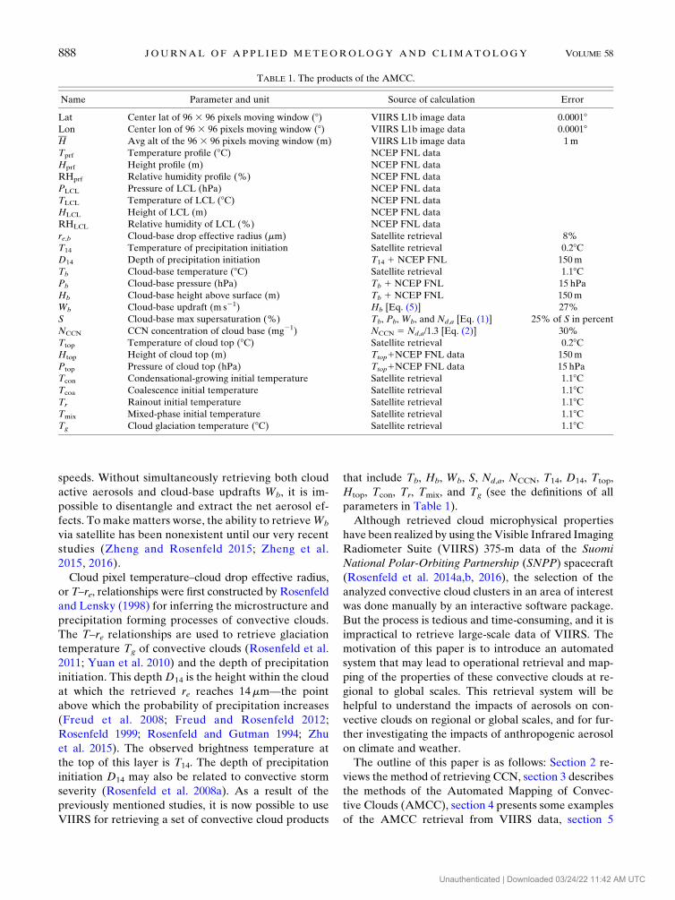
TABLE 1. The products of the AMCC.

Name Parameter and unit Source of calculation Error

Lat Center lat of 96 3 96 pixels moving window (8) VIIRS L1b image data 0.00018Lon Center lon of 96 3 96 pixels moving window (8) VIIRS L1b image data 0.00018H Avg alt of the 96 3 96 pixels moving window (m) VIIRS L1b image data 1m

Tprf Temperature profile (8C) NCEP FNL data

Hprf Height profile (m) NCEP FNL data

RHprf Relative humidity profile (%) NCEP FNL data

PLCL Pressure of LCL (hPa) NCEP FNL data

TLCL Temperature of LCL (8C) NCEP FNL data

HLCL Height of LCL (m) NCEP FNL data

RHLCL Relative humidity of LCL (%) NCEP FNL data

re,b Cloud-base drop effective radius (mm) Satellite retrieval 8%

T14 Temperature of precipitation initiation Satellite retrieval 0.28CD14 Depth of precipitation initiation T14 1 NCEP FNL 150m

Tb Cloud-base temperature (8C) Satellite retrieval 1.18CPb Cloud-base pressure (hPa) Tb 1 NCEP FNL 15 hPa

Hb Cloud-base height above surface (m) Tb 1 NCEP FNL 150m

Wb Cloud-base updraft (m s21) Hb [Eq. (5)] 27%

S Cloud-base max supersaturation (%) Tb, Pb, Wb, and Nd,a [Eq. (1)] 25% of S in percent

NCCN CCN concentration of cloud base (mg21) NCCN 5 Nd,a/1.3 [Eq. (2)] 30%

Ttop Temperature of cloud top (8C) Satellite retrieval 0.28CHtop Height of cloud top (m) Ttop1NCEP FNL data 150m

Ptop Pressure of cloud top (hPa) Ttop1NCEP FNL data 15 hPa

Tcon Condensational-growing initial temperature Satellite retrieval 1.18CTcoa Coalescence initial temperature Satellite retrieval 1.18CTr Rainout initial temperature Satellite retrieval 1.18CTmix Mixed-phase initial temperature Satellite retrieval 1.18CTg Cloud glaciation temperature (8C) Satellite retrieval 1.18C

888 JOURNAL OF APPL IED METEOROLOGY AND CL IMATOLOGY VOLUME 58

Unauthenticated | Downloaded 03/24/22 11:42 AM UTC

discusses the limitations of applicability, and section 6

summarizes and concludes the paper.

2. A review of the method of retrieving CCNfrom satellite

The full description of the method is provided by

Rosenfeld et al. (2016) and references therein. Here a

brief review is provided, because this paper builds on

that method and takes it to the next level of automated

mapping of CCN and related cloud properties.

The approach relies on the fact that, at cloud base,

adiabatic drop concentrations Nd,a, updraft Wb, and

peak vapor supersaturation S are related to each

other by

S5CW3/4b N21/2

d,a , (1)

where the coefficient C is calculated from cloud-base

temperature Tb and pressure Pb (Pinsky et al. 2012). The

Tb andPb are based on satellite retrievals. The approach is

to retrieve Nd,a andWb and then to obtain S from Eq. (1).

Then, Nd,a is the CCN concentration at supersaturation S.

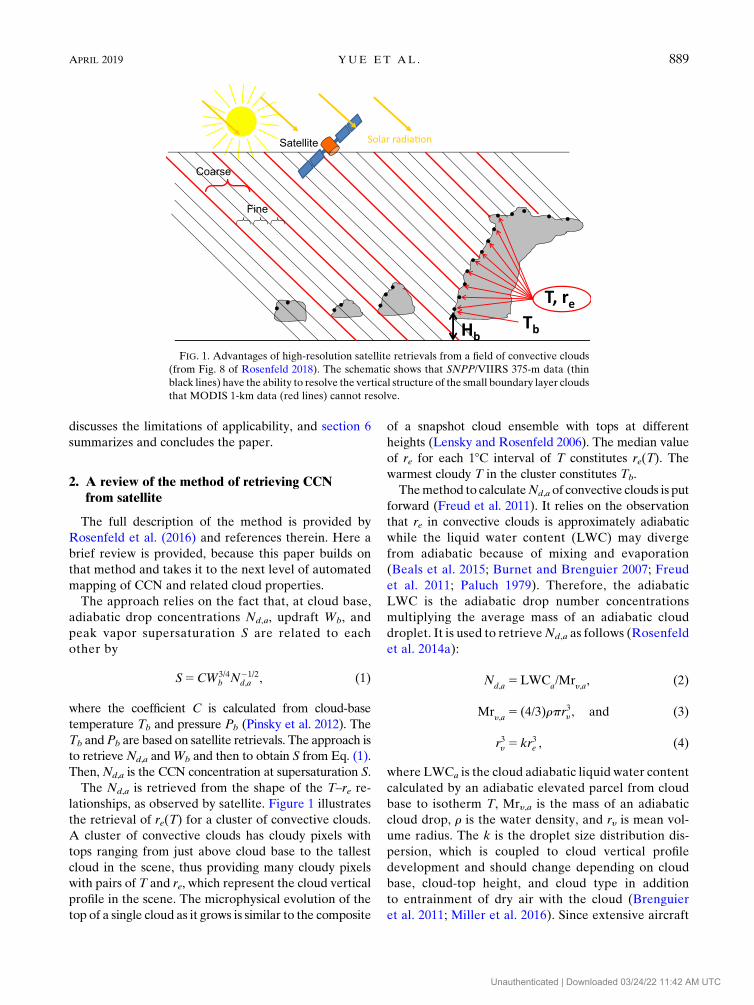
The Nd,a is retrieved from the shape of the T–re re-

lationships, as observed by satellite. Figure 1 illustrates

the retrieval of re(T) for a cluster of convective clouds.

A cluster of convective clouds has cloudy pixels with

tops ranging from just above cloud base to the tallest

cloud in the scene, thus providing many cloudy pixels

with pairs of T and re, which represent the cloud vertical

profile in the scene. The microphysical evolution of the

top of a single cloud as it grows is similar to the composite

of a snapshot cloud ensemble with tops at different

heights (Lensky and Rosenfeld 2006). The median value

of re for each 18C interval of T constitutes re(T). The

warmest cloudy T in the cluster constitutes Tb.

Themethod to calculateNd,a of convective clouds is put

forward (Freud et al. 2011). It relies on the observation

that re in convective clouds is approximately adiabatic

while the liquid water content (LWC) may diverge

from adiabatic because of mixing and evaporation

(Beals et al. 2015; Burnet and Brenguier 2007; Freud

et al. 2011; Paluch 1979). Therefore, the adiabatic

LWC is the adiabatic drop number concentrations

multiplying the average mass of an adiabatic cloud

droplet. It is used to retrieveNd,a as follows (Rosenfeld

et al. 2014a):

Nd,a

5LWCa/Mr

y,a, (2)

Mry,a

5 (4/3)rpr3y , and (3)

r3y 5 kr3e , (4)

where LWCa is the cloud adiabatic liquid water content

calculated by an adiabatic elevated parcel from cloud

base to isotherm T, Mry,a is the mass of an adiabatic

cloud drop, r is the water density, and ry is mean vol-

ume radius. The k is the droplet size distribution dis-

persion, which is coupled to cloud vertical profile

development and should change depending on cloud

base, cloud-top height, and cloud type in addition

to entrainment of dry air with the cloud (Brenguier

et al. 2011; Miller et al. 2016). Since extensive aircraft

FIG. 1. Advantages of high-resolution satellite retrievals from a field of convective clouds

(from Fig. 8 of Rosenfeld 2018). The schematic shows that SNPP/VIIRS 375-m data (thin

black lines) have the ability to resolve the vertical structure of the small boundary layer clouds

that MODIS 1-km data (red lines) cannot resolve.

APRIL 2019 YUE ET AL . 889

Unauthenticated | Downloaded 03/24/22 11:42 AM UTC

observations in India, Israel, and Texas show that

the ratio between re and ry of the convective clouds is

1.08 6 0.01 (k 5 0.79 6 0.02) with little variance, re 51.08ry is used (Freud et al. 2011). This is limited to

conditions of boundary layer convective clouds without

significant coalescence or secondary drop activation

above cloud base, which are required for the method of

CCN retrieval (Rosenfeld et al. 2016). The calculated

Nd,a is used in Eq. (1) for calculating S.

Equation (1) also requires Wb as input. This is calcu-

lated as a simple linear function of cloud-base height

above the surface Hb, according to Eq. (5), a linear

empirical relationship (Zheng and Rosenfeld 2015):

Wb5 0:0009H

b, (5)

where Hb is the distance from surface to cloud base in

meters and the unit of Wb is meters per second.

The accuracy of these calculations relies on the ac-

curacy of Tb, Wb, and satellite-retrieved re (Rosenfeld

et al. 2016). The possibility of obtaining useful accuracy

began with the advent of the SNPP, which was launched

on 28 October 2011. The VIIRS of SNPP contains 5

channels of 375-m imagery resolution and 17 channels

of 750-m moderate resolution at nadir. The spatial

resolution of 375m represents a reduction of the pixel

area by a factor of 7 at nadir (the factor becomes even

higher away from nadir) relative to the 1-km pixels of

MODIS in the thermal IR bands (Rosenfeld et al.

2014b). It brings the most evident improvement in

viewing the top of small-scale features in the thermal

channels (Hillger et al. 2013), such as small convective

clouds. Rosenfeld et al. (2014b) developed a method to

apply VIIRS Imager 375-m data for retrieving high-

resolution T–re relations (Fig. 1). Its advantages in re-

trieving the microphysical properties and precipitation

forming process of convective clouds under different

aerosol conditions were demonstrated (Rosenfeld et al.

2014b; Zhu et al. 2015). However, the standard cloud

products of the VIIRS Environmental Data Records

are derived at the base resolution of 750m (Kopp et al.

2014). To resolve the scale of small convective ele-

ments, we used the cloud products that were developed

based on the 375-m resolution data, which consist of

cloud-base height Hb (Zhu et al. 2014) and the T–reprofiles (Rosenfeld et al. 2014b).

Retrieving re at a resolution of 375m is more sus-

ceptible to 3D effects than at 1000 or 750m. The 3D

effects, such as illuminating and shadowing, can lead to

significant uncertainty in re (Davis and Marshak 2010;

Marshak and Davis 2005; Marshak et al. 2006; Zhang

et al. 2012). It is also found that 3D effects tend to have

stronger impact on retrieval re of 2.1mm than 3.7mm,

where the absorption is largest and mean free path of

the photons is shortest (Zhang et al. 2012). Therefore

our retrievals are based on 3.7mm, and we limited the

geometry only to near backscattering angles with de-

viations of up to ;6358, which is approximated by

satellite zenith angles between 2208 and 508, whereilluminating and shadowing is minimal. The shadowing

effect increases (Fig. 1) and leads to an overestimate of

rewhen the satellite is observed westward. Therefore the

backscatter angle is an important factor to limit the

retrieval. The early afternoon time of the SNPP over-

pass means that backscatter angles occur between the

ranges of satellite zenith angles of 2208 and 508,where a positive angle is to the east of the orbit track.

Figure 1 illustrates how the 375-m resolution of the

VIIRS Imager is advantageous, especially for the

smaller convective clouds, and thus provides more

accurate retrievals at the initial stage of cloud for-

mation and near the bases of more developed clouds

(Rosenfeld et al. 2014b). This allows for the retrieval

of Tb (Zhu et al. 2014) with improved accuracy, which

validated by a combination of ceilometer and sound-

ing showed a root-mean-square (RMS) error of 1.18Cfor the satellite retrieved Tb. In building on this result,

the calculation ofHb and the vapor mixing ratio of the

boundary layer are within an accuracy of approxi-

mately 10%. A method is developed to retrieve Wb

based on the satellite retrieved Tb, Hb, and surface

temperature (Zheng et al. 2015). The RMS error was

0.41m s21, as validated by lidar-measured updraft

speed at the Southern Great Plains (SGP) Atmo-

spheric Radiation Measurement Program site.

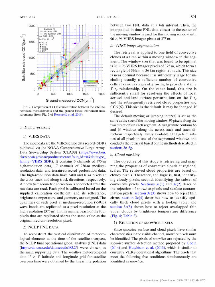
The VIIRS 375-m satellite-retrieved T–re profiles

and Tb are applied to retrieve CCN by the validation of

the satellite retrieved CCN against ground-based ob-

servations at three sites in Oklahoma and the Amazon

River Basin and on board a ship as shown in Fig. 2,

with an accuracy of about 630% (Rosenfeld et al.

2014a, 2016).

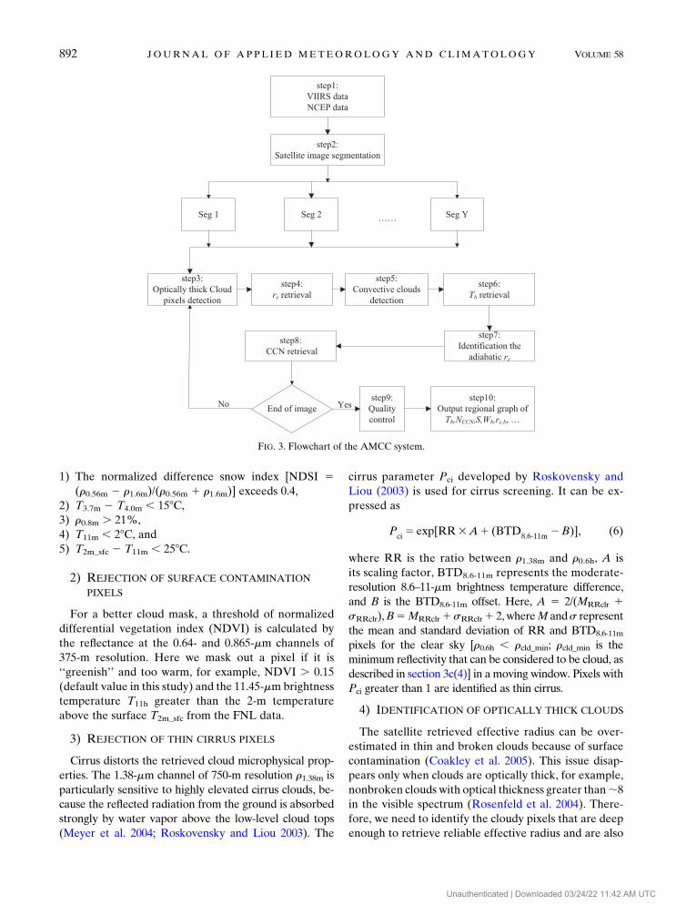
3. Method of the AMCC

The key point in the automated retrieval system is the

compilation of our various methods that work as sepa-

rate programs into one complete automated package.

The AMCC is composed of 10 modules including data

processing, image segmentation, identification of cloud

pixel, re retrieval, convective clouds detection, Tb re-

trieval, identification of the adiabatic re, CCN retrieval,

quality control, and graphical display. The flowchart of

AMCC is presented in Fig. 3. Its final output is gridded

datasets of microphysical properties for convective

clouds at regional or global scales.

890 JOURNAL OF APPL IED METEOROLOGY AND CL IMATOLOGY VOLUME 58

Unauthenticated | Downloaded 03/24/22 11:42 AM UTC

a. Data processing

1) VIIRS DATA

The input data are theVIIRS sensor data record (SDR)

published via the NOAA Comprehensive Large Array-

Data Stewardship System (CLASS) (https://www.bou.

class.noaa.gov/saa/products/search?sub_id50&datatype_

family5VIIRS_SDR). It contains 5 channels of 375-m

high-resolution data, 17 channels of 750-m medium-

resolution data, and terrain-corrected geolocation data.

The high-resolution data have 6400 and 6144 pixels at

the cross-track and along-track directions, respectively.

A ‘‘bow tie’’ geometric correction is conducted after the

raw data are read. Each pixel is calibrated based on the

supplied calibration coefficient, and its reflectance,

brightness temperature, and geometry are assigned. The

quantities of each pixel at medium-resolution (750m)

wave bands are replicated to a pixel resolution at the

high resolution (375m). In this manner, each of the four

pixels that are replicated shares the same value as the

original medium-resolution pixel.

2) NCEP FNL DATA

To reconstruct the vertical distribution of meteoro-

logical elements at the time of the satellite overpass,

the NCEP final operational global analysis (FNL) data

(http://rda.ucar.edu/datasets/ds083.2/) were chosen as

the main supporting data. The weather meteorological

data 18 3 18 latitude and longitude grid for satellite

overpass time were obtained by the linear interpolation

between two FNL data at a 6-h interval. Then, the

interpolated-in-time FNL data closest to the center of

the moving window is used for this moving window with

96 3 96 VIIRS Imager pixels of 375m.

b. VIIRS image segmentation

The retrieval is applied to one field of convective

clouds at a time within a moving window in the seg-

ment. The window size that was found to be optimal

is 963 96 VIIRS Imager pixels of 375m, which form a

rectangle of 36 km 3 36 km region at nadir. This size

is near optimal because it is sufficiently large for in-

cluding usually a sufficient number of convective

cells at various stages of growing to provide a stable

T–re relationship. On the other hand, this size is

sufficiently small for resolving the effects of local

aerosol and land surface perturbations on the T–reand the subsequently retrieved cloud properties and

CCN(S). This size is the default; it may be changed, if

desired.

The default moving or jumping interval is set as the

same as the size of themovingwindow, 96 pixels along the

two directions in each segment. A full granule contains 66

and 64 windows along the across-track and track di-

rections, respectively. Every available CPU gets quanti-

ties of all pixels in one of the segmented windows and

conducts the retrieval based on the methods described in

sections 3c–3g.

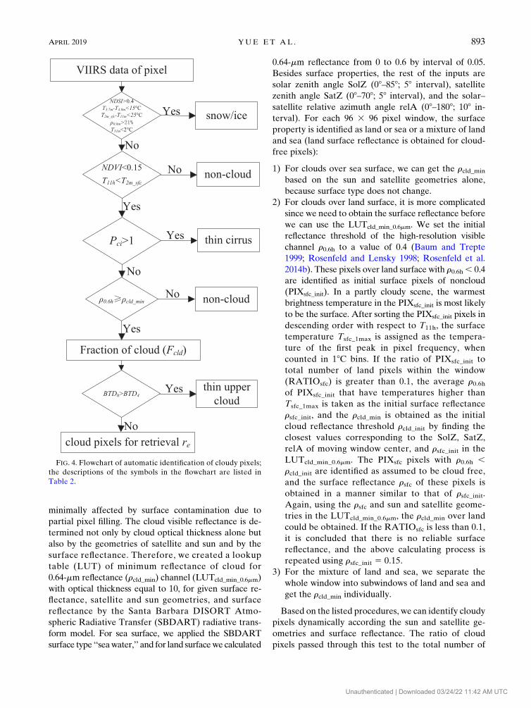
c. Cloud masking

The objective of this study is retrieving and map-

ping the properties of convective clouds at regional

scales. The retrieved cloud properties are based on

cloudy pixels. Therefore, the logic is, first, identify-

ing cloudy pixels; second, identifying the subset of

convective pixels. Sections 3c(1) and 3c(2) describe

the rejection of snow/ice pixels and surface contam-

ination pixels, section 3c(3) shows how to reject thin

cirrus, section 3c(4) describes how to identify opti-

cally thick cloud pixels with a lookup table, and

section 3c(5) shows how to reject overlapped thin

upper clouds by brightness temperature difference

(Fig. 4; Table 2).

1) REJECTION OF SNOW/ICE PIXELS

Since snow/ice surface and cloud pixels have similar

characteristics in the visible channel, snow/ice pixels must

be identified. The pixels of snow/ice are rejected by the

snow/ice surface detection method proposed by Godin

(2014) and Hutchison et al. (2013), which is similar to

currently VIIRS operational algorithms. The pixels that

meet the following five conditions simultaneously are

identified as snow/ice:

FIG. 2. Comparison of CCN concentration between the satellite-

retrieved measurements and the ground-based instrument mea-

surements (from Fig. 3 of Rosenfeld et al. 2016).

APRIL 2019 YUE ET AL . 891

Unauthenticated | Downloaded 03/24/22 11:42 AM UTC

1) The normalized difference snow index [NDSI 5(r0.56m 2 r1.6m)/(r0.56m 1 r1.6m)] exceeds 0.4,

2) T3.7m 2 T4.0m , 158C,3) r0.8m . 21%,

4) T11m , 28C, and5) T2m_sfc 2 T11m , 258C.

2) REJECTION OF SURFACE CONTAMINATION

PIXELS

For a better cloud mask, a threshold of normalized

differential vegetation index (NDVI) is calculated by

the reflectance at the 0.64- and 0.865-mm channels of

375-m resolution. Here we mask out a pixel if it is

‘‘greenish’’ and too warm, for example, NDVI . 0.15

(default value in this study) and the 11.45-mmbrightness

temperature T11h greater than the 2-m temperature

above the surface T2m_sfc from the FNL data.

3) REJECTION OF THIN CIRRUS PIXELS

Cirrus distorts the retrieved cloud microphysical prop-

erties. The 1.38-mm channel of 750-m resolution r1.38m is

particularly sensitive to highly elevated cirrus clouds, be-

cause the reflected radiation from the ground is absorbed

strongly by water vapor above the low-level cloud tops

(Meyer et al. 2004; Roskovensky and Liou 2003). The

cirrus parameter Pci developed by Roskovensky and

Liou (2003) is used for cirrus screening. It can be ex-

pressed as

Pci5 exp[RR3A1 (BTD

8.6-11m2B)], (6)

where RR is the ratio between r1.38m and r0.6h, A is

its scaling factor, BTD8.6-11m represents the moderate-

resolution 8.6–11-mm brightness temperature difference,

and B is the BTD8.6-11m offset. Here, A 5 2/(MRRclr 1sRRclr),B5MRRclr1 sRRclr1 2,whereM ands represent

the mean and standard deviation of RR and BTD8.6-11m

pixels for the clear sky [r0.6h , rcld_min; rcld_min is the

minimum reflectivity that can be considered to be cloud, as

described in section 3c(4)] in a moving window. Pixels with

Pci greater than 1 are identified as thin cirrus.

4) IDENTIFICATION OF OPTICALLY THICK CLOUDS

The satellite retrieved effective radius can be over-

estimated in thin and broken clouds because of surface

contamination (Coakley et al. 2005). This issue disap-

pears only when clouds are optically thick, for example,

nonbroken clouds with optical thickness greater than;8

in the visible spectrum (Rosenfeld et al. 2004). There-

fore, we need to identify the cloudy pixels that are deep

enough to retrieve reliable effective radius and are also

FIG. 3. Flowchart of the AMCC system.

892 JOURNAL OF APPL IED METEOROLOGY AND CL IMATOLOGY VOLUME 58

Unauthenticated | Downloaded 03/24/22 11:42 AM UTC

minimally affected by surface contamination due to

partial pixel filling. The cloud visible reflectance is de-

termined not only by cloud optical thickness alone but

also by the geometries of satellite and sun and by the

surface reflectance. Therefore, we created a lookup

table (LUT) of minimum reflectance of cloud for

0.64-mm reflectance (rcld_min) channel (LUTcld_min_0.6mm)

with optical thickness equal to 10, for given surface re-

flectance, satellite and sun geometries, and surface

reflectance by the Santa Barbara DISORT Atmo-

spheric Radiative Transfer (SBDART) radiative trans-

form model. For sea surface, we applied the SBDART

surface type ‘‘seawater,’’ and for land surfacewe calculated

0.64-mm reflectance from 0 to 0.6 by interval of 0.05.

Besides surface properties, the rest of the inputs are

solar zenith angle SolZ (08–858; 58 interval), satellite

zenith angle SatZ (08–708; 58 interval), and the solar–

satellite relative azimuth angle relA (08–1808; 108 in-

terval). For each 96 3 96 pixel window, the surface

property is identified as land or sea or a mixture of land

and sea (land surface reflectance is obtained for cloud-

free pixels):

1) For clouds over sea surface, we can get the rcld_min

based on the sun and satellite geometries alone,

because surface type does not change.

2) For clouds over land surface, it is more complicated

since we need to obtain the surface reflectance before

we can use the LUTcld_min_0.6mm. We set the initial

reflectance threshold of the high-resolution visible

channel r0.6h to a value of 0.4 (Baum and Trepte

1999; Rosenfeld and Lensky 1998; Rosenfeld et al.

2014b). These pixels over land surface with r0.6h, 0.4

are identified as initial surface pixels of noncloud

(PIXsfc_init). In a partly cloudy scene, the warmest

brightness temperature in the PIXsfc_init is most likely

to be the surface. After sorting the PIXsfc_init pixels in

descending order with respect to T11h, the surface

temperature Tsfc_1max is assigned as the tempera-

ture of the first peak in pixel frequency, when

counted in 18C bins. If the ratio of PIXsfc_init to

total number of land pixels within the window

(RATIOsfc) is greater than 0.1, the average r0.6hof PIXsfc_init that have temperatures higher than

Tsfc_1max is taken as the initial surface reflectance

rsfc_init, and the rcld_min is obtained as the initial

cloud reflectance threshold rcld_init by finding the

closest values corresponding to the SolZ, SatZ,

relA of moving window center, and rsfc_init in the

LUTcld_min_0.6mm. The PIXsfc pixels with r0.6h ,rcld_init are identified as assumed to be cloud free,

and the surface reflectance rsfc of these pixels is

obtained in a manner similar to that of rsfc_init.

Again, using the rsfc and sun and satellite geome-

tries in the LUTcld_min_0.6mm, the rcld_min over land

could be obtained. If the RATIOsfc is less than 0.1,

it is concluded that there is no reliable surface

reflectance, and the above calculating process is

repeated using rsfc_init 5 0.15.

3) For the mixture of land and sea, we separate the

whole window into subwindows of land and sea and

get the rcld_min individually.

Based on the listed procedures, we can identify cloudy

pixels dynamically according the sun and satellite ge-

ometries and surface reflectance. The ratio of cloud

pixels passed through this test to the total number of

FIG. 4. Flowchart of automatic identification of cloudy pixels;

the descriptions of the symbols in the flowchart are listed in

Table 2.

APRIL 2019 YUE ET AL . 893

Unauthenticated | Downloaded 03/24/22 11:42 AM UTC

pixels of the moving window is defined as the fraction of

cloud Fcld.

5) REJECTION OF MULTILAYER CLOUD PIXELS

Because brightness temperature of the colder cloud

pixels is affected by less water vapor absorption, the

difference of brightness temperature (BTD) of a thick

cloud should decrease with decreasing temperature.

However, when a thin cloud overlaps another clouds,

the brightness temperature and reflectance of these

cloud pixels are disturbed, and the BTD will be in-

creased (Inoue 1987). It is necessary to exclude those

cloud pixels that are optically thin or newly formed

water clouds over lower clouds because they lead to an

overestimate the BTD. Traditionally, BTD between 11

and 12mmwas used to reject such types of clouds (Inoue

1985). Rosenfeld et al. (2014b) have developed a

method to obtain BTD of 375-m resolution (BTDh)

because of the fact that 12.0mm is not available sepa-

rately at 375-m resolution of VIIRS. For a given T11h,

pixels that have passed through cloud mask of sections

3c(2) and 3c(3) (PIXcld) in this moving window are

sorted from small to large BTDh, and the BTDh of 25th-

percentile pixel number is marked as BTD4 for thisT11h.

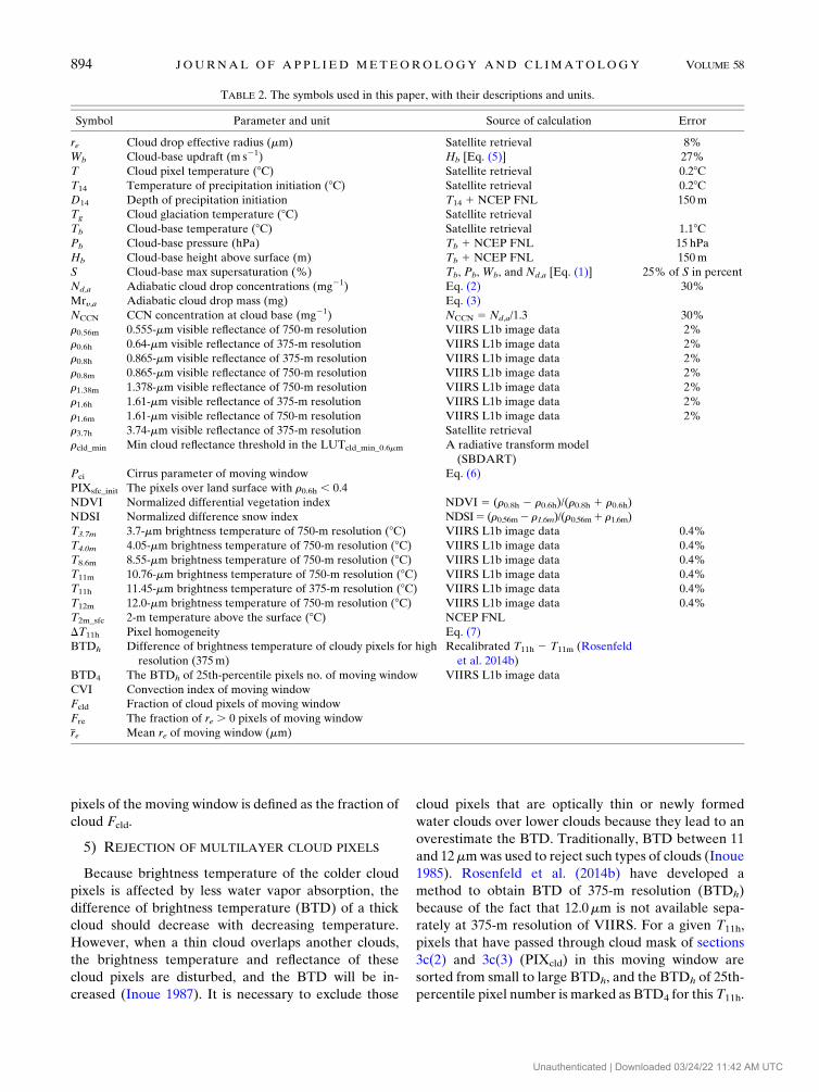
TABLE 2. The symbols used in this paper, with their descriptions and units.

Symbol Parameter and unit Source of calculation Error

re Cloud drop effective radius (mm) Satellite retrieval 8%

Wb Cloud-base updraft (m s21) Hb [Eq. (5)] 27%

T Cloud pixel temperature (8C) Satellite retrieval 0.28CT14 Temperature of precipitation initiation (8C) Satellite retrieval 0.28CD14 Depth of precipitation initiation T14 1 NCEP FNL 150m

Tg Cloud glaciation temperature (8C) Satellite retrieval

Tb Cloud-base temperature (8C) Satellite retrieval 1.18CPb Cloud-base pressure (hPa) Tb 1 NCEP FNL 15 hPa

Hb Cloud-base height above surface (m) Tb 1 NCEP FNL 150m

S Cloud-base max supersaturation (%) Tb, Pb, Wb, and Nd,a [Eq. (1)] 25% of S in percent

Nd,a Adiabatic cloud drop concentrations (mg21) Eq. (2) 30%

Mry,a Adiabatic cloud drop mass (mg) Eq. (3)

NCCN CCN concentration at cloud base (mg21) NCCN 5 Nd,a/1.3 30%

r0.56m 0.555-mm visible reflectance of 750-m resolution VIIRS L1b image data 2%

r0.6h 0.64-mm visible reflectance of 375-m resolution VIIRS L1b image data 2%

r0.8h 0.865-mm visible reflectance of 375-m resolution VIIRS L1b image data 2%

r0.8m 0.865-mm visible reflectance of 750-m resolution VIIRS L1b image data 2%

r1.38m 1.378-mm visible reflectance of 750-m resolution VIIRS L1b image data 2%

r1.6h 1.61-mm visible reflectance of 375-m resolution VIIRS L1b image data 2%

r1.6m 1.61-mm visible reflectance of 750-m resolution VIIRS L1b image data 2%

r3.7h 3.74-mm visible reflectance of 375-m resolution Satellite retrieval

rcld_min Min cloud reflectance threshold in the LUTcld_min_0.6mm A radiative transform model

(SBDART)

Pci Cirrus parameter of moving window Eq. (6)

PIXsfc_init The pixels over land surface with r0.6h , 0.4

NDVI Normalized differential vegetation index NDVI 5 (r0.8h 2 r0.6h)/(r0.8h 1 r0.6h)

NDSI Normalized difference snow index NDSI5 (r0.56m2 r1.6m)/(r0.56m1 r1.6m)

T3.7m 3.7-mm brightness temperature of 750-m resolution (8C) VIIRS L1b image data 0.4%

T4.0m 4.05-mm brightness temperature of 750-m resolution (8C) VIIRS L1b image data 0.4%

T8.6m 8.55-mm brightness temperature of 750-m resolution (8C) VIIRS L1b image data 0.4%

T11m 10.76-mm brightness temperature of 750-m resolution (8C) VIIRS L1b image data 0.4%

T11h 11.45-mm brightness temperature of 375-m resolution (8C) VIIRS L1b image data 0.4%

T12m 12.0-mm brightness temperature of 750-m resolution (8C) VIIRS L1b image data 0.4%

T2m_sfc 2-m temperature above the surface (8C) NCEP FNL

DT11h Pixel homogeneity Eq. (7)

BTDh Difference of brightness temperature of cloudy pixels for high

resolution (375m)

Recalibrated T11h 2 T11m (Rosenfeld

et al. 2014b)

BTD4 The BTDh of 25th-percentile pixels no. of moving window VIIRS L1b image data

CVI Convection index of moving window

Fcld Fraction of cloud pixels of moving window

Fre The fraction of re . 0 pixels of moving window

re Mean re of moving window (mm)

894 JOURNAL OF APPL IED METEOROLOGY AND CL IMATOLOGY VOLUME 58

Unauthenticated | Downloaded 03/24/22 11:42 AM UTC

The BTD4 values from the highest to the lowest T11h of

PIXcld are calculated. If BTD4 of a given T11h increases

with decreasing T11h, it is replaced by the monotonically

decreasing or invariant BTD4, which is obtained by the

linear interpolation of the nearest BTD4 with decreasing

T11h. Then, themonotonic reduction is enforced for BTD4

of PIXcld with decreasing T11h because only optically thin

upper clouds can increase BTD4 with decreasing T11h.

BTD4 dynamically obtained for each T11h of PIXcld in

each moving window is used as a criterion for identifying

overlapped thin upper clouds. If BTDh of a cloud pixel is

greater than BTD4 corresponding to its T11h, it will be

masked as overlapped thin upper clouds and rejected.

d. re retrieval

The 3.74-mm reflectance r3.7h is used to retrieve re from a

lookup table (LUTre; Kaufman and Nakajima 1993;

Rosenfeld and Lensky 1998) for the pixels identified as

cloudy using the cloud screening described above. The

LUTre is established for an effective radius of the water

cloud drop for given re, r3.7h, SolZ, SatZ, and relA

(Rosenfeld and Lensky 1998; Rosenfeld et al. 2014b). The

r3.7h of larger cloud particles decreases to near the channel

noise level, so the maximum size of re retrieved by this

method is 40mm. Note that, because the liquid phase re is

from 1 to 40mm in LUTre, the allowable retrieval solution

space for liquid clouds is limited to 1–40mm. The percent-

age of re . 0 pixels in the moving window Fre is obtained.

e. Convective clouds detection

The clouds addressed in this study are generated by

convection that is propelled by surface heating and

consist of convective clouds with flat base at the lifting

condensation level (LCL), as illustrated in Fig. 1.

Therefore, early-afternoon satellite overpasses are best

suited for observing such convective clouds over land.

Boundary layer convective clouds over ocean are much

less affected by the diurnal cycle.

Aircraft measurements of vertical microphysical pro-

files of such convective clouds show that cloud droplet reincreases monotonically from cloud base to top in de-

veloping convective clouds (Andreae et al. 2004; Konwar

et al. 2012; Prabha et al. 2011; Rosenfeld and Lensky

1998; Rosenfeld and Woodley 2000; Rosenfeld et al.

2006; Braga et al. 2017), and cloud-top re in different

stages of a vertically growing convective clouds cluster

are similar to the re of different heights within a single

convective cloud. This relationship of increasing re with

height is often ambiguous for nonconvective clouds,

however.As the temperature decreases with the increase

of height, the positive correlation between re and cloud-

top height is characterized by a corresponding negative

correlation between re and temperature. Thus, the T–re

relationships can be used to separate a mixture of layer

and convective clouds (Lensky and Rosenfeld 1997) and

applied to detection of convective clouds. The following

four steps are used to distinguish the convective and

nonconvective clouds in each moving window.

1) The analysis is done on a small runningwindow of 25325 5 625 pixels in a moving window, centered at the

tested cloudy pixel. The re and T values of an inner

small running window are sorted from high to low by

temperature. The correlation coefficient between the

sorted T and re is calculated as the relation of convec-

tion Rcv. A negative Rcv means increasing re with

decreasing T, which characterizes a convective cloud.

2) The Rcv of each cloud pixel in the moving window is

calculated.

3) The average value of Rcv of all cloud pixels in the

moving window is defined as the convection index

(CVI). If CVI. 0, the cloud in this moving window is

not a convective cloud.

4) The T–re profile of retrieval CCN is required to start

from cloud base. If most pixels of the moving window

are cloudy, there is a risk of insufficient documenta-

tion of the lower parts of the clouds. On the other

extreme, the T–re profile cannot be established with

too few cloud pixels with re. Aircraft measurements

show that the cloud base re is generally in the range of

1–8mm and that formation of precipitation-sized

drops occurs when re . 13mm (Braga et al. 2017;

Rosenfeld et al. 2006, 2008b). Too large of a mean re,

or re, indicates glaciated clouds. Therefore, a cloud is

identified as water convective cloud when CVI , 0

and Fcld , 95% and Fre . 0.4% and re , 35mm.

f. The retrieval of convective clouds basetemperature (Tb)

The cloud base is taken as the warmest cloudy pixel in a

moving window of convective clouds having different ex-

tent of vertical development above their base. Cloud base

is assumed to be at constant heights for convective clouds

over awell-mixed boundary layer.Under these conditions,

the warmest cloudy pixel can approximate Tb. Here the

algorithm of Zhu et al. (2014) is used for retrieving Tb.

It is based on pixel homogeneity DT11h, which is the

pixel homogeneity parameter of the 11.45-mm bright-

ness temperature T11h at 375-m resolution. The DT11h

was defined as (Rosenfeld et al. 2014b)

DT11h

51

4�4

i51

jT11hi

2T11h

j , (7)

where T11h is the brightness temperature average of

four pixels in the 375-m-resolution channel that reside

APRIL 2019 YUE ET AL . 895

Unauthenticated | Downloaded 03/24/22 11:42 AM UTC

within one 750-m-resolution pixel and T11hi is the T11h

of each these four points, respectively. If DT11h is

greater than the given threshold (DT11h_threshold5 18C),it is considering to be a mixed pixel by cloud and sur-

face. All of the pixels within the moving window are

sorted by their T11h. The warmest T11h for which a

percentile DT11h (P_DT11h) of DT11h ,DT11h_threshold is

considered to be theTb. A value ofP_DT11h5 30%was

found to be optimal (Zhu et al. 2014). This method was

validated against a combination of ceilometer and

sounding with Tb RMS error of 1.18C over the SGP site.

An error of 61.18C in Tb propagates to an ;5% error in

the retrieved Nd,a (Rosenfeld et al. 2016).

g. Identification the adiabatic re and retrieval CCN

Because the calculation of CCN is based on the

adiabatic assumption of convective clouds, it is very

important to identify the nearly adiabatic part from the

T–re profile of convective clouds. To avoid the in-

authentic re of nearby cloud base that is due to surface

contamination, the warmest temperature level is skip-

ped. If re . 15mm at their lowest 500m or re . 20mm

in the T–re profile, an underestimate of CCN would

otherwise result because of active cloud droplet coa-

lescence or heavily precipitation. Therefore, the ap-

proximate adiabatic part of convective clouds will be

searched from Tb 2 18C with re , 15mm at the lowest

500m to the T with the first re 5 20mm (T20mm). LWCa

should increase monotonically with decreasing tem-

perature or increasing droplet mass in an ideal adia-

batic condition. Therefore, the slope of linear best fit is

calculated between LWCa and Mry,a from Tb 2 18C to

each T with T, T20mm, and the fit is forced to Mry,a 5 0

at LWCa 5 0. The maximum slope is the end of adia-

batic process and the respectiveNd,a [Eq. (2)]. Because

of the mean deviation from the extreme inhomoge-

neous mixing assumption, the NCCN is equal to Nd,a

divided by 1.3 (Freud et al. 2011; Rosenfeld et al.

2014a, 2016).

h. Quality control and display

A postprocessing procedure is to eliminate the

convective clouds that are not suitable for retrieval

boundary layer CCN. These cloud bases are elevated

and, consequently, not coupled to the surface. The

filtering of such elevated clouds is made mainly by

analyzing the spatial distribution of Tb. Each Tb is

compared with all Tb in the box area of 28 3 28 latitudeand longitude that is centered on itself. The median

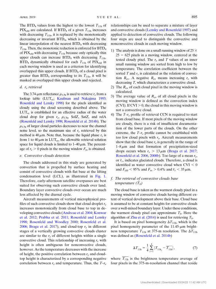
FIG. 5. Day-natural RGB composite image of 375-m resolution

(red: r1.6h; green: r0.8h; blue: r0.6h), for which the satellite zenith

angle is between 2208 and 508 and which was acquired around

1930 UTC 30 Jul 2016. In this color scheme, vegetation, water

clouds with small droplets, snow and ice clouds, bare ground, and

the ocean appear greenish, whitish, cyan, brown, and black, re-

spectively (Lensky and Rosenfeld 2008).

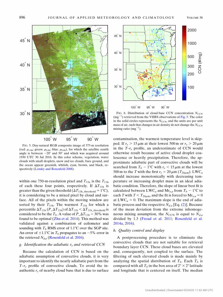
FIG. 6. Distribution of cloud-base CCN concentration NCCN

(mg21) retrieved from the VIIRS observations of Fig. 5. The color

in the solid circles represents the NCCN, and the units are per unit

mass of air, such that changes in air density do not change theNCCN

mixing ratio (mg21).

896 JOURNAL OF APPL IED METEOROLOGY AND CL IMATOLOGY VOLUME 58

Unauthenticated | Downloaded 03/24/22 11:42 AM UTC

of Tb, or Tb,m, the 75th-percentile terrain heightH75th,

and the standard deviation of terrain height Hstd are

calculated in this area. If H75th , Hstd, the moving

window is identified as occurring over flat land. If

jTb 2 Tb,mj. 38C over the ocean or flat land, the Tb is

considered to be an outlier and is filtered out. This

procedure is not applied over rough terrain (H75th .Hstd) that may cause large gradients in Tb. Isolated

windows of marine clouds are defined as those that

have less than 10 moving windows in the range of 18 oflatitude and longitude and are filtered if their Tb is 58Cwarmer or colder than the NCEP FNL data computed

LCL temperature TLCL for the examined window. By

applying these criteria, a large portion of the elevated

cloudy windows is filtered out. The criteria were tuned

over homogeneous areas with no obvious reasons for

changes in aerosols or meteorological conditions.

4. Applications

The output parameters include the latitude and longi-

tude, Tb, Hb, T14, D14, Tg, NCCN, S, and other auxiliary

analysis data such as temperature, pressure, relative hu-

midity, and height profile from the FNL data (Table 1).

Then, the map of the microphysical properties is dis-

played graphically.

The applied scene is one SNPP/VIIRS granule of

satellite zenith angle between 2208 and 508 acquiredaround 1930 UTC 30 July 2016, covering an area from

238 to 478N and from 1188 to 828W. The ‘‘day natural’’

red–green–blue (RGB) composite image (Lensky and

Rosenfeld 2008) of 375-m resolution showed some

deep convective cloud clusters located both inland and

along the southern coast (Fig. 5). Shallow convective

clouds are found in most regions except for more arid

parts of the north-central United States.

The distribution of cloud base NCCN (Fig. 6) with

their corresponding S (Fig. 7) shows that the higher

NCCN occurred over the coastal plain, especially above

big cities such as Houston and Dallas in Texas, Kansas

City (Missouri), and Topeka, Kansas (numbers 1–4 of

the black small circles in Fig. 6). Above these cities,

NCCN are very high (exceeding 1000mg21) probably

because of air pollution, and the corresponding S is

lower than 0.2%. Areas inland far from pollution

sources exhibit relatively low NCCN of about 200–

300mg21, and the corresponding S is about 0.3%. The

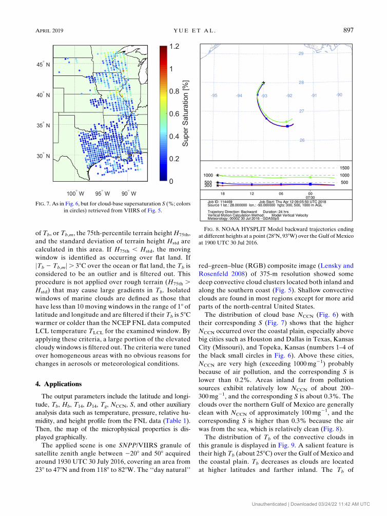
clouds over the northern Gulf of Mexico are generally

clean with NCCN of approximately 100mg21, and the

corresponding S is higher than 0.3% because the air

was from the sea, which is relatively clean (Fig. 8).

The distribution of Tb of the convective clouds in

this granule is displayed in Fig. 9. A salient feature is

their high Tb (about 258C) over the Gulf of Mexico and

the coastal plain. Tb decreases as clouds are located

at higher latitudes and farther inland. The Tb of

FIG. 7. As in Fig. 6, but for cloud-base supersaturation S (%; colors

in circles) retrieved from VIIRS of Fig. 5.

FIG. 8. NOAA HYSPLIT Model backward trajectories ending

at different heights at a point (288N, 938W) over theGulf ofMexico

at 1900 UTC 30 Jul 2016.

APRIL 2019 YUE ET AL . 897

Unauthenticated | Downloaded 03/24/22 11:42 AM UTC

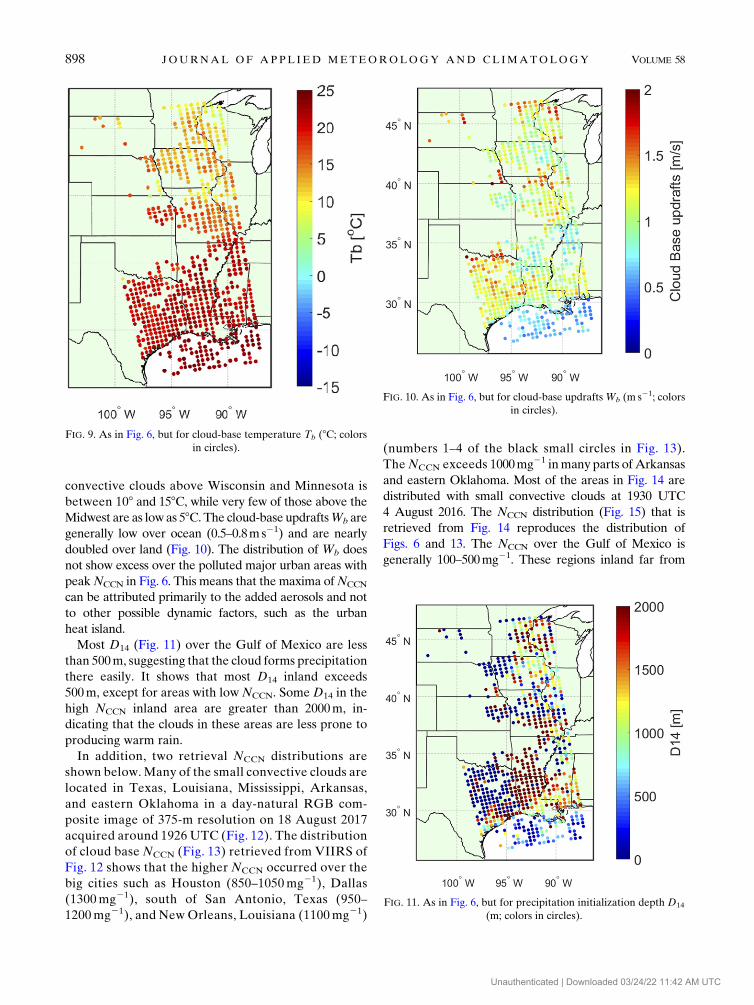
convective clouds above Wisconsin and Minnesota is

between 108 and 158C, while very few of those above the

Midwest are as low as 58C.The cloud-base updraftsWb are

generally low over ocean (0.5–0.8ms21) and are nearly

doubled over land (Fig. 10). The distribution of Wb does

not show excess over the polluted major urban areas with

peakNCCN in Fig. 6. This means that the maxima ofNCCN

can be attributed primarily to the added aerosols and not

to other possible dynamic factors, such as the urban

heat island.

Most D14 (Fig. 11) over the Gulf of Mexico are less

than 500m, suggesting that the cloud forms precipitation

there easily. It shows that most D14 inland exceeds

500m, except for areas with low NCCN. SomeD14 in the

high NCCN inland area are greater than 2000m, in-

dicating that the clouds in these areas are less prone to

producing warm rain.

In addition, two retrieval NCCN distributions are

shown below.Many of the small convective clouds are

located in Texas, Louisiana, Mississippi, Arkansas,

and eastern Oklahoma in a day-natural RGB com-

posite image of 375-m resolution on 18 August 2017

acquired around 1926 UTC (Fig. 12). The distribution

of cloud base NCCN (Fig. 13) retrieved from VIIRS of

Fig. 12 shows that the higher NCCN occurred over the

big cities such as Houston (850–1050mg21), Dallas

(1300mg21), south of San Antonio, Texas (950–

1200mg21), and New Orleans, Louisiana (1100mg21)

(numbers 1–4 of the black small circles in Fig. 13).

TheNCCN exceeds 1000mg21 inmany parts of Arkansas

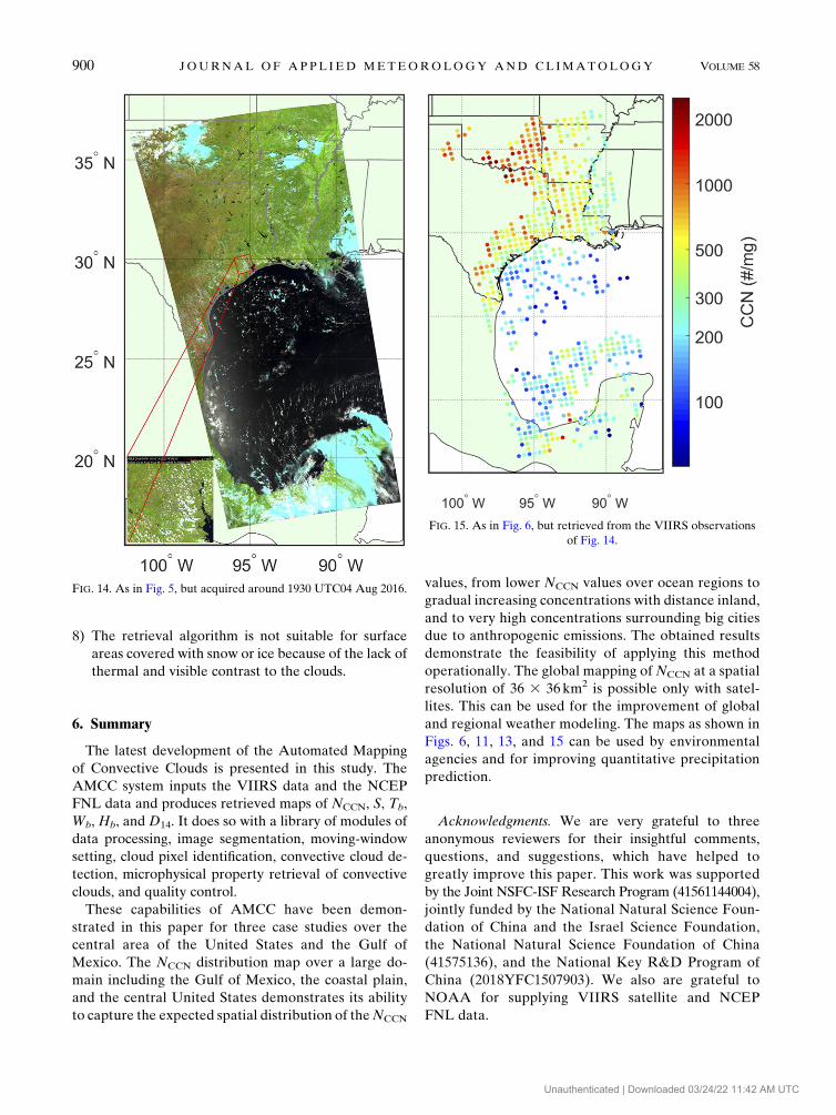
and eastern Oklahoma. Most of the areas in Fig. 14 are

distributed with small convective clouds at 1930 UTC

4 August 2016. The NCCN distribution (Fig. 15) that is

retrieved from Fig. 14 reproduces the distribution of

Figs. 6 and 13. The NCCN over the Gulf of Mexico is

generally 100–500mg21. These regions inland far from

FIG. 9. As in Fig. 6, but for cloud-base temperature Tb (8C; colorsin circles).

FIG. 10. As in Fig. 6, but for cloud-base updraftsWb (m s21; colors

in circles).

FIG. 11. As in Fig. 6, but for precipitation initialization depth D14

(m; colors in circles).

898 JOURNAL OF APPL IED METEOROLOGY AND CL IMATOLOGY VOLUME 58

Unauthenticated | Downloaded 03/24/22 11:42 AM UTC

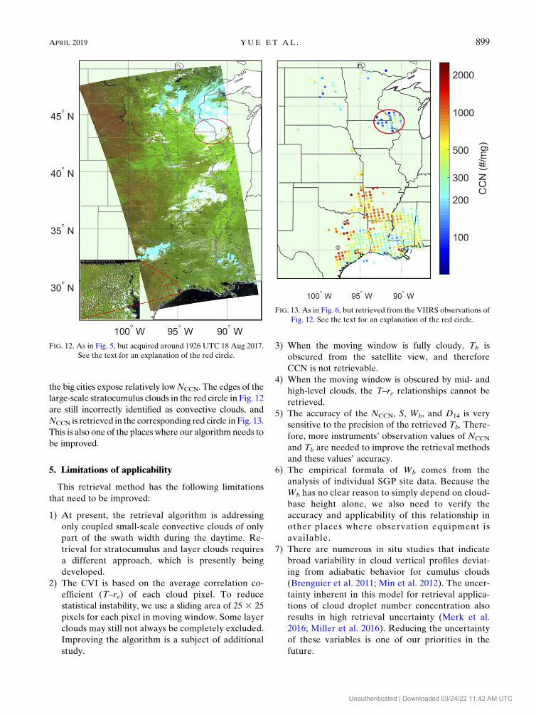
the big cities expose relatively lowNCCN. The edges of the

large-scale stratocumulus clouds in the red circle in Fig. 12

are still incorrectly identified as convective clouds, and

NCCN is retrieved in the corresponding red circle inFig. 13.

This is also one of the places where our algorithm needs to

be improved.

5. Limitations of applicability

This retrieval method has the following limitations

that need to be improved:

1) At present, the retrieval algorithm is addressing

only coupled small-scale convective clouds of only

part of the swath width during the daytime. Re-

trieval for stratocumulus and layer clouds requires

a different approach, which is presently being

developed.

2) The CVI is based on the average correlation co-

efficient (T–re) of each cloud pixel. To reduce

statistical instability, we use a sliding area of 25 3 25

pixels for each pixel in moving window. Some layer

clouds may still not always be completely excluded.

Improving the algorithm is a subject of additional

study.

3) When the moving window is fully cloudy, Tb is

obscured from the satellite view, and therefore

CCN is not retrievable.

4) When the moving window is obscured by mid- and

high-level clouds, the T–re relationships cannot be

retrieved.

5) The accuracy of the NCCN, S, Wb, and D14 is very

sensitive to the precision of the retrieved Tb. There-

fore, more instruments’ observation values of NCCN

and Tb are needed to improve the retrieval methods

and these values’ accuracy.

6) The empirical formula of Wb comes from the

analysis of individual SGP site data. Because the

Wb has no clear reason to simply depend on cloud-

base height alone, we also need to verify the

accuracy and applicability of this relationship in

other places where observation equipment is

available.

7) There are numerous in situ studies that indicate

broad variability in cloud vertical profiles deviat-

ing from adiabatic behavior for cumulus clouds

(Brenguier et al. 2011; Min et al. 2012). The uncer-

tainty inherent in this model for retrieval applica-

tions of cloud droplet number concentration also

results in high retrieval uncertainty (Merk et al.

2016; Miller et al. 2016). Reducing the uncertainty

of these variables is one of our priorities in the

future.

FIG. 12. As in Fig. 5, but acquired around 1926 UTC 18 Aug 2017.

See the text for an explanation of the red circle.

FIG. 13. As in Fig. 6, but retrieved from the VIIRS observations of

Fig. 12. See the text for an explanation of the red circle.

APRIL 2019 YUE ET AL . 899

Unauthenticated | Downloaded 03/24/22 11:42 AM UTC

8) The retrieval algorithm is not suitable for surface

areas covered with snow or ice because of the lack of

thermal and visible contrast to the clouds.

6. Summary

The latest development of the Automated Mapping

of Convective Clouds is presented in this study. The

AMCC system inputs the VIIRS data and the NCEP

FNL data and produces retrieved maps of NCCN, S, Tb,

Wb, Hb, and D14. It does so with a library of modules of

data processing, image segmentation, moving-window

setting, cloud pixel identification, convective cloud de-

tection, microphysical property retrieval of convective

clouds, and quality control.

These capabilities of AMCC have been demon-

strated in this paper for three case studies over the

central area of the United States and the Gulf of

Mexico. The NCCN distribution map over a large do-

main including the Gulf of Mexico, the coastal plain,

and the central United States demonstrates its ability

to capture the expected spatial distribution of theNCCN

values, from lower NCCN values over ocean regions to

gradual increasing concentrations with distance inland,

and to very high concentrations surrounding big cities

due to anthropogenic emissions. The obtained results

demonstrate the feasibility of applying this method

operationally. The global mapping of NCCN at a spatial

resolution of 36 3 36 km2 is possible only with satel-

lites. This can be used for the improvement of global

and regional weather modeling. The maps as shown in

Figs. 6, 11, 13, and 15 can be used by environmental

agencies and for improving quantitative precipitation

prediction.

Acknowledgments. We are very grateful to three

anonymous reviewers for their insightful comments,

questions, and suggestions, which have helped to

greatly improve this paper. This work was supported

by the Joint NSFC-ISF Research Program (41561144004),

jointly funded by the National Natural Science Foun-

dation of China and the Israel Science Foundation,

the National Natural Science Foundation of China

(41575136), and the National Key R&D Program of

China (2018YFC1507903). We also are grateful to

NOAA for supplying VIIRS satellite and NCEP

FNL data.

FIG. 14. As in Fig. 5, but acquired around 1930 UTC04 Aug 2016.

FIG. 15. As in Fig. 6, but retrieved from the VIIRS observations

of Fig. 14.

900 JOURNAL OF APPL IED METEOROLOGY AND CL IMATOLOGY VOLUME 58

Unauthenticated | Downloaded 03/24/22 11:42 AM UTC

REFERENCES

Andreae, M. O., 2009: Correlation between cloud condensation

nuclei concentration and aerosol optical thickness in remote

and polluted regions. Atmos. Chem. Phys., 9, 543–556, https://

doi.org/10.5194/acp-9-543-2009.

——, and D. Rosenfeld, 2008: Aerosol–cloud–precipitation in-

teractions. Part 1. The nature and sources of cloud-active

aerosols. Earth-Sci. Rev., 89, 13–41, https://doi.org/10.1016/

j.earscirev.2008.03.001.

——, ——, P. Artaxo, A. A. Costa, G. P. Frank, K. M. Longo,

and M. A. F. Silva-Dias, 2004: Smoking rain clouds over the

Amazon. Science, 303, 1337–1342, https://doi.org/10.1126/

science.1092779.

Baum, B. A., and Q. Trepte, 1999: A grouped threshold approach

for scene identification in AVHRR imagery. J. Atmos. Oceanic

Technol., 16, 793–800, https://doi.org/10.1175/1520-0426(1999)

016,0793:AGTAFS.2.0.CO;2.

Beals, M. J., J. P. Fugal, R. A. Shaw, J. Lu, S. M. Spuler, and J. L.

Stith, 2015: Holographic measurements of inhomogeneous

cloud mixing at the centimeter scale. Science, 350, 87–90,

https://doi.org/10.1126/science.aab0751.

Braga, R. C., and Coauthors, 2017: Further evidence for CCN

aerosol concentrations determining the height of warm rain

and ice initiation in convective clouds over the Amazon

basin. Atmos. Chem. Phys., 17, 14 433–14 456, https://doi.org/

10.5194/acp-17-14433-2017.

Brenguier, J. L., F. Burnet, and O. Geoffroy, 2011: Cloud optical

thickness and liquid water path—Does the k coefficient vary

with droplet concentration? Atmos. Chem. Phys., 11, 9771–

9786, https://doi.org/10.5194/acp-11-9771-2011.

Burnet, F., and J.-L. Brenguier, 2007: Observational study of

the entrainment-mixing process in warm convective clouds.

J. Atmos. Sci., 64, 1995–2011, https://doi.org/10.1175/

JAS3928.1.

Coakley, J. A., M. A. Friedman, and W. R. Tahnk, 2005: Retrieval

of cloud properties for partly cloudy imager pixels. J. Atmos.

Oceanic Technol., 22, 3–17, https://doi.org/10.1175/JTECH-

1681.1.

Davis, A. B., andA.Marshak, 2010: Solar radiation transport in the

cloudy atmosphere: A 3D perspective on observations and

climate impacts. Rep. Prog. Phys., 73, 026801, https://doi.org/

10.1088/0034-4885/73/2/026801.

Freud, E., and D. Rosenfeld, 2012: Linear relation between con-

vective cloud drop number concentration and depth for rain

initiation. J. Geophys. Res., 117, D02207, https://doi.org/

10.1029/2011JD016457.

——, J. Ström, D. Rosenfeld, P. Tunved, and E. Swietlicki, 2008:

Anthropogenic aerosol effects on convective cloud micro-

physical properties in southern Sweden. Tellus, 60B, 286–297,

https://doi.org/10.1111/j.1600-0889.2007.00337.x.

——, D. Rosenfeld, and J. R. Kulkarni, 2011: Resolving both

entrainment-mixing and number of activated CCN in deep

convective clouds. Atmos. Chem. Phys., 11, 12 887–12 900,

https://doi.org/10.5194/acp-11-12887-2011.

Godin,R., 2014: Joint polar satellite system (JPSS)VIIRS cloudmask

(VCM) algorithm theoretical basis document (ATBD). JPSS

Ground Project Code 474 Rep. 474-00033 (Revision E), 117 pp.,

https://www.star.nesdis.noaa.gov/JPSS/documents/ATBD/

D0001-M01-S01-011_JPSS_ATBD_VIIRS-Cloud-Mask_E.pdf.

Hillger, D., and Coauthors, 2013: First-light imagery from Suomi

NPP VIIRS. Bull. Amer. Meteor. Soc., 94, 1019–1029, https://

doi.org/10.1175/BAMS-D-12-00097.1.

Hutchison, K. D., B. D. Iisager, and R. L. Mahoney, 2013: En-

hanced snow and ice identification with the VIIRS cloud mask

algorithm. Remote Sens. Lett., 4, 929–936, https://doi.org/

10.1080/2150704X.2013.815381.

Inoue, T., 1985: On the temperature and effective emissivity de-

termination of semi-transparent cirrus clouds by bi-spectral

measurements in the 10mm window region. J. Meteor. Soc.

Japan Ser. II, 63, 88–99.

——, 1987: An instantaneous delineation of convective rainfall areas

using split window data of NOAA-7AVHRR. J. Meteor. Soc.

Japan Ser. II, 65, 469–481, https://www.jstage.jst.go.jp/article/

jmsj1965/65/3/65_3_469/_pdf/-char/en.

Kaufman, Y. J., and T. Nakajima, 1993: Effect of amazon smoke on

cloud microphysics and albedo-analysis from satellite imag-

ery. J. Appl. Meteor., 32, 729–744, https://doi.org/10.1175/

1520-0450(1993)032,0729:EOASOC.2.0.CO;2.

Konwar, M., R. S. Maheskumar, J. R. Kulkarni, E. Freud, B. N.

Goswami, and D. Rosenfeld, 2012: Aerosol control on depth

of warm rain in convective clouds. J. Geophys. Res., 117,

D13204, https://doi.org/10.1029/2012JD017585.

Kopp, T. J., and Coauthors, 2014: The VIIRS Cloud Mask: Prog-

ress in the first year of S-NPP toward a common cloud de-

tection scheme. J. Geophys. Res. Atmos., 119, 2441–2456,

https://doi.org/10.1002/2013JD020458.

Lensky, I. M., andD. Rosenfeld, 1997: Estimation of precipitation area

and rain intensity based on the microphysical properties retrieved

fromNOAAAVHRRdata. J. Appl.Meteor., 36, 234–242, https://

doi.org/10.1175/1520-0450(1997)036,0234:EOPAAR.2.0.CO;2.

——, and ——, 2006: The time–space exchangeability of satellite

retrieved relations between cloud top temperature and parti-

cle effective radius.Atmos. Chem. Phys., 6, 2887–2894, https://

doi.org/10.5194/acp-6-2887-2006.

——, and ——, 2008: Clouds–aerosols–precipitation satellite

analysis tool (CAPSAT). Atmos. Chem. Phys., 8, 6739–6753,

https://doi.org/10.5194/acp-8-6739-2008.

Marshak, A., and A. B. Davis, Eds., 2005: 3D Radiative Transfer in

CloudyAtmospheres. Springer, https://doi.org/10.1007/3-540-28519-9.

——, S.Platnick, T.Várnai,G.Wen, andR.F. Cahalan, 2006: Impact

of three-dimensional radiative effects on satellite retrievals of

cloud droplet sizes. J. Geophys. Res. Atmos., 111, D09207,

https://doi.org/10.1029/2005JD006686.

Merk, D., H. Deneke, B. Pospichal, and P. Seifert, 2016: In-

vestigation of the adiabatic assumption for estimating cloud

micro- and macrophysical properties from satellite and ground

observations. Atmos. Chem. Phys., 16, 933–952, https://doi.org/

10.5194/acp-16-933-2016.

Meyer, K., Y. Ping, and G. Bo-Cai, 2004: Optical thickness of

tropical cirrus clouds derived from the MODIS 0.66 and

1.375mm channels. IEEE Trans. Geosci. Remote, 42, 833–841,

https://doi.org/10.1109/TGRS.2003.818939.

Miller,D. J., Z. Zhang,A. S.Ackerman, S. Platnick, andB.A.Baum,

2016: The impact of cloud vertical profile on liquid water path

retrieval based on the bispectral method: A theoretical study

based on large-eddy simulations of shallow marine boundary

layer clouds. J. Geophys. Res. Atmos., 121, 4122–4141, https://

doi.org/10.1002/2015JD024322.

Min, Q., and Coauthors, 2012: Comparison of MODIS cloud mi-

crophysical properties with in-situ measurements over the

southeast Pacific. Atmos. Chem. Phys., 12, 11 261–11 273,

https://doi.org/10.5194/acp-12-11261-2012.

Paluch, I. R., 1979: The entrainment mechanism in Colorado cu-

muli. J. Atmos. Sci., 36, 2467–2478, https://doi.org/10.1175/

1520-0469(1979)036,2467:TEMICC.2.0.CO;2.

APRIL 2019 YUE ET AL . 901

Unauthenticated | Downloaded 03/24/22 11:42 AM UTC

Pinsky, M., A. Khain, I. Mazin, and A. Korolev, 2012: Analytical

estimation of droplet concentration at cloud base. J. Geophys.

Res., 117, D18211, https://doi.org/10.1029/2012JD017753.

Prabha, T. V., A. Khain, R. S. Maheshkumar, G. Pandithurai, J. R.

Kulkarni, M. Konwar, and B. N. Goswami, 2011: Microphysics

of premonsoon and monsoon clouds as seen from in situ mea-

surements during the Cloud Aerosol Interaction and Pre-

cipitation Enhancement Experiment (CAIPEEX). J. Atmos.

Sci., 68, 1882–1901, https://doi.org/10.1175/2011JAS3707.1.

Quaas, J., B. Stevens, P. Stier, and U. Lohmann, 2010: Interpreting

the cloud cover–aerosol optical depth relationship found in

satellite data using a general circulation model. Atmos. Chem.

Phys., 10, 6129–6135, https://doi.org/10.5194/acp-10-6129-2010.

Rosenfeld, D., 1999: TRMM observed first direct evidence of

smoke from forest fires inhibiting rainfall.Geophys. Res. Lett.,

26, 3105–3108, https://doi.org/10.1029/1999GL006066.

——, 2018: Cloud–aerosol–precipitation interactions based of sat-

ellite retrieved vertical profiles of cloud microstructure. Re-

mote Sensing of Aerosols, Clouds, and Precipitation, Y. Hu,

A.Kokhanovsky, and J.Wang, Eds., Elsevier, 129–152, https://

doi.org/10.1016/B978-0-12-810437-8.00006-2.

——, and G. Gutman, 1994: Retrieving microphysical properties

near the tops of potential rain clouds by multispectral analysis

of AVHRR data. Atmos. Res., 34, 259–283, https://doi.org/

10.1016/0169-8095(94)90096-5.

——, and I. M. Lensky, 1998: Satellite-based insights into pre-

cipitation formation processes in continental and maritime

convective clouds. Bull. Amer. Meteor. Soc., 79, 2457–

2476, https://doi.org/10.1175/1520-0477(1998)079,2457:

SBIIPF.2.0.CO;2.

——, and W. L. Woodley, 2000: Deep convective clouds with sus-

tained supercooled liquid water down to237.58C.Nature, 405,

440–442, https://doi.org/10.1038/35013030.

——, E. Cattani, S. Melani, and V. Levizzani, 2004: Considerations

on daylight operation of 1.6- versus 3.7-mmchannel onNOAA

and METOP satellites. Bull. Amer. Meteor. Soc., 85, 873–882,

https://doi.org/10.1175/BAMS-85-6-873.

——,W. L.Woodley, T. W. Krauss, and V.Makitov, 2006: Aircraft

microphysical documentation from cloud base to anvils of

hailstorm feeder clouds in Argentina. J. Appl. Meteor. Cli-

matol., 45, 1261–1281, https://doi.org/10.1175/JAM2403.1.

——, ——, A. Lerner, G. Kelman, and D. T. Lindsey, 2008a:

Satellite detection of severe convective storms by their re-

trieved vertical profiles of cloud particle effective radius

and thermodynamic phase. J. Geophys. Res., 113, D04208,

https://doi.org/10.1029/2007JD008600.

——,——,D. Axisa, E. Freud, J. G. Hudson, andA. Givati, 2008b:

Aircraft measurements of the impacts of pollution aerosols on

clouds and precipitation over the Sierra Nevada. J. Geophys.

Res., 113, D15203, https://doi.org/10.1029/2007JD009544.

——, and Coauthors, 2011: Glaciation temperatures of convective

clouds ingesting desert dust, air pollution and smoke from

forest fires. Geophys. Res. Lett., 38, L21804, https://doi.org/

10.1029/2011GL049423.

——, B. Fischman, Y. Zheng, T. Goren, and D. Giguzin, 2014a:

Combined satellite and radar retrievals of drop concentration

and CCN at convective cloud base. Geophys. Res. Lett., 41,

3259–3265, https://doi.org/10.1002/2014GL059453.

——,G. Liu, X. Yu, Y. Zhu, J. Dai, X. Xu, and Z. Yue, 2014b: High

resolution (375m) cloud microstructure as seen from the

NPP/VIIRS satellite imager. Atmos. Chem. Phys., 14, 2479–

2496, https://doi.org/10.5194/acp-14-2479-2014.

——, and Coauthors, 2016: Satellite retrieval of cloud condensa-

tion nuclei concentrations by using clouds as CCN chambers.

Proc. Natl. Acad. Sci. USA, 113, 5828–5834, https://doi.org/

10.1073/pnas.1514044113.

Roskovensky, J. K., and K. N. Liou, 2003: Detection of thin cirrus

from 1.38mm/0.65mm reflectance ratio combined with 8.6–

11mm brightness temperature difference.Geophys. Res. Lett.,

30, 1985, https://doi.org/10.1029/2003GL018135.

Stevens, B., and G. Feingold, 2009: Untangling aerosol effects on

clouds and precipitation in a buffered system. Nature, 461,

607–613, https://doi.org/10.1038/nature08281.

Stier, P., 2016: Limitations of passive remote sensing to constrain

global cloud condensation nuclei. Atmos. Chem. Phys., 16,

6595–6607, https://doi.org/10.5194/acp-16-6595-2016.

Várnai, T., and A. Marshak, 2009: MODIS observations of en-

hanced clear sky reflectance near clouds. Geophys. Res. Lett.,

36, L06807, https://doi.org/10.1029/2008GL037089.

Yuan, T., J. V. Martins, Z. Li, and L. A. Remer, 2010: Estimating

glaciation temperature of deep convective clouds with remote

sensing data. Geophys. Res. Lett., 37, L08808, https://doi.org/

10.1029/2010GL042753.

Zhang, Z., A. S.Ackerman,G. Feingold, S. Platnick, R. Pincus, and

H. Xue, 2012: Effects of cloud horizontal inhomogeneity and

drizzle on remote sensing of cloud droplet effective radius:

Case studies based on large-eddy simulations. J. Geophys.

Res., 117, D19208, https://doi.org/10.1029/2012JD017655.

Zheng, Y., and D. Rosenfeld, 2015: Linear relation between con-

vective cloud base height and updrafts and application to

satellite retrievals.Geophys. Res. Lett., 42, 6485–6491, https://doi.org/10.1002/2015GL064809.

——, ——, and Z. Li, 2015: Satellite inference of thermals and

cloud-base updraft speeds based on retrieved surface and

cloud-base temperatures. J. Atmos. Sci., 72, 2411–2428, https://doi.org/10.1175/JAS-D-14-0283.1.

——, ——, and ——, 2016: Quantifying cloud base updraft speeds

of marine stratocumulus from cloud top radiative cooling.

Geophys. Res. Lett., 43, 11 407–11 413, https://doi.org/10.1002/2016GL071185.

Zhu, Y., D. Rosenfeld, X. Yu, G. Liu, J. Dai, and X. Xu, 2014:

Satellite retrieval of convective cloud base temperature based

on the NPP/VIIRS Imager. Geophys. Res. Lett., 41, 1308–1313, https://doi.org/10.1002/2013GL058970.

——,——,——, and Z. Li, 2015: Separating aerosol microphysical

effects and satellite measurement artifacts of the relationships

between warm rain onset height and aerosol optical depth.

J. Geophys. Res., 120, 7726–7736, https://doi.org/10.1002/

2015JD023547.

902 JOURNAL OF APPL IED METEOROLOGY AND CL IMATOLOGY VOLUME 58

Unauthenticated | Downloaded 03/24/22 11:42 AM UTC