Autoencoding Neural Networks as Musical Audio Synthesizers

The Cooper Union

Albert Nerken School of Engineering

Electrical Engineering

Autoencoding Neural Networks as MusicalAudio Synthesizers

Joseph T. Colonel

November 2018

A thesis submitted in partial fulfillment of the requirements for the degree ofMaster of Engineering

Advised by Professor Sam Keene

Acknowledgements

I would like to thank Sam Keene for his continuing guidance, faith in my efforts, and

determination to see me pursue studies in machine learning and audio.

I would like to thank Christopher Curro for seeing this work through its infancy.

I would like to thank the Cooper Union’s Dean of Engineering’s office, Career Development

Services, and Electrical Engineering department for funding my trip to DAFx 2018 to present

my thesis work.

Special thanks to Yonatan Katzelnik, Benjamin Sterling, Ella de Buck, Richard Yi, George

Ho, Jonathan Tronolone, Alex Hu, and Ingrid Burrington for stewarding this work and

stretching it beyond what I thought possible.

Finally I would like to thank my family and friends for their nonstop love and support. I

would be nowhere without you all.

i

Abstract

Methodology for designing and training neural network autoencoders for applications in-

volving musical audio is proposed. Two topologies are presented: an autoencoding sound

effect that transforms the spectral properties of an input signal (named ANNe); and an au-

toencoding synthesizer that generates audio based on activations of the autoencoder’s latent

space (named CANNe). In each case the autoencoder is trained to compress and reconstruct

magnitude short-time Fourier transform frames. When an autoencoder is trained in such

a manner it constructs a latent space that contains higher-order representations of musical

audio that a musician can manipulate.

With ANNe, a seven layer deep autoencoder is trained on a corpus of improvisations on

a MicroKORG synthesizer. The musician selects an input sound to be transformed. The

spectrogram of this input sound is mapped to the autoencoder’s latent space, where the

musician can alter it with multiplicative gain constants. The newly transformed latent

representation is passed to the decoder, and an inverse Short-Time Fourier Transform is

taken using the original signal’s phase response to produce audio.

With CANNe, a seventeen layer deep autoencoder is trained on a corpus of C Major scales

played on a MicroKORG synthesizer. The autoencoder produces a spectrogram by activat-

ing its smallest hidden layer, and a phase response is calculated using phase gradient heap

integration. Taking an inverse short-time Fourier transform produces the audio signal.

Both algorithms are lightweight compared to current state-of-the-art audio-producing ma-

chine learning algorithms. Metrics related to the autoencoders’ performance are measured

using various corpora of audio recorded from a MicroKORG synthesizer. Python implemen-

tations of both autoencoders are presented.

ii

Contents

Acknowledgements i

Abstract ii

1 Introduction 1

2 Background 3

2.1 Audio Signal Processing . . . . . . . . . . . . . . . . . . . . . . . . . . . . . 3

2.1.1 Analogue to Digital Conversion . . . . . . . . . . . . . . . . . . . . . 3

2.1.2 Short-Time Fourier Transform . . . . . . . . . . . . . . . . . . . . . . 4

2.2 Musical Audio . . . . . . . . . . . . . . . . . . . . . . . . . . . . . . . . . . . 10

2.2.1 Western Music Theory . . . . . . . . . . . . . . . . . . . . . . . . . . 11

2.2.2 Timbre . . . . . . . . . . . . . . . . . . . . . . . . . . . . . . . . . . . 12

2.2.3 Traditional Methods of Musical Audio Synthesis . . . . . . . . . . . . 12

2.3 Machine Learning . . . . . . . . . . . . . . . . . . . . . . . . . . . . . . . . . 13

2.3.1 Definition . . . . . . . . . . . . . . . . . . . . . . . . . . . . . . . . . 13

iii

CONTENTS iv

2.3.2 Autoencoding Neural Networks . . . . . . . . . . . . . . . . . . . . . 14

2.3.3 Latent Spaces . . . . . . . . . . . . . . . . . . . . . . . . . . . . . . . 16

2.3.4 Machine Learning Approaches to Musical Audio Synthesis . . . . . . 17

3 ANNe Sound Effect 19

3.1 Architecture . . . . . . . . . . . . . . . . . . . . . . . . . . . . . . . . . . . . 19

3.2 Corpus and Training Regime . . . . . . . . . . . . . . . . . . . . . . . . . . . 20

3.3 Discussion of Methods . . . . . . . . . . . . . . . . . . . . . . . . . . . . . . 21

3.3.1 Training Methods . . . . . . . . . . . . . . . . . . . . . . . . . . . . . 21

3.3.2 Regularization . . . . . . . . . . . . . . . . . . . . . . . . . . . . . . . 22

3.3.3 Activation Functions . . . . . . . . . . . . . . . . . . . . . . . . . . . 23

3.3.4 Additive Bias . . . . . . . . . . . . . . . . . . . . . . . . . . . . . . . 24

3.3.5 Corpus . . . . . . . . . . . . . . . . . . . . . . . . . . . . . . . . . . . 24

3.4 Optimization Method Improvements . . . . . . . . . . . . . . . . . . . . . . 24

3.5 ANNe GUI . . . . . . . . . . . . . . . . . . . . . . . . . . . . . . . . . . . . 28

3.5.1 Interface . . . . . . . . . . . . . . . . . . . . . . . . . . . . . . . . . . 28

3.5.2 Functionality . . . . . . . . . . . . . . . . . . . . . . . . . . . . . . . 29

3.5.3 Guiding Design Principles . . . . . . . . . . . . . . . . . . . . . . . . 30

3.5.4 Usage . . . . . . . . . . . . . . . . . . . . . . . . . . . . . . . . . . . 30

3.5.5 “Unlearned” Audio Representations . . . . . . . . . . . . . . . . . . . 32

4 CANNe Synthesizer 33

4.1 Architecture . . . . . . . . . . . . . . . . . . . . . . . . . . . . . . . . . . . . 33

4.2 Corpus . . . . . . . . . . . . . . . . . . . . . . . . . . . . . . . . . . . . . . . 34

4.3 Cost Function . . . . . . . . . . . . . . . . . . . . . . . . . . . . . . . . . . . 36

4.4 Feature Engineering . . . . . . . . . . . . . . . . . . . . . . . . . . . . . . . . 38

4.5 Task Performance and Evaluation . . . . . . . . . . . . . . . . . . . . . . . . 38

4.6 Spectrogram Generation . . . . . . . . . . . . . . . . . . . . . . . . . . . . . 40

4.7 Phase Generation with PGHI . . . . . . . . . . . . . . . . . . . . . . . . . . 41

4.8 CANNE GUI . . . . . . . . . . . . . . . . . . . . . . . . . . . . . . . . . . . 41

5 Conclusions and Future Work 43

5.1 Conclusions . . . . . . . . . . . . . . . . . . . . . . . . . . . . . . . . . . . . 43

5.2 Future Work . . . . . . . . . . . . . . . . . . . . . . . . . . . . . . . . . . . . 44

Bibliography 45

A Python Code 50

A.1 ANNe Backend . . . . . . . . . . . . . . . . . . . . . . . . . . . . . . . . . . 50

A.2 CANNe Backend . . . . . . . . . . . . . . . . . . . . . . . . . . . . . . . . . 54

A.3 CANNe GUI . . . . . . . . . . . . . . . . . . . . . . . . . . . . . . . . . . . . 65

v

List of Tables

3.1 Single Layer Autoencoder Topology MSEs . . . . . . . . . . . . . . . . . . . 25

3.2 Three Layer Autoencoder Topology MSEs . . . . . . . . . . . . . . . . . . . 25

3.3 Deep Topology MSEs and Train Times . . . . . . . . . . . . . . . . . . . . . 28

4.1 5 Octave Dataset Autoencoder validation set SC loss and Training Time . . 39

4.2 1 Octave Dataset Autoencoder validation set SC loss and Training Time . . 39

vi

List of Figures

2.1 Gaussian Window and its Frequency Response https://docs.scipy.org/doc/scipy-

1.0.0/reference/generated/scipy.signal.gaussian.html . . . . . . . . . . . . . . 5

2.2 Hann Window and its Frequency Response https://docs.scipy.org/doc/scipy-

0.19.1/reference/generated/scipy.signal.hanning.html . . . . . . . . . . . . . 5

2.3 Spectrogram of a speaker saying “Free as Air and Water” . . . . . . . . . . . 7

2.4 Linear frequency scale vs Mel scale . . . . . . . . . . . . . . . . . . . . . . . 10

2.5 Triangular Mel frequency bank . . . . . . . . . . . . . . . . . . . . . . . . . 10

2.6 Comparison of a time signal with its spectrogram and cepstrogram . . . . . . 11

2.7 Multi-layer Autoencoder Topology . . . . . . . . . . . . . . . . . . . . . . . . 15

2.8 MNIST Example: Interpolation between 5 and 9 in the pixel space . . . . . 16

2.9 MNIST Example: Interpolation between 5 and 9 in the latent space . . . . . 16

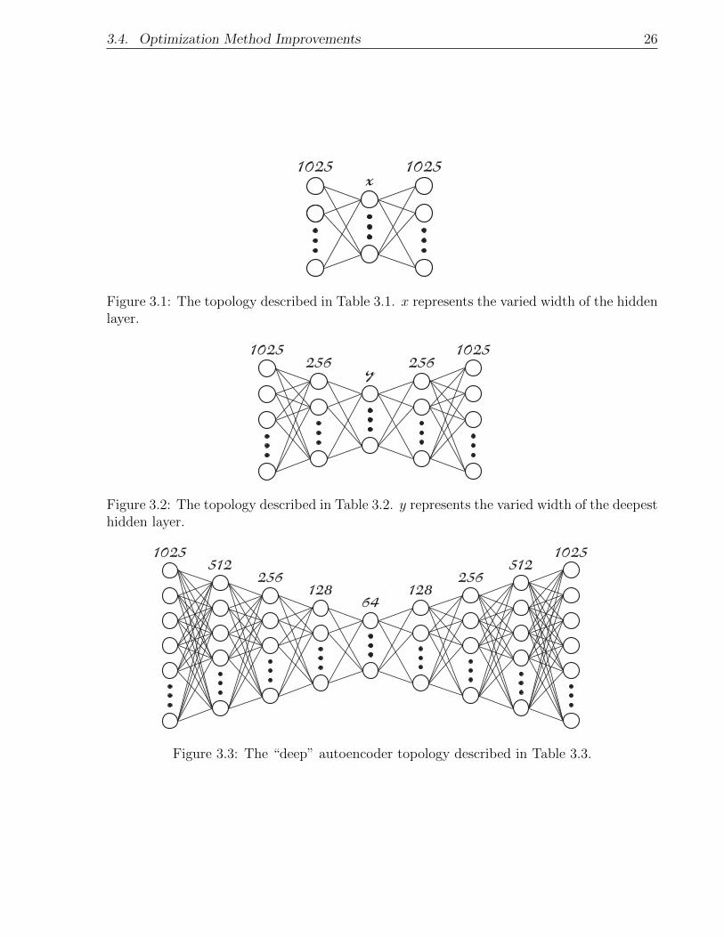
3.1 The topology described in Table 3.1. x represents the varied width of the

hidden layer. . . . . . . . . . . . . . . . . . . . . . . . . . . . . . . . . . . . . 26

3.2 The topology described in Table 3.2. y represents the varied width of the

deepest hidden layer. . . . . . . . . . . . . . . . . . . . . . . . . . . . . . . . 26

vii

3.3 The “deep” autoencoder topology described in Table 3.3. . . . . . . . . . . . 26

3.4 Plots demonstrating how autoencoder reconstruction improves when the width

of the hidden layer is increased. . . . . . . . . . . . . . . . . . . . . . . . . . 27

3.5 The ANNe interface . . . . . . . . . . . . . . . . . . . . . . . . . . . . . . . . 28

3.6 Block diagram demonstrating ANNe’s signal flow . . . . . . . . . . . . . . . 29

4.1 Final CANNe Autoencoder Topology . . . . . . . . . . . . . . . . . . . . . . 34

4.2 Autoencoder Reconstructions without L2 penalty . . . . . . . . . . . . . . . 37

4.3 Sample input and recosntruction using three different cost functions . . . . . 40

4.4 Sample input and recosntruction using three different cost functions . . . . . 40

4.5 Mock-up GUI for CANNe. . . . . . . . . . . . . . . . . . . . . . . . . . . . . 42

4.6 Signal flow for CANNe. . . . . . . . . . . . . . . . . . . . . . . . . . . . . . . 42

viii

Chapter 1

Introduction

The first instance of digital music can be traced back to 1950, with the completion of the

CSIRAC computer in Australia [5]. Engineers designing the computer equipped it with a

speaker that would emit a tone after reading a specific piece of code. Programmers were

able to modify this debugging mechanism to produce tones at given intervals. Since then,

the complexity of digital music and sound synthesis has scaled with the improvements of

computing machines. For example, early digital samplers such as the Computer Musician

Melodian and Fairlight CMI cost thousands of dollars upon release in the late 1970s and

could hold fewer than two seconds of recorded audio. Now, portable recorders can record

hours of professional quality audio for less than one hundred dollars.

With the advancement of computing hardware, so too have methods of digital music synthe-

sis advanced. Many analogue methods of sound synthesis, including additive and subtractive

synthesis, have be modeled in software synthesizers and digital audio workstations (DAWs).

DAWs have also come to provide an array of tools to mimic musical instruments, from gui-

tars to tubas. As such, musicians looking to push the boundaries of music and sound design

have turned to more advanced algorithms to create new sonic palettes.

Recently, musicians have turned to machine learning and artificial intelligence to augment

1

2

music production. Advancements in the field of artificial neural networks have produced

impressive results in computer vision and categorization tasks. Several attempts have been

made to bring these advancements to digital music and sound synthesis. Google’s Wavenet

uses a convolutional neural network to synthesize digital audio sample-by-sample, and has

been used to create complex piano performances [25]. Google’s NSynth uses an autoencoding

neural network topology to encode familiar sounds, such as a trumpet or a violin, and output

sounds that interpolate a timbre between the two [7].

While implementations such as these are impressive both in technical scale and imagination,

they are often too large and computationally intensive to be used by musicians. Algorithms

that have reached market, on the other hand, frequently are handicapped and restricted in

order to reduce computational load. There remains an opportunity for a neural network ap-

proach to music synthesis that is light enough to run on typical workstations while providing

the musician with meaningful control over the network’s parameters.

Two neural network topologies are presented: an autoencoding sound effect,(named ANNe

[3]) , that transforms the spectral properties of an input signal based on the work presented

in [20]; and an autoencoding synthesizer that generates audio based on activations of the

autoencoder’s latent space (named CANNe [4]). These models are straightforward to train

on user-generated corpora and lightweight compared to state-of-the-art algorithms. Fur-

thermore, both generate in real time at inference. Chapter 2 covers background information

regarding audio processing and analysis, Western music, and machine learning. Chapter

3 outlines our experiment design, setup, performance metrics, and Python implementation

for the ANNe sound effect. Chapter 4 outlines our experiment design, setup, performance

metrics, and Python implementation of CANNe synthesizer. Chapter 5 concludes the thesis

with observations and suggestions for future work.

Chapter 2

Background

2.1 Audio Signal Processing

A brief overview of the basics of audio signal processing follows. Because the model presented

in this thesis deals with digital audio exclusively, this discussion will primarily focus on

digital signals.

2.1.1 Analogue to Digital Conversion

Human hearing occurs when the brain processes excitations of the organs in the ear caused by

vibrations in air. Human beings can hear frequencies from approximately 20Hz to 20,000Hz,

though this range shrinks at the high end due to aging and overexposure to loud sounds.

As such, when converting sound from analogue to digital, it is necessary to bandlimit the

signal from DC to 20,000Hz [9].

Let xc(t) be a bandlimited continuous-time signal with no spectral power above ΩN Hz. The

Nyquist-Shannon sampling theorem states that xc(t) is uniquely determined by its samples

x[n] = xc(nT ), n = 0,±1,±2, . . . if

3

2.1. Audio Signal Processing 4

Ωs =2π

T≥ 2ΩN (2.1)

Ωs is referred to as the sampling frequency and ΩN is referred to as the Nyquist frequency

[17]. To ensure that all audible portions of a signal are maintained when converted from

analogue to digital, the sampling frequency must be at least 40,000 Hz. To adhere to CD

quality audio standards, the sampling rate used throughout this work is 44,100 Hz.

2.1.2 Short-Time Fourier Transform

Analysis of musical audio signals often involves discssuion of pitch and frequency. Thus it is

useful to obtain a representation of a finite discrete signal in terms of its frequency content.

One useful representation is the Short-Time Fourier Transform (STFT). The STFT of a

signal x[n] is

X(n, ω) =∞∑

m=−∞

x[n+m]w[m]e−jωm (2.2)

where w[n] is a window sequence and ω is the frequency in radians. Note that the STFT is

periodic in ω with period 2π. Thus we need only consider values of ω for −π ≤ ω ≤ π.

Two window sequences were considered for use in this thesis. The first, and the one ulti-

mately chosen, is the Hann window, defined as

wHann[n] =

0.5− 0.5cos(2πn/M) 0 ≤ n ≤M

0 otherwise

The second window sequence considered is the Gaussian window, defined as


Figure 2.1: Gaussian Window and its Frequency Response https://docs.scipy.org/doc/scipy-1.0.0/reference/generated/scipy.signal.gaussian.html

Figure 2.2: Hann Window and its Frequency Response https://docs.scipy.org/doc/scipy-0.19.1/reference/generated/scipy.signal.hanning.html

wGaussian[n] =

e−12(n−(M−1)/2σ(M−1)/2

)2 0 ≤ n ≤M

0 otherwise

When choosing a window function for the STFT, one must be cognizant of spectral smearing

and resolution issues [17].

Refer to Figures 2.1 and 2.2 for plots of the Gaussian and Hann windows. Spectral resolu-

tion refers to the STFT’s ability to distinguish two sinusoidal components of a signal with

fundamental frequencies close to one another. Spectral resolution is influenced primarily


by the width of the main lobe of the window’s frequency response. Spectral leakage, on

the other hand, refers to a window’s tendency to smear a sinusoid’s fundamental frequency

into neighboring frequency bins. Spectral leakage is influenced primarily by the relative

amplitude of the main lobe to the side lobes.

The Gaussian window possesses optimal time-frequency characteristics, i.e. it achieves min-

imum time-frequency spread [18]. However, it is not often found native to signal processing

libraries. The Hann window provides low leakage but slightly decreased frequency resolu-

tion when compared to the Gaussian window. However, the Hann window is implemented

natively in many signal processing libraries and thus is chosen for use in this work. These

quick native implementations allow for the software implementations presented in this work

to run in real time, which is essential for ease of use by musicians.

A signal’s STFT can be inverted using an overlap-add procedure [21]. First, a windowed

output frame is obtained via:

x′m(n) =1

N

N/2−1∑k=−N/2

X ′m(ejωk)ejωkn (2.3)

Then, the final output is reconstructed by overlapping and adding the windowed output

frames:

x(n) =∑m

x′m(n−mR) (2.4)

where R is the hop size, or how many samples are skipped between frames. This analysis

and resynthesis becomes an identity operation if the analysis windows sum to unity, i.e.

Aw(n) ,∞∑

m=−∞

w(n−mR) = 1 (2.5)


0

2500

5000

7500

10000

12500

15000

17500

20000

Hz

Linear-frequency power spectrogram

-80 dB

-70 dB

-60 dB

-50 dB

-40 dB

-30 dB

-20 dB

-10 dB

+0 dB

Figure 2.3: Spectrogram of a speaker saying “Free as Air and Water”

The Spectrogram

The STFT is a complex valued signal, which means that each X(ni, ωj) has a magnitude

and phase component. We refer to a three dimensional representation of the magnitude of

the STFT ‖X(n, ω)‖2 as “the spectrogram.” The spectrogram is used throughout audio

analysis because it succinctly describes a signal’s spectral power distribution, or how much

energy is present in different frequency bands, over time. Refer to Figure 2.3 for an example

spectrogram.

Phase Construction

When both a signal’s STFT magnitude and phase response are available, the spectrogram

can be inverted into a time signal. However, should no phase information be present at all,

inversion becomes difficult. Algorithms that produce a spectrogram based on input param-

eters, such as the synthesizer presented in Section 4, often do not produce a corresponding


phase response and thus necessitate a phase construction technique in order to produce

audio.

A non-iterative algorithm for the construction of a phase response can be derived based on

the direct relationship between the partial derivatives of the phase and logarithm of the

magnitude response with respect to the Gaussian window [19]. A fudge factor is applied to

modify this derivation for use with a Hann window.

Let us denote the logarithm of the magnitude of a given spectrogram ‖X(n, ω)‖2 as slog,n(m),

where n denotes the n-th time-frame of the STFT and m represents the m-th frequency

channel. The estimate of the scaled phase derivative in the frequency direction φ(w,n)(m)

and in the time direction φ(t,n)(m) expressed solely using the magnitude can be written as

φω,n(m) = − γ

2aM(slog,n+1(m)− slog,n−1(m)) (2.6)

φt,n(m) =aM

2γ(slog,n(m+ 1)− slog,n(m− 1)) + 2πam/M (2.7)

where M denotes the total number of frequency bins and φt,n(0, n) = φt,n(M/2, n) = 0.

These equations come from the Cauchy-Riemann equations, which outline the necessary and

sufficient conditions for a function of complex variables to be differentiable. Because a Hann

window of length 4098 is used to generate the STFT frames in this work, γ = 0.25645×40982.

Given the phase estimate φn−1(m), the phase φn(m) for a particular m is computed using

one of the following equations:

φn(m)← φn−1(m) +1

2(φt,n−1(m) + φt,n(m)) (2.8)

φn(m)← φn(m− 1) +1

2(φω,n(m− 1) + φω,n(m)) (2.9)

φn(m)← φn(m+ 1)− 1

2(φω,n(m+ 1) + φω,n(m)) (2.10)


Mathematically speaking, these equations perform numerical differentiation using finite dif-

ference estimation on consecutive phase approximations. In this work, equations 2.7 and

2.8 are used to construct a phase response with φ0(0) initialized to 0. These equations were

chosen because they are causal, i.e. they do not rely on future frame calculations. These

equations only rely on frames n− 1 and n.

Cepstral Analysis

In certain applications, such as automatic speech detection, it is helpful to think of a signal’s

frequency response as the product of an excitation signal and a voicing signal:

‖X(n, ω)‖2 = ‖E(n, ω)‖2‖V (n, ω)‖2 (2.11)

For tasks such as speaker detection, the voicing signal is sufficient to identify a speaker. The

following procedure is used to separate the two signals [17]. First, X(n, ω) is run through

a mel scale filter bank (Figure 2.5), which is a series of triangular filters centered on mel

scale frequencies. The Mel scale (Figure 2.4) is a scale of pitches perceived by listeners to be

equal in distance from one another and is thought to more accurately model human hearing

than a linear frequency scale [6].

The excitation and voicing components can then be separated using a logarithm

log(‖X(n, ω)‖2) = log(‖E(n, ω)‖2) + log(‖V (n, ω)‖2) (2.12)

Finally a Discrete Fourier Transform is taken, though this reduces to a Discrete Cosine

Transform because log(‖X(n, ω)‖2) is an even signal. The resulting signal is referred to as

Mel Frequency Cepstral Coefficients, and are used as features throughout machine listening

algorithms. As with the STFT, a signal produces a series of MFCCs over time, and a three

2.2. Musical Audio 10

Figure 2.4: Linear frequency scale vs Mel scale

Figure 2.5: Triangular Mel frequency bank

dimensional representation of these coefficients changing over time is called a cepstrogram.

Refer to Figure 2.6 for a comparison of a time signal’s spectrogram and cepstrogram. The

excitation signal will be present in the lower cepstrum bands, and the voicing signal will be

present in the higher cepstral bands.

2.2 Musical Audio

As this thesis deals with musical audio, it is necessary to outline what is meant by “music.”

Though a definition of music would seem obvious to most readers, care must be taken to


0.0 0.5 1.0 1.5 2.0 2.5Time

1.00

0.75

0.50

0.25

0.00

0.25

0.50

0.75

1.00Raw Waveform

0 0.5 1 1.5 2Time

Mel-Spectrogram

0 0.5 1 1.5 2Time

MFCC

Figure 2.6: Comparison of a time signal with its spectrogram and cepstrogram

distinguish between popular music heard on the radio in the West and the mathematical

abstractions of music. Traditional western music has strict technical formulations, which

are presented below. A quick definition of timbre follows. Finally, as the corpora used in

this work are generated from a MicroKORG synthesizer, the last subsection defines the two

types of electronic sound synthesis the synthesizer uses: additive synthesis and subtractive

synthesis.

2.2.1 Western Music Theory

Western music uses what is known as equal temperment to divide an octave, or a range of

frequencies starting at f0 and ending at 2f0, into twelve equally spaced notes. The frequency


of the nth note in an octave with root note f0 can be expressed as 12√

2n ∗ f0. The distance

between two notes f0 and 12√

2 ∗ f0 is called a half step. Two half steps make a whole step.

Furthermore, Western music creates a scale using eight notes across an octave. The most

common scale heard in popular music is the major scale. This scale is constructed by

choosing a root note and the following steps: whole-whole-half-whole-whole-whole-half.

The letters A-G are used to label notes. The C major scale, equivalent to playing the white

keys on a piano, runs C-D-E-F-G-A-B. When tuning instruments, the concert A note (A

above middle C) is tuned to be 440 Hz. This places middle C at about 262 Hz.

2.2.2 Timbre

Timbre describes the quality of a sound or tone that distinguishes it from another with the

same pitch and intensity. For example, a violin playing concert A sounds different from a

piano playing concert A. Timbre primarily relies on the spectral characteristics of a sound,

including the spectral power in its various harmonics, though the temporal aspects such as

envelope and decay also influence its perception.

2.2.3 Traditional Methods of Musical Audio Synthesis

Two traditional methods of electronic music synthesis are additive and subtractive synthesis.

In a standard electronic synthesizer, these methods are used to generate waveforms with

different timbres, which are stored as “patches”. The musician can toggle which patch he

or she wants to use and play notes using a keyboard.

In additive synthesis, waveforms such as sine, triangle, and sawtooth waves are generated

and added to one another to create a sound. The parameters of each waveform in the sum

are controlled by the musician, and the fundamental frequency is chosen by striking a key.

2.3. Machine Learning 13

In subtractive synthesis, a waveform such as a square wave or sawtooth wave is generated

and then filtered to subtract and alter harmonics. In this case, the parameters of the filter

and input waveform are controlled by the musician, and the fundamental frequency is chosen

by striking a key.

2.3 Machine Learning

The following section offers a broad definition of machine learning, presents a formulation

of the autoencoding neural network, explains how the latent space of an autoencoder can

be used for creative purposes, and discusses current machine learning approaches to audio

synthesis.

2.3.1 Definition

A broad definition of a computer program that can learn was suggested by Mitchell in 1997

[15]:

A computer program is said to learn from experience E with respect to some

class of tasks T and performance measure P , if its performance at tasks in T ,

and measured by P , improves with experience E.

Increasingly complex classes of machine learning algorithms have been designed as comput-

ing storage and power have improved.

Machine learning tasks are usually described in terms of how the machine learning system

should process an example, or collection of quantitative features, expressed as a vector

x ∈ Rd. Common tasks for a computer program to learn include classification, which

produces a function f : Rn → 1, . . . , k that maps an input to a numerically identified


category, and regression, which produces a function f : Rn → R that maps an input to a

continuous output.

Machine learning algorithms experience an entire dataset, or “corpus”. These experiences

E can be broadly categorized as supervised or unsupervised. In the supervised case each

data point xi in the corpus is associated with a label yi, and the algorithm is trained to map

xi → yi ≈ yi. In the unsupervised case, no data point is labelled. Instead, the algorithm

used to learn useful properties of the structure of the dataset.

The performance measure P is specific to the task T being carried out by the system and

measures the accuracy of the model. In the supervised case, P is calculated by evaluating

a cost function f : (y, y) → R that measures how close the prediction y is to y. This cost

function is measured on a portion of the dataset that was not used to train the algorithm.

2.3.2 Autoencoding Neural Networks

An autoencoding neural network (i.e. autoencoder) is a machine learning algorithm that is

typically used for unsupervised learning of an encoding scheme for a given input domain, and

is comprised of an encoder and a decoder [26]. For the purposes of this work, the encoder

is forced to shrink the dimension of an input into a latent space using a discrete number of

values, or “neurons.” The decoder then expands the dimension of the latent space to that

of the input, in a manner that reconstructs the original input.

In a single layer model, the encoder maps an input vector x ∈ Rd to the hidden layer y ∈ Re,

where d > e. Then, the decoder maps y to x ∈ Rd. In this formulation, the encoder maps

x→ y via

y = f(Wx+ b) (2.13)

where W ∈ R(e×d), b ∈ Re, and f(· ) is an activation function that imposes a non-linearity


Figure 2.7: Multi-layer Autoencoder Topology

in the neural network. The decoder has a similar formulation:

x = f(Wouty + bout) (2.14)

with Wout ∈ R(d×e), bout ∈ Rd.

A multi-layer autoencoder acts in much the same way as a single-layer autoencoder. The

encoder contains n > 1 layers and the decoder contains m > 1 layers. Using equation 2.13

for each mapping, the encoder maps x→ x1 → . . .→ xn. Treating xn as y in equation 2.14,

the decoder maps xn → xn+1 → . . .→ xn+m = x.

The autoencoder trains the weights of the W ’s and b’s to minimize some cost function. This

cost function should minimize the distance between input and output values.The choice of

activation functions f(· ) and cost functions depends on the domain of a given task.

Figure 2.7 depicts a generic typical multi-layer autoencoder. The mapping function can be

read from left to right. The input x is represented by the leftmost column of neurons, and

the output x is represented by the rightmost column. The smallest middle column is the

“latent space” or “hiddenmost layer.”

The autoencoders used in this work are tasked with encoding and reconstructing STFT


Figure 2.8: MNIST Example: Interpolation between 5 and 9 in the pixel space

Figure 2.9: MNIST Example: Interpolation between 5 and 9 in the latent space

magnitude frames, with the aim of having the autoencoder produce a latent space that

contains high level descriptors of musical audio.

2.3.3 Latent Spaces

The latent space that an autoencoder constructs can be viewed as a compact space that

contains high level descriptions of the corpus used for training. In order for the autoencoder

to perform well at reconstruction tasks, this latent space is forced to represent the most

relevant descriptors of the corpus.

Once constructed the latent space can become a powerful creative tool, allowing for seman-

tically meaningful interpolation between two inputs. Consider the following visual example.

The MNIST dataset consists of thousands of images of handwritten digits [13]. All images in

the dataset are greyscale and are 28x28 pixels. Two images in the dataset are shown in Figure

2.8, as well as an interpolation between the two images in “pixel space.” The interpolation

of these two images in the pixel space produces a cross-fading effect, whereby the 5 and 9

are proportionally summed and averaged. As can be seen, the middle interpolation makes

little to no sense semantically (i.e. as a handwritten digit) and instead creates a jumble of

pixels from both the 5 and 9. Fortunately, an autoencoder can be used to interpolate more


meaningful outputs between the 5 and 9.

An autoencoder can be trained to encode and decode these images, thereby constructing a

latent space containing high level representations of handwritten digits. By interpolating

images from the latent space, rather than the pixel space, semantically meaningful images

are produced. The interpolation shown in Figure 2.9 shows a handwritten digit transforming

from a 5 to a 9 rather than crossfading from one to the other.

This ability to interpolate meaningful and novel examples from a latent space is why the

autoencoder is used in this work. Any DAW can crossfade two sounds for a musician, but

few if any can interpolate between two input sounds in a semantically consistent manner.

This thesis aims to present a novel tool that allows musicians to harness the capabilities of

an autoencoder’s latent space to generate novel audio.

2.3.4 Machine Learning Approaches to Musical Audio Synthesis

Recently, machine learning techniques have been applied to musical audio sythesis. One

version of Google’s Wavenet architecture uses convolutional neural networks (CNNs) trained

on piano performance recordings to prooduce raw audio one sample at a time [25]. The

outputs of this neural network have been described as sounding like a professional piano

player striking random notes. Another topology, presented by Dadabots, uses recurrent

neural networks (RNNs) trained to reproduce a given piece of music [1]. These RNNs are

given a random initialization and then left to produce music in batches of raw audio samples.

Another Google project, NSynth [7], uses autoencoders to interpolate audio between the

timbres of different instruments. While all notable in scope and ability, these models require

immense computing power to train. These requirements are often prohibitively expensive

for an end user and thus do not allow for musicians to have any control over the design of

the algorithm’s architecture. For example, the architecture presented by Dadabots requires


24 hours to train on a GPU, and takes five minutes to generate 10 seconds of audio. In

other words these barriers prevent musicians from having a meaningful dialogue with the

tools they are given, which is a missed opportunity for creative innovation.

Another approach, proposed by Andy Sarroff, uses a small autoencoding neural network

(autoencoder) [20]. Compared to the work of [25] and [7], this architecture has the advantage

of being easy to train by new users. Furthermore, this lightweight architecture allows for

real time tuning and audio generation.

In [20]’s implementation, the autoencoder’s encoder compresses an input magnitude short-

time Fourier transform (STFT) frame to a latent representation, and its decoder uses the

latent representation to reconstruct the original input. The phase information bypasses

the encoder/decoder entirely. By modifying the latent representation of the input, the

decoder generates a new magnitude STFT frame. However, [20]’s proposed architecture

suffers from poor performance, measured by mean squared error (MSE) of a given input

magnitude STFT frame and its reconstruction. This poor MSE performance suggests a lack

of robust encodings for input magnitude STFT frames and thus a poor range of musical

applications. The work presented in Section 3 builds on these initial results and improves

the designed autoencoder through modern techniques and frameworks. These improvements

reduce MSE for each of [20]’s proposed topologies, thus improving the representational

capacity of the neural network’s latent space and widening the scope of the autoencoder’s

musical applications.

The work presented in Section 4 expands and improves on the work in Section 3. Section

4 introduces a new corpus more suited to designing a synthesizer as well as a larger and

more powerful autoencoder architecture than that of Section 3. Encodings are improved

by introducing a new cost function to the autoencoder’s training regime. Finally a phase

construction technique is implemented that can invert spectrograms generated by the au-

toencoder rather than relying on an input phase response.

Chapter 3

ANNe Sound Effect

This section outlines the experimental procedure done to reproduce and improve on the

work presented in [20]. This includes exploring different neural network training methods,

investigating different activation functions to be used in the neural network’s hidden layers,

training several different architectures, using regularization techniques, and weighing the

pros and cons of the additive bias terms.

When implemented in code, this autoencoder is considered a “sound effect” rather than a

“synthesizer.” This is because the autoencoder generates no phase information and thus

cannot invert the STFT on its own. Instead, the output STFT is inverted by using phase

information passed from the input.

3.1 Architecture

Several different network topologies were used, varying the depth of the autoencoder, width

of hidden layers, and choice of activation function. [20]’s topology is reproduced, using the

Adam training method instead of using stochastic gradient descent with momentum 0.5.

19

3.2. Corpus and Training Regime 20

Afterwards a seven layer deep autoencoder is designed that can be used for unique audio

effect generation and audio synthesis. For both the single layer and three layer deep models,

no additive bias term b was used, and all activations were the sigmoid (or logistic) function:

f(x) =1

1 + e−x(3.1)

The seven layer deep model uses both the sigmoid activation function and the rectified linear

unit (ReLU) [16]. The ReLU is formulated as

f(x) =

0 , x < 0

x , x ≥ 0(3.2)

As outlined in [20], the autoencoding neural network takes 1025 points from a 2048 point

magnitude STFT frame as its input, i.e. x ∈ [0, 1]1025. These 1025 points represent the DC

and positive frequency values of a given frame’s STFT.

A more in depth look at the neural network design choices made is in the 3.3 Discussion

of Methods section.

3.2 Corpus and Training Regime

All topologies presented in this section were trained using 50, 000 magnitude STFT frames,

with an additional 10, 000 frames held out for testing and another 10, 000 for validation.

Since [20]’s original corpus was not available, the audio used to generate these frames was

an hour’s worth of improvisation played on a MicroKORG synthesizer/vocoder. To ensure

the integrity of the testing and validation sets, the dataset was split on the “clip” level.

This means that the frames in each three sets were generated from distinct passages in the

improvisation, which ensures that duplicate or nearly duplicate frames are not found across

3.3. Discussion of Methods 21

the three sets. The MicroKORG has a maximum of four note polyphony for a given patch,

thus the autoencoder must learn to encode and decode mixtures of at most four complex

harmonic tones. These tones often have time variant timbres and effects, such as echo and

overdrive.

The neural network framework was handled using TensorFlow [2]. All training used the

Adam method for stochastic gradient descent with mini-batch size of 100 [11]. Across the

different autoencoder topologies explored, learning rates used for training varied from 10−3 to

10−4. For the single layer deep (Figure 3.1) and three layer deep (Figure 3.2) autoencoders,

the learning rate was set to 10−3 for the duration of training, which was 300 epochs. For the

deep autoencoder (Figure 3.3) the learning rate was set to 10−4 for the duration of training,

which was 500 epochs. This is a departure from [20]’s proposed methodology, which used

stochastic gradient descent with learning rate 5× 10−3 and momentum 0.5 [24].

The encoder and decoder are trained on these magnitude STFT frames to minimize the

MSE of the original and reconstructed frames.

3.3 Discussion of Methods

There are several distinctions between the architecture originally proposed by [20] and the

architectures used in this work: the choice of the autoencoder’s stochastic training method,

the regularization techniques used to create a robust latent space, the activation functions

chosen, the use of additive bias terms b, and the corpus used for training.

3.3.1 Training Methods

The improved MSEs in Table 3.1 and Table 3.2 demonstrate the ability of the Adam method

to train autoencoders in this context better than the momentum method [20] used. The


momentum method produced MSEs orders of magnitude higher than Adam, suggesting that

the momentum method found a poor local minimum and did not explore further. The result

of the 8-neuron hidden layer in Figure 4.1 demonstrates the poor reconstructions produced

by an autoencoder with MSE on the order of 10−3. [20]’s performance suggests that the

momentum method produced similar results. While these reconstructions are interesting to

listen to, they do not accurately reconstruct an input magnitude STFT frame. The adaptive

properties of the Adam technique ensure that the autoencoder searches the weight space in

order to find robust minima.

3.3.2 Regularization

[20] suggested using denoising techniques to improve the robustness of autoencoder topolo-

gies. During the course of the work presented here it was found that denoising was not

necessary to create robust one and three layer deep autoencoders. However, issues were

encountered when training the seven layer deep autoencoder topology.

Two regularization techniques were explored: dropout and an l2 penalty [22] [12]. Dropout

involves multiplying a Bernoulli random vector z ∈ 0, 1ti to each layer in the autoencoder,

with ti equal the dimension of the ith layer. Dropout encourages robustness in an autoen-

coder’s encoder and decoder, and the autoencoder’s quantitative performance did reflect

this. However, it was found that the dropout regularizer hampered the expressiveness of the

autoencoder when generating audio because it ignored slight changes to the latent space.

The second technique, l2 regularization, proved to perform the best in qualitative listening

comparisons. This technique imposes the following addition to the cost function:

C(θn) =1

Nobs

Nobs∑k=1

(x− x)2 + λl2‖θn‖2 (3.3)


where λl2 is a tuneable hyperparameter and ‖θn‖2 is the Euclidean norm of the autoencoder’s

weights. This normalization technique encourages the autoencoder to use smaller weights

in training, which was found to improve convergence.

3.3.3 Activation Functions

It was found that when using sigmoids as activation functions throughout the seven layer

deep model, the autoencoder did not converge. This is potentially due to the vanishing

gradient problem inherent to deep training [10]. To fix this, sigmoid activations were used

on only the deepest hidden layer and the output layer. Rectified linear units (ReLUs) were

used for the remaining the layers. This activation function has the benefit of having a

gradient of either zero or one, thus avoiding the vanishing gradient problem.

The choice of sigmoid activation for the deepest hidden layer of the deep model was mo-

tivated by the use of multiplicative gains for audio modulation. Because the range of the

sigmoid is strictly greater than zero, multiplicative gains were guaranteed to have an effect

on the latent representation, whereas a ReLU activation may be zero, thus invalidating

multiplicative gain.

The choice of sigmoid activation for the output layer of the deep model was twofold. First,

the normalized magnitude STFT frames used here have a minimum of zero and maximum

of one, which neatly maps to the range of the sigmoid function. Second, it was found that

while the ReLU activation on the output would produce acceptable MSEs, the sound of

the reconstructed signal was often tinny. The properties of the sigmoid activation lend

themselves to fuller sounding reconstructions.

3.4. Optimization Method Improvements 24

3.3.4 Additive Bias

Finally, it was found that using additive bias terms b in Equation 2.13 created a noise floor

on output STFT frames. With the bias term present, using gain constants in the hidden

layer produced noisy results. Though additive bias terms did improve the convergence of

the deep autoencoder, they were ultimately left out in the interest of musical applications.

3.3.5 Corpus

An issue with [20] is the use of several genres of music to generate a dataset. As different

genres have different frequency profiles, the neural network’s performance drops. For exam-

ple, a rock song’s frequency profile can be broken down as the sum of spiky low frequency

content created by drums, tonal components from guitar and bass, complex vocal profiles,

and high frequency activity from cymbals. Including several genres of music in a corpus

trains an autoencoder to be a jack of all trades, but master of none. By focusing the corpus

on tonal sounds, this work encourages the neural network to master representations of those

sounds. Thus when it comes time for modifying an input, the autoencoder’s latent space

contains representations of similar yet distinct synthesizer frequency profiles.

3.4 Optimization Method Improvements

Table 3.1 and Table 3.2 compare the MSEs of the network topologies as implemented by

[20] (Sarroff) and as implemented here (ANNe).

The first column of Table 3.1 describes the autoencoder’s topology, with the first integer

representing the neuron width of the hidden layer. The first column of Table 3.2 describes

the autoencoder’s topology, with the first integer representing the neuron width of the first


Table 3.1: Single Layer Autoencoder Topology MSEs

Hidden Layer Width Sarroff MSE ANNe MSE

8 4.40× 10−2 5.30× 10−3

16 4.14× 10−2 5.28× 10−3

64 2.76× 10−2 7.10× 10−4

256 1.87× 10−2 1.64× 10−4

512 1.98× 10−2 9.62× 10−4

1024 3.52× 10−2 7.13× 10−5

Table 3.2: Three Layer Autoencoder Topology MSEs

Hidden Layer Widths Sarroff MSE ANNe MSE

256-8-256 1.84× 10−2 1.91× 10−3

256-16-256 1.84× 10−2 1.19× 10−3

256-32-256 1.84× 10−2 7.30× 10−4

layer, the second integer representing the neuron width of the second layer, and the third

integer representing the neuron width of the third layer. Table 3.3 shows the MSEs of a

seven layer deep autoencoder, with hidden layer widths 512 → 256 → 128 → 64 → 128 →

256→ 512. Table 3.3 also shows the MSEs of three different topologies that were chosen for

the deep autoencoder: one with sigmoid activations throughout, one with ReLU activations

throughout, and a hybrid model. This hybrid model used a sigmoid on the innermost

hidden layer and on the output layer, with all other layers using a ReLU activation. This

hybrid topology performed best in minimizing MSE. All train times were measured using

TensorFlow 1.2.1 running on an Intel R© CoreTM

i5-6300HQ CPU @ 2.30GHz.

Figure 4.1 shows graphs of a single input magnitude STFT frame (top) and correspond-

ing reconstructions (bottom), with magnitude on the y axis and frequency bin on the x

axis. Contrary to [20]’s work, the signal reconstruction improves both qualitatively and

quantitatively as the depth of the hidden layer is increased.


x1025 1025

Figure 3.1: The topology described in Table 3.1. x represents the varied width of the hiddenlayer.

y256 2561025 1025

Figure 3.2: The topology described in Table 3.2. y represents the varied width of the deepesthidden layer.

64128 128256 256512 5121025 1025

Figure 3.3: The “deep” autoencoder topology described in Table 3.3.


Figure 3.4: Plots demonstrating how autoencoder reconstruction improves when the widthof the hidden layer is increased.

0 256 512 768 1024Frequency Bin

0.0

0.5

1.0Magnitude Original Signal

0 256 512 768 1024Frequency Bin

0.0

0.5

1.0Magnitude Reconstruction with 8 Neurons

0 256 512 768 1024Frequency Bin

0.0

0.5


0 256 512 768 1024Frequency Bin

0.0

0.5


3.5. ANNe GUI 28

Table 3.3: Deep Topology MSEs and Train Times

Activations MSE Time to Train

All Sigmoid 1.72× 10−3 20 minutesAll ReLU 8.00× 10−2 60 minutes

Hybrid 4.91× 10−4 25 minutes

Figure 3.5: The ANNe interface

3.5 ANNe GUI

3.5.1 Interface

The following section present a graphical user interface (GUI) ‘ANNe’ that allows users to

modify audio signals with the neural network presented in this section. First, a user loads an

audio file that they want to modify. Then, they adjust values that modify the autoencoding

neural network. Finally, the program processes the input file through the neural network

which outputs a new audio file. The GUI’s front end was coded in C++ using Qt Creator

and interacts with a backend coded in Python3.

All audio processing was handled by the librosa Python library [14]. In this application,

3.5. ANNe GUI 29

User Parameters

Latent Representation

PHASE ф

Encoder Decoder New Magnitude Response

Magnitude Response

Audio In Audio Out

STFT ISTFT

Figure 3.6: Block diagram demonstrating ANNe’s signal flow

librosa was used to read .wav files, sample them at 22.05kHz, perform STFTs of length

2048 with centered Hann window, hop length 512 (75% overlap), and write .wav files with

sampling frequency 22.05kHz from reconstructed magnitude STFT frames. The phase of

each magnitude STFT frame was passed directly from input to output, circumventing the

autoencoder. ANNe is available on github at https://github.com/JTColonel/ANNe and

has been tested on Ubuntu 16.04 LTS and Arch Linux distributions.

3.5.2 Functionality

On startup ANNe initializes the Python backend, which loads the neural network topology

and saved network weights.

ANNe begins processing the input audio signal by performing a STFT. On a frame-by-

frame basis the inputs phase is saved untouched in memory, but the magnitude response

is normalized to [0, 1]. The normalizing factor is saved and stored in memory, and the

normalized magnitude response is passed to the neural network. The neural network first

encodes the normalized magnitude response into a 64 dimensional latent space, and then

subsequently decodes the latent representation into a new normalized magnitude response.

ANNe then reapplies the frames normalizing factor, and performs an ISTFT with the original

phase.

3.5. ANNe GUI 30

3.5.3 Guiding Design Principles

In total, ANNe contains nearly 4000 neurons and 1.4 million weight constants that could be

modulated to create an audio effect. In practice, however, it is unreasonable to present an

entry level user with so many tunable parameters and expect them to use a program. The

challenge was to design an interface that would be immediately recognizable to musicians

and sound designers and allow users to access the full potential of the neural network. As

such, guitar pedals were used for inspiration.

Despite having innumerable design parameters, guitar pedals expose only a handful of them

to a user. Furthermore, by presenting knobs and dials as actuators, guitar pedal designers

simultaneously presents users with an intuitive interface while tacitly limiting the parameters

altering the pedals circuitry.

With these principles in mind, ANNe allows users to modify the 64 neurons in the hidden

layer with knobs and sliders.

3.5.4 Usage

ANNe does not process audio in real time. Instead, ANNe processes an entire audio file in

one go. Thus in order to begin using ANNe, a user first must load a file that they want to

modify. A user chooses the file they would like to load by turning the aux in dial. Settings

1-3 are prepackaged .wav files (a piano striking middle C, a violin section tuning, and a

snare drum hit respectively), and settings 4-5 allow a user to select their own file.

The choice of preset sounds are intentional - it was chosen to give the user a sense of the

range of sound domains we found worked well with ANNe. First, all the preset sounds are no

longer than two seconds. While it is possible to load a track of any length into the program,

more interesting results were found when working with small clips of audio. Second, the

3.5. ANNe GUI 31

presets encompass a wide range of harmonic and timbral complexity. In testing, ANNe

could scramble the piano notes harmonic profile to sound like a bass kick, and the snares to

sound like an 808 cowbell.

After choosing a sound to modify the user then selects a preset and tunes the knobs a-e.

These are what allow a user to modify the 64 neuron hidden layer. Knobs a through e specify

multiplicative gain constants that get sent to the hidden layer, and the preset specifies how

those gains get mapped to the hidden layer.

Each preset 1-3 divides the hidden layer vector H into five adjacent, non-overlapping sub-

vectors H = ha, hb, ..., he

When it comes time to process an input file, each neuron in a sub-vector is multiplied by the

gain constant specified by its corresponding knob after the sigmoid activation. For example,

each neuron contained in hb is multiplied by the gain set by knob b. The presets determine

how long each sub-vector is: preset 1 has each sub-vector approximately equal in length,

preset 2 increases their size logarithmically from “a” to “e”, and preset 3 decreases their

size logarithmically from “a” to “e”. Options 4 and 5 allow for a user to specify their own

sub-vector lengths by moving the sliders and saving their positions for later use.

The GUI places constraints so that each sub-vector contains at least one neuron and so that

the gain constants can take a value in [0.5, 5.5].

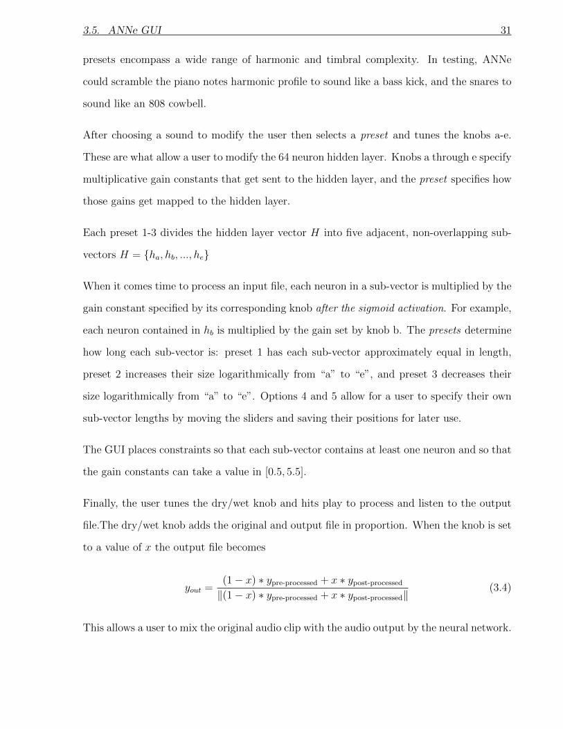
Finally, the user tunes the dry/wet knob and hits play to process and listen to the output

file.The dry/wet knob adds the original and output file in proportion. When the knob is set

to a value of x the output file becomes

yout =(1− x) ∗ ypre-processed + x ∗ ypost-processed‖(1− x) ∗ ypre-processed + x ∗ ypost-processed‖

(3.4)

This allows a user to mix the original audio clip with the audio output by the neural network.

3.5. ANNe GUI 32

3.5.5 “Unlearned” Audio Representations

During training, the sigmoid activation at the hidden layer forces the autoencoder to map

input magnitude responses inside a 64 dimensional unit hypercube within a 64 dimensional

latent space. This hypercube contains “learned” representations of the corpus. ANNe’s

multiplicative gain constants allows a user to alter how an input signal is mapped to this

latent space, or to put it another way, ANNe allows a user to morph an input signals latent

representation in 64 dimensional space.

If the gain constants a-e are all set less than or equal to 1, it is guaranteed that the signal’s

latent representation is moving within the “learned” space, or unit hypercube. However,

when values are greater than 1, that condition is no longer guaranteed. If, say, the gain

constant a is set to 4, and some neurons in ha are greater than 0.25, then ANNe has

pushed the signals latent representation out of the “learned” space and into what we call

an “unlearned” space.

After testing the model, it was found that setting gain constants greater than two frequently

pushed a signal’s latent representation into the unlearned space. With gain constants greater

than 2 the output signals were found to be harmonically distinct from the input signal,

whereas applying very large gains on the order of 102 before the sigmoid activation (thus

pushing the hidden layer’s neurons towards a value of zero or one, i.e. the boundary of

the learned space) generated output signals harmonically similar to the input. By allowing

users to access audio from this unlearned space, ANNe allows users to explore completely

novel sound.

Chapter 4

CANNe Synthesizer

This section expands on the work presented in Section 3 and presents CANNe, an au-

toencoding neural network synthesizer. CANNe acts in much the same way as ANNe, but

includes a phase construction technique. This allows CANNe to generate audio directly

from activating its hiddenmost layer, rather than relying on the phase response of an input

signal.

By using some of the design principles that led to ANNe, the autoencoder was made much

deeper (from seven to seventeen layers). The choice of overall architecture, corpus, cost

function, and feature engineering are presented and justified.

A GUI is also presented at the end of the section.

4.1 Architecture

A fully-connected, feed-forward neural network acts as the autoencoder. Refer to Figure

4.1 for an explicit diagram of the network architecture. The number above each column

of neurons represents the width of that hidden layer. Design decisions regarding activation

33

4.2. Corpus 34

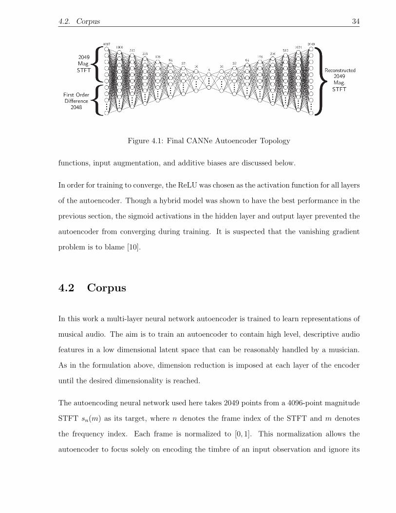
Figure 4.1: Final CANNe Autoencoder Topology

functions, input augmentation, and additive biases are discussed below.

In order for training to converge, the ReLU was chosen as the activation function for all layers

of the autoencoder. Though a hybrid model was shown to have the best performance in the

previous section, the sigmoid activations in the hidden layer and output layer prevented the

autoencoder from converging during training. It is suspected that the vanishing gradient

problem is to blame [10].

4.2 Corpus

In this work a multi-layer neural network autoencoder is trained to learn representations of

musical audio. The aim is to train an autoencoder to contain high level, descriptive audio

features in a low dimensional latent space that can be reasonably handled by a musician.

As in the formulation above, dimension reduction is imposed at each layer of the encoder

until the desired dimensionality is reached.

The autoencoding neural network used here takes 2049 points from a 4096-point magnitude

STFT sn(m) as its target, where n denotes the frame index of the STFT and m denotes

the frequency index. Each frame is normalized to [0, 1]. This normalization allows the

autoencoder to focus solely on encoding the timbre of an input observation and ignore its

4.2. Corpus 35

loudness relative to other observations in the corpus.

Two corpora were used to train the autoencoder in two separate experiments. The first

corpus is comprised of approximately 79, 000 magnitude STFT frames, with an additional

6, 000 frames held out for testing and another 6, 000 for validation. This makes the corpus

91, 000 frames in total. The audio used to generate these frames is composed of five octave

C Major scales recorded from a MicroKORG synthesizer/vocoder across 80 patches.

The second corpus is a subset of the first. It is comprised of one octave C Major scales

starting from concert C. Approximately 17, 000 frames make up the training set, with an

additional 1, 000 frames held out for testing and another 1, 000 for validation.

In both cases, 70 patches make up the training set, 5 patches make up the testing set, and 5

patches make up the validation set. These patches ensured that different timbres are present

in the corpus. To ensure the integrity of the testing and validation sets, the dataset is split

on the “clip” level. This means that the frames in each of the three sets are generated from

distinct passages in the recording, which prevents duplicate or nearly duplicate frames from

appearing across the three sets.

By restricting the corpus to single notes played on a MicroKORG, the autoencoder needs

only to learn higher level features of harmonic synthesizer content. These tones often have

time variant timbres and effects, such as echo and overdrive. Thus the autoencoder is also

tasked with learning high level representations of these effects.

4.3. Cost Function 36

4.3 Cost Function

Three cost functions were considered for use in this work:

Spectral Convergence (SC) [23]

C(θn) =

√∑M−1m=0 (sn(m)− sn(m))2∑M−1

m=0 (sn(m))2(4.1)

where θn is the autoencoder’s trainable weight variables,sn(m) is the original magnitude

STFT frame, sn(m) is the reconstructed magnitude STFT frame, and M is the total num-

ber of frequency bins in the STFT

Mean Squared Error (MSE)

C(θn) =1

M

M−1∑m=0

(sn(m)− sn(m))2 (4.2)

and Mean Absolute Error (MAE)

C(θn) =1

M

M−1∑m=0

|sn(m)− sn(m)| (4.3)

Ultimately, SC (Eqn. 4.1) was chosen as the cost function for this autoencoder instead of

mean squared error (MSE) or mean absolute error (MAE).

The decision to use SC is twofold. First, its numerator penalizes the autoencoder in much

the same way mean squared error (MSE) does. Reconstructed frames dissimilar from their

input are penalized on a sample-by-sample basis, and the squared sum of these deviations

dictates magnitude of the cost. This ensures that SC is a valid cost function because perfect

4.3. Cost Function 37

Figure 4.2: Autoencoder Reconstructions without L2 penalty

reconstructions have a cost of 0 and similar reconstructions have a lower cost than dissimilar

reconstructions.

The second reason, and the primary reason SC was chosen over MSE, is that its denomina-

tor penalizes the autoencoder in proportion to the total spectral power of the input signal.

Because the training corpus used here is comprised of “simple” harmonic content (i.e. not

chords, vocals, percussion, etc.), much of a given input’s frequency bins will have zero or

close to zero amplitude. SC’s normalizing factor gives the autoencoder less leeway in recon-

structing harmonically simple inputs than MSE or MAE. Refer to Figure 4.3 for diagrams

demonstrating the reconstructive capabilities each cost function produces.

As mentioned in [3], the autoencoder does not always converge when using SC by itself as

the cost function. See Figure 4.2 for plotted examples. Thus, an L2 penalty is added to the

cost function

C(θn) =

√∑M−1m=0 (sn(m)− sn(m))2∑M−1

m=0 (sn(m))2+ λl2‖θn‖2 (4.4)

where λl2 is a tuneable hyperparameter and ‖θn‖2 is the Euclidean norm of the autoen-

coder’s weights [12]. This normalization technique encourages the autoencoder to use smaller

4.4. Feature Engineering 38

weights in training, which was found to improve convergence. For this work λl2 is set to

10−10. This value of λl2 is large enough to prevent runaway weights while still allowing the

SC term to dominate in the loss evaluation.

4.4 Feature Engineering

To help the autoencoder enrich its encodings, its input is augmented with higher-order

information. Augmentations with different permutations of the input magnitude spectrum’s

first-order difference,

x1[n] = x[n+ 1]− x[n] (4.5)

second-order difference,

x2[n] = x1[n+ 1]− x1[n] (4.6)

and Mel-Frequency Cepstral Coefficients (MFCCs) were used.

MFCCs have seen widespread use in automatic speech recognition, and can be thought of as

the “spectrum of the spectrum.” In this application, a 100 band mel-scaled log-transform

of sn(m) is taken. Then, a 50-point discrete-cosine transform is performed. The resulting

aplitudes of this signal are the MFCCs. Typically the first few cepstral coefficients are orders

of magnitude larger than the rest, which can impede training. Thus before appending the

MFCCs to the input, the first five cepstral values are thrown out and the rest are normalized

to [-1,1].

4.5 Task Performance and Evaluation

Tables 4.1 and 4.2 show the SC loss on the validation set after training. For reference, an

autoencoder that estimates all zeros for any given input has a SC loss of 1.0. All train

4.5. Task Performance and Evaluation 39

Input Append Validation SC Training TimeNo Append 0.257 25 minutes

1st Order Diff 0.217 51 minutes2nd Order Diff 0.245 46 minutes

1st and 2nd Order Diff 0.242 69 minutesMFCCs 0.236 29 minutes

Table 4.1: 5 Octave Dataset Autoencoder validation set SC loss and Training Time

Input Append Validation SC Training TimeNo Append 0.212 5 minutes

1st Order Diff 0.172 6 minutes2nd Order Diff 0.178 6 minutes

1st and 2nd Order Diff 0.188 7 minutesMFCCs 0.208 6 minutes

Table 4.2: 1 Octave Dataset Autoencoder validation set SC loss and Training Time

times presented were measured by training the autoencoder for 300 epochs, using the Adam

method with mini-batch size 200, on an Nvidia Titan V GPU.

As demonstrated, the appended inputs to the autoencoder improve over the model with

no appendings. Results show that while autoencoders are capable of constructing high

level features from data unsupervised, providing the autoencoder with common-knowledge

descriptive features of an input signal can improve its performance.

The model trained by augmenting the input with the signal’s 1st order difference (1st-order-

appended model) outperformed every other model. Compared to the 1st-order-appended

model, the MFCC trained model often inferred overtonal activity not present in the original

signal (Figure 4.4). While it performs worse on the task than the 1st-order-append model, the

MFCC trained model presents a different sound palette that a musician may find interesting.

4.6. Spectrogram Generation 40

Figure 4.3: Sample input and recosntruction using three different cost functions

Figure 4.4: Sample input and recosntruction using three different cost functions

4.6 Spectrogram Generation

The training scheme outline above forces the autoencoder to construct a latent space con-

tained in R8 that contains representations of synthesizer-based musical audio. Thus a musi-

cian can use the autoencoder to generate spectrograms by removing the encoder and directly

activating the 8 neuron hidden layer. However, these spectrograms come with no phase in-

formation. Thus to obtain a time signal, phase information must be generated as well.

4.7. Phase Generation with PGHI 41

4.7 Phase Generation with PGHI

Phase Gradient Heap Integration (PGHI) [19] is used to generate the phase for the spectro-

gram.

An issue arises when using PGHI with this autoencoder architecture. A spectrogram gen-

erated from a constant activation of the hidden layer contains constant magnitudes for

each frequency value. This leads to the phase gradient not updating properly due to the 0

derivative between frames. To avoid this, uniform random noise drawn from [0.999, 1.001]

is multiplied to each magnitude value in each frame. By multiplying this noise rather than

adding it, we avoid adding spectral power to empty frequency bins and creating a noise floor

in the signal.

4.8 CANNE GUI

We realized a software implementation of our autoencoder synthesizer, “CANNe (Cooper’s

Autoencoding Neural Network)” in Python using TensorFlow, librosa, pygame, soundfile,

and Qt 4.0. Tensorflow handles the neural network infrastructure, librosa and soundfile

handle audio processing, pygame allows for audio playback in Python, and Qt handles the

GUI. Figure 4.6 depicts CANNe’s signal flow.

Figure 4.5 shows a mock-up of the CANNe GUI, and Figure 4.6 shows CANNe’s signal flow.

A musician controls the eight Latent Control values to generate a tone. The Frequency Shift

control performs a circular shift on the generated magnitude spectrum, thus effectively acting

as a pitch shift. It is possible, though, for very high frequency content to roll into the lowest

frequency values, and vice-versa.

4.8. CANNE GUI 42

Latent Control

Figure 4.5: Mock-up GUI for CANNe.

Figure 4.6: Signal flow for CANNe.

Chapter 5

Conclusions and Future Work

5.1 Conclusions

Two methods of training and implementing autoencoding neural networks for musical audio

applications are presented. Both autoencoders are trained to compress and reconstruct

Short-Time Fourier Transform magnitude frames of musical audio.

The first autoencoder, ANNe, acts as a sound effect. An input sound’s spectrogram is

mapped to the autoencoder’s latent space, where it can be modified by a user. The newly

modified latent representation is then sent through the decoder, and an altered spectrogram

is produced. This spectrogram is inverted using the original signal’s phase information to

generate new audio.

The second autoencoder, CANNe, acts as a musical audio synthesizer. An autoencoder

is trained on recordings of C major scales played on a MicroKORG synthesizer, thereby

constructing a latent space that contains high level representations of individual notes. A

user can then send activations to the latent space, which when fed through the decoder

produce a spectrogram on the output. Phase gradient heap integration is used to construct

43

5.2. Future Work 44

a phase response from the spectrogram, which is then used to invert the spectrogram into

a time signal.

Each autoencoder has been implemented with a GUI that was designed with the musician in

mind. Both topologies are lightweight when compared to state-of-the-art neural methods for

audio synthesis, which allows the musician to have a meaningful dialogue with the network

architecture and training corpora.

5.2 Future Work

The author sees three main directions in which future work can take for this thesis.

First, it would be worthwhile to explore using variational autoencoders (VAE) rather than

standard autoencoders [8]. VAEs target a Gaussian distribution at the latent space rather

than a deterministic latent space. Cost function parameters can be placed on these latent

distributions to encourage them to decouple. Experiments with VAEs have demonstrated

that this decoupling can increase the ease-of-use for creative tools.

Second, alternative representations of audio can be used to train the autoencoder. Repre-

sentations such as the constant-Q transform offer more compact representations than the

STFT [8]. Though more dense than the STFT, these transforms offer more resolution in the

lower frequency bands of a signal, where human beings can distinguish more detail in audio,

than the higher frequency bands. Though perfect reconstruction is not guaranteed with

such transforms, machine learning techniques have been applied to minimize reconstruction

error.

Finally, a more robust dataset that tags note information along with the raw STFT may

allow the autoencoders to perform better on reconstruction tasks [8]. Conditioning inputs

to the autoencoder based on its note may help musicians design sounds with a target root

5.2. Future Work 45

harmonic.

Bibliography

[1] Generating black metal and math rock: Beyond bach, beethoven, and beat-

les. http://dadabots.com/nips2017/generating-black-metal-and-math-rock.

pdf, Zack Zukowski and Cj Carr 2017.

[2] M. Abadi. Tensorflow: Learning functions at scale. ICFP, 2016.

[3] J. Colonel, C. Curro, and S. Keene. Improving neural net auto encoders for music

synthesis. In Audio Engineering Society Convention 143, Oct 2017.

[4] J. Colonel, C. Curro, and S. Keene. Neural network autoencoders as musical audio

synthesizers. Proceedings of the 21st International Conference on Digital Audio Effects

(DAFx-18). Aveiro, Portugal, 2018.

[5] P. Doornbusch. Computer sound synthesis in 1951: The music of csirac. Computer

Music Journal, 28(1):1025, 2004.

[6] P. Doornbusch. Computer sound synthesis in 1951: The music of csirac. Computer

Music Journal, 28(1):1025, 2004.

[7] J. Engel, C. Resnick, A. Roberts, S. Dieleman, D. Eck, K. Simonyan, and M. Norouzi.

Neural Audio Synthesis of Musical Notes with WaveNet Autoencoders. ArXiv e-prints,

Apr. 2017.

46

BIBLIOGRAPHY 47

[8] P. Esling, A. Bitton, et al. Generative timbre spaces with variational audio synthesis.

Proceedings of the 21st International Conference on Digital Audio Effects (DAFx-18).

Aveiro, Portugal, 2018.

[9] B. Gold, N. Morgan, and D. Ellis. Speech and Audio Signal Processing: Processing and

Perception of Speech and Music. Wiley, 2011.

[10] S. Hochreiter, Y. Bengio, P. Frasconi, and J. Schmidhuber. Gradient flow in recurrent

nets: the difficulty of learning long-term dependencies, 2001.

[11] D. P. Kingma and J. Ba. Adam: A method for stochastic optimization. CoRR,

abs/1412.6980, 2014.

[12] A. Krogh and J. A. Hertz. A simple weight decay can improve generalization. In NIPS,

volume 4, pages 950–957, 1991.

[13] Y. LeCun and C. Cortes. MNIST handwritten digit database. 2010.

[14] B. McFee, C. Raffel, D. Liang, D. P. Ellis, M. McVicar, E. Battenberg, and O. Nieto.

librosa: Audio and music signal analysis in python. In Proceedings of the 14th python

in science conference, pages 18–25, 2015.

[15] T. Mitchell. Machine Learning. McGraw-Hill International Editions. McGraw-Hill,

1997.

[16] V. Nair and G. E. Hinton. Rectified linear units improve restricted boltzmann machines.

In Proceedings of the 27th international conference on machine learning (ICML-10),

pages 807–814, 2010.

[17] A. Oppenheim and R. Schafer. Discrete-Time Signal Processing. Pearson Education,

2011.

BIBLIOGRAPHY 48

[18] Z. Prusa, P. Balazs, and P. L. Søndergaard. A noniterative method for reconstruction of

phase from stft magnitude. IEEE/ACM Transactions on Audio, Speech, and Language

Processing, 25(5):1154–1164, 2017.

[19] Z. Prusa and P. L. Søndergaard. Real-time spectrogram inversion using phase gradient

heap integration. In Proc. Int. Conf. Digital Audio Effects (DAFx-16), pages 17–21,

2016.

[20] A. Sarroff. Musical audio synthesis using autoencoding neural nets, Dec 2015.

[21] J. Smith, X. Serra, S. U. C. for Computer Research in Music, Acoustics, and C. Sys-

tem Development Foundation (Palo Alto. PARSHL: an analysis/synthesis program for

non-harmonic sounds based on a sinusoidal representation. Number no. 43 in Report.

CCRMA, Dept. of Music, Stanford University, 1987.

[22] N. Srivastava, G. Hinton, A. Krizhevsky, I. Sutskever, and R. Salakhutdinov. Dropout:

A simple way to prevent neural networks from overfitting. The Journal of Machine

Learning Research, 15(1):1929–1958, 2014.

[23] N. Sturmel and L. Daudet. Signal reconstruction from stft magnitude: A state of the

art.

[24] I. Sutskever, J. Martens, G. Dahl, and G. Hinton. On the importance of initialization

and momentum in deep learning. In S. Dasgupta and D. McAllester, editors, Proceedings

of the 30th International Conference on Machine Learning, volume 28 of Proceedings of

Machine Learning Research, pages 1139–1147, Atlanta, Georgia, USA, 17–19 Jun 2013.

PMLR.

[25] A. van den Oord, S. Dieleman, H. Zen, K. Simonyan, O. Vinyals, A. Graves, N. Kalch-

brenner, A. W. Senior, and K. Kavukcuoglu. Wavenet: A generative model for raw

audio. CoRR, abs/1609.03499, 2016.

BIBLIOGRAPHY 49

[26] P. Vincent, H. Larochelle, I. Lajoie, Y. Bengio, and P.-A. Manzagol. Stacked denoising

autoencoders: Learning useful representations in a deep network with a local denoising

criterion. Journal of Machine Learning Research, 11(Dec):3371–3408, 2010.

Appendix A

Python Code

A.1 ANNe Backend

1 import t en so r f l ow as t f

2 import t en so r f l ow . con t r i b . s l im as s l im

3 import numpy as np

4 import matp lo t l i b . pyplot as p l t

5 import os

6 import l i b r o s a

7 import sys

8 #

|

9

10 s e s s = t f . S e s s i on ( )

11

12 #Creates we igh t v a r i a b l e s f o r the ANN and groups them in a c o l l e c t i o n f o r use

in L2 r e g u l a r i z a t i o n

13 def we i gh t va r i ab l e ( shape , name ) :

14 i n i t i a l = t f . t runcated normal ( shape , name=name , stddev =0.15) #I n i t i a l i z e d

50

A.1. ANNe Backend 51

with a t runca ted normal random va r i a b l e

15 t f . a d d t o c o l l e c t i o n ( ’ l 2 ’ , t f . reduce sum ( t f .pow( i n i t i a l , 2 ) ) ) #Adding to L2

c o l l e c t i o n , summing squares

16 return t f . Var iab le ( i n i t i a l )

17

18 #Takes a f i l e path to a . wav f i l e and ou tpu t s sa id f i l e processed us ing the

t ra ined ANN

19 #Audio f i l e must be in the same f o l d e r as t h i s s c r i p t

20 #Dependent on the LIBROSA python l i b r a r y and os l i b r a r y

21 def wr i t e aud i o ( f i l ename , outname , ne t ) :

22 data path = f i l ename #Finds f i l e path to s c r i p t and appends f i l ename

23 y , s r = l i b r o s a . load ( data path ) #Loads audio in to python with samples ’ y ’

and sampling ra t e ’ s r ’ − 22.05 kHz by d e f a u l t

24 D = l i b r o s a . s t f t ( y ) #STFT of input audio saved as D

25 mag = D

26 mag = np . abs (mag) #Magnitude response o f the STFT

27 remember = mag .max( ax i s=0)+0.000000001 #Used f o r normal i z ing STFT frames (

wi th add i t i on to avoid d i v i s i o n by zero )

28 mag = mag / remember #Normaliz ing

29 phase = np . ang le (D) #Phase response o f STFT

30 mag = np . t ranspose (mag) #Because dimensions were g i v i n g problems

31 new mag = np . asar ray ( s e s s . run ( net , f e e d d i c t=x :mag) ) #Process magnitude

STFT frames through the ANN

32 new mag = np . t ranspose (new mag) #Again dimensions were g i v i n g problems

33 new mag ∗= remember #Un−normal ize the STFT frames

34 E = new mag∗np . exp (1 j ∗phase ) #Use magnitude and phase to produce complex−

va lued STFT

35 out = l i b r o s a . i s t f t (E) #Inver se STFT

36 out = out /(np .max( out ) +0.2)

37 f i l ename = f i l ename [:−4]+ ’ ’

38 l i b r o s a . output . write wav ( f i l ename+str ( outname ) , out , s r ) #Write output

39

40 def tune knobs ( f i l ename , tag , knobs ) :


41 ckpt = t f . t r a i n . l a t e s t c h e c kpo i n t ( ’ checkpo int s ’ )

42 saver . r e s t o r e ( s e s s , ckpt )

43 l ength = len ( knobs )

44 a = np . ones ( ( 1 , f c 4 ) ) #Pre−a l l o c a t i o n

45 i t s = f c4 // l ength

46 for w in range ( l ength ) :

47 a [ : , (w∗ i t s ) : ] = knobs [w] #Vector o f knob va l u e s

48 a = np . f l o a t 3 2 ( a ) #Type matching to l a t e n t r ep r e s en t a t i on

49 l aye r1 = t f . nn . r e l u ( t f . matmul ( x , W fc1 ) )

50 l aye r2 = t f . nn . r e l u ( t f . matmul ( layer1 , W fc2 ) )


52 l aye r4 = t f . nn . s igmoid ( t f . matmul ( layer3 , W fc4 ) )

53 l aye r4 = t f . mul t ip ly ( layer4 , a )




57 output = t f . nn . s igmoid ( t f . matmul ( layer7 , W fc8 ) )

58 f i l ename = f i l ename

59 wr i t e aud i o ( f i l ename , tag , output )

60

61 #Generating we i gh t s f o r the f u l l y connected l a y e r s

62 #fc− r e f e r s to the −th f u l l y connected l a y e r ’ s neuron width

63 i n pu t s i z e = 1025

64 f c1 = 512

65 f c2 = 256

66 f c3 = 128

67 f c4 = 64

68 f c5 = f c3

69 f c6 = f c2

70 f c7 = f c1

71 ou tpu t s i z e = i n pu t s i z e

72 W fc1 = we i gh t va r i ab l e ( [ i npu t s i z e , f c 1 ] , ’W fc1 ’ )

73 W fc2 = we i gh t va r i ab l e ( [ fc1 , f c 2 ] , ’W fc2 ’ )







79 W fc8 = we i gh t va r i ab l e ( [ fc7 , i n p u t s i z e ] , ’W fc8 ’ )

80 print ( ’ Ful ly Connected Layer Params Def ined ’ )

81

82 #Generating p l a c e ho l d e r s f o r the input and l a b e l data

83 x = t f . p l a c eho ld e r ( t f . f l o a t32 , shape=[None , 1025 ] )

84 y = t f . p l a c eho ld e r ( t f . f l o a t32 , shape=[None , 1025 ] )

85

86 #Mul t i p l y i n g f u l l y connected l a y e r s wi th ReLU/Sigmoid a c t i v a t i o n s

87 l aye r1 = t f . nn . r e l u ( t f . matmul ( x , W fc1 ) )



90 l aye r4 = t f . nn . s igmoid ( t f . matmul ( layer3 , W fc4 ) )




94 output = t f . nn . s igmoid ( t f . matmul ( layer7 , W fc8 ) )

95

96

97 saver = t f . t r a i n . Saver ( )

98

99 r e s t o r e = True

100

101 i f r e s t o r e :

102 ckpt = t f . t r a i n . l a t e s t c h e c kpo i n t ( ’ checkpo int s ’ )

103 saver . r e s t o r e ( s e s s , ckpt )

104

105 print ( ’ Everything Loaded \n ’ )

106 while True :

A.2. CANNe Backend 54

107 s = input ( )

108 s = s . s p l i t ( )

109 f i l ename = s [ 0 ]

110 knobs = s [ 1 ] . s p l i t ( ’ , ’ )

111 nameout = s [ 2 ]

112 print ( f i l ename )

113 tune knobs ( f i l ename , nameout , knobs )

114 i f s == ’ break ’ :

115 break

116

117

118 # fi l ename = sys . argv [ 1 ]

119 # knobs = sys . argv [ 2 ] . s p l i t ( ’ , ’ )

120 # nameout = sys . argv [ 3 ]

121 # tune knobs ( f i lename , nameout , knobs )

122

123 print ( ’ Everything Done ’ )

A.2 CANNe Backend

1 import t en so r f l ow as t f

2 import numpy as np

3 import matp lo t l i b

4 matp lo t l i b . use ( ’Agg ’ )

5 import matp lo t l i b . pyplot as p l t

6 from matp lo t l i b import animation

7 import os

8 import l i b r o s a

9 import sys

10 import s c ipy as s c i

11 import s o und f i l e as s f

12 from time import time


13 from tqdm import tqdm

14

15 def do rtpgh i gauss ian window (mag , len window , hop l ength ) :

16 th r e sho ld = 1e−3

17 p i e = np . p i

18 r e l a t i v e h e i g h t = 0.01

19 width = ( len window /2) /np . sq r t (−2∗np . l og ( r e l a t i v e h e i g h t ) )

20 gaussian window = s c i . s i g n a l . get window ( ( ’ gauss ian ’ , width ) , len window )

21 mag = np . c l i p (mag , thresho ld , None )

22 log mag = np . l og (mag)

23 qwe = np . shape ( log mag )

24 recon phase de r = np . z e ro s (qwe)

25 recon phase output = np . z e ro s (qwe)# np . random . uniform ( low=0, h igh=2∗pie , s i z e

=qwe )

26 M freqs = qwe [ 0 ]

27 N frames = qwe [ 1 ]

28 f r e q t im e r a t i o = −1∗( p i e /4) ∗(np . power ( len window , 2 ) /np . l og ( r e l a t i v e h e i g h t )

)

29 s c a l e c o n s t a n t 6 = ( hop l ength ∗M freqs ) /(−2∗ f r e q t im e r a t i o )

30

31 #This i s Equation 6 from the paper , which r e qu i r e s no look−ahead frames

32 for i i in range (1 , M freqs−1) :

33 r econ phase de r [ i i , : ] = s c a l e c o n s t a n t 6 ∗( log mag [ i i +1 ,:]− log mag [ i i −1 , : ] )

+(p i e ∗ hop l ength ∗ i i /( M freqs ) )

34 for j j in range (1 , N frames−1) :

35 b ins to randomize = mag [ : , j j ]==thre sho ld

36 recon phase output [ : , j j ] = recon phase output [ : , j j −1]+0.5∗( r e con phase de r

[ : , j j −1]+recon phase de r [ : , j j ] )

37 #recon phase ou tpu t [ b ins to randomize , j j ] = np . random . uniform ( low=0, h igh=2∗

pie , s i z e=np . shape ( log mag [mag [ : , j j ]==thre sho l d , j j ] ) )

38 E = mag∗np . exp (1 j ∗ recon phase output )

39 return l i b r o s a . i s t f t (E, hop length=hop l ength )

40


41 #Topology AutoEncoder :

42 #Generating we i gh t s f o r the f u l l y connected l a y e r s fc− r e f e r s to the −th

f u l l y connected l a y e r ’ s neuron width

43 class Topology :

44 def i n i t ( s e l f , i n p u t s i z e ) :

45 ##Calcu la t ed Below

46 s e l f . f c = np . z e ro s ( ( 15 ) ) . astype ( int )

47 s e l f . b =

48 s e l f . W fc =

49 s e l f . o u tpu t s i z e = 2049

50 s e l f . i n p u t s i z e = i n pu t s i z e

51

52 ##Constant Values be l ong ing to t opo l o gy :

53 s e l f . chkpt name = ’ checkpo int s ’

54 s e l f . min HL = 8

55 s e l f . epochs = 300 #Number o f epochs the ANN i s t ra ined f o r − 300 shou ld be

s u f f i c i e n t

56 s e l f . l ea rn ing ra te adam = 1e−3 #ADAM lea rn ing ra t e − 1e−3 was found to

produce robus t ANNs

57 s e l f . l2 lamduh = 1e−10 #Lamda va lue f o r L1 Regu l a r i z a t i on

58 s e l f . b a t c h s i z e = 100 #Typica l ba tch s i z e f o r ADAM useage

59 s e l f . f c = [1000 ,512 ,256 ,128 ,64 ,32 ,16 ,8 , 16 ,32 ,64 ,128 ,256 ,512 ,1024 ]

60

61 for i in range (15) :

62 s e l f . b [ i ] =s e l f . g e tB ia sVar iab l e ( s e l f . f c [ i ] , ’ b ’ + str ( i ) )

63 s e l f . b [ 1 5 ] = s e l f . g e tB ia sVar i ab l e ( s e l f . ou tput s i z e , ’ b 13 ’ )

64

65 #Making weigh t v a r i a b l e s

66 s e l f . W fc [ 0 ] = s e l f . getWeightVariable ( [ s e l f . i npu t s i z e , s e l f . f c [ 0 ] ] , ’W fc1 ’

)

67 for i in range (1 , 15 ) :

68 s e l f . W fc [ i ] = s e l f . getWeightVariable ( [ s e l f . f c [ i − 1 ] , s e l f . f c [ i ] ] , ’W fc ’ +

str ( i + 1) )


69 s e l f . W fc [ 1 5 ] = s e l f . getWeightVariable ( [ s e l f . f c [ 1 4 ] , s e l f . o u tpu t s i z e ] , ’

W fc14 ’ )

70

71 def ge tB ia sVar iab l e ( s e l f , shape , name ) :

72 i n i t i a l = t f . t runcated normal ( [ shape ] , name=name , stddev =0.15) #

I n i t i a l i z e d wi th a t runca ted normal random va r i a b l e


74

75 #Creates we igh t v a r i a b l e s f o r the ANN and groups them in a c o l l e c t i o n f o r

use in L2 r e g u l a r i z a t i o n

76 def getWeightVariable ( s e l f , shape , name ) :

77 i n i t i a l = t f . t runcated normal ( shape , name=name , stddev =0.15) #I n i t i a l i z e d

wi th a t runca ted normal random va r i a b l e

78 t f . a d d t o c o l l e c t i o n ( ’ l 2 ’ , t f . reduce sum ( t f .pow( i n i t i a l , 2 ) ) ) #Adding to L2

c o l l e c t i o n , summing squares


80

81 class OperationMode :

82 def i n i t ( s e l f , t r a i n=False , n ew in i t=False , v a l i d a t i o n=False , c on t r o l=False ,

b i a s=False ) :

83 s e l f . t r a i n = t r a i n

84 s e l f . n ew in i t = new in i t

85 s e l f . v a l i d a t i o n = va l i d a t i o n

86 s e l f . c on t r o l = con t r o l

87 s e l f . b i a s = b ia s

88

89 class ANNeSynth :

90 def i n i t ( s e l f , operationMode ) :

91 s e l f . operationMode = operationMode

92 s e l f . s e s s = t f . S e s s i on ( )

93

94 #Load the s t f t so we have an i n p u t s i z e ( from the topo l o gy )

95 s e l f . loadDataSet ( )


96

97 ##Generating p l a c e ho l d e r s f o r the input and l a b e l data

98 s e l f . x = t f . p l a c eho ld e r ( t f . f l o a t32 , shape=[None , s e l f . topo logy . i n p u t s i z e

] )

99 s e l f . y = t f . p l a c eho ld e r ( t f . f l o a t32 , shape=[None , s e l f . topo logy . ou tpu t s i z e

] )

100 s e l f . c o n t r o l l e r = t f . p l a c eho ld e r ( t f . f l o a t32 , shape=[None , s e l f . topo logy .

min HL ] )

101 ##

102 s e l f . makeTensorFlowLayers ( )

103

104

105 def loadDataSet ( s e l f ) :

106 #Loading 95 ,443 Magnitude STFT frames saved as . npy ( Loading in data )

107 f i l ename = ’ o o a l l f r ame s . npy ’ #5 Octave S t a t i c Data used f o r t r a i n i n g net

108 # fi l ename = ’ oo a l l f r ame s . npy ’ #One Octave s e t

109 data path = os . path . j o i n ( os . getcwd ( ) , f i l ename )

110 s e l f . f rames = np . load ( data path )

111 s e l f . f rames = np . asar ray ( s e l f . frames )

112 n mels = 512

113 n mfccs = 256

114 mel append = l i b r o s a . f e a t u r e . melspectrogram (S=np . t ranspose ( s e l f . frames ) ,

n mels = n mels )

115 mfcc append = np . t ranspose ( l i b r o s a . f e a t u r e . mfcc (S=l i b r o s a . core . power to db (

mel append ) , n mfcc = n mfccs ) )

116 mfcc append = mfcc append [ : , 2 6 : ]

117 mel append = np . t ranspose ( mel append )

118 f i r s t d i f f = np . d i f f ( s e l f . f rames )

119 s e c o nd d i f f = np . d i f f ( s e l f . frames , n=2)

120 s e l f . f rames = np . hstack ( ( s e l f . frames , f i r s t d i f f ) )

121 s e l f . f rames = np . hstack ( ( s e l f . frames , s e c o nd d i f f ) )

122 # s e l f . frames = np . hs tack ( ( s e l f . frames , mfcc append ) )

123 #s e l f . frames = np . hs tack ( ( s e l f . frames , mel append ) )


124 print (np . shape ( s e l f . frames ) )

125

126 #Five Octave Dataset

127 # s e l f . v a l i d a t e = s e l f . frames [ 8 4 7 1 2 : , : ]

128 #One Octave Dataset

129 s e l f . v a l i d a t e = s e l f . frames [ 1 7 9 9 8 : , : ]

130

131 s e l f . topo logy = Topology (np . shape ( s e l f . frames ) [ 1 ] )

132

133 def recurseThroughLayer ( s e l f , l ayer , i , d e s i r e d s t op ) :

134 Product = t f . matmul ( layer , s e l f . topo logy . W fc [ i ] )

135

136 i f ( s e l f . operationMode . b i a s ) :

137 new layer = t f . nn . r e l u ( t f . add ( Product , s e l f . topo logy . b [ i ] ) )

138 else :

139 new layer = t f . nn . r e l u ( t f . add ( Product , 0 ) )

140

141 i f ( i == de s i r e d s t op ) :

142 return new layer

143 else :

144 return s e l f . recurseThroughLayer ( new layer , i + 1 , d e s i r e d s t op )

145

146 def makeTensorFlowLayers ( s e l f ) :

147 ##Making the t en so r f l ow l a y e r s from b i a s and weigh t v a r i a b l e s

148 i n i t i a l L a y e r = t f . nn . r e l u ( t f . add ( t f . matmul ( s e l f . x , s e l f . topo logy . W fc [ 0 ] ) ,

s e l f . topo logy . b [ 0 ] ) )

149 i n i t i a l L a y e r 2 = t f . nn . r e l u ( t f . add ( t f . matmul ( s e l f . c o n t r o l l e r , s e l f . topo logy .

W fc [ 8 ] ) , s e l f . topo logy . b [ 8 ] ) )

150 s e l f . modulators = t f . p l a c eho ld e r ( t f . f l o a t32 , shape=[None , s e l f . topo logy . f c

[ 7 ] ] )

151 s e l f . outputLayer = s e l f . recurseThroughLayer ( i n i t i a l L a y e r , 1 , 1 5 )

152 s e l f . outputLayer2 = s e l f . recurseThroughLayer ( i n i t i a l L ay e r 2 , 9 , 1 5 )

153 s e l f . i n i t f i l t e r = t f . mul t ip ly ( s e l f . recurseThroughLayer ( i n i t i a l L a y e r , 1 , 7 ) ,


s e l f . modulators )

154 s e l f . outputLayer4 = s e l f . recurseThroughLayer ( s e l f . i n i t f i l t e r , 8 , 1 5 )

155

156 def trainNeuralNetwork ( s e l f ) :

157 #Sp l i t t i n g s e l f . frames in to d i f f e r e n t b u f f e r s

158 #Five Octave Dataset

159 # tra in = s e l f . frames [ : 7 8 9 9 1 , : ]

160 # t e s t = s e l f . frames [ 78991 : 84712 , : ]

161 # va l i d a t e = s e l f . frames [ 8 4 7 1 2 : , : ]

162 #One Octave Dataset

163 t r a i n = s e l f . frames [ : 1 6 6 8 5 , : ]

164 t e s t = s e l f . frames [ 1 6 6 8 5 : 1 7 9 9 8 , : ]

165 va l i d a t e = s e l f . f rames [ 1 7 9 9 8 : , : ]

166

167 #Generating Parameters f o r the Neural Network and I n i t i a l i z i n g the Net

168 t o t a l b a t c h e s = int ( len ( t r a i n ) / s e l f . topo logy . b a t ch s i z e ) #Number o f ba t che s

per epoch

169 l 2 = t f . reduce sum ( t f . g e t c o l l e c t i o n ( ’ l 2 ’ ) )

170 # lo s s 2 = t f . reduce mean ( t f . pow( y − output , 2) ) # MSE error

171

172 subt = s e l f . y − s e l f . outputLayer

173 arg1 = t f .pow( subt , 2)

174 arg2 = t f . reduce mean ( t f .pow( s e l f . y , 2 ) )

175 s e l f . l o s s 2 = t f . d i v id e ( t f . reduce mean ( arg1 ) , arg2 ) #Spec t r a l Convergence

c a l c u l a t i o n f o r input and output magnitude STFT frames

176 s e l f . l o s s 3 = t f . reduce mean ( arg1 )

177 s e l f . l o s s 4 = t f . reduce mean ( t f . abs ( subt ) )

178 l o s s = s e l f . l o s s 2+s e l f . topo logy . l2 lamduh∗ l 2 #Imposing L2 pena l t y

179 t r a i n s t e p = t f . t r a i n . AdamOptimizer ( s e l f . topo logy . l ea rn ing ra te adam ) .

minimize ( l o s s )

180

181 ###Loads the t ra ined neura l network in to memory

182 i f s e l f . operationMode . new in i t :


183 s e l f . s e s s . run ( t f . g l o b a l v a r i a b l e s i n i t i a l i z e r ( ) )

184 else :

185 ckpt = t f . t r a i n . l a t e s t c h e c kpo i n t ( s e l f . topo logy . chkpt name )

186 s e l f . saver . r e s t o r e ( s e l f . s e s s , ckpt )

187 #Trains the neura l net f o r the number o f epochs s p e c i f i e d above

188 #Prin t s t e s t accuracy every 10 th epoch

189 t e x t f i l e = open( ”metr i c s . txt ” , ”a” )

190 s t a r t i n g t ime = time ( )

191 for i in tqdm( range ( s e l f . topo logy . epochs ) ) :

192 frames = np . random . permutation ( t r a i n ) #permuting the t r a i n i n g data between

epochs improves ADAM’ s performance

193 for in range ( t o t a l b a t c h e s ) :

194 batch = frames [ ∗ s e l f . topo logy . b a t ch s i z e : ∗ s e l f . topo logy . b a t ch s i z e+s e l f

. topo logy . b a t ch s i z e ] #Generates batch o f s i z e b a t c h s i z e f o r t r a i n i n g

195 s e l f . s e s s . run ( t r a i n s t ep , f e e d d i c t= s e l f . x : batch , s e l f . y : batch [ : , 0 :

s e l f . topo logy . ou tpu t s i z e ] )

196 t e s = np . reshape ( t e s t [ : , : ] , [ − 1 , s e l f . topo logy . i n p u t s i z e ] ) #Reshaping t e s t

array to f i t wi th TF

197 i f i%10 == 1 :

198 s e l f . saver . save ( s e l f . s e s s , s e l f . topo logy . chkpt name+’ /my−model ’ ,

g l o b a l s t e p=i )

199 temp value = s e l f . s e s s . run ( s e l f . l o s s2 , f e e d d i c t= s e l f . x : tes , s e l f . y :

t e s t [ : , 0 : s e l f . topo logy . ou tpu t s i z e ] )

200 t e x t f i l e . wr i t e ( ’ \n%g ’% i )

201 t e x t f i l e . wr i t e ( ’ \ nt e s t accuracy %g ’% temp value )

202 #pr in t ( ’ t e s t accuracy %g’% s e l f . s e s s . run ( s e l f . l o s s2 , f e e d d i c t= s e l f . x :

tes , s e l f . y : t e s t [ : , 0 : s e l f . t opo l o gy . o u t p u t s i z e ] ) )

203 end time = time ( )−s t a r t i n g t ime

204 print ( ’ Train ing Complete \n Evaluat ing Model ’ )

205 t e x t f i l e . wr i t e ( ’ \n%g ’% i )

206 va l = np . reshape ( v a l i d a t e [ : , : ] , [ − 1 , s e l f . topo logy . i n p u t s i z e ] )

207 temp value = s e l f . s e s s . run ( s e l f . l o s s2 , f e e d d i c t= s e l f . x : val , s e l f . y :

v a l i d a t e [ : , 0 : s e l f . topo logy . ou tpu t s i z e ] )


208 t e x t f i l e . wr i t e ( ’ \ nva l i da t i on accuracy %g ’% temp value )

209 t e x t f i l e . wr i t e ( ’ \ntook %g seconds ’% end time )

210 t e x t f i l e . c l o s e ( )

211 s e l f . p l o tTra in ingF igure s ( )

212

213 def p lo tTra in ingF igure s ( s e l f ) :

214 #Plo t s 5 examples o f the ANN’ s output g i ven a magnitude STFT frame as input

as 5 separa t e pd f s

215 #Dependent on the ma t p l o t l i b l i b r a r y

216 t e s t = np . asar ray ( s e l f . v a l i d a t e ) #This i s not a good move DON’T KNOW WHY IT

’S HERE

217 for di sp in range (10) :

218 x ax i s = np . arange ( s e l f . topo logy . ou tpu t s i z e ) #X−ax i s f o r magnitude

response

219 o r i g = np . reshape ( t e s t [ d i sp ∗200+200 , : ] , [−1 , s e l f . topo logy . i n p u t s i z e ] ) #

Pu l l i n g frames from the ’ t e s t ’ ba tch f o r p l o t t i n g

220 o r i g ha t = np . reshape ( s e l f . s e s s . run ( s e l f . outputLayer , f e e d d i c t= s e l f . x :

o r i g ) , [ s e l f . topo logy . ou tput s i z e ,−1]) #Process ing frame us ing ANN

221 p l t . f i g u r e (1 )

222 p l t . subp lot (211)

223 p l t . p l o t ( x ax i s , np . t ranspose ( o r i g [ : , 0 : s e l f . topo logy . ou tpu t s i z e ] ) , c o l o r=’b

’ ) #Plo t s the o r i g i n a l magnitude STFT frame

224 p l t . yl im ( [ 0 , 1 . 2 ] )

225 p l t . subp lot (212)

226 p l t . p l o t ( x ax i s , o r i g hat , c o l o r=’ r ’ ) #Plo t s the output magnitude STFT frame

227 p l t . t i g h t l a y ou t ( )

228 p l t . yl im ( [ 0 , 1 . 2 ] )

229 plotname = ’HL ’+str ( s e l f . topo logy . f c [ 0 ] )+’− ’+str ( s e l f . topo logy . f c [ 1 ] )+’− ’+

str ( s e l f . topo logy . f c [ 2 ] )+’− ’+str ( d i sp )+’ . pdf ’

230 p l t . s a v e f i g ( plotname , format = ’ pdf ’ , bbox inches=’ t i g h t ’ )

231 p l t . c l f ( )

232 print ( ’ P l o t t i ng Fin i shed ’ )

233


234 def execute ( s e l f , va lues , f i l ename=’ long ’ ) :

235 s e l f . saver = t f . t r a i n . Saver ( )

236 i f not s e l f . operationMode . t r a i n :



239 else :


241 print ( ’ h i ’ )

242 s e l f . tra inNeuralNetwork ( )

243

244 #Prin t s v a l i d a t i o n accuracy o f the t ra ined ANN

245 i f s e l f . operationMode . v a l i d a t i o n :

246 print ( ’ v a l i d a t i o n accuracy %g ’% s e l f . s e s s . run ( s e l f . l o s s2 , f e e d d i c t=

247 s e l f . x : s e l f . va l i da t e , s e l f . y : s e l f . v a l i d a t e [ : , 0 : s e l f . topo logy .

ou tpu t s i z e ] ) )

248

249 i f s e l f . operationMode . c on t r o l :

250 len window = 4096 #Spe c i f i e d l en g t h o f ana l y s i s window

251 hop length = 1024 #Spe c i f i e d percentage hop l en g t h between windows

252 t = time ( )

253 n frames = 750

254 mag buf fer = np . z e ro s ( ( s e l f . topo logy . ou tput s i z e , 1 ) )

255 a c t i v a t i o n s = va lues [ : , 0 : 8 ]

256 print ( va lue s )

257 for i i in range ( n frames ) :

258 o r i g ha t = np . reshape ( s e l f . s e s s . run ( s e l f . outputLayer2 , f e e d d i c t= s e l f .

c o n t r o l l e r : a c t i v a t i o n s ) , [ s e l f . topo logy . ou tput s i z e ,−1])

259 mag buf fer = np . hstack ( ( mag buffer , o r i g ha t ) )

260 mag buf fer = 50∗mag buf fer#∗np . random . uniform ( low=0.999 , h igh =1.001 , s i z e=

np . shape ( mag bu f f er ) )#+np . random . uniform ( low=1, h igh=20, s i z e=np . shape (

mag bu f fer ) )

261 bas s boos t = (np . exp (np . l i n s p a c e (0 .95 , −0 .95 , s e l f . topo logy . ou tpu t s i z e ) ) )



263 mag buf fer [ : , i i ] = np . r o l l ( mag buf fer [ : , i i ] , int ( va lue s [ : , 8 ] ) ) ∗ bas s boos t

264 T = do rtpgh i gauss ian window ( mag buffer , len window , hop length ) #

I n i t i a l i z e s phase

265 T = 0.8∗T/np .max(np . abs (T) )

266 c r o s s f ad e t ime = 0.35

267 c r o s s f ad e t ime = int ( c r o s s f ad e t ime ∗44100)

268 f ad e i n = np . l og (np . l i n s p a c e ( 1 , 2 . 7 1 , c r o s s f ad e t ime ) )

269 fade out = np . l og (np . l i n s p a c e ( 2 . 7 1 , 1 , c r o s s f ad e t ime ) )

270 T [ : c r o s s f ad e t ime ] = f ad e i n ∗T [ : c r o s s f ad e t ime ]+ fade out ∗T[ len (T)−

c r o s s f ad e t ime : ]

271 U = T [ : len (T)−c r o s s f ad e t ime ]

272 s f . wr i t e ( f i l ename+’ . wav ’ , U, 44100 , subtype=’PCM 16 ’ ) #Must be 16 b i t PCM

to work wi th pygame

273 e lapsed = time ( ) − t

274 print ( ’Method took ’+str ( e l apsed )+’ seconds to proce s s the whole f i l e ’ )

275 print ( ’The whole f i l e i s ’+str ( len (U) /44100)+’ seconds long ’ )

276

277 def l oad weights into memory ( s e l f ) :




281

282 def play synth ( s e l f , va lue s ) :

283 len window = 4096 #Spe c i f i e d l en g t h o f ana l y s i s window

284 hop length = 1024 #Spe c i f i e d percentage hop l en g t h between windows

285 n frames = 200

286 mag buf fer = np . z e ro s ( ( s e l f . topo logy . ou tput s i z e , 1 ) )

287 a c t i v a t i o n s = va lues [ : , 0 : 8 ]


289 o r i g ha t = np . reshape ( s e l f . s e s s . run ( s e l f . outputLayer2 , f e e d d i c t= s e l f .

c o n t r o l l e r : a c t i v a t i o n s ) , [ s e l f . topo logy . ou tput s i z e ,−1])

290 mag buf fer = np . hstack ( ( mag buffer , o r i g ha t ) )

291 mag buf fer = 50∗mag buf fer#∗np . random . uniform ( low=0.999 , h igh =1.001 , s i z e=

A.3. CANNe GUI 65

np . shape ( mag bu f fer ) )#+np . random . uniform ( low=1, h igh=20, s i z e=np . shape (

mag bu f fer ) )

292 bas s boos t = (np . exp (np . l i n s p a c e (0 .95 , −0 .95 , s e l f . topo logy . ou tpu t s i z e ) ) )


294 mag buf fer [ : , i i ] = np . r o l l ( mag buf fer [ : , i i ] , int ( va lue s [ : , 8 ] ) ) ∗ bas s boos t

295 T = do rtpgh i gauss ian window ( mag buffer , len window , hop length ) #

I n i t i a l i z e s phase

296 T = 0.8∗T/np .max(np . abs (T) )

297 c r o s s f ad e t ime = 0 .4

298 c r o s s f ad e t ime = int ( c r o s s f ad e t ime ∗44100)

299 f ad e i n = np . l og (np . l i n s p a c e ( 1 , 2 . 7 1 , c r o s s f ad e t ime ) )

300 fade out = np . l og (np . l i n s p a c e ( 2 . 7 1 , 1 , c r o s s f ad e t ime ) )

301 T [ : c r o s s f ad e t ime ] = f ad e i n ∗T [ : c r o s s f ad e t ime ]+ fade out ∗T[ len (T)−

c r o s s f ad e t ime : ]

302 U = T [ : len (T)−c r o s s f ad e t ime ]

303 s f . wr i t e ( ’ loop . wav ’ , U, 44100 , subtype=’PCM 16 ’ ) #Must be 16 b i t PCM to

work wi th pygame

A.3 CANNe GUI

1 import sys

2 from PyQt4 . QtGui import ∗

3 from PyQt4 . QtCore import ∗

4 from PyQt4 import QtGui

5 from canne import ∗

6 import os

7 import pygame

8

9 mode = OperationMode ( t r a i n=False , n ew in i t=False , c on t r o l=True )

10 synth = ANNeSynth(mode)

11

12 class s l i d e rGu i (QWidget ) :

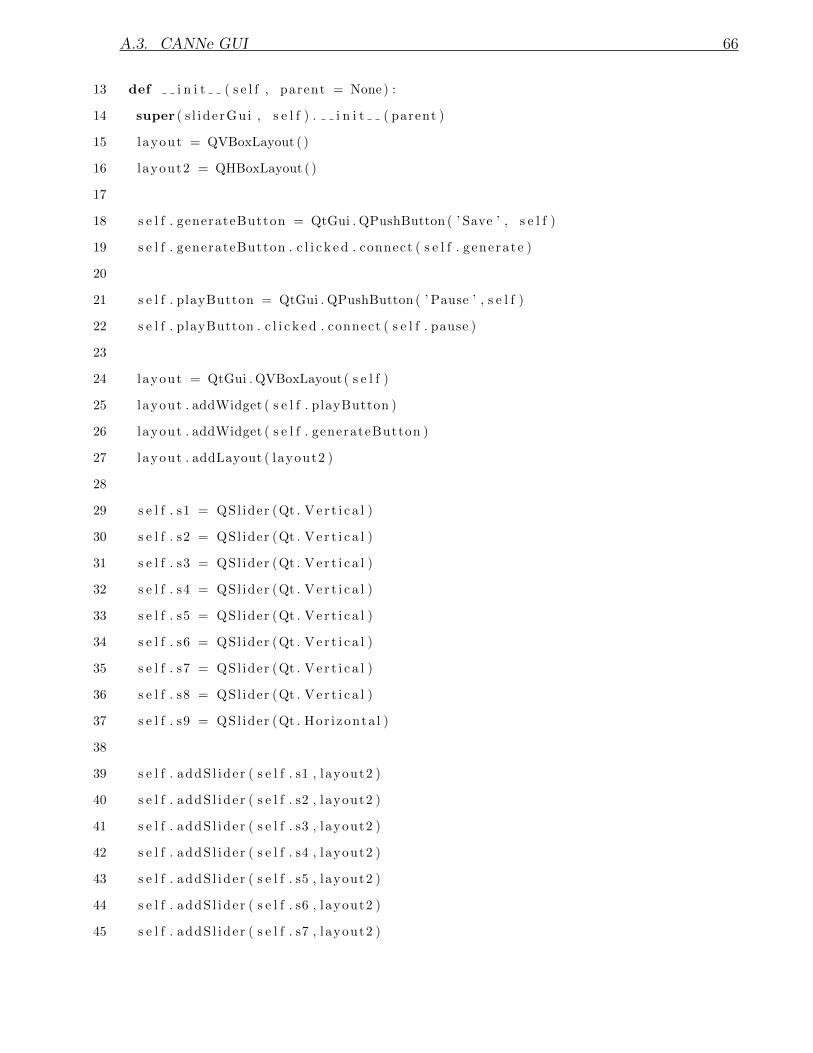
A.3. CANNe GUI 66

13 def i n i t ( s e l f , parent = None ) :

14 super ( s l i de rGu i , s e l f ) . i n i t ( parent )

15 layout = QVBoxLayout ( )

16 layout2 = QHBoxLayout ( )

17

18 s e l f . generateButton = QtGui . QPushButton ( ’ Save ’ , s e l f )

19 s e l f . generateButton . c l i c k e d . connect ( s e l f . generate )

20

21 s e l f . playButton = QtGui . QPushButton ( ’ Pause ’ , s e l f )

22 s e l f . playButton . c l i c k e d . connect ( s e l f . pause )

23

24 layout = QtGui . QVBoxLayout( s e l f )

25 layout . addWidget ( s e l f . playButton )

26 layout . addWidget ( s e l f . generateButton )

27 layout . addLayout ( layout2 )

28

29 s e l f . s1 = QSl ider (Qt . Ve r t i c a l )








37 s e l f . s9 = QSl ider (Qt . Hor i zonta l )

38

39 s e l f . addS l ide r ( s e l f . s1 , layout2 )







A.3. CANNe GUI 67



48 s e l f . s9 . setMinimum(−30)

49 s e l f . s9 . setMaximum(30)

50 s e l f . s9 . setValue (0 )

51 s e l f . s9 . s e tT i c k I n t e r v a l (3 )

52

53 s e l f . setLayout ( layout )

54 s e l f . setWindowTitle ( ”CANNe” )

55

56 def addS l ide r ( s e l f , s l i d e r , l ayout ) :

57 s l i d e r . setMinimum (0)

58 s l i d e r . setMaximum(40)

59 s l i d e r . setValue (10)

60 s l i d e r . s e tT i ckPos i t i on ( QSl ider . TicksBelow )

61 s l i d e r . s e tT i c k I n t e r v a l (2 )

62 layout . addWidget ( s l i d e r )

63 s l i d e r . s l i d e rRe l e a s e d . connect ( s e l f . valuechange )

64

65 def valuechange ( s e l f ) :

66 tmp = np . z e r o s ( ( 1 , 9 ) )

67 tmp [ 0 , 0 ] = s e l f . s1 . va lue ( )

68 tmp [ 0 , 1 ] = s e l f . s2 . va lue ( )

69 tmp [ 0 , 2 ] = s e l f . s3 . va lue ( )

70 tmp [ 0 , 3 ] = s e l f . s4 . va lue ( )

71 tmp [ 0 , 4 ] = s e l f . s5 . va lue ( )

72 tmp [ 0 , 5 ] = s e l f . s6 . va lue ( )

73 tmp [ 0 , 6 ] = s e l f . s7 . va lue ( )

74 tmp [ 0 , 7 ] = s e l f . s8 . va lue ( )

75 tmp /= 10 .

76 tmp [ 0 , 8 ] = 2∗ s e l f . s9 . va lue ( )

77 synth . p lay synth (tmp)

78 pygame . mixer . music . load ( ’ loop . wav ’ )

A.3. CANNe GUI 68

79 pygame . mixer . music . play (−1)

80

81

82 def generate ( s e l f ) :

83 tmp = np . z e r o s ( ( 1 , 9 ) )

84 tmp [ 0 , 0 ] = s e l f . s1 . va lue ( )

85 tmp [ 0 , 1 ] = s e l f . s2 . va lue ( )

86 tmp [ 0 , 2 ] = s e l f . s3 . va lue ( )

87 tmp [ 0 , 3 ] = s e l f . s4 . va lue ( )

88 tmp [ 0 , 4 ] = s e l f . s5 . va lue ( )

89 tmp [ 0 , 5 ] = s e l f . s6 . va lue ( )

90 tmp [ 0 , 6 ] = s e l f . s7 . va lue ( )

91 tmp [ 0 , 7 ] = s e l f . s8 . va lue ( )

92 tmp /= 10 .

93 tmp [ 0 , 8 ] = s e l f . s9 . va lue ( )

94 text , ok = QInputDialog . getText ( s e l f , ’ Save F i l e ’ , ’ Enter f i l ename : ’ )

95 i f ok :

96 f i l e name =str ( t ex t )

97 synth . execute (tmp , f i l e name )

98

99

100

101 def pause ( s e l f ) :

102 pygame . mixer . music . stop ( )

103

104

105 def main ( ) :

106 synth . load weights into memory ( )

107 pygame . i n i t ( )

108 pygame . mixer . i n i t ( channe l s=1)

109 app = QApplication ( sys . argv )

110 ex = s l i d e rGu i ( )

111 ex . show ( )

A.3. CANNe GUI 69

112 sys . e x i t ( app . exec ( ) )

113

114 i f name == ’ ma in ’ :

115 main ( )

Autoencoding Neural Networks as Musical Audio Synthesizers

Documents