CHAPTER 44 ATMOSPHERIC OPTICS Dennis K. Killinger Center for Laser Atmospheric Sensing Department of Physics Uniy ersity of South Florida Tampa , Florida James H. Churnside National Oceanic and Atmospheric Administration Eny ironmental Technology Laboratory Boulder , Colorado Laurence S. Rothman Air Force Geophysics Directorate / Phillips Lab Optical Eny ironment Di y ision Hanscom AFB , Massachusetts 44.1 GLOSSARY c speed of light C 2 n atmospheric turbulence strength parameter F hypergeometric function g (… ) optical absorption lineshape function h height above sea level h Planck’s constant I intensity of optical beam (watts / m 2 ) J Bessel function L o outer scale size of atmospheric turbulence l o inner scale size of atmospheric turbulence N density or concentration of molecules P … Planck radiation function R gas constant S molecular absorption line intensity T temperature 44.1

Welcome message from author
This document is posted to help you gain knowledge. Please leave a comment to let me know what you think about it! Share it to your friends and learn new things together.
Transcript
CHAPTER 44 ATMOSPHERIC OPTICS
Dennis K . Killinger Center for Laser Atmospheric Sensing Department of Physics Uni y ersity of South Florida Tampa , Florida
James H . Churnside National Oceanic and Atmospheric Administration En y ironmental Technology Laboratory Boulder , Colorado
Laurence S . Rothman Air Force Geophysics Directorate / Phillips Lab Optical En y ironment Di y ision Hanscom AFB , Massachusetts
4 4 . 1 GLOSSARY
c speed of light
C 2 n atmospheric turbulence strength parameter
F hypergeometric function
g ( … ) optical absorption lineshape function
h height above sea level
h Planck’s constant
I intensity of optical beam (watts / m 2 )
J Bessel function
L o outer scale size of atmospheric turbulence
l o inner scale size of atmospheric turbulence
N density or concentration of molecules
P … Planck radiation function
R gas constant
S molecular absorption line intensity
T temperature
44 .1

44 .2 TERRESTRIAL OPTICS
W wind speed b backscatter coef ficient of the atmosphere
g p pressure-broadened half-width of absorption line k optical attenuation l wavelength … optical frequency (wave numbers)
r ( I ) probability density function of irradiance fluctuations r o phase coherence length s 2
l variance of irradiance fluctuations s R Rayleigh scattering cross section
4 4 . 2 INTRODUCTION
Atmospheric optics involves the transmission , absorption , emission , refraction , and reflection of light by the atmosphere and is probably one of the most widely observed of all optical phenomena . 1–5 The atmosphere interacts with light due to the composition of the atmosphere , which under normal conditions , consists of a variety of dif ferent molecular species and small particles or aerosols . This interaction of the atmosphere with light is observed to produce a wide variety of optical phenomena including the blue color of the sky , the red sunset , the optical absorption of specific wavelengths due to atmospheric molecules , the twinkling of stars at night , and the greenish tint sometimes observed during a severe wind storm due to the high density of dust and water-related aerosols in the atmosphere .
One of the most basic optical phenomena of the atmosphere is the absorption of light . This absorption process can be depicted as in Fig . 1 which shows the transmission spectrum of the atmosphere as a function of wavelength . 5 The transmission of the atmosphere is highly dependent upon the wavelength of the spectral radiation , and , as will be covered later in this chapter , upon the composition and specific optical properties of the
FIGURE 1 Transmittance through the earth’s atmosphere as a function of wavelength taken with low spectral resolution (path length 1800 m) . ( From Measures , Ref . 5 . )

ATMOSPHERIC OPTICS 44 .3
constituents in the atmosphere . The prominent spectral features in the transmission spectrum in Fig . 1 are primarily due to absorption bands and individual absorption lines of the molecular gases in the atmosphere , while a portion of the slowly varying background transmission is due to aerosol extinction , continuum absorption , and particulates in the atmosphere .
This chapter presents a tutorial overview of some of the basic optical properties of the atmosphere , with an emphasis on those properties associated with optical propagation and transmission of light through the Earth’s atmosphere . The physical phenomena of optical absorption , scattering , emission , and refractive properties of the atmosphere will be covered for optical wavelengths from the UV to the far-infrared . The primary focus of this chapter is on linear optical properties associated with the transmission of light through the atmosphere . Historically , the study of atmospheric optics has centered around the radiance transfer function of the atmosphere , and the linear transmission spectrum and blackbody emission spectrum of the atmosphere . This emphasis was due to the large body of research associated with passive , electro-optical sensors which primarily use the transmission of ambient optical light or light from selected emission sources . During the past decade , however , the use of lasers has added a new dimension to the study of atmospheric optics . In this case , not only is one interested in the transmission of light through the atmosphere , but also information regarding the optical properties of the backscattered optical radiation .
In this chapter , the standard linear optical interactions of an optical or laser beam with the atmosphere will be covered , with an emphasis placed on linear absorption and scattering interactions . It should be mentioned that the first edition of the OSA Handbook of Optics chapter on ‘‘Atmospheric Optics’’ had considerable nomographs and computa- tional charts to aid the user in numerically calculating the transmission of the atmosphere . 2 Because of the present availability of a wide range of spectral databases and computer programs (such as the HITRAN Spectroscopy Database , and LOWTRAN , MODTRAN , and FASCODE atmospheric transmission computer programs) that model and calculate the transmission of light through the atmosphere , these nomographs , while still useful , are not as vital . As a result , the emphasis of this second edition of the ‘‘Atmospheric Optics’’ chapter is on the basic theory of the optical interactions , how this theory is used to model the optics of the atmosphere , the use of available computer programs and databases to calculate the optical properties of the atmosphere , and examples of instruments and meteorological phenomena related to optical or visual remote sensing of the atmosphere .
The overall organization of this chapter begins with a description of the natural , homogeneous atmosphere and the representation of its physical and chemical composition as a function of altitude . A brief survey is then made of the major linear optical interactions that can occur between a propagating optical beam and the naturally occurring constituents in the atmosphere . The next section covers several major computational programs (HITRAN , LOWTRAN , MODTRAN , and FASCODE) and U . S . Standard Atmospheric Models which are used to compute the optical transmission , scattering , and absorption properties of the atmosphere . The next major technical section presents an overview of the influence of atmospheric refractive turbulence on the statistical propaga- tion of an optical beam or wavefront through the atmosphere . Finally , the last two sections of the chapter include a brief introduction to some optical and laser remote sensing experiments of the atmosphere and a brief introduction to the visually important field of meteorological optics .
It should be noted that the material contained within this chapter has been compiled from several recent overview / summary publications on the optical transmission and atmospheric composition of the atmosphere , as well as from a large number of technical reports and journal publications . These major overview references are : (1) the previous edition of the OSA Handbook of Optics (chapter on ‘‘Optical Properties of the Atmosphere’’) , (2) Handbook of Geophysics and the Space En y ironment (chapter on ‘‘Optical and Infrared Properties of the Atmosphere’’) , (3) The Infrared Handbook , (4) Laser Remote Sensing , and (5) Atmospheric Radiation . 1–5 The interested reader is directed
44 .4 TERRESTRIAL OPTICS
toward these comprehensive treatments as well as to the listed references therein for detailed information concerning the topics covered in this brief overview of atmospheric optics .
4 4 . 3 PHYSICAL AND CHEMICAL COMPOSITION OF THE STANDARD ATMOSPHERE
The atmosphere is a fluid composed of gases , particulates , and aerosols whose physical and chemical properties vary as a function of time , altitude , and geographical location . Although these properties can be highly dependent upon local and regional conditions , many of the optical properties of the atmosphere can be described to an adequate level by looking at the compositon of what one normally calls a standard atmosphere . This section will describe the background , homogeneous standard composition of the atmosphere . This will serve as a basis for the determination of the quantitative interaction of the molecular gases , aerosols , and particulates in the atmosphere with a propagating optical wavefront .
Molecular Gas Concentration , Pressure , and Temperature
The majority of the atmosphere is composed of lightweight molecular gases . Table 1 lists the major gases and trace species of the terrestrial atmosphere , and their approximate concentration in units of atmospheres (atm) at standard room temperature (296 K) , altitude at sea level , and total pressure of 1 atm . 6 The major optically active molecular constituents of the atmosphere are N 2 , O 2 , H 2 O , and CO 2 , with a secondary grouping of CH 4 , N 2 O , CO , and O 3 . The other 22 species in the table are present in the atmosphere at trace-level concentrations (ppb , down to less than ppt by volume) , however the concentration may be increased by many orders of magnitude due to local emission sources of these gases .
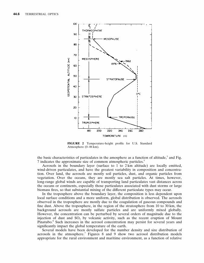
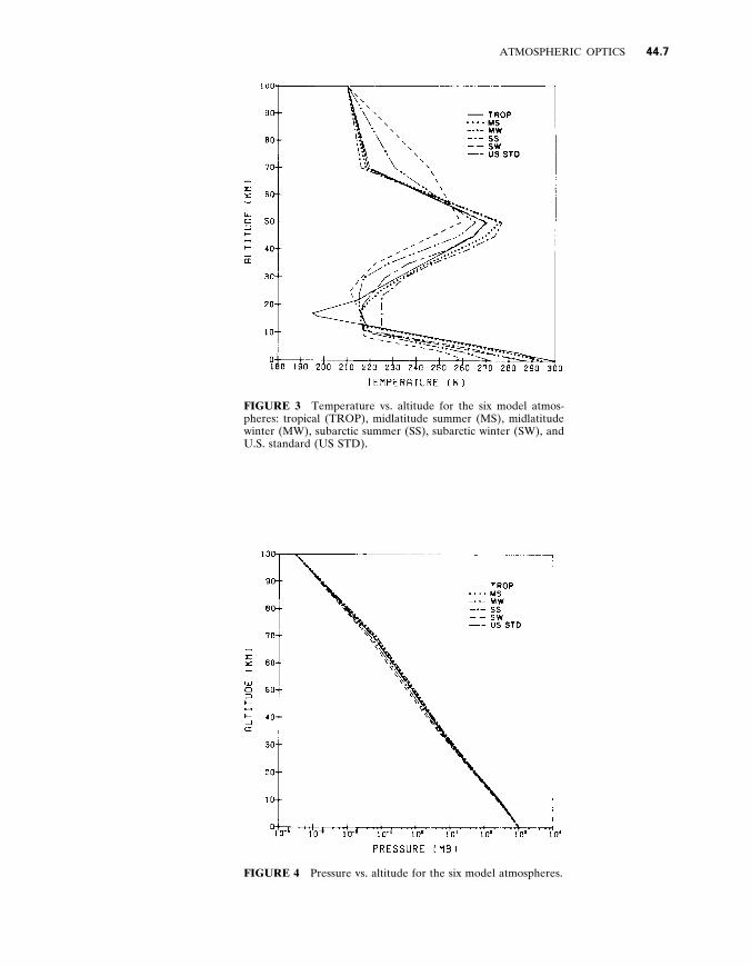
The temperature of the atmosphere varies both with seasonal changes and altitude . Figure 2 shows the average temperature profile of the atmosphere as a function of altitude presented for the U . S . Standard atmosphere . 7 The temperature decreases significantly with altitude until the level of the stratosphere is reached where the temperature profile has an inflection point . The U . S . Standard Atmosphere is one of six basic atmospheric models developed by the U . S . government ; these dif ferent models furnish a good representation of the dif ferent atmospheric conditions which are often encountered . Figure 3 shows the temperature profile for the six atmospheric models . 7
The pressure of the atmosphere decreases with altitude due to the gravitational pull of the earth and the hydrostatic equilibrium pressure of the atmospheric fluid . This is indicated in Fig . 4 which shows the total pressure of the atmosphere in millibars (1013 mb 5 1 atm 5 760 torr) as a function of altitude for the dif ferent atmospheric models . 7 The fractional or partial pressure of most of the major gases (N 2 , O 2 , CO 2 , N 2 O , CO , and CH 4 ) follows this profile and these gases are considered uniformly mixed . However , the concentration of water vapor is very temperature-dependent due to freezing and is not uniformly mixed in the atmosphere . Figure 5 a shows the partial pressure (density) of water vapor as a function of altitude ; the units of density are in molecules / cm 3
and are related to 1 atm by the appropriate value of Loschmidts number (the number of molecules in 1 cm 3 of air) at a temperature of 296 K , which is 2 . 479 3 10 1 9 molecules / cm 3 . 7
The partial pressure of ozone (O 3 ) also varies significantly with altitude because it is generated in the upper altitudes and near ground level by solar radiation , and is in chemical equilibrium with other gases in the atmosphere which themselves vary with altitude and time of day . Figure 5 b shows the typical concentration of ozone as a function

ATMOSPHERIC OPTICS 44 .5
TABLE 1 List of Molecular Gases and Their Typical Concentration for the Ambient U . S . Standard Atmo- sphere (Note that the trace species have concentra- tions less than 1 3 10 2 9 , with a value that is variable and often dependent upon local emission sources . )
Molecule p (atm)
N 2 O 2 H 2 O CO 2 A (Argon) CH 4 N 2 O CO O 3
0 . 781 0 . 209 0 . 0775 (variable) 3 . 3 E 2 4 0 . 0093 1 . 7 E 2 6 3 . 2 E 2 7 1 . 5 E 2 7 2 . 66 E 2 8 (variable)
H 2 CO C 2 H 6 HCl CH 3 Cl OCS C 2 H 2 SO 2 NO H 2 O 2 HCN
2 . 4 E 2 9 2 E 2 9 1 E 2 9 7 E 2 10 6 E 2 10 3 E 2 10 3 E 2 10 3 E 2 10 2 E 2 10 1 . 7 E 2 10
HNO 3 NH 3 NO 2 HOCl HI HBr OH HF ClO HCOOH COF 2 SF 6 H 2 S PH 3
5 E 2 11 5 E 2 11 2 . 3 E 2 11 7 . 7 E 2 12 3 E 2 12 1 . 7 E 2 12 4 . 4 E 2 14 1 E 2 14 1 E 2 14 1 E 2 14 1 E 2 14 1 E 2 14 1 E 2 14 1 E 2 20
of altitude . 7 The ozone concentration peaks at an altitude of approximately 20 km and is one of the principal molecular optical absorbers in the atmosphere at that altitude . Further details of these atmospheric models under dif ferent atmospheric conditions are contained within the listed references and the reader is encouraged to consult these references for more detailed information . 3 , 7
Aerosols and Particulates
The atmospheric propagation of optical radiation is influenced by particulate matter suspended in the air such as dust , fog , haze , cloud droplets , and aerosols . Figure 6 shows
44 .6 TERRESTRIAL OPTICS
FIGURE 2 Temperature-height profile for U . S . Standard Atmosphere (0 – 86 km) .
the basic characteristics of particulates in the amosphere as a function of altitude , 3 and Fig . 7 indicates the approximate size of common atmospheric particles . 5
Aerosols in the boundary layer (surface to 1 to 2 km altitude) are locally emitted , wind-driven particulates , and have the greatest variability in composition and concentra- tion . Over land , the aerosols are mostly soil particles , dust , and organic particles from vegetation . Over the oceans , they are mostly sea salt particles . At times , however , long-range global winds are capable of transporting land particulates vast distances across the oceans or continents , especially those particulates associated with dust storms or large biomass fires , so that substantial mixing of the dif ferent particulate types may occur .
In the troposphere above the boundary layer , the composition is less dependent upon local surface conditions and a more uniform , global distribution is observed . The aerosols observed in the troposphere are mostly due to the coagulation of gaseous compounds and fine dust . Above the troposphere , in the region of the stratosphere from 10 to 30 km , the background aerosols are mostly sulfate particles and are uniformly mixed globally . However , the concentration can be perturbed by several orders of magnitude due to the injection of dust and SO 2 by volcanic activity , such as the recent eruption of Mount Pinatubo . 8 Such increases in the aerosol concentration may persist for several years and significantly impact the global temperature of the earth .
Several models have been developed for the number density and size distribution of aerosols in the atmosphere . 7 Figures 8 and 9 show two aerosol distribution models appropriate for the rural environment and maritime environment , as a function of relative
ATMOSPHERIC OPTICS 44 .7
FIGURE 3 Temperature vs . altitude for the six model atmos- pheres : tropical (TROP) , midlatitude summer (MS) , midlatitude winter (MW) , subarctic summer (SS) , subarctic winter (SW) , and U . S . standard (US STD) .
FIGURE 4 Pressure vs . altitude for the six model atmospheres .

44 .8 TERRESTRIAL OPTICS
(a) (b)
FIGURE 5 ( a ) Water vapor profile of several models ; ( b ) ozone profile for several models ; the U . S . standard model shown is the 1962 model .
FIGURE 6 Physical characteristics of atmospheric aerosols .

ATMOSPHERIC OPTICS 44 .9
FIGURE 7 Representative diameters of common atmospheric particles . ( From Measures , Ref . 5 . )
FIGURE 8 Aerosol number density distribution (cm 2 3
m m 2 1 ) for the rural model at dif ferent relative humidities with total particle concentrations fixed at 15 , 000 cm 2 3 .
FIGURE 9 Aerosol number density distribution (cm 2 3
m m 2 1 ) for the maritime model at dif ferent relative humidities with total particle concentrations fixed at 4000 cm 2 3 .

44 .10 TERRESTRIAL OPTICS
humidity 7 ; the humidity influences the size distribution of the aerosol particles and their growth characteristics . The greatest number density (particles / cm 3 ) occurs near a size of 0 . 01 m m but a significant number of aerosols are still present even at the larger sizes near 1 to 2 m m . Finally , the optical characteristics of the aerosols can also be dependent upon water vapor concentration , with changes in surface , size , and growth characteristics of the aerosols sometimes observed to be dependent upon the relative humidity . Such humidity changes can also influence the concentration of some pollutant gases , if these gases have been absorbed onto the surface of the aerosol particles . 7
44 . 4 FUNDAMENTAL THEORY OF INTERACTION OF LIGHT WITH THE ATMOSPHERE
The propagation of light through the atmosphere depends upon several optical interaction phenomena and the physical composition of the atmosphere . In this section , we consider some of the basic interactions involved in the transmission , absorption , emission , and scattering of light as it passes through the atmosphere . Although all of these interactions can be described as part of an overall radiative transfer process , it is common to separate the interactions into distinct optical phenomena of molecular absorption , Rayleigh scattering , Mie or aerosol scattering , and molecular emission . Each of these basic phenomena will be discussed in this section following a brief outline of the fundamental equations for the transmission of light in the atmosphere centered around the Beer- Lambert law .
The linear transmission (or absorption) of monochromatic light by species in the atmosphere may be expressed approximately by the Beer-Lambert law as
I ( l , t 9 , x ) 5 I ( l , t , 0)e 2 e x 0 k ( l ) N ( x 9 , t ) dx 9 (1)
where I ( l , t 9 , x ) is the intensity of the optical beam after passing through a path length of x , k ( l ) is the optical attenuation or extinction coef ficient of the species per unit of species density and length , and N ( x , t ) is the spatial and temporal distribution of the species density that is producing the absorption ; l is the wavelength of the monochromatic light , and the parameter time t 9 is inserted to remind one of the potential propagation delay . Equation (1) contains the term N ( x , t ) which explicitly indicates the spatial and temporal variability of the concentration of the attenuating species since in many experimental cases such variability may be a dominant feature .
It is common to write the attenuation coef ficient in terms of coef ficients that can describe the dif ferent phenomena that can cause the extinction of the optical beam . The most dominant interactions in the natural atmosphere are those due to Rayleigh (elastic) scattering , linear absorption , and Mie (aerosol / particulate) scattering ; elastic means that the scattered light does not change in wavelength from that which was transmitted while inelastic infers a shift in the wavelength . In this case , one can write k ( l ) as
k ( l ) 5 k a ( l ) 1 k R ( l ) 1 k M ( l ) (2)
where these terms represent the individual contributions due to absorption , Rayleigh scattering , and Mie scattering , respectively . The values for each of these extinction coef ficients will be described in the following sections along with the appropriate species

ATMOSPHERIC OPTICS 44 .11
density term N ( x , t ) . In some of these cases , the reemission of the optical radiation , possibly at a dif ferent wavelength , is also of importance . Rayleigh extinction will lead to Rayleigh backscatter , Raman extinction leads to spontaneous Raman scattering , absorp- tion can lead to fluorescence emission or thermal heating of the molecule , and Mie extinction is defined primarily in terms of the scattering coef ficient . Under idealized conditions , the scattering processes can be related directly to the value of the attenuation processes . However , if several complex optical processes occur simultaneously , such as in atmospheric propagation , the attenuation and scattering processes are not directly linked via a simple analytical equation . In this case , independent measurements of the scattering coef ficient and the extinction coef ficient have to be made , or approximation formulas are used to relate the two coef ficients . 4 , 5
Molecular Absorption
The absorption of optical radiation by molecules in the atmosphere is primarily associated with individual optical absorption transitions between the allowed quantized energy levels of the molecule . The energy levels of a molecule can usually be separated into those associated with rotational , vibrational , or electronic energy states . Absorption transitions between the rotational levels occur in the far-IR and microwave spectral region , transitions between vibrational levels occur in the near-IR (2 to 20 m m wavelength) , and electronic transitions occur in the UV-visible region (0 . 3 to 0 . 7 m m) . Transitions can occur which combine several of these categories , such as rotational-vibrational transitions or electronic- vibrational-rotational transitions .
Some of the most distinctive and identifiable absorption lines of many atmospheric molecules are the rotational-vibrational optical absorption lines in the infrared spectral region . These lines are often clustered together into vibrational bands according to the allowed quantum transitions of the molecule . In many cases , the individual lines are distinct and can be resolved if the spectral resolution of the measuring instrument is fine enough (i . e ., , 0 . 1 cm 2 1 ) . An example of such a region is the absorption feature near 2 . 04 m m in Fig . 1 which is actually composed of individual absorption lines if viewed under higher spectral resolution . Figure 10 is a computed high-resolution expansion of the
FIGURE 10 High-resolution transmission spectrum of the atmosphere for a horizontal path of 1800 m (similar to that in Fig . 1) for the spectral region near 2 . 04 m m . The individual rotational absorption lines due to CO 2 and H 2 O are easily observed .

44 .12 TERRESTRIAL OPTICS
FIGURE 11 High-resolution absorption spectrum of Freon-12 gas showing complex band structure typical of heavy , complex molecules in the atmosphere (path of 1000 m with 1 ppm concentration) .
atmospheric spectrum of Fig . 1 near 2 . 04 m m over a path length of 1800 m which shows these individual lines . In this case , the individual lines are well-separated and appear like a ‘‘picket fence’’ spectrum showing gaps between the absorption lines . Many of the atmospheric gaseous molecules listed earlier in Table 1 have similar spectral structure . These gases are relatively lightweight and have few (less than 5 or 6) atoms per molecule so that their moments of inertia are relatively small . The resulting energy spacing between the allowed rotational-vibrational absorption transitions is large and well-separated in wavelength .
In other spectral regions , however , the individual lines overlap or are so strong or saturated that the transmission spectrum displays only broad spectral features ; an example of such a spectral region is the strong absorption seen near 2 . 7 m m , 5 to 8 m m , and beyond 13 m m in Fig . 1 . Finally , the molecular absorption observed in the UV is often due to optical transitions to an electronic energy level , molecular energy continuum or a predissociation energy level . In some cases , such as that for O 3 or SO 2 , this results in broad absorption bands that extend throughout the UV region (250 to 350 nm) .
More complex , heavier molecules , such as benzene or chlorofluorocarbons , have absorption spectra which are blended or merged together into band spectra due to the complexity and overlap of the rotational-vibrational transitions of these molecules . Figure 11 shows a transmission spectrum of Freon-12 (C Cl 2 F 2 ) which has a complex spectrum near 11 m m . As seen , the individual rotational lines are merged into a band spectrum . A band spectrum is often unique for each gas and can be used to identify the chemical composition of the gas . Heavy molecules in the atmosphere are not normally part of the natural atmosphere and are usually the result of pollution or gaseous plumes injected into the atmosphere .
The overall transmission or absorption of the atmosphere due to an individual molecular absorption line can be given quantitatively as
k a ( l ) N ( x , t ) 5 Sg ( … 2 … o ) NP a (3)
where S is the molecular transition line intensity (units of cm / molecule) , g ( … 2 … o ) is the normalized lineshape function (units of cm or 1 / cm 2 1 ) , N is the number of molecules of absorbing species per cm 3 per atm , and P a is the partial pressure of the absorbing gas in
ATMOSPHERIC OPTICS 44 .13
atm . The value of N is equal to the value of Loschmidt’s number , which is 2 . 479 3 10 1 9 molecules cm 2 3 atm 2 1 at a temperature of 296 K ; The value of N is inversely proportional to temperature due to the change in gas concentration as a function of temperature for 1 atm of pressure . As will be seen later , the definition of S as given in Eq . (3) is that used in the U . S . Air Force Phillips Laboratory / Geophysics Directorate HITRAN database . 9 In this case , S contains the Boltzmann population factor and isotope fraction (natural abundance) as well as the stimulated emission term due to finite population in the upper energy states of the molecule . 9 In Eq . (3) , Sg ( … 2 … o ) is the absorption cross section per molecule (cm 2 / molecule) and NP a is the number of absorbing molecules in units of molecules / cm 3 .
The lineshape function can be described by several dif ferent models . The two most prevalent are the lorentzian lineshape associated with pressure broadening and the gaussian lineshape associated with Doppler broadening which becomes important at elevated temperatures or low pressures .
The lorentzian / pressure-broadened profile is given by
g L ( … 2 … o ) 5 ( g p / π ) / [( … 2 … o ) 2 1 g 2 p ] (4)
where g p is the pressure-broadened half-width at half-maximum (HWHM) in wave numbers (cm 2 1 ) . The pressure-broadened half-width is obtained from the air-broadened half-width parameter g as g p 5 gP t , where P t is the total background atmospheric pressure . Under ambient atmospheric conditions , g is approximately 0 . 05 cm 2 1 (i . e ., 1 . 5 GHz) for many molecules in the atmosphere .
It should be noted that under very low pressure conditions , where the time between collisions with other molecules is relatively long , the intrinsic radiative lifetime of the molecule will determine the lineshape profile . Under these conditions , the linewidth is called the natural linewidth . The natural linewidth of many molecules is on the order of a few MHz (i . e ., approximately 0 . 0001 cm 2 1 ) or less .
The gaussian or Doppler line profile is expressed as
g D ( … 2 … o ) 5 (1 / g D )(ln 2 / π ) . 5 exp [ 2 ln 2( … 2 … o ) 2 / g 2 D ] (5)
where g D is the Doppler linewidth (HWHM in cm 2 1 ) given by
g D 5 ( … o / c )[2 RT ln 2 / M ] 1/2 (6)
where R is the gas constant , T is the temperature in Kelvin , and M is the molecular weight of the molecule .
The value for the lineshape at the peak (line center) is equal to 1 / ( π g p ) 5 0 . 318 / g p for the pressure-broadened case . For the Doppler peak , the maximum value is (ln 2 / π ) 1/2 / g D 5 0 . 469 / g D . Under ambient atmospheric conditions , the Doppler linewidth is usually much smaller than the pressure-broadened linewidth .
For those cases where both lorentzian and Doppler broadening are present in approximately equal amounts , a convolution of the Doppler and lorentzian profile must be used . This convolution of a Doppler and lorentzian is called a Voigt profile and involves a double integral for an exact calculation . Fortunately , several numerical approximations are available for the computation of the Voigt profile and lineshape parameters . 1 0 The Voigt profile is important in the spectroscopy of molecules in the upper atmosphere where the ambient pressure is low and the Doppler and pressure-broadened linewidths are of the same order of magnitude .
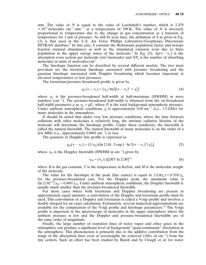
Finally , the large number of transition lines of water vapor and other gases in the atmosphere can produce a significant level of background ‘‘quasi-continuum’’ absorption in the atmosphere . This phenomenon is primarily due to the additive contribution from the wings of the absorption lines even at wavelengths far removed (100 s of cm 2 1 ) from the line centers . Such an ef fect has been studied by Burch and by Clough et al . for water
44 .14 TERRESTRIAL OPTICS
FIGURE 12 Self-density absorption continuum values C s for water vapor as a function of wave number . The experimental values were measured by Burch . ( From Ref . 3 . )
vapor due to strong self-broadening interactions . 1 1 Figure 12 shows a plot of the relative continuum coef ficient for water vapor as a function of wave number . Good agreement with the experimental data and model calculations is shown . Models for water vapor and nitrogen continuum absorption are contained within many of the major atmospheric transmission programs (such as FASCODE) . The typical value for the continuum absorption is negligible in the visible to the near-IR , but can be significant at wavelengths in the range of 5 to 20 m m .
Molecular Rayleigh Scattering
Rayleigh scattering is elastic scattering of the optical radiation due to the displacement of the weakly bound electronic cloud surrounding the gaseous molecule which is perturbed by the incoming electro-magnetic (optical) field . This phenomenon is associated with optical scattering where the wavelength of light is much larger than the physical size of the scatterers (i . e ., atmospheric molecules) . Rayleigh scattering , which makes the color of the sky blue and the setting or rising sun red , was first described by Lord Rayleigh in 1871 . The Rayleigh dif ferential scattering cross section for polarized , monochromatic light is given by 5
d s R / d Ω 5 [ π 2 ( n 2 2 1) 2 / N 2 l 4 ][cos 2 f cos 2 θ 1 sin 2 f ] (7)
where n is the index of refraction of the atmosphere , N is the density of molecules , l is the wavelength of the optical radiation , and f and θ are the spherical coordinate angles of the scattered polarized light referenced to the direction of the incident light . As seen from Eq . (7) , shorter-wavelength light (i . e ., blue) is more strongly scattered out from a propagating beam than the longer wavelengths (i . e ., red) , which is consistent with the preceding comments regarding the color of the sky or the sunset . A typical value for d s R / d Ω at a wavelength of 700 nm in the atmosphere (STP) is approximately 2 3 10 2 2 8 cm 2 sr 2 1 . 3 This value depends upon the molecule and has been tabulated for many of the major gases in the atmosphere . 10–12

ATMOSPHERIC OPTICS 44 .15
The total Rayleigh scattering cross section can be determined from Eq . (7) by integrating over 4 π steradians to yield
s R (total) 5 [8 / 3][ π 2 ( n 2 2 1) 2 / N 2 l 4 ] (8)
At sea level (and room temperature , T 5 296 K) where N 5 2 . 5 3 10 1 9 molecules / cm 3 , Eq . (8) can be multiplied by N to yield the total Rayleigh scattering extinction coef ficient as
k R ( l ) N ( x , t ) 5 N s R (total) 5 1 . 18 3 10 2 8 [550 nm / l (nm)] 4 cm 2 1 (9)
The neglect of the ef fect of dispersion of the atmosphere (variation of the index of refraction n with wavelength) results in an error of less than 3 percent in Eq . (9) in the visible wavelength range . 5
The molecular Rayleigh backscatter ( θ 5 π ) cross section for the atmosphere has been given by Collins and Russell for polarized incident light (and received scattered light of the same polarization) as 1 2
s R 5 5 . 45 3 10 2 2 8 [550 nm / l (nm)] 4 cm 2 sr 2 1 (10)
At sea level where N 5 2 . 47 3 10 1 9 molecules / cm 3 , the atmospheric volume backscatter coef ficient , b R , is thus given by
b R 5 N s R 5 1 . 39 3 10 2 8 [550 nm / l (nm)] 4 cm 2 1 sr 2 1 (11)
The backscatter coef ficient for the reflectivity of a laser beam due to Rayleigh backscatter is determined by multiplying b R by the range resolution or length of the optical interaction being considered .
For unpolarized incident light , the Rayleigh scattered light has a depolarization factor d which is the ratio of the two orthogonal polarized backscatter intensities . d is usually defined as the ratio of the perpendicular and parallel polarization components measured relative to the direction of the incident polarization . Values of d depend upon the anisotropy of the molecules or scatters , and typical values range from 0 . 02 to 0 . 11 . 1 3
Depolarization also occurs for multiple scattering and is of considerable interest in laser or optical transmission through dense aerosol clouds . 1 4 The depolarization factor can sometimes be used to determine the physical and chemical composition of the cloud constituents , such as the relative ratio of water vapor or ice crystals in a cloud .
Mie Scattering : Aerosols , Particulates , and Clouds
Mie scattering is similar to Rayleigh scattering , except the size of the scattering sites is on the same order of magnitude as the wavelength of the incident light , and is , thus , due to aerosols and fine particulates in the atmosphere . The scattered radiation is the same wavelength as the incident light but experiences a more complex functional dependence upon the interplay of the optical wavelength and particle size distribution than that seen for Rayleigh scattering .
In 1908 , Mie investigated the scattering of light by dielectric spheres of size comparable to the wavelength of the incident light . 1 5 His analysis indicated the clear asymmetry between the forward and backward directions , where for large particle sizes the forward-directed scattering dominates . Complete treatments of Mie scattering can be found in several excellent works by Deirmendjian and others , which take into account the complex index of refraction and size distribution of the particles . 16 , 17 These calculations are also influenced by the asymmetry of the aerosols or particulates which may not be spherical in shape .
The ef fect of Mie scattering in the atmosphere can be described as in the following figures . Figure 13 shows the aerosol Mie extinction coef ficient as a function of wavelength for several atmospheric models , along with a typical Rayleigh scattering curve for

44 .16 TERRESTRIAL OPTICS
FIGURE 13 Aerosol extinction coef ficient as a function of wavelength . ( From Measures , Ref . 5 . )
FIGURE 14 Aerosol volume backscattering coef ficient as a function of wavelength . ( From Ref . 5 . )
comparison . 1 8 Figure 14 shows similar values for the volume Mie backscatter coef ficient as a function of wavelength . 1 8 Extinction and backscatter coef ficient values are highly dependent upon the wavelength and particulate composition .
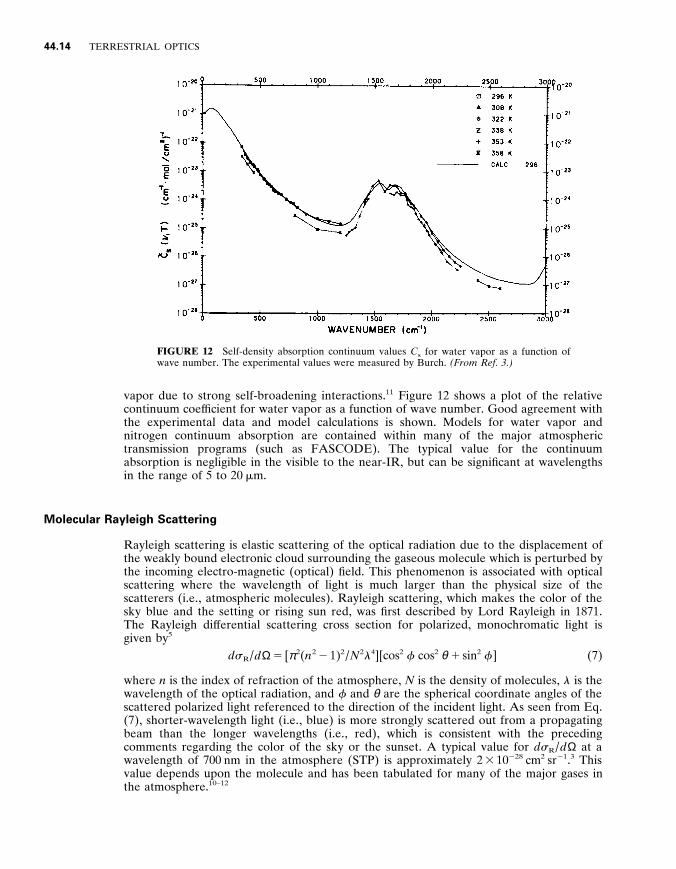
Figures 15 and 16 show the calculated extinction coef ficient for the rural and maritime aerosol models described in Sec . 44 . 3 as a function of relative humidity and wavelength . 3 Significant changes in the backscatter can be produced by relatively small changes in the humidity .
The extinction coef ficient is also a function of altitude , following the dependence of the composition of the aerosol and particulates . Figure 17 shows an atmospheric aerosol extinction model as a function of altitude for a wavelength of 0 . 55 m m . 3 , 8 The influence of the visibility (in km) at ground level dominates the extinction value at the lower altitudes and the composition and density of volcanic particulate dominates the upper altitude regions . The dependence of the extinction on the volcanic composition at the upper altitudes is shown in Fig . 18 which shows these values as a function of wavelength and of composition . 3 , 8
The variation of the backscatter coef ficient as a function of altitude is shown in Fig . 19 which displays atmospheric backscatter data obtained by McCormick using a 1 . 06- m m Nd : YAG Lidar . 1 9 The boundary layer aerosols dominate at the lower levels and the decrease in the atmospheric particulate density determines the overall slope with altitude . Of interest is the increased value near 20 km due to the presence of volcanic aerosols in the atmosphere due to the eruption of Mt . Pinatubo in 1991 .
Molecular Emission and Thermal Spectral Radiance
The same optical molecular transitions that cause absorption also emit light when they are thermally excited . Since the molecules have a finite temperature T they will act as blackbody radiators with optical emission given by the Planck radiation law . The allowed transitions of the molecules will modify the intensity distribution of the radiation due to emission of the radiation according to the thermal distribution of the population within
ATMOSPHERIC OPTICS 44 .17
FIGURE 15 Extinction coef ficients vs . wavelength for the rural aerosol model for dif ferent relative humidities and constant number density of particles .
FIGURE 16 Extinction coef ficients vs . wavelength for the maritime aerosol model for dif ferent relative humidities and constant number density of particles .
the energy levels of the molecule ; it should be noted that the Boltzmann thermal population distribution is essentially the same as that which is described by the Planck radiation law for local thermodynamic equilibrium conditions . As such , the molecular emission spectrum of the radiation is similar to that for absorption . The thermal radiance from the clear atmosphere involves the calculation of the blackbody radiation emitted by each elemental volume of air multiplied by the absorption spectral distribution of the molecular absorption lines , k a ( s ) , and then this emission spectrum is attenuated by the rest of the atmosphere as the emission propagates toward the viewer . This may be expressed as
I … 5 E s
0 k a ( s ) P … ( s ) exp F 2 E s
0 k a ( s 9 ) ds 9 G ds (12)
where the exponential term is Beer’s law , and P … ( s ) is the Planck function given by
P … ( s ) 5 2 h … 3 / [ c 2 exp ([ h … / kT ( s )] 2 1)] (13)
In these equations , s is the distance from the receiver along the optical propagation path , … is the optical frequency , h is Planck’s constant , c is the speed of light , k is Boltzmann’s constant , and T ( s ) is the temperature at position s along the path . As seen in Eq . (12) , each volume element emits thermal radiation of k a ( s ) P … ( s ) , which is then attenuated by Beer’s law . The total emission spectral density is obtained by summing or integrating over all the emission volume elements and calculating the appropriate absorption along the optical path for each element .
As an example , Fig . 20 shows a plot of the spectral radiance measured on a clear day with 1 cm 2 1 spectral resolution . Note that the regions of strong absorption produce more radiance as the foregoing equation suggests , and that regions of little absorption correspond to little radiance . In the 800 to 1200 wave number spectral region (i . e ., 8 . 3- to 12 . 5- m m wavelength region) , the radiance is relatively low . This is consistent with the fact that the spectral region from 8 to 12 m m is a transmission window of the atmosphere with relatively little absorption of radiation .

44 .18 TERRESTRIAL OPTICS
FIGURE 17 The vertical distribution of the aerosol extinction coef ficient (at 0 . 55- m m wavelength) for the dif ferent atmospheric models . Also shown for comparison are the Rayleigh profile (dotted line) . Between 2 and 30 km , where the distinction on a seasonal basis is made , the spring-summer conditions are indicated with a solid line and fall-winter conditions are indicated by a dashed line . ( From Ref . 3 . )
Surface Reflectivity and Multiple Scattering
The spectral intensity of naturally occurring light at the earth’s surface is primarily due to the incident intensity from the sun in the visible to mid-IR wavelength range , and due to thermal emission from the atmosphere and background radiance in the mid-IR . In both cases , the optical radiation is af fected by the reflectance characteristics of the clouds and surface layers . For instance , the fraction of light that falls on the earth’s surface and is reflected back into the atmosphere is dependent upon the reflectivity of the surface , the incident solar radiation (polarization and spectral density) , and the absorption of the atmosphere .
The reflectivity of a surface , such as the earth’s surface , is often characterized using the bidirectional reflectance function (BDRF) . This function accounts for the nonspecular reflection of light from common rough surfaces and describes the changes in the reflectivity of a surface as a function of the angle which the incident beam makes with the surface . In addition , the reflectivity of a surface is usually a function of wavelength . This latter ef fect can be seen in Fig . 21 which shows the reflectance of several common substances for normal incident radiation . 2 As seen in Fig . 21 , the reflectivity of these surfaces is a strong function of wavelength .

ATMOSPHERIC OPTICS 44 .19
FIGURE 18 Extinction coef ficients for the dif ferent stratospheric aerosol models (background , volcanic , and fresh volcanic) . The extinction coef ficients have been normalized to values around peak levels for these models .
FIGURE 19 1 . 06- m m lidar backscatter coef ficient measurements as a function of vertical altitude . ( From McCormick and Winker , Ref . 1 9 . )

44 .20 TERRESTRIAL OPTICS
FIGURE 20 Spectral radiance (molecular thermal emission) measured on a clear day showing the relatively low value of radiance near 1000 cm 2 1 (i . e ., 10- m m wavelength) . ( Pro y ided by Churnside . )
FIGURE 21 Typical reflectance of water surface , snow , dry soil , and vegetation . ( From Ref . 2 . )

ATMOSPHERIC OPTICS 44 .21
The ef fect of multiple scattering sometimes must be considered when the scattered light undergoes more than one scatter event , and is rescattered on other particles or molecules . These multiple scattering events increase with increasing optical thickness and produce deviations from the Beer-Lambert law . Extensive analyses of the scattering processes for multiple scattering have been conducted and have shown some success in predicting the overall penetration of light through a thick dense cloud . Dif ferent computational techniques have been used including the Gauss-Seidel Iterative Method , Layer Adding Method , and Monte-Carlo Techniques . 3 , 5
Additional Optical Interactions
In some optical experiments on the atmosphere , a laser beam is used to excite the molecules in the atmosphere to emit inelastic radiation . Two important inelastic optical processes for atmospheric remote sensing are fluorescence and Raman scattering . 5 , 20
For the case of laser-induced fluorescence , the molecules are excited to an upper energy state and the reemitted photons are detected . In these experiments , the inelastic fluorescence emission is red-shifted in wavelength and can be distinguished in wavelength from the elastic scattered Rayleigh or Mie backscatter . Laser-induced fluorescence is mostly used in the UV to visible spectral region ; collisional quenching is quite high in the infrared so that the fluorescence ef ficiency is higher in the UV-visible than in the IR . Laser-induced fluorescence is sometimes reduced by saturation ef fects due to stimulated emission from the upper energy levels . However , in those cases where laser-induced fluorescence can be successfully used , it is one of the most sensitive optical techniques for the detection of atomic or molecular species in the atmosphere .
Laser-induced Raman scattering of the atmosphere is a useful probe of the composition and temperature of concentrated species in the atmosphere . The Raman-shifted emitted light is often weak due to the relatively small cross section for Raman scattering . However , for those cases where the distance is short from the laser to the measurement cloud , or where the concentration of the species is high , it of fers significant information concerning the composition of the gaseous atmosphere .
The use of an intense laser beam can also bring about nonlinear optical interactions as the laser beam propagates through the atmosphere . The most important of these are stimulated Raman scattering , thermal blooming , dielectric breakdown , and harmonic conversion . Each of these processes requires a tightly focused laser beam to initiate the nonlinear optical process . The reader is referred to Refs . 21 and 22 for information on these nonlinear optical processes .
4 4 . 5 PREDICTION OF ATMOSPHERIC OPTICAL TRANSMISSION : COMPUTER PROGRAMS AND DATABASES
During the past decade , several computer programs and databases have been developed which are very useful for the determination of the optical properties of the atmosphere . Many of these are based upon an ongoing program at the U . S . Air Force Geophysics Laboratory (AFGL) , Phillips Laboratory , which has compiled extensive databases for the modeling of atmospheric optical phenomena . The latest versions of these programs and databases are the HITRAN database , FASCODE computer program , and the LOWTRAN or MODTRAN computer code . In addition , several PC (personal computer) versions of these database / computer programs have recently become available so that the user can easily use these computational aids .
The HITRAN database contains the spectroscopic optical parameters of over 30 dif ferent molecules in the atmosphere and lists these parameters for over 709 , 000 separate
44 .22 TERRESTRIAL OPTICS
absorption lines from a wavelength of 0 . 44 m m to the microwave region . 9 The data contained in the database include the transition frequencies (or wave number … ) , line intensity S , linewidth , transition probabilities , and energy levels of the transitions , along with 10 other parameters for each transition line . The HITRAN database has recently been updated in 1992 , and a new version is expected in 1994 or 1995 .
The FASCODE program calculates the high-resolution transmission spectrum of the atmosphere using the HITRAN database as input . 23 , 24 It uses computational algorithms to speed the computations of the line-by-line spectra , and contains information for calculating the continuum molecular extinction . FASCODE also calculates the radiance and transmit- tance of atmospheric slant paths , and can calculate the integrated transmittance through the atmosphere from the ground up to higher altitudes . Voigt lineshape profiles are also used to handle the transition from pressure-broadened lineshapes near ground level to the Doppler-dominated lineshapes at very high altitudes . Several representative models of the atmosphere are contained within FASCODE , so that the user can specify dif ferent seasonal and geographical models .
The LOWTRAN computer program calculates the low-resolution (broadband) trans- mission spectrum and background radiance of the atmosphere at moderate resolution (20 cm) 2 1 ) . 25 , 26 Molecular absorption , Rayleigh scattering , and aerosol extinction are computed . Slant path geometry can be specified . LOWTRAN contains many representa- tive atmospheric models (geographical and seasonal) , so that the user can see the dif ferences between rural , maritime , winter , tropical , etc . models . Finally , it should be noted that a higher-resolution version of LOWTRAN , called MODTRAN , has recently been released , which calculates the transmission of the atmosphere with a resolution from 2 to 20 cm 2 1 .
Molecular Absorption Line Database : HITRAN
The HITRAN database contains optical spectral data on most of the major molecules in the atmosphere ; details of HITRAN are covered in several recent journal articles . 9 The molecules contained in HITRAN are those given previously in Table 1 , and cover the spectral range from 0 . 000001 cm 2 1 to 22 , 656 cm 2 1 (i . e ., 0 . 4414 m m to 10 1 0 m m) . A copy of this database on magnetic tape can be obtained from the U . S . government , and has recently (1992) been put onto CD-ROM optical disks . 2 7 Each line in the database contains 14 molecular data items that consist of the molecule formula code , isotope type , transition frequency (cm 2 1 ) , line intensity S in cm / molecule , transition probability , air-broadened half-width (cm 2 1 / atm) , self-broadened half-width (cm 2 1 / atm) , lower state energy (cm 2 1 ) , temperature coef ficient for air-broadened linewidth , upper-state global quanta index , lower-state global quanta index , upper- and lower-state quanta , error codes , and reference numbers . The density of the lines of the HITRAN database is shown in Fig . 22 .
Figure 23 shows an output from a computer program that was used to search the HITRAN database and display some of the pertinent information . The data in HITRAN are in sequential order by transition frequency in wave numbers , and list the molecular name , isotope , absorption line strength S , transition probability R , air-pressure-broadened linewidth g g , lower energy state E 0 , and upper / lower quanta for the dif ferent molecules and isotopic species in the atmosphere .
Line-by-line Transmission Program : FASCODE
FASCODE is a large , sophisticated computer program that uses molecular absorption equations (similar to those under ‘‘Molecular Absorption’’) and the HITRAN database to calculate the high-resolution spectra of the atmosphere . The FASCODE program includes the ef fects of the continuum , Rayleigh and aerosol scattering , spectral radiance , slant

ATMOSPHERIC OPTICS 44 .23
FIGURE 22 Density of absorption lines in HITRAN spectral database .
paths , and altitude density profiles . FASCODE generates the transmission , emission , and radiance of the atmosphere at a spectral resolution which is essentially infinite (i . e ., , 0 . 0001 cm 2 1 ) . 2 4 Figure 24 shows a sample output generated from data produced from the FASCODE program and a comparison with experimental data obtained by J . Dowling at NRL . 2 3 As can be seen , the agreement is very good .
Broadband Transmission : LOWTRAN and MODTRAN
The LOWTRAN computer program does not use the HITRAN database directly , but uses absorption band models to calculate the moderate resolution (20 cm 2 1 ) transmission spectrum of the atmosphere . LOWTRAN uses extensive band-model calculations to speed up the computations , and provides an accurate and rapid means of estimating the transmittance and background radiance of the earth’s atmosphere over the spectral
FIGURE 23 Example of data contained within the HITRAN database showing individual absorption lines , frequency , line intensity , and other spectroscopic parameters .

44 .24 TERRESTRIAL OPTICS
FIGURE 24 Comparison of an FASCOD2 transmittance calculation with an ex- perimental atmospheric measurement (from NRL) over a 6 . 4-km path at the ground . ( Courtesy of S . Clough , Ref . 2 3 . )
interval of 350 cm 2 1 to 40 , 000 cm 2 1 (i . e ., 250-nm to 28- m m wavelength) . The spectral range of the LOWTRAN program extends into the UV . In the LOWTRAN program , the total transmittance at a given wavelength is given as the product of the transmittances due to molecular band absorption , molecular scattering , aerosol extinction , and molecular continuum absorption . The molecular band absorption is composed of four components of water vapor , ozone , nitric acid , and the uniformly mixed gases (CO 2 , N 2 O , CH 4 , CO , O 2 , and N 2 ) .
The latest version of LOWTRAN (7) contains models treating solar and lunar scattered radiation , spherical refractive geometry , wind-dependent maritime aerosols , vertical structure aerosols , cirrus cloud model , and a rain model . 2 6 As an example , Fig . 25 shows a
FIGURE 25 Solar radiance model (dashed line) and directly transmitted solar irradiance (solid line) for a vertical path , from the ground (U . S . standard 1962 model , no aerosol extinction) as used by the LOWTRAN program .
ATMOSPHERIC OPTICS 44 .25
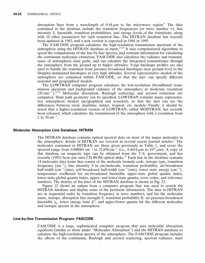
FIGURE 26 Atmospheric transmittance for dif ferent rain rates and for spectral frequencies from 400 to 4000 cm 2 1 . The measurement path is 300 m at the surface with T 5 T dew 5 10 8 C , with a meteorological range of 23 km in the absence of rain .
ground-level solar radiance model used by LOWTRAN , and Fig . 26 shows an example of a rain-rate model and its ef fect upon the transmission of the atmosphere as a function of rain rate in mm of water per hour . 2 6
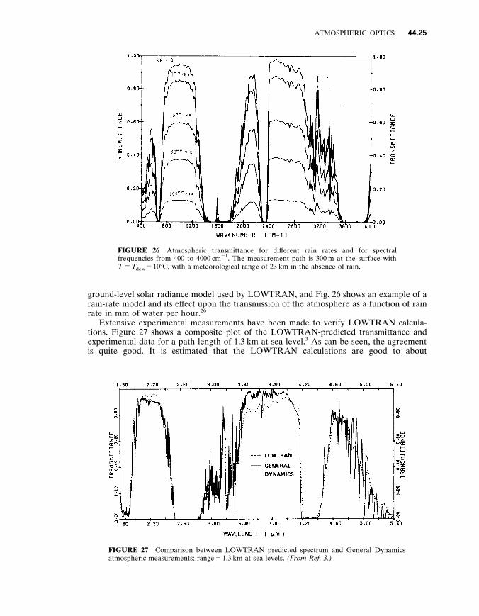
Extensive experimental measurements have been made to verify LOWTRAN calcula- tions . Figure 27 shows a composite plot of the LOWTRAN-predicted transmittance and experimental data for a path length of 1 . 3 km at sea level . 3 As can be seen , the agreement is quite good . It is estimated that the LOWTRAN calculations are good to about
FIGURE 27 Comparison between LOWTRAN predicted spectrum and General Dynamics atmospheric measurements ; range 5 1 . 3 km at sea levels . ( From Ref . 3 . )
44 .26 TERRESTRIAL OPTICS
10 percent . 3 It should be added that the molecular absorption portion of the preceding LOWTRAN (moderate-resolution) spectra can also be generated using the high-resolution FASCODE / HITRAN program and then spectrally smoothing (i . e ., degrading) the spectra to match that of the LOWTRAN spectra .
The most recent extension of the LOWTRAN program is the MODTRAN program . MODTRAN is similar to LOWTRAN but has increased spectral resolution . At present , the resolution for MODTRAN can be specified by the user between 2 and 20 cm 2 1 .
Programs and Databases for Use on Personal Computers
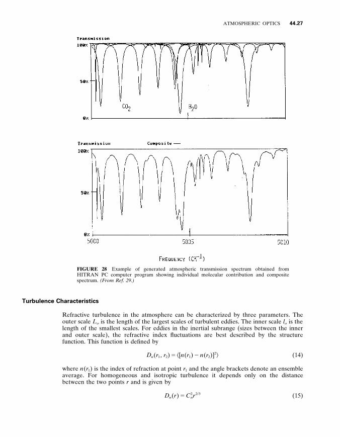
The preceding databases and computer programs have been converted or modified to run on dif ferent kinds of personal computers . 28 , 29 Currently , the HITRAN 1992 database can be obtained on CD-ROMs , and is also being of fered as a random-access database which will fit on the hard disk drive of a personal computer (MS-DOS IBM-compatible computers) . Several related programs are available , ranging from a complete copy of the FASCODE and LOWTRAN programs 2 8 to a simpler molecular transmission program of the atmosphere . 2 9 These programs calculate the transmission spectrum of the atmosphere and some show the overlay spectra of known laser lines . As an example , one version of these PC programs uses the HITRAN database and a transmission program to calculate the high-resolution spectrum of the atmosphere and displays the contribution of each individual molecule . Figure 28 shows the transmission spectrum produced by such a program . 2 9 The individual absorption lines are shown in the upper plot in Fig . 28 and the composite transmission is shown in the lower plot .
While these PC versions of the HITRAN database and transmission programs have become available only recently , they have already made a significant impact in the fields of atmospheric optics and optical remote sensing . They allow quick and easy access to atmospheric spectral data which was previously only available on a mainframe computer . It should be added that other computer programs are available which allow one to add or subtract dif ferent spectra generated by these HITRAN-based programs , from spectro- scopic instrumentation such as FT-IR spectrometers or from other IR gas spectra databases . In the latter case , for example , the U . S . National Institute of Standards and Technology (NIST) has compiled a computer database of the qualitative IR absorption spectra of over 5200 dif ferent gases (toxic and other hydrocarbon compounds) with a spectral resolution of 4 cm 2 1 . 3 0 In addition , higher-resolution quantitative spectra for a limited group of gases can be obtained from several commercial companies . 3 0
4 4 . 6 ATMOSPHERIC OPTICAL TURBULENCE
The most familiar ef fects of refractive turbulence in the atmosphere are the twinkling of stars and the shimmering of the horizon on a hot day . The first of these is a random fluctuation of the amplitude of light also known as scintillation . The second is a random fluctuation of the phase front that leads to a reduction in the resolution of an image . Other ef fects include the wander and break-up of an optical beam .
In the visible and near-IR region of the spectrum , the fluctuations of the refractive index in the atmosphere are determined by fluctuations of the temperature . These temperature fluctuations are caused by turbulent mixing of air of dif ferent temperatures . In the far-IR region , humidity fluctuations also contribute .
ATMOSPHERIC OPTICS 44 .27
FIGURE 28 Example of generated atmospheric transmission spectrum obtained from HITRAN PC computer program showing individual molecular contribution and composite spectrum . ( From Ref . 2 9 . )
Turbulence Characteristics
Refractive turbulence in the atmosphere can be characterized by three parameters . The outer scale L o is the length of the largest scales of turbulent eddies . The inner scale l o is the length of the smallest scales . For eddies in the inertial subrange (sizes between the inner and outer scale) , the refractive index fluctuations are best described by the structure function . This function is defined by
D n ( r 1 , r 2 ) 5 k [ n ( r 1 ) 2 n ( r 2 )] 2 l (14)
where n ( r 1 ) is the index of refraction at point r 1 and the angle brackets denote an ensemble average . For homogeneous and isotropic turbulence it depends only on the distance between the two points r and is given by
D n ( r ) 5 C 2 n r 2/3 (15)

44 .28 TERRESTRIAL OPTICS
FIGURE 29 Plot of refractive-turbulence structure parameter C 2
n for a typical summer day near Boul- der , Colorado . ( Courtesy G . R . Ochs , NOAA WPL . )
where C 2 n is a measure of the strength of turbulence and is defined by this equation .
In the boundary layer (the lowest few hundred meters of the atmosphere) , turbulence is generated by radiative heating and cooling of the ground . During the day , solar heating of the ground drives convective plumes . Refractive turbulence is generated by the mixing of these warm plumes with the cooler air surrounding them . At night , the ground is cooled by radiation and the cooler air near the ground is mixed with warmer air higher up by winds . A period of extremely low turbulence exists at dawn and at dusk when there is no temperature gradient in the lower atmosphere . Turbulence levels are also very low when the sky is overcast and solar heating and radiative cooling rates are low . Measured values of turbulence strength near the ground vary from less than 10 2 1 7 to greater than 10 2 1 2 m 2 2/3
at heights of 2 to 2 . 5 m . 31 , 32
Figure 29 illustrates typical summertime values near Boulder , Colorado . This is a 24-hour plot of 15-minute averages of C 2
n measured at a height of about 1 . 5 m on August 22 , 1991 . At night , the sky was clear , and C 2
n was a few parts times 10 2 1 3 . The dawn minimum is seen as a very short period of low turbulence just after 6 : 00 . After sunrise , C 2
n increases rapidly to over 10 2 1 2 . Just before noon , cumulus clouds developed , and C 2
n became lower with large fluctuations . At about 18 : 00 , the clouds , dissipated , and turbulence levels increased . The dusk minimum is evident just after 20 : 00 , and then turbulence strength returns to typical nighttime levels .
From a theory introduced by Monin and Obukhov , 3 3 a theoretical dependence of turbulence strength on height in the boundary layer above flat ground can be derived . 34 , 35
During periods of convection C 2 n decreases as the 2 4 / 3 power of height . At other times
(night or overcast days) , the power is more nearly 2 2 / 3 . These height dependencies have been verified by a number of experiments over relatively flat terrain . 36–40 However , values measured in mountainous regions are closer to the 2 1 / 3 power of height day or night . 4 1
Under certain conditions , the turbulence strength can be predicted from meteorological parameters and characteristics of the underlying surface . 42–44
Farther from the ground , no theory for the turbulence profile exists . Measurements have been made from aircraft 31 , 36 and with balloons . 45–47 Profiles of C 2
n have also been measured remotely from the ground using acoustic sounders , 48–50 radar , 36 , 37 , 51–56 and optical techniques . 46 , 57–60 The measurements show large variations in refractive turbulence strength . They all exhibit a sharply layered structure in which the turbulence appears in layers of the order of 100 m thick with relatively calm air in between . In some cases these layers can be associated with orographic features ; that is , the turbulence can be attributed to mountain lee waves . Generally , as height increases , the turbulence decreases to a minimum value that occurs at a height of about 3 to 5 km . The turbulence level then increases to a maximum at about the tropopause (10 km) . Turbulence levels decrease rapidly above the tropopause .
ATMOSPHERIC OPTICS 44 .29
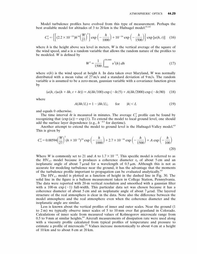
Model turbulence profiles have evolved from this type of measurement . Perhaps the best available model for altitudes of 3 to 20 km is the Hufnagel model : 61 , 62
C 2 n 5 H F (2 . 2 3 10 2 5 3 ) h 1 0 S W
27 D 2 G exp S 2
h 1000
D 1 10 2 1 6 exp S 2 h
1500 D J exp [ u ( h , t )] (16)
where h is the height above sea level in meters , W is the vertical average of the square of the wind speed , and u is a random variable that allows the random nature of the profiles to be modeled . W is defined by
W 2 5 1
1500 E 20 , 000
5000
y 2 ( h ) dh (17)
where y ( h ) is the wind speed at height h . In data taken over Maryland , W was normally distributed with a mean value of 27 m / s and a standard deviation of 9 m / s . The random variable u is assumed to be a zero-mean , gaussian variable with a covariance function given by
k u ( h , t ) u ( h 1 d h , t 1 d t ) l 5 A ( d h / 100) exp ( 2 d t / 5) 1 A ( d h / 2000) exp ( 2 d t / 80) (18)
where A ( d h / L ) 5 1 2 u d h / L u , for u h u , L (19)
and equals 0 otherwise . The time interval d t is measured in minutes . The average C 2
n profile can be found by recognizing that k exp ( u ) l 5 exp (1) . To extend the model to local ground level , one should add the surface layer dependence (e . g ., h 2 4/3 for daytime) .
Another attempt to extend the model to ground level is the Hufnagel-Valley model . 6 3
This is given by
C 2 n 5 0 . 00594 S W
27 D 2
( h 3 10 2 5 ) 1 0 exp S 2 h
1000 D 1 2 . 7 3 10 2 1 6 exp S 2
h 1500
D 1 A exp S 2 h
100 D
(20)
Where W is commonly set to 21 and A to 1 . 7 3 10 2 1 4 . This specific model is referred to as the HV 5/7 model because it produces a coherence diameter r 0 of about 5 cm and an isoplanatic angle of about 7 m rad for a wavelength of 0 . 5 m m . Although this is not as accurate for modeling turbulence near the ground , it has the advantage that the moments of the turbulence profile important to propagation can be evaluated analytically . 6 3
The HV 5/7 model is plotted as a function of height in the dashed line in Fig . 30 . The solid line in the figure is a balloon measurement taken in College Station , Pennsylvania . The data were reported with 20-m vertical resolution and smoothed with a gaussian filter with a 100-m exp ( 2 1) full-width . This particular data set was chosen because it has a coherence diameter of about 5 cm and an isoplanatic angle of about 7 m rad . The layered structure of the real atmosphere is clear in the data . Note also the dif ference between the model atmosphere and the real atmosphere even when the coherence diameter and the isoplanatic angle are similar .
Less is known about the vertical profiles of inner and outer scales . Near the ground (1 to 2 m) we typically observe inner scales of 5 to 10 mm over flat grassland in Colorado . Calculations of inner scale from measured values of Kolmogorov microscale range from 0 . 5 to 9 mm at similar heights . 6 4 Aircraft measurements of dissipation rate were used along with a viscosity profile calculated from typical profiles of temperature and pressure to estimate a profile of microscale . 6 5 Values increase monotonically to about 4 cm at a height of 10 km and to about 8 cm at 20 km .

44 .30 TERRESTRIAL OPTICS
FIGURE 30 Turbulence strength C 2 n as a function
of height . The solid line is a balloon measurement made in College Station , Pennsylvania , and the dashed line is the HV 5/7 model . ( Courtesy R . R . Beland , Geophysics Directorate , Phillips Laboratory , U .S . Air Force . )
Near the ground , the outer scale can be estimated using Monin-Obukhov similarity theory . 3 3 The outer scale can be defined as that separation at which the structure function of temperature fluctuations is equal to twice the variance . Using typical surface layer scaling relationships 6 6 we see that
L 0 5 H 7 . 04 h (1 2 7 S M O )(1 2 16 S M O ) 2 3/2
7 . 04 h (1 1 S M O ) 2 3 (1 1 2 . 75 S 2/3 MO ) 2 3/2
for 2 2 , S M O , 0 for 0 , S M O , 1
(21)
where S M O is the Monin-Obukhov stability parameter . For typical daytime conditions ( S M O , 0) , L o is generally between h / 2 and h .
Above the boundary layer , the situation is more complex . Weinstock 6 7 calculated that L o should be about 330 m in moderate turbulence in the stratosphere . Barat and Bertin 6 8
measured outer scale values of 10 to 100 m in a turbulent layer using a balloon-borne instrument . Some recent optical data 69 , 70 suggest that the outer scale is generally smaller with a peak value of about 4 m at a height of 8 . 5 km . Other data 7 1 supply no evidence for an outer scale less than about 1 km . These results are still controversial and more measurements of outer scale are needed to resolve the issue .
Beam Wander
The first ef fect of refractive turbulence to consider is the wander of an optical beam in the atmosphere . The deviations of the centroid of a beam in each of the two orthogonal transverse axes will be independent gaussian random variables . This wander is generally characterized statistically by the variance of the angular displacement . In isotropic turbulence , the variances in the two axes are equal and the magnitude of the displacement is a Rayleigh random variable with a variance that is twice that of the displacement in a single axis . Both the single-axis and the magnitude variances are reported in the literature .
Three main approaches to the calculation of beam-wander variance have been used . (1) If dif fraction ef fects are negligible and if the path-integrated turbulence is small enough , the geometric optics approximation 72–75 can be used . Dif fraction ef fects are negligible
ATMOSPHERIC OPTICS 44 .31
when the aperture diameter is greater than the Fresnel zone size . 7 5 The other condition requires that the product of the transverse coherence of the field and the aperture diameter is greater than the square of the Fresnel zone size . 7 5 (2) If dif fraction must be considered , the Huygens-Fresnel approximation 76–79 can be used . (3) The most complete theory uses the Markov random process approximation to the moment equation . 80–82 In the two types of calculation that include dif fraction , beams with a gaussian irradiance profile are generally assumed .
In the geometric optics approximation , the variance of the angular displacement in a single axis is given by 7 5
s 2 d 5 2 . 92 D 2 1/3 E L
0 dzC 2
n ( z ) S 1 2
z
L D 2
U 1 2 z
F U 1/3 (22)
where D is the diameter of the initial beam , z is position along the path , L is the propagation path length , and F is the geometric focal range of the initial beam (negative for a diverging beam) . For homogeneous turbulence and a beam that does not come to a focus between the transmitter and observation plane , Eq . (22) reduces to
s 2 d 5 0 . 97 C 2
n D 2 1/3 L 2 F 1 S 1 – 3 , 1 ; 4 ; L
F D (23)
where 2 F 1 is the hypergeometric function . The hypergeometric function is 1 for a collimated beam and 1 . 125 for a focused beam .
In the Markov approximation , the single-axis variance is given by 8 0
s 2 d 5 4 π 2 E L
0 dz S 1 2
z
L D 2 E
0 dKK 3 F n ( K , z )
3 exp H 2 K 2 D 2
8 F S 1 2
z
F D 2
1 16 z 2
K 2 D 4 G 2 π D S Kz
k D J (24)
where F n ( K , z ) is the path-dependent refractive index spectrum , K is the wave number of turbulence , D is the exp ( 2 1) intensity diameter of the initial beam , k is the optical wave number , and D ( r ) is the wave structure function for separation r of a spherical wave . The structure function is given by
D ( r ) 5 8 π 2 k 2 E z
0 dz 9 E
0 dK 9 K 9 F n ( K 9 , z 9 )[1 2 J 0 ( K 9 r z 9 / z )] , (25)
where J 0 is the zero-order Bessel function of the first kind . The last term in the exponential of Eq . (24) is a correction term for strong turbulence . The middle term includes the ef fects of dif fraction .
Beam Spreading
The next ef fect of refractive turbulence to consider is the spread of an optical beam as it propagates through the atmosphere . There are two types of beam spread denoted as long-term and short-term . The long-term beam spread is defined as the turbulence-induced beam spread observed over a long time average . It includes the ef fects of the slow wander of the entire beam . The short-term beam spread is defined as the beam spread observed at an instant of time . It does not include the ef fects of beam wander and is often approximated by the long-term beam spread with the ef fects of wander removed , although the two are not identical .
44 .32 TERRESTRIAL OPTICS
We can consider beam wander to be caused by turbulent eddies that are larger than the beam . Short-term beam spread is caused by turbulent eddies that are smaller than the beam . There are more small eddies than large in the beam at any time which implies that the beam spread at any instant is averaged over more eddies . As a result , the fluctuations of short-term beam spread are much smaller than those of beam wander and are typically neglected . The primary ef fect of short-term beam spread is to spread the average energy over a larger area . Thus , the average value of the on-axis irradiance is reduced , and the average value of the irradiance at large angles is increased .
The extended Huygens-Fresnel principle can be used to calculate the long-term spread of a gaussian beam in refractive turbulence . 83–87 The exp ( 2 1) intensity radius of a gaussian beam is
p 1 5 F 4 k 2 D 2 1
D 2
4 S 1 2
L
F D 2
1 4
k 2 r 2 0 G 1/2
(26)
where D is the exp ( 2 1) intensity diameter of the source and r o is the phase coherence length that would be observed for a point source propagating from the receiver to the transmitter . The first term in this equation is the dif fraction beam spread , the second is the geometrical optics projection of the transmitter aperture , and the final term is the total turbulence-induced spread .
The phase coherence length is defined as the transverse separation at which the coherence of the field is reduced to exp ( 2 1) . If the coherence length r o is much larger than the inner scale , the structure function is given by D ( r ) 5 2( r / r o ) 5/3 and
r o 5 F 1 . 46 k 2 E L
0 dz S z
L D 5/3
C 2 n ( z ) G 2 3/5
(27)
If the coherence length is much smaller than the inner scale , then D ( r ) 5 2( r / r o ) 2 and
r o 5 F 1 . 86 k 2 E L
0 dz S z
L D 2
C 2 n ( z ) l 2 1/3
o ( z ) G 2 1/2
(28)
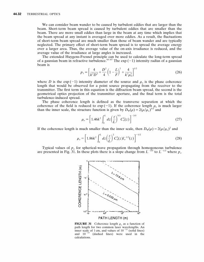
Typical values of p o for spherical-wave propagation through homogeneous turbulence are presented in Fig . 31 . In these plots there is a slope change from L 2 3/5 to L 2 1/2 where p o
FIGURE 31 Coherence length r o as a function of path length for two common laser wavelengths . An inner scale of 1 cm , and values of 10 2 1 2 (solid lines) and 10 2 1 3 (dashed lines) were used in the calculations .
ATMOSPHERIC OPTICS 44 .33
is about equal to the inner scale of 1 cm . This small change is nearly imperceptible in the figure .
The extended Huygens-Fresnel principle has been used to calculate the short-term beam spread by explicitly subtacting the beam wander . 88–91 If p o and l o are much smaller than D , then the short-term beam spread is approximately given by
p s 5 H 4 k 2 D 2 1
D 2
4 L 2 S 1 2 L F D 2
1 4
k 2 r 2 0 F 1 2 0 . 62 S r o
D D 1/3 G 6/5 J 1/2
(29)
If r o is much greater than D , the turbulence-induced component of beam spreading can be neglected .
If inner scale and outer scale ef fects are included , more complicated integral expressions result . 9 2 Numerical calculations were performed for truncated gaussian beams with central obscurations . 9 3 The following approximation was obtained by a curve fit to the results :
(30) p s 5 S 1 1 0 . 182
D 2 ef f
r 2 o D 1/2
p d for D ef f
r o , 3
p s 5 F 1 1 S D ef f
r o D 2
2 1 . 18 S D ef f
r o D 2 5/3 G 1/2
p d for 3 , D ef f
r o , 7 . 5
where D ef f is the ef fective diameter of the truncated aperture , r o 5 2 . 099 p o , and p d is the dif fraction-limited value . These expressions agree fairly well with available data . 78 , 94 , 95
Imaging and Heterodyne Detection
The problem of imaging through the turbulent atmosphere is similar to the problem of beam propagation through the atmosphere . The dancing of an image in the focal plane of an imaging system is mathematically equivalent to the wander of a beam focused at the object by the same optical system . The resolution of the short-exposure image is equivalent to the short-term beam spread of the same focused beam . The resolution for a long exposure is related to the long-term beam spread .
Thus , the position of the image of a point object will drift in each axis in the focal plane . The variance of that drift is given by 9 6
s 2 i 5 1 . 10 C 2
n D 2 1/3 LF 2 (31)
where D is the aperture diameter of the imaging system , F is its focal length , and L is the distance to the object .
Fried 9 7 used the idea of tilt correction to calculate the average image resolution for a short-exposure image in the turbulent atmosphere . This problem is mathematically equivalent to the propagation of a beam in the opposite direction if the imaging aperture replaces the beam width . These results were refined by Lutomirski et al . 9 8 and applied to a space-to-ground path by Valley . 9 2
Image resolution is also related to the signal-to-noise ratio of an optical heterodyne receiver . The long-exposure resolution is equivalent to a staring receiver . The short- exposure resolution is equivalent to a receiver that employs tilt-correction of the signal or of the local oscillator . 97 , 99–101
44 .34 TERRESTRIAL OPTICS
Scintillation
The refractive index inhomogeneities that distort the optical phase front also produce amplitude scintillation at some distance . The first cases to be considered were plane-wave and spherical-wave propagation through weak path-integrated turbulence where the weak-turbulence condition requires that fluctuations of irradiance be much less than the mean value . Tatarskii 1 0 2 used a perturbation approach to the wave equation . Lee and Harp 1 0 3 used a physical approach to arrive at the same results . These results are summarized in a number of good reviews . 90 , 91 , 104 , 105
We will first consider the weak-turbulence results . For propagation from space to the ground , the plane wave formula is generally valid . The variance of irradiance fluctuations (normalized by the mean irradiance value) is given by 1 0 4
s 2 r 5 k 7/6 sec 11/6 θ E
0 dhh 5/6 C 2
n ( h ) (32)
where k is the optical wave number , θ is the zenith angle , and h is the height of the receiver above the ground . This expression is valid as long as the path-integrated turbulence is weak enough that the variance is much less than unity . This condition is usually met for near-zenith propagation .
For propagation of diverging waves near the ground , the spherical-wave approximation is often valid . Assuming constant turbulence along the path , the weak-turbulence variance in this case is given by 1 0 4
(33) s 2
r 5 exp [0 . 5 k 7/6 L 11/6 C 2 n ] 2 1 for l o , 4 l L
s 2 r 5 exp [1 . 28 L 3 l 2 7/3
o C 2 n ] 2 1 for l o . 4 l L
where L is the path length and l o is the inner scale of turbulence . For narrow-beam propagation , the ef fects of the finite beam must be considered . Kon
and Tatarskii 1 0 6 calculated the amplitude fluctuations of a collimated beam using the perturbation technique . Schmeltzer 1 0 7 extended these results to include focused beams . These results were used to obtain numerical values for a variety of propagation conditions . 108–110 Ishimaru 111–113 used a spectral representation to obtain similar results . Under certain conditions , one sees a reduction in the variance on the optical axis 108 , 109 , 114 , 115
and an increase of f of the optical axis . 1 1 6
The spatial scale of weak scintillations is about equal to the larger of either the Fresnel zone size ( L / k ) 1/2 or the inner scale . 1 0 4 Scintillation will be reduced if an aperture larger than the scale size is used to collect the light . If the aperture diameter D is much larger than the scale size , the reduction factor can be expressed as 117 , 118
A 5 C S D
D 0 D 2 7/3
(34)
where D 0 is ( l L ) 1/2 and C is 4 . 71 for a plane wave and 23 . 5 for a spherical wave when the inner scale is much smaller than the Fresnel zone . If the inner scale is much larger than the Fresnel zone , D 0 is the inner scale and C is 0 . 45 for a plane wave and 9 . 17 for a spherical wave .
It is generally accepted that the probability density function for weak scintillation is log normal . 90 , 102 , 104 , 119 This density function has the form
p ( I ) 5 1
4 2 π s I I exp F 2
1 2 s 2
r (ln I 1 0 . 5 s 2
r ) 2 G (35)

ATMOSPHERIC OPTICS 44 .35
FIGURE 32 Plot of normalized variance of ir- radiance s 2
I as a function of turbulence strength C 2 n .
Circles are data taken with a 488-nm wavelength laser over a 1200-m path , and the line is the corresponding weak-turbulence theory .
The weak-turbulence theory is , in essence , a single-scattering theory . As the path- integrated turbulence becomes larger , multiple-scattering ef fects become important , and this theory breaks down . Actual observed values of irradiance variance are smaller than predicted in this region as shown in Fig . 32 . The circles in this figure are one-minute averages of irradiance variance for 488-nm laser light propagated across 1200 m of flat grassland . The solid line is the weak-turbulence approximation .
In these and other experiments , variance values reach a peak value of between 3 and 5 for a spherical wave and they begin to decrease with increasing turbulence strength . 120–123
In the limit of infinite path-integrated turbulence , the normalized variance of irradiance is predicted to approach unity . 124 , 125 In the intermediate region near the peak irradiance , numerical evaluation of currently available theories is impractical .
An asymptotic theory has been developed for very large path-integrated turbulence . 125–129
We assume that the inner scale is much less than the Fresnel zone in this regime because long paths are necessary to obtain large values of path-integrated turbulence . Then the irradiance variance can be approximated by
(36) s 2
r 5 1 1 1 . 9 s 2 4/5 R for spherical waves
s 2 r 5 1 1 0 . 86 s 2 4/5
R for plane waves
where s 2 R is the appropriate (spherical-wave or plane-wave) variance calculated from the
Rytov approximation given by Eq . (32) or (33) . In very strong turbulence two distinct spatial scales are evident in the scintillation
pattern . 125–129 The smaller scale is about the size of the coherence length r o discussed under ‘‘Beam Spreading . ’’ The larger scale is the size of the scattering disk which is the ratio of the square of the Fresnel zone to the coherence length ( L / k r o ) . As turbulence increases , the small scale becomes smaller and the large scale becomes larger . The strength of the small-scale fluctuations is constant in this regime and contributes a value of unity to the variance . The large-scale fluctuations contribute the rest of the variance and become weaker with increasing turbulence strength .
At high turbulence values , the density function is a log-normally modulated exponential . 123 , 130 This density function has the form
p ( I ) 5 1
4 2 π s z E
0
dz
z 2 exp F 2 I
z 2
(ln z 1 1 – 2 s 2 z )
2
2 s 2 z
G (37)
where the parameter s 2 z is related to the irradiance variance by the relationship
s 2 I 5 2 exp ( s 2
z ) 2 1 (38)
44 .36 TERRESTRIAL OPTICS
An interesting feature of this density function is that the most likely value of the irradiance is 0 . Although the observed signal is occasionally very bright , quite often there is no signal unless some sort of averaging is performed .
4 4 . 7 EXAMPLES OF ATMOSPHERIC OPTICAL REMOTE SENSING
One of the more important applications of atmospheric optics is optical remote sensing . Atmospheric optical remote sensing concerns the use of an optical or laser beam to remotely sense information about the atmosphere or a distant target . Optical remote sensing measurements are diverse in nature and include the use of a spectral radiometer aboard a satellite for the detection of trace species in the upper atmosphere , the use of spectral emission and absorption from the earth for the detection of the concentration of water vapor in the atmosphere , the use of lasers to measure the range-resolved distribution of several molecules including ozone in the atmosphere , and Doppler wind measurements . In this section , some typical optical remote sensing experiments will be presented in order to give a flavor of the wide variety of atmospheric optical measurements that are currently being conducted . More in-depth references can be found in several current journal papers and conference proceedings . 131–136
The Upper Atmospheric Research Satellite (UARS) was placed into orbit in September 1991 as part of the Earth Observing System . One of the optical remote sensing instruments aboard UARS is the High Resolution Doppler Imager (HRDI) developed by P . Hays’ and V . Abreu’s group at the University of Michigan . 1 3 7 The HRDI is a triple etalon Fabry-Perot Interferometer designed to measure Doppler shifts of molecular absorption and emission lines in the earth’s atmosphere in order to determine the wind velocity of the atmosphere . A wind velocity of 10 m / s causes a Doppler shift of 2 3 10 2 5 nm for the oxygen lines detected near a wavelength of 600 – 800 nm . A schematic of the instrument is given in Fig . 33 a which shows the telescope , triple Fabry-Perots , and unique imaging Photo-Multiplier tubes to detect the Fabry-Perot patterns of the spectral absorption lines . The HRDI instrument is a passive remote sensing system and uses the reflected or scattered sunlight as its illumination source . Figure 33 b shows the wind field measured by UARS (HRDI) for an altitude of 90 km .
Another kind of atmospheric remote sensing instrument is represented by an airborne laser radar (lidar) system operated by E . Browell’s group at NASA / Langley . 1 3 8 Their system consists of two pulsed , visible-wavelength dye laser systems that emit short (10-ns) pulses of tunable optical radiation that can be directed toward aerosol clouds in the atmosphere . By the proper tuning of the wavelength of these lasers , the dif ference in the absorption due to ozone , water vapor , or oxygen in the atmosphere can be measured . Because the laser pulse is short , the timing out to the aerosol scatterers can be determined and range-resolved lidar measurements can be made . Figure 34 shows range-resolved lidar backscatter profiles obtained as a function of the lidar aircraft ground position . The variation in the atmospheric density and ozone distribution as a function of altitude and distance is readily observed .
A Coherent Doppler Lidar is one which is able to measure the Doppler shift of the backscattered lidar returns from the atmosphere . Several Doppler lidar systems have been developed which can determine wind speed with an accuracy of 0 . 1 m / s at ranges of up to 15 km . One such system is operated by M . Hardesty’s group at NOAA / WPL for the mapping of winds near airports and for meteorological studies . 1 3 9 Figure 35 shows a two-dimensional plot of the measured wind velocity obtained during the approach of a wind gust front associated with colliding thunderstorms ; the upper figure shows the real-time Doppler lidar display of the measured radial wind velocity , and the lower plot shows the computed wind velocity . As seen , a Doppler lidar system is able to remotely measure the wind speed with spatial resolution on the order of 100 m . A similar Doppler
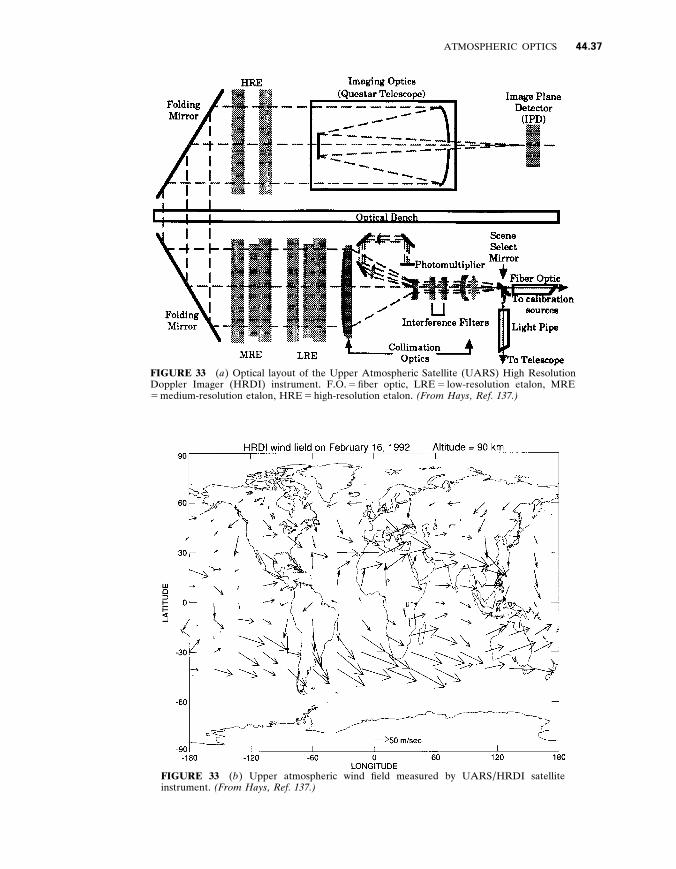
ATMOSPHERIC OPTICS 44 .37
FIGURE 33 ( a ) Optical layout of the Upper Atmospheric Satellite (UARS) High Resolution Doppler Imager (HRDI) instrument . F . O . 5 fiber optic , LRE 5 low-resolution etalon , MRE 5 medium-resolution etalon , HRE 5 high-resolution etalon . ( From Hays , Ref . 1 3 7 . )
FIGURE 33 ( b ) Upper atmospheric wind field measured by UARS / HRDI satellite instrument . ( From Hays , Ref . 1 3 7 . )

44 .38 TERRESTRIAL OPTICS
FIGURE 34 Range-resolved lidar measurements of atmospheric aerosols and ozone density . ( From E . Browell , Ref . 1 3 8 . )
lidar system is being considered for the early detection of windshear in front of commercial aircraft .
A further example of atmospheric optical remote sensing is that of the remote measurement of the global concentration and distribution of atmospheric aerosols and particulates . P . McCormick’s group at NASA / Langley has developed the SAGE II satellite system which is part of a package of instruments to detect global aerosol and selected species concentrations in the atmosphere . 1 4 0 This system measures the dif ference in the optical radiation emitted from the earth’s surface and the dif ferential absorption due to known absorption lines or spectral bands of several species in the atmosphere , including ozone . The instrument also provides for the spatial mapping of the concentration of aerosols and particulates in the atmosphere , and an example of such a measurement is shown in Fig . 36 . This figure shows the measured concentration of aerosols and particulates after the eruption of Mt . Pinatubo and demonstrates the global circulation and transport of the injected material into the earth’s atmosphere .

ATMOSPHERIC OPTICS 44 .39
FIGURE 35 Coherent Doppler lidar measurements of atmospheric winds showing velocity profile of gust front . Upper plot is real-time display of Doppler signal and lower plot is range-resolved wind field . ( From M . Hardesty , Ref . 1 3 9 . )
The preceding examples are just a few of many dif ferent optical remote sensing instruments that are being used to measure the physical dynamics and chemical properties of the atmosphere . As is evident in these examples , an understanding of atmospheric optics plays an important and integral part in these measurements .
4 4 . 8 METEOROLOGICAL OPTICS
One of the most colorful aspects of atmospheric optics is that associated with meteorologi- cal optics . Meteorological optics involves the interplay of light with the atmosphere and the physical origin of the observed optical phenomena . Several excellent books have been written about this subject , and the reader should consult these and the contained references . 141 , 142 While it is beyond the scope of this chapter to present an overview of meteorological optics , some specific optical phenomena will be described to give the reader a sampling of some of the interesting ef fects involved in naturally occurring atmospheric and meteorological optics .
Some of the more common and interesting meteorological optical phenomena involve rainbows , ice-crystal halos , and mirages . The rainbow in the atmosphere is caused by internal reflection and refraction of sunlight by water droplets in the atmosphere . Figure 37 shows the geometry involved in the formation of a rainbow , including both the primary and larger secondary rainbow . Because of the dispersion of light within the water droplet , the colors or wavelengths are separated in the backscattered image . Although rainbows are commonly observed in the visible , such refraction also occurs in the infrared spectrum . As an example , Fig . 38 shows a natural rainbow in the atmosphere photographed with IR-sensitive film by R . Greenler . 1 4 2
The phenomena of halos , arcs , and spots are due to the refraction of light by ice crystals suspended in the atmosphere . Figure 39 shows a photograph of collected ice crystals as

44 .40 TERRESTRIAL OPTICS
FIGURE 36 Measurement of global aerosol and particulate concentration using SAGE II satellite following eruption of Mt . Pinatubo . ( From P . McCormick , Ref . 1 4 0 . )
they fell from the sky . The geometrical shape , especially the hexagonal (six-sided) crystals , play an important role in the formation of halos and arcs in the atmosphere .
The common optical phenomenon of the mirage is caused by variation in the temperature and thus , the density of the air as a function of altitude or transverse geometrical distance . As an example , Fig . 40 shows the geometry of light-ray paths for a case where the air temperature decreases with height to a suf ficient extent over the viewing angle that the dif ference in the index of refraction can cause a refraction of the image similar to total internal reflection . The heated air (less dense) near the ground can thus act like a mirror , and reflect the light upward toward the viewer . As an example , Fig . 41 shows a photograph taken by Greenler of motorcycles on a hot road surface . The reflected image of the motorcycles ‘‘within’’ the road surface is evident . There are many manifestations of mirages dependent upon the local temperature gradient and geometry of the situation . In many cases , partial and distorted images are observed leading to the almost surreal connotation often associated with mirages .
Finally , another atmospheric meteorological optical phenomenon is that of the green flash . A green flash is observed under certain conditions just as the sun is setting below the horizon . This phenomenon is easily understood as being due to the dif ferent relative displacement of each dif ferent wavelength or color in the sun’s image due to spatially distributed refraction of the atmosphere . 1 4 2 As the sun sets , the last image to be observed

ATMOSPHERIC OPTICS 44 .41
FIGURE 37 Dif ferent raindrops contribute to the primary and to the larger , secondary rainbow . ( From R . Greenler , Ref . 1 4 2 . )
FIGURE 38 A natural infrared rainbow . ( Photograph courtesy of R . Greenler , Ref . 1 4 2 . )
44 .42 TERRESTRIAL OPTICS
FIGURE 39 Photograph of magnified small ice crystals collected as they fell from the sky . ( From R . Greenler , Ref . 1 4 2 . )
FIGURE 40 The origin of the inverted image in the desert mirage . ( From R . Greenler , Ref . 1 4 2 . )
ATMOSPHERIC OPTICS 44 .49
109 . D . L . Fried , ‘‘Scintillation of a Ground-to-Space Laser Illuminator , ’’ J . Opt . Soc . Am . 57 : 980 – 983 (1967) .
110 . Y . Kinoshita , T . Asakura , and M . Suzuki , ‘‘Fluctuation Distribution of a Gaussian Beam Propagating through a Random Medium , ’’ J . Opt . Soc . Am . 58 : 798 – 807 (1968) .
111 . A . Ishimaru , ‘‘Fluctuations of a Beam Wave Propagating through a Locally Homogeneous Medium , ’’ Radio Sci . 4 : 295 – 305 (1969) .
112 . A . Ishimaru , ‘‘Fluctuations of a Focused Beam Wave for Atmospheric Turbulence Probing , ’’ Proc . IEEE 57 : 407 – 414 (1969) .
113 . A . Ishimaru , ‘‘The Beam Wave Case and Remote Sensing , ’’ in J . W . Strohbehn (ed . ) , Laser Beam Propagation in the Atmosphere , Springer-Verlag , New York , 1978 , pp . 129 – 170 .
114 . P . J . Titterton , ‘‘Scintillation and Transmitter-aperture Averaging over Vertical Paths , ’’ J . Opt . Soc . Am . 63 : 439 – 444 (1973) .
115 . H . T . Yura and W . G . McKinley , ‘‘Optical Scintillation Statistics for IR Ground-to-Space Laser Communication Systems , ’’ Appl . Opt . 22 : 3353 – 3358 (1983) .
116 . P . A . Lightsey , J . Anspach , and P . Sydney , ‘‘Observations of Uplink and Retroreflected Scintillation in the Relay Mirror Experiment , ’’ Proc . SPIE 1482 (in press) (1991) .
117 . D . L . Fried , ‘‘Aperture Averaging of Scintillation , ’’ J . Opt . Soc . Am . 57 : 169 – 175 (1967) . 118 . J . H . Churnside , ‘‘Aperture Averaging of Optical Scintillations in the Turbulent Atmosphere , ’’
Appl . Opt . 30 : 1982 – 1994 (1991) . 119 . J . H . Churnside and R . G . Frehlich , ‘‘Experimental Evaluation of Log-normally Modulated
Rician and IK Models of Optical Scintillation in the Atmosphere , ’’ J . Opt . Soc . Am . A 6 : 1760 – 1766 (1989) .
120 . G . Parry and P . N . Pusey , ‘‘K Distributions in Atmospheric Propagation of Laser Light , ’’ J . Opt . Soc . Am . 69 : 796 – 798 (1979) .
121 . G . Parry , ‘‘Measurement of Atmospheric Turbulence Induced Intensity Fluctuations in a Laser Beam , ’’ Opt . Acta 28 : 715 – 728 (1981) .
122 . W . A . Coles and R . G . Frehlich , ‘‘Simultaneous Measurements of Angular Scattering and Intensity Scintillation in the Atmosphere , ’’ J . Opt . Soc . Am . 72 : 1042 – 1048 (1982) .
123 . J . H . Churnside and S . F . Clif ford , ‘‘Lognormal Rician Probability-density Function of Optical Scintillations in the Turbulent Atmosphere , ’’ J . Opt . Soc . Am . A 4 : 1923 – 1930 (1987) .
124 . R . Dashen , ‘‘Path Integrals for Waves in Random Media , ’’ J . Math . Phys . 20 : 894 – 920 (1979) . 125 . K . S . Gochelashvily and V . I . Shishov , ‘‘Multiple Scattering of Light in a Turbulent Medium , ’’
Opt . Acta 18 : 767 – 777 (1971) . 126 . K . S . Gochelashvily , V . G . Pevgov , and V . I . Shishov , ‘‘Saturation of Fluctuations of the
Intensity of Laser Radiation at Large Distances in a Turbulent Atmosphere (Fraunhofer Zone of Transmitter) , ’’ So y . J . Quantum Electron . 4 : 632 – 637 (1974) .
127 . A . M . Prokhorov , F . V . Bunkin , K . S . Gochelashvily , and V . I . Shishov , ‘‘Laser Irradiance Propagation in Turbulent Media , ’’ Proc . IEEE 63 : 790 – 810 (1975) .
128 . R . L . Fante , ‘‘Inner-scale Size Ef fect on the Scintillations of Light in the Turbulent Atmosphere , ’’ J . Opt . Soc . Am . 73 : 277 – 281 (1983) .
129 . R . G . Frehlich , ‘‘Intensity Covariance of a Point Source in a Random Medium with a Kolmogorov Spectrum and an Inner Scale of Turbulence , ’’ J . Opt . Soc . Am . A . 4 : 360 – 366 (1987) .
130 . J . H . Churnside and R . J . Hill , ‘‘Probability Density of Irradiance Scintillations for Strong Path-integrated Refractive Turbulence , ’’ J . Opt . Soc . Am . A . 4 : 727 – 733 (1987) .
131 . D . K . Killinger and A . Mooradian (eds . ) , Optical and Laser Remote Sensing , Springer-Verlag , Optical Sciences , vol . 39 , 1983 .
132 . L . J . Radziemski , R . W . Solarz , and J . A . Paisner (eds . ) , Laser Spectroscopy and Its Applications , Marcel Dekker , Optical Eng ., vol . 11 , 1987 .
133 . T . Kobayashi , ‘‘Techniques for Laser Remote Sensing of the Environment , ’’ Remote Sensing Re y iews , 3 : 1 – 56 (1987) .
134 . E . D . Hinkley (ed . ) , Laser Monitoring of the Atmosphere , Springer-Verlag , Berlin , 1976 .
44 .50 TERRESTRIAL OPTICS
135 . W . B . Grant and R . T . Menzies , ‘‘A Survey of Laser and Selected Optical Systems for Remote Measurement of Pollutant Gas Concentrations , ’’ APCA Journal 33 : 187 (1983) .
136 . ‘‘Optical Remote Sensing of the Atmosphere , ’’ Conf . Proceedings , OSA Topical Meeting , Williamsburg , 1991 .
137 . P . B . Hays , V . J . Abreu , D . A . Gell , H . J . Grassl , W . R . Skinner , and M . E . Dobbs , ‘‘The High Resolution Doppler Imager on the Upper Atmospheric Research Satellite , ’’ J . Geophys . Res . ( Atmosphere ) 98 : 10713 (1993) ; P . B . Hays , V . J . Abreu , M . D . Burrage , D . A . Gell , A . R . Marshall , Y . T . Morton , D . A . Ortland , W . R . Skinner , D . L . Wu , and J . H . Yee , ‘‘Remote Sensing of Mesopheric Winds with the High Resolution Imager , ’’ Planet . Space Sci . 40 : 1599 (1992) .
138 . E . Browell , ‘‘Dif ferential Absorption Lidar Sensing of Ozone , ’’ Proc . IEEE 77 : 419 (1989) . 139 . J . M . Intrieri , A . J . Dedard , and R . M . Hardesty , ‘‘Details of Colliding Thunderstorm Outflow as
Observed by Doppler Lidar , ’’ J . Atmospheric Sciences 47 : 1081 (1990) ; R . M . Hardesty , K . Elmore , M . E . Jackson , in 2 1 st Conf . on Radar Meteorology , American Meteorology Society , Boston , 1983 .
140 . M . P . McCormick and R . E . Veiga , ‘‘Initial Assessment of the Stratospheric and Climatic Impact of the 1991 Mount Pinatubo Eruption—Prolog , ’’ Geophysical Research Lett . 19 : 155 (1992) .
141 . R . A . R . Tricker , Introduction to Meteorological Optics , American Elsevier , New York , 1970 . 142 . R . Greenler , Rainbows , Halos , and Glories , Cambridge University Press , 1980 .
Related Documents