Asymptotic inference in system identification for the atom maser

Asymptotic inference in system identification

for the atom maser

Catalin Catana, Merlijn van Horssen and Madalin Guta

University of Nottingham, School of Mathematical Sciences

University Park, NG7 2RD Nottingham, UK

Abstract

System identification is an integrant part of control theory and plays an increasing

role in quantum engineering. In the quantum set-up, system identification is usually

equated to process tomography, i.e. estimating a channel by probing it repeatedly

with different input states. However for quantum dynamical systems like quantum

Markov processes, it is more natural to consider the estimation based on continuous

measurements of the output, with a given input which may be stationary. We address

this problem using asymptotic statistics tools, for the specific example of estimating

the Rabi frequency of an atom maser. We compute the Fisher information of different

measurement processes as well as the quantum Fisher information of the atom maser,

and establish the local asymptotic normality of these statistical models. The statistical

notions can be expressed in terms of spectral properties of certain deformed Markov

generators and the connection to large deviations is briefly discussed.

1 Introduction

We are currently entering a new technological era [20] where quantum control is a becoming

a key component of quantum engineering [23]. In the standard set-up of quantum filtering

and control theory [2, 28] the dynamics of the system and its environment, as well as

the initial state of the system, are usually assumed to be known. In practice however,

these objects may depend on unknown parameters and inaccurate models may compromise

the control objective. Therefore, system identification [22] which lies at the intersection

of control theory and statistics, is becoming an increasingly relevant topic for quantum

engineering [16].

1

arX

iv:1

112.

2080

v1 [

quan

t-ph

] 9

Dec

201

1

In this paper we introduce probabilistic and statistical tools aimed at a better under-

standing of the measurement process, and at solving system identification problems in the

set-up of quantum Markov processes. Although the mathematical techniques have a broader

scope, we focus on the physically relevant model of the atom maser which has been exten-

sively investigated both theoretically [4, 6] and experimentally [24, 26] and found to exhibit

a number of interesting dynamical phenomena. In the standard set-up of the atom maser,

a beam of two-level atoms prepared in the excited state passes through a cavity with which

they are in resonance, interact with the cavity field, and are detected after exiting the cav-

ity. We consider the case where the atoms are measured in the standard basis, but more

general measurements can be analysed in the same framework.

The specific questions we want to address are how to estimate the strength of the inter-

action between cavity and atoms, what is the accuracy of the estimator, and how it relates

to the spectral properties of the Markov evolution. More generally, we aim at developing

techniques for treating identifiability for multiple dynamical parameters, finding the associ-

ated Fisher information matrix, establishing asymptotic normality of the estimators. These

topics are well understood in the classical context and our aim is to adapt and extend such

techniques to the quantum set-up. In classical statistics it is known that if we observe the

first n steps of a Markov chain whose transition matrix depends on some unknown param-

eter θ, then θ can be estimated with an optimal asymptotic mean square error of (nI(θ))−1

where I(θ) is the Fisher information (per sample) of the Markov chain. Moreover the error

is asymptotically normal (Gaussian)

√n(θn − θ)

L−→ N(0, I(θ)−1). (1)

The key feature of our estimation problem is that the atom maser’s output consists

of atoms which are correlated with each other and with the cavity. Therefore, state and

process tomography methods do not apply directly. In particular it is not clear what is the

optimal measurement, what is the quantum Fisher information of the output, and how it

compares with the Fisher information of simple (counting) measurements. These questions

were partly answered in [14] in the context of a discrete time quantum Markov chain, and

here we extend the results to a continuous time set-up with an infinite dimensional system.

For a better grasp of the statistical model we consider several thought and real experiments,

and compute the Fisher informations of the data collected in these experiments. For example

we analyse the set-up where the cavity is observed as it jumps between different Fock states

when counting measurements are performed on the output as well as in the temperature

bath. We also consider estimators which are based solely on the statistic given by the

total number of ground or excited state atoms detected in a time period. Our findings are

2

illustrated in Figures 2 and 3 which shows the dependence of different (asymptotic) Fisher

informations on the interaction parameter. In particular the quantum Fisher information

of the closed system made up of atoms, cavity and bath, depends strongly on the value

of the interaction strength and is proportional to the cavity mean photon number in the

stationary state. Furthermore, we find that monitoring all channels achieves the quantum

Fisher information, while excluding the detection of excited atoms leads to a drastic decrease

of the Fisher information in the neighbourhood of the first ‘transition point’. The asymptotic

regime relevant for statistics is that of central limit, i.e. moderate deviations around the

mean of order n−1/2 as in (1). One of our main results is to establish local asymptotic

normality for the atom counting process, which implies the Central Limit and provides the

formula of the Fisher information. We also prove a quantum version of this result showing

that the quantum statistical model of the atom maser can be approximated in a statistical

sense by a displaced coherent state model. The moderate deviations regime analysed as well

as the related regime of large deviations are closely connected to the spectral properties of

certain deformations of the Lindblad operator. Some of these connections are pointed out

in this paper but other questions such as the existence of dynamical phase transitions [7, 8]

and the quantum Perron-Frobenius Theorem will be addressed elsewhere [12].

In sections 2 and 3 we give brief overviews of the atom maser’s dynamics, and respectively

of classical and quantum statistical concepts used in the paper. Section 4 contains the main

results about Fisher information and asymptotic normality in different set-ups. We conclude

with comments on future work.

2 The atom maser

The atom maser’s dynamics is based on the Jaynes-Cummings model of the atom-cavity

Hamiltonian

H = Hfree +Hint = ~Ωa∗a+ ~ωσ∗σ − ~g(t)(σa∗ + σ∗a) (2)

where a is the annihilation operators of the cavity mode, σ is the lowering operator of the

two-level atom, Ω and ω are the cavity frequency and the atom transition frequency which

are assumed to be equal, and g is the coupling strength or Rabi frequency. In the standard

experimental set-up the atoms prepared in the excited state arrive as a Poisson process of

a given intensity, and interact with the cavity for a fixed time. Additionally, the cavity is

in contact with a thermal bath with mean photon number ν. By coarse graining the time

evolution to ignore the very short time scale changes in the cavity field, one arrives at the

3

following master equation for the cavity state ρ

dρ

dt= L(ρ), (3)

where L is the Lindblad generator

L(ρ) =4∑i=1

(LiρL

∗i −

1

2L∗iLi, ρ

); (4)

with operators

L1 =√Nexa

∗ sin(φ√aa∗)√

aa∗, L2 =

√Nex cos(φ

√aa∗), (5)

L3 =√ν + 1a, L4 =

√νa∗. (6)

Here Nex the effective pump rate (number of atoms per cavity lifetime), and the parameter

φ called the accumulated Rabi angle is proportional to g. Later we will consider that φ is

an unknown parameter to be estimated.

The operators Li can be interpreted as jump operators for different measurement pro-

cesses: detection of an output atom in the ground state or excited state (L1 and L2) and

emission or absorption of a photon by the cavity (L3 and L4). In each case the cavity makes

a jump up or down on the ladder of Fock states. Since both the atom-cavity interaction (2)

and the cavity-bath interaction leave the commutative algebra of number operators invari-

ant, we can restrict our attention to this classical dynamical system provided that the atoms

are measured in the σz basis. The cavity jumps are described by a birth-death (Markov)

process with birth and death rates

qk,k+1 := Nex sin(φ√k + 1)2 + ν(k + 1), k ≥ 0

qk,k−1 := (ν + 1)k, k ≥ 1. (7)

In section 4 we will come back to the birth-death process, in the context of estimating φ.

The Lindblad generator (4) has a unique stationary state ( i.e. L(ρs) = 0) which is

diagonal in the Fock basis and has coefficients

ρs(n) = ρs(0)

n∏k=1

(ν

ν + 1+

Nex

ν + 1

sin2(φ√k)

k

). (8)

This means that the cavity evolution is ergodic in the sense that in the long run any

initial state converges to the stationary state. In figure 1 we illustrate the dependence on

α := φ√Nex of the stationary state. The notable features are the sharp change of the mean

4

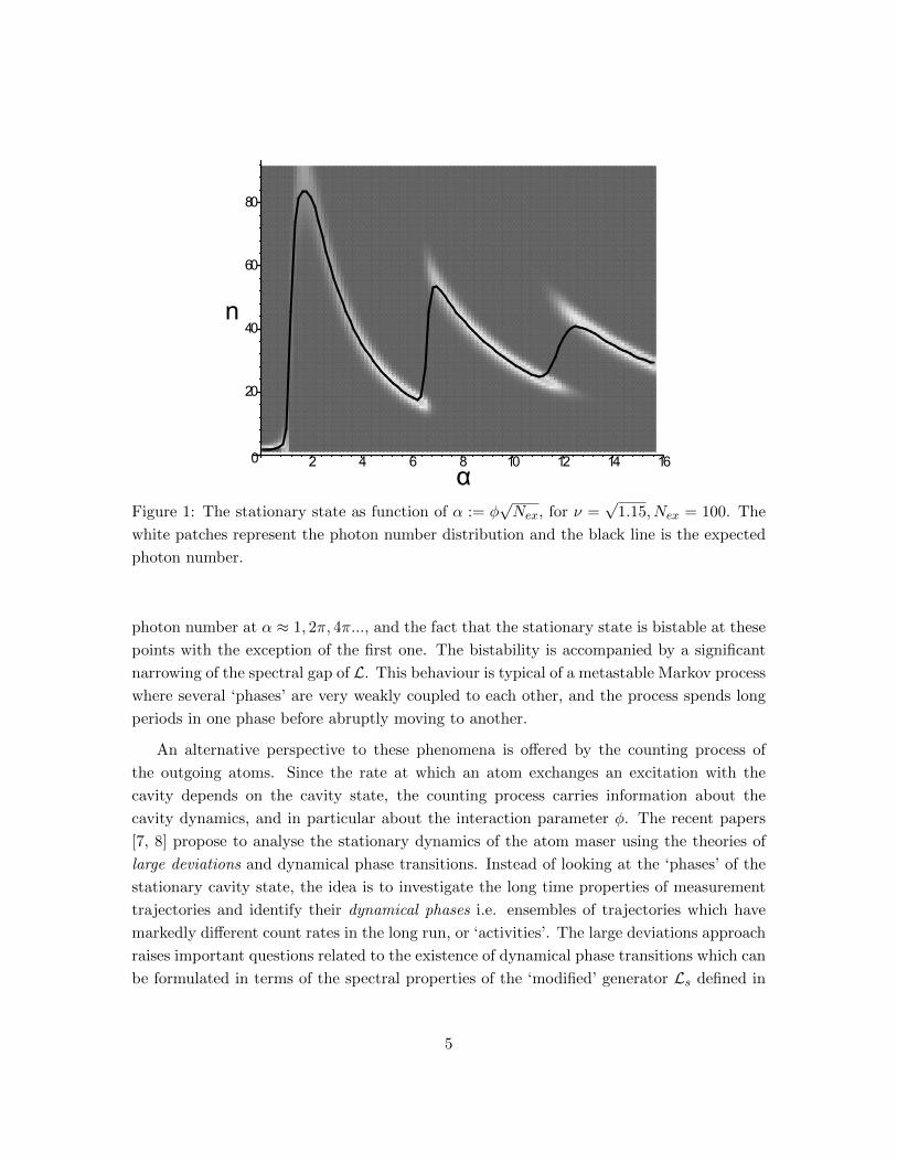
Figure 1: The stationary state as function of α := φ√Nex, for ν =

√1.15, Nex = 100. The

white patches represent the photon number distribution and the black line is the expected

photon number.

photon number at α ≈ 1, 2π, 4π..., and the fact that the stationary state is bistable at these

points with the exception of the first one. The bistability is accompanied by a significant

narrowing of the spectral gap of L. This behaviour is typical of a metastable Markov process

where several ‘phases’ are very weakly coupled to each other, and the process spends long

periods in one phase before abruptly moving to another.

An alternative perspective to these phenomena is offered by the counting process of

the outgoing atoms. Since the rate at which an atom exchanges an excitation with the

cavity depends on the cavity state, the counting process carries information about the

cavity dynamics, and in particular about the interaction parameter φ. The recent papers

[7, 8] propose to analyse the stationary dynamics of the atom maser using the theories of

large deviations and dynamical phase transitions. Instead of looking at the ‘phases’ of the

stationary cavity state, the idea is to investigate the long time properties of measurement

trajectories and identify their dynamical phases i.e. ensembles of trajectories which have

markedly different count rates in the long run, or ‘activities’. The large deviations approach

raises important questions related to the existence of dynamical phase transitions which can

be formulated in terms of the spectral properties of the ‘modified’ generator Ls defined in

5

section 4, and the Perron-Frobenius Theorem for infinite dimensional quantum Markov

processes [12]. In this work we concentrate on the closely related, but distinct regime of

moderate deviations characterised by the Central Limit Theorem, which is more relevant

for statistical inference problems. For later purposes we introduce a unitary dilation of

the master evolution which is defined by the unitary solution of the following quantum

stochastic differential equation

dU(t) =4∑i=1

(LidA

∗i,t − L∗i dAi,t −

1

2L∗iLidt

)U(t). (9)

The pairs (dAi,t, dA∗i,t) represent the increments of the creation and annihilation operators

of 4 independent bosonic input channels, which couple with the cavity through the operators

Li. The master evolution can be recovered as usual by tracing out the bosonic environment

which is initially in the vacuum state

etL(ρ) = Trenv(U(t) (ρ⊗ |Ω〉〈Ω|)U(t)∗)

If dΓi,t denote the increments of the four number operators of the input channels then the

counting operators of the output are

Λi,t := U(t)∗ (1⊗ Γi,t)U(t), (10)

which provide the statistics of counting atoms in the ground state, excited state, emitted

and absorbed photons.

3 Brief overview of classical and quantum statistics notions

For reader’s convenience we recall here some basic notions of classical and quantum para-

metric statistics which will be useful for interpreting the results of the next section.

3.1 Estimation for independent identically distributed variables

A typical statistical problem is to estimate an unknown parameter θ = (θ1, . . . , θk) ∈ Rk

given the data consisting of independent, identically distributed samples X1, . . . , Xn from

a distribution Pθ which depends on θ.

An estimators θn := θn (X1, ..., Xn) is called unbiased if E(θn) = θ for all θ. The Cramer-

Rao inequality gives a lower bound to the covariance matrix and mean square error of any

6

unbiased estimator

Cov(θn) = Eθ[(θn − θ)T (θn − θ)

]≥ 1

nI(θ)−1 (11)

Eθ[‖θn − θ‖2

]≥ 1

nTr(I(θ)−1

). (12)

The k×k positive matrix I(θ) is called the Fisher information matrix and can be computed

in terms of the log-likelihood functions `θ := log pθ where pθ is the probability density of Pθwith respect to some reference measure µ:

I(θ)i,j = Eθ(∂`θ∂θi

∂`θ∂θi

)=

∫pθ(x)

∂ log pθ∂θi

∂ log pθ∂θj

µ (dx)

The Cramer-Rao bound is in general not achievable for a given n. However, what makes

the Fisher information important is the fact that the bound is asymptotically achievable.

Furthermore, asymptotically optimal estimators (or efficient estimators) are asymptotically

normal in the sense that √n(θn − θ)

L−→ N(0, I(θ)−1) (13)

where the right side is a centred k-variate Gaussian distribution with covariance I(θ)−1 and

the convergence is in law for n → ∞. Under certain regularity conditions, the maximum

likelihood estimator

θn := arg maxθ′

∏i

pθ′(Xi)

is efficient. The asymptotic normality of efficient estimators can be seen as a consequence

of the more fundamental theory of local asymptotic normality (LAN) which states that the

i.i.d. statistical model Pnθ can be ‘linearised’ in a local neighbourhood of any point θ0 and

approximated by a Gaussian model. Since the uncertainty in θ is of the order n−1/2 we

write θ := θ0 +u/√n where u is a local parameter which is considered unknown, while θ0 is

fixed and known. Local asymptotic normality can be expressed as the (local) convergence

of statistical models [25]Pnθ0+u/√n : u ∈ R

→N(u, I(θ0)

−1) : u ∈ R

where the limit is approached as n → ∞, and consists of a single sample from the normal

distribution with unknown mean u and known variance I(θ0)−1. In sections 4.(4.4) and

4.(4.5) we will prove two versions of LAN, one for quantum states and one for a classical

counting process.

7

3.2 Quantum estimation with identical copies

Consider now the problem of estimating θ ∈ Rk, given n identical and independent copies

of a quantum state ρθ. The quantum Cramer-Rao bound [3, 18, 19] says that for any

measurement on ρ⊗nθ (including joint ones) and any unbiased estimator θn constructed

from the outcome of this measurement, the lower bound (11) holds with I(θ) replaced by

the quantum Fisher information matrix

F (θ)i,j = Tr (ρθDθ,i Dθ,j)

where X Y := X,Y /2 and Dθ,i are the self-adjoint operators defined by

∂ρθ∂θi

= Dθ,i ρθ.

When θ is one dimensional, the quantum Cramer-Rao bound is asymptotically achiev-

able by the following two steps adaptive procedure. First, a small proportion n n of the

systems is measured in a ‘standard’ way and a rough estimator θ0 is constructed; in the

second step, one measures Dθ0 separately on each system to obtain results D1, . . . , Dn−n

and defines the efficient estimator

θn = θ0 +1

(n− n)F (θ0)

∑i

Di.

However, for multi-dimensional parameters, the quantum Cramer-Rao bound is not achiev-

able even asymptotically, due to the fact that the operators Dθ,i may not commute with

each other and cannot be measured simultaneously. Moreover, unlike the classical case,

there are several Cramer-Rao bounds based on different notions of ‘Fisher information’ [1].

In this case it is more meaningful to search for asymptotically optimal estimators in the

sense of optimising the risk given by mean square error (12). In [17] it has been shown

that for qubits, the asymptotically optimal risk is given by the so called Holevo bound [19].

For arbitrary dimensions, the achievability of the Holevo bound can be deduced from the

theory of quantum local asymptotic normality developed in [21] and a discussion on this

can be found in [15].

3.3 Fisher information for classical Markov processes

Often, the data we need to investigate is not a sequence of i.i.d. variables but a stochastic

process, e.g. a Markov process. A theory of efficient estimators and (local) asymptotic

normality can be developed along the lines of the i.i.d. set-up, provided that the process

8

is ergodic. We will describe the basic ingredients of a continuous time Markov process and

write its Fisher information.

Let I = 1, ...,m be a set of states, and let Q = [qij ] be a m×m matrix of transition

rates, with qij ≥ 0 for i 6= j and diagonal elements qii = −qi := −∑

j 6=i qij . The rate

matrix is the generator of a continuous time Markov process, and the associated semigroup

of transition operators is

P (t) = exp(tQ).

A continuous time stochastic process (Xt)t≥0 with state space I is a Markov process

with transition semigroup P (t) if

P(Xtn+1 = in+1|Xt0 = i0, ..., Xtn = in

)= p(tn+1 − tn)inin+1 ,

for all n = 0, 1, 2, ..., all times 0 ≤ t0 ≤ ... ≤ tn+1, and all states i0, ..., in+1 where p(t)ij are

the matrix elements of P (t).

Let us denote by J0, J1, ... the times when the process jumps from one state to another,

so that J0 = 0 and Jn+1 = inf t > Jn : Xt 6= XJn. The time between two jumps is called

’holding time’ and is defined by Si = Ji − Ji−1.

A probability distribution π = (π1, . . . , πm) over I is stationary for the Markov process

(Xt)t≥0 if it satisfies νQ = 0 or equivalently πP (t) = π at all t. If the transition matrix is

irreducible then this distribution is unique and the process is called ergodic, in which case

any initial distribution µ converges to the stationary distribution

limt→∞

µP (t) = π.

Suppose now that we observe the ergodic Markov process Xt for t ∈ [0, T ], and that the rate

matrix depends smoothly on some unknown parameter θ (which for simplicity we consider

one dimensional), so that qij = qθij . The asymptotic theory says that ‘good’ estimators like

maximum likelihood (under some regularity conditions) are asymptotically normal in the

sense of (13), with Fisher information given by

I (θ) :=∑i 6=j

πθi qθij

(V θij

)2(14)

where

V θij :=

d

dθlog qθij

and πθ is the stationary distribution at θ.

9

4 Fisher informations for the atom maser

In this section we return to the atom maser and investigate the problem of estimating the

interaction parameter φ, based on outcomes of measurements performed on the outgoing

atoms. State and process tomography are key enabling components in quantum engineering,

and have become the focus of research at the intersection of quantum information theory

and statistics. Our contribution is to go beyond the usual set-up of repeated measurements

of identically prepared systems, or that of process tomography, and look at estimation in

the quantum Markov set-up. The first step in this direction was made in [14] which deals

with asymptotics of system identification in a discrete time setting with finite dimensional

systems. Here we extend these ideas to the atom maser, including the effect of the thermal

bath. In the next subsections we consider several thought experiments in which counting

measurements are performed in the output bosonic channels determined by the unitary

coupling (9). While some of these scenarios are not meant to have a practical relevance, the

point is to analyse and compare the amount of Fisher information carried by the various

stochastic processes associated to the atom maser, as illustrated in Figures 2 and 3.

4.1 Observing the cavity

Consider first the scenario where all four channels are monitored by means of counting

measurements. As already discussed in section 2, the conditional evolution of the cavity is

described by the birth and death process consisting of jumps up and down the Fock ladder,

with rates (7). Note that when an atom is detected in the excited state, the cavity state

remains unchanged, so the corresponding rate Nex cos(φ√i+ 1

)2does not appear in the

birth and death rates. Later we will see that these atoms do carry Fisher information about

the interaction parameter even if they do not modify the state of the cavity.

Since the cavity dynamics is Markovian, we can use (14) and the expression of the

stationary state (8) to compute the Fisher information of the stochastic process determined

by the cavity state

Icav (φ) =

∞∑i=0

ρφs (i)

(qφi,i+1

)′

qφi,i+1

2

qφi,i+1

We stress that this information refers to an observer who only has access to the cavity state,

and cannot infer whether a jump up is due to exchanging an excitation with an atom or

absorbing a photon from the bath. Moreover, the observer does not get any information

about atoms passing through the cavity without exchanging the excitation.

10

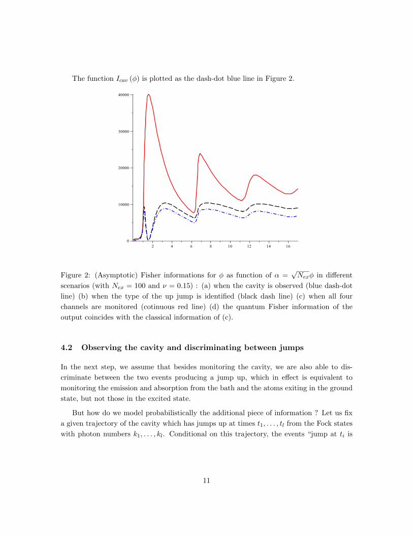
The function Icav (φ) is plotted as the dash-dot blue line in Figure 2.

Figure 2: (Asymptotic) Fisher informations for φ as function of α =√Nexφ in different

scenarios (with Nex = 100 and ν = 0.15) : (a) when the cavity is observed (blue dash-dot

line) (b) when the type of the up jump is identified (black dash line) (c) when all four

channels are monitored (cotinuous red line) (d) the quantum Fisher information of the

output coincides with the classical information of (c).

4.2 Observing the cavity and discriminating between jumps

In the next step, we assume that besides monitoring the cavity, we are also able to dis-

criminate between the two events producing a jump up, which in effect is equivalent to

monitoring the emission and absorption from the bath and the atoms exiting in the ground

state, but not those in the excited state.

But how do we model probabilistically the additional piece of information ? Let us fix

a given trajectory of the cavity which has jumps up at times t1, . . . , tl from the Fock states

with photon numbers k1, . . . , kl. Conditional on this trajectory, the events “jump at ti is

11

due to atom” and its complement “jump at ti is due to bath” have probabilities

pia =rkia

rkia + rkib, pib =

rkibrkia + rkib

where rka = Nexsin(φ√k + 1

)2and rkb = ν (k + 1) are the rates for atoms and bath jumps.

This means that we can model the process by independently tossing a coin with probabilities

pia and pib at each time ti. For each toss the additional Fisher information is

Iti(φ) =

(dpiadφ

)21

pia(1− pia),

and the information for the whole trajectory is obtained by summing over i. The (asymp-

totic) Fisher information of the process is obtained by taking the time and stochastic aver-

aging over trajectories, in the large time limit. Since in the long run the system is in the

stationary state, the average number of k → k + 1 jumps per unit of time is ρφs (k) qφk,k+1,

so the additional Fisher information provided by the jumps is

Iup (φ) =∞∑k=0

ρφs (k) qφk,k+1

(dpkadφ

)21

pka(1− pka).

Therefore the Fisher information gained by following the cavity and discriminating between

jumps is

Icav+up (φ) = Icav (φ) + Iup (φ)

which is plotted as the black dash line in Figure 2.

4.3 Observing all counting processes

The next step is to incorporate the information contained in the detection of excited atoms,

to obtain the full classical Fisher information of all four counting measurements. We will

consider again a fixed cavity trajectory and compute the additional (conditional) Fisher

information provided by the counts of excited atoms. During each holding time period

Si = ti+1− ti the cavity is in the state ki and the excited atoms are described by a Poisson

process with rate

rkie := Nex cos(φ√ki + 1

)2.

Moreover the Poisson processes for different holding times are independent, so the condi-

tional Fisher information is the sum of informations for each Poisson process. Now, for a

Poisson process the total number of counts in a time interval is a sufficient statistic and the

12

times of arrival can be neglected. Thus, we only need to compute the Fisher information of

a Poisson distribution with mean λi := rkie Si and add up over i. A short calculation shows

that this is equal to

Ji =

(dλidφ

)2 1

λi=

(drkiedφ

)2Si

rkie.

As before, it remains to add over all holding times and take average over trajectories,

and average over a long period of time. This amounts to replacing Si by the stationary

distribution ρs(ki) which is the average time in the state ki per unit of time. The Fisher

information is

Iexc =

∞∑k=0

ρs(k)1

rke

(drkedφ

)2

.

We can now write down the total classical Fisher information of the four counting

processes

Itot := Iexc + Iup + Icav = 4Nex

∞∑k=0

ρs(k) (k + 1) .

where the last equality follows from a simple calculation based on the explicit expressions

of the three terms. The total information Itot is plotted as continuous red line in Figure 2.

The last expression is surprisingly simple, and as we will see in the next section, it is

equal to the quantum Fisher information of the atom maser output process, which is the

maximum information extracted by any measurement!

4.4 The quantum Fisher information of the atom maser

Up to this point we considered the problem of estimating φ in several scenarios involving

counting processes. We will now investigate the more general problem of estimating φ when

arbitrary measurements are allowed. As discussed in section 33.2, the key statistical notions

of Cramer-Rao bounds, Fisher information and asymptotic normality can be extended to

i.i.d. quantum statistical models, and can be used to find asymptotically optimal measure-

ment strategies for parameter estimation problems. In [14] these notions were extended

to the non-i.i.d. framework of a quantum Markov chain with finite dimensional systems.

Here we extend these results further to the atom maser, which is a continuous time Markov

process with a infinite dimensional system. The general mathematical theory is developed

in forthcoming paper [9] and we refer to [14] more details on the physical and statistical

interpretation of the results.

13

Let |χ〉 be the initial state of the cavity and |Ω〉 the joint vacuum state of the bosonic

fields. The joint (pure) state of the cavity and the four Bosonic channels at time t is

|ψφ(t)〉 = Uφ(t) (|χ〉 ⊗ |Ω〉)

where Uφ(t) is the unitary solution of the quantum stochastic differential equation (9). We

emphasise that both the unitary and the state depend on the parameter φ and we would like

to know what is the ultimate precision limit for the estimation of φ assuming that arbitrary

measurements are available.

As argued in section 3(3.1), for asymptotics it suffices to understand the statistical

model in a local neighbourhood of a given point, whose size is of the order of the statistical

uncertainty, in this case t−1/2. For this we write φ = φ0 + u/√t and focus on the structure

of the quantum statistical model with parameter u ∈ R:

|ψ(u, t)〉 :=∣∣∣ψφ0+u/√t(t)⟩ .

Our main result is to show that this quantum model is asymptotically Gaussian, in the

sense that this family of vectors converges to a family of coherent state of a continuous

variables system, similarly to results obtained in [10, 11, 13, 21] for identical copies of

quantum states, and in [14] for quantum Markov chains. More precisely

limt→∞〈ψ(u, t)|ψ(v, t)〉 =

⟨√2F v|

√2F u

⟩= e−(u−v)

2/8F (15)

where |√

2F u〉 denotes a coherent state of a one mode continuous variables system, with

displacement√

2F u along one axis, and F = F (φ0) is a constant which plays the role

of quantum Fisher information (per unit of time). The meaning of this result is that

for large times, the state of the atom maser and environment is approximately Gaussian

when seen from the perspective of parameter estimation, and by performing an appropriate

measurement we can extract the maximum amount of information F . At the end of the

following calculation we will find that F = Itot, so the counting measurement is in fact

optimal! Recall however that the counting measurement involves the detection of emitted

and absorbed photons which is experimentally unrealistic. However, the result is relevant as

it puts an upper bound on any Fisher information that can be extracted by measurements

on the output. To prove (15) we express the inner product in terms of a (non completely

positive) semigroup on the cavity space, by tracing over the atoms and bath

〈ψ(u, t)|ψ(v, t)〉 = 〈φ|etLu,v(1)|φ〉 (16)

where the generator Lu,v is

Lu,v (X) =4∑i=1

(Lu∗i XL

vi −

1

2Lu∗i L

ui X −

1

2XLv∗i L

vi

)

14

and Lui = Li(φ0 + u/√t) are the operators appearing in the Lindblad generator (4), where

we emphasised the dependence on the local parameter. The proof of (15) uses a second

order perturbation result of Davies [5] which will be discussed in more detail in the next

section. Here we give the final result which says that the quantum Fisher information is

proportional to the mean energy of the cavity in the stationary state, and is equal to the

classical Fisher information Itot for the counting measurement :

F = 4Nex

∞∑k=0

ρs(k)(k + 1).

4.5 Counting ground or excited state atoms

We now consider the scenario in which the estimation is based on the total number of ground

state atoms Λ1,t defined in (10), ignoring their arrival times. A similar argument can be

applied to the excited state atoms. The generating function of Λt can be computed from

the unitary dilation (9) which gives

E (exp (sΛ1,t)) = Tr(ρ0e

tLs(1))

(17)

where ρ0 is the initial state of the cavity and Ls is the modified generator

Ls(ρ) = esL1ρL∗1 −

1

2L∗1L1, ρ+

∑j 6=1

(LjρL

∗j −

1

2L∗jLj , ρ

). (18)

Note that Ls is the generator of a completely positive but not trace preserving semigroup.

We will analyse the moderate deviations of Λ1,t and show that it satisfies the Central Limit

Theorem. In what concerns the estimation of φ we find an explicit expression of the Fisher

information and establish asymptotic normality. The latter means that

Λ1,t :=1√t(Λ1,t − Eφ0(Λ1,t))

L−→ N(µu, V ) (19)

where the convergence holds as t → ∞, with a fixed local parameter, i.e φ = φ0 + u/√t.

In particular, for u = 0 we recover the Central Limit Theorem for Λ1,t. From (19) we find

that the estimator

φt := φ0 +1√tΛ1,t/µ

is efficient (as well as the maximum likelihood estimator), in the sense that its (rescaled)

asymptotic variance tVar(φt) is equal to the inverse of the Fisher information of the total

counts of ground state atoms

Igr = µ2/V.

15

In the rest of the section we describe the main ideas involved in proving (19) and give the

expressions of µ and V . We first rewrite (19) in terms of the moment generating functions

ϕ(s, t) := E[exp

(is√t(Λ1,t − Eφ0(Λ1,t))

)]→ exp

(iµus− 1

2s2V

). (20)

Using (18) and (17) with s replaced by s/√t, the left side can be written as

ϕ(s, t) = Tr

[ρ0e

tL(

s√t, u√

t

)(1)

], with L

(s√t,u√t

)= L s√

t− 1√

tEφ0

(Λtt

),

where ρ0 is the initial state of the cavity. The generator can be expanded in t−1/2

L(s/√t, u/√t) = L(0) +

1√tL(1) +

1

tL(2) +O

(t−3/2

)and by applying the second order perturbation theorem 5.13 of [5] we get

limt→∞

ϕ(s, t) = exp(

Tr(ρs L(2)(1)

)− Tr

(ρs L(1) L L(1)(1)

))where L is effectively the inverse of the restriction of L(0) to the subspace of operators X

such that Tr(ρsX) = 0, which contains L(1)(1). From the power expansion it can be seen

that the the expression inside the last exponential is quadratic in u, s which provides the

formulas for µ and V in (20). The method outlined above is very general and can be applied

to virtually any ergodic quantum Markov process. However in numerical computations we

found that the fact L(0) has a small spectral gap for certain values of φ0 may pose some

difficulties in computing the inverse L. An alternative method which we do not detail here

is based on large deviation theory and shows that

µ =dr(s)

ds

∣∣∣∣s=0

, V =d2r(s)

ds2

∣∣∣∣s=0

where r(s) is the dominant eigenvalue of Ls. Moreover, the coefficient µ can be computed

in a more direct way as µ = dTr(ρφsN)/dφ since for large times

Eφ(

Λ1,t

t

)= Tr(ρφsN)− ν =

∞∑k=0

ρφs(k)k − ν

which follows from an energy conservation argument in the stationary state.

A similar argument can be made for the total counts of the excited state atoms. The

Fisher informations of both ground and excited state atoms are represented in Figure 3.

The Fisher information for both counting processes together cane computed as well and is

represented by the red line. We note that the counts Fisher informations are comparable

to those of the previous scenarios (see Figure 2) in the region 0 ≤ α ≤ 4, but significantly

smaller in the bistability regions. Also, they are equal to zero at φ ≈ 0.16 due to the fact

that the derivative with φ of the mean atom number is zero at this point.

16

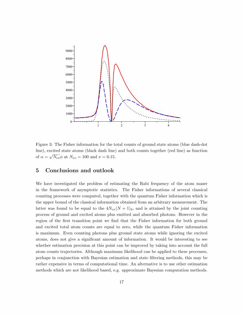
Figure 3: The Fisher information for the total counts of ground state atoms (blue dash-dot

line), excited state atoms (black dash line) and both counts together (red line) as function

of α =√Nexφ at Nex = 100 and ν = 0.15.

5 Conclusions and outlook

We have investigated the problem of estimating the Rabi frequency of the atom maser

in the framework of asymptotic statistics. The Fisher informations of several classical

counting processes were computed, together with the quantum Fisher information which is

the upper bound of the classical information obtained from an arbitrary measurement. The

latter was found to be equal to the 4Nex〈N + 1〉s, and is attained by the joint counting

process of ground and excited atoms plus emitted and absorbed photons. However in the

region of the first transition point we find that the Fisher information for both ground

and excited total atom counts are equal to zero, while the quantum Fisher information

is maximum. Even counting photons plus ground state atoms while ignoring the excited

atoms, does not give a significant amount of information. It would be interesting to see

whether estimation precision at this point can be improved by taking into account the full

atom counts trajectories. Although maximum likelihood can be applied to these processes,

perhaps in conjunction with Bayesian estimation and state filtering methods, this may be

rather expensive in terms of computational time. An alternative is to use other estimation

methods which are not likelihood based, e.g. approximate Bayesian computation methods.

17

Another future direction is to explore the relation between the moderate deviations regime

which we have analysed here, and the large deviations regime which is relevant for the

study of dynamical phase transition [7, 8]. Ultimately the goal is to design measurements

which optimise the statistical performance of the estimation, in the spirit of Wiseman’s

adaptive phase estimation protocol [27] and to explore the connections with control theory,

e.g. in the frame of adaptive control. Two papers detailing the proofs of the asymptotic

normality results in a general Markov set-up [9] and the large deviations perspective [12]

are in preparation.

References

[1] V. P. Belavkin. Generalized heisenberg uncertainty relations, and efficient measure-

ments in quantum systems. Theor. Math. Phys., 26:213–222, 1976.

[2] V. P. Belavkin. Measurement, Filtering and Control in Quantum Open Dynamical

Systems. Rep. on Math. Phys., 43:405–425, 1999.

[3] S. L. Braunstein and Caves C. M. Statistical distance and the geometry of quantum

states. Phys. Rev. Lett., 72:3439–3443, 1994.

[4] H.-J. Briegel, Englert B.-G., N. Sterpi, and H. Walther. One-atom maser: Statistics of

detector clicks. Phys. Rev. A, 49:2962–2985, 1994.

[5] E. B. Davies. One-parameter semigroups. Academic Press, 1980.

[6] B.-G. Englert. Elements of micromaser physics. arXiv:quant-ph/0203052v1, 2002.

[7] J. P. Garrahan and I. Lesanovsky. Thermodynamics of quantum jump trajectories.

Phys. Rev. Lett., 104:160601, 2010.

[8] J. P. Garrahan, A. D. Armour, and I. Lesanovsky. Quantum trajectory phase transi-

tions in the micromaser. Phys. Rev. E, 84:021115, 2011.

[9] M. Guta and L. Bouten. in preparation.

[10] M. Guta and A. Jencova. Local asymptotic normality in quantum statistics. Commun.

Math. Phys., 276:341–379, 2007.

[11] M. Guta and J. Kahn. Local asymptotic normality for qubit states. Phys. Rev. A, 73:

052108, 2006.

[12] M. Guta and M. van Horssen. in preparation.

18

[13] M. Guta, B. Janssens, and J. Kahn. Optimal estimation of qubit states with continuous

time measurements. Commun. Math. Phys., 277:127–160, 2008.

[14] M. Guta. Fisher information and asymptotic normality in system identification for

quantum markov chains. Phys. Rev. A, 83:062324, 2011.

[15] M. Guta and J. Kahn. Local asymptotic normality and optimal estimation for d-

dimensional quantum systems. In V.P. Belavkin and M. Guta, editors, Quantum

Stochastics and Information: statistics, filtering and control. World Scientific, 2008.

[16] H. Haffner, W. Hansel, C. F. Roos, J. Benhelm, D. Chek-al kar, M. Chwalla, T. Korber,

U.D. Rapol, M. Riebe, P.O. Schmidt, C. Becher, O. Guhne, W. Dur, and R. Blatt.

Scalable multiparticle entanglement of trapped ions. Nature, 438:643, 2005.

[17] M. Hayashi and Matsumoto, K. Asymptotic performance of optimal state estimation

in quantum two level system. quant-ph/0411073, 2004.

[18] C. W. Helstrom. Quantum Detection and Estimation Theory. Academic Press, New

York, 1976.

[19] A. S. Holevo. Probabilistic and Statistical Aspects of Quantum Theory. North-Holland,

1982.

[20] Dowling J.P. and G.J. Milburn. Quantum technology: the second quantum revolution.

Phil. Trans. R. Soc. Lond. A, 361:1655–1674, 2003.

[21] J. Kahn and M. Guta. Local asymptotic normality for finite dimensional quantum

systems. Commun. Math. Phys., 289:597–652, 2009.

[22] L. Ljung. System Identification: Theory for the user. Prentice Hall, 2007.

[23] H. Mabuchi and N. Khaneja. Principles and applications of control in quantum systems.

Int. J. Robust Nonlinear Control, 15:647–667, 2005.

[24] G. Rempe, H. Walther, and N. Klein. Observation of quantum collapse and revival in

a one-atom maser. Phys. Rev. Lett., 58:353–356, 1987.

[25] A.W. van der Vaart. Asymptotic Statistics. Cambridge University Press, 1998.

[26] H. Walther. Experiments on quantum electrodynamics. Rep. Phys., 219:263, 1992.

[27] H. M. Wiseman. Adaptive phase measurements of optical modes: Going beyond the

marginal Q distribution. Phys. Rev. Lett., 75:4587–4590, 1995.

19

[28] H. M. Wiseman and G. J. Milburn. Quantum Measurement and Control. Cambridge

University Press, 2009.

20