Hydrogen Maser Humphrey

Precision measurements with atomic hydrogen masers

A thesis presented

by

Marc Andrew Humphrey

to

The Department of Physics

in partial fulfillment of the requirements

for the degree of

Doctor of Philosophy

in the subject of

Physics

Harvard University

Cambridge, Massachusetts

May 2003

c©2003 by Marc Andrew Humphrey

All rights reserved

Advisor: Dr. Ronald Walsworth Author: Marc Andrew Humphrey

Precision measurements with atomic hydrogen masers

We report two experimental results and a theoretical study involving atomic hydrogen

masers oscillating on the ∆F = 1, ∆mF = 0 hyperfine transition. In the first experiment,

we placed a new limit on Lorentz and CPT violation of the proton in terms of a recent

standard model extension. By placing a bound on sidereal variation of the F = 1, ∆mF =

±1 Zeeman frequency in atomic hydrogen, our search set a limit on violation of Lorentz

and CPT symmetry of the proton at the 10−27 GeV level, independent of nuclear model

uncertainty, and improved significantly on previous bounds. This test utilized a double

resonance technique in which the oscillation frequency of a hydrogen maser is shifted

by applied radiation near the F = 1, ∆mF = ±1 Zeeman resonance. We used the

dressed atom formalism to calculate this frequency shift and found excellent agreement

with a previous calculation made in the bare atom basis. Qualitatively, the dressed atom

analysis gave a simpler physical interpretation of the double resonance process. In the

second experiment, we investigated low temperature hydrogen-hydrogen spin-exchange

collisions using a cryogenic hydrogen maser. Operational details of the apparatus are

presented and a description of our measurement of the semi-classical spin-exchange shift

cross section λ0 at 0.5 K is given. We report a value of λ0 = 56.70 A2 with a statistical

error of 15.51 A2 and a systematic uncertainty between 80.6 and 318.8 A2. A discussion

of this systematic is given and the possiblity of an improved measurement is discussed.

Contents

Acknowledgments viii

List of Figures x

List of Tables xxv

1 Introduction 1

2 Hydrogen maser theory 5

2.1 Standard hydrogen maser theory . . . . . . . . . . . . . . . . . . . . . . . . 7

2.1.1 Interaction of atoms with cavity field . . . . . . . . . . . . . . . . . . 7

2.1.2 Interaction of cavity and magnetization . . . . . . . . . . . . . . . . 12

2.1.3 Maser oscillation frequency . . . . . . . . . . . . . . . . . . . . . . . 15

2.1.4 Maser power . . . . . . . . . . . . . . . . . . . . . . . . . . . . . . . 16

2.2 Double resonance theory . . . . . . . . . . . . . . . . . . . . . . . . . . . . . 17

2.2.1 Bare atom analysis . . . . . . . . . . . . . . . . . . . . . . . . . . . . 17

2.2.2 Dressed atom analysis . . . . . . . . . . . . . . . . . . . . . . . . . . 19

2.2.3 Application of double resonance . . . . . . . . . . . . . . . . . . . . 29

3 Practical realization of the hydrogen maser 31

3.1 Hydrogen maser apparatus . . . . . . . . . . . . . . . . . . . . . . . . . . . 31

3.1.1 Hydrogen source . . . . . . . . . . . . . . . . . . . . . . . . . . . . . 33

3.1.2 State selection . . . . . . . . . . . . . . . . . . . . . . . . . . . . . . 35

iv

3.1.3 Maser interaction region . . . . . . . . . . . . . . . . . . . . . . . . . 36

3.1.4 Thermal shielding . . . . . . . . . . . . . . . . . . . . . . . . . . . . 38

3.1.5 Microwave signal . . . . . . . . . . . . . . . . . . . . . . . . . . . . . 39

3.1.6 Microwave receiver . . . . . . . . . . . . . . . . . . . . . . . . . . . . 40

3.2 Hydrogen maser characterization . . . . . . . . . . . . . . . . . . . . . . . . 42

3.2.1 Mechanical and electronic parameters . . . . . . . . . . . . . . . . . 42

3.2.2 Operational parameters . . . . . . . . . . . . . . . . . . . . . . . . . 43

3.2.3 Spin-exchange characterization . . . . . . . . . . . . . . . . . . . . . 47

3.3 Hydrogen maser frequency stability . . . . . . . . . . . . . . . . . . . . . . . 50

3.3.1 General definition of clock stability . . . . . . . . . . . . . . . . . . . 50

3.3.2 Fundamental limits to frequency stability . . . . . . . . . . . . . . . 52

3.3.3 Systematic effects on frequency stability . . . . . . . . . . . . . . . . 54

4 Testing CPT and Lorentz symmetry with hydrogen masers 58

4.1 Lorentz and CPT violation in the standard model . . . . . . . . . . . . . . 59

4.2 Experimental procedure . . . . . . . . . . . . . . . . . . . . . . . . . . . . . 62

4.2.1 Double resonance technique . . . . . . . . . . . . . . . . . . . . . . . 62

4.2.2 Zeeman frequency measurement . . . . . . . . . . . . . . . . . . . . 66

4.2.3 Data analysis . . . . . . . . . . . . . . . . . . . . . . . . . . . . . . . 72

4.2.4 Run 1 . . . . . . . . . . . . . . . . . . . . . . . . . . . . . . . . . . . 73

4.2.5 Field-inverted runs 2 and 3 . . . . . . . . . . . . . . . . . . . . . . . 76

4.2.6 Combined result . . . . . . . . . . . . . . . . . . . . . . . . . . . . . 77

4.3 Systematics and error analysis . . . . . . . . . . . . . . . . . . . . . . . . . . 80

4.3.1 Magnetic field systematics . . . . . . . . . . . . . . . . . . . . . . . . 80

4.3.2 Other systematics . . . . . . . . . . . . . . . . . . . . . . . . . . . . 86

4.3.3 Final result . . . . . . . . . . . . . . . . . . . . . . . . . . . . . . . . 89

4.4 Discussion . . . . . . . . . . . . . . . . . . . . . . . . . . . . . . . . . . . . . 90

4.4.1 Transformation to fixed frame . . . . . . . . . . . . . . . . . . . . . . 90

v

4.4.2 Comparison to previous experiments . . . . . . . . . . . . . . . . . . 93

4.4.3 Future work . . . . . . . . . . . . . . . . . . . . . . . . . . . . . . . . 93

5 The cryogenic hydrogen maser 94

5.1 Cryogenic hydrogen maser frequency stability . . . . . . . . . . . . . . . . . 95

5.1.1 Decreased thermal noise . . . . . . . . . . . . . . . . . . . . . . . . . 96

5.1.2 Increased maser power . . . . . . . . . . . . . . . . . . . . . . . . . . 99

5.1.3 Cryogenic systematics . . . . . . . . . . . . . . . . . . . . . . . . . . 102

5.2 Superfluid 4He wall coating . . . . . . . . . . . . . . . . . . . . . . . . . . . 102

5.2.1 Historic overview . . . . . . . . . . . . . . . . . . . . . . . . . . . . . 102

5.2.2 Effects of superfluid 4He wall coating . . . . . . . . . . . . . . . . . . 103

5.3 Maser setup . . . . . . . . . . . . . . . . . . . . . . . . . . . . . . . . . . . . 106

5.3.1 Hydrogen source and state selection . . . . . . . . . . . . . . . . . . 108

5.3.2 Maser interaction region . . . . . . . . . . . . . . . . . . . . . . . . . 111

5.3.3 Steady state operation . . . . . . . . . . . . . . . . . . . . . . . . . . 119

5.3.4 Pulsed operation . . . . . . . . . . . . . . . . . . . . . . . . . . . . . 121

5.4 3He refrigerator . . . . . . . . . . . . . . . . . . . . . . . . . . . . . . . . . . 124

5.4.1 Vacuum system . . . . . . . . . . . . . . . . . . . . . . . . . . . . . . 124

5.4.2 Liquid nitrogen shield . . . . . . . . . . . . . . . . . . . . . . . . . . 126

5.4.3 Liquid 4He bath . . . . . . . . . . . . . . . . . . . . . . . . . . . . . 126

5.4.4 Pumped liquid 4He pot . . . . . . . . . . . . . . . . . . . . . . . . . 127

5.4.5 Pumped liquid 3He pot . . . . . . . . . . . . . . . . . . . . . . . . . 128

5.4.6 Temperature measurement and control . . . . . . . . . . . . . . . . . 133

5.4.7 Cooldown procedure . . . . . . . . . . . . . . . . . . . . . . . . . . . 137

5.5 CHM performance . . . . . . . . . . . . . . . . . . . . . . . . . . . . . . . . 139

5.5.1 Maser power . . . . . . . . . . . . . . . . . . . . . . . . . . . . . . . 140

5.5.2 Superfluid film and operating temperature . . . . . . . . . . . . . . . 141

5.5.3 Maser frequency stability . . . . . . . . . . . . . . . . . . . . . . . . 146

vi

5.5.4 Maser cavity tuning . . . . . . . . . . . . . . . . . . . . . . . . . . . 147

6 Spin-exchange in hydrogen masers 152

6.1 Degenerate internal states approximation . . . . . . . . . . . . . . . . . . . 154

6.2 Semi-classical hyperfine interaction effects . . . . . . . . . . . . . . . . . . . 157

6.3 Quantum mechanical hyperfine interaction effects . . . . . . . . . . . . . . . 159

6.4 Prior measurements . . . . . . . . . . . . . . . . . . . . . . . . . . . . . . . 165

6.5 SAO CHM measurement . . . . . . . . . . . . . . . . . . . . . . . . . . . . . 167

6.5.1 Experimental procedure . . . . . . . . . . . . . . . . . . . . . . . . . 168

6.5.2 Data reduction and error analysis . . . . . . . . . . . . . . . . . . . . 194

6.5.3 Conclusions . . . . . . . . . . . . . . . . . . . . . . . . . . . . . . . . 198

A Dressed atom double resonance Bloch equations 200

Bibliography 204

vii

Acknowledgments

No page of this thesis could have been written without the positive leadership of Ron

Walsworth. His countless ideas, broad physical insight, and experimental inventiveness

underly every result, while his support, motivation, and management set the stage on

which all of this work was performed. Much the same echos true for David Phillips. A

scientist, teacher, and friend, David taught me how to survive in graduate school, and

equally important, how to get out. With Ron at the helm and David in the trenches this

thesis was brought to completion.

My understanding and appreciation of hydrogen masers would have been much less

complete without the ubiquitous presence of Bob Vessot and Ed Mattison. They taught

me what only world-class experts could, and did so wearing nothing but smiles. I am

grateful that I could conduct my research under their distinguished guidance. Moreover,

the SAO hydrogen maser lab would be wholly incomplete without the presence of Jim

Maddox. Much extra effort was spared and unnecessary grief avoided because of his

technical ingenuity.

The offices and labs of the SAO were filled with life by each of the past and current

members of the Walsworth group. Many smiles were shown, some tears suppressed, and

much camaraderie shared by the great people who made my days less lonely. David Bear

showed me how to live life outside the lab; Glenn Wong showed me how to do so while

in. Rick Stoner taught me the value of perseverance and attention to detail. Caspar van

der Wal and Federico Cane kept my mind from growing flat. In their different ways, Ross

Mair and Matt Rosen always brought the same broad smile to my face. I thank Ruopeng

Wang, Yanhong Xiao, Leo Tsai, Mason Klein and John Ng for letting me show that one

really can make it through the PhD. Of course, we would have all gone mad were it not

for Kristi Armstrong.

Beyond the four walls of B-112, my life has been rounded out by a few very special

people. I thank Bob Michniak for the many fruitful discussions about everything but

viii

physics, and Mike Bassik for the numerous hours over numerous pints and the numerous

trips to Fenway. I thank Brandon Johnson for saving me early on from being far too

serious. Above all, I thank Kathrin Konitzer for her patience, for her cheer, and for

showing me that one really can strike gold in the foothills of Nepal.

From the very beginning to the very last day, I have relied on and benefitted from

the constant and unconditional support of Christie Hong. While working on our own, we

made it through graduate school together. Time after time she offered me her ear and

lent me her shoulder, and during the darkest days it was she who pulled me through when

nobody else could. I would not have survived without her, nor will I ever find the words

to show her my full gratitude.

It goes without saying that I would not have finished my PhD without the love and

support of my family. More importantly, without them I would have never even begun. I

thank my brother for showing me what it means to succeed, and my parents for sharing

in our achievements. Their simple lesson that hard work and determination are all one

needs to reach their dreams gave me the courage to begin, the strength to continue, and

the will to finish this chapter of my life. I thank my family for being my biggest fans, my

closest friends, and my greatest inspiration.

ix

List of Figures

2.1 Hydrogen hyperfine structure. A hydrogen maser oscillates on the first-

order magnetic-field-independent |2〉 ↔ |4〉 hyperfine transition near 1420

MHz. The maser typically operates with a static field less than 1 mG. For

these low field strengths, the two F = 1, ∆mF = ±1 Zeeman frequencies

are nearly degenerate, and ν12 ≈ ν23 ≈ 1 kHz. . . . . . . . . . . . . . . . . . 6

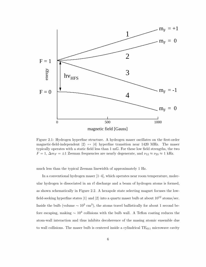
2.2 Hydrogen maser schematic. The solenoid generates a weak static magnetic

field B0 which defines a quantization axis inside the maser bulb. The mi-

crowave cavity field HC (dashed field lines) and the coherent magnetization

M of the atomic ensemble form the coupled actively oscillating system. . . 8

x

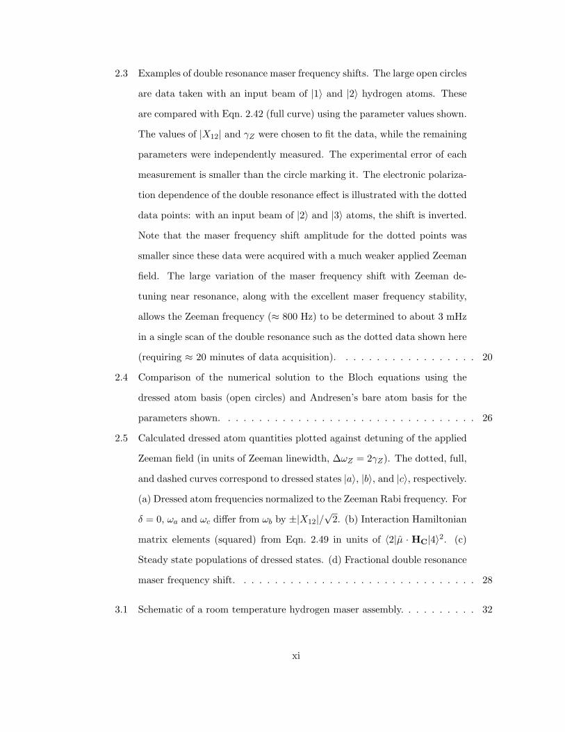
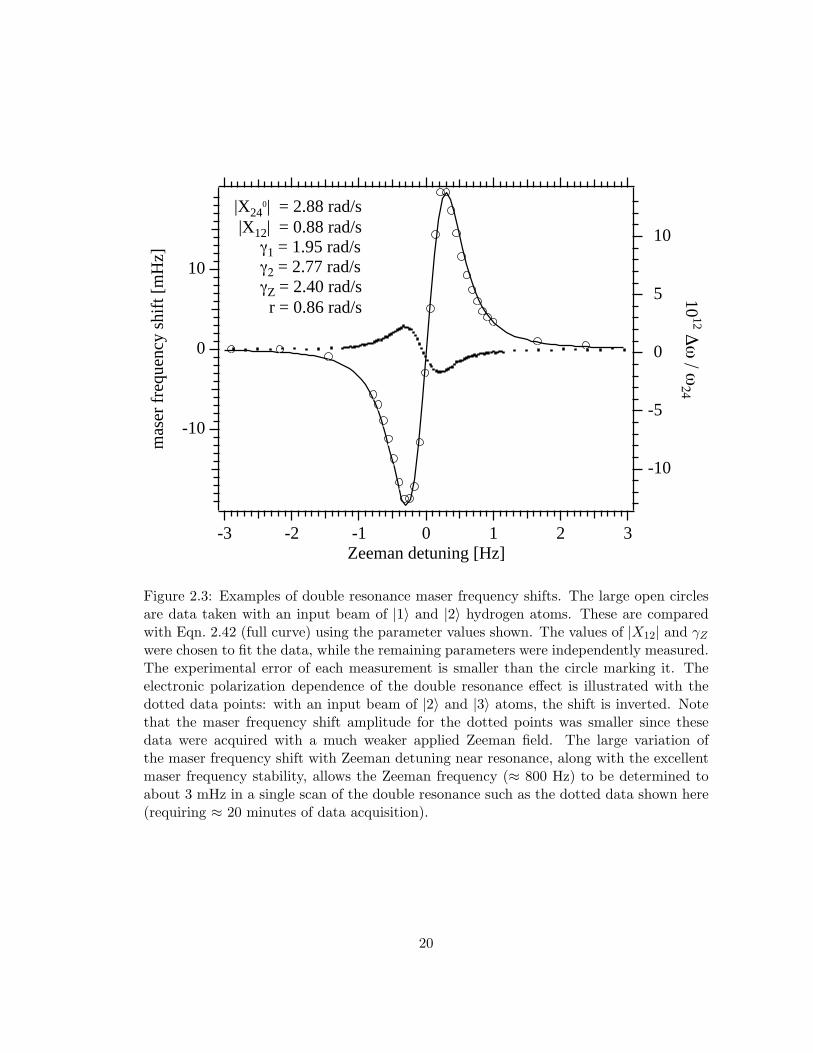
2.3 Examples of double resonance maser frequency shifts. The large open circles

are data taken with an input beam of |1〉 and |2〉 hydrogen atoms. These

are compared with Eqn. 2.42 (full curve) using the parameter values shown.

The values of |X12| and γZ were chosen to fit the data, while the remaining

parameters were independently measured. The experimental error of each

measurement is smaller than the circle marking it. The electronic polariza-

tion dependence of the double resonance effect is illustrated with the dotted

data points: with an input beam of |2〉 and |3〉 atoms, the shift is inverted.

Note that the maser frequency shift amplitude for the dotted points was

smaller since these data were acquired with a much weaker applied Zeeman

field. The large variation of the maser frequency shift with Zeeman de-

tuning near resonance, along with the excellent maser frequency stability,

allows the Zeeman frequency (≈ 800 Hz) to be determined to about 3 mHz

in a single scan of the double resonance such as the dotted data shown here

(requiring ≈ 20 minutes of data acquisition). . . . . . . . . . . . . . . . . . 20

2.4 Comparison of the numerical solution to the Bloch equations using the

dressed atom basis (open circles) and Andresen’s bare atom basis for the

parameters shown. . . . . . . . . . . . . . . . . . . . . . . . . . . . . . . . . 26

2.5 Calculated dressed atom quantities plotted against detuning of the applied

Zeeman field (in units of Zeeman linewidth, ∆ωZ = 2γZ). The dotted, full,

and dashed curves correspond to dressed states |a〉, |b〉, and |c〉, respectively.

(a) Dressed atom frequencies normalized to the Zeeman Rabi frequency. For

δ = 0, ωa and ωc differ from ωb by ±|X12|/√

2. (b) Interaction Hamiltonian

matrix elements (squared) from Eqn. 2.49 in units of 〈2|µ · HC|4〉2. (c)

Steady state populations of dressed states. (d) Fractional double resonance

maser frequency shift. . . . . . . . . . . . . . . . . . . . . . . . . . . . . . . 28

3.1 Schematic of a room temperature hydrogen maser assembly. . . . . . . . . . 32

xi

3.2 Schematic of the hydrogen maser receiver. Output voltages of 5 MHz, 100

MHz, and 1200 MHz are derived from a voltage controlled crystal oscillator

which is phase locked to the maser signal. Only the 1200 MHz output is

shown here. . . . . . . . . . . . . . . . . . . . . . . . . . . . . . . . . . . . . 41

3.3 Maser power vs maser flux as a function of the spin-exchange parameter q.

The maser power is normalized relative to the oscillation threshold power

Pc and the flux is normalized to the oscillation threshold flux Ith. . . . . . . 49

3.4 Hydrogen maser frequency stability due to thermal noise at room temper-

ature. The dotted lines depict the limit due to added white phase noise

(Eqn. 3.31), and white frequency noise (Eqn. 3.30), and the solid line shows

the net limit due to thermal sources. We have used T = 290 K, Ql =

1.6×109, P = 6×10−13 W, TN = 920 K, B = 6 Hz, and β = 0.23, the

values for SAO maser P-8. . . . . . . . . . . . . . . . . . . . . . . . . . . . . 54

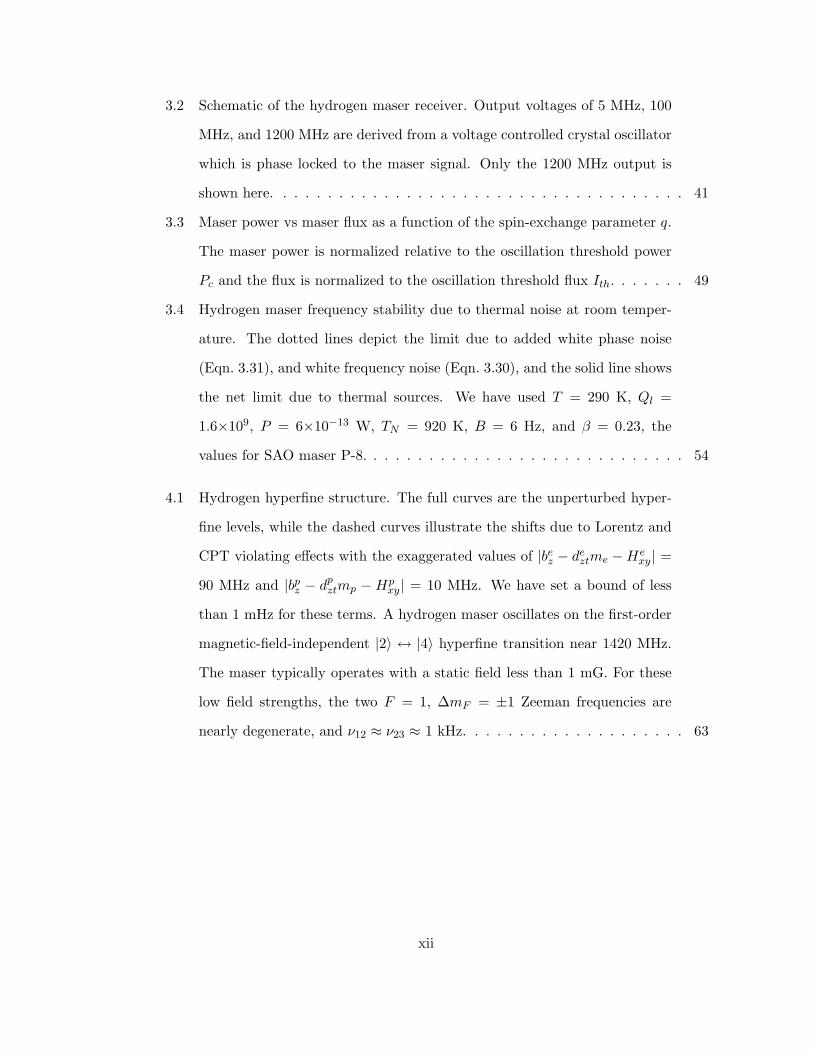
4.1 Hydrogen hyperfine structure. The full curves are the unperturbed hyper-

fine levels, while the dashed curves illustrate the shifts due to Lorentz and

CPT violating effects with the exaggerated values of |bez − de

ztme − Hexy| =

90 MHz and |bpz − dp

ztmp − Hpxy| = 10 MHz. We have set a bound of less

than 1 mHz for these terms. A hydrogen maser oscillates on the first-order

magnetic-field-independent |2〉 ↔ |4〉 hyperfine transition near 1420 MHz.

The maser typically operates with a static field less than 1 mG. For these

low field strengths, the two F = 1, ∆mF = ±1 Zeeman frequencies are

nearly degenerate, and ν12 ≈ ν23 ≈ 1 kHz. . . . . . . . . . . . . . . . . . . . 63

xii

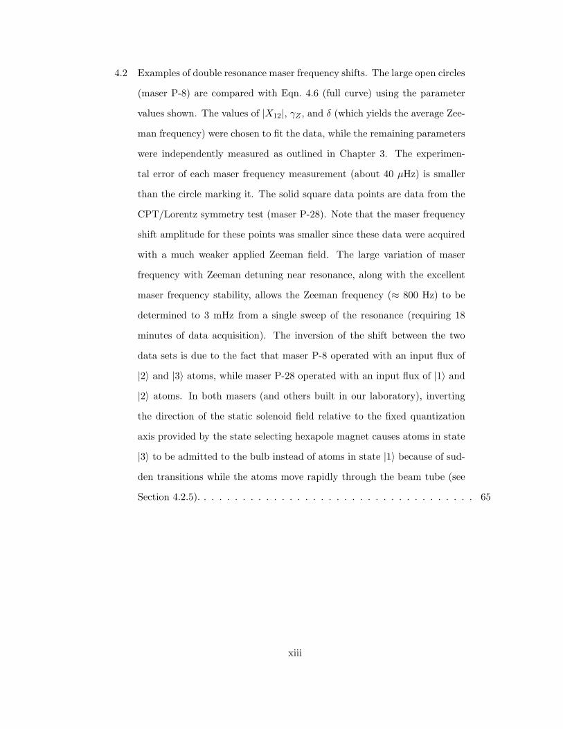
4.2 Examples of double resonance maser frequency shifts. The large open circles

(maser P-8) are compared with Eqn. 4.6 (full curve) using the parameter

values shown. The values of |X12|, γZ , and δ (which yields the average Zee-

man frequency) were chosen to fit the data, while the remaining parameters

were independently measured as outlined in Chapter 3. The experimen-

tal error of each maser frequency measurement (about 40 µHz) is smaller

than the circle marking it. The solid square data points are data from the

CPT/Lorentz symmetry test (maser P-28). Note that the maser frequency

shift amplitude for these points was smaller since these data were acquired

with a much weaker applied Zeeman field. The large variation of maser

frequency with Zeeman detuning near resonance, along with the excellent

maser frequency stability, allows the Zeeman frequency (≈ 800 Hz) to be

determined to 3 mHz from a single sweep of the resonance (requiring 18

minutes of data acquisition). The inversion of the shift between the two

data sets is due to the fact that maser P-8 operated with an input flux of

|2〉 and |3〉 atoms, while maser P-28 operated with an input flux of |1〉 and

|2〉 atoms. In both masers (and others built in our laboratory), inverting

the direction of the static solenoid field relative to the fixed quantization

axis provided by the state selecting hexapole magnet causes atoms in state

|3〉 to be admitted to the bulb instead of atoms in state |1〉 because of sud-

den transitions while the atoms move rapidly through the beam tube (see

Section 4.2.5). . . . . . . . . . . . . . . . . . . . . . . . . . . . . . . . . . . . 65

xiii

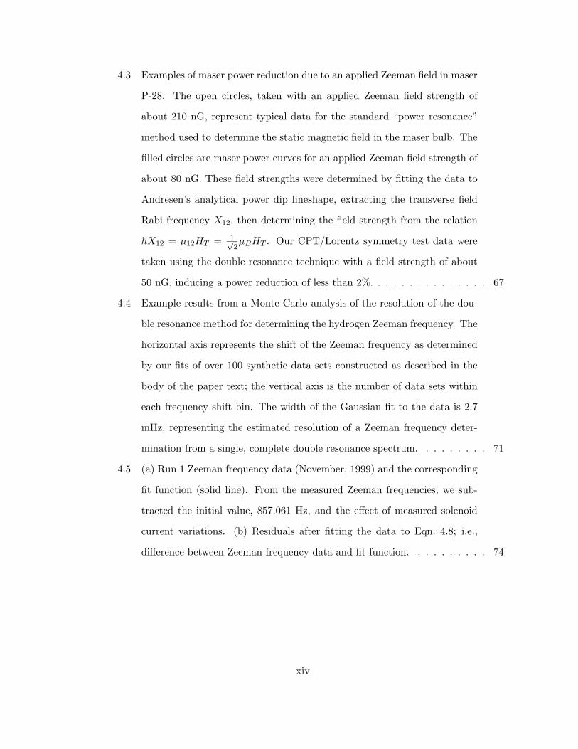
4.3 Examples of maser power reduction due to an applied Zeeman field in maser

P-28. The open circles, taken with an applied Zeeman field strength of

about 210 nG, represent typical data for the standard “power resonance”

method used to determine the static magnetic field in the maser bulb. The

filled circles are maser power curves for an applied Zeeman field strength of

about 80 nG. These field strengths were determined by fitting the data to

Andresen’s analytical power dip lineshape, extracting the transverse field

Rabi frequency X12, then determining the field strength from the relation

hX12 = µ12HT = 1√2µBHT . Our CPT/Lorentz symmetry test data were

taken using the double resonance technique with a field strength of about

50 nG, inducing a power reduction of less than 2%. . . . . . . . . . . . . . . 67

4.4 Example results from a Monte Carlo analysis of the resolution of the dou-

ble resonance method for determining the hydrogen Zeeman frequency. The

horizontal axis represents the shift of the Zeeman frequency as determined

by our fits of over 100 synthetic data sets constructed as described in the

body of the paper text; the vertical axis is the number of data sets within

each frequency shift bin. The width of the Gaussian fit to the data is 2.7

mHz, representing the estimated resolution of a Zeeman frequency deter-

mination from a single, complete double resonance spectrum. . . . . . . . . 71

4.5 (a) Run 1 Zeeman frequency data (November, 1999) and the corresponding

fit function (solid line). From the measured Zeeman frequencies, we sub-

tracted the initial value, 857.061 Hz, and the effect of measured solenoid

current variations. (b) Residuals after fitting the data to Eqn. 4.8; i.e.,

difference between Zeeman frequency data and fit function. . . . . . . . . . 74

xiv

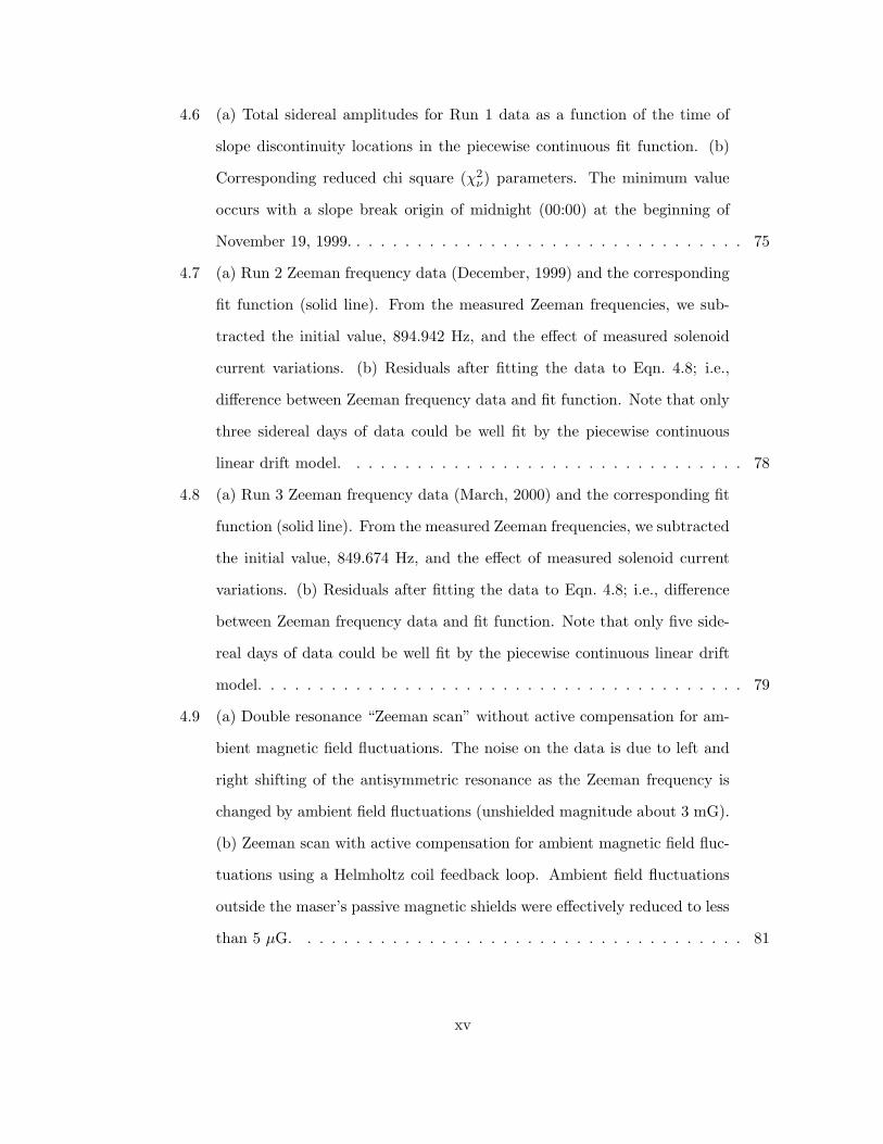
4.6 (a) Total sidereal amplitudes for Run 1 data as a function of the time of

slope discontinuity locations in the piecewise continuous fit function. (b)

Corresponding reduced chi square (χ2ν) parameters. The minimum value

occurs with a slope break origin of midnight (00:00) at the beginning of

November 19, 1999. . . . . . . . . . . . . . . . . . . . . . . . . . . . . . . . . 75

4.7 (a) Run 2 Zeeman frequency data (December, 1999) and the corresponding

fit function (solid line). From the measured Zeeman frequencies, we sub-

tracted the initial value, 894.942 Hz, and the effect of measured solenoid

current variations. (b) Residuals after fitting the data to Eqn. 4.8; i.e.,

difference between Zeeman frequency data and fit function. Note that only

three sidereal days of data could be well fit by the piecewise continuous

linear drift model. . . . . . . . . . . . . . . . . . . . . . . . . . . . . . . . . 78

4.8 (a) Run 3 Zeeman frequency data (March, 2000) and the corresponding fit

function (solid line). From the measured Zeeman frequencies, we subtracted

the initial value, 849.674 Hz, and the effect of measured solenoid current

variations. (b) Residuals after fitting the data to Eqn. 4.8; i.e., difference

between Zeeman frequency data and fit function. Note that only five side-

real days of data could be well fit by the piecewise continuous linear drift

model. . . . . . . . . . . . . . . . . . . . . . . . . . . . . . . . . . . . . . . . 79

4.9 (a) Double resonance “Zeeman scan” without active compensation for am-

bient magnetic field fluctuations. The noise on the data is due to left and

right shifting of the antisymmetric resonance as the Zeeman frequency is

changed by ambient field fluctuations (unshielded magnitude about 3 mG).

(b) Zeeman scan with active compensation for ambient magnetic field fluc-

tuations using a Helmholtz coil feedback loop. Ambient field fluctuations

outside the maser’s passive magnetic shields were effectively reduced to less

than 5 µG. . . . . . . . . . . . . . . . . . . . . . . . . . . . . . . . . . . . . 81

xv

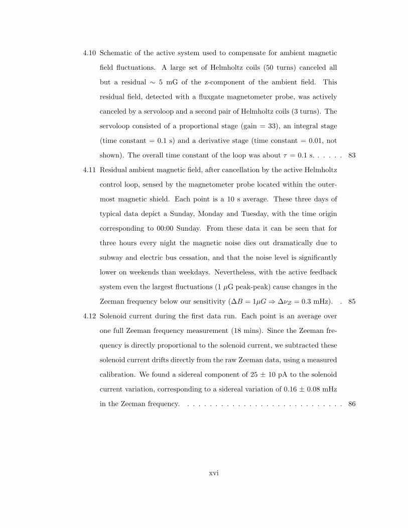
4.10 Schematic of the active system used to compensate for ambient magnetic

field fluctuations. A large set of Helmholtz coils (50 turns) canceled all

but a residual ∼ 5 mG of the z-component of the ambient field. This

residual field, detected with a fluxgate magnetometer probe, was actively

canceled by a servoloop and a second pair of Helmholtz coils (3 turns). The

servoloop consisted of a proportional stage (gain = 33), an integral stage

(time constant = 0.1 s) and a derivative stage (time constant = 0.01, not

shown). The overall time constant of the loop was about τ = 0.1 s. . . . . . 83

4.11 Residual ambient magnetic field, after cancellation by the active Helmholtz

control loop, sensed by the magnetometer probe located within the outer-

most magnetic shield. Each point is a 10 s average. These three days of

typical data depict a Sunday, Monday and Tuesday, with the time origin

corresponding to 00:00 Sunday. From these data it can be seen that for

three hours every night the magnetic noise dies out dramatically due to

subway and electric bus cessation, and that the noise level is significantly

lower on weekends than weekdays. Nevertheless, with the active feedback

system even the largest fluctuations (1 µG peak-peak) cause changes in the

Zeeman frequency below our sensitivity (∆B = 1µG ⇒ ∆νZ = 0.3 mHz). . 85

4.12 Solenoid current during the first data run. Each point is an average over

one full Zeeman frequency measurement (18 mins). Since the Zeeman fre-

quency is directly proportional to the solenoid current, we subtracted these

solenoid current drifts directly from the raw Zeeman data, using a measured

calibration. We found a sidereal component of 25 ± 10 pA to the solenoid

current variation, corresponding to a sidereal variation of 0.16 ± 0.08 mHz

in the Zeeman frequency. . . . . . . . . . . . . . . . . . . . . . . . . . . . . 86

xvi

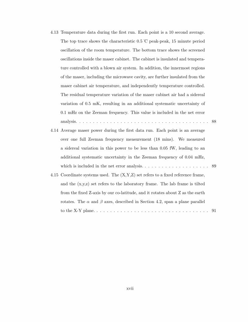
4.13 Temperature data during the first run. Each point is a 10 second average.

The top trace shows the characteristic 0.5 C peak-peak, 15 minute period

oscillation of the room temperature. The bottom trace shows the screened

oscillations inside the maser cabinet. The cabinet is insulated and tempera-

ture controlled with a blown air system. In addition, the innermost regions

of the maser, including the microwave cavity, are further insulated from the

maser cabinet air temperature, and independently temperature controlled.

The residual temperature variation of the maser cabinet air had a sidereal

variation of 0.5 mK, resulting in an additional systematic uncertainty of

0.1 mHz on the Zeeman frequency. This value is included in the net error

analysis. . . . . . . . . . . . . . . . . . . . . . . . . . . . . . . . . . . . . . . 88

4.14 Average maser power during the first data run. Each point is an average

over one full Zeeman frequency measurement (18 mins). We measured

a sidereal variation in this power to be less than 0.05 fW, leading to an

additional systematic uncertainty in the Zeeman frequency of 0.04 mHz,

which is included in the net error analysis. . . . . . . . . . . . . . . . . . . . 89

4.15 Coordinate systems used. The (X,Y,Z) set refers to a fixed reference frame,

and the (x,y,z) set refers to the laboratory frame. The lab frame is tilted

from the fixed Z-axis by our co-latitude, and it rotates about Z as the earth

rotates. The α and β axes, described in Section 4.2, span a plane parallel

to the X-Y plane. . . . . . . . . . . . . . . . . . . . . . . . . . . . . . . . . . 91

xvii

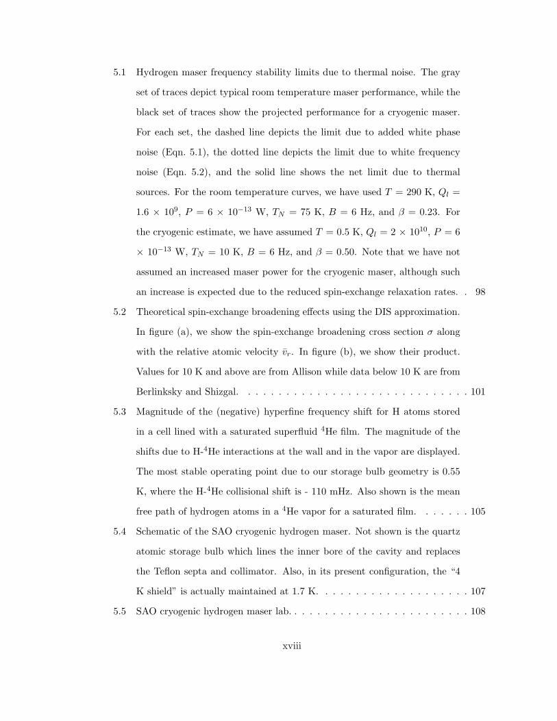
5.1 Hydrogen maser frequency stability limits due to thermal noise. The gray

set of traces depict typical room temperature maser performance, while the

black set of traces show the projected performance for a cryogenic maser.

For each set, the dashed line depicts the limit due to added white phase

noise (Eqn. 5.1), the dotted line depicts the limit due to white frequency

noise (Eqn. 5.2), and the solid line shows the net limit due to thermal

sources. For the room temperature curves, we have used T = 290 K, Ql =

1.6 × 109, P = 6 × 10−13 W, TN = 75 K, B = 6 Hz, and β = 0.23. For

the cryogenic estimate, we have assumed T = 0.5 K, Ql = 2 × 1010, P = 6

× 10−13 W, TN = 10 K, B = 6 Hz, and β = 0.50. Note that we have not

assumed an increased maser power for the cryogenic maser, although such

an increase is expected due to the reduced spin-exchange relaxation rates. . 98

5.2 Theoretical spin-exchange broadening effects using the DIS approximation.

In figure (a), we show the spin-exchange broadening cross section σ along

with the relative atomic velocity vr. In figure (b), we show their product.

Values for 10 K and above are from Allison while data below 10 K are from

Berlinksky and Shizgal. . . . . . . . . . . . . . . . . . . . . . . . . . . . . . 101

5.3 Magnitude of the (negative) hyperfine frequency shift for H atoms stored

in a cell lined with a saturated superfluid 4He film. The magnitude of the

shifts due to H-4He interactions at the wall and in the vapor are displayed.

The most stable operating point due to our storage bulb geometry is 0.55

K, where the H-4He collisional shift is - 110 mHz. Also shown is the mean

free path of hydrogen atoms in a 4He vapor for a saturated film. . . . . . . 105

5.4 Schematic of the SAO cryogenic hydrogen maser. Not shown is the quartz

atomic storage bulb which lines the inner bore of the cavity and replaces

the Teflon septa and collimator. Also, in its present configuration, the “4

K shield” is actually maintained at 1.7 K. . . . . . . . . . . . . . . . . . . . 107

5.5 SAO cryogenic hydrogen maser lab. . . . . . . . . . . . . . . . . . . . . . . . 108

xviii

5.6 Cryomaser microwave cavity formed by a silver plated sapphire cylinder

and a pair of copper endcaps. The sapphire acts to dielectrically load the

cavity, allowing a reduction in its physical size. One coil from a Helmholtz

pair used to drive the F=1, ∆mF =±1 Zeeman transitions is shown. . . . . 112

5.7 Quartz bulb for the cryogenic hydrogen maser. . . . . . . . . . . . . . . . . 115

5.8 Copper pot containing cryomaser cavity (top), magnetic shields (left), and

solenoid (right). . . . . . . . . . . . . . . . . . . . . . . . . . . . . . . . . . . 118

5.9 Cryogenic hydrogen maser receiver. The maser is used to phase lock a

voltage controlled crystal oscillator (VCXO), from which output frequencies

of 5, 100 and 1200 MHz are derived. . . . . . . . . . . . . . . . . . . . . . . 120

5.10 Electronics configuration for pulsed maser operation. See Section 5.3.4 for

details. . . . . . . . . . . . . . . . . . . . . . . . . . . . . . . . . . . . . . . . 123

5.11 Pumped 3He cryostat. See Section 5.4 for details. . . . . . . . . . . . . . . . 125

5.12 Cryostat and maser. At the top is the 77 K jacket (77 K shield not

mounted). Below this is the perimeter of the 2K plate (without the 2K

shield). The 4He pot is at the left, the 3He pot is to the right, and the

maser’s outermost magnetic shield is at center. . . . . . . . . . . . . . . . . 129

5.13 3He recirculation system. Prior to use, the 3He is stored in the dumps at

the lower left. Under normal operation, 3He gas enters the cryostat at valve

q, liquifies at the flow impedance, and collects in the 3He pot. Evaporated

gas is pumped away with a molecular drag pump and sealed forepump. A

zeolite trap, oil mist filter, liquid nitrogen cold trap and liquid helium cold

trap purify the 3He gas before it reenters the cryostat. . . . . . . . . . . . . 131

5.14 Bridge circuit to monitor resistive temperature sensors. The temperature

is deduced by balancing the bridge with the variable resistor RV and then

comparing its value with the temperature sensor calibration table. See

Section 5.4.6 for details. . . . . . . . . . . . . . . . . . . . . . . . . . . . . . 134

xix

5.15 Control circuit for maser temperature regulation. An analogous circuit is

used to control the 2K plate. See Section 5.4.6 for details. . . . . . . . . . . 136

5.16 (a) Measured maser frequency (markers) vs temperature for different un-

saturated superfluid 4He film flows. The solid line is the expected net

collisional shift for a saturated film (taken directly from Figure 5.3). (b)

Measured maser power vs temperature for different unsaturated superfluid

4He film flows. . . . . . . . . . . . . . . . . . . . . . . . . . . . . . . . . . . 143

5.17 Typical maser power decay due to H2 and 4He accumulation in the sorption

pump. These data were taken for a superfluid 4He film flow of 0.50 sccm.

It was later found that the net running time could be increased by running

with a superfluid 4He film of 0.20 sccm. . . . . . . . . . . . . . . . . . . . . 145

5.18 Measured CHM Allan variance (markers) and theoretical Allan variance

limited only by thermal noise (lines). The thermal limit was calculated

for the actual CHM line-Q (3×109) and maser power (2×10−14 W). The

data were taken with the maser temperature controlled at 511 mK and the

unsaturated superfluid 4He film setting of 0.2 sccm. The maser frequency

dependence on temperature was measured to be about 35 mHz/mK. The

short-term (less than 10 s) Allan variance is therefore set by the residual 150

µK maser temperature fluctuations. For longer times, the maser stability

is degraded due mainly to superfluid 4He film thickness variation and slow

drift of maser temperature and thermal gradients across the storage bulb. . 148

5.19 Typical line-Q measurement using the mechanical tuning plunger for maser

cavity tuning. . . . . . . . . . . . . . . . . . . . . . . . . . . . . . . . . . . . 150

6.1 Potential energy curves for the triplet 3Σ+u and singlet 1Σ+

g states of the

hydrogen molecule. . . . . . . . . . . . . . . . . . . . . . . . . . . . . . . . . 153

6.2 Thermally averaged spin-exchange shift and broadening cross sections. . . . 162

xx

6.3 Dimensionless frequency shift parameters αλ0 (for a typical room temper-

ature maser system constant α) and Ω as functions of temperature. . . . . . 164

6.4 CHM power (a) and frequency (b) for a superfluid 4He film setting 0.2 sccm.171

6.5 (a) Maser power reductions while sweeping a transverse oscillating field

through the F = 1, ∆mF = ±1 Zeeman resonance for the five magnetic

gradient settings used for our spin-exchange measurements. (b) Fit Zeeman

frequency shift (open circles) away from the average value of 3360.5 Hz

and unperturbed maser power (filled circles) for the five gradient settings.

Among the five gradients, the Zeeman shift is maintained within a 10 Hz

bound, which corresponds to a negligible 0.1 mHz second-order Zeeman

shift in the the hyperfine frequency ω24/2π. . . . . . . . . . . . . . . . . . . 175

6.6 Atomic free induction decay signal (markers) and a damped sinusoidal fit

(line). With the maser conditions set below oscillation threshold, a π/2

pulse of microwave radiation transfers atoms in the upper state |2〉 to the

radiating superposition state 1√2(|2〉 + |4〉). This state rings down near the

atomic hyperfine frequency with a decay time set by the decoherence rate γ2.176

6.7 (a) Fast Fourier transforms (FFTs) of atomic free induction decays for the

five magnetic gradient settings used in our spin-exchange measurements.

Each FFT is an average of 10 FFTs taken from amplitude traces in the

time domain 3 seconds in duration. The value of γ2 for each setting is given

by the half width at half maximum of a Lorentzian fit to the data. (b) The

extracted γ2/2π values for each setting plotted against the maser power

for that setting measured in Figure 6.5. The error bars here are from the

statistical error in the Lorentzian fit. . . . . . . . . . . . . . . . . . . . . . . 178

xxi

6.8 Typical measurement of the relative magnetic-inhomogeneity-induced broad-

ening δγ2/(2π) between magnetic gradient settings. Each point comes from

the Lorentzian fit to a 10 average FFT spectrum (as shown in Figure 6.7).

The relative γ2 values are measured while toggling between the different

gradient settings. Any drift in the overall broadening γ2 is corrected for by

fitting a slowly varying drift function to the values measured for gradient

setting 1. This drift is subtracted from the data at each setting, and the

residual values give the relative broadening δγ2/(2π). . . . . . . . . . . . . . 180

6.9 Relative magnetic-inhomogeneity-induced broadening values δγ2/(2π) plot-

ted against the maser power for each magnetic gradient setting. Two mea-

surements at 505 mK (solid markers) and two measurements at 496 mK

(open markers) are shown, each taken with a superfluid film setting of 0.2

sccm. For a given temperature the two measurements were made on differ-

ent days during different 20 K warming cycles; their variation is less than

a few percent. . . . . . . . . . . . . . . . . . . . . . . . . . . . . . . . . . . . 181

6.10 Experimental setup to measure the cavity detuning parameter ∆ using the

reflection technique. See text for details. . . . . . . . . . . . . . . . . . . . . 183

6.11 (a) Typical cavity resonance for the reflection technique of measuring ∆.

From a fit to these data using Eqn. 6.20 the cavity’s resonant frequency νC

and resonant linewidth ∆νC can be found, from which the cavity-Q QC and

detuning parameter ∆ can be determined. From this technique, we achieve

0.1% statistical precision in ∆. (b) Fit residuals for the fit to Eqn. 6.20. . . 185

6.12 Experimental setup to measure the cavity detuning parameter ∆ using the

ringdown technique. See text for details. . . . . . . . . . . . . . . . . . . . . 187

xxii

6.13 Typical cavity ringdown used for measuring ∆ (points) and a fit to Eqn. 6.21

(line). The fit begins after a 6 µs delay so as not to include artifacts due

to the finite switching-off time of the pulse. From the fit the cavity’s reso-

nant frequency νC and cavity-Q QC can be found from which the detuning

parameter ∆ can be determined. Using this technique, we achieve 0.4%

statistical precision in ∆ after ten ringdown averages. . . . . . . . . . . . . 188

6.14 Measured cavity parameters (a) νC , (b) QC and (c) ∆ as a function of the

measurement position on the transmission line (determined by the length

of the microwave trombone). The full markers and solid lines are data from

the reflection method, while the open markers and dashed lines are from

the ringdown method. Most of our measurements of λ0 were made with

the trombone setting such that there was agreement in ∆ between the two

methods. Measurements of λ0 made at different trombone settings were

in statistical disagreement with each other, and hence error in determining

∆ was the largest source of systematic error in this study, as described in

Section 6.5.2. . . . . . . . . . . . . . . . . . . . . . . . . . . . . . . . . . . . 190

6.15 Typical data from a spin-exchange frequency shift measurement. For this

particular measurement, only data at gradient settings 1, 3, 4, and 5 were

collected. (a) Raw maser frequency data for each of four gradient settings.

Each point is a 10 s average. A slow drift function was fit to the data from

setting 1. (b) Spin-exchange shift data found after subtracting the slow

drift and the cavity pulling shift from each point. (c) Spin-exchange shift

vs relative magnetic-inhomogeneity-induced broadening δγ2/2π. The slope

from this plot, combined with the cavity detuning ∆, determined αλ0 using

Eqn. 6.19. . . . . . . . . . . . . . . . . . . . . . . . . . . . . . . . . . . . . . 192

6.16 Results of λ0 measurements made with the microwave trombone set for

agreement between the two cavity measurement techniques for ∆. . . . . . . 195

xxiii

6.17 Maser power vs cavity detuning as an estimate of the systematic uncertainty

in ∆. The maser power should be maximum for ∆ = 0. A quadratic fit to

these data implies there is an offset of −0.0490 ± 0.0866 in our measurement

of ∆. From this we estimate a systematic error in detuning of σ∆ = 0.087. . 196

6.18 Comparison of ∆ measured using the reflection and ringdown method as

an estimate of the systematic uncertainty in ∆. (a) Measured values of ∆

from the two techniques and sinusoidal fits of the same period to the data.

(b) The differences in values for ∆ from the two methods (points) and the

difference sinusoid from the two fits in (a) (line). From the rms value of the

difference sinusoid we estimate a systematic error in detuning of σ∆ = 0.022.197

xxiv

List of Tables

3.1 Operational parameters for SAO room temperature hydrogen maser P-8.

All quantities have been converted into SI units. . . . . . . . . . . . . . . . 44

4.1 Experimental bounds on Lorentz and CPT violation for the electron, pro-

ton, and neutron. Bounds are listed by order of magnitude and in terms

of a sum of Lorentz violating parameters in the standard model extension

(see Eqns. 4.2, 4.3, and 4.13). . . . . . . . . . . . . . . . . . . . . . . . . . . 61

xxv

4.2 Operational parameters for masers P-8 and P-28. All values have been con-

verted into SI units. All parameters were defined previously in Chapter 3,

with the exception of the Zeeman field Rabi frequency |X12| and the Zee-

man decoherence rate γZ . The second column depicts parameters measured

directly as in Chapter 3 for maser P-8. The last two columns depict param-

eters inferred from the double resonance fit parameters for both masers P-8

and P-28, as described in Section 4.2.2. Note that in the third column, the

audio field Rabi frequency |X12| and Zeeman decoherence rate γZ for P-8

were inferred by comparing the Andresen fit function (Eqn. 4.6) to data

and inserting the measured values for γ1, γ2, r, and |X24|. When inferring

maser parameters from the P-28 double resonance fit (last columns), the

value of |X12| for P-28 was set such that the ratio of the square of |X12| for

P-28 to that for P-8 was equal to the ratio of the measured maser frequency

shift amplitudes. We speculate that the discrepancy between measured and

inferred maser parameters for maser P-8 (between columns 2 and 3) is due

to the perfect state selection approximation in Eqn. 4.6. . . . . . . . . . . . 70

4.3 Sidereal-period amplitudes from all runs. . . . . . . . . . . . . . . . . . . . . 77

6.1 Calculated values of the spin exchange shift and broadening cross sections,

near the operating temperatures of room temperature and cryogenic hydro-

gen masers. . . . . . . . . . . . . . . . . . . . . . . . . . . . . . . . . . . . . 161

6.2 Theoretical values for the spin exchange shift and broadening cross sections

compared with previous hydrogen maser experiments. The reported values

for Ω assume (ρ22 − ρ44) = 1/2. . . . . . . . . . . . . . . . . . . . . . . . . . 166

6.3 Results of λ0 measurements made with the microwave trombone set for

agreement between the two cavity measurement techniques for ∆. . . . . . . 194

xxvi

This thesis is dedicated to my mom,

the only genuine hero that I have ever known.

Chapter 1

Introduction

The atomic hydrogen maser [1–4] was developed in the early 1960s in the laboratory of

Norman Ramsey at Harvard University. Its realization came as an extension of the attempt

to increase the precision of atomic beam magnetic resonance experiments by narrowing

the atomic linewidth. In a hydrogen maser, a beam of hydrogen atoms is magnetically

state selected such that the higher energy, low-field-seeking hyperfine states flow into a

storage bulb situated inside a microwave cavity resonant with the 1420 MHz hyperfine

transition. The atoms reside inside the storage bulb for about 1 s, during which time they

interact coherently with the microwave field. The microwave field stimulates a macroscopic

magnetization within the atomic ensemble, and this magnetization in turn stimulates the

microwave cavity field. This continuous coherent interaction is referred to as active maser

oscillation.

The hydrogen maser utilizes two ideas that were under investigation at the time of its

development. First, it applies the concept of narrowing the atomic linewidth by increas-

ing the coherent interaction time between the atom and the field. This was essentially

an extension of Ramsey’s separated oscillatory fields technique [5] where atoms are pre-

pared and then detected using two separated but coherent microwave fields. The atomic

linewidth is reduced as the transit time between the separated fields is increased. Hy-

drogen masers dramatically increase this interaction time by storing the coherent atomic

1

ensemble in the presence of the microwave field. This was enabled by the discovery of

suitable wall coatings which allow the atoms to be stored in a cell for times greatly ex-

ceeding the atom transit time across the cell. Indeed, the choice of hydrogen was made

since its small atomic polarizability allows for considerably longer storage times before

losing coherence due to collisions with the cell wall. In a room temperature maser, a

wall coating of Teflon1 was found to be optimal; in a cryogenic hydrogen maser [6–11], a

superfluid 4He film is employed.

Second, the concept of microwave amplification by stimulated emission is utilized, as

first demonstrated with the ammonia beam maser [12, 13]. Since the choice of hydrogen

as the atomic species precluded typical atomic detection schemes, such as the hot wire

method, the use of maser oscillation allowed for the interrogation of the atoms by detecting

their radiation field rather than by direct detection of the atoms themselves.

Soon after its original demonstration 40 years ago, it was realized that hydrogen masers

could be employed as ultra-stable atomic frequency standards. Today, well engineered

hydrogen masers have fractional frequency stabilities of about 10−15 over intervals of

103 - 105 s [4]. This stability is enabled by the long atom-field interaction time and

the reduced atom-wall interaction, plus reduced Doppler effects (the atoms are confined

to a region of uniform microwave field phase), reduced Zeeman effects (the hyperfine

transition is magnetic-field-independent to first order), mechanically stable resonant cavity

materials, and multiple layers of thermal and magnetic field control. Hydrogen masers are

currently used for applications including radioastronomy and geophysics [14], deep-space

tracking and navigation, and metrology [15]. The hydrogen maser has also served as

a robust tool capable of making high-precision measurements by utilizing its excellent

frequency stability. Hydrogen masers have been used to make precision atomic physics

measurements [16–19] and for sensitive tests of general relativity [20, 21] and quantum

mechanics [22,23].

The contents of this thesis are as follows. We begin in Chapter 2 with a complete1Teflon is a trademark of E.I. duPont de Nemours and Co., Inc.

2

theoretical description of the hydrogen maser. We first review standard hydrogen maser

theory and develop analytic expressions for maser oscillation frequency and maser power.

Then we review a treatment of double resonance in hydrogen masers in which the effects

of radiation resonant with the F = 1, ∆mF = ±1 Zeeman transitions [24] are studied.

Finally we present an analysis of these double resonance effects using the dressed atom

formalism [25], an analysis we made in an attempt to gain physical insight into this double

resonance process.

In Chapter 3 we discuss the practical realization of a room temperature hydrogen

maser. A thorough description of the technical development of Smithsonian Astrophysical

Observatory VLG-10 and VLG-12 series masers is presented. We begin with a detailed

description of the maser apparatus, then discuss its characterization and typical operating

parameters. We conclude with a discussion of frequency stability of room temperature

hydrogen masers.

In Chapter 4 we present an application of hydrogen maser double resonance in a test of

Lorentz and CPT symmetry. By searching for sidereal variations in the hydrogen F = 1,

∆mF = ±1 Zeeman frequency, we set a limit on violation of Lorentz and CPT symmetry

of the proton at the 10−27 GeV level, the cleanest such bound placed to date [26]. First

we review a theoretical framework recently developed which incorporates possible CPT

and Lorentz symmetry violation into the standard model [27, 28]. Then we describe the

experimental procedure we used to test it and present our results within the context of

the standard model extension.

In Chapter 5 we describe the principles and development of a cryogenic hydrogen

maser (CHM). Compared to a room temperature hydrogen maser, a cryogenic maser

has the potential for a three-order-of-magnitude improvement in frequency stability [6],

however the realization of this improvement is compromised by technical challenges and

by low temperature hydrogen-hydrogen collisional effects. After reviewing the motivation

for a cryogenic maser, we discuss in detail the technical development of such a device,

including the employment of a superfluid 4He film wall coating, the construction of the

3

maser apparatus, and the cryogenic requirements needed to maintain a hydrogen maser

at 0.5 K. We conclude with a discussion of the performance of our CHM.

Finally, in Chapter 6 we discuss the effects of hydrogen-hydrogen spin-exchange col-

lisions in hydrogen masers. There currently remain a number of discrepancies between

experiment and the theory for these effects. We begin with a historical overview of hydro-

gen maser spin-exchange theory and then discuss several experimental studies. Finally, we

present our measurement of the semi-classical spin-exchange shift parameter λ0 at 0.5 K.

Within systematic error, our measurement is in agreement with previous experimental [29]

and theoretical [30, 31] values, however it lacks the precision to resolve the discrepancy

between them. We conclude with a discussion on the source of our systematic error and

on possible routes with which to improve the measurement.

4

Chapter 2

Hydrogen maser theory

In this chapter we will develop a theoretical treatment for the hydrogen maser. We begin

with a description of the atomic hydrogen hyperfine levels and an overview of standard

hydrogen maser operation. In Section 2.1 we will assume a single coupling between the

F = 1, mF = 0 and F = 0, mF = 0 hyperfine levels. In Section 2.2, we will examine

the effect of a transverse field tuned near the F = 1, ∆mF = ±1 Zeeman transitions.

For simplicity, we also assume throughout a simplified relaxation effect of spin-exchange

collisions. The effect of these collisions will be considered in more detail in Chapter 6.

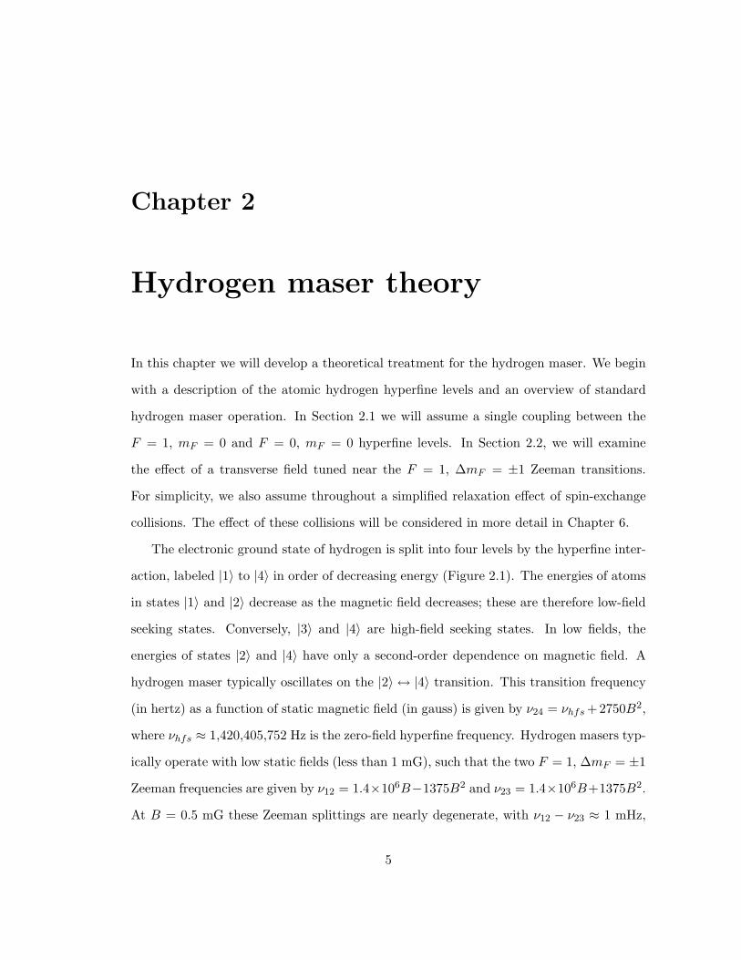
The electronic ground state of hydrogen is split into four levels by the hyperfine inter-

action, labeled |1〉 to |4〉 in order of decreasing energy (Figure 2.1). The energies of atoms

in states |1〉 and |2〉 decrease as the magnetic field decreases; these are therefore low-field

seeking states. Conversely, |3〉 and |4〉 are high-field seeking states. In low fields, the

energies of states |2〉 and |4〉 have only a second-order dependence on magnetic field. A

hydrogen maser typically oscillates on the |2〉 ↔ |4〉 transition. This transition frequency

(in hertz) as a function of static magnetic field (in gauss) is given by ν24 = νhfs +2750B2,

where νhfs ≈ 1,420,405,752 Hz is the zero-field hyperfine frequency. Hydrogen masers typ-

ically operate with low static fields (less than 1 mG), such that the two F = 1, ∆mF = ±1

Zeeman frequencies are given by ν12 = 1.4×106B−1375B2 and ν23 = 1.4×106B+1375B2.

At B = 0.5 mG these Zeeman splittings are nearly degenerate, with ν12 − ν23 ≈ 1 mHz,

5

ener

gy

10005000

magnetic field [Gauss]

hνHFS

F = 1

F = 0

mF = +1

mF = 0

mF = -1

mF = 0

1

2

3

4

Figure 2.1: Hydrogen hyperfine structure. A hydrogen maser oscillates on the first-ordermagnetic-field-independent |2〉 ↔ |4〉 hyperfine transition near 1420 MHz. The masertypically operates with a static field less than 1 mG. For these low field strengths, the twoF = 1, ∆mF = ±1 Zeeman frequencies are nearly degenerate, and ν12 ≈ ν23 ≈ 1 kHz.

much less than the typical Zeeman linewidth of approximately 1 Hz.

In a conventional hydrogen maser [1–4], which operates near room temperature, molec-

ular hydrogen is dissociated in an rf discharge and a beam of hydrogen atoms is formed,

as shown schematically in Figure 2.2. A hexapole state selecting magnet focuses the low-

field-seeking hyperfine states |1〉 and |2〉 into a quartz maser bulb at about 1012 atoms/sec.

Inside the bulb (volume ∼ 103 cm3), the atoms travel ballistically for about 1 second be-

fore escaping, making ∼ 104 collisions with the bulb wall. A Teflon coating reduces the

atom-wall interaction and thus inhibits decoherence of the masing atomic ensemble due

to wall collisions. The maser bulb is centered inside a cylindrical TE011 microwave cavity

6

resonant with the 1420 MHz hyperfine transition. The thermal microwave field stimu-

lates a coherent magnetization M on the |2〉 to |4〉 transition in the atomic ensemble, and

this magnetization acts as a source to stimulate the microwave cavity field HC . With

sufficiently high atomic flux and low cavity losses, this feedback induces active maser

oscillation.

The maser signal (typically about 10−13 W) is inductively coupled out of the microwave

cavity, amplified, and detected with a low noise heterodyne external receiver. Surround-

ing the cavity, a main solenoid and two end coils produce a weak static magnetic field

(B0 ≈ 1 mG) which establishes the quantization axis inside the maser bulb and sets the

Zeeman frequency (≈ 1 kHz). Another pair of coils can be used to produce the oscillating

transverse magnetic field HT that drives the F = 1, ∆mF = ±1 Zeeman transitions. The

cavity, solenoid and Zeeman coils are all enclosed within several layers of high permeability

magnetic shielding.

2.1 Standard hydrogen maser theory

In this section, we will derive analytic expressions for the hydrogen maser oscillation

frequency and power. These relations are found by first considering the effect of the

microwave cavity field on the atoms, which acts to establish a macroscopic magnetization

in the atomic ensemble. This magnetization is then coupled back to the cavity, by treating

it as a source term for the microwave cavity field, and the steady state maser frequency

and amplitude are found.

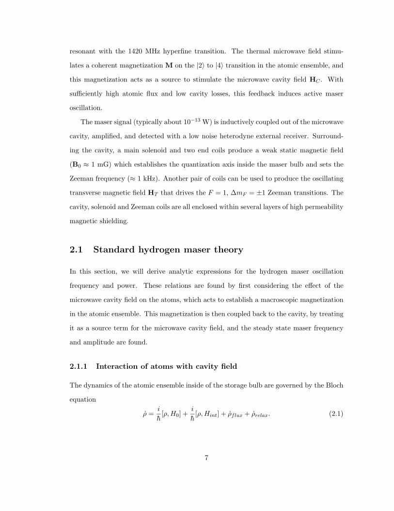
2.1.1 Interaction of atoms with cavity field

The dynamics of the atomic ensemble inside of the storage bulb are governed by the Bloch

equation

ρ =i

h[ρ, H0] +

i

h[ρ, Hint] + ρflux + ρrelax. (2.1)

7

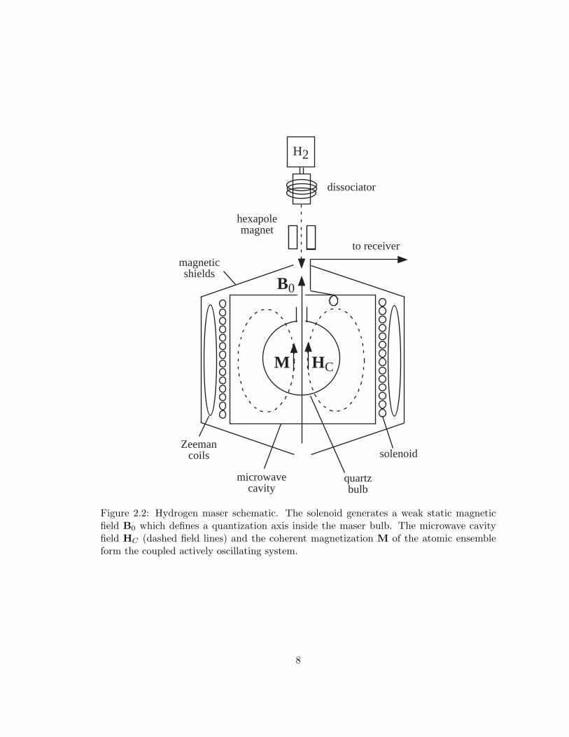
H2

dissociator

hexapolemagnet

solenoid

magneticshields

microwavecavity

quartzbulb

to receiver

B0

M HC

Zeemancoils

Figure 2.2: Hydrogen maser schematic. The solenoid generates a weak static magneticfield B0 which defines a quantization axis inside the maser bulb. The microwave cavityfield HC (dashed field lines) and the coherent magnetization M of the atomic ensembleform the coupled actively oscillating system.

8

The first term describes the interaction of the atoms with the static solenoid field. Tak-

ing the energy of state |4〉 as our energy zero, and assuming the hyperfine and Zeeman

splittings are fixed, then H0 is given by

H0 = hω14|1〉〈1| + hω24|2〉〈2| + hω34|3〉〈3| (2.2)

where the difference frequency between levels i and j is denoted by ωij = ωi − ωj .

The second term of the Bloch equation (Eqn. 2.1) describes the interaction of the atoms

with the microwave cavity field, with the interaction Hamiltonian given by Hint = −µ·HC ,

where µ is the net magnetic moment of the atomic ensemble. Since the cavity field HC

is parallel to the quantization axis (the static field B0) in the atomic storage region, it

therefore couples states |2〉 and |4〉:

Hint = H24|2〉〈4| + h.c. (2.3)

where h.c. denotes Hermitian conjugate. If we denote the cavity field by HC = HC z cos(ωt),

then

H24 = − h

2X24

(eiωt + e−iωt

)(2.4)

where X24 is the Rabi frequency, given by hX24 = µ24HC , with the dipole matrix element

µ24 = 〈2|µz|4〉 =12µB(gJ − gI) ≈ µB, (2.5)

where gJ and gI are the electron on proton g-factors and µB is the Bohr magneton.

The third term of the Bloch equation (Eqn. 2.1) describes the atomic flux into the

bulb. For perfect hexapole state selection, this term is written

ρflux =r

2(|1〉〈1| + |2〉〈2|) , (2.6)

accounting for the injection of atoms in states |1〉 and |2〉 at rate r.

9

The final term of the Bloch equation (Eqn. 2.1) is a relaxation term that describes

population decay and decoherence. Population decay is characterized by

ρrelax,ii = −γ1(ρii −14), (2.7)

where we assume relaxation to an equipopulation of the four states, and decoherence is

described by

ρrelax,ij = −γ2ρij . (2.8)

The relaxation rates, written as

γi =1Ti

= r +1

Ti,m+

1Ti,w

+1

Ti,se, (2.9)

account for relaxation due to bulb escape, magnetic field inhomogeneities, wall collisions,

and spin-exchange collisions. Here we assume a simplified spin-exchange model where the

relaxation rate is given by the collision rate, so that γ1,se = nvrσ, with n the atomic

density, vr the mean relative atomic velocity, and σ the hydrogen-hydrogen spin-exchange

cross section. Note that γ2,se = 12γ1,se in a hydrogen maser.

In the absence of any other couplings, we are solely interested in the population dif-

ference and coherence between states |2〉 and |4〉. Therefore, we are only concerned with

three terms of the full Bloch equations: ρ22, ρ24, and ρ44. These terms are most easily

handled by moving to the interaction picture, in which the rapid secular variation at fre-

quency ω24 drops out. This transformation is given by O = e−iH0t/h ˜O eiH0t/h, where

˜O is an interaction picture operator. After making the rotating wave approximation, the

Bloch equations in the interaction picture become

˙ρ22 = i

(X24

2ρ42e

−i∆t − X42

2ρ24e

i∆t)− γ1ρ22 +

r

2+

γ1

4

˙ρ24e−iω24t = −i

(X24

2(ρ22 − ρ44)e−i∆te−iω24t

)− γ2ρ24e

−iω24t (2.10)

˙ρ44 = i

(X42

2ρ24e

i∆t − X24

2ρ42e

−i∆t)− γ1ρ44 +

γ1

4

10

where ∆ = ω − ω24 is the difference frequency between the microwave field and the

hyperfine frequency.

In the steady state, the populations in the interaction picture are static, ˙ρ22 = ˙ρ44 = 0.

The coherence exhibits sinusoidal precession, ρ24 = R24e−i∆t, where R24 is constant.

Substituting these into Eqn. 2.10, we find the following set of algebraic, time-independent

equations:

0 = i(X24

2R42 −

X42

2R24) − γ1ρ22 +

r

2+

γ1

4

−i(ω − ω24)R24 = −iX24

2(ρ22 − ρ44) − γ2R24 (2.11)

0 = i(X42

2R24 −

X24

2R42) − γ1ρ44 +

γ1

4.

Rearranging these, and moving out of the interaction picture, we arrive at simple relations

for the steady state population inversion and the steady state atomic coherence. In terms

of T1 = 1/γ1 and T2 = 1/γ2, these can be written as

ρ22 − ρ44 =rT1

21 + T 2

2 (ω − ω24)2

1 + T 22 (ω − ω24)2 + T1T2|X24|2

(2.12)

and

ρ24(ω) =rX24T1T2

4

(i + T2(ω − ω24)

1 + T 22 (ω − ω24)2 + T1T2|X24|2

)eiωt. (2.13)

We note that the coherence can be decomposed into a component in phase and a com-

ponent in quadrature with the microwave field. As a function of oscillation frequency

ω, the in-phase component (real part of Eqn. 2.13) has a dispersive lineshape, and this

leads to phenomena such as frequency shifts. The quadrature component (the imaginary

part of Eqn. 2.13) has a Lorentzian lineshape, with a maximum for ω = ω24, and this

leads to absorption or amplification. This will be explored later in Section 2.1.4 where

we find an analytic expression for maser power. Equations 2.12 and 2.13 show that both

the population difference and the coherence are decreasing functions of the saturation

factor T1T2|X24|2. This quantity is proportional to the square of the amplitude of the

11

magnetic induction and therefore to the energy stored in the cavity. As the saturation

factor increases, the populations of states |2〉 and |4〉 tend to equalize and the coherence

is reduced.

Finally, the macroscopic magnetization produced by the oscillating atomic ensemble

is given by (neglecting the term oscillating at -ω)

M(ω) = n〈µ〉 = n Tr(ρµ) = nµ24ρ42(ω) ≈ nµBρ42(ω). (2.14)

Since the coherence is set by X24 and therefore the microwave cavity field, Eqn. 2.14

shows that the macroscopic magnetization is driven by the microwave cavity field. We

will discuss the effect of this at the end of Sec 2.1.2.

2.1.2 Interaction of cavity and magnetization

We will now calculate the effect of the ensemble’s magnetization on the microwave cavity

field. In a charge-free, external-current-free, polarization-free, lossless medium, Maxwell’s

equations take the form

∇ · B = 0 (2.15)

∇× H =1c

∂D∂t

(2.16)

∇ · D = 0 (2.17)

∇× E = −1c

∂B∂t

, (2.18)

with D = E+ 4πP = E and H = B− 4πM. If we take the curl of Eqn. 2.16 and combine

it with the time derivative of Eqn. 2.18, we see

∇×∇× H = − 1c2

∂2

∂t2(H + 4πM) . (2.19)

12

Within the cavity, we can expand the magnetic field into orthonormal cavity modes [32]

H(r, t) =√

4π∑λ

pλ(t)Hλ(r) (2.20)

where pλ(t) is the time varying amplitude and Hλ(r) is the time-independent spatial

variation of the mode λ. For a particular mode, Eλ and Hλ obey

∇× Eλ =(

ωλ

c

)Hλ (2.21)

∇× Hλ =(

ωλ

c

)Eλ.

The orthonormality condition implies

∫

cav|Hλ|2dV = 1 (2.22)

and thus the average magnitude of Hλ in the cavity is

〈H2λ〉cav =

1VC

∫

cav|Hλ|2dV =

1VC

(2.23)

where VC is the cavity volume.

If we combine Eqns. 2.19 and 2.20, and apply Eqn. 2.21, we see

∇×∇× H =√

4π

c2

∑λ

pλ(t)Hλ(r)ω2λ. (2.24)

Next, if we apply Eqn. 2.19 to Eqn. 2.20, we have

∇×∇× H = −√

4π

c2

∑λ

pλ(t)Hλ(r) − 4π

c2M. (2.25)

Combining Eqns. 2.24 and 2.25, we see

∑λ

pλ(t)Hλ(r) +∑λ

pλ(t)Hλ(r)ω2λ = −

√4πM. (2.26)

13

If we multiply both sides by Hλ(r) and integrate over the cavity volume, we obtain (using

the orthonormality condition)

pλ(t) +ωC

QCpλ(t) + ω2

Cpλ(t) = −√

4π

∫

cavM(r, t) · Hλ(r)dV. (2.27)

The second term on the left side has been added phenomenologically to account for the

effect of losses in the cavity walls [33]. Here QC is the cavity quality factor (cavity-Q) and

ωC = ωλ is the cavity’s resonant frequency for mode λ. The cavity-Q is defined as the

ratio of energy stored in the cavity to energy dissipated (per radian) and it essentially is

a measure of inverse cavity linewidth. For our room temperature and cryogenic hydrogen

masers, the cavity quality factors are typically about 104.

Within the maser storage bulb, the atoms’ fast thermal motion averages the magneti-

zation over the bulb, making M(r, t) independent of position, so

∫

cavM(r, t) · Hλ(r)dV = Mz(t)〈Hλ〉bVb. (2.28)

where 〈Hλ〉b is the average of the z-component of Hλ over the maser bulb (volume = Vb), a

restriction made since the |2〉 - |4〉 maser transition is a ∆mF = 0 transition which is only

driven by the component of the microwave field that is parallel to the the quantization axis.

We combine Eqns. 2.27 and 2.28, and then rewrite the result in the frequency domain.

We do so by replacing the time-dependent amplitudes pλ(t) and Mz(t) by their complex

representations pλ(ω) and M(ω), found by taking their Fourier transforms [34]. We obtain

(−ω2 + i

ωCω

QC+ ω2

C

)pλ(ω) =

√4πω2M(ω)〈Hλ〉bVb. (2.29)

This equation shows that the microwave cavity field is driven by the source magnetization,

which is generated by the coherent atomic ensemble. At the end of Section 2.1.1, however,

we saw that this magnetization is driven by the microwave cavity field. These two effects

then provide the positive feedback which allows for active maser oscillation. Together,

14

Eqns. 2.14 and 2.29 provide the self-consistent description of maser oscillation.

2.1.3 Maser oscillation frequency

To determine the maser oscillation frequency, we treat the magnetization due to the co-

herent atomic ensemble, Eqns. 2.13 and 2.14 as the source for the microwave cavity field

in Eqn. 2.29. From the real part of this equation,

ω2C − ω2 =

√4πω2〈Hλ〉bVbnµB

4pλ(ω)· rX24T1T

22 (ω − ω24)

1 + T 22 (ω − ω24)2 + T1T2|X24|2

(2.30)

and for the imaginary part,

ωCω

QC=

√4πω2〈Hλ〉bVbnµB

4pλ(ω)· rX24T1T2

1 + T 22 (ω − ω24)2 + T1T2|X24|2

. (2.31)

Combining these, we find

ω2C − ω2 =

T2ωCω

QC(ω − ω24) . (2.32)

If we assume that the maser frequency ω, cavity frequency ωC , and atomic hyperfine

frequency ω24 are all very close to one another, then (ω2C − ω2) = (ωC − ω)(ωC + ω) ≈

(ωC − ω24)(2ωC), and ωCω ≈ ωCω24. Therefore, Eqn. 2.32 takes the form of the familiar

cavity pulling equation

ω − ω24 =QC

Ql(ωC − ω24) (2.33)

where we have introduced the maser’s line-Q parameter, Ql = ω24T2/2. This relation

tells us that the maser oscillation frequency will be shifted from the atomic hyperfine

frequency by an amount proportional to the detuning of the cavity frequency from the

hyperfine frequency. However, the pulling is diminished by the ratio of cavity-Q to line-Q,

a factor of about 10−5 in most hydrogen masers for which Ql ≈ 109 (since T2 ≈ 1 s) and

QC ≈ 104.

15

2.1.4 Maser power

Since the maser Rabi frequency is given in terms of the magnitude of the cavity field,

X42 = µBHC/h, Eqns. 2.13 and 2.14 allow us to write the macroscopic magnetization in

terms of the cavity field. We may extract a magnetic susceptibility, defined as

χ =M(ω)HC(ω)

= χ′ + iχ′′. (2.34)

The component of the magnetic susceptibility in phase with the cavity field is therefore

χ′ =nrT1T2µ

2B

2h

T2(ω − ω24)1 + T 2

2 (ω − ω24)2 + T1T2|X24|2(2.35)

and the quadrature component is

χ′′ =nrT1T2µ

2B

2h

11 + T 2

2 (ω − ω24)2 + T1T2|X24|2. (2.36)

In terms of the quadrature susceptibility component, the average power radiated by

the atomic ensemble in the storage bulb is given by [35]

P =H2

CVb

2ωχ′′ =

h2|X24|2Vb

2µ2B

ωχ′′. (2.37)

Therefore, using Eqn. 2.36 we find that the average power radiated by the atoms is given

by

P =Ihω

2T1T2|X24|2

1 + T 22 (ω − ω24)2 + T1T2|X24|2

(2.38)

where I is the input flux of atoms in state |2〉, which for perfect state selection is 1/2 the

total atomic flux, I = 12Itot = 1

2nrVb.

16

2.2 Double resonance theory

Hydrogen masers can also be used as sensitive probes of the F = 1, ∆mF = ±1 Zeeman

transitions through a double resonance technique [24], in which an oscillating transverse

magnetic field tuned near the atomic Zeeman resonance shifts the ∆F = 1, ∆mF = 0

maser frequency. At low static magnetic fields, this maser frequency shift is an antisym-

metric function of the detuning of the applied transverse field from the Zeeman resonance.

Thus, by observing the antisymmetric pulling of the otherwise stable maser frequency, the

hydrogen Zeeman frequency can be determined with high precision.

2.2.1 Bare atom analysis

An early investigation of atomic double resonance was made by Ramsey [36], who cal-

culated the frequency shift between two levels coupled by radiation to other levels. This

calculation treated the problem perturbatively to first order in the coupling field strength,

and it neglected damping.

The first rigorous calculation of double resonance in the hydrogen maser was performed

by Andresen [24,37], who calculated the maser frequency shift to second order in the trans-

verse field strength. His calculation used the same approach as in Section 2.1: the maser

frequency and power were found by coupling the atomic magnetization to the microwave

cavity using Eqn. 2.29, and the magnetization was found using Eqns. 2.1 and 2.14. The

same flux and relaxation terms were used, including the same simplified spin-exchange

relaxation terms.

In Andresen’s bare atom calculation, the effect of the applied transverse field was in-

cluded in the interaction Hamiltonian. The transverse field, written as HT = HT x cos(ωT t),

acts to couple states |1〉 to |2〉 and |2〉 to |3〉. The interaction Hamiltonian therefore takes

the form

Hint = H24|2〉〈4| + H12|1〉〈2| + H23|2〉〈3| + h.c. (2.39)

17

where H24 is defined in Eqn. 2.4 and H12 is given similarly by

H12 = − h

2X12

(eiωT t + e−iωT t

). (2.40)

The transverse field Rabi frequency, X12, is defined as hX12 = µ12HT and the dipole

matrix element is given by

µ12 = 〈1|µx|2〉 =µB

2√

2(gJ − gI) ≈

1√2µB. (2.41)

The terms H23 and X23 are defined analogously, and X12 = X23.

To second order in the transverse field Rabi frequency, |X12|, and in terms of the

unperturbed maser Rabi frequency |X024|, atom flow rate r, population decay rate γ1,

hyperfine decoherence rate γ2, and Zeeman decoherence rate γZ , Andresen found that the

small static field limit of the maser shift is given by1

∆ω = −|X12|2γZ

r(γ1γ2 + |X0

24|2)δ (ρ0

11 − ρ033)

(γ2Z − δ2 + 1

4 |X024|2)2 + (2δγZ)2

(2.42)

where δ = ωT − ωZ is the detuning of the transverse field from the mean atomic Zeeman

frequency ωZ = 12(ω12 + ω23), and ρ0

11 − ρ033 = r/(2γ1) is the steady state population

difference between states |1〉 and |3〉 in the absence of the applied transverse field (following

Eqn. 8 of reference [24]). Physically, the population difference between states |1〉 and |3〉

represents the electronic spin polarization of the hydrogen ensemble [37]:

P =〈SZ〉

S= 2 Tr(ρSZ) = ρ11 − ρ33. (2.43)

Equation 2.42 implies that a steady state electronic polarization, and hence a population

difference between states |1〉 and |3〉 injected into the maser bulb, is a necessary condition

for the maser to exhibit a double resonance frequency shift. Walsworth et al. demon-1We have introduced a factor of 1

2to the values for the Rabi frequencies |X24|, |X12|, and |X23| to

account for the use of the rotating wave approximation.

18

strated this polarization dependence experimentally by operating a hydrogen maser in

three configurations: (i) with the usual input flux of atoms in states |1〉 and |2〉; (ii) with

a pure input flux of atoms in state |2〉, where the maser frequency shift vanishes; and (iii)

with an input beam of atoms in states |2〉 and |3〉, where the maser shift is inverted [19].

For typical applied transverse Zeeman field strengths (about 1 µG near the Zeeman

transitions at about 1 kHz), the 1420 MHz maser frequency is shifted tens of mHz by the

double resonance effect (see Figure 2.3), a fractional shift of ≈ 10−11. This shift is easily

resolved because of the excellent fractional maser frequency stability (parts in 1015 over

the tens of minutes typically required to carefully probe the antisymmetric lineshape).

In addition to the maser frequency shift due to the applied transverse field, there is a

reduction in the maser power as the transverse field is swept through the Zeeman reso-

nance. This amplitude reduction has also been calculated by Andresen [37] to second order

in the transverse field strength. Savard [38] revisited the double resonance problem with

a more realistic spin-exchange relaxation description [39], and found a small correction to

the earlier work.

2.2.2 Dressed atom analysis

Although the work of Andresen and Savard provides a thorough description for the double

resonance maser frequency shift, intuitive understanding is obscured by the length of the

calculations and their use of the bare atom basis. In particular, these works demonstrate

that the amplitude of the antisymmetric maser frequency shift is directly proportional

to the electronic polarization of the masing atomic ensemble. The maser frequency shift

vanishes as this polarization goes to zero. The previous bare atom analyses provide no

physical interpretation of this effect.

Since the dressed atom formalism [40] often adds physical insight to the understanding

of the interaction of matter and radiation, we apply it here to the double resonance

frequency shift in a hydrogen maser [25]. We retain the same approach as in Section 2.1,

however we determine the steady state coherence ρ42(ω) in a dressed atom basis. In a

19

10

0

-10

mas

er f

requ

ency

shi

ft [

mH

z]

-3 -2 -1 0 1 2 3Zeeman detuning [Hz]

10

5

0

-5

-10

1012 ∆

ω / ω

24

|X240| = 2.88 rad/s

|X12| = 0.88 rad/s γ1 = 1.95 rad/s γ2 = 2.77 rad/s γΖ = 2.40 rad/s r = 0.86 rad/s

Figure 2.3: Examples of double resonance maser frequency shifts. The large open circlesare data taken with an input beam of |1〉 and |2〉 hydrogen atoms. These are comparedwith Eqn. 2.42 (full curve) using the parameter values shown. The values of |X12| and γZ

were chosen to fit the data, while the remaining parameters were independently measured.The experimental error of each measurement is smaller than the circle marking it. Theelectronic polarization dependence of the double resonance effect is illustrated with thedotted data points: with an input beam of |2〉 and |3〉 atoms, the shift is inverted. Notethat the maser frequency shift amplitude for the dotted points was smaller since thesedata were acquired with a much weaker applied Zeeman field. The large variation ofthe maser frequency shift with Zeeman detuning near resonance, along with the excellentmaser frequency stability, allows the Zeeman frequency (≈ 800 Hz) to be determined toabout 3 mHz in a single scan of the double resonance such as the dotted data shown here(requiring ≈ 20 minutes of data acquisition).

20

two-step process, we will first use the dressed atom picture to determine the effect of

the applied transverse field on the atomic states. Then we will analyze the effect of the

microwave cavity field on the dressed states, and determine the maser frequency shift.

For simplicity, we assume the static magnetic field is sufficiently low that the two F =

1, ∆mF = ±1 Zeeman frequencies are nearly degenerate, ω12 − ω23 γZ , as is the case

for typical hydrogen maser operation. We use the simplified spin-exchange relaxation

model [24] and neglect Savard’s small spin-exchange correction to the double resonance

maser frequency shift [38].

Dressed atom basis

By incorporating the applied transverse field into the unperturbed Hamiltonian, it takes

the form H0 = Ha + Hf + Vaf . The atomic states (defining state |2〉 as energy zero) are

described by Ha = hω12|1〉〈1| − hω23|3〉〈3| − hω24|4〉〈4|; the applied transverse field (at

frequency ωT ) is described by Hf = hωT a†a; and the interaction between them is given

by

Vaf = hg(a + a†

)[|1〉〈2| + |2〉〈3| + h.c.] . (2.44)

Here, the transverse field creation and annihilation operators are a† and a, and g is the

single-photon Rabi frequency for the Zeeman transitions. We will use eigenkets with

two indices to account for the atomic state and the number of photons in the transverse

field, denoted by n. We select four of these as our bare atom/transverse field basis,

|1, n − 1〉, |2, n〉, |3, n + 1〉, |4, n〉, where the first entry indicates the atomic state and the

second entry indicates the transverse field photon number. We note that for a resonant

field, ωT = ω12 = ω23, the first three basis states are degenerate. Also, n 1 in practice

for there to be a measurable double resonance maser frequency shift: e.g., n ≈1012 for a

1 µG transverse field which for a typical SAO hydrogen maser creates a double resonance

frequency shift of about 10 mHz.

In this bare atom/transverse field basis, the unperturbed Hamiltonian operator takes

21

the following matrix form:

H0 = h

−δ 12X12 0 0

12X12 0 1

2X23 0

0 12X23 δ 0

0 0 0 −ω24

, (2.45)

where δ = ωT − ω12 is the detuning of the applied transverse field, and

X12

2= g

√n ≈ g

√n + 1 =

X23

2(2.46)

define the transverse field Rabi frequency (the factor of two has been inserted to be

consistent with our rotating wave approximation convention).

By diagonalizing H0, we find new basis states which physically represent the atomic

states dressed by the applied transverse field. The dressed energy levels are the eigenvalues

of H0: Ea = hΩ, Eb = 0, Ec = −hΩ, and E4 = −hω24, where Ω =√

δ2 + 12X2

12 represents

the generalized Rabi frequency of the driven Zeeman transition. The dressed states are

the eigenvectors of H0:

|a〉 =12

(1 − δ

Ω

)|1, n − 1〉 +

X12

2Ω|2, n〉 +

12

(1 +

δ

Ω

)|3, n + 1〉

|b〉 =X12

2Ω|1, n − 1〉 +

δ

Ω|2, n〉 − X12

2Ω|3, n + 1〉 (2.47)

|c〉 =12

(1 +

δ

Ω

)|1, n − 1〉 − X12

2Ω|2, n〉 +

12

(1 − δ

Ω

)|3, n + 1〉

|4〉 = |4, n〉.

Note that in the limit of large negative δ, |a〉 → |1〉 and |c〉 → |3〉, while in the limit of

large positive δ, |a〉 → |3〉 and |c〉 → |1〉. This will become important in the physical

interpretation of the maser frequency shift (see Section 2.2.2).

An operator O transforms between bare and dressed atom bases as Od = T−1ObT ,

where T is the unitary matrix linking the dressed atom and bare atom basis states (com-

22

prised of the coefficients of Eqn. 2.47). The dressed and bare atom energies and eigenvec-

tors are equivalent for the F = 0 hyperfine state |4〉 because this state is unaffected by

the applied transverse field.

Dressed basis Bloch equations

We now couple the dressed states to the microwave cavity using the Bloch equation, which

remains of the form

ρd =i

h[ρd, Hd

0 ] +i

h[ρd, Hd

int] + ρdrelax + ρd

flux. (2.48)

The unperturbed Hamiltonian, H0, now accounts for the bare atom energies and the

applied transverse field, while the microwave cavity field alone is included in the interaction

Hamiltonian, Hint. Since the dressed states |a〉, |b〉, and |c〉 all have a component of the

atomic state |2〉 (see Eqn. 2.47), the microwave field couples state |4〉 to each:

Hdint =

X12

2ΩH24|a〉〈4| +

δ

ΩH24|b〉〈4| −

X12

2ΩH24|c〉〈4| + h.c. (2.49)

Recall that H24 = −〈2|µ · HC|4〉 is the only nonzero coupling between state |4〉 and the

other bare atom states that is supported by the TE011 mode microwave cavity. To simplify

the relaxation terms in the dressed basis, we make the approximation that all relaxation

rates (population decay γ1, hyperfine decoherence γ2, and Zeeman decoherence γZ) have

the same value, γ + r (γ includes all relaxation exclusive of bulb loss). Typically, these

rates are within a factor of two (see the values listed in Figure 2.3). Then,

ρdrelax = −γρd +

γ

41. (2.50)

In the bare atom basis, the flux term has a very simple form (Eqn. 2.6) with no off-diagonal

input entries since the injected beam has no coherence between the bare atomic states. In

the dressed basis, however, there is an injected Zeeman coherence, so the flux term takes

23

a considerably more complicated form

ρdflux =

r

2F d − rρd (2.51)

where F d = T−1 (|1〉〈1| + |2〉〈2|) T is given by

F d =

(X122Ω

)2+ 1

4(1 − δΩ)2 X12

4Ω (1 + δΩ) 1

4(1 − δ2

Ω2 ) −(

X122Ω

)20

X124Ω (1 + δ

Ω) δ2+(X12/2)2

Ω2X124Ω (1 − δ

Ω) 0

14(1 − δ2

Ω2 ) −(

X122Ω

)2X124Ω (1 − δ

Ω)(

X122Ω

)2+ 1

4(1 + δΩ)2 0

0 0 0 0

. (2.52)

Steady state solution

The Bloch equations are most easily handled by moving to the interaction picture, given

by O = e−iH0t/h ˜O eiH0t/h, where ˜

O is an interaction picture operator.

The 4×4 matrix equation (Eqn. 2.48) yields sixteen independent equations that we

give in Appendix A. We solve these in the steady state, where the populations in the

interaction picture are static, ˙ρνν = 0, and the coherences exhibit sinusoidal precession.

In particular, ρ4a = R4ae−i(Ω−∆)t, ρ4b = R4be

i∆t, and ρ4c = R4cei(Ω+∆)t, where the

Rµν are time independent, and ∆ = ω − ω24. The other coherences precess at frequencies

ωµν = (Eµ−Eν)/h. Making these steady state substitutions, the sixteen Bloch differential

equations transform to a set of time-independent algebraic equations, also presented in

Appendix A. We assume that ωC = ω24, so that the small cavity pulling shift vanishes.

The total maser frequency shift due to the applied transverse field is then given by ∆.

In terms of dressed basis density matrix elements (rotated out of the interaction pic-

ture), the atomic coherence ρ42(ω) is given by

ρ42(ω) =(

X12

2Ωρ4a +

δ

Ωρ4b −

X12

2Ωρ4c

)=

(X12

2ΩR4a +

δ

ΩR4b −

X12

2ΩR4c

)eiωt (2.53)

and the magnetization is found from Eqn. 2.14. Inserting this into Eqn. 2.29 we find the

24

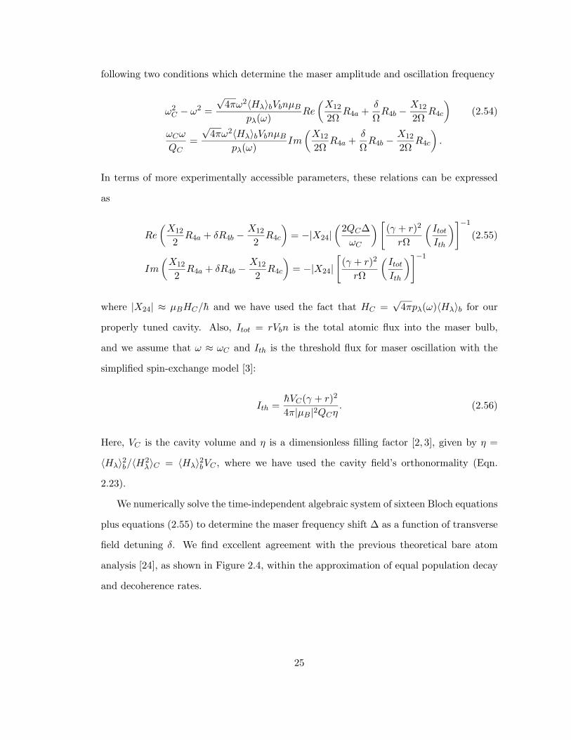
following two conditions which determine the maser amplitude and oscillation frequency

ω2C − ω2 =

√4πω2〈Hλ〉bVbnµB

pλ(ω)Re

(X12

2ΩR4a +

δ

ΩR4b −

X12

2ΩR4c

)(2.54)

ωCω

QC=

√4πω2〈Hλ〉bVbnµB

pλ(ω)Im

(X12

2ΩR4a +

δ

ΩR4b −

X12

2ΩR4c

).

In terms of more experimentally accessible parameters, these relations can be expressed

as

Re

(X12

2R4a + δR4b −

X12

2R4c

)= −|X24|

(2QC∆

ωC

) [(γ + r)2

rΩ

(Itot

Ith

)]−1

(2.55)

Im

(X12

2R4a + δR4b −

X12

2R4c

)= −|X24|

[(γ + r)2

rΩ

(Itot

Ith

)]−1

where |X24| ≈ µBHC/h and we have used the fact that HC =√

4πpλ(ω)〈Hλ〉b for our

properly tuned cavity. Also, Itot = rVbn is the total atomic flux into the maser bulb,

and we assume that ω ≈ ωC and Ith is the threshold flux for maser oscillation with the

simplified spin-exchange model [3]:

Ith =hVC(γ + r)2

4π|µB|2QCη. (2.56)

Here, VC is the cavity volume and η is a dimensionless filling factor [2, 3], given by η =

〈Hλ〉2b/〈H2λ〉C = 〈Hλ〉2bVC , where we have used the cavity field’s orthonormality (Eqn.

2.23).

We numerically solve the time-independent algebraic system of sixteen Bloch equations

plus equations (2.55) to determine the maser frequency shift ∆ as a function of transverse

field detuning δ. We find excellent agreement with the previous theoretical bare atom

analysis [24], as shown in Figure 2.4, within the approximation of equal population decay

and decoherence rates.

25

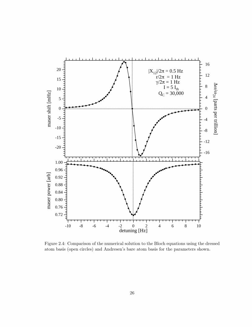
-20

-15

-10

-5

0

5

10

15

20

mas

er s

hift

[m

Hz]

-10 -8 -6 -4 -2 0 2 4 6 8 10detuning [Hz]

-16

-12

-8

-4

0

4

8

12

16

∆ω

/ω24 [parts per trillion]

|X12|/2π = 0.5 Hz r/2π = 1 Hz γ/2π = 1 Hz I = 5 Ith QC = 30,000

1.00

0.96

0.92

0.88

0.84

0.80

0.76

0.72

mas

er p

ower

[ar

b]

-10 -8 -6 -4 -2 0 2 4 6 8 10detuning [Hz]

Figure 2.4: Comparison of the numerical solution to the Bloch equations using the dressedatom basis (open circles) and Andresen’s bare atom basis for the parameters shown.

26

Physical interpretation

The dressed state analysis provides a straightforward physical interpretation of the double

resonance maser frequency shift. In the absence of the applied Zeeman field, atoms injected

in bare state |2〉 are the sole source of the magnetization that provides the positive feedback

needed for active oscillation. However, when the near-resonant transverse field is applied,

it also allows atoms injected in the mF = ± 1 states (bare states |1〉 and |3〉) to contribute

via a two-photon process.

A dressed atom interpretation shows how these mF = ± 1 state atoms can become

the dominant source of maser magnetization as the applied Zeeman field nears resonance.

Viewed from this basis, three factors contribute to this interpretation. First, as shown

in Figure 2.5(a), the applied Zeeman field shifts the energies of the two dressed levels |a〉

and |c〉 symmetrically relative to level |b〉, which remains unperturbed. Second, near the

Zeeman resonance, the ∆F = 1 dipole coupling H24b = 〈4|µ · HC|b〉2 vanishes while H2

4a

and H24c become equally dominant, as shown in Figure 2.5(b). Third, below resonance

(δ < 0) the steady state population of state |a〉 is greater than that of state |c〉 (ρaa > ρcc),

while above resonance (δ > 0) the opposite is true (ρcc > ρaa), as shown in Figure 2.5(c).

These dressed state population differences arise from the fact that atoms in bare state |1〉

are injected into the maser while those in bare state |3〉 are not, under normal operation,

so in the steady state ρ11 > ρ33. For large negative Zeeman detunings, |a〉 → |1〉 and

|c〉 → |3〉 (see discussion following Eqn. 2.47). The opposite holds for positive detuning,

where |a〉 → |3〉 and |c〉 → |1〉.

These three ingredients combine to create the double resonance shift of the maser

frequency, shown in Figure 2.5(d). For small negative Zeeman detunings (|δ| < 2γZ), the

excess of ρaa over ρcc and the relatively small size of H24b leads to maser oscillation primarily

on the |a〉 ↔ |4〉 transition. That is, atoms injected into the maser cavity in the bare state

|1〉 contribute significantly to the maser oscillation via a two-photon process: one Zeeman

transition photon and one microwave photon within the resonant cavity linewidth. This

|a〉 ↔ |4〉 transition is at a slightly higher frequency than in the unperturbed (no applied

27

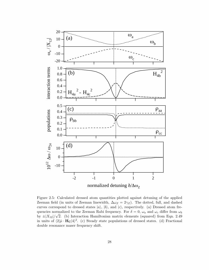
-20

-10

0

10

20

ων

/ |X

12|

-2 -1 0 1 2

ωa ωb

ωc

(a)

1.0

0.8

0.6

0.4

0.2

0.0inte

ract

ion

term

s

-2 -1 0 1 2

H4a 2

= H4c2

H4b2

(b)

0.5

0.4

0.3

0.2

0.1

0.0

popu

latio

ns

-2 -1 0 1 2

ρaa

ρcc

ρbb

(c)

-10

0

10

1012

∆ω

/ ω

24

-2 -1 0 1 2

normalized detuning δ/∆ωZ

(d)

Figure 2.5: Calculated dressed atom quantities plotted against detuning of the appliedZeeman field (in units of Zeeman linewidth, ∆ωZ = 2γZ). The dotted, full, and dashedcurves correspond to dressed states |a〉, |b〉, and |c〉, respectively. (a) Dressed atom fre-quencies normalized to the Zeeman Rabi frequency. For δ = 0, ωa and ωc differ from ωb

by ±|X12|/√

2. (b) Interaction Hamiltonian matrix elements (squared) from Eqn. 2.49in units of 〈2|µ · HC|4〉2. (c) Steady state populations of dressed states. (d) Fractionaldouble resonance maser frequency shift.

28

field) maser, so the maser frequency is increased. Conversely, for small positive Zeeman

detunings (δ < 2γZ), the maser oscillates preferentially on the |c〉 ↔ |4〉 transition, and

the maser frequency is decreased. For larger Zeeman detunings (positive or negative), the

coupling of state |4〉 to unshifted dressed state |b〉 becomes dominant, and the magnitude

of the frequency shift is reduced. For zero Zeeman detuning, dressed states |a〉 and |c〉 are

equally populated in the steady state and the maser frequency shift exactly vanishes.

We see now why the injection of an electronic polarization into the maser bulb is

needed for the applied Zeeman field to induce a maser frequency shift. Since ωa and ωc

are spaced equally about the unperturbed maser frequency ωb, and since H24a = H2

4c, a

necessary condition for a maser shift is a difference in the steady state values of ρaa and

ρcc, which is a direct consequence of a difference in the injected populations of bare states

|1〉 and |3〉, i.e., a net electronic polarization.

2.2.3 Application of double resonance

The double resonance hydrogen maser technique was originally studied for use in auto-

tuning the maser cavity [24]. In addition to the double resonance frequency shift, there

is a cavity pulling shift for a mistuned maser cavity, with magnitude dependent on the

linewidth of the hyperfine transitions, through the line-Q (see Eqn. 2.33). The applied Zee-

man radiation depletes the population of bare state |2〉, thereby increasing the linewidth

of the hyperfine transition. Andresen [24] showed that the cavity can be tuned to the

atomic frequency by modulating the hyperfine linewidth with applied Zeeman radiation

and adjusting the cavity frequency such that there is no modulation of the maser fre-

quency. However, this method requires accurate setting of the applied Zeeman field to the

Zeeman resonance (i.e., δ = 0).

The standard method in hydrogen masers for determining the average static magnetic

field strength, and thus the Zeeman frequency, is to scan the Zeeman resonance with a

large amplitude oscillating magnetic field and record the reduced maser power (such as

that shown in Figure 2.4). From the applied field frequency which yields minimum maser

29

power, typically at the center of a “power resonance” with a width of about 1 Hz, the

magnetic field can be found with a resolution of a fraction of 1 µG and the average Zeeman

frequency can be determined only to ≈ 0.1 Hz.

The double resonance maser frequency shift can be used for precision Zeeman spec-

troscopy in a hydrogen maser. By utilizing the sharp, antisymmetric profile of this double

resonance maser frequency shift, the hydrogen Zeeman frequency can be determined with

a resolution of about 1 mHz. In Chapter 4 we will discuss the use of this double resonance

technique in a search for Lorentz and CPT symmetry violation of the hydrogen atom’s

electron and proton spin [26], a search motivated by a general extension of the standard

model of elementary particle physics [41].

30

Chapter 3

Practical realization of the

hydrogen maser

The hydrogen maser was designed and first realized in the group of Norman Ramsey at

Harvard University in 1960 [1–3]. Soon after, the development of hydrogen masers as fre-

quency standards began at the Bomac laboratories of the Varian company in Beverly, MA.

A continuation of this production was eventually moved to the Smithsonian Astrophysical

Observatory (SAO) where all of the work described in this thesis was conducted. In Sec-

tion 3.1, we present the construction of an SAO VLG-12 series atomic hydrogen maser,

such as that used (maser P-28) for the experiment described in Chapter 4. In Section 3.2

we discuss a series of measurements used to characterized the operational parameters of

a hydrogen maser. These measurements were made with maser P-8, an SAO VLG-10

series maser. Finally, in Section 3.3 we discuss frequency stability in room temperature

hydrogen masers.

3.1 Hydrogen maser apparatus

In a hydrogen maser [1–4], molecular hydrogen is dissociated in an rf discharge and a

beam of hydrogen atoms is formed, as shown schematically in Figure 3.1. A hexapole

31

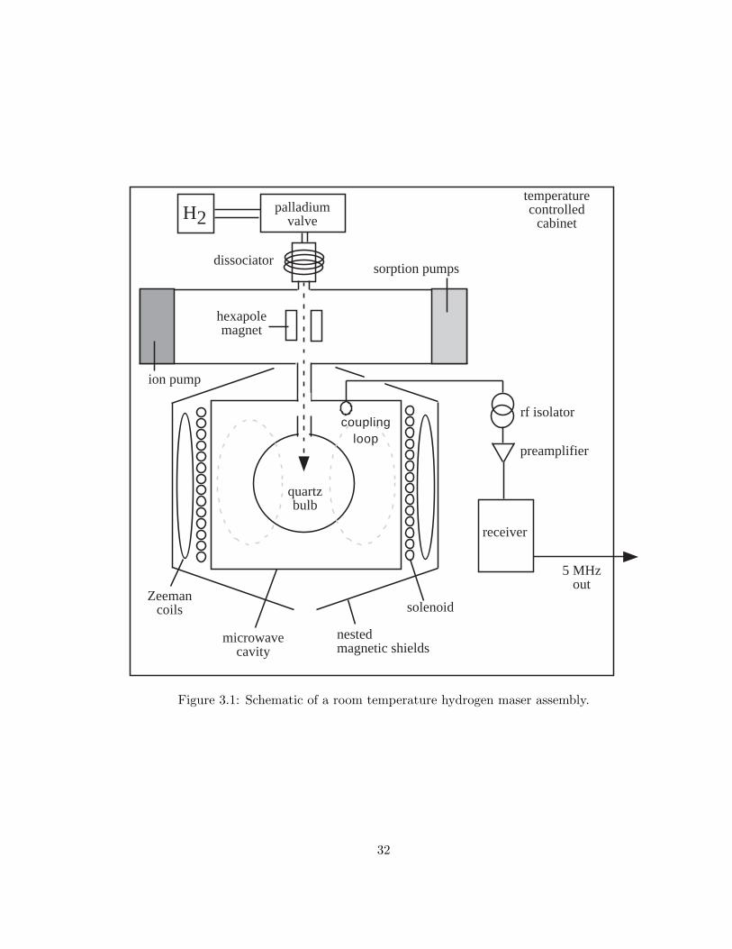
H2

dissociator

hexapolemagnet

solenoid

nestedmagnetic shields

microwavecavity

quartzbulb

Zeemancoils

palladiumvalve

sorption pumps

ion pump

receiver

rf isolator

preamplifier

temperaturecontrolled

cabinet

5 MHzout

couplingloop

Figure 3.1: Schematic of a room temperature hydrogen maser assembly.

32

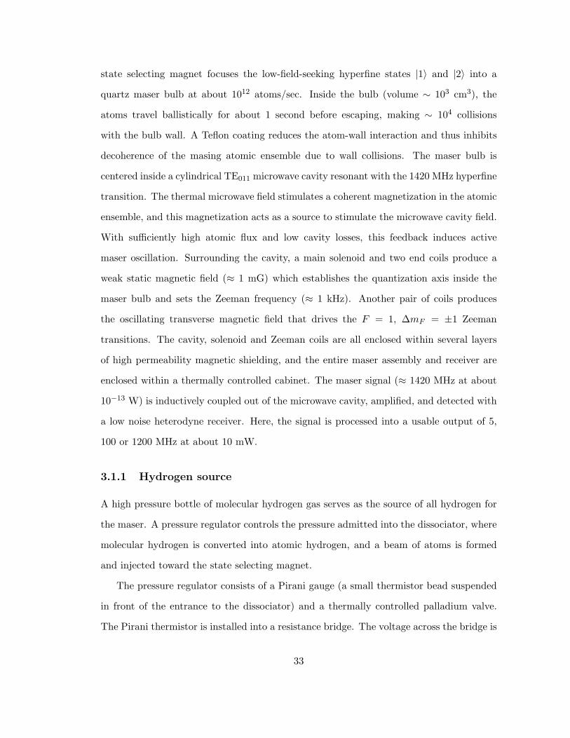
state selecting magnet focuses the low-field-seeking hyperfine states |1〉 and |2〉 into a

quartz maser bulb at about 1012 atoms/sec. Inside the bulb (volume ∼ 103 cm3), the

atoms travel ballistically for about 1 second before escaping, making ∼ 104 collisions

with the bulb wall. A Teflon coating reduces the atom-wall interaction and thus inhibits

decoherence of the masing atomic ensemble due to wall collisions. The maser bulb is

centered inside a cylindrical TE011 microwave cavity resonant with the 1420 MHz hyperfine

transition. The thermal microwave field stimulates a coherent magnetization in the atomic

ensemble, and this magnetization acts as a source to stimulate the microwave cavity field.

With sufficiently high atomic flux and low cavity losses, this feedback induces active

maser oscillation. Surrounding the cavity, a main solenoid and two end coils produce a

weak static magnetic field (≈ 1 mG) which establishes the quantization axis inside the

maser bulb and sets the Zeeman frequency (≈ 1 kHz). Another pair of coils produces

the oscillating transverse magnetic field that drives the F = 1, ∆mF = ±1 Zeeman

transitions. The cavity, solenoid and Zeeman coils are all enclosed within several layers

of high permeability magnetic shielding, and the entire maser assembly and receiver are

enclosed within a thermally controlled cabinet. The maser signal (≈ 1420 MHz at about

10−13 W) is inductively coupled out of the microwave cavity, amplified, and detected with

a low noise heterodyne receiver. Here, the signal is processed into a usable output of 5,

100 or 1200 MHz at about 10 mW.

3.1.1 Hydrogen source

A high pressure bottle of molecular hydrogen gas serves as the source of all hydrogen for

the maser. A pressure regulator controls the pressure admitted into the dissociator, where

molecular hydrogen is converted into atomic hydrogen, and a beam of atoms is formed

and injected toward the state selecting magnet.

The pressure regulator consists of a Pirani gauge (a small thermistor bead suspended

in front of the entrance to the dissociator) and a thermally controlled palladium valve.

The Pirani thermistor is installed into a resistance bridge. The voltage across the bridge is

33

fed back to power the bridge and also compared to the setpoint with a voltage comparator.

The output of the voltage comparator controls the thermal setting of the palladium valve.

At low pressures, the small current in the bridge will warm the thermistor to match the

set point. At higher pressure, the flux of the molecular hydrogen will act to cool the

thermistor, so a larger current is needed to heat the thermistor to the set point. If the

resistance bridge indicates that the pressure is higher than the setpoint, the output of

the voltage comparator will be zero. If the pressure is below the setpoint, however, the

(amplified) positive voltage comparator output will heat the palladium valve and increase

the flow of molecular hydrogen. Generally, the setpoint is such that about 1 to 2 mTorr

of molecular hydrogen will be input to the dissociator.

Since the pressure is sensed thermally, any variation in ambient temperature will be

transformed into variations in molecular hydrogen flux. Therefore, a second Pirani gauge,

well matched to the first, is installed at the high vacuum side (≈ 10−8 Torr) of the

dissociator. This reference Pirani is used to remove thermal fluctuations of the output

from the pressure-sensing Pirani.

The pressure regulated beam of molecular hydrogen enters into the glass cell (V ≈ 102

cm3) of the rf dissociator. A tuned rf circuit with a (≈ 3 cm radius) rf coil surrounding the

glass cell accelerates stray electrons and produces a hydrogen plasma discharge within the

cell. The electrons accelerated by the rf electric field drive the hydrogen molecules into

excited energy levels, causing the discharge to glow with a gray-pink color. Under proper

conditions, the electron-molecular hydrogen collisions act to dissociate the molecules into

hydrogen atoms. When the rate of dissociation exceeds the rate of recombination, the

discharge glows with a bright reddish-pink color (the light coming chiefly from spontaneous

emission from the atomic hydrogen Balmer series). At the exit end of the dissociator, a

multitube collimator maintains the pressure difference between the discharge and the high

vacuum region of the maser, and also directs the atomic hydrogen into a collimated beam.

34

3.1.2 State selection

The beam of atomic hydrogen atoms consists of nearly equal populations of all four hyper-

fine states. However, a hydrogen maser requires a population inversion in these hyperfine

states. A beam of state |2〉 atoms would be ideal, since these are the only atoms that

participate in the hyperfine transition. In practice, however, most hydrogen masers are

designed to have an input flux of |1〉 and |2〉 atoms into the storage bulb. A hexapole

state selecting magnet is used to focus these low-field-seeking states (|1〉 and |2〉) into the

atomic storage bulb, while defocusing the high-field-seeking states (|3〉 and |4〉) away from

the storage bulb. These unwanted hydrogen atoms, as well as hydrogen atoms which have

exited the storage bulb, are then pumped away with a set of sorption pumps.

The collimated atomic hydrogen beam is directed along the axis of the the hexapole

state selecting magnet. The magnet consists of six pole faces of alternating polarity

mounted azimuthally around the atomic hydrogen beam. This cylindrical construction is

about 10 cm in length with an outer radius of about 5 cm. The inner bore has a radius of

approximately 1 cm.

On the axis, the magnetic fields from the six poles cancel and the net field is zero. The

field grows quadratically in the radial direction, with a field amplitude approaching 1 Tesla

at the pole tips. In the presence of this large field gradient, the atoms feel a force that

depends on the hyperfine state i, given by Fi = µeffi ∇B, where µeff

i = −∂Ui/∂B is the

effective magnetic moment of the ith hyperfine state. For fields greater than about 2000

G, atoms in low-field-seeking states |1〉 and |2〉 have µeff = −µB, while atoms in high field

seeking states |3〉 and |4〉 have µeff = +µB (µB is the Bohr magneton). Therefore, the

low-field seeking atoms feel a force directed in the negative radial direction (i.e., are focused

on axis) while the high-field seeking atoms feel a force in the positive radial direction (i.e.,

are defocused out of the beam).

The atoms travel through the hexapole with a thermal distribution of velocities. The

atoms also have a distribution in the velocity component transverse to the beam, albeit

reduced by the dissociator’s collimator, therefore there will be a spread in the distance

35

required for the atoms to be properly focused. The geometry of the hexapole magnet and

the relative placement of the storage bulb entrance are chosen to optimize the population

inversion focused into the storage bulb. Typically, the total flux for a room temperature

hydrogen maser is about 1013 atoms/s, with a state selection of about 80% equally in

the |1〉 and |2〉 states (implying that about 40% of the total flux consists of atoms in the

radiating |2〉 state).

The hydrogen atoms which do not enter the storage bulb, as well as those that have

exited the storage bulb, are pumped out of the high vacuum space by one of four cylin-

drically mounted sorption pumps. In addition, other gases inside this space (including

nitrogen, argon, and carbon dioxide) are removed by a small ion pump. The pressure in

this high vacuum region is approximately 10−8 Torr.

3.1.3 Maser interaction region

The population inversion flux of atomic hydrogen is focused into a storage bulb centered

inside a microwave cavity. The microwave cavity is tuned near the atomic hyperfine

frequency, and this field drives stimulated emission transitions in the hydrogen atoms.

Through this stimulated emission process, the atoms give energy back to the microwave

cavity. If the atomic flux is high enough to counter the energy lost in the cavity, the

system will actively oscillate.

The storage bulb is constructed from thin-walled quartz to minimize electromagnetic

loss and loading of the resonant cavity. The spherical bulb has a diameter of approxi-

mately 21 cm (volume ≈ 3,000 cm3). A thin collimator at the entrance aperture acts to

lengthen the storage time inside the bulb to approximately 1 s. With an input flux of

1013 atoms/s, typical hydrogen densities in the storage bulb are about 109 atoms/cm3.

At room temperature, the atoms travel about 3×105 cm/s and therefore make about 104

collisions with the storage bulb wall.

In order to decrease the interaction of the atoms with the storage bulb wall, the inside

of the bulb is coated with Teflon FEP. This helps to reduce the hydrogen recombination

36

rate at the bulb, and to reduce the decoherence of the coherently radiating ensemble.

However, there is an appreciable hyperfine frequency shift due to wall collisions. When a

hydrogen atom collides with the bulb wall, its electron cloud deforms, varying the hyperfine

interaction between the electron cloud and the nucleus. A small phase shift is accumulated

with each collision. The net wall frequency shift is given by the average phase shift per

collision times the average collision rate. This shift is temperature dependent, is sensitive

to the nature of a particular Teflon coating, and tends to change slightly as the wall coating

ages. These factors limit the ability of a hydrogen maser to serve as an accurate frequency

standard.

The quartz storage bulb is mounted in the center of a TE011 mode microwave cavity.

The relative size and placement of the bulb are chosen so that the microwave cavity field is

uniform and has a constant phase over the atomic storage region (as shown by the dashed

field lines in Figure 3.1). The cylindrical cavity (volume ≈ 14,000 cm3) is constructed out

of Zerodur,1 a ceramic material with a low thermal expansion coefficient, high mechanical

stiffness and stability, and an absence of magnetism. The inner walls of the ceramic are

coated with a thin layer of silver to form the electromagnetic resonant cavity, which has a

resonant frequency of around 1,420,405,752 Hz and a resonant width of about 40 kHz for

a cavity-Q of around 40,000.

In room temperature masers, the microwave cavity frequency is set using two methods.

Course tuning is done with a mechanical tuning plunger. By inserting this plunger into the

cavity, the effective length of the cavity is reduced and the frequency is therefore increased.

Fine, resettable tuning of the cavity is made using a varactor diode which is inductively

coupled to the cavity (via a coupling loop very similar to that used to couple the maser

signal out, see below). The capacitance of this diode is changed when it is reverse biased,

changing the reactance coupled into the microwave cavity and thereby shifting the cavity

resonant frequency. With this system, the cavity frequency can be controllably varied over

a range of about 10 kHz in 0.1 Hz steps.1Zerodur is a trademark of Schott Optical Glass, Inc.

37

A solenoid coil assembly, consisting of one main solenoid and two trim coils wound

around the microwave cavity, sets the static magnetic field of the hydrogen maser. In

addition to establishing a quantization axis, this field sets the F = 1, ∆mF = ±1 Zeeman

frequency. The current in each solenoid is generated by a voltage regulated supply and set

with a adjustable voltage divider and a current-limiting precision 5 kΩ resistor. Typically,

the solenoid field is set at about 1 mG, which sets the ∆mF = ±1 Zeeman frequency at

about 1.4 kHz. In addition to this solenoid assembly, an orthogonal pair of coils mounted

on the microwave cavity can generate an oscillating field transverse to the quantization

axis to drive the ∆mF = ±1 Zeeman transitions. By doing so, the Zeeman frequency

(and therefore the amplitude of the solenoid field) can be determined using the double

resonance technique described in Chapter 2.

The entire maser assembly (bulb, cavity, and coils) is surrounded by four nested high-

permeability magnetic shields. These are used to prevent ambient field variations from

affecting the maser oscillation frequency. For the room temperature SAO masers, these

magnetic shields have an axial shielding factor of about ∆Hext/∆Hint = 30,000. These

act to attenuate the earth’s field (about 0.5 G) to an insignificant level (about 20 µG)

and to reduce the effect of ambient field fluctuations, about 3 mG in our laboratory, to

a level of about 0.1 µG. Reducing ambient field fluctuations is especially important when

using the hydrogen maser for precision Zeeman frequency spectroscopy, as discussed in

Chapter 4.

3.1.4 Thermal shielding

Thermal variations in numerous components of the hydrogen maser will lead to instabilities

in the maser oscillation frequency. For example, thermal variations in the cavity will alter

the cavity frequency and effect the maser frequency via cavity pulling, thermal fluctuations

in the solenoid setup will lead to a magnetic-field-dependent shift in the atomic hyperfine

frequency, and thermally induced flux variation can lead to maser frequency variation due

to spin-exchange effects. Therefore, steps have been taken to thermal control the various

38

components of room temperature hydrogen masers.

To isolate the hydrogen maser from ambient thermal variations, the maser and receiver

electronics are housed inside an insulated, temperature controlled cabinet (22” wide × 33”

deep × 60” high). This cabinet, whose temperature is controlled using blown air, provides

a factor of ten isolation from ambient thermal variations. Within the cabinet, the maser

assembly has several additional layers of thermal control, each with its own heater, thermal

sensor and control loop. An oven located within the two outermost magnetic shields is

controlled near 47 C, while the vacuum belljar that surrounds the resonant cavity is

maintained near 50 C. The net fractional thermal isolation of the maser cavity from

ambient fluctuations has been measured at about 10−5 [42].

Finally, the temperature of the coaxial cables leading to the microwave cavity is care-

fully controlled to reduce effects of changing coaxial line lengths, and the rf isolator and

preamplifier are housed in an insulated temperature controlled box to reduce the effect of

added white phase noise (discussed in more detail below in Section 3.3.2).

3.1.5 Microwave signal

The hydrogen maser’s microwave signal is coupled out of the microwave cavity inductively

using a small coupling loop. This signal, near 1,420,405,752 Hz has a typical magnitude

of 10−13 W. It is passed through an rf isolator and a preamplifier and then input into a

low noise heterodyne receiver.

The coupling loop, about 2 cm in diameter, is mounted to one end plate of the mi-

crowave cavity. It is oriented axially relative to the cavity such that the oscillating radial

magnetic cavity field lines pass through the loop. The alternating magnetic flux sampled

by the loop induces a voltage in the coil at a frequency near 1420 MHz. This microwave

signal is coupled out from the loop with semi-rigid microcoaxial cable into an rf isolator

which reduces the effects of external load changes on the microwave cavity frequency (the

net isolation from this stage is more than 90 dB). After the isolator, the signal is input to

a low noise preamplifier which provides 23 dB of gain.

39

3.1.6 Microwave receiver

In order to generate a useful reference signal, the low power maser signal is used to phase

lock a quartz crystal oscillator in the maser’s receiver system, as shown in the block

diagram in Figure 3.2. The receiver produces three buffered outputs of about 10 mW

at 5 MHz, 100 MHz and 1200 MHz. The hydrogen maser frequency at 1420. . . MHz is

significantly more stable than the quartz crystal oscillator, so in what follows we will treat

the maser frequency as constant.

The receiver consists of a voltage controlled crystal oscillator (VCXO), a frequency

synthesizer, a phase detector (integrator), and numerous frequency mixers, multipliers,

and dividers. The quartz crystal oscillator has a nominal frequency of about 100 MHz.

This frequency is multiplied up to 1200 MHz and 200 MHz, and divided down to 20 MHz.

Each of these frequencies is mixed in turn with the maser input signal, producing several

intermediate frequencies at 220. . . MHz, 20. . . MHz, and 405. . . kHz (see Figure 3.2).

This final intermediate frequency of 405. . . kHz is mixed with the output of a tunable

frequency synthesizer. The synthesizer is locked to a 5 MHz signal divided down from the

VCXO, and it is tunable from 405,750 Hz to 405,760 Hz in increments of 10−8 Hz. The

synthesizer is set so that the output, after mixing with the maser signal, is nearly a DC

voltage. The DC voltage from this final stage of frequency mixing is input into a phase

detector (integrator), and the output of the integrator then controls the VCXO.

As the output frequency of the VCXO drifts, the synthesizer, which is locked to the

VCXO, will drift correspondingly. Therefore the near-DC voltage at the final mixing stage

will vary, and these variations will be integrated by the phase detector. The integrated,

drift-induced signal is then fed back to the VCXO. As a result, the VCXO and all signals

derived from it are phase locked to the hydrogen maser. Finally, an rf buffer system

provides isolated outputs (at approximately 10 mW) derived from the VCXO at 5 MHz,

100 MHz, and 1200 MHz.

40

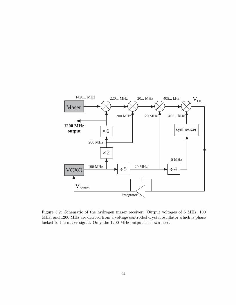
Maser

VCXO. 5.

2

synthesizer

100 MHz 20 MHz

5 MHz

200 MHz

200 MHz 20 MHz 405... kHz

1420... MHz 220... MHz 20... MHz 405... kHz VDC

Vcontrol

integrator

1200 MHzoutput

4..

6

Figure 3.2: Schematic of the hydrogen maser receiver. Output voltages of 5 MHz, 100MHz, and 1200 MHz are derived from a voltage controlled crystal oscillator which is phaselocked to the maser signal. Only the 1200 MHz output is shown here.

41

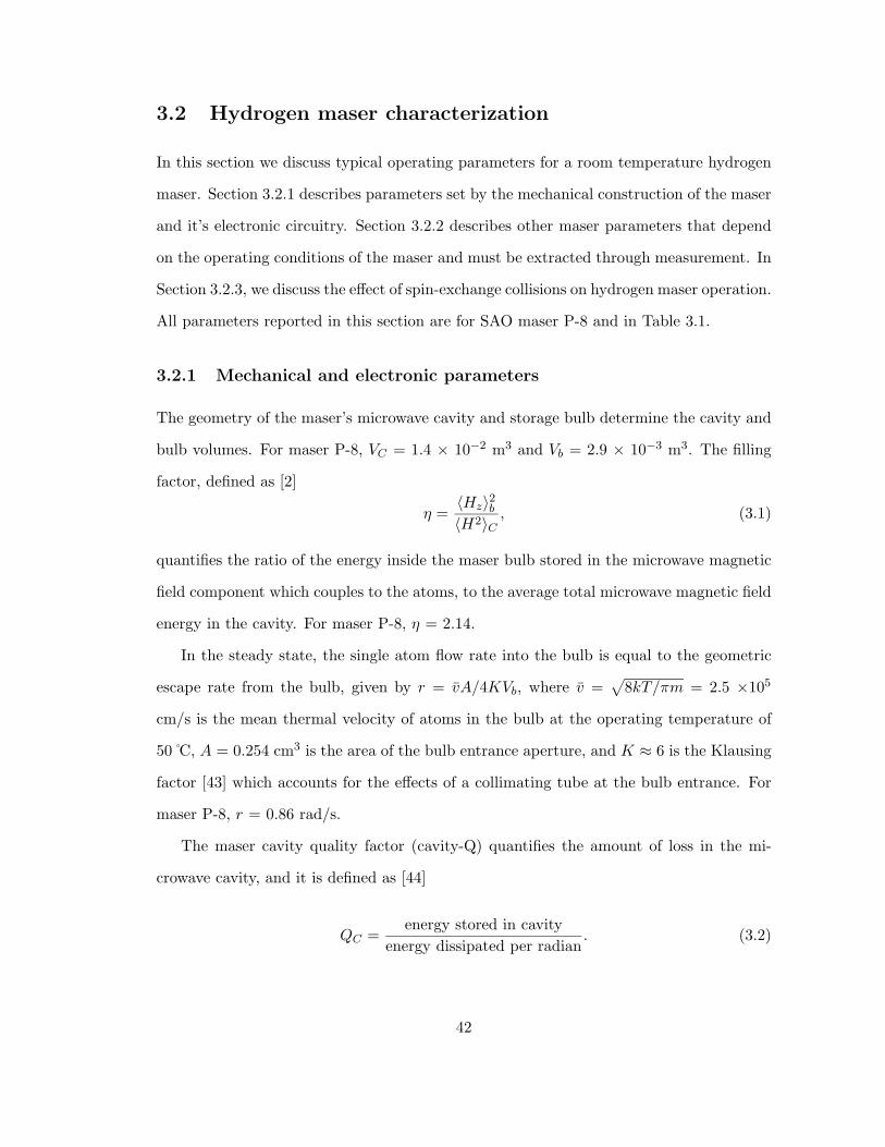
3.2 Hydrogen maser characterization

In this section we discuss typical operating parameters for a room temperature hydrogen

maser. Section 3.2.1 describes parameters set by the mechanical construction of the maser

and it’s electronic circuitry. Section 3.2.2 describes other maser parameters that depend

on the operating conditions of the maser and must be extracted through measurement. In

Section 3.2.3, we discuss the effect of spin-exchange collisions on hydrogen maser operation.

All parameters reported in this section are for SAO maser P-8 and in Table 3.1.

3.2.1 Mechanical and electronic parameters

The geometry of the maser’s microwave cavity and storage bulb determine the cavity and

bulb volumes. For maser P-8, VC = 1.4 × 10−2 m3 and Vb = 2.9 × 10−3 m3. The filling

factor, defined as [2]

η =〈Hz〉2b〈H2〉C

, (3.1)

quantifies the ratio of the energy inside the maser bulb stored in the microwave magnetic

field component which couples to the atoms, to the average total microwave magnetic field

energy in the cavity. For maser P-8, η = 2.14.

In the steady state, the single atom flow rate into the bulb is equal to the geometric

escape rate from the bulb, given by r = vA/4KVb, where v =√

8kT/πm = 2.5 ×105

cm/s is the mean thermal velocity of atoms in the bulb at the operating temperature of

50 C, A = 0.254 cm3 is the area of the bulb entrance aperture, and K ≈ 6 is the Klausing

factor [43] which accounts for the effects of a collimating tube at the bulb entrance. For

maser P-8, r = 0.86 rad/s.

The maser cavity quality factor (cavity-Q) quantifies the amount of loss in the mi-

crowave cavity, and it is defined as [44]

QC =energy stored in cavity

energy dissipated per radian. (3.2)

42

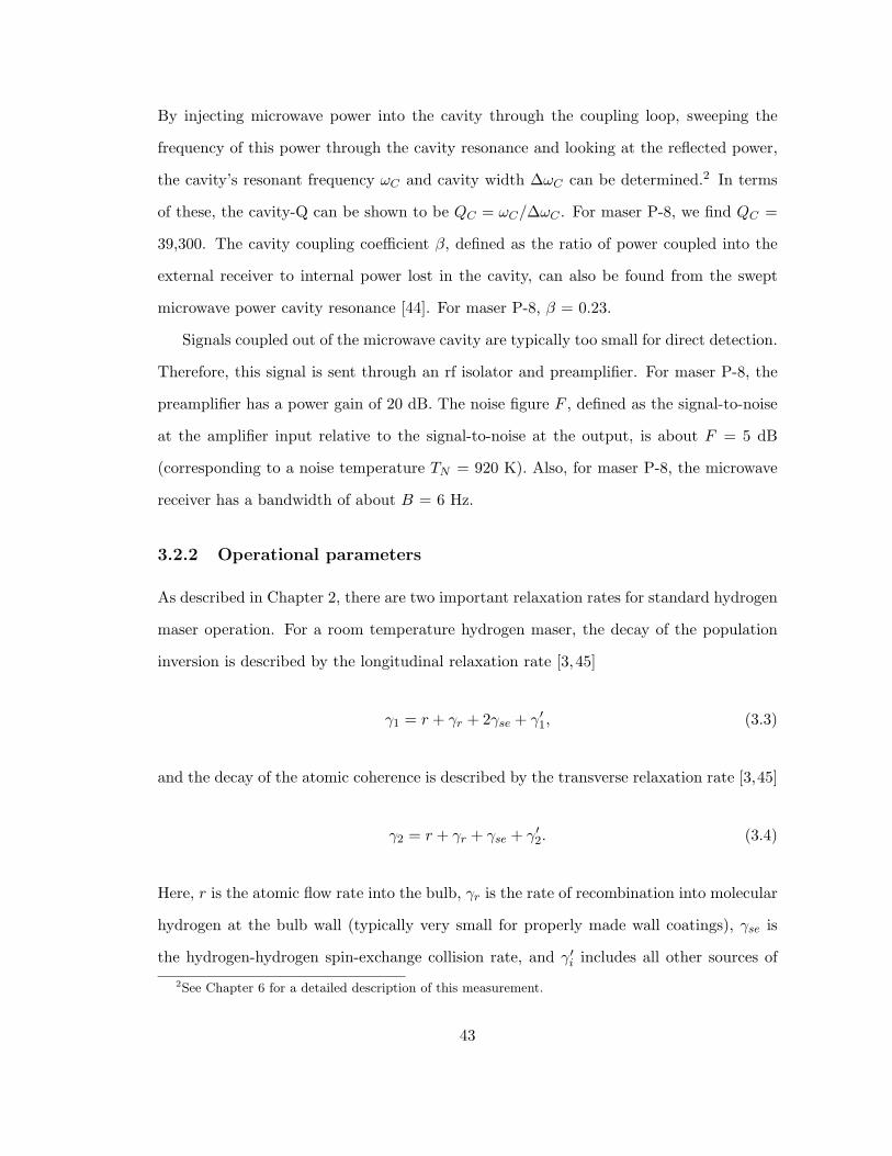
By injecting microwave power into the cavity through the coupling loop, sweeping the

frequency of this power through the cavity resonance and looking at the reflected power,

the cavity’s resonant frequency ωC and cavity width ∆ωC can be determined.2 In terms

of these, the cavity-Q can be shown to be QC = ωC/∆ωC . For maser P-8, we find QC =

39,300. The cavity coupling coefficient β, defined as the ratio of power coupled into the

external receiver to internal power lost in the cavity, can also be found from the swept

microwave power cavity resonance [44]. For maser P-8, β = 0.23.

Signals coupled out of the microwave cavity are typically too small for direct detection.

Therefore, this signal is sent through an rf isolator and preamplifier. For maser P-8, the

preamplifier has a power gain of 20 dB. The noise figure F , defined as the signal-to-noise

at the amplifier input relative to the signal-to-noise at the output, is about F = 5 dB

(corresponding to a noise temperature TN = 920 K). Also, for maser P-8, the microwave

receiver has a bandwidth of about B = 6 Hz.

3.2.2 Operational parameters

As described in Chapter 2, there are two important relaxation rates for standard hydrogen

maser operation. For a room temperature hydrogen maser, the decay of the population

inversion is described by the longitudinal relaxation rate [3, 45]

γ1 = r + γr + 2γse + γ′1, (3.3)

and the decay of the atomic coherence is described by the transverse relaxation rate [3,45]

γ2 = r + γr + γse + γ′2. (3.4)

Here, r is the atomic flow rate into the bulb, γr is the rate of recombination into molecular

hydrogen at the bulb wall (typically very small for properly made wall coatings), γse is

the hydrogen-hydrogen spin-exchange collision rate, and γ′i includes all other sources of

2See Chapter 6 for a detailed description of this measurement.

43

Parameter Symbol Room temperature value

cavity volume VC 1.4 × 10−2 m3

bulb volume Vb 2.9 × 10−3 m3

filling factor η 2.14bulb escape rate r 0.86 rad/scavity-Q (quality factor) QC 39,300cavity coupling coefficient β 0.23preamplifier gain 20 dBpreamplifier noise figure F 5 dBpreamplifier noise temperature TN 920 Kreceiver bandwidth B 6 Hz

line-Q (quality factor) Ql 1.6 × 109

output power Po 112 fWradiated power P 600 fWmaser quality parameter q 0.05spin-exchange-independent relaxation rate γt 1.71 rad/soscillation threshold power Pc 220 fWoscillation threshold flux Ith 0.47 × 1012 atoms/satomic population inversion flux I 2.11 × 1012 atoms/stotal atomic flux Itot 5.1 × 1012 atoms/satomic density n 1.0 × 1015 atoms/m3

spin-exchange rate γse 0.38 rad/smaser Rabi frequency |X24| 2.88 rad/spopulation decay rate γ1 1.95 rad/smaser decoherence rate γ2 2.77 rad/s

Table 3.1: Operational parameters for SAO room temperature hydrogen maser P-8. Allquantities have been converted into SI units.

decay, such as decoherence during wall collisions and effects of magnetic field gradients.

The spin-exchange rate is given approximately by [3, 45]

γse =12nvrσ (3.5)

where vr = 4√

kT/πm = 3.6 ×105 cm/s is the mean relative velocity of atoms in the bulb

and σ = 21 × 10−16 cm2 is the hydrogen-hydrogen spin-exchange cross section at room

44

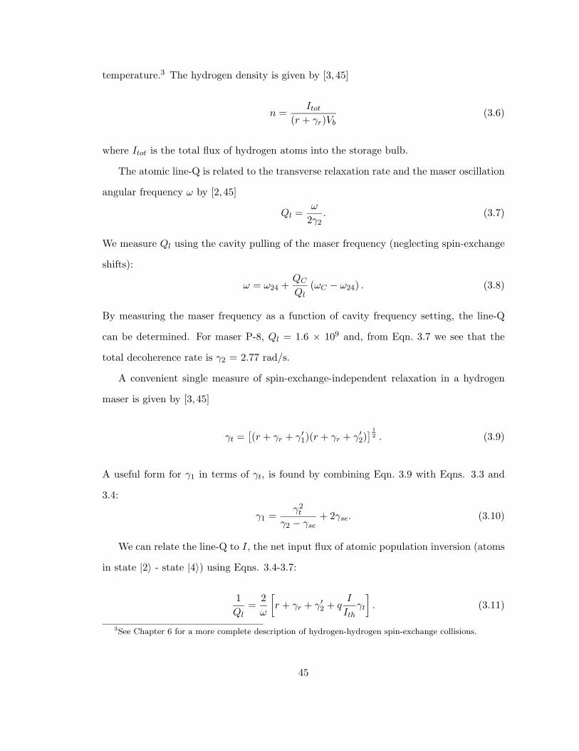
temperature.3 The hydrogen density is given by [3, 45]

n =Itot

(r + γr)Vb(3.6)

where Itot is the total flux of hydrogen atoms into the storage bulb.

The atomic line-Q is related to the transverse relaxation rate and the maser oscillation

angular frequency ω by [2, 45]

Ql =ω

2γ2. (3.7)

We measure Ql using the cavity pulling of the maser frequency (neglecting spin-exchange

shifts):

ω = ω24 +QC

Ql(ωC − ω24) . (3.8)

By measuring the maser frequency as a function of cavity frequency setting, the line-Q

can be determined. For maser P-8, Ql = 1.6 × 109 and, from Eqn. 3.7 we see that the

total decoherence rate is γ2 = 2.77 rad/s.

A convenient single measure of spin-exchange-independent relaxation in a hydrogen

maser is given by [3, 45]

γt =[(r + γr + γ′

1)(r + γr + γ′2)

] 12 . (3.9)

A useful form for γ1 in terms of γt, is found by combining Eqn. 3.9 with Eqns. 3.3 and

3.4:

γ1 =γ2

t

γ2 − γse+ 2γse. (3.10)

We can relate the line-Q to I, the net input flux of atomic population inversion (atoms

in state |2〉 - state |4〉) using Eqns. 3.4-3.7:

1Ql

=2ω

[r + γr + γ′

2 + qI

Ithγt

]. (3.11)

3See Chapter 6 for a more complete description of hydrogen-hydrogen spin-exchange collisions.

45

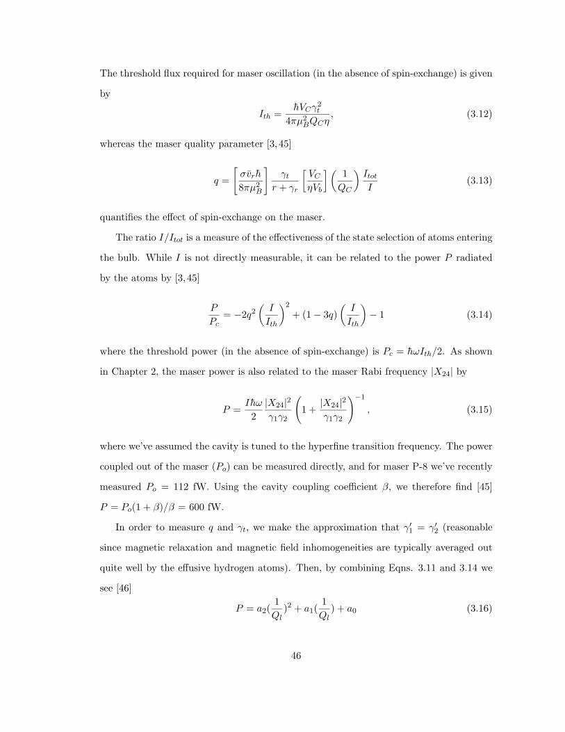
The threshold flux required for maser oscillation (in the absence of spin-exchange) is given

by

Ith =hVCγ2

t

4πµ2BQCη

, (3.12)

whereas the maser quality parameter [3, 45]

q =

[σvrh

8πµ2B

]γt

r + γr

[VC

ηVb

] (1

QC

)Itot

I(3.13)

quantifies the effect of spin-exchange on the maser.

The ratio I/Itot is a measure of the effectiveness of the state selection of atoms entering

the bulb. While I is not directly measurable, it can be related to the power P radiated

by the atoms by [3, 45]

P

Pc= −2q2

(I

Ith

)2

+ (1 − 3q)(

I

Ith

)− 1 (3.14)

where the threshold power (in the absence of spin-exchange) is Pc = hωIth/2. As shown

in Chapter 2, the maser power is also related to the maser Rabi frequency |X24| by

P =Ihω

2|X24|2γ1γ2

(1 +

|X24|2γ1γ2

)−1

, (3.15)

where we’ve assumed the cavity is tuned to the hyperfine transition frequency. The power

coupled out of the maser (Po) can be measured directly, and for maser P-8 we’ve recently

measured Po = 112 fW. Using the cavity coupling coefficient β, we therefore find [45]

P = Po(1 + β)/β = 600 fW.

In order to measure q and γt, we make the approximation that γ′1 = γ′

2 (reasonable

since magnetic relaxation and magnetic field inhomogeneities are typically averaged out

quite well by the effusive hydrogen atoms). Then, by combining Eqns. 3.11 and 3.14 we

see [46]

P = a2(1Ql

)2 + a1(1Ql

) + a0 (3.16)

46

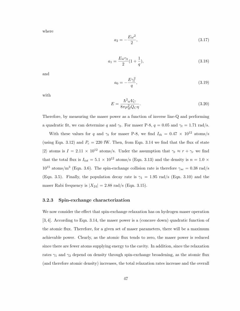
where

a2 = −Eω2

2, (3.17)

a1 =Eωγt

2(1 +

1q), (3.18)

and

a0 = −Eγ2t

q, (3.19)

with

E =h2ωVC

8πµ2BQCη

. (3.20)

Therefore, by measuring the maser power as a function of inverse line-Q and performing

a quadratic fit, we can determine q and γt. For maser P-8, q = 0.05 and γt = 1.71 rad/s.

With these values for q and γt for maser P-8, we find Ith = 0.47 × 1012 atoms/s

(using Eqn. 3.12) and Pc = 220 fW. Then, from Eqn. 3.14 we find that the flux of state

|2〉 atoms is I = 2.11 × 1012 atoms/s. Under the assumption that γt ≈ r + γr we find

that the total flux is Itot = 5.1 × 1012 atoms/s (Eqn. 3.13) and the density is n = 1.0 ×

1015 atoms/m3 (Eqn. 3.6). The spin-exchange collision rate is therefore γse = 0.38 rad/s

(Eqn. 3.5). Finally, the population decay rate is γ1 = 1.95 rad/s (Eqn. 3.10) and the

maser Rabi frequency is |X24| = 2.88 rad/s (Eqn. 3.15).

3.2.3 Spin-exchange characterization

We now consider the effect that spin-exchange relaxation has on hydrogen maser operation

[3,4]. According to Eqn. 3.14, the maser power is a (concave down) quadratic function of

the atomic flux. Therefore, for a given set of maser parameters, there will be a maximum

achievable power. Clearly, as the atomic flux tends to zero, the maser power is reduced

since there are fewer atoms supplying energy to the cavity. In addition, since the relaxation

rates γ1 and γ2 depend on density through spin-exchange broadening, as the atomic flux

(and therefore atomic density) increases, the total relaxation rates increase and the overall

47

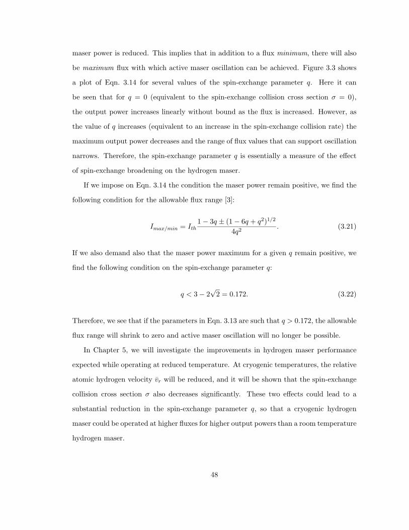
maser power is reduced. This implies that in addition to a flux minimum, there will also

be maximum flux with which active maser oscillation can be achieved. Figure 3.3 shows

a plot of Eqn. 3.14 for several values of the spin-exchange parameter q. Here it can

be seen that for q = 0 (equivalent to the spin-exchange collision cross section σ = 0),

the output power increases linearly without bound as the flux is increased. However, as

the value of q increases (equivalent to an increase in the spin-exchange collision rate) the

maximum output power decreases and the range of flux values that can support oscillation

narrows. Therefore, the spin-exchange parameter q is essentially a measure of the effect

of spin-exchange broadening on the hydrogen maser.

If we impose on Eqn. 3.14 the condition the maser power remain positive, we find the

following condition for the allowable flux range [3]:

Imax/min = Ith1 − 3q ± (1 − 6q + q2)1/2

4q2. (3.21)

If we also demand also that the maser power maximum for a given q remain positive, we

find the following condition on the spin-exchange parameter q:

q < 3 − 2√

2 = 0.172. (3.22)

Therefore, we see that if the parameters in Eqn. 3.13 are such that q > 0.172, the allowable

flux range will shrink to zero and active maser oscillation will no longer be possible.

In Chapter 5, we will investigate the improvements in hydrogen maser performance

expected while operating at reduced temperature. At cryogenic temperatures, the relative

atomic hydrogen velocity vr will be reduced, and it will be shown that the spin-exchange

collision cross section σ also decreases significantly. These two effects could lead to a

substantial reduction in the spin-exchange parameter q, so that a cryogenic hydrogen

maser could be operated at higher fluxes for higher output powers than a room temperature

hydrogen maser.

48

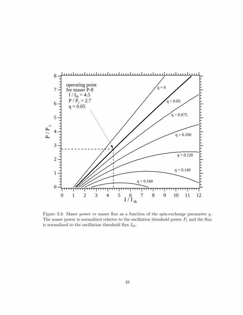
8

7

6

5

4

3

2

1

0

P / P

c

1211109876543210I / I th

q = 0

q = 0.05

q = 0.075

q = 0.100

q = 0.120

q = 0.140

q = 0.160

operating point for maser P-8 I / Ith = 4.5 P / Pc = 2.7 q = 0.05

Figure 3.3: Maser power vs maser flux as a function of the spin-exchange parameter q.The maser power is normalized relative to the oscillation threshold power Pc and the fluxis normalized to the oscillation threshold flux Ith.

49

3.3 Hydrogen maser frequency stability

Hydrogen masers are among the most stable oscillators available. Generally, the factors

which determine the limit to hydrogen maser stability can be divided into two classes.

Fundamental limits, which mostly stem from thermodynamic noise processes, determine

hydrogen maser stability at short- to medium-term averaging times up to about 10,000

s. For averaging times 10 < τ < 10,000 s, the fractional frequency stability is limited by

thermal noise, from sources inside the maser cavity as well as in the receiver electronics.

These effects are treated in Section 3.3.2. For averaging times longer than about 10,000 s,

the frequency stability is limited by various systematic effects, predominantly related to

slow changes in the frequency of the microwave resonant cavity. In Section 3.3.3 we treat

these and other systematic effects which limit hydrogen maser stability.4

3.3.1 General definition of clock stability

Typically, hydrogen maser frequency stability is characterized in the time domain using

a standard measure of stability, the two-sample Allan variance [47, 48]. This variance is

defined using the following model. We assume the oscillator signal voltage can be written

as

V (t) = [V0 + ε(t)] sin [2πν0t + φ(t)] (3.23)

where V0 and ν0 are the nominal amplitude and frequency, while ε(t) and φ(t) represent

time-varying amplitude and phase variations. We will assume that these variations are

small, such that |ε(t)/V0| 1 and |φ(t)/ν0| 1. The time varying phase of the signal is

then

Φ(t) = 2πν0t + φ(t) (3.24)4For averaging times τ < 1-10 s, (i.e., less than the interaction time of the hydrogen atoms with the

microwave cavity field) the fractional frequency stability of the hydrogen maser is set by the quartz crystaloscillator in the maser receiver.

50

and the time varying instantaneous frequency, defined by 2πν(t) = Φ(t), is therefore

ν(t) = ν0 +12π

φ(t). (3.25)

We now define the parameter

y(t) =φ(t)2πν0

(3.26)

as a measure of the instantaneous fractional frequency deviation on which the time-domain

frequency stability definition will be based.

If we measure the fractional frequency deviation for a time τ beginning at time tk, the

average over this time is given by

yk =1τ

∫ tk+τ

tk

y(t)dt =φ(tk + τ) − φ(tk)

2πν0τ. (3.27)

If we allow no dead time between measurements, then tk+1 = tk + τ . The two-sample

Allan variance is then defined as the variance of the differences between adjacent fractional

frequency deviations (yk+1 − yk) given by [48]

σ2Allan(τ) =

⟨(yk+1 − yk)2

2

⟩. (3.28)

In practice, one first measures the oscillator frequency for a time T , and the data

stream is broken up into m intervals of time τ = T/m. Then, the average fractional

frequency deviation yk is computed for each interval. The differences between the frac-

tional frequency deviations for adjacent intervals are then computed, forming a set of

(m − 1) differences (yk+1 − yk). Finally, the Allan variance is found as the variance of

these differences using

σ2Allan(τ) =

1m

m∑k=1

(yk+1 − yk)2

2. (3.29)

With this definition, an Allan variance for multiple averaging times (up to τ = T/2) can

be computed from a single data set of length T , and the stability of an oscillator as a

51

function of averaging times can be found.

3.3.2 Fundamental limits to frequency stability

In addition to the coherent microwave cavity field stimulated by the oscillating atomic

ensemble, there is also a thermal microwave field present in the maser cavity. The presence

of this thermal field is the chief limitation to hydrogen maser stability at short- to medium-

term averaging times up to about 10,000 s.

The thermal microwave field leads directly to white frequency noise in the coherent

maser output signal. Along with the hyperfine transitions stimulated by the coherent

microwave field, there are also hyperfine transitions stimulated by the incoherent thermal

microwave cavity field. The addition of this incoherent radiation leads to a random walk

through time in the phase of the microwave field and introduces a√

τ dependence in this

phase. Since the maser frequency over this interval is given by the net accumulated phase

divided by 2πτ , the thermal cavity noise leads to a frequency instability that varies as

1/√

τ . The magnitude of this instability will be determined by the ratio of noise power

of the thermal cavity field (given by kT times the maser linewidth, with T the cavity

temperature) to the power P delivered by the atoms to the cavity. The Allan deviation

for this process is found to be [2, 7, 42]

σc(τ) =1Ql

√kT

2Pτ(3.30)

where Ql is the maser’s line-Q.

To obtain an estimate of the thermal white frequency noise stability limit for one of

the SAO room temperature hydrogen masers, we will use the parameters from Section 3.2

for maser P-8. Operating at T = 290 K, this maser has Ql = 1.6 × 109 and P = 6 × 10−13

W. Therefore, the thermal stability limit due to white frequency noise is approximately

σc(τ) = 3.6×10−14/√

τ .

A fraction of the energy from the coherent microwave field is coupled out of the cavity

52

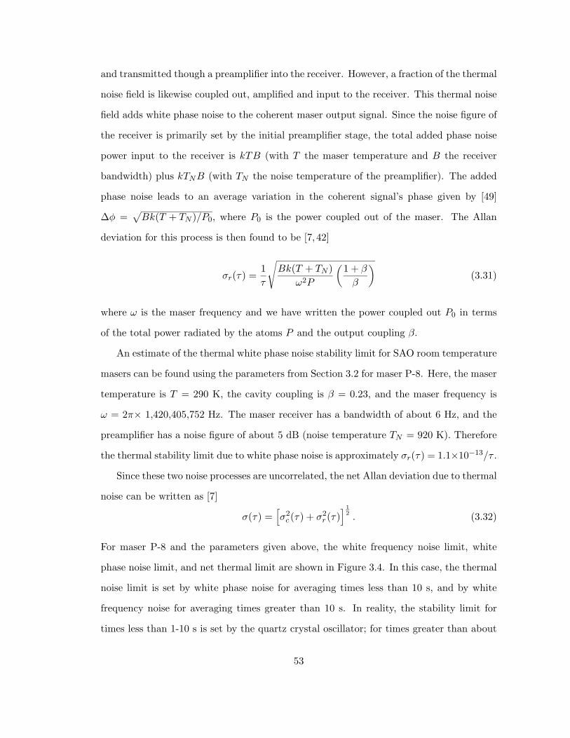
and transmitted though a preamplifier into the receiver. However, a fraction of the thermal

noise field is likewise coupled out, amplified and input to the receiver. This thermal noise

field adds white phase noise to the coherent maser output signal. Since the noise figure of

the receiver is primarily set by the initial preamplifier stage, the total added phase noise

power input to the receiver is kTB (with T the maser temperature and B the receiver

bandwidth) plus kTNB (with TN the noise temperature of the preamplifier). The added

phase noise leads to an average variation in the coherent signal’s phase given by [49]

∆φ =√

Bk(T + TN )/P0, where P0 is the power coupled out of the maser. The Allan

deviation for this process is then found to be [7, 42]

σr(τ) =1τ

√Bk(T + TN )

ω2P

(1 + β

β

)(3.31)

where ω is the maser frequency and we have written the power coupled out P0 in terms

of the total power radiated by the atoms P and the output coupling β.

An estimate of the thermal white phase noise stability limit for SAO room temperature

masers can be found using the parameters from Section 3.2 for maser P-8. Here, the maser

temperature is T = 290 K, the cavity coupling is β = 0.23, and the maser frequency is

ω = 2π× 1,420,405,752 Hz. The maser receiver has a bandwidth of about 6 Hz, and the

preamplifier has a noise figure of about 5 dB (noise temperature TN = 920 K). Therefore

the thermal stability limit due to white phase noise is approximately σr(τ) = 1.1×10−13/τ .

Since these two noise processes are uncorrelated, the net Allan deviation due to thermal

noise can be written as [7]

σ(τ) =[σ2

c (τ) + σ2r (τ)

] 12 . (3.32)

For maser P-8 and the parameters given above, the white frequency noise limit, white

phase noise limit, and net thermal limit are shown in Figure 3.4. In this case, the thermal

noise limit is set by white phase noise for averaging times less than 10 s, and by white

frequency noise for averaging times greater than 10 s. In reality, the stability limit for

times less than 1-10 s is set by the quartz crystal oscillator; for times greater than about

53

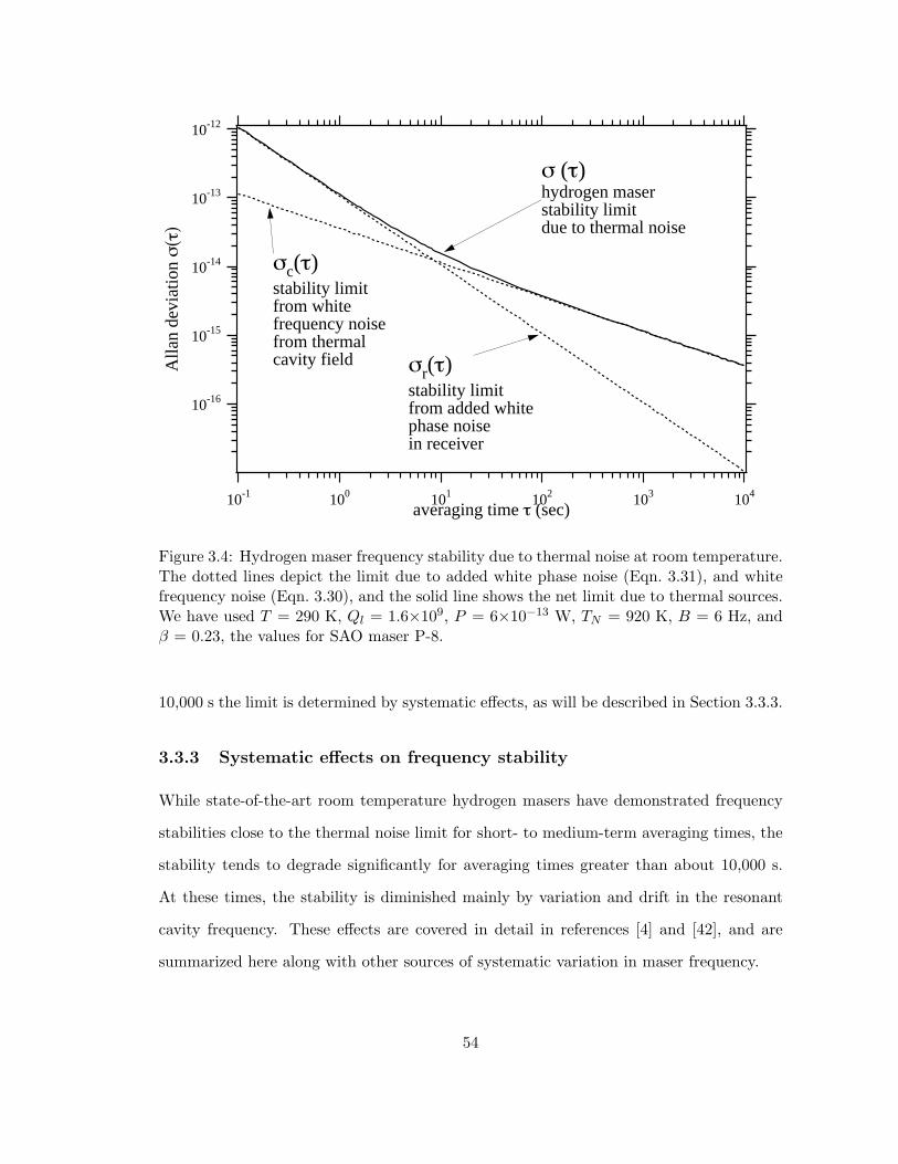
10-16

10-15

10-14

10-13

10-12

Alla

n de

viat

ion σ

(τ)

10-1 100 101 102 103 104

averaging time τ (sec)

σr(τ)stability limitfrom added white phase noisein receiver

σc(τ)stability limitfrom white frequency noisefrom thermalcavity field

σ (τ)hydrogen maserstability limitdue to thermal noise

Figure 3.4: Hydrogen maser frequency stability due to thermal noise at room temperature.The dotted lines depict the limit due to added white phase noise (Eqn. 3.31), and whitefrequency noise (Eqn. 3.30), and the solid line shows the net limit due to thermal sources.We have used T = 290 K, Ql = 1.6×109, P = 6×10−13 W, TN = 920 K, B = 6 Hz, andβ = 0.23, the values for SAO maser P-8.

10,000 s the limit is determined by systematic effects, as will be described in Section 3.3.3.

3.3.3 Systematic effects on frequency stability

While state-of-the-art room temperature hydrogen masers have demonstrated frequency

stabilities close to the thermal noise limit for short- to medium-term averaging times, the

stability tends to degrade significantly for averaging times greater than about 10,000 s.

At these times, the stability is diminished mainly by variation and drift in the resonant

cavity frequency. These effects are covered in detail in references [4] and [42], and are

summarized here along with other sources of systematic variation in maser frequency.

54

Effects on resonant cavity frequency

The maser oscillation frequency ω depends directly on the resonant cavity frequency ωC ,

as shown in Eqn. 3.8, although this dependence is diminished by the ratio of cavity-Q to

line-Q (typically a factor of 10−5). Since the cavity frequency will be set by its mechanical

dimensions, the maser frequency will be affected by thermal expansion and contraction of

the cavity. Therefore, the microwave cavities are constructed from ceramic material with

a low thermal expansion coefficient. For Zerodur, the ceramic from which SAO VLG-

12 maser cavities are constructed, the cavity frequency temperature coefficient is about

140 Hz/K [42]. Therefore, typical short-term (tens of minutes) ambient temperature

fluctuations of 1 C, which cause 10−5 C changes in the cavity temperature, would induce

a 1.4 mHz cavity frequency shift and a negligible 1×10−17 fractional maser frequency

shift. Furthermore, the relatively longer maser cavity time constant (approximately 10

hours [42]) further attenuates the effect of short-term room temperature variations.

Over longer timescales, the cavity frequency can be affected by slow drift of the tem-

perature control setpoint (due to imperfect tuning of the temperature control loop) or

drift in the temperature sensor itself. However, the dominant sources of long-term cavity

frequency shifts are mechanical relaxation and stress. For example, the joints between the

cavity cylinder and endcaps are known to shrink with time. Also, following the heating

process with which the cavity’s silver coating is applied, the endcaps are known to flatten

with time. Both of these effects act to raise the microwave’s cavity frequency, and the

estimated rate of fractional maser frequency shifts due to these effects is on the order of

7×10−16/day. [42]

Additional thermal effects

Along with thermally-induced microwave cavity shifts, other thermal effects can limit

maser frequency stability. These include changes in the storage bulb’s dielectric constant,

variation in the storage bulb’s Teflon coating, variation in the length of the transmission

line from the coupling loop to the receiver (both length and dielectric constant), and the

55

second-order Doppler effect. These are treated in detail in references [4] and [42].

Magnetic field effects

The maser oscillation frequency also depends directly on the atomic hyperfine frequency

ω24. The hyperfine frequency is a second-order function of the static solenoid magnetic

field, given by ω24 = 2πνhfs +17300B20 with ω24 in radians per second for B0 in gauss, and

νhfs ≈ 1,420,405,752 Hz is the zero-field hyperfine frequency. To decrease the sensitivity

to fractional variations in the static field, hydrogen masers are operated at very low fields

typically less than 1 mG. At this field, the fractional frequency dependence is given by

dω24/ω24 = (3.9 × 10−9/G)dB0. We have measured long-term (10,000 s) solenoid field

fluctuations on the order of 6 nG, which would lead to negligible fractional frequency

variations of 2×10−17 (see Chapter 4).

In addition to running at a low, carefully stabilized field, the maser is shielded from

ambient magnetic fields and field gradients with high permeability magnetic shielding. As

described in Section 3.1.3, an SAO VLG-12 maser has an axial shielding factor of about

∆Hext/∆Hint = 30,000. Typical short-term (10-100 s) ambient field fluctuations in our

laboratory at about 3 mG. These are then shielded to a level of about 0.1 µG which would

lead to a short-term fractional frequency stability limit of about 4×10−16.

Spin-exchange effects

Throughout our discussion of hydrogen maser theory (Chapter 2) and hydrogen maser

characterization (Section 3.2) we have used a simple treatment of spin-exchange relaxation,

where the population decay rate (γ1,se = nvrσ) and the decoherence rate (γ2,se = γ1,se/2)

can be combined additively to the other forms of decay. In Chapter 6 we will remove

this simplification, and it will be shown that a more complete treatment of spin-exchange

collisions predicts an additional, hydrogen-density-dependent maser frequency shift. For

56

a room temperature hydrogen maser,5 the frequency is found to be approximately

ω = ω24 +QC

Ql(ωC − ω24) + αλ0γ2 = ω24 +

(∆ + αλ0

)γ2 (3.33)

where γ2 is the total broadening (including spin-exchange and all other sources) and we

have introduced the cavity detuning parameter ∆ = 2QC(ωC−ω24)/ω24, the spin-exchange

shift cross-section λ0, and a system constant

α =hVC vr

µ0µ2BηQCVb

(3.34)

where VC and Vb are the cavity and bulb volumes, vr is the average relative atomic velocity,

and η is the filling factor.

If the maser cavity is tuned exactly to the hyperfine frequency (eliminating the fre-

quency pulling term), then the maser frequency will be shifted from the atomic frequency

by an amount proportional to the total broadening γ2. Since this broadening will depend

on the hydrogen density in the bulb, the overall maser stability will be degraded by den-

sity or flux variations, which are difficult to eliminate in practice. However, as pointed

out in 1967 by Crampton [17], if the maser is instead tuned so that ∆ = −αλ0, then

the maser frequency will become independent of γ2 and therefore insensitive to density

fluctuations. This procedure, known as “spin-exchange tuning” is typically employed in

room temperature hydrogen masers.

5We will discuss spin-exchange tuning for a cryogenic hydrogen maser in Chapter 6.

57

Chapter 4

Testing CPT and Lorentz

symmetry with hydrogen masers

A theoretical framework has recently been developed which incorporates possible spon-

taneous CPT and Lorentz symmetry violation into a realistic extension of the standard

model of elementary particle physics [27,28,50–60]. One branch of this framework empha-

sizes low energy, experimental searches for symmetry violating effects in atomic energy

levels [27,28]. In particular, it has been shown that Lorentz and CPT violation results in

variations in the atomic hydrogen F = 1, ∆mF = ±1 Zeeman frequency as a function of

the orientation of the quantization axis (set by the maser’s static magnetic field) relative

to a preferred frame (e.g., the cosmic microwave background) [41]. Motivated by this the-

oretical framework, we conducted a search for sidereal variations in the hydrogen Zeeman

frequency and placed a new, clean bound of approximately 10−27 GeV on Lorentz and

CPT violation of the proton [26].

In this chapter we will discuss the theoretical framework, experiment, and analysis

that underly our hydrogen maser test of CPT and Lorentz symmetry. In Section 4.1 we

discuss the standard model extension. In Section 4.2 we discuss the procedure used to

collect data and extract a sidereal bound on the Zeeman frequency. In Section 4.3 we

describe efforts to reduce and characterize systematic effects. Finally, in Section 4.4 we

58

compare our result to other clock-comparison tests of CPT and Lorentz symmetry, and

discuss potential means of improving our measurement.

4.1 Lorentz and CPT violation in the standard model

Experimental investigations of Lorentz symmetry provide important tests of the standard

model of particle physics as well as general relativity. While the standard model suc-

cessfully describes particle phenomenology, it is believed to be the low energy limit of a

fundamental theory that incorporates gravity. This underlying theory may be Lorentz in-

variant, yet contain spontaneous symmetry-breaking that could result in small violations

of Lorentz invariance and CPT at the level of the standard model [50–52].

A theoretical framework has been developed by Kostelecky and coworkers to describe

Lorentz and CPT violation at the level of the standard model [27,28,50–60]. This standard-

model extension is quite general: it emerges as the low-energy limit of any underlying

theory that generates the standard model and contains spontaneous Lorentz symmetry

violation, and hence can include CPT violation [50–52]. For example, such characteristics

might emerge from string theory [53–56]. A key feature of the standard model extension

is that it is formulated at the level of the known elementary particles, and thus enables

quantitative comparison of a wide array of searches for Lorentz and CPT violation [57–60].

“Clock comparison experiments” are high precision searches for temporal variations in

atomic energy levels. According to the standard model extension considered here, Lorentz

and CPT violation may produce shifts in certain atomic levels, with magnitudes of the

shifts that depend on the orientation of the atom’s spin quantization axis relative to some

unknown, fixed inertial frame [27,28]. (Boosts relative to the preferred inertial frame may

also cause atomic energy level shifts.) Certain atomic transition frequencies, therefore,

may exhibit sinusoidal variation as the earth rotates on its axis. New limits can be placed

on Lorentz and CPT violation by bounding sidereal variation of these atomic transition

frequencies.

59

Specifically, the description of Lorentz and CPT violation is included in the relativistic

Lagrange density of the constituent particles of the atom. For example, the modified

electron Lagrangian becomes [27]

L =12iψΓν∂

νψ − ψMψ + LQEDint (4.1)

where

Γν = γν +(

cµνγµ + dµνγ5γ

µ + eν + ifνγ5 +12gλµνσ

λµ)

(4.2)

and

M = m +(

aµγµ + bµγ5γµ +

12Hµνσ

µν)

. (4.3)

The parameters aµ, bµ, cµν , dµν , eν , fν , gλµν and Hµν represent possible vacuum expecta-

tion values of Lorentz tensors generated through spontaneous Lorentz symmetry breaking

in an underlying theory. These parameters and associated terms are absent in the stan-

dard model. The parameters aµ, bµ, eν , fν and gλµν represent coupling strengths for terms

that violate both CPT and Lorentz symmetry, while cµν , dµν , and Hµν violate Lorentz

symmetry only. An analogous expression exists for the modified proton and neutron La-

grangians (a superscript will be appended to differentiate between the sets of parameters

for different particle types). The standard model extension treats only the free particle

properties of constituent systems (nuclei, atoms, etc.), estimating that all interaction ef-

fects will be of higher order [27]. As a result, the interaction term LQEDint of Eqn. 4.1 is

unchanged from the conventional, Lorentz invariant, QED interaction term.

Within this framework, the values of the parameters that characterize Lorentz violation

are not presently calculable; instead, values or constraints must be determined experimen-

tally. The general nature of this theory ensures that different experimental searches may

place bounds on different combinations of Lorentz and CPT violating terms, and direct

comparisons between these experiments are possible (see Table 4.1 and reference [27]).

The leading-order Lorentz and CPT violating energy level shifts for a given atom are

60

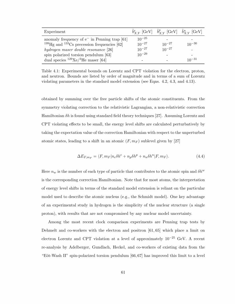
Experiment beX,Y [GeV] bp

X,Y [GeV] bnX,Y [GeV]

anomaly frequency of e− in Penning trap [61] 10−25 - -199Hg and 133Cs precession frequencies [62] 10−27 10−27 10−30

hydrogen maser double resonance [26] 10−27 10−27 -spin polarized torsion pendulum [63] 10−29 - -dual species 129Xe/3He maser [64] - - 10−31

Table 4.1: Experimental bounds on Lorentz and CPT violation for the electron, proton,and neutron. Bounds are listed by order of magnitude and in terms of a sum of Lorentzviolating parameters in the standard model extension (see Eqns. 4.2, 4.3, and 4.13).

obtained by summing over the free particle shifts of the atomic constituents. From the

symmetry violating correction to the relativistic Lagrangian, a non-relativistic correction

Hamiltonian δh is found using standard field theory techniques [27]. Assuming Lorentz and

CPT violating effects to be small, the energy level shifts are calculated perturbatively by

taking the expectation value of the correction Hamiltonian with respect to the unperturbed

atomic states, leading to a shift in an atomic (F, mF ) sublevel given by [27]

∆EF,mF= 〈F, mF |neδh

e + npδhp + nnδhn|F, mF 〉. (4.4)

Here nw is the number of each type of particle that contributes to the atomic spin and δhw

is the corresponding correction Hamiltonian. Note that for most atoms, the interpretation

of energy level shifts in terms of the standard model extension is reliant on the particular

model used to describe the atomic nucleus (e.g., the Schmidt model). One key advantage

of an experimental study in hydrogen is the simplicity of the nuclear structure (a single

proton), with results that are not compromised by any nuclear model uncertainty.

Among the most recent clock comparison experiments are Penning trap tests by

Dehmelt and co-workers with the electron and positron [61, 65] which place a limit on

electron Lorentz and CPT violation at a level of approximately 10−25 GeV. A recent

re-analysis by Adelberger, Gundlach, Heckel, and co-workers of existing data from the

“Eot-Wash II” spin-polarized torsion pendulum [66,67] has improved this limit to a level

61

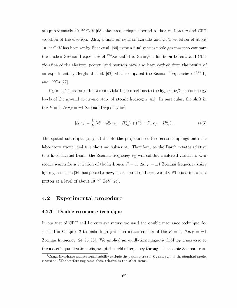
of approximately 10−29 GeV [63], the most stringent bound to date on Lorentz and CPT

violation of the electron. Also, a limit on neutron Lorentz and CPT violation of about

10−31 GeV has been set by Bear et al. [64] using a dual species noble gas maser to compare

the nuclear Zeeman frequencies of 129Xe and 3He. Stringent limits on Lorentz and CPT

violation of the electron, proton, and neutron have also been derived from the results of

an experiment by Berglund et al. [62] which compared the Zeeman frequencies of 199Hg

and 133Cs [27].

Figure 4.1 illustrates the Lorentz violating corrections to the hyperfine/Zeeman energy

levels of the ground electronic state of atomic hydrogen [41]. In particular, the shift in

the F = 1, ∆mF = ±1 Zeeman frequency is:1

|∆νZ | =1h|(be

z − deztme − He

xy) + (bpz − dp

ztmp − Hpxy)|. (4.5)

The spatial subscripts (x, y, z) denote the projection of the tensor couplings onto the

laboratory frame, and t is the time subscript. Therefore, as the Earth rotates relative

to a fixed inertial frame, the Zeeman frequency νZ will exhibit a sidereal variation. Our

recent search for a variation of the hydrogen F = 1, ∆mF = ±1 Zeeman frequency using

hydrogen masers [26] has placed a new, clean bound on Lorentz and CPT violation of the

proton at a level of about 10−27 GeV [26].

4.2 Experimental procedure

4.2.1 Double resonance technique

In our test of CPT and Lorentz symmetry, we used the double resonance technique de-

scribed in Chapter 2 to make high precision measurements of the F = 1, ∆mF = ±1

Zeeman frequency [24, 25, 38]. We applied an oscillating magnetic field ωT transverse to

the maser’s quantization axis, swept the field’s frequency through the atomic Zeeman tran-1Gauge invariance and renormalizability exclude the parameters eν , fν , and gλµν in the standard model

extension. We therefore neglected them relative to the other terms.

62

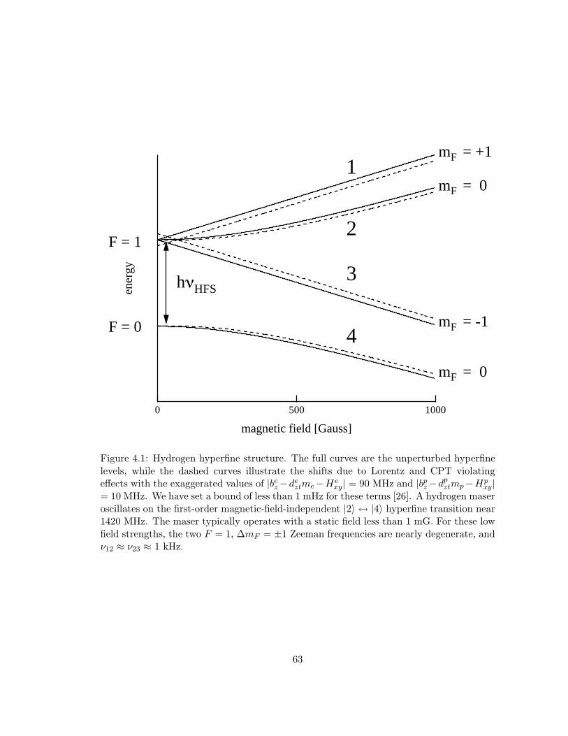
ener

gy

10005000

magnetic field [Gauss]

hνHFS

F = 1

F = 0

mF = +1

mF = 0

mF = -1

mF = 0

1

2

3

4

Figure 4.1: Hydrogen hyperfine structure. The full curves are the unperturbed hyperfinelevels, while the dashed curves illustrate the shifts due to Lorentz and CPT violatingeffects with the exaggerated values of |be

z −deztme−He

xy| = 90 MHz and |bpz −dp

ztmp−Hpxy|

= 10 MHz. We have set a bound of less than 1 mHz for these terms [26]. A hydrogen maseroscillates on the first-order magnetic-field-independent |2〉 ↔ |4〉 hyperfine transition near1420 MHz. The maser typically operates with a static field less than 1 mG. For these lowfield strengths, the two F = 1, ∆mF = ±1 Zeeman frequencies are nearly degenerate, andν12 ≈ ν23 ≈ 1 kHz.

63

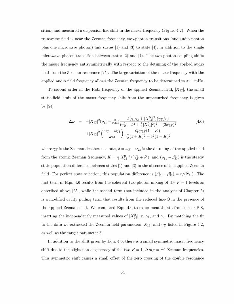
sition, and measured a dispersion-like shift in the maser frequency (Figure 4.2). When the

transverse field is near the Zeeman frequency, two-photon transitions (one audio photon

plus one microwave photon) link states |1〉 and |3〉 to state |4〉, in addition to the single

microwave photon transition between states |2〉 and |4〉. The two photon coupling shifts

the maser frequency antisymmetrically with respect to the detuning of the applied audio

field from the Zeeman resonance [25]. The large variation of the maser frequency with the

applied audio field frequency allows the Zeeman frequency to be determined to ≈ 1 mHz.

To second order in the Rabi frequency of the applied Zeeman field, |X12|, the small

static-field limit of the maser frequency shift from the unperturbed frequency is given

by [24]

∆ω = −|X12|2(ρ011 − ρ0

33)δ(γ1γ2 + |X0

24|2)(γZ/r)(γ2

Z − δ2 + 14 |X0

24|2)2 + (2δγZ)2(4.6)

+|X12|2(

ωC − ω24

ω24

)QCγZ(1 + K)

γ2Z(1 + K)2 + δ2(1 − K)2

where γZ is the Zeeman decoherence rate, δ = ωT −ω23 is the detuning of the applied field

from the atomic Zeeman frequency, K = 14 |X0

24|2/(γ2Z + δ2), and (ρ0

11 − ρ033) is the steady

state population difference between states |1〉 and |3〉 in the absence of the applied Zeeman

field. For perfect state selection, this population difference is (ρ011 − ρ0

33) = r/(2γ1). The

first term in Eqn. 4.6 results from the coherent two-photon mixing of the F = 1 levels as

described above [25], while the second term (not included in the analysis of Chapter 2)

is a modified cavity pulling term that results from the reduced line-Q in the presence of

the applied Zeeman field. We compared Eqn. 4.6 to experimental data from maser P-8,

inserting the independently measured values of |X024|, r, γ1, and γ2. By matching the fit

to the data we extracted the Zeeman field parameters |X12| and γZ listed in Figure 4.2,

as well as the target parameter δ.

In addition to the shift given by Eqn. 4.6, there is a small symmetric maser frequency

shift due to the slight non-degeneracy of the two F = 1, ∆mF = ±1 Zeeman frequencies.

This symmetric shift causes a small offset of the zero crossing of the double resonance

64

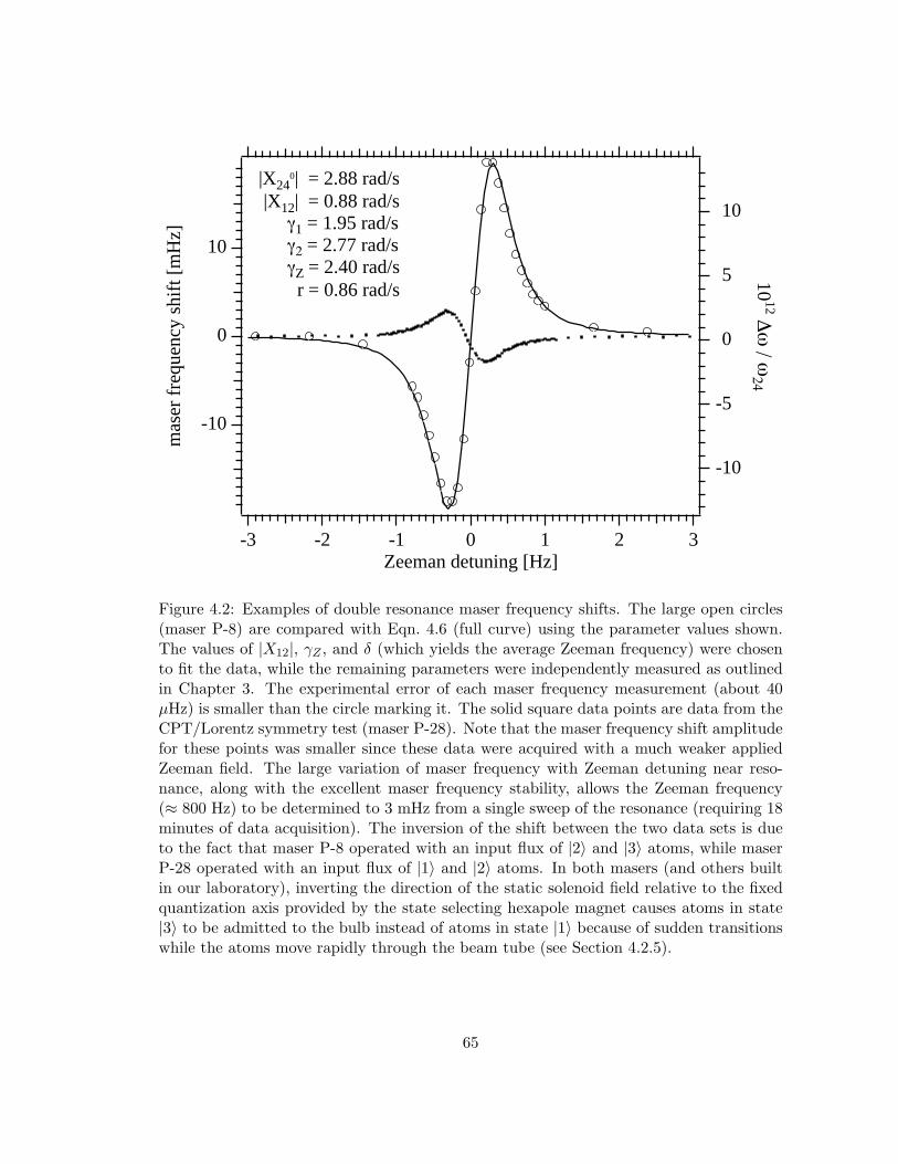
10

0

-10

mas

er f

requ

ency

shi

ft [

mH

z]

-3 -2 -1 0 1 2 3Zeeman detuning [Hz]

10

5

0

-5

-10

1012 ∆

ω / ω

24

|X240| = 2.88 rad/s

|X12| = 0.88 rad/s γ1 = 1.95 rad/s γ2 = 2.77 rad/s γΖ = 2.40 rad/s r = 0.86 rad/s

Figure 4.2: Examples of double resonance maser frequency shifts. The large open circles(maser P-8) are compared with Eqn. 4.6 (full curve) using the parameter values shown.The values of |X12|, γZ , and δ (which yields the average Zeeman frequency) were chosento fit the data, while the remaining parameters were independently measured as outlinedin Chapter 3. The experimental error of each maser frequency measurement (about 40µHz) is smaller than the circle marking it. The solid square data points are data from theCPT/Lorentz symmetry test (maser P-28). Note that the maser frequency shift amplitudefor these points was smaller since these data were acquired with a much weaker appliedZeeman field. The large variation of maser frequency with Zeeman detuning near reso-nance, along with the excellent maser frequency stability, allows the Zeeman frequency(≈ 800 Hz) to be determined to 3 mHz from a single sweep of the resonance (requiring 18minutes of data acquisition). The inversion of the shift between the two data sets is dueto the fact that maser P-8 operated with an input flux of |2〉 and |3〉 atoms, while maserP-28 operated with an input flux of |1〉 and |2〉 atoms. In both masers (and others builtin our laboratory), inverting the direction of the static solenoid field relative to the fixedquantization axis provided by the state selecting hexapole magnet causes atoms in state|3〉 to be admitted to the bulb instead of atoms in state |1〉 because of sudden transitionswhile the atoms move rapidly through the beam tube (see Section 4.2.5).

65

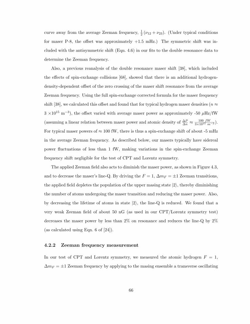
curve away from the average Zeeman frequency, 12 (ν12 + ν23). (Under typical conditions

for maser P-8, the offset was approximately +1.5 mHz.) The symmetric shift was in-

cluded with the antisymmetric shift (Eqn. 4.6) in our fits to the double resonance data to

determine the Zeeman frequency.

Also, a previous reanalysis of the double resonance maser shift [38], which included

the effects of spin-exchange collisions [68], showed that there is an additional hydrogen-

density-dependent offset of the zero crossing of the maser shift resonance from the average

Zeeman frequency. Using the full spin-exchange corrected formula for the maser frequency

shift [38], we calculated this offset and found that for typical hydrogen maser densities (n ≈

3 ×1015 m−3), the offset varied with average maser power as approximately -50 µHz/fW

(assuming a linear relation between maser power and atomic density of ∆P∆n ≈ 100 fW

3×1015 m−3 ).

For typical maser powers of ≈ 100 fW, there is thus a spin-exchange shift of about -5 mHz

in the average Zeeman frequency. As described below, our masers typically have sidereal

power fluctuations of less than 1 fW, making variations in the spin-exchange Zeeman

frequency shift negligible for the test of CPT and Lorentz symmetry.

The applied Zeeman field also acts to diminish the maser power, as shown in Figure 4.3,

and to decrease the maser’s line-Q. By driving the F = 1, ∆mF = ±1 Zeeman transitions,

the applied field depletes the population of the upper masing state |2〉, thereby diminishing

the number of atoms undergoing the maser transition and reducing the maser power. Also,

by decreasing the lifetime of atoms in state |2〉, the line-Q is reduced. We found that a

very weak Zeeman field of about 50 nG (as used in our CPT/Lorentz symmetry test)

decreases the maser power by less than 2% on resonance and reduces the line-Q by 2%

(as calculated using Eqn. 6 of [24]).

4.2.2 Zeeman frequency measurement

In our test of CPT and Lorentz symmetry, we measured the atomic hydrogen F = 1,

∆mF = ±1 Zeeman frequency by applying to the masing ensemble a transverse oscillating

66

135

130

125

120

115

110

105

100

95

90

mas

er p

ower

[fW

]

869.0868.0867.0866.0865.0864.0Zeeman field frequency [Hz]

Zeeman field strength 80 nG 210 nG

Figure 4.3: Examples of maser power reduction due to an applied Zeeman field in maserP-28. The open circles, taken with an applied Zeeman field strength of about 210 nG,represent typical data for the standard “power resonance” method used to determine thestatic magnetic field in the maser bulb. The filled circles are maser power curves for anapplied Zeeman field strength of about 80 nG. These field strengths were determined byfitting the data to Andresen’s analytical power dip lineshape [37], extracting the transversefield Rabi frequency X12, then determining the field strength from the relation hX12 =µ12HT = 1√

2µBHT . Our CPT/Lorentz symmetry test data were taken using the double

resonance technique with a field strength of about 50 nG, inducing a power reduction ofless than 2%.

67

magnetic field of about 50 nG peak amplitude,2 and then sweeping the frequency of this

transverse field through the Zeeman resonance. As described above, the applied transverse

field shifted the maser frequency in a dispersive-like manner by a few mHz (at the extrema),

a fractional shift of about 2 parts in 1012. Because of the excellent fractional frequency

stability of the maser (2 parts in 1014 over averaging times of 10 s), the shift was easily

resolved (see the solid square data points in Figure 4.2). As the frequency of the applied

field was stepped through the Zeeman resonance, the perturbed maser frequency (maser

P-28) was compared to a second, unperturbed hydrogen maser frequency (maser P-13).3

Independent voltage controlled crystal oscillators were phase locked to the signals from the

two masers. The output frequencies of the two oscillators were set by tunable synthesizers

as part of heterodyne receivers for each maser, such that there was about a 1.2 Hz offset

between the oscillators. The two output signals were combined in a double-balanced mixer

and the resulting beat note (period ≈ 0.8 s) was averaged for 10 s (about 12 periods) with a

counter.4 From this measured beat period we straightforwardly determined the frequency

of maser P-28 relative to that of maser P-13. Typically we made 100 such relative maser

frequency measurements to map out a full double resonance spectrum. For each spectrum,

80% of the points were taken over the middle 40% of the scan range, where the frequency

shift varied the most.

Each double resonance spectrum of beat period vs applied transverse field frequency

was fit to the function

Tb = A0 +A3δ(1 − κ)

A1(1 + κ)2 + δ2(1 − κ)2− A3(δ + τ)(1 − κ)

A1(1 + κ)2 + (δ + τ)2(1 − κ)2(4.7)

+A5δ

(A1 − δ2 + A4)2 + 4δ2A1+

A6(1 + κ)A1(1 + κ)2 + δ2(1 − κ)2

to determine the hydrogen Zeeman frequency. Here δ = νT − νZ is the detuning of2This field strength was determined from the transverse field Rabi frequency X12 (extracted from the

maser frequency shift fits) using the relation hX12 = µ12HT = 1√2µBHT .

3Maser P-28 was chosen for Zeeman interrogation since it had the best magnetic shielding of the masersin our laboratory. Maser P-13 was chosen as the unperturbed reference since its stability was the best outof the remaining masers.

4Hewlett-Packard model HP 5334B.

68

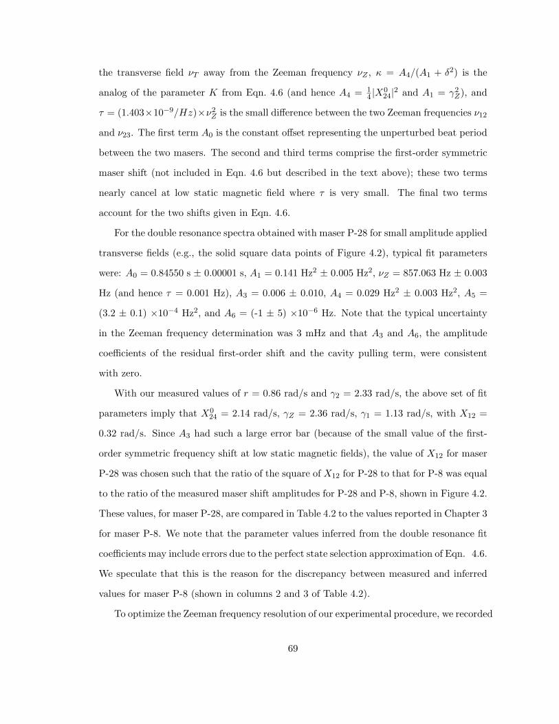
the transverse field νT away from the Zeeman frequency νZ , κ = A4/(A1 + δ2) is the

analog of the parameter K from Eqn. 4.6 (and hence A4 = 14 |X0

24|2 and A1 = γ2Z), and

τ = (1.403×10−9/Hz)×ν2Z is the small difference between the two Zeeman frequencies ν12

and ν23. The first term A0 is the constant offset representing the unperturbed beat period

between the two masers. The second and third terms comprise the first-order symmetric

maser shift (not included in Eqn. 4.6 but described in the text above); these two terms

nearly cancel at low static magnetic field where τ is very small. The final two terms

account for the two shifts given in Eqn. 4.6.

For the double resonance spectra obtained with maser P-28 for small amplitude applied

transverse fields (e.g., the solid square data points of Figure 4.2), typical fit parameters

were: A0 = 0.84550 s ± 0.00001 s, A1 = 0.141 Hz2 ± 0.005 Hz2, νZ = 857.063 Hz ± 0.003

Hz (and hence τ = 0.001 Hz), A3 = 0.006 ± 0.010, A4 = 0.029 Hz2 ± 0.003 Hz2, A5 =

(3.2 ± 0.1) ×10−4 Hz2, and A6 = (-1 ± 5) ×10−6 Hz. Note that the typical uncertainty

in the Zeeman frequency determination was 3 mHz and that A3 and A6, the amplitude

coefficients of the residual first-order shift and the cavity pulling term, were consistent

with zero.

With our measured values of r = 0.86 rad/s and γ2 = 2.33 rad/s, the above set of fit

parameters imply that X024 = 2.14 rad/s, γZ = 2.36 rad/s, γ1 = 1.13 rad/s, with X12 =

0.32 rad/s. Since A3 had such a large error bar (because of the small value of the first-

order symmetric frequency shift at low static magnetic fields), the value of X12 for maser

P-28 was chosen such that the ratio of the square of X12 for P-28 to that for P-8 was equal

to the ratio of the measured maser shift amplitudes for P-28 and P-8, shown in Figure 4.2.

These values, for maser P-28, are compared in Table 4.2 to the values reported in Chapter 3

for maser P-8. We note that the parameter values inferred from the double resonance fit

coefficients may include errors due to the perfect state selection approximation of Eqn. 4.6.

We speculate that this is the reason for the discrepancy between measured and inferred

values for maser P-8 (shown in columns 2 and 3 of Table 4.2).

To optimize the Zeeman frequency resolution of our experimental procedure, we recorded

69

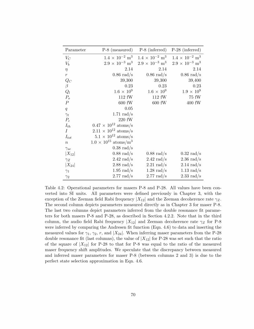
Parameter P-8 (measured) P-8 (inferred) P-28 (inferred)

VC 1.4 × 10−2 m3 1.4 × 10−2 m3 1.4 × 10−2 m3

Vb 2.9 × 10−3 m3 2.9 × 10−3 m3 2.9 × 10−3 m3

η 2.14 2.14 2.14r 0.86 rad/s 0.86 rad/s 0.86 rad/sQC 39,300 39,300 39,400β 0.23 0.23 0.23Ql 1.6 × 109 1.6 × 109 1.9 × 109

Po 112 fW 112 fW 75 fWP 600 fW 600 fW 400 fWq 0.05γt 1.71 rad/sPc 220 fWIth 0.47 × 1012 atoms/sI 2.11 × 1012 atoms/sItot 5.1 × 1012 atoms/sn 1.0 × 1015 atoms/m3

γse 0.38 rad/s|X12| 0.88 rad/s 0.88 rad/s 0.32 rad/sγZ 2.42 rad/s 2.42 rad/s 2.36 rad/s|X24| 2.88 rad/s 2.21 rad/s 2.14 rad/sγ1 1.95 rad/s 1.28 rad/s 1.13 rad/sγ2 2.77 rad/s 2.77 rad/s 2.33 rad/s

Table 4.2: Operational parameters for masers P-8 and P-28. All values have been con-verted into SI units. All parameters were defined previously in Chapter 3, with theexception of the Zeeman field Rabi frequency |X12| and the Zeeman decoherence rate γZ .The second column depicts parameters measured directly as in Chapter 3 for maser P-8.The last two columns depict parameters inferred from the double resonance fit parame-ters for both masers P-8 and P-28, as described in Section 4.2.2. Note that in the thirdcolumn, the audio field Rabi frequency |X12| and Zeeman decoherence rate γZ for P-8were inferred by comparing the Andresen fit function (Eqn. 4.6) to data and inserting themeasured values for γ1, γ2, r, and |X24|. When inferring maser parameters from the P-28double resonance fit (last columns), the value of |X12| for P-28 was set such that the ratioof the square of |X12| for P-28 to that for P-8 was equal to the ratio of the measuredmaser frequency shift amplitudes. We speculate that the discrepancy between measuredand inferred maser parameters for maser P-8 (between columns 2 and 3) is due to theperfect state selection approximation in Eqn. 4.6.

70

40

30

20

10

0nu

mbe

r

-10 -5 0 5 10Zeeman frequency shift [mHz]

σν12 = 2.7 mHz

Figure 4.4: Example results from a Monte Carlo analysis of the resolution of the doubleresonance method for determining the hydrogen Zeeman frequency. The horizontal axisrepresents the shift of the Zeeman frequency as determined by our fits of over 100 syntheticdata sets constructed as described in the body of the paper text; the vertical axis isthe number of data sets within each frequency shift bin. The width of the Gaussianfit to the data is 2.7 mHz, representing the estimated resolution of a Zeeman frequencydetermination from a single, complete double resonance spectrum.

several spectra with 50, 100, and 150 points at 5 s and 10 s averaging. We also varied the

distribution of points along the drive frequency axis, including spectra where the middle

40% of the scan contained 80% of the points and those where the middle 30% contained

80% of the points (thus increasing the number of points in the region where the maser

frequency varies the most). With each of these spectra, we ran the following Monte Carlo

analysis [69]: after fitting each scan to Eqn. 4.7, we constructed 100 synthetic data sets

by adding Gaussian noise to the fit, with the noise amplitude determined by the unper-

turbed maser frequency resolution of about 40 µHz. Each of these synthetic data sets was

fit and a histogram of the fitted Zeeman frequencies was constructed. The resolution of

the fit was taken as the Gaussian width of the fitted Zeeman histogram (see Figure 4.4).

As the total length of the scans increased, the resolution improved and converged to a

limit of around 2.5 mHz. While the resolution improved slowly with increased acquisition

time, it eventually began to degrade due to long-term drifting of the Zeeman frequency.

(As will be described below, we found that the Zeeman frequency exhibited slow drifts

71

of about 10-100 mHz/day.) We therefore chose a scan of 100 points at 10 s averaging,

for a total length of about 18 minutes for each double resonance spectrum used in the

Lorentz symmetry test. As mentioned above, we also chose to operate with 80% of the

points acquired over the middle 40% of the scan range. As an example, Figure 4.4 shows

the results from the Monte Carlo analysis for one of the test spectra, indicating a Zeeman

frequency resolution of 2.7 mHz.

4.2.3 Data analysis

Our net bound on a sidereal variation of the atomic hydrogen F = 1, ∆mF = ±1 Zeeman

frequency combines data from three multi-day runs. During each data run, the 18 minute

Zeeman frequency scans were automated and run consecutively. After every 10 scans, 20

minutes of “unperturbed” maser frequency stability data was taken to track the maser’s

unperturbed frequency. Each run contained about 10 continuous days of data and more

than 500 Zeeman frequency measurements.

For each day in a run, the Zeeman frequency data, corrected for measured variations

in the solenoid current (see Section 4.3.1), was fit to a function of the form

fit = (piecewise continuous linear function) + δνZ,α cos(ωsidt) + δνZ,β sin(ωsidt) (4.8)

where δνZ,α and δνZ,β represent the cosine and sine components of a sidereal-day-period

sinusoid. For all times in the nth sidereal day, the piecewise continuous linear function

was given by

fn(t) =n∑

i=0

Ai + An+1(t − n). (4.9)

The time origin of the sinusoids for all three runs was taken as midnight (00:00) of Novem-

ber 19, 1999. The subscripts α and β refer to two non-rotating orthogonal axes perpendic-

ular to the rotation axis of the earth. The total amplitude of a sidereal-period modulation

of νZ was determined by adding δνZ,α and δνZ,β in quadrature. During each run, the Zee-

man frequency drifted hundreds of mHz over tens of days (see discussion in Section 4.3.2).

72

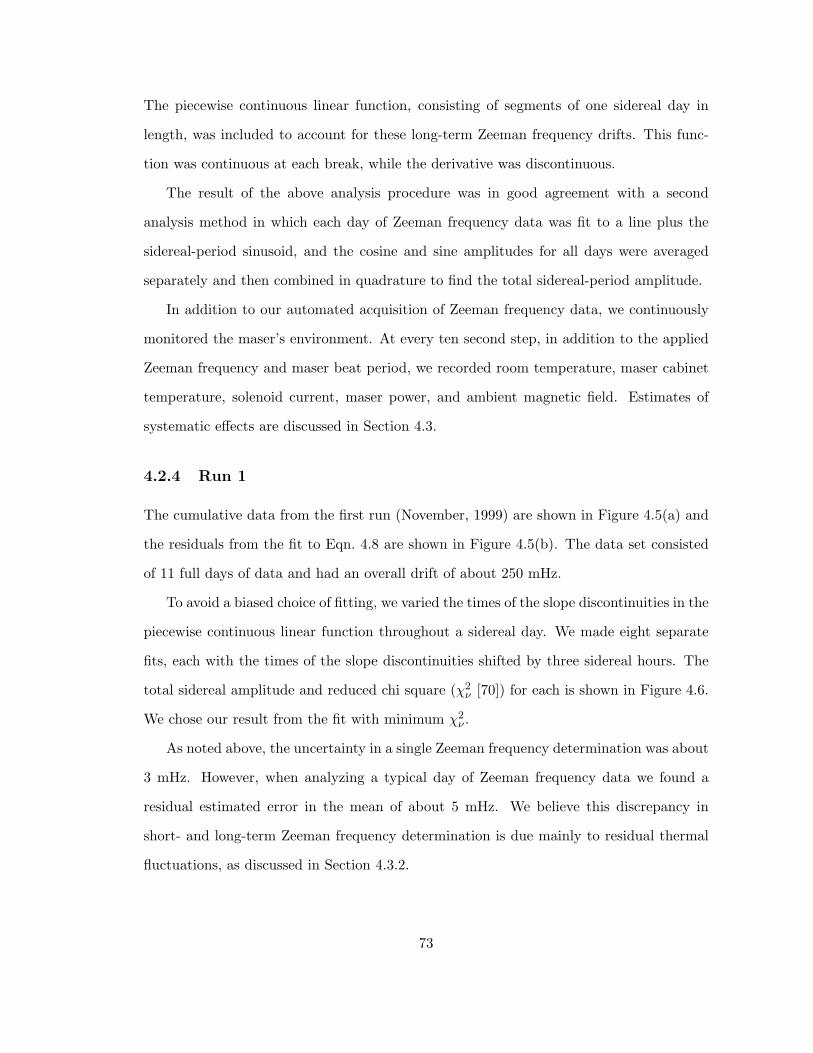
The piecewise continuous linear function, consisting of segments of one sidereal day in

length, was included to account for these long-term Zeeman frequency drifts. This func-

tion was continuous at each break, while the derivative was discontinuous.

The result of the above analysis procedure was in good agreement with a second

analysis method in which each day of Zeeman frequency data was fit to a line plus the

sidereal-period sinusoid, and the cosine and sine amplitudes for all days were averaged

separately and then combined in quadrature to find the total sidereal-period amplitude.

In addition to our automated acquisition of Zeeman frequency data, we continuously

monitored the maser’s environment. At every ten second step, in addition to the applied

Zeeman frequency and maser beat period, we recorded room temperature, maser cabinet

temperature, solenoid current, maser power, and ambient magnetic field. Estimates of

systematic effects are discussed in Section 4.3.

4.2.4 Run 1

The cumulative data from the first run (November, 1999) are shown in Figure 4.5(a) and

the residuals from the fit to Eqn. 4.8 are shown in Figure 4.5(b). The data set consisted

of 11 full days of data and had an overall drift of about 250 mHz.

To avoid a biased choice of fitting, we varied the times of the slope discontinuities in the

piecewise continuous linear function throughout a sidereal day. We made eight separate

fits, each with the times of the slope discontinuities shifted by three sidereal hours. The

total sidereal amplitude and reduced chi square (χ2ν [70]) for each is shown in Figure 4.6.

We chose our result from the fit with minimum χ2ν .

As noted above, the uncertainty in a single Zeeman frequency determination was about

3 mHz. However, when analyzing a typical day of Zeeman frequency data we found a

residual estimated error in the mean of about 5 mHz. We believe this discrepancy in

short- and long-term Zeeman frequency determination is due mainly to residual thermal

fluctuations, as discussed in Section 4.3.2.

73

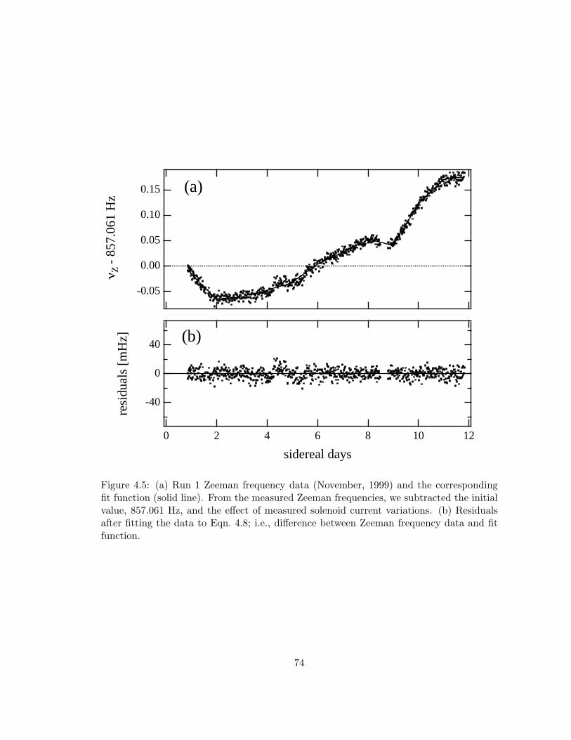
0.15

0.10

0.05

0.00

-0.05

νΖ -

857.

061

Hz

121086420

sidereal days

(a)

-40

0

40

resi

dual

s [m

Hz]

121086420

sidereal days

(b)

Figure 4.5: (a) Run 1 Zeeman frequency data (November, 1999) and the correspondingfit function (solid line). From the measured Zeeman frequencies, we subtracted the initialvalue, 857.061 Hz, and the effect of measured solenoid current variations. (b) Residualsafter fitting the data to Eqn. 4.8; i.e., difference between Zeeman frequency data and fitfunction.

74

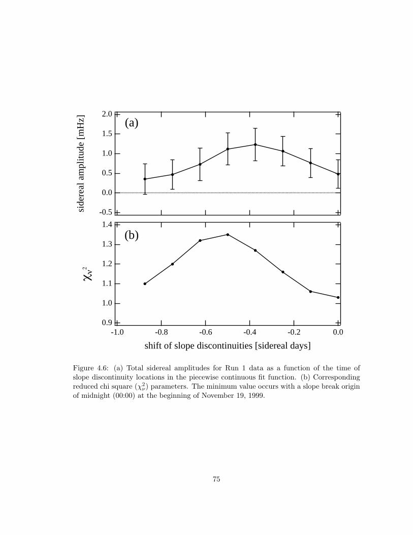
2.0

1.5

1.0

0.5

0.0

-0.5side

real

am

plitu

de [

mH

z]

-1.0 -0.8 -0.6 -0.4 -0.2 0.0

shift of slope discontinuities [sidereal days]

(a)

1.4

1.3

1.2

1.1

1.0

0.9

χ ν2

-1.0 -0.8 -0.6 -0.4 -0.2 0.0

shift of slope discontinuities [sidereal days]

(b)

Figure 4.6: (a) Total sidereal amplitudes for Run 1 data as a function of the time ofslope discontinuity locations in the piecewise continuous fit function. (b) Correspondingreduced chi square (χ2

ν) parameters. The minimum value occurs with a slope break originof midnight (00:00) at the beginning of November 19, 1999.

75

For the choice of slope discontinuity with minimum χ2ν ,

5 the cosine amplitude was 0.43

mHz ± 0.36 mHz, and the sine amplitude was -0.21 mHz ± 0.36 mHz. The total sidereal-

period amplitude was therefore 0.48 mHz ± 0.36 mHz. Note that this total amplitude is,

by definition, positive with the most probable value (for a normal distribution consistent

with no Lorentz-violating effect) equal to one standard deviation. Thus the mean value

(0.48 mHz) for run 1 is less than one standard deviation away from the most probable

value (0.36 mHz) (see Section 4.2.6).

4.2.5 Field-inverted runs 2 and 3

In runs 2 and 3, the static solenoid magnetic field orientation was opposite that of the initial

run, which enabled us to investigate potential systematics associated with the solenoid

field. With the static field inverted, and therefore directed opposite to the quantization

axis at the exit of the state selecting hexapole magnet, the input flux consisted of atoms

in states |2〉 and |3〉 (rather than the states |1〉 and |2〉). Thus, reversing the field inverted

the steady state population difference (ρ011 − ρ0

33) of Eqn. 4.6 and acted to invert the

antisymmetric double resonance maser frequency shift [25].

Operating the maser in the field reversed mode also degraded the maser frequency

stability and hence the Zeeman frequency measurement sensitivity (see Figures 4.7(a) and

4.8(a)). With opposed quantization fields inside the maser bulb and at the exit of the

state selecting hexapole magnet, a narrow region of field inversion was created. Where

the field passed through zero, Majorana transitions between the different mF sublevels of

the F = 1 manifold could occur. This reduced the number of atoms in the upper maser

state (F = 1, mF = 0, state |2〉), diminishing the overall maser amplitude (by ≈ 30%

in maser P-28) and degrading the frequency stability. In addition, the overall Zeeman

frequency drift was larger in runs 2 and 3 than in run 1 (nearly 800 mHz over about 10

days); also, the scatter in the data was increased, as can be seen from the residual plots

Figures 4.7(b) and 4.8(b) which have been plotted on the same scale as the residuals from5Had we chosen the slope discontinuity with maximum χ2

ν , the total sidereal amplitude for this runwould have been 1.1 mHz ± 0.4 mHz.

76

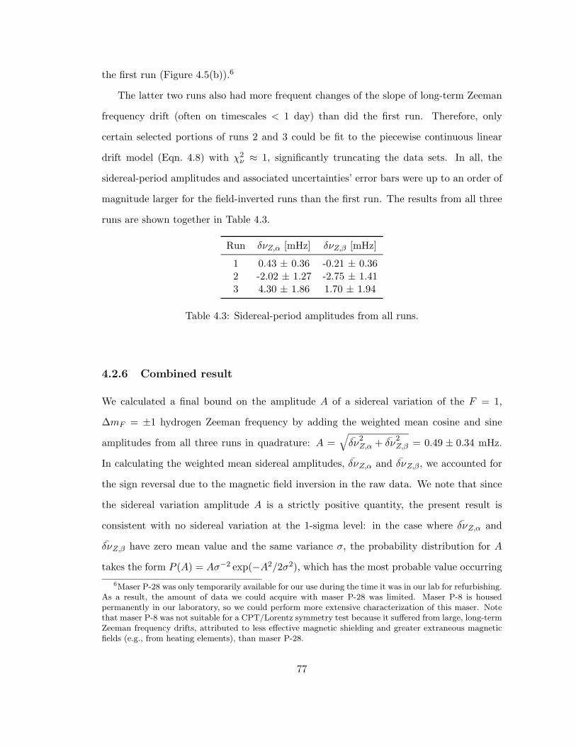
the first run (Figure 4.5(b)).6

The latter two runs also had more frequent changes of the slope of long-term Zeeman

frequency drift (often on timescales < 1 day) than did the first run. Therefore, only

certain selected portions of runs 2 and 3 could be fit to the piecewise continuous linear

drift model (Eqn. 4.8) with χ2ν ≈ 1, significantly truncating the data sets. In all, the

sidereal-period amplitudes and associated uncertainties’ error bars were up to an order of

magnitude larger for the field-inverted runs than the first run. The results from all three

runs are shown together in Table 4.3.

Run δνZ,α [mHz] δνZ,β [mHz]

1 0.43 ± 0.36 -0.21 ± 0.362 -2.02 ± 1.27 -2.75 ± 1.413 4.30 ± 1.86 1.70 ± 1.94

Table 4.3: Sidereal-period amplitudes from all runs.

4.2.6 Combined result

We calculated a final bound on the amplitude A of a sidereal variation of the F = 1,

∆mF = ±1 hydrogen Zeeman frequency by adding the weighted mean cosine and sine

amplitudes from all three runs in quadrature: A =√

δν2Z,α + δν

2Z,β = 0.49 ± 0.34 mHz.

In calculating the weighted mean sidereal amplitudes, δνZ,α and δνZ,β , we accounted for

the sign reversal due to the magnetic field inversion in the raw data. We note that since

the sidereal variation amplitude A is a strictly positive quantity, the present result is

consistent with no sidereal variation at the 1-sigma level: in the case where δνZ,α and

δνZ,β have zero mean value and the same variance σ, the probability distribution for A

takes the form P (A) = Aσ−2 exp(−A2/2σ2), which has the most probable value occurring6Maser P-28 was only temporarily available for our use during the time it was in our lab for refurbishing.

As a result, the amount of data we could acquire with maser P-28 was limited. Maser P-8 is housedpermanently in our laboratory, so we could perform more extensive characterization of this maser. Notethat maser P-8 was not suitable for a CPT/Lorentz symmetry test because it suffered from large, long-termZeeman frequency drifts, attributed to less effective magnetic shielding and greater extraneous magneticfields (e.g., from heating elements), than maser P-28.

77

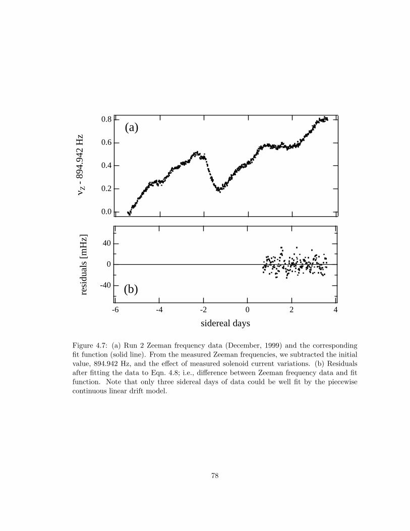
0.8

0.6

0.4

0.2

0.0

νΖ -

894.

942

Hz

-6 -4 -2 0 2 4

sidereal days

(a)

-40

0

40

resi

dual

s [m

Hz]

-6 -4 -2 0 2 4

sidereal days

(b)

Figure 4.7: (a) Run 2 Zeeman frequency data (December, 1999) and the correspondingfit function (solid line). From the measured Zeeman frequencies, we subtracted the initialvalue, 894.942 Hz, and the effect of measured solenoid current variations. (b) Residualsafter fitting the data to Eqn. 4.8; i.e., difference between Zeeman frequency data and fitfunction. Note that only three sidereal days of data could be well fit by the piecewisecontinuous linear drift model.

78

-0.8

-0.6

-0.4

-0.2

0.0

νΖ -

849.

674H

z

121086420

sidereal days

(a)

-40

0

40

resi

dual

s [m

Hz]

121086420

sidereal days

(b)

Figure 4.8: (a) Run 3 Zeeman frequency data (March, 2000) and the corresponding fitfunction (solid line). From the measured Zeeman frequencies, we subtracted the initialvalue, 849.674 Hz, and the effect of measured solenoid current variations. (b) Residualsafter fitting the data to Eqn. 4.8; i.e., difference between Zeeman frequency data andfit function. Note that only five sidereal days of data could be well fit by the piecewisecontinuous linear drift model.

79

at A = σ.

4.3 Systematics and error analysis

4.3.1 Magnetic field systematics

The F = 1, mF = ±1 Zeeman frequency depends to first order on the z-component of

the magnetic field in the storage bulb. Thus, all external field fluctuations had to be

sufficiently screened to enable high sensitivity to frequency shifts from CPT and Lorentz

symmetry violation. The maser cavity and bulb were therefore surrounded by a set of

four nested magnetic shields that reduce the ambient z-component field by a factor of

about 32,000. We measured unshielded fluctuations in the ambient field of about 3 mG

(peak-peak) throughout any given day, and even when shielded these fluctuations added

significant noise to each Zeeman frequency determination using the double resonance tech-

nique (“Zeeman scan”), as illustrated in Figure 4.9(a). Furthermore, the amplitude of the

field fluctuations was significantly reduced late at night, due to the cessation of the local

subway and electric bus lines, which could have generated a diurnal systematic effect in

our data.

To reduce the effect of fluctuations in the ambient magnetic field, we installed an

active feedback system (see Figure 4.10) consisting of two large Helmholtz coil pairs (2.4

m diameter) and a fluxgate magnetometer. The magnetometer probe7 was placed inside

the maser’s outermost magnetic shield near the maser cavity and had a magnetic field

sensitivity of s = 1.7 mG/V. Due to its location inside one magnetic shield, the probe was

shielded by a factor of about six from external fields, reducing the effective sensitivity to

s′ = 0.3 mG/V, and producing a differential shielding of 5300 between the magnetometer

probe and the hydrogen atoms in the maser bulb. The first pair of Helmholtz coils (50

turns) produced a uniform, static field that canceled most of the z-component of the

ambient field, leaving a residual field of around 5 mG (as measured by the shielded probe).7RFL Industries model 101.

80

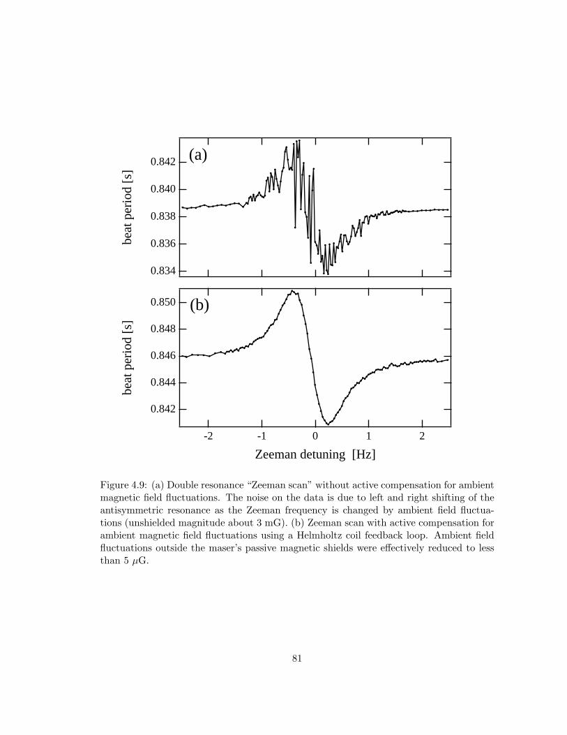
0.842

0.840

0.838

0.836

0.834

beat

per

iod

[s]

-2 -1 0 1 2

Zeeman detuning [Hz]

(a)

0.850

0.848

0.846

0.844

0.842

beat

per

iod

[s]

-2 -1 0 1 2

Zeeman detuning [Hz]

(b)

Figure 4.9: (a) Double resonance “Zeeman scan” without active compensation for ambientmagnetic field fluctuations. The noise on the data is due to left and right shifting of theantisymmetric resonance as the Zeeman frequency is changed by ambient field fluctua-tions (unshielded magnitude about 3 mG). (b) Zeeman scan with active compensation forambient magnetic field fluctuations using a Helmholtz coil feedback loop. Ambient fieldfluctuations outside the maser’s passive magnetic shields were effectively reduced to lessthan 5 µG.

81

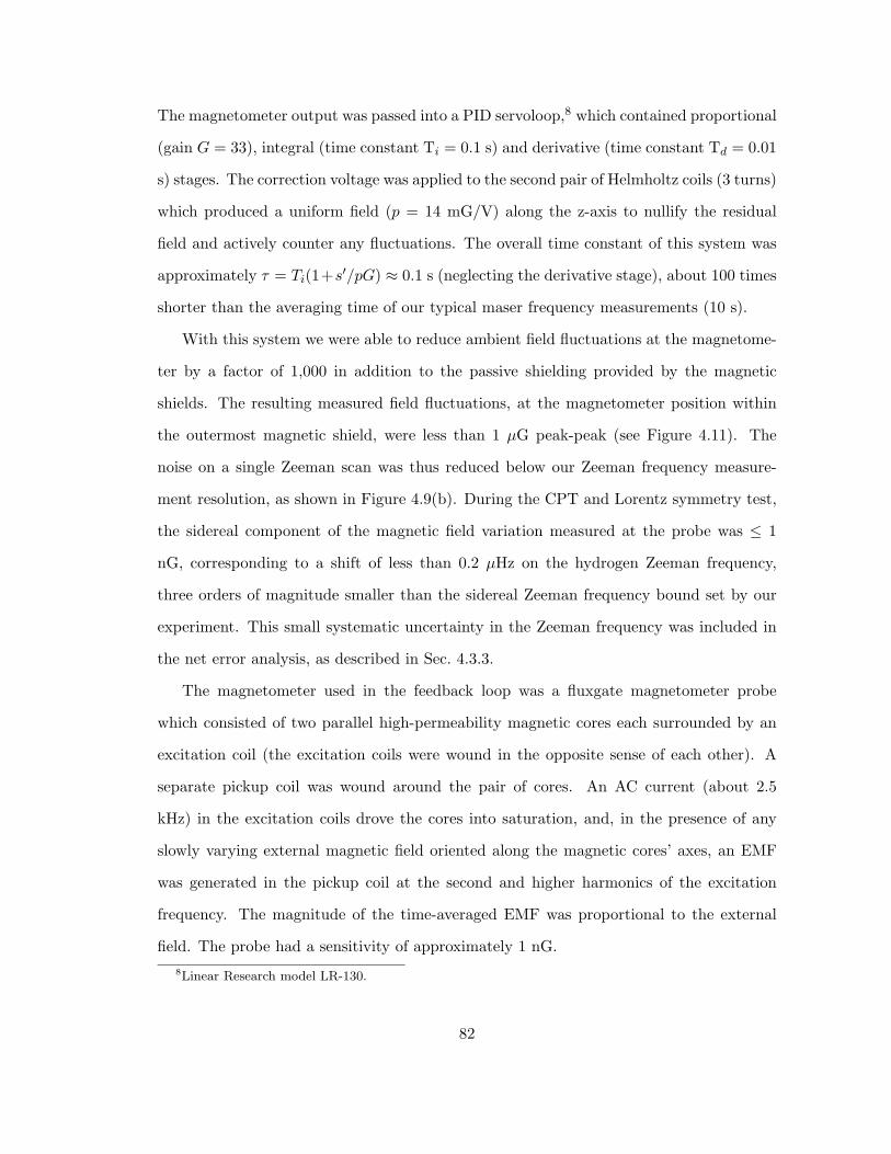
The magnetometer output was passed into a PID servoloop,8 which contained proportional

(gain G = 33), integral (time constant Ti = 0.1 s) and derivative (time constant Td = 0.01

s) stages. The correction voltage was applied to the second pair of Helmholtz coils (3 turns)

which produced a uniform field (p = 14 mG/V) along the z-axis to nullify the residual

field and actively counter any fluctuations. The overall time constant of this system was

approximately τ = Ti(1+s′/pG) ≈ 0.1 s (neglecting the derivative stage), about 100 times

shorter than the averaging time of our typical maser frequency measurements (10 s).

With this system we were able to reduce ambient field fluctuations at the magnetome-

ter by a factor of 1,000 in addition to the passive shielding provided by the magnetic

shields. The resulting measured field fluctuations, at the magnetometer position within

the outermost magnetic shield, were less than 1 µG peak-peak (see Figure 4.11). The

noise on a single Zeeman scan was thus reduced below our Zeeman frequency measure-

ment resolution, as shown in Figure 4.9(b). During the CPT and Lorentz symmetry test,

the sidereal component of the magnetic field variation measured at the probe was ≤ 1

nG, corresponding to a shift of less than 0.2 µHz on the hydrogen Zeeman frequency,

three orders of magnitude smaller than the sidereal Zeeman frequency bound set by our

experiment. This small systematic uncertainty in the Zeeman frequency was included in

the net error analysis, as described in Sec. 4.3.3.

The magnetometer used in the feedback loop was a fluxgate magnetometer probe

which consisted of two parallel high-permeability magnetic cores each surrounded by an

excitation coil (the excitation coils were wound in the opposite sense of each other). A

separate pickup coil was wound around the pair of cores. An AC current (about 2.5

kHz) in the excitation coils drove the cores into saturation, and, in the presence of any

slowly varying external magnetic field oriented along the magnetic cores’ axes, an EMF

was generated in the pickup coil at the second and higher harmonics of the excitation

frequency. The magnitude of the time-averaged EMF was proportional to the external

field. The probe had a sensitivity of approximately 1 nG.8Linear Research model LR-130.

82

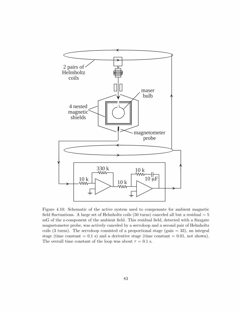
10 k10 k

10 k330 k

10 µF

magnetometerprobe

4 nestedmagneticshields

maserbulb

2 pairs ofHelmholtz

coils

Figure 4.10: Schematic of the active system used to compensate for ambient magneticfield fluctuations. A large set of Helmholtz coils (50 turns) canceled all but a residual ∼ 5mG of the z-component of the ambient field. This residual field, detected with a fluxgatemagnetometer probe, was actively canceled by a servoloop and a second pair of Helmholtzcoils (3 turns). The servoloop consisted of a proportional stage (gain = 33), an integralstage (time constant = 0.1 s) and a derivative stage (time constant = 0.01, not shown).The overall time constant of the loop was about τ = 0.1 s.

83

Any Lorentz violating spin-orientation dependence of the energy of the electrons in the

magnetic cores of the fluxgate magnetometer would have induced a sidereal variation in

the cores’ magnetization and could have generated, or masked, a sidereal variation in the

hydrogen Zeeman frequency through the ambient field control system. However, based

on the latest bound on electron Lorentz violation (10−29 GeV [66]), any Lorentz violating

effect on the magnetometer corresponds to an effective magnetic field change of less than

δB = 1µB

δE = 10−12 G, far below the level of residual ambient field fluctuations. Also,

the additional shielding factor of 5300 between the magnetometer probe and the hydrogen

atoms further reduced the effect of any Lorentz violating shift in the probe electrons’

energies.

With the ambient field well controlled near zero, the Zeeman frequency was set by

the magnetic field generated by the three coil maser solenoid, and hence by the solenoid

current. Each low-resistance coil (main and two end coils) of the maser solenoid was driven

by a voltage-regulated supply in series with an adjustable voltage divider and a current-

limiting precision 5 kΩ resistor. We monitored solenoid current fluctuations by measuring

the voltage across the main coil’s current-limiting resistor with a 5 1/2 digit multimeter.9

By measuring the Zeeman frequency shift caused by large current changes, we found a

dependence of 8 mHz/nA. Long-term drifts in the current were typically about 5 nA (see

Figure 4.12), significant enough to produce detectable shifts in the Zeeman frequency. In

particular, the measured sidereal component of the solenoid current variation was 25 ±

10 pA, corresponding to a sidereal Zeeman frequency variation of 0.16 ± 0.08 mHz. We

corrected for these drifts directly in the Zeeman data during data analysis using the above

current/Zeeman frequency calibration. The resultant sidereals systematic uncertainty

in the Zeeman frequency was included in the net error analysis for the Lorentz/CPT

symmetry test (Sec. 4.3.3).9Fluke model 8840A/AF.

84

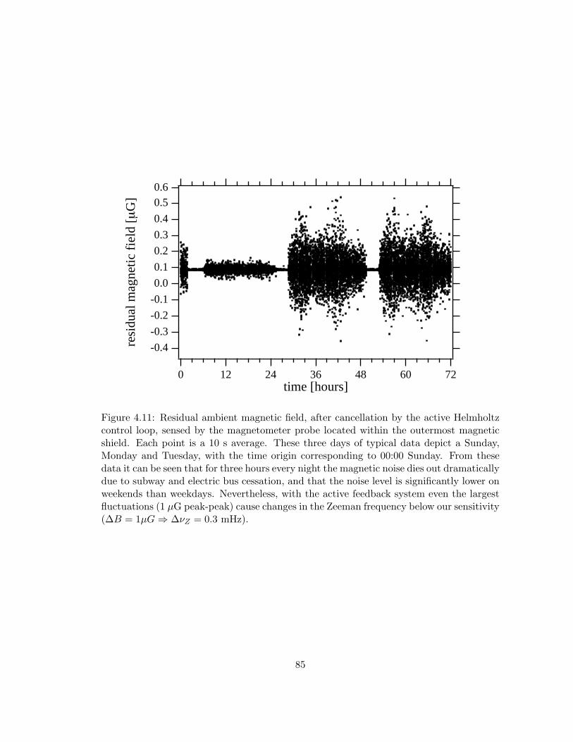
0.60.5

0.4

0.3

0.2

0.1

0.0

-0.1

-0.2

-0.3

-0.4resi

dual

mag

netic

fie

ld [

µG

]

7260483624120time [hours]

Figure 4.11: Residual ambient magnetic field, after cancellation by the active Helmholtzcontrol loop, sensed by the magnetometer probe located within the outermost magneticshield. Each point is a 10 s average. These three days of typical data depict a Sunday,Monday and Tuesday, with the time origin corresponding to 00:00 Sunday. From thesedata it can be seen that for three hours every night the magnetic noise dies out dramaticallydue to subway and electric bus cessation, and that the noise level is significantly lower onweekends than weekdays. Nevertheless, with the active feedback system even the largestfluctuations (1 µG peak-peak) cause changes in the Zeeman frequency below our sensitivity(∆B = 1µG ⇒ ∆νZ = 0.3 mHz).

85

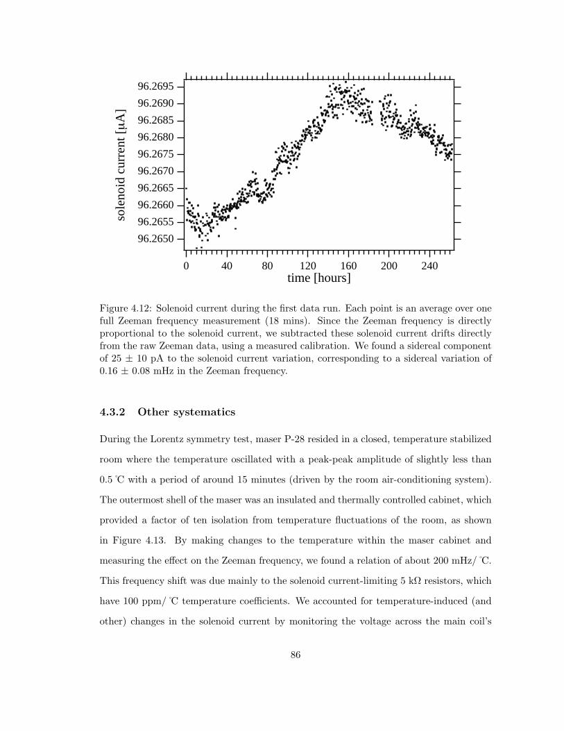
96.2695

96.2690

96.2685

96.2680

96.2675

96.2670

96.2665

96.2660

96.2655

96.2650

sole

noid

cur

rent

[µ

A]

24020016012080400time [hours]

Figure 4.12: Solenoid current during the first data run. Each point is an average over onefull Zeeman frequency measurement (18 mins). Since the Zeeman frequency is directlyproportional to the solenoid current, we subtracted these solenoid current drifts directlyfrom the raw Zeeman data, using a measured calibration. We found a sidereal componentof 25 ± 10 pA to the solenoid current variation, corresponding to a sidereal variation of0.16 ± 0.08 mHz in the Zeeman frequency.

4.3.2 Other systematics

During the Lorentz symmetry test, maser P-28 resided in a closed, temperature stabilized

room where the temperature oscillated with a peak-peak amplitude of slightly less than

0.5 C with a period of around 15 minutes (driven by the room air-conditioning system).

The outermost shell of the maser was an insulated and thermally controlled cabinet, which

provided a factor of ten isolation from temperature fluctuations of the room, as shown

in Figure 4.13. By making changes to the temperature within the maser cabinet and

measuring the effect on the Zeeman frequency, we found a relation of about 200 mHz/ C.

This frequency shift was due mainly to the solenoid current-limiting 5 kΩ resistors, which

have 100 ppm/ C temperature coefficients. We accounted for temperature-induced (and

other) changes in the solenoid current by monitoring the voltage across the main coil’s

86

current-limiting resistor, as described above.

However, remnant temperature-induced changes in the magnetic field and hence the

Zeeman frequency could arise from adjusting currents in the 4-layer system of maser

temperature control. On an intermediate timescale of a few hours, we estimate that

such temperature-induced effects produced additional variations of about 1 mHz in the

measured Zeeman frequency, increasing the estimated error in the mean of the fitted

residual Zeeman frequency in a given day from about 3 mHz to 5 mHz. On a longer

timescale, our measurements placed a bound of 0.5 mK on the sidereal component of the

cabinet temperature fluctuations, which would produce a systematic sidereal variation of

100 µHz on the Zeeman frequency, about a factor of 3 smaller than the measured limit on

sidereal variation in Zeeman frequency.

The Zeeman frequency data from all runs (Figures 4.5, 4.7, and 4.8) show that the

Zeeman frequency drift over longer time scales (i.e., days) was up to hundreds of mHz.

While this long-term drift was accounted for by a fit to a linear drift function, its presence

certainly degraded our overall sensitivity to Zeeman frequency variation. Indeed, the rapid

changes in this drift in runs 2 and 3 precluded our use of a sizable fraction of the Zeeman

frequency data. We speculate that possible sources of these long-term drifts were changing

magnetic fields near the maser bulb caused by stray currents in heaters or power supplies

or drift of the thermal control loops of the temperature control system.

As mentioned in Section 4.2.1, spin-exchange effects induce a small offset of the Zeeman

frequency determined by the double resonance technique from the actual Zeeman frequency

[38]. Thus, variations in the input atomic flux (and therefore the atomic density and the

maser power) could cause variations in the Zeeman frequency measurement. We measured

a limit on the shift of the Zeeman frequency due to large changes in average maser power of

less than 0.8 mHz/fW. (Expected shifts from spin-exchange are ten times smaller than this

level, see Section 4.2.1. We believe the measured limit is related to heating of the maser

as the flux is increased). During long-term operation, the average maser power drifted

approximately 1 fW/day (see Figure 4.14). The sidereal component of the variations

87

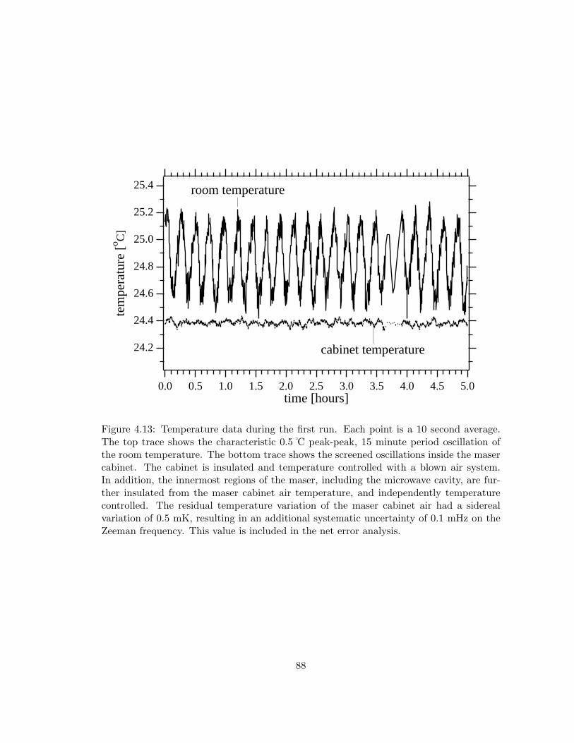
25.4

25.2

25.0

24.8

24.6

24.4

24.2

tem

pera

ture

[o C

]

5.04.54.03.53.02.52.01.51.00.50.0time [hours]

room temperature

cabinet temperature

Figure 4.13: Temperature data during the first run. Each point is a 10 second average.The top trace shows the characteristic 0.5 C peak-peak, 15 minute period oscillation ofthe room temperature. The bottom trace shows the screened oscillations inside the masercabinet. The cabinet is insulated and temperature controlled with a blown air system.In addition, the innermost regions of the maser, including the microwave cavity, are fur-ther insulated from the maser cabinet air temperature, and independently temperaturecontrolled. The residual temperature variation of the maser cabinet air had a siderealvariation of 0.5 mK, resulting in an additional systematic uncertainty of 0.1 mHz on theZeeman frequency. This value is included in the net error analysis.

88

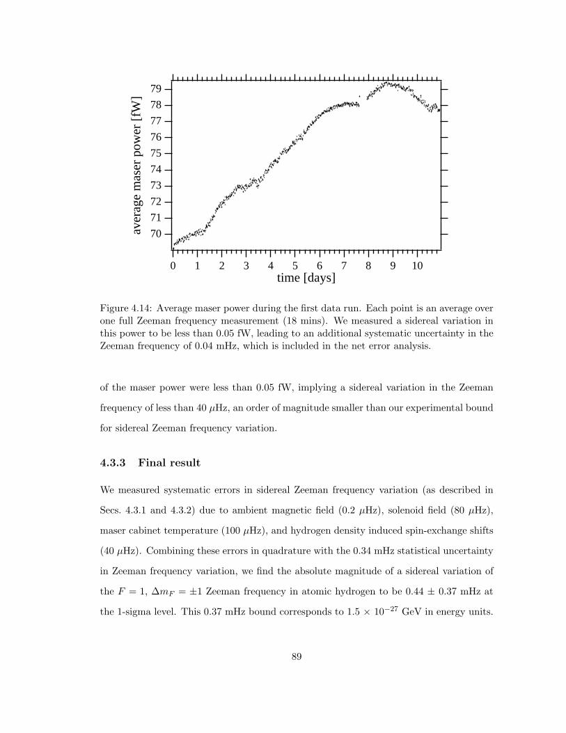
79

78

77

76

75

74

73

72

71

70aver

age

mas

er p

ower

[fW

]

109876543210time [days]

Figure 4.14: Average maser power during the first data run. Each point is an average overone full Zeeman frequency measurement (18 mins). We measured a sidereal variation inthis power to be less than 0.05 fW, leading to an additional systematic uncertainty in theZeeman frequency of 0.04 mHz, which is included in the net error analysis.

of the maser power were less than 0.05 fW, implying a sidereal variation in the Zeeman

frequency of less than 40 µHz, an order of magnitude smaller than our experimental bound

for sidereal Zeeman frequency variation.

4.3.3 Final result

We measured systematic errors in sidereal Zeeman frequency variation (as described in

Secs. 4.3.1 and 4.3.2) due to ambient magnetic field (0.2 µHz), solenoid field (80 µHz),

maser cabinet temperature (100 µHz), and hydrogen density induced spin-exchange shifts

(40 µHz). Combining these errors in quadrature with the 0.34 mHz statistical uncertainty

in Zeeman frequency variation, we find the absolute magnitude of a sidereal variation of

the F = 1, ∆mF = ±1 Zeeman frequency in atomic hydrogen to be 0.44 ± 0.37 mHz at

the 1-sigma level. This 0.37 mHz bound corresponds to 1.5 × 10−27 GeV in energy units.

89

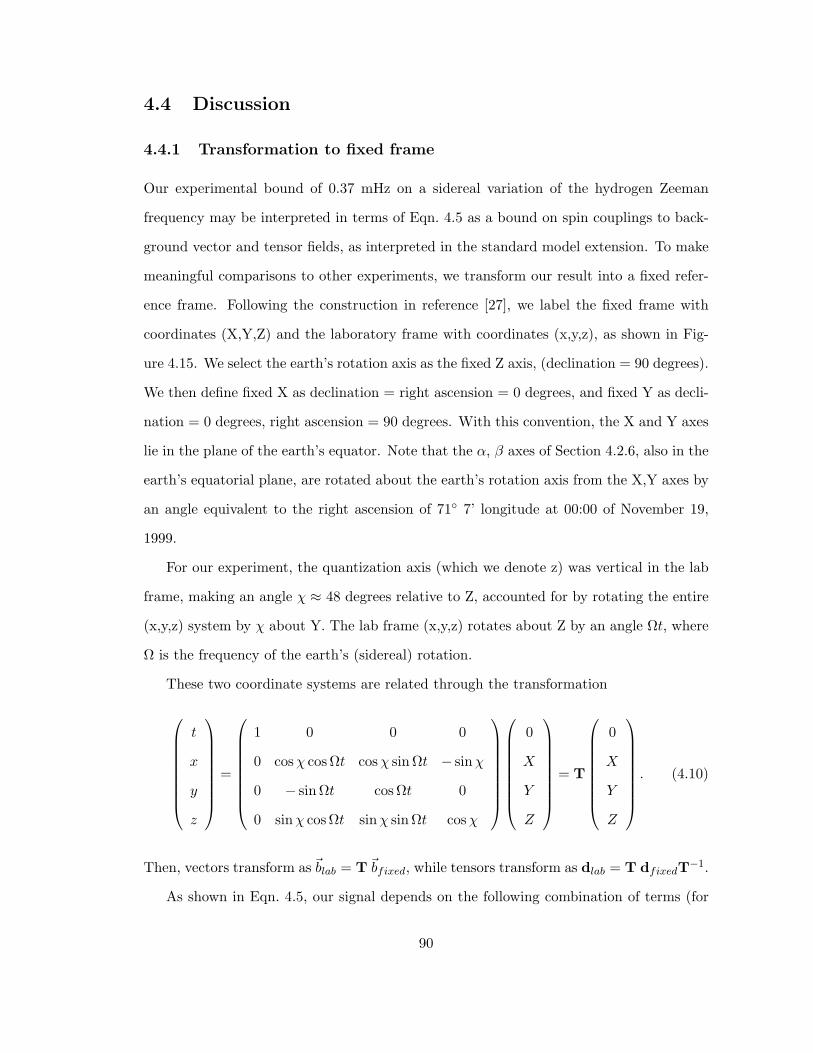
4.4 Discussion

4.4.1 Transformation to fixed frame

Our experimental bound of 0.37 mHz on a sidereal variation of the hydrogen Zeeman

frequency may be interpreted in terms of Eqn. 4.5 as a bound on spin couplings to back-

ground vector and tensor fields, as interpreted in the standard model extension. To make

meaningful comparisons to other experiments, we transform our result into a fixed refer-

ence frame. Following the construction in reference [27], we label the fixed frame with

coordinates (X,Y,Z) and the laboratory frame with coordinates (x,y,z), as shown in Fig-

ure 4.15. We select the earth’s rotation axis as the fixed Z axis, (declination = 90 degrees).

We then define fixed X as declination = right ascension = 0 degrees, and fixed Y as decli-

nation = 0 degrees, right ascension = 90 degrees. With this convention, the X and Y axes

lie in the plane of the earth’s equator. Note that the α, β axes of Section 4.2.6, also in the

earth’s equatorial plane, are rotated about the earth’s rotation axis from the X,Y axes by

an angle equivalent to the right ascension of 71 7’ longitude at 00:00 of November 19,

1999.

For our experiment, the quantization axis (which we denote z) was vertical in the lab

frame, making an angle χ ≈ 48 degrees relative to Z, accounted for by rotating the entire

(x,y,z) system by χ about Y. The lab frame (x,y,z) rotates about Z by an angle Ωt, where

Ω is the frequency of the earth’s (sidereal) rotation.

These two coordinate systems are related through the transformation

t

x

y

z

=

1 0 0 0

0 cos χ cos Ωt cos χ sin Ωt − sinχ

0 − sin Ωt cos Ωt 0

0 sinχ cos Ωt sinχ sin Ωt cos χ

0

X

Y

Z

= T

0

X

Y

Z

. (4.10)

Then, vectors transform asblab = Tbfixed, while tensors transform as dlab = T dfixedT−1.

As shown in Eqn. 4.5, our signal depends on the following combination of terms (for

90

X

Y

Z

x

y

z

χ

χ

Ωt

Figure 4.15: Coordinate systems used. The (X,Y,Z) set refers to a fixed reference frame,and the (x,y,z) set refers to the laboratory frame. The lab frame is tilted from the fixedZ-axis by our co-latitude, and it rotates about Z as the earth rotates. The α and β axes,described in Section 4.2, span a plane parallel to the X-Y plane.

91

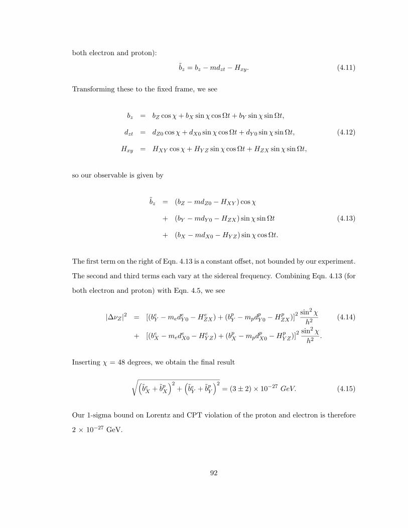
both electron and proton):

bz = bz − mdzt − Hxy. (4.11)

Transforming these to the fixed frame, we see

bz = bZ cos χ + bX sinχ cos Ωt + bY sinχ sin Ωt,

dzt = dZ0 cos χ + dX0 sinχ cos Ωt + dY 0 sinχ sin Ωt, (4.12)

Hxy = HXY cos χ + HY Z sinχ cos Ωt + HZX sinχ sin Ωt,

so our observable is given by

bz = (bZ − mdZ0 − HXY ) cos χ

+ (bY − mdY 0 − HZX) sinχ sin Ωt (4.13)

+ (bX − mdX0 − HY Z) sinχ cos Ωt.

The first term on the right of Eqn. 4.13 is a constant offset, not bounded by our experiment.

The second and third terms each vary at the sidereal frequency. Combining Eqn. 4.13 (for

both electron and proton) with Eqn. 4.5, we see

|∆νZ |2 = [(beY − med

eY 0 − He

ZX) + (bpY − mpd

pY 0 − Hp

ZX)]2sin2 χ

h2(4.14)

+ [(beX − med

eX0 − He

Y Z) + (bpX − mpd

pX0 − Hp

Y Z)]2sin2 χ

h2.

Inserting χ = 48 degrees, we obtain the final result

√(beX + bp

X

)2+

(beY + bp

Y

)2= (3 ± 2) × 10−27 GeV. (4.15)

Our 1-sigma bound on Lorentz and CPT violation of the proton and electron is therefore

2 × 10−27 GeV.

92

4.4.2 Comparison to previous experiments

We compare our result with other recent tests of Lorentz and CPT symmetry in Ta-

ble 4.1. Although our bounds are numerically similar to the those from the 199Hg/133Cs

experiment, the simplicity of the hydrogen atom allows us to place bounds directly on

the electron and proton; uncertainties in nuclear structure models do not complicate the

interpretation of our result. The recent limit of ≈ 10−29 GeV on electron Lorentz and

CPT violation set by the torsion pendulum experiment of Adelberger et al. [63] casts our

result as a clean bound on Lorentz and CPT violation of the proton.

4.4.3 Future work

To make a more sensitive measure of the sidereal variation of the Zeeman frequency in a

hydrogen maser, it will be important to clearly identify and reduce the magnitude of the

long-term drifts of the Zeeman frequency. Possible sources of these drifts are magnetic

fields near the maser bulb caused by stray currents in heaters or power supplies in the

inner regions of the maser. Also, the scatter of the Zeeman data points, believed to be

due mainly to residual thermal fluctuations, should be reduced. Both of these objectives

could be accomplished by carefully rebuilding a hydrogen maser, with better engineered

power and temperature control systems.

93

Chapter 5

The cryogenic hydrogen maser

In 1978 Crampton, Phillips and Kleppner [6] first pointed out that the frequency stability

of a hydrogen maser could be improved by operating at low temperature due to a decrease

in thermal noise and a decrease in the rate of hydrogen-hydrogen spin-exchange colli-

sions. The first detailed analyses of a cryogenic hydrogen maser (CHM) [7,8] predicted an

improvement of two to three orders of magnitude in frequency stability over a room tem-

perature hydrogen maser. A discussion of this predicted CHM stability will be presented

in Section 5.1 and our technical strides to achieve it will be presented in Sections 5.2, 5.3,

and 5.4.

In the years following its original proposal, theoretical studies of low temperature

hydrogen-hydrogen spin-exchange collisions have demonstrated that these effects could in

fact limit this expected frequency stability improvement. In this sense, the CHM has been

recast as a useful tool with which to study low temperature hydrogen-hydrogen collisions.

This topic will be treated in more detail in Chapter 6.

Eight years after its initial proposal, groups at MIT [9], the University of British

Columbia (UBC) [10], and Harvard/SAO [11] independently achieved oscillation of a cryo-

genic hydrogen maser. The MIT cryogenic hydrogen maser resulted as an offshoot of their

efforts to magnetically trap spin-polarized hydrogen. After their initial CHM demonstra-

tion, research in this area was discontinued. The UBC maser program continued for several

94

years, producing a number of important results, before its termination in the mid 1990s.

The Harvard/SAO cryogenic hydrogen maser was developed following the conventional

design of their numerous room temperature hydrogen masers. The Harvard/SAO group

is the only group currently engaged in CHM research.

We report in this chapter the first oscillation of the SAO CHM in nearly five years and

the first oscillation since the addition of a quartz atomic storage bulb. Originally intended

to improve maser frequency stability, we will discuss below how overall maser stability has

been degraded. A thorough survey of current SAO CHM performance will be presented

in Section 5.5.

5.1 Cryogenic hydrogen maser frequency stability

For short-term averaging times (up to 10,000 s), the frequency stability of a room temper-

ature hydrogen maser is limited by thermal noise. Therefore, the short-term performance

of a hydrogen maser is expected to improve as the apparatus is cooled to lower tempera-

ture. White frequency noise due to thermal noise power in the microwave cavity will be

reduced as the maser is cooled. Likewise, if the cryogenic environment is employed to cool

the preamplifier, the white phase noise will also be reduced.

There are also a number of indirect factors which could lead to improved stability

at lower temperatures. First, the hydrogen atoms will travel more slowly, thus reducing

the wall collision rate and increasing the atomic storage time; this will act to increase

the maser’s line-Q. Second, because the hydrogen atoms’ relative velocity and the spin-

exchange collision cross sections both decrease at lower temperature, it is possible to

operate a maser at an increased density and therefore increased output power. Finally,

because the physical properties of materials (e.g., thermal contraction) tend to become

more stable at lower temperatures, it is possible that some of the mechanically-induced

systematic effects can be reduced with a cryogenic maser.

95

5.1.1 Decreased thermal noise

As shown in Chapter 3, for averaging times of τ < 100 s, the stability limit of a room

temperature maser is set by added white phase noise in the preamplifier and receiver. In

this region, the Allan variance [47] as a function of averaging time τ is given by [7]

σr(τ) =1τ

√Bk(T + TN )

ω2P

(1 + β

β

)(5.1)

where B is the receiver bandwidth, T is the maser temperature, TN is the preamplifier noise

temperature, P is the power delivered by the atoms to the cavity, β is the cavity coupling

constant, and ω = 2πν is the maser frequency. Note that for a room temperature amplifier,

the amplifier’s noise temperature TN and noise figure F are related by T +TN = FT . The

room temperature preamplifier we use for our cryogenic maser has TN = 75 K.1 Assuming

a bandwidth B = 6 Hz and a maser power P = 6×10−13 W, the Allan variance for a room

temperature maser over this interval is typically about σr(τ) = 6×10−14/τ .

For longer averaging times, the room temperature maser stability is limited by white

frequency noise from the incoherent thermal microwave cavity field. Over this interval,

the Allan variance [47] as a function of averaging time τ is given by [7]

σc(τ) =1Ql

√kT

2Pτ(5.2)

where Ql is the maser’s line-Q, T is the maser temperature, and P is the power delivered

from the atoms to the cavity. For a room temperature maser with Ql = 1.6×109, the

Allan variance over this interval is given by σc(τ) = 4 × 10−14/√

τ .

Because these two processes are uncorrelated, we can compute the combined short-

term (τ < 1000 s) Allan variance as [7]

σ(τ) =[σ2

c (τ) + σ2r (τ)

] 12 . (5.3)

1This room temperature preamplifier is considerably better than that of VLG-10 series maser P-8.Therefore these room temperature results are better than those presented in Chapter 3.

96

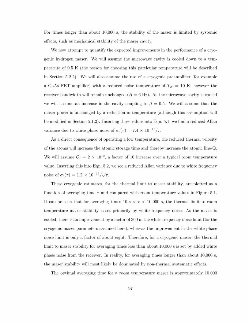
For times longer than about 10,000 s, the stability of the maser is limited by systemic

effects, such as mechanical stability of the maser cavity.

We now attempt to quantify the expected improvements in the performance of a cryo-

genic hydrogen maser. We will assume the microwave cavity is cooled down to a tem-

perature of 0.5 K (the reason for choosing this particular temperature will be described

in Section 5.2.2). We will also assume the use of a cryogenic preamplifier (for example

a GaAs FET amplifier) with a reduced noise temperature of TN = 10 K, however the

receiver bandwidth will remain unchanged (B = 6 Hz). As the microwave cavity is cooled

we will assume an increase in the cavity coupling to β = 0.5. We will assume that the

maser power is unchanged by a reduction in temperature (although this assumption will

be modified in Section 5.1.2). Inserting these values into Eqn. 5.1, we find a reduced Allan

variance due to white phase noise of σr(τ) = 7.4 × 10−15/τ .

As a direct consequence of operating a low temperature, the reduced thermal velocity

of the atoms will increase the atomic storage time and thereby increase the atomic line-Q.

We will assume Ql = 2 × 1010, a factor of 10 increase over a typical room temperature

value. Inserting this into Eqn. 5.2, we see a reduced Allan variance due to white frequency

noise of σc(τ) = 1.2 × 10−16/√

τ .

These cryogenic estimates, for the thermal limit to maser stability, are plotted as a

function of averaging time τ and compared with room temperature values in Figure 5.1.

It can be seen that for averaging times 10 s < τ < 10,000 s, the thermal limit to room

temperature maser stability is set primarily by white frequency noise. As the maser is

cooled, there is an improvement by a factor of 300 in the white frequency noise limit (for the

cryogenic maser parameters assumed here), whereas the improvement in the white phase

noise limit is only a factor of about eight. Therefore, for a cryogenic maser, the thermal

limit to maser stability for averaging times less than about 10,000 s is set by added white

phase noise from the receiver. In reality, for averaging times longer than about 10,000 s,

the maser stability will most likely be dominated by non-thermal systematic effects.

The optimal averaging time for a room temperature maser is approximately 10,000

97

10-18

10-17

10-16

10-15

10-14

Alla

n va

rian

ce σ

(τ)

100 101 102 103 104

averaging time τ (sec)

limit from thermal white frequency noise limit from added white phase noise combined thermal noise limit

T = 290K T = 0.5K

Figure 5.1: Hydrogen maser frequency stability limits due to thermal noise. The grayset of traces depict typical room temperature maser performance, while the black set oftraces show the projected performance for a cryogenic maser. For each set, the dashedline depicts the limit due to added white phase noise (Eqn. 5.1), the dotted line depictsthe limit due to white frequency noise (Eqn. 5.2), and the solid line shows the net limitdue to thermal sources. For the room temperature curves, we have used T = 290 K, Ql

= 1.6 × 109, P = 6 × 10−13 W, TN = 75 K, B = 6 Hz, and β = 0.23. For the cryogenicestimate, we have assumed T = 0.5 K, Ql = 2 × 1010, P = 6 × 10−13 W, TN = 10 K, B= 6 Hz, and β = 0.50. Note that we have not assumed an increased maser power for thecryogenic maser, although such an increase is expected due to the reduced spin-exchangerelaxation rates.

98

s. For times longer than this, systematic effects tend to reduce the maser’s performance.

From Figure 5.1, we see that at τ = 10,000 s, the thermal noise limited stability of a

room temperature maser is about σ(τ) = 3 × 10−16, while the expected cryogenic maser

stability is approximately σ(τ) = 2 × 10−18. Therefore we see that by accounting for

thermal effects alone, an improvement of over two orders of magnitude in hydrogen maser

stability is predicted for a maser operating at cryogenic temperatures.

5.1.2 Increased maser power

In Chapter 3 we discussed the effect of spin-exchange broadening on the operation of a

hydrogen maser. In particular, we introduced the spin-exchange parameter q, defined by

q =

[σvrh

8πµ2B

]γt

r + γr

[VC

ηVb

] (1

QC

)Itot

I(5.4)

which essentially quantified the amount of spin-exchange broadening in the maser. Here,

σ is the spin-exchange broadening cross section and vr is the relative atomic velocity. For

q = 0 (equivalent to no spin-exchange broadening) we saw that the maser power increased

monotonically without bound with hydrogen flux. However, as the value of q increased,

the maximum obtainable power decreased and the range of flux that would support active

oscillation narrowed. For q > 0.176, active oscillation was no longer achievable.

Here we consider the effect of temperature on the spin-exchange collision rate, in par-

ticular the effect of reduced temperature on the broadening cross section σ and the relative

atomic velocity vr. Prior to the work of Verhaar et al. [30, 31], all of the theoretical work

on hydrogen-hydrogen spin-exchange collisions had been done using an approximation

known as the degenerate internal states (DIS) approximation [17,68,71–77]. This approx-

imation essentially neglects the small hyperfine splitting (about 0.07 K) in the atomic

ground state relative to the thermal energies of the collisions and the electron exchange

potential (about 50,000 K). The inclusion of the hyperfine interaction energies in a fully

quantum mechanical treatment of hydrogen-hydrogen spin-exchange collisions led to new

99

hyperfine-induced (h-i) effects. In Chapter 6 we will discuss these h-i effects, however we

consider here only the results of DIS theory.

The relative atomic velocity is given by vr = 4√

kT/πm and it therefore is a decreasing

function with a reduction in T , as shown in Figure 5.2(a). For example, from room tem-

perature to 0.5 K, vr decreases by a factor of√

290/0.5 = 24. Since the hydrogen atoms

are traveling at a reduced rate, the frequency of hydrogen-hydrogen collisions will be re-

duced, therefore reducing spin-exchange broadening. In addition, there is also a significant

reduction in the spin-exchange broadening cross-section σ. A theoretical prediction of this

is given in Figure 5.2(b). Here it can be seen that from room temperature to 0.5 K, there

is a reduction by a factor of about 30 in σ [75, 77].

Therefore, because the spin-exchange collision rate is proportional to σvr, there is a

reduction by nearly three orders of magnitude in the collision rate from room temperature

to 0.5 K, as shown in Figure 5.2. This reduction is directly incorporated in the spin-

exchange parameter q, and as a result, we expect to be able to run at higher fluxes before

spin-exchange broadening effects begin to play a limiting role. Since both forms of short-

to medium-term frequency stability (Eqns. 5.1 and 5.2) are inversely proportional to√

P ,

within the DIS theory the stability of a cryogenic hydrogen maser can be significantly

improved over the estimate obtained in Section 5.1.1 above, where we considered thermal

noise effects alone.

Of course, the primary assumption of DIS theory, that the hyperfine interaction energy

(≈ 70 mK) can be neglected relative to the collision energy, begins to break down as the

temperature of the colliding atoms is reduced. Therefore, an accurate estimate of the

improvement in cryogenic maser stability will need to include h-i effects. In Chapter 6 we

will analyze these effects and how they limit the ultimate stability of a cryogenic hydrogen

maser.

100

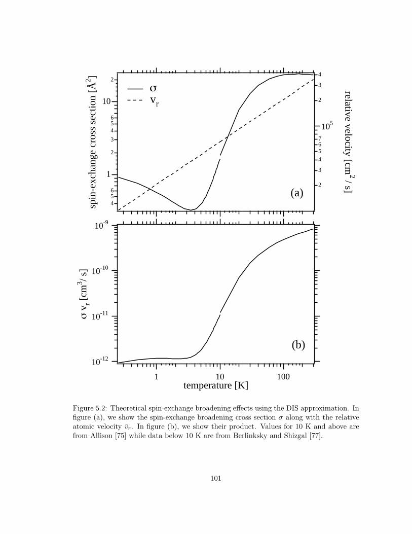
456

1

2

3

456

10

2

spin

-exc

hang

e cr

oss

sect

ion

[Å2 ]

1 10 100temperature [K]

2

3

4567

105

2

3

4

relative velocity [cm2 / s]

σ vr

(a)

10-12

10-11

10-10

10-9

σ v

r [cm

3 / s]

1 10 100temperature [K]

(b)

Figure 5.2: Theoretical spin-exchange broadening effects using the DIS approximation. Infigure (a), we show the spin-exchange broadening cross section σ along with the relativeatomic velocity vr. In figure (b), we show their product. Values for 10 K and above arefrom Allison [75] while data below 10 K are from Berlinksky and Shizgal [77].

101

5.1.3 Cryogenic systematics

Important systematic limits to hydrogen maser stability, magnetic and thermo-mechanical

effects, can both be reduced by operating at low temperature [7, 8]. Operation at 0.5 K

allows for the use of superconducting magnetic shields which can reduce maser frequency

shifts due to variations in the magnetic-field-dependent atomic hyperfine frequency. In

addition, since the thermal expansion coefficients of materials decrease significantly at low

temperature, and since a hydrogen maser can be operated with a higher line-Q and lower

cavity-Q, maser frequency shifts due to variations in the microwave cavity frequency will

also be reduced.

5.2 Superfluid 4He wall coating

5.2.1 Historic overview

The most serious technical complication for operating a hydrogen maser at cryogenic

temperatures is finding an appropriate wall coating. The binding energy of hydrogen on

Teflon is on the order of 200 K; therefore this no longer functions as an effective wall

coating at cryogenic temperatures. Initial investigations into low temperature coatings

included a study of Teflon from 372 K to 77 K [78], Teflon from 77 K to 48 K [79], solid

neon at 10 K [80], and frozen molecular hydrogen at 4 K [81]. The best of these candidates,

solid H2, was found to have a binding energy of around 40 K, and was thus not effective

at liquid helium temperatures or below.

However, in 1980, while working in an early attempt to realize a hydrogen BEC,

Silvera and Walraven [82] successfully stabilized an atomic hydrogen gas within a storage

vessel coated by a superfluid 4He film. In their initial study, they reported that at 0.3 K,

approximately 1015 atoms were confined for a period of about 500 s.

102

5.2.2 Effects of superfluid 4He wall coating

In this section we will analyze the effects of confining cold atomic hydrogen within a storage

cell lined with a saturated superfluid 4He film. In particular, we quantify the hyperfine

frequency shifts due the hydrogen-helium interactions, and determine the most stable

operating point for our cryogenic hydrogen maser. It will be shown that the frequency

stability of the cryogenic maser will be limited by the net hyperfine shift due to hydrogen-

helium interactions, and this shift’s variation as a function of temperature.

We consider a storage bulb of radius R, volume V and surface area A. Hydrogen atoms

(of mass m) confined to this region at a temperature T will have a thermal de Broglie

wavelength of Λ = h/√

2πmkT and an average velocity of v =√

8kT/πm. The average

length of time between wall collisions is given by τc = 4R/3v [8]. Occasionally, a hydrogen

atom will stick to the 4He coated surface during a wall collision. If we define the average

length of time between collisions where the hydrogen atoms stick to the wall as τb, and

the average length of stay on the surface as τs, then the sticking probability is given by

α = τc/τb [8]. For H on 4He, this probability has been measured to be α = 0.04 [83].

Finally, the fraction of time an atom spends on the wall is given by [84]

x =τs

τb=

ΛA

VeEB/kT (5.5)

where EB/k = 1.15 K is the binding energy of hydrogen on a 4He surface at 0.5 K [84,85].

Due to the interaction with the 4He film during a sticking collision, the hyperfine

frequency of the H atom is shifted by an amount ∆s. This introduces an average hyperfine

frequency shift due to surface interactions of [83]

∆νs =1

2πτb

φ

1 + φ2≈ φ

2πτb=

τs

τb∆s (5.6)

where the average phase accumulated during a sticking event is given by φ = 2πτs∆s, and

we have used the fact that φ2 1. For hydrogen on a 4He surface at 0.5 K, the hyperfine

103

shift has been measured to be ∆s = -49 kHz [84,85].

Because a superfluid 4He coated surface will also have a non-negligible 4He vapor

pressure above the surface, we also need to consider effects of H-4He interactions in the

vapor phase. Collisions of hydrogen with vapor phase 4He introduces a pressure shift in

the hyperfine frequency given by [8]

∆νv = βHenHe, (5.7)

where βHe = -11.8 × 10−18 Hz/cm3. From 0.06 to 1 K, the 4He vapor density above a

saturated 4He film can be expressed as nHe = (1.5×1021)T 3/2 exp(−7.1688/T ), where nHe

is in cm3 for T in K [8]. At normal cryogenic hydrogen maser operating temperatures,

the 4He vapor pressure is sufficiently high that the mean free path of the hydrogen atoms

is no longer large relative to the bulb dimensions (as in a room temperature maser). For

example, at 0.55 K, the mean free path of hydrogen is about 1 cm, hence the atoms

move diffusively inside the storage bulb. This mean free path is also a strong function of

temperature. From 0.45 to 0.6 K, the mean free path is reduced from about 10 cm down

to about 0.1 cm, as shown in Figure 5.3.

The net hyperfine frequency shift due to H-He interactions at the wall and in the vapor

is found by combining Eqns. 5.5 - 5.7,

∆ν = ∆sΛA

VeEB/kT + βHenHe. (5.8)

Figure 5.3 shows a plot of Eqn. 5.8 for our quartz atomic storage bulb (with V = 172 cm3

and A = 176 cm2). Here, the magnitude of the frequency shift is plotted; the sign of both

the wall shift and the vapor shift is negative. Because the two shifts have the same sign

but opposite trends, the net shift passes through an magnitude minimum of 110 mHz at

0.55 K. Here, the first-order temperature dependence is eliminated, so this is therefore the

target operating temperature for our cryogenic hydrogen maser. At lower temperatures,

the hydrogen atoms tend to stick longer at the wall and therefore accumulate more negative

104

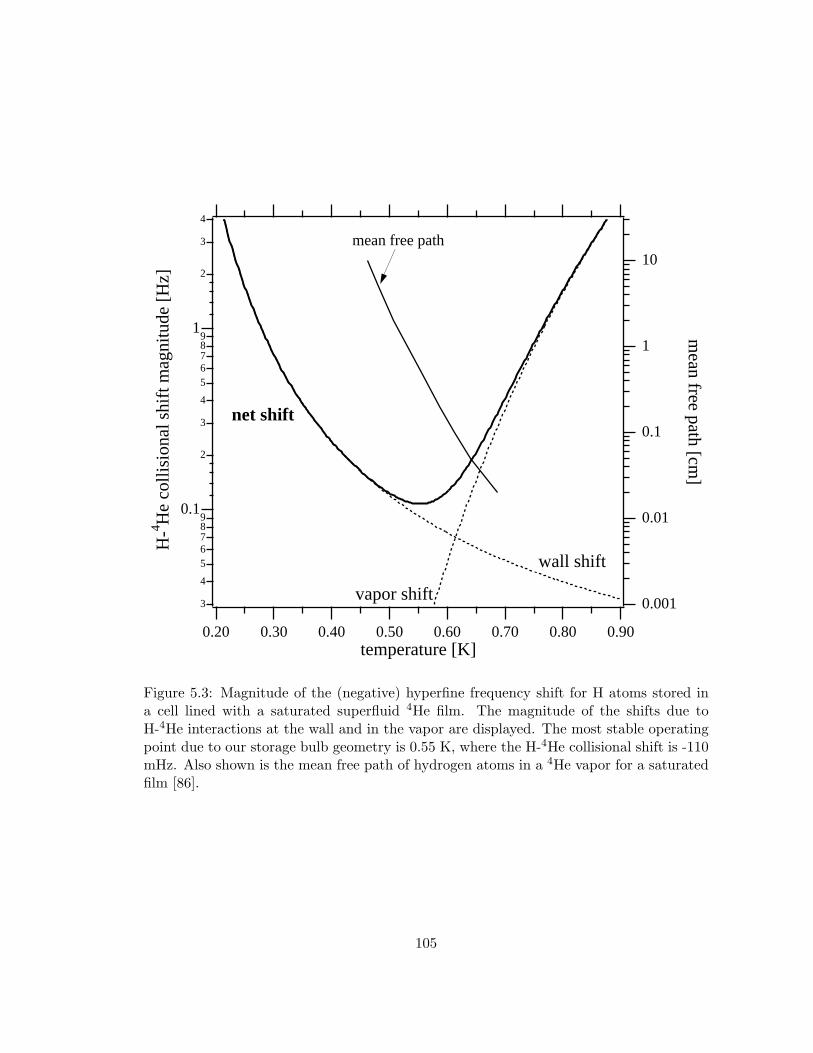
3

4

56789

0.1

2

3

4

56789

1

2

3

4

H-4 H

e co

llisi

onal

shi

ft m

agni

tude

[H

z]

0.900.800.700.600.500.400.300.20temperature [K]

0.001

0.01

0.1

1

10

mean free path [cm

]

wall shift

vapor shift

mean free path

net shift

Figure 5.3: Magnitude of the (negative) hyperfine frequency shift for H atoms stored ina cell lined with a saturated superfluid 4He film. The magnitude of the shifts due toH-4He interactions at the wall and in the vapor are displayed. The most stable operatingpoint due to our storage bulb geometry is 0.55 K, where the H-4He collisional shift is -110mHz. Also shown is the mean free path of hydrogen atoms in a 4He vapor for a saturatedfilm [86].

105

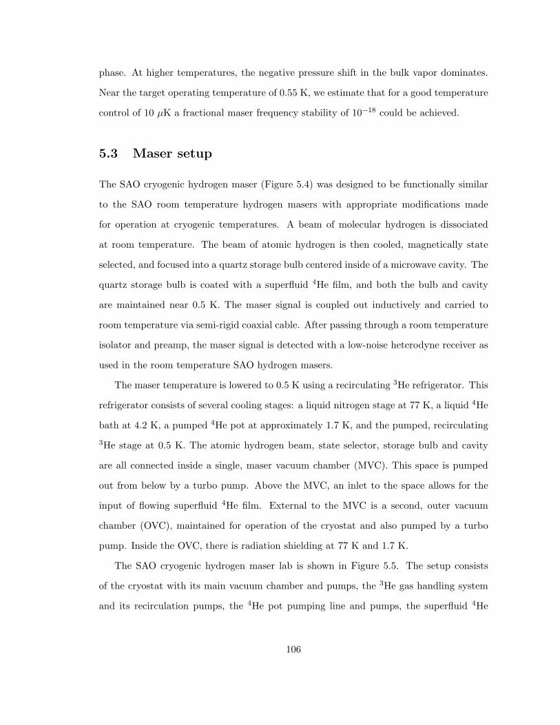
phase. At higher temperatures, the negative pressure shift in the bulk vapor dominates.

Near the target operating temperature of 0.55 K, we estimate that for a good temperature

control of 10 µK a fractional maser frequency stability of 10−18 could be achieved.

5.3 Maser setup

The SAO cryogenic hydrogen maser (Figure 5.4) was designed to be functionally similar

to the SAO room temperature hydrogen masers with appropriate modifications made

for operation at cryogenic temperatures. A beam of molecular hydrogen is dissociated

at room temperature. The beam of atomic hydrogen is then cooled, magnetically state

selected, and focused into a quartz storage bulb centered inside of a microwave cavity. The

quartz storage bulb is coated with a superfluid 4He film, and both the bulb and cavity

are maintained near 0.5 K. The maser signal is coupled out inductively and carried to

room temperature via semi-rigid coaxial cable. After passing through a room temperature

isolator and preamp, the maser signal is detected with a low-noise heterodyne receiver as

used in the room temperature SAO hydrogen masers.

The maser temperature is lowered to 0.5 K using a recirculating 3He refrigerator. This

refrigerator consists of several cooling stages: a liquid nitrogen stage at 77 K, a liquid 4He

bath at 4.2 K, a pumped 4He pot at approximately 1.7 K, and the pumped, recirculating

3He stage at 0.5 K. The atomic hydrogen beam, state selector, storage bulb and cavity

are all connected inside a single, maser vacuum chamber (MVC). This space is pumped

out from below by a turbo pump. Above the MVC, an inlet to the space allows for the

input of flowing superfluid 4He film. External to the MVC is a second, outer vacuum

chamber (OVC), maintained for operation of the cryostat and also pumped by a turbo

pump. Inside the OVC, there is radiation shielding at 77 K and 1.7 K.

The SAO cryogenic hydrogen maser lab is shown in Figure 5.5. The setup consists

of the cryostat with its main vacuum chamber and pumps, the 3He gas handling system

and its recirculation pumps, the 4He pot pumping line and pumps, the superfluid 4He

106

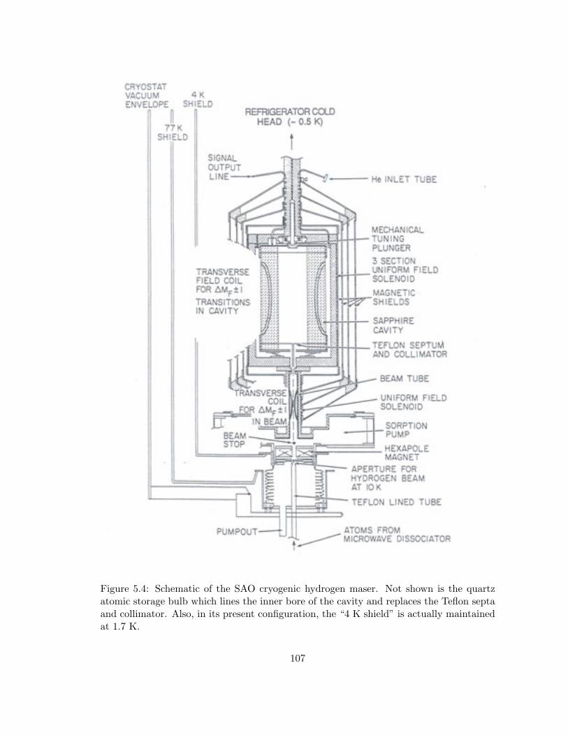
Figure 5.4: Schematic of the SAO cryogenic hydrogen maser. Not shown is the quartzatomic storage bulb which lines the inner bore of the cavity and replaces the Teflon septaand collimator. Also, in its present configuration, the “4 K shield” is actually maintainedat 1.7 K.

107

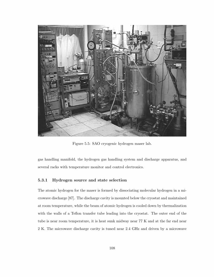
Figure 5.5: SAO cryogenic hydrogen maser lab.

gas handling manifold, the hydrogen gas handling system and discharge apparatus, and

several racks with temperature monitor and control electronics.

5.3.1 Hydrogen source and state selection

The atomic hydrogen for the maser is formed by dissociating molecular hydrogen in a mi-

crowave discharge [87]. The discharge cavity is mounted below the cryostat and maintained

at room temperature, while the beam of atomic hydrogen is cooled down by thermalization

with the walls of a Teflon transfer tube leading into the cryostat. The outer end of the

tube is near room temperature, it is heat sunk midway near 77 K and at the far end near

2 K. The microwave discharge cavity is tuned near 2.4 GHz and driven by a microwave

108

generator2 at about 40 W. A microwave isolator3 between the generator and the discharge

prevents frequency pulling of the generator. The molecular hydrogen pressure is regu-

lated with a pressure controller4 and maintained at approximately 1 Torr. The resulting

beam of atomic hydrogen flows upward into the cryostat and is ultimately thermalized to

10 K by the 0.210” diameter Teflon tube and a 3 mm diameter copper nozzle, shown in

Figure 5.4.

The 10 K beam of atomic hydrogen entering the cryostat consists of a near uniform

population distribution between the four atomic hyperfine states. The population inver-

sion necessary for maser action is created using magnetic state selection with a hexapole

magnet. After passing through the magnet, atoms in states |1〉 and |2〉 are focused into the

maser storage bulb while those in states |3〉 and |4〉 are defocused from the beam. Since

the focusing of the hexapole is dependent on the velocity of the atoms, the thermalizing

copper nozzle’s temperature is monitored and adjusted (via a resistive heater) to optimize

the population inversion flux. In practice, the nozzle temperature is set to maximize the

maser power.

Since the 10 K atoms travel much slower than room temperature atoms, the low

temperature hexapole magnet is significantly shorter that the room temperature hexapole.

The cryogenic hexapole is about 1.3 cm in length, with a 3 mm bore diameter. The

radial field is zero on axis and grows to about 0.88 T at the pole tips. A small beam

stop mounted on axis at the exit of the magnet blocks undeflected atomic hydrogen and

residual molecular hydrogen from entering the storage bulb.

Nominally, atoms in low-field-seeking states |1〉 and |2〉 are focused into the maser

interaction region. After a few seconds, these atoms escape from the storage bulb and

return toward the focusing region where they, along with the high-field-seeking atoms

that were deflected out of the atomic beam, are pumped away with an activated charcoal

filled sorption pump (see Figure 5.4). (The sorption pump also acts to pump away the2Raytheon Microtherm, 2.45 GHz, 0 - 100 W.3Alcatel model 20A111-11 coaxial isolator, 2.3 - 2.7 GHz.4Edwards model 1501B pressure controller.

109

superfluid 4He which has flowed from the atomic storage bulb). The sorption pump is

constructed from two (largely copper) circular plates, about 24 cm in diameter and spaced

about 4 cm apart. The plates are connected using six tubes of low thermal conductance

Vespel.5 The top copper plate of the sorption pump is in thermal contact with the maser

(0.5 K) while the bottom copper plate is in thermal contact with the 4He pot (1.7 K). The

vacuum seal on the outer rim of the sorption pump (separating the MVC from the OVC)

is made with a 0.010” thick Kapton6 film epoxied around the perimeter of the plates with

Stycast7 1266 epoxy.

The atoms focused into a beam by the state selecting hexapole travel through a 15

cm long (1.5 cm inner diameter) copper beam tube before entering the storage bulb. To

maintain a static quantization field in this region, a small solenoid “neck coil” was installed

inside the beam tube. This coil is about 4.5 cm long and contains about 160 turns of 30

AWG copper wire. Applying a field with this coil was seen to have only a small effect on

overall maser power. Typically, a field of about 100 mG was found to optimize the power.

About 2 mA of current was needed to produce this field, resulting in an insignificant 30

µW of heating.

In addition to the neck coil, a small coil capable of producing a transverse rf field was

installed into the beam tube. This coil could be used to drive F = 1, ∆mF = ±1 Zeeman

transitions in the incident atomic beam and therefore to alter the population distribution

among the atoms in the beam. For a field with a Rabi frequency large compared to the

inverse transit time of the atoms in the beam tube, the populations of the F = 1 states

would be essentially equalized. These rectangular rf coils were 5 cm long and 1.5 cm wide

and mounted so that the current in each coil had the same direction. Each coil had 15

turns of 32 AWG copper wire. A field of about 13 mG, which would have twice the Rabi

frequency needed to mix the states during the atoms’ transit time, is produced by 0.9 mA

which would add about 7 µW of heating to the maser. The neck coil and the rf coil were5Vespel is a trademark of E.I. duPont de Nemours and Co., Inc.6Kapton is a trademark of E.I. duPont de Nemours and Co., Inc.7Stycast is a trademark of Emerson and Cuming.

110

both wound around a Kapton form 5 cm in length and 1.3 cm in diameter and inserted

into the copper beam tube.

5.3.2 Maser interaction region

The state selected atoms travel through the beam tube into the maser interaction region

where they enter the quartz storage bulb centered inside the maser’s microwave cavity. In

contrast to a room temperature maser cavity, which is entirely evacuated, the cryogenic

maser cavity is dielectric loaded to reduce the physical size of the 1420 MHz resonant

cavity, and hence make the cavity more suitable for housing in a cryostat. The microwave

cavity, shown in Figure 5.6, is constructed from single crystal sapphire cut into a cylinder

17 cm long and 10 cm in diameter. An inner bore, 4.5 cm in diameter has been cut and

a quartz storage bulb is placed in this region. A pair of copper endcaps, at each end of

the sapphire cylinder, and a thin layer of silver deposited around the outer surface of the

cylinder serve as the electrically conducting surfaces which establish the TE011 microwave

cavity mode. The two copper endcaps are thermally connected with a copper braid, and

the entire cavity (sapphire cylinder plus endcaps) is sealed within a copper enclosure (the

“copper pot”) which separates the MVC and OVC and keeps the entire cavity in thermal

equilibrium. The copper enclosure is vacuum sealed using 1 mm diameter indium wire.

We note that since indium is a superconductor below 3.4 K [88], its presence leads to

difficulties in removing unwanted (and applying desired) magnetic field gradients with the

solenoid assembly.

A 1.5” diameter copper disk has been installed at the upper end of the microwave

cavity which can be inserted and withdrawn into the cavity in order to tune the cavity’s

resonance frequency. This depth of this spring-loaded tuning plunger into the cavity can

be set with a tuning knob easily accessible at the top of the cryostat, and the full tuning

range is approximately 1 MHz.

Microwave signals are coupled into and out of the cavity inductively using a near-

critically coupled inductive pickup loop, with a total area of about 1 cm2. The loop is

111

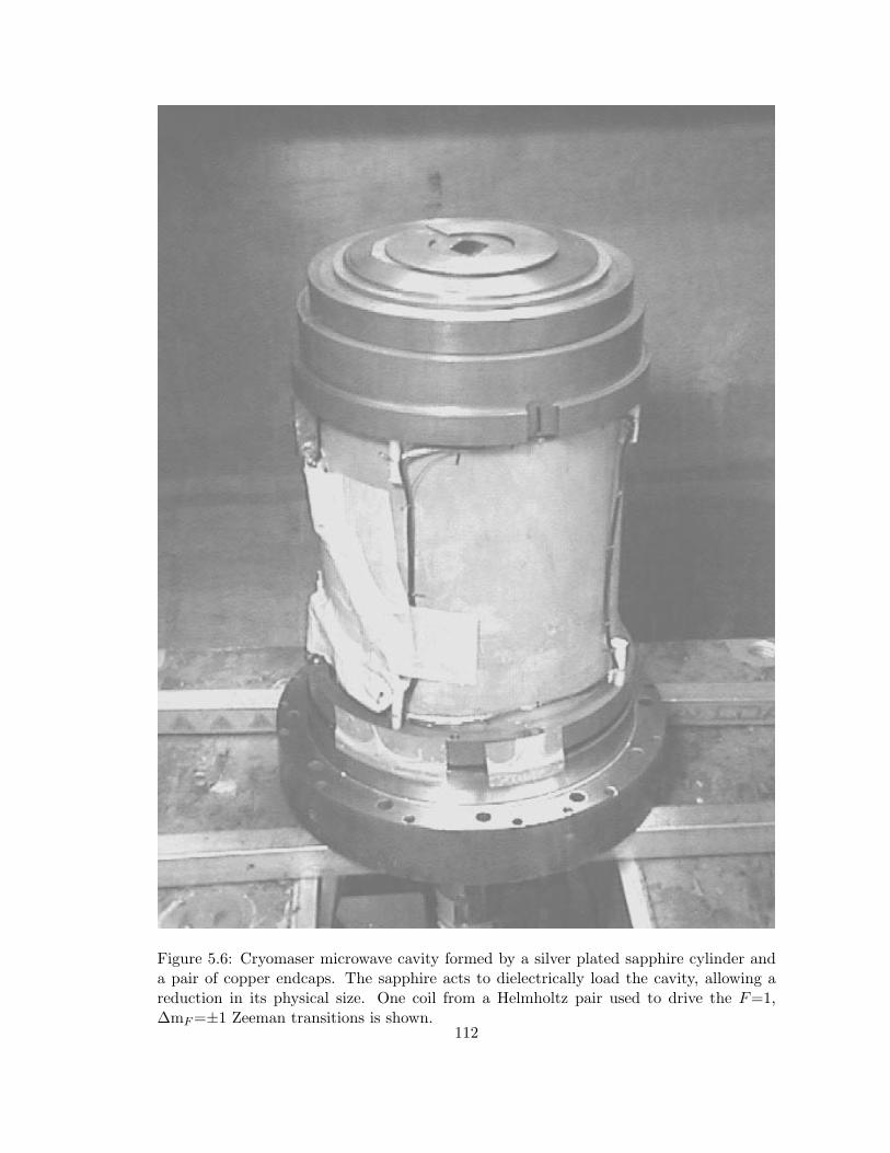
Figure 5.6: Cryomaser microwave cavity formed by a silver plated sapphire cylinder anda pair of copper endcaps. The sapphire acts to dielectrically load the cavity, allowing areduction in its physical size. One coil from a Helmholtz pair used to drive the F=1,∆mF =±1 Zeeman transitions is shown.

112

mounted at the top of the microwave cavity and oriented to maximize the flux of the

microwave cavity’s radial magnetic field through the loop. The loop is coupled to a

50 Ω semi-rigid coaxial line through a superfluid-leak-tight SMA feedthrough. At room

temperature, the cavity resonant frequency is about 1410.5 MHz with a loaded cavity-Q

(i.e., including losses due to coupling of power out through the pickup loop) of about

13,000 (full width ≈ 110 kHz) and a cavity coupling coefficient of β = 0.15. As the

microwave cavity is cooled to 0.5 K, it’s dimensions contract and the resistive losses are

reduced. At 0.5 K, the cavity frequency can be tuned to the atomic hyperfine frequency

of 1,420,405,752 Hz, it’s loaded cavity-Q increases to about 27,000 (full width ≈ 53 kHz),

and the cavity coupling coefficient increases nearly to β = 0.33.

As discussed in Chapter 3, each SAO room temperature hydrogen maser is equipped

with a varactor diode, inductively coupled via a second coupling loop to the cavity, which

serves for resettable fine tuning of the cavity frequency. To date, the cryogenic hydrogen

maser has not been equipped with a second coupling port so this tuning scheme was not

utilized. An attempt was made, however, to put a tuning diode in series with the single

coupling loop. This diode was reverse biased with a positive voltage applied to the inner

conductor of the semi-rigid coaxial cable used to couple out the maser signal (the negative

terminal of the diode was kept at ground). When back biased, this diode shifted the

microwave cavity frequency and it allowed for a resettable tuning range of approximately

10 kHz with only a mild modification of the cavity-Q and cavity coupling. Unfortunately,

the diode that was installed had a small residual magnetism (tens of µG up to an inch

away) so it generated a non-uniform DC magnetic field in close proximity to the atomic

ensemble. This field inhomogeneity acted to decohere the atomic ensemble enough so that

active maser oscillation could not be achieved.

Once the small field inhomogeneity was discovered, the diode was immediately re-

moved. A number of attempts were then made to connect a varactor diode in parallel

with the coupling loop, outside the cryostat, using various directional couplers. While this

allowed for the placement of the diode outside of the maser’s magnetic shields (eliminating

113

any ill-consequence of diode magnetic fields), it was found that due to reflections in the

transmission line, no significant, resettable tuning of the resonant cavity could be achieved.

Therefore, the cryogenic hydrogen maser is currently limited to mechanical tuning using

the tuning plunger.

As described in Section 5.2, a superfluid 4He film is used to coat the surface of the

atomic storage region to reduce the interaction between the atoms and the storage region

wall. As originally designed, the Teflon-coated inner bore of the sapphire cylinder served

as the atomic storage region (with Teflon septa making the two ends) and the superfluid

film simply flowed into the cavity from an inlet port and coated these walls. However,

when operated in this configuration, the stability of the cryogenic maser was degraded and

the maser frequency was found to be excessively sensitive to 4He flow and temperature;

indeed, the cryogenic maser was less stable than a room temperature maser for averaging

times over 100 s. It was postulated that the source of this poor performance was a large

frequency shift caused by the interaction between the masing atoms and paramagnetic

impurities in the underlying sapphire crystal. Since this frequency shift will depend on

the distance between the atoms and the impurities in the wall, and therefore the thickness

of the superfluid helium film, fluctuations in this film thickness will lead to instability in

the maser oscillation frequency. Therefore, it was decided to install a quartz maser bulb

into the inner bore of the sapphire cylinder to create an inert “buffer” between the masing

atoms and the sapphire wall.

A quartz bulb was designed (Figure 5.7) and constructed8 to fit snugly into the inner

bore of the sapphire. This bulb provides an approximately 0.025” thickness of inert quartz

between the atoms and the sapphire wall. A transfer tube was constructed out of fine

copper capillary (0.020” OD) to transport the superfluid from the cavity inlet port into

the inner space of the bulb through an inlet spout. The copper capillary was epoxied

with Stycast 2850 at the film entrance aperture into the cavity and at the inlet spout of

the bulb. The transfer tube was coiled around one full turn between the copper tuning8Mikoski Inc. Fused Quartz and Glass Specialists, Stow, MA.

114

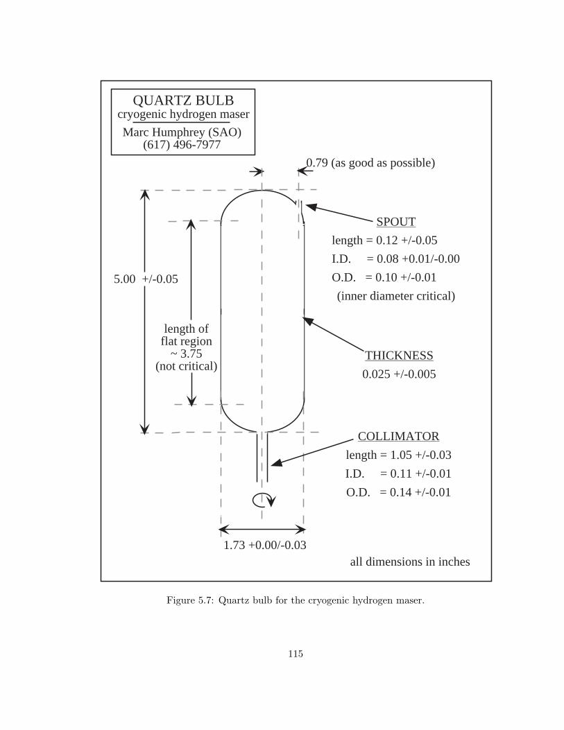
0.79 (as good as possible)

SPOUT

length = 0.12 +/-0.05

I.D. = 0.08 +0.01/-0.00

O.D. = 0.10 +/-0.01

(inner diameter critical)

length offlat region

~ 3.75(not critical)

COLLIMATOR

length = 1.05 +/-0.03

I.D. = 0.11 +/-0.01

O.D. = 0.14 +/-0.01

1.73 +0.00/-0.03

THICKNESS

0.025 +/-0.005

QUARTZ BULBcryogenic hydrogen maser

all dimensions in inches

Marc Humphrey (SAO)(617) 496-7977

5.00 +/-0.05

Figure 5.7: Quartz bulb for the cryogenic hydrogen maser.

115

plunger disk and the end of the cavity to provide elasticity and to maintain the radial

symmetry inside of the microwave cavity. The tube caused a slight (5%) decrease in the

cavity-Q.

The flow of superfluid helium is regulated at room temperature with a mass flow

controller,9 typically set near 0.2 standard cubic centimeters per minute. The regulated

4He gas flows into the cryostat, is thermalized at 77 K and 4 K, and then passes through

a flow impedance at about 1.7 K. The flow impedance liquifies the helium, which is then

thermalized at a 0.5 K heat sink before entering the maser bulb. The superfluid film enters

the bulb, evenly coats the quartz surface, and then drains out the entrance collimator

into the beam tube. The helium film is eventually vaporized at higher temperatures in

the focusing region and adsorbed by the activated charcoal sorption pump. As will be

described in Section 5.5.2, the CHM could only be operated with thin, unsaturated 4He

films.

The helium film in the beam tube will produce a helium vapor above it which will

attenuate the flow of hydrogen into the storage bulb (see Figure 5.3). Since the vapor

pressure increases with temperature, every effort is made to reduce the base temperature

of the maser and the temperature of the surfaces between the focusing region and the

maser interaction region. Because of the hydrogen beam attenuation, the maser would

not oscillate at maser temperatures above about 540 mK.

A pair of transverse rf-field-producing coils is mounted to the external surface of the

microwave cavity sapphire. These coils are used to drive F = 1, ∆mF = ±1 Zeeman

transitions in the atomic ensemble for double resonance maser studies. These rectangular

coils are 3 18” × 3 3

4” and constructed from 20 turns of 32 AWG copper wire. The rf

field generated by these coils is slightly screened by the thin layer of silver deposited on

the external surface of the sapphire cylinder, however a current of 0.8 mA (dissipating

0.009 µW) is sufficient to produce a field strong enough to uniformly mix the F = 1

state populations on the order of 1 ms. These transverse field “Zeeman” coils (shown in9Brooks Instrument Division model 5850E mass flow controller.

116

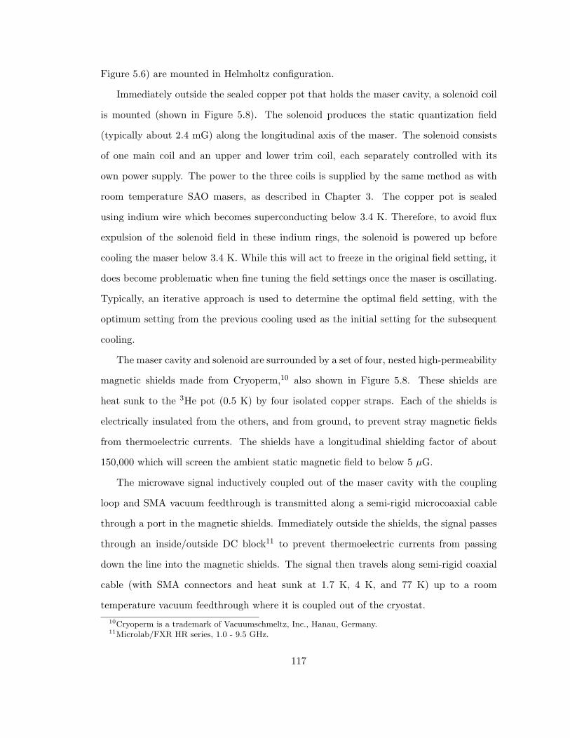
Figure 5.6) are mounted in Helmholtz configuration.

Immediately outside the sealed copper pot that holds the maser cavity, a solenoid coil

is mounted (shown in Figure 5.8). The solenoid produces the static quantization field

(typically about 2.4 mG) along the longitudinal axis of the maser. The solenoid consists

of one main coil and an upper and lower trim coil, each separately controlled with its

own power supply. The power to the three coils is supplied by the same method as with

room temperature SAO masers, as described in Chapter 3. The copper pot is sealed

using indium wire which becomes superconducting below 3.4 K. Therefore, to avoid flux

expulsion of the solenoid field in these indium rings, the solenoid is powered up before

cooling the maser below 3.4 K. While this will act to freeze in the original field setting, it

does become problematic when fine tuning the field settings once the maser is oscillating.

Typically, an iterative approach is used to determine the optimal field setting, with the

optimum setting from the previous cooling used as the initial setting for the subsequent

cooling.

The maser cavity and solenoid are surrounded by a set of four, nested high-permeability

magnetic shields made from Cryoperm,10 also shown in Figure 5.8. These shields are

heat sunk to the 3He pot (0.5 K) by four isolated copper straps. Each of the shields is

electrically insulated from the others, and from ground, to prevent stray magnetic fields

from thermoelectric currents. The shields have a longitudinal shielding factor of about

150,000 which will screen the ambient static magnetic field to below 5 µG.

The microwave signal inductively coupled out of the maser cavity with the coupling

loop and SMA vacuum feedthrough is transmitted along a semi-rigid microcoaxial cable

through a port in the magnetic shields. Immediately outside the shields, the signal passes

through an inside/outside DC block11 to prevent thermoelectric currents from passing

down the line into the magnetic shields. The signal then travels along semi-rigid coaxial

cable (with SMA connectors and heat sunk at 1.7 K, 4 K, and 77 K) up to a room

temperature vacuum feedthrough where it is coupled out of the cryostat.10Cryoperm is a trademark of Vacuumschmeltz, Inc., Hanau, Germany.11Microlab/FXR HR series, 1.0 - 9.5 GHz.

117

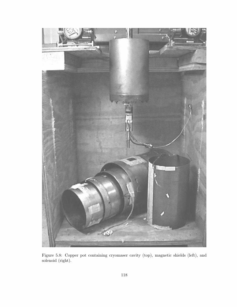
Figure 5.8: Copper pot containing cryomaser cavity (top), magnetic shields (left), andsolenoid (right).

118

5.3.3 Steady state operation

During normal, steady state maser oscillation, the raw maser signal coupled out of the

cryostat (10−14 W at 1420 MHz) is passed through an rf isolator and then into a room

temperature preamplifier12 which provides a gain of 41 dB with a maximum noise figure of

1.0 dB. The amplified signal at 1420. . . MHz is then passed directly into the low-noise het-

erodyne receiver, described in detail in Chapter 3 and shown schematically in Figure 5.9.

By phase locking a high quality, voltage controlled crystal oscillator (VCXO), the receiver

converts the amplified maser signal (10−10 W at 1420. . . MHz) into a more useful reference

signal (10 mW at 5, 100 and 1200 MHz).

The SAO laboratory is equipped with a pair of room temperature masers which serve

as “house” frequency references, masers P-8 and P-13. By comparing the cryogenic maser

directly against one of these sources, its stability relative to a room temperature maser

can be determined. Each of the masers (cryogenic and room temperature) has its own

independent receiver with its own phase locked voltage controlled crystal oscillator. To

compare two masers, the relative output frequency of their oscillators is adjusted by tuning

the receivers’ synthesizers so that there is approximately a 1.2 Hz offset between them.

These two signals are then combined with a double-balanced mixer, and the resulting 0.8 s

beat note is averaged over 10 or 100 s intervals with a frequency counter.13 By combining

these 10 and 100 s averages, the relative Allan variance of the two masers being compared

can be determined for various averaging times, and the Allan variance can be calculated

independently using DOS and LabVIEW programs.

In order to measure the absolute frequency stability of the cryogenic maser, it would

have to be compared to a device with equal or better frequency stability. However, there

exists a method in which the cryogenic maser can be compared with the two different

room temperature masers in a “three cornered hat” configuration [89] to determine the

absolute frequency stability of each maser.12MITEQ model AFS3-01300150-10-10P-4, 1.3 - 1.5 GHz.13Hewlett-Packard model HP 5334B (for DOS program) and Hewlett-Packard model HP 53131A (for

LabVIEW program).

119

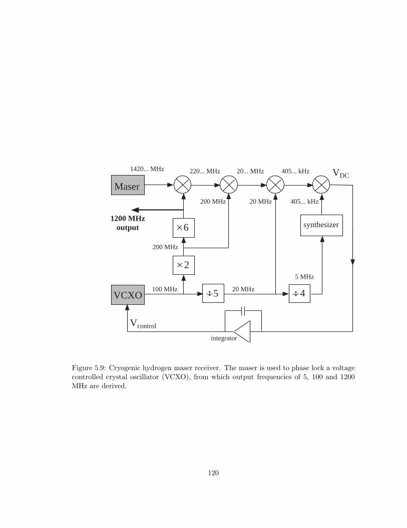
Maser

VCXO. 5.

2

synthesizer

100 MHz 20 MHz

5 MHz

200 MHz

200 MHz 20 MHz 405... kHz

1420... MHz 220... MHz 20... MHz 405... kHz VDC

Vcontrol

integrator

1200 MHzoutput

4..

6

Figure 5.9: Cryogenic hydrogen maser receiver. The maser is used to phase lock a voltagecontrolled crystal oscillator (VCXO), from which output frequencies of 5, 100 and 1200MHz are derived.

120

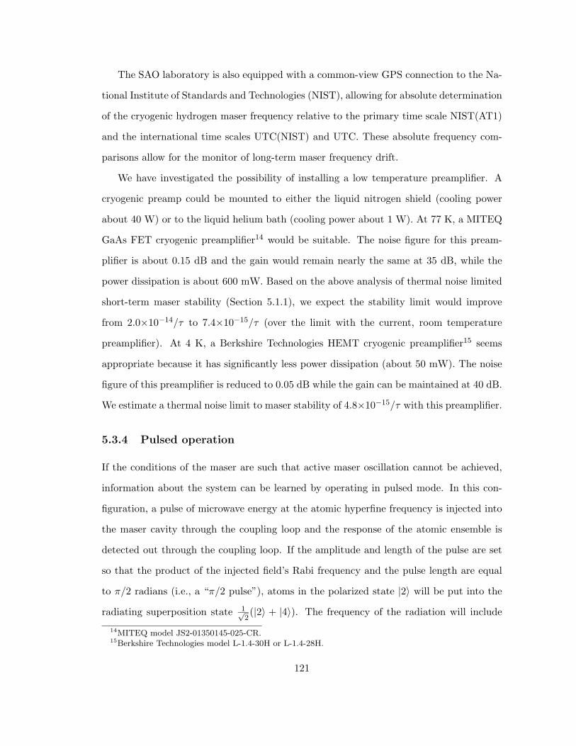
The SAO laboratory is also equipped with a common-view GPS connection to the Na-

tional Institute of Standards and Technologies (NIST), allowing for absolute determination

of the cryogenic hydrogen maser frequency relative to the primary time scale NIST(AT1)

and the international time scales UTC(NIST) and UTC. These absolute frequency com-

parisons allow for the monitor of long-term maser frequency drift.

We have investigated the possibility of installing a low temperature preamplifier. A

cryogenic preamp could be mounted to either the liquid nitrogen shield (cooling power

about 40 W) or to the liquid helium bath (cooling power about 1 W). At 77 K, a MITEQ

GaAs FET cryogenic preamplifier14 would be suitable. The noise figure for this pream-

plifier is about 0.15 dB and the gain would remain nearly the same at 35 dB, while the

power dissipation is about 600 mW. Based on the above analysis of thermal noise limited

short-term maser stability (Section 5.1.1), we expect the stability limit would improve

from 2.0×10−14/τ to 7.4×10−15/τ (over the limit with the current, room temperature

preamplifier). At 4 K, a Berkshire Technologies HEMT cryogenic preamplifier15 seems

appropriate because it has significantly less power dissipation (about 50 mW). The noise

figure of this preamplifier is reduced to 0.05 dB while the gain can be maintained at 40 dB.

We estimate a thermal noise limit to maser stability of 4.8×10−15/τ with this preamplifier.

5.3.4 Pulsed operation

If the conditions of the maser are such that active maser oscillation cannot be achieved,

information about the system can be learned by operating in pulsed mode. In this con-

figuration, a pulse of microwave energy at the atomic hyperfine frequency is injected into

the maser cavity through the coupling loop and the response of the atomic ensemble is

detected out through the coupling loop. If the amplitude and length of the pulse are set

so that the product of the injected field’s Rabi frequency and the pulse length are equal

to π/2 radians (i.e., a “π/2 pulse”), atoms in the polarized state |2〉 will be put into the

radiating superposition state 1√2(|2〉 + |4〉). The frequency of the radiation will include

14MITEQ model JS2-01350145-025-CR.15Berkshire Technologies model L-1.4-30H or L-1.4-28H.

121

the hyperfine frequency plus any shifts such as cavity pulling or collisional shifts. If the

atomic magnetization is sufficiently weak that radiation damping can be neglected, the

amplitude of the radiation from the superposition state will decay exponentially with a

time constant given by the decoherence time T2. Such an exponentially damped sinusoidal

signal is termed a “ringdown” or a free induction decay (FID).

The electronics used for pulsed operation include those for the generation of the pulse

and those for the signal detection (see Figure 5.10). A directional coupler, installed at

the maser output just outside the cryostat, allows the injected pulse into the cavity while

coupling the atomic response out. A frequency synthesizer, set near the atomic hyperfine

frequency is gated by pulse shaping electronics which set the length of the pulse as well

as the interval between pulses. The output of the pulse shaping electronics is injected

into the maser cavity. The atomic signal is input into an open-loop heterodyne receiver

which mixes the 1420.405. . . MHz signal down to 405. . . kHz, then mixes it further with a

tunable synthesizer. The resulting damped beat note can be displayed on an oscilloscope

or sampled with data acquisition software triggered by the pulse shaping electronics. Both

synthesizers and the open loop receiver are all locked to a 5 MHz reference signal from an

SAO room temperature hydrogen maser.

Four types of information about the below-oscillation-threshold maser can be gained

from the free induction decay signals. By calibrating the receiver with a synthesizer

of known amplitude, the amplitude of the maser signal can be determined. By tuning

the reference synthesizer for the open loop receiver so that the output signal has a zero

beat, the maser frequency can be determined. By fitting an exponential decay envelope

to the free induction decay, an estimate of the atomic hyperfine decoherence time T2 can

measured. Finally, by applying more sophisticated pulse sequences to the atomic ensemble,

an estimate of the population decay time T1 can also be made.

While monitoring the free induction decays, various maser parameters (such as hydro-

gen discharge pressure and power, hydrogen nozzle temperature, superfluid film flow, and

main solenoid and trim field settings) can be tuned to maximize the signal amplitude,

122

-2.0

-1.0

0.0

1.0

2.0

1.51.00.50.0

20 dB dir. coupler 20 dB dir. coupler

terminator

terminator

isolator

isolatormaser

computer

cryostat

open loopreceiver

synthesizer

terminator

oscilloscope

1,420,405,751 Hz

pulse shapingpanel

synthesizer405,765.82 Hz

DAQ card

trigger

Figure 5.10: Electronics configuration for pulsed maser operation. See Section 5.3.4 fordetails.

123

reduce maser frequency shifts, or lengthen the decoherence or population decay times.

5.4 3He refrigerator

The refrigeration requirements for the SAO cryogenic hydrogen maser are a base temper-

ature near 0.5 K and, equally important, a relatively large amount of cooling power. The

latter requirement comes from the relatively large thermal mass of the system and as a

result of the steady flow of hydrogen gas and superfluid 4He into the maser during oper-

ation. A pumped, recirculating 3He refrigerator best meets these criteria. The SAO 3He

cryostat was constructed from a modified 4 K liquid 4He cryostat used by the SAO group

for early investigations into cold hydrogen maser wall coatings [79]. It’s transformation

into a recirculating 3He cryostat was undertaken by Alabama Cryogenic Engineering in

collaboration with SAO and Harvard scientists.

Various constraints during the initial development of the SAO CHM led to a very

cramped cryostat design. These limited the cryostat to only two vacuum spaces and

reduced the vertical length of the device which leads to reduced isolation from the envi-

ronment (hence higher heat loads) and requires increased cooling power.

The cryostat, shown schematically in Figure 5.11 contains two vacuum spaces and four

thermal zones. The vacuum spaces, described above, include the outer vacuum chamber

(OVC) used to evacuate gases from the cold regions of the cryostat and the maser vacuum

chamber (MVC) used for the operation of the hydrogen maser. The thermal zones include

an outer liquid-nitrogen-cooled shield at 77 K, a liquid 4He bath at 4.2 K, a pumped 4He

pot at 1.7 K, and the pumped 3He pot and recirculation system at about 0.5 K.

5.4.1 Vacuum system

The entire maser is sealed within a large, room temperature vacuum tank. A 450 liter/s

turbomolecular pump16 evacuates, in parallel, the OVC through a 2.75” Conflat flange

and the MVC through a 1/4” tube with an o-ring seal. The pressure of both of these16Leybold TURBOVAC model 450.

124

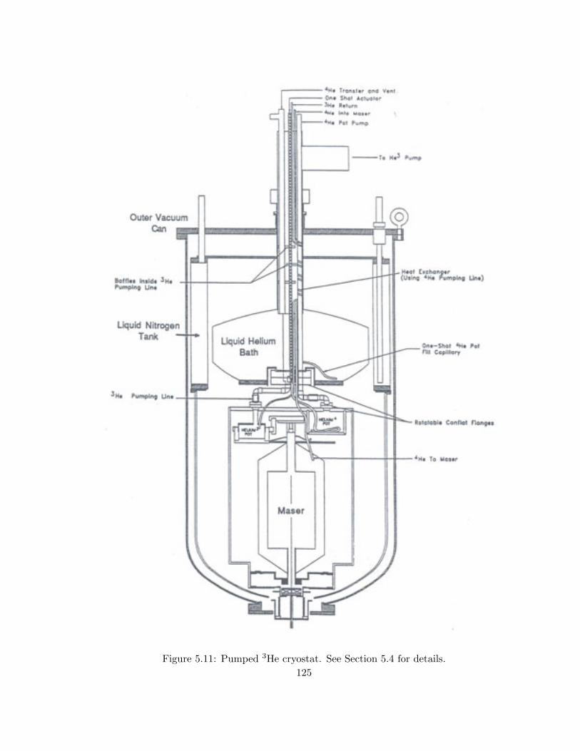
Figure 5.11: Pumped 3He cryostat. See Section 5.4 for details.125

regions is monitored with an ion gauge17 and, while operating, is typically less than 10−8

Torr. A second, 145 liter/s turbomolecular pump18 is used to evacuate the hydrogen gas

manifold, the 3He gas handling manifold, and the 4He manifold for the superfluid 4He film

prior to operation.

5.4.2 Liquid nitrogen shield

As shown in Figure 5.11, immediately inside the vacuum chamber is a liquid nitrogen

cooled radiation shield that surrounds the rest of the cryostat. The top half of this shield

is an annular, liquid nitrogen filled jacket; the bottom half is a large copper hemisphere

which is bolted into good thermal contact with the jacket. Both inner and outer surfaces

of the liquid nitrogen shield are covered with highly reflective superinsulation to prevent

the absorption of radiation. The shield, which holds nearly 30 l, requires filling about

once every 36 hours, implying that there is a 40 W heat load on this thermal zone (liquid

nitrogen latent heat = 160 kJ/l at 77 K).

5.4.3 Liquid 4He bath

Inside the liquid nitrogen shield, a large liquid 4He bath is suspended by thin walled

stainless steel tubing. The bath is accessed from above by a 0.5” ID stainless steel tube

which serves as an inlet and exhaust port. This bath, also having a capacity of about 30

l, requires filling about once every 25 hours during steady state operation. This implies

that there is a heat load of 900 mW on the bath (liquid helium latent heat = 2.6 kJ/l at

4.2 K), due to thermal conduction through the support structures above and below and

due to thermal radiation.

The temperature of the bath is monitored with a silicon diode temperature sensor19

which has an operating range down to 1.4 K. In addition, a set of three 75 W power

resistors are bolted in series to the base of the bath in order to quickly boil off its contents17Varian Smart Gauge model 973-5028.18Leybold TURBOVAC model 151.19Lake Shore Cryotronics DT-470 Si diode with Lake Shore model 201 temperature monitor.

126

when necessary.

5.4.4 Pumped liquid 4He pot

Below the liquid 4He bath, the pumped liquid 4He pot is situated. The 4He pot is filled

by a small transfer tube from the 4He bath, and connected through an exhaust port to a

large mechanical pump. By pumping on the pot, the vapor pressure of the 4He is lowered,

therefore lowering the temperature. Typically, the 4He pot is pumped down to below 10

Torr, resulting in a temperature below 2 K.

The 4He pot is constructed of copper and has a volume of about 500 cm3. It is in good

thermal contact with a copper platform (the “2K plate”), about 12 inches in diameter. To

this platform are mounted numerous thermal sinks for electric leads, the superfluid 4He

film input line, and the 3He recirculation input line.

The 4He pot is suspended by low thermal conductivity stainless steel tubing. In ad-

dition, a graphite “heat switch” has been installed between the liquid 4He bath and 4He

pot, which utilizes the property that graphite has moderately high thermal conductivity at

higher temperatures (102 W/mK at 100 K) and a significantly lower thermal conductivity

at lower temperatures (10−3 W/mK at 1 K). Therefore, the 4He pot is in relatively good

thermal contact with the bath during the cooldown, while it is thermally isolated from

the bath at normal operating conditions.

Liquid 4He flows from the bath into the 4He pot through a stainless steel tube, which

is spiral soldered to the bottom of the 4He pot to improve the thermal link between the

liquid and the copper pot, and the flow is regulated with an externally controlled needle

valve.

The pumping line of the 4He pot, made of 1/2” diameter stainless steel tubing from

the pot to the top of the cryostat, is heat sunk at 4 K and 77 K before reaching room

temperature. Room temperature pumping lines of 1.25” diameter extend to the inlet of

several mechanical pumps connected in parallel20 for a total pumping speed of about 250020Welch DuoSeal models 1397 and 1398.

127

liter/min. The pressure of the 4He pot is monitored at room temperature at the top of the

cryostat. Under normal operation, the 4He pot is cooled to about 1.75 K, corresponding

to a vapor pressure of about 11 Torr [88]. The cooling power of the 4He pot has been

measured and calculated [90] to be about 600 mW (latent heat of 4He = 87 J/mol at 1.7

K [91]).

During the cooldown process, the 4He pot temperature is measured using a silicon

diode temperature sensor.21 Below 2 K, however, a more accurate temperature reading

is made using a RuO2 resistive temperature sensor monitored with a bridge circuit (see

Section 5.4.6). A 1000 Ω metal film resistor is mounted to the 2K plate which allows for

temperature stabilization of this region if desired.

As depicted in Figure 5.11, a large, cylindrical radiation shield (the “2K shield”) is

suspended from the perimeter of the 2K plate. This copper shield, 12 inches in diameter

and about 20 inches in length, is in good thermal contact with the 2K plate and acts

to shield the 0.5 K maser region from thermal radiation from the 77 K radiation shield.

The outer surface of the 2K shield is covered with highly reflective superinsulation (to

minimize absorption of 77 K thermal radiation) while the inner surface is blackened (to

absorb radiation from the 0.5 K region). At the bottom of the 2K shield, the lower plate

of the sorption pump is pressed into good thermal contact at 1.7 K.

5.4.5 Pumped liquid 3He pot

The final stage of cooling is achieved using a recirculating liquid 3He system. Room

temperature 3He gas enters the cryostat, is liquified, and passes down to a 3He pot. The

3He pot is pumped to lower its vapor pressure, thereby cooling the 3He liquid and lowering

the 3He pot temperature. The 3He gas is pumped using hermetically sealed pumps behind

which the 3He is recollected. The gas is then input back into the cryostat, completing the

circuit.

The 3He pot is also constructed of copper and has a volume of about 200 cm3. Silver21Lake Shore Cryotronics DT-470 Si diode with Conductus LTC-20 temperature controller.

128

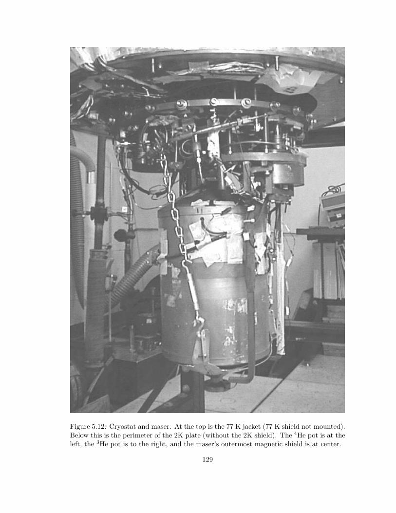
Figure 5.12: Cryostat and maser. At the top is the 77 K jacket (77 K shield not mounted).Below this is the perimeter of the 2K plate (without the 2K shield). The 4He pot is at theleft, the 3He pot is to the right, and the maser’s outermost magnetic shield is at center.

129

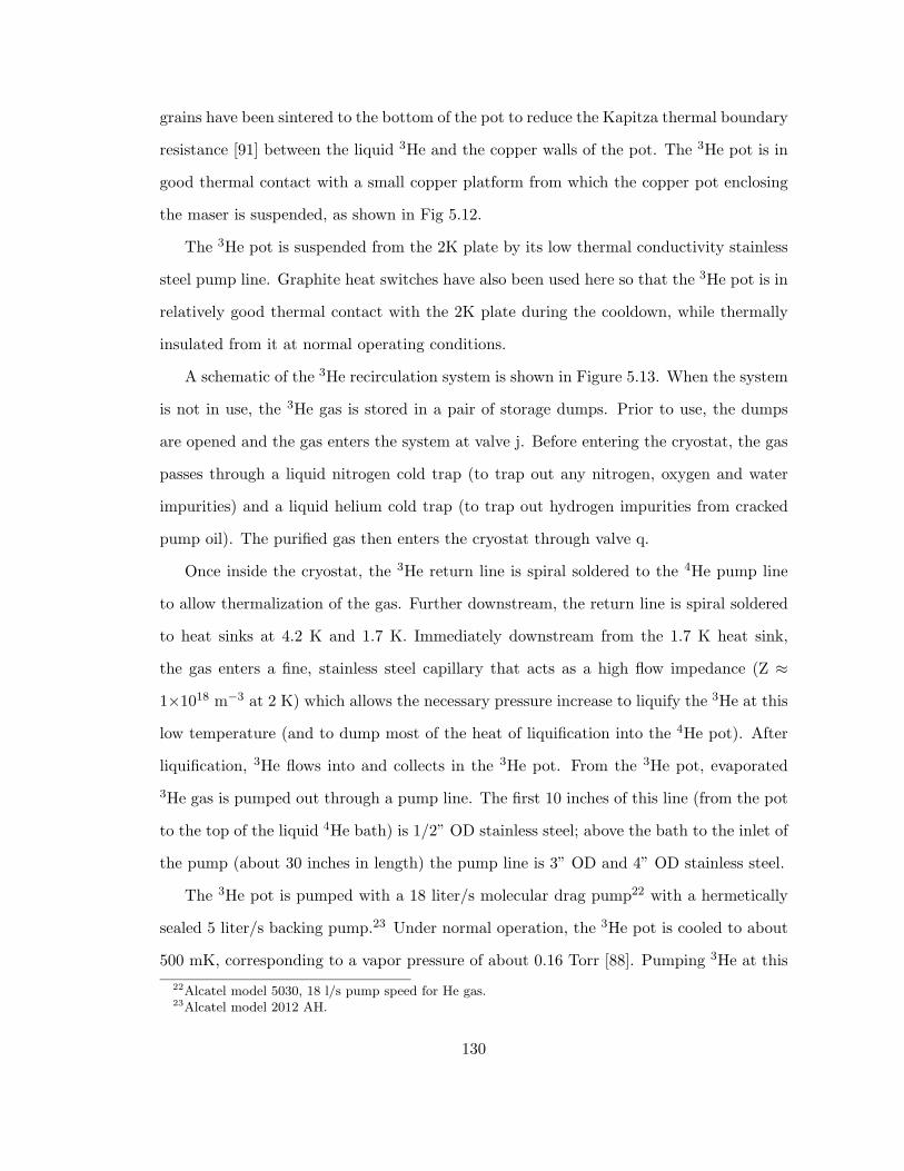
grains have been sintered to the bottom of the pot to reduce the Kapitza thermal boundary

resistance [91] between the liquid 3He and the copper walls of the pot. The 3He pot is in

good thermal contact with a small copper platform from which the copper pot enclosing

the maser is suspended, as shown in Fig 5.12.

The 3He pot is suspended from the 2K plate by its low thermal conductivity stainless

steel pump line. Graphite heat switches have also been used here so that the 3He pot is in

relatively good thermal contact with the 2K plate during the cooldown, while thermally

insulated from it at normal operating conditions.

A schematic of the 3He recirculation system is shown in Figure 5.13. When the system

is not in use, the 3He gas is stored in a pair of storage dumps. Prior to use, the dumps

are opened and the gas enters the system at valve j. Before entering the cryostat, the gas

passes through a liquid nitrogen cold trap (to trap out any nitrogen, oxygen and water

impurities) and a liquid helium cold trap (to trap out hydrogen impurities from cracked

pump oil). The purified gas then enters the cryostat through valve q.

Once inside the cryostat, the 3He return line is spiral soldered to the 4He pump line

to allow thermalization of the gas. Further downstream, the return line is spiral soldered

to heat sinks at 4.2 K and 1.7 K. Immediately downstream from the 1.7 K heat sink,

the gas enters a fine, stainless steel capillary that acts as a high flow impedance (Z ≈

1×1018 m−3 at 2 K) which allows the necessary pressure increase to liquify the 3He at this

low temperature (and to dump most of the heat of liquification into the 4He pot). After

liquification, 3He flows into and collects in the 3He pot. From the 3He pot, evaporated

3He gas is pumped out through a pump line. The first 10 inches of this line (from the pot

to the top of the liquid 4He bath) is 1/2” OD stainless steel; above the bath to the inlet of

the pump (about 30 inches in length) the pump line is 3” OD and 4” OD stainless steel.

The 3He pot is pumped with a 18 liter/s molecular drag pump22 with a hermetically

sealed 5 liter/s backing pump.23 Under normal operation, the 3He pot is cooled to about

500 mK, corresponding to a vapor pressure of about 0.16 Torr [88]. Pumping 3He at this22Alcatel model 5030, 18 l/s pump speed for He gas.23Alcatel model 2012 AH.

130

3Hestoragedump

1

M3

toturbopump

LN2,LHecoldtraps

toturbopump

moleculardrag

pump

zeolitetrap

oilmistfilter

butterflyvalve (c)

needlevalve (b)

high impedance3He return line

3He pot

M4

M1

M2

r

q

mkl

i

v

j

w u

d

pn

t

3Hestoragedump

2

tosorptionpump

sealedforepump

Figure 5.13: 3He recirculation system. Prior to use, the 3He is stored in the dumps atthe lower left. Under normal operation, 3He gas enters the cryostat at valve q, liquifies atthe flow impedance, and collects in the 3He pot. Evaporated gas is pumped away with amolecular drag pump and sealed forepump. A zeolite trap, oil mist filter, liquid nitrogencold trap and liquid helium cold trap purify the 3He gas before it reenters the cryostat.

131

speed and temperature (latent heat = 30 J/mol at 0.5 K [91]) gives a cooling power of the

3He pot to be about 5 mW. In the absence of flowing hydrogen and flowing superfluid 4He

film, the heat load on the 3He pot comes from conduction down the stainless steel pump

line, conduction up the Vespel rods through the sorption pump, conduction along the

maser signal coaxial cable, conduction along the numerous electrical leads, and thermal

radiation. Measurements of this heat load on the 3He pot give an estimate of 1.4 mW.

Oil vapor and its byproducts (such as H2) can be a serious problem for the 3He re-

circulation as these will be cryopumped at the cold regions of the return line and can

block the return of 3He. Therefore, a zeolite foreline trap is installed at the mechanical

pump inlet and an oil mist filter is installed at the mechanical pump exhaust. The liquid

nitrogen and liquid helium cold traps complete the removal of oil products from the 3He

gas supply. Both of the pumps are leak tight so that no 3He is lost from the system and

no contaminants leak in. The 3He pumped from the pot is then recollected in a room

temperature gas handling panel, where it passes through the cold traps and back into the

cryostat, thus completing the cycle.

During the cooldown process, the 3He pot and maser temperature are measured using

a silicon diode temperature sensor.24 Below 2 K, however, a more accurate temperature

reading is made using a RuO2 resistive temperature sensor monitored with a bridge cir-

cuit. For absolute temperature determination, we use a high quality germanium resistor

which was previously calibrated up to 600 mK by comparison with 3He vapor pressure

measurements. A 10 kΩ resistor, mounted to the 3He pot, serves as a heater. Using

the RuO2 sensor as a control thermometer and the resistive heater, we maintain thermal

control of the maser using a PID servoloop.25 Our system of thermometry and thermal

control will be described in detail in Section 5.4.6.24Lake Shore Cryotronics DT-470 Si diode with Conductus LTC-20 temperature controller.25Linear Research model LR-130 temperature controller.

132

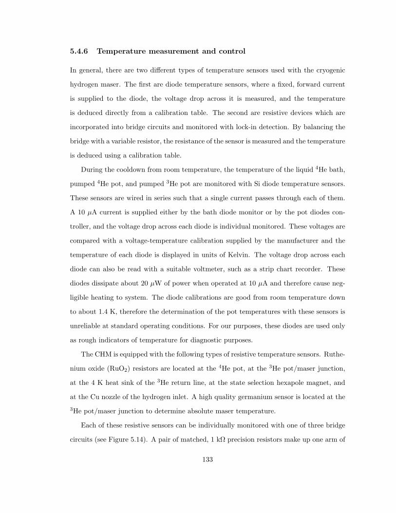
5.4.6 Temperature measurement and control

In general, there are two different types of temperature sensors used with the cryogenic

hydrogen maser. The first are diode temperature sensors, where a fixed, forward current

is supplied to the diode, the voltage drop across it is measured, and the temperature

is deduced directly from a calibration table. The second are resistive devices which are

incorporated into bridge circuits and monitored with lock-in detection. By balancing the

bridge with a variable resistor, the resistance of the sensor is measured and the temperature

is deduced using a calibration table.

During the cooldown from room temperature, the temperature of the liquid 4He bath,

pumped 4He pot, and pumped 3He pot are monitored with Si diode temperature sensors.

These sensors are wired in series such that a single current passes through each of them.

A 10 µA current is supplied either by the bath diode monitor or by the pot diodes con-

troller, and the voltage drop across each diode is individual monitored. These voltages are

compared with a voltage-temperature calibration supplied by the manufacturer and the

temperature of each diode is displayed in units of Kelvin. The voltage drop across each

diode can also be read with a suitable voltmeter, such as a strip chart recorder. These

diodes dissipate about 20 µW of power when operated at 10 µA and therefore cause neg-

ligible heating to system. The diode calibrations are good from room temperature down

to about 1.4 K, therefore the determination of the pot temperatures with these sensors is

unreliable at standard operating conditions. For our purposes, these diodes are used only

as rough indicators of temperature for diagnostic purposes.

The CHM is equipped with the following types of resistive temperature sensors. Ruthe-

nium oxide (RuO2) resistors are located at the 4He pot, at the 3He pot/maser junction,

at the 4 K heat sink of the 3He return line, at the state selection hexapole magnet, and

at the Cu nozzle of the hydrogen inlet. A high quality germanium sensor is located at the

3He pot/maser junction to determine absolute maser temperature.

Each of these resistive sensors can be individually monitored with one of three bridge

circuits (see Figure 5.14). A pair of matched, 1 kΩ precision resistors make up one arm of

133

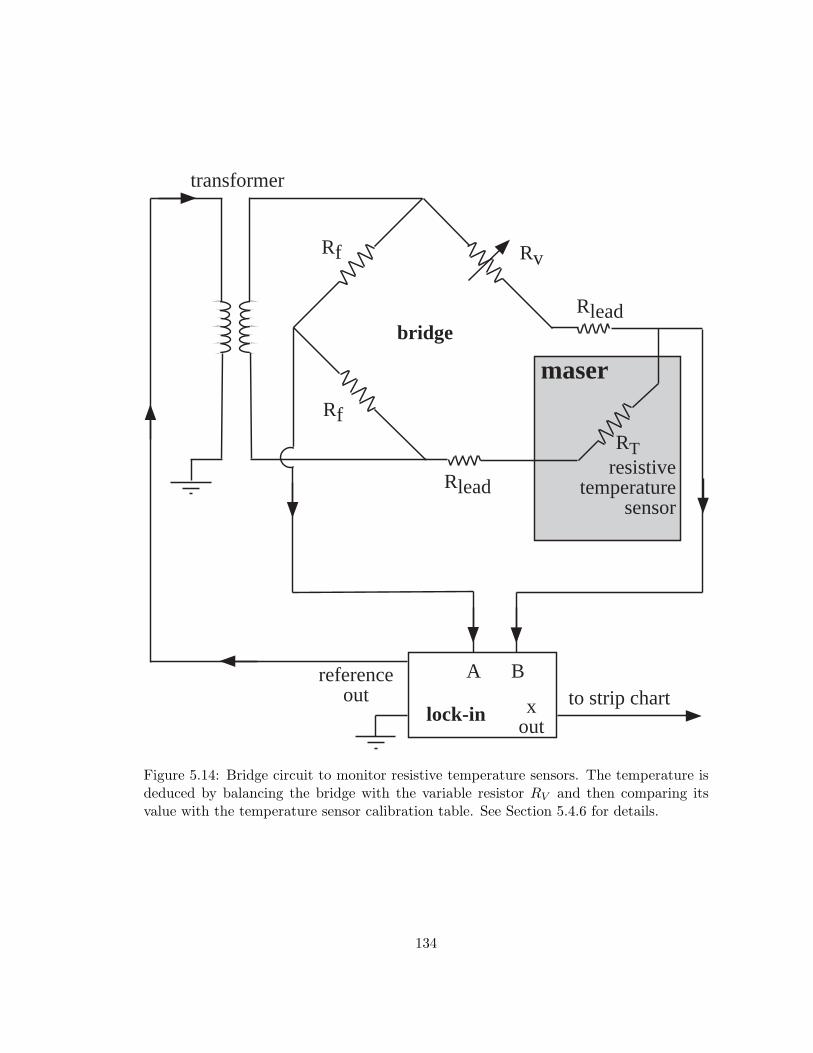
lock-in

A B

xout

referenceout

maser

RTresistive

temperaturesensor

Rf

Rf

Rv

transformer

bridge

Rlead

Rlead

to strip chart

Figure 5.14: Bridge circuit to monitor resistive temperature sensors. The temperature isdeduced by balancing the bridge with the variable resistor RV and then comparing itsvalue with the temperature sensor calibration table. See Section 5.4.6 for details.

134

a Wheatstone bridge while a variable decade resistor and temperature sensor make up the

second arm. The output reference signal from a lock-in amplifier26 is used to drive a low

level, audio frequency current across the bridge. The voltage of this device is attenuated

sufficiently to eliminate Joule heating of the sensor (typically about 4 mV plus 10 to

50 dB attenuation depending on the sensor). Then, the voltage across the bridge (from

between the matched reference resistors and from between the sensor and decade resistor)

is measured with the lock-in amplifier. By varying the setting of the decade resistor, the

output voltage can be adjusted. For a decade resistor value equal to the sensor value, the

output voltage is zero and the bridge is balanced. By comparing the decade resistor setting

to the sensor calibration, the temperature of the sensor is determined. All of these resistive

sensors is wired in “three lead” configuration to eliminate error due to lead resistances.

As can be seen from Figure 5.14, in the balanced configuration, the resistances from the

sensor leads cancel out.

In addition the the temperature sensors, a number of resistive heaters are installed

throughout the cryostat. Some of these heaters are used for warming various parts of

the maser during different stages of the cooling. A series of three 75 W power resistors

mounted below the liquid 4He bath (15 Ω total) are used when the liquid in the bath

needs to be evaporated to allow the maser to warm. A resistive heater mounted to the 4

K heat sink of the 3He return line (120 Ω) is used to warm this heat sink when hydrogen

impurities in the 3He have cryopumped to the walls of the tube and impeded the flow. A

similar heater (10 kΩ) is mounted to the flow impedance used to liquify the incoming 4He

for the superfluid film wall coating.

There are also a number of resistive heaters used for temperature regulation. Resis-

tors at the state selection hexapole magnet (1100 Ω) and the Cu nozzle of the hydrogen

inlet (1100 Ω) allow for adjustment of the atomic hydrogen state selected flux. Resistors

mounted onto the 2K plate (1000 Ω) and at the 3He pot/maser junction (10 kΩ) enable

temperature regulation of the 2K plate and the maser.26Stanford Research Systems SR830 DSP.

135

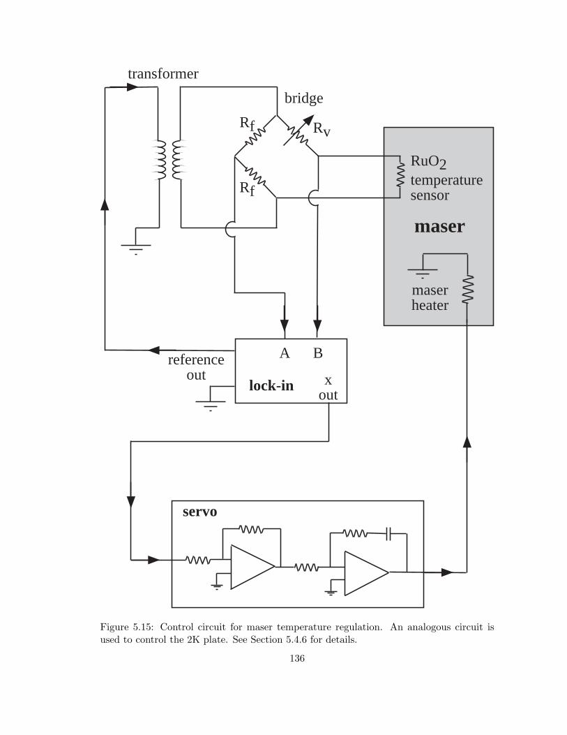
lock-in

A B

xout

referenceout

maser

RuO2temperaturesensor

maserheater

servo

Rf

Rf Rv

transformer

bridge

Figure 5.15: Control circuit for maser temperature regulation. An analogous circuit isused to control the 2K plate. See Section 5.4.6 for details.

136

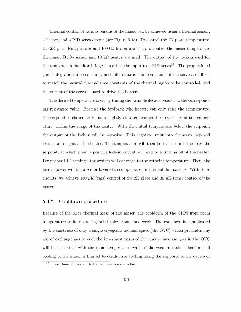
Thermal control of various regions of the maser can be achieved using a thermal sensor,

a heater, and a PID servo circuit (see Figure 5.15). To control the 2K plate temperature,

the 2K plate RuO2 sensor and 1000 Ω heater are used; to control the maser temperature

the maser RuO2 sensor and 10 kΩ heater are used. The output of the lock-in used for

the temperature monitor bridge is used as the input to a PID servo27. The proportional

gain, integration time constant, and differentiation time constant of the servo are all set

to match the natural thermal time constants of the thermal region to be controlled, and

the output of the servo is used to drive the heater.

The desired temperature is set by tuning the variable decade resistor to the correspond-

ing resistance value. Because the feedback (the heater) can only raise the temperature,

the setpoint is chosen to be at a slightly elevated temperature over the initial temper-

ature, within the range of the heater. With the initial temperature below the setpoint,

the output of the lock-in will be negative. This negative input into the servo loop will

lead to an output at the heater. The temperature will then be raised until it crosses the

setpoint, at which point a positive lock-in output will lead to a turning off of the heater.

For proper PID settings, the system will converge to the setpoint temperature. Then, the

heater power will be raised or lowered to compensate for thermal fluctuations. With these

circuits, we achieve 150 µK (rms) control of the 2K plate and 30 µK (rms) control of the

maser.

5.4.7 Cooldown procedure

Because of the large thermal mass of the maser, the cooldown of the CHM from room

temperature to its operating point takes about one week. The cooldown is complicated

by the existence of only a single cryogenic vacuum space (the OVC) which precludes any

use of exchange gas to cool the innermost parts of the maser since any gas in the OVC

will be in contact with the room temperature walls of the vacuum tank. Therefore, all

cooling of the maser is limited to conductive cooling along the supports of the device or27Linear Research model LR-130 temperature controller.

137

to controlled flow of evaporated liquids and gases through the 4He and 3He pots.

Typically, liquid nitrogen is employed as a precooling agent because of its large latent

heat (60 times greater) and low cost (about 10 times less) relative to liquid 4He [91].

Therefore, during precooling we initially fill the liquid 4He bath with liquid nitrogen to

cool the maser down to 77 K (the liquid nitrogen boiling point). The initial fill is done

slowly to utilize the enthalpy of the evaporated nitrogen gas leaving the exhaust as well

as the latent heat of the evaporating liquid [91,92].

Once the bath is filled with liquid nitrogen, the needle valve controlling flow from the

bath into the 4He pot is opened, and the 4He pot pump is used to draw some of the cold,

evaporated gas out through the 4He pot. This allows an acceleration of the cooling of the

4He pot over the cooling strictly due to conduction along its support connections to the

bath. The precooling of the 3He pot, however, is limited solely to the conduction of heat

along its support connections to the 4He pot. Note that from room temperature to the

77 K, the heat switches in the support structures (described in Sections 5.4.4 and 5.4.5)

are essentially “on,” so there is a relative high thermal conductivity between the bath and

the 4He pot, and between the 4He pot and the 3He pot.

After about two days of precooling, the temperature of the 3He pot/maser is lowered

to about 77 K. At this point all of the liquid nitrogen in the bath is boiled away (using

the 75 W bath heaters), and liquid 4He is used to cool the maser. The bath is slowly filled

with liquid 4He, again allowing the enthalpy of the cold escaping gas to do much of the

cooling. During this time, some of the cold evaporating gas is also pumped through the

4He pot. Once the bath is filled with liquid 4He, pumping of cold 4He gas through the

4He pot is continued for about one day. During the second day, enough heat has been

removed from the 4He pot that it can be filled with liquid 4He. After about two days of

liquid 4He cooling, and four days of net cooling, the temperature of the 3He pot/maser is

reduced to below 10 K.

On about the fifth day of cooling, 3He is able to condense in the 3He pot. During this

initial condensation, the 3He is flowed into the pot through the pump port, rather than

138

through the high impedance return line, so that any residual impurities not filtered by

the liquid nitrogen and liquid 4He cold traps are harmlessly cryopumped to the walls of

the large diameter pumping lines. This significantly reduces the probability of clogging

any portion of the return line with cryopumped impurities. The 3He gas is incrementally

introduced to the 3He pot over a period of about three hours, and during this time, the

temperature of the 3He pot is reduced from around 10 K to below 3 K, the normal boiling

point of liquid 3He.

On about the sixth day of cooling, after the 3He pot/maser has had one day for

thermal equilibration in this state, pumping of the 3He pot and recirculation is begun.

Initially, the 3He is pumped on very slowly by opening a needle valve at the inlet of the

molecular drag pump (see Figure 5.13). The vapor pressure above the 3He is reduced and

the temperature of the 3He pot is lowered. The 3He gas that was pumped away collects in

the gas handling panel and a pressure head is established above the cryostat. Eventually

a sufficient pressure gradient is established across the return line impedance so that the

recirculated 3He returns to the 3He pot in the form of cold liquid. Incrementally, the

pumping speed is increased (by opening the valves at the molecular drag pump inlet), and

after about two hours the valves are fully open and the 3He pot is pumped on with full

pumping speed. During this time, the 3He pot temperature is reduced from around 3 K

down to about 0.5 K.

Typically, one full day is needed to remove all the heat from the innermost regions of

the maser (for example, a lot of heat is trapped in the high heat capacity sapphire used

to load the cavity). Therefore, about seven days after the initial cooling has begun, the

maser is sufficiently cold that maser oscillation can be achieved.

5.5 CHM performance

Following the removal of the internal tuning diode installed in series with the transmission

line inside the maser cavity (and the removal of its residual magnetization) the CHM first

139

oscillated with the quartz atomic storage bulb in the summer of 2001, its first oscillation

in nearly 5 years. Once this was achieved, it was quickly discovered that a number of

technical limitations significantly degraded the CHM performance. It was found that the

CHM would only oscillate with relatively weak maser powers and that its running was

restricted to thin, unsaturated films at relatively low temperatures (below 540 mK). In

addition, with the removal of the internal tuning diode, all cavity tuning was restricted to

the mechanical tuning plunger. These three difficulties significantly reduced the ability of

the CHM to be used as an ultra stable frequency source or for ultra precise measurements

of atomic physics processes.

During our spin-exchange studies with the CHM, the double resonance effect was

employed. A discussion of this effect in the CHM will be presented in Chapter 6.

5.5.1 Maser power

Historically, a number of modifications have been made to the atomic state selection and

beam tube region of the SAO CHM in order to increase the net population inversion flux

into the atomic storage region. It was believed that the chief cause of population inversion

flux loss between the hexapole magnet and atomic storage region was scattering of the H

beam by 4He vapor above the flowing superfluid 4He film. A number of efforts were made

to reduce the temperature of the beam tube, thereby decreasing the vapor pressure of the

superfluid 4He film in this region. Attempts were also made to lower the temperature

at the top and bottom of the sorption pump. Finally an effort was made to increase

the surface area inside the beam tube (by installing a multi-foil Cu tube, constructed by

rolling a thin copper foil into a tube with many layers). As a result of these efforts, maser

powers exceeding 100 fW were achieved in the mid 1990s.

However, with the installation of the quartz storage bulb and the present thermal

environment of the beam tube, maser powers during this thesis work were seen to be

significantly lower, with maximum powers of around 30 fW observed. Efforts made to

cool the beam tube region by lowering the temperature of the 4He pot, and therefore

140

the lower plate of the sorption pump, had no significant effect on maser power. An

attempt made to vary the surface area of the beam tube over which the 4He film flowed,

by removing and reinstalling the multi-foil copper tube, likewise showed little effect on

maser power. Finally, out of concern that population inversion flux was being lost due to

Majorana transitions in the beam in the region between the hexapole magnet and atomic

storage region, a quantization-axis-preserving neck coil was installed inside the beam tube.

However, this led to only a slight increase in overall maser power.

This inability to improve overall maser power by decreasing population inversion flux

loss between the hexapole magnet and the atomic storage bulb has led to speculation that

a majority of the flux loss may occur at the collimator of the quartz storage bulb. While

the collimator was designed to have an aperture equivalent to the Teflon collimator used

previously, the actual bulb we received had wall thicknesses exceeding specifications which

inevitably led to a small decrease in aperture size. Furthermore, the bulb was installed

with a copper capillary which directed the superfluid 4He flow straight into the bulb. With

this design, the superfluid 4He film flowed first through the bulb, out the collimator, then

along the outer surface of the bulb to the cavity (i.e. the bulb and cavity were connected in

series). This could increase the thickness of the superfluid film inside the bulb collimator,

thereby increasing the 4He vapor pressure inside the collimator and possibly reducing the

population inversion flux into the bulb through H-4He scattering. In the next section we

will discuss the balance between scattering of the input flux and wall losses.

5.5.2 Superfluid film and operating temperature

As described in Section 5.2, for a saturated superfluid 4He film, the CHM should exhibit

a minimum in the magnitude of the negative H-4He collisional shift at around 550 mK.

At this temperature, the frequency shift due to collisions with 4He at the wall (where

shift magnitude decreases with increasing temperature) offsets the shift due to collisions

with 4He in the vapor (where shift magnitude increases with temperature) as shown in

Figure 5.3. At 550 mK, for a saturated superfluid film, a negative shift of about 110 mHz

141

away from the atomic hyperfine frequency would be expected.

For an unsaturated superfluid 4He film, it is observed that the magnitude of the H-

4He wall shift is increased, as shown in the plot of maser frequency vs temperature, for

various unsaturated superfluid 4He film flow settings (Figure 5.16(a)). The film flows are

quantified by the flow control setting of room temperature 4He gas in the outer manifold

just above the cryostat. No atomic signals were observed for film flow settings below

0.2 standard cubic centimeters per minute (sccm), implying that below this temperature

there is insufficient film thickness on the quartz bulb to prevent H-H recombination at

the bulb wall. It can be seen that the magnitude of the negative shift decreases as the

flow of superfluid film is increased, and the net shift approaches that of a saturated film

for a superfluid film flow of 4.0 sccm. For each film flow, the shift magnitude decreased

as temperature is increased (implying the wall shift dominates), and the slope |df/dT |

decreased as the film flow is increased.

Because of the reduction in maser power due to scattering of hydrogen atoms off of 4He

vapor in the beam tube and collimator, it is also observed that maser power is reduced for

increased superfluid 4He film flows. This can be seen in Figure 5.16(b), where the overall

maser power is reduced for a given temperature as the film flow is increased. The highest

maser powers are seen for the lowest film flow settings, while the maser is nearly quenched

for film flows approaching those needed for a saturated 4He film. For a saturated film at

0.5 K, the hydrogen mean free path is about 2 cm (see Figure 5.3) so that a hydrogen

atom would make on the order of ten collisions with helium atoms while traveling from

the hexapole magnet to the atomic storage bulb.

In addition to the strong dependence of maser frequency on temperature due to H-4He

collisions, there is also a dependence of maser power on temperature. As the temperature

of the maser is raised, the vapor pressure above the 4He film increases and the maser

power is reduced. However, for low thin film settings (just above the minimum) it can

also be seen that maser power decreases when the temperature is lowered. Here, the thin

superfluid film is insufficient to act as a wall coating and H atoms in the bulb are lost due

142

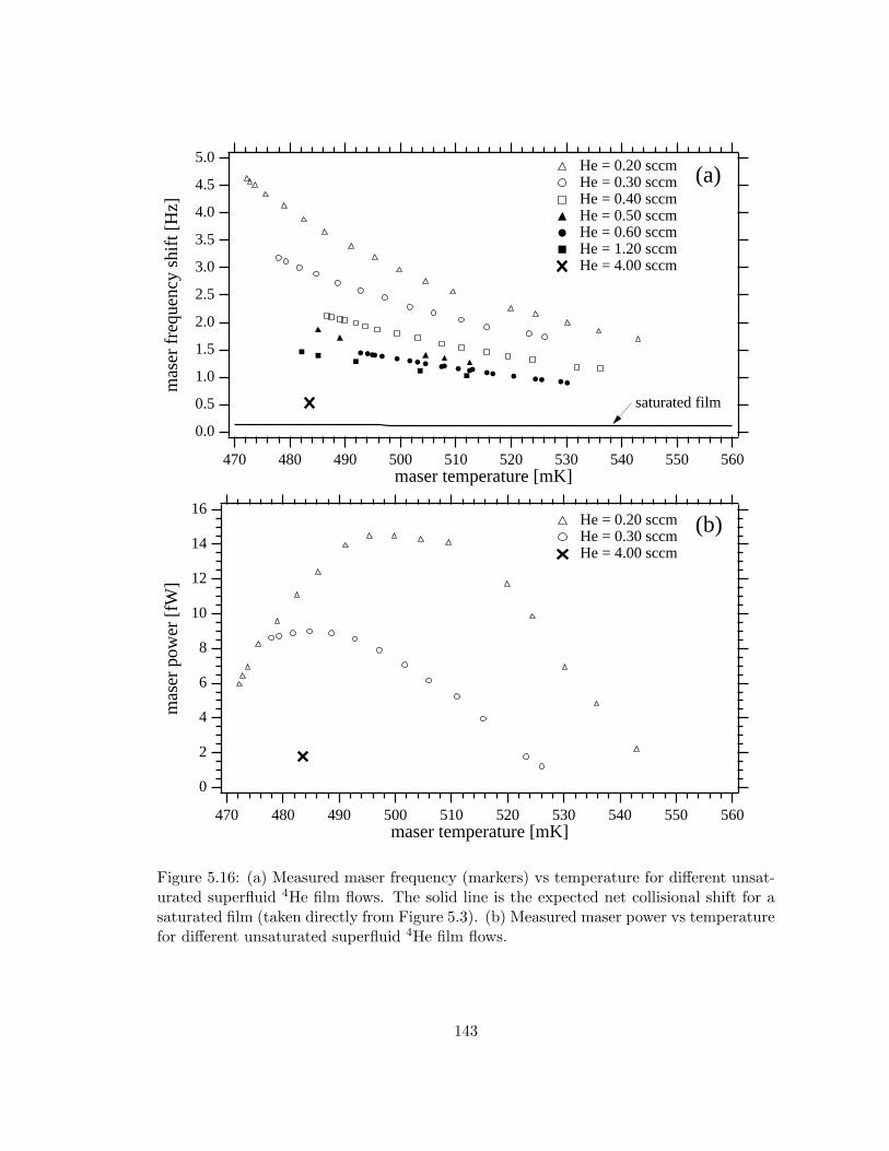
5.0

4.5

4.0

3.5

3.0

2.5

2.0

1.5

1.0

0.5

0.0

mas

er f

requ

ency

shi

ft [

Hz]

560550540530520510500490480470maser temperature [mK]

He = 0.20 sccm He = 0.30 sccm He = 0.40 sccm He = 0.50 sccm He = 0.60 sccm He = 1.20 sccm He = 4.00 sccm

(a)

saturated film

16

14

12

10

8

6

4

2

0

mas

er p

ower

[fW

]

560550540530520510500490480470maser temperature [mK]

He = 0.20 sccm He = 0.30 sccm He = 4.00 sccm

(b)

Figure 5.16: (a) Measured maser frequency (markers) vs temperature for different unsat-urated superfluid 4He film flows. The solid line is the expected net collisional shift for asaturated film (taken directly from Figure 5.3). (b) Measured maser power vs temperaturefor different unsaturated superfluid 4He film flows.

143

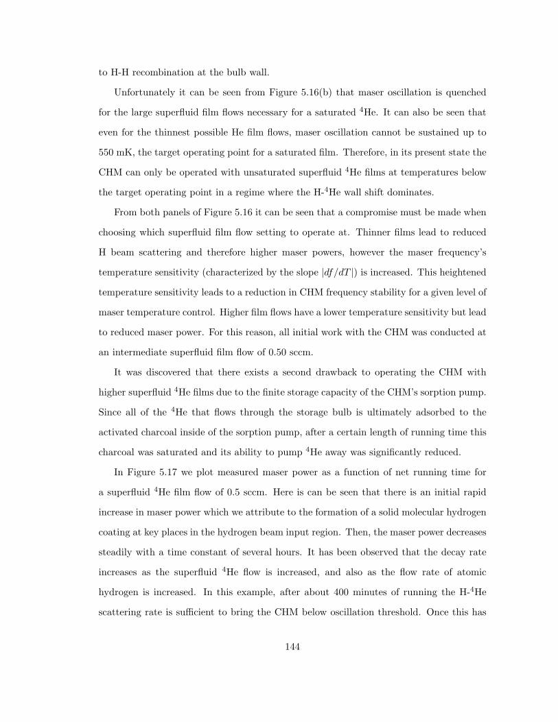
to H-H recombination at the bulb wall.

Unfortunately it can be seen from Figure 5.16(b) that maser oscillation is quenched

for the large superfluid film flows necessary for a saturated 4He. It can also be seen that

even for the thinnest possible He film flows, maser oscillation cannot be sustained up to

550 mK, the target operating point for a saturated film. Therefore, in its present state the

CHM can only be operated with unsaturated superfluid 4He films at temperatures below

the target operating point in a regime where the H-4He wall shift dominates.

From both panels of Figure 5.16 it can be seen that a compromise must be made when

choosing which superfluid film flow setting to operate at. Thinner films lead to reduced

H beam scattering and therefore higher maser powers, however the maser frequency’s

temperature sensitivity (characterized by the slope |df/dT |) is increased. This heightened

temperature sensitivity leads to a reduction in CHM frequency stability for a given level of

maser temperature control. Higher film flows have a lower temperature sensitivity but lead

to reduced maser power. For this reason, all initial work with the CHM was conducted at

an intermediate superfluid film flow of 0.50 sccm.

It was discovered that there exists a second drawback to operating the CHM with

higher superfluid 4He films due to the finite storage capacity of the CHM’s sorption pump.

Since all of the 4He that flows through the storage bulb is ultimately adsorbed to the

activated charcoal inside of the sorption pump, after a certain length of running time this

charcoal was saturated and its ability to pump 4He away was significantly reduced.

In Figure 5.17 we plot measured maser power as a function of net running time for

a superfluid 4He film flow of 0.5 sccm. Here is can be seen that there is an initial rapid

increase in maser power which we attribute to the formation of a solid molecular hydrogen

coating at key places in the hydrogen beam input region. Then, the maser power decreases

steadily with a time constant of several hours. It has been observed that the decay rate

increases as the superfluid 4He flow is increased, and also as the flow rate of atomic

hydrogen is increased. In this example, after about 400 minutes of running the H-4He

scattering rate is sufficient to bring the CHM below oscillation threshold. Once this has

144

30

28

26

24

22

20

18

16

14

12

10

8

6

4

2

0

mas

er p

ower

[fW

]

400350300250200150100500total time running [mins]

day 1 day 2 day 3 day 4

superfluid 4He film flow = 0.5 sccm

Figure 5.17: Typical maser power decay due to H2 and 4He accumulation in the sorptionpump. These data were taken for a superfluid 4He film flow of 0.50 sccm. It was laterfound that the net running time could be increased by running with a superfluid 4He filmof 0.20 sccm.

145

occurred, it is necessary to warm the sorption pump (and therefore the maser) above the

hydrogen freezing point to about 20 K. This warming takes about 2 hours, and during

this time there are significant MVC pressure spikes at 4 K (as the 4He is pumped from

the sorption pump) and at about 15 K (as the H2 is pumped away). Once the maser is

warmed to 20 K it is immediately recooled. Unfortunately, nearly one full day of recooling

is needed to bring the base temperature down to a level where stable maser oscillation

can again be achieved.

Since the power decay rate is decreased while running at lower films, it was decided to

lower the superfluid film flow for typical operation from 0.5 sccm to 0.2 sccm. Doing so

increased by roughly a factor of two the amount of time the maser could be run between

20 K warming cycles. For a typical hydrogen flux and a superfluid film setting of 0.2, the

CHM could generally be run for four days before a warming cycle (with the maser running

3 to 4 hours per day).

5.5.3 Maser frequency stability

Since maser operating temperatures were limited to below the (saturated film) target

operating point of 550 mK, the maser would only run in a regime where frequency stability

would be compromised by the H-4He collisional wall shift. Furthermore, this wall shift

was accentuated due to the necessity of running with unsaturated superfluid films.

From Figure 5.16(b), it can be seen that with the superfluid film flow of 0.2 sccm,

the maser power has a maximum near 500 mK. Therefore, this was chosen as the typical

operating temperature for normal operation at 0.2 sccm. A plot of measured CHM Allan

variance at 511 mK is given in Figure 5.18. This plot shows that for averaging times less

than one minute the Allan variance is around 3×10−12. These data were taken with a

superfluid film flow of 0.2 sccm and maser temperature control of about 150 µK (rms).28

Under these conditions, the frequency sensitivity on temperature was about |df/dT | =28We note that this temperature control was not up to our optimal level of 30 µK. We attribute this to

the fact that, during the run where these data were taken, the thermal contact between the 3He pot, themaser, and the maser temperature sensors and heaters was not optimal.

146

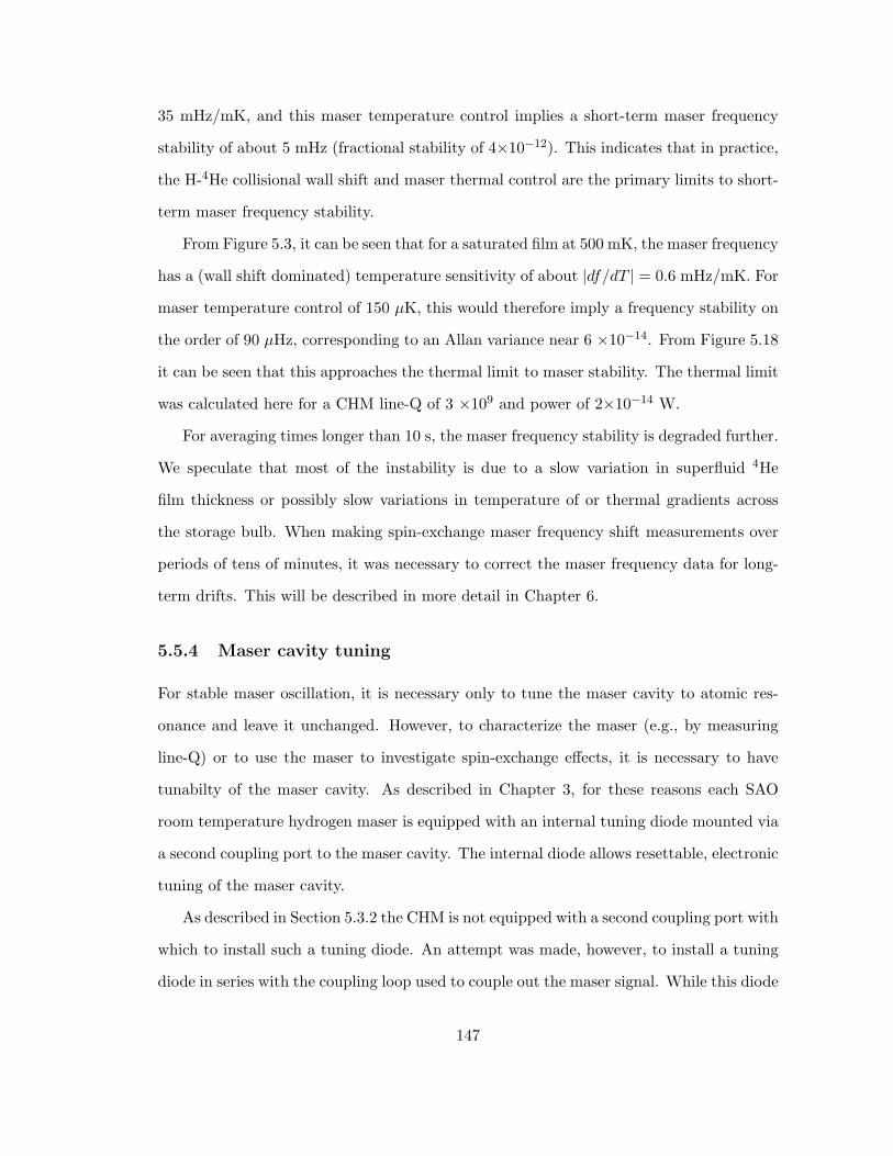
35 mHz/mK, and this maser temperature control implies a short-term maser frequency

stability of about 5 mHz (fractional stability of 4×10−12). This indicates that in practice,

the H-4He collisional wall shift and maser thermal control are the primary limits to short-

term maser frequency stability.

From Figure 5.3, it can be seen that for a saturated film at 500 mK, the maser frequency

has a (wall shift dominated) temperature sensitivity of about |df/dT | = 0.6 mHz/mK. For

maser temperature control of 150 µK, this would therefore imply a frequency stability on

the order of 90 µHz, corresponding to an Allan variance near 6 ×10−14. From Figure 5.18

it can be seen that this approaches the thermal limit to maser stability. The thermal limit

was calculated here for a CHM line-Q of 3 ×109 and power of 2×10−14 W.

For averaging times longer than 10 s, the maser frequency stability is degraded further.

We speculate that most of the instability is due to a slow variation in superfluid 4He

film thickness or possibly slow variations in temperature of or thermal gradients across

the storage bulb. When making spin-exchange maser frequency shift measurements over

periods of tens of minutes, it was necessary to correct the maser frequency data for long-

term drifts. This will be described in more detail in Chapter 6.

5.5.4 Maser cavity tuning

For stable maser oscillation, it is necessary only to tune the maser cavity to atomic res-

onance and leave it unchanged. However, to characterize the maser (e.g., by measuring

line-Q) or to use the maser to investigate spin-exchange effects, it is necessary to have

tunabilty of the maser cavity. As described in Chapter 3, for these reasons each SAO

room temperature hydrogen maser is equipped with an internal tuning diode mounted via

a second coupling port to the maser cavity. The internal diode allows resettable, electronic

tuning of the maser cavity.

As described in Section 5.3.2 the CHM is not equipped with a second coupling port with

which to install such a tuning diode. An attempt was made, however, to install a tuning

diode in series with the coupling loop used to couple out the maser signal. While this diode

147

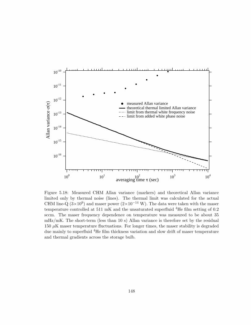
10-16

10-15

10-14

10-13

10-12

10-11

10-10

Alla

n va

rian

ce σ

(τ)

100 101 102 103 104

averaging time τ (sec)

measured Allan variance theoretical thermal limited Allan variance limit from thermal white frequency noise limit from added white phase noise

Figure 5.18: Measured CHM Allan variance (markers) and theoretical Allan variancelimited only by thermal noise (lines). The thermal limit was calculated for the actualCHM line-Q (3×109) and maser power (2×10−14 W). The data were taken with the masertemperature controlled at 511 mK and the unsaturated superfluid 4He film setting of 0.2sccm. The maser frequency dependence on temperature was measured to be about 35mHz/mK. The short-term (less than 10 s) Allan variance is therefore set by the residual150 µK maser temperature fluctuations. For longer times, the maser stability is degradeddue mainly to superfluid 4He film thickness variation and slow drift of maser temperatureand thermal gradients across the storage bulb.

148

was able to shift the maser cavity frequency, it also introduced a residual magnetization

near the atomic storage region which decohered the atomic ensemble enough to quench

maser oscillation. Therefore, this diode was removed.

Following this, attempts were made to couple an external diode in parallel with the

transmission line outside of the cryostat. While biasing this diode had a small effect on the

cavity resonance, the cavity shifting was small and reflections in the transmission line led

to discrepancies between the apparent cavity frequency measured and the cavity frequency

sensed by the atoms. For this reason, external diode tuning was not pursued further.

As a result, microwave cavity tuning of the CHM was restricted to the mechanical

tuning plunger. The plunger could be thread into and out of the cavity by a wingnut

connected to a small gear mounted on axis with the cavity. Movement of this gear was

achieved with a Delrin29 chain connected to a second gear mounted below the liquid

nitrogen jacket. Movement of this gear was accomplished by turning a knob mounted on

the top of the cryostat. The cavity could be tuned about 15 kHz per turn of this external

knob over a total range of about 1 MHz.

Tuning by this mechanism had several drawbacks. First, the mechanical tuner was

designed for coarse tuning of the microwave cavity. Therefore, resettable cavity tuning

with any precision was not possible. Second, slack in the Delrin chain between the outer

and inner gear led to hysteresis in the tuning. After moving the plunger in one direction,

about two turns of the outer knob were needed to engage movement of the plunger in the

opposite direction.

The third and most serious drawback arose from the fact that the Delrin chain was

in thermal contact with the 77 K shield at one side and in thermal contact with the 0.5

K maser at the other. Therefore, a significant thermal gradient was established across

the chain and any movement of the chain brought Delrin at an elevated temperature into

thermal contact with the maser, thus warming the maser. This warming was significant,

with one turn of the external knob (15 kHz shift in the cavity) warming the maser by tens29Delrin is a trademark of E.I. duPont de Nemours and Co., Inc.

149

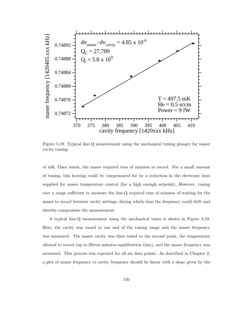
0.74892

0.74888

0.74884

0.74880

0.74876

0.74872

mas

er f

requ

ency

[14

2040

5.xx

x kH

z]

410405400395390385380375370cavity frequency [1420xxx kHz]

dνmaser / dνcavity = 4.85 x 10-6

QC = 27,700

Ql = 5.8 x 109

T = 497.5 mKHe = 0.5 sccmPower = 9 fW

Figure 5.19: Typical line-Q measurement using the mechanical tuning plunger for masercavity tuning.

of mK. Once warm, the maser required tens of minutes to recool. For a small amount

of tuning, this heating could be compensated for by a reduction in the electronic heat

supplied for maser temperature control (for a high enough setpoint), However, tuning

over a range sufficient to measure the line-Q required tens of minutes of waiting for the

maser to recool between cavity settings, during which time the frequency could drift and

thereby compromise the measurement.

A typical line-Q measurement using the mechanical tuner is shown in Figure 5.19.

Here, the cavity was tuned to one end of the tuning range and the maser frequency

was measured. The maser cavity was then tuned to the second point, the temperature

allowed to recool (up to fifteen minutes equilibration time), and the maser frequency was

measured. This process was repeated for all six data points. As described in Chapter 2,

a plot of maser frequency vs cavity frequency should be linear with a slope given by the

150

ratio of cavity-Q to atomic line-Q: dνmaser/dνcavity = QC/Ql. The error bars in this plot

characterize the statistical uncertainty in the maser frequency at each cavity point. The

fact that the linear fit to the data misses the error bars for these points is indicative

of a systematic error, in this case maser frequency drift during the time between maser

frequency measurements at each cavity frequency setting. In Chapter 6 we will discuss the

need to make accurate line-Q measurements in order to investigate spin-exchange effects

with the CHM.

We note that in general the line-Qs we measured with the CHM were up to a factor

of 10 less than expected (expected Ql ≈ 1010). We have evidence that this is chiefly due

to the increased wall relaxation rate caused by running with unsaturated superfluid films:

With an (unsaturated) superfluid film flow of 0.5 sccm, we found Ql ≈ 5×109, while at

0.2 sccm, this dropped further to Ql ≈ 1×109.

An additional difficulty with the maser tuning was a thermal-cycle-induced shift of

the cavity tuning range. It had been observed that once the CHM was fully assembled, a

thermal cycle to room temperature and then back to 0.5 K would lead to a negative shift in

the mechanical tuning range relative to the atomic hyperfine frequency. We speculate that

this shift can be attributed to a thermal-contraction-induced loosening of the screws which

seal the copper pot that contains and compresses the maser cavity. Such a loosening would

reduce the compression, physically enlarging the cavity and leading to a net downward

shift of the tuning range.

Following the room temperature warm-up preceding the final few months of CHM

work, the mechanical tuning range of the maser cavity was shifted below the atomic

hyperfine frequency; the highest cavity frequency achievable was about 1420.38 MHz (or

about 25 kHz below atomic resonance). The tuning range shift was discovered once the

maser was at 0.5 K, and since a warm up, disassembly, and recool would have taken about

one month, the decision was made to continue work with the maser slightly detuned from

resonance. The ramifications of this limitation will be discussed more in Chapter 6.

151

Chapter 6

Spin-exchange in hydrogen masers

The earliest treatments of spin-exchange in hydrogen-hydrogen collisions were an effort

to understand the interaction and equilibration of interstellar atomic hydrogen [71–73].

Today, spin-exchange collisions are seen to have direct consequences in conventional [19,

30,31] and cryogenic [29] hydrogen masers, and more generally, in all forms of cold atomic

clocks.

An electron spin-exchange collision involves the exchange interaction between elec-

trons in the colliding atoms, the same interaction which stabilizes the hydrogen molecule.

Therefore, a spin-exchange collision between hydrogen atoms can be treated as the short

term creation of a hydrogen molecule. The molecular interaction potential depends on

whether the electrons’ spins are aligned or anti-aligned, forming a triplet 3Σ+u or singlet

1Σ+g potential, respectively. The triplet and singlet potentials ET (R) and ES(R) are plot-

ted as functions of the internuclear separation R in Figure 6.1 [93]. However, since the

mF = 0 hyperfine states in hydrogen can be admixtures of electron spin up and down,

spin-exchange collisions can cause changes in level populations and decoherence of the

hyperfine transition (characterized by a spin-exchange relaxation cross section σ) as well

as shifts in the hyperfine transition frequency (characterized by a spin-exhange shift cross

section λ). Therefore, a proper treatment of spin-exchange in hydrogen-hydrogen collisions

is required for a complete understanding of the hydrogen maser.

152

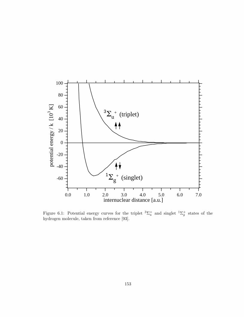
100

80

60

40

20

0

-20

-40

-60

pote

ntia

l ene

rgy

/ k [

103 K

]

7.06.05.04.03.02.01.00.0internuclear distance [a.u.]

3Σu+ (triplet)

1Σg+ (singlet)

Figure 6.1: Potential energy curves for the triplet 3Σ+u and singlet 1Σ+

g states of thehydrogen molecule, taken from reference [93].

153

Early investigations of spin-exchange effects in hydrogen-hydrogen collisions used the

approximation that the small hyperfine energy splittings could be neglected relative to

the interaction potentials and collision energies [17,68,71–75,77,94,95]. In Section 6.1, we

review this approximation, known as the degenerate internal states (DIS) approximation,

which accurately describes spin-exchange effects in room temperature hydrogen masers.

In Section 6.2, we review the first attempt to include the hyperfine interaction which did

so perturbatively using a semi-classical description [76]. This work led to the prediction

of a new, hyperfine-induced maser frequency shift which was confirmed experimentally

using a room temperature hydrogen maser. In Section 6.3 we consider the first fully

quantum mechanical treatment of hydrogen-hydrogen spin-exchange collisions [19,29–31].

This treatment also predicts a number of small, hyperfine-induced (h-i) effects which

may become important in the operation of the cryogenic hydrogen maser and other cold

atomic clocks. In Section 6.4 we review previous experimental investigations of h-i effects

in hydrogen masers, and note the significant discrepancies that persist between experiment

and theory. In Section 6.5 we discuss the investigation of low temperature spin-exchange

collisions using the SAO CHM.

6.1 Degenerate internal states approximation

All of the early work on spin-exchange in hydrogen-hydrogen collisions neglected the small

hyperfine energy splitting (≈ 0.07 K) relative to the colliding atoms thermal energy and

the depth of the molecular potential (≈ 50,000 K). The first results using this so-called

degenerate internal states (DIS) approximation calculated spin-exchange induced varia-

tions in the population of the hyperfine states [71], the spin-exchange broadening cross

sections [72, 73], the hyperfine frequency shift [72], and changes in the atomic hydrogen

density matrix [74] due to spin-exchange collisions.

The first attempt to use DIS theory to calculate the effects of spin-exchange collisions

in a hydrogen maser was made by Bender in 1963 [68]. His analysis proceeded similarly

154

to our hydrogen maser analysis of Chapter 2 in that the steady state density matrix for

the hydrogen ensemble is found by solving a Bloch equation that included the effects of

the microwave cavity field, atom flow into and out of the bulb, and spin-exchange (using a

more sophisticated treatment than given in Chapter 2). All other forms of relaxation were

neglected, as well as the interaction of the atomic ensemble with the microwave cavity.

The first step of Bender’s treatment was to determine the effect of spin-exchange

collisions on the hydrogen ensemble density matrix. The basic idea was to assume that as

two atoms approach one another, their 4 × 4 single atom density matrices (in the |F, mF 〉

basis) can be written via a direct product as a single, 16 × 16 collision matrix. The

collision matrix is then rotated from the |F1, mF1 ;F2, mF2〉 basis into the |S, mS ; I, mI〉

basis. Those elements of the density matrix with S = 1 evolve under the molecular triplet

potential ET (R), while those with S = 0 evolve under the singlet potential ES(R). The

time dependence enters through the relative motion of the atoms and therefore the time-

variation of the internuclear separation R. A classical collision trajectory was assumed,

and as the collision proceeds the triplet and singlet parts of the combined wavefunction

acquire different phases ∆T,S , given by

∆T,S =1h

∫ET,S(R)dt. (6.1)

The differential phase shift (∆T − ∆S) was then averaged over the impact parameter of

the collision and the thermal velocity distribution. The post-collision density matrix was

rotated back to the |F1, mF1 ;F2, mF2〉 basis, and by taking the trace of the final 16 × 16

collision density matrix over the second atom’s quantum numbers, the final form of the 4

× 4 single atom density matrix, post-spin-exchange-collision, was found. This was then

used to characterize the relaxation due to spin-exchange in the Bloch equation. Finally,

by solving the Bloch equation, the effect on the hydrogen hyperfine transition was found.

This treatment predicted a hyperfine frequency shift proportional to the spin-exchange

collision contribution to the atomic linewidth. Since this contribution is essentially the

155

spin-exchange collision rate, which depends on the atomic density, Bender’s calculation

predicted that spin-exchange collisions could limit the frequency stability of hydrogen

masers, where density fluctuations are difficult to control.

In 1967, Crampton [17] extended the work of Bender to include the effects of power

broadening and cavity pulling, along with spin-exchange, in the hydrogen maser. In his

analysis, Crampton discovered that the hydrogen maser frequency ω was shifted away

from the density-independent hyperfine frequency ω24 by an amount given by

ω = ω24 + (∆ + αλ) γ2 (6.2)

where λ is the spin-exchange frequency shift cross section,1 γ2 is the total line broadening,

and ∆ is a measure of cavity detuning given by

∆ = QC

(ωC

ω24− ω24

ωC

)≈ 2QC

(ωC − ω24

ω24

)(6.3)

with QC and ωC the cavity-Q and cavity frequency, respectively. Crampton also intro-

duced a system constant

α =hVC vr

µ0µ2BηQCVb

(6.4)

where VC and Vb are the cavity and bulb volumes, vr is the average relative atomic

velocity, and η is the cavity filling factor, defined in Chapter 3. Crampton showed that

the linewidth-dependent cavity pulling term could be used to compensate for the linewidth-

dependent spin-exchange shift if the maser cavity was tuned such that ∆ = −αλ. This

is the “spin-exchange tuning” procedure that has turned out to be vital in reducing the

effects of density variation on hydrogen maser stability (see Chapter 3). Crampton et

al. later investigated these effects experimentally with a room temperature hydrogen

maser [94] and found good agreement with the DIS theory.

Using the DIS approximation, Allison [75] calculated thermal-averaged spin-exchange1We have redefined this parameter from Crampton’s original notation to be − 1

4λ → λ to agree with

the notation introduced by VKSLC.

156

broadening and shift cross sections as a function of temperature from 1000 K to 10 K. A

measurement of spin-exchange relaxation rates from 363 - 77 K was performed by Desaint-

fuscien and Audoin [95], and very good agreement with the DIS theory was found. The

DIS approximation was then used by Berlinsky and Shizgal [77] to extend the calculations

of Allison down to 0.25 K. Because of the technical complications of operating a hydro-

gen maser at such low temperature, no immediate experimental results were achieved to

compare to DIS theory at low temperature where, as the kinetic energy of the colliding

atoms is lowered, the DIS approximation becomes increasingly less reliable.

6.2 Semi-classical hyperfine interaction effects

In 1975, Crampton and Wang [76] made the first attempt to move beyond the DIS approx-

imation and account for the hyperfine interaction during spin-exchange collisions. Their

treatment used first-order perturbation theory in a semi-classical picture. They took as

the unperturbed Hamiltonian the DIS Hamiltonian, given by

H(t) = ET (t)PT + ES(t)PS (6.5)

where PT and PS are matrix operators that project out the triplet and singlet parts

of the wavefunction, and ET (t) and ES(t) are the corresponding interaction potentials.

Again, the time dependence enters through the varying internuclear separation during the

collision. To the unperturbed Hamiltonian, they added a perturbation Vhf which included

the intra-atomic hyperfine interaction to first order:

Vhf = hω24

(I1 · S1 + I2 · S2

)(6.6)

where I1,2 and S1,2 are the nuclear and electron spins of the colliding atoms and ω24 is

the density-independent hyperfine frequency. In general, this frequency includes a number

of small, density-independent shifts, such as the wall shift, or the second-order Zeeman or

157

Doppler shifts. The procedure of Bender [68] was then followed to determine the effect

of spin-exchange collisions, now including the hyperfine interaction semi-clasically to first

order, on the hydrogen ensemble’s density matrix and on the oscillation frequency of the

hydrogen maser.

The result of this calculation predicted that the hydrogen maser frequency would be

given by

ω = ω24 +(∆ + αλ′) γ2 + εHγH . (6.7)

It can be seen that in addition to the cavity pulling and DIS spin-exchange shift (both

proportional to the total broadening γ2), there is also a semi-classical, hyperfine-induced

maser frequency shift, characterized by εH and proportional to the spin-exchange collision

rate γH = nσvr, where σ is the spin-exchange broadening cross section. Also, the inclusion

of the hyperfine interaction leads to a modification of the spin-exchange shift cross section:2

λ′ = λ + 2σεH . The semi-classical shift parameter is given by εH = −ω24TD/4, where TD

is the average duration a spin-exchange collision.

The interpretation provided for this new shift [76] was that during a hydrogen-hydrogen

spin-exchange collision, the hyperfine interaction is “interrupted” for a time TD, and this

interruption leads to a negative shift in the hyperfine frequency by an amount proportional

to TD and to the spin-exchange collision rate γH . Crampton and Wang measured the semi-

classical hyperfine-induced shift parameter εH in a room temperature hydrogen maser and

found good agreement with the theory [76].

We note that the hyperfine-induced shift is proportional to that component of the

broadening due solely to spin-exchange collisions γH , and not proportional to the full

broadening γ2. Therefore, if the canonical spin-exchange tuning technique is applied,

where the maser cavity is tuned so that there is no variation in maser frequency ω with

spin-exchange collision rate γH (i.e., the cavity detuning is set at ∆ = −αλ′ + εH), then

the maser oscillation frequency will no longer be density-dependent. Instead, there will be2We have redefined this parameter from Crampton’s original notation to be − 1

4λ → λ to agree with

the notation introduced by VKSLC.

158

a residual density-independent maser frequency shift of −γ0εH , where γ0 is the density-

independent portion of the total broadening. In this formalism, however, the residual

frequency shift does not appreciably degrade the stability of a hydrogen maser operat-

ing at room temperature since γ0 and εH are sufficiently stable in practice. By tuning

the maser in this manner, Crampton and Wang were able to measure the semi-classical

hyperfine-induced frequency shift. They found that εH = 4.04(0.35)×10−4 at T = 308 K,

in reasonable agreement with their calculation [76].

6.3 Quantum mechanical hyperfine interaction effects

A full, quantum mechanical treatment of hydrogen-hydrogen spin-exchange collisions and

an analysis of their effect on the hydrogen maser was completed by Verhaar et al. (VKSLC)

in 1987 [30, 31]. The starting point for their analysis was the Bloch equation describing

the interaction of the atoms in the presence of the maser field:

dρκκ′

dt= − i

h(Eκ − Eκ′) ρκκ′ − i

h[H1(t), ρ]κ,κ′ +

(dρκκ′

dt

)

se+

(dρκκ′

dt

)

relax(6.8)

where H1(t) represents the maser cavity field. Assuming conventional hydrogen maser

operation, the only coherence lies between the |2〉 and |4〉 hyperfine levels, so the spin-

exchange relaxation term includes only off-diagonal matrix elements having the form

(dρ24

dt

)

se= nρ24

∑ν

Gνρνν (6.9)

where n is the hydrogen density and ν corresponds to a hyperfine state. Taking into

account the rotational symmetry of a hydrogen-hydrogen collision, VKSLC showed that

the coefficients of Eqn. 6.9 were given by Gν = 〈vΛν〉 = vrΛν (vr is the relative atomic

velocity, and the brackets and overbars denote thermal averaging). The cross sections

Λν are written in terms of a sum of S-matrix elements [30] which follow from the same

159

potential used in previous DIS analyses

V = PT ET (R) + PSES(R) + hω24

(I1 · S1 + I2 · S2

)(6.10)

in which PT and PS are the triplet and singlet projection operators, ET (R) and ES(R)

are the triplet and singlet molecular potentials, ω24 is the density-independent atomic

hyperfine frequency, and I1,2 and S1,2 are the nuclear and electron spins of the colliding

atoms.

By substituting into Eqn. 6.9 a solution of the form

ρ42(t) = ρ42(0) exp [i(ω24 + δω + iγ2)t] , (6.11)

they found that the hyperfine transition frequency would be shifted from the density-

independent hyperfine frequency by

δω =[λ0(ρ22 − ρ44) + λ1(ρ22 + ρ44) + λ2

]vrn (6.12)

where the overbar indicates a thermal average. The spin-exchange shift cross sections are

given by

λ0 = Im [(Λ2 − Λ4)/2]

λ1 = Im [(Λ2 + Λ4)/2 − Λ3] (6.13)

λ2 = Im[Λ3],

and we note that Λ3 = Λ1 due to symmetry considerations. The collision-induced broad-

ening would be given by

γH = [σ0(ρ22 − ρ44) + σ1(ρ22 + ρ44) + σ2] vrn, (6.14)

where the spin-exchange broadening cross sections σi are given analogously from Eqn. 6.13

160

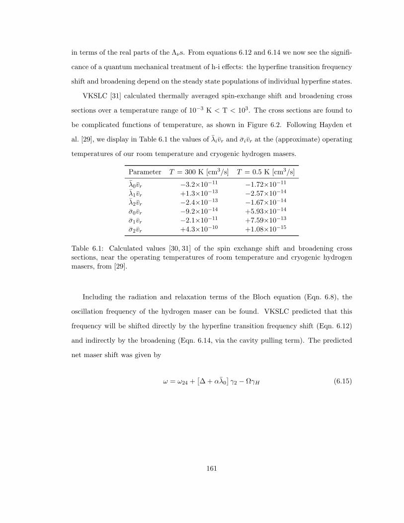
in terms of the real parts of the Λνs. From equations 6.12 and 6.14 we now see the signifi-

cance of a quantum mechanical treatment of h-i effects: the hyperfine transition frequency

shift and broadening depend on the steady state populations of individual hyperfine states.

VKSLC [31] calculated thermally averaged spin-exchange shift and broadening cross

sections over a temperature range of 10−3 K < T < 103. The cross sections are found to

be complicated functions of temperature, as shown in Figure 6.2. Following Hayden et

al. [29], we display in Table 6.1 the values of λivr and σivr at the (approximate) operating

temperatures of our room temperature and cryogenic hydrogen masers.

Parameter T = 300 K [cm3/s] T = 0.5 K [cm3/s]

λ0vr −3.2×10−11 −1.72×10−11

λ1vr +1.3×10−13 −2.57×10−14

λ2vr −2.4×10−13 −1.67×10−14

σ0vr −9.2×10−14 +5.93×10−14

σ1vr −2.1×10−11 +7.59×10−13

σ2vr +4.3×10−10 +1.08×10−15

Table 6.1: Calculated values [30, 31] of the spin exchange shift and broadening crosssections, near the operating temperatures of room temperature and cryogenic hydrogenmasers, from [29].

Including the radiation and relaxation terms of the Bloch equation (Eqn. 6.8), the

oscillation frequency of the hydrogen maser can be found. VKSLC predicted that this

frequency will be shifted directly by the hyperfine transition frequency shift (Eqn. 6.12)

and indirectly by the broadening (Eqn. 6.14, via the cavity pulling term). The predicted

net maser shift was given by

ω = ω24 +[∆ + αλ0

]γ2 − ΩγH (6.15)

161

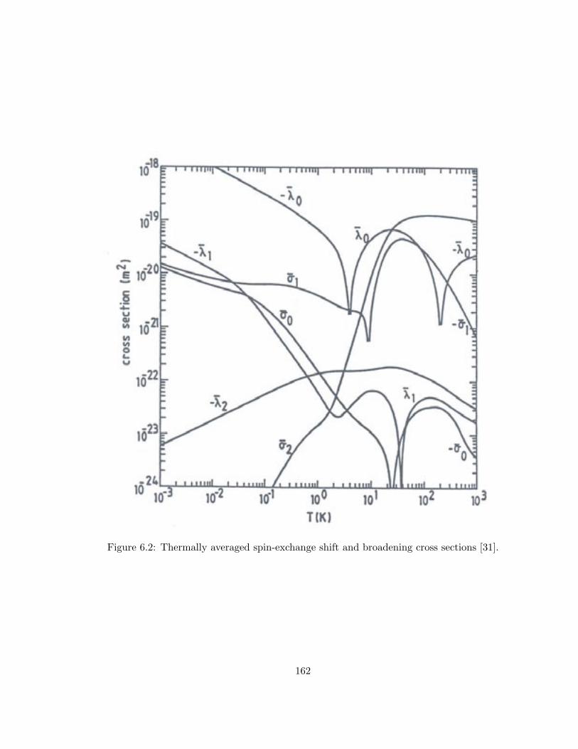
Figure 6.2: Thermally averaged spin-exchange shift and broadening cross sections [31].

162

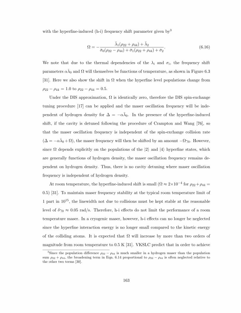
with the hyperfine-induced (h-i) frequency shift parameter given by3

Ω = − λ1(ρ22 + ρ44) + λ2

σ0(ρ22 − ρ44) + σ1(ρ22 + ρ44) + σ2. (6.16)

We note that due to the thermal dependencies of the λi and σi, the frequency shift

parameters αλ0 and Ω will themselves be functions of temperature, as shown in Figure 6.3

[31]. Here we also show the shift in Ω when the hyperfine level populations change from

ρ22 − ρ44 = 1.0 to ρ22 − ρ44 = 0.5.

Under the DIS approximation, Ω is identically zero, therefore the DIS spin-exchange

tuning procedure [17] can be applied and the maser oscillation frequency will be inde-

pendent of hydrogen density for ∆ = −αλ0. In the presence of the hyperfine-induced

shift, if the cavity is detuned following the procedure of Crampton and Wang [76], so

that the maser oscillation frequency is independent of the spin-exchange collision rate

(∆ = −αλ0 +Ω), the maser frequency will then be shifted by an amount −Ωγ0. However,

since Ω depends explicitly on the populations of the |2〉 and |4〉 hyperfine states, which

are generally functions of hydrogen density, the maser oscillation frequency remains de-

pendent on hydrogen density. Thus, there is no cavity detuning where maser oscillation

frequency is independent of hydrogen density.

At room temperature, the hyperfine-induced shift is small (Ω ≈ 2×10−4 for ρ22+ρ44 =

0.5) [31]. To maintain maser frequency stability at the typical room temperature limit of

1 part in 1015, the linewidth not due to collisions must be kept stable at the reasonable

level of δγ0 ≈ 0.05 rad/s. Therefore, h-i effects do not limit the performance of a room

temperature maser. In a cryogenic maser, however, h-i effects can no longer be neglected

since the hyperfine interaction energy is no longer small compared to the kinetic energy

of the colliding atoms. It is expected that Ω will increase by more than two orders of

magnitude from room temperature to 0.5 K [31]. VKSLC predict that in order to achieve3Since the population difference ρ22 − ρ44 is much smaller in a hydrogen maser than the population

sum ρ22 + ρ44, the broadening term in Eqn. 6.14 proportional to ρ22 − ρ44 is often neglected relative tothe other two terms [30].

163

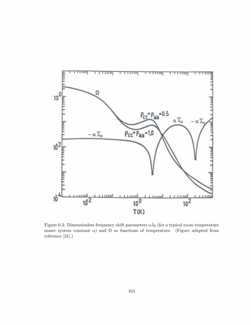
Figure 6.3: Dimensionless frequency shift parameters αλ0 (for a typical room temperaturemaser system constant α) and Ω as functions of temperature. (Figure adapted fromreference [31].)

164

the predicted CHM fractional frequency stability limit of 2×10−18, the maximum allowed

instability in the linewidth not due to collisions would be δγ0 ≈ 10−7 rad/s, a stability

unlikely to be achieved in practice [31]. Therefore, hyperfine-induced effects in a cryogenic

hydrogen maser may significantly reduce the expected improvement in cryogenic hydrogen

maser stability.

6.4 Prior measurements

The hyperfine-induced hydrogen maser frequency shift predicted by VKSLC [30, 31] has

been investigated with a room temperature hydrogen maser [19] and with a cryogenic

hydrogen maser [29]. In both cases, a hyperfine-induced maser shift frequency was ob-

served, however there are disagreements both in magnitude and sign with the theoretical

calculations. These disagreements induced further theoretical investigations [96, 97], but

to date the discrepancies between experiment and theory have not been explained.

The room temperature experiment was carried out by our group using a room tem-

perature SAO hydrogen maser (maser P-27). In this study, the maser frequency shift’s

dependence on hyperfine level population was exploited to detect hyperfine-induced effects.

The hydrogen maser was equipped with an adiabatic fast passage (AFP) state selector.

This device allowed for a switch in the composition of the input beam from approximately

half the atoms in each of states |1〉 and |2〉 (the AFP “off” configuration), to an input

beam of pure state |2〉 atoms (the AFP “on” configuration). Because of the dependence of

Ω on (ρ22+ρ44), VKSLC predicted a measurable difference of the hyperfine-induced maser

shift between the two configurations of Ωon −Ωoff = −0.76×10−4 to −1.12×10−4 (for the

range of masing state populations used in the experiment). However, the experimentally

determined value was Ωon − Ωoff = +5.38(1.06)×10−4 [19]. Equivalently, the theoretical

prediction was λ1 = 3.0×10−19 cm2, while the measured value was λ1 = −1.8×10−19. Al-

though this result confirmed the dependence of the hyperfine-induced maser frequency shift

on hyperfine level populations, it produced a glaring discrepancy between measurement

165

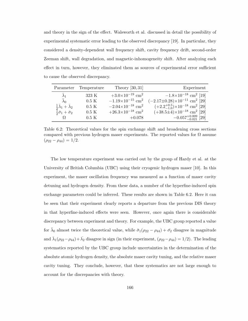
and theory in the sign of the effect. Walsworth et al. discussed in detail the possibility of

experimental systematic error leading to the observed discrepancy [19]. In particular, they

considered a density-dependent wall frequency shift, cavity frequency drift, second-order

Zeeman shift, wall degradation, and magnetic-inhomogeneity shift. After analyzing each

effect in turn, however, they eliminated them as sources of experimental error sufficient

to cause the observed discrepancy.

Parameter Temperature Theory [30,31] Experiment

λ1 323 K +3.0×10−19 cm2 −1.8×10−18 cm2 [19]λ0 0.5 K −1.19×10−15 cm2 (−2.17±0.28)×10−11 cm2 [29]

12 λ1 + λ2 0.5 K −2.04×10−18 cm2 (+2.2+0.5

−1.0)×10−18 cm2 [29]12 σ1 + σ2 0.5 K +26.3×10−18 cm2 (+38.5±4)×10−18 cm2 [29]

Ω 0.5 K +0.078 −0.057+0.009−0.021 [29]

Table 6.2: Theoretical values for the spin exchange shift and broadening cross sectionscompared with previous hydrogen maser experiments. The reported values for Ω assume(ρ22 − ρ44) = 1/2.

The low temperature experiment was carried out by the group of Hardy et al. at the

University of British Columbia (UBC) using their cryogenic hydrogen maser [10]. In this

experiment, the maser oscillation frequency was measured as a function of maser cavity

detuning and hydrogen density. From these data, a number of the hyperfine-induced spin

exchange parameters could be inferred. These results are shown in Table 6.2. Here it can

be seen that their experiment clearly reports a departure from the previous DIS theory

in that hyperfine-induced effects were seen. However, once again there is considerable

discrepancy between experiment and theory. For example, the UBC group reported a value

for λ0 almost twice the theoretical value, while σ1(ρ22 − ρ44) + σ2 disagree in magnitude

and λ1(ρ22−ρ44)+λ2 disagree in sign (in their experiment, (ρ22−ρ44) = 1/2). The leading

systematics reported by the UBC group include uncertainties in the determination of the

absolute atomic hydrogen density, the absolute maser cavity tuning, and the relative maser

cavity tuning. They conclude, however, that these systematics are not large enough to

account for the discrepancies with theory.

166

A third experiment has been conducted which allows a test of VKSLC theory [98].

This experiment was also carried out by the UBC group, however it was not done with an

oscillating hydrogen maser. Using pulsed NMR techniques in a gas of hydrogen atoms at

1.2 K, they measured the longitudinal broadening cross section for the hydrogen hyperfine

transition to be σT1 = +0.51(2) A2. The theoretical prediction from VKSLC was σT1 =

+0.37 A2 [96]. This discrepancy is particularly significant because it compares parameters

which are independent of the operation of a hydrogen maser.

These discrepancies between theory and experiment bring into question the accuracy of

the theoretical calculations of VKSLC [96]. A possible source of error in these calculations

would be the use of inaccurate interatomic potentials, however it has been reported that

no reasonable variation of these potentials has been shown to be sufficient to account to

the observed disagreement [29, 96]. Other possibilities are a breakdown of some of the

theoretical assumptions, such as the neglect of spin-dipole interactions [96] or the way

in which nonadiabatic corrections are treated. Finally, there remains the possible that

there is some overlooked physics in the hydrogen maser which could mimic the hyperfine-

induced frequency shift, although this would not explain the observed disagreement in the

longitudinal relaxation measurement which was not carried out in a hydrogen maser. In

sum, an important problem in atomic physics is reconciling experiment and theory for

binary spin-exchange collisions for the simplest atom, hydrogen.

6.5 SAO CHM measurement

Because of the relative simplicity of low-energy hydrogen-hydrogen collisions, and because

an understanding of spin-exchange between atomic species is critical for the understanding

of all cold atomic clocks, there is a great impetus to resolve the current discrepancies be-

tween theory and experiment for hydrogen-hydrogen spin-exchange collisions. Therefore,

it would be valuable to measure these spin-exchange parameters in a new cryogenic hy-

drogen maser system, which could have different systematic considerations than the UBC

167

CHM.

At the end of Chapter 5, we described a number of practical limitations to the perfor-

mance of the SAO CHM, including the necessity of running with unsaturated superfluid

4He films, the necessity of running at temperatures below the collisional shift minimum

(and therefore in a regime dominated by H-4He collisional wall shift), and the need to run

with a relatively low range of maser powers. These factors combine to limit the frequency

stability of the CHM, and place a limit on maser frequency stability at a level where only

one of the low temperature hydrogen-hydrogen spin-exchange parameters is accessible for

study, the semi-classical frequency shift cross section λ0. We describe here our measure-

ment of this parameter and then compare it with its theoretical value [30,31] and previous

experimental value [29].

6.5.1 Experimental procedure

Overview

We begin our discussion by considering the maser frequency shift due to the semi-classical

frequency shift cross section λ0. Neglecting the other spin-exchange parameters in Eqn. 6.15,

and including the quadratic cavity detuning term, we see that the maser frequency ω is

shifted from the density-independent hyperfine frequency ω24 as

ω = ω24 +[∆ + αλ0(1 + ∆2)

]γ2 (6.17)

where ∆ is the cavity detuning parameter given in Eqn. 6.3, α is the system constant

given in Eqn. 6.4, and γ2 includes all sources of maser line broadening.

The traditional spin-exchange tuning method, described in detail in Chapter 3, would

conceptually be the most natural method with which to measure λ0. Here the maser

frequency is measured as a function of cavity detuning at two different flux settings, and

therefore two different γ2 values. Interpolating for the cavity setting where the maser

frequency is independent of flux, ∆tuned, the spin-exchange parameter can be found using

168

the relation

λ0 = − ∆tuned

α(1 + ∆2tuned)

. (6.18)

This method requires the ability to change the maser cavity setting without perturbing

the system and relies on the ability to stably set two values of population inversion flux.

As discussed at the end of Chapter 5, however, neither of these can be achieved without

difficulty with the SAO CHM in its current realization.

Therefore, a second method was devised which utilizes one easily resettable CHM

operating parameter. Instead of varying γ2 by changing hydrogen density, we utilize the

fact that a portion of γ2 is set by broadening due to magnetic field inhomogeneities across

the atomic storage bulb. Such magnetic field inhomogeneities could easily be established

by changing the current in the trim coils of the maser’s static field solenoid. A set of

solenoid coil settings which produce varying magnetic field gradients but do not change

the average magnetic field over the bulb will broaden the atomic line (increase γ2) but

will not shift the oscillation frequency (no second-order Zeeman shift in ω24). Once the

relative change in line broadening for each of the gradient settings is known, and the maser

frequency shift per change in line broadening, dω/dγ2, is measured, the spin-exchange

parameter can be found from the relation

λ0 =dω/dγ2 − ∆α(1 + ∆2)

. (6.19)

We applied this technique to measure λ0 at 0.5 K using the CHM. We note that this

method was also employed using room temperature maser P-8, and the value of λ0 at 325

K was found to be in good agreement with the value determined using the spin-exchange

tuning method and Eqn. 6.18.

Operating conditions

As described at the end of Chapter 5, the selection of a set of operating conditions (mainly

superfluid film flow and temperature) involves a trade-off between maser frequency sta-

169

bility and maser power. Thinner superfluid films and lower temperatures provide more

maser power, but lead to a reduction in maser frequency stability (due to the temperature

dependence of the H-4He collisional wall shift). For these reasons, an intermediate super-

fluid film flow setting near 0.5 sccm seemed a good compromise. However, since it was

discovered that running at this superfluid film flow led to a significant reduction in CHM

operating time (due to the finite storage capacity of the sorption pump), lower superfluid

film flows were more suitable. For a majority of our investigation of spin-exchange effects,

we chose to operate at a superfluid film setting of 0.2 sccm. We note that as a systematic

check for sensitivity on superfluid film setting, one measurement of λ0 was made at an

elevated superfluid film flow of 0.4 sccm. There was no apparent effect on our value of λ0

for varying the superfluid film flow over this range. While running with this flow, however,

the single spin-exchange measurement was enough to exhaust the total running time of

the CHM between 20 K warming cycles.

A plot of the CHM power and frequency dependence on temperature for a superfluid

film setting of 0.2 sccm is given in Figure 6.4. These data were taken at the beginning of

the run in which all the spin-exchange measurements were made. From Figure 6.4(a) it

can be seen that for this superfluid film flow setting, the maser power was maximum at

a temperature of about 500 mK. Therefore, all of our measurements were made within a

temperature range of 495 to 505 mK. There was no apparent effect on our value of λ0 for

varying the maser temperature over this range.

From Figure 6.4(b) it can be seen that near 500 mK, the (wall shift dominated) fre-

quency dependence on temperature is approximately 35 mHz/mK. During this run, the

maser frequency control we typically achieved was about 150 µK (rms), which would

therefore lead to short-term maser frequency fluctuations of about 5 mHz. While this

temperature and frequency stability were not as good as during previous runs, they were

sufficient to resolve the spin-exchange effects under study. As we will describe in Sec-

tion 6.5.2 the measurement error due to frequency stability was insignificant relative to

the other sources of measurement error.

170

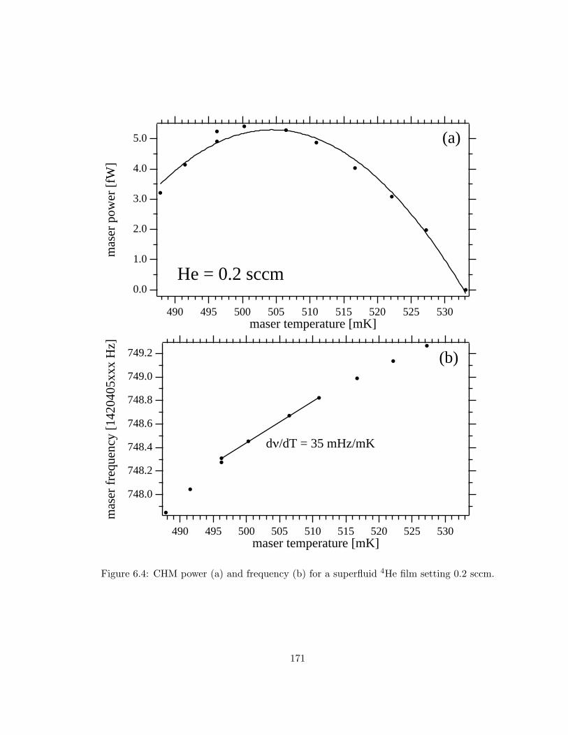
5.0

4.0

3.0

2.0

1.0

0.0

mas

er p

ower

[fW

]

530525520515510505500495490maser temperature [mK]

He = 0.2 sccm

(a)

749.2

749.0

748.8

748.6

748.4

748.2

748.0

mas

er f

requ

ency

[14

2040

5xxx

Hz]

530525520515510505500495490maser temperature [mK]

dν/dT = 35 mHz/mK

(b)

Figure 6.4: CHM power (a) and frequency (b) for a superfluid 4He film setting 0.2 sccm.

171

Because the length of maser running time between 20 K warming cycles was also

decreased as hydrogen flux was increased, the choice of hydrogen flux also involved a

trade-off between running time and maser power. We have found that a molecular flux

setting of 1.2 units (corresponding to an upstream pressure of 2.4 PSI) was sufficient to

allow stable running of the discharge and ample maser power without significantly reducing

the maser running time. We note that as a systematic check for sensitivity on molecular

hydrogen flux setting, one measurement of λ0 was made at an elevated flux setting of 1.7

units (corresponding to an upstream pressure of 3.4 PSI). There was no apparent effect

on our value of λ0 for varying the molecular flux over this range.

As described at the end of Chapter 5, the CHM suffered from a negative shift of the

microwave cavity tuning range during thermal cycles to room temperature and back to 0.5

K. After the room temperature warm-up immediately preceding the run in which these

spin-exchange measurements were made, the cavity tuning range was shifted low enough

that the cavity could not be tuned to atomic resonance. The highest achievable cavity

tuning was about 1420.38 MHz, about 25 kHz (one half the cavity linewidth) below atomic

resonance. The cavity-Q was typically about 26,500, and all spin-exchange measurements

were made with the cavity set between 1,420,381,792 and 1,420,378,996 Hz, resulting in a

cavity tuning parameter ∆ range of −0.891 to −0.998. There was no apparent effect on

our value of λ0 for varying ∆ over this range.

Selection of magnetic gradients

Our method of determining λ0 by measuring the maser frequency shift due to varying the

magnetic-inhomogeneity-induced broadening required us to find a collection of solenoid

field settings which vary γ2 but do not shift the atomic hyperfine frequency ω24. Equiv-

alently, these settings would vary the magnetic field gradient across the bulb, but would

not shift the ensemble-average magnetic field experienced by atoms in the bulb. To find

these settings, we kept the lower trim coil setting fixed and varied the upper trim and

main solenoid settings. The lower coil was left untouched since changing its current led to

172

large changes in overall maser power, implying that the lower coil helps to maintain the

quantization axis for the atomic beam into the storage bulb.

Our gradient search was done by applying the double resonance techniques discussed

in Chapter 2. By applying a oscillating transverse field with the CHM’s Zeeman coils, and

sweeping this field through the atoms F = 1, ∆mF = ±1 Zeeman frequency, the maser

power was reduced as shown in Figure 6.5. A Lorentzian fit to these maser power data

(with a linear background to account for maser power drift during the scan) was used to

determine the Zeeman frequency and Zeeman linewidth.

Initially, a solenoid setting was found which produced the narrowest Zeeman linewidth.

In a room temperature maser, this search is conducted by simply varying the current in

the solenoid’s trim coils while monitoring the Zeeman linewidth. Unfortunately, due to

the presence of superconducting indium rings (used for cryogenic vacuum seals), this

technique was considerably less effective because of the magnetic flux expulsion from the

superconducting indium rings. Thus, shimming of the CHM solenoid involved a series of

maser warmings above the 3.4 K critical temperature of indium, followed by recoolings

to “freeze in” the magnetic flux for the new solenoid setting. An iterative approach was

applied, where the solenoid settings were varied to find the narrowest line and then held

there through a warming/cooling cycle. Once recooled, the settings were changed slightly

to narrow the line, and then held through another warming/cooling cycle. Eventually

a solenoid setting was found where the Zeeman linewidth was narrowest for the frozen-

in setting, with no narrowing found by making small deviations from it. This setting

produced a Zeeman frequency of 3360 Hz (corresponding to an average solenoid field of

2.4 mG) and a Zeeman width of approximately 30 Hz.

Once this minimum magnetic inhomogeneity setting was found, a set of four additional

settings were found which increased γ2 but did not shift ω24. To find them, the current

in the upper trim coil was reduced, thus increasing the gradient across the bulb, until a

measurable reduction in the maser power was observed. This power reduction signified

the increase in γ2. Then, the current in the main solenoid coil was increased until the

173

measured F = 1, ∆mF = ±1 Zeeman frequency was restored to the original value.

The Zeeman resonances for the five solenoid settings used for the spin-exchange studies

are shown in Figure 6.5(a). Here it can be seen that solenoid setting 1 produces the

narrowest line and maximum maser power. The subsequent settings broaden the Zeeman

line and reduce the maser power (increase γ2), but produce only a small shift in the

Zeeman frequency. A plot of maser power and fit Zeeman frequency vs gradient setting

(Figure 6.5(b)) shows a uniform reduction in maser power as the magnetic gradient is

increased, while the overall Zeeman frequency shift (away from the average value of 3360.5

Hz) is less than 10 Hz. For this average 2.4 mG main field, a shift of 10 Hz in the F = 1,

∆mF = ±1 Zeeman frequency would produce a second-order Zeeman shift in the hyperfine

frequency ω24/2π of less than 0.1 mHz, more than an order of magnitude below the typical

spin-exchange shifts measured in this study. We note that the Zeeman frequencies for these

gradients, and therefore the second-order Zeeman shift in the hyperfine frequency, were

not changed significantly by a 20 K warming cycle.

Measurement of γ2

To determine λ0 from the maser frequency shift caused by magnetic-inhomogeneity-induced

line broadening, it is necessary to quantify the changes in γ2 caused by the magnetic field

gradients. In particular, the relative broadening, δγ2 must be known as the field gradients

are changed between settings.

At the highest achievable cavity frequency setting of around 1420.38 MHz, the maser

power was reduced by about 10% from its maximum value for the cavity tuned to atomic

resonance. Since we could then only shift the cavity frequency even further from resonance

(thereby reducing further the maser power), our ability to measure γ2 using the cavity

pulling effect was severely compromised. Furthermore, mechanical cavity tuning involved

the undesirable effect of warming the maser.

A considerably different method was therefore employed to determine the relative

γ2 values. Instead of making these measurements with the maser actively oscillating,

174

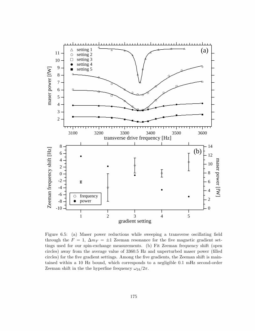
11

10

9

8

7

6

5

4

3

2

mas

er p

ower

[fW

]

360035003400330032003100transverse drive frequency [Hz]

setting 1 setting 2 setting 3 setting 4 setting 5

(a)

-10

-8

-6

-4

-2

0

2

4

6

8

Zee

man

fre

quen

cy s

hift

[H

z]

54321gradient setting

14

12

10

8

6

4

2

0

maser pow

er [fW] frequency

power

(b)

Figure 6.5: (a) Maser power reductions while sweeping a transverse oscillating fieldthrough the F = 1, ∆mF = ±1 Zeeman resonance for the five magnetic gradient set-tings used for our spin-exchange measurements. (b) Fit Zeeman frequency shift (opencircles) away from the average value of 3360.5 Hz and unperturbed maser power (filledcircles) for the five gradient settings. Among the five gradients, the Zeeman shift is main-tained within a 10 Hz bound, which corresponds to a negligible 0.1 mHz second-orderZeeman shift in the the hyperfine frequency ω24/2π.

175

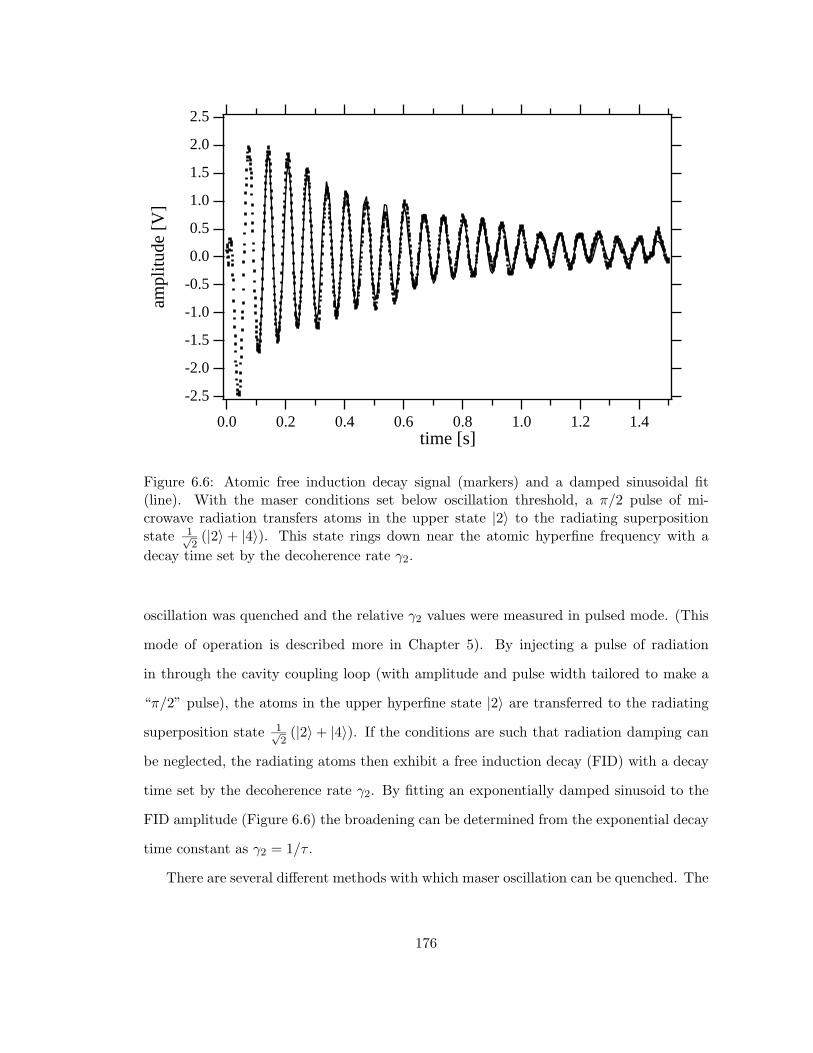
-2.5

-2.0

-1.5

-1.0

-0.5

0.0

0.5

1.0

1.5

2.0

2.5

ampl

itude

[V

]

1.41.21.00.80.60.40.20.0time [s]

Figure 6.6: Atomic free induction decay signal (markers) and a damped sinusoidal fit(line). With the maser conditions set below oscillation threshold, a π/2 pulse of mi-crowave radiation transfers atoms in the upper state |2〉 to the radiating superpositionstate 1√

2(|2〉 + |4〉). This state rings down near the atomic hyperfine frequency with a

decay time set by the decoherence rate γ2.

oscillation was quenched and the relative γ2 values were measured in pulsed mode. (This

mode of operation is described more in Chapter 5). By injecting a pulse of radiation

in through the cavity coupling loop (with amplitude and pulse width tailored to make a

“π/2” pulse), the atoms in the upper hyperfine state |2〉 are transferred to the radiating

superposition state 1√2(|2〉 + |4〉). If the conditions are such that radiation damping can

be neglected, the radiating atoms then exhibit a free induction decay (FID) with a decay

time set by the decoherence rate γ2. By fitting an exponentially damped sinusoid to the

FID amplitude (Figure 6.6) the broadening can be determined from the exponential decay

time constant as γ2 = 1/τ .

There are several different methods with which maser oscillation can be quenched. The

176

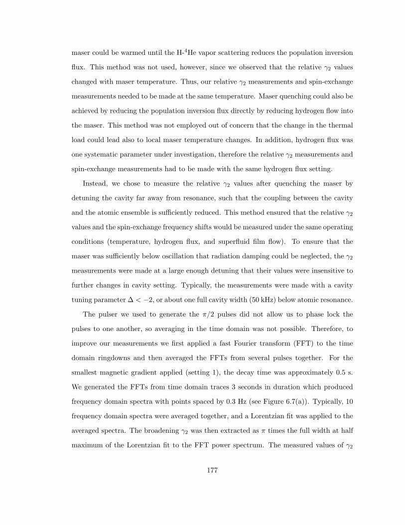
maser could be warmed until the H-4He vapor scattering reduces the population inversion

flux. This method was not used, however, since we observed that the relative γ2 values

changed with maser temperature. Thus, our relative γ2 measurements and spin-exchange

measurements needed to be made at the same temperature. Maser quenching could also be

achieved by reducing the population inversion flux directly by reducing hydrogen flow into

the maser. This method was not employed out of concern that the change in the thermal

load could lead also to local maser temperature changes. In addition, hydrogen flux was

one systematic parameter under investigation, therefore the relative γ2 measurements and

spin-exchange measurements had to be made with the same hydrogen flux setting.

Instead, we chose to measure the relative γ2 values after quenching the maser by

detuning the cavity far away from resonance, such that the coupling between the cavity

and the atomic ensemble is sufficiently reduced. This method ensured that the relative γ2

values and the spin-exchange frequency shifts would be measured under the same operating

conditions (temperature, hydrogen flux, and superfluid film flow). To ensure that the

maser was sufficiently below oscillation that radiation damping could be neglected, the γ2

measurements were made at a large enough detuning that their values were insensitive to

further changes in cavity setting. Typically, the measurements were made with a cavity

tuning parameter ∆ < −2, or about one full cavity width (50 kHz) below atomic resonance.

The pulser we used to generate the π/2 pulses did not allow us to phase lock the

pulses to one another, so averaging in the time domain was not possible. Therefore, to

improve our measurements we first applied a fast Fourier transform (FFT) to the time

domain ringdowns and then averaged the FFTs from several pulses together. For the

smallest magnetic gradient applied (setting 1), the decay time was approximately 0.5 s.

We generated the FFTs from time domain traces 3 seconds in duration which produced

frequency domain spectra with points spaced by 0.3 Hz (see Figure 6.7(a)). Typically, 10

frequency domain spectra were averaged together, and a Lorentzian fit was applied to the

averaged spectra. The broadening γ2 was then extracted as π times the full width at half

maximum of the Lorentzian fit to the FFT power spectrum. The measured values of γ2

177

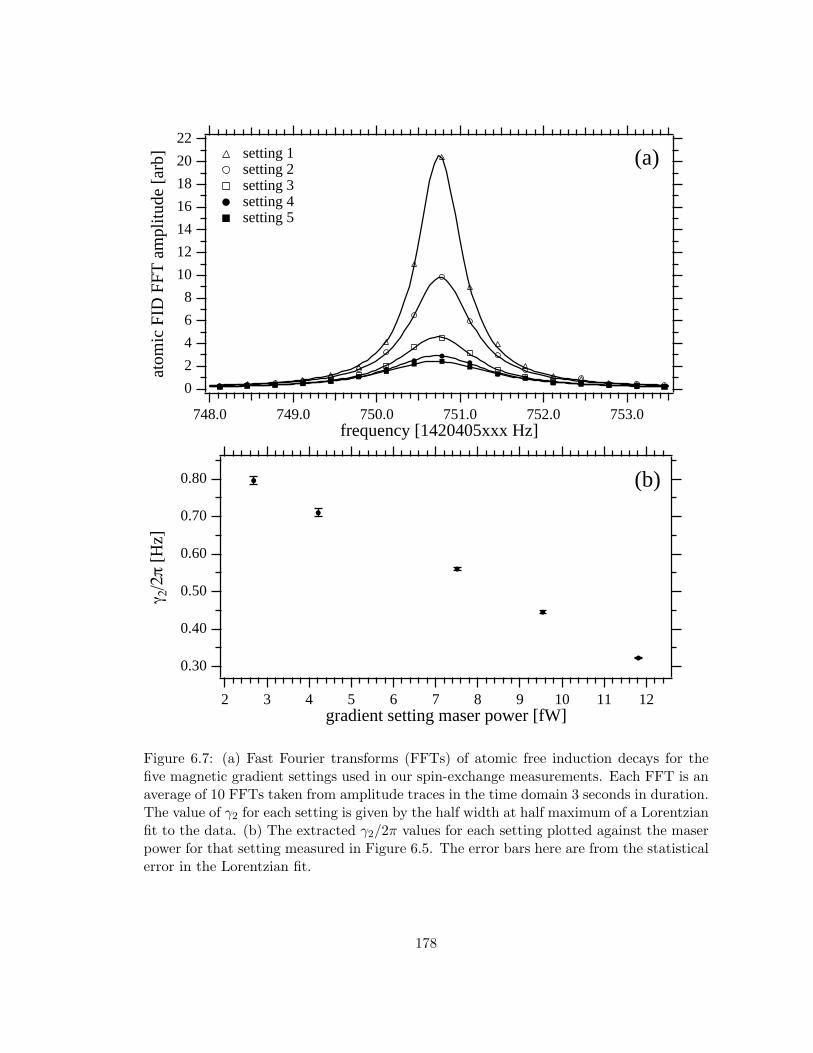
22

20

18

16

14

12

10

8

6

4

2

0

atom

ic F

ID F

FT a

mpl

itude

[ar

b]

753.0752.0751.0750.0749.0748.0frequency [1420405xxx Hz]

setting 1 setting 2 setting 3 setting 4 setting 5

(a)

0.80

0.70

0.60

0.50

0.40

0.30

γ 2/2π

[Hz]

12111098765432gradient setting maser power [fW]

(b)

Figure 6.7: (a) Fast Fourier transforms (FFTs) of atomic free induction decays for thefive magnetic gradient settings used in our spin-exchange measurements. Each FFT is anaverage of 10 FFTs taken from amplitude traces in the time domain 3 seconds in duration.The value of γ2 for each setting is given by the half width at half maximum of a Lorentzianfit to the data. (b) The extracted γ2/2π values for each setting plotted against the maserpower for that setting measured in Figure 6.5. The error bars here are from the statisticalerror in the Lorentzian fit.

178

for each of the gradient settings’ FFTs are plotted in Figure 6.7(b) as a function of the

unperturbed maser power for each setting (taken from Figure 6.5).

When determining the relative γ2 values for a spin-exchange frequency shift measure-

ment, multiple 10 average points were taken for each gradient setting. Since the frequency

domain FID amplitude was considerably smaller for the larger magnetic field gradient set-

tings, more averages were taken of these points. As shown in Figure 6.8 the FFT averages

were taken in the gradient setting sequence 1-2-1-3-1-4-1-5-1. . . such that any drift in the

overall γ2 (e.g., due to slow superfluid film variation) could be monitored and corrected for.

By fitting any such drift for gradient setting 1 to a slowly varying drift function (typically

a one- or two-piece quadratic), and then subtracting this drift from each of the gradient

settings, the average value of the residuals for each setting was a measure of the relative

magnetic-inhomogeneity-induced broadening δγ2/2π. These values are given in Figure 6.8

for a superfluid film setting of 0.2 sccm, a hydrogen flux of 1.2 units (upstream pressure

2.4 PSI), and a maser temperature of 496 mK. From the averages of these values it can

be seen that our measurement technique allowed us to determine δγ2 for each gradient

setting with a statistical precision of a few percent.

It was observed that the overall broadening γ2 (for a given gradient setting) would

vary from day to day even with the operating conditions reproduced. We believe that this

variation is due to small changes in the superfluid film thickness. The relative magnetic-

inhomogeneity-induced broadening δγ2, however, was found to be very stable from day

to day (to within a few percent), and showed no significant variation even between 20 K

warming cycles. In Figure 6.9 we plot four measurements of the relative γ2 values at two

different temperatures made on four different days and between different 20 K warming

cycles. Here, it can be seen that there is a noticeable shift in relative γ2 values between the

two temperatures, however the shift for a given temperature is within the experimental

uncertainty of a few percent.

Since the relative γ2 values were stable from day to day, it was not necessary to

complete both the γ2 measurements and the spin-exchange frequency shift measurements

179

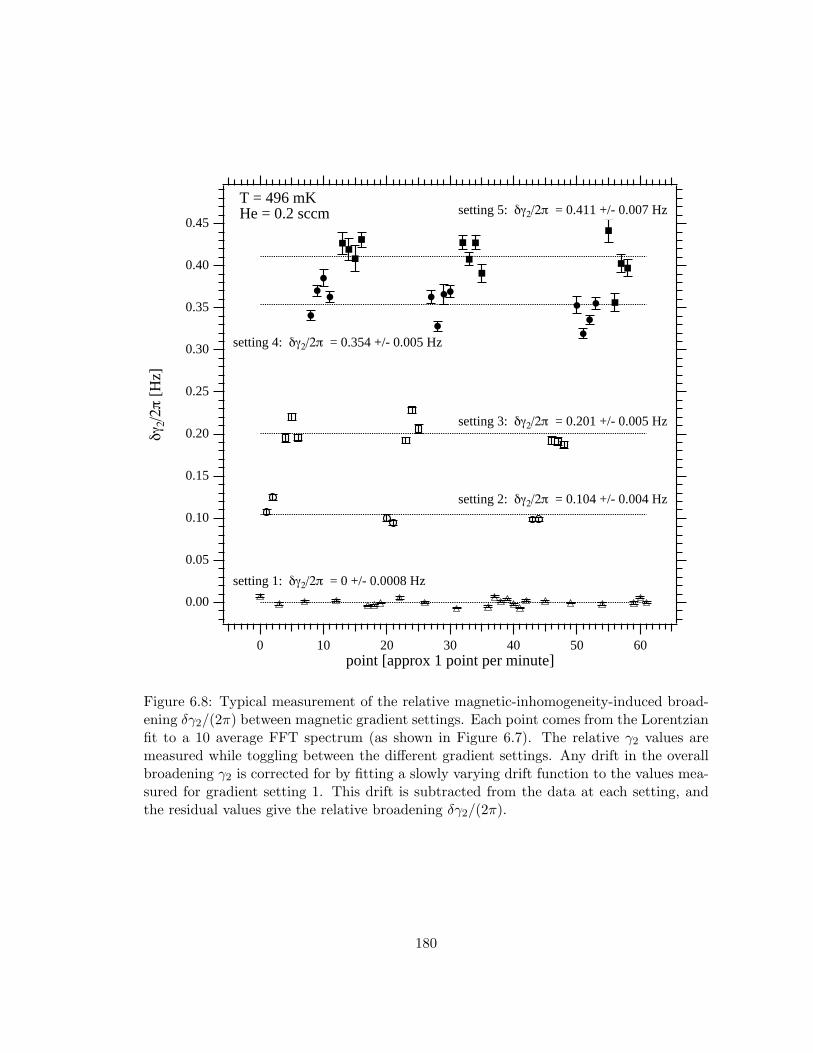
0.45

0.40

0.35

0.30

0.25

0.20

0.15

0.10

0.05

0.00

δγ2/

2π [

Hz]

6050403020100point [approx 1 point per minute]

setting 1: δγ2/2π = 0 +/- 0.0008 Hz

setting 2: δγ2/2π = 0.104 +/- 0.004 Hz

setting 3: δγ2/2π = 0.201 +/- 0.005 Hz

setting 4: δγ2/2π = 0.354 +/- 0.005 Hz

setting 5: δγ2/2π = 0.411 +/- 0.007 HzT = 496 mKHe = 0.2 sccm

Figure 6.8: Typical measurement of the relative magnetic-inhomogeneity-induced broad-ening δγ2/(2π) between magnetic gradient settings. Each point comes from the Lorentzianfit to a 10 average FFT spectrum (as shown in Figure 6.7). The relative γ2 values aremeasured while toggling between the different gradient settings. Any drift in the overallbroadening γ2 is corrected for by fitting a slowly varying drift function to the values mea-sured for gradient setting 1. This drift is subtracted from the data at each setting, andthe residual values give the relative broadening δγ2/(2π).

180

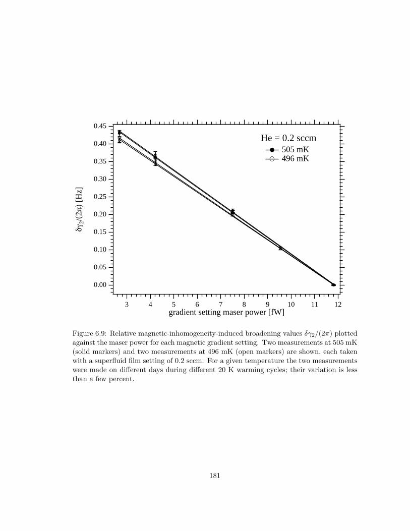
0.45

0.40

0.35

0.30

0.25

0.20

0.15

0.10

0.05

0.00

δγ2/

(2π)

[H

z]

1211109876543gradient setting maser power [fW]

505 mK 496 mK

He = 0.2 sccm

Figure 6.9: Relative magnetic-inhomogeneity-induced broadening values δγ2/(2π) plottedagainst the maser power for each magnetic gradient setting. Two measurements at 505 mK(solid markers) and two measurements at 496 mK (open markers) are shown, each takenwith a superfluid film setting of 0.2 sccm. For a given temperature the two measurementswere made on different days during different 20 K warming cycles; their variation is lessthan a few percent.

181

during the same day. To do so would require the maser to continue running while the cavity

was tuned back to its value nearest atomic resonance. This amount of mechanical tuning

would require up to one hour of thermal re-equilibration. For some of the measurements

reported below, the relative γ2 and spin-exchange frequency shift data were taken on the

same day. For others, previously measured γ2 values for the same operating conditions

were used in the analysis of the spin-exchange maser frequency shift data.

Measurement of ∆

From Eqn. 6.17 it can be seen that the maser frequency shift due to cavity detuning

combines additively with the maser shift due to spin-exchange collisions. For this reason,

the absolute error in the cavity detuning parameter ∆ must be sufficiently small to resolve

the spin-exchange shift product αλ0. A considerable effort was therefore made to refine

our measurement of ∆, and two measurement techniques were developed.

The first technique used cw microwave power to interrogate the cavity through re-

flection. The setup for this reflection technique is given in Figure 6.10. A frequency

generator,4 locked to a room temperature hydrogen maser and initially set about one

cavity linewidth below the resonant frequency, was stepped through the cavity resonance.

The cw power was directed toward the cavity using a 20 dB directional coupler. The

first port of a second 20 dB directional coupler directed a portion of the microwave power

towards one input of a vector voltmeter.5 The remainder of the cw power passed into

the cryostat, along the transmission line to the cavity’s coupling loop. Here, some of the

microwave power was absorbed by the cavity (maximum absorption on resonance) and the

rest of the power was reflected back. After traveling back up the transmission line, 20 dB

of this reflected power was directed with the second port of the second 20 dB directional

coupler into the second input of the vector voltmeter. (The remainder of the reflected

power was absorbed into a 50 Ohm terminator).

A computer running a LabVIEW program controlled the frequency steps of the fre-4Hewlett-Packard model 8660D.5Hewlett-Packard model 8508A.

182

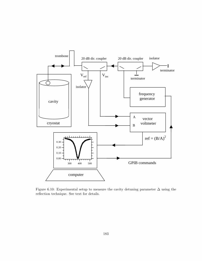
VincVref

ref = (B/A)2

0.30

0.20

0.10

0.00

500400300

generator

20 dB dir. coupler 20 dB dir. coupler

terminator

terminator

vectorA

B

isolator

isolator

cavity

computer

GPIB commands

trombone

cryostat

frequency

voltmeter

Figure 6.10: Experimental setup to measure the cavity detuning parameter ∆ using thereflection technique. See text for details.

183

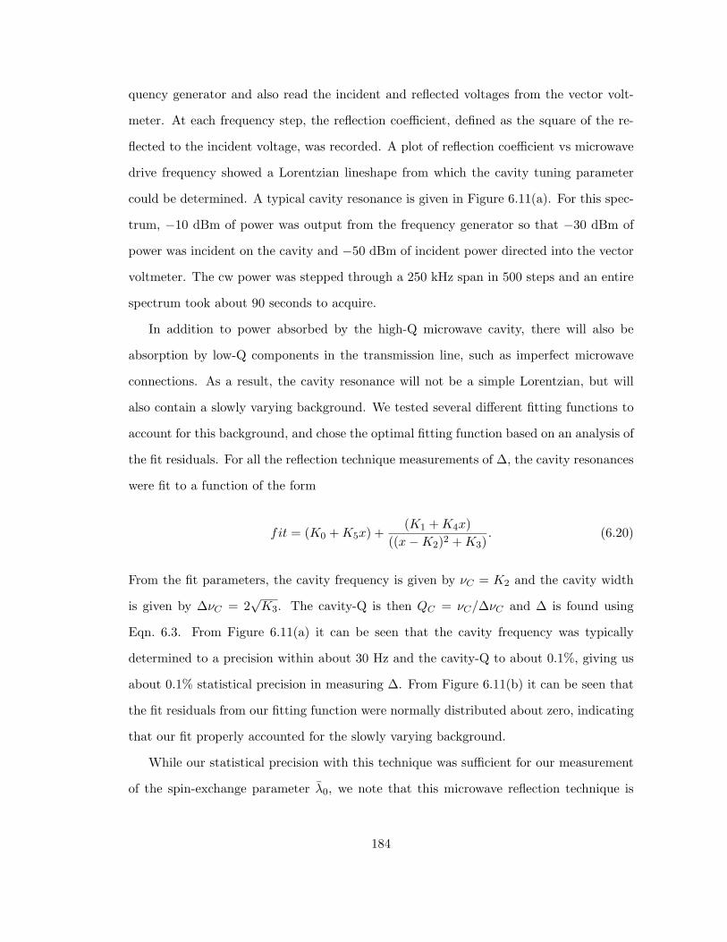
quency generator and also read the incident and reflected voltages from the vector volt-

meter. At each frequency step, the reflection coefficient, defined as the square of the re-

flected to the incident voltage, was recorded. A plot of reflection coefficient vs microwave

drive frequency showed a Lorentzian lineshape from which the cavity tuning parameter

could be determined. A typical cavity resonance is given in Figure 6.11(a). For this spec-

trum, −10 dBm of power was output from the frequency generator so that −30 dBm of

power was incident on the cavity and −50 dBm of incident power directed into the vector

voltmeter. The cw power was stepped through a 250 kHz span in 500 steps and an entire

spectrum took about 90 seconds to acquire.

In addition to power absorbed by the high-Q microwave cavity, there will also be

absorption by low-Q components in the transmission line, such as imperfect microwave

connections. As a result, the cavity resonance will not be a simple Lorentzian, but will

also contain a slowly varying background. We tested several different fitting functions to

account for this background, and chose the optimal fitting function based on an analysis of

the fit residuals. For all the reflection technique measurements of ∆, the cavity resonances

were fit to a function of the form

fit = (K0 + K5x) +(K1 + K4x)

((x − K2)2 + K3). (6.20)

From the fit parameters, the cavity frequency is given by νC = K2 and the cavity width

is given by ∆νC = 2√

K3. The cavity-Q is then QC = νC/∆νC and ∆ is found using

Eqn. 6.3. From Figure 6.11(a) it can be seen that the cavity frequency was typically

determined to a precision within about 30 Hz and the cavity-Q to about 0.1%, giving us

about 0.1% statistical precision in measuring ∆. From Figure 6.11(b) it can be seen that

the fit residuals from our fitting function were normally distributed about zero, indicating

that our fit properly accounted for the slowly varying background.

While our statistical precision with this technique was sufficient for our measurement

of the spin-exchange parameter λ0, we note that this microwave reflection technique is

184

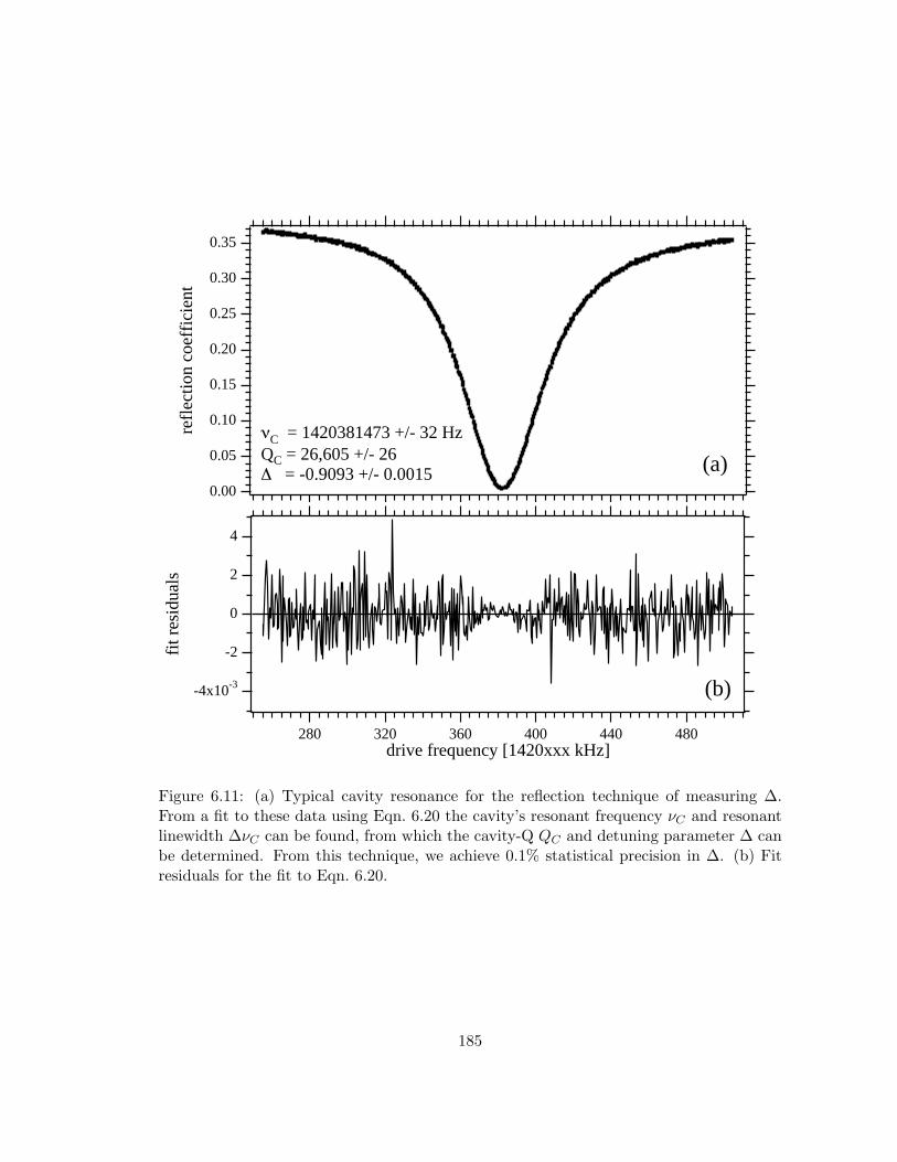
0.35

0.30

0.25

0.20

0.15

0.10

0.05

0.00

refl

ectio

n co

effi

cien

t

480440400360320280drive frequency [1420xxx kHz]

νC = 1420381473 +/- 32 HzQC = 26,605 +/- 26∆ = -0.9093 +/- 0.0015 (a)

-4x10-3

-2

0

2

4

fit r

esid

uals

480440400360320280drive frequency [1420xxx kHz]

(b)

Figure 6.11: (a) Typical cavity resonance for the reflection technique of measuring ∆.From a fit to these data using Eqn. 6.20 the cavity’s resonant frequency νC and resonantlinewidth ∆νC can be found, from which the cavity-Q QC and detuning parameter ∆ canbe determined. From this technique, we achieve 0.1% statistical precision in ∆. (b) Fitresiduals for the fit to Eqn. 6.20.

185

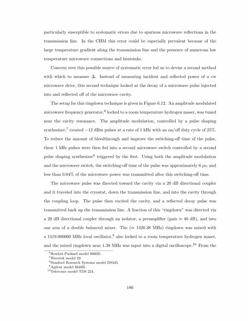
particularly susceptible to systematic errors due to spurious microwave reflections in the

transmission line. In the CHM this error could be especially prevalent because of the

large temperature gradient along the transmission line and the presence of numerous low

temperature microwave connections and heatsinks.

Concern over this possible source of systematic error led us to devise a second method

with which to measure ∆. Instead of measuring incident and reflected power of a cw

microwave drive, this second technique looked at the decay of a microwave pulse injected

into and reflected off of the microwave cavity.

The setup for this ringdown technique is given in Figure 6.12. An amplitude modulated

microwave frequency generator,6 locked to a room temperature hydrogen maser, was tuned

near the cavity resonance. The amplitude modulation, controlled by a pulse shaping

synthesizer,7 created −12 dBm pulses at a rate of 1 kHz with an on/off duty cycle of 25%.

To reduce the amount of bleedthrough and improve the switching-off time of the pulse,

these 1 kHz pulses were then fed into a second microwave switch controlled by a second

pulse shaping synthesizer8 triggered by the first. Using both the amplitude modulation

and the microwave switch, the switching-off time of the pulse was approximately 6 µs, and

less than 0.04% of the microwave power was transmitted after this switching-off time.

The microwave pulse was directed toward the cavity via a 20 dB directional coupler

and it traveled into the cryostat, down the transmission line, and into the cavity through

the coupling loop. The pulse then excited the cavity, and a reflected decay pulse was

transmitted back up the transmission line. A fraction of this “ringdown” was directed via

a 20 dB directional coupler through an isolator, a preamplifier (gain ≈ 40 dB), and into

one arm of a double balanced mixer. The (≈ 1420.38 MHz) ringdown was mixed with

a 1419.000000 MHz local oscillator,9 also locked to a room temperature hydrogen maser,

and the mixed ringdown near 1.38 MHz was input into a digital oscilloscope.10 From the6Hewlett-Packard model 8660D.7Wavetek model 29.8Stanford Research Systems model DS345.9Agilent model 8648B.

10Tektronix model TDS 224.

186

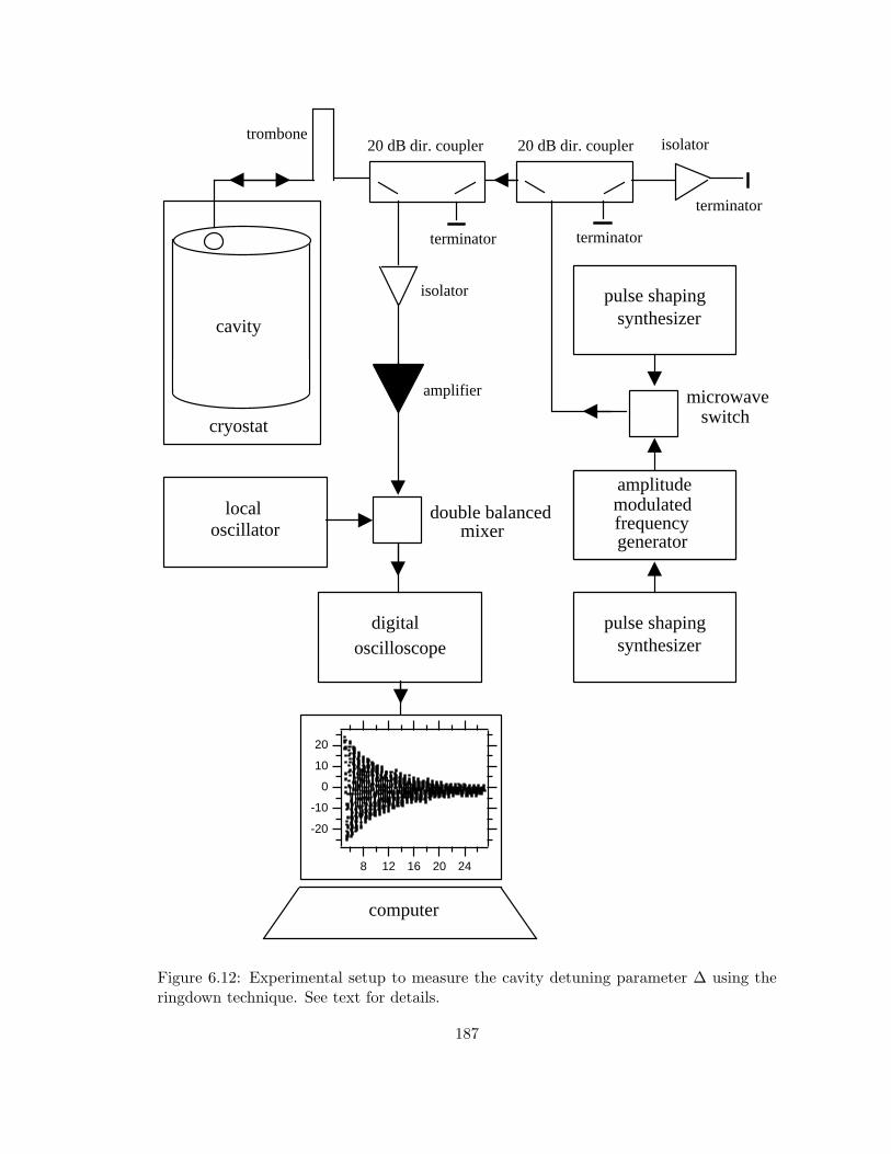
-20

-10

0

10

20

242016128

generator

20 dB dir. coupler 20 dB dir. coupler

terminator

terminator

isolator

isolator

cavity

computer

trombone

cryostat

frequencyfrequencygenerator

pulse shapingsynthesizer

modulated

pulse shapingsynthesizer

terminator

microwaveswitch

amplifier

localoscillator

digitaloscilloscope

double balanced

amplitude

mixer

Figure 6.12: Experimental setup to measure the cavity detuning parameter ∆ using theringdown technique. See text for details.

187

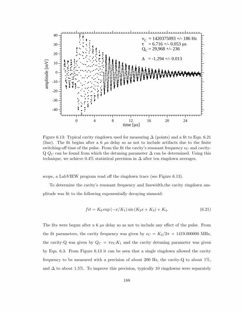
-40

-30

-20

-10

0

10

20

30

40

ampl

itude

[m

V]

24201612840time [µs]

νC = 1420375093 +/- 186 Hzτ = 6.716 +/- 0.053 µsQC = 29,968 +/- 236 ∆ = -1.294 +/- 0.013

Figure 6.13: Typical cavity ringdown used for measuring ∆ (points) and a fit to Eqn. 6.21(line). The fit begins after a 6 µs delay so as not to include artifacts due to the finiteswitching-off time of the pulse. From the fit the cavity’s resonant frequency νC and cavity-Q QC can be found from which the detuning parameter ∆ can be determined. Using thistechnique, we achieve 0.4% statistical precision in ∆ after ten ringdown averages.

scope, a LabVIEW program read off the ringdown trace (see Figure 6.13).

To determine the cavity’s resonant frequency and linewidth,the cavity ringdown am-

plitude was fit to the following exponentially decaying sinusoid:

fit = K0 exp (−x/K1) sin (K2x + K3) + K4. (6.21)

The fits were begun after a 6 µs delay so as not to include any effect of the pulse. From

the fit parameters, the cavity frequency was given by νC = K2/2π + 1419.000000 MHz,

the cavity-Q was given by QC = πνCK1 and the cavity detuning parameter was given

by Eqn. 6.3. From Figure 6.13 it can be seen that a single ringdown allowed the cavity

frequency to be measured with a precision of about 200 Hz, the cavity-Q to about 1%,

and ∆ to about 1.5%. To improve this precision, typically 10 ringdowns were separately

188

fit and the fit parameters were averaged together which improved the statistical precision

in ∆ to about 0.4%, comparable to that from the reflection method measurements.

Unfortunately we observed that the microwave cavity parameters measured using the

reflection technique disagreed with those measured using the ringdown technique (νC by

parts in 106, QC and ∆ by a few percent). We believe the source of the disagreement to

be microwave reflections in the transmission line. In order to investigate these effects, a

microwave trombone was installed between the cryostat and the first 20 dB directional

coupler (see Figures 6.10 and 6.12). Changing the length of the trombone varied the

line length between the cavity and the detection devices and allowed us to make our

measurements at different places on the transmission line. This potentially allowed us to

find the proper place on the line where spurious microwave reflections would be eliminated.

A comparison of the cavity frequency, cavity-Q, and detuning parameter measured by

the two techniques is shown in Figure 6.14 for a small variation in the trombone setting

and therefore the measurement position along the transmission line. From these plots,

it can be seen that the individual cavity parameters (νC , QC , and ∆) agree between

the two measurement techniques at different locations on the transmission line. Because

the cavity pulling maser shift depends on the complete detuning parameter ∆, most of

our spin-exchange measurements were made with the trombone set such that there was

agreement in ∆ between the two techniques. Good agreement in λ0 was found between

all measurements made at this trombone setting. An additional measurement was made

with the trombone set such that the cavity frequencies (νC) were in agreement, and it

was unfortunately found that both values of λ0 (extracted using the reflection method

∆ and the ringdown method ∆) were in statistical disagreement with the data from the

trombone setting for agreement in ∆. As will be discussed in Section 6.5.2, uncertainty in

∆ turned out to be the dominate source of systematic error for our measurement of the

spin-exchange parameter λ0.

189

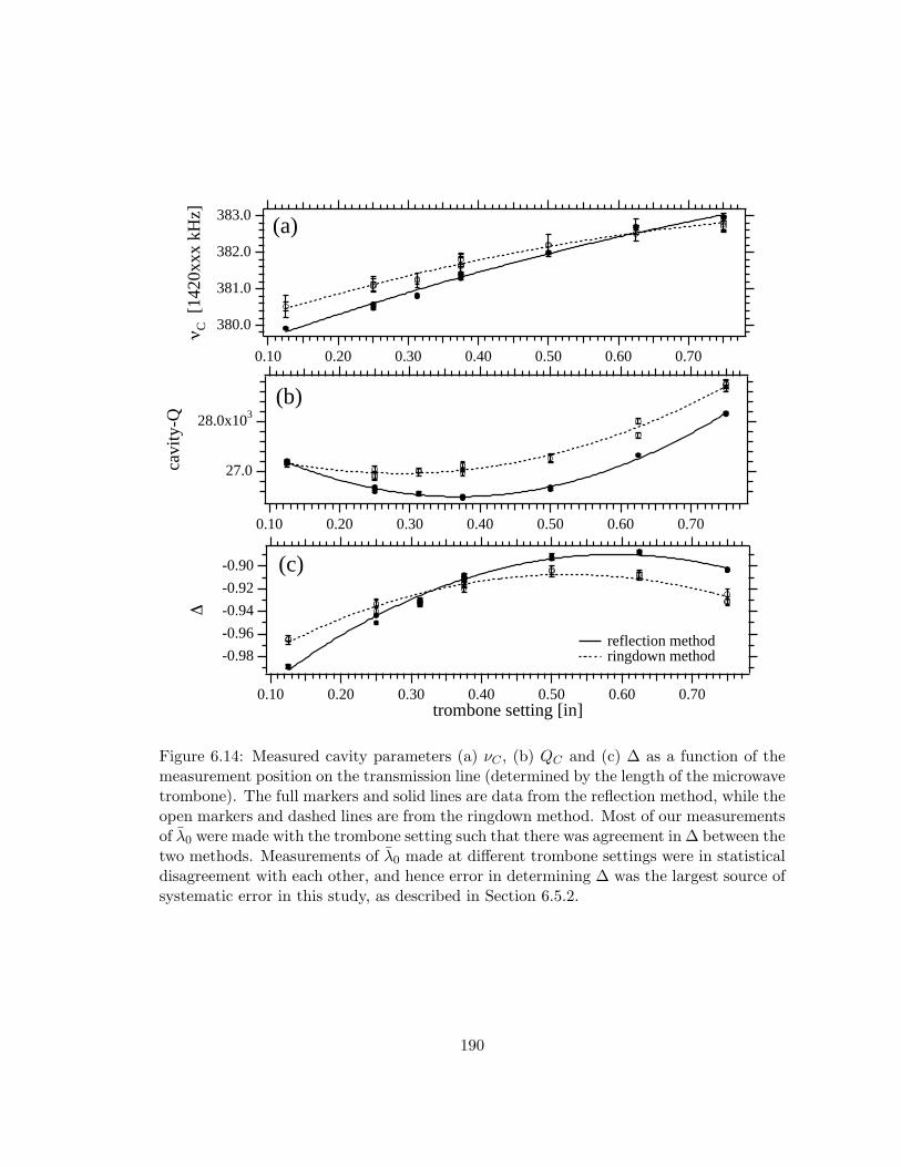
383.0

382.0

381.0

380.0

ν C [

1420

xxx

kHz]

0.700.600.500.400.300.200.10

(a)

28.0x103

27.0cavi

ty-Q

0.700.600.500.400.300.200.10

(b)

-0.98

-0.96

-0.94

-0.92

-0.90

∆

0.700.600.500.400.300.200.10trombone setting [in]

reflection method ringdown method

(c)

Figure 6.14: Measured cavity parameters (a) νC , (b) QC and (c) ∆ as a function of themeasurement position on the transmission line (determined by the length of the microwavetrombone). The full markers and solid lines are data from the reflection method, while theopen markers and dashed lines are from the ringdown method. Most of our measurementsof λ0 were made with the trombone setting such that there was agreement in ∆ between thetwo methods. Measurements of λ0 made at different trombone settings were in statisticaldisagreement with each other, and hence error in determining ∆ was the largest source ofsystematic error in this study, as described in Section 6.5.2.

190

Measurement of λ0

Once the cavity detuning parameter ∆ and the relative magnetic-inhomogeneity-induced

broadening δγ2/2π for each gradient setting were determined, a simple measurement of

the maser frequency shift between the gradient settings was sufficient to determine the

spin-exchange parameter using Eqn. 6.19.

With our level of maser temperature control, the short term (10 s) stability of the maser

was on the order of 5 mHz. By taking multiple points at each setting the maser frequency

shift resolution was improved to about 0.3 mHz. As we toggled between magnetic gradient

settings, the CHM frequency was compared to an unperturbed room temperature maser

(maser P-13). (For a detailed description of the maser receivers, see Chapters 3 and

5). The output frequencies of the two voltage controlled crystal oscillators in the maser

receivers were set such that there was about a 1.2 Hz offset between the oscillators. The

two output signals were combined in a double-balanced mixer and the resulting beat note

(period ≈ 0.8 s) was averaged for 10 s (about 12 periods) with a counter11 and logged

with a LabVIEW routine. From this measured beat period we determined the frequency

of the CHM relative to that of maser P-13. The frequency stability of maser P-13 (parts

in 1014) was more than two orders of magnitude smaller than the induced spin-exchange

effects (parts in 1012), therefore we neglected any variation in our reference frequency.

Over longer intervals (tens of minutes), the CHM frequency exhibited slow drifts on

the order of tens of mHz presumably due to slow variation of superfluid film thickness.

Therefore a correction was made for this slow drift. To monitor the maser drift, the data

were taken in 120 s “bunches” in the gradient setting sequence 1-2-1-3-1-4-1-5-1. . . (see

Figure 6.15(a)) so that a bunch of data from gradient setting 1 was taken between each

bunch at the other gradient settings. Then, the setting 1 data were fit to a piecewise

continuous quadratic function where a new quadratic was allowed for every six bunches11Hewlett-Packard model HP 53131A.

191

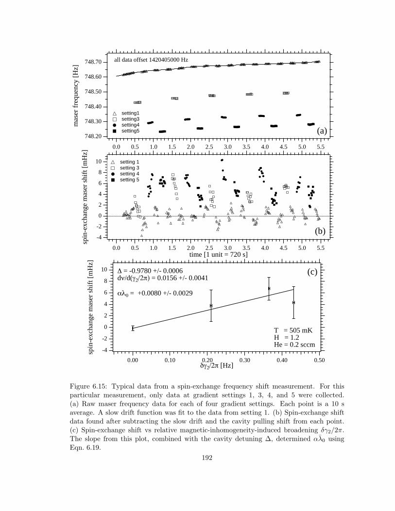
748.70

748.60

748.50

748.40

748.30

748.20

mas

er f

requ

ency

[H

z]

5.55.04.54.03.53.02.52.01.51.00.50.0time [1 unit = 720 s]

setting1 setting3 setting4 setting5

all data offset 1420405000 Hz

(a)

10

8

6

4

2

0

-2

-4

spin

-exc

hang

e m

aser

shi

ft [

mH

z]

5.55.04.54.03.53.02.52.01.51.00.50.0time [1 unit = 720 s]

setting 1 setting 3 setting 4 setting 5

(b)

10

8

6

4

2

0

-2

-4spin

-exc

hang

e m

aser

shi

ft [

mH

z]

0.500.400.300.200.100.00δγ2/2π [Hz]

∆ = -0.9780 +/- 0.0006dν/d(γ2/2π) = 0.0156 +/- 0.0041 αλ0 = +0.0080 +/- 0.0029

T = 505 mKH = 1.2He = 0.2 sccm

(c)

Figure 6.15: Typical data from a spin-exchange frequency shift measurement. For thisparticular measurement, only data at gradient settings 1, 3, 4, and 5 were collected.(a) Raw maser frequency data for each of four gradient settings. Each point is a 10 saverage. A slow drift function was fit to the data from setting 1. (b) Spin-exchange shiftdata found after subtracting the slow drift and the cavity pulling shift from each point.(c) Spin-exchange shift vs relative magnetic-inhomogeneity-induced broadening δγ2/2π.The slope from this plot, combined with the cavity detuning ∆, determined αλ0 usingEqn. 6.19.

192

(720 s) of data. For data in the nth 720 s window, this function is given by

fn(t) =2n∑i=0

Ai + A2n+1(t − n) + A2n+2(t − n)2. (6.22)

This drift function, plotted along with the setting 1 frequency data in Figure 6.15(a), was

then subtracted from the data at each of the gradient settings.

After correcting for the slow drift, the cavity pulling maser shift was subtracted from

the data at each gradient setting. This shift is formed by the product of the cavity detuning

parameter ∆ and the relative magnetic-inhomogeneity-induced broadening δγ2/2π for each

gradient setting.

After these two corrections, the residual shift is therefore the spin-exchange maser

frequency shift, given for each gradient setting as δν = αλ0δγ2/2π and plotted in Fig-

ure 6.15(b). At each gradient setting, the maser frequency shift was averaged and these

values are plotted as a function of relative magnetic-inhomogeneity-induced broadening in

Figure 6.15(c). The error bar for each gradient setting was found by adding in quadrature

the fractional statistical error in maser frequency (error in the mean), the error due to

imprecision in determining the cavity detuning ∆ (given that the microwave trombone

was set for agreement between the reflection and ringdown methods to measure ∆), and

the error due to uncertainty in the relative magnetic-inhomogeneity-induced broadening

δγ2/2π. After fitting these data to a line, the spin-exchange shift parameter (multiplied

by the system constant α) is found from the slope dν/d(γ2/2π) and the detuning ∆ using

Eqn. 6.19.

In order to extract the spin-exchange parameter λ0, the system constant α must be

determined. This parameter is given by

α =hVC vr

µ0µ2BηQCVb

(6.23)

where VC and Vb are the cavity and bulb volumes, vr is the average relative atomic velocity,

and η is the cavity filling factor, defined in Chapter 3. Calculation of η for the CHM is

193

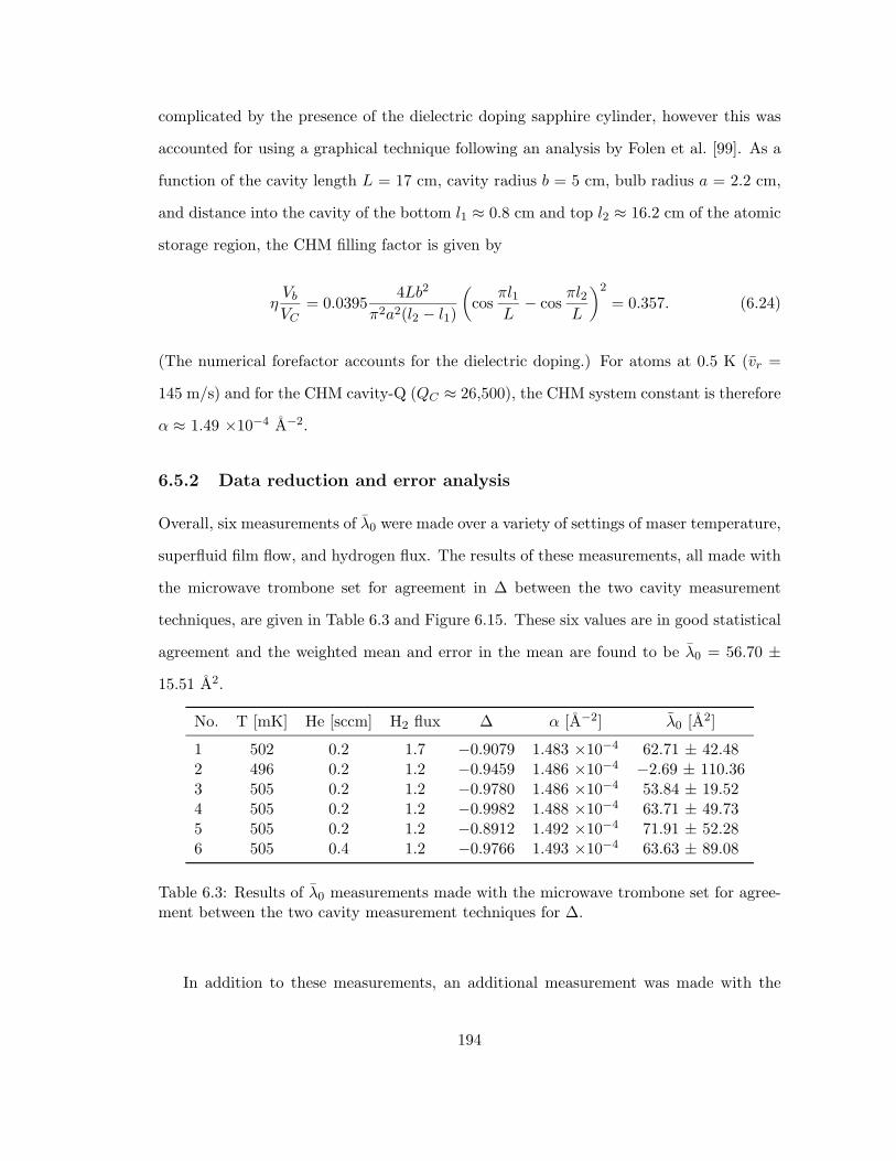
complicated by the presence of the dielectric doping sapphire cylinder, however this was

accounted for using a graphical technique following an analysis by Folen et al. [99]. As a

function of the cavity length L = 17 cm, cavity radius b = 5 cm, bulb radius a = 2.2 cm,

and distance into the cavity of the bottom l1 ≈ 0.8 cm and top l2 ≈ 16.2 cm of the atomic

storage region, the CHM filling factor is given by

ηVb

VC= 0.0395

4Lb2

π2a2(l2 − l1)

(cos

πl1L

− cosπl2L

)2

= 0.357. (6.24)

(The numerical forefactor accounts for the dielectric doping.) For atoms at 0.5 K (vr =

145 m/s) and for the CHM cavity-Q (QC ≈ 26,500), the CHM system constant is therefore

α ≈ 1.49 ×10−4 A−2.

6.5.2 Data reduction and error analysis

Overall, six measurements of λ0 were made over a variety of settings of maser temperature,

superfluid film flow, and hydrogen flux. The results of these measurements, all made with

the microwave trombone set for agreement in ∆ between the two cavity measurement

techniques, are given in Table 6.3 and Figure 6.15. These six values are in good statistical

agreement and the weighted mean and error in the mean are found to be λ0 = 56.70 ±

15.51 A2.

No. T [mK] He [sccm] H2 flux ∆ α [A−2] λ0 [A2]

1 502 0.2 1.7 −0.9079 1.483 ×10−4 62.71 ± 42.482 496 0.2 1.2 −0.9459 1.486 ×10−4 −2.69 ± 110.363 505 0.2 1.2 −0.9780 1.486 ×10−4 53.84 ± 19.524 505 0.2 1.2 −0.9982 1.488 ×10−4 63.71 ± 49.735 505 0.2 1.2 −0.8912 1.492 ×10−4 71.91 ± 52.286 505 0.4 1.2 −0.9766 1.493 ×10−4 63.63 ± 89.08

Table 6.3: Results of λ0 measurements made with the microwave trombone set for agree-ment between the two cavity measurement techniques for ∆.

In addition to these measurements, an additional measurement was made with the

194

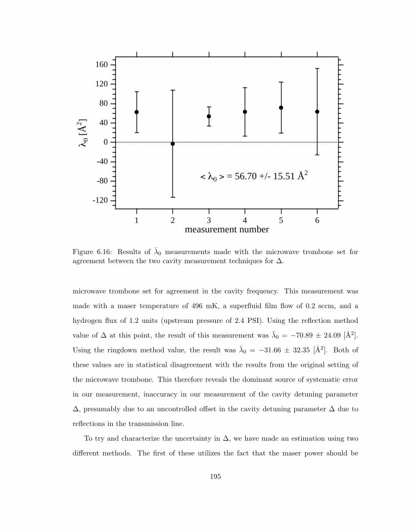
160

120

80

40

0

-40

-80

-120

λ 0 [

Å2 ]

654321measurement number

< λ0 > = 56.70 +/- 15.51 Å2

Figure 6.16: Results of λ0 measurements made with the microwave trombone set foragreement between the two cavity measurement techniques for ∆.

microwave trombone set for agreement in the cavity frequency. This measurement was

made with a maser temperature of 496 mK, a superfluid film flow of 0.2 sccm, and a

hydrogen flux of 1.2 units (upstream pressure of 2.4 PSI). Using the reflection method

value of ∆ at this point, the result of this measurement was λ0 = −70.89 ± 24.09 [A2].

Using the ringdown method value, the result was λ0 = −31.66 ± 32.35 [A2]. Both of

these values are in statistical disagreement with the results from the original setting of

the microwave trombone. This therefore reveals the dominant source of systematic error

in our measurement, inaccuracy in our measurement of the cavity detuning parameter

∆, presumably due to an uncontrolled offset in the cavity detuning parameter ∆ due to

reflections in the transmission line.

To try and characterize the uncertainty in ∆, we have made an estimation using two

different methods. The first of these utilizes the fact that the maser power should be

195

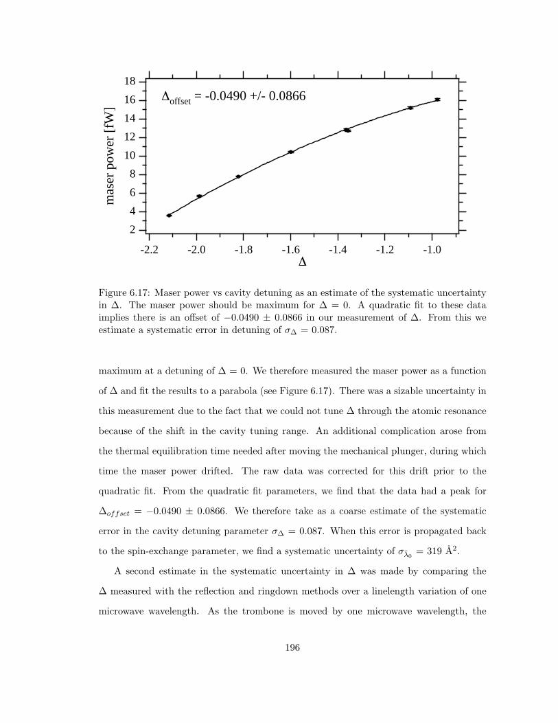
18

16

14

12

10

8

6

4

2

mas

er p

ower

[fW

]

-2.2 -2.0 -1.8 -1.6 -1.4 -1.2 -1.0∆

∆offset = -0.0490 +/- 0.0866

Figure 6.17: Maser power vs cavity detuning as an estimate of the systematic uncertaintyin ∆. The maser power should be maximum for ∆ = 0. A quadratic fit to these dataimplies there is an offset of −0.0490 ± 0.0866 in our measurement of ∆. From this weestimate a systematic error in detuning of σ∆ = 0.087.

maximum at a detuning of ∆ = 0. We therefore measured the maser power as a function

of ∆ and fit the results to a parabola (see Figure 6.17). There was a sizable uncertainty in

this measurement due to the fact that we could not tune ∆ through the atomic resonance

because of the shift in the cavity tuning range. An additional complication arose from

the thermal equilibration time needed after moving the mechanical plunger, during which

time the maser power drifted. The raw data was corrected for this drift prior to the

quadratic fit. From the quadratic fit parameters, we find that the data had a peak for

∆offset = −0.0490 ± 0.0866. We therefore take as a coarse estimate of the systematic

error in the cavity detuning parameter σ∆ = 0.087. When this error is propagated back

to the spin-exchange parameter, we find a systematic uncertainty of σλ0= 319 A2.

A second estimate in the systematic uncertainty in ∆ was made by comparing the

∆ measured with the reflection and ringdown methods over a linelength variation of one

microwave wavelength. As the trombone is moved by one microwave wavelength, the

196

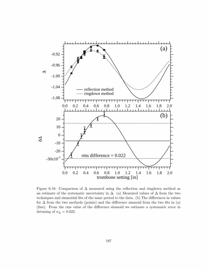
-1.08

-1.04

-1.00

-0.96

-0.92

∆

2.01.81.61.41.21.00.80.60.40.20.0trombone setting [in]

reflection method ringdown method

(a)

-30x10-3

-20

-10

0

10

20

δ∆

2.01.81.61.41.21.00.80.60.40.20.0trombone setting [in]

rms difference = 0.022

(b)

Figure 6.18: Comparison of ∆ measured using the reflection and ringdown method asan estimate of the systematic uncertainty in ∆. (a) Measured values of ∆ from the twotechniques and sinusoidal fits of the same period to the data. (b) The differences in valuesfor ∆ from the two methods (points) and the difference sinusoid from the two fits in (a)(line). From the rms value of the difference sinusoid we estimate a systematic error indetuning of σ∆ = 0.022.

197

measured values of ∆ shift through one sinusoidal period. To make this estimate, we

took the reflection and ringdown method data from Figure 6.14(c) and fit each to a

sinusoid of the same wavelength but differing amplitude and phase. These two fits are

displayed in Figure 6.18(a). The difference between these two fits is the sinusoid displayed

in Figure 6.18(b). We take as a more refined estimate of the systematic error in ∆ the

rms value of this difference sinusoid, and find σ∆ = 0.022. When this error is propagated

back to the spin-exchange parameter, we find a systematic uncertainty of σλ0= 81 A2.

6.5.3 Conclusions

We now make a comparison between our result (λ0 = +56.7 ± 15.5 ± 319/81 A2) and

previous results for the semi-classical spin-exchange shift parameter. At 0.5 K, this pa-

rameter was found by the group at UBC to be λ0 = −21.7 ± 2.8 A2 [29]. We point out

that their maser had a significantly lower cavity-Q than ours and because of this, their

system constant α was approximately 50 times larger than ours. Therefore, although the

statistical error in our experiment for the measurable αλ0 was comparable to theirs, our

statistical error in λ0 is considerably larger.

Nevertheless, our measurement suffered from a significant systematic uncertainty in

determining ∆. Because of this uncertainty, our measurement unfortunately cannot ad-

dress the discrepancy between the original theoretical value (−11.86 A2) [30, 31] and the

measurement made by the UBC group (−21.7 ± 2.8 A2) [29]. Within our systematic error,

however, our measurement is in agreement with both of these previous works.

The obvious place for improvement of this measurement is the elimination of the sys-

tematic uncertainty in the cavity detuning ∆. An independent determination of the proper

setting of the microwave trombone, such that the effects of reflections in the transmission

line are eliminated, would be the cleanest way of doing so; however at the moment there

is no candidate practical approach for such a determination.

If the effects of reflections in the line could not be removed, a precise and accurate

measure of the offset in cavity detuning ∆ would be sufficient to reduce the systematic

198

uncertainty of our measurement. This offset in ∆ could then be applied as a correction

to the data. We note that this is precisely the method used by the UBC group in their

λ0 measurement [29]. Specifically, they used the same method as in our coarse estimate

of the uncertainty in ∆ (see Figure 6.17): a measurement of maser power vs detuning

followed by a quadratic fit to determine the detuning for which power is maximized.

(Their estimate had the advantage of tuning ∆ through zero and therefore tuning through

the maser power peak, so their systematic uncertainty from this technique was about 4

times smaller than ours.) However, the heightened cavity sensitivity of our experiment

(due to our significantly higher cavity-Q) inflates our systematic error extracted using this

technique.12

Therefore, it would be desirable to devise a new technique in which λ0 could be mea-

sured with the CHM in a way that is insensitive to ∆. One possibility would be to run

the device instead below oscillation threshold in pulsed mode with the cavity detuned

sufficiently that radiation damping effects (i.e., sensitivity to ∆), could be eliminated.

In its present form, the CHM can only be used for a new measurement of the semi-

classical spin-exchange shift parameter λ0. Equally important, however, would be a new

measurement of the h-i parameter Ω. A significant rebuild of the CHM would be required

in order to make this parameter accessible for study. At the very least, steps must be

made to increase the population inversion flux and to reduce the 4He vapor pressure in

the beam tube and collimator so that the maser could be run with saturated superfluid

films at a temperature high enough to reach the H-4He collision amplitude minimum. In

addition, the development of a cavity tuning mechanism that was resettable and that did

not thermally perturb the maser would be highly desirable. Finally, an improved means of

controlling and resettably changing the population inversion flux would greatly facilitate

a probe of the h-i parameter Ω, and therefore take a new step toward resolving cur-

rent theoretical and experimental discrepancies in our understanding of low temperature

hydrogen-hydrogen spin-exchange collisions.12Note that the SAO CHM cannot be operated as an active maser with a low cavity-Q, as in the UBC

CHM, because of the modest input hydrogen flux.

199

Appendix A

Dressed atom double resonance

Bloch equations

Here, we present some of the details of the dressed atom treatment of the double resonance

hydrogen maser frequency shift. We refer the reader to notation introduced in Chapter 2.

We begin with several definitions. First, the interaction Hamiltonian matrix elements

coupling each of the dressed states |a〉, |b〉, and |c〉 to bare state |4〉 will be given by

Ha4 = −〈a|µ · HC|4〉 =X12

2ΩH24

Hb4 = −〈b|µ · HC|4〉 =δ

ΩH24 (A.1)

Hc4 = −〈c|µ · HC|4〉 = −X12

2ΩH24

where we recall that H24 = −〈2|µ ·HC|4〉 is the bare atom interaction Hamiltonian matrix

element, δ = ωT −ωZ is the detuning of the transverse field from the mean atomic Zeeman

frequency ωZ = 12(ω12 + ω23), Ω =

√δ2 + 1

2X212 represents the generalized Rabi frequency

of the driven Zeeman transition, and X12 = µ12HT /h is the transverse field Rabi frequency.

We also define a modified maser Rabi frequency

Z24 =X24

2iΩ=

µ24HC

2ihΩ(A.2)

200

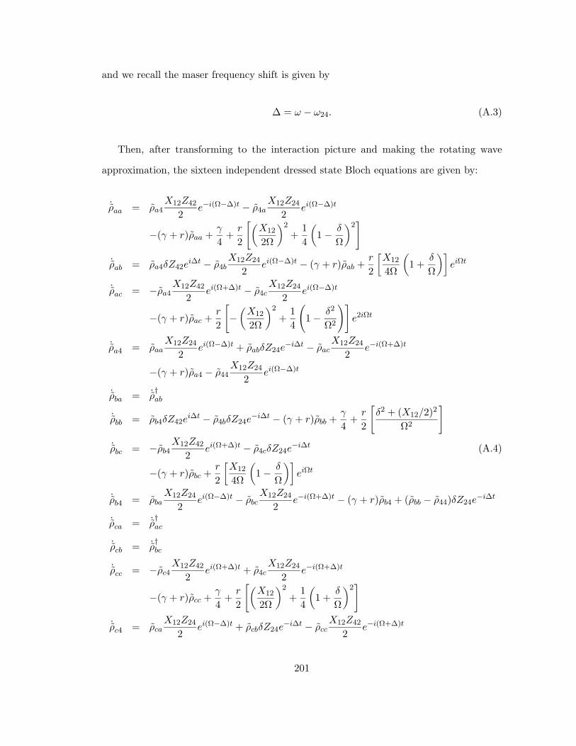
and we recall the maser frequency shift is given by

∆ = ω − ω24. (A.3)

Then, after transforming to the interaction picture and making the rotating wave

approximation, the sixteen independent dressed state Bloch equations are given by:

˙ρaa = ρa4X12Z42

2e−i(Ω−∆)t − ρ4a

X12Z24

2ei(Ω−∆)t

−(γ + r)ρaa +γ

4+

r

2

[(X12

2Ω

)2

+14

(1 − δ

Ω

)2]

˙ρab = ρa4δZ42ei∆t − ρ4b

X12Z24

2ei(Ω−∆)t − (γ + r)ρab +

r

2

[X12

4Ω

(1 +

δ

Ω

)]eiΩt

˙ρac = −ρa4X12Z42

2ei(Ω+∆)t − ρ4c

X12Z24

2ei(Ω−∆)t

−(γ + r)ρac +r

2

[−

(X12

2Ω

)2

+14

(1 − δ2

Ω2

)]e2iΩt

˙ρa4 = ρaaX12Z24

2ei(Ω−∆)t + ρabδZ24e

−i∆t − ρacX12Z24

2e−i(Ω+∆)t

−(γ + r)ρa4 − ρ44X12Z24

2ei(Ω−∆)t

˙ρba = ˙ρ†ab

˙ρbb = ρb4δZ42ei∆t − ρ4bδZ24e

−i∆t − (γ + r)ρbb +γ

4+

r

2

[δ2 + (X12/2)2

Ω2

]

˙ρbc = −ρb4X12Z42

2ei(Ω+∆)t − ρ4cδZ24e

−i∆t (A.4)

−(γ + r)ρbc +r

2

[X12

4Ω

(1 − δ

Ω

)]eiΩt

˙ρb4 = ρbaX12Z24

2ei(Ω−∆)t − ρbc

X12Z24

2e−i(Ω+∆)t − (γ + r)ρb4 + (ρbb − ρ44)δZ24e

−i∆t

˙ρca = ˙ρ†ac

˙ρcb = ˙ρ†bc

˙ρcc = −ρc4X12Z42

2ei(Ω+∆)t + ρ4c

X12Z24

2e−i(Ω+∆)t

−(γ + r)ρcc +γ

4+

r

2

[(X12

2Ω

)2

+14

(1 +

δ

Ω

)2]

˙ρc4 = ρcaX12Z24

2ei(Ω−∆)t + ρcbδZ24e

−i∆t − ρccX12Z42

2e−i(Ω+∆)t

201

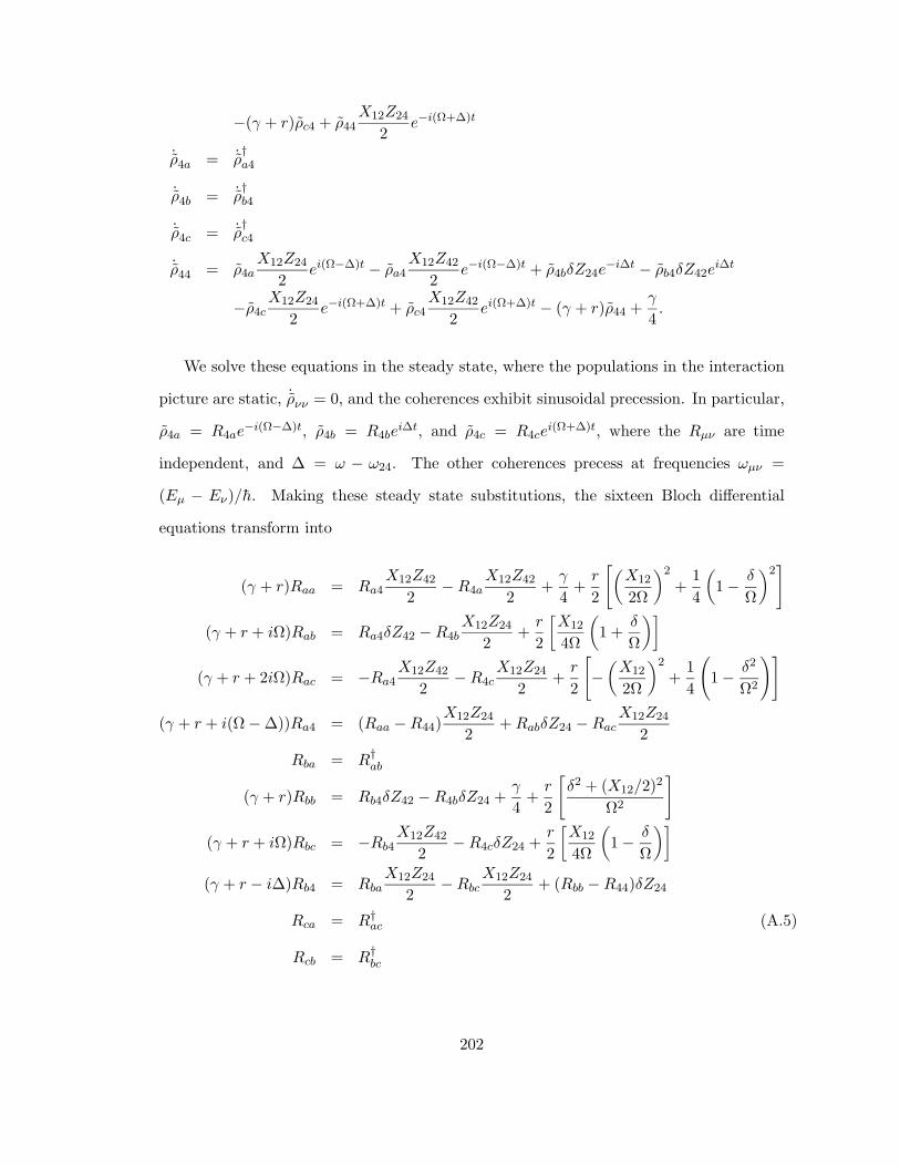
−(γ + r)ρc4 + ρ44X12Z24

2e−i(Ω+∆)t

˙ρ4a = ˙ρ†a4

˙ρ4b = ˙ρ†b4

˙ρ4c = ˙ρ†c4

˙ρ44 = ρ4aX12Z24

2ei(Ω−∆)t − ρa4

X12Z42

2e−i(Ω−∆)t + ρ4bδZ24e

−i∆t − ρb4δZ42ei∆t

−ρ4cX12Z24

2e−i(Ω+∆)t + ρc4

X12Z42

2ei(Ω+∆)t − (γ + r)ρ44 +

γ

4.

We solve these equations in the steady state, where the populations in the interaction

picture are static, ˙ρνν = 0, and the coherences exhibit sinusoidal precession. In particular,

ρ4a = R4ae−i(Ω−∆)t, ρ4b = R4be

i∆t, and ρ4c = R4cei(Ω+∆)t, where the Rµν are time

independent, and ∆ = ω − ω24. The other coherences precess at frequencies ωµν =

(Eµ − Eν)/h. Making these steady state substitutions, the sixteen Bloch differential

equations transform into

(γ + r)Raa = Ra4X12Z42

2− R4a

X12Z42

2+

γ

4+

r

2

[(X12

2Ω

)2

+14

(1 − δ

Ω

)2]

(γ + r + iΩ)Rab = Ra4δZ42 − R4bX12Z24

2+

r

2

[X12

4Ω

(1 +

δ

Ω

)]

(γ + r + 2iΩ)Rac = −Ra4X12Z42

2− R4c

X12Z24

2+

r

2

[−

(X12

2Ω

)2

+14

(1 − δ2

Ω2

)]

(γ + r + i(Ω − ∆))Ra4 = (Raa − R44)X12Z24

2+ RabδZ24 − Rac

X12Z24

2

Rba = R†ab

(γ + r)Rbb = Rb4δZ42 − R4bδZ24 +γ

4+

r

2

[δ2 + (X12/2)2

Ω2

]

(γ + r + iΩ)Rbc = −Rb4X12Z42

2− R4cδZ24 +

r

2

[X12

4Ω

(1 − δ

Ω

)]

(γ + r − i∆)Rb4 = RbaX12Z24

2− Rbc

X12Z24

2+ (Rbb − R44)δZ24

Rca = R†ac (A.5)

Rcb = R†bc

202

(γ + r)Rcc = −Rc4X12Z42

2+ R4c

X12Z24

2+

γ

4+

r

2

[(X12

2Ω

)2

+14

(1 +

δ

Ω

)2]

(γ + r − i(Ω + ∆))Rc4 = RcaX12Z24

2+ RcbδZ24 − Rcc

X12Z42

2+ R44

X12Z24

2

R4a = R†a4

R4b = R†b4

R4c = R†c4

(γ + r)R44 = R4aX12Z24

2− Ra4

X12Z42

2+ R4bδZ24 − Rb4δZ42

−R4cX12Z24

2+ Rc4

X12Z42

2+

γ

4.

The results of a numerical solution to these equations is provided in Chapter 2.

203

Bibliography

[1] H. Goldenberg, D. Kleppner, and N. Ramsey, Phys. Rev. Lett. 5, 361 (1960).

[2] D. Kleppner, H. Goldenberg, and N. Ramsey, Phys. Rev. 126, 603 (1962).

[3] D. Kleppner et al., Phys. Rev. 138, A 972 (1965).

[4] J. Vanier and C. Audoin, The Quantum Physics of Atomic Frequency Standards

(Adam Hilger, Bristol, 1989), Chap. 6.

[5] N. Ramsey, Phys. Rev. 78, 695 (1950).

[6] S. Crampton, W. Phillips, and D. Kleppner, Bull. Am. Phys. Soc. 23, 86 (1978).

[7] R. Vessot, M. Levine, and E. Mattison, in Proceedings of the 9th Annual Precise Time

and Time Interval Conference (NASA, Greenbelt, MD, 1978), p. 549, conference

publication 2129.

[8] W. Hardy and M. Morrow, Journal de Physique 42, C8 (1981).

[9] H. Hess et al., Phys. Rev. A 34, 1602 (1986).

[10] M. Hurlimann, W. Hardy, A. Berlinsky, and R. Cline, Phys. Rev. A 34, 1605 (1986).

[11] R. Walsworth et al., Phys. Rev. A 34, 2550 (1986).

[12] J. Gordon, H. Zeiger, and C. Townes, Phys. Rev. 95, 282 (1954).

[13] K. Shimoda, T. Wang, and C. Townes, Phys. Rev. 102, 1308 (1956).

204

[14] A. Rogers and J. Moran, IEEE Trans. Instrum. Meas. IM-30, 283 (1981).

[15] P. Kuhnle and R. Sydnor, J. Physique Suppl. C8, 373 (1981).

[16] E. Fortson, D. Kleppner, and N. Ramsey, Phys. Rev. Lett. 13, 22 (1964).

[17] S. Crampton, Phys. Rev. 158, 158 (1967).

[18] P. Winkler, D. Kleppner, T. Myint, and F. Walther, Phys. Rev. A 5, 83 (1972).

[19] R. Walsworth, I. Silvera, E. Mattison, and R. Vessot, Phys. Rev. A 46, 2495 (1992).

[20] R. Vessot et al., Phys. Rev. Lett. 45, 2081 (1980).

[21] J. Turneaure et al., Phys. Rev. D 27, 1705 (1983).

[22] R. Walsworth, I. Silvera, E. Mattison, and R. Vessot, Phys. Rev. Lett. 64, 2599

(1990).

[23] R. Walsworth and I. Silvera, Phys. Rev. A 42, 63 (1990).

[24] H. Andresen, Z. Phys. 210, 113 (1968).

[25] M. Humphrey, D. Phillips, and R. Walsworth, Phys. Rev. A 62, 063405 (2000).

[26] D. Phillips et al., Phys. Rev. D 63, 111101 (2001).

[27] V. Kostelecky and C. Lane, Phys. Rev. D 60, 116010 (1999).

[28] V. Kostelecky and C. Lane, J. Math. Phys. 40, 6245 (1999).

[29] M. Hayden, M. Hurlimann, and W. Hardy, Phys. Rev. A 53, 1589 (1996).

[30] B. Verhaar et al., Phys. Rev. A 35, 3825 (1987).

[31] J. Koelman et al., Phys. Rev. A 38, 3535 (1988).

[32] J. Vanier and C. Audoin, The Quantum Physics of Atomic Frequency Standards

(Adam Hilger, Bristol, 1989), p. 118.

205

[33] J. Vanier and C. Audoin, The Quantum Physics of Atomic Frequency Standards

(Adam Hilger, Bristol, 1989), p. 119.

[34] J. Vanier and C. Audoin, The Quantum Physics of Atomic Frequency Standards

(Adam Hilger, Bristol, 1989), p. 983.

[35] J. Vanier and C. Audoin, The Quantum Physics of Atomic Frequency Standards

(Adam Hilger, Bristol, 1989), p. 121.

[36] N. Ramsey, Phys. Rev. 100, 1191 (1955).

[37] H. Andresen, Technical report, United States Army Electronics Command (unpub-

lished).

[38] J.-Y. Savard et al., Can. J. Phys. 57, 904 (1979).

[39] P. Bender, Phys. Rev. 132, 7154 (1963).

[40] C. Cohen-Tannoudji, J. Dupont-Roc, and G. Grynberg, Atom-Photon Interactions

(J. Wiley and Sons, New York, 1992), Chap. VI.

[41] R. Bluhm, V. Kostelecky, and N. Russell, Phys. Rev. Lett. 82, 2254 (1999).

[42] E. Mattison and R. Vessot, Technical report, Jet Propulsion Laboratory (unpub-

lished).

[43] N. Ramsey, Molecular Beams (Clarendon Press, Oxford, 1956), Chap. 2.

[44] M. Sucher and J. Fox, Handbook of Microwave Measurements (Polytechnic Press,

New York, 1963), Vol. 2, Chap. VIII.

[45] E. Mattison, W. Shen, and R. Vessot, in Proceedings of the 39th Annual Frequency

Contol Symposium (IEEE, New York, 1985), p. 72.

[46] R. Vessot and E. Mattison, Technical report, Jet Propulsion Laboratory (unpub-

lished).

206

[47] D. Allan, Proc. IEEE 54, 221 (1966).

[48] J. Barnes et al., Trans. on Instr. and Meas. 20, 105 (1971).

[49] R. Vessot, L. Mueller, and J. Vanier, Proc. IEEE 54, 199 (1966).

[50] V. Kostelecky and S. Samuel, Phys. Rev. Lett. 63, 224 (1989).

[51] V. Kostelecky and S. Samuel, Phys. Rev. D 40, 1886 (1989).

[52] V. Kostelecky and S. Samuel, Phys. Rev. Lett. 66, 1811 (1991).

[53] V. Kostelecky and S. Samuel, Phys. Rev. D 39, 683 (1989).

[54] V. Kostelecky and R. Potting, Nucl. Phys. B 359, 545 (1991).

[55] V. Kostelecky and R. Potting, Phys. Lett. B 381, 89 (1996).

[56] V. Kostelecky, M. Perry, and R. Potting, Phys. Rev. Lett. 84, 4541 (2000).

[57] V. Kostelecky and R. Potting, in Gamma Ray-Neutrino Cosmology and Planck

Scale Physics, edited by D. Cline (World Scientific, Singapore, 1993), see also

(hepth/9211116).

[58] V. Kostelecky and R. Potting, Phys. Rev. D 51, 3923 (1995).

[59] D. Colladay and V. Kostelecky, Phys. Rev. D 55, 6760 (1997).

[60] D. Colladay and V. Kostelecky, Phys. Rev. D 58, 116002 (1998).

[61] R. Mittleman, I. Ioannou, H. Dehmelt, and N. Russell, Phys. Rev. Lett. 83, 2116

(1999).

[62] C. Berglund et al., Phys. Rev. Lett. 75, 1879 (1995).

[63] B. Heckel, presented at the International Conference on Orbis Scientiae 1999, Fort

Lauderdale, Florida, Dec., 1999.

207

[64] D. Bear et al., Phys. Rev. Lett. 85, 5038 (2000).

[65] H. Dehmelt, R. Mittleman, R. V. Dyck, and P. Schwinberg, Phys. Rev. Lett. 83, 4694

(1999).

[66] E. Adelberger et al., in Physics Beyond the Standard Model, edited by P. Herczeg, C.

Hoffman, and H. Klapdor-Kleingrothaus (World Scientific, Singapore, 1999), p. 717.

[67] M. Harris, Ph.D. thesis, Univ. of Washington, 1998.

[68] P. Bender, Phys. Rev. 132, 2154 (1963).

[69] W. Press, S. Teukolsky, W. Vetterling, and B. Flannery, Numerical Recipes in C, 2nd

ed. (Cambridge University Press, Cambridge, 1988), p. 689.

[70] P. R. Bevington and D. K. Robinson, Data Reduction and Error Analysis for the

Physical Sciences (McGraw Hill, New York, 1992), p. 64.

[71] E. Purcell and G. Field, Astrophys. J. 124, 542 (1956).

[72] J. Wittke and R. Dicke, Phys. Rev. 103, 620 (1956).

[73] A. Dalgarno, Proc. R. Soc. London, Ser. A 262, 132 (1961).

[74] L. Balling, R. Hanson, and F. Pipkin, Phys. Rev. 133, A607 (1964).

[75] A. Allison, Phys. Rev. A 5, 2695 (1972).

[76] S. Crampton and H. Wang, Phys. Rev. A 12, 1305 (1975).

[77] A. Berlinsky and B. Shizgal, Can. J. Phys. 58, 881 (1980).

[78] M. Desaintfuscien, Ph.D. thesis, University of Paris, 1975.

[79] R. Vessot, E. Mattison, and E. Imbier, in Proceedings of the 37th Annual Frequency

Control Symposium (IEEE, New York, 1983), p. 49.

208

[80] J. Krupczak et al., in Proceedings International Cryogenic Materials Confer-

ence/Cryogenic Engineering Conference (Plenum Press, New York, 1996), p. 1769.

[81] S. Crampton et al., Phys. Rev. Lett. 42, 1039 (1979).

[82] I. Silvera and J. Walraven, Phys. Rev. Lett. 44, 164 (1980).

[83] R. Jochemsen, M. Morrow, A. Berlinsky, and W. Hardy, Phys. Rev. Lett. 47, 852

(1981).

[84] M. Morrow, R. Jochemsen, A. Berlinksky, and W. Hardy, Phys. Rev. Lett. 46, 195

(1981).

[85] M. Morrow, R. Jochemsen, A. Berlinksky, and W. Hardy, Phys. Rev. Lett. 47, 455

(1981).

[86] R. Walsworth, Ph.D. thesis, Harvard University, 1991.

[87] J. Walraven and I. Silvera, Rev. Sci. Instrum. 53, 1167 (1982).

[88] G. White, Experimental Techniques in Low-Temperature Physics (English Universities

Press LTD, London, 1964).

[89] J. Groslambert, D. Fest, M. Oliver, and J. Gagnepain, in Proceedings of the 35th An-

nual Frequency Control Symposium (Electronics Industries Association, Washington,

D.C., 1981), p. 458.

[90] G. Nunes, in Experimental Techniques in Condensed Matter Physics at Low Temper-

atures, edited by R. Richardson and E. Smith (Addison-Wesley, Reading, MA, 1988),

Chap. 2.

[91] F. Pobell, Matter and Methods at Low Temperatures, 2nd ed. (Springer, Berlin, 1996).

[92] A. Rose-Innes, Low-Temperature Techniques (Oxford University Press, Oxford, 1979),

p. 6.

209

[93] W. Kolos and L. Wolniewicz, J. Chem. Phys. 43, 2429 (1965).

[94] S. Crampton, J. Duvivier, G. Read, and E. Williams, Phys. Rev. A 5, 1752 (1972).

[95] M. Desaintfuscien and C. Audoin, Phys. Rev. A 13, 2070 (1976).

[96] S. Kokkelmans and B. Verhaar, Phys. Rev. A 56, 4038 (1997).

[97] B. Zygelman, A. Dalgarno, M. Jamieson, and P. Stancil, Phys. Rev. A (in press).

[98] M. Hayden and W. Hardy, Phys. Rev. Lett. 76, 2041 (1996).

[99] V. Folen et al., Technical report, Naval Research Laboratory (unpublished).

210