ECONOMICS 351* -- Assignment 2 ANSWERS M.G. Abbott Queen’s University Department of Economics ECON 351* -- Introductory Econometrics ASSIGNMENT 2: ANSWERS Winter Term 2009 M.G. Abbott TOPIC: Statistical Inference in Simple Linear Regression Models INSTRUCTIONS: • Answer all questions on standard-sized 8.5 x 11-inch paper. • Answers need not be typewritten (document processed), but if hand-written must be legible. Illegible assignments will be returned unmarked. • Please label clearly each answer with the appropriate question number and letter. Securely staple all answer sheets together, and make certain that your name(s) and student number(s) are printed clearly at the top of each answer sheet. • Students submitting joint assignments with one other student must ensure that the name and student number of each student are printed clearly at the top of each answer sheet. Submit only one copy of the assignment. MARKING: Marks for each question are indicated in parentheses. Total marks for the assignment equal 100. Marks are given for both content and presentation. SOFT DUE DATE: Friday February 27, 2009 by 4:00 pm. HARD DUE DATE: Thursday March 5, 2009 by 4:00 pm. • Assignments submitted on or before the soft due date will receive a bonus of 3 points to a maximum total mark of 100. • Assignments submitted after the hard due date will be penalized 20 points per day. • Please submit your assignments either to me in class, or by depositing them in the ECON 351 slot of the Assignment Collection Box located immediately inside the double doors on the second floor of Dunning Hall (opposite the elevator). DATA FILE: 351assn1w09.raw (a text-format, or ASCII-format, data file) • Data Description: A random sample of 472 employees drawn from the 1976 U.S. population of all employed paid workers. NOTE: Assignment 2 uses that same dataset as Assignment 1. • Variable Definitions: WAGE i ≡ average hourly earnings of worker i in 1976, in dollars per hour. ED i ≡ years of formal education completed by worker i, in years. FEMALE i ≡ an indicator variable equal to 1 if worker i is female, and 0 if worker i is male. ECON 351* -- Winter 2009: Assignment 2 ANSWERS Page 1 of 24 pages

Welcome message from author
This document is posted to help you gain knowledge. Please leave a comment to let me know what you think about it! Share it to your friends and learn new things together.
Transcript
ECONOMICS 351* -- Assignment 2 ANSWERS M.G. Abbott
Queen’s University Department of Economics
ECON 351* -- Introductory Econometrics
ASSIGNMENT 2: ANSWERS
Winter Term 2009 M.G. Abbott TOPIC: Statistical Inference in Simple Linear Regression Models INSTRUCTIONS:
• Answer all questions on standard-sized 8.5 x 11-inch paper.
• Answers need not be typewritten (document processed), but if hand-written must be legible. Illegible assignments will be returned unmarked.
• Please label clearly each answer with the appropriate question number and letter. Securely staple all answer sheets together, and make certain that your name(s) and student number(s) are printed clearly at the top of each answer sheet.
• Students submitting joint assignments with one other student must ensure that the name and student number of each student are printed clearly at the top of each answer sheet. Submit only one copy of the assignment.
MARKING: Marks for each question are indicated in parentheses. Total marks for the assignment
equal 100. Marks are given for both content and presentation. SOFT DUE DATE: Friday February 27, 2009 by 4:00 pm.
HARD DUE DATE: Thursday March 5, 2009 by 4:00 pm.
• Assignments submitted on or before the soft due date will receive a bonus of 3 points to a maximum total mark of 100.
• Assignments submitted after the hard due date will be penalized 20 points per day. • Please submit your assignments either to me in class, or by depositing them in the ECON 351
slot of the Assignment Collection Box located immediately inside the double doors on the second floor of Dunning Hall (opposite the elevator).
DATA FILE: 351assn1w09.raw (a text-format, or ASCII-format, data file)
• Data Description: A random sample of 472 employees drawn from the 1976 U.S. population of all employed paid workers. NOTE: Assignment 2 uses that same dataset as Assignment 1.
• Variable Definitions:
WAGEi ≡ average hourly earnings of worker i in 1976, in dollars per hour. EDi ≡ years of formal education completed by worker i, in years. FEMALEi ≡ an indicator variable equal to 1 if worker i is female, and 0 if worker i is male.
ECON 351* -- Winter 2009: Assignment 2 ANSWERS Page 1 of 24 pages
ECONOMICS 351* -- Assignment 2 ANSWERS M.G. Abbott
ECON 351* -- Winter 2009: Assignment 2 ANSWERS Page 2 of 24 pages
• Stata Infile Statement: Use the following Stata infile statement to read the text-format data file 351assn1w09.raw:
infile wage ed female using 351assn1w09.raw
QUESTIONS: (50 marks) 1. Compute and present OLS estimates of the following population regression equation for the full
sample of 472 employees: (1) ii10i uEDWAGE +β+β=
where ui is a random error term that is assumed to satisfy all the assumptions of the classical linear regression model.
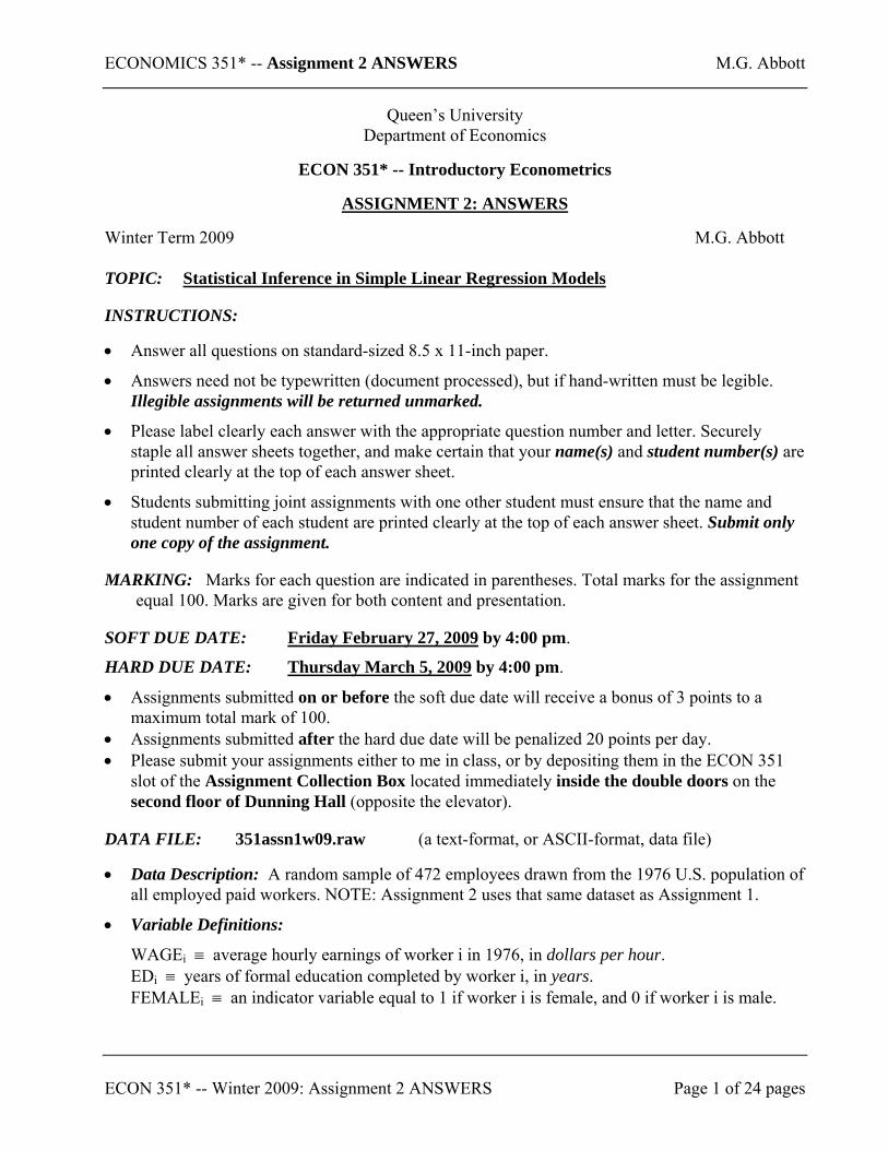
(10 marks) (a) Report the OLS coefficient estimates 0β and $β1 computed by estimating population
regression equation (1), the estimated standard errors of 0β and $β1 , the t-ratios for 0β and $β1 , the estimate $σ2 of the constant error variance σ2, the R2 and F-statistic for the OLS sample regression equation, and the number of observations N used in estimation. .
ANSWER Question 1(a)
Source | SS df MS Number of obs = 472 -------------+------------------------------ F( 1, 470) = 95.35 Model | 1129.04675 1 1129.04675 Prob > F = 0.0000 Residual | 5565.30746 470 11.8410797 R-squared = 0.1687 -------------+------------------------------ Adj R-squared = 0.1669 Total | 6694.3542 471 14.2130662 Root MSE = 3.4411 ------------------------------------------------------------------------------ wage | Coef. Std. Err. t P>|t| [95% Conf. Interval] -------------+------------------------------- --------------------- ed | .5752019 .0589061 9.76 0.000 .4594501 .6909537
------------
_cons | -1.312499 .7613451 -1.72 0.085 -2.808561 .1835623 ------------------------------------------------------------------------------
Regressor jβ ( )jβes ( )jβt Lower 95% limit Upper 95% limit
Constant -1.31250 0.761345 -1.72 -2.80856 0.183562
EDi 0.575202 0.0589061 9.76 0.459450 0.690954
N = 472; = 11.84108; R2 = 0.1687; F(1, 470) = 95.35 $σ2
ECONOMICS 351* -- Assignment 2 ANSWERS M.G. Abbott
(10 marks) (b) Use the estimation results from OLS estimation of regression equation (1) to perform a t-
test of the proposition that employees’ hourly wage rates are unrelated to their years of formal education. State the null and alternative hypotheses. Show how the appropriate test statistic is calculated (give its formula). Report the sample value of the test statistic and its p-value. State the decision rule you use to decide between rejection and retention of the null hypothesis. State the inference you would draw from the test at the 5 percent and 1 percent significance levels. What would you conclude from the results of the test?
ECON 351* -- Winter 2009: Assignment 2 ANSWERS Page 3 of 24 pages
ECONOMICS 351* -- Assignment 2 ANSWERS M.G. Abbott
ECON 351* -- Winter 2009: Assignment 2 ANSWERS Page 4 of 24 pages
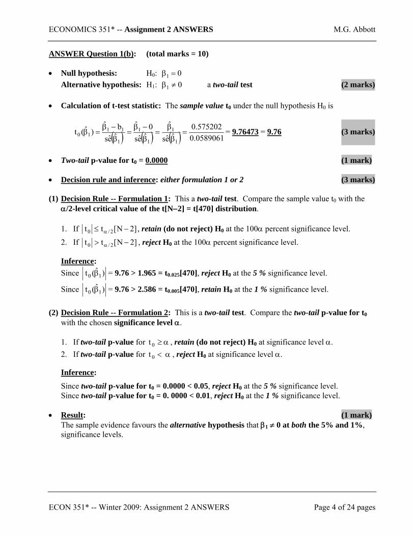
ANSWER Question 1(b): (total marks = 10) • Null hypothesis: H0: 01 =β
Alternative hypothesis: H1: 01 ≠β a two-tail test (2 marks)
• Calculation of t-test statistic: The sample value t0 under the null hypothesis H0 is
( ) ( ) ( ) 0589061.0575202.0
ˆes
ˆˆes
0ˆˆesbˆ
)ˆ(t1
1
1
1
1
1110 =
ββ
=β−β
=β−β
=β = 9.76473 = 9.76 (3 marks)
• Two-tail p-value for t0 = 0.0000 (1 mark)
• Decision rule and inference: either formulation 1 or 2 (3 marks) (1) Decision Rule -- Formulation 1: This a two-tail test. Compare the sample value t0 with the
α/2-level critical value of the t[N−2] = t[470] distribution.
1. If ]2N[tt 2/0 −≤ α , retain (do not reject) H0 at the 100α percent significance level.
2. If ]2N[tt 2/0 −> α , reject H0 at the 100α percent significance level.
Inference: Since )ˆ(t 10 β = 9.76 > 1.965 = t0.025[470], reject H0 at the 5 % significance level.
Since )ˆ(t 10 β = 9.76 > 2.586 = t0.005[470], retain H0 at the 1 % significance level.
(2) Decision Rule -- Formulation 2: This is a two-tail test. Compare the two-tail p-value for t0
with the chosen significance level α.
1. If two-tail p-value for α≥0t , retain (do not reject) H0 at significance level α. 2. If two-tail p-value for α<0t , reject H0 at significance level α.
Inference:
Since two-tail p-value for t0 = 0.0000 < 0.05, reject H0 at the 5 % significance level. Since two-tail p-value for t0 = 0. 0000 < 0.01, reject H0 at the 1 % significance level.
• Result: (1 mark)
The sample evidence favours the alternative hypothesis that β1 ≠ 0 at both the 5% and 1%, significance levels.
ECONOMICS 351* -- Assignment 2 ANSWERS M.G. Abbott
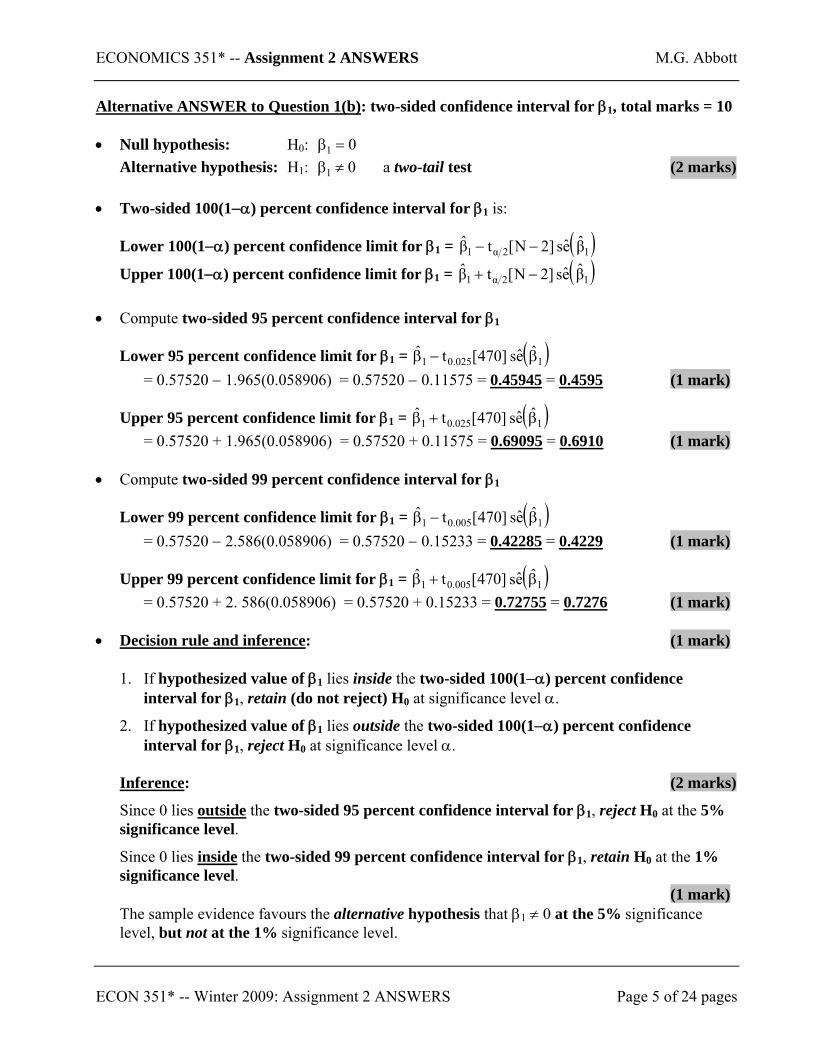
Alternative ANSWER to Question 1(b): two-sided confidence interval for β1, total marks = 10 • Null hypothesis: H0: 01 =β
Alternative hypothesis: H1: 01 ≠β a two-tail test (2 marks)
• Two-sided 100(1−α) percent confidence interval for β1 is:
Lower 100(1−α) percent confidence limit for β1 = ( )12α1 βes]2N[tβ −−
Upper 100(1−α) percent confidence limit for β1 = ( )12α1 βes]2N[tβ −+
• Compute two-sided 95 percent confidence interval for β1
Lower 95 percent confidence limit for β1 = ( )1025.01ˆes]470[tˆ β−β
= 0.57520 − 1.965(0.058906) = 0.57520 − 0.11575 = 0.45945 = 0.4595 (1 mark)
Upper 95 percent confidence limit for β1 = ( )1025.01ˆes]470[tˆ β+β
= 0.57520 + 1.965(0.058906) = 0.57520 + 0.11575 = 0.69095 = 0.6910 (1 mark)
• Compute two-sided 99 percent confidence interval for β1
Lower 99 percent confidence limit for β1 = ( )1005.01ˆes]470[tˆ β−β
= 0.57520 − 2.586(0.058906) = 0.57520 − 0.15233 = 0.42285 = 0.4229 (1 mark)
Upper 99 percent confidence limit for β1 = ( )1005.01ˆes]470[tˆ β+β
= 0.57520 + 2. 586(0.058906) = 0.57520 + 0.15233 = 0.72755 = 0.7276 (1 mark) • Decision rule and inference: (1 mark)
1. If hypothesized value of β1 lies inside the two-sided 100(1−α) percent confidence interval for β1, retain (do not reject) H0 at significance level α.
2. If hypothesized value of β1 lies outside the two-sided 100(1−α) percent confidence interval for β1, reject H0 at significance level α.
Inference: (2 marks)
Since 0 lies outside the two-sided 95 percent confidence interval for β1, reject H0 at the 5% significance level.
Since 0 lies inside the two-sided 99 percent confidence interval for β1, retain H0 at the 1% significance level.
(1 mark) The sample evidence favours the alternative hypothesis that β1 ≠ 0 at the 5% significance level, but not at the 1% significance level.
ECON 351* -- Winter 2009: Assignment 2 ANSWERS Page 5 of 24 pages
ECONOMICS 351* -- Assignment 2 ANSWERS M.G. Abbott
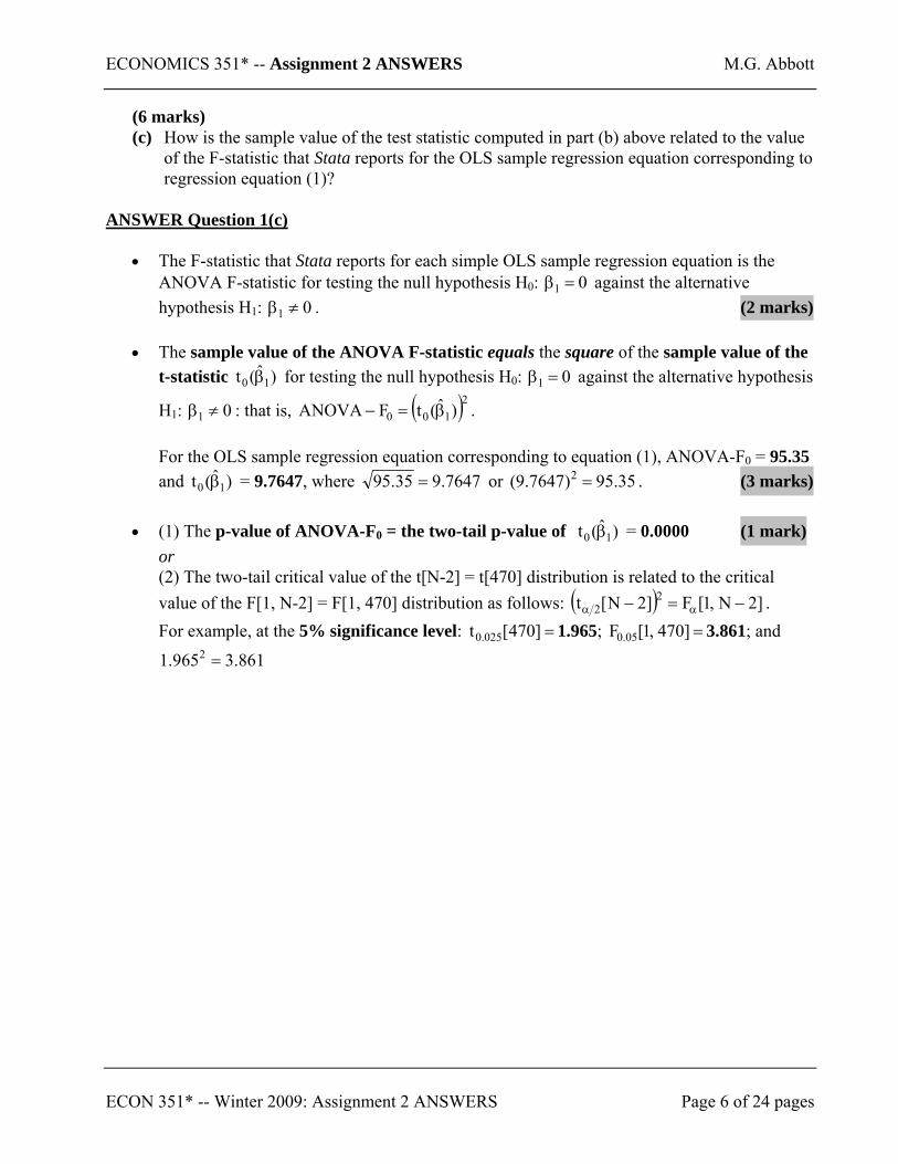
(6 marks) (c) How is the sample value of the test statistic computed in part (b) above related to the value
of the F-statistic that Stata reports for the OLS sample regression equation corresponding to regression equation (1)?
ANSWER Question 1(c)
• The F-statistic that Stata reports for each simple OLS sample regression equation is the ANOVA F-statistic for testing the null hypothesis H0: 01 =β against the alternative hypothesis H1: 01 ≠β . (2 marks)
• The sample value of the ANOVA F-statistic equals the square of the sample value of the
t-statistic )ˆ(t 10 β for testing the null hypothesis H0: 01 =β against the alternative hypothesis
H1: 01 ≠β : that is, ( )210 . 0 )ˆ(tFANOVA β=− For the OLS sample regression equation corresponding to equation (1), ANOVA-F0 = 95.35 and = 9.7647, where )ˆ(t 10 β 7647.935.95 = or . (3 marks) 35.95)7647.9( 2 =
• (1) The p-value of ANOVA-F0 = the two-tail p-value of )ˆ(t 10 β = 0.0000 (1 mark) or (2) The two-tail critical value of the t[N-2] = t[470] distribution is related to the critical value of the F[1, N-2] = F[1, 470] distribution as follows: ( ) ]2N,1[F]2N[t 2
2 −=− αα . For example, at the 5% significance level: =]470[t 025.0 1.965; 3.861; and
=]470,1[F 05.0
861.3965.1 2 =
ECON 351* -- Winter 2009: Assignment 2 ANSWERS Page 6 of 24 pages
ECONOMICS 351* -- Assignment 2 ANSWERS M.G. Abbott
(12 marks) (d) Use the estimation results from OLS estimation of regression equation (1) to perform a test
of the empirical proposition that workers’ hourly earnings are positively related to their years of formal education. State the null and alternative hypotheses. Show how the appropriate test statistic is calculated (give its formula). Report the sample value of the test statistic and its p-value. Report the appropriate critical values of the test statistic at the 5 percent and 1 percent significance levels. State the decision rule you use to decide between rejection and retention of the null hypothesis. State the inference you would draw from the test at both the 5 percent and 1 percent significance levels. What would you conclude from the results of the test?
ECON 351* -- Winter 2009: Assignment 2 ANSWERS Page 7 of 24 pages
ECONOMICS 351* -- Assignment 2 ANSWERS M.G. Abbott
ECON 351* -- Winter 2009: Assignment 2 ANSWERS Page 8 of 24 pages
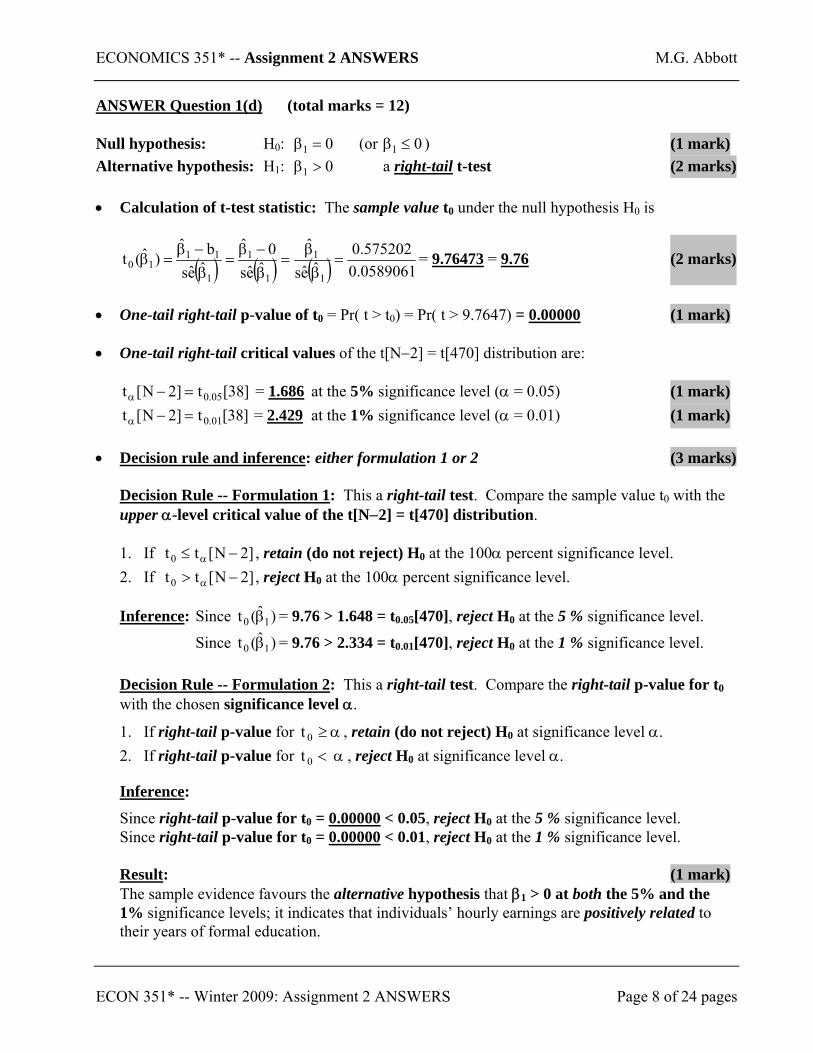
ANSWER Question 1(d) (total marks = 12) Null hypothesis: H0: 01 =β (or 01 ≤β ) (1 mark) Alternative hypothesis: H1: a right-tail01 >β t-test (2 marks)
• Calculation of t-test statistic: The sample value t0 under the null hypothesis H0 is
( ) ( ) ( ) 0589061.0575202.0
ˆes
ˆˆes
0ˆˆesbˆ
)ˆ(t1
1
1
1
1
1110 =
ββ
=β−β
=β−β
=β = 9.76473 = 9.76 (2 marks)
• One-tail right-tail p-value of t0 = Pr( t > t0) = Pr( t > 9.7647) = 0.00000 (1 mark)
• One-tail right-tail critical values of the t[N−2] = t[470] distribution are:
]38[t]2N[t 05.0=−α = 1.686 at the 5% significance level (α = 0.05) (1 mark) ]38[t]2N[t 01.0=−α = 2.429 at the 1% significance level (α = 0.01) (1 mark)
• Decision rule and inference: either formulation 1 or 2 (3 marks)
Decision Rule -- Formulation 1: This a right-tail test. Compare the sample value t0 with the upper α-level critical value of the t[N−2] = t[470] distribution.
1. If ]2N[ , retain (do not reject) H0 at the 100α percent significance level. tt 0 −≤ α
2. If ]2N[ , reject H0 at the 100α percent significance level. tt0 −> α
Inference: Since = 9.76 > 1.648 = t0.05[470], reject H0 at the 5 % significance level. )ˆ(t 10 β
Since = 9.76 > 2.334 = t0.01[470], reject H0 at the 1 % significance level. )ˆ(t 10 β
Decision Rule -- Formulation 2: This a right-tail test. Compare the right-tail p-value for t0 with the chosen significance level α.
1. If right-tail p-value for α≥0t , retain (do not reject) H0 at significance level α. 2. If right-tail p-value for α<0t , reject H0 at significance level α.
Inference:
Since right-tail p-value for t0 = 0.00000 < 0.05, reject H0 at the 5 % significance level. Since right-tail p-value for t0 = 0.00000 < 0.01, reject H0 at the 1 % significance level.
Result: (1 mark) The sample evidence favours the alternative hypothesis that β1 > 0 at both the 5% and the 1% significance levels; it indicates that individuals’ hourly earnings are positively related to their years of formal education.

ECONOMICS 351* -- Assignment 2 ANSWERS M.G. Abbott
(12 marks) (e) Use the results from OLS estimation of regression equation (1) to perform a test of the
hypothesis that the mean hourly wage rate of workers with 16 years of schooling was equal to $8.00 per hour (in 1976 US dollars). State the null and alternative hypotheses. Show how the appropriate test statistic is calculated (give its formula). Report the sample value of the test statistic and its p-value. State the decision rule you use to decide between rejection and retention of the null hypothesis. State the inference you would draw from the test at the 5 percent and the 10 percent significance levels. What would you conclude from the results of the test?
ECON 351* -- Winter 2009: Assignment 2 ANSWERS Page 9 of 24 pages
ECONOMICS 351* -- Assignment 2 ANSWERS M.G. Abbott
ECON 351* -- Winter 2009: Assignment 2 ANSWERS Page 10 of 24 pages
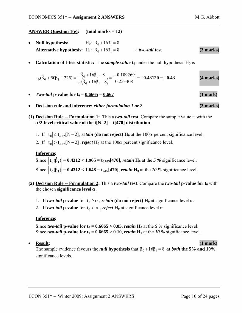
ANSWER Question 1(e): (total marks = 12) • Null hypothesis: H0: 816 10 =β+β
Alternative hypothesis: H1: 816 10 ≠β+β a two-tail test (3 marks)
• Calculation of t-test statistic: The sample value t0 under the null hypothesis H0 is
( ) 253408.0109269.0
8ˆ16ˆes8ˆ16ˆ
)225ˆ50ˆ(t10
10100
−=
−β+β−β+β
=−β+β = −0.43120 = −0.43 (4 marks)
• Two-tail p-value for t0 = 0.6665 = 0.667 (1 mark)
• Decision rule and inference: either formulation 1 or 2 (3 marks) (1) Decision Rule -- Formulation 1: This a two-tail test. Compare the sample value t0 with the
α/2-level critical value of the t[N−2] = t[470] distribution.
1. If ]2N[tt 2/0 −≤ α , retain (do not reject) H0 at the 100α percent significance level.
2. If ]2N[tt 2/0 −> α , reject H0 at the 100α percent significance level.
Inference: Since )ˆ(t 10 β = 0.4312 < 1.965 = t0.025[470], retain H0 at the 5 % significance level.
Since )ˆ(t 10 β = 0.4312 < 1.648 = t0.05[470], retain H0 at the 10 % significance level.
(2) Decision Rule -- Formulation 2: This a two-tail test. Compare the two-tail p-value for t0 with
the chosen significance level α.
1. If two-tail p-value for α≥0t , retain (do not reject) H0 at significance level α. 2. If two-tail p-value for α<0t , reject H0 at significance level α.
Inference:
Since two-tail p-value for t0 = 0.6665 > 0.05, retain H0 at the 5 % significance level. Since two-tail p-value for t0 = 0.6665 > 0.10, retain H0 at the 10 % significance level.
• Result: (1 mark)
The sample evidence favours the null hypothesis that 816 10 =β+β at both the 5% and 10% significance levels.
ECONOMICS 351* -- Assignment 2 ANSWERS M.G. Abbott
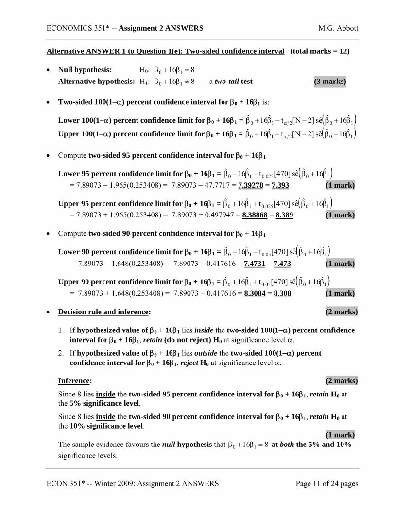
Alternative ANSWER 1 to Question 1(e): Two-sided confidence interval (total marks = 12) • Null hypothesis: H0: 816 10 =β+β
Alternative hypothesis: H1: 816 10 ≠β+β a two-tail test (3 marks) • Two-sided 100(1−α) percent confidence interval for β0 + 16β1 is:
Lower 100(1−α) percent confidence limit for β0 + 16β1 = ( )10210ˆ16ˆes]2N[tˆ16ˆ β+β−−β+β α
Upper 100(1−α) percent confidence limit for β0 + 16β1 = ( )10210ˆ16ˆes]2N[tˆ16ˆ β+β−+β+β α
• Compute two-sided 95 percent confidence interval for β0 + 16β1
Lower 95 percent confidence limit for β0 + 16β1 = ( )10025.010ˆ16ˆes]470[tˆ16ˆ β+β−β+β
= 7.89073 − 1.965(0.253408) = 7.89073 − 47.7717 = 7.39278 = 7.393 (1 mark)
Upper 95 percent confidence limit for β0 + 16β1 = ( )10025.010ˆ16ˆes]470[tˆ16ˆ β+β+β+β
= 7.89073 + 1.965(0.253408) = 7.89073 + 0.497947 = 8.38868 = 8.389 (1 mark)
• Compute two-sided 90 percent confidence interval for β0 + 16β1
Lower 90 percent confidence limit for β0 + 16β1 = ( )1005.010ˆ16ˆes]470[tˆ16ˆ β+β−β+β
= 7.89073 − 1.648(0.253408) = 7.89073 − 0.417616 = 7.4731 = 7.473 (1 mark)
Upper 90 percent confidence limit for β0 + 16β1 = ( )1005.010ˆ16ˆes]470[tˆ16ˆ β+β+β+β
= 7.89073 + 1.648(0.253408) = 7.89073 + 0.417616 = 8.3084 = 8.308 (1 mark) • Decision rule and inference: (2 marks)
1. If hypothesized value of β0 + 16β1 lies inside the two-sided 100(1−α) percent confidence interval for β0 + 16β1, retain (do not reject) H0 at significance level α.
2. If hypothesized value of β0 + 16β1 lies outside the two-sided 100(1−α) percent confidence interval for β0 + 16β1, reject H0 at significance level α.
Inference: (2 marks)
Since 8 lies inside the two-sided 95 percent confidence interval for β0 + 16β1, retain H0 at the 5% significance level.
Since 8 lies inside the two-sided 90 percent confidence interval for β0 + 16β1, retain H0 at the 10% significance level.
(1 mark) The sample evidence favours the null hypothesis that 816 10 =β+β at both the 5% and 10% significance levels.
ECON 351* -- Winter 2009: Assignment 2 ANSWERS Page 11 of 24 pages
ECONOMICS 351* -- Assignment 2 ANSWERS M.G. Abbott
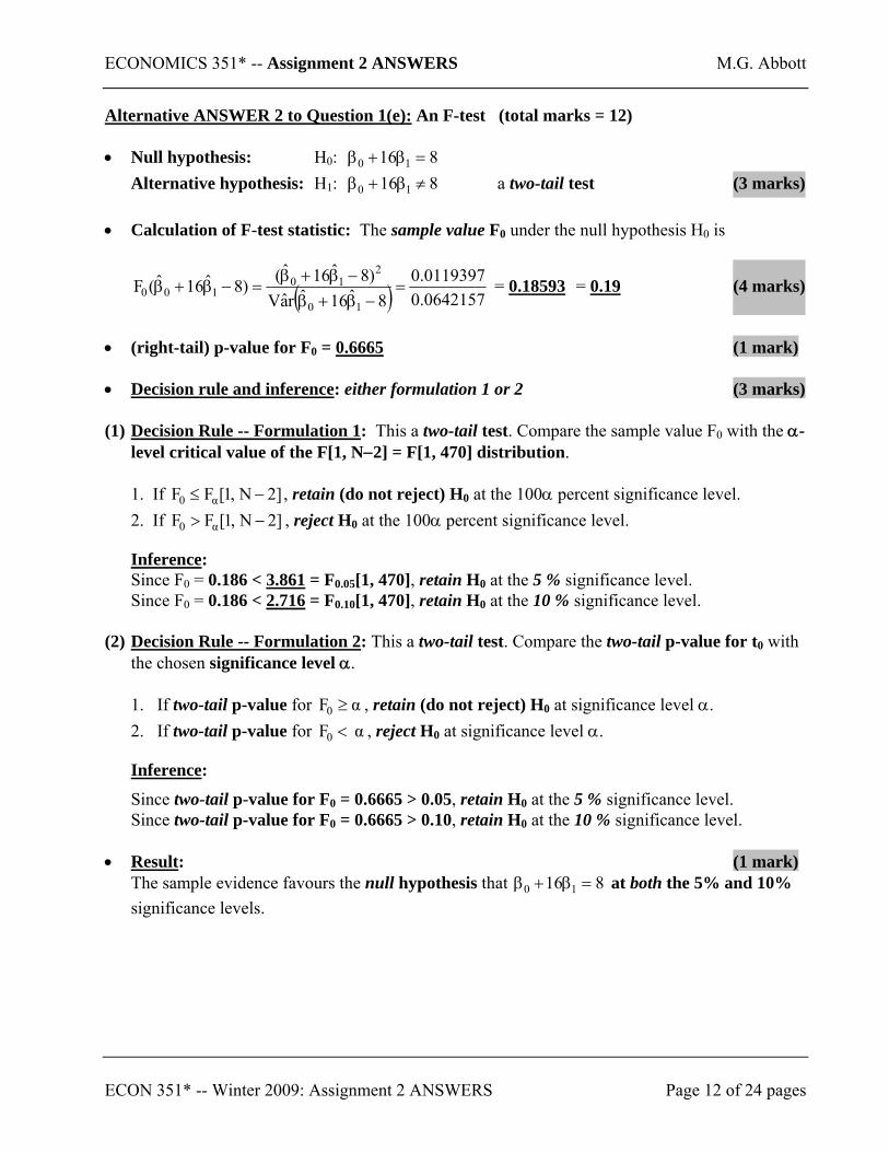
Alternative ANSWER 2 to Question 1(e): An F-test (total marks = 12) • Null hypothesis: H0: 816 10 =β+β
Alternative hypothesis: H1: 816 10 ≠β+β a two-tail test (3 marks)
• Calculation of F-test statistic: The sample value F0 under the null hypothesis H0 is
( ) 0642157.00119397.0
8ˆ16ˆraV)8ˆ16ˆ()8ˆ16ˆ(F
10
210
100 =−β+β
−β+β=−β+β = 0.18593 = 0.19 (4 marks)
• (right-tail) p-value for F0 = 0.6665 (1 mark)
• Decision rule and inference: either formulation 1 or 2 (3 marks) (1) Decision Rule -- Formulation 1: This a two-tail test. Compare the sample value F0 with the α-
level critical value of the F[1, N−2] = F[1, 470] distribution.
1. If , retain (do not reject) H0 at the 100α percent significance level. ]2N,1[FF α0 −≤2. If , reject H0 at the 100α percent significance level. ]2N,1[FF α0 −>
Inference: Since F0 = 0.186 < 3.861 = F0.05[1, 470], retain H0 at the 5 % significance level. Since F0 = 0.186 < 2.716 = F0.10[1, 470], retain H0 at the 10 % significance level.
(2) Decision Rule -- Formulation 2: This a two-tail test. Compare the two-tail p-value for t0 with
the chosen significance level α.
1. If two-tail p-value for αF0 ≥ , retain (do not reject) H0 at significance level α. 2. If two-tail p-value for αF0 < , reject H0 at significance level α.
Inference:
Since two-tail p-value for F0 = 0.6665 > 0.05, retain H0 at the 5 % significance level. Since two-tail p-value for F0 = 0.6665 > 0.10, retain H0 at the 10 % significance level.
• Result: (1 mark)
The sample evidence favours the null hypothesis that 816 10 =β+β at both the 5% and 10% significance levels.
ECON 351* -- Winter 2009: Assignment 2 ANSWERS Page 12 of 24 pages
ECONOMICS 351* -- Assignment 2 ANSWERS M.G. Abbott
ECON 351* -- Winter 2009: Assignment 2 ANSWERS Page 13 of 24 pages
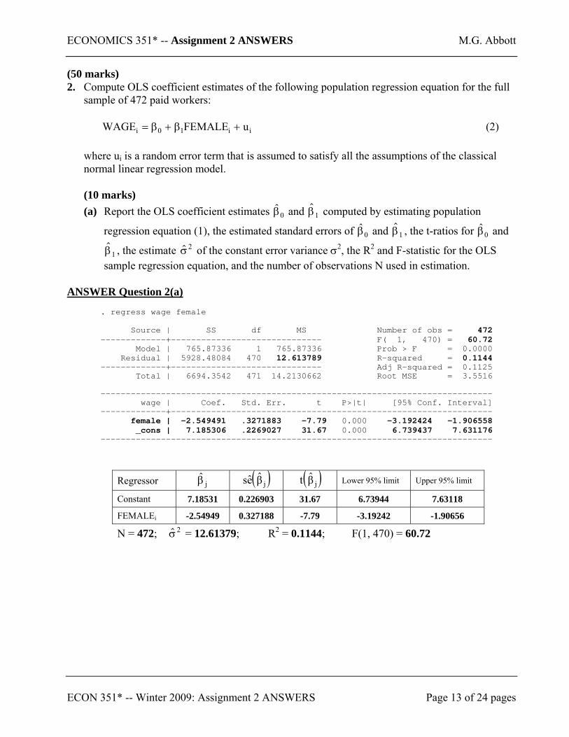
(50 marks) 2. Compute OLS coefficient estimates of the following population regression equation for the full
sample of 472 paid workers:
ii10i uFEMALEWAGE +β+β= (2)
where ui is a random error term that is assumed to satisfy all the assumptions of the classical normal linear regression model.
(10 marks) (a) Report the OLS coefficient estimates 0β and $β1 computed by estimating population
regression equation (1), the estimated standard errors of 0β and $β1 , the t-ratios for 0β and $β1 , the estimate $σ2 of the constant error variance σ2, the R2 and F-statistic for the OLS sample regression equation, and the number of observations N used in estimation.
ANSWER Question 2(a)
. regress wage female Source | SS df MS Number of obs = 472 -------------+------------------------------ F( 1, 470) = 60.72 Model | 765.87336 1 765.87336 Prob > F = 0.0000 Residual | 5928.48084 470 12.613789 R-squared = 0.1144 -------------+------------------------------ Adj R-squared = 0.1125 Total | 6694.3542 471 14.2130662 Root MSE = 3.5516 ------------------------------------------------------------------------------ wage | Coef. Std. Err. t P>|t| [95% Conf. Interval] -------------+---------------------------------------------------------------- female | -2.549491 .3271883 -7.79 0.000 -3.192424 -1.906558 _cons | 7.185306 .2269027 31.67 0.000 6.739437 7.631176 ------------------------------------------------------------------------------
Regressor jβ ( )jβes ( )jβt Lower 95% limit Upper 95% limit
Constant 7.18531 0.226903 31.67 6.73944 7.63118
FEMALEi -2.54949 0.327188 -7.79 -3.19242 -1.90656
N = 472; = 12.61379; R2 = 0.1144; F(1, 470) = 60.72 $σ2

ECONOMICS 351* -- Assignment 2 ANSWERS M.G. Abbott
(6 marks) (b) Report the value of the coefficient of determination R2 for the sample regression equation
that corresponds to regression equation (2). Explain in words what the value of the R2 means.
ANSWER Question 2(b)
• R2 = 0.1144 for the OLS sample regression equation. (2 marks) • The R2 measures the proportion or fraction of the total sample variation of the observed
values of the dependent variable WAGEi (the proportion of the total sum-of-squares TSS for WAGEi) that is explained by (1) the binary gender variable FEMALEi or (2) the estimated OLS sample regression function, i.e., by
i10i FEMALEˆˆGEAW β+β= = 7.1853 − 2.5495FEMALEi (1 mark)
• The value R2 = 0.1144 thus means that (1) the binary gender variable FEMALE or (2)
the OLS sample regression function explains 11.44 percent of the total sample variation of hourly wage rates, or 11.44 percent of the total sum-of-squares of the observed WAGEi values. (3 marks)
ECON 351* -- Winter 2009: Assignment 2 ANSWERS Page 14 of 24 pages
ECONOMICS 351* -- Assignment 2 ANSWERS M.G. Abbott
(10 marks) (c) Use the estimation results from OLS estimation of regression equation (2) to perform a t-
test of the empirical proposition that gender was unrelated to individuals’ hourly wage rates in 1976, i.e., that there was no difference in hourly earnings between female and male workers in 1976. State the null and alternative hypotheses. Show how the appropriate test statistic is calculated (give its formula). Report the sample value of the test statistic and its p-value. State the decision rule you use to decide between rejection and retention of the null hypothesis. State the inference you would draw from the test at the 5 percent and 1 percent significance levels. What conclusion would you draw from the test?
ECON 351* -- Winter 2009: Assignment 2 ANSWERS Page 15 of 24 pages
ECONOMICS 351* -- Assignment 2 ANSWERS M.G. Abbott
ECON 351* -- Winter 2009: Assignment 2 ANSWERS Page 16 of 24 pages
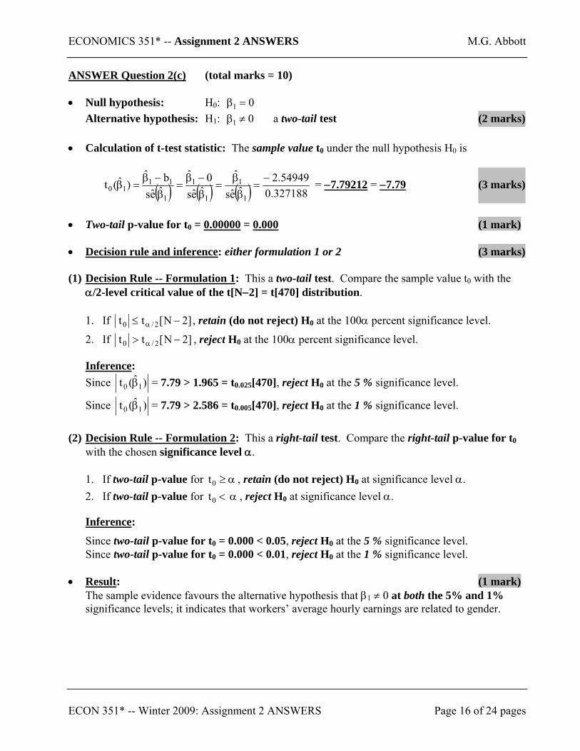
ANSWER Question 2(c) (total marks = 10) • Null hypothesis: H0: 01 =β
Alternative hypothesis: H1: 01 ≠β a two-tail test (2 marks)
• Calculation of t-test statistic: The sample value t0 under the null hypothesis H0 is
( ) ( ) ( ) 327188.054949.2
ˆes
ˆˆes
0ˆˆesbˆ
)ˆ(t1
1
1
1
1
1110
−=
ββ
=β−β
=β−β
=β = −7.79212 = −7.79 (3 marks)
• Two-tail p-value for t0 = 0.00000 = 0.000 (1 mark) • Decision rule and inference: either formulation 1 or 2 (3 marks) (1) Decision Rule -- Formulation 1: This a two-tail test. Compare the sample value t0 with the
α/2-level critical value of the t[N−2] = t[470] distribution.
1. If ]2N[tt 2/0 −≤ α , retain (do not reject) H0 at the 100α percent significance level.
2. If ]2N[tt 2/0 −> α , reject H0 at the 100α percent significance level.
Inference: Since )ˆ(t 10 β = 7.79 > 1.965 = t0.025[470], reject H0 at the 5 % significance level.
Since )ˆ(t 10 β = 7.79 > 2.586 = t0.005[470], reject H0 at the 1 % significance level.
(2) Decision Rule -- Formulation 2: This a right-tail test. Compare the right-tail p-value for t0
with the chosen significance level α.
1. If two-tail p-value for α≥0t , retain (do not reject) H0 at significance level α. 2. If two-tail p-value for α<0t , reject H0 at significance level α.
Inference:
Since two-tail p-value for t0 = 0.000 < 0.05, reject H0 at the 5 % significance level. Since two-tail p-value for t0 = 0.000 < 0.01, reject H0 at the 1 % significance level.
• Result: (1 mark)
The sample evidence favours the alternative hypothesis that β1 ≠ 0 at both the 5% and 1% significance levels; it indicates that workers’ average hourly earnings are related to gender.
ECONOMICS 351* -- Assignment 2 ANSWERS M.G. Abbott
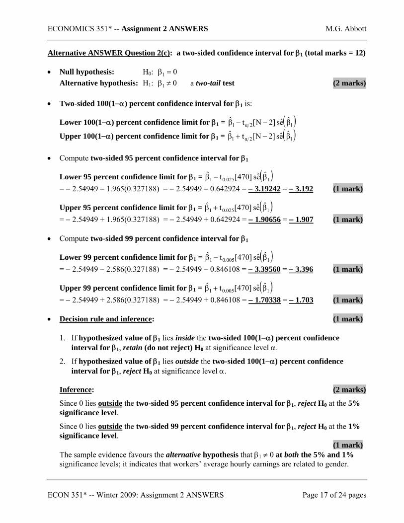
Alternative ANSWER Question 2(c): a two-sided confidence interval for β1 (total marks = 12) • Null hypothesis: H0: 01 =β
Alternative hypothesis: H1: 01 ≠β a two-tail test (2 marks) • Two-sided 100(1−α) percent confidence interval for β1 is:
Lower 100(1−α) percent confidence limit for β1 = ( )12α1 βes]2N[tβ −−
Upper 100(1−α) percent confidence limit for β1 = ( )12α1 βes]2N[tβ −+
• Compute two-sided 95 percent confidence interval for β1
Lower 95 percent confidence limit for β1 = ( )1025.01ˆes]470[tˆ β−β
= − 2.54949 − 1.965(0.327188) = − 2.54949 − 0.642924 = − 3.19242 = − 3.192 (1 mark)
Upper 95 percent confidence limit for β1 = ( )1025.01ˆes]470[tˆ β+β
= − 2.54949 + 1.965(0.327188) = − 2.54949 + 0.642924 = − 1.90656 = − 1.907 (1 mark)
• Compute two-sided 99 percent confidence interval for β1
Lower 99 percent confidence limit for β1 = ( )1005.01ˆes]470[tˆ β−β
= − 2.54949 − 2.586(0.327188) = − 2.54949 − 0.846108 = − 3.39560 = − 3.396 (1 mark)
Upper 99 percent confidence limit for β1 = ( )1005.01ˆes]470[tˆ β+β
= − 2.54949 + 2.586(0.327188) = − 2.54949 + 0.846108 = − 1.70338 = − 1.703 (1 mark) • Decision rule and inference: (1 mark)
1. If hypothesized value of β1 lies inside the two-sided 100(1−α) percent confidence interval for β1, retain (do not reject) H0 at significance level α.
2. If hypothesized value of β1 lies outside the two-sided 100(1−α) percent confidence interval for β1, reject H0 at significance level α.
Inference: (2 marks)
Since 0 lies outside the two-sided 95 percent confidence interval for β1, reject H0 at the 5% significance level.
Since 0 lies outside the two-sided 99 percent confidence interval for β1, reject H0 at the 1% significance level.
(1 mark) The sample evidence favours the alternative hypothesis that β1 ≠ 0 at both the 5% and 1% significance levels; it indicates that workers’ average hourly earnings are related to gender.
ECON 351* -- Winter 2009: Assignment 2 ANSWERS Page 17 of 24 pages

ECONOMICS 351* -- Assignment 2 ANSWERS M.G. Abbott
(12 marks) (d) Use the OLS estimation results for regression equation (2) to test the proposition that
females’ mean hourly wage rate was less than males’ mean hourly wage rate in 1976. State the null and alternative hypotheses. Show how the appropriate test statistic is calculated (give its formula). Report the sample value of the test statistic and its p-value. Report the appropriate critical values of the test statistic at the 5 percent and 1 percent significance levels. State the decision rule you use to decide between rejection and retention of the null hypothesis. State the inference you would draw from the test at both the 5 percent and 1 percent significance levels. What would you conclude from the results of the test?
ECON 351* -- Winter 2009: Assignment 2 ANSWERS Page 18 of 24 pages

ECONOMICS 351* -- Assignment 2 ANSWERS M.G. Abbott
ECON 351* -- Winter 2009: Assignment 2 ANSWERS Page 19 of 24 pages
ANSWER Question 2(d) (total marks = 12) Null hypothesis: H0: 01 =β (or 0≥1β ) (1 mark) Alternative hypothesis: H1: a left-tail01 <β t-test (2 marks)
• Calculation of t-test statistic: The sample value t0 under the null hypothesis H0 is
( ) ( ) ( ) 327188.054949.2
ˆes
ˆˆes
0ˆˆesbˆ
)ˆ(t1
1
1
1
1
1110
−=
ββ
=β−β
=β−β
=β = −7.79212 = −7.79 (2 marks)
• One-tail left-tail p-value of t0 = Pr( t < −t0) = Pr( t < −7.792) = 0.00000 = 0.0000 (1 mark)
• One-tail left-tail critical values of the t[N−2] = t[470] distribution are:
]470[t]2N[t 05.0−=−− α = −1.648 at the 5% significance level (α = 0.05) (1 mark) ]470[t]2N[t 01.0−=−− α = −2.334 at the 1% significance level (α = 0.01) (1 mark)
• Decision rule and inference: either formulation 1 or 2 (3 marks) (1) Decision Rule -- Formulation 1: This a left-tail test. Compare the sample value t0 with the
lower α-level critical value of the t[N−2] = t[470] distribution.
1. If ]2N[ , reject H0 at the 100α percent significance level. tt0 −−< α
2. If ]2N[ , retain (do not reject) H0 at the 100α percent significance level. tt0 −−≥ α
Inference: Since = −7.792 < −1.648 = −t0.05[470], reject H0 at the 5 % significance level.
)ˆ(t 10 β
Since = −7.792 < −2.334 = −t0.01[470], reject H0 at the 1 % significance level.
)ˆ(t 10 β
(2) Decision Rule -- Formulation 2: This a left-tail test. Compare the left-tail p-value for t0 with
the chosen significance level α.
1. If left-tail p-value for α≥0t , retain (do not reject) H0 at significance level α. 2. If left-tail p-value for α<0t , reject H0 at significance level α.
Inference:
Since left-tail p-value for t0 = 0.0000 < 0.05, reject H0 at the 5 % significance level. Since left-tail p-value for t0 = 0.0000 < 0.01, reject H0 at the 1 % significance level.
Result: The sample evidence favours the alternative hypothesis that β1 < 0 at both the 5% and 1%, significance levels; it indicates that females’ mean hourly earnings are less than males’ mean hourly earnings. (1 mark)
ECONOMICS 351* -- Assignment 2 ANSWERS M.G. Abbott
(12 marks) (e) Use the results from OLS estimation of regression equation (2) to test the hypothesis that
the mean hourly wage rate of female workers in 1976 was equal to $4.00 per hour (in 1976 US dollars). State the null and alternative hypotheses. Show how the appropriate test statistic is calculated (give its formula). Report the sample value of the test statistic and its p-value. State the decision rule you use to decide between rejection and retention of the null hypothesis. State the inference you would draw from the test at the 5 percent and the 1 percent significance levels. What conclusion would you draw from the results of the test?
ECON 351* -- Winter 2009: Assignment 2 ANSWERS Page 20 of 24 pages
ECONOMICS 351* -- Assignment 2 ANSWERS M.G. Abbott
ECON 351* -- Winter 2009: Assignment 2 ANSWERS Page 21 of 24 pages
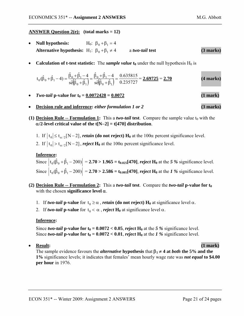
ANSWER Question 2(e): (total marks = 12) • Null hypothesis: H0: 410 =β+β
Alternative hypothesis: H1: 410 ≠β+β a two-tail test (3 marks)
• Calculation of t-test statistic: The sample value t0 under the null hypothesis H0 is
( ) ( ) 235727.0635815.0
ˆˆes4ˆˆ
ˆˆes4ˆˆ
)4ˆˆ(t10
10
10
10100 =
β+β−β+β
=β+β−β+β
=−β+β = 2.69725 = 2.70 (4 marks)
• Two-tail p-value for t0 = 0.0072428 = 0.0072 (1 mark)
• Decision rule and inference: either formulation 1 or 2 (3 marks) (1) Decision Rule -- Formulation 1: This a two-tail test. Compare the sample value t0 with the
α/2-level critical value of the t[N−2] = t[470] distribution.
1. If ]2N[tt 2/0 −≤ α , retain (do not reject) H0 at the 100α percent significance level.
2. If ]2N[tt 2/0 −> α , reject H0 at the 100α percent significance level.
Inference: Since )200ˆˆ(t 100 −β+β = 2.70 > 1.965 = t0.025[470], reject H0 at the 5 % significance level.
Since )200ˆˆ(t 100 −β+β = 2.70 > 2.586 = t0.005[470], reject H0 at the 1 % significance level.
(2) Decision Rule -- Formulation 2: This a two-tail test. Compare the two-tail p-value for t0
with the chosen significance level α.
1. If two-tail p-value for α≥0t , retain (do not reject) H0 at significance level α. 2. If two-tail p-value for α<0t , reject H0 at significance level α.
Inference:
Since two-tail p-value for t0 = 0.0072 < 0.05, reject H0 at the 5 % significance level. Since two-tail p-value for t0 = 0.0072 < 0.01, reject H0 at the 1 % significance level.
• Result: (1 mark)
The sample evidence favours the alternative hypothesis that β1 ≠ 4 at both the 5% and the 1% significance levels; it indicates that females’ mean hourly wage rate was not equal to $4.00 per hour in 1976.
ECONOMICS 351* -- Assignment 2 ANSWERS M.G. Abbott
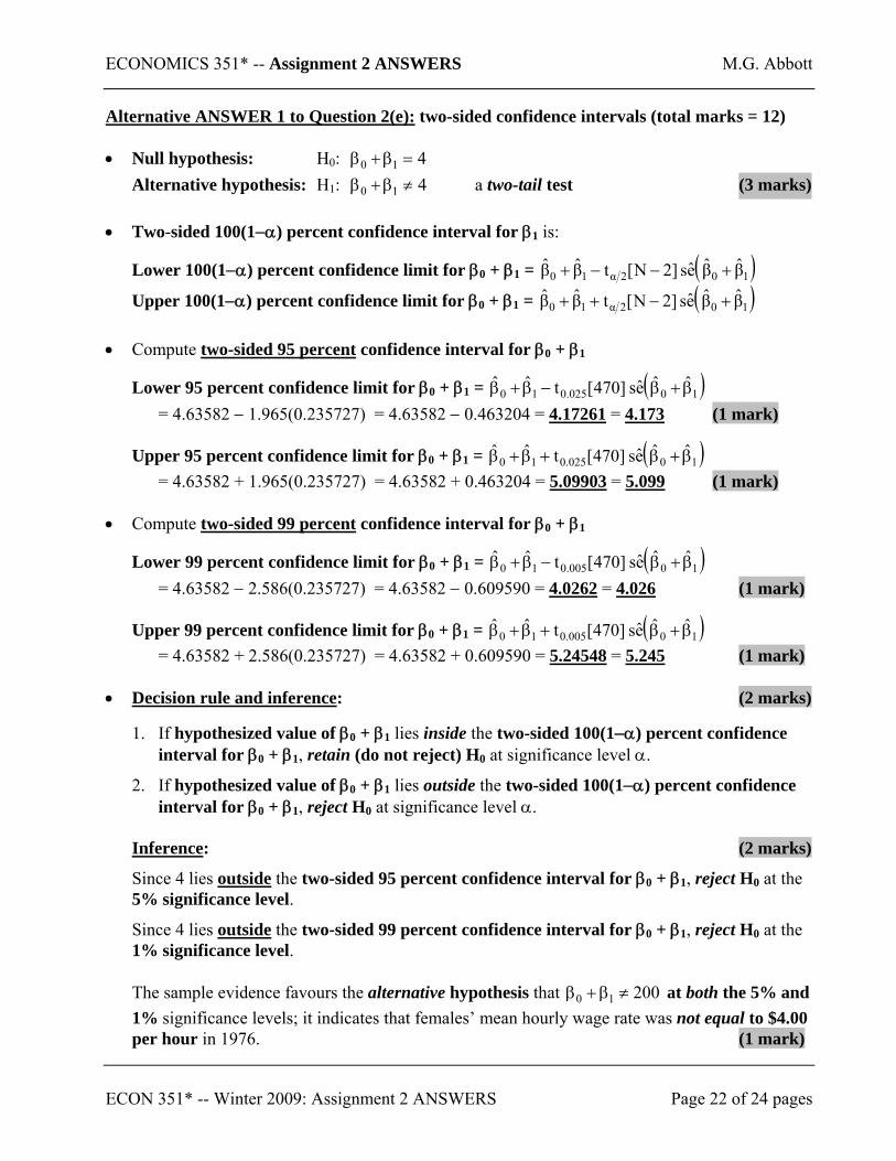
Alternative ANSWER 1 to Question 2(e): two-sided confidence intervals (total marks = 12) • Null hypothesis: H0: 410 =β+β
Alternative hypothesis: H1: 410 ≠β+β a two-tail test (3 marks) • Two-sided 100(1−α) percent confidence interval for β1 is:
Lower 100(1−α) percent confidence limit for β0 + β1 = ( )102α10 ββes]2N[tββ +−−+
Upper 100(1−α) percent confidence limit for β0 + β1 = ( )102α10 ββes]2N[tββ +−++
• Compute two-sided 95 percent confidence interval for β0 + β1
Lower 95 percent confidence limit for β0 + β1 = ( )10025.010ˆˆes]470[tˆˆ β+β−β+β
= 4.63582 − 1.965(0.235727) = 4.63582 − 0.463204 = 4.17261 = 4.173 (1 mark)
Upper 95 percent confidence limit for β0 + β1 = ( )10025.010ˆˆes]470[tˆˆ β+β+β+β
= 4.63582 + 1.965(0.235727) = 4.63582 + 0.463204 = 5.09903 = 5.099 (1 mark)
• Compute two-sided 99 percent confidence interval for β0 + β1
Lower 99 percent confidence limit for β0 + β1 = ( )10005.010ˆˆes]470[tˆˆ β+β−β+β
= 4.63582 − 2.586(0.235727) = 4.63582 − 0.609590 = 4.0262 = 4.026 (1 mark)
Upper 99 percent confidence limit for β0 + β1 = ( )10005.010ˆˆes]470[tˆˆ β+β+β+β
= 4.63582 + 2.586(0.235727) = 4.63582 + 0.609590 = 5.24548 = 5.245 (1 mark) • Decision rule and inference: (2 marks)
1. If hypothesized value of β0 + β1 lies inside the two-sided 100(1−α) percent confidence interval for β0 + β1, retain (do not reject) H0 at significance level α.
2. If hypothesized value of β0 + β1 lies outside the two-sided 100(1−α) percent confidence interval for β0 + β1, reject H0 at significance level α.
Inference: (2 marks)
Since 4 lies outside the two-sided 95 percent confidence interval for β0 + β1, reject H0 at the 5% significance level.
Since 4 lies outside the two-sided 99 percent confidence interval for β0 + β1, reject H0 at the 1% significance level.
The sample evidence favours the alternative hypothesis that 20010 ≠β+β at both the 5% and 1% significance levels; it indicates that females’ mean hourly wage rate was not equal to $4.00 per hour in 1976. (1 mark)
ECON 351* -- Winter 2009: Assignment 2 ANSWERS Page 22 of 24 pages
ECONOMICS 351* -- Assignment 2 ANSWERS M.G. Abbott
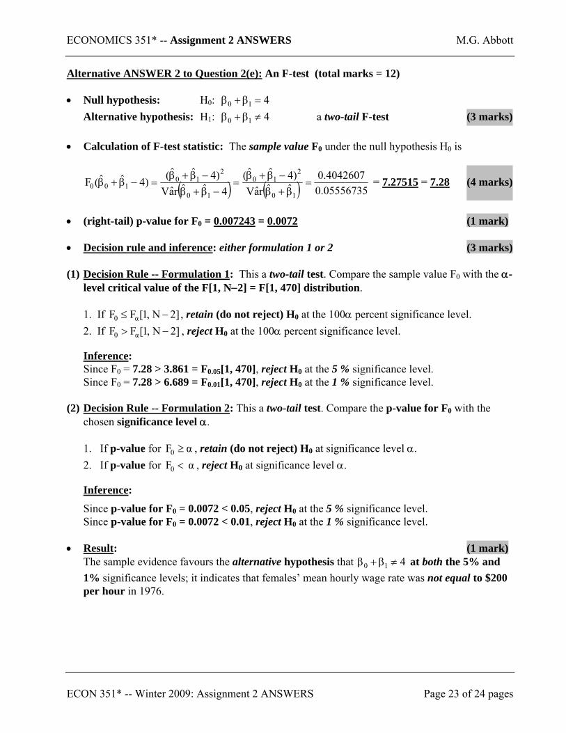
Alternative ANSWER 2 to Question 2(e): An F-test (total marks = 12) • Null hypothesis: H0: 410 =β+β
Alternative hypothesis: H1: 410 ≠β+β a two-tail F-test (3 marks)
• Calculation of F-test statistic: The sample value F0 under the null hypothesis H0 is
( ) ( ) 05556735.04042607.0
ˆˆraV)4ˆˆ(
4ˆˆraV)4ˆˆ()4ˆˆ(F
10
210
10
210
100 =β+β
−β+β=
−β+β−β+β
=−β+β = 7.27515 = 7.28 (4 marks)
• (right-tail) p-value for F0 = 0.007243 = 0.0072 (1 mark)
• Decision rule and inference: either formulation 1 or 2 (3 marks) (1) Decision Rule -- Formulation 1: This a two-tail test. Compare the sample value F0 with the α-
level critical value of the F[1, N−2] = F[1, 470] distribution.
1. If , retain (do not reject) H0 at the 100α percent significance level. ]2N,1[FF α0 −≤2. If , reject H0 at the 100α percent significance level. ]2N,1[FF α0 −>
Inference: Since F0 = 7.28 > 3.861 = F0.05[1, 470], reject H0 at the 5 % significance level. Since F0 = 7.28 > 6.689 = F0.01[1, 470], reject H0 at the 1 % significance level.
(2) Decision Rule -- Formulation 2: This a two-tail test. Compare the p-value for F0 with the
chosen significance level α.
1. If p-value for αF0 ≥ , retain (do not reject) H0 at significance level α. 2. If p-value for αF0 < , reject H0 at significance level α.
Inference:
Since p-value for F0 = 0.0072 < 0.05, reject H0 at the 5 % significance level. Since p-value for F0 = 0.0072 < 0.01, reject H0 at the 1 % significance level.
• Result: (1 mark)
The sample evidence favours the alternative hypothesis that 410 ≠β+β at both the 5% and 1% significance levels; it indicates that females’ mean hourly wage rate was not equal to $200 per hour in 1976.
ECON 351* -- Winter 2009: Assignment 2 ANSWERS Page 23 of 24 pages

ECONOMICS 351* -- Assignment 2 ANSWERS M.G. Abbott
ECON 351* -- Winter 2009: Assignment 2 ANSWERS Page 24 of 24 pages
Output of Stata ‘regress’ command for Questions 1 and 2: . * . * Question 1: be = b0 + b1*income + u . * . * Question 1(a): . * . regress be income Source | SS df MS Number of obs = 40 -------------+------------------------------ F( 1, 38) = 5.95 Model | 128366.057 1 128366.057 Prob > F = 0.0195 Residual | 819285.843 38 21560.1538 R-squared = 0.1355 -------------+------------------------------ Adj R-squared = 0.1127 Total | 947651.9 39 24298.7667 Root MSE = 146.83 ------------------------------------------------------------------------------ be | Coef. Std. Err. t P>|t| [95% Conf. Interval] -------------+---------------------------------------------------------------- income | 1.457651 .597385 2.44 0.019 .2483081 2.666994 _cons | 128.9803 34.59125 3.73 0.001 58.95401 199.0067 ------------------------------------------------------------------------------ . . * . * Question 2: be = b0 + b1*female + u . * . * Question 2(a): . * . regress be female Source | SS df MS Number of obs = 40 -------------+------------------------------ F( 1, 38) = 21.01 Model | 337400.872 1 337400.872 Prob > F = 0.0000 Residual | 610251.028 38 16059.2376 R-squared = 0.3560 -------------+------------------------------ Adj R-squared = 0.3391 Total | 947651.9 39 24298.7667 Root MSE = 126.73 ------------------------------------------------------------------------------ be | Coef. Std. Err. t P>|t| [95% Conf. Interval] -------------+---------------------------------------------------------------- female | -183.9148 40.12417 -4.58 0.000 -265.1419 -102.6877 _cons | 288.1053 29.07272 9.91 0.000 229.2506 346.9599
Related Documents