ECONOMICS 452* -- Stata 12 Tutorial 2 M.G. Abbott Stata 12 Tutorial 2 TOPIC: Estimation and Hypothesis Testing in Linear Regression Models: A Review with Stata DATA: auto1.dta (a Stata-format dataset you created in Stata 12 Tutorial 1) TASKS: Stata 12 Tutorial 2 is largely a review of OLS estimation and hypothesis testing procedures that most students learned in ECON 351*. It is intended to give you some practice in using Stata to estimate multiple linear regression models, to save and display the estimation results, and to compute t-tests and F-tests of linear coefficient restrictions. The Stata commands included in this tutorial should work in both Stata 11 (Stata Release 11) and Stata 12 (Stata Release 12). Topics introduced in Tutorial 2 include: Using the Stata regress command to perform OLS (Ordinary Least Squares) estimation of linear regression models • • • • • • • • Using the ereturn list command to display all of the temporarily-saved results from the most recent regress command Using the display and scalar commands to display and save selected results of OLS estimation, including individual coefficient estimates, the standard errors and variances of individual coefficient estimates, and summary statistics for OLS sample regression equations Using the matrix command to save the OLS regression coefficient vector and the estimated variance-covariance matrix of the OLS coefficient estimates Using the Stata statistical function ttail(df, t 0 ) to compute one-tail and two-tail p-values for calculated t-statistics, and the Stata statistical function invttail(df, p) to compute one-tail and two-tail critical values of t-distributions Using the Stata lincom command to compute two-tail and one-tail t-tests of individual regression coefficients and of individual hypotheses that take the form of single linear combinations of two (or more) regression coefficients Using the Stata statistical function Ftail(df 1 , df 2 , F 0 ) to compute p-values of calculated F-statistics, and the Stata statistical function invFtail(df 1 , df 2 , α) to compute critical values of F-distributions Using the Stata test command to compute F-tests of linear coefficient equality restrictions after OLS estimation. ECON 452* -- Fall 2012: Stata 12 Tutorial 2 Page 1 of 31 pages 452tutorial02_f2012.doc

Welcome message from author
This document is posted to help you gain knowledge. Please leave a comment to let me know what you think about it! Share it to your friends and learn new things together.
Transcript
ECONOMICS 452* -- Stata 12 Tutorial 2 M.G. Abbott
Stata 12 Tutorial 2 TOPIC: Estimation and Hypothesis Testing in Linear Regression Models:
A Review with Stata DATA: auto1.dta (a Stata-format dataset you created in Stata 12 Tutorial 1) TASKS: Stata 12 Tutorial 2 is largely a review of OLS estimation and hypothesis
testing procedures that most students learned in ECON 351*. It is intended to give you some practice in using Stata to estimate multiple linear regression models, to save and display the estimation results, and to compute t-tests and F-tests of linear coefficient restrictions. The Stata commands included in this tutorial should work in both Stata 11 (Stata Release 11) and Stata 12 (Stata Release 12).
Topics introduced in Tutorial 2 include:
Using the Stata regress command to perform OLS (Ordinary Least Squares) estimation of linear regression models
•
•
•
•
•
•
•
•
Using the ereturn list command to display all of the temporarily-saved results from the most recent regress command Using the display and scalar commands to display and save selected results of OLS estimation, including individual coefficient estimates, the standard errors and variances of individual coefficient estimates, and summary statistics for OLS sample regression equations Using the matrix command to save the OLS regression coefficient vector and the estimated variance-covariance matrix of the OLS coefficient estimates Using the Stata statistical function ttail(df, t0) to compute one-tail and two-tail p-values for calculated t-statistics, and the Stata statistical function invttail(df, p) to compute one-tail and two-tail critical values of t-distributions Using the Stata lincom command to compute two-tail and one-tail t-tests of individual regression coefficients and of individual hypotheses that take the form of single linear combinations of two (or more) regression coefficients Using the Stata statistical function Ftail(df1, df2, F0) to compute p-values of calculated F-statistics, and the Stata statistical function invFtail(df1, df2, α) to compute critical values of F-distributions Using the Stata test command to compute F-tests of linear coefficient equality restrictions after OLS estimation.
ECON 452* -- Fall 2012: Stata 12 Tutorial 2 Page 1 of 31 pages 452tutorial02_f2012.doc
ECONOMICS 452* -- Stata 12 Tutorial 2 M.G. Abbott
•
•
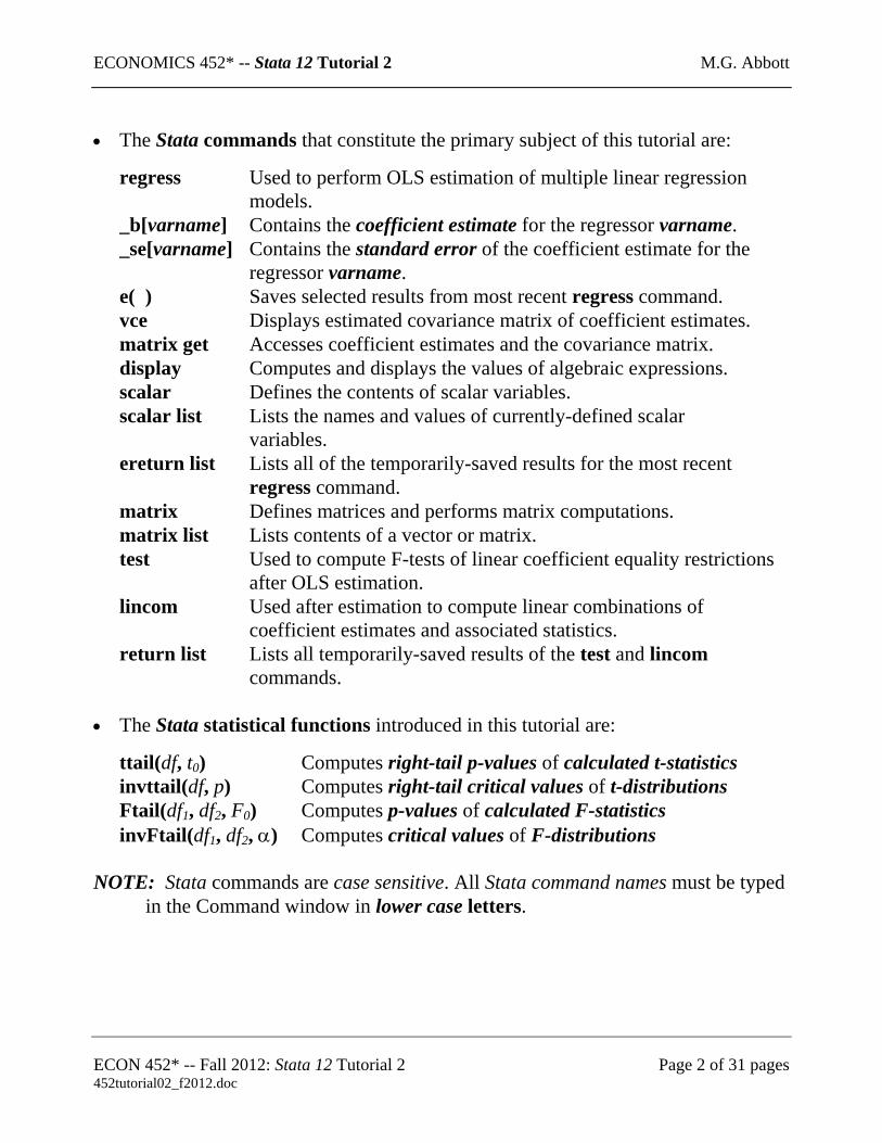
The Stata commands that constitute the primary subject of this tutorial are:
regress Used to perform OLS estimation of multiple linear regression models.
_b[varname] Contains the coefficient estimate for the regressor varname. _se[varname] Contains the standard error of the coefficient estimate for the
regressor varname. e( ) Saves selected results from most recent regress command. vce Displays estimated covariance matrix of coefficient estimates. matrix get Accesses coefficient estimates and the covariance matrix. display Computes and displays the values of algebraic expressions. scalar Defines the contents of scalar variables. scalar list Lists the names and values of currently-defined scalar
variables. ereturn list Lists all of the temporarily-saved results for the most recent regress command. matrix Defines matrices and performs matrix computations. matrix list Lists contents of a vector or matrix.
test Used to compute F-tests of linear coefficient equality restrictions after OLS estimation.
lincom Used after estimation to compute linear combinations of coefficient estimates and associated statistics.
return list Lists all temporarily-saved results of the test and lincom commands.
The Stata statistical functions introduced in this tutorial are:
ttail(df, t0) Computes right-tail p-values of calculated t-statistics invttail(df, p) Computes right-tail critical values of t-distributions Ftail(df1, df2, F0) Computes p-values of calculated F-statistics invFtail(df1, df2, α) Computes critical values of F-distributions
NOTE: Stata commands are case sensitive. All Stata command names must be typed
in the Command window in lower case letters.
ECON 452* -- Fall 2012: Stata 12 Tutorial 2 Page 2 of 31 pages 452tutorial02_f2012.doc
ECONOMICS 452* -- Stata 12 Tutorial 2 M.G. Abbott
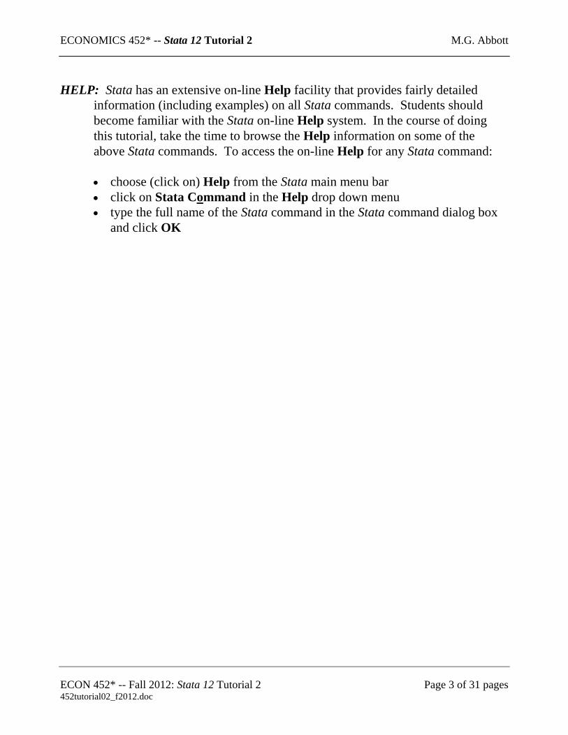
HELP: Stata has an extensive on-line Help facility that provides fairly detailed
information (including examples) on all Stata commands. Students should become familiar with the Stata on-line Help system. In the course of doing this tutorial, take the time to browse the Help information on some of the above Stata commands. To access the on-line Help for any Stata command:
• choose (click on) Help from the Stata main menu bar • click on Stata Command in the Help drop down menu • type the full name of the Stata command in the Stata command dialog box
and click OK
ECON 452* -- Fall 2012: Stata 12 Tutorial 2 Page 3 of 31 pages 452tutorial02_f2012.doc

ECONOMICS 452* -- Stata 12 Tutorial 2 M.G. Abbott
Preparing for Your Stata Session Before beginning your Stata session, use Windows Explorer to copy the Stata-format data set auto1.dta from your portable storage device to the Stata working directory on the C:-drive or D:-drive of the computer at which you are working. • On the computers in Dunning 350, the default Stata working directory is usually
C:\data. • On the computers in MC B111, the default Stata working directory is usually
D:\courses.
Start Your Stata Session There are two ways to start a Stata session. •
•
If you see a Stata 11 or Stata 12 icon on the Windows desktop, simply double-click it.
If there is no Stata 11 or Stata 12 icon on the Windows desktop of the computer at which you are working, click on the Start button located at the left end of the Windows XP or Windows 7 taskbar along the bottom of the desktop window. From the All Programs menu, select (click on) the Stata 11 or Stata 12 icon.
After you start your Stata session, the first screen you will see contains four Stata windows (or five Stata windows of you’re using Stata 12): • the Stata Command window, in which you type all Stata commands. • the Stata Results window, which displays the results of each Stata command as
you enter it. • the Review window, which displays the past commands you have issued during the
current Stata session. • the Variables window, which lists the variables in the currently-loaded data file. • (in Stata 12 only) the Properties window, which displays the properties of the
variables and dataset currently in memory.
ECON 452* -- Fall 2012: Stata 12 Tutorial 2 Page 4 of 31 pages 452tutorial02_f2012.doc
ECONOMICS 452* -- Stata 12 Tutorial 2 M.G. Abbott
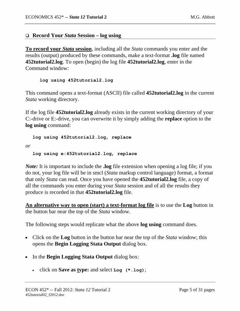
Record Your Stata Session – log using To record your Stata session, including all the Stata commands you enter and the results (output) produced by these commands, make a text-format .log file named 452tutorial2.log. To open (begin) the log file 452tutorial2.log, enter in the Command window:
log using 452tutorial2.log This command opens a text-format (ASCII) file called 452tutorial2.log in the current Stata working directory. If the log file 452tutorial2.log already exists in the current working directory of your C:-drive or E:-drive, you can overwrite it by simply adding the replace option to the log using command:
log using 452tutorial2.log, replace
or log using e:452tutorial2.log, replace
Note: It is important to include the .log file extension when opening a log file; if you do not, your log file will be in smcl (Stata markup control language) format, a format that only Stata can read. Once you have opened the 452tutorial2.log file, a copy of all the commands you enter during your Stata session and of all the results they produce is recorded in that 452tutorial2.log file. An alternative way to open (start) a text-format log file is to use the Log button in the button bar near the top of the Stata window. The following steps would replicate what the above log using command does. •
•
Click on the Log button in the button bar near the top of the Stata window; this opens the Begin Logging Stata Output dialog box.
In the Begin Logging Stata Output dialog box:
• click on Save as type: and select Log (*.log);
ECON 452* -- Fall 2012: Stata 12 Tutorial 2 Page 5 of 31 pages 452tutorial02_f2012.doc
ECONOMICS 452* -- Stata 12 Tutorial 2 M.G. Abbott
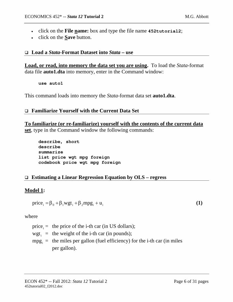
• click on the File name: box and type the file name 452tutorial2; • click on the Save button.
Load a Stata-Format Dataset into Stata – use
Load, or read, into memory the data set you are using. To load the Stata-format data file auto1.dta into memory, enter in the Command window:
use auto1 This command loads into memory the Stata-format data set auto1.dta.
Familiarize Yourself with the Current Data Set To familiarize (or re-familiarize) yourself with the contents of the current data set, type in the Command window the following commands:
describe, short describe summarize list price wgt mpg foreign codebook price wgt mpg foreign
Estimating a Linear Regression Equation by OLS – regress
Model 1:
ii2i10i umpgwgtprice +β+β+β= (1) where
iprice = the price of the i-th car (in US dollars); iwgt = the weight of the i-th car (in pounds);
mpgi = the miles per gallon (fuel efficiency) for the i-th car (in miles per gallon).
ECON 452* -- Fall 2012: Stata 12 Tutorial 2 Page 6 of 31 pages 452tutorial02_f2012.doc

ECONOMICS 452* -- Stata 12 Tutorial 2 M.G. Abbott
• To estimate by OLS the linear regression model given by PRE (1), enter in the Command window the following regress command:
regress price wgt mpg
Accessing Coefficient Estimates and Standard Errors – _b[…] and _se[…]
Basic Syntax:
_b[varname] (or its synonym _coef[varname]); _se[varname]
where varname is the user-supplied variable name for one of the regressors in the most recent regress command.
Accessing coefficient estimates. _b[varname], or its synonym _coef[varname],
contains the coefficient estimate for the regressor varname in the most recent regress command. Thus, _b[wgt] and _coef[wgt] both contain the value of the OLS estimate of the regression coefficient on the regressor wgt in the OLS sample regression equation for Model 1.
1β
• Use either of the following display commands to simply display in the Results
window the value of the OLS slope coefficient estimate : 1β
display _b[wgt] display _coef[wgt]
• Use either of the following display commands to simply display in the Results
window the value of the OLS slope coefficient estimate : 2β
display _b[mpg] display _coef[mpg]
• The Stata system variable _cons is always equal to the number 1, and refers to the intercept coefficient estimate when used with _b[ ] and _coef[ ]. Thus, _b[_cons] and _coef[_cons] both contain the value of the OLS estimate of the intercept coefficient β
0β
0 in the previous OLS regression. To display in the Results window
ECON 452* -- Fall 2012: Stata 12 Tutorial 2 Page 7 of 31 pages 452tutorial02_f2012.doc
ECONOMICS 452* -- Stata 12 Tutorial 2 M.G. Abbott
the value of the OLS intercept coefficient estimate , enter either of the following commands in the Command window:
0β
display _b[_cons] display _coef[_cons]
Note: _b[ ] and _coef[ ] are equivalent; that is, they are synonyms. Therefore,
_b[_cons] = _coef[_cons] = = the OLS intercept coefficient estimate; 0β
_b[wgt] = _ coef[wgt] = = the OLS slope coefficient estimate for wgt. 1β
_b[mpg] = _ coef[mpg] = = the OLS slope coefficient estimate for mpg. 2β
Accessing estimated standard errors. _se[varname] contains the estimated standard error of the coefficient estimate for the regressor varname in the most recent regress command. Thus, _se[wgt] contains , the estimated standard error of the OLS slope coefficient estimate . Similarly, _se[_cons] contains
, the estimated standard error of the OLS intercept coefficient estimate .
)ˆ(es 1β
1β
)ˆ(es 0β 0β • Enter the following display commands to display in the Results window the
values of , and from the OLS sample regression equation for Model 1:
)ˆ(es 0β se$( $ )β1 se$( $ )β 2
display _se[_cons] display _se[wgt] display _se[mpg]
Saving Coefficient Estimates and Standard Errors – scalar
Stata stores the values of coefficient estimates in _b[ ] (or in _ coef[ ]) and the values of estimated standard errors in _se[ ] only temporarily -- that is until another model estimation command such as regress is entered. To save the values of coefficient estimates and their estimated standard errors for subsequent use, you can use scalar commands to assign names to these values.
ECON 452* -- Fall 2012: Stata 12 Tutorial 2 Page 8 of 31 pages 452tutorial02_f2012.doc
ECONOMICS 452* -- Stata 12 Tutorial 2 M.G. Abbott
Basic Syntax:
scalar scalar_name = exp where scalar_name is the user-supplied name for the scalar and exp is an algebraic expression or function.
• The following scalar commands name and save the values of the OLS coefficient
estimates , and for Model 1. Enter the commands: 0β 1β $β 2
scalar b0 = _b[_cons] scalar b1 = _b[wgt] scalar b2 = _b[mpg]
• The following scalar commands name and save the values of the estimated
standard errors for the OLS coefficient estimates , and . Enter the commands:
0β 1β $β 2
scalar seb0 = _se[_cons] scalar seb1 = _se[wgt] scalar seb2 = _se[mpg]
• You may also wish to generate the estimated variances of the OLS coefficient
estimates , and for Model 1, which are equal to the squares of the corresponding estimated standard errors. Enter the following scalar commands to do this:
0β 1β $β 2
scalar varb0 = seb0^2 scalar varb1 = seb1^2 scalar varb2 = seb2^2
To display the values of scalar variables, use the scalar list command. The scalar list command for scalars is the analog of the list command for variables. • To list the values of all currently-defined scalars, enter the following command:
scalar list
ECON 452* -- Fall 2012: Stata 12 Tutorial 2 Page 9 of 31 pages 452tutorial02_f2012.doc
ECONOMICS 452* -- Stata 12 Tutorial 2 M.G. Abbott
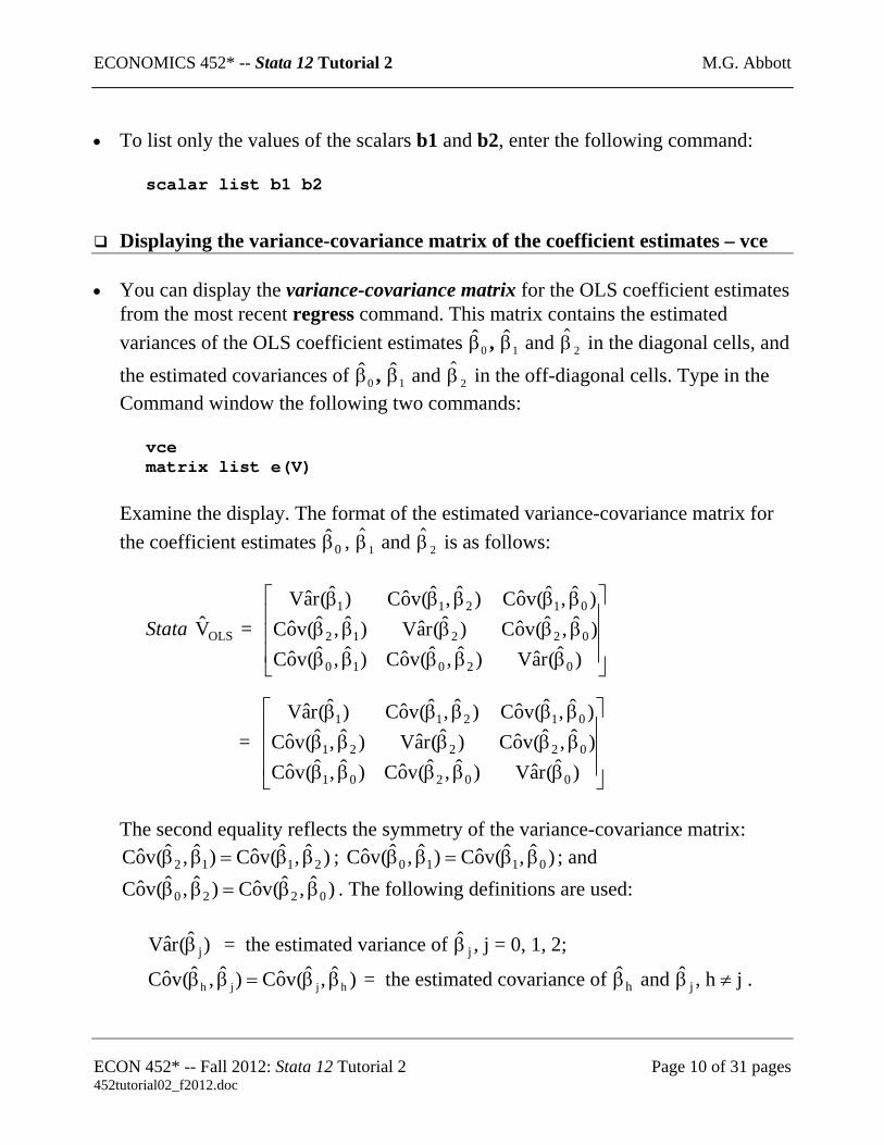
• To list only the values of the scalars b1 and b2, enter the following command:
scalar list b1 b2
Displaying the variance-covariance matrix of the coefficient estimates – vce
• You can display the variance-covariance matrix for the OLS coefficient estimates
from the most recent regress command. This matrix contains the estimated variances of the OLS coefficient estimates , and in the diagonal cells, and the estimated covariances of , and in the off-diagonal cells. Type in the Command window the following two commands:
0β 1β $β 2
0β 1β $β 2
vce matrix list e(V)
Examine the display. The format of the estimated variance-covariance matrix for the coefficient estimates , and is as follows: 0β $β1
$β 2
Stata = OLSV⎥⎥⎥
⎦
⎤
⎢⎢⎢
⎣
⎡
βββββββββββββββ
)ˆ(raV)ˆ,ˆ(voC)ˆ,ˆ(voC)ˆ,ˆ(voC)ˆ(raV)ˆ,ˆ(voC)ˆ,ˆ(voC)ˆ,ˆ(voC)ˆ(raV
02010
02212
01211
= ⎥⎥⎥
⎦
⎤
⎢⎢⎢
⎣
⎡
βββββββββββββββ
)ˆ(raV)ˆ,ˆ(voC)ˆ,ˆ(voC)ˆ,ˆ(voC)ˆ(raV)ˆ,ˆ(voC)ˆ,ˆ(voC)ˆ,ˆ(voC)ˆ(raV
00201
02221
01211
The second equality reflects the symmetry of the variance-covariance matrix:
; ; and . The following definitions are used:
)ˆ,ˆ(voC)ˆ,ˆ(voC 2112 ββ=ββ )ˆ,ˆ(voC)ˆ,ˆ(voC 0110 ββ=ββ
)ˆ,ˆ(voC)ˆ,ˆ(voC 0220 ββ=ββ
= the estimated variance of , j = 0, 1, 2; )ˆ(raV jβ jβ
= the estimated covariance of and , h ≠ j . )ˆ,ˆ(voC)ˆ,ˆ(voC hjjh ββ=ββ hβ jβ
ECON 452* -- Fall 2012: Stata 12 Tutorial 2 Page 10 of 31 pages 452tutorial02_f2012.doc
ECONOMICS 452* -- Stata 12 Tutorial 2 M.G. Abbott
Saving the coefficient vector and variance-covariance matrix To save the entire vector of OLS coefficient estimates and the associated variance-covariance matrix, you can use the matrix get command. Basic Syntax: matrix matname = get(internal_Stata_matrix_name) where matname is the user-supplied name given to the matrix or vector, and internal_Stata_matrix_name is the internal name that Stata gives to the matrix or vector.
1. The internal name that Stata gives to the vector of OLS coefficient estimates is _b or e(b).
2. The internal name that Stata gives to the estimated variance-covariance matrix is VCE or e(V).
•
•
To save the vector of OLS coefficient estimates and give it the name bvec, enter the following command:
matrix bvec = get(_b)
An alternative way to save the vector of OLS coefficient estimates is to use a matrix command and the e(b) matrix function. To save the OLS coefficient vector and give it the name b, enter the following command:
matrix b = e(b)
• Use the following matrix list commands to display the saved coefficient vectors
bvec and b (which are, of course, identical):
matrix list bvec matrix list b
• To save the estimated variance-covariance matrix and give it the name V1, enter
the following matrix get command:
ECON 452* -- Fall 2012: Stata 12 Tutorial 2 Page 11 of 31 pages 452tutorial02_f2012.doc
ECONOMICS 452* -- Stata 12 Tutorial 2 M.G. Abbott
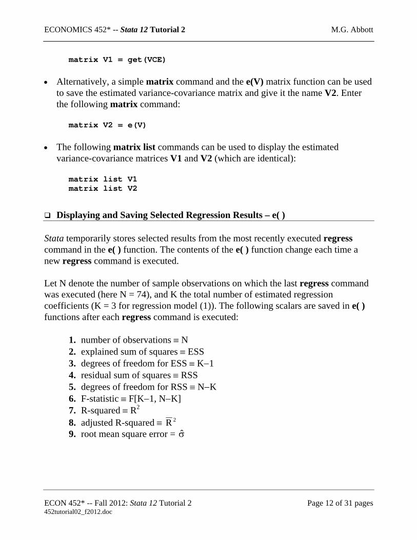
matrix V1 = get(VCE) • Alternatively, a simple matrix command and the e(V) matrix function can be used
to save the estimated variance-covariance matrix and give it the name V2. Enter the following matrix command:
matrix V2 = e(V)
• The following matrix list commands can be used to display the estimated
variance-covariance matrices V1 and V2 (which are identical):
matrix list V1 matrix list V2
Displaying and Saving Selected Regression Results – e( )
Stata temporarily stores selected results from the most recently executed regress command in the e( ) function. The contents of the e( ) function change each time a new regress command is executed. Let N denote the number of sample observations on which the last regress command was executed (here N = 74), and K the total number of estimated regression coefficients (K = 3 for regression model (1)). The following scalars are saved in e( ) functions after each regress command is executed:
1. number of observations ≡ N 2. explained sum of squares ≡ ESS 3. degrees of freedom for ESS ≡ K−1 4. residual sum of squares ≡ RSS 5. degrees of freedom for RSS ≡ N−K 6. F-statistic ≡ F[K−1, N−K] 7. R-squared ≡ R2 8. adjusted R-squared ≡ 2R 9. root mean square error = σ
ECON 452* -- Fall 2012: Stata 12 Tutorial 2 Page 12 of 31 pages 452tutorial02_f2012.doc
ECONOMICS 452* -- Stata 12 Tutorial 2 M.G. Abbott
•
•
•
•
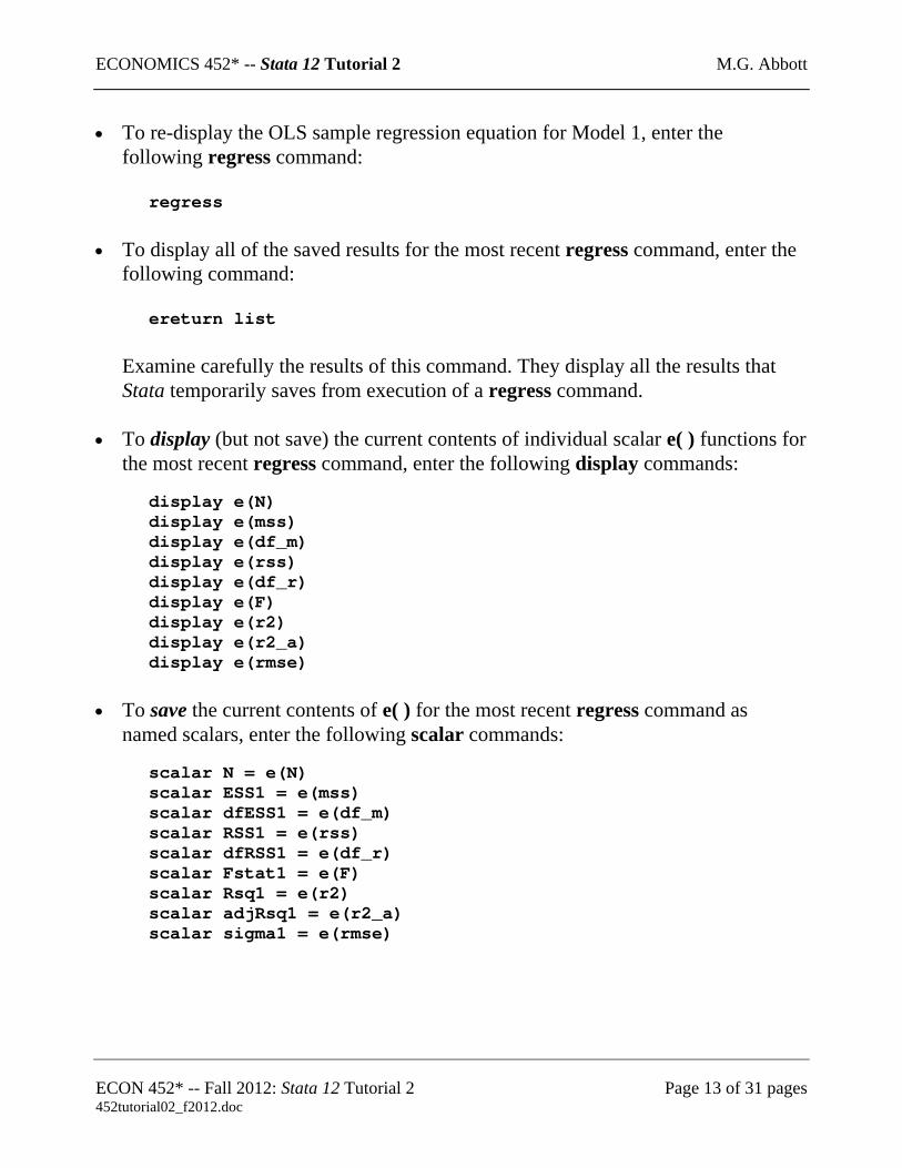
To re-display the OLS sample regression equation for Model 1, enter the following regress command:
regress
To display all of the saved results for the most recent regress command, enter the following command:
ereturn list
Examine carefully the results of this command. They display all the results that Stata temporarily saves from execution of a regress command.
To display (but not save) the current contents of individual scalar e( ) functions for the most recent regress command, enter the following display commands:
display e(N) display e(mss) display e(df_m) display e(rss) display e(df_r) display e(F) display e(r2) display e(r2_a) display e(rmse)
To save the current contents of e( ) for the most recent regress command as named scalars, enter the following scalar commands:
scalar N = e(N) scalar ESS1 = e(mss) scalar dfESS1 = e(df_m) scalar RSS1 = e(rss) scalar dfRSS1 = e(df_r) scalar Fstat1 = e(F) scalar Rsq1 = e(r2) scalar adjRsq1 = e(r2_a) scalar sigma1 = e(rmse)
ECON 452* -- Fall 2012: Stata 12 Tutorial 2 Page 13 of 31 pages 452tutorial02_f2012.doc

ECONOMICS 452* -- Stata 12 Tutorial 2 M.G. Abbott
•
•
•
•
To display the values of the scalars created by the foregoing commands, enter the following scalar list command:
scalar list N ESS1 dfESS1 RSS1 dfRSS1 Fstat1 Rsq1 adjRsq1 sigma1
You can also use the scalar command to save other results of the regress command. For example, enter the following commands to create and display some additional scalars for the sample regression equation obtained by OLS estimation of equation (1):
scalar K1 = dfESS1 + 1 scalar TSS1 = ESS1 + RSS1 scalar dfTSS1 = N - 1 scalar list N K1 TSS1 ESS1 RSS1 dfTSS1 dfESS1 dfRSS1
You have just saved a lot of scalars. To display or list all of the currently-defined scalars, enter the following scalar list command:
scalar list
Instead of the foregoing scalar list command, you could have displayed all of the currently-defined scalars by entering any of the following commands:
scalar list _all scalar dir scalar dir _all
Compare the results of these three commands; they should be identical to each other and to the results of the scalar list command.
ECON 452* -- Fall 2012: Stata 12 Tutorial 2 Page 14 of 31 pages 452tutorial02_f2012.doc
ECONOMICS 452* -- Stata 12 Tutorial 2 M.G. Abbott
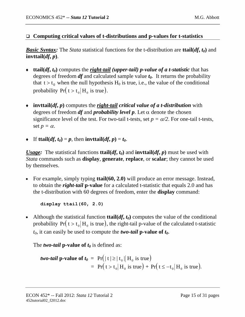
Computing critical values of t-distributions and p-values for t-statistics Basic Syntax: The Stata statistical functions for the t-distribution are ttail(df, t0) and invttail(df, p). ♦ ttail(df, t0) computes the right-tail (upper-tail) p-value of a t-statistic that has
degrees of freedom df and calculated sample value t0. It returns the probability that when the null hypothesis H0tt > 0 is true, i.e., the value of the conditional probability ( )trueisHttPr 00> .
♦ invttail(df, p) computes the right-tail critical value of a t-distribution with
degrees of freedom df and probability level p. Let α denote the chosen significance level of the test. For two-tail t-tests, set p = α/2. For one-tail t-tests, set p = α.
♦ If ttail(df, t0) = p, then invttail(df, p) = t0. Usage: The statistical functions ttail(df, t0) and invttail(df, p) must be used with Stata commands such as display, generate, replace, or scalar; they cannot be used by themselves. • For example, simply typing ttail(60, 2.0) will produce an error message. Instead,
to obtain the right-tail p-value for a calculated t-statistic that equals 2.0 and has the t-distribution with 60 degrees of freedom, enter the display command:
display ttail(60, 2.0) • Although the statistical function ttail(df, t0) computes the value of the conditional
probability ( )trueisHttPr 00> , the right-tail p-value of the calculated t-statistic t0, it can easily be used to compute the two-tail p-value of t0.
The two-tail p-value of t0 is defined as:
two-tail p-value of t0 = ( )trueisH|t||t|Pr 00≥ = ( )trueisHttPr 00> + ( )trueisHttPr 00−≤ .
ECON 452* -- Fall 2012: Stata 12 Tutorial 2 Page 15 of 31 pages 452tutorial02_f2012.doc
ECONOMICS 452* -- Stata 12 Tutorial 2 M.G. Abbott
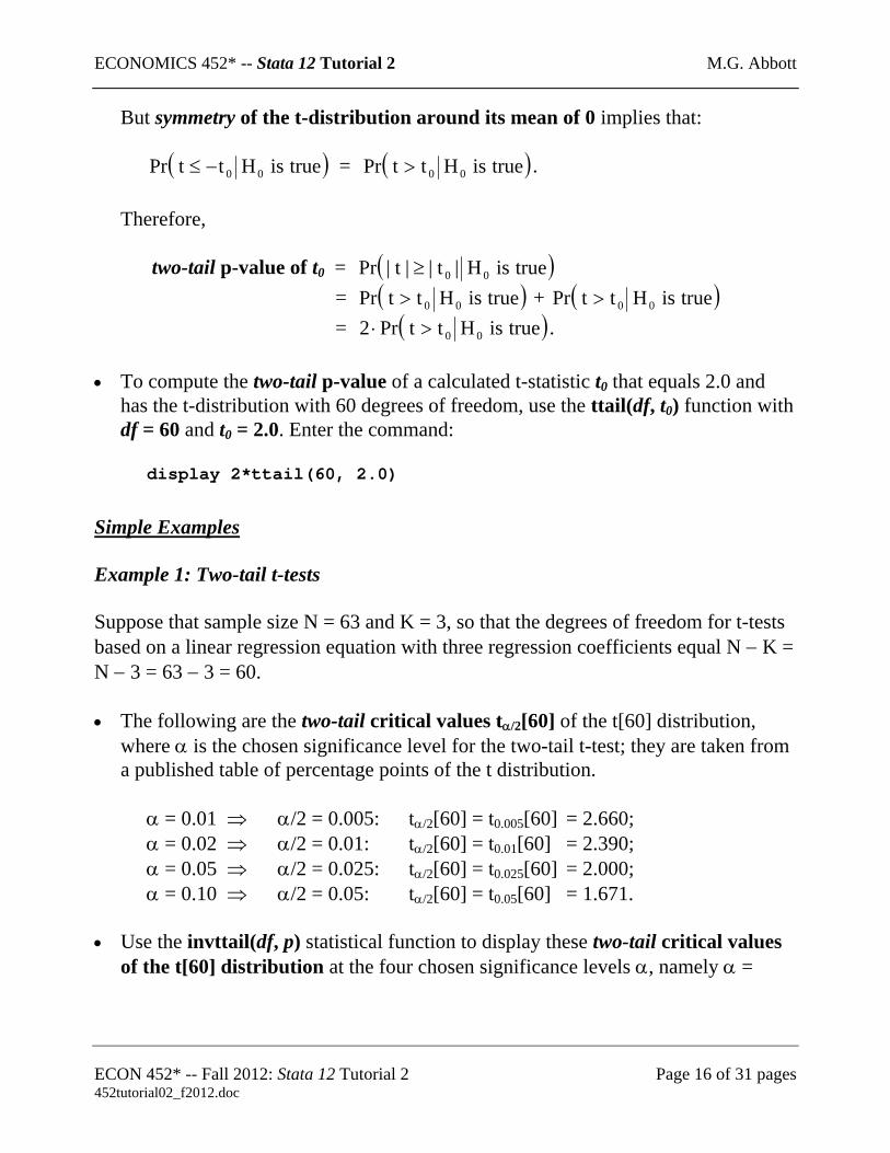
But symmetry of the t-distribution around its mean of 0 implies that:
( )trueisHttPr 00−≤ = ( )trueisHttPr 00> .
Therefore,
two-tail p-value of t0 = ( )trueisH|t||t|Pr 00≥ = ( )trueisHttPr 00> + ( )trueisHttPr 00> = ( )trueisHttPr2 00>⋅ .
• To compute the two-tail p-value of a calculated t-statistic t0 that equals 2.0 and
has the t-distribution with 60 degrees of freedom, use the ttail(df, t0) function with df = 60 and t0 = 2.0. Enter the command:
display 2*ttail(60, 2.0)
Simple Examples Example 1: Two-tail t-tests Suppose that sample size N = 63 and K = 3, so that the degrees of freedom for t-tests based on a linear regression equation with three regression coefficients equal N − K = N − 3 = 63 − 3 = 60. •
•
The following are the two-tail critical values tα/2[60] of the t[60] distribution, where α is the chosen significance level for the two-tail t-test; they are taken from a published table of percentage points of the t distribution.
α = 0.01 ⇒ α/2 = 0.005: tα/2[60] = t0.005[60] = 2.660; α = 0.02 ⇒ α/2 = 0.01: tα/2[60] = t0.01[60] = 2.390; α = 0.05 ⇒ α/2 = 0.025: tα/2[60] = t0.025[60] = 2.000; α = 0.10 ⇒ α/2 = 0.05: tα/2[60] = t0.05[60] = 1.671.
Use the invttail(df, p) statistical function to display these two-tail critical values of the t[60] distribution at the four chosen significance levels α, namely α =
ECON 452* -- Fall 2012: Stata 12 Tutorial 2 Page 16 of 31 pages 452tutorial02_f2012.doc

ECONOMICS 452* -- Stata 12 Tutorial 2 M.G. Abbott
0.01, 0.02, 0.05, and 0.10. Recall that for two-tail t-tests, set p = α/2. Enter the commands:
display invttail(60, 0.005) display invttail(60, 0.01) display invttail(60, 0.025) display invttail(60, 0.05)
•
•
•
Now use the ttail(df, t0) statistical function to display the two-tail p-values of the four sample values t0 = 2.660, 2.390, 2.000, and 1.671, which you already know equal the corresponding values of α (0.01, 0.02, 0.05, and 0.10):
display 2*ttail(60, 2.660) display 2*ttail(60, 2.390) display 2*ttail(60, 2.000) display 2*ttail(60, 1.671)
Note that to compute the two-tail p-values of the calculated t-statistics, the values of the ttail(df, t0) function must be multiplied by 2.
This example demonstrates the relationship between the two statistical functions ttail(df, t0) and invttail(df, p) for the t-distribution.
Example 2: Two-tail t-tests
Suppose the sample t-values are negative, rather than positive. For example, consider the sample t-values t0 = −2.660, and −2.000; you already know that for the t[60] distribution their two-tail p-values are, respectively, 0.01, and 0.05.
There are (at least) two alternative ways of using the ttail(df, t0) statistical function to compute the correct two-tail p-values for negative values of t0. To illustrate, enter the following display commands:
display 2*(1 - ttail(60, -2.660)) display 2*ttail(60, abs(-2.660)) display 2*(1 - ttail(60, -2.000)) display 2*ttail(60, abs(-2.000))
Note the use of the Stata absolute value operator abs( ).
ECON 452* -- Fall 2012: Stata 12 Tutorial 2 Page 17 of 31 pages 452tutorial02_f2012.doc

ECONOMICS 452* -- Stata 12 Tutorial 2 M.G. Abbott
♦
•
•
General recommendation for computing two-tail p-values of t-statistics
Let t0 be any calculated sample value of a t-statistic that is distributed under the null hypothesis as a t[df] distribution, where t0 may be either positive or negative.
The following command will always display the correct two-tail p-value of t0:
display 2*ttail(df, abs(t0)) Example 3: Two-tail critical values of calculated t-statistics
Two-tail critical values of the t[71] distribution can be obtained using the following display commands with the invttail(df, p) statistical function. Note that to obtain two-tail critical values, the value of the argument p equals α/2, where α is the significance level chosen for the two-tail test. Compute two-tail critical values of the t[71] distribution for significance levels α = 0.01, 0.05, and 0.10, i.e., for the 1%, 5%, and 10% significance levels. Enter the commands:
display invttail(71, 0.005) (for α = 0.01, α/2 = 0.005) display invttail(71, 0.025) (for α = 0.05, α/2 = 0.025) display invttail(71, 0.05) (for α = 0.10, α/2 = 0.05)
Two-tail p-values for calculated t-statistics. The following sections of this tutorial will illustrate how to use the ttail (df, t0) function to compute and display the two-tailed p-values for calculated t-statistics.
Computing Two-Tail t-tests of Restrictions on Individual Regression
Coefficients – scalar A very common type of hypothesis test in applied econometrics consists of testing whether a regression coefficient is equal to some specified value. Two-tail tests of such hypotheses take the following general form:
ECON 452* -- Fall 2012: Stata 12 Tutorial 2 Page 18 of 31 pages 452tutorial02_f2012.doc
ECONOMICS 452* -- Stata 12 Tutorial 2 M.G. Abbott
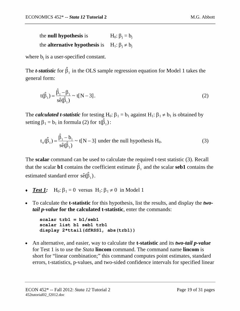
the null hypothesis is H0: βj = bj
the alternative hypothesis is H1: βj ≠ bj where bj is a user-specified constant. The t-statistic for in the OLS sample regression equation for Model 1 takes the general form:
1β
]3N[t~)ˆ(es
ˆ)ˆ(t
1
111 −
ββ−β
=β . (2)
The calculated t-statistic for testing H0: β1 = b1 against H1: β1 ≠ b1 is obtained by setting β1 = b1 in formula (2) for : )ˆ(t 1β
]3N[t~)ˆ(es
bˆ)ˆ(t
1
1110 −
β−β
=β under the null hypothesis H0. (3)
The scalar command can be used to calculate the required t-test statistic (3). Recall that the scalar b1 contains the coefficient estimate and the scalar seb1 contains the estimated standard error .
1β
)ˆ(es 1β
Test 1: H0: β1 = 0 versus H1: β1 ≠ 0 in Model 1
♦
•
•
To calculate the t-statistic for this hypothesis, list the results, and display the two-tail p-value for the calculated t-statistic, enter the commands:
scalar trb1 = b1/seb1 scalar list b1 seb1 trb1 display 2*ttail(dfRSS1, abs(trb1))
An alternative, and easier, way to calculate the t-statistic and its two-tail p-value for Test 1 is to use the Stata lincom command. The command name lincom is short for “linear combination;” this command computes point estimates, standard errors, t-statistics, p-values, and two-sided confidence intervals for specified linear
ECON 452* -- Fall 2012: Stata 12 Tutorial 2 Page 19 of 31 pages 452tutorial02_f2012.doc
ECONOMICS 452* -- Stata 12 Tutorial 2 M.G. Abbott
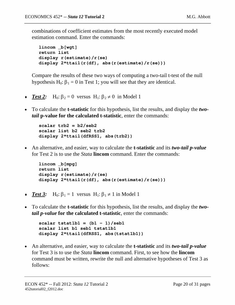
combinations of coefficient estimates from the most recently executed model estimation command. Enter the commands:
lincom _b[wgt] return list display r(estimate)/r(se) display 2*ttail(r(df), abs(r(estimate)/r(se)))
Compare the results of these two ways of computing a two-tail t-test of the null hypothesis H0: β1 = 0 in Test 1; you will see that they are identical.
♦ Test 2: H0: β2 = 0 versus H1: β2 ≠ 0 in Model 1 •
•
♦
To calculate the t-statistic for this hypothesis, list the results, and display the two-tail p-value for the calculated t-statistic, enter the commands:
scalar trb2 = b2/seb2 scalar list b2 seb2 trb2 display 2*ttail(dfRSS1, abs(trb2))
An alternative, and easier, way to calculate the t-statistic and its two-tail p-value for Test 2 is to use the Stata lincom command. Enter the commands:
lincom _b[mpg] return list display r(estimate)/r(se) display 2*ttail(r(df), abs(r(estimate)/r(se)))
Test 3: H0: β1 = 1 versus H1: β1 ≠ 1 in Model 1
•
•
To calculate the t-statistic for this hypothesis, list the results, and display the two-tail p-value for the calculated t-statistic, enter the commands:
scalar tstat1b1 = (b1 - 1)/seb1 scalar list b1 seb1 tstat1b1 display 2*ttail(dfRSS1, abs(tstat1b1))
An alternative, and easier, way to calculate the t-statistic and its two-tail p-value for Test 3 is to use the Stata lincom command. First, to see how the lincom command must be written, rewrite the null and alternative hypotheses of Test 3 as follows:
ECON 452* -- Fall 2012: Stata 12 Tutorial 2 Page 20 of 31 pages 452tutorial02_f2012.doc
ECONOMICS 452* -- Stata 12 Tutorial 2 M.G. Abbott
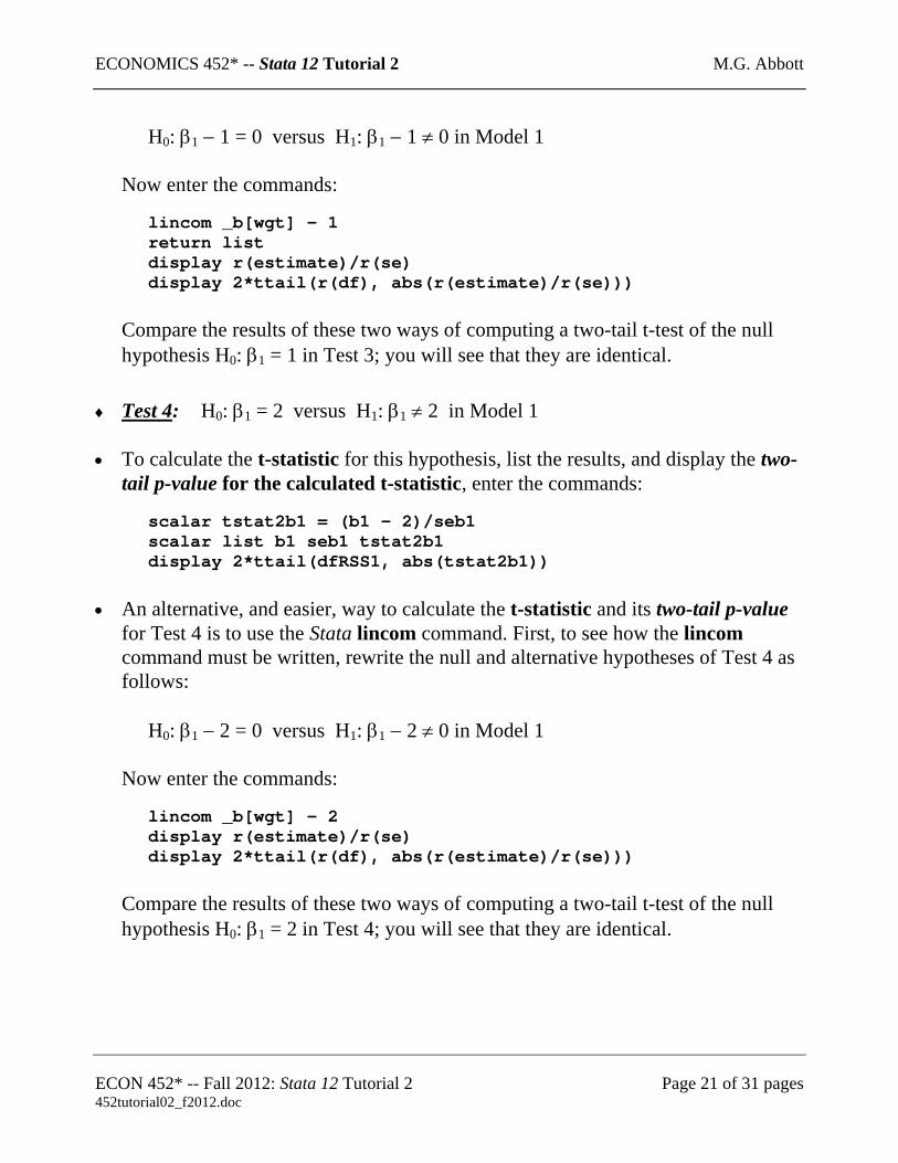
H0: β1 − 1 = 0 versus H1: β1 − 1 ≠ 0 in Model 1
Now enter the commands:
lincom _b[wgt] - 1 return list display r(estimate)/r(se) display 2*ttail(r(df), abs(r(estimate)/r(se)))
Compare the results of these two ways of computing a two-tail t-test of the null hypothesis H0: β1 = 1 in Test 3; you will see that they are identical.
♦ Test 4: H0: β1 = 2 versus H1: β1 ≠ 2 in Model 1
•
•
To calculate the t-statistic for this hypothesis, list the results, and display the two-tail p-value for the calculated t-statistic, enter the commands:
scalar tstat2b1 = (b1 - 2)/seb1 scalar list b1 seb1 tstat2b1 display 2*ttail(dfRSS1, abs(tstat2b1))
An alternative, and easier, way to calculate the t-statistic and its two-tail p-value for Test 4 is to use the Stata lincom command. First, to see how the lincom command must be written, rewrite the null and alternative hypotheses of Test 4 as follows:
H0: β1 − 2 = 0 versus H1: β1 − 2 ≠ 0 in Model 1
Now enter the commands:
lincom _b[wgt] - 2 display r(estimate)/r(se) display 2*ttail(r(df), abs(r(estimate)/r(se)))
Compare the results of these two ways of computing a two-tail t-test of the null hypothesis H0: β1 = 2 in Test 4; you will see that they are identical.
ECON 452* -- Fall 2012: Stata 12 Tutorial 2 Page 21 of 31 pages 452tutorial02_f2012.doc
ECONOMICS 452* -- Stata 12 Tutorial 2 M.G. Abbott
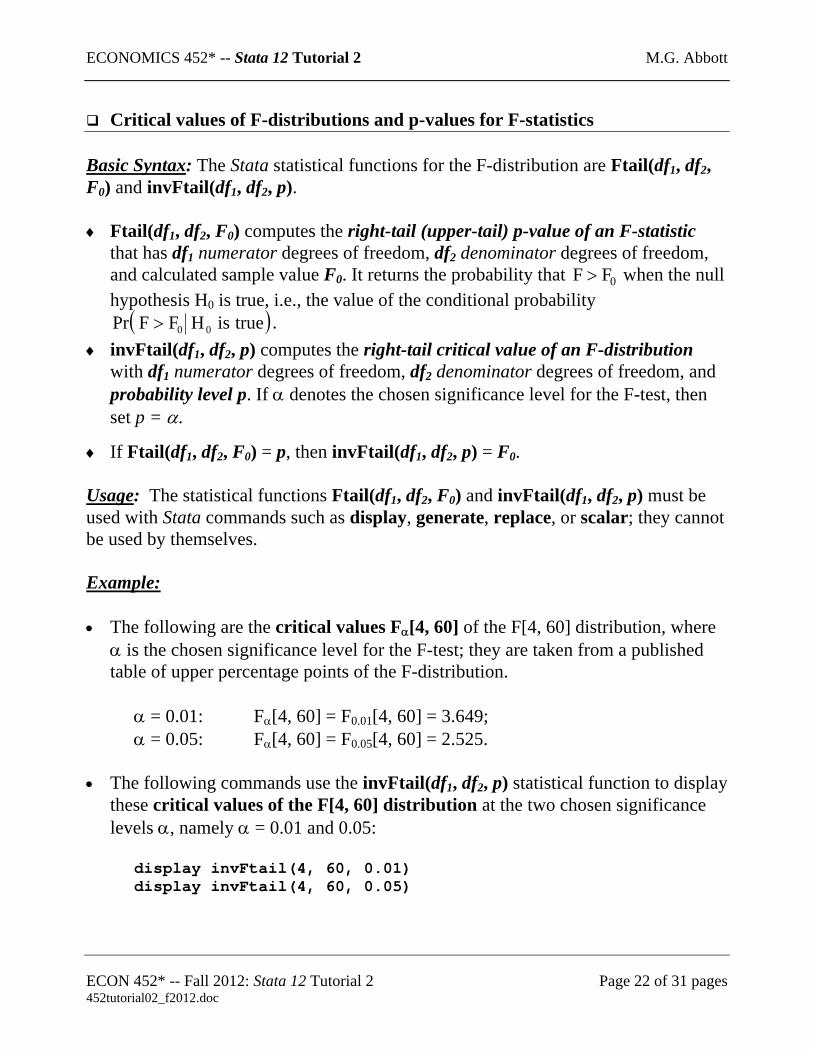
Critical values of F-distributions and p-values for F-statistics Basic Syntax: The Stata statistical functions for the F-distribution are Ftail(df1, df2, F0) and invFtail(df1, df2, p). ♦ Ftail(df1, df2, F0) computes the right-tail (upper-tail) p-value of an F-statistic
that has df1 numerator degrees of freedom, df2 denominator degrees of freedom, and calculated sample value F0. It returns the probability that when the null hypothesis H
0FF >0 is true, i.e., the value of the conditional probability
( )trueisHFFPr 00> . ♦ invFtail(df1, df2, p) computes the right-tail critical value of an F-distribution
with df1 numerator degrees of freedom, df2 denominator degrees of freedom, and probability level p. If α denotes the chosen significance level for the F-test, then set p = α.
♦ If Ftail(df1, df2, F0) = p, then invFtail(df1, df2, p) = F0. Usage: The statistical functions Ftail(df1, df2, F0) and invFtail(df1, df2, p) must be used with Stata commands such as display, generate, replace, or scalar; they cannot be used by themselves. Example: •
•
The following are the critical values Fα[4, 60] of the F[4, 60] distribution, where α is the chosen significance level for the F-test; they are taken from a published table of upper percentage points of the F-distribution.
α = 0.01: Fα[4, 60] = F0.01[4, 60] = 3.649; α = 0.05: Fα[4, 60] = F0.05[4, 60] = 2.525.
The following commands use the invFtail(df1, df2, p) statistical function to display these critical values of the F[4, 60] distribution at the two chosen significance levels α, namely α = 0.01 and 0.05:
display invFtail(4, 60, 0.01) display invFtail(4, 60, 0.05)
ECON 452* -- Fall 2012: Stata 12 Tutorial 2 Page 22 of 31 pages 452tutorial02_f2012.doc
ECONOMICS 452* -- Stata 12 Tutorial 2 M.G. Abbott
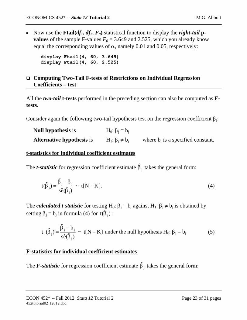
• Now use the Ftail(df1, df2, F0) statistical function to display the right-tail p-values of the sample F-values F0 = 3.649 and 2.525, which you already know equal the corresponding values of α, namely 0.01 and 0.05, respectively:
display Ftail(4, 60, 3.649) display Ftail(4, 60, 2.525)
Computing Two-Tail F-tests of Restrictions on Individual Regression
Coefficients – test All the two-tail t-tests performed in the preceding section can also be computed as F-tests. Consider again the following two-tail hypothesis test on the regression coefficient βj:
Null hypothesis is H0: βj = bj
Alternative hypothesis is H1: βj ≠ bj where bj is a specified constant. t-statistics for individual coefficient estimates The t-statistic for regression coefficient estimate takes the general form: jβ
]KN[t~)ˆ(es
ˆ)ˆ(t
j
jjj −
β
β−β=β . (4)
The calculated t-statistic for testing H0: βj = bj against H1: βj ≠ bj is obtained by setting βj = bj in formula (4) for : )ˆ(t jβ
]KN[t~)ˆ(es
bˆ)ˆ(t
j
jjj0 −
β
−β=β under the null hypothesis H0: βj = bj (5)
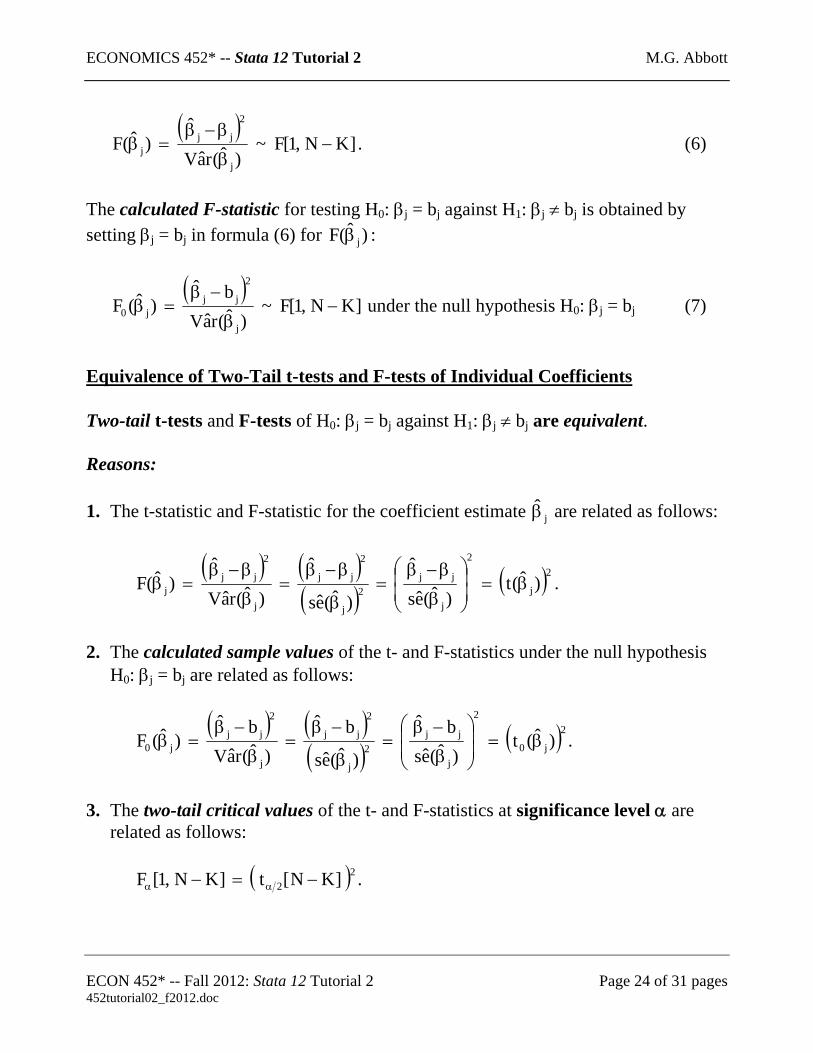
F-statistics for individual coefficient estimates The F-statistic for regression coefficient estimate takes the general form: jβ
ECON 452* -- Fall 2012: Stata 12 Tutorial 2 Page 23 of 31 pages 452tutorial02_f2012.doc
ECONOMICS 452* -- Stata 12 Tutorial 2 M.G. Abbott
( )]KN,1[F~
)ˆ(raV
ˆ)ˆ(F
j
2
jjj −
β
β−β=β . (6)
The calculated F-statistic for testing H0: βj = bj against H1: βj ≠ bj is obtained by setting βj = bj in formula (6) for : )ˆ(F jβ
( )]KN,1[F~
)ˆ(raVbˆ
)ˆ(Fj
2
jjj0 −
β
−β=β under the null hypothesis H0: βj = bj (7)
Equivalence of Two-Tail t-tests and F-tests of Individual Coefficients Two-tail t-tests and F-tests of H0: βj = bj against H1: βj ≠ bj are equivalent. Reasons: 1. The t-statistic and F-statistic for the coefficient estimate are related as follows: jβ
( ) ( )
( ) ( )2j
2
j
jj2
j
2
jj
j
2
jjj )ˆ(t
)ˆ(es
ˆ
)ˆ(es
ˆ
)ˆ(raV
ˆ)ˆ(F β=⎟
⎟⎠
⎞⎜⎜⎝
⎛
β
β−β=
β
β−β=
β
β−β=β .
2. The calculated sample values of the t- and F-statistics under the null hypothesis
H0: βj = bj are related as follows:
( ) ( )( ) ( )2j0
2
j
jj2
j
2
jj
j
2
jjj0 )ˆ(t
)ˆ(esbˆ
)ˆ(es
bˆ
)ˆ(raVbˆ
)ˆ(F β=⎟⎟⎠
⎞⎜⎜⎝
⎛
β
−β=
β
−β=
β
−β=β .
3. The two-tail critical values of the t- and F-statistics at significance level α are
related as follows:
( )22 ]KN[t]KN,1[F −=− αα .
ECON 452* -- Fall 2012: Stata 12 Tutorial 2 Page 24 of 31 pages 452tutorial02_f2012.doc
ECONOMICS 452* -- Stata 12 Tutorial 2 M.G. Abbott
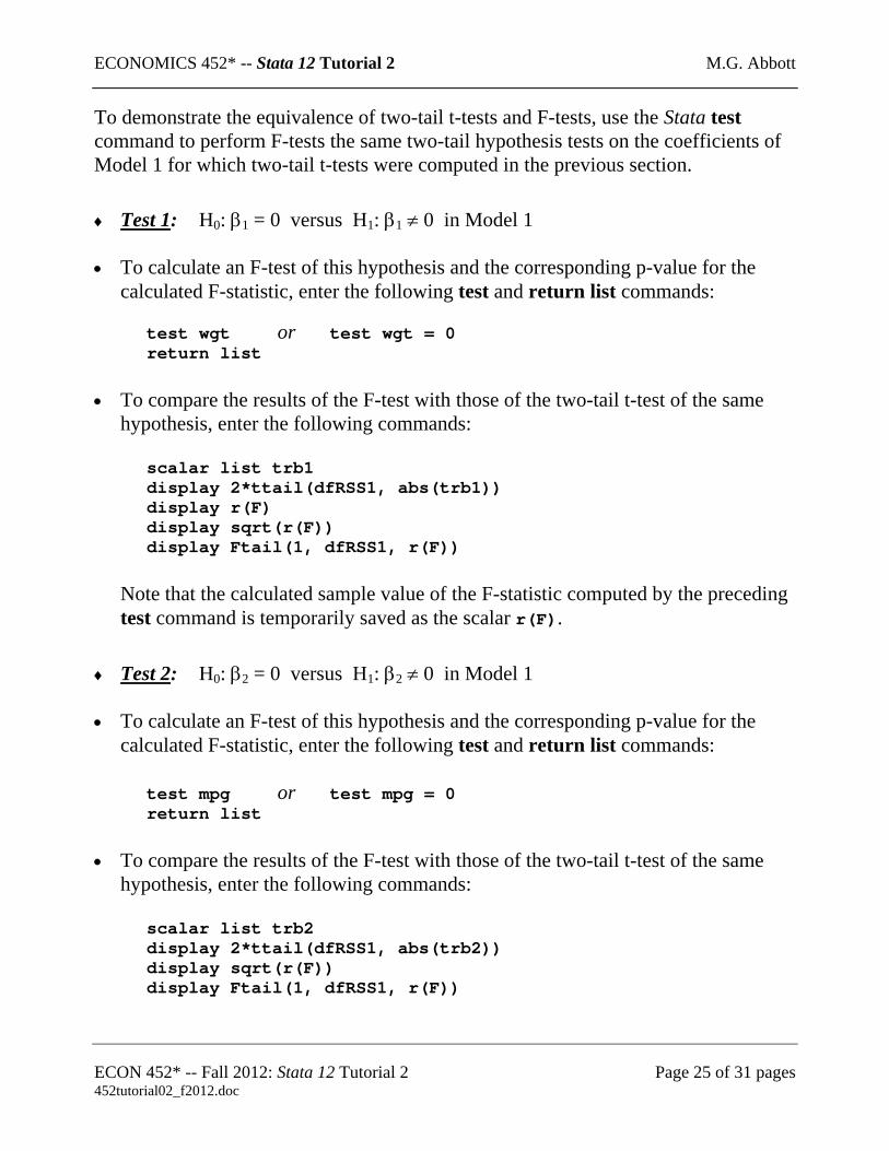
To demonstrate the equivalence of two-tail t-tests and F-tests, use the Stata test command to perform F-tests the same two-tail hypothesis tests on the coefficients of Model 1 for which two-tail t-tests were computed in the previous section.
♦ Test 1: H0: β1 = 0 versus H1: β1 ≠ 0 in Model 1
•
•
♦
To calculate an F-test of this hypothesis and the corresponding p-value for the calculated F-statistic, enter the following test and return list commands:
test wgt or test wgt = 0 return list
To compare the results of the F-test with those of the two-tail t-test of the same hypothesis, enter the following commands:
scalar list trb1 display 2*ttail(dfRSS1, abs(trb1)) display r(F) display sqrt(r(F)) display Ftail(1, dfRSS1, r(F))
Note that the calculated sample value of the F-statistic computed by the preceding test command is temporarily saved as the scalar r(F).
Test 2: H0: β2 = 0 versus H1: β2 ≠ 0 in Model 1
•
•
To calculate an F-test of this hypothesis and the corresponding p-value for the calculated F-statistic, enter the following test and return list commands:
test mpg or test mpg = 0 return list
To compare the results of the F-test with those of the two-tail t-test of the same hypothesis, enter the following commands:
scalar list trb2 display 2*ttail(dfRSS1, abs(trb2)) display sqrt(r(F)) display Ftail(1, dfRSS1, r(F))
ECON 452* -- Fall 2012: Stata 12 Tutorial 2 Page 25 of 31 pages 452tutorial02_f2012.doc
ECONOMICS 452* -- Stata 12 Tutorial 2 M.G. Abbott
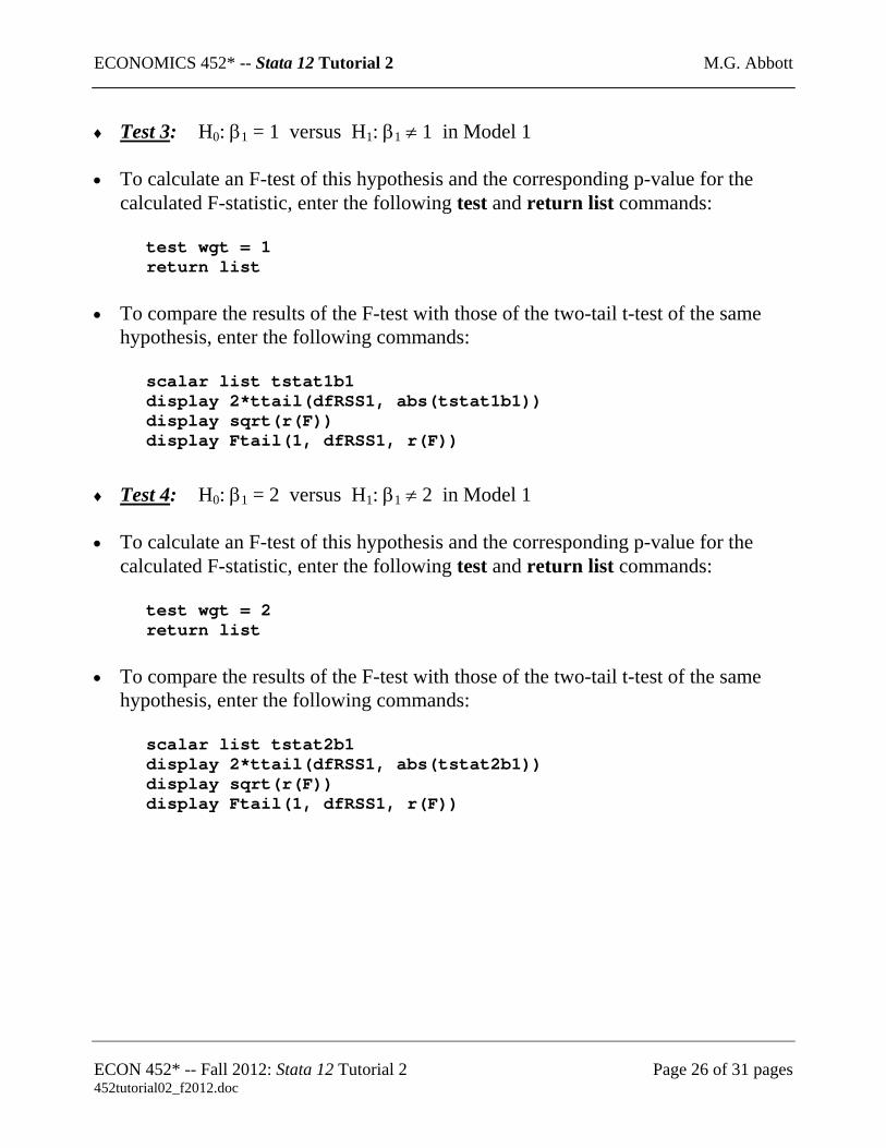
♦ Test 3: H0: β1 = 1 versus H1: β1 ≠ 1 in Model 1
•
•
♦
To calculate an F-test of this hypothesis and the corresponding p-value for the calculated F-statistic, enter the following test and return list commands:
test wgt = 1 return list
To compare the results of the F-test with those of the two-tail t-test of the same hypothesis, enter the following commands:
scalar list tstat1b1 display 2*ttail(dfRSS1, abs(tstat1b1)) display sqrt(r(F)) display Ftail(1, dfRSS1, r(F))
Test 4: H0: β1 = 2 versus H1: β1 ≠ 2 in Model 1
•
•
To calculate an F-test of this hypothesis and the corresponding p-value for the calculated F-statistic, enter the following test and return list commands:
test wgt = 2 return list
To compare the results of the F-test with those of the two-tail t-test of the same hypothesis, enter the following commands:
scalar list tstat2b1 display 2*ttail(dfRSS1, abs(tstat2b1)) display sqrt(r(F)) display Ftail(1, dfRSS1, r(F))
ECON 452* -- Fall 2012: Stata 12 Tutorial 2 Page 26 of 31 pages 452tutorial02_f2012.doc
ECONOMICS 452* -- Stata 12 Tutorial 2 M.G. Abbott
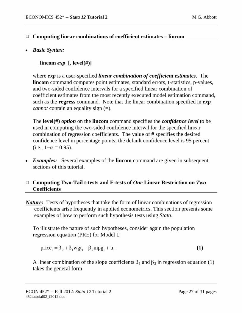
Computing linear combinations of coefficient estimates – lincom
• Basic Syntax:
lincom exp [, level(#)]
where exp is a user-specified linear combination of coefficient estimates. The lincom command computes point estimates, standard errors, t-statistics, p-values, and two-sided confidence intervals for a specified linear combination of coefficient estimates from the most recently executed model estimation command, such as the regress command. Note that the linear combination specified in exp cannot contain an equality sign (=). The level(#) option on the lincom command specifies the confidence level to be used in computing the two-sided confidence interval for the specified linear combination of regression coefficients. The value of # specifies the desired confidence level in percentage points; the default confidence level is 95 percent (i.e., 1−α = 0.95).
• Examples: Several examples of the lincom command are given in subsequent
sections of this tutorial.
Computing Two-Tail t-tests and F-tests of One Linear Restriction on Two Coefficients
Nature: Tests of hypotheses that take the form of linear combinations of regression
coefficients arise frequently in applied econometrics. This section presents some examples of how to perform such hypothesis tests using Stata.
To illustrate the nature of such hypotheses, consider again the population regression equation (PRE) for Model 1:
ii2i10i umpgwgtprice +β+β+β= . (1) A linear combination of the slope coefficients β1 and β2 in regression equation (1) takes the general form
ECON 452* -- Fall 2012: Stata 12 Tutorial 2 Page 27 of 31 pages 452tutorial02_f2012.doc
ECONOMICS 452* -- Stata 12 Tutorial 2 M.G. Abbott
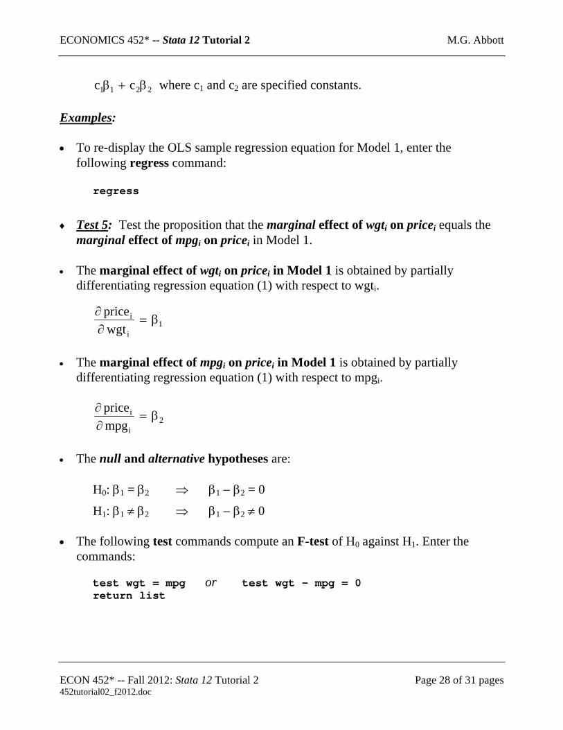
2211 cc β+β where c1 and c2 are specified constants. Examples: •
♦
To re-display the OLS sample regression equation for Model 1, enter the following regress command:
regress
Test 5: Test the proposition that the marginal effect of wgti on pricei equals the marginal effect of mpgi on pricei in Model 1.
• The marginal effect of wgti on pricei in Model 1 is obtained by partially
differentiating regression equation (1) with respect to wgti.
1i
i
wgtprice
β=∂∂
• The marginal effect of mpgi on pricei in Model 1 is obtained by partially
differentiating regression equation (1) with respect to mpgi.
2i
i
mpgprice
β=∂∂
• The null and alternative hypotheses are:
H0: β1 = β2 ⇒ β1 − β2 = 0
H1: β1 ≠ β2 ⇒ β1 − β2 ≠ 0 The following test commands compute an F-test of H0 against H1. Enter the commands:
test wgt = mpg or test wgt - mpg = 0 return list
•
ECON 452* -- Fall 2012: Stata 12 Tutorial 2 Page 28 of 31 pages 452tutorial02_f2012.doc
ECONOMICS 452* -- Stata 12 Tutorial 2 M.G. Abbott
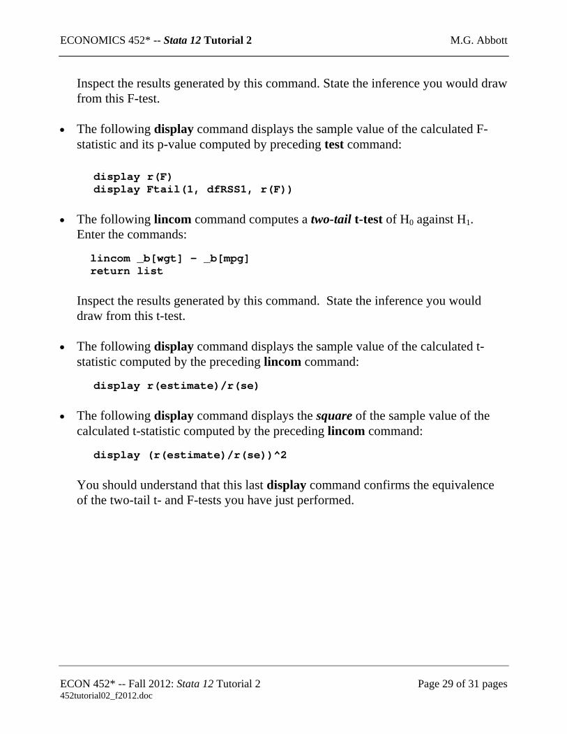
Inspect the results generated by this command. State the inference you would draw from this F-test.
•
•
•
•
The following display command displays the sample value of the calculated F-statistic and its p-value computed by preceding test command:
display r(F) display Ftail(1, dfRSS1, r(F))
The following lincom command computes a two-tail t-test of H0 against H1. Enter the commands:
lincom _b[wgt] - _b[mpg] return list
Inspect the results generated by this command. State the inference you would draw from this t-test.
The following display command displays the sample value of the calculated t-statistic computed by the preceding lincom command:
display r(estimate)/r(se)
The following display command displays the square of the sample value of the calculated t-statistic computed by the preceding lincom command:
display (r(estimate)/r(se))^2
You should understand that this last display command confirms the equivalence of the two-tail t- and F-tests you have just performed.
ECON 452* -- Fall 2012: Stata 12 Tutorial 2 Page 29 of 31 pages 452tutorial02_f2012.doc
ECONOMICS 452* -- Stata 12 Tutorial 2 M.G. Abbott
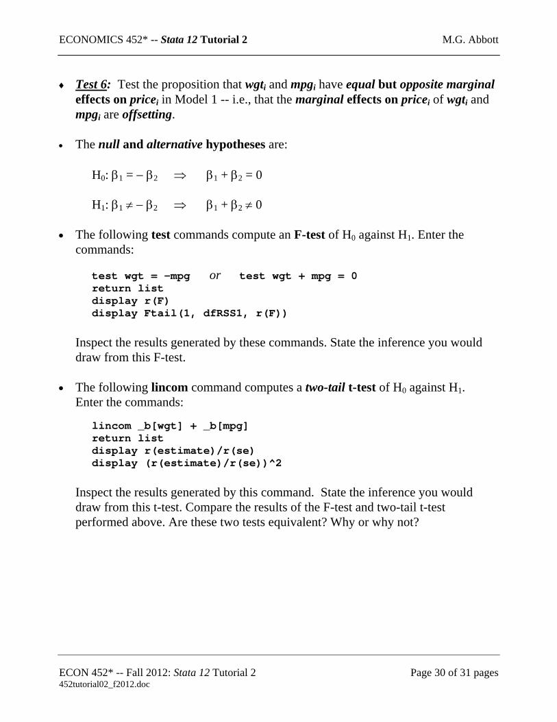
♦ Test 6: Test the proposition that wgti and mpgi have equal but opposite marginal effects on pricei in Model 1 -- i.e., that the marginal effects on pricei of wgti and mpgi are offsetting.
• The null and alternative hypotheses are:
H0: β1 = − β2 ⇒ β1 + β2 = 0
H1: β1 ≠ − β2 ⇒ β1 + β2 ≠ 0
The following test commands compute an F-test of H0 against H1. Enter the commands: test wgt = -mpg or test wgt + mpg = 0
return list display r(F) display Ftail(1, dfRSS1, r(F))
Inspect the results generated by these commands. State the inference you would draw from this F-test.
•
• The following lincom command computes a two-tail t-test of H0 against H1. Enter the commands:
lincom _b[wgt] + _b[mpg] return list display r(estimate)/r(se) display (r(estimate)/r(se))^2
Inspect the results generated by this command. State the inference you would draw from this t-test. Compare the results of the F-test and two-tail t-test performed above. Are these two tests equivalent? Why or why not?
ECON 452* -- Fall 2012: Stata 12 Tutorial 2 Page 30 of 31 pages 452tutorial02_f2012.doc
ECONOMICS 452* -- Stata 12 Tutorial 2 M.G. Abbott
Preparing to End Your Stata Session Before you end your Stata session, you should do two things.
• First, you may want to save the current data set. Enter the following save
command with the replace option to save the current data set as Stata-format data set auto2.dta and overwrite any dataset of the same name:
save auto2, replace
• Second, close the log file you have been recording. Enter the command:
log close Alternatively, you could have closed the log file by: • clicking on the Log button in the Stata button bar; • clicking on Close log file in the Stata Log Options dialog box; • clicking the OK button.
End Your Stata Session – exit
• To end your Stata session, use the exit command. Enter the command:
exit or exit, clear
Cleaning Up and Clearing Out
After returning to Windows, you should copy all the files you have used and created during your Stata session to your own portable electronic storage device such as a flash memory stick. These files will be found in the Stata working directory, which is usually C:\data on the computers in Dunning 350. There is one file you will want to be sure you have: the Stata log file 452tutorial2.log. If you saved the Stata-format data set auto2.dta, you will want to take it with you as well. Use the Windows copy command to copy any files you want to keep to your own portable storage device (e.g., a flash memory stick). Finally, as a courtesy to other users of the computing classroom, please delete all the files you have used or created from the Stata working directory.
ECON 452* -- Fall 2012: Stata 12 Tutorial 2 Page 31 of 31 pages 452tutorial02_f2012.doc
Related Documents