Assessment of Aircraft Flight Controllers Using Nonlinear Robustness Analysis Techniques and Simulation http://www.aem.umn.edu/ ∼ AerospaceControl Gary J. Balas and Peter Seiler Aerospace Engineering and Mechanics University of Minnesota Andrew Packard Department of Mechanical Engineering University of California, Berkeley 28 January 2010

Assessment of Aircraft Flight Controllers Using Nonlinear Robustness Analysis Techniques and Simulation
Jul 29, 2015
Welcome message from author
This document is posted to help you gain knowledge. Please leave a comment to let me know what you think about it! Share it to your friends and learn new things together.
Transcript

Assessment of Aircraft Flight Controllers UsingNonlinear Robustness Analysis Techniques and
Simulation
http://www.aem.umn.edu/∼ AerospaceControl
Gary J. Balas and Peter SeilerAerospace Engineering and Mechanics
University of Minnesota
Andrew PackardDepartment of Mechanical Engineering
University of California, Berkeley
28 January 2010
Acknowledgments
� Dr. Ufuk Topcu, Control and Dynamical Systems, Caltech� Members of Berkeley Center for Control and Identification
� Ryan Feeley, Evan Haas, George Hines, ZacharyJarvis-Wloszek, Erin Summers, Kunpeng Sun, Weehong Tan,and Timothy Wheeler
� University of Minnesota Aerospace Controls Group� Abhijit Chakraborty and Qian Zheng
� Air Force Office of Scientific Research (AFOSR) for the grant #FA9550-05-1-0266 (Development of Analysis Tools forCertification of Flight Control Laws) 05/01/05 - 04/30/08
� NASA NRA Grant/Cooperative Agreement NNX08AC80A,“Analytical Validation Tools for Safety Critical Systems,” Dr.Christine Belcastro, Technical Monitor, 01/01/2008 -12/31/2010
� Software: http://www.aem.umn.edu/∼ AerospaceControl
2/51

Motivation: Flight Controls
� Validation of flight controls mainly relies on linear analysistools and nonlinear (Monte Carlo) simulations.
� This approach generally works well but there are drawbacks:� It is time consuming and requires many well-trained engineers.� Linear analyses are valid over an infinitesimally small region of
the state space.� Linear analyses are not sufficient to understand truly nonlinear
phenomenon, e.g. the falling leaf mode in the F/18 Hornet.� Linear analyses are not applicable for adaptive control laws or
systems with hard nonlinearities.� There is a need for nonlinear analysis tools which provide
quantitative performance/stability assessments over aprovable region of the state space.
3/51

Our Perspective
Linear analysis: provides a quick answer to a related, but differentquestion:
� Q: How much gain and time-delay variation can beaccommodated without undue performance degradation?
� A: (answers a different question) Here’s a scatter plot ofmargins at 1000 trim conditions throughout envelope.
Why does linear analysis have impact in nonlinear problems?
� Domain-specific expertise exists to interpret linear analysisand assess relevance.
� Speed, scalable: Fast, defensible answers on high-dimensionalsystems.
Extend validity of the linearized analysis
� Infinitesimal → local (with certified estimates)
� Address uncertainty
4/51

Overiew
Numerical tools to quantify/certify dynamic behavior� Locally, near equilibrium points
Analysis considered� Region-of-attraction, input/output gain, reachability,
establishing local IQCs
Methodology� Enforce Lyapunov/Dissipation inequalities locally, on sublevel
sets� Set containments via S-procedure and SOS constraints
� Bilinear semi-definite programs� “Always” feasible� Simulation aids nonconvex proof/certificate search
� Address model uncertainty� Parametric Uncertainty
� Parameter-independent Lyapunov/Storage functions� Branch-&-Bound
� Dynamic Uncertainty� Local small-gain theorems
5/51

Tools for quantitative nonlinear robustness/performanceanalysis
Quantify with certificate
............................. Internal
Regions-of-attraction
Input-output
Reachable sets,Local gains
Nominalsystem
x = f(x)z� x = f(x,w)
z = h(x)�w
Parametricuncertainty
x = f(x, δ)z� x = f(x,w, δ)
z = h(x, δ)�w
Unmodeleddynamics
y u
� Φ
x = f(x, u)y = g(x)
� y uz � � w
� Φ
x = f(x,w, u)z = h(x)y = g(x)
�
6/51

Nonlinear Analysis
Autonomous dynamics: x = f(x), f(x) = 0
� Equilibrium point
� Uncertain initial condition, x(0) = G� Question: Do all solutions converge to x?
Drive dynamics: x = f(x,w), f(x, 0) = 0
� Equilibrium point
� Uncertain inputs, ||w||2 ≤ R, ||w||∞ ≤ σ
� Question: How large can z = h(x) get?
Uncertain dynamics: x = f(x, δ), or x = f(x,w, δ)
� Unknown, constant parameters, δ ∈ Δ
� Unmodeled dynamics
� Same questions . . ..
7/51

Region-of-Attraction and Reachability
Dynamics, equilibrium point
x = f(x), f(x) = 0
p : Analyst-defined functionwhose (well-understood)sub-level sets are to bein region-of-attraction.{x : p(x) β} , ROAN
By choice of positive-definite V ,maximize β so that
{x : p(x) ≤ β} ⊆ {x : V (x) ≤ 1}{x : V (x) ≤ 1} is bounded{x : x �= x, V (x) ≤ 1}
⊆{x :
dV
dxf(x) < 0
}
Given a differential equation x = f(x,w) and a positive definite function p,how large can e(t) get, knowing x(0) = 0, ||w||2 ≤ R?
x = f(x,w), e = p(x)
Conditions on Rn+nw
dV
dxf(x,w) ≤ wTw on
{x : V (x) ≤ R2} , all w
{x : V (x) ≤ R2} ⊆ {x : p(x) ≤ β}
Conclusion on ODE
x(0)0, ||w||2 ≤ R ⇒ for allt, solution exists and e(t) ≤ β 8/51

Solution Approach
1. Sum-of-squares to (conservatively) enforce nonnegativity.
f ∈ Σ if f = ΣG2i for some gi
2. Easy (semi-definite program) to check if a given polynomial is SOS3. S-procedure to (conservatively) enforce set containment4. Apply S-procedure to Analysis conditions. For (e.g.) reachability,
minimize β (by choice of si and V ) such that
(β − p)− s1(R2 − V ) ∈ Σx,w
−((R2 − V )s2 +
dV
dxf(x,w)− wTw
)∈ Σx,w
5. Semi-definite program iteration: Initialize V , then5.1 Optimize objective by changing S-procedure multipliers5.2 Optimize objective by changing V5.3 Iterate on (5.1) and (5.2)
6. Initialization of V is important for the iteration to work6.1 Simulation of system dynamics yields convex constraints which
contain all feasible Lyapunov function candidates. This set canbe sampled to initialize V .
9/51

Applications
� Region of attractions and reachability analysis for GTMaircraft longitudinal axis dynamics
� Region of attraction for F/A-18 falling leaf mode
10/51

NASA Generic Transport Model (GTM) AircraftNASA constructed the remote-controlled GTM aircraft forstudying advanced safety technologies.
� The GTM is a 5.5 percent scale commercial aircraft.� NASA created a high-fidelity 6DOF model of the GTM
including look-up tables for the aerodynamic coefficients.
References:
Jordan, T., Foster, J.V., Bailey, R.M, and Belcastro, C.M., AirSTAR: A UAV platform for flight dynamics andcontrol system testing. 25th AIAA Aerodynamic Measurement Technology and Ground Testing Conf.,AIAA-2006-3307 (2006).
Cox, D., The GTM DesignSim v0905.
11/51

Aircraft Longitudinal Axis Dynamics
The aircraft longitudinal axis dynamics are described by:
V = −D
m+mg sin (θ − α)− T cosα
α = − L
mV+mg cos (θ − α)− T sinα+ q
q =M
Iyy
θ = q
States: air speed V (ft/sec), angle of attack α (deg), pitch rate q(deg/sec) and pitch angle θ (deg).
Controls: elevator deflection δelev (deg) and engine thrust T (lbs).
Forces/Moment: drag force D (lbs), lift force L (lbs), andpitching moment M (lbs-ft).
12/51

Model ParametersThe forces/moment are given by:
D = qSCD(α, δelev)
L = qSCL(α, δelev)
M = qScCm(α, δelev, q)
where q = 12ρV
2 is dynamic pressure, q = c2V q normalized pitch
rate, S wing area, and c mean aerodynamic chord.
Table: Aircraft Parameters∗
Wing Area, S 0.5483 m2
Mean Aerodynamic Chord, c 0.2790 mMass, m 22.50 kg
Pitch Axis Moment of Inertia, Iyy 5.768 kg-m2
Air Density, ρ 1.224 kg/m3
Gravity Constant, g 9.810 m/sec2
∗ A. Chakraborty, P. Seiler and G.J. Balas, “Nonlinear Region of AttractionAnalysis for Flight Control Verification and Validation,” submitted to ControlEngineering Practice, January, 2010.
13/51

GTM Polynomial Modeling
� Aerodynamic look-up table data, engine data, trigonometricfunctions, and 1/V with low-order polynomials were fit.
� Resulting model is a 7th order polynomial.� Two facts for obtaining accurate models:
� The raw aerodynamic data is provided in body-axes but betterfits can be obtained in wind axes.
� Matching the trim characteristics requires very accurate fits atlow angles of attack.
14/51

GTM Polynomial Modeling cont’d
0−10 20 40 60 80 90−0.5
0
0.5
1
1.4
α (deg)
CL,
α
Raw DataPoly Fit
0−10 20 40 60 80 900
0.5
1
1.5
2
α (deg)
CD
,α
Raw DataPoly Fit
0−10 9020 40 60 80−1.5
−1
−0.5
0
0.5
α (deg)
Cm
,α
Raw DataPoly Fit
15/51

Trim ConditionsComputed the level-flight trim conditions for the nonlinear(look-up tables, etc.) and polynomial models.
30 35 40 45 50 55 600
5
10α
(deg
) Original ModelPoly Model
30 35 40 45 50 55 6010
20
30
δth
(per
cent
)
30 35 40 45 50 55 60−2
024
V (m/sec)
δel
ev (d
eg)
16/51

Open-loop Short Period ModelShort period model analytically linearized about trim condition.
� Linear, nonlinear phase plane have stable spiral characteristics.� Qualitative similarity implies nonlinearities are not significant,
linear analyses valid over a wide range of flight conditions.
−40 −20 0 20 40 60
−100
−50
0
50
100
alpha (deg)
q (d
eg/s
)
Nonlinear (solid) and linear (dashed) phase plane simulation for polynomial
GTM short period model.
17/51

Pitch Rate Damping Derivative, Cm,q
Cm,q is look-up table data on a grid of α. The polynomiallongitudinal model a linear fit.
� To demonstrate the effects of nonlinearities consider thefollowing cubic pitch rate damping function:
Cm,q(α, q) = −41.25q + 5.318q3
18/51

Region of Attraction: Cubic Pitch Rate DampingLinearization predicts no change in the aircraft stability withinclusion of cubic rate damping term (Cm,q). Ellipsoidal estimatesof ROA computed using the V -s iteration.
� Solid ellipse p1(x) = xTN1x, x := [α− αt, q − qt] andN1 := diag(20 deg, 50 deg/s)−2.
� Dashed ellipse N2 := diag(10 deg, 50 deg/s)−2 decreases ellipse in the αas compared with q direction.
−40 −20 0 20 40 60
−100
−50
0
50
100
alpha (deg)
q (d
eg /
s)
ROA Lower Bound with Shape Matrix N
2
ROA Lower Boundwith Shape Matrix N
1
19/51

Reachable Sets
� For a nonlinear system x = f(x, u), the vector xf ∈ Rn isunit energy reachable if there exists a final time T and aninput u(t) defined on [0, T ] satisyfing ‖u‖2 ≤ 1 and thatdrives the state from x(0) = 0 to x(T ) = xf .
� The unit energy reachable set Rue is the set of points that arereachable from the origin with a unit energy.
� For linear systems this set is an ellipsoid that can be computed froma semidefinite programming problem. The size of the ellipsoid scaleswith the magnitude of the input energy.
� For nonlinear systems the this set can be difficult to compute andits size does not, in general, scale linearly with the magnitude of theinput energy.
� Our approach is to approximate nonlinear models with polynomials
and then estimate the size of this set with polynomial optmization
tools.
� Knowledge of the reachable set for an aircraft can be used fordynamic flight envelope assessment.
20/51

Computing Reachable Set Estimates
� We approximate the reachable set by an ellipsoid of the formRβ := {x : (x− xtrim)TN(x− xtrim) ≤ β} where Nreflects a scaling of the coordinates.
� Upper bounds: β(γ) := min‖u‖2≤γ β subject to Rue ⊆ Rβ
� For polynomial systems this computation takes the form of an
iteration involving polynomial (sum-of-squares) optimizations that
are converted into semidefinte programs.
� Lower bounds: β(γ) := max‖u‖2≤γ(x−xtrim)TN(x−xtrim).� One method is a power-method iteration [Tierno, et. al., 1997]� Another method is to simulate the nonlinear system with the exact
(scaled) worst-case input for the linearized system.
� The exact reachable set for the linearization can be computedand this can be used to compute the maximal value of(x− xtrim)TN(x− xtrim).
21/51
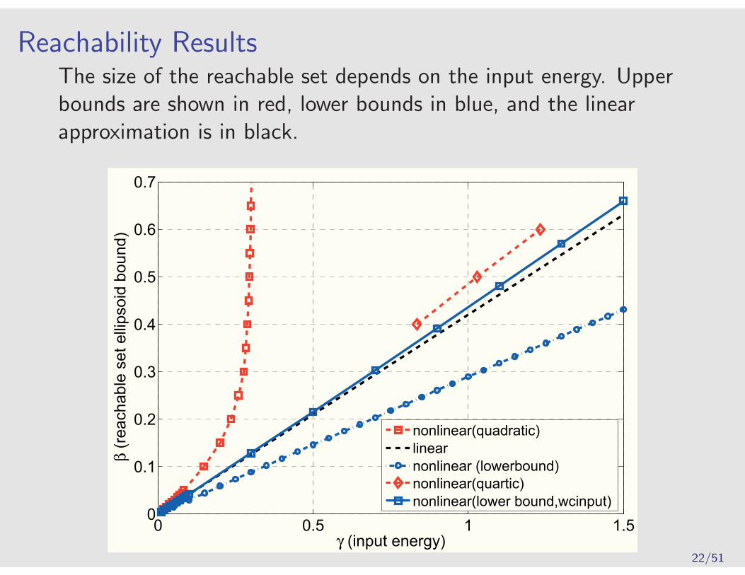
Reachability ResultsThe size of the reachable set depends on the input energy. Upperbounds are shown in red, lower bounds in blue, and the linearapproximation is in black.
0 0.5 1 1.50
0.1
0.2
0.3
0.4
0.5
0.6
0.7
γ (input energy)
β (r
each
able
set
elli
psoi
d bo
und)
nonlinear(quadratic)linearnonlinear (lowerbound)nonlinear(quartic)nonlinear(lower bound,wcinput)
22/51

Reachability ResultsTested the worse-case input signal for polynominal model(β = 0.48) on the full, nonlinear GTM model (β = .35).
0 50 100 15060
80
100
120
time (sec)
TAS
(kno
ts)
0 50 100 1502
3
4
time (sec)
alph
a (d
eg)
0 50 100 150−5
0
5
time (sec)
q (d
eg/s
ec)
0 50 100 150−10
0
10
20
time (sec)th
eta
(deg
)
0 50 100 15014.5
15
15.5
16
time (sec)
thro
ttle
(per
cent
)
0 50 100 1502
2.5
3
3.5
time (sec)
elev
(deg
)PolyGTM
23/51

4-State Longitudinal Axis GTM Analysis
Proportional pitch rate feedback is used to improve the damping ofthe GTM aircraft:
δelev = Kqq + δelev = 0.0698q + δelev
Region of attraction analysis is performed for the GTM aircraftaround the level flight condition at V = 45 m/s.
� Shape function is p(z) = zTNz
N := diag(20 m/s, 20 deg, 50 deg/s, 20 deg)−2
� p roughly scales each state by the maximum magnitudeobserved during the flight condition.
24/51
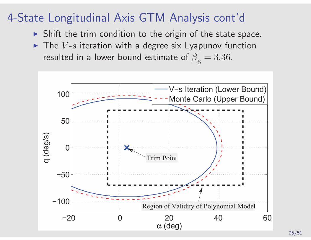
4-State Longitudinal Axis GTM Analysis cont’d� Shift the trim condition to the origin of the state space.� The V -s iteration with a degree six Lyapunov function
resulted in a lower bound estimate of β6= 3.36.
−20 0 20 40 60
−100
−50
0
50
100
α (deg)
q (d
eg/s
)
V−s Iteration (Lower Bound)Monte Carlo (Upper Bound)
Trim Point
Region of Validity of Polynomial Model
25/51

F/A-18 Out-of-Control Flight
� The US Navy has lost many F/A-18A/B/C/D Hornet aircraft due to anout-of-control flight (OCF) departurephenomenon described as ’falling leaf’ mode.
F/A-18 : NASA Dryden Photo
� The falling leaf mode is associated with sustained oscillatory OCF modethat can require 4.5K-6K meters altitude to recover∗.
∗ Heller, David and Holmberg, “Falling Leaf Motion Suppression in the F/A-18 Hornet with Revised Flight Control
Software,” AIAA-2004-542, 42nd AIAA Aerospace Sciences Meeting, Jan 2004, Reno, NV.
26/51

Analysis of F/A-18 Aircraft Flight Control Laws Motivation
� Administration action by the Naval AirSystems Command (NAVAIR) to preventaircraft losses due to falling leaf entry tofocused on
� aircrew training,� restrictions on angle-of-attack and� center-of-gravity location. F/A-18 Hornet: NASA Dryden Photo
� A solution to falling leaf mode entry was also pursued via modification ofthe baseline flight control law.
� The revised control law was tested and integrated into the F/A-18 E/FSuper Hornet aircraft.
27/51

Analysis of F/A-18 Aircraft Flight Control Laws Motivation
Flight Control Law Analysis Objectives∗:
� Identify the susceptibility of F/A-18 baseline and revised flightcontrol laws to entry in falling leaf mode.
� Identify limits on the F/A-18 aircraft angle-of-attack (α) andsideslip (β) to prevent falling leaf entry for both F/A-18 flightcontrol laws.
∗Chakraborty, Seiler, and Balas, “Applications of Linear and Nonlinear Robustness Analysis Techniques to the
F/A-18 Flight Control Laws,” AIAA Guidance, Navigation, and Control Conference, Chicago, IL, August 2009
28/51
Characteristics of Falling Leaf Mode
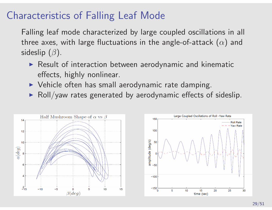
Falling leaf mode characterized by large coupled oscillations in allthree axes, with large fluctuations in the angle-of-attack (α) andsideslip (β).
� Result of interaction between aerodynamic and kinematiceffects, highly nonlinear.
� Vehicle often has small aerodynamic rate damping.� Roll/yaw rates generated by aerodynamic effects of sideslip.
29/51

Baseline/Revised Control Law Architecture (simplified)
30/51

Model Formulation
Computational burden and limitation of the nonlinear analysistechnique used in this analysis restricts the F/A-18 modeldescription :
� to be cubic degree polynomial function of the states.
� to have minimal state dimensions.
These limitations impose a challenge in formulating a cubicpolynomial description of the F/A-18 aircraft with fewer statedimensions and yet capture the characteristics of the falling leafmotion.
31/51

Model Approximation
������������ ����������
������������� ��������������������
��������������� ���������������������������
�������������������� ���������������������������
��� ����������������������
������!"���������"�������������
��������#�"������"�������������
!"��������������"��������
��#�"������������"�������
$�%&�'�%����!"���������"�������������
������'�%����!"���������"�������������
$�%&�'�%������#�"������"�������������
������'�%������#�"�����"�������������
������������ ����������
��������������� ����������
���������������� �������������!������� "�#����
!������� "�#�����������������
32/51
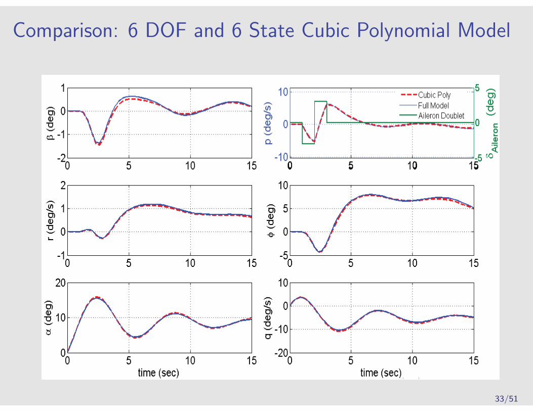
Comparison: 6 DOF and 6 State Cubic Polynomial Model
33/51

Modeling Summary
� The reduced order, nonlinear polynomial model captures thecharacteristics of the falling leaf motion.
� For analysis purpose, roll-coupled maneuvers are considerwhich drive the aircraft to the falling leaf motion.
� The velocity is assumed to be fixed at 250 ft/s.
x = f(x, u) , y = h(x)
x=
⎡⎢⎢⎢⎢⎢⎣
angle-of-attack(α)sideslip angle(β)
roll rate(p)yaw rate(r)pitch rate(q)bank angle(φ)
⎤⎥⎥⎥⎥⎥⎦
, y =
⎡⎢⎢⎢⎢⎢⎢⎢⎣
angle-of-attack(α)roll rate(p)yaw rate(r)pitch rate(q)
lateral acceleration(ay)
sideslip rate(β)sideslip angle(β)
⎤⎥⎥⎥⎥⎥⎥⎥⎦
u =
⎡⎣
aileron deflection(δail)rudder deflection(δrud)
stabilator deflection(δstab)
⎤⎦
34/51

Flight Control Law Analysis
We have presented a cubic degree nonlinear polynomial modelrepresentation of the F/A-18 aircraft. Now, both the baseline andthe revised flight control laws will be analyzed using the linear andnonlinear analysis techniques.
� The reduced order, nonlinear polynomial model will betrimmed at different equilibrium points.
� Linear robustness analyses will be performed around thoseequilibrium conditions for both the control laws.
� Similarly, V − s iteration procedure will be perfroemd toestimate the invariant ellipsoid of the region-of-attraction forboth the control laws.
35/51

Linear Analysis
� F/A-18 aircraft is trimmed at selected equilibrium points
� VT = 250 ft/s; Altitude = 25,000 feet; α = 26o .
� φ = [0o 25o 45o 60o ]
� β = [0o (Coordinated) 10o(Non-coordinated) ]
� Classical Loop-at-a-time Margin Analysis
� Disk Margin Analysis
� Multivariable Input Margin Analysis
� Diagonal Input Multiplicative Uncertainty Analysis
� Full Block Input Multiplicative Uncertainty Analysis
� Robustness Analysis with Uncertainty in AerodynamicCoefficients & Stability Derivatives
The linearized aircraft models do not exhibit the falling leaf modecharacteristics.
36/51

Linear Analysis (cont’d)
For classical margin analysis we consider the linearized plant at25,000 feet with φ = 60o, β = 10o
Classical Loop-at-a-time Margin Analysis
Input Channel Baseline Revised
Aileron Gain Margin ∞ 27 dB
Phase Margin 104o 93o
Delay Margin 0.81 sec 0.44 sec
Rudder Gain Margin 34 dB 34 dB
Phase Margin 82o 76o
Delay Margin 2.23 sec 1.99 sec
Stabilator Gain Margin ∞ ∞Phase Margin 91o 91o
Delay Margin 0.24 sec 0.24 sec
37/51

Linear Analysis (cont’d)
The same linearized plant at 25,000 feet, φ = 60o, β = 10o, isused for the disk margin analysis.
Disk Margin Analysis (Similar to Nichols Chart)Combined gain/phase variations Loop-at-a-time
Input Channel Baseline Revised
Aileron Gain Margin 20 dB ∞Phase Margin 78o 90o
Rudder Gain Margin 15 dB 14 dB
Phase Margin 69o 67o
Stabilator Gain Margin ∞ ∞Phase Margin 90o 90o
38/51

Linear Analysis (cont’d)
Multivariable Input Margin AnalysisSimultaneous independent gain / phase variations across all channels
Coordinated Turn: φ = 60o Non-coordinated Turn :φ = 60o
� Both flight control laws have similar margins for coordinatedmaneuvers.
� Revised performs slightly better for non-coordinated maneuvers.
� The margins indicate both the controllers are robust.
39/51

Linear Analysis (cont’d)
Diagonal Input Multiplicative Uncertainty Analysis
� Diagonal uncertainty structure models no uncertain cross-couplingin actuation channels.
Coordinated Turns Non-coordinated Turns
� Both control laws have similar stability margins ( km = 1μ ).
� The margins indicate both the controllers are robust for coordinatedmaneuvers.
40/51
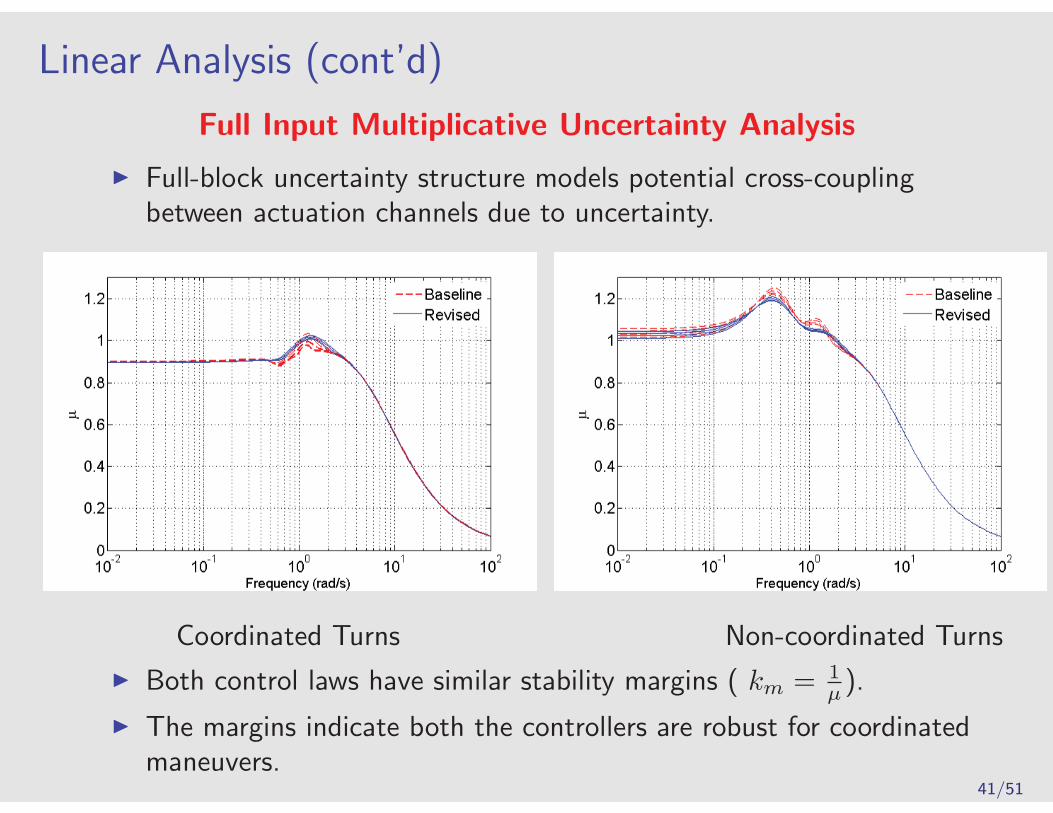
Linear Analysis (cont’d)
Full Input Multiplicative Uncertainty Analysis
� Full-block uncertainty structure models potential cross-couplingbetween actuation channels due to uncertainty.
Coordinated Turns Non-coordinated Turns
� Both control laws have similar stability margins ( km = 1μ ).
� The margins indicate both the controllers are robust for coordinatedmaneuvers.
41/51

Linear Analysis (cont’d)
Robustness to Uncertainty in Aerodynamic Coefficients &Stability Derivatives
� ±10% real parametric uncertainty is introduced in important eightaerodynamic / stability derivatives in open loop A matrix.
Coordinated Turns Non-coordinated Turns
� Again, both controllers have excellent robustness properties.
42/51

Linear Analysis: F/A-18 Summary
Results provided are based on the coordinated turn at φ = 60o.
Linear Analysis Baseline Revised
Multivariable Loop Phase Margin ±63.4◦ ±64.0◦
Multivariable Loop Gain Margin (dB) ±12.53 ±12.73Diagonal Input Multiplicative: (km = 1
μ) 1.03 1.03
Full Input Multiplicative: (km = 1μ) 0.98 0.98
Parametric Uncertainty: (km = 1μ) 8.70 10.8
Linear analysis has shown :
� both the controllers have similar stability margins for differentrobustness tests.
� both controllers are very robust for coordinated maneuvers andslightly less robust for non-coordinated maneuvers.
43/51

Nonlinear Region-of-Attraction (ROA) Analysis
Motivation:
Falling leaf motion is a nonlinear phenomenon which is notcaptured by linear analysis around equilibrium points.
� Linear analysis does not provide any quantitative guarantee onthe stable region of flight that each controller provides.
� Nonlinear Region-of-Attraction analysis techniques can beused to certify regions of stability for individual controllers.
Definition: Region-of-Attraction (ROA) provides the set of theinitial conditions whose state trajectories converge to theequilibrium point.
Consider:x = f(x), x(0) = x0
R0 ={x0 ∈ R
n : If x(0) = x0 then limt→∞x(t) = 0
}44/51

Nonlinear Region-of-Attraction Analysis (cont’d)
Choosing the Shape Factor of the Ellipsoid
� N = NT > 0 is user-specified diagonalmatrix which determines the shape of theellipsoid.
� Here, we have chosen N such that theshape factor is normalized by the inverseof the maximum value each state canachieve.
� Both the closed loopmodels have 7-states :
β : Sideslip Angle, radp : Roll rate, rad/sr : Yaw rate, rad/sφ : Bank angle, radα : Angle-of-attack, radq : Pitch rate, rad/sxc : Controller State
45/51

Nonlinear Region-of-Attraction Analysis (cont’d)
Results on Estimating ROALower & Upper Bounds of ROA Slices in α-β Space for
Coordinated 60o Bank Turn
46/51

Nonlinear Region-of-Attraction Analysis (cont’d)
Results on Estimating ROALower & Upper Bounds of ROA Slices in p - r Space for
Coordinated 60o Bank Turn
47/51

Summary of F/A-18 Nonlinear Analysis Results
Nonlinear Analysis Baseline Revised
Generic Quartic −5.90o ≤ α ≤ +57.9o −19.6o ≤ α ≤ +71.6o
Lyapunov Function −6.40o ≤ β ≤ +6.4o −9.10o ≤ β ≤ +9.10o
−25.0o ≤ p ≤ +25.5o −36.4o ≤ p ≤ +36.4o
+1.32o ≤ r ≤ +14.0o −1.46o ≤ r ≤ +16.81o
Monte Carlo Simulation −9.78o ≤ α ≤ +61.8o −23.2o ≤ α ≤ +75.2o
−7.16o ≤ β ≤ +7.16o −9.85o ≤ β ≤ +9.85o
−28.6o ≤ p ≤ +28.6o −39.4o ≤ p ≤ +39.4o
+0.55o ≤ r ≤ +14.8o −2.14o ≤ r ≤ +17.54o
� Upper and lower bounds on ROA shows significant improvement ofthe stability region for the Revised control law over the Baselinecontrol law.
� Hence, the revised control law is more robust to disturbances andupset conditions that may lead to the falling leaf motion.
48/51

Summary of F/A-18 Flight Control Law Analysis
� F/A-18 Hornet with baseline control law was susceptible to thefalling leaf motion.
� The revised flight control law suppresses the falling leaf motion inthe F/A-18 aircraft.
� Linear analysis provided similar robustness properties for both thecontrol laws for both steady and unsteady maneuvers.
� Nonlinear analysis showed the revised control law leads to asignificant increase in the stability region estimate over the baselinedesign.
Nonlinear analysis tools are required to address nonlinear phenomenon
like the falling leaf motion in certifying flight control law.
49/51

Region-of-Attraction Bounds: Computation
Computational Aspects
� Computational time for estimating both lower and upperbound are as follows:
Analysis Iteration Steps Baseline Revised
Lower Bound Estimation(1) 50 7 Hrs 5 Hrs
Monte Carlo Upper Bound(2) 2 million 2 days 2 days
(1) V-s iteration analysis performed on Intel(R) Core(TM) i7 CPU 2.67GHz 8.00GB RAM
(2) Monte Carlo analysis performed on Intel(R) Core(TM)2 Duo CPU E65550 2.33GHz 3.00GB RAM
50/51
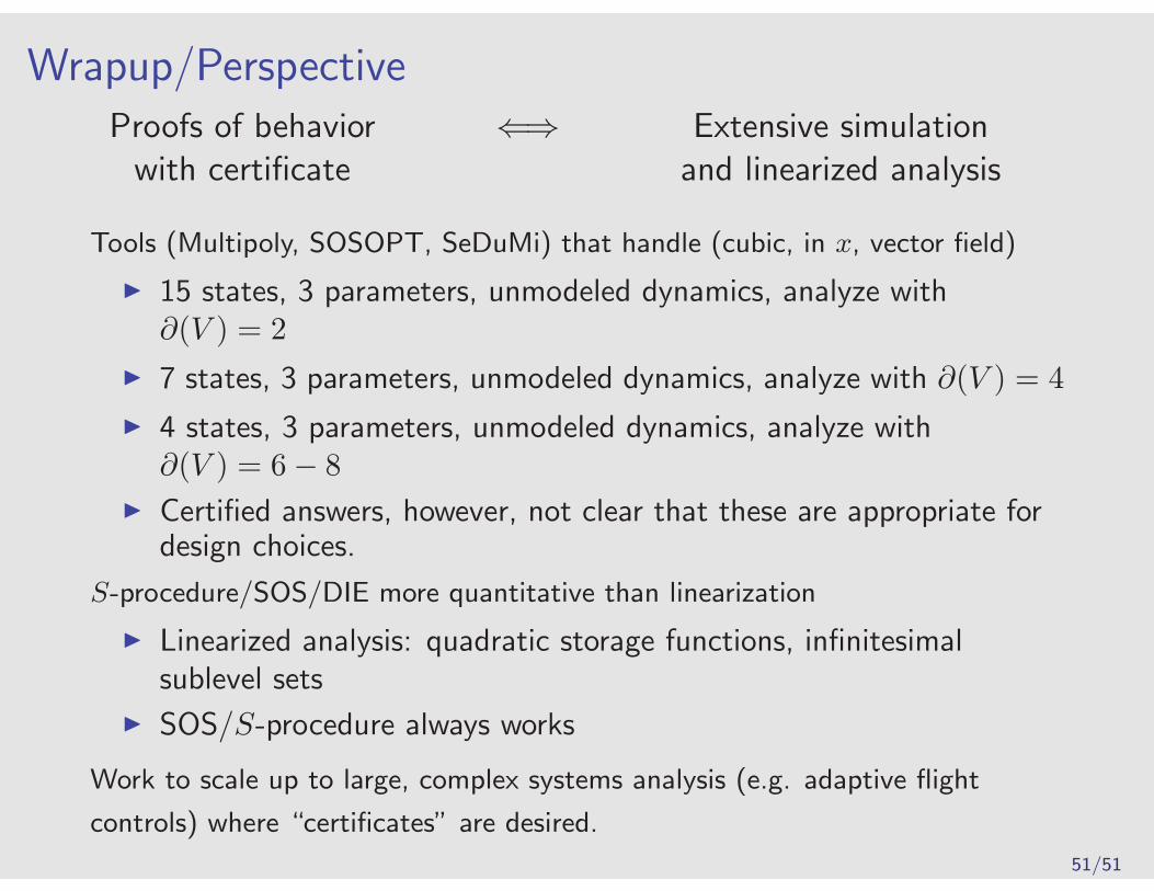
Wrapup/PerspectiveProofs of behavior ⇐⇒ Extensive simulationwith certificate and linearized analysis
Tools (Multipoly, SOSOPT, SeDuMi) that handle (cubic, in x, vector field)
� 15 states, 3 parameters, unmodeled dynamics, analyze with∂(V ) = 2
� 7 states, 3 parameters, unmodeled dynamics, analyze with ∂(V ) = 4
� 4 states, 3 parameters, unmodeled dynamics, analyze with∂(V ) = 6− 8
� Certified answers, however, not clear that these are appropriate fordesign choices.
S-procedure/SOS/DIE more quantitative than linearization
� Linearized analysis: quadratic storage functions, infinitesimalsublevel sets
� SOS/S-procedure always works
Work to scale up to large, complex systems analysis (e.g. adaptive flight
controls) where “certificates” are desired.
51/51
Related Documents
![Performance, Robustness and Sensitivity Analysis of the ...arXiv:1604.05524v1 [math.DS] 19 Apr 2016 Performance, Robustness and Sensitivity Analysis of the Nonlinear Tuned Vibration](https://static.cupdf.com/doc/110x72/60b8c81c212f1a6e00391245/performance-robustness-and-sensitivity-analysis-of-the-arxiv160405524v1-mathds.jpg)


![Robustness Analysis Of Nonlinear Feedback Systems: An ...people.ece.umn.edu/users/georgiou/papers/nonlinear.pdfresult was first presented in the context of nonlinear systems in [14]](https://static.cupdf.com/doc/110x72/5e81d1b024bfca395f4fdcd7/robustness-analysis-of-nonlinear-feedback-systems-an-result-was-irst-presented.jpg)


![Stability and Robustness Analysis of Nonlinear Systems via Contraction Metrics … · 2008. 2. 2. · arXiv:math/0603313v1 [math.OC] 13 Mar 2006 Stability and Robustness Analysis](https://static.cupdf.com/doc/110x72/60dc24f0f575a33e3e4eb829/stability-and-robustness-analysis-of-nonlinear-systems-via-contraction-metrics-2008.jpg)


