arXiv:hep-ph/0606135v4 2 Nov 2006

arX

iv:h

ep-p

h/06

0613

5v4

2 N

ov 2

006

A Comprehensive Analysis of the Pion-Photon Transition Form

Factor Beyond the Leading Fock State

Tao Huang1,2∗ and Xing-Gang Wu3†

1CCAST(World Laboratory), P.O.Box 8730, Beijing 100080, P.R.China

2Institute of High Energy Physics, Chinese Academy of Sciences,

P.O.Box 918(4), Beijing 100039, P.R. China

3Institute of Theoretical Physics, Chinese Academy of Sciences,

P.O.Box 2735, Beijing 100080, P.R. China

(Dated: August 10, 2018)

Abstract

We perform a comprehensive analysis of the pion-photon transition form factor Fπγ(Q2)

involving the transverse momentum corrections with the present CLEO experimental data, in

which the contributions beyond the leading Fock state have been taken into consideration. As

is well-known, the leading Fock-state contribution dominates of Fπγ(Q2) at large momentum

transfer (Q2) region. One should include the contributions beyond the leading Fock state in

small Q2 region. In this paper, we construct a phenomenological expression to estimate the

contributions beyond the leading Fock state based on its asymptotic behavior at Q2 → 0. Our

present theoretical results agree well with the experimental data in the whole Q2 region. Then,

we extract some useful information of the pionic leading twist-2 distribution amplitude (DA)

by comparing our results of Fπγ(Q2) with the CLEO data. By taking best fit, we have the DA

moments, a2(µ20) = 0.002+0.063

−0.054, a4(µ20) = −0.022+0.026

−0.012 and all of higher moments, which are closed

to the asymptotic-like behavior of the pion wavefunction.

PACS numbers: 13.40.Gp, 12.38.Bx, 12.39.Ki, 14.40.Aq

∗ email: [email protected]† email: [email protected]

1

I. INTRODUCTION

The pion-photon transition form factor, which relates two photons with one lightest me-

son, is the simplest example for the perturbative application to exclusive processes. By

neglecting k⊥ (the transverse momentum of the constitute quarks) relative to q⊥ (the trans-

verse momentum of the virtual photon) in the hard-scattering amplitude, one can obtain

the leading Fock-state formula [1]:

Fπγ(Q2) =

2fπ3Q2

∫

dx

xφπ(x,Q

2)

[

1 +O(

αs(Q2),

m2

Q2

)]

, (1)

where Q2 = −q2 stands for the momentum transfer in the process, the pion decay constant

fπ = 92.4± 0.25 MeV [2], and φπ(x,Q2) stands for the leading Fock-state pion distribution

amplitude (DA) at the factorization scale µ2 = Q2, which can be derived from the initial

DA φπ(x, µ20) (µ0 stands for some hadronic scale) through QCD evolution. The initial DA

is defined as

φπ(x, µ20) =

2√3

fπ

∫

|k⊥|2≤µ20

d2k⊥16π3

Ψqq(x,k⊥). (2)

Hence, the value of Q2Fπγ(Q2) tends to be a constant (2fπ) for asymptotic DA:

φas(x,Q2)|Q2→∞ = 6x(1 − x). However, it has been argued that the k⊥-dependence of

the pion wavefunction can not be safely neglected at the end-point region xi → 0, 1 (xi

the momentum fraction of the constitute quarks in pion) and Q2 ∼ a few GeV2. Under

the light-cone (LC) pQCD approach, the leading contribution to Fπγ(Q2) that keeps the

k⊥-corrections in both the hard-scattering amplitude and the wavefunction can be written

as [4, 5]:

Fπγ(Q2) = 2

√3(e2u − e2d)

∫ 1

0[dx]

∫ d2k⊥16π3

Ψqq(x,k⊥)× TH(x, x′,k⊥), (3)

where [dx] = dxdx′δ(1−x−x′), eu, d are the quark charges in unites of e, Ψqq(x,k⊥) stands for

the leading Fock-state wavefunction and the hard-scattering amplitude TH(x, x′,k⊥) takes

the form,

TH(x, x′,k⊥) =

q⊥ · (x′q⊥ + k⊥)

q2⊥(x

′q⊥ + k⊥)2+ (x↔ x′). (4)

With the help of Eqs.(3,4), Ref.[5] performed a careful analysis of the quark transverse-

momentum effect to Fπγ(Q2). They pointed out that the transverse-momentum dependence

in both the numerator and the denominator of the hard-scattering amplitude are of the

same importance and should be considered consistently. Similar improved treatment has

2

also been done in Refs.[6, 7, 8, 9, 10, 11, 12]. It was shown that pQCD can give the correct

prediction for the pion-photon transition form factor that is consistent with the present

experimental data by keeping the k⊥-dependence in both the hard-scattering amplitude and

the pion wavefunction and by properly choosing of the pion wavefunction.

It should be noted that Eqs.(1,3) were obtained by assuming the leading Fock-state

dominance. This approximation is valid only for large Q2 region and one can not expect

that these expressions can describe the present experimental data well in low Q2 region.

Refs.[13, 14] show that the approximation of the leading Fock-state dominance to the pion

electro-magnetic form factor is valid as Q2 >∼ 4 GeV2, which is improved to be Q2 >∼ 1 GeV2

by including the next-to-leading order (NLO) contribution [15, 16]. A similar discussion has

been done in Ref.[5] for the pion-photon transition form factor. These references tell us that

one should take into account the higher Fock states’ contributions as Q2 < a few GeV2.

In fact, it has been shown that the expression (3) gives half contribution to Fπγ(Q2) as one

extends it to Q2 = 0 [4]. It means that the leading Fock state contributes to Fπγ(0) only half

and the remaining half should be come from the higher Fock states. Both contributions from

the leading Fock state and the higher Fock states are needed to get the correct π0 → γγ

rate [4]. Any attempt that involves only the leading Fock-state contribution to explain

both the π0 → γγ rate and the pion-photon transition form factor for low Q2 region is

incorrect. It should be pointed out that the above conclusion does not contradict with that

of Ref.[17], where with the help of an “effective” two-body wavefunction that includes the soft

contributions from the higher Fock components, the authors pointed that the contributions

corresponding to higher Fock states in a hard region appear as radiative corrections and are

suppressed by powers of (αs/π) ∼ 10%.

In this paper, we will take the contributions from both the leading Fock state and the

higher Fock states into consideration. Especially, we will discuss how to consider the con-

tributions beyond the leading Fock state at low Q2 region and give a careful analysis of the

pion-photon transition form factor in the whole Q2 region. Furthermore, we can learn more

information of the leading twist-2 DA from the present CLEO data, since the pion-photon

transition form factor in the simplest exclusive process only involves one pion and the con-

tributions from the higher twist structures and higher helicity states are highly suppressed

(at least by 1/Q4) in comparison to the leading twist-2 pion wavefunction. In the present

paper, we will not include the NLO contribution into our formulae. Since we need a full

3

NLO result in order to be consistent with our present calculation technique, in which the

effects caused by the transverse-momentum dependence in the hard-scattering amplitude

and the pion wavefunction and by the Sudakov factor should be fully considered, however

such a full NLO calculation is not available at the present 1.

The paper is organized as follows. In Sec.II, we analyze the contributions to Fπγ(Q2)

beyond the leading Fock state at low Q2 region under the LC pQCD approach and give

a complete expression for Fπγ(Q2) in the whole Q2 region. In Sec.III, we discuss what

we can learn of the pionic leading Fock-state wavefunction/DA in comparison with CLEO

experimental data. Some further discussion and comments are made in Sec.IV. The last

section is reserved for a summary.

II. AN EXPRESSION OF Fπγ(Q2) FROM ZERO TO LARGE Q2 REGION

First, we give a brief review of the LC formalism [1, 19, 20]. The LC formalism provides

a convenient framework for the relativistic description of hadrons in terms of quark and

gluon degrees of freedom and for the application of pQCD to exclusive processes. The LC

Fock-state expansion of wavefunction provides a precise definition of the parton model and

a general method to calculate the hadronic matrix element. As for the pion wavefunction,

its Fock-state expansion is

|π〉 =∑

|qq〉Ψqq +∑

|qqg〉Ψqqg + · · · , (5)

where the Fock-state wavefunctions Ψn(xi,k⊥i, λi) (n = 2, 3, · · ·) satisfy the normalization

condition∑

n,λi

∫

[dxd2k⊥]n|Ψn(xi,k⊥i, λi)|2 = 1, (6)

with [dxd2k⊥]n = 16π3δ(1 − ∑ni=1 xi)δ

2(∑n

i=1 k⊥i)∏n

i=1

[

dxid2k⊥i

16π3

]

. λi is the helicity of the

constituents and n stands for all Fock states, e.g. Ψ2 = Ψqq. It should be pointed out that

we have∫

[dxd2k⊥]2∑

λi|Ψqq(xi,k⊥i, λi)|2 < 1 for the leading Fock state.

The pion-photon transition form factor is connected with the π0γγ∗ vertex in the ampli-

1 The present NLO result is derived without considering the transverse-momentum dependence in the hard-

scattering amplitude and the wavefunction, see e.g. Refs.[9, 10, 15, 16, 18].

4

(0,q⊥)

γ

γ∗

(x,k⊥)

(x′,−k⊥)

(a) (b)

γ

γ∗

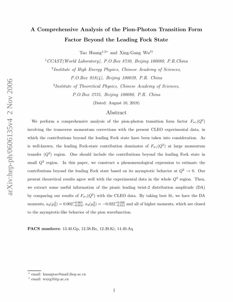
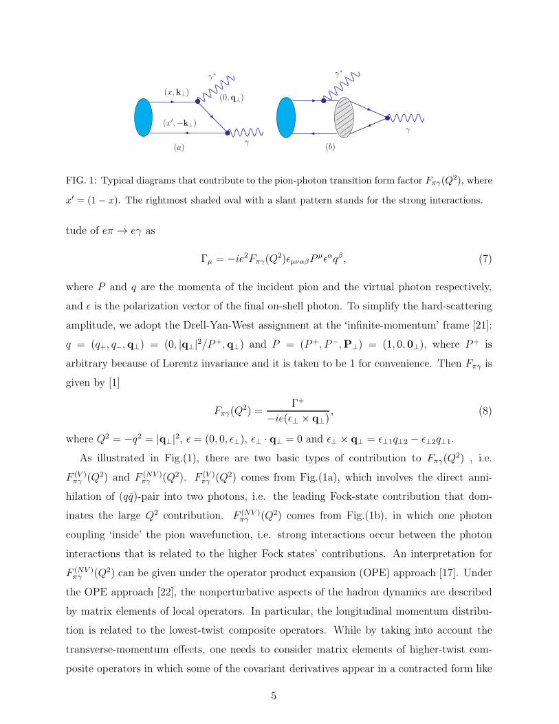
FIG. 1: Typical diagrams that contribute to the pion-photon transition form factor Fπγ(Q2), where

x′ = (1− x). The rightmost shaded oval with a slant pattern stands for the strong interactions.

tude of eπ → eγ as

Γµ = −ie2Fπγ(Q2)ǫµναβP

µǫαqβ, (7)

where P and q are the momenta of the incident pion and the virtual photon respectively,

and ǫ is the polarization vector of the final on-shell photon. To simplify the hard-scattering

amplitude, we adopt the Drell-Yan-West assignment at the ‘infinite-momentum’ frame [21]:

q = (q+, q−,q⊥) = (0, |q⊥|2/P+,q⊥) and P = (P+, P−,P⊥) = (1, 0, 0⊥), where P+ is

arbitrary because of Lorentz invariance and it is taken to be 1 for convenience. Then Fπγ is

given by [1]

Fπγ(Q2) =

Γ+

−ie(ǫ⊥ × q⊥), (8)

where Q2 = −q2 = |q⊥|2, ǫ = (0, 0, ǫ⊥), ǫ⊥ · q⊥ = 0 and ǫ⊥ × q⊥ = ǫ⊥1q⊥2 − ǫ⊥2q⊥1.

As illustrated in Fig.(1), there are two basic types of contribution to Fπγ(Q2) , i.e.

F (V )πγ (Q2) and F (NV )

πγ (Q2). F (V )πγ (Q2) comes from Fig.(1a), which involves the direct anni-

hilation of (qq)-pair into two photons, i.e. the leading Fock-state contribution that dom-

inates the large Q2 contribution. F (NV )πγ (Q2) comes from Fig.(1b), in which one photon

coupling ‘inside’ the pion wavefunction, i.e. strong interactions occur between the photon

interactions that is related to the higher Fock states’ contributions. An interpretation for

F (NV )πγ (Q2) can be given under the operator product expansion (OPE) approach [17]. Under

the OPE approach [22], the nonperturbative aspects of the hadron dynamics are described

by matrix elements of local operators. In particular, the longitudinal momentum distribu-

tion is related to the lowest-twist composite operators. While by taking into account the

transverse-momentum effects, one needs to consider matrix elements of higher-twist com-

posite operators in which some of the covariant derivatives appear in a contracted form like

5

D2 = DµDµ. By using the equation of motion for the light quark, γµDµq = 0, one can

convert a two-body quark-antiquark operator q{γµ1Dµ2 . . .Dµn}D2q into the “three-body”

operator q{γµ1Dµ2 . . .Dµn}(σµνGµν)q with an extra gluonic field Gµν being involved, which

is just related to the higher Fock state of pion.

The first type of contribution F (V )πγ (Q2) stands for the conventional leading Fock-state

contribution. Under the LC pQCD approach and by keeping the full kT -dependence in

both the hard-scattering amplitude and the wavefunction, the expression for F (V )πγ (Q2) is

the one that is given in Eqs.(3,4), where the terms involving the higher helicity states

(λ1+λ2 = ±1, λi stands for the corresponding helicity of the two constitute quarks of pion)

and the higher twist structures of the pion wavefunction are not explicitly written. Since

by direct calculating, one may observe that the contributions from the higher helicity states

and the higher twist structures of the pion wavefunction are suppressed by at least 1/Q4 to

that of the usual helicity state (λ1 + λ2 = 0) of the leading Fock state, which agrees with

the discussion made in Ref.[9] 2.

As for the second type of contribution F (NV )πγ (Q2), it is difficult to be calculated in any Q2

region. If treating the photon vertex in Fig.(1b) as a vector meson dressed photon vertex,

Fig.(1b) can be calculated approximately under the vector meson dominance (VMD) ap-

proach, see e.g. Ref.[23] for a review and Refs.[24, 25] for an explicit VMD calculation of the

pion electro-magnetic form factor. By adopting the VMD approach to approximate Fig.(1b),

one needs to introduce some undetermined coupling factor either for VMD1 or VMD2 for-

mulation [23], which together with the undetermined parameters in the pion wavefunction

can not be definitely determined by the CLEO experimental data of the pion transition

form factor only and some other constraints should also be taken into consideration, e.g.

the constraint from the experimental value for the pion charge radius or the constraint from

the experimental value for the pion electro-magnetic form factor. In fact, one usually takes

the value of Fπγ(Q2) = F (V )

πγ (Q2) + F (NV )πγ (Q2) derived from the VMD approach to be in a

simple monopole form [26], i.e. Fπγ(Q2) = 1/

[

4π2fπ(1 +Q2/m2ρ)]

, with the ρ-meson mass

mρ serves as a parameter determined by the pion charge radius. For the purpose of extract-

ing some useful information of the pion wavefunction from the CLEO experimental data,

2 The present condition is quite different from the case of pion electro-magnetic form factor, where the

contributions from the higher helicity states and higher twist structures are only suppressed by 1/Q2 and

then they can provide sizable contribution in the intermediate Q2 region [37, 38].

6

we adopt the method raised by Ref.[4] to deal with F (NV )πγ (Q2) 3.

As stated in Ref.[4], around the region of Q2 ∼ 0, since the wavelength of the photon

‘inside’ the pion wavefunction ∼ 1/mπ is assumed to be much larger than the pion radius

1/λ (λ is some typical hadronic scale ∼ 1 GeV), we can treat such photon (nearly on-shell)

as an external field which is approximately constant throughout the pion volume. And

then, a fermion in a constant external field is modified only by a phase, i.e. SA(x − y) =

e−ie(y−x)·ASF (x − y). Consequently, the lowest qq-wavefunction for the pion is modified

only by a phase e−iey·A, where y is the qq-separation. Transforming such phase into the

momentum space and applying it to the wavefunction, the second contribution F (NV )πγ (Q2)

at q⊥ → 0 can be simplified to

F (NV )πγ (Q2)|q⊥→0 =

−2√3Q2

∫

[dx]∫

d2k⊥16π3

{

(k⊥ × q⊥)2

(x′q⊥ + k⊥)2

[

∂

∂k2⊥Ψqq(x,k⊥)

]

+ (x↔ x′)

}

,

(9)

where [dx] = dxdx′δ(1 − x − x′) and k⊥ = |k⊥|. Eq.(9) gives the expression for F (NV )πγ (Q2)

at Q2 → 0. Here different from Ref.[4], all q⊥-terms that are necessary to obtain its first

derivative over Q2 are retained and the relation (ǫ⊥×q⊥)(k⊥×q⊥) = Q2(ǫ⊥ ·k⊥) is implicitly

adopted. After doing the integration over k⊥, one can easily find that

F (NV )πγ (0) = F (V )

πγ (0) =1

8√3π2

∫

dxΨqq(x, 0⊥), (10)

which means that the leading Fock state contributes to Fπγ(0) = F (V )πγ (0) + F (NV )

πγ (0) only

half, and one can get the correct rate of the process π0 → γγ provided that the two basic

contributions F (V )πγ (0) and F (NV )

πγ (0) are considered simultaneously. By taking into account

the PCAC prediction [27], Fπγ(0) = 1/(4π2fπ), one can obtain the important constraint of

the pion wavefunction, i.e.∫ 1

0dxΨqq(x,k⊥ = 0) =

√3

fπ. (11)

Without loss of generality, we can assume that the pion wavefunction depending on k⊥

through k2⊥ only, i.e. Ψqq(x,k⊥) = Ψqq(x, k2⊥)

4. Then F (V )πγ (Q2) (Eq.(3)) can be simplified

3 A careful VMD calculation of the pion transition form factor along the line of Refs.[24, 25] can be used

as a cross check of our results, however it is out of the range of the present paper.4 The spin-space Wigner rotation might change this property for the higher helicity components as shown

in Ref.[28]. Since the higher helicity components’ contribution are highly suppressed for the present case,

we do not take this point into consideration in the present paper.

7

after doing the integration over the azimuth angle as [9]

F (V )πγ (Q2) =

1

4√3π2

∫ 1

0

dx

xQ2

∫ x2Q2

0Ψqq(x, k

2⊥)dk

2⊥. (12)

Similarly, for the first derivative of F (NV )πγ (Q2) over Q2, we have

F (NV )′

πγ (Q2)|Q2→0 =1

8√3π2

[

∂

∂Q2

∫ 1

0

∫ x2Q2

0

(

Ψqq(x, k2⊥)

x2Q2

)

dxdk2⊥

]

Q2→0

. (13)

Furthermore, the leading twist-2 pion DA at the factorization scale µ can be simplified as

φπ(x, µ2) =

√3

8π2fπ

∫ µ2

0ψqq(x, k

2⊥)dk

2⊥. (14)

With the help of Eqs.(12,14), F (V )πγ (Q2) can be rewritten as

F (V )πγ (Q2) =

2fπ3Q2

∫ 1

0

dx

xφπ(x, x

2Q2). (15)

Note that Eq.(15) is different from Eq.(1) only by replacing φπ(x,Q2) to φπ(x, x

2Q2). It

means that the leading contribution to Fπγ(Q2) as shown in Eq.(3), which was given by

keeping the k⊥-corrections in both the hard-scattering amplitude and the pion wavefunction,

can be equivalently obtained by setting the upper limit for the integral of the pion DA to

be [µ2 = x2Q2]. The x-dependent upper limit [x2Q2] affects F (V )πγ (Q2) from the small to

intermediate Q2 region, and such effect will be more explicit for a wider pion DA, such as

the CZ (Chernyak-Zhitnitsky)-like model [3] that emphasizes the end-point region in a strong

way, as has been discussed in Ref.[5]. In the literature, the pion DA is usually expanded in

Gegenbauer polynomial expansion as

φπ(x, µ2) = φas(x) ·

[

1 +∞∑

n=1

a2n(µ2)C

3/22n (ξ)

]

, (16)

where ξ = (2x− 1), C3/2n (ξ) are Gegenbauer polynomials and a2n(µ

2), the so called Gegen-

bauer moments, are hadronic parameters that depend on the factorization scale µ. The

Gegenbauer moments a2n(µ2) can be related to a2n(µ

20) with the help of QCD evolution,

where µ0 stands for some fixed low energy scale. To leading logarithmic accuracy, we

have [10, 29]

a2n(µ2) = a2n(µ

20)

(

αs(µ2)

αs(µ20)

)γ(2n)0 /(2β0)

, (17)

where β0 = 11− 2nf/3, αs(Q2) = 4π/[β0 ln(Q

2/Λ2QCD)] and the one-loop anomalous dimen-

sion is

γ(2n)0 = 8CF

(

ψ(2n + 2) + γE − 3

4− 1

(2n+ 1)(2n+ 2)

)

. (18)

8

We need to know φπ(x, x2Q2) and F (NV )

πγ (Q2) to get the whole behavior of Fπγ(Q2), i.e.

Fπγ(Q2) = F (V )

πγ (Q2) + F (NV )πγ (Q2), (19)

where F (V )πγ (Q2) is determined by φπ(x, x

2Q2). The φπ(x, x2Q2) depends on the behavior

of Ψqq(x,k⊥) and its Gegenbauer moments can not be directly obtained from the QCD

evolution equation (17), since [x2Q2] can be very small and then the Landau ghost singularity

in the running coupling αs can not be avoided. As for F (NV )πγ (Q2), Eq.(9) presents an

expression only at Q2 ∼ 0 region, and it can not be directly extended to the whole Q2

region. Ref.[9] did an attempt to understand the higher Q2 behavior of Fπγ(Q2) within

the QCD sum rule approach, i.e. they raised a simple picture: the sum over the soft

qG · · ·Gq Fock components is dual to qq-state generated by the local axial vector current.

Furthermore, they raised an ‘effective’ two-body pion wavefunction that includes all soft

contributions from the higher Fock states based on the QCD sum rule analysis and then

calculated Fπγ(Q2) within the pQCD approach. Here we will not adopt such an ‘effective’

pion wavefunction to do the calculation, since we plan to extract some information for the

leading Fock-state wavefunction by comparing with the CLEO experimental data.

In order to construct an expression of F (NV )πγ (Q2) in the whole Q2 region, we require the

following conditions at least:

i) F (NV )πγ (Q2)|Q2=0 should be given by Eq.(10).

ii) F (NV )′

πγ (Q2)|Q2→0 = ∂F (NV )πγ (Q2)/∂Q2|Q2→0 should be derived from Eq.(9).

iii)F

(NV )πγ (Q2)

F(V )πγ (Q2)

→ 0, as Q2 → ∞.

One can construct a phenomenological model for F (NV )πγ (Q2) that satisfies the above three

requirements. It is natural to assume the following form

F (NV )πγ (Q2) =

α

(1 +Q2/κ2)2, (20)

where κ and α are two parameters that can be determined by the above conditions (i,ii), i.e.

α =1

2Fπγ(0) =

1

8π2fπ(21)

and

κ =

√

√

√

√− Fπγ(0)∂

∂Q2F(NV )πγ (Q2)|Q2→0

. (22)

As for the phenomenological formula (20), it is easy to find that F (NV )πγ (Q2) will be suppressed

by 1/Q2 to F (V )πγ (Q2) in the limit Q2 → ∞. Such a 1/Q2-suppression is reasonable, since the

9

0 2 4 6 8 10

0.05

0.1

0.15

0.2

0.25

Q2 F

πγ(Q

2 ) (G

eV)

Q2(GeV2)

CLEOCELLO

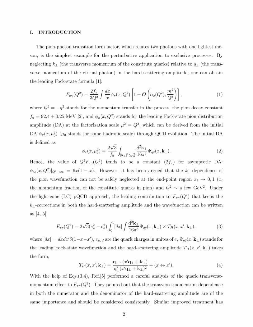
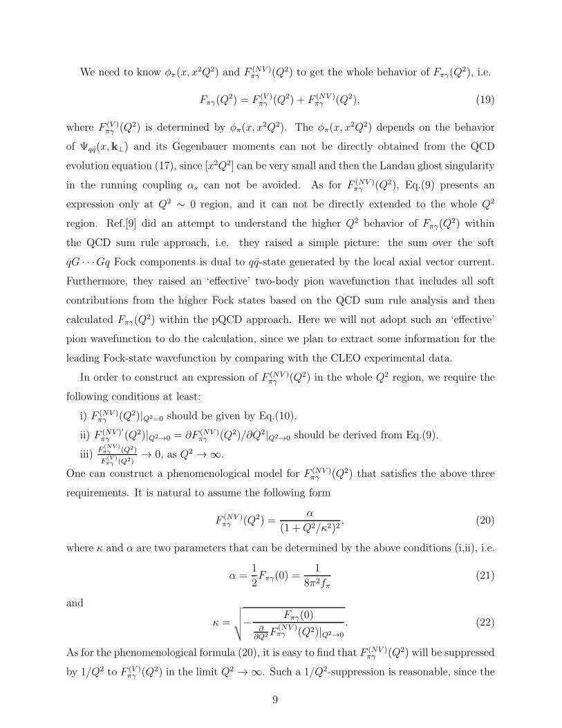
FIG. 2: The fitting curve (the solid line) for Q2Fπγ(Q2) from the CLEO and CELLO experimental

data [30, 31], where a shaded band shows its uncertainty of ±20%.

phenomenological expression (20) can be regarded as a summed up effect of all the high twist

structures of the pion wavefunction, even though each higher twist structure is suppressed

by at least 1/Q4 [9].

III. CALCULATED RESULTS WITH THE MODEL WAVEFUNCTION

The CLEO collaboration has measured the γγ∗ → π0 form factor [30]. In this experiment,

one of the photons is nearly on-shell and the other one is highly off-shell, with a virtuality

in the range 1.5 GeV2 - 9.2 GeV2 [30]. There also exists older experimental results obtained

by the CELLO collaboration [31]. By comparing the theoretical prediction with the experi-

mental results, it provides us a chance to determine a precise form for the leading Fock-state

pion wavefunction. Similar attempt to determine the pion DA has been done in literature

[32, 33], e.g. Ref.[32] used the QCD light-cone sum rule analysis of the CLEO data to obtain

parameters of the pion DA. In Fig.2, we show the fitting curve for Q2Fπγ(Q2) (derived by

using the conventional χ2-fitting method described in Ref.[34] with slight change to make

the curve more smooth) from the CLEO and CELLO experimental data, i.e. under the

region of Q2 ∈ [0.5, 10.0] GeV2, Q2Fπγ(Q2) ≃ [8.81×10−7(Q

′2)5−4.78×10−5(Q′2)4+9.96×

10−4(Q′2)3−1.01×10−2(Q

′2)2+5.29×10−2(Q′2)+4.48×10−2] GeV with the dimensionless

10

parameter Q′2 = Q2/GeV2. Here the shaded band shows its ±20% uncertainty 5. In fact,

most of the results given in literature, e.g. Refs. [5, 6, 7, 8, 9, 10, 11, 32], are mainly within

such region. The shaded band (region) for Q2Fπγ(Q2) can be regarded as a constraint to

determine the pion wavefunction, i.e. the values of the parameters in the pion wavefunction

should make Q2Fπγ(Q2) within the region of the shaded band as shown in Fig.(2).

Now we are in position to calculate the pion-photon transition from factor with the help of

Eq.(19). As has been discussed in the last section, we need to know the leading Fock-state

pion wavefunction Ψqq(x,k⊥) so as to derive φπ(x, x2Q2) that is necessary for F (V )

πγ (Q2)

and to derive the values of α and κ for F (NV )πγ (Q2). Several non-perturbative approaches

have been developed to provide the theoretical predictions for the hadronic wavefunction.

One useful way is to use the approximate bound-state solution of a hadron in terms of the

quark model as the starting point for medeling the hadronic wavefunction. The Brodsky-

Huang-Lepage (BHL) prescription [4] for the hadronic wavefunction is obtained in this way

by connecting the equal-time wavefunction in the rest frame and the wavefunction in the

infinite momentum frame. In the present paper, we shall adopt the revised LC harmonic

oscillator model as suggested in Ref.[28] to do our calculation, which is constructed based on

the BHL-prescription. As discussed in the above section, the contribution from the higher

helicity states (λ1 + λ2 = ±1) is highly suppressed in comparison to that of the usual helicity

state (λ1 + λ2 = 0), so we only write down the form of the pion wavefunction for the usual

helicity state:

Ψqq(x,k⊥) = ϕBHL(x,k⊥)χK(x,k⊥) = A exp

[

− k2⊥ +m2

8β2x(1− x)

]

χK(x,k⊥), (23)

with the normalization constant A, the harmonic scale β and the quark mass m to be

determined. The spin-space wavefunction χK(x,k⊥) can be written as [28], χK(x,k⊥) =

m/√

m2 + k2⊥ with k⊥ = |k⊥|. By taking the BHL-like wavefunction (23), F (V )πγ (Q2) (Eq.(12))

can be simplified as

F (V )πγ (Q2) =

∫ 1

0dx

Amβ√6π3/2Q2

√

x′

x

(

Erf

[√m2 + x2Q2

2β√2xx′

]

− Erf

[√m2

2β√2xx′

])

, (24)

where the error function Erf(x) is defined as Erf(x) = 2√π

∫ x0 e

−t2dt. And similarly, for the

limiting behaviors of F (NV )πγ (Q2) that are necessary to determine the parameters α and κ,

5 It is so chosen since the sum of the statistical and systematic errors of the experimental data is <∼±20% [30, 31].

11

0.4 0.5 0.6 0.7 0.8 0.9 1.0

0.1

0.2

0.3

0.4

0.5

0.6

0.7

m(G

eV)

(GeV)

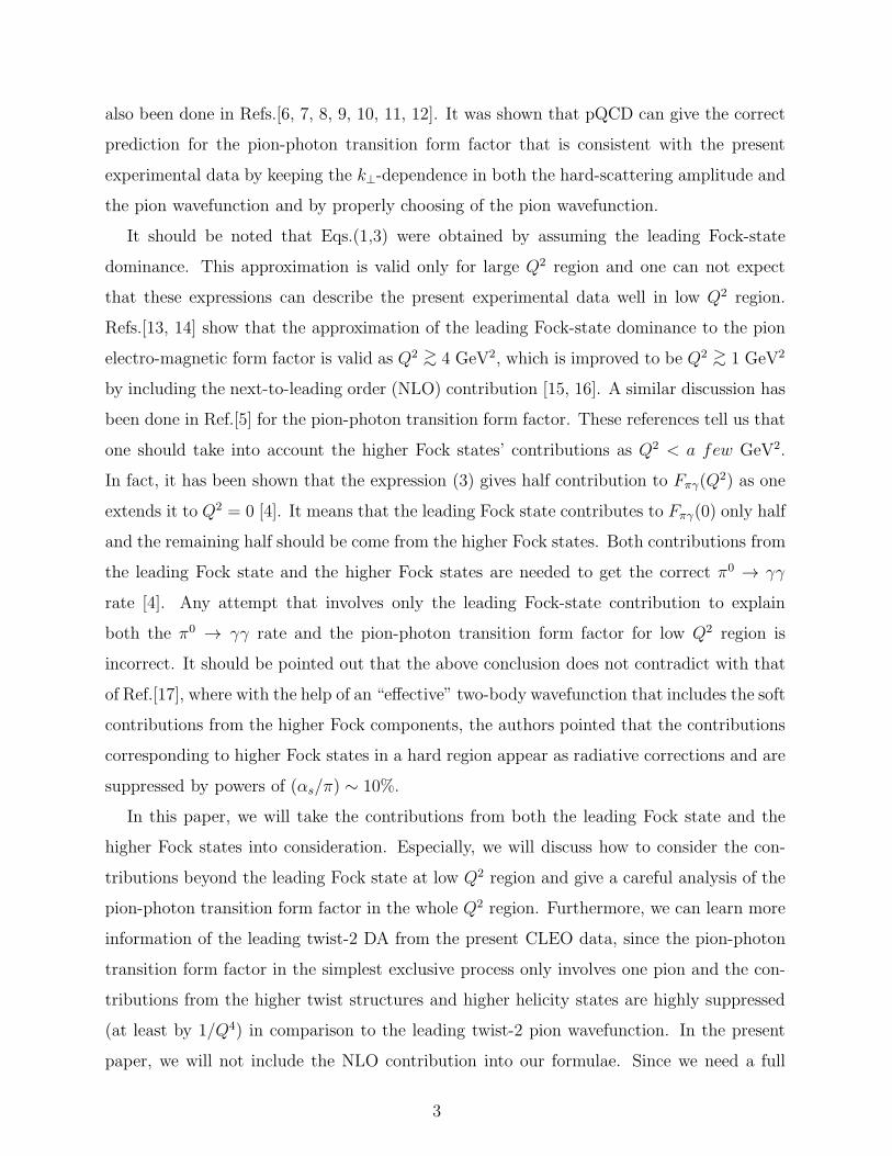
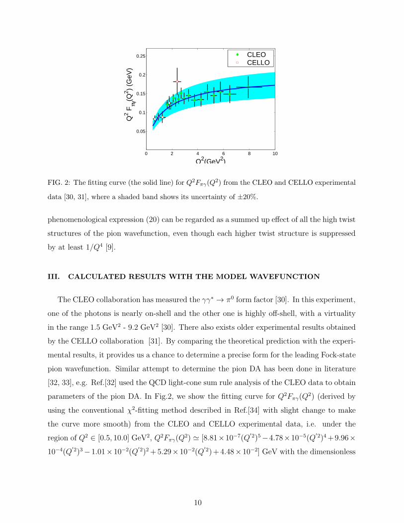
FIG. 3: The curve for the value of m versus β, which shows that if m is in the reasonable region

[0.20 GeV, 0.40 GeV] then β ∈ [0.48 GeV, 0.70 GeV].

we obtain

F (NV )πγ (Q2)|Q2→0 =

A

8√3π2

∫ 1

0exp

[

− m2

8β2xx′

]

dx (25)

and

F (NV )′

πγ (Q2)|Q2→0 =−A

128√3m2π2β2

∫ 1

0

x

x′(m2 + 4xx′β2) exp

[

− m2

8β2xx′

]

dx, (26)

where x′ = 1− x.

The possible range for the parameters of the pion wavefunction (23) can be derived by

comparing our result of Q2Fπγ(Q2) with the experimental data. Further more, the model

wavefunction should satisfy the following two conventional constraints:

• The pion wavefunction satisfies the normalization that is derived from the π → µν

process [4, 28]:∫ 1

0dx∫

|k⊥|2<µ2

d2k⊥16π3

Ψqq(x,k⊥) =fπ

2√3, (27)

where the cut |k⊥|2 < µ2 has been explicitly included. Substituting the pion wave-

function (23) into Eq.(27), we obtain

∫ 1

0

Amβ√

x(1− x)

4√2π3/2

Erf

√

√

√

√

m2 + µ2

8β2x(1− x)

− Erf

√

√

√

√

m2

8β2x(1− x)

dx =fπ

2√3.

(28)

As for the model wavefunction (23), it can be found that the contribution from higher

|k⊥| region to the wavefunction normalization drops down exponentially, e.g. by taking

12

reasonable values for the wavefunction parameters, the wavefunction in the region of

|k⊥| > 1 GeV only contributes about 5% to its total normalization, which changes to

be less than 1% in the region of |k⊥| > 2 GeV. For clarity, we take the factorization

scale µ to be µ = µ0 ≃ 2 GeV, where µ0 stands for some hadronic scale that is of order

O(1 GeV) and the choice of µ0 ≃ 2 GeV is also close to the virtuality of the photons

in the central region of the experimental data. By taking 1 GeV ≤ µ0 ≤ 2 GeV that

is of order µ0 ∼ O(1 GeV), we find that the following results will be slightly changed,

especially for the DA moments due to the fact that they satisfy the QCD evolution

equation (17) within errors. A similar discussion on this point can also be found in

Ref.[32]. Furthermore, one can safely take µ = ∞ to simplify the calculation due to

the smallness of the wavefunction in the region of [|k⊥| > µ0 = 2 GeV].

• Another constraint, as shown in Eq.(11), for the pion wavefunction can be derived

from π0 → γγ decay amplitude [4], which can be further simplified as

∫ 1

0A exp

[

− m2

8β2x(1− x)

]

dx =

√3

fπ. (29)

Solving Eqs.(28,29) numerically, we obtain an approximate relation for m and β, i.e.

6.00mβ

f 2π

∼= 1.12

(

m

β+ 1.31

)(

m

β+ 5.47× 101

)

, (30)

which shows that the value of m is decreased with the increment of β. More explicitly,

Fig.(3) shows that β should be within the region of [0.48 GeV, 0.70 GeV] so as to restrict m

within the reasonable region of [0.20 GeV, 0.40 GeV].

Before doing the numerical calculation for Fπγ(Q2), we note a naive interpolation formula

for both perturbative and non-perturbative regions has been proposed by Brodsky and

Lepage [1], which is similar to the monopole form derived from VMD approach [26], i.e.

FBLπγ (Q2) =

1

4π2fπ(1 +Q2/s0)

(

1− 5

3

αs(Q2)

π

)

, s0 = 8π2f 2π = 0.67 GeV2 ∼ m2

ρ (31)

where the NLO perturbative contribution(

−53αs(Q2)

π

)

has been added to the original result

according to the suggestion of Ref.[9, 18].

The conventional value for the constitute quark mass m is around 0.30 GeV. In the

present section, we concentrate our attention on the case of m = 0.30 GeV and we will

study the uncertainty caused by varying m within a wider region of [0.20 GeV, 0.40 GeV]

13

0 1 2 3 4 5 6 7 8 9 10

0.05

0.1

0.15

0.2

0.25

Q2 F

πγ(Q

2 ) (G

eV)

Q2(GeV2)

CLEOCELLO

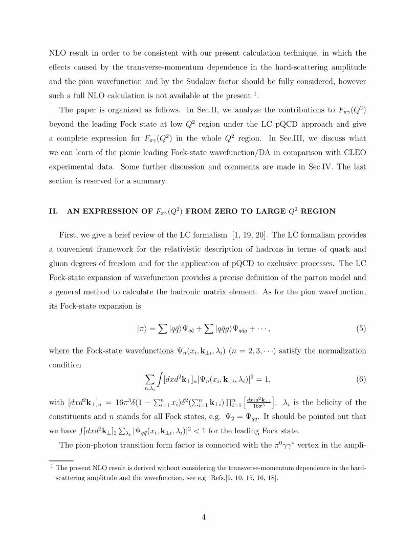
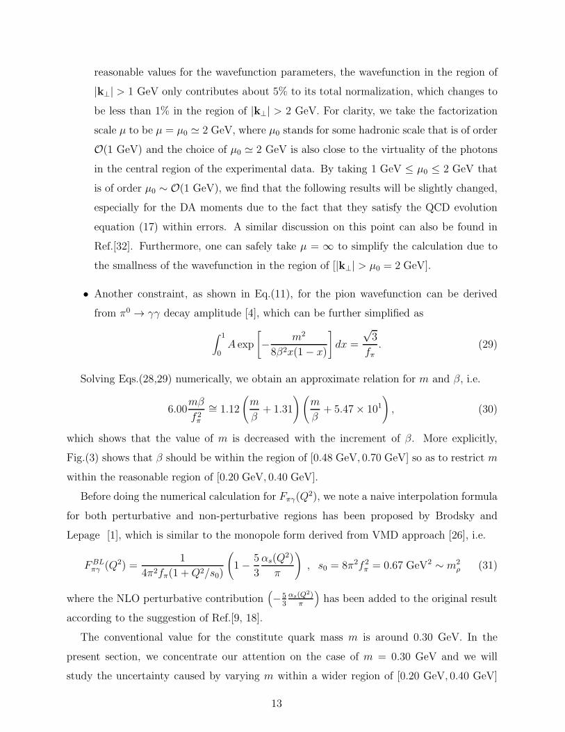
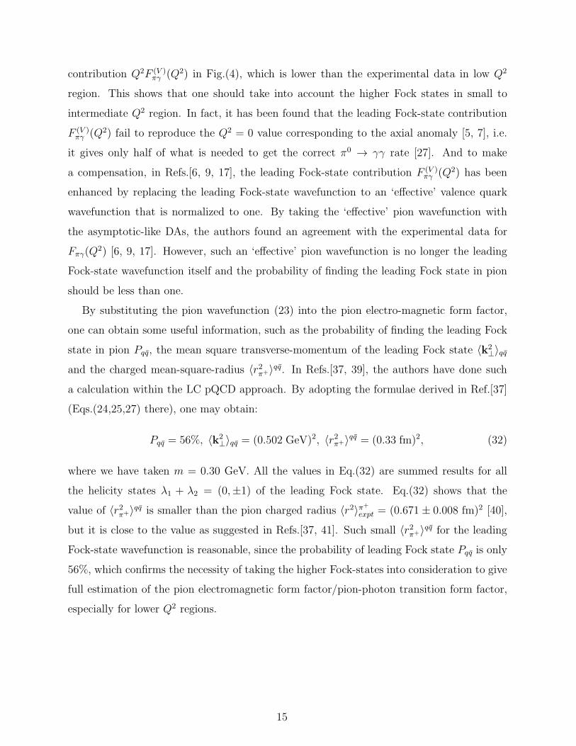
FIG. 4: Q2Fπγ(Q2) that is defined in Eq.(19) and is calculated with the model wavefunction (23)

for the case of m = 0.30 GeV (β = 0.55 GeV), which is shown by a dash-dotted line. The dashed

line is best fit for the CLEO experimental data [30, 31], the solid line is from the interpolation

formula (31) and the dotted line is the results for Q2F(V )πγ (Q2) only.

in the next section. We show the pion-photon transition form factor Q2Fπγ(Q2) with the

model wavefunction (23) for the case of m = 0.30 GeV in Fig.(4), where the values for

β = 0.55 GeV and A = 25.6 GeV−1 can be obtained by using Eqs.(27,30). Fig.(4) shows

that by taking the model wavefunction (23) with m = 0.30 GeV, the predicted value of

Q2Fπγ(Q2) agrees well with the experimental data. We also show the leading Fock-state

contribution Q2F (V )πγ (Q2) in Fig.(4), which is drawn in a dotted line and its value is lower

than the experimental data especially in low Q2 region. As a comparison, we draw the curve

for the interpolation formula (31) in Fig.(4), where similar to Ref.[36], we adopt the one

loop αs-running with ΛNf=3QCD = 312 MeV to do our calculation. It shows that Q2FBL

πγ (Q2)

agrees with the data especially for the low Q2 region, which is reasonable as the effective

value of s0 in FBLπγ (Q2) is determined by the known behavior of Q2 → 0.

IV. DISCUSSION AND COMMENT

A. Information of the leading Fock state

As shown in Fig.(4), Fπγ(Q2) agrees well with the experimental data by taking the leading

Fock-state pion wavefunction (23) with m = 0.30 GeV. We also show the leading Fock-state

14

contribution Q2F (V )πγ (Q2) in Fig.(4), which is lower than the experimental data in low Q2

region. This shows that one should take into account the higher Fock states in small to

intermediate Q2 region. In fact, it has been found that the leading Fock-state contribution

F (V )πγ (Q2) fail to reproduce the Q2 = 0 value corresponding to the axial anomaly [5, 7], i.e.

it gives only half of what is needed to get the correct π0 → γγ rate [27]. And to make

a compensation, in Refs.[6, 9, 17], the leading Fock-state contribution F (V )πγ (Q2) has been

enhanced by replacing the leading Fock-state wavefunction to an ‘effective’ valence quark

wavefunction that is normalized to one. By taking the ‘effective’ pion wavefunction with

the asymptotic-like DAs, the authors found an agreement with the experimental data for

Fπγ(Q2) [6, 9, 17]. However, such an ‘effective’ pion wavefunction is no longer the leading

Fock-state wavefunction itself and the probability of finding the leading Fock state in pion

should be less than one.

By substituting the pion wavefunction (23) into the pion electro-magnetic form factor,

one can obtain some useful information, such as the probability of finding the leading Fock

state in pion Pqq, the mean square transverse-momentum of the leading Fock state 〈k2⊥〉qq

and the charged mean-square-radius 〈r2π+〉qq. In Refs.[37, 39], the authors have done such

a calculation within the LC pQCD approach. By adopting the formulae derived in Ref.[37]

(Eqs.(24,25,27) there), one may obtain:

Pqq = 56%, 〈k2⊥〉qq = (0.502 GeV)2, 〈r2π+〉qq = (0.33 fm)2, (32)

where we have taken m = 0.30 GeV. All the values in Eq.(32) are summed results for all

the helicity states λ1 + λ2 = (0,±1) of the leading Fock state. Eq.(32) shows that the

value of 〈r2π+〉qq is smaller than the pion charged radius 〈r2〉π+

expt = (0.671 ± 0.008 fm)2 [40],

but it is close to the value as suggested in Refs.[37, 41]. Such small 〈r2π+〉qq for the leading

Fock-state wavefunction is reasonable, since the probability of leading Fock state Pqq is only

56%, which confirms the necessity of taking the higher Fock-states into consideration to give

full estimation of the pion electromagnetic form factor/pion-photon transition form factor,

especially for lower Q2 regions.

15

0 1 2 3 4 5 6 7 8 9 10

0.05

0.1

0.15

0.2

0.25

Q2 F

πγ(Q

2 ) (G

eV)

Q2(GeV2)

CLEOCELLO

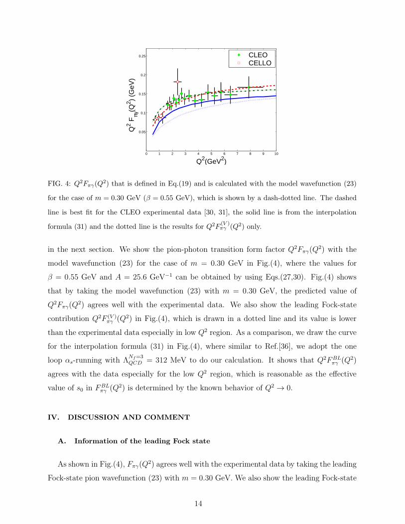
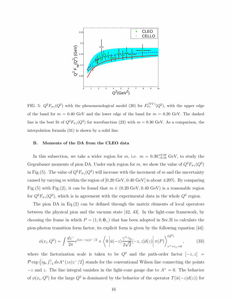
FIG. 5: Q2Fπγ(Q2) with the phenomenological model (20) for F

(NV )πγ (Q2), with the upper edge

of the band for m = 0.40 GeV and the lower edge of the band for m = 0.20 GeV. The dashed

line is the best fit of Q2Fπγ(Q2) for wavefunction (23) with m = 0.30 GeV. As a comparison, the

interpolation formula (31) is shown by a solid line.

B. Moments of the DA from the CLEO data

In this subsection, we take a wider region for m, i.e. m = 0.30+0.10−0.10 GeV, to study the

Gegenbauer moments of pion DA. Under such region for m, we show the value of Q2Fπγ(Q2)

in Fig.(5). The value of Q2Fπγ(Q2) will increase with the increment ofm and the uncertainty

caused by varyingm within the region of [0.20 GeV, 0.40 GeV] is about±20%. By comparing

Fig.(5) with Fig.(2), it can be found that m ∈ (0.20 GeV, 0.40 GeV) is a reasonable region

for Q2Fπγ(Q2), which is in agreement with the experimental data in the whole Q2 region.

The pion DA in Eq.(2) can be defined through the matrix elements of local operators

between the physical pion and the vacuum state [42, 43]. In the light-cone framework, by

choosing the frame in which P = (1, 0, 0⊥) that has been adopted in Sec.II to calculate the

pion-photon transition form factor, its explicit form is given by the following equation [44]:

φ(xi, Q2) =

∫

dz−

2πei(x1−x2)z−/2 ×

⟨

0

∣

∣

∣

∣

∣

u(−z)γ+γ5

2√2[−z, z]d(z)

∣

∣

∣

∣

∣

π(P )

⟩(Q2)

z+=z⊥=0

, (33)

where the factorization scale is taken to be Q2 and the path-order factor [−z, z] =

P exp(

igs∫ 1−1 dsA

+(zs)z−/2)

stands for the conventional Wilson line connecting the points

−z and z. The line integral vanishes in the light-cone gauge due to A+ = 0. The behavior

of φ(xi, Q2) for the large Q2 is dominated by the behavior of the operator T (u(−z)d(z)) for

16

z2 = O(1/Q2). One can apply the usual OPE and only gauge invariant operator that is

actually contributes to the matrix element in the light-cone gauge. Therefore only the qq

component is required in the above definition for the leading power behavior [43]. Also the

corresponding higher twist operators of the wave function matrix elements are suppressed

at the short distance by power of 1/Q2. Thus, the DA φ(xi, Q2) defined in Eq.(33) is the

amplitude for finding the qq component that is collinear up to the scale Q2. On the other

hand, the matrix element 〈0|uγµγ5d|π(P )〉 can be expressed by the following expansion [45]

〈0|u(−z)γµγ5[−z, z]d(z)|π(P )〉(Q2) =

i√2fπPµ

∫ 1

0du ei(2u−1)P ·zφπ(u,Q

2) +i√2m2

π

zµP · z

∫ 1

0duei(2u−1)P ·zgπ(u,Q

2),(34)

where φπ is the leading twist-2 DA, gπ is the twist-4 DA. Under the light-cone gauge, the

DA φ(xi, Q2) defined in Eq.(33) corresponds to the leading twist-2 DA φπ defined in Eq.(34),

except for an overall normalization factor. Both definitions are consistent with each other.

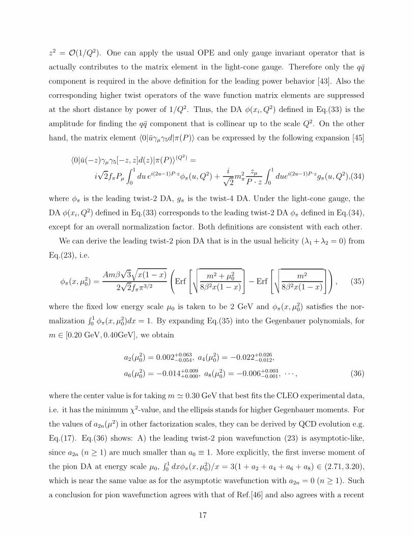
We can derive the leading twist-2 pion DA that is in the usual helicity (λ1+λ2 = 0) from

Eq.(23), i.e.

φπ(x, µ20) =

Amβ√3√

x(1− x)

2√2fππ3/2

Erf

√

√

√

√

m2 + µ20

8β2x(1− x)

− Erf

√

√

√

√

m2

8β2x(1− x)

, (35)

where the fixed low energy scale µ0 is taken to be 2 GeV and φπ(x, µ20) satisfies the nor-

malization∫ 10 φπ(x, µ

20)dx = 1. By expanding Eq.(35) into the Gegenbauer polynomials, for

m ∈ [0.20 GeV, 0.40GeV], we obtain

a2(µ20) = 0.002+0.063

−0.054, a4(µ20) = −0.022+0.026

−0.012,

a6(µ20) = −0.014+0.009

+0.000, a8(µ20) = −0.006+0.003

−0.001, · · · , (36)

where the center value is for takingm ≃ 0.30 GeV that best fits the CLEO experimental data,

i.e. it has the minimum χ2-value, and the ellipsis stands for higher Gegenbauer moments. For

the values of a2n(µ2) in other factorization scales, they can be derived by QCD evolution e.g.

Eq.(17). Eq.(36) shows: A) the leading twist-2 pion wavefunction (23) is asymptotic-like,

since a2n (n ≥ 1) are much smaller than a0 ≡ 1. More explicitly, the first inverse moment of

the pion DA at energy scale µ0,∫ 10 dxφπ(x, µ

20)/x = 3(1 + a2 + a4 + a6 + a8) ∈ (2.71, 3.20),

which is near the same value as for the asymptotic wavefunction with a2n = 0 (n ≥ 1). Such

a conclusion for pion wavefunction agrees with that of Ref.[46] and also agrees with a recent

17

study that is based on the nonlocal chiral-quark model from the instanton vacuum [47]. B)

a2, a4 will increase with the decrement of m, and a2 ≥ 0 if m ≤ 0.30 GeV. C) the absolute

values of a4, a6 and a8 are comparable to a2 for bigger m (e.g. m ∼ 0.30 GeV); but they

are suppressed to a2 about one order for smaller m. The value of the Gegenbauer moments

have been studied in various processes, cf. Refs.[15, 32, 35, 36, 47, 48, 49, 50, 51, 52, 53].

The lattice result of Ref.[52] prefers a narrower DA with a2(1 GeV2) = 0.07(1), while the

lattice results [50, 51] prefer wider DA, i.e. they obtain a2(1 GeV2) = 0.38 ± 0.23+0.11−0.06 and

a2(1 GeV2) = 0.364± 0.126 respectively. However as argued in Ref.[54], the accuracy of the

lattice results needs to be further improved, e.g. the results in Ref.[51] for the second moment

〈ξ2〉 are obtained for the “pion” with the masses µπ > 550 MeV and then extrapolated

to the chiral limit µπ → 0. These references favor a positive value for a2(1 GeV2) and

the most recent one is done by Ref.[49], which shows that a2(1 GeV2) = 0.19 ± 0.19 and

a4(1 GeV2) ≥ −0.07 by analyzing the leptonic mass spectrum of B → πlν. Here, the range

of m should be reduced to m ∈ [0.20 GeV, 0.30 GeV] if we require a2(1 GeV2) ≥ 0 for the

pion DA. Or inversely, we have a2(1 GeV2) ∈ [0, 0.08] with the help of the QCD evolution

equation (17) for m ∈ [0.20 GeV, 0.30 GeV].

C. Comparison with the broad wavefunction

One typical broad wavefunction is described by the CZ-like wavefunction, which can not

be excluded by the pion-photon transition form factor [5] although it is disfavored by the

pion structure function at x→ 1 [28].

We take the CZ-like wavefunction as

ΨCZqq (x,k⊥) = A(1− 2x)2 exp

[

− k2⊥ +m2

8β2x(1 − x)

]

χK(x,k⊥), (37)

where an extra factor (1− 2x)2 is introduced into the pion wavefunction (23) [3]. Following

a similar procedure, we find that the relation between m and β changes to

6.00mβ

f 2π

∼= 1.24

(

m

β+ 2.12

)(

m

β+ 4.58× 101

)

. (38)

Similarly, for m = 0.30 GeV, we have

Pqq = 73%, 〈k2⊥〉qq = (0.496 GeV)2, 〈r2π+〉qq = (0.45 fm)2, (39)

18

0 2 4 6 8 10

0.05

0.1

0.15

0.2

0.25

Q2 F

πγ(Q

2 ) (G

eV)

Q2(GeV2)

CLEOCELLO

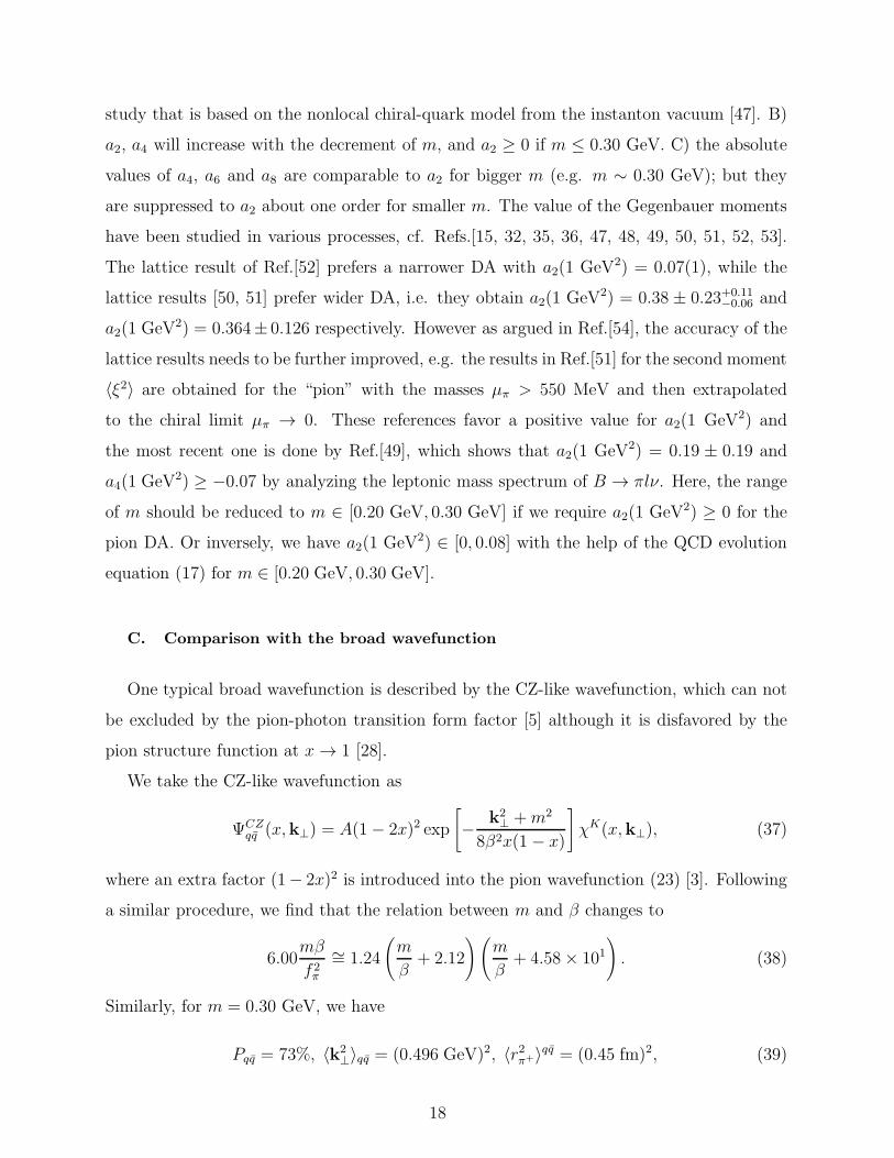
FIG. 6: Comparison of Q2Fπγ(Q2) that is derived from two different types of wavefunctions, i.e.

the BHL-like wavefunction (the solid line) and the CZ-like wavefunction (the dash-dotted line),

under the condition of m = 0.30 GeV.

where all the values are summed results for all the helicity states λ1 + λ2 = (0,±1) of

the leading Fock state. One may observe that the second Gegenbauer moment a2 is always

dominant over other higher Gegenbauer moments for the CZ-like DA. And for the first inverse

moment of the CZ-like pion DA at energy scale µ0, we obtain∫ 10 dxφ

CZπ (x, µ2

0)/x = 4.69.

In Fig.(6), we make a comparison of Q2Fπγ(Q2) that is derived from two different types

of wavefunctions, i.e. the BHL-like wavefunction and the CZ-like wavefunction, under the

same value of m = 0.30 GeV. Both the BHL-like wavefunction and the CZ-like wavefunction

lead to Q2Fπγ(Q2) within the possible region of the experimental data as shown in Fig.(2).

However, the value of Q2Fπγ(Q2) derived from the BHL-like wavefunction is better than

that of the CZ-like wavefunction. One may observe that the value of Q2Fπγ(Q2) caused by

the CZ-like wavefunction shall increase with the increment of m, so the CZ-like model can

give a better result for Q2Fπγ(Q2) in comparison to the experimental data only by taking a

bigger value for m, e.g. at least, m = 0.40 GeV.

As a summary, the main differences for the BHL-like wavefunction and the CZ-like wave-

function are listed in the following:

• By comparing with the experimental data for Q2Fπγ(Q2), one may observe that m =

0.30+0.10−0.10 GeV is a reasonable region for the BHL-like wavefunction, where the best fit

to the experimental data is achieved when m ≈ 0.30 GeV; while for the case of the

19

0 2 4 6 8 10

0.1

0.2

0.3

0.4

0.5

R

Q2(GeV2)

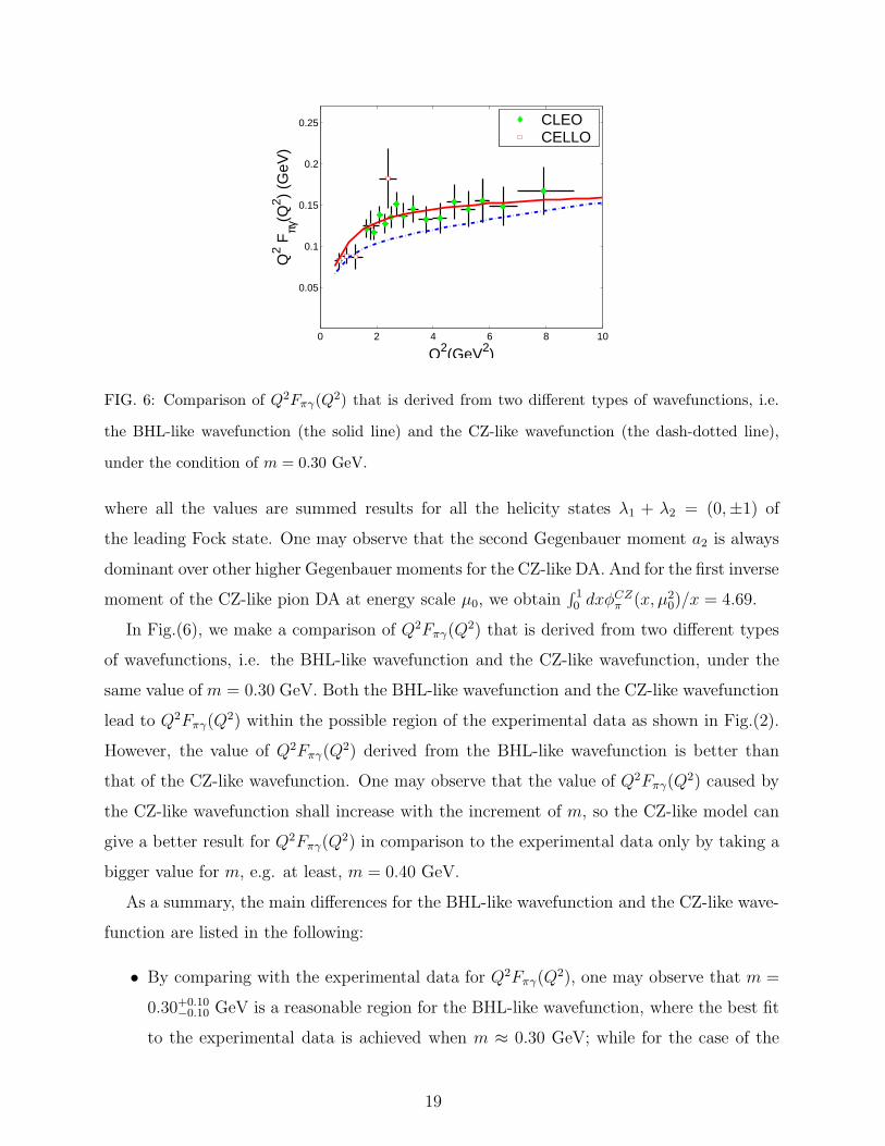
FIG. 7: The value of R =F

(NV )πγ (Q2)

F(V )πγ (Q2)+F

(NV )πγ (Q2)

versus Q2 for the BHL-like wavefunction, whose

value increases with the increment of m. The solid, dashed and dotted lines are for m = 0.20GeV ,

m = 0.30GeV and m = 0.40GeV , respectively.

CZ-like wavefunction, such region is shifted to a higher one, i.e. m = 0.40+0.10−0.10 GeV,

and the best fit to the experimental data is achieved as m ≈ 0.40 GeV, which is

somewhat bigger than the conventional value for the constitute quark mass of pion.

• The difference among the Gegenbauer moments e.g. a2(µ20) are big due to the different

behavior of the two models. Under the condition ofm = 0.30 GeV, the two Gegenbauer

moments a2(µ20) = 0.002 and a4(µ

20) = −0.022 for the BHL-like model (20); while for

the CZ-like model (37), a2(µ20) = 0.678 and a4(µ

20) = −0.024.

• The first inverse moments are different. Under the condition of m = 0.30 GeV, for the

case of the BHL-like model (20),∫ 10 dxφ

BHLπ (x, µ2

0)/x = 2.88, which is close to that of

the asymptotic DA; while for the case of the CZ-like model (37),∫ 10 dxφ

CZπ (x, µ2

0)/x =

4.69, which is close to that of the original CZ-model [3].

In Ref.[54], it was shown that by taking the asymptotic DA and considering the suppres-

sion from the NLO contribution, the value of Q2Fπγ(Q2) at Q2 = 8.0 GeV2 is somewhat

smaller than the experimental value (16.7±2.5±0.4)·10−2 GeV, i.e. Q2Fπγ(Q2)|Q2=8.0 GeV2 ≃

0.115 GeV. However it should be pointed out that Ref.[54] is only a simplified analysis, since

the effects caused by the kT -dependence in both the pion wavefunction and the hard scatter-

ing amplitude, and the contribution from F (NV )πγ (Q2) have not been taking into consideration.

20

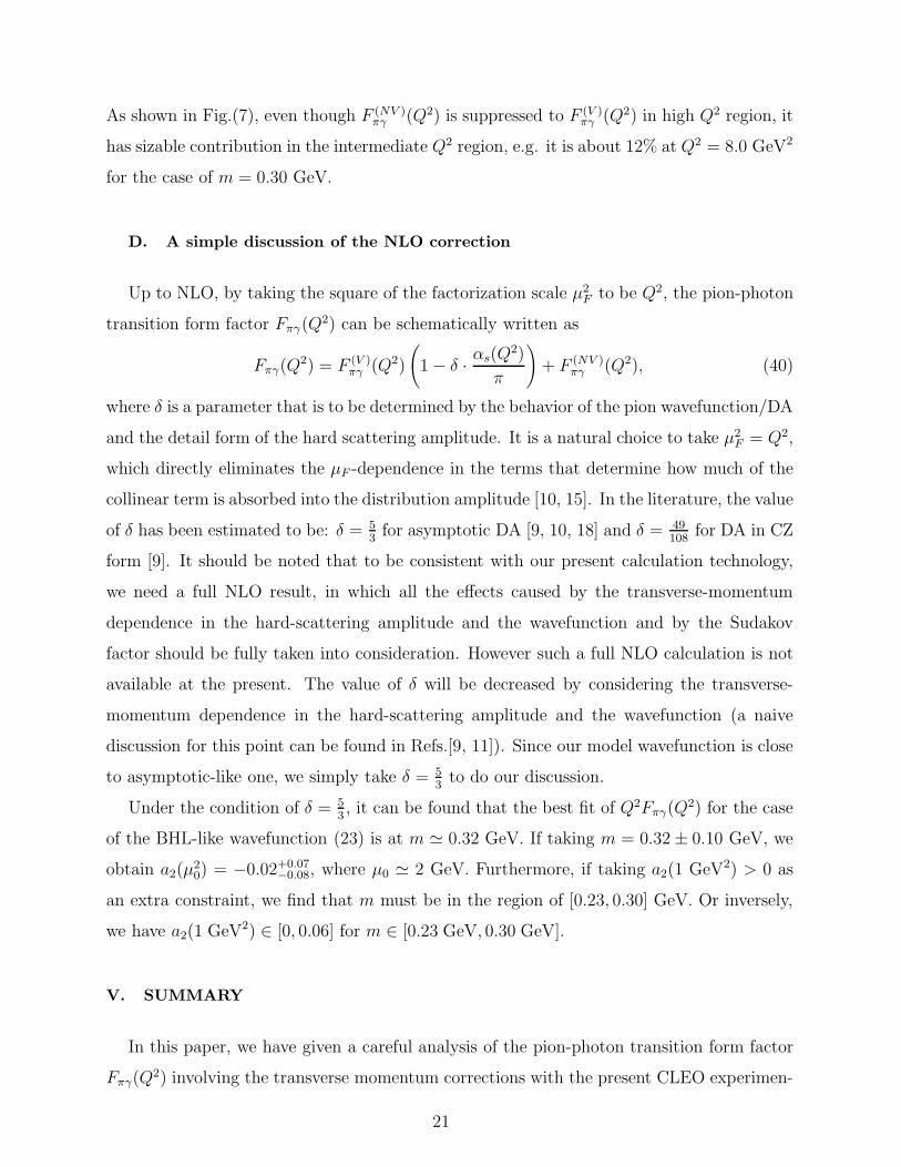
As shown in Fig.(7), even though F (NV )πγ (Q2) is suppressed to F (V )

πγ (Q2) in high Q2 region, it

has sizable contribution in the intermediate Q2 region, e.g. it is about 12% at Q2 = 8.0 GeV2

for the case of m = 0.30 GeV.

D. A simple discussion of the NLO correction

Up to NLO, by taking the square of the factorization scale µ2F to be Q2, the pion-photon

transition form factor Fπγ(Q2) can be schematically written as

Fπγ(Q2) = F (V )

πγ (Q2)

(

1− δ · αs(Q2)

π

)

+ F (NV )πγ (Q2), (40)

where δ is a parameter that is to be determined by the behavior of the pion wavefunction/DA

and the detail form of the hard scattering amplitude. It is a natural choice to take µ2F = Q2,

which directly eliminates the µF -dependence in the terms that determine how much of the

collinear term is absorbed into the distribution amplitude [10, 15]. In the literature, the value

of δ has been estimated to be: δ = 53for asymptotic DA [9, 10, 18] and δ = 49

108for DA in CZ

form [9]. It should be noted that to be consistent with our present calculation technology,

we need a full NLO result, in which all the effects caused by the transverse-momentum

dependence in the hard-scattering amplitude and the wavefunction and by the Sudakov

factor should be fully taken into consideration. However such a full NLO calculation is not

available at the present. The value of δ will be decreased by considering the transverse-

momentum dependence in the hard-scattering amplitude and the wavefunction (a naive

discussion for this point can be found in Refs.[9, 11]). Since our model wavefunction is close

to asymptotic-like one, we simply take δ = 53to do our discussion.

Under the condition of δ = 53, it can be found that the best fit of Q2Fπγ(Q

2) for the case

of the BHL-like wavefunction (23) is at m ≃ 0.32 GeV. If taking m = 0.32± 0.10 GeV, we

obtain a2(µ20) = −0.02+0.07

−0.08, where µ0 ≃ 2 GeV. Furthermore, if taking a2(1 GeV2) > 0 as

an extra constraint, we find that m must be in the region of [0.23, 0.30] GeV. Or inversely,

we have a2(1 GeV2) ∈ [0, 0.06] for m ∈ [0.23 GeV, 0.30 GeV].

V. SUMMARY

In this paper, we have given a careful analysis of the pion-photon transition form factor

Fπγ(Q2) involving the transverse momentum corrections with the present CLEO experimen-

21

tal data, in which the contributions beyond the leading Fock state have been taken into

consideration. As is well-known, the leading Fock-state contribution dominates the pion-

photon transition from factor Fπγ(Q2) for large Q2 region and it gives only half contribution

to Fπγ(0) as one extends it to Q2 = 0. One should consider the higher Fock states’ contri-

bution to Fπγ(0) at the present experimental Q2 region. We have constructed a phenomeno-

logical expression to estimate the contributions beyond the leading Fock state based on the

limiting behavior of F (NV )πγ (Q2) at Q2 → 0. The calculated results favor the asymptotic-like

behavior by comparing the predictions from different type of the model wavefunctions with

the experimental data.

On the other hand, the present CLEO data provides the important information of the

pion DA as one has a complete expression for the pion-photon transition form factor relates

two photons with one pion. Our expression for Fπγ(Q2) only involves a single pion DA. Thus,

comparing the calculated results of Fπγ(Q2) by taking the BHL-like pion wavefunction with

the CLEO data one can extract some useful information of the pionic leading twist-2 DA.

Our analysis shows that (1) the probability of finding the leading Fock state in the pion is

less than one, i.e. Pqq = 56% and 〈r2π+〉qq = (0.33 fm)2 with m = 0.30 GeV. This means that

the leading Fock state is more compact in the pion and it is necessary to take the higher

Fock states into account to give full estimation of the pion-photon transition form factor

and other exclusive processes. (2) under the region of m ∈ [0.20 GeV, 0.40 GeV], we have

the DA moments: a2(µ20) = 0.002+0.063

−0.054, a4(µ20) = −0.022+0.026

−0.012 and all of higher moments.

Such result is helpful to understand other exclusive processes involving the pion.

ACKNOWLEDGEMENTS

This work was supported in part by the Natural Science Foundation of China (NSFC).

X.-G. Wu thanks the support from the China Postdoctoral Science Foundation.

[1] G.P. Lepage and S.J. Brodsky, Phys.Rev.D22, 2157(1980); S.J. Brodsky and G.P. Lepage,

Phys.Rev.D24, 1808(1981).

[2] Particle Data Group, E.J. Weinberg, etal., Phys.Rev. D66, 010001(2002).

[3] V.L. Chernyak and A.R. Zhitnitsky, Nucl.Phys. B201, 492(1982).

22

[4] S.J. Brodsky, T. Huang and G.P. Lepage, in Particles and Fields-2, Proceedings of the Banff

Summer Institute, Banff, Alberta, 1981, edited by A.Z. Capri and A.N. Kamal (Plenum,

New York, 1983), P143; T. Huang, in Proceedings of XXth International Conference on High

Energy Physics, Madison, Wisconsin, 1980, edited by L.Durand and L.G. Pondrom, AIP

Conf.Proc.No. 69(AIP, New York, 1981), p1000.

[5] Fu-Guang Cao, Tao Huang and Bo-Qiang Ma, Phys.Rev. D53, 6582(1996).

[6] Bo-Wen Xiao and Bo-Qiang Ma, Phys.Rev. D68, 034020(2003).

[7] R. Jakob etal., J.Phys. G22, 45(1996); P. Kroll and M. Raulfs, Phys.Lett. B387, 848(1996).

[8] A.V. Radyushkin and R. Ruskov, Nucl.Phys. B481, 625(1996).

[9] I.V. Musatov and A.V. Radyushkin, Phys.Rev. D56, 2713(1997).

[10] B. Melic, B. Nizic and K. Passek, Phys.Rev. D65, 053020(2002); F. Del Aguila and M.K.

Chase, Nucl.Phys. B193, 517(1981); E. Braaten, Phys.Rev. D28, 524(1983).

[11] N.G. Stefanis, W. Schroers and H.-Ch. Kim, Eur.Phys.J. C18, 137(2000).

[12] S. Ong, Phys.Rev. D52, 3111(1995).

[13] Tao Huang and Qi-Xing Shen, Proceedings of the international seminar of Quark’90, Telavi,

USSR, (1990), Ed. by Matveev etal., page 340; Z.Phys. C50, 139(1991).

[14] J. Boots and G. Sterman, Nucl.Phys. B325, 62(1989); H.N. Li and G. Sterman, Nucl.Phys.

B381, 129(1992).

[15] A.P. Bakulev, K. Passek-Kumericki, W. Schroers and N.G. Stefanis Phys.Rev. D70,

033014(2004); Erratum-ibid.D70, 079906(2004).

[16] T.W. Yeh, Phys.Rev. D65, 074016(2002).

[17] A.V. Radyushkin, Acta Phys.Polon. B26, 2067(1995); hep-ph/9511272.

[18] S.J. Brodsky, C.R. Ji, A. Pang and D.G. Robertson, Phys.Rev. D57, 245(1998).

[19] G.P. Lepage, S.J. Brodsky, T. Huang and P.B. Mackezie, in Particles and Fields-2, page 83,

Invited talk presented at the Banff summer Institute on Particle Physics, Banff, Alberta,

Canada, 1981.

[20] S.J. Brodsky, H.C. Pauli and S.S. Pinsky, Phys.Rept. 301, 299(1998); and references therein.

[21] S.D. Drell and T.M. Yan, Phys.Rev. Lett.24, 181(1970); G.B. West, Phys.Rev. Lett.24,

1206(1970).

[22] K. Wilson, Phys.Rev. 179, 1499(1969); R. Brandt and G. Preparata, Nucl.Phys. B27,

541(1971); N. Christ, B. Hasslacher and A.H. Mueller, Phys.Rev. D6, 3543(1972).

23

[23] H.B. O’Connell, B.C. Pearce, A.W. Thomas and A.G. Williams, Prog.Part.Nucl.Phys. 39,

201(1997).

[24] J.P.B.C. de Melo, T. Frederico, E. Pace and G. Salme, Phys.Lett. B581, 75(2004);

[25] J.P.B.C. de Melo, T. Frederico, E. Pace and G. Salme, Phys.Rev. D73, 074013(2006).

[26] T. Draper, R.M. Woloshyn, W. Wilcox and K. Liu, Nucl.Phys. B318, 319(1989).

[27] S. Treiman, R. Jackiw and D. Gross, Lectures on the Current Algebra and its Applications,

Princeton University Press (Princeton, 1972).

[28] T. Huang, B.Q. Ma and Q.X. Shen, Phys.Rev. D49, 1490(1994).

[29] Dieter Muller, Phys.Rev. D51, 3855(1995).

[30] CLEO collaboration, V. Savinov et al., hep-ex/9707028; CLEO Collaboration, J. Gronberg et

al., Phys.Rev. D57, 33(1998).

[31] CELLO collaboration, H.-J. Behrend et al, Z.Phys. C49, 401(1991).

[32] A. Schmedding and O. Yakovlev, Phys.Rev. D62, 116002(2000).

[33] A.E. Dorokhov, JETP Lett. 77, 63(2003); hep-ph/0212156.

[34] W.H. Press, S.A. Teukolsky, W.T. Vetterling and B.P. Flannery, Numerical Recipes in Fortran

77: The Art of Scientific Computing, Second Editon, Published by the Press Syndicate of the

University of Cambridge (1992), p650.

[35] A.P. Bakulev, S.V. Mikhailov and N.G. Stefanis, Phys.Lett. B578, 91(2004).

[36] A.P. Bakulev, S.V. Mikhailov and N.G. Stefanis, Phys.Rev. D67, 074012(2003); Phys.Rev.

D73, 056002(2006).

[37] Tao Huang, Xing-Gang Wu and Xing-Hua Wu, Phys.Rev. D70, 053007(2004); Xing-Gang Wu

and Tao Huang, Int.J.Mod.Phys. A21, 901(2006).

[38] Tao Huang and Xing-Gang Wu, Phys.Rev. D70, 093013(2004).

[39] F. Cardarelli, etal., Phys.Rev. D53, 6682(1996).

[40] S.R. Amendolia, etal., Phys.Lett. B146, 116(1985).

[41] B. Povh and J. Hufner, Phys.Lett. B245, 653(1990); T. Huang, Nucl.Phys. (Proc. Suppl.) 7,

320(1989).

[42] A.V. Radyushkin, hep-ph/0410276.

[43] S.J. Brodsky, Y. Frishman and G.P. Lepage, Phys.Lett. B91, 239(1980).

[44] S.J. Brodsky, P. Damgaard, Y. Frishman and G.P. Lepage, Phys.Rev. D33, 1881(1986).

[45] P. Ball, J. High Energy Phys. 9901, 010(1999).

24

[46] P. Kroll and M. Raulfs, Phys.Lett. B387, 848(1996); A.P. Bakulev, S.V. Mikhailov, N.G.

Stefanis, Phys.Lett. B508, 279(2001), Erratum: ibid B590, 309(2004).

[47] Seung-il Nam, Hyun-Chul Kim, Atsushi Hosaka and M. M. Musakhanov, hep-ph/0605259.

[48] V.M. Braun, A. Khodjamirian and M. Maul, Phys.Rev. D61, 073004(2000).

[49] P. Ball and R. Zwicky, Phys.Lett. B625, 225(2005).

[50] L. Del Debbio, M. Di Perro and A. Dougall, Nucl.Phys.Proc.Suppl. 119, 416(2003).

[51] M. Gockeler, et al hep-lat/0510089.

[52] S. Dalley and Brett van de Sande, Phys.Rev. D67, 114507(2003).

[53] S.S. Agaev, Phys.Rev. D72, 114010(2005); Erratum-ibid. D73, 059902(2006).

[54] V.L. Chernyak, hep-ph/0605327.

25