arXiv:hep-ph/0504242v1 26 Apr 2005

arX

iv:h

ep-p

h/05

0424

2v1

26

Apr

200

5NIKHEF 05-006 hep-ph/0504242DCPT/05/28, IPPP/05/14DESY 05-063, SFB/CPP-05-13April 2005

The third-order QCD corrections to

deep-inelastic scattering by photon exchange

J.A.M. Vermaserena, A. Vogtb and S. Mochc

aNIKHEF Theory Group

Kruislaan 409, 1098 SJ Amsterdam, The Netherlands

bIPPP, Department of Physics, University of Durham

South Road, Durham DH1 3LE, United Kingdom

cDeutsches Elektronensynchrotron DESY

Platanenallee 6, D–15738 Zeuthen, Germany

Abstract

We compute the full three-loop coefficient functions for thestructure functionsF2 andFL in mass-less perturbative QCD. The results forFL complete the next-to-next-to-leading order descriptionof unpolarized electromagnetic deep-inelastic scattering. The third-order coefficient functions forF2 form, at not too small values of the Bjorken variablex, the dominant part of the next-to-next-to-next-to-leading order corrections, thus facilitating improved determinations of the strong couplingαs from scaling violations. The three-loop corrections toFL are larger than those forF2. Espe-cially for the latter quantity the expansion in powers ofαs is very stable, for photon virtualitiesQ2 ≫ 1 GeV2, over the fullx-range accessible to fixed-target and collider measurements.

1 Introduction

Structure functions in deep-inelastic scattering (DIS) and their scale evolution are closely relatedto the origins of Quantum Chromodynamics (QCD) and its very formulation as the gauge theoryof the strong interaction [1–5]. In fact, ever since the pioneering measurements at SLAC [6–8],DIS structure functions have been the subject of detailed theoretical and experimental investiga-tions, see, e.g., the Review of Particle Properties [9] and references therein. Today, with high-precision data from the electron–proton collider HERA and in view of the outstanding importanceof hard scattering processes at proton–(anti-)proton colliders like the TEVATRON and the forth-coming LHC, a quantitative understanding of deep-inelastic processes is indispensable.

For quantitatively reliable predictions of DIS and hard hadronic scattering processes, perturba-tive QCD corrections beyond the next-to-leading order (NLO) need to be taken into account. Wehave therefore calculated the three-loop splitting functions for the evolution of unpolarized partondistributions of hadrons [10, 11]. Together with the second-order coefficient functions [12–16],these recent results form the complete next-to-next-to-leading order (NNLO, N2LO) approxima-tion of massless perturbative QCD for the structure functionsF1, F2 andF3 in DIS.

In the present article, we extend the calculation of electromagnetic (photon-exchange) DISin perturbative QCD to the three-loop coefficient functionsfor bothF2 andFL = F2−2xF1. Thisrepresents the first calculation of third-order perturbative corrections to hard scattering observablesdepending on a dimensionless variable (Bjorken-x in the case at hand) in the Standard Model. Forthe longitudinal structure functionFL the third-order corrections are actually required to completethe NNLO predictions, since the leading contribution to thecoefficient functions is of first order inthe strong coupling constantαs. In a recent letter [17] we have already presented the correspondingresults in a compact numerical form, and briefly discussed their phenomenological implications.

For the structure functionsF1 andF2, on the other hand, the three-loop coefficient functions arepart of the next-to-next-to-next-to-leading order (N3LO) description of DIS in perturbative QCD.In fact, due to the fast convergence of the splitting function series [10, 11], these coefficient func-tions dominate the N3LO corrections for not too small values of the Bjorken variable, x >

∼ 10−2.Thus the extraction ofαs from the scaling violations of structure functions can be effectively pro-moted to N3LO accuracy, reducing the (formerly dominant) uncertaintydue to the truncation of theperturbation series to less than 1%, see, e.g., Refs. [18–22]. The three-loop coefficient functionsare also of considerable theoretical interest, for examplefacilitating the derivation of higher-orderresults for the resummation of threshold logarithms [23–28] and the quark form factor [29,30]. Wewill address these issues in a forthcoming publication [31].

As discussed in Refs. [10,11], see also Refs. [32–35], the NNLO splitting functions have beendetermined via a Mellin-N space calculation of physical matrix elements of electromagnetic DISat three loops in dimensional regularization withD = 4− 2ε. While the splitting functions areextracted from the 1/ε poles, the coefficient functions are obtained from the finiteterms of thephysical matrix elements corresponding to the structure functionsF2 andFL. This is possible since

1

we have taken care to control all necessary three-loop integrals up to (and including) the finitecontributions. In this respect our approach closely follows the third-order calculations of sumrules in DIS [36,37] and of low integer moments of structure functions [38–42], however with theobvious distinction that we now derive the analytic dependence onN and, consequently, onx.

The outline of this article is as follows. In Section 2 we briefly recall the formalism, based onthe operator product expansion, for calculating inclusiveDIS in Mellin-N space and discuss theextraction of the anomalous dimensions (splitting functions) and coefficient functions. Section 3explains selected details of the method to calculate the analytic N-dependence of the diagrams andaddresses issues which did not occur in the calculation of the splitting functions. In Section 4 wepresent our results forF2 in a compact parametrized form and discuss the end-point behaviour ofthe coefficient functions forF2 andFL. The lengthy full expressions for both coefficient functionsare deferred to Appendix A (N-space) and Appendix B (x-space). The numerical implications ofthese results are illustrated in Section 5 before we summarize our findings in Section 6.

2 General formalism

The subject of our calculation is unpolarized inclusive deep-inelastic lepton-nucleon scattering,

l(k) + nucl(p) → l(k′) + X (2.1)

whereX stands for all hadronic states allowed by quantum number conservation. Specifically,we here consider the lowest-order (one-photon exchange) QED contribution to this process. Thehadronic part of the corresponding amplitude is given by the(spin-averaged) tensor

Wµν(p,q) =14π

∫d4zeiq·z〈nucl,p|Jµ(z)Jν(0)|nucl,p〉

=(qµqν

q2 −gµν

)F1(x,Q

2)− (qµ+2xpµ)(qν +2xpν)1

2xq2 F2(x,Q2) . (2.2)

Here|nucl,p〉 denotes the nucleon state with momentump, andJµ represents the electromagneticcurrent. q = k− k′ is the momentum transferred by the lepton,Q2 = −q2, andx = Q2/(2p · q)

is the Bjorken variable with 0< x ≤ 1. The longitudinal structure functionFL is related to thestructure functionF1 in Eq. (2.2) byFL = F2−2xF1.

The hadronic tensorWµν is connected by the optical theorem to the imaginary part of the for-ward amplitudeTµν for the scattering of a virtual photon off the nucleon,

Tµν(p,q) = i∫

d4z eiqz〈nucl,p|T(Jµ(z)Jν(0)) |nucl,p〉 . (2.3)

This quantity represents a convenient starting point for practical calculations, due to the presenceof the time-ordered product of currents to which standard perturbation theory applies.

2

Approaching the Bjorken limit,Q2 → ∞ for fixed x, the integrations in Eq. (2.2) and (2.3) aredominated by the region near the light-cone,z2 ≈ 0, as only there the phase of the exponentialfactor becomes stationary. In this situation, the operator-product expansion (OPE) can be appliedto the product of currents in Eq. (2.3) together with a dispersion relation [43]. This procedure isidentical to that in previous lower-order and fixed-N third-order calculations. Thus we will recallit only briefly, referring the reader to Refs. [16,40] and thereviews [44,45] for more details.

Disregarding contributions suppressed by powers of 1/Q2, the OPE involves the standard setof the spin-N twist-two irreducible flavour non-singlet quark, singlet quark and gluon operators,

O{µ1,...,µN}ns = ψλα γ{µ1Dµ2 . . .DµN}ψ , α = 3,8, ...,(n2

f −1) ,

O{µ1,...,µN}q = ψγ{µ1Dµ2 . . .DµN}ψ ,

O{µ1,...,µN}g = Fν{µ1Dµ2 · · ·DµN−1 FµN}ν , (2.4)

and their respective coefficient functionsCa,i(N) for a = 2, L. Hereψ represents the quark field,Fµν the gluon field strength tensor, andDµ the covariant derivative. The diagonal generators of theflavour groupSU(nf ) are denoted byλα. The spin-averaged matrix elements of the (renormalized)operators in Eq. (2.4) are given by

〈nucl,p|O{µ1,...,µN}i |nucl,p〉 = p{µ1...pµN}Ai,nucl(N,µ2) , i = ns, q, g, (2.5)

whereµ stands for the renormalization scale. It is understood in Eqs. (2.4) and (2.5) that thesymmetric and traceless part is taken with respect to the indices in curved brackets.

The application of the operator-product expansion to the forward Compton amplitude (2.3),neglecting 1/Q2 power corrections, leads to the expansion

Tµν(p,q) = ∑N,i

( 2p ·qQ2

)NAi,nucl(N,µ2)

[(gµν +

qµqν

Q2

)CL,i

(N,

Q2

µ2 ,αs

)

−

(gµν − pµpν

4x2

Q2 − (pµqν + pνqµ)2xQ2

)C2,i

(N,

Q2

µ2 ,αs

)]. (2.6)

The continuation of this result to the physical region 0< x ≤ 1 by a dispersion relation in thecomplex-x plane finally yields the even-integer Mellin-N moments of the structure functions1

xF2and 1

xFL in Eq. (2.2),

Fa(N,Q2) =

∫ 1

0dxxN−1 1

xFa(x,Q

2) , (2.7)

in terms of the matrix elements (2.5) and the corresponding coefficient functions,

1+(−1)N

2Fa(N,Q2) = ∑

i=ns,q,gCa,i

(N,

Q2

µ2 ,αs

)Ai,nucl(N,µ2) , a = 2,L . (2.8)

Note that all (complex) momentsN, and thus, by the inverse of the Mellin transformation (2.7),the completex-dependence, are uniquely fixed by analytic continuation ofthese even-N results.

3

The operatorsOq andOg in Eq. (2.4) mix under renormalization. Expressing the renormalizedoperators in terms of their bare counterparts, this mixing can be written as

Oi = Zik Obarek . (2.9)

The anomalous dimensionsγik governing the scale dependence of the operatorsOi ,

dd lnµ2 Oi = −γik Ok ≡ Pik Ok , (2.10)

are connected to the mixing matrixZik in Eq. (2.9) by

γik = −

(d

d lnµ2 Zi j

)(Z−1) jk . (2.11)

The summation convention is understood in Eqs. (2.9) – (2.11), and the dependence onN hasbeen suppressed for brevity. In Eq. (2.10) we have taken the opportunity to recall the conventionalrelation between the anomalous dimensions and the moments of the splitting functionsPik(x).Corresponding scalar relations, independent of the generator λα in Eq. (2.4), hold for the non-singlet operators collectively denoted byOns.

In order to make practical use of Eq. (2.11) a regularizationprocedure and a renormalizationscheme need to be selected. We choose dimensional regularization [46–49] and the modified [50]minimal subtraction [51] scheme,MS, the standard choice for modern higher-order calculations inQCD. For this choice the running coupling inD = 4−2ε dimensions evolves according to

dd lnµ2

αs

4π≡

d as

d lnµ2 = −εas−β0a2s−β1a3

s−β2a4s − . . . , (2.12)

whereβn denote the usual four-dimensional expansion coefficients of the beta function in QCD[52–57], β0 = 11−2/3nf etc, withnf representing the number of active quark flavours.

In this framework, the renormalization factorsZik in Eq. (2.9) andZns are a series of poles in1/ε, expressed in terms ofβn and the expansion coefficientsγ(l) of the anomalous dimensions interms ofas,

γ(N) =∞

∑l=0

al+1s γ(l)(N) . (2.13)

For example, the expansion ofZns up to the third order in the coupling constant reads

Zns = 1 + as1ε

γ(0)ns + a2

s

[1

2ε2

{(γ(0)

ns −β0

)γ(0)

ns

}+

12ε

γ(1)ns

]

+ a3s

[1

6ε3

{(γ(0)

ns −2β0

)(γ(0)

ns −β0

)γ(0)

ns

}

+1

6ε2

{3γ(0)

ns γ(1)ns −2β0γ(1)

ns −2β1γ(0)ns

}+

13ε

γ(2)ns

]. (2.14)

4

The anomalous dimensionsγ(l) can thus be read off from theε−1 terms of the renormalizationfactors at orderal+1

s , while the higher poles in 1/ε can serve as checks for the calculation. Thecoefficient functions in Eq. (2.6), on the other hand, have anexpansion in positive powers ofε, viz

Ca,i = δa2(1−δig)+∞

∑l=1

als

(c(l)

a,i + εa(l)a,i + ε2b(l)

a,i + . . .)

(2.15)

wherea = 2, L andi = ns, q, g, and we have again suppressed the dependence onN (andQ2/µ2).

Due to the non-perturbative character of the nucleon state|nucl,p〉, Eqs. (2.3) and (2.8) are notaccessible to a perturbative computation. However, as the OPE represents an operator relation,the anomalous dimensions (2.13) and the coefficient functions (2.15) do not depend on this state.Hence the calculation can be performed using quark and gluonstates|k, p〉. Instead of Eq. (2.3)we thus consider

T kµν(p,q) = i

∫d4zeiqz〈k, p|T(Jµ(z)Jν(0)) |k, p〉 , k = ns, q, g . (2.16)

At leading-twist accuracy the decomposition ofT kµν into T2,k andTL,k analogous to Eq. (2.2) is

provided by

TL,k(p,q) = −q2

(p ·q)2 pµpν T kµν(p,q)

T2,k(p,q) = −

(3−2ε2−2ε

q2

(p ·q)2 pµpν +1

2−2εgµν

)T k

µν(p,q) (2.17)

with spin-averaging again being understood. TheNth moments are obtained from Eqs. (2.17) byapplying the projection operator [58,59]

Ta,k

(N,

Q2

µ2 ,αs,ε)

=

[q{µ1 · · ·qµN}

2NN!∂N

∂pµ1 . . .∂pµN

]Ta,k(p,q,αs,ε)

∣∣∣∣p=0

, (2.18)

whereq{µ1 · · ·qµN} is the harmonic, i.e., the symmetric and traceless part of the tensorqµ1 · · ·qµN .

This operator does not act on the coefficient functionsCa,k and the renormalization constantsZik in Eq. (2.9), which are functions only ofN, as, andε. It does act, however, on the bare matrixelementsAi,k (defined analogously to Eq. (2.5)) and eliminates all diagrams containing loops, asthe nullification ofp transform these diagrams to massless tadpole diagrams which are zero indimensional regularization. Hence only the matrix elementsAtree

k,k (N,ε) remain, leading to

Ta,k

(N,

Q2

µ2 ,αs,ε)

= Ca,i

(N,

Q2

µ2 ,αs,ε)

Zik

(N,αs,

1ε

)Atree

k,k (N,ε) (2.19)

for a = 2,L andk = ns, q, g. Here summation overi = q, g is understood for the singlet casesk = q, g, whileCa,i andZik have to be replaced byCa,ns andZns of Eq. (2.14), respectively, for thenon-singlet casek = ns. Expansion of (2.19) in powers ofαs andε provides a system of equationswhich can be solved for the anomalous dimensions (2.13) and coefficient functions (2.15).

5

For brevity suppressing the function arguments for the restof this section, the expansion of the‘master formula’ (2.19) to the third order in the strong coupling αs can by written as

Ta,k =3

∑l=0

als Sl

ε

( µ2

Q2

)lεδk T(l)

a,k Atreek,k . (2.20)

The factorSε = exp(ε{ln(4π)−γe}), whereγe denotes the Euler-Mascheroni constant, is an arte-fact of dimensional regularization [46–49] kept out of the coefficient functions and anomalousdimensions in theMS scheme [50].δk collects the quark charge factors,

δns = 1, δq = δg =1nf

nf

∑i=1

e2qi≡ 〈e2〉 . (2.21)

Theαs = 0 partsT(0)2,ns andT(0)

2,q can be rendered equal by a suitable normalization of non-singletmatrix elementsAtree

ns,ns. The amplitudesTa,ns andTa,q are then identical also at the first order inαs.Consequently, the same holds for the anomalous dimensions and coefficient functions (recall thedifferent counting of the superscripts in Eqs. (2.13) and (2.15)),

γ(0)ns = γ(0)

qq , c(1)ns = c(1)

q , c = c, a, b . . . . (2.22)

In the expansions shown below, we will use these right-hand sides also in the results forT(n>1)a,ns .

The zeroth-order contributions, withT(0)2,q being normalized by virtue of Eq. (2.21), read

T(0)2,q = c(0)

2,q = 1 , T(0)2,g = T(0)

L,q = T(0)L,g = 0 . (2.23)

As will become clear below, the amplitudes at the first order in αs need to be calculated up to orderε2 for our purposes, yielding

T(1)2,p =

1ε

γ(0)qp + c(1)

2,p + εa(1)2,p + ε2b(1)

2,p (2.24)

andT(1)

L,p = c(1)L,p + εa(1)

L,p + ε2b(1)L,p , (2.25)

with p = q, g. Correspondingly theα2s contributions, where the non-singlet and singlet quark

amplitudes differ for the first time, are required up to orderε. These quantities are given by

T(2)2,ns =

12ε2

{(γ(0)

qq −β0

)γ(0)

qq

}+

12ε

{γ(1)

ns +2c(1)2,qγ(0)

qq

}

+ c(2)2,ns+a(1)

2,qγ(0)qq + ε

{a(2)

2,ns+b(1)2,qγ(0)

qq

}, (2.26)

T(2)2,p =

12ε2

{(γ(0)

qi −β0δqi

)γ(0)

ip

}+

12ε

{γ(1)

qp +2c(1)2,i γ(0)

ip

}

+ c(2)2,p +a(1)

2,i γ(0)ip + ε

{a(2)

2,p +b(1)2,i γ(0)

ip

}, (2.27)

6

whereδik is the Kronecker symbol, and

T(2)L,ns =

1ε

{c(1)

L,qγ(0)qq

}+ c(2)

L,ns+a(1)L,qγ(0)

qq + ε{

a(2)L,p+b(1)

L,qγ(0)qq

}, (2.28)

T(2)L,p =

1ε

{c(1)

L,i γ(0)ip

}+ c(2)

L,p +a(1)L,i γ(0)

ip + ε{

a(2)L,p+b(1)

L,i γ(0)ip

}. (2.29)

We are now finally ready to write down the third-order coefficientsT(3)a,k in Eq. (2.20), reading

T(3)2,ns =

16ε3

{(γ(0)

qq −2β0

)(γ(0)

qq −β0

)γ(0)

qq

}

+1

6ε2

{3γ(1)

ns γ(0)qq −2β0γ(1)

ns −2β1γ(0)qq +3c(1)

2,q

(γ(0)

qq −β0

)γ(0)

qq

}

+16ε

{2γ(2)

ns +3c(1)2,qγ(1)

ns +6c(2)2,nsγ(0)

qq +3a(1)2,q

(γ(0)

qq −β0

)γ(0)

qq

}

+ c(3)2,ns+

12

a(1)2,qγ(1)

ns +a(2)2,nsγ(0)

qq +12

b(1)2,q

(γ(0)

qq −β0

)γ(0)

qq , (2.30)

T(3)2,p =

16ε3

{γ(0)

qi γ(0)ik γ(0)

kp −3β0γ(0)qi γ(0)

ip +2β20γ(0)

qp

}

+1

6ε2

{γ(0)

qi γ(1)ip +2γ(1)

qi γ(0)ip −2β0γ(1)

qp −2β1γ(0)qp +3c(1)

2,i

(γ(0)

ik −β0δik

)γ(0)

kp

}

+16ε

{2γ(2)

qp +3c(1)2,i γ(1)

ip +6c(2)2,i γ(0)

ip +3a(1)2,i

(γ(0)

ik −β0δik

)γ(0)

kp

}

+ c(3)2,p +

12

a(1)2,i γ(1)

ip +a(2)2,i γ(0)

ip +12

b(1)2,i

(γ(0)

ik −β0δik

)γ(0)

kp (2.31)

and

T(3)L,ns =

12ε2

{c(1)

L,q

(γ(0)

qq −β0

)γ(0)

qq

}

+12ε

{c(1)

L,qγ(1)ns +2c(2)

L,nsγ(0)qq +a(1)

L,q

(γ(0)

qq −β0

)γ(0)

qq

}

+ c(3)L,n+

12

a(1)L,qγ(1)

ns +a(2)L,nsγ(0)

qq +12

b(1)L,q

(γ(0)

qq −β0

)γ(0)

qq , (2.32)

T(3)L,p =

12ε2

{c(1)

L,i

(γ(0)

ik −β0δik

)γ(0)

kp

}

+12ε

{c(1)

L,i γ(1)ip +2c(2)

L,i γ(0)ip +a(1)

L,i

(γ(0)

ik −β0δik

)γ(0)

kp

}

+ c(3)L,p+

12

a(1)L,i γ(1)

ip +a(2)L,i γ(0)

ip +12

b(1)L,i

(γ(0)

ik −β0δik

)γ(0)

kp . (2.33)

Summation over i,k = q,g is understood in the singlet relations (2.27), (2.29), (2.31) and (2.33).

The object of the present calculation, the coefficient functionsc(3)a,ns andc(3)

a,p with a = 2, L andp = q, g, can therefore be extracted from the projected three-loopcontributions (2.30) – (2.33) tothe partonic forward-Compton amplitudes (2.16), once the respectiveε2 termsba,k at one loop andε1 piecesaa,k up to two loops have been determined using Eqs. (2.24) – (2.29).

7

The relations (2.30) and (2.31) are also part of the system ofequations from which we havedetermined the three-loop anomalous dimensions [10,11]. Theε−1 term of Eq. (2.30) fixes one of

the three non-singlet combinations, denoted byγ(2)+ns in Ref. [10]. To obtain the other two combi-

nations, quark–antiquark differences inaccessible in electromagnetic DIS, we have also computedtheW-exchange neutrino–nucleon structure functionF νN+νN

3 . The results for the correspondingcoefficient function will be presented elsewhere. In the flavour-singlet sector, Eq. (2.31) includes

γ(2)qq andγ(2)

qg , but, since the gluon does not directly couple to the photon,not the lower row of the

anomalous dimension matrix,γ(2)gq andγ(2)

gg . These quantities have been computed in Ref. [11] viaDIS by exchange of a (not entirely) fictitious scalarφdirectly coupling only to gluons.

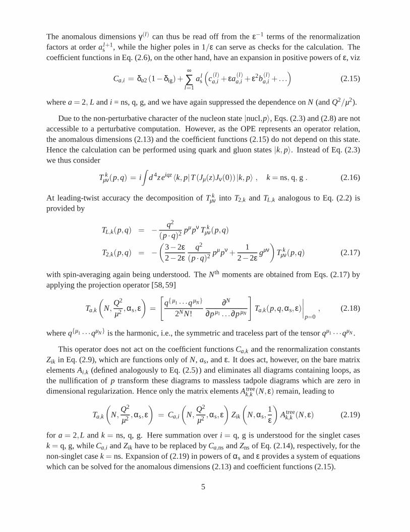
The forward Compton diagrams contributing to the present calculation of the electromagneticthree-loop coefficient functions, generated automatically with the diagram generator QGRAF [60],are enumerated in Table 1. Among the partonsk in Eq. (2.16) we also include an external ghosth.This is a standard procedure, allowing us to take the sum overexternal gluon spins by contractingwith −gµν instead of the full physical expression which would, due to the presence of extra powersof the gluon momentump, lead to a considerable complication of our task. For the same reasonour all-N computations have been performed in the Feynman gauge. We have however checkedthe gauge independence for a few low values ofN using the MINCER program [61,62]. The latestversion version of FORM [63,64] has been employed for all symbolic manipulations.

process tree 1-loop 2-loop 3-loop

qγ → qγ 1 3 25 359gγ → gγ 2 17 345hγ → hγ 2 56

sum 2 10 88 1520

Table 1: The number of diagrams for the amplitudes employed for the calculation of the three-loopcoefficient functions. The sums includes a factor of two fromLorentz projections toF2 andFL.

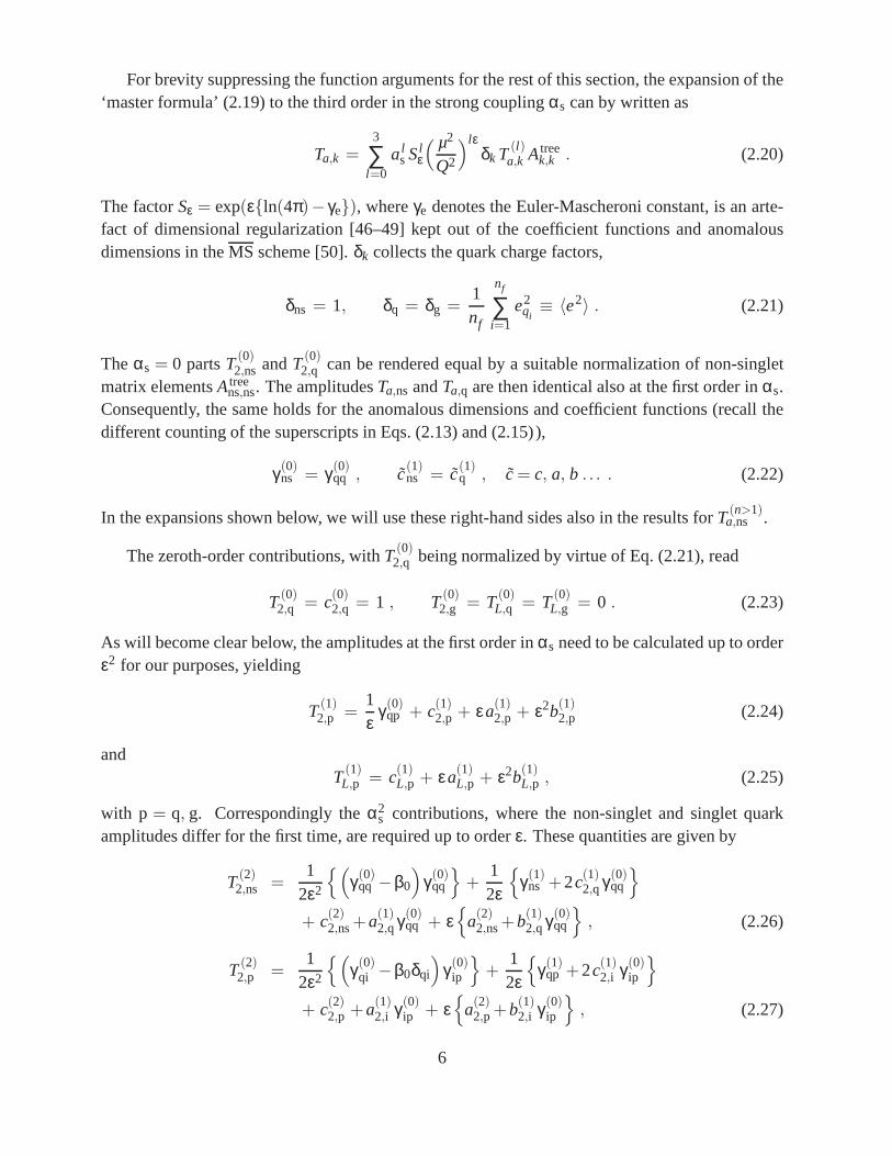
We close this section by briefly noting that a new flavour structure enters at the third order inαs.In this flavour structure, denoted byf l11 below, the in- and outgoing photons couple to differentquark lines, see Fig. 1. The corresponding flavour factors are listed in Table 2. Note that thesediagrams do not upset theλα independence of the non-singlet quantities, as discussed in Ref. [39].

flavour factor f l2 f l02 f l11 f l g2 f l g

11

non-singlet 1 0 3〈e〉 – –

singlet 1 1〈e〉2

〈e2〉1

〈e〉2

〈e2〉

Table 2: The charge factors for the flavour topologies entering up to three loops, see also Ref. [40].

8

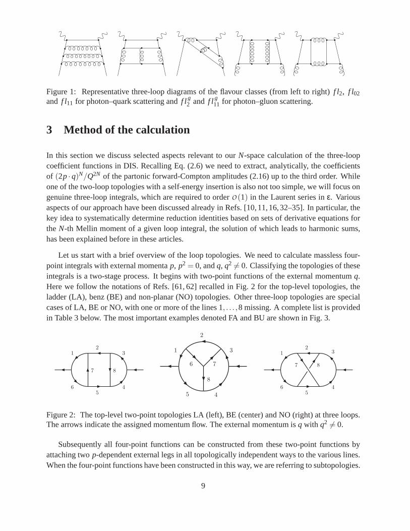
Figure 1: Representative three-loop diagrams of the flavourclasses (from left to right)f l2, f l02

and f l11 for photon–quark scattering andf l g2 and f l g

11 for photon–gluon scattering.

3 Method of the calculation

In this section we discuss selected aspects relevant to ourN-space calculation of the three-loopcoefficient functions in DIS. Recalling Eq. (2.6) we need to extract, analytically, the coefficientsof (2p ·q)N/Q2N of the partonic forward-Compton amplitudes (2.16) up to thethird order. Whileone of the two-loop topologies with a self-energy insertionis also not too simple, we will focus ongenuine three-loop integrals, which are required to orderO (1) in the Laurent series inε. Variousaspects of our approach have been discussed already in Refs.[10,11,16,32–35]. In particular, thekey idea to systematically determine reduction identitiesbased on sets of derivative equations forthe N-th Mellin moment of a given loop integral, the solution of which leads to harmonic sums,has been explained before in these articles.

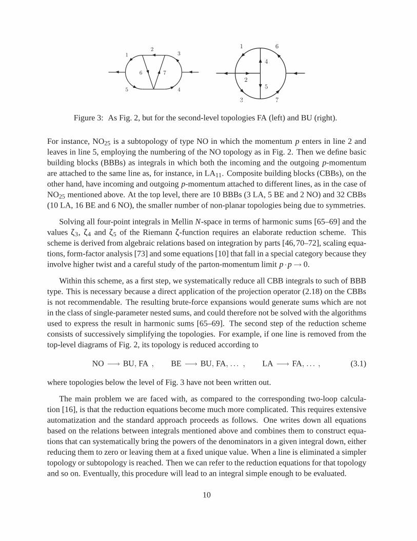
Let us start with a brief overview of the loop topologies. We need to calculate massless four-point integrals with external momentap, p2 = 0, andq, q2 6= 0. Classifying the topologies of theseintegrals is a two-stage process. It begins with two-point functions of the external momentumq.Here we follow the notations of Refs. [61, 62] recalled in Fig. 2 for the top-level topologies, theladder (LA), benz (BE) and non-planar (NO) topologies. Other three-loop topologies are specialcases of LA, BE or NO, with one or more of the lines 1, . . . ,8 missing. A complete list is providedin Table 3 below. The most important examples denoted FA and BU are shown in Fig. 3.

5

2

7 8

1

6

3

4

8

76

3

2

1

5 4

2

5

7 8

1

6 4

3

Figure 2: The top-level two-point topologies LA (left), BE (center) and NO (right) at three loops.The arrows indicate the assigned momentum flow. The externalmomentum isq with q2 6= 0.

Subsequently all four-point functions can be constructed from these two-point functions byattaching twop-dependent external legs in all topologically independentways to the various lines.When the four-point functions have been constructed in thisway, we are referring to subtopologies.

9

2

6 7

1

5

3

4

2

4

5

61

3 7

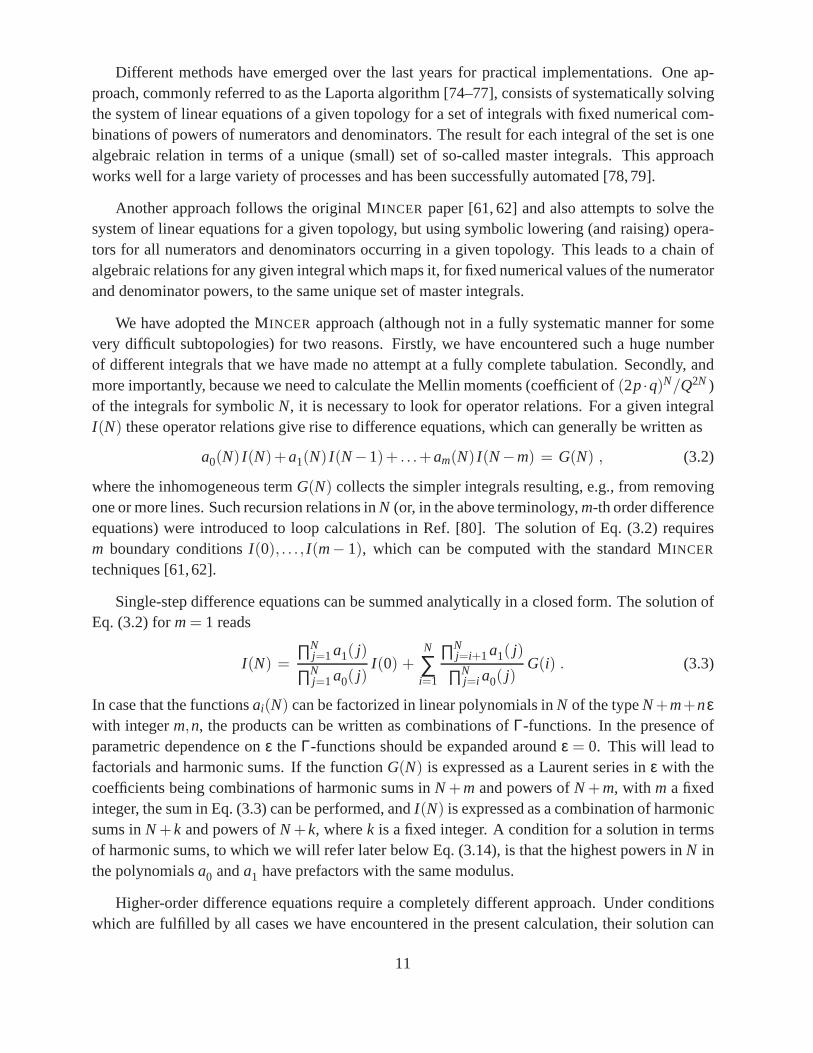
Figure 3: As Fig. 2, but for the second-level topologies FA (left) and BU (right).

For instance, NO25 is a subtopology of type NO in which the momentump enters in line 2 andleaves in line 5, employing the numbering of the NO topology as in Fig. 2. Then we define basicbuilding blocks (BBBs) as integrals in which both the incoming and the outgoingp-momentumare attached to the same line as, for instance, in LA11. Composite building blocks (CBBs), on theother hand, have incoming and outgoingp-momentum attached to different lines, as in the case ofNO25 mentioned above. At the top level, there are 10 BBBs (3 LA, 5 BEand 2 NO) and 32 CBBs(10 LA, 16 BE and 6 NO), the smaller number of non-planar topologies being due to symmetries.

Solving all four-point integrals in MellinN-space in terms of harmonic sums [65–69] and thevaluesζ3, ζ4 and ζ5 of the Riemannζ-function requires an elaborate reduction scheme. Thisscheme is derived from algebraic relations based on integration by parts [46,70–72], scaling equa-tions, form-factor analysis [73] and some equations [10] that fall in a special category because theyinvolve higher twist and a careful study of the parton-momentum limit p ·p→ 0.

Within this scheme, as a first step, we systematically reduceall CBB integrals to such of BBBtype. This is necessary because a direct application of the projection operator (2.18) on the CBBsis not recommendable. The resulting brute-force expansions would generate sums which are notin the class of single-parameter nested sums, and could therefore not be solved with the algorithmsused to express the result in harmonic sums [65–69]. The second step of the reduction schemeconsists of successively simplifying the topologies. For example, if one line is removed from thetop-level diagrams of Fig. 2, its topology is reduced according to

NO −→ BU, FA , BE −→ BU, FA, . . . , LA −→ FA, . . . , (3.1)

where topologies below the level of Fig. 3 have not been written out.

The main problem we are faced with, as compared to the corresponding two-loop calcula-tion [16], is that the reduction equations become much more complicated. This requires extensiveautomatization and the standard approach proceeds as follows. One writes down all equationsbased on the relations between integrals mentioned above and combines them to construct equa-tions that can systematically bring the powers of the denominators in a given integral down, eitherreducing them to zero or leaving them at a fixed unique value. When a line is eliminated a simplertopology or subtopology is reached. Then we can refer to the reduction equations for that topologyand so on. Eventually, this procedure will lead to an integral simple enough to be evaluated.

10

Different methods have emerged over the last years for practical implementations. One ap-proach, commonly referred to as the Laporta algorithm [74–77], consists of systematically solvingthe system of linear equations of a given topology for a set ofintegrals with fixed numerical com-binations of powers of numerators and denominators. The result for each integral of the set is onealgebraic relation in terms of a unique (small) set of so-called master integrals. This approachworks well for a large variety of processes and has been successfully automated [78,79].

Another approach follows the original MINCER paper [61, 62] and also attempts to solve thesystem of linear equations for a given topology, but using symbolic lowering (and raising) opera-tors for all numerators and denominators occurring in a given topology. This leads to a chain ofalgebraic relations for any given integral which maps it, for fixed numerical values of the numeratorand denominator powers, to the same unique set of master integrals.

We have adopted the MINCER approach (although not in a fully systematic manner for somevery difficult subtopologies) for two reasons. Firstly, we have encountered such a huge numberof different integrals that we have made no attempt at a fullycomplete tabulation. Secondly, andmore importantly, because we need to calculate the Mellin moments (coefficient of(2p·q)N/Q2N )of the integrals for symbolicN, it is necessary to look for operator relations. For a given integralI(N) these operator relations give rise to difference equations, which can generally be written as

a0(N) I(N)+a1(N) I(N−1)+ . . .+am(N) I(N−m) = G(N) , (3.2)

where the inhomogeneous termG(N) collects the simpler integrals resulting, e.g., from removingone or more lines. Such recursion relations inN (or, in the above terminology,m-th order differenceequations) were introduced to loop calculations in Ref. [80]. The solution of Eq. (3.2) requiresm boundary conditionsI(0), . . . , I(m− 1), which can be computed with the standard MINCER

techniques [61,62].

Single-step difference equations can be summed analytically in a closed form. The solution ofEq. (3.2) form= 1 reads

I(N) =∏N

j=1a1( j)

∏Nj=1a0( j)

I(0) +N

∑i=1

∏Nj=i+1a1( j)

∏Nj=i a0( j)

G(i) . (3.3)

In case that the functionsai(N) can be factorized in linear polynomials inN of the typeN+m+nεwith integerm,n, the products can be written as combinations ofΓ-functions. In the presence ofparametric dependence onε theΓ-functions should be expanded aroundε = 0. This will lead tofactorials and harmonic sums. If the functionG(N) is expressed as a Laurent series inε with thecoefficients being combinations of harmonic sums inN+m and powers ofN+m, with m a fixedinteger, the sum in Eq. (3.3) can be performed, andI(N) is expressed as a combination of harmonicsums inN+k and powers ofN+k, wherek is a fixed integer. A condition for a solution in termsof harmonic sums, to which we will refer later below Eq. (3.14), is that the highest powers inN inthe polynomialsa0 anda1 have prefactors with the same modulus.

Higher-order difference equations require a completely different approach. Under conditionswhich are fulfilled by all cases we have encountered in the present calculation, their solution can

11

be expressed in terms of harmonic sums, and hence a corresponding ansatz can by used. Supposewe have for some integralI(N) a relation like Eq. (3.2) withm≥ 2. The inhomogeneous functionG(N) is again assumed to be a Laurent series inε with the coefficients being combinations ofharmonic sums inN+k with a fixed integerk. The functionsai(N) in Eq. (3.2) are polynomials inN andε subject to certain conditions. In order to solve forI(N) under these assumptions, we writedown an ansatz in powers ofε, harmonic sumsS~m of given weight, possibly in combination withvalues of theζ-function and factors(−1)N. The harmonic sums have argumentsN+ l , where theintegerl samples the various offsets. One may have to introduce positive powers ofNk multiplyingthe harmonic sums as well (see also the discussion below). ThusI(N) is written as

I(N) = ∑ c+( j,k, l ,~m)ε j (N− l)kS~m(N− l)+

∑ c−( j,k, l ,~m)ε j (−1)N (N− l)kS~m(N− l)+

∑ c+( j,k, l ,~m,n)ε j (N− l)kζnS~m(N− l)+

∑ c−( j,k, l ,~m,n)ε j (−1)N (N− l)kζnS~m(N− l) . (3.4)

The sum runs over a suitable set of the parameter space spanned by the powersε j , the weight~mofthe harmonic sums, positive powersNk, and the offsetl in the argument of the harmonic sums. Forefficiency, it is important to take into account the correlation between the loop order and the weightof harmonic sums in the ansatz, i.e. in the choice of the parameter setj,k, l ,~m,n. In the case ofDIS structure functions, one- (two-, three-) loop integrals can be expressed, at orderε0, in terms ofharmonic sums up to weight two (four, six). Accordingly, thesingle (double, triple) pole terms inε are expressed through harmonic sums with maximal weights decreased by one (two, three).

The solution for the integralI(N) is obtained by determining the coefficientsc− andc+. Tothat end, we insert the ansatz (3.4) into Eq. (3.2) and normalize the left hand side by pulling allexpressions back to the unique basis in harmonic sums. This synchronization can be performedwith the algorithms of the SUMMER package [67] in FORM. The coefficients of all individual termssuch asε j (−1)N (N− l)kS~m(N− l)ζn then determine a set of linear equations for the unknownc− andc+ in our ansatz (3.4), which can be solved by standard means if the chosen parameterset j,k, l ,~m,n was large enough. In practice, an iterative procedure for the determination of thecoefficientsc− andc+ is advantageous, since an improved ansatz reduces the size of the system ofequations. We will give an explicit example for a two-step difference equation below.

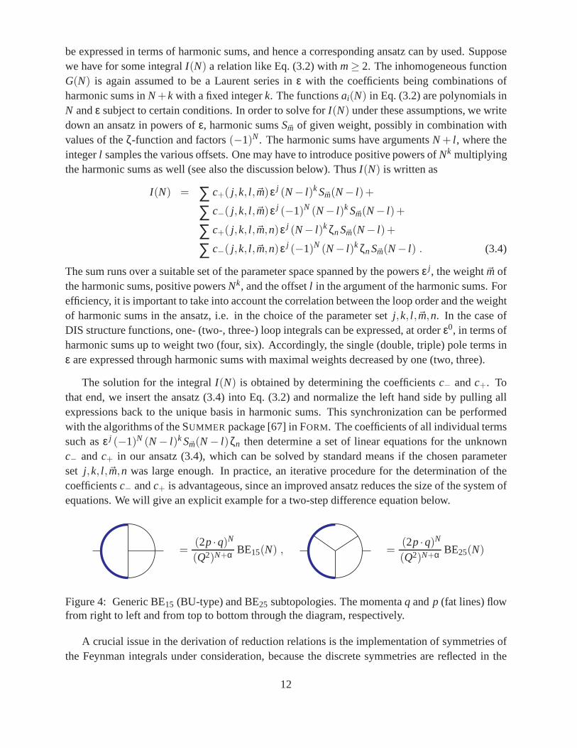
=(2p ·q)N

(Q2)N+α BE15(N) , =(2p ·q)N

(Q2)N+α BE25(N)

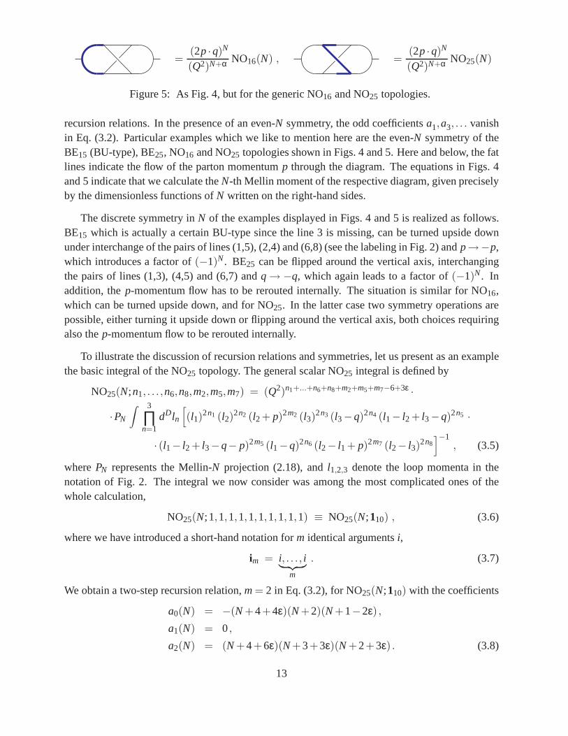
Figure 4: Generic BE15 (BU-type) and BE25 subtopologies. The momentaq andp (fat lines) flowfrom right to left and from top to bottom through the diagram,respectively.

A crucial issue in the derivation of reduction relations is the implementation of symmetries ofthe Feynman integrals under consideration, because the discrete symmetries are reflected in the

12

=(2p ·q)N

(Q2)N+α NO16(N) , =(2p ·q)N

(Q2)N+α NO25(N)

Figure 5: As Fig. 4, but for the generic NO16 and NO25 topologies.

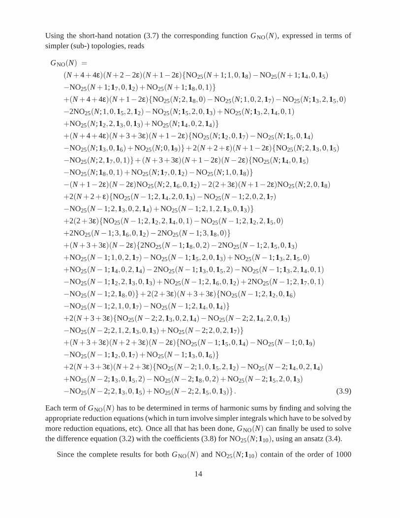
recursion relations. In the presence of an even-N symmetry, the odd coefficientsa1,a3, . . . vanishin Eq. (3.2). Particular examples which we like to mention here are the even-N symmetry of theBE15 (BU-type), BE25, NO16 and NO25 topologies shown in Figs. 4 and 5. Here and below, the fatlines indicate the flow of the parton momentump through the diagram. The equations in Figs. 4and 5 indicate that we calculate theN-th Mellin moment of the respective diagram, given preciselyby the dimensionless functions ofN written on the right-hand sides.

The discrete symmetry inN of the examples displayed in Figs. 4 and 5 is realized as follows.BE15 which is actually a certain BU-type since the line 3 is missing, can be turned upside downunder interchange of the pairs of lines (1,5), (2,4) and (6,8) (see the labeling in Fig. 2) andp→−p,which introduces a factor of(−1)N. BE25 can be flipped around the vertical axis, interchangingthe pairs of lines (1,3), (4,5) and (6,7) andq → −q, which again leads to a factor of(−1)N. Inaddition, thep-momentum flow has to be rerouted internally. The situation is similar for NO16,which can be turned upside down, and for NO25. In the latter case two symmetry operations arepossible, either turning it upside down or flipping around the vertical axis, both choices requiringalso thep-momentum flow to be rerouted internally.

To illustrate the discussion of recursion relations and symmetries, let us present as an examplethe basic integral of the NO25 topology. The general scalar NO25 integral is defined by

NO25(N;n1, . . . ,n6,n8,m2,m5,m7) = (Q2)n1+...+n6+n8+m2+m5+m7−6+3ε ·

·PN

∫ 3

∏n=1

dDln[(l1)

2n1 (l2)2n2 (l2+ p)2m2 (l3)

2n3 (l3−q)2n4 (l1− l2+ l3−q)2n5 ·

· (l1− l2 + l3−q− p)2m5 (l1−q)2n6 (l2− l1+ p)2m7 (l2− l3)2n8

]−1, (3.5)

wherePN represents the Mellin-N projection (2.18), andl1,2,3 denote the loop momenta in thenotation of Fig. 2. The integral we now consider was among themost complicated ones of thewhole calculation,

NO25(N;1,1,1,1,1,1,1,1,1,1) ≡ NO25(N;110) , (3.6)

where we have introduced a short-hand notation form identical argumentsi,

im = i, . . . , i︸ ︷︷ ︸m

. (3.7)

We obtain a two-step recursion relation,m= 2 in Eq. (3.2), for NO25(N;110) with the coefficients

a0(N) = −(N+4+4ε)(N+2)(N+1−2ε) ,

a1(N) = 0,

a2(N) = (N+4+6ε)(N+3+3ε)(N+2+3ε) . (3.8)

13

Using the short-hand notation (3.7) the corresponding function GNO(N), expressed in terms ofsimpler (sub-) topologies, reads

GNO(N) =

(N+4+4ε)(N+2−2ε)(N+1−2ε){NO25(N+1;1,0,18)−NO25(N+1;14,0,15)

−NO25(N+1;17,0,12)+NO25(N+1;18,0,1)}

+(N+4+4ε)(N+1−2ε){NO25(N;2,18,0)−NO25(N;1,0,2,17)−NO25(N;13,2,15,0)

−2NO25(N;1,0,15,2,12)−NO25(N;15,2,0,13)+NO25(N;13,2,14,0,1)

+NO25(N;12,2,13,0,13)+NO25(N;14,0,2,14)}

+(N+4+4ε)(N+3+3ε)(N+1−2ε){NO25(N;12,0,17)−NO25(N;15,0,14)

−NO25(N;13,0,16)+NO25(N;0,19)}+2(N+2+ ε)(N+1−2ε){NO25(N;2,13,0,15)

−NO25(N;2,17,0,1)}+(N+3+3ε)(N+1−2ε)(N−2ε){NO25(N;14,0,15)

−NO25(N;18,0,1)+NO25(N;17,0,12)−NO25(N;1,0,18)}

−(N+1−2ε)(N−2ε)NO25(N;2,16,0,12)−2(2+3ε)(N+1−2ε)NO25(N;2,0,18)

+2(N+2+ ε){NO25(N−1;2,14,2,0,13)−NO25(N−1;2,0,2,17)

−NO25(N−1;2,13,0,2,14)+NO25(N−1;2,1,2,13,0,13)}

+2(2+3ε){NO25(N−1;2,12,2,14,0,1)−NO25(N−1;2,12,2,15,0)

+2NO25(N−1;3,16,0,12)−2NO25(N−1;3,18,0)}

+(N+3+3ε)(N−2ε){2NO25(N−1;18,0,2)−2NO25(N−1;2,15,0,13)

+NO25(N−1;1,0,2,17)−NO25(N−1;15,2,0,13)+NO25(N−1;13,2,15,0)

+NO25(N−1;14,0,2,14)−2NO25(N−1;13,0,15,2)−NO25(N−1;13,2,14,0,1)

−NO25(N−1;12,2,13,0,13)+NO25(N−1;2,16,0,12)+2NO25(N−1;2,17,0,1)

−NO25(N−1;2,18,0)}+2(2+3ε)(N+3+3ε){NO25(N−1;2,12,0,16)

−NO25(N−1;2,1,0,17)−NO25(N−1;2,14,0,14)}

+2(N+3+3ε){NO25(N−2;2,13,0,2,14)−NO25(N−2;2,14,2,0,13)

−NO25(N−2;2,1,2,13,0,13)+NO25(N−2;2,0,2,17)}

+(N+3+3ε)(N+2+3ε)(N−2ε){NO25(N−1;15,0,14)−NO25(N−1;0,19)

−NO25(N−1;12,0,17)+NO25(N−1;13,0,16)}

+2(N+3+3ε)(N+2+3ε){NO25(N−2;1,0,15,2,12)−NO25(N−2;14,0,2,14)

+NO25(N−2;13,0,15,2)−NO25(N−2;18,0,2)+NO25(N−2;15,2,0,13)

−NO25(N−2;2,13,0,15)+NO25(N−2;2,15,0,13)} . (3.9)

Each term ofGNO(N) has to be determined in terms of harmonic sums by finding and solving theappropriate reduction equations (which in turn involve simpler integrals which have to be solved bymore reduction equations, etc). Once all that has been done,GNO(N) can finally be used to solvethe difference equation (3.2) with the coefficients (3.8) for NO25(N;110), using an ansatz (3.4).

Since the complete results for bothGNO(N) and NO25(N;110) contain of the order of 1000

14

terms, they are too long to be presented here. However we write down the two leading polesin ε for illustration. We choose a compact representation for the harmonic sums, employing theabbreviationS~m ≡ S~m(N), together with the notation

N±S~m = S~m(N±1) , N±i S~m = S~m(N± i) , (3.10)

for arguments shifted by±1 or a larger integeri. In the G-scheme [61,81], in whichl -loop integralsare divided by thel -th power of the basic massless one-loop integral,GNO(N) then reads

GNO(N) =163ε3(1+(−1)N)

(6− (8+6N+N2)

[3S−3−2S−2,1+S3

]− (13+4N)

[S−2

+S2

]−7S1−3N+2S1 +(3−3N+−N+2 +N+3)

[S1,−2+S1,1 +S1,2+2S2,1−S2−2S3

]

+11S1,1−11S2−N+

[13S1,1−17S2

]+2N+2

[S1,1−3S2

])+

163ε2(1+(−1)N)(−24

+(8+6N+N2)[79

4S−4 +

374

S−3−854

S−3,1−S−2,−2−112

S−2,1+10S−2,1,1−132

S−2,2

+112

S1,−2,1−374

S1,−3−72

S1,3 +2S2,−2+S2,2+72

S3−12

S3,1 +174

S4

]−N

[938

S−3

−172

S−2−74

S−2,1+9S1,−2 +212

S1,2−414

S2+112

S2,1+114

S3

]−

872

S−3+394

S−2

+16S−2,1+9S1−1114

S1,−2−1012

S1,1+55S1,1,1−4378

S1,2+3298

S2−3934

S2,1+3458

S3

+(3−3N+−N+2 +N+3)[7

4S1,−3 +

74

S1,−2−2S1,−2,1−S1,1 +5S1,1,1+32

S1,1,−2

+94

S1,1,2−14

S1,2 +74

S1,2,1−114

S1,3+S2+10S2,1,1−314

S2,2−3S2,−2−72

S2,1+12

S3

−834

S3,1+312

S4

]+N+

[14S1+

14

S1,−2 +1638

S1,1−65S1,1,1 +2278

S1,2−1138

S2

+3814

S2,1−4438

S3

]+N+2

[16S1+

12

S1,−2−1598

S1,1+10S1,1,1−274

S1,2+578

S2

−16S2,1+414

S3

])+ O

(1ε

). (3.11)

Note the positive powers ofN multiplying some harmonic sums in Eq. (3.11). We will returntothis issue below. The boundary conditions for the NO25(N;110) integral of Eq. (3.6) are shorter,

NO25(0;110) = −103

1ε3 +

13

1ε2 + O

(1ε

),

NO25(1;110) = 0 . (3.12)

Finally the following expression for NO25(N;110) in the G-scheme is obtained:

NO25(N;110) =163

(1+(−1)N)1ε3

(−

32

S−3+S−2,1+(N+2 −2N+3 +N+4)[S1 +S1,1−S2

]

+12(N+2 −N+4)

[S1,−2+S1,2

]+(1−2N+ +2N+2)

[S2,1−

32

S3

]−N+3S2,1+N+4S3

)

15

+163

(1+(−1)N)1ε2

(798

S−4+152

S−3−858

S−3,1−12

S−2,−2−5S−2,1 +5S−2,1,1−134

S−2,2

+(N+2 −2N+3 +N+4)[27

16S1,−3−

32

S1,−2−94

S1,−2,1−11S1−4S1,1−32

S1,1,−2 +5S1,1,1

−32

S1,1,2−32

S1,2−12

S1,2,1−12

S1,3−9S2,1 +72

S2,2+5S3

]− (1−2N+ +2N+2)

[12

S2,−2

+5S2,1−5S2,1,1+134

S2,2−152

S3+858

S3,1−798

S4

]+(N+2 −N+3)

[94

S1,1,−2+218

S1,1,2

−4S1,2+118

S1,2,1+7S2+6S2,1

]−N+2

[8716

S1,−3+2S1,−2−4S1,−2,1 +218

S1,3+298

S2,2

+5S3

]+N+3

[78

S1,3−2S2,−2+5S2,1−5S2,1,1+598

S2,2+518

S3,1−74

S4

]+N+4

[1316

S1,−3

+2S1,−2−54

S1,−2,1+72

S2,−2+4S3,1−6S4

])+ O

(1ε

). (3.13)

In the remainder of this section we briefly address three issues which are, to a varying extent,special to the calculation of the coefficient functions. Thefirst is the control of the expansionin powers of the dimensional offsetε. This is more critical here than for the computation of theanomalous dimensions [10, 11], as we now rely on the last coefficients inε kept in Eqs. (2.24) –(2.33). In other words, if some three-loop integrals entering the diagram calculation were actuallynot accurate to orderε0 (something, in fact, our extensive fixed-N checks using the MINCER pro-gram [61,62] would have indicated), then that would not haveaffected the results for the anomalousdimensions, but spoiled the present calculation of the coefficient functions.

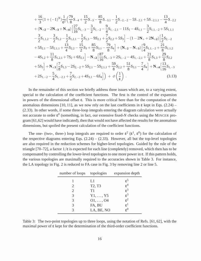
The one- (two-, three-) loop integrals are required to orderε2 (ε1, ε0) for the calculation ofthe respective diagrams entering Eqs. (2.24) – (2.33). However, all but the top-level topologiesare also required in the reduction schemes for higher-leveltopologies. Guided by the rule of thetriangle [70–72], a factor 1/ε is expected for each line (completely) removed, which then has to becompensated by controlling the lower-level topologies to one more power inε. If this pattern holds,the various topologies are maximally required to the accuracies shown in Table 3. For instance,the LA topology in Fig. 2 is reduced to FA case in Fig. 3 by removing line 2 or line 5.

number of loops topologies expansion depth

1 L1 ε5

2 T2, T3 ε4

2 T1 ε3

3 Y1, . . . , Y5 ε3

3 O1, . . . , O4 ε2

3 FA, BU ε1

3 LA, BE, NO ε0

Table 3: The two-point topologies up to three loops, using the notation of Refs. [61, 62], with themaximal power ofε kept for the determination of the third-order coefficient functions.

16

If a reduction equation introduces a factorε−2 while removing a line, or a factorε−1 in asimplification not removing a line, the equation is said to contain a spurious pole. The lower-leveltopologies are worked out to a finite accuracy as well, eitherfor efficiency or since the underlyingintegrals, for instance providing the boundary conditionsfor Eq. (3.2), are known only to a certainaccuracy inε. Therefore spurious poles endanger the integrity of the reduction procedure. Indeed,one of the greatest difficulties in constructing reduction schemes is to avoid such poles.

Actually, for some cases we have not found expressions free of spurious poles. Consequentlythese integrals have not been calculated to the design orderin ε. For instance, most O115 integrals,generated by removing line 2 from the FA17 subtopology, have only been computed to orderεinstead of including theε2 terms as indicated in Table 3. This was only permissible since in factmany more reductions are actually more benign than the triangle reduction, removing lines withoutintroducing anyε−1 pole, see, e.g., Eq. (3.9). Carefully utilizing this fact, we were able to reachthe requiredε0 accuracy for all three-loop integrals entering the diagramcalculations.

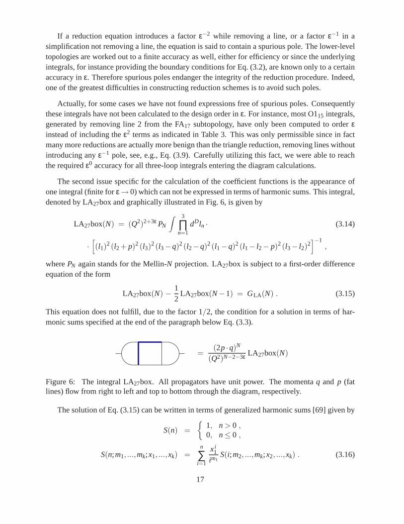
The second issue specific for the calculation of the coefficient functions is the appearance ofone integral (finite forε→ 0) which can not be expressed in terms of harmonic sums. This integral,denoted by LA27box and graphically illustrated in Fig. 6, is given by

LA27box(N) = (Q2)2+3ε PN

∫ 3

∏n=1

dDln · (3.14)

·[(l1)

2(l2+ p)2(l3)2(l3−q)2(l2−q)2(l1−q)2(l1− l2− p)2(l3− l2)

2]−1

,

wherePN again stands for the Mellin-N projection. LA27box is subject to a first-order differenceequation of the form

LA27box(N) −12

LA27box(N−1) = GLA (N) . (3.15)

This equation does not fulfill, due to the factor 1/2, the condition for a solution in terms of har-monic sums specified at the end of the paragraph below Eq. (3.3).

=(2p ·q)N

(Q2)N−2−3ε LA27box(N)

Figure 6: The integral LA27box. All propagators have unit power. The momentaq and p (fatlines) flow from right to left and top to bottom through the diagram, respectively.

The solution of Eq. (3.15) can be written in terms of generalized harmonic sums [69] given by

S(n) =

{1, n > 0 ,0, n≤ 0 ,

S(n;m1, ...,mk;x1, ...,xk) =n

∑i=1

xi1

im1S(i;m2, ...,mk;x2, ...,xk) . (3.16)

17

Using the short-hand notation of Eq. (3.7) the result reads

LA27box(N) = (−1)N2−N−1(

20S(N+1;1;2)ζ5+4S(N+1;13;2,12)ζ3

+6S(N+1;14,2;2,13,−1)+3S(N+1;14,2;2,14)−S(N+1;13,2,1;2,14)

−9S(N+1;13,3;2,12,−1)−3S(N+1;13,3;2,13)−2S(N+1;12,2,12;2,14)

−6S(N+1;12,22;2,12,−1)+6S(N+1;12,3,1;2,13)+6S(N+1;12,4;2,1,−1)

−6S(N+1;12,4;2,12)+12S(N+1;1,2;2,−1)ζ3−6S(N+1;1,2,1,2;2,12,−1)

−3S(N+1;1,2,1,2;2,13)−12S(N+1;1,22,1;2,−1,−1,1)−3S(N+1;1,22,1;2,13)

+18S(N+1;1,2,3;2,−1,−1)+9S(N+1;1,2,3;2,1,−1)+9S(N+1;1,2,3;2,12)

+6S(N+1;1,3,12;2,13)+6S(N+1;1,3,2;2,1,−1)−6S(N+1;1,3,2;2,12)

−4S(N+1;2,1;2,1)ζ3−6S(N+1;2,12,2;2,12,−1)−3S(N+1;2,12,2;2,13)

+S(N+1;2,1,2,1;2,13)+9S(N+1;2,1,3;2,1,−1)+3S(N+1;2,1,3;2,12)

+2S(N+1;22,12;2,13)+6S(N+1;23;2,1,−1)−6S(N+1;2,3,1;2,12)

−6S(N+1;2,4;2,−1)+6S(N+1;2,4;2,1)−12S(N+1;3;−2)ζ3−9S(N+1;32;2,1)

+6S(N+1;3,1,2;2,1,−1)+3S(N+1;3,1,2;2,12)+12S(N+1;3,2,1;−2,−1,1)

+3S(N+1;3,2,1;2,12)−18S(N+1;32;−2,−1)−9S(N+1;32;2,−1)

−6S(N+1;4,12;2,12)−6S(N+1;4,2;2,−1)+6S(N+1;4,2;2,1))

, (3.17)

including terms withx j = ±2 in the sums (3.16). Note also the overall factor of 2−N, which keepsalso sums over LA27box within the class of generalizedS-sums.

We did not need sums over LA27box, for which all algorithms are however known fromRef. [69], in our reduction procedures for higher-level subtopologies, e.g., LA78. Thus we actuallykept this integral as an ‘unknown’ function in all intermediate expressions, only using Eq. (3.15)to shift the argumentN. Finally, while termsNk LA27box(N) occurred in the results of individualdiagrams, all dependence on LA27box cancelled in the final results for the coefficient functions.

The final issue we need to mention is that certain combinations of harmonic sums multipliedwith positive powers ofN occur in the three-loop coefficient functions. Such structures are encoun-tered in very many integrals also at the level of the 1/ε poles, see Eq. (3.11) above, but they cancelin the final results for the anomalous dimensions. On the other hand, the following combinationsare present in the final result for the coefficient functions:

g1(N) = N f(N) , (3.18)

g2(N) = N2 f (N) , (3.19)

g3(N) = N3 f (N)−2N(ζ3−S−3−S−2+2S−2,1) , (3.20)

with the functionf (N) given by

f (N) = 5ζ5−2S−5+4S−2ζ3−4S−2,−3 +8S−2,−2,1+4S3,−2−4S4,1+2S5 . (3.21)

18

This function vanishes sufficiently fast forN → ∞ for Eqs. (3.18) – (3.20) to behave at most asconstants in this limit. Thus the standard asymptotic behaviour lnk(N), k = 1, . . . , 6 of the three-

loop quark coefficient functionsc(3)2,ns andc(3)

2,q is unaffected by these new structures.

Positive powers as in Eqs. (3.18) – (3.20), unlike negative powers ofN, cannot be writtenentirely in terms of harmonic sums. Consequently a larger class of functions is required also inx-space, as a one-to-one relation exists between the set of harmonic sums of weightw and theharmonic polylogarithms [83–85]H~m(x)/(1±x) where~mhas weightw−1. The Mellin inverse ofg1(N) in Eq. (3.18) can be derived by partial integration from thatof f (N) in Eq. (3.21),

g1(N) = N f(N) = N∫ 1

0dxxN−1 f (x) = f (1) −

∫ 1

0dxxN−1 x f ′(x)

=

∫ 1

0dxxN−1

{δ(1−x) f (1)− x f ′(x)

}, (3.22)

whereg1(x) is given by the expression in curved brackets in the second line. This procedure isthen repeated for the functionsg2 andg3, leading to thex-space expressions

g1(x) =1

(1−x)2

(−

45

ζ22+8H−2ζ2−4H−2,0,0−8H−2,2−6H0ζ3−6H0,0ζ2+2H0,0,0,0

+4H4

)+

11−x

(45

ζ22−6ζ3−8H−2ζ2 +4H−2,0,0+8H−2,2 +8H−1ζ2−4H−1,0,0

−8H−1,2−6H0ζ2 +6H0ζ3 +6H0,0ζ2+2H0,0,0−2H0,0,0,0+4H3−4H4

)

+1

(1+x)2

(215

ζ22+4H−3,0+4H0ζ3 +2H0,0ζ2−2H0,0,0,0

)+

11+x

(−

215

ζ22 +4ζ3

−4H−3,0 +4H−2,0+2H0ζ2−4H0ζ3−2H0,0ζ2−2H0,0,0+2H0,0,0,0

)+2ζ3−4H−2,0

−8H−1ζ2 +4H−1,0,0+8H−1,2 +4H0ζ2−4H3 , (3.23)

g2(x) =1

(1−x)3

(85

ζ22−16H−2ζ2 +8H−2,0,0+16H−2,2+12H0ζ3+12H0,0ζ2−4H0,0,0,0

−8H4

)+

1(1−x)2

(−

125

ζ22+12ζ3 +24H−2ζ2−12H−2,0,0−24H−2,2−16H−1ζ2

+8H−1,0,0 +16H−1,2+12H0ζ2−18H0ζ3−18H0,0ζ2−4H0,0,0+6H0,0,0,0−8H3

+12H4

)+

11−x

(2ζ2 +

45

ζ22−12ζ3−8H−2ζ2+4H−2,0,0 +8H−2,2+16H−1ζ2

−8H−1,0,0−16H−1,2−12H0ζ2+6H0ζ3+6H0,0ζ2+4H0,0,0−2H0,0,0,0+8H3−4H4

)

+1

(1+x)3

(−

425

ζ22−8H−3,0−8H0ζ3−4H0,0ζ2 +4H0,0,0,0

)+

1(1+x)2

(635

ζ22−8ζ3

+12H−3,0−8H−2,0−4H0ζ2+12H0ζ3+6H0,0ζ2+4H0,0,0−6H0,0,0,0

)+

11+x

(−6ζ2

−215

ζ22+8ζ3−4H−3,0+8H−2,0−4H−1,0+4H0ζ2−4H0ζ3+4H0,0−2H0,0ζ2

−4H0,0,0 +2H0,0,0,0+4H2

)+δ(1−x)(ζ2 + ζ3)+4ζ2 +4H−1,0−4H0,0−4H2 , (3.24)

19

g3(x) =1

(1−x)4

(−

245

ζ22+48H−2ζ2−24H−2,0,0−48H−2,2−36H0ζ3−36H0,0ζ2

+12H0,0,0,0 +24H4

)+

1(1−x)3

(485

ζ22−36ζ3−96H−2ζ2+48H−2,0,0 +96H−2,2

+48H−1ζ2−24H−1,0,0−48H−1,2−36H0ζ2 +72H0ζ3 +72H0,0ζ2 +12H0,0,0−24H0,0,0,0

+24H3−48H4

)+

1(1−x)2

(−6ζ2−

285

ζ22 +54ζ3+56H−2ζ2−28H−2,0,0−56H−2,2

−72H−1ζ2+36H−1,0,0 +72H−1,2+54H0ζ2−42H0ζ3−42H0,0ζ2−18H0,0,0+14H0,0,0,0

−36H3 +28H4

)+

11−x

(2ζ2 +

45

ζ22−18ζ3−8H−2ζ2+4H−2,0,0 +8H−2,2+24H−1ζ2

−12H−1,0,0−24H−1,2−18H0ζ2 +6H0ζ3 +2H0,0+6H0,0ζ2 +6H0,0,0−2H0,0,0,0+4H2

+12H3−4H4

)+

1(1+x)4

(1265

ζ22 +24H−3,0+24H0ζ3 +12H0,0ζ2−12H0,0,0,0

)

+1

(1+x)3

(−

2525

ζ22+24ζ3−48H−3,0+24H−2,0+12H0ζ2−48H0ζ3−24H0,0ζ2

−12H0,0,0 +24H0,0,0,0

)+

1(1+x)2

(6ζ2 +

1475

ζ22−36ζ3 +28H−3,0−36H−2,0

+12H−1,0−6H0−18H0ζ2 +28H0ζ3−6H0,0+14H0,0ζ2+18H0,0,0−14H0,0,0,0

)

+1

1+x

(−2−2ζ2−

215

ζ22+12ζ3−4H−3,0+12H−2,0−12H−1,0 +8H0+6H0ζ2

−4H0ζ3 +4H0,0−2H0,0ζ2−6H0,0,0 +2H0,0,0,0−4H2

)−δ(1−x)(ζ2+ ζ3)

+2−2H0 . (3.25)

The above equations are not suitable for a numerical implementation atx-values very close tox = 1, a region which contributes to all numerical calculationsof moments and, more importantly,Mellin convolutions. For application in this region we instead provide the expansions

g1(x) ≃ ζ2+ ζ3− (1−x)(ζ2+ ζ3)+(1−x)2(5

8−

14

ζ2−12

ζ3−12

ln(1−x))

+O ((1−x)3) , (3.26)

g2(x) ≃ δ(1−x)(ζ2 + ζ3)− ζ2− ζ3 +(1−x)(3

4+

12

ζ2− ln(1−x))

− (1−x)2(9

8−

14

ζ2−12

ζ3−12

ln(1−x))

+O ((1−x)3) , (3.27)

g3(x) ≃ −δ(1−x)(ζ2+ ζ3)+34

+12

ζ2+ ln(1−x)− (1−x)(1

2− ζ3

)

− (1−x)2( 7

24+

112

ζ2−12

ζ3 +12

ln(1−x))

+O ((1−x)3) . (3.28)

These expansions have been derived by expanding the harmonic polylogarithms sufficiently deepin (1−x) via the transformationt = (1−x)/(1+x) and an expansion aroundt = 0 as described inRef. [85] and implemented in FORM [63,64].

20

4 Results and discussion

We are now ready to present the third-order contributionsc(3)a,i to the coefficient functionsCa,i for

the structure functionsFa=2,L in electromagnetic DIS,

x−1Fa = Ca,ns⊗qns+ 〈e2〉(Ca,q⊗qs+Ca,g⊗g

). (4.1)

Recall thatqi andg represent the number distributions of quarks and gluons, respectively, in thefractional hadron momentum, withqs standing for the flavour-singlet quark distribution,qs =

∑nfi=1(qi + qi) wherenf denotes the number of effectively massless flavours. The normalization

of the corresponding non-singlet combinationqns is defined via Eq. (4.2) below. Again〈e2〉 repre-sents the average squared charge, and⊗ denotes the Mellin convolution which turns into a simplemultiplication in N-space. Below the singlet-quark coefficient function is decomposed into the

non-singlet and a ‘pure singlet’ contribution,c(n)a,q = c(n)

a,ns+ c(n)a,ps, and the results are given in the

MS scheme for the standard choiceµ2r = µ2

f = Q2 of the renormalization and factorization scales.The complete expressions for the dependence onµr andµf up to the third order in our expansionparameteras≡ αs/(4π) can be found, for example, in Eqs. (2.16) – (2.18) of Ref. [82].

As discussed above, our calculation via the optical theoremand a dispersion relation directlydetermines the coefficient functions for all even-integer momentsN in terms of harmonic sums[65–69]. From these results thex-space expressions can be reconstructed algebraically [16, 85]in terms of harmonic polylogarithms [83–85]. Unfortunately, but not entirely unexpectedly, theexact results are very lengthy. The complete expressions inbothN-space andx-space are thereforedeferred to the appendices of this article. Here we confine ourselves to (sufficiently accurate)

approximations forc(3)2,i (x), quite analogous to those already presented forc(3)

L,i (x) in Ref. [17].

For the convenience of the reader we first recall the known results up to the second order. Thecoefficient functions at zeroth and first order [50] are givenby

c(0)2,ns(x) = δ(x1) , c(0)

2,ps(x) = c(0)2,g(x) = c(1)

2,ps(x) = 0 (4.2)

and

c(1)2,ns(x) = CF{4D 1−3D 0− (9+4ζ2)δ(x1)−2(1+x)(L1−L0)

−4x−11 L0 +6+4x} , (4.3)

c(1)2,g(x) = nf {(2−4xx1)(L1−L0)−2+16xx1} (4.4)

with CF = (N2c −1)/(2Nc) = 4/3 in QCD. Here and below we use the abbreviations

x1 = 1−x , L0 = ln x , L1 = ln x1 , D k = [x−11 Lk

1]+ (4.5)

where, as usual, the +-distributions are defined via∫ 1

0dxa(x)+ f (x) =

∫ 1

0dxa(x){ f (x)− f (1)} (4.6)

21

for regular functionsf (x). Convolutions with the distributionsD k in Eq. (4.5) can be written as

x[D k⊗ f ](x) =

∫ 1

xdy

lnk(1−x)1−x

{xy

f

(xy

)−x f(x)

}+ x f(x)

1k+1

lnk+1(1−x) . (4.7)

With an error of 0.1% or less, the two-loop coefficient functions [12–16] can be represented by

c(2)2,ns(x)

∼= 128/9D 3−184/3D 2−31.1052D 1+188.641D 0−338.513δ(x1)

−17.74L31+72.24L2

1−628.8L1−181.0−806.7x+0.719xL40

+L0L1(37.75L0−147.1L1)−28.384L0−20.70L20−80/27L3

0

+ nf {16/9D 2−232/27D 1+6.34888D 0+46.8531δ(x1)−1.500L21

+24.87L1−7.8109−17.82x−12.97x2−0.185xL30+8.113L0L1

+16/3L0+20/9L20} , (4.8)

c(3)2,ps(x)

∼= nf {(8/3L21−32/3L1+9.8937)x1+(9.57−13.41x+0.08L3

1)x21

+5.667xL30−L2

0L1(20.26−33.93x)+43.36x1L0−1.053L20

+40/9L30 +5.2903x−1x2

1} , (4.9)

c(3)2,g(x)

∼= nf {58/9L31−24L2

1−34.88L1+30.586− (25.08+760.3x

+29.65L31)x1 +1204xL2

0 +L0L1(293.8+711.2x+1043L0)

+115.6L0−7.109L20+70/9L3

0+11.9033x−1x1} . (4.10)

Eqs. (4.8) – (4.10) are less compact, but more accurate than the previous parametrizations [82,86].

Now we present our three-loop results. As in Eqs. (4.8)–(4.10) inserting the numerical valuesof thenf -independent colour factors, the non-singlet coefficient function can be parametrized as

c(3)2,ns(x)

∼= 512/27D 5−5440/27D 4+501.099D 3+1171.54D 2−7328.45D 1

+4442.76D 0−9170.38δ(x1)−512/27L51+704/3L4

1−3368L31

−2978L21+18832L1−4926+7725x+57256x2+12898x3

−56000x1L21−L0L1(6158+1836L0)+4.719xL5

0−775.8L0

−899.6L20−309.1L3

0−2932/81L40−32/27L5

0

+ nf {640/81D 4−6592/81D 3+220.573D 2+294.906D 1−729.359D 0

+2574.687δ(x1)−640/81L41+153.5L3

1−828.7L21−501.1L1+831.6

−6752x−2778x2+171.0x1L41 +L0L1(4365+716.2L0−5983L1)

+4.102xL40+275.6L0+187.3L2

0+12224/243L30+728/243L4

0}

+ nf2{64/81D 3−464/81D 2+7.67505D 1+1.00830D 0−103.2366δ(x1)

−64/81L31+18.21L2

1−19.09L1+129.2x+102.5x2+L0L1(−96.07

−12.46L0+85.88L1)−8.042L0−1984/243L20−368/243L3

0}

22

+ f l ns11 nf {(126.42−50.29x−50.15x2)x1−11.888δ(x1)−26.717−9.075xx1L1

−xL20(101.8+34.79L0+3.070L2

0)+59.59L0−320/81L20(5+L0)}x .

(4.11)

Slightly less accurate parametrizations of the (non-f l11) nf -contributions were already presentedin Ref. [32]. The corresponding pure-singlet coefficient function can be approximated by

c(3)2,ps(x)

∼= nf {(856/81L41−6032/81L3

1+130.57L21−542L1 +8501−4714x+61.5x2)

·x1+L0L1(8831L0+4162x1)−15.44xL50+3333xL2

0 +1615L0+1208L20

−333.73L30+4244/81L4

0−40/9L50−x−1(2731.82x1+414.262L0)}

+ n2f {(−64/81L3

1+208/81L21+23.09L1−220.27+59.80x−177.6x2)x1

−L0L1(160.3L0+135.4x1)−24.14xL30−215.4xL2

0−209.8L0−90.38L20

−3568/243L30−184/81L4

0+40.2426x1x−1}

+ f l ps11 nf {(126.42−50.29x−50.15x2)x1−11.888δ(x1)−26.717−9.075xx1L1

−xL20(101.8+34.79L0+3.070L2

0)+59.59L0−320/81L20(5+L0)}x .

(4.12)

Finally the third-order gluon coefficient function can be written as

c(3)2,g(x)

∼= nf {966/81L51−1871/18L4

1+89.31L31+979.2L2

1−2405L1+1372x1L41

−15729−310510x+331570x2−244150xL20−253.3xL5

0

+L0L1(138230−237010L0)−11860L0−700.8L20−1440L3

0

+4961/162L40−134/9L5

0−x−1(6362.54−932.089L0)+0.625δ(x1)}

+ n2f {131/81L4

1−14.72L31+3.607L2

1−226.1L1+4.762−190x−818.4x2

−4019xL20−L0L1(791.5+4646L0)+739.0L0+418.0L2

0+104.3L30

+809/81L40+12/9L5

0 +84.423x−1}

+ f l g11n2

f {3.211L21+19.04xL1 +0.623x1L3

1−64.47x+121.6x2−45.82x3

−xL0L1(31.68+37.24L0)+11.27x2L30−82.40xL0−16.08xL2

0

+520/81xL30 +20/27xL4

0} . (4.13)

The new charge factorsf l11 have been specified in Table 2 above, andf l ps11 is given by f l s

11− f l ns11.

The coefficients ofD k and ofx−1 in Eqs. (4.8) – (4.13) are exact up to a truncation of irrationalnumbers. Also exact are those coefficients ofLk

0 ≡ lnk x andLk1 ≡ lnk(1− x) given as fractions.

Most of the remaining coefficients have been obtained by fits to the exact coefficient functionsat 10−6 ≤ x ≤ 1−10−6 which we evaluated using a weight-five extension of the program [87]for the evaluation of the harmonic polylogarithms [85]. Finally the coefficients ofδ(1− x) havebeen slightly adjusted from their exact values using the lowest integer moments, as discussed inRef. [11]. Like their second-order counterparts (4.8) – (4.10), the three-loop parametrizations(4.11) – (4.13) deviate from the exact results by less than one part in a thousand.

23

For use withN-space evolution programs (see, e.g., Refs. [88,89]) for parton distributions andstructure functions, the above approximations can be readily transformed to Mellin space for anycomplex value ofN. For the time being, this is especially important for our newresults for which(unlike the two-loop coefficient functions and three-loop splitting functions [90, 91]) the analyticcontinuations of the exact expressions toN 6= 2k, k = 1, 2, 3 . . . are not yet known.

We now address the end-point behaviour of the third-order coefficient functions forF2. The

leading terms at largex are the soft-gluon +-distributionsD k, k = 0, . . . , 2n−1 of c(n)2,ns(x) in

Eqs. (4.3), (4.8) and (4.11). For the highest four coefficients at three loops, our exact results

c(3)2,ns

∣∣∣D 5

= 8C3F , (4.14)

c(3)2,ns

∣∣∣D 4

= −2209

CAC2F −30C3

F +409

C2Fnf , (4.15)

c(3)2,ns

∣∣∣D 3

=48427

C2ACF + CAC2

F

[1732

9−32ζ2

]+ C3

F

[−36−96ζ2

]

−17627

CFCAnf −2809

C2Fnf +

1627

CFn2f , (4.16)

c(3)2,ns

∣∣∣D 2

= C2ACF

[−

464927

+883

ζ2

]+ CAC2

F

[−

842518

+7243

ζ2 +240ζ3

]

+ C3F

[2792

+288ζ2 +16ζ3

]+ CACFnf

[155227

−163

ζ2

]

+ C2Fnf

[6839

−1123

ζ2

]−

11627

CFn2f (4.17)

completely agree with the prediction [92] of the next-to-leading logarithmic threshold resummation[23–26]. The remaining two terms read

c(3)2,ns

∣∣∣D 1

= C2ACF

[50689

81−

6803

ζ2−264ζ3+1765

ζ 22

]+ CAC2

F

[−

556318

−972ζ2−1603

ζ3 +7645

ζ 22

]+ C3

F

[1872

+240ζ2−360ζ3 +3765

ζ 22

]

+CACFnf

[−

1506281

+5129

ζ2 +16ζ3

]+ C2

Fnf

[839

+168ζ2+1123

ζ3

]

+ CFn2f

[94081

−329

ζ2

], (4.18)

c(3)2,ns

∣∣∣D 0

= C2ACF

[−

599375729

+32126

81ζ2 +

2103227

ζ3−65215

ζ 22 −

1763

ζ2ζ3 +232ζ5

]

+ CAC2F

[16981

24+

2688527

ζ2−3304

9ζ3−209ζ 2

2 −400ζ2ζ3−120ζ5

]

+ C3F

[−

10018

−429ζ2+274ζ3−210ζ 22 +32ζ2ζ3 +432ζ5

]

24

+ CACFnf

[160906

729−

992081

ζ2−7769

ζ3+20815

ζ22]

+ C2Fnf

[−

2003108

−422627

ζ2−60ζ3+16ζ 22

]+ CFn2

f

[−

8714729

+23227

ζ2−3227

ζ3

]. (4.19)

The fermionic (nf ) contributions in Eqs. (4.18) and (4.19) were presented already in Ref. [32].From this part of Eq. (4.18), the non-fermionic part is actually predicted [32] by the next-to-next-to-leading logarithmic threshold resummation [27] in terms of the leading large-x coefficientA3 ofthe three-loop quark-quark splitting function [10], cf. the three-loop prediction for the Drell-Yancoefficient function in Ref. [27]. Our result (4.18) agrees with this prediction, thus constitutingthe first verification of the next-to-next-to-leading logarithmic soft-gluon resummation by a fullcalculation at third order. The final coefficient (4.19) ofD 0 (of which the leading-nf part couldhave been inferred already from Ref. [93]) can in turn be employed for the next order of the soft-gluon resummation which we will present in Ref. [31].

The analytic expression for theδ(1−x) term ofc(3)2,ns(x) can be read off, with a bit of patience,

from Eq. (B.8) in the appendix together with Eqs. (3.26) and (3.27). Also this coefficient is relevantfor the prediction of higher-order +-distributions by means of the threshold resummation [31].

The subleading class of large-x terms inc(n)2,ns(x) (and the leading one inc(n)

2,g(x) ) is formed by

the logarithmsLk1 with k = 0, . . . , 2n−1. For brevity we refrain from writing down the correspond-

ing coefficients. There is, however, a relation between coefficients of the +-distributions and the

logarithms inc(n)2,ns(x) which we would like to mention: as predicted in Ref. [94], thecoefficient

of the highest powerLk1 for a given colour factor equals, up to a sign, that of the leading termD k.

This means that the coefficients ofL51 for theC3

F term, those ofL41 for theCAC2

F andC2Fnf terms,

and those ofL31 for the remaining contributions can be directly read off from Eqs. (4.14) – (4.16).

The small-x limit of the non-singlet coefficient functionsc(n)2,ns(x) is dominated by the contribu-

tionsLk0 with againk = 0, . . . , 2n−1. The corresponding three-loop coefficients are

c(3)2,ns

∣∣∣L5

0

= −12

C3F , (4.20)

c(3)2,ns

∣∣∣L4

0

= −1001108

CAC2F +

6712

C3F +

9154

C2Fnf , (4.21)

c(3)2,ns

∣∣∣L3

0

= C2ACF

[−

278381

+20ζ2

]+ CAC2

F

[−

83554

−64ζ2

]+ C3

F

[5+

2623

ζ2

]

+101281

CFCAnf +527

C2Fnf −

9281

CFn2f , (4.22)

c(3)2,ns

∣∣∣L2

0

= C2ACF

[−

2306281

+84ζ2

]+ CAC2

F

[17315162

−2659

ζ2−64ζ3

]

+ C3F

[−

1136

+2993

ζ2+6463

ζ3

]+ CACFnf

[719681

−8ζ2

]

25

+ C2Fnf

[−

131581

−2669

ζ2

]−

49681

CFn2f , (4.23)

c(3)2,ns

∣∣∣L1

0

= C2ACF

[−

7833881

+3058

9ζ2+32ζ3−24ζ 2

2

]+ CAC2

F

[106801

324

+5999

ζ2 +4183

ζ3 +65615

ζ 22

]+ C3

F

[161912

+7643

ζ2+154ζ3−5563

ζ 22

]

+CACFnf

[707627

−6889

ζ2 +1283

ζ3

]+ C2

Fnf

[−

2999162

−4829

ζ2−132ζ3

]

+ CFn2f

[−

120481

+163

ζ2

], (4.24)

c(3)2,ns

∣∣∣L0

0

= C2ACF

[−

17790231458

+14917

27ζ2−

196027

ζ3−1483

ζ 22 −

4363

ζ2ζ3−1523

ζ5

]

+ CAC2F

[193961

648+

601481

ζ2+13189

27ζ3−

343445

ζ 22 +520ζ2ζ3 +

19703

ζ5

]

+ C3F

[560324

+5333

ζ2 +1730

3ζ3−

6815

ζ 22 −904ζ2ζ3−872ζ5

]

+ CACFnf

[224219

729−

452027

ζ2 +141227

ζ3+35215

ζ22]

+ C2Fnf

[−

2881324

+42781

ζ2−590227

ζ3−42445

ζ 22

]+ CFn2

f

[−

11170729

+23227

ζ2 +3227

ζ3

], (4.25)

or, after insertingCA = Nc = 3 andCF = 4/3 and the numerical values of theζ-function

c(3)2,ns|L5

0

∼= −1.18519

c(3)2,ns|L4

0

∼= −36.1975+2.99588nf

c(3)2,ns|L3

0

∼= −309.079+50.3045nf −1.51440n2f

c(3)2,ns|L2

0

∼= −899.553+187.429nf −8.16461n2f

c(3)2,ns|L1

0

∼= −787.175+278.856nf −8.12162n2f

c(3)2,ns|L0

0

∼= −591.159+123.002nf +0.31540n2f . (4.26)

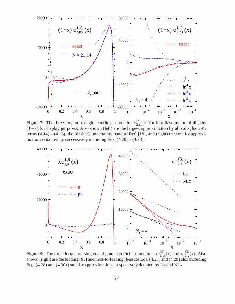
In Fig. 7 the non-singlet coefficient functionc(3)2,ns(x) of Eqs. (B.8) and (4.11) is compared

for nf = 4 with the large-x and small-x approximations specified above and with the previousuncertainty band [19] based on the lowest seven even-integer momentsN = 2. . .14 of Refs. [39–41] and the four large-x coefficients (4.14)–(4.17) predicted by the threshold resummation [92].

The complete soft-gluon contribution includingD 0 . . .D 5 deviates from the full coefficientfunction by less than 20% only atx ≥ 0.85. The correspondingx-range readsx ≤ 0.09 for thesmall-x approximation by the terms lnx. . . ln5x. Note that this range only arises when all small-x

26

-10000

0

10000

20000

0 0.2 0.4 0.6 0.8 1x

(1−x) c (3) (x)2,ns

exact

N = 2...14

Dk part

x

(1−x) c (3) (x)2,ns

exact

ln5 x

+ ln4 x

+ ln3 x

+ ln2 xNf = 4

-80000

-40000

0

40000

80000

10-5

10-4

10-3

10-2

10-1

Figure 7: The three-loop non-singlet coefficient functionc(3)2,ns(x) for four flavours, multiplied by

(1−x) for display purposes. Also shown (left) are the large-x approximation by all soft-gluonD k

terms (4.14) – (4.18), the (dashed) uncertainty band of Ref.[19], and (right) the small-x approxi-mations obtained by successively including Eqs. (4.20) – (4.23).

0

20000

40000

60000

0 0.2 0.4 0.6 0.8 1x

xc (3) (x)2,a

exact

a = ga = ps

x

xc (3) (x)2,a

Lx

NLx

Nf = 40

10000

20000

30000

40000

10-5

10-4

10-3

10-2

10-1

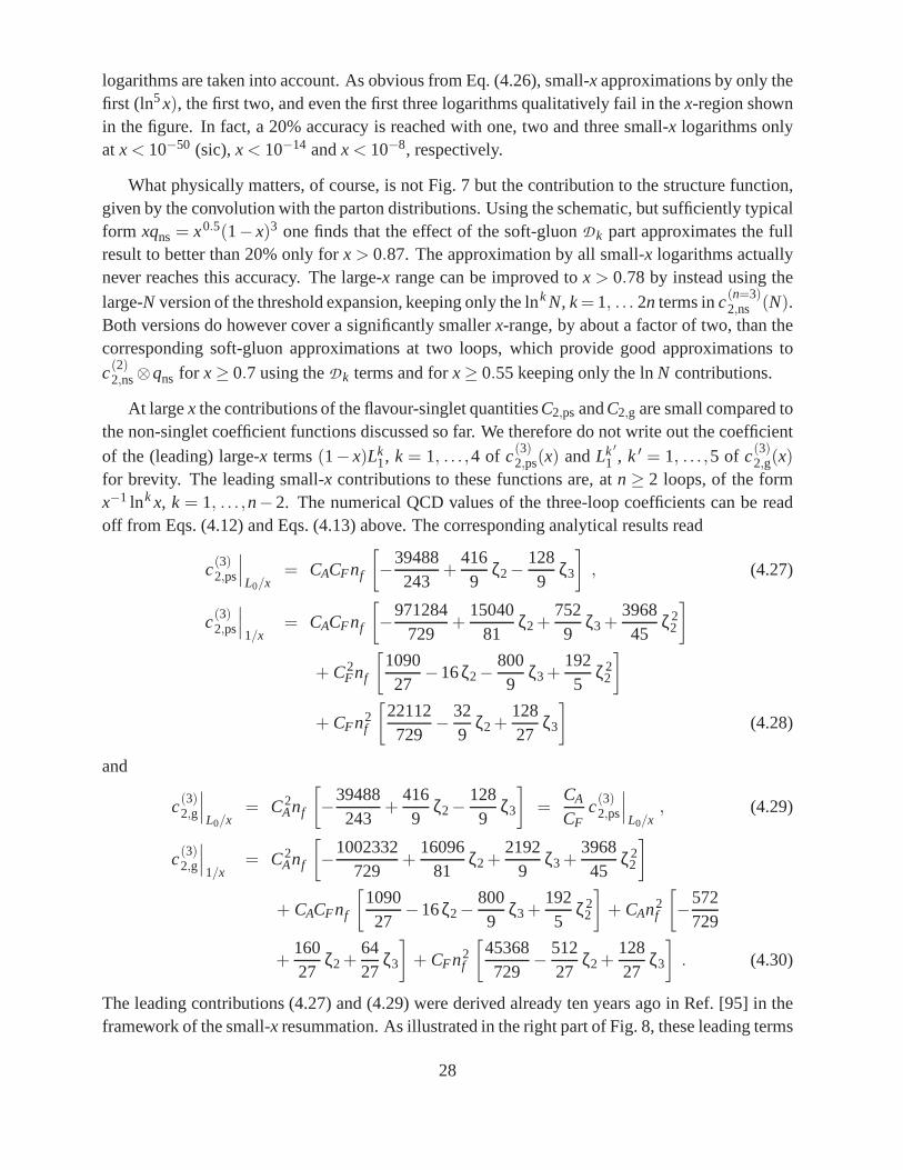
Figure 8: The three-loop pure-singlet and gluon coefficientfunctionsxc(3)2,ps(x) andxc(3)

2,g(x). Alsoshown (right) are the leading [95] and next-to-leading (besides Eqs. (4.27) and (4.29) also includingEqs. (4.28) and (4.30)) small-x approximations, respectively denoted by Lx and NLx.

27

logarithms are taken into account. As obvious from Eq. (4.26), small-x approximations by only thefirst (ln5x), the first two, and even the first three logarithms qualitatively fail in thex-region shownin the figure. In fact, a 20% accuracy is reached with one, two and three small-x logarithms onlyat x < 10−50 (sic),x < 10−14 andx < 10−8, respectively.

What physically matters, of course, is not Fig. 7 but the contribution to the structure function,given by the convolution with the parton distributions. Using the schematic, but sufficiently typicalform xqns = x0.5(1− x)3 one finds that the effect of the soft-gluonD k part approximates the fullresult to better than 20% only forx > 0.87. The approximation by all small-x logarithms actuallynever reaches this accuracy. The large-x range can be improved tox > 0.78 by instead using the

large-N version of the threshold expansion, keeping only the lnkN, k= 1, . . . 2n terms inc(n=3)2,ns (N).

Both versions do however cover a significantly smallerx-range, by about a factor of two, than thecorresponding soft-gluon approximations at two loops, which provide good approximations to

c(2)2,ns⊗qns for x≥ 0.7 using theD k terms and forx≥ 0.55 keeping only the lnN contributions.

At largex the contributions of the flavour-singlet quantitiesC2,psandC2,g are small compared tothe non-singlet coefficient functions discussed so far. We therefore do not write out the coefficient

of the (leading) large-x terms(1− x)Lk1, k = 1, . . . ,4 of c(3)

2,ps(x) andLk ′

1 , k ′ = 1, . . . ,5 of c(3)2,g(x)

for brevity. The leading small-x contributions to these functions are, atn ≥ 2 loops, of the formx−1 lnk x, k = 1, . . . ,n−2. The numerical QCD values of the three-loop coefficients can be readoff from Eqs. (4.12) and Eqs. (4.13) above. The corresponding analytical results read

c(3)2,ps

∣∣∣L0/x

= CACFnf

[−

39488243

+4169

ζ2−1289

ζ3

], (4.27)

c(3)2,ps

∣∣∣1/x

= CACFnf

[−

971284729

+15040

81ζ2 +

7529

ζ3 +396845

ζ 22

]

+ C2Fnf

[109027

−16ζ2−8009

ζ3+1925

ζ 22

]

+ CFn2f

[22112729

−329

ζ2 +12827

ζ3

](4.28)

and

c(3)2,g

∣∣∣L0/x

= C2Anf

[−

39488243

+4169

ζ2−1289

ζ3

]=

CA

CFc(3)

2,ps

∣∣∣L0/x

, (4.29)

c(3)2,g

∣∣∣1/x

= C2Anf

[−

1002332729

+16096

81ζ2 +

21929

ζ3 +396845

ζ 22

]

+ CACFnf

[109027

−16ζ2−8009

ζ3 +1925

ζ 22

]+ CAn2

f

[−

572729

+16027

ζ2 +6427

ζ3

]+ CFn2

f

[45368729

−51227

ζ2+12827

ζ3

]. (4.30)

The leading contributions (4.27) and (4.29) were derived already ten years ago in Ref. [95] in theframework of the small-x resummation. As illustrated in the right part of Fig. 8, these leading terms

28

alone do not provide a useful approximation atx-values relevant to collider measurements. Atx =

10−4, for example, they overshoot the respective full results for c(3)2,ps(x) andc(3)

2,g(x) in Eqs. (B.10),(4.12) and (B.9), (4.13) by a factor of about three. This situation is completely analogous to, ifsomewhat worse than that for the three-loop splitting functions discussed in Ref. [11].

It should be noted that also the singlet coefficient functions receive contributions from non-1/x logarithms up to ln2k−1 x at orderα k

s . In fact, the 1/x terms (4.27) – (4.30) contribute more

than 80% ofc(3)2,ps(x) andc(3)

2,g(x) only atx≤ 3 ·10−4. One may expect this range to shrink furtherat higher orders due to the double-logarithmic enhancementof the non-1/x terms. However, asthe above third-order range is rather similar to that for thesecond-order coefficient functions, ourresults do not provide evidence for this effect.

For the rest of this section we turn to the third-order coefficient functions for the longitudinalstructure functionFL which we only briefly discussed in Ref. [17]. The behaviour ofthe coefficient

functionsc(3)L,i (x) for x → 1 is given by lnk(1− x) ≡ Lk

1, k = 0, . . . ,4 for i = ns, by (1− x)Lk1,

k = 0, . . . ,4 for i = g and (1−x)2Lk1, k = 0, . . . ,3 for i = ps. The coefficients for the dominant

non-singlet contribution read

c(3)L,ns

∣∣∣L4

1

= 8C3F , (4.31)

c(3)L,ns

∣∣∣L3

1

= CAC2F

[−

6409

+32ζ2

]+ C3

F

[72−64ζ2

]+

649

CFn2f , (4.32)

c(3)L,ns

∣∣∣L2

1

= C2ACF

[1276

9−56ζ2−32ζ3

]+ CAC2

F

[−

5309

+80ζ2+80ζ3

]

+ C3F

[−34−32ζ2−32ζ3

]+ CACFnf

[−

3209

+16ζ2

]

+ C2Fnf

[929−32ζ2

]+

169

CFn2f , (4.33)

c(3)L,ns

∣∣∣L1

1

= C2ACF

[−

2575627

+3008

9ζ2 +

8803

ζ3−1285

ζ 22

]

+ CAC2F

[32732

27−

47209

ζ2+4723

ζ3−1152

5ζ 2

2

]+ C3

F

[−264

+16ζ2−752ζ3−2816

5ζ 2

2

]+ CACFnf

[664027

−3209

ζ2−2563

ζ3

]

+ C2Fnf

[−

473627

+3529

ζ2 +3203

ζ3

]−

30427

CFn2f , (4.34)

c(3)L,ns

∣∣∣L0

1

= C2ACF

[67312

81+

8243

ζ2−1264

3ζ3+56ζ 2

2 −80ζ2ζ3−160ζ5

]

+ CAC2F

[−

52556

−10988

9ζ2 +

32803

ζ3−516ζ 22 +416ζ2ζ3 +1200ζ5

]

29

+ C3F

[1937

6−+508ζ2−88ζ3 +

33845

ζ 22 −512ζ2ζ3−1760ζ5

]

+ CACFnf

[−

2148881

+329

ζ2 +643

ζ3−325

ζ 22

]

+ C2Fnf

[79+

10649

ζ2−4003

ζ3 +2565

ζ 22

]+ CFn2

f

[162481

−329

ζ2

]

+ 9 f l ns11 nf

[−320−1120ζ2−1760ζ3+32ζ 2

2 +320ζ2ζ3 +3200ζ5]

. (4.35)

Except for Eq. (4.31) addressed already in Ref. [17], these large-x coefficients do not exhibit any

obvious relation to those ofc(3)2,ns in Eqs. (4.14) – (4.19). Thus the above coefficients should provide

important checks and inputs for an explicit higher-order threshold resummation forFL along thelines of Refs. [96,97]. Such a resummation might not be of a large phenomenological relevance inview of the rather narrow region of validity of the large-x approximation, see the left part of Fig. 9,and the experimental status ofFL at largex. It would definitely be useful, however, in conjunctionwith a possible future four-loop generalization of the fixed-N calculations of Ref. [39].

The leading small-x contributions toc(m)L,ns(x) are given by the termsLk

0 with k = 0, . . . ,2m−3.The corresponding three-loop coefficients read

c(3)L,ns

∣∣∣L3

0

= −203

C3F , (4.36)

c(3)L,ns

∣∣∣L2

0

= −66CAC2F +32C3

F +12C2Fnf , (4.37)

c(3)L,ns

∣∣∣L1

0

= C2ACF

[−

9689

+120ζ2

]+ CAC2

F

[−

18329

−384ζ2

]

+ C3F

[168+416ζ2

]+

3529

CFCAnf +2249

C2Fnf −

329

CFn2f , (4.38)

c(3)L,ns

∣∣∣L0

0

= C2ACF

[−

1306027

+244ζ2

]+ CAC2

F

[580027

−1696

3ζ2−96ζ3

]

+ C3F

[288+608ζ2

]+ CACFnf

[418427

−16ζ2

]

+ C2Fnf

[−

114427

−323

ζ2

]−

30427

CFn2f . (4.39)

In the flavour-singlet sector, the dominantn-loop small-x terms forFL are of the same form as those

for F2 discussed above. The respective 1/x contributions toc(3)L,i , i = ps,g are given by

c(3)L,ps

∣∣∣L0/x

= CACFnf

[−

217627

+643

ζ2

], (4.40)

c(3)L,ps

∣∣∣1/x

= CACFnf

[−

1438427

+112ζ2+3203

ζ3

]

+ C2Fnf

[179227

−323

ζ2−1283

ζ3

]+ CFn2

f

[339281

−649

ζ2

](4.41)

30

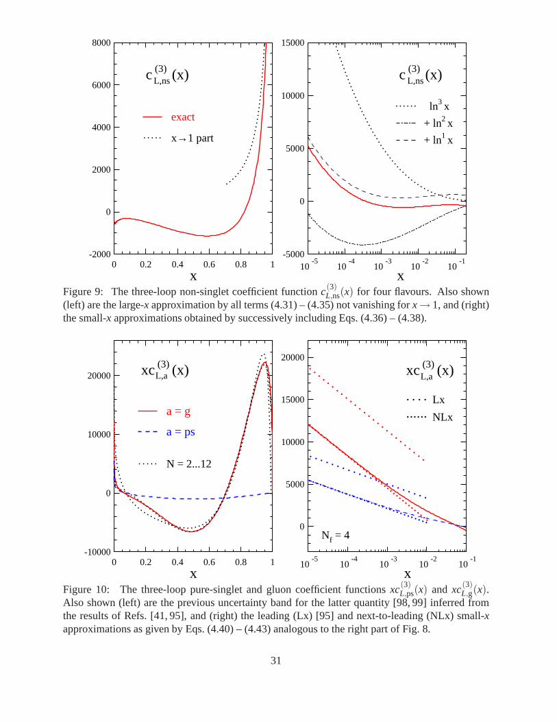
-2000

0

2000

4000

6000

8000

0 0.2 0.4 0.6 0.8 1x

c (3) (x)L,ns

exact

x→1 part

x

c (3) (x)L,ns

ln3 x

+ ln2 x

+ ln1 x

-5000

0

5000

10000

15000

10-5

10-4

10-3

10-2

10-1

Figure 9: The three-loop non-singlet coefficient functionc(3)L,ns(x) for four flavours. Also shown

(left) are the large-x approximation by all terms (4.31) – (4.35) not vanishing forx→ 1, and (right)the small-x approximations obtained by successively including Eqs. (4.36) – (4.38).

-10000

0

10000

20000

0 0.2 0.4 0.6 0.8 1x

xc (3) (x)L,a

a = g

a = ps

N = 2...12

x

xc (3) (x)L,a

Lx

NLx

Nf = 40

5000

10000

15000

20000

10-5

10-4

10-3

10-2

10-1

Figure 10: The three-loop pure-singlet and gluon coefficient functionsxc(3)L,ps(x) and xc(3)

L,g(x).Also shown (left) are the previous uncertainty band for the latter quantity [98, 99] inferred fromthe results of Refs. [41, 95], and (right) the leading (Lx) [95] and next-to-leading (NLx) small-xapproximations as given by Eqs. (4.40) – (4.43) analogous tothe right part of Fig. 8.

31

and

c(3)L,g

∣∣∣L0/x

= C2Anf

[−

217627

+643

ζ2

]=

CA

CFc(3)

L,ps

∣∣∣L0/x

, (4.42)

c(3)L,g

∣∣∣1/x

= C2Anf

[−

4409681

+1040

9ζ2+

3203

ζ3

]+ CAn2

f

[80827

−329

ζ2

]

+ CACFnf

[179227

−323

ζ2−1283

ζ3

]+ CFn2

f

[193681

−649

ζ2

]. (4.43)

The exactCF/CA relation between the leading small-x terms [95] ofc(n)a,ps andc(n)

a,g does not holdfor the subleading 1/x-contributions at three loops. However, most coefficients (actually those forall colour-factor/ζ-function combinations not occurring in the leading terms)are still closely re-lated. Besides the relations obvious from Eqs. (4.28) and (4.30) forc2,g and Eqs. (4.41) and (4.43)

for cL,g, we note that in both cases the sum of half the coefficient ofCFn2f and the coefficient of

CAn2f in the gluonic coefficient function equals that ofCFn2

f in the pure-singlet coefficient function.Numerically theCF/CA relation is violated by less than 5% for realistic values ofnf .

Eqs. (4.36) – (4.43) lead to the following numerical values for QCD,

c(3)L,ns|L3

0

∼= −15.8025

c(3)L,ns|L2

0

∼= −276.148+21.3333nf

c(3)L,ns|L1

0

∼= −1356.17+200.691nf −4.74074n2f

c(3)L,ns|L0

0

∼= −2226.25+408,058nf +15.0123n2f (4.44)

and

c(3)L,ps

∣∣∣L0/x

∼= −182.003nf

c(3)L,ps

∣∣∣1/x

∼= −885.534nf +40.2390n2f , (4.45)

c(3)L,g

∣∣∣L0/x

∼= −409.506nf

c(3)L,g

∣∣∣1/x

∼= −2044.70nf +88.5037n2f . (4.46)

The coefficients in both the non-singlet and singlet cases exhibit the pattern by now familiar fromthe three-loop splitting functions [10,11] and the coefficient functions forF2 discussed above. The

successive approximations ofc(3)L,i by the leading small-x terms are compared in the right parts of

Figs. 9 and 10 to the complete results (B.16) – (B.18). Also here the dominantx → 0 contribu-tions, ln3x for i = ns andx−1 lnx for i = ps, g, alone do not provide useful approximations forpractically relevant values ofx. Such endpoint constraints are however phenomenologically im-portant when combined with other partial results as, e.g., in Refs. [98, 99] for the previously used

approximations illustrated in the left part of Fig. 10 forc(3)L,g(x).

32

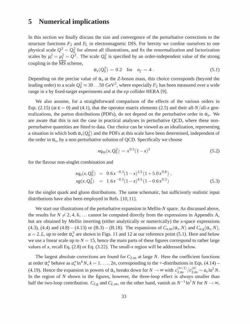
5 Numerical implications

In this section we finally discuss the size and convergence ofthe perturbative corrections to thestructure functionsF2 and FL in electromagnetic DIS. For brevity we confine ourselves to onephysical scaleQ2 = Q2

0 for almost all illustrations, and fix the renormalization and factorizationscales byµ2

r = µ2f = Q2. The scaleQ2

0 is specified by an order-independent value of the strong

coupling in theMS scheme,αs(Q

20) = 0.2 for nf = 4 . (5.1)

Depending on the precise value ofαs at theZ-boson mass, this choice corresponds (beyond theleading order) to a scaleQ2

0 ≈ 30. . .50 GeV2, where especiallyF2 has been measured over a widerange inx by fixed-target experiments and at theepcollider HERA [9].

We also assume, for a straightforward comparison of the effects of the various orders inEqs. (2.15) (atε = 0) and (4.1), that the operator matrix elements (2.5) and their all-N/all-x gen-eralizations, the parton distributions (PDFs), do not depend on the perturbative order inαs. Weare aware that this is not the case in practical analyses in perturbative QCD, where these non-perturbative quantities are fitted to data. Our choice can beviewed as an idealization, representinga situation in which bothαs(Q2

0) and the PDFs at this scale have been determined, independentofthe order inαs, by a non-perturbative solution of QCD. Specifically we choose

xqns(x,Q20) = x0.5(1−x)3 (5.2)

for the flavour non-singlet combination and

xqs(x,Q20) = 0.6x−0.3(1−x)3.5(1+5.0x0.8) ,

xg(x,Q20) = 1.6x−0.3(1−x)4.5(1−0.6x0.3) (5.3)

for the singlet quark and gluon distributions. The same schematic, but sufficiently realistic inputdistributions have also been employed in Refs. [10,11].

We start our illustrations of the perturbative expansion inMellin-N space. As discussed above,the results forN 6= 2, 4, 6, . . . cannot be computed directly from the expressions in Appendix A,but are obtained by Mellin inverting (either analytically or numerically) thex-space expressions(4.3), (4.4) and (4.8) – (4.13) or (B.3) – (B.18). The expansions ofCa,ns(αs,N) andCa,g(αs,N),a = 2,L, up to orderα 3

s are shown in Figs. 11 and 12 at our reference point (5.1). Hereand belowwe use a linear scale up toN = 15, hence the main parts of these figures correspond to ratherlargevalues ofx, recall Eq. (2.8) or Eq. (3.22). The small-x region will be addressed below.

The largest absolute corrections are found forC2,ns at largeN. Here the coefficient functionsat orderα n

s behave asans lnk N, k = 1, . . . , 2n, corresponding to the +-distributions in Eqs. (4.14) –

(4.19). Hence the expansion in powers ofαs breaks down forN → ∞ with c(n+1)2,ns /c(n)

2,ns∼ as ln2N.In the region ofN shown in the figures, however, the three-loop effect is always smaller thanhalf the two-loop contribution.C2,g andCL,ns, on the other hand, vanish asN−1 ln l N for N → ∞,

33

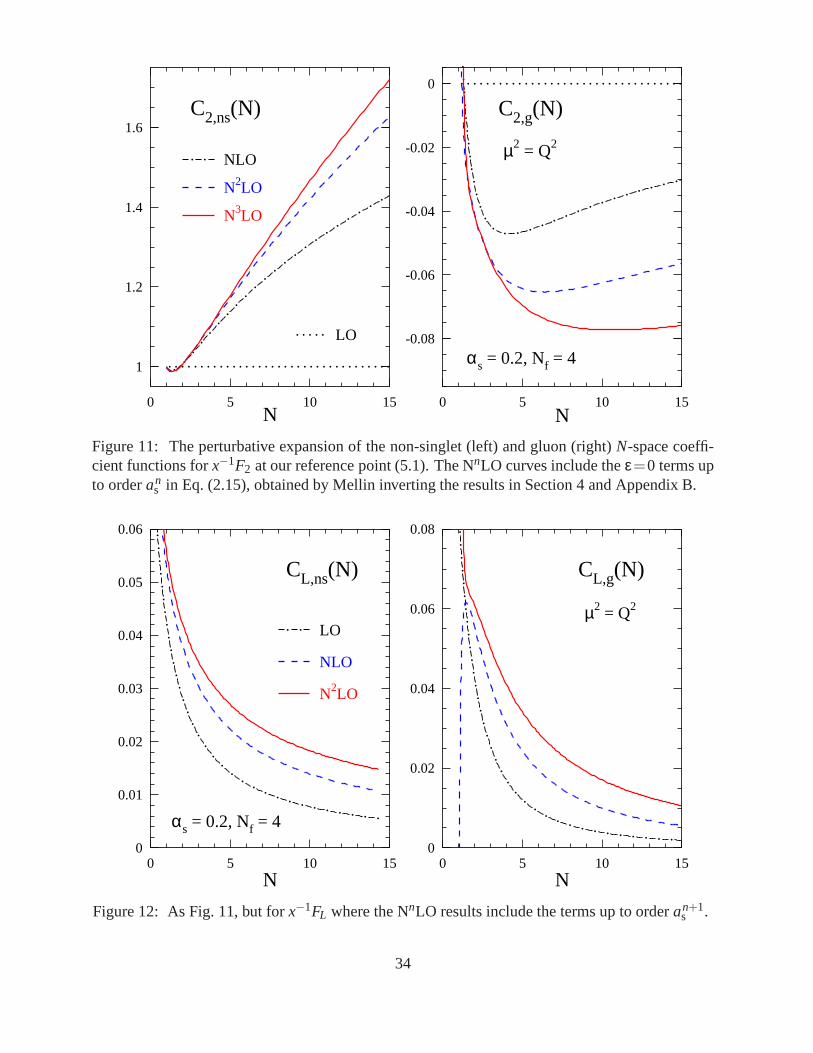
1

1.2

1.4

1.6

0 5 10 15N

C2,ns(N)

LO

NLO

N2LO

N3LO

N

C2,g(N)

µ2 = Q2

αs = 0.2, Nf = 4-0.08

-0.06

-0.04

-0.02

0

0 5 10 15

Figure 11: The perturbative expansion of the non-singlet (left) and gluon (right)N-space coeffi-cient functions forx−1F2 at our reference point (5.1). The NnLO curves include theε=0 terms upto orderan

s in Eq. (2.15), obtained by Mellin inverting the results in Section 4 and Appendix B.

0

0.01

0.02

0.03

0.04

0.05

0.06

0 5 10 15N

CL,ns(N)

LO

NLO

N2LO

αs = 0.2, Nf = 4

N

CL,g(N)

µ2 = Q2

0

0.02

0.04

0.06

0.08

0 5 10 15

Figure 12: As Fig. 11, but forx−1FL where the NnLO results include the terms up to orderan+1s .

34

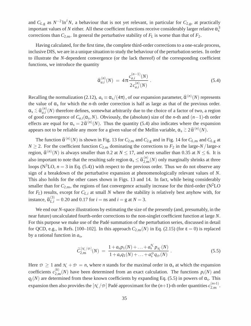
andCL,g as N−2 ln l N, a behaviour that is not yet relevant, in particular forC2,g, at practicallyimportant values ofN either. All these coefficient functions receive considerably larger relativeα 3

s

corrections thanC2,ns. In general the perturbative stability ofFL is worse than that ofF2.

Having calculated, for the first time, the complete third-order corrections to a one-scale process,inclusive DIS, we are in a unique situation to study the behaviour of the perturbation series. In orderto illustrate theN-dependent convergence (or the lack thereof) of the corresponding coefficientfunctions, we introduce the quantity

α (n)a,i (N) = 4π

c(n−1)a,i (N)

2c(n)a,i (N)

. (5.4)

Recalling the normalization (2.12),as≡ αs/(4π) , of our expansion parameter,α (n)(N) representsthe value ofαs for which then-th order correction is half as large as that of the previous order.

αs<∼ α (n)

a,i (N) therefore defines, somewhat arbitrarily due to the choice ofa factor of two, a regionof good convergence ofCa,i(αs,N). Obviously, the (absolute) size of then-th and(n−1)-th ordereffects are equal forαs = 2α (n)(N). Thus the quantity (5.4) also indicates where the expansionappears not to be reliable any more for a given value of the Mellin variable,αs

>∼ 2α (n)(N).

The functionα (n)(N) is shown in Fig. 13 forC2,ns andC2,g and in Fig. 14 forCL,ns andCL,g atN ≥ 2. For the coefficient functionC2,ns dominating the corrections toF2 in the large-N/ large-xregion,α (n)(N) is always smaller than 0.2 atN ≤ 17, and even smaller than 0.35 atN ≤ 6. It is

also important to note that the resulting safe regionαs≤ α (n)2,ns(N) only marginally shrinks at three

loops (N3LO, n = 3 in Eq. (5.4)) with respect to the previous order. Thus we do not observe anysign of a breakdown of the perturbative expansion at phenomenologically relevant values ofN.This also holds for the other cases shown in Figs. 13 and 14. Infact, while being considerablysmaller than forC2,ns, the regions of fast convergence actually increase for the third-order (N2LOfor FL) results, except forCL,i at smallN where the stability is relatively best anyhow with, for

instance,α(3)L,i = 0.20 and 0.17 fori = ns andi = g atN = 3.

We end ourN-space illustrations by estimating the size of the presently (and, presumably, in thenear future) uncalculated fourth-order corrections to thenon-singlet coefficient function at largeN.For this purpose we make use of the Padé summation of the perturbation series, discussed in detailfor QCD, e.g., in Refs. [100–102]. In this approachC2,ns(N) in Eq. (2.15) (forε = 0) is replacedby a rational function inas,

C [N /D ]2,ns (N) =

1+asp1(N)+ . . .+aNs pN (N)

1+asq1(N)+ . . .+aDs qD (N). (5.5)

HereD ≥ 1 andN +D = n, wheren stands for the maximal order inαs at which the expansion

coefficientsc(k)2,ns(N) have been determined from an exact calculation. The functions pi(N) and

qj(N) are determined from these known coefficients by expanding Eq. (5.5) in powers ofαs. This

expansion then also provides the[N /D ] Padé approximant for the (n+1)-th order quantitiesc(n+1)2,ns .

35

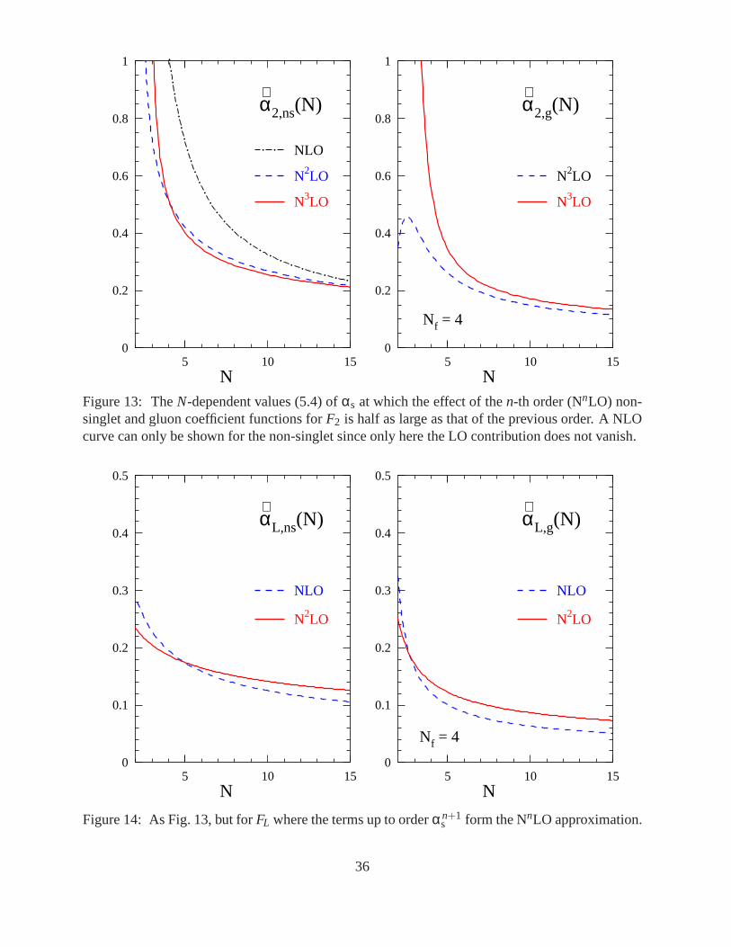
0

0.2

0.4

0.6

0.8

1

5 10 15N

α∧

2,ns(N)

NLO

N2LO

N3LO

N

α∧

2,g(N)

N2LO

N3LO

Nf = 4

0

0.2

0.4

0.6

0.8

1

5 10 15

Figure 13: TheN-dependent values (5.4) ofαs at which the effect of then-th order (NnLO) non-singlet and gluon coefficient functions forF2 is half as large as that of the previous order. A NLOcurve can only be shown for the non-singlet since only here the LO contribution does not vanish.

0

0.1

0.2

0.3

0.4

0.5

5 10 15N

α∧

L,ns(N)

NLO

N2LO

N

α∧

L,g(N)

NLO

N2LO

Nf = 4

0

0.1

0.2

0.3

0.4

0.5

5 10 15

Figure 14: As Fig. 13, but forFL where the terms up to orderα n+1s form the NnLO approximation.

36

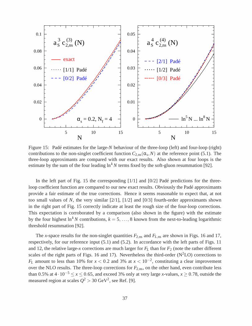
0

0.02

0.04

0.06

0.08

0.1

5 10 15N

a 3 c (3) (N)S 2,ns

exact

[0/2] Padé

[1/1] Padé

αs = 0.2, Nf = 4

N

a 4 c (4) (N)S 2,ns

[2/1] Padé

[0/3] Padé

[1/2] Padé

ln5 N ... ln8 N0

0.01

0.02

0.03

0.04

0.05

5 10 15

Figure 15: Padé estimates for the large-N behaviour of the three-loop (left) and four-loop (right)contributions to the non-singlet coefficient functionC2,ns(αs,N) at the reference point (5.1). Thethree-loop approximants are compared with our exact results. Also shown at four loops is theestimate by the sum of the four leading lnk N terms fixed by the soft-gluon resummation [92].

In the left part of Fig. 15 the corresponding [1/1] and [0/2] Padé predictions for the three-loop coefficient function are compared to our new exact results. Obviously the Padé approximantsprovide a fair estimate of the true corrections. Hence it seems reasonable to expect that, at nottoo small values ofN, the very similar [2/1], [1/2] and [0/3] fourth-order approximants shownin the right part of Fig. 15 correctly indicate at least the rough size of the four-loop corrections.This expectation is corroborated by a comparison (also shown in the figure) with the estimateby the four highest lnk N contributions,k = 5, . . . , 8 known from the next-to-leading logarithmicthreshold resummation [92].

Thex-space results for the non-singlet quantitiesF2,ns andFL,ns are shown in Figs. 16 and 17,respectively, for our reference input (5.1) and (5.2). In accordance with the left parts of Figs. 11and 12, the relative large-x corrections are much larger forFL than forF2 (note the rather differentscales of the right parts of Figs. 16 and 17). Nevertheless the third-order (N2LO) corrections toFL amount to less than 10% forx < 0.2 and 3% atx < 10−2, constituting a clear improvementover the NLO results. The three-loop corrections forF2,ns, on the other hand, even contribute lessthan 0.5% at 4·10−5 ≤ x≤ 0.65, and exceed 3% only at very largex-values,x≥ 0.78, outside themeasured region at scalesQ2 > 30 GeV2, see Ref. [9].

37

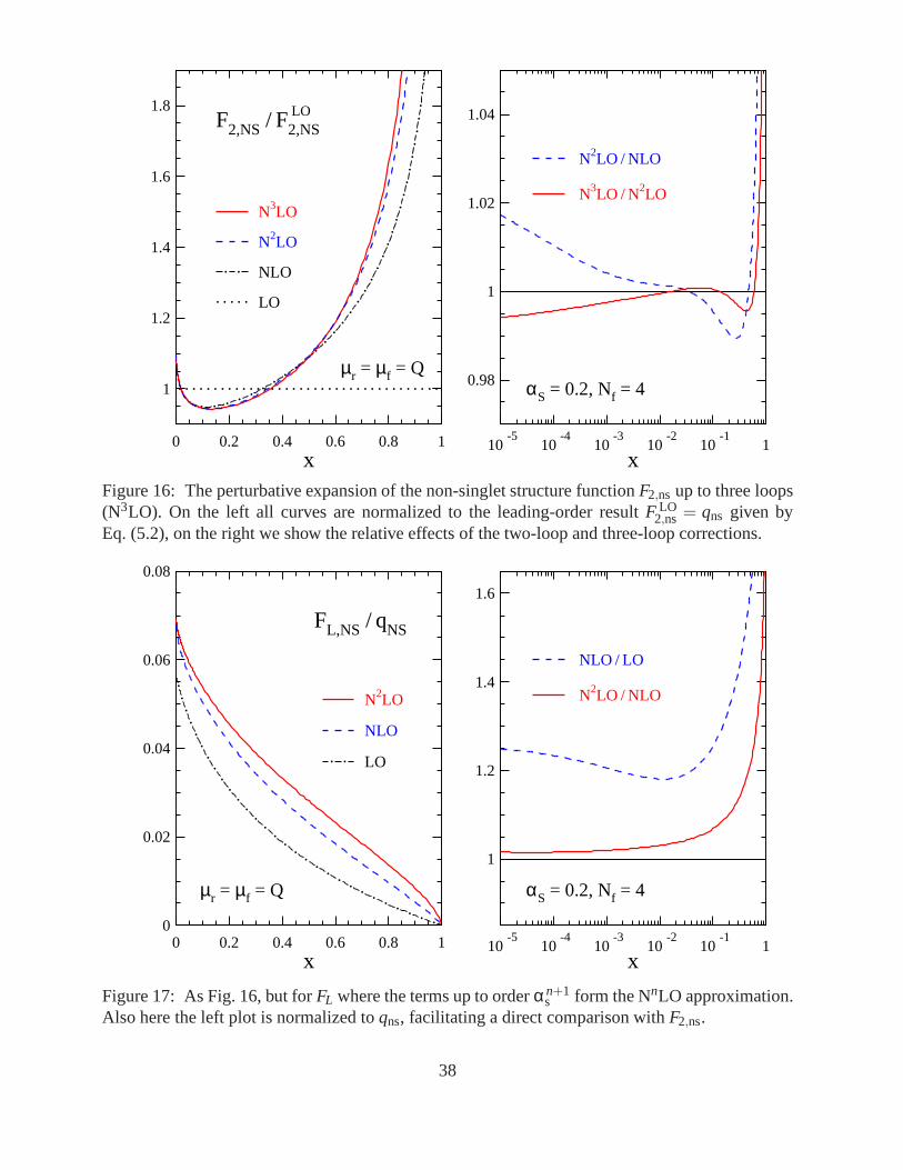
1

1.2

1.4

1.6

1.8

0 0.2 0.4 0.6 0.8 1x

F2,NS / F2,NS

LO

LO

NLO

N2LO

N3LO

µr = µf = Q

x

N2LO / NLO

N3LO / N2LO

αS = 0.2, Nf = 40.98

1

1.02

1.04

10-5

10-4

10-3

10-2

10-1

1

Figure 16: The perturbative expansion of the non-singlet structure functionF2,ns up to three loops(N3LO). On the left all curves are normalized to the leading-order resultF LO

2,ns = qns given byEq. (5.2), on the right we show the relative effects of the two-loop and three-loop corrections.

0

0.02

0.04

0.06

0.08

0 0.2 0.4 0.6 0.8 1x

FL,NS / qNS

LO

NLO

N2LO

µr = µf = Q

x

NLO / LO

N2LO / NLO

αS = 0.2, Nf = 4

1

1.2

1.4

1.6

10-5

10-4

10-3

10-2

10-1

1

Figure 17: As Fig. 16, but forFL where the terms up to orderα n+1s form the NnLO approximation.

Also here the left plot is normalized toqns, facilitating a direct comparison withF2,ns.

38

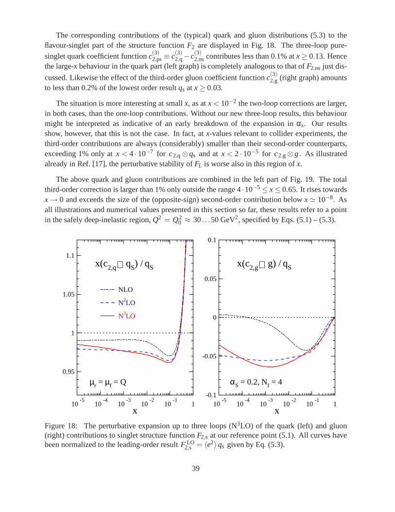
The corresponding contributions of the (typical) quark andgluon distributions (5.3) to theflavour-singlet part of the structure functionF2 are displayed in Fig. 18. The three-loop pure-

singlet quark coefficient functionc(3)2,ps≡ c(3)

2,q−c(3)2,ns contributes less than 0.1% atx≥ 0.13. Hence

the large-x behaviour in the quark part (left graph) is completely analogous to that ofF2,ns just dis-

cussed. Likewise the effect of the third-order gluon coefficient functionc(3)2,g (right graph) amounts

to less than 0.2% of the lowest order resultqs at x≥ 0.03.

The situation is more interesting at smallx, as atx < 10−2 the two-loop corrections are larger,in both cases, than the one-loop contributions. Without ournew three-loop results, this behaviourmight be interpreted as indicative of an early breakdown of the expansion inαs. Our resultsshow, however, that this is not the case. In fact, atx-values relevant to collider experiments, thethird-order contributions are always (considerably) smaller than their second-order counterparts,exceeding 1% only atx < 4 ·10−7 for c2,q⊗qs and atx < 2 ·10−5 for c2,g⊗g. As illustratedalready in Ref. [17], the perturbative stability ofFL is worse also in this region ofx.

The above quark and gluon contributions are combined in the left part of Fig. 19. The totalthird-order correction is larger than 1% only outside the range 4·10−5 ≤ x≤ 0.65. It rises towardsx→ 0 and exceeds the size of the (opposite-sign) second-order contribution belowx≃ 10−8. Asall illustrations and numerical values presented in this section so far, these results refer to a pointin the safely deep-inelastic region,Q2 = Q2

0 ≈ 30. . .50 GeV2, specified by Eqs. (5.1) – (5.3).

0.95

1

1.05

1.1

10-5

10-4

10-3

10-2

10-1

1x

x(c2,q qS) / qS⊗

NLO

N2LO

N3LO

µr = µf = Q

x

x(c2,g g) / qS⊗

αS = 0.2, Nf = 4

-0.1

-0.05

0

0.05

0.1

10-5

10-4

10-3

10-2

10-1

1

Figure 18: The perturbative expansion up to three loops (N3LO) of the quark (left) and gluon(right) contributions to singlet structure functionF2,s at our reference point (5.1). All curves havebeen normalized to the leading-order resultF LO

2,s = 〈e2〉qs given by Eq. (5.3).

39

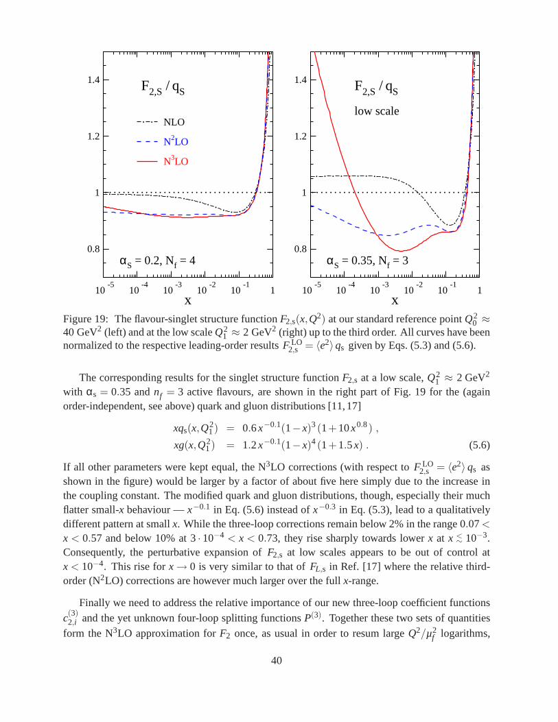
0.8

1

1.2

1.4

10-5

10-4

10-3

10-2

10-1

1x

F2,S / qS

NLO

N2LO

N3LO

αS = 0.2, Nf = 4

x

F2,S / qS

low scale

αS = 0.35, Nf = 30.8

1

1.2

1.4

10-5

10-4

10-3

10-2

10-1

1

Figure 19: The flavour-singlet structure functionF2,s(x,Q2) at our standard reference pointQ20 ≈

40 GeV2 (left) and at the low scaleQ21 ≈ 2 GeV2 (right) up to the third order. All curves have been

normalized to the respective leading-order resultsF LO2,s = 〈e2〉qs given by Eqs. (5.3) and (5.6).

The corresponding results for the singlet structure function F2,s at a low scale,Q21 ≈ 2 GeV2

with αs = 0.35 andnf = 3 active flavours, are shown in the right part of Fig. 19 for the(againorder-independent, see above) quark and gluon distributions [11,17]

xqs(x,Q21) = 0.6x−0.1(1−x)3(1+10x0.8) ,

xg(x,Q21) = 1.2x−0.1(1−x)4(1+1.5x) . (5.6)

If all other parameters were kept equal, the N3LO corrections (with respect toF LO2,s = 〈e2〉qs as

shown in the figure) would be larger by a factor of about five here simply due to the increase inthe coupling constant. The modified quark and gluon distributions, though, especially their muchflatter small-x behaviour —x−0.1 in Eq. (5.6) instead ofx−0.3 in Eq. (5.3), lead to a qualitativelydifferent pattern at smallx. While the three-loop corrections remain below 2% in the range 0.07<

x < 0.57 and below 10% at 3· 10−4 < x < 0.73, they rise sharply towards lowerx at x <∼ 10−3.

Consequently, the perturbative expansion ofF2,s at low scales appears to be out of control atx < 10−4. This rise forx→ 0 is very similar to that ofFL,s in Ref. [17] where the relative third-order (N2LO) corrections are however much larger over the fullx-range.

Finally we need to address the relative importance of our newthree-loop coefficient functions

c(3)2,i and the yet unknown four-loop splitting functionsP(3). Together these two sets of quantities

form the N3LO approximation forF2 once, as usual in order to resum largeQ2/µ2f logarithms,

40

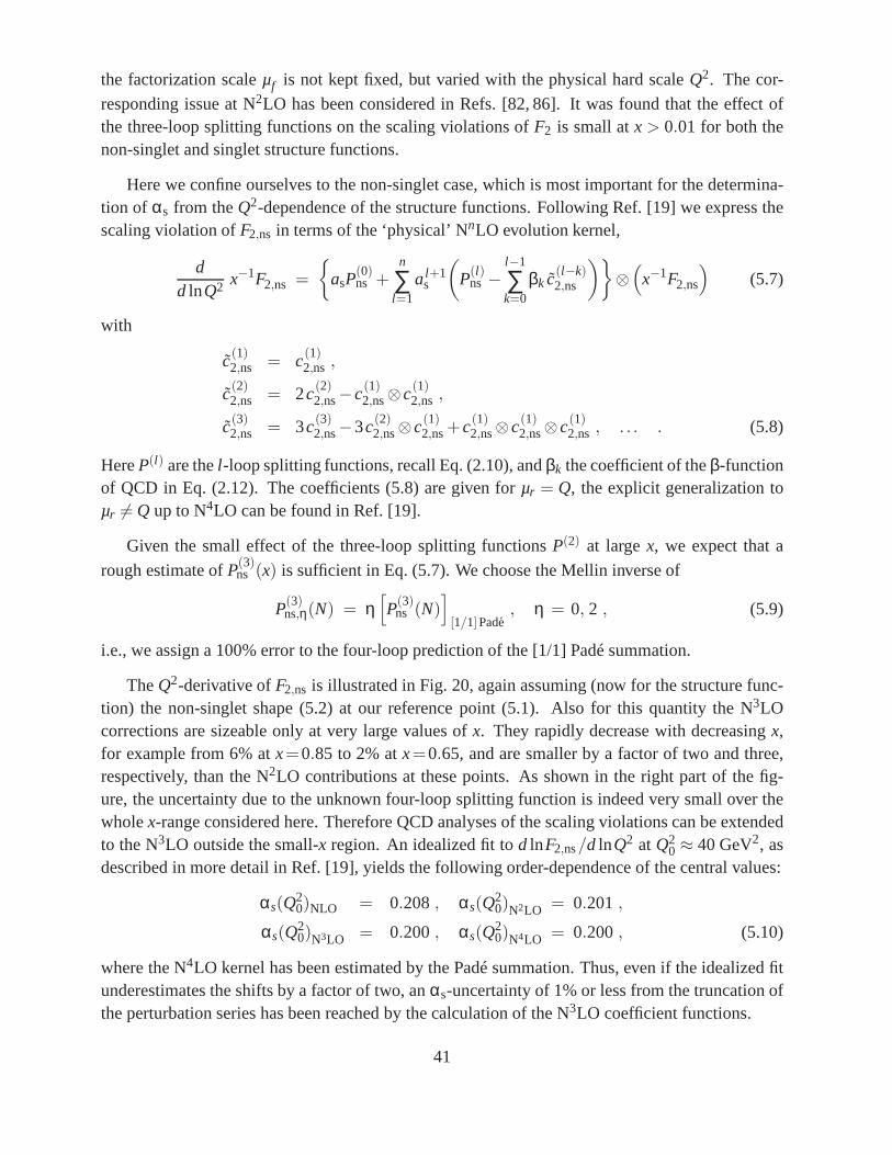
the factorization scaleµf is not kept fixed, but varied with the physical hard scaleQ2. The cor-

responding issue at N2LO has been considered in Refs. [82, 86]. It was found that theeffect ofthe three-loop splitting functions on the scaling violations ofF2 is small atx > 0.01 for both thenon-singlet and singlet structure functions.

Here we confine ourselves to the non-singlet case, which is most important for the determina-tion of αs from theQ2-dependence of the structure functions. Following Ref. [19] we express thescaling violation ofF2,ns in terms of the ‘physical’ NnLO evolution kernel,

dd lnQ2 x−1F2,ns =

{asP

(0)ns +

n

∑l=1

al+1s

(P(l)

ns −l−1

∑k=0

βk c(l−k)2,ns

)}⊗

(x−1F2,ns

)(5.7)

with

c(1)2,ns = c(1)

2,ns ,

c(2)2,ns = 2c(2)

2,ns−c(1)2,ns⊗c(1)

2,ns ,

c(3)2,ns = 3c(3)

2,ns−3c(2)2,ns⊗c(1)

2,ns+c(1)2,ns⊗c(1)

2,ns⊗c(1)2,ns , . . . . (5.8)

HereP(l) are thel -loop splitting functions, recall Eq. (2.10), andβk the coefficient of theβ-functionof QCD in Eq. (2.12). The coefficients (5.8) are given forµr = Q, the explicit generalization toµr 6= Q up to N4LO can be found in Ref. [19].

Given the small effect of the three-loop splitting functions P(2) at largex, we expect that a

rough estimate ofP(3)ns (x) is sufficient in Eq. (5.7). We choose the Mellin inverse of

P(3)ns,η(N) = η

[P(3)

ns (N)]

[1/1]Pade, η = 0, 2 , (5.9)

i.e., we assign a 100% error to the four-loop prediction of the [1/1] Padé summation.

TheQ2-derivative ofF2,ns is illustrated in Fig. 20, again assuming (now for the structure func-tion) the non-singlet shape (5.2) at our reference point (5.1). Also for this quantity the N3LOcorrections are sizeable only at very large values ofx. They rapidly decrease with decreasingx,for example from 6% atx=0.85 to 2% atx=0.65, and are smaller by a factor of two and three,respectively, than the N2LO contributions at these points. As shown in the right part of the fig-ure, the uncertainty due to the unknown four-loop splittingfunction is indeed very small over thewholex-range considered here. Therefore QCD analyses of the scaling violations can be extendedto the N3LO outside the small-x region. An idealized fit tod lnF2,ns/d lnQ2 at Q2

0 ≈ 40 GeV2, asdescribed in more detail in Ref. [19], yields the following order-dependence of the central values:

αs(Q20)NLO = 0.208 , αs(Q

20)N2LO = 0.201 ,

αs(Q20)N3LO = 0.200 , αs(Q

20)N4LO = 0.200 , (5.10)

where the N4LO kernel has been estimated by the Padé summation. Thus, even if the idealized fitunderestimates the shifts by a factor of two, anαs-uncertainty of 1% or less from the truncation ofthe perturbation series has been reached by the calculationof the N3LO coefficient functions.

41

-0.7

-0.6

-0.5

-0.4

-0.3

-0.2

-0.1

0

0.1

0 0.2 0.4 0.6 0.8 1

x

d ln F2,NS / d ln Q2

LO

NLO

NNLO

N3LO η = 0, 2

µr = Q

x

F2,NS − ( F2,NS )NNLO

. .

αS = 0.2, Nf = 4

-0.01

-0.005

0

0.005

0.01

10-3

10-2

10-1

1

Figure 20: The perturbative expansion (5.7) of the scale derivativeF2,ns≡ d lnF2,ns/d lnQ2 for theinitial conditionF2,ns = x0.5(1− x)3 at the reference point (5.1). The two N3LO curves indicatethe uncertainty due to the four-loop splitting functions asestimated in Eq. (5.9).

6 Summary

We have calculated the complete third-order coefficient functions for the electromagnetic structurefunctionsF2 andFL in massless perturbative QCD. Our calculation has been performed in Mellin-Nspace, as previous fixed-N computations of deep-inelastic scattering [39–42] using the opticaltheorem and a dispersion relation in the Bjorken variablex. However, generalizing the two-loopcalculation of Ref. [16] and our previous computation of thefermionic non-singlet corrections atthree loops [32], we have now obtained the complete third-order coefficient functions for all evenvalues ofN by deriving the analyticN-dependence of all required integrals through an elaborateiterative system of reduction equations. The full dependence of the coefficient functions onx andN has then been reconstructed from the even-N results by analytic continuation, making use of therelation between the harmonic sumsS~n(N) [67] and the harmonic polylogarithmsH~m(x) [85] inwhich the respective results can be expressed.

Our coefficient functions agree with all partial results available in the literature. The coeffi-cients of the leading small-x terms x−1 lnx of the singlet quark and gluon coefficient functionswere derived already in Ref. [95] in the framework of the small-x resummation. No correspondingresult is known for the non-singlet case, in contrast to the splitting functions [103]. The first fourlarge-x terms, lnk N with k = 3, . . .6 in Mellin space, were predicted by the soft-gluon threshold

42

resummation [92]. Most importantly, the even momentsN = 2, . . . ,12 for the singlet case andN = 2, . . . ,14 for the non-singlet coefficient function were computed before [39–41] using theFORM [63, 64] version of the MINCER program [61, 62]. In fact, we have made extensive use ofthis program for checks at intermediate stages of our calculations. Finally our results also agreewith the recent computation of theN = 16 non-singlet moments ofF2 andFL [104], which wasspecifically performed as an independent simultaneous check of our calculations.

We have investigated the convergence of the perturbative expansion of the coefficient functionsCa,i(N,αs) by determining, at 2≤ N ≤ 20, theN-dependent range ofαs for which then-th ordercorrections are at most half as large as the(n−1)-th order contributions. ForC2,ns this αs-regionshrinks significantly from the first to the second order, but only marginally from the second to thethird. The coefficient functionsC2,g andCL,i exhibit larger corrections thanC2,ns — at N = 6, forexample, the aboveαs-region isαs < 0.35 forC2,ns, butαs < 0.17 forCL,ns— however this smallerregion actually increases from the second to the third orderfor most values ofN. Thus, up to thethird order, we find no sign of the supposed asymptotic character of the perturbative expansion.

Besides the phenomenologically less relevant limitx→ 1, the above region ofN also excludesthe small-x region opened up experimentally by HERA. The expansion of the coefficient functionsis unstable forx→ 0 asc(n)/c(n−1) ∼ αs lnξ x with ξ = 2 (ξ = 1) for the non-singlet (singlet) cases.This behaviour does not spoil the convergence of theαs-expansion forx-values relevant to collidermeasurements in the safely deep-inelastic regimeQ2 ≫ 1 GeV2, however, due to an apparentlysystematic suppression of the coefficients of leading terms(see also Refs. [10,11]) and the Mellinconvolution with the parton distributions. AtQ2 ≈ 30 GeV2, for instance, the total third-ordercorrection toF2 is larger than 1% only outside the wide range 4·10−5 ≤ x ≤ 0.65, and exceeds5% only atx <

∼ 10−7 andx > 0.8. At low scalesQ2 ≈ 2 GeV2, on the other hand, the perturbativeexpansion appears to be out of control atx < 10−4.

Our three-loop results for the splitting functions [10, 11]andFL (briefly discussed already inRef. [17] ) facilitate NNLO analyses of deep-inelastic scattering over the fullx-range covered bydata. The present additional results forF2 can be employed to effectively extend the main partof DIS analyses to the N3LO at x > 10−2 where the effect of the unknown fourth-order splittingfunctions is expected to be very small, for example leading to determinations ofαs(MZ) with anerror of less than 1% from the truncation of the perturbationseries. For use in such analyses wehave provided compact and accurate parametrizations of ourvery lengthy exact results. FORM

files of these results, and FORTRAN subroutines of the exact and approximate coefficient functionscan be obtained from the preprint serverHTTP://arXiv.org by downloading the source of thisarticle. Furthermore they are available from the authors upon request.

Finally our three-loop results for a one-scale process alsoare of theoretical interest, as theyopen up a new order in the study of perturbative QCD. As first further steps they facilitate theextension of the Sudakov resummations of threshold logarithms in DIS and of the quark formfactor beyond the orders obtained so far [27–30, 32]. We haveperformed the required additionalcalculations for both cases and will report the results in a forthcoming publication [31].

43

Acknowledgments

We would like to thank S.A. Larin, F. J. Yndurain, E. Remiddi,E. Laenen, W.L. van Neerven,P. Uwer, S. Weinzierl and J. Blümlein for stimulating discussions. M. Zhou has contributed someFORM routines in an early stage of this project. We are grateful toT. Gehrmann for providing aweight-five extension of the FORTRAN package [87] for the harmonic polylogarithms. The Feyn-man diagrams in this article have been drawn using the packages AXODRAW [105] and JAXO-DRAW [106]. The work of S.M. has been supported in part by the Deutsche Forschungsgemein-schaft in Sonderforschungsbereich/Transregio 9. The workof J.V. has been part of the researchprogram of the Dutch Foundation for Fundamental Research ofMatter (FOM).

Appendix A: The exact Mellin-space results

Here we provide the exact even-N expressions for the coefficient functionsC2,i andCL,i up tothe third order inas = αs/(4π). These results are expressed in terms of harmonic sums [65–68],following Ref. [67] recursively defined by

S±m1,m2,...,mk(N) =N

∑i=1

(±1)i

i m1Sm2,...,mk(i) , S(N) = 1 . (A.1)

The sum of the absolute values of the indicesmk defines the weight of the harmonic sum. Sumswith weight up to 2n occur in then-loop coefficient functions for bothF2 andFL. As in Section 3we employ the notation (3.10),

N±S~m = S~m(N±1) , N±i S~m = S~m(N± i) ,

together with the abbreviations

gqq = N+ +N− ,

gqg = 2N+2 −4N+ −N− +3 . (A.2)

TheN-independent zeroth-order quark coefficient function forF2 is set to unity, recall Eq. (4.2).In the above notation the well-known first-order results forF2 read

c(1)2,q(N) = CF(9(S1−1)+2gqq(S1,1+2S1−S2)−7(N−+1)S1) , (A.3)

c(1)2,g(N) = nf (−2gqg(S1,1+4S1−S2)−6(N−−1)S1) . (A.4)

The corresponding expressions for the two-loop coefficientfunctions [12,13,16] are given by

c(2)2,ns(N) = δ(N−2)

{CFnf (−4)+CF

2(−

4189810

+965

ζ3

)+CACF

(3677135

−1285

ζ3

)}

+θ(N−4)

{CF

(CF −

CA

2

)(16S−3,1 +48S−2,−2 +144S1,−2−

165

(N−3 −N−2)S1,−2

44

−80S2,−2−24S−4−16S−2 +1445

(N+3 −N+2)(S1,−2 +S3)+1445

(N+2 −3)(S1−S2)

−165

(N−2 −N−)(S1 +S2)−16(2N− +3)(S1,−3−S1,3−2S1,1,−2 +3S1ζ3)

)+CFnf

(45736

−23

S1,1−227

gqq(102S1,1 −18S1,2−36S2,1 +18S1,1,1 +244S1−171S2 +45S3)−239

S1

+143

S2 +19(N− +1)(42S1,1 +133S1−78S2)

)+CF

2(

59S1,1−28S1,2−40S2,1 +8S2,2

+20S1,1,1−8S2,1,1 +15

gqq(400S1,−3 −200S1,−2−340S1,1−160S1,2−140S1,3−240S2,1

+140S2,2 +120S3,1−80S1,−2,1−560S1,1,−2 +180S1,1,1−160S1,1,2 −120S1,2,1−160S2,1,1

+120S1,1,1,1 −605S1 +720S1ζ3 +646S2−20S3−30S4)+672

S1−1695

S2 +42S3 +4S4

−110

(N− +1)(320S1,−2−250S1,1−280S1,2−640S2,−2−560S2,1 +80S2,2 +280S1,1,1

−80S2,1,1−1203S1 +1106S2 +140S3 +40S4)+3318

−72ζ3

)+CACF

(−

853

S1,1 +8S3,1

−1

135gqq(5400S1,−3 −2700S1,−2−10020S1,1 +990S1,2−3780S1,3 +1980S2,1−1080S3,1

−1080S1,−2,1 −7560S1,1,−2−990S1,1,1−540S1,1,2 +540S1,2,1−19570S1 +11340S1ζ3

+17181S2−5175S3 +1620S4)−58118

S1 +22115

S2−12S4 +190

(N− +1)(1440S1,−2

−3570S1,1 −2880S2,−2−720S3,1−10261S1 +8502S2−1800S3 +1080S4)−546572

+54ζ3

)}, (A.5)

c(2)2,g(N) = δ(N−2)

{CFnf

(−

4799810

+165

ζ3

)+CAnf

(115324

−2ζ3

)}

+θ(N−4)

{CFnf

(−

815

(N−3 −N−2)S1,−2−25

gqg(20S1,−3−24S1,−2 +30S1,1−90S1,2

+30S1,3 +40S2,−2−90S2,1 +40S2,2 +60S3,1−40S1,1,−2 +90S1,1,1−40S1,1,2−60S1,2,1

−50S2,1,1 +50S1,1,1,1 +9S1−54S2 +66S3−50S4)−965

(N+3 −1)(S1,−2 +S3)+130

(2N+

+ N−−3)(240S1,−3 +256S1,−2 +240S1,1−120S1,2−240S1,3−480S2,−2 +240S2,1

−120S2,2−240S3,1−480S1,1,−2 +120S1,1,1 +120S2,1,1 +609S1 +720S1ζ3 +309S2−284S3

+300S4)−130

(N−−1)(1408S1,−2 +180S1,1−420S1,2−960S2,−2−360S2,1 +420S1,1,1

−593S1 +117S2 +418S3)−815

(N−2 −1)(S1 +S2)

)+CAnf

(−

154

gqg(648S1,−3−720S1,−2

+4710S1,1−2412S1,2 +432S1,3 +432S2,−2−3996S2,1 +432S2,2 +432S3,1−432S1,−2,1

+2196S1,1,1−648S1,1,2 −216S1,2,1−432S2,1,1 +216S1,1,1,1 +4493S1−6270S2 +3492S3)

−154

(2N+ + N−−3)(216S1,−3−720S1,−2 +624S1,1−252S1,2−216S1,3 +432S2,−2

−108S2,1−864S2,2−1296S3,1−432S1,1,−2 +252S1,1,1 +864S2,1,1 +1277S1 +648S1ζ3

−1014S2−1260S3 +1512S4)+127

(N−−1)(792S1,−2−2913S1,1 +828S1,2 +1728S2,1

45

−648S2,2−1080S3,1−720S1,1,1 +648S2,1,1−1981S1 +4194S2−2322S3 +1296S4)

−827

(N−2 −1)(18S1,−2−39S1,1−18S1,2 +18S1,1,1 +43S1)

)}(A.6)

and

c(2)2,ps(N) = CFnf

(−

1283

S1,−2 +6889

S1,1 +32S2,1 +16S2,2 +32S3,1−16S2,1,1

+227

gqq(288S1,−2 −408S1,1−18S1,2−216S2,1 +108S2,2 +216S3,1 +18S1,1,1

−108S2,1,1 −857S1 +204S2 +693S3−270S4)+184427

S1−7529

S2−1403

S3−40S4

−1627

(N+2 −3)(9S1,−2−6S1,1−9S1,2−27S2,1 +9S1,1,1−28S1−24S2 +36S3)

−827

(N−2 −N−)(18S1,−2−39S1,1−18S1,2 +18S1,1,1 +43S1)−427

(N− +1)(36S1,−2

+30S1,1−108S2,1 +108S2,2 +216S3,1−108S2,1,1−310S1−276S2 +333S3−270S4)

+83(2N− +3)(S1,2−S1,1,1)

)(A.7)

Our new three-loop non-singlet quark coefficient function for the structure functionF2 reads

c(3)2,ns(N) = δ(N−2)

{dabcdabc

ncf l11

(4965

−2563

ζ5−121615

ζ3

)+CFnf

2(

78142187

+6481

ζ3

)

+CF2nf

(−

34170121870

+323

ζ4−135245

ζ3

)+CF

3(−

2015777290

+4163

ζ5 +643

ζ4−50864405

ζ3

)

+CACFnf

(−

99815310935

+803

ζ5−323

ζ4 +17432405

ζ3

)+CACF

2(−

101357810935

−1552

3ζ5−32ζ4

+30776

45ζ3

)+CA

2CF

(366749810935

+296ζ5 +323

ζ4−46160

81ζ3

)}

+θ(N−4)

{dabcdabc

ncf l11

(128S−2,−2−512S−2,1 +

2124815

S1,−3−7168

3S1,−2−

204815

S1,3

−2048S1,−2ζ3 +204815

S1,1−1024S1,1ζ3 +2816S2,−2 +2048S2,1ζ3 +1536S2,3−22784

15S2,1

−15104

15S3,1−1536S4,1−1024S1,−4,1−

409615

S1,−2,1 +1024S1,−2,3 −2560S1,1,−2

+512S1,1,3−512S1,3,1 −1024S2,1,3 +1024S2,3,1 −6415

gqq(30S1,−4 +286S1,−3−430S1,−2

−480S1,−2ζ3 +216S1,1 +160S1,1ζ3−66S1,3−30S1,4 +20S2,−3 +280S2,−2−612S2,1

−480S2,1ζ3 +40S2,3−346S3,1−240S1,−4,1−60S4,1−80S1,−3,1 +60S1,−2,−2−202S1,−2,1

−80S1,1,−3−370S1,1,−2−40S1,1,3 +240S1,−2,3 +40S1,3,1−100S2,−2,1 +60S2,1,−2

+240S2,1,3−240S2,3,1 +160S1,1,−2,1 +135S1−1200S1ζ5 +801S1ζ3−252S2−160S2ζ3

+272S3 +10S4)+64S−4 +256S−3−320S−2 +384S1−5120S1ζ5 +55808

15S1ζ3−

2969615

S2

−3072S2ζ3 +4480

3S3−64S4−

3845

(N+3 −N+2)(10S1,−3−13S1,−2 +4S1,1ζ3−4S2,−3

+10S2,−2 +4S2,3−10S3,1 +4S1,−3,1−10S1,−2,1 +4S1,1,−3−10S1,1,−2−4S1,1,3 +4S1,3,1

46

+8S2,−2,1−8S1,1,−2,1−4S2ζ3−13S3 +10S4)+12815

(N−3 −N−2)(10S1,−3−13S1,−2

+4S1,1ζ3 +4S1,−3,1−10S1,−2,1 +4S1,1,−3−10S1,1,−2−4S1,1,3 +4S1,3,1−8S1,1,−2,1)

+3845

(N+2 −3)(4S1,−3−10S1,−2 +10S1,1 +20S1,1ζ3−4S1,3 +15S2,−2−10S2,1 +10S2,3

−7S3,1−10S4,1 +7S1,−2,1−15S1,1,−2−10S1,1,3 +10S1,3,1 +3S1 +19S1ζ3−13S2−20S2ζ3

+10S3)−12815

(N−2 −N−)(4S1,−3−10S1,−2 +10S1,1−4S1,3 +10S2,1−8S1,−2,1 +3S1

+4S1ζ3 +3S2−10S3)+6415

(N− +1)(30S1,−4 +192S1,−3−330S1,−2−240S1,−2ζ3

+380S1,1 +640S1,1ζ3−122S1,3−30S1,4 +20S2,−3 +220S2,−2−614S2,1−720S2,1ζ3

+40S2,3−354S3,1−60S4,1−120S1,−4,1−80S1,−3,1 +60S1,−2,−2−44S1,−2,1 +120S1,−2,3

−80S1,1,−3−340S1,1,−2−280S1,1,3 +280S1,3,1−100S2,−2,1 +60S2,1,−2 +360S2,1,3

−360S2,3,1 +160S1,1,−2,1 +144S1−600S1ζ5 +707S1ζ3−254S2−160S2ζ3 +262S3

+10S4)+323

(6−40ζ5 +7ζ3)

)

+CF

(CF −

CA

2

)2(923

g1(N)−43

g2(N)

)

+CFnf2(−

11627

S1,1−89

S1,2−83

S2,1 +89

S1,1,1 +4

729gqq(5040S1,1 −1836S1,2 +324S1,3

−3672S2,1 +648S2,2 +972S3,1 +1836S1,1,1−324S1,1,2 −324S1,2,1−648S2,1,1 +324S1,1,1,1

+9187S1 +108S1ζ3−9864S2 +5310S3−1242S4)−151481

S1−17281

S2 +15227

S3

−281

(N− +1)(798S1,1−252S1,2−468S2,1 +252S1,1,1 +1421S1−1590S2 +684S3)

−1

486(9517+432ζ3)

)

+CF2(

CF −CA

2

)(−384gqq(5S1ζ5 +3S3ζ3)+384(N− +1)(5S1ζ5 +3S3ζ3)−168S−3,2

+64S−2,2−64S−2,1,1−16S−2,1,2 +16S−2,2,1 +192S1,2,3 +192S−3,1,1,1−448S1,1,1,3

+576S1,1,3,1

)

+CF2nf

(1289

S−4,1 +5123

S−3,−2−64027

S−3,1 +5123

S−2,−3−4163

S−2,−2 +6656

9S1,−3

−121856

135S1,−2−

7523

S1,1 +866227

S1,2−9409

S1,3−320S2,−3 +9280

9S2,−2 +

3034135

S2,1

+1123

S2,3−8963

S3,−2−13904

27S3,1 +

1123

S3,2 +4249

S4,1 +1289

S−3,1,1−2563

S−2,−2,1

+5129

S1,−2,1−5888

9S1,1,−2−

11149

S1,1,1−8249

S1,1,2 +3043

S1,2,1 +128S2,−2,1 +8009

S2,1,1

−16S2,1,2−16S2,2,1−4649

S3,1,1 +16S2,1,1,1 +1

4050gqq(1137600S1,−4 −1824000S1,−3

+1658240S1,−2 +973875S1,1 −1144800S1,1ζ3−800S1,2 +42000S1,3−457200S1,4

+360000S2,−3 −628800S2,−2 +416020S2,1 −1107600S2,2 +72000S2,3 +14400S3,−2

−592500S3,1 +424800S3,2 +430200S4,1 −28800S1,−3,1 −604800S1,−2,−2 −364800S1,−2,1

47

−1785600S1,1,−3 +2534400S1,1,−2 −217800S1,1,1 +982800S1,1,2 −327600S1,1,3

−1180800S1,2,−2 +622800S1,2,1 −439200S1,2,2 +414000S1,3,1 +576000S2,−2,1

−1180800S2,1,−2 +1083600S2,1,1 −399600S2,1,2 −306000S2,2,1 −468000S3,1,1

−57600S1,−2,1,1 +1152000S1,1,1,−2 −680400S1,1,1,1 +403200S1,1,1,2 +108000S1,1,2,1

+244800S1,2,1,1 +327600S2,1,1,1 −216000S1,1,1,1,1 +1751525S1 +32400S1ζ4

−2415600S1ζ3−2741907S2 +907200S2ζ3 +2449340S3 +226500S4−160200S5)

−7369

S−5 +132827

S−4−611281

S−3 +4649

S−2 +4483

S−2ζ3−88169324

S1 +2024

3S1ζ3

+1186942025

S2−352S2ζ3−108566

405S3 +

320827

S4 +89

S5 +1625

(N+3 −N+2)(180S1,−3

−159S1,−2 +60S2,−2 +125S2,2−185S3,1−60S1,−2,1−60S1,1,−2−125S1,1,2

+125S1,2,1−570S1ζ3−159S3 +180S4)−16225

(N−3 −N−2)(180S1,−3 −119S1,−2

+120S2,−2−60S1,−2,1−60S1,1,−2 +180S1ζ3)+1625

(N+2 −3)(60S1,−2 +65S1,1

+125S1,2 +200S2,−2−65S2,1 +50S2,2−250S3,1 +200S1,−2,1−200S1,1,−2−50S1,1,2

+50S1,2,1−219S1−100S1ζ3 +154S2−180S3)−16225

(N−2 −N−)(60S1,−2 −60S1,1

−60S2,1−179S1−59S2 +180S3)−1

8100(N− +1)(115200S1,−3 −915840S1,−2

+558240S1,1 −117000S1,2 +414000S1,3 −1555200S2,−3 +2361600S2,−2 +896520S2,1

−1641600S2,2 −216000S2,3 −1900800S3,−2 −751200S3,1 +302400S3,2 +381600S4,1

−1728000S1,−2,1 +2880000S1,1,−2 −322200S1,1,1 +885600S1,1,2 +475200S1,2,1

+1728000S2,−2,1 +1598400S2,1,1 −129600S2,1,2 −129600S2,2,1 −417600S3,1,1

−604800S1,1,1,1 +129600S2,1,1,1 +3461121S1 −1317600S1ζ3−5325512S2

+86400S2ζ3+4583840S3 +444000S4 +7200S5)

−323

(2N− +3)(6S1,−4−10S1,1ζ3−6S1,4−4S1,−2,−2−12S1,1,−3−8S1,2,−2−S1,2,2

+5S1,3,1−8S2,1,−2 +8S1,1,1,−2 +S1,1,1,2−S1,1,2,1)−136

(341+432ζ4−13344ζ3)

)

+CF3(

1120S−5,1 +2560

3S−4,−2 +104S−4,1 +

19523

S−4,2 +1920S−3,−3−288S−3,−2

+9763

S−3,1 +1024

3S−3,3 +1088S−2,−4−

16163

S−2,−3−704S−2,1ζ3 +16888

3S1,−4

−2963

S−2,−2 +2083

S−2,1−128S−2,4−6000S1,−3−60856

75S1,−2−

2533615

S1,1−1600S1,1ζ3

+799S1,2−320S1,2ζ3 +953815

S1,3−6064

3S1,4−1120S2,−4 +

145603

S2,−3 +37136

15S2,−2

+35643

25S2,1−320S2,1ζ3−

507215

S2,2−5264

3S2,3 +560S2,4−

40963

S3,−3 +2144

3S3,−2

−18206

5S3,1−24S3,2 +

323

S3,3−2563

S4,−2 +1236S4,1−6403

S4,2−664S5,1−864S−4,1,1

−2048

3S−3,−2,1−2304S−3,1,−2 +256S−3,1,1−192S−3,1,2−

46723

S−2,−3,1 +1283

S−2,−2,−2

−8323

S−3,2,1 +1744

3S−2,−2,1−192S−2,−2,2−2240S−2,1,−3 +1008S−2,1,−2 +128S−2,1,3

48

−704S−2,2,−2−1283

S−2,2,2 +192S−2,3,1−9344S1,−3,1 +2256S1,−2,−2 +22288

3S1,−2,1

−5056

3S1,−2,2−

284323

S1,1,−3 +12464

5S1,1,−2−

37313

S1,1,1 +832S1,1,1ζ3−1220

3S1,1,2

+3368

3S1,1,3−

52963

S1,2,−2−1408

3S1,2,1 +

643

S1,2,2−5923

S1,3,1−768S1,4,1 +7328

3S2,−3,1

−8963

S2,−2,−2−4000S2,−2,1 +6403

S2,−2,2 +9632

3S2,1,−3−

132163

S2,1,−2 +2044

5S2,1,1

+1448

3S2,1,2−

3043

S2,1,3 +832S2,2,−2 +1112

3S2,2,1−224S2,2,2−816S2,3,1 +576S3,−2,1

+6848

3S3,1,−2−

4963

S3,1,1−8323

S3,1,2−2243

S3,2,1 +1232

3S4,1,1 +192S−2,−2,1,1

+6464

3S−2,1,−2,1 +

26243

S−2,1,1,−2 +643

S−2,1,1,2−643

S−2,1,2,1 +2112S1,−2,1,1

+34880

3S1,1,−2,1 +

64963

S1,1,1,−2 +468S1,1,1,1 −2723

S1,1,1,2−32S1,1,2,1−4243

S1,2,1,1

−192S2,−2,1,1 −3840S2,1,−2,1 −3392

3S2,1,1,−2−360S2,1,1,1 +

7043

S2,1,1,2 +7363

S2,1,2,1

+192S2,2,1,1 +192S3,1,1,1 +48S1,1,1,1,1 −192S2,1,1,1,1 +1

900gqq(1857600S1,−5

−2388000S1,−4 +2661600S1,−3 −140144S1,−2 −1843200S1,−2ζ3 +1463355S1,1

+2040000S1,1ζ3 +177000S1,2 −288000S1,2ζ3−146040S1,3 −964800S1,5

+825600S1,4 +1915200S2,−4 −2289600S2,−3 +906240S2,−2 −1267200S2,1ζ3

−867912S2,1 −1210920S2,2 +973200S2,3 −525600S2,4 +662400S3,−3−432000S3,−2

−4748760S3,1 −82800S3,2 +105600S3,3 +115200S4,−2 +237000S4,1 +163200S4,2

−274800S5,1 −3470400S1,−4,1 −124800S1,−3,−2 +4502400S1,−3,1 −984000S1,−3,2

+249600S1,−2,−3 −1166400S1,−2,−2 −4711200S1,−2,1 +816000S1,−2,2 −76800S1,−2,3

−4344000S1,1,−4 +4644000S1,1,−3 +553440S1,1,−2 +215400S1,1,1 −230400S1,1,1ζ3

+717000S1,1,2 −1288800S1,1,3 +1219200S1,1,4 −4416000S1,2,−3 +1089600S1,2,−2

+678600S1,2,1 +585600S1,2,2 −340800S1,2,3 −1507200S1,3,−2 +1492800S1,3,1

−350400S1,3,2 +1339200S1,4,1 −2092800S2,−3,1 +259200S2,−2,−2 +3912000S2,−2,1

−652800S2,−2,2 −2457600S2,1,−3 −648000S2,1,−2 +1526520S2,1,1 +861600S2,1,2

−184800S2,1,3 −950400S2,2,−2 +808800S2,2,1 −624000S2,2,2 −472800S2,3,1

−835200S3,−2,1 −86400S3,1,−2 +175200S3,1,1 −638400S3,1,2 −518400S3,2,1

−194400S4,1,1 +1228800S1,−3,1,1 −1814400S1,−2,−2,1 +1200000S1,−2,1,−2

−1065600S1,−2,1,1 +163200S1,−2,1,2 +259200S1,−2,2,1 +6470400S1,1,−3,1

−1027200S1,1,−2,−2 −6028800S1,1,−2,1 +1478400S1,1,−2,2 +6681600S1,1,1,−3

−1876800S1,1,1,−2 −577800S1,1,1,1 −756000S1,1,1,2 +648000S1,1,1,3 +1526400S1,1,2,−2

−616800S1,1,2,1 +604800S1,1,2,2 −57600S1,1,3,1 +4665600S1,2,−2,1 +1555200S1,2,1,−2

−571200S1,2,1,1 +595200S1,2,1,2 +518400S1,2,2,1 +364800S1,3,1,1 +844800S2,−2,1,1

+1900800S2,1,−2,1 +1305600S2,1,1,−2 −842400S2,1,1,1 +753600S2,1,1,2

−7315200S1,1,1,−2,1 +662400S2,1,2,1 +614400S2,2,1,1 +619200S3,1,1,1

−172800S1,−2,1,1,1 −1785600S1,1,−2,1,1 −1555200S1,1,1,1,−2 +604800S1,1,1,1,1

49

−604800S1,1,1,1,2 −518400S1,1,1,2,1 −475200S1,1,2,1,1 −475200S1,2,1,1,1

−604800S2,1,1,1,1 +979578S1−3888000S1ζ5 +43200S1ζ4−603360S1ζ3)

−1

900gqq(2271219S2 −43200S2ζ4 +1327200S2ζ3 +173168S3−1089600S3ζ3

−4587720S4 +969000S5−356400S6 −432000S1,1,1,1,1,1)−544S−6−1192

3S−5 +

9563

S−4

−4403

S−3 +1216S−3ζ3 +9643

S−2−96S−2ζ4 +2243

S−2ζ3−3959571800

S1 +3040S1ζ5

−96S1ζ4−19688

15S1ζ3 +

260401225

S2 +96S2ζ4+4880S2ζ3−29433

25S3−992S3ζ3−

981415

S4

+1564

3S5 +184S6 +

2425

(N+3 −N+2)(400S1,−4 −948S1,−3 +337S1,−2 +1820S1,1ζ3

−40S1,4 +1000S2,−3−788S2,−2 +770S2,3 +200S3,−2 +788S3,1−120S3,2−1770S4,1

−1000S1,−3,1 +80S1,−2,−2 +788S1,−2,1−120S1,−2,2−1000S1,1,−3 +788S1,1,−2

−770S1,1,3−120S1,2,−2 +770S1,3,1 −1400S2,−2,1−120S2,1,−2 +120S3,1,1 +120S1,−2,1,1

+1400S1,1,−2,1 +120S1,1,1,−2 −240S1ζ3−1820S2ζ3 +337S3−948S4 +440S5)

−8

225(N−3 −N−2)(1200S1,−4 −2604S1,−3 +1501S1,−2 +5460S1,1ζ3−120S1,4 +720S2,−3

−480S2,−2−3000S1,−3,1 +240S1,−2,−2 +2124S1,−2,1 −360S1,−2,2−3000S1,1,−3

+2124S1,1,−2 −2310S1,1,3−360S1,2,−2 +2310S1,3,1 −720S2,−2,1−720S2,1,−2

+360S1,−2,1,1 +4200S1,1,−2,1 +360S1,1,1,−2−720S1ζ3)+825

(N+2 −3)(3000S1,−3

−2124S1,−2−1506S1,1−5000S1,1ζ3−360S1,2 +2310S1,3 +4620S2,−2 +1146S2,1

+360S2,2−2500S2,3−3810S3,1 +2500S4,1 +300S1,−2,1−4860S1,1,−2 +360S1,1,1

+2500S1,1,3 −2500S1,3,1 −360S2,1,1−1353S1−960S1ζ3 +2859S2 +5000S2ζ3

−1386S3−1080S4)−8

225(N−2 −N−)(3000S1,−3 −2244S1,−2−1746S1,1−360S1,2

+2310S1,3 +600S2,−2−2466S2,1−360S2,2−5310S3,1−4200S1,−2,1 −360S1,1,−2

+360S1,1,1 +360S2,1,1 −983S1−5460S1ζ3−743S2−2004S3 +1320S4)

−1

1800(N− +1)(225600S1,−4 −1425600S1,−3 +270464S1,−2 +2189856S1,1 +923160S1,2

+5520000S1,1ζ3−230400S1,2ζ3−717360S1,3 −38400S1,4 −518400S2,−4−182400S2,−3

+1787520S2,−2 −1350072S2,1 −2361600S2,1ζ3−2267520S2,2 +1756800S2,3 −144000S2,4

−2592000S3,−3 −288000S3,−2 −9933840S3,1 +28800S3,2 −115200S3,3 −768000S4,−2

+832800S4,1 −499200S4,2 −1492800S5,1 −124800S1,−3,1 −432000S1,−2,−2

−2611200S1,−2,1 −230400S1,−2,2 +326400S1,1,−3 +5688960S1,1,−2 −644760S1,1,1

−230400S1,1,1ζ3 +621600S1,1,2 −3028800S1,1,3 +374400S1,2,−2 +590400S1,2,1

+614400S1,2,2 +3571200S1,3,1 +2073600S1,4,1 +2841600S2,−3,1 −307200S2,−2,−2

+3792000S2,−2,1 +268800S2,−2,2 +2496000S2,1,−3 −5462400S2,1,−2 +3177120S2,1,1

+1617600S2,1,2 +105600S2,1,3 +1512000S2,2,1 −403200S2,2,2 −720000S2,3,1

+1497600S3,−2,1 +3302400S3,1,−2 −259200S3,1,1 −460800S3,1,2 −172800S3,2,1

+854400S4,1,1 +230400S1,−2,1,1 −902400S1,1,−2,1 −1286400S1,1,1,−2 −540000S1,1,1,1

−816000S1,1,1,2 +230400S1,1,1,3 −614400S1,1,2,1 −691200S1,1,3,1 −686400S1,2,1,1

50

−230400S2,−2,1,1 −4377600S2,1,−2,1 +153600S2,1,1,−2 −1425600S2,1,1,1 +422400S2,1,1,2

+441600S2,1,2,1 +345600S2,2,1,1 +345600S3,1,1,1 +604800S1,1,1,1,1 −345600S2,1,1,1,1

+2427893S1 −4032000S1ζ5−1266240S1ζ3−4786568S2 +172800S2ζ4

−1488000S2ζ3−506488S3 +921600S3ζ3+9086880S4 −1696800S5 +820800S6)

−64(2N− +3)(5S1,−5−9S1,−2ζ3−5S1,5−11S1,−4,1 +S1,−3,−2−S1,−3,2 +3S1,−2,−3

+2S1,−2,3−12S1,1,−4 +6S1,1,4−15S1,2,−3−5S1,3,−2 +S1,3,2 +S1,−3,1,1−8S1,−2,−2,1

+2S1,−2,1,−2 +19S1,1,−3,1−4S1,1,−2,−2 +2S1,1,−2,2 +25S1,1,1,−3 +6S1,1,2,−2

+16S1,2,−2,1 +6S1,2,1,−2−S1,3,1,1−2S1,1,−2,1,1−28S1,1,1,−2,1 −6S1,1,1,1,−2)

−124

(7255−48320ζ5 +1440ζ4 +9824ζ3)

)

+CACFnf

(−

649

S−4,1−2563

S−3,−2 +32027

S−3,1−2563

S−2,−3 +2083

S−2,−2

−3328

9S1,−3 +

60928135

S1,−2 +443827

S1,1−5443

S1,1ζ3−1672

9S1,2 +

14249

S1,3

+160S2,−3−4640

9S2,−2 +

125215

S2,1−43

S2,2−2243

S2,3 +4483

S3,−2 +158827

S3,1

+6409

S4,1−649

S−3,1,1 +1283

S−2,−2,1−2569

S1,−2,1 +2944

9S1,1,−2 +

9289

S1,1,1

+1849

S1,1,2 +64S1,1,3−1849

S1,2,1−1123

S1,3,1−64S2,−2,1−803

S2,1,1 +649

S3,1,1

−1

18225gqq(2559600S1,−4 −4104000S1,−3 +3731040S1,−2 +7996950S1,1 −4441500S1,2

−4276800S1,1ζ3 +3272400S1,3 −1717200S1,4 +810000S2,−3 −1414800S2,−2

−4264380S2,1 +729000S2,2 −1377000S2,3 +32400S3,−2 +1382400S3,1

−194400S3,2 +405000S4,1 −64800S1,−3,1 −1360800S1,−2,−2 −820800S1,−2,1

−4017600S1,1,−3 +5702400S1,1,−2 +3744900S1,1,1 −64800S1,1,2 +567000S1,1,3

−2656800S1,2,−2 −648000S1,2,1 −388800S1,2,2 +972000S1,3,1 +1296000S2,−2,1

−2656800S2,1,−2 −469800S2,1,1 −113400S2,1,2 +113400S2,2,1 +113400S3,1,1

−129600S1,−2,1,1 +2592000S1,1,1,−2 +356400S1,1,1,1 +469800S1,1,1,2 −324000S1,1,2,1

−145800S1,2,1,1 +16836575S1 +145800S1ζ4−10597500S1ζ3 +4276800S2ζ3

−17163522S2 +12371940S3 −3159000S4 +745200S5)+3689

S−5−66427

S−4 +305681

S−3

−2329

S−2−2243

S−2ζ3 +43324

81S1−720S1ζ3−

462222025

S2 +8963

S2ζ3−10372405

S3

+66427

S4−3689

S5−2425

(N+3 −N+2)(60S1,−3−53S1,−2−100S1,1ζ3+20S2,−2 +50S2,2

−50S2,3−70S3,1 +50S4,1−20S1,−2,1−20S1,1,−2−50S1,1,2 +50S1,1,3 +50S1,2,1

−50S1,3,1−240S1ζ3 +100S2ζ3−53S3 +60S4)+8

225(N−3 −N−2)(180S1,−3 −119S1,−2

−300S1,1ζ3 +120S2,−2−60S1,−2,1−60S1,1,−2 +150S1,1,3 −150S1,3,1 +180S1ζ3)

−825

(N+2 −3)(60S1,−2 +240S1,1 +200S1,1ζ3 +150S1,2−150S1,3 +200S2,−2

−240S2,1 +100S2,3−50S3,1−100S4,1 +200S1,−2,1−200S1,1,−2−100S1,1,3

+100S1,3,1−219S1 +500S1ζ3−21S2−200S2ζ3−30S3)

51

+8

225(N−2 −N−)(60S1,−2 +90S1,1−150S1,3 +90S2,1 +150S3,1−179S1

+300S1ζ3−59S2 +180S3)+2

2025(N− +1)(7200S1,−3−57240S1,−2 +189165S1,1

−194400S1,1ζ3−147600S1,2 +117000S1,3 −97200S2,−3 +147600S2,−2−64980S2,1

−7200S2,2−64800S2,3 −118800S3,−2 +2100S3,1−2700S3,2 +38700S4,1

−108000S1,−2,1 +180000S1,1,−2 +97650S1,1,1 −3150S1,1,2 +43200S1,1,3 +3150S1,2,1

+10800S1,3,1 +108000S2,−2,1 +27000S2,1,1 +2700S2,1,2 −2700S2,2,1−7200S3,1,1

+623806S1 −332100S1ζ3−686307S2 +113400S2ζ3+506890S3 −99600S4

+41400S5)+163

(2N− +3)(6S1,−4−6S1,4−4S1,−2,−2−12S1,1,−3−8S1,2,−2−S1,2,2

−8S2,1,−2 +8S1,1,1,−2 +S1,1,1,2−S1,1,2,1)+1

486(142883+5832ζ4 −113508ζ3)

)

+CACF2(−880S−5,1−

14723

S−4,−2−3764

9S−4,1−

13603

S−4,2−1088S−3,−3−1280

3S−3,−2

−384827

S−3,1−8323

S−3,3−2272

3S−2,−4−8S−2,−3 +572S−2,−2−

7843

S−2,1 +608S−2,1ζ3

−32S−2,3 +4483

S−2,4−11884

3S1,−4 +

64729

S1,−3 +4004332

675S1,−2 +

7255145

S1,1

+7000

3S1,1ζ3−

6160327

S1,2 +416S1,2ζ3−16126

45S1,3 +

51643

S1,4 +2480

3S2,−4−

68323

S2,−3

−325448

45S2,−2−

980213675

S2,1 +912S2,1ζ3 +1072

5S2,2 +2520S2,3−

12803

S2,4 +1984

3S3,−3

+2128

3S3,−2 +

693448135

S3,1−1756

3S3,2 +

8803

S3,3 +1603

S4,−2−26896

9S4,1 +

16483

S4,2

+1072S5,1 +1936

3S−4,1,1−256S−3,−2,1 +2176S−3,1,−2−

18569

S−3,1,1 +1603

S−3,1,2

+5443

S−3,2,1 +2912

3S−2,−3,1−64S−2,−2,−2−376S−2,−2,1−

2243

S−2,−2,2 +5984

3S−2,1,−3

−1080S−2,1,−2−4483

S−2,1,3 +2080

3S−2,2,−2 +64S−2,2,2 +8576S1,−3,1 −

84083

S1,−2,−2

−7363

S−2,3,1−51032

9S1,−2,1 +

38083

S1,−2,2 +23464

3S1,1,−3 +

2855245

S1,1,−2 +15619

9S1,1,1

−928S1,1,1ζ3 +7124

9S1,1,2−

83443

S1,1,3 +2392

3S1,2,−2−

1843

S1,2,1 +83

S1,2,2 +6848

3S1,3,1

+640S1,4,1−1888S2,−3,1 +1408

3S2,−2,−2 +

77923

S2,−2,1 +1603

S2,−2,2−8512

3S2,1,−3

+9616

3S2,1,−2−

4112845

S2,1,1 +1643

S2,1,2−96S2,1,3−2048

3S2,2,−2 +

3163

S2,2,1−1283

S2,2,2

+1568

3S2,3,1 +

12803

S3,−2,1−6080

3S3,1,−2 +

81689

S3,1,1 +163

S3,1,2−240S3,2,1−2416

3S4,1,1

+3523

S−2,−2,1,1−5792

3S−2,1,−2,1−

27203

S−2,1,1,−2−32S−2,1,1,2 +32S−2,1,2,1−384S1,1,1,1

−1696S1,−2,1,1 −36128

3S1,1,−2,1−

39523

S1,1,1,−2 +1043

S1,1,1,2−2723

S1,1,2,1 +56S1,2,1,1

−3523

S2,−2,1,1 +3744S2,1,−2,1 +928S2,1,1,−2−88S2,1,1,1−32S2,1,2,1 +32S2,2,1,1 +96S3,1,1,1

52

−1

8100gqq(13456800S1,−5 −5878800S1,−4 −123600S1,−3 +16658632S1,−2

−18662400S1,−2ζ3 +21666165S1,1 +13284000S1,1ζ3−679600S1,2 −907200S1,2ζ3

−3225840S1,3 +6526800S1,4 −11253600S1,5 +11901600S2,−4 −10231200S2,−3

+2061600S2,−2 −17987404S2,1 −12765600S2,1ζ3−18621840S2,2 +19011600S2,3

−6782400S2,4 +5788800S3,−3 −3211200S3,−2 −39614460S3,1 +8647200S3,2

−3823200S3,3 +734400S4,−2 +2539800S4,1 −3153600S4,2 −6328800S5,1

−28317600S1,−4,1 +4104000S1,−3,−2 +35064000S1,−3,1 −6544800S1,−3,2

+9504000S1,−2,−3 −20196000S1,−2,−2 −38749200S1,−2,1 +5400000S1,−2,2

−259200S1,−2,3 −28706400S1,1,−4 +16700400S1,1,−3 +27661680S1,1,−2

+1119600S1,1,1 −4017600S1,1,1ζ3 +14871600S1,1,2 −23864400S1,1,3

+14320800S1,1,4 −30758400S1,2,−3 −5623200S1,2,−2 +9928800S1,2,1 −4647600S1,2,2

+4492800S1,2,3 −9720000S1,3,−2 +17427600S1,3,1 +12484800S1,4,1 +345600S1,3,2

−18165600S2,−3,1 +4190400S2,−2,−2 +36943200S2,−2,1 −6091200S2,−2,2

−13888800S2,1,−3 −21650400S2,1,−2 +21270240S2,1,1 −4352400S2,1,2 +6739200S2,1,3

−3024000S2,2,−2 −3236400S2,2,1 +324000S2,2,2 −4168800S2,3,1 −11577600S3,−2,1

+3542400S3,1,−2 −9792000S3,1,1 +324000S3,1,2 +1576800S3,2,1 +4190400S4,1,1

+8985600S1,−3,1,1 −25444800S1,−2,−2,1 +9028800S1,−2,1,−2 −8020800S1,−2,1,1

+302400S1,−2,1,2 +1598400S1,−2,2,1 +55555200S1,1,−3,1 −14126400S1,1,−2,−2

−50976000S1,1,−2,1 +11491200S1,1,−2,2 +49248000S1,1,1,−3 −655200S1,1,1,−2

−10918800S1,1,1,1 +3614400S1,1,1,2 −5356800S1,1,1,3 +6350400S1,1,2,−2

+1544400S1,1,2,1 +129600S1,1,2,2 +2505600S1,1,3,1 +41990400S1,2,−2,1 +129600S1,2,1,2

+6739200S1,2,1,−2 +3157200S1,2,1,1 −475200S1,2,2,1 −129600S1,3,1,1 +8121600S2,−2,1,1

+15940800S2,1,−2,1 +4406400S2,1,1,−2 +3603600S2,1,1,1 +669600S2,1,1,2 −129600S2,1,2,1

−540000S2,2,1,1 −777600S3,1,1,1 −777600S1,−2,1,1,1 −14947200S1,1,−2,1,1

−69206400S1,1,1,−2,1 −6998400S1,1,1,1,−2 −2376000S1,1,1,1,1 −777600S1,1,1,1,2

+86400S1,1,1,2,1 +302400S1,1,2,1,1 +388800S1,2,1,1,1 +34803466S1 −32400000S1ζ5

+583200S1ζ4−22037400S1ζ3)+1

8100gqq(48164505S2 −583200S2ζ4 +9979200S2ζ3

−38377324S3 −4082400S3ζ3−30815580S4 +9311400S5 −4600800S6)+400S−6

+7732

9S−5−

1911827

S−4 +55048

81S−3−1312S−3ζ3−

61709

S−2

+144S−2ζ4−608S−2ζ3 +37427779

16200S1−2640S1ζ5 +144S1ζ4

−1058S1ζ3−5525594

2025S2−144S2ζ4−5048S2ζ3 +

62076492025

S3 +1072S3ζ3+38818135

S4

−3728

9S5−400S6−

425

(N+3 −N+2)(1440S1,−4 −914S1,−3−2727S1,−2 +13800S1,1ζ3

−360S1,4 +5400S2,−3−3074S2,−2 +2750S2,2 +5280S2,3 +1080S3,−2 +324S3,1

−360S3,2−10680S4,1−5400S1,−3,1 +720S1,−2,−2 +3074S1,−2,1 −360S1,−2,2−5400S1,1,−3

+3074S1,1,−2 −2750S1,1,2−5280S1,1,3 −360S1,2,−2 +2750S1,2,1 +5280S1,3,1−9000S2,−2,1

−360S2,1,−2 +360S3,1,1 +360S1,−2,1,1 +9000S1,1,−2,1 +360S1,1,1,−2−13260S1ζ3

53

−13800S2ζ3−2727S3−914S4 +1800S5)+4

225(N−3 −N−2)(1440S1,−4 −674S1,−3

−1357S1,−2 +13800S1,1ζ3−360S1,4 +720S2,−3 +2160S2,−2−5400S1,−3,1 +720S1,−2,−2

+2834S1,−2,1 −360S1,−2,2−5400S1,1,−3 −5280S1,1,3−360S1,2,−2 +5280S1,3,1 +3240S1ζ3

+360S1,1,1,−2 +2834S1,1,−2−720S2,−2,1−720S2,1,−2 +360S1,−2,1,1 +9000S1,1,−2,1)

−425

(N+2 −3)(5400S1,−3−2354S1,−2−3416S1,1−16800S1,1ζ3 +2390S1,2 +5280S1,3

+10240S2,−2 +3056S2,1 +1460S2,2 −8400S2,3−11580S3,1 +8400S4,1 +1600S1,−2,1

−10960S1,1,−2 +360S1,1,1−1100S1,1,2 +8400S1,1,3 +1100S1,2,1−8400S1,3,1 −360S2,1,1

−7961S1−9800S1ζ3+11377S2 +16800S2ζ3−8686S3−1080S4)

+4

225(N−2 −N−)(5400S1,−3 −2474S1,−2−6406S1,1−360S1,2 +5280S1,3 +1080S2,−2

−7126S2,1−360S2,2−10680S3,1 −9000S1,−2,1−360S1,1,−2 +360S1,1,1

+360S2,1,1−6711S1−13800S1ζ3−3831S2 +406S3 +1800S4)

+1

16200(N− +1)(9396000S1,−4 −9021600S1,−3 −11780352S1,−2 +36624072S1,1

+53481600S1,1ζ3 +1287720S1,2 +1036800S1,2ζ3−8051760S1,3 −6285600S1,4

−5616000S2,−4 −12916800S2,−3 +44516160S2,−2 −36332904S2,1 −29030400S2,1ζ3

−31695840S2,2 +32140800S2,3 +691200S2,4 −11923200S3,−3 −19526400S3,−2

−78133440S3,1 +14774400S3,2 −5356800S3,3 −3974400S4,−2 +6033600S4,1

−9417600S4,2 −18878400S5,1 −1944000S1,−3,1 −14212800S1,−2,−2 −34704000S1,−2,1

−1036800S1,−2,2 −21124800S1,1,−3 +68800320S1,1,−2 −5168520S1,1,1 −5184000S1,1,1ζ3

+13413600S1,1,2 −37368000S1,1,3 −11707200S1,2,−2 +6804000S1,2,1 −2030400S1,2,2

+3110400S1,2,3 +40651200S1,3,1 +14515200S1,4,1 +19440000S2,−3,1 −4492800S2,−2,−2

+51537600S2,−2,1 −1382400S2,−2,2 +27043200S2,1,−3 −63201600S2,1,−2 −1360800S2,1,2

+39255840S2,1,1 +8035200S2,1,3 +4320000S2,2,−2 −1144800S2,2,1 +691200S2,2,2

−10281600S2,3,1 −3283200S3,−2,1 +29203200S3,1,−2 −19713600S3,1,1 +259200S3,1,2

+3542400S3,2,1 +13564800S4,1,1 +1036800S1,−2,1,1 −1296000S1,1,−2,1 +5356800S1,1,1,−2

−9374400S1,1,1,1 +1036800S1,1,1,2 −5184000S1,1,1,3 −1252800S1,1,2,1 +3110400S1,1,3,1

+216000S1,2,1,1 +2419200S2,−2,1,1 −40953600S2,1,−2,1 +1425600S2,1,1,1 +518400S2,1,2,1

−5184000S2,1,1,−2 −518400S2,2,1,1 −1555200S3,1,1,1 +65796867S1 −38880000S1ζ5

+10800S1ζ3−90885568S2 +2332800S2ζ4−31233600S2ζ3 +71824864S3

−3110400S3ζ3 +59972640S4 −15019200S5 +9201600S6)

+32(2N− +3)(9S1,−5−21S1,−2ζ3−9S1,5−21S1,−4,1 +5S1,−3,−2−S1,−3,2

+11S1,−2,−3 +4S1,−2,3−16S1,1,−4 +10S1,1,4−23S1,2,−3−9S1,3,−2 +S1,3,2 +S1,−3,1,1

−24S1,−2,−2,1 +2S1,−2,1,−2 +35S1,1,−3,1−12S1,1,−2,−2 +2S1,1,−2,2 +41S1,1,1,−3

+6S1,1,2,−2 +32S1,2,−2,1 +6S1,2,1,−2−S1,3,1,1−2S1,1,−2,1,1−60S1,1,1,−2,1 −6S1,1,1,1,−2)

+112

(9161−15520ζ5 +1080ζ4−20084ζ3)

)

+CA2CF

(160S−5,1 +32S−4,−2 +

16489

S−4,1 +64S−4,2 +64S−3,−3 +8563

S−3,−2

54

−27227

S−3,1 +1603

S−3,3 +3203

S−2,−4 +4163

S−2,−3−7843

S−2,−2 +3403

S−2,1−128S−2,1ζ3

+16S−2,3−1283

S−2,4 +1720

3S1,−4 +

102649

S1,−3−373048

135S1,−2−

94801135

S1,1

−1280

3S1,1ζ3+

36743

S1,2−128S1,2ζ3−19696

45S1,3−

11443

S1,4−4003

S2,−4−2243

S2,−3

+134872

45S2,−2 +

945445

S2,1−320S2,1ζ3−4363

S2,2−760S2,3 +3523

S2,4 +323

S3,−3

−1600

3S3,−2−

133892135

S3,1 +100S3,2−56S3,3−163

S4,−2 +6500

9S4,1−88S4,2

−208S5,1−3203

S−4,1,1 +8963

S−3,−2,1−512S−3,1,−2 +3529

S−3,1,1 +643

S−3,1,2−643

S−3,2,1

−96S−2,−3,1 +643

S−2,−2,−2 +1283

S−2,−2,1 +2563

S−2,−2,2−1312

3S−2,1,−3 +288S−2,1,−2

+1283

S−2,1,3−5123

S−2,2,−2−643

S−2,2,2 +2243

S−2,3,1−1952S1,−3,1 +2512

3S1,−2,−2

+8800

9S1,−2,1−

6403

S1,−2,2−4624

3S1,1,−3−

84649

S1,1,−2−2650

3S1,1,1 +256S1,1,1ζ3

−8569

S1,1,2 +952S1,1,3 +1283

S1,2,−2 +8569

S1,2,1 +323

S1,2,2−2584

3S1,3,1−128S1,4,1

+1000

3S2,−3,1−160S2,−2,−2−

8963

S2,−2,1−80S2,−2,2 +616S2,1,−3−1504

3S2,1,−2

+1120

3S2,1,1 +

43

S2,1,2 +403

S2,1,3 +4003

S2,2,−2 +203

S2,2,1 +563

S2,2,2−3443

S2,3,1

−1072

3S3,−2,1 +

13283

S3,1,−2−1864

9S3,1,1−

803

S3,1,2 +803

S3,2,1−3203

S−2,−2,1,1

+4403

S4,1,1 +1280

3S−2,1,−2,1 +

7043

S−2,1,1,−2 +323

S−2,1,1,2−323

S−2,1,2,1 +320S1,−2,1,1

+9344

3S1,1,−2,1 +

3523

S1,1,1,−2−563

S1,1,1,2 +403

S1,1,2,1 +163

S1,2,1,1 +3203

S2,−2,1,1

−912S2,1,−2,1 −5443

S2,1,1,−2−323

S2,1,1,2 +323

S2,1,2,1 +1

36450gqq(11469600S1,−5

+10951200S1,−4 −27226800S1,−3 +38900880S1,−2 −23328000S1,−2ζ3 +68981310S1,1

−6220800S1,1ζ3−40178700S1,2 +3499200S1,2ζ3 +22654080S1,3 −5184000S1,4

−11469600S1,5 +7387200S2,−4 +162000S2,−3 −4537080S2,−2 −69701040S2,1

−12247200S2,1ζ3 +1717200S2,2 +13235400S2,3 −5346000S2,4 +6318000S3,−3

−2851200S3,−2 −13247280S3,1 +631800S3,2 −3159000S3,3 +486000S4,−2

−13672800S4,1 −1020600S4,2 −3402000S5,1 −28576800S1,−4,1 +10497600S1,−3,−2

+33307200S1,−3,1 −4762800S1,−3,2 +18856800S1,−2,−3 −33631200S1,−2,−2

−39484800S1,−2,1 +3888000S1,−2,2 +194400S1,−2,3 −20606400S1,1,−4 −9444600S1,1,−3

+56635200S1,1,−2 +35213400S1,1,1 −9331200S1,1,1ζ3 +2170800S1,1,2 −24526800S1,1,3

+15940800S1,1,4 −24494400S1,2,−3 −23684400S1,2,−2 −6139800S1,2,1 −3985200S1,2,2

−6609600S1,3,−2 +34894800S1,3,1 −2527200S1,3,2 +6706800S1,4,1 −19683000S2,−3,1

+8748000S1,2,3 +6804000S2,−2,−2 +43513200S2,−2,1 −7095600S2,−2,2 −6366600S2,1,−3

−42152400S2,1,−2 +2932200S2,1,1 −1927800S2,1,2 +11518200S2,1,3 +2818800S2,2,−2

+2073600S2,2,1 +631800S2,2,2 −12490200S2,3,1 −17593200S3,−2,1 +8845200S3,1,−2

55

−1814400S3,1,1 −291600S3,1,2 +291600S3,2,1 +1701000S4,1,1 +7776000S1,−3,1,1

−38880000S1,−2,−2,1 +8164800S1,−2,1,−2 −7257600S1,−2,1,1 −972000S1,−2,1,2

+59486400S1,1,−3,1 +972000S1,−2,2,1 −21384000S1,1,−2,−2 −53654400S1,1,−2,1

+10886400S1,1,−2,2 +43156800S1,1,1,−3 +17528400S1,1,1,−2 +1960200S1,1,1,1

+4973400S1,1,1,2 −14774400S1,1,1,3 −1166400S1,1,2,−2 −3515400S1,1,2,1 −583200S1,1,2,2

+13024800S1,1,3,1 +47239200S1,2,−2,1 −583200S1,2,1,−2 −1458000S1,2,1,1

−194400S1,2,1,2 +194400S1,2,2,1 +3888000S1,3,1,1 +9720000S2,−2,1,1 +16621200S2,1,−2,1

−3304800S2,1,1,−2 −97200S2,1,1,2 +97200S2,2,1,1 −15552000S1,1,−2,1,1

−81648000S1,1,1,−2,1 +388800S1,1,1,2,1 −388800S1,1,2,1,1 +136806035S1 −29160000S1ζ5

+874800S1ζ4−94664160S1ζ3−143170722S2 +874800S2ζ4 +12733200S2ζ3

+132482160S3 −5248800S3ζ3−8115660S4 +4212000S5 +2916000S6)−64S−6

−2972

9S−5 +

740827

S−4−24554

81S−3 +352S−3ζ3 +

23629

S−2−48S−2ζ4 +8563

S−2ζ3

−1068388

405S1 +560S1ζ5−48S1ζ4 +

3810415

S1ζ3 +2573501

2025S2 +48S2ζ4 +

30403

S2ζ3

−314078

405S3−352S3ζ3−

740827

S4 +2972

9S5 +64S6 +

425

(N+3 −N+2)(120S1,−4

+965S1,−3−1869S1,−2 +2190S1,1ζ3−120S1,4 +1200S2,−3−355S2,−2

+1650S2,2 +495S2,3 +240S3,−2−1295S3,1−1695S4,1−1200S1,−3,1 +240S1,−2,−2

+355S1,−2,1−1200S1,1,−3 +355S1,1,−2−1650S1,1,2 −495S1,1,3 +1650S1,2,1 +495S1,3,1

−2400S2,−2,1 +2400S1,1,−2,1−7920S1ζ3−2190S2ζ3−1869S3 +965S4 +240S5)

−4

225(N−3 −N−2)(120S1,−4 +965S1,−3−1429S1,−2 +2190S1,1ζ3−120S1,4 +1320S2,−2

−1200S1,−3,1 +240S1,−2,−2 +355S1,−2,1−1200S1,1,−3 +355S1,1,−2−495S1,1,3 +495S1,3,1

+2400S1,1,−2,1 +1980S1ζ3)+425

(N+2 −3)(1200S1,−3−115S1,−2 +310S1,1−4700S1,1ζ3

+1650S1,2 +495S1,3 +2810S2,−2−310S2,1−2350S2,3−2345S3,1 +2350S4,1−3304S1

+650S1,−2,1−3050S1,1,−2 +2350S1,1,3 −2350S1,3,1 +860S1ζ3 +2994S2 +4700S2ζ3

−2660S3)−4

225(N−2 −N−)(1200S1,−3 −115S1,−2−1340S1,1 +495S1,3 +240S2,−2

−1340S2,1−1695S3,1−2400S1,−2,1 −2864S1−2190S1ζ3−1544S2 +1205S3 +240S4)

−1

2025(N− +1)(523800S1,−4 −162900S1,−3 −812340S1,−2 +2387235S1,1

+1101600S1,1ζ3−1231650S1,2 +129600S1,2ζ3 +408420S1,3 −523800S1,4

−205200S2,−4 −756000S2,−3 +2279520S2,−2 −2710350S2,1 −1036800S2,1ζ3

−349200S2,2 +788400S2,3 +172800S2,4 −16200S3,−3−1139400S3,−2

−1411320S3,1 +221400S3,2 −113400S3,3 −32400S4,−2−419400S4,1 −178200S4,2

−432000S5,1 −86400S1,−3,1 −766800S1,−2,−2 −1434600S1,−2,1 −1412100S1,1,−3

+2700000S1,1,−2 +713250S1,1,1 −259200S1,1,1ζ3+12600S1,1,2 −1031400S1,1,3

−837000S1,2,−2 −15300S1,2,1 −129600S1,2,2 +194400S1,2,3 +1509300S1,3,1

+324000S1,4,1 +415800S2,−3,1 −194400S2,−2,−2 +2154600S2,−2,1 −162000S2,−2,2

+988200S2,1,−3 −2413800S2,1,−2 +758700S2,1,1 −18900S2,1,2 +351000S2,1,3

56

+270000S2,2,−2 +27000S2,2,1 +37800S2,2,2 −556200S2,3,1 −626400S3,−2,1

+896400S3,1,−2 −411300S3,1,1 −43200S3,1,2 +43200S3,2,1 +297000S4,1,1

+172800S1,1,−2,1 +696600S1,1,1,−2 +118800S1,1,1,2 −388800S1,1,1,3 −132300S1,1,2,1

+388800S1,1,3,1 +13500S1,2,1,1 +216000S2,−2,1,1 −1328400S2,1,−2,1 −367200S2,1,1,−2

−21600S2,1,1,2 +21600S2,1,2,1 +5167396S1 −1296000S1ζ5−2036340S1ζ3

−5979747S2 +97200S2ζ4−550800S2ζ3 +6159140S3 −583200S3ζ3−33420S4

+234000S5 +162000S6)−32(2N− +3)(2S1,−5−6S1,−2ζ3−2S1,5−5S1,−4,1

+2S1,−3,−2 +4S1,−2,−3 +S1,−2,3−2S1,1,−4 +2S1,1,4−4S1,2,−3−2S1,3,−2

−8S1,−2,−2,1 +8S1,1,−3,1−4S1,1,−2,−2 +8S1,1,1,−3 +8S1,2,−2,1−16S1,1,1,−2,1)

−1

1944(1909753+71280ζ5 +58320ζ4−2524176ζ3)

)}, (A.8)

where the functionsgi(N) collecting the terms with positive powers ofN have been defined inEqs. (3.18)–(3.21). Thenf andn2

f contributions to Eq. (A.8) were presented already, in a slightlydifferent notation, in Ref. [32]. The corresponding third-order gluon coefficient function is

c(3)2,g(N) = δ(N−2)

{dabcdabc

NAf lg

11

(−8−

1283

ζ5 +54415

ζ3

)+CFnf

2(

232914860

−104405

ζ3

)

+CF2nf

(284034860

−1603

ζ5 +163

ζ4 +4148405

ζ3

)+CACFnf

(−

1612843645

+40ζ5−523

ζ4

+27415

ζ3

)+CAnf

2(

13021921870

+622405

ζ3

)+CA

2nf

(−

344449387480

+12ζ5 +12ζ4 +1828405

ζ3

)}

+θ(N−4)

{dabcdabc

NAf lg

11

(147245

g1(N)−6415

g2(N)+6445

g3(N)+179215

S−2,−3 +102445

S−2,1

−179215

S3,−2 +179215

S4,1−358415

S−2,−2,1−32225

gqg(3300S1,−4 −4014S1,−3 +4749S1,−2

−7734S1,1 +35520S1,1ζ3 +6825S1,2−16200S1,2ζ3−5310S1,3−3300S1,4 +3900S2,−3

−12829S2,−2 +7854S2,1−16200S2,1ζ3 +19710S2,3 −4560S3,−2 +15889S3,1 −17850S4,1

+2700S1,−2,−2−4801S1,−2,1−3900S1,1,−3 +12829S1,1,−2 −13650S1,1,1 +32400S1,1,1ζ3

−19710S1,1,3 −3900S1,2,−2 +8100S1,2,3 +23610S1,3,1 −8100S1,4,1 −5760S2,−2,1

−2040S2,1,−2 +8100S2,1,3 −8100S2,3,1 +7800S1,1,1,−2 −16200S1,1,1,3 +16200S1,1,3,1

−2436S1 +40500S1ζ5 +2480S1ζ3+6780S2−41280S2ζ3−2394S3−1764S4)

+89615

S−5−51245

S−3−51245

S−2−179215

S−2ζ3−89615

S5−12825

(N+3 −1)(98S1,−3

−45S1,−2−840S1,1ζ3 +98S2,−2−420S2,3−98S3,1 +420S4,1−98S1,−2,1−98S1,1,−2

+420S1,1,3−420S1,3,1 +840S2ζ3−45S3 +98S4)−32225

(N−3 −N−2)(98S1,−3

−45S1,−2−840S1,1ζ3−98S1,−2,1−98S1,1,−2 +420S1,1,3 −420S1,3,1)

−32225

(2N+ + N−−3)(300S1,−4 −768S1,−3−3334S1,−2 +1642S1,1 +30840S1,1ζ3

−975S1,2 +1800S1,2ζ3−3690S1,3−300S1,4 +6060S2,−3−12733S2,−2 +1307S2,1

+1800S2,1ζ3 +23370S2,3 −4200S3,−2 +11023S3,1−23670S4,1 +900S1,−2,−2

+2603S1,−2,1 +300S1,1,−3−1067S1,1,−2 +1950S1,1,1 −3600S1,1,1ζ3−15270S1,1,3

+300S1,2,−2−900S1,2,3 +14970S1,3,1 +900S1,4,1 −12120S2,−2,1−900S2,1,3

57

+900S2,3,1−600S1,1,1,−2 +1800S1,1,1,3 −1800S1,1,3,1 −318S1−4500S1ζ5

+8540S1ζ3 +5432S2−52800S2ζ3−8832S3−1668S4 +360S5)

−32225

(N−−1)(1800S1,−4 +5324S1,−3−6666S1,−2−7176S1,1−12720S1,1ζ3

+4950S1,2−10800S1,2ζ3−3660S1,3−1800S1,4−5400S2,−3 +4404S2,−2 +6379S2,1

−10800S2,1ζ3−3660S2,3−360S3,−2 +4656S3,1 +5820S4,1 +1800S1,−2,−2

−13724S1,−2,1 −1800S1,1,−3 +3076S1,1,−2−9900S1,1,1 +21600S1,1,1ζ3 +5460S1,1,3

−1800S1,2,−2 +5400S1,2,3 −3660S1,3,1 −5400S1,4,1 +9600S2,−2,1 +1200S2,1,−2

+5400S2,1,3 −5400S2,3,1 +3600S1,1,1,−2 −10800S1,1,1,3 +10800S1,1,3,1 −2305S1

+27000S1ζ5 +270S1ζ3+1349S2 +11520S2ζ3 +6501S3−96S4−360S5)

−32225

(N−2 −1)(98S1,−2 +322S1,1−420S1,3 +322S2,1 +420S3,1 +53S1

+840S1ζ3 +53S2 +98S3)−6445

(105ζ5−8ζ3)

)

+CFnf2(−

136450

gqg(583200S1,−4 +1697760S1,−3 −1991088S1,−2 −7615380S1,1

−907200S1,1ζ3 +6013800S1,2 −3607200S1,3 +907200S1,4 +2527200S2,−3

−589680S2,−2 +3734280S2,1 −3758400S2,2 +2332800S3,−2 −1030320S3,1

−194400S3,2 −972000S4,1 −194400S1,−3,1 −388800S1,−2,−2 −771120S1,−2,1

−1360800S1,1,−3 +460080S1,1,−2 −5261400S1,1,1 +3888000S1,1,2 −388800S1,1,3

−777600S1,2,−2 +2656800S1,2,1 −972000S1,2,2 −1166400S1,3,1 −777600S2,−2,1

−1166400S2,1,−2 +2667600S2,1,1 −194400S2,1,2 −194400S2,2,1 +194400S3,1,1

+388800S1,1,−2,1 +777600S1,1,1,−2 −2797200S1,1,1,1 +583200S1,1,1,2 +583200S1,1,2,1

+972000S1,2,1,1 +162000S2,1,1,1 −550800S1,1,1,1,1 −16071037S1 +10856160S1ζ3

+9442692S2 +2332800S2ζ3 +2095992S3 −570240S4 +1879200S5)

−3275

(N+3 −1)(90S1,−3−107S1,−2 +30S2,−2 +75S2,2−105S3,1−30S1,−2,1

−30S1,1,−2−75S1,1,2 +75S1,2,1−360S1ζ3−107S3 +90S4)

−8

675(N−3 −N−2)(90S1,−3−127S1,−2 +60S2,−2−30S1,−2,1−30S1,1,−2 +90S1ζ3)

+1

72900(2N+ + N−−3)(1166400S1,−4 −6013440S1,−3 +12625632S1,−2 −39675780S1,1

−1166400S1,1ζ3 +14299200S1,2 −1522800S1,3 −1166400S1,4 −11275200S2,−3

+10458720S2,−2 +10993320S2,1 +3823200S2,2 −6998400S3,−2 −13131720S3,1

+6220800S3,2 −1166400S3,3 +18079200S4,1 −3499200S4,2 −6415200S5,1

−388800S1,−3,1 −777600S1,−2,−2 +1594080S1,−2,1 −2721600S1,1,−3 +4056480S1,1,−2

−14477400S1,1,1 −939600S1,1,2 +388800S1,1,3 −1555200S1,2,−2 +6447600S1,2,1

−388800S1,2,2 +777600S1,3,1 +3888000S2,−2,1 +3110400S2,1,−2 −129600S2,1,1

−388800S2,1,2 −388800S2,2,1 −6220800S3,1,1 +1166400S3,1,2 +1166400S3,2,1

+3499200S4,1,1 +777600S1,1,−2,1 +1555200S1,1,1,−2 −2754000S1,1,1,1

+388800S1,1,1,2 −388800S1,1,2,1 +388800S2,1,1,1 −1166400S3,1,1,1

−85078177S1 −28801440S1ζ3 +32969748S2 −10756800S2ζ3−30867588S3

58

+777600S3ζ3 +39260160S4 −33048000S5 +8748000S6)

−1

18225(N−−1)(3946320S1,−3 −7632576S1,−2 +7131915S1,1 −668250S1,2

+24300S1,3−4665600S2,−3 +7341840S2,−2 −8095410S2,1 +4009500S2,2

−437400S2,3 −3499200S3,−2 +5128110S3,1 −145800S3,2 +1385100S4,1

−1315440S1,−2,1 −1315440S1,1,−2 +1001700S1,1,1 −542700S1,1,2 +234900S1,2,1

+1555200S2,−2,1 +1555200S2,1,−2 −3685500S2,1,1 +437400S2,1,2 +437400S2,2,1

+145800S3,1,1 +218700S1,1,1,1 −437400S2,1,1,1 +10832806S1 +2288520S1ζ3

−18838809S2 −4374000S2ζ3 +10648989S3 −2472930S4 −4009500S5)

−8

18225(N−2 −1)(48600S1,−3 +44010S1,−2−78210S1,1 −43200S1,2−16200S1,3

−810S2,1−16200S1,−2,1−16200S1,1,−2 +43200S1,1,1 +16200S1,1,2 +16200S1,2,1

−16200S1,1,1,1 +137536S1 +59400S1ζ3−2619S2 +2430S3)

)

+CF2nf

(−

175

gqg(2000S1,−5 −4720S1,−4 +24700S1,−3−29788S1,−2−120000S1,−2ζ3

+111885S1,1 +22320S1,1ζ3−44500S1,2−5600S1,2ζ3 +19520S1,3−41280S1,4

+16000S1,5 +28800S2,−4 +9260S2,−3−26820S2,−2 −36110S2,1 +89600S2,1ζ3

+40850S2,2−9220S2,3 +11600S2,4 +58400S3,−3−1240S3,−2 +106650S3,1

−48000S3,2 +19600S3,3 +51200S4,−2−91240S4,1 +31600S4,2 +32800S5,1

−48000S1,−4,1 −30400S1,−3,−2−3360S1,−3,1−2400S1,−3,2 −32000S1,−2,−3

+20960S1,−2,−2−71100S1,−2,1 +3600S1,−2,2 +48800S1,−2,3 −28800S1,1,−4

−9260S1,1,−3 +32580S1,1,−2 +54350S1,1,1 −3200S1,1,1ζ3−40850S1,1,2 +9220S1,1,3

−11600S1,1,4 −26400S1,2,−3 +1400S1,2,−2−37950S1,2,1 +44400S1,2,2 −25600S1,2,3

−20800S1,3,−2 +73480S1,3,1 −29200S1,3,2 −27600S1,4,1 −7200S2,−3,1 −16000S2,−2,−2

−15120S2,−2,1 −4800S2,−2,2−24000S2,1,−3 −3000S2,1,−2−45450S2,1,1 +47500S2,1,2

−77600S2,1,3 −16000S2,2,−2 +47300S2,2,1 −25600S2,2,2 +30000S2,3,1 −19200S3,−2,1

−27200S3,1,−2 +56400S3,1,1 −30000S3,1,2 −32400S3,2,1 −39200S4,1,1 +2400S1,−3,1,1

+19200S1,−2,−2,1 +9600S1,−2,1,−2−3600S1,−2,1,1 +7200S1,1,−3,1 +16000S1,1,−2,−2

+24720S1,1,−2,1 +4800S1,1,−2,2 +24000S1,1,1,−3 −6600S1,1,1,−2 +45450S1,1,1,1

−47500S1,1,1,2 +34800S1,1,1,3 +16000S1,1,2,−2 −47300S1,1,2,1 +25600S1,1,2,2

+12800S1,1,3,1 +17600S1,2,1,−2 −52800S1,2,1,1 +29600S1,2,1,2 +32400S1,2,2,1

+37200S1,3,1,1 +4800S2,−2,1,1 −9600S2,1,−2,1 +16000S2,1,1,−2 −51200S2,1,1,1

+27200S2,1,1,2 +28400S2,1,2,1 +32800S2,2,1,1 +35200S3,1,1,1 −4800S1,1,−2,1,1

+9600S1,1,1,−2,1 −16000S1,1,1,1,−2 +51200S1,1,1,1,1 −26800S1,1,1,1,2 −28400S1,1,1,2,1

−33200S1,1,2,1,1 −35200S1,2,1,1,1 −30000S2,1,1,1,1 +57793S1−240000S1ζ5

+14280S1ζ3−92853S2−12720S2ζ3 +75392S3 +39200S3ζ3−53340S4

+51760S5−18000S6 +30000S1,1,1,1,1,1)

+1625

(N+3 −1)(120S1,−4 −460S1,−3 +533S1,−2−1320S1,1ζ3−120S1,4 +240S2,−3

−220S2,−2−780S2,3 +240S3,−2 +220S3,1 +540S4,1−240S1,−3,1 +240S1,−2,−2

59

+220S1,−2,1−240S1,1,−3 +220S1,1,−2 +780S1,1,3−780S1,3,1−480S2,−2,1

+480S1,1,−2,1−360S1ζ3 +1320S2ζ3+533S3−460S4 +240S5)

+4

225(N−3 −N−2)(120S1,−4−460S1,−3 +463S1,−2−1320S1,1ζ3−120S1,4−240S2,−2

−240S1,−3,1 +240S1,−2,−2 +220S1,−2,1−240S1,1,−3 +220S1,1,−2 +780S1,1,3

−780S1,3,1 +480S1,1,−2,1 −360S1ζ3)−1

1800(2N+ + N−−3)(115200S1,−5

+882240S1,−4 −4009280S1,−3 +5220416S1,−2 +576000S1,−2ζ3 +722160S1,1

−1559040S1,1ζ3 +27000S1,2−230400S1,2ζ3−90480S1,3−474240S1,4 −115200S1,5

+873600S2,−4 −551520S2,−3−1365920S2,−2 +1421820S2,1 +3868800S2,1ζ3

−452400S2,2 +1295040S2,3 −465600S2,4 +1516800S3,−3 −237120S3,−2

+3551000S3,1 −588000S3,2 +28800S3,3 +1228800S4,−2 −1738320S4,1

+451200S4,2 +588000S5,1 +230400S1,−4,1 +115200S1,−3,−2 −353280S1,−3,1

+115200S1,−2,−3 −126720S1,−2,−2 +2036960S1,−2,1 −57600S1,−2,2 −345600S1,−2,3

−115200S1,1,−4 −1325280S1,1,−3 +2500640S1,1,−2 +45000S1,1,1 +460800S1,1,1ζ3

+388800S1,1,2 +132960S1,1,3 +115200S1,1,4 −115200S1,2,−3 −763200S1,2,−2

+417600S1,2,1 −211200S1,2,2 +172800S1,2,3 −115200S1,3,−2 −960S1,3,1

−57600S1,4,1 −115200S2,−3,1 −268800S2,−2,−2 +455040S2,−2,1 −57600S2,−2,2

−1171200S2,1,−3 +849600S2,1,−2 +490800S2,1,1 +211200S2,1,2 −2808000S2,1,3

−768000S2,2,−2 +177600S2,2,1 −211200S2,2,2 +2827200S2,3,1 −172800S3,−2,1

−1171200S3,1,−2 +592800S3,1,1 −297600S3,1,2 −326400S3,2,1 −230400S1,−2,−2,1

−513600S4,1,1 +57600S1,−2,1,1 +230400S1,1,−3,1 −230400S1,1,−2,−2 +418560S1,1,−2,1

+230400S1,1,1,−3 +936000S1,1,1,−2 −393600S1,1,1,1 +199200S1,1,1,2 −345600S1,1,1,3

+160800S1,1,2,1 +345600S1,1,3,1 +230400S1,2,−2,1 +211200S1,2,1,1 +57600S2,−2,1,1

−57600S2,1,−2,1 +787200S2,1,1,−2 −182400S2,1,1,1 +187200S2,1,1,2 +177600S2,1,2,1

+206400S2,2,1,1 +321600S3,1,1,1 −460800S1,1,1,−2,1 −177600S1,1,1,1,1 −177600S2,1,1,1,1

+188829S1 +2448000S1ζ5−129600S1ζ4−3763200S1ζ3−1776576S2 −43200S2ζ4

−2708160S2ζ3 +5801216S3 +2016000S3ζ3−3034640S4 +1307280S5 −487200S6)

−1

450(N−−1)(39120S1,−4 −572920S1,−3 +761688S1,−2−345600S1,−2ζ3 +825910S1,1

+1050480S1,1ζ3−237900S1,2 +101520S1,3 −142920S1,4 −134400S2,−4 +882240S2,−3

−990160S2,−2 −612015S2,1 −748800S2,1ζ3 +288600S2,2 −400080S2,3 +134400S2,4

−312000S3,−3 +575040S3,−2−288860S3,1 −61200S3,2 +76800S3,3−240000S4,−2

−70260S4,1−14400S4,2 −28800S5,1 −172800S1,−4,1 +111360S1,−3,1 −212160S1,−2,−2

+1840S1,−2,1 +7200S1,−2,2 +172800S1,−2,3 −167040S1,1,−3 +663520S1,1,−2

+306600S1,1,1 −125400S1,1,2 −699720S1,1,3 −182400S1,2,−2 −120000S1,2,1

+98400S1,2,2 +1009320S1,3,1 −57600S2,−3,1 +144000S2,−2,−2 −485280S2,−2,1

+249600S2,1,−3 −712800S2,1,−2 −301200S2,1,1 +87600S2,1,2 +595200S2,1,3

+211200S2,2,−2 +103200S2,2,1 +4800S2,2,2−724800S2,3,1 +28800S3,−2,1 +78600S3,1,1

+307200S3,1,−2 +14400S4,1,1 −7200S1,−2,1,1 −186720S1,1,−2,1 +194400S1,1,1,−2

+136200S1,1,1,1 −107400S1,1,1,2 −108600S1,1,2,1 −121800S1,2,1,1 +115200S2,1,−2,1

60

−230400S2,1,1,−2 −97800S2,1,1,1 −4800S2,1,1,2 +4800S2,1,2,1 +113400S1,1,1,1,1

+417102S1−864000S1ζ5−16200S1ζ4−389040S1ζ3−136298S2 +21600S2ζ4

+1245120S2ζ3−1043312S3 −518400S3ζ3 +467240S4−9660S5 +40800S6)

+4

225(N−2 −1)(240S1,−3 +20S1,−2 +760S1,1−780S1,3 +240S2,−2 +760S2,1

+540S3,1−480S1,−2,1 +723S1 +1320S1ζ3 +483S2−220S3 +240S4)

)

+CAnf2(

415

S1,−2(N−3 −N−2)−1

7290gqg(149040S1,−4 −238680S1,−3 +261612S1,−2

−2855640S1,1 +142560S1,1ζ3 +1031400S1,2 −328320S1,3 +77760S1,4 +97200S2,−3

−110160S2,−2 +1312200S2,1 −340200S2,2 +58320S2,3 +38880S3,−2−385560S3,1

+38880S3,2 +38880S4,1 −97200S1,−3,1 +38880S1,−2,−2 +110160S1,−2,1

−38880S1,−2,2 +19440S1,1,−3−12960S1,1,−2 −1052640S1,1,1 +448200S1,1,2

−129600S1,1,3 +38880S1,2,−2 +115560S1,2,1 −51840S1,2,2 +32400S1,3,1 −38880S2,−2,1

+340200S2,1,1 −77760S2,1,2 −38880S3,1,1 +38880S1,−2,1,1 −38880S1,1,1,−2

−266760S1,1,1,1 +64800S1,1,1,2 +51840S1,1,2,1 −6480S1,2,1,1 +38880S2,1,1,1

−45360S1,1,1,1,1 −4708987S1 +193320S1ζ3 +2569392S2 −880668S3 +253800S4)

+485

(N+3 −1)(S1,−2 +S3)−1

7290(2N+ + N−−3)(58320S1,−4 −255960S1,−3

+416124S1,−2 −138240S1,1 −58320S1,1ζ3+63720S1,2 +38880S1,3 −58320S1,4

+136080S2,−3 −165240S2,−2−748980S2,1 +289980S2,2 −97200S2,3 +38880S3,−2

+691740S3,1 −155520S3,2 −252720S4,1 −19440S1,−3,1 −38880S1,−2,−2

+64800S1,−2,1 −136080S1,1,−3 +187920S1,1,−2 −70200S1,1,1 +22680S1,1,2

+19440S1,1,3 −77760S1,2,−2 +22680S1,2,1 −19440S1,2,2 +38880S1,3,1 −38880S2,−2,1

−77760S2,1,−2 −298080S2,1,1 +77760S2,1,2 +77760S2,2,1 +155520S3,1,1

+38880S1,1,−2,1 +77760S1,1,1,−2 −22680S1,1,1,1 +19440S1,1,1,2 −19440S1,1,2,1

−77760S2,1,1,1 −385579S1−422280S1ζ3−1521924S2 +226800S2ζ3 +2088144S3

−1134000S4 +330480S5)+1

3645(N−−1)(191160S1,−3 −209304S1,−2 +1356570S1,1

−419040S1,2 +77760S1,3 +108540S2,−2 −990090S2,1 +305370S2,2 −58320S2,3

−38880S3,−2 +549990S3,1 −97200S3,2 −136080S4,1 −61560S1,−2,1 −61560S1,1,−2

+419580S1,1,1 −116640S1,1,2 −32400S1,2,1 −309420S2,1,1 +58320S2,1,2 +58320S2,2,1

+97200S3,1,1 +77760S1,1,1,1 −58320S2,1,1,1 +2392019S1 +73440S1ζ3−2221866S2

+38880S2ζ3 +1533366S3 −765720S4 +168480S5)−4

3645(N−2 −1)(9720S1,−3

−5400S1,−2 +2700S1,1 +5400S1,2−3240S1,3−3240S1,−2,1−3240S1,1,−2 −5400S1,1,1

+3240S1,1,2 +3240S1,2,1−3240S1,1,1,1 −958S1 +11880S1ζ3−243S2)

)

+CACFnf

(−

12025

gqg(729000S1,−5 −1751220S1,−4 +498564S1,−3 +188460S1,−2

+3110400S1,−2ζ3−4195196S1,1 +48600S1,1ζ4 +853020S1,1ζ3 +453215S1,2

−151200S1,2ζ3 +770520S1,3 +283140S1,4 −243000S1,5 +891000S2,−4

61

−3669300S2,−3 +1667214S2,−2 +522961S2,1 −2905200S2,1ζ3 +1796685S2,2

−1797120S2,3 +91800S2,4 +313200S3,−3 −2411640S3,−2 −98379S3,1

−2084040S3,2 +399600S3,3 −604800S4,−2 −1309680S4,1 +162000S4,2

+54000S5,1 +280800S1,−4,1 +464400S1,−3,−2 +1665900S1,−3,1 −356400S1,−3,2

+421200S1,−2,−3 −211680S1,−2,−2 +1016766S1,−2,1 +326160S1,−2,2 −1544400S1,−2,3

−1117800S1,1,−4 +3528900S1,1,−3 −1949094S1,1,−2 −1423215S1,1,1 +691200S1,1,1ζ3

−977925S1,1,2 +1377720S1,1,3 +124200S1,1,4 −1236600S1,2,−3 +1616760S1,2,−2

−557175S1,2,1 +1307700S1,2,2 −172800S1,2,3 −216000S1,3,−2 +181080S1,3,1

−118800S1,3,2 +351000S1,4,1 −1776600S2,−3,1 +540000S2,−2,−2 +2230200S2,−2,1

−378000S2,−2,2 −1744200S2,1,−3 +2334960S2,1,−2 −1205310S2,1,1 +1671300S2,1,2

+1339200S2,1,3 −410400S2,2,−2 +1906200S2,2,1 −329400S2,2,2 −1701000S2,3,1

−820800S3,−2,1 −540000S3,1,−2 +2285640S3,1,1 +421200S1,−3,1,1 −475200S1,−2,−2,1

−378000S3,1,2 −270000S3,2,1 +237600S1,−2,1,−2 −358560S1,−2,1,1 +1873800S1,1,−3,1

−183600S4,1,1 +162000S1,−2,1,2 +183600S1,−2,2,1 −561600S1,1,−2,−2 −2489400S1,1,−2,1

+378000S1,1,−2,2 +2116800S1,1,1,−3 −1794960S1,1,1,−2 +400050S1,1,1,1 −108000S1,1,1,3

−1083600S1,1,1,2 +529200S1,1,2,−2 −1075500S1,1,2,1 +372600S1,1,2,2 +453600S1,1,3,1

+1490400S1,2,−2,1 +486000S1,2,1,−2 −1047600S1,2,1,1 +259200S1,2,1,2 +232200S1,2,2,1

−135000S1,3,1,1 +453600S2,−2,1,1 +2300400S2,1,−2,1 +648000S2,1,1,−2 −1665000S2,1,1,1

+329400S2,1,1,2 +313200S2,1,2,1 +178200S2,2,1,1 +248400S3,1,1,1 −172800S1,−2,1,1,1

−453600S1,1,−2,1,1 −2494800S1,1,1,−2,1 −572400S1,1,1,1,−2 +766800S1,1,1,1,1

−275400S1,1,1,1,2 −210600S1,1,1,2,1 −64800S1,1,2,1,1 −162000S2,1,1,1,1 −4855533S1

+6318000S1ζ5 +251100S1ζ4)+1

2025gqg(1837260S1ζ3−2771054S2 −48600S2ζ4

+1182420S2ζ3 +1256337S3 +1069200S3ζ3 +811116S4−1266840S5)

−1675

(N+3 −1)(1620S1,−4 −4104S1,−3 +3671S1,−2−5220S1,1ζ3−540S1,4

+2700S2,−3−2424S2,−2−825S2,2−2880S2,3 +1440S3,−2 +3249S3,1−360S3,2

+180S4,1−2700S1,−3,1 +1080S1,−2,−2 +2424S1,−2,1−360S1,−2,2−2700S1,1,−3

+2424S1,1,−2 +825S1,1,2 +2880S1,1,3 −360S1,2,−2−825S1,2,1−2880S1,3,1

−3600S2,−2,1−360S2,1,−2 +360S3,1,1 +360S1,−2,1,1 +3600S1,1,−2,1 +360S1,1,1,−2

+2430S1ζ3 +5220S2ζ3+3671S3−4104S4 +2160S5)

−4

675(N−3 −N−2)(1620S1,−4 −3594S1,−3 +3481S1,−2−5220S1,1ζ3−540S1,4

+720S2,−3−1680S2,−2−2700S1,−3,1 +1080S1,−2,−2 +1914S1,−2,1 −360S1,−2,2

−2700S1,1,−3 +1914S1,1,−2 +2880S1,1,3−360S1,2,−2−2880S1,3,1 −720S2,−2,1

−720S2,1,−2 +360S1,−2,1,1 +3600S1,1,−2,1 +360S1,1,1,−2 −2520S1ζ3)

+1

48600(2N+ + N−−3)(9331200S1,−5 +14398560S1,−4 −121401072S1,−3

+163294992S1,−2 +12441600S1,−2ζ3 +24916708S1,1 −42953760S1,1ζ3−2294520S1,2

−15552000S1,2ζ3 +3566880S1,3 −13849920S1,4 −9331200S1,5 +16977600S2,−4

+32983200S2,−3 −58795632S2,−2 +57317208S2,1 +92145600S2,1ζ3−53764920S2,2

62

+66108960S2,3 −27475200S2,4 +5184000S3,−3 +49403520S3,−2 +48005352S3,1

+28321920S3,2 −2332800S3,3 +15552000S4,−2 +22645440S4,1 +14644800S4,2

+15552000S5,1 −3110400S1,−4,1 +3110400S1,−3,−2 +6609600S1,−3,1 +60653232S1,−2,1

−1555200S1,−3,2 +3110400S1,−2,−3 −4095360S1,−2,−2 +1710720S1,−2,2 −9331200S1,−2,3

−20217600S1,1,−4 −16588800S1,1,−3 +70062192S1,1,−2 +393720S1,1,1 +26438400S1,1,1ζ3

+17433000S1,1,2 +1499040S1,1,3 +10886400S1,1,4 −21772800S1,2,−3 −15266880S1,2,−2

−5117400S1,2,1 −1965600S1,2,2 +6220800S1,2,3 −9331200S1,3,−2 +4570560S1,3,1

+1555200S1,3,2 +6220800S1,4,1 +24753600S2,−3,1 −11923200S2,−2,−2 +1684800S2,−2,1

+6998400S2,−2,2 −32270400S2,1,−3 −3991680S2,1,−2 +40875120S2,1,1 −15163200S2,1,2

−84110400S2,1,3 −32659200S2,2,−2 −17949600S2,2,1 −11275200S2,2,2 +86443200S2,3,1

+32400000S3,−2,1 −21513600S3,1,−2 −34974720S3,1,1 −10238400S3,1,2 −14644800S3,2,1

−16718400S4,1,1 +1555200S1,−3,1,1 −9331200S1,−2,−2,1 +3110400S1,−2,1,−2

−2877120S1,−2,1,1 +26438400S1,1,−3,1 −9331200S1,1,−2,−2 −12571200S1,1,−2,1

+3110400S1,1,−2,2 +35769600S1,1,1,−3 +18636480S1,1,1,−2 −7318800S1,1,1,1

+2548800S1,1,1,2 −10886400S1,1,1,3 +9331200S1,1,2,−2 +3067200S1,1,2,1

+7776000S1,1,3,1 +21772800S1,2,−2,1 +9331200S1,2,1,−2 +3758400S1,2,1,1

−1555200S1,3,1,1 −8294400S2,−2,1,1 −23587200S2,1,−2,1 +36288000S2,1,1,−2

+16351200S2,1,1,1 +11275200S2,1,1,2 +10497600S2,1,2,1 +12571200S2,2,1,1

+13867200S3,1,1,1 −3110400S1,1,−2,1,1 −37324800S1,1,1,−2,1 −9331200S1,1,1,1,−2

−3607200S1,1,1,1,1 −12052800S2,1,1,1,1 +29287105S1 +56376000S1ζ5

−7192800S1ζ4−51576480S1ζ3−3072980S2 −6998400S2ζ4−76321440S2ζ3

+130853940S3 +67780800S3ζ3−35726472S4 −24239520S5 −9460800S6)

−1

12150(N−−1)(3800520S1,−4 +5176116S1,−3 −12721788S1,−2 +9331200S1,−2ζ3

−30019849S1,1 −29547720S1,1ζ3 +6683910S1,2 −1406880S1,3 +1978560S1,4

+3628800S2,−4 −17690400S2,−3 +23125176S2,−2 +22469436S2,1 +17107200S2,1ζ3

−2932740S2,2 +10021320S2,3 −7711200S2,4 +6998400S3,−3 −12357360S3,−2

+11758284S3,1 −4435560S3,2 +583200S3,3 +9072000S4,−2 −1046520S4,1

+6544800S4,2 +6868800S5,1 +4665600S1,−4,1 −16216200S1,−3,1 +10018080S1,−2,−2

+7736904S1,−2,1 −2507760S1,−2,2 −4665600S1,−2,3 −2835000S1,1,−3 −14151456S1,1,−2

−10583610S1,1,1 −1254600S1,1,2 +25726680S1,1,3 +6920640S1,2,−2 −4632300S1,2,1

+2727000S1,2,2 −26903880S1,3,1 +11793600S2,−3,1 −5832000S2,−2,−2 +10238400S2,−2,1

+2592000S2,−2,2 −7646400S2,1,−3 +13854240S2,1,−2 +2646540S2,1,1 +4179600S2,1,2

−22809600S2,1,3 −10627200S2,2,−2 +5119200S2,2,1 +22096800S2,3,1 +6220800S3,−2,1

−4471200S2,2,2 −9331200S3,1,−2 +3528360S3,1,1 −5119200S3,1,2 +20055600S1,1,−2,1

−6415200S3,2,1 −7322400S4,1,1 +2604960S1,−2,1,1 −8346240S1,1,1,−2 −2851200S2,−2,1,1

+1837800S1,1,1,1 −2241000S1,1,1,2 −2046600S1,1,2,1 −1765800S1,2,1,1 −12960000S2,1,−2,1

−4131000S2,1,1,1 +4471200S2,1,1,2 +4082400S2,1,2,1 +4665600S2,2,1,1 +5961600S3,1,1,1

+11145600S2,1,1,−2 +1290600S1,1,1,1,1 −4471200S2,1,1,1,1 −36057811S1 +23328000S1ζ5

+1652400S1ζ4 +21648600S1ζ3 +20322285S2 −2624400S2ζ4−42693480S2ζ3

63

+23324085S3 +23328000S3ζ3−15582564S4 −667440S5 −3823200S6)

+2

6075(N−2 −1)(259200S1,−4 +189000S1,−3 −27108S1,−2−33487S1,1

−216000S1,1ζ3 +45780S1,2 −57960S1,3−140400S1,4 −25920S2,−2 −50652S2,1

+6480S2,2−3240S3,1−129600S1,−3,1 −32400S1,−2,1 −518400S1,1,−3 −371520S1,1,−2

−17430S1,1,1 −39600S1,1,2 −216000S1,1,3 −259200S1,2,−2 −136800S1,2,1

−237600S1,2,2 −86400S1,3,1 −6480S2,1,1 +259200S1,1,−2,1 +259200S1,1,1,−2

+88200S1,1,1,1 +237600S1,1,1,2 +237600S1,1,2,1 −41166S2 +259200S1,2,1,1

−248400S1,1,1,1,1 −181071S1−97200S1ζ4+316440S1ζ3 +38772S3−38880S4)

)

+CA2nf

(−

114580

gqg(1321920S1,−5 −10885104S1,−4 +7457508S1,−3 −9110196S1,−2

−5365440S1,−2ζ3 +77840592S1,1 −349920S1,1ζ4−11577168S1,1ζ3−39153960S1,2

+2177280S1,2ζ3 +27245700S1,3 −11017296S1,4 +2177280S1,5 +1244160S2,−4

−10854648S2,−3 +1207332S2,−2 −44635932S2,1 +6065280S2,1ζ3 +35764740S2,2

−8861400S2,3 +855360S2,4 +1088640S3,−3 −6289488S3,−2 +47422368S3,1

−9447840S3,2 +233280S3,3 +622080S4,−2 −11070432S4,1 +1166400S4,2

+1399680S5,1 −4471200S1,−4,1 −1477440S1,−3,−2 +10073808S1,−3,1 −1866240S1,−3,2

−1166400S1,−2,−3 +903312S1,−2,−2 −6627636S1,−2,1 +4237920S1,−2,2 +1866240S1,−2,3

−1632960S1,1,−4 +2871288S1,1,−3 +1341900S1,1,−2 +43750620S1,1,1 −4354560S1,1,1ζ3

−29059020S1,1,2 +11433960S1,1,3 −2954880S1,1,4 +894240S1,2,−3 −1218240S1,2,−2

−26818020S1,2,1 +9259920S1,2,2 −1788480S1,2,3 −466560S1,3,−2 +10925280S1,3,1

−1944000S1,3,2 −3188160S1,4,1 −1905120S2,−3,1 −1477440S2,−2,−2 +6345216S2,−2,1

−1010880S2,−2,2 −894240S2,1,−3 +2935440S2,1,−2 −37847520S2,1,1 +12214800S2,1,2

−4510080S2,1,3 −77760S2,2,−2 +9438120S2,2,1 −1283040S2,2,2 +1127520S2,3,1

−622080S3,−2,1 −1555200S3,1,−2 +10967400S3,1,1 −1244160S3,1,2 +2177280S1,−3,1,1

−1555200S3,2,1 −2099520S4,1,1 +544320S1,−2,−2,1 +544320S1,−2,1,−2 −4652640S1,−2,1,1

+544320S1,−2,1,2 +388800S1,−2,2,1 +894240S1,1,−3,1 +1166400S1,1,−2,−2

−1783296S1,1,−2,1 +1632960S1,1,−2,2 −2877120S1,1,1,−3 +2766960S1,1,1,−2

+26653320S1,1,1,1 −9434880S1,1,1,2 +2877120S1,1,1,3 −1088640S1,1,2,−2 −9185400S1,1,2,1

+1671840S1,1,2,2 +1710720S1,1,3,1 −1166400S1,2,−2,1 −1088640S1,2,1,−2 −8472600S1,2,1,1

+1710720S1,2,1,2 +1360800S1,2,2,1 +2604960S1,3,1,1 +1244160S2,−2,1,1 −388800S2,1,−2,1

−466560S2,1,1,−2 −8754480S2,1,1,1 +1671840S2,1,1,2 +1555200S2,1,2,1 +1671840S2,2,1,1

+1399680S3,1,1,1 −155520S1,−2,1,1,1 −1710720S1,1,−2,1,1 +3499200S1,1,1,−2,1

+1632960S1,1,1,1,−2 +7464960S1,1,1,1,1 −1205280S1,1,1,1,2 −1360800S1,1,1,2,1

−1477440S1,1,2,1,1 −1555200S1,2,1,1,1 −1399680S2,1,1,1,1 +79819747S1 −11664000S1ζ5)

+1

1215gqg(150660S1ζ4 +2064699S1ζ3 +6629957S2 +29160S2ζ4−314604S2ζ3

−3076389S3 −174960S3ζ3+3423240S4 −265356S5 −97200S1,1,1,1,1,1)

+125

(N+3 −1)(16S1,−4 +10S1,−3−19S1,−2−128S1,1ζ3−16S1,4 +32S2,−3 +10S2,−2

64

−80S2,3 +32S3,−2−10S3,1 +48S4,1−32S1,−3,1 +32S1,−2,−2−10S1,−2,1−32S1,1,−3

−10S1,1,−2 +80S1,1,3−80S1,3,1−64S2,−2,1 +64S1,1,−2,1 +128S2ζ3−19S3 +10S4 +32S5)

+115

(N−3 −N−2)(16S1,−4 +10S1,−3−19S1,−2−128S1,1ζ3−16S1,4

−32S1,−3,1 +32S1,−2,−2−10S1,−2,1−32S1,1,−3−10S1,1,−2 +80S1,1,3

−80S1,3,1 +64S1,1,−2,1)−1

14580(2N+ + N−−3)(1166400S1,−5 −3114288S1,−4

−411588S1,−3 +3880008S1,−2 +699840S1,−2ζ3−1755828S1,1 −2742336S1,1ζ3

+362700S1,2 −1866240S1,2ζ3 +2451060S1,3 −2588112S1,4 −1166400S1,5

−1905120S2,−4 −11859696S2,−3 −2980044S2,−2 +23221008S2,1 +1321920S2,1ζ3

+698220S2,2 +13134960S2,3 −7931520S2,4 +583200S3,−3 −5729616S3,−2

+3579984S3,1 +14725800S3,2 −8378640S3,3 −349920S4,−2 +21194136S4,1

−7989840S4,2 −9136800S5,1 −933120S1,−4,1 +233280S1,−3,−2 +4935816S1,−3,1

−233280S1,−3,2 +233280S1,−2,−3 −364176S1,−2,−2 +425196S1,−2,1 +874800S1,−2,2

−699840S1,−2,3 −2799360S1,1,−4 +3720816S1,1,−3 +1789020S1,1,−2 −1959120S1,1,1

+3032640S1,1,1ζ3−2002860S1,1,2 +1367280S1,1,3 +1399680S1,1,4 −3032640S1,2,−3

−71280S1,2,−2 −896940S1,2,1 +1292760S1,2,2 +583200S1,2,3 −1166400S1,3,−2

+1960200S1,3,1 +233280S1,3,2 +1049760S1,4,1 +2080080S2,−3,1 −1632960S2,−2,−2

+8782992S2,−2,1 +1205280S2,−2,2 −5423760S2,1,−3 +8223120S2,1,−2 −273240S2,1,1

−7264080S2,1,2 −1302480S2,1,3 −4237920S2,2,−2 −8641080S2,2,1 +3751920S2,2,2

+12150000S2,3,1 +1905120S3,−2,1 −5248800S3,1,−2 −16102800S3,1,1 +7426080S3,1,2

+6570720S3,2,1 +8339760S4,1,1 +233280S1,−3,1,1 −933120S1,−2,−2,1 +466560S1,−2,1,−2

−803520S1,−2,1,1 +3499200S1,1,−3,1 −933120S1,1,−2,−2 +466560S1,1,−2,2 −965520S1,1,1,2

−4882032S1,1,−2,1 +4898880S1,1,1,−3 +550800S1,1,1,−2 +1074600S1,1,1,1 −933120S1,1,1,3

+1399680S1,1,2,−2 −839160S1,1,2,1 +466560S1,1,3,1 +2799360S1,2,−2,1 +1399680S1,2,1,−2

−826200S1,2,1,1 −233280S1,3,1,1 −1399680S2,−2,1,1 +1360800S2,1,−2,1 +5365440S2,1,1,−2

+8897040S2,1,1,1 −3032640S2,1,1,2 −3188160S2,1,2,1 −2799360S2,2,1,1 −6376320S3,1,1,1

−466560S1,1,−2,1,1 −4665600S1,1,1,−2,1 −1399680S1,1,1,1,−2 +589680S1,1,1,1,1

+2021760S2,1,1,1,1 −4564193S1 +3499200S1ζ5−1108080S1ζ4−7680852S1ζ3

−1749600S2ζ4 +365064S2−23462784S2ζ3−21096612S3 +13141440S3ζ3−778896S4

−23530176S5 +7698240S6)+1

7290(N−−1)(4931928S1,−4 −7855164S1,−3

−4812048S1,−2 +1399680S1,−2ζ3−24931458S1,1 −2376864S1,1ζ3 +22178430S1,2

−13081500S1,3 +3488832S1,4 −2643840S2,−4 −1882764S2,−3 −2956176S2,−2

+36800442S2,1 −933120S2,1ζ3−15864660S2,2 +11212020S2,3 −5520960S2,4

−913680S3,−3 −2519424S3,−2 −16461144S3,1 +12057660S3,2 −5423760S3,3

−1283040S4,−2 +16365564S4,1 −4840560S4,2 −4860000S5,1 +699840S1,−4,1

−6622236S1,−3,1 +1712016S1,−2,−2 +5334768S1,−2,1 −1487160S1,−2,2 −699840S1,−2,3

−4046436S1,1,−3 −1614600S1,1,−2 −23254290S1,1,1 +12641940S1,1,2 +458460S1,1,3

+482760S1,2,−2 +11611080S1,2,1 −3027780S1,2,2 −8464500S1,3,1 +3557520S2,−3,1

−1399680S2,−2,−2 +868968S2,−2,1 +1283040S2,−2,2 −1846800S2,1,−3 +3188160S2,1,−2

65

+16079580S2,1,1 −9175680S2,1,2 +19440S2,1,3 −2527200S2,2,−2 −8553600S2,2,1

+2818800S2,2,2 +7678800S2,3,1 +1866240S3,−2,1 −2604960S3,1,−2 −13292100S3,1,1

+5054400S3,1,2 +4276800S3,2,1 +1451520S1,−2,1,1 +6084072S1,1,−2,1 −1276560S1,1,1,−2

+5307120S4,1,1 −11043000S1,1,1,1 +2883600S1,1,1,2 +2980800S1,1,2,1 +2935440S1,2,1,1

−1399680S2,−2,1,1 −1283040S2,1,−2,1 +8411040S2,1,1,1 −2293920S2,1,1,2

−2371680S2,1,2,1 +3032640S2,1,1,−2 −2099520S2,2,1,1 −4121280S3,1,1,1 +729000S1ζ4

−2404080S1,1,1,1,1 +1516320S2,1,1,1,1 −56294033S1 +3499200S1ζ5 +11314944S1ζ3

+21814674S2 −1224720S2ζ4−17536176S2ζ3−36642258S3 +7931520S3ζ3

+11327580S4 −14520384S5 +2099520S6)+1

3645(N−2 −1)(272160S1,−4

+1811376S1,−3 +1267326S1,−2 −2756286S1,1 +531360S1,1ζ3−1128780S1,2

−165240S1,3 +440640S1,4 −311040S2,−3 −160704S2,−2 +542034S2,1 +336960S2,2

+155520S2,3 +11664S3,1−155520S1,−3,1 +51840S1,−2,−2−918432S1,−2,1

−155520S1,−2,2 +311040S1,1,−3 −483840S1,1,−2 +1210140S1,1,1 +130680S1,1,2

−362880S1,1,3 +181440S1,2,−2 +258120S1,2,1 −311040S1,2,2 −362880S1,3,1

+155520S2,−2,1 +155520S2,1,−2 −442800S2,1,1 −194400S2,1,2 −194400S2,2,1

+207360S1,−2,1,1 −259200S1,1,−2,1 −207360S1,1,1,−2 −292680S1,1,1,1 +259200S1,1,1,2

+259200S1,1,2,1 +233280S1,2,1,1 +207360S2,1,1,1 −168480S1,1,1,1,1 +5017249S1

+116640S1ζ4 +1212624S1ζ3−586731S2−285120S2ζ3 +10206S3 +7776S4)

)}. (A.9)

Finally thea3s contribution to the pure-singlet coefficient function forF2, defined in the paragraph

below Eq. (4.1), is given by

c(3)2,ps(N) = δ(N−2)

{CFnf

2(−

7762310935

+3232405

ζ3

)+CF

2nf

(−

282492430

+1283

ζ5

+323

ζ4−17296405

ζ3

)+CACFnf

(117767921870

−643

ζ5−323

ζ4−137645

ζ3

)}

+θ(N−4)

{CFnf

2(−

10249

S1,−3 +4483

S1,−2 +3245

S1,−2(N−3 −N−2)−4969

S1,1

−17627

S1,2−1024

9S2,−2 +

49681

S2,1−3209

S2,2−188827

S3,1 +649

S4,1 +548881

S1,1,1

+107227

S2,1,1 +323

S2,1,2 +323

S2,2,1 +2249

S3,1,1−1289

S2,1,1,1

+8

3645gqq(25920S1,−3 −40500S1,−2 +405S1,1 +3915S1,2 +6480S2,−2 +28125S2,1

−7290S2,2−15120S3,1 +1620S4,1−15435S1,1,1 −405S1,1,2−405S1,2,1

−1485S2,1,1 +2430S2,1,2 +2430S2,2,1 +5670S3,1,1 +540S1,1,1,1 −3240S2,1,1,1

+65150S1 +39420S1ζ3 +71781S2−3240S2ζ3−131130S3 +86805S4−18630S5)

−313024

729S1−

467227

S1ζ3 +1595361215

S2−1289

S2ζ3−14752

81S3 +

203227

S4−7369

S5

−325

(N+3 −N+2)(S1,−2 +S3)−16

3645(N+2 −3)(3240S1,−3 −4050S1,−2−5760S1,1

+2565S1,2 +3240S2,−2 +4455S2,1 +810S2,2 +810S3,1−2655S1,1,1 −810S1,1,2

−810S1,2,1−3240S2,1,1 +1080S1,1,1,1 −9587S1 +5940S1ζ3 +26262S2−14715S3

66

+6480S4)−16

3645(N−2 −N−)(3240S1,−3 +810S1,−2 +315S1,1 +1350S1,2

−2655S1,1,1 −810S1,1,2−810S1,2,1 +1080S1,1,1,1 +6748S1 +5940S1ζ3−162S2)

−16

3645(N− +1)(3240S1,−3 −7290S1,−2−11835S1,1 +3780S1,2−6480S2,−2

+19215S2,1 −6885S2,2−14715S3,1 +1620S4,1−2655S1,1,1 +540S2,1,1

+2430S2,1,2 +2430S2,2,1 +5670S3,1,1 −3240S2,1,1,1 −25922S1 +5940S1ζ3

+77109S2−3240S2ζ3−101025S3 +58455S4−18630S5)

+1627

(2N− +3)(3S1,1,2 +3S1,2,1−4S1,1,1,1)

)

+CF2nf

(−

25603

S1,−4 +11360

3S1,−3−

9020845

S1,−2 +1163168

405S1,1−

2569

S1,1ζ3

−135208

81S1,2 +

128528135

S1,3 +3344

9S1,4 +512S2,−4−

37763

S2,−3 +18400

9S2,−2

−624232

405S2,1−

8963

S2,1ζ3 +30112

27S2,2−

5123

S2,3−9923

S2,4 +1152S3,−3

−1472

3S3,−2 +

77365

S3,1 +3152

9S3,2 +

10883

S3,3 +768S4,−2 +8576

9S4,1

+2144

3S4,2 +

26563

S5,1 +1280

3S1,−3,1−

190409

S1,−2,1 +5123

S1,−2,2 +2816

3S1,1,−3

−21856

9S1,1,−2 +

16464881

S1,1,1−23096

27S1,1,2 +

56329

S1,1,3 +512S1,2,−2

−34040

27S1,2,1−

80009

S1,3,1−128S2,−3,1 +2368

3S2,−2,1−896S2,1,−3 +

18563

S2,1,−2

−37144

27S2,1,1−

3683

S2,1,2−1408

3S2,1,3−512S2,2,−2−144S2,2,1−

8963

S2,2,2

+5123

S2,3,1−512S3,−2,1−768S3,1,−2−1696

9S3,1,1−

14723

S3,1,2

−576S3,2,1−800S4,1,1 −5123

S1,−2,1,1−512S1,1,1,−2 +2560

3S1,1,1,1

+256S2,1,−2,1 +512S2,1,1,−2 +2569

S2,1,1,1 +8003

S2,1,1,2 +8003

S2,1,2,1

+288S2,2,1,1 +1408

3S3,1,1,1−

7043

S2,1,1,1,1 +2

2025gqq(432000S1,−4 −1971000S1,−3

+960240S1,−2 −1293985S1,1 +100800S1,1ζ3 +1053850S1,2 −616980S1,3

−188100S1,4 +259200S2,−4 −75600S2,−3−869400S2,−2 +552950S2,1

−151200S2,1ζ3−213600S2,2 +243000S2,3 −167400S2,4 +64800S3,−3

−54000S3,−2 +1221030S3,1 −593100S3,2 +183600S3,3 −1384200S4,1

+361800S4,2 +448200S5,1 −216000S1,−3,1 +1128600S1,−2,1 −86400S1,−2,2

−475200S1,1,−3 +1222200S1,1,−2 −1150100S1,1,1 +416850S1,1,2 −360000S1,1,3

−259200S1,2,−2 +654450S1,2,1 +25200S1,2,2 +493200S1,3,1 −64800S2,−3,1

+226800S2,−2,1 −453600S2,1,−3 +54000S2,1,−2 +87600S2,1,1 +240300S2,1,2

−237600S2,1,3 −259200S2,2,−2 +315900S2,2,1 −151200S2,2,2 +86400S2,3,1

+129600S3,−2,1 −259200S3,1,−2 +716400S3,1,1 −248400S3,1,2 −291600S3,2,1

−405000S4,1,1 +86400S1,−2,1,1 +259200S1,1,1,−2 −432000S1,1,1,1 −22500S1,1,1,2

67

−22500S1,1,2,1 −24300S1,2,1,1 +129600S2,1,−2,1 +259200S2,1,1,−2 −262800S2,1,1,1

+135000S2,1,1,2 +135000S2,1,2,1 +145800S2,2,1,1 +237600S3,1,1,1 +19800S1,1,1,1,1

−118800S2,1,1,1,1 −959530S1 +8100S1ζ4−978840S1ζ3 +1782744S2 −48600S2ζ4

−1029600S2ζ3 +53225S3 +237600S3ζ3−1303650S4 +725400S5−243000S6)

+406724

405S1 +

11580845

S1ζ3−545324

675S2−96S2ζ4−

43529

S2ζ3−465281

S3

+2944

3S3ζ3−

21523

S4−10256

9S5−480S6 +

3275

(N+3 −N+2)(45S1,−3−17S1,−2

+360S1,1ζ3−15S2,−2 +180S2,3 +15S3,1−180S4,1 +15S1,−2,1 +15S1,1,−2−180S1,1,3

+180S1,3,1 +90S1ζ3−360S2ζ3−17S3 +45S4)−32675

(N−3 −N−2)(45S1,−3−22S1,−2

+360S1,1ζ3 +60S2,−2 +15S1,−2,1 +15S1,1,−2−180S1,1,3 +180S1,3,1 +90S1ζ3)

+4

2025(N+2 −3)(10800S1,−4 +48600S1,−3 +23760S1,−2−15440S1,1

−126000S1,1ζ3−68750S1,2 +52080S1,3−12600S1,4 +54000S2,−3 +55800S2,−2

+72890S2,1 −69600S2,2 +32400S2,3 +54000S3,−2−148680S3,1 +187200S3,2

+327600S4,1 +10800S1,−3,1 −41400S1,−2,1 +10800S1,−2,2−54000S1,1,−3

−55800S1,1,−2 +26050S1,1,1 +2400S1,1,2 +18000S1,1,3 −32400S1,2,−2

−30000S1,2,1 −50400S1,2,2 −90000S1,3,1 −10800S2,−2,1−54000S2,1,−2

+80400S2,1,1 −113400S2,1,2 −135000S2,2,1 −196200S3,1,1 −10800S1,−2,1,1

+32400S1,1,−2,1 +32400S1,1,1,−2 −3600S1,1,1,1 +45000S1,1,1,2 +45000S1,1,2,1

+48600S1,2,1,1 +104400S2,1,1,1 −39600S1,1,1,1,1 +207453S1 −16200S1ζ4

−106560S1ζ3−75838S2 +169200S2ζ3 +5450S3 +109800S4−214200S5)

+2

2025(N−2 −N−)(21600S1,−4 +64800S1,−3−15480S1,−2 +129095S1,1

+7200S1,1ζ3 +71300S1,2 −30840S1,3 −25200S1,4 +7920S2,1 +8640S3,1

+21600S1,−3,1 −18000S1,−2,1 +21600S1,−2,2−108000S1,1,−3 −111600S1,1,−2

−68950S1,1,1 −11400S1,1,2 −93600S1,1,3 −64800S1,2,−2−43800S1,2,1

−100800S1,2,2 −50400S1,3,1 −21600S1,−2,1,1 +64800S1,1,−2,1 +64800S1,1,1,−2

−7200S1,1,1,1 +90000S1,1,1,2 +90000S1,1,2,1 +97200S1,2,1,1 −79200S1,1,1,1,1

−36219S1−32400S1ζ4 +154080S1ζ3 +1776S2−2160S3)

+2

2025(N− +1)(21600S1,−4 +151200S1,−3 +102120S1,−2 −190855S1,1 −346300S1,2

−338400S1,1ζ3 +239160S1,3 −25200S1,4 −518400S2,−4 +820800S2,−3−54000S2,−2

+373120S2,1 +302400S2,1ζ3−490200S2,2 −91800S2,3 +334800S2,4 −648000S3,−3

+410400S3,−2 −2301660S3,1 +790200S3,2 −367200S3,3 −388800S4,−2

+1557000S4,1 −723600S4,2 −896400S5,1 +21600S1,−3,1−140400S1,−2,1

+21600S1,−2,2 −108000S1,1,−3 −104400S1,1,−2 +173150S1,1,1 +21000S1,1,2

+79200S1,1,3 −64800S1,2,−2 −76200S1,2,1 −223200S1,3,1 +129600S2,−3,1

−648000S2,−2,1 +907200S2,1,−3 −475200S2,1,−2 +769650S2,1,1 −405000S2,1,2

+475200S2,1,3 +518400S2,2,−2 −513000S2,2,1 +302400S2,2,2 −172800S2,3,1

+129600S3,−2,1 +648000S3,1,−2 −1013400S3,1,1 +496800S3,1,2 +583200S3,2,1

68

+810000S4,1,1 −21600S1,−2,1,1 +64800S1,1,−2,1 +64800S1,1,1,−2 −7200S1,1,1,1

−259200S2,1,−2,1 −518400S2,1,1,−2 +457200S2,1,1,1 −270000S2,1,1,2 −270000S2,1,2,1

−291600S2,2,1,1 −475200S3,1,1,1 +237600S2,1,1,1,1 +866031S1 −537120S1ζ3

−1525427S2 +97200S2ζ4 +1612800S2ζ3−13250S3−734400S3ζ3 +1886400S4

−576900S5 +486000S6)

−169

(2N− +3)(28S1,2,2 −25S1,1,1,2−25S1,1,2,1−27S1,2,1,1 +22S1,1,1,1,1 +9S1ζ4)

)

+CACFnf

(1120

3S1,−4 +

3041627

S1,−3 +869645

S1,−2−3471092

1215S1,1 +

20329

S1,1ζ3

−67808

81S1,2−

1544845

S1,3−1856

9S1,4 +

6403

S2,−4 +10400

9S2,−3 +

4139227

S2,−2

−301912

135S2,1 +

8003

S2,1ζ3−13336

9S2,2 +

27289

S2,3 +1408

3S2,4 +

6403

S3,−3

+8752

9S3,−2−

387176135

S3,1 +3443

S3,2 +208S3,3 +9923

S4,−2−2096

9S4,1 +16S4,2

−6403

S5,1−1843

S1,−3,1 +3529

S1,−2,−2−862427

S1,−2,1−144S1,−2,2−3283

S1,1,−3

+123227

S1,1,−2 +28648

81S1,1,1 +

246427

S1,1,2−3880

9S1,1,3−

14569

S1,2,−2−24S1,2,2

+12848

27S1,2,1 +

41849

S1,3,1−6883

S2,−3,1 +643

S2,−2,−2−1648

3S2,−2,1−

3523

S2,−2,2

+6883

S2,1,−3−1232

3S2,1,−2 +

4470427

S2,1,1−1744

9S2,1,2−112S2,1,3 +

6083

S2,2,−2

−176S2,2,1−5923

S2,2,2−432S2,3,1 −3523

S3,−2,1 +3523

S3,1,−2−2344

9S3,1,1

−7363

S3,1,2−4163

S3,2,1−1763

S4,1,1 +1792

9S1,−2,1,1−

35369

S1,1,−2,1 +1568

9S1,1,1,−2

−745627

S1,1,1,1 +128S2,−2,1,1 −2243

S2,1,−2,1−7043

S2,1,1,−2 +176S2,1,1,1

+5443

S2,1,1,2 +5443

S2,1,2,1 +160S2,2,1,1 +6083

S3,1,1,1−4483

S2,1,1,1,1

−2

3645gqq(340200S1,−4 +585900S1,−3−554526S1,−2 −1689369S1,1 +283500S1,1ζ3

−446130S1,2 −653022S1,3 −187920S1,4 −194400S2,−4 +61560S2,−3 +107460S2,−2

+94644S2,1 −243000S2,1ζ3−738720S2,2 +757350S2,3 −427680S2,4 −68040S3,−3

+341820S3,−2 −1056078S3,1 +444690S3,2 −403380S3,3 −68040S4,−2 +495720S4,1

−422820S4,2 −486000S5,1 −55890S1,−3,1 +35640S1,−2,−2 +3780S1,−2,1 −60840S1,1,1

−131220S1,−2,2 −99630S1,1,−3 +44820S1,1,−2 +228960S1,1,2 −431730S1,1,3

−147420S1,2,−2 +637740S1,2,1 −21870S1,2,2 +462510S1,3,1 +208980S2,−3,1

−19440S2,−2,−2 +247860S2,−2,1 +106920S2,−2,2 −208980S2,1,−3 +121500S2,1,−2

+559710S2,1,1 −234900S2,1,2 +102060S2,1,3 −184680S2,2,−2 −160380S2,2,1

+179820S2,2,2 +393660S2,3,1 +165240S3,−2,1 −223560S3,1,−2 −386370S3,1,1

+379080S3,1,2 +320760S3,2,1 +461700S4,1,1 +181440S1,−2,1,1 −358020S1,1,−2,1

+158760S1,1,1,−2 −426600S1,1,1,1 +27540S1,1,1,2 +27540S1,1,2,1 +24300S1,2,1,1

69

−116640S2,−2,1,1 +68040S2,1,−2,1 +213840S2,1,1,−2 +197640S2,1,1,1 −165240S2,1,1,2

−165240S2,1,2,1 −145800S2,2,1,1 −359640S3,1,1,1 −22680S1,1,1,1,1 +136080S2,1,1,1,1

+726001S1 +14580S1ζ4 +850824S1ζ3 +3069669S2 −87480S2ζ4

−1475820S2ζ3−2009556S3 +690120S3ζ3 +2752110S4 −1085400S5 +437400S6)

+13630024

3645S1 +

2281645

S1ζ3 +1886512

405S2 +96S2ζ4 +

49769

S2ζ3 +1648048

405S3

−1120

3S3ζ3 +

9708827

S4 +6832

9S5 +480S6 +

165

(N+3 −N+2)(4S1,−3−S1,−2

−24S1,1ζ3+4S2,−2−12S2,3−4S3,1 +12S4,1−4S1,−2,1−4S1,1,−2 +12S1,1,3

−12S1,3,1 +24S2ζ3−S3+4S4)−1645

(N−3 −N−2)(4S1,−3−S1,−2−24S1,1ζ3

−4S1,−2,1−4S1,1,−2 +12S1,1,3−12S1,3,1)+2

3645(N+2 −3)(252720S1,−4

+428760S1,−3 −121932S1,−2−592494S1,1 +356400S1,1ζ3−304920S1,2

−411804S1,3 +181440S1,4 +362880S2,−3 +361800S2,−2−556776S2,1

−785700S2,2 +317520S2,3 +336960S3,−2 −1238436S3,1 +155520S3,2

−25920S4,1 −194400S1,−3,1 +25920S1,−2,−2−137160S1,−2,1 −116640S1,−2,2

+38880S1,1,−3 −219240S1,1,−2 +277200S1,1,1 +181980S1,1,2 −259200S1,1,3

+51840S1,2,−2 +304020S1,2,1 −116640S1,2,2 −25920S1,3,1 −194400S2,−2,1

−38880S2,1,−2 +712260S2,1,1 −200880S2,1,2 −136080S2,2,1 −168480S3,1,1

+142560S1,−2,1,1 −90720S1,1,−2,1 −64800S1,1,1,−2 −227340S1,1,1,1 +110160S1,1,1,2

+110160S1,1,2,1 +97200S1,2,1,1 +162000S2,1,1,1 −90720S1,1,1,1,1 −255239S1

+58320S1ζ4 +940248S1ζ3 +1798638S2 −369360S2ζ3+100836S3 +1696140S4)

+4

3645(N−2 −N−)(126360S1,−4 +447660S1,−3 +301104S1,−2−753222S1,1

+61560S1,1ζ3−310815S1,2 −35802S1,3 +90720S1,4 −77760S2,−3−42120S2,−2

+130608S2,1 +84240S2,2 +38880S2,3−3888S3,1−97200S1,−3,1 +12960S1,−2,−2

−228960S1,−2,1 −58320S1,−2,2 +19440S1,1,−3 −124200S1,1,−2 +330165S1,1,1

+18090S1,1,2 −71280S1,1,3 +25920S1,2,−2 +49950S1,2,1 −58320S1,2,2

−71280S1,3,1 +38880S2,−2,1 +38880S2,1,−2 −110700S2,1,1 −48600S2,1,2

−48600S2,2,1 +71280S1,−2,1,1 −45360S1,1,−2,1 −32400S1,1,1,−2 −26190S1,1,1,1

+55080S1,1,1,2 +55080S1,1,2,1 +48600S1,2,1,1 +51840S2,1,1,1 −45360S1,1,1,1,1

+1213133S1 +29160S1ζ4 +275724S1ζ3−149052S2−71280S2ζ3−1296S3)

+2

3645(N− +1)(252720S1,−4 −11880S1,−3−852552S1,−2 +321456S1,1

+434160S1,1ζ3 +11790S1,2 −752004S1,3 +181440S1,4 −388800S2,−4 −628560S2,−3

−927720S2,−2 +1575774S2,1 −486000S2,1ζ3−174150S2,2 +798660S2,3

−855360S2,4 −262440S3,−3 −207360S3,−2 +318924S3,1 +495720S3,2

−592920S3,3 −369360S4,−2 +682020S4,1 −437400S4,2 −291600S5,1

−194400S1,−3,1 +25920S1,−2,−2 +157680S1,−2,1 −116640S1,−2,2 +38880S1,1,−3

−216000S1,1,−2 −105930S1,1,1 +327780S1,1,2 −298080S1,1,3 +51840S1,2,−2

+508140S1,2,1 −116640S1,2,2 +12960S1,3,1 +417960S2,−3,1 −38880S2,−2,−2

70

+554040S2,−2,1 +213840S2,−2,2 −417960S2,1,−3 +456840S2,1,−2 −236790S2,1,1

−259200S2,1,2 +204120S2,1,3 −369360S2,2,−2 −136080S2,2,1 +359640S2,2,2

+787320S2,3,1 +272160S3,−2,1 −330480S3,1,−2 −317520S3,1,1 +602640S3,1,2

+447120S3,2,1 +515160S4,1,1 +142560S1,−2,1,1 −90720S1,1,−2,1 −64800S1,1,1,−2

−402300S1,1,1,1 −233280S2,−2,1,1 +136080S2,1,−2,1 +427680S2,1,1,−2 +199260S2,1,1,1

−330480S2,1,1,2 −330480S2,1,2,1 −291600S2,2,1,1 −544320S3,1,1,1 +272160S2,1,1,1,1

−2936744S1 +1329048S1ζ3 +623655S2−174960S2ζ4−2349000S2ζ3

−5616828S3 +1030320S3ζ3 +1171530S4 −1777140S5)

+169

(2N− +3)(17S1,1,1,2 +17S1,1,2,1 +15S1,2,1,1−14S1,1,1,1,1 +9S1ζ4)

)}. (A.10)

The leading-order coefficient functions for the logitudinal structure function are given by

c(1)L,q(N) = CF(4(N+−1)S1) , (A.11)

c(1)L,g(N) = nf (−8(N+2 −2N+ +1)S1) . (A.12)

The corresponding second-order (NLO) corrections [13,16,107] read

c(2)L,ns(N) = δ(N−2)

{CFnf

(−

9227

)+CF

2(−

1906135

+645

ζ3

)+CACF

(2878135

−325

ζ3

)}

+θ(N−4)

{CF

(CF −

CA

2

)(128S1,−2−

645

(N−3 −N−2)S1,−2 +965

(N+3 −N+2)(S1,−2

+S3)+965

(N+2 −3)(S1−S2)−645

(N−2 −N−)(S1 +S2)

)+CFnf

(−

49

gqq(6S1,1 +25S1

−12S2)+163

S1 +49(N− +1)(6S1,1 +19S1−12S2)

)+CF

2(−16S1,1 +

25

gqq(80S1,−3

−80S1,−2−70S1,1−40S1,2−80S1,3−60S2,1−160S1,1,−2 +40S1,1,1−235S1 +240S1ζ3

+152S2−40S3)+56S1−1765

S2−25(N− +1)(80S1,−3 +80S1,−2−90S1,1−40S1,2

−80S1,3−60S2,1−160S1,1,−2 +40S1,1,1−213S1 +240S(1)ζ3 +156S2−40S3)

)

+CACF

(−

245

gqq(360S1,−3−360S1,−2−690S1,1−360S1,3−720S1,1,−2−1945S1

+1080S1ζ3 +1344S2−360S3)−1363

S1 +1285

S2 +245

(N− +1)(360S1,−3 +360S1,−2

−690S1,1−360S1,3−720S1,1,−2−1651S1 +1080S1ζ3+1272S2−360S3)

)}, (A.13)

c(2)L,g(N) = δ(N−2)

{CFnf

(−

116135

−165

ζ3

)+CAnf

(17327

)}

+θ(N−4)

{CFnf

(−

3215

(N−3 −N−2)S1,−2 +85

gqg(4S1,−2 +10S1,1 +21S1−6S2 +4S3)

−645

(N+3 −1)(S1,−2 +S3)+415

(2N+ + N−−3)(68S1,−2 +15S1,1 +30S2,1 +12S1 +42S2

71

+8S3)−415

(N−−1)(44S1,−2−75S1,1 +30S2,1−154S1 +96S2−16S3)−3215

(N−2 −1)(S1

+S2)

)+CAnf

(89

gqg(18S1,−2−87S1,1 +18S1,2 +18S2,1−18S1,1,1−53S1 +117S2)

−89(2N+ + N−−3)(6S1,1 +36S2,1 +2S1−45S2−54S3)+

89(N−−1)(18S1,−2−105S1,1

+18S1,2 +54S2,1−18S1,1,1−59S1 +90S2−54S3)+169

(N−2 −1)(3S1,1 +S1)

)}(A.14)

and

c(2)L,ps(N) = CFnf

(323

S1,1 +169

gqq(6S1,1−9S2,1−22S1−9S2 +18S3)+4169

S1

+32S2−329

(N+2 −3)(3S1,1−5S1−9S2)+169

(N−2 −N−)(3S1,1 +S1)

−169

(N− +1)(15S1,1−9S2,1−19S1−18S2 +18S3)

). (A.15)

For the third-order (N2LO) non-singlet coefficient function ofFL we obtain

c(3)L,ns(N) = δ(N−2)

{dabcdabc

ncf l11

(131215

+512ζ5−2688

5ζ3

)+CFnf

2(

2168243

)

+CF2nf

(25534405

−284845

ζ3

)+CF

3(−

2327981215

+3584

3ζ5−

3942445

ζ3

)

+CACFnf

(−

2045481215

+3203

ζ5−156845

ζ3

)+CACF

2(−

41536405

−5248

3ζ5 +

7350445

ζ3

)

+CA2CF

(5486681215

−3680

9ζ3 +224ζ5

)}

+θ(N−4)

{dabcdabc

ncf l11

(51215

S1,−3−2560

3S1,−2−

332815

S1,1−51215

S1,3 +1536S2,−2

−33536

15S2,1 +1024S2,3−

1433615

S3,1−1024S4,1 +14336

15S1,−2,1−1024S1,1,−2

−6415

gqq(30S1,−4 +124S1,−3−250S1,−2−240S1,−2ζ3 +174S1,1 +280S1,1ζ3−54S1,3

−30S1,4 +20S2,−3 +160S2,−2−408S2,1−240S2,1ζ3 +100S2,3−154S3,1

−120S4,1−120S1,−4,1−80S1,−3,1 +60S1,−2,−2−58S1,−2,1 +120S1,−2,3−80S1,1,−3

−190S1,1,−2−100S1,1,3 +100S1,3,1 −100S2,−2,1 +60S2,1,−2 +120S2,1,3−120S2,3,1

+160S1,1,−2,1 +90S1−600S1ζ5 +489S1ζ3−198S2−280S2ζ3 +218S3−20S4)

+15872

15S1ζ3−

1894415

S2−2048S2ζ3 +4096

3S3

−2565

(N+3 −N+2)(10S1,−3−13S1,−2 +4S1,1ζ3−4S2,−3 +10S2,−2 +4S2,3−10S3,1

+4S1,−3,1−10S1,−2,1 +4S1,1,−3−10S1,1,−2−4S1,1,3 +4S1,3,1 +8S2,−2,1−8S1,1,−2,1

−4S2ζ3−13S3 +10S4)+51215

(N−3 −N−2)(10S1,−3−13S1,−2 +4S1,1ζ3 +4S1,−3,1

−10S1,−2,1 +4S1,1,−3−10S1,1,−2−4S1,1,3 +4S1,3,1−8S1,1,−2,1)+2565

(N+2 −3)(4S1,−3

−10S1,−2 +10S1,1 +20S1,1ζ3−4S1,3 +15S2,−2−10S2,1 +10S2,3−7S3,1−10S4,1

72

+7S1,−2,1−15S1,1,−2−10S1,1,3 +10S1,3,1 +3S1 +19S1ζ3−13S2−20S2ζ3 +10S3)

−12815

(N−2 −N−)(16S1,−3−40S1,−2 +40S1,1 +60S1,1ζ3−16S1,3 +40S2,1

+13S1,−2,1−45S1,1,−2−30S1,1,3 +30S1,3,1 +12S1 +61S1ζ3 +12S2−40S3)

+6415

(N− +1)(30S1,−4 +168S1,−3−270S1,−2−240S1,−2ζ3+320S1,1−98S1,3−30S1,4

+520S1,1ζ3 +20S2,−3 +160S2,−2−266S2,1−240S2,1ζ3 +100S2,3−126S3,1−120S4,1

−120S1,−4,1−80S1,−3,1 +60S1,−2,−2−86S1,−2,1 +120S1,−2,3−80S1,1,−3−250S1,1,−2

−220S1,1,3 +220S1,3,1 −100S2,−2,1 +60S2,1,−2 +120S2,1,3−120S2,3,1 +160S1,1,−2,1

+126S1−600S1ζ5 +593S1ζ3−206S2−280S2ζ3 +178S3−20S4)

)

+CF

(CF −

CA

2

)2(32g1(N)−1024S1,4

)

+CFnf2(−

649

S1,1 +881

gqq(150S1,1−36S1,2−72S2,1 +36S1,1,1 +317S1−300S2

+108S3)−60827

S1 +649

S2−881

(N− +1)(114S1,1 −36S1,2−72S2,1 +36S1,1,1

+203S1−264S2 +108S3)

)

+CF2(

CF −CA

2

)(−256gqq(5S1ζ5 +3S3ζ3)+256(N− +1)(5S1ζ5 +3S3ζ3)+2048S2,−3

+512S3,−2−512S1,−2,2−1024S1,2,−2 −1536S2,−2,1−1536S2,1,−2 +512S1,−2,1,1

+1024S1,1,1,−2

)

+CF2nf

(512S1,−3−

3084845

S1,−2 +329

S1,1 +1603

S1,2 +512S2,−2−217615

S2,1

+1283

S2,2−6403

S3,1−1024

3S1,1,−2 +

1603

S1,1,1−1283

S1,1,2(2N− +3)+1283

S1,2,1

+1

675gqq(86400S1,−4 −163200S1,−3 +180960S1,−2 +110000S1,1 −144000S1,1ζ3

−22200S1,2 +58800S1,3−86400S1,4 +28800S2,−3−72000S2,−2 +37080S2,1

−61200S2,2 −28800S2,3 +25200S3,1 −57600S1,−2,−2−57600S1,−2,1 −172800S1,1,−3

+268800S1,1,−2 −4200S1,1,1 +57600S1,1,2 −115200S1,2,−2 +7200S1,2,1−14400S1,2,2

+72000S1,3,1 +57600S2,−2,1 −115200S2,1,−2 +46800S2,1,1 +115200S1,1,1,−2

−28800S1,1,1,1 +14400S1,1,1,2 −14400S1,1,2,1 +236725S1 −237600S1ζ3−290248S2

+144000S2ζ3 +270960S3−30600S4)−641627

S1 +1280

3S1ζ3 +

22144225

S2−7845

S3

+3275

(N+3 −N+2)(180S1,−3−159S1,−2 +60S2,−2 +125S2,2−185S3,1−60S1,−2,1

−60S1,1,−2−125S1,1,2 +125S1,2,1−570S1ζ3−159S3 +180S4)

−64225

(N−3 −N−2)(180S1,−3 −149S1,−2 +120S2,−2−60S1,−2,1−60S1,1,−2 +180S1ζ3)

+3275

(N+2 −3)(60S1,−2 +65S1,1 +125S1,2 +200S2,−2−65S2,1 +50S2,2−250S3,1

73

+200S1,−2,1−200S1,1,−2−50S1,1,2 +50S1,2,1−219S1−100S1ζ3 +154S2−180S3)

−64225

(N−2 −N−)(60S1,−2−60S1,1−60S2,1 +150S1,−2,1−150S1,1,−2−209S1

+150S1ζ3−89S2 +180S3)−1

675(N− +1)(86400S1,−4 +9600S1,−3−67680S1,−2

+92480S1,1 −144000S1,1ζ3−40200S1,2 +58800S1,3−86400S1,4 +28800S2,−3

+43200S2,−2 +6840S2,1−61200S2,2 −28800S2,3 +25200S3,1−57600S1,−2,−2

−115200S1,−2,1 −172800S1,1,−3 +211200S1,1,−2 +13800S1,1,1 −115200S1,2,−2

+7200S1,2,1 −14400S1,2,2 +72000S1,3,1 +57600S2,−2,1 −115200S2,1,−2 +46800S2,1,1

+115200S1,1,1,−2 −28800S1,1,1,1 +14400S1,1,1,2 −14400S1,1,2,1 +219597S1

−64800S1ζ3−301384S2 +144000S2ζ3+269880S3 −30600S4)

)

+CF3(

2560S1,−4−9472

3S1,−3−

11110475

S1,−2−43984

15S1,1−

6403

S1,1ζ3−512S1,2

+4384

5S1,3 +

2214415

S2,−2 +115936

75S2,1 +

2245

S2,2−3200

3S2,3−

2739215

S3,1 +3200

3S4,1

−4736S1,−3,1 +1024S1,−2,−2 +12416

3S1,−2,1−5504S1,1,−3 +

85765

S1,1,−2 +448S1,1,1

+256S1,1,2 +1280

3S1,1,3 +192S1,2,1−

5123

S1,3,1−645

S2,1,1 +6912S1,1,−2,1 −192S1,1,1,1

+1

450gqq(288000S1,−5 −494400S1,−4 +782400S1,−3 +102752S1,−2−518400S1,−2ζ3

+1023360S1,1 +628800S1,1ζ3 +207000S1,2 −57600S1,2ζ3−52080S1,3 +249600S1,4

−288000S1,5 +172800S2,−4 −465600S2,−3 +161280S2,−2 +335496S2,1

−547200S2,1ζ3−195840S2,2 +381600S2,3 −172800S2,4 +28800S3,−3

−96000S3,−2−1002720S3,1 −50400S3,2−28800S3,3 −88800S4,1 −633600S1,−4,1

+57600S1,−3,−2 +1012800S1,−3,1 −57600S1,−3,2 +172800S1,−2,−3 −412800S1,−2,−2

−1540800S1,−2,1 +57600S1,−2,2 +115200S1,−2,3 −691200S1,1,−4 +1214400S1,1,−3

+348480S1,1,−2 −189000S1,1,1 −57600S1,1,1ζ3+136800S1,1,2 −518400S1,1,3

+345600S1,1,4 −864000S1,2,−3 +259200S1,2,−2 +172800S1,2,1 −288000S1,3,−2

+86400S1,2,2 +504000S1,3,1 +57600S1,3,2 +518400S1,4,1 −86400S2,−3,1 +988800S2,−2,1

−374400S2,1,−3 −230400S2,1,−2 +260640S2,1,1 +144000S2,1,2 +144000S2,1,3

−230400S2,2,−2 +129600S2,2,1 +28800S2,3,1 +57600S3,−2,1 −115200S3,1,−2

+86400S3,1,1 +57600S1,−3,1,1 −460800S1,−2,−2,1 +115200S1,−2,1,−2 −57600S1,−2,1,1

+1094400S1,1,−3,1 −230400S1,1,−2,−2 −1737600S1,1,−2,1 −151200S1,1,1,1 +57600S1,1,1,3

+115200S1,1,−2,2 +1440000S1,1,1,−3 −460800S1,1,1,−2 −115200S1,1,1,2 +345600S1,1,2,−2

−86400S1,1,2,1 −172800S1,1,3,1 +921600S1,2,−2,1 +345600S1,2,1,−2 −100800S1,2,1,1

−57600S1,3,1,1 +172800S2,1,−2,1 +345600S2,1,1,−2 −129600S2,1,1,1 −115200S1,1,−2,1,1

−1612800S1,1,1,−2,1 −345600S1,1,1,1,−2 +86400S1,1,1,1,1 +426651S1−1296000S1ζ5

−258720S1ζ3−1243248S2 −340800S2ζ3−401656S3 +489600S3ζ3 +1082640S4

−157200S5)−84736225

S1−15232

15S1ζ3 +

202384225

S2 +8704

3S2ζ3−

6361675

S3−2672

5S4

74

+1625

(N+3 −N+2)(400S1,−4−948S1,−3 +337S1,−2 +1820S1,1ζ3−40S1,4 +1000S2,−3

−788S2,−2 +770S2,3 +200S3,−2 +788S3,1−120S3,2−1770S4,1−1000S1,−3,1

+80S1,−2,−2 +788S1,−2,1−120S1,−2,2−1000S1,1,−3 +788S1,1,−2−770S1,1,3

−120S1,2,−2 +770S1,3,1−1400S2,−2,1 −120S2,1,−2 +120S3,1,1 +120S1,−2,1,1

+1400S1,1,−2,1 +120S1,1,1,−2 −240S1ζ3−1820S2ζ3 +337S3−948S4 +440S5)

−32225

(N−3 −N−2)(1200S1,−4 −2784S1,−3 +1621S1,−2 +5460S1,1ζ3−120S1,4

+720S2,−3−480S2,−2−3000S1,−3,1 +240S1,−2,−2 +2304S1,−2,1 −360S1,−2,2

−3000S1,1,−3 +2304S1,1,−2 −2310S1,1,3 −360S1,2,−2 +2310S1,3,1 −720S2,−2,1

−720S2,1,−2 +360S1,−2,1,1 +4200S1,1,−2,1 +360S1,1,1,−2 −720S1ζ3)

+1675

(N+2 −3)(3000S1,−3−2124S1,−2−1506S1,1−5000S1,1ζ3−360S1,2

+2310S1,3 +4620S2,−2 +1146S2,1 +360S2,2−2500S2,3−3810S3,1

+2500S4,1 +300S1,−2,1−4860S1,1,−2 +360S1,1,1 +2500S1,1,3−2500S1,3,1

−360S2,1,1−1353S1−960S1ζ3 +2859S2 +5000S2ζ3−1386S3−1080S4)

−32225

(N−2 −N−)(3000S1,−3 −2424S1,−2−1566S1,1−3750S1,1ζ3−360S1,2 +2310S1,3

+600S2,−2−2286S2,1 −360S2,2−5310S3,1−825S1,−2,1−3735S1,1,−2 +360S1,1,1

+1875S1,1,3 −1875S1,3,1 +360S2,1,1−1043S1−2085S1ζ3−803S2−2184S3 +1320S4)

−1

450(N− +1)(288000S1,−5 +81600S1,−4−216000S1,−3−26656S1,−2 −518400S1,−2ζ3

+508176S1,1 +1060800S1,1ζ3 +126360S1,2 −57600S1,2ζ3−76560S1,3 +19200S1,4

−288000S1,5 +172800S2,−4 −4800S2,−3 +49920S2,−2 +573288S2,1 −547200S2,1ζ3

−220320S2,2 +381600S2,3 −172800S2,4 +28800S3,−3 +19200S3,−2 −1047840S3,1

−50400S3,2 −28800S3,3−88800S4,1 −633600S1,−4,1 +57600S1,−3,−2 −52800S1,−3,1

−57600S1,−3,2 +172800S1,−2,−3 −182400S1,−2,−2 −638400S1,−2,1 −57600S1,−2,2

+115200S1,−2,3 −691200S1,1,−4 −24000S1,1,−3 +1200960S1,1,−2 −122760S1,1,1

−57600S1,1,1ζ3 +194400S1,1,2 −662400S1,1,3 +345600S1,1,4 −864000S1,2,−3

+28800S1,2,−2 +216000S1,2,1 +86400S1,2,2 −288000S1,3,−2 +705600S1,3,1

+57600S1,3,2 +518400S1,4,1 −86400S2,−3,1 +643200S2,−2,1 −374400S2,1,−3

−576000S2,1,−2 +292320S2,1,1 +144000S2,1,2 +144000S2,1,3 −230400S2,2,−2

+129600S2,2,1 +28800S2,3,1 +57600S3,−2,1 −115200S3,1,−2 +86400S3,1,1

+57600S1,−3,1,1 −460800S1,−2,−2,1 +115200S1,−2,1,−2 +57600S1,−2,1,1 +1094400S1,1,−3,1

−230400S1,1,−2,−2 −182400S1,1,−2,1 +115200S1,1,−2,2 −230400S1,1,1,−2 −194400S1,1,1,1

+1440000S1,1,1,−3 −115200S1,1,1,2 +57600S1,1,1,3 +345600S1,1,2,−2 −86400S1,1,2,1

−172800S1,1,3,1 +921600S1,2,−2,1 +345600S1,2,1,−2 −100800S1,2,1,1 −57600S1,3,1,1

+172800S2,1,−2,1 +345600S2,1,1,−2 −129600S2,1,1,1 −115200S1,1,−2,1,1 −345600S1,1,1,1,−2

−1612800S1,1,1,−2,1 +86400S1,1,1,1,1 +471803S1 −1296000S1ζ5−395040S1ζ3

−1315328S2 −168000S2ζ3−459448S3 +489600S3ζ3 +1066080S4 −157200S5)

)

75

+CACFnf

(−256S1,−3 +

1542445

S1,−2 +7049

S1,1−64S1,2 +64S1,3−256S2,−2

+5765

S2,1−1283

S2,3 +643

S3,1 +1283

S4,1 +5123

S1,1,−2 +1283

S1,1,3−1283

S1,3,1

−8

2025gqq(16200S1,−4 −30600S1,−3 +33930S1,−2 +54075S1,1−43200S1,1ζ3

−26100S1,2 +25200S1,3−16200S1,4 +5400S2,−3−13500S2,−2−8460S2,1

−13500S2,3 +5400S3,1 +8100S4,1−10800S1,−2,−2−10800S1,−2,1 −32400S1,1,−3

+50400S1,1,−2 +18000S1,1,1 +2700S1,1,2 +8100S1,1,3 −21600S1,2,−2

−2700S1,2,1 −2700S1,2,2 +5400S1,3,1 +10800S2,−2,1 −21600S2,1,−2 +2700S1,1,1,2

+21600S1,1,1,−2 −2700S1,1,2,1 +137425S1−81000S1ζ3−124584S2

+43200S2ζ3 +75780S3−13500S4)+10864

27S1−

14083

S1ζ3−220825

S2 +25615

S3

−1625

(N+3 −N+2)(60S1,−3−53S1,−2−100S1,1ζ3+20S2,−2 +50S2,2−50S2,3−70S3,1

+50S4,1−20S1,−2,1−20S1,1,−2−50S1,1,2 +50S1,1,3 +50S1,2,1−50S1,3,1−240S1ζ3

+100S2ζ3−53S3 +60S4)+32225

(N−3 −N−2)(180S1,−3−149S1,−2−300S1,1ζ3

+120S2,−2−60S1,−2,1−60S1,1,−2 +150S1,1,3 −150S1,3,1 +180S1ζ3)

−1675

(N+2 −3)(60S1,−2 +240S1,1 +200S1,1ζ3 +150S1,2−150S1,3 +200S2,−2−240S2,1

+100S2,3−50S3,1−100S4,1 +200S1,−2,1−200S1,1,−2−100S1,1,3 +100S1,3,1−219S1

+500S1ζ3−21S2−200S2ζ3−30S3)+32225

(N−2 −N−)(60S1,−2 +90S1,1 +150S1,1ζ3

−150S1,3 +90S2,1 +150S3,1 +150S1,−2,1−150S1,1,−2−75S1,1,3 +75S1,3,1−209S1

+450S1ζ3−89S2 +180S3)+8

2025(N− +1)(16200S1,−4 +1800S1,−3−12690S1,−2

+31215S1,1 −26100S1,2 +25200S1,3 −16200S1,4 +5400S2,−3 +8100S2,−2−10080S2,1

−13500S2,3 +5400S3,1 +8100S4,1−10800S1,−2,−2−21600S1,−2,1 −32400S1,1,−3

+39600S1,1,−2 +18000S1,1,1 +2700S1,1,2 +8100S1,1,3 −21600S1,2,−2−2700S1,2,1

−2700S1,2,2 +5400S1,3,1 +10800S2,−2,1−21600S2,1,−2 +21600S1,1,1,−2 +2700S1,1,1,2

−2700S1,1,2,1 +98326S1−48600S1ζ3−112272S2 +75240S3−13500S4)

−2563

(2N− +3)(S1,1ζ3−S2ζ3)

)

+CACF2(−1792S1,−4−

7043

S1,−3 +404032

75S1,−2 +

11934445

S1,1 +832S1,1ζ3−3043

S1,2

−15328

15S1,3−

5766415

S2,−2−439264

225S2,1−

505615

S2,2 +1792S2,3 +35008

15S3,1

−1792S4,1 +4416S1,−3,1 −1536S1,−2,−2−2944S1,−2,1 +4800S1,1,−3−166415

S1,1,−2

−1456

3S1,1,1 +

6083

S1,1,2−1600S1,1,3 −6083

S1,2,1 +1472S1,3,1 +5125

S2,1,1−7552S1,1,−2,1

−1

1350gqq(777600S1,−5 −410400S1,−4 +240000S1,−3 +2157648S1,−2 −1814400S1,−2ζ3

+4516360S1,1 +1130400S1,1ζ3−53400S1,2 +86400S1,2ζ3 +57840S1,3 +151200S1,4

76

−777600S1,5 +259200S2,−4 −684000S2,−3 +26400S2,−2 −199656S2,1 −1684800S2,1ζ3

−988560S2,2 +1612800S2,3 −259200S2,4 +43200S3,−3−331200S3,−2 −2018640S3,1

+86400S3,2 −43200S3,3−864000S4,1 −1814400S1,−4,1 +432000S1,−3,−2 +2786400S1,−3,1

−86400S1,−3,2 +950400S1,−2,−3 −2318400S1,−2,−2 −4533600S1,−2,1 +86400S1,−2,2

+345600S1,−2,3 −1382400S1,1,−4 +1360800S1,1,−3 +3345120S1,1,−2 −255000S1,1,1

−432000S1,1,1ζ3 +871200S1,1,2 −2296800S1,1,3 +864000S1,1,4 −1987200S1,2,−3

−705600S1,2,−2 +360000S1,2,1 −158400S1,2,2 +259200S1,2,3 −777600S1,3,−2

+2570400S1,3,1 +86400S1,3,2 +1209600S1,4,1 −129600S2,−3,1 +3384000S2,−2,1

−561600S2,1,−3 −2275200S2,1,−2 +938160S2,1,1 +21600S2,1,2 +648000S2,1,3

−345600S2,2,−2 −21600S2,2,1 −388800S2,3,1 +86400S3,−2,1 −172800S3,1,−2

−2073600S1,−2,−2,1 −86400S3,1,1 +86400S1,−3,1,1 +172800S1,−2,1,−2 −86400S1,−2,1,1

+3024000S1,1,−3,1 −5140800S1,1,−2,1 +172800S1,1,−2,2 +3542400S1,1,1,−3 −576000S1,1,1,1

+115200S1,1,1,2 +230400S1,1,1,−2 −1036800S1,1,−2,−2 −432000S1,1,1,3 +518400S1,1,2,−2

−115200S1,1,2,1 +259200S1,1,3,1 +2764800S1,2,−2,1 +518400S1,2,1,−2 −86400S1,3,1,1

+259200S2,1,−2,1 +518400S2,1,1,−2 −172800S1,1,−2,1,1 −5184000S1,1,1,−2,1

−518400S1,1,1,1,−2 +4121399S1−3672000S1ζ5−2016000S1ζ3−7154120S2

−417600S2ζ3 +3011136S3 +734400S3ζ3+2012520S4 −482400S5)+1079264

675S1

−672S1ζ3−53216

25S2−3968S2ζ3 +

517624225

S3 +1536

5S4

−875

(N+3 −N+2)(1440S1,−4 −914S1,−3−2727S1,−2 +13800S1,1ζ3−360S1,4

+5400S2,−3−3074S2,−2 +2750S2,2 +5280S2,3 +1080S3,−2 +324S3,1−360S3,2

−10680S4,1 −5400S1,−3,1 +720S1,−2,−2 +3074S1,−2,1−360S1,−2,2−5400S1,1,−3

+3074S1,1,−2−2750S1,1,2 −5280S1,1,3 −360S1,2,−2 +2750S1,2,1 +5280S1,3,1

−9000S2,−2,1−360S2,1,−2 +360S3,1,1 +360S1,−2,1,1 +9000S1,1,−2,1 +360S1,1,1,−2

−13260S1ζ3−13800S2ζ3−2727S3−914S4 +1800S5)

+16225

(N−3 −N−2)(1440S1,−4 −854S1,−3−1897S1,−2 +13800S1,1ζ3

−360S1,4 +720S2,−3 +2160S2,−2−5400S1,−3,1 +720S1,−2,−2 +3014S1,−2,1

−360S1,−2,2−5400S1,1,−3 +3014S1,1,−2 −5280S1,1,3−360S1,2,−2 +5280S1,3,1

−720S2,−2,1−720S2,1,−2 +360S1,−2,1,1 +9000S1,1,−2,1 +360S1,1,1,−2 +3240S1ζ3)

−875

(N+2 −3)(5400S1,−3−2354S1,−2−3416S1,1−16800S1,1ζ3 +2390S1,2 +5280S1,3

+10240S2,−2 +3056S2,1 +1460S2,2 −8400S2,3−11580S3,1 +8400S4,1 +1600S1,−2,1

−10960S1,1,−2 +360S1,1,1−1100S1,1,2 +8400S1,1,3 +1100S1,2,1−8400S1,3,1

−360S2,1,1−7961S1−9800S1ζ3 +11377S2 +16800S2ζ3−8686S3−1080S4)

+16225

(N−2 −N−)(5400S1,−3 −2654S1,−2−6226S1,1−12600S1,1ζ3−360S1,2

+5280S1,3 +1080S2,−2−6946S2,1−360S2,2−10680S3,1−1050S1,−2,1

−8310S1,1,−2 +360S1,1,1 +6300S1,1,3−6300S1,3,1 +360S2,1,1

−7431S1−5850S1ζ3−4551S2 +226S3 +1800S4)

77

+1

1350(N− +1)(777600S1,−5 +799200S1,−4 −379200S1,−3−1139664S1,−2

−1814400S1,−2ζ3+3218104S1,1 +2988000S1,1ζ3−329160S1,2 +86400S1,2ζ3

−12720S1,3 −540000S1,4 −777600S1,5 +259200S2,−4 +7200S2,−3

+1146720S2,−2 +678072S2,1 −1684800S2,1ζ3−971280S2,2 +1612800S2,3

−259200S2,4 +43200S3,−3−158400S3,−2 −1926480S3,1 +86400S3,2

−43200S3,3 −864000S4,1 −1814400S1,−4,1 +432000S1,−3,−2 −194400S1,−3,1

−86400S1,−3,2 +950400S1,−2,−3 −1281600S1,−2,−2 −2776800S1,−2,1 −86400S1,−2,2

+345600S1,−2,3 −1382400S1,1,−4 −1879200S1,1,−3 +4998240S1,1,−2 +20760S1,1,1

−432000S1,1,1ζ3 +892800S1,1,2 −2426400S1,1,3 +864000S1,1,4 −1987200S1,2,−3

−1051200S1,2,−2 +338400S1,2,1 −158400S1,2,2 +259200S1,2,3 −777600S1,3,−2

+2786400S1,3,1 +86400S1,3,2 +1209600S1,4,1 −129600S2,−3,1 +2865600S2,−2,1

−561600S2,1,−3 −2793600S2,1,−2 +920880S2,1,1 +21600S2,1,2 +648000S2,1,3

−345600S2,2,−2 −21600S2,2,1 −388800S2,3,1 +86400S3,−2,1 −172800S3,1,−2

−86400S3,1,1 +86400S1,−3,1,1 −2073600S1,−2,−2,1 +172800S1,−2,1,−2 +86400S1,−2,1,1

+3024000S1,1,−3,1 −43200S1,1,−2,1 +172800S1,1,−2,2 +3542400S1,1,1,−3 −576000S1,1,1,1

−1036800S1,1,−2,−2 +576000S1,1,1,−2 +115200S1,1,1,2 −432000S1,1,1,3 +518400S1,1,2,−2

−115200S1,1,2,1 +259200S1,1,3,1 +2764800S1,2,−2,1 +518400S1,2,1,−2 −86400S1,3,1,1

+259200S2,1,−2,1 +518400S2,1,1,−2 −172800S1,1,−2,1,1 −5184000S1,1,1,−2,1

−518400S1,1,1,1,−2 +4188519S1−3672000S1ζ5−151200S1ζ3−7355576S2

−158400S2ζ3 +2709048S3 +734400S3ζ3+1960680S4 −482400S5)

)

+CA2CF

(256S1,−4 +

27203

S1,−3−11616

5S1,−2−

47525

S1,1−3203

S1,1ζ3 +352S1,2

+51215

S1,3 +23296

15S2,−2 +

2329645

S2,1−1504

3S2,3−

659215

S3,1 +1504

3S4,1−1024S1,−3,1

+512S1,−2,−2 +1312

3S1,−2,1−1024S1,1,−3−

11203

S1,1,−2 +1696

3S1,1,3−

16963

S1,3,1

+2048S1,1,−2,1 +4

2025gqq(64800S1,−5 +62100S1,−4−175050S1,−3 +375660S1,−2

−194400S1,−2ζ3 +754995S1,1 −86400S1,1ζ3−232650S1,2 +32400S1,2ζ3 +137610S1,3

−62100S1,4 −64800S1,5 +2700S2,−3−40410S2,−2−215280S2,1 −162000S2,1ζ3

+112050S2,3 −35100S3,−2−46260S3,1 −114750S4,1 −162000S1,−4,1 +64800S1,−3,−2

+237600S1,−3,1 +129600S1,−2,−3 −318600S1,−2,−2 −416700S1,−2,1 +32400S1,−2,3

−64800S1,1,−4 −86400S1,1,−3 +529200S1,1,−2 +143550S1,1,1 −64800S1,1,1ζ3

+29700S1,1,2 −207900S1,1,3 +64800S1,1,4 −129600S1,2,−3 −205200S1,2,−2 −29700S1,2,1

−29700S1,2,2 +48600S1,2,3 −64800S1,3,−2 +324000S1,3,1 +81000S1,4,1 +356400S2,−2,1

−361800S2,1,−2 +81000S2,1,3 −81000S2,3,1 −259200S1,−2,−2,1 +259200S1,1,−3,1

−129600S1,1,−2,−2 −475200S1,1,−2,1 +259200S1,1,1,−3 +172800S1,1,1,−2 +29700S1,1,1,2

−97200S1,1,1,3 −29700S1,1,2,1 +97200S1,1,3,1 +259200S1,2,−2,1 −518400S1,1,1,−2,1

+1096495S1 −324000S1ζ5−655020S1ζ3−1330584S2 +135000S2ζ3 +799020S3

78

−7470S4−35100S5)−203944

135S1 +

2617615

S1ζ3+211376

225S2 +

30083

S2ζ3−34048

45S3

+875

(N+3 −N+2)(120S1,−4 +965S1,−3−1869S1,−2 +2190S1,1ζ3−120S1,4 +1200S2,−3

−355S2,−2 +1650S2,2 +495S2,3 +240S3,−2−1295S3,1 −1695S4,1 +240S1,−2,−2

−1200S1,−3,1 +355S1,−2,1−1200S1,1,−3 +355S1,1,−2−1650S1,1,2−495S1,1,3 +1650S1,2,1

+495S1,3,1−2400S2,−2,1 +2400S1,1,−2,1 −7920S1ζ3−2190S2ζ3−1869S3 +965S4

+240S5)−16225

(N−3 −N−2)(120S1,−4 +965S1,−3−1759S1,−2 +2190S1,1ζ3−120S1,4

+1320S2,−2−1200S1,−3,1 +240S1,−2,−2 +355S1,−2,1−1200S1,1,−3 +355S1,1,−2−495S1,1,3

+495S1,3,1 +2400S1,1,−2,1 +1980S1ζ3)

+875

(N+2 −3)(1200S1,−3−115S1,−2 +310S1,1−4700S1,1ζ3 +1650S1,2 +495S1,3

+2810S2,−2−310S2,1−2350S2,3−2345S3,1 +2350S4,1 +650S1,−2,1−3050S1,1,−2

+2350S1,1,3 −2350S1,3,1 −3304S1 +860S1ζ3+2994S2 +4700S2ζ3−2660S3)

−8

225(N−2 −N−)(2400S1,−3 −230S1,−2−2680S1,1−7050S1,1ζ3 +990S1,3

+480S2,−2−2680S2,1 −3390S3,1−225S1,−2,1−4575S1,1,−2 +3525S1,1,3

−3525S1,3,1 −6388S1 +195S1ζ3−3748S2 +2410S3 +480S4)

−4

2025(N− +1)(64800S1,−5 +126900S1,−4−10350S1,−3−206190S1,−2 +497685S1,1

−194400S1,−2ζ3 +140400S1,1ζ3−232650S1,2 +32400S1,2ζ3 +119520S1,3 −126900S1,4

−64800S1,5 +2700S2,−3 +200970S2,−2 −67500S2,1 −162000S2,1ζ3 +112050S2,3

−35100S3,−2−30870S3,1 −114750S4,1 −162000S1,−4,1 +64800S1,−3,−2 −21600S1,−3,1

+129600S1,−2,−3 −189000S1,−2,−2 −341100S1,−2,1 +32400S1,−2,3 −64800S1,1,−4

−345600S1,1,−3 +599400S1,1,−2 +143550S1,1,1 −64800S1,1,1ζ3 +29700S1,1,2

−191700S1,1,3 +64800S1,1,4 −129600S1,2,−3 −205200S1,2,−2 −29700S1,2,1

−29700S1,2,2 +48600S1,2,3 −64800S1,3,−2 +307800S1,3,1 +81000S1,4,1 +356400S2,−2,1

−361800S2,1,−2 +81000S2,1,3 −81000S2,3,1 −259200S1,−2,−2,1 +259200S1,1,−3,1

−129600S1,1,−2,−2 +43200S1,1,−2,1 +259200S1,1,1,−3 +172800S1,1,1,−2 +29700S1,1,1,2

−97200S1,1,1,3 −29700S1,1,2,1 +97200S1,1,3,1 +259200S1,2,−2,1 −518400S1,1,1,−2,1

+892516S1 −324000S1ζ5−259740S1ζ3−1254462S2 +135000S2ζ3 +751140S3

−7470S4−35100S5)

)}. (A.16)

The correspondinga3s contribution to the gluon coefficient function is given by

c(3)L,g(N) = δ(N−2)

{dabcdabc

NAf lg

11

(163

−1792

3ζ5 +

761615

ζ3

)+CFnf

2(

90311215

+25645

ζ3

)

+CF2nf

(512831215

−1603

ζ5 +92845

ζ3

)+CAnf

2(−

5431405

+415

ζ3

)+CACFnf

(−

716571215

+803

ζ5−2485

ζ3

)+CA

2nf

(2352832430

+643

ζ5−1485

ζ3

)}

+θ(N−4)

{dabcdabc

NAf lg

11

(12815

ζ3+6415

g1(N)−6415

g2(N)+25615

S−2,1−64225

gqg(900S1,−4

79

−1488S1,−3 +1383S1,−2−3303S1,1 +12240S1,1ζ3 +2475S1,2−5400S1,2ζ3−1620S1,3

−900S1,4 +900S2,−3−4288S2,−2 +3018S2,1−5400S2,1ζ3 +6570S2,3−1920S3,−2

+5008S3,1−5550S4,1 +900S1,−2,−2−1312S1,−2,1−900S1,1,−3 +4288S1,1,−2−4950S1,1,1

+10800S1,1,1ζ3−6570S1,1,3 −900S1,2,−2 +2700S1,2,3 +7470S1,3,1−2700S1,4,1

−1920S2,−2,1 +120S2,1,−2 +2700S2,1,3 −2700S2,3,1 +1800S1,1,1,−2 −5400S1,1,1,3

+5400S1,1,3,1 −1512S1 +13500S1ζ5 +1115S1ζ3 +2985S2−14160S2ζ3−798S3−588S4)

−12815

S−3−12815

S−2−25675

(N+3 −1)(98S1,−3−45S1,−2−840S1,1ζ3 +98S2,−2−420S2,3

−98S3,1 +420S4,1−98S1,−2,1−98S1,1,−2 +420S1,1,3−420S1,3,1 +840S2ζ3−45S3 +98S4)

−128225

(N−3 −N−2)(98S1,−3−45S1,−2−840S1,1ζ3−98S1,−2,1−98S1,1,−2 +420S1,1,3

−420S1,3,1)+64225

(2N+ + N−−3)(916S1,−3 +823S1,−2−529S1,1−10680S1,1ζ3

+1080S1,3−1560S2,−3 +4616S2,−2−974S2,1−8040S2,3 +2160S3,−2−3896S3,1

+7680S4,1−1266S1,−2,1−566S1,1,−2 +5340S1,1,3 −5340S1,3,1 +3480S2,−2,1

−360S2,1,−2 +81S1−2510S1ζ3−1829S2 +18000S2ζ3 +2469S3 +916S4 +240S5)

−64225

(N−−1)(900S1,−4 +988S1,−3−1302S1,−2−4062S1,1−2040S1,1ζ3 +2475S1,2

−5400S1,2ζ3−1020S1,3−900S1,4−660S2,−3 +328S2,−2 +1968S2,1−5400S2,1ζ3

−1470S2,3 +240S3,−2 +1592S3,1 +2130S4,1 +900S1,−2,−2−4778S1,−2,1−900S1,1,−3

+2802S1,1,−2−4950S1,1,1 +10800S1,1,1ζ3+570S1,1,3 −900S1,2,−2 +2700S1,2,3

+330S1,3,1−2700S1,4,1 +1560S2,−2,1−240S2,1,−2 +2700S2,1,3 −2700S2,3,1

+1800S1,1,1,−2 −5400S1,1,1,3 +5400S1,1,3,1 −1805S1 +13500S1ζ5−1075S1ζ3

+1158S2 +3840S2ζ3 +1797S3 +328S4 +240S5)−128225

(N−2 −1)(98S1,−2 +322S1,1

−900S1,1ζ3−420S1,3 +322S2,1 +420S3,1 +320S1,−2,1−320S1,1,−2 +450S1,1,3

−450S1,3,1 +53S1 +1160S1ζ3 +53S2 +98S3)

)

+CFnf2(

42025

gqg(6480S1,−3 +20736S1,−2 +20460S1,1−25200S1,2 +12960S2,−2

−26460S2,1−2700S2,2 −42660S3,1−2160S1,−2,1 −2160S1,1,−2 +22500S1,1,1 −8100S1,1,2

+8100S1,2,1 +10800S2,1,1 +137689S1−58320S1ζ3+9576S2 +9576S3 +71280S4)

−64225

(N+3 −1)(90S1,−3−107S1,−2 +30S2,−2 +75S2,2−105S3,1−30S1,−2,1−30S1,1,−2

−75S1,1,2 +75S1,2,1−360S1ζ3−107S3 +90S4)−64675

(N−3 −N−2)(45S1,−3−71S1,−2

+30S2,−2−15S1,−2,1−15S1,1,−2 +45S1ζ3)+4

2025(2N+ + N−−3)(3870S2,1 +2700S2,2

+18360S1,−3−7548S1,−2−73455S1,1 +20700S1,2 +49320S2,−2−100620S3,1 +16200S3,2

+48600S4,1−6120S1,−2,1 −6120S1,1,−2−20700S1,1,1 −16200S1,1,2 +16200S1,2,1

+13500S2,1,1 −16200S3,1,1 −151547S1 −78840S1ζ3 +128628S2−105018S3 +216810S4

−89100S5)−4

2025(N−−1)(11880S1,−3 −64644S1,−2 +55635S1,1 +11700S1,2

+36360S2,−2−38790S2,1 +21600S2,2−25560S3,1 +16200S3,2 +48600S4,1 −3960S1,−2,1

80

−3960S1,1,−2−9000S1,1,1 −8100S1,1,2 +8100S1,2,1−13500S2,1,1 −16200S3,1,1 −2086S1

−20520S1ζ3−69246S2−39534S3 +105030S4 −89100S5)−16

2025(N−2 −1)(1080S1,−2

−330S1,1−900S1,2−180S2,1 +900S1,1,1 +1993S1−672S2 +540S3)

)

+CF2nf

(−

8225

gqg(6120S1,−4 −5550S1,−3−2922S1,−2−21600S1,−2ζ3 +23190S1,1

−2520S1,1ζ3−675S1,2 +1080S1,3−6120S1,4 +15840S2,−3−17380S2,−2 +2760S2,1

+21600S2,1ζ3−1800S2,2 +3420S2,3 +14640S3,−2 +10900S3,1 −7260S4,1−10800S1,−4,1

−5040S1,−3,1−2160S1,−2,−2−14200S1,−2,1 +10800S1,−2,3 −15840S1,1,−3

+18820S1,1,−2 +1800S1,1,1 +1800S1,1,2 −3420S1,1,3 −7200S1,2,−2 +2700S1,2,1

+7020S1,3,1 −7680S2,−2,1−9600S2,1,−2 +2250S2,1,1 −10800S2,1,3 +10800S2,3,1

+10080S1,1,−2,1 +7200S1,1,1,−2 −2250S1,1,1,1 +24642S1−54000S1ζ5 +4370S1ζ3

−18432S2 +4920S2ζ3 +3873S3 +2190S4 +1440S5)

+3275

(N+3 −1)(120S1,−4−460S1,−3 +533S1,−2−1320S1,1ζ3−120S1,4 +240S2,−3

−220S2,−2−780S2,3 +240S3,−2 +220S3,1 +540S4,1−240S1,−3,1 +240S1,−2,−2

+220S1,−2,1−240S1,1,−3 +220S1,1,−2 +780S1,1,3−780S1,3,1−480S2,−2,1 +480S1,1,−2,1

−360S1ζ3 +1320S2ζ3 +533S3−460S4 +240S5)+16225

(N−3 −N−2)(120S1,−4

−460S1,−3 +523S1,−2−1320S1,1ζ3−120S1,4−240S2,−2−240S1,−3,1 +240S1,−2,−2

+220S1,−2,1−240S1,1,−3 +220S1,1,−2 +780S1,1,3−780S1,3,1 +480S1,1,−2,1 −360S1ζ3)

−2

225(2N+ + N−−3)(22560S1,−4 −116720S1,−3 +134884S1,−2 +5215S1,1

−78960S1,1ζ3−5850S1,2−1620S1,3−22560S1,4 +28800S2,−4−4080S2,−3

−78480S2,−2 +73730S2,1 +136800S2,1ζ3−10800S2,2 +31560S2,3−28800S2,4

+7200S3,−3 +59520S3,−2 +96600S3,1−12600S3,2 −7200S3,3−19080S4,1

−19920S1,−3,1 +16320S1,−2,−2 +60640S1,−2,1 −41520S1,1,−3 +68160S1,1,−2

+4950S1,1,1 +3600S1,1,2 +35040S1,1,3 −14400S1,2,−2 +5400S1,2,1 −27840S1,3,1

−7200S2,−3,1−13440S2,−2,1 −50400S2,1,−3 +50400S2,1,−2 +13500S2,1,1 +7200S2,1,2

−93600S2,1,3 −28800S2,2,−2 +10800S2,2,1 +108000S2,3,1 +14400S3,−2,1

−28800S3,1,−2 +14400S3,1,1 +39840S1,1,−2,1 +14400S1,1,1,−2 −4500S1,1,1,1

+14400S2,1,−2,1 +28800S2,1,1,−2 −9000S2,1,1,1 −2004S1−82600S1ζ3

−199S2−80640S2ζ3 +83909S3 +36000S3ζ3−23360S4 +2220S5)

−2

225(N−−1)(30720S1,−4 −72520S1,−3 +50948S1,−2−86400S1,−2ζ3 +110135S1,1

+148080S1,1ζ3−8550S1,2−9780S1,3−30720S1,4 −28800S2,−4 +125040S2,−3

−81760S2,−2−27690S2,1 −50400S2,1ζ3−1800S2,2−17880S2,3 +28800S2,4

−7200S3,−3 +27840S3,−2−49160S3,1 +12600S3,2 +7200S3,3−9960S4,1

−43200S1,−4,1 −7440S1,−3,1−24960S1,−2,−2−27360S1,−2,1 +43200S1,−2,3

−72240S1,1,−3 +107120S1,1,−2 +12150S1,1,1 +10800S1,1,2 −113520S1,1,3

−43200S1,2,−2 +16200S1,2,1 +135120S1,3,1 +7200S2,−3,1−46080S2,−2,1

81

+50400S2,1,−3 −117600S2,1,−2 +2700S2,1,1 −7200S2,1,2 +50400S2,1,3

+28800S2,2,−2 −10800S2,2,1 −64800S2,3,1 −14400S3,−2,1 +28800S3,1,−2

−14400S3,1,1 +14880S1,1,−2,1 +43200S1,1,1,−2 −13500S1,1,1,1 −14400S2,1,−2,1

−28800S2,1,1,−2 +9000S2,1,1,1 +109092S1−216000S1ζ5 +11360S1ζ3

−70333S2 +143520S2ζ3−76427S3−36000S3ζ3 +38540S4 +3540S5)

+16225

(N−2 −1)(240S1,−3 +20S1,−2 +760S1,1 +3600S1,1ζ3−780S1,3 +240S2,−2

+760S2,1 +540S3,1−80S1,−2,1−400S1,1,−2−1800S1,1,3 +1800S1,3,1 +783S1

+1720S1ζ3 +543S2−220S3 +240S4)

)

+CAnf2(

1615

(N−3 −N−2)S1,−2 +2

135gqg(2160S1,−3 −2256S1,−2 +15260S1,1 −4680S1,2

+720S1,3 +1440S2,−2−5760S2,1 +720S2,2 +720S3,1−720S1,−2,1−720S1,1,−2−720S2,1,1

+4680S1,1,1 −1440S1,1,2 +720S1,1,1,1 +24961S1 +540S1ζ3−12896S2 +4464S3)

+325

(N+3 −1)(S1,−2 +S3)−2

135(2N+ + N−−3)(552S1,−2−220S1,1 +240S1,2

−1080S2,−2−4140S2,1 +1440S2,2 +2880S3,1−240S1,1,1−1440S2,1,1 −617S1−8832S2

+7152S3−4320S4)+4

135(N−−1)(1080S1,−3 −552S1,−2 +8740S1,1−2700S1,2 +360S1,3

+180S2,−2−4950S2,1 +1080S2,2 +1800S3,1 −360S1,−2,1−360S1,1,−2 +2700S1,1,1

−720S1,1,2−1080S2,1,1 +360S1,1,1,1 +14737S1 +270S1ζ3−11218S2 +5628S3

−2160S4)−8

135(N−2 −1)(60S1,−2 +250S1,1−60S1,2 +60S1,1,1 +487S1−18S2)

)

+CACFnf

(2

675gqg(55080S1,−4 −121896S1,−3−10140S1,−2 +556644S1,1 −224460S1,2

−259200S1,−2ζ3−82080S1,1ζ3 +119520S1,3 −29160S1,4 +151200S2,−3 −250896S2,−2

−257904S2,1 +259200S2,1ζ3−5940S2,2 +17280S2,3 +171360S3,−2 +203556S3,1

−8640S3,2−121680S4,1 −129600S1,−4,1 −86400S1,−3,1 −49680S1,−2,−2−94224S1,−2,1

−8640S1,−2,2 +129600S1,−2,3 −172800S1,1,−3 +287616S1,1,−2 +272160S1,1,1

−18900S1,1,2 +4320S1,1,3 −73440S1,2,−2 −67500S1,2,1 +38880S1,3,1 −90000S2,−2,1

−91440S2,1,−2 −34560S2,1,1 −129600S2,1,3 +129600S2,3,1 +8640S3,1,1 +8640S1,−2,1,1

+129600S1,1,−2,1 +95040S1,1,1,−2 +37800S1,1,1,1 +578087S1−648000S1ζ5

+161340S1ζ3−527556S2 +56880S2ζ3 +369768S3 −104976S4 +51840S5)

−32225

(N+3 −1)

(1620S1,−4−4104S1,−3 +3671S1,−2−5220S1,1ζ3−540S1,4

+2700S2,−3−2424S2,−2−825S2,2−2880S2,3 +1440S3,−2 +3249S3,1

−360S3,2 +180S4,1−2700S1,−3,1 +1080S1,−2,−2 +2424S1,−2,1−360S1,−2,2

−2700S1,1,−3 +2424S1,1,−2 +825S1,1,2 +2880S1,1,3 −360S1,2,−2−825S1,2,1

−2880S1,3,1 −3600S2,−2,1−360S2,1,−2 +360S3,1,1 +360S1,−2,1,1 +3600S1,1,−2,1

+360S1,1,1,−2 +2430S1ζ3 +5220S2ζ3 +3671S3−4104S4 +2160S5

)

−16675

(N−3 −N−2)(1620S1,−4 −3774S1,−3 +3901S1,−2−5220S1,1ζ3−540S1,4

82

+720S2,−3−1680S2,−2−2700S1,−3,1 +1080S1,−2,−2 +2094S1,−2,1 −360S1,−2,2

−2700S1,1,−3 +2094S1,1,−2 +2880S1,1,3−360S1,2,−2−2880S1,3,1 −720S2,−2,1

−720S2,1,−2 +360S1,−2,1,1 +3600S1,1,−2,1 +360S1,1,1,−2 −2520S1ζ3)

+2

675(2N+ + N−−3)(131760S1,−4 −454992S1,−3 +543512S1,−2 +3813S1,1

−295560S1,1ζ3−22320S1,2 +46080S1,3−58320S1,4 +43200S2,−4 +66600S2,−3

−375552S2,−2 +176688S2,1 +464400S2,1ζ3−167220S2,2 +144360S2,3 −43200S2,4

+10800S3,−3 +227520S3,−2 +258072S3,1 +18720S3,2−10800S3,3 −57960S4,1

−189000S1,−3,1 +73440S1,−2,−2 +269352S1,−2,1 −24480S1,−2,2 −221400S1,1,−3

+320712S1,1,−2 +22320S1,1,1 +51300S1,1,2 +147240S1,1,3 −46080S1,2,−2

−62100S1,2,1 −136440S1,3,1 −10800S2,−3,1 −154800S2,−2,1 −75600S2,1,−3

+213120S2,1,−2 +107820S2,1,1 −16200S2,1,2 −270000S2,1,3 −43200S2,2,−2

−5400S2,2,1 +291600S2,3,1 +21600S3,−2,1 −43200S3,1,−2 −18720S3,1,1 +24480S1,−2,1,1

+255600S1,1,−2,1 +46080S1,1,1,−2 +2700S1,1,1,1 +21600S2,1,−2,1 +43200S2,1,1,−2

+5400S2,1,1,1 +9305S1 +4020S1ζ3−5880S2−318240S2ζ3 +427040S3 +54000S3ζ3

−124092S4 +29880S5)−2

675(N−−1)(33480S1,−4 −12696S1,−3−21172S1,−2

+259200S1,−2ζ3−631881S1,1 −505080S1,1ζ3 +274140S1,2 −133920S1,3 +14040S1,4

+43200S2,−4−171000S2,−3 +84144S2,−2 +341184S2,1 +205200S2,1ζ3−156960S2,2

+127080S2,3 −43200S2,4 +10800S3,−3 +12960S3,−2 +80796S3,1 +27360S3,2

−10800S3,3 +63720S4,1 +129600S1,−4,1 −91800S1,−3,1 +123120S1,−2,−2 +188376S1,−2,1

−15840S1,−2,2 −129600S1,−2,3 +27000S1,1,−3 −272664S1,1,−2 −321840S1,1,1

+86400S1,1,2 +326520S1,1,3 +70560S1,2,−2 +10800S1,2,1 −380520S1,3,1 −10800S2,−3,1

−21600S2,−2,1 −75600S2,1,−3 +347760S2,1,−2 +138060S2,1,1 −16200S2,1,2

−140400S2,1,3 −43200S2,2,−2−5400S2,2,1 +162000S2,3,1 +21600S3,−2,1−43200S3,1,−2

−27360S3,1,1 +15840S1,−2,1,1 +104400S1,1,−2,1 −92160S1,1,1,−2 −40500S1,1,1,1

+21600S2,1,−2,1 +43200S2,1,1,−2 +5400S2,1,1,1 −687984S1 +648000S1ζ5 +138000S1ζ3

+517890S2−439920S2ζ3 +73940S3 +54000S3ζ3−67716S4−21960S5)

−16675

(N−2 −1)(1800S1,−3 −924S1,−2 +4464S1,1 +10800S1,1ζ3−1710S1,2−1980S1,3

+1440S2,−2 +2994S2,1−360S2,2 +180S3,1−1950S1,−2,1−210S1,1,−2 +1710S1,1,1

−5400S1,1,3 +5400S1,3,1 +360S2,1,1 +6287S1 +4170S1ζ3 +2527S2−2334S3 +2160S4)

)

+CA2nf

(2

405gqg(50868S1,−4 −228366S1,−3−19728S1,−2 +38880S1,−2ζ3−413139S1,1

+20736S1,1ζ3 +454680S1,2 −200070S1,3 +20412S1,4 +40176S2,−3 −172674S2,−2

+718164S2,1 −38880S2,1ζ3−207360S2,2 +16200S2,3−25704S3,−2 −222066S3,1

+12960S3,2 +19224S4,1 +19440S1,−4,1 −59616S1,−3,1 −1944S1,−2,−2 +136962S1,−2,1

−12960S1,−2,2 −19440S1,−2,3−72576S1,1,−3 +51930S1,1,−2 −494280S1,1,1 +230040S1,1,2

−48600S1,1,3 −19440S1,2,−2 +206280S1,2,1 −38880S1,2,2 −42120S1,3,1 −39312S2,−2,1

−41040S2,1,−2 +227880S2,1,1 −38880S2,1,2 +19440S2,1,3 −38880S2,2,1 −19440S2,3,1

83

−25920S3,1,1 +12960S1,−2,1,1 +54432S1,1,−2,1 +12960S1,1,1,−2 −199800S1,1,1,1

+45360S1,1,1,2 +45360S1,1,2,1 +45360S1,2,1,1 +38880S2,1,1,1 −38880S1,1,1,1,1 −1098464S1

+97200S1ζ5 +35766S1ζ3 +55413S2 +864S2ζ3−863316S3 +69660S4−5184S5)

+85(N+3 −1)(16S1,−4 +10S1,−3−19S1,−2−128S1,1ζ3−16S1,4 +32S2,−3 +10S2,−2

−80S2,3 +32S3,−2−10S3,1 +48S4,1−32S1,−3,1 +32S1,−2,−2−10S1,−2,1−32S1,1,−3

−10S1,1,−2 +80S1,1,3−80S1,3,1−64S2,−2,1 +64S1,1,−2,1 +128S2ζ3−19S3 +10S4 +32S5)

+415

(N−3 −N−2)(16S1,−4 +10S1,−3−19S1,−2−128S1,1ζ3−16S1,4−32S1,−3,1

+32S1,−2,−2−10S1,−2,1−32S1,1,−3−10S1,1,−2 +80S1,1,3−80S1,3,1 +64S1,1,−2,1)

−2

405(2N+ + N−−3)(7344S1,−4 −5346S1,−3 +24606S1,−2−45711S1,1 −45792S1,1ζ3

−3960S1,2 +31050S1,3 −7344S1,4 +66528S2,−3 +137142S2,−2 −235854S2,1 −123120S2,2

+77760S2,1ζ3 +120420S2,3 +64368S3,−2−152802S3,1 +168480S3,2 +204012S4,1

−14688S1,−3,1 +14688S1,−2,−2 +14022S1,−2,1 −14688S1,1,−3 +22590S1,1,−2

+10080S1,1,1 −15120S1,1,2 +30240S1,1,3 −15120S1,2,1 −30240S1,3,1 −34776S2,−2,1

+144720S2,1,1 +57240S2,1,−2−90720S2,1,2 −38880S2,1,3 −90720S2,2,1 +38880S2,3,1

−181440S3,1,1 +29376S1,1,−2,1 +12960S1,1,1,1 +77760S2,1,1,1 −31471S1−33984S1ζ3

+703653S2−92448S2ζ3 +415476S3 +237708S4−150552S5)

+2

405(N−−1)(58212S1,−4 −251856S1,−3 −107352S1,−2 +38880S1,−2ζ3−406092S1,1

−76896S1,1ζ3 +535680S1,2 −257040S1,3 +13068S1,4 +106704S2,−3 −50004S2,−2

+484398S2,1 +38880S2,1ζ3−352080S2,2 +136620S2,3 +38664S3,−2−356616S3,1

+181440S3,2 +223236S4,1 +19440S1,−4,1 −74304S1,−3,1 +12744S1,−2,−2

+139392S1,−2,1 −12960S1,−2,2 −19440S1,−2,3 −87264S1,1,−3 +18720S1,1,−2

−585000S1,1,1 +275400S1,1,2 +7560S1,1,3 −19440S1,2,−2 +251640S1,2,1

−38880S1,2,2 −98280S1,3,1 −74088S2,−2,1 +16200S2,1,−2 +402840S2,1,1

−129600S2,1,2 −19440S2,1,3 −129600S2,2,1 +19440S2,3,1 −207360S3,1,1

+12960S1,−2,1,1 +83808S1,1,−2,1 +12960S1,1,1,−2 −238680S1,1,1,1 +45360S1,1,1,2

+45360S1,1,2,1 +45360S1,2,1,1 +116640S2,1,1,1 −38880S1,1,1,1,1 −1289957S1

+97200S1ζ5 +70326S1ζ3 +679896S2 −91584S2ζ3−487422S3 +273240S4 −155736S5)

+4

405(N−2 −1)(9504S1,−3 +11394S1,−2 +9666S1,1 +6480S1,1ζ3−19260S1,2

+6480S1,3−1296S2,−2−414S2,1 +4320S2,2 +1296S3,1−6408S1,−2,1 +360S1,1,−2

+20160S1,1,1 −7560S1,1,2 −3240S1,1,3 −7560S1,2,1 +3240S1,3,1 −5400S2,1,1

+6480S1,1,1,1 +55741S1−144S1ζ3−7539S2 +1134S3 +864S4)

)}. (A.17)

Finally ourN-space result for the N2LO pure-singlet coefficient function forFL reads

c(3)L,ps(N) = δ(N−2)

{CFnf

2(

3364405

+6415

ζ3

)+CF

2nf

(−

468981215

+5123

ζ5−505645

ζ3

)

+CACFnf

(−

480581215

−2563

ζ5 +3045

ζ3

)}

84

+θ(N−4)

{CFnf

(CF −

CA

2

)5123

(−2S1,1ζ3−S2,3 +S4,1 +S1,1,3−S1,3,1 +2S2ζ3

)

+CFnf2(

2569

S1,−2 +12845

S1,−2(N−3 −N−2)−12827

S1,1 +1289

S2,1 +649

S1,1,1

−32405

gqq(360S1,−2 +330S1,1−405S2,1−90S1,1,1 +135S2,1,1 +310S1−1614S2 +2160S3

−810S4)−10624

81S1−

2624135

S2 +1283

S3−6415

(N+3 −N+2)(S1,−2 +S3)

+32405

(N+2 −3)(180S1,−2 +285S1,1 +90S2,1−90S1,1,1 +646S1−771S2 +540S3)

−32405

(N−2 −N−)(90S1,−2 +75S1,1−45S1,1,1 +494S1−36S2)+32405

(N− +1)(360S1,−2

+645S1,1−405S2,1−225S1,1,1 +135S2,1,1 +1786S1−2262S2 +2430S3−810S4)

)

+CF2nf

(128S1,−3−

1254415

S1,−2 +122944

135S1,1−

33929

S1,2−1024

5S1,3 +

10243

S2,−2

−11072

45S2,1−

2565

S3,1−1283

S1,−2,1−384S1,1,−2 +3488

9S1,1,1−

1283

S1,1,2−1283

S1,2,1

−1283

S2,1,1 +643

S1,1,1,1−16675

gqq(3600S1,−3 −17090S1,−2 +3985S1,1−10800S1,1ζ3

−7950S1,2−720S1,3 +2700S2,−3−3300S2,−2 +12825S2,1 −9450S2,2−10800S2,3

−900S3,−2−30480S3,1 +5400S3,2 +17100S4,1 −3300S1,−2,1−5100S1,1,−2 +4800S1,1,1

+1800S1,1,2 +5400S1,1,3 +1800S1,2,1−5400S1,3,1 +900S2,−2,1−9900S2,1,−2

+13275S2,1,1 −2700S2,1,2 −2700S2,2,1 −5400S3,1,1 −900S1,1,1,1 +1350S2,1,1,1 +6855S1

−2160S1ζ3−19279S2 +29700S2ζ3−9800S3 +20175S4−2700S5)+31232135

S1

+2688

5S1ζ3−

1222475

S2−6083

S3 +192S4 +64225

(N+3 −N+2)(45S1,−3−17S1,−2

+360S1,1ζ3−15S2,−2 +180S2,3 +15S3,1−180S4,1 +15S1,−2,1 +15S1,1,−2−180S1,1,3

+180S1,3,1 +90S1ζ3−360S2ζ3−17S3 +45S4)−128675

(N−3 −N−2)(45S1,−3−37S1,−2

+360S1,1ζ3 +60S2,−2 +15S1,−2,1 +15S1,1,−2−180S1,1,3 +180S1,3,1 +90S1ζ3)

+16675

(N+2 −3)(720S1,−2 −9005S1,1−7200S1,1ζ3−300S1,2 +2160S1,3−1800S2,−2

+5580S2,1−5400S2,2−3600S2,3 −12960S3,1 +3600S4,1−1800S1,−2,1 +1800S1,1,−2

−2400S1,1,1 +1800S1,1,2 +3600S1,1,3 +1800S1,2,1 −3600S1,3,1 +4500S2,1,1 −900S1,1,1,1

+71S1−9720S1ζ3 +809S2 +7200S2ζ3−2700S3 +10800S4)−16675

(N−2 −N−)(330S1,−2

−6220S1,1−3600S1,1ζ3 +300S1,2 +1440S1,3 −1320S2,1−1440S3,1−900S1,−2,1

+900S1,1,−2−975S1,1,1 +900S1,1,2 +1800S1,1,3 +900S1,2,1 −1800S1,3,1−450S1,1,1,1

+1904S1−5580S1ζ3−416S2 +360S3)+16675

(N− +1)(900S1,−3 +1270S1,−2−24230S1,1

−10800S1,1ζ3−300S1,2 +5760S1,3 +2700S2,−3−12300S2,−2 +23595S2,1−14850S2,2

−10800S2,3 −900S3,−2−42360S3,1 +5400S3,2 +17100S4,1−4200S1,−2,1 +4800S1,1,−2

−5775S1,1,1 +4500S1,1,2 +5400S1,1,3 +4500S1,2,1 −5400S1,3,1 +900S2,−2,1−9900S2,1,−2

85

+18675S2,1,1 −2700S2,1,2 −2700S2,2,1 −5400S3,1,1 −2250S1,1,1,1 +1350S2,1,1,1

+2046S1−23220S1ζ3−15032S2 +29700S2ζ3−8225S3 +26925S4−2700S5)

)

+CACFnf

(−

643

S1,−3−11776

45S1,−2 +

86368135

S1,1 +1984

9S1,2 +

13125

S1,3−8323

S2,−2

+51424

45S2,1−

8963

S2,2−2272

5S3,1 +

2563

S1,−2,1 +6403

S1,1,−2−1888

9S1,1,1−

3203

S1,1,2

−3203

S1,2,1 +7043

S2,1,1 +3203

S1,1,1,1 +16135

gqq(2670S1,−3 +4839S1,−2−8279S1,1

−1080S1,1ζ3−3765S1,2 +873S1,3−1710S2,−3 +420S2,−2−4416S2,1 +1530S2,2

−2835S2,3−630S3,−2 +687S3,1−2700S3,2−3015S4,1 −2130S1,−2,1−1050S1,1,−2

+3495S1,1,1 −900S1,1,2 +540S1,1,3 −900S1,2,1−540S1,3,1 +900S2,−2,1−720S2,1,−2

−1305S2,1,1 +1350S2,1,2 +1350S2,2,1 +2970S3,1,1 +900S1,1,1,1 −1350S2,1,1,1 +20761S1

−306S1ζ3 +3739S2 +3510S2ζ3 +16134S3−3315S4 +3420S5)−6176

5S1−

531215

S1ζ3

−282304

135S2−

9219245

S3 +320S4 +3215

(N+3 −N+2)(4S1,−3−S1,−2−24S1,1ζ3 +4S2,−2

−12S2,3−4S3,1 +12S4,1−4S1,−2,1−4S1,1,−2 +12S1,1,3−12S1,3,1 +24S2ζ3−S3 +4S4)

−6445

(N−3 −N−2)(4S1,−3−S1,−2−24S1,1ζ3−4S1,−2,1−4S1,1,−2 +12S1,1,3−12S1,3,1)

−16135

(N+2 −3)(1800S1,−3 +2928S1,−2−5069S1,1−720S1,1ζ3−1650S1,2 +1296S1,3

+1980S2,−2−5751S2,1 +1260S2,2−360S2,3 +864S3,1 +360S4,1−1260S1,−2,1 −180S1,1,−2

+1515S1,1,1 −900S1,1,2 +360S1,1,3 −900S1,2,1−360S1,3,1−1260S2,1,1 +900S1,1,1,1

+11091S1−1152S1ζ3 +10103S2 +720S2ζ3 +11526S3)+16135

(N−2 −N−)(900S1,−3

+777S1,−2−511S1,1−360S1,1ζ3−1185S1,2 +684S1,3−180S2,−2−216S2,1 +360S2,2

−144S3,1−630S1,−2,1−90S1,1,−2 +1095S1,1,1 −450S1,1,2 +180S1,1,3 −450S1,2,1

−180S1,3,1 −450S2,1,1 +450S1,1,1,1 +4459S1−648S1ζ3−716S2−48S3)

−16135

(N− +1)(4380S1,−3 +6663S1,−2−10649S1,1−1080S1,1ζ3−4485S1,2 +3276S1,3

−1710S2,−3 +1230S2,−2−5346S2,1 +1530S2,2−2835S2,3−630S3,−2−366S3,1

−2700S3,2−3015S4,1−3030S1,−2,1 −330S1,1,−2 +4125S1,1,1−2250S1,1,2 +540S1,1,3

−2250S1,2,1 −540S1,3,1 +900S2,−2,1−720S2,1,−2−1575S2,1,1 +1350S2,1,2 +1350S2,2,1

+2970S3,1,1 +2250S1,1,1,1 −1350S2,1,1,1 +26641S1−2952S1ζ3+5020S2 +3510S2ζ3

+19017S3−1965S4 +3420S5)

)}. (A.18)

Note that the (additional) bracketing of factors of(CF −CA/2) in the non-singlet coefficient func-tions (A.5), (A.8), (A.13) and (A.18) and their counterparts in Appendix B has no physical signif-icance, but has only been performed to shorten the formulae.

86

Appendix B: The exact x-space results

In this final appendix we write down the fullx-space coefficient functions up to the third order.These functions can be expressed in terms of harmonic polylogarithms [83–85], for which weadopt the notationHm1,...,mw(x), mj = 0,±1 of Ref. [85]. Then-loop coefficient functions forF2

andFL involve harmonic polylogarithms up to weightw = 2n−1. Below we use the short-handnotation

H0, . . . ,0︸ ︷︷ ︸m

,±1,0, . . . ,0︸ ︷︷ ︸n

,±1, ...(x) = H±(m+1),±(n+1), ...(x) (B.1)

and suppress the argumentx for brevity. Furthermore we employ the abbreviations

pqq(x) = 2(1−x)−1−1−x,

pqg(x) = 1−2x+2x2 ,

pgq(x) = 2x−1−2+x,

pgg(x) = (1−x)−1+x−1−2+x−x2 . (B.2)

All divergences forx → 1 in Eq. (B.2) and below are to be read as the+-distributionsD k ofEqs. (4.5) and (4.6).

In this notation the one-loop coefficient functions forF2 are given by

c(1)2,q(x) = CF

(12(9+5x)−

12

pqq(x)(3+4H0+4H1)−δ(1−x)(9+4ζ2))

, (B.3)

c(1)2,g(x) = nf (6−2pqg(x)(4+H0+H1)) . (B.4)

The exact two-loop results corresponding to the approximations (4.8) – (4.10) read

c(2)2,ns(x) = CF

(CF −

CA

2

)(85(9pqg(−x)(1−x)+ pgq(−x)(1−x−1)+ (37+17x))H−1,0

+4pqq(−x)(7ζ3 +6H−2,0 +4H−1,2−8H−1,−1,0 +10H−1,0,0−3H0,0,0−8H−1ζ2−2H0

+2H0ζ2−2H3)−725

pqg(x)((1+x)(ζ2 −H0,0)−1−H0)+85

pgq(x)(1−H0)

+8(1−5x)(H1,0,0−H1ζ2)−8(1+5x)(2H−1,−1,0−H−1,0,0 +H−1ζ2)

)

+CFnf

(154

pqq(x)(247−144ζ2 +180H0,0 +72H1,0 +72H1,1 +342H0 +174H1 +144H2)

−13(7+19x)H0−

13(1+13x)H1−

118

(23+243x)+δ(1−x)

(45736

+43

ζ3 +383

ζ2

))

+CF2(

16H−2,0 +15(33+37x)H0,0 +

14

pqq(x)(51+128ζ3 +48ζ2 +96H−2,0−12H0,0

−72H1,0−72H1,1−96H1,2−96H2,0−112H2,1−32H0,0,0−48H1,0,0−128H1,1,0−96H1,1,1

+122H0 +96H0ζ2 +54H1+32H1ζ2−48H2−96H3)−12(43+63x)H0 +

12(59−109x)H1

−4(1−19x)ζ3 +2(1+x)(7H1,0 +2H2,0+2H2,1 +5H0,0,0−4H0ζ2 +4H3)+2(5+9x)(H1,1

87

+2H2)−45(7+13x)ζ2−

14(93+209x)+δ(1−x)

(3318

−78ζ3 +69ζ2 +6ζ22))

+CACF

(−

1108

pqq(x)(3155−216ζ3 −1584ζ2 +1296H−2,0 +1980H0,0 +792H1,0

+792H1,1 +432H1,2 +648H0,0,0 +864H1,0,0−432H1,1,0 +4302H0−432H0ζ2 +2202H1

−1296H1ζ2 +1584H2 +432H3)+16(71+323x)H0−

176

(5−19x)H1−45(9+16x)(ζ2

−H0,0)+136

(139+3159x)−8(5ζ3x+H−2,0)−δ(1−x)

(546572

−1403

ζ3 +2513

ζ2

−715

ζ22))

, (B.5)

c(2)2,g(x) = CFnf

(415

(pgq(−x)(1−x−1)+ (217+117x))H−1,0 +115

(639−1004x)H0,0

−85

pqg(−x)(6(1−x)H−1,0−5(2H−2,0−2H−1,−1,0+H−1,0,0−H−1ζ2))

+25

pqg(x)(6(19+4x)(ζ2 −H0,0)− (9−90ζ3+90H1,0 +90H1,1 +60H1,2 +40H2,0 +50H2,1

+50H0,0,0 +30H1,0,0 +40H1,1,0 +50H1,1,1 +54H0−60H0ζ2 +30H1−40H1ζ2 +90H2

+60H3))+415

pgq(x)(1−H0)+13(16−61x)H0−2(1−8x)H1 +4(5−4x)H2

−4(1−18x)ζ3 +2(1−2x)(8H−2,0 +2H2,0 +2H2,1 +5H0,0,0 +4H1,0,0−4H0ζ2−4H1ζ2

+4H3)−8(1+2x)(2H−1,−1,0−H−1,0,0 +H−1ζ2)+2(5+4x)(H1,0 +H1,1)

−415

(111−176x)ζ2 −13(117−121x)

)+CAnf

(83(pgq(−x)−3(4+3x))H−1,0

+43

H0,0(47+35x)+2(23−6x)H1,0 +6(7−2x)H1,1 +4(5+14x)H0,0,0 +43

pqg(−x)(6H−2,0

+10H−1,0 +6H−1,2+9H−1,0,0−6H−1ζ2)−154

pqg(x)(4493−648ζ3 −3996ζ2 +3492H0,0

+2412H1,0 +2196H1,1 +216H1,2 +432H2,0 +432H2,1 +432H1,0,0 +648H1,1,0 +216H1,1,1

+6270H0−432H0ζ2 +4710H1−216H1ζ2 +3996H2 +432H3)+427

pgq(x)(43−18ζ2

+18H1,0 +18H1,1−39H1)+19(1567−338x)H0 +

13(289−52x)H1 +2(33−2x)H2

−4(1−2x)(H1,0,0−H1ζ2)−4(1+2x)(2H−2,0−2H−1,−1,0 +H−1,0,0−H−1ζ2)

−8(1+3x)(ζ3 +2H0ζ2−2H3)+8(1+4x)(H2,0 +H2,1)+76(105−46x)

−23(107−10x)ζ2

)(B.6)

and

c(2)2,ps(x) = CFnf

(83(−pqg(−x)+ pgq(−x))H−1,0 +

827

pqg(x)(28+27ζ2−36H0,0−9H1,0

−9H1,1−24H0+6H1−27H2)+427

pgq(x)(43−18ζ2 +18H1,0 +18H1,1−39H1)

+89(71−49x)H0 +

43(16−13x)H1 +8(1−2x)H2 +12(1−x)(H1,0 +H1,1)

88

−23(1+x)(12ζ3 +12H−1,0−13H0,0−12H2,0−12H2,1−30H0,0,0 +24H0ζ2−24H3)

+223

(3−5x)−83(5−x)ζ2

). (B.7)

The full three-loop non-singlet coefficient function forF2 underlying the parametrization (4.11) is

c(3)2,ns(x) =

dabcdabc

ncf l11

(−

643

(6−37x)H−2,0−25615

(18−7x)H−2,2−12815

(67+92x)H−1,0

+12815

(16−39x)H−1,0ζ2−6415

(317+542x)H−1,2 −12815

(101−130x)H0,0

+12815

(149−129x)H1,0ζ2−25615

(9+4x)H−2,0,0−643

(5+18x)H−1,−1,0

−12815

(73+113x)H−1,0,0 −643

(18−17x)H0,0,0 +12815

(42−37x)H1,0,0

+12815

(27−142x)H2,0,0 +32pqq(−x)(8ζ2−4H0,0 +H0,0,0−5H0−H0ζ2−8H2)

+32pqq(x)(3ζ3 +2H−2,0 +2H0,0−H0,0,0 +H0ζ2)+965

pqg(−x)(2(3−13x)H−1,0

+2(17−10x)H−1,2 +4(3−5x)H−1,0,0− (29−30x)H−1ζ2 +4(1−x)(4H−2,2 +2H−1,3

+4H−1,−1ζ2−2H−1,0ζ2 +2H−2,0,0−4H−1,−1,2−2H−1,−1,0,0−4H−2ζ2−3H−1ζ3)

−10(1+2x)(H−2,0−H−1,−1,0))+9625

pqg(x)(100(1+x)H0,0,0 +20(1−4x)H0ζ3

−10(13+20x)H0ζ2 +25(1−2x)H1ζ2+20(4−x)H1ζ3 +10(3+10x)H3

−20(3−2x)(H1,0ζ2−H1,3 +H2,0,0 +H1,1,0,0)+8(7−3x)ζ22−10(23+13x)(ζ2−H0,0)

−5(43+50x)ζ3 +10(3−10H0,0ζ2−4H1,0,0 +13H0+10H1 +10H2 +10H4))

+6415

pgq(−x)((3−13x−1)H−1,0 +2(1−5x−1)H−1,2 +2(3−5x−1)H−1,0,0

− (7−15x−1)H−1ζ2 +2(1−x−1)(4H−1,−1ζ2−2H−1,0ζ2 +2H−1,3−5H−1,−1,0−4H−1,−1,2

−2H−1,−1,0,0−3H−1ζ3))+6415

pgq(x)((1+x−1)(4H1,0ζ2−4H1,3 +4H1,1,0,0−2H1ζ3

−5H1ζ2)+3+8ζ3+20ζ2−10H0,0−4H1,0,0−3H0 +10H1−10H2)+12815

H−2(36+x)ζ2

+22415

H−1(87+142x)ζ2−12815

H0(9−134x)ζ3 +6415

H0(109−269x)ζ2

−3215

H0(175−513x)−323

H1(5−18x)ζ2−12815

H1(117−67x)−12815

H1(157−177x)ζ3

−166415

H2(2+7x)−6415

H3(19−184x)−128(1+x)−5125

(1+2x)(5H−1,0ζ3 +5H−1,4

−5H2,0ζ2 +5H2,3−5H−1,0,0ζ2−5H−1,2,0,0−5H2,1,0,0 +4H−1ζ22+5H2ζ3)

−51215

(2−3x)(4H−1,−1ζ2 +2H−1,3−4H−1,−1,2−2H−1,−1,0,0−3H−1ζ3)

+128(3−10x)(H0,0ζ2−H4)+645

(63−65x)ζ2−6425

(84−409x)ζ22 +

325

(122−637x)ζ3

−12815

(149−144x)(H1,3 −H1,1,0,0)+128x(40ζ5 +4ζ2ζ3+2H−2,−1,0 +2H1,−2,0−H1,0,0,0

+H−1,0,0,0−H2ζ2)+δ(1−x)

(64−

12803

ζ5 +2243

ζ3 +160ζ2−325

ζ22))

89

+CF

(CF −

CA

2

)2(923

g1(x)−43

g2(x)

)

+CFnf

(CF −

CA

2

)(−

1645

(673−297x)H−2,0−32675

(9661+8536x)H−1,0

−6445

(103+88x)H−1,2−323

(7+5x)H−2,0,0 +6445

(83+198x)H−1,−1,0

−12845

(112+107x)H−1,0,0 −8

405pqq(−x)(2700ζ3 +830ζ2 +1026ζ2

2 +4500H−3,0

+3000H−2,0 +360H−2,2 +1800H−1,−1ζ2 +1660H−1,0−1260H−1,0ζ2 +1200H−1,2

+360H−1,3−1910H0,0 +450H0,0ζ2 +360H3,1−3960H−2,−1,0 +6120H−2,0,0

−3960H−1,−2,0−3600H−1,−1,0 +4800H−1,0,0−720H−1,2,1−1245H0,0,0

+3600H−1,−1,−1,0−6120H−1,−1,0,0 +6120H−1,0,0,0 −2070H0,0,0,0−2340H−2ζ2

−1440H−1ζ3−3000H−1ζ2−1305H0 +990H0ζ3 +345H0ζ2−600H3−360H4)

−825

pqg(−x)(3(33−53x)H−1,0 −20(7+3x)H−1,2 +180(1−x)H−1,0,0 +10(1+9x)H−1ζ2

+20(13−3x)(H−2,0−H−1,−1,0))−8

225pgq(−x)((59−119x−1)H−1,0 +30(1−x−1)(4H−2,0

+2H−1,2−2H−1,−1,0 +6H−1,0,0−3H−1ζ2))+54445

(17+22x)H−1ζ2

−323

(1+5x)(2H−1,−1ζ2−H−1,0ζ2−4H−2,−1,0−4H−1,−2,0 +4H−1,−1,−1,0−6H−1,−1,0,0

+3H−1,0,0,0−2H−1ζ3)

)

+CFnf2(

7627

(1+5x)H0,0−1

729pqq(x)(4357−864ζ3 −7236ζ2 +10980H0,0 +3132H1,0

+3132H1,1 +1296H1,2 +2592H2,0 +2592H2,1 +4968H0,0,0 +1296H1,0,0 +1296H1,1,0

+1296H1,1,1 +11610H0−3888H0ζ2+4230H1−1296H1ζ2 +7236H2 +3888H3)

+281

(43+1547x)H0−227

(29−295x)H1 +49(1+13x)(H1,0 +H1,1)−

49(3+23x)(ζ2−H2)

−181

(757−3599x)−δ(1−x)

(9517486

+15281

ζ3 +86027

ζ2 +3227

ζ22))

+CF2nf

(1

2025(131057+525143x)H0,0 −

127

(1091+1759x)H1,0 −19(557−199x)H1,1

+163

(7−27x)H1,2−83(33+25x)H2,0−

169

(25+86x)H2,1−45(33+97x)H0,0,0

−109

(47−93x)H1,0,0−49(95+43x)H1,1,0 −

83(7−17x)H2,0,0−

13240

pqq(x)(30045

+580080ζ3 +92280ζ2−89568ζ22 +276480H−3,0 +224640H−2,0 +138240H−2,2

+64920H0,0 +262080H0,0ζ2−306680H1,0 +43200H1,0ζ2−245880H1,1 +57600H1,1ζ2

−368640H1,2 −100800H1,3−333120H2,0−371520H2,1−218880H2,2 −279360H3,0

−290880H3,1 +276480H−2,0,0−196080H0,0,0 +138240H1,−2,0−301200H1,0,0

−387360H1,1,0 −302400H1,1,1 −172800H1,1,2 −264960H1,2,0 −195840H1,2,1

−204480H2,0,0 −293760H2,1,0 −236160H2,1,1 −129600H0,0,0,0 −152640H1,0,0,0

−262080H1,1,0,0 −236160H1,1,1,0 −172800H1,1,1,1 −138240H−2ζ2 +287700H0

90

+420480H0ζ3 +505680H0ζ2 +14940H1 +187200H1ζ3 +253440H1ζ2−145400H2

+92160H2ζ2−489360H3−267840H4)−825

pqg(x)(3(113+53x)H0,0 +180(1+x)H0,0,0

−5(99+49x)H0ζ2−5(61+31x)H1ζ2+5(87+37x)H3 +25(7+5x)(H1,2−H2,0−H1,1,0)

+25(11+9x)ζ3− (94+159x)ζ2 +219+125H1,0 +154H0−65H1−65H2)

+8

225pgq(x)(30(1+x−1)H1ζ2−179−120ζ2 +180H0,0 +59H0−60H1 +60H2)

+43(13−67x)H0ζ3−

845

(276−2071x)H0ζ2 +181

(7853+29421x)H0 +1645

(61+9x)H1ζ2

−3227

(162−271x)H1 +83(11−37x)H2ζ2−

127

(1873−627x)H2 +845

(168−2173x)H3

−163

(1−5x)(4H−2,2−7H1,0ζ2−5H1,1ζ2+5H1,3 +4H1,−2,0 +H1,1,2−H1,2,0 +6H1,0,0,0

−H1,1,1,0−3H1ζ3)+49(1+x)(69H0,0ζ2−18H2,2−42H3,0−42H3,1−18H2,1,0−18H2,1,1

−91H0,0,0,0−69H4)−45(21+13x)ζ2

2 +49(229−757x)ζ3 +

1675

(9601−260051x)ζ2

+1

3240(199091+483559x)−

323

(6H−3,0 +7H1,1,1x−4H−2ζ2)−δ(1−x)

(34136

+5929

ζ5

+16472135

ζ22−

13483

ζ3 +549127

ζ2 +3529

ζ2ζ3

))

+CF3(−

1283

(9−x)H−4,0 +323

(11+53x)H−3,0−323

(5+19x)H−3,2

+323

(85+104x)H−2,−1ζ2−163

(101+151x)H−2,0ζ2 +475

(11963+70513x)H−2,0

+815

(1969+7009x)H−2,2 +163

(83+79x)H−2,3 +815

(10747+12357x)H−1,−1ζ2

−83(1953+2011x)H−1,0ζ2 +

4225

(22441+73581x)H−1,0 +875

(28883+41833x)H−1,2

+163

(796+783x)H−1,3−43(361−127x)H0,0ζ3 +

25(1039+5031x)H0,0ζ2

−1

450(103377+404653x)H0,0 −16(19−119x)H1,0ζ3−

1615

(1627−1102x)H1,0ζ2

−16(3357−1355x)H1,0 −48(1−21x)H1,1ζ3−

815

(997−1027x)H1,1ζ2

−16(4691−3617x)H1,1 +

83(88−211x)H1,2 +

565

(69+x)H1,3 +384(1−4x)H1,4

−8(51−61x)H2,0ζ2−83(121+265x)H2,0 −16(11−27x)H2,1ζ2−

23(537+1765x)H2,1

+43(145+497x)H2,2 +104(3−x)H2,3 +

85(24+71x)H3,0−

815

(23−233x)H3,1

+163

(33+37x)H3,2 +163

(41+29x)H4,0 +83(85+61x)H4,1 +

323

(1−43x)H−3,−1,0

−323

(26−19x)H−3,0,0−64(1+12x)H−2,−2,0−815

(3101−699x)H−2,−1,0

−323

(79+53x)H−2,−1,2 +815

(3169+4369x)H−2,0,0 −815

(1559+1949x)H−1,−2,0

91

−875

(30243+22543x)H−1,−1,0 −323

(489+536x)H−1,−1,2 +875

(36793+43368x)H−1,0,0

+3215

(371+311x)H−1,2,0 +325

(157+137x)H−1,2,1 −4(57+5x)H0,0,0ζ2

−175

(63943+301457x)H0,0,0 −83(439−497x)H1,−2,0 −96(5−21x)H1,0,0ζ2

−115

(10631−21901x)H1,0,0 −64(7−23x)H1,1,0ζ2 +23(305−823x)H1,1,0

+6(39−89x)H1,1,1 +163

(3+61x)H1,1,2 +96(3−7x)H1,1,3 +323

(1+31x)H1,2,0

+43(53+233x)H1,2,1 +

3215

(22+83x)H2,0,0 +43(175+487x)H2,1,0 +36(5+17x)H2,1,1

+163

(33+19x)H3,0,0 +643

(11+10x)H3,1,0 +64(2+17x)H−2,−1,−1,0

−163

(91+251x)H−2,−1,0,0 +16(1+51x)H−2,0,0,0 +1615

(967+1637x)H−1,−1,−1,0

−83(1617+1685x)H−1,−1,0,0 +

43(1983+1889x)H−1,0,0,0 −

25(373+2977x)H0,0,0,0

+815

(1863−1823x)H1,0,0,0 −415

(1163+647x)H1,1,0,0 +1363

(1+9x)H1,1,1,0

+8(27−53x)H2,0,0,0 +4(45−23x)H0,0,0,0,0 −32(7−11x)H1,1,1,0,0

+215

pqq(−x)(4960ζ5 +150ζ3−140ζ2−7320ζ2ζ3+816ζ22 +3840H−4,0−280H−3,0

+11040H−3,2 +22680H−2,−1ζ2−1700H−2,0−23680H−2,0ζ2 +1800H−2,2 +20120H−2,3

+22560H−1,−2ζ2 +30600H−1,−1ζ3 +3960H−1,−1ζ2 +240H−1,0−18600H−1,0ζ3

−3180H−1,0ζ2 +1240H−1,2 +1640H−1,2ζ2 +3000H−1,3 +15720H−1,4 +550H0,0

+5720H0,0ζ3−1070H0,0ζ2−240H2,0−2120H2,0ζ2−240H2,1−1720H2,1ζ2−60H2,2

+720H2,3−630H3,0−960H3,1−1040H3,2−2440H4,0−3240H4,1−5920H−3,−1,0

+11200H−3,0,0−4800H−2,−2,0−840H−2,−1,0−19680H−2,−1,2 +120H−2,0,0 +5760H−2,2,0

+7280H−2,2,1−6560H−1,−3,0−900H−1,−2,0−19680H−1,−2,2−30240H−1,−1,−1ζ2

+1920H−1,−1,0 +35760H−1,−1,0ζ2−2880H−1,−1,2−31120H−1,−1,3−1580H−1,0,0

−17880H−1,0,0ζ2 +1440H−1,2,0 +1920H−1,2,1 +2160H−1,2,2 +7000H−1,3,0 +9040H−1,3,1

+1195H0,0,0 +4520H0,0,0ζ2−160H2,−2,0 +60H2,1,0 +80H2,1,2−160H2,2,0−1280H3,0,0

−720H3,1,0−720H3,1,1 +6000H−2,−1,−1,0−18840H−2,−1,0,0 +13920H−2,0,0,0

+5760H−1,−2,−1,0−18800H−1,−2,0,0 +5520H−1,−1,−2,0 +2160H−1,−1,−1,0

+27360H−1,−1,−1,2−1800H−1,−1,0,0−9920H−1,−1,2,0−12480H−1,−1,2,1−270H−1,0,0,0

+3040H−1,2,0,0 +1360H−1,2,1,0 +1440H−1,2,1,1 +1490H0,0,0,0 +480H2,0,0,0 +480H2,1,0,0

−80H2,1,1,0−5760H−1,−1,−1,−1,0 +25680H−1,−1,−1,0,0−21800H−1,−1,0,0,0

+9480H−1,0,0,0,0 −2040H0,0,0,0,0 −14000H−3ζ2−22000H−2ζ3−2220H−2ζ2

−4110H−1ζ3−280H−1ζ2 +952H−1ζ22 +1205H0−10H0ζ3 +555H0ζ2 +772H0ζ2

2

+260H2−3080H2ζ3−1830H2ζ2−1220H3−3280H3ζ2 +390H4−4200H5)

−1

240pqq(x)(15015+214400ζ5 −34320ζ3 +35480ζ2 +74240ζ2ζ3−3136ζ2

2

−102400H−4,0−34560H−3,0−81920H−3,2−311040H−2,−1ζ2 +11840H−2,0

92

+231680H−2,0ζ2−69760H−2,2−186880H−2,3−13480H0,0−35840H0,0ζ3

−113280H0,0ζ2−55040H1,−2ζ2−47640H1,0 +175360H1,0ζ3−84480H1,0ζ2−33480H1,1

+253440H1,1ζ3−51840H1,1ζ2−45920H1,2−46080H1,2ζ2 +90240H1,3 +11520H1,4

−88800H2,0−14080H2,0ζ2−60160H2,1−51200H2,1ζ2 +58560H2,2 +128000H2,3

+28800H3,0 +61440H3,1 +124160H3,2 +84480H4,0 +116480H4,1 +276480H−3,−1,0

−230400H−3,0,0 +84480H−2,−2,0 +120960H−2,−1,0 +258560H−2,−1,2−64640H−2,0,0

−23040H−2,2,0−23040H−2,2,1−16240H0,0,0 −35840H0,0,0ζ2−71680H1,−3,0

−17280H1,−2,0 +176640H1,−2,2 −44400H1,0,0 +57600H1,0,0ζ2−59520H1,1,0

+2560H1,1,0ζ2−25920H1,1,1−46080H1,1,1ζ2 +86400H1,1,2 +145920H1,1,3

+76800H1,2,0 +77760H1,2,1 +138240H1,2,2 +131840H1,3,0 +135680H1,3,1 +74240H2,−2,0

−6720H2,0,0 +72000H2,1,0 +77760H2,1,1 +147200H2,1,2 +139520H2,2,0 +140800H2,2,1

+44800H3,0,0 +142080H3,1,0 +142080H3,1,1−104960H−2,−1,−1,0 +268800H−2,−1,0,0

−130560H−2,0,0,0 +30400H0,0,0,0 +243200H1,−2,−1,0 −48640H1,−2,0,0 +17280H1,0,0,0

+120320H1,1,−2,0 +2880H1,1,0,0 +103680H1,1,1,0 +86400H1,1,1,1 +138240H1,1,1,2

+161280H1,1,2,0 +126720H1,1,2,1 +67840H1,2,0,0 +158720H1,2,1,0 +126720H1,2,1,1

−53760H2,0,0,0 +75520H2,1,0,0 +172800H2,1,1,0 +138240H2,1,1,1 −7680H0,0,0,0,0

−65280H1,0,0,0,0 −94720H1,1,0,0,0 +88320H1,1,1,0,0 +161280H1,1,1,1,0 +115200H1,1,1,1,1

+220160H−3ζ2 +263680H−2ζ3 +130240H−2ζ2 +48140H0−167040H0ζ3 +64880H0ζ2

+59520H0ζ22 +11220H1−17280H1ζ3 +15200H1ζ2 +54528H1ζ2

2−31640H2

+148480H2ζ3−45120H2ζ2−86160H3−29440H3ζ2 +91520H4 +46080H5)

−1225

pqg(−x)(4(188+197x)H−2,0 +(371+337x)H−1,0−4(222−197x)H−1,2

−4(208+197x)H−1,−1,0 +4(13+237x)H−1,0,0 +2(236−591x)H−1ζ2

−20(1−x)(10H−3,0 +70H−2,2 +73H−1,−1ζ2−55H−1,0ζ2 +50H−1,3−6H−2,−1,0

+50H−2,0,0−6H−1,−2,0−70H−1,−1,2 +6H−1,2,0 +6H−1,2,1 +4H1,−2,0 +6H−1,−1,−1,0

−50H−1,−1,0,0 +20H−1,0,0,0−73H−2ζ2−60H−1ζ3))−425

pqg(x)(3(125−337x)H0,0

+10(341+591x)H0,0ζ2 +10(11+261x)H1,0ζ2−36(109+79x)H0,0,0 +6(153+788x)H0ζ2

+10(373+123x)H0ζ3 +10(13−237x)H1ζ3−6(208−197x)H1ζ2 +6(241−394x)H3

−10(281+531x)H4 +60(1+x)(3H1,1ζ2−6H3,0−6H3,1−22H0,0,0,0−2H1,0,0,0 +3H2ζ2)

+10(19−231x)(H1,3 −H2,0,0−H1,1,0,0)−3(45−337x)ζ2 +30(321+197x)ζ3

−2(359+1359x)ζ22 +3(451−120H1,0−120H1,1−120H2,0−120H2,1−770H1,0,0

+953H0 +502H1 +382H2))−4

225pgq(−x)(120(1+4x−1)H−2,0 +(743+1501x−1)H−1,0

+12(173+177x−1)H−1,2 +36(49−59x−1)H−1,−1,0 +12(33+217x−1)H−1,0,0

−6(199+531x−1)H−1ζ2−60(1−x−1)(12H−2,2 +73H−1,−1ζ2−55H−1,0ζ2 +50H−1,3

−12H−2,−1,0 +12H−2,0,0−6H−1,−2,0−70H−1,−1,2 +6H−1,2,0 +6H−1,2,1−4H1,−2,0

+6H−1,−1,−1,0−50H−1,−1,0,0 +20H−1,0,0,0−18H−2ζ2−60H−1ζ3))

−4

225pgq(x)(18(49+59x−1)H1ζ2 +30(1+x−1)(87H1,0ζ2 +6H1,1ζ2−77H1,3−4H1,0,0,0

+77H1,1,0,0−79H1ζ3 +12H2ζ2)+983−1230ζ3 +222ζ2 +2004H0,0−360H1,0−360H1,1

93

+360H2,0 +360H2,1 +1320H0,0,0−2310H1,0,0−743H0−5910H0ζ2 +1746H1−2466H2

+5310H3)+163

(11−5x)H−3ζ2−8(87+127x)H−2ζ3−415

(7039+13319x)H−2ζ2

−83(1901+2140x)H−1ζ3−

475

(88009+106209x)H−1ζ2−415

(151+15x)H0ζ22

+215

(421+20889x)H0ζ3 +175

(59681+674569x)H0ζ2 +1

450(296731+143711x)H0

+245

(25−61x)H1ζ22−

415

(689−2424x)H1 −415

(6729−9769x)H1ζ3

−475

(34643−33093x)H1ζ2−815

(1913+1592x)H2ζ2−130

(3293−8527x)H2

−323

(16−3x)H3ζ2−175

(29713+504037x)H3 −215

(2397+10853x)H4 +43(171+47x)H5

+32(1−5x)(7H1,−2ζ2−3H1,2ζ2−H1,−3,0−8H1,−2,2−3H1,1,1ζ2 +H1,3,0 +H1,3,1

−2H1,−2,−1,0−3H1,−2,0,0−4H1,1,−2,0 +5H1,0,0,0,0 +6H1,1,0,0,0)−48(1−x)(ζ4 +2H1,2,0,0)

+163

(1+x)(21H2,1,2 +25H2,2,0 +18H2,2,1 +36H3,1,1 +24H2,1,1,0 +18H2,1,1,1)

+815

(1+5x)(1140H−1,−2ζ2 +1530H−1,−1ζ3−630H−1,0ζ3 +60H−1,2ζ2 +660H−1,4

+20H−2,2,0−300H−1,−3,0−960H−1,−2,2−1860H−1,−1,−1ζ2 +1440H−1,−1,0ζ2

−1140H−1,−1,3−840H−1,0,0ζ2 +60H−1,3,0 +60H−1,3,1 +360H−1,−2,−1,0

−900H−1,−2,0,0 +360H−1,−1,−2,0 +1680H−1,−1,−1,2−120H−1,−1,2,0−120H−1,−1,2,1

−120H−1,2,0,0−360H−1,−1,−1,−1,0 +1500H−1,−1,−1,0,0−720H−1,−1,0,0,0 +300H−1,0,0,0,0

+177H−1ζ22)+

83(1+13x)(9H1,1,1,1 −5H2,1,0,0)−

1283

(15+59x)ζ5 +83(143−437x)ζ2ζ3

−475

(4164+1231x)ζ22 +

115

(28381+106709x)ζ3 +1

450(158091+142879x)ζ2

+1

3600(1816203+638687x)+16(4H−2,2,1x−8H2,−2,0 +79H2ζ3x)−δ(1−x)

(725524

−1240ζ5 +2148

5ζ2

2 +9503

ζ3 +3043

ζ32 +

33716

ζ2−4184315

ζ23−808ζ2ζ3

))

+CACFnf

(−

2675

(13561+138889x)H0,0 −403

(1−7x)H1,0ζ2+49(47−213x)H1,0

+49(116−333x)H1,1 +

83(3−25x)H1,3 +

29(105−73x)H2,0 +

403

(1+x)H2,1

−845

(162+253x)H0,0,0 +169

(7−30x)H1,0,0 +83(5−11x)H2,0,0 +

13645

pqq(x)(402265

+66690ζ3−521010ζ2 +27216ζ22 +155520H−3,0 +126360H−2,0 +77760H−2,2

+731250H0,0 −74520H0,0ζ2 +193320H1,0−139320H1,0ζ2 +209520H1,1 −81000H1,1ζ2

+103680H1,2 +106920H1,3 +174150H2,0 +142560H2,1 +32400H2,2 +29160H3,0

+35640H3,1 +155520H−2,0,0 +318060H0,0,0 +77760H1,−2,0 +119880H1,0,0 +38880H1,1,0

+71280H1,1,1 +16200H1,1,2−29160H1,2,0 +29160H1,2,1 +22680H2,0,0−32400H2,1,0

+74520H0,0,0,0 +51840H1,0,0,0 −42120H1,1,0,0 −45360H1,1,1,0 −77760H−2ζ2 +895905H0

+119880H0ζ3−210870H0ζ2 +338895H1 +12960H1ζ3−168480H1ζ2 +491130H2

94

−103680H2ζ2 +220050H3 +71280H4)+425

pqg(x)(3(63+53x)H0,0 −10(32+27x)ζ2H0

−20(14+9x)ζ2H1 +10(26+21x)H3 +30(1+x)(5H1,2−5H2,0 +6H0,0,0−5H1,1,0)

+10(1+3x)(4ζ22−5H0,0ζ2−5H1,0ζ2 +5H1,3−5H2,0,0−5H1,1,0,0 +5H0ζ3 +5H1ζ3

+5H4)+50(1+6x)ζ3 +3(27−53x)ζ2 +3(73+50H1,0 +50H1,0,0−7H0−80H1−80H2))

−4

225pgq(x)(30(1+x−1)(5H1,0ζ2−5H1,3 +5H1,1,0,0−5H1ζ3 +H1ζ2)−179+150ζ3

+30ζ2 +180H0,0−150H1,0,0 +59H0−150H0ζ2 +90H1−90H2 +150H3)−8(1−8x)H0ζ3

+245

(837−1117x)H0ζ2 +181

(2615−56333x)H0 −403

(1−3x)H1ζ3−445

(177−602x)H1ζ2

+127

(5243−13441x)H1 −83(4−19x)H2ζ2 +

109

(69−229x)H2−245

(621−1321x)H3

+83(1−5x)(4H−2,2−5H1,1ζ2 +4H1,−2,0 +H1,1,2−H1,2,0 +6H1,0,0,0−H1,1,1,0)

−815

(1−2x)ζ22 +

83(3−2x)(H0,0ζ2−H4)−

23(13−237x)ζ3−

49(31−38x)(H1,2−H1,1,0)

−2

675(16569−146969x)ζ2 +

2405

(34157−136987x)+163

(6H−3,0 +H1,1,0,0−4H−2ζ2)

+83

x(H2,2−H3,0−H2,1,0)+δ(1−x)

(142883

486+

83

ζ5−2488135

ζ22−

1831481

ζ3 +40862

81ζ2

−563

ζ2ζ3

))

+CACF2(

163

(41−5x)H−4,0 +815

(427−1033x)H−3,0 +323

(8+13x)H−3,2

−304(3+2x)H−2,−1ζ2 +83(209+163x)H−2,0ζ2 +

2225

(130141−392209x)H−2,0

−415

(1489+14829x)H−2,2 −6883

(2+x)H−2,3−415

(21367+21047x)H−1,−1ζ2

+415

(17871+17711x)H−1,0ζ2 +2

135(151139+62435x)H−1,0

−4

225(116459+219859x)H−1,2 −8(488+473x)H−1,3 −

1415

(673+3017x)H0,0ζ2

−1

4050(1771723+5003917x)H0,0 +8(47−283x)H1,0ζ3 +

45(1701−1181x)H1,0ζ2

+154

(30283+4811x)H1,0 +8(11−151x)H1,1ζ3+415

(1017−107x)H1,1ζ2

+718

(2437−1847x)H1,1 −43(340−853x)H1,2 −

815

(936−11x)H1,3 −64(5−19x)H1,4

+83(89+17x)H2,0ζ2+

43

H2,0(501+682x)+163

(1−56x)H2,1ζ2 +49(1201+3992x)H2,1

+23(73+21x)H2,2−

163

(26+47x)H2,3 +415

(1048+2057x)H3,0 +415

(1423+2367x)H3,1

+16(3+5x)H4,0 +16(5+7x)H4,1−2243

(1−4x)H−3,−1,0 +323

(20−13x)H−3,0,0

−163

(1−79x)H−2,−2,0 +415

(3901−6679x)H−2,−1,0 +323

(85+29x)H−2,−1,2

−415

(2689+5649x)H−2,0,0 −323

(1+2x)H−2,2,0 +415

(1399−1311x)H−1,−2,0

95

+475

(39113+8863x)H−1,−1,0 +163

(1009+1024x)H−1,−1,2

−4

225(83949+128224x)H−1,0,0 −

1615

(571+511x)H−1,2,0 −165

(257+237x)H−1,2,1

−24(4+9x)H0,0,0ζ2 +2

225(64641+404134x)H0,0,0 +

43(1099−1661x)H1,−2,0

+48(9−37x)H1,0,0ζ2 +145

(44737−81507x)H1,0,0 +29(397+2141x)H1,1,0

−83(72−289x)H1,1,1 +

83(17−46x)H1,1,2 −48(3+x)H1,1,3 +

43(1+93x)H1,2,0

−43(21−31x)H1,2,1 +

323

(19+x)H2,−2,0 +23(47+91x)H2,1,0 +

83(3+17x)H3,0,0

−323

(1+56x)H−2,−1,−1,0 +163

(79+140x)H−2,−1,0,0 −83(13+167x)H−2,0,0,0

−815

(1187+567x)H−1,−1,−1,0 +43(2645+1667x)H−1,−1,0,0 −

215

(14087+9737x)H−1,0,0,0

+29(1649+6389x)H0,0,0,0 −

215

(6263−3353x)H1,0,0,0 +415

(937+153x)H1,1,0,0

−43(13−61x)H1,1,1,0 +48(1+3x)H1,2,0,0 −

323

(13−23x)H2,0,0,0 +163

(23+98x)H2,1,0,0

+16(7+13x)H1,1,1,0,0 −1

405pqq(−x)(197640ζ5 −98550ζ3−92260ζ2−338040ζ2ζ3

+33102ζ22 +125280H−4,0−183960H−3,0 +583200H−3,2 +1143720H−2,−1ζ2

−208860H−2,0−1185840H−2,0ζ2 +32760H−2,2 +1011960H−2,3 +1134000H−1,−2ζ2

+1608120H−1,−1ζ3 +27720H−1,−1ζ2−78680H−1,0−860760H−1,0ζ3−33660H−1,0ζ2

+25320H−1,2 +113400H−1,2ζ2 +65160H−1,3 +735480H−1,4 +137620H0,0

+232200H0,0ζ3−133470H0,0ζ2−6480H2,0−126360H2,0ζ2−6480H2,1−98280H2,1ζ2

−1620H2,2 +49680H2,3−17010H3,0−41760H3,1−36720H3,2−91800H4,0−130680H4,1

−142560H−3,−1,0 +453600H−3,0,0 −120960H−2,−2,0 +151560H−2,−1,0

−1062720H−2,−1,2 −272520H−2,0,0 +280800H−2,2,0 +369360H−2,2,1−194400H−1,−3,0

+149940H−1,−2,0−1062720H−1,−2,2 −1594080H−1,−1,−1ζ2 +244800H−1,−1,0

+1864080H−1,−1,0ζ2−77760H−1,−1,2−1643760H−1,−1,3−276180H−1,0,0

−854280H−1,0,0ζ2 +38880H−1,2,0 +83520H−1,2,1 +79920H−1,2,2 +294840H−1,3,0

+416880H−1,3,1 +143385H0,0,0 +191160H0,0,0ζ2−12960H2,−2,0 +6480H2,0,0

+1620H2,1,0 +6480H2,1,2−12960H2,2,0 −56160H3,0,0−10800H3,1,0−19440H3,1,1

+162000H−2,−1,−1,0 −795960H−2,−1,0,0 +568080H−2,0,0,0 +142560H−1,−2,−1,0

−792720H−1,−2,0,0 +123120H−1,−1,−2,0−100080H−1,−1,−1,0 +1516320H−1,−1,−1,2

+220680H−1,−1,0,0 −509760H−1,−1,2,0 −682560H−1,−1,2,1−273330H−1,0,0,0

+142560H−1,2,0,0 +15120H−1,2,1,0 +38880H−1,2,1,1 +173970H0,0,0,0 +30240H2,0,0,0

+30240H2,1,0,0 −6480H2,1,1,0 −155520H−1,−1,−1,−1,0 +1134000H−1,−1,−1,0,0

−916920H−1,−1,0,0,0 +381240H−1,0,0,0,0 −81000H0,0,0,0,0 −654480H−3ζ2

−1088640H−2ζ3 +43020H−2ζ2−47610H−1ζ3+97080H−1ζ2+35856H−1ζ22

+138825H0−99990H0ζ3−17655H0ζ2 +38124H0ζ22 +52920H2−182520H2ζ3

96

−107730H2ζ2−28860H3−183600H3ζ2 +84690H4−178200H5)+1

6480pqq(x)(2292435

+4812480ζ5 +2680080ζ3 +1050360ζ2−1347840ζ2ζ3−1746432ζ22−1589760H−4,0

+1382400H−3,0 +829440H−3,2−7724160H−2,−1ζ2 +1853280H−2,0 +4371840H−2,0ζ2

−1218240H−2,2 −3144960H−2,3 +1045320H0,0 +2056320H0,0ζ3−188640H0,0ζ2

−4821120H1,−2ζ2−3855640H1,0 +9849600H1,0ζ3 +501120H1,0ζ2−3033000H1,1

+10108800H1,1ζ3 +1229760H1,1ζ2−4279680H1,2 +1520640H1,2ζ2−1005120H1,3

−2108160H1,4 −4427520H2,0 +1866240H2,0ζ2−4648320H2,1 +1503360H2,1ζ2

−2472480H2,2 +915840H2,3−2904480H3,0 −2888640H3,1 −622080H3,2−535680H4,0

−535680H4,1 +7050240H−3,−1,0−3525120H−3,0,0 +2246400H−2,−2,0 +3499200H−2,−1,0

+6255360H−2,−1,2 +25920H−2,0,0 +241920H−2,2,0 +380160H−2,2,1 −851520H0,0,0

+1192320H0,0,0ζ2 +691200H1,−3,0 +1391040H1,−2,0 +7914240H1,−2,2 −3673200H1,0,0

+4008960H1,0,0ζ2−5107680H1,1,0 +1831680H1,1,0ζ2−3741120H1,1,1 +1313280H1,1,1ζ2

−2030400H1,1,2 +1693440H1,1,3 −2914560H1,2,0 −2257920H1,2,1 −380160H1,2,2

+241920H1,3,0 +414720H1,3,1 +3628800H2,−2,0 −2897280H2,0,0 −3114720H2,1,0

−2597760H2,1,1 −207360H2,1,2 −120960H2,2,0−328320H2,2,1 −1866240H3,0,0

−138240H3,1,0 −311040H3,1,1 −2937600H−2,−1,−1,0 +6462720H−2,−1,0,0

−2453760H−2,0,0,0 −99360H0,0,0,0 +6186240H1,−2,−1,0 +1900800H1,−2,0,0

−2158560H1,0,0,0 +5080320H1,1,−2,0 −3841920H1,1,0,0 −2364480H1,1,1,0

−1900800H1,1,1,1 −69120H1,1,1,2 +103680H1,1,2,0 −241920H1,1,2,1 −2661120H1,2,0,0

+103680H1,2,1,0 −311040H1,2,1,1 −4320000H2,0,0,0 −2488320H2,1,0,0 +535680H2,1,1,0

−1296000H0,0,0,0,0 −4337280H1,0,0,0,0 −6272640H1,1,0,0,0 −2937600H1,1,1,0,0

+622080H1,1,1,1,0 +2695680H−3ζ2 +6048000H−2ζ3 +2967840H−2ζ2 +5132100H0

−1625760H0ζ3 +4330560H0ζ2 +271296H0ζ22 +1001340H1 +1838880H1ζ3

+2321280H1ζ2 +1565568H1ζ22−1679800H2 +7568640H2ζ3 +1260000H2ζ2

−5074800H3 +1762560H3ζ2−591840H4−984960H5)

+225

pqg(−x)(2(3583+1537x)H−2,0 +(5081−2727x)H−1,0 −2(2337−1537x)H−1,2

−2(3943+1537x)H−1,−1,0 +2(2243+457x)H−1,0,0 +(731−4611x)H−1ζ2

−180(1−x)(6H−3,0 +50H−2,2 +51H−1,−1ζ2−33H−1,0ζ2 +30H−1,3−2H−2,−1,0

+30H−2,0,0−2H−1,−2,0−50H−1,−1,2 +2H−1,2,0 +2H−1,2,1 +4H1,−2,0 +2H−1,−1,−1,0

−30H−1,−1,0,0 +8H−1,0,0,0−51H−2ζ2−40H−1ζ3))+225

pqg(x)(1680(2+7x)H0,0ζ2

+101(113+27x)H0,0 −10(421+275x)H2,0 −2(997+457x)H0,0,0 +60(163+23x)H0ζ3

−2(4091−1699x)H0ζ2− (7793+1213x)H1ζ2 +12(938−27x)H3−120(19+89x)H4

+180(1+x)(H1,1ζ2−2H3,0−2H3,1−10H0,0,0,0−2H1,0,0,0 +H2ζ2)+550(7+5x)(H1,2

−H1,1,0)+240(13−22x)(H1,3 −H2,0,0−H1,1,0,0)−60(43−97x)(H1,0ζ2−H1ζ3)

+6(263−857x)ζ22 +5(5391+3187x)ζ3 − (5783+2727x)ζ2 +7961+2390H1,0

−360H1,1−360H2,1−5280H1,0,0 +11377H0 +3416H1 +3056H2)

+2

225pgq(−x)(1080(3−2x−1)H−2,0 +(3831−1357x−1)H−1,0 +2(3083+1417x−1)H−1,2

97

+2(1237−1417x−1)H−1,−1,0 +2(2363+337x−1)H−1,0,0−3(1643+1417x−1)H−1ζ2

−180(1−x−1)(4H−2,2 +51H−1,−1ζ2−33H−1,0ζ2 +30H−1,3−4H−2,−1,0 +4H−2,0,0

−2H−1,−2,0−50H−1,−1,2 +2H−1,2,0 +2H−1,2,1−4H1,−2,0 +2H−1,−1,−1,0−30H−1,−1,0,0

+8H−1,0,0,0−6H−2ζ2−40H−1ζ3))+2

225pgq(x)((1237+1417x−1)H1ζ2

+60(1+x−1)(97H1,0ζ2 +3H1,1ζ2−88H1,3−6H1,0,0,0 +88H1,1,0,0−97H1ζ3 +6H2ζ2)

+6711−1380ζ3 +4652ζ2−406H0,0−360H1,0−360H1,1 +360H2,0 +360H2,1

+1800H0,0,0−5280H1,0,0−3831H0−11760H0ζ2 +6406H1−7126H2 +10680H3)

−163

(23−2x)H−3ζ2+43(511+419x)H−2ζ3 +

215

(6879+22979x)H−2ζ2

+43(3649+3534x)H−1ζ3 +

2225

(350257+466307x)H−1ζ2 +3215

(45+52x)H0ζ22

−215

(4793+15387x)H0ζ3−2

225(22362+1067413x)H0ζ2

−2

2025(1105108+1150983x)H0 −

45(35+209x)H1ζ2

2 +154

(5409−80143x)H1

+415

(5507−8662x)H1ζ3 +275

(56113−51513x)H1ζ2−43(77+839x)H2ζ3

−1

270(911+353151x)H2 +

415

(1768+3287x)H2ζ2−83(25+59x)H3ζ2

−875

(622−71447x)H3 +215

(4063+16987x)H4 +83(36+71x)H5−16(1−5x)(23H1,−2ζ2

−3H1,2ζ2−5H1,−3,0−24H1,−2,2−3H1,1,1ζ2 +H1,3,0 +H1,3,1−2H1,−2,−1,0−11H1,−2,0,0

−12H1,1,−2,0 +9H1,0,0,0,0 +10H1,1,0,0,0)+45(1−x)(90ζ4 +437H2,0,0)+

43(1+x)(33H2,1,1

−8H2,2,0 +12H2,2,1−12H2,1,1,0)−45(1+5x)(700H−1,−2ζ2 +990H−1,−1ζ3−450H−1,0ζ3

+20H−1,2ζ2 +420H−1,4−180H−1,−3,0−640H−1,−2,2−1260H−1,−1,−1ζ2+880H−1,−1,0ζ2

−700H−1,−1,3−560H−1,0,0ζ2+20H−1,3,0 +20H−1,3,1 +120H−1,−2,−1,0−460H−1,−2,0,0

+120H−1,−1,−2,0 +1200H−1,−1,−1,2−40H−1,−1,2,0−40H−1,−1,2,1−80H−1,2,0,0

−120H−1,−1,−1,−1,0 +820H−1,−1,−1,0,0−320H−1,−1,0,0,0 +180H−1,0,0,0,0 +51H−1ζ22)

+323

(3−7x)(4H0,0ζ3 +9H1,1,0ζ2)−643

(5−68x)ζ2ζ3+83(11+3x)(H3,2−H3,1,0)

+2(201+985x)ζ5 +275

(4496+21049x)ζ22 +

1270

(47939+701327x)ζ2

−245

(50257+100858x)ζ3 −1

32400(20611421+47144809x)−8x(4H−2,2,1 −21H0,0,0,0,0)

+δ(1−x)

(916112

−4952

9ζ5 +

87632135

ζ22−2141ζ3 +

10163

ζ32 +

10404554

ζ2−33556315

ζ23

−6644

9ζ2ζ3

))

+CA2CF

(−

83(5−x)H−4,0−

415

(537−503x)H−3,0 −83(11+7x)H−3,2

+163

(43+5x)H−2,−1ζ2−16(9+x)H−2,0ζ2−245

(16603−18067x)H−2,0

98

−83(24−391x)H−2,2 +

43(89+7x)H−2,3 +

43(1062+869x)H−1,−1ζ2

−45(1351+1276x)H−1,0ζ2−

2675

(411509+266459x)H−1,0 +445

(2981+9436x)H−1,2

+163

(167+159x)H−1,3 +415

(163+2437x)H0,0ζ2 +2

675(91133+621237x)H0,0

−16(7−41x)H1,0ζ3−415

(1081−336x)H1,0ζ2−19(1947−3857x)H1,0

−32(1−11x)H1,1ζ3−43(17+161x)H1,1ζ2−

59(795−1429x)H1,1 +

49(190−173x)H1,2

+3215

(46+39x)H1,3 +32(2−7x)H1,4−83(17+65x)H2,0ζ2−

29(921−145x)H2,0

−43(140+141x)H2,1 +

103

(1+3x)H2,2 +20(1+9x)H2,3−23(75+89x)H3,0

−4(21+20x)H3,1−563

(2−x)H−3,0,0−83(40−299x)H−2,−1,0−

83(91+5x)H−2,−1,2

−643

(3−8x)H−2,0,0 +83(8+163x)H−1,−2,0−

415

(887−1368x)H−1,−1,0

−643

(65+61x)H−1,−1,2−445

(2643+188x)H−1,0,0 +8(3+4x)H0,0,0ζ2

+215

(547−2497x)H0,0,0 −8(55−97x)H1,−2,0−96(1−4x)ζ2H1,0,0

−245

(7399−14709x)H1,0,0 −89(95−88x)H1,1,0 −

43(5−54x)H1,1,2 +

163

(1−13x)H1,2,0

−43(2+3x)H1,2,1−

163

(13+x)H2,−2,0−215

(1143−2333x)H2,0,0 +23(1−15x)H2,1,0

−43(67+29x)H−2,−1,0,0 +

83(5+7x)H−2,0,0,0 +

83(22−107x)H−1,−1,−1,0

−43(514−9x)H−1,−1,0,0 +

415

(1043+73x)H−1,0,0,0 −415

(72+733x)H0,0,0,0

+415

(683+287x)H1,0,0,0 −415

(198−403x)H1,1,0,0 +43(7−51x)H1,1,1,0 +

163

(7+x)H2,0,0,0

−4(7+47x)H2,1,0,0 +1

405pqq(−x)(31860ζ5 −51300ζ3−44240ζ2−70200ζ2ζ3 +5535ζ2

2

+10800H−4,0−88200H−3,0 +142560H−3,2 +265680H−2,−1ζ2−81480H−2,0

−273240H−2,0ζ2−7920H−2,2 +234360H−2,3 +262440H−1,−2ζ2 +390960H−1,−1ζ3

−39600H−1,−1ζ2−42580H−1,0−179280H−1,0ζ3 +26100H−1,0ζ2−4080H−1,2

+34560H−1,2ζ2−7920H−1,3 +155520H−1,4 +61385H0,0 +38880H0,0ζ3−52290H0,0ζ2

−34560H2,0ζ2−25920H2,1ζ2+15120H2,3−7920H3,1−4320H3,2−12960H4,0

−21600H4,1 +8640H−3,−1,0 +75600H−3,0,0 +4320H−2,−2,0 +87120H−2,−1,0

−265680H−2,−1,2−137880H−2,0,0 +62640H−2,2,0 +86400H−2,2,1−8640H−1,−3,0

+87120H−1,−2,0−265680H−1,−2,2−388800H−1,−1,−1ζ2 +96480H−1,−1,0

+449280H−1,−1,0ζ2−401760H−1,−1,3−116760H−1,0,0−185760H−1,0,0ζ2 +15840H−1,2,1

+10800H−1,2,2 +52920H−1,3,0 +86400H−1,3,1 +55560H0,0,0 +34560H0,0,0ζ2

−4320H2,−2,0 +3240H2,0,0 +2160H2,1,2−4320H2,2,0−10800H3,0,0 +4320H3,1,0

−143640H−2,−1,0,0 +96120H−2,0,0,0 −6480H−1,−2,−1,0−142560H−1,−2,0,0

99

−12960H−1,−1,−2,0−79200H−1,−1,−1,0 +388800H−1,−1,−1,2 +134640H−1,−1,0,0

−120960H−1,−1,2,0 −172800H−1,−1,2,1 −133020H−1,0,0,0 +30240H−1,2,0,0

−10800H−1,2,1,0 +66870H0,0,0,0 +8640H2,0,0,0 +8640H2,1,0,0 −2160H2,1,1,0

+220320H−1,−1,−1,0,0 −164160H−1,−1,0,0,0 +62640H−1,0,0,0,0 −12960H0,0,0,0,0

−138240H−3ζ2−247320H−2ζ3 +51480H−2ζ2+31680H−1ζ3+52320H−1ζ2

+5076H−1ζ22 +53145H0−49860H0ζ3−16320H0ζ2 +8640H0ζ2

2 +22950H2

−49680H2ζ3−29160H2ζ2 +2040H3−47520H3ζ2+37080H4−32400H5)

−1

7290pqq(x)(2996875+651240ζ5 −797580ζ3−3438810ζ2 −252720ζ2ζ3−20412ζ2

2

−116640H−4,0 +1040040H−3,0 +1088640H−3,2−1982880H−2,−1ζ2 +952560H−2,0

+699840H−2,0ζ2−155520H−2,2−349920H−2,3 +4599450H0,0 +699840H0,0ζ3

−1607040H0,0ζ2−2293920H1,−2ζ2 +1062450H1,0 +3285360H1,0ζ3−1474200H1,0ζ2

+1255230H1,1 +2799360H1,1ζ3−891000H1,1ζ2 +826200H1,2−97200H1,2ζ2

+1146960H1,3 +291600H1,4 +1070820H2,0 −213840H2,0ζ2+784080H2,1 +38880H2,1ζ2

+341820H2,2 +913680H2,3 +306180H3,0 +362880H3,1 +116640H4,0 +194400H4,1

+1866240H−3,−1,0 −233280H−3,0,0 +622080H−2,−2,0 +1049760H−2,−1,0

+1555200H−2,−1,2 +505440H−2,0,0 +311040H−2,2,0 +388800H−2,2,1 +2502900H0,0,0

−77760H0,0,0ζ2 +933120H1,−3,0 +913680H1,−2,0 +3110400H1,−2,2 +887760H1,0,0

+252720H1,0,0ζ2−42120H1,1,0−349920H1,1,0ζ2 +392040H1,1,1 +77760H1,1,1ζ2

+178200H1,1,2 +1205280H1,1,3 −291600H1,2,0 +320760H1,2,1 +38880H1,2,2

+505440H1,3,0 +777600H1,3,1 +1477440H2,−2,0 +220320H2,0,0 −312660H2,1,0

−38880H2,1,2 −58320H2,2,0 +19440H2,2,1 −427680H3,0,0−855360H−2,−1,−1,0

+1594080H−2,−1,0,0 −388800H−2,0,0,0 +1203660H0,0,0,0 +1632960H1,−2,−1,0

+1438560H1,−2,0,0 +541080H1,0,0,0 +1944000H1,1,−2,0 −463320H1,1,0,0

−498960H1,1,1,0 −77760H1,1,1,2 −116640H1,1,2,0 +77760H1,1,2,1 −1049760H1,2,0,0

−38880H1,2,1,0 −1263600H2,0,0,0 −1088640H2,1,0,0 +19440H2,1,1,0 −233280H0,0,0,0,0

−1127520H1,0,0,0,0 −2021760H1,1,0,0,0 −1555200H1,1,1,0,0 −155520H−3ζ2

+1399680H−2ζ3 +680400H−2ζ2 +5966955H0−1296000H0ζ3−1808460H0ζ2

+252720H0ζ22 +2281005H1−324000H1ζ3−1694520H1ζ2 +1183896H1ζ2

2

+3055590H2 +2099520H2ζ3−1125900H2ζ2 +1551420H3−77760H3ζ2 +1333260H4

+116640H5)−125

pqg(−x)(10(491+71x)H−2,0 +2(1984−1869x)H−1,0

−10(201−71x)H−1,2 −10(539+71x)H−1,−1,0 +10(433−193x)H−1,0,0

−5(137+213x)H−1ζ2−240(1−x)(2H−3,0 +20H−2,2 +20H−1,−1ζ2−11H−1,0ζ2

+10H−1,3 +10H−2,0,0−20H−1,−1,2 +2H1,−2,0−10H−1,−1,0,0 +H−1,0,0,0−20H−2ζ2

−15H−1ζ3))+125

pqg(x)(10(83−387x)H0,0ζ2−14(647+267x)H0,0

+10(347−123x)H1,0ζ2 +10(657+188x)H0ζ2−10(683+213x)H0ζ3

−10(323−147x)H1ζ3 +5(1199+589x)H1ζ2−70(104+37x)H3−10(131−339x)H4

−10(1+x)(330H1,2 −330H2,0 +193H0,0,0−330H1,1,0−48H0,0,0,0−24H1,0,0,0)

−40(73−21x)ζ22−10(371−99x)(H1,3 −H2,0,0−H1,1,0,0)+2(1559+1869x)ζ2

100

−5(2739+2335x)ζ3 −2(3304+1650H1,0−495H1,0,0 +2994H0−310H1−310H2))

−1

225pgq(−x)(240(13−11x−1)H−2,0 +2(1544−1429x−1)H−1,0 +10(409+71x−1)H−1,2

+10(433−193x−1)H−1,0,0−15(249+71x−1)H−1ζ2−10(1−x−1)(480H−1,−1ζ2

−264H−1,0ζ2 +240H−1,3−71H−1,−1,0−480H−1,−1,2−48H1,−2,0−240H−1,−1,0,0

+24H−1,0,0,0−360H−1ζ3))−1

225pgq(x)(5(1+x−1)(246H1,0ζ2−198H1,3−48H1,0,0,0

+198H1,1,0,0−294H1ζ3 +71H1ζ2)+2(2864−1065ζ3 +1225ζ2−1205H0,0 +240H0,0,0

−495H1,0,0−1544H0−1935H0ζ2 +1340H1−1340H2 +1695H3))+43(35+x)H−3ζ2

+43(8−483x)H−2ζ2−

43(125+19x)H−2ζ3−

43(874+697x)H−1ζ3

−245

(8623+14768x)H−1ζ2−815

(20+51x)H0ζ22−

43(77−1339x)H0ζ2

+215

(1879+611x)H0ζ3−1

810(16723−1625125x)H0 −

165

(5−49x)H1ζ22

−415

(1081−1486x)H1ζ3−245

(4561+2374x)H1ζ2−1

270(121321−456491x)H1

+643

(1+10x)H2ζ3−23(85+613x)H2ζ2−

145

(9553−68567x)H2 +43(15+11x)H3ζ2

+149

(87−913x)H3−415

(91+1934x)H4−83(9+11x)H5 +32(1−5x)(4H1,−2ζ2−H1,−3,0

−4H1,−2,2−2H1,−2,0,0−2H1,1,−2,0 +H1,0,0,0,0 +H1,1,0,0,0)−83(1−x)(9ζ4 +H3,2

−13H−3,−1,0−7H−2,−2,0−H−2,2,0−H3,1,0 +10H−2,−1,−1,0)+43(1+x)(10H2,1ζ2−9H4,0

−15H4,1 +80H−1,2,0 +120H−1,2,1−24H1,1,0ζ2 +H2,2,0−H3,0,0)+165

(1+5x)(40H−1,−2ζ2

+60H−1,−1ζ3−30H−1,0ζ3 +25H−1,4−10H−1,−3,0−40H−1,−2,2−80H−1,−1,−1ζ2

+50H−1,−1,0ζ2−40H−1,−1,3−35H−1,0,0ζ2−20H−1,−2,0,0 +80H−1,−1,−1,2−5H−1,2,0,0

+40H−1,−1,−1,0,0−10H−1,−1,0,0,0 +10H−1,0,0,0,0−H−1ζ22)−

43(5+299x)ζ2ζ3

+10115

(9−25x)ζ22−

83(15+133x)ζ5 +

145

(21999+14831x)ζ3

+1

675(43749−1565269x)ζ2 −

2405

(116833−467843x)+83

x(19H0,0ζ3 +72H1,1,3

−36H1,2,0,0−6H0,0,0,0,0−72H1,1,1,0,0)−δ(1−x)

(1909753

1944+

4163

ζ5−25184135

ζ22

−105739

81ζ3 +

2483

ζ32 +

14322881

ζ2 +351263

ζ23−540ζ2ζ3

)), (B.8)

where the functionsgi(x) are specified in Eqs. (3.23) – (3.25). The gluon coefficient function reads

c(3)2,g(x) =

dabcdabc

NAf lg

11

(147245

g1(x)−6415

g2(x)+6445

g3(x)−12815

(83+147x)H−3,0

+32225

(4801+16646x)H−2,0 −16225

(22893+21383x)H−1,0 −32225

(14698+3663x)H−1,2

−6415

(49−342x)H0,0ζ2−3245

(727−4357x)H0,0 +6415

(64−249x)H1,0ζ2

101

−6415

(134−269x)H1,3 −12815

(10−223x)H−2,0,0 +32225

(1568+11003x)H−1,−1,0

−32225

(8133+7333x)H−1,0,0 −12875

(147−457x)H0,0,0 −128(3+10x)H1,−2,0

−6415

(273−253x)H1,0,0 −6415

(153−298x)H2,0,0 −12815

(14+19x)H0,0,0,0

+1283

(7−2x)H1,0,0,0 +6415

(184−249x)H1,1,0,0 −16225

pqg(−x)(6(1043+270x)H−1,0

−2(8329−1764x)H−1,2 +36(27+98x)H−1,0,0 +7(1051−756x)H−1ζ2

+2(9301+1764x)(H−2,0 −H−1,−1,0)−120(83H−3,0−110H−2,2−65H−1,−1ζ2

+55H−1,0ζ2+34H−2,−1,0−72H−2,0,0 +65H−1,−2,0 +45H1,−2,0−130H−1,−1,−1,0

+65H−1,−1,0,0−55H−1,0,0,0 +127H−2ζ2 +65H−1ζ3))+16225

pqg(x)(4H0,0(2027+405x)

+180(131−84x)H1,0ζ2−60(283−252x)H1,3 +3528(1+x)H0,0,0

−1680(2−9x)H0ζ3 +2(10597−3528x)H0ζ2 +180(59+84x)H1ζ3 +(9301−1764x)H1ζ2

−2(12361−1764x)H3 +420(11−36x)(H0,0ζ2−H4)+540(17−28x)(H2,0,0 +H1,1,0,0)

+6(367+2016x)ζ22−35(535+252x)ζ3 −4(4372+405x)ζ2 +2(2436+6825H1,0

−8100H1,0ζ3 +13650H1,1−16200H1,1ζ3 +3900H1,1ζ2−8100H1,4 +8100H2,0ζ2

−8100H2,3 +5310H1,0,0 +8100H1,0,0ζ2 +16200H1,1,0ζ2−16200H1,1,3 −3300H1,0,0,0

+8100H1,2,0,0 +8100H2,1,0,0 +16200H1,1,1,0,0 +6740H0 +7734H1−6480H1ζ22 +7934H2

−8100H2ζ3 +1020H2ζ2))+16225

pgq(−x)((53+45x−1)H−1,0−49(1−x−1)(2H−1,2

−2H−1,−1,0 +2H−1,0,0−3H−1ζ2)−840(H−3,0 +2H−2,2 +H−2,0,0−2H−2ζ2))

+16225

pgq(x)(7(1+x−1)(60H1,0ζ2−60H1,3 +60H1,1,0,0−60H1ζ3 +7H1ζ2)+53+420ζ3

+64ζ2 +1050ζ22 +178H0,0 +1680H0,0ζ2−420H1,0,0−840H0,0,0,0 −133H0 +2100H0ζ3

−420H0ζ2 +322H1−162H2 +420H3−840H4)−64225

pgg(−x)(80ζ2−441ζ22−420H−3,0

−40H0,0−210H0,0ζ2 +210H0,0,0,0 +40H0−420H0ζ3−80H2)−89675

pgg(x)(2ζ22

+20H−2,2 +15H0,0ζ2 +10H−2,0,0−5H0,0,0,0−20H−2ζ2 +15H0ζ3−10H4)

+25615

(5−223x)H−2ζ2 +16225

(30964+18329x)H−1ζ2 +6415

(112+111x)H0ζ3

−208225

(1078−1657x)H0 −32225

(11227−7952x)H0ζ2−6415

(394−309x)H1ζ3

−3245

(978+689x)H1 +16225

(1568−11003x)H1ζ2−3245

(1618−603x)H2

+32225

(12991−13436x)H3 +6415

(77−304x)H4 +1283

(5−2x)(H−1,−1ζ2−H−1,−2,0

+2H−1,−1,−1,0−H−1,−1,0,0−H−1ζ3)+12815

(5+2x)(15H1,0ζ3 +30H1,1ζ3−5H1,1ζ2

+15H1,4−15H2,0ζ2 +15H2,3−15H1,0,0ζ2−30H1,1,0ζ2 +30H1,1,3−15H1,2,0,0

−15H2,1,0,0−30H1,1,1,0,0 +12H1ζ22 +15H2ζ3)−

1283

(7+2x)(H−1,0ζ2−H−1,0,0,0)

−323

(53+26x)(H1,0 +2H1,1)+3275

(221+2221x)ζ22+

11245

(571−1382x)ζ3

102

+64225

(4401−10781x)ζ2 −16225

(5034−1219x)+25615

(223H−2,2x+10H−2,−1,0 +5H2ζ2)

+δ(1−x)

(25645

ζ3 +25645

ζ2)

)

+nf2(

CF −CA

2

)(−

323

(1−6x)H1,−2,0

)

+CFnf2(−

845

(1533−1432x)H−2,0 −323

(3−10x)H−2,2−4

675(101209+76209x)H−1,0

−845

(682+447x)H−1,2 −4(43−140x)H0,0ζ2+2

675(325421−247471x)H0,0

+227

(3655−5424x)H1,0 +1027

(787−1098x)H1,1 +83(11−35x)H1,2 +

49(449+56x)H2,0

+49(451+8x)H2,1−

163

(19−58x)H−2,0,0 +845

(872+827x)H−1,−1,0

−845

(2141+1531x)H−1,0,0 +2

135(42919−66224x)H0,0,0 +

89(9−43x)H1,0,0

+83(13−19x)H1,1,0 +

89(40−81x)H1,1,1 +24H2,0,0 +

203

(35−136x)H0,0,0,0

−4

675pqg(−x)(30(19+36x)H−2,0 −2(8461−1926x)H−1,0 −30(191−36x)H−1,2

+30(1−36x)H−1,−1,0−60(239−54x)H−1,0,0 +15(383−108x)H−1ζ2 +450(24H−3,0

+8H−2,2 +8H−1,−1ζ2−4H−1,0ζ2 +2H−1,3−12H−2,−1,0 +26H−2,0,0−8H−1,−2,0

−4H−1,−1,2 +4H1,−2,0 +8H−1,−1,−1,0−14H−1,−1,0,0 +6H−1,0,0,0−14H−2ζ2−7H−1ζ3))

−1

36450pqg(x)(72(5999−11556x)H0,0 −64800(59+9x)H1,2 −64800(40−9x)H2,0

−25920(32+27x)H0,0,0 −194400(14−3x)H1,1,0 +19440(149+54x)H0ζ2

+3240(1181+216x)H1ζ2−19440(137+42x)H3 +48600(115−24x)ζ3

+72(63421+11556x)ζ2 −16071037+511920ζ22−972000H0,0ζ2−6013800H1,0

+972000H1,0ζ2−5261400H1,1 +194400H1,1ζ2−1166400H1,3 −2667600H2,1

−194400H2,2 +194400H3,0 +194400H3,1−3607200H1,0,0 −2797200H1,1,1 −583200H1,1,2

−972000H1,2,0 −972000H1,2,1 −194400H2,1,0 −162000H2,1,1 +1879200H0,0,0,0

−907200H1,0,0,0 −388800H1,1,0,0 −583200H1,1,1,0 −550800H1,1,1,1 −9442692H0

+388800H0ζ3−7615380H1 +550800H1ζ3−3734280H2−388800H2ζ2 +972000H4)

−4

675pgq(−x)(60(1−x−1)H−2,0− (1503+127x−1)H−1,0 +15(21−x−1)(2H−1,2

−2H−1,−1,0 +6H−1,0,0−3H−1ζ2))+4

18225pgq(x)(405(61+x−1)H1ζ2 +137536

+10800ζ3−44820ζ2 +2430H0,0 +43200H1,0 +43200H1,1−16200H1,2−16200H1,0,0

−16200H1,1,0 −16200H1,1,1 +2619H0−78210H1 +810H2)+323

(5−14x)H−2ζ2

+445

(2236+1721x)H−1ζ2−49(293−796x)H0ζ3−

445

(4616−5441x)H0ζ2

+2

243(180821−109969x)H0 +

445

(542+223x)H1ζ2 +281

(35110−43389x)H1

−83(3−20x)H2ζ2 +

427

(4021−2037x)H2 +445

(4688−2793x)H3 +4H4(43−124x)

103

−815

(1−2x)(45ζ5−60ζ2ζ3 +180H−3,0 +95H0,0ζ3−30H1,0ζ2−30H1,1ζ2 +20H1,3

−30H3,2−90H4,0−90H4,1−80H−2,−1,0 +165H0,0,0ζ2 +10H1,1,2−10H1,2,0−30H3,0,0

−30H3,1,0−30H3,1,1 +30H1,0,0,0 +10H1,1,0,0−10H1,1,1,0−225H0,0,0,0,0 −21H0ζ22

−5H1ζ3 +30H3ζ2−165H5)−83(1+2x)(8H−1,−1ζ2−4H−1,0ζ2 +2H−1,3−8H−1,−2,0

−4H−1,−1,2 +8H−1,−1,−1,0−14H−1,−1,0,0 +6H−1,0,0,0−7H−1ζ3)+83(11−4x)(H2,2

+H2,1,0 +H2,1,1)−415

(23+668x)ζ22 +

83(35−64x)(H3,0 +H3,1)−

49(514−763x)ζ3

−4

675(99933−983x)ζ2 +

1540

(1016383−1276718x)

)

+CF2nf

(−

643

(7+64x)H−4,0 +815

(1861−1214x)H−3,0 −32(1+6x)H−3,2

+643

(12+19x)H−2,0ζ2 +445

(31779+13114x)H−2,0 +325

(81−199x)H−2,2

−64(3+2x)H−2,3−415

(67−798x)H−1,−1ζ2−32(1−22x)H−1,0ζ3

+415

(529−626x)H−1,0ζ2 +2

225(477779+556129x)H−1,0 +

445

(11363+21528x)H−1,2

−3215

(97−3x)H−1,3−256(1−x)H−1,4−43(251−358x)H0,0ζ3−

43(1043−1751x)H0,0ζ2

+8

225(16063−157358x)H0,0 −128(1−12x)H1,−2ζ2 +

13(1541+90x)H1,0

−85(1759−884x)H1,0ζ2−

43(471−256x)H1,1ζ2 +

13(2119−150x)H1,1 +

83(13+174x)H1,2

+415

(10307−4702x)H1,3 +83(9−1282x)H2,0ζ2 +

263

(45+58x)H2,0−403

(11+18x)H2,1ζ2

+23(595+818x)H2,1 +

83(123−74x)H2,2 +

83(15+1178x)H2,3 +

43(347−490x)H3,0

+83(189−247x)H3,1 +

163

(41−94x)H4,0 +83(95−214x)H4,1−

323

(3−122x)H−3,−1,0

−643

(7+79x)H−3,0,0−1283

(1−20x)H−2,−2,0−8(139−118x)H−2,−1,0

+32(7−2x)H−2,−1,2 +415

(5627−3738x)H−2,0,0 −83(311+318x)H−1,−2,0

−445

(30611+27276x)H−1,−1,0 +1615

(463+288x)H−1,−1,2 +64(5−2x)H−1,0,0ζ2

+445

(36119+41814x)H−1,0,0 +245

(8139−59354x)H0,0,0 +643

(3−82x)H1,−3,0

+323

(51−125x)H1,−2,0 +128(1−10x)H1,−2,2 +215

(1523+702x)H1,0,0

+43(47+324x)H1,1,0 +

43(63+328x)H1,1,1 +

83(57+67x)H1,1,2 +

163

(19+44x)H1,2,0

+43(115+176x)H1,2,1 +

1283

(4−13x)H2,−2,0−1615

(309−2519x)H2,0,0

+83(117−88x)H2,1,0 +

43(239−152x)H2,1,1 +

83(41−74x)H2,1,2 +

643

(5−11x)H2,2,0

104

+163

(35−6x)H3,0,0 +323

(7−82x)H−2,−1,−1,0 +323

(9+122x)H−2,−1,0,0

−1123

(5+26x)H−2,0,0,0 +8(119+130x)H−1,−1,−1,0 −415

(3569+4074x)H−1,−1,0,0

+965

(26+41x)H−1,0,0,0 +415

(2067−4007x)H0,0,0,0 +512xH1,−2,−1,0

+643

(3−86x)H1,−2,0,0 +415

(1887−1252x)H1,0,0,0 +1283

(3−26x)H1,1,−2,0

−165

(621−346x)H1,1,0,0 +83(48+83x)H1,1,1,0 +

43(115+148x)H1,1,1,1

+83(15+194x)H2,0,0,0 +

83(89−1170x)H2,1,0,0 +

83(35−78x)H2,1,1,0

+43(135−406x)H0,0,0,0,0 +

275

pqg(−x)(20(319−144x)H−3,0 −30(271+88x)H−2,0

+360(11−16x)H−2,2 +90(9−64x)H−1,−1ζ2−90(23−48x)H−1,0ζ2

+2(13843−3198x)H−1,0 +30(1361−88x)H−1,2 +240(17−12x)H−1,3

+30(367+88x)H−1,−1,0 +120(7+48x)H−1,−1,2 +10(2339−552x)H−1,0,0

−30(107−192x)H−2ζ2−30(79−144x)H−1ζ3−45(785−88x)H−1ζ2

+10(113−288x)(H−2,0,0 −H−1,−1,0,0)+40(131−36x)(2H1,−2,0 +H−1,0,0,0)

+20(1280H−4,0 +480H−3,2−40H−2,−1ζ2−180H−2,0ζ2 +180H−2,3 +220H−1,−2ζ2

+110H−1,−1ζ3 +1250H−1,0ζ3 +120H−1,2ζ2+1200H−1,4−600H1,−2ζ2−680H−3,−1,0

+1460H−3,0,0−400H−2,−2,0 +75H−2,−1,0 +240H−2,−1,2 +120H−2,2,0 +120H−2,2,1

−520H−1,−3,0−35H−1,−2,0 +40H−1,−1,−1ζ2 +180H−1,−1,0ζ2−180H−1,−1,3

−1080H−1,0,0ζ2 +90H−1,2,0 +90H−1,2,1 +60H−1,3,0 +60H−1,3,1 +760H1,−3,0

+480H1,−2,2 +400H2,−2,0 +400H−2,−1,−1,0−600H−2,−1,0,0 +720H−2,0,0,0

+440H−1,−2,−1,0−660H−1,−2,0,0 +400H−1,−1,−2,0 +165H−1,−1,−1,0−240H−1,−1,−1,2

−120H−1,−1,2,0−120H−1,−1,2,1−1220H−1,2,0,0−240H1,−2,−1,0 +800H1,−2,0,0

+400H1,1,−2,0−400H−1,−1,−1,−1,0 +600H−1,−1,−1,0,0−720H−1,−1,0,0,0 +50H−1,0,0,0,0

−820H−3ζ2−110H−2ζ3+788H−1ζ22))+

175

pqg(x)(200(557+36x)H0,0ζ2

−8(6226−1599x)H0,0 +20(5747+792x)H1,0ζ2−40(2773+468x)H1,3

−60(521−184x)H0,0,0 −80(503−72x)H0,0,0,0 −960(37−3x)H1,0,0,0

−20(121+1656x)H0ζ3 +30(3027−352x)H0ζ2 +40(133−612x)H1ζ3

+240(204−11x)H1ζ2−30(3203−176x)H3 −40(2929+324x)H4 −10(331+1320x)ζ3

+20(1411+936x)(H2,0,0 +H1,1,0,0)−8(8681+2376x)ζ22 +2(11659−6396x)ζ2

−57793+13800ζ5 −31200ζ2ζ3+46400H0,0ζ3−44500H1,0 +53200H1,0ζ3−54350H1,1

+44000H1,1ζ3 +44000H1,1ζ2−37950H1,2 +23600H1,2ζ2−27600H1,4−40850H2,0

−30000H2,0ζ2−45450H2,1 +20400H2,1ζ2−47300H2,2 +30000H2,3−48000H3,0

−56400H3,1−32400H3,2−31600H4,0−39200H4,1 +32800H0,0,0ζ2−19520H1,0,0

+32400H1,0,0ζ2−40850H1,1,0 +12800H1,1,0ζ2−45450H1,1,1 +20400H1,1,1ζ2

−47300H1,1,2 −12800H1,1,3−44400H1,2,0−52800H1,2,1 −32400H1,2,2−29200H1,3,0

−37200H1,3,1 −47500H2,1,0−51200H2,1,1−28400H2,1,2 −25600H2,2,0−32800H2,2,1

−19600H3,0,0 −30000H3,1,0−35200H3,1,1−47500H1,1,1,0 −51200H1,1,1,1 −28400H1,1,1,2

105

−25600H1,1,2,0 −33200H1,1,2,1 −25600H1,2,0,0 −29600H1,2,1,0 −35200H1,2,1,1

−11600H2,0,0,0 −77600H2,1,0,0 −27200H2,1,1,0 −30000H2,1,1,1 −18000H0,0,0,0,0

−16000H1,0,0,0,0 −11600H1,1,0,0,0 −34800H1,1,1,0,0 −26800H1,1,1,1,0 −30000H1,1,1,1,1

−92853H0−3360H0ζ22−111885H1−5840H1ζ2

2−36110H2 +87200H2ζ3 +48800H2ζ2

+18800H3ζ2−32800H5)+2

225pgq(−x)(240x−1H−2,0− (483−463x−1)H−1,0

+20(13+11x−1)H−1,2−20(11−23x−1)H−1,0,0−30(5+11x−1)H−1ζ2

−20(1−x−1)(24H−1,−1ζ2−18H−1,0ζ2 +12H−1,3−11H−1,−1,0−24H−1,−1,2−12H1,−2,0

−12H−1,−1,0,0 +6H−1,0,0,0−18H−1ζ3))−2

225pgq(x)(10(1+x−1)(66H1,0ζ2−78H1,3

+12H1,0,0,0 +78H1,1,0,0−102H1ζ3−11H1ζ2)+723+1380ζ3 +740ζ2−220H0,0

−240H0,0,0−780H1,0,0−483H0−300H0ζ2 +760H1−760H2 +540H3)

+163

(3+158x)H−3ζ2 +163

(29+82x)H−2ζ3−45(1343−2182x)H−2ζ2

−325

(17−62x)H−1ζ22−

45(147+422x)H−1ζ3−

215

(17779+23444x)H−1ζ2

+415

(197+1390x)H0ζ22 +

415

(1246−13941x)H0ζ3−145

(49713−188198x)H0ζ2

+145

(58817−89022x)H0 +815

(2954−1069x)H1ζ3−245

(31391−16836x)H1ζ2

+145

(99429−35804x)H1 −16(7−142x)H2ζ3−43(663+206x)H2ζ2

+145

(26872+70787x)H2 −163

(37+54x)H3ζ2+145

(52689−161494x)H3

+415

(5503−10483x)H4 +815

(1−2x)(480H1,0ζ3 +600H1,1ζ3+60H1,4 +340H3,2

+60H1,0,0ζ2−240H1,1,0ζ2 +360H1,1,3 +215H2,2,1 +310H3,1,0 +335H3,1,1 +360H−1,2,0,0

−180H1,2,0,0 +185H2,1,1,1−120H1,0,0,0,0 −120H1,1,0,0,0 −360H1,1,1,0,0 +228H1ζ22)

−83(1+2x)(70H−2,−1ζ2 +48H−1,−2ζ2 +72H−1,−1ζ3+12H−2,2,0 +12H−2,2,1−24H−1,−3,0

−48H−1,−2,2−96H−1,−1,−1ζ2 +72H−1,−1,0ζ2−48H−1,−1,3−24H−1,−2,0,0 +96H−1,−1,−1,2

+48H−1,−1,−1,0,0−24H−1,−1,0,0,0 +24H−1,0,0,0,0 +9H0ζ4)+16(1+4x)(H−1,2,0 +H−1,2,1)

+643

(12−35x)ζ2ζ3−43(197−490x)(H0,0,0ζ2−H5)−

43(231+5482x)ζ5

+475

(18722−26587x)ζ22−

175

(31968−338243x)ζ2 +145

(34203+272182x)ζ3

+1

120(120731−24406x)

)

+CAnf2(

163

(3+2x)H−3,0 +89(59+51x)H−2,0 +

2135

(6272+5877x)H−1,0

+83(7+6x)H−1,2−

2405

(29127+111148x)H0,0 −49(305−46x)H1,0 −

827

(461−75x)H1,1

−49(43−18x)H1,2−

49(99+179x)H2,0−

49(99+184x)H2,1−

649

(5+7x)H−1,−1,0

+49(149+146x)H−1,0,0 −

1627

(92+525x)H0,0,0 −169

(13+5x)H1,0,0 −49(95−18x)H1,1,0

106

−49(71−18x)H1,1,1 −

83(1+10x)H2,0,0−

89(1+102x)H0,0,0,0

−2

405pqg(−x)((5323+972x)H−1,0 +30(36H−3,0 +102H−2,0 +36H−2,2−18H−1,−1ζ2

−90H−1,0ζ2+102H−1,2 +90H−1,3 +90H−2,0,0 +36H−1,−2,0 +12H−1,−1,0 +221H−1,0,0

+36H−1,2,0 +36H−1,2,1−36H1,−2,0−36H−1,−1,−1,0 +18H−1,−1,0,0 +138H−1,0,0,0

−36H−2ζ2−9H−1ζ3−96H−1ζ2))+1

7290pqg(x)(36(26407+972x)H0,0

−17496(77+2x)ζ2 +4708987−403920ζ3 +25272ζ22−38880H0,0ζ2 +1031400H1,0

+32400H1,0ζ2 +1052640H1,1 −71280H1,1ζ2 +115560H1,2−32400H1,3 +340200H2,0

+340200H2,1 +38880H3,0 +38880H3,1 +253800H0,0,0 +328320H1,0,0 +448200H1,1,0

+266760H1,1,1 +51840H1,1,2 +51840H1,2,0 −6480H1,2,1 +58320H2,0,0 +77760H2,1,0

+38880H2,1,1 +77760H1,0,0,0 +129600H1,1,0,0 +64800H1,1,1,0 +45360H1,1,1,1

+2569392H0−58320H0ζ3−385560H0ζ2 +2855640H1 +68040H1ζ3−122040H1ζ2

+1312200H2 +385560H3 +38880H4)−2

135pgq(−x)((209−9x−1)H−1,0 +60(2H−1,2

−2H−1,−1,0 +6H−1,0,0−3H−1ζ2))−2

3645pgq(x)(958−2160ζ3 −5400ζ2 +5400H1,0

+5400H1,1 +3240H1,2 +3240H1,0,0 +3240H1,1,0 +3240H1,1,1−243H0−2700H1

−4860H1ζ2)−89(41+46x)H−1ζ2+

89(1+70x)H0ζ3+

49(126+461x)H0ζ2

−2

243(48632+50747x)H0 +

49(3+38x)H1ζ2−

281

(15601−1476x)H1 +32xH2ζ2

−7627

(60+73x)H2−289

(18+61x)H3−43(1−2x)(6H1,0ζ2 +6H1,1ζ2−4H1,3−2H1,1,2

+2H1,2,0−6H1,0,0,0−2H1,1,0,0 +2H1,1,1,0 +H1ζ3)+43(1+2x)(4H−2,2 +8H−1,−1ζ2

−4H−1,0ζ2 +2H−1,3−8H−2,−1,0+14H−2,0,0−8H−1,−2,0−4H−1,−1,2+8H−1,−1,−1,0

−14H−1,−1,0,0 +6H−1,0,0,0−8H−2ζ2−7H−1ζ3)−163

(1+4x)(H2,2 +H2,1,0 +H2,1,1)

−163

(1+8x)(H3,0 +H3,1)+83(1+26x)(H0,0ζ2−H4)+

445

(3−94x)ζ22 +

49(63+440x)ζ3

+4

405(18186+23339x)ζ2 −

1162

(115221−17222x)

)

+CACFnf

(−

6403

(2−3x)H−4,0−815

(3237+2372x)H−3,0 −163

(29+250x)H−3,2

+16(31−14x)H−2,−1ζ2−83(179−222x)H−2,0ζ2−

2225

(293407+126682x)H−2,0

−815

(71−3734x)H−2,2 +83(173−382x)H−2,3 +

415

(7259+7864x)H−1,−1ζ2

−32(7+38x)H−1,0ζ3−1615

(1924+1719x)H−1,0ζ2−2

675(1213559+1602219x)H−1,0

−2

225(7549+134124x)H−1,2 +

283

(211+182x)H−1,3 +64(7+2x)H−1,4

−16(9−47x)H0,0ζ3−445

(7507−18512x)H0,0ζ2−1

2025(30724−6952739x)H0,0

107

+32(5−32x)H1,−2ζ2 +815

(5234−2969x)H1,0ζ2−227

(7657−1173x)H1,0

+815

(363−268x)H1,1ζ2−427

(5857−90x)H1,1 +19(3257−1862x)H1,2

−45(3593−2148x)H1,3 +24(1+166x)H2,0ζ2 +

527

(3697−9566x)H2,0

−83(13−118x)H2,1ζ2 +

427

(4178−11347x)H2,1 +43(593−554x)H2,2 −

83(15+1334x)H2,3

+445

(11527−15272x)H3,0 +445

(12227−18352x)H3,1 +83(85+226x)H3,2

+83(89+226x)H4,0 +

83(97+258x)H4,1 +

163

(61−166x)H−3,−1,0−1283

(11−5x)H−3,0,0

+323

(19−126x)H−2,−2,0 +6415

(268−7x)H−2,−1,0−163

(109−182x)H−2,−1,2

−415

(5837−318x)H−2,0,0 +163

(13−54x)H−2,2,0 +643

(3−16x)H−2,2,1

+815

(1831+896x)H−1,−2,0 +2

225(206879+171404x)H−1,−1,0 −

163

(472+451x)H−1,−1,2

−192(3+2x)H−1,0,0ζ2−4

225(107627+155552x)H−1,0,0 +

815

(599+494x)H−1,2,0

+815

(659+584x)H−1,2,1 −323

(23+56x)H0,0,0ζ2 +1

675(943193−480718x)H0,0,0

−643

(3−49x)H1,−3,0−163

(171−131x)H1,−2,0 −643

(9−62x)H1,−2,2

−445

(1699−1544x)H1,0,0 +19(2339−2438x)H1,1,0 +

29(1097−1290x)H1,1,1

+43(291−124x)H1,1,2 +

83(158−45x)H1,2,0 +

43(295−148x)H1,2,1 −

643

(11−27x)H2,−2,0

+815

(2156−7981x)H2,0,0 +16(41−39x)H2,1,0 +89(761−757x)H2,1,1 +24(5+18x)H2,1,2

+83(47+194x)H2,2,1 +96(1−x)H3,0,0 +

83(77+214x)H3,1,1 −

1283

(4−35x)H−2,−1,−1,0

−83(13+498x)H−2,−1,0,0 +

83(19+262x)H−2,0,0,0 −

815

(2181+1156x)H−1,−1,−1,0

−43(101+510x)H−1,−1,0,0 +

1615

(184+219x)H−1,0,0,0 +445

(10177−24182x)H0,0,0,0

−643

(3−28x)H1,−2,−1,0−64(1−15x)H1,−2,0,0 −815

(794−569x)H1,0,0,0

−643

(9−70x)H1,1,−2,0 +815

(5347−2847x)H1,1,0,0 +43(295−108x)H1,1,1,0

+83(129−71x)H1,1,1,1 −

163

(13+212x)H2,0,0,0 +883

(5+118x)H2,1,0,0

+8(15+62x)H2,1,1,1 +83(45+146x)H0,0,0,0,0 +

1225

pqg(−x)(120(1657+288x)H−3,0

+2(34447+29088x)H−2,0 +600(125+144x)H−2,2 +3360(58+27x)H−1,−1ζ2

−120(1021+684x)H−1,0ζ2−12(16429−7342x)H−1,0 −6(38221−9696x)H−1,2

+300(185+216x)H−1,3 −240(1009+36x)H−2,−1,0 +2700(103+24x)H−2,0,0

−360(451+24x)H−1,−2,0 −2(50107+29088x)H−1,−1,0 −600(173+144x)H−1,−1,2

108

−4(35399−24624x)H−1,0,0 +240(79+36x)H−1,2,0 +480(47+18x)H−1,2,1

−480(49−54x)H1,−2,0 +720(253+12x)H−1,−1,−1,0 −300(875+216x)H−1,−1,0,0

+180(649+216x)H−1,0,0,0 −240(817+378x)H−2ζ2−150(1163+504x)H−1ζ3

+(179219−87264x)H−1ζ2−120(560H−4,0−760H−3,2−2430H−2,−1ζ2 +2085H−2,0ζ2

−1645H−2,3−1605H−1,−2ζ2−2230H−1,−1ζ3 +2665H−1,0ζ3 +60H−1,2ζ2 +260H−1,4

−330H1,−2ζ2 +500H−3,−1,0−290H−3,0,0 +380H−2,−2,0 +2130H−2,−1,2−350H−2,2,0

−420H−2,2,1 +200H−1,−3,0 +1380H−1,−2,2 +2575H−1,−1,−1ζ2−2240H−1,−1,0ζ2

+1735H−1,−1,3 +55H−1,0,0ζ2−170H−1,2,2−330H−1,3,0−390H−1,3,1 +430H1,−3,0

+440H1,−2,2 +500H2,−2,0−600H−2,−1,−1,0 +1615H−2,−1,0,0−825H−2,0,0,0

−450H−1,−2,−1,0 +1145H−1,−2,0,0−490H−1,−1,−2,0−2310H−1,−1,−1,2 +350H−1,−1,2,0

+420H−1,−1,2,1−1430H−1,2,0,0 −150H−1,2,1,0−160H−1,2,1,1 +220H1,−2,−1,0

+390H1,−2,0,0 +520H1,1,−2,0 +530H−1,−1,−1,−1,0−1960H−1,−1,−1,0,0 +1035H−1,−1,0,0,0

−675H−1,0,0,0,0 +1010H−3ζ2 +2130H−2ζ3 +662H−1ζ22))

+1

2025pqg(x)(720(2143+378x)H0,0ζ2−27(12205+29368x)H0,0

−180(9257+2592x)H1,0ζ2 +180(1421+216x)H1,1ζ2−75(12181+2376x)H1,2

+360(2953+1728x)H1,3 −165(8729−1080x)H2,0 −360(6221+216x)H3,0

−360(6781+216x)H3,1 −36(71779+24624x)H0,0,0 −75(8287−2376x)H1,1,0

−69120(44+9x)H2,0,0 −3240(679+144x)H0,0,0,0 +180(277−648x)H1,0,0,0

−360(7283+1728x)H1,1,0,0 +360(11113+4428x)H0ζ3 +9(203197+136152x)H0ζ2

+90(1517+10152x)H1ζ3+12(38551+36666x)H1ζ2 +38880(21+x)H2ζ2

−9(145021+77976x)H3 −720(1711−54x)H4 +720(1429+675x)ζ22

+90(26377+8604x)ζ3 +(269975+792936x)ζ2 +4855533+240300ζ5 −251100ζ4

−540000ζ2ζ3 +75600H0,0ζ3 +453215H1,0 −1587600H1,0ζ3 +1423215H1,1

−1803600H1,1ζ3−10800H1,2ζ2 +351000H1,4 +1225800H2,0ζ2−1205310H2,1

−10800H2,1ζ2−1906200H2,2 −1701000H2,3 −270000H3,2−162000H4,0−183600H4,1

+54000H0,0,0ζ2−770520H1,0,0 −691200H1,0,0ζ2−91800H1,1,0ζ2−400050H1,1,1

−75600H1,1,1ζ2−1075500H1,1,2 −453600H1,1,3 −1307700H1,2,0 −1047600H1,2,1

−232200H1,2,2 −118800H1,3,0 +135000H1,3,1 −1671300H2,1,0 −1665000H2,1,1

−313200H2,1,2 −329400H2,2,0 −178200H2,2,1 −399600H3,0,0−378000H3,1,0

−248400H3,1,1 −1083600H1,1,1,0 −766800H1,1,1,1 −210600H1,1,1,2 −372600H1,1,2,0

−64800H1,1,2,1 −172800H1,2,0,0 −259200H1,2,1,0 −91800H2,0,0,0 +1339200H2,1,0,0

−329400H2,1,1,0 −162000H2,1,1,1 +243000H1,0,0,0,0 +124200H1,1,0,0,0 +108000H1,1,1,0,0

−275400H1,1,1,1,0 +2771054H0−211680H0ζ22 +4195196H1−133920H1ζ2

2 +522961H2

−2705400H2ζ3−54000H5)+2

675pgq(−x)(240(1−7x−1)H−2,0 +180(61+19x−1)H−1,0ζ2

+(4987−3481x−1)H−1,0 +6(619−319x−1)H−1,2−900(5+3x−1)H−1,3

−6(3759−319x−1)H−1,−1,0 +3600(3+x−1)H−1,−1,2 +6(2349−599x−1)H−1,0,0

+900(29+3x−1)H−1,−1,0,0−180(71+9x−1)H−1,0,0,0−3(4997−957x−1)H−1ζ2

+360(1−x−1)(2H−2,2−2H−2,−1,0 +2H−2,0,0 +H−1,2,0+H−1,2,1−3H1,−2,0−3H−2ζ2)

109

−90(33+7x−1)(6H−1,−1ζ2−5H−1ζ3)+360(39+x−1)(H−1,−2,0−H−1,−1,−1,0))

+1

6075pgq(x)(4320(19+9x−1)H1,0ζ2−1080(103+3x−1)H1,1ζ2 +17280(2−3x−1)H1,3

−1080(121−9x−1)H1,0,0,0 +8640(31+6x−1)H1,1,0,0 +540(139−141x−1)H1ζ3

−18(3677+957x−1)H1ζ2−6480(1+x−1)H2ζ2 +181071−137160ζ3 +23544ζ2

+116640ζ22−38772H0,0 +45780H1,0 +17430H1,1−136800H1,2−6480H2,0−6480H2,1

−38880H0,0,0 +57960H1,0,0−39600H1,1,0−88200H1,1,1 +237600H1,1,2 +237600H1,2,0

+259200H1,2,1 +237600H1,1,1,0 +248400H1,1,1,1 −41166H0 +22680H0ζ2+33487H1

−50652H2 +3240H3)+83(119+334x)H−3ζ2−

923

(13−6x)H−2ζ3

+245

(127−418x)H−2ζ2 +85(101−182x)H−1ζ2

2−83(579+631x)H−1ζ3

+1

225(221977+439652x)H−1ζ2 +

325

(5−8x)H0ζ22−

445

(20581−114206x)H0ζ3

−7

225(29741+7834x)H0ζ2−

16075

(10709929−809411x)H0 −815

(4222−2387x)H1ζ3

+275

(20909−20809x)H1ζ2−1

405(1199371−413046x)H1 +

43(5−1482x)H2ζ3

−415

(821−2826x)H2ζ2−181

(56969+190382x)H2 −32(2+5x)H3ζ2

+1

225(151931+54494x)H3 +

445

(5779−9404x)H4 +323

(23+60x)H5

−85(1−2x)(340H1,0ζ3 +390H1,1ζ3 +60H1,2ζ2−80H1,4 +160H1,0,0ζ2 +20H1,1,0ζ2

+60H1,1,1ζ2+100H1,1,3−20H1,3,0−20H1,3,1 +120H−1,2,0,0−80H1,2,0,0−120H1,0,0,0,0

−140H1,1,0,0,0 −140H1,1,1,0,0 +59H1ζ22)+

83(1+2x)(204H−1,−2ζ2 +270H−1,−1ζ3

+12H−1,2ζ2−72H−1,−3,0−168H−1,−2,2−324H−1,−1,−1ζ2 +276H−1,−1,0ζ2−204H−1,−1,3

+12H−1,3,0 +12H−1,3,1 +79H3,1,0 +72H−1,−2,−1,0−168H−1,−2,0,0 +72H−1,−1,−2,0

+288H−1,−1,−1,2−24H−1,−1,2,0−24H−1,−1,2,1−72H−1,−1,−1,−1,0 +276H−1,−1,−1,0,0

−156H−1,−1,0,0,0 +72H−1,0,0,0,0)+163

(17−173x)ζ2ζ3 +8(17+58x)(H2,2,0 +H2,1,1,0)

+23(285+12658x)ζ5 −

22135

(6893+15152x)ζ3 −445

(6359−19705x)ζ22

+1

2025(613217−6837442x)ζ2 −

148600

(167724077−57125642x)

)

+CA2nf

(−8(19−6x)H−4,0−

445

(1397+11002x)H−3,0 −83(47−98x)H−3,2

−323

(23+52x)H−2,−1ζ2 +163

(67−20x)H−2,0ζ2−127

(7163−12062x)H−2,0

−815

(1034+2939x)H−2,2 −43(259−214x)H−2,3 −

215

(7647+7262x)H−1,−1ζ2

+24(5+18x)H−1,0ζ3 +215

(11309+7494x)H−1,0ζ2 +1

270(74807+127717x)H−1,0

−145

(7846−11009x)H−1,2 −415

(5288+3343x)H−1,3 −32(5+4x)H−1,4

110

−163

(71+277x)H0,0ζ3−445

(9766+29899x)H0,0ζ2 +1

405(1465864+1126431x)H0,0

−16(3−20x)H1,−2ζ2−25(3979−1734x)H1,0ζ2 +

427

(16187+1381x)H1,0

−43(579−152x)H1,1ζ2 +

127

(64571+11738x)H1,1 +19(16163−1426x)H1,2

+43(1267−601x)H1,3 −

163

(39+346x)H2,0ζ2 +19(18353−446x)H2,0

−83(49+302x)H2,1ζ2 +

427

(13375+157x)H2,1 +23(1031+1738x)H2,2

+203

(33+250x)H2,3 +4(161+505x)H3,0 +109

(647+1988x)H3,1 +83(51+338x)H3,2

+4(29+274x)H4,0 +52(3+22x)H4,1 +83(1+270x)H−3,−1,0−

163

(31+15x)H−3,0,0

−83(21−218x)H−2,−2,0 +

43(31+830x)H−2,−1,0 +

83(101+70x)H−2,−1,2

−19445

(107+412x)H−2,0,0 −83(35−62x)H−2,2,0−

83(64+13x)H−1,−2,0

−19(5706+3349x)H−1,−1,0 +

815

(2218+1913x)H−1,−1,2 +16(13+14x)H−1,0,0ζ2

−115

(466−5479x)H−1,0,0 −83(131+53x)H−1,2,0−

163

(69+26x)H−1,2,1

−40(1+28x)H0,0,0ζ2 +2

135(110399−11334x)H0,0,0 +

163

(3−82x)H1,−3,0

+49(587−770x)H1,−2,0 +

643

(3−13x)H1,−2,2 +179

(1087−190x)H1,0,0

+19(17489−2634x)H1,1,0 +

29(7871−844x)H1,1,1 +

23(913−226x)H1,1,2

+443

(46−15x)H1,2,0 +23(881−218x)H1,2,1 +

163

(15−34x)H2,−2,0

+29(2387+10172x)H2,0,0 +

49(1951+2182x)H2,1,0 +

43(493+894x)H2,1,1

+323

(10+41x)H2,1,2 +43(97+386x)H2,2,0 +

43(127+862x)H3,0,0 +

83(69+382x)H3,1,0

+643

(6+41x)H3,1,1 +16(3−46x)H−2,−1,−1,0 +43(89+558x)H−2,−1,0,0

−83(87−98x)H−2,0,0,0 +

43(245+78x)H−1,−1,−1,0 +

215

(5381+4956x)H−1,−1,0,0

−1615

(1011+526x)H−1,0,0,0 +11245

(121+1374x)H0,0,0,0 +323

(3+8x)H1,−2,−1,0

+16(1−22x)H1,−2,0,0 +415

(3221−1196x)H1,0,0,0 +64(1−7x)H1,1,−2,0

+23(53+368x)H1,1,0,0 +4(151−42x)H1,1,1,0 +

43(347−78x)H1,1,1,1

+643

(10+51x)H2,0,0,0 +43(69−134x)H2,1,0,0 +

323

(10+39x)H2,1,1,0

−48(5−22x)H0,0,0,0,0 +1

810pqg(−x)(72(5717−432x)H−3,0 +6(7939+1620x)H−2,0

+20736(23−3x)H−2,2 +36(4073−1728x)H−1,−1ζ2 +38(12347+486x)H−1,0

111

−36(16501−1296x)H−1,0ζ2 +6(58127+1620x)H−1,2 +216(2879−144x)H−1,3

+36(18479−864x)H−2,0,0 +30(3133−324x)H−1,−1,0 −2304(97−27x)H−1,−1,2

+18(21937+540x)H−1,0,0 +72(697−432x)H1,−2,0 −108(2053−288x)H−1,−1,0,0

+72(8831−216x)H−1,0,0,0 −108(5171−576x)H−2ζ2−324(809−144x)H−1ζ3

−3(100589+4860x)H−1ζ2 +72(480H−4,0 +480H−3,2−480H−2,−1ζ2−930H−2,0ζ2

+1470H−2,3−1320H−1,−2ζ2−1950H−1,−1ζ3 +1140H−1,0ζ3−90H−1,2ζ2 +3450H−1,4

−630H1,−2ζ2−1200H−3,−1,0 +840H−3,0,0−60H−2,−2,0−2265H−2,−1,0 +300H−2,−1,2

+780H−2,2,0 +960H−2,2,1−360H−1,−3,0 +940H−1,−2,0 +900H−1,−2,2 +3330H−1,−1,−1ζ2

−180H−1,−1,0ζ2−690H−1,−1,3−3060H−1,0,0ζ2 +3270H−1,2,0 +3590H−1,2,1 +300H−1,2,2

+1440H−1,3,0 +1680H−1,3,1 +1140H1,−3,0 +420H1,−2,2 +1140H2,−2,0−360H−2,−1,−1,0

−690H−2,−1,0,0 +960H−2,0,0,0−840H−1,−2,−1,0 +690H−1,−2,0,0−840H−1,−1,−2,0

−2135H−1,−1,−1,0−2700H−1,−1,−1,2−1260H−1,−1,2,0−1320H−1,−1,2,1−1440H−1,2,0,0

+420H−1,2,1,0 +120H−1,2,1,1−420H1,−2,−1,0 +900H1,−2,0,0 +900H1,1,−2,0

+1260H−1,−1,−1,−1,0−2220H−1,−1,−1,0,0−1260H−1,−1,0,0,0 +1020H−1,0,0,0,0

−1080H−3ζ2−210H−2ζ3 +1113H−1ζ22))+

172900

pqg(x)(12960(4703+108x)H0,0ζ2

−540(347977+3078x)H0,0 +3240(21953+1728x)H1,0ζ2−194400(353+36x)H1,3

−10800(19180+81x)H0,0,0 −16200(1871−432x)H2,0,0 −174960(59−16x)H0,0,0,0

−6480(8069−216x)H1,0,0,0 −16200(2665−432x)H1,1,0,0 +32400(2005−432x)H0ζ3

+2160(110989+810x)H0ζ2 +3240(17401−3024x)H1ζ3+4050(34153+108x)H1ζ2

−2160(110584+405x)H3 −12960(4919+324x)H4 −15552(2261+486x)ζ22

+2430(83699+900x)ζ3 +180(1249121+9234x)ζ2 −5(79819747+4237920ζ5

−1807920ζ4 +1671840ζ2ζ3 +39153960H1,0 −6026400H1,0ζ3 +43750620H1,1

−6181920H1,1ζ3−10568880H1,1ζ2 +26818020H1,2 −1905120H1,2ζ2 +3188160H1,4

+35764740H2,0 +427680H2,0ζ2 +37847520H2,1 −1788480H2,1ζ2 +9438120H2,2

−1127520H2,3 +9447840H3,0 +10967400H3,1 +1555200H3,2 +1166400H4,0

+2099520H4,1 −1399680H0,0,0ζ2+27245700H1,0,0 −3693600H1,0,0ζ2 +29059020H1,1,0

−2838240H1,1,0ζ2 +26653320H1,1,1 −2177280H1,1,1ζ2 +9185400H1,1,2 +1710720H1,1,3

+9259920H1,2,0 +8472600H1,2,1 +1360800H1,2,2 +1944000H1,3,0 +2604960H1,3,1

+12214800H2,1,0 +8754480H2,1,1 +1555200H2,1,2 +1283040H2,2,0 +1671840H2,2,1

+233280H3,0,0 +1244160H3,1,0 +1399680H3,1,1 +9434880H1,1,1,0 +7464960H1,1,1,1

+1360800H1,1,1,2 +1671840H1,1,2,0 +1477440H1,1,2,1 +1788480H1,2,0,0 +1710720H1,2,1,0

+1555200H1,2,1,1 +855360H2,0,0,0 +4510080H2,1,0,0 +1671840H2,1,1,0 +1399680H2,1,1,1

+2177280H1,0,0,0,0 +2954880H1,1,0,0,0 +2877120H1,1,1,0,0 +1205280H1,1,1,1,0

+1166400H1,1,1,1,1 +79559484H0 +894240H0ζ22 +77840592H1 +58320H1ζ2

2

+44635932H2 −7231680H2ζ3−7970400H2ζ2−777600H3ζ2 +1399680H5))

+1

270pgq(−x)(192(67+3x−1)H−1,−1ζ2 +48(79−9x−1)H−1,0ζ2−3(15589+57x−1)H−1,0

+2(17053−45x−1)H−1,2−288(21−x−1)H−1,3−10(1801−9x−1)H−1,−1,0

−192(47+3x−1)H−1,−1,2 +2(33589−45x−1)H−1,0,0−96(17+3x−1)H1,−2,0

112

−288(39+x−1)H−1,−1,0,0−144(71−x−1)H−1,0,0,0−432(14+x−1)H−1ζ3

− (43111−135x−1)H−1ζ2−192(31H−2,0−30H−2,2 +30H−2,−1,0−60H−2,0,0

+35H−1,−2,0 +30H−1,2,0 +40H−1,2,1−40H−1,−1,−1,0 +45H−2ζ2))

−1

7290pgq(x)(7776(57+2x−1)H1,0ζ2−6480(59+3x−1)H1,3−1296(337−3x−1)H1,0,0,0

−6480(53−3x−1)H1,1,0,0 +1296(274−21x−1)H1ζ3 +135(3713+9x−1)H1ζ2 +5017249

−257040ζ3−725292ζ2−321408ζ22 +10206H0,0 +1128780H1,0 +1210140H1,1

+362880H1,1ζ2−258120H1,2 +336960H2,0 +442800H2,1−194400H2,2 −7776H0,0,0

−165240H1,0,0 −130680H1,1,0 −292680H1,1,1 −259200H1,1,2−311040H1,2,0

−233280H1,2,1 −155520H2,0,0 −194400H2,1,0 −207360H2,1,1−259200H1,1,1,0

−168480H1,1,1,1 +586731H0 +51840H0ζ3−172368H0ζ2−2756286H1−542034H2

+272160H2ζ2 +11664H3)+43(95+74x)H−3ζ2 +4(61+94x)H−2ζ3

+215

(4291+15906x)H−2ζ2−45(67−58x)H−1ζ2

2 +215

(7379+6184x)H−1ζ3

−190

(12838+38763x)H−1ζ2−815

(37−1016x)H0ζ22−

49(2141+8828x)H0ζ3

−28135

(12001−5486x)H0ζ2 +1

810(2142802+105755x)H0 −

215

(449+2406x)H1ζ3

−118

(38032−6201x)H1ζ2 +1

405(1948816−55581x)H1 −

83(31+58x)H2ζ3

−163

(125+321x)H2ζ2 +1

135(506631+419981x)H2 −

43(101+946x)H3ζ2

+427

(17018−3709x)H3 +445

(10198+29467x)H4 +403

(3+94x)H5

+45(1−2x)(260H1,0ζ3 +290H1,1ζ3 +60H1,2ζ2−90H1,4−120H−2,2,1 +150H1,0,0ζ2

+60H1,1,0ζ2+60H1,1,1ζ2 +40H1,1,3−20H1,3,0−20H1,3,1 +60H−1,2,0,0−50H1,2,0,0

−100H1,0,0,0,0 −120H1,1,0,0,0 −80H1,1,1,0,0 +21H1ζ22)−8(1+2x)(30H−1,−2ζ2

+39H−1,−1ζ3 +2H−1,2ζ2−10H−1,−3,0−24H−1,−2,2−46H−1,−1,−1ζ2+40H−1,−1,0ζ2

−30H−1,−1,3 +2H−1,3,0 +2H−1,3,1 +12H−1,−2,−1,0−26H−1,−2,0,0 +12H−1,−1,−2,0

+40H−1,−1,−1,2−4H−1,−1,2,0−4H−1,−1,2,1−12H−1,−1,−1,−1,0 +42H−1,−1,−1,0,0

−24H−1,−1,0,0,0 +10H−1,0,0,0,0)+163

(1+4x)(18H2,2,1 +13H2,1,1,1)+43(247+914x)ζ2ζ3

−43(435+1654x)ζ5 +

2225

(62009−2214x)ζ22−

1270

(829687−580202x)ζ3

−1

405(1388313+580970x)ζ2 +

14860

(22628627+6387628x)

). (B.9)

The exact three-loop pure-singlet coefficient function corresponding to Eq. (4.12) is given by

c(3)2,ps(x) = CFnf

2(

649

(5−2x)H−2,0 +1645

(153+163x)H−1,0−8

405(9353+8192x)H0,0

−89(22−19x)H1,0 −

169

(7+13x)H2,0 +4027

(1−17x)H2,1−827

(271+451x)H0,0,0

+1645

pqg(−x)((16+9x)H−1,0 +20(H−2,0 +H−1,0,0))+8

3645pqg(x)(27(491−54x)H0,0

113

−81(37−18x)ζ2 +9587+1350ζ3 +2565H1,0 +2655H1,1−810H1,2−810H2,0−3240H2,1

+6480H0,0,0−810H1,1,0−1080H1,1,1 +26262H0 +810H0ζ2 +5760H1 +810H1ζ2

+4455H2−810H3)+1645

pgq(−x)((4+x−1)H−1,0−20H−1,0,0)+8

3645pgq(x)(6748

+1080ζ3−810ζ2−1350H1,0−2655H1,1 +810H1,2 +810H1,1,0 +1080H1,1,1 +162H0

+315H1−810H1ζ2)−8

243(7225−2207x)H0 −

881

(649−514x)H1−881

(328+229x)H2

+827

(1−x)(16H1,1 +27H1,2 +27H1,1,0 +36H1,1,1−27H1ζ2)+845

(1+x)(21ζ22

+20H0,0ζ2+30H2,2 +70H3,1 +120H−1,0,0 +30H2,1,0 +40H2,1,1−230H0,0,0,0−10H0ζ3

−30H2ζ2−20H4)+3227

(25+34x)(H0ζ2−H3)+827

(47+29x)ζ3 +8

405(1298+4997x)ζ2

−881

(2513−2150x)

)

+CF2nf

(−

323

(38+15x)H−3,0−128(2+x)H−3,2−1645

(2423+1808x)H−2,0

−323

(40−17x)H−2,2−8

675(88958+87033x)H−1,0 −

3245

(1294+1329x)H−1,2

−1283

(5+2x)H0,0ζ3−1645

(1282+463x)H0,0ζ2−2

2025(39593−70273x)H0,0

+1615

(347−327x)H1,0ζ2 +89(789−905x)H1,0 +

227

(13598−14405x)H1,1

+49(1121−1139x)H1,2 −

6415

(38−33x)H1,3 +1627

(1289−820x)H2,0

+427

(6251−2728x)H2,1 +83(123−83x)H2,2 +

89(427−173x)H3,0 +

329

(137−19x)H3,1

+128(3−2x)H−3,−1,0−64(9−x)H−3,0,0 +323

(44+15x)H−2,−1,0−323

(74+13x)H−2,0,0

+6445

(662+657x)H−1,−1,0 −1615

(1572+1607x)H−1,0,0 +445

(7803+9497x)H0,0,0

+845

(1981−2356x)H1,0,0 +49(953−935x)H1,1,0 +

1615

(206−381x)H2,0,0

+83(103−79x)H2,1,0 +

329

(83−43x)H2,1,1 +5849

(1−2x)H0,0,0,0 +3215

(181−171x)H1,1,0,0

+8

225pqg(−x)(6(93+17x)H−1,0 −10(106+9x)H−1,2−270(6−x)H−1,0,0

+5(358+27x)H−1ζ2−10(146+9x)(H−2,0−H−1,−1,0)+150(10H−3,0 +2H−2,2

+9H−1,−1ζ2−H−1,0ζ2−2H−1,3−10H−2,−1,0 +10H−2,0,0−6H−1,−2,0−6H−1,−1,2

−2H−1,2,0−2H−1,2,1 +6H−1,−1,−1,0−10H−1,−1,0,0 +2H−1,0,0,0−7H−2ζ2−6H−1ζ3))

+2

2025pqg(x)(2(889−1836x)H0,0 +360(97−108x)H1,0ζ2−720(71−54x)H1,3

−360(332+27x)H0,0,0 −6480(11+6x)H2,0,0 −720(29+54x)H1,1,0,0

+720(139+54x)H0ζ3 +360(395−18x)H0ζ2−1440(23−27x)H1ζ3−60(62+27x)H1ζ2

−360(404−9x)H3 +720(401−54x)(H0,0ζ2−H4)−72(1043−432x)ζ22

−60(1808+135x)ζ3 +2(38281+1836x)ζ2 +207453−16200ζ4 +68750H1,0 +26050H1,1

+28800H1,1ζ2 +30000H1,2−69600H2,0−80400H2,1−135000H2,2−187200H3,0

114

−196200H3,1 +52080H1,0,0−2400H1,1,0−3600H1,1,1−45000H1,1,2 −50400H1,2,0

−48600H1,2,1−113400H2,1,0 −104400H2,1,1 −214200H0,0,0,0 +12600H1,0,0,0

−45000H1,1,1,0 −39600H1,1,1,1 +75838H0−15440H1−72890H2 +108000H2ζ2)

−8

675pgq(−x)(120(1−x−1)H−2,0− (601+44x−1)H−1,0−30(26−x−1)H−1,2

+30(156−x−1)H−1,−1,0−90(29+x−1)H−1,0,0 +15(208−3x−1)H−1ζ2+450(9H−1,−1ζ2

−H−1,0ζ2−2H−1,3−6H−1,−2,0−6H−1,−1,2−2H−1,2,0−2H−1,2,1 +6H−1,−1,−1,0

−10H−1,−1,0,0 +2H−1,0,0,0−6H−1ζ3))−1

2025pgq(x)(720(37+12x−1)H1,0ζ2

−1440(41+6x−1)H1,3−1440(59−6x−1)H1,1,0,0−2880(8+3x−1)H1ζ3

+120(103+3x−1)H1ζ2−36219+98640ζ3 +23400ζ2−38880ζ22−2160H0,0−71300H1,0

−68950H1,1 +57600H1,1ζ2 +43800H1,2−30840H1,0,0 +11400H1,1,0−7200H1,1,1

−90000H1,1,2−100800H1,2,0 −97200H1,2,1 +25200H1,0,0,0 −90000H1,1,1,0 −79200H1,1,1,1

−1776H0−8640H0ζ2+129095H1−7920H2 +8640H3)+163

(124−19x)H−2ζ2

+6415

(326+331x)H−1ζ2 +83(29+41x)H0ζ2

2−1645

(353−1243x)H0ζ3

−445

(13491+15499x)H0ζ2 +2

405(36651−296056x)H0 −

445

(309−439x)H1ζ2

+815

(521−561x)H1ζ3 +1

405(548474−516479x)H1 −

83(35−53x)H2ζ2

References

[1] D.J. Gross and F. Wilczek, Phys. Rev. Lett. 30 (1973) 1343
[2] H.D. Politzer, Phys. Rev. Lett. 30 (1973) 1346
[3] D.J. Gross and F. Wilczek, Phys. Rev. D8 (1973) 3633
[4] H. Georgi and H.D. Politzer, Phys. Rev. D9 (1974) 416
[5] D.J. Gross and F. Wilczek, Phys. Rev. D9 (1974) 980
[6] D. H. Cowardet al., Phys. Rev. Lett. 20 (1968) 292
[7] E. D. Bloomet al., Phys. Rev. Lett. 23 (1969) 930
[8] M. Breidenbachet al., Phys. Rev. Lett. 23 (1969) 935
[9] Particle Data Group, S. Eidelman et al., Phys. Lett. B592(2004) 1
[10] S. Moch, J.A.M. Vermaseren and A. Vogt, Nucl. Phys. B688(2004) 101, hep-ph/0403192
[11] A. Vogt, S. Moch and J.A.M. Vermaseren, Nucl. Phys. B691(2004) 129, hep-ph/0404111
[12] W.L. van Neerven and E.B. Zijlstra, Phys. Lett. B272 (1991) 127
[13] E.B. Zijlstra and W.L. van Neerven, Phys. Lett. B273 (1991) 476
[14] E.B. Zijlstra and W.L. van Neerven, Phys. Lett. B297 (1992) 377
[15] E.B. Zijlstra and W.L. van Neerven, Nucl. Phys. B383 (1992) 525
[16] S. Moch and J.A.M. Vermaseren, Nucl. Phys. B573 (2000) 853, hep-ph/9912355
[17] S. Moch, J.A.M. Vermaseren and A. Vogt, Phys. Lett. B606(2005) 123, hep-ph/0411112
[18] J. Santiago and F.J. Yndurain, Nucl. Phys. B611 (2001) 447, hep-ph/0102247
[19] W.L. van Neerven and A. Vogt, Nucl. Phys. B603 (2001) 42,hep-ph/0103123
[20] A. L. Kataev, G. Parente and A. V. Sidorov, Phys. Part. Nucl. 34 (2003) 20, hep-ph/0106221
133
[21] S.I. Alekhin, JHEP 0302 (2003) 015, hep-ph/0211294
[22] J. Blümlein, H. Böttcher and A. Guffanti, Nucl. Phys. Proc. Suppl. 135 (2004) 152, hep-ph/0407089
[23] G. Sterman, Nucl. Phys. B281 (1987) 310
[24] S. Catani and L. Trentadue, Nucl. Phys. B327 (1989) 323
[25] L. Magnea, Nucl. Phys. B349 (1991) 703
[26] S. Catani and L. Trentadue, Nucl. Phys. B353 (1991) 183
[27] A. Vogt, Phys. Lett. B497 (2001) 228, hep-ph/0010146
[28] S. Catani, D. de Florian, M. Grazzini and P. Nason, JHEP 0307 (2003) 028, hep-ph/0306211
[29] L. Magnea and G. Sterman, Phys. Rev. D42 (1990) 4222
[30] L. Magnea, Nucl. Phys. B593, 269 (2001), hep-ph/0006255
[31] S. Moch, J.A.M. Vermaseren and A. Vogt, to appear
[32] S. Moch, J.A.M. Vermaseren and A. Vogt, Nucl. Phys. B646(2002) 181, hep-ph/0209100
[33] J.A.M. Vermaseren, S. Moch and A. Vogt, Nucl. Phys. Proc. Suppl. 116 (2003) 100, hep-ph/0211296
[34] A. Vogt, S. Moch and J. Vermaseren, Proceedings of DIS05, Strbske Pleso, April 2004, p. 231; hep-ph/0407321
[35] S. Moch, J.A.M. Vermaseren and A. Vogt, Nucl. Phys. Proc. Suppl. 135 (2004) 137, hep-ph/0408075
[36] S.A. Larin, F.V. Tkachev and J.A.M. Vermaseren, Phys. Rev. Lett. 66 (1991) 862
[37] S.A. Larin and J.A.M. Vermaseren, Phys. Lett. B259 (1991) 345
[38] S.A. Larin, F.V. Tkachov and J.A.M. Vermaseren, Phys. Lett. B272 (1991) 121
[39] S.A. Larin, T. van Ritbergen and J.A.M. Vermaseren, Nucl. Phys. B427 (1994) 41
[40] S.A. Larin, P. Nogueira, T. van Ritbergen and J. Vermaseren, Nucl. Phys. B492 (1997) 338, hep-ph/9605317
[41] A. Retey and J.A.M. Vermaseren, Nucl. Phys. B604 (2001)281, hep-ph/0007294
[42] S. Moch, J.A.M. Vermaseren and A. Vogt, Nucl. Phys. B621(2002) 413, hep-ph/0110331
[43] N. Christ, B. Hasslacher and A.H. Mueller, Phys. Rev. D6(1972) 3543
[44] A.J. Buras, Rev. Mod. Phys. 52 (1980) 199
[45] E. Reya, Phys. Rept. 69 (1981) 195
[46] G. ’t Hooft and M. Veltman, Nucl. Phys. B44 (1972) 189
[47] C.G. Bollini and J.J. Giambiagi, Nuovo Cim. 12B (1972) 20
[48] J.F. Ashmore, Lett. Nuovo Cim. 4 (1972) 289
[49] G.M. Cicuta and E. Montaldi, Nuovo Cim. Lett. 4 (1972) 329
[50] W. A. Bardeen, A. J. Buras, D. W. Duke, and T. Muta, Phys. Rev. D18 (1978) 3998
[51] G. ’t Hooft, Nucl. Phys. B61 (1973) 455
[52] W.E. Caswell, Phys. Rev. Lett. 33 (1974) 244
[53] D.R.T. Jones, Nucl. Phys. B75 (1974) 531
[54] O.V. Tarasov, A.A. Vladimirov and A.Y. Zharkov, Phys. Lett. 93B (1980) 429
[55] S.A. Larin and J.A.M. Vermaseren, Phys. Lett. B303 (1993) 334, hep-ph/9302208
[56] T. van Ritbergen, J.A.M. Vermaseren and S.A. Larin, Phys. Lett. B400 (1997) 379, hep-ph/9701390
[57] M. Czakon, Nucl. Phys. B710 (2005) 485, hep-ph/0411261
134
[58] S.G. Gorishnii, S.A. Larin and F.V. Tkachev, Phys. Lett. 124B (1983) 217
[59] S.G. Gorishnii and S.A. Larin, Nucl. Phys. B283 (1987) 452
[60] P. Nogueira, J. Comput. Phys. 105 (1993) 279
[61] S.G. Gorishnii, S.A. Larin, L.R. Surguladze and F.V. Tkachov, Comput. Phys. Commun. 55 (1989) 381
[62] S.A. Larin, F.V. Tkachev and J.A.M. Vermaseren, NIKHEF-H-91-18
[63] J.A.M. Vermaseren, math-ph/0010025
[64] J.A.M. Vermaseren, Nucl. Phys. Proc. Suppl. 116 (2003)343, hep-ph/0211297
[65] A. Gonzalez-Arroyo, C. Lopez and F.J. Yndurain, Nucl. Phys. B153 (1979) 161
[66] A. Gonzalez-Arroyo and C. Lopez, Nucl. Phys. B166 (1980) 429
[67] J.A.M. Vermaseren, Int. J. Mod. Phys. A14 (1999) 2037, hep-ph/9806280
[68] J. Blümlein and S. Kurth, Phys. Rev. D60 (1999) 014018, hep-ph/9810241
[69] S. Moch, P. Uwer and S. Weinzierl, J. Math. Phys. 43 (2002) 3363, hep-ph/0110083
[70] F.V. Tkachov, Phys. Lett. B100 (1981) 65
[71] K.G. Chetyrkin and F.V. Tkachev, Nucl. Phys. B192 (1981) 159
[72] F.V. Tkachov, Theor. Math. Phys. 56 (1983) 866
[73] G. Passarino and M. Veltman, Nucl. Phys. B160 (1979) 151
[74] T. van Ritbergen and R.G. Stuart, Nucl. Phys. B564 (2000) 343, hep-ph/9904240
[75] S. Laporta, Phys. Lett. B504 (2001) 188, hep-ph/0102032
[76] S. Laporta, Int. J. Mod. Phys. A15 (2000) 5087, hep-ph/0102033
[77] Y. Schröder, Nucl. Phys. Proc. Suppl. 116 (2003) 402, hep-ph/0211288
[78] C. Anastasiou and A. Lazopoulos, JHEP 07 (2004) 046, hep-ph/0404258
[79] M. Awramik et al., Nucl. Phys. Proc. Suppl. 135 (2004) 119, hep-ph/0408207
[80] D.I. Kazakov and A.V. Kotikov, Nucl. Phys. B307 (1988) 721
[81] K.G. Chetyrkin, A.L. Kataev and F.V. Tkachev, Nucl. Phys. B174 (1980) 345
[82] W.L. van Neerven and A. Vogt, Nucl. Phys. B588 (2000) 345, hep-ph/0006154
[83] A.B. Goncharov, Math. Res. Lett. 5 (1998) 497, (available at http://www.math.uiuc.edu/K-theory/0297)
[84] J.M. Borwein et al., Trans. Am. Math. Soc. 353 (2001) 907, math.CA/9910045
[85] E. Remiddi and J.A.M. Vermaseren, Int. J. Mod. Phys. A15(2000) 725, hep-ph/9905237
[86] W.L. van Neerven and A. Vogt, Nucl. Phys. B568 (2000) 263, hep-ph/9907472
[87] T. Gehrmann and E. Remiddi, Comput. Phys. Commun. 141 (2001) 296, hep-ph/0107173
[88] S. Weinzierl, Comput. Phys. Commun. 148 (2002) 314, hep-ph/0203112
[89] A. Vogt, hep-ph/0408244; (to appear in Comput. Phys. Commun.)
[90] J. Blümlein, Comput. Phys. Commun. 133 (2000) 76, hep-ph/0003100
[91] J. Blümlein and S. Moch, hep-ph/0503188 (to appear in Phys. Lett. B)
[92] A. Vogt, Phys. Lett. B471 (1999) 97, hep-ph/9910545
[93] E. Gardi and R.G. Roberts, Nucl. Phys. B653, 227 (2003),hep-ph/0210429
[94] M. Krämer, E. Laenen and M. Spira, Nucl. Phys. B511 (1998) 523, hep-ph/9611272
135
[95] S. Catani and F. Hautmann, Nucl. Phys. B427 (1994) 475, hep-ph/9405388
[96] R. Akhoury, M.G. Sotiropoulos and G. Sterman, Phys. Rev. Lett. 81 (1998) 3819, hep-ph/9807330
[97] R. Akhoury and M.G. Sotiropoulos, hep-ph/0304131
[98] A.D. Martin, R.G. Roberts, W.J. Stirling and R.S. Thorne, Eur. Phys. J. C18 (2000) 117, hep-ph/0007099
[99] R.S. Thorne et al, Proceedings of DIS05, Strbske Pleso,April 2004, p. 427; hep-ph/0407311
[100] M.A. Samuel, J. Ellis and M. Karliner, Phys. Rev. Lett.74 (1995) 4380
[101] J. Ellis, E. Gardi, M. Karliner and M.A. Samuel, Phys. Lett. B366 (1996) 268
[102] J. Ellis, E. Gardi, M. Karliner and M.A. Samuel, Phys. Rev. D54 (1996) 6986
[103] J. Blümlein and A. Vogt, Phys. Lett. B370, 149 (1996), hep-ph/9510410
[104] J. Blümlein and J.A.M. Vermaseren, Phys. Lett. B605 (2005) 130, hep-ph/0411111
[105] J.A.M. Vermaseren, Comput. Phys. Commun. 83 (1994) 45
[106] D. Binosi and L. Theussl, Comput. Phys. Commun.161 (2004) 76, hep-ph/0309015
[107] J.S. Guillen et al., Nucl. Phys. B353 (1991) 337
136
Related Documents