Aridification of the Indian subcontinent during the Holocene

Aridification of the Indian subcontinent during the Holocene:

Implications for landscape evolution, sedimentation, carbon cycle, and human civilizations

By

Camilo Ponton

B.S., M.S., Geology, Florida International University, 2003, 2006

Submitted in partial fulfillment of the requirements for the degree of

Doctor of Philosophy

at the

MASSACHUSETTS INSTITUTE OF TECHNOLOGY

and the

WOODS HOLE OCEANOGRAPHIC INSTITUTION

JUNE 2012

©2012 Camilo Ponton. All rights reserved.

The author hereby grants to MIT and WHOI permission to reproduce and to distribute publicly

paper and electronic copies of this thesis document in whole or in part in any medium now

known or heareafter created.

Signature of Author _______________________________________________________

Joint Program in Oceanography/Applied Ocean Science and Engineering

Massachusetts Institute of Technology and Woods Hole Oceanographic Institution

May 21, 2012

Certified by _____________________________________________________________

Dr. Timothy I. Eglinton

Thesis Co-Supervisor

Certified by _____________________________________________________________

Dr. Liviu Giosan

Thesis Co-Supervisor

Accepted by _____________________________________________________________

Dr. Robert L. Evans

Chair, Joint Committee for Geology and Geophysics

Massachusetts Institute of Technology/Woods Hole Oceanographic Institution

2

3

Aridification of the Indian Subcontinent during the Holocene:

Implications for landscape evolution, sedimentation, carbon cycle, and human civilizations

by

Camilo Ponton

Submitted to the MIT/WHOI Joint Program in Oceanography on May 21, 2012, in partial

fulfillment of the requirements for the degree of Doctor of Philosophy in the field of Marine

Geology and Geophysics

Abstract

The Indian monsoon affects the livelihood of over one billion people. Despite the

importance of climate to society, knowledge of long-term monsoon variability is limited.

This thesis provides Holocene records of monsoon variability, using sediment cores from

river-dominated margins of the Bay of Bengal (off the Godavari River) and the Arabian

Sea (off the Indus River). Carbon isotopes of terrestrial plant leaf waxes (13

Cwax)

preserved in sediment provide integrated and regionally extensive records of flora for

both sites. For the Godavari River basin the 13

Cwax record shows a gradual increase in

aridity-adapted vegetation from ~4,000 until 1,700 years ago followed by the persistence

of aridity-adapted plants to the present. The oxygen isotopic composition of planktonic

foraminifera from this site indicates drought-prone conditions began as early as ~3,000

years BP. The aridity record also allowed examination of relationships between

hydroclimate and terrestrial carbon discharge to the ocean. Comparison of radiocarbon

measurements of sedimentary plant waxes with planktonic foraminifera reveal increasing

age offsets starting ~4,000 yrs BP, suggesting that increased aridity slows carbon cycling

and/or transport rates. At the second site, a seismic survey of the Indus River subaqueous

delta describes the morphology and Holocene sedimentation of the Pakistani shelf and

identified suitable coring locations for paleoclimate reconstructions. The 13

Cwax record

shows a stable arid climate over the dry regions of the Indus plain and a terrestrial biome

dominated by C4 vegetation for the last 6,000 years. As the climate became more arid

~4,000 years, sedentary agriculture took hold in central and south India while the urban

Harappan civilization collapsed in the already arid Indus basin. This thesis integrates

marine and continental records to create regionally extensive paleoenvironmental

reconstructions that have implications for landscape evolution, sedimentation, the

terrestrial organic carbon cycle, and prehistoric human civilizations in the Indian

subcontinent.

4

5

A mi Tito y mi Sense,

por haberme despertado el interés por la Ciencia.

6

Creo muy poco en lo que veo. Y de lo que me cuentan… nada.

-Juan Sáyago

7

Acknowledgements

I am indebted to my Advisors for their unconditional support and generosity with their

ideas and their time. Thank you for keeping me afloat when the seas were rough and I

had started to drown. I learned that persistence is key and Science is humbling. Through

this journey Liviu’s tenacity and strong guidance, and Tim’s enthusiasm and optimistic

outlook delivered me safely to shore.

I will like to thank my committee members and Chair for their invaluable contributions to

improve this thesis, but most importantly for their continuous support, concern and

encouragement through out these years. Delia, for always being my advocate and

offering your experience to suggest alternative solutions. Valier, I have learned

immensely from you in the lab and our discussions have always been fruitful. I always

leave your office with more questions that I came with, but this is terribly insightful. Ed,

for always having an open door and for your innate ability to point out the possible

caveats before I have invested too much time and efforts on bad ideas. The

Paleoceanography community patiently awaits your return. Dan, your fairness and insight

have kept me balanced along the way.

The technical support I received in Woods Hole was certainly top-notch not only

consisting of cutting edge technology but also and most importantly of an abundance of

human quality. Honorable mentions go to Daniel Montluçon, Carl Johnson, Al Gagnon,

and the NOSAMS team. Thank you!

To everyone at the Academic Programs Office for knitting such a strong safety net for all

students to rely on. Thank you very much Julia, Marsha and Tricia for your friendly

attitude, constant support and advocacy for students. Thank you to Jim Yoder, Meg

Tivey and Jim Price who have held the helm during my time in the JP under the policy of

no student left behind.

To the many people I interacted in the friendly environment at WHOI and enriched my

life both professionally and personally, thank you. Among them Lloyd Keigwin, Henry

Dick, Karen Bice, Olivier Marchal, Bill Curry, Jeff Donnelly, Andrew Ashton, Rob

Sohn, Chris Reddy, Maryanne Ferreira, Suellen Garner, Kelly Servant, Lori Floyd.

To the few but very good friends that I had the privilege to meet during these years in

Woods Hole, I want them to know that they made me feel much closer to home.

Especially to Fern for her outlandish sense of humor almost always accompanied by my

favorite spice: sarcasm. To my compadre Ricardo, muchas gracias por la buena vida que

nos dimos en las altas latitudes! To Casey and Emily for showing me the way on many

things and always having encouraging words. To Andrea, Dave, Mike, Andrew and

Peggy for sharing some good laughs! I want to express especial gratitude to my dear

friend Min who forced me to increase my tolerance for spicy food and taught me that the

simplest way of life is the best one. Finally, to our dear neighbors Nathan and Katie: may

the yummy food and spirits keep flowing freely between our homes for times to come.

To all of you, fair winds and following seas.

8

Para con mi familia no tengo más que infinitos agradecimientos por todo. A mis padres

por tantos sacrificios y por haber siempre puesto mi educación como su prioridad más

importante. A mi Papá por su interés en mi ciencia, a mi Mamá por su incondicional

apoyo y buenos consejos, a mi hermanita por dejar todo botado y despurrundungarse

siempre a ayudarme porque a mi se me hizo tarde con la tarea para el día siguiente. A

Sense por oírme las explicaciones de lo que estoy haciendo y a mi Madrinita por

consentirme tanto y traerme arequipe siempre. De todos ustedes siempre percibo ese

sentido de incondicionalidad a prueba de todo que sólo la familia puede brindar. A mi

familia de Ohio muchas gracias por haberme acogido como a uno de los suyos desde el

principio.

Por último pero, en muchos sentidos más importante, muchas gracias a Karin por

haberme querido tanto durante estos años y por haberme aguantando siempre con una

sonrisa en la boca cuando me pongo chinchoso, que no ha sido poco. Compartir mi vida

contigo y ser felíz han sido aspectos primordiales en este proceso en el que me ha

cambiado la vida. Ahora espero que podamos seguir disfrutando de más aventuras

juntos.

This thesis was funded by the National Science Foundation, Woods Hole Oceanographic

Institution (Arctic Research Initiative, Ocean and Climate Change Institute, Coastal

Oceans Institute, Stanley Watson Chair for Excellence in Oceanography and the

Academic Programs Office), and by the ETH Zurich.

9

TABLE OF CONTENTS

Chapter 1. General Introduction ....................................................................................17

General Introduction ......................................................................................................17

The Indian Monsoon System..........................................................................................17

Climatology ................................................................................................................17

The last 1,000 years ....................................................................................................20

The last 10,000 years and beyond ..............................................................................21

River-dominated continental margins in monsoonal settings ........................................23

Global Carbon Cycle ......................................................................................................24

Thesis Outline ................................................................................................................26

References ......................................................................................................................28

Chapter 2. Holocene aridification of India ....................................................................33

Abstract ..........................................................................................................................34

Introduction ....................................................................................................................34

Methods ..........................................................................................................................35

Monsoon Variability in the Core Monsoon Zone ..........................................................36

Aridification and Cultural Change .................................................................................38

References ......................................................................................................................38

Supplementary Material .................................................................................................40

Chapter 3. Climate Controls Residence Time of Organic Carbon in Monsoonal

River Basin .......................................................................................................................65

Abstract ..........................................................................................................................65

Introduction ....................................................................................................................65

Terrestrial organic carbon: from source to sink .........................................................65

Residence times of terrestrial organic carbon ............................................................67

Study area .......................................................................................................................69

10

Methods ..........................................................................................................................73

Bulk elemental and isotopic analysis .........................................................................73

Fatty acid extraction ...................................................................................................73

Compound specific ∆14

C analysis ..............................................................................74

Results and Discussion ...................................................................................................76

Storage time vs. availability of aged carbon ..............................................................81

Seasonality .............................................................................................................81

Sedimentation rates ................................................................................................82

Sediment provenance .............................................................................................84

Climate control on organic carbon transport ..............................................................86

Implications for increased carbon storage time ..........................................................87

Implications of mixing fresh biospheric carbon with aged carbon ............................88

Additional implications for paleoclimate proxies ......................................................92

Conclusions ....................................................................................................................93

References ......................................................................................................................94

Supplementary information ............................................................................................98

Chapter 4. The Indus Shelf: Holocene Sedimentation and Paleoclimate

Reconstruction................................................................................................................113

Abstract ........................................................................................................................113

Introduction ..................................................................................................................113

Background ..................................................................................................................115

Shelf morphology .....................................................................................................115

Indian monsoon variability .......................................................................................118

Study Area ....................................................................................................................119

Methods ........................................................................................................................120

Results and Discussion .................................................................................................122

The western shelf ......................................................................................................122

The eastern shelf .......................................................................................................128

11

Sediment cores..........................................................................................................128

Paleoclimate record ..................................................................................................130

Conclusions ..................................................................................................................134

References ....................................................................................................................135

Chapter 5. Conclusions and Directions for Future Research ....................................141

12

13

LIST OF FIGURES

Chapter 1

Figure 1. Physiographic map of the Indian peninsula and adjacent ocean regions ...19

Chapter 2

Figure 1. (a) Physiographic map of the Indian peninsula and adjacent ocean regions

(b) Average δ13

C of bulk terrestrial biomass in modern-day India ............................35

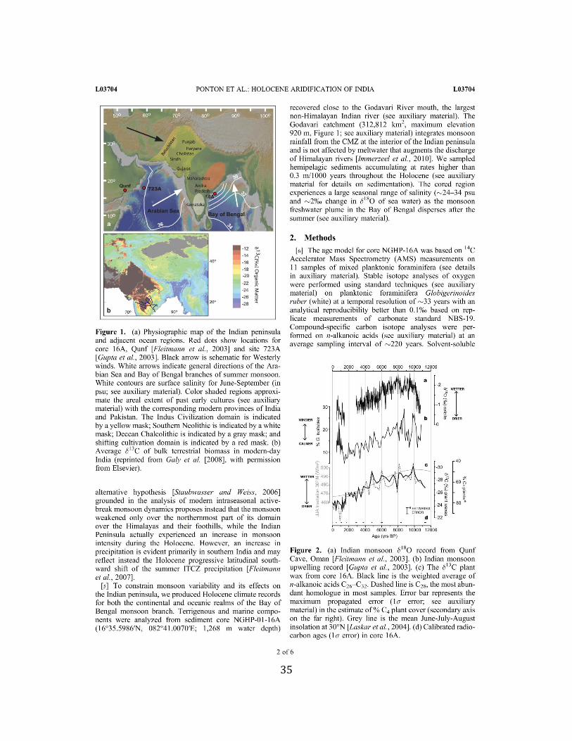
Figure 2. (a) Indian monsoon δ18

O record from Qunf Cave, Oman (b) Indian

monsoon upwelling record (c) δ13

C plant wax from core 16A (d) Calibrated

radiocarbon ages from core 16A .................................................................................35

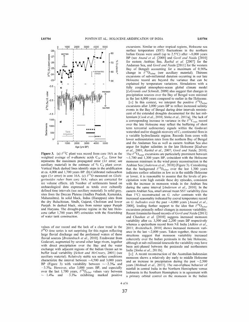
Figure 3. (a) δ13

C plant wax record from core 16A as the weighted average of n-

alkanoic acids C26-C32 (b) calibrated radiocarbon ages in core 16A (c) δ18

O measured

on G. ruber from core 16A (d) Number of settlements based on archeological data .37

Figure S1. Age-depth relationship for core NGHP-16A ...........................................56

Figure S2. Geography of the Indian Peninsula. .........................................................57

Figure S3. Hydro-climatology of the Indian peninsula and Bay of Bengal ..............58

Figure S4. Proxies for population dynamics in peninsular India between 5,000 and

2,000 years ago ...........................................................................................................59

Figure S5. δ13

C values of n-alkanoic acids from core NGHP-16A. .........................60

Chapter 3

Figure 1. Conceptual model for the transport of riverine terrestrial OC into the

oceans .........................................................................................................................69

Figure 2. Godavari River drainage basin in its geological and physiographical

context .........................................................................................................................71

Figure 3. Sedimentation rates from core NGHP-16A ................................................72

Figure 4. δ13

Cwax, calibrated ages and δ18

O from core 16A ......................................72

Figure 5. Comparative ages of planktonic forminifera, TOC, and long chain fatty

acids ............................................................................................................................77

Figure 6. Age offsets between different dated fractions ............................................79

Figure 7. Age offset between long chain fatty acids and forminifera ........................80

Figure 8. Sedimentation rates and age offsets between fatty acids and forminifera .83

14

Figure 9. εNd (provenance proxy) and δ13

C of fatty acids (aridification proxy) .......85

Figure 10. Two different chronologies for δ13

C of C26-32 fatty acids ........................88

Chapter 4

Figure 1. (a) Cross section along direction of propagation of the Lewis-Fox Hill

shelf margin (b) Anatomy of a clinoform (c) Schematic illustrating controls in

clinoform geometry ..................................................................................................116

Figure 2. Map of the Indus shelf with bathymetry of the subaqueous delta and ship

track of the seismic survey .......................................................................................123

Figure 3. Composite of chirp lines along the western shelf clinoform extending

westward from the canyon ........................................................................................123

Figure 4. Two dip-oriented chirp lines across the western shelf clinoform ............125

Figure 5. Two dip-oriented chirp lines across the eastern shelf clinofrom ..............127

Figure 6. Sediment cores from the Indus shelf ........................................................129

Figure 7. Age-depth relationships for core 10 .........................................................130

Figure 8. δ13

Cwax from the Indus River drainage basin compared to other regional

records ......................................................................................................................133

15

LIST OF TABLES

Chapter 2

Table S1. Radiocarbon ages for mixed planktonic foraminifera and corresponding

calendar age ................................................................................................................52

Table S2. Tally of archaeological sites by period and region ....................................53

Table S3. Tally of sites and radiocarbon dates for Neolithic/Chalcolithic Indian

peninsula .....................................................................................................................54

Table S4. Tally of Iron Age (“megalithic”) sites in South India in relation to rainfall

zone .............................................................................................................................55

Chapter 3

Table 1. 14

C ages of long-chain fatty acids, total organic carbon and mixed

planktonic foraminifera ..............................................................................................76

Table 2. Percent of aged and fresh carbon required to yield 1000 and 5000 yr age

offsets ..........................................................................................................................89

Table 3. Age offsets for mixing with dead carbon .....................................................92

Table S1. Total organic carbon and fatty acid estimated fluxes ................................98

Table S2. Fatty acid δ13

C data ....................................................................................99

Table S3. Nd isotopic data .......................................................................................100

Table S4. δ18

O G. ruber data ...................................................................................101

16

17

CHAPTER 1

General Introduction

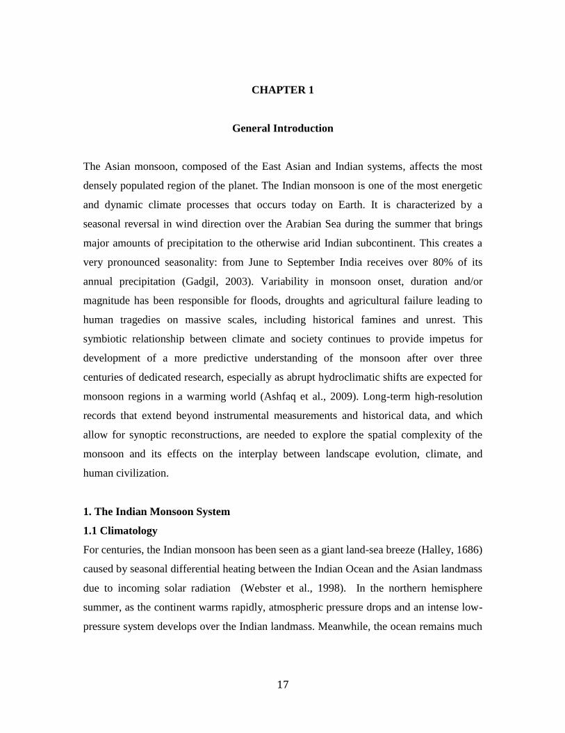
The Asian monsoon, composed of the East Asian and Indian systems, affects the most

densely populated region of the planet. The Indian monsoon is one of the most energetic

and dynamic climate processes that occurs today on Earth. It is characterized by a

seasonal reversal in wind direction over the Arabian Sea during the summer that brings

major amounts of precipitation to the otherwise arid Indian subcontinent. This creates a

very pronounced seasonality: from June to September India receives over 80% of its

annual precipitation (Gadgil, 2003). Variability in monsoon onset, duration and/or

magnitude has been responsible for floods, droughts and agricultural failure leading to

human tragedies on massive scales, including historical famines and unrest. This

symbiotic relationship between climate and society continues to provide impetus for

development of a more predictive understanding of the monsoon after over three

centuries of dedicated research, especially as abrupt hydroclimatic shifts are expected for

monsoon regions in a warming world (Ashfaq et al., 2009). Long-term high-resolution

records that extend beyond instrumental measurements and historical data, and which

allow for synoptic reconstructions, are needed to explore the spatial complexity of the

monsoon and its effects on the interplay between landscape evolution, climate, and

human civilization.

1. The Indian Monsoon System

1.1 Climatology

For centuries, the Indian monsoon has been seen as a giant land-sea breeze (Halley, 1686)

caused by seasonal differential heating between the Indian Ocean and the Asian landmass

due to incoming solar radiation (Webster et al., 1998). In the northern hemisphere

summer, as the continent warms rapidly, atmospheric pressure drops and an intense low-

pressure system develops over the Indian landmass. Meanwhile, the ocean remains much

18

cooler and a low-pressure cell installs over the south Indian Ocean. This pressure gradient

initiates a strong moist-wind flow across the equator from the ocean onshore, bringing

heavy precipitation inland (Schott and McCreary, 2001). In the winter, as the Asian

continent cools, the winds blow from the continent to the ocean and bring dry, cool air

down from the Himalaya, significantly reducing precipitation over South Asia.

An emerging view considers the monsoon as a global phenomenon resulting from the

seasonal overturning of the atmosphere over tropical and sub-tropical latitudes (Sikka and

Gadgil, 1980; Chao, 2000; Boos and Kuang, 2010; Sinha et al., 2011a) in response to the

seasonal variation of the latitude of maximum insolation (Trenberth et al., 2000; Gadgil,

2003). Under this view, the Indian monsoon is the expression of the northward summer

migration of the Intertropical Convergence Zone (ITCZ) over the heated continental

South Asia instead of remaining above the warm waters of the equatorial Indian Ocean.

The maximum excursion of the ITCZ depends on the temperature of continental South

Asia, which is primarily controlled by insolation (Webster et al., 1998).

Although these two proposed views differ, the net result is the seasonal reversal in the

direction of the wind over the monsoon region and a unimodal rainfall distribution

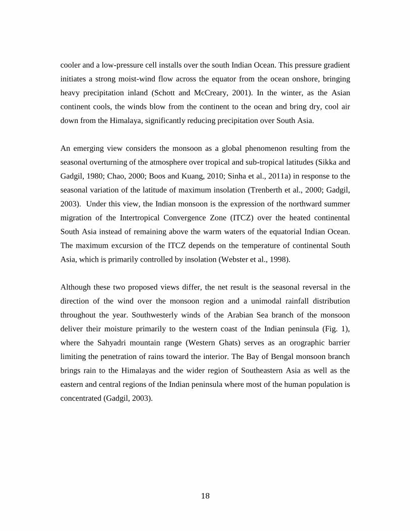
throughout the year. Southwesterly winds of the Arabian Sea branch of the monsoon

deliver their moisture primarily to the western coast of the Indian peninsula (Fig. 1),

where the Sahyadri mountain range (Western Ghats) serves as an orographic barrier

limiting the penetration of rains toward the interior. The Bay of Bengal monsoon branch

brings rain to the Himalayas and the wider region of Southeastern Asia as well as the

eastern and central regions of the Indian peninsula where most of the human population is

concentrated (Gadgil, 2003).

19

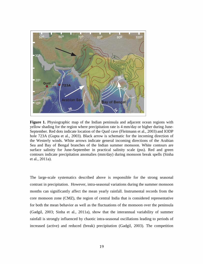
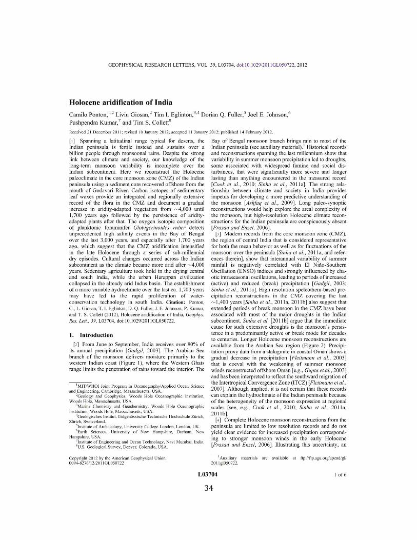
Figure 1. Physiographic map of the Indian peninsula and adjacent ocean regions with

yellow shading for the region where precipitation rate is 4 mm/day or higher during June-

September. Red dots indicate location of the Qunf cave (Fleitmann et al., 2003) and IODP

hole 723A (Gupta et al., 2003). Black arrow is schematic for the incoming direction of

the Westerly winds. White arrows indicate general incoming directions of the Arabian

Sea and Bay of Bengal branches of the Indian summer monsoon. White contours are

surface salinity for June-September in practical salinity scale (pss). Red and green

contours indicate precipitation anomalies (mm/day) during monsoon break spells (Sinha

et al., 2011a).

The large-scale systematics described above is responsible for the strong seasonal

contrast in precipitation. However, intra-seasonal variations during the summer monsoon

months can significantly affect the mean yearly rainfall. Instrumental records from the

core monsoon zone (CMZ), the region of central India that is considered representative

for both the mean behavior as well as the fluctuations of the monsoon over the peninsula

(Gadgil, 2003; Sinha et al., 2011a), show that the interannual variability of summer

rainfall is strongly influenced by chaotic intra-seasonal oscillations leading to periods of

increased (active) and reduced (break) precipitation (Gadgil, 2003). The competition

20

between the continental and oceanic loci of the ITCZ (i.e., the Indian peninsula and the

Equatorial Indian Ocean respectively) results in a characteristic increased/reduced

precipitation dipole (Fig. 1) between the CMZ and northeast India/Bangladesh (Sinha et

al., 2011a) as the system passes from active to break monsoon episodes and vice-versa.

Although active and break spells of the monsoon are short lived, lasting from days to a

few weeks (Gadgil, 2003; Sinha et al., 2011a), extended periods of break monsoon in the

CMZ have been associated with most of the major droughts in the Indian subcontinent

during the interval covered by the instrumental record (Joseph et al., 2009). The agrarian-

based societies of south Asia have suffered relentlessly the profound effects from these

droughts, strongly associated to migrations, famines and mass mortality.

1.2 The last 1,000 years

Sinha et al. (2011b) have recently used sub-annual precipitation reconstructions from

stalagmites in the CMZ and northeast India extending over the last ~700 years to argue

that the monsoon can persist in a predominantly active or break mode for decades to

centuries. Although the mechanism for the multicentennial variability has yet to be

clarified, migrations of the ITCZ in response to changes in the Northern Hemisphere

temperatures (Sinha et al., 2011b; Tierney et al., 2010) and/or changes in the Indo-Pacific

tropical climatology (Sinha et al., 2011b) are plausible external modulators of the

monsoon system state (Sinha et al., 2011b). High resolution speleothem-based

precipitation reconstructions in the CMZ (Sinha et al., 2011a) extend only for the late

Holocene (i.e., last ~1,400 years), but they convincingly show that periods of drought

(10% less precipitation than the average monsoon) or even megadrought (20% less

precipitation than the average monsoon) that were at least as severe as historical events,

but longer lasting, are common features during this time interval. Tree-ring-based

reconstructions (e.g., Cook et al., 2010; Buckley et al., 2010) indicate a widespread

spatial signature of some intense CMZ droughts at the scale of the entire Asian monsoon

domain (Sinha et al., 2011a).

21

1.3 The last 10,000 years and beyond

The monsoon picture becomes less clear for longer records as spatial variability and

lower resolution limitations make it difficult to comprehensively describe changes in the

Indian monsoon during the Holocene and last glacial age. Previous studies of the salinity

variations in the Bay of Bengal (Cullen, 1981; Duplessy, 1982; Rashid et al., 2007)

indicate that during the last glacial maximum (LGM) the riverine influx and precipitation

over the area was lower than today. However, these studies could not address the

millennial scale variability in hydrology, due to low sedimentation rates, since most of

their cores were located in the southern reaches of the Bay of Bengal or in the Andaman

Sea. In a recent study of Himalayan basin paleo-vegetation, Galy et al. (2008) suggest

more arid conditions during the LGM than during the mid Holocene. Speleothem records

from monsoon regions in China (i.e. Wang et al., 2008) and Oman (Fleitmann et al.,

2007) generally agree with these marine sediment records but also show evidence for

abrupt change in monsoon intensity during the mid-Holocene.

Detailed records of Holocene climate from the CMZ and particularly the Indian peninsula

are conspicuously absent (Prasad and Enzel, 2006). High-resolution proxy records of

precipitation (Fleitmann et al., 2003) and wind intensity (Gupta et al., 2003) during the

Holocene are available for the Arabian Sea monsoon branch from the coastal and

offshore regions of Oman respectively. These reconstructions, supported by other records

(Sirocko et al., 1993; Overpeck et al., 1996; Schulz et al., 1998; Ivanochko et al., 2005),

show a gradual decrease in precipitation during the Holocene associated with coeval

weakening of summer monsoon winds, and have been interpreted (Fleitmann et al., 2007)

as the result of the ITCZ southward migration (Haug et al., 2001). Foraminiferal oxygen

isotopic records from the southeastern Arabian Sea suggest that monsoon intensified in

late Holocene (Sarkar et al., 2000) as does reconstructed precipitation on the island of

Socotra, offshore Yemen (Fleitmann et al., 2007), possibly responding to the same ITCZ

southward retreat. Although implied, it is not certain if these records are coupled with

climate in the Indian peninsula at all times. Holocene monsoon reconstructions from the

22

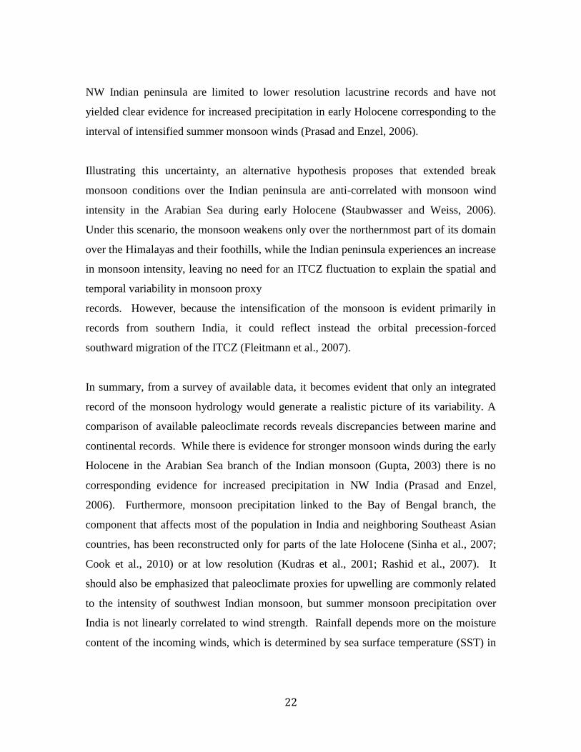
NW Indian peninsula are limited to lower resolution lacustrine records and have not

yielded clear evidence for increased precipitation in early Holocene corresponding to the

interval of intensified summer monsoon winds (Prasad and Enzel, 2006).

Illustrating this uncertainty, an alternative hypothesis proposes that extended break

monsoon conditions over the Indian peninsula are anti-correlated with monsoon wind

intensity in the Arabian Sea during early Holocene (Staubwasser and Weiss, 2006).

Under this scenario, the monsoon weakens only over the northernmost part of its domain

over the Himalayas and their foothills, while the Indian peninsula experiences an increase

in monsoon intensity, leaving no need for an ITCZ fluctuation to explain the spatial and

temporal variability in monsoon proxy

records. However, because the intensification of the monsoon is evident primarily in

records from southern India, it could reflect instead the orbital precession-forced

southward migration of the ITCZ (Fleitmann et al., 2007).

In summary, from a survey of available data, it becomes evident that only an integrated

record of the monsoon hydrology would generate a realistic picture of its variability. A

comparison of available paleoclimate records reveals discrepancies between marine and

continental records. While there is evidence for stronger monsoon winds during the early

Holocene in the Arabian Sea branch of the Indian monsoon (Gupta, 2003) there is no

corresponding evidence for increased precipitation in NW India (Prasad and Enzel,

2006). Furthermore, monsoon precipitation linked to the Bay of Bengal branch, the

component that affects most of the population in India and neighboring Southeast Asian

countries, has been reconstructed only for parts of the late Holocene (Sinha et al., 2007;

Cook et al., 2010) or at low resolution (Kudras et al., 2001; Rashid et al., 2007). It

should also be emphasized that paleoclimate proxies for upwelling are commonly related

to the intensity of southwest Indian monsoon, but summer monsoon precipitation over

India is not linearly correlated to wind strength. Rainfall depends more on the moisture

content of the incoming winds, which is determined by sea surface temperature (SST) in

23

the southern Hemisphere (Webster et al., 1998). Therefore, proxy records of summer

monsoon rainfall and evaporation–precipitation (E–P) may better constrain monsoon

intensity in the Bay of Bengal.

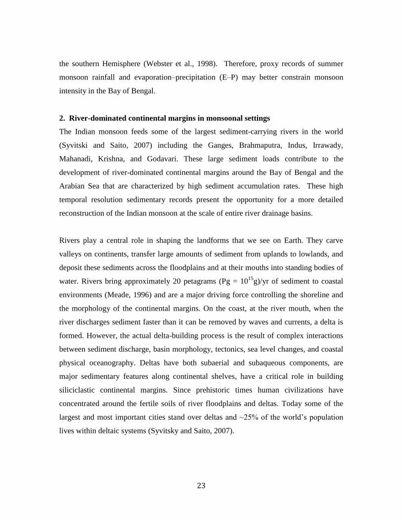
2. River-dominated continental margins in monsoonal settings

The Indian monsoon feeds some of the largest sediment-carrying rivers in the world

(Syvitski and Saito, 2007) including the Ganges, Brahmaputra, Indus, Irrawady,

Mahanadi, Krishna, and Godavari. These large sediment loads contribute to the

development of river-dominated continental margins around the Bay of Bengal and the

Arabian Sea that are characterized by high sediment accumulation rates. These high

temporal resolution sedimentary records present the opportunity for a more detailed

reconstruction of the Indian monsoon at the scale of entire river drainage basins.

Rivers play a central role in shaping the landforms that we see on Earth. They carve

valleys on continents, transfer large amounts of sediment from uplands to lowlands, and

deposit these sediments across the floodplains and at their mouths into standing bodies of

water. Rivers bring approximately 20 petagrams (Pg = 1015

g)/yr of sediment to coastal

environments (Meade, 1996) and are a major driving force controlling the shoreline and

the morphology of the continental margins. On the coast, at the river mouth, when the

river discharges sediment faster than it can be removed by waves and currents, a delta is

formed. However, the actual delta-building process is the result of complex interactions

between sediment discharge, basin morphology, tectonics, sea level changes, and coastal

physical oceanography. Deltas have both subaerial and subaqueous components, are

major sedimentary features along continental shelves, have a critical role in building

siliciclastic continental margins. Since prehistoric times human civilizations have

concentrated around the fertile soils of river floodplains and deltas. Today some of the

largest and most important cities stand over deltas and ~25% of the world’s population

lives within deltaic systems (Syvitsky and Saito, 2007).

24

From an environmental context, river mouths have a disproportionate impact compared to

their surface area because fluvial systems collect and integrate signals from surface

processes over an extensive drainage area. Rivers are the source of dissolved and

particulate materials entering into the ocean; they bring sediments, organic carbon,

nutrients and a suite of chemical species as well as pollutants. The fluvial input of organic

carbon into the oceans is estimated to be ~0.4 PgC/yr (Schlünz and Schneider, 2000) with

roughly 50% of this in particulate form (Hedges, 1992). River-dominated continental

margins are major organic carbon repositories and one of the most important sites of

active organic matter burial on Earth (Hedges and Keil, 1995). The fate of terrestrial

materials in continental margins affects the global ocean and has the potential to

influence global biogeochemical cycles (McKee et al., 2004). In addition, sediments

deposited on river-dominated margins provide integrated records of both terrestrial and

marine processes that can shed light on past environmental conditions, as well as on

source-to-sink processes such as terrestrial OC cycling (Hedges et al. 1997; Weijers et al.,

2007). The role of continental margin sediments in the carbon cycle as well as the use of

these sedimentary archives for paleoenvironmental reconstructions rely upon a robust

understanding of how organic matter is transferred from land to ocean, and how carbon

signatures are ultimately recorded in marine sediments.

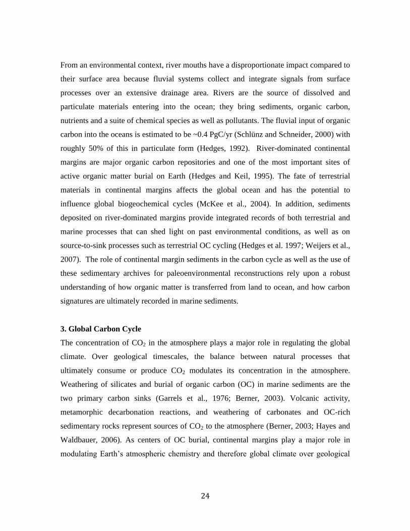
3. Global Carbon Cycle

The concentration of CO2 in the atmosphere plays a major role in regulating the global

climate. Over geological timescales, the balance between natural processes that

ultimately consume or produce CO2 modulates its concentration in the atmosphere.

Weathering of silicates and burial of organic carbon (OC) in marine sediments are the

two primary carbon sinks (Garrels et al., 1976; Berner, 2003). Volcanic activity,

metamorphic decarbonation reactions, and weathering of carbonates and OC-rich

sedimentary rocks represent sources of CO2 to the atmosphere (Berner, 2003; Hayes and

Waldbauer, 2006). As centers of OC burial, continental margins play a major role in

modulating Earth’s atmospheric chemistry and therefore global climate over geological

25

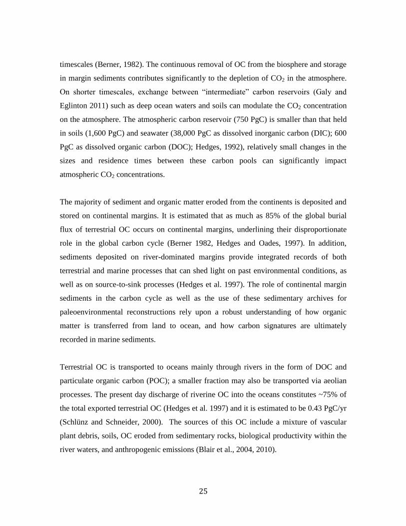
timescales (Berner, 1982). The continuous removal of OC from the biosphere and storage

in margin sediments contributes significantly to the depletion of CO2 in the atmosphere.

On shorter timescales, exchange between “intermediate” carbon reservoirs (Galy and

Eglinton 2011) such as deep ocean waters and soils can modulate the CO2 concentration

on the atmosphere. The atmospheric carbon reservoir (750 PgC) is smaller than that held

in soils (1,600 PgC) and seawater (38,000 PgC as dissolved inorganic carbon (DIC); 600

PgC as dissolved organic carbon (DOC); Hedges, 1992), relatively small changes in the

sizes and residence times between these carbon pools can significantly impact

atmospheric CO2 concentrations.

The majority of sediment and organic matter eroded from the continents is deposited and

stored on continental margins. It is estimated that as much as 85% of the global burial

flux of terrestrial OC occurs on continental margins, underlining their disproportionate

role in the global carbon cycle (Berner 1982, Hedges and Oades, 1997). In addition,

sediments deposited on river-dominated margins provide integrated records of both

terrestrial and marine processes that can shed light on past environmental conditions, as

well as on source-to-sink processes (Hedges et al. 1997). The role of continental margin

sediments in the carbon cycle as well as the use of these sedimentary archives for

paleoenvironmental reconstructions rely upon a robust understanding of how organic

matter is transferred from land to ocean, and how carbon signatures are ultimately

recorded in marine sediments.

Terrestrial OC is transported to oceans mainly through rivers in the form of DOC and

particulate organic carbon (POC); a smaller fraction may also be transported via aeolian

processes. The present day discharge of riverine OC into the oceans constitutes ~75% of

the total exported terrestrial OC (Hedges et al. 1997) and it is estimated to be 0.43 PgC/yr

(Schlünz and Schneider, 2000). The sources of this OC include a mixture of vascular

plant debris, soils, OC eroded from sedimentary rocks, biological productivity within the

river waters, and anthropogenic emissions (Blair et al., 2004, 2010).

26

4. Thesis outline

This thesis provides new Holocene records of Indian monsoon variability using sediment

cores with high accumulation rates from river-dominated margins in the Bay of Bengal

and the Arabian Sea. Integrating marine and continental records, it presents regionally

extensive paleoenvironmental reconstructions that have implications for landscape

evolution, sedimentation, the terrestrial organic carbon cycle, and prehistoric human

civilizations in the Indian subcontinent.

Chapter 2 presents a reconstruction of the Holocene paleoclimate in the core monsoon

zone (CMZ) of the Indian peninsula using a sediment core recovered offshore from the

mouth of the Godavari River in the Bay of Bengal. Carbon isotopes of the terrestrial

plant leaf waxes that have been transported to, and preserved in, these margin sediments

yield an integrated and regionally extensive record of the flora in the CMZ and provide

evidence for a gradual increase in the proportion of aridity-adapted vegetation from

~4,000 until 1,700 years ago followed by the persistence of aridity-adapted plants after

that as the drainage basin became increasingly perturbed by anthropogenic activity. The

oxygen isotopic composition of planktonic foraminifer Globigerinoides ruber detects

unprecedented high salinity events in the Bay of Bengal over the last 3,000 years, and

especially after 1,700 years ago, which suggest that the CMZ aridification intensified in

the late Holocene through a series of sub-millennial dry episodes. This chapter also

considers archeological evidence from the Indian peninsula as a proxy for human

population and reliance on early agricultural practices to assess correlations between

major cultural and climatic changes in this region.

Chapter 3 also uses sediments from the same core described in the previous chapter, but

focuses on the terrestrial carbon cycle as climatic conditions change in the Godavari

River basin. It compares the ages of marine planktonic foraminifera with those of

terrestrial plant waxes isolated from the same sediment horizons, and examines the

27

relationships between hydroclimate and the mode and dynamics of terrestrial carbon

discharge from the river drainage basin. Results show increasing age offsets from mid to

late Holocene. Since ~4,000 yrs BP, higher plant fatty acids are on average ~1,200 yrs

older than the foraminifera, indicating either increasing residence times of terrestrial

carbon or increasing erosion and mobilization of pre-aged vascular plant-derived carbon

as a consequence of a less humid climate. In addition to shedding light on past

continental carbon cycle dynamics, these results also have important implications for the

use of organic terrestrial proxies in paleoclimate reconstructions. They show that the

temporal phasing of terrestrial and marine proxy signals may vary as a function of

changes in hydroclimate.

Chapter 4 presents the first high-resolution seismic survey of the Indus River subaqueous

delta on the Pakistani shelf in the northeastern Arabian Sea, and describes its morphology

and Holocene sedimentation history. Seismic and core records are used to explore the

suitability of using subaqueous deltaic sedimentary deposits from the Pakistani shelf to

reconstruct the paleoclimate in the Indus drainage basin. Radiocarbon dates on mollusk

shells from sediment cores show that sediment accumulation has been heterogeneous

across the Indus shelf and the utility of sedimentary records for climate reconstruction

appears strongly dependent on the stratigraphy of the cores.

A core recovered from a morphological depression is inferred to preserve an integrative

paleoclimate record of the entire Indus River drainage basin. The carbon isotopic

composition of sedimentary plant waxes suggests a remarkably stable climate over the

arid regions of the Indus plain with a terrestrial biome dominated by C4 vegetation for the

last 6,000 yrs. While reconstructions from the Arabian Sea and Bay of Bengal provide a

consistent account of monsoon weakening over the Holocene, this reconstruction from

the Indus River does not reflect these changes, and instead indicates that conditions in the

drainage basin remained predominantly dry.

28

Chapter 5 summarizes the most important findings of this thesis, highlights key new

questions that this research has raised, and offers some directions for future research

initiatives.

Overall this thesis provides new paleoclimate reconstructions of the Indian monsoon

from river-dominated margins, contributing to the efforts of obtaining a more cohesive

view of the Indian monsoon variability during the Holocene. It combines a wide range of

observations and analytical techniques, and employs continental and marine climate

proxies that integrate signals over extensive regions to present regional reconstructions.

Results from this work have implications for the Indian monsoon system as whole, as

well as vegetation cover, sedimentation, terrestrial carbon cycle and past human

civilizations of the Indian subcontinent.

References

Ashfaq, M., Y. Shi, W. W. Tung, R. J. Trapp, X. J. Gao, J. S. Pal, and N. S. Diffenbaugh.

2009. Suppression of south Asian summer monsoon precipitation in the 21st century.

Geophysical Research Letters 36 (1).

Berner, R. A. 1982. Burial of organic-carbon and pyrite sulfur in the modern ocean - its

geochemical and environmental significance. American Journal of Science 282 (4):451-

473.

Berner, R.A. 2003. The long-term carbon cycle, fossil fuels and atmospheric

composition. Nature 426 (6964):323-326.

Blair, N. E., E. L. Leithold, and R. C. Aller. 2004. From bedrock to burial: the evolution

of particulate organic carbon across coupled watershed-continental margin systems.

Marine Chemistry 92 (1-4):141-156.

Blair, N. E., K. Fournillier, E. L. Leithold, and L. B. Childress. 2010. Resolving organic

carbon of differing diagenetic/catagenetic states in riverine and marine sediments.

Geochimica Et Cosmochimica Acta 74 (12):A95-A95.

Boos, W. R., and Z. M. Kuang. 2010. Dominant control of the South Asian monsoon by

orographic insulation versus plateau heating. Nature 463 (7278):218-U102.

29

Buckley, B. M., K. J. Anchukaitis, D. Penny, R. Fletcher, E. R. Cook, M. Sano, C. N. Le,

A. Wichienkeeo, T. M. Ton, and M. H. Truong. 2010. Climate as a contributing factor in

the demise of Angkor, Cambodia. Proceedings of the National Academy of Sciences of

the United States of America 107 (15):6748-6752.

Chao, W. C. 2000. Multiple quasi equilibria of the ITCZ and the origin of monsoon

onset. Journal of the Atmospheric Sciences 57 (5):641-651.

Cook, E. R., K. J. Anchukaitis, B. M. Buckley, R. D. D'Arrigo, G. C. Jacoby, and W. E.

Wright. 2010. Asian Monsoon Failure and Megadrought During the Last Millennium.

Science 328 (5977):486-489.

Cullen, J. L. 1981. Microfossil evidence for changing salinity patterns in the Bay of

Bengal over the last 20000 years. Palaeogeography Palaeoclimatology Palaeoecology 35

(2-4):315-356.

Duplessy, J. C. 1982. Glacial to interglacial contrasts in the northern Indian-ocean.

Nature 295 (5849):494-498.

Fleitmann, D., S. J. Burns, M. Mudelsee, U. Neff, J. Kramers, A. Mangini, and A. Matter.

2003. Holocene forcing of the Indian monsoon recorded in a stalagmite from Southern

Oman. Science 300 (5626):1737-1739.

Fleitmann, D., S. J. Burns, A. Mangini, M. Mudelsee, J. Kramers, I. Villa, U. Neff, A. A.

Al-Subbary, A. Buettner, D. Hippler, and A. Matter. 2007. Holocene ITCZ and Indian

monsoon dynamics recorded in stalagmites from Oman and Yemen (Socotra). Quaternary

Science Reviews 26 (1-2):170-188.

Gadgil, S. 2003. The Indian monsoon and its variability. Annual Review of Earth and

Planetary Sciences 31:429-467.

Galy, V., L. Francois, C. France-Lanord, P. Faure, H. Kudrass, F. Palhol, and S. K.

Singh. 2008. C4 plants decline in the Himalayan basin since the Last Glacial Maximum.

Quaternary Science Reviews 27 (13-14):1396-1409.

Galy, V., Eglinton, T.I. 2011. Protracted storage of biospheric carbon in the Ganges-

Brahmaputra basin. Nature Geoscience 4:843-847.

Garrels, R. M., A. Lerman, and F. T. Mackenzie. 1976. Controls of atmospheric O2 and

CO2 - past, present, and future. American Scientist 64 (3):306-315.

30

Gupta, A. K., D. M. Anderson, and J. T. Overpeck. 2003. Abrupt changes in the Asian

southwest monsoon during the Holocene and their links to the North Atlantic Ocean.

Nature 421 (6921):354-357.

Halley, E. 1686. An historical account of the trade winds and monsoons observable in the

seas between and near the tropics with an attempt to assign a physical cause of the said

winds.†. Philosophical Transactions of the Royal Society of London (16):153-168.

Haug, G. H., K. A. Hughen, D. M. Sigman, L. C. Peterson, and U. Rohl. 2001.

Southward migration of the intertropical convergence zone through the Holocene.

Science 293 (5533):1304-1308.

Hayes, J. M., and J. R. Waldbauer. 2006. The carbon cycle and associated redox

processes through time. Philosophical Transactions of the Royal Society B-Biological

Sciences 361 (1470):931-950.

Hedges, J.I.1992. Global biogeochemical cycles: progress and problems. Marine

Chemistry 39: 67–93.

Hedges, J.I., Keil, R.G.1995. Sedimentary organic matter preservation: an assessment and

speculative synthesis. Marine Chemistry 49:81–115.

Hedges, J. I., and J. M. Oades. 1997. Comparative organic geochemistries of soils and

marine sediments. Organic Geochemistry 27 (7-8):319-361.

Hedges, J. I., R. G. Keil, and R. Benner. 1997. What happens to terrestrial organic matter

in the ocean? Organic Geochemistry 27 (5-6):195-212.

Ivanochko, T. S., R. S. Ganeshram, G. J. A. Brummer, G. Ganssen, S. J. A. Jung, S. G.

Moreton, and D. Kroon. 2005. Variations in tropical convection as an amplifier of global

climate change at the millennial scale. Earth and Planetary Science Letters 235 (1-2):302-

314.

Joseph, S., A. K. Sahai, and B. N. Goswami. 2009. Eastward propagating MJO during

boreal summer and Indian monsoon droughts. Climate Dynamics 32 (7-8):1139-1153.

Kudrass, H. R., A. Hofmann, H. Doose, K. Emeis, and H. Erlenkeuser. 2001. Modulation

and amplification of climatic changes in the Northern Hemisphere by the Indian summer

monsoon during the past 80 k.y. Geology 29 (1):63-66.

McKee, B.A., Aller, R.C., Allison, M.A., Bianchi, T.S. and Kineke, G.C. 2004. Transport

and transformation of dissolved and particulate materials on continental margins

influenced by major rivers: benthic boundary layer and seabed processes. Continental

Shelf Research 24:899–926.

31

Meade, R.H., 1996, River-sediment inputs to major deltas. In: Milliman, J., Haq, B.

(Eds.), Sea-level rise and coastal subsidence. Kluwer: London, 63–85.

Overpeck, J., D. Anderson, S. Trumbore, and W. Prell. 1996. The southwest Indian

Monsoon over the last 18000 years. Climate Dynamics 12 (3):213-225.

Prasad, S., and Y. Enzel. 2006. Holocene paleoclimates of India. Quaternary Research 66

(3):442-453.

Rashid, H., B. P. Flower, R. Z. Poore, and T. M. Quinn. 2007. A similar to 25 ka Indian

Ocean monsoon variability record from the Andaman Sea. Quaternary Science Reviews

26 (19-21):2586-2597.

Sarkar, A., R. Ramesh, B. L. K. Somayajulu, R. Agnihotri, A. J. T. Jull, and G. S. Burr.

2000. High resolution Holocene monsoon record from the eastern Arabian Sea. Earth and

Planetary Science Letters 177 (3-4):209-218.

Schott, F. A., and J. P. McCreary. 2001. The monsoon circulation of the Indian Ocean.

Progress in Oceanography 51 (1):1-123.

Schlunz, B., and R. R. Schneider. 2000. Transport of terrestrial organic carbon to the

oceans by rivers: re-estimating flux- and burial rates. International Journal of Earth

Sciences 88 (4):599-606.

Schulz, H., U. von Rad, and H. Erlenkeuser. 1998. Correlation between Arabian Sea and

Greenland climate oscillations of the past 110,000 years. Nature 393 (6680):54-57.

Sikka, D. R., and S. Gadgil. 1980. On the maximum cloud zone and the ITCZ over Indian

longitudes during the southwest monsoon. Monthly Weather Review 108 (11):1840-

1853.

Sinha, A., K. G. Cannariato, L. D. Stott, H. Cheng, R. L. Edwards, M. G. Yadava, R.

Ramesh, and I. B. Singh. 2007. A 900-year (600 to 1500 A. D.) record of the Indian

summer monsoon precipitation from the core monsoon zone of India. Geophysical

Research Letters 34 (16).

Sinha, A., M. Berkelhammer, L. Stott, M. Mudelsee, H. Cheng, and J. Biswas. 2011a.

The leading mode of Indian Summer Monsoon precipitation variability during the last

millennium. Geophysical Research Letters 38.

Sinha, A., L. Stott, M. Berkelhammer, H. Cheng, R. L. Edwards, B. Buckley, M.

Aldenderfer, and M. Mudelsee. 2011b. A global context for megadroughts in monsoon

Asia during the past millennium. Quaternary Science Reviews 30 (1-2):47-62.

32

Sirocko, F., M. Sarnthein, H. Erlenkeuser, H. Lange, M. Arnold, and J. C. Duplessy.

1993. Century-scale events in monsoonal climate over the past 24,000 years. Nature 364

(6435):322-324.

Staubwasser, M., and H. Weiss. 2006. Holocene climate and cultural evolution in late

prehistoric-early historic West Asia - Introduction. Quaternary Research 66 (3):372-387.

Syvitski, J. P. M. and Saito, Y. 2007. Morphodynamics of deltas under the influence of

humans.

Global and Planetary Change 57:261–282.

Tierney, J. E., D. W. Oppo, Y. Rosenthal, J. M. Russell, and B. K. Linsley. 2010.

Coordinated hydrological regimes in the Indo-Pacific region during the past two

millennia. Paleoceanography 25.

Trenberth, K. E., D. P. Stepaniak, and J. M. Caron. 2000. The global monsoon as seen

through the divergent atmospheric circulation. Journal of Climate 13 (22):3969-3993.

Wang, Yongjin, Hai Cheng, R. Lawrence Edwards, Xinggong Kong, Xiaohua Shao,

Shitao Chen, Jiangyin Wu, Xiouyang Jiang, Xianfeng Wang, and Zhisheng An. 2008.

Millennial- and orbital-scale changes in the East Asian monsoon over the past 224,000

years. Nature 451 (7182):1090-1093.

Webster, P. J., V. O. Magana, T. N. Palmer, J. Shukla, R. A. Tomas, M. Yanai, and T.

Yasunari. 1998. Monsoons: Processes, predictability, and the prospects for prediction.

Journal of Geophysical Research-Oceans 103 (C7):14451-14510.

Weijers, J. W. H., E. Schefuss, S. Schouten, and J. S. S. Damste. 2007. Coupled thermal

and hydrological evolution of tropical Africa over the last deglaciation. Science 315

(5819):1701-1704.

33

CHAPTER 2

Holocene Aridification of India

This work originally appeared as:

Ponton, C., L. Giosan, T.I. Eglinton, D.Q. Fuller, J.E. Johnson, P. Kumar, and T.S.

Collett. 2012. Holocene aridification of India. Geophysical Research Letters (39)

L03704, doi:10.1029/2011GL050722. Copyright, 2012, American Geophysical Union.

Reproduced by permission of the American Geophysical Union.

34

35

36

37

38

39

40

Supplementary Material

1. Methods

1.1 Radiocarbon chronology

Samples for radiocarbon dating from core NGHP-16A were disaggregated using distilled

water and then sieved. Mixed planktonic foraminifera from the >250μm size fraction

were picked first, and supplemented by tests from the >150μm size fraction when

necessary. Radiocarbon measurements were performed at the National Ocean Sciences

Accelerator Mass Spectrometry Facility (NOSAMS) in Woods Hole, MA, USA.

Radiocarbon ages were converted to calendar ages using the CALIB 6.0 program [Stuiver

and Reimer, 1993] and the Marine09 calibration curve [Reimer et al., 2009]. Available

reservoir estimates for the Bay of Bengal surface waters are not substantially different

than the standard marine reservoir correction [Dutta et al., 2001; Southon et al., 2002],

which we used to calibrate our data. Ages for samples between calibrated dates were

obtained by linear interpolation. Results are shown in Supplementary Table 1 and

Supplementary Figure 1.

1.2 Planktonic foraminifera oxygen isotopes

Stable isotope analysis of oxygen were performed on planktonic foraminifera

Globigerinoides ruber (white) from the first 5.0 meters of core NGHP-16A at an average

sampling resolution of 3 samples per century. Sediment samples of 10 cm3 were wet-

washed in a 63 μm sieve and picked foraminifera were washed and sonicated in distilled

water before processing. All samples contained between 8-10 tests from the >150 μm

fraction and weighed between 100-150 μg. Samples were processed using a VG Prism

Mass Spectrometer at NOSAMS. Analytical reproducibility as determined from replicate

measurements on carbonate standard NBS-19 is better than 0.1‰.

1.3 Plant Wax Lipid Carbon Isotopes

Compound-specific carbon isotope analyses of n-alkanoic acids were performed on

41

samples from the upper 8.0 meters of core NGHP-16A at a sampling resolution of 20 cm

corresponding to an average sampling interval of 220 years (from ~440 years near the

bottom of the core to ~ 125 years near the top of the core). Lipid organic matter was

extracted from 10-12 grams of the freeze-dried sediment samples using a

dichloromethane (DCM):methanol (MeOH) solution(9:1) in a CEM Microwave

Accelerated Reaction System (MARS). Concentrated lipid extract was saponified with

0.5N KOH in methanol solution. Liquid/liquid extraction of the neutral fraction was done

using pure hexane. Then the pH was adjusted to 2 by addition of HCl and liquid/liquid

extraction of the acid fraction was performed using hexane:DCM (4:1). Lipids in the acid

fraction, including leaf wax n-alkanoic acids, were methylated using HCl 5% in MeOH

(70 oC for 12 hours). The resulting fatty acid methylesters (FAMEs) were extracted using

hexane:DCM (4:1), then dried with anhydrous sodium sulfate, and then purified via silica

gel chromatography. A FAMEs standard C13 – C24 was added to each sample sequence

prior to analysis by gas chromatography (GC). All samples were initially analyzed by GC

using an HP 5890 Series II GC equipped with flame ionization detector (FID). Isotope

ratio monitoring GC–MS (GC/irMS) was used to determine 13

C values of FAMEs.

Measurements were performed on a Finnigan DeltaPlus

stable isotope mass spectrometer

attached to an HP 6890 GC (DB5-MS column) and Finnigan GC combustion III

interface. All analyses were performed in triplicate. δ13

C values were determined relative

to a reference gas (CO2) of known isotopic composition, introduced in pulses during each

run. GC/irMS accuracy and precision are both better than 0.3‰. The results were

corrected for the δ13

C composition of the methyl derivative (MeOH -39.56‰ ±0.2‰,

measured at NOSAMS) based on isotopic mass balance in order to derive δ13

C values for

the original n-alkanoic acids.

2. Geographical features of the Indian peninsula

The Indian peninsula is bordered by the Arabian Sea to the west, the Bay of Bengal to the

east, the Indian Ocean to the south and the Tibetan plateau on the north (Supplementary

Fig. 2). Important geographic features include: the Thar dessert to the northeast, the Indo-

42

Gangetic Plain to the south of the Himalayas, which lies between the Indus and Ganga

(Ganges) rivers, and the Deccan Plateau, a large igneous province consisting of multiple

layers of flood basalts; the coastal mountain range of Sahyadri (Western Ghats) along the

western coast, and the Eastern Ghats range along the eastern coast of the peninsula

[Washington, 1922]. The Godavari Basin covers an area of 312,812 km2, representing

about 12% of the area of continental India (see fig.1b). The river headwaters lie on the

northern end of the Western Ghats at an elevation of 920 m. However the mean elevation

of the basin is estimated at 420 m [Bikshamaiah and Subramanian, 1980].

3. Hydroclimatology of the Indian peninsula and Bay of Bengal

The Indian peninsula and the Bay of Bengal exhibit pronounced seasonality with marked

wet and dry seasons. In June through September precipitation is brought in by the moist

southwest winds. The Western Ghats affects the precipitation pattern over peninsular

India. Monsoonal rains in western India fall preferentially on the strip of land between

the coast and the Ghats. Consequently the region located inland of the Ghats receives less

precipitation and is semi-arid to arid because of this particular orography [Gunnell et al.,

2007].

The Western Ghats also form the drainage divide for peninsular India: main rivers within

the Deccan plateau have their headwaters in the Western Ghats and flow east towards the

Bay of Bengal. The Godavari River and its tributaries, drain most of the northern portion

of the plateau, The Krishna River and its tributaries, drain the central portion of the

plateau, and the southernmost portion of the plateau is drained by the Kaveri (Cauveri)

River. There is a large seasonal variability in freshwater flux, with most of the total river

runoff coming in during the summer monsoon. As a result, there is a strong freshening of

surface waters in the coastal regions of the Bay of Bengal during/after the summer

monsoon. The large impact of river discharge produces salinity changes on the order of 6

psu between summer and winter [Antonov et al., 2006]. Modern salinity patterns indicate

that the strongest salinity variations in the western Bay of Bengal occur in front of the

Godavari mouths (Supplementary Fig. 3). A persistent sediment plume extends ~300 km

43

offshore the Godavari river mouth [Sridhar et al., 2008]. During the Holocene, the

Godavari delivered ample sediment quantities to the continental slope, giving rise to an

expanded sedimentary sequence [Forsberg et al., 2007].

Supplementary Figure 3 shows the seasonal patterns for precipitation and sea surface

salinity in the study region. Precipitation data is an average from 1948-2009 from NOAA

Earth System Research Laboratory (ESRL). Precipitation maxima occur during Jul-Sep,

and highest rainfall areas are located in the western and northeastern part of the Indian

peninsula associated with the orographic effects of the Western Ghats and the Himalayan

plateau respectively. Another region of high rainfall occurs in northeastern India and

extends westward into the head of the Bay of Bengal, defining the core monsoon zone

[Gadgil, 2003]. Salinity fluctuations occur simultaneously, with the appearance of a

coastal freshwater plume fed by Indian rivers during the summer monsoon season and in

the northwest margin of the Bay of Bengal. Sea surface salinity is from the Levitus

database [Antonov et al., 2006] from IRI/Lamont-Doherty Earth Observatory Climate

Data Library. Supplementary Figure 3 also includes the drainage area of the Godavari

River in context with climatology.

4. Archaeological evidence for subsistence, settlement and trends in human

population in late prehistoric South India.

Archaeological evidence provides a record of past populations and their subsistence

strategies [Hassan, 1981]. Throughout most of the early and middle Holocene

populations in peninsular India (Figure 1a in main text) continued the hunter-gatherer

traditions of the Late Pleistocene, characterized by a Mesolithic technology that focused

on composite tools using a complex of microlithic artefacts [Misra, 2002; Clarkson et al.,

2009]. Such societies were predominantly mobile. Ceramics and groundstone tools are

generally associated with food-producing societies of the past 5000 years in which

population size is expected to have increased and mobility decreased. South India,

specifically the Southern Deccan Plateau, has been identified as a region of early

cultivation of indigenous Indian millet began around 5000 years ago, while the Northern

44

Deccan provides evidence for early farming based on a mixture of South Indian crops and

those introduced from the Indus region, such as wheat and barley [Fuller, 2006; 2008;

2011]. Wheat and barley subsequently spread southwards after 4000 years ago. This early

farming was focused initially on the drier savannah corridor and some dry deciduous

woodland areas down the middle of the Indian peninsula [Asouti and Fuller, 2008;

Fuller, 2011]. The indigenous crops of South India included minor millets as staple

cereals, Brachiaria ramosa and Setaria verticillata, both C4 grasses, as well as C3

legumes Macrotyloma uniflorum and Vigna radiata. Thus early farming in the Deccan

replaced C4 dominated savannah and adjacent woodland with cultivated flora with a

similarly large C4 component. Later periods saw a broadening of the crop repertoire,

much of this involved additional C4 crops, such as little millet (Panicum sumatense) and

kodo millet (Paspalum scrobiculatum), native to other parts of India, and millets of

African origin (Sorghum, Eleusine, Pennisetum). The adoption of rice, which is a C3

plant, took place after 1000 BC and was more restricted towards coastal regions and the

far south, especially near population centers [Fuller, 2006; Fuller et al., 2010]. After

1,500 BC and increasingly over the subsequent 1,000-2,000 years, agricultural

settlements encroached into the moister tropical forest zones in the Western Ghats

[Kingwell-Banham and Fuller, 2011] introducing C4 anthropogenic vegetation into a zone

with naturally higher proportions of C3 vegetation. In the Eastern Ghats region, which

stores most of the C3 vegetation in the Godavari watershed, smaller scale shifting

cultivation was typical until modern times; this type of agriculture replaces forest tracts

used temporarily for agriculture with fast growing C3 forests after abandonment, notably

sal (Shorea robusta) forests in the east and north with more teak (Tectona grandis)

towards the west [Kingwell-Banham and Fuller, 2011]. Massive and permanent

deforestation in the Eastern Ghats took place during British colonial times in the 19th

century [Hill, 2008], which led to a rapid expansion of the Godavari delta [Rao et al.,

2005].

It has previously been suggested that the beginnings of agriculture in the Deccan

region are associated with the beginnings of a trend towards increasing aridity, and

45

declining monsoons across this region [Fuller and Korisettar, 2004; Fuller, 2008; 2011].

Given the new palaeoclimatic data reported in this paper, we wanted to consider the

archaeological evidence as a proxy for human population and reliability of early

agricultural practices to assess any correlations between major cultural and climatic

changes in this region. There have been few systematic studies of prehistoric settlement

patterns in south India, all restricted to small regions [e.g. Paddayya, 1973;

Venkatasubbaiah, 1992; Shinde, 1998]. Nevertheless available archaeological data

provides a record of past human population in the region, biased towards sedentary

agriculturalists who would have lived at higher population densities than hunters or

shifting cultivators [cf. Kingwell-Banham and Fuller 2011]. We therefore compiled

counts of known archaeological sites from the third millennium BC (5,000 BP) through

the first millennium BC (2,000 BP) for the states of Andhra Pradesh, Karnataka, and

Maharashtra (Supplementary Table 2). For sites of the earlier period, referred to the

Southern Neolithic in Karanataka and Andhra, and the Deccan Chalcolithic in

Maharashtra, we followed the quasi-comprehensive map published in Asouti and Fuller

[2008] (Supplementary Table 3). For the subsequent Iron Age, also known as the

'Megalithic Period' we used the site counts in Moorti [1994] (Supplementary Table 4),

which provided a comprehensive compilation at the time of its publication. These data

have a number of drawbacks. First, because of the vagaries of archaeological phasing

based on material culture, chronological divisions are often potentially finer in periods

that have been more heavily sampled, including the upper strata of deeply stratified sites,

and archaeological phases are not all of equal length. Second, site numbers cannot be

directly computed as population since site sizes may vary and the density of human

populations of sites may vary systematically, nevertheless very few sites will represent

less population than many sites, especially when difference are in orders of magnitude.

Thirdly, the type of sites varies between the earlier Neolithic/Chalcolithic and the later

Iron Age periods: in the Iron Age many sites consist of cemeteries, which have been

easier to find because of monumental stone superstructures on tombs, whereas in the

earlier period all sites represent occupation sites and burials when they do occur are

46

found within those sites. Our tallies for the Iron Age therefore include both cemeteries

(which are likely to have connected to nearby settlements even when these have not been

found) and habitation sites, and this may lead to an over estimation (Iron Age versus

earlier). Iron Age cemeteries have perhaps been easier to find too, so fieldwork may be

biased towards finding these. For these reasons Iron Age numbers may be overestimated

relative to earlier site numbers but the differences are so great as to suggest that some

change is represented despite this.

An additional approach to estimating relative population sizes across regions is to

use summed probability distributions of calibrated radiocarbon dates, which we have

attempted here for the earlier Neolithic/Chalcolithic period for the southern and northern

Deccan plateau. This approach has been used for example to look at population growth in

Britain with the beginnings of agriculture [Collard et al., 2010a] and hunter-gatherers

population dynamics in north American and northern Europe [e.g. Shennan and

Edinborough, 2007; Collard et al., 2010b). This approach assumes that radiocarbon dates

represent a more or less random sample of available archaeological evidence and

therefore periods with higher population are more likely to have been dated more times.

It also assumed than any regional biases, such as those due to research focuses on

particular periods, will be insignificant by comparison to large chronological trends in the

data. For south India the total number of radiocarbon dates is quite limited

(Supplementary Table 3) by comparison to the thousands of dates in European databases

for example. For example a recent study of the Neolithic of South India reports just 116

dates from 23 sites [Fuller et al., 2007]. This dataset was used to produce a summed

distribution of all radiocarbon dates associated with the Southern Neolithic. In the North

Deccan most dates have been associated with particular long excavation projects, mostly

conducted in the 1970s and 1980s, and so the total number of dated sites with readily

available data is limited to 83 dates and 11 sites [data from: Possehl and Rissman, 1992;

Shinde, 1998]. Radiocarbon dates from the Iron Age are, by contrast, much more limited

and dating has often been inferred from grave artefacts. Therefore we have not attempted

to include radiocarbon data from this later period. While such data are an imperfect

47

dataset, they still demonstrate that there is an apparent growth in population, which was

based on agricultural villages, over the course of the Second Millennium BC, i.e., after

4,000 BP (Supplementary Table 4). Radiocarbon dates were summed with the OxCal

3.10 software [Bronk Ramsey, 2001; 2005]. The sums for the North Deccan and South

Deccan have been run separately and each is scaled independently as the relative

contribution of radiocarbon date contribution to the dataset at any given point in time. For

ease of viewing, these two datasets have been plotted along the same time scale with one

shown inverted below the timeline in Supplementary Figure 4.

The patterns in these data point to directional increases in archaeological

population after 4,000 BP up to ca. 3,300 BP for South India and 3,200 BP for the North

Deccan. While the declines after this time are to a large degree a product of the end of

respective archaeological phases, it also does appear to represent a period of major social

transformation. A great many sites of the Jorwe cultural phase in the North Deccan

[Shinde, 1998] and at this stage many of the hilltop settlement sites of the Southern

Neolithic cease to be occupied at this period [Fuller et al., 2007]. While the earliest dates

for the Iron Age come from around this period, most of the Iron Age in the North Deccan

indicates an eastward shift in settlement distribution to the somewhat wetter subzones of

eastern Maharashtra. By contrast in South India there is continuity in the regions that

were previously occupied and more regions came to be occupied after Neolithic.

Nevertheless, as in the Neolithic period, Iron Age settlement seems to predominantly

focus on savannah and dry-deciduous zone when judged by modern rainfall patterns

(Supplementary Table 4). Nevertheless there are local shifts. For example, many more

settlements are found on the plains in contrast to predominantly hilltop locations in the

Neolithic. These changes with the transition to the Iron Age are increasingly seen as

driven by social changes, as opposed to earlier ideas about new immigrants [Moorti,

1994; Fuller et al., 2007]. Nevertheless, there is clearly overall increase in agriculture

and population in the Deccan as a whole after the 2,000 BP onset of highly arid

conditions, which can be contrasted with some other parts of the South Asian

subcontinent such as in the Indus valley [Madella and Fuller, 2006].

48

5. Data Analysis

5.1 18

O G. ruber

G. ruber is abundant in the surface mixed layer (~100m) but its shell growth has been

found to be restricted to the top 35 m of water [Fairbanks et al., 1982]. In sediment trap

studies from the Arabian Sea and the Bay of Bengal, G. ruber has been found to be a

year-round species with summer peak abundances [Curry et al., 1992; Unger et al.,

2003]. The habitat of this species is ideal to record salinity and SST where and when

fluctuations are highest. Our 18

O G. ruber record after 3000 years BP exhibits brief

excursions of ca. 0.6 to over 1‰ heavier than the background values (between -2.9 and -

2.5 ‰). According to the calcification equation for G. ruber [Mulitza et al., 2003], the

temperature increase of 2.5°C, the maximum Holocene variability in the Arabian Sea

(Govil and Naidu, 2010) and Bay of Bengal (Govil and Naidu, 2011), can explain 0.56 ‰

of the amplitude of these positive excursions in 18

O ruber. We have also corrected the

raw 18

O ruber data for ice volume effects using a glacio-eustatic sea level record for the

Holocene [Fairbanks, 1989] and a sea level - 18

O water relationship of 0.0083‰/m

[Adkins and Schrag, 2003].

5.2 13

C in n-alkanoic acids

δ13

C was measured on n-alkanoic acids (C26-C32) from 42 sediment samples. All

measurements were done in triplicate. Results are plotted on Supplementary Figure 5.

The solid line represents the weighted average of δ13

C measurements for n-alkanoic acids

(C26-C32). This weighted average was calculated by taking into account the concentration

of each homologue and its δ13

C value:

Wt. Average = (C1X1 + C2X2+ …….+CnXn) / (C1 + C2 +….+Cn)

where X is the measured δ13

C average value for a particular n-alkanoic acid and C its

concentration in the sample.

49

A previous study [Chikaraishi et al., 2004] measured the δ13

C of the different n-alkanoic

acids directly extracted from C3 and C4 modern plants. From their reported values we

extracted 52 measurements for n-alkanoic acids of C3 plants between C26 and C32

averaging -37.7 1.8 ‰ and 16 measurements of the same compounds in C4 plants with

an average of -21.1 1.4 ‰. Using these values as end members [-37.7 = 0% C4 plants; -

21.1 = 100% C4], we expressed our 13

C plant wax values as a percentage of C4 plants in

the Godavari river catchment (Fig 2(e), secondary axis in black). We excluded from our

analysis 2 samples measured in the core interval between 2.78 and 2.93 cm depth in core

NGHP-16A due to anomalously high woody and charred organic matter visible under

microscope as it may represent a direct and/or a redeposition event similar to events that

are encountered deeper within core as organic-rich turbidites.

The measured 13

C value of a sample can be expressed as a mixture of pure C3 and C4

plants. Where (

f ) is the fraction of C4 plants, (

1 f ) the fraction of C3 plants in the

mixture, and f is a number between 0 and 1:

(1)

13Csample f 13C4 (1 f )

13C3

For simplicity in nomenclature, equation (1) can be written as:

(1.1)

f C4 (1 f ) C3

Where is the 13

C value of the sample,

f the fraction of C4 plants, C4 the 13

C value

of a pure C4 plant, and C3 the 13

C value of a pure C3 plant.

If we rearrange equation (1.1) to clear for

f , then the fraction of C4 plants represented

by a single 13

C value of a sample could be expressed as:

(1.2) 34

3

CC

Cf

Using equation (1.2) and the previously calculated end member 13

C values for C3 and C4

plants we estimated the percent of C4 vegetation coverage in the central Indian peninsula

50

during the Holocene, given that the recovered sediment samples represent an integrated

signal of vegetation cover in the Godavari River catchment.

To quantify uncertainties associated with this estimate of C3 /C4 ratios based on a simple

end-member mixing model we propagate the errors introduced by instrumental

uncertainties in the measurement of our samples, and the variability of measured 13

C

values for different species of C3 and C4 plants used to calculate the end-member values.

Based on the error propagation equation of Bevington and Robinson [1992] the variance

(square of the standard deviation, ) in the estimated fraction of C4 plants (

f ) can be

expressed as:

(2)

2

4

2

3

2

2

43

CCf

C

f

C

ff

After solving the three partial derivatives of

f with respect to the 13

C values of the

sample, and the C3 and C4 end-members, equation (2) can be expressed as:

(2.1)

f2

f 2

( C3)2

2f 2 ( f 1)2

( C3)2 C3

2

f 2

(C4 C3)2 C4

2

And further simplified into:

(2.2)

f

f

2

2

( C3)2 ( f 1)2

C32

( C3)2

C42

(C4 C3)2

Solving for the standard deviation in the calculated fraction of C4 plants (

f) provides a

way to quantify the propagated error in the application of the mixing model to estimate

changes in vegetation cover:

51

(2.3) fCCC

fC

CC

f

2

34

2

2

3

2

2

2

3

2

)()()1(

)(

43

After solving equation (2.3) for all measured samples in this study, the maximum error in

the calculation of the fraction of C4 plant cover (

f ) is estimated to be 0.066 and the

minimum 0.062 with an average of 0.063. The propagated error estimate for

f (fraction

of C4 plants) would correspond to one standard deviation (), assuming no correlation

between the errors in the different pools of 13

C measurements (sedimentary plant waxes,

C3 plants, C4 plants). The calculated propagated error implies an uncertainty of 6.3% in

the estimation of percent C4 plant cover. For comparison, the magnitude of the estimated

changes in vegetation cover from mid Holocene to late Holocene is ~30%.

The main contributor to error in this mixing model is the variability in the end-members

13

C values. However, changes in plant biosynthesis in a stressed ecosystem are still

poorly constrained. As more studies on plant biosynthesis become available and the

survey for compound specific isotopic measurements of plant species diversifies, we will

be able to better constrain the end-member values and decrease the uncertainty of the

mixing model.

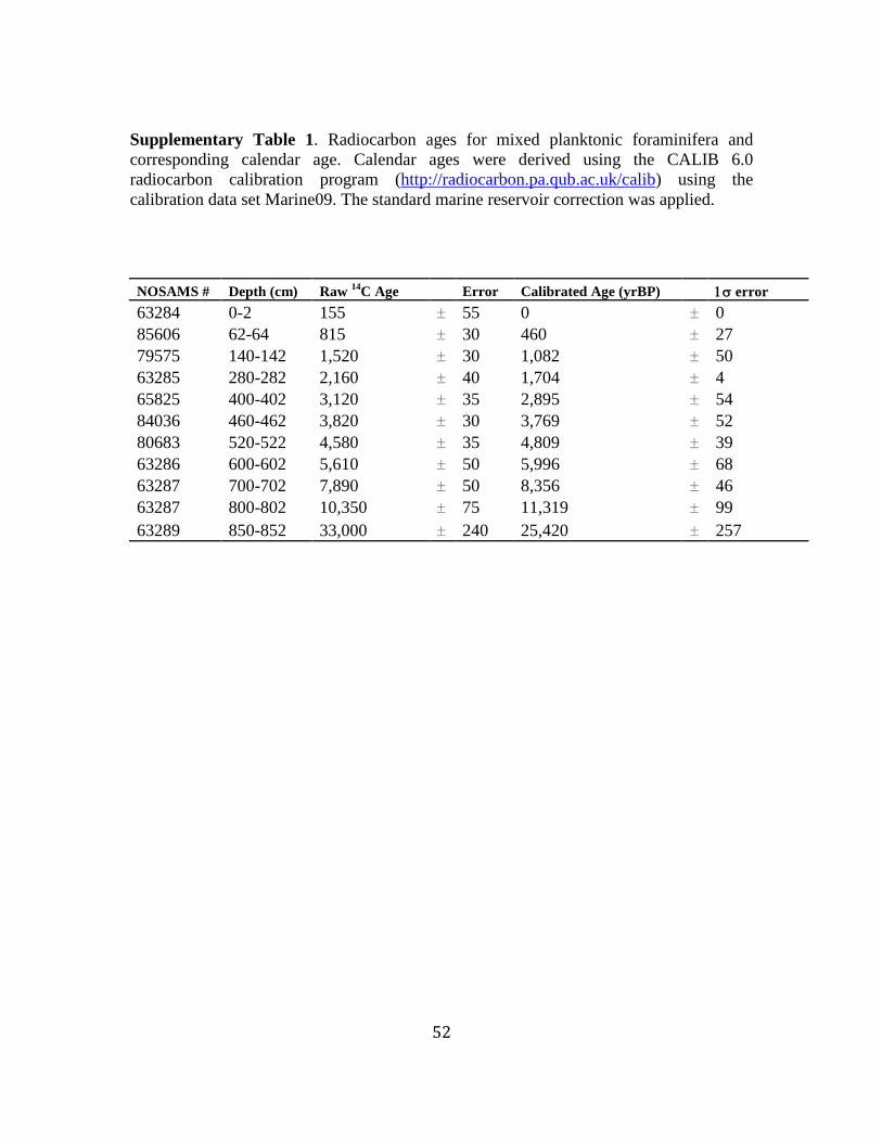
52

Supplementary Table 1. Radiocarbon ages for mixed planktonic foraminifera and

corresponding calendar age. Calendar ages were derived using the CALIB 6.0

radiocarbon calibration program (http://radiocarbon.pa.qub.ac.uk/calib) using the

calibration data set Marine09. The standard marine reservoir correction was applied.

NOSAMS # Depth (cm) Raw 14

C Age Error Calibrated Age (yrBP) error

63284 0-2 155 ± 55 0 ± 0

85606 62-64 815 ± 30 460 ± 27

79575 140-142 1,520 ± 30 1,082 ± 50

63285 280-282 2,160 ± 40 1,704 ± 4

65825 400-402 3,120 ± 35 2,895 ± 54

84036 460-462 3,820 ± 30 3,769 ± 52

80683 520-522 4,580 ± 35 4,809 ± 39

63286 600-602 5,610 ± 50 5,996 ± 68

63287 700-702 7,890 ± 50 8,356 ± 46

63287 800-802 10,350 ± 75 11,319 ± 99

63289 850-852 33,000 ± 240 25,420 ± 257

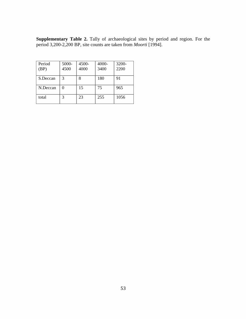
53

Supplementary Table 2. Tally of archaeological sites by period and region. For the

period 3,200-2,200 BP, site counts are taken from Moorti [1994].

Period

(BP) 5000-

4500 4500-

4000 4000-

3400 3200-

2200

S.Deccan 3 8 180 91

N.Deccan 0 15 75 965

total 3 23 255 1056

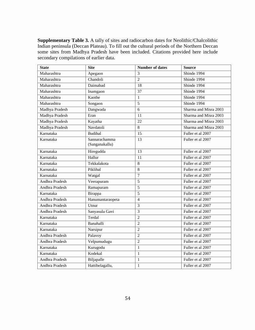
54

Supplementary Table 3. A tally of sites and radiocarbon dates for Neolithic/Chalcolithic

Indian peninsula (Deccan Plateau). To fill out the cultural periods of the Northern Deccan

some sites from Madhya Pradesh have been included. Citations provided here include

secondary compilations of earlier data.

State Site Number of dates Source

Maharashtra Apegaon 3 Shinde 1994

Maharashtra Chandoli 2 Shinde 1994

Maharashtra Daimabad 18 Shinde 1994

Maharashtra Inamgaon 37 Shinde 1994

Maharashtra Kaothe 1 Shinde 1994

Maharashtra Songaon 5 Shinde 1994

Madhya Pradesh Dangwada 6 Sharma and Misra 2003

Madhya Pradesh Eran 11 Sharma and Misra 2003

Madhya Pradesh Kayatha 22 Sharma and Misra 2003

Madhya Pradesh Navdatoli 8 Sharma and Misra 2003

Karnataka Budihal 15 Fuller et al 2007

Karnataka Sannarachamma

(Sanganakallu)

13 Fuller et al 2007

Karnataka Hiregudda 13 Fuller et al 2007

Karnataka Hallur 11 Fuller et al 2007

Karnataka Tekkalakota 8 Fuller et al 2007

Karnataka Piklihal 8 Fuller et al 2007

Karnataka Watgal 7 Fuller et al 2007

Andhra Pradesh Veerapuram 5 Fuller et al 2007

Andhra Pradesh Ramapuram 5 Fuller et al 2007

Karnataka Birappa 5 Fuller et al 2007

Andhra Pradesh Hanumantaraopeta 4 Fuller et al 2007

Andhra Pradesh Utnur 3 Fuller et al 2007

Andhra Pradesh Sanyasula Gavi 3 Fuller et al 2007

Karnataka Terdal 2 Fuller et al 2007

Karnataka Banahalli 2 Fuller et al 2007

Karnataka Narsipur 2 Fuller et al 2007

Andhra Pradesh Palavoy 2 Fuller et al 2007

Andhra Pradesh Velpumudugu 2 Fuller et al 2007

Karnataka Kurugodu 1 Fuller et al 2007

Karnataka Kodekal 1 Fuller et al 2007

Andhra Pradesh Biljapalle 1 Fuller et al 2007

Andhra Pradesh Hattibelagallu, 1 Fuller et al 2007

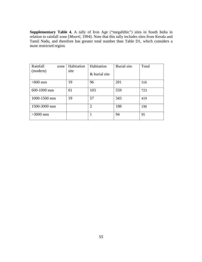
55

Supplementary Table 4. A tally of Iron Age (“megalithic”) sites in South India in

relation to rainfall zone [Moorti, 1994]. Note that this tally includes sites from Kerala and

Tamil Nadu, and therefore has greater total number than Table D1, which considers a

more restricted region.

Rainfall zone

(modern)

Habitation

site

Habitation

& burial site

Burial site

Total

<600 mm 19 96 201 316

600-1000 mm 61 103 559 723

1000-1500 mm 19 57 343 419

1500-3000 mm 2 188 190

>3000 mm 1 94 95

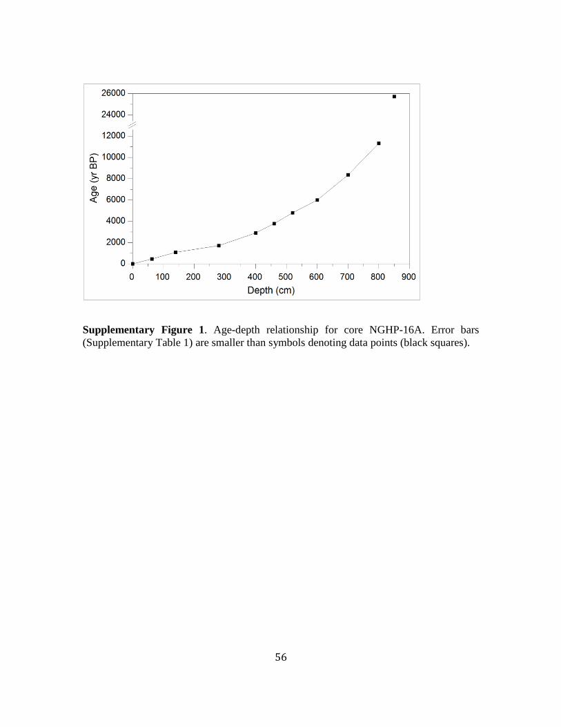
56

Supplementary Figure 1. Age-depth relationship for core NGHP-16A. Error bars

(Supplementary Table 1) are smaller than symbols denoting data points (black squares).

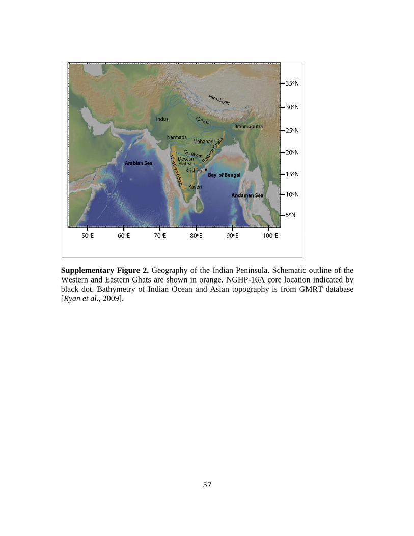
57

Supplementary Figure 2. Geography of the Indian Peninsula. Schematic outline of the

Western and Eastern Ghats are shown in orange. NGHP-16A core location indicated by

black dot. Bathymetry of Indian Ocean and Asian topography is from GMRT database

[Ryan et al., 2009].

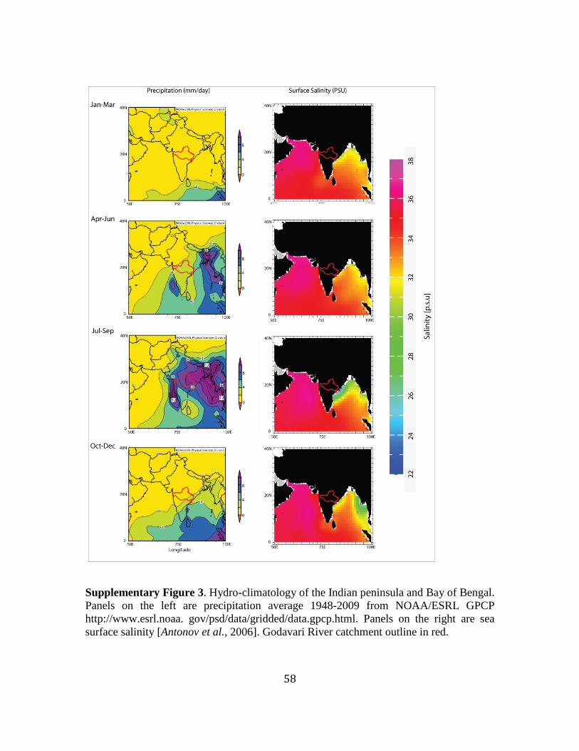
58

Supplementary Figure 3. Hydro-climatology of the Indian peninsula and Bay of Bengal.

Panels on the left are precipitation average 1948-2009 from NOAA/ESRL GPCP

http://www.esrl.noaa. gov/psd/data/gridded/data.gpcp.html. Panels on the right are sea

surface salinity [Antonov et al., 2006]. Godavari River catchment outline in red.

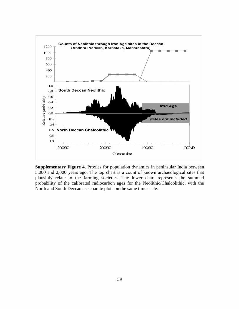
59

Supplementary Figure 4. Proxies for population dynamics in peninsular India between

5,000 and 2,000 years ago. The top chart is a count of known archaeological sites that

plausibly relate to the farming societies. The lower chart represents the summed

probability of the calibrated radiocarbon ages for the Neolithic/Chalcolithic, with the

North and South Deccan as separate plots on the same time scale.

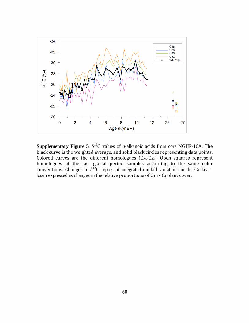
60

Supplementary Figure 5. 13

C values of n-alkanoic acids from core NGHP-16A. The black curve is the weighted average, and solid black circles representing data points. Colored curves are the different homologues (C26-C32). Open squares represent homologues of the last glacial period samples according to the same color conventions. Changes in 13

C represent integrated rainfall variations in the Godavari

basin expressed as changes in the relative proportions of C3 vs C4 plant cover.

61

References

Adkins, J. F., and D. P. Schrag (2003), Reconstructing Last Glacial Maximum bottom

water salinities from deep-sea sediment pore fluid profiles, Earth and Planetary Science

Letters, 216(1-2), 109-123.

Antonov, J.I., R.A. Locarnini, T.P. Boyer, A.V. Mishonov, and H.E. Garcia (2006), Sea

Surface Salinity, in World Ocean Atlas 2005, Vol. 2: Salinity, edited by S. Levitus, Ed.,

NOAA, Washington, D.C.

Asouti, E. and D.Q. Fuller, (2008) Trees and Woodlands in South India. Archaeological

Perspectives, Left Coast Press, Walnut Creek, Calif.

Bevington, P.R. and D.K. Robinson, (1992) Data Reduction and Error Analysis for the

Physical Sciences,2nd

edition, WCB/McGraw-Hill, USA.

Bikshamaiah, G., and V. Subramanian (1980), Chemical and sediment mass-transfer in

the Godavari River Basin in India, Journal of Hydrology, 46(3-4), 331-342.

Bronk Ramsey, C. ( 2001), Development of the radiocarbon calibration program OxCal,

Radiocarbon, 43(2A), 355-63.

Bronk Ramsey, C. (2005), OxCal version 3.10. Computer Program. Available at:

http://c14.arch.oxoac.uk/.

Chikaraishi, Y., H. Naraoka, and S. R. Poulson (2004), Hydrogen and carbon isotopic

fractionations of lipid biosynthesis among terrestrial (C3, C4 and CAM) and aquatic

plants, Phytochemistry, 65(10), 1369-1381.

Clarkson, C., et al. (2009), The oldest and longest enduring microlithic sequence in India:

35 000 years of modern human occupation and change at the Jwalapuram Locality 9

rockshelter, Antiquity, 83(320), 326-348.

Collard, M., B. Buchanan, M. J. Hamilton, and M. J. O'Brien (2010a), Spatiotemporal

dynamics of the Clovis-Folsom transition, Journal of Archaeological Science, 37(10),

2513-2519.

Collard, M., K. Edinborough, S. Shennan, and M. G. Thomas (2010b), Radiocarbon

evidence indicates that migrants introduced farming to Britain, Journal of Archaeological

Science, 37(4), 866-870.

Curry, W. B., D. R. Ostermann, M. V. S. Guptha, and V. Ittekkot (1992), Foraminiferal

production and mosoonal upwelling in the Arabian Sea: evidence from sediment trap, in

Upwelling Systems: Evolution since the Early Miocene, edited by E. A. Se, pp. 93-106,

Geological Society Special Publication.

62

Dutta, K., R. Bhushan and B.L. Somayajulu (2001), Delta R correction values for the

northern Indian Ocean, Radiocarbon, 43, 483-488.

Fairbanks, R. G. (1989), A 17,000-year glacio-eustatic sea-level record - influence of

glacial melting rates on the Younger Dryas event and deep-ocean circulation, Nature,

342(6250), 637-642.

Fairbanks, R. G., M. Sverdlove, R. Free, P. H. Wiebe, and A. W. H. Be (1982), Vertical-

distribution and isotopic fractionation of living planktonic-foraminifera from the Panama

Basin, Nature, 298(5877), 841-844.

Forsberg, C. F., A. Solheim, T.J., Kvalstad, R. Vaidya, and S. Mohanty (2007), Slope

instability and mass transport deposits on the Godavari river delta, east Indian margin

from a regional geological perspective, Submarine Mass Movements and Their

Consequences 27, 19-27.

Fuller, D.Q. (2006), Agricultural Origins and Frontiers in South Asia: A Working

Synthesis. Journal of World Prehistory, 20, 1-86.

Fuller, D.Q. (2008). Asia, South: Neolithic Cultures, in Encyclopedia of Archaeology,

edited by D. Pearsall, pp.756-768, Elsevier, Amsterdam.

Fuller, D.Q. (2011), Finding Plant Domestication in the Indian Subcontinent. Current

Anthropology, 52(S4), S347-S362

Fuller, D.Q. and R. Korisettar, (2004), The Vegetational Context of Early Agriculture in

South India, Man and Environment XXIX(1), 7-27.

Fuller, D. Q., N. Boivin, and R. Korisettar (2007), Dating the Neolithic of South India:

new radiometric evidence for key economic, social and ritual transformations, Antiquity,

81(313), 755-778.

Gadgil, S. (2003), The Indian monsoon and its variability, Annual Review of Earth and

Planetary Sciences, 31, 429-467.

Govil, P., and P. D. Naidu (2010), Evaporation-precipitation changes in the eastern

Arabian Sea for the last 68 ka: Implications on monsoon variability, Paleoceanography,

25.

Govil, P., and P. D. Naidu (2011), Variations of Indian monsoon precipitation during the

last 32 kyr reflected in the surface hydrography of the Western Bay of Bengal,

Quaternary Science Reviews, 30, 3871-3879.

Gunnell, Y., K. Anupama, and B. Sultan (2007), Response of the South Indian runoff-

harvesting civilization to northeast monsoon rainfall variability during the last 2000

63

years: instrumental records and indirect evidence, Holocene, 17(2), 207-215.

Hassan, F.A. (1981), Demographic Archaeology, Academic Press, New York.

Hill, C.V., 2008, South Asia: An Environmental History, ABC-CLIO Press, 329 p.

Kingwell-Banham E. and D.Q. Fuller (2011), Shifting cultivators in South Asia:

expansion, marginalisation and specialisaton over the long term. Quaternary

International [on-line/in press]: DOI: 10.1016/j.quaint.2011.05.025.

Madella, M., and D. Q. Fuller (2006), Palaeoecology and the Harappan Civilisation of

South Asia: a reconsideration, Quaternary Science Reviews, 25(11-12), 1283-1301.

Misra, V.N. (2002), Mesolithic culture in India, in Mesolithic India, edited by V.N. Misra

and J.N. Pal, pp. 1-66, Department of Ancient History, Culture and Archaeology,

University of Allahbad, Allahbad, India.

Moorti, U.S. (1994), Megalithic Culture of South India. Socio-economic Perspectives,

Ganga Kaveri Publishing House, Varanasi.

Mulitza, S., D. Boltovskoy, B. Donner, H. Meggers, A. Paul, and G. Wefer (2003),

Temperature: delta O-18 relationships of planktonic foraminifera collected from surface

waters, Palaeogeography Palaeoclimatology Palaeoecology, 202(1-2), 143-152.

Paddayya K. (1973), Investigations into the Neolithic Culture of the Shorapur Doab,

South India, Brill, Leiden.

Possehl, G.L. and P. Rissman (1992). The chronology of prehistoric India from earliest

times to the Iron Age, in Chronologies in old world archaeology, edited by R.W. Ehrich,

pp. 1, 465–490; 462, 447–474, University of Chicago Press, Chicago.

Rao, K.N., Sadakata, N., Malini, B.H., Takayasu, K., 2005, Sedimentation processes and

asymmetric development of the Godavari delta, India, in River Deltas: Concepts, Models,

and Examples, edited by L. Giosan, and J.P. Bhattacharya, pp. 435-452, SEPM Special

Publication 83.

Reimer, P. J., et al. (2009), INTCAL09 and MARINE09 radiocarbon age calibration

curves, 0-50,000 years cal BP, Radiocarbon, 51(4), 1111-1150.

Ryan, W. B. F., et al. (2009), Global Multi-Resolution Topography synthesis,

Geochemistry Geophysics Geosystems, 10.

Sharma R.K. and O.P. Misra (2003), Archaeological Excavations in Central India

(Madhya Pradesh and Chhattisgarh), Mittal Publications, New Delhi.

Shennan, S., and K. Edinborough (2007), Prehistoric population history: from the late

64

glacial to the late neolithic in central and northern Europe, Journal of Archaeological

Science, 34(8), 1339-1345.

Sridhar, P. N., M. M. Ali, P. Vethamony, M. T. Babu, I. V. Ramana, and S. Jayakumar

(2008), Seasonal Occurrence of Unique Sediment Plume in the Bay of Bengal, EOS

Trans. AGU 89, 22-23.

Shinde, V.S. (1994), The Deccan Chalcolithic: a recent perspective, Man and

Environment 19, 1-2.

Shinde, V.S. (1998), Early Settlements in the Central Tapi Basin, Munshiram Manoharlal,

New Delhi.

Southon, J., M. Kashgarian, M. Fontugne, B. Metivier, and W. W. S. Yim (2002), Marine

reservoir corrections for the Indian Ocean and southeast Asia, Radiocarbon, 44(1), 167-

180.

Stuiver, M., and P. J. Reimer (1993), Extended C-14 data-base and revised calib 3.0 C-14

age calibration program, Radiocarbon, 35(1), 215-230.

Unger, D., V. Ittekkot, P. Schafer, J. Tiemann, and S. Reschke (2003), Seasonality and

interannual variability of particle fluxes to the deep Bay of Bengal: influence of riverine

input and oceanographic processes, Deep-Sea Research Part II-Topical Studies in

Oceanography, 50(5), 897-923.

Venkattasubbaiah, P.C. (1992), Protohistoric investigation in the Central Pennar Basin,

Cuddapah, Andhra Pradesh, PhD Thesis, University of Poona, Pune, India.

Washington, H. S. (1922), Deccan traps and other plateau basalts, Bulletin of the

Geological Society of America, 33, 765-803.

65

CHAPTER 3

Climate Controls Residence Time of Organic Carbon in a Monsoonal River Basin

Abstract

This study compares radiocarbon age relationships between planktonic foraminifera and

higher (terrestrial) plant wax fatty acids isolated from the same depth horizons in a

sediment core off the mouth of the Godavari River in the Bay of Bengal. The Godavari

drainage basin has been experiencing aridification over the Holocene and provides a good

opportunity to examine relationships between hydroclimate and the dynamics of

terrestrial carbon discharge to the sea. Radiocarbon measurements of long-chain fatty

acids compared to planktonic foraminifera show an increase in age offset from mid to late

Holocene, suggesting that increased aridity either slowed carbon cycling and/or transport

rates, or resulted in mobilization of older (soil) organic carbon, the net result being an

apparent increase of terrestrial storage times of vascular plants carbon. Since ~4,000 yrs

BP the fatty acids are on average ~1,200 yrs older than the foraminifera, indicating either

increasing residence times of terrestrial carbon or increasing erosion and mobilization of

pre-aged vascular plant-derived carbon as a consequence of a less humid climate. At the

core top, the age discrepancy between depositional age and plant wax fatty acids is

approximately ~5,000 yrs, which we attribute to enhanced exhumation of old soil organic

matter as a consequence of anthropogenic activity.

The findings of this study show that there are key facets of organic matter transfer from

the continents to the oceans that remain poorly understood, and demonstrate a direct link

between climate dynamics and carbon cycling within river drainage basins. In addition to

their pertinence to carbon cycle studies, these results also have implications for the use of

terrestrial proxies preserved in continental margin sediments in paleoclimate

reconstructions; in particular the temporal phasing of terrestrial and marine proxy signals

in the context of a variable hydroclimate deserves closer scrutiny.

3.1 Introduction

3.1.1 Terrestrial organic carbon: from source to sink

Once a CO2 molecule is captured by a terrestrial plant and incorporated into tissue

through photosynthesis it can take several paths before being transported by a river into

the ocean and then buried within continental margin sediments. A conceptual model with

different transport pathways for terrestrial biospheric carbon and other continental OC

sources is presented in Figure 1 (modified from Blair et al., 2004). The model includes a

66

series of interconnected reservoirs where terrestrial OC resides and is

transformed/degraded before moving to the next compartment and eventually being

discharged to, and preserved in, receiving marine sedimentary basins. From Figure 1 it is

clear that the resulting sedimentary terrestrial OC is likely to comprise a mixture of

material from different carbon pools that can make its way to the ocean sediments with

different transit times. While some of the terrestrial OC may have been transported to the

continental margin almost instantaneously, other portions of it may have resided in soils

or in the flood plains for thousands of years before being eroded and transported. We

have an understanding of the different pathways carbon can take from land into the

oceans, but we do not have tight constraints on the time elapsed between the production

of terrestrial biomass via photosynthetic fixation of a CO2 and its burial in marine

sediments or its continental “residence time”. Furthermore, terrestrial OC turnover and

residence times are expected to vary with other environmental properties such as climate

(aridity, temperature), soil type, and topography of the river catchment (e.g. Schimel et

al., 2011; Trumbore 1997; Quideau et al., 2001). In addition to this, anthropogenic

activities including deforestation, agricultural practices, and river damming (e.g. Wang et

al. 1999; Fisher et al. 2003) have shifted the type and discharge rate of terrestrial OC into

the oceans (Syvitski et al., 2005).

Environmental signatures encoded in terrestrial OC exported by rivers result from

complex processes occurring at various spatial and temporal scales. One of the caveats in

using sedimentary records for paleoclimatic reconstructions based on terrestrial organic

proxies is the uncertainty in the timescales over which terrestrial organic matter is

synthesized, transferred and stored in marine sediments. In fact, several studies have

shown a significant storage time for OC on land prior to deposition in continental

margins (Drenzek, 2007; Drenzek et al., 2009; Kusch et al., 2010a, Gustafsson et al.,

2011; Galy and Eglinton 2011).

67

In order to improve our understanding on the burial of OC in marine sediments, as well

as to accurately interpret signals of continental climate embedded in terrestrial proxies, it

is important to better constrain the residence or storage time of terrestrial OC associated

with its transfer from the continental river drainage basins to marine sediments, as well as

to identify the key factors that control timescales of terrestrial carbon transfer. These

aspects provide motivation for the present study and we explore here the effect of

aridification on the dynamics of terrestrial organic carbon transfer from biological source

to sedimentary sink.

3.1.2 Residence times of terrestrial organic carbon

One approach in addressing climatic effects on the dynamics of terrestrial carbon is to

examine radiocarbon age relationships between terrestrial and marine components co-

deposited in sedimentary sequences proximal to the mouths of river systems, in our case

higher plant wax biomarker compounds and marine planktonic foraminifera. While

marine planktonic foraminiferal tests are expected to settle quickly through the water

column and deposit on the ocean floor not far away from the organism’s surface water

habitat, carbon derived from the terrestrial biosphere must travel from its source of

production within continental drainage basins, and move through multiple reservoirs

(soils, floodplains, etc., Fig. 1) before deposition on the ocean floor. Excluding the

marine “reservoir effect” (Stuiver and Ostlund, 1983; Stuiver et. al., 1986; Southon et al.,

2002), terrestrial organic matter would therefore be anticipated to be of an older

radiocarbon age than the planktonic foraminiferal shells deposited on the same sediment

horizon. Previous radiocarbon studies by Drenzek (2007) and Drenzek et al. (2009) show

that higher plant wax fatty acids deposited in marine shelf sediments proximal to river

mouths can predate the depositional age by several thousand years. However, no

comparison to foraminifera age was attempted in these prior studies. Coupled biomarker-

specific and planktonic foraminiferal 14

C measurements have been made before (e.g.,

Ohkouchi et al. 2002; Kusch et al. 2010b) but with a focus on marine sediment

redistribution processes and not supply of continentally-derived OC. Mollenhauer and

68

Eglinton (2007) report alkenone, foraminifera and fatty acid ages in California

Borderland core top and pre-bomb sediments and show that long-chain fatty acids are

systematically depleted in 14

C (older) than the planktonic formanifera. The authors

calculate residence times for long-chain fatty acids and report values of 380 - 1,200 yrs.

However, for simplification, they assumed terrigenous compounds were delivered to the

ocean immediately after production and did not considered intermediate carbon

reservoirs.

A recent biomarker 14

C study indicates that the residence time of vascular plant OC

supplied to surface sediments near the mouths of rivers flowing into the Black Sea varies

from between 900 and 4,400 years (Kusch et al., 2010a), indicating a significant storage

time in intermediate carbon reservoirs within continental drainage basins. The

radiocarbon ages of vascular plant biomarkers in river sediments along the Ganges-

Brahmaputra river system suggest an overall residence time of the OC in the basin of

approximately 50 - 1,300 years (Galy and Eglinton, 2011). There is also evidence of the

potential influence of climate change on the age of terrestrial OC discharged from the

Arctic rivers. Gustaffson et al. (2011) show that the vascular plant biomarkers extracted

from surface sediments from Eurasian Arctic rivers are older on those rivers most heavily

affected by warming and destabilization of permafrost soils. While prior studies have

examined links between river drainage basin properties and 14

C residence times, there

have been no reported studies that explore links between past climate variability and

residence time.

In this study we compare the radiocarbon age relationships between planktonic

foraminifera and higher (terrestrial) plant wax fatty acids isolated from the same depth

horizons in a sediment core off the mouth of the Godavari River. The core, which spans

the entire Holocene, provides an opportunity to examine the effect of long-term

aridification on the residence time of terrestrial organic carbon as it is transferred from

source to sedimentary sink.

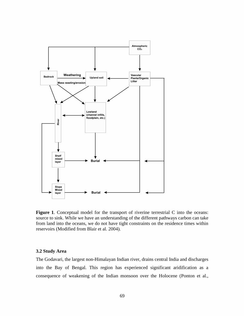
69

Figure 1. Conceptual model for the transport of riverine terrestrial C into the oceans:

source to sink. While we have an understanding of the different pathways carbon can take

from land into the oceans, we do not have tight constraints on the residence times within

reservoirs (Modified from Blair et al. 2004).

3.2 Study Area

The Godavari, the largest non-Himalayan Indian river, drains central India and discharges

into the Bay of Bengal. This region has experienced significant aridification as a

consequence of weakening of the Indian monsoon over the Holocene (Ponton et al.,

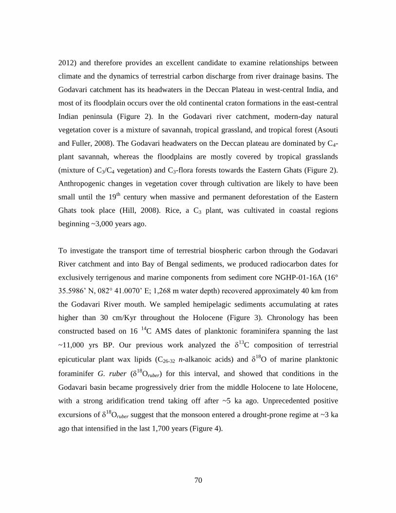
70

2012) and therefore provides an excellent candidate to examine relationships between

climate and the dynamics of terrestrial carbon discharge from river drainage basins. The

Godavari catchment has its headwaters in the Deccan Plateau in west-central India, and

most of its floodplain occurs over the old continental craton formations in the east-central

Indian peninsula (Figure 2). In the Godavari river catchment, modern-day natural

vegetation cover is a mixture of savannah, tropical grassland, and tropical forest (Asouti

and Fuller, 2008). The Godavari headwaters on the Deccan plateau are dominated by C4-

plant savannah, whereas the floodplains are mostly covered by tropical grasslands

(mixture of C3/C4 vegetation) and C3-flora forests towards the Eastern Ghats (Figure 2).

Anthropogenic changes in vegetation cover through cultivation are likely to have been

small until the 19th

century when massive and permanent deforestation of the Eastern

Ghats took place (Hill, 2008). Rice, a C3 plant, was cultivated in coastal regions

beginning ~3,000 years ago.

To investigate the transport time of terrestrial biospheric carbon through the Godavari

River catchment and into Bay of Bengal sediments, we produced radiocarbon dates for

exclusively terrigenous and marine components from sediment core NGHP-01-16A (16°

35.5986’ N, 082° 41.0070’ E; 1,268 m water depth) recovered approximately 40 km from

the Godavari River mouth. We sampled hemipelagic sediments accumulating at rates

higher than 30 cm/Kyr throughout the Holocene (Figure 3). Chronology has been

constructed based on 16 14

C AMS dates of planktonic foraminifera spanning the last

~11,000 yrs BP. Our previous work analyzed the 13

C composition of terrestrial

epicuticular plant wax lipids (C26-32 n-alkanoic acids) and 18

O of marine planktonic

foraminifer G. ruber (18

Oruber) for this interval, and showed that conditions in the

Godavari basin became progressively drier from the middle Holocene to late Holocene,

with a strong aridification trend taking off after ~5 ka ago. Unprecedented positive

excursions of 18

Oruber suggest that the monsoon entered a drought-prone regime at ~3 ka

ago that intensified in the last 1,700 years (Figure 4).

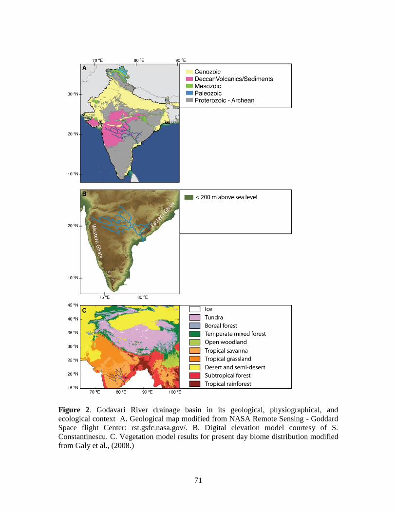
71

Figure 2. Godavari River drainage basin in its geological, physiographical, and

ecological context A. Geological map modified from NASA Remote Sensing - Goddard

Space flight Center: rst.gsfc.nasa.gov/. B. Digital elevation model courtesy of S.

Constantinescu. C. Vegetation model results for present day biome distribution modified

from Galy et al., (2008.)

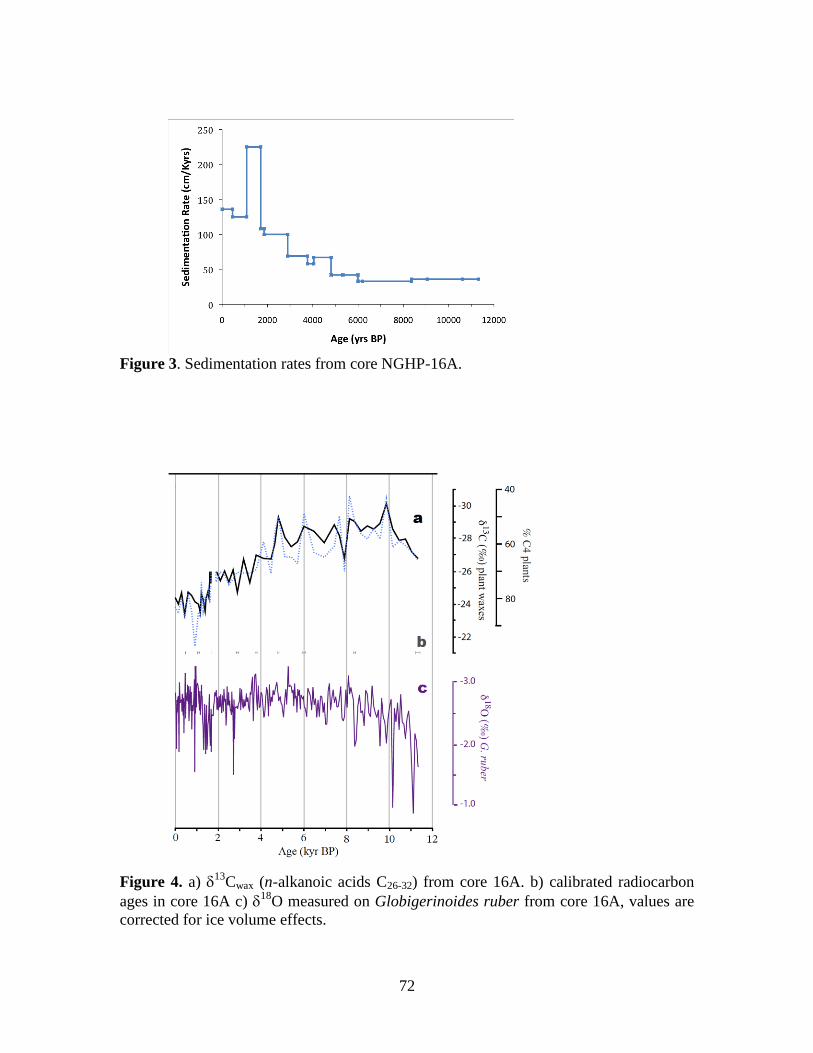
72

Figure 3. Sedimentation rates from core NGHP-16A.

Figure 4. a) 13

Cwax (n-alkanoic acids C26-32) from core 16A. b) calibrated radiocarbon

ages in core 16A c) 18

O measured on Globigerinoides ruber from core 16A, values are

corrected for ice volume effects.

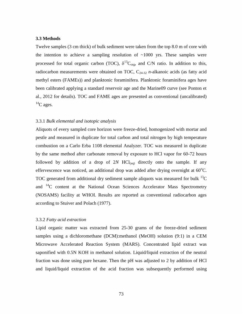
73

3.3 Methods

Twelve samples (3 cm thick) of bulk sediment were taken from the top 8.0 m of core with

the intention to achieve a sampling resolution of ~1000 yrs. These samples were

processed for total organic carbon (TOC), 13

Corg, and C/N ratio. In addition to this,

radiocarbon measurements were obtained on TOC, C24-32 n-alkanoic acids (as fatty acid

methyl esters (FAMEs)) and planktonic foraminifera. Planktonic foraminifera ages have

been calibrated applying a standard reservoir age and the Marine09 curve (see Ponton et

al., 2012 for details). TOC and FAME ages are presented as conventional (uncalibrated)

14C ages.

3.3.1 Bulk elemental and isotopic analysis

Aliquots of every sampled core horizon were freeze-dried, homogenized with mortar and

pestle and measured in duplicate for total carbon and total nitrogen by high temperature

combustion on a Carlo Erba 1108 elemental Analyzer. TOC was measured in duplicate

by the same method after carbonate removal by exposure to HCl vapor for 60-72 hours

followed by addition of a drop of 2N HCl(aq) directly onto the sample. If any

effervescence was noticed, an additional drop was added after drying overnight at 60oC.

TOC generated from additional dry sediment sample aliquots was measured for bulk 13

C

and 14

C content at the National Ocean Sciences Accelerator Mass Spectrometry

(NOSAMS) facility at WHOI. Results are reported as conventional radiocarbon ages

according to Stuiver and Polach (1977).

3.3.2 Fatty acid extraction

Lipid organic matter was extracted from 25-30 grams of the freeze-dried sediment

samples using a dichloromethane (DCM):methanol (MeOH) solution (9:1) in a CEM

Microwave Accelerated Reaction System (MARS). Concentrated lipid extract was

saponified with 0.5N KOH in methanol solution. Liquid/liquid extraction of the neutral

fraction was done using pure hexane. Then the pH was adjusted to 2 by addition of HCl

and liquid/liquid extraction of the acid fraction was subsequently performed using

74

hexane:DCM (4:1). Lipids in the acid fraction, including leaf wax n-alkanoic acids, were

methylated using HCl 5% in MeOH (70 oC for 12 hours). The resulting fatty acid

methylesters (FAMEs) were extracted using hexane:DCM (4:1), dried over anhydrous

sodium sulfate, and then purified via silica gel chromatography. A FAME external

standard (C18 and C28) was included each run sequence prior to sample analysis by gas

chromatography with flame ionization detection (GC/FID) for initial quantification.

3.3.3. Compound specific 14C analysis

For isolation of the individual FAMEs, preparative capillary gas chromatography

(PCGC) was used following (Eglinton et al., 1996). FAME samples were blown to

dryness and re-dissolved in 50-150L of iso-octane to achieve concentrations in the

range of 100 - 200 ng/L per compound. The samples were repeatedly injected (24-45

times) into an Agilent 7890 gas chromatograph equipped with a Gerstel PTV injection

system and coupled to a Gerstel preparative fraction collector (PFC). The target was to

have 300 - 500 ng of each individual compound on column on every injection. Separation

was achieved on a Varian VF-1ms fused silica capillary column (30 m, 0.53 lm i.d., 0.5

lm). The PTV injector temperature program was 50oC (0.05 min), 12

oC/s to 320

oC (5

min), 12oC/s to 340

oC (4 min). For FAMEs, the GC oven was programmed 50

oC (1

min), 6oC/min to 320

oC (20 min). Hydrogen was used as carrier gas (10 mL/min). The

transfer line and PFC were heated at 320oC. Individual nC16, nC24, nC26, nC28, nC30, nC32

homologues were isolated into 6 clean glass PFC traps kept at 5oC. PFC traps were eluted

with hexane and brought up to a known volume for purity check and quantification for

recovery calculations on a GC-FID. Recoveries averaged 64% (54% min and 78% max),

which is typical for this process. After isolation, FAMEs were eluted over a silica gel

column using hexane:DCM (2:1) to remove potential column bleed contamination. In

order to obtain sample yields large enough for radiocarbon measurements some isolates

were re-combined (nC24 – nC32).

75

For combustion, purified FAMEs were transferred into pre-combusted quartz tubes, the

hexane evaporated, and ~150 g pre-combusted copper oxide was added for oxygen

supply. The tubes were evacuated while kept chilled in a dry-ice/isopropanol slurry, then

flame-sealed and subsequently combusted at 850oC for 5 h. After cooling, the quartz

tubes were cracked under vacuum; the escaping CO2 gas was stripped of water, trapped

and quantified manometrically. The CO2 was further transferred into evacuated pyrex

tubes which were flame-sealed for storage before AMS measurement.

Compound-specific AMS radiocarbon measurements were performed at ETH Zurich

using the MICADAS system equipped with a gas-ion source (Ruff et al., 2007). Results

are reported as conventional radiocarbon ages (years BP) and 14

C referring to Stuiver

and Polach (1977). The radiocarbon ages of the individual n-alkanoic acids were

corrected for the addition of one methyl group during derivatization using isotopic mass

balance. In addition, internal corrections for additional modern and dead carbon that can

be introduced as contamination in the combustion, vacuum line work, and AMS

analytical procedures have been applied before reporting final 14

C values, based on

quantitative measurements of OX-I and coal standards as well as the long-term blank

average of the facility.

Possible contamination derived from sample preparations steps before combustion have

been recognized to be significant when measuring C samples smaller than 100gC

(Drenzek 2007; Santos et al. 2010). This contamination can derive from carbon in the lab

environment, or from sample preparatory techniques like gas chromatography that via

column bleed or carry over from previous injections can introduce external carbon into

the sample. Drenzek (2007) running a standard of n-alkanoic acids of known 14

C

composition through a very similar methodology as we describe here, determined that

contamination of fossil carbon due to pre-combustion lab procedures for small C samples

was 0.75 +/- 0.4 g of C. Using this value, we assess that pre-combustion fossil carbon

contamination on our samples (9 – 36 g of C) can overestimate the age of the samples

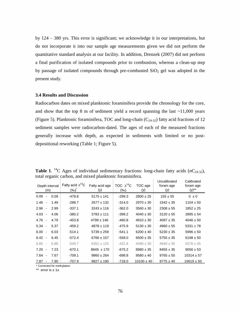
76

by 124 – 380 yrs. This error is significant; we acknowledge it in our interpretations, but

do not incorporate it into our sample age measurements given we did not perform the

quantitative standard analysis at our facility. In addition, Drenzek (2007) did not perform

a final purification of isolated compounds prior to combustion, whereas a clean-up step

by passage of isolated compounds through pre-combusted SiO2 gel was adopted in the

present study.

3.4 Results and Discussion

Radiocarbon dates on mixed planktonic foraminifera provide the chronology for the core,

and show that the top 8 m of sediment yield a record spanning the last ~11,000 years

(Figure 5). Planktonic foraminifera, TOC and long-chain (C24-32) fatty acid fractions of 12

sediment samples were radiocarbon-dated. The ages of each of the measured fractions

generally increase with depth, as expected in sediments with limited or no post-

depositional reworking (Table 1; Figure 5).

Table 1. 14

C Ages of individual sedimentary fractions: long-chain fatty acids (nC24-32),

total organic carbon, and mixed planktonic foraminifera.

Fatty acid ∆14

C

(‰)*

Fatty acid age

(y)

TOC ∆14

C

(‰)

TOC age

(y)

Uncalibrated

foram age

(y)

Calibrated

foram age

(y)**

0.06 - 0.09 -478.8 5175 ± 141 -299.3 2800 ± 25 155 ± 55 0 ± 0

1.46 - 1.49 -288.7 2677 ± 132 -314.0 2970 ± 30 1542 ± 35 1104 ± 50

2.96 - 2.99 -337.1 3243 ± 116 -362.0 3560 ± 30 2308 ± 55 1852 ± 25

4.03 - 4.06 -380.2 3783 ± 111 -399.2 4040 ± 30 3120 ± 55 2895 ± 54

4.76 - 4.79 -453.8 4799 ± 146 -460.8 4910 ± 30 4097 ± 35 4046 ± 50

5.34 - 5.37 -459.2 4878 ± 119 -475.9 5130 ± 30 4960 ± 55 5331 ± 78

6.00 - 6.03 -514.1 5739 ± 259 -541.1 6200 ± 40 5230 ± 35 5996 ± 50

6.42 - 6.45 -572.4 6766 ± 157 -558.0 6500 ± 35 5755 ± 35 6198 ± 50

6.85 - 6.88 -549.7 6351 ± 125 -431.8 4490 ± 30 4940 ± 35 5276 ± 45

7.20 - 7.23 -670.1 8849 ± 170 -675.2 8980 ± 35 8455 ± 35 9056 ± 53

7.64 - 7.67 -709.1 9860 ± 264 -698.8 9580 ± 40 9765 ± 50 10314 ± 57

7.87 - 7.90 -707.9 9827 ± 190 -718.0 10100 ± 40 9775 ± 40 10619 ± 50

Depth interval

(m)

* Corrected for methylation

** error is ± 1σ

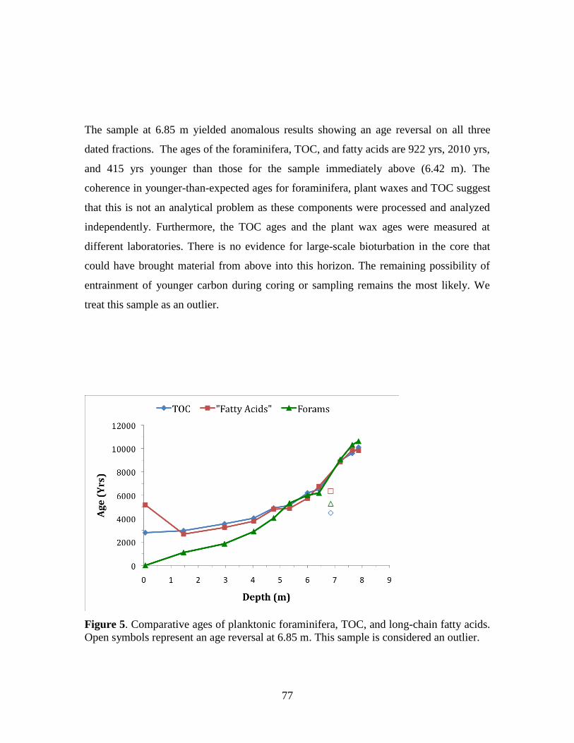
77

The sample at 6.85 m yielded anomalous results showing an age reversal on all three

dated fractions. The ages of the foraminifera, TOC, and fatty acids are 922 yrs, 2010 yrs,

and 415 yrs younger than those for the sample immediately above (6.42 m). The

coherence in younger-than-expected ages for foraminifera, plant waxes and TOC suggest

that this is not an analytical problem as these components were processed and analyzed

independently. Furthermore, the TOC ages and the plant wax ages were measured at

different laboratories. There is no evidence for large-scale bioturbation in the core that

could have brought material from above into this horizon. The remaining possibility of

entrainment of younger carbon during coring or sampling remains the most likely. We

treat this sample as an outlier.

Figure 5. Comparative ages of planktonic foraminifera, TOC, and long-chain fatty acids.

Open symbols represent an age reversal at 6.85 m. This sample is considered an outlier.

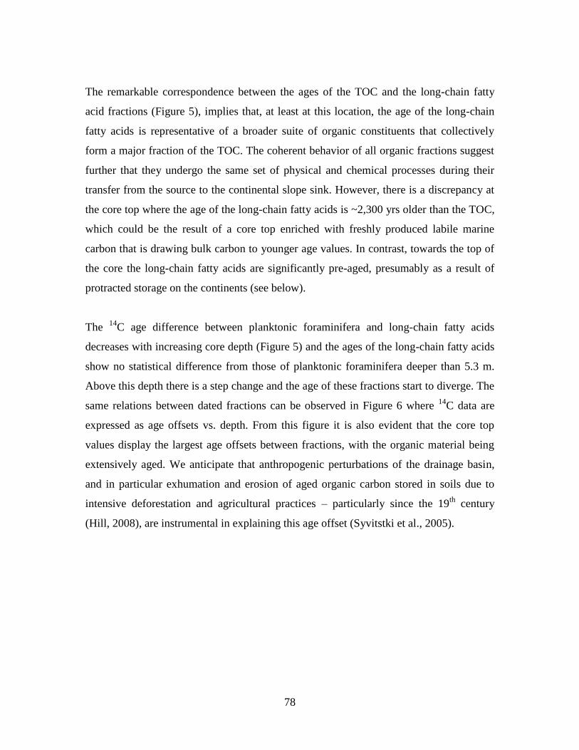
78

The remarkable correspondence between the ages of the TOC and the long-chain fatty

acid fractions (Figure 5), implies that, at least at this location, the age of the long-chain

fatty acids is representative of a broader suite of organic constituents that collectively

form a major fraction of the TOC. The coherent behavior of all organic fractions suggest

further that they undergo the same set of physical and chemical processes during their

transfer from the source to the continental slope sink. However, there is a discrepancy at

the core top where the age of the long-chain fatty acids is ~2,300 yrs older than the TOC,

which could be the result of a core top enriched with freshly produced labile marine

carbon that is drawing bulk carbon to younger age values. In contrast, towards the top of

the core the long-chain fatty acids are significantly pre-aged, presumably as a result of

protracted storage on the continents (see below).

The 14

C age difference between planktonic foraminifera and long-chain fatty acids

decreases with increasing core depth (Figure 5) and the ages of the long-chain fatty acids

show no statistical difference from those of planktonic foraminifera deeper than 5.3 m.

Above this depth there is a step change and the age of these fractions start to diverge. The

same relations between dated fractions can be observed in Figure 6 where 14

C data are

expressed as age offsets vs. depth. From this figure it is also evident that the core top

values display the largest age offsets between fractions, with the organic material being

extensively aged. We anticipate that anthropogenic perturbations of the drainage basin,

and in particular exhumation and erosion of aged organic carbon stored in soils due to

intensive deforestation and agricultural practices – particularly since the 19th

century

(Hill, 2008), are instrumental in explaining this age offset (Syvitstki et al., 2005).

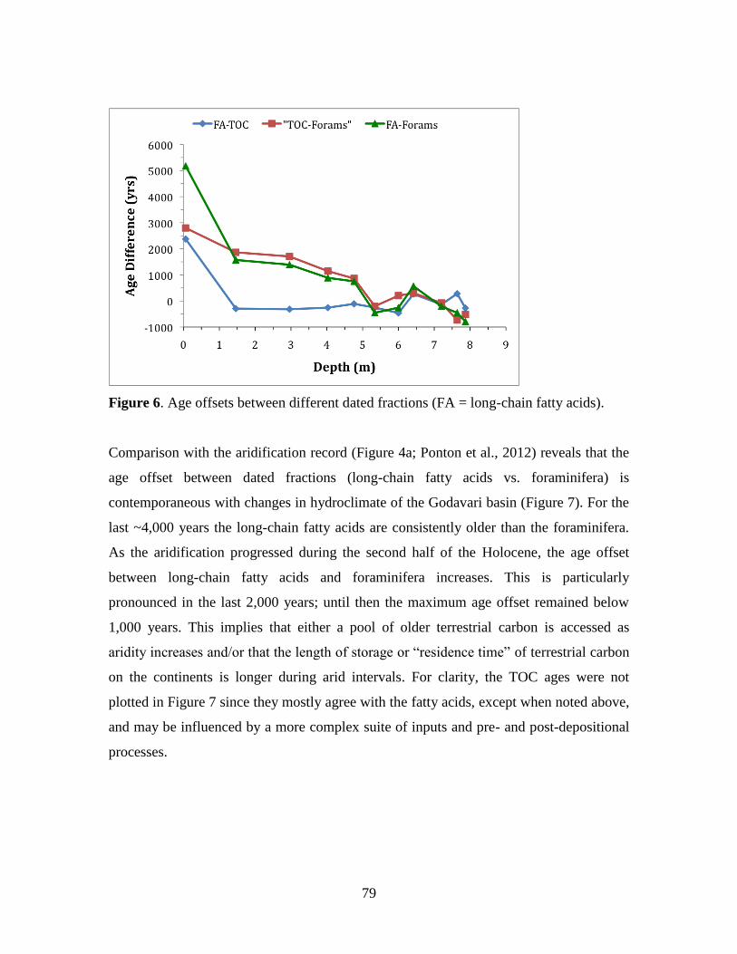
79

Figure 6. Age offsets between different dated fractions (FA = long-chain fatty acids).

Comparison with the aridification record (Figure 4a; Ponton et al., 2012) reveals that the

age offset between dated fractions (long-chain fatty acids vs. foraminifera) is

contemporaneous with changes in hydroclimate of the Godavari basin (Figure 7). For the

last ~4,000 years the long-chain fatty acids are consistently older than the foraminifera.

As the aridification progressed during the second half of the Holocene, the age offset

between long-chain fatty acids and foraminifera increases. This is particularly

pronounced in the last 2,000 years; until then the maximum age offset remained below

1,000 years. This implies that either a pool of older terrestrial carbon is accessed as

aridity increases and/or that the length of storage or “residence time” of terrestrial carbon

on the continents is longer during arid intervals. For clarity, the TOC ages were not

plotted in Figure 7 since they mostly agree with the fatty acids, except when noted above,

and may be influenced by a more complex suite of inputs and pre- and post-depositional

processes.

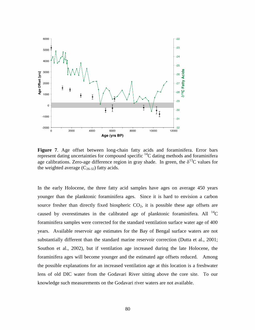
80

Figure 7. Age offset between long-chain fatty acids and foraminifera. Error bars

represent dating uncertainties for compound specific 14

C dating methods and foraminifera

age calibrations. Zero-age difference region in gray shade. In green, the 13

C values for

the weighted average (C26-32) fatty acids.

In the early Holocene, the three fatty acid samples have ages on average 450 years

younger than the planktonic foraminifera ages. Since it is hard to envision a carbon

source fresher than directly fixed biospheric CO2, it is possible these age offsets are

caused by overestimates in the calibrated age of planktonic foraminifera. All 14

C

foraminifera samples were corrected for the standard ventilation surface water age of 400

years. Available reservoir age estimates for the Bay of Bengal surface waters are not

substantially different than the standard marine reservoir correction (Dutta et al., 2001;

Southon et al., 2002), but if ventilation age increased during the late Holocene, the

foraminifera ages will become younger and the estimated age offsets reduced. Among

the possible explanations for an increased ventilation age at this location is a freshwater

lens of old DIC water from the Godavari River sitting above the core site. To our

knowledge such measurements on the Godavari river waters are not available.

81

3.4.1 Storage time vs. availability of aged carbon

As discussed previously, there are several pathways and loops that an organic molecule

originally produced by a vascular plant can take before being buried in marine

continental margin sediments (Fig 1; e.g. Blair et al. 2004). It is also evident that the

terrestrial organic matter buried in marine sediments is a mixture from different carbon

pools that come from different reservoirs (e.g. Drenzek, 2007). The results of this study

reveal an increasing age offset between long-chain fatty acid ages and planktonic

foraminifera ages starting at ~5,000 yr BP. This implies that the age of the long-chain

fatty acids being deposited by the river is increasing. There are two possibilities to

explain this progressive aging: 1) the storage time of OC is increasing in the river basin

or 2) a source, or sources, of older OC have become available and older fatty acids are

mixing with freshly produced ones increasing the resulting ages.

The measured increased age offsets appear to be synchronous with the onset of

aridification in central India, implying a climate-driven forcing of terrestrial carbon

residence times. Recent studies have attempted to describe the effect of climatic changes

in OC turnover times in soils (Schimel, et al., 2011; Yang et al., 2011; Butzer et al.,

2008). These studies show that dry/wet cycles affect the turnover times of carbon

removal or storage and supporting results from previous model simulations suggest rates

of carbon turnover can be much larger in recently disturbed ecosystems than in more

mature (climatically stable) ecosystems (Trumbore, 1997). In the following sections we

incorporate other available data from the same core in order to evaluate different

scenarios that may favor increased storage time or variations in age populations to

explain the observed increase in age offsets.

3.4.1.1 Seasonality

Decreases in monsoon precipitation responsible for the increasing aridity translate to

lower average discharges for the Godavari River and its tributaries as the monsoon is

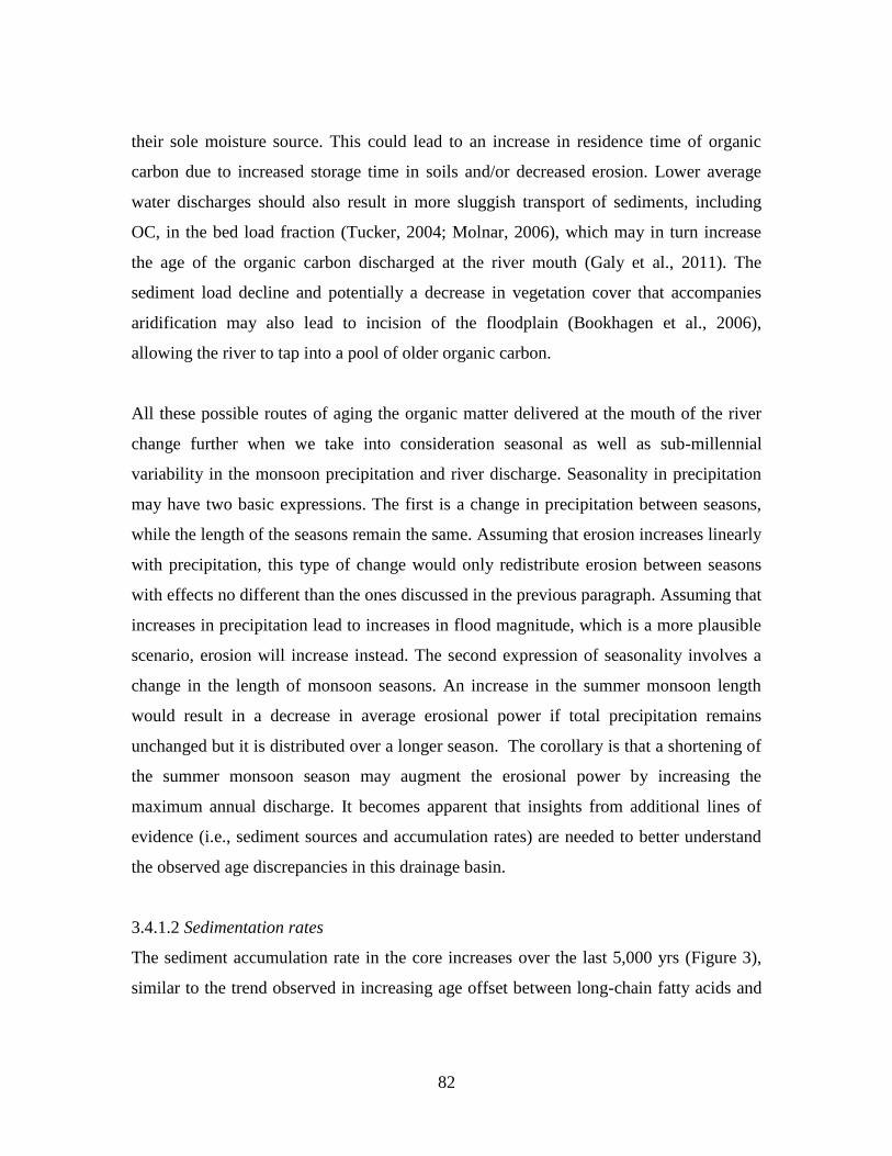
82

their sole moisture source. This could lead to an increase in residence time of organic

carbon due to increased storage time in soils and/or decreased erosion. Lower average

water discharges should also result in more sluggish transport of sediments, including

OC, in the bed load fraction (Tucker, 2004; Molnar, 2006), which may in turn increase

the age of the organic carbon discharged at the river mouth (Galy et al., 2011). The

sediment load decline and potentially a decrease in vegetation cover that accompanies

aridification may also lead to incision of the floodplain (Bookhagen et al., 2006),

allowing the river to tap into a pool of older organic carbon.

All these possible routes of aging the organic matter delivered at the mouth of the river

change further when we take into consideration seasonal as well as sub-millennial

variability in the monsoon precipitation and river discharge. Seasonality in precipitation

may have two basic expressions. The first is a change in precipitation between seasons,

while the length of the seasons remain the same. Assuming that erosion increases linearly

with precipitation, this type of change would only redistribute erosion between seasons

with effects no different than the ones discussed in the previous paragraph. Assuming that

increases in precipitation lead to increases in flood magnitude, which is a more plausible

scenario, erosion will increase instead. The second expression of seasonality involves a

change in the length of monsoon seasons. An increase in the summer monsoon length

would result in a decrease in average erosional power if total precipitation remains

unchanged but it is distributed over a longer season. The corollary is that a shortening of

the summer monsoon season may augment the erosional power by increasing the

maximum annual discharge. It becomes apparent that insights from additional lines of

evidence (i.e., sediment sources and accumulation rates) are needed to better understand

the observed age discrepancies in this drainage basin.

3.4.1.2 Sedimentation rates

The sediment accumulation rate in the core increases over the last 5,000 yrs (Figure 3),

similar to the trend observed in increasing age offset between long-chain fatty acids and

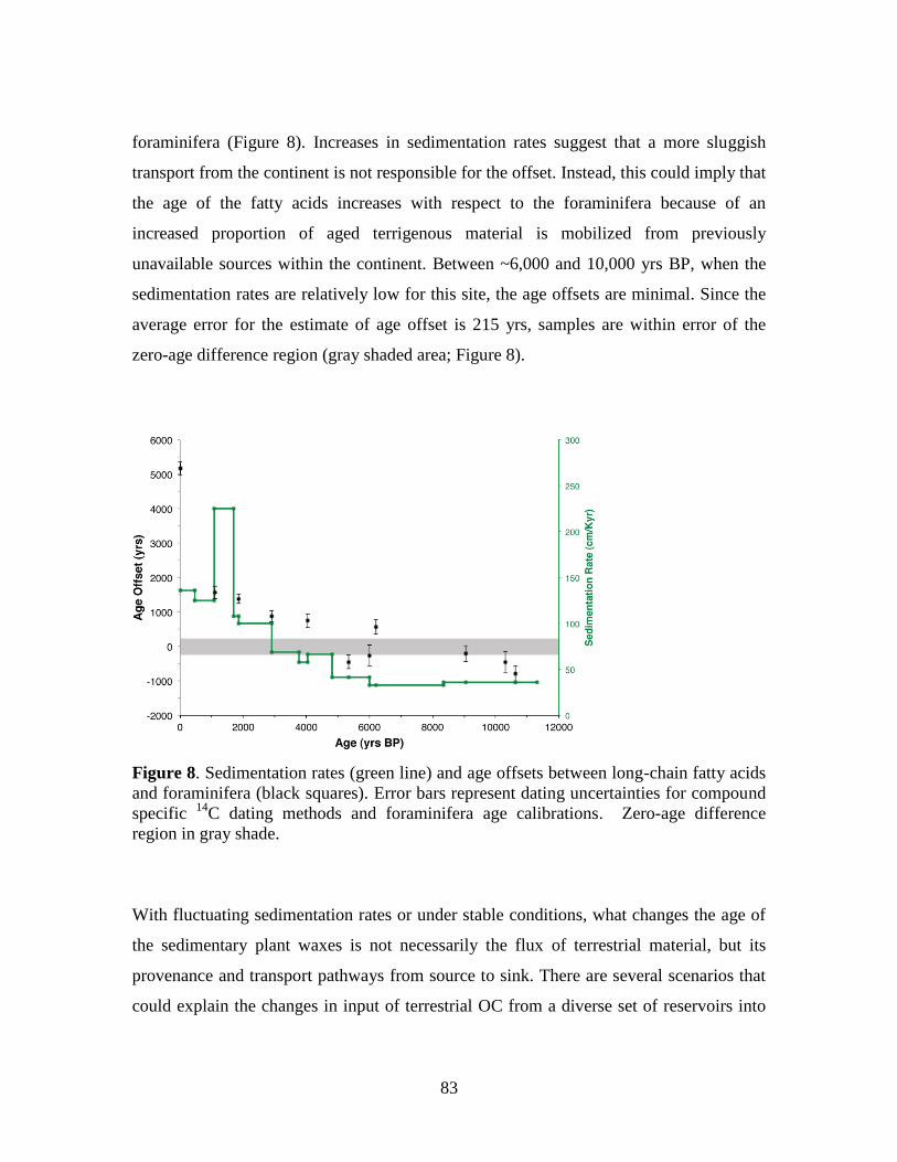
83

foraminifera (Figure 8). Increases in sedimentation rates suggest that a more sluggish

transport from the continent is not responsible for the offset. Instead, this could imply that

the age of the fatty acids increases with respect to the foraminifera because of an

increased proportion of aged terrigenous material is mobilized from previously

unavailable sources within the continent. Between ~6,000 and 10,000 yrs BP, when the

sedimentation rates are relatively low for this site, the age offsets are minimal. Since the

average error for the estimate of age offset is 215 yrs, samples are within error of the

zero-age difference region (gray shaded area; Figure 8).

Figure 8. Sedimentation rates (green line) and age offsets between long-chain fatty acids

and foraminifera (black squares). Error bars represent dating uncertainties for compound

specific 14

C dating methods and foraminifera age calibrations. Zero-age difference

region in gray shade.

With fluctuating sedimentation rates or under stable conditions, what changes the age of

the sedimentary plant waxes is not necessarily the flux of terrestrial material, but its

provenance and transport pathways from source to sink. There are several scenarios that

could explain the changes in input of terrestrial OC from a diverse set of reservoirs into

84

the basin. In this context, it is important to bear in mind that even at the molecular level,

mixed (age) populations of a source-specific biomarker compound are encountered in

sedimentary environment as a consequence of the multiple storage points and transport

routes (see Figure 1). Therefore, the measured 14

C age for a specific biomarker is a

composite of these different populations (e.g., fatty acids from fresh leaf litter vs. from

soils; Drenzek, 2007). Consequently, observed changes in apparent age of long-chain

fatty acids could reflect changes in the overall storage/residence time of these compounds

or changes in the proportions of fresh vs. pre-aged (soil) fractions.

3.4.1.3 Sediment provenance

Sedimentation rates provide evidence of the amount of material being exported by the

river at different times, but do not provide information regarding the provenance of that

sediment within the drainange basin. Evidence on signal provenance was derived from

the sediment’s inorganic fraction using detrital Nd isotopic ratios (L. Giosan, unpublished

data). Very low, negative Nd values are generally found in continental crusts, whereas

positive Nd values are commonly found in mantle derived melts (DePaolo, 1988), such

as those of large igneous provinces. The bedrock in the Godavari drainage basin is

composed of two distinct geological provinces: flood basalts from the Deccan Plateau in

the upper basin and crystalline igneous/metamorphic rocks from the Indian craton in the

lower basin (Murthy et al., 2011; Figure 2). These two geological provinces have very

distinct Nd isotopic signatures: The Deccan basalts have an average Nd of ~ +1 5

while the average craton Nd is ~ -35 8. Sediments preserve the Nd isotopic signal of

the weathered bedrock from which they originated, and Nd isotope analyses on bulk

sediments constitute a robust provenance indicator (e.g., Clift and Blusztajn, 2005; Colin

et al., 1999).

Nd values of bulk sediment samples from core 16A show that there is clearly a stronger

input of Deccan-derived sediments in the last 2,000 yrs, when conditions are driest in the

drainage basin and sedimentation rates are highest (Figure 9). Adopting the average Nd

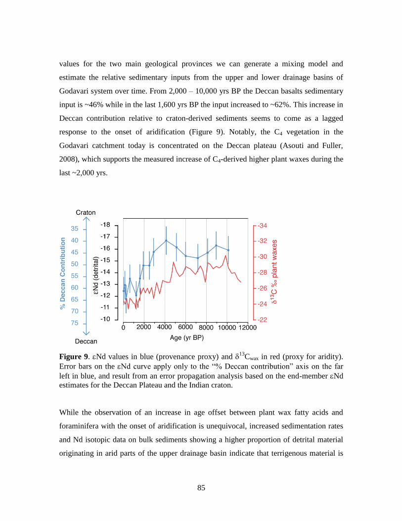
85

values for the two main geological provinces we can generate a mixing model and

estimate the relative sedimentary inputs from the upper and lower drainage basins of

Godavari system over time. From 2,000 – 10,000 yrs BP the Deccan basalts sedimentary

input is ~46% while in the last 1,600 yrs BP the input increased to ~62%. This increase in

Deccan contribution relative to craton-derived sediments seems to come as a lagged

response to the onset of aridification (Figure 9). Notably, the C4 vegetation in the

Godavari catchment today is concentrated on the Deccan plateau (Asouti and Fuller,

2008), which supports the measured increase of C4-derived higher plant waxes during the

last ~2,000 yrs.

Figure 9. Nd values in blue (provenance proxy) and 13

Cwax in red (proxy for aridity).

Error bars on the Nd curve apply only to the “% Deccan contribution” axis on the far

left in blue, and result from an error propagation analysis based on the end-member Nd

estimates for the Deccan Plateau and the Indian craton.

While the observation of an increase in age offset between plant wax fatty acids and

foraminifera with the onset of aridification is unequivocal, increased sedimentation rates

and Nd isotopic data on bulk sediments showing a higher proportion of detrital material

originating in arid parts of the upper drainage basin indicate that terrigenous material is

86

more efficiently transferred and exported through the river drainage basin under drier

conditions. Therefore, it is not clear that an increase in storage times of OC in the

drainage basin produced the increased in age offsets. Instead, re-mobilization of aged

carbon from the arid upper basin may be a more influential factor. Nevertheless,

mobilization of aged carbon from the upper basin, together with the strong C4 signal,

implies that the aged soils must also contain a predominantly C4 vegetation signal. In

other words, the Deccan Plateau must have been C4 dominated for some extended period

of time prior to the inferred aridification. This does not necessarily contradict the

interpretation that vegetation in the entire drainage basin shifts in response to climate, but

rather implies the Deccan Plateau has been a relatively arid region within the basin

through time.

3.4.2. Climate control on organic carbon transport

The scenarios discussed above clearly have different but profound implications in terms

of our understanding of climate-driven impacts on the terrestrial carbon cycle and on

interpretations of terrestrial proxy records embedded in continental margin sediments.

During the early Holocene the OC is transported efficiently through the drainage basin at

a time when precipitation and therefore water discharge is relatively high. In the mid

Holocene the age offsets between planktonic foraminifera and long-chain fatty acids start

to increase at the same time that the climate starts turning arid in central India. Changes

in fluxes from different reservoirs within the system cannot be precisely constrained, but

it becomes apparent that increased residence time of terrestrial carbon within the system

can have the same effects. During the last 2,000 yrs the measured age offsets are the

largest during a time when the climate turned arid, the monsoon entered in a drought-

prone regime – potentially causing a decrease in the size of the plant biomass reservoir

(fresh OC flux) and an increase in erosion rates (aged OC flux) - and when the impacts of

human intervention on the landscape are most acutely felt through mobilization and loss

of soil OC. These conditions can occur simultaneously exacerbating the increase in

storage times of OC due to aridity. While further work is clearly needed to resolve

87

underlying processes, the present study clearly demonstrates that changing climate in

monsoonal regions markedly affects the nature and dynamics of terrestrial carbon transfer

to the marine environment. Variations in either storage time or the proportions of fresh

versus aged carbon both indicate climate-driven controls on the overall flow of terrestrial

carbon through drainage systems.

3.4.3 Implications for increased carbon storage time

If the reason for the observed age offsets between long-chain fatty acids and planktonic

foraminifera is an increase in storage time, this will have implications for the terrestrial

carbon cycle and for paleoclimate reconstructions. An increased storage time implies that

under arid conditions the system is more sluggish and it takes longer to transport carbon

from the continents to the oceans, prolonging the stay in the intermediate carbon

reservoirs on land. For paleoclimate reconstructions the increasing age of long-chain fatty

acids poses a problem when interpreting the organic proxy data using a chronology based

on marine sedimentary components (e.g. planktonic foraminifera). Figure 10 illustrates

this problem by presenting the 13

C record of the weighted average of long-chain fatty

acids (nC26-32) using two different chronologies based on planktonic foraminifer and plant

wax fatty acid 14

C ages. In this context, reconstructing fatty acid records using an

independent age model based on fatty acid 14

C measurements would only be valid when

dealing with variations in storage time, and would be in appropriate for multimode age

populations. Given that there is compelling evidence for the presence of terrestrial

carbon with mixed age populations in river and continental margin sediments (Drenzek,

2007; Blair 2010, Galy & Eglinton, 2011) it may prove difficult to reconcile chronologies

for terrestrial and marine proxy records in marine sedimentary sequences. It is also

important to note that this issue my be pertinent to other terrestrial proxies recorded in

river-proximal marine sediments. For example, pollen, titanium, 15

N, and even Nd

isotope records may all exhibit varying lags and unique transmission times.

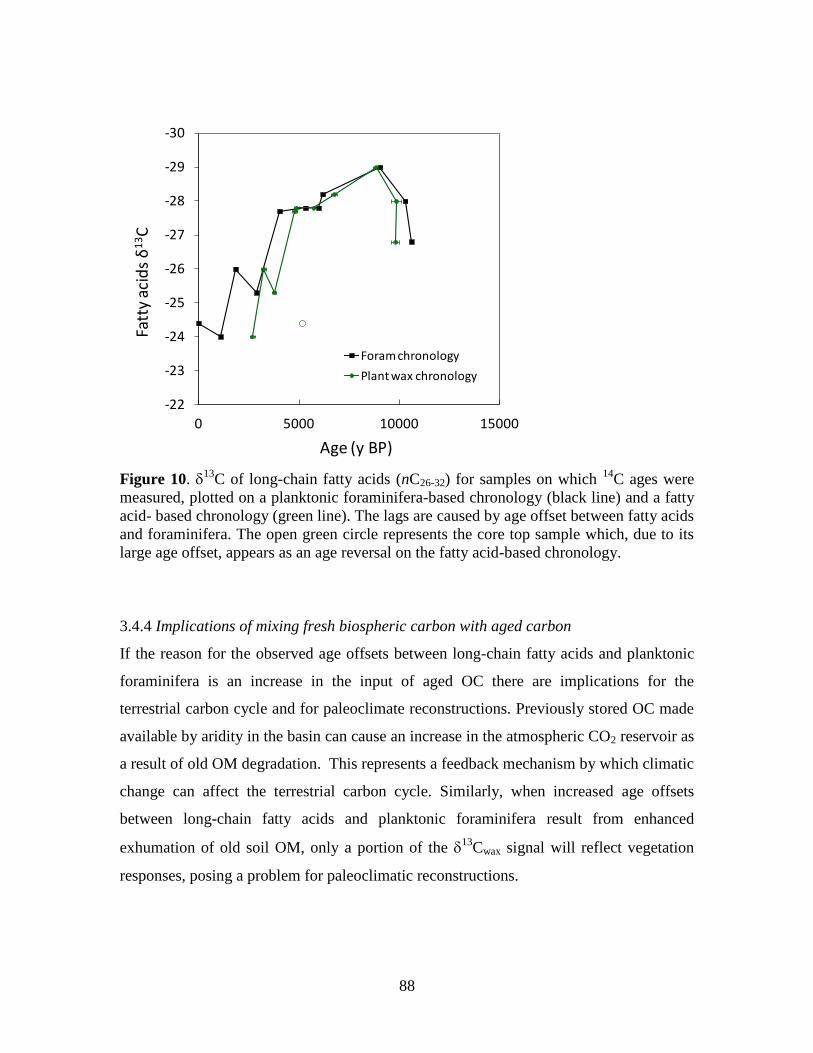
88

-30

-29

-28

-27

-26

-25

-24

-23

-22

0 5000 10000 15000

Fatt

y ac

ids δ

13C

Age (y BP)

Foram chronology

Plant wax chronology

Figure 10. 13

C of long-chain fatty acids (nC26-32) for samples on which 14

C ages were

measured, plotted on a planktonic foraminifera-based chronology (black line) and a fatty

acid- based chronology (green line). The lags are caused by age offset between fatty acids

and foraminifera. The open green circle represents the core top sample which, due to its

large age offset, appears as an age reversal on the fatty acid-based chronology.

3.4.4 Implications of mixing fresh biospheric carbon with aged carbon

If the reason for the observed age offsets between long-chain fatty acids and planktonic

foraminifera is an increase in the input of aged OC there are implications for the

terrestrial carbon cycle and for paleoclimate reconstructions. Previously stored OC made

available by aridity in the basin can cause an increase in the atmospheric CO2 reservoir as

a result of old OM degradation. This represents a feedback mechanism by which climatic

change can affect the terrestrial carbon cycle. Similarly, when increased age offsets

between long-chain fatty acids and planktonic foraminifera result from enhanced

exhumation of old soil OM, only a portion of the 13

Cwax signal will reflect vegetation

responses, posing a problem for paleoclimatic reconstructions.

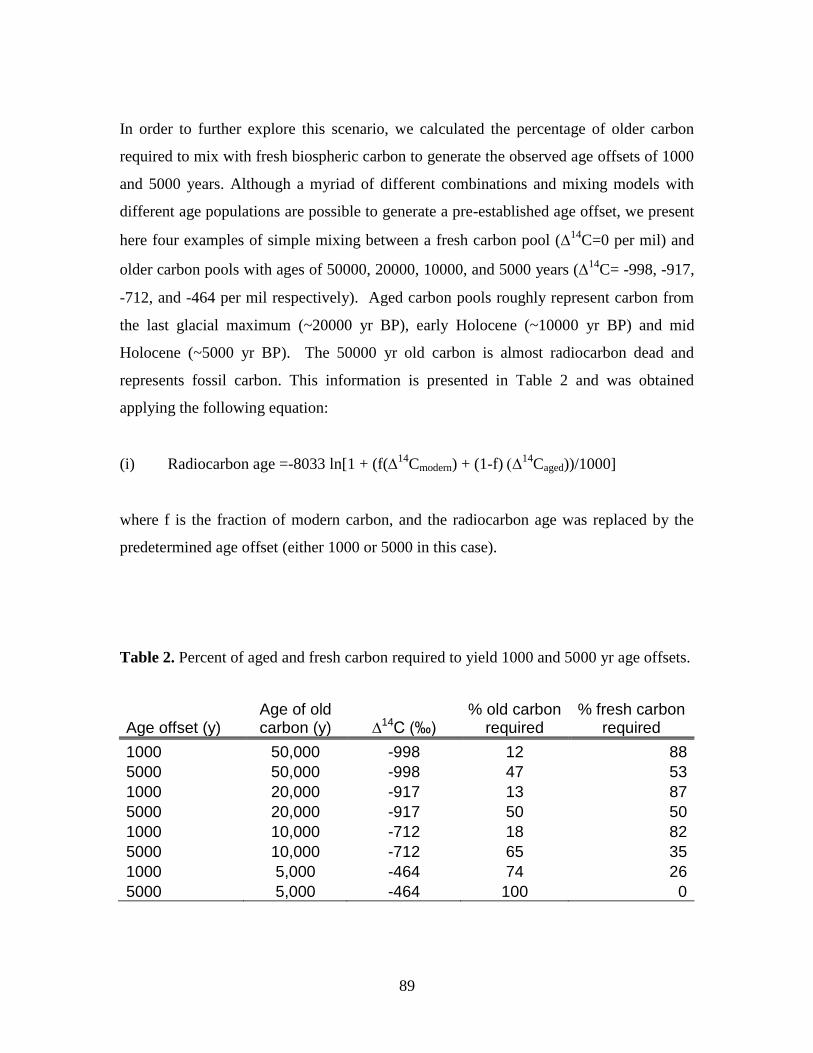
89

In order to further explore this scenario, we calculated the percentage of older carbon

required to mix with fresh biospheric carbon to generate the observed age offsets of 1000

and 5000 years. Although a myriad of different combinations and mixing models with

different age populations are possible to generate a pre-established age offset, we present

here four examples of simple mixing between a fresh carbon pool (14

C=0 per mil) and

older carbon pools with ages of 50000, 20000, 10000, and 5000 years (14

C= -998, -917,

-712, and -464 per mil respectively). Aged carbon pools roughly represent carbon from

the last glacial maximum (~20000 yr BP), early Holocene (~10000 yr BP) and mid

Holocene (~5000 yr BP). The 50000 yr old carbon is almost radiocarbon dead and

represents fossil carbon. This information is presented in Table 2 and was obtained

applying the following equation:

(i) Radiocarbon age =-8033 ln[1 + (f(14

Cmodern) + (1-f)14

Caged))/1000]

where f is the fraction of modern carbon, and the radiocarbon age was replaced by the

predetermined age offset (either 1000 or 5000 in this case).

Table 2. Percent of aged and fresh carbon required to yield 1000 and 5000 yr age offsets.

Age offset (y) Age of old carbon (y) ∆14C (‰)

% old carbon required

% fresh carbon required

1000 50,000 -998 12 88

5000 50,000 -998 47 53

1000 20,000 -917 13 87

5000 20,000 -917 50 50

1000 10,000 -712 18 82

5000 10,000 -712 65 35

1000 5,000 -464 74 26

5000 5,000 -464 100 0

90

The selected ages for the old carbon pools represent possible carbon mixing scenarios in

this basin, and give an estimate of how much carbon of a specific age is needed to

generate the observed age offsets. Mixing with pools of 10000 and 5000 yr old carbon

represent the likely scenarios that early and mid Holocene soils are being eroded during

the late Holocene. To increase the age of sedimentary long-chain fatty acids by 1000

years with respect to the planktonic foraminifera, 74% of the carbon must be from the

5000 yr pre-aged pool, which implies significant erosion of relatively young soils across

the drainage basin. On the other hand, only 18% of the total carbon must come from a

10000 yr old pool to create the same age offset suggesting that deeper erosion of soils

would be more effective in generating age offsets. Similarly, to generate the same 1000

years offset, 13% of the carbon from the 20000 yr old pool is needed, and 50% of this last

glacial carbon is required to generate a 5000 yr offset. Thus, the erosional style within

the drainage basin whether uniformly surficial or deeper more localized in e.g., gullies or

fluvial incision would be important to assess via additional proxies to understand

processes of organic carbon recycling and transfer. Our mixing estimates show that

fluctuations in the availability of aged carbon pools caused by climatic variability can

change the residence times of organic carbon in the drainage system and therefore have

implication for the terrestrial carbon cycle. Furthermore, mixing with aged carbon also

affects paleoclimate reconstructions. For example given than during the last glacial

maximum conditions were much drier in the Indian subcontinent with respect to present

(e.g. Galy et al., 2008; Ponton et al., 2012) soils from this age have a strong C4 biomass

isotopic signature. If mixing with 50% carbon from the last glacial period causes the

observed 5000 yr offset at the core top, the measured 13

C values should be corrected for

the strong pre-aged carbon input prior to interpretation.

Mixing with radiocarbon dead or fossil carbon should also be considered given its

common occurrence in river basins and soils (e.g. Drenzek, 2007; 2009; Hedges and

Oades, 1997; Galy et al., 2008; Gustafsson et al., 2011). Table 2 also provides

information on the percent of 50000 yr old carbon required to yield the observed age

91

offsets. While only 12% percent of 50000 yr old carbon is required to create a 1000 yr

age offset by mixing with modern carbon, 47% is required to generate a 5000 yr offset.

Age-depth soil profiles within the basin or soil sedimentation rates will be needed to

determine the age and proportion of older carbon pools within the erodible reservoirs in

the Godavari river catchment and to test if the estimated values are reasonable.

So far we have examined mixing of modern biospheric carbon with aged carbon pools

representing specific geologic stages. Now we examine mixing of different proportions of

fossil carbon (14

C =-999 per mil) with carbon pools of all age ranges (14

C between 0 –

-999). Results are reported in Table 3 and show what the age offsets of samples of

different ages will be when mixed with 10, 20, 50 and 70% of dead carbon. Equation (i)

was used to calculate the different sample ages, and age offsets represent the difference

between the age of the sample with mixed dead carbon and what the age of a pure sample

(0% dead carbon) will be.

Our mixing scenarios show that a mixture with the same proportion of dead carbon

creates the same offset regardless of the real sample age and that increasing the amount

of dead carbon in the mixture rapidly increases the age offset. A mixture with 20% dead

carbon produces an age offset of ~1790 years while a mixture with 50% dead carbon

produces an age offset of ~5560 years. Assuming that dead carbon is widely available,

these calculations show the potential of relatively small amounts of very old carbon to

have strong impacts on the residence time of carbon in the system.

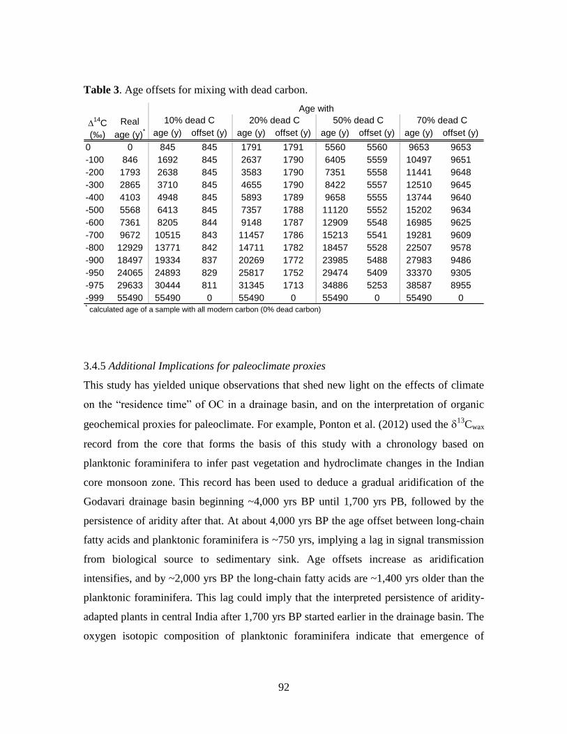
92

Table 3. Age offsets for mixing with dead carbon.

age (y) offset (y) age (y) offset (y) age (y) offset (y) age (y) offset (y)

0 0 845 845 1791 1791 5560 5560 9653 9653

-100 846 1692 845 2637 1790 6405 5559 10497 9651

-200 1793 2638 845 3583 1790 7351 5558 11441 9648

-300 2865 3710 845 4655 1790 8422 5557 12510 9645

-400 4103 4948 845 5893 1789 9658 5555 13744 9640

-500 5568 6413 845 7357 1788 11120 5552 15202 9634

-600 7361 8205 844 9148 1787 12909 5548 16985 9625

-700 9672 10515 843 11457 1786 15213 5541 19281 9609

-800 12929 13771 842 14711 1782 18457 5528 22507 9578

-900 18497 19334 837 20269 1772 23985 5488 27983 9486

-950 24065 24893 829 25817 1752 29474 5409 33370 9305

-975 29633 30444 811 31345 1713 34886 5253 38587 8955

-999 55490 55490 0 55490 0 55490 0 55490 0

Real

age (y)*

* calculated age of a sample with all modern carbon (0% dead carbon)

∆14

C

(‰)

10% dead C 20% dead C 50% dead C 70% dead C

Age with

3.4.5 Additional Implications for paleoclimate proxies

This study has yielded unique observations that shed new light on the effects of climate

on the “residence time” of OC in a drainage basin, and on the interpretation of organic

geochemical proxies for paleoclimate. For example, Ponton et al. (2012) used the 13

Cwax

record from the core that forms the basis of this study with a chronology based on

planktonic foraminifera to infer past vegetation and hydroclimate changes in the Indian

core monsoon zone. This record has been used to deduce a gradual aridification of the

Godavari drainage basin beginning ~4,000 yrs BP until 1,700 yrs PB, followed by the

persistence of aridity after that. At about 4,000 yrs BP the age offset between long-chain

fatty acids and planktonic foraminifera is ~750 yrs, implying a lag in signal transmission

from biological source to sedimentary sink. Age offsets increase as aridification

intensifies, and by ~2,000 yrs BP the long-chain fatty acids are ~1,400 yrs older than the

planktonic foraminifera. This lag could imply that the interpreted persistence of aridity-

adapted plants in central India after 1,700 yrs BP started earlier in the drainage basin. The

oxygen isotopic composition of planktonic foraminifera indicate that emergence of

93

drought-prone conditions started as early as ~3000 years BP, but their frequency may not

be captured at the current resolution of that proxy.

The observed protracted storage of terrestrial carbon in the drainage basin described

above also suggests that the 13

Cwax may be a relatively blunt or sluggish proxy for

reconstructing short-lived and or less intense changes in hydroclimate under certain

climatic conditions. Although frequently employed as an integrative proxy to reconstruct

drainage basin-wide paleoclimate, changes in the source area (provenance) and transport

times within the basin can affect the results to show responses biased by changes only

occurring in sub-sectors of the drainage basin.

3.5 Conclusions

Radiocarbon measurements of plant wax biomarkers (long-chain fatty acids) compared to

planktonic foraminifera show an increase in age offset from mid to late Holocene. When

coupled with 13

Cwax and bulk sediment Nddetrital measurements, this suggests that

increased aridity may have either slowed carbon cycling and/or transport rates, or altered

the proportions and/or fluxes of fresh versus pre-aged biospheric carbon, resulting in an

apparent increase of terrestrial storage times of vascular plant carbon. Either scenario

implies a direct link between climate dynamics and carbon cycling within this river

drainage basin.

During the early Holocene (5,000 – 11,000 yrs BP), the residence time of terrestrial

carbon within the system is short, implying near-instantaneous transfer (within dating

uncertainties) of terrestrial biospheric carbon from source to sink. During the mid

Holocene (5,000 – 2,000 yrs BP), increased latency of terrestrial carbon within the

system appears to accompany the onset of aridification in central India. During the late

Holocene (2,000 – 0 yrs BP), the climate turned arid, resulting in a shift in vegetation

type towards a preponderance of C4 biomass. The increasing age offsets during this

period may stem from slower carbon turnover within soils coupled with enhanced

94

exhumation of old soil OM as a consequence of greater erosion under more arid

conditions and anthropogenic pertubation.

Irrespective of the underlying mechanisms and processes, the marked variations in

storage time and/or proportions of fresh versus aged biospheric carbon under

progressively more arid conditions imply there is direct a climatic effect on the flow of

OC through the drainage basin. This poses problems for paleoclimate reconstructions

using long-chain fatty acids and possibly other terrestrial proxies – both organic and

inorganic – as well. Climate-driven modulation of terrestrial biomarker transfer times

through the river drainage basin and to the ocean may cause variable offsets of the

associated proxy signal when interpreted using a chronology based on marine

sedimentary components. Furthermore, when there is enhanced exhumation of old soil

OM, only a small fraction of the long-chain fatty acid 13

C signal will actually reflect

instantaneous vegetation responses within the drainage basin. Clearly, many aspects of

the carbon cycle remain poorly understood, and important questions concerning the

transfer of organic matter from continents to oceans remain unresolved.

References

Asouti, E. and D.Q. Fuller. 2008. Trees and Woodlands in South India, Archaeological

Perspectives. Walnut Creek (California): Left Coast Press.

Blair, N. E., K. Fournillier, E. L. Leithold, and L. B. Childress. 2010. Resolving organic

carbon of differing diagenetic/catagenetic states in riverine and marine sediments.

Geochimica Et Cosmochimica Acta 74 (12):A95-A95.

Blair, N. E., E. L. Leithold, and R. C. Aller. 2004. From bedrock to burial: the evolution

of particulate organic carbon across coupled watershed-continental margin systems.

Marine Chemistry 92 (1-4):141-156.

Bookhagen, B., D. Fleitmann, K. Nishiizurrli, M. R. Strecker, and R. C. Thiede. 2006.

Holocene monsoonal dynamics and fluvial terrace formation in the northwest Himalaya,

India. Geology 34 (7):601-604.

95

Butzer, K. W., J. T. Abbott, C. D. Frederick, P. H. Lehman, C. E. Cordova, and J. F.

Oswald. 2008. Soil-geomorphology and "wet" cycles in the Holocene record of North-

Central Mexico. Geomorphology 101 (1-2):237-277.

Clift, P. D., and J. Blusztajn. 2005. Reorganization of the western Himalayan river

system after five million years ago. Nature 438 (7070):1001-1003.

Colin, C., L. Turpin, J. Bertaux, A. Desprairies, and C. Kissel. 1999. Erosional history of

the Himalayan and Burman ranges during the last two glacial-interglacial cycles. Earth

and Planetary Science Letters 171 (4):647-660.

DePaolo, D.J., 1988. Neodymium Isotope Geochemistry, An Introduction. Springer-

Verlag, Berlin, 187 p.

Drenzek N. J. 2007. The temporal dynamics of terrestrial organic matter transfer to the

oceans: initial assessment and application. Ph. D. thesis, MIT/WHOI Joint Program in

Oceanography/Applied Ocean Science and Engineering.

Drenzek, N. J., K. A. Hughen, D. B. Montlucon, J. R. Southon, G. M. dos Santos, E. R.

M. Druffel, L. Giosan, and T. I. Eglinton. 2009. A new look at old carbon in active

margin sediments. Geology 37 (3):239-242.

Dutta, K., R. Bhushan, and B. L. K. Somayajulu. 2001. Delta R correction values for the

northern Indian Ocean. Radiocarbon 43 (2A):483-488.

Fisher, E., F. Oldfield, R. Wake, J. Boyle, P. Appleby, and G. A. Wolff. 2003. Molecular

marker records of land use change. Organic Geochemistry 34 (1):105-119.

Galy, V., Eglinton, T.I. 2011. Protracted storage of biospheric carbon in the Ganges-

Brahmaputra basin. Nature Geoscience 4:843-847.

Galy, V., C. France-Lanord, O. Beyssac, B. Lartiges, and M. Rhaman. 2011. Organic

Carbon Cycling During Himalayan Erosion: Processes, Fluxes and Consequences for the

Global Carbon Cycle. In Climate Change and Food Security in South Asia, edited by R.

Lal, M. V. K. Sivakumar, S. M. A. M. A. Faiz, A. H. M. H. M. M. Mustafizur Rahman

and K. R. R. Islam: Springer Netherlands.

Galy, V., C. France-Lanord, and B. Lartiges. 2008. Loading and fate of particulate

organic carbon from the Himalaya to the Ganga-Brahmaputra delta. Geochimica Et

Cosmochimica Acta 72 (7):1767-1787.

96

Gustafsson, O., B. E. van Dongen, J. E. Vonk, O. V. Dudarev, and I. P. Semiletov. 2011.

Widespread release of old carbon across the Siberian Arctic echoed by its large rivers.

Biogeosciences 8 (6):1737-1743.

Hedges, J. I., and J. M. Oades. 1997. Comparative organic geochemistries of soils and

marine sediments. Organic Geochemistry 27 (7-8):319-361.

Hill, C.V. 2008. South Asia – An environmental history. Santa Barbara (California):

ABC-Clio Inc.

Kusch, S., J. Rethemeyer, E. Schefuss, and G. Mollenhauer. 2010a. Controls on the age

of vascular plant biomarkers in Black Sea sediments. Geochimica et Cosmochimica Acta

74 (24):7031-7047.

Kusch, S., T. I. Eglinton, A. C. Mix, and G. Mollenhauer. 2010b. Timescales of lateral

sediment transport in the Panama Basin as revealed by radiocarbon ages of alkenones,

total organic carbon and foraminifera. Earth and Planetary Science Letters 290 (3-4):340-

350.

Mollenhauer, G., and T. I. Eglinton. 2007. Diagenetic and sedimentological controls on

the composition of organic matter preserved in California Borderland Basin sediments.

Limnology and Oceanography 52 (2):558-576.

Molnar, P., R. S. Anderson, G. Kier, and J. Rose. 2006. Relationships among probability

distributions of stream discharges in floods, climate, bed load transport, and river

incision. Journal of Geophysical Research-Earth Surface 111 (F2).

Murthy, M. V. K., P. K. Padhy, and D. N. Prasad. 2011. Mesozoic hydrogeologic systems

and hydrocarbon habitat, Mandapeta-Endamuru area, Krishna Godavari Basin, India.

AAPG Bulletin 95 (1):147-167.

Ohkouchi, N., T. I. Eglinton, L. D. Keigwin, and J. M. Hayes. 2002. Spatial and temporal

offsets between proxy records in a sediment drift. Science 298 (5596):1224-1227.

Ponton, C., L. Giosan, T. I. Eglinton, D. Q. Fuller, J. E. Johnson, P. Kumar, and T. S.

Collett. 2012. Holocene aridification of India. Geophysical Research Letters (39)

L03704, doi:10.1029/2011GL050722.

Quideau, S. A., O. A. Chadwick, A. Benesi, R. C. Graham, and M. A. Anderson. 2001. A

direct link between forest vegetation type and soil organic matter composition. Geoderma

104 (1-2):41-60.

Ruff, M., L. Wacker, H. W. Gaggeler, M. Suter, H. A. Synal, and S. Szidat. 2007. A gas

ion source for radiocarbon measurements at 200 kV. Radiocarbon 49 (2):307-314.

97

Santos, G. M., J. R. Southon, N. J. Drenzek, L. A. Ziolkowski, E. Druffel, X. M. Xu, D.

C. Zhang, S. Trumbore, T. I. Eglinton, and K. A. Hughen. 2010. Blank assessment for

ultra-small radiocarbon samples: chemical extraction and separation versus AMS.

Radiocarbon 52 (3):1322-1335.

Schimel, J. P., J. A. M. Wetterstedt, P. A. Holden, and S. E. Trumbore. 2011.

Drying/rewetting cycles mobilize old C from deep soils from a California annual

grassland. Soil Biology & Biochemistry 43 (5):1101-1103.

Southon, J., M. Kashgarian, M. Fontugne, B. Metivier, and W. W. S. Yim. 2002. Marine

reservoir corrections for the Indian Ocean and southeast Asia. Radiocarbon 44 (1):167-

180.

Stuiver, M., and H. A. Polach. 1977. Reporting of C-14 data - Discussion. Radiocarbon

19 (3):355-363.

Stuiver, M., and H. G. Ostlund. 1983. GEOSECS Indian-ocean and Mediterranean

radiocarbon. Radiocarbon 25 (1):1-29.

Stuiver, M., G. W. Pearson, and T. Braziunas. 1986. Radiocarbon age calibration of

marine samples back to 9000 cal yr bp. Radiocarbon 28 (2B):980-1021.

Syvitski, J. P. M., C. J. Vorosmarty, A. J. Kettner, and P. Green. 2005. Impact of humans

on the flux of terrestrial sediment to the global coastal ocean. Science 308 (5720):376-

380.

Trumbore, S. E. 1997. Potential responses of soil organic carbon to global environmental

change. Proceedings of the National Academy of Sciences of the United States of

America 94 (16):8284-8291.

Tucker, G. E. 2004. Drainage basin sensitivity to tectonic and climatic forcing:

Implications of a stochastic model for the role of entrainment and erosion thresholds.

Earth Surface Processes and Landforms 29 (2):185-205.

Wang, Y., R. Amundson, and S. Trumbore. 1999. The impact of land use change on C

turnover in soils. Global Biogeochemical Cycles 13 (1):47-57.

Yang, H., Y. Yuan, Q. Zhang, J. Tang, Y. Liu, and X. Chen. 2011. Changes in soil

organic carbon, total nitrogen, and abundance of arbuscular mycorrhizal fungi along a

large-scale aridity gradient. Catena 87 (1):70-77.

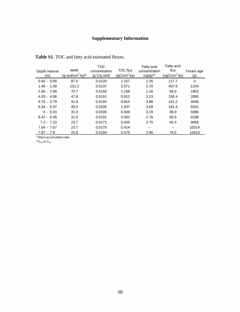
98

Supplementary Information

Table S1. TOC and fatty acid estimated fluxes.

MAR

(g sed/cm2∙ky)*

TOC

concentration

(g C/g sed)

TOC flux

(gC/cm2∙ky)

Fatty acid

concentration

(ug/g)**

Fatty acid

flux

(ugC/cm2∙ky)

Foram age

(y)

0.06 - 0.09 87.0 0.0133 1.157 1.35 117.7 0

1.46 - 1.49 151.2 0.0137 2.071 2.70 407.8 1104

2.96 - 2.99 70.7 0.0169 1.198 1.26 88.9 1852

4.03 - 4.06 47.8 0.0191 0.912 2.23 106.4 2895

4.76 - 4.79 41.8 0.0194 0.810 3.86 161.2 4046

5.34 - 5.37 49.2 0.0205 1.007 3.69 181.4 5331

6 - 6.03 31.0 0.0196 0.608 3.19 98.9 5996

6.42 - 6.45 31.0 0.0191 0.592 2.76 85.6 6198

7.2 - 7.23 23.7 0.0171 0.405 2.75 65.3 9056

7.64 - 7.67 23.7 0.0175 0.414 -- -- 10314

7.87 - 7.9 25.8 0.0184 0.475 2.96 76.5 10619

Depth interval

(m)

* Mass accumulation rate

**C26 to C32

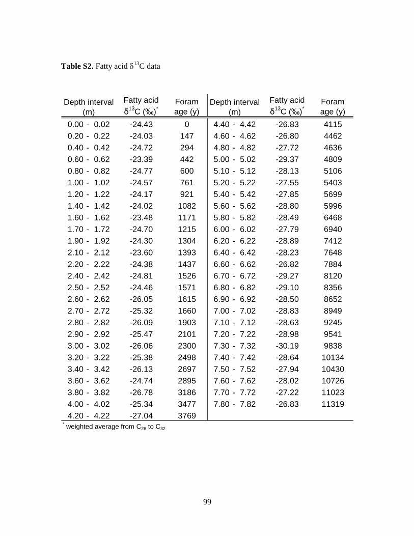
99

Table S2. Fatty acid 13

C data

Fatty acid

δ13

C (‰)*

Foram

age (y)

Fatty acid

δ13

C (‰)*

Foram

age (y)

0.00 - 0.02 -24.43 0 4.40 - 4.42 -26.83 4115

0.20 - 0.22 -24.03 147 4.60 - 4.62 -26.80 4462

0.40 - 0.42 -24.72 294 4.80 - 4.82 -27.72 4636

0.60 - 0.62 -23.39 442 5.00 - 5.02 -29.37 4809

0.80 - 0.82 -24.77 600 5.10 - 5.12 -28.13 5106

1.00 - 1.02 -24.57 761 5.20 - 5.22 -27.55 5403

1.20 - 1.22 -24.17 921 5.40 - 5.42 -27.85 5699

1.40 - 1.42 -24.02 1082 5.60 - 5.62 -28.80 5996

1.60 - 1.62 -23.48 1171 5.80 - 5.82 -28.49 6468

1.70 - 1.72 -24.70 1215 6.00 - 6.02 -27.79 6940

1.90 - 1.92 -24.30 1304 6.20 - 6.22 -28.89 7412

2.10 - 2.12 -23.60 1393 6.40 - 6.42 -28.23 7648

2.20 - 2.22 -24.38 1437 6.60 - 6.62 -26.82 7884

2.40 - 2.42 -24.81 1526 6.70 - 6.72 -29.27 8120

2.50 - 2.52 -24.46 1571 6.80 - 6.82 -29.10 8356

2.60 - 2.62 -26.05 1615 6.90 - 6.92 -28.50 8652

2.70 - 2.72 -25.32 1660 7.00 - 7.02 -28.83 8949

2.80 - 2.82 -26.09 1903 7.10 - 7.12 -28.63 9245

2.90 - 2.92 -25.47 2101 7.20 - 7.22 -28.98 9541

3.00 - 3.02 -26.06 2300 7.30 - 7.32 -30.19 9838

3.20 - 3.22 -25.38 2498 7.40 - 7.42 -28.64 10134

3.40 - 3.42 -26.13 2697 7.50 - 7.52 -27.94 10430

3.60 - 3.62 -24.74 2895 7.60 - 7.62 -28.02 10726

3.80 - 3.82 -26.78 3186 7.70 - 7.72 -27.22 11023

4.00 - 4.02 -25.34 3477 7.80 - 7.82 -26.83 11319

4.20 - 4.22 -27.04 3769

Depth interval

(m)

* weighted average from C26 to C32

Depth interval

(m)

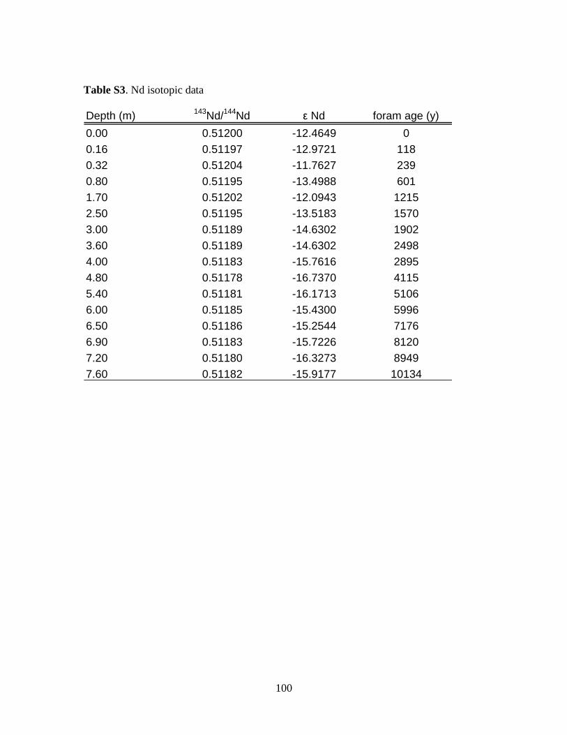
100

Table S3. Nd isotopic data

Depth (m)143

Nd/144

Nd ε Nd foram age (y)

0.00 0.51200 -12.4649 0

0.16 0.51197 -12.9721 118

0.32 0.51204 -11.7627 239

0.80 0.51195 -13.4988 601

1.70 0.51202 -12.0943 1215

2.50 0.51195 -13.5183 1570

3.00 0.51189 -14.6302 1902

3.60 0.51189 -14.6302 2498

4.00 0.51183 -15.7616 2895

4.80 0.51178 -16.7370 4115

5.40 0.51181 -16.1713 5106

6.00 0.51185 -15.4300 5996

6.50 0.51186 -15.2544 7176

6.90 0.51183 -15.7226 8120

7.20 0.51180 -16.3273 8949

7.60 0.51182 -15.9177 10134

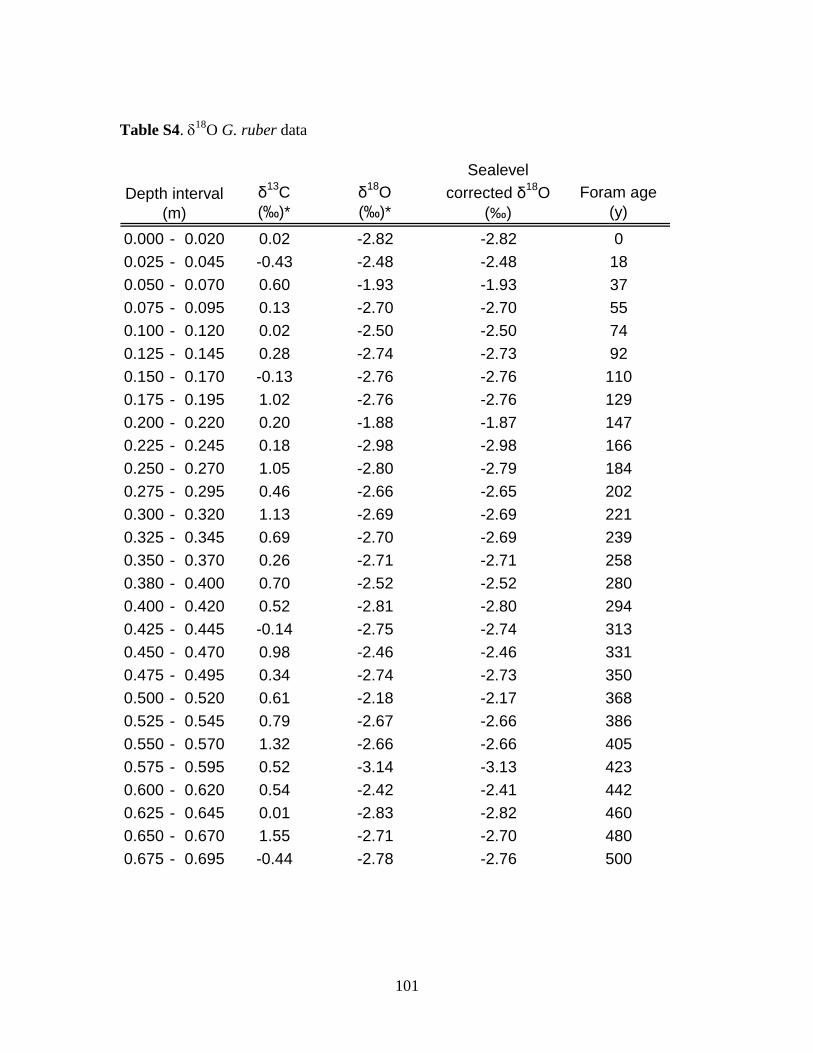
101

Table S4. 18

O G. ruber data

δ13

C

(‰)*

δ18

O

(‰)*

Sealevel

corrected δ18

O

(‰)

Foram age

(y)

0.000 - 0.020 0.02 -2.82 -2.82 0

0.025 - 0.045 -0.43 -2.48 -2.48 18

0.050 - 0.070 0.60 -1.93 -1.93 37

0.075 - 0.095 0.13 -2.70 -2.70 55

0.100 - 0.120 0.02 -2.50 -2.50 74

0.125 - 0.145 0.28 -2.74 -2.73 92

0.150 - 0.170 -0.13 -2.76 -2.76 110

0.175 - 0.195 1.02 -2.76 -2.76 129

0.200 - 0.220 0.20 -1.88 -1.87 147

0.225 - 0.245 0.18 -2.98 -2.98 166

0.250 - 0.270 1.05 -2.80 -2.79 184

0.275 - 0.295 0.46 -2.66 -2.65 202

0.300 - 0.320 1.13 -2.69 -2.69 221

0.325 - 0.345 0.69 -2.70 -2.69 239

0.350 - 0.370 0.26 -2.71 -2.71 258

0.380 - 0.400 0.70 -2.52 -2.52 280

0.400 - 0.420 0.52 -2.81 -2.80 294

0.425 - 0.445 -0.14 -2.75 -2.74 313

0.450 - 0.470 0.98 -2.46 -2.46 331

0.475 - 0.495 0.34 -2.74 -2.73 350

0.500 - 0.520 0.61 -2.18 -2.17 368

0.525 - 0.545 0.79 -2.67 -2.66 386

0.550 - 0.570 1.32 -2.66 -2.66 405

0.575 - 0.595 0.52 -3.14 -3.13 423

0.600 - 0.620 0.54 -2.42 -2.41 442

0.625 - 0.645 0.01 -2.83 -2.82 460

0.650 - 0.670 1.55 -2.71 -2.70 480

0.675 - 0.695 -0.44 -2.78 -2.76 500

Depth interval

(m)

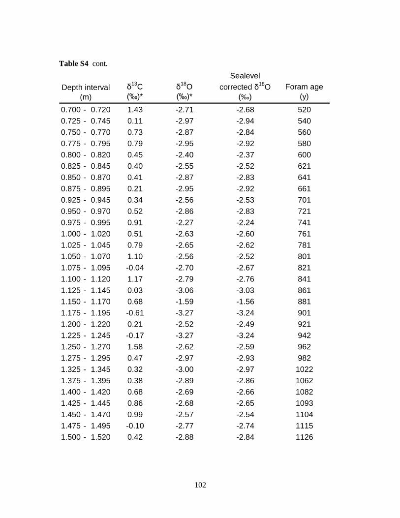
102

Table S4 cont.

δ13

C

(‰)*

δ18

O

(‰)*

Sealevel

corrected δ18

O

(‰)

Foram age

(y)

0.700 - 0.720 1.43 -2.71 -2.68 520

0.725 - 0.745 0.11 -2.97 -2.94 540

0.750 - 0.770 0.73 -2.87 -2.84 560

0.775 - 0.795 0.79 -2.95 -2.92 580

0.800 - 0.820 0.45 -2.40 -2.37 600

0.825 - 0.845 0.40 -2.55 -2.52 621

0.850 - 0.870 0.41 -2.87 -2.83 641

0.875 - 0.895 0.21 -2.95 -2.92 661

0.925 - 0.945 0.34 -2.56 -2.53 701

0.950 - 0.970 0.52 -2.86 -2.83 721

0.975 - 0.995 0.91 -2.27 -2.24 741

1.000 - 1.020 0.51 -2.63 -2.60 761

1.025 - 1.045 0.79 -2.65 -2.62 781

1.050 - 1.070 1.10 -2.56 -2.52 801

1.075 - 1.095 -0.04 -2.70 -2.67 821

1.100 - 1.120 1.17 -2.79 -2.76 841

1.125 - 1.145 0.03 -3.06 -3.03 861

1.150 - 1.170 0.68 -1.59 -1.56 881

1.175 - 1.195 -0.61 -3.27 -3.24 901

1.200 - 1.220 0.21 -2.52 -2.49 921

1.225 - 1.245 -0.17 -3.27 -3.24 942

1.250 - 1.270 1.58 -2.62 -2.59 962

1.275 - 1.295 0.47 -2.97 -2.93 982

1.325 - 1.345 0.32 -3.00 -2.97 1022

1.375 - 1.395 0.38 -2.89 -2.86 1062

1.400 - 1.420 0.68 -2.69 -2.66 1082

1.425 - 1.445 0.86 -2.68 -2.65 1093

1.450 - 1.470 0.99 -2.57 -2.54 1104

1.475 - 1.495 -0.10 -2.77 -2.74 1115

1.500 - 1.520 0.42 -2.88 -2.84 1126

Depth interval

(m)

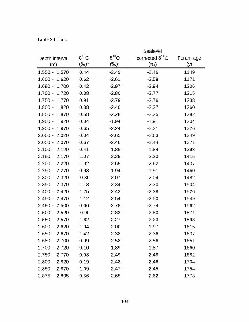
103

Table S4 cont.

δ13

C

(‰)*

δ18

O

(‰)*

Sealevel

corrected δ18

O

(‰)

Foram age

(y)

1.550 - 1.570 0.44 -2.49 -2.46 1149

1.600 - 1.620 0.62 -2.61 -2.58 1171

1.680 - 1.700 0.42 -2.97 -2.94 1206

1.700 - 1.720 0.38 -2.80 -2.77 1215

1.750 - 1.770 0.91 -2.79 -2.76 1238

1.800 - 1.820 0.38 -2.40 -2.37 1260

1.850 - 1.870 0.58 -2.28 -2.25 1282

1.900 - 1.920 0.04 -1.94 -1.91 1304

1.950 - 1.970 0.65 -2.24 -2.21 1326

2.000 - 2.020 0.04 -2.65 -2.63 1349

2.050 - 2.070 0.67 -2.46 -2.44 1371

2.100 - 2.120 0.41 -1.86 -1.84 1393

2.150 - 2.170 1.07 -2.25 -2.23 1415

2.200 - 2.220 1.02 -2.65 -2.62 1437

2.250 - 2.270 0.93 -1.94 -1.91 1460

2.300 - 2.320 -0.36 -2.07 -2.04 1482

2.350 - 2.370 1.13 -2.34 -2.30 1504

2.400 - 2.420 1.25 -2.43 -2.38 1526

2.450 - 2.470 1.12 -2.54 -2.50 1549

2.480 - 2.500 0.66 -2.78 -2.74 1562

2.500 - 2.520 -0.90 -2.83 -2.80 1571

2.550 - 2.570 1.62 -2.27 -2.23 1593

2.600 - 2.620 1.04 -2.00 -1.97 1615

2.650 - 2.670 1.42 -2.38 -2.36 1637

2.680 - 2.700 0.99 -2.58 -2.56 1651

2.700 - 2.720 0.10 -1.89 -1.87 1660

2.750 - 2.770 0.93 -2.49 -2.48 1682

2.800 - 2.820 0.19 -2.48 -2.46 1704

2.850 - 2.870 1.09 -2.47 -2.45 1754

2.875 - 2.895 0.56 -2.65 -2.62 1778

Depth interval

(m)

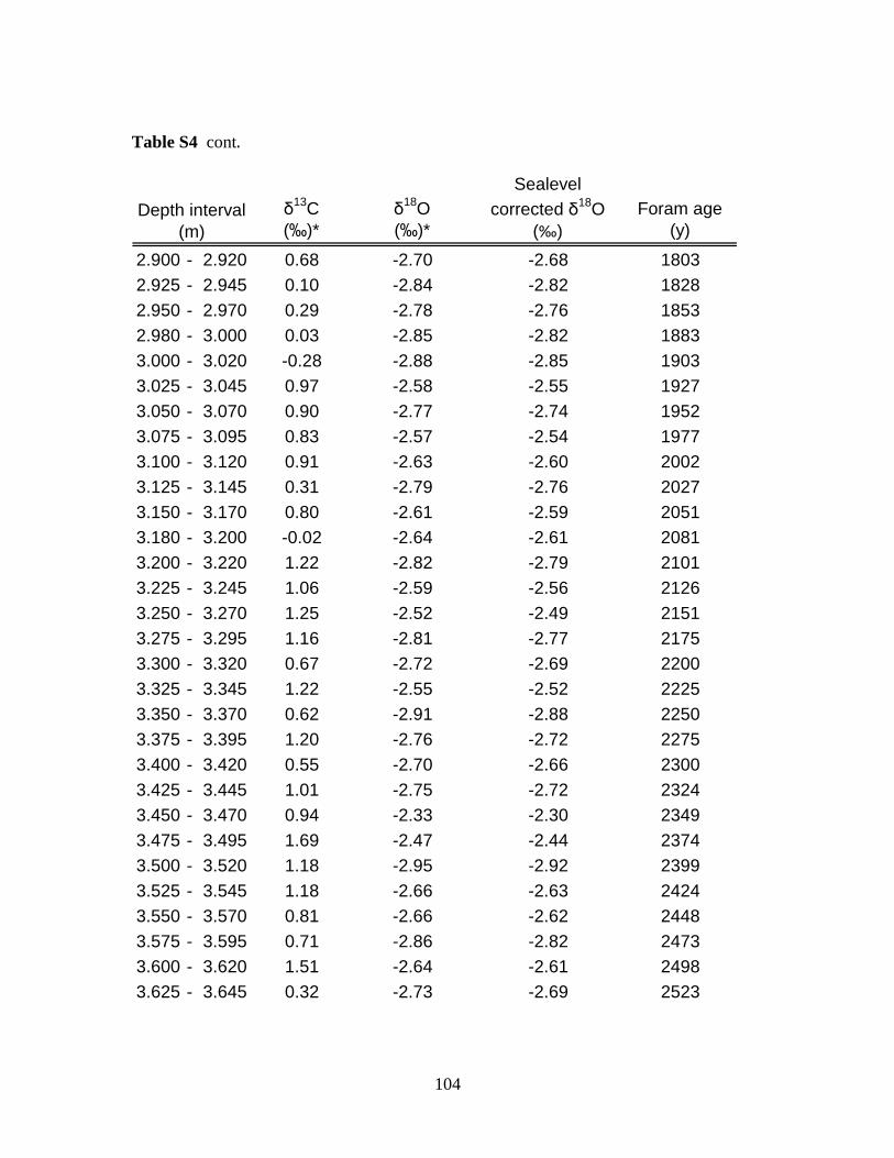
104

Table S4 cont.

δ13

C

(‰)*

δ18

O

(‰)*

Sealevel

corrected δ18

O

(‰)

Foram age

(y)

2.900 - 2.920 0.68 -2.70 -2.68 1803

2.925 - 2.945 0.10 -2.84 -2.82 1828

2.950 - 2.970 0.29 -2.78 -2.76 1853

2.980 - 3.000 0.03 -2.85 -2.82 1883

3.000 - 3.020 -0.28 -2.88 -2.85 1903

3.025 - 3.045 0.97 -2.58 -2.55 1927

3.050 - 3.070 0.90 -2.77 -2.74 1952

3.075 - 3.095 0.83 -2.57 -2.54 1977

3.100 - 3.120 0.91 -2.63 -2.60 2002

3.125 - 3.145 0.31 -2.79 -2.76 2027

3.150 - 3.170 0.80 -2.61 -2.59 2051

3.180 - 3.200 -0.02 -2.64 -2.61 2081

3.200 - 3.220 1.22 -2.82 -2.79 2101

3.225 - 3.245 1.06 -2.59 -2.56 2126

3.250 - 3.270 1.25 -2.52 -2.49 2151

3.275 - 3.295 1.16 -2.81 -2.77 2175

3.300 - 3.320 0.67 -2.72 -2.69 2200

3.325 - 3.345 1.22 -2.55 -2.52 2225

3.350 - 3.370 0.62 -2.91 -2.88 2250

3.375 - 3.395 1.20 -2.76 -2.72 2275

3.400 - 3.420 0.55 -2.70 -2.66 2300

3.425 - 3.445 1.01 -2.75 -2.72 2324

3.450 - 3.470 0.94 -2.33 -2.30 2349

3.475 - 3.495 1.69 -2.47 -2.44 2374

3.500 - 3.520 1.18 -2.95 -2.92 2399

3.525 - 3.545 1.18 -2.66 -2.63 2424

3.550 - 3.570 0.81 -2.66 -2.62 2448

3.575 - 3.595 0.71 -2.86 -2.82 2473

3.600 - 3.620 1.51 -2.64 -2.61 2498

3.625 - 3.645 0.32 -2.73 -2.69 2523

Depth interval

(m)

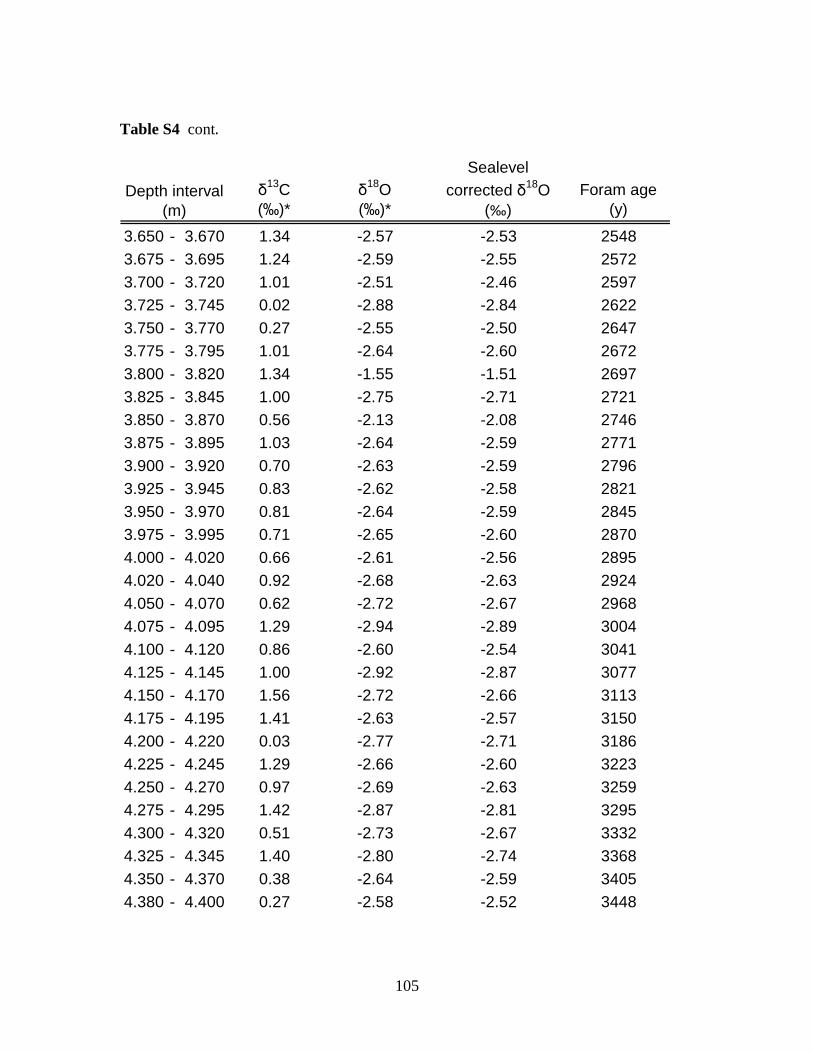
105

Table S4 cont.

δ13

C

(‰)*

δ18

O

(‰)*

Sealevel

corrected δ18

O

(‰)

Foram age

(y)

3.650 - 3.670 1.34 -2.57 -2.53 2548

3.675 - 3.695 1.24 -2.59 -2.55 2572

3.700 - 3.720 1.01 -2.51 -2.46 2597

3.725 - 3.745 0.02 -2.88 -2.84 2622

3.750 - 3.770 0.27 -2.55 -2.50 2647

3.775 - 3.795 1.01 -2.64 -2.60 2672

3.800 - 3.820 1.34 -1.55 -1.51 2697

3.825 - 3.845 1.00 -2.75 -2.71 2721

3.850 - 3.870 0.56 -2.13 -2.08 2746

3.875 - 3.895 1.03 -2.64 -2.59 2771

3.900 - 3.920 0.70 -2.63 -2.59 2796

3.925 - 3.945 0.83 -2.62 -2.58 2821

3.950 - 3.970 0.81 -2.64 -2.59 2845

3.975 - 3.995 0.71 -2.65 -2.60 2870

4.000 - 4.020 0.66 -2.61 -2.56 2895

4.020 - 4.040 0.92 -2.68 -2.63 2924

4.050 - 4.070 0.62 -2.72 -2.67 2968

4.075 - 4.095 1.29 -2.94 -2.89 3004

4.100 - 4.120 0.86 -2.60 -2.54 3041

4.125 - 4.145 1.00 -2.92 -2.87 3077

4.150 - 4.170 1.56 -2.72 -2.66 3113

4.175 - 4.195 1.41 -2.63 -2.57 3150

4.200 - 4.220 0.03 -2.77 -2.71 3186

4.225 - 4.245 1.29 -2.66 -2.60 3223

4.250 - 4.270 0.97 -2.69 -2.63 3259

4.275 - 4.295 1.42 -2.87 -2.81 3295

4.300 - 4.320 0.51 -2.73 -2.67 3332

4.325 - 4.345 1.40 -2.80 -2.74 3368

4.350 - 4.370 0.38 -2.64 -2.59 3405

4.380 - 4.400 0.27 -2.58 -2.52 3448

Depth interval

(m)

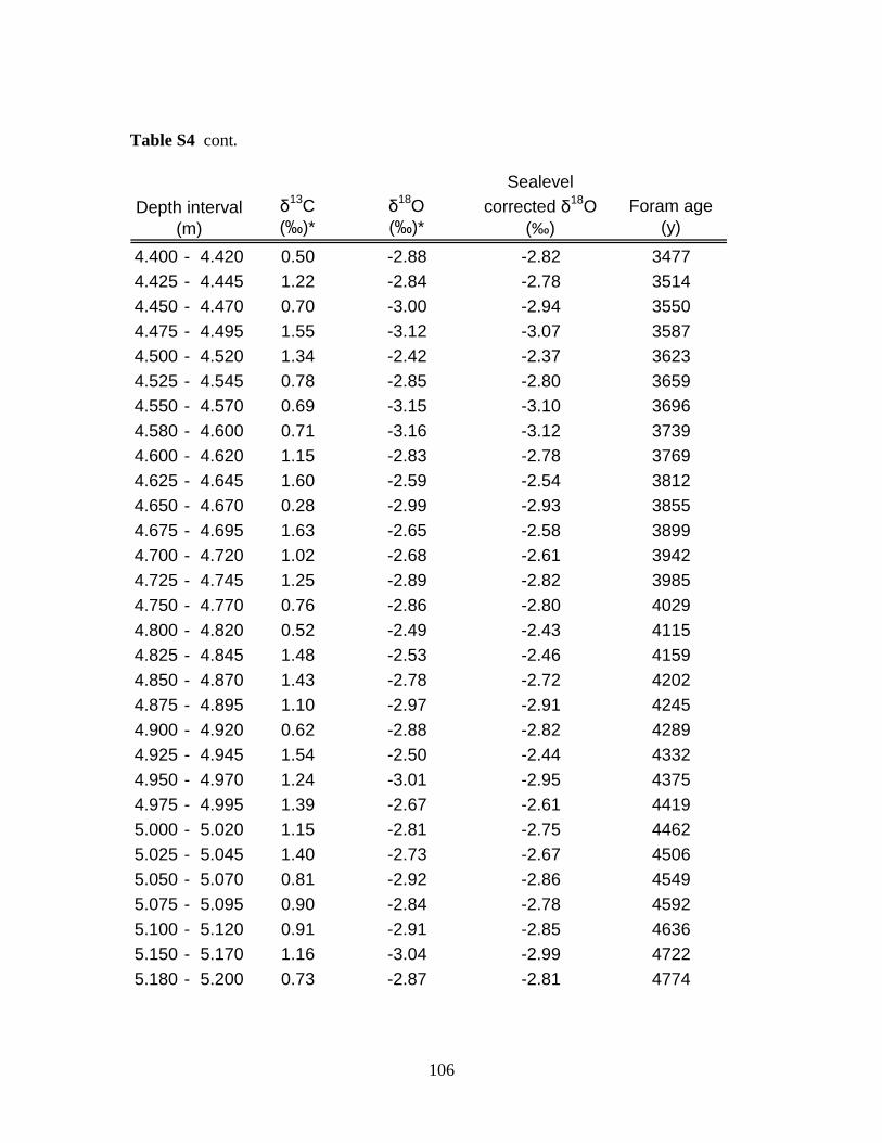
106

Table S4 cont.

δ13

C

(‰)*

δ18

O

(‰)*

Sealevel

corrected δ18

O

(‰)

Foram age

(y)

4.400 - 4.420 0.50 -2.88 -2.82 3477

4.425 - 4.445 1.22 -2.84 -2.78 3514

4.450 - 4.470 0.70 -3.00 -2.94 3550

4.475 - 4.495 1.55 -3.12 -3.07 3587

4.500 - 4.520 1.34 -2.42 -2.37 3623

4.525 - 4.545 0.78 -2.85 -2.80 3659

4.550 - 4.570 0.69 -3.15 -3.10 3696

4.580 - 4.600 0.71 -3.16 -3.12 3739

4.600 - 4.620 1.15 -2.83 -2.78 3769

4.625 - 4.645 1.60 -2.59 -2.54 3812

4.650 - 4.670 0.28 -2.99 -2.93 3855

4.675 - 4.695 1.63 -2.65 -2.58 3899

4.700 - 4.720 1.02 -2.68 -2.61 3942

4.725 - 4.745 1.25 -2.89 -2.82 3985

4.750 - 4.770 0.76 -2.86 -2.80 4029

4.800 - 4.820 0.52 -2.49 -2.43 4115

4.825 - 4.845 1.48 -2.53 -2.46 4159

4.850 - 4.870 1.43 -2.78 -2.72 4202

4.875 - 4.895 1.10 -2.97 -2.91 4245

4.900 - 4.920 0.62 -2.88 -2.82 4289

4.925 - 4.945 1.54 -2.50 -2.44 4332

4.950 - 4.970 1.24 -3.01 -2.95 4375

4.975 - 4.995 1.39 -2.67 -2.61 4419

5.000 - 5.020 1.15 -2.81 -2.75 4462

5.025 - 5.045 1.40 -2.73 -2.67 4506

5.050 - 5.070 0.81 -2.92 -2.86 4549

5.075 - 5.095 0.90 -2.84 -2.78 4592

5.100 - 5.120 0.91 -2.91 -2.85 4636

5.150 - 5.170 1.16 -3.04 -2.99 4722

5.180 - 5.200 0.73 -2.87 -2.81 4774

Depth interval

(m)

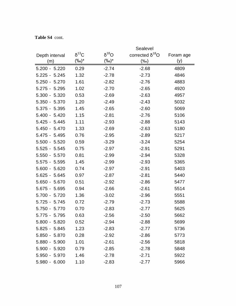
107

Table S4 cont.

δ13

C

(‰)*

δ18

O

(‰)*

Sealevel

corrected δ18

O

(‰)

Foram age

(y)

5.200 - 5.220 0.29 -2.74 -2.68 4809

5.225 - 5.245 1.32 -2.78 -2.73 4846

5.250 - 5.270 1.61 -2.82 -2.76 4883

5.275 - 5.295 1.02 -2.70 -2.65 4920

5.300 - 5.320 0.53 -2.69 -2.63 4957

5.350 - 5.370 1.20 -2.49 -2.43 5032

5.375 - 5.395 1.45 -2.65 -2.60 5069

5.400 - 5.420 1.15 -2.81 -2.76 5106

5.425 - 5.445 1.11 -2.93 -2.88 5143

5.450 - 5.470 1.33 -2.69 -2.63 5180

5.475 - 5.495 0.76 -2.95 -2.89 5217

5.500 - 5.520 0.59 -3.29 -3.24 5254

5.525 - 5.545 0.75 -2.97 -2.91 5291

5.550 - 5.570 0.81 -2.99 -2.94 5328

5.575 - 5.595 1.45 -2.99 -2.93 5365

5.600 - 5.620 0.74 -2.97 -2.91 5403

5.625 - 5.645 0.97 -2.87 -2.81 5440

5.650 - 5.670 0.51 -2.92 -2.86 5477

5.675 - 5.695 0.94 -2.66 -2.61 5514

5.700 - 5.720 1.36 -3.02 -2.96 5551

5.725 - 5.745 0.72 -2.79 -2.73 5588

5.750 - 5.770 0.70 -2.83 -2.77 5625

5.775 - 5.795 0.63 -2.56 -2.50 5662

5.800 - 5.820 0.52 -2.94 -2.88 5699

5.825 - 5.845 1.23 -2.83 -2.77 5736

5.850 - 5.870 0.28 -2.92 -2.86 5773

5.880 - 5.900 1.01 -2.61 -2.56 5818

5.900 - 5.920 0.79 -2.85 -2.78 5848

5.950 - 5.970 1.46 -2.78 -2.71 5922

5.980 - 6.000 1.10 -2.83 -2.77 5966

Depth interval

(m)

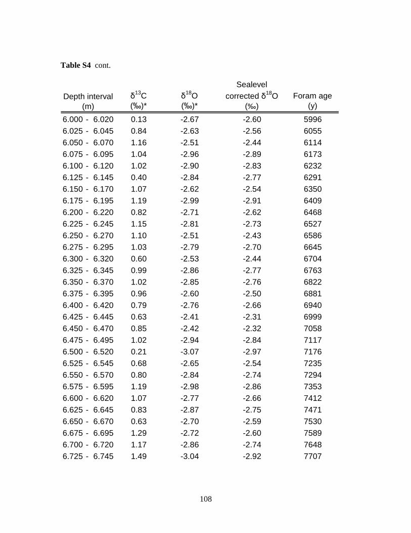
108

Table S4 cont.

δ13

C

(‰)*

δ18

O

(‰)*

Sealevel

corrected δ18

O

(‰)

Foram age

(y)

6.000 - 6.020 0.13 -2.67 -2.60 5996

6.025 - 6.045 0.84 -2.63 -2.56 6055

6.050 - 6.070 1.16 -2.51 -2.44 6114

6.075 - 6.095 1.04 -2.96 -2.89 6173

6.100 - 6.120 1.02 -2.90 -2.83 6232

6.125 - 6.145 0.40 -2.84 -2.77 6291

6.150 - 6.170 1.07 -2.62 -2.54 6350

6.175 - 6.195 1.19 -2.99 -2.91 6409

6.200 - 6.220 0.82 -2.71 -2.62 6468

6.225 - 6.245 1.15 -2.81 -2.73 6527

6.250 - 6.270 1.10 -2.51 -2.43 6586

6.275 - 6.295 1.03 -2.79 -2.70 6645

6.300 - 6.320 0.60 -2.53 -2.44 6704

6.325 - 6.345 0.99 -2.86 -2.77 6763

6.350 - 6.370 1.02 -2.85 -2.76 6822

6.375 - 6.395 0.96 -2.60 -2.50 6881

6.400 - 6.420 0.79 -2.76 -2.66 6940

6.425 - 6.445 0.63 -2.41 -2.31 6999

6.450 - 6.470 0.85 -2.42 -2.32 7058

6.475 - 6.495 1.02 -2.94 -2.84 7117

6.500 - 6.520 0.21 -3.07 -2.97 7176

6.525 - 6.545 0.68 -2.65 -2.54 7235

6.550 - 6.570 0.80 -2.84 -2.74 7294

6.575 - 6.595 1.19 -2.98 -2.86 7353

6.600 - 6.620 1.07 -2.77 -2.66 7412

6.625 - 6.645 0.83 -2.87 -2.75 7471

6.650 - 6.670 0.63 -2.70 -2.59 7530

6.675 - 6.695 1.29 -2.72 -2.60 7589

6.700 - 6.720 1.17 -2.86 -2.74 7648

6.725 - 6.745 1.49 -3.04 -2.92 7707

Depth interval

(m)

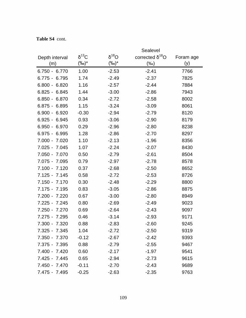
109

Table S4 cont.

δ13

C

(‰)*

δ18

O

(‰)*

Sealevel

corrected δ18

O

(‰)

Foram age

(y)

6.750 - 6.770 1.00 -2.53 -2.41 7766

6.775 - 6.795 1.74 -2.49 -2.37 7825

6.800 - 6.820 1.16 -2.57 -2.44 7884

6.825 - 6.845 1.44 -3.00 -2.86 7943

6.850 - 6.870 0.34 -2.72 -2.58 8002

6.875 - 6.895 1.15 -3.24 -3.09 8061

6.900 - 6.920 -0.30 -2.94 -2.79 8120

6.925 - 6.945 0.93 -3.06 -2.90 8179

6.950 - 6.970 0.29 -2.96 -2.80 8238

6.975 - 6.995 1.28 -2.86 -2.70 8297

7.000 - 7.020 1.10 -2.13 -1.96 8356

7.025 - 7.045 1.07 -2.24 -2.07 8430

7.050 - 7.070 0.50 -2.79 -2.61 8504

7.075 - 7.095 0.79 -2.97 -2.78 8578

7.100 - 7.120 0.37 -2.68 -2.50 8652

7.125 - 7.145 0.58 -2.72 -2.53 8726

7.150 - 7.170 0.30 -2.48 -2.29 8800

7.175 - 7.195 0.83 -3.05 -2.86 8875

7.200 - 7.220 0.67 -3.00 -2.80 8949

7.225 - 7.245 0.80 -2.69 -2.49 9023

7.250 - 7.270 0.69 -2.64 -2.43 9097

7.275 - 7.295 0.46 -3.14 -2.93 9171

7.300 - 7.320 0.88 -2.83 -2.60 9245

7.325 - 7.345 1.04 -2.72 -2.50 9319

7.350 - 7.370 -0.12 -2.67 -2.42 9393

7.375 - 7.395 0.88 -2.79 -2.55 9467

7.400 - 7.420 0.60 -2.17 -1.97 9541

7.425 - 7.445 0.65 -2.94 -2.73 9615

7.450 - 7.470 -0.11 -2.70 -2.43 9689

7.475 - 7.495 -0.25 -2.63 -2.35 9763

Depth interval

(m)

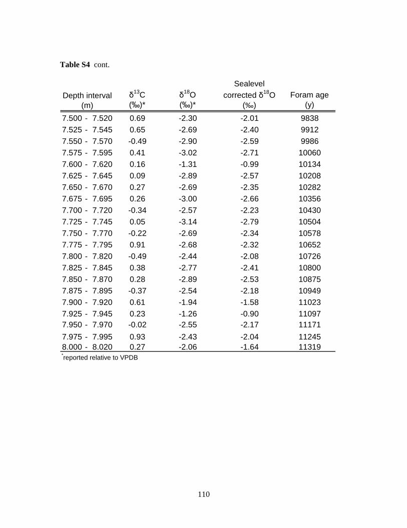
110

Table S4 cont.

δ13

C

(‰)*

δ18

O

(‰)*

Sealevel

corrected δ18

O

(‰)

Foram age

(y)

7.500 - 7.520 0.69 -2.30 -2.01 9838

7.525 - 7.545 0.65 -2.69 -2.40 9912

7.550 - 7.570 -0.49 -2.90 -2.59 9986

7.575 - 7.595 0.41 -3.02 -2.71 10060

7.600 - 7.620 0.16 -1.31 -0.99 10134

7.625 - 7.645 0.09 -2.89 -2.57 10208

7.650 - 7.670 0.27 -2.69 -2.35 10282

7.675 - 7.695 0.26 -3.00 -2.66 10356

7.700 - 7.720 -0.34 -2.57 -2.23 10430

7.725 - 7.745 0.05 -3.14 -2.79 10504

7.750 - 7.770 -0.22 -2.69 -2.34 10578

7.775 - 7.795 0.91 -2.68 -2.32 10652

7.800 - 7.820 -0.49 -2.44 -2.08 10726

7.825 - 7.845 0.38 -2.77 -2.41 10800

7.850 - 7.870 0.28 -2.89 -2.53 10875

7.875 - 7.895 -0.37 -2.54 -2.18 10949

7.900 - 7.920 0.61 -1.94 -1.58 11023

7.925 - 7.945 0.23 -1.26 -0.90 11097

7.950 - 7.970 -0.02 -2.55 -2.17 11171

7.975 - 7.995 0.93 -2.43 -2.04 11245

8.000 - 8.020 0.27 -2.06 -1.64 11319

Depth interval

(m)

*reported relative to VPDB

111

112

113

CHAPTER 4

The Indus Shelf: Holocene Sedimentation and Paleoclimate Reconstruction

Abstract

This study presents results from the first high-resolution seismic survey of the Indus

River subaqueous delta, and documents the existence of a well-developed Holocene

clinoform deposited over relict clinoforms that survived previous sea level cycles. We

use seismic and core records to explore the suitability of using subaqueous deltaic

sedimentary deposits from the Pakistani shelf to reconstruct the paleoclimate in the Indus

drainage basin. We find that fine-grained sediments trapped primarily from suspension in

morphological depressions located laterally from the shelf clinothems are well suited for

climate reconstructions. 13

C analyses on terrestrial plant leaf waxes preserved in such

sediments show a remarkably stable record indicating a predominance of C4 plants

(~75%) in the Indus River drainage basin during the last 6,000 yrs. These results are in

disagreement with the consistent accounts of Indian monsoon weakening over the

Holocene in other regions of South Asia. However, given that modern C3 vegetation

cover is restricted to small areas of the upper river basin, monsoon variability was

probably too small to decisively affect the dominant C4 vegetation of the arid lower Indus

basin.

4.1 Introduction

Continental shelves are the terrace-like submerged edges of continents that gently slope

offshore and extend to a point of steep descent (the shelf break) toward the ocean bottom.

They are usually covered with sediments that originated from inland erosion and were

transported by rivers to the shore (Mitchum et al., 1977; Nittrouer et al., 1986; Kuehl et

al., 1989; Walsh et al., 2004). Sediments on the continental shelf are redistributed and

deposited along and across the shelf by waves, currents and underwater sediment flows

(Nittrouer and Wright, 1994; Friedrichs and Wright, 2004; Macquaker et al., 2010). Sea

level changes exert a first-order control on sedimentary processes because they represent

changes of the base level above which sediments cannot be deposited in the ocean and

114

also the base level below which rivers cannot erode their beds (Mitchum et al., 1977;

Posamentier et al., 1988: Chistie-Blick and Driscoll, 1995). However, the presence of

persistent sediment source, such as in front of large, delta-building rivers, adds another

primary control on the sedimentation patterns and sedimentary architecture (McKee et

al., 1983; Nittrouer et al., 1986; Kuehl et al., 2004).

River-dominated continental margins offer an opportunity for paleoclimate reconstruction

because they integrate both marine and continental signals in their sedimentary record

(e.g., Galy et al., 2008; Colin et al. 2010; Ponton et al., 2012). Furthermore,

sedimentation rates are generally higher than anywhere in the ocean and thus, allow high

temporal resolution studies. Because delta-building processes directly respond to fluvial

sediment discharge, deltaic shelves where river loads are climatically controlled are good

candidates for paleoclimatic studies using both stratigraphy and sediment composition to

track climatic variability. In contrast, sedimentary records from continental slope settings

are additionally modified and delayed by shelf processes before reaching their

depositional locus (Nittrouer and Wright, 1994; Macquaker et al, 2010), which adds a

layer of complexity in their interpretation. Exceptions to this rule are systems with

narrow continental shelves (e.g., Ponton et al., 2012) or submarine canyons that extend

near to the river mouth where fluvial sediments are directly deposited on the slope (e.g.,

Weijers et al., 2009).

Here we use seismic imaging and downcore records to explore the suitability of using

deltaic sedimentary deposits from the Pakistani shelf to reconstruct paleoclimate in the

Indus drainage basin. This study presents results from the first high-resolution seismic

survey of the Indus River subaqueous delta, which documents the existence of a well-

developed modern clinoform on the Indus subaqueous delta deposited over relict

clinoforms that survived previous sea level cycles. Based on the interpretation of

sedimentary environments and plant wax compositional variability in sedimentary

deposits, I present results suggesting large-scale stability of the flora within the Indus

watershed since middle Holocene.

115

4.2 Background

4.2.1 Shelf morphology

Shelf sedimentary architecture and sediment composition can be used for paleoclimatic

reconstructions as long as their dynamics are understood for the time interval of interest.

Rich (1951) first described the depositional environments on sedimentary terraces of

different ocean basins and defined them as shelf, slope and bottom. The surfaces

corresponding to these environments were termed undaform, clinoform and fondoform

respectively, and their sedimentary deposits undathem, clinothem and fondothem.

Clinoforms occur at different scales varying from centimeters to tens of kilometers and

are characterized by lateral stacking of sedimentary packages of sigmoidal shape

(clinothems). Although the entire continental margin itself can be thought as a

clinoform/clinothem (Figure 1), similar landscapes and deposits of smaller scale occur

across the shelf and especially in front of deltas (Walsh et al., 2004), constituting the

building blocks of the continental margin (Sømme et al., 2009; Carvajal et al. 2009).

The term clinoform has been used to describe either the morphology of a feature (i.e.,

sigmoidal in cross-section) or its sedimentary dynamics (i.e., aggradational–

progradational feature of a sigmoidal shape; e.g., Walsh et al., 2004). In the latter,

process-based, use of the term, the clinoform is composed of topset, foreset, and

bottomset beds (Figure 1). In this work, I use “clinoform” to describe the form

(morphology) and “clinothem” to distinguish deposits associated with that form.

Variability in clinoform/clinothem in cross section has been discussed e.g., in Slingerland

et al. (2008; Figure 1) and Driscoll and Karner (1999) respectively.

Classic sequence stratigraphic models suggest that under a low-stand the coast emerges

and large quantities of terrigenous sediments are spread outwards and downward onto the

outer shelf, slope and basin floor (Mitchum et al. 1977, Posamentier et al. 1988). On the

contrary, a high-standing sea submerges the coast and as a result the environments lying

farther seaward experience sediment starvation. The progression of sea level cycles

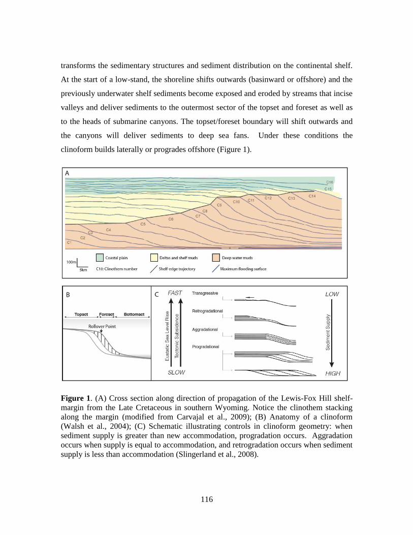
116

transforms the sedimentary structures and sediment distribution on the continental shelf.

At the start of a low-stand, the shoreline shifts outwards (basinward or offshore) and the

previously underwater shelf sediments become exposed and eroded by streams that incise

valleys and deliver sediments to the outermost sector of the topset and foreset as well as

to the heads of submarine canyons. The topset/foreset boundary will shift outwards and

the canyons will deliver sediments to deep sea fans. Under these conditions the

clinoform builds laterally or progrades offshore (Figure 1).

Figure 1. (A) Cross section along direction of propagation of the Lewis-Fox Hill shelf-

margin from the Late Cretaceous in southern Wyoming. Notice the clinothem stacking

along the margin (modified from Carvajal et al., 2009); (B) Anatomy of a clinoform

(Walsh et al., 2004); (C) Schematic illustrating controls in clinoform geometry: when

sediment supply is greater than new accommodation, progradation occurs. Aggradation

occurs when supply is equal to accommodation, and retrogradation occurs when sediment

supply is less than accommodation (Slingerland et al., 2008).

117

When the sea level begins to rise, conditions may not change much, and the lowstand

configuration will continue to accumulate. However, as the rate of submergence

increases, and the shoreline transgresses landward, the sediment supply to the offshore

region may be cut off abruptly resulting in deposition of strata much thinner than during

lowstand. On the topset, a thin and discontinuous sand layer is deposited until the

maximum submergence has been reached. However, where terrigenous sediment is

abundant, the coastline may continue to prograde or restart progradation offshore even

under rising sea levels (Posamentier et al. 1988) by constructing deltaic clinothems.

Observations on modern mid-shelf clinoforms reveal information about the processes by

which they were formed. Studies on large modern subaqueous deltas like the Amazon

(Kuehl et al, 1986; Nittrouer et al., 1986; Nittrouer et al., 1996; Kineke et al., 1996) and

the Ganges-Brahmaputra (Kuehl et al. 1997; 2005; Michels et al., 1998) show that

hyperpycnal sediment plumes play a crucial role in transporting and delivering sediment

from the river mouth to the clinoform, and that alongshore currents redistribute sediments

allowing clinoform development along-shelf as well as across-shelf (Driscoll and Karner,

1999; Giosan et al., 2006). Modeling studies for gravity-driven, wave-supported sediment

transport predict the equilibrium profile of a mid-shelf clinoform as a function of wave

climate and fluvial sediment supply (Friedrichs and Wright, 2004; Wright and Friedrichs,

2006). Deeper and broader profiles correspond to higher wave energy relative to river

supply. In the Amazon delta the clinoform rollover occurs at ~40 m water depth over

150 km from the coast (Nittrouer et al., 1986). On the Ganges-Brahmaputra rollover

occurs at ~30 m water depth (Kuehl et al., 1997). When applying the Friedrichs and

Wright (2004) model to the Indus shelf, the results suggest the Indus delta should have

developed a clinoform anywhere from ~40 to 100 m depth (Giosan et al., 2006).

118

4.2.2 Indian monsoon variability

The Indian monsoon is a principal water contributor, together with glacier meltwater, to

the Indus River (Karim and Veizer, 2002) and it has been proposed to modulate its

sediment discharge (Clift et al., 2008). Although water discharge reconstructions for the

Indus have been attempted (Staubwasser et al., 2003), it is unclear how they reflect the

variability of the Indus monsoon considering that the main contribution of the water

originates from western Asia via the Westerlies (Karim and Veizer, 2002). Other regional

high-resolution proxy records of precipitation (Fleitmann et al., 2003) and wind intensity

(Gupta et al., 2003) during the Holocene are available from the coastal and offshore

regions of Oman respectively. These reconstructions, supported by other records (Sirocko

et al., 1993; Overpeck et al., 1996; Schulz et al., 1998; Ivanochko et al., 2005), show a

gradual decrease in precipitation during the Holocene associated with coeval weakening

of summer monsoon winds, and have been interpreted (Fleitmann et al., 2007) as the

result of the ITCZ southward migration (Haug et al., 2001). Foraminiferal oxygen

isotopic records from the southeastern Arabian Sea (Sarkar et al., 2000) and reconstructed

precipitation on the island of Socotra, offshore Yemen (Fleitmann et al., 2007), both

suggest that the monsoon intensified in the late Holocene, possibly responding to the

ITCZ southward retreat. Terrestrial and marine records from the core monsoon zone in

central India present a consistent picture of progressive monsoon weakening since the

mid-Holocene, and document that after a humid early Holocene there was a gradual

increase in aridity-adapted vegetation (Ponton et al., 2012). The same records also

suggest that in the late Holocene aridification intensified in central India through a series

of sub-millennial dry episodes. Holocene monsoon reconstructions from the NW Indian

peninsula are limited to lower resolution lacustrine records and have not yielded clear

evidence for increased precipitation in early Holocene corresponding to the interval of

intensified summer monsoon winds (Prasad and Enzel, 2006). Instead the lake records

show active periods and intervals of desiccation that are not coherent across the region,

suggesting localized causes for hydrologic variability.

119

4.3 Study area

The Indus River drains the western Himalaya and Karakoram Mountains, crosses the arid

plains of Pakistan and flows into the Arabian Sea via a complex network of mouths. The

Indus is now heavily dammed but it used to be one of the most important sediment-

producing rivers in the world and built an extensive delta and the second largest

submarine fan in the present-day ocean. It is estimated that before the 1960’s the annual

sediment discharge for the Indus River was between 300 and 675 million tons (Milliman

et al., 1982; Milliman and Syvitski, 1992), making it the river with the 5th

largest

sediment load in the world (Wells and Coleman, 1984). The sediment reaching the delta

and continental shelf is dominantly silt (65%) with variable quantities of sand and clay

(Kazmi, 1984). The Indus receives the highest deep-water wave energy of major world’s

deltas due to intense monsoonal winds arriving from the southwest during May to

September (Wells and Coleman, 1984), but after attenuation by the wide shallow shelf

the wave energy at the coast is lower than for typical wave-dominated deltas (Wells and

Coleman, 1984). Sediment dispersal by tidal and wind-driven currents also occurs. The

mean current along the coast switches from southeasterly during the summer monsoon to

northwesterly during the winter monsoon (Rizvi et al., 1988; Fig 2).

The most prominent feature of the Indus shelf is the Indus Canyon that dissects the shelf.

Using successive bathymetric surveys, Giosan et al. (2006) showed that the Indus built an

extensive lobate subaqueous delta during the Holocene. This delta exhibits a compound

clinoform morphology with a shallow delta front or coastal clinoform extending along the

entire delta cost from the shore to 10-25 m water depth and a shelf clinoform between

~30-90 m water depth (Giosan et al., 2006). Herein we focus on the latter feature. The

Indus shelf clinoform developed asymmetrically around the canyon (Giosan et al., 2006).

On the eastern shelf the clinoform is much more advanced towards the edge of the shelf

and the rollover point occurs between 80 and 100 km offshore, while on the western shelf

the rollover point occurs at less than 50 km offshore (Figure 2). One explanation

proposed by Giosan et al. (2006) for the advanced position of the shelf clinoform east of

120

the Indus Canyon, is the existence of a relict pre-Holocene clinoform on the eastern shelf.

Alternatively, Holocene sedimentation may have preferentially occurred on the eastern

shelf due to subaerial delta morphodynamics and/or shelf circulation (Giosan et al.,

2006).

4.4 Methods

During December 2008 - January 2009 the R/V Pelagia cruise 64PE300 surveyed the

Indus shelf to image and core the shallow sub-seafloor and document the nature of

sediment transport in the Holocene subaqueous delta. We employed an Edgetech SB-512i

Chirp seismic reflection system optimized for imaging in the 20–200 m sub-seafloor

range. The frequency range was set to 0.7–12.0 kHz for the duration of our operations,

and the fish was towed behind the ship at a depth of ~5m and a speed of ~4 knots. The

data was recorded using EdgeTech Sub-Bottom 3.42 software and then imported into

analysis software package Triton SB-I. Automatic gain control filters and swell

corrections were applied when necessary to optimize seismic imaging. Sediment

thicknesses were estimated using a sound velocity of 1500 ms-1

. Prominent reflectors

were digitized across the acquired lines and high-resolution image files with

predetermined scaling factor were exported to construct composite seismic profiles for

interpretation.

The cruise recovered 11 piston cores, 16 gravity cores, 16 multi-cores, and 5 box cores

along the Indus shelf. These cores were described and information recorded on core logs

during the cruise. Samples for radiocarbon dating were collected upon description where

in situ mollusk shells, preferably articulated, were available. Additional samples for

radiocarbon dating were obtained after washing the sediment on 63m sieves and picking

fresh-looking mollusk shells. When whole pteropod shells were available they were

preferentially used, given that their fragile tests insure that they are preserved in situ.

Otherwise, small articulated bivalves and gastropod shells (<1 cm diameter) were used.

121

Radiocarbon measurements were performed at the National Ocean Sciences Accelerator

Mass Spectrometry Facility (NOSAMS) in Woods Hole, MA, USA. 14

C ages were

converted to calendar ages using the CALIB 6.0 program (Stuiver and Reimer, 1993) and

the Marine09 calibration curve (Reimer et al., 2009). Available reservoir estimates for the

Arabian Sea surface waters are not substantially different from the standard marine

reservoir correction (Dutta et al., 2001; Southon et al., 2002), which we used to calibrate

our data. However, Staubwasser et al. (2003) counting seasonal layers from a laminated

core in the Pakistani margin documented elevated ages for the natural 14

C marine

reservoir during the Holocene and proposed an age calibration model with variable

reservoir ages between 530 – 670 yrs. We also converted our 14

C ages to calendar ages

using their age model and present results for both calibrations for comparison.

Compound-specific carbon isotope analyses on sedimentary plant waxes (long-chain

[>C24] n-alkanoic acids) were performed on 17 samples of core Indus-10A-P spanning

the last 6,000 yrs BP. Complete methodology for this procedure can be found in Chapter

2 of this dissertation. In brief, solvent-soluble organic matter was extracted from freeze-

dried sediments using a microwave-accelerated reaction system. The resulting total lipid

extract was saponified and the acid fraction purified and then methylated using methanol

of known isotopic composition. A gas chromatograph with isotope ratio monitoring mass

spectrometer (GC-irMS; Thermo Trace GC Ultra connected to a Thermo Delta V Plus

MS via a Thermo GC Isolink and Thermo Conflow IV) was used to obtain the δ13

C

measurements on the isolated n-alkanoic acids (measured as fatty acid methyl esters). All

samples were analyzed in triplicate; δ13

C values were determined relative to a reference

gas (CO2) of known isotopic composition, introduced in pulses during each run. GC-irMS

accuracy and precision are both better than 0.3‰. Results were corrected for δ13

C of the

methyl derivative based on isotopic mass balance to derive δ13

C values for the original n-

alkanoic acids.

122

4.5 Results and Discussions

4.5.1 The western shelf

The extent of the entire seismic survey of the Indus shelf on both sides of the canyon can

be seen in Figure 2 . Bathymetry shows the difference in the shapes of the two lobes of

the delta divided by the canyon. The spacing of the contours indicates where the rollover

of the clinoform occurs. The western shelf clinoform does not develop out far onto the

shelf (ca. 50 km from shore), and extends laterally along the shoreline for more than 120

km. A composite of chirp lines tracking the western clinoform along-shore (strikewise)

is shown in Figure 3. It presents the modern clinothem deposited along-shore. The

composite line provides a general cross section of the western delta lobe thinning

westward, with the bulge of sediment developed close to the canyon.

The stratigraphy and architecture of the clinoform has been imaged close to the canyon

down to ca. 20 meters below sea floor (mbsf). The presence of gas (blue mask in Figure

3) precluded deeper penetration of the seismic signal. At shallower depths homogenous

transparent units reminiscent of mudflows occur (traced in black with a white mask in

Figures 3-4). Similar transparent units consisting of homogenized sediments have been

observed in the Ganges-Brahmaputra subaqueous delta and interpreted as liquefaction

flows triggered by earthquakes (Palamenghi et al., 2011) and the passage of tropical

cyclones (Rogers and Goodbred, 2010).

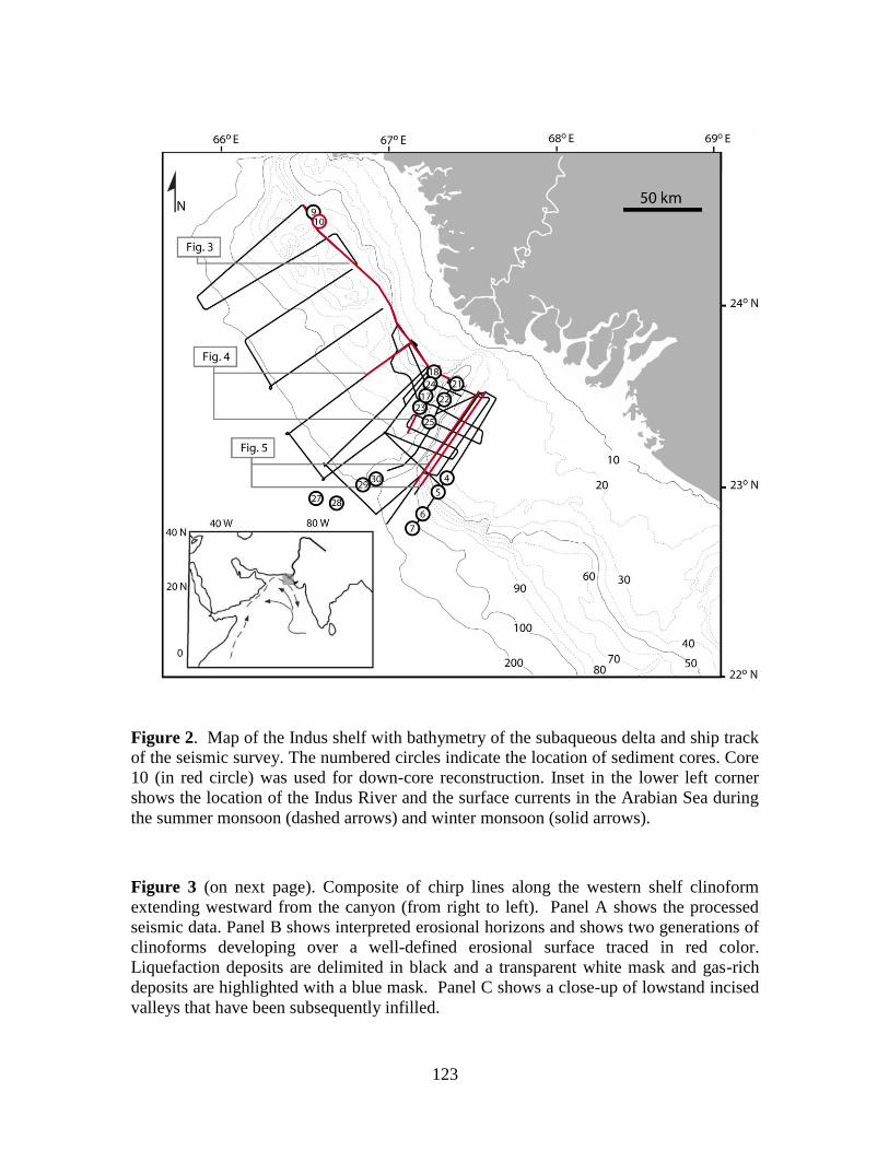
123

Figure 2. Map of the Indus shelf with bathymetry of the subaqueous delta and ship track

of the seismic survey. The numbered circles indicate the location of sediment cores. Core

10 (in red circle) was used for down-core reconstruction. Inset in the lower left corner

shows the location of the Indus River and the surface currents in the Arabian Sea during

the summer monsoon (dashed arrows) and winter monsoon (solid arrows).

Figure 3 (on next page). Composite of chirp lines along the western shelf clinoform

extending westward from the canyon (from right to left). Panel A shows the processed

seismic data. Panel B shows interpreted erosional horizons and shows two generations of

clinoforms developing over a well-defined erosional surface traced in red color.

Liquefaction deposits are delimited in black and a transparent white mask and gas-rich

deposits are highlighted with a blue mask. Panel C shows a close-up of lowstand incised

valleys that have been subsequently infilled.

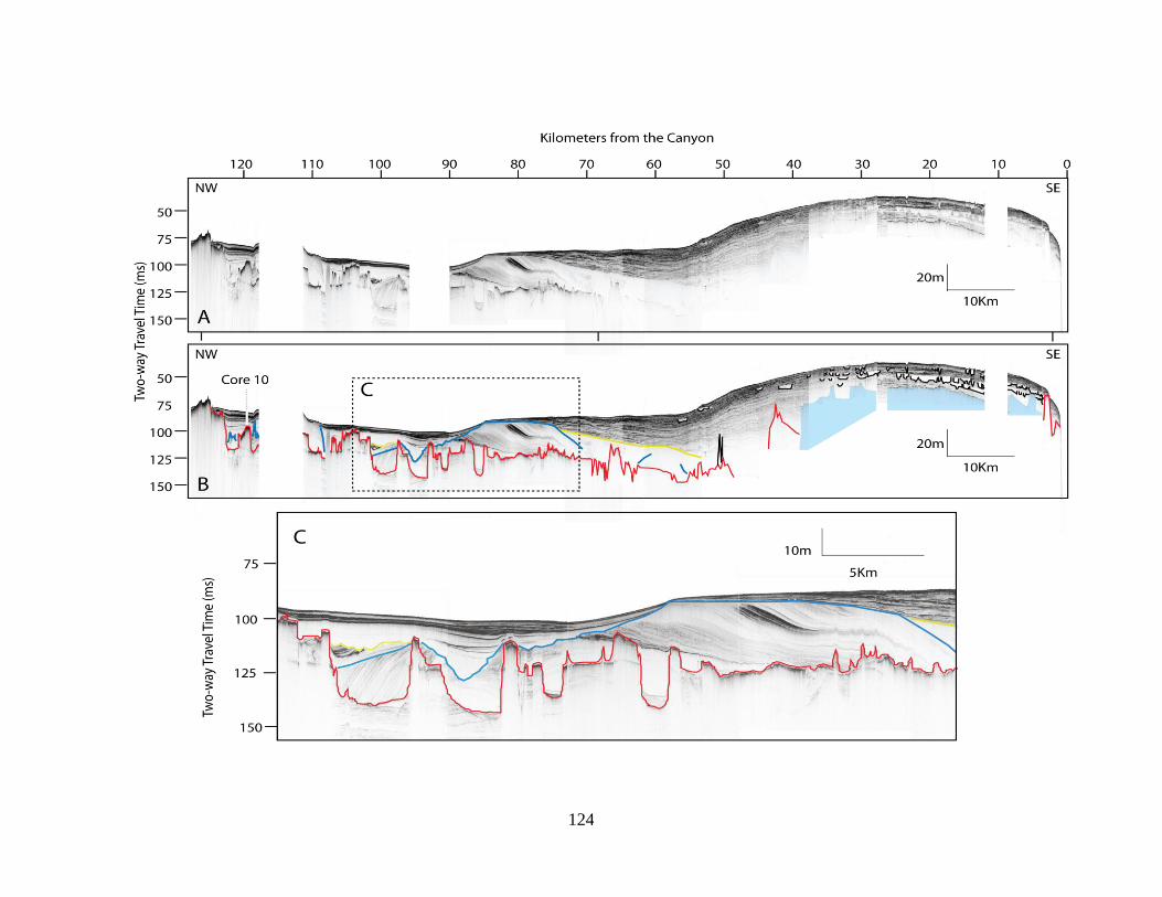
124

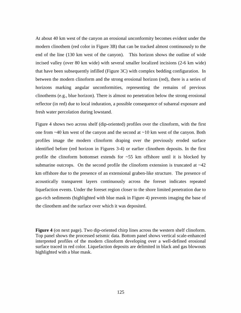
125

At about 40 km west of the canyon an erosional unconformity becomes evident under the

modern clinothem (red color in Figure 3B) that can be tracked almost continuously to the

end of the line (130 km west of the canyon). This horizon shows the outline of wide

incised valley (over 80 km wide) with several smaller localized incisions (2-6 km wide)

that have been subsequently infilled (Figure 3C) with complex bedding configuration. In

between the modern clinoform and the strong erosional horizon (red), there is a series of

horizons marking angular unconformities, representing the remains of previous

clinothems (e.g., blue horizon). There is almost no penetration below the strong erosional

reflector (in red) due to local induration, a possible consequence of subareal exposure and

fresh water percolation during lowstand.

Figure 4 shows two across shelf (dip-oriented) profiles over the clinoform, with the first

one from ~40 km west of the canyon and the second at ~10 km west of the canyon. Both

profiles image the modern clinoform draping over the previously eroded surface

identified before (red horizon in Figures 3-4) or earlier clinothem deposits. In the first

profile the clinoform bottomset extends for ~55 km offshore until it is blocked by

submarine outcrops. On the second profile the clinoform extension is truncated at ~42

km offshore due to the presence of an extensional graben-like structure. The presence of

acoustically transparent layers continuously across the foreset indicates repeated

liquefaction events. Under the foreset region closer to the shore limited penetration due to

gas-rich sediments (highlighted with blue mask in Figure 4) prevents imaging the base of

the clinothem and the surface over which it was deposited.

Figure 4 (on next page). Two dip-oriented chirp lines across the western shelf clinoform.

Top panel shows the processed seismic data. Bottom panel shows vertical scale-enhanced

interpreted profiles of the modern clinoform developing over a well-defined erosional

surface traced in red color. Liquefaction deposits are delimited in black and gas blowouts

highlighted with a blue mask.

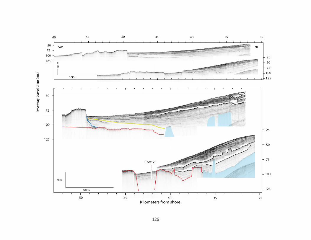
126

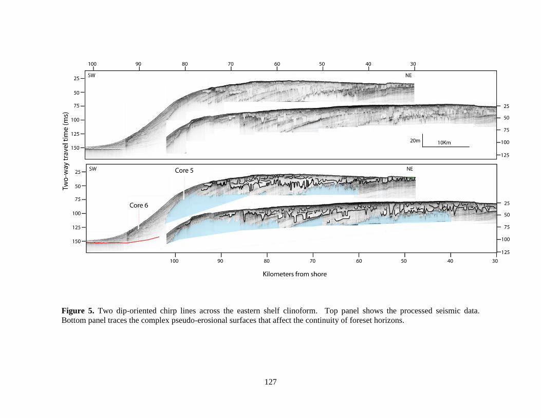
127

Figure 5. Two dip-oriented chirp lines across the eastern shelf clinoform. Top panel shows the processed seismic data.

Bottom panel traces the complex pseudo-erosional surfaces that affect the continuity of foreset horizons.

128

4.5.2 The eastern shelf

The eastern lobe of the subaqueous delta extends much farther towards the shelf edge,

with the clinoform rollover occurring between 80 and 100 km offshore (Figure 2). The

eastern clinothem is not only more extensive but also much thicker than its western shelf

equivalent. Profiles in Figure 5 show two chirp lines extending offshore across the shelf.

The well-defined erosional horizon in these profiles, likely equivalent to the one traced

on the western side, is only observed under the bottomset, where the clinothem is thinnest

(traced in red in Figure 5). At the topset, the clinothem exhibits a complex structure with

clear but discontinuous (pseudo-)erosional surfaces (traced in black and with white masks

in Figure 5) infilled by homogenous sediments for the most part. These could represent

the topset expression of liquefaction events (Rogers and Goodbred, 2010; Palamenghi et

al., 2011) similar to those observed on the western shelf.

4.5.3 Sediment cores

Analysis of seismic data across the Indus shelf indicates that sediments of the topset and

foreset are not appropriate for paleoclimate reconstructions where effects of liquefaction

and mass sediment transport are dominant. Therefore, sediment cores from locations on

the western shelf, away from clinothems and within morphological depressions stemming

from lowstand incision (Core 10; Figure 3) or tectonic subsidence (Core 23; Figure 4),

were selected for investigation. These locations receive most of the sediment through

suspension and resuspension of topset sediments and are less influenced by turbidites and

liquefaction. On the eastern shelf, cores were selected from the foreset where the

clinothem is less affected by erosional channels and liquefaction events (Cores 5-6;

Figure 5).

Figure 6 presents the sedimentary logs for the cores considered in this study with

corresponding radiocarbon ages. Ages indicate that the last Indus delta clinothem is

Holocene in age. Cores from the eastern shelf contain frequent turbidite-like coarse beds

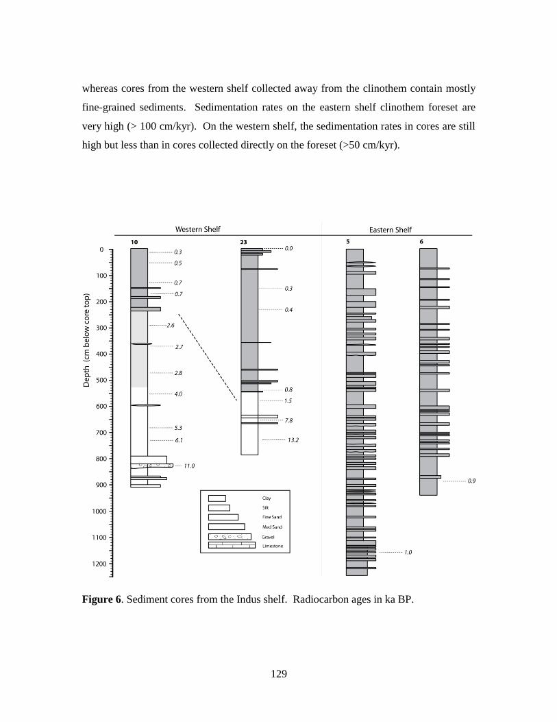
129

whereas cores from the western shelf collected away from the clinothem contain mostly

fine-grained sediments. Sedimentation rates on the eastern shelf clinothem foreset are

very high (> 100 cm/kyr). On the western shelf, the sedimentation rates in cores are still

high but less than in cores collected directly on the foreset (>50 cm/kyr).

Figure 6. Sediment cores from the Indus shelf. Radiocarbon ages in ka BP.

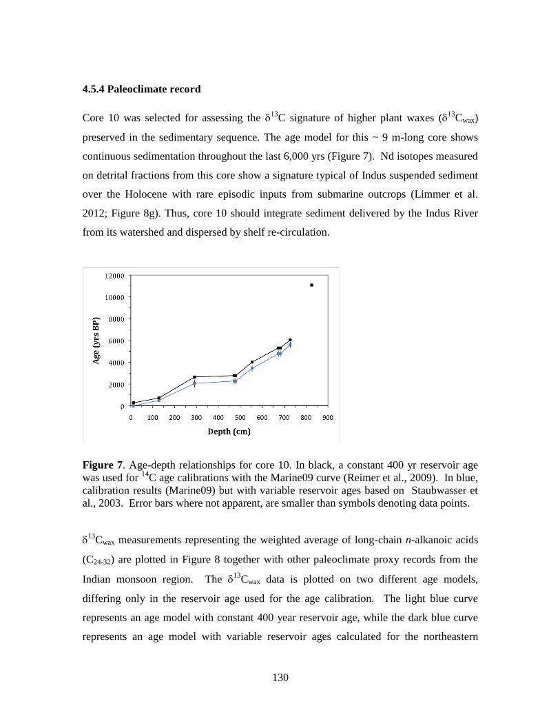
130

4.5.4 Paleoclimate record

Core 10 was selected for assessing the 13

C signature of higher plant waxes (13

Cwax)

preserved in the sedimentary sequence. The age model for this ~ 9 m-long core shows

continuous sedimentation throughout the last 6,000 yrs (Figure 7). Nd isotopes measured

on detrital fractions from this core show a signature typical of Indus suspended sediment

over the Holocene with rare episodic inputs from submarine outcrops (Limmer et al.

2012; Figure 8g). Thus, core 10 should integrate sediment delivered by the Indus River

from its watershed and dispersed by shelf re-circulation.

Figure 7. Age-depth relationships for core 10. In black, a constant 400 yr reservoir age

was used for 14

C age calibrations with the Marine09 curve (Reimer et al., 2009). In blue,

calibration results (Marine09) but with variable reservoir ages based on Staubwasser et

al., 2003. Error bars where not apparent, are smaller than symbols denoting data points.

13

Cwax measurements representing the weighted average of long-chain n-alkanoic acids

(C24-32) are plotted in Figure 8 together with other paleoclimate proxy records from the

Indian monsoon region. The 13

Cwax data is plotted on two different age models,

differing only in the reservoir age used for the age calibration. The light blue curve

represents an age model with constant 400 year reservoir age, while the dark blue curve

represents an age model with variable reservoir ages calculated for the northeastern

131

Arabian Sea by Staubwasser et al. (2003). On average, the calibrated ages using the

standard reservoir age model are 260 yr older than those calibrated using the variable age

model (Figure 7). The 13

Cwax data shows a remarkably stable record with values that

suggest a dominant C4 plant population (~75%) in the Indus River drainage basin

throughout the record. Vegetation cover was estimated using the same two-end member

model described in Chapter 2 of this dissertation.

Precipitation and upwelling records from the Arabian Sea (Fleitmann et al., 2003; Gupta

et al., 2003; Figure 8a-b) show a decreasing rainfall trend and relatively low wind

intensities for the past 6,000 yrs indicting a weakening of the monsoon, culminating with

a brief monsoon strengthening after 1,000 yrs BP. Records from the Bay of Bengal

monsoon branch provide a consistent account of monsoon weakening over the Holocene.

Plant wax isotope records reveal the aridification of central India in a stepwise fashion

starting at around 4,000 years ago and again after 1,700 years, manifested as a change in

flora toward aridity-adapted (C4) vegetation (Ponton et al., 2012; Figure 8e). Oxygen

isotopic compositions of G. ruber from the same core shows high variability over the last

1,700 years, indicating the monsoon entered into a drought-prone regime (Sinha et al.,

2011; Ponton et al., 2012; Figure 8d). The Indian monsoon weakening from the mid to

late Holocene is not captured by records from the Indus River. Besides our new 13

Cwax

data (Figure 8f), oxygen isotopic composition of G. ruber from sediments off the mouth

of the Indus River have been interpreted as a proxy for river discharge (Staubwasser et

al., 2003; Figure 8c) and also show a relatively flat record. This is not surprising, given

the Indus River discharge is not exclusively depending on monsoonal rains. Karim and

Veizer (2002) estimate that currently ~30% of the Indus River discharge is the result of

runoff from the Karakoram and the Himalayas.

We interpret our new plant wax data as an integrated record of the entire Indus River

drainage basin. The lack of variability in floral composition suggests that the Indus

watershed has been arid overall during the last 6,000 years and the wetter monsoon that is

evident in other regions of South Asia never developed in the Indus basin to the extent to

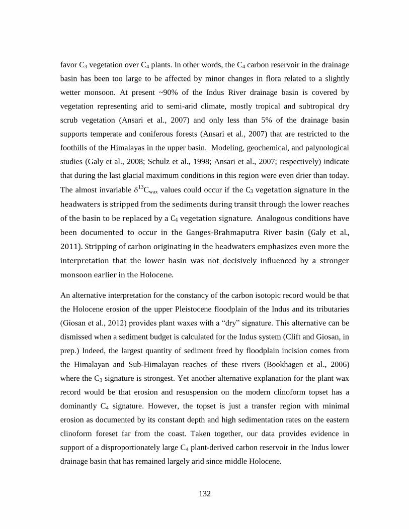
132

favor C3 vegetation over C4 plants. In other words, the C4 carbon reservoir in the drainage

basin has been too large to be affected by minor changes in flora related to a slightly

wetter monsoon. At present ~90% of the Indus River drainage basin is covered by

vegetation representing arid to semi-arid climate, mostly tropical and subtropical dry

scrub vegetation (Ansari et al., 2007) and only less than 5% of the drainage basin

supports temperate and coniferous forests (Ansari et al., 2007) that are restricted to the

foothills of the Himalayas in the upper basin. Modeling, geochemical, and palynological

studies (Galy et al., 2008; Schulz et al., 1998; Ansari et al., 2007; respectively) indicate

that during the last glacial maximum conditions in this region were even drier than today.

The almost invariable 13

Cwax values could occur if the C3 vegetation signature in the

headwaters is stripped from the sediments during transit through the lower reaches

of the basin to be replaced by a C4 vegetation signature. Analogous conditions have

been documented to occur in the Ganges-Brahmaputra River basin (Galy et al.,

2011). Stripping of carbon originating in the headwaters emphasizes even more the

interpretation that the lower basin was not decisively influenced by a stronger

monsoon earlier in the Holocene.

An alternative interpretation for the constancy of the carbon isotopic record would be that

the Holocene erosion of the upper Pleistocene floodplain of the Indus and its tributaries

(Giosan et al., 2012) provides plant waxes with a “dry” signature. This alternative can be

dismissed when a sediment budget is calculated for the Indus system (Clift and Giosan, in

prep.) Indeed, the largest quantity of sediment freed by floodplain incision comes from

the Himalayan and Sub-Himalayan reaches of these rivers (Bookhagen et al., 2006)

where the C3 signature is strongest. Yet another alternative explanation for the plant wax

record would be that erosion and resuspension on the modern clinoform topset has a

dominantly C4 signature. However, the topset is just a transfer region with minimal

erosion as documented by its constant depth and high sedimentation rates on the eastern

clinoform foreset far from the coast. Taken together, our data provides evidence in

support of a disproportionately large C4 plant-derived carbon reservoir in the Indus lower

drainage basin that has remained largely arid since middle Holocene.

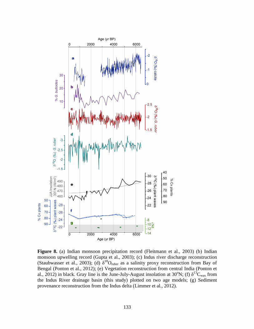
133

Figure 8. (a) Indian monsoon precipitation record (Fleitmann et al., 2003) (b) Indian

monsoon upwelling record (Gupta et al., 2003); (c) Indus river discharge reconstruction

(Staubwasser et al., 2003); (d) δ18

Oruber as a salinity proxy reconstruction from Bay of

Bengal (Ponton et al., 2012); (e) Vegetation reconstruction from central India (Ponton et

al., 2012) in black. Gray line is the June-July-August insolation at 30oN; (f) δ

13Cwax from

the Indus River drainage basin (this study) plotted on two age models; (g) Sediment

provenance reconstruction from the Indus delta (Limmer et al., 2012).

134

4.6 Conclusions

Our study confirms that the clinoforms of the Indus shelf have been built during the

Holocene (Giosan et al. 2006). The western clinoform is developed in part over partially

eroded, relict clinothems, but limited penetration due to gas and/or local induration of

sedimentary layers precludes an assessment on the occurrence of similar relict features at

the base of the western clinothem. Acoustically transparent sediment layers suggest that

repeated liquefaction events affected both the western and eastern clinothems. Textural

and structure variations in cores collected on foreset clinoforms show sandy micro-

turbidite layers. Both liquefaction and turbiditic activity affect the quality of the

sedimentary records collected on clinoforms and limit their suitability for paleoclimate

reconstructions.

Sediment accumulation has been heterogeneous across the Indus shelf and controlled by

subaerial delta dynamics as well as the morphology of the shelf and a strong alongshore

redistribution (Giosan et al., 2006). The utility of Indus shelf sedimentary records for

climate reconstruction appears strongly dependent on the stratigraphy of the cores.

Whereas cores collected on the foreset of the shelf clinothems offer the highest

sedimentation rates (> 100 cm/ka), they also contain frequent turbidite-like coarse beds

that imply reworking. Instead, fine-grained sediments trapped in morphological

depressions located laterally from the shelf clinothems and trapping sediments delivered

in suspension are better suited for climate reconstructions. These latter sequences are still

characterized by high sedimentation rates at >50 cm/ka and are largely compositionally

uniform (Limmer et al., 2012).

Core 10, located in a morphological depression, preserves an integrative paleoclimate

record of the entire Indus River drainage basin. The 13

Cwax data suggests a remarkably

stable climate over the arid regions of the Indus plain with a biome dominated by C4

vegetation for the last 6,000 yrs. While reconstructions from the Arabian Sea and Bay of

Bengal provide a consistent account of monsoon weakening over the Holocene, our

reconstruction from the Indus River does not track these changes, and instead indicates

135

that conditions in the lower drainage basin remained predominantly dry. Because C3

vegetation cover is restricted to small areas of the upper river basin, any signal coming

from these areas appears to be overprinted by a large invariable C4 plant-derived carbon

reservoir in the lower drainage basin.

References

Ansari, M. H., and A. Vink. 2007. Vegetation history and palaeoclimate of the past 30 kyr in

Pakistan as inferred from the palynology of continental margin sediments off the Indus Delta.

Review of Palaeobotany and Palynology 145 (3-4):201-216.

Carvajal, C., R. Steel, and A. Petter. 2009. Sediment supply: The main driver of shelf-margin

growth. Earth-Science Reviews 96 (4):221-248.

Christie-Blick, N., and N. W. Driscoll. 1995. Sequence stratigraphy. Annual Review of Earth and

Planetary Sciences 23:451-478.

Clift, P. D., L. Giosan, J. Blusztajn, I. H. Campbell, C. Allen, M. Pringle, A. R. Tabrez, M.

Danish, M. M. Rabbani, A. Alizai, A. Carter, and A. Lueckge. 2008. Holocene erosion of the

Lesser Himalaya triggered by intensified summer monsoon. Geology 36 (1):79-82.

Clift , P. D. and L. Giosan, in prep., Control on sediment buffering and flux rates in the post-

glacial Indus River basin, Quaternary Science Reviews.

Colin, C., G. Siani, M. A. Sicre, and Z. Liu. 2010. Impact of the East Asian monsoon rainfall

changes on the erosion of the Mekong River basin over the past 25,000 yr. Marine Geology 271

(1-2):84-92.

Driscoll, N. W., and G. D. Karner. 1999. Three-dimensional quantitative modeling of

clinoform development, Marine Geology 154 (1-4):383– 398.

Dutta, K., R. Bhushan, and B. L. K. Somayajulu. 2001. Delta R correction values for the

northern Indian Ocean. Radiocarbon 43 (2A):483-488.

Fleitmann, D., S. J. Burns, A. Mangini, M. Mudelsee, J. Kramers, I. Villa, U. Neff, A. A. Al-

Subbary, A. Buettner, D. Hippler, and A. Matter. 2007. Holocene ITCZ and Indian monsoon

dynamics recorded in stalagmites from Oman and Yemen (Socotra). Quaternary Science

Reviews 26 (1-2):170-188.

Fleitmann, D., S. J. Burns, M. Mudelsee, U. Neff, J. Kramers, A. Mangini, and A. Matter. 2003.

136

Holocene forcing of the Indian monsoon recorded in a stalagmite from Southern Oman. Science

300 (5626):1737-1739.

Friedrichs, C. T., and L. D. Wright. 2004. Gravity-driven sediment transport on the continental

shelfimplications for equilibrium profiles near river mouths. Coastal Engineering 51 (8-9):795-

811.

Galy, V., L. Francois, C. France-Lanord, P. Faure, H. Kudrass, F. Palhol, and S. K. Singh. 2008.

C4 plants decline in the Himalayan basin since the Last Glacial Maximum. Quaternary Science

Reviews 27 (13-14):1396-1409.

Galy, V., T. Eglinton, C. France-Lanord, and S. Sylya. 2011. The provenance of vegetation and

environmental signatures encoded in vascular plant biomarkers carried by the Ganges-

Brahmaputra rivers. Earth and Planetary Science Letters 304 (1-2):1-12.

Giosan, L., S. Constantinescu, P. D. Clift, A. R. Tabrez, M. Danish, and A. Inam. 2006. Recent

morphodynamics of the Indus delta shore and shelf. Continental Shelf Research 26 (14):1668-

1684.

Giosan L. et al., 2012, Fluvial Landscapes of the Harappan Civilization, PNAS, in press.

Gupta, A. K., D. M. Anderson, and J. T. Overpeck. 2003. Abrupt changes in the Asian southwest

monsoon during the Holocene and their links to the North Atlantic Ocean. Nature 421

(6921):354-357.

Haug, G. H., K. A. Hughen, D. M. Sigman, L. C. Peterson, and U. Rohl. 2001. Southward

migration of the intertropical convergence zone through the Holocene. Science 293 (5533):1304-

1308.

Ivanochko, T. S., R. S. Ganeshram, G. J. A. Brummer, G. Ganssen, S. J. A. Jung, S. G. Moreton,

and D. Kroon. 2005. Variations in tropical convection as an amplifier of global climate change at

the millennial scale. Earth and Planetary Science Letters 235 (1-2):302-314.

Karim, A., and J. Veizer. 2002. Water balance of the Indus River Basin and moisture source in

the Karakoram and western Himalayas: Implications from hydrogen and oxygen isotopes in river

water. Journal of Geophysical Research-Atmospheres 107 (D18).

Kazmi, A.H.1984. Geology of the Indus Delta. In: Haq, B.U., Milliman, J.D. (Eds.),

Marine Geology and Oceanography of Arabian Sea and Coastal Pakistan. Van Nostrand

Reinhold, New York, pp. 65–70.

Kineke, G. C., R. W. Sternberg, J. H. Trowbridge, and W. R. Geyer. 1996. Fluid-mud processes

on the Amazon continental shelf. Continental Shelf Research 16 (5-6):667-696.

137

Kuehl, S. A., G. J. Brunskill, K. Burns, D. Fugate, T. Kniskern, and L. Meneghini. 2004. Nature

of sediment dispersal off the Sepik River, Papua New Guinea: preliminary sediment budget and

implications for margin processes. Continental Shelf Research 24 (19):2417-2429.

Kuehl, S. A., D. J. Demaster, and C. A. Nittrouer. 1986. Nature of sediment accumulation on the

Amazon continental-shelf. Continental Shelf Research 6 (1-2):209-225.

Kuehl, S. A., T. M. Hariu, and W. S. Moore. 1989. Shelf sedimentation off the Ganges-

Brahmaputra river system - evidence for sediment bypassing to the bengal fan. Geology 17

(12):1132-1135.

Kuehl, S. A., B. M. Levy, W. S. Moore, and M. A. Allison. 1997. Subaqueous delta of the

Ganges-Brahmaputra river system. Marine Geology 144 (1-3):81-96.

Limmer, D. R., P. Boning, L. Giosan, C. Ponton, C. M. Kohler, M. J. Cooper, A. R. Tabrez, and

P. D. Clift. 2012. Geochemical record of Holocene to Recent sedimentation on the Western

Indus continental shelf, Arabian Sea. Geochemistry Geophysics Geosystems 13.

Macquaker, J. H. S., S. J. Bentley, and K. M. Bohacs. 2010. Wave-enhanced sediment-gravity

flows and mud dispersal across continental shelves: Reappraising sediment transport processes

operating in ancient mudstone successions. Geology 38 (10):947-950.

McKee, B. A., C. A. Nittrouer, and D. J. DeMaster. 1983. Concepts of sediment deposition and

accumulation applied to the continental-shelf near the mouth of the Yangtze-River. Geology 11

(11):631-633.

Michels, K. H., H. R. Kudrass, C. Hubscher, A. Suckow, and M. Wiedicke. 1998. The submarine

delta of the Ganges-Brahmaputra: cyclone-dominated sedimentation patterns. Marine Geology

149 (1-4):133-154.

Milliman, J.D., Meade, R.H. 1982. World-wide delivery of sediment to the oceans.

Journal of Geology 91 (1), 1–21.

Milliman, J.D., Syvistski, J.P.M.. 1992. Geomorphic/tectonic control of sediment

discharge to the ocean: the importance of small mountainous rivers. Journal of Geology,

100, 525-544, doi.10.1086/629606.

Mitchum, R. M., Jr., P. R. Vail, and J. B. Sangree. 1977). Seismic stratigraphy and global

changes of sea level. Part 6: Stratigraphic interpretation of seismic reflection patterns in

depositional sequences, in Seismic Stratigraphy: Applications to Hydrocarbon

Exploration, C. E. Payton (ed), pp. 135– 143, Am. Assoc. of Petrol. Geol., Tulsa, Okla.

Nittrouer, C. A., S. A. Kuehl, A. G. Figueiredo, M. A. Allison, C. K. Sommerfield, J. M. Rine, L.

E. C. Faria, and O. M. Silveira. 1996. The geological record preserved by Amazon shelf

sedimentation. Continental Shelf Research 16 (5-6):817.

138

Nittrouer, C. A., and L. D. Wright. 1994. Transport of particles across continental shelves.

Reviews of Geophysics 32 (1):85-113.

Overpeck, J., D. Anderson, S. Trumbore, and W. Prell. 1996. The southwest Indian Monsoon

over the last 18000 years. Climate Dynamics 12 (3):213-225.

Palamenghi, L., T. Schwenk, V. Spiess, and H. R. Kudrass. 2011. Seismostratigraphic analysis

with centennial to decadal time resolution of the sediment sink in the Ganges-Brahmaputra

subaqueous delta. Continental Shelf Research 31 (6):712-730.

Ponton, C., L. Giosan, T. I. Eglinton, D. Q. Fuller, J. E. Johnson, P. Kumar, and T. S. Collett.

2012. Holocene aridification of India. Geophysical Research Letters 39:6.

Posamentier, H. W., and P. R. Vail. 1988. Sequences, systems tracts, and eustatic cycles. Aapg

Bulletin-American Association of Petroleum Geologists 72 (2):237-237.

Prasad, S., and Y. Enzel. 2006. Holocene paleoclimates of India. Quaternary Research 66

(3):442-453.

Reimer, P. J., M. G. L. Baillie, E. Bard, A. Bayliss, J. W. Beck, P. G. Blackwell, C. B. Ramsey,

C. E. Buck, G. S. Burr, R. L. Edwards, M. Friedrich, P. M. Grootes, T. P. Guilderson, I. Hajdas,

T. J. Heaton, A. G. Hogg, K. A. Hughen, K. F. Kaiser, B. Kromer, F. G. McCormac, S. W.

Manning, R. W. Reimer, D. A. Richards, J. R. Southon, S. Talamo, C. S. M. Turney, J. van der

Plicht, and C. E. Weyhenmeye. 2009. Intcal09 and marine09 radiocarbon age calibration curves,

0-50,000 years cal BP. Radiocarbon 51 (4):1111-1150.

Rich, J. L. 1951. Three critical environments of deposition, and criteria for recognition of rocks

deposited in each of them. Geological Society of America Bulletin 62 (1):1.

Rizvi, S.H.N., Ali, A., Naeem, S.A., Tahir, M., Baquer, J., Saleem, M., Tabrez, S.M.

1988. Comparison of the physical properties of seawater offshore the Karachi coast

between the northeast and southwest monsoons. In: Thompson, M., Tirmizi, N.M. (Eds.),

Marine Science of the Arabian Sea. Proceedings of an International Conference,

American Institute of Biological Sciences, Washington, DC.

Rogers, K. G., and S. L. Goodbred. 2010. Mass failures associated with the passage of a large

tropical cyclone over the Swatch of No Ground submarine canyon (Bay of Bengal). Geology 38

(11):1051-U123.

Sarkar, A., R. Ramesh, B. L. K. Somayajulu, R. Agnihotri, A. J. T. Jull, and G. S. Burr. 2000.

High resolution Holocene monsoon record from the eastern Arabian Sea. Earth and Planetary

Science Letters 177 (3-4):209-218.

139

Schulz, H., U. von Rad, and H. Erlenkeuser. 1998. Correlation between Arabian Sea and

Greenland climate oscillations of the past 110,000 years. Nature 393 (6680):54-57.

Sinha, A., L. Stott, M. Berkelhammer, H. Cheng, R. L. Edwards, B. Buckley, M. Aldenderfer,

and M. Mudelsee. 2011. A global context for megadroughts in monsoon Asia during the past

millennium. Quaternary Science Reviews 30 (1-2):47-62.

Sirocko, F., M. Sarnthein, H. Erlenkeuser, H. Lange, M. Arnold, and J. C. Duplessy. 1993.

Century-scale events in monsoonal climate over the past 24,000 years. Nature 364 (6435):322-

324.

Slingerland, R., N. W. Driscoll, J. D. Milliman, S. R. Miller, and E. A. Johnstone. 2008.

Anatomy and growth of a Holocene clinothem in the Gulf of Papua. Journal of Geophysical

Research-Earth Surface 113 (F1).

Somme, T. O., W. Helland-Hansen, and D. Granjeon. 2009. Impact of eustatic amplitude

variations on shelf morphology, sediment dispersal, and sequence stratigraphic interpretation:

Icehouse versus greenhouse systems. Geology 37 (7):587-590.

Staubwasser, M., F. Sirocko, P. M. Grootes, and M. Segl. 2003. Climate change at the 4.2 ka BP

termination of the Indus valley civilization and Holocene south Asian monsoon variability.

Geophysical Research Letters 30 (8).

Stuiver, M., and P. J. Reimer. 1993. Extended C-14 data-base and revised Calib 3.0 c-14 age

calibration program. Radiocarbon 35 (1):215-230.

Walsh, J. P., C. A. Nittrouer, C. M. Palinkas, A. S. Ogston, R. W. Sternberg, and G. J. Brunskill.

2004. Clinoform mechanics in the Gulf of Papua, New Guinea. Continental Shelf Research 24

(19):2487-2510.

Weijers, J. W. H., S. Schouten, E. Schefuss, R. R. Schneider, and J. S. Sinninghe Damste. 2009.

Disentangling marine, soil and plant organic carbon contributions to continental margin

sediments: A multi-proxy approach in a 20,000 year sediment record from the Congo deep-sea

fan. Geochimica Et Cosmochimica Acta 73 (1):119-132.

Wells, J.T., Coleman, J.M. 1984. Deltaic morphology and sedimentology, with special

reference to the Indus River delta. In: Haq, B.U., Milliman, J.D. (Eds.), Marine Geology

and Oceanography of Arabian Sea and Coastal Pakistan. Van Nostrand Reinhold, New

York, pp. 85–100.

Wright, L. D., and C. T. Friedrichs. 2006. Gravity-driven sediment transport on continental

shelves: A status report. Continental Shelf Research 26 (17-18):2092-2107.

140

141

CHAPTER 5

Conclusions and Directions for Future Research

Complete Holocene Indian monsoon reconstructions that are available from the Arabian

Sea region show a gradual decrease in precipitation coeval with a weakening of the

summer monsoon winds. These trends in monsoon characteristics have been interpreted

to reflect a southward migration of the intertropical convergence zone (ITCZ). Although

implied, it is not certain these records can also explain the hydroclimate of the Indian

peninsula because of the heterogeneity of the monsoon expression at regional scales.

Furthermore, monsoon precipitation linked to the Bay of Bengal branch, the component

that affects most of the population in India and neighboring Southeast Asian countries,

has been reconstructed only for portions of the late Holocene or at low resolution.

This thesis provides new Holocene records of Indian monsoon variability using sediment

cores characterized by high accumulation rates from river-dominated margins in the Bay

of Bengal and the Arabian Sea, allowing millennial scale variability in hydrology and

integrate marine and continental signals to be resolved over extensive regions on the

Indian subcontinent. Results from this work have implications for the Indian monsoon

system as whole, as well as for changes in vegetation cover, sedimentation, terrestrial

carbon cycle and human civilizations in this region during the Holocene.

This thesis first reconstructs the Holocene paleoclimate in the core monsoon zone (CMZ)

of the Indian peninsula using a sediment core recovered offshore from the mouth of

Godavari River (Chapter 2). Carbon isotopes of sedimentary leaf waxes can provide an

integrated and regionally extensive record of the flora in the CMZ, and here we interpret

carbon isotopic compositions as evidence for a gradual increase in aridity-adapted

vegetation from ~4,000 until 1,700 years ago followed by the persistence of aridity-

adapted plants after that as the drainage basin became increasingly perturbed by

142

anthropogenic activity. The oxygen isotopic composition of planktonic foraminifer

Globigerinoides ruber detects unprecedented high salinity events in the Bay of Bengal

over the last 3,000 years, and especially after 1,700 years ago, which suggest that the

CMZ aridification intensified in the late Holocene through a series of sub-millennial dry

episodes. The Holocene aridification of central India supports the view that changes in

the seasonality of Northern Hemisphere insolation associated with the orbital precession,

led to progressively weaker monsoons. However, in order to better constrain ITCZ

fluctuations, a latitudinal transect of complete Holocene hydroclimate reconstructions

would be necessary. Replicating this summer monsoon rainfall record, both to the north

and south of the Godavari basin, will hopefully allow observing a correlation between the

time of onset of aridification and latitudinal location, reconstructing the regional

monsoon regime and its relationship to ITCZ variability.

The newly generated paleoclimate record for central India was also compared to cultural

changes in prehistoric human civilizations of the Indian subcontinent (Chapter 2).

Considering archeological evidence as a proxy for activities of past human population

and their reliability on early agricultural practices, correlations between major cultural

and climatic changes in this region become apparent. As the Indian subcontinent became

more arid after ~4,000 yrs sedentary agriculture took hold in central and south India. In

the already arid northwestern region of the subcontinent along the Indus River (Chapter

4), from ~3,900 to 3,200 years BP, the urban Harappan civilization entered a phase of

protracted collapse. Late Harappan rural settlements became instead more numerous in

the rainier regions of the foothills of the Himalaya and in the Ganges watershed.

Correlations between hydroclimate and cultural changes in the Indian subcontinent

suggest distinct societal responses to climate stress, and underline the importance of

studying the monsoon in a dynamic context at synoptic scales.

The aridity record from the Godavari river drainage basin also provided an opportunity to

examine relationships between hydroclimate and the dynamics of terrestrial carbon

143

discharge to the sea (Chapter 3), which in turn, provides important constraints on the

temporal phasing of terrestrial proxy records embedded in continental margins sediments

influenced by Godavari River discharge. Radiocarbon measurements of long-chain fatty

acids derived from higher plants are compared to planktonic foraminifera and show

increasing age offsets between the two from mid to late Holocene. This trend implies

that increased aridity slowed carbon cycling and/or transport rates resulting in an

apprarent increase of terrestrial storage times of vascular plant carbon. Since ~4,000 yrs

BP, higher plant fatty acids are on average ~1,200 yrs older than the foraminifera,

indicating either increasing residence times of terrestrial carbon or increasing erosion and

mobilization of pre-aged vascular plant-derived carbon as a consequence of a less humid

climate.

The observed progressive increase in age offset suggests that storage times of plant

waxes, and, by inference, terrestrial biospheric carbon, on the continents is very sensitive

to environmental changes. While an ecosystem requires a significant change in

hydrological cycle to restructure its vegetation cover from C3 to C4 flora or vice versa, it

seems that the residence time of terrestrial carbon might rapidly respond to more subtle

changes in hydroclimate. In this respect, it may be useful to compare the changes in age

offsets between plant waxes and foraminifera with more direct and sensitive hydrological

proxies such as plant wax deuterium isotopes (δD). An enrichment in deuterium will

indicate a more precise timing for the onset of aridification in the drainage basin, and

record short-lived variability in the precipitation regime to which carbon cycling can be

sensitive.

The observed correlation between climate change and terrestrial carbon dynamics

justifies a more quantitative approach to reconstruct carbon fluxes between different

reservoirs within the drainage basin. Besides TOC and long-chain fatty acids,

quantification of other biomarker proxies, like soil-derived branched glycerol dialkyl

glycerol tetraether lipids (GDGT’s) will be helpful in discerning those fractions of the

144

complex mixture of total organic matter that are preferentially being stored or mobilized

in the drainage basin. It is important to bear in mind that organic matter concentrations in

sediments reflect both input fluxes and preservation characteristics, so examining carbon-

normalized fluxes may be of value in distinguishing the effects of supply versus

preservation. Another key addition to this research will be to obtain estimates of soil

accumulation rates within different regions of the drainage basin, or access soil age-depth

profiles, to understand how deep soils incise to expose and erode significantly pre-aged

organic carbon. This type of information will also place some bounds on the relative size

and age of the different soil reservoirs (upland, lowland) in the basin. Detailed

characterization of the parameters described above will make the Godavari basin an ideal

setting for running quantitative modeling simulations to match the age offsets between

planktonic foraminifera and long-chain fatty acids observed in the sediments and

generate different scenarios or modes of climate dynamics and carbon cycling within the

basin.

While further work is clearly needed to resolve underlying processes, the present study

clearly demonstrates that changing climate in monsoonal regions markedly affects the

nature and dynamics of terrestrial carbon transfer to the marine environment. Variations

in either storage time or the proportions of fresh versus aged carbon both indicate

climate-driven controls on the overall flow of terrestrial carbon through drainage systems.

In an effort to provide a more comprehensive view of river-dominated margins affected

by the Indian monsoon, this thesis also includes a morphological description of the Indus

River subaqueous delta on the Arabian Sea continental margin and a paleoclimate

reconstruction from a sediment core at this location (Chapter 4). Results from the first

high-resolution seismic survey of the Indus River subaqueous delta confirm the most

prominent feature of the Indus shelf is the Indus Canyon that dissects the shelf and the

subaqueous delta in two asymmetric lobes. The Indus shelf clinoform developed

asymmetrically around the canyon. On the eastern shelf it is much more advanced

145

towards the edge of the shelf and the rollover occurs between 80 and 100 km offshore,

while on the western shelf the rollover occurs at less than 50km offshore. This work

presents the surface morphology and internal stratigraphy of a modern subaqueous

clinoform as imaged by a 2-D chirp survey and reveals the occurrence of well-developed

Holocene shelf clinothems deposited over relict clinoforms. Radiocarbon dates on

mollusk shells from sediment cores show that sediment accumulation has been

heterogeneous across the Indus shelf and the utility sedimentary records for climate

reconstruction appears strongly dependent on the stratigraphy of the cores. Whereas cores

collected on the foreset of the shelf clinothems offer the highest sedimentation rates (>

100 cm/ka), they also contain frequent turbidite-like coarse beds that imply reworking.

Instead, fine-grained sediments trapped in morphological depressions located laterally

from the shelf clinothems and trapping sediments delivered in suspension are deduced to

be better suited for climate reconstructions. These latter sequences are still characterized

by high sedimentation rates at >50 cm/ka and are largely compositionally uniform.

A core recovered from a morphological depression, preserves an integrative paleoclimate

record of the entire Indus River drainage basin. The carbon isotopic composition of

sedimentary plant waxes suggests a remarkably stable climate over the arid regions of the

Indus plain with a terrestrial biome dominated by C4 vegetation for the last 6,000 yrs.

While reconstructions from the Arabian Sea and Bay of Bengal provide a consistent

account of monsoon weakening over the Holocene, this reconstruction from the Indus

River does not reflect these changes, and instead indicates that conditions in the lower

drainage basin remained predominantly dry. Because C3 vegetation cover is restricted to

small areas of the upper river basin, any signal coming from these areas appears to be

overprinted by a large invariable C4 plant-derived carbon reservoir in the lower drainage

basin. On the other hand, the collapse of the Indus Harappan civilization (3,900 – 3,200

yrs BP; Chapter 2) implies that human populations were more susceptible to the monsoon

weakening that imposed water limitations on an already arid environment.

146

Overall this thesis provides new paleoclimate reconstructions of the Indian monsoon

from river-dominated margins, and shows the monsoon displayed a largely cohesive

response during the Holocene. It combines continental and marine climate proxies from

high accumulation rate sites in river-dominated margins that integrate signals over

extensive areas to present regional reconstructions. Results from this work have

importance for our understanding of the Indian monsoon system as whole, as well as its

impact on vegetation cover, sedimentation, terrestrial carbon cycle and human

civilizations in the Indian subcontinent. Results also have implications for the use of

terrestrial proxies preserved in continental margin sediments in paleoclimate

reconstructions; in particular the temporal phasing of terrestrial and marine proxy signals

in the context of a variable hydroclimate deserves further investigation.