Applied time-series analysis Part II - univie.ac.athomepage.univie.ac.at/robert.kunst/tspres2.pdf · Applied time-series analysis Part II Robert M. Kunst [email protected]

Introduction and overview ARMA processes Time series with a trend Cointegration

Applied time-series analysis

Part II

Robert M. [email protected]

University of Viennaand

Institute for Advanced Studies Vienna

November 29, 2011

Applied time-series analysis Part II University of Vienna and Institute for Advanced Studies Vienna


Outline

Introduction and overview

ARMA processes

Time series with a trend

Cointegration



Trending time series

Many economic time-series variables do not look stationary, asthey indicate monotonic changes in their mean, so-called ‘trends’.

Such variables should be transformed, before one may treat themas ‘stationary’. Two classes of transformations are oftenconsidered:

1. Fitting simple (for example, linear) functions of time τ(t) tothe data and subtracting them. This may yield stationaryXt = Xt − τ(t);

2. First differences ∆Xt = Xt − Xt−1 may also be stationary.

Transformations of the first kind reportedly dominated theliterature before the days of Box and Jenkins who preferredtransformations of the second kind.



Trend stationarity and difference stationarity

If Xt is not stationary but Xt − τ(t) is stationary for a smooth andmonotonic trend function τ(t), Xt is called trend stationary.

If Xt is not stationary but ∆Xt = Xt − Xt−1 is stationary, Xt iscalled ‘difference stationary’, first-order integrated, or I(1). If ∆Xt

is a stable ARMA(p, q) process, Xt can also be calledARIMA(p, 1, q).



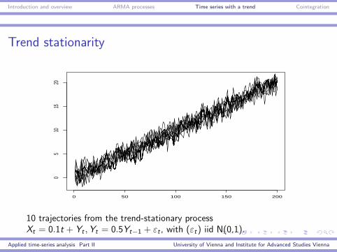
Trend stationarity

0 50 100 150 200

05

1015

20

10 trajectories from the trend-stationary processXt = 0.1t + Yt ,Yt = 0.5Yt−1 + εt , with (εt) iid N(0,1).



Difference stationarity

Time

0 50 100 150 200

050

100

10 trajectories from the integrated process ∆Xt = 0.5 + 0.5∆Xt−1 + εt ,with (εt) iid N(0,1).



Discrimination of trend and difference stationarity

Wrong transformations are no good. First differences oftrend-stationary processes are stationary but often non-invertible.Fitting trends to difference-stationary processes does not yieldstationary residuals.

How distinguish the two generating types of model?

1. Visual analysis (Box and Jenkins): compare residuals fromtrend fitting and differencing, prefer the transformation withsimpler ACF;

2. Unit-root tests (since 1979).

Warning: usual information criteria do not work for this decisionproblem.



Dickey-Fuller test DF-0: the idea

Assume the AR(1) model

Xt = φXt−1 + εt .

For the test problem with the null and alternative hypotheses

H0 : φ = 1, HA : φ ∈ (−1, 1),

one may consider the test statistic

DF0 =φ− 1

σ(φ),

where σ(φ) is the usual standard error of the coefficient from aregression output.



Properties of the DF-0 statistic

Under the null hypothesis φ = 1, the random walk, will thecoefficient estimate φ converge with great speed to the true valueφ = 1:

T (φ− 1) →

∫ 10 B(ω)dB(ω)∫ 10 B2(ω)dω

in distribution, with a non-standard limit law expressed in the formof integrals over functions of Brownian motion. Also the teststatistic DF0 has a related limit under H0:

DF0 →

∫ 10 B(ω)dB(ω)

(∫ 10 B2(ω)dω)0.5



Brownian motion

DefinitionBrownian motion or a Wiener process is a real-valued stochasticprocess (Xt) defined on T = [0, 1] satisfying

1. X0 = 0;

2. for any s1 ≤ t1 ≤ s2 ≤ t2 ≤ . . . ≤ tn, the random variablesXt1 − Xs1, . . . ,Xtn − Xsn are independent;

3. for any s < t, the r.v. Xt − Xs has a normal distribution withmean 0 and variance (t − s)σ2;

4. the paths (trajectories) are continuous.



The shape of Brownian motion

Time

x[1:10

0]

0 20 40 60 80 100

02

46

810

1214

Time

x[1:10

00]

0 200 400 600 800 1000

−50

510

1520

Time

x[1:10

000]

0 2000 4000 6000 8000 10000

050

100

150

Time

x[1:1e

+05]

0 e+00 2 e+04 4 e+04 6 e+04 8 e+04 1 e+05

−300

−200

−100

010

020

0

Identifying the sample end with ‘1’ and the start with ‘0’, generated random

walks with increasing T give an impression of Brownian motion that evolves for

T → ∞.



Problems with the DF-0 test

◮ The distributions of T (φ− 1) and of DF0 are non-standardunder the null: tabulated significance points must be used;

◮ neither the null of a pure random walk nor the alternative ofan AR(1) variable with zero mean are very interesting inpractice: deterministic terms must be added, and thesemodify the distributions;

◮ the null distribution is very sensitive to autocorrelation:higher-order models should be considered.



Dickey-Fuller test DF–µ

Assume the AR(1) model with a constant

Xt = µ+ φXt−1 + εt .

For the test problem with the null and alternative hypotheses

H0 : φ = 1, HA : φ ∈ (−1, 1),


DFµ =φ− 1

σ(φ),




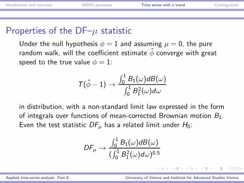
Properties of the DF–µ statistic

Under the null hypothesis φ = 1 and assuming µ = 0, the purerandom walk, will the coefficient estimate φ converge with greatspeed to the true value φ = 1:

T (φ− 1) →

∫ 10 B1(ω)dB(ω)∫ 10 B2

1 (ω)dω

in distribution, with a non-standard limit law expressed in the formof integrals over functions of mean-corrected Brownian motion B1.Even the test statistic DFµ has a related limit under H0:

DFµ →

∫ 10 B1(ω)dB(ω)

(∫ 10 B2

1 (ω)dω)0.5



Usage of the DF–µ test

The null hypothesis of a pure random walk and the alternative of astable AR(1) model with general mean can be interesting fornon-trending variables. They are still not representative of thedifference-stationary and trend-stationary models.



Dickey-Fuller test DF–τAssume the AR(1) model with a constant

Xt = µ+ τ t + φXt−1 + εt .

This model is equivalent to Xt = a + bt + Yt ,Yt = φYt−1 + εt .For the test problem with the null and alternative hypotheses

H0 : φ = 1, HA : φ ∈ (−1, 1),


DFτ =φ− 1

σ(φ),




Properties of the DF–τ statistic

Under the null hypothesis φ = 1 and assuming τ = 0, thepotentially drifting random walk, will the coefficient estimate φconverge with great speed to the true value φ = 1:

T (φ− 1) →

∫ 10 B2(ω)dB(ω)∫ 10 B2

2 (ω)dω

in distribution, with a non-standard limit law expressed in the formof integrals over functions of trend-corrected Brownian motion B2.Even the test statistic DFτ has a related limit under H0:

DFτ →

∫ 10 B2(ω)dB(ω)

(∫ 10 B2

2 (ω)dω)0.5



Trend-corrected Brownian motion

0 20 40 60 80 100

−20

24

0 200 400 600 800 1000

−30

−20

−10

010

20

0 2000 4000 6000 8000 10000

−40

−20

020

40

0e+00 2e+04 4e+04 6e+04 8e+04 1e+05

−200

−100

010

020

0

Approximating de-trended Brownian motion by random walks with extracted

linear time trends and increasing T .



Handling autocorrelation by augmenting

All DF tests (DF–µ and DF–τ) are sensitive to autocorrelation ofut in the basic regression Xt = dt + φXt−1 + ut or its equivalentform

∆Xt = dt + ϕXt−1 + ut .

This autocorrelation invalidates the asymptotic distribution. Aremedy is adding lags of ∆Xt as regressors, such that errors arenow approximately white noise:

∆Xt = dt + ϕXt−1 +

p−1∑

j=1

ψj∆Xt−j + ut .

Statistics such as tϕ will again have the DF distributions.



Why use lagged differences for augmentation?

◮ Lagged differences are stationary both under H0 and HA;

◮ any autoregression Xt =∑p

j=1 φjXt−j + εt can be transformed

to the model ∆Xt = ϕXt−1 +∑p−1

j=1 ψj∆Xt−j + εt ;

◮ ϕ = 0 iff there is a unit root in the characteristic polynomialΦ(z).



How find the augmenting lag order?

Two recommended suggestions:

1. Fit autoregressive models with appropriate deterministic termsto the data, choose the one (p) with lowest AIC (or BIC). Usep − 1 lags for the differences ∆Xt ;

2. determine p as a (slowly increasing) function of the samplesize.

It is not recommended to use different lag selection procedures,such as portmanteau (Q) tests on residuals.



Alternative unit-root tests

Three types of alternative tests deserve attention:

1. Phillips-Perron test is a variant of the DF test, with thesame asymptotic distribution and no recognizable differencesin general performance;

2. various modifications of the DF test are available, some ofthem with power advantages (Elliot, Rothenberg,

Stock);

3. the KPSS (Kwiatkowski, Phillips, Schmidt, Shin) testuses I(0) as the null and I(1) as the alternative: generally lessreliable than DF test, interesting additional tool.



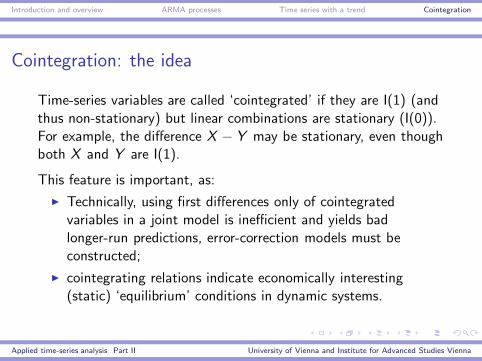
Cointegration: the idea

Time-series variables are called ‘cointegrated’ if they are I(1) (andthus non-stationary) but linear combinations are stationary (I(0)).For example, the difference X − Y may be stationary, even thoughboth X and Y are I(1).

This feature is important, as:

◮ Technically, using first differences only of cointegratedvariables in a joint model is inefficient and yields badlonger-run predictions, error-correction models must beconstructed;

◮ cointegrating relations indicate economically interesting(static) ‘equilibrium’ conditions in dynamic systems.



A prototypical example: consumption and income

1975 1980 1985 1990 1995 2000 2005

4.44.6

4.85.0

Austrian private consumption and disposable income for the years 1976–2009,

in logarithms. Series are trending but difference remains roughly constant.



A definition for cointegration of two series

DefinitionIf two processes Xt , Yt are each ARIMA(p, 1, q) and if there existsa linear combination Zt = β1Xt + β2Yt with β1 6= 0 and β2 6= 0such that Zt is stationary, then Xt and Yt are called cointegrated,and (β1, β2)

′ is called the cointegrating vector.

Remark. The definition can be extended to I(1) processes, whichare slightly more general than ARIMA(p, 1, q).

Example. For consumption and income in logarithms, β = (1,−1)′

could be the cointegrating vector. For a version withoutlogarithms, β = (1,−0.9)′ may be the cointegrating vector.



The general definition for n variables

DefinitionGiven an n–dimensional vector process Xt = (X1t , . . . ,Xnt)

′,suppose that ∆Xt = (∆X1t , . . . ,∆Xnt)

′ is stationary, whereas atleast one component Xjt is I (1), and that a linear combinationwith at least one βk 6= 0

Zt = β1X1t + . . .+ βnXnt = (β1, . . . , βn)′Xt

is stationary (or I (0)). Then, Xt is called cointegrated, in symbolsCI (1, 1), and the vector β is a cointegrating vector.



Another empirical example: interest rates

Clive Granger and Heather Anderson considered 11interest rates with terms to maturity of one to eleven months.They showed these are all cointegrated and individually I(1).X (j) − X (k) are stationary for any pairs of maturities j , k . Allvectors of the form (0, 0, 1, 0, 0,−1, 0, . . .)′ are cointegratingvectors.

Remark. A deeper problem is whether we can accept that interestrates are I(1).



Procedures for estimating and testing cointegration

For the two main tasks, i.e. for statistical decisions oncointegration and estimating cointegrating vectors, there exist twoclasses of methods:

1. Methods based on the cointegrating regression (simple andinefficient EG–2step, and other techniques, some of themefficient);

2. Methods based on system estimation (VAR-based method ofJohansen and others: efficient procedures).

EG–2 and Johansen’s VAR method are by far the most popularestimation and inference procedures.



Engle-Granger two-step method

The EG–2 method is the most popular single-equation method forestimating and testing cointegration. It involves inefficient andefficient components.

It is called EG–2step, as it has two steps:

1. A cointegrating regression: an I(1) variable Y is regressed onother I(1) variables X1, . . . ,Xk . If Y and some of the Xj

cointegrate, residuals should be nearly I(0). Unit-root tests onresiduals should reject unit roots.

2. An error-correction model: first differences ∆Yt are regressedon lags of first differences ∆Yt−l and ∆Xj ,t−l and on theresiduals from step 1.



The cointegrating regression

If (Y ,X1, . . . ,Xk)′ cointegrate with cointegrating vector

(β∗0 , β∗

1 , . . . , β∗

k)′ and β∗0 6= 0 and at least one of the β∗j 6= 0 for

j = 1, . . . , k , then the coefficient estimates in the regression

Yt = µ+ β1X1,t + . . .+ βkXk,t + ut

converge to βj = −β∗j /β∗

0 fast, in the sense that T (βj − βj ) → D

for some distribution D. Even for the true values, the residuals aretypically not white noise.



Testing for cointegration using residuals

If ut is I(1), the ‘cointegrating’ regression is not balanced. Themost customary test is an (augmented) DF test on the residuals ut .

◮ If the DF test on ut accepts its null, Y and (X1, . . . ,Xk)′ do

not cointegrate. Abandon the project.

◮ If the DF test on ut rejects, Y and (X1, . . . ,Xk)′ cointegrate.

Proceed to next step.

Warning: The null distribution of this DF test is not the usualtabulated DF distribution, automatic significance points are invalid.Quantiles were tabulated first by Phillips and Ouliaris.



Modelling following the cointegrating regression

If ut really cointegrates,

ut = Yt − µ− β1X1,t − . . . − βkXk,t

estimates the disequilibrium term. The full description of thedynamic behavior of Y follows from the error-correction model

∆Yt = µ0 + αut−1 +

p∑

j=1

γ0,j∆Yt−j +

k∑

l=1

pl∑

j=1

γl ,j∆Xl ,t−j + εt ,

where lag orders p,pl are set such that εt is white noise.



Example: consumption and income

Suppose we think that consumption C and income Y arecointegrated.

1. Run DF tests on C and Y : both should be I(1);

2. Regress C on Y : yields residuals u;

3. Run DF tests on u: use quantiles from Phillips and

Ouliaris: should be I(0);

4. Regress ∆Ct on ut−1 and on lags of ∆Ct and of ∆Yt .

5. Complete the model by regressing ∆Yt on ut−1 and on lags of∆Ct , ∆Yt .



Problems of the EG–2 procedure

1. EG–2 is not efficient in the statistical sense;

2. EG–2 requires that the dependent variable Y and at leastsome of the explanatory variables are I(1): requires pre-testing;

3. EG–2 fails if Y is not cointegrated with X1, . . . ,Xn but theexplanatory variables are cointegrated among themselves.

4. By construction, EG–2 expresses a causal direction fromX1, . . . ,Xn to Y . This does not correspond to thecointegration concept, where all variables are jointlyendogenous.



Johansen’s system estimation

Johansen’s procedure is the most popular efficient procedure forestimating and testing in cointegrating models. It builds on vectorautoregressions (VAR).

The Johansen procedure may be interpreted as a multivariateDickey-Fuller test.



Multivariate Dickey-Fuller models

Any vector autoregression

Xt = µ+Φ1Xt−1 + . . .+ΦpXt−p + εt

can be re-written as

∆Xt = µ+ ΠXt−1 +Ψ1∆Xt−1 + . . . +Ψp−1∆Xt−p+1 + εt ,

with identical errors and a one-to-one correspondence betweenparameters in both forms.



The long-run impact matrix Π

O.c.s. that, if X = (X1, . . . ,Xn)′ is cointegrated, then Π in

∆Xt = µ+ ΠXt−1 +Ψ1∆Xt−1 + . . . +Ψp−1∆Xt−p+1 + εt ,

is singular and can be represented as

Π = αβ′,

with (n × r)–matrices α, β of rank r . The r columns of β arecointegrating vectors. These are not unique, any linearcombination will do.



Loading coefficients α

The cointegrating vectors in β describe equilibrium relations. Thecoefficients in α describe how the variables react to deviationsfrom equilibrium. Typically, deviations tend to be corrected: errorcorrection. β sets the target, α does the work.

The coefficients in α are called loading coefficients or adjustment

coefficients.



Johansen procedure step by step

The procedure uses the following steps:

1. All variables Xj , j = 1, . . . , n should be either I(1) or I(0);

2. Determine the VAR lag order p: multivariate informationcriteria;

3. Determine the cointegrating rank r by sequences ofhypothesis tests: estimate β;

4. Estimate the full EC-VAR model given p and r to estimate αand all Ψj .



The test sequence

In order to determine the ‘cointegrating’ rank of Π, use thesequence:

1. Test for H00 : r = 0 versus H0A : r > 0; if accepted stop: nocointegration;

2. Test for H10 : r ≤ 1 versus H1A : r > 1; if accepted stop:r = 1;

3. etc. until Hn−1,0 : r ≤ n − 1 versus Hn−1,A : r = n; if rejectedbe surprised: the system is stationary.

Most authors prefer this testing ‘up’ to testing ‘down’.



The mathematical principle behind the scene

The Johansen procedure builds on canonical correlations betweenthe n variables in X and in ∆X . If a linear relationship betweenthe stationary ∆X and a linear combination of the integrated X isstrong, this combination is a cointegrating vector.

Canonical correlation problems are solved by eigenvector andeigenvalue analysis. Eigenvectors corresponding to non-zeroeigenvalues are cointegrating vectors.



Deterministic terms in the Johansen procedure

Multivariate unit-root tests are affected by the presence ofintercepts, trends. There are many combinations, only two arereally relevant:

1. If some variables are trending, use the standard model with anunrestricted intercept: do not include trends;

2. If no variable is trending, use the model with restrictedintercept

∆Xt = α(µ∗+βXt−1)+Ψ1∆Xt−1+ . . .+Ψp−1∆Xt−p+1+εt .

The two versions have separate tables of significance points.



Example: consumption and income

If C and Y cointegrate, the rank r should be 1. The system canbe written as

[

∆Ct

∆Yt

]

=

[

µ1µ2

]

+

[

α1

α2

]

[1,−1]

[

Ct−1

Yt−1

]

+

[

Ψ11 Ψ12

Ψ21 Ψ22

] [

∆Ct−1

∆Yt−1

]

+

[

ε1,tε2,t

]

α1 < 0 corrects previous over- or under-consumption by changingC . α2 is often small. Ψ describes short-run fluctuations and inertiaof consumer behavior.


Applied time-series analysis Part II - univie.ac.athomepage.univie.ac.at/robert.kunst/tspres2.pdf · Applied time-series analysis Part II Robert M. Kunst [email protected]

Documents