260 0 0 NATIONAL COOPERATIVE HIGHWAY RESEARCH PROGRAM REPORT 260 APPLICATION OF STATEWIDE FREIGHT DEMAND FORECASTING TECHNIQUES 0 TRANSPORTATION RESEARCH BOARD NATIONAL RESEARCH COUNCIL

Welcome message from author
This document is posted to help you gain knowledge. Please leave a comment to let me know what you think about it! Share it to your friends and learn new things together.
Transcript
260 0
0
NATIONAL COOPERATIVE HIGHWAY RESEARCH PROGRAM REPORT 260
APPLICATION OF STATEWIDE FREIGHT DEMAND
FORECASTING TECHNIQUES 0
TRANSPORTATION RESEARCH BOARD NATIONAL RESEARCH COUNCIL
TRANSPORTATION RESEARCH BOARD EXECUTIVE COMMITTEE 1983
Officers
Chairman
LAWRENCE D. DARMS, Executive Director. Metropolitan Transportation Commission, Berkeley, California Vice Chairman RICHARD S. PAGE, President; The Washington Roundtable, Seattle, Washington
THOMAS B. DEEN, Executive Director, Transportation Research Board Members
RAY A. BARNHART, Federal Highway Administrator, US Department of Transportation (cx officio) FRANCIS B. FRANCOIS, Executive Director, American Association of State Highway and Transportation Officials (cx officio) WILLIAM J. HARRIS, JR., Vice President for Research and Test Department, Association of American Railroads (cx officio) J. LYNN HELMS, Federal Aviation Administrator, U.S Department of Transportation (cx officio) THOMAS D. LARSON, Secretary of Transportation, Pennsylvania Department of Transportation (cx officio, Past Chairman 1981) DARRELL V MANNING, Director, Idaho Transportation Department (cx officio, Past Chairman 1982) DIANE STEED, National Highway Traffic Safety Administrator, U.S Department of Transportation (cx officio) RALPH STANLEY, Urban Mast Transportation Administrator, US Department of Transportation (cx officio) DUANE BERENTSON, Secretary, Washington State Department of Transportation JOHN R. BORCHERT, Professor, Department of Geography. University of Minnesota ARTHUR I. BRUEN, JR., Vice President. Continental Illinois National Bank and Trust Company of Chicago JOSEPH M. CLAPP, Senior Vice President; Roadway Express; Inc JOHN A. CLEMEN'I'S, Commissioner, New Hajnpshire Department of Public Works and Highways ERNEST A. DEAN, Executive Director, Dallas/Fort Worth Airport ALAN G. DUSTIN, President and Chief Executive Officer. Boston and Maine Corporation ROBERT E. FARRIS, Commissioner, Tennessee Department of Transportation JACK R. GILSTRAP, Executive Vice President; American Public Transit Association MARK G. GOODE, Engineer-Director, Texas State Department of Highways and Public Transportation LESTER A. HOEL, Chairman, Department of Civil Engineering, University of Virginia LOWELL B. JACKSON, Secretary, Wisconsin Department of Transportation MARVIN L. MANHEIM, Professor, Department of Civil Engineering, Northwestern University FUJIO MATSUDA, President; University of HawaII JAMES K. MITCHELL, Professor and Chairman, Dept. of Civil Engineering, University of California DANIEL T. MURPHY, County Executive, Oakland County Courthouse, Michigan ROLAND A. OUELLETFE, Director of Transportation Affairs; General Motors Corporation MILTON PIKARSKY, Director of Transportation Research, IllinoLi Institute of Technology WALTER W. SIMPSON, Vice President-Engineering, Southern Railway System, Norfolk Southern Corporation JOHN E. STEINER, Vice President, Corporate Product Development, The Boeing Company RICHARD A. WARD, Director-Chief Engineer, Oklahoma Department of Transportation
NATIONAL COOPERATIVE HIGHWAY RESEARCH PROGRAM
Transportation Research Boon! Executive Committee Subcommittee for NCHRP
LAWRENCE D. DAHMS, Metropolitan Transp, Comm.. Berkeley. Calif (Chairman) RICHARD S. PAGE, The Washington Roundtable FRANCIS B. FRANCOIS, Amer. Axsn, of State Hwy. & Transp. Officials
Field of Special Peojectt Project PaneL SP20-17A
NAT SIMONS, JR., Consultant, Columbus; Ohio (Chairman) WILLIAM R. BROOKS, Federal Railroad Administration JOHN F. CONRAD, Washington Dept. of Transp. Hwy. Administration DAVID J. DEBOER, Southern Pacific Transportation Co. DAVID GOE'rI'EE, National Hwy, Transp. Safety Administration PAUL 0. ROBERTS, Roberts As,wciates
Program Staff
KRIEGER W. HENDERSON, JR., Director. Cooperative Research Fvgrams LOUIS M. Ms;CGREGOR, Administrative Engineer CRAWFORD F. JENCKS, Projects Engineer R. IAN KINGHAM, Projects Engineer
RAY A. BARNHART, US Dept. of Transp. THOMAS D. LARSON, Pennsylvania Dept. of Trans. THOMAS B. DEEN, Transportation Research Boon!
ISAAC SHAFRAN Maryland Dept. of Transportation RICHARD K. TAUBE, Consultant; Alexandria, Va, WILLIAM A. TIPPIN, Peat, Marwick, Mitchell Co. DONALD G. WARD, Iowa Dept. of Transportation PHILIP I. HAZEN, Federal Highway Administration EDWARD J. WARD, Transportation Research Boon!
ROBERT J. REILLY, Projects Engineer HARRY A. SMITH, Projects Engineer ROBERT B. SPICHER, Projects Engineer HELEN MACK, Editor
NATIONAL COOPERATIVE HIGHWAY RESEARCH PROGRA
REPORT 260,
APPLICATION OF STATEWIDE FREIGHT DEMAND
FORECASTING TECHNIQUES
FREDERICK W. MEMMOTT Roger Crelghton Associates, Inc.
Delmar, New York
RESEARCH SPONSORED BY THE AMERICAN ASSOCIATION OF STATE HIGHWAY AND TRANSPORTATION OFFICIALS IN COOPERATION WITH THE FEDERAL HIGHWAY ADMINISTRATION
AREAS OF INTEREST:
PLANNING FORECASTING SOCIOECONOMICS USER NEEDS (HIGHWAY TRANSPORTATION) (RAIL TRANSPORTATION) -
TRANSPORTATION RESEARCH BOARD NATIONAL RESEARCH COUNCIL WASHINGTON, D.C. SEPTEMBER 1983
NATIONAL COOPERATIVE HIGHWAY RESEARCH PROGRAM
Systematic, well-designed research provides the most effec-tive approach to the solution of many problems facing high-way administrators and engineers. Often, highway problems are of local interest and can best be studied by highway departments individually or in cooperation with their state universities and others. However, the accelerating growth of highway transportation develops increasingly complex prob-lems of wide interest to highway authorities. These problems are best studied through a coordinated program of coopera-tive research.
In recognition of these needs, the highway administrators of the American Association of State Highway and Transporta-tion Officials in 1962 an objective national highway research program employing modern scientific techniques. This pro-gram is supported on a continuing basis by funds from partic-ipating member states of the-Association and it receives the full cooperation and support of the Federal Highway Admin-istration, United States Department of Transportation.
The Transportation Research Board of the National Re-search Council was requested by the Association to admin-ister the research program because of the Board's recognized objectivity and understanding of modern research practices. The Board is uniquely suited for this purpose as: it maintains an extensive committee structure from which authorities on any highway transportation subject may be drawn; it pos-sesses avenues of communications and cooperation with federal, state, and local governmental agencies, universities, and industry: its relationship to its parent organization, the National Academy of Sciences, a private, nonprofit institu-tion, is an insurance of objectivity; it maintains a full-time research correlation staff of specialists in highway transpor-tation matters to bring the findings of research directly to those who are in a position to use them.
The program is developed on the basis of research needs identified by chief administrators of the highway and trans-portation departments and by committees of AASHTO. Each year, specific areas of research needs to be included in the program are proposed to the Academy and the Board by the American Association of State Highway and Transporta-tion Officials. Research projects to fulfill these needs are defined by the Board, and qualified research agencies are selected from those that have submitted proposals. Adminis-tration and surveillance of research contracts are the re-sponsibilities of the Academy and its Transportation Re-search Board. The needs for highway research are many, and the National Cooperative Highway Research Program can make signifi-cant contributions to the solution of highway transportation problems of mutual concern to many responsible groups. The program, however, is intended to complement rather than to substitute for or duplicate other highway research programs.
NCHRP REPORT 260
Project 20-1A FY'81
ISSN 0077-5614
ISBN 0-309-03601-1
L. C. Catalog Card No. 83-50215
Price: $12.80
NOTICE
The project that is the subject of this report was a part of the National Co-operative Highway Research Program conducted by the Transportation Research Board with the approval of the Governing Board of the National Research Council, acting in behalf of the National Academy of Sciences. Such approval reflects the Governing Board's judgment that the program concerned is of national importance and appropriate with respect to both the purposes and resources of the National Research Council. The members of the technical committee selected to monitor this project and to review this report were chosen for recognized scholarly competence and with due consideration for the balance of disciplines appropriate to the project. The opinions and conclusions expressed or implied are those of the research agency that performed the research, and, while they have been accepted as appropriate by the technical committee, they are not necessarily those of the Transporta-tion Research Board, the National Research Council, the National Academy of Sciences, or the program sponsors. Each report is reviewed and processed according to procedures established and monitored by the Report Review Committee of the National Academy of Sci-ences. Distribution of the report is approved by the President of the Academy upon satisfactory completion of the review process. The National Research Council was established by the National Academy of Sciences in 1916 to associate the broad community of science and technology with the Academy's purposes of furthering knowledge and of advising the Federal Government. The Council operates in accordance with general poli-cies determined by the Academy under the authority of its congressional charter of 1863, which establishes the Academy as a pnvate, nonprofit, self-governing membership corporation. The Council has become the principal operating agency of both the National Academy of Sciences and the National Academy of Engineering in the conduct of their services to the government, the public, and the scientific and engineering communities. It is administered jointly by both Academies and the Institute of Medicine. The National Acad- emy of Engineering and the Institute of Medicine were established in 1964 and 1970. respectively, under the charter of the National Academy of Sciences. The Transportation Research Board evolved from the 54-year-old Highway Research Board. The TRB incorporates all former HRB activities and also performs additional functions under a broader scope involving all modes of transportation and the interactions of transportation with society.
Special Notice
The Transportation Research Board, the National Academy of Sciences, the Federal Highway Administration, the American Association of State Highway and Transportation Officials, and the individual states participating in the National Cooperative Highway Research Program do not endorse products or manufacturers. Trade or manufacturers' names appear herein solely because they are considered essential to the object of this report.
Published reports of the
NATIONAL COOPERATIVE HIGHWAY RESEARCH PROGRAM
are available from:
Transportation Research Board National Academy of Sciences 2101 Constitution Avenue, N.W. Washington, D.C. 20418
Prinied in the tJniied States of Amenca.
FOREWORD This report will be most useful to states that undertake freight planning activities on a recurring basis and will be of special interest to state and regional planners
By Staff having responsibility for the analysis of freight transportation services. Most freight Transportation planning techniques developed in the past have been designed for national or regional
Research Board analyses; therefore, this research was initiated to modify, demonstrate, and document those techniques for state-level applications. The methodology presented herein is based on actual studies conducted in various states, thus ensuring a practical approach for addressing typical freight transportation issues. This report along with NCHRP Report 177 and NCHRP Report 178, which document freight data requirements, provide a comprehensive reference and guide for state freight planning studies.
Participants at the TRB Conference on Statewide Transportation Planning, held on February 21-24, 1974, identified a critical research need for the development of better planning techniques and data sources for statewide freight planning activities. Shortly after the Conference, NCHRP Project 8-17 was initiated to assess and doc-ument freight data requirements, and the results were published in 1977 as NCHRP Report 177 and NCHRP Report 178.
Attention then turned from data needs to the development of improved planning techniques that, would have general applicability. While several freight forecasting techniques were available, they either were too data intensive for general use or were too oriented to national-level analyses for application at the state level. NCHRP Project 20-17 was conducted to identify and specify multiregional and state freight demand forecasting techniques that could be applied using readily available data. Based on this research, conducted by Cambridge Systematics, Inc., Project 20-17A was initiated to develop a generalized technique for use by state transportation agencies.
Roger Creighton Associates, Inc., had completed freight planning studies for several states just prior to the initiation of Project 20-1 7A. Drawing on that experience, as well as their work on NCHRP Project 8-17, the research team developed a systematic approach for other states to follow in conducting similar analyses.
The resulting freight demand forecasting technique represents a compromise between specificity and flexibility. Even though a highly structured, step-by-step tech-nique initially seemed like an ideal objective, the need to be responsive to widely different applications and varying data resources dictated a more generalized process than was originally envisioned. However, the general nature of the overall technique is offset by the specificity of its individual components. For example, a truck costing model was developed as part of this research providing a new analysis tool for freight planning studies.
The technique requires the transportation planner to (1) define the problem, (2) structure the technique to address that problem, and (3) simplify and adapt both the problem and the technique to produce results within applicable fiscal, time, and data

resource constraints. Following these three preliminary steps, the analysis is completed using the customized freight demand forecasting technique. The technique will be straightforward to most state transportation planners, but it does require some ex-perience with and background knowledge of freight transport. Familiarity with urban and statewide tranportation planning processes is also helpful because the technique follows, the traditional analysIs sequence— freight generation, freight distribution, mode split, and traffic assignment.
The technique can be used to (1) develop current or future estimates of freight flows by highway, rail, and water; (2) forecast freight volume shifts among modes; and (3) provide origins and destinations by commodity within a corridor or region at the sub-state, state, or multi-state level. A user manual is provided, supplemented by three case examples illustrating the usefulness of the method in addressing state-level problems. Each example describes in considerable detail how the technique was applied to the particular problem. While some data came from national data sets, most 'were obtained from state or local sources and represent the kinds of secondary data generally available.
Developing the capability to conduct effective freight planning activities is a new and difficult challenge for many states. Having trained and experienced personnel, becoming knowledgeable with this and other freight planning techniques, developing a state-level data base of commodity or vehicle flows, rates, and costs, and keeping abreast of the changes taking place both with the state's economy and the transport industry in general are all major parts of this challenge. While a substantial corn-mitment of time and resources is required, the type of freight-planning decisions and issues confronting state governments dictates the need for comprehensive and objective analyses. It is expected that the results of this research will be of value in conducting these analyses.
CONTENTS
SUMMARY
PART I
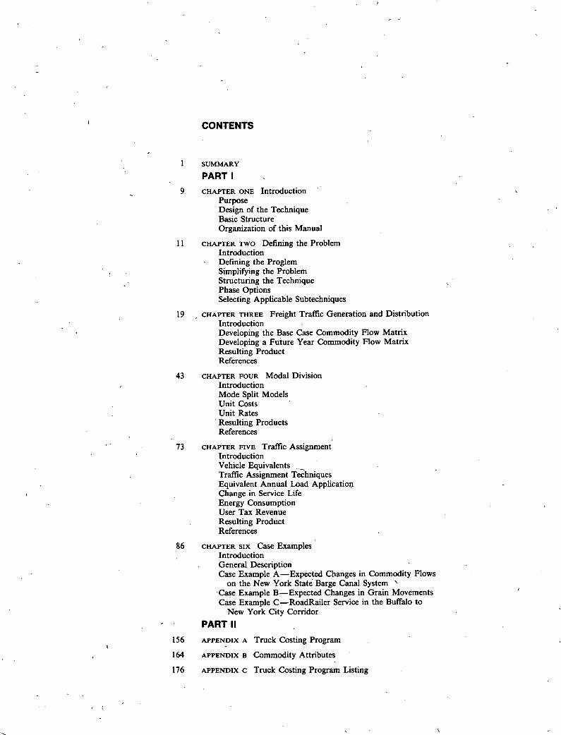
9 CHAPTER ONE Introduction Purpose Design of the Technique Basic Structure Organization of this Manual
11 CHAPTER TWO Defining the Problem Introduction Defming the Proglem Simplifying the Problem Structuring the Technique Phase Options Selecting Applicable Subtechniques
19 CHAPTER THREE Freight• Traffic Generation and Distribution Introduction Developing the Base Case Commodity Flow Matrix Developing a Future Year Commodity Flow Matrix Resulting Product References
43 CHAPTER FOUR Modal Division Introduction Mode Split Models Unit Costs Unit Rates Resulting Products References
73 CHAPTER FIVE Traffic Assignment Introduction Vehicle Equivalents Traffic Assignment Techniques Equivalent Annual Load Applicatiop Change in Service Life Energy Consumption User Tax Revenue Resulting Product References
86 CHAPTER SIX Case Examples Introduction General Description Case Example A—Expected Changes in Commodity Flows
on the New York State Barge Canal System ' Case Example B—Expected Changes in Grain Movements Case Example C—RoadRailer Service in the Buffalo to
New York City Corridor PARTII
156 APPENDIX A Truck Costing Program
164 APPENDIX B Commodity Attributes
176 APPENDIX C Truck Costing Program Listing

ACKNOWLEDGMENTS
The research reported herein was performed under NCHRP Project 20-17A by Roger Creighton Associates, Inc. Mr. Frederick W. Mem-mott, vice president of RCAI, was the principal investigator. Other contributors to the study were Mr. Daniel Gealt, Transportation Plan-ner, Mr. Russell H. Boekenkroeger, Jr., Senior Transportation Planner, Mr. George J. LaRue, Transportation Planner, and Mr. Roger L. Creighton, president, all of RCAI. (Mr. Boekenkroeger and Mr. LaRue are now with Computervision, Inc., and Wang Laboratories, Inc., respectively.)
APPLICATION OF STATEWIDE FREIGHT DEMAND FORECASTING TECHNIQUES
SUMMARY This report was prepared at atime when major changes were taking place in the transport industry. A recessionary economy combined with rail and motor carrier deregulation had led to (1) greatly intensified competition among car-riers, stemming in part from increased pricing and market entry freedom; (2) a proliferation of new, customized services, including carrier ability to tailor services and rates to closely meet the needs of individual shippers; (3) deteri-oration in the economic health of many long-established common carriers; and (4) less information being available to the public sector (i.e., through the regula-tory process) with which to'plan or monitor changes taking place in the supply of, demand for, and the price and quality of transport services being offered.
Despite the thrust of deregulation, the purpose of which was to lessen gov-ernment intervention and involvement in freight transport, it appears that state interest in freight-related matters is increasing. Although driven in part by interest sparked by light density rail line abandonments and highway maintenance problems accentuated by-the use of longer, heavier trucks, the underlying moti-vations are broader. State DOTs are increasingly accepting the idea that their responsibilities are not solely confined to the state highway system, but in-chide the larger arena of freight transport services being provided by the dif-ferent modes. States are recognizing the need for better management and coordi-nation of transport resources -- and, hence, the need for better freight plan-ning -- irrespective of whether the infrastructure and services are provided by the public or private sectors.
Given the largely private character of freight transport, planning undertak-en by state DOTs is far different from that associated with making physical im-provements to the state highway system. In freight planning, the emphasis is on early identification and resolution of problems. It involves working with the carriers to ensure that no economic sector, group, or substate area will be Se-ri'ously disadvantaged through changes in the type and cost of services being of-fered. It is not primarily capital oriented, although it may involve state in-vestment in facilities or equipment. Occasionally, it might involve subsidies to retain essential services.
Past Efforts to Address the Problem
Prior to the commencement of this research project, a number of state DOTs had begun to conduct studies requiring, freight demnd forecasts to address vari-ous freight-related issues and problems. These were relatively new activities for many state DOTs; in the past, their concerns had focused primarily on highs way transportation and particularly on planning for capital facilities.
Over the years, state DOT ability to carry out freight-oriented studies has been adversely affected by (1) a lack of freight-flow data at the national and state levels in a form that could, readily be used for forecasting purposes and (2) a lack of readily available freight demand forecasting techniques that states could directly apply. Given the paucity of appropriate data and analysis techniques, states felt that they were not able to address adequately emerging problems such as the impacts of deregulation, shifts in the economic base of an area brought about by transportation system changes, anticipated changes in transport rate structures, energy availability and price changes, service chan- ges, and so forth. Although techniques and data bases had been developed by others, they had not been widely applied by states nor had they been fully, tes- ted. Furthermore, most of the existing techniques and databases were not de- veloped for application at the state level and, therefore, required further adaptation to make them suitable for use by state DOTs.
Past and Current NCHRP Research
Initial work in freight planning is documented in NCHRP Reports 177 and 178, which focus on the freight data required for statewide transportation systems planning. NCHRP Report 177 provi-ded a detailed assessment of existing freight issues and identified the data required to apply related analysis techniques. The companion document, NCHRP Report 178, contained a user's manual presenting a detailed catalog of existing data sources, methods for obtaining missing data, and guidelines for data collection and management activities by state DOTs.
The first phase of NCHRP Project 20-17 identified freight transportation is-sues that need to be addressed by demand forecasting techniques and proposed a comprehensive research approach to develop a spectrum of such techniques. How-ever, because of limited funding, it was not possible to undertake the extensive development required to develop this capability. Instead, the scope of the cur-rent project (20-17A) was redefined to limit continuing work to the demonstra-tion of an existing technique for immediate application by states through the preparation of a user's manual supplemented by case study examples. Extensive development work was not envisioned; rather the technique was to be based on the -current state of the art. The specifications called for a technique which, at a minimum, would (1) develop- freight flows by highway, rail, and water for the current year; (2) forecast the likely annual freight. volumes and shifts among the modes over the short term (five years or less); and (3) provide origins and destinations by commodity within a corridor or region at the substate, state, or multistate level. The technique must use generally available data and methods, with modification if necessary, to facilitate application to specific problems. The end-product was to be a usable freight demand forecasting technique supple-mented by several case studies illustrating the application of the technique. Both the technique and the case examples were to be documented in a self-con-tained user's manual for general application at the state level.
Research Objective and Approach to Meet Changing State Needs and Data Resources
The objective of NCHRP project 20-17A is to demonstrate the applicability of a freight demand forecasting technique for direct use by state DOTs.
In pursuing this goal, it soon became apparent that the immediate action technique desired by states for freight demand forecasting purposes had to be adapted largely from similar. procedures being used for other purposes. Rela-tively little research work was currently being undertaken in developing freight demand techniques, nor were significant breakthroughs anticipated in the near future. Thus the technique was not expected to overcome the manifest limita-tions and constraints of present methodologies, but rather be a conduit for sup-plying information and relevant examples.
In spite of the findings and needs identified in NCHRP Reports 177 and 178, the data resources available to states for freight planning- purposes were found not to have improved much in recent years. Given the current federal focus on deregulation and decreasing governmental expenditures, it seems likely that the amount of secondary data to be made available to states through federal programs will decrease. This is in part offset by improving working relationships be- tween the public and private sectors, which in the past has often resulted in required data being made available to states from private sources -- hence, em-phasis in this project was shifted away from reliance on traditional, public sector, secondary data sources. / It also became apparent that the emerging problems identified earlier had not materialized to the degree originally expected. For example, deregulation does not seem to have resulted in any significant loss of common carrier service to smaller communities, nor has it placed shippers located therein at any great-er economic disadvantage than previously experienced. Likewise, spiraling ener-gy prices and shortages have abated as the worldwide demand for petroleum prod-ucts has slackened. This is not to suggest that freight problems per se have disappeared; rather that the character of the problems likely to be addressed by states In the near future differ from those identified in the research problem statement -- hence emphasis was placed on application flexibility.
It is important to recognize that these shifts in emphasis do not represent any major change to the research approach as originally laid out. They illus-trate the changing character of freight planning likely to be undertaken by state DOTs and the need for maximum flexibility and adaptability in the ensuing technique.
Results of the Research
The product of this research project is the freight demand forecasting tech-nique presented in the user's manual. This technique is designed to meet a wide range of potential freight-oriented planning needs, such as:
1. Addressing facility, service, or regulatory problems. 2.. Conducting project or program studies having a modal, facility, or com-
modity type orientation. Assessing state policies toward infrastructure investment, required serv-
ices, costs, and maintenance of competition. Preparing freight components of statewide master plans.
The overall technique is diyided into four phases: (1) freight generation, (2) freight distribution, (3) mode division, and (4) traffic assignment. The main inputs are present and future economic activities (base and forecast year vehicle or commodity flows) and present and future mode service, cost, and price (rate) characteristics for rail, truck, and inland waterway transport. In most
applications, the full technique need not be employed. Nor will all of the
identified inputs generally be required. A series of subtechniques, of which most have previously been used for freight planning purposes, represent the "building blocks" of the technique. In designing the technique, the researchers sought:
As much application flexibility as possible in view of the diverse freight issues and problems likely to be faced by states in the future.
Making the technique as user-oriented as possible. The technique will not become an integral part of statewide transportation planning unless the user readily comprehends and understands how the technique can be applied.
Adaptability to the varying amounts and quality of data available in dif-ferent applications. Although the lack of secondary freight flow data has been and will continue to be a perpetual problem, most applications can be undertaken readily if the planner (1) is resourceful in seeking out and adapting appropri-ate secondary data obtainable from government sources, carriers, and shippers and (2) structures the technique to meet the constraints imposed by available data resources. By allowing flexibility in data inputs, greater adaptability is provided to the planner in marrying the application and data resources.
The use of a structured approach incorporating the major independent var-iables affecting freight demand. The alternative was using direct forecasting techniques, which provide less flexibility. Such techniques focus only on a single aspect of the relationship between economic activity, mode choice, com-modity flows and cost and service factors.
The technique was applied to three applicability. The examples are: (1) the (2) the Montana Grain Subterminal Stu RoadRailer Service in the Buffalo to New examples are included in the user's manua
case examples to illustrate its general New York Barge Canal Marketing Study, , and (3) an informal examination of York City Corridor. The complete case
1 in Chaoter Six.
Findings
A pervasive finding of the NCHRP Project 20-1A research is the continuing immature and fragmented state of the art of freight planning. The present lack of freight demand forecasting techniques at the state level stems from numerous causes, among which are the following:
Until recently, a limited need.or desire by states to undertake freight-oriented studies.
State legislation and financial impediments to implementing transport policies or undertaking capital projects involving the nonhighway modes.
Unavailability of a freight data base, and the lack of interest in as-sembling such a data base in view of its potentially limited use.
The lack of understanding of the impact that changes in traffic on the rail or waterway systems have on highwaysystem truck traffic and especially on highway maintenance and capital investment needs.
There are other reasons why states have been reluctant to become involved in freight planning. One of the major ones is divided responsibility not only be-tween federal and state governments, but more so between government and private enterprise. Consequently, there remains a great deal of uncertainty as to the
proper role for state government in this field. Another reason is preoccupation with the modes and systems over which states have full control. Limited staff and fiscal resources also hinder involvement in areas beyond those of direct re-sponsibility.
The foregoing situation is slowly changing, however, as states become in-creasingly involved in issues relating to truck use of the state highway system. The advent of the 3R and 4R Acts several years ago gave a major impetus to freight planning for those states faced with substantial light density rail line abandonments. The alternatives to light density line retention in some cases meant increased heavy truck volumes on roads not capable of handling this added traffic without upgrading. Much of the interest generated in retaining the rail infrastructure remains, even though federal rail planning and project funds have recently diminished.
Although the freight demand forecasting technique will handle many potential applications, users should recognize that occasionally the scope of the intended issue or problem will be too broad (or narrow or specific), or the available da-ta too limited, to permit full use of the presented technique. While the tech-nique will make it somewhat easier for states tb tackle freight-oriented prob-lems, companion requirements include development of the data resources necessary to support the technique, and the mandate and motivation to address freight problems.
Present State Capabilities: Highway Mode. Even though states are largely responsible for the highway system, the development of forecasting techniques and data bases specifically dealing with truck movements over the highway system has been slow. In most states, the collection of truck traffic flow data, and the preparation of demand forecasts, is treated as an appendage to similar data collection and forecasting being done for passenger vehicles, rather than as a related, but separate, data set. Automobiles do comprise the large majority of vehicles in the traffic stream. This, coupled with the inability to easily sep-arate automobiles and trucks when using automatic traffic-counting equipment (and the consequent necessity to count and classify trucks manually), has miti-gated against developing separate data bases for trucks and automobiles. In most states, current and historical vehicle flow data by truck size (i.e., axle and wheel configuration, but not weight) is available from classification and volume counts taken on a periodic basis at sample locations. Data on truck gross and net vehicle weights, however, are usually not available except at a very limited number of locations, typically stations included within FHWA's biannual truck-weighing program. Up until recently, the field work involved in collecting truck weight data has been extremely labor intensive; states have not been re-ceptive to extending the truck weighing program beyond that mandated by the FHWA program due to doubts as to the cost effectiveness and value of such data in meeting their immediate capital program needs. Although such data provide in-formation on equivalent annual load applications, these data are usually not ex-tended to other highway segments. Thus information on vehicle loadings by high-way segment is generally not available for the system as a whole.
Many states have permanent weigh stations that are regularly used to weigh trucks for enforcement purposes. Usually, the weight data obtained are not re-tained in a form adaptable to statistical analysis and summarization. Although most states maintain manual records of the trucks weighed and citations issued, the researchers are not aware of any automation of the record-keeping process, such as using terminals tied into the state DOT's central computer. Nor are da-ta on the vehicle's origin or destination and type and weight of the commodities being carried usually collected. Inasmuch as the lack of data pertaining to truck movements is particularly crucial to developing a freight demand forecast-ing capability, one solution would be to install computer terminals to access the commodity flow and weight data being generated by an existing program, •even though the location of the weigh stations may not be ideal from a statistical standpoint. In doing so, there may be some institutional problems requiring resolution, such as the separation of administrative (data gathering) from en-forcement activities. Recognizing that the availability of adequate truck move-ment data is unlikely through government, carrier, or industry sources, because of the fragmentation of the motor carrier industry and the ubiquitous use of heavy trucks, the importance of capitalizing on existing data resources becomes quite apparent.
In most states, future truck volumes are forecast as a percentage of aggre-gate traffic volumes for both existing and proposed facilities. The truck per-centage typically applied to total traffic is usually determined from historical data rather than from any detailed examination of economic growth or projected truck movements. Thus, the forecasts made are prepared using trend extension forecasting techniques rather than by relating observed volumes with present economic activities and, then, preparing forecasts based on projections of eco-nomic activity. Consequently, state DOT personnel often do not consider the re-sulting forecasts to be very reliable.
Because the relationship between vehicle weight and pavement deterioration has not been well understood, states have in the past expressed only a limited interest in collecting and using vehicle weight data. Thus, truck weight data are typically not used in forecasting rehabilitation or maintenance needs, even though the volume and weight of heavy vehicles do affect pavement life. This appears to be changing, however, as states develop improved pavement management systems.
The limited capability for undertaking truck-oriented freight demand fore-casts stems more from the lack of a data base rather than from any inability to devise suitable truck traffic forecasting techniques. This will be rectified as state DOTs develop necessary data bases and forecasting techniques; the respon-sibility for doing this clearly rests with state DOTs.
Present State Capabilities: Nonhighway Modes. Most of the limitations listed previously also apply to the nonhighway modes. With perhaps the excep- tion of railroad branchline studies, states tend to develop data bases and tech-niques strictly on an' ad hoc basis. For nonhighway mode applications, states are largely dependent on secondary data obtained through federal agency programs or supplied directly by carriers or shippers. Development of a comprehensive data base for the nonhighway modes is likely to occur in only a few states. Other states will limit the freight data collection to (1) conducting special-ized surveys of particular activities (e.g., shippers' surveys in connection with branchline abandonments) or (2) assembling commodity flow information from secondary sources. When undertaking freight planning, most states will apply techniques developed by others, such as those being developed by this research project, rather than on developing forecasting techniques themselves.
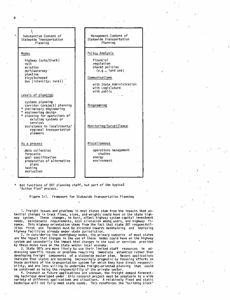
The Emerging Framework. The emerging framework for conducting and managing statewide transportation planning by state DOTs is diagrammed in Figure S-l. This shows statewide transportation planning' as being organized into two parts:
Substantive content -- that which deals with the different modes; their physical and service properties; the way people, vehicles, and freight move over different systems; how well they function; and how they can be improved.
Management content -- that which is concerned broadly with implementa-tion, from the setting of policy and communications to detailed programming of projects and the monitoring and surveillance of system performance.
The substantive content of statewide transportation' planning is a highly technical activity that in the past, has usually led to the publication and adoption of a comprehensive, long-range master plan. Most often, the prepara-tion of these plans was done by an organizational unit detached from the state DOT's day-to-day operations. This reflected the magnitude of the undertaking and the highly specialized character of the work involved.
However, in recent years, greater planning staff efforts have been directed by states towards the management rather than the substantive content of state- wide planning. While the management content does have its technical aspects, the emphasis is mainly on staff support of the DOT director or commissioner in policy-level decision-making and program monitoring and surveillance for the purpose of better managing the existing state transportation system. Technical work more often involves policy analysis, analysis of problems having a rela-tively limited scope, and communications (oral and written) rather than the preparation of a comprehensive, long-range master plan.
The framework shown in Figure S-1 contrasts with the older linear conception of statewide transportation planning that prevailed between 1965 and, say, the mid-1970s. Under that concept the dominating idea was to produce a good techni- cal plan, whether for one mode or all modes, and then to implement that plan. The then prevailing concept was that in order for the plan to be good, it had to be comprehensive' and be developed on a systems basis. The latter was a carry-over of the urban area 3-C process applied'at the statewide level. Implementa-tion, programming, and communication came after the technical work, and were treated by planners as components of plan implementation.
The new framework treats the management content of statewide transportation planning as being at least an equal partner. In many states, it will dominate. This framework recognizes that the day-to-day work of policy planning, communi-cations, programming, monitoring, and surveillance are integral parts of plan-' fling processes and perhaps the most important emphasis areas during the 1980s. Furthermore, it r,ecognizes that states are already acting along these lines, and staff assignments are less likely to be geared towards producing older style comprehensive master plans than they are to providing direct support to' the DOT director.
Implications Relative to Freight Planning. The implications arising from emerging changes in the substance and content of statewide transportation sys-tems planning vis-a-vis freight planning are these:
Substantive Content of Statewide Transportation
Planning
Modes
highway (auto/truck) rail aviation po't/waterway pipeline bicycle/moped bus (intercity; rural)
Levels of planning:
systems planning corridor (project) planning
* preliminary engineering * engineering design * planning for operations of
existing systems or services
assistance to local/county/ regional transportation planners
As a process
data collection forecasts goal specification preparation of alternative
plans testing evaluation
Management Content of Statewide Transportation
Planning
Policy Analysis
financial regulation shared policies (e.g., land use)
Comunicati ons
with State Administration with Legislature with public
Programming
Moni tori ng/Survei 11 ance
Miscellaneous
operations management studies
energy environment
6
* Not functions of DOT planning staff, but part of the typical Action Plan" process.
Figure S-l. Framework for Statewide Transportation Planning
'-I
Freight issues and problems in most states stem from the impacts that po-tential changes in truck flows, sizes, and weights could have on the state high- way system. These changes, in turn, affect highway system capital investment needs, maintenance requirements, cost allocation among users, and highway fi-nance. This highway orientation stems from the fact that state DOT responsibil-ities first and foremost must be directed towards maintaining and improving highway facilities already under state jurisdiction.
In considering the nonhighway modes, the primary concerns of most states are the impact that changes in the use of these modes could have on the highway system and secondarily the impact that changes in the cost or services provided by these modes have on the state and/or local economy.
State DOTs are more likely to use their limited staff resources in ad-dressing specific issues or problems requiring immediate attention rather than developing freight components of a statewide master plan. Recent applications indicate that states are becoming increasingly pragmatic by focusing efforts on those portions of the transportation system for which they have direct responsi-bility, and are less willing to undertake freight-oriented planning that could be construed as being the responsibility of the private sector.
Inasmuch as future applications are unknown, the freight demand forecast-ing technique developed under this research project must be adaptable to a wide variety of different applications and situations. A relatively fixed and static technique will not fully meet state needs. This reinforces the "building block"
approach used whereby components can be assembled and used on an as-needed ba- sis. Many applications do not require demand forecasts in a traditional sense, but rather involve comparisons between proposed alternatives and a base condi- tion or case. Frequently, the question to be answered is 'What would happen if...?"
Even if a forecast is desired, usually it is for a relatively short time period. Sophisticated forecasting techniques per se are really not required, because the limiting factor is the ability to forecast economic activity.
Although a freight demand forecasting technique is vitally important to states, by itself it cannot provide the desired capability to analyze freight-related issues and problems. Equally important is the maintenance of adequate data bases, including better information on present and projected truck flows, vehicle weights, and pavement structure and conditions.
Conclusions
Freight Demand Forecasting Technique. Because flexibility and adaptability were paramount considerations, the structure of the technique was purposely generalized. This requires the user at the outset to (1) define the problem, (2) structure the technique to address that problem, and (3) concurrently sim-plify and adapt both the problem and the technique to produce the desired prod-uct within applicable fiscal, time, and data resource constraints. Once done, the user then carries out his customized freight demand forecasting technique. The result is that the user's manual lacks some of the specificity normally as-sociated with a detailed procedural manual. This, however, is offset by the level of detail shown in the included subtechniques.
The user's manual contains over two dozen subtechniques. The majority of them are not unique to freight planning and stem from other areas of transporta-tion planning, as well as from other disciplines. The three modal costing sub-techniques, the shipper costing model and the rate estimating models pertain on-ly to freight planning. These subtechniques are probably the portions of the user's manual that will be used most often by state DOTs. It is expected that further development of these subtechniques will occur over time both as a result of refinements brought about by usage and from the need for keeping these sub-techniques current. Before using these techniques, users should make necessary adjustments to default values and other input parameters so that the subtech-niques reflect current conditions. Thus, users must not consider the subtech-niques as being fixed, but as evolving over time.
While the technique is designed to handle a wide range of potential freight-oriented applications, its general applicability can only be established through user experience. Appreciable field testing has been done both through the three case examples, as well as through applications of portions of the technique by the researchers in other freight planning studies. The eperience gained to date indicates that the technique is flexible and adaptable to a wide range of applications. However, it is not a universal panacea for all freight-planning needs. Users must be alert not to try and apply the technique in situations where it will not work. As a general rule, the greater the specificity of the application and the completeness of available data resources, the easier it will be to apply the technique.
Freight planning is an extremely broad field. The user's manual is not in-tended to be a complete text on freight planning or demand forecasting. It is virtually impossible to package the subject in one document or as a single com-prehensive technique. Freight planning expertise is not something that can be individually acquired without appreciable effort (i.e., through independent stu-dy and experience). Urban planning experience is helpful, but is not a direct substitute for this acquired expertise.
Data Resources. Although there are substantial quantities of secondary data available at the national level for freight planning purposes, the quality and suitability of the data for use at the state or substate level planning is gen-erally poor. By the same token, although much has been written about the inade-quacies of available freight data and its adverse effects on state DOT ability to carry out freight studies, and the need for the federal government to improve both the quality and comprehensiveness of public sector freight data resources, states should not anticipate much future improvement in the data resources made available at the national level. The demand for better data issimply not strong enough to offset the costs involved. Thus, users will typically have to make do with what is available, or turn to other than published sources to meet their data needs.
As the case examples in the user's manual illustrate, often some very good data sets are available from other governmental agencies, shippers, and car-riers. All-too-often, such resources are not fully exploited by users. While one can never truly get away from data problems, sufficient data can generally be found or assembled if the user is resourceful. Also important is maintaining
good working relationships between state DOTs, shippers, and carriers to facili-tate information exchange for freight planning purposes. Users must recognize that occasionally quantitative analysis may not always be possible because of the unavailability of suitable data or time and cost considerations involved in assembling required data sets. One pitfall users should avoid is spending too much time attempting to surmount data problems, or trying to perfect the avail-able data, instead of focusing on the application itself. Users must accept the fact that the desired quality attributes are not always available and that they must (1) assemble, synthesize, substitute, or otherwise adapt available data from other sources to develop estimates for missing data, and (2) make estimates and exercise professional judgment when faced with the absence of data. Users should utilize sensitivity analysis to supplement and strengthen the answers obtained, especially when the data resources being used are weak or possibly inaccurate.
One of the greatest needs and opportunities for improving available data re-sources is through obtaining vehicle and commodity flow information on medium and long-distance truck movements on a regular basis. This is an appropriate area for greater state activity than has been exercised in the past. Creation of a truck-oriented commodity or vehicle movement data base would greatly im-prove state DOT capabilities for undertaking freight planning activities.
Application by States. The technique will only be useful to those states that choose to undertake freight planning. Because not all states are interest-ed in doing this, the technique has a somewhat limited audience.
Originally, it was hoped that the technique would be simple enough for vir-tually anyone to apply. However, in making the technique flexible and adaptable to different applications, a highly structured and detailed technique simply was not possible. Thus, some of the desired simplicity has been lost. Although the technique will be straightforward to experienced transportation planners, it does require the user to have experience with and background knowledge of freight transport. Familiarity with the urban and statewide transportation planning process'es is also most helpful.
Both the Staggers Rail Act and the Motor Carrier Act of 1980 have substan-tially changed the character of freight transport. The greater freedom afforded in setting rates present major ramifications in terms of obtaining reliable data on transport charges. Not only is there far more temporal change, but also less information is publicly available as shippers increasingly resort to contract and negotiated rates. Thus, states will find it harder to assemble accurate rate information, and thus, may be forced to use cost rather than rate based ap- proaches. In view of this situation, the researchers anticipate that the cost- ing subtechniques contained in the user's manual will be increasingly important to states in conducting freight planning studies.
States should consider assembling their own commodity flow data base if they plan on undertaking freight planning on a recurring basis. The user's manual describes how this may be accomplished by supplementing existing secondary sour-ces with information on truck movements. The freight demand forecasting tech-nique will not be particularly useful unless it is supported by adequate data resources.
In addition to computerizing the freight data base, states should also con-sider installing the costing models on the agency's central computer (or on mic-rocomputers). In this way, states will have instant capability to cost out movements by rail, truck, or water. States may also elect to assemble a data base providing information on the physical characteristics, use, and condition of facilities used for freight transport and to develop the capability to per-form network assignments. These latter computer tools, however, are not as im-portant as the ability to cost out transport movements.
States must also keep up with what is happening with freight transport both on the national scene and locally within the state. it is particularly impor-tant to know the various types of services being provided and the carriers in-volved, and the economic health of the industry. The more background state DOT personnel have, the easier it will be for them to apply the freight demand fore-casting technique as well as to know whom to contact for information and data.
States will find that the technique will become easier to use as staff mem- bers gain experience in applying it to different problems. In spite of the en- couragement offered in this document, freight planning is not an easy process and it can really only be gained through practice and experience. If it were otherwise, there would have been little need for this research project.
CHAPTER ONE
INTRODUCTION
PURPOSE
This user's manual is a guide for conducting studies that involve or require freight demand fore-casts. The technique is designed to handle a wide range of potential freight-oriented applications, such as:
Addressing facility, service or regulatory problems.
Conducting project or program studies having a modal, facility, or commodity type orientation.
Assessing state policies toward infrastruc-ture investment, required services, costs, and main-tenance of competition..
Preparing freight components of statewide master plans.
The manual presents an overall process or meth-odology to be followed in conducting such studies along with appropriate subtechniques. Through text, diagrams, and illustrative case examples, this manu-al describes the means by which users can apply the subtechniques to examine problems and issues at the systems, network, or corridor levels for multistate, state, and sub-state areas.
The overall process and subtechniques both re-flect the pragmatic approach used in developing this manual -- emphasis on substantive knowledge and un-derstanding of the problem by the user from which practical quantitative solutions can readily be derived, rather than on methods largely rooted in economic theory or mathematical modeling.
DESIGN OF THE TECHNIQUE
Desired Attributes
Early on, the researchers concluded that the re-sulting technique should at a minimum:
Base freight traffic projections on economic activity rather than on trend extrapolation.
Utilize vehicle or commodity flow data rather than vehicle count or density data alone.
Be sensitive to changes in the relative costs of, and prices charged by, the rail, truck, and in-land waterway modes.
Allow changes to factor inputs, such as vehi-cle size and/or capacity, fuel costs, energy inten-sity, cost of capital wage rates, etc.
Calculate both efficiency and distributional benefits.
Allow for the incorporation of public policy factors, as needed.
Provide comparisons among alternatives and to a base case.
Allow the user to estimate resulting impact on the highway system in terms of vehicles, load-ings, and changes in pavement service life.
Design Parameters and Principles
Given the objectives of the project and the foregoing attributes, the technique was designed to satisfy the following requirements and constraints.
Application Flexibility. Because there is no prescribed set of problems or issues that states may wish to address, the technique had to be adaptable to a wide range of potential applications. In es-sence this means that neither the variables nor the end products of the technique can be defined a prio-ri. Thus the freight demand forecasting technique must be specifically tailored to the application at hand. Although states would probably prefer a high-ly structured, step-by-step technique where essen-tially all that is required of the user is to supply the specified data inputs, such a technique cannot be developed if application flexibility is to be achieved. The researchers, therefore, opted for a more generalized technique that retains a capability of being applied under widely different situations and for varying purposes. In applying the developed technique, the user is required to (1) define the problem, (2) structure the technique to address that problem, and (3) concurrently simplify and adapt both the problem and the technique to produce the desired products and answers within applicable fis-cal, time, and data resource constraints. Once this is done, the user then carries out his customized version of the freight demand forecasting technique.
User-Familarity. If the technique is to be practical for state use, it must not only be easy-to-use, but must build on the previous knowledge and experience of state DOT personnel. This has been accomplished by (1) structuring the technique so that it parallels the well-known urban transporta-tion planning process and (2) carefully selecting component subtechniques. Even so, users should be aware that the subtechniques selected generally (1) were not designed for state or local applications, (2) have diverse and sometimes incompatible data re-quirements, (3) are not being maintained by any gov-ernmental agency for use by others outside the de-veloping agency, and (4) in most cases were not in-tended for inclusion within a larger freight demand forecasting technique, such as is presented in this user's manual. Criteria used in selecting component subtechniques included (1) the need to establish a complete and integrated overall technique, (2) gen-eral usefulness and past utilization of the subtech-nique in freight planning, (3) public availability, and (4) general simplicity and understandability of the subtechnique. In preparing the user's manual, the researchers have deliberately chosen not to (1) make the freight demand forecasting technique simply be acompendium of models developed by others or (2) select models developed primarily in a research en-vironment and employing mathematical techniques or computer programs that tend to be unfamiliar or una-vailable to state personnel. This is not to suggest that more sophisticated subtechniques could or should not be employed, but rather their usefulness depends on the level of - staff training and experi-ence available to state DOTs. Unless state person-nel feel comfortable with a method, it will not be used. Hence, emphasis was placed on simplicity.
10
Adaptability to Varying Data Resources. In the past, state DOTs have been generally self-sufficient in obtaining the data needed for planning capital facilities. Either already available traffic data are used, or agency personnel go out and directly collect such additional data as may be necessary. However, when dealing with freight problems involv-ing nonhighway modes, it is usually not practical for states to directly collect such data. Although some national-level freight-flow data sets are available, these generally have only limited appli-cability to state and local level problems. Thus, states are dependent on shippers or carriers for a large portion of their data needs. Because the availability of appropriate data sets directly af-fects the choice of subtechniques, decisions on whether to use a subtechnique or not must be made concurrent with the determination that the necessary data are available from published sources or can be obtained readily from other organizations. The im-portance of this is borne out by the experience of .the researchers on this project. One of the case examples was initially selected without a thorough enough investigation as to the availability of vehi-cle flow data. This case example later had to be abandoned when it became apparent available that movement data were not comprehensive enough to per-form quantitative analysis without undertaking ad-ditional field work. Because data availability de-pends on the unique circumstances surrounding the application, users must never assume that suitable data will be available, but must carefully determine the amount and quality of required data concurrently with selecting subtechniques.
Using a Structured Approach. A structured ap-proach is one based on the concept of freight demand as being (1) derived from underlying economic activ-ities and (2) subject to intramodal and intermodal competitive forces. It is the approach the re-searchers have used in this manual. The alternative is to use direct forecasting or "single-step" tech-niques to estimate the quantity of interest based on derived relationships between the forecast quantity and available estimates of economic activities or changes in transportation service. Such approaches are not presented because they focus on a single as-pect of the relationship between (1) economic activ-ity, (2) commodity flows, (3) mode choice, and (4) cost and service factors while disregarding other aspects. Although direct forecasting techniques can, in principle, incorporate all of the indepen-dent variables found in the structured forecasting approach, users are typically forced by the con-straints of empirical model building to limit the number of variables being considered. Depending on state DOT objectives, the freight issue at hand, and the time and data resources available, the user must determine at the outset which variables to address and which to deemphasize or ignore. In con- trast, a structured approach provides the flexibility need-ed when neither the variables nor the end-products can be defined a priori. It also provides the abil-ity to handle multiple variables simultaneously.
BASIC STRUCTURE
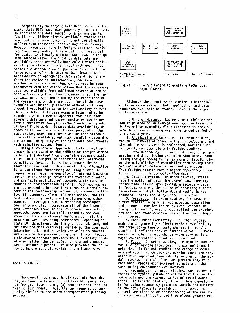
The overall technique is divided into four pha-ses, as shown in Figure 1: (1) freight generation, (2) freight distribution, (3) mode division, and (4) traffic assignment. Thus, the technique is concep-tually similar to the urban transportation planning process. /
Present Present Service, Econnic Cost 8 Price
Activities Characteristics
Frt. Traffic Ert. Traffic Modal I Network Generation '_]Distribation Division Assignment
Future I Future Service, Econnic Cost Price I
Activities Characteristics i
Traffic Generation and Modal Choice Traffic Assignment Distribution I I
Figure 1. Freight Demand Forecasting Technique: Major Phases.
Although the structure is similar, substantial differences do arise in both application and data resources available to states. Some of the major differences are:
Unit of Measure. Rather than vehicle or per-son trips made on an average weekday, the basic unit is freight or commodity flows expressed in tons or vehicle equivalents made over an extended period of time, say a year.
Replicationof Universe. In urban studies, the full universe of travel within, into/out of, and through the study area is replicated, whereas such is usually not possible with freight studies.
Data Dependency. In urban studies, trip gen-eration and distribution are often simulated. Simu-lating freight movements is far more difficult, giv-en the multiplicity of commodities each having their own unique distribution pattern and attributes. Thus freight studies have a higher dependency on da-ta -- particularly commodity flow data.
Data Collection. In urban studies, states have the option of obtaining travel data directly, rather than relying upon available secondary data. In freight studies, the option of obtaining traffic generation and distribution data directly is not practical unless the study scope is limited.
Forecasts. In •urban studies, forecasts of future traffic largely reflect expected population and income change for the study area, whereas in freight studies, forecasts must reflect the broader, national and state economies as well as technologi-cal changes.
Mode Choice Complexity. In urban studies, mode choice generally reflects vehicle availability and comparative time or cost, whereas in freight studies it reflects service factors as well. Proce-dures for modeling mode choice where service is a major consideration are not well developed.
Focus. In urban studies, the main product or focus is on vehicle flows over highway and transit networks. In freight studies, the change in modal use and resulting shipper and carrier costs are very often more important than vehicle volumes on the mo-dal networks. Vehicle flows are particularly rele-,vant when impacts upon pavement structure or the surrounding environment are involved.
Redundancy. In urban studies, various cross-checks are typically made to ensure that the results being obtained are representative of actual condi-tions. In freight studies, there is less opportuni.-ty for using redundancy given the amount and quality of the data typically available. This makes inde-pendent verification or crosschecking of the results obtained more difficult, and thus places greater re-
sponsibility upon those conducting the study to en-sure that the data and techniques used in reaching study conclusions are reasonable and defensible.
The implication of this is that even though the basic phases are similar, the specific techniques will differ appreciably from those used, by planners in solving urban transportation problems. The tech-nique presented is more complex than its urban coun-terpart because of (1) the lack of a prescribed set of problems and issues to which the technique will beapplied, (2) the customized nature of the result-ing products, and (3) the need to adapt the tech-nique to widely varying data resources and the in-ability of users to collect required data directly.
11
ORGANIZATION OF THIS MANUAL
A chapter is provided for each major element of freight demand forecasting:
Chapter Two: Defining the Problem Chapter Three: Freight Traffic Generation
and Distribution Chapter Four: Modal Division Chapter Five: Traffic Assignment Chapter Six: Case examples illustrating
the application of the technique.
CHAPTER TWO
DEFINING THE PROBLEM
INTRODUCTION General Parameters
The starting point in any application is:
First, defining the problem. Second, structuring the freight demand fore-
casting technique to address that problem. Concurrently, simplifying and adapting both
the problem and the technique to produce the desired products and/or answers within applicable fiscal, time, and data resource constraints.
Since states may elect to address a wide range of problems or issues, appreciable flexibility and adaptability had to be incorporated into the design of the technique. The underlying premise was that the technique could not be rigidly specified in advance, because neither the variables nor the prod-ucts can be determined apriori. Thus in applying the technique, the user must tailor the technique to the application (and vice versa) before becoming im-mersed in the computational detail involved in car-rying out the application. This chapter provides guidance on accomplishing this.
DEFINING THE PROBLEM
Before attempting to apply the technique, the user should first take time to fully determine the parameters and constraints both affecting and shap-ing the application at hand. The secondary objec-tive is to reduce the scope of the application, to the maximum extent possible, while retaining the ca-pability to provide desired answers. The greater the effort spent initially in defining the problem, the easier it will be for the user to apply the technique and obtain meaningful results.
Specifically, the user should look for, and identify or decide on, the following.
The user should identify the general parameters or overall dimensions of the application, which include:
Physical and cultural aspects, defined by identifying affected (1) geographic space, (2) transport infrastructure, and (3) shippers and re-ceivers constituting the universe of interest. The spatial dimension can be multistate, statewide, sub-state, or corridor. Infrastructure can include all facilities or be limited to particular transporta-tion modes, routes, and services. The universe of shippers and receivers can include all or, alterna-tively, be a subset delineated by (1) establishment size, (2) shipment sizes, (3) commodity type, or (4) total volume (weight) of shipments or receipts made over a selected time period
The general orientation, which can be modal (primary emphasis is on a single mode, although com-parisons may be made with other modes), commodity (emphasis is on a single or limited number of com-modities or types of freight), or specific facility (emphasis is on changing traffic and its impacts).
The modes, transport facilities, and services presently being used and expected to be used in the future. Modal definitions should not be limited by their traditional classifications (i.e., rail, truck, inland waterway), but rather the user should explicityl recognize any significant variations in intramodal services, shipment sizes or competition between modes or mode combinations.
The commodity or commodities and related shipment sizes presently being transported or ex-pected to be transported in the future.
The alternative futures, scenarios, or condi-tions to be examined in comparison with a base year.
The regulatory environment surrounding the problem at hand, both at present and in the future.
In examining the general parameters of the prob-lem, the user must simultaneously sort out what is important and must be incorporated into the tech-nique from that having little effect and, hence, can be'dropped from further consideration.
12
Major Tasks to be Accomplished
In considering the desired products or answers, the user should decide whether the application ne-cess i tates:
Preparing forecasts of commodity production and consumption (or freight shipped and received) in addition to assembling comparable base year informa-tion. Wherever appropriate, production and consump-tion forecasts prepared by others should be used. If not available, such forecasts must be prepared by the user.
Preparing forecasts of vehicle or commodity flows or distribution in addition to assembling com-parable base year information. In most cases, the user must prepare such forecasts.
Dividing commodity flows among competing modes or services based on anticipated or hypothe-sized changes in the type, price or cost of the ser-vices offered along with assembling similar informa-tion on base year modal shares.
Determining commodity or vehicle flows over each modal network. If detailed information on seg-ment volumes is required, determining whether the size of the area, complexity of the modal network, and required level of detail dictates that a compu-terized process be used to assign traffic to modal networks.
Determining the impacts of changes in commod-ity or vehicle flows on the use of the highway sys-tem and resulting capital and maintenance needs to be supplied by government. Such impacts include (1) changes in truck volumes, sizes and weights, (2) changes in pavement loadings, (3) changes in antici-pated pavement service life, and (4) direct and in-direct effects of vehicles on other highway system users as well as on the adjacent environment.
By determining the general parameters and major tasks that must be accomplished, users have largely defined the problem or application while beginning the process of customizing the technique to the ap-plication.
Analytical Choices
The user should now consider whether to:
Measure performance in (1) economic, (2) physical, or (3) impact terms. Economic performance involves estimating and weighing the benefits and costs accruing from each alternative future, scenar-io or condition being tested in comparison with the base case. A comprehensive framework covering total system economics can be used or, alternatively, a more restrictive framework limited to (1) changes in the cost incurred by shippers and receivers, (2) relative profitability to the carriers providing the transport service, or (3) costs avoided or incurred by government. Physical performance involves mea-suring and comparing commodity or vehicle flows. Impacts are simply the projected effects of antici-pated changes in vehicle flows in comparison with the base case and relevant standards.
Estimate modal shares based on selecting the mode or service minimizing prices charged or unit costs. Underlying premises are that (1) rates re-flect carrier market share competition versus profit maximization, and thus reflect service differences, versus (2) the unit costs of the movement, which
provide a better indication of long-term prices be-cause such costs reflect the relative efficiencies of the competing carriers.'
Adopt a physical distribution or a transport economics orientation in determining modal shares. The former includes costs associated with inventory carrying, warehousing, packaging, shipping and re-ceiving in addition to transport charges to the shipper or receiver (revenues to the carrier) used by itself in the more conventional transport econom-ics approach.
To cost or price movements on a one-way or round trip basis, with the latter accounting for differences in backhaul revenue and vehicle/vessel utilization.
To optimize locations or flows in addition to, or in place of, determining the costs and reve-nues of different alternatives.
Users should recognize that the analytical choices made above dictate, in part, which subtech-niques must be employed.
Resulting Product
The user should finally consider the resulting product, which includes:
Contents of the output record, which for each unique movement usually includes an (1) origin, (2) destination, (3) mode, (4) commodity type, (5) com-modity flow, (6) vehicle equivalents, (7) carrier revenues, and (8) shipper or receiver costs. This manual presumes that most users will elect to use computers in summarizing data. It does not imply the need for a large mainframe computer; most of the computations presented herein can be made with a mi-crocomputer (e.g., a TRS-80, Apple II, or IBM Per-sonal Computer) or even be done manually.
Contents and layout of the various summary tables describing the efficiency benefits and im-pacts of individual alternatives in comparison with the base case.
Written analyses formatted to meet management requirements and providing the specific answers be-ing sought.
SIMPLIFYING THE PROBLEM
Concurrent with structuring the technique is the need to simplify the problem; that is, scaling down the total freight universe to only that portion needed to address the problem. Simplification in-volves the following steps:
Reviewing and accepting simplifying premises and assumptions.
Defining the geographic area of interest. Aggregating data. Focusing only on those economic sectors necessary
and appropriate to the problem. Determining transport characteristics to be exam-
i ned. Adjusting the scale of the application to that
for which data are readily available.
13
Simplifying Premises and Assumptions
Most short-range problems can be appreciably simplified if the user is willing to accept the fol-lowing premises and assumptions:
Aggregate freight demand is price and service inelastic. Most economic activities producing sig-nificant quantities of freight are resource based or tied to a given location by its investment in plant, equipment, and employees. In the short run, such producers have no option but to transport their freight irrespective of the cost or quality of the transport service supplied. Although locational changes do occur, such tend to be the outcome of a variety of factors, only one of which is transpor-tation.
Freight traffic generation is independent of the factors determining the division of traffic among the modes. In the short run, production and marketing decisions are made independently of mode choice decisions.
Modal division is dependent on the price and service characteristics of the individual modes. Where service is not a major factor, modal division can be simulated by comparing modes on a price or cost basis. When service is a factor, modal divi-sion can be simulated by comparing logistics costs.
Freight traffic forecasts are dependent on the anticipated amount and location of economic ac-tivities. Since the economy generates freight, changes in freight generation and distribution must stem from changes in the location and intensity of economic activity. Thus, the ability to forecast freight flows can inherently be no better than the ability to predict changes in the national, state and local economies.
Changes in the composition of freight traffic should be implicitly recognized, although the user can usually ignore such trends for short-run fore-casts. Even though little consistent change has ta-ken place in the average length of haul for all modes (spatial dimension), changes in industrial structure and technology have resulted in diminished commodity use (weight dimension). Consequently, freight volumes are growing increasingly more slowly relative to the gross national product (GNP) and other economic measures. As an economymatures, it tends to economize on its use of commodities.
Products produced by agriculture, manufactur-ing, and mining establishments will eventually be transported and consumed. Thus, commodities pro-duced equal freight shipped. Variables, such as changes in inventory levels, product shrinkage, loss, and so forth, can be ignored. (The above will not be true for some agricultural products that may partially be consumed on-site or stored for long pe-riods awaiting higher market prices).
Defining the Geographic Area of Interest
In most statewide transportation studies, state boundaries logically delimit the study area. Unfor-tunately, such areal units do not work well in freight studies because a large portion of freight flows are interstate. Given the economic interde-pendence of states, a regional, if not national, study area is often more appropriate.
1. If a statewide freight study is being under-taken, the immediate study area will usually be de-fined by state boundaries. If significant economic activity is concentrated adjacent to state borders,
it may be desirable to extend the immediate study area boundaries to include this activity. Equally important is the tributary area formed by shippers or markets located in surrounding states. Users should consider a two-tier approach whereby freight activity is defined at a finer level of detail with-in or adjacent to the state and at a coarser level of detail for neighboring or remaining states (and, if necessary, adjacent countries).
Rather than focusing on geography in defining tributary areas, users should consider specific eco-nomic centers or markets. For example, the study area for an agricultural transport study might in-clude the crop or vegetable-growing areas of the state and the principal out-of-state markets for the resulting agricultural products.
Data availability is a strong factor in de-termining study area limits. Because disclosure regulations limit the availability of most secondary economic data to the county level at best, study ar-ea and subarea boundaries should be coincident with county boundaries (or their equivalent in New Eng-land). Thus, the county itself becomes the smallest common building block' typically used in freight studies.
Finally, the size of the study area should be kept as small as the application and data resources will permit.
Aggregating Production and Consumption or Movement Dat a
If more disaggregated secondary data are avail-able, the user has the choice of retaining the geo-graphic detail or aggregating up to the county lev-el. Supplementary information is readily available by which to aggregate port, railroad station, or ci-ty and town level data upward to the county level. - Unless the application involves such localized
facilities as railroad branchlines, grain elevators, ports, and terminals, and the commodity flow data being used is reasonably comprehensive and complete, data should be aggregated to the county level.
Economic Sectors of Interest
If the application encompasses all freight move-ments, it will include movements within and between the following economic sectors: agriculture; manu-facturing; mining; contract construction; transport and public utilities; finance, insurance and real estate; retail trade; wholesale trade; services; government; and consumers. Only a few of the eco-nomic sectors listed above generate significant freight volumes (see Figure 2 ), but most sectors receive freight. The main producing sectors include agriculture, manufacturing, and mining. Major con-suming sectors include agriculture, manufacturing, mining, contract construction, transport and public utilities, retail and wholesale trade, services, government, and consumers.
If the application permits, the user should con-centrate or restrict study efforts to freight move-ments originating from as few economic sectors as possible, keeping in mind that commodity flow data are really only available for agricultural, manufac-turing, or mining activities.
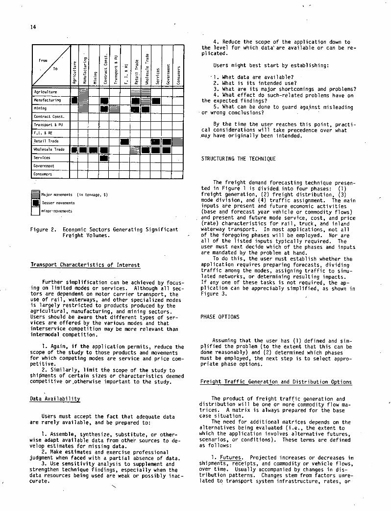
14
/TO
o CE
Agriculture
Manufacturing . IIIIIIII Mining
Contract Comst.
Transport & Pu
P.1, 8 RE
Retail Trade _ Wholesale Trade
.• • Services
Goverrmient
Consumers
Major movements (in tonnage, $)
, lesser movements
minor-movements
Figure 2. Economic Sectors Generating Significant Freight Volumes.
Transport Characteristics of Interest
Further simplification can be achieved by focus-ing on limited modes or services. Although all sec-tors are dependent on motor carrier transport, the use of rail, waterways, and other specialized modes is largely restricted to products produced by the agricultural, manufacturing, and mining sectors. Users should be aware that different types of ser-vices are offered by the various modes and that interservice competition may be more relevant than intermodal competition.
Again, if the application permits, reduce the scope of the study to those products and movements for which competing modes are service and price com-petitive.
Similarly, limit the scope of the study to shipments of certain sizes or characteristics deemed competitive Or_otherwise important to the study.
Data Availability
Users must accept the fact that adequate data are rarely available, and be prepared to:
Assemble, synthesize, substitute, or other-wise adapt available data from other sources to de-velop estimates for missing data.
Make estimates and exercise professional judgment when faced with a partial absence of data.
Use sensitivity analysis to supplement and strengthen technique findings, especially when the data resources being used are weak or possibly inac-curate.
Reduce the scope of the application down to the level for which data-are available or can be re-p1 icated.
Users might best start by establishing:
l. What data are available? What is its intended use? What are its major shortcomings and problems? What effect do such-related problems have on
the expected findings? What can be done to guard aganst misleading
or wrong conclusions?
By the time the user reaches this point, practi-cal considerations will take precedence over what may have originally been intended.
STRUCTURING THE TECHNIQUE
The freight demand forecasting technique presen-ted in Figure 1 is divided, into four phases: (1) freight generation, (2) freight distribution, (3) mode division, and (4) traffic assignment. The main inputs are present and future economic activities (base and forecast year vehicle or commodity flows) and present and future mode service, cost, and price (rate) characteristics for rail, truck, and inland waterway transport. In most applications, not all of the foregoing phases will be employed. Nor are all of the listed inputs typically required. The user must next decide which of the phases and inputs are mandated by the problem at hand.
To do this, the user must establish whether the application requires preparing forecasts, dividing traffic among the modes, assigning traffic to simu-lated networks, or determining resulting impacts. If any one of these tasks is not required, the ap-plication can be appreciably simplified, as shown in Figure 3.
PHASE OPTIONS
Assuming that the user has (1) defined and sim-plified the problem (to the extent that this can be done reasonably) and (2) determined which phases must be employed, the next step is to select appro-priate phase options.
Freight Traffic Generation and Distribution Options
The product of freight traffic generation and distribution will be one or more commodity flow ma-trices. A matrix is always prepared for the base case situation.
The need for additional matrices depends on the alternatives being evaluated (i.e., the extent to which the application involves alternative futures, scenarios, or conditions). These terms are defined as follows:
1. Futures. Projected increases or decreases in shipments, receipts, and commodity or vehicle flows, over time. Usually accompanied by changes in dis-tribution patterns'. Changes stem from factors unre-lated to transport system infrastructure, rates, or
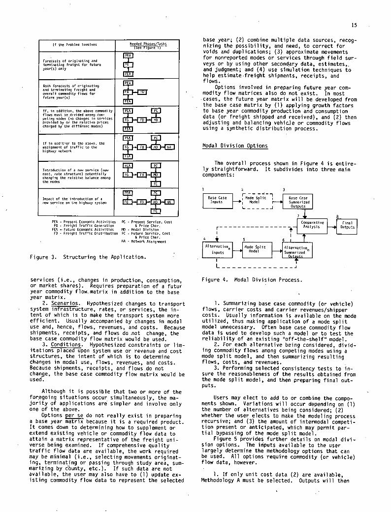
15
If the Problem Involves NeededPhases/Tasks (See Figure 1)
Forecasts of originating and
PEA
terminating freight for future year(s) only
Both forecasts of originating PEA
and terminating freight and overall commodity flows for future year(s)
If, in addition, the above commodity flows must be divided among con- peting modes (no changes in services PG FD MO prooided by or the relative prices charged by the diffrent modes)
PEA PC
If in addition to the above, the assigrument of traffic to the highuay network
PEA PC Introduction of a new service (new cost, rate structure) potentially changing the relative balance among
Ji)..ufI...fi
FC -
the modes
PE PC
Impact of the introduction of a new service on the highway system
9-M MD NA
FC
PEA - Present Economic Activities PC - Present Service, Cost FG - Freight Traffic Generation & Price Char.
FEA -, Fvture Economic Activities MD - Modal Division PD - Freight Traffic Distribution PC - Future Service, Cost
& Price Char. NA - Network Assignment
Figure 3. Structuring the Application.
services (i.e., changes in production, consumption, or market shares). Requires preparation of a futur year commodity flow..matrix in addition to the base year matrix.
Scenarios. Hypothesized changes to transport system infrastructure, rates, or services, the in-tent of which is to make the transport system more efficient. Usually accompanied by changes in modal use and, hence, flows, revenues, and costs. Because shipments, receipts, and flows do .not change, the base case commodity flow matrix would be used.
Conditions. Hypothesized constraints or lim-itations placed upon system use or revenue and cost structures, the intent of which is to determine changes in modal use, flows, revenues, and costs. Because shipments, receipts, and flows do not change, the base case commodity flow matrix would be used.
Although it is possible that two or more of the foregoing situations occur simultaneously, the ma-jority of applications are simpler and involve only one of the above.
Options per se do not really exist in preparing a base year matrix because it is a required product. It comes down to determining how to supplement or extend existing vehicle or commodity flow data to attain a matrix representative of the freight uni-verse being examined. If comprehensive quality traffic flow data are available, the work required may be minimal (i.e., selecting movements originat-ing, terminating or passing through study area, sum-marizing by county, etc.). If such data are not available, the user may also have to (1) update ex-isting commodity flow data to represent the selected
base year; (2) combine multiple data sources, recog-nizing the possibility, and need, to correct for voids and duplications; (3) approximate movements for nonreported modes or services through field sur-veys or by using other secondary data, estimates,, and judgment; and (4) use simulation techniques to help estimate.freight shipments, receipts, and flows.
Options involved in preparing future year com-modity flow matrices also do not exist. In most cases, the future year matrix will be developed from the base case matrix by (1) applying growth factors to base year commodity production and consumption data (or freight shipped and received), and (2) then adjusting and balancing vehic.le or commodity flows using a synthetic distribution process.
Modal Division Options
The overall process shown in Figure 4 is entire-ly straightforward. It subdivides into three main components:
1 2 3
I Base Case [ModeS;liti ,fBase ase Inputs Model Surnarized
1.. Outputs
Comparative Final
r-----------------Analysis —P1utputs
Alternative H Mode Split AlternativeSunriarized Ilodel Inpats
L--------------
Figure 4. Modal Division Process.
Summarizing base case commodity (or vehicle) flows, carrier costs and carrier revenues/shipper costs. Usually information is available on the mode utilized, thus making application of a mode split model unnecessary. Often base case commodity flow data is used to develop such a model or to test the reliability of an existing "off-the-shelf' model.
For each alternative being considered, divid-ing commodity flows among competing modes using a mode split model, and then summarizing resulting flows, costs, and revenues.
Performing selected consistency tests to in-sure the reasonableness of the results obtained from the mode split model, and then preparing final out-puts.
Users may elect to add to or combine the compo-nents shown. Variations will occur depending on (1) the number of alternatives being considered; (2) whether the user elects to make the modeling process recursive; and (3) the amount of intermodal competi-tion present or anticipated, which may permit par-tial bypassing of the mode split model.
Figure 5 provides further details on modal divi-sion options. The inputs available to the user largely determine the methodology options that can be used. All options require commodity (or vehicle) flow data, however.
1. If only unit cost data (2) are available, Methodology A must be selected. Outputs will then
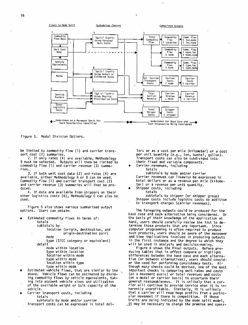
16
Inputs to Mode Split Methodology Choices Summarized Outputs
1 A 1
Flow Data SPlit Traffic
____
___________________ iiodity cmde I
Total
JCorn. Flow'
Using rginal Connnodity low
U:_-~ c
lOc Unit Costs Flow cation lo type
2 . ___
Conenodity ___
I I Cones. Flow I Flow c d,loc I. mode I I mode,typ
IN
D.Carr
Commodity Corn.Flow Flow c type,loc type E type,mod
4 I Split Traffic I Using Actual or
_______
B
__________________
Estimted Rates Carrier
ransport Coss ~Carrrjieer
Costs mode
Service I. —!I "Split Traffic j............J I I Total I Carrier Carrier
Factors Using Physical _____________________ Carrier Revenue Revenue Distribution Cost Revenue i i c mode i i c carrier
Logistics Costs Total Shipper
Shipper H Costs Costs E shipper
Undertaken on a Movement Basis for ________________ Undertaken for Base Case and Each Mode/Service Identified Each Alternative Being Considered
Figure 5. Modal Division Options.
be limited to commodity flow (1) and carrier trans-port cost (2) summaries.
If only rates (4) are available, Methodology B must be selected. Outputs will then be limited to commodity flow (1) and carrier revenue (3) summa-ries..
umma- ries. -
If both unit cost data (2) and rates (4) are available, either Methodology A or B can be used. Commodity flow (1) and carrier transport cost (2) and carrier revenue (3) summaries will then be pro-duced.
If data are available from shippers on their other logistics costs (6), Methodology C can also be used.
Figure 5 also shows various sumarized output options. Users can obtain:
Estimated commodity flows in terms of: totals subtotals by
location (origin, destination, and origin-destination pair)
mode type (STCC category or equivalent)
detail mode within location type within location location within mode type within mode location within type type within mode
Estimated vehicle flows, that are similar to the above. Vehicle flows can be estimated by divid- ing commodity flows by vehicle equivalents, tak- ing into account vehicle sizes and utilization of the available weight or bulk capacity of the vehicle. Carrier transport costs, including
totals subtotals by mode and/or carrier
Transport costs can be expressed in total dol-
lars or as •a cost per mile (kilometer) or a cost per unit quantity (e.g., ton, bushel, gallon). Transport costs can also be subdivided into their fixed and variable components. Carrier revenues, including
totals subtotals by mode and/or carrier
Carrier revenues can likewise be expressed in total dollars or as a revenue per mile (kilome-ter) or a revenue per unit quantity. Shipper costs, including
totals subtotals by shipper (or shipper group)
Shipper costs include logistic costs in addition to transport charges (carrier revenues).
The foregoing outputs could be produced for the base case and each alternative being considered. on the basis pf their knowledge of the application at hand, users should carefully review the list to de-termine those products that are important. Since computer programming- is often required to produce such products, users should be aware of the manpower and time implications involved in producing outputs in the first instance and the degree to which they will be used in analysis and decision-making.
Figure 6 shows the final outputs. Before pro-ducing tables that in effect compare or highlight differences betwen the base, case and each alterna-tive (or between alternatives); users should consid-er the need for performing consistency tests. Al-though many checks could be devised, one of the most important checks is comparing unit rates and costs (on a movement basis) or total revenues and costs (on a modal or carrier basis) to ascertain their general reasonableness. It is unlikely that a car-rier will continue to provide service when it is in-herently unprofitable. Similarly, it is unlikely that a carrier will reap huge profits from a partic-ular movement if there is competition. If these traits are being indicated by the mode split model, J,t may be necessary to change the premise and opera-
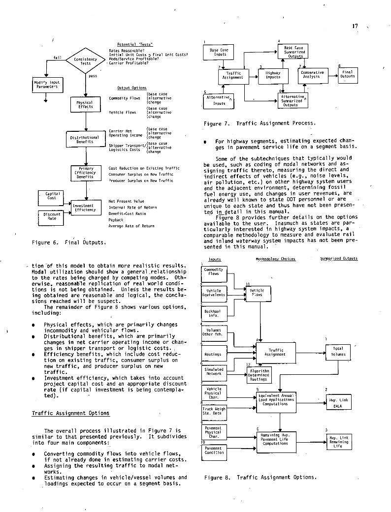
17
Potential Tests i
P Sunonarized Rates Reasonable?
Initial Unit Costs Final Unit Costs? InPuts Outpats Mode/Service Profitable?
Tests Carrier Profitable? I
4' pass
Modify Input i Parameters Output Options
(base case
Jr Conaiiodity Flows (alternative
Physical (change Effects (base case
Vehicle Flows (alternative
I
(change
Carrier Net (base case (alternative
Distributional Operating Income (change
Benefits Shipper Transport/a5e case
(alternative Logistics Costs
(change
Primary I Cost Reduction on Eoisting Traffic
EfficiencyJ
Consumer Surplus on New Traffic Benefits
Producer Surplus on New Traffic
Capital Cost
Net Present Value Investment Internal Rate of Return fficiency
Discount Benefit-Cost Ratio
Paybuck
Average Rate of Return
Figure 6. Final Outputs.
- tion of this model to obtain more realistic results. Modal utilization should show a general relationship to the rates being charged by competing modes. Oth-erwise, reasonable replication of real world condi-tions is not being obtained. Unless the results be-ing obtained are reasonable and logical, the conclu-sions reached will be suspect.
The remainder of Figure 6 shows various options, including:
Physical effects, which are primarily changes incommodity and vehicular flows. Distributional benefits, which are primarily changes in net carrier operating income or chan-ges in shipper transport or logistic costs. Efficiency benefits, which include cost reduc-tion on existing traffic, consumer surplus on new traffic, and producer surplus on new traffic. Investment efficiency, which takes into account project capital cost and an appropriate discount rate (if capital investment is being contempla-ted).
Traffic Assignment Options
The overall process illustrated in Figure 7 is similar to that presented previously. It subdivides into four main components:
Converting commodity flows into vehicle flows, if not already done in estimating carrier costs. Assigning the resulting traffic to modal net-works. Estimating changes in vehicle/vessel volumes and loadings expected to occur on a segment basis.
Traffic Highway Comparative Final
Assignment Impacts Analysis Outputs
Alternative0 Alternative Sumunarized
Inputs Outputs
Figure 7. Traffic Assignment Process.
For highway segments, estimating expected chan-ges in pavement service life on a segment basis.
Some of the subtechniques that typically would be used, such as coding of modal networks and as-signing traffic thereto, measuring the direct and indirect effects of vehicles (e.g., noise levels, air pollution, etc.) on other highway system users and the adjacent environment, determining fossil fuel energy use, and changes in user revenues, are already well known to state DOT personnel or are unique to each state and thus have not been presen- ted in detail in this manual. -
Figure 8 provides further details on the options available to the user. Inasmuch as states are par-ticularly interested in highway system impacts, a comparable methodology to measure and evaluate rail and inland waterway system impacts has not been pre-sented in this manual.
Inputs Methodology Choices Suronarized Outputs
Conumodi ty Flows
Vehicle Vehicle Equivalents Flows
Backhaul Info.
Vol umes Other Veh.
ngs IA+ATruc l T0t al
Vol unes ssignment
Simulated Al gorithm Network riDeterynine]d
Routings
Vehicle Physical
Hwy. Link Computations
EAIA Weigh Truck
Ste. Data
Pavement Physical
Hwy. Link Remaining
e nt Life
Condition
Figure 8. Traffic Assignment Options.
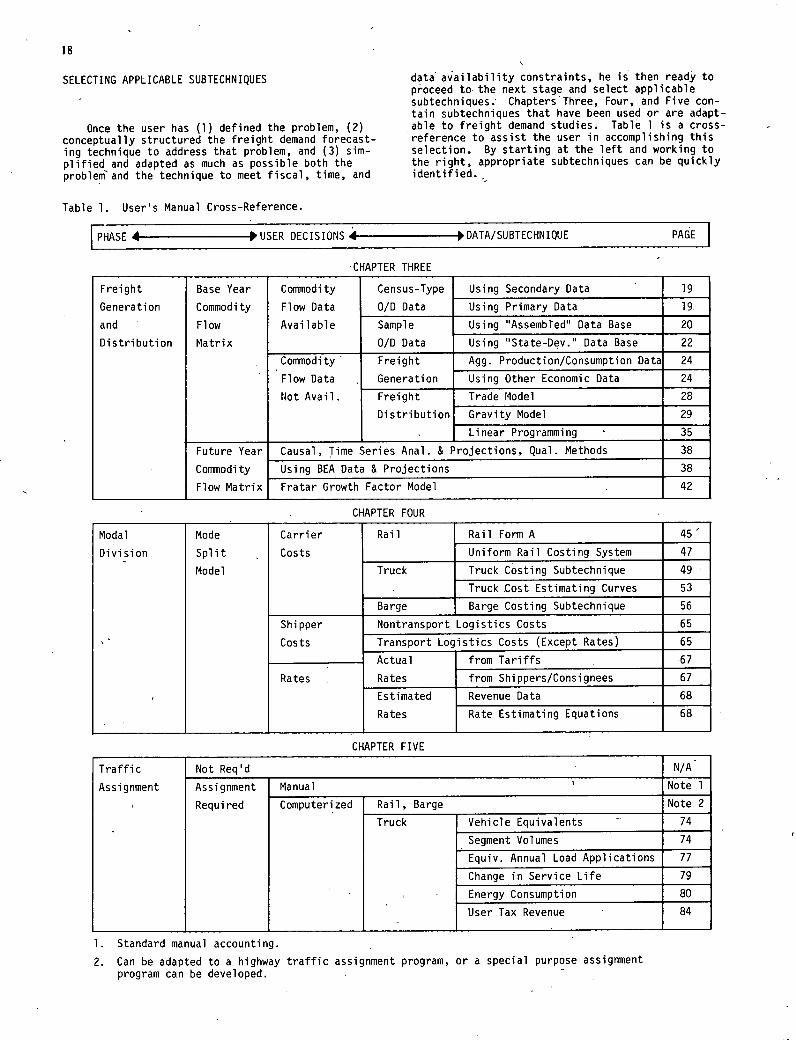
18
SELECTING APPLICABLE SUBTECHNIQUES
Once the user has (1) defined the problem, (2) conceptually structured the freight demand forecast-ing technique to address that problem, and (3) sim-plified and adapted as much as possible both the problem' and the technique to meet fiscal, time, and
Table 1. User's Manual Cross-Reference.
data availability constraints, he is then ready to proceed to the next stage and select applicable subtechniques. ChaptersThree, Four, and Five con-tain subtechniques that have been used or are adapt-able to freight demand studies. Table 1 is a cross-reference to assist the user in accomplishing this selection. By starting at the left and working to the right, appropriate subtechniques can be quickly identified.
PHASE 4 -PUSER DECISIONS I DATA/SUBTECHNIQUE PAGE
CHAPTER THREE
Freight
Generation
and
Distribution
Base Year
Commodity
Flow
Matrix
•
Commodity
Flow Data
Available
Census-Type
O/D Data
Using Secondary Data 19
Using Primary Data 19.
Sample
O/D Data
Using "Assembled" Data Base 20
Using 'State-Dev." Data Base 22
Commodity
Flow Data
Not Avail.
Freight
Generation
Agg. Production/Consumption Data 24
Using Other Economic Data 24
Freight
Distribution
Trade Model 28
Gravity Model 29
Linear Programming 35
Future Year
Commodity
Flow Matrix
Causal, Time Series Anal. & Projections, Qual. Methods 38
Using BEA Data & Projections 38
Fratar Growth Factor Model 42
CHAPTER FOUR
Modal
Division
Mode
Split
Model
Carrier
Costs
Rail Rail Form A 45'
Uniform Rail Costing System 47
Truck Truck Costing Subtechnique 49
Truck •Cost Estimating Curves 53
Barge Barge Costing Subtechnique 56
Shipper
Costs
Nontransport Logistics Costs 65
Transport Logistics Costs (Except Rates) 65
Actual
Rates
from Tariffs 67
Rates • from Shippers/Consignees 67
Estimated
Rates
Revenue Data 68
Rate Estimating Equations 68
CHAPTER FIVE
Traffic
Assignment
Not Req'd • N/A
Assignment
Required
Manual Note 1
Computerized
•
Rail, Barge Note 2
Truck Vehicle Equivalents 74
Segment Volumes 74
Equiv. Annual Load Applications 77
Change in Service Life 79
Energy Consumption 80
User Tax Revenue 84
Standard manual accounting.
Can be adapted to a highway traffic assignment program, or a special purpose assignment program can be developed.
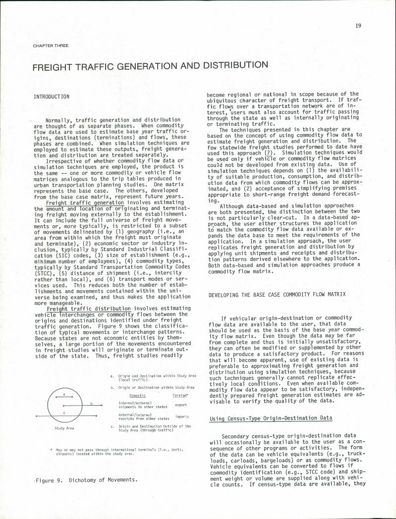
CHAPTER THREE
FREIGHT TRAFFIC GENERATION AND DISTRIBUTION
19
INTRODUCTION
Normally, traffic generation and distribution are thought of as separate phases. When commodity flow data are used to estimate base year traffic or-igins, destinations (terminations) and flows, these phases are combined. When simulation techniques are employed to estimate these outputs, freight genera-tion and distribution are treated separately.
Irrespective of whether commodity flow data or simulation techniques are employed, the product is the same -- one or more commodity or vehicle flow matrices analogous to the trip tables produced in urban transportation planning studies. One matrix represents the base case. The others, developed from the base case matrix, represent future years.
Freight traffic 9eneration involves estimating the amount and location of originating and terminat-ing freight moving externally to the establishment. It can include the full universe of freight move-ments or, more typically, is restricted to a subset of movements delineated by (1) geography (i.e., an area from within which the freight must originate and terminate), (2) economic sector or industry in-clusion, typically by Standard Industrial Classifi-cation (SIC) codes, (3) size of establishment (e.g., minimum number of employees), (4) commodity types, typically by Standard Transportation Commodity Codes (STCC), (5) distance of shipment (i.e., intercity rather than local), and (6) transport modes or ser-vices used. This reduces both the number of estab-lishments and movements contained within the uni-verse being examined, and thus makes the application more manageable.
Freight traffic distribution involves estimating vehicle interchanges or commodity flows between the origins and destinations identified under freight traffic generation. Figure 9 shows the classifica-tion of typical movements or interchange patterns. Because states are not economic entities by them-selves, a large portion of the movements encountered in freight studies will originate or terminate out-side of the state. Thus, freight studies readily
Origin and Destination within Study Area (local traffic).
n Origin or Destination within Study Area
____ Domestic Foreig
b - internal/eoternal shipments to other states
export
external/i nternal receipts from other states
imports
Study Area c. Origin and Destination Outside of the
Study Area (through traffic)
May or may not pass through international terminals (i.e., ports, airports) located within the study area.
Figure 9. Dichotomy of Movements.
become regional or national in scope because of the ubiquitous character of freight transport. If traf-fic flows over a transportation network are of in-terest, users must also account for traffic passing through the state as well as internally originating or terminating traffic.
The techniques presented in this chapter are based on the concept of using commodity flow data to estimate freight generation and distribution. The few statewide freight studies performed to date have used this approach (7). Simulation techniques would be used only if vehicle or commodity flow matrices could not be developed from existing data. Use of simulation techniques depends on (1) the availabili-ty of suitable production, consumption, and distrib-ution data from which commodity flows can be approx-imated, and (2) acceptance of simplifying premises appropriate to short-range freight demand forecast-ing.
Although data-based and simulation approaches are both presented, the distinction between the two is notparticularly clear-cut. In a data-based ap-proach, the user either structures the application to match the commodity flow data available or ex-pands the data base to meet the requirements of the application. In a simulation approach, the user replicates freight generation and distribution by applying unit shipments and receipts and distribu-tion patterns derived elsewhere to the application. Both data-based and simulation approaches produce a commodity flow matrix.
DEVELOPING THE BASE CASE COMMODITY FLOW MATRIX
If vehicular origin-destination or commodity flow data are available to the user, that data should be used as the basis of the base year commod-ity flow matrix. Even though the data may be far from complete and thus is initially unsatisfactory, they can often be modified or supplemented by other data to produce a satisfactory product. For reasons that will become apparent, use of existing data is preferable to approximating freight generation and distribution using simulation techniques, because such techniques generally cannot replicate effec-tively local conaitions. Even when available com-modity flow data appear to be satisfactory, indepen-dently prepared freight generation estimates are ad-visable to verify the quality of the data.
Using Census-Type Origin-Destination Data
Secondary census-type origin-destination data will occasionally be available to the user as a con-sequence of other programs or activities. The form of the data can be vehicle equivalents (e.g., truck-loads, carloads, bargeloads) or as commodity flows. Vehicle equivalents can be converted to flows if commodity identification (e.g., STCC code) and ship-ment weight or volume are supplied along with vehi-cle counts. If census-type data are available, they
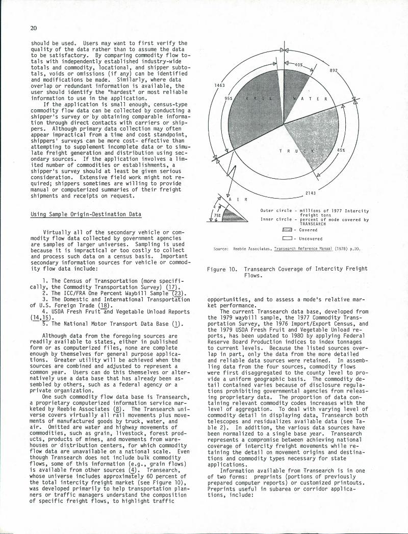
20
should be used. Users may want to first verify the quality of the data rather than to assume the data to be satisfactory. By comparing commodity flow to-tals with independently established industry-wide totals and commodity, locational, and shipper subto-tals, voids or omissions (if any) can be identified and modifications be made. Similarly, where data overlap or redundant information is available, the user should identify the 'hardest' or most reliable information to use in the application.
If the application is small enough, census-type commodity flow data can be collected by conducting a shipper's survey or by obtaining comparable informa-tion through direct contacts with carriers or ship-pers. Although primary data collection may often appear impractical from a time and cost standpoint, shippers' surveys can be more cost- effective than attempting to supplement incomplete data or to simu-late freight generation and distribution using sec-ondary sources. If the application involves a lim-ited number of commodities or establishments, a shipper's survey should at least be given serious consideration. Extensive field work might not re-quired; shippers sometimes are willing to provide manual or computerized summaries of their freight shipments and receipts on request.
Using Sample Origin-Destination Data
Virtually all of the secondary vehicle or com-modity flow data collected by government agencies are samples of larger universes. Sampling is used because it is impractical or too costly to collect and process such data on a census basis. Important secondary information sources for vehicle or commod-ity flow data include:
The Census of Transportation (more specifi-cally, the Commodity Transportation Survey) (17).
The ICC/FRA One Percent Waybill SampleT23). The Domestic and International Transportation
of U.S. Foreign Trade (18). USDA Fresh Fruit and Vegetable Unload Reports
(14,15). - The National Motor Transport Data Base (1).
Although data from the foregoing sources are readily available to states, either in published form or as computerized files, none are complete enough by themselves for general purpose applica-tions. Greater utility will be achieved when the sources are combined and adjusted to represent a common year. Users can do this themselves or alter-natively use a data base that has already been as-sembled by others, such as a federal agency or a private organization.
One such commodity flow data base is Transearch, a proprietary computerized information service mar-keted by Reebie Associates (8). The Transearch uni-verse covers virtually all rail movements plus move-ments of manufactured goods by truck, water, and air. Omitted are water and highway movements of commodities, such as grain, livestock, forest prod-ucts, products of mines, and movements from ware-houses or distribution centers, for which commodity flow data are unavailable on a national scale. Even though Transearch does not include bulk commodity flows, some of this information (e.g., grain flows) is available from other sources (4). Transearch, whose universe includes approximately 60 percent of the total intercity freight market (see Figure 10), was developed primarily to help transportation plan-ners or traffic managers understand the composition of specific freight flows, to highlight traffic
Outer circle - millions of 1977 Intercity freight tons
Inner circle - percent of node covered by
TRANSEARCH
- Covered
Uncovered
Source: Reebie Associates, Transearch Reference Manual (1978) p.20.
Figure 10. Transearch Coverage of Intercity Freight Flows.
opportunities, and to assess a mode's relative mar-ket performance.
The current Transearch data base, developed from the 1979 waybill sample, the 1977 Commodity Trans-portation Survey, the 1976 Import/Export Census, and the 1979 USDA Fresh Fruit and Vegetable Unload re-ports, has been updated to 1980 by applying Federal Reserve Board Production indices to index tonnages to current levels. Because the listed sources over-lap in part, only the data from the more detailed and reliable data sources were retained. In assemb-ling data from the four sources, commodity flows were first disaggregated to the county level to pro-vide a uniform geographic basis. The commodity de-tail contained varies because of disclosure regula-tions prohibiting governmental agencies from releas-ing proprietary data. The proportion of data con-taining relevant commodity codes increases with the level of aggregation. To deal with varying level of commodity detail in displaying data, Transearch both telescopes and residualizes available data (see Ta-ble 2). In addition, the various data sources have been normalized to a single base year. Transearch represents a compromise between achieving national coverage of intercity freight movements while re-taining the detail on movement origins and destina-tions and commodity types necessary for state applications.
Information available from Transearch is in one of two forms: preprints (portions of previously prepared computer reports) or customized printouts. Preprints useful in subarea or corridor applica-tions, include:
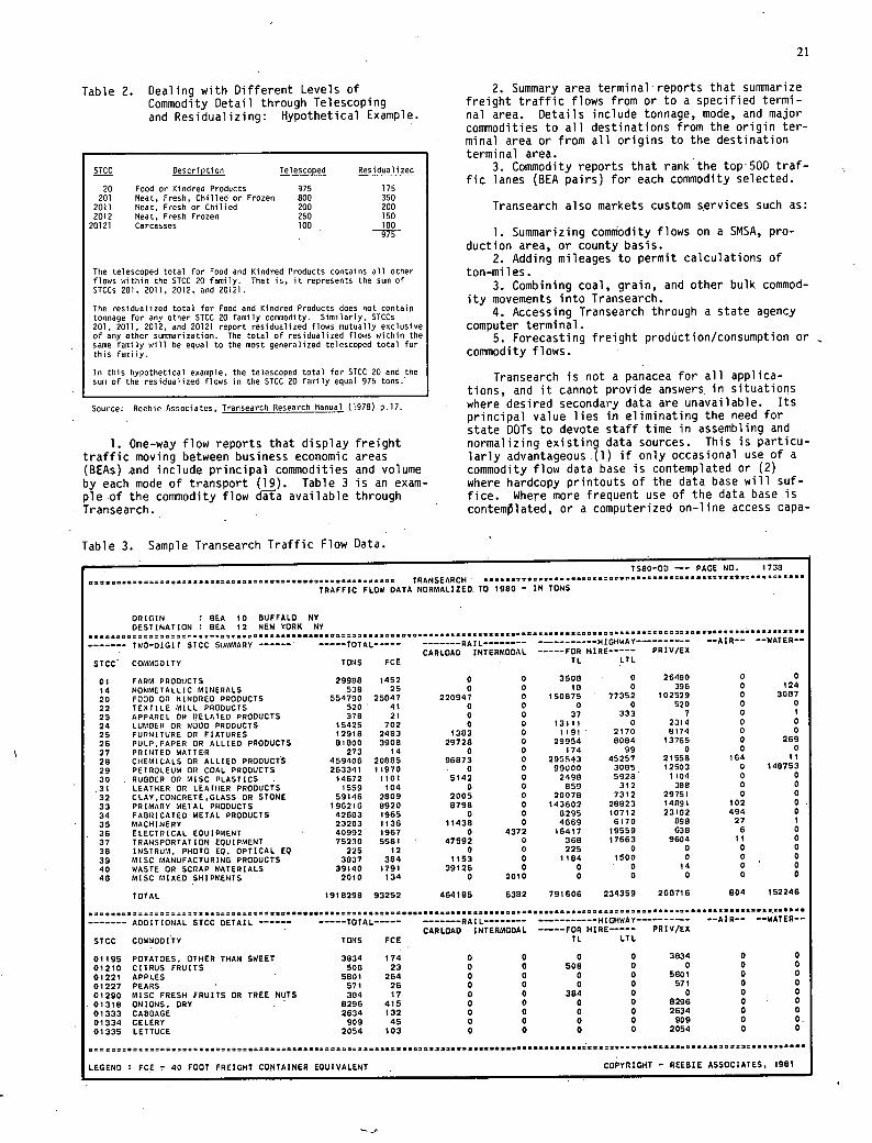
FT
Table 2. Dealing with Different Levels of Commodity Detail through Telescoping and Residualizing: Hypothetical Example.
STCC Description Telescoped Residualized
20 Food or Kindred Products 975 175 201 Meat. Fresh. Chilled or Frozen 800 350
2011 Meat, Fresh or Chilled 200 200 2012 Meat, Fresh Frozen 250 150 20121 Carcasses 100 100
975
The telescoped total for Food and Kindred Products contains all other flows within the STCC 20 family. That is, it represents the sum of STCCs 201, 2011, 2012, and 20121.
The residualized total for Food and Kindred Products does not contain tonnage for any other STCC 20 family commodity. Similarly, STCCs 201, 2011, 2012 and 20121 report residualized flows mutually exclusive of any other surmuarization. The total of residualized flows within the same family will be equal to the most generalized telescoped total for this family.
In this hypothetical example, the telescoped total for STCC 20 and the surr of the residualized flows in the STCC 20 family equal 975 tons.
Source: Reebie Associates, Transearch Research Manual (1978) p.17
1. One-way flow reports that display freight traffic moving between business economic areas (BEAs) and include principal commodities and volume by each mode of transport (19). Table 3 is an exam-ple.of the commodity flow data available through Transearch.
Table 3. Sample Transearch Traffic Flow Data.
Summary area terminal reports that summarize freight traffic flows from or to a specified termi-nal area. Details include tonnage, mode, and major commodities to all destinations from the origin ter-minal area or from all origins to the destination terminal area.
Commodity reports that rank the top 500 traf-fic lanes (BEA pairs) for each commodity selected.
Transearch also markets custom services such as:
Summarizing commodity flows on a SMSA, pro-duction area, or county basis.
Adding mileages to permit calculations of ton-miles.
Combining coal, grain, and other bulk commod-ity movements into Transearch,
Accessing Transearch through a state agency computer terminal.
Forecasting freight production/consumption or commodity flows.
Transearch is not a panacea for all applica-tions, and it cannot provide answers in situations where desired secondary data are unavailable. Its principal value lies in eliminating the need for state DOTs to devote staff time in assembling and normalizing existing data sources. This is particu-larly advantageous (1) if only occasional use of a commodity flow data base is contemplated or (2) where hardcopy printouts of the data base will suf-fice. Where more frequent use of the data base is contemplated, or a computerized on-line access capa-
TSOO—OD -- PAGE NO. 1738
TRANSEARCH TRAFFIC FLOW DATA NORMALIZED. TO 1980 - IN TONS
ORIGIN flEA 10 BUFFALO NY DESTINATION 1 flEA 12 NEW YORK NY
— --------- HIGHWAY -------- - --AIR-- --WATER— • TWO—DIGIT STCC SUMMARY ------ ------ TOTAL ----- ------- RAIL
CARLOAD --------
INTERMODAL -----FOR HIRE----- PRIV/EX
STCC" COMMODITY TONS FCE TI. LTL
01 FARM PRODUCTS 29988 1452 0 0 3500 0 26480 0 0 124
14 20
NONMETALLIC MINERALS FOOD OR MINOREDPRODUCTS
538 554700
25 25047
0 220947
0 0
10 150875
0 77352
396 102529
0 0 3007
22 TEXTILE MILL PRODUCTS 520 4* 0 0 0 0 520 0 0
23 APPAREL OR I1ELAILD PRODUCTS 378 21 0 0 37 333 7 0 0 24 LUMBEROR WOOD PRODUCTS 15425 702 0 0 13111 0 23*4 0
25 FURNITURE OR FIXTURES 12918 2483 1383 0 1191 2170 8*74 0 0
26 PULP,PAPER OR ALLIED PRODUCTS 81800 3908 29728 0 29954 8084 13765 0 269
27 PRINTED MATTER 273 14 0 0 174 99 0 0 0
28 CHEMICALS OR ALLIED PRODUCTS 459406 20805 96873 0 295543 45257 21558 164 II
29 PEIROLEUM OR COAL PRODUCTS 263341 11970 . 0 0 90000 3085 12503 0 149753
30 RUBBER OR MISC l'LASTICS . *4672 1101 5*42 0 2490 5926 1104 0 0 . 31 LEATHER OR LEAIHER PRODUCTS 1559 104 0 0 859 312 388 0 0
32 CLAY,CONCRETE,GLASS OR STONE 59*46 2809 2005 0 20078 73*2 29751 0 0
33 PRIMARY METAL PRODUCTS 196216 8920 8798 0 143602 28823 *4091 102 0
34 FABRICATED METAL PRODUCTS 42603 *965 0 0 6295 *07*2 23102 494 0
35 MACHINERY 23203 1136 1*438 0 4669 6*70 898 27 I
36 ELECTRICAL EQUIPMENT 40992' 1967 0 4372 16417 19559 638 6 0
37 TRANSPORTATION EQUIPMENT 75230 5501 ' 47592 0 368 17663 9604 11 0
38 INSTRUM, PHOTO EQ. OPTICAL EQ 225 *2 0 0 225 0 0 0 0
39 MISC MANUFACTURING PRODUCTS 3837 384 1*53 0 1184 1500 0 0 0
40 WASTE OR SCRAP MATERIALS 39140 179* 39126 0 0 0 *4 0 0
40 MISC MIXED SHIPMENTS 2010 134 0 20*0 0 0 0 0 0
TOTAL *918290 93252 464*85 6382 791606 234359 260716 904 *52246
ADDITIONAL STCC DETAI TOTAL ----- ------- RAIL -------- ----------HIGHWAY-----'-- --AIR-- --WATER--
CARLOAD INTERMODAI. -----FOR HIRE----- PRIV/EX
STCC COMMODITY TONS FCE FL LIL
01195 POTATOES, OTHER THAN SWEET 3834 174 0 0 0 0 3834 0 0
01210 CITRUS FRUITS 500 23 0 0 508 0 0 0 0
01221 APPLES ' 580* 264 0 0 0 0 5801 0 0
01227 PEARS 571 26 0 0 0 0 511 0 0
0*290 MISC FRESH FRUITS OR TREE NUTS 304 17 0 0 384 0 0 0 0
013*8 ONIONS. DRY . ' 8296 415 0 0 0 0 8296 0 0
01333 CABBAGE 2634 *32 0 0 0 0 2634 0 0
01334 CELERY 909 45 0 0 0 0 909 0 0,
01335 LETTUCE 2054 103 0 0 0 0 2054 0 0
LEGEND FCE ' 40 FOOT FREIGHT CONTAINER EQUIVALENT COPYRIGHT - REEBIE ASSOCIATES, *961
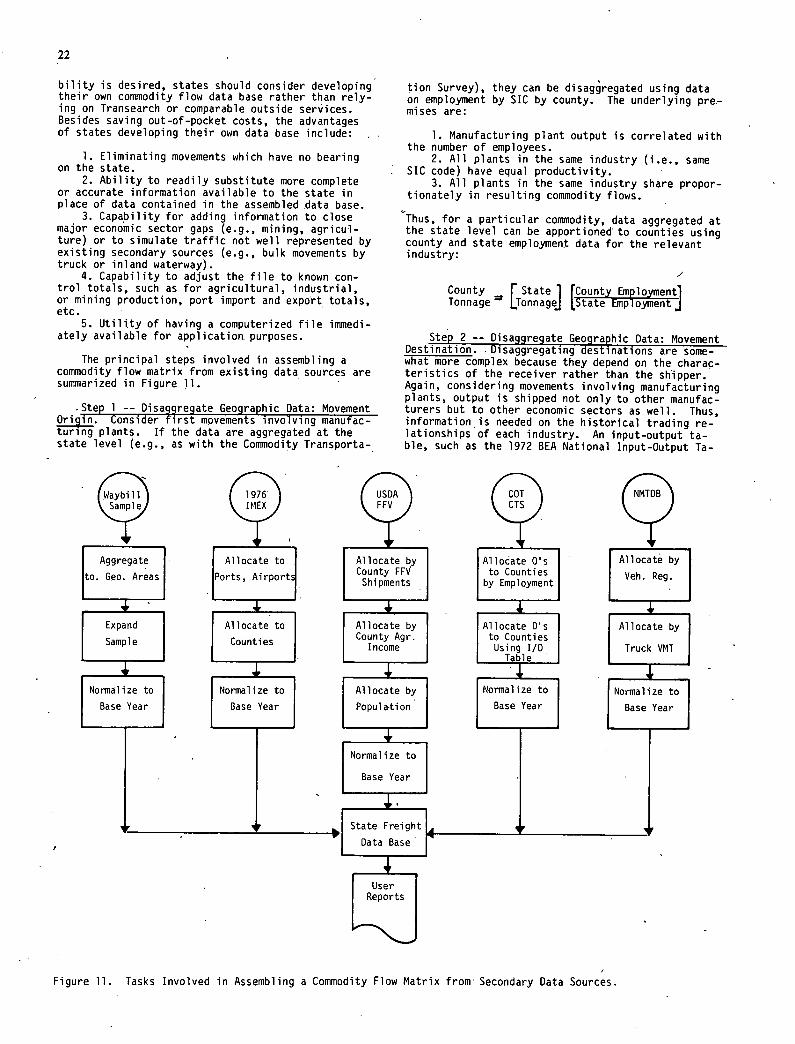
22
bility is desired, states should consider developing their own commodity flow data base rather than rely-ing on Transearch or comparable outside services. Besides saving out-of-pocket costs, the advantages of states developing their own data base include:
Eliminating movements which have no bearing on the state.
Ability to readily substitute more complete or accurate information available to the state in place of data contained in the assembled data base.
Capability for adding information to close major economic sector gaps (e.g., mining, agricul-ture) or to simulate traffic not well represented by existing secondary sources (e.g., bulk movements by truck or inland waterway).
Capability to adjust the file to known con-trol totals, such as for agricultural, industrial, or mining production, port import and expo'rt totals, etc.
Utility of having a computerized file immedi-ately available for application, purposes.
The principal steps involved in assembling a commodity flow matrix from existing data sources are summarized in Figure 11.
Step 1 -- Disaggregate Geographic Data: Movement Origin. Consider first movements involving manufac-turing plants. If the data are aggregated at the state level (e.g., as with the Comodity Transporta-
tion Survey), they can be disagregated using data on employment by SIC by county. The underlying pre.-mises are:
Manufacturing plant output is 'correlated with the number of employees.
All plants in the same industry (i.e., same SIC code) have equal productivity.
All plants in the same industry share propor-tionately in resulting commodity flows.
Thus, for a particular commodity, data aggregated at the state level can be apportioned' to counties using county and state employment data for the relevant industry:
County[Tonnage State 1 fCounty Employment
Tonnage J IState Employmentj
Step 2 -- Disaggregate Geograhic Data: Movement Destination. . Disaggregating destinations are some-what more complex because they depend on the charac-teristics of the receiver rather than the shipper. Again, considering movements involving manufacturing plants, output is shipped not only to other manufac-turers but to other economic sectors as well. Thus, information,is needed on the historical trading re-lationships of each industry. An input-output ta-ble, such as the 1972 BEA National Input-Output Ta-
ll CTS Sae IMEX_ FFV
Aggregatel• Allocate to 1 o. Go. Areas
JPorts, AirPorti
[County FFV to Counties [ Veh. Reg.
Allocate by Allocate Os ' F Allocate by
Shipments by Employment
Expand I Allocate to I Allocate by I lAllocate D's I Allocate by Sample Counties
j
County Agr. I I to Counties I Income I Using I/O I Truck VMT
Table '
F Normalize to rmalize to I I Allocate by I Normalize to I Normalize to Base Year Base Year I Population I Base Year I Base Year
Normalize to
L Base Year
4,. State Freight
L Data Base
4, User Reports
Figure 11. Tasks Involved in Assembling a Commodity Flow Matrix from' Secondary Data Sources.
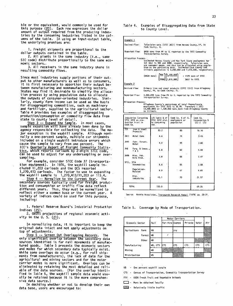
23
ble or the equivalent, would commonly be used for this purpose (20). Each row expresses the dollar amount of output required from the producing indus-tries by the consuming industries listed in the col-umns of the table. In using an input-output table, the underlying premises are:
Freight shipments are proportional to the dollar outputs contained in the table.
All plants in the same industry (i.e., same SIC code) distribute proportionally to the same eco-nomic sectors..
All receivers in the same industry share in resulting comodity flows.
Since most industries supply portions of their out-put to other manufacturers as well as to consumers, it is first necessary to apportion their output be-tween manufacturing and nonmanufacturing sectors. States may find it desirable to simplify the alloca-tion process by using population data to allocate the outputs of consumer-oriented industries. Simi-larly, countyfarm income can be used as the basis for disaggregating commodities, such as machinery and fertilizer, supplied to the agricultural sector. Table 4 provides two examples of dIsaggregating production/cpnsumption or commodity flow data from state to county level of detail.
Step 3 -- Expand the Sample. In most cases, sample expansion will have already been done by the agency responsible for collecting the data. The ma-jor exception is the waybill sample. Although nomi-nally a one-percent sample, multiple car shipments included on a single waybill introduce errors which cause the sample to vary from one percent. The ICC's Quarterly Report of Freight Commodity Statis-tics, which reports carloads by 2-digit STCC code, can be used to adjust for any undersampling or over-sampling.
For example, consider STCC Code 37 (transporta-tion equipment). In 1976, the waybill sample in-cluded 11,203 carloads and the QCS reported 1,270,413 carloads. The factor to use in expanding the waybill sample is 1,270,413/11,203 or 113.4.
Step 4 -- Normalize to the Current Year. The secondary sources typically used for freight produc-tion and consumption or traffic flow data reflect different years. Thus, they must be normalized to reflect either a common base or the current year. A variety of indices could be used for this purpose, including:
Federal Reserve Board's Industrial Production Indices (25).
0BtS projections of regional economic acti-vity in the U. S. (21).
In normalizing data, it is important to keep the original data intact and not apply adjustments on top of adjustments.
Step 5 -- Screen Out Overlapping Records. The only significant overlap between the secondary data sources identified is for rail movements of manufac-tured goods. Table 5 presents the economic sectors and modes for which secondary data typically exist. While some overlaps do occur (e.g., for rail ship-ments from manufacturers), the lack of data for the agricultural and mining sectors and for the motor carrier modes is more significant. Overlaps can be eliminated by retaining the most detailed and reli-able of-the data sources. (For the overlap identi-fied in Table 5, the waybill sample data would usu-ally be retained because it is the more comprehen-sive data source.)
In deciding whether or not to develop their own data base, users are encouraged to:
Table 4. Examples of Disaggregating Data from State to County Level.
Example I
Desired Flow: Television sets (STCC 3651) from Nassau County. NY. to Cook County, IL.
Reported flow: 8928 tons from NY to IL reported by the 1972 Comodity Transportation Survey.
Allocation Process: Estimated Nassao County and New York State employment for SIC 3651 is 985 and 3088. respectively. Television sets are consumer goods, and thus can be allocated using popula- tion as the portioning data. Estimated Cook County and Illinois population is 3,200,000 and 7.615,000, respectively.
(8928 tons) 12113.200.0001 1125 tons of STCC
[3088] L7.615.000J 3651 in 1972.
Example 2
Desired Flow: Primary iron and steel products (STCC 3312) from Allegheny County, PA, to Cook County, IL.
Reported Flow: 4.000.000 tons from PA to IL reported by the 1972 Cononodity Transportation Survey.
Al location Prvcess: Allegheny County's percentage of total Pennsylvania employment for STCC 3312 is 35.7%. Therefore (.357) (4.000,000) or 1.428,000 tons more from Allegheny County to Illinois.
Industries Consuming I/O Table S of Cook Co. C of IL. Cook Co. STCC 3312 as pro- STCC 3312 dist. employment or Consumption S duction input in to consuming population (2) 0 (3) Cook Co. md.
331 ut eel 20.2 80 16.16 Prod
3411 Metal Cans 4.6 75 3.45
3441 Fabr. Struct. 4.0 95 3.80 Metal
346 Forg. & Stiops. 6.8 60 4.08
3496 Misc. Fab 3.8 65 2.47
3711, 3714 Automobiles 5.6 55 3.08
Population- 9.9 47 4.65 Related
MiscIndustries 45.1 70 31.57
TOTAL 100.0 69.26
Source: Reebiv Associates,. Transeurch Research Manual (1978) pp. 28-31.
Table 5. Coverage by Mode of Transportation.
Economic Sector Rail
Motor Carriers
Water - , Air - For-Hire Exempt Private
Agricul tore Farm
Forest
Other
Munufacturing
Mining
Distribution
118 FF9
WB / WB
WB, CTS CTS CTS CTS CT.. I1
WB
1dB
118 - One percent waybill sample
CTS - Census of Transportation, Conomodity Transportation Survey
EFY - USDA Fresh Fruit and Yegetable Unloads
- Most be obtained locally
- Relatively little traffic
24
Purchase rather than assemble such informa-tion in-house unless (1) a number of applications are contemplated, (2) staff and fiscal resources are available to properly maintain a commodity flow data base, and (3) considerable enrichment of the data base is anticipated.
Consider supplementing the information avail-able from secondary sources, especially for ship-ments originating from the agriculture and mining sectors. A mechanism for accomplishing this may al-ready be in place. For example, if permanent truck weighing stations exist, states should consider si-multaneously obtaining information on the origin, destination, and commodities in addition to weighing the vehicle for conformance to state load limits.
Simulating Freight Generation
If commodity flow data are not available, such data will have to be simulated. First, freight shipments and receipts must be estimated either from industry production and consumption information, or from other economic data. Then, the generated traf-fic must be distributed to obtain flows.
In general, freight shipments or receipts can be approximated by converting employment or monetary measures of industrial production and consumption into physical units. If the total value (dollars) is known, the commodity attribute file contained in Appendix B (or the equivalent thereto) can be used to estimate shipments and receipts. If employment data are available, it must first be translated into industrial production or consumption (dollars) by using national or regional productivity data.
Equally important as the mechanics of simulating freight generation is background knowledge and fa-miliarity with the amounts and types of freight be-ing generated and consumed by different economic sectors within the study area. In addition, a gen-eral understanding of the types of changes taking place in freight generation as the economy continues to mature is most helpful (6).
Using Industry Production and Consumption Data
Assuming that industry production and consump-tion data are available, these data can be disaggre-gated to the county level. The process works rea-sonably well when:
The products involved are few in number, are relatively homogeneous, are readily identifiable in available statistical data, and are transported in significant volumes.
The number of establishments shipping or re-ceiving identified products are either few in number or readily aggregated.
Aggregate sector or industry information on the identified products produced and/or received within the study area is available.
Information exists on which to adjust produc-tion outputs to shipments.
This approach will not work well when:
Only partial or incomplete information can be obtained on product production or consumption.
Information is lacking on the amount and lo-cation of out-of-state or out-of-country production and consumption.
A valid basis for disaggregating estimates of freight shipments and receipts to counties or their equivalent does not exist.
The following example illustrates how the U.S. Department of Energy (DOS) national and regional coal supply and demand (production and consumption) projections were disaggregated to 173 BEA5, using supplied projections of coal supply and demand (13).
Because coal production data are not collect or aggregated by BEA, the methodology employed dis-aggregated the regional projections to the county level, which were then aggregated to BEAs. Four steps were involved: (1) estimating coal production on a preliminary basis in each county using a re-gression-derived equation stating production as a function of known reserves, past production, and coal characteristics, (2) estimating "production share" obtained by dividing the prepared county-level estimates by the sum for all counties in each DOE region, (3) applying the county production share to the regional production projections to obtain normalized forecasts for each county, and (4) sum-ming production forecasts over all counties in each BEA to obtain BEA production forecasts.
A similar procedure was employed to disaggregate projected regional coal demand. Four steps were similarly involved: (1) disaggregating past county coal consumption by coal type and utility/nonutility use, (2) allocating coal consumption by county in the nonutility sector using data on past nonutility coal consumption by type, (3) allocating coal con-sumption by county in the utility sector using coal-fired generation capacity as a proxy for coal con-sumption, and (4) summing the county coal consump-tion projections for both sectors by type and BEA to obtain total BEA coal consumption by type..
As the application is broadened to include other products or economic sectors, the task of determin-ing the fypes, amounts, and allocation procedure for each product can become quite extensive. In some instances, it will be impractical to estimate freight generation and distribution by assembling and allocating production and consumption statis-tics.
Using Other Economic Data
Instead of estimating freight generation through industry production and consumption statistics, an alternative approach is to convert employment or monetary measures of industry production and con-sumption into physical units. The advantage of this approach is that it potentially covers the full uni-verse of freight movements. However, a number of important assumptions do underly the use of economic data to generate freight estimates.
The unit tons or value of raw and semifin-ished goods required to produce a unit ton or value of product remains constant for that SIC group.
Output tonnage for a particular industry is proportional to its earnings or employment. This means that all plants within an SIC group have equal productivity.
The tonnage of each commodity used in person-al consumption is proportional to the population. This means that all persons consume equally irres-pective of income or location.
Average unit tonnage and value are applicable to all products and commodities contained within that SIC group.
County level output tonnage is proportional to county employment in that SIC group. This means that all plants within an SIC group have equal pro-ductivity.
ro- ductivity.
The procedure for estimating freight generation is conceptually straightforward. The following sub-technique uses a combination of value added and em-
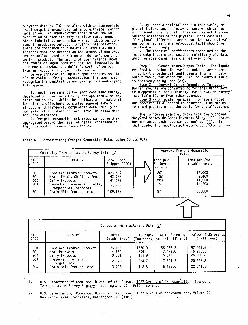
25
ployment data by SIC code along with an appropriate input-output transactions table to estimate freight generation. An input-output table shows how the production of each industry is distributed among other industries, or concisely what industries con-sume in producing output. Industry interrelation-ships are contained in a matrix of technical coef-ficients that are defined as the amount of one prod-uct in dollars used in making one dollar's worth of another product. The matrix of coefficients shows the amount of input required from the industries in each row to produce one dollar's worth of output from an industry in a particular column.
Before applying an input-output transactions ta-ble to estimate freight consumption, the user must recognize the constraints and assumptions underlying this approach:
Input requirements for each consuming entity, developed on a national basis, are applicable to any state and county. While the application of national technical coefficients to states ignores likely structural differences, comparable data usually do not exist at the state or local level to allow more accurate estimates.
Freight consumption estimates cannot be dis-aggregated beyond the level of detail contained in the input-output transactions table.
By using a national input-output table, re-gional differences in factor prices, which can be significant, are ignored. This can distort the re-sulting estimates of the physical units consumed. If regional differences are known, the national val-ues contained in the input-output table should be modified accordingly.
The technical coefficients contained in the input-output table are based on relatively old data which in some cases have changed over time.
Step 1 -- Obtain Input/Output Table. The inputs required to produce the various outputs are deter-mined by the technical coefficients from an input-output table, for which the 1972 Input-Output Table is presently being used (20).
Step 2 -- Convert DolTr Amounts to Tonnages. Dollar amounts are converted to tonnages using data from Appendix B, the Commodity Transportation Survey (see Table 6), or from other sources.
Step 3 -- Allocate Tonnages. Tonnage shipped and received is allocated to counties using employ-ment and population as the basis for the allocation.
The following example, drawn from the proposed Maryland Statewide Goods Movement Study, illustrates how the above technique can be applied (11). In that study, the input-output matrix consisted of the
Table 6. Approximating Freight Generation Rates Using Census Data.
Commodity Transportation Survey Data 1/
STCC COMMODITY Total Tons CODE Shipped (000)
20 Food and Kindred Products 426,587 201 Meat: Fresh, Chilled, Frozen 42,728 202 Dairy Products 44,372 203 Canned and Preserved Fruits, 36 825-
Vegetables, Seafoods 204 Grain Mill Products etc., 109,538
Approx. Freight Generation Rates
Tons per Tons per Ave. Employee Establ ishment
201 16,000 138 9,400 288 11,900 157 15,500
971 36,000
Census of Manufacturers Data 2/
SIC INDUSTRY Total All Emps. Value Added by Value of Shipments CODE Estab. (No.) (Thousands) Man. ($ millions) ($ millions)
20 Food and Kindred Products 26,656 1520.0 56,062.2 192,911.6 201 Meat Products 4,534 309.1 7,478.0 46,276.3 202 Dairy Products 3,731 153.9 5,648.3 26,009.8 203 Preserved Fruits and 2,379 234.7 7,684.5 20,332.8
Vegetables 204 Grain Mill Products etc. 3,043 112.8 6,625.6 22,344.2
1/ U.S. Department of Commerce, Bureau of the Census, 1977 Census of Transportation, Commodity Transportation Survey Summary. Washington, DC (1981) Table 5.
2/ U.S. Department of Commerce, Bureau of the Census, 1977 Census of Manufacturers, Volume III Geographic Area Statistics, Washington, DC (1981). -
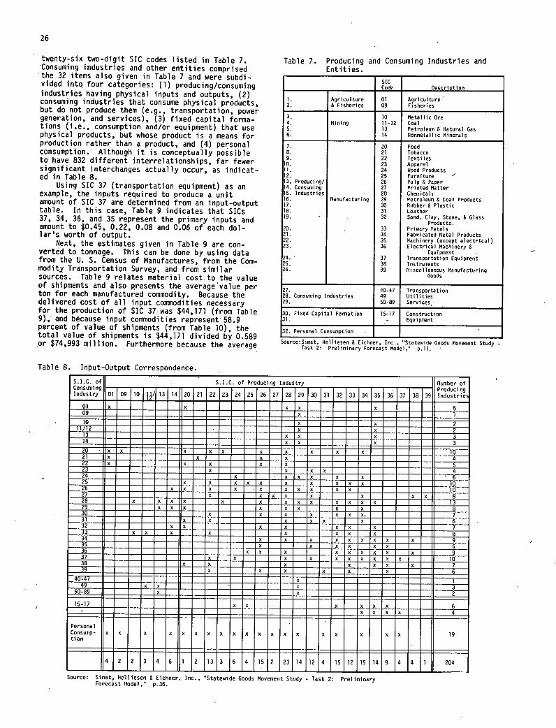
26
twenty-six two-digit SIC codes listed in Table 7. 'Consuming industries and other entities comprised the 32 items also given in Table 7 and were subdi-vided into four categories: (1) producing/consuming industries having physical inputs and outputs, (2) consuming industries that consume physical products, but do not produce them (e.g., transportation, power generation, and services), (3) fixed capital forma-tions (i.e., consumption and/or equipment) that' use physical products, but whose product is a means for production rather than a product, and (4) personal consumption. Although it is conceptually possible to have 832 different interrelationships, far fewer significant interchanges actually occur, as indicat-ed in Table 8.
Using SIC 37 (transportation equipment) as an example, the inputs required to produce a unit amount of SIC 37 are determined from an input-output table. In this case, Table 9 indicates that SICs 37, 34, 36, and 35 represent the primary inputs and amount to $0.45, 0.22, 0.08 and 0.06 of each dol-lar's worth of output.
Next, the estimates given in Table 9 are con-verted to tonnage. This can be done by using data from the U. S. Census of Manufactures, from the Com-modity, Transportation Survey, and from similar sources. Table 9 relates material cost to the value of shipments and also presents the average'value per ton for each manufactured commodity. Because the delivered cost of all input commodities necessary for the production of SIC 37 was $44,171 (from Table 9),' and because input commodities represent' 58.9 percent of value of shipments (from Table 10), the total value of shipments is $44,171 divided by 0.589 or $74,993 million. Furthermore because the average
Table 8. Input-Output Correspondence.
Table 7. Producing and Consuming Industries and Entities.
SIC Code Description
1. Agriculture 01 Agriculture 2. 8 Fisheries 09 Fisheries
3. 10 Metallic Ore 4. Mining 11-12 Coal 5. 13 Petroleum & Natural Gas 6. , 14 Nonmetallic Minerals
7. 20 Food 8. 21 Tobacco 9. 22 Textiles 0. 23 Apparel 1. 24 Wood Products 2. 25 Furniture ' 3. Producing! 26 Pulp & Paper
14. Consuming 27 Printed Matter 15. Industries ' 28 Chemicals 16. Manufacturing 29 Petroleum & Coal Products 17. 30 Rubber 8 Plastic 18. 31 Leather 19. , 32 Sand, Clay, Stone. & Glass
Products. 20. 33 Primary Metals 21. 34 Fabricated Metal Products 22. 35 Machinery (except electrical) 23. 36 Electrical Machinery &
Equipment 24. ' 37 Transportation Equipment 25. 38 Instruments 26. 39 Miscellaneous Manufacturing
Goods
40-47 Transportation Consuming Industries 49 Utilities
' , 50-89 Services,
Fixed Capital Formation 15-17 Construction ' - Equipment
Personal Consumption
Source:Simat, Helliesen & Eichner, Inc.," Statewide Goods Movement Study -Task 2: Preliminary Forecast Model," p.11.
S.I.C. of Producing Industry
I1M
I4IUIHhIIIIIUhIpflhIIIIi Source: Simat, Helliesen & Eichner, Inc., "Statewide Goods Movement Study - Task 2: Preliminary
Forecast tlodel," p.36.
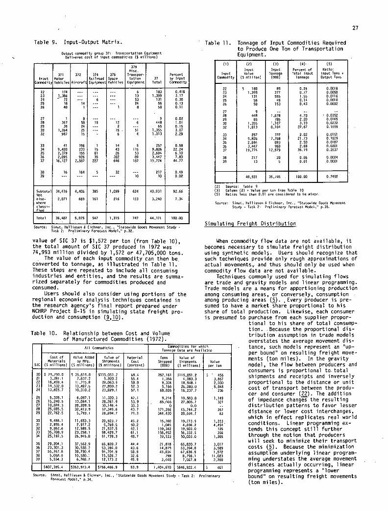
Table 9. Input-Output Matrix.
Output commodity group 37: Transportation Equipment Delivered cost of input comodities ($ millions)
379 Misc.
371 372 374 376 Transpor- Percent Input Motor Railroad Space tation 37 by Input
Comodity Vehicles Aircraft Equipment Vehicles Equipment Total Comodity
22 174 --- 6 180 0.41% 23 1,386 --- 13 1,399 3.17 24 - 72 -- 6 --- 53 131 0.30 25 18 14 - --- 24 56 0.13 26 40 1 --- 1 8 50 0.11
27 1 8 --- --- --- 9 0.02 28 357 58 15 12 6 448 1.01 29 39 24 --- 2 --- 65 0.15 30 1,264 25 --- 15 51 1,355 3.07 32 987 15 - 6 4 1.013 2.29
33 41 196 1 14 5 257 0.58 34 9.420 233 15 43 115 9,826 22.24 35 2.379 155 81 26 53 2.694 6.10 36 2.095 926 35 302 89 3,447 7.80 37 16.127 2.587 227 646 187 19.774 44.77
38 16 164 5 32 --- 217 0.49 39 - --- 10 10 0.02
Subtotal 34,416 4,406 385 1,099 624 40,931 92.66 Not else- 2,071 669 161 216 123 3,240 7.34 where classi - fled
Total 36,487 5,075 547 1,315 747 44.171 100.00
Source: Sinat. Heiliesem & Eichner. Inc., Statewide Goods Movement Study Task 2: Preliminary Forecast Model," p.32.
value of SIC 37 is $1,572 per ton (from Table 10), the total amount of SIC 37 produced in 1972 was 74,993 million divided by 1,572 or 47,705,000 tons.
The value of each input commodity can then be. converted to tonnage, as illustrated in Table 11. These steps are repeated to include all consuming industries and entities, and the results are summa-rized separately for commodities produced and consumed.
Users should also consider using portions of the regional economic analysis techniques contained in the research agency's final report prepared under NCHRP Project 8-15 in simulating state freight pro-duction and consumption (9,10).
Table 10. Relationship between Cost and Volume of Manufactured Commodities (1972).
27
Table 11. Tonnage of Input Commodities Required to Produce One Ton of Transportation Equipment.
(1)
Input Cuniosdity
(2)
Input Value
)S million)
)3)
Input Tonnu9e (000)
(4)
Percent of Total Input
Tonnage
)5)
Ratio: Input Tons Output Tons
22 S 180 89 0.24 0.0018 23 1,399 277 0.77 0.0058 24 131 555 1.55 0.0116 25 56 49 0.14 0.0010 26 50 153 0.43 0.0032
27 9 -- -- -- 28 448 1,678 4.70 0.0352 29 65 786 2.20 0.0165 30 1,355 1.107 3.10 0.0232 32 1,013 8,104 22.67 0.1699
33 257 722 2.02 0.0151 34 9,826 7,768 21.73 0.1629 35 2,694 893 2.50 0.0187 36 3,447 960 2.69 0.0201 37 19,774 12,579 35.19 0.2637
38 217 20 0.06 0.0004 39 10 5 0.01 0.0001
40,931 35,745 . 100.00 0.7492
Source: Table 9 Column (2) Value per ton from Table 10
(5) Ratios less than 0.01 are considered to be minor.
Source: Smut, Helliesen & Eichner, Inc., Statewide Goods Movement Study - Task 2: Preliminary Forecast Model," p.35.
Simulating Freight Distribution
When commodity flow data are not available, it becomes necessary to simulate freight distribution using synthetic mode1. Users should recognize that such techniques provide only rough approximations of actual movements,, and thus should only be used when commodity flow data are not available.
Techniques commonly used for simulating flows are trade and gravity models and linear programming. Trade models are a means for apportioning production among consuming areas, or conversely, consumption among producing areas (5). ,Every producer is pre-sumed to have a market share proportional to his share of total production. Likewise, each consumer is presumed to purchase from each supplier propor-
tional to his share of total consump-tion. . Because the proportional dis-tribution assumption in trade models overstates the average movement dis- tance, such models represent an "up-per bound" on resulting freight move-ments (ton miles). In the gravity model, the flow between producers and consumers is proportional to. total shipments and receipts and inversely proportional to the distance or unit cost of transport between the produ-cer and consumer (22). The addition of impedance changes the resulting distribution patterns to favor lesser distance or lower cost interchanges, which in effect replicates real world conditions. Linear programming ex-tends this concept still further through the notion that producers will seek to minimize their transport costs (5). Because the minimization assumption underlying linear program-ming understates the average movement distances actually occurring, linear r,n-nrn'mmminr, rrircnt r, "lwør
- All c Commodities Comodities for which Tonnage Data are Available
Cost of Value Added Value of Material Tons Value of Materials by Mfg. Shipments Cost Shipped Shipments Value
SIC (5 millions) (5 millions) )S millions) (percent) (000) (S millions) per Ton
20 $ 79,793.0 $ 35,614.8 $115,051.2 69.4 252,161 $115,051.2 S ' 456 21 3,281.1 2,637.2 5,920.2 55.4 1,056 4,083.3 3,867 22 16,499.4 11,715.8 28,063.9 58.8 9,334 18,948.1 2,030 23 14,532.0 13,487.5 27,809.2 52.3 5,166 26,080.0 5,048 24 13,605.7 10,310.2 23,829.1 57.1 68.826 16,237.7 236
25 5,335.1 6,097.1 11,320.3 47.1 9,214 10,583.8 1,149 26 15,240.5 13,064.1 28,261.9 53.9 85,066 27,805.7 327 27 10,044.3 20,209.5 30,146.4 33.3 0 0.0 -- 28 25,085.5 32,413.9 57,349.6 43.7 171.266 45,744.2 267 29 22,762.5 5,793.1 28,694.7 79.3 344,420 28,694.7 83
30 9,466.1 11,653.3 20,923.7 45.2 15,760 19,273.9 1,223 31 2,895.4 2,917.2 5,769.5 50.2 1,045 4,696.2 4.494 32 9,062.6 12,586.5 21,537.5 42.1 159.342 19,903.0 125 33 35,708.9 23,258.1 58,429.7 61.1 158,452 56,332.5 356 34 25,197.5 26,945.8 51,739.3 48.7 39,533 50,003.0 1.265
35 29,204.1 37,562.9 65,820.7 44.4 21,818 65,820.7 3.017 36 23,301.3 30,558.2 53,394.0 43.6 14,879 53,394.0 3,589 37 55,767.8 39,790.4 94,704.9 58.9 43,034 67,636.5 1,572 38 5,058.5 10,580.1 15,526.7 32.6 798 8,796.1 11,023 39 5,554.3 6,768.7 12,173.2 45.9 3.440 7,567.8 2:200 - $407,395.4 $353,973.4 $756,466.9 53.9 1 1.404,610 1 $646,922.4 S 461
r ' '" • r' Source: Smut. Ilelliesen & Eichner, Inc., • Statewide Goods Movement Study - Task 2: Preliminary bound" on resulting freight movements
Forecast Model," p.34. (ton miles).
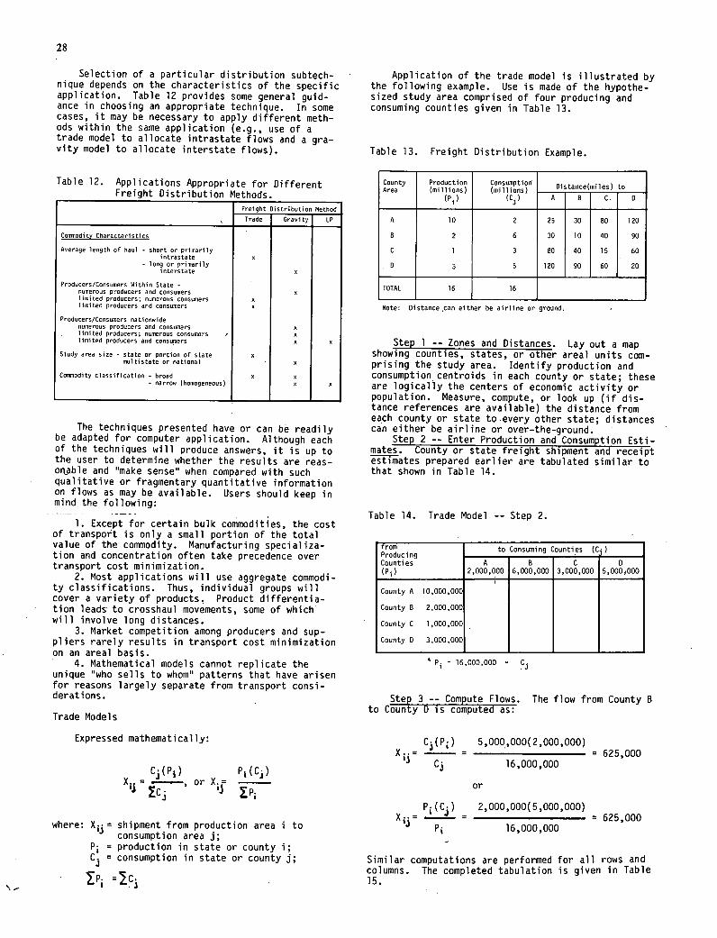
28
Selection of a particular distribution subtech-nique depends on the characteristics of the specific application. Table 12 provides some general guid-ance in choosing an appropriate technique. In some cases, it may be necessary to apply different meth-ods within the same application (e.g., use of a trade model to allocate intrastate flows and a gra-vity model to allocate interstate flows).
Table 12. Applications Appropriate for Different Frejqht Distribution Mthndc
Freight Distribution Method
Trade Gravity LP
Conynodi ty Characteristics
Average length of haul - short or primarily intraState 0 - long or primarily interstate
Producers/Consumers Within State - numerous producers and consumers limited producers; numerous consumers limited producers and consumers
Producers/Consumers nationwide numerous producers and consumers limited producers; numerous consumers , limited producers and consumers x
Study area size - state or pnrtinn of state multistate or national
Cononodity classification - broad 0 - narrow (homogeneous) o
The techniques presented have or can be readily be adapted for computer application. Although each of the techniques will produce answers, it is up to the user to determine whether the results are reas-on,,able and make sense' when compared with such qualitative or fragmentary quantitative information on flows as may be available. Users should keep in mind the following:
Except for certain bulk commodities, the cost of transport is only a small portion of the total value of the commodity. Manufacturing specializa-tion and concentration often take precedence over transport cost minimization.
Most applications will use aggregate commodi-ty classifications. Thus, individual groups will cover a variety of products. Product differentia-tion leads to crosshaul movements, some of which will involve long distances.
Market competition among producers and sup-pliers rarely results in transport cost minimization on an areal basis.
4. Mathematical models cannot replicate the unique "who sells to whom" patterns that have arisen for reasons largely separate from transport consi-derations.
Trade Models
Expressed mathematically:
C(P1) P(C) XIj =
, or Xç
where: X,3= shipment from production area i to consumption area j;
Pi = production in state or county i; C = consumption in state or county j;
zPi =,
Application of the trade model is illustrated by the following example. Use is made of the hypothe-sized study area comprised of four producing and consuming counties given in Table 13.
Table 13. Freight Distribution Example.
County Area
Production (millions)
Consumption (millions) Distance(miles) to - -
A B C. D (Ci)
A 10 2 25 30 80 120
B 2 6 30 10 40 90
C 1 3 80 40 15 60
D 3 5 120 90 60 20
TOTAL 16 16
Note: Distance can either be airline or ground
Step 1 -- Zones and Distances. Lay out a map showing counties, states, or other areal units com-prising the study area. Identify production and consumption centroids in each county or state; these are logically the centers of economic activity or population. Measure, compute, or look up (if dis-tance references are available) the distance from each county or state to-every other state; distances can either be airline or over-the-ground.
Step 2 -- Enter Production and Consumption Esti-mates. County or state freight shipment and receipt tTiiates prepared earlier are tabulated similar to
that shown in Table 14.
Table 14. Trade Model -- Step 2.
from Produclng Counties
to Consuming Counties (C1
A B C 0 (P1) 2,000,000 6,000,000 3.000.000 5.00000O
County A 10,000,000
County B 2,000,000
County C 1,000,000
County D 3,000.000
" P1 = 16,000,000 =
Step 3 -- Compute Flows. The flow from County B to County 0 is computed as:
xii=C.(P;) 5,000,000(2,000,000) ' = =625,000 CS 16,000,000
or
P(C, ) = 2,000,000(5,000,000) = 625,000
p. 16,000,000
Similar computations are performed for all rows and columns. The completed tabulation is given in Table 15.
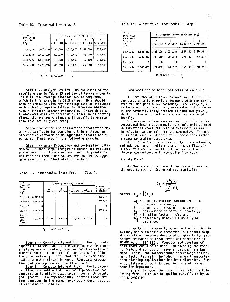
29
Table 15. Trade Model -- Step 3. Table 17. Alternative Trade Model -- Step 3
from Producing Counties
to Consuming Counties (C
A B C 0
(P) 2,000,000 6,000,000 3,000,000 5,000,000
County A 10,000,000 1,250,000 3,750,000 1,875,000 3,125,000
County B 2,000,000 250,000 750,000 375,000 625,000
County C 1,000,000 125,000 375,000 187,500 312,500
County 0 3,000,000 375,000 1,250,000 562,500 937,500
P1 = 16,000,000 =
fro Producing Counties/
to Consuming Counties/$tates (Ci)
States A B C 0
('i) 1,857,143 4,642,857 2,785,714 3,714,286
County A 8,666,667 1,238,095 3,095,238 1,857,143 2,476,191
County B 1,733,333 247,619 619,048 371,428 495,238
CountyC 0 .0 0 O 0
County D 2,600,000 371,429 928,572 557,143 742,857
P1 = 13,000,000 = C
Step 4 -- Analyze Results. On the basis of the results given in Table 15 and the distances shown in Table 13, the average distance can be computed, which in this example is 62.5 miles. This should then be compared with any existing data or discussed with industry representatives to determine whether such a distance appears reasonable. Inasmuch as a trade model does not consider distance in allocating flows, the average distance will usually be greater than that actually occurring.
Since production and consumption information may only be available for counties within a state, an alternative approach is to aggregate imports and ex-ports as illustrated in the following example.
Step 1 -- Enter Production and ConsumDtion Esti-mates. In this step, freight shipments and receipts are entered for study area counties. Shipments to and receipts from other states are entered as aggre-gate amounts, as illustrated, in Table 16.
Table 16. Alternative Trade Model -- Step 1.
ucing ProdCounties/
to Consuming Counties/States (ci ) Exports to
States A B C 8 Other States (P.) 2,000,000 5,000,000 3.000,000 4.000,000 2,000.000
County A 10,000,000 1.333.333
County B 2,000,000 266,667
Countyt 0 0
County 0 3,000,000 400.000
imports from 1,000,000 142,857 357,143 214,286 285.714 0 Other States
Pi = 16,000,000 = C
Step 2 -- Compute External Flows. Next, county exports to other states and county imports from oth-er states are allocated, based on total exports and imports, which in this example are 2 and 1 million tons, respectively. Note that the flow from other states to other states is zero. Aggregate produc-tion and consumption is 16 million tons.
Step 3 -- Compute Internal Flows. Next, exter-nal flows are subtracted from total production and consumption to obtain study area internal shipments and receipts. County-to-county internal flows are then computed in the manner previously described, as illustrated in Table 17.
Some application hints and notes of caution:
Care should be taken to make sure the size of the study area is roughly coincident with the market area for the particular commodity. For example, a multistate or national study area makes little sense if the commodity being studied is sand and gravel, which for the most part is produced 'and consumed locally.
Because no impedance or cost function is in-corporated into a cost model, it should only be used in situations where the cost of transport is small in relation to the value of the commodity. The mod-el is best used for distributing commodities within a state or smaller study area.
Since a trade model is solely an apportioning method, the results obtained may be significantly different from real world patterns as evidenced through comparisons with commodity flOw data.
Gravity Model
Another model often used to estimate flows is the gravity model. Expressed mathematically:
- _____
Jt where: FU =
= shipment from production area i to consumption area j;
= production in state or county i Cj = consumption in state or county j;
= friction factor = ut; and t. = impedance, which will usually be i distance.
In applying the gravity model to freight distri-bution, the subtechnique presented is a manual trip-distribution procedure developed originally for pas-senger transport in urban areas and documented in NCHRP Report 187 (12). Computerized versions of this model can also be used. In adapting the model to freight distribution, several changes have been made. First, the socioeconomic interchange adjust-ment factor typically included in urban transporta-tion planning applications has been discarded. Sec-ond, distance or cost is used in place of travel time for impedance.
The gravity model then simplifies into the fol-lowing form, which can be applied manually or by us-ing a computer:

30
X,,= R1CF ii
where: Pi R1=.--
R is the 'production index," which remains con- stant for each production area. C F is the eat- traction factor' for consumption area j. In this version of the gravity model, a production balance is maintained (i.e., the row totals equal the input production for that county or state). On the other hand, the consumption totals for each county or state output will not necessarily match the desired values. To obtain •an acceptable balance, an itera-tive process must be employed to adjust the calcu-lated commodity flows. Several iterations may be required to bring the consumption totals to within 5 to 10 percent of the originally specified values.
Application of the gravity model for freight distribution is illustrated using the example given in Table 13.
Step 1 -- Geographic Delineation. As before, lay out a map showing study area boundaries and the subareas being used for analysis purposes -- coun-ties, states, or some other areal unit. Also iden-tify the logical centers of economic activity or population.
Step 2 -- Enter Frei9ht Shipment and Receipt Es-timates. Assume that subarea estimates of commodi-ties shipped and received have been prepared from production and consumption estimates. These esti-mates would be entered in the freight flow matrix shown in Table 18; a separate form would be used for each unique commodity.
Step 3 -- Enter Impedances. First determine whether to use distance or cost as the basis for-es-timating impedances. If distances are to be used, measure, compute, or look up (if distances are available in tabular form) the ground or airline distance from each county to every other county or state. If shipping cost is to be used, first deter-mine the mileage and then look up the equivalent rate for that commodity. Distances or costs would be entered into the freight flow matrix as indicated in Table 18. These distances or costs would then be converted to impedances by inverting and raising the number to selected power. Also enter the impedances in the freight flow matrix.
Selecting an appropriate exponent to use in com-puting the friction factor presently can only be done using a trial and error approach. Since the gravity model has only infrequently been applied to freight distribution, a body of knowledge on appro-priate exponent values has not been developed. Us-ers should start with an exponent value of 1.0, and compare the computed average distance with any other data on average distance for similar movements or commodities. Another approach is to compare the computed average distance with that obtained fràm applying a trade model (should be less) or linear programming (should be higher).
For example, the estimated distance from County B to County 0 is 90 miles. In this case, the impe-dance is the inverted distance raised to a power of 1.0 or 0.0111.
Step 4 -- Calculate Attraction Factors, Accesi-bility Index, and Production Index (First itera-tion)-. The Attraction Factor from County B to Coun-ty D is:
C.3F.. '. = 0.0111(5,000,000) = 55,556
The Accessibility Index for County B is: p
C F = 66,667+600,000±75,000+55,556 = 797,223
The Production Index for County B is:
P 2,000,000 R.=b— = ________ = 2.5087
'Zc4i 797,223
The foregoing computations would be undertaken for all rows and columns in the freight flow matrix as illustrated in Table 19.
Step 5 -- Calculate Commodity Flows (First Iter-ation-). The commodity flow from County B to County Dis:
X.. '
= R.Ciii.F,. = 2.5087(55,556) = 139,374
'.3
Thus, the total commodity flow for County B is:
P = = 167,248+1,505,225+188,153+139,374 = 2,000,000 which matches the desired p.
The Commodity flow to County D is:
C=X; 2,325,595+139,394+299,400+1,956,518 = 4,720,887 which is 6% under the de-sired C of 5,000,000
The foregoing computations would be undertaken for all rows and columns in the freight flow matrix, as illustrated in Table 20.
Becaifse of the structure of this form of the gravity model, the computed shipments for each coun-ty must match the initial amount. County consump-tion totals, however, will not necessarily match the initial value.. While within the 5 to 10 percent range for County D, the results obtained for Coun-ties A and B show niuch greater variance. Thus, a second iteration becomes necessary. To refine the calculated interchanges, consumption totals are ad-justed before the second iteration by the ratio of the desired receipts over actual receipts or, for County D, by:
5,000,000 = 1.0591
4,720,887
The above computations would be repeated for all consuming counties.
Step 6 -- Recalculate Attraction Factors, Acces-sibility Index, and Production Index (Second Itera-
). This step is a repeat of Step 4, but UTig [heidjusted consumption totals. The Attraction Factor from County B to County D is:
CF = 55,556(1.0591) = 58,841
The Accessibility Index for County B is: to
= 27,477+977,685+81,987+58,841 = 1,145,990
The Production Index for County B is:
Pi 2,000,000 R. ---- --------- = 1.7452
C3 Fli 1,145,990 JZA
As before, the foregoing computations would be undertaken for all rows and columns in the freight flow matrix, as illustrated in Table 21.
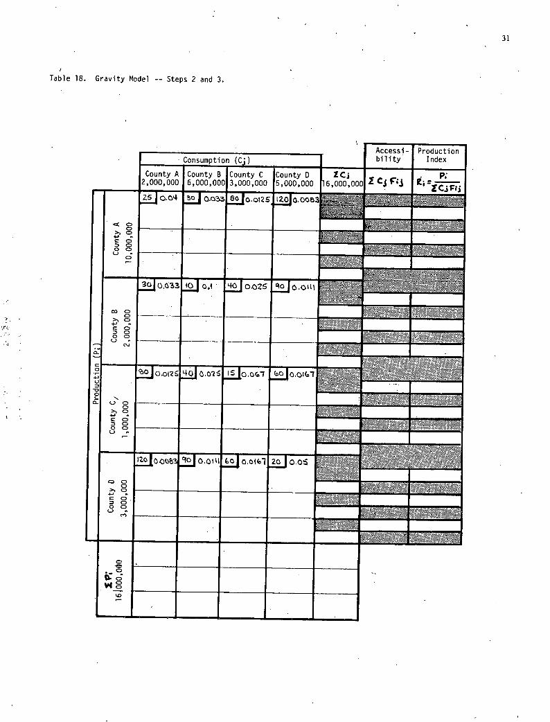
Table 18. Gravity Model -- Steps 2 and 3.
Accessi- Production Consumij5 J bility Index
P; C D ZCJ lCounty 2,000,00 6,000'000 3,000'000 5,000,000 16,000,000
cM J Q oIZS Ldk
CD
(3.633 400 02S to
> C o
LOJ
Iz
4-' .' C
o L)
C..)
CD '-I CD
'.0
31
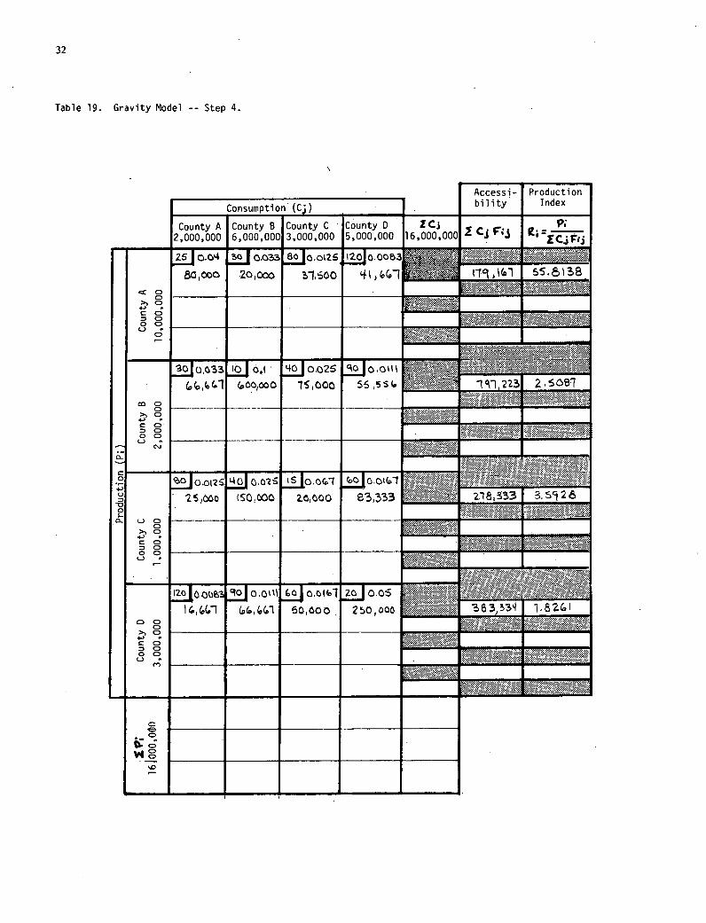
32
Table 19. Gravity Model -- Step 4.
Accessi- Production
Consumption (C;) . bility Index
1 CjF3 ili:ZCF .
County A County B County C County 0 ZC
2,000,000 6,000,000 3,000,000 5,000,000 116,000,000
451 004 0.Q33 jo otZ6 17010.0053
8 I 00 20,0 115OO
CD
cc, CD
0 Q L)
Sol 0.033 4 4010.025 o' I
CD
C c, Q
L) c, -..-- c'J
Jo.oi2 L40 0,025 [o.01 GoJc.cii
25,60 SO00 200 £3,333 -
CD
120 toos- JooI ots
IG(hl CD(o,CD1 60,0o 20,000
41
0.0 0
TI
0
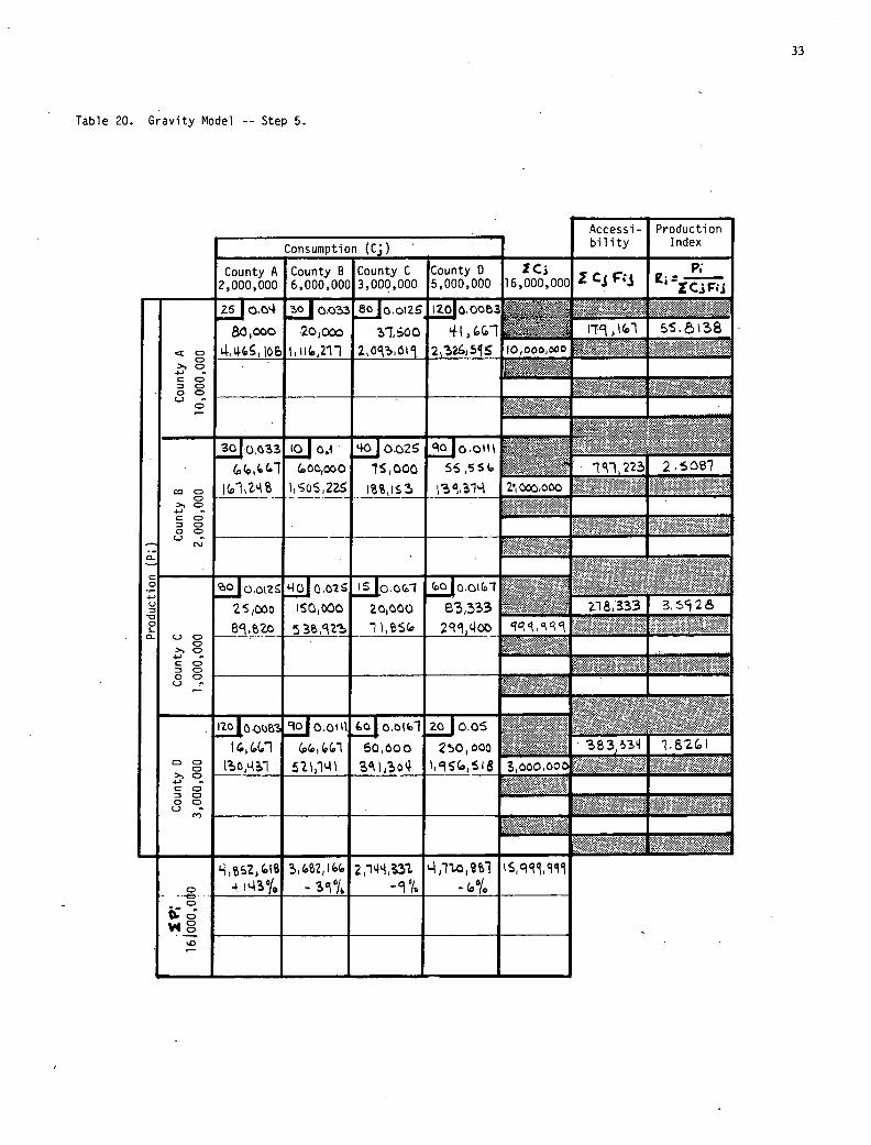
Table 20. Gravity Model -- Step 5.
Accessi- Production bility Index
CJ F-J lZi ZCjFJ
County A County B County C County 0 IC3
2,000,000 6,000,000 3,000,000 5,000,000 16,000,000
Jo.4 Joc3 jo.oizs IZO
&oco 20,0 1oo 4 1 j CD1
CD I444Ø (o,211 Z03t 22 5 5
CD
CD
0 3 LOJ o i 0 o2S
(.("1 (O,000 15,000 56 J 5
CO
- JO,Oi2 JQ02 JO0(1 JC.QI(D1 41
IIO(PJ Jo.eii J0.05
((C1 60600 2000
I
- 4,2(I8 5,422,i6G 21H32 '4,110fl1 ISII
CD
33
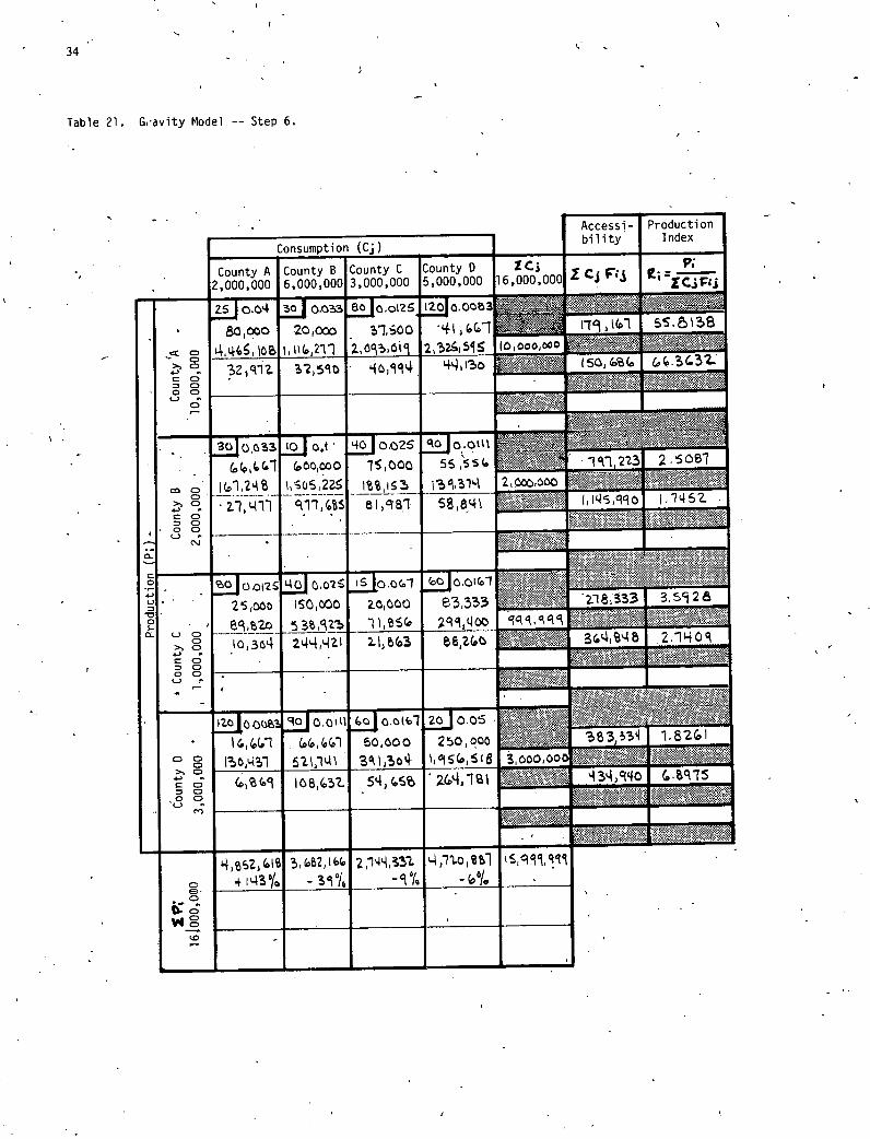
34
Table 21. G'avity Model -- Step 6.
Accessi- Production
Consumption (Ci) bility Index
P CF"
County A County B County C County 0 ZC.I 5,000,000 16,000,000 2,000,000 6,000,000 3,000,000
.jcoizs 411 80000 20,0 10O
0000 0O0 4 4tO C(,211 2. O03tj
: c
al I
!1 oG33Jo4 40J0026 d~,!55 (.0C'1 (o0,000 100Q
(p12'4. \062Z5 C%%iS
J
JO,Ot2 j Q02 Jp.ci Jocti ii3
2000 IS000 2000 e3333 —
0 - -- (_) -
-
Joo'i jo,c1 LOJo.o
250000 (hi C04(1 60000
cccc _________
§ (0L1 .\ CCo,6I8
, 41 0B3? 54.S 2L04,1& ______
-3 -4o
!
- &4,ztS 3IB2 2142 11.O1 0/
0
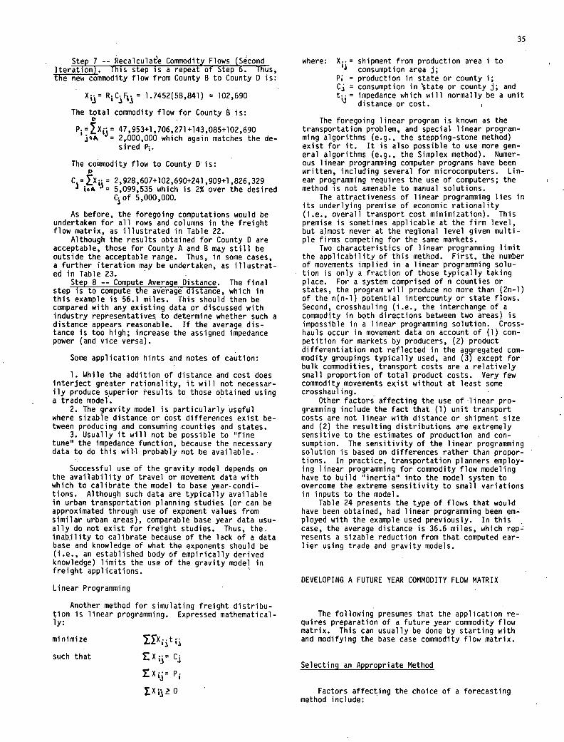
35
Step 7 -- Recalculat'e Commodity Flows (Second Iteration). This step is a repeat of Step 6. Thus, The new commodity flow from County B to County 0 is:
X= RCF= 1.7452(58,841) = 102,690
The total commodity flow for County B is:
47,953+1,706,271+143,085+102,690 = 2,000,000 which again matches the de-
sired P1.
The commodity flow to County D is:
C =Zx. = 2,928,607+102,690+241,909+19 826,329 lA = 5,099,535 which is 2% over the desired
Cof 5,000,000.
As before, the foregoing computations would be undertaken for all rows and columns in the freight flow matrix, as illustrated in Table 22.
Although the results obtained for County D are acceptable, those for County A and B may still be outside the acceptable range. Thus, in some cases, a further iteration may be undertaken, as illustrat-ed in Table 23.
Step 8 -- Compute Average Distance. The final step is to compute the average distance, which in this example is 56.1 miles. This should then be compared with any existing data or discussed with industry representatives to determine whether such a distance appears reasonable. If the average dis-tance is too high; increase the assigned impedance power (and vice versa).
Some application hints and notes of caution:
While the addition of distance and cost does interject greater rationality, it will not necessar-ily produce superior results to those obtained using a trade model.
The gravity model is particularly useful where sizable distance or cost differences exist be-tween producing and consuming counties and states.
Usually it will not be possible to "fine tune" the impedance function, because the necessary data to do this will probably not be available.
Successful use of the gravity model depends on the availability of travel or movement data with which to calibrate the model to base year. condi-tions. Although such data are typically available in urban transportation planning studies (or can be approximated through use of exponent values from similar urban areas), comparable base year data usu-ally do not exist for freight studies. Thus, the, inability to calibrate because of the lack of a data base and knowledge of what the exponents should be (i.e., an established body of empirically derived knowledge) limits the use of the gravity model in freight applications.
Linear Programming
Another method for simulating freight distribu-tion is linear programming. Expressed mathematical-ly:
minimize
such that X= Cj
x .j= P1
X 0
where: X. = shipment from production area i to consumption area j;
= production in state or county i; C) = consumption in 'state or county ,j; and t.= impedance which will normally be a unit
distance or cost.
The foregoing linear program is known as the transportation problem, and special linear program-ming algorithms (e.g., the stepping-stone method) exist for it. It is also possible to use more gen-eral algorithms (e.g., the Simplex method). Numer-ous linear programming computer programs have been written, including several for microcomputers. Lin-ear programming requires the use of computers; the method is not amenable to manual solutions.
The attractiveness of linear programming lies in its underlying premise of economic rationality (i.e., overall transport cost minimization). This premise is sometimes applicable at the firm level, but almost never at the regional level given multi-ple firms competing for the same markets.
Two characteristics of linear programming limit the applicability of this method. First, the number of movements implied in a linear programming solu-tion is only a fraction of those typically taking place. For a system comprised of n counties or states, the program will produce no more than (2n-1) of the n(n-1) potential intercounty or state flows. Second, crosshauling (i.e., the interchange of a commodity in both directions between two areas) is impossible in a linear programming solution. Cross-hauls occur in movement data on account of (1) com-petition for markets by producers, (2) product differentiation not reflected in the aggregated com-modity groupings typically used, and (3) except for bulk commodities, transport costs are a relatively small proportion of total product costs. Very few commodity movements exist without at least some crosshaul ing.
Other factors affecting the use of linear pro-gramming include the fact that (1) unit transport costs are not linear with distance or shipment size and (2) the resulting distributions are extremely sensitive to the estimates of production and con-sumption. The sensitivity of the linear programming solution is based on differences rather than propor-tions. In practice, transportation planners employ-ing linear programming for commodity flow modeling have to build "inertia" into the model system to overcome the extreme sensitivity to small variations in inputs to the model.
Table 24 presents the type of flows that would have been obtained, had linear programming been em-ployed with the example used previously. In this case, the average distance is 36.6 miles, which rep-resents a sizable reduction from that computed ear-lier using trade and gravity models.
DEVELOPING A FUTURE YEAR COMMODITY FLOW MATRIX
The following presumes that the application re-quires preparation of a future year commodity flow matrix. This can usually be done by starting with and modifying the base case commodity flow matrix.
Selecting an Appropriate Method
Factors affecting the choice of a forecasting method include:
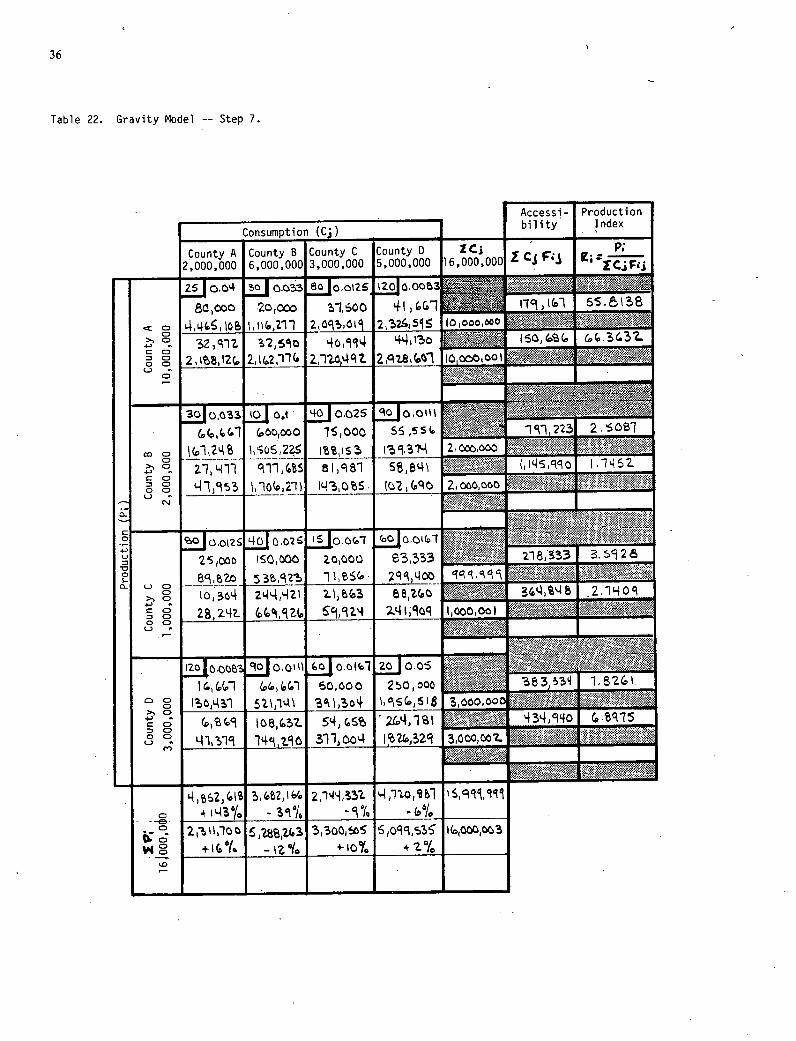
36
Table 22. Gravity Model -- Step 7.
Accessi- Production
Consumption (Ci) bility Index
Z Cj F3 P.
s:ZC.F.
County A County B County C County D ZCI
2,000,000 6,000,000 3,000,000 5,000,000 f16,000,000
o 4 aooQ3 Jô oZS Jo 'm 800 L5OO
0000000 g I4L4oB (211 21 2i5S
32,q12. f4 + .32.. .
CD 2,%8,l2(
Jo33 .2J.t J0025 qOJOO'I (D,OOO 7,000 56 55 6
'WM ts
zi,-ni qi1r.s 8Ia1 5884\ PI
cli
°JOOt25 4cJIO2$ Joi
25,oco ISOI OO 2000
>1 104 z44,L(2J BI2(
8 ZB,242. Wi.Z %V4 ?4I
2Joot' Jo.i LOJO.O5
20000 s000 3, CI s(D6I8
41
g 2Lo4,1 41,V1 14M,2.
-
S21 IS 2I12 flb1
CD S28V3 3O3~
+I o( _Zcio 4I0' 42.°f
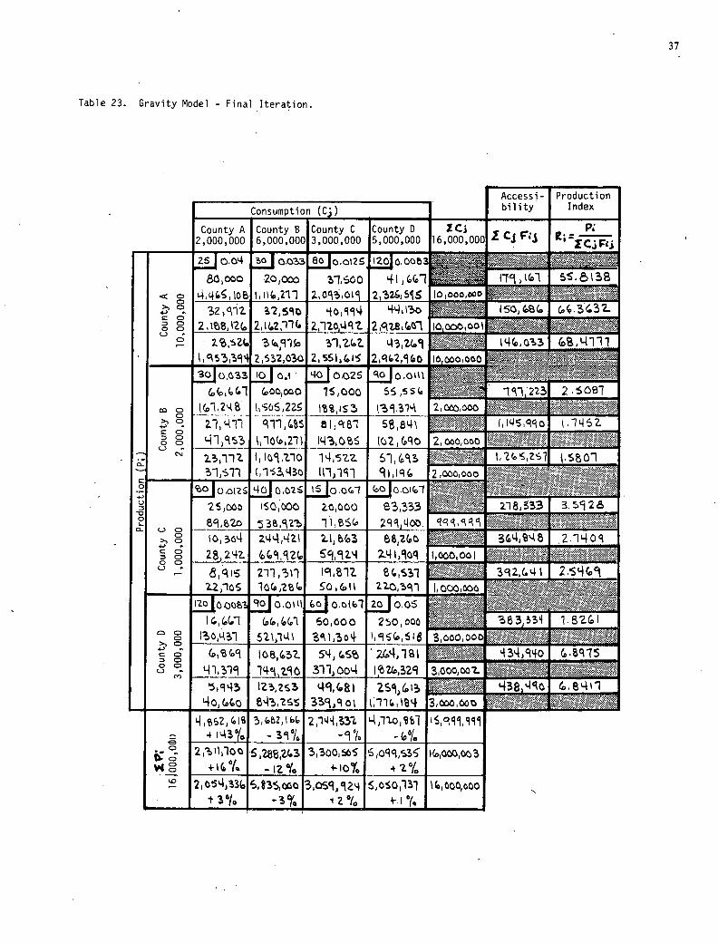
Table 23. Gravity Model - Final Iteration.
Accessi- Production
Consumption (Ci) bility Index
• . - ______
County A County B County C County 0 IC3
2,000,000 6,000,000 3,000,000 5,000,000 J16OOOOOO
- c c4 o Q33 Jo ot2 S IJO
oo 20,0 oo 9' I01 000,000 08 tS,211 03( 2,25S
'
C. 32q1z 40,4 44, i5o F 11 2 t8,%2(0 2l2,1(. o4qt. t0000
,9Th 1,VoZ. 43,2.(D t4(3 (D841 2 lo 252,030 z I ss I 1 (0 15 2621 0
21o,03 Jo.i J0.27 (00,000 ss,5s
2c'o %iS 1'4
11,(C ei°ai 58841 L
J2T i,s
2.3,11Z tflo i4szz S1(D _______ - cli
2,C000 ______ '111 I13,43.o U1)1j
'941 JO.Oi2S JQ02S JO.Q(T jooiii 251000
_L!_ 3•0t L& oo _______ _______ c CD 0,64 v4'.,'ZI 2.1543 2 g 28,2.42. 69,92.4 2.4I,0q I,0ccc I
81 qp 2fl,fl tciB1Z 81 2
I,cc-<ccc 220,q I
!L ti LGJo.o5 1(4(D1 ((Cl 60,000 250,000 83J 3' 1.82(I
CD 41
8/32. 54,(S 3443 CE7 S '- i,i ci 311) O Vo,3Z 3c co, c7
5,94 149,(681 2S%i 3,000 4o,o 84,2S 311,9 oi cm,lf
21'42 41L3I
EB /
2i00 £,28,ZLD3 3o0,O wg +°6 _izci 4Z°(O
2'4 3 3os9,29 I S,O!SO,131 li16,000,000
37
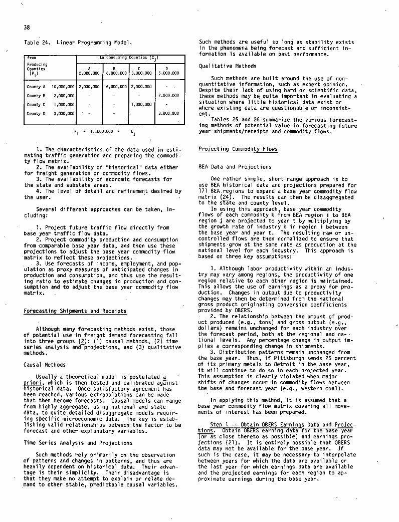
38
Table 24. Linear Programming Model.
from
Producing Counties
to Consuming Counties (C i
)
A B C 0 (P.) 2,000.000 6,000,000 3,000,000 5,000,000
County A 10,000,000 2.000.000 6,000,000 2,000,000 -
County 8 2,000,000 - - - 2,000,000
County C 1 1000,000 - - 1,000,000 -
County 0 3,000,000 - - 3,000,000
P1 = 16,000,000 = C
The characteristics of the data used in esti-mating traffic generation and preparing the commodi-ty flow matrix.
The availability of "historical" data either for freight generation or commodity flows.
3-. The availability of economic forecasts for the state and substate areas.
4. The level of detail and refinement desired by the user.
Several different approaches can be taken, in-ci udi ng:
1. Project future traffic flow directly from base year traffic flow data.
2. Project commodity production and consumption from - comparable base year data, and then use these projections to adjust the base year commodity flow matrix to reflect these projections.
3. Use forecasts of income, employment, and pop-ulation as proxy measures of anticipated changes in production and consumption, and thus use the result-ing ratio to estimate changes in production and con-sumption and to adjust the base year commodity flow matrix. - -
Forecasting Shipments and Receipts
Although many forecasting methods exist, those of potential use in freight demand forecasting fall into three groups (2): (1) causal methods, (2) time series analysis and—projections, and (3) qualitative methods.
Causal Methods
Usually a theoretical model is postulated a priori, which is then tested.and calibrated agiinst historical data. Once satisfactory agreement has been reached, various extrapolations can be made that then become forecasts. Causal models can range from highly aggregate, using national and state data, to quite detailed disaggregate models requir- ing specific microeconomic data The key is estab- lishing valid relationships between, the factor to be forecast and other explanatory variables.
Time Series Analysis and Projections
Such methods rely primarily on the observation of patterns and changes in patterns, and thus are heavily dependent on historical data. Their advan-tage is their simplicity. Their disadvantage is that they make no attempt to explain or relate de-mand to other stable, predictable causal variables.
Such methods are useful so long as stability exists in the phenomena being forecast and sufficient in-formation is available on past performance.
Qualitative Methods
Such methods are built around the use of non-quantitative information, such as expert opinion. Despite their lack of using hard or scientific data, these methods may be quite important in evaluating a situation where little historical data exist or where existing data are questionable or inconsist-ent.
Tables 25 and 26 summarize the various forecast-ing methods of potential value in forecasting future year shipments/receipts and commodity flows.
Projecting Commodity Flows
BEA Data and Projections
One rather simple, short range approach is to use BEA historical data and projections prepared for 171 BEA.regions to expand a base year commodity flow matrix (24). The results can then be disaggregated to the s'Eite and county level.
In using this approach, base year commodity flows of each commodity k from BEA region i to BEA region j are projected to year t by multiplying by the growth rate of industry k in region i between the base year and year t. The resulting raw or un-controlled flows are then normalized to ensure that shipments-grow at the same rate as production at the national level for each industry. This approach is based on three key assumptions:
Although labor productivity within an indus-try may vary among regions, the productivity of one region relative to each other region is maintained. This allows the use of earnings as a proxy for pro-duction. Changes in output due to productivity changes may then be determined from the national gross product originating conversion coefficients provided by OBERS.
The relationship between the amount of prod-uct produced (e.g., tons) and gross output (e.g., dollars) remains unchanged for each industry over the forecast period, both at the regional and na-tional levels. Any percentage change in output im-plies a corresponding change in shipments.
Distribution patterns remain unchanged from the base year. Thus, if Pittsburgh sends 25 percent of its primary metals to Detrpit in the base year, it will continue to do so in each projected year. This assumption is clearly violated when major shifts of changes occur in commodity flows between the base and forecast year (e.g., western coal).
In applying this method, it is assumed that a base year commodity flow matrix covering all move-ments of interest has been prepared.
Step 1 -- Obtain OBERS Earnings Data and Projec-tions. Obtain OBERS earning data f ase year (or as close thereto as possible) and earnings pro-jections (21). It is entirely possible that OBERS data may not be available for the base year. If such is the case, it may be necessary to interpolate between years for which the data are available or the last year for which earnings data are available and the projected earnings for each region to ap-proximate earnings during the base year.
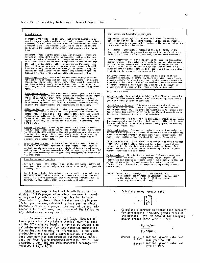
Table 25. Forecasting Techniques: General Description.
Causal Methods
Regreson Analysis: The ordinary least squares methOd can be applied
si to any single-equation model that is purported to capture
a one-way flow of causality from a set of independent variables to a dependent one. The dependent variable is the one to be fore-cast, using the specified historical relationship as the founda-tion.
Econometric Models (Simultaneous Equation Systems): These are systems of independent regression equations that describe some sector or region of economic or transportation activity. As a rule, these models are relatively expensive to develop and oper-ate, but they are more effective in expressing the causalities involved than ordinary regression models and consequently will forecast turning points more accurately. In general, they re-present the most attractive and potentially necessary modeling framework to handle regional and statewide conmiodity flows.
Input-Output Models: These reflect the interindustry or inter-regional flows of goods and services in the regional (or national) economy and its markets. Considerable effort must be expended to use these models properly and additional detail, not normally available, must be obtained if they are to be applied to specific regions.
Anticipation Surveys: These surveys of various groups of shippers, carriers, and users of different classes of corinnodities and freight are quite useful for short range forecasts. The surveys are usually quite brief and are geared to the respondents immediate decision-making needs. In the case of general consumer surveys; however, the questionnaires are occasionally quite lengthy.
Diffusion Indices: A diffusion index is a composite of various business and economic indicators. Its purpose is to capture the general flow or trend of all the leading, coinciding, and lagging indicators normally used to reflect general business conditions. To the extent that the demand for commodities is derived from more aggregate demands, this method could be useful in comodity trans-port planning.
Leading Indicators: A leading indicator is a particular index that has been estimated by the National Bureau of Economic Research to reflect changing aggregate economic conditions by preceding or leading the change. It is particularly useful in forecasting
turning points in the rate of growth in various categories of economic and monetary data.
Economic Base Studies: To some extent, economic base studies are the heart of classical regional location theory. These studies reflect the changing economic and industrial base in local areas and regions. They are extremely useful in capturing the industrial mix of local coimiunity and in generating employment information on its industries.
Time Series and Projections
Moving Averages: This method is one of the most basic statistical exercises; it uses quarterly or monthly data ordinarily to generate a moving trend.
Box-Jenkins Method: This method assigns probability weights to a series of historical data with the assistance of a quantitative model. It is more cumbersome than using moving averages, but its accuracy in forecasting short-term movements is much higher.
Time Series and Projections, Continued
Exponential Smoothing: In some ways this method is merely a special case of the Box-Jenkins method. It assigns progressively higher weights in an exponential fashion to the more recent points of observation in a time series.
X-ll Method: Originally developed at the U. S. Bureau of the Census, this method decomposes time series into the classic dis-tribution of trend, cyclical, seasonal, and irregular components.
Trend Projections: This in some ways is the simplest forecasting method in usage. The analyst needs only to take an existing series or equation and extrapolate the value of the dependent variable. This extrapolation can be done in many ways; for example, by a range or band of extrapolations, or by applying a known statistical distribution to generate the extrapolation.
Motionary Triangles: These are among the most complex of the statistical methods. Essentially, there is a wide range of tech-niques available for plotting or charting short-range movements in a particular indicator. Some of the movements are calculated with different triangle" configurations, such that a 'breakout" on either side of the apex of the triangle could be forecast.
Qualitative Methods
Delphi Method: This method is a fairly well defined procedure for using cumulative questionnaires to solicit expert opinions from a group of carefully selected panelists.
Market Research Methods: This method uses personal and on-site interviews with shippers, carriers, agencies, and users of com-modity transportation. The principal intention is to forecast the longer-range developments or shifts in the flows of comodities or in the contributions of the critical industries.
Panel Consensus: This is simply an organized approach to appraising the consensus of a panel of individuals on a specific set of issues. The approach is quite useful to generate fairly quick and accurate short-range predictions.
Historical Analogy: This method requires the use of an analyst who is familiar with previous patterns of behavior or who can asnociate a trend in current events with some historical configuration. One must be very cautious, however, about its use in forecasting.
Visionary Forecasts: Quite often, it is valuable to hire a reputed "visionary" in the field, someone who has a track record of pro-viding feasible insight to a particular problem or issue. In a sense, this method is a control or an anchor against which other methods' forecasts can be compared.
Factor Analysis: This is the most mathematical method among the set of qualitative ones. It incorporates the preferences of individuals and experts by ranking their views either with cardinal or ordinal measures. The end product is a set of important "factors" or attributes that are regarded as explaining a parti-cular event.
Source: Bruck, lw., Kneafsey, J.T. , and Roberts, P.O., "A Methodological Approach to Commodity Flow Analysis in the State of California." MIT Urban Systems Laboratory, Cambridge, MA (1974).
Step 2 -- Compute Regional Growth Rates by In-dustry. OBERS projected earnings are used to devel-op regional growth rates for application to base year commodity flows. Growth rates are simply pro-jected year earnings divided by base year earnings. Because such data or projections may not be entirely amenable to direct use, one or more of the following adjustments may be required:
1. Suppression of Historical Data. Because of the suppression of certain historical earnings data at the BEA-industry level, it may not be possible to calculate growth rates for some regional industries for estimating the missing information. Since OBERS projections are basically extrapolative, missing base year earnings can often be estimated by "back-casting" from future projected earnings levels. For example, given 1980 and 1985 projected earnings for industry 1 (Er, E,):
Calculate annual growth rate:
Calculate a correction factor that accounts for differential industry growth rates at the national level to account for changing growth trends (base year = 1972):
9,9 72.180
g 1 ,lzjso-.
where: g = national growth rate from 1-12160
base year to 1980 goo:e6= national growth rate from
1980 to 1985
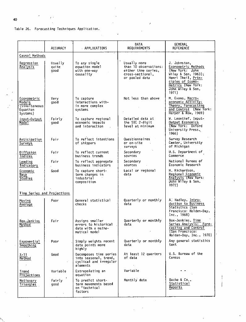
40
Table 26. Forecasting Techniques Application.
DATA GENERAL ACCURACY APPLICATIONS REQUIREFiENTS REFERENCE
Causal Methods
Usually To any single Usually more J. Johnston, Regression Analysis quite equation model than 10 observations: Econometric Methods
good with one-way either time series, (New York: John causality cross-sectional, Wiley & Son, 1963);
or pooled data Henri Theil, Prin- ciples of Econo- metrics (New York: John Wiley & Son, 1971)
Econometric Very good
To capture interactions with-
Not less than above M. Evans, Macro-economic Activity: Models
(Simultaneous in more complex Theory, Forecasting Equation systems and Control (New York: Systems) Harper & Row, 1969)
Input-Output Fairly good
To capture regional economic impacts
Detailed data at the SIC 2-digit
W. Leontief, Input- Output Economics Model
and interaction level at minimum (New York: Oxford University Press, 1966)
Anticipation Fair To reflect intentions of shippers
Questionnaires or on-site
Survey Research Center, University Surveys
surveys of Michigan
Diffusion Fair To reflect current Secondary U.S. Department of Indices business trends sources Commerce
Leading Fair To reflect aggregate Secondary National Bureau of
Indicators business indicators sources Economic Research
Economic Good To capture short- Local or regional H. Richardson, Base term changes in data Regional Economic Tt—udies industrial Analysis New York:
composition John Wiley & Son, 1972)
Time Series and Projections
General statistical Quarterly or monthly A. Hadley, Intro- Moving Poor Average checks data duction to Business
Statistics (San Francisco: Holden-Day, Inc., 1968)
Box-Jenkins Fair Assigns smaller errors to historical
Quarterly or monthly data
Box-Jenkins, Time Series Analysis: Fore- Method casting and Control data with a mathe-
matical model (San Francisco: Holden-Day, Inc., 1970)
Exponential Poor Simply weights recent data points more
Quarterly or monthly data
Any general statistics text Smoothing
highly
X-11 Good Decomposes time series At least 12 quarters U.S. Bureau of the
Method into seasonal, trend, of data Census cyclical and irregular elements
Trend Variable Extrapolating an Variable - - Projections
Fairly
equation
To predict short- Monthly data Bache & Co., Motionary Triangles good term movements based Statistical
on 'technical Reports factors
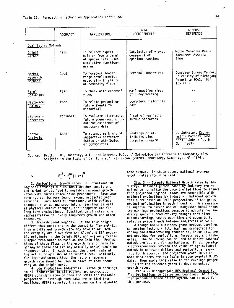
Table 26. Forecasting Techniques Application Continued. 41
ACCURACY APPLICATIONS DATA
REQUIREMENTS GENERAL REFERENCE
Qualitative Methods
Fair To collect expert Tabulation of views; Motor Vehicles Manu- Delphi Method opinion from a panel consensus of facturers Associa-
of specialists; uses opinion; rankings tion cumulative question- nai res
Market Good To forecast longer Personal interviews Consumer Survey Center,
Research range developments, University of Michigan;
Methods especially in shifts Report to SCAG, 1974
of commodity flows (by MIT)
Panel Fair To check with experts' Mail questionnaire; --
Consensus views or 1 day meeting
Historical Poor To relate present or Long-term historical --
Analogy future events to data historical
Visionary Variable To evaluate alternative A set of realistic --
Forecasts future scenarios, with- future scenarios outthe existence of necessary data
Factor Good To attempt rankings of Rankings of at- J. Johnston, Econo-
Analysis subjective character- tributes plus metric Methods New
istics or attributes computer program York: John Wiley &
of commodities Son (1963)
Source: Bruck, H.W., Kneafsey, J.T., and Roberts, P.O., 'A Methodological Approach to Commodity Flow Analysis in the State of California." MIT Urban Systems Laboratory, Cambridge, MA (1974).
C. E1 = E (l+rc)
Agricultural Growth Rates. Fluctuations in regional earnings due to local weather conditions and market prices lead to unstable regional growth rates with normal calculation procedures. Base year earnings can be very low or exceed projected year earnings. Such local fluctuations, which reflect changes in price and proprietors' earnings as well as physical output changes, are inappropriate for long-term projections. Substitution of rates more representative of likely long-term growth are often necessary.
Transshipment Regions. If the true origin differs that contained in the commodity flow matrix, then a different growth rate may have to be used. For example, ore flows from the Cleveland BEA proba-bly originate in the Duluth BEA, and are only trans-shipped from water to rail at the Ohio BEA. Projec-tions of these flows by the growth rate of metallic mining in Cleveland (if any actually occur) would be inappropriate. in such cases, the growth rate at the actual origin should be substituted. Similarly for imported commodities, the national average growth rate should be used in place of that occur-ring at the origin port.
Low Production Industries. Although earnings in all industries in all regions. are projected, OBERS considers some of them too small for reliable projection. Although such data are omitted from
'published OBERS reports, they appear on the magnetic
tape output. In these cases, national average growth rates should be used.
Steo 3 -- Comoute National Growth Rates by In-dustNatiônal growth rates by industry are re-quired to normalize the uncontrolled flows to ensure that projected regional flows are compatible with national projections by industry. National growth totals are based on OBERS projections of the gross product originating in each industry. This measure is superior to direct use of unadjusted OBERS indus-try earnings projections because it adjusts for in-dustry specific productivity changes that alter output/earnings ratios over time and accounts for relative price trends between industries as well.
Although OBERS publishes gross-product earnings conversion factors (historical and projected) for mining and manufacturing industries, these data are not provided for agriculture, forestries, and fish-eries. The following can be used to derive national output projections for agriculture. First, develop a correspondence between the value of agricultural output in constant dollars and agricultural earn-ings for historical and projected years in which both data items are available in supplemental OBERS data. Then apply this ratio to the earnings projec-tions for the forecast years to develop output growth rates.
Steo 4 -- Disaggregate BEA Regional Commodity Flow Projections to States and Counties. An alloca-tion procedure based on employment can be used for this purpose.
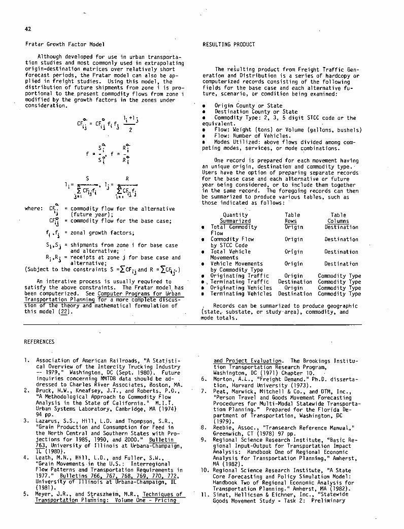
The reulting product from Freight Traffic Gen-eration and Distribution is a series of hardcopy or computerized records consisting of the following fields for the base case and each alternative fu-ture, scenario, or condition being examined:
Origin County or State Destination County or State Commodity Type: 2, 3, 5 digit STCC code or the
equi valent. Flow: Weight (tons) or Volume (gallons, bushels) Flow: Number of Vehicles. Modes Utilized: above flows divided among com-
peting modes, services, or mode combinations.
One record is prepared for each movement having an unique origin, destination' and commodity type. Users have the option of preparing separate records for the base case and each alternative or future year being considered, or to include them together in the same record. The foregoing records can then be summarized to produce various tables, such as those indicated as follows:
Quantity Table Table Summarized Rows Columns
Total Commodity Origin Destination Flow Commodity Flow Origin Destination by STCC Code Total Vehicle Origin Destination Movements Vehicle Movements Origin Destination by Commodity Type Originating Traffic Origin Commodity Type Terminating Traffic Destination Commodity Type Originating Vehicles Origin Commodity Type Terminating Vehicles Destination Commodity Type
42
Fratar Growth Factor Model
RESULTING PRODUCT
Although developed for use in urban transporta-tion studies and most commonly used in extrapolating origin-destination matrices over relatively short forecast periods, the Fratar model can also be ap-plied in freight studies. Using this model, the distribution of future shipments from zone i is pro-portional to the, present commodity flows from zone i modified by the growth factors in the zones under consideration.
3. CF.. = CE. f.f ' •
' 2
a. where: CE. = commodity flow for the alternative
'.i (future year); C FP = commodity flow for the base case;
f ,f i = zonal growth factors;
S1,S3 = shipments from zone i for base case and alternative;
= receipts at zone j for base case and alternative;
(Subject to the constraints S =CFand R =!CF3.)
An interative process is usually required to satisfy the above constraints. The Fratar model has been computerized. See Computer Programs for Urban Transportation Planning for a more complete discus- sion of the theory and mathematical formulation of Records can be summarized to produce geographic this model (22). (state, substate, or studyarea), commodity, and
mode totals.
REFERENCES
sl~ 0.. R
f = ..i,
= ,
Co 0.
S R
CFçf ' - CFf3
Association of American Railroads, "A Statisti-cal Overview of the Intercity Trucking Industry -- 1979," Washington, DC (Sept. 1980). Future inquiries concerning NMTDB data should be ad-dressed to Charles River Associates, Boston, MA. Bruck, H.W., Kneafsey, J.T., and Roberts, P.O., 'A Methodological Approach to Commodity Flow Analysis in the State of California. M.I.T. Urban Systems Laboratory, Cambridge, MA (1974) 94 pp. Lazarus, S.S., Hill, L.D. and Thompson, S.R., "Grain Production and Consumption for Feed in the North Central and Southern States with Pro-jections for 1985, 1990, and 2000." Bulletin 763, University of Illinois at Urbana-Champaign, IL (1980). Leath, M.N., Hill, L.D., and Fuller, S.W., "Grain Movements in the U.S.: Interregional Flow Patterns and Transportation Requirements in 1977." Bulletins 766, 767 768, 769, 770, 772, University of Illinois at (Jrbana-Champaign, IL (1981). Meyer, J.R., and Straszheim, M.R., Techniques of Transportation Planning: Volume One - Pricing
and Project Evaluation. The Brookings Institu-tion Transportation Research Program, Washington, DC (1971) Chapter 10. Morton, A.L., "Freight Demand." Ph.D. disserta-tion, Harvard University (1973). Peat, Marwick, Mitchell & Co., and DTM, Inc., "Person Travel and Goods Movement Forecasting Procedures for Multi-Modal Statewide Transporta-tion Planning." Prepared for the Florida De-partment of Transportation, Washington, DC (1979). Reebie, Assoc., "Transearch Reference Manual,," Greenwich, CT (1978) 97 pp. Regional Science Research Institute, "Basic Re-gional Input-Output for Transportation Impact Analysis: Handbook One of Regional Economic Analysis for Transportation Planning," Amherst, MA (1982). Regional Science Research Institute, "A State Core Forecasting and Policy Simulation Model: Handbook Two of Regional Economic Analysis for Transportation Planning." Amherst, MA (1982). Simat, Hellicsen & Eichner, Inc., "Statewide Goods Movement Study - Task 2: Preliminary
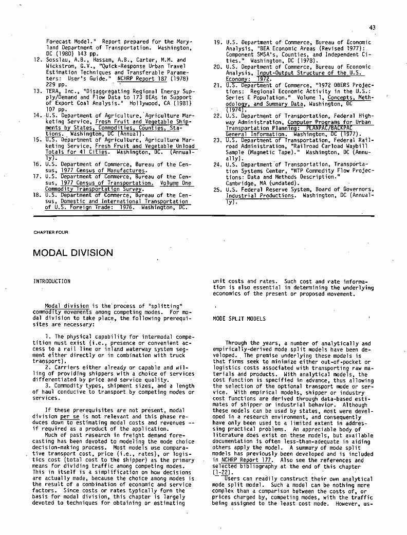
Forecast Model." Report prepared for the Mary-land Department of Transportation. Washington, DC (1980) 143 pp. Sosslau, A.B., Hassam, A.B., Carter, M.M. and Wickstrom, G.V., "Quick-Response Urban Travel Estimation Techniques and Transferable Parame-ters: User's Guide." NCHRP Report 187 (1978) 229 pp. TERA, Inc., "Disaggregating Regional Energy Sup-ply/Demand and Flow Data to 173 BEAs in Support of Export Coal Analysis." Hollywood, CA (1981) 107 pp. U.S. Department of Agriculture, Agriculture Mar-keting Service, Fresh Fruit and Vegetable Ship-ments by States, Commodities, Counties, Sta-tions. Washington, DC (Annual). U.S. Department of Agriculture, Agriculture Mar-keting Service, Fresh Fruit and Vegetable Unload Totals for 41 Cities. Washington, DC. (Annual-ly). U.S. Department of Commerce, Bureau of the Cen-sus, 1977 Census of Manufactures. U.S. Department of Commerce, Bureau of the Cen-sus, 1977 Census of Transportation. Volume One Commodity Transportation Survey. U.S. Department of Commerce, Bureau of the Cen-sus, Domestic and International Transportation of U.S. Foreign Trade: 1976. Washington, DC.
43
U.S. Department of Commerce, Bureau of Economic Analysis, "BEA Economic Areas (Revised 1977): Component SMSA's, Counties, and Independent Ci-ties." Washington, DC (1978). U.S. Department of Commerce, Bureau of Economic Analysis, Input-Output Structure of. the.U.S. Economy: 1972. U.S. Department of Commerce, "1972 OBERS Projec-tions: Regional Economic Activity in the U.S.: Series E Population." Volume 1, Concepts, Meth-odology, and Summary Data, Washington, DC (1974). U.S. Department of Transportation, Federal High-way Administration, Computer Programs for Urban Transportation Planning: PLANPAC/BACKPAC General Information. Washington, DC (1977). U.S. Department of Transportation, Federal Rail-road Administration, "Railroad Carload Waybill Sample (Magnetic Tape)." Washington, DC (Annu-ally). U.S. Department of Transportation, Transporta-tion Systems Center, "NTP Commodity Flow Projec-tions: Data and Methods Description." Cambridge, MA (undated). U.S. Federal Reserve System, Board of Governors, Industrial Productions. Washington, DC (Annual-ly).
CHAPTER FOUR
MODAL DIVISION
INTRODUCTION
Modal division is theprocess of "splitting" commodity movements among competing modes. For mo-dal division to take place, the following prerequi-sites are necessary:
The physical capability for intermodal compe-tition must exist (i.e., presence or convenient ac-cess to a rail line or inland waterway system seg-ment either directly or in combination with truck transport).
Carriers either already or capable and wil-ling of providing shippers with a choice of services differentiated by price and service quality.
Commodity types, shipment sizes, and a length of haul conducive to transport by competing modes or services.
If these prerequisites are not present, modal division per se is not relevant and this phase re-duces down to estimating modal costs and revenues --if required as a product of the application.
Much of past research in freight demand fore-casting has been devoted to modeling the mode choice decision-making process. Most models use compara-tive transport cost, price (i.e., rates), or logis-tics cost (total cost to the shipper) as the primary means for dividing traffic among competing modes. This in itself is a simplification on how decisions are actually made, because the choice among modes is the result of a combination of economic and service factors. Since costs or rates typically form the basis for modal division, this chapter is largely devoted to techniques for obtaining or estimating
unit costs and rates. Such cost and rate informa-tion is also essential in determining the underlying economics of the present or proposed movement.
MODE SPLIT MODELS
Through the years, a number of analytically and empirically-derived mode split models have been de-veloped. The premise underlying these models is that firms seek to minimize either out-of-pocket or logistics costs associated with transporting raw ma-terials and products. With analytical models, the cost function is specified in advance, thus allowing the selection of the optional transport mode or ser-vice. With empirical models, shipper or industry cost functions are derived through data-based esti-mates of shipper or industrial behavior. Although these models can be used by states, most were devel-oped in a research environment, and consequently have only been used to a limited extent in addres-sing practical problems. An appreciable body of literature does exist on these models, but available documentation is often less-than-adequate in aiding others apply the model. A summary of mode split models has previously been developed and is included in NCHRP Report 177. Also see the references and selected bibliography at the end of this chapter (1-22).
lJsers can readily construct their own analytical mode split model. Such a model can be nothing more complex than a comparison between the costs of, or prices charged by, competing modes, with the traffic being assigned to the least cost mode. However, us-
44
ers must first choose between a physical distribu-tion (logistics) or transport economics approach. If the latter is selected, users must further decide whether the resulting model will use rates (charges to shipper) or unit costs (incurred by carriers) in dividing commodity movements among competing car-riers. The underlying logic is straightforward, as indicated below:
Mode split model using marginal unit costs: Let cb = base case unit cost (to carriers)
c0 = alternate unit cost (to carriers) If c<cb, assign traffic movement to the alternative mode; otherwise assign movement to the base case mode.
Mode split model using actual or estimated rates: Let rb = base case rate
r = alternative rate If r< rb, assign traffic movement to the alternative mode; otherwise assign movement to the base case mode.
Mode split model using physical distribution costs: Let 5b = base case unit cost (to shippers)
s0, = alternate unit cost (to shippers) where: s = transport logistics cost + non-
transport logistics costs = c*+ c, cJ = rate + unit loss and damage +
unit pick-up and delivery. c = unit order cost + unit storage " cost + unit inventory + unit
carrying cost in-transit + unit stockout cost.
If ssassign traffic movement to the alternative mode; otherwise assign movement to the base case mode.
The foregoing logic presumes choosing between two modes or services. However, the concep,t can readily be extended to include additional modes or services.
The mode split model assigns all of the traffic to the mode having the least cost or rate regardless of the magnitude of the cost or rate difference. Given known indifference to small variations in unit costs or rates, users may wish to incorporate con-straints on an "all-or-nothing' assignment approach. One method for doing this is to establish a zone of indifference within that competing modes or services would share the traffic proportionally. Alterna-tively, the user can predefine a point at which di-version from an existing mode or service is presumed to take place, or place limits on the amount of di-version or the maximum market share possible for different modes or transport services. While such logic will reduce the sensitivity of modal division to small unit price or cost differences, they should reflect observed behavior and thus would not be im-plemented arbitrarily. On condition that appropri-ate data are available, the user can also develop diversion curves governing the assignment of traffic to competing modes and/or services on the basis of their relative prices or costs.
Users can also use various empirical models, such as the (1) disaggregate multinomial logit, (2) aggregate multinomial logit, and (3) aggregate translog (2-5,7,10-19). These models have not been included as su5techniques, because they employ math-ematical techniques and computer programs that tend to be unfamiliar or are unavailable to state DOT personnel. Users potentially interested in using these models should obtain copies of the listed re-ferences and communicate directly with the research-ers involved for further information.
Regardless of which model is chosen, it will perform no better than the quality of the input data, which are unit costs or prices. Hence the em-phasis in this chapter on developing unit costs and rates.
UNIT COSTS
Virtually all the larger carriers have developed extensive costing systems for strategic planning and internal management purposes. These systems are tailored to meet the specific needs of individual carriers, and thus vary greatly in design and so-phistication. Neither these systems nor the prod-ucts produced therefrom are generally available to states except for information introduced into the record at regulatory proceedings.
Consequently, the public sector has had to de-velop its own cost-estimating systems. Development of such systems has been uneven; in the rail area, the Interstate Commerce Commission's need for a sys-tem that would produce comparable cost data led originally to the development of "Rail Form A" in 1939. Since then, this methodology has become the standard, recognized rail costing tool for regula-tory-oriented applications and is being widely used by others to estimate the costs associated with rail movements. Recent legislation has resulted in the development of the Uniform Rail Costing System (URCS) as a replacement of Rail Form A for use by the public and private sectors.
Analogous public sector techniques for costing truck and inland waterway movements do not exist. As part of this research project, a computerized truck costing system comparable in detail to URCS has been developed. Procedures have also been pre-sented for costing barge movements on the inland wa-terway system and for determining logistics or dis-tribution costs from a shipper's perspective.
The costing subtechniques presented must be ap-plied correctly. In particular, the user must rec-ognize that:
The resulting unit cost will never be a sin-gle "true" cost, but only an estimate.
Costs can be measured in a variety of ways, any one of which can be correct under the particular circumstances of the application.
Unit costs will vary appreciably within the carrier or within the mode, depending on location, financial condition and management expertise of the carrier and the specific movement being costed.
The unit costs chosen must be compatible with the application at hand.
Unit costs will vary over time, thus making it necessary to determine the time period on which the unit costs are based, and to update these costs to reflect the desired time period.
The user should also recognize that the unit cost data available to the public sector will always be limited. First, government is not providing the transport service and thus is dependent on common and private carriers for necessary data. Second, carriers provide data in response to requirements laid down by regulatory agencies. Because of poten-tial competitive difficulties stemming from inadver-tent release of proprietary data, regulatory agen-cies generally treat such data confidentially, only releasing carrier data in aggregated or summary form. Consequently, detailed information describing how such unit costs were derived, or indicating ex-
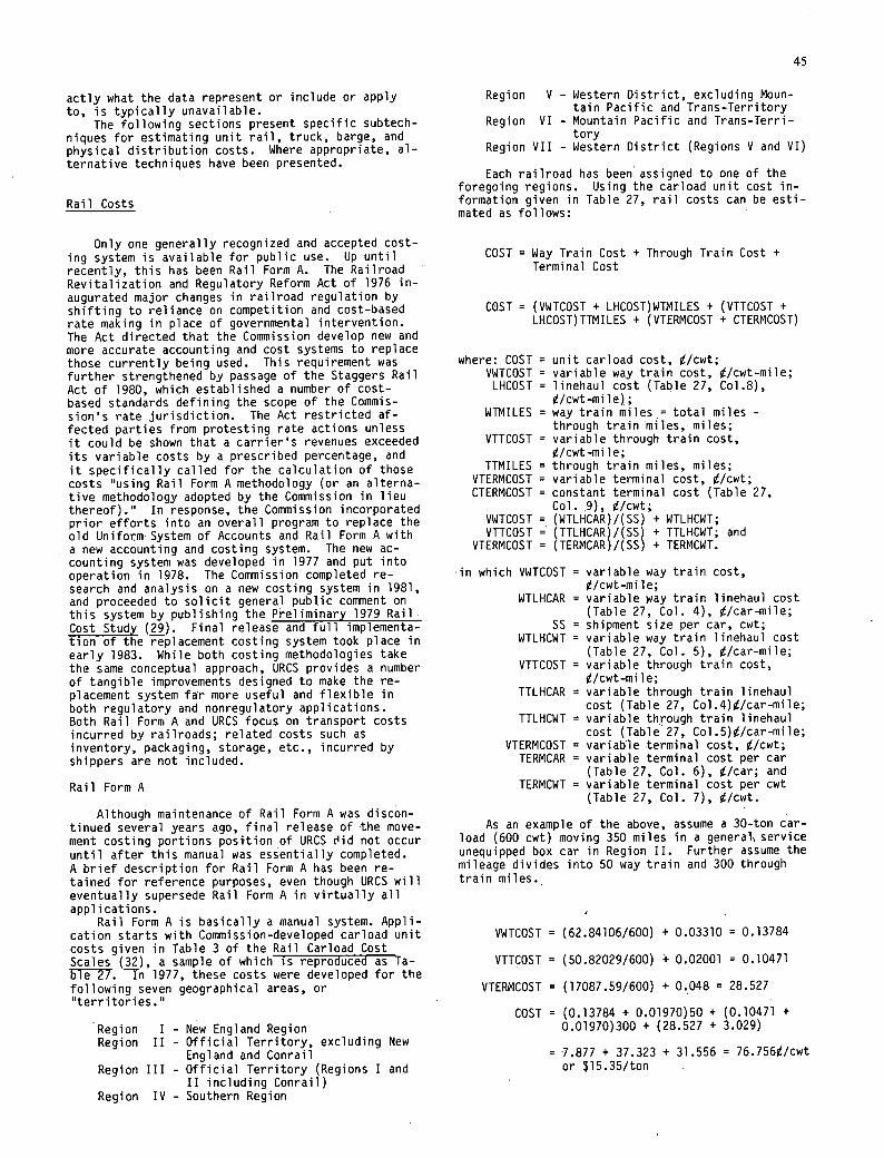
45
actly what the data represent or include or apply to, is typically unavailable.
The following sections present specific subtech-niques for estimating unit rail, truck, barge, and physical distribution costs. Where appropriate, al-ternative techniques have been presented.
Rail Costs
Only one generally recognized and accepted cost-ing system is available for public use. Up until recently, this has been Rail Form A. The Railroad Revitalization and Regulatory Reform Act of 1976 in-augurated major changes in railroad regulation by shifting to reliance on competition and cost-based rate making in place of governmental intervention. The Act directed that the Commission develop new and more accurate accounting and cost systems to replace those currently being used. This requirement was further strengthened by passage of the Staggers Rail Act of 1980, which established a number of cost-based standards defining the scope of the Commis-sion's rate jurisdiction. The Act restricted af-fected parties from protesting rate actions unless it could be shown that a carrier's revenues exceeded its variable costs by a prescribed percentage, and it specifically called for the calculation of those costs "using Rail Form A methodology (or an alterna-tive methodology adopted by the Commission in lieu thereof)." In response, the Commission incorporated prior efforts into an overall program to replace the old Uniform System of Accounts and Rail Form A with a new accounting and costing system. The new ac-counting system was developed in 1977 and put into operation in 1978. The Commission completed re-search and analysis on a new costing system in 1981, and proceeded to solicit general public comment on this system by publishing the Preliminary 1979 Rail Cost Study (29). Final release and full implementa-tion of the replacement costing system took place in early 1983. While both costing methodologies take the same conceptual approach, URCS provides a number of tangible improvements designed to make the re-placement system fr more useful and flexible in both regulatory and nonregulatory applications. Both Rail Form A and URCS focus on transport costs incurred by railroads; related costs such as inventory, packaging, storage, etc., incurred by shippers are not included.
Rail Form A
Although maintenance of Rail Form A was discon-tinued several years ago, final release of the move-ment costing portions position of URCS c'id not occur until after this manual was essentially completed. A brief description for Rail Form A has been re-tained for reference purposes, even though URCS will eventually supersede Rail Form A in virtually all applications.
Rail Form A is basically a manual system. Appli-cation starts with Commission-developed carload unit costs given in Table 3 of the Rail Carload Cost Scales (32), a sample of which is reproduced as Ta-ble 27. Tn 1977, these costs were developed for the following seven geographical areas, or "territories."
Region I - New England Region Region II - Official Territory, excluding New
England and Conrail Region III - Official Territory (Regions I and
II including Conrail) Region IV - Southern Region
Region V - Western District, excluding Moun- tain Pacific and Trans-Territory
Region VI - Mountain Pacific and Trans-Terri-tory
Region VII - Western District (Regions V and VI)
Each railroad has been assigned to one of the foregoing regions. Using the carload unit cost in-formation given in Table 27, rail costs can be esti-mated as follows:
COST = Way Train Cost + Through Train Cost + Terminal Cost
COST = (VWTCOST + LHCOST)WTMILES + (VTTCOST + L}-ICOST)TTMILES + (VTERMCOST + CTERMCOST)
where: COST = unit carload cost,0/cwt; VWTCOST = variable way train cost, /cwt-mile; LHCOST = linehaul cost (Table 27, Col.8),
/cwt-mi1e); WIMILES = way train miles .= total miles -
through train miles, miles; VTTCOST = variable through train cost,
/cwt-mile; TIMILES = through train miles, miles;
VTERMCOST = variable terminal cost,0/cwt; CTERMCOST = constant terminal cost (Table 27,
Col. 9),0/cwt; VWTCOST = (WTLHCAR)/(SS) + WTLHCWT; VTTCOST = (TTLHCAR)/(SS) + TTLHCWT; and
VTERMCOST = (TERMCAR)/(SS) + TERMCWT.
in which VWTCOST = variable way train cost, /cwt-mile;
WTLHCAR = variable way train linehaul cost (Table 27, Col. 4), i/car-mile;
SS = shipment size per car, cwt; WTLHCWT = variable way train linehaul cost
(Table 27, Col. 5), i/car-mile; VTTCOST = variable through train cost,
/cwt-mi le; TTLHCAR = variable through train linehaul
cost (Table 27, Col.4)/car-mile; TTLHCWT = variable through train linehaul
cost (Table 27, Co1.5)/car-mi1e; VTERMCOST = variable terminal cost,0/cwt; TERMCAR = variable terminal cost per car
(Table 27, Col. 6), 0/car; and TERMCWT = variable terminal cost per cwt
(Table 27, Col. 7),9/cwt.
As an example of the above, assume a 30-ton car-load (600 cwt) moving 350 miles in a generals service unequipped box car in Region II. Further assume the mileage divides into 50 way train and 300 through train miles.
VWTCOST =(62.84106/600) + 0.03310 = 0.13784
VTTCOST = (50.82029/600) + 0.02001 = 0.10471
VTERMCOST = (17087.59/600) + 0.048 = 28.527
COST = (0.13784 + 0.01970)50 + (0.10471 + 0.01970)300 + (28.527 + 3.029)
= 7.877 + 37.323 + 31.556 = 76.756/cwt or $15.35/ton
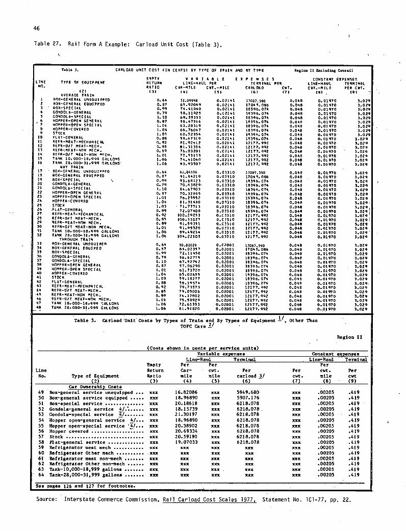
46
Table 27. Rail Form .4 Example: Carload Unit Cost (Table 3).
Table 3. CARLOAD UNIT COST (EN CENTS) BY TYPE OF TRAIN AND BY TYPE Region II Excluding Conrail
EMPTY V A R I AOL E E B PT N € S S CONSTANT EXPENSES LINE TYPE OF EQUIPMENT RETURN LINE-HAUL PER TERMINAL PER LINE-HAUL TERMINAL
RATIO CAR-NILE CWT.-MILE CARLOAD CWT. CWT.-MILE PER CWT. (2) (3) (4) IS) (6) (7) (5) (9)
AVERAGE TRAIN 1 BOX-GENERAL UMEOUIPPFO 0.64 52.09998 0.02141 17087.590 0.048 0.01970 3.029 2 803-GENERAL EQUIPPED 0.97 65.92049 0.02141 17045.086 0.048 0.01970 3.029 3 BOX-SPECIAL 0.99 74.41040 0.02141 18396.014 0.048 0.01970 3.029 4 Gn4001A-GENERgL 0.79 58.11925 0.02141 16396.074 0.048 0.01970 3.029 S GONOOLA-SPEC14L 1.10 69.39333 0.02141 18396.074 0.048 0.01970 3.029 - 6 HOPPER-OPEN GENERAL 0.87 98.47518 0.02141 15306.074 0.048 0.01970 3.029 7 HOPPER-OPEN SPECIAL 1.01 63.28319 0.02141 18396.074 0.048 0.01970 3.029 B HOPPER-COVERED 1.04 66.76047 0.02141 18306.074 0.048 0.01970 3.029
STOCK 1.03 60.52354 0.02141 15306. 074 0.048 0.01970 3.029 10 FLAT-GENERAL 0.88 59.67319 0.02141 15396. 074 0.048 0.01970 3.029 11 REFR-NEAT-MECHAN(CAL 0.92 81.92412 0.02141 12177.992 0.048 0.01970 3.029 12 REER-OIT MEAT-MECH. 0.85 81.31334 0.02141 12177. 992 0.048 0.01970 3.029 13 REFR-MEAT-NTIN MECH. 0.89 76.03201 0.C2141 12177. 992 0.048 0.01970 3.029 14 BEER-OIl MEAT-NON "EON. 1.01 77.33133 0.02141 12177.992 0.048 0.01970 3.029 15 TANK 10.000-18,099 GALLONS 1.06 74.41040 0.02141 12177.992 0.048 0.01970 3.029 16 TANK 28.000-31,099 GALLONS 1.06 63.93507 0.02141 12177.992 0.048 0.01970 3.029
WAY TRAIN 17 BOX-GENERAL UNEQUIPPED 0.64 6.84106 0.03310 17087.590 0.048 0.01970 3.029 19 BOX-GENE04L EQUIPPED 0.67 91.54219 0.03310 17045.086 0.048 0.01970 3.029 10 BOX-:SPECIAL 0.09 93.68123 0.07310 1R306. 074 0.048 0.01970 3.029 20 GONDOLA-GENERAL 0.79 70.63829 0.C3310 18306.074 0.048 0.01070 3.020 21 GONDOLA-SPECIAL 1.10 84.67003 0.03310 18306.074 0.048 0.01070 3.029 22 HOPPER-OPEN GENERAL 0.87 70.32805 0.03310 15306.074 0.048 0.01970 3.029 23 HOPPER-OPEN SPECIAL 1.01 76.25952 0.03310 15396.074 0.048 0.01970 3.029 24 HOPPER-COVERED 1.04 81.31430 0.03310 16396.074 0.048 0.01070 3.029 25 STOCK 1.03 71.77713 0.033 10 18306. 074 0.048 0.01970 3.029, 26 FLAT-GENERAL 0.85 72.07408 0.07310 15306.074 0.045 0.01970 3.020; 77 REFR-MEAT-MECHANICAL 0.92 100.20233 0.03310 12117.992 0.048 0.01970 3.020 29 REFR-OFT MEAT-MECH. 0.85 100.31027 0.C5310 12177.992 0.048 0.01970 3.029 29 REFR-MEAT.NON MECH. 0.89 91.59391 0.02310 12177. 902 0.048 0.01970 5.029 30 BEER-OFT MEAT-NON MECH. 1.01 91.95320 0.03310 12177.902 0.048 0.01070 3.029 11 TANK 10.000-18.900 GALLONS 1.06 80.40234 0.03310 12177. 992 0.048 0.01070 3.029 32 TANK 28.000-31099 GALLONS 1.06 104.22105 0.03310 12177.992 0.048 0.01970 3.020
THROUGH TRAIN 33 BOX-GENERAL UNEOUIP€fl 0.64 50.82029 0.C2001 17087.590 0.048 0.01070 3.020 34 8OX-GENERAL EOUIPED 0.67 64.02357 0.02001 17045.086 0.048 0.01070 3.020 39 BOX-SPECIAL 0.09 72.11450 0.02001 18306.074 0.048 0.01970 3.020 36 GONOOLA-GENERAL 0.70 86.62775 0.02001 18306.074 0.048 0.01970 3.020 37 GONDOLA-SPECIAL 1.10 67.52742 0.02001 18306.074 0.048 0.01970 3.029 38 H0PPER-OPEN GENERAL 0.87 37.06200 0.02001 18306. 074 0.048 0.01970 3.020 30 HOPPER-OPEN SPECIAL 1.01 61.73720 0.02001 18308. 074 0.048 0.01070 3.020 40 HOPPER-COVERED . 1.04 65.02655 0.02001 15396.074 0.048 0.01970 3.020 41 STOCK 1.03 90.18277 0.02001 15396.074 0.045 0.01970 3.020 42 FLAT-GENERAL 0.80 58.10574 0.02001 18306.074 0.045 0.01070 3.020. 43 REFQ-MEAT-MECHANICAL 0.92 79.73573 0.02001 12177. 902 0.046 0.01070 3.029 44 BEER-OFT MEAT-MECH. 0.95 79.09006 0.02001 12177. 092 0.048 0.01070 3.029 .45 REFRMEATNON "ECH. 0.59 74.17502 0.02001 12177.902 0.048 0.01070 3.029 46 REFR-OIT MEAT-NON MECH. 1.01 79.58929 O..C200L 12177. 992 0.048 0.01070 3.020 47 TANK 10,000-18,900 GALLONS 1.06 72.61353 0.02001 12177.992 0.048 0.01070 3.020 48 TANK 28.000-31.090 GALLONS 1.06 81.91820 0.02001 . 12177.092 0.048 0.01970 3.020
Table 3. Carload Unit Costs !I, by Types of Train and By Types of Equipment Other Than TOFC Cars V
Region II
(Costs shown in cents per service units) Variable expenses Constant expenses
Line-Haul Terminal Line-Haul Terminal Empty Per Per Per
Line Return Car- cut. Per Per cut. Per No. Type of Equipment Ratio mile mile carload 3/ cut, mile cut
(2) (3) (4) (5) (6) (7) (8) (9) Car Ownership Costs
49 Box-general service unequipped xxx 16.82086 xxx 5949.680 xxx .00205 .419 50 Box-general service equipped ..... xxx 18.96890 xxx 5907.176 xxx .00205 .419 51 Box-special service .............. xxx 20.18618 xxx 6218.078 xxx .00205 .419 52 Gondola-general service 4/.'...... xxx 18.15739 xxx 6218.078 . xxx .00205 .419 53 Gondola-special service 7/....... xxx 21.30197 xxx 6218.078 xxx .00205 .419 54 Hopper open-general servie 4/ xxx 18.96890 xxx 6218.078 xxx .00205 .419 55 Hopper open-special service '/ xxx 20.38902 xxx 6218.078 xxx .00205 .419 56 Hopper covered ................... xxx 20.69334 xxx 6218.078 xxx .00205 .419 57 Stock ............................ xxx 20.59190 xxx 6218.078 xxx .00205 .419 58 Flat-general service ............. xxx 19.07033 xxx 6218.078 xxx .00205 .419 59 Refrigerator meat mech ........... xxx xxx xxx xxx xxx .00205 .419 60 Refrigerator Other mech .......... . xxx xxx xxx xxx xxx .00205 .419 61 Refrigerator meat non-mech ....... xxx xxx xxx xxx xxx .00205 .419 62 Refrigerator Other non-mech ...... xxx xxx xxx xxx xxx .00205 .419 63 Tank-10,000-18,999 gsllons ....... xxx. xxx xxx xxx xxx .00205 .419 64 Tank-28,000-31,999 gallons ....... xxx xxx xxx xxx xxx .00205 .419
See pages 126 and 127 for footnotes. - Source: Interstate Commerce Commission, Rail Carload Cost Scales 1977, Statement No. 1C1-77, pp. 22.
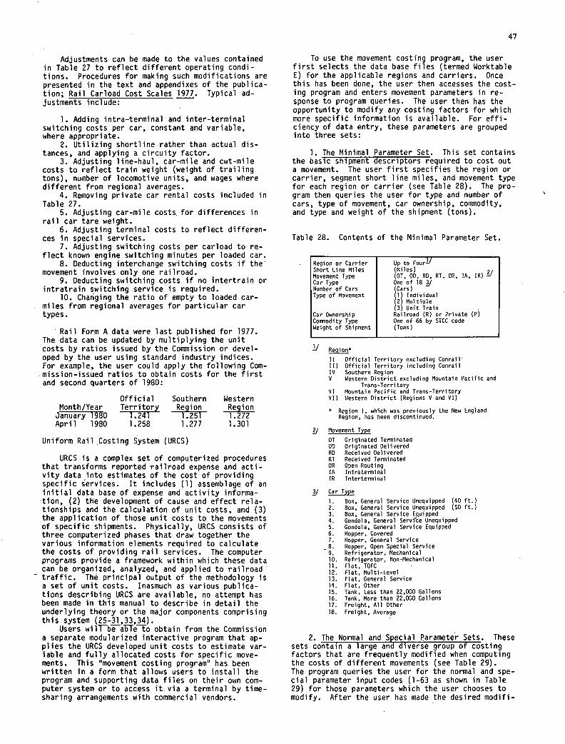
47
Adjustments can be made to the values contained in Table 27 to reflect different operating condi-tions. Procedures for making such modifications are presented in the text and appendixes of the publica-tion; Rail Carload Cost Scales 1977. Typical ad-justments include:
Adding intra-terminal and inter-terminal switching costs per car, constant and variable, where appropriate.
utilizing shortline rather than actual dis-tances, and applying a circuity factor.
Adjusting line-haul, car-mile and cwt-mile costs to reflect train weight (weight of trailing tons), number of locomotive units, and wages where different from regional averages.
Removing private car rental costs included Table 27.
Adjusting car-mile costs, for differences in rail car tare weight.
Adjusting terminal costs to reflect differe ces in special services.
Adjusting switching costs per carload to re flect known engine switching minutes per loaded ca
Deducting interchange switching costs if th movement involves only one railroad.
Deducting switching costs if no intertrain intratrain switching service is required.
Changing the ratio of empty to loaded car-miles from regional averages for particular car types.
Rail Form A data were last published for 1977. The data can be updated by multiplying the unit costs by ratios issued by the Commission or devel-oped by the user using standard industry indices. For example, the user could apply the following Com-mission-issued ratios to obtain costs for the first and second quarters of 1980:
Official Southern Western Month/Year Territory Region Region January 1980 1.241 1.251 1.272 April 1980 1.258 1.277 1.301
uniform Rail Costing System (URCS)
URCS is a complex set of computerized procedures that transforms reported 'railroad expense and acti-vity data into estimates of the cost of providing specific services. It includes (1) assemblage of an initial data base of expense and activity informa- tion, (2) the development of cause and effect rela-tionships and the calculation of unit costs, and (3) the application of those unit costs to the movements of specific shipments. Physically, URCS consists of three computerized phases that draw together the various information elements required to calculate the costs of providing rail services. The computer programs provide a framework within which these data can be organized, analyzed, and applied to railroad traffic. The principal output of the methodology is a set of unit costs. Inasmuch as various publica-tions describing URCS are available, no attempt has been made in this manual to describe in detail the underlying theory or the major components comprising this system (25-31,33,34).
Users wilTbe a5Te to obtain from the Commission a separate modularized interactive program that ap-plies the URCS developed unit costs to estimate var-iable and fully allocated costs for specific move-ments. This "movement costing program" has been written in a form that allows users to install the program and supporting data files on their own com-puter system or to access it. via a terminal by time-sharing arrangements with commercial vendors.
To use the movement costing program, the user first selects the data base files (termed Worktable E) for the applicable regions and carriers. Once this has been done, the user then accesses the cost-ing program and enters movement parameters in re-sponse to program queries. The user then has the opportunity to modify any costing factors for which more specific information is available. For effi-ciency of data entry, these parameters are grouped into three sets:
1. The Minimal Parameter Set. This set contains the basic shipment descriptors required to cost out a movement. The user first specifies the region or carrier, segment short line miles, and movement type for each region or carrier (see Table 28). The pro-gram then queries the user for type and number of cars, type of movement, car ownership, commodity, and type and weight of the shipment (tons).
Table 28. Contents of the Minimal Parameter Set.
Region or Carrier Up to Four.!.I Short Line Miles (Miles) 2 Movement Type (OT. OD, RD, RT, OR, IA, IR) Car Type One of 18 Number of Cars (Cars) Type of Movement Individual
Multiple Unit Train
Car Ownership Railroad (R) or Private (P) Comodity Type One of 66 by SICC code Weight of Shipment (Tons)
.11
II Official Territory excluding Conrail' III Official Territory including Conrail IV Southern Region V Western Oistrict excluding Mountain Pacific and
Trans-Territory VIMountain Pacific and Trans-Territory VII Western District (Regions V and VI)
* Region I, which was previously the New England Region, has been discontinued.
V Movement Type 01 Originated Terminated 00 Originated Delivered RD Received Delivered RI Received Terminated OR Open Routing IA Intraterminal IR Interterminal
,/ Car Type
Box, General Service Unequipped (40 ft.) Box, General Service Unequipped (50 ft.) Box, General ServiceEquipped Gondola, General Service Unequipped Gondola, General Service Equipped Hopper, Covered Hopper, General Service
- B. Hopper, Open Special Service Refrigerator, Mechanical Refrigerator, Non-Mechanical Flat, TOFC Flat, Multi-Level Flat, General Service Flat, Other Tank, Less than 22,000 Gallons Tank, More than 22,000 Gallons Freight, All Other
18, Freight, Average
2. The Normal and Special Parameter Sets. These sets contain a large and diverse group of costing factors that are frequently modified when computing the costs of different movements (see Table 29). The program queries the user for the normal and spe-ci'al parameter input codes (1-63 as shown in Table 29) for those parameters which the user chooses to modify. After the user has made the desired modifi-
in
n-
r. e
or
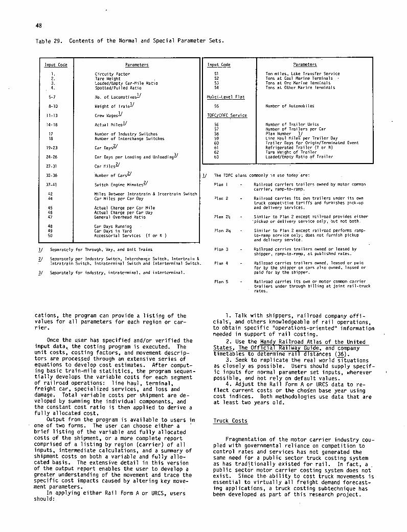
48
Table 29. Contents of the Normal and Special Parameter Sets.
Input Code Parameters
Circuity Factor Tare Weight Loaded/Empty Car-Mile Ratio Spotted/Pulled Ratio
5-7 No. of, Locomotives1'
8-10 Weight of Train'
11-13 Crew Wages-1'
14-16 Actual Miles1'
17 Number of Industry Switches 18 Number of Interchange Switches
19-23 Car DaysV
24-26 Car Days per Loading and Unloading-"
27-31 Car Miles'
32-36 Number of Cars
37-41 Switch Engine Minutes'
42 Miles Between Intratrain & Intertrain Switch 44 Car Miles per Car Day
45 Actual Charge per Car Mile 46 Actual Charge per Car Day 47 General Overhead Ratio
48 Car Days Running - 49 Car Days in Yard 50 Accessorial Services (Y or N
1/ Separately for Through, Way, and Unit Trains
2/ Separately per Industry Switch, Interchange Switch, Intertrain & Intratrain Switch, Intraterminal Switch and Interterminal Switch
3/ Separately for industry, intraterminal, and interterminal.
Input Code Parameters
51 Ton miles, Lake Transfer Service 52 Tons at Coal Marine Terminals 53 Tons at Ore Marine Terminals 54 Tons at Other Marine Terminals
Multi-Level Flat
55 Number of Automobiles
TOFC/COFC Service
56 Number of Trailer Units 57 Number of Trailers per Car 58 Plan Number 1/ 59 Line Haul Miles per Trailer Day 60 Trailer Days for Origin/Terminated Event 61 Refrigerated Trailer (V or N) 62 Tare Weight of Trailer 63 Loaded/Empty Ratio of Trailer
1/ The TOFC plans consnonly in use today are:
Plan 1 - Railroad carriers trailers owned by motor cormnon carrier, ramp-to-ramp.
Plan 2 - Railroad carries its own trailers under its own truck competitivetariffs and furnishes pick-up and delivery services.
Plan 2u - Similar to Plan 2 except railroad provides either pickup or delivery service only, but not both.
Plan 2½ - Similar to Plan 2 except railroad performs ramp- to-ramp service only; does not furnish pickup and delivery service.
Plan 3 - Railroad carries trailers owned or leased by shipper, ramp-to-ramp, at published rates.
Plan 4 - Railroad carries trailers owned, leased or paid for by the shipper on cars also owned, leased or paid for by the shipper.
Plan S - Railroad carries its own or motor corinnon carrier trailers under through billing at joint rail-truck rates.
cations, the program can provide a listing of the values for all parameters for each region or car-rier.
Once the user has specified and/or verified the input data, the costing program is executed. The unit costs, costing factors, and movement descrip-tors are processed through an extensive series of equations to develop cost estimates. After comput-ing basic train-mile statistics, the program sequen-tially develops the variable costs for each segment of railroad operations: line haul, terminal, freight car, specialized services, and loss and damage. Total variable costs per shipment are de-veloped by summing the individual components, and the constant cost ratio is then applied to derive a fully allocated cost.
Output from the program is available to users in one of two forms. The user can choose either a brief listing of the variable and fully allocated costs of the shipment, or a more complete report comprised of a listing by region (carrier) of all inputs, intermediate calculations, and a summary of shipment costs on both a variable and fully allo-cated basis. The extensive detail in this version of the output report enables the user to develop a greater understanding of the movement and trace the specific cost impacts caused by altering key move-ment parameters.
In applying either Rail Form A or URCS, users should:
Talk with shippers, railroad company offi-cials, and others knowledgeable of rail operations, to obtain specific "operations-oriented" information needed in support of rail costing.
Use the Handy Railroad Atlas of the United States, The Official Railway Guide, and company timetables to determine rail distances (36).
Seek to replicate the real world situations as closely as possible. Users should supply specif-ic inputs for normal parameter set inputs, wherever possible, and not rely on default values.
Adjust the Rail Form A or URCS data to re-flect current costs or the chosen base year using cost indices. Both methodologies use data that are at least two years old.
Truck Costs
Fragmentation of the motor carrier industry cou-pled with governmental reliance on competition to control rates and services has not generated the same need for a public sector truck costing system as has traditionally existed for rail. In fact, a - public sector motor carrier costing system does not exist. Since the- ability to cost truck movements is essential to virtually all freight demand forecast-ing applications, a truck costing subtechnique has been developed as part of this research project.
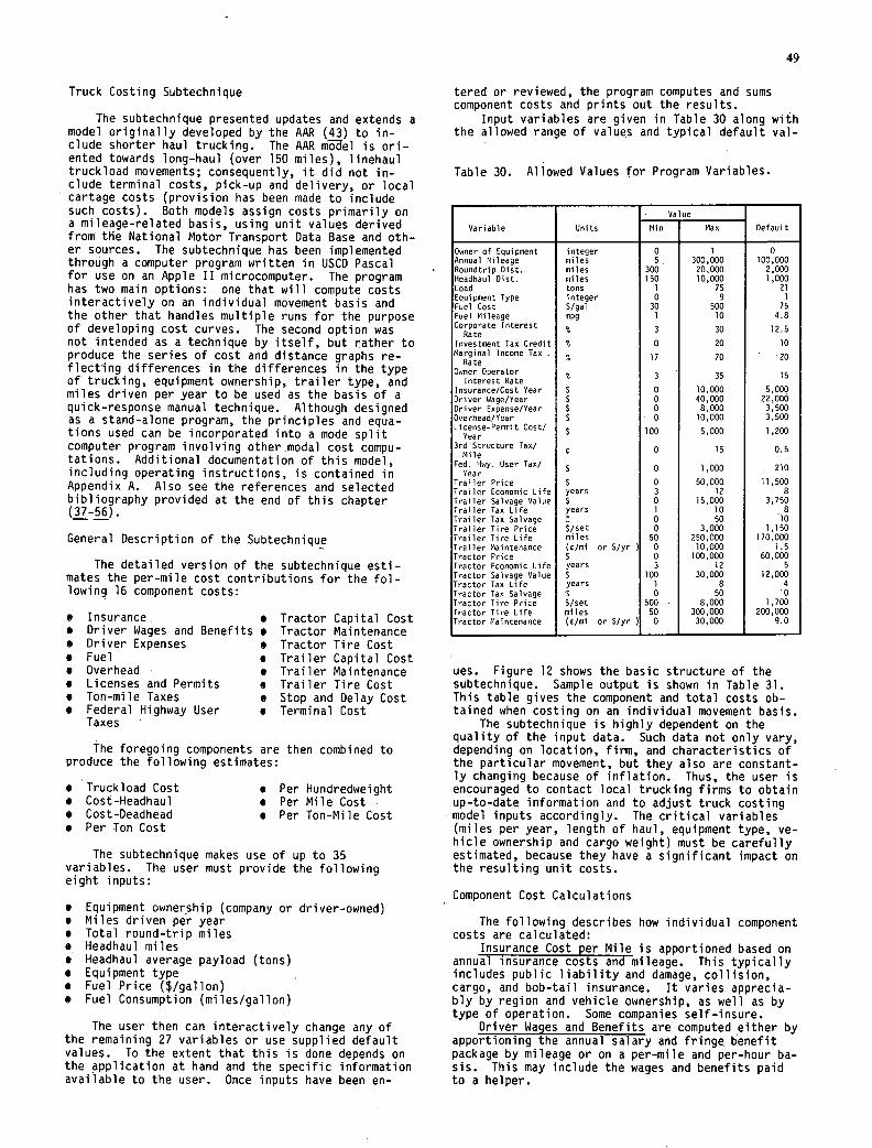
49
Truck Costing Subtechnique
The subtechnique presented updates and extends a model originally developed by the AAR (43) to in-clude shorter haul trucking. The AAR m6el is ori-ented towards long-haul (over 150 miles), linehaul truckload movements; consequently, it did not in-clude terminal costs, pick-up and delivery, or local cartage costs (provision has been made to include such costs). Both models assign costs primarily on a mileage-related basis, using unit, values derived from the National Motor Transport Data Base and oth-er sources. The subtechnique has been implemented through a computer program written in USCD Pascal for use on an Apple II microcomputer. The program has two main options: one that will compute costs interactively on an individual movement basis and the other that handles multiple runs for the purpose of developing cost curves. The second option was not intended as a technique by itself, but rather to produce the series of cost and distance graphs re-flecting differences in the differences in the type of trucking, equipment ownership, trailer type, and miles driven per year to be used as the basis of a quick-response manual technique. Although designed as a stand-alone program, the principles and equa-tions used can be incorporated into a mode split computer program involving other modal cost compu-tations. Additional documentation of this model, including operating instructions, is contained in Appendix A. Also see the references and selected bibliography provided at the end of this chapter (37-56).
General Description of the Subtechnique
The detailed version of the subtechnique esti- mates the per-mile cost contributions for the fol- lowing 16 component costs:
Insurance • Tractor Capital Cost Driver Wages and Benefits • Tractor Maintenance Driver Expenses • Tractor Tire Cost Fuel • Trailer Capital Cost Overhead ' • Trailer Maintenance Licenses and Permits • Trailer Tire Cost Ton-mile Taxes • Stop and Delay Cost Federal Highway User • Terminal Cost Taxes
The foregoing components are then combined to produce the following estimates:
Truckload Cost • Per Hundredweight Cost-Headhaul • Per Mile Cost Cost-Deadhead . Per Ton-Mile Cost Per Ton Cost
The subtechnique makes use of up to 35 variables. The user must provide the following eight inputs:
Equipment ownership (company or driver-owned) Miles driven per year Total round-trip miles Headhaul miles Headhaul average payload (tons) Equipment type Fuel Price ($/gallon) Fuel Consumption (miles/gallon)
The user then can interactively change any of the remaining 27 variables or use supplied default values. To the extent that this is done depends on the application at hand' and the specific information available to the user. Once inputs have been en-
tered or reviewed, the program computes and sums component costs and prints out the results.
Input variables are given in Table 30 along with the allowed range of values and typical default val-
Table 30. Allowed Values for Program Variables.
Variable Units
Value
Default Min Max
Owner of Equipment integer 0 1 0 Annual Mileage miles 5 , 300,000 100,000 Roundtrip Dist. miles 300 20.000 2,000 Headhaul Dist. miles 150 10,000 1,000 Load tons 1 75 21 Equipment Type integer 0 9 Fuel Cost S/gal 30 500 75 Fuel Mileage mpg 1 10 4.8 Corporate Interest 3 30 12.5
Rate Investment Tax Credit % 0 20 10 Marginal Income Tax.
Rate 17 70 ' 20
Owner Operator 3 ' 35 15 Interest Rate
Insurance/Cost Year S 0 10,000 5.000 Driver Wage/Year S 0 40,000 22,000 Driver Expense/Year S 0 8,000 3,500 Overhead/Year 5 0 10,000 3,500 Lic:nse-Perimit Cost/ 100 5,000 1,200
Year 3rdStracture Tax/ 0 15 0.5 Mile
Fed. Hwy. User Tax/ 1,000 210 Year
Trailer Price S 0 50,000 11,500 Trailer Economic Life years 3 12 8 Trailer Salvage Value S 0 15,000 3,750 Trailer Tax Life years 1 10 , 8 Trailer Tax Salvage 3 0 50 10 Trailer Tire Price S/set 0 3.000 1,150 Trailer Tire Life miles 50 250,000 170,000 Trailer Maintenance (d/mi or S/yr ) 0 10.000 1.5 Tractor Price 5 0 100.000 60.000 Tractor Economic Life years 3 12 5 Tractor Salvage Value 5 100 30,000 12,000 Tractor Tax Life years 1 8 4 Tractor Tax Salvage 3 0 50 10 Tractor Tire Price S/set 500 8,000 1,700 Tractor Tire Life miles 50 300,000 200.000 Tractor Maintenance (c/mi or S/yr ) 0 30.000 9.0
ues. Figure 12 shows the basic structure of the subtechnique. Sample output is shown in Table 31. This table gives the component and total costs ob-tained when costing on an individual movement basis.
The subtechnique is highly dependent on the quality of the input data. Such data not only vary, depending on location, firm, and characteristics of the particular movement, but they also are constant-ly changing because of inflation. Thus, the user is encouraged to contact local trucking firms to obtain up-to-date information and to adjust truck costing model inputs accordingly. The critical variables (miles per year, length of haul, equipment type, ve-hicle ownership and cargo weight) must be carefully estimated, because they have a significant impact on the resulting unit costs.
Component Cost Calculations
The following describes how individual component costs are calculated:
Insurance Cost per Mile is apportioned based on annual insurance costs and mileage. This typically includes public liability and damage, collision, cargo, and bob-tail insurance. It varies apprecia-bly by region and vehicle ownership, as well as by type of operation. Some companies self-insure.
Driver Wages and Benefits are computed either by apportioning the annual salary and fringe benefit package by mileage or on a per-mile and per-hour ba-sis. This may include the wages and benefits paid to a helper.
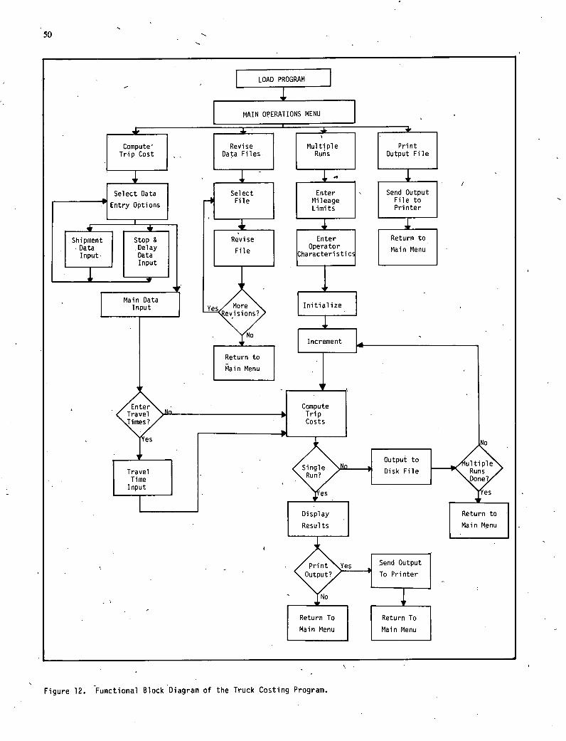
50
- [ LOAD PROGRAM ]
MAIN OPERATIONS MENU
Compute' I I Revise I i Multjple I I Print Trip Cost
j
Data Files Runs Output File
I Select Data I I Select Enter Send Output
File I Mileage I I File to Entry Options Limits I I
Printer
Shipment I I Stop & I Revise I I Enter I I Return to Data I . Delay File I
I Operator I Main Menu
Input. Data haracteristic1 Input
Data
5
Main Input 4Ye Initi alize
evi
1 No
Increment
Return to I
M
I ain Menu
'I
Enter - Compute Travel Trip Times? - Costs
es No
Output to Ui ti pie
Travel
+es
Disk File Runs Time uone Input
es
Display Return to
Results Main Menu
Print Yes Send Output - Output? To Printer
No
Return To Return To
Main Menu Main Menu
Figure 12. 'Functional Block Diagram of the Truck Costing Program.
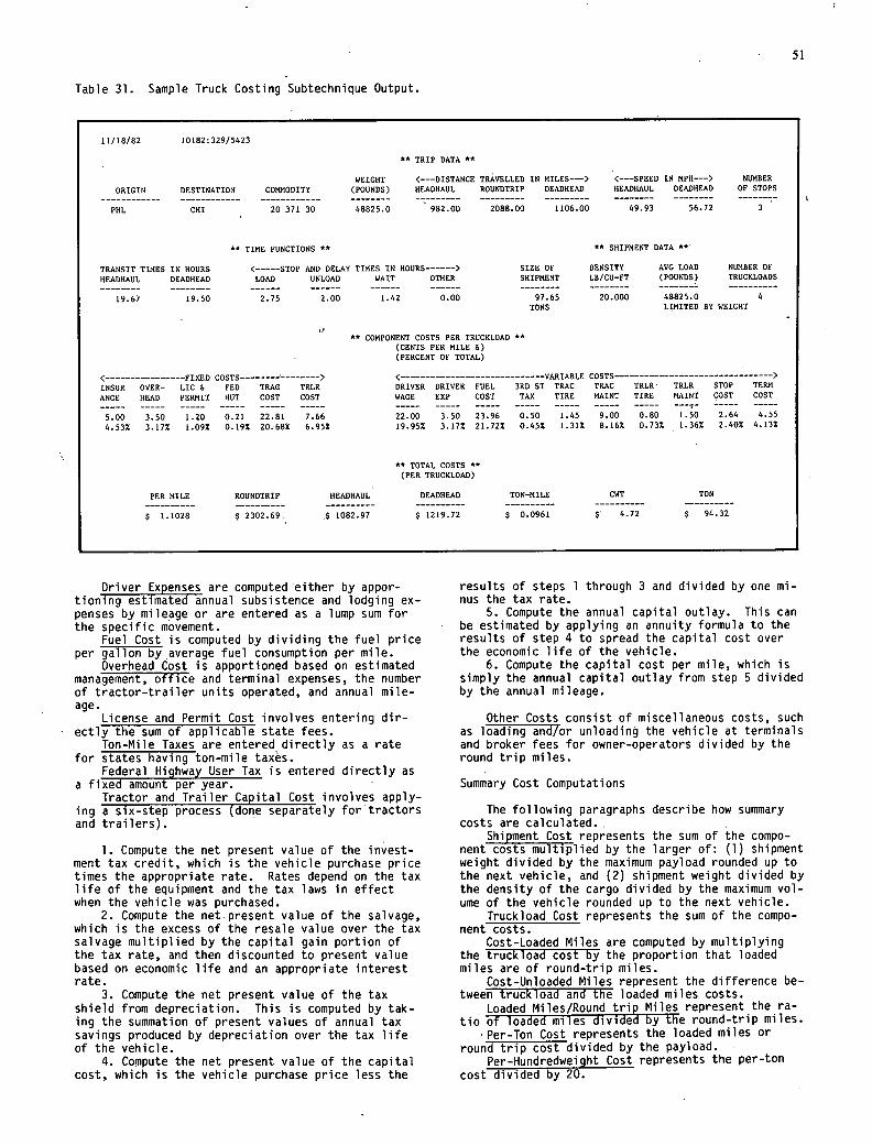
Table 31. Sample Truck Costing Subtechnique Output.
11/18/82 10182:329/5423
** TRIP DATA **
WEIGHT < --- DISTANCE TRAVELLED IN MILES--> <---SPEED IN MPH --- > NUMBER ORIGIN DESTINATION COMMODITY (POUNDS) HEAOHAUL ROUNDTRIP DEADHEAD HEADHAUL DEADHEAD OF STOPS
PHL CHI 20 371 30 48825.0 982.00 2088.00 1106.00 49.93 56.72 3
** TIME FUNCTIONS **
** SHIPMENT DATA **•
TRANSIT TIMES IN HOURS <-----STOP AND DELAY TIMES IN HOURS ------> SIZE OF DENSITY AVG LOAD NUMBER OF
HEADHAUL DEADHEAD LOAD UNLOAD WAIT OTHER SHIPMENT LB/CU-FT (POUNDS) TRUCKLOADS
19.67 19.50 2.75 2.00 1.42 0.00 97.65 20.000 48825.0 4 TONS LIMITED BY WEIGHT
** COMPONENT COSTS PER TRUCKLOAD ** (CENTS PER MILE 6) (PERCENT OF TOTAL)
FIXED COSTS ------- -------- > ( ----------------------------- VARIABLE COSTS ------------------------------- > INSUR OVER- LIC & FED TRAC TRLR DRIVER DRIVER FUEL 3RD ST TRAC TRAC TRLR TRLR STOP TERN
ANCE HEAD PERMIT HUT COST COST WAGE EXP COST TAX TIRE MAINT TIRE MAINT COST COST
5.00 3.50 1.20 0.21 22.81 7.66 22.00 3.50 23.96 0.50 1.45 9.00 0.80 1.50 2.64 4.55
4.532 3.17% 1.09% 0.19% 20.68% 6.95% 19.95% 3.17% 21.72% 0.45% 1.31% 8.162 0.73% 1.36% 2.40% 4.13%
** TOTAL COSTS ** (PER TRUCKLOAD)
PER MILE ROUNDTRIP HEADHAUL DEADHEAD TON-MILE CWT TON
$ 1.1028 $ 2302.69. $ 1082.97 $ 1219.72 $ 0.0961 9 4.72 $ 94.32
51
Driver Expenses are computed either by appor-tioning estimated annual subsistence and lodging ex-penses by mileage or are entered as a lump sum for the specific movement.
Fuel Cost is computed by dividing the fuel price per gallon by average fuel consumption per mile.
Overhead Cost is apportioned based on estimated management, office and terminal expenses, the number of tractor-trailer units operated, and annual mile-age.
License and Permit Cost involves entering dir-ectly the sum of applicable state fees.
Ton-Mile Taxes are entered, directly as a rate for states having ton-mile taxes.
Federal Highway User Tax is entered directly as a fixed amount per year.
Tractor and Trailer Capital Cost involves apply-ing a six-step process (done separately for tractors and trailers).
Compute the net present value of the invest-ment tax credit, which is the vehicle purchase price times the appropriate rate. Rates depend on the tax life of the equipment and the tax laws in effect when the vehicle was purchased.
Compute the net present value of the salvage, which is the excess of the resale value over the tax salvage multiplied by the capital gain portion of the tax rate, and then discounted to present value based on economic life and an appropriate interest rate.
Compute the net present value of the tax shield from depreciation. This is computed by tak-ing the summation of present values of annual tax savings produced by depreciation over the tax life of the vehicle.
Compute the net present value of the capital cost, which is the vehicle purchase price less the
results of steps 1 through 3 and divided by one mi-nus the tax rate.
Compute the annual capital outlay. This can be estimated by applying an annuity formula to the results of step 4 to spread the capital cost over the economic life of the vehicle.
Compute the capital cost per mile, which is simply the annual capital outlay from step 5 divided by the annual mileage.
Other Costs consist of miscellaneous costs, such as loading and/or unloading the vehicle at terminals and broker fees for owner-operators divided by the round trip miles.
Summary Cost Computations
The following paragraphs describe how summary costs are calculated.
Shipment Cost represents the sum of the compo-nent costs multiplied by the larger of: (1) shipment weight divided by the maximum payload rounded up to the next vehicle, and (2) shipment weight divided by the density of the cargo divided by the maximum vol-ume of the vehicle rounded up to the next vehicle.
Truckload Cost represents the sum of the compo-nent costs.
Cost-Loaded Miles are computed by multiplying the truckload cost by the proportion that loaded miles are of round-trip miles.
Cost-Unloaded Miles represent the difference be-tween truckload and the loaded miles costs.
Loaded Miles/Round trip Miles represent the ra-tio of loaded miles divided by the round-trip miles.
Per-Ton Cost represents the loaded miles or round trip cost divided by the payload.
Per-Hundredweight Cost represents the per-ton cost divided by 20.
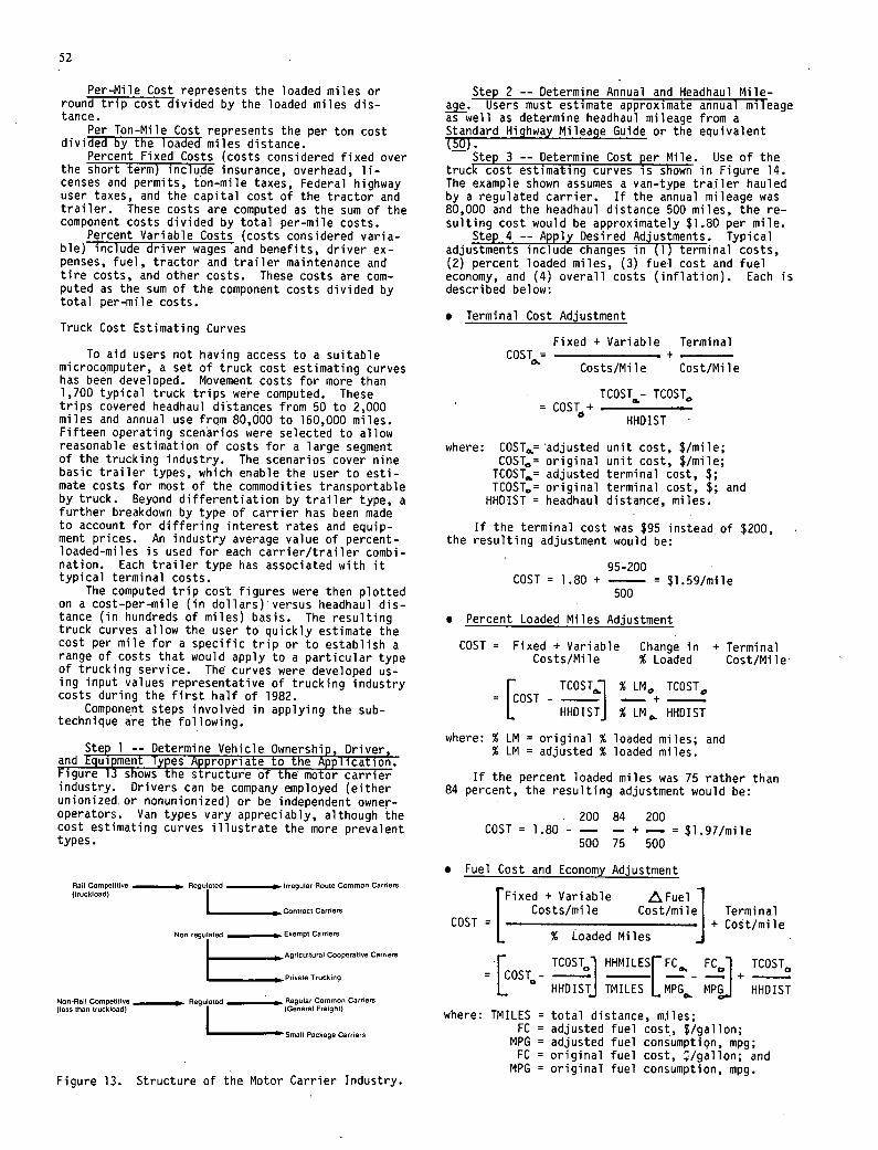
52
Per-Mile Cost represents the loaded miles or round trip cost divided by the loaded miles dis-tance.
Per Ton-Mile Cost represents the per ton cost divided by the loaded miles distance.
Percent Fixed Costs (costs considered fixed over the short term) include insurance, overhead, li-censes and permits, ton-mile taxes, Federal highway user taxes, and the capital cost of the tractor and trailer. These costs are computed as the sum of the component costs divided by total per-mile costs.
Percent Variable Costs (costs considered varia-ble) include driver wages and benefits, driver ex-penses, fuel, tractor and trailer maintenance and tire costs, and other costs. These costs are com-puted as the sum of the component costs divided by total per-mile costs.
Truck Cost Estimating Curves
To aid users not having access to a suitable microcomputer, a set of truck cost estimating curves has been developed. Movement costs for more than 1,700 typical truck trips were computed. These trips covered headhaul distances from 50 to 2,000 miles and annual use from 80,000 to 160,000 miles. Fifteen operating scenarios were selected to allow reasonable estimation of costs for a large segment of the trucking industry. The scenarios cover nine basic trailer types, which enable the user to esti-mate costs for most of the commodities transportable by truck. Beyond differentiation by trailer type, a further breakdown by type of carrier has been made to account for differing interest rates and equip-ment prices. An industry average value of percent-loaded-miles is used for each carrier/trailer combi-nation. Each trailer type has associated with it typical terminal costs.
The computed trip cost figures were then plotted on a cost-per-mile (in dollars)'versus headhaul dis-tance (in hundreds of miles) basis. The resulting truck curves allow the user to quickly estimate the cost per mile for a specific trip or to establish a range of costs that would apply to a particular type of trucking service. The curves were developed us-ing input values representative of trucking industry costs during the first half of 1982.
Component steps involved in applying the sub-technique are the following.
Step 1 -- Determine Vehicle Ownership, Driver, and Equipment Types Appropriate to the Application. Figure 13 shows the structure of the motor carrier industry. Drivers can be company employed (either unionized, or nonunionized) or be independent owner-operators. Van types vary appreciably, although the cost estimating curves illustrate the more prevalent types.
Rail Competitive • Regulated Irregular Route Common Carriers (truckload)
p Contract Carriers
Non regulated , Exempt Carriers
Agricultural Cooperative Carriers
Private Trucking
Non-Rail Competitive p Regulated • Regular Common Carriers
(less than truckload) (General Freight)
Small Package Carriers
Figure 13. Structure of the Motor Carrier Industry.
Steo 2 -- Determine Annual and Headhaul Mile- Users must estimate approximate annual mileage
as well as determine headhaul mileage from a Standard Highway Mileage Guide or the equivalent (50).
Step 3 -- Determine Cost per Mile. Use of the truck cost estimating curves is shown in Figure 14. The example shown assumes a van-type trailer hauled by a regulated carrier. If the annual mileage was 80,000 and the headhaul distance 500 miles, the re-sulting cost would be approximately $1.80 per mile.
Step 4 -- Apply Desired Adjustments. Typical adjustments include changes in (1) terminal costs, (2) percent loaded miles, (3) fuel cost and fuel economy, and (4) overall costs (inflation). Each is described below:
. Terminal Cost Adjustment
Fixed + Variable Terminal C0ST= -+-
Costs/Mile Cost/Mi 1 e
TCOST- TCOST0 COST" -
HHDIST
where: COST0,= adjusted unit cost, $/mile; COST0 m original unit cost, $/mile; TCOST0.= adjusted terminal cost, $; TCOST0= original terminal cost, $; and
HHDIST m headhaul distance, miles.
If the terminal cost was $95 instead of $200, the resulting adjustment would be:
95-200 COST = 1.80 + _____ m $1.59/mile
500
Percent Loaded Miles Adjustment
COST = Fixed + Variable Change in + Terminal Costs/Mile % Loaded Cost/Mile'
[COST - TC0Sl ±o+ HH DISTJ % LM. HHDIST
where: % LM m original % loaded miles; and % LM = adjusted % loaded miles.
If the percent loaded miles was 75 rather than 84 percent, the resulting adjustment would be:
200 84 200 COST m 1.80 — - - + — = $1.97/mile
500 75 500
Fuel Cost and Economy Adjustment
I + Variable Fuel I Costs/mile Cost/mile
I
Fixed Terminal
% LCOST =I . + Cost/mile
L oaded Mils
f TCOST0 ) HHMILESrFC FCO1 TCOST0 C O S T I ------1+
L HHDISTJ TMILES LMPGC.. MPJHHDIST
where: TMILES = total distance, miles; FC = adjusted fuel cost, $/gallon;
MPG = adjusted fuel consumption, mpg; FC = original fuel cost, /gallon; and
MPG m original fuel consumption, mpg.
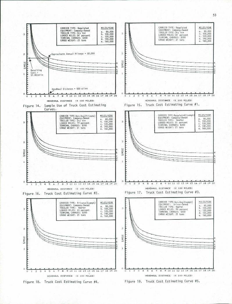
3
53
CARRIER TYPE: Regulated MILES/YEAR EQUIPMENT: Company-Owned a. 80,000 TRAILER TYPE: Dry Van b. 100,000 LOADED MILES: 84 percent . 120,000 TERMINAL CHARGES: $200 d. 140,000 CARGO WEIGHT: 21 tons e. 160,000
mate Annual Mileage = 80.000
H Resulting Cost = $1.80/mile
Neadhual Distance = 500 miles
1 3 4 56 7 8 9 10 11 12 13 14 15 16 17 18
HEADHAUL DISTANCE (X 100 MILES)
14. Sample Use of Truck Cost Estimating Curves.
CARRIER TYPE: Non-Reg(Private) MILES/YEAR EQUIPMENT: Company-Owned a. 80,000 TRAILER TYPE: Dry Van b. 100,000 LOADED MILES: 79 percent . 120,000 TERMINAL CHARGES: $200 d. 140,000 CARGO WEIGHT: 21 tons e. 160,000
CARRIER TYPE: Regulated MILES/YEAR EQUIPMENT: Company-Owned
a. 80,000 TRAILER TYPE: Dry Van 6. 100.000
LOADED MILES: 84 percent 120,000 .
TERMINAL CHARGES: $200 140,000
CARGO WEIGHT: 21 tons 160,000
o 1 2 3 4 5 6 7 8 9 10 11 12 13 14 15 16 17 15 19 2C
HEADHAUL DISTANCE (0 100 MILES)
Figure 15. Truck Cost Estimating Curve #1.
CARRIER TYPE:Regulated(Exemptj MILES/YEAR EQUIPMENT: Company-Owned I 80,000 TRAILER TYPE: Reefer I 100,000 I LOADED MILES: 91 percent I 120,000 TERMINAL CHARGES: $200 I 140,000 I CARGO WEIGHT: 21 tons I 160,000 I
3
0
Fl
2
0 C 1 2 3 4 5 6 7 8 9101112131413181/1017.1
HEADHAUL DISTANCE )X 100 MILES)
gure 16. Truck Cost Estimating Curve #2.
0 1 2 3 4 5 6 7 8 9 10 11 12 13 14 15 16 17 18 19 (
HEADHAUL DISTANCE )X 100 MILES)
Figure 17. Truck Cost Estimating Curve #3.
CARRIER TYPE:Non-Reg(Exempt) I MILES/YEAR 1 EQUIPMENT: Driver-Owned I 80,000 I TRAILER TYPE: Reefer I 100,000 I LOADED MILES: 88 percent I C. 120,000 I TERMINAL CHARGES: $200 I 140,000 I CARGO WEIGHT: 21 tons 160,000
I
1 2 7 A 4. 7 0 0 10 1117 17 IA 1m 14.17101970
HEADHAUL DISTANCE (X 100 MILES) HEADHAUL DISTANCE )X 100 MILES)
Figure 18. Truck Cost Estimating Curve #4. Figure 19. Truck Cost Estimating Curve #5.
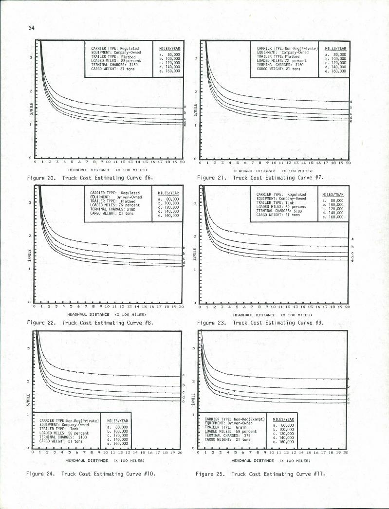
54
CARRIER TYPE: Regulated MILES/YEAR EQUIPMENT: Company-Owned
80,000 TRAILER TYPE: Flatbed 100,000 LOADED MILES: 83 percent 120,000 . TERMINAL CHARGES: $150 140,000 CARGO WEIGHT: 21 tons 160,000
lb
340678 9101112131415161718
HEADHAUL DISTANCE (X 100 MILES)
0. Truck Cost Estimating Curve #6.
CARRIER TYPE: Non-Reg(Private)I MILES/YEAR I EQUIPMENT: Company-Owned I 80,000 I TRAILER TYPE: Flatbed
i 100,000 LOADED MILES: 72 percent i 120,000 TERMINAL CHARGES: $150 I
. d. 140,000 I CARGO WEIGHT: 21 tons
i a. 160,000 I
............... -. . . . I ) 1 2 3 4 5 6 7 8 9 10 11 12 13 14 15 16 17 18 19 20
HEADHAUL DISTANCE (U 100 MILES)
21. Truck Cost Estimating Curve V.
CARRIER TYPE: Regulated MILES/YEAR EQUIPMENT: Driver-Owned 80,000 TRAILER TYPE: Flatbed 100,000 LOADED MILES: 76 percent . 120,000 TERMINAL CHARGES: $150
140,000 CARGO WEIGHT: 21 tons 160,000
CARRIER TYPE: Regulated MILES/YEAR EQUIPMENT: Company-Owned
80,000 TRAILER TYPE: Tank
100,000 LOADED MILES: 52 percent . 120,000 TERMINAL CHARGES: $100 140,000 CARGO WEIGHT: 21 tons
160,000
a
b
c d e
23458789101112131415161718
HEADHAUL DISTANCE n 100 MILES)
22. Truck Cost Estimating Curve #8.
0 1 2 3 4 5 6 7 8 9 10 11 12 13 14 15 18 17 18 19 2)
HEADHAUL DISTANCE (8 100 MILES)
Figure 23. Truck Cost Estimating Curve #9.
3
r
0
Fi
3
S
0
a
b
C
d e
0 0 1 2 3 4 5 6 7 8 9 10 11 12 13 14 10 18 17 18 19 20 0 1 2 3 4 5 6 7 8 9 10 11 12 13 14 15 18 17 18 19 20
HEADHAUL DISTANCE (D 100 MILES) HEADHAUL DISTANCE (X 100 MILES)
Figure 24. Truck Cost Estimating Curve #10. Figure 25. Truck Cost Estimating Curve #11.
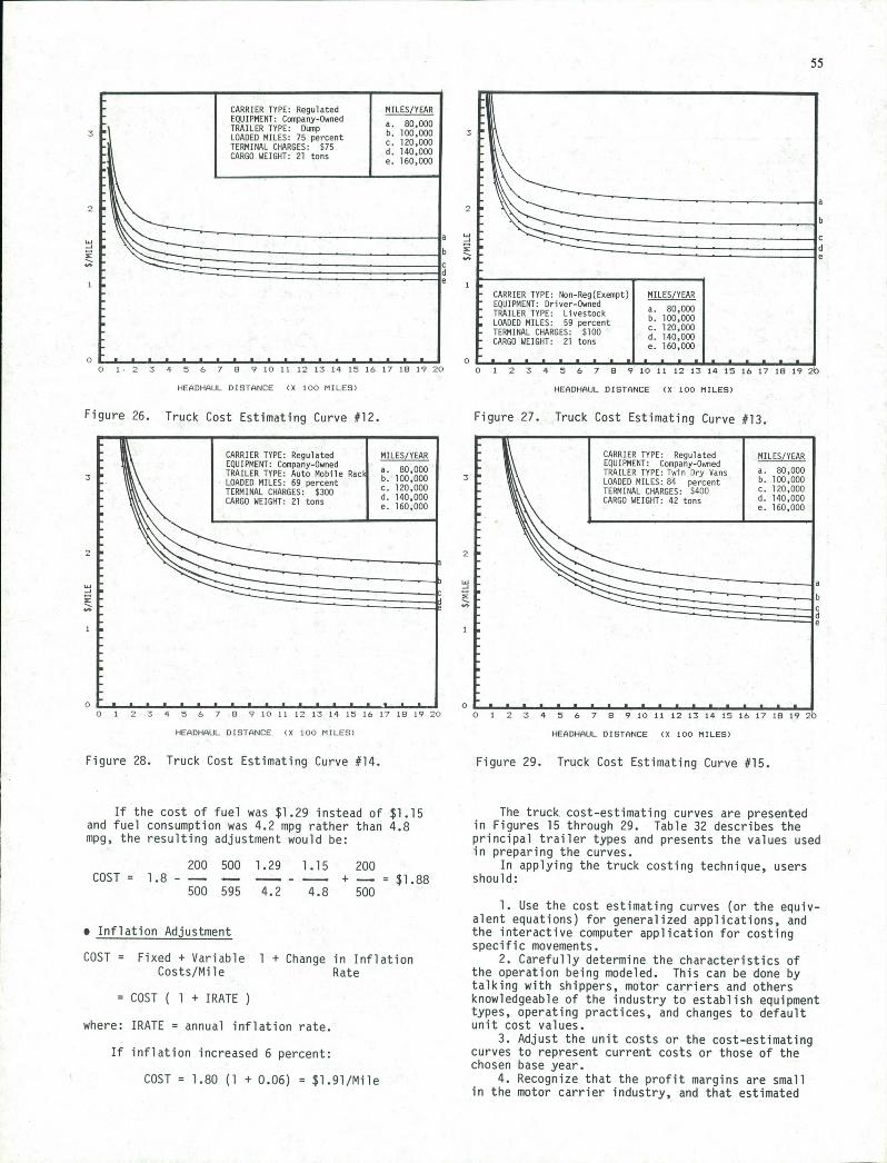
55
CARRIER TYPE: Regulated I MILES/YEAR EQUIPMENT: Company-Owned
80,000 TRAILER TYPE: Dump 100,000 LOADED MILES: 75 percent C. 120,000 TERMINAL CHARGES $75
d 140000
Je6OOOO b LGOWEIGHT:21tons
0
S
0 2 3 4 5 6 7 8 9 10 11 12 13 14 15 16 17 18 1920
HEADHAUL DISTANCE (X 100 MILES)
FCARRIER TYPE: MILES/YEAR EQUIPMENT: Driver-Owned I
I TRAILER TYPE: Livestock a. 80,000 b. 100,000 I
LOADED MILES: 59 percent c. 120,000 I
I• I
I. TERMINAL CHARGES: $100 140,000 I
CARGO WEIGHT: 21 tons 160,000
1 7 3 4 5 6 7 5 clot, 171% 141514171510
HEADHAUL DISTANCE (8 100 MILES)
a:
0
Figure 26. Truck Cost Estimating Curve #12.
CARRIER TYPE: Regulated I MILES/YEAR EQUIPMENT: Company-Owned I a. 80,000 TRAILER TYPE: Auto Mobile Rac9 b. 100,000 LOADED MILES: 69 percent I . 120,000 TERMINAL CHARGES: $300 I d. 140,000 CARGO WEIGHT 21 tons
e 160,000
0 1 234567891011121314151617181920
Figure 27. Truck Cost Estimating Curve #13.
CARRIER TYPE: Regulated I MILES/YEAR EQUIPMENT: Company-Owned TRAILER TYPE: Twin Dry Vans I a. 80,000 LOADED MILES: 84 percent b. 100,000 TERMINAL CHARGES $400 c. 120,000
GO WEIGHT: 42 tons d 140'000
e
0 1 2 3 4 5 6 7 8 9 10 11 12 13 14 15 16 17 18 19 20
HEADHAUL DISTANCE (X 100 MILES) HEADHAUL DISTANCE (0 100 MILES)
Figure 28. Truck Cost Estimating Curve #14. Figure 29. Truck Cost Estimating Curve #15.
If the cost of fuel was $1.29 instead of $1.15 and fuel consumption was 4.2 mpg rather than 4.8 mpg, the resulting adjustment would be:
200 500 1.29 1,15 200 COST= 1.8-- - -- - + - =$1.88
500 595 4.2 4.8 500
. Inflation Adjustment
COST = Fixed + Variable 1 + Change in Inflation Costs/Mile Rate
= COST ( 1 + IRATE
where: IRATE = annual inflation rate.
If inflation increased 6 percent:
COST = 1.80 (1 + 0.06) = $1.91/Mile
The truck cost-estimating curves are presented in Figures 15 through 29. Table 32 describes the principal trailer types and presents the values used in preparing the curves.
In applying the truck costing technique, users should:
Use the cost estimating curves (or the equiv-alent equations) for generalized applications, and the interactive computer application for costing specific movements.
Carefully determine the characteristics of the operation being modeled. This can be done by talking with shippers, motor carriers and others knowledgeable of the industry to establish equipment types, operating practices, and changes to default unit cost values.
Adjust the unit costs or the cost-estimating curves to represent current costs or those of the chosen base year.
Recognize that the profit margins are small in the motor carrier industry, and that estimated
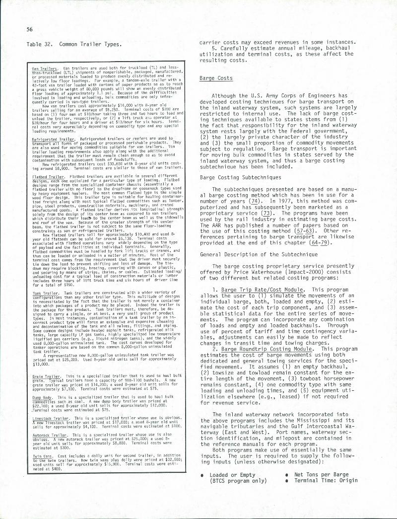
56
Table 32. Common Trailer Types.
Van Trailers. Van trailers are used both for truckload (IL) and less-than-truckload (LTL) shipments of nonperishable, packaged, manufactured, or processed materials loaded to produce evenly distributed and re-latively low floor load ings. For example, a tandem-axle trailer with a 42-foot van trailer loaded with cartons of paper products so as to reach a gross vehicle weight of 80,000 pounds will show an evenly distributed floor loading of approximately 1.1 psi. Because of the diffficalties involved in loading and unloading, bulk commodities are only infre-quently carried in van-type trailers.
New van trailers cost approximately $14,000 with 8-year old trailers selling for an average of $5,250. Terminal costs of $200 are based on (1) four men at $10/hour taking three and two hours to load and unload the trailer, respectively, or (2) a lift track ac operator at $28/hour for four hours and a driver at $13/hoar for six hours.Termi-nal costs vary appreciably depending on commodity type and any special loading requirements.
5gferatej:aile3. Refrigerated trailers or reefers are used to transport all forms of packaged or processed perishable products. They are also used for moving commodities suitable for van trailers. Van trailer loading requirements also apply along with the additional requirement that the trailer must remain clean enough so as to avoid contamination with subsequent loads of foodstuffs.
New refrigerated trailers cost $30,600 with 8-year old units cost-ing around $8,900. Terminal costs are similar to those of van trailers.
Flatbed Trailer. Flatbed trailers are available in several different designs, each one optimized for a particular type of loading. Flatbed designs range from the specialized container chassis (essentially a flatbed trailer with no floor) to the dropframe or gooseneck types used by heavy equipment haulers. The most common flatbed type is the simple wood floor design. This trailer type is suitable for hauling container-ized freight along with most typical flatbed commodities such as lumber, pipe, steel products, construction materials, machinery, and crated manufactured goods. A flatbed trailer derives its longitudinal strength solely from the design of its center beam as compared to van trailers which distribute their loads' to the center beam as well as the sidewalls and roof of the van. Because of the greater strength of its center beam, the flatbed trailer is not subject to the same floor-loading constraints as van or refrigerated trailers.
New flatbed trailers sell for approximately $10,400 and used 8-year old fRatbeds can be sold for around $5,130. Terminal costs associated with flatbed operations vary widely depending on the type of payload and the facilities at individual terminals, generally, flatbed commodities must be handled by fork lift trucks or cranes, and thus can be loaded or unloaded in a matter of minutes. Most of the terminal cost comes from the requirement that the driver must securely tie down the load to prevent shifting and loss of damage. The tie-down may require blocking, bracing, covering with canvas or plastic, and securing by means of strips, chains, or cables. Estimated loading/ unloading cost for a typical load of construction materials or lumber includes three hours of lift truck time and six hours of driver time for a total of $150.
Tank Trailer. Tank trailers are constructed with a wider variety of configurations than any other trailer type. This multitude of designs is necessitated by the fact that the trailer is not merely a container into which packages of a product may be placed. Indeed the trailer is the package for the product. Tank trailers must, therefore, be de-signed to carry a single, or at best, a very small group of product types. In most instances, contamination of a tank trailer by an in-correct product type will force an extensive and expensive cleaning and decontamination of the tank and all valves, fittings, and piping. Some common designs include heated asphalt tanks, refrigerated milk tanks, large capacity LP gas tanks, highly specialized low temperature liquified gas carriers (e.g., liquid nitrogen tanks), and the widely used 8,000-gallon uninsulated tank. The cost curves developed for tanker operations are based on the common 8,000-gallon uninsulated tank trailer.
A representative new 8,000-gallon uninsulated tank trailer was priced out at $25,200. Used 8-year old units sell for approximately $13,000.
Grain Trailer. This is a specialized trailer that is used to haul bulk grain. Typical trailers have a capacity of goo-lloo bushels. A mew grain trailer was priced at $14,200; a used 8-year old unit sells for approximately $7,100. Terminal costs were estimated at $75.
Dump Body. This is a specialized trailer that is used to haul bulk commodities such as coal. A new dump body trailer was priced at $22,100; a used 8-year old unit sells for approximately $12,000. Terminal costs were estimated at $75.
Livestock Trailer. This is a specialized trailer whose use is obvious. A new livestock trailer was priced at $17,000; a used 8-year old unit sells for approximately $4,100. Terminal costs were estimated at $100.
Autorack Trailer. This is a specialized trailer whose use is also obvious. A new autorack trailer was priced at $25,000; a used 8-year old unit sells for approximately $8,800. Terminal costs were estimated at $300.
Twin Vans. Cost includes a dolly unit for second trailer, in additiom to the twin trailers. New twin vans plus dolly were priced at $32,500; used units sell for approximately $15,900. Terminal costs were esti-mated at $400.
carrier costs may exceed revenues in some instances. 5. Carefully estimate annual mileage, backhaul
utilization and terminal costs, as these affect the resulting costs.
Barge Costs
Although the U.S. Army Corps of Engineers has developed costing techniques for barge transport on the inland waterway system, such systems are largely restricted to internal use. The lack of barge cost-ing techniques available to states stems from (1) the fact that responsibility for the inland waterway system rests largely with the Federal government, (2) the largely private character of the industry and (3) the small proportion of commodity movements subject to regulation. Barge transport is important for moving bulk commodities in states served by the inland waterway system, and thus a barge costing subtechnique has been included.
Barge Costing Subtechniques
The subechniques presented are based on a manu-al barge costing method which has been in use for a number of years (74). In 1977, this method was com-puterized and has subsequently been marketed as a proprietary service (73). The programs have been used by the rail industry in estimating barge costs. The AAR has published a number of papers based on the use of this costing method (57-63). Other re-ferences pertaining to barge transport are likewise provided at the end of this chapter (64-79).
General Description of the Subtechnique
The barge costing proprietary service presently offered by Price Waterhouse (Impact-2000) consists of two different but related costing programs:
Barge Trip Rate/Cost Module. This program allows the user to (1) simulate the movements of an individual barge, both, loaded and empty, (2) esti-mate the cost of each trip component, and (3) assem-ble statistical data for the entire series of move-ments. The program can incorporate any combination of loads and empty and loaded backhauls. Through use of percent of tariff and time contingency varia-bles, adjustments can easily be made to reflect changes in transit time and towing charges.
Barge Roundtrip Costing Module. This program estimates the cost of barge movements using both dedicated and general towing services for the speci-fied movement. It assumes (1) an empty backhaul, (2) towsize and towload remain constant for the en-tire length of the movement, (3) towboat horsepower remains constant, (4) one commodity type with same loading and unloading times, and (5) equipment uti-lization elsewhere (e.g., leased) if not required for revenue service.
The inland waterway network incorporated into the above programs includes the Mississippi and its navigable tributaries and the Gulf Intercoastal Wa-terway (East and West). Port names, waterway sec-tion identification, and milepost are contained in the reference manuals for each program.
Both programs make use of essentially the same inputs. The user is required to supply the follow-ing inputs (unless otherwise designated):
Loaded or Empty • Net Tons per Barge (BTCS program only) • Terminal Time: Origin
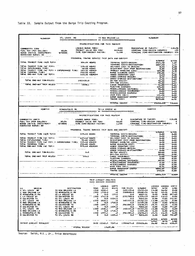
57
Table 33. Sample Output from the Barge Trip Costing Program.
*LOADED* ST. LOUIS MO TO NEW ORLEANS LA *LOADED* 00000000 000 0080*0000*000000 00 000000000000000000000000000
0*SPECIFICATIONS FOR THIS ROUTE*0
COMMODITY: CORN . LOADED BARGE TONS: 1350 PERCENTAGE OF TARIFF:' ' 110.05 FUEL 7 (PER G $o oo PRODUCT VALUE PER T0P1 $120.00 TERMINAL TIME-ORIGIN (HOURS I) 125 BARGE INITIAL INVE5INSNT: IG,EC FACTOR 1.100 TERMINAL TIME-DESTINATION (HOURS) 125 OVERSIZED BARGE: NO -
0*GENERAL. TOWING SERVICE TRIP DATA AND COSTSC* - .
S/BARGE S/TON TOTAL TRANSIT TIME (W/O TCF): 304.80 HOURS TERMINAL COSTS-ORIGIN: 2524.50 1.87
TERMINAL COSTS-DESTINATION: 6007.50 4.45 TOTAL TRANSIT TIME (WI TCF): 335.32 HOURS ' DELIVERY COST TO ORIGIN: 0.00 - 0.00 TOTAL INTERCHANGE TIME: 48.00 HOURS RESHIPMENT COST FROM DESTINATION: 0.00 0.00 TOTAL TRANSIT TIME (WI TCF) * INTERCHANGE TIME: 383.32 HOURS' PRODUCT HANOLING LOSS: 405.00 0.30 TOTAL TERMINAL TIME: 250.00 HOURS - -- BARGE 'CLEANING COST`-* ..150.00 0.11 TOTAL ONE-WAY TIME (W/ TCF): - 633.32 HOURS** ADDED INVENTORY COST 0.00 0.00
- . - --------- -.-.-..-.'--'-- ADDED STORAGE-ORIGIN: - 0.00 0.00 " A'OOED7ORAGE-DE5T'INIT -0.00
- ........
0.OD TOTAL ONE-WAY TON-MILES: 1401435.0 ON-TOW ASSIST: 90.00 0.07
OFF-TOW ASSIST: 90.00 0.07 DIAl ONE-WAY'tR'IP 'MIIE5:"
_________
CARG01N~UEA'NC FLEETING CHARGES: ' 125.00 0.09
---- . - -------- --- ------- MISCELLANEOUS SWITCHES: 90.00 0.07 ---------------------
MISCEtLANEOUS'INSU1NCCf 000'0.00 MISCELLANEOUS CHARGES: 0.00 0.00 USER FEES (NI): __ ______ 121.50 0.09
-. BARGr'OWNERSHIPCOSTSZ 4422'.83 3j6' TOWING COST: 9072.00 602
- ...................... ............ ' ----
0'*TOYAL '312.33T3.B8*
- *EMPTYC - MINNEAPOLIS MN TO LA CROSSE WI *EMPTY* 000000000000000000000000000000 0* 00000000000000000000000000 -
*ASPECIFICATIONS FOR THIS RUUTEOO
COMMODITY: EMPTY LOADED BARGE TONS: 0 PERCENTAGE 'OF TARIFF: ' ' 110.05 FUEL TAR (PER GALLON): $0.04 PRODUCT VALUE PER TON: $0.00 TERMINAL TIME-ORIGIN (HOURS): 0 BARGE INITIAL INVESTMENT: $250000 . TIME CONTINGENCY FACTOR: 1.100 TERMINAL TIME-DESTINATION (HOURS): 0 OVERSIZED BARGE: NO
000ENERAL TOWING SERVICE TRIP DATA AND COSTSOC - ' '
S/BARGE"'"' S/TON TOTAL TRANSIT TIME (W(0 TCF): 519.53 HOURS TERMINAL COSTS-ORIGIN: 0.00 0.00
TERMINAL COSTS-DESTINATION: 0.00 0.00 TOTAL TRANSIT TIME (W/ TCF): ' '637.48HOURS DELIVERY'COST'TOORIGINi 0.00 0.00 TOTAL INTER(.HANGE TIME: 92.00 HOURS RESHIPMENT COST FROM DESTINATION: 0.00 0.00 TOTAL TRANSIT TIME (W/ ICFP • INTERCHANGE TIME: 129.48 HOURSO PRODUCT HANDLING LOSS: 0.00 0.00 TOTAL TERMINAL TIME: ' ' - 250.00 HOURS BARGE CLEANING COST: --------------------- 0.000.00 TOTAL ONE-WAY TIME (WI TCF): 979.48 HOURS** ADDED INVENTORY COST 0.00 0.00
ADDED STORAGE-ORIGIN: '
0.00 0.00 ADDED STORAGE-OE SI INAETONT 0.00 " 0.00
TOTAL ONE-WAY TON-MILES: 0.0 ON-TOW ASSIST: 90.00 0.00 OFF-TOW ASSIST: 90.00 0.00
'TOTAL ONE-WAY TRIP MILE'S: ' £55.1 - ARGO'IPSURANCtT " ----------
--- ----
O.o00.o0' FLEETING CHARGES: ' 0.00 0.00 MISCELLANEOUS SWITCHES: 90.00 0.00 MISCELLANEOUS INSURANCE: 0.00 0.00
- MISCELLANEOUS CHARGES: 0.00 0.00 - USER FEES (NIl: 8.74 0.00
BARGE OWNERSHIP OSIS: Sd94.31ó.oO TOWING COST: 672.20 0.00
TRIP CIRCUIT ANALYSIS - 00*0 000*000 00000000
LOADED EMPTY LOADED LOADED EMPTY LE ORIGIN DESTINATION - TONS MILES MILES TON MILES S/BARGE $/PNT N/TM C/BR L ST. LOUIS NO TO NEW ORLEANS LA ' 1350 1038.1 .0 1401435.0 23152.33 13.88 16.52 ' 0.00 I. NEW ORLEANS LA TO MINNEAPOLIS MN ' 1350 1710.0 .0 2308500.0 28482.54 16.52 12.34 0.00 S MINNEAPOLIS MN TO LA CROSSE WI 0 0.0 155.1 0.0 6045.31 0.00 0.00 897.69 L LA CROSSE WI TO GALVESTON 'TX 1350 1742.0 .0 2351700.0 31574.19 18.49 13.43 0.00 E GALVESTON TM TO ST. LOUIS NO ' 0 0.0 1224.1 0.0 9203.65 0.00 0.00 751.87 L ST. LOUIS MO TO NEW ORLEANS LA 1350 1038.1 .0 1401435.0 23152.33 13.88 16.52 0.00 S NEW ORLEANS LA TO MINNEAPOLIS MN - 0 0.0 1710.0 0.0' 11459.20 - 0.00 '0.00 '670.13 L MINNEAPOLIS MN TO GALVESTON TX 1350 1897.1 .0 2561085.0 33670.23 19.14 13.15 0.00 € GALVESTON TX TO ST. LOUIS NO 0 0.0 1224.1 0.0 9203.85 0.00 0.00 T51.87 L ST. LOUIS NO TO NEW ORLEANS LA'"''''' 1350 1038.1 -- .0 1401435.0 23152.33 13.88 16.52 - 0.00 E NEW ORLEANS LA , TO MINNEAPOLIS MN 0 0.0 1710.0 0.0 11459.20 0.00 0.00 670.13 L MINNEAPOLIS MN TO GALVESTON TX 1350 1891.1 .0 2561085.0 33670.23 19.14 13.15- 0.00 € GALVESTON TX TO ST. LOUIS 183 ' 0 0.0 - 1224.1 ' 0.0' " 9203.65 - 0.00 -- 0.00" 151.87'
W/AVG ' W/AVG W/AVG "$/PNI - AfTM C/BM
**TRIP CIRCUIT TOTALSOO' - 9450 10360.5 7241.4 13986675.0 253428.84 26.82 18.12 439.29
0OTALMILES0 17607.90''' - ------ - - - --
Source: Smith, M.L., Jr., Price Waterhouse
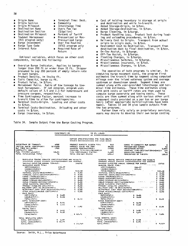
58
Origin Name • Termtnal Time: Dest. Origin Section . Commodity Origin Milepost • Interchange Time Destination Name • Users Fee Tax Destination Section ($/gallon) Destination Milepost • Percent of Tariff Towboat Horsepower • PressurizedorNon- (BCS program only) Pressurized Cargo Barge Investment • User Fee Routine Barge Type Code (BTCS program only Interest Rate • Required Rate of
Return
Optional variables, which focus on other cost components, include the following:
Oversize Barge Indicator. Applies to barges longer than 200 ft or wider than 35 ft. Shipper presumed to pay 200 percent of empty return' rate on such barges. Product Density, in lbs/cu ft. Cubic Capacity, barge cu ft. Product Value,,in $/ton. Horsepower Ratio. Ratio of tow tonnage to tow-boat horsepower. If not entered, program uses
- default values of. 3.5 and 2.3 for nonpressure and pressure cargoes, respectively. Time Contingency Factor, percent increase in transit time to allow for contingencies. Terminal Costs-Origin. Loadinq and other costs in $/ton. Terminal Costs-Destination. Unloading and other costs in $/ton. Cargo Insurance, in $/ton.
Cost of holding inventory in storage at origin and destination and while in-transit. Added Storage-Origin, in $/ton. Added Storage-Destination, in $/ton. Barge Cleaning, in $/barge. Product Handling Loss. Product lost during load- ing and unloading procedures, in $/ton. Delivery Cost to Origin. Transport from actual origin to origin dock, in $/ton. Reshipment Cost to Destination. Transport from destination dock to final destination, in $/ton. On-Tow Assist, in $/barge. 0ff-Tow Assist, in $/barge. Fleeting Charges, in $/barge. Miscellaneous Switches, in $/barge. Miscellaneous Insurance, in $/ton. Miscellaneous Charges, in $/ton.
The operation of both programs is similar. In computing barge movement costs, the program first estimates the transit time by segment using computed mileage over the inland waterway system and average upstream or downstream speed. Segment times are summed along with user-provided interchange and ter-minal time estimates. These time estimates along with unit costs or tariff rates are then used to compute barge-ownership and towing costs. These costs are then summed along with various other unit component costs provided on a per ton or per barge basis (after appropriate multiplications have been made). Tables 33 and 34 give sample outputs from the two programs.
Rather than rely solely on proprietary services, users may desire to develop their own barge costing
Table 34. Sample Output from the Barge Costing Program.
KUSI6LP0.EII OP TOWbOAT: INITIAl. UAI4GE INVt$TENT: NET TONS PEW 6ERGáS COW93.I1Y: COAL FUEL TAXIPEM UALLUNI TOTAL JI,TE.'Ll.APIGE TIME:
CINCINN*TI OH TO ST. LOUIS 00 000000000000P00000000000000P0
CUM'UN SPECIFICATIONS FIR THIS ROUTE 000000 00004flCSOC:000 Ott 0000 00000 -
6000 PRUOUCT OEP,SITY ILRICU FTI: 0.0 CUIIIC FT CAPACITY PER BARGE: - 0 8433600 PROQUCI VALUE PER TON: 10.03 PRESSuRIZED CaRGO: NO
1600 AVERaGE TOWLUAOI TOIlS:: 1*000 HORSEPOwER RATIO: 3.000 TERMINAL - (c1): 72 TERMINAL TIMROESTINATION(HOURSP 120
30.04 TIME CONTIN&0NLY IACTOM: 1.003 OVERSLZEO BARUE: NU TOTAL ONE-WAY MILES: 690.7 PERCENTAGE OF TARIFF: 100.0
OEOILA,T.0 TOWING SERVICE SPECIFICATIONS ANO RESULTS 000*00000 *00000 9*00000 00000000000090 Oct 000000* MA*IMUM E*P€CtEO, ANNUAL TCNT.AGE: 346592 OLOLCATRO ROUTE TIME:
IMPTYIHOURSI: 118.37 IOAOEC(HUURS) 324.11 TUTAI(HOUMSI: '442.48
TERMINAL coSrs-ORIGI'IIpNT,: 1 0.00 TtKRII,*L LUSTS-UESTINATIONIPNTI: I 0.00 CARGO IN5uRA10ElPNTl: 6 0.00 AAUEU INVENTCRY(PNTI: 0.00 AOOEO STQRAGE-QNIOTNIP'IT):. 3 0.00 AC,OEU STURACE-DESTTNATIONIPNTI: 1 0.00 3aq01 CLEANIN. COST(PNTI: S 0.00 'MUOUCT I,AIIUL INC LOS.IPNT): 3 0.00 DELIVERY COST TO UR1SIFIIPNT): 1 0.00 MASNIPMEPJT LOST FIllY 01Sf INAT I0.iPNT): 0.00 3I4tR MISLELLANEOUS COSTSIPNTI: 1 0.00 USER FEES:
(MPTY(PNTI: S 0.09 LUAUEOIPNfl:. I 0.0* TOTALTPNTP: 1 0.13
lAPSE fl - YI6ISH!P COST: EMPTYIPNT3: I 0.61
1 1.41 TOIAI.IPI,II: 0 1.92
TOIINO COST: EMPTY(PNTI: I 3.61 L000EOIPNTP: S 9.30 - TUTAIIPNTI: $12.11
TOTAL OEDILATEU LOST: TOTAL EMPIYIPIT): 3.97 TOTAL L0AOtOIPNT): 10.77 TOIALIPNTI: N 14.1'
GENERAL TOWING SERVICE SPECIFICATIONS *110 RESULTS 0900999 **Oct* 0090000 00000000900000 000 0000000 MAAIRUM EAPECTED ANNUAL TONNAGE PER BARGE: 23733 GN6R*t.ROUTE TIME:
. EM000IHOURS,: 186.37 LOAOEC(HOURSP: 372.11 TOTALIHOURS): . 538.48
TERMINAL COSTS-ORIGINIPNTI: 8 0.00 TEPPINAL COSTC-OESTINATIONIPNTP: 1 0.00 CA8GU IPISURANCE(PYITI: 1 0.00 40060 IF.VENTORY(PNT: $ 0.00 40010 STURACE-ORTGIN(PIT): $ 0.00 AEJUt0 STURAGL-OESTIIATIONTPITT: - 1 0.00 WARGE CLEANING CDSTIPNTI: 1 0.00
TICUCT HANULING LOSSIFNTI: 3 0.00 DELIVEAY COST TO OQIGINIPNTIT ........ $ 0.00 RESHIPMENT COST FROM OESTINATIONIPNfl: 1 0.00 OT.IEM MISCELLANEOUS CUSTS(PNII: 1 0.00 USER FEES:
EUPTYIPITI: 3 0.05 LOAOEOIPNTP: 1 0.08 TOTALTPNTI: 1 0.13
OblIGE OWNERSHIP COST: EMPTYIPItI: $ 0.72 LOROLIJIPNTI: $ 1.62 TOTALIPNTI: IS 2.4
TOWING COST: EMPTYlNTI: - 3 3.81 L010EO(PNTI: IS 6.24 TOTA(IPNTI: 3 7.05.
TOTALGENERIL COST: TOTAL EMPTYIPIT): 1 2.58 TrITOL IOAOEOIPNT: $ 6.94 TOTALIPITI: ' 9.520
Source: Smith, M.L., Price Waterhouse
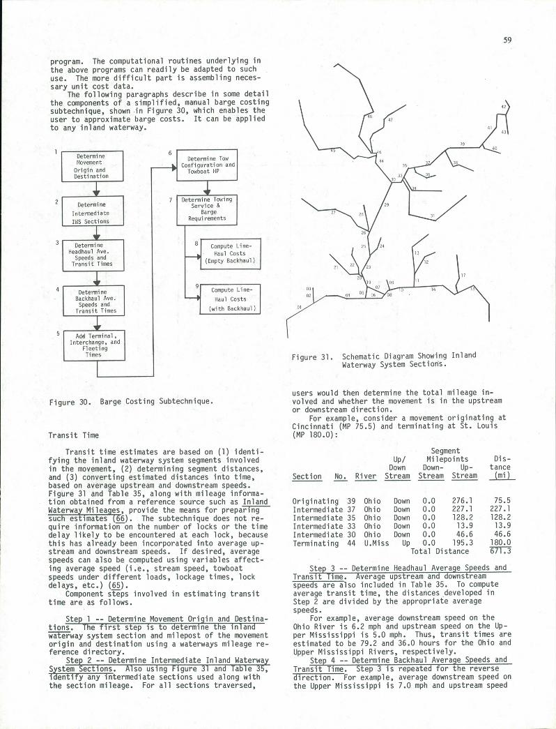
59
Figure 31. Schematic Diagram Showing Inland Waterway System Sections.
program. The computational routines underlying in the above programs can readily be adapted to such use. The more difficult part is assembling neces-sary unit cost data.
The following paragraphs describe in some detail the components of a simplified, manual barge costing subtechnique, shown in Figure 30, which enables the user to approximate barge costs. It can be applied to any inland waterway.
1 Determi I
Destination r-3J Configuration and
I 6
Ilov en ent ne
Origin and I Towboat HP
Ser 2
7 Determine Towi ngvice & Determine
Intermediate Barge
I IllS Sections i Requirements
. Determine I I
F___: Compute Line-
Headhaul Ave Haul Costs Speeds and (Empty Backhaul)
Transit Times I
I Determine I I Compute Line-
Backhaul Ave. I I Haul Costs Speeds and
Transit Times I I (with _Backhaul) 9 Adl Terminal,
Interchange, and Fleeting Times
Figure 30. Barge Costing Subtechnique.
Transit Time
Transit time estimates are based on (1) identi-fying the inland waterway system segments involved in the movement, (2) determining segment distances, and (3) converting estimated distances into time, based on average upstream and downstream speeds. Figure 31 and Table 35, along with mileage informa-tion obtained from a reference source such as Inland Waterway Mileages, provide the means for preparing such estimates (66). The subtechnique does not re-quire information on the number of locks or the time delay likely to be encountered at each lock, because this has already been incorporated into average up-stream and downstream speeds. If desired, average speeds can also be computed using variables affect-ing average speed (i.e., stream speed, towboat speeds under different loads, lockage times, lock delays, etc.) (65).
Component steps involved in estimating transit time are as follows.
Steo 1 -- Determine Movement Oriain and Destina-tions. The first step is to determine the inland waterway system section and milepost of the movement origin and destination using a waterways mileage re-ference directory.
Step 2 -- Determine Intermediate Inland Waterway System Sections. Also usingFigure 31 and Table 35, identify any Intermediate sections used along with the section mileage. For all sections traversed,
users would then determine the total mileage in-volved and whether the movement is in the upstream or downstream direction.
For example, consider a movement originating at Cincinnati (MP 75.5) and terminating at St. Louis (MP 180.0):
Segment Up! Milepoints Dis-
Down Down- Up- tance Section No. River Stream Stream Stream (ml)
Originating 39 Ohio Down 0.0 276.1 75.5 Intermediate 37 Ohio Down 0.0 227.1 227.1 Intermediate 35 Ohio Down 0.0 128.2 128.2 Intermediate 33 Ohio Down 0.0 13.9 13.9 Intermediate 30 Ohio Down 0.0 46.6 46.6 Terminating 44 U.Miss Up 0.0 195.3 180.0
Total Distance 671.3
Steo 3 -- Determine 1-leadhaul Average Speeds and Transit Time. Average upstream and downstream speeds are also included in Table 35. To compute average transit time, the distances developed in Step 2 are divided by the appropriate average speeds.
For example, average downstream speed on the Ohio River is 6.2 mph and upstream speed on the Up-per Mississippi is 5.0 mph. Thus, transit times are estimated to be 79.2 and 36.0 hours for the Ohio and Upper Mississippi Rivers, respectively.
Steo 4 -- Determine Backhaul Average Speeds and Transit Time. Step 3 is repeated for the reverse direction. For example, average downstream speed on the Upper Mississippi is 7.0 mph and upstream speed
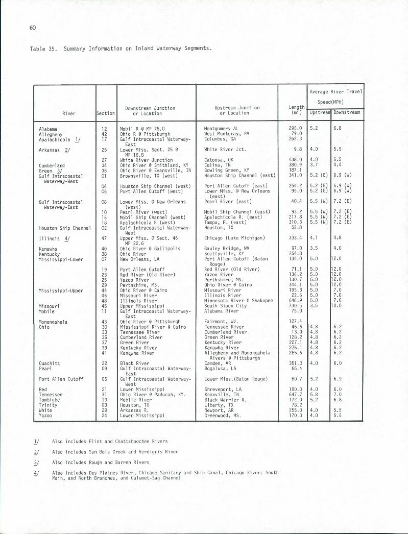
60
Table 35. Summary Information on Inland Waterway Segments.
River Section Downstream Junction
or Location Upstream Junction or Location
Length (mi )
Average River Travel
Speed(MPH)
Upstreaa Downstream
Alabama 12 Mobil R @ MP 75.0 Montgomery AL 295.0 5.2 6.8
Allegheny 42 Ohio R 9 Pittsburgh West Monterey, PA 79.0 Apalachicola 1/ 17 Gulf Intracoastal Waterway- Columbus, GA 262.3
East Arkansas 2/ 26 Lower Miss. Sect. 25 9 White River Uct. - 9.8 4.0 5.5
MP 16.8 27 White River Junction Catoosa, OK 438.0 4.0 5.5
Cumberland 34 Ohio River 9 Sniithland, KY Celina, TN 380.9 3.7 4.4
Green 3/ 36 Ohio River 9 Evansville, IN Bowling Green, KY 187.1 Gulf Intracoastal 01 Brownsville, TX (west) Houston Ship Channel (east) 341.0 5.2 (E) 6.9 (W)
Waterway-West 04 Houston Ship Channel (west) Port Allen Cutoff (east) 254.2 5.2 (E) 6.9 (W) 06 Port Allen Cutoff (west) Lower Miss. 9 New Orleans 95.0 5.2 (E) 6.9 (W)
(east) Gulf Intracoastal 08 Lower Miss. 9 New Orleans Pearl River (east) 40.4 5.5 (W) 7.2 (E)
Waterway-East (west) 10 Pearl River (west) Mobil Ship Channel (east) 93.2 5.5 (W) 7.2 (E) 16 Mobil Ship Channel (west) Apalachicola R. (east) 217.8 5.5 (W) 7.2 (E) 18 Apalachicola R (west) Tampa, FL (east) 310.3 5.5 (W) 7.2 (E)
Houston Ship Channel 02 Gulf Intracoastal Waterway- Houston, TX 52.8 West
Illinois 4/ 47 Upper Miss. @ Sect. 46 Chicago (Lake Michigan) 333.4 4.1 4.8 MP 22.6
Kanawha 40 Ohio River 9 Gallipolis Gauley Bridge, WV 97.0 3.5 4.0 Kentucky 38 Ohio River Beattyville, KY 254.8 Mississippi-Lower 07 New Orleans, LA Port Allen Cutoff (Baton 134.0 5.0 12.0
Rouge) 19 Port Allen Cutoff Red River (Old River) 71.1 5.0 12.0 23 Red River (Old River) Yazoo River 136.2 5.0 12.0 25 Yazoo River Perthshire, MS. 130.7 5.0 12.0 29 Perthshire, MS. Ohio River 9 Cairo 344.1 5.0 12.0
Mississippi-Upper 44 Ohio River @ Cairo Missouri River 195.3 5.0 7.0 46 Missouri River Illinois River 22.6 5.0 7.0 48 Illinois River Minnesota River 9 Shakopee 646.9 5.0 7.0
Missouri 45 Upper Mississippi South Sioux City 730.5 3.5 10.0 Mobile 11 Gulf Intracoastal Waterway- Alabama River 75.0
East Mononqahela 43 Ohio River 9 Pittsburgh Fairmont, WV. 127.4 Ohio 30 Mississippi River 9 Cairo Tennessee River 46.6 4.8 6.2
33 Tennessee River Cumberland River 13.9 4.8 6.2 35 Cumberland River Green River 128.2 4.8 6.2 37 Green River Kentucky River 227.1 4.8 6.2 39 Kentucky River Kanawha River 276.1 4.8 6.2 41 Kanawha River Allegheny and Monongahela 265.6 4.8 6.2
Rivers @ Pittsburgh Ouachita 22 Black River Camden, AR 351.0 4.0 6.0 Pearl 09 Gulf Intracoastal Waterway- Bogalusa, LA 66.4
East Port Allen Cutoff 05 Gulf Intracoastal Waterway- Lower Miss.(Baton Rouge) 60.7 5.2 6.9
West Red 21 Lower Mississippi Shreveport, LA 180.0 4.0 6.0 Tennessee 31 Ohio River 9 Paducah, KY. Knoxville, TN 647.7 5.8 7.0 Tombigbe 13 Mobile River Black Warner R. 172.0 5.2 6.8 Trinity 03 Houston, TX Liberty, TX 78.2 White 28 Arkansas R. Newport, AR 255.0 4.0 5.5 Yazoo 24 Lower Mississippi Greenwood, MS. 170.0 4.0 5.5
1/ Also includes Flint and Chattahoochee Rivers
2/ Also includes San Bois Creek and Verdigris River
3/ Also includes Rough and Barren Rivers
4/ Also includes Des Plaines River, Chicago Sanitary and Ship Canal, Chicago River: South Main, and North Branches, and Calumet-Sag Channel
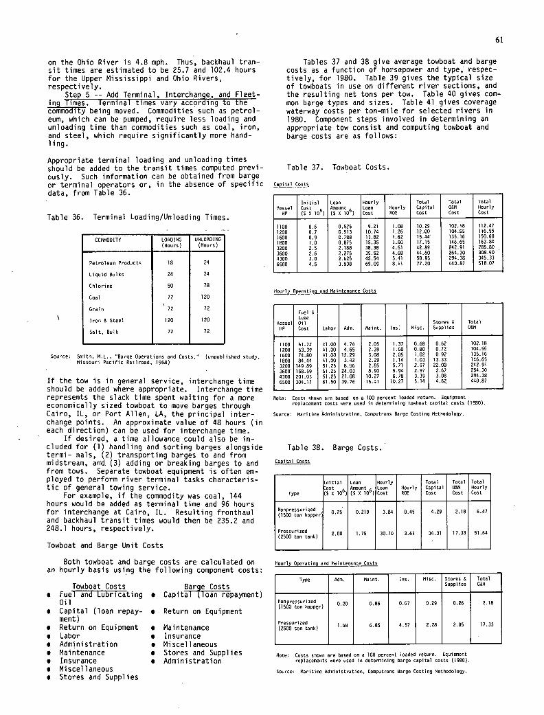
61
on the Ohio River is 4.8 mph. Thus, backhaul tran-sit times are estimated to be 25.7 and 102.4 hours for the Upper Mississippi and Ohio Rivers, respectively.
Step 5 -- Add Terminal, Interchange, and Fleet-ing Times. Terminal times vary according to the commodity being moved. Commodities such as petrol-eum, which can be pumped, require less loading and unloading time than commodities such as coal, iron, and steel, which require significantly more hand-ling.
Appropriate terminal loading and unloading times should be added to the transit times computed previ-ously. Such information can be obtained from barge or terminal operators or, in the absence of specific data, from Table 36.
Table 36. Terminal Loading/Unloading Times.
COMMODITY - LOADING
(Hours)
UNLOADING (Hours)
Petroleum Products 18 24
Liquid Bulks 24 24
Chlorine 50 78
Coal 72 120
Grain 72 72
Iron U Steel 120 120
Salt, Bulk 72 72
Source: Smith, M.L "Barge Operations and Costs," (unpublished study, Missouri Pacific Railroad, 1968)
If the tow is in general service, interchange time should be added where appropriate. Interchange time represents the slack time spent waiting for a more economically sized towboat to move barges through Cairo, IL, or Port Allen, LA, the principal inter-change points. An approximate value of 48 hours (in each direction) can be used for interchange time.
If desired, a time allowance could also be in-cluded for (1) handling and sorting barges alongside termi- nals, (2) transporting barges to and from midstream, and. (3) adding or breaking barges to and from tows. Separate towboat equipment is often em-ployed to perform river terminal tasks characteris-tic of general towing service.
For example, if the commodity was coal, 144 hours would be added as terminal time and 96 hours for interchange at Cairo, IL. Resulting fronthaul and backhaul transit times would then be 235.2 and 248.1 hours, respectively.
Towboat and Barge Unit Costs
Both towboat and barge costs are calculated on an hourly basis using the following component costs:
Towboat Costs Barge Costs Fuel and Lubricating • Capital (loan repayment) Oil Capital (loan repay- . Return on Equipment ment) Return on Equipment • Maintenance Labor • Insurance Administration • Miscellaneous Maintenance • Stores and Supplies Insurance • Administration Miscellaneous Stores and Supplies
Tables 37 and 38 give average towboat and barge costs as a function of horsepower and type, respec-tively, for 1980. Table 39 gives the typical size of towboats in use on different river sections, and the resulting net tons per tow. Table 40 gives com-mon barge types and sizes. Table 41 gives coverage waterway costs per ton-mile for selected rivers in 1980. Component steps involved in determining an appropriate tow consist and computing towboat and barge costs are as follows:
Table 37. Towboat Costs.
Capital Costs
Hourly Operating and Maintenance Costs
Fuel & Lube
Vessel Oil Stores 6 Total
HP Cost Labor Ado. Maint. Ins Misc. Supplies OUM
1100 51.72 41.00 4.74 2.05 1.37 0.68 0.62 102.18
1200 53.39 41.00 4.65 2.39 1.60 0.80 0.72 104.55
1600 74.80 41.00 12.29 3.08 2.05 1.02 0.92 135.16
1800 84.44 41.00 3.42 2.29 1.14 1.03 13.33 146.65
3200 149.89 51.25 8.56 2.85 5.71 2.57 22.08 242.91
3600 168.59 51.25 24.03 8.90 5.94 2.97 2.67 264.30
4300 201.03 51.25 27.08 10.27 6.78 3.39 3.08 294.38
6500 304.17 61.50 39.76 15.41 10.27 5.14 4.62 440.87
Note: Costs shoun are based on a 100 percent loaded return. Equipment replacement costs were used in determining towboat capital costs (1980).
Source: Maritime Administration, Computrans Barge Costing Methodology.
Table 38. Barge Costs.
Capital Costs
Initial Loan Hourly Total Total Total
Cost (5 0 106)
Amount (S 0 106)
Loan Cost
Hourly ROE
Capital Cost
OSM Cost
Hourly Cost Type
Nonpressurized 0.25 0.219 3.84 0.45 4.29 2.18 6.47
(1500 ton hopper
Pressuri zed 2.00 1.75 30.70 3.61 34.31 17.33 51.64
(2500 ton tank)
Hourly Operating and Maintenance Costs
Type 8dm. Maint. Ins. Misc. I Stores & Supplies
Total 0011
000pressurized 0.20 0.86 0.67 0.29 0.26 2.18 (1500 ton hopper)
Pressurized 1.58 6.85 4.67 2.28 2.05 17.33
(2500 ton tank)
Note: Costs shown are based on a 100 percent loaded return. Equipment replacements were used in determining barge capital costs (1980).
Source: Maritime Administration, Conputrans Barge Costing Methodology.
Vessel HP
Initial Cost (S 010)
Loan Amount 6 (SO 10)
Hourly Loan Cost
Hourly ROE
Total Capital Cost
Total 0811 Cost
Total Hourly Cost
1100 0.6 0.525 9.21 1.08 10.29 102.18 112.47
1200 0.7 0.613 10.74 1.26 12.00 104.55 116.55
1600 0.9 0.788 .13.82 1.62 15.44 135.16 150.60
1800 1.0 0.875 15.35 1.80 17.15 146.65 163.80
3200 2.5 2.188 38.38 4.51 42.89 242.91 285.80
3600 2.6 2.275 39.92 4.68 44.60 264.30 308.90
4300 3.0 2.625 45.54 5.41 50.95 294.38 345.33
6500 4.5 3.938 69.09 8.11 77.20 440.87 518.07
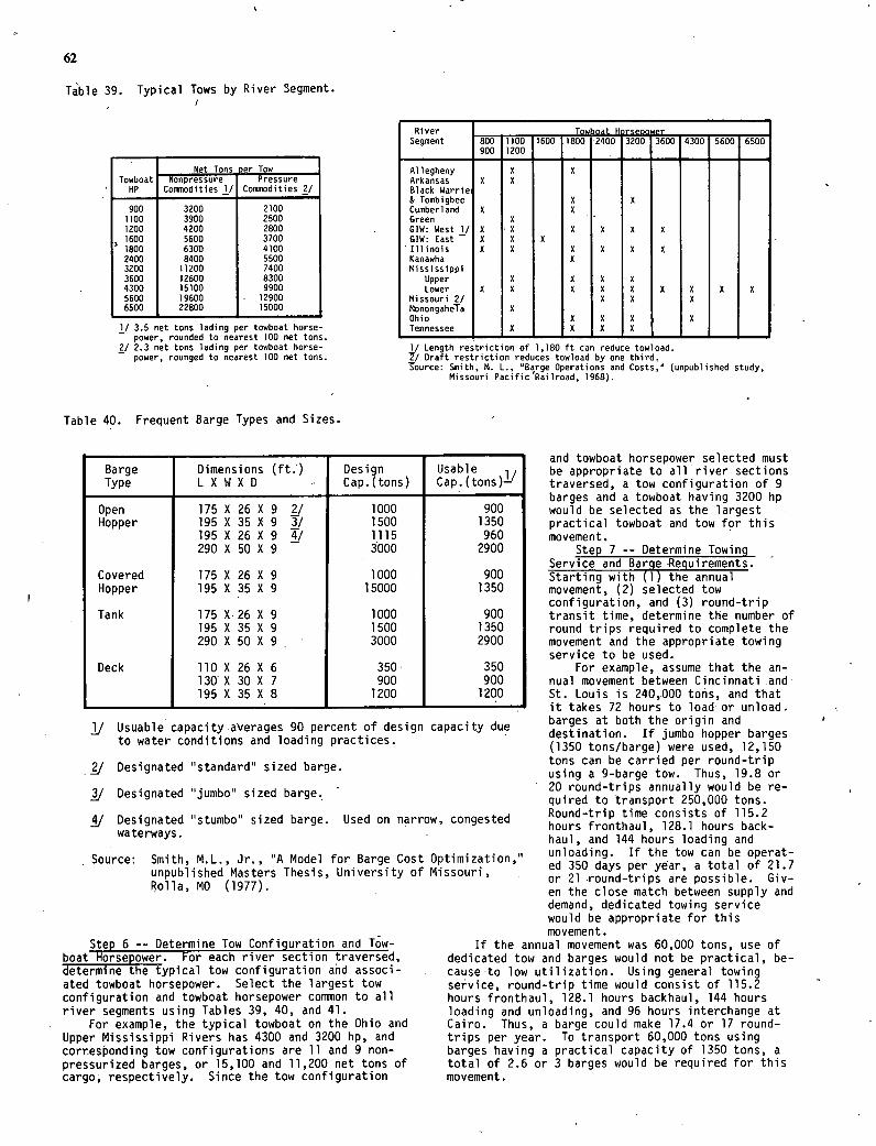
Towboat Net Tons rier Tow
Nonpressure Pressure HP Cormiodities !/ Coriunodities 2/
900 3200 2100 1100 3900 2500 1200 4200 2800 1600 5600 3700 1800 6300 4100 2400 8400 5500 3200 11200 7400 3600 12600 8300 4300 15100 9900 5600 19600 12900 6500 22800 15000
1/ 3.5 net tons lading per towboat horse- power, rounded to nearest 100 net tons.
2/ 2.3 net tons lading per towboat horse- power, rounged to nearest 100 net tons.
62
Table 39. Typical Tows by River Segment.
River Segment
- - - .,_Towboat L' ter - c.... - - - 800 1100 1600 1800 2400 3200 3600 4300 5600 6500 900 1200
Allegheny X X Arkansas X X Black Warrie & Tombigbee X U Cumberland X U Green X 61W: West 1/ X X X X X X 61W: East X X
'Illinois X X X X X X Kanawha X Mississippi
Upper X X X X Lower X X X X X X X X X
Missouri 2/ X X X MonongaheTa X Ohio X X X X Tennessee X X I X
1/ Length restriction of 1,180 ft can reduce towload. 2/ Draft restriction reduces towload by one third. 'source: Smith, M. L., 'Barge Operations and Costs,' (unpublished study,
Missouri Pacific Railroad, 1968).
Table 40. Frequent Barge Types and Sizes.
Steo 6 -- Determine Tow Confiquration and Tow-boat Horsepower. For each river section traversed, determine the typical tow configuration and associ-ated towboat horsepower. Select the largest tow configuration and towboat horsepower common to all river segments using Tables 39, 40, and 41.
For example, the typical towboat on the Ohio and Upper Mississippi Rivers has 4300 and 3200 hp, and corresjonding tow configurations are 11 and 9 non-pressurized barges, or 15,100 and 11,200 net tons of cargo, respectively. Since the tow configuration
'
and towboat horsepower selected must be appropriate to all river sections traversed, a tow configuration of 9 barges and a towboat having 3200 hp would be selected as the largest practical towboat and tow for this movement.
Step 7 -- Determine Towing - Service and Barge Requirements. Starting with (1) the annual movement, (2) selected tow configuration, and (3) round-trip transit time, determine the number of round trips required to complete the movement and the appropriate towing service to be used.
For example, assume that the an-nual movement between Cincinnati and St. Louis is 240,000 tons, and that it takes 72 hours to load or unload,
due barges at both the origin and destination. If jumbo hopper barges (1350 tons/barge) were used, 12,150 tons can be carried per round-trip using a 9-barge tow. Thus, 19.8 or 20 round-trips annually would be re-quired to transport 250,000 tons.
connested Round-trip time consists of 115.2 hours fronthaul, 128.1 hours back-haul, and 144 hours loading and
Limization , unloading. If the tow can be operat-
souri ed 350 days per year, a total of 21.7 or 21 round-trips are possible. Giv-en the close match between supply and demand, dedicated towing service would be appropriate for this movement.
If the annual movement was 60,000 tons, use of dedicated tow and barges would not be practical, be-causeto low utilization. Using general towing service, round-trip time would consist of 115.2 hours fronthaul, 128.1 hours backhaul, 144 hours loading and unloading, and 96 hours interchange at Cairo. Thus, a barge could make 17.4 or 17 round-trips per year. To transport 60,000 tons using barges having a practical capacity of 1350 tons, a total of 2.6 or 3 barges would be required for this movement.
2/ Designated "standard" sized barge.
/ Designated "jumbo" sized barge.
/ Designated "stumbo" sized barge. Used on narrow, waterways.
Source: Smith, M.L., Jr., "A Model for Barge Cost Opi unpublished Masters Thesis, University of Mi Rolla, MO (1977).
Barge Type
Dimensions (ft.) L X W X D
Design Cap.(tons)
Usable 1/ Cap.(tons)—
Open 175 X 26 X 9 2/ 1000 900 Hopper 195 X 35 X 9 3/ 1500 1350
195 X 26 X 9 4/ 1115 960 290 X 50 X 9 - 3000 2900
Covered 175 X 26 X 9 1000 900 Hopper 195 X 35 X 9 15000 1350
Tank 175 X26 X 9 1000 900 195 X 35 X 9 1500 1350 290 X 50 X 9 3000 2900
Deck 110 X 26 X 6 350 350 130 X 30 X 7 900 900 195 X 35 X 8 1200 1200
1/ Usuable capacity averages 90 percent of design capacity to water conditions and loading practices.
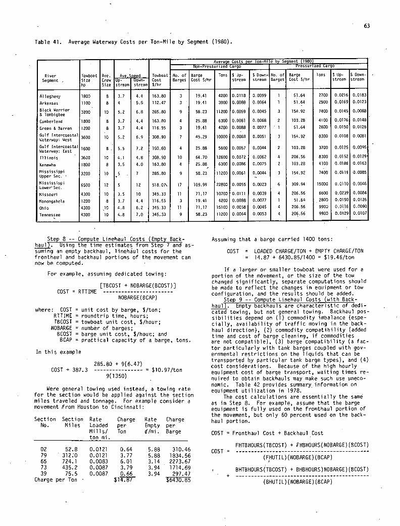
63
Table 41. Average Waterway Costs per Ton-Mile by Segment (1980).
Averae Costs per Ton-Mile by Segment (1980) _____________________ Non-Pressurized Cargo Pressui ed Cargo -
No. of Barge Tons $ Up- $ Down- No. of Barge Tons $ Up- $ Down- River Towboat Ave. Ave.Soeed Towboat Segment - Size Crew Cost Barges Cost $/hr stream stream Barges Cost $/hr stream stream
hp Size stream stream $/hr
Allegheny 1800 8 3.7 4.4 163.80 3 19.41 4200 0.0118 0.0099 1 51.64 2700 0.0216 0.0183
Arkansas 1100 8 4 5.5 112.47 3 19.41 3900 0.0088 0.0064 1 51.64 2500 0.0169 0.0123
Black Warner 3200 10 5.2 6.8 285.80 9 58.23 11200 0.0059 0.0045 3 154.92 7400 0.0145 0.0088 & Tombigbee
Cumberland 1800 8 3.7 4.4 163.80 4 25.88 6300 0.0081 0.0068 2 103.28 4100 0.0176 0.0148
Green & Barren 1200 8 3.7 4.4 116.55 3 19.41 4200 0.0088 0.0077 1 51.64 2800 0.0150 0.0126
Gulf Intercoastal 3600 10 5.2 6.9 308.90 7 45.29 10000 0.0068 0.0051 3 154.92 8300 0.0108 0.0081 Waterway: West
Gulf Intercoastal 1600 8 5.5 7.2 150.60 4 25.88 5600 0.0057 0.0044 2 103.28 3700 0.0125 0.0095 Waterway: East
Illinois 3600 10 4.1 4.8 308.90 10 64.70 12600 0.0072 0.0062 4 206.56 8300 0.0152 0.0129
Kanawha 1800 8 3.5 4.0 163.80 4 25.88 6300 0.0086 0.0075 2 103.28 4100 0.0186 0.0163
Mississippi 3200 10 5 7 285.80 9 58.23 11200 0.0061 0.0044 3 154.92 7400 0.0119 0.0085 Upper Sec.
Mississippi 6500 12 5 12 518.07 17 109.99 22800 0.0065 0.0023 6 309.94 15000 0.0110 0.0046
Lower Sec.
MisSouri 4300 10 3.5 10 345.33 11 71.17 10700 0.0111 0.0039 4 206.56 6600 0.0239 0.0084
Monongahela 1200 8 3.7 4.4 116.55 3 19.41 4200 0.0088 0.0077 1 51.64 2800 0.0150 0.0126
Ohio 4300 10 4.8 6.2 345.33 11 71.17 15100 0.0058 0.0045 4 206.56 9900 0.0116 0.0090
Tennessee 4300 10 4.8 7.0 345.33 9 58.23 11200 0.0064 0.0053 4 206.56 9900 0.0129 0.0107
Step 8 -- Compute Linehaul Costs (Empty Back-haul). Using the time estimates from Step 7 and as-suming an empty backhaul, linehául costs for the fronthaul and backhaul portions of the movement can now be computed.
For example, assuming dedicated towing:
[TBCOST + NOBARGE(BCOST)] COST = RTTIME
NOBARGE(BCAP)
where: COST = unit cost by barge, $/ton; RTTIME = roundtrip time, hours; TBCOST = towboat unit cost, $/hour; NOBARGE = number of barges; BCOST = barge unit cost, $/hour.; and BCAP = practical capacity of a barge, tons.
In this example
285.80 + 9(6.47) COST + 387.3 ----------------= $10.97/ton
9(1350)
Were general towing used instead, a towing rate for the section would be applied against the section miles traveled and tonnage. For example consider a movement from Houston to Cincinnati:
Section Section Rate Charge Rate Charge No. Miles Loaded per Empty per
Mills! Ton i/mi. Barge ton mi.
02 52.8 0.0121 0.64 5.88 310.46 79 312.0 0.0121 3.77 5.88 1834.56 65 724.1 0.0083 6.01 3.14 2273.67 73 435.2 0.0087 3.79 3.94 1714.69 39 75.5 0.0087 0.66 3.94 297.47
Charge per Ton $14.87 $6430.85
Assuming that a barge carried 1400 tons:
COST = LOADED CHARGE/TON + EMPTY CHARGE/TON = 14.87 + 6430.85/1400 = $19.46/ton
If a larger or smaller towboat were used for a portion of the mOvement, or the size of the tow changed significantly, separate computations should be made to reflect the changes in equipment or tow configuration, and the results should be added.
Step 9 -- Compute Linehaul Costs (with Back-haul). Empty backhauls are characteristic of dedi-cated towing, but not general towing. Backhaul pos-sibilities depend on (1) commodity imbalance (espe-cially, availability of traffic moving in the back-haul direction), (2) commodity compatibility (added time and cost of barge cleaning, if commodities are not compatible), (3) barge compatibility (a fac-tor particularly with tank barges coupled with gov-ernmental restrictions on the liquids that can be transported by particular tank barge types), and (4) cost considerations. Because of the high hourly equipment cost of barge transport, waiting times re-quired to obtain backhauls may make such use uneco-nomic. Table 42 provides summary information on equipment utilization in 1978.
The cost calculations are essentially the same as in Step 8. For example, assume that the barge equipment is fully used on the fronthaul portion of the movement, but only 60 percent used on the back-haul portion.
COST = Fronthaul Cost + Backhaul Cost
FHTBHOURS(TBCOST) + FHBHOURS(NOBARGE) (BCOST) COST -
(FHUTIL) (NOBARGE) (BCAP)
BHTBHOURS(TBCOSI) + BHBHOURS)NOBARGE)(BCOST) + (BHUTIL) (NOBARGE) (BCAP)
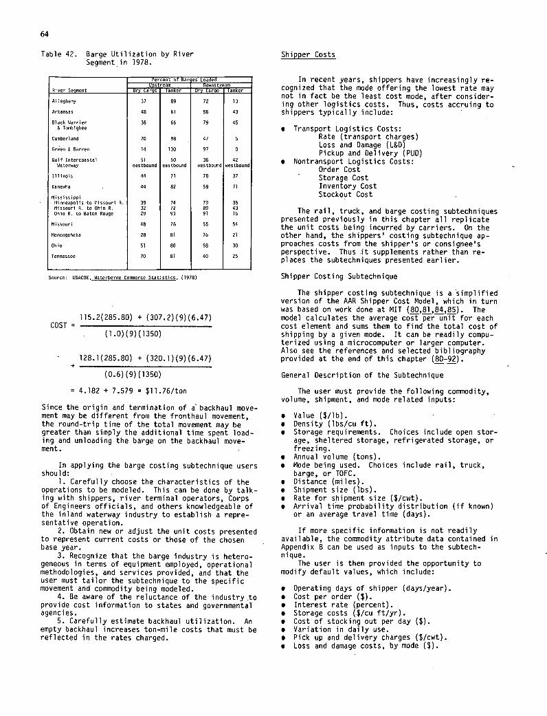
64
Table 42. Barge Utilization by River Segment in 1978.
Percent of Bar"es Loaded Llpstrean Downstream
River Segment Dry Cargo Tanker Dry Cargo Tanker
Allegheny 37 89 72 13
Arkansas 48 61 56 43
Black Worrier 36 66 79 45 A Tombigbee
Cumberland 70 98 47 5
Green B Barren 14 100 97 0
Gulf Intercoastal 51 60 36 42 Waterway eastbound eastbound westbound westbound
Illinois 44 71 70 37
Kanawha 44 82 58 71
Mississippi Minneapolis Cu Missouri R. 39 74 79 35 Missouri R. toOhio R. 32 72 89 43 Ohio B. to Baton Rouge 29 93 91 16
MiSsouri 48 78 56 54
Monongahela 28 81 76 21
Ohio 51 80 58 30
Tennessee 70 81 40 25
Source: IJSACOE, Waterborne Comerce Statistics, (1978)
115.2(285.80) + (307.2)(9)(6.47) COST =
(1.0)(9)(1350)
- 128.1(285.80) + (320.1)(9)(6.47) +
(0.6)(9)(1350)
= 4.182 + 7.579 = $11.76/ton
Since the origin and termination of abackhaul move-ment may be different from the fronthaul movement, the round-trip time of the total movement may be greater than simply the additional time spent load-ing and unloading the barge on the backhaul move-ment.
In applying the barge costing subtechnique users should:
Carefully choose the characteristics of the operations to be modeled. This can be done by talk-ing with shippers, river terminal operators, Corps of Engineers officials, and others knowledgeable of the inland waterway industry to establish a repre-sentative operation.
Obtain new or adjust the unit costs presented to represent current costs or those of the chosen base year.
Recognize that the barge industry is hetero-geneous in terms of equipment employed, operational methodologies, and services provided, and that the user must tailor the subtechnique to the specific movement and commodity being modeled.
Be aware of the reluctance of the industry to provide cost information to states and governmental agencies.
Carefully estimate backhaul utilization. An empty backhaul increases ton-mile costs that must be reflected in the rates charged.
Shipper Costs
In recent years, shippers have increasingly re-cognized that the mode offering the lowest rate may not in fact be the least cost mode, after consider-ing other logistics costs. Thus, costs accruing to shippers typically include:
Transport Logistics Costs: Rate (transport charges) Loss and Damage (L&D) Pickup and Delivery (PUD)
Nontransport Logistics Costs: Order Cost Storage Cost Inventory Cost Stockout Cost
The rail, truck, and barge costing subtechniques presented previously in this chapter all replicate the unit costs being incurred by carriers. On the other hand, the shippers' costing subtechnique ap-proaches costs from the shipper's or consignee's perspective. Thus it supplements rather than re-places the subtechniques presented earlier.
Shipper Costing Subtechnique
The shipper costing subtechnique is a simplified version of the AAR Shipper Cost Model, which in turn was based on work done at MIT (80,81,84,85). The model calculates the average cost per unit for each cost element and sums them to find the total cost of shipping by a given mode. It can be readily compu-terized using a microcomputer or larger computer. Also see the references and selected bibliography provided at the end of this chapter (80-92).
General Description of the Subtechniqu.e
The user must provide the following commodity, volume, shipment, and mode related inputs:
Value ($/lb). Density (lbs/cu ft). Storage requirements. Choices include open stor- age, sheltered storage, refrigerated storage, or freezing. Annual volume (tons). Mode being used. Choices include rail, truck, barge, or TOFC. Distance (miles). Shipment size (lbs). Rate for shipment size ($/cwt). Arrival time probability distribution (if known) or an average travel time (days).
If more specific information is not readily available, the commodity attribute data contained in Appendix B can be used as inputs to the subtech-nique.
The user is then provided the opportunity to modify default values, which include:
Operating days of shipper (days/year). Cost per order ($). Interest rate (percent). Storage costs ($/cu ft/yr). Cost of stocking out per day ($). Variation in daily use. Pick up and delivery charges ($/cwt).
. Loss and damage costs, by mode (U.
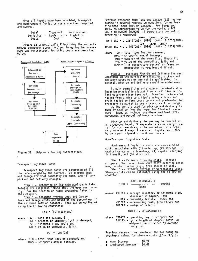
65
Once all inputs have been provided, transport and nontransport logistics costs are then computed and summed.
Total Transport Nontransport Logistics = Logistics + Logistics Costs Cost Cost
Figure 32 schematically illustrates the subtech-nique; component steps involved in estimating trans-port and nontransport logistics costs are described below.
Transport Logistics Costs Nontransport Logistics Costs
1'- Determine or I Estimate
Estimate I Ordering
lApplicable Rate Costs
2 - I 51 Estimate
I
I I Estimate
Average Loss I Storage or I Warehousing
I and Damage I i Costs
3 Estimate 6 Estimate
I Pick-up and Inventory Delivery
I
i I Charges I I Costs
Estimate
Stock-Out
Costs (Optional)
8 Sum
Component
Costs
Figure 32. Shipper's Costing Subtechnique
Transport Logistics Costs
Transport logistics costs are comprised of (1) the rate charged by the carrier, (2) average loss and damage for that commodity and mode, and (3) any pick-up and delivery charges.
Steø 1 -- Determine or Estimate Applicable Rate. Rate(s) are exogenous inputs that the user must sup-ply. See the section on rates presented later in this chapter.
Step 2 -- Estimate Average Loss and Damage. Loss and damage costs are based on the percentage of the shipment lost or damaged. They can be estimated using the following equations: -
L&D = (PCI) (SS)(VAL)
where: 'L&D = loss and damage, $; PCI = percent of shipment lost or damaged; SS = shipment size, lbs); and VAL = value of commodity, $/lb).
PCI = TLD/TONS
where: TLD = total tons lost or damaged; and TONS = shipper's annual tonnage.
Previous research into loss and damage (92) has re-sulted in several regression equations for estima-ting total tons lost or damaged. For Barge and TOFC, an appropriate value for the variable PCI would be 0.0001 (0.0002, if temperature control or freezing is required).
.SI4 .g'*2. Rail TLD = 0.0251(IONS) (DEN) (VAL) 1.0257(TEMP)
.561% - .105% Truck TLD = 0.0175(TONS) (DEN) (VAL) 0.4369(TEMP)
where: TLD = total tons lost or damaged; TONS = shjpper's annual tonnage; DEN = density of the commodity, lbs/cu ft; VAL = value of the commodity, $/lb; and
TEMP = '1 if temperature control or freezing protection is required; 0 if not.
Step 3 -- Estimate Pick-Up and Delivery Charges. Depending on the particular situation, pick-up and delivery costs may or may not be applicable. In general, pick-up and delivery should be added when:
Bulk commodities originate or terminate at a location physically distant from a rail line or in-land waterway river terminal. Examples include coal hauled from a mine to a tipple using a truck and grain hauled by farm truck to a country elevator for transport to market by grain truck, rail, or barge.
The vehicle used for pick-up and delivery is usually smaller from that used for linehaul trans-port. Examples include less-than-truckload (LTL) movements and parcel delivery services.
Pick-up and delivery charges may be treated as an exogenous input, if separate rates or charges ex-ist for such services, or be costed out as a sepa-rate mode or transport service. Inputs can either be on a per shipment or unit cost basis.
Non-Transport Logistics Costs
Nontransport logistics costs are comprised of costs associated with (1) ordering, (2) storage, (3) capital carrying in inventory, (4) capital carrying in transit, and (5) stock out.
Step 4 -- Estimate Ordering Costs. Because shippers often do not know what their ordering costs are, constant value (e.g., $20) should be used.
Steo 5 -- Estimate Storage or Warehousing Costs. Storage costs can beestimated using the following equation:
(AVE INV) (WHSECT) STOR = ________________ - ORDERS
(DEN)
where: AVEINV = average inventory or shipment size, whichever is higher, lbs;
DEN = commodity density, lbs/cu ft; WHSECT = warehousing cost, $/cu ft/yr; and ORDERS = number of orders.
ORDERS = YRDAYS/CYCLEN
where: YRDAYS = operating day of shipper; and CYCLEN = cycle length of shipper (days) or
shipment size divided by average daily use.
Previous research has developed the'following ap-proximate values for storage costs ($/cu ft/yr).
Open Storage 1
$0.24 9 Sheltered Storage $0.68
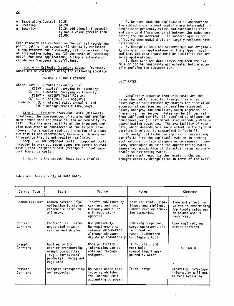
66
Temperature Control $0.81 Freezing $1.20 Security $0.34 additional if cornmodi-
ty has a value greater than $5.00.
Much research has centered on the optimal reordering point, taking into account (1) the daily variation in requirements for a commodty, (2) the arrival time of alternative modes, and (3) the costs of 'stocking out." For most applications, a simple estimate of reordering frequency is sufficient.
Step 6 -- Estimate Inventory Costs. Inventory costs can be estimated using the following equation:
INVCOST = CCINV + CCTRNST
where: INVCOST = total inventory cost; CCINV = capital carrying in inventory;
CCTRNST = capital carrying in transit; CCINV = (AVEINV)(VAL)(IR); and
CCTRNST = '(SS)(VAL)(IR/365)(AvE) in which: IR = interest rate, annual %; and
AVE = average transit time, days.
Step 7 -- Estimate Stock-Out Costs (Optional). Sometimes, the consequences of running out are far more severe than the value of item or cornniodity it-self. Thus the unreliability of the transport ser-vice must often be considered at the shipper level. However, for areawide studies, inclusion of a stock-out cost is not recommended, because it depends on information that is not readily available.
Step 8 -- Sum Component Costs. Component costs computed in previous seven steps are summed to esti-mate a total shipper's cost (transport + nontrans-port logistics costs).
In applying the subtechnique, users should:
Be sure that the application is appropriate. The subtechnique is most useful where intermodal competition presently exists and substantial cost and service differences exist between the modes com-peting for the movement. The subtechnique is not effective when modal division largely reflects rate differences.
Recognize that the subtechnique was original-ly designed for applications at the shipper level and that the data inputs must be simplified for are-awide applications.
Make sure the data inputs required are avail-able or can be reasonably approximated before actu- ally applying the subtechnique. -
UNIT RATES
Completely separate from unit costs are the rates charged for specific transport services. Rates may be supplemented by charges for special or accessorial services and by penalties assessed. Rates, charges, and penalties, taken together, re-present carrier income. Rates can be (1) derived from published tariffs, (2) supplied by shippers or consignees, or (3) estimated using secondary data or approximating equations. The availability of rate data, which depends to a large extent on the type of carriers involved, is summarized in Table 43.
No analytical technique applies in researching tariffs to find the applicable rate or in seeking such information from shippers or consignees. How-ever, techniques do exist for approximating rates. Generally, acquisition of the actual rates is pref-erable to estimating rates.
Users must recognize the resulting changes brought about by deregulation in terms of the avail-
Table 43. Availability of Rate Data.
Carrier Type Basis Source Modes Coments
Common Carriers Common carrier legal Tariffs published by Most railroads, pipe- Time and effort in- obligation to charge carriers and rate lines, and airlines. volved in determining reasonable rates to bureaus, and filed Common carrier truck- applicable rates may all users. with regulatory ing companies. be beyond user's
agencies. resources.
Contract Contract law. Rates Non publically. Trucking companies, User must rely on Carriers negotiated between No requirement to barge operators, and direct contacts.
carrier and shipper. release information, rail contract although shippers rates (authorized may do so voluntarily, by Staggers Act).
Exempt Applies to any None publically. Truck, rail, and Carriers carrier transporting Information can be most bulk SEE ABOVE
exempt commodities obtained through commodities trans- (e.g., agricultural shippers. ported by water. products). Rates not regul ated.
Private Shippers transporting No rates other than Truck, barge Generally, rate-type Carriers own products. those established information will not
for internal cost be made available. accounting purposes.
67
ability of rate information. Prior to the Staggers and Motor Carrier Acts of 1980, intramodal carriers essentially charged the same rates, varying only in the quality of service provided. With deregulation, carriers are now competing both in terms of service and price. Intensified competition has increasingly resulted in "discounts" and "volume contracts" de-signed to capture high volume movements. This has led to a tremendous proliferation of rates. Conse-quently, the user will be less able to rely on his-torical or even published tariffs as rates continue to fluctuate and additional or different services are offered. Thus, the user must increasingly de-pend on direct contacts with carriers and shippers in order to obtain information on current rates.
Obtaining Rates from Tariffs
In the past, the most accurate and reliable rate information was that obtained directly from tariffs. Given the present volatality of rates, coupled with increasing reliance on discount and contract rates, this may no longer be true. Thus, the user must first decide whether-tariff rates are generally be-ing used as such by shippers and carriers. If so, the user must then decide whether the effort in-volved in locating the tariff rate is warranted. Working with tariffs is practical only if a rela-tively few movements or commodities are of interest.
In addition, trade associations and transporta-tion specialists often publish summaries for specif-ic commodities and geographic areas. Although such summaries do not replace tariffs, they are usually far more convenient to use.
When seeking rates for the same movement by dif-ferent modes, the rate clerk must ensure that the services provided are comparable. Differences some-times arise concerning equipment ownership (e.g., use of shipper or carrier-owned equipment) and ori-gin and destination points if other than the ship-per's or consignee's loading docks. For example, in comparing motor carrier and TOFC service, it may be necessary to include local cartage costs if the TOFC plan requires customer pick-up and/or delivery.
The following illustrates the steps a rate clerk would go through in searching for a specific tariff rate.
Step 1 -- Classification. Review the classifi-cation (Uniform for rail and/or National for motor) and find the proper nomenclature for the commodity, shipment size, and volume class rating.
Step 2 -- Locate Tariff. Next check in a tariff index to find the tariff covering the commodity be-tween the specified origin and destination.
Step 3 -- Check Tariff. Check the tariff to identify the specific commodity and rate between the specified origin and destination.
Step 4 -- Further Investigation. Because there may be lower rates, check the tariff for any alter-nate provision that would reveal another rate in the same tariff or one in a class tariff. If so identi-fied, search out any such provisions to determine whether other rates are allowable.
Step 5 -- Origin or Destination Not Specified. If the origin or destination is not specifically identified in the tariff, determine the larger areas to which the more specific points might be attached for rate purposes.
Step 6 -- Specified Commodity Rates Not Found. If specified commodity rates cannot be found, refer to a Rate Basis Tariff to find the origin and desti-nation points and associated base points. Using the base points from the Rate Basis Tariff, go to the applicable tariff to find a rate basis number. Us-
ing the class rate tariff and rating table, line up the rating with the rate base number. This will es-tablish the base rate for the classified commodity.
Step 7 -- Supplements. In searching tariffs, the rate clerk must check every supplement of every classification and tariff in use to determine wheth-er any applicable changes have been made. The rate clerk must make sure that the tariff is currently in use and has not been superseded by a reissue of the tariff. -
Step 8 -- Contract Rates or Discounts. To make matters even more complex, the rate clerk must de-termine whether the movement is large enough to po-tentially qualify for contract rates or discounts. Since contract rates and discounts will generally not be made available to public agencies, the reduc-tioris possible initially will have to be inferred from comparable situations.
Because of the intricacies involved in locating and understanding appropriate tariffs, freight rate determination is best performed by specialists.
Alternatively, if the number of rates desired is not too large, such information can often be ob-tained from shippers or directly from the carriers. Normally, this represents a more practical way of acquiring rates for long-established commodity move-ments. However it can lead to mixed results. Often a shipper will not know the rate if it is being paid by the consignee (and vice versa). Occasionally, wrong information will be supplied. This also hap-pens, with carriers, who by law are not responsible for wrong quotations regardless of the form of the communication.
Obtaining Rates from Shippers and Consignees
Published rates do not exist for contract car-riers. Here the analyst must rely on direct con-tacts with carriers and shippers for rate informa-tion. Much depends on the arrangements made by the analyst to protect the confidentiality of the infor-mation being supplied.
Given perseverance and a willingness to search, information on the rates charged by exempt carriers can usually be obtained. In so doing, the analyst should be alert to the complexities involved in ac-tual situations, a few of which are listed as fol-lows:
Often a common carrier (e.g., rail) will es-tablish a set of rates which incidently serves as the basis for comparable rates charged by exempt carriers transporting the same commodity. These competing rates are usually set a few cents per cwt lower than the rail rate.
Truck rates for hauling exempt commodities are negotiated and often depend on the "clout" of the individual shipper, the amount and type of com-petition, and the nature of the haul. Large ship-pers using trucking on a regular basis often estab-lish the rates that they are willing to pay for par-ticular movements. Rates are also affected by loca-tion and the amount of trucking competition. Rates for movements convenient to the Interstate system are generally lower than those involving locations off the beaten path. Also, rates are lower where the competition is intense, be it from firms spec-ializing in hauling exempt commodities, independent owner-operators obtaining loads through truck brok-ers, or others seeking to offset an empty movement. Shippers sometimes negotiate different rates depend-ing on the timing and character (e.g., fronthaul or backhaul) of the movement. Thus, the analyst often will be confronted with a large variety of situa-
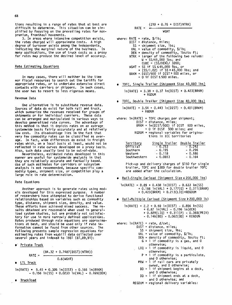
68
tions resulting in a range of rates that at best are difficult to determine. This situation can be sim-plified by focusing on the prevailing rates for non-premium, fronthaul movements.
3. In areas where intensive competition exists, the rates charged will approximate costs. A high degree of turnover exists among the independents, indicating the marginal nature of the business. In many applications, the use of truck costs as a proxy for rates may produce the desired level of accuracy.
Rate Estimating Equations
In many cases, there will neither be the time nor fiscal resources to search out the tariffs for appropriate rates, or to undertake extensive direct contacts with carriers or shippers. In such cases, the user has to resort to less rigorous means.
Revenue Data
One alternative is to substitute revenue data. Sources of data do exist for both rail and truck, which summarize the revenues received for groups of shipments or for individual carriers. These data can be arranged and manipulated in various ways to develop generalized rate curves. The advantage of this method is that it depicts rates on an average systemwide basis fairly accurately and at relatively low cost. Its disadvantage lies in the fact that very few commodity rates can be classified as aver-age. In fact, wide differences do exist in freight rates which, on a local basis at least, would not be reflected in rate curves developed on a proxy basis. Also, such data usually tend to be out-of-date.
Nevertheless, estimated rates developed in this manner are useful for systemwide analysis in that they are relatively accurate and factually based. Use of such estimates for corridors or subsystem analysis is not recommended, because specific com-modity types, shipment size, or competition play a large role in rate determination.
Rate Equations
Another approach is to generate rates using mod-els developed for this expressed purpose. A number of researchers have attempted to derive functional relationships based on variables such as commodity type, distance, shipment size, density, and value. These efforts have achieved mixed success. The re-sults obtained are reasonable when used in general-ized system studies, but are probably not satisfac-tory for use in more narrowly defined applications. Rates produced through rate equations are approxima-tions at best, and should be used only if rate in-formation cannot be found from other sources. The following presents sample regression equations for estimating rates from waybill data collected over several years and indexed to 1981 (87,89,91):
Private Truck
(84.32 + 0.7487(DIST)(NTRK)) RATE
O.6(WGHT) LTL Truck
ln(RATE) = 5.45 + 0.305 ln(DIST) - 0.166 ln(BRKM) - 0.156 ln(SS) + 0.0233 ln(VAL) - 0.169(DEN)
Truckload
(219 + 0.76 + DIST)NTRK) RATE =
WGHT
where: RATE = rate, $/lb; DIST = distance, miles; SS = shipment size, lbs; VAL = value of commodity, $/lb; DEN = density of commodity, lbs/cu ft; NTRK = larger of the following two values:
W = SS/45,000 lbs; and CUBE = (SS/DEN)/ 3200;
WGHT = SS if SS45,0O0 lbs, or = (SS/l.02) if SS>45,000 lbs; and
BRKM =. DIST/500 if DIST> 500 miles, or = 0 if DIST.500 miles.
TOFC, Single Trailer (Shipment Size 40,000 lbs)
ln(RATE) = 3.38 + 0.37 ln(DIST) + 0.423(BRKM) + RGDUM
TOFC, Double Trailer (Shipment Size 40,000 lbs)
ln(RATE) = 3.54 + 0.443 ln(DIST) + 0.401(BRKM) + RGDUM
where: ln(RATE) = TOFC charges per shipment; DIST = distance, miles; BRKM = ln(DIST/500) if DIST 500 miles,
= 0 if DIST 500 miles; and RGDUM = regional variables for origina-
tions in ICC territories
Territory Single Trailer Double Trailer Official - 0.253 - 0.242 Southern - 0.195 - 0.296 Western - 0.118 - 0.186 Southwestern - 0.0653 - 0.164
Pick-up and delivery charges of $150 for single trailer, TOFC and $300 for double trailer TOFC are added after the calculation.
Rail-Single Carload (Shipment Sizec200,000 lbs)
ln(RATE) = 8.89 + 0.438 ln(DIST) . 0.633 ln(SS) + 0.166 ln(VAL) + 0.177(G) + 0.311(BRKM) + 0.423(BRKM) + 0.213(LIQ)+REGDUM
Rail-Multiple Carload (Shipment Size )200,000 lb)
ln(RATE) = 2.2 + 0.59 ln(DIST) - 0.856 ln(SS) + 0.87 ln(VAL) - 0.196 ln(DEN) + 0.829(LIQ) + 0.311(P) -. O.368(PRIV) - 0.146(BD) - 0.062(DD) + REGDUM
where: ln(RATE) rate, /cwt; DIST = distance, miles; SS = shipment size, lbs; VAL = value of commodity, $/lb; DEN = density of commodity, lbs/cu ft; G = 1 if commodity is a gas, and 0
otherwise; LIQ = 1 if. commodity is liquid, and 0
otherwise; P = 1 if commodity is a particulate,
and 0 otherwise; PRW = 1 if rail cars are privately
owned, and 0 otherwise; BD = 1 if shipment begins at a dock,
and 0 otherwise; DD = 1 if shipment ends at a dock,
and 0 otherwise; and REGDUM = regional delivery variables:
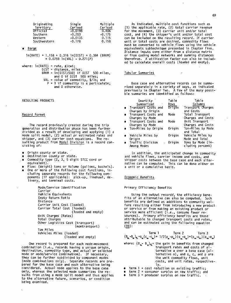
69
Originating Single Multiple As indicated, multiple cost functions such as Territory Carload Carload (1) the applicable rate, (2) total carrier revenue
Official -0.0198 0.406 for the movement, (3) carrier unit and/or total Southern -0.203 -0.175 cost, and (4) the shipper's unit and/or total cost Western -0.0135 0.115 can be included on the resulting record. If carrier Southwestern -0.178 0.158 unit or total costs are desired, commodity flows
must be converted to vehicle flows using the vehicle Barge equivalents subtechnique presented in Chapter Five.
Distance inputs come either from a distance matrix ln(RATE) = 1.158 + 0.316 ln(DIST) + 0.384 (BRKM) or from coding modal networks and summing distances
+ 0.0759 ln(VAL) - 0.271(P) therefrom. A utilization factor can also be includ- ed to calculate overall costs (loaded and empty).
where: ln(RATE) = rate, /cwt; DIST = distance, miles; BRKM = ln(DIST/500) if 0151 500 miles,
and 0 if 01ST 500 miles; VAL = value of commodity, $/lb; and P = 1 if commodity is a particulate;
and 0 otherwise.
RESULTING PRODUCTS
Rrnrd Frrmat
The record previously created during the trip generation and distribution phase has been further divided as a result of developing and applying (1) a mode split model, (2) actual r estimated rates and shipper, and (3) carrier cost equations. The re-sulting product from Modal Division is a record con-sisting of:
Origin county or state. Destination county or state. Commodity type (2, 3, 5 digit STCC cord or equivalent). Flow: (Weight) tons or Volume (gallons, bushels). One or more of the following cost functions, in-cluding separate records for the following com-ponents (if applicable): pick-up, linehaul, de-livery, and terminal costs.
Mode/Service Identification Carrier Vehicle Equivalents Empty Return Ratio Distance Carrier Unit Cost (loaded) Carrier Total Cost (loaded)
(loaded and empty) Unit Charges (Rates) Total Charges Other Logistics Cost (transport)
(nontransport) Ton Miles Vehicles Miles (loaded)
(loaded and empty)
One record is prepared for each mode-movement combination (i.e., records having a unique origin, destination, commodity type, and actual or selected mode or mode/service combination). If necessary, they can be further subdivided by component modes (mode combinations only). Separate records are pre-pared for the base case and each alternative being considered. Actual mode applies to the base case only, whereas the selected mode summarizes the re-sults from using a mode split model and thus applies to the alternative future, scenarios, or condition being examined.
Tabular Summaries
Base case and alternative records can be sumrna-rized separately in a variety of ways, as indicated previously in Chapter Two. A few of the many possi-ble summaries are identified as follows:
Quantity Table Table Summarized Rows Columns
Transport Costs and Origin Transport Charges Charges by Origin and Costs Transport Costs and Mode Total Transport Charges by Mode Charges and Costs Transport Costs and Mode Unit Transport Charges by Mode Charges and Costs Ton-Miles by Origin Origin Ton-Miles by Mode
and Total Vehicle Miles by Origin Vehicle Miles by Origin Mode and Total Traffic Division Origin Tons by Mode (in- Among Modes cluding percent)
In addition, the anticipated change in commodity and vehicle flows, carrier income and costs, and shipper costs between the base case and each alter-native can be computed. This can be done either on a unit or a cumulative basis.
Economic Benefits
Primary Efficiency Benefits
Using the output record, the efficiency bene-fits of an alternative can also be computed. Such benefits are defined as additions to community wel-fare resulting either from introducing a new product or service or from making an existing product or service more efficient (i.e., consume fewer re-sources). Primary efficiency benefits are those attributable to changed transport costs and rates, and can be estimated using the following equation (99):
Term 1 Term 2 Term 3 (B,,-B0)=q0(c0_ç)+ 1/2(p-p)(q 0. -q)+(p,,-cj(q0-q0)
where: (B - B)t= the gain in benefits from changed transport rates and costs of al-ternative a over a base case (al-ternative o), and q, c, and p are the unit commodity flows, unit costs, and unit rates, respective-ly.
term 1 = cost reduction on existing traffic; term 2 = consumer surplus on new traffic; and term 3 = producer surplus on new traffic.
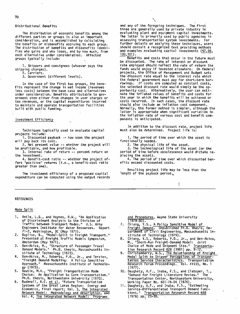
70
Distributional Benefits
The distribution of economic benefits among the different parties or groups is also an important consideration, and is accomplished by calculating the benefits or disbenefits accruing to each group. The distribution of benefits and disbenefits identi-fies who gains and who loses, and by how much, from each alternative under consideration. Affected groups typically include:
.1. Shippers and consignees (whoever pays the shipping charges).
Carriers. Government (different levels).
In the case of the first two groups, the bene-fits represent the change in net income (revenues less costs) between the base case and alternatives under consideration. Benefits attributable to gov-ernment stem either from changes in user charges or tax revenues, or the capital expenditures incurred to maintain and operate transportation facilities built with public funding.
Investment Efficiency
Techniques typically used to evaluate capital projects include:
Discounted payback -- how soon the project will pay back its cost.
Net present value -- whether the project will be profitable, and how profitable.
Internal rate of return -- percent return on the investment.
Benefit-cost ratio -- whether the project of-fers "positive" returns (i.e., a benefit-cost ratio greater than one).
The investment efficiency of a proposed capital expenditure can be computed using the output records
and any of the foregoing techniques. The first three are generally used by private industry in evaluating plant and equipment capital investments. The latter is primarily used by public agencies in assessing transportation system investments. For further details on applying these techniques, users should consult a recognized text providing methods and examples evaluating capital investments (97,98, 100-101).
- Benefits and costs that occur in the future must
be discounted. The rate of interest or discount rate employed should reflect the rate of return the funds would enjoy if invested elsewhere. On federal projects, the Office of Management and Budget sets the discount rate equal to the interest rate which the federal government must pay for short-term bor-rowings. If costs are computed as constant costs, the selected discount rate would simply be the op-portunity cost. Alternatively, the user can esti-mate the inflated values of benefits and costs for the year in which the benefits will be achieved or costs incurred. In such cases, the discount rate should also include an inflation cost component. Normally, the former method is simpler, although the latter is appropriate when significant variation in the inflation rate of various cost and benefit com-ponents is anticipated.
In addition to the discount rate, project life must also be determined. Project life is:
The period of time over which the asset is functionally needed.
The physical life of the asset. The technological life of the asset (or the
period of time before obsolescence would dictate re-placing the asset).
The period of time over which discounted ben-efits exceed discounted costs.
Resulting project life may be less than the length of the payback period.
REFERENCES
Mode Split
Antle, L.G., and Haynes, R.W., "An Application of Discriminant Analysis to the Division of Traffic between Transport Modes." U.S. Army Engineers Institute for Water Resources. Report 71-2, Washington, DC (May 1971). Bayliss,B., "Modal-Split in Freight Transport." Presented at Freight Traffic Models Symposium, Amsterdam (May 1971). Ben-Akiva, M., "Structure of Passenger Travel Demand Models." Ph.D. thesis, Massachusetts In-stitute of Technology (1973). Ben-Akiva, M., Roberts, P.O., Jr., and Terziev, "Freight Demand Modeling: A Policy Sensitive Approach." Massachusetts Institute of Technolo-gy (1975). Beutle, M.V., "Freight Transportation Mode Choice: An Application to Corn Transportation." Ph.D. thesis, Northwestern University (1970). Bushnell, R.C. et al, "Future Transportation Systems of the Great Lakes Region: Energy and Economics, final report; Vol. 3, The Integrated Network Model: Methodology and Description, and Vol. 4, The Integrated Network Model: Programs
and Procedures, Wayne State University (1979-80). Chiang, Y.S., A Policy Sensitive Model of Freight Demand. Unpublished Ph.D. thesis, De-partment of Civil Engineering, Massachusetts In-stitute of Technology (1979). Chiang, Y.S., Roberts, P.O., Jr., and Ben-Akiva, M., "Short-Run Freight-Demand Model: Joint Choice of Mode and Shipment Size." Transporta-tion Research Record 828 (1981) pp. 9-12. Christenberry, W.S., The Relationship of Freight Modal Split to Shipper Perceptions of Transpor-tation Service Characteristics. Transportation Research Forum Proceedings.. Vol. XVIII, No. 1 (1977). Daughety, A.F., Inaba, F.S., and Ziatoper, T., "Demand for Freight Literature Review." The Transportation Center, Northwestern University, Working Paper No. 601-76-04 (1976). Daughety, A.F., and Inaba, F.S., "Estimating Service-Differentiated Transport Demand Func-tions." Transportation Research Record 668 (1978) pp. 23-30.
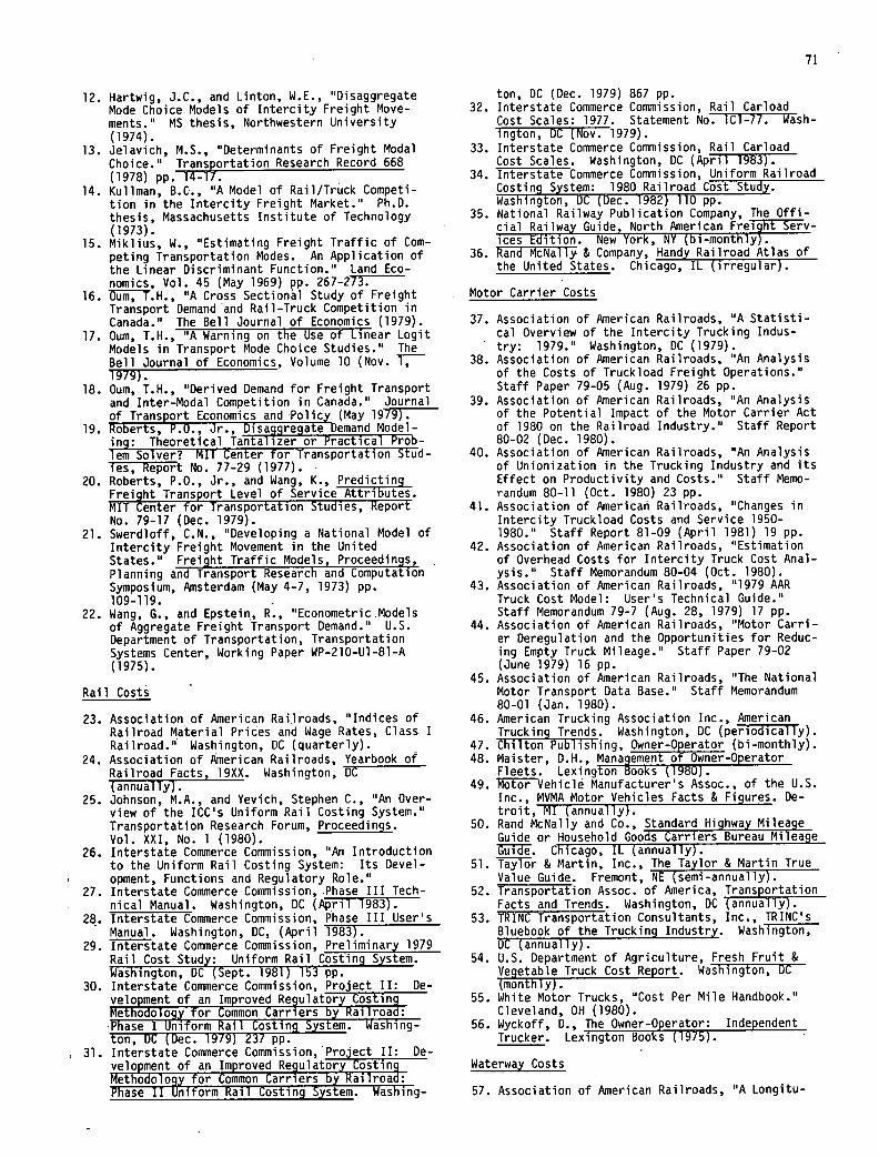
71
Hartwig, J.C., and Linton, W.E., "Disaggregate Mode Choice Models of Intercity Freight Move-ments." MS thesis, Northwestern University (1974). Jelavich, M.S., "Determinants of Freight Modal Choice." Transportation Research Record 668 (1978) pp. 14-1. Kuliman, B.C., "A Model of Rail/Truck Competi-tion in the Intercity Freight Market." Ph.D. thesis, Massachusetts Institute of Technology (1973). Miklius, W., "Estimating Freight Traffic of Com-peting Transportation Modes. An Application of the Linear Discriminant Function." Land Eco-nomics, Vol. 45 (May 1969) pp. 267-273. Oum, T.H., "A Cross Sectional Study of Freight Transport Demand 'and Rail-Truck Competition in Canada." The Bell Journal of Economics (1979). Oum, T.H., "A Warning on the Use of Linear Logit Models in Transport Mode Choice Studies." The Bell Journal of Economics, Volume 10 (Nov. T 1979). Oum, T.H., "Derived Demand for Freight Transport and Inter-Modal Competition in Canada." Journal of Transport Economics and Policy (May 1979). Roberts, P.O., Jr., Disagregate Demand Model-ing: Theoretical Tantalizer or Practical Prob-lem Solver? MIT Center for Transportation Stud-ies, Report No. 77-29 (1977). Roberts, P.O., Jr., and Wang, K., Predicting Freight Transport Level of Service Attributes. MIT Center for Transportation Studies, Report No. 79-17 (Dec. 1979). Swerdloff, C.N., "Developing a National Model of Intercity Freight Movement in the United States." Freight Traffic Models, Proceedings, Planning and Transport Research and Computation Symposium, Amsterdam (May 4-7, 1973) pp. 109-119. Wang, G., and Epstein, R., "Econometric.Models of Aggregate Freight Transport Demand." U.S. Department of Transportation, Transportation Systems Center, Working Paper WP-210-Ul-81-A (1975).
Rail Costs
Association of American Railroads, "Indices of Railroad Material Prices and Wage Rates, Class I Railroad." Washington, DC (quarterly). Association of American Railroads, Yearbook of Railroad Facts, 19XX. Washington, DC (annually). Johnson, M.A., and Yevich, Stephen C., "An Over-view of the ICC's Uniform Rail Costing System." Transportation Research Forum, Proceedings. Vol. XXI, No. 1 (1980). Interstate Commerce Commission, "An Introduction to the Uniform Rail Costing System: Its Devel-opment, Functions and Regulatory Role." Interstate Commerce Commission, Phase III Tech-nical Manual. Washington, DC (April 1983). Interstate Commerce Commission, Phase III User's Manual. Washington, DC, (April 1983). Interstate Commerce Commission, Preliminary 1979 Rail Cost Study: Uniform Rail Costing System. Washington, DC (Sept. 1981) 153 pp. Interstate Commerce Commission, Project II: De-velopment of an Improved Re9ulatory Costin Meth0d010g for Common Carriers by Railroa Phase I Uniform Rail Costing System. Washing-ton, DC (Dec. 1979) 237 pp. Interstate Commerce Commission,'Project II: De-velopment of an Improved Reulatory Costin Methodology for Common Carriers by Railroa Phase 11 Uniform Rail Costing System. Washing-
ton, DC (Dec. 1979) 867 pp. Interstate Commerce Commission, Rail Carload Cost Scales: 1977. Statement No. lCl-77. Wash-ington, DC (Nov. 1979). Interstate Commerce Commission, Rail Carload Cost Scales. Washington, DC (April 1983). Interstate Commerce Commission, Uniform Railroad Costing System: 1980 Railroad Cost Study. Washington, DC (Dec. 1982) 110 pp. National Railway Publication Company, The Offi-cial Railway Guide, North American Freight Serv-ices Edition. New York, NY (bi-monthly). Rand McNally & Company, Handy Railroad Atlas of the United States. Chicago, IL (irregular).
Motor Carrier Costs
Association of American Railroads, "A Statisti-cal Overview of the Intercity Trucking Indus-try: 1979." Washington, DC (1979). Association of American Railroads, "An Analysis of the Costs of Truckload Freight Operations." Staff Paper 79-05 (Aug. 1979) 26 pp. Association of American Railroads, "An Analysis of the Potential Impact of the Motor Carrier Act of 1980 on the Railroad Industry." Staff Report 80-02 (Dec. 1980). Association of American Railroads, "An Analysis of Unionization in the Trucking Industry and its Effect on Productivity and Costs." Staff Memo-randum 80-11 (Oct. 1980) 23 pp. Association of American Railroads, "Changes in Intercity Truckload Costs and Service 1950-1980." Staff Report 81-09 (April 1981) 19 pp. Association of American Railroads, "Estimation of Overhead Costs for Intercity Truck Cost Anal-ysis." Staff Memorandum 80-04 (Oct. 1980). Association of American Railroads, "1979 AAR Truck Cost Model: User's Technical Guide." Staff Memorandum 79-7 (Aug. 28, 1979) 17 pp. Association of American Railroads, "Motor Carri-er Deregulation and the Opportunities for Reduc-ing Empty Truck Mileage." Staff Paper 79-02 (June 1979) 16 pp. Association of American Railroads, "The National Motor Transport Data Base." Staff Memorandum 80-01 (Jan. 1980). American Trucking Association Inc., American Trucking Trends. Washington, DC (periodically). Chilton Publishing, Owner-Operator (bi-monthly). Maister, D.H., Management of Owner-Operator Fleets. Lexington Books (1980). Motor Vehicle Manufacturer's Assoc., of the U.S. Inc., MVMA Motor Vehicles Facts & Figures. De-troit, MI (annually). Rand McNally and Co., Standard Highway Mileage Guide or Household Goods Carriers Bureau Mileage Guide. Chicago, IL (annually). Taylor & Martin, Inc., The Taylor & Martin True Value Guide. Fremont, NE (semi-annually). Transportation Assoc. of America, Transportation Facts and Trends. Washington, DC (annually). TRINC Transportation Consultants, Inc., TRINC's Bluebook of the Trucking Industry. Washington, DC (annually). U.S. Department of Agriculture, Fresh Fruit & Vegetable Truck Cost Report. Washington, DC (monthly). White Motor Trucks, "Cost Per Mile Handbook." Cleveland, OH (1980). Wyckoff, D., The Owner-Operator: Independent Trucker. Lexington Books (1975).
Waterway Costs
Association of American Railroads, "A Longitu-
26.
72
dma] Study of Inland Waterway Fuel Efficien-cy.1' Staff Report 81-04 (April 1981). Association of American Railroads, "An Analysis of Empty Movements Occurring on the U.S. Inland and Intercoastal Waterway System." Staff Report 80-04 (Dec. 1980) 36 pp. Association of American Railroads, "An Introduc-tion to AAR Barge Costing Resources." Staff Memorandum 80-9 (Oct. 9, 1980) 62 pp. Association of American Railroads, "An Overview of Dominant Inland Water Carriers." Staff Re-port 81-05 (May 1981) 79 pp. Association of American Railroads. "Estimate of Current and Forecast Linehaul Barge Costs." Staff Report 81-10 (May 1981) 41 pp. Association of American Railroads, "TheCompu-trans Computerized Barge Costing Model: Opera-tion Instructions for Batch Use." (Oct. 22, 1980) 39 pp. Association of American Railroads, "Waterborne Commodity Flows -- An Overview." Staff Report 81-11 (Nov. 1981) 36 pp. The American Waterways Operators, Inc., "Big Load Afloat." Washington, DC (1973). Bronzini, M.S., and Margiotta, R.A., "Analysis of Lock Capacity by Simulation." Transportation Center, University of Tennessee, Knoxville, TN. (Aug. 1981). Canal Barge Company, Inc., "Inland Waterway Mileages." New Orleans, LA Cook, P.O., Roark, P., and McGaw, D.C., "Water Flow, Light Loading and Transport Costs on the Missouri, Apalachicola, and Alabama Rivers." Transportation Research Forum, Proceedings, Vol. XXI, No. 1 (1980). Fairchild Publications,"Map of Commercially Na-vigable Inland Waterways of the United States." New York, NY (annually). John Helms, Inc., Interstate Port Handbook 19XX. Chicago, IL (annually). Lengyel, B.W., "Inland Navigation Simulation Model: Verification and Evaluation." Transpor-tation Research Record 704 (1979) pp. 21-24. Matzzie, D.E., Camino, M.M., and Syskowski, D.F., "Development of Inland Waterway and Com-peting Overland Rate Matrices." Transportation Research Forum, Proceedings, Vol. XXI, No. 1 (1980). Reiber, M., and Soo, S.L., "Comparative Coal Transportation Costs: An Economic and Engineer-ing Analysis of Truck, Belt, Rail, Barge, and Coal Slurry and Pneumatic Pipelines Volume 4-Barge Transport." Report prepared for the U.S. Bureau of Mines by the Illinois University at Urbana-Champaign (Aug. 1977) 85 pp. Smith, M.L., Jr., "A Model for Barge Cost Opti-mization." Unpublished Masters thesis, Univer-sity of Missouri, Rolla, MO (1977) 62 pp. Smith, M.L., "Barge Operations and Costs." Un-published study, Missouri Pacific Railroad (1968). U.S. Army Corps of Engineers, Institute for Wa-ter Resources, "National Waterways Study- Over-view of Transportation Industry." Wash- ington, DC (1980). U.S. Army Corps of Engineers, Institute for Wa-ter Resources, "National Waterways Study-Waterways System and Commodity Movement Maps." U.S. Department of Commerce, National Oceanic and Atmospheric Administration, "Distances be-tween United States Ports." 5th Edition. U.S. Department of Transportation, Maritime Ad-ministration, "Estimated Vessel Operating Ex-penses - 1980." Washington, DC (Sept. 1981) 46 pp.
The Waterways Journal, Inc., "Inland River Guide." St. Louis, MO.
Logistics Costs
Association of American Railroads, "The AAR Shipper Cost Model: User's Guide" (undated). Association of American Railroads, "The AAR Shipper Cost Model: An Introduction." Staff Paper 80-10 (Oct. 1980) 6 pp. Association of American Railroads, "Non-Trans-port Logistics Costs and Their Affect on Mode Choice." Staff Paper 80-05 (Oct. 1980) 19 pp. Crew, J.G., and Horn, K.H., "Logistics Total Cost Prescriptions: Do the Theoretical Results Necessarily Conform with Reality?" Transporta-tion Research Forum, Proceedings, Vol. XXI, No. 1 (1980). Longhorn, R.A., "User's Manual: The Logistics Strategu Analyzer." MIT Center for Transporta-tion Studies, Report No. 76-10 (1976). Marcus, H. et a], "Analysis of Freight Markets: An Example Application of the Logistics Strategy Analyzer Within the Food Distribution Industry." MIT Center for Transportation Studies, Report No. 76-9 (1976). Mason, S. and Kullman, B., "An Analysis of In-land Waterway Diversions Using a Total Logistics Cost Model." Transportation Research Forum, Proceedings, Vol. XX, No. 1 (1979). Roberts, P.O., Jr., "A Model for Private Truck Costs." Informal Memorandum to Y.S. Chiang, Massachusetts Institute of Technology (Nov. 1979). Samualson, R.D., and Lerman, S.R., "Modeling the Freight Rate Structure." Transportation Re-search Forum, Proceedings, Vol. XVIII, No. 1 (1977). Samualson, R.D., "Modeling the Freight Rate Structure." MIT Center for Transportation Stud-ies, Report No. 77-7 (Feb. 1977). Samualson, R.D., "Models for Freight Tariff Es-timation." MIT Center for Transportation Stud-ies, Report No. 76-7 (1976). Wang, K., "Reestimation of the Truckload Rate Models Using a Mixed Data Set." Informal Memo-randum to P.O. Roberts, Jr., Massachusetts In-stitute of Technology (Aug. 1979). Wilson, L.B., Roberts, P.O., Jr., Kneafsey, J.T., "Models of Freight Loss and Damage." Transportation Research Forum, Proceedings, Vol. XVIII, No. 1 (1977).
Rates
Donionkos, G., "Opportunities and Challenges of Rail Contract Rates." Transportation Research Forum, Proceedings, Vol. XXII, No. 1 (1981). Matzzie, D.E., Camino, M., and Syskowski, D., "Statistically Based Methods for Efficient Sam-pling of Inland Waterway Freight Changes." Transportation Research Record 763 (1980) pp.
Morse, L.W., Practical Handbook of Industrial Traffic Management. The Traffic Service Corpo-ration (1980). Wood, D.F., and Johnson, J.C., Contemporary Transportation PPC Books. Tulsa, OK (1980) 636 pp.
Economic Analysis
Anderson, L.G., and Settle, R.F., Benefit Cost Analysis: A Practical Guide. Lexington Books, Lexington, MA (1977) 182 pp.
73
Cavinato, J.L., Finance for Transportation and Logistics Managers. The Traffic Service Corpor-ation, Washington, DC (1977) 128 pp. Federal Railroad Administration, Benefit-Cost Guidelines: Rail Branchline Continuation Assis-tance Program, (Jan. 11, 1980) 87 pp.
lOO.Herendeen, J.H., Jr., "Role of Economic Analysis in Plan Selection." Transportation Engineerin Journal of ASCE, Vol. 104, No. TE 1 (Jan. 1978 pp. 55-67.
101.Winfrey, R., Economic Analysis for Highways. International Textbook Company, Scranton, PA (1969) 923 pp.
CHAPTER FIVE
TRAFFIC ASSIGNMENT
INTRODUCTION
Traffic Assignment converts commodity flows into vehicle flows (if not already done as a prerequisite to estimating carrier costs), and then allocates the resulting vehicle interchanges to the transportation system. The process may be used to estimate the traffic load on various segments of a system for a proposed alternative or to simulate present condi-tions. Optional components include estimating the expected change in truck volumes, pavement loadings, and pavement life on a segment basis, and computing therefrom system changes in energy consumption and user tax revenue.
The basic component, traffic assignment, is car-ried out for the base case and each alternative be-ing considered. The results are then compared to determine anticipated change. Either manual or com-puterized techniques (or a combination thereof) can be used in assigning traffic to modal subsystems, the selection of which depends on the complexity of the application and the number of alternatives being analyzed. Usually, the route choices involved with rail, inland waterway, and even intercity highway movements will be obvious. Thus the advantage of using computerized assignment techniques lies not so much in finding the least distance or cost route through a network, but rather in the systematic ac-counting of vehicle volumes by segment and the cal-culation of distance or traffic related costs. Com-puterized highway assignment techniques commonly used in urban transportation studies can be applied with little modification. Such techniques are par-ticularly valuable in assigning motor carrier traf- fic to the statewide highway system. Manual or simplified computerized techniques often suffice in assigning rail and inland waterway traffic.
Because states are particularly interested in highway system impacts, this chapter focuses pri-marily on methodologies useful in measuring highway system impacts unique to freight transportation. While changes in highway segment volumes are import-ant, such information by itself provides only limit-ed insight into the effect or impacts that such changes have on the highway itself or the surround-ing environment. Thus other techniques are required to assess the impact of changes in traffic volumes. A number of techniques are already available to states to use in measuring the direct effects of ve-hicles (i.e., noise, air pollution, etc.). Since such techniques have been widely applied by states in determining the impacts of major highway projects and are well documented elsewhere, they have not
been included in this manual. Techniques pertaining to the impacts of changes in truck volumes on pave-ment life are not as well known or documented, and hence are presented in this chapter.
In considering just how far to go in assigning traffic to networks and estimating impacts, the ba-sic choices available to the user are:
1.. Whether to undertake traffic assignment at all or only for selected modes (e.g., highway sys-tem). Traffic assignment is required if segment-level assessments are contemplated. If segment - vol-umes are not required, traffic assignment per se is not necessary, provided that a distance matrix is available to use in computing cost and revenues.
Whether to limit the application to summariz-ing and comparing vehicular flows on a segment ba-sis. Information on projected changes in traffic volumes do not take into account the larger impact that trucks used for intercity transport have on pavement structure. Users should recognize that in addition to vehicular flows for the base case and each alternative, information is also required on background automobile and truck traffic.
Whether to estimate the impact of changed loadings on pavement structure. To do this, use must be made of truck weight data such as that col-lected periodically by states. Change is measured in terms of 18-kip equivalent annual load applica-tions. Such measurements neutralize differences be-tween vehicle types and weights. Using vehicle count and classification data (or estimates), the relatively limited truck weight data collected at limited locations can be extended to estimate the wheel/axle configurations, tare weights, and vehicle loadings expected to occur at different locations. Because the effects of design strength, pavement age, and past traffic are not included, this ap-proach does not identify expected changes in pave-ment life.
Estimate changes in pavement service life. In addition to the above, this requires as inputs detailed data on pavement condition and structure. If such data are not available, states can substi-tute the assumptions and default data developed by FHWA for use in highway needs studies.
g n Usinetwork flows to estimate changes in energy consumption on a system basis and/or changes in revenues derived through user taxes.
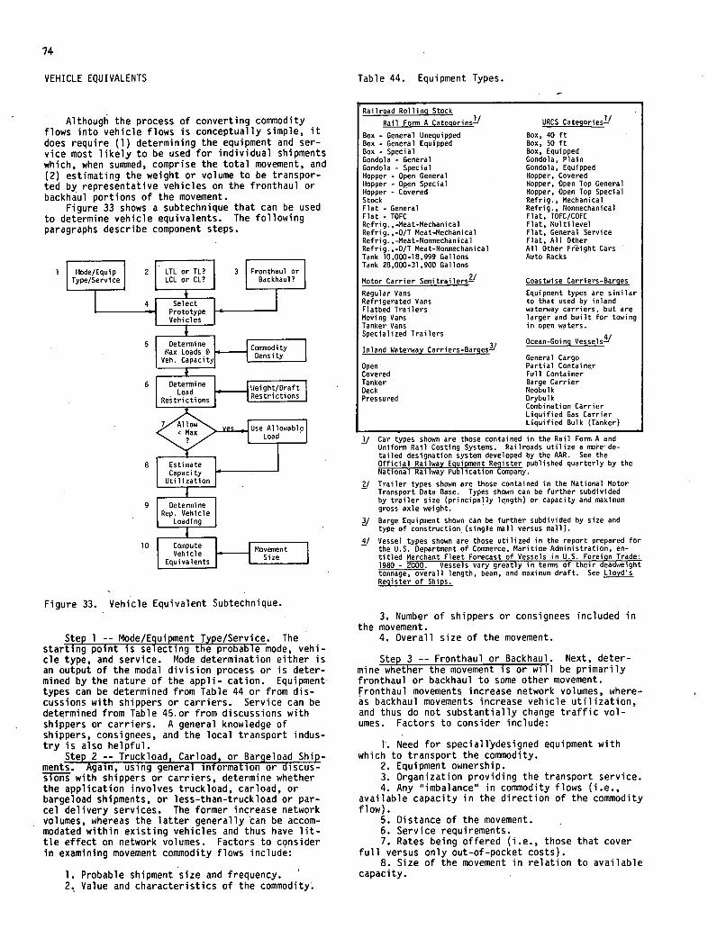
74
VEHICLE EQUIVALENTS
Although the process of converting commodity flows into vehicle flows is conceptually simple, it does require (1) determining the equipment and ser-vice most likely to be used for individual shipments which, when summed, comprise the total movement, and (2) estimating the weight or volume to be transpor-ted by representative vehicles on the fronthaul or backhaul portions of the movement.
Figure 33 shows a subtechnique that can be used to determine vehicle equivalents. The following paragraphs describe component steps.
1 I Mode/Equip 1 2 1 LTL or IL? 3 1 Fronthaul or Type/Service LCL or CL? Backhau, ?
4 Select
-I Prototype Vehicles
Max Loads @ 5 I Determine H: itY
Veh. Capacity Density
6 Determine I ht/Draft Load
' I Restrictions I1Restn1ctb0riction5
Allow <M ad
ax All01ab le
8
1
Estimate Capaci ty Utilization
9 Determine IRep . Vehicle
Loading
10 I Compute Vehicle ' 1 e
Equivalents
Figure 33. Vehicle Equivalent Subtechnique.
Step 1 -- Mode/Equipment Type/Service. The starting point is selecting the probable mode, vehi-cle type, and service. Mode determination either is an output of the modal division process or is deter-mined by the nature of the appli- cation. Equipment types can be determined from Table 44 or from dis-cussions with shippers or carriers. Service can be determined from Table 45.or from discussions with shippers or carriers. A general knowledge of shippers, consignees, and the local transport indus-try is also helpful.
Steo 2 -- Truckload. Carload, or Baraeload Shiø-ments. Again, using general information or discus-sions with shippers or carriers, determine whether the application involves truckload, carload, or bargeload shipments, or less-than-truckload or par-cel delivery services. The former increase network volumes, whereas the latter generally 'can be accom-modated within existing vehicles and thus have lit-tle effect on network volumes. Factors to consider in examining movement commodity flows include:
Probable shipment size and frequency. Value and characteristics of the commodity.
Table 44. Equipment Types.
'Railroad Rolling Stock
Rail Form A Categories-' URCS Categories1' Box - General Unequipped Box, 40 ft Box - General Equipped Box, 50 ft Box - Special Box, Equipped Gondola - General Gondola, Plain Gondola - Special Gondola, Equipped Hopper - Open General Hopper, Covered Hopper - Open Special Hopper, Open Top General Hopper - Covered Hopper, Open Top Special Stock Refrig., Mechanical Flat - General Refrig. • Nonmechanical Flat - TOFC Flat, TOFC/COFC Refrig. ,-Meat-Mechanical Flat, Multilevel Refrig. ,-O/T Meat-Mechanical Flat, General Service Refrig. ,-Meat-Nonmechanical Flat, All Other Refrig. ,-O/T Meat-Nonmechanical All Other Freight Cars Tank 10,000-18,999 Gallons Auto Racks Tank 28,000-31,900 Gallons
Motor Carrier Semitrailers Coastwise Carriers-Barges
Regular Vans Equipment types are similar Refrigerated Vans to that used by inland Flatbed Trailers waterway carriers, but are Moing Vans larger and built for towing Tanker Vans in open waters. Specialized Trailers 4
3/ Ocean-Going Vessels Inland Waterway Carriers-Barges—
General Cargo Open Partial Containe,r Covered Full Container Tanker Barge Carrier Deck Neobulk Pressured Drybulk
Combination Carrier Liquified Gas Carrier Liquified Bulk (Tanker)
1' Car types shown are those contained in the Rail Form A and Uniform Rail Costing Systems. Railroads utilize a more'de-tailed designation system developed by the AAR. See the Official RailwayEquipment Register published quarterly by the National Railway Publication Company.
V Trailer types shown are those contained in the National Motor Transport Data Base. Types shown can be further subdivided by trailer size (principally length) or capacity and maximum gross axle weight.
Barge Equipment shown can be further subdivided by size and type of construction, (single mall versus mall).
/ Vessel types shown are those utilized in the report prepared for the U.S. Department of Commerce, Maritime Administration, en-titled Merchant Fleet Forecast of Vessels in U.S. Foreign Trade: 1980 - 200O Vessels vary greatly in terms of their deadweight tonnage, overall length, beam, and maximum draft. See Lloyds Register of Ships.
Number of shippers or consignees included in the movement.
Overall size of the movement.
Step 3 -- Fronthaul or Backhaul. Next, deter-mine whether the movement is or will be primarily fronthaul or backhaul to some other movement. Fronthaul movements increase network volumes, where-as backhaul movements increase vehicle utilization, and thus do not substantially change traffic vol-umes. Factors to consider include:
1'. Need for speciall'ydesigned equipment with which to transport the commodity.
Equipment ownership. Organization providing the transport service. Any "imbalance" in commodity flows (i.e.,
available capacity in the direction of the commodity flow).
Distance of the movement. Service requirements. Rates being offered (i.e., those that cover
full versus only out-of-pocket costs). Size of the movement in relation to available
capacity.
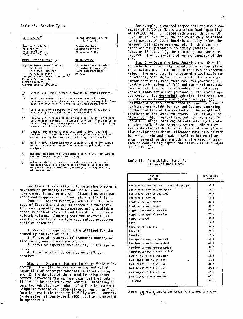
75
Table 45. Service Types.
Rail Service!' Inland Waterway Carrier Service !/
Regular Single Car Coninon Carriers Multicar 2/ Contract Carriers Unit Train J Private Carriers TOFC/COFC Plan 4/
Motor Carrier Service / Ocean Service
Regular Route Consnon Carriers Liner Service (scheduled Truckload routes & frequency) Less-than-Truckload Tramp (nonscheduled) Package Delivery
6' Private
Irregular Route Cononon Carriers -' Private Carriers 6/ Exempt Carriers 77 Agricultural Cooperatives
!I Virtually all rail service is provided by conison carriers.
V Multicar service refers to two or more carloads moving between a single origin and destination on one waybill. Car- loads are handled as a unit" in way and through trains.
/ Unit train service refers to a trainload moving between a single origin and destination on one waybill.
4/ TOEC/COFC Plan refers to one of six plans involving trailers or containers handled in intermodal service. Plans differ in terms of equipment ownership and responsibility for providing pickup and delivery services.
/ Linehaul service using tractors, semitrailers, and full- trailers. Excludes pickup and delivery service or similar movements using two- and three-axle single-unit trucks.
/ Will include independent owner-operators hauling for comon or private carriers as well as carrier or privately owned equipment.
2/ Designation stems from the cononodities handled. Any type of carrier can,haul exempt cornodities.
/ A further distinction could be.made based on the use of dedicated tows (a two moving as an integral unit between origin and destination) and the number of barges and size of towboat used.
Sometimes it is difficult to determine whether a movement is primarily fronthaul or backhaul. In some cases, it may be either. Discussions with car-riers and shippers will often help clarify this.
Step 4 -- Select Prototype Vehicles. One pur-pose of Steps 2 and 3 was to screen out movements that can generally be accommodated using available space in present vehicles and thus do not increase network volumes. AssUming that the movement will result in additional vehicle use, select prototype vehicles based on:
Prevailing equipment being utilized for the comodity and type of haul.
Financial resources of transport company or firm (e.g., new or used equipment).
Known or expected availability of the equip-ment.
Anticipated size, weight, or draft con-straints.
Step 5 -- Determine Maximum Loads at Vehicle Ca-pacit'. Using (1) the maximum volume and weight capacities of prototype vehicles selected in Step 4 and (2) the density of the comnlodity being trans-ported, determine the maximum size load that poten-tially can be carried by the vehicle. Depending on density, vehicles may "cube out" before the maximum weight is reached or, alternatively, "weigh out" be-fore the available capacity is fully used. Comodi- ty densities at the 5-digit STCC level are presented in Appendix B.
For example, a covered hopper rail car has a Ca-'pacity of 4,750 cu ft and a maximum load capability of 199,000 lbs. If loaded with wheat (density: 60 lb/bu or 47 lb/cu ft), the car could only be filled to 89 percent of its volumetric capacity before the maximum load rating was reached. If this car in-stead was fully loaded with barley (density: 48 ib/bu or 37 lb/cu ft), the resulting load would be 175,750 lbs or 88 percent of weight capacity of the car. -
Step 6 -- Determine Load Restriction. Even if the vehicle can be fully loaded, other route-related restrictions may limit the load that can be accomino-dated. The next step is to determine applicable re-strictions, both physical and legal. For highways (motor carriers), each state has laws governing a1-lowable combinations of full and semi-trailers, max-imum overall length, and allowable axle and gross vehicle loads for all or portions of the state high-way system. See Overweight Vehicles, Penalties, and Permits -- An Inventory of State Practices (2). Railroads also have established for each raiT line a maximum gross weight for car and. lading, depending on the condition of the roadbed and the weight and condition of the track structure.' See Railway Line Clearances (5). Typical tare weights are given in Table 46. Brge loads may be restricted by the ef-fective draft of the waterway system. Minimum or available channel depth is not the usable or effec-tive navigational depth; allowance must also be made for vessel trim and squat as well as bottom clear-ance. Several guides are published giving informa-tion on controlling depths and clearances at bridges and locks (I).
Table 46. Tare Weight (Tons) for Different Rail Cars.
Tyge of Equipment
Tare Weight (tons)'
Box-general service, unequipped and equipped 30.9
Box-general service unequipped 28.0
Box-general service equipped 36.4
Box special service 41.4
Gondola-general service 29.9
Gondola-special service 31.2
Hopper open-general service 27.1
Hopper open-special service 27.6
Hopper covered 30.5
Stock 23.7
Flat-general service 28.2
Flat-TOFC 33.6
Auto Rack 47.8
Refrigerator-meat mechanical 40.9
Refrigerator-other mechanical 43.9
Refrigerator-meat-nonniechani cal 35.2
Refri gerator-other-nonmechanical 31.1
Tank 9,999 gallons and under 24.4
Tank 10,000-18,999 gallons , 31.3
Tank 19,000-21,999 gallons 33.7
Tank 22,000-27,999 gallons 37.4
Tank 28,000-31,999 gallons 42.1
Tank 32,000 gallons and over 47.1
All Other 30.1
Source: Interstate Coonnerce Conusission, Rail Carload Cost Scales 1977, p. 137.
76
Step 7 -- Compute the Maximum Allowable Load. The next step is to compute the maximum allowable load. For motor carriers, this involves apportion-ing the gross weight among the different axles and determining whether the legal weights and distances between axles are met. If not, the maximum load must be reduced to bring the gross weight down to the legal limits. This may differ from the loadings being reported by shippers, because of a lack of en-forcement of weight limits. For rail lines, the maximum load must be reduced to attain the maximum gross weight allowable. For inland waterways, maxi-mum vessel •loadings can be determined as follows:
SS = CAP1-12( IFACTOR) (MAXDRAFT-ACTDRAFT)
where: SS = maximum cargo, tons; CAP = vessel capacity at maximum draft, tons;
IFACTOR = immersion factor, tons/in; MAXDRAFI = vessel maximum draft, feet; and ACTORAFT = maximum allowable draft, feet.
For example, a jumbo barge has a practical ca-pacity of 1,350 tons at a draft of 8.5 ft. The same barge empty has a draft of 1.5 ft. If the effective draft of the waterway segment was 6 ft, the maximum cargo which could be carried by that barge would be:
SS = 1350 1-12(16.1)(8.5-6.0) = 867 tons
In all cases, either the maximum load must be reduced to the allowable load, or alternative equip-ment or vessels capable of meeting the physical or legal constraints must be substituted for that orig-inally selected.
Step 8 -- Estimate Capacity Utilization. Once a maximum allowable load has been established, then it is necessary to estimate how this capacity is typi-cally used on an individual shipment basis. In many cases, the typical load will run considerably less than the maximum allowable load, while in other ca-ses, utilization may be at or even above the maximum allowable load. Factors to consider include:
The particular commodity involved. The amount of unused 'space" in the vehicle. Variation in shipment size and loading prac-
tices. The risks involved of damage or delay to the
vehicle/vessel from overloading. Likelihood of enforcement and penalties
against overweight, if caught.
Step 9 -- Determine Representative Vehicle Load- in results from Step7 are applied to the re- üTts of Step 8 to determine a representative vehi-
cle or vessel loading. Step 10 -- Compute Vehicle Equivalents. The
fronthaul portion of the total movement is then di-vided by the representative loading to determine the vehicle or vessel equivalents needed to accommodate that movement.
TRAFFIC ASSIGNMENT TECHNIQUES
The traffic assignment procedure involves the selection by computer of a minimum impedance path between zones and the "accounting" associated with assigning this movement to the identified route seg-ments. To accomplish this, a description of the network is first coded, edited and stored in the memory of the computer. After selecting the minimum
impedance path between zones, the computer then pro-ceeds to assign associated movements to the selected routing. Traffic volumes are thus accumulated for each route segment.
In recent years, a number of states have under-taken studies involving statewide traffic assign-ments. These studies have generally utilized traf-fic assignment computer programs developed original-ly for urban areas with only minor modifications to the inputs being necessary to adapt the programs to statewide applications. The following sets of pro-grams or "packages" are available to states having IBM mainframe computers:
PLANPAC/BACKPAC. Originally developed by the Bureau of Public Roads (predecessor to the FHWA), "PLANPAC" contains programs for analysis of survey data and trip table building, trip generation, trip distribution, traffic assignment, network evalua-tion, plotting, and a few utility programs for mov-ing, copying, and dumping data sets. The programs have been widely used by state DOTs and other orga-nizations involved in urban area highway planning. "BACKPAC" contains additional programs of a "backup" character as well as. other miscellaneous programs of potential use in freight demand forecasting, such as spider web assignment and statistical analysis pack-ages. An appreciable body of literature is avail-able describing the programs in the PLANPAC/BACKPAC battery and their application in urban transporta-tion planning (11-14).
Urban Transportation Planning S'stem (UTPS). Developed by the Urban Mass Transportation Adminis-tration, UTPS is a package of computer programs, at-tendant documentation, users guides and manuals pro-viding state-of-the-art methods for multimodal urban transportation planning. UTPS, which has many of the same capabilities as PLANPAC/BACKPAC vis-a-vis highway traffic assignment, is widely used for ap-plications involving both highway and transit net-works. Extensive literature describing UTPS is also readily available describing individual programs and their applications (16-21).
The foregoing sets of programs are useful pri-marily for assigning freight traffic (i.e., trucks) to highway networks. In addition, analogous simula-tion models exist for assigning freight traffic to national-level rail and inland waterway networks (7-10). Such models are generally not appropriate for use at the state level, however, and thus are not described in detail in this manual.
Detailed procedures and suggestions for (1) sub-dividing states into appropriately sized traffic analysis zones, (2) selecting segments and coding a statewide highway network, and (3) adapting the as-signment process to the smaller scale network typi-cally employed in statewide planning have been docu-mented elsewhere (13-14). A statewide highway net-work can be coded with the minimum data required for traffic assignment (i.e., A-node, B-node, speed, distance, and ADT for each segment). Other data fields often included by states are functional class, federal aid class, capacity, DHV/ADT factor, link class, type of facility, rural versus urban section, and route number. The above data fields are oriented towards automobile or total traffic ra-ther than truck traffic. Statewide assignments are usually unrestrained (i.e., no limit is placed on the number of vehicles assigned to any one segment), because few highways outside of urban areas have traffic volumes approaching their capacity.
Only a few of the programs contained in the PLANPAC or UTPS packages would normally be employed. Programs within PLANPAC useful in assigning truck volumes to highway networks include:

77
BUILDHR (or NETWORK), which performs edit and consistency checks on the input link records and writes a sorted file of link and intersection de-scription records (historicalrecord).
PRINTHR (or FORMAT), which prints the histor-ical record.
BUILDVN, which reads the historical record and computes the minimum paths.
PRINTVN, which prints out the minimum impe-dance paths to allow the user to examine them for logical accuracy.
LOADVN, which reads the minimum impedance paths and the zone-to-zone vehicle flow matrix and then routes these flows over the minimum path. As it does so, the program accumulates the volumes by link for all zone-to-zone movements. When all vehi-cle flow records have been processed, the program reads the historical record file, merges the link volumes with it, and writes out a new, more detailed historical file.
PRINTLD, which prepares printed summaries of the assigned link flows. (Alternatively, the pro-gram FORMAT could be used).
Comparable UTPS program are:
HR, the highway network builder/updater pro-gram, which builds an "historical record" from link cards for input to the highway assignment program, UROAD. HR also processes updates to an historical record, inserts node coordinates, and prints the historical record along with messages regarding the correctness of the data. HR optionally produces mechanical or printer plots of the network and asso-ciated data.
UROAD, the highway analyzer, which performs many of the traditional functions associated with planning a highway system, including pathfinding, "skimming" •(time and/or distance and/or toll) and traffic assignment (with or without capacity re-straint). Its input is a "historical record" de-scribing the highway network and up to four highway trip tables. The program permits the user to select from a variety of built-in capacity restraint tech-niques using network equilibrium concepts or alter-natively to specify his own methodology. Besides an historical record updated with forecasted link and turn volumes, UROAD outputs optionally include impe-dance matrices and printouts of selected paths, link loadings and speeds, turn volumes, VMT, VHT and speed summaries by volume/capacity groups, and pol-lution emission and energy consumption estimates. Mechanical or printer plots of networks, loads, and associated data can be produced optionally.
Before using either of the foregoing assignment packages, users must first decide whether to assign all traffic (automobiles and trucks), truck traffic only, or only applicable truck movements. The first option, which represents a total simulation of flows over the developed network, necessitates developing a zone-to-zone trip table for all automobile and truck movements. The second option similarily re-quires developing a zone-to-zone trip table for all truck movements. The preparation of such trip ta-bles does entail appreciable work, and may not be practical unless previously done by the state DOT.
In addition to the above assignment packages, less sophisticated approaches based on user-deter-mined routings coupled with computerized segment ac-counting can also be employed. These are particu-larly useful when the application involves (1) se-lected movements or (2) a statewide network and trip tables that have not previously been developed by the state DOT or are out-of-date.
EQUIVALENT ANNUAL LOAD APPLICATION
Users are often interested in estimating equiva-lent annnual load applications on a segment basis for the base year and each alternative, and then computing the net change in pavement loadings.
Equivalent annual load applications (EALA) can be estimated by:
EALA = (ADT)(%TRKS)(CLF)(18KSAEC)365
where: EALA = equivalent annual 18-kip single-axle load applications;
ADT = average daily traffic; %TRKS = percent that trucks and combinations
are of total traffic (after excluding pickups, panels, and other 2-axle, single-tired vehicles);
CLF = critical lane factor, defined as the percent of vehicles in the right-hand lane:
number direction of lanes one-way two-way 2or3 100 50 4 or more 80 40
18KSAEC = 18-kip, single-axle equivalent con- stant. can be obtained from the W-4 tables of a state's bi-annual truck weight study.
The following example illustrates the applica-tion of the subtechnique. A company presently ships 115,000 tons of cement a year in covered hoppers over a rail line which the owning railroad contem-plates abandoning. The company is considering shifting to privately owned trucking, using tandem trailers to serve two distribution terminals. Be-cause specialized bulk cement semitrailers will be used, an empty backhaul is contemplated. The state is concerned over the impact that such a shift will have on the highway system. Table 47 provides com-bined W-4 data for four rural Interstate stations, two of which are on the Interstate route which would be used, if the traffic shifts to truck. Table 48 shows vehicle and classification counts at these four stations. Table 49 correlates axle loads and 18-kip equivalents for both rigid and flexible pave-ments. Table 50 provides data on the semitrailer-trailer vehicle which will be used for this move-ment. The Interstate route is for the most part surfaced with portland cement concrete (rigid pave-ment).
Component steps involved in computing an EALA for this route areas follows:
Step 1 -- Obtain or Estimate the Percent that Tractor/Semitrailers and Combinations are of Total Vehicles. Although average daily traffic volumes (Aol) are typically available for most highway sys-tem segments, information on the composition of trucks by type, axle, and tire configuration is much less available. This step consists of obtaining available information and estimating the percent that tractors/semitrailers and combinations are of total vehicles for highway segments where such in-formation is not available.
In this example, the classification count made during the summer of 1981 is two-thirds greater than the AOl value. Because much of this difference can be attributed to passenger cars, the assumption was made that average daily trucks are approximately 80
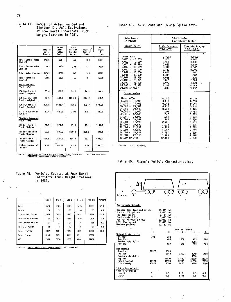
Table 49. Axle Loads and 18-Kip Equivalents.
Axle Loads 18-Kip Axle in Pounds Equivalency Factor
Rigid Pavement Flexible Pavement Single Axles
P=2.5, SN=5
Under 3000 0.0002 0.0002 3,000 - - 6,999 0.005 0.005 7,000 - 7,999 0.026 0.032 8,000 - 11,999 0.082 0.087
12,000 - 15,999 0.341 0.360 16,000 - 18,000 .0.783 0.796 18,001 - 18,500 1.065 1.060 18,501 - 20,000 1.336 1.307 20,001 - 21,999 1.926- 1.826 22,000 - 23,999 2.818 2.583 24,000 - 25,999 3.976 26,000 - 29,999 6.289 5.389 30,000 or Over 11.395 9.432
Tandem Axles
Under 6000 0.010 0.010 6,000 - 11,999 0.010 • 0.010
12,000 - 17,999 0.062 0.044 18,000 - 23,999 0.253 0.148 24,000 - 29,09 0.729 0.426 30,000 - 32,000 1.305 0.753 32,001 - 32,500 1.542 0.885 32,501 - 33,999 1.751 1.002 34,000 - 35,999 2.165 1.230 36,000 - 37,999 2.721 1.533 38,000 - 39,999 3.373 1.885 40,000 - 41,999 4.129 2.289 42,000 - 43,999 4.997 2.749 44,000 - 45,999 5.987 3.269 46,000 - 49,999 7.725 . 4.170 50,000 or Over 10.160 5.100
Source: W-4 Tables.
78
Table 47. Number of Axles Counted and Eighteen Kip Axle Equivalents at Four Rural Interstate Truck Weight Stations in 1981.
Single- Unit
Trucks
Tractor Semi-
Trailer Comb.
Semi- Trailer Trailer Comb;
Truck & Trailer
Comb.
All Trucks
& Comb.
Total Single Axles 14025 3951 652 153 18781 Counted
Total Tandem Axles 242 6714 123 121 7200 Counted
Total Axles Counted 14509 17379 898 395 33181
Total Vehicles 7166 3506 155 81 10908 Counted
Rigid Pavement P=2.5, 09°
18K Eqo.for All 85.8 1580.0 54.0 28.4 1748.2 Trucks Weighed
18K Eqv.per 1000 62.5 1690.1 1283.3 1644.2 614.7 Trucks Weighed
18K Ego. for All 451.6 5922.4 198.0 132.2 6705.0 Trucks Counted
% Distribution of 6.74 88.33 2.96 1.97 100.00 18K Eqv.
Flexible Pavement, P2.5, 59.5
18K Eqv.for All 70.9 970.5 49.3 19.1 1109.8 Trucks Weighed
18K Eqv. per 1000 56.2 1035.0 1190.2 1106.2 394.8 Trucks Weighed
18K Eqv. for All 404.9 3627.2. 184.3 88.7 4305.1 Trucks Counted
% Distribution of 9.40 84.26 4.28 2.06 100.00 18K Eqv.
Source: South Dakota Truck Weight Study, 1981, Table 4-4. Data are for four combined Interstate rural stations.
Table 50. Example Vehicle Characteristics.
/
Table 48. Vehicles Counted at Four Rural Interstate Truck Weight Stations
- in 1981.
Sta A Sta 8 Sta C Sta 0 All Sta. Percevt
Cars 5623 4185 4030 4505 18441 62.3
noses 25 32 27 10 89 0.3
Single Unit Trucks 2364 1458 1700 1644 7166 24.3
Tractor Sevitrailer 726 535 1339 906 3506 11.9
Semitrailer Trailer 31 36 64 24 155 0.5
Truck 0 Trailer 38 5 15 -23 81 0.3
8807 6251 7178 7202 29438 100.0 Total Traffic
Total Trucks 3159 2034. 3110 2597 10908
ADT 7666 3230 9026 6240 27462
Source: South Dakota Truck Weight Study, 1981 Table W-1
r Axle no.
co -
Approximate Weights
Tractor less fuel and driver 14,000 lbs Fuel at 200 gallons 1,600 lbs Trailers (each) 9,100 lbs Tandem axle dolly 5,080 lbs Maximum allowable gross 129,888 lbs Less tare weight 38,880 lbs Maximum payload 90,120 lbs
Axle or Tandem 1 2 3 4 5
Weight Distribution Tractor 70% 30% Trailer 40% 60% 40% 60% Tandem axle dolly 100% Payload 50% 50% 50% 50%
Net Weight Tractor 10920 4680 Trailer 3640 5460 3640 5460 Tandem axle dolly . . 5080 Payload 22530 22530 22530 22530 Total loaded 10920 30850 27990 31250 27990 Total empty 10920 8320 5460 8720 5460
18-Kip Equivalents (Rigid Pavement) Loaded 0.1 1.3 0.7 1.3 0.7 Empty 0.1 0.01 0.01 0.01 0.01
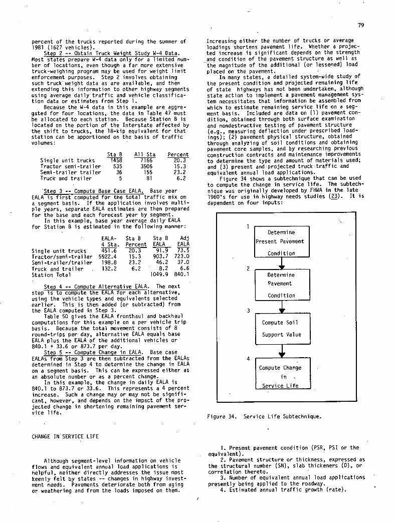
79
percent of the trucks reported during the summer of 1981 (1627 vehicles).
Step 2 -- Obtain Truck Weight Study W-4 Data. Most states prepare W-4 data only for a limited num-ber of locations, even though a far more extensive truck-weighing program may be used for weight limit enforcement purposes. Step 2 involves obtaining such truck weight data as are available, and then extending this information to other highway segments using average daily traffic and vehicle classifica-tion data or estimates from Step 1.
BecaUse the W-4 data in this example are aggre-gated for four locations, the data in Table 47 must be allocated to each station. Because Station B is located on the portion of the Interstate affected by the shift to trucks, the 18-kip equivalent for that station can be apportioned on the basis of traffic volumes:
StaB All Sta Percent Single unit trucks 1458 7166 20.3 Tractor semi-trailer 535 3506 15.3 SemI-trailer trailer 36 155 23.2 Truck and trailer 5 81 6.2
'Step 3 -- Compute Base Case EALA. Base year EALA is first computed for the total traffic mix on a segment basis. If the application involves multi-pie years, separate EALA estimates are then prepared for the base and each forecast year by segment.
In this example, base year average daily- EALA for Station B is estimated in the following manner:
EALA- ' Sta B Sta B Adj 4 Sta. Percent EALA EALA
Single unit trucks 451.6 20.3 91.9 73.5 Tractor/semi-trailer 5922.4 15.3 903.7 723.0 Semi-trailer/trailer 198.8 23.2 46.2 37.0 Truck and trailer 132.2 6.2 8.2 6.6 Station Total 1049.9 840.1
Step 4 -- Compute Alternative EALA. The next step is to compute the EALA for each alternative, using the vehicle types and equivalents selected earlier. This is then added (or subtracted) from the EALA computed in Step 3.
Table 50 gives the EALA fronthaul and backhaul computations for this example on a per vehicle trip basis. Becaus.e the total movement consists of 8 round-trips per day, alternative EALA equals base EALA plus the EALA of the additional vehicles or 840.1 + 33.6 or 873.7 per day.
Step 5 -- Compute Change in EALA. Base case EALAs from Step 3 are then subtracted from the EALAs determined in Step 4 to determine the change in EALA on a segment basis. This can be expressed either as an absolute number or as a percent change.
In this example, the change in daily EALA is 840.1 to 873.7 or 33.6. This represents a 4 percent increase. Such a change may or may not be signifi-cant, however, and depends on the impact of the pro-jected change in shortening remaining pavement ser-vice life.
Increasing either the number of trucks or average loadings shortens pavement life. Whether a projec-ted increase is significant depends on the strength and condition of the pavement structure as well as the magnitude of the additional (or lessened) load placed on the pavement.
In many states, a detailed system-wide study of the present condition and projected remaining life of state highways has not been undertaken, although state action to implement a pavement management sys-tem necessitates that information be assembled from which to estimate remaining service life on a seg-ment basis. Included are data on (1) pavement con-dition, obtained through both surface examination and nondestructive testing of pavement structure (e.g., measuring deflection under prescribed load-ings); (2) pavement physical structure, obtained through analyzing of soil conditions and obtaining pavement core samples, and by researching previous construction contracts and maintenance improvements to determine the type and amount of materials used; and (3) present andprojected truck'tra,ffic and equivalent annual load applications.
Figure 34 shows a subtechnique that can be used to compute the change in service life. The subtech-nique was originally developed by FHWA in the late 1960's for use in highway needs studies (23). It is dependent on four inputs:
Determine
Present Pavement
Condition
2 Determine
Pavement
Condition
Compute Soil
Support Value
Compute Change
in
Service Life
Figure 34. Service Life Subtechnique.
CHANGE IN' SERVICE LIFE
Although segment-level information on vehicle flows and equivalent annual load applications is helpful, neither directly addresses the issue most keenly felt by states -- changes in highway invest-ment needs. Pavements deteriorate both from aging or weathering and from the loads imposed on them.
Present pavement condition (PSR, PSI or the equivalent).
Pavement structure or thickness, expressed as the structural number (SN), slab thickeners (D), or correlation thereto.
Number of equivalent annual load applications presently being applied to the roadway.
Estimated annual traffic growth (rate).
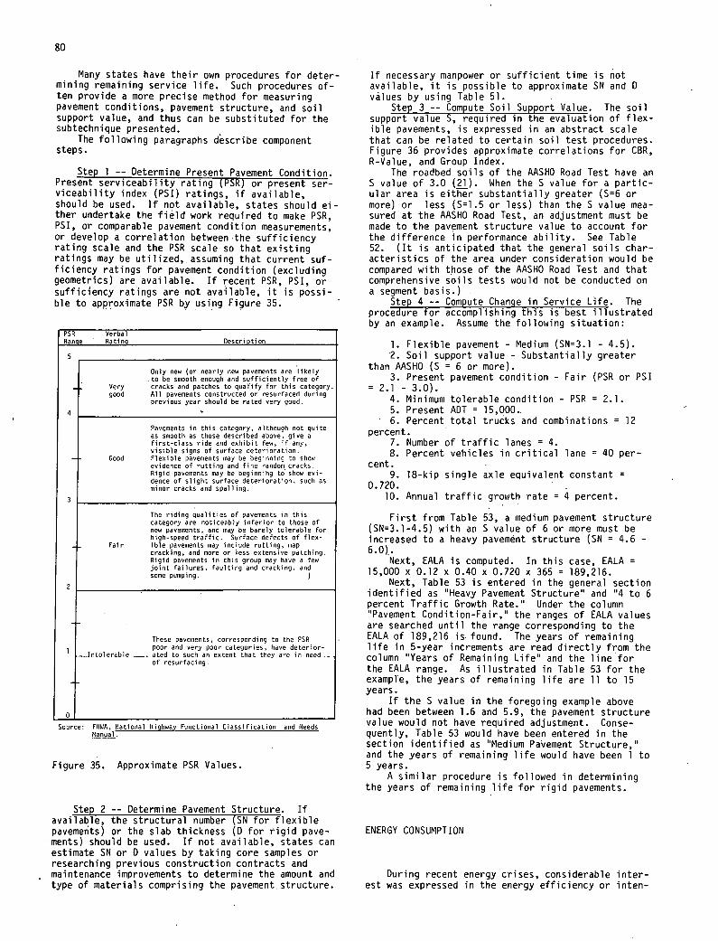
80
Many states have their own procedures for deter-mining remaining service life. Such procedures of-ten provide a more precise method for measuring pavement conditions, pavement structure, and soil support value, and thus can be substituted for the subtechnique presented.
The following paragraphs describe component steps.
Step 1 -- Determine Present Pavement Condition. Present serviceability rating (PSR) or present ser-viceability index (PSI) ratings, if available, should be used. If not available, states should ei-ther undertake the field work required to make PSR, PSI, or comparable pavement condition measurements, or develop a correlation between the sufficiency rating scale and the PSR scale so that existing ratings may be utilized,.assuming that current suf-ficiency ratings for pavement condition (excluding geometrics) are available. If recent PSR, PSI, or sufficiency ratings are not available, it is possi-ble to approximate PSR by using Figure 35.
PSR Verbal Range Rating Description
Only new (or nearly new pavements are likely to be smooth enough and sufficiently free of
Very cracks and patches to qualify for this category. good All pavements constructed or resurfaced during
previous year should be rated very good.
Pavements in this category, although not quite as smooth as those described above, give a first-class ride and exhibit few, if any, visible signs of surface deterioration.
Good Flexible pavements may be beginning to show evidence of rutting and fine random cracks. Rigid pavements may be beginning to show evi- dence of slight surface deterioration, such as minor cracks and spalling.
The riding qualities of pavements in this category are noticeably inferior to those of new pavements, and may be barely tolerable for high-speed traffic. Surface defects of flex-
Fair ible pavements may include rutting, map cracking, and more or less extensive patching. Rigid pavements in this group may have a few joint failures, faulting and cracking, and some pumping.
These pavements, corresponding to the PSR poor and very poor categories, have deterior-
._...,Tntolerable -. ated to such an extent that they are in need.. of resuacing. rf
Source: FHWA, Rational highway Functional Classification and Reeds Manual.
Figure 35. Approximate PSR Values.
Step 2 -- Determine Pavement Structure. If available, the structural number (SN for flexible pavements) or the slab thickness (D for rigid pave-ments) should be used. If not available, states can estimate SN or D values by taking core samples or researching previous construction contracts and maintenance improvements to determine the amount and type of materials comprising the pavement.structure.
If necessary manpower or sufficient time is not available, it is possible to approximate SN and 0 values by using Table 51.
Step 3 -- Compute Soil Support Value. The soil support value S, required in the evaluation of flex-ible pavements, is expressed in an abstract scale that can be related to certain soil test procedures. Figure 36 provides approximate correlations for CBR, R-Value, and Group Index.
The roadbed soils of the AASHO Road Test have an S value of 3.0 (21). When the S value for a partic-ular area is either substantially greater (S=6 or more) or less (S1.5 or less) than the S value mea-sured at the AASHO Road Test, an adjustment must be made to the pavement structure value to account for the difference in performance ability. See Table 52. (It is anticipated that the general soils char-acteristics of the area under consideration would be compared with those of the AASHO Road Test and that comprehensive soils tests would not be conducted on a segment basis.)
Sten 4 -- Comoute Chanqe in Service Lfe. The procedure for accomplishing this is best illustrated by an example. Assume the following situation:
Flexible pavement - Medium (SN3.1 - 4.5). Soil support value - Substantially greater
than AASHO (S = 6 or more). Present pavement condition - Fair (PSR or PSI
= 2.1 - 3.0). Minimum tolerable condition - PSR = 2.1. Present ADT = 15,000.. Percent total trucks and combinations = 12
percent. Number of traffic lanes = 4. Percent vehicles in critical lane = 40 per-
cent. 18-kip single axle equivalent constant =
0.720. Annual traffic growth rate = 4 percent.
First from Table 53, a medium pavement structure (SN=3.1-4.5) with an S value of 6 or more must be increased to a heavy pavement structure (SN = 4.6 - 6.0).
Next, EALA is computed. In this case, EALA = 15,000 x 0.12 x 0.40 x 0.720 x 365 = 189,216.
Next, Table 53 is entered in the general section identified as "Heavy Pavement Structure" and "4 to 6 percent Traffic Growth Rate." Under the column "Pavement Condition-Fair," the ranges of EALA values are searched until the range corresponding to the EALA of 189,216 is. found. The years of remaining life in 5-year increments are read directly from the column "Years of Remaining Life" and the line for the EALA range. As illustrated in Table 53 for the example, the years of remaining life are 11 to 15 years.
If the S value in the foregoing example above had been between 1.6 and 5.9, the pavement structure value would not have required adjustment. Conse-quently, Table 53 would have been entered in the section identified as "Medium Pavement Structure," and the years of remaining life would have been 1 to 5 years.
A similar procedure is followed in determining the years of remaining life for rigid pavements.
ENERGY CONSUMPTION
During recent energy crises, considerable inter-est was expressed in the energy efficiency or inten-
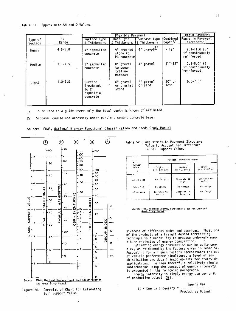
200 .100 90
70
-60
-50---- ioo— 90
-40 -80 -70
30__. - -60
50 20 • 40____
>. 30
_____ - .9 2 • W20
.7 -. 5 'C —
Cr 0 -5 2
0 - a. 10
-10 — .3 -8 Cr
-7 15
-6 .2— —
- 5
20
-3
I-i Source: FHWA, National Highway Functional Classification
and Needs Study Manual -
Figure 36. Correlation Chart for Estimating Soil Support Value.
—90 90
10-
80 80
9- 70
70
8-
- 60 - (9
cr I
'± 50
0 6--- —LiJ
LU 40
5cr— Cr 30
60
5-
0
30 cr m 0
20
4— 20
I0
.3- 10— -
0
-2-
81
Table 51. Approximate SN and D Values.
Type of SN Flexible Pavement _ Rigid Pavement _____________
Surface Type Base Type Subbase type Combii,içd Range in Pavement
Section Range & Thickeners & Thickeners & Thickeners Depth..!] ThickenersD
Heavy 4.6-6.0 4' asphaltic 9" crushed 4" gravel' > 12' 9.1-11.0 (8"
concrete stone to if continuously
PC concrete reinforced)
Medi urn 3.1-4.5 3" asphal tic 8" gravel 4" gravel 11-12" 7.1-9.0" (6"
concrete to pene- if continuously tration 'reinforced) macadam
Light 1.0-3.0 Surface 6" gravel 2" gravel 10" or 6.0-7.0"
Treatment or crushed or sand less
to 2" stone asphal tic concrete
1/ To be used as a guide where only the total depth is known or estimated.
2/ Subbase course not necessary under portland cement concrete base.
Source: FHWA, National Highway Functional Classification and Needs Study Manual
Table 52. Adjustment to Pavement Structure Value to Account for Difference in Soil Support Value.
SumpOr So1
Pavement stricture value
Lscht l4edlurn Heavy = 1.0-3.0 SN = 3.1.I.5 SN =
1.5 or less Na clar€e . Dc-crease to Decrease to
1t(tt
1.6 • 5.9 1) rhane No chaoe Na chan5e
6.0 or more ThCrease to Increase to No ctar.e
tee.vy
Source: FHWA,National Highway Functional Classification and Needs Study Manual
siveness of different modes and ser,vices. Thus, one of the products of a freight demand forecasting technique is a capability to produce order-of- mag-nitude estimates of energy consumption.
Estimating energy consumption can be quite com-plex, as evidenced by the factors given in Table 54. Accounting for all such factors necessitates the use of vehicle performance simulators, a level of so-phistication and detail inappropriate for statewide applications. In lieu thereof, a relatively simple subtechnique using the concept of energy intensity is presented in the following paragraphs.
Energy intensity is simply energy use per unit of productive output (32):
Energy Use El = Energy Intensity = --
Productive Output
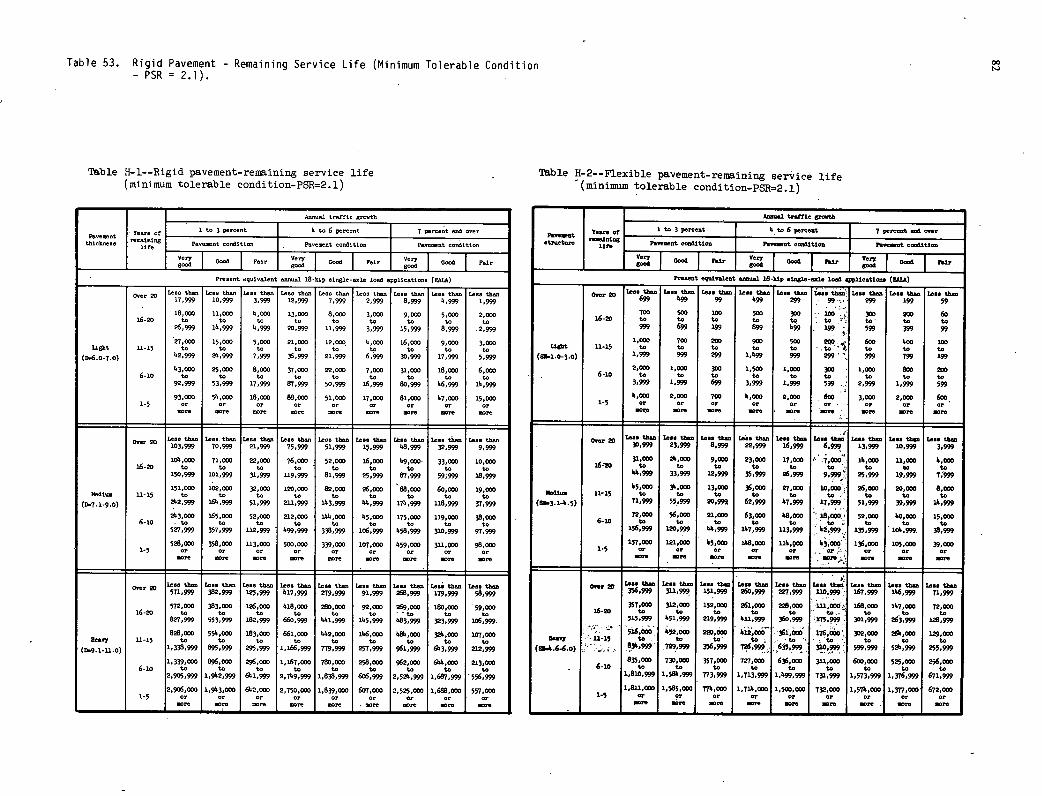
Table 53. Rigid Pavement - Remaining Service Life (Minimum Tolerable Condition 00
- PSR = 2.1).
b1e H-i--Rigid pavement-remaining service life (minimum tolerable condition-PSR=2.1)
A,o,00l trolTir growth
1 to 3 percent I to 6 percent 7 percent nod over
thickne reoolnng life Povownt cooditioo Pveeeot oocdittoo Povenont
IGood Feir
Preoentcqticolent o,00,ei 18-hip 010 10-owl, lood epplicotioo, (toi,g)
Over 20 10,0 the,, Leo. thoo tooe the,, too, the,, too, the,, ton. then to,. tIn,, 1.0.0 tIn,, Low. too,, 17,999 10,999 3,999 12,999 7,999 2,999 8,999 4,999 1,999
18, ll,ODO 1,000 13,000 8,000 3,000 91 5,000 2,000 16-20 to to to to to to to to to
26,999 11,999 1,999 20,999 11,999 3,999 15,999 8,999 .21999
27,000 15.000 51000 21,000 12, 4,000 16,000 91 3,ODO Light 11-15 to to to to
to to to to to (D.6.0-7.0) 42,999 24,999 7.999 36,999 21,999 6,999 30,999 17,999 51999
43,000 25,000 8,000 37,000 22,000 7,000 31,000 18,000 6,coo 6-10 to to to to to
to to
to to
92,999 53,999 17,999 87,999 50,999 18,999 80,999 46,999 14,999
93,000 54,000 18,OOD 88,000 51,000 17,000 81,000 17,000 15,000 1-5 or or or or or or or or or
Ovor 20 toe. than toe.. thee too, than to,. the,, to,. thee to.. thee thee thee to.. thee too. too,, 103,999 70,999 21,999 75,999 51,999 15,999 48,999 32,999 91999
104, 71,000 22,000 76,000 52,000 16,200 49,000 33,000 10,000 16-20 to to to to to to to to to
150,999 101,999 31,999 119,999 81,999 25,999 87,999 59;999 18,999
151,000 102,000 32,000 120,000 82,ODD 26,000 88,000 60,000 19,000 pedine 11-15 to to to to to to to to to
(D.7.1-9.0) 212,999 161,999 51,999 212,999 113,999 44,999 174,999 118,999 37,999
243,000 i65,000 52,000 212,000 111,000 15,000 175,000 119, 38, 6-10 . to to to to to to to to to
527,999 357,999 1.12,999 199,999 338,999 106,999 458,999 31.0,999 97,999
528.000 358,000 113, 50D,000 339,000 107,000 459, 311, 98,000 1-5 or
woe or
woe or
woe or
woe or
woe or
woe or
woe or
woe or
STe
Over 20 boo thee Lees than ee to the,, ieee thee La,. thee to.. thee to.. than to.i thee I..q than 571,999 382,999 125,999 417,999 279,999 91,999 268,999 179,999 58,999
572,000 383,000 126,OOD 418,ODO 280,000 92,000 269,000 180,000 59,000 16-20 to to to to to to - to to to
827,999 553,999 182,999 660,999 441,999 115,999 483,999 303,999 106,999.
828,000 554,000 183,000 661,000 442,000 146,800 484,000 324,000 i07, 20.07 11-15 to to to to to to to to to
(0.9.1-11.0) 1,338,999 895,999 295'999 1,166,999 779,999 257,999 961,999 613,999 212,999
1,339,000 W,000 296,000 1,167,000 T80,000 258,000 962,000 614,200 213,ODO 6-10 to to to to to to to to to
2,905,999 1,942,999 641,999 2,149,999 1,838,999 606,999 2,524,999 1,687,999 556,999
2,906,000 1,943,000 612,000 2,750,000 1,639,000 607,000 2,525,000 1,688,000 557,000 1-5 or
woe or
woe or
Sr. or
woe or
woe or . woe
or Sr.
or woe
or woe
¶[ble H-2-- Flexible pavement-remaining service life (minimum tolerable conditiofl-PSR=2.1)
Aeeusi trottie grwth
1 to 3 percent 4 to 6 perneot 7 percent and none Y.er. or life Powewot ooeditio Poret 000ditioo Peowset citiee
__ __ Very good Ico0aI I0oo6I Fair
Poesot equivelcot ee000l lO-hip .i.gle-eel.e toed pplioetloe. (2618)
Oeer 20 to.. thee lee, thee to.. thee leO, thee lee, thee Tens thee toe. thee toe, thee ee Lee. th 699 499 99 499 299 99 ., 299 199 59
16-20 700 to
500 100 to
500 300 -- 100 ., 300 60
999 to 699 199
to 899
to 499
- . - 199. to - to to
Lit 12-15 1,000
to 700 to
200 to
900 to
500 to
800 - . '' to 600 400 100
(i.0-3.0) 1,999 999 299 1,499 999 299 ' to 999
to 799
to 199
6-10 2,000
to I,ODO 3DO 11500 1,000 0 11000 800 800
3,999 to
11999 to 699
to 3,999
to 11999
to 599 to 2,999
to 1,999
to 599
5,000 2,00D 700 5,000 2,000 600 - 3,000 2,000 600 1-5 or
sit or
woe Zrwee or
se're or
ale or .
W2 Or
woe or
are or
ale
Orer 20 to.. thee Le.. than Low, thee Loje than to.. thee ie.O t to.. thee to.. then to.. thee 23,999 8,999 20,999 16,999 6,999 13,999 10,999 3,999
31,000 24,000 91020 23,000 17,000 f. 00 15,000 n,000 5,ODD 16-20 to to to to to to •- to to to
45,999 33,999 12,999 35,999 26,999 9,999, 25,999 19,999 7,999
59,000 35,000 13,000 36,000 27,000 10,020- 26,000 20,000 8,000 Nodi,a
(3.1-5.5) 11-15 to
71,999 to
551999 to
201999 to
62,999 to
57,999 to .
17,999 to
51,999 to
39,999 to
14,999
72,000 56,000 21,000 63,000 48,000 38,020, 1 52,000 40,000 15,000 6-10 to
156,999 to
1201999 to
",999 to
147,999 to
123,999 to
42,999 to
135,999 to
184,999. to
38,999
157,000 121,000 59,000 148,000 114,900 53,000 136,000 105,000 39,000 1-5 or Sr.
or Sr.
or or or ,. Or,. OT 00 or woe woe woe . wot,.! Mr. woe woe
20 Lee. then Low, thee to.. then Leg, thee ieee thee ieee theo ieee thee ieee then toe, than 396,999 311,999 151,999 060,999 207,999 310,999- 167,999 146,999 71,999
357,000 312,000 152,000 261,ODO 226,000 111,0001 168,000 147,000 T2,ODD 16-80 to to to to to . to ... to to to 515,999 5511999 219,999 512,999 360,999 175,999. 301,999 263,999 126,999
916 000 552 000 220,000 512 000 361 000 176 000 302 065 000 129,000 20.iy -11-15 to -. to to' ta . to to to (80.5.6-6.0) ----., 835,99 729,999 356,999 7,999 63s,9 310,999 599,999 524,999 255,999
835,000 730,000 357,000 797,000 636,000 311,000 600,000 529,000 256,000 6-10 to to to to to
to to to to
1,810,999 1,584,999 775,999 1,713,999
to ...
1,499,999 731,999 1,573,999 1,376,999 671,999
1,8u, 1,583,000 775, 1,711,000 1,500, 730,000 1,575,000 1,317,000 672,000 1-5 or
woe or
floe or
woe or
woe or
woe or
are or
woe ,r
woe or
wee
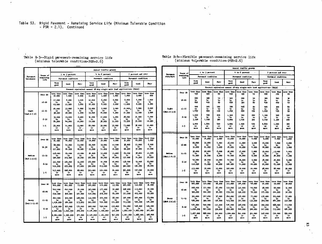
Table 53. Rigid Pavement - Remaining Service Life (Minimum Tolerable Condition - PSR = 2.1). Continued
Table H-3--Rigid pavement-remaining service life (minimum tolerable condition-PSR=2.6)
Mol0i tr,tfic 8rOth
1 to 3 porcent 4 to 6 peroect 7 percent nod over
Pevevent con&it000 P,veet co,4ltIo,, Pnovnont conution
:zI 000a l Folr I0oo4ITc1. I0000ITci
Pevoent cquircicnt coocol 18-tip ningie-nole 10,0 eppl100ti000 (EAIA)
Over 20 1.coo 1100 1000 Oboe Lee, 11.00 Leo, too,, Lee, tboo Lee, tboo 10,0 Oboe Leo, Oboe Lee, tboo 16,999 7,999 2,999 11,999 5,999 1,999 7,999 3,999 999
17,020 8,000 3,000 12,000 6,000 2,000 to
8, to
,000 1to
1,000 16-20 to to to to to. to
23,999 11,999 3,999 18,999 81999 2,999 13,999 6,999 1,999
21,000 12,000 1,000 19,ODO 91000 3, 7, 2,000 Ligbt 11-15 to to to to to to
to to to
(D.6.0-7.0) 3'999 18,999 51999 33,999 16,999 4,999 27,999 13,999 3,999
39,000 19,000 6,000 to
34,000 to
17,000 5, 28, 11,200 4, 6-10 to to to to to to to
81,999 10,999 12,999 79,999 38,999 11,999 72,999 35,999 10,999
1-5 85,020 or
41,000 or
13,000 or
80, or
39,WO or
L2,000 or
73,000 or
36,000 or
U,000 or
Leee Oboe Len, Oboe Leno than Leo, than Leo. than 1000 thoo Lee, Oboe Leo, than Leoe 11.0° Over 00 81,999 . 44,999 1.2,999 59,999 32,999 91999 37.999 20,999 51999
82,000 b,5,000 13,000 60,000 33,000 10,000 38,005 21,000 6,000 16-70 to to to to to to to to to
117,999 64,999 18,999 - 93,999 51,999 14,999 68,999 37,999 10,999
118.020 65,000 19,000 94,020 52,000 15,000 69,020 38,000 11,000 Medic 11-15 to to to to to to to to to
(0.7.1-9.0) 190,999 103,999 30,999 166,999 90,999 26,999 137,999 74,999 22,999
191,ODO 104,000 31,000 167,000 91,000 77,020 138,000 75,000 23,000 6-10 to to to to to to to to 00
616,999 225,999 67,999 392,999 213,999 63,999 360,999 196,999 58,999
415,000 226,000 68,00D 393,000 214,000 64,000 361,000 197;000 59,000 1-5 or or or or or or or or or
LeO, Oboe Lee, than Leo, Oboe 10.0 tboo Leon 11.0 LeO, th,o 10,. Oboe 1.00, Oboe Leo. 1100 Over 00 441,999 211,999 73,999 302,999 176,999 53,999 207,999 112.999 36,999
442,000 262,000 74,000 323,OOD IT7,000 54,200 208,000 113,000 35,000 16-20 to to to to to to to to to
639,999 348,999 107,999 510,999 278,999 85,999 373,999 203,999 62,999
640,000 349,000 108,000 511,000 279,ODD 86,020 314,000 204,200 63,000 H.,7 11-15 to to to to to to to to to
(0.9.1-11.0) 1,034.999 564,999 173,999 901,999 491,999 151,999 743,999 605,999 1.26,999
1,035,00D 565,020 174,000 902,000 492,000 152,000 744,020 426,000 125,020 6-10 to to to to to to to to to
2,244,999 1,225,999 376,999 2,124,999 1,160,999 356,999 1,950,999 1,265,999 307,999
2,045,000 1,226,000 3T7,000 2,125,000 1,161,000 357,OOD i,951,000 1,266,000 308,000 1-5 or or or or or or or or or
Table J1-14--Flexible pavement-remaining service life (minimum to)2erable condition-PSR=2.6)
Aom,,1 tr,fttc 000011
I 1 to 3 perOent 5 to 6 perceet 7 percent end ove.- Yeare of Poveet 0trUoto'e
life Pove.ent co,ditioo Pevent cooditto,. Povvnt nonditico
I°°°I" I 0oo6 I Feir I0000I Pair _Igood
PrO,Ont etuivelent nonuel 18-kip eiogle-oole 1od ,ppllc,ti000 (EAIA)
Over 20 Oboe bc. thee Lee. thee Le.o 040, LOne Oboe to.. thee 1.0cc too, Lee, too, 10.0 than 299. 69 499 199 49 299 199 29
600 300 70 500 200 50 . 300 200 30 16-20 to to to to to to to to to
899 699 99 699 399 89 699 299 59
900 500 100 700 4o6 90 50D 300 60 13.640 11-15 to to to to to to to to to
(61.1.0.3.0) 1,699 699 199 11299 699 199 11099 499 99
1,500 700 200 1, 3DO 700 200 1,100 500 100 6-10 to to to to to to to to . to
3,199 11599 399 2,999 1,499 399 2,799 1,399 299
3,200 1,600 600 3,000 11500 600 2,800 1,400 1-5 or
cot or
eye or
eye or
eve or
eve or
eye or
eye or r -
or eve
Over 20 1.0.0 than 10cc the, Leco than 10cc thee 10cc Ob.oe Leo. o, tone then Lee, 11.0, Lee. thee 21,999 16,999 3,999 15,999 101999 2,999 9,999 6,999 1,999
22,000 15,200 4,wo 16,000 11,000 3,000 10, 7,000 2,000 i6-eD to to to to to to to . to to
31,999 21,999 5,999 25,999 . 16,999 61999. 18,999 12,999 3,999
30,000 22, 6,000 26,000 17,000 51000 19,000 13, 6,000 Medic 11-15 to to to to to to to / to to
(81.3.1-4.5) 51,999 34,999 9.999 44,999 29,999 81999 3r,999 24,999 .7,999
.52,OW 35,000 10,000 65,000 3D,ODD 91000 38,000 25,000 8,000 6-1.0 to to to to to to to to to
112,999 75,999 22,999 106,999 71,999 20,999 97,999 65,999 19,999
113,000 76,000 23,000 107,000 72,000 21,ODD 98,000 66,000 20,000 1-5 or or or or or or or or or
Over 20 Use thee Lee. tIc 10,, Oboe Lee, tbeo Leoc thee Leo, Oboe 10,0 then 10,0 the, Lee. than 207999 170,999 66,999 151,999 126,999 68,999 97,999 79,999 30,999
208,000 171,000 67,000 152,000 125,000 49,00D 98,000 80,ODO 31,000 16-20 to
to
to
to
to to
to to
3DO,999 266,999 96,999 239,999 196,999 76,999 175,999 144,999 to 56,999
301,000 267,000 91,000 260,000 197,000 77, 176,000 155,000 57,ODO Honey 11-15 to
to to
to
to
to to to
(c.6.6.6.o) 486,999 399,999 156,999 523,999 357,999 135,999 to 349,999 087,999 112,999
587,OOD 400,ODO 157,020 626,000 348,000 136,020 350,ODO 288,000 U3,000 6-10 to
to to , to to to to to to
1,056,999 867,999 339,999 999,999 820,999 320,999 917,999 753,999 296,999
1,057,000 868,000 340, 1,,000 821, 301,000 918, 756, 295,000 1-5 or or or or or or or or or
00 LJ
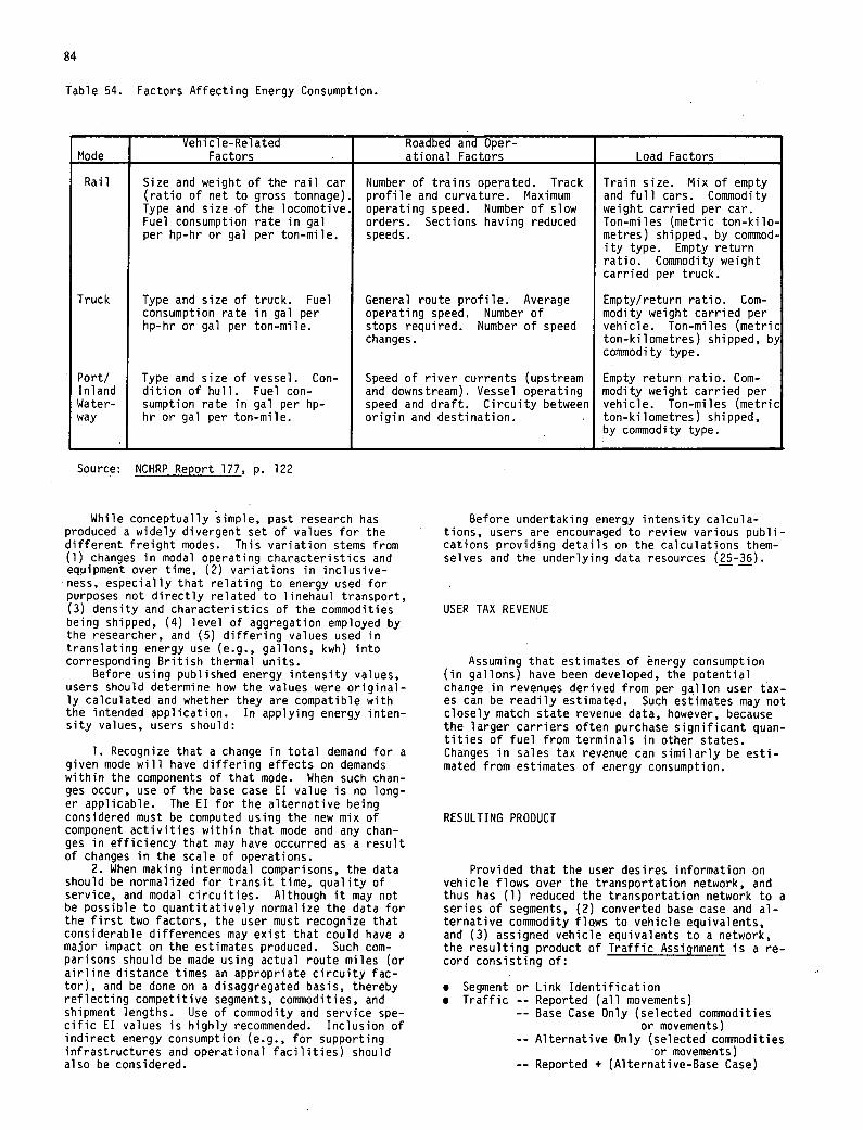
84
Table 54. Factors Affecting Energy Consumption.
Mode Vehicle-Related
Factors Roadbed and Oper- ational Factors Load Factors
Rail Size and weight of the rail car Number of trains operated. Track Train size. Mix of empty (ratio of net to gross tonnage). profile and curvature. Maximum and full cars. Commodity Type and size of the locomotive, operating speed. Number of slow weight carried per car. Fuel consumption rate in gal orders. Sections having reduced Ton-miles (metric ton-kilo- per hp-hr or gal per ton-mile, speeds. metres) shipped, by commod-
ity type. Empty return ratio. Commodity weight carried per truck.
Truck Type and size of truck. Fuel General route profile. Average Empty/return ratio. Corn- consumption rate in gal per operating speed. Number of modity weight carried per hp-hr or gal per ton-mile, stops required. Number of speed vehicle. Ton-miles (metric
changes. ton-kilometres) shipped, by commodity type.
Port/ Type and size of vessel. Con- Speed of river currents (upstream Empty return ratio. Corn- Inland dition of hull. Fuel con- and downstream). Vessel operating modity weight carried per Water- sumption rate in gal per hp- speed and draft. Circuity between vehicle. Ton-miles (metric way hr or gal per ton-mile, origin and destination. ton-kilometres) shipped,
by commodity type.
Source: NCHRP Report 177, p. 122
While conceptually simple, past research has produced a widely divergent set of values for the different freight modes. This variation stems from (1) changes in modal operating characteristics and equipment over time, (2) variations in inclusive-ness, especially that relating to energy used for purposes not directly related to linehaul transport, (3) density and characteristics of the commodities being shipped, (4) level of aggregation employed by the researcher, and (5) differing values used in translating energy use (e.g., gallons, kwh) into corresponding British thermal units.
Before using published energy intensity values, users should determine how the values were original-ly calculated and whether they are compatible with the intended application. In applying energy inten-sity values, users should:
Recognize that a change in total demand for a given mode will have differing effects on demands within the components of that mode. When such chan-ges occur, use of the base case El value is no long-er applicable. The El for the alternative being considered must be computed using the new mix of component activities within that mode and any chan-ges in efficiency that may have occurred as a result of changes in the scale of operations.
When making intermodal comparisons, the data should be normalized for transit time, quality of service, and modal circuities. Although it may not be possible to quantitatively normalize the data for the first two factors, the user must recognize that considerable differences may exist that could have a major impact on the estimates produced. Such com-parisons should be made using actual route miles (or airline distance times an appropriate circuity fac-tor), and be done on a disaggregated basis, thereby reflecting competitive segments, commodities, and shipment lengths. Use of commodity and service spe-cific El values is highly recommended. Inclusion of indirect energy consumption (e.g., for supporting infrastructures and operational facilities) should also be considered.
Before undertaking energy intensity calcula-tions, users are encouraged to review various publi-cations providing details on the calculations them-selves and the underlying data resources (25-36).
USER TAX REVENUE
Assuming that estimates of energy consumption (in gallons) have been developed, the potential change in revenues derived from per gallon user tax-es can be readily estimated. Such estimates may not closely match state revenue data, however, because the larger carriers often purchase significant quan-tities of fuel from terminals in other states. Changes in sales tax revenue can similarly be esti-mated from estimates of energy consumption.
RESULTING PRODUCT
Provided that the user desires information on vehicle flows over the transportation network, and thus has (1) reduced the transportation network to a series of segments, (2) converted base case and al-ternative commodity flows to vehicle equivalents, and (3) assigned vehicle equivalents to a network, the resulting product of Traffic Assignment is a re-cord consisting of:
Segment or Link Identification Traffic -- Reported (all movements)
-- Base Case Only (selected commodities or movements)
-- Alternative Only (selected commodities or movements)
-- Reported + (Alternative-Base Case)
85
Optional: EALA - Base Case - Alternative
Remaining Service Life -- Base Case -- Alternative
Energy Consumption -- Base Case -- Alternative
User Tax Revenues -- Base Case -- Alternative
One record is prepared for each segment identi-fied. The user has numerous options, such as (1) to include different modes, (2) to use manual or compu-
terized methods, and (3) for the highway network, to compute equivalent annual load applications, esti-mate remaining service life, or approximate energy consumption and user tax revenues on a segment ba-sis.
Once the above record has been assembled, seg-ment and system level summaries can be readily pre-pared showing base case and alternative totals as well as projected change. If so desired, the re-sults can be plotted provided that coordinates have been included in the resulting record.
REFERENCES
Vehicle Equivalents
The American Waterways Operators, Inc., Big Load Afloat." Washington, DC (1973). Federal Highway Administration, Overweight Vehi-cles, Penalties, and Permits-An Inventory of State Practices. U.S. Department of Transpor-tation, Washington, DC (1979). Motor Vehicle Manufacturers Association of the U.S., Inc., Motor Truck Facts, 19XX. Detroit, MI (annually). National Railway Publication Company, The Offic-ial Railway Equipment Register, New York, NY (quarterly). National Railway Publication Company, Railway. Line Clearances, New York, NY (annually). Transportation Research Board, NCHRP Synthesis of Highway Practice 68, "Motor Vehicle Size and Weight Regulations, Enforcement and Permit Oper-ations," Transportation Research Board, National Academy of Sciences, Washington, DC (1980) 45 pp.
Traffic Assignment
Kornhauser, A.L., Development of an Interactive-Graphic Computer Model for the Nationwide As-signment of Railroad Traffic. U.S. Department of Transportation. Federal Railroad Administra-tion. Washington, DC (Sept. 1977). Landsdowne, Z.F., "Rail Freight Traffic Assign-ment." U.S. Department of Transportation, Of-fice of the Secretary, Report DOT-TSC-OST-79, -Washington, DC (Feb. 1979). Memmott, F.W., and Scholz, F.S., "Trunk Route Analyses: A Useful Tool for Statewide and Re-gional Rail Planning." Transportation Research Rê'cord 591, Washington, DC (1976) pp. 44-50. U.S. Army Corps of Engineers, Inland Navigation Systems Analysis. Eight Volumes, Washington, DC (July 1976). U.S. Department of Transportation, Federal High-way Administration, FHWA Computer Programs for Urban Transportation Planning. Washington, DC (July 1974). U.S.Thàrtment of Transportation, Federal High-way Administration, PLAN/BACKPAC General Infor-mation Manual. Washington, DC (April 1977). U.S. Department of Transportation, Federal High-way Administration, Statewide Travel Demand Forecasting. Washington, DC (Nov. 1973). U.S. Department of Transportation, Federal High-way Administration, Traffic Assignment. Wash-ington, DC (Aug. 1973). U.S. Department of Transportation, Transporta-tion Systems Center, "Freight Transportation En-ergy Use, Volume Ill-Freight Network and Opera-
tions Data Base." Report DOT-TSC-OST-79-1 (July 1979). U.S. Department of Transportation, Urban Mass Transportation Administration, "Urban Transpor-tation Planning System: Introduction." Wash-ington, DC (July 1977). U.S. Department of Transportation, Urban Mass Transportation Administration, "HNET Lecture Guide." Washington, DC (1982). U.S. .Department of Transportation, Urban Mass Transportation Administration, "UROAD Lecture Guide." Washington, DC (1982). U.S. Department of Transportation, Urban Mass Transportation Administration, "UTPS Highway Network Development Guide." Washington, DC (1982). U.S. Department of Transportation, Urban Mass Transportation Administration, UTPS Reference Manual. Washington, DC (April 1979). U.S. Department of Transportation, Urban Mass Transportation Administration, UTPS User's Guide. Washington, DC (1979).
Equivalent Annual Load Applications and Change in Service Life
AASHTO Subcommittee on Highway Design. AASHTO Interim Guide for Design of Pavement Structures, American Association of State Highway and Trans-portation Officials, Washington, DC (1972). Federal Highway Administration, National Highway Functional Classification and Needs Manual. Highway Research Board, The AASHO Road Test. Series of special reports 61A-61G. Highway Re-search Board, National Academy of Sciences, Washington, DC (1961-1962). American Trucking Associations, Inc., Measuring Energy Efficiency in Freight Transportation. Washington, DC (1976).
Energy Consumption and User Tax Revenue
Battelle-Columbus Laboratories, Energy Require-ments for the Movement of Intercity Freight. Prepared for Association of American Railroads (1972). Hirst, E., "Energy Intensiveness of Passenger and Freight Transport Modes: 1950-1970." Oak Ridge National Laboratory Report ORNL-NSF-EP-44 (1973). Hopkins, J.B., "Railroads and the Environment-Estimation of Fuel Transportation." Vol. I, Analytical Model, prepared for USDOT-FRA, final report, reprint (Oct. 1975). Moelok, E.K., "A Comparison of Railroad and Truck Line-Haul Work (Energy) Requirements Under Various Shipment Weight, Speed, and Topographic
86
Conditions." University of Pennsylvania, Phila-delphia, PA (Jan. 1976). National Aeronautics and Space Administration and U.S. Department of Transportation (an Inter-agency Working Group), Transportation Vehicle Energy Intensities. Washington, DC (June 1974). Peat, Marwick, Mitchell and Company and Jack Faucett Associates, Industrial Energy Studies of Ground Freight Transportation. Prepared for U.S. Department of Commerce, Industrial Energy Analysis Group (1974). Rose, A.B., and Reed, K.J., Energy Intensity and Related Parameters of Selected Transportation Modes: Freight Movements. Oak Ridge National Laboratory, Oak Ridge, TN (June 1979).
33 Seibold, A.V., Energy Intensity of Barge and Rail Freight Hauling. Prepared for National Science Foundation (May 1974). Tihansky, D.P., Methods for Estimating the Volume and Energy Demand of Freight Transport. Rand Corporation, prepared for the National Sci-ence Foundation (Dec. 1972). U.S. Department of Transportation, Federal High-way Administration, A Method for Estimating Fuel Consumption and Vehicle Emissions on Urban Ar-terial Networks. Washington, DC (April 1981). U.S. Department of Transportation, Federal High-way Administration, Procedure for Estimating Highway User Costs, Fuel Consumption, and Air Poflution. Washington, DC (March 1980).
CHAPTER SIX
CASE EXAMPLES
INTRODUCTION
Previous chapters have provided the user with guidance in defining the problem, structuring the technique to address the problem, and simplifying and adapting both problem and technique to meet ap-plicable constraints. A variety of subtechniques have been provided for use in addressing different phases and components. The subtechniques presented are conceptually simple and straight-forward. Some can be applied manually; others are best done using a computer. In most cases, specific examples have been provided to illustrate how the - subtechniques can be applied.
The purpose of this chapter is to illustrate the application of the technique by using several case examples. In reviewing the examples, users should recognize that the individuality of freight planning applications makes it unlikely that any case example can directly serve as a model for similar on-going work Most applications will necessitate innova- tiveness andresourcefulness on the part of the user.
It is important to keep in mind also that an in-depth explanation of the choices made among candi-date analytical methods and/or data sources has not been included, because it would not be relevant to most readers. A sensitivity analysis of the results to the assumptions made or computational process em-ployed has not been shown, even though such testing is commonly done, because of the the length and com-plexity of the examples. However, users are encour-aged to include a sensitivity assessment when apply-ing the freight demand forecasting technique. Fi-nally, comparisons of the results obtained with sim-ilar studies have not been attempted because of the uniqueness of the case examples.
GENERAL DESCRIPTION
The first two case examples are abridgements of previously completed studies undertaken by the re-
searchers. While it can be argued that a post-study application of the technique does not provide a true test or "shakedown" of the technique, the availabil-ity of commodity flow, cost, and rate data reduced the time and effort that would have been required had the application started "from scratch." In both cases, the conclusions reached were borne out by subsequent events.
The third case example, which was expressly un-dertaken for this project, was an informal examina-tion of Roadrailer service in the Buffalo-New York City corridor. The case example chosen involves ex-amining volume, rate and cost structures of the ser-vice to estimate the point at which services become competitive with trucking, and thus can survive on a self-sustaining basis. Roadrail'er is a dual-mode: semi-trailer having flanged wheels which can be as-sembled into trains for lineha&fl movement over the rail system. It is similar to TOFC (trailer-on-flat-car) except that it obviates the need for the flat car. Its main competition is trucking. The Buffalo-New York City corridor was chosen by the Bi-Modal Corporation (the operator of the service) to demonstrate the feasibililty of intermodal services between markets 200-800 miles apart. (Approximately 73 percent of the national market for containeriza-ble commodities lies within this distance range.)
Most of the computations illustrated by the case examples can be done with minicomputers or microcom-puters. The latter are becoming increasingly avail-able within government because of their low price and performance. A number of the applications could be done using comercially available generic soft-ware, such as VisiCalc or dBASE II. Otherwise, cus-tom programming using BASIC or USCD Pascal would have to be employed. Because of compatibility prob-lems stemming from different manufacturers' hardware and software, various operating systems, language variants, and differences in disk storage capabili-ties and formats, application specific software de-veloped for a particular microcomputer may not be readily transportable to other machines. At the present time, relatively little public sector or proprietary software is available expressly for freight demand forecasting purposes. Nor are all applications appropriate for microcomputers (e.g., a main frame computer is reqUired for rail costing us-ing URCS).
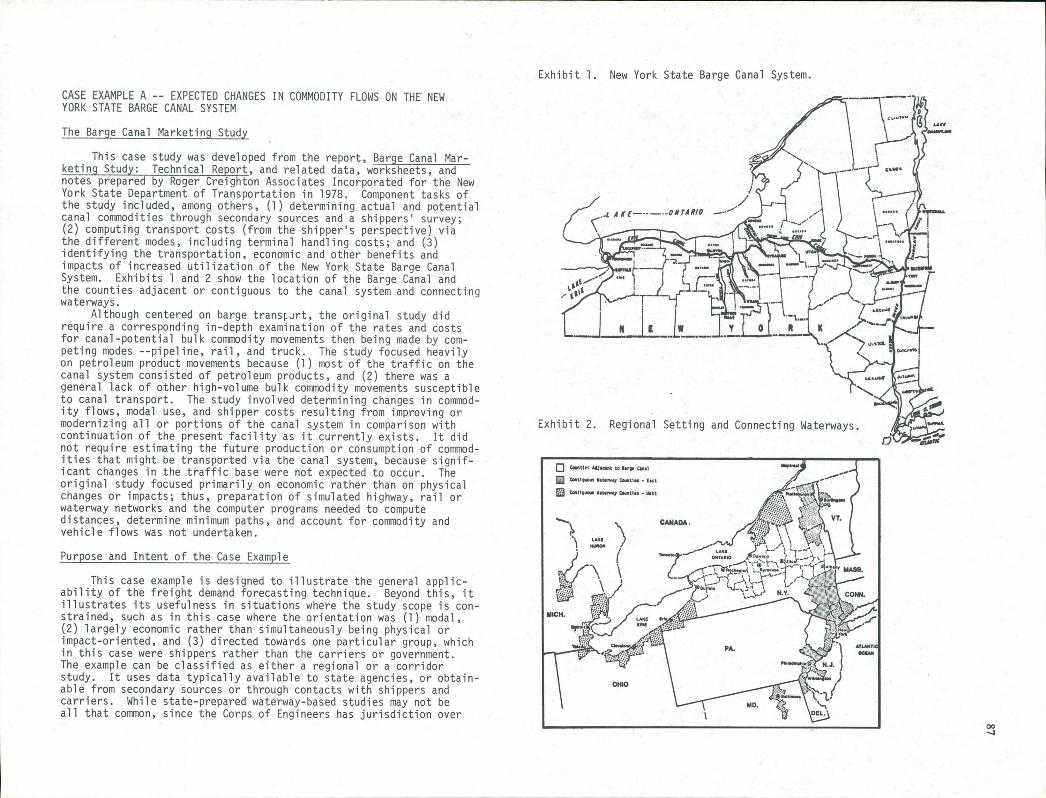
Exhi
Exhibit 1. New York State Barge Canal System.
CASE EXAMPLE A -- EXPECTED CHANGES IN COMMODITY FLOWS ON THE NEW YORK STATE BARGE CANAL SYSTEM
The Barge Canal Marketing Study
This case study was developed from the report, Barge Canal Mar-keting Study: Technical Report, and related data, worksheets, and notes prepared by Roger Creighton Associates Incorporated for the New York State Department of Transportation in 1978. Component tasks of the study included, among others, (1) determining actual and potential canal commodities through secondary sources and a shippers survey; (2) computing transport costs (from the shippers perspective) via the different modes, including terminal handling costs; and (3) identifying the transportation, economic and other benefits and impacts of increased utilization of the New York State Barge Canal System. Exhibits 1 and 2 show the location of the Barge Canal and the counties adjacent or contiguous to the canal system and connecting waterways.
Although centered on barge transjrt, the original study did require a corresponding in-depth examination of the rates and costs for canal-potential bulk commodity movements then being made by com-peting modes --pipeline, rail, and truck. The study focused heavily on petroleum product movements because (1) most of the traffic on the canal system consisted of petroleum products, and (2) there was a general lack of other high-volume bulk commodity movements susceptible to canal transport. The study involved determining changes in commod-ity flows, modal use, and shipper costs resulting from improving or modernizing all or portions of the canal system in comparison with continuation of the present facility as it currently exists. It did not require estimating the future production or consumption of commod-ities that might be transported via the canal system, because signif-icant changes in the traffic base were not expected to occur. The original study focused primarily on economic rather than on physical changes or impacts; thus, preparation of simulated highway, rail or waterway networks and the computer programs needed to compute distances, determine minimum paths, and account for commodity and vehicle flows was not undertaken.
Purpose and Intent of the Case Example
This case example is designed to illustrate the general applic-ability of the freight demand forecasting technique. Beyond this, it illustrates its usefulness in situations where the study scope is con-strained, such as in this case where the orientation was (1) modal, (2) largely economic rather than simultaneously being physical or impact-oriented, and (3) directed towards one particular group, which in this case were shippers rather than the carriers or government. The example can be classified as either a regional or a corridor study. It uses data typically available to state agencies, or obtain-able from secondary sources or through contacts with shippers and carriers. While state-prepared waterway-based studies may not be all that common, since the Corps of Engineers has jurisdiction over
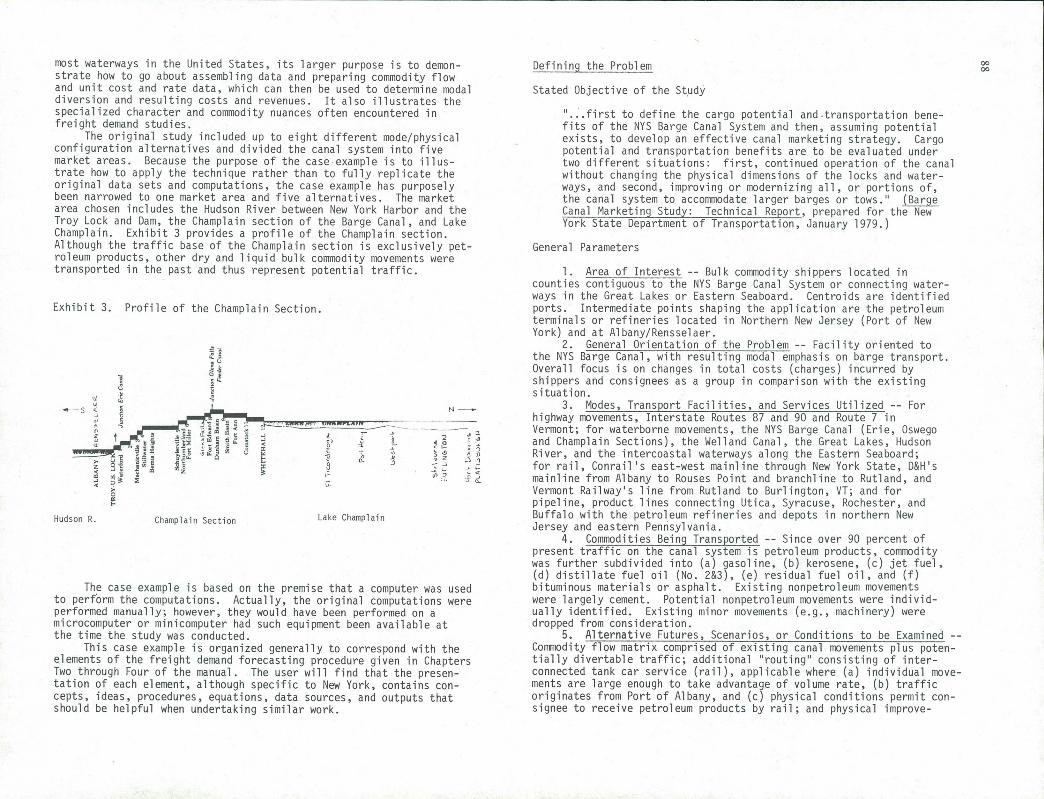
most waterways in the United States, its larger purpose is to demon-strate how to go about assembling data and preparing commodity flow and unit cost and rate data, which can then be used to determine modal diversion and resulting costs and revenues. It also illustrates the specialized character and commodity nuances often encountered in freight demand studies.
The original study included up to eight different mode/physical configuration alternatives and divided the canal system into five market areas. Because the purpose of the case example is to illus-trate how to apply the technique rather than to fully replicate the original data sets and computations, the case example has purposely been narrowed to one market area and five alternatives. The market area chosen includes the Hudson River between New York Harbor and the Troy Lock and Dam, the Champlain section of the Barge Canal, and Lake Champlain. Exhibit 3 provides a profile of the Champlain section. Although the traffic base of the Champlain section is exclusively pet-roleum products, other dry and liquid bulk commodity movements were transported in the past and thus represent potential traffic.
Exhibit 3. Profile of the Champlain Section.
r
-H
r Hudson R. Champlain Section Lake Champlain
The case example is based on the premise that a computer was used to perform the computations. Actually, the original computations were performed manually; however, they would have been performed on a microcomputer or minicomputer had such equipment been available at the time the study was conducted.
This case example is organized generally to correspond with the elements of the freight demand forecasting procedure given in Chapters Two through Four of the manual. The user will find that the presen-tation of each element, although specific to New York, contains con-cepts, ideas, procedures, equations, data sources, and outputs that should be helpful when undertaking similar work.
Definino the Problem
Stated Objective of the Study
"...first to define the cargo potential and transportation bene-fits of the NYS Barge Canal System and then, assuming potential exists, to develop an effective canal marketing strategy. Cargo potential and transportation benefits are to be evaluated under two different situations: first, continued operation of the canal without changing the physical dimensions of the locks and water-ways, and second, improving or modernizing all, or portions of, the canal system to accommodate larger barges or tows. (Barge Canal Marketing Study: Technical Report, prepared for the New York State Department of Transportation, January 1979.)
General Parameters
Area of Interest -- Bulk commodity shippers located in counties contiguous to the NYS Barge Canal System or connecting water-ways in the Great Lakes or Eastern Seaboard. Centroids are identified ports. Intermediate points shaping the application are the petroleum terminals or refineries located in Northern New Jersey (Port of New York) and at Albany/Rensselaer.
General Orientation of the Problem -- Facility oriented to the NYS Barge Canal, with resulting modal emphasis on barge transport. Overall focus is on changes in total costs (charges) incurred by shippers and consignees as a group in comparison with the existing situation.
Modes, Transport Facilities, and Services Utilized -- For highway movements, Interstate Routes 87 and 90 and Route 7 in Vermont; for waterborne movements, the NYS Barge Canal (Erie, Oswego and Champlain Sections), the Welland Canal, the Great Lakes, Hudson River, and the intercoastal waterways along the Eastern Seaboard; for rail, Conrail's east-west mainline through New York State, D&H's mainline from Albany to Rouses Point and branchline to Rutland, and Vermont Railway's line from Rutland to Burlington, VT; and for pipeline, product lines connecting Utica, Syracuse, Rochester, and Buffalo with the petroleum refineries and depots in northern New Jersey and eastern Pennsylvania.
Commodities Being Transported -- Since over 90 percent of present traffic on the canal system is petroleum products, commodity was further subdivided into (a) gasoline, (b) kerosene, (c) jet fuel, (d) distillate fuel oil (No. 20), (e) residual fuel oil, and (f) bituminous materials or asphalt. Existing nonpetroleum movements were largely cement. Potential nonpetroleum movements were individ-ually identified. Existing minor movements (e.g., machinery) were dropped from consideration.
Alternative Futures, Scenarios, or Conditions to be Examined --Commodity flow matrix comprised of existing canal movements plus poten-tially divertable traffic; additional "routing" consisting of inter-connected tank car service (rail), applicable where (a) individual move-ments are large enough to take advantage of volume rate, (b) traffic originates from Port of Albany, and (c) physical conditions permit con-signee to receive petroleum products by rail; and physical improve-
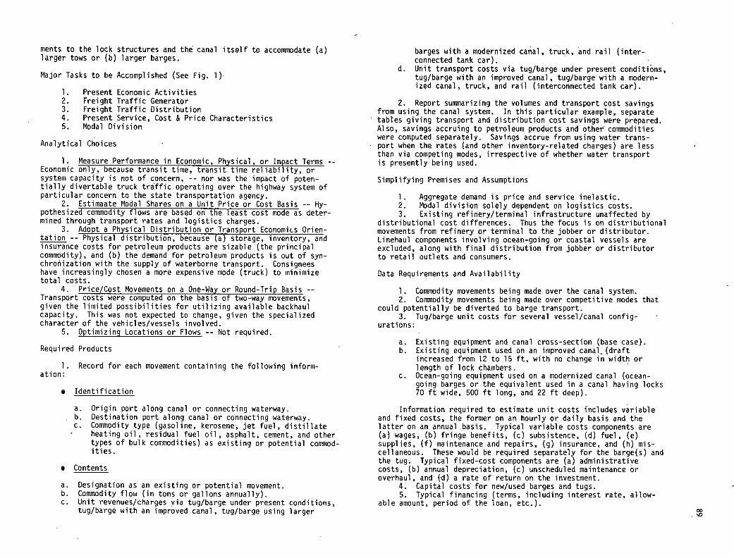
ments to the lock structures and the canal itself to accommodate (a) larger tows or (b) larger barges.
Major Tasks to be Accomplished (See Fig. 1)
Present Economic Activities Freight Traffic Generator Freight Traffic Distribution Present Service, Cost & Price Characteristics Modal Division
Analytical Choices
Measure Performance in Economic, Physical, or Impact Terms --Economic only, because transit time, transit time reliability, or system capacity is not of concern, -- nor was the impact of poten-tially divertabie truck traffic operating over the highway system of particular concern to the state transportation agency.
Estimaate Modal Shares on a Unit Price or Cost Basis -- Hy-pothesized comodity flows are based on the least cost mode as deter-mined through transport rates and logistics charges.
Adopt a Physical Distribution or Transport Economics Orien-tation -- Physical distribution, because (a) storage, inventory, and insurance costs for petroleum products are sizable (the principal commodity), and (b) the demand for petroleum products is out of syn-chronization with the supply of waterborne transport. Consignees have increasingly chosen a more expensive mode (truck) to minimize total costs.
Price/Cost Movements on a One-Way or Round-Trip Basis --Transport costs were computed on the basis of two-way movements, given the limited possibilities for utilizing available backhaul capacity. This was not expected to change, given the specialized character of the vehicles/vessels involved.
Optimizing Locations or Flows -- Not required.
Required Products
1. Record for each movement containing the following inform-ation:
. Identification
Origin port along canal or connecting waterway. Destination port along canal or connecting waterway. Commodity type (gasoline, kerosene, jet fuel, distillate heating oil, residual fuel oil, asphalt, cement, and other types of bulk commodities) as existing or potential commod-ities.
Contents
Designation as an existing or potential movement. Commodity flow (in tons or gallons annually). Unit revenues/charges via tug/barge under present conditions, tug/barge with an improved canal, tug/barge using larger
barges with a modernized canal, truck, and rail (inter-connected tank car).
d. Unit transport costs via tug/barge under present conditions, tug/barge with an improved canal, tug/barge with a modern-ized canal, truck, and rail (interconnected tank car).
2. Report summarizing the volumes and transport cost savings from using the canal system. In this particular example, separate tables giving transport and distribution cost savings were prepared. Also, savings accruing to petroleum products and other commodities were computed separately. Savings accrue from using water trans-port when the rates (and other inventory-related charges) are less than via competing modes, irrespective of whether water transport is presently being used.
Simplifying Premises and Assumptions
Aggregate demand is price and service inelastic. Modal division solely dependent on logistics costs. Existing refinery/terminal infrastructure unaffected by
distributional cost differences. Thus the focus is on distributional movements from refinery or terminal to the jobber or distributor. Linehaul components involving ocean-going or coastal vessels are excluded, along with final distribution from jobber or distributor to retail outlets and consumers.
Data Requirements and Availability
1. Commodity movements being made over the canal system. 2. Commodity movements being made over competitive modes that
could potentially be diverted to barge transport. 3. Tug/barge unit costs for several vessel/canal config-
urations:
Existing equipment and canal cross-section (base case). Existing equipment used on an improved canal (draft increased from 12 to 15 ft, with no change in width or length of lock chambers. Ocean-going equipment used on a modernized canal (ocean-going barges or the equivalent used in a canal having locks 70 ft wide, 500 ft long, and 22 ft deep).
Information required to estimate unit costs includes variable and fixed costs, the former on an hourly or daily basis and the latter on an annual basis. Typical variable costs components are (a) wages, (b) fringe benefits, (c) subsistence, (d) fuel, (e) supplies, (f) maintenance and repairs, (g) insurance, and (h) mis-cellaneous. These would be required separately for the barge(s) and the tug. Typical fixed-cost components are (a) administrative costs, (b) annual depreciation, (c) unscheduled maintenance or overhaul, and (jd) a rate of return on the investment.
4. Capital costs for new/used barges and tugs. 5. Typical financing (terms, including interest rate, allow-
able amount, period of the loan, etc.). 00
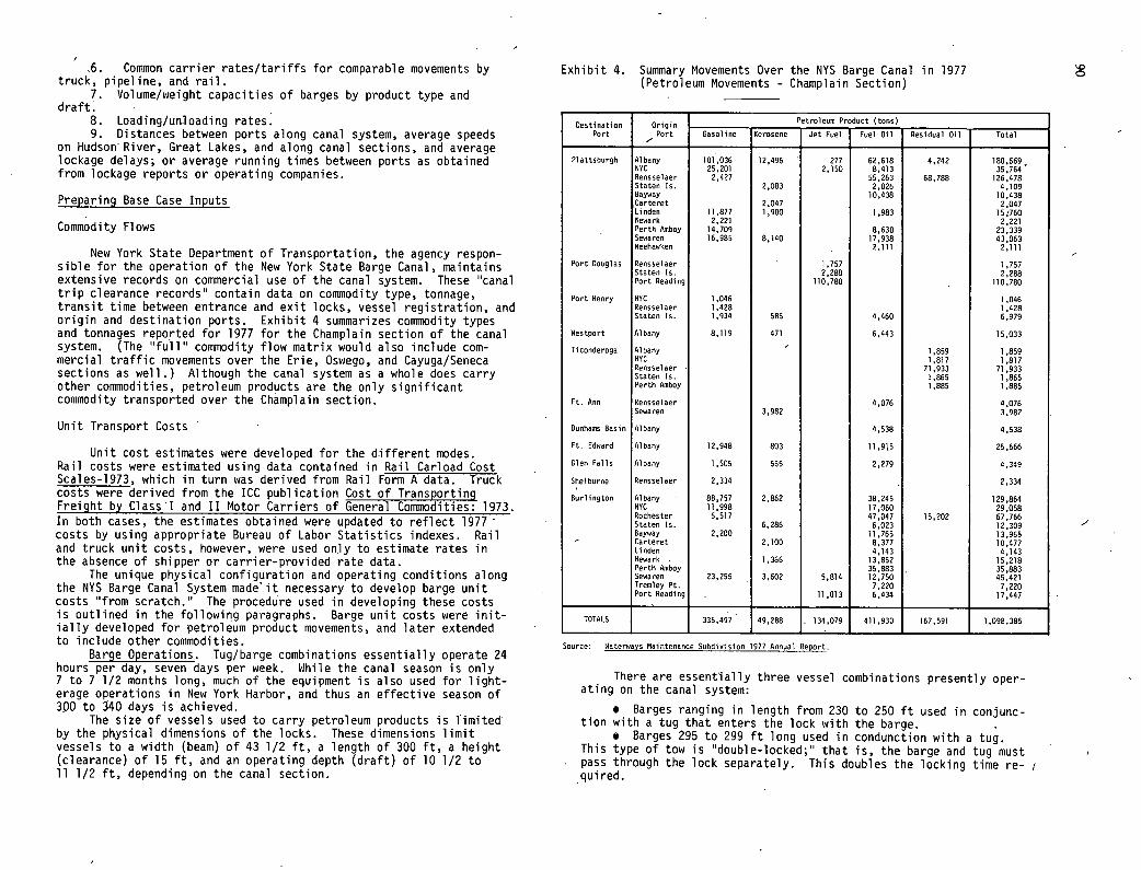
.6. Common carrier rates/tariffs for comparable movements by truck, pipeline, and rail.
Volume/weight capacities of barges by product type and draft.
Loading/unloading rates. Distances between ports along canal system, average speeds
on Hudson River, Great Lakes, and along canal sections, and average lockage delays; or average running times between ports as obtained from lockage reports or operating companies.
Preparing Base Case Inputs
Commodity Flows
New York State Department of Transportation, the agency respon-sible for the operation of the New York State Barge Canal, maintains extensive records on commercial use of the canal system. These canal trip clearance records" contain data on commodity type, tonnage, transit time between entrance and exit locks, vessel registration, and origin and destination ports. Exhibit 4 summarizes commodity types and tonnages reported for 1977 for the Champlain section of the canal system. (The "full" commodity flow matrix would also include com-mercial traffic movements over the Erie, Oswego, and Cayuga/Seneca sections as well.) Although the canal system as a whole does carry other commodities, petroleum products are the only significant commodity transported over the Champlain section.
Unit Transport Costs
Unit cost estimates were developed for the different modes. Rail costs were estimated using data contained in Rail Carload Cost Scales-1973, which in turn was derived from Rail Form A data. Truck costs were derived from the ICC publication Cost of Transporting Freight by Class'I and II Motor Carriers of General Commodities: 1973. In both cases, the estimates obtained were updated to reflect 1977 -costs
977-costs by using appropriate Bureau of Labor Statistics indexes. Rail and truck unit costs, however, were used only to estimate rates in the absence of shipper or carrier-provided rate data.
The unique physical configuration and operating conditions along the NYS Barge Canal System made' it necessary to develop barge unit costs 'from scratch." The procedure used in developing these costs is outlined in the following paragraphs. Barge unit costs were init-ially developed for petroleum product movements, and later extended to include other commodities.
Barge Operations. Tug/barge combinations essentially operate 24 hours per day, seven days per week. While the canal season is only 7 to 7 1/2 months long, much of the equipment is also used for light-erage operations in New York Harbor, and thus an effective season of 300 to 340 days is achieved.
The size of vessels used to carry petroleum products is limited by the physical dimensions of the locks. These dimensions limit vessels to a width (beam) of 43 1/2 ft, a length of 300 ft, a height (clearance) of 15 ft, and an operating depth (draft) of 10 1/2 to 11 1/2 ft, depending.on the canal section.
Exhibit 4. Summary Movements Over the NYS Barge Canal in 1977 (Petroleum Movements - Champlain Section)
Destination Origin Petroleum Prnduct (tons)
Gasoline Kerosene Jet Fuel Fuel Oil Residual Oil Total Port Port
Plattsburgh Albany 101,036 12,496 277 62,618 4.242 180.669, NYC 25.201 2,150 8,413 35.764 Rensselaer 2,427 55.263 68,788 126,478 Staten Is. 2.083 2,026 4,109 Bayway 10,438 10,438 Carteret 2.047 2.047 Linden 11,877 1,900 1,983 15,760 Newark 2.221 2.221 Perth Yanboy 14,709 8,630 23.339 Sewaren 16,985 8,140 17,938 43.063 Weehawken 2,111 2.111
Port Douglas Rensselaer 1.757 1.757 Staten Is. 2.288 2.288 Port Reading 110,780 110.780
Port Henry NYC 1.046 1.046 Rensselaer 1,428 1.428 Staten Is. 1.934 585 4.460 6.979
Westport Albany 8.119 471 6,443 15,033
Ticanderoga Albany 1,859 1.859 NYC 1.817 1,817 Rensselaer 71 .933 71,933 Staten Is. 1,865 1,865 Perth Ainbay 1.885 1.885
Ft. Ann Rensselaer 4,076 4,076 Sewaren 3,982 3.982
Danhams Basin Albany 4,538 4,538
Ft. Edward Albany 12,948 803 11,915 25,666
Glen Falls Albany 1,505 565 2,279 4,349
Shelbarne Rensselaer 2,334 2,334
Burlington Albany 88.757 2,862 38.245 129,864 NYC 11,998 17,060 29.058 Rochester 5,517 47.047 15,202 67.766 Staten Is. 6,286 6,023 12,309 Bayway 2,200 11.765 13,965 - Carteret 2,100 8,377 10.477 Linden 4.143 4,143 Newark 1,366 13.852 15.218 Perth M,boy 35.883 . 35,883 Sewaren 23,255 3,602 5.814 12,750 45,421 Treinley Pt. 7.220 7,220 Port Reading 11.013 6.434 17.447
TOTALS 335,497 49,288 134.079 411,930 167,591 1,098,385
Source: Waterways Maintenance Subdivision 1977 Annual Repurt.
There are essentlally three vessel combinations presently oper-ating on the canal system:
Barges ranging in length from 230 to 250 ft used in conjunc-tion with a tug that enters the lock with the barge.
Barges 295 to 299 ft long used in condunction with a tug. This type of tow is "double-locked;" that is, the barge and tug must pass through the lock separately. This doubles the locking time re- i quired.
0
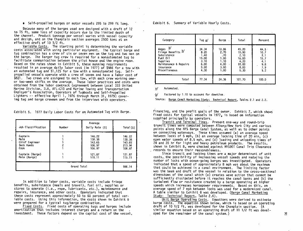
e Self-propelled barges or motor vessels 295 to 299 ft long.
Because many of the barges used are designed with a draft of 12 to 15 ft, some loss of capacity occurs due to the limited depth of the channel. Product tonnage per vessel varies with vessel capacity and design, and on the Champlain section averages 2500 tons at an effective draft of 10 1/2 ft.
Variable Costs. The starting point is determining the variable costs associated with using particular equipment. The typical barge and tug combination has a crew of six or seven men on the tug and two men on the barge. The larger tug crew is required for a nonäutomated tug to facilitate communication between the pilot house and the engine room. Based on the rates shown in Exhibit 5, these manning requirements resulted in an average daily labor cost (in 1977) of $986 for a tow with an automated tug and $1,125 for a tow with a nonautomated tug. Self-propelled vessels operate with a crew of seven and have a labor cost of $821 . Two crews are assigned to each tow, with each crew working one-or two-week shifts on the average. These labor practices and costs were obtained from the labor contract (agreement between Local 333 United Marine Division, ILA, AFL-CIO and Marine Towing and Transportation Employer's Association, Operators of Tugboats and Self-Propelled Lighters -- effective April 1, 1976 through March 31, 1979) cover-ing tug and barge crewmen and from the interviews with operators.
Exhibit 6. Summary of Variable Hourly Costs.
Category Tug a! Barge . Total Percent
Wagesb'
34.34 10.86 45.20 44.5 Fringe Benefits 1 8.20 2.70 10.90 10.7 Subsistence 1.40 .70 2.10 2.1 Fuel Oil 15.00 1.00 16.00 15.7 Supplies 3.10 1.10 4.20 4.1 Maintenance & Repairs 6.00 4.00 10.00 9.8 Insurance 5.00 3.00 8.00 7.9 Miscellaneous 4.30 1.00 5.30 5.2
Total 77.34 24.36 101.70 100.0
!/ Automated.
b/ Factored by 1.10 to account for downtime.
Source: Barge Canal Marketing Study: Technical Report, Tables 2.1 and 2.2.
Exhibit 5. 1977 Daily Labor Costs for an Automated Tug with Barge
Job Classification Number
Average
Daily Rate ($) Total(s)
Captain. 1 146.22 146.22 Mate 1 138.38 138.38 Chief Engineer 1 143.65 143.65 Deck Hands 2 106.97 213.94 Cook 1 106.97 106.97
Captain (Barge) 1 121.87 121.87 Mate (Barge) 1 115.11 . 115.11
Grand Total 986.14
In addition to labor costs, variable costs include fringe benefits, subsistence (meals and travel), fuel oil, supplies or stores to operate (i.e., rope, lubricants, etc.), maintenance and repairs, insurance, and other costs. Operators indicated that these costs represent approximately 50 to 60 percent of total var-iable costs. Using this information, the costs shown in Exhibit 6 were prepared for a typical tug/barge combination.
Fixed Costs. Fixed costs of operating tugs and barges include amortization that includes interest charges and a return on the investment. These factors depend on the capital cost of the vessel,
financing, and the profit goals of the owner. Exhibit 7, which shows fixed costs for typical vessels in 1977, is based on information supplied principally by operators.
Transit and Terminal Times. Present one-way and round-trip transit times were computed between Albany/New York City and various points along the NYS Barge Canal System, as well as to other points on connecting waterways. These times assumed (a) an average speed between locks of 5 mph, (b) an average locking time of 20 mi (c) open water speeds of 8.5 mph, and (d) loading and unloading times of 24 and 35 hr for light and heavy petroleum products. The results, shown in Exhibit 8, were checked against NYSDOT Canal Trip Clearance records to ensure their reasonableness.
Since transit and locking times are a major determinant of unit costs,.the possibility of increasing vessel speeds and reducing the number of locks with ocean-going barges was investigated. Operators indicated that a speed of approximately 8 mph was about the maximum that could be achieved in a canal environment. The limiting factor was the beam and draft of the vessel in relation to the cross-sectional dimensions of the canal which (a) creates wave action that cannot be sufficiently dissipated before it reaches the canal banks and (b) the turbulent flow or resistance created by a barge operating at higher speeds which increases horsepower requirements. Based on this, an average speed of 7 mph between locks was used for a modernized canal. A table similar to Exhibit 8 was developed. (Barge Canal Marketing Study: Technical Report, Table 2.6).
Unit Barge Operating Costs. Equations were derived to estimate barge costs. The equation shown below, which is based on an operating draft of 10 1/2 ft, was developed for the Champlain section. (A similar equation based on an operating draft of 11 1/2 ft was devel-oped for the remainder of the canal system.)
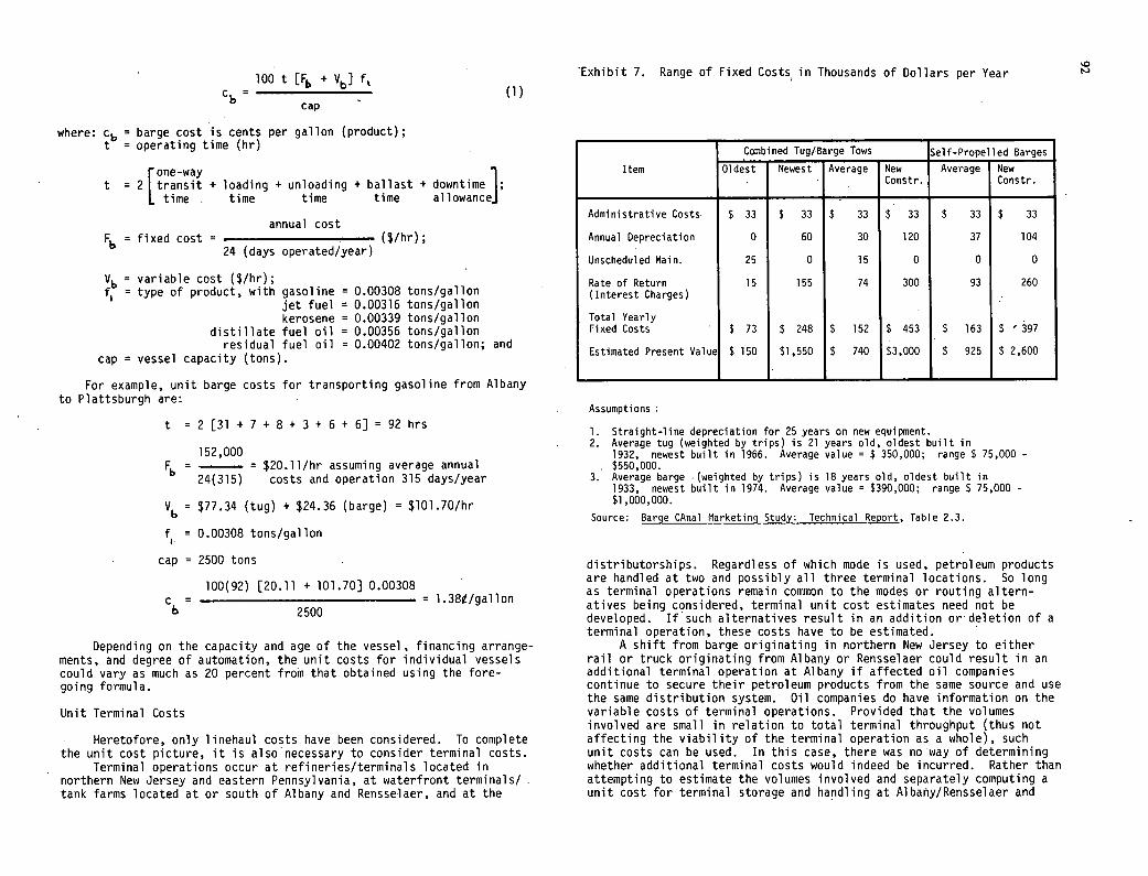
100 t [F11 + Vb] f
Exhibit 7. Range of Fixed Costs in Thousands of Dollars per Year
cb= (1) cap
where: Cb = barge cost is cents per gallon (product); t = operating time (hr)
none-way t = 2 transit + loading + unloading + ballast + downtime
I time time time time allowance
annual cost = fixed cost =
($/hr); 24 (days operated/year)
Vb = variable cost ($/hr); = type of product, with gasoline = 0.00308 tons/gallon
jet fuel = 0.00316 tons/gallon kerosene = 0.00339 tons/gallon
distillate fuel oil = 0.00356 tons/gallon residual fuel oil = 0.00402 tons/gallon; and
cap = vessel capacity •(tons).
For example, unit barge costs for transporting gasoline from Albany to Plattsburgh are:
t = 2 [31 + 7 + 8 + 3 + 6 + 6] = 92 hrs
152,000 Fb = _______ = $20.11/hr assuming average annual
24(315) costs and operation 315 days/year
= $77.34 (tug) + $24.36 (barge) = $101.70/hr
f1 = 0.00308 tons/gallon
cap = 2500 tons
100(92) [20.11 + 101.701 0.00308 C = b
2500 = 1.38/ga1lon
Depending on the capacity and age of the vessel , financing arrange-ments, and degree of automation, the unit costs for individual vessels could vary as much as 20 percent from that obtained using the fore-going formula.
Unit Terminal Costs
Heretofore, only linehaul costs have been considered. To complete the unit cost picture, it is also necessary to consider terminal costs.
Terminal operations occur at refineries/terminals located in northern New Jersey and eastern Pennsylvania, at waterfront terminals/ tank farms located at or south of Albany and Rensselaer, and at the
Item
Combined Tug/Barge Tows Self-Propelled Barges
Oldest Newest Average New Average New constr. Constr.
Administrative Costs $ 33 $ 33 $ 33 $ 33 $ 33 $ 33
Annual Depreciation 0 60 30 120 37 104
Unscheduled Main. 25 0 15 0 0 0
Rate of Return 15 155 74 300 93 260 (Interest Charges)
Total Yearly Fixed Costs $ 73 $ 248 $ 152 $ 453 $ 163 $ 1 397
Estimated Present Value $150 $1,550 $ 740 $3,000 $ 925 $ 2,600
Assumptions
Straight-line depreciation for 25 years on new equipment. Average tug (weighted by trips) is 21 years old, oldest built in 1932, newest built in 1966. Average value = $ 350,000; range $ 75,000 - $550,000. Average barge (weighted by trips) is 18 years old, oldest built in 1933, newest built in 1974. Average value = $390,000; range $ 75,000 - $1,000,000.
Source: Barge CAnal Marketing Study: Technical Report, Table 2.3.
distributorships. Regardless of which mode is used, petroleum products are handled at two and possibly all three terminal locations. So long as terminal operations remain common to the modes or routing altern-atives being considered, terminal unit cost estimates need not be developed. If such alternatives result in an addition ordeletion of a terminal operation, these costs have to be estimated.
A shift from barge originating in northern New Jersey to either rail or truck originating from Albany or Rensselaer could result in an additional terminal operation at Albany if affected oil companies continue to secure their petroleum products from the same source and use the same distribution system. Oil companies do have information on the variable costs of terminal operations. Provided that the volumes involved are small in relation to total terminal throughput (thus not affecting the viability of the terminal operation as a whole), such unit costs can be used. In this case, there was no way of determining whether additional terminal costs would indeed be incurred. Rather than attempting to estimate the volumes involved and separately computing a unit cost for terminal storage and handling at Albany/Rensselaer and
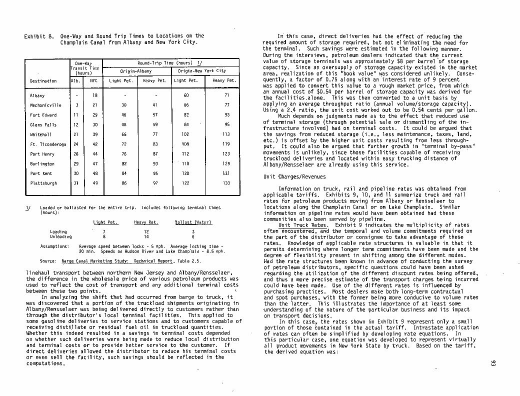
Exhibit 8. One-Way and Round Trip Times to Locations on the Champlain Canal from Albany and New York City.
One-Way Round-Trip Time (hours) 1/ ransit Time (hours) Origin-Albany
- Origin-New York City
AIb. NYC Light Pet. Heavy Pet. Light Pet. Heavy Pet. Destination
Albany - 18 - - 60 71
Mechanicville 3 21 30 41 66 77
Fort Edward 11 29 46 57 82 93
Glens Falls 12 30 48 59 84 95
Whitehall 21 39 66 77 102 113
Ft. Ticonderoga 24 42 72 83 108 119
Port Henry 26 44 76 87 112 123
Burlington 29 47 82 93 118 129
Port Kent 30 48 84 95 120 131
Plattsburgh 31 49 86 97 122 133
1/ Loaded or ballasted for the entire trip. Includes following terminal times (hours):
Light Pet. Heavy Bet. Ballast (Water)
Loading
12 Unloading
14
Assumptions: Average speed between locks - 5 mph. Average, locking time - 20 mm. Speeds on Hudson River and Lake Champlain - 8.5 mph.
Source: BargeCana1 Marketing Study: Technical Report, Table 2.5.
linehaul transport between northern New Jersey and Albany/Rensselaer, the difference in the wholesale price of various petroleum products was used to reflect the cost of transport and any additional terminal costs between these two points.
In analyzing the shift that had occurred from barge to truck, it was discovered that a portion of the truckload shipments originating in Albany/Rensselaer was being delivered directly to customers rather than through the distributor's local terminal facilities. This applied to some gasoline deliveries to service stations and to customers capable of receiving distillate or residual fuel oil in truckload quantities. Whether this indeed resulted in a savings in terminal costs depended on whether such deliveries were being made to reduce local distribution and terminal costs or to provide better service to the customer. If direct deliveries allowed the distributor to reduce his terminal costs or even sell the facility, such savings should be reflected in the computations.
In this case, direct deliveries had the effect of reducing the required amount of storage required, but not eliminating the need for the terminal. Such savings were estimated in the following manner. During the interviews, petroleum dealers indicated that the current value of storage terminals was approximately $8 per barrel of storage capacity. Since an oversupply of storage capacity existed in the market area., realization of this "book value" was considered unlikely. Conse-quently, a factor of 0.75 along with an interest rate of 9 percent was applied to convert this value to a rough market price, from which an annual cost of $0.54 per barrel of storage capacity was derived for the facilities,alone. This was then converted to a unit basis by applying an average throughput ratio (annual volume/storage capacity). Using a 2..4 ratio, the unit cost worked out to be 0.54 cents per gallon.
Much depends on judgments made as to the effect that reduced use of terminal storage (through potential sale or dismantling of the in-frastructure involved) had on terminal costs. It could be argued that the savings from reduced storage (i.e., less maintenance, taxes, land, etc.) is offset by the higher unit costs resulting from less through-put. It could also be argued that further growth in "terminal by-pass" movements is unlikely, since those facilities capable of receiving truckload deliveries and located within easy trucking distance of Albany/Rensselaer are already using this service.
Unit Charges/Revenues
Information on truck, rail and pipeline rates was obtained from applicable tariffs. Exhibits 9, 10, and 11 summarize truck and rail rates for petroleum products moving from Albany or Rensselaer to locations along the Champlain Canal or on Lake Champlain. Similar information on pipeline rates would have been obtained had these communities also been served by pipeline.
Unit Truck Rates. Exhibit 9 indicates the multiplicity of rates often encountered, and the temporal and volume commitments required on the part of the distributor or consignee to take advantage of these rates. Knowledge of applicable rate structures is valuable in that it permits determining where longer term commitments have been made and the degree of flexibility present in shifting among the different modes. Had the rate structures been known in advance of conducting the survey of petroleum distributors, specific questions could have been asked regarding the utilization of the different discount rates being offered, and thus a more precise estimate of the transport charges being incurred could have been made. Use of the different rates is influenced by purchasing practices. Most dealers make both long-term contractual and spot purchases, with the former being more conducive to volume rates than the latter. This illustrates the importance of at least some understanding of the nature o.f the particular business and its impact on transport decisions.
In this case, the rates shown in Exhibit 9 represent only a small portion of those contained in the actual tariff. Intrastate application of rates can often be simplified by developing rate equations. In this particular case, one equation was developed to represent virtually all product movements in New York State by truck. Based on the tariff, the derived equation was:
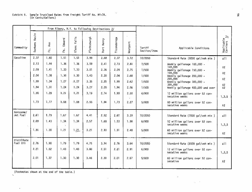
Exhibit 9. Sample Truckload Rates from Freight Tariff No. NY-7A. (In Cents/Gallons)
FromAlbany, N.Y. to_Following_Destinations 2/
C
Cnj
0 I) C E
Li.. C 0.)
S- cli
4-' 0 I - CO
Commodity - . U.) .
U, - 4- i-' 4-'
C o
CL ..-' Tariff Applicable Conditions
1-' 41 o .,- Section/Item
Gasoline 2.37 1.60 1.51 1.51 3.99 2.68 2.37 3.12 10/2050 Standard Rate (8000 gal/veh mm ) all
2.13 1.44 1.36 1.36 3.59 2.41 2.13 2.81 1/500 Weekly gallonage 100,000 - 149,999 X2
2.09 1.41 1.33 1.33 3.51 2.36 2.09 2.75 1/500 Weekly gallonage 150,000 - 199,999 X2
2.04 1.38 1.30 1.30 3.43 2.30 2.04 2.68 1/500 Weekly gallonage 200,000 - 299,999 X2
1.99 1.34 1.27 1.27 3.35 2.25 1.99 2.62 1/500 Weekly gallonage 300,000 - 399,999 X2
1.94 1.31 1.24 1.24 3.27 2.20 1.94 2.56 1/500 Weekly gallonage 400,000 and over X2
1.90 1.28 1.21 1.21 3.19 2.14 1.90 2.50 6/900 12 million gallons over 52 con- secutive weeks 1,3,5
1.73 1.17 1.08 1.08 2.93 1.94 1.73 2.27 5/800 60 million gallons over 52 con- secutive weeks X2
Kerosene/ Jet Fuel 2.61 1.79 1.67 1.67 4.41 2.92 2.61 3.39 10/2050 Standard Rate (7000 gal/veh mm ) all
2.09 1.43 1.34 1.34 2.57 1.68 1.53 1.98 6/900 12 million gallons over 52 con- secutive weeks 1,3,5
1.91 1.30 1.21 l.] 3.21 2.10 1.91 2.48 5/800 60 million gallons over 52 con- secutive weeks X2
Distillate Fuel Oil 2.76 1.90 1.79 1.79 4.75 3.14 2.76 3.64 10/2050 Standard - Rate (6500 gal/veh mm ) all
2.21 1.52 1.43 1.43 3.80 2.51 2.21 2.91 6/900 12 million gallons over 52 con- secutive weeks 1,3,5
2.01 1.37 1.30 1.30 3.46 2.30 2.01 2.67 5/800 60 million gallons over 52 con- secutive X2
(Footnotes shown at the end of the table.)
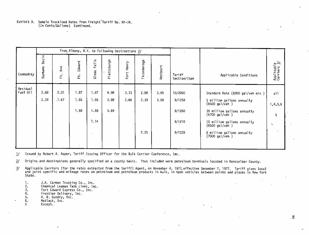
Exhibit 9. Sample Truckload Rates from Freight'Tariff No. NY-7A. (In Cents/Gallons) Continued.
From Albany, N.Y. to Following Destinations 2/
"I CA _c 0
III E
C C
ID 0 a, a, 4- s-
0
Commodity
ID - .
4-'
UJ
. 4-
(/1 C w
4141 ID
4-' 5- 0
0 u CL 4-'
Tariff Applicable Conditions
OW
os- a- I—
(1)
Section/Item D ID
Residual Fuel Oil 2.88 2.01 1.87 1.87 4.98 3.33 2.88 3.85 10/2050 Standard Rate (6000 gal/veh min all
2.39 J.67 1.55 1.55 3.98 2.66 2.39 3.08 9/1250 5 million gallons annually (6500 gal/veh ) 1,4,5,6
1.58 1.58 3.69 9/1260 35 million gallons annually (6700 gal/veh ) 5
1.14 9/1210 10 million gallons annually (6500 gal/veh
2.25 9/1220 8 million gallons annually (7000 gal/veh
1/ Issued by Robert A. Roper, Tariff Issuing Officer for the Bulk Carrier Conference, Inc.
2/ Origins and destinations generally specified on a county basis. Thus included were petroleum terminals located in Rensselaer County.
3/ Applicable Carriers (for the rates extracted from the tariff) Agent, on November 4, 19779 effective December 7, 1977. Tariff gives local and joint specific andmileage rates on petroleum and petroleum products in bulk, in tank vehicles between points and places in New York State.
J.A. Cannan Trucking Co., Inc. Chemical Leaman Tank Lines, Inc. Fort Edward Express Co., Inc. Frontier Delivery, Inc. A. R. Gundry, Inc.
- 6. Matlack, Inc. X Except.
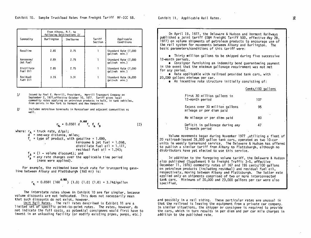
Exhibit 10. Sample Truckload Rates from Freight Tariff ME-ICC 58. Exhibit 11. Applicable Rail Rates.
Comniodity
From Albany, N.Y. to following Destinations 2/
Tariff Applicable Burlington Shelburne Section Conditions
Gasoline 2.85 2.75 1 Standard Rate (7,000 gal/veh mm.)
Kerosene! 2.85 2.75 1 Standard Rate (7,000 Jet Fuel gal/veh mm.)
Distillate 2.85 2.75 1 Standard Rate (7,000 Fuel Oil gal/veh mm.)
Residual 3.33 3.31 1 Standard Rate (6,000 Fuel Oil gal/veh mis.)
1/ Issued by Paul E. Merrill, President, Merrill Transport Company on September 2, 1977,effective October 10, 1977. Tariff gives local connnodity rates applying on petroleum products in bulk, in tank vehicles, from points in New York to Vermont and New Hampshire.
gi Includes petroleum terminals in Rensselaer and adjacent conmiunities as well.
0.8s r = 0.0501 d f) f f3 (2)
where: r. = truck rate, i/gal; d = one-way distance, miles; f, = type of product, with gasoline = 1.000,
kerosene & jet fuel = 1.098, distillate fuel oil = 1.177, residual fuel oil = 1.243;
f = (1 - volume discount); and f3 = any rate changes over the applicable time period
(none were applied).
For example, the estimated base truck rate for transporting gaso-line between Albany and Plattsburgh (160 mi) is:
o.s rt = 0.0501 (160 ) (1.0) (1.0) (1.0) = 3.74/gallon
The interstate rates shown in Exhibit 10 are far simpler, because volume discounts are not indicated. This does not necessarily mean that such discounts do not exist, however.
Unit Rail Rates. The rail rates described in Exhibit 11 are a limited set of specific point-to-point rates. The rates, however, do not indicate the full costs, as potential consignees would first have to invest in an unloading facility (or modify existing pipes, pumps, etc.)
On April 19, 1977, the Delaware & Hudson and Vermont Railways published a joint tariff (D&H Freight Tariff 500, effective May 28, 1977) on volume shipments of petroleum products to encourage use of the rail system for movements between Albany and Burlington. The basic parameters/conditions of this tariff were:
Thirty million gallons to be shipped during five successive 12-month periods.
Consignor furnishing an indemnity bond guaranteeing payment in the event that the minimum gallonage requirement was not met for any period.
Rate applicable with railroad provided tank cars, with 20,000 gallons minimum per car.
An incentive rate structure initially consisting of:
Cents/100 gallons
First 30 million gallons in 12-month period 107
Excess over 30 million gallons 95 mileage or per diem paid
No mileage or per diem paid 80
Deficit in gallonage during any 47 12-month period
Volume movements began during November 1977 ,utilizing a fleet of 20 railroad-leased 26,000 gallon tank cars, operated as two 10-car units in weekly turnaround service. The Delaware & Hudson has offered to publish a similar tariff from Albany to Plattsburgh, although no distributors have yet elected to use this service.
In addition to the foregoing volume tariff, the Delaware & Hudson also published (Supplement 9 to Freight Traffic 3-G, effective December 11, 1976) commodity rates of 167 and 155 cents/lOO gallons on petroleum products (including, residual) and residual fuel oil, respectively,.moving between Albany and Plattsburgh. The latter rate applied only on shipments comprised of two or more interconnected tank cars. Minimums of 20,000 and 2.3,000 gallons per car were also specified.
and possibly in a rail siding. These particular rates are unusual in that the railroad is leasing the equipment from a private car company. In similar situations, the shipper or consignee is required to provide the cars, which in turn results in per diem and per car mile charges in addition to the published rate.
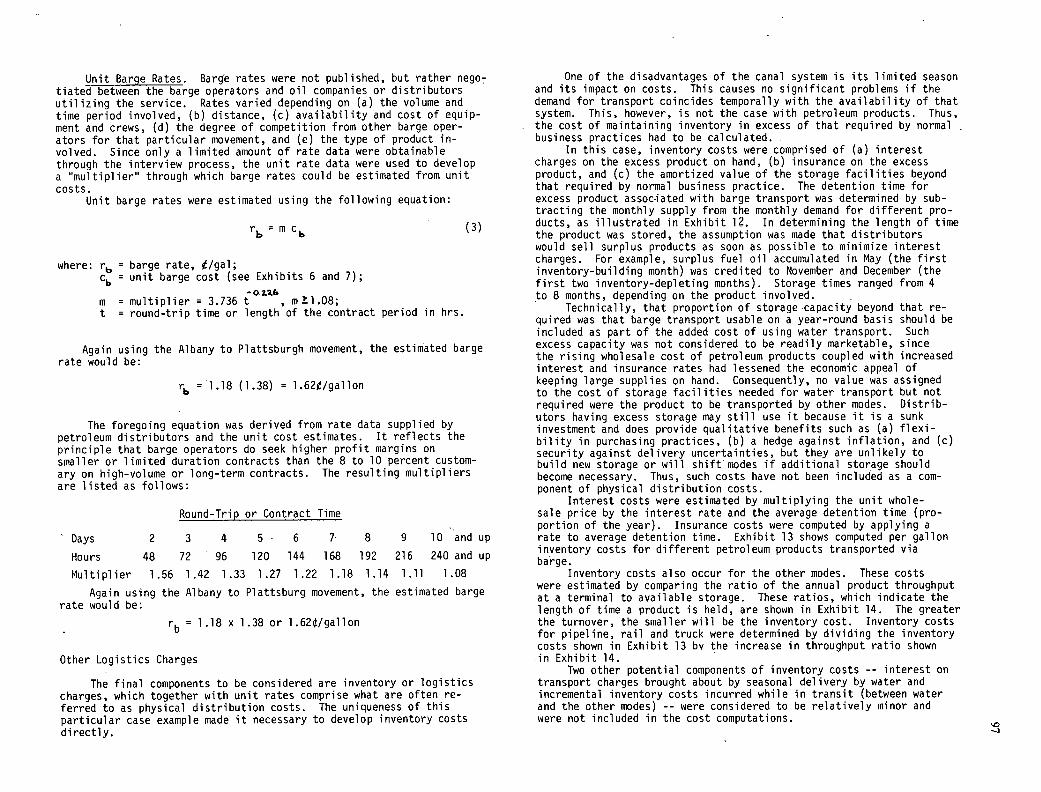
Unit Barge Rates. Barge rates were not published, but rather nego-tiated between the barge operators and oil companies or distributors utilizing the service. Rates varied depending on (a) the volume and time period involved, (b) distance, (c) availability and cost of equip-ment and crews, (d) the degree of competition from other barge oper-ators for that particular movement, and (e) the type of product in-volved. Since only a limited amount of rate data were obtainable through the interview process, the unit rate data were used to develop a multiplier through which barge rates could be estimated from unit costs.
Unit barge rates were estimated using the following equation:
rb=mcb (3)
where: rb = barge rate, i/gal;
cb = unit barge cost (see Exhibits 6 and 7); 0.22.6
m = multiplier = 3.736 t , rnfl.08; t = round-trip time or length of the contract period in hrs.
Again using the Albany to Plattsburgh movement, the estimated barge rate would be:
r. =1.18 (1.38) = 1.62e/gallon
The foregoing equation was derived from rate data supplied by petroleum distributors and the unit cost estimates. It reflects the principle that barge operators do seek higher profit margins on smaller or limited duration contracts than the 8 to 10 percent custom-ary on high-volume or long-term contracts. The resulting multipliers are listed as follows:
Round-Trip or Contract Time
Days 2 3 4 5 6 7' 8 9 10 and up
Hours 48 72 96 120 144 168 192 216 240 and up
Multiplier 1.56 1.42 1.33 1.27 1.22 1.18 1.14 1.11 1.08
Again using the Albany to Plattsburg movement, the estimated barge rate would be:
rb = 1.18 x 1.38 or 1.62/gallon
Other Logistics Charges
The final components to be considered are inventory or logistics charges, which together with unit rates comprise what are often re-ferred to as physical distribution costs. The uniqueness of this particular case example made it necessary to develop inventory costs directly.
One of the disadvantages of the canal system is its limited season and its impact on costs. This causes no significant problems if the demand for transport coincides temporally with the availability of that system. This, however, is not the case with petroleum products. Thus, the cost of maintaining inventory in excess of that required by normal business practices had to be calculated.
In this case, inventory costs were comprised of (a) interest charges on the excess product on hand, (b) insurance on the excess product, and (c) the amortized value of the storage facilities beyond that required by normal business practice. The detention time for excess product assoc-iated with barge transport was determined by sub-tracting the monthly supply from the monthly demand for different pro-ducts, as illustrated in Exhibit 12. In determining the length of time the product was stored, the assumption was made that distributors would sell surplus products as soon as possible to minimize interest charges. For example, surplus fuel oil accumulated in May (the first inventory-building month) was credited to November and December (the first two inventory-depleting months). Storage times ranged from 4 to 8 months, depending on the product involved.
Technically, that proportion of storage capacity beyond that re-quired was that barge transport usable on a year-round basis should be included as part of the added cost of using water transport. Such excess capacity was not considered to be readily marketable, since the rising wholesale cost of petroleum products coupled with increased interest and insurance rates had lessened the economic appeal of keeping large supplies on hand. Consequently, no value was assigned to the cost of storage facilities needed for water transport but not required were the product to be transported by other modes. Distrib-utors having excess storage may still use it because it is a sunk investment and does provide qualitative benefits such as (a) flexi-bility in purchasing practices, (b) a hedge against inflation, and (c) security against delivery uncertainties, but they are unlikely to build new storage or will shift modes if additional storage should become necessary. Thus, such costs have not been included as a com-ponent of physical distribution costs.
Interest costs were estimated by multiplying the unit whole-sale price by the interest rate and the average detention time (pro-portion of the year). Insurance costs were computed by applying a rate to average detention time. Exhibit 13 shows computed per gallon inventory costs for different petroleum products transported via barge.
Inventory costs also occur for the other modes. These costs were estimated by comparing the ratio of the annual product throughput at a terminal to available storage. These ratios, which indicate the length of time a product is held, are shown in Exhibit 14. The greater the turnover, the smaller will be the inventory cost. Inventory costs for pipeline, rail and truck were determined by dividing the inventory costs shown in Exhibit 13 by the increase in throughput ratio shown in Exhibit 14.
Two other potential components of inventory costs -- interest on transport charges brought about by seasonal delivery by water and incremental inventory costs incurred while in transit (between water and the other modes) -- were considered to be relatively minor and were not included in the cost computations.
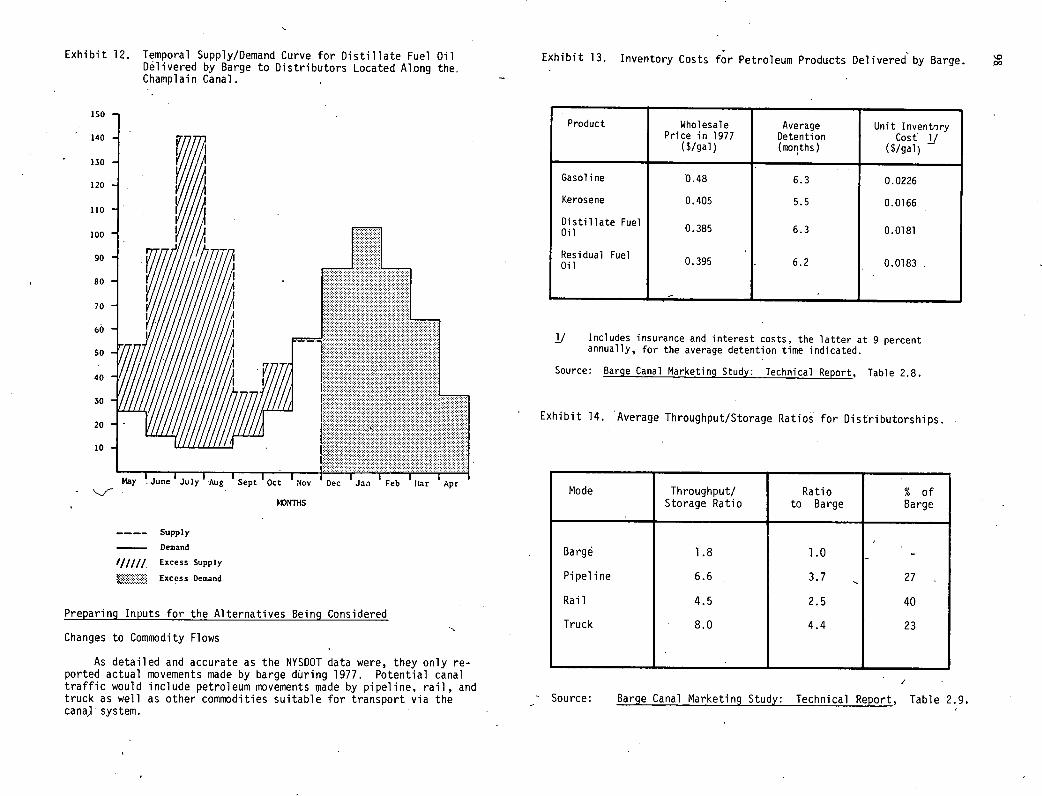
Exhibit 12. Temporal Supply/Demand Curve for Distillate Fuel Oil Exhibit 13. Inventory Costs for Petroleum Products Delivered by Barge.
Delivered by Barge to Distributors Located Al.ong the, 00
Champlain Canal.
150
140
130
120
110
100
90
80
70
60
So
40
30
20
10
ry ..,une July Aug bPt Oct Nov Dec Jai Feb lIar Apr
N111S
Supply
- Demand
Excess Supply
Excess Demand
Preparing Inputs for the Alternatives Being Considered
Changes to Commodity Flows
As detailed and accurate as the NYSDOT data were, they only re-ported actual movements made by barge during 1977. Potential canal traffic would include petroleum movements made by pipeline, rail, and truck as well as other commodities suitable for transport via the cana) system.
Product Wholesale Price in 1977
($/gal)
Average Detention (months)
Unit Inventnry Cost 1'
($/gal)
Gasoline 0.48 6.3 0.0226
Kerosene 0.405 5.5 0.0166
Distillate Fuel Oil 0.385 6.3 0.0181
Residual Fuel ' Oil 0.395 6.2 0.0183
1/ Includes insurance and interest costs, the latter at 9 percent annually, for the average detention time indicated.
Source: Barge Canal Marketing Study: Technical Report, Table 2.8.
Exhibit 14. Average Throughput/Storage Ratios for Distributorships
Mode Throughput/ Storage Ratio
Ratio to Barge
% of Barge
Barge 1.8 1.0 - Pipeline 6.6 3.7 . 27
Rail 4.5 2.5 40
Truck 8.0 4.4 23
Source: Barge Canal Marketing Study: Technical Report, Table 2.9.
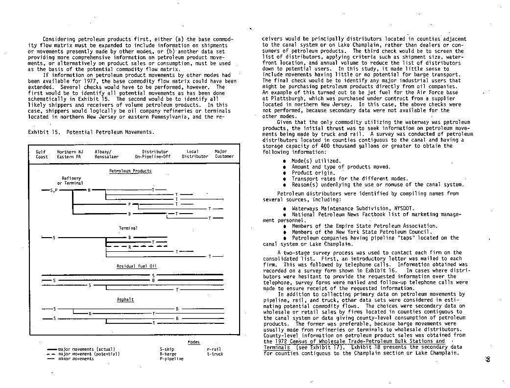
Considering petroleum products first, either (a) -the base commod-ity flow matrix must be expanded to include information on shipments or movements presently made by other modes, or (b)another data set providing more comprehensive information on petroleum product move-ments, or alternatively on product sales or consumption, must be used as the basis of the potential commodity flow matrix.
If information on petroleum product movements by other modes had been available for 1977, the base commodity flow matrix could have been extended. Several checks would have to be performed, however. The first would be to identify all potential movements as has been done schematically in Exhibit 15. The second would be to identify all likely shippers and receivers of volume petroleum products. In this case, shippers would logically be oil company refineries or terminals located in northern New Jersey or eastern Pennsylvania, and the re-
Exhibit 15. Potential Petroleum Movements.
Gulf Northern NJ Albany! Distributor Local Major Coast Eastern PA Renssalaer On-Pipeline-Off Distributor Customer
Petroleum Products
Refinery or Terminal
S,P B T
Terminal
—s 8
I -
Residual Fuel Oil
Asphalt
—S B I _________________________________________________ B I —S B
I 1•
Modes
—major movements (actual) S-ship r-rail - - major movement (potential) B-barge t-truck - minor movements P-pipeline
ceivers would be principally distributors located in counties adjacent to the canal system or on Lake Champlain, rather than dealers or con-sumers of petroleum products. The third check would be to screen the list of distributors, applying criteria such as shipment size, water-front location, and annual volume to reduce the list of distributors down to potential users. In this study, it made little sense to include movements having little or no potential for barge transport. The final check would be to identify any major industrial users that might be purchasing petroleum products directly from oil companies. An example of this turned out to be jet fuel for the Air Force base at Plattsburgh, which was purchased under contract from a supplier located in northern New Jersey. In this case, the above checks were not performed, because secondary data were not available for the other modes.
Given that the only commodity utilizing the waterway was petroleum products, the initial thrust was to seek information on petroleum move-ments being made by truck and rail . A survey was conducted of petroleum distributors located in counties contiguous to the canal and having a storage capacity of 400 thousand gallons or greater to obtain the following information:
Mode(s) utilized. Amount and type of products moved. Product origin. Transport rates for the different modes. Reason(s) underlying the use or nonuse of the canal system.
Petroleum distributors were identified by compiling names from several sources, including:
Waterways Maintenance Subdivisibn, NYSDOT. National Petroleum News Factbook list of mArketing manage-
ment personnel. Members of the Empire State Petroleum Association. Members of the New York State Petroleum Council. Petroleum companies having pipeline taps' located on the
canal system or Lake Champlain.
A two-stage survey process was used to contact each firm on the consolidated list. First, an introductory letter was mailed to each firm. This was followed by telephone calls. Information obtained was recorded on a survey form shown in Exhibit 16. In cases where distri- butors were hesitant to provide the requested information over the telephone, survey forms were mailed and follow-up telephone calls were made to ensure receipt of the requested information.
In addition to collecting primary data on petroleum movements by pipeline, rail, and truck, other data sets were considered in esti-mating potential commodity flows. The choices were secondary data on wholesale or retail sales by firms located in counties contiguous to the canal system or data giving county-level consumption of petroleum products. The former was preferable, because barge movements were usually made from refineries or terminals to wholesale distributors. County-level information on petroleum product sales was obtained from the 1972 Census of Wholesale Trade-Petroleum Bulk Stations and Terminals (see Exhibit ifl. Exhibit .18 presents the secondary data for counties contiguous to the Champlain section or Lake Champlain.
'0
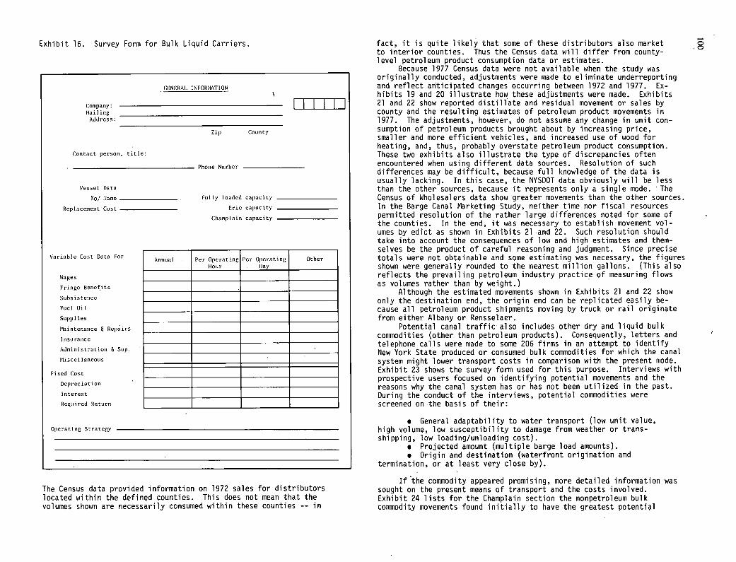
Exhibit 16. Survey Form for Bulk Liquid Carriers.
GENERAL INFORHATION
Company: I I I I Hailing
Address:
Zip County
Contact person, title:
Phone Number
Vessel Data
No/ Name Fully loaded capacity
Replacement Cost Erie capacity
Champlain capacity
Variable Cost Data For Annual per Operating Per Operating Other Flour Day
Wages
Fringe Benetits
Subsistence
Fuel Oil
Supplies
Flaintenance S Repairs
Insurance
Adninistration S Sup.
Fliscel laneous
Fixed Cost
Depreciation
Interest
Required Return
Operating Strategy
The Census data provided information on 1972 sales for distributors located within the defined counties. This does not mean that the volumes shown are necessarily consumed within these counties -- in
fact, it is quite likely that some of these distributors also market to interior counties. Thus the Census data will differ from county-level petroleum product consumption data or estimates.
Because 1977 Census data were not available when the study was originally conducted, adjustments were made to eliminate underreporting and reflect anticipated changes occurring between 1972 and 1977. Ex-hibits 19 and 20 illustrate how these adjustments were made. Exhibits 21 and 22 show reported distillate and residual movement or sales by county and the resulting estimates of petroleum product movements in 1977. The adjustments, however, do not assume any change in unit con-sumption of petroleum products brought about by increasing price, smaller and more efficient vehicles, and increased use of wood for heating, and, thus, probably overstate petroleum product consumption. These two exhibits also illustrate the type of discrepancies often encountered when using different data sources. Resolution of such differences may be difficult, because full knowledge of the data is usually lacking. In this case, the NYSDOT data obviously will be less than the other sources, because it represents only a single mode. The Census of Wholesalers data show greater movements than the other sources. In the Barge Canal Marketing Study, neither time nor fiscal resources permitted resolution of the rather large differences noted for some of the counties. In the end, it was necessary to establish movement vol-umes by edict as shown in Exhibits 21 and 22. Such resolution should take into account the consequences of low and high estimates and them-selves be the product of careful reasoning and judgment. Since precise totals were not obtainable and some estimating was necessary, the figures shown were generally rounded to the nearest million gallons. (This also reflects the prevailing petroleum industry practice of measuring flows as volumes rather than by weight.)
Although the estimated movements shown in Exhibits 21 and 22 show only the destination end, the origin end can be replicated easily be-cause all petroleum product shipments moving by truck or rail originate from either Albany or Rensselaer.
Potential canal traffic also includes other dry and liquid bulk commodities (other than petroleum products). Consequently, letters and telephone calls were made to some 206 firms in an attempt to identify New York State produced or consumed bulk commodities for which the canal system might lower transport costs in comparison with the present mode. Exhibit 23 shows the survey form used for this purpose. Interviews with prospective users focused on identifying potential movements and the reasons why the canal system has or has not been utilized in the past. During the conduct of the interviews, potential commodities were screened on -the basis of their:
General adaptability to water transport (low unit value, high volume, low susceptibility to damage from weather or trans-shipping, low loading/unloading cost).
Projected amount (multiple barge load amounts). Origin and destination (waterfront origination and
termination, or at least very close by).
Ifthe commodity appeared promising, more detailed information was sought on the present means of transport and the costs involved. Exhibit 24 lists for the Champlain section the nonpetroleum bulk commodity movements found initially to have the greatest potential
0
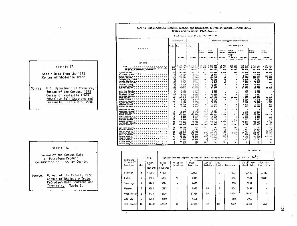
TABLE 8. Gallon Sales to Retailers, Jobbers, and Consumers, by Type 01 Product—United States, States, and Counties: 1972—Continued
7E.cU7n..c,,:,0.'.r,ILPjgub,.4 O.tOu.V81w719.NI
i
C'.Seb,p'Nthc,
04.6.60 *6.516 616 50NO1 •t 666 6.666* 041411 0.8041 çNl -. O6* flOK4TO46 754416665' f.sl,8. 7.1117,
,vpflI ls7., IOII 11.6.64.1 7l#4.) .6.0.' 716.051.) l764.I €1 0514 )I0A.I
Hr. TORN
000ls(p-,uoscy(. 0056 STNYSCNS, N RIHINOLS. COstl RUIN 57*67995, TCSIN*1.S
aLBANY COUNTY .................. ALLEUSRY COUNTY .................
.890,0 COL"ATY .................. OROOYE COUNTY .................. CUTTARAUUUS COUNTY ....... . ......... CUYUGO COUNTY .................. CNAUT 00000 COUNTY ................ CMC'UNG COUNTY ................. CYCNUNOO COUNTY .................. CLI7.736 COUNTY ................. COLU0011 COUNTY: CORTLAMO COUNTY ................. OEL*.AYE COUNTY ................. DOTCYESS COUNTY: ................ ERIE COUNTY .................. ESUEU COUNTY ................... FRANKLIN COUNTY ................. FULTON COUNTY .................. NE€'TUEC COUSTY ................. 6REEUE COUNTY .................. HIMILTONCOUNTY ................. 806.00716 COUNTY................. JEFTENSOW COUNTY ................ 00655 COUNTY .................. LEWIS COUNTY .................. I.101NUSTON COUNTY ................ MADISON COUNTY ................. 00000! COUNTY .................. HONT000ERY COUNTY ................ NOSSRU COUNTY.................. NEW YORK COUNTY ................. MAUSTA COUNTY ................. ONEIDA COUNTY .................. 030.0305. COUNTY ................. 05T4410 COUNTY .................. ORANGE COUNTY ..................
- OOI.EUSS COO'ITY ................. 057160 COUNTY. TTSTUT CO................. PUTNAY COU
UNNTTYY
. ............... I
9051 2 536 537.2 149 RON ON 0.01 N 660 75) 1 IT 725 I 295 1TY7272 :67 7705 )YN:YUL701UO' 1307 0 370 652 35 .TN 5.4 1 105 090 573 453
16 lOS 023 132 101 0311 227 685 5 723 7 I S ION 3 221 TN , 6 973 - 7
16 12295. 50977
73 617 N 91 373 i
-. -I
74 jUI 126 2491
1 ON
9 N
01 "1 S SAN
N 670 5 590
20. -.
20 3'6 7 NT)
ON 6
OR . 7
S ANN
IN 305 A 065
15 375 - . -
N 892 35 022
9) 1
N . ON
6 360 00 065
0 5.0 91 005
- - ,
5 9251 57 OST
- -
7 7 CON . 0 WIN - 5033 - - 5 11
3 597 5 162
3 209 5009
- -:
6 781- 01 075
- -
N I 32
S UY3 153 815
3 773 14,2661
- 1 43N1
6 730 I 6I3 2511
- 520
7 II 311 . 4 30 4 23 N 339 - '11
N, N 059 6 135
8 556 N 109
- -
13 INN 9 328
- -.
N 6
10 169 7 125 ,
6 55') 6 205 - .
23 217 10 009 -
II IN '
A 619 . 10 366
401 c97 .
4 227 10 160
207 090 N'
223 .
N' 17704
605 065 A
3 571 9 3 375 7 II) 20: 3 996: -
00' 00 I
8 37'. 6 580
'7 234 N 450
- - 1 13 703 IN 330
- 2
20 101 563 NO 976 o: 216 )41 1 660 01 N 752 5 499 63. 7 350 - 601 300 AN) 279 029 5'. 160 705 665 21
171 52 622 . €01 70) - IT) (VI 12 (N) (0) 7 930
979671 -
26 Ha 55)
020 350 67 NUN
ITO 609 -,
239. 205 616 22
309 13 01 997 100.5 . 206361 20
I 65 031 -
3 IUO 80 991 3 316
003: -
217 077 7 975
ION
10 9
21 853 12 594
20 653 IV)
- 897
32 262 (0)!
2 (VI
1 (DI ID) 007 107 707
005 126 205 2N2 3 708 550 1 97* 659 57 279 200 0251 2 SON 206 953 100 97 007 49 207' 1 2.30 276 I 011 35)
340 33 593 213522 37 509 - SN3 0923 - 2 506 101 903 329 302
IT UTO 1 003 059 1 775 - 1907 6060 3029 - -
1 3691 . I .7
00 690 3252
06032
- 250
- - - 1565 9 237 - 6 07 97) 58 NOt 37 112
- 690 0 931 - - -
732 659
6991 0170
- -
- 322 5929 06 008 7 593 1338-0 81 016
- 1524 5501 30621 - 2672 00367 5)02 - 3466 4303 0767
- 1032
699 6505
06 021 600 300
: 530 - 3380 26166 -
233 NO 310 339 NON 000 571 575 5995 -
- 1603 5603 270 102
4 377 1 043
22 663 6 043
INN 78 5 -
6 749
057 1063 N 396
12702 502 505
IN MN 577
095 - - 70€ VI (V) - 661 25022 - - 9 259 79 972 55 343
2 220 00 306 015 NSA DO 103 - 3904 20742 1)22 - 6 060 OIl 536 2"315 - -
325 5930
2050 27397
- 0700
(TI IV) - RN) 7UI (0) 707 €01 (DI
Exhibit 17.
Sample Data from the 1972 Census of Wholesale Trade.
Source: U.S. Department of Commerce, Bureau of the Census, 1972 Census of Wholesale Trade: Petroleum Bulk Stations and Terminals, Table 8 p. 2-96.
Source: Bureau of the Census, 1972 Census of Wholesale Trade, Petroleum Bulk Stations and Terminals, Table 8.
Selected All Est. Establishments Reporting Gallon Sales by Type of Product (gallons X 10 3
________ NY and VT Sales Sales Aviation Motor Special Jet Distillate Residual Counties No. ($ (5 Gasoline Gasoline Naphthas Fuels Kerosene Fuel Oils Fuel Oils
- housands Thousands )
Clinton 14 41065 41065 - 57057 - 9 17973 56402 33112
Essex 7 4314 4314 20 4339 - - 1524 5501 30411
Saratoga 4 4749 3224 - 8633 - - 508 3247 -
Warren 7 3393 2987 - 5377 56 1 1154 5482 -
Washington 9 13433 12926 - 17336 56 - 4424 39450 -
Addison 3 2799 2799 - 5506 - - 268 2907 -
Chittenden 12 42409 40942 16 77078 32 343 8932 83455 16375
Exhibit 18.
Bureau of the Census Data on Petroleum Product
Consumption in 1972, by County.
C
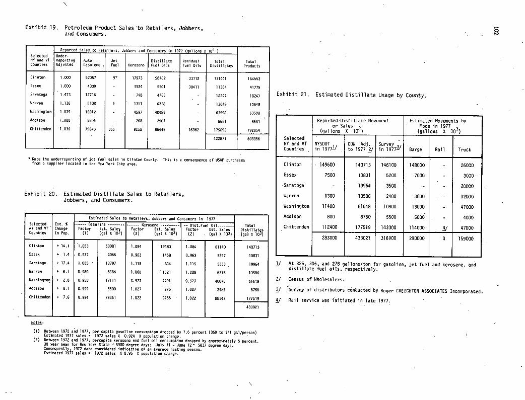
Exhibit 21. Estimated Distillate Usage by County.
Reported'Distillate Movement Estimated Movements by or Sales
(gallons X 10
Mode in 1977 (gallons X 10
Selected NY and VT counties
NYSDOT 1' in 1977-' ,
cow Adj. to 1977 2/
Survey 3/ in 1977—' Barge Rail Truck
Clinton 149600 140713 146100 148000 - 26000
Essex 7500 10831 5200 7000 - 3000
'Saratoga - 19964 3500 - - 20000
Warren 1300 13586 2400 3000 - 12000
Washington 11400 61648 10900 13000 - 47000
Addison 800 8760 5500 5000 , - 4000
.Chittenden 112400 177519 143300 114000 , 4/ 47000
283000 433021 316900 290000 0 159000
]j At 325, 305, and 278 gallons/ton for gasoline, jet fuel and kerosene, and distillate fuel oils, respectively.
2/ census of Wholesalers.
3/ Survey of distributors conducted by Roger CREIGHTON ASSOCIATES Incorporated.
4/ Rail service was initiated in late 1977.
Exhibit 19. Petroleum Product Sales to Retailers, Jobbers, and Consumers.
Reported Sales to Retailers, Jobbers and Consumers in 1972 (gallons X 102
Selected Under- NY and VT Counties
Reporting Adjusted
Auto Gasolene .
Jet Fuel Kerosene
Distillate Fuel Oils
Residual Fuel Oils
Total Distillates
Total Products
Clinton 1.000 57057 9* 17973 56402 33112 131441 164553
Essex 1.000 4339 - 1524 5501 30411 11364 41775
Saratoga 1.473 12716 - 748 4783 - 18247 18247
Warren 1.136 6108 1 1311 6228 - 13648 13648
Washington 1.039 18012 - 4597 40989 - 63598 63598
Addison 1.000 5506 - 268 2907 - 8681 8681
Chittenden 1.036 79840 355 9252 86445 16962 175892 192854
422871 503356
* Note the underreporting of jet fuel sales in Clinton County. This is a consequence of USAF purchases from a supplier located in the New York City area.
Exhibit 20. Estimated Distillate Sales to Retailers, Jobbers, and Consumers.
Estimated Sales to Retailers, Jobbers and Consumers in 1977 Selected NY and VT Counties
Est. S Change In Pop.
Total Distilla9u (gal 0 10
Gasoline --------- Factor Est. Sales (1) (gal 8 10 )
Kerosene --- ------ Factor Est. Sales (2) (gal X lOs)
— Dist.Fuel Oil Factor Est. Sales (2) (gal X 103)
Clinton + 14.1 1.053 60081 1.084 19483 1.084 61140 140713
Essex + 1.4 0.937 4066 0.963 1468 0.963 5297 10831
Saratoga 17.4 1.085 13797 1.115 834 1.115 5333 19964
Warren + 6.1 0.980 5986 1.008 1321 1.008 6278 13586
Washington + 2.8 0.950 17111 0.977 4491 0.977 40046 61648
Addison + 8.1 0.999 5500 1.027 275 1.027 2985 8760
Chittenden + 7.6 0.994 79361 1.022 9456 1.022 88347 177519
433021
Notes:
Between 1972 and 1977, per capita gasoline consumption dropped by 7.6 percent (369 to 341 gal/person) Estimated 1977 sales * 1972 sales X 0.924 8 population change. Between 1972 and 1977, percapita kerosene and fuel oil consumption dropped by approximately 5 percent. 30 year mean for New York State = 5900 degree days; July 71 - June 72= 5837 degree days. Consequently, 1972 data considered indicative of an average heating season. Estimated 1977 sales = 1972 sales 0 0.95 0 population change.
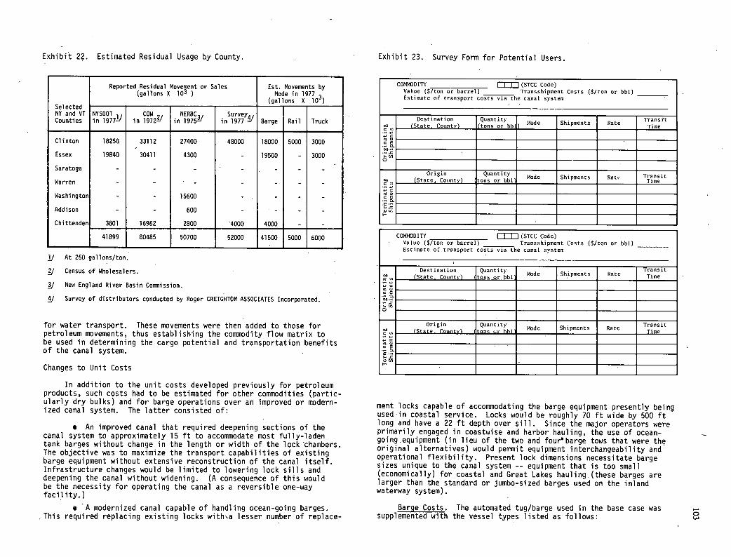
Exhibit 22. Estimated Residual Usage by County.
Reported Residual Movement or Sales (gallons X 10 )
Est. Movements by Mode in 1977
(gallons X 10
NYSDOT ,
in 1977—' cow
2' in 1972—'
Selected NERBC3,
in 1975—' Survey4,
in 1977 - Barge Rail Truck NY and VT Counties
Clinton 18258 33112 27400 48000 18000 5000 3000
Essex 19840 30411 4300 - 19500 - 3000
Saratoga - - - - - - -
warren - - - - - - -
Washington - - 15600 - - - -
Addison - - 600 - - - -
Chittenden 3801 16962 2800 4000 1 4000 1 - -
41899 80485 50700 52000 41500 5000 6000
jj At 250 gallons/ton.
/ Census of Wholesalers.
/ New England River Basin Comission.
/ Survey of distributors conducted by Roger CREIGHTON ASSOCIATES Incorporated.
for water transport. These movements were then added to those for petroleum movements, thus establishing the commodity flow matrix to be used in determining the cargo potential and transportation benefits of the canal system.
Changes to Unit Costs
In addition to the unit costs developed previously for petroleum products, such costs had to be estimated for other commodities (partic-ularly dry bulks) and for barge operations over an improved or modern-ized canal system. The latter consisted of:
An improved canal that required deepening sections of the canal system to approximately 15 ft to accommodate most fully-laden tank barges without change in the length or width of the lock chambers. The objective was to maximize the transport capabilities of existing barge equipment without extensive reconstruction of the canal itself. Infrastructure changes would be limited to lowering lock sills and deepening the canal without widening. (A consequence of this would be the necessity for operating the canal as a reversible one-way facility.)
A modernized canal capable of handling ocean-going barges. This required replacing existing locks witha lesser number of replace-
Exhibit 23. Survey Form for Potential Users.
COMMODITY JJJ (51CC Code) Value ($/tonor barrel) Transshipment Costs ($/ton or bbl) Estimate of transport costs via the canal system
Destination Quantity Mode Shipments Rate Transit
00 (State, County) (tons or bb1 Time Cu
mc. en
C. 00.
0. U) 0
- Origin Quantity Mode Shipments Rat' Transit
Os Cv
(State. County) ons or bbl Time
4.40 coo CE
0.
0. .0
I-.
COMMODITY (STCC Code) ____________ Value ($7 nor barrel) Transshipment Costs (S/ton or bbl) Estimate of transport costs via the canal system
Destination Quantity Mode Shipments Rate
Transit 00 C (State. County) tons or bbl Time
4.4
C 0.
0
00 = Origin
(State. County) Quantity
tons s,r bbl Mode Shipments Rate Transit
Time - 4.4
a C
0. C- 0. .0
In
ment locks capable of accommodating the barge equipment presently being used in coastal service. Locks would be roughly 70 ft wide by 500 ft long and have a 22 ft depth over sill. Since the major operators were primarily engaged in coastwise and harbor hauling, the use of ocean-going.equipment (in lieu of the two and four'barge tows that were the original alternatives) would permit equipment interchangeability and operational flexibility. Present lock dimensions necessitate barge sizes unique to the canal system -- equipment that is too small (economically) for coastal and Great Lakes hauling.(these barges are larger than the standard or jumbo-sized barges used on the inland waterway system).
Barge Costs. The automated tug/barge used in the base case was supplemented with the vessel types listed as follows:
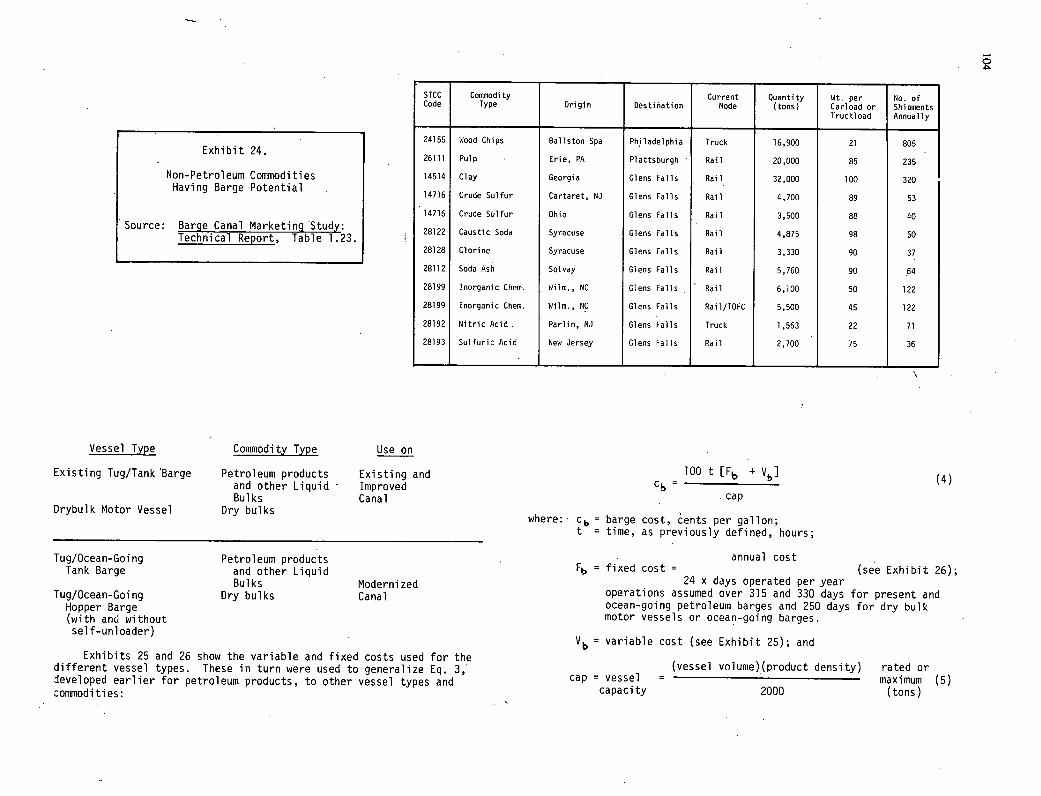
51CC Code
Comodity Type Origin Destination
Current Mode
Quantity (tons)
Wt. per Carload or Truckload
No. of Shipments Annually
24155 Wood Chips Ballston Spa Philadelphia Truck 16,900 21 805
26111 Pulp Erie, PA Plattsburgh Rail 20,000 85 235
14514 Clay Georgia Glens Falls Rail 32,000 100 320
14716 Crude Sulfur Cartaret, NJ Glens Falls Rail 4,700 89 53
14716 Crude Sulfur Ohio Glens Falls Rail 3,500 88 40
28122 Caustic Soda Syracuse Glens Falls Rail 4,875 98 50
28128 Clorine Syracuse Glens Falls Rail 3,330 90 37
28112 Soda Ash Solvay Glens Falls Rail 5,760 90 64
28199 inorganic Chem. Wilm. , NC Glens Falls Rail 6,100 50 122
28199 inorganic Chem. Wilm. , NC Glens Falls Rail/TOFC 5,500 45 122
28192 Nitric Acid. Parlin, NJ Glens Falls Truck 1,563 22 71
28193 Sulfuric Acid New Jersey Glens Falls Rail 2,700 75 36
Exhibit 24.
Non-Petroleum Commodities Having Barge Potential
Source: Barge Canal Marketing Study: Technical Report, Table 1.23.
Vessel Type Commodity Type Use on
Existing Tug/Tank Barge Petroleum products Existing and and other Liquid - Improved Bulks Canal
Drybulk Motor Vessel Dry bulks
Tug/Ocean-Going Petroleum products Tank Barge and other Liquid
Bulks Modernized Tug/Ocean-Going Dry bulks Canal
Hopper Barge (with and without self-unloader)
Exhibits 25 and 26 show the variable and fixed costs used for the different vessel types. These in turn were used to generalize Eq. 3, developed earlier for petroleum products, to other vessel types and commodities:
100 t [Fb + Vb] (4
cap
where: cb = barge cost, ents per gallon; t = time, as previously defined, hours;
annual cost = fixed cost = (see Exhibit 26);
24 x days operated per year operations assumed over 315 and 330 days for present and ocean-going petroleum barges and 250 days for dry bulk motor vessels or ocean-going barges.
Vb = variable cost (see Exhibit 25); and
(vessel volume)(product density) rated or cap = vessel = maximum (5)
capacity 2000 (tons)
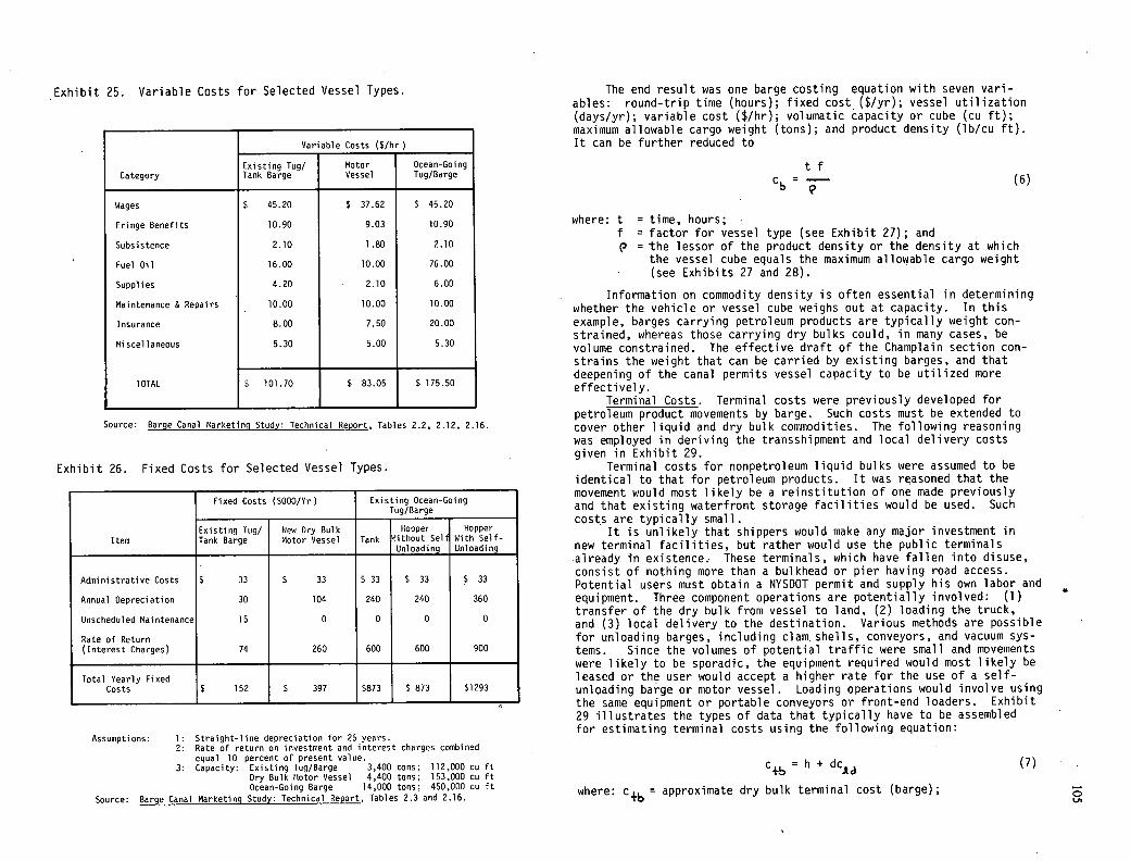
Exhibit 26. Fixed Costs for Selected Vessel Types.
Fixed Costs ($000/Yr) Existing Ocean-Going Tug/Barge
Existing Tug! Tank Barge
New Dry Balk Motor Vessel Tank
Hopper Hithout Self
Hopper With Self- Item
________________________ Unloading Unloading
Administrative Costs 5 33 $ 33 $ 33 $ 33 S 33
Annual Depreciation 30 104 240 240 360
Unscheduled Maintenance 15 0 0 0 0
Rate of Return (Interest Charges) 74 260 600 600 900
Total Yearly Fixed Costs S 152 S 397 $873 S 873 $1293
Exhibit 25. Variable Costs for Selected Vessel Types.
Variable Costs (5/hr______________
Existing Tug! Tank Barge
Motor Vessel
Ocean-Going Tug/Barge Category
Wages $ 45.20 $ 37.62 $ 45.20
Fringe Benefits 10.90 9.03 10.90
Subsistence 2.10 1.80 2.10
Fuel Oil 16.00 10.00 76.00
Supplies 4.20 2.10 6.00
Maintenance & Repairs 10.00 10.00 10.00
Insurance 8.00 7.50 20.00
Miscellaneous 5.30 5.00 5.30
TOTAL $ 101.70 $ 83.05 $175.50
Source: Barge Canal Marketing Study: Technical Report, Tables 2.2, 2.12, 2.16.
Assumptions: 1: Straight-line depreciation for 25 years. Rate of return on investment and interest charges combined equal 10 percent of present value. Capacity: Existing Tug/Barge 3,400 tons; 112,000 cu ft
Dry Bulk Motor Vessel 4,400 tons; 153,000 cu ft Ocean-Going Barge 14,000 tons; 450,000 cu ft
Source: Barge Canal Marketing Study: Technical Report, Tables 2.3 and 2.16.
The end result was one barge costing equation with seven vari-ables: round-trip time (hours); fixed cost ($/yr); vessel utilization (days/yr); variable cost ($/hr); volumatic capacity or cube (cu ft); maximum allowable cargo weight (tons); and product density (lb/cu ft). It can be further reduced to
tf
cb (6)
where: t = time, hours; f = factor for vessel type (see Exhibit 27); and
= the lessor of the product density or the density at which the vessel cube equals the maximum allowable cargo weight (see Exhibits 27 and 28).
Information on commodity density is often essential in determining whether the vehicle or vessel cube weighs out at capacity. In this example, barges carrying petroleum products are typically weight con-strained, whereas those carrying dry bulks could, in many cases, be volume constrained. The effective draft of the Champlain section con-strains the weight that can be carried by existing barges, and that deepening of the canal permits vessel capacity to be utilized more effectively.
Terminal Costs. Terminal costs were previously developed for petroleum product movements by barge. Such costs must be extended to cover other liquid and dry bulk commodities. The following reasoning was employed in deriving the transshipment and local delivery costs given in Exhibit 29.
Terminal costs for nonpetroleum liquid bulks were assumed to be identical to that for petroleum products. It was reasoned that the movement would most likely be a reinstitution of one made previously and that existing waterfront storage facilities would be used. Such costs are typically small.
It is unlikely that shippers would make any major investment in new terminal facilities, but rather would use the public terminals already in existence. These terminals, which have fallen into disuse, consist of nothing more than a bulkhead or pier having road access. Potential users must obtain a NYSDOT permit and supply his own labor and equipment. Three component operations are potentially involved: (1) transfer of the dry bulk from vessel to land, (2) loading the truck, and (3) local delivery to the destination. Various methods are possible for unloading barges, including clam, shells, conveyors, and vacuum sys- tems. Since the volumes of potential traffic were small and movements were likely to be sporadic, the equipment required would most likely be leased or the user would accept a higher rate for the use of a self-unloading barge or motor vessel. Loading operations would involve using the same equipment or portable conveyors or front-end loaders. Exhibit 29 illustrates the types of data that typically have to be assembled for estimating terminal costs using the following equation:
c+b = h + dc, (7)
where: c+b = approximate dry bulk terminal cost (barge);
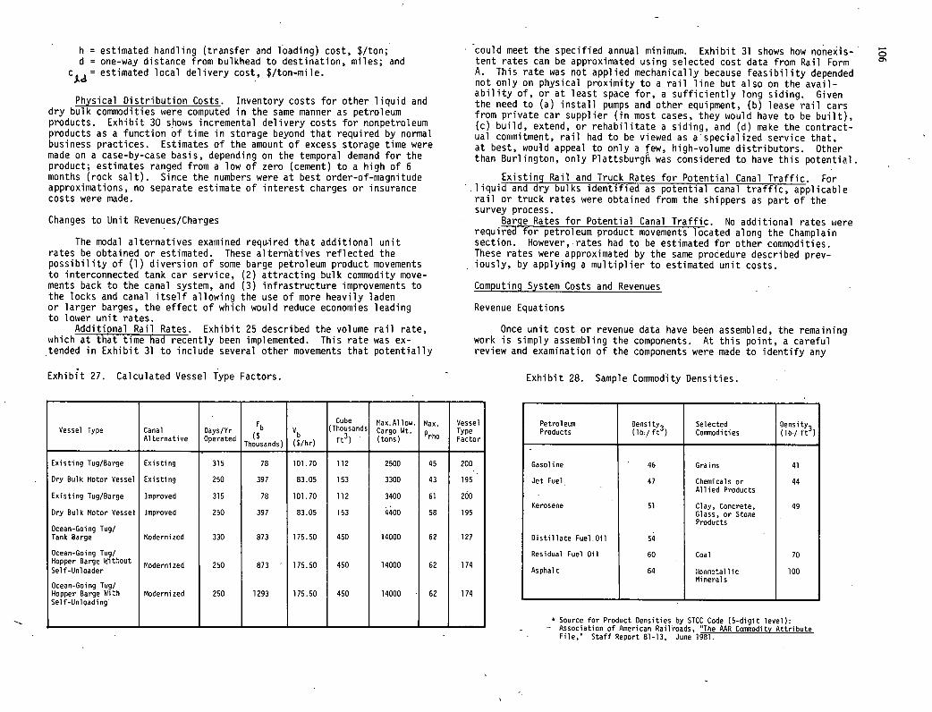
h = estimated handling (transfer and loading) cost, $/ton; d = one-way distance from bulkhead to destination, miles; and
c 1 = estimated local delivery cost, $/ton-mile.
Physical Distribution Costs. Inventory costs for other liquid and dry bulk commodities were computed in the same manner as petroleum products. Exhibit 30 shows incremental delivery costs for nonpetroleum products as a function of time in storage beyond that required by normal business practices. Estimates Gf the amount of excess storage time were made on a case-by-case basis, depending on the temporal demand for the product; estimates ranged from a low of zero (cement) to a high of 6 months (rock salt). Since the numbers were at best order-of-magnitude approximations, no separate estimate of interest charges or insurance costs were made.
Changes to Unit Revenues/Charges
The modal alternatives examined requ-ired that additional unit rates be obtained or estimated. These alternatives reflected the possibility of (1) diversion of some barge petroleum product movements to interconnected tank car service, (2) attracting bulk commodity move-ments back to the canal system, and (3) infrastructure improvements to the locks and canal itself allowing the use of more heavily laden or larger barges, the effect of which would reduce economies leading to lower unit rates.
Additional Rail Rates. Exhibit 25 described the volume rail rate, which at that time had recently been implemented. This rate was ex-tended in Exhibit 31 to include several other movements that potentially
Exhibit 27. Calculated Vessel Type Factors.
could meet the specified annual minimum. Exhibit 31 shows how nonexis-tent rates can be approximated using selected cost data from Rail Form A. This rate was not applied mechanically because feasibility depended not only on physical proximity to a rail line but also on the avail-ability of, or at least space for, a sufficiently long siding. Given the need to (a) install pumps and other equipment, (b) lease rail cars from private car supplier (in most cases, they would have to be built), (c) build, extend, or rehabilitate a siding, and (d) make the contract-ual commitment, rail had to be viewed as aspecialized service that, at best, would appeal to only a few, high-volume distributors. Other than Burlington, only Plattsburgh was considered to have this potential.
Existing Rail and Truck Rates for Potential Canal Traffic. For liquid and dry bulks identified as potential canal traffic, applicable rail or truck rates were obtained from the shippers as part of the survey process.
Barge Rates for Potential Canal Traffic. No additional rates were required for petroleum product movements located along the Champlain section. However, rates had to be estimated for other commodities. These rates were approximated by the same procedure described prev-iously, by applying a multiplier to estimated unit costs.
Computing System Costs and Revenues
Revenue Equations
Once unit cost or revenue data have been assembled, the remaining work is simply assembling the components. At this point, a careful review and examination of the components were made to identify any
Exhibit 28. Sample Commodity Densities
0 ON
Vessel Type Canal Alternative
Days/Yr Operated
F b
Thsands)
Vb
($/hr)
Cube (Thousands
ft3
Max.Allow. Cargo Wt. (tons)
Max.
p rho
Vessel Type Factor
Existing Tug/Barge Existing 315 78 101.70 112 2500 45 200
Dry Bulk Motor Vessel Existing 250 397 83.05 153 3300 43 195
Existing Tug/Barge Improved 315 78 101.70 112 3400 61 200
Dry Bulk Motor Vessel Improved 250 397 83.05 153 4400 58 195
Ocean-Going Tug! Tank Barge Modernized 330 873 176.50 450 14000 62 127
Ocean-Going Tug! Hopper Barge Without
Modernized 250 873 175.50 450 14000 62 174 Self-Unloader
Ocean-Going Tug! Hopper Barge With Modernized 250 1293 175.50 450 14000 62 174 Self -Unloading
Petroleum Products
Density3 (lb/ ft )
Selected Cononoditieu
Density3 (lb/ ft
Gasoline 46 Grains 41
Jet Fuel 47 Chemicals or 44 Allied Products
Kerosene 51 Clay, Concrete, 49 Glass, or Stone Products
Distillate Fuel Oil 54
Residual Fuel Oil 60 Coal 70
Asphalt 64 0onmtallic 100 Minerals
* Source for Product Densities by STCC Code (S-digit level): -. Association of American Railroads, The MR Conunodity Attribute
File, Staff Report 81-13, June 1981.
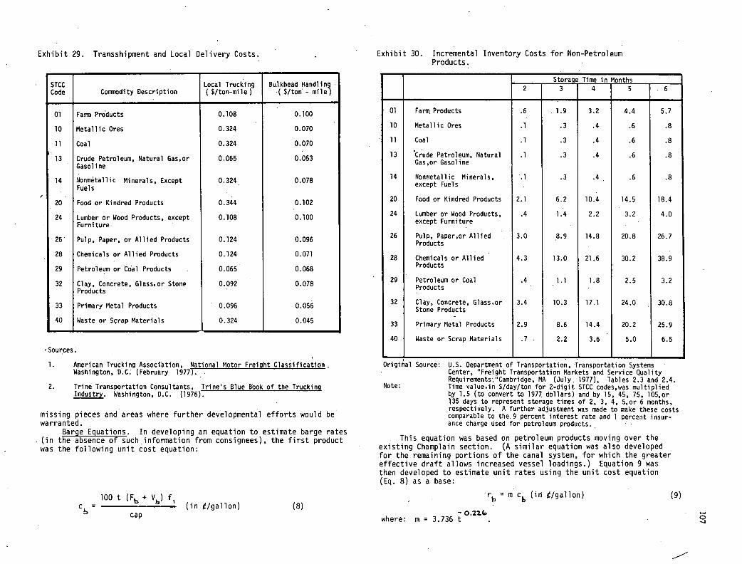
Exhibit 29. Transshipment and Local Delivery Costs.
STCC Code Conneodity Description
Local Trucking
( $/ton-mile) Bulkhead Handling
( $/ton - mile)
01 Farm Prducts 0.108 0.100
10 Metallic Ores 0.324 0.070
11 Coal 0.324 0.070
13 Crude Petroleum, Natural Gas,or 0.065 0.053 Gasoline
14 Nonmetallic Minerals, Except 0.324 0.078 Fuels
20 Food or Kindred Products 0.344 0.102
24 Lumber or Wood Products, except 0.108 0.100 Furni ture
26 Pulp, Paper, or Allied Products 0.124 0.096
28 Chemicals or Allied Products 0.124 0.071
29 Petroleum or Coal Products 0.065 0.068
32 Clay, Concrete, Glass, or Stone 0.092 0.078 Products
33 Primary Metal Products 0.096 0.056
40 Waste or Scrap Materials 0.324 0.045
Sources.
American Trucking Association, National Motor Freight Classification Washington, D.C; (February 1977).
Trine Transportation Consultants, Trifles Blue Book of the Trucking Industry. Washington, D.C. (1976).
missing pieces and areas where further developmental efforts would be warranted.
Barge Equations. In developing an equation to estimate barge rates (in the absence of such information from consignees), the first product was the following unit cost equation:
100 t (Fb + V) f1 cs = ( in i/gallon) (8)
cap
Exhibit 30. Incremental Inventory Costs for Non-Petroleum Products.
- Storage Time in Months 2 3 4 5 .6
01 Farm• Products .6 . 1.9 3.2 4.4 5.7
10 Metallic Ores .1 .3 .4 .6 .8
11 Coal .1 .3 .4 .6 .8
13 'Crude Petroleum, Natural .1 .3 .4 .6 .8 Gas,or Gasoline
14 Nonmetallic Minerals, .1 .3 .4 .6 .8 except Fuels
20 Food or Kindred Products 2.1 6.2 10.4 14.5 18.4
24 Lumber or Wood Products, .4 1.4 2.2 3.2 4.0 except Furniture
26 Pulp, Paper,or Allied . 3.0 8.9 14.8 20.8 26.7 Products
28 Chemicals or Allied 4.3 13.0 21.6 30.2 38.9 Products
29 Petroleum or Coal .4 1.1 1.8 2.5 3.2 Products .
32 Clay, Concrete, Glass,or 3.4 10.3 17.1 24.0 30.8 Stone Products
33 Primary Metal Products 2.9 8.6 14.4 20.2 25.9
40 Waste or Scrap Materials .7 . 2.2 3.6 5.0 6.5
OrigiCal Source: U.S. Department of Transportation, Transportation Systems Center, Freight Transportation Markets and Service Quality RequirementsCambridge, MA (July. 1977), Tables 2.3 and 2.4.
Note: Time value,in $/day/ton for 2-digit STCC codes,was multiplied by 1.5 (to convert to 1977 dollars) and by 15, 45, 75, 105,or 135 days to represent storage times of 2, 3, 4, 5,or 6 months, respectively. A further adjustment was made to make these costs comparable to the.9 percent interest rate and 1 percent insur-ance charge Used for petroleum products. •
This equation was based on petroleum products moving over the existing Champlain section. (A similar equation was also developed for the remaining portions of the canal system, for which the greater effective draft allows increased vessel loadings.) Equation 9 was then developed to estimate unit rates using the unit cost equation (Eq. 8) as a base:
- rb = m cb (in /gal1on)
(9)
- O.22. where: m = 3.736 t
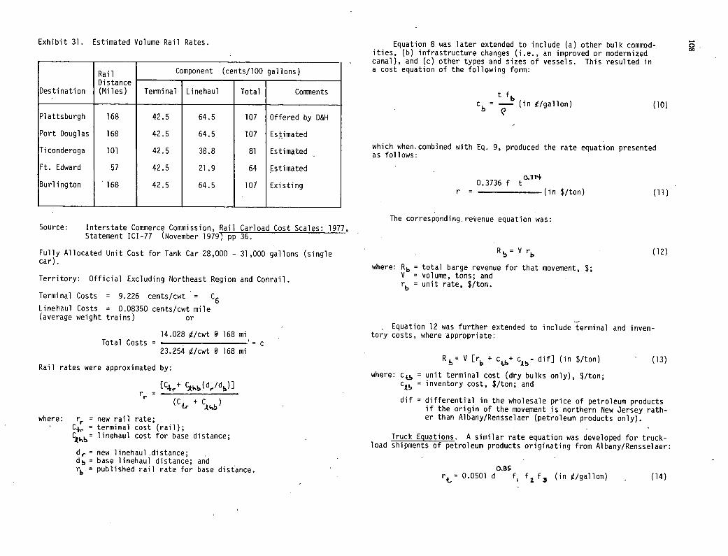
Exhibit 31. Estimated Volume Rail Rates.
Destination
Rail Distance (Miles)
Component (cents/lOO gallons)
Terminal Linehaul Total Comments
Plattsburgh 168 42.5 64.5 107 Offered by D&H
Port Douglas 168 42.5 64.5 107 Estimated
Ticonderoga 101 42.5 38.8 81 Estimated -
Ft. Edward 57 42.5 21.9 64 Estimated
Burlington 168 42.5 64.5 107 Existing
Source: Interstate Commerce Commission, Rail Carload Cost Scales: 1977, Statement ICI-77 (November 1979) pp 36.
Fully Allocated Unit Cost for Tank Car 28,000 - 31,000 gallons (single car).
Territory: Official Excluding Northeast Region and Conrail.
Terminal Costs = 9.226 cents/cwt = C6
Linehaul Costs = 0.08350 cents/cwt mile (average weight trains) or
14.028 /cwt @ 168 ml Total Costs =
= C 23.254 /cwt @ 168 ml
Rail rates were approximated by:
where: rr = new rail rate; C',. = terminal cost (rail);
linehaul cost for base distance;
d = new linehaul distance; db = base linehaul distance; and rb.= published rail rate for base distance.
Equation 8 was later extended to include (a) other bulk commod-ities, (b) infrastructure changes (i.e., an improved or modernized canal), and (c) other types and sizes of vessels. This resulted in a cost equation of the following form:
f c = - (in i/gallon) (10)
which when combined with Eq. 9, produced the rate equation presented as follows:
o.11 0.3736 f t
r = (in $/ton) (11)
The corresponding. revenue equation was:
V rb (12)
where: Rb = total barge revenue for that movement, $; V = volume, tons; and rb = unit rate, $/ton.
Equation 12 was further extended to include terminal and inven-tory costs, where appropriate:
R b = V [rb + Ctb dif] (in $/ton) (13)
where: c = unit terminal cost (dry bulks only), i/ton; c, = inventory cost, $/ton; and
dif = differential in the wholesale price of petroleum products if the origin of the movement is northern New Jersey rath-er than Albany/Rensselaer (petroleum products only).
Truck Equations. A similar rate equation was developed for truck-load shipments of petroleum products originating from Albany/Rensselaer:
O.B5 r€= 0.0501 d f1 f
z3 (in i/gallon) (14)
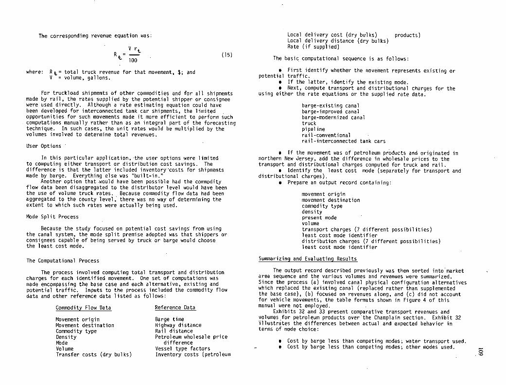
The corresponding revenue equation was:
V
Rt= _
(15) ;
where: R= total truck revenue for that movement, $; and V = volume, gallons.
For truckload shipments of other commodities and for all shipments made by rail, the rates supplied by the potential shipper or consignee were used directly. Although a rate estimating equation could have been developed for interconnected tank car shipments, the limited opportunities for such movements made it more efficient to perform such computations manually rather than as an integral part of the forecasting technique. In such cases, the unit rates would be multiplied by the volumes involved to determine total revenues.
User Options
In this particular application, the user options were limited to computing either transport or distribution cost savings. The difference is that the latter included inventorycosts for shipments made by barge. Everything else was built-in.
Another option that would have been possible had the commodity flow data been disaggregated to the distributor level would have been the use of volume truck rates. Because commodity flow data had been aggregated to the county level, there was no way of determining the extent to which such rates were actually being used.
Mode Split Process
Because the study focused on potential cost savings' from using the canal system, the mode split premise adopted was that shippers or consignees capable of being served by truck or barge would choose the least cost mode.
The Computational Process
The process involved computing total transport and distribution charges for each identified movement. One set of computations was made encompassing the base case and each alternative, existing and potential traffic. Inputs to the process included the commodity flow data and other reference data listed as follows:
Commodity Flow Data Reference Data
Movement origin
Barge time Movement destination
Highway distance Commodity type
Rail distance Density
Petroleum wholesale price MOde
difference Vol ume
Vessel type factors Transfer costs (dry bulks)
Inventory costs (petroleum
Local delivery cost (dry bulks) products) Local delivery distance (dry bulks) Rate (if supplied)
The basic computational sequence is as follows:
First identify whether the movement represents existing or potential traffic.
If the latter, identify the existing mode. Next, compute transport and distributional charges for the
using either the rate equations or the supplied rate data.
barge-existing canal barge-improved canal barge-modernized canal truck pipe] me rail-conventional rail-interconnected tank cars
If the movement was of petroleum products and originated in northern New Jersey, add the difference in wholesale prices to the transport and distributional charges computed for truck and rail.
Identify the least cost mode (separately for transport and distributional charges).
Prepare an output record containing:
movement origin movement destination commodity type density present mode volume transport charges (7 different possibilities) least cost mode identifier distribution charges (7 different possibilities) least cost mode identifier
Summarizing and Evaluating Results
The output record described previously was then sorted into'market area sequence and the various volumes and revenues were summarized. Since the process (a) involved canal physical configuration alternatives which replaced the existing canal (replaced rather than supplemented the base case), (b) focused on revenues along, and (c) did not account for vehicle movements, the table formats shown in Figure 4 of this manual were not employed.
Exhibits 32 and 33 present comparative transport revenues and volumes for petroleum products over'the Champlain section. Exhibit 32 illustrates the differences between actual and expected behavior in terms of mode choice:
Cost by barge less than competing modes; water transport used. Cost by barge less than competing modes; other modes used.
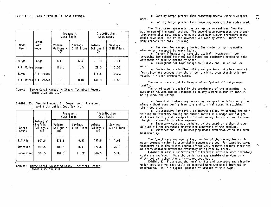
Exhibit 32. Sample Product 1: Cost Savings. • Cost by barge greater than competing modes; water transport used.
Cost by barge greater than competing modes; other modes used.
Least
Transport Cost Basis
Distribution Cost Basis
Mode Cost Volume Savings Volume Savings Used Mode Gallons X $ Millions Gallons X $ Millions
10b 106
Barge Barge 331.5 6.43 215.0 1.91
Alt. Modes Barge 165.0 1.77 29.0 0.08
Barge Alt. Modes - - 116.5 0.29
Alt. Modes Alt. Modes 5.0 0.04 141.0 0.83
Source: Barge Canal Marketing Study: Technical Report, Tables 2.25 and 2.27.
Exhibit 33. Sample Product 2: Comparison: Transport and Distribution Cost Savings.
Potential
Transport Cost Basis
Distribution Cost Basis
Traffic Volume Savings Volume Savings Barge Gallons X Gallons X $ Millions Gallons X $ Millions Canal 106 106 106
Existing 501.5 331.5 6.43 331.5 1.62
Improved 501.5 404.5 8.91 370.5 3.10
Modernized 501.5 404.5 11.82 388.5 5.38
Source: Barge Canal Marketing Study: Technical Report, Tables 2.29 and 2.30.
The first case represents the savings being realized from the active use of the canal system. The second case represents the situa-tion where alternate modes are being used even though transport costs would have been less if the movement was made by water. There are many reasons for this including:
The need for resupply during the winter or spring months when water transport is unavailable.
An unwillingness to make the capital investment in con-structing (or rehabilitating) facilities and equipment needed to take advantage of bulk shipments by water.
Throughput not high enough to justify the use of rail or water.
Desire to retain flexibility and purchase petroleum products from alternate sources when the price is right, even though this may result in higher transport costs.
The second case might be thought of as potential" waterborne traffic.
The third case is basically the complement of the preceding. A number of reasons can be advanced as to why a more expensive mode is being used, including:
Some distributors may be making transport decisions on price along without considering inventory and terminal costs in reaching their decision.
Distributors may have a deliberate policy of seeking and main-taining an inventory during the summar months as a hedge against pro-duct availability and transport problems during the winter months, even though this results in added expense.
Inventory costs may be borne by the supplier either through delayed billing practices or retained ownership of the product.
Institutional lag in changing modes from that which has been historically.
The fourth case represents that portion of the market for which water transportation is essentially noncompetitive. For example, barge transport as it now exists cannot effectively compete against pipelines or short distance movements presently being made by truck.
Exhibit 32 also illustrates the differences obtained when inventory costs are included. Mode choice is more explainable when done on a distribution rather than a transport cost basis.
Exhibit 33 illustrates the modal shifts and transport and distrib-ution cost savings that would be expected were the canal improved or modernized. it is a typical product of studies of this type.
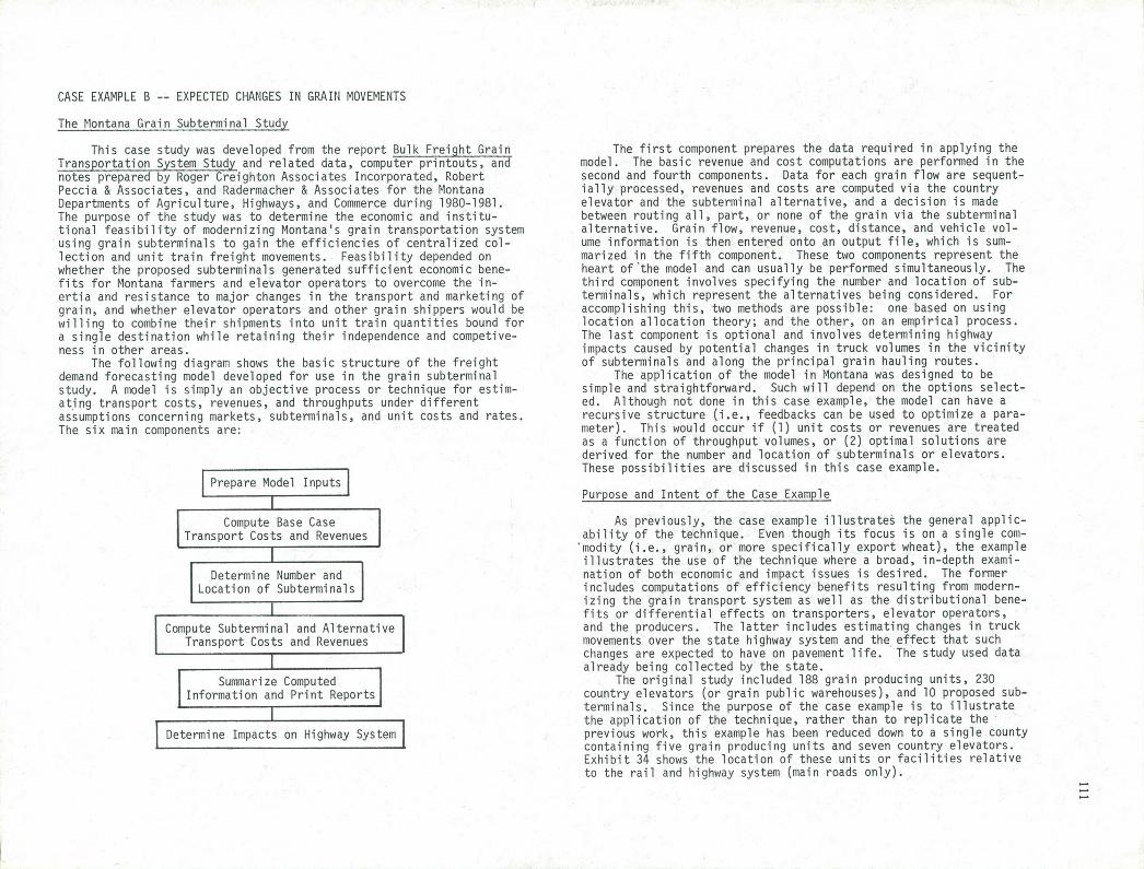
CASE EXAMPLE B -- EXPECTED CHANGES IN GRAIN MOVEMENTS
The Montana Grain Subterminal St
This case study was developed from the report Bulk Freight Grain Transportation System Study and related data, computer printouts, and notes prepared by Roger Creighton Associates Incorporated, Robert Peccia & Associates, and Radermacher & Associates for the Montana Departments of Agriculture, Highways, and Commerce during 1980-1981. The purpose of the study was to determine the economic and institu-tional feasibility of modernizing Montana's grain transportation system using grain subterminals to gain the efficiencies of centralized col-lection and unit train freight movements. Feasibility depended on whether the proposed subterminals generated sufficient economic bene-fits for Montana farmers and elevator operators to overcome the in-ertia and resistance to major changes in the transport and marketing of grain, and whether elevator operators and other grain shippers would be willing to combine their shipments into unit train quantities bound for a single destination while retaining their independence and competive-ness in other areas.
The following diagram shows the basic structure of the freight demand forecasting model developed for use in the grain subterminal study. A model is simply an objective process or technique for estim-ating transport costs, revenues, and throughputs under different assumptions concerning markets, subterminals, and unit costs and rates. The six main components are:
Prepare Model Inputs
Compute Base Case Transport Costs and Revenues
Determine Number and Location of Subterminals
Compute Subterminal and Alternative Transport Costs and Revenues
Summarize Computed Information and Print Reports
I Determine Impacts on Highway System I
The first component prepares the data required in applying the model. The basic revenue and cost computations are performed in the second and fourth components. Data for each grain flow are sequent-ially processed, revenues and costs are computed via the country elevator and the subterminal alternative, and a decision is made between routing all, part, or none of the grain via the subterminal alternative. Grain flow, revenue, cost, distance, and vehicle vol-ume information is then entered onto an output file, which is sum-marized in the fifth component. These two components represent the heart of 'the model and can usually be performed simultaneously. The third component involves specifying the number and location of sub-terminals, which represent the alternatives being considered. For accomplishing this, two methods are possible: one based on using location allocation theory; and the other, on an empirical process. The last component is optional and involves determining highway impacts caused by potential changes in truck volumes in the vicinity of subterminals and along the principal grain hauling routes.
The application of the model in Montana was designed to be simple and straightforward. Such will depend on the options select-ed. Although not done in this case example, the model can have a recursive structure (i.e., feedbacks can be used to optimize a para-meter). This would occur if (1) unit costs or revenues are treated as a function of throughput volumes, or (2) optimal solutions are derived for the number and location of subterminals or elevators. These possibilities are discussed in this case example.
Purpose and Intent of the Case Example
As previously, the case example illustrates the general applic-ability of the technique. Even though its focus is on a single com-modity (i.e., grain, or more specifically export wheat), the example illustrates the use of the technique where a broad, in-depth exami-nation of both economic and impact issues is desired. The former includes computations of efficiency benefits resulting from modern-izing the grain transport system as well as the distributional bene-fits or differential effects on transporters, elevator operators, and the producers. The latter includes estimating changes in truck movements over the state highway system and the effect that such changes are expected to have on pavement life. The study used data already being collected by the state.
The original study included 188 grain producing units, 230 country elevators (or grain public warehouses), and 10 proposed sub-terminals. Since the purpose of the case example is to illustrate the application of the technique, rather than to replicate the previous work, this example has been reduced down to a single county containing five grain producing units and seven country elevators. Exhibit 34 shows the location of these units or facilities relative to the rail and highway system (main roads only).
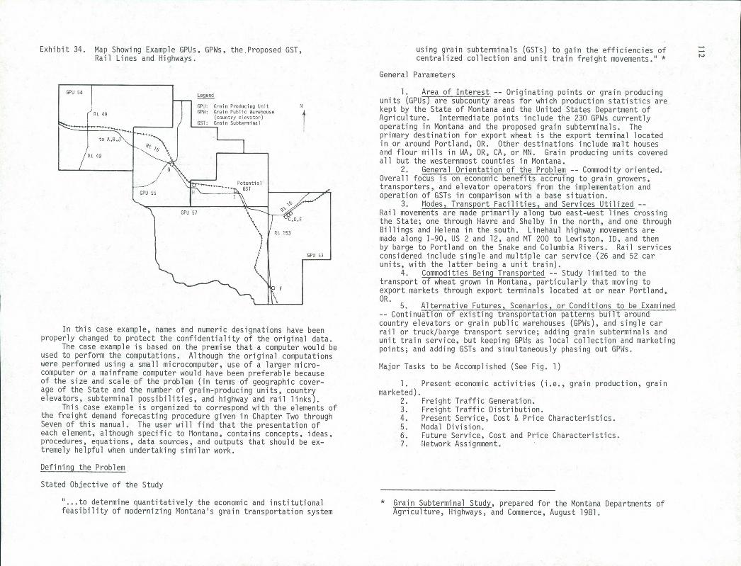
Exhibit 34. Map Showing Example GPUs, GPWs, the.Proposed GST, using grain subterminals (GSTs) to gain the efficiencies of Rail Lines and Highways. centralized collection and unit train freight movements. *
General Parameters
In this case example, names and numeric designations have been properly changed to protect the confidentiality of the original data.
The case example is based on the premise that a computer would be used to perform the computations. Although the original computations were performed using a small microcomputer, use of a larger micro-computer or a mainframe computer would have been preferable because of the size and scale of the problem (in terms of geographic cover-age of the State and the number of grain-producing units, country elevators, subterminal possibilities, and highway and rail links).
This case example is organized to correspond with the elements of the freight demand forecasting procedure given in Chapter Two through Seven of this manual. The user will find that the presentation of each element, although specific to Montana, contains concepts, ideas, procedures, equations, data sources, and outputs that should be ex-tremely helpful when undertaking similar work.
Defining the Problem
Stated Objective of the Study
'...to determine quantitatively the economic and institutional feasibility of modernizing Montana's grain transportation system
Area of Interest -- Originating points or grain producing units (GPUs) are subcounty areas for which production statistics are kept by the State of Montana and the United States Department of Agriculture. Intermediate points include the 230 GPWs currently operating in Montana and the proposed grain subterminals. The primary destination for export wheat is the export terminal located in or around Portland, OR. Other destinations include malt houses and flour mills in WA, OR, CA, or MN. Grain producing units covered all but the westernmost counties in Montana.
General Orientation of the Problem -- Commodity oriented. Overall focus is on economic benefits accruing to grain growers, transporters, and elevator operators from the implementation and operation of GSTs in comparison with a base situation.
Modes, Transport Facilities, and Services Utilized --Rail movements are made primarily along two east-west lines crossing the State; one through Havre and Shelby in the north, and one through Billings and Helena in the south. Linehaul highway movements are made along 1-90, US 2 and 12, and MT 200 to Lewiston, ID, and then by barge to Portland on the Snake and Columbia Rivers. Rail services considered include single and multiple car service (26 and 52 car units, with the latter being a unit train).
Commodities Being Transported -- Study limited to the transport of wheat grown in Montana, particularly that moving to export markets through export terminals located at or near Portland, OR.
Alternative Futures, Scenarios, or Conditions to be Examined -- Continuation of existing transportation patterns built around country elevators or grain public warehouses (GPWs), and single car rail or truck/barge transport service; adding grain subterminals and unit train service, but keeping GPWs as local collection and marketing points; and adding GSTs and simultaneously phasing out GPWs.
Major Tasks to be Accomplished (See Fig. 1)
Present economic activities (i.e., grain production, grain marketed).
Freight Traffic Generation. Freight Traffic Distribution. Present Service, Cost & Price Characteristics. Modal Division. Future Service, Cost and Price Characteristics. Network Assignment.
* Grain Subterminal Study, prepared for the Montana Departments of Agriculture, Highways, and Commerce, August 1981.
Analytical Choices
Measure Performance in Economic, Physical or Impact Terms -- Economic, primarily, because transit time, transit time reliabi-lity, and system capacity impose no major constraints on the exist-ing system and are not expected to produce major effects under the alternative plans. The potential for accelerated pavement deteri-oration and associated increases in maintenance costs due to in-creased truck volumes near the GSTs examined, thus also requiring measurement in physical and impact terms.
Estimate Modal Shares on a Unit Price or Cost Basis --Both, because rates are determined by costs, competition, and the transporter's desire to maximize profits.
Adopt a Physical Distribution or Transport Economics Orientation -- Transport economics, because growers seek to maxi-mize profits in their grain marketing decisions, of which logistics costs (e.g., on-farm or country elevator storage costs) are but one component.
Price/Cost Movements on a One-Way or Round-Trip Basis --Two-way, because the cost computations must reflect empty backhauls where these occur.
Optimizing Locations or Flows -- Not required in the study, although study could have been expanded to include optimizing GST locations.
Required Products
1. Record for each movement containing the following inform- ati on:
Identi fi cati on
Originating node (GPU). Destination.
Contents
a. Base Case
Commodity flow volumes. Linehaul mode. Composite unit cost (including collection, ware- house, and linehaul components). Composite unit rate.
b. Alternative Scenarios
Commodity flow volume. Linehaul mode. Composite unit cost. Composite unit rate.
2. Report summarizing expected economic benefits or dis- benefits associated with GST operations. Specifically, tables
showing profitability for the hypothesized subterminals, and tables showing potential impacts on grain growers, rail carriers, motor carriers, barge operators, and warehouse operators.
3. Report summarizing expected impacts on the highway network stemming from increased truck traffic in the vicinity of the hypo-thesized GSTs.
Simplifying Premises and Assumptions
Aggregate market demand is price and service inelastic. Modal division solely dependent on transport charges. Study focused solely on grain movements from the grower
to the terminal elevator (for export movements). Linehaul corn-ponents involving ocean-going vessels are excluded along with final distribution.
Types of Supporting Data Required
Commodity flows from all GPWs to all destinations via all modes.
Rail and highway network descriptions with distances and locations of warehouses.
Number and location of hypothesized GSTs, including esti-mation of GST tributary areas and, by extension, annual GST through-put.
Unit costs and revenies for all transport modes. Costs and revenues must be developed for truck, single car rail, and unit train using accepted costing models, published tariffs, and shipper- and operator-provided information.
Unit costs and revenues for the different modes, GPWs, and GSTs under several alternatives: existing GPWs (base case), existing GPWs and new GSTs, and new GSTS only. Should include constructions costs, interest, and all operating expenses.
Preparing Base Case Inputs
Grain Production and Market Data
Ample statistics are usually available on the acreage, amount, and value of the feed and food grains produced in a state each year, aggregated at the county, district, and statewide levels. Examination of such data typically reveals: (1) sizable variability in the amount of grain produced from year to year, which usually is a function of natural conditions (e.g., weather) and to a lesser extent economic factors (price, demand), (2) the relatively constant amount of acreage planted or harvested each year, and (3) gradual shifts over time among different agricultural products. Exhibit 35, which summarizes acreage and resulting production of wheat and barley grown in Montana during the 1970's, illustrates these phenomena.
The first major decision the user must make is establishing a control total for the amount of grain produced in a region or a state. This can be based on a recent or typical year, or be arbitrarily chosen to represent average conditions, as was done in choosing 1979 as the case example base year. In this particular year, Montana growers
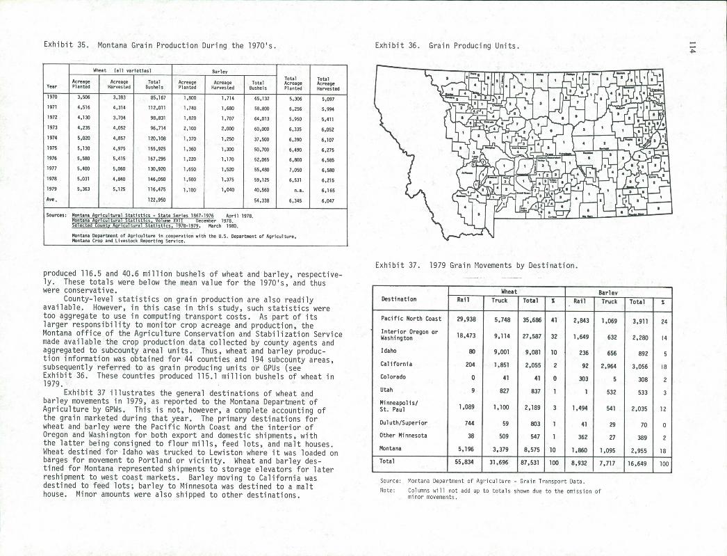
Exhibit 35. Montana Grain Production During the 1970's. Exhibit 36. Grain Producing Units. P.
Wheat (all varieties) Barley
Acreage Acreage Total Acreage Acreage Total Total Acreage
Total Acreage
Year Planted Harvested Bushels Planted Harvested Bushels Planted Hareested
1970 3,506 3.303 85,167 1,800 1.714 65,132 5.306 5,097
1971 4,516 4.314 112.011 1.740 1,600 50,000 6.256 5,994
1972 4,130 3.704 98,831 1,820 1.707 64.013 5.950 5,411
1973 4,235 4,052 96.714 2.100 2,000 60,000 6.335 6,052
1974 5,020 4,057 120,108 1.370 1.250 37,500 6,390 6,107
1975 5.130 4,975 155.925 1.360 1,300 50,700 6,490 6.275
1976 5.590 5.415 167,295 1,220 1,170 52,065 6,800 6.585
1977 5,400 5.060 130,920 1.650 1.520 55,480 7,050 6.580
1978 5,031 4.840 146.050 1.500 1,375 59.125 6.531 6,215
1979 5.363 5.125 116.475 11100 1,040 40.560 na. 6,165
Ave. 122.950 54,330 6.345 6,047
Sources: Montana Arlcultural Statistics - State Series 1067-1976 Apr11 1978. Montana Agricultural Statistics, Volume XVII December 1978. Selected county Agricultural Statistics. 1978-1979, March 1980.
Montana Department of Agriculture in cooperation with the U.S. Department of Agriculture, Montana Crop and Livestock Reporting Service.
produced 116.5 and 40.6 million bushels of wheat and barley, respective-ly. These totals were below the mean value for the 1970's, and thus were conservative.
County-level statistics on grain production are also readily available. However, in this case in this study, such statistics were too aggregate to use in computing transport costs. As part of its larger responsibility to monitor crop acreage and production, the Montana office of the Agriculture Conservation and Stabilization Service made available the crop production data collected by county agents and aggregated to subcounty areal units. Thus, wheat and barley produc-tion information was obtained for 44 counties and 194 subcounty areas, subsequently referred to as grain producing units or GPUs (see Exhibit 36. These counties produced 115.1 million bushels of wheat in 1979.
Exhibit 37 illustrates the general destinations of wheat and barley movements in 1979, as reported to the Montana Department of Agriculture by GPWs. This is not, however, a complete accounting of the grain marketed during that year. The primary destinations for wheat and barley were the Pacific North Coast and the interior of Oregon and Washington for both export and domestic shipments, with the latter being consigned to flour mills, feed lots, and malt houses. Wheat destined for Idaho was trucked to Lewiston where it was loaded on barges for movement to Portland or vicinity. Wheat and barley des-tined for Montana represented shipments to storage elevators for later reshipment to west coast markets. Barley moving to California was destined to feed lots; barley to Minnesota was destined to a malt house. Minor amounts were also shipped to other destinations.
Exhibit 37. 1979 Grain Movements by Destination.
Wheat Barley Destination Rail Truck Total % Rail Truck Total %
Pacific North Coast 29,938 5,748 35,686 41 2.843 1,069 3,911 24
Interior Oregon or Washington 18,473 9.114 27,587 32 1,649 632 2,280 14
idaho 80 9,001 9.081 10 236 656 892 5
California 204 1.851 2,055 2 92 2,964 3,056 18
Colorado 0 41 41 0 303 5 308 2
Utah 9 827 837 1 1 532 533 3
Minneapolis/ St. Paul 1.089 1,100 2.189 3 1,494 541 2.035 12
Duluth/Superior 744 59 803 1 41 29 70 0
Other Minnesota 38 509 547 1 362 27 389 2
Montana 5,196 3.379 8,575 10 1.860 1,095 2.955 18
Total 55,834 31,696 87,531 100 8,932 7.717 16.649 100
Source: Montana Department of Agriculture - Grain Transport Data.
Note: Columns will not add up to totals shown due to the omission of minor movements.
Grain produced is not necessarily grain marketed and transported. The availability of large amounts of storage both in GPWs and, par-ticularly, in on-farm silos provides appreciable flexibility to the grain grower seeking the most advantageous moment to market his product. Other factors affecting marketing (besides price or demand) include the amount retained on-farm for seed or as cattle feed, losses from shrink-age age or spoilage, transport availability, and the need to provide room for future crop storage. Thus the second major decision the user must make is to estimate the aggregate amount or the proportion of grain produced that is actually marketed, recognizing that substantial differences can occur between grain produced and grain marketed from year to year, although over the long run grain consumption must be in balance with grain production. Montana grain reported as being marketed in 1979 includes a portion of the 1979 harvest plus portions of previous years' harvests.
Most of the Montana-produced wheat and barley was marketed by the 230 State or Federal licensed country elevators or GPWs then in exis-tence in Montana. The fairly small portion not marketed through GPWs typically finds its way to markets through "track buyers," who pre-dominantly use motor carriers to transport wheat and barley directly to customers. Unfortunately, little information existed on the amount and destination of grain bypassing GPWs, thus making a complete account-ing of grain movements impossible. However, such grain is unlikely to move through subterminals.
Commodity Flows
The case example essentially involves a two-step process: (1) linking GPU-produced grain with GPW throughputs, and then (2) linking these throughputs with market demand. To do this, the user would have to accomplish the following subsidiary tasks:
Define the boundaries of GPUs; determine associated grain production, and approximate or calculate the centroid locations.
Determine the total throughput of each GPW. Determine the over-the-highway distance between GPU5 and
nearby GPWs, or assign Cartesian coordinates to each GPU and GPW and compute airline distances, using a circuity factor to approximate over-the-highway distances.
Estimate the proportion of GPU-produced grain that is actually marketed.
Allocate GPU-marketed grain among different GPWs. Determine markets, associated demand, and mode combi- -
nations servicing those markets. Determine over-the-rail and over-the-highway distance
between GPWs and markets. Allocate GPW-handled grain among the different market/
mode combinations.
The latter task is all-important. It can be accomplished in one of several ways:
Using Data Collected on a Systematic Basis by a State Agricultural Agency -- An example of this is Montana's Grain Move-
ment System, which collects commodity flow information on a monthly basis from all elevators licensed by the State. Information is ob-tained on the volume (bushels), vehicles and mode used (number of boxcars, covered hoppers, and grain trucks) and commodity type (winter, spring and durum wheat, barley, etc.), and destination. Such a system can provide excellent information on present flows provided that (1) a high degree of participation is maintained, (2) periodic audits or checks are conducted to ensure the receipt of accurate information, and (3) the information is afforded the confi-dentiality mandated by elevator operators and grain companies in supplying the information.
A Comprehensive Survey of Grain Movements -- Such a sur-vey, if carefully executed, should produce results comparable to the above. It does place a greater immediate burden on elevator operators because it forces them to go back and dig out records covering, say, a one-year period.
Allocation Models (Entropy Maximizing Models) -- To do this, further information is required on the aggregate use of different modes by market. Application of the model normally requires that two constraints be satisfied: (1) the sum of the commodity flows from the GPW must equal the total throughput of the GPW, and (2) the sum of the traffic received at each market/mode possibility must equal predetermined totals. An iterative process must be used to accom-plish this allocation. The impedance function that drives the al-location process (algorithm) usually involves "generalized cost" (i.e., some function representative of cost/distance). Close agree-ment with observed market patterns may not be achieved, however, given the competition taking place and institutional factors affect-ing the choice of markets.
In this case example, a combination of data sources was used to estimate GPW throughputs (where necessary) and GPW-to-market commodity flows, because no single source covered all GPWs or grain movements. Component data sources used included.
Montana's Grain Movement System. The Montana Wheat and Marketing Research Commission's
records on bushels of wheat and barley for which assessments were paid to the Commission.
A mailout-mailback survey of all GPWs conducted in June 1980.
Aggregated carload data for both origins and destinations, as prepared by the Burlington Northern.
Disaggregate traffic data by station, as provided by the Milwaukee Road.
The methodology fashioned to reconcile differences among data sources exploited the positive attributes of each of the available sources, relying on reasoning, professional judgment, and knowledge of grain operations in Montana to derive reasonable estimates in the face of conflicting or missing data. Exhibit 38 illustrates how this was done. -
Once GPW throughputs were estimated, it was then possible to apportion GPU production to GPWs. It can be done by either:
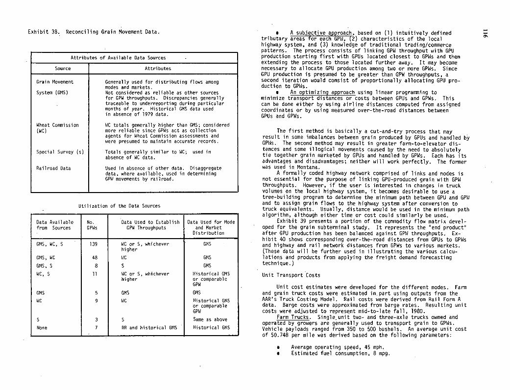
Exhibit 38. Reconciling Grain Movement Data.
Attributes of Available Data Sources -
Source Attributes
Grain Movement Generally used for distributing flows among modes and markets.
System (GMS) Not considered as reliable as other sources for GPW throughputs. Discrepancies generally traceable to underreporting during particular months of year. Historical GMS data used in absence of 1979 data.
Wheat Commission WC totals generally higher than GMS; considered (WC) more reliable since GPWs act as collection
agents for Wheat Commission assessments and were presumed to maintain accurate records.
Special Survey (s) Totals generally similar to WC; used in absence of WC data.
Railroad Data Used in absence of other data. Disaggregate data, where available, used in determining GPW movements by railroad.
Utilization of the Data Sources
Data Available from Sources
No. GPWs
Data Used to Establish GPW Throughputs
Data Used for Mode and Market Distribution
GMS, WC, S 139 WC or 5, whichever GMS higher
GMS, WC 48 WC GMS
GMS, 5 8 S GMS
WC, S 11 WC or 5, whichever Historical GMS higher or comparable
GPW
GMS 5 GMS GMS
WC 9 WC Historical GMS or comparable GPW
5 3 5 Same as above
None 7 RR and historical GMS Historical GMS
A subjective approach, based on (1) intuitively defined tributary areas for each GPW, (2) characteristics of the local highway system, and (3) knowledge of traditional trading/commerce patterns. The process consists of linking GPW throughput with GPU production starting first wi.th GPUs located closest to GPWs and then extending the process to those located further away. It may become necessary to allocate GPU production among two or more GPWs. Since GPU production is presumed to be greater than GPW throughputs, a second iteration would consist of proportionally allocating GPU pro-duction to GPWs.
An optimizing approach using linear programming to minimize transport distances or costs between GPUs and GPWs. This can be done either by using airline distances computed from assigned coordinates or by using measured over-the-road distances between GPUs and GPWs.
The first method is basically a cut-and-try process that may result in some imbalances between grain produced by GPUs and handled by GPWs. The second method may result in greater farm-to-elevator dis-tances and some illogical movements caused by the need to absolutely tie together grain marketed by GPUs and handled by GPWs. Each has its advantages and disadvantages; neither will work perfectly. The former was used in Montana.
A formally coded highway network comprised of links and nodes is not essential for the purpose of linking GPU-produced grain with GPW throughputs. However, if the user is interested in changes in truck volumes on the local highway system, it becomes desirable to use a tree-building program to determine the minimum path between GPU and GPW and to assign grain flows to the highway system after conversion to truck equivalents. Usually, distance would be used in the minimum path algorithm, although either time or cost could similarly be used.
Exhibit 39 presents a portion of the commodity flow matrix devel-oped for the grain subterminal study. It represents the "end product" after GPU production has been balanced against GPW throughputs. Ex-hibit 40 shows corresponding over-the-road distances from GPUs to GPWs and highway and rail network distances from GPWs to various markets. (These data will be further used in illustrating the various calcu-lations and products from applying the freight demand forecasting technique.)
Unit Transport Costs
Unit cost estimates were developed for the different modes. Farm and grain truck costs were estimated in. part using outputs from the AAR's Truck Costing Model. Rail costs were derived from Rail Form A data. Barge costs were approximated from barge rates. Resulting unit costs were adjusted to represent mid-to-late fall, 1980.
Farm Trucks. Single.unit two- and three-axle trucks owned and operated by growers are generally used to transport grain to GPWs. Vehicle payloads ranged from 350 to 500 bushels. An average unit cost of $0.748 per mile was derived based on the following parameters:
Average operating speed, 45 mph. Estimated fuel consumption, 8 mpg.
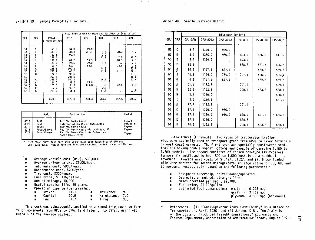
Exhibit 39. Sample Commodity Flow Data.
- Act. Transported by Mode and Destination (see below)
8012 8022 8011 8014 8021 SPU GPW Wheat (Thousands bu)
53 C 63.6 34.0 29.6 53 D 186.9 38.3 114.1 1.3 28.7 4.5 53 E 92.4 90.4 2.0 53 F 152.5 53.4 2.1 97.0 54 5 158.8 69.2 53.5 28.5 7.6 54 3 83:9 27.6 39.8 1.7 7.7 7.1 55 5 158.7 69.1 53.5 28.5 7.6 55 A 245.5 200.2 14.6 30.7 55 B 281.7 66.2 11.1 11.7 192.7 56 H 127.9 96.6 31.3 56 1 250.4 201.6 48.8 56 A 245.5 200.2 14.6 30.7 57 C 64.0 34.2 29.8 57 D 186.6 38.3 114.0 1.2 28.6 4.5 57 E 92.7 90.7 2.0 57 B 281.7 66.2 11.1 11.7 192.7
r 2672.8 I
1322.8 434.3 I
113.0 I I
147.5 I
655.2
Mode Destination Market
8012 Rail Pacific North Coast Export 8022 Rail Interior of Oregon or Washington Domestic 8011 Truck Pacific North Coast Export 8014 Truck/Barge Pacific North Coast via Lewiston, ID. Export 8021 Truck/Barge Pacific North Coast via Columbia or Export
Snake River Ports.
* Fictitious names have been used to maintain confidentiality of GPO and GPW-level data. Actual data are from two counties located in central Montana
Average vehicle cost (new), $30,000. Average driver salary, $5.00/hour. Insurance cost, $900/year. Maintenance cost, $700/year. Tire cost, $300/year. Fuel Price, $1.176/gallon. Annual mileage, 10,000. Useful service life, 10 years. Operating Expense (cents/mile):
Driver 11.1 • Insurance 9.0 Capital 30.0 • Maintenance 7.0 Fuel 14.7 • Tires 3.0
This cost was subsequently applied on a round-trip basis to farm truck movements from GPUs to GPWs (and later on to GSTs), using 425 bushels as the average payload.
Exhibit 40. Sample Distance Matrix.
GPU GPW Distance (miles)
GPU-GPW GPW-8012 GPW-8022 GPW-8011 GPW-8014 GPW-8021
53 C 3.7 1330.9 960.9 53 D 3.7 1330.9 960.9 893.5 526.6 641.5 53 E 3.7 1330.9 . 893.5 53 F 22.2 888.2 521.3 636.2 54 G 16.6 1197.6 827.6 454.8 569.7 54 J 44.2 1129.9 759.9 787.4 420.5 5354 55 G 4.3 1197.6 827.6 454.8 569.7 55 A 61.8 1132.8 791.1 539.1 55 B 62.3 1132.2 790.1 423.2 538.1 56 H 3.1 1210.9 558.3 56 I 3.8 1216.3 551.5 56 A 77.7 1132.8 791.1 57 C 17.1 1330.9 960.9 57 D 17.1 1330.9 960.9 888.5 521.6 636.5 57 E 17.1 1330.9 888.5 57 B 80.2 1332.2 790.1 423.2 538.1
Grain Trucks (Linehaul). Two types of tractor/semitrailer rigs were typically used to transport grain from GPWs to river terminals or west coast markets. The first type was specially constructed semi-trailers having double hopper bottoms and capable of carrying 1,100 to 1,200 bushels. The second consisted of varied box-type semitrailers temporarily outfitted to haul 800 to 1,000 bushels as a backhaul movement. Average unit costs of $1.427, $1.27, and $1.15 per loaded mile were derived for loaded mileage/total mileage ratios of 70, 80, and 90 percent, respectively, based on the following parameters:*
Equipment ownership, driver owned/operated. Depreciation method, straight line. Miles operated per year, 99,700. Fuel price, $1.12/gallon. Estimated fuel consumption: empty - 6.273 mpg
grain - 3.162 mpg plywood- 3.802 mpg (backhaul)
References: (1) Owner-Operator Truck Cost Guide," USDA Office of Transportation, April 1980; and (2) Jansen, D.R., "An Analysis of the Costs of Truckload Freight Operations," Economics and Finance Department, Association of American Railroads, August 1979.
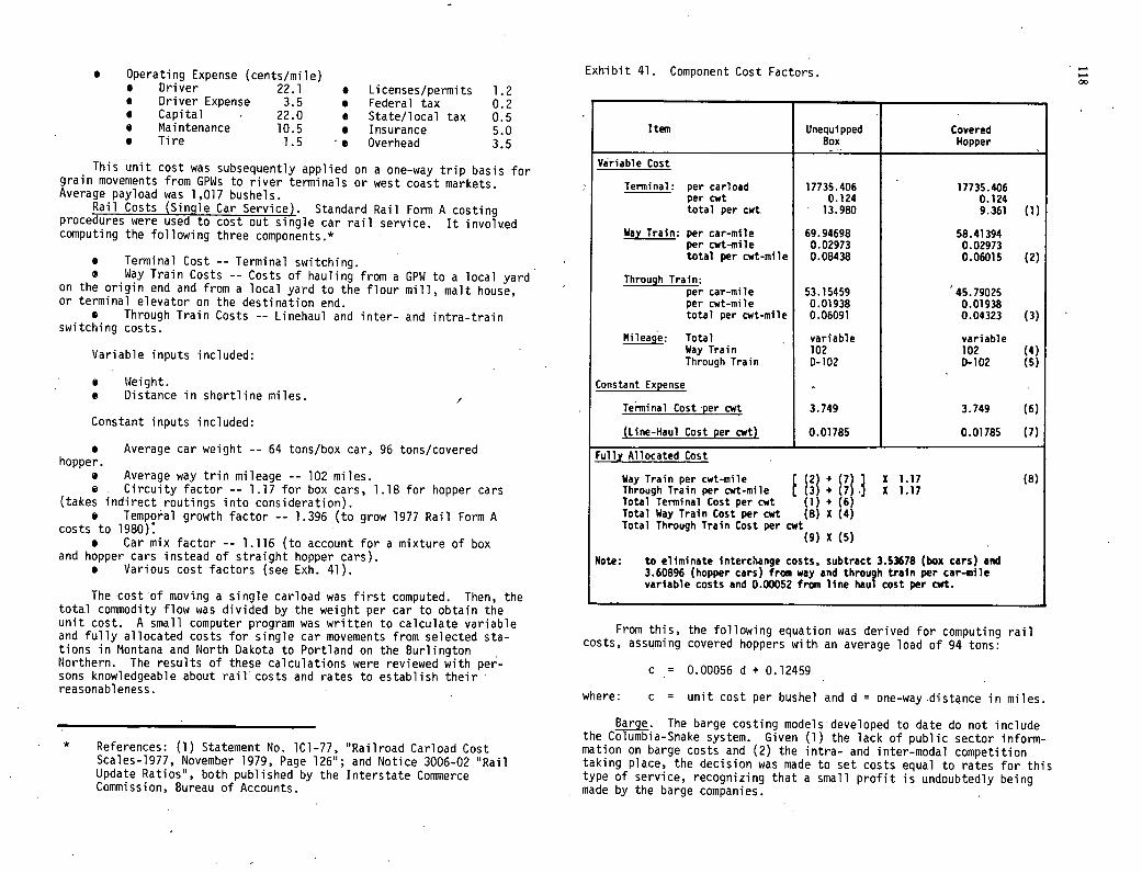
a Operating Expense (cents/mile) • Driver 22.1 • Licenses/permits 1.2 • Driver Expense 3.5 • Federal tax 0.2 • Capital - 22.0 a State/local tax 0.5 • Maintenance 10.5 . Insurance 5.0 • Tire 1.5 - e Overhead 3.5
This unit cost was subsequently applied on a one-way trip basis for grain movements from GPWs to river terminals or west coast markets. Average payload was 1,017 bushels.
Rail Costs (Single Car Service). Standard Rail Form A costing procedures were used to cost out single car rail service. It involved computing the following three components.*
Terminal Cost -- Terminal switching. a Way Train Costs -- Costs of hauling from a GPW to a local yard
on the origin end and from a local yard to the flour mill, malt house, or terminal elevator on the destination end.
Through Train Costs -- Linehaul and inter- and intra-train switching costs.
Variable inputs included:
Weight. a Distance in shortline miles. /
Constant inputs included:
Average car weight -- 64 tons/box car, 96 tons/covered hopper.
Average way trin mileage -- 102 miles. a Circuity factor -- 1.17 for box cars, 1.18 for hopper cars
(takes indirect routings into consideration). Temporal growth factor -- 1.396 (to grow 1977 Rail Form A
costs to 1980): Car mix factor -- 1.116 (to account for a mixture of box
and hopper cars instead of straight hopper cars). Various cost factors (see Exh. 41).
The cost of moving a single carload was first computed. Then, the total commodity flow was divided by the weight per car to obtain the unit cost. A small computer program was written to calculate variable and fully allocated costs for single car movements from selected sta-tions in Montana and North Dakota to Portland on the Burlington Northern. The results of these calculations were reviewed with per-sons knowledgeable about rail costs and rates to establish their reasonableness.
* References: (1) Statement No. 1C1-77, "Railroad Carload Cost Scales-1977, November 1979, Page 126"; and Notice 3006-02 "Rail Update Ratios", both published by the Interstate Commerce Commission, Bureau of Accounts.
Exhibit 41. Component Cost Factors.
Item Unequipped Covered Box Hopper
Variable Cost
Terminal: per carload 17735.406 17735.406 per cwt 0.124 0.124 total per cwt 13.980 9.361 (1)
Way Train: per car-mile 69.94698 58.41394 per cwt-mile 0.02973 0.02973 total per cwt-mile 0.08438 0.06015 (2)
Through Train: per car-mile 53.15459 45.79025 per cwt-mile 0.01938 0.01938 total per cwt-mile 0.06091 0.04323 (3)
Mileage: Total variable variable Way Train 102 102 (4) Through Train 0-102 D-102 (5)
Constant Expense
Terminal Cost per cwt 3.749 3.749 (6)
(Line-Haul Cost per cwt) 0.01785 0.01785 (7)
Fully Allocated Cost
Way Train per cwt-mile [ (2) + (7) ) X 1.17 (8) Through Train per cwt-mile [ (3) + (7) ] 1 1.17 Total Terminal Cost per cwt (1) + (6) Total Way Train Cost per cwt (8) I (4) Total Through Train Cost per cwt
(9)x(5)
Note: to eliminate 1ntercange costs, subtract 3.53678 (box cars) and 3.60896 (hopper cars) from way and through train per car-mile variable costs and 0.00052 from line haul cost per cwt.
From this, the following equation was derived for computing rail costs, assuming covered hoppers with an average load of 94 tons:
c = 0.00056 d + 0.12459
where: c = unit cost per bushel and d = one-way distance in miles.
The barge costing models developed to date do not include the Columbia-Snake system. Given (1) the lack of public sector inform-mation on barge costs and (2) the intra- and inter-modal competition taking place, the decision was made to set costs equal to rates for this type of service, recognizing that a small profit is undoubtedly being made by the barge companies.
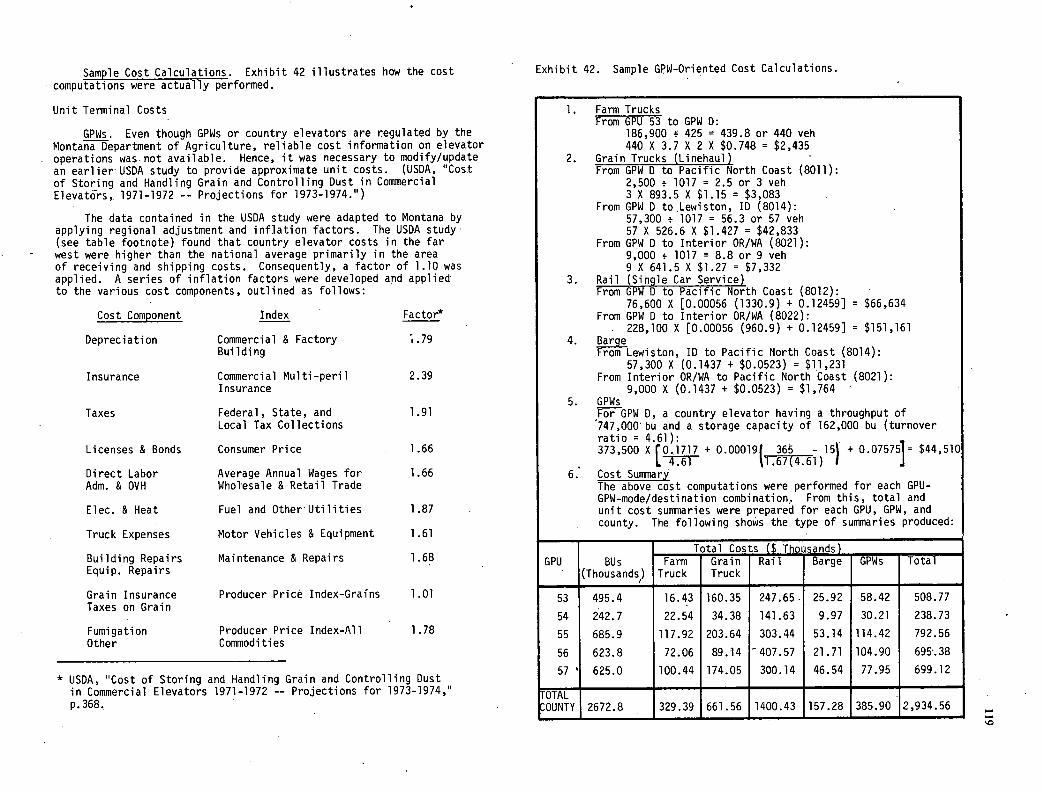
Sample Cost Calculations. Exhibit 42 illustrates how the cost computations were actually performed.
Unit Terminal Costs
GPWs. Even though GPWs or country elevators are regulated by the Montana Department of Agriculture, reliable cost information on elevator operations was not available. Hence, it was necessary to modify/update an earlier' USDA study to provide approximate unit costs. (USDA, "Cost of Storing and Handling Grain and Controlling Dust in Commercial Elevatdrs,, 1971-1972 -- Projections for 1973-1974.")
The data contained in the USDA study were adapted to Montana by applying regional adjustment and inflation factors. The USDA study' (see table footnote) found that country elevator costs in the far west were higher than the national average primarily in the area of receiving and shipping costs. Consequently, a factor of 1.10 was applied. A series of inflation factors were developed and applied' to the various cost components, outlined as follows:
Cost Component Index Factor
Depreciation Commercial & Factory 1.79 Building
Insurance Commercial Multi-peril 2.39 Insurance
Taxes Federal, State, and 1.91 Local Tax Collections
Licenses & Bonds Consumer Price 1.66
Direct Labor Average Annual Wages for 1.66 Adm. & OVH Wholesale & Retail Trade
Elec. & Heat Fuel and Other'Utilities 1.87
Truck Expenses Motor Vehicles & Equipment 1.61
Building Repairs Maintenance & Repairs 1.68 Equip. Repairs
Grain Insurance Producer Price Index-Grains 1.01 Taxes on Grain
Fumigation Producer Price Index-All 1.78 Other Commodities
* USDA, "Cost of Storing and Handling Grain and Controlling Dust in Commercial Elevators 1971-1972 -- Projections for 1973-1974," p.368.
Exhibit 42. Sample GPW-Oriented Cost Calculations.
Farm Trucks From GPU 53 to GPW D:
186,900 425 = 439.8 or 440 veh 440 X 3.7 X 2 X $0.748 = $2,435
Grain Trucks (Linehaul) - From GPW 0 to Pacific North Coast (8011):
2,500 f 1017 = 2.5 or 3 veh 3 X 893.5 X $1.15 = $3,083
From GPW D to,Lewiston, ID (8014): 57,300 + 1017 = 56.3 or 57 veh 57 X 526.6 X $1.427 = $42,833
From GPW D to Interior OR/WA (8021): 9,000 1017 = 8.8 or 9 veh 9 X 641.5 X $1.27 = $7,332
Rail (Single Car Service) From GPW D to Pacific North Coast (8012):
76,600 X [0.00056 (1330.9) + 0.124591 = $66,634 From GPW D to Interior OR/WA (8022):
228,100 X [0.00056 (960.9) + 0.124591 = $151,161 Barge
From Lewiston, ID to Pacific North Coast (8014): 57,300 X (0.1437 + $0.0523) = $11,231
From Interior OR/WA to Pacific North Coast (8021): 9,000 X (0.1437 + $0.0523) = $1,764
GPWs For GPW D, a country elevator having a throughput of 747,000' bu and a storage capacity of 162,000 bu (turnover ratio = 4.61): 373,500 X ro.17l7 + 0.000191365 - 15 + 0.075751= $44,510 _
1 4.61 1.67(4.6l) I .1 Cost Summary
The above cost computations were performed for each GPU- GPW-mode/destinatiori combination. From this, total and unit cost summaries were prepared for each GPU, GPW, and county. The following shows the type of summaries produced:
TotalCosts ($ Tho"sands) GPU BUs Farm Grain Rail Barge GPWs Total
(Thousands) Truck I Truck
53 495.4 16.43 160.35 247.65. 25.92 58.42 508.77
54 2'42.7 22.54 34.38 141.63 9.97 30.21 238.73
55 685.9 117.92 203.64 303.44 53.14 114.42 792.56
56 623.8 72.06 89.14 407.57 21.71 104.90 695'.38
57 1 625.0 100.44 174.05 300.14 46.54 77.95 699.12
'OTAL ' :OUNTY 2672.8 329.39 661.56 1400.43 157.28 385.90 2,934.56
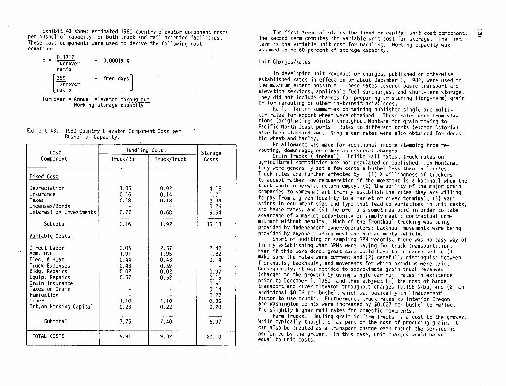
Exhibit 43 shows estimated 1980 country elevator component costs per bushel of capacity for both truck and rail oriented facilities. These cost components were used to derive the following cost equation:
0.1717 c = + 0.00019 X
ratio
r. - free days Turnover
Lratio
Turnover = Annual elevator throughput Working storage capacity
Exhibit 43. 1980 Country Elevator Component Cost per Bushel of Capacity.
Cost Handling Costs Storage
Truck/Rail Truck/Truck Component Costs
Fixed Cost
Depreciation 1.05 0.92 4.18 Insurance 0.16 0.14 1.71 Taxes 0.18 0.18 2.34 Licenses/Bonds - - 0.26 Interest on Investments 0.77 0.68 6.64
Subtotal 2.16 1.92 15.13
Variable Costs
Direct Labor 3.05 2.57 2.42 Adm. OVH 1.91 1.95 1.82 Elec. & Heat 0.44 0.43 0.14 Truck Expenses 0.43 0.59 - Bldg. Repairs 0.02 0.02 0.97 Equip. Repairs 0.57 0.52 0.15 Grain Insurance - - 0.51 Taxes on Grain - - 0.14 Fumigation - - 0.27 Other 1.10 1.10 0.35 Int.on Working Capital 0.23 0.22 0.20
Subtota.l 7.75 7.40 6.97
TOTAL COSTS 9.91 9.32 22.10
The first term calculates the fixed or capital unit cost component. The second'term computes the variable unit cost for storage. The last term is the variable unit cost for handling. Working capacity was assumed to be 60 percent of storage capacity.
Unit Charges/Rates
In developing unit revenues or charges., published or otherwise established rates in effect on or about December 1, 1980, were used to the maximum extent possible. These rates covered basic transport and elevation services, applicable fuel surcharges, and short-term storage. They did not include charges for preparing or storing (long-term) grain or for rerouting or other in-transit privileges.
Rail. Tariff summaries containing published single and multi-car rates for export wheat were obtained. These rates were from sta-tions (originating points) throughout Montana for grain moving to Pacific North Coast ports. Rates to different ports (except Astoria) have been standardized. Single car rates were also obtained for domes-tic wheat and barley.
No allowance was made for additional income stemming from re-routing, demurrage, or other accessorial charges.
Grain Trucks (Linehaul). Unlike rail rates, truck rates on agricultural commodities are not regulated or published. In Montana, they were generally set a few cents a bushel less than rail rates. Truck rates are further affected by: (1) 'a willingness of truckers to accept rather low remuneration if the movement is a backhaul when the truck would otherwise return empty, (2) the ability of the major grain companies to somewhat arbitrarily establish the rates they are willing to pay from a given locality to a market or river terminal, (3) vari-ations in equipment size and type that lead to variations in unit costs, and hence rates, and (4) the premiums sometimes paid in order to take advantage of a market opportunity or simply meet a contractual com-mitment without penalty. Much of the fronthaul trucking was being provided by independent owner/operators; backhaul movements were being provided by anyone heading west who had an empty vehicle.
Short of auditing or sampling GPW records, there was no easy way of firmly establishing what GPWs were paying for truck transportation. Even if this were done, great care would have to be exercised to (1) make sure the rates were current and (2) carefully distinguish between fronthauls, backhauls, and movements for which premiums were paid. Consequently, it was decided to approximate grain truck revenues (charges to the grower) by using single car rail rates in existence prior to December 1, 1980, and then subject (1) the cost of barge transport and river elevator throughput charges (0.196 $/bu) and (2) an additional $0.06 per bushel, which' was basically an inducement" factor to use trucks. Furthermore, truck rates to interior Oregon and Washington points were increased by $0.027 per bushel to reflect the slightly higher rail rates for domestic movements.
Farm Trucks. Hauling grain in farm trucks is a cost to the grower. While typically thought of as part of the cost of producing grain, it can also be treated as a transport charge even though the service is performed by the grower. In this case, unit charges would be set equal to unit costs.
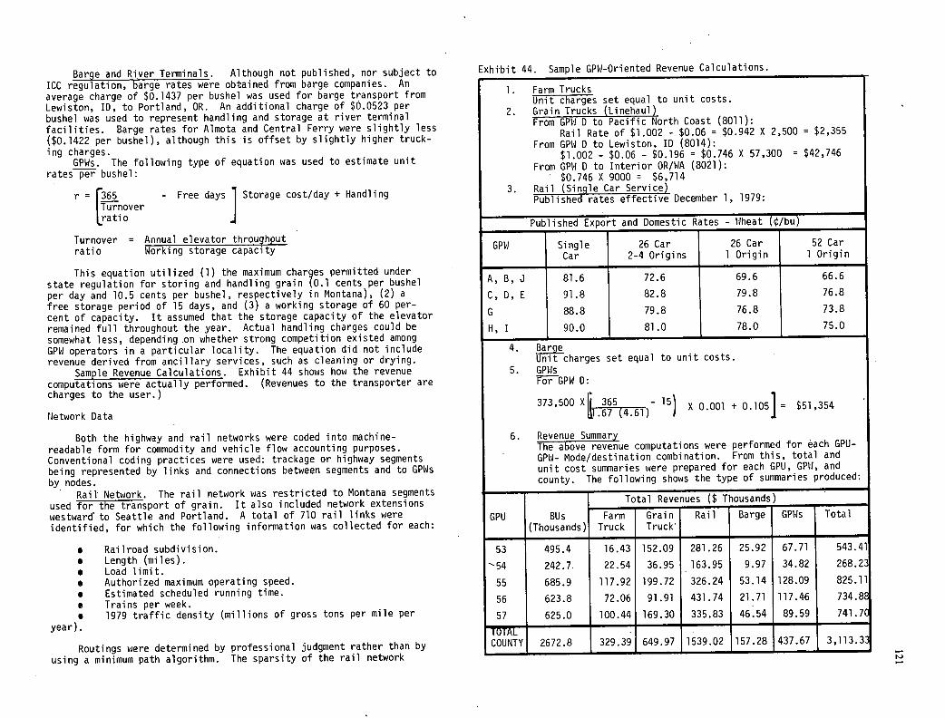
Barge and River Terminals. Although not published, nor subject to ICC regulation, barge rates were obtained from barge companies. An average charge of $0.1437 per bushel was used for barge transport from Lewiston, ID, to Portland, OR. An additional charge of $0.0523 per bushel was used to represent handling and storage at river terminal facilities. Barge rates for Almota and Central Ferry were slightly less ($0.1422 per bushel), although this is offset by slightly higher truck-ing charges.
GPWs. The following type of equation was used to estimate unit rates per bushel:
r = [ratio
36s - Free days Storage cost/day + Handling Turnover
Turnover = Annual elevator throughput ratio Working storage capacity
This equation utilized (1) the maximum charges permitted under state regulation for storing and handling grain (0.1 cents per bushel per day and 10.5 cents per bushel, respectively in Montana), (2) a free storage period of 15 days, and (3) a working storage of 60 per-cent of capacity. It assumed that the storage capacity of the elevator remained full throughout the year. Actual handling charges could be somewhat less, depending on whether strong competition existed among GPW operators in a particular locality. The equation did not include revenue derived from ancillary services, such as cleaning or drying.
Sample Revenue Calculations. Exhibit 44 shows how the revenue computations were actually performed. (Revenues to the transporter are charges to the user.)
Network Data
Both the highway and rail networks were coded into machine-readable form for commodity and vehicle flow accounting purposes. Conventional coding practices were used: trackage or highway segments being represented by links and connections between segments and to GPWs by nodes.
Rail Network. The rail network was restricted to Montana segments used for the transport of grain. It also included network extensions westwardS to Seattle and Portland. A total of 710 rail links were identified, for which the following information was collected for each:
Railroad subdivision. Length (miles). Load limit. Authorized maximum operating speed. Estimated scheduled running time. Trains per week. 1979 traffic density (millions of gross tons per mile per
year).
Routings were determined by professional judgment rather than by using a minimum path algorithm. The sparsity of the rail network
Exhibit 44. Sample GPW-Oriented Revenue Calculations.
Farm Trucks Unit charges set equal to unit costs.
Grain Trucks (Linehaul) From GPW D to Pacific North Coast (8011):
Rail Rate of $1 .002 - $0.06 = $0.942 X 2,500 = $2,355 From GPW D to Lewiston, ID (8014):
$1.002 - $0.06 - $0.196 = $0.746 X 57,300 = $42,746 From GPt'I D to Interior OR/WA (8021):
$0.746 X 9000 = $6,714 Rail (Single Car Service)
Published rates effective December 1, 1979:
Published Export and Domestic Rates - Wheat (/bu)
GPW I Single 26 Car 26 Car I 52 Car Car 2-4 Origins 1 Origin 1 Origin
A, B, J 81.6 72.6 69.6 66.6
C, D, E 91.8 82.8 79.8 76.8
G 88.8 79.8 76.8 73.8
H, I 90.0 81.0 78.0 75.0
Barge Unit charges set equal to unit costs. -
GPWs PEGPW 0:
373,500 X_ 15) 15) x 0.001 + 0.105J= $51,354
Revenue Sumjy The above revenue computations were performed for each GPU- GPW- Mode/destination combination. From this, total and
unit cost summaries were prepared for each GPU, GPt-1, and
county. The following shows the type of summaries produced:
Total Revenues ($ Thousands)_______
GPU BUs Farm Grain Rail Barge GPWs Total
(Thousands) Truck Truck'
53 495.4 16.43 152.09 281.26 25.92 67.71 543.41
-54 242.7, 22.54 36.95 163.95 9.97 34.82 268.23
55 685.9 117.92 199.72 326.24 53.14 128.09 825.11
56 623.8 72.06 91.91 431.74 21.71 117.46 734.8
57 625.0 1 100.44 169.30 1 335.83 1 46:54 89.59 741.7
TOTAL COUNTY 2672.8
- 329.39 649.97 1539.02 157.28 437.67 3,113.3
coupled with the fact that train movements do not always follow the shortest route dictated this approach.
Highway Network. The highway network included state and county highway segments used for the transport of grain from GPWs to west coast markets, plus connecting segments that would potentially be used, depending on the location of subterminals. Also included were generalized network extensions westward to Lewiston, ID, via US 12 (Lolo pass) and to Portland, OR, and Seattle, WA, via inter-state routes. A total of 1080 highway links were identified for which the following information was collected for each:
Route number. Length (miles). Functional classification. Jurisdiction. Free flow speed. Existing daily truck volume.
In assigning traffic to the network, use was made of routings developed through professional judgment, rather than those developed using a minimum path algorithm . At the statewide level, routes used for grain movements are fairly obvious, although in several areas truck movements were apportioned among parallel routings in accord-ance with observations and data on segment use.
Base Case Inputs
The specific base case inputs were summarized into the five arrays and one data file listed below for input into the freight demand forecasting model:
GPW Information File (array)
Identification rio. County Identification No. Distances to markets via individual modes or mode combinations Linehaul rates via rail, truck, and barge corresponding to the above distances
X, Y coordinates (optional) GPW name GPW location GPW capacity GPW storage and handling charges (initial or maximum values) Alternative GPWs
GPU Distance File (array)
Shortest practical distance from the GPU centroid to each GPW.
GPU Information File
Identification No. County Identification No. Total grain production subdivided by that.having GST potential
or not
X, V coordinates (optional)
County File (array)
County Identification No. County Name
Grain Flow Data (data file containing one record for each unique GPU/GPW/market/mode combi nation)
GPU Identification No. GPW- Identification No., Market Identification Total volume per specified period moving by identified modes
having GST potential Total volume of other grains not having GST potential
Preparing Inputs for the Alternatives Being Considered
Future Grain Production and Markets
The case example involved determining (1) the economic feasibility, of grain subterminals and unit train service; (2) resulting benefits or disbenefits to growers, elevator operators, and transport companies, if implemented; and (3) estimating impacts on the highway system. GSTs and unit train service together represented a hypothesized change to the transport services and rate structures then existing, the intent of which was to reduce transport costs. No estimates of future world or domestic demand for wheat and barley were prepared or used in this example. Consequently no 'future" production or market demand forecasts were prepared for Montana wheat and barley, because the ap-plication did not require changes occurring in commodity flows over time.
On the other hand, the case example did require determining which grains and markets have subterminal and unit train potential, and establishing appropriate control totals. In the Montana study, grain having GST potential included all varieties of wheat being shipped to Pacific North Coast ports and other transshipment points located in the interior of Oregon or Washington. Although a number of terminals handle export wheat, all were located in proximity to one another and use the same rail lines. Of the 119.8 million bushels of Montana wheat marketed in 1979, 109.9 million moved west and thus •were deemed to have GST potential.
Although the assumption was made that market demand does not change, this may not necessarily hold true if the markets being serviced by unit trains/GSTs are able to offer a better price for the product than the smaller markets. Not only is it possible to have market shifts, but the production of different grains may also change over the long term to cash in on the better price.
Function of GSTs. In this study, GSTs were viewed as the hinterland component of a grain assembly and delivery system consisting of GSTs, rail lines/unit train service, and improved port facilities. Under this concept, it was visualized that a number of port terminal elevator functions (e.g., storage, blending, inspection, certification) would be transferred back to GSTs located at strategic inland points.
Not only would the GST act as a regional assembly point and "pump house" for loading wheat into unit trains, but it also would perform most of the traditional GPW service functions, except for long-term storage. Subterminal loadout operations, unit train movements, and vessel loading would then become highly integrated and coordinated.
Alternatives. Potential alternatives included:
Complete replacement of GPWs by GSTs (considered to be unlikely).
GPWs and GSTs coexist whereby the former markets through the latter.
Partial replacement of GPWs by GSTs, where GPWs continue to function in areas where the trans-port costs via GST are greater than via local GPWs. Portions of the grain traffic continue to move via single car rail for volume or service reasons. GPWs on branchlines are phased out where railroads are successful in eliminating light density line rail operations.
Upgrading of selected GPWs to handle multiple carloads (e.g., 26 cars) rather than full unit trains.
All of the foregoing alternatives could have been examined using the freight demand forecasting technique. In the Montana case example, alternatives were limited to (1) adding GSTs by simultaneously phasing out many of the existing GPWs, and (2) adding GSTs but keeping GPWs as local collection and marketing points. Retaining single car rail service exclusively was not considered to be a viable alternative with the introduction of volume rates, although it was useful as a base against which the other two alternatives could be compared. (The alternative of upgrading GPWs was not examined to the same degree as the other two alternatives for reasons unrelated to the case example.)
Under the first alternative, GPWs would continue to function in the same fashion as at present, except that westbound wheat would be shipped by truck to the GST instead of being loaded into covered hopper cars at the GPW. GPWs would retain their traditional marketing function, except that cooperative decision-making (with other GST users) would be necessary to assemble and market unit train loads of wheat.
Under the second alternative, the role of GPWs would change dras-tically in that the GSTs would largely supplant GPWs in assembling and marketing westbound wheat. As structured, this alternative required GSTs to provide a collector service (using motor carriers) to move grain from the more distant farms to the GST, or offer allowances in lieu thereof, to offset the longer farm-to-market hauls that many growers would face with the phase-out of the GPW system. Remaining GPWs would concentrate on marketing barley and wheat destined to other markets and low volume shipments either by truck or by single car rail.
Alternative Futures, Scenarios, and Conditions
Determining the Number and Location of GSTs. In determining the efficiency of subterminals, it was necessary to identify the number and location of GSTs. The two basic approaches for accomplishing this are:
Location allocation theory, which addresses the problem of allocating one set of facilities (GSTs) to serve a second set of pro-ducers (GPUs). It seeks to minimize total transport costs (or maxi-mize net income) in situations having up to three unknowns: the number, size (capacity or throughput), and location of facilities. A systematic search-and-evaluate process readily adaptable to computer application is used to develop optimal solutions.
An empirical approach based on (1) subdividing a state into a series of grain producing regions, based on known prodUction, (2) examining potential GST sites to determine which ones have the best potential, and (3) linking GPUs to GSTs on the basis of historical commerce/trade patterns and transport cost minimization. In this process, the analyst uses his knowledge of the grain industry in a state to.make decisions on tributary areas and GPU-GST relationships, with the computer being used simply to make the computations and perform the accounting.
Irrespective of whether a mechanical or empirical process is employed, typical criteria used include:
Maximizing profits (private enterprise). Coverage of the state (i.e., more or less equal opportunity
for grower access to GSTs). Minimizing distance between GPUs and the nearest GST. Capitalizing on published rail rate structures -- especially
where sizable differentials occur. Each GST or system of GSTs must be profitable. Minimizing the total number of GSTs to keep total infra-
structure and operating costs as low as possible. Locations restricted to places having mainline rail service
not requiring corporate capital investment to upgrade the track. Site characteristics. Specific site factors include (1)
size and terrain, (2) ownership, (3) highway access, (4) availability of utilities, and (5) availability of land on either side of the poposed GST to allow for construction of side tracks that are un-interrupted by highway grade crossings.
Some of the foregoing criteria obviously conflict; not all of them can be fully satisfied. Philosophically, the two methods are somewhat different. Location allocation theory, if applied correctly, will produce a solution that minimizes total transportation costs. It requires that no a priori judgments be made, although prescreening of sites to make sure they have acceptable characteristics is wise. Location allocation theory will not ensure coverage of the state, nor will it minimize the distance between GPUs and the nearest GST. On the other hand, an empirical approach cannot ensure that the number and location of GSTs selected are optimal. Neither method can ensure GST profitability, nor can it handle the desire for retaining competition in the larger grain producing areas through multiple (overlapping) GSTs.
The method to be chosen depends on the intended application and the available resources. In the Montana study, an empirical process was employed to select ten locations for GSTs. Once selected, each GPU was then assigned to a GST based on highway distances and long-standing patterns of local or regional commerce. Exhibit 45 shows the t•-)
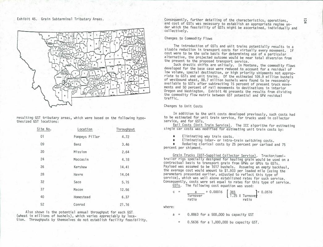
Exhibit 45. Grain Subterminal Tributary Areas. Consequently, further detailing of the characteristics, operations, and cost of GSTs was necessary to establish an appropriate regime un-der which the feasibility of GSTs might be ascertained, individually and collectively.
Changes to Commodity Flows
The introduction of GSTs and unit trains potentially results in a sizable reduction in transport costs for virtually every movement. If cost were to be the sole basis for determining use of a particular alternative, the projected outcome would be near total diversion from the present to the proposed transport service.
Such drastic shifts are unlikely. In Montana, the commodity flows developed for the base case were reduced to account for a residual of low volume, special destination, or high priority shipments not approp-riate to GSTs and unit trains. Of the estimated 109.9 million bushels of westbound wheat, 88.7 million bushels were found to be reasonably available to GSTs after subtracting 15 percent of present truck move-ments and 50 percent of rail movements to destinations in interior Oregon and 1'4ashington. Exhibit 46 presents the results from dividing the comodity flow matrix between GST potential and GPW residual traffic.
Changes to Unit Costs
Site No.
01
09
20
24
26
28
32
37
40
52
In addition to the unit costs developed previously, such costs had to be estimated for unit train service, for trucks used in collector service, and for GSTs.
Rail Costs (Unit Train Service). The ICC algorithm for estimating single car costs was modified for estimating unit train costs by:
Pompeys Pillar 4.72 Eliminating way train costs. Eliminating inter- or intra-train switching costs.
Benz 3.46 Reducing clerical costs by 25 percent per carload and 75 percent per shipment.
Mission 2.64 Grain Trucks (GST-Supplied Collector Service). Tractor/semi-
Moccasin 4.18 trailer rigs specially designed for hauling grain would be used on a contractual basis to transport grain from GPWs or GPUs to GSTs.
Kershaw 14.41 Payload was assumed to be 1017 bushels. Assuming an empty backhaul, the average cost would amount to $1 .933 per loaded mile (using the
Havre 14.04 parameters presented earlier, adjusted to reflect this type of service), which was well above established rates for such service.
Saco 5.15 Consequently, costs were set equal to rates for this type of service. GSTs. The following cost equation was used:
Macon 12.56 c = a + 0.00016 1 365 + 0.0516
Homestead 6.37 Turnover 1 1.25 X Turnovet ratio ratio
Conrad 21.16 where:
resulting GST tributary areas, which were based on the following hypo-thesized GST locations:
Location Throughput
Also shown is the potential annual throughput for each GST, (wheat in millions of bushels), which varies appreciably by loca- tion. Throughputs by themselves do not establish facility feasibility.
a = 0.8863 for a 500,000 bu capacity GST
= 0.5636 for a 1,000,000 bu capacity GST.

Exhibit 46. GST and Residual Traffic.
Base Case ,uternat,ves Mode and Destination
GPU Wheat 8012 8022 8011 8014 021 GST GPW (Thousands Potential Residual bu)
53 495.4 162.7 145.7 54.7 30.8 101.5 395.1 100.3
54 242.7 96.8 93.3 1.7 36.2 14.7 188.2 54.5
55 685.9 335.5 53.5 25.7 40.2 231.0 614.6 71.3
56 . 623.8 498.4 0 14.6 0 110.8 605.0 18.8
57 625.0 229.4 143.8 14.3 40.3 197.2 515.4 109.6.
TOTAL COUNTY 2672.8 1322.8 436.3 11.0 147.5 655.2 2318.3 354.5
Mode Destination
8012 Rail Pacific North Coast
8022 Rail Interior of Oregon or Washington
8011 Truck Pacific North Coast
8014 Truck/Barge Pacific North Coast via Lewiston, ID
8021 Truck/Barge Pacific North Coast via Columbia or Snake River Ports
The first term calculates the fixed or capital unit cost component. The second term computes the variable unit cost for storage. The last term computes the variable unit cost for handling. Working capacity was assumed to be 80 percent of storage capacity.
Sample Cost Calculations. Exhibit 47 shows how the additional cost computations were performed.
Changes to Unit Revenues/Charges
The modal alternatives examined required that additional unit rates be obtained or estimated for trucks used in collector service and for GSTs.
Exhibit 47. Sample GST-Oriented Cost Calculations.
Farm Trucks From GPU 53 to GST 24:
395,100 425 = 929.6 or 930 veh 930 X 16.1 X 2 X $0.748 = $22,400
Grain Trucks (GST-Supplied Collector Service) From GPU 55 to GST (42 ml):
614,600 1017 = 604.3 or 605 veh 605 X 1017 X [0.0917.1 + (0.0009329 * 42) +
(0.0000013 * 422)] = $82,000 From GPU 57 to GST (64 mi):
515,000 1017 = 506.4 or 507 veh 507 X 1017 X [0.15171 - (0.0004338 * 64) +
(0.0000093 * 642) - (0.0000000132 * 64")] = $81,700
Rail (Unit Train Service) From GST 24 to Pacific North Coast:
4,181,100 X [0.000515 (1054.3) + 0.076231 = $2,588,900 GSTs In the Montana study, it was assumed that GSTs would be new facilities constructed primarily for the rapid loading of grain rather than for grain storage purposes. GST land acquisition, site preparation, side track construction and elevator construction, and equipping were estimated to cost $3.31 million for a 500,000-bushel facility.
Component costs included (in thousands):
Sitework $ 385 General elevator and structures 1,600 500,000-bu storage annex (optional) 900 General elevator machinery 1 1100 Special equipment 85 Electrical . 140
$ 3,310 (500,000 bu)
or $ 4,210 (1,000,000 bu)
The annual cost of such a facility would amount to $443,150 assuming financing at a 12 percent interest rate over 20 years, or $0.8863 per bushel of capacity.
For GST 24, a medium-sized facility having a potential annual throughput of 4,181,100 bu and a storage capacity of 500,000 bu (turnover ratio = 8.3622):
4,181,100 X [0.8863
0.00016 (
365 ) + 0.0516
1 .2 ]
8.3622 + 5X 8 3627 = $682,356
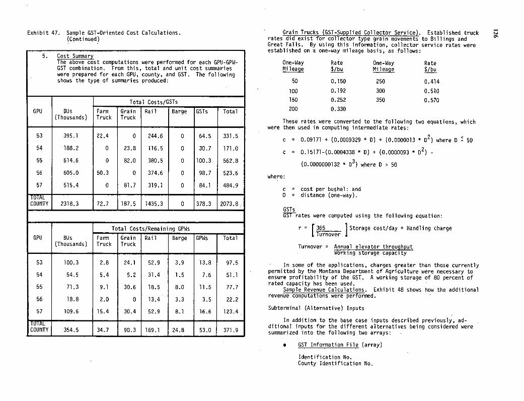
Exhibit 47. Sample GST-Oriented Cost Calculations. (Continued)
5. Cost Summary The above cost computations were performed for each GPU-GPW- GST combination. From this, total and unit cost summaries were prepared for each GPU, county, and GST. The following shows the type of summaries produced:
Total Costs/GSTs
GPU BUs Farm Grain Rail Barge GSTs Total (Thousands) Truck Truck
53 395.1 22.4 0 244.6 0 64.5 331.5
54 188.2 0 23.8 116.5 0 30.7 171.0
55 614.6 0 82.0 380.5 0 100.3 562.8
56 605.0 50.3 0 374.6 0 98.7 523.6
57 515.4 0 81.7 319.1 0 84.1 484.9
TOTAL COUNTY 2318.3 72.7 187.5 1435.3 0 378.3 2073.8.
Total_Costs/Remaining GPW5
GPU BUs Farm Grain Rail Barge GPWs Total (Thousands) Truck Truck
53 100.3 2.8 24.1 52.9 3.9 13.8 97.5
54 54.5 5.4 5.2 31.4 1.5 7.6 51.1
55 71.3 9.1 30.6 18.5 8.0 11.5 77.7
56 18.8 2.0 0 13.4 3.3 3.5 22.2
57 109.6 15.4 30.4 52.9 8.1 16.6 123.4
TOTAL COUNTY 354.5 34.7 90.3 169.1 24.8 53.0 371.9
Grain Trucks (GST-Supplied Collector Service). Established truck rates did exist for collector type grain movements to Billings and Great Falls. By using this information, collector service rates were established on •a one-way mileage basis, as follows:
One-Way Rate One-Way Rate Mileage $/bu Mileage $/bu
50 0.150 250 0.414
100 0.192 300 0.510
150 0.252 350 0.570
200 0.330
These rates were converted to the following two equations, which were then used in computing intermediate rates:
c = 0.09171 + (0.0009329 * D) + (0.0000013 * D2) where D f 50
c = 0.15171-(0.0004338 * D) + (0.0000093 * D2) -
(0.0000000132 * D3) where D > 50
where:
c = cost per bushel: and D = distance (one-way).
GSTs GST rates were computed using the following equation:
r = 1 365 ] Storage cost/day + Handling charge I. Turnover I
Turnover = Annual elevator throughput Working storage capacity
In some of the applications, charges greater than those currently permitted by the Montana Department of Agriculture were necessary to ensure profitability of the GST. A working storage of 80 percent of rated capacity has been used.
Sample Revenue Calculations. Exhibit 48 shows how the additional revenue computations were performed.
Subterminal (Alternative) Inputs
In addition to the base case inputs described previously, ad-ditional inputs for the different alternatives being considered were summarized into the following two arrays:
. GST Information File (array)
Identification No. County Identification No.
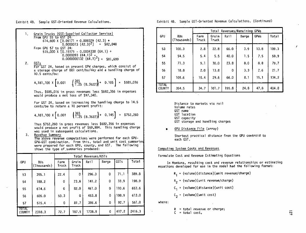
Exhibit 48. Sample GST-Oriented Revenue Calculations.
Grain Trucks (GST-Supplied Collector Service) From GPU 55 to GST 24:
614,600 X [0.09171 + 0.00939 (42.3) + 0.0000013 (42.3) = $82,048
From GPU 57 to GST 24: 515,000 X [0.15171 - 0.0004338 (64.1) +
0.0000093 (64.1)2 - 0.0000000132 (64.1)] = $81,699
GSTs For GST 24, based on present GPW charges, which consist of a storage charge of 001 cent/bu/day and a handling charge of 10.5 cents/bu:
4,181,100 X [0.001 4TT5 (8.3622) 0.1051 - $585,016
Thus, $585,016 in gross revenues less $682,356 in expenses would produce a net loss of $97,340.
For GST 24, based on increasing the handling charge to 14.5 cents/bu to return a 10 percent profit:
4,181,100 x[o.00i (8.3622)) 0.145] = $752,260
Thus $752,260 in gross revenues less $682,356 in expenses would produce a net profit of $69,904. This handling charge was used in subsequent calculations.
Revenue Summary The above revenue computationswere performed for each GPU- GPW-GST combination. From this, total and unit cost summarier were prepared for each GPU, county, and GST. The following shows the type of sunimaries produced:
Total Revenues/GST5
Farm Grain Rail Barge GSTs Total .GPU BUs (Thousands) Truck Truck
53 395.1 22.4 0 296.3 0 71.1 389.8
54 188.2 0 23.8 141.2 0 33.9 198.9
55 614.6 0 82.0 461.0 0 110.6 653.6
56 605.0 50.3 0 453.8 0 108.9 613.0
57 515.4 0 81.7 386.6 0 92.7 561.0
TOTAL COUNTY 2318.3 72.7 187.5 1738.9 0 417.2 2416.3
Exhibit 48. Sample GST-Oriented Revenue Calculations. (Continued)
Total Revenues/Remaining GPWs
Farm Grain Rail Barge GPWs Total GPU BUs (Thousands) Truck Truck
53 100.3 2.8 22.8 66.0 3.9 13.8 109.3
54 54.5 5.4 5.5 40.0 1.5 7.5 59.9
55 71.3 9.1 30.0 23.8 8.0 8.8 79.7
56 18.8 2.0 13.8 0 3.3 2.6 21.7
57 109.6 15.4 29.6. 66.0 8.1 15.1 134.2
TOTAL COUNTY 354.5 34.7 101.7 195.8 24.8 47.8 404.8
Distance to markets via rail Volume rates GST name GST location GST capacity GST storage and handling charges
e GPU Distance File (array)
Shortest practical distance from the GPU centroid to each GST.
Computing System Costs and Revenues
Formulate Cost and Revenue Estimating Equations
In Montana, resulting cost and revenue relationships or estimating equations developed for use in the model had the following format:
R1 = (volume)(distance)(unit revenue/charge)
R2 = (volume)(unit revenue/charge)
C1 = (volume)(distance)(unit cost)
C2 = (volume)(unit cost)
where:
R = total revenue or charge; C = total cost,
FA
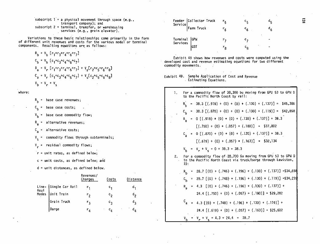
Rb = base case revenues;
Cb = base case costs;
Vb = base case commodity flow;
Ra = alternative revenues;
Ca = alternative costs;
V5 = commodity flows through subterminals;
Vr = residual commodity flows;
= unit rates, as defined below;
c = unit costs, as defined below; arid
d = unit distances, as defined below.
Revenues! Charges Costs Distance
where:
Line- Single Car Rail r1 Haul Modes Unit Train r2 c2
Grain Truck r3 c3
Barge r4 c4
d1
d2
d3
d4
Variations to these basic relationships come primarily in the form of different unit revenues and costs for the various modal or terminal components. Resulting equations are, as follows:
Rb = Vb [r1+r3+r4+r6+r7]
Cb = Vb [c1+c3+c4+c6+c7]
Ra = Vr [r1+r3+r4+r5+r7] + V5[r2+r5+r6+r8]
C8 = Vr [c1+c3+c4+c5+c7] + V[c2+c5+c6+c8]
V b = V r + V s
subscript 1 = a physical movement through space (e.g., transport company); and
subscript 2 = terminal, transfer, or warehousing services (e.g., grain elevator).
Feeder 'Collector Truck r5 c5 d5 Service
Farm Truck r6 c6 d6
Terminal GPW I
r7 c7 - Services
GST r8 c8 -
Exhibit 49 shows how revenues and costs were computed using the developed cost and revenue estimating equations for two different commodity movements.
Exhibit 49. Sample Application of Cost and Revenue Estimating Equations.
For a commodity flow of 38,300 bu moving from GPU 53 to GPW D to the Pacific North Coast by rail:
Rb = 38.3 [(.918) + (0) + (0) + (.130) + (.137)] = $45,386
Cb = 38.3 [(.870) + (0) + (0) + (.130) + (.119)] = $42,858
Ra = 0 [(.918) + (0) + (0) + (.130) + (.137)] + 38.3
[(.750) + (0) + (.057) + (.180)] = $37,802
Ca = 0 [(.870) + (0) + (0) + (.130) + (.137)] + 38.3
[(.619) + (0) + (.057) + (.163)] = $32,134
Vb = Vr + V = 0 + 38.3 = 38.3
For a commodity flow of 28,700 bu moving from GPU 53 to GPW D to the Pacific North Coast via truck/barge through Lewiston, ID:
Rb = 28.7 [(0) + (.746) + (.196) + (.130) + (.137)] =$34,6
Cb = 28.7 [(0) + (.748) + (.196) + (.130) + (.119)] =$34,2
R = 4.3 [(0) + (.746) + (.196) + (.130) + (.137)] +
24.4 [(.750) + (0) + (.057) + (.180)] = $29,282
Ca = 4.3 [(0) + (.748) + (.196) + (.130) + (.119)] +
24.4 [(.619) + (0) + (.057) + (.163)] = $25,602
Vb = V + V = 4.3 + 24.4 = 28.7
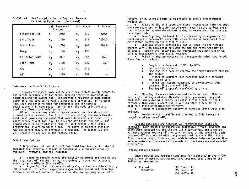
Exhibit 49. Sample Application of Cost and Revenue Estimating Equations. (Continued)
Unit Revenues! Unit Costs Distances Charges
Single Car Rail r1 .918 C1 .870 1330.9
Unit Train r .750 c2 .619 1054.3
Grain Truck r3 .746 c3 .748 526.6
Barge r .196 c4 .196
Collector Truck r5 .057 c5 .057 16.1
Farm Truck r6 .130 c6 .130 3.7
GPW r7 .137 c7 .119 -
GST r8 .180 c8 .163 -
Determine the Mode Split Process
In grain transport, mode choice decisions reflect partly economics and partly service, with the former lending itself to quantitative solutions and the latter not. Introducing a new mode or mode combin-ation or a new service is really a routing alternative. If it costs less than the existing mode for comparable quality service, substitution will take place. In Montana, the mode split process used this "least cost mode' principle.
Often, the user may wish to impose several constraints on such a quantitative process. The first involves setting a minimum thresh-hold level governing the point that modal diversion will occur (e.g., users rarely divert for, say, half a cent per bushel savings). The second would be to establish a zone of indifference within which proportional diversion takes place. The third is to set a limit on maximum market share, as previously discussed. The latter was the only constraint applied in the Montana study.
Select User Options
A large number of potential options could have been built into the computational process, although in Montana only a few were actually employed. Potential options included:
Choosing between having the computer determine and thus select the least cost GST routing, or using previously determined tributary areas tying to GPWs or GPUs to GSTs.
Adjusting the total amounts of grain, or that considered having GST.potential, to reflect expected changes in the amount and varieties produced and market demands. This can be done by applying one or more
factors, or by using a normalizing process to meet a predetermined projection.
Adjusting the unit costs and rates incorporated into the cost and rate equations or location-based rate arrays to more-oe-less bring such information'up-to-date without having to reconstruct the cost and rate input data.
Investigating the benefits of cost-sharing arrangements for trucking grain between GPUs and GSTs so as to lessen locational dis-crimination created in the siting of GSTs.
Choosing between letting GPW and GST handling and storage charges vary with throughput or using the maximum rates that may be allowable. Use of the latter does not guarantee that each GPW or GST will be independently profitable, however.
Adjusting the computations to the scenario being considered. Scenarios can include:
Complete replacement of GPWs by GSTs. Partial replacement. GPWs and GSTs coexist whereby the former markets through the latter. A system of upgraded GPWs handling multiple carloads in lieu of GSTs. A three-tier system comprised of conventional GPWs, upgraded GPWs, and full GSTs. Testing GST proposals developed by others.
Choosing the mode choice assumption to be used. This can invole (1) setting a minimum threshhold level governing the point that modal diversion will occur, (2) establishing a zone of indif-ference within which proportional diversion takes place, or (3) setting a limit on maximum market share.
Adjusting assumptions concerning farm and grain truck size and use.
Rerouting grain traffic not diverted to GSTs through a consolidated system of GPWs.
Compute Base Case and Alternative Transportation Costs and Revenues. Each grain flow record was sequentially read, revenues and costs were computed via the GPW and GST alternatives, and a choice was made between routing all, or part, or none of the grain via each proposed GST as compared with the present routing via a GPW. Grain flow, revenue, cost, distance, and vehicle volume information was then entered onto one or more output records for the base case and each GST alternative.
Prepare Output Records
Once computations had been completed for a particular grain flow record, one or more output records were prepared consisting of the following information:
Control GPU Ident. No. Information GPW Ident. No.
GST Ident. No.
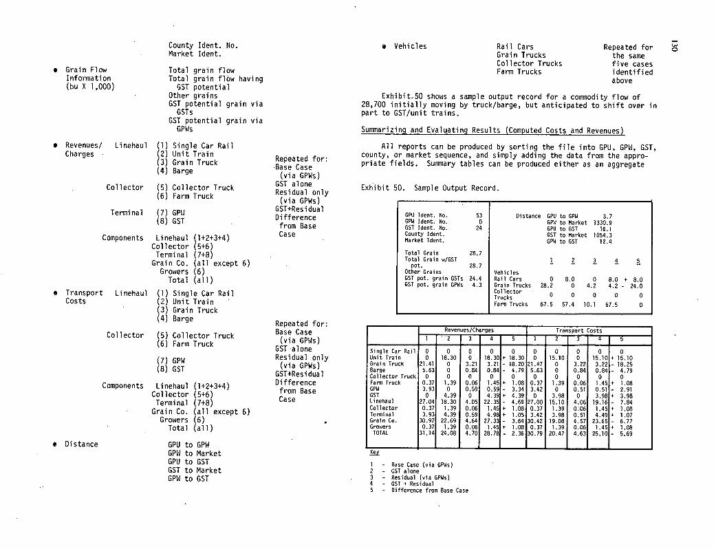
County Ident. No. Market Ident.
Grain Flow Total grain flow Information Total grain flow having (bu X 1,000) GST potential
Other grains GST potential grain via GSTs
GST potential grain via GPWs
Revenues! Linehaul (1) Single Car Rail Charges (2) Unit Train
Grain Truck Barge
Collector (5) Collector Truck (6) Farm Truck
Terminal (7) GPW (8) GST
Components Linehaul (1+2+3+4) Collector (5+6) Terminal (7+8)
Grain Co. (all except 6) Growers (6) Total (all)
Transport Linehaul (1) Single Car Rail Costs (2) Unit Train
Grain Truck Barge
Collector (5) Collector Truck Farm Truck
GPW GST
Components Linehaul (1+2+3+4) Collector (5+6) Terminal (7+8)
Grain Co. (all except 6) Growers (6) Total (all)
Distance GPU to GPW GPW to Market GPU to GST GST to Market GPW to GST
Repeated for: Base Case (via GPWs) GST alone Residual only (via GPWs) GST+Residual Difference from Base Case
Repeated for: Base Case (via GPWs) GST alone Residual only (via GPWs) GST+Residual Difference from Base Case
Vehicles Rail Cars Repeated for Grain Trucks the same Collector Trucks five cases Farm Trucks identified
above
Exhibit50 shows a sample output record for a conunodity flow of 28,700 initially moving by trucki'barge, but anticipated to shift over in part to GST!unit trains.
Summarizing and Evaluating Results (Computed Costs and Revenues)
All reports can be produced by sorting the file into GPU, GPW, GST, county, or market sequence, and simply adding the data from the appro-priate fields. Summary tables can be produced either as an aggregate
Exhibit 50. Sample Output Record.
GPU Ident. No. 53 GPW Ident. No. 0 GST Ident. No. 24 County Ident. Market Ident.
TotalGrain 28.7 Total Grain w/GST
pot. 28.7 Other Grains GST pot. grain GST5 24.4 GST pot. grain GPWs 4.3
Distance GPU to GPW 3.7 GPW to Market 1330.9
GPU to GST 16.1 GST to Market 1054.3
GPW to GST 12.4
Vehicles Rail Cars 0 8.0 0 8.0 + 8.0 Grain Trucks 28.2 0 4.2 4.2 - 24.0 Collector Trucks 0 0 0 0 0
Farm Trucks 67.5 57.4 10.1 67.5 0
Revenues/Charges Transport Costs 1 2 3 4 1 5 1 2 3 4 5
Single Car Rail 0 0 0 0 0 0 0 0 0 0 Unit Train 0 18.30 0 18.30+18.30 0 15.10 0 15.10+15.10 Grain Truck 21.41 0 3.21 3.21 - 18.20 21.47 0 3.22 3.22 - 18.25 Barge 5.63 0 0.84 0.84- 4.79 5.63 0 0.84 0.84- 4.79 Collector Truck 0 0 0 0 0 0 0 0 0 0 Farm Truck 0.37 1.39 0.06 1.45 + 1.08 0.37 1.39 0.06 1.45 + 1.08 GPW 3.93 0 0.59 0.59- 3.34 3.42 0 0.51 0.51- 2.91 GST 0 4.39 0 4.39+ 4.39 0 3.98 0 3.98+ 3.98 Linehaul 27.04 18.30 4.05 22.35- 4.69 27.00 15.10 4.06 19.16- 7.84 Collector 0.37 1.39 0.06 1.45 + 1.08 0.37 1.39 0.06 1.45 + 1.08 Terminal 3.93 4.39 0.59 4.98 + 1.05 3.42 3.98 0.51 4.49 + 1.07 Grain Co. 30.97 22.69 4.64 27.33- 3.64 30.42 19.08 4.57 23.65- 6.77 Growers 0.37 1.39 0.06 1.45 + 1.08 0.37 1.39 0.06 1.45 + 1.08
TOTAL 31.14 24.08 4.70 28.7 - 2.36 30.79 20.47 4.63 25.10 - 5.69
- Base Case (via GPWs) 2 - GST alone 3 - Residual (via GPWs) 4 - GST + Residual 5 - Difference from Base Case
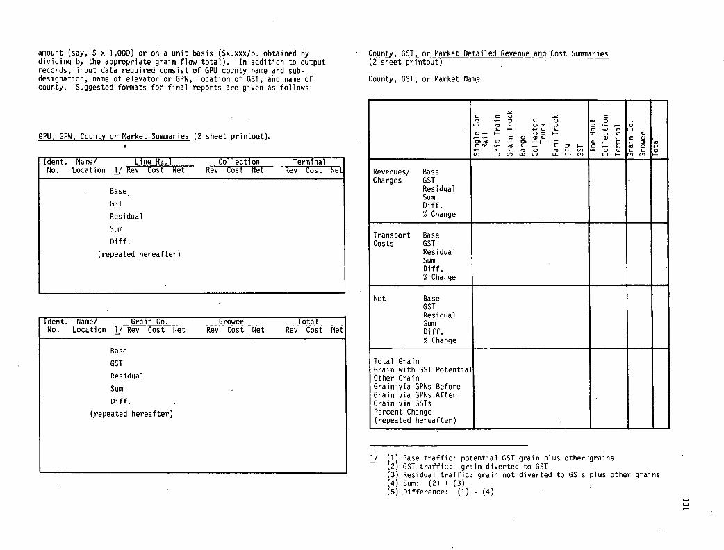
amount (say, $ x 1,000) or on a unit basis ($x.xxx/bu obtained by dividing by the appropriate grain flow total). In addition to output records, input data required consist of GPU county name and sub-designation, name of elevator or GPW, location of GST, and name of county. Suggested formats for final reports are given as follows:
GPtJ, GPW, County or Market Summaries (2 sheet printout).
Ident. Name! Line Haul Collection - Terminal No. Location jJ Rev Cost Net Rev Cost Net Rev Cost Net
Base
GST
Residual
Sum
Diff.
(repeated hereafter)
Ident. Name! Grain Co. Grower Total No. Location J Rev Cost Net Rev Cost Net Rev Cost Net
Base
GST
Residual
Sum
Diff.
(repeated hereafter)
County, GST, or Market Detailed Revenue and Cost Summaries (2 sheet printout)
County, GST, or Market Name
S.) ( 5- S. 0.
0 '-0
a).— I— S.- +'U
U 5-
F— 4-'
1 U C S.)
5-
D' 4- .- . Or—I— S..— 5-
C a)
S.
(5)
. 04-'
5/) CS.
CD . 0 ao 5-)
0 LI.
. VS (D C)
0 i C.) G
5— 5-5- (SC)
0 I—
Revenues! Base Charges GST
Residual Sum Diff. % Change
Transport Base Costs GST
Residual Sum Diff. % Change
Net Base GST Residual Sum Diff. % Change
Total Grain Grain with GST Potential Other Grain Grain- via GPWs Before Grain via GPWs After Grain via GSTs Percent Change (repeated hereafter)
1/ (1) Base traffic: potential GST grain plus other'grains GST traffic: grain diverted to GST Residual traffic: grain not diverted to GSTs plus other grains Sum: (2) + (3) Difference: (1) - (4)
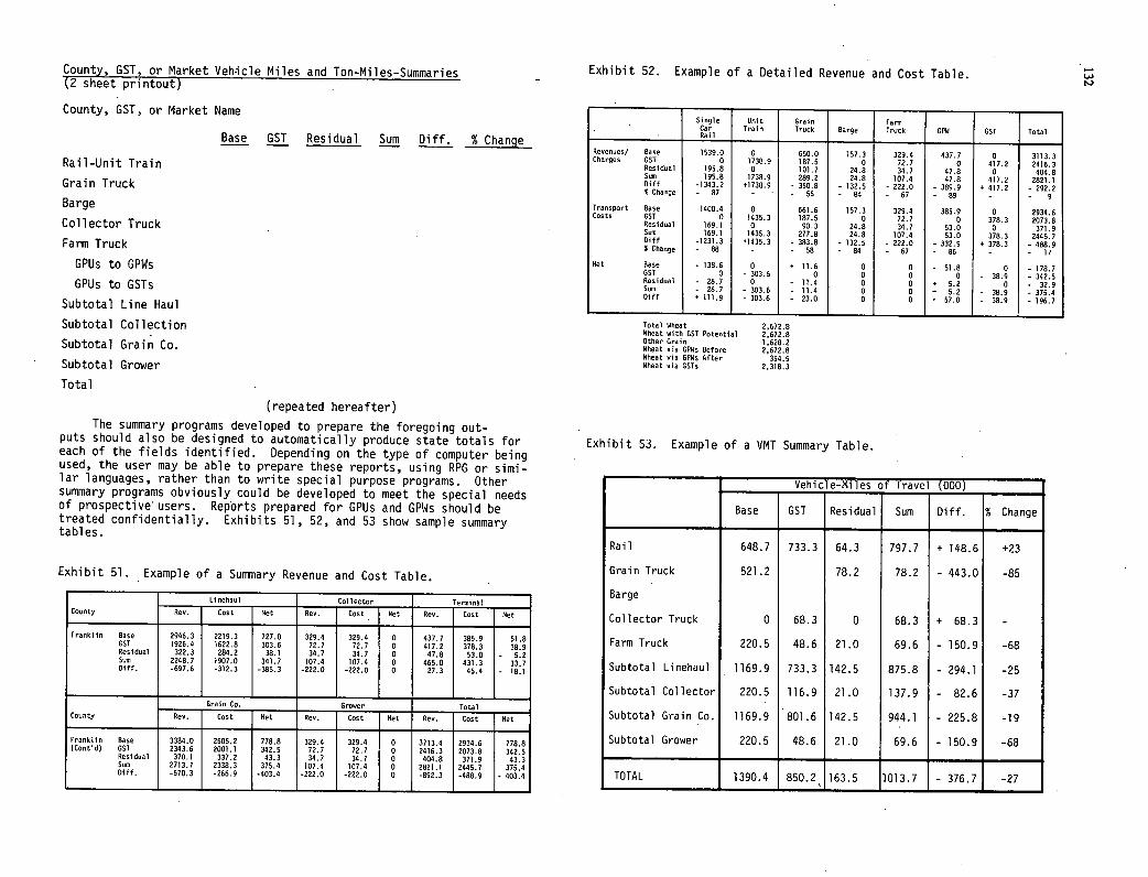
County, GST, or Market Veh-icle Miles and Ton-Miles-Summaries Exhibit 52. Example of a Detailed Revenue and Cost Table. (2 sheet printout)
Single Car Rail
Unit Train
Grain Truck Barge
Farm Truck GPO GST Total
Revenues! Base 1539.0 0 650.0 157.3 329.4 437.7 0 3113.3 Charges GST 0 1738.9 187.5 0 72.7 0 417.2 2416.3 Residual 195.8 0 101.7 24.8 34.7 47.8 0 404.8 Sum 195.8 1738.9 289.2 24.8 107.4 47.8 417.2 2821.1 Diff -1343.2 +1738.9 - 360.8 - 132.5 - 222.0 - 389.9 1 417.2 - 292.2 S Change - 87 - - 56 - 84 - 67 - 89 - - 9 Transpart Base 1400.4 0 661.6 157.3 329.4 385.9 0 2934.6 Costs GST 0 1435.3 187.5 0 72.7 0 378.3 2073.8 Residual 169.1 0 00.3 24.8 34.7 53.0 0 371.9 Sum 169.1 1435.3 277.8 24.8 107.4 53.0 378.3 2445.7 Diff -1231.3 01435.3 - 383.8 - 132.5 - 222.0 - 332.9 + 378.3 - 488.9 % Change - 88 - - 58 - 84 - 67 - 86 - - 17 Net Base - 138.6 0 + 11.6 0 0 - 51.8 0 - 178.7 GST 0 - 303.6 0 0 0 0 - 38.9 - 342.5 Residual - 26.7 0 - 11.4 0 0 + 5.2 0 - 32.9 Sum - 26.7 - 303.6 - 11.4 0 0 5.2 - 38.9 - 375.4 Diff * 111.9 - 303.6 - 23.0 0 0 57.0 - 38.9 - 196.7
Total Wheat 2672.8 Wheat with GOT Potential 2672.8 Other Grain 1628.2 Wheat via GPWs Before 2,672.8 Wheat via GPWs Ufter 354.5 Wheat via OSTs 2,318.3
County, GST, or Market Name
Base GST Residual Sum Diff. % Change
Rail-Unit Train
Grain Truck
Barge
Collector Truck
Farm Truck
GPUs to GPWs
GPUs to GSTs
Subtotal Line Haul
Subtotal Collection
Subtotal Grain Co.
Subtotal Grower
Total
(repeated hereafter)
The summary programs developed to prepare the foregoing out-puts should also be designed to automatically produce state totals for each of the fields identified. Depending on the type of computer being used, the user may be able to prepare these reports, using RPG or simi-lar languages, rather than to write special purpose programs. Other summary programs obviously could be developed to meet the special needs of prospective users. Reports prepared for GPUs and GPWs should be treated confidentially. Exhibi.ts 51, 52, and 53 show sample summary tables.
Exhibit 51. Example of a Summary Revenue and Cost Table.
Linehaul Collector Terminal County Rev. Cost Net Rev. Cost Net Rev. Cost Net
Franklin Base GST Residual Sum Diff.
2946.3 1926.4 322.3
2248.7 -697.6
2219.3 1622.8 284.2
1907.0 -312.3
727.0 303.6 38.1
341.7 -385.3
329.4 72.7 34.7 107.4
-222.0
329.4 72.7 34.7 107.4 -222.0
0 0 0 0 0
437.7 417.2 47.8 465.0 27.3
385.9 378.3 53.0 431.3 45.4
51.8 38.9
- 5.2 33.7
- 18.1
Grain Co. Grower Total Rev. Cost Net Rev. Cost Net Rev. Cost Net County
Franklin Base (Contd) GST
Residual Sun Diff.
3384.0 2343.6 370.1
2713.7 -670.3
2605.2 2001.1 337.2
2338.3 -266.9
778.8 342.5 43.3 375.4
-403.4
329.4 72.7 34.7
107.4 -222.0
329.4 72.7 34.7
107.4 -222.0
0 0 0 0 0
3713.4 2416.3 404.8 2821.1 -892.3
2934.6 2073.8 371.9
2445.7 -488.9
778.8 342.5 43.3 375.4 403.4
Exhibit 53. Example of a VMT Summary Table.
Vehicle-Miles of Travel (000)
Base GST Residual Sum Diff. % Change
Rail 648.7 733.3 64.3 797.7 + 148.6 +23
Grain Truck 521.2 78.2 78.2 - 443.0 -85
Barge
Collector Truck 0 68.3 0 68.3 + 68.3 -
Farm Truck 220.5 48.6 21.0 69.6 - 150.9 -68
Subtotal Linehaul 1169.9 733.3 142.5 875.8 - 294.1 -25
Subtotal Collector 220.5 116.9 21.0 137.9 - 82.6 -37
Subtotal Grain Co. 1169.9 801.6 142.5 944.1 - 225.8 -19
Subtotal Grower 220.5 48.6 21.0 69.6 - 150.9 -68
7T0TAL_ 1390.4 850.2 163.5 1013.7 - 376.7 -27
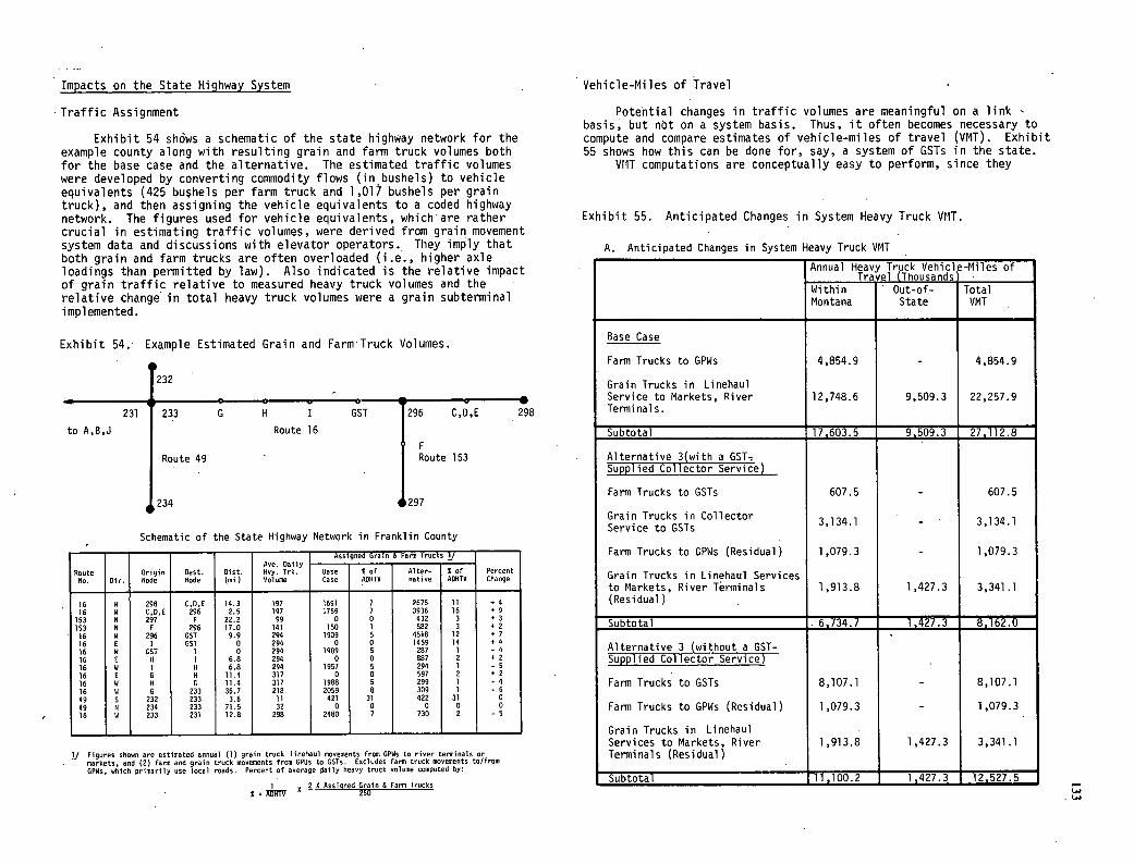
Impacts on the State Highway System
Traffic Assignment
Exhibit 54 shows a schematic of the state highway network for the example county along with resulting grain and farm truck volumes both for the base case and the alternative. The estimated traffic volumes were developed by converting commodity flows (in bushels) to vehicle equivalents (425 bushels per farm truck and 1,017 bushels per grain truck), and then assigning the vehicle equivalents to a coded highway network. The figures used for vehicle equivalents, which are rather crucial in estimating traffic volumes, were derived from grain movement system data and discussions with elevator operators. They imply that both grain and farm trucks are often overloaded (i.e., higher axle loadings than permitted by law). Also indicated is the relative impact of grain traffic relative to measured heavy truck volumes and the relative change in total heavy truck volumes were a grain subterminal implemented.
Exhibit 54. Example Estimated Grain and Farm Truck Volumes.
232 - 231 233 G H I GST 296 C,D,E 298
to A,B,J Route 16
F Route 49 Route 153
234
Schematic of the State Highway Network in Franklin County - Route
- Origin Rest.
- Gist.
Ave. Daily Buy. Irk.
Assigned Grain & Farm Trucks )J
Percent Base S of Alter- S of
No. Dir. Node Bode (mi ) Volume Case ADHTV native ADMTV Change
16 6 298 C.D.t 14.3 197 1691 7 2675 11 + 4 16 W C.D.t 296 2.5 197 1759 7 3936 16 9
153 N 297 F 22.2 99 0 0 432 3 3
153 9 F 296 17.0 141 150 1 562 3 v 2
16 6 296 GST 9.9 294 1909 5 4518 12 a 7
16 E I GOT 0 294 0 0 1459 14 a 4
16 6 GST 1
0 294 1909 5 287 - 4 16 V H 1 6.8 294 0 0 887 2 + 2 16 6 1 H 6.8 294 1957 5 294 - 5 16 E 0 H 11.4 317 0 0 597 2 * 2 16 6 H G 11.4 317 1988 5 299 1 4
16 6 6 233 36.7 218 2059 8 309 - 6 49 S 232 233 3.6 11 421 31 422 31
49 N 234 233 71.5 32 0 0 0 0 0
16 8 233 231 12.8 298 2480 7 730 2 - 5
jj Figures shown are estinated annual (1) grain truck linehaul movements from GPW5 to river terminals or markets, and (2) farm and grain truck movements from OPUs to GSTs. Excludes farm truck movements to/from GPW5, which primarily use local roads. Percent of average daily heavy truck voluoe computed by:
1 2 A Assigned Grain 6 Farm Trucks s=81iTV 250
Vehicle-Miles of Travel
Potential changes in traffic volumes are meaningful on a link basis, but not on a system basis. Thus, it often becomes necessary to compute and compare estimates of vehicle-miles of travel (VMT). Exhibit 55 shows how this can be done for, say, a system of GSTs in the state.
VI1T computations are conceptually easy to perform, since they
Exhibit 55. Anticipated Changes in System Heavy Truck VMT.
A. Anticipated Changes in System Heavy Truck VMT
Annual Heavy Trpck Vehicle-Miles of Travel (Thousands
Within Out-of- Total Montana State VMT
Base Case
Farm Trucks to GPW5 4,854.9 - 4,854.9
Grain Trucks in Linehaul Service to Markets, River 12,748.6 9,509.3 22,257.9 Terminals.
Subtotal 17,603.5 9,509.3 27,112.8
Alternative 3(with a GST Supplied Collector Service)
607.5 - 607.5 Farm Trucks to GSTs
Grain Trucks in Collector 3,134.1 - 3,134.1
Service to GSTs
Farm Trucks to GPW5 (Residual) 1,079.3 - 1,079.3
Grain Trucks in Linehaul Services to Markets, River Terminals 1,913.8 1,427.3 3,341.1 (Residual)
Subtotal 6,734.7 1,427.3 8,162.0
Alternative 3 (without a GST-
8,107.1 - 8,107.1
Supplied Collector Service)
Farm Trucks to GSTs
Farm Trucks to GPWs (Residual) 1,079.3 - 1,079.3
Grain Trucks in Linehaul Services to Markets, River 1,913.8 1,427.3 3,341.1 Terminals (Residual)
Subtotal 11,100.2 1 1,427.3 1 12,527.5
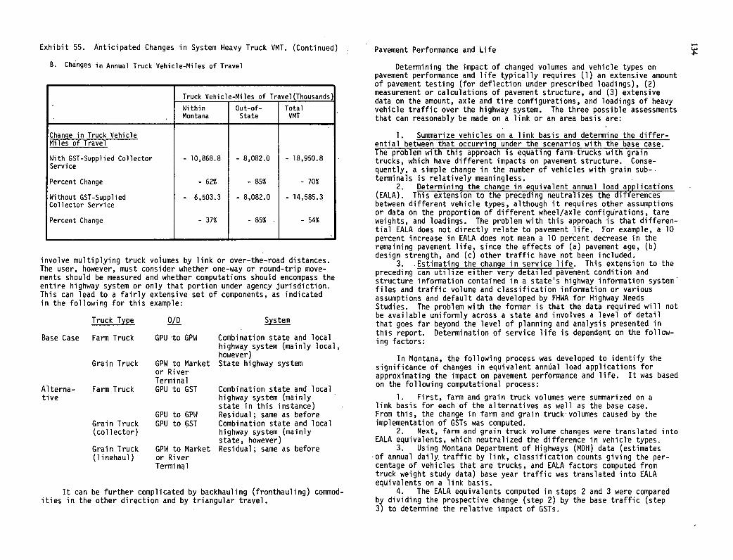
Exhibit 55. Anticipated Changes in System Heavy Truck VMT. (Continued) Pavement Performance and Life
B. Changes in Annual Truck Vehicle-Miles of Travel
- Truck Vehicle-Miles of Travel (Thousands)
Within Out-of- Total • Montana State VMT
Change in Truck Vehicle Miles of Travel
With GST-Supplied Collector - 10,868.8 - 8,082.0 - 18,950.8 Service
Percent Change - 62% - 85% - 70%
Without GST-Supplied - 6,503.3 - 8,082.0 - 14,585.3 Collector Service
Percent Change - 37% - 85% - 54%
involve multiplying truck volumes by link or over-the-road distances. The user, however, must consider whether one-way or round-trip move-ments should be measured and whether computations should encompass the entire highway system or only that portion under agency jurisdiction. This can lead to a fairly extensive set of components, as indicated in the following for this example:
Truck Type O/D
System
Base Case Farm Truck
GPU 'to GPW
Combination state and local highway system (mainly local, however)
Grain Truck
GPW to Market State highway system or River Terminal
Alterna- Farm Truck
GPU to GST
Combination state and local tive
highway system (mainly state in this instance)
GPU to GPW
Residual; same as before Grain Truck
GPU to GST
Combination state and local (collector)
highway system (mainly state, however)
Grain Truck
GPW to Market Residual; same as before (linehaul)
or River Termi n.1
It can be further complicated by backhauling (fronthauling) commod-ities in the other direction and by triangular travel.
Determining the impact of changed volumes and vehicle types on pavement performance and life typically requires (1) an extensive amount of pavement testing (for deflection under prescribed loadings), (2) measurement or calculations of pavement structure, and (3) extensive data on the amount, axle and tire configurations, and loadings of heavy vehicle traffic over the highway system. The three possible assessments that can reasonably be made on a link or an area basis are:
Summarize vehicles on a link basis and determine the differ-ential between that occurring under the scenarios with the base case. The problem with this approach is equating farm-trucks with grain trucks, which have different impacts on pavement structure. Conse-quently, a simple change in the number of vehicles with grain sub-terminals is relatively meaningless.
Determining the change in equivalent annual load applications (EALA). This extension to the preceding neutralizes the differences between different vehicle types, although it requires other assumptions or data on the proportion of different wheel/axle configurations, tare weights, and loadings. The problem with this approach is that differen-tial EALA does not directly relate to pavement life. For example, a 10 percent increase in EALA does not mean a 10 percent decrease in the remaining pavement life, since the effects of (a) pavement age, (b) design strength, and (c) other traffic have not been included.
• Estimating the change in service life. This extension to the preceding can utilize either very detailed pavement condition and structure information contained in a state's highway information system files and traffic volume and classification information or various assumptions and default data developed by FHWA for Highway Needs Studies. The problem with the former is that the data required will not be available uniformly across a state and involves a level of detail that goes far beyond the level of planning and analysis presented in this report. Determination of service life is dependent on the follow-ing factors:
In Montana, the following process was developed to identify the significance of changes in equivalent anntal load applications for approximating the impact on pavement performance and life. It was based on the following computational process:
First, farm and grain truck volumes were summarized on a link basis for each of the alternatives as well as the base case. From this, the change in farm and grain truck' volumes caused by the implementation of GSTs was computed.
Next, farm and grain truck volume changes were translated into EALA equivalents, which neutralized the difference in vehicle types.
Using Montana Department of Highways (MDH) data (estimates of annual daily, traffic by link, classification counts giving the per-centage of vehicles that are trucks, and EALA factors computed from truck weight study data) base year traffic was translated into EALA equivalents on a link basis.
The EALA equivalents computed in steps 2 and 3 were compared by dividing the prospective change (step 2) by the base traffic (step 3) to determine the relative impact of GSTs.
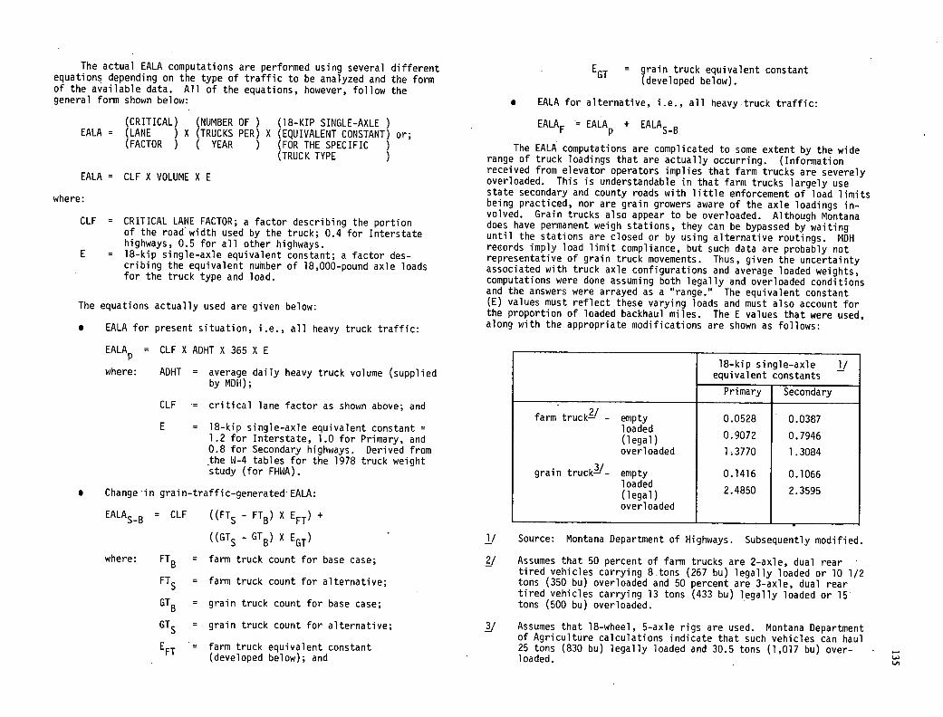
The actual EALA computations are performed using several different equations depending on the type of traffic to be analyzed and the form of the available data. All of the equations, however, follow the general form shown below:
(CRITICAL) (NUMBER OF ) (18-KIP SINGLE-AXLE EALA = (LANE ) X (TRUCKS PER) X (EQUIVALENT CONSTANT) or;
(FACTOR ) C YEAR ) (FOR THE SPECIFIC (TRUCK TYPE
The equations actually used are given below:
. EALA for present situation, i.e., all heavy truck traffic:
EALA = CLF X ADHT X 365 X E
where: ADHT = average daily heavy truck volume (supplied by MDH);
CLF '= critical lane factor as shown above; and
E = 18-kip single-axle equivalent constant = 1.2 for Interstate, 1.0 for Primary, and 0.8 for Secondary highways. Derived from .the W-4 tables for the 1978 truck weight study (for FHWA).
Change 'in grain-traffic-generated' EALA:
EALASB = CLF ((FIs - FIB) X EFT) +
((GIs - GTB) X EGI)
where: FIB = farm truck count for base case;
FT5 = farm truck count for alternative;
GTB = grain truck count for base case;
GT5 = grain truck count for alternative;
EFT '= farm truck equivalent constant (developed below); and
EGI = grain truck equivalent constant (developed below).
EALA for alternative, i.e., all heavytruck traffic:
EALAF '= EALA + EALASB
The EALA computations are complicated to some extent by the wide range of truck loadings that are actually occurring. (Information received from elevator operators implies that farm trucks are severely overloaded. This is understandable in that farm trucks largely use state secondary and county roads with little enforcement of load limits being practiced, nor are grain growers aware of the axle loadings in-volved. Grain trucks also appear to be overloaded. Although Montana does have permanent weigh stations, they can be bypassed by waiting until the stations are closed or by using alternative routings. MDH records imply load limit compliance, but such data are probably not representative of grain truck movements. Thus, given the uncertainty associated with truck axle configurations and average loaded weights, computations were done assuming both legally and overloaded conditions and the answers were arrayed as a "range." The equivalent constant (E) values must reflect these varying loads and must also account for the proportion of loaded backhaul miles. The E values that were used, along with the appropriate modifications are shown as follows:
18-kip single-axle 1/ equivalent constants
Primary Secondary
farm truck-" - empty 0.0528 0.0387 loaded (legal) 0.9072 0.7946
overloaded 1.3770 1.3084
grain truck'- empty 0.1416 0.1066 loaded (legal) 2.4850 2.3595
overloaded
1/ Source: Montana Department of Highways. Subsequently modified.
2/ Assumes that 50 percent of farm trucks are 2-axle, dual rear tired vehicles carrying 8,tons (267 bu) legally loaded or 10 1/2 tons (350 bu) overloaded and 50 percent are 3-axle, dual rear tired vehicles carrying 13 tons (433 bu) legally loaded or 15 tons (500 bu) overloaded.
3/ Assumes that 18-wheel, 5-axle rigs are used. Montana Department of Agriculture calculations indicate that such vehicles can haul 25 tons (830 bu) legally loaded and 30.5 tons (1,017 bu) over-loaded.
EALA = CLF X VOLUME X E
where:
CLF = CRITICAL LANE FACTOR; a factor describing the portion of the road width used by the truck; 0.4 for Interstate highways, 0.5 for all other highways.
E = 18-kip single-axle equivalent constant; a factor des- cribing the equivalent number of 18,000-pound axle loads for the truck type and load.
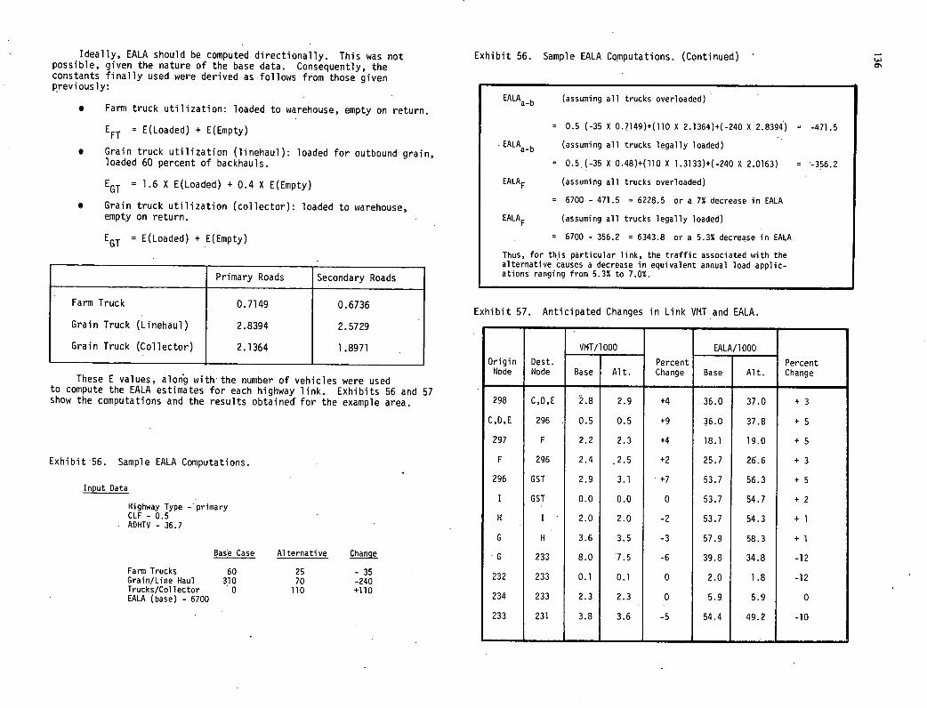
Ideally, EALA should be computed directionally. This was not possible, given the nature of the base data. Consequently, the constants finally used were derived as follows from those given previously:
Farm truck utilization: loaded to warehouse, empty on return.
EEl = E(Loaded) + E(Empty)
Grain truck utilization (linehaul): loaded for outbound grain, loaded 60 percent of backhauls.
EGT = 1.6 X E(Loaded) + 0.4 X E(Empty)
Grain truck utilization (collector): loaded to warehouse, empty on return.
EGT = E(Loaded) + E(Empty)
Primary Roads Secondary Roads
Farm Truck 0.7149 0.6736
Grain Truck (Linehaul) 2.8394 2.5729
Grain Truck (Collector) 2.1364 1.8971
These E values, alon with the number of vehicles were used to compute the EALA estimates for each highway link. Exhibits 56 and 57 show the computations and the results obtained' for the example area.
Exhibit - 56. Sample EALA Computations.
Input Data
Highway Type -'primary CLF - 0.5 ADHTV - 36.7
Base Case Alternative Change
Farm Trucks 60 25 - 35 Grain/Line Haul 310 70 -240 Trucks/Collector 0 110 +110 EALA (base) - 6700
Exhibit 56. Sample EALA Computations. (Continued)
EALAa_b (assuming all trucks overloaded)
= 0.5 (-35 X 0.7149)+(110 X 2.1364)+(-240 X 2.8394) = -471.5
EALAa b (assuming all trucks legally loaded)
= 0.5(-35 X 0.48)+(11O X 1.3133)+(-240 X 2.0163) = -356.2
EALAF (assuming all trucks overloaded)
= 6700 - 471.5 = 6228.5 or a 7% decrease in EALA
EALAF (assuming all trucks legally loaded)
= 6700-356.2 = 6343.8 or a 5.3% decrease in EALA
Thus, for this particular link, the traffic associated with the alternative causes a decrease in equivalent annual load applic-ations ranging from 5.3% to 7.0%.
Exhibit 57. Anticipated Changes in Link VMT and EALA.
Origin Dest.
VMT/1000
Percent
EALA/1000
Percent Node Node Base Alt. Change Base Alt. Change
298 C,D,E 2.8 2.9 +4 36.0 37.0 + 3
C,D,E 296 , 0.5 0.5 +9 36.0 37.8 + 5
297 F 2.2 2.3 +4 18.1 19.0 + 5
F 296 2.4 2.5 +2 25.7 26.6 + 3
296 GST 2.9 3.1 +7 53.7 56.3 + 5
I GST 0.0 0.0 0 53.7 54.7 + 2
H , I 2.0 2.0 -2 53.7 54.3 + 1
G H 3.6 3.5 -3 57.9 58.3 + 1
6 233 8.0 7.5 -6 39.8 34.8 -12
232 233 0.1 0.1 0 2.0 1.8 -12
234 233 2.3 2.3 0 5.9 5.9 0
233 231 3.8 3.6 -5 54.4 49.2 -10
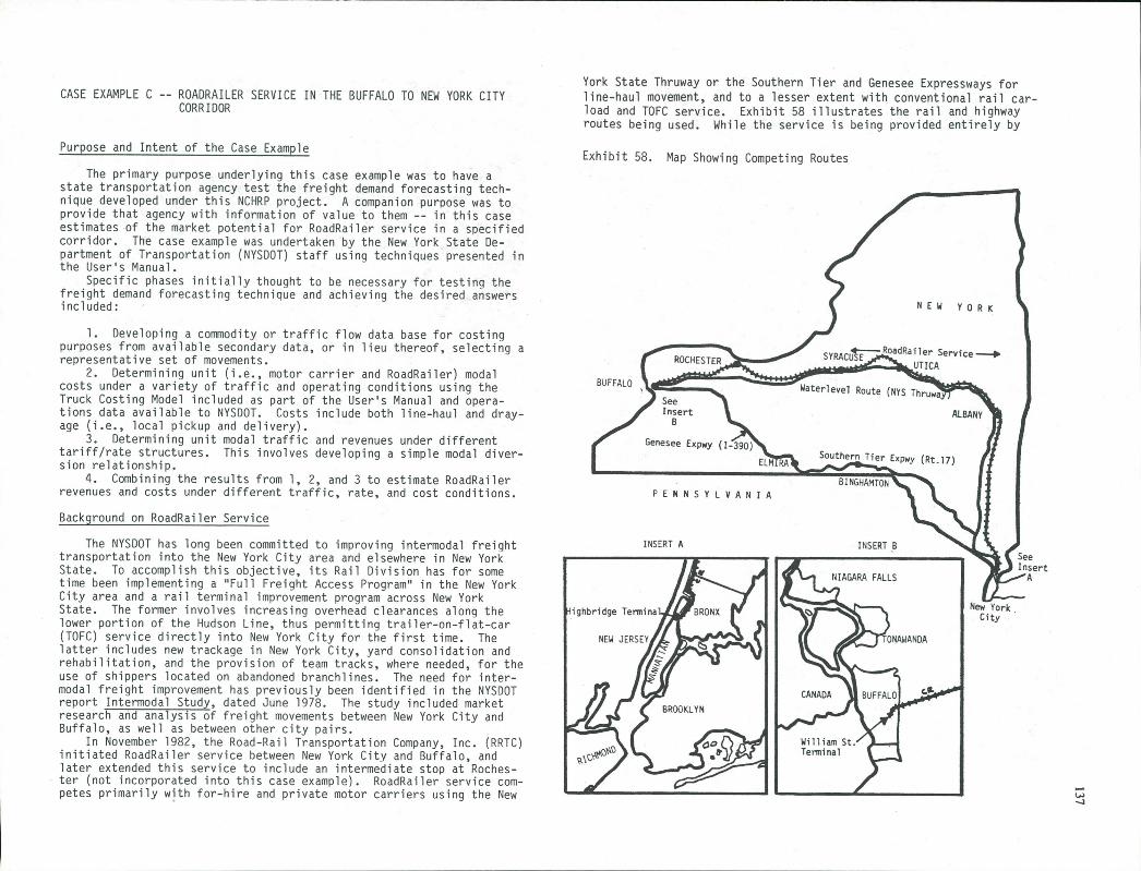
N E W YORK
Service —+
BUFFALO
Genesee Expwy
P E N N S V L V A N I A
INSERT A
Waterleve] Route (NYS Th
Southern Tier Ex
AMTON
INSERT B
ALBANY
New York City
See Insert
York State Thruway or the Southern Tier and Ienesee Expressways for line-haul movement, and to a lesser extent with conventional rail car-load and TOFC service. Exhibit 58 illustrates the rail and highway routes being used. While the service is being provided entirely by
CASE EXAMPLE C -- ROADRAILER SERVICE IN THE BUFFALO TO NEW YORK CITY CORRIOOR
Purpose and Intent of the Case Example
The primary purpose underlying this case example was to have a state transportation agency test the freight demand forecasting tech-nique developed under this NCHRP project. A companion purpose was to provide that agency with information of value to them -- in this case estimates of the market potential for RoadRailer service in a specified corridor. The case example was undertaken by the New York State De-partment of Transportation (NYSDOT) staff using techniques presented in the Users Manual.
Specific phases initially thought to be necessary for testing the freight demand forecasting technique and achieving the desired answers included:
Developing a commodity or traffic flow data base for costing purposes from available secondary data, or in lieu thereof, selecting a representative set of movements.
Determining unit (i.e., motor carrier and RoadRailer) modal costs under a variety of traffic and operating conditions using the Truck Costing Model included as part of the User's Manual and opera-tions data available to NYSDOT. Costs include both line-haul and dray-age (i.e., local pickup and delivery).
Determining unit modal traffic and revenues under different tariff/rate structures. This involves developing a simple modal diver-sion relationship.
Combining the results from 1, 2, and 3 to estimate RoadRailer revenues and costs under different traffic, rate, and cost conditions.
Background on RoadRailer Service
The NYSDOT has long been committed to improving intermodal freight transportation into the New York City area and elsewhere in New York State. To accomplish this objective, its Rail Division has for some time been implementing a "Full Freight Access Program" in the New York City area and a rail terminal improvement program across New York State. The former involves increasing overhead clearances along the lower portion of the Hudson Line, thus permitting trailer-on-flat-car (TOFC) service directly into New York City for the first time. The latter includes new trackage in New York City, yard consolidation and rehabilitation, and the provision of team tracks, where needed, for the use of shippers located on abandoned branchlines. The need for inter-modal freight improvement has previously been identified in the NYSDOT report Intermodal Study, dated June 1978. The study included market research and analysis of freight movements between New York City and Buffalo, as well as between other city pairs.
In November 1982, the Road-Rail Transportation Company, Inc. (RRTC) initiated RoadRailer service between New York City and Buffalo, and later extended this service to include an intermediate stop at Roches-ter (not incorporated into this case example). RoadRailer service com-petes primarily with for-hire and private motor carriers using the New
Exhibit 58. Map Showing Competing Routes
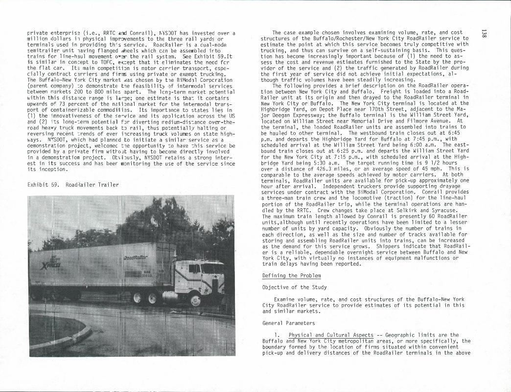
private enterprise (i.e., RRTC .as.:1 Conrail), 'ISJ01 has invested over a million dDllars i -i physical imprwements to the three rail yards or terminals used in providing ths service. RoacRailer is a cual-mode semitrailer unit iaving flanged .ieels hich can be asserthied irto trains for line-heul movement o-- the rail system. See Exhibit 59.It is similar in con :ept to TOFC, meept that it eliminates the neec fcr the flat car. It; main competitijn is rotor carrier traispert, espe-cially contract cirriers and firTc using private or exempt trucking. The Buffalo-New Yrk City market 4as chosen by tie BiN'dnl Corperation (parent company) :0 demonstrate tie feasibility of int.ermiodal services between rarkets 200 to 800 mile. apart. The lcnl-term market pctential ithin this distaice range is li"-9e; one estimate is tha: it cortairs upwards of 73 percent of the natinnal market for the intermodal trars-port of container izable commodities. Its importance to states lies in (1) the innovativeness of the se"ice and its aplication across the 115 and (2) ts long-erm potential fr diverting rredium-dis:ance over-the-road heaw'j truck novements back tn rail, thus po:entialli haltirg or reversing recent :rends of ever increasing truck voluns on state high-hays. NVSDOT, which had planned to initiate a similar service as a demonstration project, welcomec tie opportunity =0 have :his service be provided by a pri'ate firm witcjt having to lcome directly invclved in a demonstration project. Ob.iusly, NYSDOT retains a strong inter-est in its success and has beer msnitoring the use of the service since its incep:ion.
Exhibit 59. Roadailer Trailer
The case example chosen involves examining volume, rate, and cost structures of the Buffalo/Rochester/New York City RoadRailer service to estimate the point at which this service becomes truly competitive with trucking, and thus can survive on a self-sustaining basis. This ques-tion has become increasingly important because of (1) the need to as-sess the cost and revenue estimates furnished to the State by the pro-vider of the service and (2) the traffic generated by RoadRailer during the first year of service did not achieve initial expectations, al-though traffic volumes have been steadily increasing.
The following provides a brief description on the RoadRailer opera-tion between New York City and Buffalo. Freight is loaded into a Road-Railer unit at its origin and then drayed to the RoadRailer terminal in New York City or Buffalo. The New York City terminal is located at the Highbridge Yard, on Depot Place near 170th Street, adjacent to the Ma-jor Deegan Expressway; the Buffalo terminal is the William Street Yard, located on William Street near Memorial Drive and Filmore Avenue. At the terminal, the loaded RoadRailer units are assembled into trains to be hauled to other terminal. The westbound train closes out at 6:45 p.m. and departs the Highbridge Yard for Buffalo at 7:45 p.m., with scheduled arrival at the William Street Yard being 6:00 a.m. The east-bound train closes out at 6:25 p.m. and departs the William Street Yard for the New York City at 7:15 p.m., with scheduled arrival at the High-bridge Yard being 5:30 a.m. The target running time is 9 1/2 hours over a distance of 426.3 miles, or an average speed of 45 mph. This is comparable to the average speeds achieved by motor carriers. At both terminals, RoadRailer units are available for pick-up approximately one hour after arrival. Independent truckers provide supporting drayage services under contract with the BiModal Corporation. Conrail provides a three-man train crew and the locomotive (traction) for the line-haul portion of the RoadRailer trip, while the terminal operations are han-dled by the RRTC. Crew changes take place at Selkirk and Syracuse. The maximum train length allowed by Conrail is presently 60 RoadRailer units,although until recently operations have been limited to a lesser number of units by yard capacity. Obviously the number of trains in each direction, as well as the size and number of tracks available for storing and assembling RoadRailer units into trains, can be increased as the demand for this service grows. Shippers indicate that RoadRail-er is a reliable, dependable overnight service between Buffalo and New York City, with virtually no instances of equipment malfunctions or train delays having been reported.
Defining the Problem
Objective of the Study
Examine volume, rate, and cost structures of the Buffalo-New York City RoadRailer service to provide estimates of its potential in this and similar markets.
General Parameters
1. Physical and Cultural Aspects -- Geographic limits are the Buffalo and New York City metropolitan areas, or more specifically, the boundary formed by the location of firms situated within convenient pick-up and delivery distances of the RoadRailer terminals in the above
00
two cities. (The notion of a service area boundary, which can never really be delineated, is at best an imprecise measure of market poten-tial.) Affected transport infrastructure (routes) includes Conrail's Hudson and Albany-Buffalo mainlines and the Interstate highways (or equivalent expressways) connecting Buffalo and New York City. Affected shippers are those presently utilizing motor carriers or private truck-ing to ship merchandise in truckload quantities between Buffalo and New York City who could find it more economical to utilize RoadRailer ser-vice .instead of motor carriers.
General Orientation -- Primarily modal with the emphasis being on comparing services.
Modes, Transport Facilities, and Services Utilized -- Road-Railer service and truckload motor carrier service between Buffalo and New York City over previously identified routes. Trucking includes common, contract, and private carriers operating both single and tandem trailers. Much of the freight is thought to be moving under contract rates.
Commodities being Transported -- Merchandise and some bulk commodities moving in truckload units. Market is limited to commodi-ties originating and terminating in the identified service areas.
Alternative Futures, Scenarios, or Conditions to be Examined Application is primarily focused on the present or base year, although it includes the removal of tolls from the New York State Thruway. Al-ternative futures or scenarios involving the projection of traffic for future years are not a part of this case example.
Regulatory Environment -- Unrestrained competition between existing trucking and the recently introduced RoadRailer service.
Major Tasks to be Accomplished (See Figure 1 of the User's Manual)
Present Economic Activities Freight Traffic Generation Freight Traffic Distribution Present Service, Cost & Price Characteristics Modal Division
Analytical Choices
Measure Performance in Economic, Physical, or Impact Terms --Economic, since the application involves examining the costs of compet-ing transport services to appraise the potential of RoadRailer service.
Estimate Modal Shares on a Unit Price or Cost Basis -- Pri-marily on a cost basis, although rates must be considered in determin-ing traffic volumes.
Apply a Physical Distribution or Transport Economics Orienta-tion -- Transport economics, since storage and distribution costs in-curred by individual firms would be approximately the same among com-peting modes.
Price/Cost Movements on a One-way or Round-Trip Basis -- In this application, transport costs have been computed as one-way move-ments. Normally, such costs would be computed on a round-trip basis taking into account backhaul utilization. This requires reliable in-formation on backhaul utilization, which does not exist in this case example. In this case, an analysis of rOund-trips would be more de-pendent upon the backhaul assumptions made rather than on the unit costs employed.
Optimizing Locations or Flows -- Not required.
Required Products
1. Record for all or selected movements -containing the following information:
Identification
Assigned origin. Assigned destination. Commodity type.
Contents
Commodity flow volume (in tons annually). Designation as an existing or potential movement. Unit revenues/charges via RoadRailer and various motor carrier services (for-hire, private, exempt, etc.). Unit transport costs via RoadRailer and various motor carrier services. RoadRailer costs to be based on those expected once anticipated traffic volumes have been achieved.
2. Report summarizing the anticipated economics of RoadRailer service compared with existing truck transport.
Simplifying Premises and Assumptions
RoadRailer service and costs are based on an average of 40 units per train. Thus, the case example assumes normal operations ra-ther than start-up conditions.
Aggregate demand within the Buffalo-New York City corridor is price and service inelastic.
Modal division solely dependent on logistics costs. Use of the higher truck weights allowed by the Surface Trans-
portation Reform Act of 1982. Reducing the scope of the case example by disregarding the
Rochester traffic.
Data Requirements and Availability
Aggregate commodity movements by RoadRailer and truck between Buffalo and New York City.
Unit costs for RoadRailer and truck service.
Preparing Base Case Inputs
Commodity Flows
Acquisition of or development of a suitable commodity flow matrix is the single most important input for this application. Since a mat-rix containing data-giving commodity identification, volume or weight of the movement, motor carrier type, and unit or total carrier charges disaggregated to the county level was not available, nor could one be
developed from available secondary data, NYSDOT instead identified a set of representative movements to be used as a proxy for the desired commodity flow matrix in examining the feasibility of RoadRailer service. While this substitution was not ideal from the standpoint of illustrating the use of the freight demand forecasting technique, it does illustrate how'a partial set of data can be assembled and used to carry out the intended study in situations where a state has neither the staff time nor fiscal resources to collect alternative primary data. In this case, primary data would have been preferred, and is considered essential if the market potential of RoadRailer service is to be fully established. In making this substitution, the resulting product will not be as statistically reliable as that which would have been achieved had more complete commodity flow data been available.
The starting point was the following two Transearch tabulations showing originating and terminating freight by geographic area (see Ex-hibits 60 and 61):
A tabulation of freight to/from the New York City (NYC) Busi-ness Economic Area (BEA) from/to the Buffalo BEA (a standard Transearch proauct), which reports traffic generated in tons and 40-foot freight container equivalents. Traffic is also further divided by the follow-ing modes or submodes: rail carload, intermodal, for-hire truckloads, shipments carried by private or exempt truckers, airborne, and water-8orne. Volumes reported are an estimate of all traffic between the NYC BEA and the Buffalo BEA classified by Standard Transportation Commodity Code (STCC) at the 5-digit level of detail.
A tabulation of freight to/from the Mid-West Region to that portion of the NYC BEA east of the Hudson River (a special tabulation purchased by NYSDOT), which reports traffic by mode or submode in tons for rail, TOFC, and truck. Traffic reported was an estimate of surface traffic between a NYSDOT Rail Division defined Mid-West Region and the New York State part of the NYC BEA classified by STCC at the 3-digit level, of detail.
The foregoing data sets had these limitations:
Since the data were not true commodity flow data, origin and destination linkages could not be ascertained directly, and thus had to be approximated through using other information.
Since the data were highly aggregated, the tabulations report-ed traffic from a far larger geographic area than for which shippers would normally consider using RoadRailer service. The tabulations also included movements which did not represent potential RoadRailer traffic.
Direct identification of the f.irms generating or receiving the traffic from the data was not possible. Thus pick-up and delivery movements from the RoadRailer terminal had to be approximated.
Thus, NYSDOT had to devise a process to enhance and extend these data to produce a set of representative movements. This, then, would allow preparation of modal cost estimates and extension to all surface traffic between Buffalo and New York City. The key lay in selecting representative movements. Since this could not be done statistically, guidelines were developed to develop likely commodity flows and mini-mize possible distortions. Commodities selected by NYSDOT were:
Known, relatively large-scale movements between New York City and Buffalo.
Representative of the principal types of commodities likely to move between these two cities.
Typically, (1) inputs to manufacturing activities located in these cities, (2) outputs of manufacturing processes located in these cities, or (3) widely used consumer products. $ Capable of being shipped (economically) by rail, truck, or Road-
Railer.
Steps used by the NYSDOT staff in developing representative move-ments are outlined below:
1. First, identify the principal commodity groups generating traf-fic from which to select representative movements. In this case, NYSDOT used the Transearch tabulations to identify the following com-modity groups:
Food or kindred products (STCC Code 20). Pulp, paper, or allied products (STCC Code 26). Chemicals or allied products (STCC Code 28). Petroleum and coal products (STCC Code 29). Clay, concrete, glass, or stone (STCC Code 32). Metal products (STCC Codes 33 and 34). Manufacturers (STCC Codes 35, 36, 379 38 and 39). Freight, all kinds (STCC Code 46).
Although appreciable tonnages of petroleum products move between New York and Buffalo, most of this traffic moves by water. Because di-version of this traffic to RoadRailer was unlikely, NYSDOT chose to ex-clude this commodity group.
2. Using the foregoing tabulations and other supplementary infor-mation, NYSDOT staff then selected representative commodities. The following documents a portion of the reasoning used by the NYSDOT staff for accomplishing this.
The choices from the food and kindred products group were relative-ly easy: flour in the eastbound directiorl and sugar in the westbound. Because Buffalo is a major milling center, and because flour is a major commodity flowing from Buffalo to New York City, flour (in bags) was included. Although New York City is not a sugar refining center in the sense that Buffalo is a flour milling center, sugar beets and sugar cane are received and refined in the New York City BEA. For this rea-son, sugar (in bags) was included.
The pulp, paper and allied products and printed paper groups are important, because New York City is a major printing center. On the other hand, the Buffalo BEA is neither a major printing nor a major pa-per manufacturing area. The largest eastbound flow was printing paper. Inasmuch as the tabulation indicated that this traffic moved entirely by rail, it was excluded from further consideration. Paper (other than printing paper) was a better candidate because a majority of this traf-fic moves by truckload (TL), less-than-truckload (LTL), private/ exempt truck, and RoadRailer. A similar situation occurred in the westbound direction. Containers or boxes and paper move by private/exempt truck, LTL, and to a lesser extent, by TL. Converted paper or paperboard products move almost entirely by TL. While the foregoing commodities
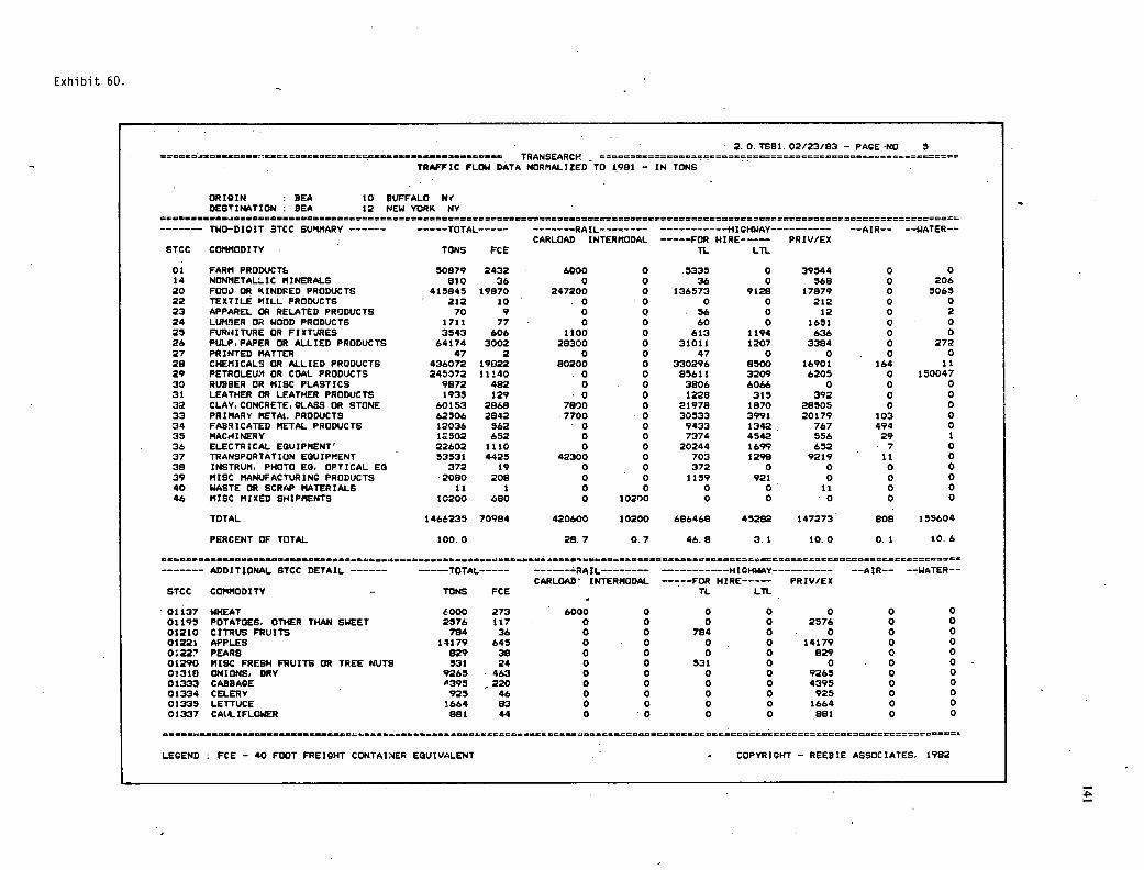
Exhibit 60. - -
2. 0. TS81. 02/23/83 - PAGE-NO S ................ ... ..... n TRANSEARSH TRAFFIC FLOW DATA NORMALIZED TO 1981 - IN TONS
ORIGIN SEA 10 BUFFALO N' DESTINATION : SEA 12 NEW YORK NV
TWO-DIGIT STCC SUMMARY TOTAL ----- ------- RAIL-- ------ ----------- HIGHWAY ---------- --AIR-- --WATER-- CARLOAD INTERMODAL -----FOR HIRE---- PRIV/EX
STCC COMMODITY TONS FCC TL LTL
01 FARM PRODUCTS 50879 2432 6000 0 .5335 0 39544 0 0 14 NONMETALLIC MINERALS 810 36 0 0 36 0 568 0 206 20 FO0I) OR KINDRED PRODUCTS 415845 19870 247200 0 136573 9128 17879 0 5065 22 TEXTILE MILL PRODUCTS 212 10 . 0 0 0 0 212 0 0 23 APPAREL OR RELATED PRODUCTS 70 9 0 0 56 0 12 0 2 24 LUMSER OR WOOD PRODUCTS 1711 77 0 0 60 0 1651 0 0 25 FUR1ITURE OR FIXTURES 3543 608 1100 0 613 1194 636 0 0 26 PULP.PAPER OR ALLIED PRODUCTS 64174 3002 28300 0 31011 1207 3384 0 272 27 PRINTED MATTER 47 2 0 0 47 0 0 . 0 0 28 CHEMICALS OR ALLIED PRODUCTS 438072 19022 80200 0 330296 8500 16901 164 11 29 PETROLEUM OR COAL PRODUCTS 245072 11140 0 0 85611 3209 6205 0 150047 30 RUBBER OR MISC PLASTICS 9872 482 0 0 3806 6066 0 0 0 31 LEATHER OR LEATHER PRODUCTS 1935 129 0 0 1228 315 392 0 0 32 CLAY, CONCRETE GLASS OR STONE 60153 2888 7800 0 21978 1870 28505 0 0 33 PRIMARY METAL. PRODUCTS 62506 2042 7700 0 30533 3991 20179 103 0 34 FABRICATED METAL PRODUCTS 12038 582 0 0 9433 1342 767 494 0 35 MAC04INERY 1502 652 0 0 7374 4542 558 29 I 36 ELECTRICAL EQUIPMENT' 22602 1110 0 0 20244 1699 652 7 0 37 TRANSPORTATION EQUIPMENT 53531 4425 42300 0 703 1298 9219 11 0 38 INSTRUM, PHOTO EO, OPTICAL EQ 372 19 0 0 372 0 0 0 0 39 MISC MANUFACTURING PRODUCTS 2080 208 0 0 1159 921 0 0 0 40 WASTE OR SCRAP MATERIALS 11 1 0 0 0 0 11 0 0 46 MISC MIXED SHIPMENTS 10200 680 0 10200 0 0 - 0 0 0
TOTAL 1466235 70984 420600 10200 686468 45282 147273 808 155604
PERCENT OF TOTAL 100.0 28.7 0.7 46.8 3.1 10.0 0.1 10.6
ADDITIONAL STCC DETAIL ------ ----- TOTAL ----- ------ -RAIL -------- NIG.4fAV---------- --AIR- CARLOAD' INTERNDDAL -----FOR HIRE---- PRIV/EX
STCC COMMODITY - TONS ECE TL LTh
01137 WHEAT 6000 273 6000 0 0 0 0 0 0 01195 POTATOES, OTHER THAN SWEET 2576 117 0 0 0 0 2576 0 0 01210 CITRUS FRUITS 784 36 0 0 784 0 0 0 0 01221 APPLES . 14179 645 0 . 0 0 0 14179 0 0 01227 PEARS 829 38 0 0 0 0 829 0 0 01290 MISC FRESH FRUITS OR TREE NUTS 531 24 0 0 531 0 0 . 0 0 - 01318 ONIONS, DRY 9265 463 0 0 0 0 9265 0 0 01333 CARBAGE 4395 220 0 0 0 0 4395 0 0 01334 CELERY 925 46 0 0 0 0 925 0 0 01335 LETTUCE 1664 83 0 0 0 0 1664 0 0 01337 CAULIFLOWER 881 44 0 0 0 0 881 0 0
LEGEND FCE - 40 FOOT FREIGHT CONTAIHER EQUIVALENT . - COPYRIGHT - REEBIE ASSOCIATES. 1982
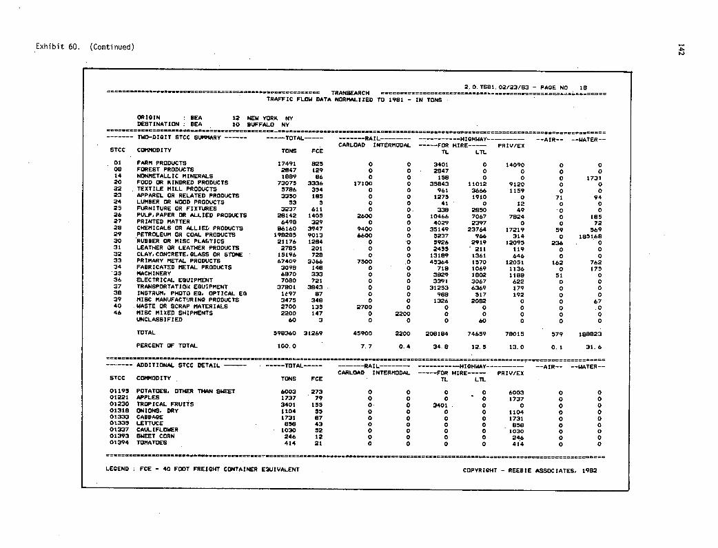
Exhibit 60. (Continued)
2. 0. TS8I.02123/83 - PAGE NO 18 cccntcn=-=r-c.flflcttwc=cn TRANSEARCH catnatnaa==c===c=s==-=___... TRAFFIC FLOW DATA NORMALIZED TO 1981 - IN TONS
ORIGIN : SEA 12 NEW YORK NY DESTINATION SEA 10 BUFFALO NY
TWO-DIGIT STCC SUMMARY ----- ----TOTAL ----- ----- -RAIL -------- -- - ----- - HIGHWAY ----- - --- --AIR-- --WATER-- CARLOAD INTERMODAL -----FOR HIRE---- PRIV/EX
STCC COMMODITY TONS FCE IL LTh
01 FARM PRODUCTS 17491 825 0 0 3401 0 14090 0 0 08 FOREST PRODUCTS 2847 129 0 0 2847 0 0 0 0 14 NONMETALLIC MINERALS 1999 86 0 0 158 0 0 0 1731 20 FOOD OR KINDRED PRODUCTS 73075 3336 17100 0 35843 11012 9120 0 0 22 TEXTILE MILL PRODUCTS 5786 354 0 0 961 3666 1159 0 0 23 APPAREL OR RELATED PRODUCTS 3350 185 0 0 1275 1910 0 71 94 24 LIfrIBER OR WOOD PRODUCTS 53 5 0 0 41 0 12 0 0 25 FURNITURE OR FIXTURES 3237 611 0 0. 338 2858 49 0 0 26 PULP. PAPER OR ALLIED PRODUCTS 28142 1405 2600 0 10466 7067 7824 0 185 27 PRINTED MATTER 6498 329 0 0 4029 2397 0 0 72 28 CHEMICALS OR ALLIED PRODUCTS 86160 3947 9400 0 35149 23764 17219 59 569 29 PETROLEUM OR COAL PRODUCTS 198295 9013 6600 0 5237 966 314 0 185168 30 RUBBER OR MISC PLASTICS 21176 1284 0 0 5926 2919 12095 236 0 31 LEATHER OR LEATHER PRODUCTS 2785 201 0 0 2455 211 119 0 0 32 CLAY, CONCRETE, GLASS OR STONE 15196 728 0 0 13189 1361 646 0 0 33 PRIMARY METAL PRODUCTS 67409 3366 7500 0 45364 1570 12051 162 762 34 FABRICATED METAL PRODUCTS 3098 148 0 0 718 1069 1136 0 175 35 MACHINERY 6870 333 0 0 3829 1802 1188 51 0 36 ELECTRICAL EQUIPMENT 7080 721 0 0 3391 3067 622 0 0 37 TRANSPORTATIO.i EQUIPMENT 37801 3843 0 0 31253 6369 179 0 0 38 INSTRUM, PHOTO EQ. OPTICAL EQ 1697 87 0 0 988 517 192 0 0 39 MISC MANUFACTURING PRODUCTS 3475 348 0 0 1326 2082 0 0 67 40 WASTE OR SCRAP MATERIALS 2700 135 2700 0 0 0 0 0 .0 46 MISC MIXED SHIPMENTS 2200 147 0 2200 0 0 0 0 0
(R4CLASSIFIED 60 3 0 0 0 60 0 0 0
TOTAL 599360 31269 45900 2200 208104 74659 78015 579 188823
PERCENT OF TOTAL 100.0 7.7 0.4 34.8 12.5 13.0 0.1 31.6
ADDITIONAL STCC DETAIL --- TOTAL ----- ------RAIL -------- --------- --HIGHWAY ----- - --- -AIR---- WATER-- CARLOAD INTERMODAL -----FOR HIRE---- PRIV/EX
STCC COMMODITY TONS FCE TL LTh
01195 POTATOES, OTHER THAN SWEET 6003 273 0 0 0 0 6003 0 0 01221 APPLES 1737 79 0 0 0 0 1737 0 0 01230 TROPICAL FRUITS 3401 155 0 0 3401 0 0 0 0 01318 ONIONS, DRY 1104 55 0 0 0 0 1104 0 0 01333 CABBAGE 1731 07 0 0 0 0 1731 0 0 01335 LETTUCE 858 43 0 0 0 0 858 0 0 01337 CA(LIFLOWER - 1030 52 - 0 0 0 0 1030 0 0 01393 SWEET CORN 246 12 0 0 0 0 246 0 0 01394 TOMATOES 414 21 0 0 0 0 414 0 0
LEGEND FCE - 40 FOOT FREIGHT CONTAINER EQUIVALENT COPYRIGHT - REEBIE ASSOCIATES, 1982
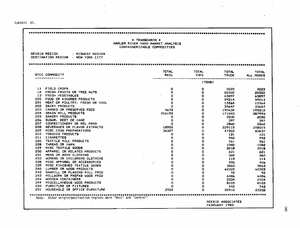
Exhibit 61.
* TRANSEARCH * HARLEM RIVER YARD MARKET ANALYSIS
CONTAINERIZABLE COMMODITIES
ORIGIN REGION : MIDWEST REGION DESTINATION REGION : NEW YORK CITY
TOTAL TOTAL TOTAL TOTAL STCC COMMODITY RAIL TOFC TRUCK ALL MODES
(TONS)
11 FIELD CROPS 0 0 3223 3223 12 FRESH FRUITS OR TREE NUTS 0 0 20522 20522 13 FRESH VEGETABLES : 0 0 65897 65897
200 FOOD OR KINDRED PRODUCTS 0 0 59214 59214 201 MEAT OR POULTRY, FRESH OR CHIL 0 0 15564 15564 202 DAIRY PRODUCTS 0 0 35647 35647 203 CANNED OR PRESERVED FOOD 4678 0 190634 195312 204 GRAIN MILL PRODUCTS 216150 0 171843 387993 205 BAKERY PRODUCTS 0 0 2030 2030 206 SUGAR, BEET OR CANE 0 0 397 397 207 CONFECTIONERY OR REL PROD 0 0 2860 2860 208 BEVERAGES OR FLAVOR EXTRACTS 18900 0 239115 258015 209 MISC FOOD PREPARATIONS 36327 0 47310 83637 210 TOBACCO PRODUCTS 0 0 121 121 211 CIGARETTES 0 0 942 942 220 TEXTILE MILL PRODUCTS 0 0 561 561 228 THREAD OR YARN 0 0 1082 1082 229 MISC TEXTILE GOODS 0 0 2018 2018 230 APPAREL OR RELATED PRODUCTS 0 0 621 621 231 MENS OR BOYS CLOTHING 0 0 360 360 233 WOMENS OR CHILDRENS CLOTHING 0 0 114 114 238 MISC APPAREL OR ACCESSORIES 0 0 406 406 239 MISC FINISHED TEXTILE GOODS 0 0 3863 3863 240 LUMBER OR WOOD PRODUCTS 0 0 62325 62325 242 SAWMILL OR PLANING MILL PROD 0 0 92 92 243 MILLUORK OR PREFAB WOOD PROD 0 0 6486 6486 244 WOODEN CONTAINERS 0 0 2334 2334 249 MISCELLANEOUS WOOD PRODUCTS 0 0 8105 8105 250 FURNITURE OR FIXTURES 0 0 542 542 251 HOUSEHOLD OR OFFICE FURNITURE 2922 0 20410 23332
Note: Other origin/destination regions were "West' and Central' • REEBIE ASSOCIATES FEBRUARY 1983
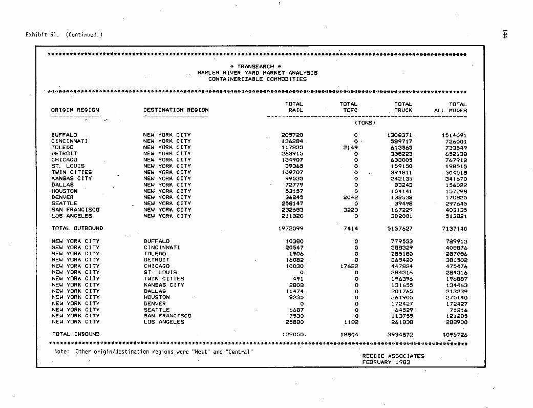
Exhibit 61. (Continued.)
**************************4
* TRANSEARCH * HARLEM RIVER YARD MARKET ANALYSIS
CONTAINERIZABLE COMMODITIES
TOTAL TOTAL TOTAL. TOTAL ORIGIN REGION DESTINATION REGION RAIL TOFC TRUCK ALL MODES
(TONS) -
BUFFALO NEW YORK CITY 205720 0 1308371 1514091 CINCINNATI NEW YORK CITY 136284 0 589717 726001 TOLEDO NEW YORK CITY 117835 2149 613565 733549 DETROIT NEW YORK CITY 263915 0 388223 652138 CHICAGO NEW YORK CITY 134907 0 633005 767912 ST. LOUIS NEW YORK CITY 39365 0 159150 198515 TWIN CITIES NEW YORK CITY 109707 0 394811 504518 KANSAS CITY NEW YORK CITY 99535 0 242135 341670 DALLAS NEW YORK CITY - 72779 0 83243 156022 HOUSTON NEW YORK CITY 53157 0 104141 157298 DENVER NEW YORK CITY 36245 2042 132538 170825 SEATTLE NEW YORK CITY 258147 0 39498 297645 SAN FRANCISCO NEW YORK CITY 232683 3223 167229 403135 LOS ANGELES NEW YORK CITY 211820 0 302001 513821
TOTAL OUTBOUND 1972099 7414 5157627 7137140
NEW YORK CITY BUFFALO 10380 0 779533 789913 NEW YORK CITY CINCINNATI 20547 0 388329 408876 NEW YORK CITY TOLEDO 1906 0 285180 287086 NEW YORK CITY DETROIT 16082 0 365420 381502 NEW YORK CITY CHICAGO 10030 17622 447824 475476 NEW YORK CITY ST. LOUIS 0 0 284316 284316 NEW YORK CITY TWIN CITIES 491 0 196396 196887 NEW YORK CITY KANSAS CITY 2808 0 131655 134463 NEW YORK CITY DALLAS 11474 0 201765 213239 NEW YORK CITY HOUSTON 8235 0 261905 270140 NEW YORK CITY DENVER 0 0 172427 172427 NEW YORK CITY SEATTLE 6687 0 64529 71216 NEW YORK CITY SAN FRANCISCO 7530 0 113755 121285 NEW YORK CITY LOS ANGELES 25880 1182 261838 288900
TOTAL INBOUND 122050. 18804 3954872 4095726 *4*****************************4**4**************4**
Note: Other origin/destination regions were West" and Central'1 REEBIE ASSOCIATES . - . FEBRUARY 1983
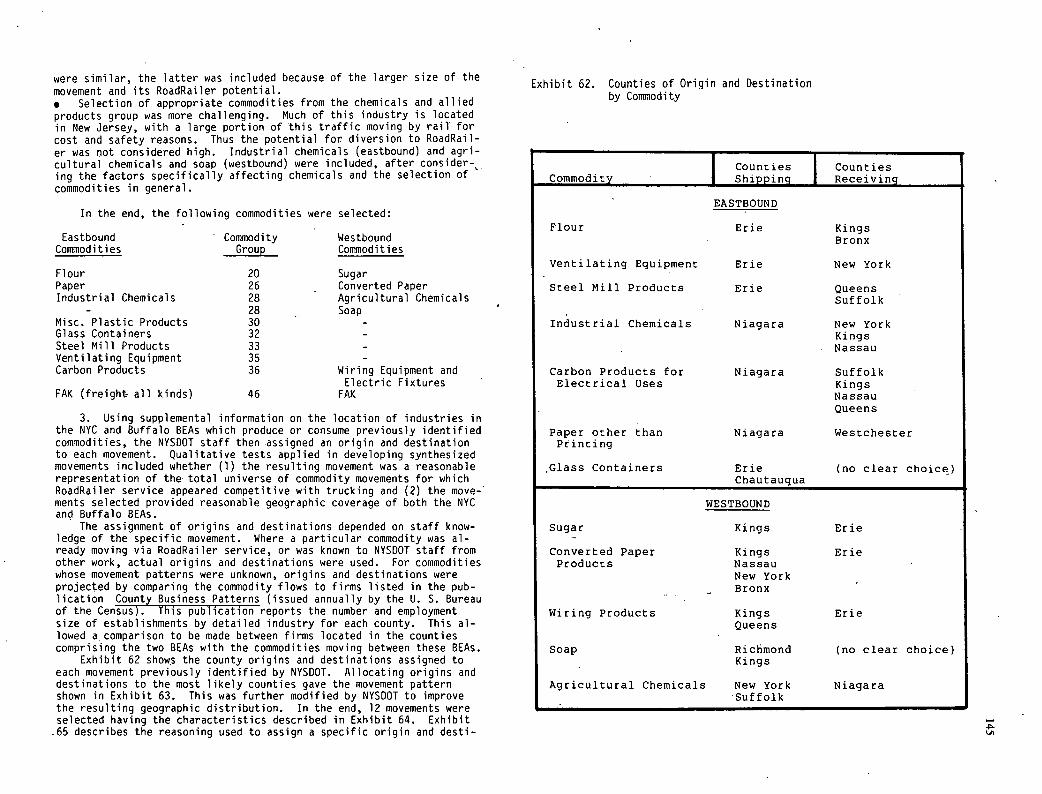
were similar, the latter was included because of the larger size of the movement and its RoadRailer potential. . Selection of appropriate commodities from the chemicals and allied products group was more challenging. Much of this industry is located in New Jersey, with a large portion of this traffic moving by rail-for cost and safety reasons. Thus the potential for diversion to RoadRail-er was not considered high. Industrial chemicals (eastbound) and agri-cultural chemicals and soap (westbound) were included, after consider-k ing the factors specifically affecting chemicals and the selection of commodities in general.
In the end, the following commodities were selected:
Eastbound Commodity Westbound Commodities Group Commodities
Flour 20 Sugar Paper 26 Converted Paper Industrial Chemicals 28 Agricultural Chemicals
- 28 - Soap Misc. Plastic Products 30 - Glass Containers 32 - Steel Mill Products 33 - Ventilating Equipment 35 - Carbon Products 36 Wiring Equipment and
Electric Fixtures FAK (freight- all kinds) 46 FAK
3. Using supplemental information on the location of industries in the NYC and Buffalo BEAs which produce or consume previously identified commodities, the NYSDOT staff then assigned an origin and destination to each movement. Qualitative tests applied in developing synthesized movements included whether (1) the resulting movement was a reasonable representation of the total universe of commodity movements for which RoadRailer service appeared competitive with trucking and (2) the move-ments selected provided reasonable geographic coverage of both the NYC and Buffalo BEAs.
The assignment of origins and destinations depended on staff know-ledge of the specific movement. Where a particular commodity was al-ready moving via RoadRailer service, or was known to NYSDOT staff from other work, actual origins and destinations were used. For commodities whose movement patterns were unknown, origins and destinations were projected by comparing the commodity flows to firms listed in the pub-lication County Business Patterns (issued annually by the U. S. Bureau of the Census). This publication reports the number and employment size of establishments by detailed industry for each county. This al-lowed a comparison to be made between firms located in the counties comprising the two BEAs with the commodities moving between these BEAs.
Exhibit 62 show.s the county origins and destinations assigned to each movement previously identified by NYSDOT. Allocating origins and destinations to the most likely counties gave the movement pattern shown in Exhibit 63. This was further modified by NYSDOT to improve the resulting geographic distribution. In the end, 12 movements were selected having the characteristics described in Exhibit 64. Exhibit 65 describes the reasoning used to assign a specific origin and desti-
Exhibit 62. Counties of Origin and Destination by Commodity
Commodity Counties
TShipping Counties Receiving
EASTBOUND
Flour Erie Kings Bronx
Ventilating Equipment Erie New York
Steel Mill Products Erie Queens Suffolk
Industrial Chemicals Niagara New York Kings
- Nassau
Carbon Products for Niagara Suffolk Electrical Uses Kings
Nassau Queens
Paper other than Niagara Westchester Printing
Glass Containers Erie (no clear choice) Chautauqua
WESTBOUND
Sugar Kings Erie
Converted Paper Kings Erie Products Nassau
New York - Bronx
Wiring Products Kings Erie Queens
Soap Richmond (no clear choice) Kings
Agricultural Chemicals New York Niagara Suffolk
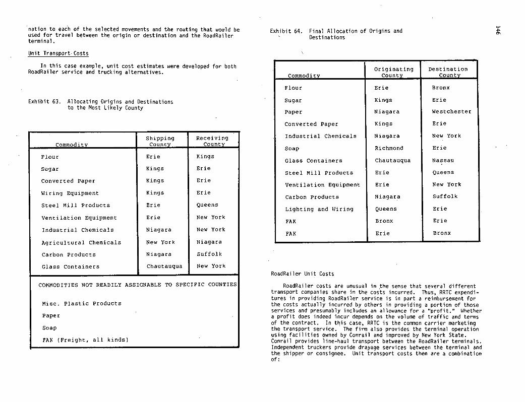
nation to each of the selected movements and the routing that would be Exhibit 64. Final Allocation of Origins and used for travel between the origin or destination and the RoadRailer Destinations terminal.
Unit Transport Costs
In this case example, unit cost estimates were developed for both RoadRailer service and trucking alternatives.
Exhibit 63. Allocating Origins and Destinations to the Most Likely County
Commodity Shipping County
Receiving County
Flour Erie Kings
Sugar Kings Erie
Converted Paper Kings Erie
Wiring Equipment Kings Erie
Steel Mill Products Erie Queens
Ventilation Equipment Erie New York
Industrial Chemicals Niagara New York
Agricultural Chemicals New York Niagara
Carbon Products Niagara Suffolk
Glass Containers Chautauqua New York
COMMODITIES NOT READILY ASSIGNABLE TO SPECIFIC COUNTIES
Misc. Plastic Products
Paper
Soap
FAK (Freight, all kinds)
Commodity Originating
County Destination
County
Flour Erie Bronx
Sugar Kings Erie
Paper Niagara Westchester
Converted Paper Kings Erie
Industrial Chemicals Niagara New York
Soap Richmond Erie
Glass Containers Chautauqua Nassau
Steel Mill Products Erie Queens
Ventilation Equipment Erie New York
Carbon Products Niagara Suffolk
Lighting and %iring Queens Erie
FAK Bronx Erie
FAK Erie Bronx
RoadRailer Unit Costs
RoadRailer costs are unusual in the sense that several different transport companies share in the costs incurred. Thus, RRTC expendi-tures in providing RoadRailer service is in part a reimbursement for the costs actually incurred by others in providing a portion of those services and presumably includes an allowance for a profit. Whether a profit does indeed incur depends on the volume of traffic and terms of the contract. In this case, RRTC is the common carrier marketing the transport service. The firm also provides the terminal operation using facilities owned by Conrail and improved by New York State. Conrail provides line-haul transport between the RoadRailer terminals. Independent truckers provide drayage services between the terminal and the shipper or consignee. Unit transport costs then are a combination of:
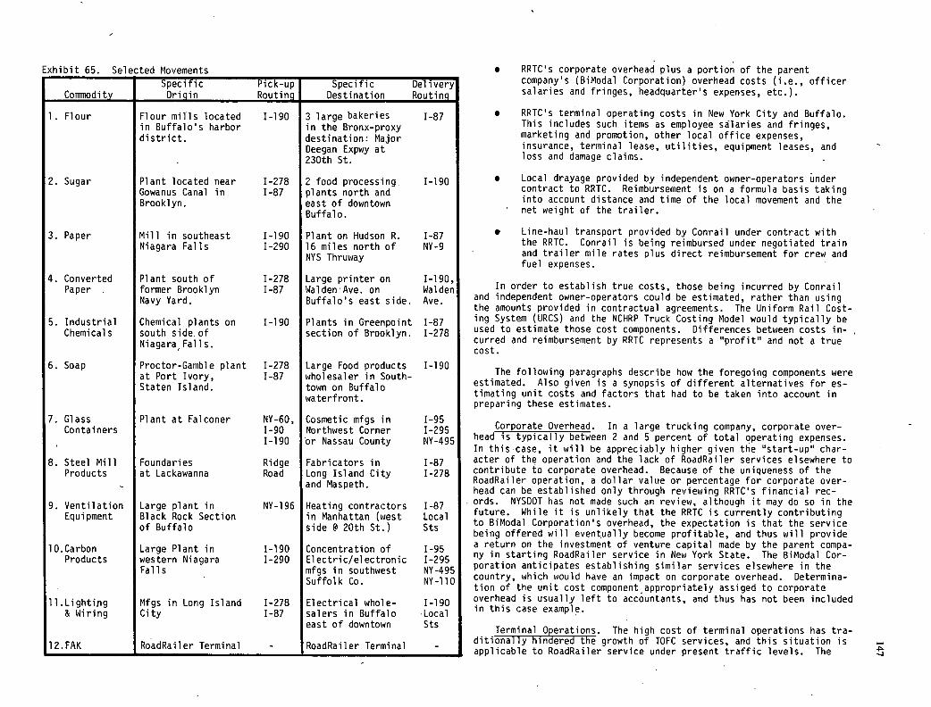
Exhibit 65. Selected Movements
Commodity Specific Origin
Pick-up Routing
Specific Destination
Delivery Routing
Flour Flour mills located 1-190 3 large bakeries 1-87 in Buffalo's harbor in the Bronx-proxy district, destination: Major
Deegan Expwy at 230th St.
Sugar Plant located near 1-278 2 food processing. 1-190 Gowanus Canal in 1-87 plants north and Brooklyn. east of downtown
Buffalo.
Paper Mill in southeast 1-190 Plant on Hudson R. 1-87 Niagara Falls 1-290 16 miles north of NY-9
NYS Thruway
Converted Plant south of 1-278 Large printer on 1-190, Paper former Brooklyn 1-87 WaldenAve. on Walden
Navy Yard. Buffalo's east side. Ave.
Industrial Chemical plants on 1-190 Plants in Greenpoint 1-87 Chemicals south side. of section of Brooklyn. 1-278
Niagara, Falls.
Soap Proctor-Gamble plant 1-278 Large Food products 1-190 at Port Ivory, 1-87 wholesaler in South- Staten Island. town on Buffalo
waterfront.
Glass Plant at Falconer NY-60, Cosmetic mfgs in 1-95 Containers 1-90 Northwest Corner 1-295
1-190 or Nassau County NY-495
Steel Mill Foundaries Ridge Fabricators in 1-87 Products at Lackawanna Road Long Island City 1-278
and Maspeth.
Ventilation Large plant in NY-196 Heating contractors 1-87 Equipment Black Rock Section in Manhattan (west Local
of Buffalo side @ 20th St.) Sts
10.Carbon Large Plant in 1-190 Concentration of 1-95 Products western Niagara 1-290 Electric/electronic 1-295
Falls mfgs in southwest NY-495 Suffolk Co. NY-hO
ll.Lightij,g Mfgs in Long Island 1-278 Electrical whole- 1-190 & Wiring City 1-87 salers in Buffalo Local
east of downtown Sts
12.FAK RoadRailer Terminal - RoadRailer Terminal -
RRTC's corporate overhead plus a portion of the parent company's (BiModal Corporation) overhead costs (i.e., officer salaries and fringes, headquarter's expenses, etc.).
RRTC's terminal operating costs in New York City and Buffalo. This includes such items as employee salaries and fringes, marketing and promotion, other local office expenses, insurance, terminal lease, utilities, equipment leases, and loss and damage claims.
Local drayage provided by independent owner-operators under contract to RRTC. Reimbursement is on a formula basis taking into account distance and time of the local movement and the net weight of the trailer.
Line-haul transport provided by Conrail under contract with the RRTC. Conrail is being reimbursed under negotiated train and trailer mile rates plus direct reimbursement for crew and fuel expenses.
In order to establish true costs, those being incurred by Conrail and independent owner-operators could be estimated, rather than using the amounts provided in contractual agreements. The Uniform Rail Cost-ing System (URCS) and the NCHRP Truck Costing Model would typically be used to estimate those cost components. Differences between costs in-curred and reimbursement by RRTC represents a "profit" and not a true cost.
The following paragraphs describe how the foregoing components were estimated. Also given is a synopsis of different alternatives for es-timating unit costs and factors that had to be taken into account in preparing these estimates.
Corporate Overhead. In a large trucking company, corporate over-head is typically between 2 and 5 percent of total operating expenses. In this case, it will be appreciably higher given the "start-up" char-acter of the operation and the lack of RoadRailer services elsewhere to contribute to corporate overhead. Because of the uniqueness of the RoadRailer operation, a dollar value or percentage for corporate over-head can be established only through reviewing RRTC's financial rec-ords. NYSDOT has not made such an review, although it may do so in the future. While it is unlikely that the RRTC is currently contributing to BiModal Corporation's overhead, the expectation is that the service being offered will eventually become profitable, and thus will provide a return on the investment of venture capital made by the parent compa-ny in starting RoadRailer service in New York State. The BiModal Cor-poration anticipates establishing similar services elsewhere in the country, which would have an impact on corporate overhead. Determina-tion of the unit cost component appropriately assiged to corporate overhead is usually left to accountants, and thus has not been included in this case example.
Terminal Operations. The high cost of terminal operations has tra- ditionally hindered the growth of TOFC services, and this situation is - applicable to RoadRailer service under present traffic levels. The
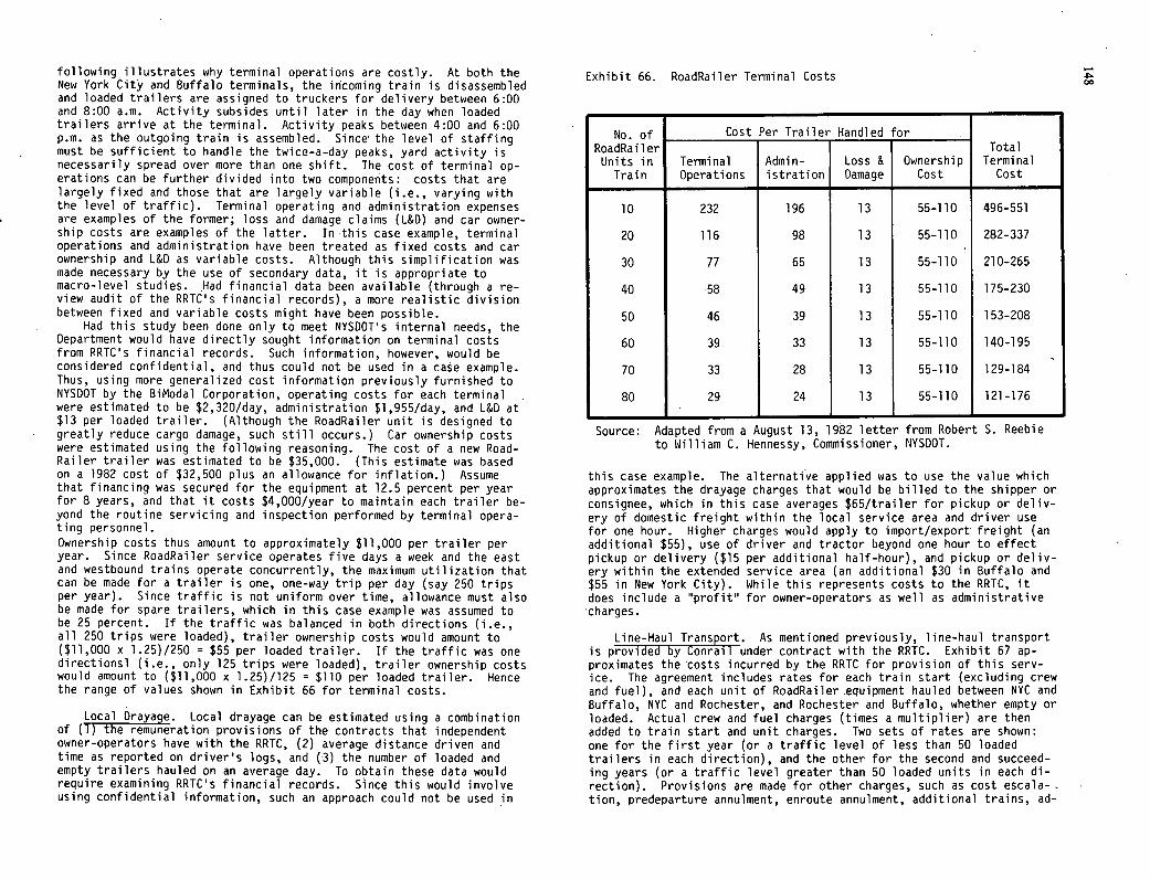
following illustrates why terminal operations are costly. At both the New York Cit,' and Buffalo terminals, the incoming train is disassembled and loaded trailers are assigned to truckers for delivery between 6:00 and 8:00 a.m. Activity subsides until, later in the day when loaded trailers arrive at the terminal. Activity peaks between 4:00 and 6:00 p.m. as the outgoing train is assembled. Since' the level of staffing must be sufficient to handle the twice-a-day peaks, yard activity is necessarily spread over more than one shift. The cost of terminal op-erations can be further divided into two components: costs that are largely fixed and those that are largely variable (i.e., varying with the level of traffic). Terminal operating and administration expenses are examples of the former; loss and damage claims (L&D) and car owner-ship costs are examples of the latter. In this case example, terminal operations and administration have been treated as fixed costs and car ownership and L&D as variable costs. Although this simplification was made necessary by the use of secondary data, it is appropriate to macro-level studies. Had financial data been available (through a re-view audit of the RRTC's financial records), a more realistic division between fixed and variable costs might have been possible.
Had this study been done only to meet NYSDOT's internal needs, the Department would have directly sought information on terminal costs from RRTC's financial records. Such information, however, would be considered confidential, and thus could not be used in a case example. Thus, using more generalized cost information previously furnished to NYSDOT by the BiModal Corporation, operating costs for each terminal were estimated to be $2,320/day, administration $1,955/day, and L&D at $13 per loaded trailer. (Although the RoadRailer unit is designed to greatly reduce cargo damage, such still occurs.) Car ownership costs were estimated using the following reasoning. The cost of a new Road-Railer trailer was estimated to be $35,000. (This estimate was based on a 1982 cost of $32,500 plus an allowance for inflation.) Assume that financing was secured for the equipment at 12.5 percent per year for 8 years, and that it costs $4,000/year to maintain each trailer be-yond the routine servicing and inspection performed by terminal opera-ting personnel.
Ownership costs thus amount to approximately $11,000 per trailer per year. Since RoadRailer service operates five days a week and the east and westbound trains operate concurrently, the maximum utilization that can be made for a trailer is one, one-way trip per day (say 250 trips per year). Since traffic is not uniform over time, allowance must also be made for spare trailers, which in this case example was assumed to be 25 percent. If the traffic was balanced in both directions (i.e., all 250 trips were loaded), trailer ownership costs would amount to ($11,000 x 1.25)/250 = $55 per loaded trailer. If the traffic was one directionsl (i.e., only 125 trips were loaded), trailer ownership costs would amount to ($11,000 x 1.25)/125 = $110 per loaded trailer. Hence the range of values shown in Exhibit 66 for terminal costs.
Local Drayage. Local drayage can be estimated using a combination of (1) the remuneration provisions of the contracts that independent owner-operators have with the RRTC, (2) average distance driven and time as reported on driver's logs, and (3) the number of loaded and empty trailers hauled on an average day. To obtain these data would require examining RRTC's financial records. Since this would involve using confidential information, such an approach could not be used in
Exhibit 66. RoadRailer Terminal Costs 00
No. of RoadRailer
Cost Per Trailer Handled for Total
Units in Terminal Admin- Loss & Ownership Terminal Train Operations istration Damage Cost Cost
10 232 196 13 55-110 496-551
20 116 98 13 55-110 282-337
30 77 65 13 55-110 210-265
40 58 49 13 55-110 175-230
50 46 39 13 55-110 153-208
60 39 33 13 55-110 140-195
70 33 28 13 55-110 129-184
80 29 24 13 55-110 121-176
Source: Adapted from a August 13, 1982 letter from Robert S. Reebie to William C. Hennessy, Commissioner, NYSDOT.
this case example. The alternative applied was to use the value which approximates the drayage charges that would be billed to the shipper or consignee, which in this case averages $65/trailer for pickup or deliv-ery of domestic freight within the local service area and driver use for one hour. Higher charges would apply to import/export freight (an additional $55), use of driver and tractor beyond one hour to effect pickup or delivery ($15 per additional half-hour), and pickup or deliv-ery within the extended service area (an additional $30 in Buffalo and $55 in New York City). While this represents costs to the RRTC, it does include a "profit" for owner-operators as well as administrative charges.
Line-Haul Transport. As mentioned previously, line-haul transport is provided by Conrail under contract with the RRTC. Exhibit 67 ap-proximates the costs incurred by the RRTC for provision of this serv-ice. The agreement includes rates for each train start (excluding crew and fuel), and each unit of RoadRailer equipment hauled between NYC and Buffalo, NYC and Rochester, and Rochester and Buffalo, whether empty or loaded. Actual crew and fuel charges (times a multiplier) are then added to train start and unit charges. Two sets of rates are shown: one for the first year (or a traffic level of less than 50 loaded trailers in each direction), and the other for the second and succeed-ing years (or a traffic level greater than 50 loaded units in each di-rection). Provisions are made for other charges, such as cost escala-tion, predeparture annulment, enroute annulment, additional trains, ad-
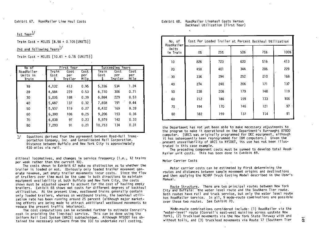
Exhibit 67. RoadRailer Line Haul Costs
1st Year-'
Train Cost = MILES [8.56 + 0.105 (UNITS)]
2nd and Following Years-"
Train Cost = MILES [10.61 + 0.18 (UNITS)]
No of RoadRailer
First Year Succeeding Years Train Cost Cost Train Cost Cost
Units in Cost per per Cost per per Train $ Trailer Mile $ Trailer Mile
10 4,132 413 0.95 5,336 534 1.24
20 4,584 229 0.53 6,110 306 0.71
30 5,035 168 0.39 6,884 229 0.53
40 5,487 137 0.32 7,658 191 0.44
50 5,937 119 0.27 8,432 169 0.39
60 6,390 106 0.25 9,206 153 0.36
70 6,838 97 0.23 9,979 142 0.33
80 7,293 91 0.21 10,753 134 0.31
1/ Equations derived from the agreement between Road-Rail Trans- portation Company, Inc. and Consolidated Rail Corporation. Distance between Buffalo and New York City is approximately 430 miles via rail.
ditional locomotives, and changes in service frequency (i.e., 12 trains per week rather than the current 10).
The costs shown in Exhibit 67 make no distinction as to whether the trailer is loaded or not. Obviously only loaded trailer movement gen-erate revenue, yet empty trailer movements incur costs. Since the flow of trailers over time must be the same in both directions to maintain equipment availability at both Buffalo and New York City, the costs shown must be adjusted upward to account for the cost of hauling empty trailers. Exhibit 68 shows net costs for different degrees of backhaul utilization. At the present time, eastbound trains generally contain only loaded trailers, whereas on westbound trains, the backhaul utili-zation rate has been running around 25 percent (although major market-ing efforts are being made to attract additional westbound movements to reduce the present traffic imbalance).
The cost computations can be extended further to estimate Conrail's cost in providing the line-haul service. This can be done using the Uniform Rail Cost System (URCS) subtechnique. Although NYSDOT has ob-tained the necessary software from the ICC to undertake rail costing,
Exhibit 68. RoadRailer Linehaul Costs Versus Backhaul Utilization (First Year)
No. of RoadRailer
Units
Cost Per Loaded Trailer at Percent Backhaul Utilization
in Train 0% 25% 50% 75% 100%
10 826 723 620 516 413
20 458 401 344 286 229
30 336 294 252 210 168
40 274 240 206 171 137
50 238 208 179 148 119
60 212 186 159 133 106
70 194 170 146 121 97
80 182 159 137 114 91
the Department has not yet been able to make necessary adjustments to the program to make it operational on the Department's Burroughs B7800 computer. (URCS was originally programmed for DEC equipment, although it has subsequently been reprogrammed for IBM computers.) Given the present unavailability of URCS to NYSDOT, its use has not been illus-
trated in this case example. The preceding component costs must be summed to develop total Road-
Railer unit costs. This has been done in Exhibit 69.
Motor Carrier Costs
Motor carrier costs can be estimated by first determining the routes and distances between sample movement origins and destinations and then applying the NCHRP Truck Costing Model described in the User's Manual.
Route Structure. There are two principal routes between New York City and Buffalo: the water level route and the Southern Tier route. Both routes have rail and truck service, but only the water level route has RoadRailer service. In all, 9 mode-route combinations are possible over these two routes. See Exhibit 70.
Mode-route combinations considered include: (1) RoadRailer via the "water-level' route (Conrail's east-west mainline across upstate New York), (2) truckload movements via the New York State Thruway with and
without tolls, and (3) truckload movements via Route 17 (Southern Tier
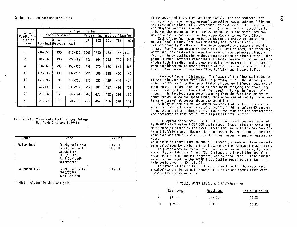
Exhibit 69. RoadRailer Unit Costs
No. of Cost_per Trailer
- Cost Component Percent Backhaul Utilization RoadRailer Local Line 0% 25% 50% 75% 100% Units in
Train Terminal Drayage Haul
10 496-551 130 413-826 1507 1390 1273 1156 1039
20 282-337 130 229-458 925 854 783 712 641
30 210-265 130 168-336 731 675 620 564 508
40 175-230 130 137-274 634 586 538 490 442
50 153-208 130 119-238 576 533 489 446 402
60 140-195 130 106-212 537 497 457 416 376
70 129-184 130 97-194 508 470 432 394 356
80 121-176 '130 91-182 488 452 415 379 342
Exhibit 70. Mode-Route Combinations Between New York City and Buffalo
Route Mode Service
Water level Truck, toll road TL/LTL Truck, no tolls TL/LTL RoadRailer TOFC/COFC* Rail Carload*. Waterborne
Southern Tier Truck, no tolls TL/LTL TOFC/COFC* Rail Carload
*Not included in this analysis
Expressway) and 1-390 (Genesee Expressway). For the Southern Tier route, appropriate 'nonexpressway" connecting routes between 1-390 and the particular plant, mill, warehouse, or distribution facility in Erie and Niagara Counties were identified. (The one partial exception to this was the use of Route 17 across the state as the route used for-moving glass containers from Chautauqua County to New York City.)
Each of the four mode-route combinations consists of three seg-ments: local pickup, line-haul movement, and local delivery. For freight moved by RoadRailer, the three segments are separate and dis-tinct. For freight moved by truck in full trailerloads, the three seg-ments are less distinct because the freight involved moves directly from origin to destination without consolidation or distribution. This point-to-point movement resembles a line-haul movement, but in fact in-cludes both line-8aul and pickup and delivery segments. The latter were considered to be those portions of the line-haul movements within the built-up areas of New York City, Buffalo, and Niagara Falls.
Line-Haul Segment Distances. The length of the line-haul segments of the trip were taken from NYSDOT's photolog file. The photolog was also used to identify the speed limits allowed on different sections of' each route. Travel time was calculated by multiplying the prevailing speed limit by the distance that the speed limit was in force. Al-though this involved some error stemming from the fact that trucks at times travel below the speed limit, this error was offset by the occur-rence of travel at speeds above the speed limit.
A delay of one minute was added for each traffic light encountered on route. While the red phase of a traffic light is seldom 60 seconds long, the use of one minute delay also allows time for the acceleration and deceleration that occurs at a signalized intersection.
PUD Segment Distances. The length of these sections was measured by NYSDOT staff using 1:250,000 scale maps. Travel times on these seg-ments were •estimated by the NYSDOT staff familiar with the New York Ci-ty.and Buffalo areas. Because this procedure is error prone, consider-able care was taken in developing these estimates to ensure reasonable-ness. As a check on travel time on the PUD segments, speeds on these segments were calculated by dividing trip distance by the estimated travel time.
Trip distances and travel times are shown for eacI route, for each commodity, in Exhibits 71 and 72. Distance and travel time are also shown by line-haul and PUD segments, and by total trip. These numbers were used as input tothe NCI-IRP Truck Costing Model to calculate the trip costs shown in Exhibit 73.
To determine the costs for the trips with tolls, the costs were recalculated, using actual Thruway tolls as an additional fixed cost. These tolls are shown below.
TOLLS, WATER LEVEL, AND SOUTHERN TIER
Eastbound Westbound Tri-Boro Bridge
WL $41.35 - $35.35 $6.25
ST $ 9.85 $ 3.85 $6.25
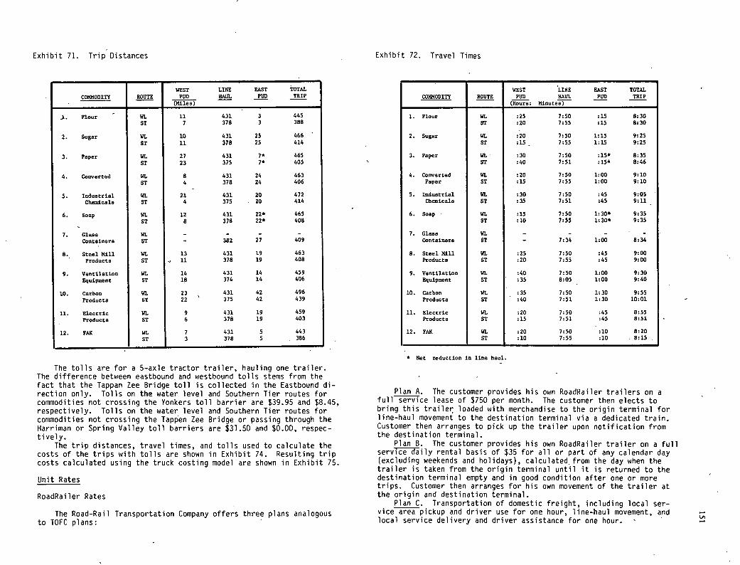
Exhibit 71. Trip Distances
COMMODITY ROUTE WEST
P130 (Mi].es)
LINE HAUL
EAST P131)
1011.1 TRIP
J. FLour WL 11 431 3 445 ST 7 378 3 388
2. Sugar WL 10 431 25 466
ST 11 378 25 414
3. Paper WL 27 431 7* 465 ST 23 375 7* 405
4. Converted WL 8 431 24 463 ST 4 378 24 406
5. Industrial WL 21 431 20 472 Chemicals ST 4 375 20 414
6. Soap WL 12 431 22* 465
ST 8 378 22* 408
7. Glass WL - - - - Containers ST - 382 27 409
8. Steel Mill WL 13 431 19 463
Products ST . 11 378 19 408
9. Ventilation WL 14 431 14 459 Equipment ST 18 374 14 406
10. Carbon WL 23 431 42 496
Products ST 22 375 42 439
11. Electric WL 9 431 19 459
Products ST 6 378 19 403
12. YAK WL 7 431 5 443 ST 3 378 5 386
Exhibit 72. Travel Times
COMMODITY ROUTE WEST
PUB (Hours:
LINE HAUL
Minutes)
EAST P130
TOTIiL TRIP
Flour WL :25 7:50 :15 8:30 ST :20 7:55 :15 8:30
Sugar WL :20 7:50 1:15 9:25 ST :15 - 7:55 1:15 9:25
Paper WL :30 7:50 :15* 8:35 ST :40 7:51 :15* 8:46
Converted WL :20 7:50 1:00 9:10 Paper ST :15 7:55 1:00 9:10
Industrial WL :30 7:50 :45 9:05 Chemicals ST :35 7:51 :45 9:11
Soap WL :15 7:50 1:30* 9:35 ST :10 7:55 1:30* 9:35
Glass WL - - - - Containers ST - 7:34 1:00 8:34
Steel Mill WL :25 7:50 :45 9:00 Products ST :20 7:55 :45 9:00
Ventilation WL :40 7:50 1:00 9:30 Equipment ST :35 8:05 1:00 9:40
Carbon WL :35 7:50 1:30 9:55 Products ST :40 7:51 1:30 10:01
Electric WL :20 7:50 :45 8:55 Products ST :15 7:51 :45 8:51
YAK WL :20 7:50 :10 8:20 ST :10 7:55 :10 - 8:15
* Net reduction in line haul.
The tolls are for a 5-axle tractor trailer, hauling one trailer. The difference between eastbound and westbound tolls stems from the fact that the Tappan Zee Bridge toll is collected in the Eastbound di-rection only. Tolls on the water level and Southern Tier routes for commodities not crossing the Yonkers toll barrier are $39.95 and $8.45, respectively. Tolls on the water level and Southern Tier routes for commodities not crossing the Tappen Zee Bridge or passing through the Harriman or Spring Valley toll barriers are $31.50 and $0.00, respec-tively.
The trip distances, travel times, and tolls used to calculate the costs of the trips with tolls are shown in Exhibit 74. Resulting trip costs calculated using the truck costing model are shown in Exhibit 75.
Unit Rates
RoadRailer Rates
The Road-Rail Transportation Company offers three plans analogous to TOFC plans:
Plan A. The customer provides his own RoadRailer trailers on a full service lease of $750 per month. The customer then elects to bring this trailer loaded with merchandise to the origin terminal for line-haul movement to the destination terminal via a dedicated train. Customer then arranges to pick up the trailer upon notification from the destination terminal.
Plan B. The customer provides his own RoadRailer trailer on a full service daily rental basis of $35 for all or part of any calendar day (excluding weekends and holidays), calculated, from the day when the trailer is taken from the origin terminal until it is returned to the destination terminal empty and in good condition after one or more trips. Customer then arranges for his own movement of the trailer at the origin and destination terminal.
Plan C. Transportation of domestic freight, including local ser-vice area pickup and driver use for one hour, line-haul movement, and local service delivery and driver assistance for one hour.
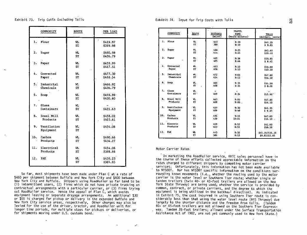
Exhibit 73. Trip Costs Exciudina Tolls Exhibit 74. Input for Trip Costs with Tolls
COMMODITY ROUTE PER LOAD
Flour WL $419.97 ST $399.98
Sugar WL $460.98 ST $426.79
Paper WL $459.99 ST $417.51
Converted WL $477.30 Paper ST $418.54
Industrial WL $466.92 Chemicals ST $426.79
Soap WL $459.99 ST $420.60
Glass WL - Containers ST $421.63
Steel Mill WL $458.02 Products ST $403.61
Ventilation WL $454.06 Equipment ST
Carbon WL $490.66 Products ST $434.27
Electrical WL $454.06 Products ST $398.66
FAR WL $438.23 ST $381.85
So far, most shipments have been made under Plan C at a rate of $460 per shipment between Buffalo and New York City and $400 between New York City and Buffalo. Shippers using RoadRailer so far tend to be (1) intermittent users, (2) firms which do not have private trucking on contractual arrangements with a particular carrier, or (3) firms trying out RoadRailer service. Hence the appeal of Plan C, which avoids equipment leasing or separate drayage arrangements. An additional $30 or $55 is charged for pickup or delivery in the extended Buffalo and New York City service areas, respectively, Other charges may also be levied for the use of the driver, tractor, and RoadRailer unit for longer time periods, for multiple stops for pickups or deliveries, or for shipments moving under U.S. customs bond.
COMMODITY ROUTE DISTANCE (miles)
TRAVEL TIME
(hours:mjnutes) TOLLS
(doll rs7cents
1. Flour WI. 445 8:30 $41.35 ST 388 8:30 $ 9.85
2. Sugar WI. 466 9:25 $41.60 ST 414 9:25 $10.10
3. Paper WL 465 8:36 $39.95 ST 405 8:46 $ 8.45
4. Converted WI. 463 9:10 $41.60 Paper ST 406 9:10 $10.10
5. Industrial WL 472 9:05 $47.60 Chemicals ST 414 9:1.1 $16.10
6. Soap WI. 465 9:35 $31.50 ST 408 9:35 $ 0.00
7. Glass WL - - - Containers ST 409 8:34 $15.60
8. Steel Mill WI. 463 9:00 $47.60 Products ST 408 9:00 $16.10
9. Ventilation WI. 459 9:30 $41.35 Equipment ST 406 9:40 $ 9.85
io. carbon WL 496 9:55 $47.60 Products ST 439 10:01 $16.10
Electric WL 459 8:55 $41.60 Products ST 403 8:51 $10.10
FAX WL 443 8:20 $41.35/$35.35 ST 386 8:15 $9.85/$3.85
Motor Carrier Rates
In marketing the RoadRailer service, RRTC sales personnel have in the course of these efforts collected appreciable information on the rates charged to different shippers by competing motor carrier services. Unfortunately, this information has not been made available to NYSDOT. Nor has NYSDOT specific information on the conditions sur-rounding known movements (i.e., whether the routing used by the motor carrier is the water level or Southern Tier route; whether single or tandem trailers (twin 40- or 45-foot trailers are allowed on the New York State Thruway) are being used; whether the service is provided by common, contract, or private carriers, and the degree to which the equipment is being utilized in the backhaul direction). As indicated in Exhibit 75, the cost incurred in using Southern Tier route is con-siderably less than that using the water level route (NYS Thruway) due largely to the shorter distance and the freedom from tolls. (Tandem 40- or 45-foot trailers are not allowed on the Southern Tier Express-way. Tandem 28-foot trailers allowed under the Surface Transportation Assistance Act of 1982, are not yet commonly used in New York State.)
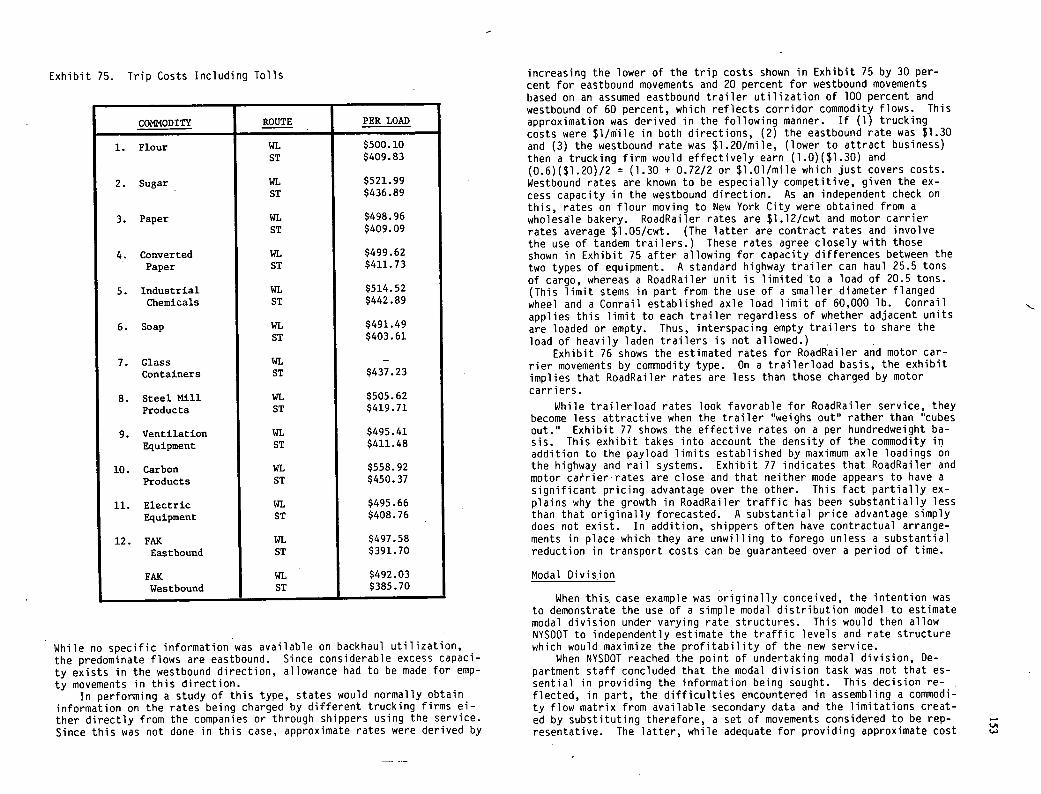
Exhibit 75. Trip Costs Including Tolls
COMMODITY ROUTE PER LOAD
Flour WL $500.10 ST $409.83
Sugar WL $521.99 ST $436.89
Paper WL $498.96 ST $409.09
Converted WL $499.62 Paper ST $411.73
Industrial WL $514.52 Chemicals ST $442.89
Soap WL $491.49 ST $403.61
Glass WL - Containers ST $437.23
Steel Mill WL $505.62 Products ST $419.71
Ventilation WL $495.41 Equipment ST $411.48
Carbon WL $558.92 Products ST $450.37
Electric WL $495.66 Equipment ST $408.76
FAX WL $497.58 Eastbound ST $391.70
FAX WL $492.03 Westbound ST $385.70
While no specific information was available on backhaul utilization, the predominate flows are eastbound. Since considerable excess capaci-ty exists in the westbound direction, allowance had to be made for emp-ty movements in this direction.
In performing a study of this type, states would normally obtain information on the rates being charged by different trucking firms ei-ther directly from the companies or through shippers using the service. Since this was not done in this case, approximate rates were derived by
increasing the lower of the trip costs shown in Exhibit 75 by 30 per-cent for eastbound movements and 20 percent for westbound movements based on an assumed eastbound trailer utilization of 100 percent and westbound of 60 percent, which reflects corridor commodity flows. This approximation was derived in the following manner. If (1) trucking costs were $l/niile in both directions, (2) the eastbound rate was $1.30 and (3) the westbound rate was $1.20/mile, (lower to attract business) then a trucking firm would effectively earn (1.0)($1.30) and (0.6)($1.20)/2 = (1.30 + 0.72/2 or $1.01/mile which just covers costs. Westbound rates are known to be especially competitive, given the ex-cess capacity in the westbound direction. As an independent check on this, rates on flour moving to New York City were obtained from a wholesale bakery. RoadRailer rates are $1.12/cwt and motor carrier rates average $1.05/cwt. (The latter are contract rates and involve the use of tandem trailers.) These rates agree closely with those shown in Exhibit 75 after allowing for capacity differences between the two types of equipment. A standard highway trailer can haul 25.5 tons of cargo, whereas a RoadRailer unit is limited to a load of 20.5 tons. (This limit stems in part from the use of a smaller diameter flanged wheel and a Conrail established axle load limit of 60,000 lb. Conrail applies this limit to each trailer regardless of whether adjacent units are loaded or empty. Thus, interspacing empty trailers to share the load of heavily laden trailers is not allowed.)
Exhibit 76 shows the estimated rates for RoadRailer and motor car-rier movements by commodity type. On a trailerload basis, the exhibit implies that RoadRailer rates are less than those charged by motor carriers.
While trailerload rates look favorable for RoadRailer service, they become less attractive when the trailer "weighs out' rather than 'cubes out." Exhibit 77 shows the effective rates on a per hundredweight ba-sis. This exhibit takes into account the density of the commodity in addition to the payload limits established by maximum axle loadings on the highway and rail systems. Exhibit 77 indicates that RoadRailer and motor ca&ier'rates are close and that neither mode appears to have a significant pricing advantage over the other. This fact partially ex-plains why the growth in RoadRailer traffic has been substantially less than that originally forecasted. A substantial price advantage simply does not exist. In addition, shippers often have contractual arrange-ments in place which they are unwilling to forego unless a substantial reduction in transport costs can be guaranteed over a period of time.
Modal Division
When this, case example was originally conceived, the intention was to demonstrate the use of a simple modal distribution model to estimate modal division under varying rate structures. This would then allow NYSDOT to independently estimate the traffic levels and rate structure which would maximize the profitability of the new service.
When NYSDOT reached the point of undertaking modal division, De-partment staff concluded that the modal division task was not that es-sential in providing the information being sought. This decision re-flected, in part, the difficulties encountered in assembling a commodi-ty flow matrix from available secondary data and the limitations creat-ed by substituting therefore, a set of movements considered to be rep-resentative. The latter, while adequate for providing approximate cost
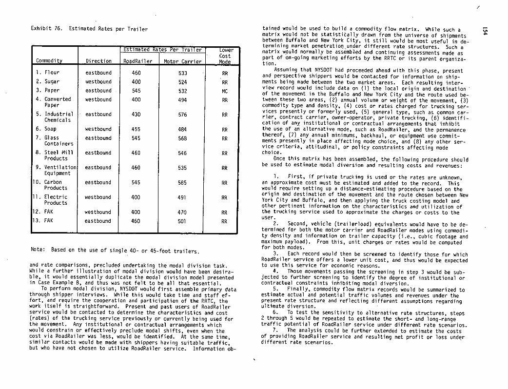
Exhibit 76. Estimated Rates per Trailer
Estimated Rates Per Trailer Lower Cost
Commodity Direction RoadRailer Motor Carrier Mode
1. Flour eastbound 460 533 RR
Sugar westbound 400 524 RR
Paper eastbound 545 532 MC
Converted westbound 400 494 RR Paper
Industrial eastbound 430 576 RR Chemicals
Soap westbound 455 484 RR
Glass eastbound 545 568 RR Containers
Steel Mill eastbound 460 546 RR Products
Ventilation eastbound 460 535 RR Equi pment
Carbon eastbound 545 585 RR Products
Electric westbound 400 491 RR Products
FAK westbound 400 470 RR
FAK eastbound 460 501 RR
Note: Based on the use of single 40- or 45-foot trailers.
and rate comparisons, precluded undertaking the modal division task. While a further illustration of modal division would have been desira-ble, it would essentially duplicate the modal division model presented in Case Example B, and thus was not felt to be all that essential.
To perform modal division, NYSDOT would first assemble primary data through shipper interviews. While this would take time and staff ef-fort, and require the cooperation and participation of the RRTC, the work itself is straightforward. Present and past users of RoadRailer service would be contacted to determine the characteristics and cost (rates) of the trucking service previously or currently being used for the movement. Any institutional or contractual arrangements which would constrain or effectively preclude modal shifts, even when the cost via RoadRailer was less, would be identified. At the same time, similar contacts would be made with shippers having suitable traffic, but who have not chosen to utilize RoadRailer service. Information ob-
tamed would be used to build a commodity flow matrix. While such a matrix would not be statistically drawn from the universe of shipments between Buffalo and New York City, it still would be most useful in de-termining market penetration under different rate structures. Such a matrix would normally be assembled and continuing assessments made as part of on-going marketing efforts by the RRTC or its parent organiza-tion.
Assuming that NYSDOT had proceeded ahead with this phase, present and perspective shippers would be contacted for information on ship-ments being made between the two market areas. Each resulting inter-view record would include data on (1) the local origin and destination of the movement in the Buffalo and New York City and the route used be-tween these two areas, (2) annual volume or weight of the movement, (3) commodity type and density, (4) cost or rates charged for trucking ser-vices presently or formerly used, (5) general type, such as common car-rier, contract carrier, owner-operator, private trucking, (6) identifi-cation of any institutional or contractual arrangements that inhibit the use of an alternative mode, such as RoadRailer, and the permanence thereof, (7) any annual minimums, backhaul, or equipment use commit-ments presently in place affecting mode choice, and (8) any other ser-vice criteria, attitudinal, or policy constraints affecting mode choice.
Once this matrix has been assembled, the following procedure should be used to estimate modal diversion and resulting costs and revenues:
First, if private trucking is used or the rates are unknown, an approximate cost must be estimated and added to the record. This would require setting up a distance-estimating procedure based on the origin and destination of the movement and the route chosen between New York City and Buffalo, and then applying the truck costing model and other pertinent information on the characteristics and utilization of the trucking service used to approximate the charges or costs to the user.
Second, vehicle (trailerload) equivalents would have to be de-termined for both the motor carrier and RoadRailer modes using commodi-ty density and information on trailer capacity (i.e., cubic footage and maximum payload). From this, unit charges or rates would be computed for both modes.
Each record would then be screened to identify those for which RoadRailer service offers a lower unit cost, and thus would be expected to use this service for economic reasons.
Those movements passing the screening in step 3 would be sub-jected to further screening to identify the degree of institutional or contractual constraints inhibiting modal diversion.
Finally, commodity flow matrix records would be summarized to estimate actual and potential traffic volumes and revenues under the present rate structure and reflecting different assumptions regarding ultimate diversion.
To test the sensitivity to alternative rate structures, steps 2 through 5 would be repeated to estimate the short- and long-range traffic potential of RoadRailer service under different rate scenarios.
The analysis could be further extended to estimate the costs of providing RoadRailer service and resulting net profit or loss under different rate scenarios.
Li,
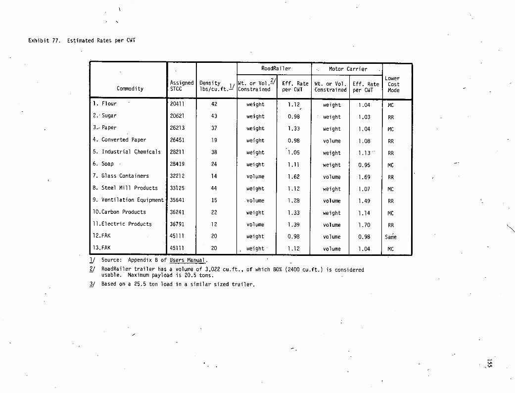
Exhibit 77. Estimated Rates per CWT
Assigned Density 1/
RoadRailer Motor Carrier
Lower Cost
2' w• or Vol.-' Eff. Rate Wt. or Vol. Eff. Rate Commodity STCC lbs/cu.ft.-, Constrained per CWT Constrained per CWT Mode
1. Flour 20411 42 weight 1.12, weight 1.04 MC
2. Sugar 20621 43 weight 0.98 weight 1.03 RR
3.- Paper 26213 37 weight 1.33 weight 1.04 MC
4. Converted Paper 26451 19 weight 0.98 volume 1.08 RR
5. Industrial Chemicals 28211 38 weight 1.05 weight 1.13' RR
6. Soap 28419 24 weight 1.11 weight 0.95 MC
7. Glass Containers 32212 14 volume 1.62 volume 1.69 RR
8. Steel Mill Products 33125 44 weight 1.12 weight 1.07 MC
9. Ventilation Equipment 35641 15 volume 1.28 volume 1.49 RR
lO.Carbon Products 36241 22 weight 1.33 weight 1.14 MC
ll.Electric Products 36791 12 volume 1.39 volume 1.70 RR
12.FAK 45111 20 weight 0.98 volume 0.98 Sane
13.FAK 45111 20 weight 1.12 volume 1.04 MC
1/ Source: Appendix B of Users Manual.
2/ RoadRailer trailer has a volume of 3,022 cu.ft., of which 80% (2400 cu.ft.) is considered usable. Maximum payload is 20.5 tons.
3/ Based on a 25.5 ton load in a similar sized trailer.
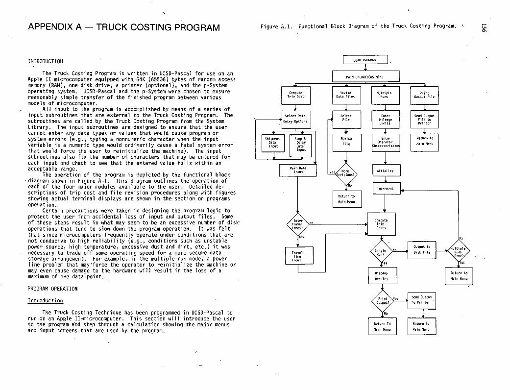
Figure A.1. Functional Block Diagram of the Truck Costing Program. APPENDIX A - TRUCK COSTING PROGRAM '-
INTRODUCTION
The Truck Costing Program is written in UCSD-Pascal for use on an Apple II microcomputer equipped with, 64K (65536) bytes of random access memory (RAM), one disk drive, a printer (optional), and the p-System operating system. UCSD-Pascal and the p-System were chosen to ensure reasonably simple transfer of the finished program between various models of microcomputer.
All input to the program is accomplished by means of a series of input subroutines that are external to the Truck Costing Program. The subroutines are called by the Truck Costing Program from the System Library. The input subroutines are designed to ensure that the user cannot enter any data types or values that would cause program or system errors (e.g., typing a nonnumeric character when the input variable is a numeric type would ordinarily cause a fatal system error that would force the user to reinitialize the machine). The input subroutines also fix the number of characters that may be entered for each input and check to see that the entered value falls within an acceptable range.
The operation of the program is depicted by the functional block 'diagram shown in Figure A-l. This diagram outlines the operation of each of the four major modules available to the user. Detailed de-scriptions of trip cost and file revision procedures along with figures showing actual terminal displays are shown in the section on programs operation.
Certain precautions were taken in designing the program logic to protect the user from accidental loss of input and output files. Some of these steps result in what may seem to be an excessive number of disk' operations that tend to slow down the program operation. It was felt that since microcomputers frequently operate under conditions that are not conducive to high reliability (e.g., conditions such as unstable power source, high temperature, excessive dust and dirt, etc.) it was necessary to trade off some operating speed for a more secure data storage arrangement. For example, in the multiple-run mode, a power line problem that mayforce the operator to reinitialize the machine or may even cause damage to the hardware will result in the loss of a maximum of one data point.
PROGRAM OPERATION
Introduction
LOAD PROGRAM I
MAIN OPERATIONS MENU
Compute Revise Multiple Print Trip Cost Data Files Ruos Output File
Select Data I Select I I Enter I Seed Output
File I Mileage I I File to Entry Options
I Limits I I Printer
Shipment Stop S I I I Revise I Enter Return to
Data Delay I File Operator J I I
Main Menu Input Data i i haructeristic1
Input I I I
Main Data Input
_ yes More Initialize
Increment
Return to
Maim Menu
'Enter\ I Compute Travel )mm Trip jimes?/ I Costs
Output to
Travel <R~nll o e3/
Inp
- Tine ut
Display Return to
Results I I Main Menu
Send Output
Output? , I To Printer
The Truck Costing Technique has been programmed in UCSD-Pascal to run on an Apple TI-microcomputer. This section will introduce the user to the program and step through a calculation showing the major menus Return To Return To
and input screens that are used by the program. Main Menu Main Neon
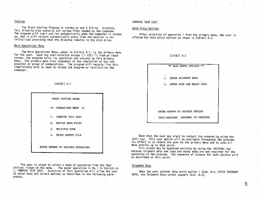
Startup
The Truck Costing Program is stored on one5 1/4-in, diskette. This diskette also contains all systemfiles needed by the computer. The program will start and run automatically when the computer is turned on, and, it will restart automatically every time the machine is re-initialized providing that the diskette remains in the disk drive.
Main Operations Menu
The Main Operations Menu, shown in Exhibit A-1, is the primary menu for the user. Upon any user-selected escape (< ESC> ) from an input screen, the program halts its operation and returns to this primary menu. The primary menu also reappears at the completion of any com-putation or group of computations. The program will recycle like this indefinitely with no need to reload the program or reinitialize the computer.
EXHIBIT. A-1
COMPUTE TRIP COST
Data Entry Options
After selection of operation 1 from the primary menu, the user is offered the data entry options as shown in Exhibit A-2.
EXHIBIT A-2
** DATA ENTRY OPTIONS
ENTER SHIPMENT DATA
ENTER STOP AND DELAY DATA
TRUCK COSTING MODEL
++ OPERATIONS MENU ++
ENTER NUMBER OF DESIRED OPTION:
COMPUTE TRIP COST
REVISE DATA FILES
MULTIPLE RUNS
PRINT OUTPUT FILE
ENTER NUMBER OF DESIRED OPERATION:
The user is asked to select a mode of operation from the four choices listed on the menu. The major operation is No.1 in Exhibit A- 1, COMPUTE TRIP COST. Selection of this operation will allow the user to enter data and select options as described in the following para-graphs.
<ESC>=RESTART <RETURN> TO CONTINUE
Note that the user may elect to restart the-program by using the <ESC> key. This user option will be available throughout the program. Its effect is to return the user to the primary menu and to undo all data entries up to that point.
This screen may be bypassed entirely by using the <RETURN> key because shipment data and stop and delay data are not required for the operation of the program. The sequence of screens for both options will be described at this point.
Shipment Data
When the user selects data entry 'Option 1 (Exh. A-?, ENTER SHIPMENT DATA, the Shipment Data screen appears (Exh. A-3).
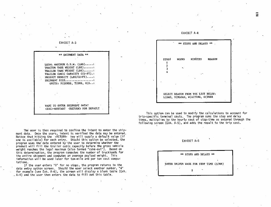
** SHIPMENT DATA **
LEGAL MAXIMUM G.V.W. (LBS) ..... TRACTOR TARE WEIGHT (LBS) ...... TRAILER TARE WEIGHT (LBS) ...... TRAILER CUBIC CAPACITY (CU-FT).: PRODUCT DENSITY (LBS/CU-FT)....: SHIPMENTSIZE..................
UNITS: P(OUNDS, T(ONS, K(G..:
WART TO ENTER SHIPMENT DATA? <ESC>=RESTART <RETURN> FOR DEFAULT
STOPII HOURS MINUTES REASON
2 3 4
SELECT REASON FROM THE LIST BELOW: L(OAD, U(NLOAD, W(AITING, O(THER
U. 00
EXHIBIT A-3
EXHIBIT A-4
** STOPS AND DELAYS ** -
This option can be used to modify the calculations to account for trip-specific terminal costs. The program sums the stop and delay times, multiplies by the hourly cost of stoptime as entered through the following screen (Exh. A-5), and adds the result to the trip cost.
The user is then required to confirm the intent to enter the ship-ment data. Once the users, intent is verified the data may be entered. Notice that hitting the <RETURN> key will supply a default value (if one is' available) for each entry. Should this option be selected, the program uses th&data entered bythe user to determine'whether the product will fill the trailer cubic capacity before thegross vehicle weight reaches the legal maximum (also termed "cube-out). Based on this determination, the program computes the number of truckloads for the entire shipment and computes an average payload weight. This information will be used later for ton-mile and per ton cost compu-tations.
If the user enters "0 for no stops, the program returns to the data entry option screen. Should the user select another number, "4" for example (see Exh. A-6), the screen will display a blank table (Exh. A-4) and the user then enters the data to fill out this table.
/
EXHIBIT;A-5
** STOPS AND DELAYS **
ENTER DRIVER WAGE FOR STOP TIME ($/HR)
$ -
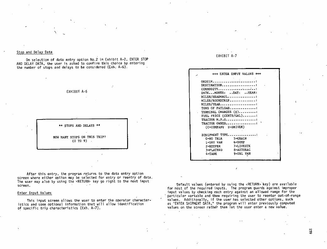
\
EXHIBIT A-7
+++ ENTER INPUT VALUES 4-4-+
ORIGIN......................... DESTINATION.................. COMMODITY.................... DATE ... MONTH: • .DAY: • .YEAR: MILES/HEADHAUL............... MILE S/ROUNDTRIP.............. MILES/YEAR................... TONSOF PAYLOAD.............. TERMINAL CHARGES ($)......... FUEL PRICE (CENTS/GAL) ....... TRACTORM.P.G................ TRACTOROWNER................ (C=COMPANY D=DRIVER)
EQUIPMENTTYPE............... O=NO TRLR 5=GRAIN 1=DRY VAN 6=DUNP 2=REEFER 7=LIVESTK 3=FLATBED 8=AUTORAC 4=TANK 9=DBL VAN
Stop and Delay Data
On selection of data entry option No.2 in Exhibit A-2, ENTER STOP AND DELAY DATA, the user is asked to confirm this choice by entering the number of stops and delays to be considered (Exh. A-6).
EXHIBIT A-6
** STOPS AND DELAYS **
HOW MANY STOPS ON THIS TRIP? (OTO9)
After this entry, the program returns to the data entry option screen where either option may be selected for entry or reentry of data. - The user may also by using the <RETURN> key go right to the next input screen. Default values (entered by using the <RETURN>key) are available
for most of the required inputs. The program guards against improper
Enter Input Values input values by checking each entry against an allowed range for the particular variable and then requiring the user to reenter out-of-range
This input screen allows the user to enter the operator character- values. Additionally, if the user has selected other options, such
istics and some optional information that will allow identification as "ENTER SHIPMENT DATA," the program will enter previously computed
of specific trip characteristics (Exh. A-7). values on the screen rath&r than let the user enter a new value.
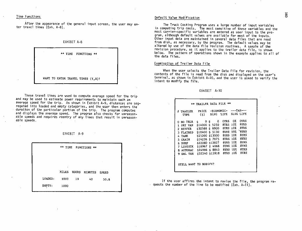
Time Functions Default Value Modification CD
After the appearance of the general input screen, the user may en-ter travel times (Exh. •A-8).
EXHIBIT A-B
** TINE FUNCTIONS **
WANT TO ENTER TRAVEL TIMES (Y,N)?
The Truck Costing Program uses a large number of input variables in computing trip costs. The most sensitive of these variables and the most carrier-specific variables are entered as user input to the pro-gram, although default values are available for most of the inputs. Other input data are maintained in several data files that are read from disk, as necessary, by the program. The default values may be altered by use of the data file revision routines. A sample of the revision procedure, as it applies to the trailer data file, is shown below. The pattern of operations shown in the example applies to all of the data files.
Examination of Trailer Data File
When the user selects the Trailer Data File for revision, the contents of the file is read from the disk and displayed on the users terminal, as shown in Exhibit A-b, and the user is asked to verify the intent to modify the file.
EXHIBIT A-b
These.travel times are used to compute average speed for the trip and may be used to estimate power requirements to maintain such an average speed for the trip. As shown in Exhibit A-9, distances are seg-regated into loaded and empty categories, and the user then enters the duration of the particular portion of the trip. The program computes and displays the average speed. The program also checks for unreason-able speeds and requires reentry of any times that result in unreason- able speeds. -
EXHIBIT A-9
** TINE FUNCTIONS **
MILES HOURS MINUTES SPEED
LOADED: 1000 19 40 50.8
EMPTY: 1000
** TRAILER DATA FILE **
II TRAILER PRICE —ECONOMIC— ---TAX--- TYPE ($) SLVG LIFE SLVG LIFE
O NO TRLR $ 0 $ 0 OYRS 0% OYRS
1 DRY VAN $14000 $ 5250 8YRS 10% 8YRS 2 REEFER $30588 $ 8900 8YRS 10% 8YRS 3 FLAT8ED $10400 $ 5130 8YRS 10% '8YRS 4 TANK $25200 $13000 8YRS 10% 8YRS
5 GRAIN $14236 $ 7075 8YRS 10% 8YRS 6 DUMP $22080 $12027 8YRS 10% 8YRS 7 LIVESTK $16967 $ 4068 8YRS 10% 8YRS 8 AUTORAC $24986 $ 8843 8YRS 10% 8YRS 9 DBL VAN $32540 $15918 8YRS 10% 8YRS
STILL WANT TO MODIFY?
If the user affirms the intent to revise the file, the program re-quests the number of the line to be modified (Exh. A-ll).
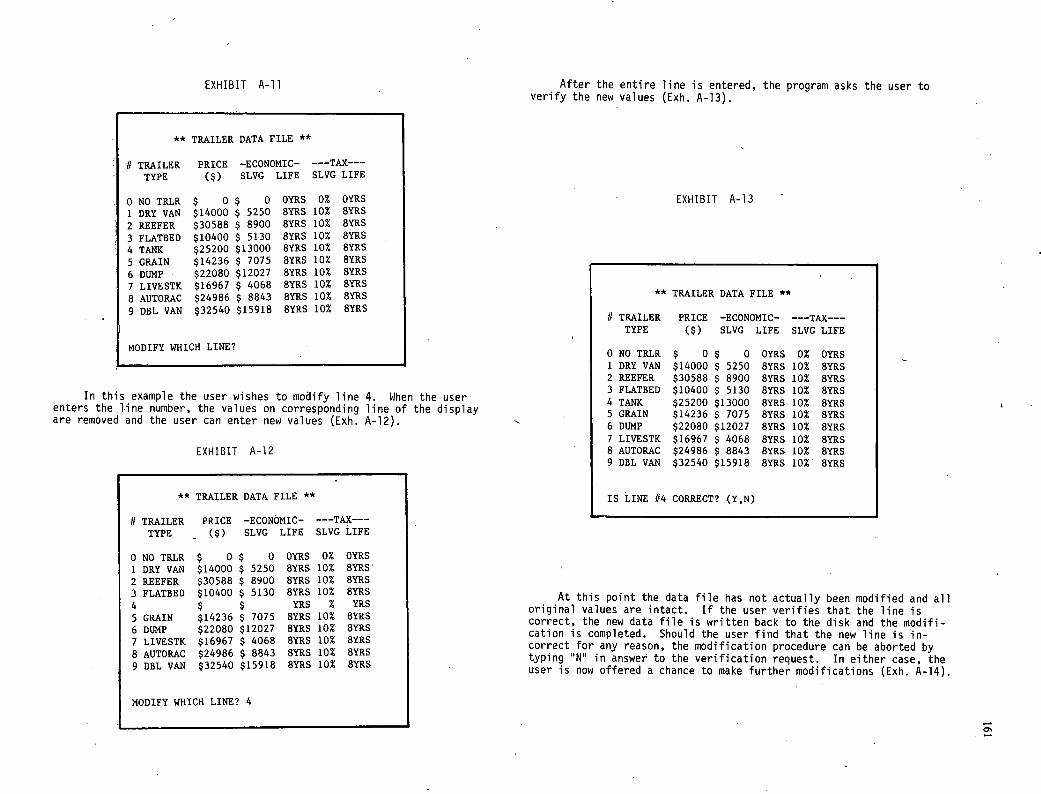
EXHIBIT A-li
** TRAILER DATA FILE **
II TRAILER PRICE -ECONOMIC- ---TAX---
TYPE (s) SLVG LIFE SLVG LIFE
O NO TRLR $ 0 $ 0 OYRS 0% OYRS 1 DRY VAN $14000 $ 5250 8YRS 10% 8YRS 2 REEFER $30588 $ 8900 8YRS 10% 8YRS 3 FLATBED $10400 $ 5130 8YRS 10% 8YRS 4 TANK $25200 $13000 8YRS 10% 8YRS 5 GRAIN $14236 $ 7075 8YRS 10% 8YRS 6 DUMP $22080 $12027 8YRS 10% 8YRS 7 LIVESTK $16967 $ 4068 8YRS 10% 8YRS 8 AUTORAC $24986 $ 8843 8YRS 10% 8YRS 9 DBL VAN $32540 $15918 8YRS 10% 8YRS
MODIFY WHICH LINE?
In this example the user wishes to modify line 4. When the user enters the line number, the values on corresponding line of the display are removed and the user can enter new values (Exh. A-12).
EXHIBIT A-12
** TRAILER DATA FILE **
1/ TRAILER PRICE -ECONOMIC- ---TAX---
TYPE - ($) SLVG LIFE SLVG LIFE
0 NO TRLR $ 0 $ 0 OYRS 0% OYRS 1 DRY VAN $14000 $ 5250 8YRS 10% 8YRS 2 REEFER $30588 $ 8900 8YRS 10% 8YRS 3 FLATBED $10400 $ 5130 8YRS 10% 8YRS 4 $ $ YRS % YRS 5 GRAIN $14236 $ 7075 8YRS 10% 8YRS
6 DUMP $22080 $12027 8YRS 10% 8YRS 7 LIVESTK $16967 $ 4068 8YRS 10% 8YRS 8 AUTORAC $24986 $ 8843 8YRS 10% 8YRS 9 DBL VAN $32540 $15918 8YRS 10% 8YRS
After the entire line is entered, the program asks the user to verify the new values (Exh. A-13).
EXHIBIT A-13
** TRAILER DATA FILE **
1/ TRAILER PRICE -ECONOMIC- ---TAX--- TYPE ($) SLVG LIFE SLVG LIFE
0 NO TRLR $ 0 $ 0 OYRS 0% OYRS 1 DRY VAN $14000 $ 5250 8YRS 10% 8YRS 2 REEFER $30588 $ 8900 8YRS 10% 8YRS 3 FLATBED $10400 $ 5130 8YRS 10% 8YRS 4 TANK $25200 $13000 8YRS 10% 8YRS 5 GRAIN $14236 $ 7075 8YRS 10% 8YRS 6 DUMP $22080 $12027 8YRS 10% 8YRS 7 LIVESTK $16967 $ 4068 8YRS 10% 8YRS 8 AUTORAC $24986 $ 8843 8YRS 10% 8YRS 9 DBL VAN $32540 $15918 8YRS 10% 8YRS
IS LINE 1/4 CORRECT? (Y,N)
At this point the data file has not actually been modified and all original values are intact. If the user verifies that the line is correct, the new data file is written back to the disk and the modifi-cation is completed. Should the user find that the new line is in-correct for any reason, the modification procedure can be aborted by typing "N" in answer to the verification request. In either case, the user is now offered a chance to make further modifications (Exh. A-14).
MODIFY WHICH LINE? 4
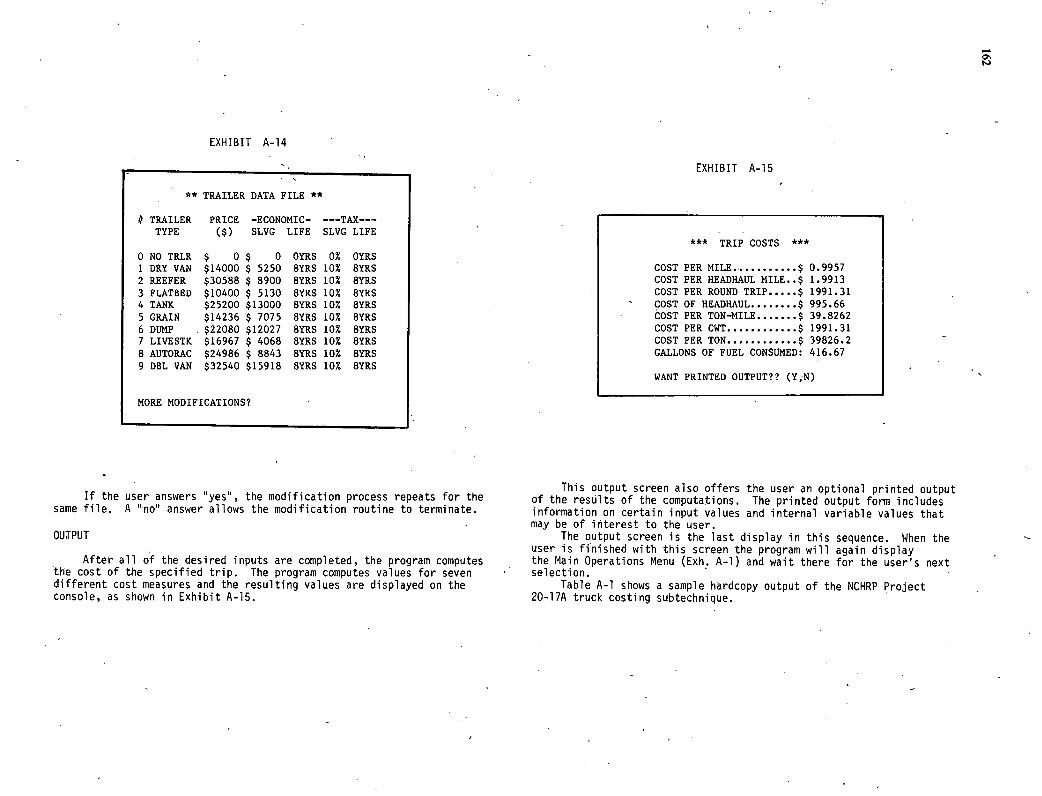
EXHIBIT A-14
EXHIBIT A-15
** TRAILER DATA FILE **
1/ TRAILER PRICE -ECONOMIC- ---TAX--- TYPE ($) SLVG LIFE SLVG LIFE
0 NO TRLR $ 0 $ 0 OYRS 0% OYRS 1 DRY VAN $14000 $ 5250 8YRS 10% 8YRS 2 REEFER $30588 $ 8900 8YRS 10% 8YRS 3 FLATBED $10400 $ 5130 8YRS 10% 8YRS 4 TANK $25200 $13000 8YRS 10% 8YRS 5 GRAIN $14236 $ 7075 8YRS 10% BYRS 6 DUMP $22080 $12027 8YRS 10% 8YRS 7 LIVESTK $16967 $ 4068 8YRS 10% 8YRS 8 AUTORAC $24986 $ 8843 8YRS 10% 8YRS 9 DBL VAN $32540 $15918 8YRS 10% 8YRS
MORE MODIFICATIONS?
*** TRIP COSTS ***
COST PER MILE ...........$ 0.9957 COST PER HEADHAUL MILE .$ 1.9913 COST PER ROUND TRIP.....$ 1991.31 COST OF HEADHAUL........$ 995.66 COST PER TON-MILE.......$ 39.8262 COST PER CWT............$ 1991.31 COST PER TON............$ 39826.2 GALLONS OF FUEL CONSUMED: 416.67
WANT PRINTED OUTPUT?? (Y,N)
If the user answers "yes", the modification process repeats for the same file. A "no" answer allows the modification routine to terminate.
OUTPUT
After all of the desired inputs are completed, the program computes the cost of the specified trip. The program computes values for seven different cost measures and the resulting values are displayed on the console, as shown in Exhibit A-15.
This output screen also offers the user an optional printed output of the resUlts of the computations. The printed output form includes information on certain input values and internal variable values that may be of interest to the user.
The output screen is the last display in this sequence. When the user is finished with this screen the program will again display the Main Operations Menu (Exh. A-l) and wait there for the user's next selection.
Table A-1 shows a sample hardcopy output of the NCHRP Project 20-17A truck costing subtechnique.
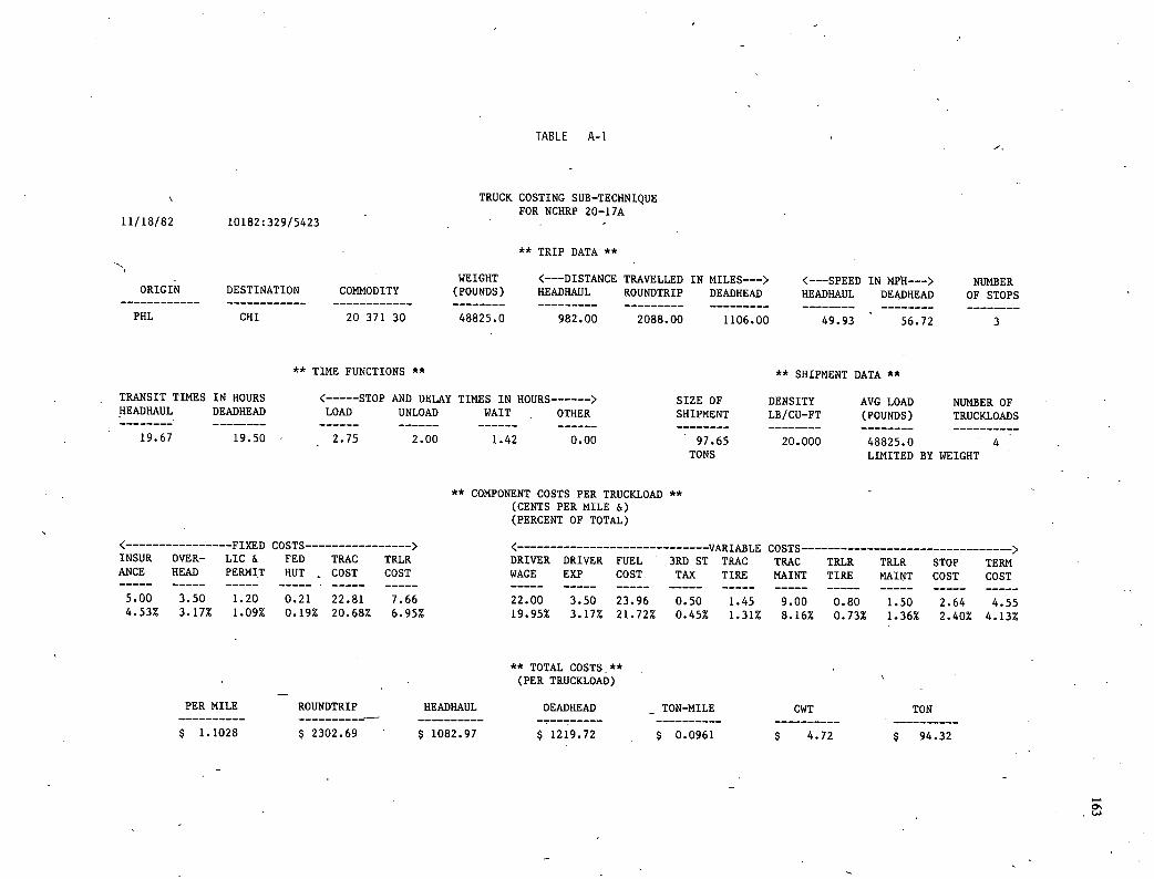
TABLE A-i
\ TRUCK COSTING SUB-TECHNIQUE FOR NCHRP 20-17A -
11/18/82 10182:329/5423
** TRIP DATA **
WEIGHT < --- DISTANCE TRAVELLED IN MILES --- > < --- SPEED IN MPH --- > NUMBER ORIGIN DESTINATION COMMODITY (POUNDS) HEADHAUL ROUNDTRIP DEADHEAD HEADHAUL DEADHEAD OF STOPS
PHL CHI 20 371 30 48825.0 982.00 2088.00 1106.00 49.93 56.72 3
** TIME FUNCTIONS ** ** SHIPMENT DATA **
TRANSIT TIMES IN HOURS <-----STOP AND DELAY TIMES IN HOURS------> SIZE OF DENSITY AVG LOAD NUMBER OF HEADHAUL DEADHEAD LOAD UNLOAD WAIT OTHER SHIPMENT LB/CU-FT (POUNDS) TRUCKLOADS
19.67 19.50 2.75 2.00 1.42 0.00 97.65 20.000 48825.0 4 TONS LIMITED BY WEIGHT
** COMPONENT COSTS PER TRUCKLOAD ** - (CENTS PER MILE &) (PERCENT OF TOTAL)
FIXED COSTS----------------> < ----------------------------- VARIABLE COSTS--------------------------------> INSUR OVER- LIC & FED TRAC TRLR DRIVER DRIVER FUEL 3RD ST TRAC TRAC TRLR TRLR STOP TERN ANCE HEAD PERMIT HUT COST COST WAGE EXP COST TAX TIRE MAINT TIRE MAINT COST COST
5.00 3.50 1.20 0.21 22.81 7.66 22.00 3.50 23.96 0.50 1.45 9.00 0.80 1.50 2.64 4.55 4.53% 3.17% 1.09% 0.19% 20.68% 6.95% 19.95% 3.17% 21.72% 0.45% 1.31% 8.16% 0.73% 1.36% 2.40% 4.13%
** TOTAL COSTS.** (PER TRUCKLOAD)
PER MILE ROUNDTRIP HEADHAUL DEADHEAD TON-MILE CWT TON
$ 1.1028 $ 2302.69 $ 1082.97 $1219.72 $ 0.0961 $ 4.72 $ 94.32
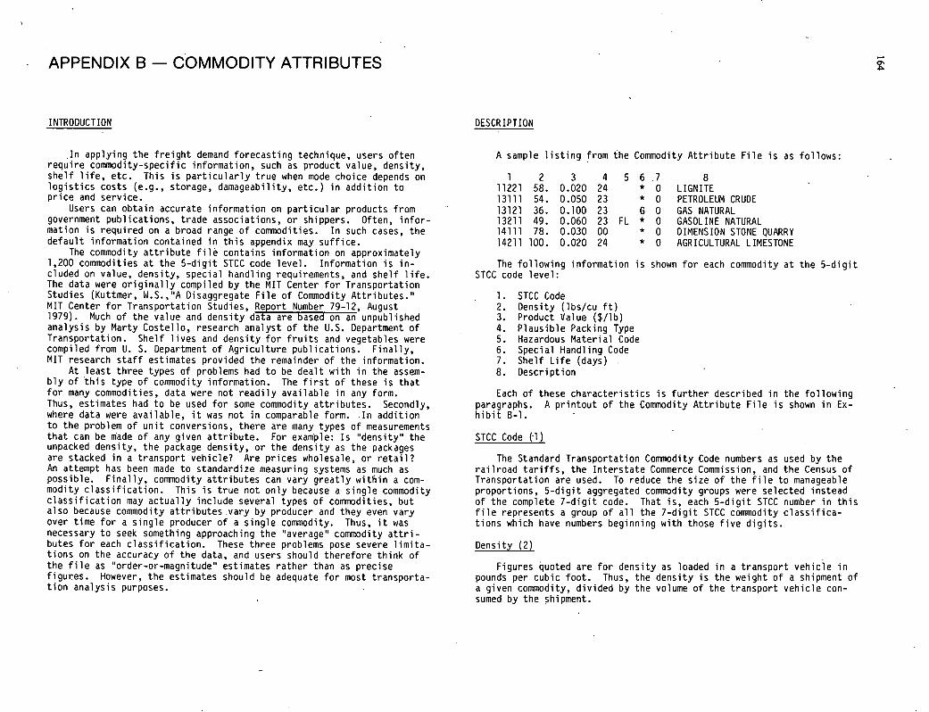
APPENDIX B - COMMODITY ATTRIBUTES
INTRODUCTION
.In applying the freight demand forecasting technique, users often require commodity-specific information, such as product value, density, shelf life, etc. This is particularly true when mode choice depends on logistics costs (e.g., storage, damageability, etc.) in addition to price and service.
Users can obtain accurate information on particular products from government publications, trade associations, or shippers. Often, infor-mation is required on a broad range of commodities. In such cases, the default information contained in this appendix may suffice.
The commodity attribute file contains information on approximately 1,200 commodities at the 5-digit STCC code level. Information is in-cluded on value, density, special handling requirements, and shelf life. The data were originally compiled by the MIT Center for Transportation Studies (Kuttmer, W.S.,"A Disaggregate File of Commodity Attributes." MIT Center for Transportation Studies, Report Number 79-12, August 1979). Much of the value and density data are based on an unpublished analysis by Marty Costello, research analyst of the U.S. Department of Transportation. Shelf lives and density for fruits and vegetables were compiled from U. S. Department of Agriculture publications. Finally, MIT research staff estimates provided the remainder of the information.
At least three types of problems had to be dealt with in the assem-bly of this type of commodity information. The first of these is that for many commodities, data were not readily available in any form. Thus, estimates had to be used for some commodity attributes. Secondly, where data were available, it was not in comparable form. In addition to the problem of unit conversions, there are many types of measurements that can be made of any given attribute. For example: Is 'density" the unpacked density, the package density, or the density as the packages are stacked in a transport vehicle? Are prices wholesale, or retail? An attempt has been made to standardize measuring systems as much as possible. Finally, commodity attributes can vary greatly within a com-modity classification. This is true not only because a single commodity classification may actually include several types of commodities, but also because commodity attributes vary by producer and they even vary over time for a single producer of a single commodity. Thus, it was necessary to seek something approaching the "average" commodity attri-butes for each classification. These three problems pose severe limita-tions on the accuracy of the data, and users should therefore think of the file as "order-or-magnitude" estimates rather than as precise figures. However, the estimates should be adequate for most transporta-tion analysis purposes.
DESCR IPT ION
A sample listing from the Commodity Attribute File is as follows:
1 2 3 4 567 8
11221 58. 0.020 24 * 0 LIGNITE
13111 54. 0.050 23 * 0 PETROLEUM CRUDE
13121 36. 0.100 23 G 0 GAS NATURAL
13211 49. 0.060 23 FL * 0 GASOLINE NATURAL
14111 78. 0.030 00 * 0 DIMENSION STONE QUARRY
14211 100. 0.020 24 * 0 AGRICULTURAL LIMESTONE
The following information is shown for each commodity at the 5-digit STCC code level:
STCC Code Density (lbs/cu ft) Product Value ($/lb) Plausible Packing Type Hazardous Material Code Special Handling Code Shelf Life (days) Description
Each of these characteristics is further described in the following paragraphs. A printout of the Commodity Attribute File is shown in Ex-hibit B-l.
STCC Code (1)
The Standard Transportation Commodity Code numbers as used by the railroad tariffs, the Interstate Commerce Commission, and the Census of Transportation are used. To reduce the size of the file to manageable proportions, 5-digit aggregated commodity groups were selected instead of the complete 7-digit code. That is, each 5-digit STCC number in this file represents a group of all the 7-digit STCC commodity classifica-tions which have numbers beginning with those five digits.
Density (2)
Figures quoted are for density as loaded in a transport vehicle in pounds per cubic foot. Thus, the density is the weight of a shipment of a given commodity, divided by the volume of the transport vehicle con-sumed by the shipment.
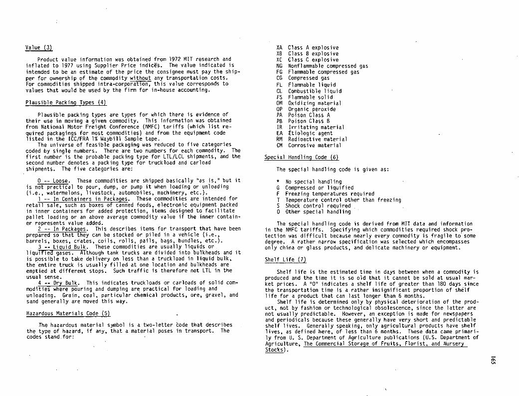
Value (3)
Product value information was obtained from 1972 MIT research and inflated to 1977 using Supplier Price indics. The value indicated is intended to be an estimate of the price the consignee must pay the ship-per for ownership of the commodity without any transportation costs. For commodities shipped intra-corporation, this value corresponds to values that would be used by the firm for in-house accounting.
Plausible Packing Types (4)
Plausible packing types are types for which there is evidence of their use in moving a given commodity. This information was obtained from National Motor Freight Conference (NMFC) tariffs (which 'list re-quired packagings for most commodities) and from the equipment code listed in the ICC/FRA 1% Waybill Sample tape.
The universe of feasible packaging was reduced to five categories coded by single numbers. There are two numbers for each commodity. The first number is the probable packing type for LTL/LCL shipments, and the second number denotes a packing type for truckload and carload shipments. The five categories are:
0 -- Loose. These commodities are shipped basically "as is," but it is not practical to pour, dump, or pump it when loading or unloading (i.e., watermelons, livestock, automobiles, machinery, etc.).
-- In Containers in Packages. These commodities are intended for retail sale, such as boxes of canned foods, electronic equipment packed in inner containers for added protection, items designed to facilitate pallet loading or an above average commodity value if the inner contain-er represents value added.
2 -- In Packages. This describes items for transport that have been prepared so that they can be stocked or piled in a vehicle (i.e., barrels, boxes, crates, coils, rolls, pails, bags, bundles, etc.).
3 -- Liquid Bulk. These commodities are usually liquids or liquified gases. Although tank trucks are divided into bulkheads and it is possible to take delivery on less than a truckload in liquid bulk, the entire truck is usually filled at one location and bulkheads are emptied at different stops. Such traffic is therefore not LTL in the usual sense.
4 -- Dry Bulk. This indicates truckloads or carloads of solid com-modities where pouring and dumping are practical for loading and unloading. Grain, coal, particular chemical products, ore, gravel, and sand generally are moved this way.
Hazardous Materials Code (5)
The hazardous material symbol is a two-letter èode that describes the type of hazard, if any, that a material poses in transport.. The codes stand.for:
XA Class A explosive XB Class B explosive XC Class C explosive NG Nonflammable compressed gas FG Flammable compressed gas CG Compressed gas FL Flammable liquid CL Combustible liquid FS Flammable solid OM Oxidizing material OP Organic peroxide PA Poison Class A PB Poison Class B IR Irritating material EA Etiologic agent RM Radioactive material CM Corrosive material
Special Handling Code (6)
The special handling code is given as:
* No special handling G Compressed or liquified F Freezing temperatures required I Temperature control other than freezing S Shock control required O Other special handling
The special handling code is derived from MIT data and information in the NMFC tariffs. Specifying which commodities required shock pro-tection was difficult because nearly every commodity is fragile to some degree. A rather narrow specification was selected which encompasses only china or glass products, and delicate machinery or equipment.
Shelf Life (7)
Shelf life is the estimated time in days between when a commodity is produced and the time it is so old that it cannot be sold at usual mar-ket prices. A "0" indicates a shelf life of greater than 180 days since the transportation time is a rather insignificant proportion of shelf life for a product that can last longer than 6 months.
Shelf life is determined only by physical deterioration of the prod-uct, not by fashion or technological obsolescence, since the latter are not usually predictable. However, an exception is made for newspapers and periodicals because these generally have very short and predictable shelf lives. Generally speaking, only agricultural products have shelf lives, as defined here, of' less than 6 months. These data came primari-ly from U. S. Department of Agriculture publications (U.S. Department of Agriculture, The Commercial Storage of Fruits, Florist, and Nursery Stocks).
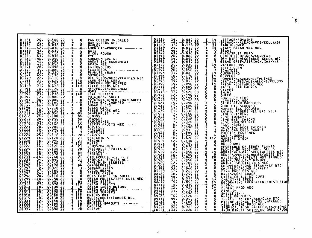
01121 20e 0.580 22 4 0 RAW COTTON IN BALES 01336 0133b
15. 0.080 22 T 4 LETTUCE/ROMAINE 01129 10.
42. 0.500 0.030
22 * 0
0 RAW COTTON NEC 01337
-9. 10.
-0.OSO 0.13C
-22 22 T
--4-14 INACM/KALE/CMARDS/C0LLARDS AULIFLOWER 01131 01132-42.---0.030
24 -4--*--- 0 ARLEY -0--1-ORN 01339 24, 0.090 22 T
21 14 LEAFY FRESH VEG NEC
01133 0.030 24 4 0 1 EXC-PO.P.C.ORN
OATS 01341 46. 0.130 24 0 0 BEANS 01134 3. 0.110 24 0 0 RICE, ROUGH 01342 43. -0.010 24 * 0 PEAS/SPLIT PEAS 01135 0.030 24 0
---4- 0 RYE 01343
01349 20. 0.080 22 * 0 NTILS/LUP1NES/COWPEAS
V RIPE VEGETABLE SEEDS PEC 01138 01137.
-46. --- 41.
0.O5O24 0.050 24 4
--0 0
SDRC.HUM GRAINS WHEAT EXC 8UCKWHEAT 01391
14. 14.
0.090 0.090
22 22
S 7
0 7 BEANS GREEP4/STRING/LIMA/W'X
01139 41. 0.050 24 0 GRAIN NEC 01392 20. 0.030 22 T 14 WATERMELONS 01141 0l1-42---39-.----0.0O-24-
20. 0.090 22 4 ..-o
0 ...-FLAXSEEDS-.
COTTONSEEDS 01393 20. H.
0.050 22 7 -
4 SWEET CORN . ----- ---- 0139'. 0.050 22 7 TOMATOES
01143 27. 0.230 22 0 0 PEANUTS (RAW) .01395 17. 0.080 22 14 CUCUMBERS 01144 45. 0.130 24 * 0 SOYBEANS 01390 10. -0.170 22 T 14 PEPPERS 01149 22. 0.120 24 4 0 OIL SEEDS/NUTS/KERNELS NEC 1 01397 20. 0.090 22 56 PUMPKINS/SQIJASH/CYPILINGS 01151 ---21.---0.-620-22 --4-1740-- 01398 19. 0.09C 22 14 CANTALCUPES/MUSKPIELONS/MELONS 01152 10. 0.150 22 4 140 POPCORN NOT POPPED - 0139 19. 0.090 22 1 14 FRESH VEGETABLES NEC 01159 21. 0.420 22 4 140 FIELD SEEDS NEC 01411 12. -0.660 00 0 0 CATTLE EXC CALVES 01191 10. .0.120 22 0 HAY/FODDER/ROUGHAGE 01412 12. 0.760 00 0 0 CALVES 01192-•-25•. --1.-0-90 22 ---*---0--HOPS ------ ----- 0141 12. 0.42000 0 0 SWINE 01193 23. 1.270 22 4 140 LEAF TOBACCO 0141'. 12. 0.440 00 0 0 SHEEP 01194 .. 12. 0.080 22 T 0 POTATOES, SWEET 1 -01415 12. 0.440 00 0 0 GOAlS QR KIDS 01195 36. 0.080 22 1 0 POTATOES OTHER THAN SWEET 01419 12. 0.740 00 0 0 LIVESTuCK NEC 01198 --17. 0.160 22 --4 -0 STRAW EXC CHOPPED -- --- 01421 15. 0.090 22 T 7 DAIRY FARM PRODUCTS 01197 .44. 0.010 24 4 0 SUGAR BEETS 01431 17. 0.800 22 ° 0 WOOL EXC SCOURED 01196 27. 0.010 24 * 0 SUGAR CANE 01432 17. 1.390 22 * 0 MOHAIR EXC SCOURED 01199 18. 0.120 24 0 0 FIELD CROPS NEC 01439 13. 1.330 22 0 ANIMAL FiBERS NEC EXC SILK 01211 ---22.--0.050 22 -- 4----35 01511 7. 0.150 22 0 0 LIVE CHICKENS 01212 24. 0.080 22 T 84 LEMONS 01512 7. 0.370 20 0 0 TU LIVE RKEYS 01214 . 26. 0.040 22 T 56 ORANGES 01513 7. 0.200 22 0 0 LIVE SABY CHICKS 01215 24. 0.120 22 1 21 TANGERINES 01519 0.320 22 0 0 LIVE POULTRY NEC 0 219- -23. --0.140 22 1 35 01521 0.750 11 T 7 EGGS MARKET 0 221 20. 0.080 22 T 140
LAWN GRASS SEED--------- - --
APPLES 01522 8. 0.890 22 S 7 HATCHING EGGS CHICKEN 0 222 25. 0.090 22 T 7 APRICOTS 01523 B. 0.97C 22 S 7 HATCHIKO EGGS TURKEY 0 223 12. 0.170 22 T .7
GRAPEFRUIT - - .......... ..
CHERRIES 01529 6. 0.860 22 T 7 POULTRY EGGS NEC 01224 -25. 0.110 22- -1- 70 - GRAPES ---- - . . - -•--- 01511 5. 1.5'.0 00 T 4 CUT FLOWERS 01225 16. 0.120 22 T .21 NECTAR INES 01912 10. 1.620 22 112 NURSERY STOCK 01226 16. 0.090 22 T 21 PEACHES 01915 42. 0.430 24 * 0 HERBS 01227 22. 0.090 22 T 112 PEARS 01S1 8. 0.750 22 1 3 MUSHROOMS 01228 ....18. 0.120 22 4 21 PLUMS/PRUNES 01917 0.970 22 0 7 VEGETABLE OR BERRY PLANTS
16. 0.130 22 1 28 DECIDUOUS FRUITS NEC 01918 1.510 22 4 0 FLOwER OR VEGETABLE SEEDS
E
229 231 16 • 0.280 22 T 21 AVOCADOS 01919 -12. --3.850 -22 ---4 -14 -eORl ICULTURAL SPEC! ALT I ES NEC 232 20. 0.070 22 T 21 BANANAS 01921 10. 7.700 CO -0 0 HDRSES/PONIES/MULES/ASSES ETC 233 --46w -0.260 22 -T- 21
CITRUS FRUITS NEC ..... .
PINEAPPLES - - --- - 01923 12. 0.960 22 T 28 HIDES/SKINS/PELTS NOT TANNED 01239 24. 0.340 22 1 21 TROPICAL FRUITS NEC 01926 51. 0.050 24 * 0 ANIMAL/POULTRY MANURE 01291 . 16. 0.410 22- 1 7 CANE/BUSH BERRIES 01929 12. 7.700 00 0 0 ANIMAL SPECIALTIES NEC 1292 16. 0.170 22 T 84 CRANBERRIES . 01991 14. O.12C 22 4 0 CHOPPED/GROUND STRAW/HAY ETC 123 8.----O.-32-O--2-2------T-----?-- 5TRAWBERRIES- - - 01992 33. 0.060 2'. 0 CHOPPED/GROUND ALFALFA 1294
~RI298
37. 0.960 22 4 0 DCOA BEANS 0199w 12. 0.260 22 0 FARM PRODUCTS NEC 1295 24. 1.880 22 * 0 COFFEE GREEN 0842 16. 1.200 22 4 0 BARKS/GUMS CRUDE
. 20. 0.410 22 4 0 NUTS EDIBLE IN SHELL 08423 46. 0.260 22 4 0 LATEX OR ALLIED GUMS 01299 --10.-0.250-22-----* - . --FRESH FRUiTS/TREE--NUTS NEC- 08611 15. 0.230 00 0 14 CHRISTrAS TREES 01311 20. 0.050 22 T 84 FRESH BEETS 08612 5. 1.850 22 * 14 DECORATIVE EVERGREENS/PIISTLETUF 01312 27. 0.07022 T 112 FRESH CARROTS 06813 16. -2.31-C. -22-4 14 -FERNS 01313 10. 0.130 22 T 0 FRESH GREEN ONIONS 0b619 n. 0.920 22 14 FOREST PROD NEC 01315 46.---0-.130--22-------56
7 ---FRESH RADISHES - -
FRESH 09121 11. .0.110 22 T 0 FINFISH - 01317 01318
0. 21.
0.120 0.080
22 22 T
112 112
TURNiPS ONIONS DRY 09122 11. 0.590 22 T
4 . 0 0
SHELLFiSH
01319 20. 0.130 22 140 JULSS/R OOTS/TUBERS NEC 09123 09131
.4. 59.
0.420 0.3C0
22 24 4 0
WHALE PRODUCTS SHELLS OYSTER/CRAB/CLAM ETC
1332 1331 12.
-.7. 0.140 0 .160
2 2
14 2.8 - RDCCOLI RUSSEL SPROUTS MARINE ANIMAL SKINS UNTANNE8
D 09132 8. 4.160 22 4 0
01333 15. 0.050 22 T 42 CABBAGE CELERY
09139 09691
12. 20.
0.340 0.700
22 22
* 0
0 0
MISC. MARINE PROD NEC TROPICAL FISH HATCHERIES/FARMS 01334 21. 0.090 22 T 70
- .1011j_433. -0.020 24 - IRON DIRECT SHI!ING ORES CRVDF
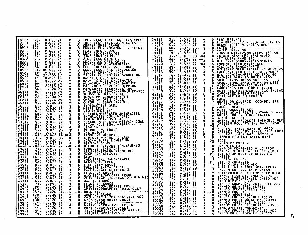
0.020 24 C 0 IRON BENEFICIATING ORES CRUDE 1917 21. 0.050 22 C 0 PEAT NATURAL P011271. 113 63. 0.020 24 C 0 IRON CCNCETR/A&GLOMERATES 14918 19. 0.050 22 * 0 DIATOMACEOU5/INFUSORIAL EARTHS 0211 120. 0.010 24 C 0 COPPER ORES CRUDE 14919 64. 0.02C 24 C 0 NONMETALLIC MINERALS NEC 1 0212 132. 0.260 24 C 0 COPPER CONCENIR/PRECIPITATES 14921 66. .0.020 23. * 0 WATER RAW 10311 67. 0.020 24 C 0 LEAD ORES CRUDE 14922 66. 0.020 13 * 0 WATER DRINKING
95. 0.200 24 0 0 LEAD CONCENTRATES 19111 9. 25.000 00 * 0 GUNS/HOWITZERS/MORTARS >30 MM
10312 0321 56. 0.020 24 C 0 ZINC ORES CRUDE 19251 14.500.0CC 00 XB* 0 GUIDED MISSILES ASSEMBLED 0322 89. 0.200 24 - C 0 ZINC CONCENTRATES 19291 31. 0.250 22 XA* 0 ARTILLERY AMMO ETC ---- - ____
10331 62. 0.020 24 0 0 LEAD/ZINC ORES CRUDE 19293 17. 0.500 22 C 0 MILITARY BOMBS/MINES/PARTS 10332 93. 0.200 24 0 0 LEAD/ZINC CONCENTRATES 19299 16. 0.500 22 XBC 0 AMMO/RELATED PARTS NEC
TANKS/PARTS MILITARY 30411 60. 0.020 24 0 0 GOLD ORE/TAILINGS CRUDE 19311 39. 5.000 00 C 0 30412 90.100.000 22 C 0 GOLD CONCENTRATES/BULLION - 9312-. -39w 5.000 00 0 0 MILITARY SELF PROPELLED WEAPONS
I0421 0. U. 0.020 24 C 0 SILVER ORE/TAILINGS 19313 35. 5.000 00 0 0 FULL TRACKED COMBAT VEH/PARIS MIL CONTROL EQ SIGHTING/FIRE 0422 32.000 22 C 0 SILVER CONCENTRATES/BULLION 19411 6. 50.000 11 C 0
10511 73. 0.020 24 0 0 BAUXITE ORES CRUDE 19511 12. 25.0CC 22 0 0 MACHINE GUNS 30 MM OR LESS 63. -0.020 24 0 BAUXITE ORES CALCINATED 19512 12. 25.000 22 0 0 SMALL ARMS 30 MM OR LESS 10513 0514 35. 0.020 24 0 0 ALUMINUM ORES EXC BAUXITE 19611 30. 25.000 11 C 0 SMALL ARMS AMMO 30 MM OR LESS 60. 0.020 24 0 0 MANGANESE DIRECT SHIPPING 19911 17. 25.000 22 4 0 MISC ORONANCE/ACC/PARTS
1
0611 0612 se. 0.020 24 0 0 MANGANESE BENEFICIAl INC 20111 33, 0.590 00 T 14 CARCASSES FRESH OR CHILLED 0613 52. 0.020 24 $ 0 MANGANESE CONCEN/AGGLOMERATES 20119 17. 0.71C 22 T 14 MEAT NEC FRESH/CHILL EXC SAUSA
60. 0.02C 24 0 0 TUNGSTEN ORES CRUDE 20121 27. 0.620 00 F 0 CARCASSES FRESH FROZEN
t
0711 0712 22. 1.000 22 C 0 TUNGSTEN CONCENTRATES 20129 30. 0.740 22 F 0 MEAT NEC FRESH FROZEN 0811 61. 0.020 24 0 0 CHROMIUM ORES CRUDE 20131 50. 0.270 23 C 0 LARD
40812 - 90. 4.000 24 S 0 CHROMIUM CONCENTRATES 20132 12. 0.770 22 T 7 MEATS OR SAUSAGE COOKED, ETC
66. 0.020 4 4
C 0
0 RADIOACTIVE oRES METAL ORES NtC
20133 20134
9. 28.
0.840 0.600
22 11
T C
7 0
SAUSAGE FRESH CANNED MEAT
1
0923 099
111 70. 60.
0.020 0.020 24 0
0 0 RAW ANTHRACITE 20139 56, 0.690 23 Q 0 MEAT PRODUCTS NEC
1112 60. 0.020 24 C 0 CLEANED/PREPARED ANTHRACITE 20141 20143
25. 57.
0.400 0.170
00 23
0 C
0 0
HIDES SKiNS PELTS UNTANNED GREASE OR INEDIBLE TALLOW
11
119 211
80. 56.
0.0 0.020
24 24
4 0
0 0
ANTHRACITE COAL WASTES RAW BITUMINOUS COAL 20144 32. 0.190 22 0 0 ANIMAL REFUSE
212 56. 0.020 24 C 0 CLEANED/PREPARED BITUMIN COAL 20149 20151
49. 10.
0.360 0.410
24 22
C T
0 0
ANIMAL BY PRODUCTS INEDIBLE NEC 219 --80. -0.0--- 24--- 4 ---0 BITUMINOUS COAL WASTES .....-
20156 8. 0.780 22 0 70 DRE
..SED POULTRY SML GAME FRSH
221 58. 54.
0.020 0.050
24 23
C C
0 0
EGG3111
LIGNITE PETROLEUM, CRUDE 20158 15. 0.390 22 F 0 POULTRY SMALL GAME BY PROD
3121 13211
36. 0.100 23 6 0 GAS NATURAL 20161 20168
23. 15.
0.410 0.390
22 22
F F
0 0
DRESSED PDJLTRY SMALL GAME FROZ POULTRY SMALL GAME BY-PROD
4111 49. 78.
-0.060 0.030
23 00
FLO 0
0 0
GASOLINE NATURAL DIMENSION STONE QUARRY 20171 19. 0.430 Ii * 0 CANNED POULTRY SMALL GAME
£4211 100. 0.020 24 0 0 AGRICULTURAL LIMESTONE 20172 8. 0.70 22 0 70 GGS 14212 61. 0.020 24 C 0 FLUXiNG STONE 20211 25. 1.020 22 T 7 REAMERY BUTTER 3-42-13- -80.- 0-.020 24 ---C -0 DOLOMITE RAW/BROKEN/CRUSHED 20231 25. 0.480 11 0 0 DRY MILK PROD 14215 74. 0.020 24 0 0 FURNACE LIMESTONE 20233 29. 0.290 22 0 0 EVAP OR CONDENSED MILK PROD 14219 74..' 0.020 24 C 0 CRUSHED/BROKEN STONE NEC i 20234 S. 0.350 il 0 0 ICE CREAM MIX OR ICE MILK MIX
I4411 99. 0.020 24 0 0 SAND EXC ABRASiVE 20241 13. 0.350 22 F 21 ICE CREAM RELATED DESSERTS 4412- 101. 0.020 24 --4 -0 GRAVEL I 0251 30. 0.960 22 T 35 CHEESE 14413 85. 0.020 24 0 0 INDUSTRIAL SAND/GRAVEL I 0252 13. 0.580 11 T 7 COTTAGE CHEESE 14511 -, 58. 0.020 24 C 0 BENTONITE CRUDE 20256 14. 0.380 22 1 21 CASE IN PRODUCTS
88. 0.020 24 4 0 FIRE CLAY CRUDE 20259 22. 0.370 22 1 7 SPEC DAIRY PROD NEC 4513 --- 24. -0.050 22--C- -0 FULLERS EARTH CRUDE 20261 8. 0.120 22 F 0 BULK FL MILK INCL SKIM CREAM
14512
4514 24. 0.050 22 0 0 KAOLIN/BALL CLAY CRUDE 20262 15. 0.370 11 T 7 PKGD MILK INCL SKIM CREAM 4515 66. 0.020 24 C 0 FELDSPAR CRUDE 20264 12. 0.380 11 T 7 BUTTERMILK CHOCO ETC FLAV MILK
14516 . 24. 0.050 22 C 0 MAGNESIIE/8RUC1TE CRUDE MIN NEI 20311 29. 0.870 11 0 0 CANNED FISH ETC INCL SOUPS
14519 14711
--57. 69.
0.020 0.020
24- 24
-* 0
0 0
CLAY CERAMIC/REFRACT(WY BARITE CRUDE
20314 26. 2.170 11 0 0 MKDASALTED,PICKLED DRIED SEA 20321 27. 0.440 11 0 0 ANNtD BABY FOODS
14712 73. 0.050 24 0 0 FLUOSPAR CRUDE 20322 28. 0.380 11 C 0 CANNED SOUPS EXC 20381 311 361 14713 66. 0.030 24 C 0 POTASH/SODA/BORATE CRUDE 20323 24. 0.340 11 0 0 CANNED BEAN SPECIALTIES 14714 110. 0.020 24 0 0 APATITE/PHOSPHATE ROCK/CLAY 20329 18. 0.360 11 0 0 CANNED SPECIALTIES, NEC 14715 -57.-- 0.020 24---- *---0--ROCK SALT - - - ' 20331 --25. -0.340 11 -0 -.0 CANNED FRUITS - - 14716 120. 0.020 23 0 0 ULPHUR CRUDE 20332 31. 0.330 11 0 0 CANNED VEGETABLES 14719 83. 0.020 24 C 0 UIEM/FERTILIZER MINERALS NEC 20333 18. 0.330 ii 0 0 CANNED HOMINY OR MUSHROOMS 14911 100. 0.020 24 C 0 GYPSUM/ANHYDRITE CRUDE 20334 36. 0.310 11 0 0 CANNED FRUIT JUICE EXC 20996 14912---24'-0.050 22-4-- .0-MICA CRUDE--- -- ' 20335 28. 0.330 11 0 0 CANNED VEGETABLE JUICES 14913 78. 0.020 24 0 0 NATIVE ASPHALT/B1TUMENS 20336 30. 0.380 11 0 0 CATSUP OR OTHER TOMATO SAUSES 14914 55. 0.020 24 0 0 PUMICE/PUMIC1TE CRUDE 20338 27. 0.300 11 0 0 JAMS JELLIES PRESERVES 14915 34. 0.030 20 * 0 TALC/SOAPSTONE/PYROPHYLLITE 20339 27. 0.310 11 0 0 CANNED FRUITS VEGETABLES NEC 14916 -78. 0.020 24 ....... 0 NATURAL ABRASIVES -- - - 20341 - 28.- 0.400 11 0 0 'DRIED OR DEHYDRATED FRUITS
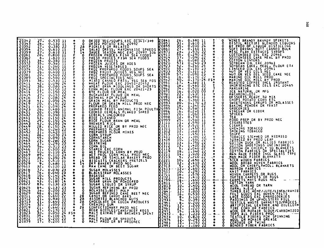
20342 * Ô DRiE'EG/SOUPS E bT41-349 0841 26. 0.390 1 T 0 BRANDY 8RANY SIkITS 20343 26. 0.130 1 C 0 DRIED POTATO EXC 20992 0851 31. 0.610 T 0 0 STIL RECTIFI BLENDED LIQUORS 20352 27, 0.380 22 T 28 PICKLES OR RELAtED 20859 35. 0.030 24 0 BY PROD OF LIQUOR DiSTILLING 20354 27. 0.610 11 T 14 SALAD DRESS, MAYONNAiSE SPREOS 20861 27. 0.140 11 0 SQFT DRINKS 8077 CANNED BULK 20359 27. 0.610 1 T 14 SAUCE SEASON NEC EXC 20997 336 20871 26. 1.57C 22 0 0 MiSC FLAy EXTRACTS SYRUPS 20361 20. 0.800 11 F 0 FROZEN PROCES FISH SEA FOODS 20911 55. 0.290 23 C 0 COTTONSEED OIL EXC 20961 20362 6, 1.820 11 F 0 FRESH PROCES FISH SEA FOODS 20914 17. 0.090 22 C 0 COTTONSEED CAKE NEAL BY PROD 20371 34. 0.380 11 F 0 FROZEN FRUITS 0915 16. 0.080 22 * 0 COTTON LINTERS 20372 35. 0.360 1 F 0 FROZEN JUICES OR ADES 0921- 571 0.240 23 C 0 SOYBEAN OIL EXC 20961 20373 31. 0.360 11 F 0 FROZEN VEGETABLES 20923 42. 0.260 24 C .0 SOYBEAN CAKE, MEAL FLOUR ETA 20374 20. 0.500 22 F 0 FROZ PREPARED FOODS SOUPS SEA 0931 55. 0.180 23 0 0 LINSEED OIL EXC 20461 20379 26. 0.400 11 F 0 FROZ FRUIT JUICES VEG NEC 20933 55. 0.310 23 C 0 NUT OR VEG OILS NEC 20381 20. 0.500 22 F 0 FROZ PREPARED FOODS SOUPS SEA 20939 57. 0.090 23 C 0 NUT OR VEG OIL SEED CAKE NEC 20389 26. 0.500 22 F 0 FROZ SPECIALTIES NEC 20941 16. 0.170 22 0 0 MARINE OIL MILL PROD 20391 38. 0.530 11 C 0 MIXED CANNED FRTS, VEG SEA FDS 0942 50. 0.170-24.FSC • MARINE OIL MILL BY PROD 20411 42. 0.090 24 C 0 WHEAT FLOUR EXC 2045 1-20452 0951 .17. 4.380 11 C 0 ROASTED COFFEE INCL iNSTANT 20412 38. 0.080 24 C 0 WHEAT SRAN MIDDLJNGS OR SHORTS 096 b. 0.460 22 1 0 SHORTENING ETC OILS EXC 20465 2041 21. 0.150 12 0 0 CORN MEAL FLOUR EXC 20421-23 0962 4. 0.510 22 T 0 MARGARINE 20414 27. 0.150 22 C 0 RYE FLOUR OR MEAL 097 16. 0.020 00 F 0 ICE NATURAL OR MFG 20415 27. 0.150 22 0 0 BUCKI.HEAT FLOUR OR MEAL 2096 22. 0.430 11 0 0 MACARONI,ETC 20416 37. 0.080 24 C 0 OATMEAL FOR FLOUR 099 18. 0.990 11 0 DESSERTS READY TO MIX 20418 41. 0.050 24 0 0 GRAIN MEAL BY PRODUCTS 0992 8. 0.360 11 0 0 CHIPS POTATO CORN ETC 20419 20. 0.150 22 0 0 FLOUR OR GRAIN MILL PROD NEC 2099 80. 0.170 23 * 0 SWEETENING SYRUPS OR MOLASSES 20421 63. 0.090 24 0 0 PREPARED FEED 0994 16. 1.340 22 C 0 BAKING POWDER OR YEAST 2042 26. 0.480 11 0 0 CANNED FEEDS ANiMAL FISH POULfl' 0995 29. 0.580 11 0 0 GROCERIES 043 20. 0.390 11 0 0 COOKED CEREALS FLAKED SHRED 0996 16. 0.200 11 C 0 VINEGAR OR CIDER 0432 20. 0.390 11 * 0 CEREALS UNCOOKED 0997 20. 1.060 11 0 SPICES
20441 20442
43. 29.
0.150 0.150
24 24
C 0
0 0
RICE CLEANED RICE FLOUR BRAN OR MEAL
0998 0999
12. 25.
0.730 0.580
11 11
0 4
0 0
TEA FOOD PREP OR BY PROD NEC
20443 42. 0.150 24 * 0 BREWERS RICE lill 11. 2590 11 C 0 CIGARETTES 20449 28. 0.150 24 C 0 MILLED RICE OR BY PROD NEC 1211 8. 3.520 1 C 0 CIGARS
33. 0.260 22 * 0 PREPARED FLOUR 1311 12. 1.450 11 C 0 CHEb.ING TOBACCO 10451 0452 21. 0.420 11 * 0 PREPARED FLOUR MIXES 1312 12. 1.680 11 C 0 SMOKING TOBACCO 20461 20462
86. 45.
0.070 0.090
23 14
0 0
0 0
CORN SYRUP CORNSTARCH
1313 1411
4. 22.
.450 1 .350
1 22
C 0 0
SNUFF TOBACCO STEMMED OR REORIED
20463 23. 0.280 22 * 0 CORN SUGAR 2141 9 10. 1.55C 22 C 0 TOBACCO BY PROD LEAF 20464 17. 0.290 22 0 0 DEXTRINE 22111 13- . .750 22 0 0 COTTON DUCK OR ALLiED FABRICS 20485 Sb. 0.310 23 0 0 CORN OIL 22112 13. 1.400 22 C 0 COTTON SHEETINGS UNFINISHED 0466 21. 0.300 22 C 0 STARCH EXC CORN 22113 5. 2.040 22 C 0 COTTON OR CHIEFLY SO BLANKETS 0467 40. 0.110 24 0 0 WET PROCESS CORN BY PROD 22119 18. 1 .340 22 0 0 COTTON FABRICS OR SPECIALTIES 20469 89. 0.110 23 0 0 WET PROC CORN MILL PROD NEC 22211 14. 1.920 22 C 0 MAN MADE FIBER INCL GLASS TYPE 20511 30. 0.350 24 0 1 BREAD OR SIMILAR BAKERY PROD 22213 5. 2.240 22 P 0 MAN MADE FIBER BLANKETS 20521 13. 0.510 11 0 14 BISCuITS CRACKERS PRETZELS 22221 10. 2.650 22 0 0 1Tk WOVEN FABRICS 20529 9, 0.680 11 * 14 DRY BAKERY PROD NEC Z2311 12. 2.410 22 C 0 WOOL BROAD WOVEN FABRICS 20611 32. 0.130 22 0 0 RAW CANE OR BEET SUGAR 22313 5. 2.370 22 0 0 WOOL OR CHIEFLYWOOL, BLANKETS 20616 72. 0.030 23 C 0 SUGAR MOLASSES 2411- -12.-- 2.650 22 4 --0 NARROW FABRICS 20617 76. 0.040 23 * 0 BLACKSTRAP MOLASSES 2251
22711 10. 16.
2.290 1.570
KNIT FABRICS 22 22
C C
0 0 WOVEN CARPETS OR RUGS 20618
20619 10. 43.
0.140 0.130
24 24
C *
0 0
BAGASSE - SUGAR MILL PRODUCTS 22721 16. 1.410 22 4 0 TUFTED CARPETS OR RUGS
20621 43. 0.180 14 C 0 UGAR GRAM OR POWDERED 2799-- 16.-- 1.440 22-- -*--- 0
-0-- 0
CAPETS MATS RUGS NEC - - YARN COtTON 20622 83. 0.130 23 C 0 SUGAR LIQUID OR SYRUP 2281
22813 17. 10.
.030 2.400
22 22 * 0 WOOL THREAD OR YARN
0625
0626 84. 16.
0.130 0.200
23 22
C *
O 0
SUGAR REFINING BY PROD MOLASSES BEET PULP
22819 12. .290 22 * 0 YARN N.E.C. THRE6 EXC HEMP/JUTE/LINEN/RAMIE
1
SUGAR REI!INED CANE BEET NEC 22841 12. i.000 11 C 0
0629 0711
46. 20.
0.160 0.640
24 22
* 1
0 28 CANDY OR CANDY BARS 22911 16. 0.530 22 0 0 FELJ 000S EXC WUVEN FELTS
22921 B. 3.120 22 4 0 LA.t bOODS EXC EMBROiDERIES 20712 21, 0.930 11 C 28 ASSORTED BLANCHED NUTS 22931 S. 0.390 22 0 0 PADDINGS OR UPHOLSTE Y FILL 20713 21. 0.640 22 1 28 CHOCOLATE OR COCOA PRODUCTS 22941 -6. 0.200 22 0 0 TEXTLE WASTE GARNET TED/PROCES- 20714 32. 1.050 11 4 0 CHEWING GUM 22951 12. 1.200 22 C 0 ARTI ICIAL LEATHER AND OILCLOTH 20719 21. 0.640 22 0 28 CONFECTIONARY PROD NEC 22961 27. 1.220 22 C 0 TIRE CORD OR FABRICS 2082 2082
27. 30.
0.170 0.050
11 24
4 FS4
0 0
BEER BOTTLES/CANS/BEER KEGS MALT EXTRACT OR BREWERS
22971 15. 1.630 22 * 0 WOOL OR MOHAIR SCOUR/CARBONIZED SPENT 2297- 6.- 1.220 22 -- C--- 0 TOP ALL FIBtRS PROC
20831 35. 0.100 24 0 0 MALT 22973 10. 0.820 22 0 0 TEA ILE FIBERS FOR SPINNING 20832 15. 0.200 22 C 0 MALT FLOUR OR SPROUTS 22974 1. 0.290 22 C 0 WOOL OR MOHAIR GREASE 2C839 17. 0.200 11 0 0 MALT PROD OR BY PRODNEC 22981 1. 1.150 22 C 0 CORDAbE OR TWINE
22991 12. --1.16022 S 0 BONDED FIBER FABRICS
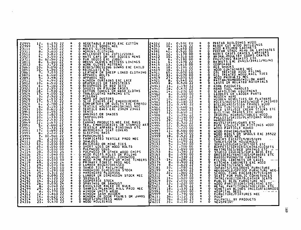
22995 12. 0.270 22 0 VEC.ETABLE FIBERS (XC COTTON 24332 12. 0 .5 9c Co 4 0 PREFAB BUILDINGS WOOD - BUILDINGS 22999 S. 1.310 22 4 0 TEXTILE GOODs NEC 24333 14. 0.470 22 4 0 READY CUT WOOD
CABINETS WOOD KITCHEN 23111 23311
3.300 3.800
22 22
4 0 0
MALES CLOTHING WOMENS CLOTHING
2434.1 24391
8. 41.
0.650 0.500
Co 00
4 0 0 PREFAB STRUC MEMB OR LAMINATES
23511 3. 3.810 22 * 0 MILLENERY EXC 23711/23961 24411 12. 0.170 00 4 0 BOXES CASES CRATES CARRiERS CRATES 23521 4. 3.550 22 4 0 HATS CAPS OR HAT BODIES HENS 24412 10. 0.310 00 $ 0 ANIMAL/POULTRY COOPS ETC FRUIT/VEG BASKETS 23711 8. 62.580 22 4
0 FUR GOODS EXC 23861 24413 6. 0.190 00 8 *
0 BASKETS EXC 24413/39411/91'1 23811
23812 S. 6.
4.b0 3.20
22 22
0 0
DRESS GLOVES MITTENS LININGS WORK GLOVES MITTENS
24414 24415
4. 13.
0.470 0.610
22 00
0 0 COOPERAGE
23841 10. 3.050 22 4 0 ROBES/DRESSING GOWNS EXC CHILD 2441e 18. 0.190 22 0 BOX SHOOKS NEC 23851 10. 4.040 22 4 0 RAINCOATS ETC 24419 18. 0.210 22 4 0 W900 CONTAINERS
D PILING 23861 7. 7.070 22 8 4
0 LEATHER OR SHEEP LINED CLOTHING 24911 65. 0.070 00 4 0 TREATED w000 RAIL TiES 23871 6. 6.480 22 0 APPAREL BELTS 24912 33. 0.070 00 0 OIL
NEC WOOD PRODUCTS 23891 5. 3.980 22 4 4
0 APPAREL NEC 24919 27. 0.070 GO 0 4
0 RATTAN/BAMBOO/WILLOW WARE 23911 4.940 22 0 WINDOW CURTAINS EXC LACE 24921 0.540 22 0 MATERIALS 23912 10. 6.510 22 0 DRAPERIES OR TAPESTRIES 24931 8. 0.520 22 * 0 LASTS OR RELATED
23921 6. 4.160 22 4 0 0
BEOSPREDS OR BED SETS SHEETS OR PILLOW CASES
24941 14. 1.19C 22 0 0 C'ORK PRODUCTS 23922 23923
11. 18.
2.350 1.930
22 22 0 COTTON TOWELS OR WASH CLOTHS
24951 24961
18. 14.
0.4 10 0.270
22 00
0 0
HAND TOOL HANDLES SCAFFOLDING EQUIPMENT
23924 17. 4.000 22 4 0 TABLECLOTHS NAPKINS ETC 24982 6. 0.330 00 c 0 LADDERS OR LADDER PARTS 23925 3. 2.980 22 4 0 PILLOwS 24971 8. 0.890 22 0 WOODEN WARE 23926 10. 1.570 22 8 0 MOPS OR DUSTERS 24972 10. 0.8SC 22 4 0 WOODEN NOVELTIES OR FLATWARE 23927 17. 5.730 22 0 0 SLIP COVERS EXC EMBROIDERED 24981 14. 0.180 22 0 0 POLES/RODS/STAKES/WOOD FINISHED 23928 6. 2.780 22 4 0 COMFORTERS OR QUILTS EXC EMBROO 24982 1 • 0.490 22 8 0 BILLBOARDS/SIGN FRAMES WOOD 23929 6. 3.150 11 0 TEXTILE P1OUSEFuiNISHINGS NEC 24983 12. O.0 i2 0 0 BATH 108/TOILET SEATS ETC 23931 10. 0.610 22 0 TEXTILE BAGS EXC 23929 23461 24985 1 • 0.560 22 0 BILE SIPS/ICE CREAM STiCKS ETC 23941 10. 1.950 22 0 0 TENTS 24981 12. 0.60 22 0 QuILTING FRAMES ETC WOOD 23942 10. I.B20 22 4 0 AWNINGS OR SHADES 24988 7. 0.390 e2 0 IRONING BOARDS/TABLES - WOOD 23943 10. 1.330 22 4 0 TARPAULINS 24992 1 • 0.190 00 4 0 PALLETS/SKIOS/PLATFQRMS WOOD 23944 10. 2.530 22 4 0 SAILS 24993 29. 0.270 22 0 HARDBOARD 23949 12. 1.670 22 0 CANVAS PRODUCTS NEC EXC BAGS 24994 12. 0.720 22 0 0 MASTS/SPARS/OARS ETC 23951 5. 2.660 22 4 0 TEA. EMBROIDERIES OR STAMPED ART 24995 12. 0.900 00 0 .0 PIPE COIOUIT OR FITTINGS WOOD 23961 7. 1.33C 22 4 0 TEXTILE APPAREL FINOINOS ETC 24996 38. 0.220 00 0 WOOD PARTICLE BOARD 23991 17. .1.690 22 0 0 AUTOMOBILE SEAT COVERS 2499 11. 0.460 00 * 0 WOOD FENCiNG/GATES 23993 8. 2.220 22 0 0 SLEEPING BAGS 24998 5. 0.470 00 • 0 WOOD REELS QR SPOOLS EXC 35522 23994 7. 10.960 22 0 0 PARACHUTES 2499 18. 0.52C 22 * 0 WOOD PROD NtC 23999 5. 2.200 22 * 0 FABRICATED TEXTILE PROD NEC 25111 4. 1.130 22 8 0 CHAiRS EXC32719/819/699 24111 29. 0.030 00 0 0 SAWLOGS 25121 5. 1.190 22. 4 0 TABLES/DESK HOUSEHOLD 24112 41. 0.030 00 4 0 RAILROAD OR MINE TIES 25131 4. 1.780 00 0 SOFAS/COUCHES/SETTEE S ETC 24113 35. 0.050 00 0 SHORT LOGS OR WOOD BOLTS 25141 7. 1 .700 00 * 0 BUFFETS/SERVER S/CHINA/CLOSETS 24114 51. 0.030 00 4 0 PULPwOOD LOGS 25151 3. - .040 00 0 MATTRESSES/BED SPRINGS ETC- -- - 24115 28. 0.030 24 4 0 PULPWOOD CR OTHER WOOD CHIPS 25153 6. 1.780 22 * 0 STUDIO COUCHES/SOFA BEDS ETC 24116 25. 0.040 00 - 0 WOOD POSTS POLES OR PILING 25161 8. 1.590 00 * 0 DRESSERS/VANITIES/DRAWERS ETC 214117 23. 0.010 CO 4 0 FUELW000 HOOFUEL CORDWOOD 25171 5. 1.330 22 0 0 RADIO/PHONO/TV CAB INEIW 24118 22. 0.030 00 4 0 WOOD MINE PROPS OR MINE TIMBERS 25173 14. 1.280 22 * 0 FILING CABINETS OR CASES 24119 49. 0.040 24 0 PRIMARY FOREST PROD NEC 25174 B. 0.900 22 4 0 KITCHEN CABINETS EXC WOOD 24211 29. 0.070 00 0 LUMBER ROUGH/DRESSED 25179 8. 1.620 22 0 CABINETS/CASES NEC 24212 56. 0.060 00 8 0 SAWED TIES RAIL/MINE 25181 10. 1.080 22 0 0 INFANTS/CHILDRENS FURNITURE 24214 41. 0.290 00 0 HARDWOOD DIMENSION STOCK 125199 4. 1.650 22 4 0 HOUSEHOLD/OFFICE FURNITURE NEC- 24215 25. 0.31C 22 0 0 HARDBOARC FLOORING 25311 22. .360 22 0 0 SCHOOL FURN EXC32819/719/699 2421 9L 28. 0.090 22 4 0 LUMBER OR DIMENSION STOCK NEC 25312 4. 1.530 22 4 0 SEATS FOR PUBLIC CONVEYANCES 24291 17. 0.120 22 8 0 SHINGLES 25314 14. 1.420 00 0 THTRE/AUDITOR/BLEACHER SEATS 24292 14. 0.120 22 * 0 000PERAGE STOCK 25319 10. 2.010 00 4 0 PUBLIC BLDG FURNITURE NEC 24293 26. 0.030 24 * 0 SHAVINGS OR SAWDUST 25411 13. 1 .220 00 0 0 WOOD PART IT IONS/SHELVING ETC 24294 8. 0.040 22 0 0 EXCELSIOR BALED OR BULK 25421 S. 1.070 22 0 -0 METAL PARTITIONS/SHELViNG ETC 24299 29. 0.110 00 0 SAWMILL/PLANING MILL PROD NEC 25911 18. 1.130 22 0 VENETIAN BLINDS INCLCURTAINRODS 24311 S. 0.770 22 8 0 WINDOW UNITS WOOD 25991 10. 2.060 00 * 0 HOSPiTAL BEDS - - 24312 12. 0.880 22 * 0 WINDOW SASH WOODEN 25999 6. 1. 90 00 0 FURNITURE/FIXTURES NEC 24313 14. 0.620 22 8 0 WINDOW OR DOOR FRAMES OR JAMBS 26111 36. 0. 2C 22 * 0 PULP 24314 13. 0.570 22 0 DOORS/SHUTTERS WOOD
11
26112 76. 0.120 23 0 PULPMILL BY PRODUCTS 24316 21. 0.470 22 0 0 WOOD MOULOINGS 26211 31. 0.130 22 4 0 NEWSPRINT
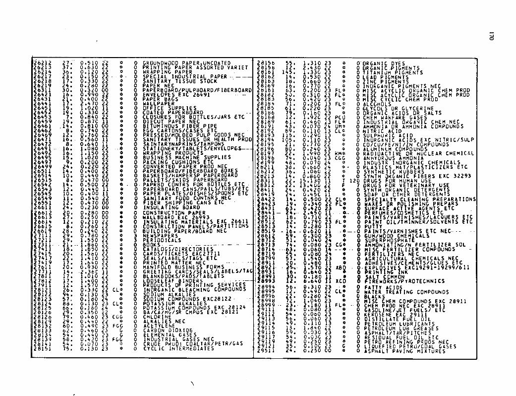
26212 27. 0.510 22 0 GROUNOW000 PAPER,UNCOATEO 28156 55. 1.310 23 4 ODROANIC DYES 26213 37. 0.630 22 4 0 PRINTING PAPER ASSORTED VARIET 2815o 12. 2.430 22 4 0 ORGANIC PIGMENTS 26214 36. 0.120 22 0 WRAPPING PAPER 28161 145. 1.330 23 4 0 TITANIUM P1G1ENTS 26217 23. 0.150 22 - 4- 0 SPECIAL INDUSTRIAL PAPER ----- 28162 14. 0.530 22 0 0 LEAD PIGMENTS 26218 17. 0.330 22 4 0 SANITARY TISSUE STOCK 28163 18. 0.6oO 22 0 ZINC PIGMENTS 26219 24. 0.280 22 4 0 PAPER NEC 28169 16. 0.770 22 4 0 INORGANIC PIGMENTS NEC 26311 30. 0.320 00 0 PAPERBOARD/PULP80ARD/FIBERBOARD 26161 63. 0.200 23 FL* 0 MISC ACYCLIC ORGANIC CHEM PROD 26421 26431
16. 21.
0.990 0.400
22 22
4 4
0 0
ENVELOPES EXC 26491 -
PAPER bAGS 28182 28183
50. 0.310 23 FL 0 MISC ACYCLIC ORGANIC CHEM PROD
26441 17. 2.470 22 4 0 WALLPAPER 28184 56. 71.
0.420 0.20C
23 13 FL3
0 0 MSC CYCLIC CHEM PROD ALC(HOL$
26451 19. 1.020 11 4 0 OFFICE SUPPLIES 28185 61. 0.220 23 4 0 GLYCOLS OR GLYCERINE 26452 19. 0.330 22 4 0 COATED PAPERBORD -- 2816 79. 0.iC 23 4 0 ORGANIC ACIDS OR SALTS 26453 7. 0.840 22 4 0 CLOSURES FOR BOTTLES/JARS ETC 26168 12. 1.92C 22 PCi) 0 CHEM WARFARE GASES 26459 19. 0.87C 11 0 0 DIECUT PAPER NEC 28169 61. 0.460 23 FL* 0 INDUSTRIAL ORGANIC CHEM NEC 26461 .14. 0.810 00 * 0 BITUMINOUS FIBER PIPE 26191 43. 0.070 24 UM3 0 AMMONIA OR AMMONIA COMPOUNDS 26462 8. 0.740 22 4 0 EGG CARTONS/CASES ETC 28192 89. 0.110 13 CL 0 NITRIC ACID 26469 12. 0.760 22 * 0 PRESSED/MOLDED PULP GOODS NEC 8193 115. 0.290 13 0 SULPI-tURIC ACID 26471 16. 0.560 11 * 0 SANITARY TISSUES OR HEALTH PROD 28194 105. 0.110 23 3 0 INORGANIC ACIDS EXC NITRIC/SULP 26472 8. 0.640 11 4 0 SAINTARYNAPKINS/TAMPONS i28195 21. 0.770 22 3 0 CO/CU/FE/NI/ZN COMPOUNDS 26491 .. 16. 1.080 22 4 0 STATIONERY/TABLETS/ENVELOP&-S----- ..8196 80. 0.240 23 3 0 ALUMINUM COMPOUNDS 2649 16. 1.150 22 4 0 WRAPPING PRODUCTS 28197 22. 1.990 22 RM3 0 RADIOACTIVE OR NUCLEAR CHEMICAl 26495 15. 1.020 22 * 0 BUSINESS MACHINE SUPPLIES 28198 74. 0.040 23 COG 0 ANHYDROUS AMMONIA 26497 9. 0.200 22 0 0 PACKING CUSHiONS ETC 28199 48. 0.070 24 3 0 1NDUSTR INORGANIC CHEMICALS 26499 24. 0.220 22 * 0 CONVERTED PAPER PROD NEC 28211 38. 0.660 24 4 0 PLASTICS MAT/PLASTICIZERS ETC 26511 14. 0.400 22 * 0 PAPERBOARD/FIBERBOARD BOXES 28212 36. 1.ObO 22 3 0 SYNTHETIC RUBBERS 26514 10. 0.440 22 0 0 BASKETS/HAMPERSP PAPERBOARD 28213 14. 0.860 22 0 0 SYNTH ORGANIC FiBERS EXC 32293 26515 8. 0.470 00 4 0 PALLETS/SKIDS PAPERBOARD 28311 22. 15.130 11 T 120 DRUGS FOR HUMAN USE 26542 14. 0.500 22 4 - 0 PAPRBD CONTRS FOR B07TES ETC - 28312 22. 13.400 22 F 7 DRUGS FOR VETERINARY USE 26543 12. 0.440 11 4 0 PAPERBOARD CANS/PAILS/lOBS/ETC 28411 24. 0.420 22 0 0 SYNIN ORGANIC DETERGENTS 26545 10, 0.400 11 * 0 PAPER PLATE S/DISHES/SPOONS ETC 28419 24. 0.45C 11 0 0 SOAP OR CTHER DETERGENTS 26549 11. 0.540 22 4 0 SANITARY FOOD CUNTNRS NEC 28422 14. 0.500 22 L* 0 SPECJALTY CLEANING PREPARATIONS 26551 26611
12. 24.
0.470 0.230
00 00
4 4
0 0
FIBER SHIPPING CANS ETC INSULATING BOARD
26423 19. 0.340 22 rL* 0 WAXE R PD' ISPILNO PREPARS
26612 20. 0.280 28431 28441- *• 0.420
2.450 23 0 .....
0 SURFAC ACTIVE AGENTS ETC t
26613 27. 0.250 00 00
* 0
0 0
CONSTRUCTION PAPER WALLBOARD EXC 26993 8511
t4.-- 18. 0.710
11 22 0
0 0
PERFUMES/COSMETICS ETC PAINTS/VARINISHES/LACQUERS ETC
26614 12, 0.210 22 0 0 INSULATING MATERIALS EXC 26611 8512 62. 0.790 23 FL 0 PAINT DIL/TH:NNER/SOLVENTS ETC 26615 8. 0.260 22 4 0 CONSTRUCTION PANELS/PARTITIONS 28513 14. 0.280 11 0 PUTTY 26619 28. 0.240 22 4 0 BUILDING PAPER/BOARD NEC 2851 4A - 16.. -0.620 11 -0--0 PAINTS/VARNISHES ETC NEC...... 27111 29. 0.780 22 0 3 NEWSPAPERS 286 9. 0.300 23 0 0 GUM/WOOD CHEMICALS 27211 29. 1.550 22 4 3 PERIODICALS 287A 1. 0.040 24 * 0 SUPERPHOSPHATt 27311- 21.-- 1.860 22 0 BOOKS - - -- ----- - - - 28713 74. 0.080 23 COO 0 AMMONIATING/N FERTILIZER SOL 27411 18. 1.850 22 * 0 CATALOGS/DIRECTORIES 28714 -63, 0.060 14 --4 - 0 MISC FERTILIZER COMPOUNDS 27415 20. 1.5e0 22 4 0 CARDS/TICKETS EXC27711 28119 55. 0.080 24 * 0 FERTILIZERS NEC 27417 22. 1.410 22 * 0 SEALS/LABELS/TAGS ETC 28799 57. 1.540 23 * 0 AGRICULTURAL CHEMICALS NEC 27419 17. 1.640 22 * 0 - PRINTED MATTER NEC 28911 20. 0.480 11 0 0 ADHESIVES/CEMENTS/GLUES ETC 27611 20. 0.930 22 4 0
------------- MANIFOLD BUSINESS FORMS GREETIPsG CARDS/SEALS/LABELS/TAG
28921- 15-.- 1.570 22 ABO . 0-FXPLOcIVES EXC1929119299/611 27711 14. 2.36C 11 4 0 28931 16. 0.640 22 * 0 RINT!NG INK 27811 27812
17. 17.
1.010 1.400
22 22
4 4
0 0
BLANKBOOKS/PADS/TABL1S BINDERS LOOSELEAF
8991 8993
30. 12.
0.180 1 * 5ALT CCMMON
27911 28121
12. 26.
1.570 0.33C
22 22
0 CL
0 0
PRODUCTS OF PRIwTING SERViCES INORGANIC BLEACHING COMPOUNDS
28994
~ 28996
56. 6.640 0.310
ii 23
XCO * 0
r1REWORKS/PYROTECHNICS FATTY ACIDS
28122 94. 0.130 23 4 0 SODIUM ALKALIES 28995 12.
22. 0.490 0.280
22 24
CL* *
0 0
WATER TREATING COMPOUNDS BLACKS 28123 57, 0.18024 4 0 SODIUM COMPOUNDS EXC28122 28998 72. 1.04023 0 MISC CHEM COMPOUNDS EXC 28911 28124
28125 88. 66.
0.130 0.160
23 4 CL* 0 0 0
POTASSIUM ALKALIES POTASSIUM COMPOUNDS EXC 28124 28999 -- 23. 2.180 ii FL* -: 0 CHEM PROD NEC EXC 28911
28126 29. 0.350 22 4 0 BA/CA/MG/SR CMPUS EXC 28121 29111 29112
48. 54.
0.080 0.ObO
23 23
0 4
0 0
GASOLINE/JET FUELS/ ETC KEROSENE EXC 29111 28126
28129 79. 29.
0.460 0.440
23 22
COG 3
0 0
CHLORINE .
ALKALIES NEC 29113 56. 0.060 23 0 0 DISTILLATE FUEL OIL
28132 60. 0.49C 23 FOG 0 ACETYLENE 29114 29115
49. 13.
0.110 1.840
13 22
* 0
0 0
PETROLEUM LUbRiCANTS PETROLEUM LOb GREASES 26133 b2.
54. O.'.O 0.440
23 23
& G
0 0
CARBON DIOXIDE ELEMENIAL GASES 29116 59. 0.030 23 0 0 ASPHALT/TAR/PITCHES
18134 8139 58. 0.420 23 FOG 0 INDUSTRIAL GASES NEC 29117
29119 54. 49.
0.036 0.250
i3 23
0 8
0 0
RESIDUAL FUEL OIL ETC PETRO REFINING PRODS NEC 28141
28151 54. 75.
0.o70 0.130
€3 23 4
0 0
CRUDE PROD: COALTAR/PETR/GAS CYCLIC INTERMEDIATES 29121 35. 0.I0C 23 0 0 LIQUEFIED PETRI)/COAL GASES
29511 24. 0.250 00 0 0 ASPHALT PAVING MIXTURES
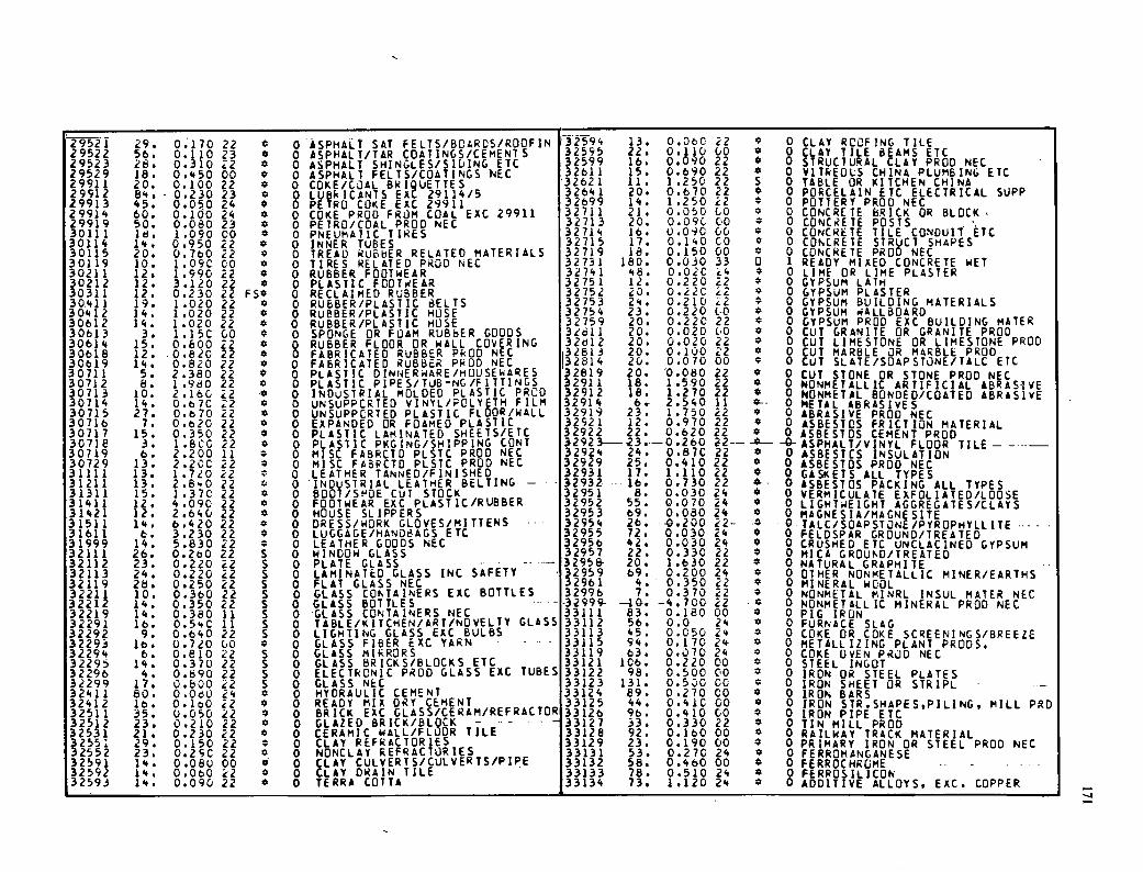
75ii 29. 0.170 22 0 ASPHALT SAT FELTS/BOARDS/ROOFIN 32594 13. 0.080 22 C 0 CLAY RCOFING TILE 29522 56. 0.110 23 C 0 ASPHALT/TAR COATINGS/CEMENTS 32595 22. 0.110 (10 * 0 CLAY TILE BEAMS ETC 29523 26. 0.310 22 0 0 ASPHALT SHINGLES/SI(1ING ETC 32599 16. 0.00 22 0 STRUC1URAL CLAY PROD NEC 29529 18. 0.450 00 * 0 ASPHALT FELTS/COATINGS NEC 32811 15. 0.690 22 0 VITREOLS CHINA PLUMBING ETC 29911 20. 0.100 22 * 0 COKE/COAL BRIQUETTES 32621 11. 1.250 22 S 0 TABLE OR KITCHEN CHINA 29912 84. - 0.230 23 0 0 LUBRICANTS EAC 29114/5 32641 20. 0.670 22 0 0 PORCELAIN ETC ELECTRICAL SUPP 29913 45. 0.050 24 0 0 PETRO COKE EAC 29911 32699 14. 1.250 22 0 POTTERY PROD NEC 29914 60. 0.100 24 0 0 COKE PROD FROM COAL EXC 29911 32711 21. 0.050 00 0 CONCRETE BRICK OR BLOCK 29919 50. 0.080 23 C 0 PETRO/COAL PROD NEC 32713 20. 0.090 00 0 0 CONCRETE POSTS 30111 18. 1.090 CO 0 0 PNEUMATIC TIRES 32714 16. U.090 CC, 0 CONCRETE TILE CONOUFT ETC 30114 14. 0.950 22 0 0 INNER TUBES 32715 17. 0.140 CO 0 CONCRETE STRUC1 SHAPES 30115 20. 0.760 22 0 0 TREAD RUBBER RELATED MATERIALS 32719 18. 0.150 00 0 CONCRETE PROD NEC 30119 10. 1.09C CO 0 0 TIRES RELATED PROD NEC 32731 180. 0.030 33 0 1 READY MiXED CONCRETE WET 30211 12, 1.990 22 0 RUBBER FOOTWEAR 32741 46. 0.C)2C i4 0 LiME OR LIME PLASTER 30212 12. 3.120 22 0 0 PLASTIC FOOTWEAR 32751 12. 0.220 22 0 GYPSUM LATH 30311 12. 0.230 22 F$* C RECLAIMED RUBBER 32752 20. 0.22C 22 0 GYPSUM PLASTER 30411 19. 1.020 22 0 RUBBER/PLASTIC 6ELTS 32753 24. 0.210 22 C 0 GYPSUM BUILDING MATERIALS 30412 14. 1.020 22 C 0 RUBBER/PLASTIC MUSE 32754 23. 0.220 (-0 0 GYPSUM RALLBOARD 30612 14. 1.020 22 0 0 RUBBER/PLASTIC HOSE 32759 20. 0.220 22 0 GYPSUM PROD EXC BUILDING MATER 30613 3. 1.15C 00 0 0 SPONGE OR FOAM RUBBER GOODS 32611 20. 0.020 (0 * 0 CUT GRANITE OR GRANITE PROD 30614 15. 0.800 22 0 0 RUBBER FLOOR OR WALL COVFRING 2d12
32813 20. 20.
0.020 0.100
22 22
0 0
CUT LIMESTONE OR LIMESTONE PROD CUT MARBLE OR MARBLE PROD 30618
30619 14. 12. .0.820
0.820 22 *
* 0 FABRICATED RUBBER PROD NC
FABRICATED RUBBER PROD NEC 32814 20. 0.070 00 0 0 CUT SLATE/SOAPSTONE/TALC ETC 30711 5. 2.380
22 22 *
0 0 PLASTIC DINNERWARE/HOUSEWARES 32819 20. 0.080 22 0 0 CUT STONE OR STONE PROD NEC
30712 8. 1.960 22 0 0 PLASTIC PIPES/TLJBNC/F1TTINGS 32911 18. .5.90 22 C 0 NONMETALLIC ARTIFICIAL ABRASIVE 30713 10. 2.160 22 0 0 INDuSTRIAL MOLDED PLASTIC PROD 32912 18. 1.270 22 C 0 NONMETAL BONDED/COATED ABRASIVE 30714 14. 0.67C 22 * 0 UNSUPPORTED VINYL/POLVETH FILM 32914 6.- 2.540 11 s-- 0 METAL ABRASIVES 30715 27. 0.670 22 C 0 UNSUPPORTED PLASTIC FLOOR/WALL 32919 23. 1 .750 22 0 ABRASIVE PROD NEC 30716 7. 0.820 22 0 0 EXPANDED OR FOAMED PLASTIC 32521 12. 0.970 22 * 0 ASBESTOS FRiCTION MATERIAL 30717 15. 0.350 22 0 PLASTIC LAMINATED SHEETS/ETC 32922 22. 0.620 22 0 0 ASBESTOS CEMENT PROD 30718 3. 1 .8CC i2 0 PLASTIC PKGING/SNIPPING ClINT 32923-23.-0.260 22-- -0--- -0- ASPHALT/VINYL FLOOR TILE - 30719 6. 2.200 11 0 0 MISC FABRCTO PLSTC PROD NEC 32924 24. 0.81C 22 0 0 ASBESTOS INSULATION 30729 13. 2.20C 0 MISC FLBRCTD PLSTC PROD NEC 32929 25. 0.410 22 0 0 ASBESTOS PROD NEC 31111 13. 1.720 .2 0 LEATHER TANNED/FINISHED 32931 17. 1.110 22 0 0 GASKETS ALL TYPES 31211 13. 2.80 22 C 0 INDUSTRIAL LEATHER BELTING - - 3293 .... lb. 0.730 22 *-- 0 ASBESTOS PACKING ALL TYPES 31311 15. 1.370 22 C 0 BOOT/SHOE CUT STOCK 32951 8. 0.030 24 C 0 VERMICULATE EXFOLIATED/LOOSE 31411 12. 4.090 22 0 Q FOOTWEAR EAC PLASTIC/RUBBER 32952 55. 0.070 24 0 0 LIGHTIE1GHT AGGREGATES/CLAYS 31421 12. 2.640 22 C 0 HOUSE SL1PPERS 32953 69. 0.080 24 0 0 MAGNESIA/MAGNE SITE 31511 14. 6.420 22 0 DRESS/WORK GLOVES/MiTTENS - 32954 28. 4.200 2- . 0TALC/SOAPSTONE/PYROPHYLL1TE 31611 6. 3.230 22 0 0 LUGGAGE/HAND8AGS ETC 32955 72. 0.030 24 * 0 FELDSPAR GROUND/TREATED 31999 14. 5.830 22 C 0 LEATHER GOODS NEC 32956 42. 0.030 24 Q 0 CRUSHED ETC UNCLACINED GYPSUM 32111 26. 0.200 22 S 0 WINDOW GLASS 32957 22. 0.330 22 0 0 MICA GROUND/TREATED 32112 23. 0.220 22 5 0 PLATE GLASS ..........- 32958- 20, 1.630 22 0 0 NATURAL GRAPHITE 32113 24. 0.220 22 0 LAMINATED GLASS INC SAFETY 2959 89. 0.200 24 0 0 OTHER NONMETALLIC MINER/EARTHS 32119 28. 0.250 22 S 0 FLAT GLASS NEC 2961 4. 0.350 22 0 0 MINERAL WOOL 32211 10. 0.380 22 S 0 GLASS CONTAINERS EXC BOTTLES 32996 7. 0.370 22 C 0 NONMETAL MINRL INSUL MATER NEC 32212 14. 0.350 22 S 0 GLASS BOTTLES ....- -32999- -14. -4. 00 22 .0 0 NONMETALLIC MINERAL PROD NEC 32219 14. 0.380 11 S 0 -GLASS CONTAINERS NEC 33111 83. 0.180 00 0 0 PIG IRON 32291 16. 0.54C 11 S 0 TABLE/KITCHEN/ART/NOVELTY GLASS 33112 56. 0.0 24 0 0 FURNACE SLAG 32292 9. 0.640 22 S 0 LIGHTING GLASS EXC BULBS 33113 45. 0.050 24 0 0 COKE OR COKE SCREENINGS/BREEZE 32293 lo. 0.720 (,0 0 0 33115 94. 0.170 24 0 0 METALLIZING PLANT PRODS. 32294 6. 0.810 22 S 0 GLASS MIRRORS 33119 63. 0.070 24 C 0 COKE OVEN PROD NEC 32295 14. 0.370 22 5 0 GLASS BRICKS/BLOCKS ETC 33121 106. 0.220 0 C 0 STEEL INGOT 32298 4. 0.690 22 S 0
GLASS FIBER EXC YARN......
ELECTRONIC PROD GLASS EAC TUBES 33122 98. 0.500 CO C 0 IRON OR STEEL PLATES 32299 17. 0.600 2 S 0 GLASS NEC 33123 131. 0.530 00 0 0 IRON SHEET OR STRIPL 32411 60. 0.080 24 0 0 HYDRAULIC CEMENT 33124 89. 0.270 00 * 0 IRON BARS 32412 18. 0.1o0 22 0 0 READY MIX DRY CEMENT 33125 44. 0.41C 00 * 0 IRON SIR.SHAPES,PILING, MILL PRO 32511 35. 0.050 22 0 0 BRICK EAC GLASS/CERAM/REFRACTOR 33126 96. 0.410 CO 0 0 IRON PIPE ETC 32512 23. 0.210 22 0 0 GLAZED BRICK/BLOCK - - -- 33127 33. 0.330 22 * 0 TIN MILL PROD 32531 21. 0.230 22 * 0 CERAMIC WALL/FLOOR TILE 33128 92. 0.160 00 C 0 RAILWAY TRACK MATERIAL 32551 29. 0.150 22 0 0 CLAY REFRACTOR1ES 33129 23. 0.190 00 C 0 PRIMARY IRON OR STEEL PROD NEC 32552 23. 0.29C 22 0 0 NDNCLAY REFRACTURIES 33131 53. 0.270 24 0 0 FERROMLNGANE5( 32591 14. 0.080 00 * 0 CLAY CULVERTS/CULVERTS/PIPE 33132 58. 0.48000 * 0 FERROCHRCME 32592 14. 0.080 2 0 0 CLAY DRAIN TILE 33133 78. 0.510 24 C 0 FERROSILICON 32593 14. 0.090 22 C 0 TERRA COTTA 33134 73. 1.120 24 0 0 ADDITIVE ALLOYS, EAC. COPPER
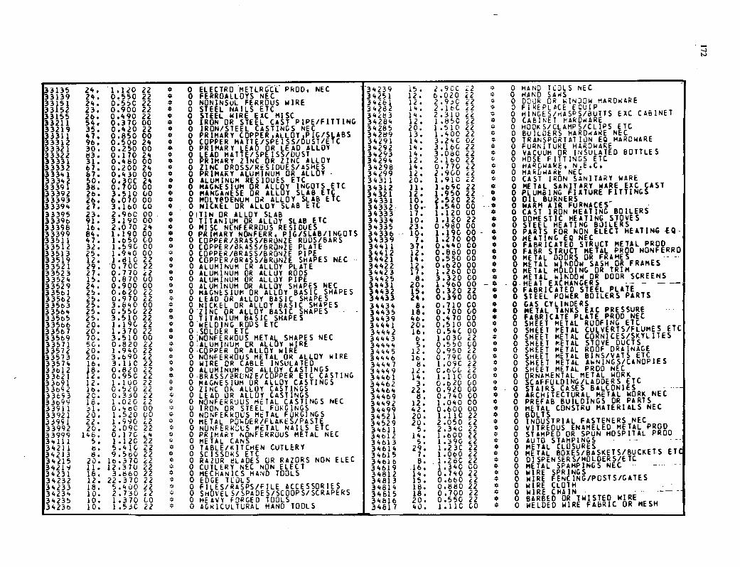
3135 24. 1.120 22 4 0 ELECTRO METLRGCL PROD, NEC 34239 15. 2.9CC .2 0 0 HAND TOOLS NEC 3139 24. 0.550 22 4 0 FERROALLOYS NEC 34251 12. 6.020 22 0 HAND SAWS 3151 24. 0.550 22 4 0 NONINSUL FERROUS WIRE 34261 12. 2.9.0 22 4 0 DOUR OR WINDOW HARDWARE 3152 3155
23. 26.
0.900 0.490
22 22
4 4
0 0
STEEL NAILS ETC STEEL WIRE EXC MISC
34282 34283
14. 14.
2.180 2.310
22 ik
0 0
FIREPLACE ECUIP HINGES/1ASPS/8UTTS EXC CABINET
33211 54, 0.370 00 4 0 IRON OR STEEL CAST PiPE/FITTING 34284 12. 1.850 22 4 0 CABINET HARDWARE 33219 35. 0.420 22 * 0 IRON/STEEL CASTINGS NEC 34265 20. 1.510 22 .. 0 HOOKS/CLAMPS/CLIPS ETC 33311 47. 0.850 00 4
4 0 PRIMARY COPPER ,ALLOY P1G/S,ABS
COPPER HATTE/SPEISS/&JST/EIC 3428'9 34291
13. 14.
1.400 3.24C
22 02
4 4
0 0
BUILDERS HARD.ARE NEC TRANSPORTATION EQ HARDWARE 33312
33321 96. 30.
0.500 0.250
24 00 *
0 0 PRIMARY LEAD OR LEAD ALLOY 34292 14. 3.160 22 4 0 FURNITURE HARDWARE
33322 83. 0.170 24 4 0 LEAD MATTE/SPEISS/DUST 34293 14. 3.080 22 4 0 VACUUM OR IrSULATED BOTTLES 33331 31. 0.480 00 4 0 PRIMARY ZINC OR ZINC ALLOY 34294 12. 2.180 22 4 0 NOSE FITTINGS ETC 33332 67. 0.200 24 4 0 ZINC DROSS/RESIDUES/ASHES 34298 14. 0.770 22 0 HARDWARE, N.E.C. 33341 67. 0.430 00 0 PRIMARY ALUMINUM OR ALLOY - 34299 1. 2.900 22 4 0 HARDWARE NEC 33342 0. N. 0.3CC 24 4 0 ALUMINUM RESiDUES ETC 34311 20. 1.910 2 4 0 CAST IRON SANITARY WARE
CAST 33391 0.700 00 0 4
0 MAGNESIUM OR ALLQY INGOTS ETC SLAB ETC
34312 ii. .69C 22 4 0
0 0
METAL SANITARY WARE ,EXC PLUMBING FUTURE FiTTINGS 33392 26. 3.510 00 0 NANGAHESE OR ALLUY 34321 12. 1.950 22
33393 26. 6,070 00 4 0 MOLYBDENUM OR ALLOY SLAB ETC 34331 10. 2.520 22 4 0 OIL BURNERS 33394 7. 3.160 00 0 0 NICKEL OR ALLOY SLAB ETC 34332 10.- 1.540 00 -0 0 WARM AIR FURNACES 33395 23. 2.960 00 4 0TIN OR ALLOY SLAB 34333 17. 1.120 00
22 4 *
0 0
CAST IRON HEATING BOILERS DOMESTIC HEATING STOVES 33396
33398 91. 16.
3.190 2.070
00 24
0 4
0 0
TITANiUM OR ALLOY SLAB ETC MISC NONFERROUS RESIDUES
34334 34335
.0. 23.
1.120 0.980 00 4 0 STEEL HEATING BOILERS
33399 84. 1.190 00 4 0 PRIMARY NONFERR. PIG/SLAB/INGOTS 34336 .- 10. 1.190 00- * 0 PARTS FOR NON ELECT HEATING -EQ- 33511 47. 1.650 00 4 0 COPPER/3RASS/BRUNZE RODS/BARS 34330 7.
37. 1.210 0.440
00 00
* 4
0 0
HEATiNG EQ NEC FABRICATED STRUCT METAL PROD 33512
33513 32. 25.
1.590 1.940
00 00
0 0
COPPER/BRASS/BRONZE PLATE COPPER/BRASS/BRONZE PiPE
34411 3441 12. 0.860 00 *
* 0 0
FABR STRUCT METAL PROD NONFERRO METAL DOR OR FRAMES -- -. 33519 12. 1.610
0.70C 22 22
4 4
0 0
COPPER/BRASS/BRONZE SHAPES NEC •- 3442 3442
14. 12.
0.550 0.620
00 00 * 0 METAL WINDuW SASH OR FRAMES 33521
33523 29 27. 0.770 i2 0
ALUMINUM CR ALLOY PLATE ALUMINUM OR ALLOY RODS 34423 17. 1.260 00 0 METAL MOLDING OR TRIM
33524 15. 0.870 00 4 0 ALUMINUM OR ALLOY PIPE 34425 8. 3.320 Co 4 0 0-HEA7
METAL WINDOW OR DOOR SCREENS EXCHANGERS -- - - - 33529
33561
0.900 0.620
00 22
4 0 0
ALUMINUM OR ALLOY SHAPES NEC MAGNESIUM OR ALLOY BASIC SHAPES
34431 34432
20. 15.
1.960 0.320
00 22
- *
- 0 FABRICATED STEEL PLATE
33582 25. 0.970 22 4 0 LEAD OR ALLOY BASIC SHAPES 34433 24. 0.390 00 0 0 STEEL POWER BOILERS PARTS 33583 25. 3.640 00 4 0 NICKEL OR ALLOY BASIC SHAPES 34434 8. 0.710 CO 0 0 GAS CYLINDERS 33564 25. 0.550 22 4 0 ZINC OR ALLOY BASIC SHAPES - - 34435 18. 0.700 00 * 0 METAL TANKS EXC PRESSURE 33565 25. 3.510 22 0 TITANIUM BASIC SHAPES 34439 46. 0.410 00 0 0 FABRICATE PLATE PROD NEC 33566 20. 1.190 22 4
4 0 WELDING RODS ETC 34441 20. 0.510 00 4
4 0 0
SHEET METAL ROOFiNG ETC SHEET rETAL CW.YERTS/FLUMES ETC 33567
33569 20. 70.
1.370 3.510
22 00 4
0 0NONFERROUS
SOLDER ETC METAl SHAPES NEC
34442 34443
16. 6.
0.54C 1 .0 30
00 22 4 0 SHEET METAL COKNICES/SKYLIIES
33571 SC. 0.820 22 4 0.ALUMINUM CR ALLOY WIRE 3444 s. 0.550 CO 0 0 SHEET METAL STOVE DUCTS 33572 20. 1.940 22 0 1COPPER OR ALLOY WIRE 34445 12. 0.950 i2 0 SHEET METAL ROOF DRAINAGE 33573 20. 3.690 22 3 0 NONFERROUS METAL OR ALLOY WIRE 34446 18. 0.790 CO 4 0 SHEET METAL BiNS/VATS ETC 33574 16. 3.110 22 0 WIRE OR CABLE INSULATED 34447 8. 1.09C 22 4 0 SHEET METAL AWNINGS/CANOPIES 33612 B. 0.820 22 4 0 ALUMINUM OR ALLOY CASTINGS 349 12. 0.600 22 4 0 SHEET METAL PROD NEC 33621 i2. 0.950 22 4 0 BRASS/8RCNZE/COPPER ETC CASTING 34461 14. 1.110 CO 0 ORNAMENTAL METAL WORK 33891 12. 1.100 22 4 0 MAGNESIUM OR ALLOY CASTINGS 34462 3. O.b20 00 4 0 SCAFFOLDING/LADDERS ETC 33692 lb. 0.520 22 3 0 ZINC OR ALLOY CASTINGS 34464 22. 0.920 00 0 STAIRS CASES BALCONIES 33653 20. 0.330 22 4 0 LEAD OR ALLOY CASTINGS 34469 8. 0.740 00 0 ARCHITECTURAL METAL WORK NEC 33699 18. 1.020 22 4 0 NONFERROUS METAL CASTINGS NEC 34492 12. 1.040 00 0 0 PREFAB BUILDINGS OR PARTS 33911 1. 0.480 00 4 0 IRON OR STEEL FORGINGS 34499 42. 0.600 00 4 0 METAL CONSTRU MATERIALS NEC 33921 20. 1.520 CO 0 NONFERROUS METAL FURCINGS 34521 20. 1.110 22 4 0 BOLTS 33991 22. 1.590 22 0 METAL POhOER/FLAKES/PASTE 34529 20. 2.050 22 4 0 INDUSTRIAL FASTENERS NEC 33992 20. 2.09C 22 4 0 NONFERROUS METAL NAILS ETC 34611 5. 2.340 22 4 0 VITREOUS ENAMELED METAL PROD 33999 146. 0.170 24 4 0 PRIMARY NONFERROUS METAL NEC 34612 14. 1.800 22 4 0 STAMPED OR SPUN HOSPITAL PROD 34111 5. I.12C 22 4 0 METAL CANS 34613 5. 1.390 22 3 0 AUTO STAMP1NGS -- 34211 e. 5.4 IC 22 3 0 TABLE/KITCHEN CUTLERY 34614 29. 1.23C 22 4
4 0 0
METAL CLOSURES BOXES/BASKETS/BUCKETS ETC METAL 34213 8. 9.560 22 0 SCISSORS ETC 34615 7. 1.060 22
34215 20. 16.370 k2 0 RAZOR 8LLDES OR RAZORS NON ELEC 34616 8. 1.28C 22 0 DISPENSERS/HOLDERS/ETC 34219 11. 12.370 22 0 CUTLERY NEC NON ELECT 34619 .16. 1.340 00 * 0 METAL SPAMPINGS NEC - ....... 34231 18. 3.860 22 0 MECHANICS HAND TOOLS 34812 14. 0.740 22
4 0 0
WIRE SPRINGS FENCING/POSTS/GATES WIRE 34232 12. 22.37C 22 3 0 EDGE TOOLS 34813 15. 0.660 22
34233 18. 5.400 22 4 0 FILES/RASPS/FILE ACCESSORIES 34814 18. 0.860 22 4 0 WIRE CLOTH 34234 10. 2.730 22 4 0 SHOVELS/SPADES/SCOOPS/SCRAPERS 34615 18. 0.700 22 3 0 WIRE CHAIN 34235 10. 1.370 CO 0 HEAVY FORGED TOOLS 34616 20. 0.550 22 *
4 0 0
BARBED OR TWISTED WIRE WIRE FABRIC OR MESH WELDED 34238 10. .53C 22 0 AGRICULTURAL HAND TOOLS 34817 40. 1.110 Co
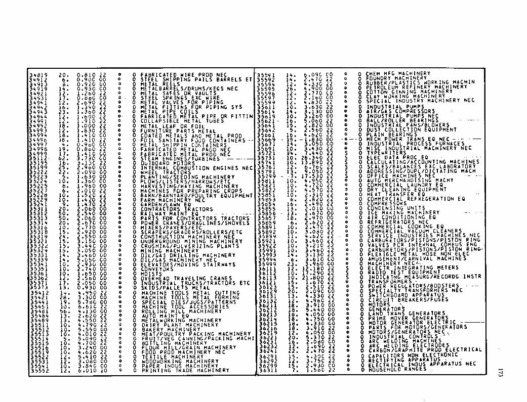
34819 20. 0.810 22 0 0 FABRICATED WIRE PROD NEC 35591 14. 6.096 CO OCHEM MFG MACHINERY 34912 6. 0.900 00 0 STEEL SHIPPING PAILS BARRELS El 35592 14. 2.470 22 0
0 FOUNDRY MACHINERY RUBBER/PLASTiCS WORKING MACHIN 14913 4919
8. 14.
0.920 0.930
00 Co 4
0 0
METAL REELS pIETALBARRELS/DRUM5/KEGS NEC
35594 35595
12. 26.
4.330 4.900
22 CO 0 PETROLEUM REFINERY MACHINERY
34921 12. 1.280 22 0 METAL SAFES OR VAULTS 35596 12. 2.770 00 * 4
0 0
COTTON GINNING MACHINERY CLAY WORKiNG MACHINERY 34531
34941 17. 12.
0.800 2.690
CO 22
4 0
0 0
STEEL SPRiNGS EXC WIRE METAL VALVES FOR PIPING
35.97 35599
12. 12.
2.160 4.830
00 22 0 0 SPECIAL INDUSTRY MACHINERY NEC
34942 16. 1.390 i2 0 0 METAL FITTINS FOR PIPING SYS 35611 10. 3.630 22 0 0 INDUSTRIAL PUMPS 3943 23. 1.380 22 ° 0 METAL PIPE COILS 35614 14. 3.130 00 * 0 AIR/GAS COMPRESSORS 34944 12. 1.800 22 ° 0 FABRICATED METAL PIPE OR FITTIN 35619 10. 3.280 00 * 0 INDUSTRIAL PUMPS NEC 34991 12. 1.910 22 0 COLLAPSIBLE METAL TUBES 35621 - 16.- 5.060 22 * 0 BALL/ROLLER BEARINGS 34992 16. 1.000 22 0 0 METAL LEAF OR FOIL 35641 15. 2.820 00 0 0 INDUSTRIAL FANS/BLOWERS 34993 12. 1.830 22 4 0 FURNITURE PARTS METAL 35642 51 2.560 22 0 0 DuST COLLECTION EQUIPMENT 34994 18. 1.410 CO 0 COATED METALS AND METAL PROD 35681 16. 4.620 22 0 PLAIN BEARINGS 34998 18. 1.410 22 0 FOIL SANITARY FOOD CONTAINERS -- 35669 - 15. -1.830 00 -*--0 NECH POWER TRANS EQ NEC - -- - 34997 .. 0.980 CO 0 METAL SrIIPPIN CONTAINERS 35671 14. 3.050 CO * 0 INDUSTRIAL PROCtSS FURNACES 34998 19. 0.860 22 0 FABRICATED METAL PROD NEC 35891 10. 3.430 22 0 0 MISC INDUSTRIAL MACHINERY NEC 34999 17. 1.4 iC 00 4 0 FABRICATED METAL PROD NEC 3572 1/4. 7.440 22 S 0 TYPEWRITERS 35112 62. 3.730 CO 4- 0 STEAM ENGiNES/TURBiNES . - -- -- 35731 10. 28.340 22 5 0 ELEC DATA PROC EQ -
35195 16. 3.13C 22 0 0 OUTbOARD MOTORS 35741 10. 13.890 22 S 0 CALCULATING/ACCOUNTING MACHINES 35199 25. 2.980 CO * 0 INTERNAL COM8USTION ENGINES NEC 35761 12. 6.78C 22 S 0 SCALES/BALANCES EXC LABORATORY 35222 22. 2.090 00 4 0 WHEEL TRACTORS 35791 13. 9.050 22 S 0 ADDRESSING/DUPL/OICTATING MACH 35223 5. 1.630 00 * 0 PLANTING/SEEDING MACHINERY 3579 - - 17.530 22 S 0 OFFICE MACHINES NEC 35224 10. 1.380 00 0 PLOWS/LISTERS/NARROWS/ETC 35811 10. 4.950 22 C 0 AUTO MERCHANDISING MACMY 35225 8. 1.960 00 4 0 HARVESTING/HAYING MACHINERY 35621 10. 4.720 22 4 0 COMMERCIAL LAUNDRY EQ 5227 6. 2.010 22 0 MACHINES FOR PREPARING CROPS 35822 10. 4.570 22 0 DRY CLEANING EQUIPMENT
35228 10. 1.520 i2 0 BARN/BARNYARD/POULTRY EQUIPMENT 35851 10. 2.310 22 0 HEAT TRANSFER EQ 35229 10. 1.420 22 4 0 FARM MACHINERY NEC 35853 6. 2.820 22 0 COMMERCIAL REFREGERATION EQ 35241 9. 1.470 22 4 0 GARDEN/LAWN EQ 35854 16. 2.490 22 4 0 COMPRESSORS 35311 20. 2.060 00 * 0 CONTRACTORS TRACTORS 35855 13. 2.010 0-0 0 CQN0ENSING UNITS 35312 50. 2.540 00 * 0 RAILWAY MAINT EQ •. - ....--. 35856 - 13. 2.670 00 0 IcE MAKING MACHINERY -- . - 35313 50. 2.060 00 4 0 PARTS FOR CONTRACTORS TRACTORS 35857 18. 2.970 00 0 AiR CONDiTIONING EQ 35314 20. 2.676 CO 4 0 POWER CRANES/DRAGLINES/SHOVELS 35859 6. 2.620 22 0 REFRIGERATORS NEC 35316 10. 2.770 00 0 MIXERS/PAyERS/ETC 35891 10. 2.47C22 4 0 COMMERCIAL COOKING EQ 35318 15. 2.920 00 0 $CRAPERS/GRAOERS/ROLLERS/ETC 35892 10. 3.080 22 0 COMMERCIAL VACUUM CLEANERS 35319 24. 2.550 00 0 CONSTRUCTION MACHINERY NEC 35899 11. 4.620 Z2 . 0 SERViCE INDUSTRIES MACHINES NEC 35321 15. 3.150 00 ° 0 UNDERGROUND MINiNG MACHINERY 35921 10. 3.460 22 0 0 CARBURETURS/PISTONS/P1STON RING 35322 15. 3.44C 00 4 0 CRUSHING/PULVERIZING PLANTS 35922 10. 3.210 22 C 0 VALVES FCR INTERNAL COMBOS ENG 35329 15. 3.050 GD 0 0 MINING MACHINERY 35991 10. 3.480 22 0 0 CARBURETORS/PISTONS/P1STON RING- 35331 14. 3.460 00 0 OIL/GAS DRILLING MACHINERY 35993 14. 3.130 22 4 0 FLEXIBLE METAL HOSE NON ELEC 35339 14. 5.050 CO 0 OIL/GAS MACMINE.Y NEC 5994 6. 3.610 CO 0 0 AMUSEMENT/CARNIVAL MACHINES 3534 10. 2.930 00 0 ELEVATORS/MOVING STAiRWAYS 5999 23. 3.960 00 4 0 MACHINERY NECL-- 35351 10. 2.740 00 0 CONVEYORS 36111 12. 12.180 22 S 0 ELECTR INTEGRATING METERS 35361 10. 1.650 00 4 0 HOISTS 36112 10. 17.290 22 S 0 RADID TEST EQUIPMENT 35382 12. 2.560 00 4 0 OVERHEAD TRAVELING CRANES 36113 10. 21.800 22 5 0 INDICATNG HEASURG/RECDRDG INSTR 35371 17. 2.050 00 4
4 0 INDUSTRIAL TRUCKS/TRACTORS ETC 36121
36123 15. 15.
1.670 2.510
22 22
* C
0 0
TRANSFORMERS - POWER REGULATORS/BOOSTERS - 35373 13. 0.930 00
0 0 SKIDS/PALLETS METAL
36129 20. 2.090 00 4 0 SPECIALTY TRANSFORMERS NEC 35412 35421
1. 28.
4.950 3.300
22CO 4
0 0
MACHINE TOOLS METAL CUTTING MACHINE TOOLS METAL FORMING 36131 13. 4.330 22 0 0 SWITCHBOARD APPARATUS
35441 19. 5.780 00 4 0 SPECIAL DIES/JUGS/PATTERNS 36132 12. 4.980 22 0 0 CIRCIjI1 BREAKERS/FUSES
35451 10. 6.61C 22 4 0 MACHINE TOOL ACCESSORIES 36211 36212
18. 18.
3.910 5.440
00 00
0 4
0 0
MOTORS GENLRATOR 35481
35484 56. 13.
4.130 2.620
00 22
4 4
0 0
ROLLING MILL MACHINERY AUTO MAINT EQ 36213 18. 4.050 00 4 0 LAND TRANS GENERATORS
35489 13. 4.550 22 0 0 METALWORKING MACHINERY 36214 36215
18. 18.
4.750 4.330
00 CD
* 0
0 0
PRIME MOVER GENERATORS MOTOR GENERATOR ELECTRIC 35511
35512 10. 10.
4.790 5.550
22 00
0 0
DAIRY PLANT MACHINERY BAKERY MACHINERY 36218 18. 3.910 22 C 0 PARTS FOR MOTORS/GENERATORS
35513 10. 4.010 22 4 0 MEAT/POULTRY PACKING MACHINERY 36219 36221
12. 20.
4.050 5.370
00 22
0 0 0
MOTORS/GENERATORS NEC.. INDUSTRIAL CONTROLS- 35514
35515 5.
10. 5.090 4.700
22 22 4
0 0
FRUIT/VEG CANNING/PACKING MACHI BOTTLING MACHINERY 36231 16. 2.080 60 0 0 ARC WELDING MACHINES
35516 10. 3.240 00 0 0 FLOUR MILL/GRAIN MACHINERY 38232 36241
12. 22.
1.690 2.470
22 22
4 *
0 0
ARC WELDING ELECTRODES CARBON/GRAPHITE PROD ELECTRICAL 35519
35522 10. 12.
4.620 5.410
22 22 4
0 0
FOOD PROD MACHINERY NEC TEXTILE MACHINERY 36291 15. 4.30C 22 0 0 CAPACiTORS NON Et.ECTRONIC
35531 12. 3.080 CO 4 0 WOOD4ORK1NG MACHINERY 36292 12. 3.756 22 * 0 RECTIFflNG APPARATUS - INDUS APPARATUS NEC 35541 10. 3.840 CO 0 PAPER INDUS MACHINERY 38299 15. 2.930 CO 0 0 ELECTRICAL
35552 12. 6.010 20 0 PRINTING TRADE MACHINERY 36311 7. 1.580 22 0 0 HOUSEHOLD RANGES -
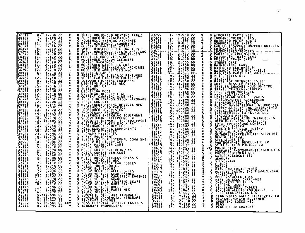
361 8.' 1 .2.30 22 0 0 SMALL HOUSEHOLD HEATING APPLI 37299 4. 19.56C 22 0 0 AIRCRAFT PARTS NEC 36321 7. 1.650 22 0 0 HOUSEHOLD REFRIGERATORS 37321 2. 1.420 00 * 0 INBOARD MOTOR BOATS 36331 9. 1.71C 22 4 0 HOUSEHOLD WASHING MACHINES 3722 -- 2-.-1.35C 22 * 0 OUTBOARD MOTOR BOATS 36332 12. 1.650 22 4 0 OTHER HOUSEHOLD LAUNDRY EQ 37323 10. 0.880 00 0 NONPROPELLED SHIPS 36341 11. 1.340 22 ° 0 ELECTRIC FANS EXC ATTIC 37324 10. 0.810 00 * 0 CAR FLOATS/PONTOON/PORT BRIDGES 36343 8. 1.230 22 * 0 SMALL HOUSEHOLD HEATING APPLI 37329 12. 1.430 22 * 0 SHIPS/BOATS NEC 38346 13. 1.420 22 4 0 SMALL HOUSEHOLD ELECTR APPLIANC 37411---36.-1.450 00- -*--__0LOCOMO1IVES/TENDERS - 36347 10. 2.970 22 4 0 PERSONAL ELECTRIC APPLIANCES 37
37421 23. 2.720 00 *
* 0 PARTS FQR LOCOMOTIVES
36349 11. .700 22 4 0 ELECTRIC HOUSEWANES NEC 37422
10. 10.
3.080 0.670 I
413 00 00 0
0 0 PASENGtR TRAIN CARS
36351 14. .770 22 4. 0 HOUSEHOLD VACUUM CLEANERS FREGHT TRAIN CARS 36361 12. 3.640 22 8 0 SEWiNG MACHINES - - 37423 10. 2e000 CD * 0 STREET CARS 36392 11. 2.020 22 4 0 HOUSEHOLD WATER HEATERS 37424 15.. 1.450 00 0 MAINTENANCE CARS 36393 13. 3.240 22 4 0 HOUSEHOLD DISHWASHING MACHINES 37426 25. 0.450 00 0 0 RAILROAD CAR WHEELS 36399 12. 2.430 22 S 0 HOUSEHOLD APPLIANCES NEC 37428 22. 2.540 00 * 0 RAILROAD PARTS EXC WHEELS 36411 36421
3.070 2.330
22 22
4 0 0
ELECTRIC LAMPS .RESIOErT1AL ELECTRIC FIXTURES
.37429 3j -0.0-- 00-- * 4
0-RAILROAD PARTS EXC WHEELS ---- - 37511 5. 3.05C 22 0 MOTORCYCLES ETC
36424 12. 1.740 i2 ° 0 VEHICULAR LIGHTING EQUIPMENT 37512 6. 1.420 22 0 0 BICYCLES 36425 8. 1.240 22 0 OUTDOOR LIGHTING EQUIPMENT 37513 10. 2.350 22 0 0 PARTS FOR MOTORCYCLES ETC 36429 8. 2.650 22 4 0 LIGHTING FIXTURES NEC 37691 16r 13.960 00 * 0 GUIDED MISSILE PARTS ETC 36432 15. 1.810 11 0 0 POWER OUTLETS 37911 4. 1.280 00 0 0 TRAILER COACHES HOUSING TYPE 36433 12. 1 .880 11 0 0 SWITCHES 37912 4. 1.390 00 0 TRAVEL TRAILERS/CAMPERS 36434 12. 1 .280 22 8 0 LIGHTNING RODS 37992 10. 1.160 00 4 0 HORSEDRAWN VEHICLES 36435 12. 1 .540 00 8 0 OVERHEAD TROLLEY LINE 37993 10. . .170 00 * 0 HAND CARTS/WAGONS 36439 10. 1.670 22 8 0 CURRENT CARRYING WIRE NEC 37994 14. 1.270 22 4 0 HORSEDRAWN VEHICLE PARTS 36441 34. 1 .350 CO 0 0 POLE LINE/TRANSMISSION HARDWARE 37995 4. 1.190 22 4 0 SLEIGHS/SLEDS HORSEDRAWN 136442 12. 1 .200 22 0 ELECT CONDUIT 37999 10. 2.300 22 0 0 IRANSPORTAT ION EQ NEC 36449 12. 1.140 22 0 NONCURRENT WIR 190 DEVICES NEC 38111 4. 6.000 22 S 0 FLIGHT NAVIGATIONAL INSTRUMENTS
136511 10. 3.03C 22 S 0 HOUSEHCLC/AUTO RADIOS 38112 5. 20.000 22 4 0 SURVEY ING/DRAF TING INSTRUMENTS 36512 13. 3.220 22 S 0 HOUSEHOLD TEVEVISION 38113 8. 60.000 22 S 0 LAB/SCIENTIFIC INSTRUMENTS 36521 12. 1.510 22 8 0 PHONOGRAPH RECORDS 38119 5. 60.000 22 S. 0 ENGiNEERiNG/LAB INSTRU NEC 36611 12. .11.170 Co 8 0 TELEPHONE SWITCHING EQUIPMENT 38212 12. 4.000 22 S 0 GAS/WATER METERS 36612 10. 9.070 22 S 0 NUNSWITCHING TELEPHONE EQ 38213 4. 30.000 22 S 0 WEATHER MEASURiNG INSTRUMENTS 36621 12. 16.680 CO 4 0 RADIO/TV TRANSMITTING EQUIPMENT 38219 6. 30.000 22 S 0 MECH MEASLRING INSTRU NEC 36711 10. 5.510 22 S 0 ELECTRONIC TUBES EXC X RAY 38221 10. 30.000 22 S 0 AUTO TEMPERATURE CONTROLS 36741 10. 0.240 22 4 0 SEMICONDUCTOR DEVICES - 38311 4. 17.600 22 S 0 OPTICAL INSTRU 3679' 12. 3.030 22 4 0 MISC ELECTRONIC COMPONENTS 38411 6. 22.480 22 0 SURGICAL/MEDICAL INSTRU 36911 30. 0.990 22 8 o STORAGE BATTERIES 38412 6. 4.500 22 0 HOSPiTAL FURNITURE 3b921 23. 1.690 22 0 PRIMARY BATTERIES 38421 8. 16.080 22 4 0 ORTHCPEDIC/PRO5TjIETIC SUPPLIES 36931 6. 11.570 22 4 0 X RAY EQUIPMENT 38431 10. 14.62C 22 4 0 DENTAL INSTRU 3694 17. 2.950 22 4 0 ELECTR EQ FUR INTERNAL COMB ENG 38511 21.130 22 4 0 SPECTACLES ETC 3699 10. 2.060 22 4 0 ELECTR MACHINERY NEC 38612 12.570 22 0 PHOTOGRAPHIC DEVELOPING EQ 37111 6. l.qOO 00 4 0 MOTOR PASSENGER CARS 38613 9. 14.170 22 S 0 cTILL/HOT ION PICTURE EQ 37112 5. 1.210 00 0 MOTOR TRUCKS 38615 16. 5.900 22 S 140 HOTO FILM 37113 3. 2.890 00 4 0 MOTOR COACHES/F IRETRUCKS 38618 12. 0.770 22 0 0 PREPARED PHOTOGRAPHIC CHEMICALS 371 8. .250 00 4 0 MOTOR COMBAT VEHICLES 38619 12. 10.110 22 S 0 PHOTO EQUIPMENT NEC 37115 5. 1.460 00 8 0 AUTO Cl-ASSIS 38711 6. 9.29C 22 S 0 wATCHES/CLOCKS ETC 37116 3. 1.260 00 8 0 MOTOR BUSSES/TRUCKS CHASSIS 39111 13. 42 .460 22 0 0 JEWELRY 37119 7. 1.480 00 4 0 MOTOR VEHICLES NEC 39141 13. 13.500 22 0 SILVERWARE 37121 7. .110 00 0 PASSENGER MOTOR CAR BODIES 39311 6. 5.73022 S 0 PIANOS 37131 5. 1.040 00 8 0 MOTOR TRUCK BODIES 39312 6. 6.120 22 S 0 ORGANS 37132 3. 0.65C 00 4 0 MOTOR BUS BODIES 39313 5. 7.030 22 4 0 PIANO OR CRGAN PARTS 37142 7. 2.090 22 8 0 MOTOR VEHICLE ACCESSORIES 39319 4. 6.060 22 S 0 MUSICAL INSTRU EXC PIANO/ORGAN 37143 10. 0.650 00 8 0 MOTOR VEHICLE GEAR FRAMES 39411 15. 2.580 11 0 GAMES/TOYS 37144 23. 1.100 00 8 0 MOTOR VEH INT CObUST ION ENGINES 39421 3. 2.740 22 4 0 DOLlS/STUFFED TOYS 37145 31. 0.970 22 8 0 MOTOR VEHICLE BRAKES 39431 6. 1.340 22 8 0 BABY OR DOLL CARRIAGES 37146 23. 1.250 00 8 0 MOTOR VEHICLE STEERING GEARS 39439 10. 1.020 22 ° 0 CHILORENS VEHICLES 37147 8. 1.110 00 0 0 MOTOR VEHICLE BUOY PARTS 39491 5. 4.750 22 4 0 FIShING TACKLE 37148 11. 0.550 22 8 0 MOTOR VEHICLE WHEELS 39492 8. 1.170 22 * 0 BILLIARD/POOL TABLES 37149 17. 1.580 22 8 0 MOTOR VEHICLE PARTS NEC 39493 13. 0.9o0 i2 4 0 BOWLING ALLEYS AND BALLS 37151 4. 0.970 00 0 0 TRUCK TRAILERS 39494 8. 5.400 22 0 0 GOLF CLUbS/BALLS ETC 37211 5.511.60 CO 4 0 COMPLETE MILITARY AIRCRAFT 39496 4. 4.100 22 * 0 TENNIS/BASESALL/CRICKET/ETC EQ 37213 5. 48.850 00 0 COMPLETE COMMERCIAL AIRCRAFT 39497 8. 1.600 22 4 0 PLAYGROUND/GYM EQUIPMENT 37221 5. 23.640 22 4 0 AIRCRAFT ENGINES 39499 7. 2.03C 22 * 0 SPORTIKc. &OCDS NEC 37224 4. 56.500 CO XB4 0 MISSILE/SPACE VEHICLE ENGINES 39511 . 5. 9.760 22 0 0 PENS 37231 6. 21.790 22 * 0 AIRCRAFT PROPELLERS 39521 14. 4.200 22 8 0 PENCILS OR CRAYONS
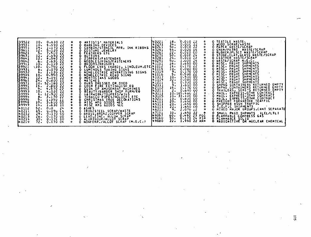
39522 10. 0.630 22 * 0 ARTISTS' MATERIALS 40221 18. 0.010 22 C 0 TEXTILE WASTE. 39531 10. 4.490 22 C 0 MARkING DEVICES 4031 34. 0.010 22 C
C 0 wOOD SCRAPWATE PAPER WASIt/S,..RAP 39551
39611 14. 12.
1.170 22 C C
0 CARBON/STENCIL PPR, INK RIBBNS 4041 40251
..0. 54.
0.010 0.020
22 04 C
0 0 CHEM/PETRO WASTE/SCRAP
39621 5. 5.120 7.510
22 22 *
a 0
COSTUME JEWELRY FEATHERS ETC 40261 22. 0.010 00 0 RUBBER/PLSCT WASTE/SCRAP
39631 12. 2.650 22 C 0 BUTTONS 40271 50. 0.010 24 C 0 STONE.CLAY,GLASS WASTE/SCRAP 39661 12. 4.540 22 C 0 ZIPPERS/FASTENERS 40281 24. 0.010 22 C 0 LEATHER WASTE/SCRAP 39642 6.. 2.630 22 * 0 NEEDLES/PINS/FASTENERS 40291 50. 1.000 24 C 0 WASTE/SCRAP N.E.C. 39911 10. 3.110 22 C 0 BROOMS/BRUSHES 41111 26. 1.650 00 C 0 MISC. FRGHT SHPMENTS 39921 '.10. 0.750 22 4 0 FLOOR CVRS (HARD) LINOLEUM,ETC 41112 14. 0.170 22 C 0 MISC. FRGHT SHPMENTS 39931 6. 2.070 22 4 0 LUPIINOLS TUbING SIGNS 41114 10. 0.080 00 C 0 MISC. FRGHT SHPMENTS 39932 4. 1.130 22 C 0 NONELECTR1C AOVERSISING SIGNS 41115 0.170 Co C 0 MISC. FRGHT SHPMENTS 39934 10. 0.950 22 C 0 NONELECTRIC ROAD SIGNS 41116 5. 0.500 22 4 0 MISC. FRGHT SHPMENTS 39941 12. 4.05C 22 4 0 MORTICIANS GOODS 41117 0.500 00 C 0 MISC. FRGHT SHPMENTS - 39961 24. 0.00 11 4 0 MATCHES 41119 32. 0.080 00 C 0 MISC. FRGHT SHPMENTS 39971 10. 52.180 22 C 0 FURS DRESSED DR DYED 4.211
42111 5. 9.
0.330 1.6C
00 00
C C
0 0
MISC. FRGHT SHPMENTS SHPNO CONTAINERS RETURNED EMPTY 39991
39992 14. 5.
2.840 4.570
22 22
4 4
0 0
CHEM FIRE EXTINGUiSH EQ COIN OP AMUSEMENT MACHINES 42112 15. 0.170 00 4 0 SHPNG CONTAiNERS RETURNED EMPTY
39993 10. 4.02C 22 C 0 BEAUTY/BARBER SHOP FURN/EQ 4 2211 2. 0.690 00 4 0 TRAILERS, SEMI'S RETURNED EMPTY 39994 4. 12.900 22 4 0 hAIRWORK/TOUPEES/WIGS 43111
43115 10.165.4o0 10. 33.1OC
22 00
C 4
0 0
MAiL, EXPRESS,DTHR CONTRACT MAIL, EXPRESS,OTNR CONTRACT 39995
39996 8. 5.
3.170 1.350
22 11
C C
0 0
TOBACCO PIPES/HOLDERS ETC CHRiSTMAS TRE DECOkATIONS 43211 10. 0.0 CO 4 0 MAI 1 EXPRESS,OTHR CONTRACT
39998 10. 3.610 00 C 0 MISC MFG GOODS NEC 4411 45111
20. 20.
I.00 1.650
00 00
4 C
0 0 FkEMT FORWARDER TRAFFIC SHIPPER ASSN TRAFFiC 39999 14. 1.630 11 4 0 MISC PIFO GOODS NLC 4611 20. 1.650 00 C 0 T.O.F.0 SHiPMENTS 40112
40211 52. 65.
0.0 0.090
24 C'.
C C
0 0
ASHES IRON/STEEL SCRAP/WASTE 46211 9. 2.070 i2 4 0 MIXED MAJOR GROUPS,CANT SEPARATE
40212 29. 0.170 00 C 0 bRASS,8RONZ,COPPER SCRAP 4711 10. 1.650 22 4 0 SMALL PKGD SHPMNTS (LCL/LTL) 40213 28.
30. 0.170 00
GO 4 C
0 LEADZ INC. ALLUW SCRAP SCRAP ALUPUNIUPI/ALLOY
49057 49160
60. 50.
0.490 0.170
23 24
FOG FS*
0 0
FLAMMABLE COMPRESS GAS FLAMMABLE SOLID 40214
40219 72. 0.17C 0.170 04 C
0 0 NONFERR./ALLOY SCRAP (N.E.C.) 49880 22. 1.990 22 KMC 0 RADiOACTIVE OR NUCLEAR CHEMICAL
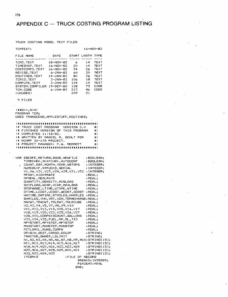
176
APPENDIX C - TRUCK COSTING PROGRAM LISTING
TRUCK COSTING MODEL TEXT FILES
TCMTEXT: 16-NOV-82
FILE NAME DATE START LNGTH TYPE
TCM3.TEXT 18-NOV-82 6 14 TEXT TIMESHIP.TEXT 16-NOV-82 20 14 TEXT COSTCOMP3. TEXT 16-NOV-82 34 26 TEXT REVISE.TEXT 6-JAN-83 60 20 TEXT ROUTINES.TEXT 14-JAN-83 80 26 TEXT TCMIO. TEXT 3-JAN-83 106 18 TEXT COMPUTE.TEXT 3-JAN-83 124 14 TEXT SYSTEM. COMPILER 19-SEP-80 138 75 CODE TCM.CODE 6-JAN-83 213 46 CODE UNUSED> 259 21
9 FILES
(*SS-4-+, N+*) PROGRAM TCM; USES TRANSCEND, APPLESTUFF, ROUTINES;
(* TRUCK COST PROGRAM VERSION 3.0 *) (* FINISHED VERSION OF THIS PROGRAM *) (* COMPLETED 11/18/82. (* 1JRITTEN BY DANIEL R. GEALT FOR (* NCHRP 20-17A PROJECT. (* PROJECT MANAGER: F.W. MEMMOTT
VAR ESCAPE.RETURN, DONE. NEWFILE :BOOLEAN; TIMECHEK, SHIPCHEK. AUTOCOMP : BOOLEAN; COUNT,DAY,MONTH.YEAR.NSTOPS : INTEGER; NJMEOUIP, NTRUCKS. SERIAL : INTEGER; V1,V6,V21,V23.V24,,V29,V31,V32 :INTEGER; MPDAY, NIGHTRATE :REAL; MPMEAL, MEALRATE :REAL; QUANTITY,DENSITY,AVGLOAD :REAL; SHIPLOAD. WCAP. VCAP, MAXLOAD : REAL; STOPWAGE, LTIME, UTIME, WTIME :REAL-, OTIME, LCOST. UCOST, WCOST. OCOST :REAL; HHTIME,DHTIME,RTMILES,HHMILES :REAL; OHM ILES. VHH, VRT. VDH, TERMCHARGE: REAL; MAXWT, TRACWT, TRLRWT, TRLRCUBE :REAL; V2,V3,V4,V5,V7,V8,V9,V10 :REAL; V11.V12,V13,V14,V15,V16,V17 :REAL; V18, V19. V20. V22, V25. V26, V27 : REAL; V28, V30, CORPDISCOUNT, GALLONS :REAL; V33,V34,V35,FIJEL,MR.ML,TX3 :REAL; MFYSTART, MPYSTEP, MPYSTOP :REAL; MHHSTART, MHHSTEP, MHHSTOP -REAL; PCTLDMIL, RUNS, COMPS REAL; ORIGIN, DEST, CARGO, EQUIP : STRING; TRACTOR,OWNER,LDLIMIT :STRING; Ni, N2, N3, N4, N5, N6. N7, NB, N9, N10: STRINGE 15]; Nil ,N12, N13, Ni4, N15, N16, N17 STRINGE 15]; N18.N19,N20,N21,N22,N23,N24 :STRINGEIS]; N25,N26,N27,N28,N29,N30,N3i :STRINGE151; N32.N33.N34,N35 :STRINGCISJ; ITCBRKS :FILE OF RECORD
BREAKS: INTEGER; PERCENT: REAL END;
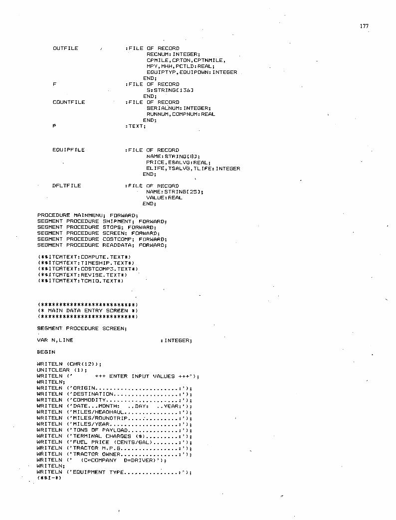
177
OUTFILE I :FILE OF RECORD RECNUM: INTEGER; CPMILECP.TON.CPTNMILE, MPY, MHH. PCTLD: REAL; EQUIPTYP,EQUIPOWN: INTEGER
END; F :FILE OF RECORD
5: STRING[ 136] END;
COUNTFILE :FILE OF RECORD SERIALNUM: INTEGER; RUNNUM, COMPNUM: REAL
END; P :TEXT;
EOUIPFILE :FILE OF RECORD NAME: STRINGCE3]; PRICE, ESALVG: REAL; ELIFE, TSALVG, TLIFE: INTEGER
END;
DFLTFILE :FILE OF RECORD NAME:STRINGC251; VALUE: REAL
END;
PROCEDURE MAINMENU; FORWARD; SEGMENT PROCEDURE SHIPMENT; FORWARD; SEGMENT PROCEDURE STOPS; FORWARD; SEGMENT PROCEDURE SCREEN; FORWARD; SEGMENT PROCEDURE COSTCOMP; FORWARD; SEGMENT PROCEDURE READDATA; FORWARD;
(*$ITCMTEXT: COMPUTE. TEXT*) (*$ITCMTEXT:TIMESHIP. TEXT*). (*$ITCMTEXT: COSTCOMP3. TEXT*) (*$ITCMTEXT:REVISETEXT*) (*$ITCMTEXT:TCMIO.TEXT*)
(* MAIN DATA ENTRY SCREEN *)
SEGMENT PROCEDURE SCREEN;
VAR N,LINE :INTEGER;
BEGIN
WRITELN (CHR(12)); UNITCLEAR (1); WRITELN (' +l-+ ENTER INPUT VALUES +++'); WRITELN; WRITELN ('ORIGIN ....................... WRITELN ('DESTINATION .................. WRITELN ('COMMODITY ..................... WRITELN ('DATE...MONTH: ..DAY: .YEAR:'); WRITELN ('MILES/HEADHAUL ............... WRITELN ('MILES/ROUNDTRIP .............. WRITELN ('MILES/YEAR................... WRITELN ('TONS OF PAYLOAD ............... WRITELN ('TERMINAL CHARGES ($) ......... WRITELN ('FUEL PRICE (CENTS/GAL) ....... WRITELN ('TRACTOR M.P..G ................ WRITELN ('TRACTOR OWNER ................ WRITELN (' (C=C(JMPANY DDRIVER)'); WRITELN; WRITELN ('EQUIPMENT TYPE............... (*$I-*)
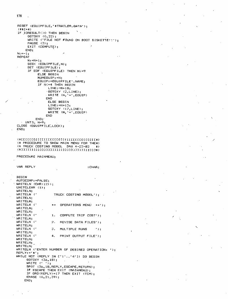
178
RESET (EQUIPFILE. '*TRAILER. DATA');
IF IORESIJLT<>0 THEN BEGIN GOTOXY (0,22); WRITE ('FILE NOT FOUND ON BOOT DISKETTE!!'); PAUSE (3); EXIT (COMPUTE); END;
REPEAT I'J:N+1; SEEK (EOUIFFILE,N); GET (EQUIPFILE); IF EOF (EOUIPFILE) THEN N:9
ELSE BEGIN NUMEQUIP:N; EQUIP: EQUIPFILE'. NAME; IF N<=4 THEN BEGIN
LINE: N+18; GOTOXY (2LINE); WRITE (N,'=',EQUIP)
END /
ELSE BEGIN LINE: N+13; GOTOXY (17,LINE); WRITE (N,'=',EQIJIP)
END END;
UNTIL N9; CLOSE (EQUIPFILELOCK); END;
(*CC [[[[CCC [[[[C [CCC CC[CC[[CC[E[[CCC[C*) (* PROCEDURE TO SHOW MAIN MENU FOR THE*) (* TRUCK COSTING MODEL DRG 4-22-82 *) (*J J ]]JJ JJJJJJJ ]J ]J]JJ ] JJJJ ]J]]33J JJ) ]*)
PROCEDURE MAINMENU;
VAR REPLY : CHAR;
BEGIN AUTOCOMP:FALSE; WRITELN (CHR(12)); UNITCLEAR (1); WRITELN; - WRITELN (' TRUCK COSTING MODEL'); WRITELN; WRITELN; WRITELN C' ++ OPERATIONS MENU 1-+'); WRITELN; WRITELN; WRITELN (' 1. COMPUTE TRIP COST'); WRITELN; WRITELN C' 2. REVISE DATA FILES'); WRITELN; WRITELN C' 3. MULTIPLE RUNS '); WRITELN; WRITELN C' 4. PRINT OUTPUT FILE'); WRITELN; WRITELN; WRITELN; - WRITELN ('ENTER NUMBER OF DESIRED OPERATION: REPLY:='*'; WHILE NOT (REPLY IN ['1'.. '4']) DO BEGIN
GOTOXY (36,18); - WRITE (' '); SPOT (36, 18,REPLY,ESCAPE,RETURN); IF ESCAPE THEN EXIT (MAINMENU); IF ORD(REPLY)=17 THEN EXIT (TCM); ERASE (0.21,39);
END;
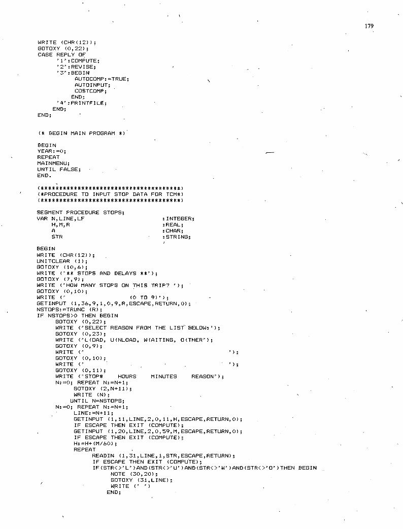
WRITE (CHR(12)); GOTOXY (0,22); CASE REPLY OF
'l':COMPUTE; '2':REVISE; '3': BEGIN
AUTIJCOMP: 'TRUE; AUTOINPUT; COSTCOPIP;
END; '4' :PRINTFILE; END;
END;
(* BEGIN MAIN PROGRAM *)
BEGIN YEAR:0; REPEAT MAINMENU; UNTIL FALSE; END.
(*PROCEDURE TO INPUT STOP DATA FOR TCM*)
SEGMENT PROCEDURE STOPS; VAR N,LINE,LF :INTEGER;
H.M,R :REAL; A :CHAR; STR : STRING;
BEGIN WRITE (CHR(12)); UNITCLEAR (1); GOTOXY (I0,6); WRITE ('** STOPS AND DELAYS GOTOXY (7,9); WRITE ('HOW MANY STOPS ON THIS TRIP? GOTOXY (0,10); WRITE (' (0 TO 9)'); GETINPUT (1,36,9.1,0,9,R,ESCAPE,RETURN,O); NSTOPS:TRUNC (R); IF NSTOPS>0 THEN BEGIN
GOTOXY (0,22); WRITE ('SELECT REASON FROM THE LIS1 BELOW:'); GOTOXY (0,23); WRITE ('L(OAD, U(NLOAD, W(AITING, O(THER'); GOTOXY (0.,9); WRITE (' GOTOXY (0, 1C)) WRITE (' GOTOXY (0.11); WRITE ('STOP* HOURS MINUTES REASON'); N:0; REPEAT N:N+1;
GOTOXY (2,N+11); WRITE (N); UNTIL NNSTOPS;
N:0; REPEAT N:N+1; LINE:N-i-11; GETINPUT (1,11,LINE,2.0,11,H,ESCAPE,RETURN,0); IF ESCAPE THEN EXIT (COMPUTE); GETINPUT (1.20,LINE,2,0,59,11,ESCAPE,RETURN.0); IF ESCAPE THEN EXIT (COMPUTE);
REPEAT READIN (1,31.,LINE,1,STR.ESCAPE,RETURN); IF ESCAPE THEN EXIT (COMPUTE); IFSTR<>'L'>ANDSTR<:>'U')AND(STR<:>'W')AND(STR<)-'O'>THEN BEGIN
NOTE (30,20); GOTOXY (31,LINE); WRITE
END;
179
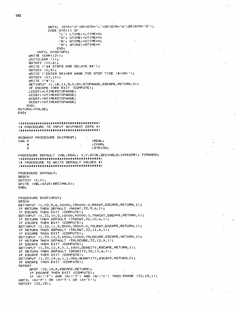
180
UNTIL (STR='U')OR(STR'L')OR(STR'W')OR(STR'O') CASE STRE1] OF
'L': LTIME:LTIME-*-H; 'U': UTIME:=UTIME+H; 'W': WTIME:WTIME+H; '0': OTIME:=OTIME+H END;
UNTIL N:=NSTOPS; WRITE (CHR(12)) UNITCLEAR (1); GOTOXY (10.6); WRITE ('** STOPS AND DELAYS GOTOXY (0,9); WRITE ('ENTER DRIVER WAGE FOR STOP TIME ($/HR)'); GOTOXY (17,11); WRITE ('$'); GETINPUT (1.1B.11,5,0.50.STOPWAGE,ESCAPE.RETURN.0); IF ESCAPE THEN EXIT (COMPUTE); LCOST: =LTIME*STOP WAGE; UCOST: =UTIME*STOPWAGE; WCOST: WT IME*STOPWAGE; OCOST: OTIME*STOP WAGE;
END; RETURN: =FALSE; END;
(*****<******************************) (* PROCEDURE TO INPUT SHIPMENT DATA *)
SEGMENT PROCEDURE SHIPMENT;
VAR R :REAL;
A CHAR;
S :STRING;
PROCEDURE DEFAULT (VBL:REAL; X,Y.,SIZE.DECIMALS: INTEGER); FORWARD;
(* PROCEDURE TO WRITE DEFAULT VALUES *)
PROCEDURE DEFAULT; BEGIN GOTOXY (X,Y); WRITE (VBL:SIZE:DECIMALS); END;
PROCEDURE SHIPINPUT; BEGIN GETINPUT (1,32,9,630000, 15C)C)C)C).0,MAXWT,ESCAPE,RETURN. 1); IF RETURN THEN DEFAULT (MAXWT,32..9,6,1); IF ESCAPE THEN EXIT (COMPUTE); GETINPUT u,33,10,5,10000.40000.0,TRACWT,ESCAPE.RETURN,1); IF RETURN THEN DEFAULT (TRACWT,32,10..6,1); IF ESCAPE THEN EXIT (COMPUTE); GETINPUT (1,33,115,000.350000,TRLRWT.ESCAPE,RETURN,1); IF RETURN THEN DEFAULT (TRLRWT,32,11,61); IF ESCAPE THEN EXIT (COMPUTE); GETINPUT u,33,12,5,1500,10000.TRLRCUBE,ESCAPE,RETURN,1); IF RETURN THEN DEFAULT (TRLRCUBE,32,12.6.1) IF ESCAPE THEN EXIT (COMPUTE); GETINPUT (1,34,13.4,0.1,1000,DENSITY,ESCAPE,RETURN,1); IF RETURN THEN DEFAULT (DENSITY,32,13,6,1); IF ESCAPE THEN EXIT (COMPUTE); GETINPUT (1,32,14,6,1.10E6,QUANTITYESCAPE.RETURN0); IF ESCAPE THEN EXIT (COMPUTE); REPEAT
SPOT (32. 15,A.ESCAPE,RETURN); IF ESCAPE THEN EXIT (COMPUTE); IF (A<>'P') AND (A<).'T') AND (A<>'K') THEN ERASE (32.1,1);
UNTIL (A='P') OR (A='T') OR (A'K'); GOTOXY (32,15);
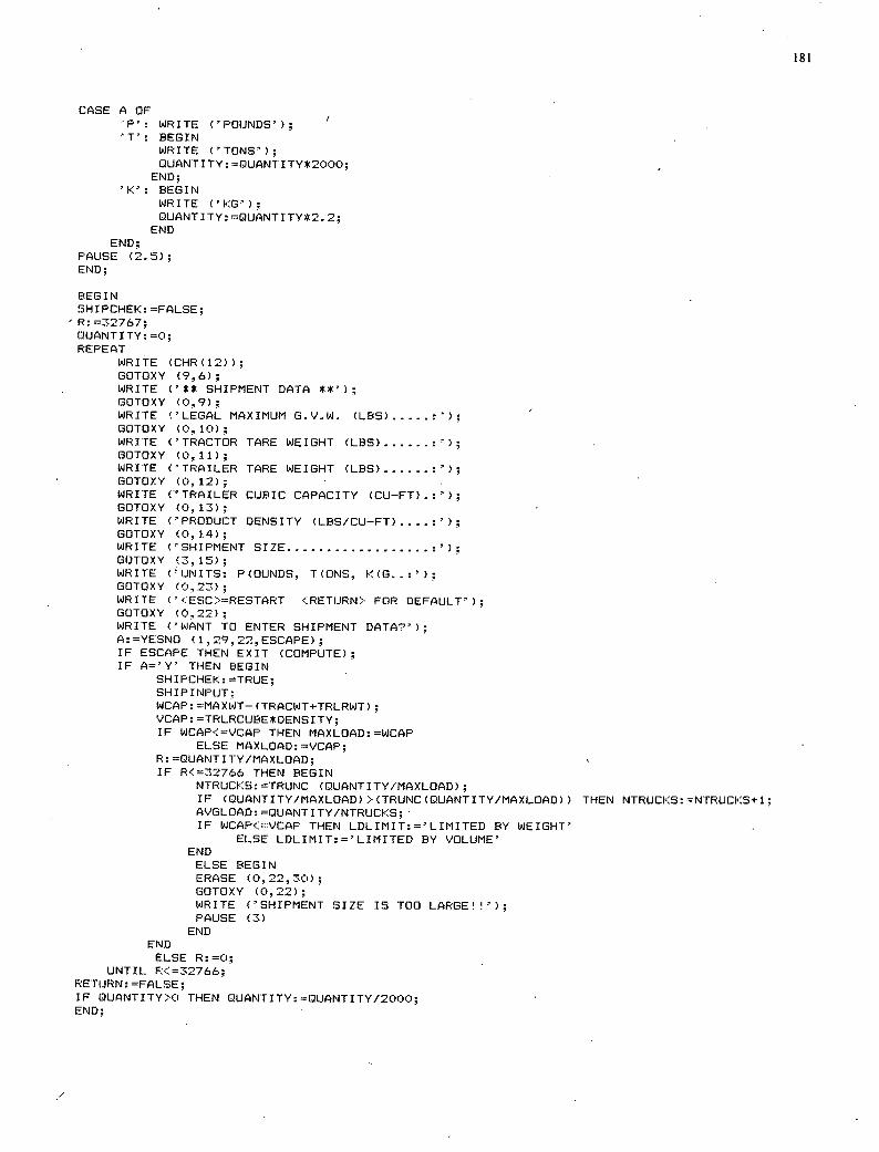
CASEAOF 'P': WRITE ('POUNDS'); 'T': BEGIN
WRITE ('TONS'); QUANTITY: =QUANTITY*2000;
END; 'K': BEGIN
WRITE ('KG'); QUANTITY: QUANTITY*2. 2;
END END;
PAUSE (2.5) END;
BEGIN SHIPCHEK: =FALSE;
- R:2767; QUANTITY: =0; REPEAT
WRITE (CHR(12)); GOTOXY (9,6); WRITE ('** SHIPMENT DATA GOTOXY (0,9); WRITE ('LEGAL MAXIMUM G.V.W. (LBS) ...'); GOTOXY (0, 10) WRITE ('TRACTOR TARE WEIGHT (LBS) ........'); GOTOXY (0, 11); WRITE ('TRAILER TARE WEIGHT (LBS) ...... GOTOXY (0,12); WRITE ('TRAILER CUBIC CAPACITY (CU—Fr).:'); GOTOXY (0,13); WRITE ('PRODUCT DENSITY (LBS/CU—FT)....:'); GOTOXY (0,14); WRITE ('SHIPMENT SIZE .................. GOTOXY (3,15); WRITE ('UNITS: P(OUNDS, ICONS, K((3..:'); GOTOXY (0,23); WRITE '<ESC:>=RESTART <RETURN> FOR DEFAULT'); GOTOXY (0,22); WRITE ('WANT TO ENTER SHIPMENT DATA"); A:YESNO (1,29,22,ESCAPE); IF ESCAPE THEN EXIT (COMPUTE); IF A='Y' THEN BEGIN
SHIPCHEIc: 'TRUE; SHIPINPUT; WCAP: =MAXWI—(TRACWI+TRLRWT); VCAP: TRLRCUBE*DENSITY; IF WCAP<=VCAP THEN MAXLOAD:WCAP
ELSE MAXLOAD: =VCAP; R: QUANTITY/MAXLOAD; IF R<=32766 THEN BEGIN
NTRUCKS: =TRUNC (QUANTITY/MAXLOAD); IF (QUANTITY/MAXLOAD) > (TRUNC (QIJANTITY/MAXLOAD) THEN NTRUCKS: =NTRUCKS+1; AVGLOAD: QUANTITY/NTRUCKS; IF WCAP<=VCAP THEN LDLIMIT:'LIMITED BY WEIGHT'
ELSE LDLIMIT:='LICIIIED BY VOLUME' END ELSE BEGIN ERASE (0,22,30); GOTOXY (0,22); WRITE ('SHIPMENT SIZE IS TOO LARGE'!'); PAUSE (3) END
END ELSE R:0;
UNTIL R<32766; RETURN: FALSE; IF QUANTITY>0 THEN QUANTITY: QUANTITY/2000; END;
181
/
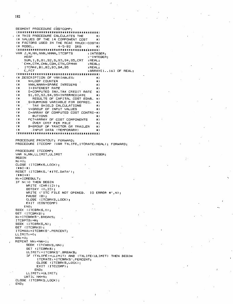
182
SEGMENT PROCEDURE COSTCOMP;
( THIS PROCEDURE CALCULATES THE (* VALUES OF THE 14 COMPONENT COST *) (* FACTORS USED IN THE RCAI TRUCK-COST*) (* MODEL. 4--82 DRG
VAR J.NNN,NNN,NNNN,ITCBPTS :INTEGER; HEAP :'INTEGER; SUM, ID.S1,S2,S,S3S4S5,CRT :REAL; CHH,CTM,CHW.CDFLCTN,CPMHH :REAL;
- ITCMAX,B1,B2,B3Et4.B5 :REAL; CPCT :ARRAY[1. .16] OF REAL;
(* DESCRIPTION OF VARIABLES: (* N=LOOP COUNTER (* NNN,NNNN=SPARE INTEGERS (* I=INTEREST RATE (* D=COMPUTED INV.TAX CREDIT RATE *) (* Si, 92, 93, S4, SZ=INTERMEDIATE
RESULTS OF CAPITAL COST EONS. *) (* S=SUMMING VARIABLE FOR DEPREC. *)
TAX SHIELDCALCULATIONS (* V=GROUP OF INPUT VALUES (* C=ARRAY OF COMPUTED COST CONTRI-*)
BUTIONS (* PCT=ARRAY OF COST COMPONENTS *)
OVER COST PER MILE (* B=GROUP OF TRACTOR OR TRAILER *)
.INPUT DATA (TEMPORARY)
PROCEDURE PRINTOUT; FORWARD; PROCEDURE ITCCOMP (VAR TXLIFE, ITCRATE: REAL); FORWARD;
PROCEDURE ITCCOMP; VAR N,NN,LLIMIT,ULIMIT :INTEGER; BEGIN - N: 0; CLOSE (ITCBRKS,LOCK); (*$I-*) RESET (ITCBRKS,'*ITC.DATA'); (*$I-4-*) N:IORESIJLT; IF N<>O THEN BEGIN
WRITE (CHR(12)); GOTOXY (0.23); WRITE ('ITC FILE NOT OPENED. 10 ERROR #',N); PAUSE (8); CLOSE (ITCBRKS,LOCK); EXIT (COSTCOMP)
END SEEK (ITCBRKS,O) ; GET (ITCBRKS); N: ITCBRKS BREAKS; - ITCBPTS: N; SEEK (ITCBRKS,N); GET (ITCBRKS); ITCMAX: =ITCBRK5- . PERCENT; LLIMIT:0; NN:O REPEAT NN:NN+1;
SEEK (ITCBRKS,NN); S GET (ITCBRKS); 1JLIMIT:ITCBRKS. BREAKS; IF (TXLIFE)-=LLIMIT) AND (TXLIFE<ULIMIT) THEN BEGIN
ITCRATE: ITCBRKS". PERCENT; CLOSE (ITCBRKS,LOCK);
EXIT (ITCCOMP); S END;
LLIMIT: ULIMIT; UNTIL NNN; S
CLOSE (ITCBRKS,LOCK); END;
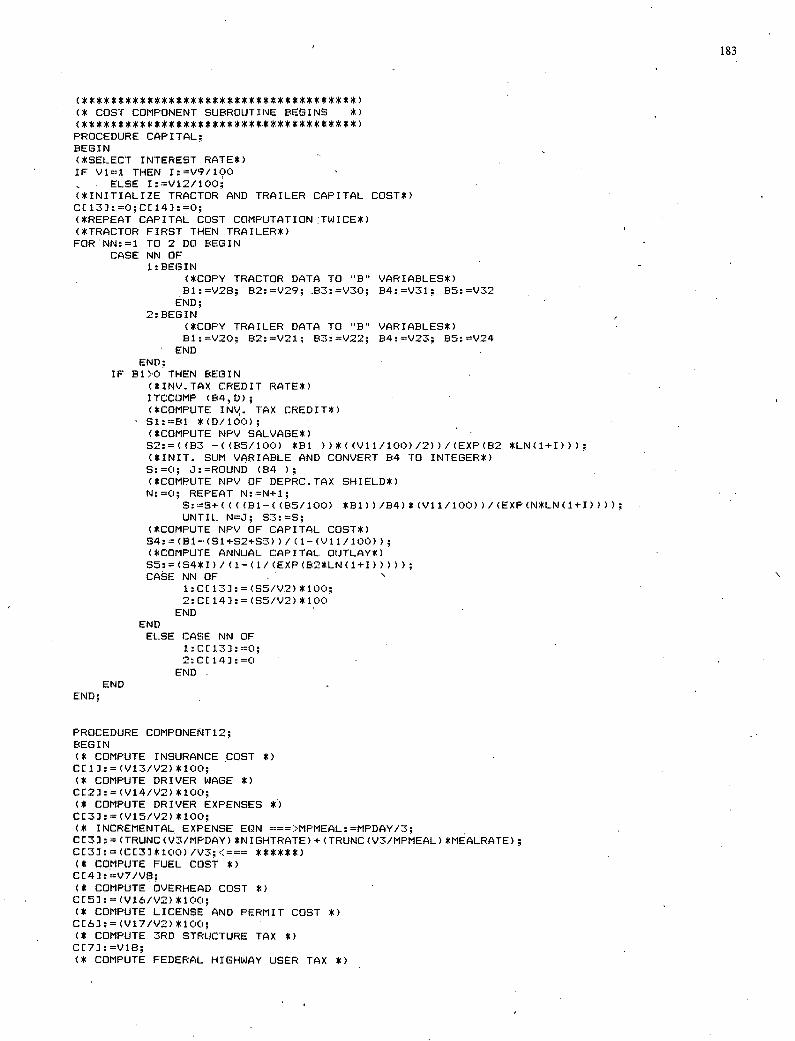
183
(* COST COMPONENT SUBROUTINE BEGINS *)
PROCEDURE CAPITAL; BEGIN (*SELECT INTEREST RATE*) IF V11 THEN I:=V9/100
ELSE I:=V12/100; (*INITIALIZE TRACTOR AND TRAILER CAPITAL COST*) CE 13]: =0; CC 14]: =0; (*REPEAT CAPITAL COST COMPUTATION :TWICE*) (*TRACTOR FIRST THEN TRAILER*) FOR'NN:i TO 2 D(J BEGIN
CASE NN OF BEGIN
(*COPY TRACTOR DATA TO "B" VARIABLES*) B1:V28; B2:'V29; .B3:=V30; B4:=V31; B5:V32
END; BEGIN
(*COPY TRAILER DATA TO B" VARIABLES*) Bi:V20; B2:'V21; B3:V22; B4:V23; B5:V24
END END;
IF B1>0 THEN BEGIN (*INV.TAX CREDIT RATE*) ITCCOMP (B4,D); (*COMPUTE IN'),. TAX CREDIT*) Si:B1 *(D/100); (*COMPUTE NPV SALVAGE*) S2:UB3 -((B5/100) *B1 ))*((V11/i00)/2))/(EXP(B2 *LN(i+I))); (*INIT. SUM VARIABLE AND CONVERT 94 TO INTEGER*) S:0; J:=ROUND (B4 ); (*COMPUTE NPV OF DEPRC.TAX SHIELD*) N:=0; REPEAT N:N+l;
S:5+((((B1-((R5/100) *Bi))/B4)*(V11/100))/(EXP(N*LN(i+I)))); UNTIL NJ; S3:=S;
(*COMPUTE NPV OF CAPITAL COST*) S4: = (51- (S1+S2+93) ) / (1- (Vii / 1OC>) (*COMPUTE ANNUAL CAPITAL OUTLAY*) Si: = (94*1) / (1- (1 / (EXP (B2*LN (1+1))))); CASE NNOF
CE 13]: =(S5/V2) *100; CE 14] : (S5/V2) *100
END END ELSE CASE NN OF
CE 13]: =0; CE 14]: =0
END
END;
PROCEDURE COMPONENT12; BEGIN (* COMPUTE INSURANCE COST *) CE1J:(V13/V2)*100; (* COMPUTE DRIVER WAGE *) CE23: = (V14/V2) * 100; CX COMPUTE DRIVER EXPENSES *) CE3]:(V15/V2) *100; CX INCREMENTAL EXPENSE EON ==>MPMEAL:=MPDAV/3; CE33: = (TRUNC (V3/MPDAV) *NIGHTRATE) + (TRUNC (V3/MPMEAL) *MEALRATE); CE3]:(CE3]*100)/V3;<=== ******) CX COMPUTE FUEL COST *) CE4] : V7/VB; (* COMPUTE OVERHEAD COST *) CE1:(Vl6/V2)*i00; CX COMPUTE LICENSE AND PERMIT COST *) CE63:(V17/V2)*100; CX COMPUTE 3RD STRUCTURE TAX *) CE71 : ViB; CX COMPUTE FEDERAL HIGHWAY USER TAX *)
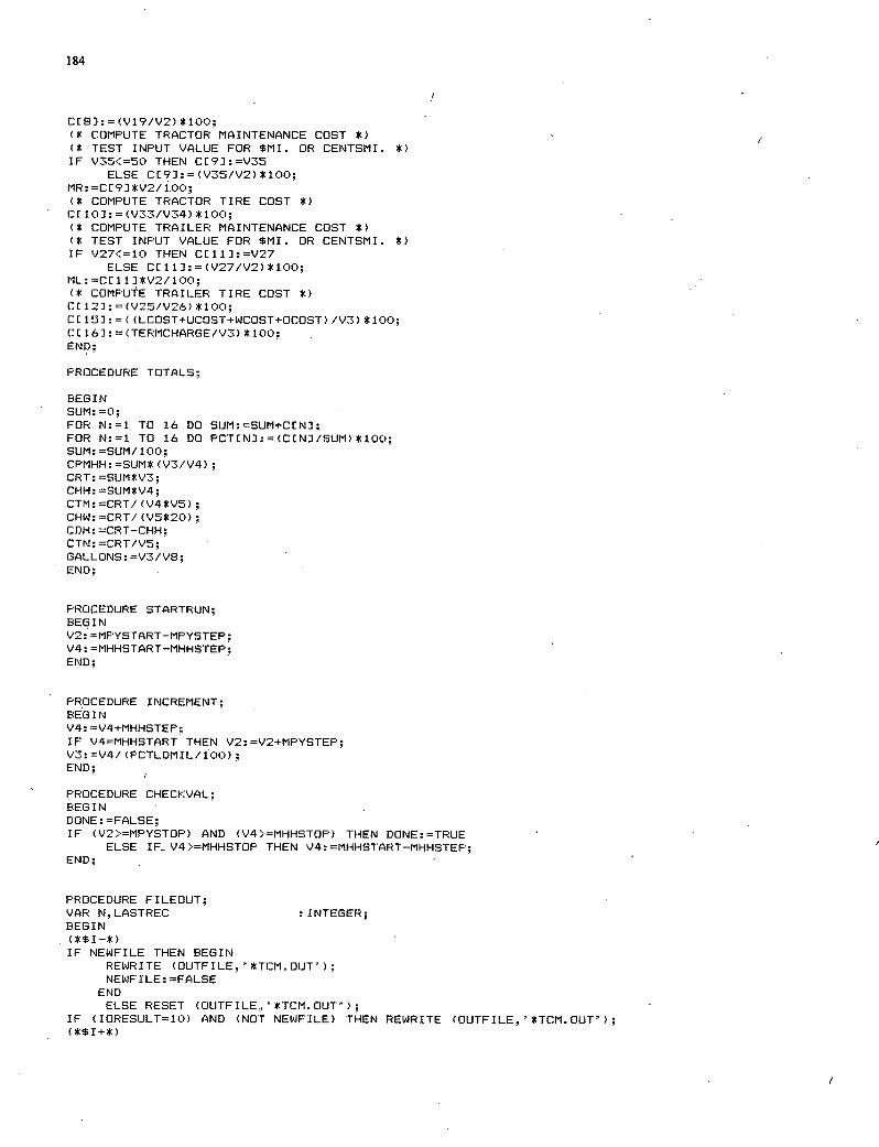
184
C183:(V19/V2) *100; (* COMPUTE TRACTOR MAINTENANCE COST *) (*TEST INPUT VALUE FOR %MI. OR CENTSMI. *) IF V35<=50 THEN C19]:-V35
ELSE CC91:=(V35/V2)*100; MR: CC9] *V2/i00; (* COMPUTE TRACTOR TIRE COST *) CC 10]: = (V33/V34) * 100; (* COMPUTE TRAILER MAINTENANCE COST *) (* TEST INPUT VALUE FOR $MI. OR CENTSML *) IF V27<10 THEN CC111:V27
ELSE CC11]:(V27/V2)*100; ML: CC1 1 J*V2/100; (* COMPUTE TRAILER TIRE COST *) CC121:=(V25/V26)*100; CC 15]: ( (LCOST+UCOST+WCOST-s-OCOST) /V3) *100; CCI61:(TERMCHARGE/V3)*100; END;
PROCEDURE TOTALS;
BEGIN SUM: 0; FOR N:1 TO 16 DO SUM:SUM+CCN]; FOR N:1 TO 16 DO PCTCNJ:(CCNJ/SUM)*100; SUM: SUM/100; CPMHH:=SUM* (V3/V4); CRT: SUM*VS; CHH: SUM*V4; CTM: CRT/ (V4*V5); CHW: CRT/ (V5*20); CDH: CRT-CHH; CTN:CRT/V5; GALLONS:=V3/V8; END;
PROCEDURE STARTRUN; BEGIN V2: MPYSTART-MPYSTEP; V4: '*lHHSTART-MHHSTEP; END;
PROCEDURE INCREMENT; BEGIN V4: V4+MHHSTEP; IF V4MHHSTART THEN V2:V2+MPYSTEP; V3:V4/ (PCTLDMIL/1C)0); END;
PROCEDURE CHECKVAL; BEGIN DONE: FALSE; IF (V2>MPYSTOP) AND (V4).MHHSTOP) THEN DONE:TRUE
ELSE IFv4:>=rlHHsTop THEN V4:MHHSTAF<T-MHH5TEP; END;
PROCEDURE FILEOUT; VAR NLASTREC :INTEGER; BEGIN
IF NEWFILE THEN BEGIN REWRITE (OUTFILE'*TCM.OUT'); NEWFILE: FALSE
END ELSE RESET COUTFILE, '*T(:M. OUT');
IF (IORESULT=10) AND (NOT NEWFILE) THEN REWRITE (OUTFILE'*TCM.OUT'); (*$I+*)
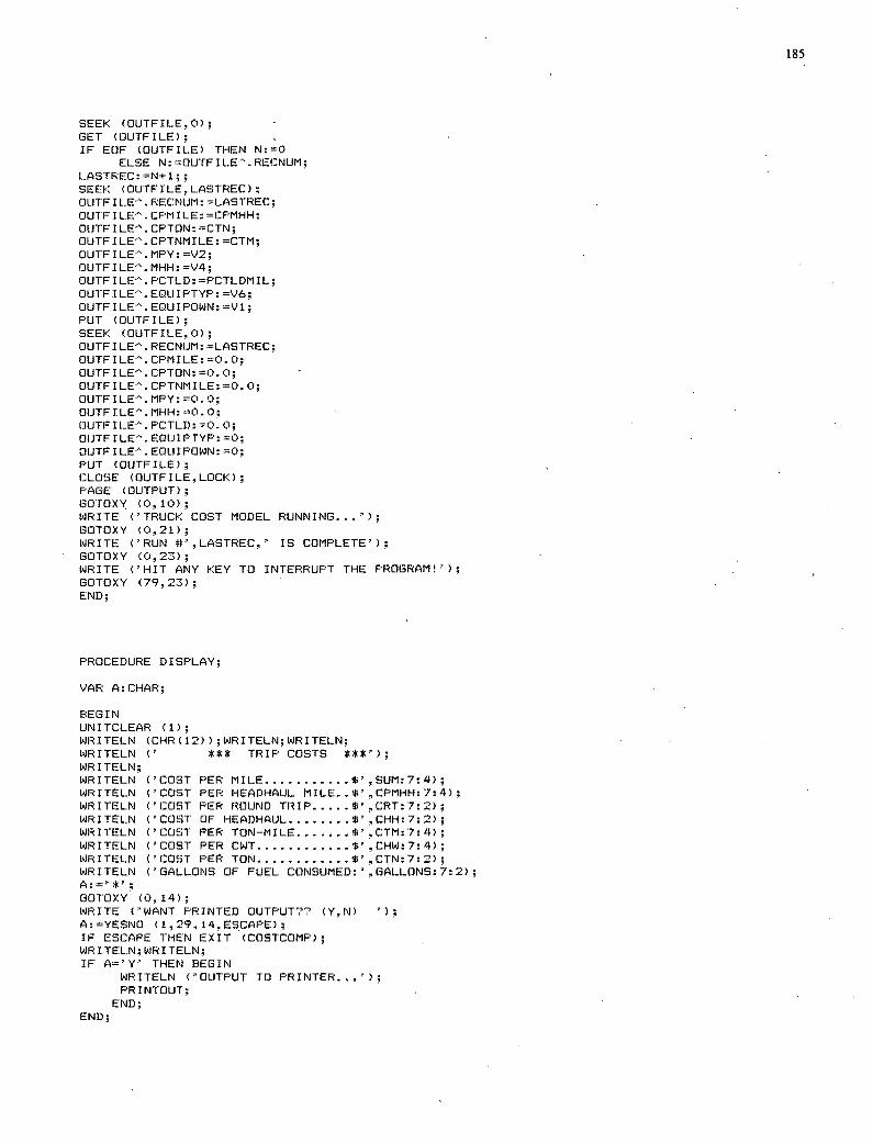
SEEK (OUTFILE,O) GET (OUTFILE); IF EOF (OUTFILE) THEN N:0
ELSE N:=OUTFILE.RECNUM; LASTREC: N+1;; SEEK (OUTFILE.LASTREC) OUTF1LE'. RECNUM: LASTREC; OUTFILE". CPMILE: =CPMHH; OUTFILE". CPTON: CTN; OUTFILE'.. CPTNMILE: =CTM; OUTFILE".MPY:rV2; OUTFILE". MHH: V4; OUTFILE". PCTLD: PCTLDMIL; OUTFILE. EQLJIPTYP: =V6; OUTFILE".EOUIPOWN:Vl; PUT (OUTFILE); SEEK (OUTFILE,0); OUTFILE". RECNUM: LASTREC; OUTFILE".CPMILE:=CLO; OUTFILE'. CPTON:=0.0; OUTFILE'.CPTNMILE:'O.O; (JUTFILE".MPY:O.O; OUTFILE".MHH:'O.O; (JLJTFILE". PCTLD: C}. 0; OUTFILE". EQUIFTYP: C); OUTFILE".EQLJIPOWN:C); PUT (OUTFILE); CLOSE (OUTFILE, LOCK) PAGE (OUTPUT); GOTOXY, (0, 10) WRITE ('TRUCK COST MODEL RUNNING...'); GOTOXY (0,21); WRITE ('RUN $',LASTREC.' IS COMPLETE'); GOTOXY (0,23); WRITE ('HIT ANY KEY TO INTERRUPT THE PROGRAM!'); GOTOXY (79,23); END;
PROCEDURE DISPLAY;
VAR A:CHAR;
BEGIN UNITCLEAR (1); WRITELN (CHR(12));WRITELN;WRITELN; WRITELN (' *** TRIP COSTS ***' WRITELN; WRITELN ('COST PER MILE ........... -- ,SUM:7:4); WRITELN ('COST PER HEADHAUL MILE..$',CPMHH:7:4); WRITELN ('COST PER ROUND TRIP ----- V ,CRT:7:2); WRITELN ('COST OF HEADHAUL -------- $' ,CHH:7:2); WRITELN ('COST PER TON-MILE....... V ,CTM:7:4); WRITELN ('COST PER CWT............ $' ,CHW:7:4); WRITELN ('COST PER TON ------------ --- .CTN:7:2); WRITELN ('GALLONS OF FUEL CONSUMED:',GALLONS:7:2); A: ' *' GOTOXY (0,14); WRITE ('WANT PRINTED OUTPUT?? (Y,N) '); A:=YESNO (1,29,14,ESCAPE); IF ESCAPE THEN EXIT (COSTCOMP); WRITELN; WRITELN; IF A='Y' THEN BEGIN
WRITELN ('OUTPUT TO PRINTER...'); PRINTOUT;
END; END
185
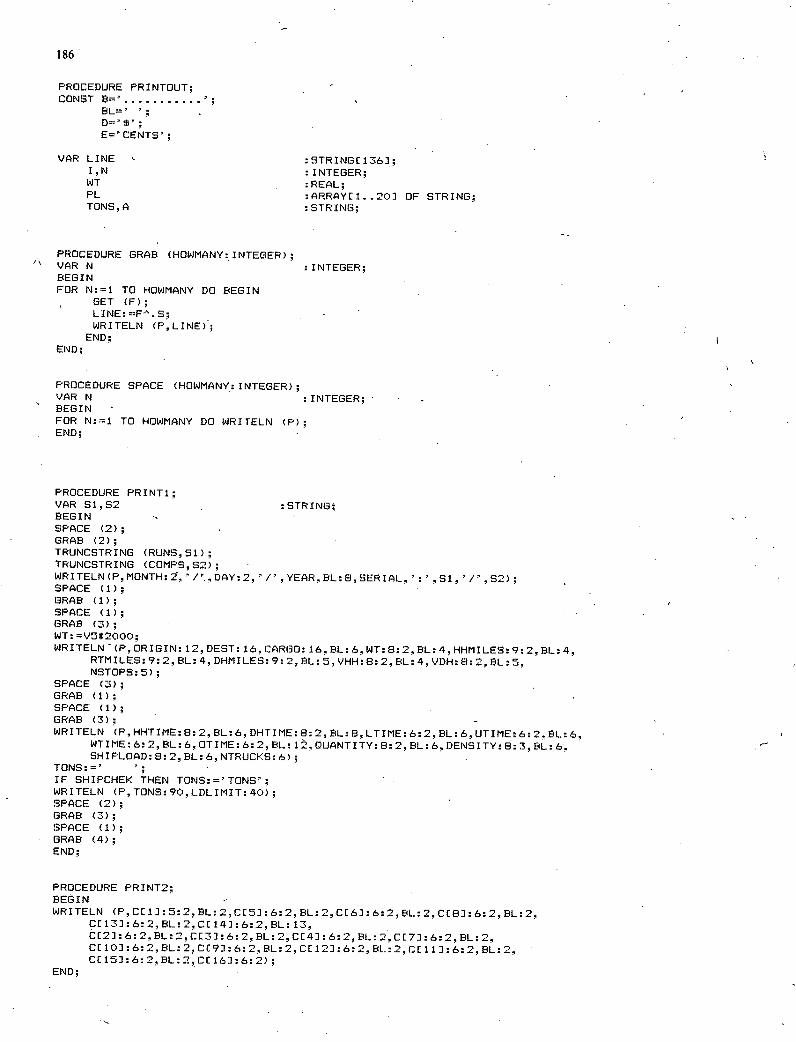
186
PROCEDURE PRINTOUT; CONST 8' ...........
E'"CENTS';
VAR LINE I.N WT PL TONS A
STRINGC 136]; INTEGER; REAL;
:ARRAYC1. .20] OF STRING; STRING;
PROCEDURE GRAB (HOWMANY:INTEGER); VAR N
INTEGER; BEGIN FOR N:=1 TO HOWMANY DO BEGIN
GET (F); LINE: Fe'. 5, WRITELN (P,LINE);
END; END;
PROCEDURE SPACE (HOWNANY: INTEGER); VAR N :INTEGER; BEGIN FOR N:=1 TO HOWMANY DO WRITELN (P); END;
PROCEDURE PRINT1; VAR S1,S2 :STRINt3; BEGIN SPACE (2); GRAB (2); TRUNCSTRING (RUNS,S1); TRUNCSTRING (COMPS,S2); WRITELN(P,MONTH:2,'/',DAY:2,'/',YEAR,BL:8,SERIAL,'..'S1'/'S2). SPACE (1); GRAB (1); SPACE (1); GRAB (3); WT: V5*2000; WRITELN(P.ORIGIN:12,DEST:16,CARGO:16,BL:6,WT:8:2BL:4HHMILES9.2BL..4
RTMILES:9:2,BL:4,DHMILES:9:2,BL:5,VHH:8:2,BL:4,VDH:8:2,EL:5, NSTOPS: 5);
SPACE (3); GRAB (1); SPACE (1); GRAB (3); WRITELN (P,HHTIME:8:2, BL:6. DHTIME:8: 2, BL:8,LTIME:6:2, BL:6,UTIME:6:2,BL:6,
WTIME: 6:2, BL: 6. OTINE: 6:2, BL: 1, (DUANTITY: 8:2, DL: 6, DENSITY: 8:3, DL: 6, SHIPLOAD: 8: 2, DL: 6, NTRUCKS: 6)
TONS:' '; IF SHIPCHEK THEN TONS:='TONS'; WRITELN (P,TONS:90,LDLIMIT:40); SPACE (2); GRAB (3); SPACE (1); GRAB (4); END;
PROCEDURE PRINT2; BEGIN WRITELN (P, CC1J:5:2, BL:2,CE5J:6:2, BL:2,C[6]:6:2, BL:2.C[8J:6:2,BL:2,
CE131:6:2,BL:2,C[141:6:2,BL:13, CC2] :6: 2,BL: 2, C[3] :6:2. BL: 2, CC4]:6:2, DL: 2, CE73: 6:2, DL: 2. CC101:6:2,BL:2,CE93:6:2,BL;2,C[121:6:2,BL:2,C[11]:6:2,BL:2, CC 15]: 6:2, DL: 2, CC 16] :6:2);
END;
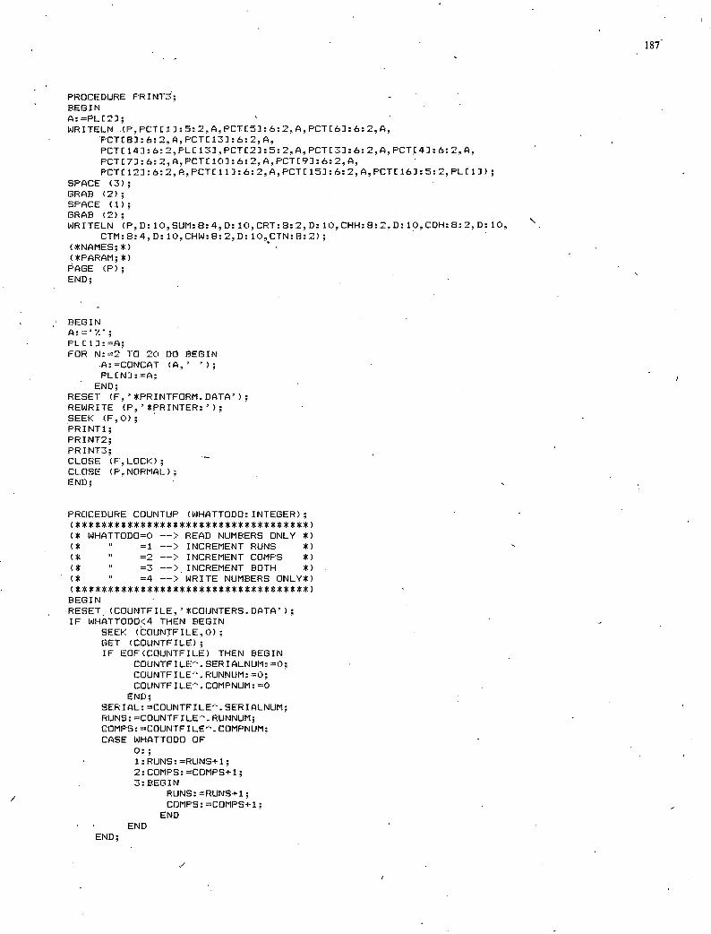
PROCEDURE PRINT3 BEGIN A:PLC2]; WRITELN (P,PCTC1 ]:5: 2,A,PCTC5]:6:2,A,PCTC6]:6:2,A,
PCTC8] :6:2, A, PCTC 13]: 6:2, A, PCTC14]:6:2,PL[13],PCTC2]:5:2.A,PCTC3]:6:2A,PCT[4]:6:2,A, PCTC71 :6:2, A, PCTC 10]: 6:2, A, PCTC9J :6:2,4, PCTC12]:6:2,A,PCTCl1]:6:2,A,PCTC15J:6:2,A,PCTt16]::2,PLC1]);
SPACE (3); GRAB (2); SPACE (1); GRAB (2); WRITELN (P,D:10,SUM:8:4.,D:10,CRT:B:2,D:10,CHH:8:2,D:10,CDH:8:2,D:1C),
CTM:8:4.D:1C),CHW:8:2,D:10,CTN:8:2); (*NAMES;*) (*PARAM; *) PAGE (P); END;
BEGIN A: ' V.'; PLC 1]: FOR N:2 TO 20 DO BEGIN
.A:CONCAT (A,' PLCN] : =A; END;
RESET (F, '*PRINTFORM. DATA'); REWRITE (P, '*PRINTER:'); SEEK (F,0) PRINT1; PRINT2; PRINT3; CLOSE (F,LOCK); CLOSE (P,NORMAL); END;
PROCEDURE COUNTUP (WHATTODO: INTEGER);
(* WHATTODO=0 --> READ NUMBERS ONLY > =1 --> INCREMENT RUNS *) =2 --> INCREMENT COMPS *) =3 --)-. INCREMENT BOTH *) =4 ---> WRITE NUMBERS ONLY*)
BEGIN RESET (COUNTFILE, '*COIJNTERS. DATA'); IF WHATTODO<4 THEN BEGIN
SEEK (COUNTFILE,0); GET (COUNTFILE); IF EOF(COUNTFILE) THEN BEGIN
COUNTFILE'. SERIALNUM: 0; COUNTFILE. RUNNUM: 0; COUNTFILE'. COMPNUM: 0 END;
SERIAL: COUNTFILE'. SERIALNUM; RUNS: COUNTFILE'. RUNNUM; COMPS: COUNTFILE. COMPNUM; CASE WHATTODO OF
0:; RUNS: RUNS+1; COMPS: COMPS+1; BEGIN
RUNS:RUNS+1; COMPS: COMPSI-1;
END END
END;
187
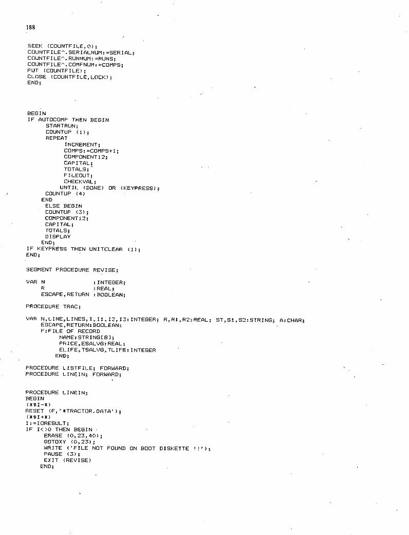
188
SEEK (COUNTFILE. 0) COUNTFILE. SERIALNUM: SERIAL; COLJNTFILE. RUNNUM: =RUNS; COUNTFILE-'. COMPNUM: COMPS; PUT (COUNTFILE); CLOSE (COUNTFILE,LOCK); END;
BEGIN IF AUTOCOMP THEN BEGIN
STARTRUN; COUNTUP (1); REPEAT
INCREMENT; COMPS: =COMPS+1; COMPONENT 12; CAPITAL; TOTALS; FrLEOUT; CHECKVAL; UNTIL (DONE) OR (KEYPRESS);
COUNTUP (4) END ELSE BEGIN COUNTUP (3); COMPONENT 12; CAPITAL; TOTALS; DISPLAY
END IF KEYPRESS THEN UNITCLEAR (1); END;
SEGMENT PROCEDURE REVISE;
VAR N : INTEGER;
R :REAL; ESCAPE. RETURN : BOOLEAN;
PROCEDURE TRAC;
VAR N,LINE,LINES,I,I1,12,13:INTEGER; R,R1,R2:REAL; ST,S1..S2:STRINt3; A:CHAR; ESCAPE, RETURN: BOOLEAN; F:FILE OF RECORD
NAME: STRINGEB]; PRICE, ESALVO: REAL; ELIFE,TSALVG,TLJFE: INTEGER
END;
PROCEDURE LISTF1LE; FORWARD; PROCEDURE LINEIN; FORWARD;
PROCEDURE LINEIN; BEGIN (*$I-*) RESET (F,' *TRACTOR.DATA');
I:'IORESULT; IF I<>0 THEN BEGIN
ERASE (0, 23, 40); GOTOXY (0,23); WRITE ('FILE NOT FOUND ON BOOT DISKETTE H'); PAUSE (3); EXIT (REVISE)
END;
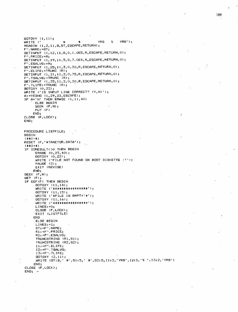
GOTOXY (1,11); WRITE C' $ $ YRS h YRS'); READIN (1,2, 11,8,51. ESCAPE. RETURN); F'. NAME:ST; GETINPUT (1.12,11,5,0.1.0E5,R,ESCAPE,RETURN,0); F. PRICE: =R; GETINPUT (1,19,11,5.0.7.0E4.R,ESCAPE.RETURN.0) F'. ESALVG:R; GETINPUT (1, 25, 11,2,0,30, R, ESCAPE, BETURN. 0); F.ELIFE:'TRUNC (R); GETINPUT (1,31,11.2.0,75,R,ESCAPE.RETURN,0) F'.TSALVG:=TRUNC (R); GETINPUT (1,35,11,2.0,30,R.ESCAPE,RETIJRN.0) F'.TLIFE:TRUNC (R); GOTOXY (0,23); WRITE ('IS INPUT LINE CORRECT? (Y,N)'); A:YESNO (1,29.23,ESCAPE); IF A='N' THEN ERASE (1,11,40)
ELSE BEGIN SEEK (F.N); PUT (F) END;
CLOSE (F,LOCK); END;
PROCEDURE LISTFILE; BEGIN (*$I-*) RESET (F,'*TRACTOR.DATA'); (*$I+*) IF IORESULT<>0 THEN BEGIN
ERASE (0,23,40); GOTOXY (0.23); WRITE ('FILE NOT FOUND ON BOOT DISKETTE H'); PAUSE (3); EXIT (REVISE) END;
SEEK (F,N); GET (F); IF EOF(F) THEN BEGIN
GOTOXY (11,14); WRITE GOTOXY (11,15); WRITE ('*FILE IS EMPTY' *'); GOTOXY (11,1); WRITE LINES: =0; CLOSE (F,LOCK); EXIT (LISTFILE)
END ELSE BEGIN LINES:1; ST:F". NAME; Ri: F'. PRICE; R2:F'.ESALVG; TRUNCSTRING (R1.51); TRUNCSTRING (R2,S2); Ii: F'. ELIFE; 12:F". TSALVG; 13: F". ILIFE; GOTOXY (2.11); WRITE (91:8,' $',Sl:Z,' $',S2:5.I1:3,'YRS,12:3,'7. ',I3:2,'YRS')
END; CLOSE (F,LOCK); END; -
189
190
BEGIN PAGE (OUTPUT);
GOTOXY (8,6); WRITE ('**TRACTOR DATA FILE GOTOXY (0,8); WRITE (' TACTOR PRICE —ECONOMIC— ---TAX---'); GOTOXY (0,9); WRITE (' TYPE CS) SLVG LIFE SLVG LIFE'); LISTFILE; GOTOXY (0,23); WRITE ('STILL WANT TO MODIFY?'); A:rYE5NO (1,22,23,ESCAPE); IF A='Y' THEN BEGIN
IF LINES=0 THEN BEGIN ERASE (11, 14, 20); ERASE (11,15,20); ERASE (11.16,20)
END ERASE (023,40); LINEIN; ERASE (0,23,40);
END;
END;
PROCEDURE TRLR;
VAR N.LINELINES.I,I1,12,13:INTEGER; R,R1,R2:REAL; ST,S1,S2:STRING; A:CHAR; ESCAPE, RETURN: BOOLEAN; F:FILE OF RECORD
NAME:STRINGCB]; PRICE, ESALVG: REAL; ELIFE,TSALVG,TLIFE: INTEGER
END;
PROCEDURE LISTFILE; FORWARD; PROCEDURE LINEIN (RECNUM:INTEGER); FORWARD;
PROCEDURE LINEIN; BEGIN (*$I—*) RESET (F,'*TRAILER.DATA');
IF IORESULT< >0 THEN BEGIN ERASE (0,23,40);
GOTOXY (0,23); - WRITE ('FILE NOT FOUND ON BOOT DISKETTE H'); PAUSE (3); EXIT (REVISE)
END; N:RECNUM; LINE: N+1 1; GOTOXY (1,LINE); WRITE (' $ $ YRS 7. YRS'); READIN (1,2,LINE,8,ST,ESCAPE,RETURN); F. NAMEST; GETINPUT (1.12,LINE,5,0,1.0E5,R,ESCAPE,RETURNo); F. PRICE:R; GETINPUT (1,19.LINE,5,0,50000.O,R,ESCAPE,RETURN,0); F'.ESALVG:R; GETINPUT (1 9 25, LINE,2,0,30,R, ESCAPE,RETURN,0); F'.ELIFE:"TRUNC (R); GETINPUT (131,LINE,2,0,75,R,E9CAPE,RETURN,(); F.TSALVc3:=TRUNC (R); GETINPUT (1,35,LINE,2,0,30,R,ESCAPE.RETURN.C)); F.TLIFE:=TRUNC (R); GOTOXY (0,23); - WRITE ('IS LINE ',N,' CORRECT? .(Y,N)'); A:=YESNO (1,26,23,ESCAPE); IF A='N' THEN ERASE (1,LINE,40)
191
ELSE BEGIN LINES: =LINES+1; SEEK (F,N) PUT (F) END;
CLOSE (F,LOCK); END;
PROCEDURE LISTFILE; BEGIN
RESET (F,'*TRAILER.DATA'); (*$I+*) IF IORESULT<>O THEN BEGIN
ERASE (0,23,40); GOTOXY (0,23); WRITE ('FILE NOT FOIJND ON BOOT DISKETTE H'); PAUSE (3); EXIT (REVISE)
END;
REPEAT N:N+1; LINE: =N+11; LINES:N; SEEK (F,N); GET (F); IF EOF(F) THEN N:9
ELSE BEGIN ST:=F.NAME; R1:=F'.PRICE; R2:=F.ESALVG; TRUNCSTRING (R1,S1); TRIJNCSTRING (R2,S2); I1:FELIFE; 12:F-'. TSALVG; I3:F.TLIFE; GOTOXY (2.LINE); WRITE (ST:8,' %',Sl:S,' $',S2:5,Ii:3,'YRS',12:3,'V. ',I3:2,'YRS')
END; UNTIL (N9);
IF LINES=0 THEN BEGIN GOTOXY (11.14); WRITE ('***************'); • GOTOXY (11,15); WRITE ('*FILE IS EMPTY!'); GOTOXY (11,16); WRITE
END; CLOSE (F,LOCK); END;
BEGIN PAGE (OUTPUT); GOTOXY (8,6); WRITE ('** TRAILER DATA FILE **'); GOTOXY (0,8); WRITE ('*t TRAILER PRICE -ECONOMIC- ----TAX---'); GOTOXY (0,9); WRITE (' TYPE ($) SLVG LIFE SLVG LIFE'); FOR N:0 TO 9 DO BEGIN
GOTOXY (0,N+11); WRITE (N);
END; LISTFILE; ERASE (0,23,40); GOTOXY (0,23); WRITE ('STILL WANT TO MODIFY?'); A:=YESNO (1,22,23,ESCAPE); • IF A='Y' THEN BEGIN
IF LINES=0 THEN BEGIN ERASE (11, 14,20); ERASE (11,15.20); ERASE (11,16.20) END;
REPEAT ERASE (0,23,40); GOTOXY (0,23); WRITE ('MODIFY WHICH LINE?') I =L.INES+l; GETINPUT (1,19,23.1,0,I,R.ESCAPE.RETURN,0); N:=TRUNC(R); LINEIN (N); ERASE (0,23,40); GOTOXY. (0,23); WRITE ('MORE MODIFICATIONS?'); A:=YESNO (1.20,23,ESCAPE);
UNTIL A='N'; END;
END;
PROCEDURE DEFAULTS; VAR N :INTEGER;
NUN :REAL; ESCAPE, RETURN BOOLEAN; S : STRING; DEFAULTFILE :FILE OF RECORD
NAME: STRINGE2SJ; VALUE: REAL
END;
BEGIN WRITE (CHR(12)); GOTOXY (7,4); WRITE ('** INPUT DEFAULT VALUES GOTOXY (0,7); WRITE (' # DESCRIPTION VALUE');
RESET (DEFAULTFILE, ' *DEFAULT.DATA'); (t$I+*) IF IORESULT<>0 THEN BEGIN
GOTOXY (0,23); WRITE ('DEFAULT FILE NOT FOUND '); PAUSE (3); EXIT (DEFAULTS)
END; FOR N:0 TO 11 DO BEGIN
SEEK (DEFAULTFILE,N); GET (DEFAULTFILE); 5: DEFAULTFILE". NAME; NUN: =DEFAULTFILE". VALUE; GOTOXY (0,(N+9)); WRITE (N:2.' ',S,' 1,NUM:8:2);
END; GOTOXY (0,23); WRITE ('<ESC)-RESTART <RETIJRN> TO CONTINUE'); REPEAT
GOTOXY (0.22); WRITE ('NuMBER OF RECORD TO BE REVISED: '); GETINPUT (1,31,22.,2,0,11,NUM,ESCAPE,RETURN.,1); IF ESCAPE THEN EXIT (DEFAULTS); IF NOT RETURN THEN BEGIN
192
N:=TRUNC(NUM); SEEK (DEFAULTFILE,N); GET (DEFAULTFILE); ERASE (30, (N+9) 10); GETINPUT (1,31,(N+9),8,0,1.0E,NUM,ESCAPE,RETURN,0); IF ESCAPE THEN EXIT (DEFAULTS); SEEK (DEFAULTFILE,N); DEFAULTFILE'. VALUE: =NUM; PUT \WEFAULTFILE END;
UNTIL RETURN; CLOSE (DEFAULTFILE, LOCK); END;
PROCEDURE MISCDFLT; VAR N :INTEGER;
NUM :REAL; ESCAPE. RETURN : BOOLEAN; S :STRING; DEFAULTFILE :FILE OF RECORD
NAME: STRINGC25]; VALUE: REAL
END;
BEGIN WRITE (CHR(12)); GOTOXY (7,1); WRITE ('** MISC. DEFAULT VALUES GOTOXY (0,3); WRITE'(' # DESCRIPTION VALUE');
RESET (DEFAULTFILE, ' *MISC.DATA'); (*$I+*) IF IORESULT<>0 THEN BEGIN
GOTOXY (0,23); WRITE ('MISC. DEFAULT FILE NOT FOUND!!'); PAUSE (3); EXIT (MISCDFLT)
END; FOR N:0 TO 15 DO BEGIN
SEEK (DEFAULTFILE,N); GET (DEFAULTFILE); S:=DEFAULTFILE'. NAME; NUM: =DEFAULTFILE'. VALUE; GOTOXY (0, (N+5)); WRITE (N:2,' ',S,' '.NUM:B:2);
END; GOTOXY (0,23); WRITE ('<ESC>RESTART <RETURN)- TO CONTINUE'); REPEAT
GOTOXY (0.22); WRITE ('NUMBER OF RECORD TO BE REVISED: '); GETINPUT (1, 31, 22. 2. 0, 15. NUM, ESCAPE, RETURN, 1) IF ESCAPE THEN EXIT (MISCDFLT); IF NOT RETURN THEN BEGIN
N:TRUNC(NUM); SEEK (DEFAULTFILE,N); GET (DEFAULTFILE); ERASE (30, (N+5), 1C)); GETINPUT (1,31,(N+5),8,0,1.0E6,NUM,ESCAPE,RETURN,0); IF ESCAPE THEN EXIT (MISCDFLT); SEEK (DEFAULTFILE,N); DEFAULTFILE'. VALUE: NUM; PUT (DEFAULTFILE) END;
UNTIL RETURN; CLOSE (DEFAULTFILE.LOCK); END;
193
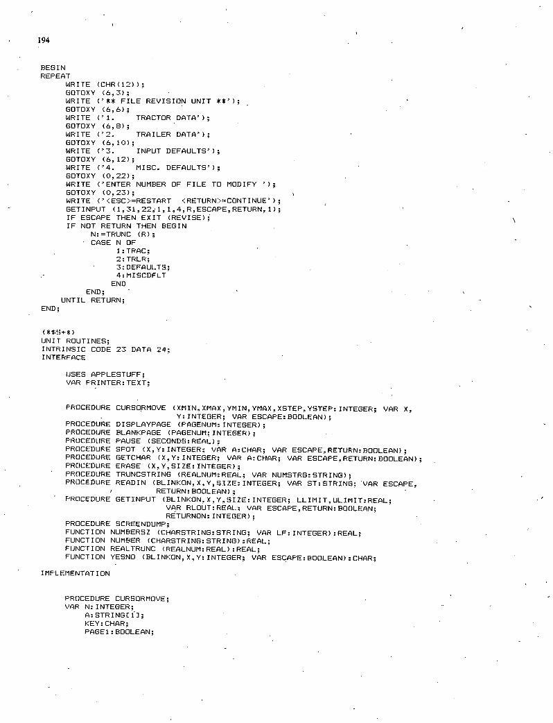
194
BEGIN REPEAT
WRITE (CHR(12)); GOTOXY (6,3); WRITE ('** FILE REVISION UNIT **') GOTOXY (6,6); WRITE ('1. TRACTOR DATA'); GOTOXY (6,8); WRITE ('2 TRAILER DATA'); GOTOXY (6,10); WRITE ('3. INPUT DEFAULTS'); GOTOXY (6,12); WRITE ('4. MISC. DEFAULTS'); GOTOXY (0,22); WRITE ('ENTER NUMBER OF FILE TO MODIFY GOTOXY (0,23); WRITE C' <ESC>=RESTART <RETURN>CONTINUE'); GETINPUT (1,31,22,1,1,4,R.ESCAPE,RETURN,1); IF ESCAPE THEN EXIT (REVISE); IF NOT RETURN THEN BEGIN
N:TRUNC (R); CASE N OF
1:TRAC; 2: TRLR; 3:DEFAULTS; 4:MISCDFLT END
END; UNTIL RETURN;
END;
(*$S+*) UNIT ROUTINES; INTRINSIC CODE 23 DATA 24; INTERFACE
USES APPLESTUFF; VAR PRINTER: TEXT;
PROCEDURE CURSORMOVE (XMIN. XMAX,YMIN,YMAX,XSTEP,YSTEp: INTEGER; VAR X, Y:INTEGER; VAR ESCAPE:BOOLEAN);
PROCEDURE DISPLAYPAGE (PAGENUM: INTEGER); PROCEDURE BLANKPAGE (PAGENUM:INTEGER); PROCEDURE PAUSE (SECONDS:REAL); PROCEDURE SPOT (X,Y:INTEGER; VAR A:CHAR; VAR ESCAPE,RETURN:BOOLEAN); PROCEDURE GETCHAR (X,Y:INTEGER; VAR A:CHAR; VAR ESCAPE,RETURN:BOOLEAN); PROCEDURE ERASE (X,Y,SIZE:INTEGER); PROCEDURE TRUNCSTRING (REALNUM:F<EAL; VAR NUMSTRG:STRING); PROCEDURE READIN (BLINKON,X,Y,SIZE:INTEGER; VAR ST:STRING; VAR ESCAPE,
RETURN:BOOLEAN); PROCEDURE GETINPUT (BLINKON,X,Y,SIZE: INTEGER; LLIMIT,ULIMIT:REAL;
VAR RLOUT:REAL; VAR ESCAPE,RETURN:BOOLEAN; RETURNON: INTEGER);
PROCEDURE SCREENDUMP; FUNCTION NUMBERSZ (CHARSTRING: STRING; VAR LF: INTEGER) : REAL; FUNCTION NUMBER (CHARSTRING: STRING) : REAL; FUNCTION REALTRUNC (REALNUM:REAL) :REAL; FUNCTION YESNO (BLINKON, X, Y: INTEGER; VAR ESCAPE: BOOLEAN) : CHAR;
IMPLEMENTATION
PROCEDURE CURSORMOVE; VAR N: INTEGER;
A: STRINGE 1]; KEY: CHAR; PAGE1 BOOLEAN;
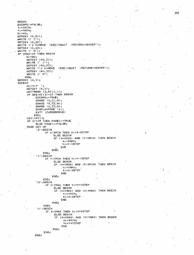
BEGIN ESCAPE: =FALSE; X:XMIN; Y:YMIN; N: 40 GOTOXY (0,21); WRITE (' I'); GOTOXY(022); WRITE ('3 KN1OVE <ESC>QUIT <RETURN>=ENTER');
GOTOXY (0..23) WRITE (' N'); IF XMAX>39 THEN BEGIN
N:80; GOTOXY (40,21); WRITE (' I'); GOTOXY (40,22); WRITE ('J K=MOVE <ESC)-OUIT <RETURN>=ENTER'); GOTOXY (40,23); WRITE C' H')
END; GOTOXY (X.,Y); REPEAT
AE1]:' GOTOXY (X,Y); UNITREAD (2,A111,1); IF ORD(AC1J)=27 THEN BEGIN
S ESCAPE:TRUE; S ERASE (0,21,N);
ERASE (0,22,N); ERASE (0,23,N); DISPLAYPAGE (1); EXIT (CURSORHOVE)
END; KEY:=AC11;, IF X<39 THEN PAGE1:TRUE
ELSE PAGE1:FALSE; CASE KEY OF
'J':BEGIN IF X>XMIN THEN X:X-XSTEP
ELSE BEGIN IF (X=XMIN) AND Y::YMIN) THEN BEGIN
X: XMAX; 'Y:Y-YSTEP END
END; END;
'I':BEGIN IF Y>YMIN THEN Y:Y-YSTEP
• ELSE BEGIN IF (Y=YMIN) AND (X>X1'lIN) THEN BEGIN
Y:=YMAX; X: 'X-XSTEP
END S
END; END;
'M' : BEGIN IF Y<YMAX THEN Y:Y+YSTEP
ELSE BEGIN IF (Y=YMAX) AND (X<XMAX) THEN BEGIN
S Y:YHIN; X:'X+XSTEP
END END;
END; S
'K' :BEGIN IF X(XMAX THEN X:X+XSTEP
ELSE BEGIN IF (XXP1AX) AND CY<YHAX) THEN BEGIN
X:XMIN; Y:'Y+YSTEP
END S
END; END;
END; •
95
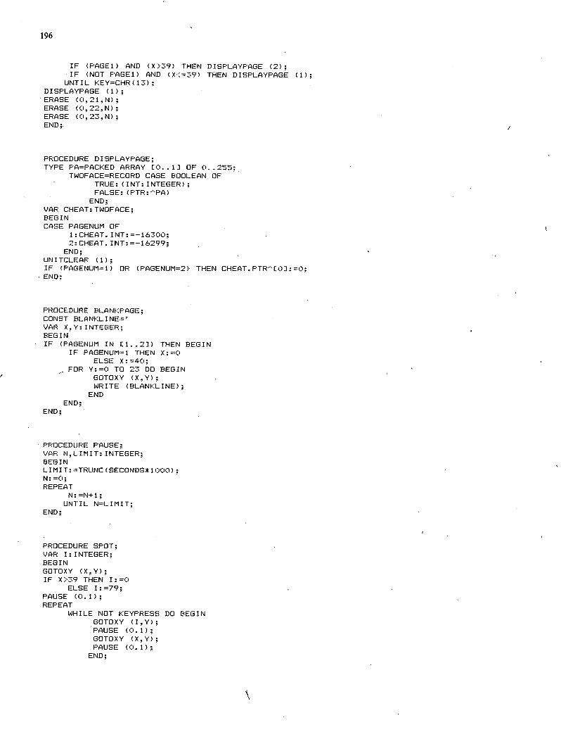
196
IF (PAGE1) AND (X>39) THEN DISPLAYPAGE (2); IF (NOT PAGE1) AND (X(=39) THEN DISPLAYPAGE (1); UNTIL KEYCHR(13);
DISPLAYPAGE (1); ERASE (021N); ERASE (022,N); ERASE (0.23,N); END;.
PROCEDURE DISPLAYPAGE; TYPE FAPACKED ARRAY E0..13 OF 0. .25;
TWOFACE=RECORD CASE BOOLEAN OF TRUE: (tNT: INTEGER); FALSE: (PTR:PA)
END; VAR CHEAT: TWOFACE; BEGIN CASE PAGENUM OF
1:CHEAT. INT:-16300; 2:CHEAT. INT:=-16299; END;
UNITCLEAR (1); IF (PAGENUM1) OR (PAGENUM2) THEN CHEAT.PTR'C01:0; END;
PROCEDURE BLANKPAGE; CONST BLANKLINE=' VAR X,Y:INTEGER; BEGIN IF (PAGENUM IN Cl. .2]) THEN BEGIN
IF PAGENUM=i THEN X:0 ELSE X:40;
FOR Y:=O TO 23 DO BEGIN GOTOXY (X,Y); WRITE (BLANKLINE);
END END;
END;
PROCEDURE PAUSE; VAR N,LIMIT: INTEGER; BEGIN LIMIT:TRUNC(SECONDS*1000); N: C); REPEAT
N: N+l; UNTIL NLIMIT;
END;
PROCEDURE SPOT; VAR I:INTEGER; BEGIN GOTOXY (X,Y); IF X>39 THEN I:0
ELSE I:79; PAUSE (01); REPEAT
WHILE NOT KEYPRESS DO BEGIN GOTOXY (I,Y); PAUSE (0.1); GOTOXY (X,Y); PAUSE (0 1); END;
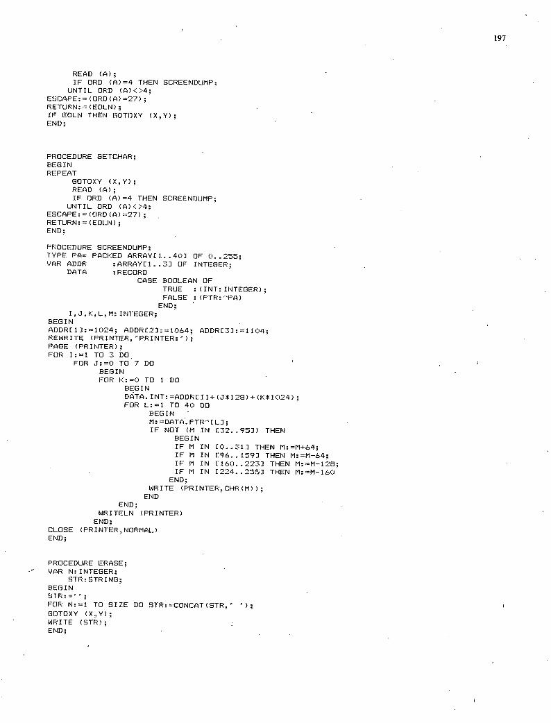
READ (A); IF ORD (A)=4 THEN SCREENDUMP;
UNTIL ORD (A)<>4; ESCAPE: (ORD (A) =27) RETURN: (EOLN); IF EOLN THEN GOTOXY (X,Y); END;
PROCEDURE GETCHAR; BEGIN REPEAT
GOTOXY (XV); READ (A); IF ORD (A)4 THEN SCREENDUMP;
UNTIL ORD (A)<>4; ESCAPE:=(ORD(A)=27); RETURN:(EOLN); END;
PROCEDURE SCREENDUMP; TYPE PA= PACKED ARRAY[ 1. .40] OF 0. . 255;
VAR ADDR :ARRAY[1. .3] OF INTEGER;
DATA :RECORD CASE BOOLEAN OF
TRUE (INT: INTEGER); FALSE : (PT•:••PA) END;
I,J.KL.,M: INTEGER; BEGIN ADDR[ 1]: =1024; ADDR123 : =1064; ADDR[3]: =1104; REWRITE (PRINIER'PRINTER:'); PAGE (PRINTER); FOR I:1 TO 3 DO
FOR J:0 TO 7 DO BEGIN FOR K:0 TO 1 DO
BEGIN D4TA.INT:=ADDR[IJ+(J*128)~(K*1024); FOR L:1 TO 40 DO
BEGIN M:DATA.PTRCLJ; IF NOT (M IN 132.. 95]) THEN
BEGIN IF N IN 10. .31] THEN M:=M+64; IF N IN [96.. 159] THEN M:=M-64; IF N IN [160. .223] THEN M:M-128; IF M IN 1224. .255] THEN M:M-160
END; WRITE (PRINTERCHR(M));
END END;
WRITELN (PRINTER) END;
CLOSE (PRINTER NORMAL) END;
PROCEDURE ERASE; VAR N: INTEGER;
STR: STRING; BEGIN SIR: FOR N:1 TO SIZE DO STR:CONCAT(STR.' GOTOXY (XY) WRITE (SIR); END;
197
198
FUNCTION REALTRUNC;
(* FUNCTION TO TRUNCATE ANY SIZE REAL *) (* NUMBER WITHOUT 'TRUNC' FUNCTION. *) ( THE PROCEDURE RETURNS A REAL VALUE.*) (* DRG. /17/82
VAR TNUM, NUM, REM: REAL; M, N, PTR, SIGN: INTEGER; DIGIT: ARRAYCO. . 40] OF INTEGER;
BEGIN SIGN: =1; IF REALNUM<0 THEN BEGIN.,
SIGN: -1; REALNUM: REALNUM*SIGN END;
N: =-l; REPEAT N:N+l;
PTR: =N; NUM: =REALNUM/PWROFTEN (N);
UNTIL (NUM<10) AND (NUM)0>; REM: REALNUM; FOR N:PTR DOWNTO 0 DO BEGIN
NUM:=REM/PWROFTEN(N); DIGITCN]:"TR1jN3 (NUM); REM:"(NUM-DIGIT[N]) *PWROFTEN(N);
END; TNUM: 0; FOR N:0 TO PTR DO BEGIN
TNUM:=TNUM+(DIGITCN]*PWROFTEN(N)); END;
WHILE (REALNUM-TNtJM)-=1) DO BEGIN TNUM: =TNUM+1; DIGITCO] : DIGITCO3+1; N: -1; REPEAT N:N+1;
IF DIGITCNJ>9 THEN BEGIN DIGITCN]:r0; DIGITCN+11: DIGITCNi-1 ]+1
END; UNTIL NPTR;
END; REALTRUNC: '"TNUM*SIGN; END;
PROCEDURE TRUNCSTRING;
(* PROCEDURE TO TRUNCATE ANY SIZE REAL*) (* NUMBER AND RETURN A "STRING OF *) (* DIGITS. (* DRG. 6/7/82 '
VAR TNUM, NUM, REM: REAL; L,M,N,PTR.SIGN: INTEGER; DIGIT: ARRAYCO. .40] OF INTEGER;
BEGIN SIGN:1; IF REALNUM<0 THEN BEGIN
SIGN: -1; REALNUM: REALNUM*SIGN
END; N: -l; REPEAT N:N+1;
- 199
PTR: N; NUM:=REALNUM/PWROFTEN(N);
UNTIL (NUM<10) AND (NUM)-=0); REM:REALNUM; FOR N:PTR DOWNTO 0 DO BEGIN S
NUM:REM/PWROFTEN(N); DIGITENJ:•TRUNC (NUN);
- REM:=(NUM-DIGIT[NJ)*PWROFTEN(N); END;
TNUM:0; FOR N:0 TO PTR DO BEGIN
TNUM:TNUM+(DIGITCN]*PWROFTEN(N)); END;
WHILE (REALNUM-TNUM)1) DO BEGIN TNUM:=TNUM-4-1; DIG IT [0] : DIG IT £ C)] -f-i N: =-i; REPEAT N:N+1;
IF DISITENJ:>9 THEN BEGIN DIGIT[N]:0; DIGITEN+13: DIGIT[N+1]+1
END; UNTIL N=PTR; S
END; NUMSTRG: IF SIGN=-i THEN BEGIN -
L:PTR+1; S - FOR N:C) TO L DO BEGIN
NUMSTRG:CONCAT (NUMSTRG,' END;
NUMSTRG[ 1]: L: =1
END ELSE BEGIN L: =PTR; FOR N:0 TO L DO BEGIN
NUMSTRG:CONCAT (NUMSTRG,' END;
L:C) END;
FOR N:PTR DOWNTO 0 DO BEGIN L: L+1; NUMSTRGCL]:CHR (DIGITCN]+48);
END; S
END;
FUNCTION NUMBERSZ; (* CONVERTS A STRING TO A REAL NUMBER *)
VAR FRAcTIONWHOLE:sTR]:NG; FACTOR., SUM: REAL; I: INTEGER;
BEGIN FRACTION:' WHOLE:''; SUM: 0; I:0;
REPEAT I:1+i; IF CHARSTRING[I] IN £'0'9'1 THEN BEGIN
WHOLE:CONCAT(WHOLE,' '); WHOLECLENGTH (WHOLE) ] : =CHARSTRINGC I];
END;
200
UNTIL (CHARSTRINGCI]='.') OR (ILENGTH(Cj-IARSTRING)); IF I<LENGTH(CHARSTRING) THEN REPEAT
IF CHARSTRINGCIJ IN E 101 .191 J THEN BEGIN FRACTION:=CONCAT(FRACTION,' '> FRACTIONELENGTH (FRACTI(IN) 3: CHARSTRINGC I]
END - UNTIL ILENGTH(CHARSTRING);
IF LENGTH(WHOLE)>0 THEN BEGIN FACTOR: PWROFTEN (LENGTH (WHOLE) -1) FOR I:1 TO LENGTH(WHOLE) DO BEGIN
SUM: =SIJM+FACTOR* (ORD (WHOLEE 13) -ORD ('0')); FACTOR: FACTOR/ 10 END
END ELSE FACTOR: =0. 1;
LF: LENGTH (FRACTION); IF LENGTH(FRACTION).,-0 THEN
FOR I:1 TO LENGTH(FRACTION) DO BEGIN SUM: SUM+FACTOR (ORD (FRACTIONC I]) -ORD ('0')); FACTOR: FACTOR/ 10
END; IF CHARSTRING11:I='-' THEN NUMBERSZ:(-i)*SUM
ELSE NIJME(ERSZ: =SUM END
FUNCTION NUMBER; (* CONVERTS A STRING TO A REAL NUMBER *)
VAR FRACTION, WI-IDLE: STRING; FACTOR, SUM: REAL; I: INTEGER;
BEGIN FRACTION: WHOLE: SUM: 0; I:
REPEAT I: IF CHARSTRING[I] IN ['0' ..'9'J THEN BEGIN
WHOLE:CONCAT(WHOLE,' '); WHOLE[LENGTH (WHOLE) 3: =CHARSTRINGC I];
END; UNTIL (CHARSTRING[IJ='.') OR (ILENGTH(CHARSTRING));
IF I<LENGTH(CHARSTRING) THEN REPEAT
IF CHARSTRINGCIJ IN C'0'..'9'J THEN BEGIN FRACTION:CONCAT(FRACTION,' '); FRACTION[LENGTH(FRACTION) 3:CHARSTRINGCIJ
END UNTIL ILENGTH(CHARSTRING);
IF LENGTH(WHOLE)>0 THEN BEGIN FACTOR: =PWROFTEN (LENGTH (WHOLE) -1); FOR I:=1 TO LENGTH(WHOLE) DO BEGIN
SIJM: =SIJM+FACTOR* (URD (WHOLE C I]) -ORD ('C)')); FACTOR: FACTOR/ 10
END END ELSE FACTOR:=CLI;
IF LENGTH(FRACTION))-0 THEN FOR I:1 TO LENGTH(FRACTION) DO BEGIN
SUM: SUM+FACTOR* (ORD (FRACTIONC 13) -ORD ('0')); FACTOR: FACTOR/ 10
END; IF CHARSTRINI3C11='-' THEN NUMBER:(-1)*SUM
ELSE NUMBER: =SUM END;
FtJNCTION YESNO; VAR A:CHAR; RETURN:BOOLEAN; BEGIN REPEAT
IF BLINKON=O THEN GETCHAR (X,Y,AESCAPE,RETURN) ELSE SPOT (XYA,ESCAPERETURN);
IF (A<>'Y') AND A<:>'N') AND (NOT ESCAPE) THEN BEGIN GOTOXY (X.Y); WRITE
END; UNTIL (A'Y') OR (A='N') OR (ESCAPE);
YESNO: A; END;
PROCEDURE READIN; (* READS FROM TERMINAL AS SPECIFIED *)
CONST BL=' '; VAR BLANKSTRING; L.NP'BSPTR: INTEGER
A: CHAR; BEGIN
ST:''; REPEAT N:N+1;
ST:CONCAT (STBL); UNTIL NSIZE;
PTR: =X; LO; N: =1; WHILE L<>SIZE DO BEGIN
IF L=O THEN BEGIN X: PTR; L: =1; REPEAT
IF BLINKON=O THEN GETCHAR (X,Y,A,ESCAPERETURN) ELSE SPOT (X,Y,AESCAPE,RETURN);
IF (ESCAPE) OR (RETURN) THEN EXIT (READIN); UNTIL (A<)-' ') AND (ORD(A<:11-8
STC 13: END;
IF (L<)-SIZE) AND (NOT RETURN) THEN BEGIN REPEAT
X: X+1; N: N+1; L: L+1; IF X=PTR THEN BEGIN
REPEAT IF BLINKON=O THEN GETCHAR (XY,AESCAPE,RETURN)
ELSE SPOT (X,YAESCAPE,RETURN); IF (ESCAPE) OR (RETURN) THEN EXIT (READIN);
UNTIL ORD(A)<>20 END ELSE BEGIN IF BLINKON=O THEN GETCHAR (XY,A.ESCAPE.RETURN)
ELSE SPOT (X,YA.ESCAPE.RETURN); IF (ESCAPE) OR (RETURN) THEN EXIT (READIN);
END; IF ORD(A)=8 THEN BEGIN
REPEAT X: =X-1; L: L-1;
IF L<::c' THEN BEGIN GOTOXY (X,Y); WRITE (' '); IF BLINKON=O THEN GETCHAR (X,YAESCAPERETtJRN)
ELSE SPOT (X,Y..A,ESCAPE.RETURN);
201
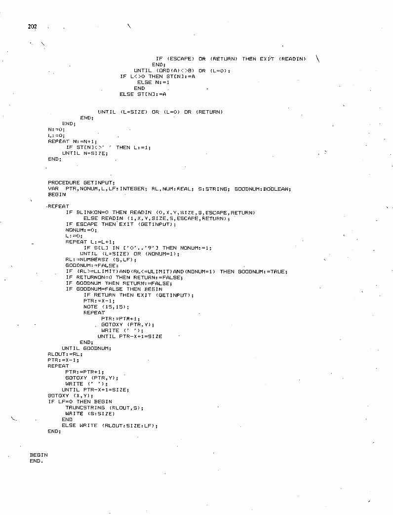
202
IF (ESCAPE) OR (RETURN) THEN EXPT (READIN) - END
UNTIL (ORD(A)<>8) OR (L=O) - IF L<>O THEN STCN]:=A
ELSE N:1 END
ELSE STENJ:A
UNTIL (L=SIZE) OR (L=O) OR (RETURN) END;
END;
L:0; REPEAT N:N+1;
IF STCNJ<>' THEN L:1; UNTIL NSIZE
END;
PROCEDURE GET INPUT; VAR PTR,NONUM,LLF: INTEGER; RL,NUM:REAL; S:STRING; GOODNUM:BOOLEAN; BEGIN
-REFEAT IF BLINKON=O THEN READIN
ELSE READIN (1X,Y5IZES,E5CAPERETUPN); IF ESCAPE THEN EXIT (GETINPUT); NONUM: 0; L:0; REPEAT L:L+l;
IF SEL) IN E'O''9'J THEN NONUM:1; UNTIL (LSIZE) OR (NONUM1);
RL:NUMBERSZ (SLF); GOODNUM:FALSE; IF (RL)-=LLIMIT)AND(RL<=ULIMIT)AND(NONUP1=1) THEN GOODNUM:=TRUE; IF RETURNON=O THEN RETURN:=FALSE; IF 600DNUM THEN RETURN:FALSE; IF GOODNUM=FALSE THEN BEGIN
IF RETURN THEN EXIT (GETINPUT); PTR: X-l; NOTE (15,1); REPEAT
PTR: PTR+l; GOTOXY (PTRY); WRITE (' ');
UNTIL PTR-X+1=SIZE END;
UNTIL 600DNUM; RLOUT: RL; PTR:X-1; REPEAT
PTR:PTR+1; GOTOXY (PTRY); WRITE (' '); UNTIL PTR-X+1SIZE;
GOTOXY (X,Y); IF LF=O THEN BEGIN
TRUNCSTRING (RLOUTS); WRITE (S:SIZE)
END ELSE WRITE (RLOUT:SIZE:LF);
END;
BEGIN END.
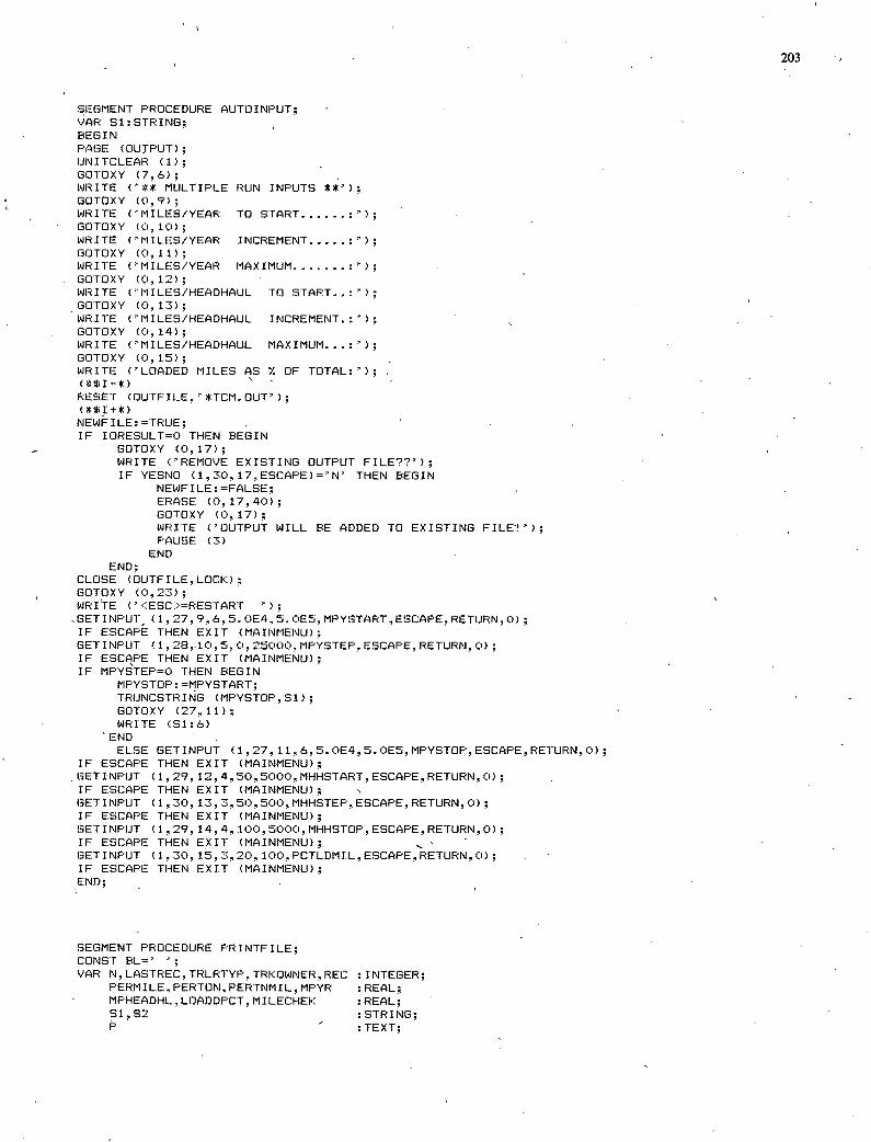
SEGMENT PROCEDURE AUTOINPUT; VAR Sl:STRING; BEGIN PAGE (OUTPUT); UNITCLEAR (1); GOTOXY (7,6); WRITE ('* MULTIPLE RUN INPUTS GOTOXY (0,9); WRITE ('MILES/YEAR TO START....... GOTOXY (0, 10) WRITE ('MILES/YEAR INCREMENT ...... GOTOXY (0,11); WRITE ('MILES/YEAR MAXIMUM....... GOTOXY (0, 12) WRITE (MILES/HEADHAUL TO START..:'); GOTOXY (0,13); WRITE ('MILES/HEADHAUL INCREMENT.:'); GOTOXY (0, 14) WRITE ('MILES/HEADHAUL MAXIMUM...:'); GOTOXY (0,15); WRITE ('LOADED MILES AS X OF TOTAL:');
RESET (OUTFILE. '*TCM. OUT'); (*$I+*) NEWFILE:TRUE; IF IORESULT=0 THEN BEGIN
GOTOXY (0,17); WRITE ('REMOVE EXISTING OUTPUT FILE??'); IF YESNO (1,30,17,ESCAPE)='N' THEN BEGIN
NEWFILE:FALSE; ERASE (0,17,40); GOTOXY (0, 17) WRITE ('OUTPUT WILL BE ADDED TO EXISTING FILE''); PAUSE (3)
END END;
CLOSE (OUTFILE. LOCK); GOTOXY (0,23); WRITE ('<ESC.>=RESTART SGETINPUT, (1,27,9,6,5.0E4,5.OES,MPYSTART,ESCAPE,RETURN,0); IF ESCAPE THEN EXIT (MAINMENU); GETINPUT (1,28,10,5,0,25000,MPYSTEP, ESCAPE, RETURN,0); IF ESCAPE THEN EXIT (MAINMENU); IF MPYSTEP=0 THEN BEGIN
MPYSTOP: MPYSTART; TRIJNCSTRING (MPYSTOP,S1); GOTOXY (27,11); WRITE (S1:8)
'END ELSE GETINPUT (1,27,11,6,5.0E4,5.OE5,MPYSTOP,ESCAPE,RETURN,0);
IF ESCAPE THEN EXIT (MAINMENU); GETINPUT (1,29.12.4,50,5000,MHHSTART,ESCAPE,RETURN,0); IF ESCAPE THEN EXIT (MAINMENU); GETINPUT (1,30,13,3,50,500,MHHSTEP,ESCAPE,RETURN,0); IF ESCAPE THEN EXIT (MAINMENU); GETINPUT (1,29,14,4,100,5000,MHHSTOP,ESCAPE,RETURN,0); IF ESCAPE THEN EXIT (MAINMENU); GETINPUT (1,30,15,3,20,100.PCTLDMIL,ESCAPE,RETURN,0); IF ESCAPE THEN EXIT (MAINMENU); END;
SEGMENT PROCEDURE PRINTFILE; CONSI E>L=' VAR N. LASTREC. TRLRTYP, TRKOWNER. REC : INTEGER;
PERMILE, PERTON, PERTNMIL, MPYR : REAL; MPHEADHL. LOADDPCT, MILECHEK : REAL; S1,S2 :STRING; P I
: TEXT;
203
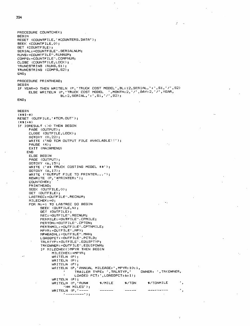
204
PROCEDURE COUNTCHEK; BEGIN RESET (COUNTFILE. '*COUNTERS. DATA'); SEEK (COUNTFILE, 0) GET (COUNTFILE); SERIAL: =COUNTFILE. SERIALNUM; RUNS: =COUNTFILE'. RUNNUM; COMPS: =COUNTFILE'. COMPNUM; CLOSE (COUNTFILE,LOCK); TRUNCSTRING (RUNS,S1); TRUNCSTRING (COMPS.S2) END;
PROCEDURE PR I NTHEAD; BEGIN IF YEARO THEN WRITELN (P,'TRUCK COST MODEL',BL:12,SERIAL,':',S1,'/',S2)
ELSE WRITELN (P,'TRUCK COST MODEL ',MONTH:2,'/',DAY:2,'/'.YEAR, BL:2,SERIAL,':',S1,'/'.S2);
END;
BEGIN (*$I-*) RESET (OUTFILE, '*TCM.. OUT'); (*$I+*) IF IORESULT <>0 THEN BEGIN
PAGE (OUTPUT); CLOSE (OUTFILE,LOCK); GOTOXY (0.22); WRITE ('NO TCM OUTPUT FILE AVAILABLEH'); PAUSE (4); EXIT (MAINMENU) END ELSE BEGIN PAGE (OUTPUT); GOTOXY (6,13); WRITE ('** TRUCK COSTING MODEL GOTOXY (6,17); WRITE ('OUTPUT FILE TO PRINTER...'); REWRITE (P, '*PRINTER:'); COUNTCHEK; PRINTHEAD; SEEK (OUTFILE. C)); GET (OUTFILE); LASTREC:OUTFILE'.RECNUM; MILECHEK: =0; FOR N:1 TO LASTREC DO BEGIN
SEEK (OUTFILE,N); GET (OUTFILE); REC:=OUTFILE".RECNUM; PERMILE: OUTFILE". CPMILE; PERTON: OUTFILE'. CPTON; PERTNMIL:OUTFILE'. CPTNMILE; MPYR: OUTFILE'.MPY; t'IPHEADHL: OUTFILE". MHH; LOADDPCT: 'OUTFILE'. PCTLD; TRLRTYP:"OUTFILE.EQUIPTYP; TRKOWNER: =OUTFILE'. EQUIPOWN; IF MILECHEK<:>MPYR THEN BEGIN
M I LECHEK: =MPYR; WRITELN (P); WRITELN (P); WRITELN (P); WRITELN (P.'ANNUAL MILEAt3E:',MPYR:10:1.
TRAILER TYPE: ',TRLRTYP.'
OWNER: ',TRKOWNER. LOADED PCT:',LOADDPCT:6:1);
WRITELN (P); WRITELN (P,'RUN# $/MILE $/TON
$/TONMILE 'HH MILES');
WRITELN (P, '----
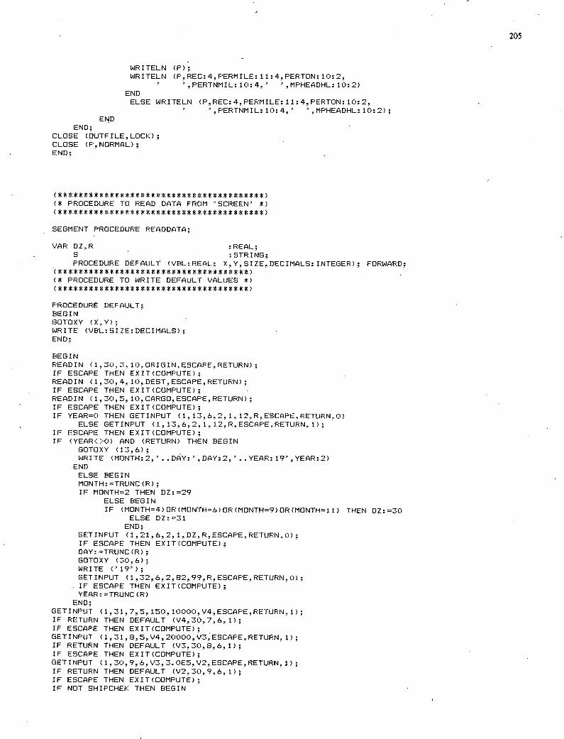
WRITELN (P) WRITELN (PREC:4.PERMILE:11:4.PERTON:10:2,
,PERTNMIL: 10:4,' ',MPHEADHL: 10:2) END ELSE WRITELN (P,REC:4.,PERMILE:11:4.PERTON:10:2,
'.PERTNMIL:1():4,' ',MPHEADHL:10:2); END
END; CLOSE (OUTFILE,LOCK); CLOSE (P,NORMAL); END;
(* PROCEDURE TO READ DATA FROM 'SCREEN' *)
SEGMENT PROCEDURE READDATA;
VAR DZ,R :REAL; S : STRING; PROCEDURE DEFAULT (VBL: REAL; X, V. SIZE, DECIMALS: INTEGER); FORWARD;
('K PROCEDURE TO WRITE DEFAULT VALUES 'K)
PROCEDURE DEFAULT; BEGIN (3OTOXV (X.Y); WRITE (VBL:SIZE:DECIMALS); END;
BEGIN READIN (1,30,3,10,ORIt3IN,ESCAPE,RETURN); IF ESCAPE THEN EXIT(COMPUTE); READIN (1,30.4,10,DEST,ESCAPE.RETURN); IF ESCAPE THEN EXIT(COMPUTE); READIN (1,30,5,10,CAF:GO,ESCAPE,RETUF:N); IF ESCAPE THEN EXIT(COMPUTE); IF YEAR=0 THEN GETINPUT (1,13,6,2,1,12,R,ESCAPE,RETURN,0)
ELSE GETINPUT (i,13,6,2,1,12,R,EE3CAPE,RETURN,1); IF ESCAPE THEN EXIT(COMPUTE); IF VEAR< >0) AND RETURN THEN BEGIN
GOTOXY (13,6); WRITE (MONTH:2,'...DAY:',DAY:2,'.YEAR:19',VEAR:2)
END ELSE BEGIN MONTH: TRUNC (R); IF MONTH2 THEN DZ:29
ELSE BEGIN IF (MONTH=4) OR (MONTH=6) OR (MONTH=9) OR (MONTH1 1) THEN DZ: '30
ELSE DZ:31 END;
GETINPUT (1,21,6,2,1,DZ,R,ESCAPE,RETURN,0); IF ESCAPE THEN EXIT(COMPUTE); DAV:TRUNC(R); GOTDXY (30,6); WRITE ('19'); GETINPUT (1.32,6,2,82,99,R,ESCAPE,RETURN,0); IF ESCAPE THEN EXIT(COMPUTE); YEAR: TRUNC (R)
END; GETINPUT (1,31,7,5,150,10000,V4,ESCAFE,RETURN,1); IF RETURN THEN DEFAULT (V4,30,7,6,1); IF ESCAPE THEN EXIT(COMPUTE); GETINPUT (1,31,8,5,V4,20000,V3,ESCAPE,RETURN,1); IF RETURN THEN DEFAULT (V3,30,8,6,1); IF ESCAPE THEN EXIT(COMPUTE); GETINPUT (1.30,9,6,V3..3.0E5.V2,ESCAPE,RETURN. 1); IF RETURN THEN DEFAULT (V2,30,9,6,1); IF ESCAPE THEN EXIT(COMPUTE); IF NOT SHIPCHE}< THEN BEGIN
205
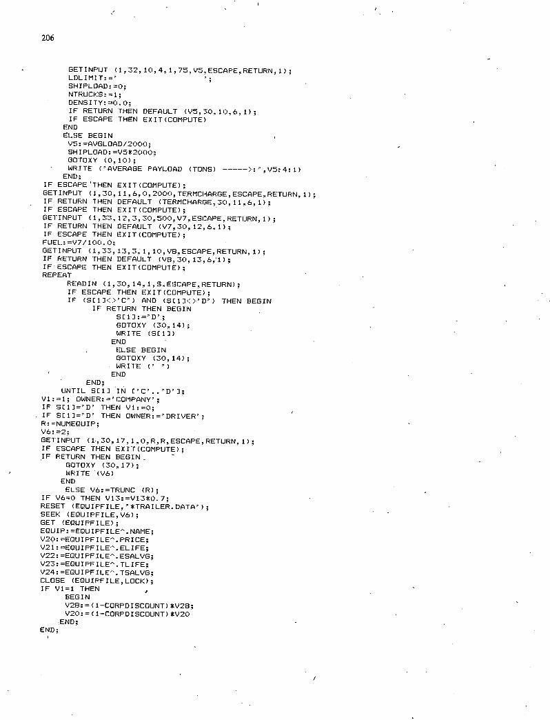
206
GETINPUT (1,32. 104. 17 V5ESCAPERETURN, 1); LDLItIIT: SHIPLOAD: 0; NTRUCKS: =1; DENSITY: =0. 0; IF RETURN THEN DEFAULT (V5,30,10,6,1); IF ESCAPE THEN EXIT(COMPUTE)
END ELSE BEGIN V5: =AVGLOAD/2000; SHIPLOAD: =V5*2000; GOTOXY (0,10); WRITE ('AVERAGE PAYLOAD (TONS) ----->: ',V:4:1)
END; IF ESCAPE THEN EXIT(COMPUTE); GETINPUT (1,30, 11,6,0,2000,TERMCHARGE,ESCAPE,RETURN, 1); IF RETURN THEN DEFAULT (TERMCHARGE, 30, 11,6, 1); IF ESCAPE THEN EXIT(COMPUTE); GETINPUT (133,123,30500,V7,ESCAPE,RETURN,1); IF RETURN THEN DEFAULT (V7,30,12,6,1); IF ESCAPE THEN EXIT(COMPUTE); FUEL:=V7/100.O; GETINPUT (1,33,13,31,10,V8,ESCApE,RETURN,1); IF RETURN THEN DEFAULT (V8, 30, 13.6,1); IF ESCAPE THEN EXIT(COMPUTE); REPEAT
READIN (1,30,14.1.S,ESCAPE,RETURN); IF ESCAPE THEN EXIT(COMPUTE); IF (S[1J<>'C') AND (S[1]<>'D') THEN BEGIN
IF RETURN THEN BEGIN GEl]: GOTOXY (30,14); WRITE (SEl])
END ELSE BEGIN GOTOXY (30,14); WRITE ('
END END;
UNTIL SEl] IN ['C'.. V1:1; OWNER:='COMPANY'; IF SE1]='D' THEN V1:=0; IF SE11='D' THEN OWNER:='DRIVER'; R: =NUMEQUIP; V6: '2; GETINPUT (1,30,17,1,0,R,R,ESCAPE,RETURN,1); IF ESCAPE THEN EXIT(COMPUTE); IF RETURN THEN BEGIN
GOTOXY (30,17); WRITE (V6)
END ELSE V6:=TRUNC (R);
IF V6=0 THEN V13:=V13*0.7; RESET (EQUIPFILE, ' *TRAILER.DATA'); SEEK (EQUIPFILE,V6); GET (EOUIPFILE); EQUIP: rEQUIPFILE". NAME; V20: =EQUIPFILE'. PRICE; V21:=EQUIPFILE.ELIFE; V22: =EQUIPFILE'. ESALVG; V23:EQUIPFILE". TLIFE; V24: =EOUIPFILE'. TSALVG; CLOSE (EQUIPFILE, LOCK); IF V1=1 THEN
BEGIN V28: = ( 1-CORPDISCOUNT) *V28; V20: = ( 1-CORPDISCOUNT) *V20
END; END;
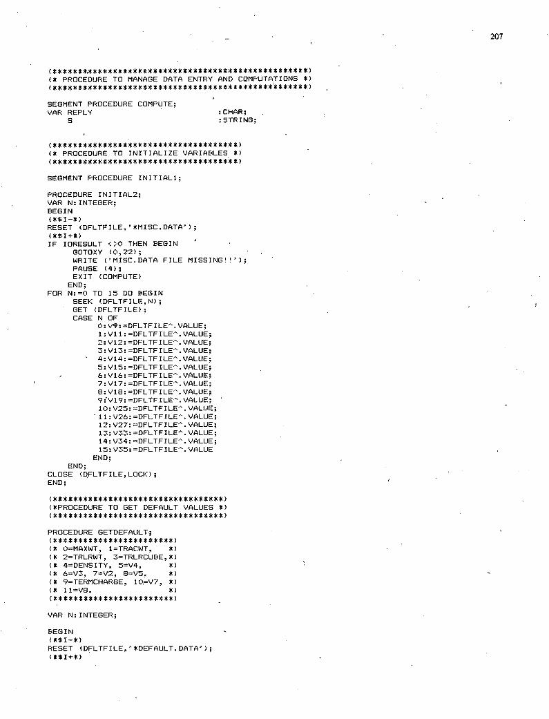
(* PROCEDURE TO MANAGE DATA ENTRY AND COMPUTATIONS *) CX * * * * * * * * * * * * * * * * * * * * * * * * * * * * * * IC * * * * * * * * * * * XX * * * * * *)
SEGMENT PROCEDURE COMPUTE; VAR REPLY CHAR;
S :STRING;
XX XXX XXX ************ ***** **** CX PROCEDURE TO INITIALIZE VARIABLES *)
SEGMENT PROCEDURE INITIAL1;
PROCEDURE INITIAL2; VAR N: INTEGER; BEGIN (X$I-X) RESET (DFLTFILE,'*MISCDATA'); (*$I+*) IF IORESULT <>0 THEN BEGIN
GOTOXY (0,22); WRITE ('MISC.DATA FILE MISSING''); PAUSE (4); EXIT (COMPUTE)
END; FOR N:0 TO 15 DO BEGIN
SEEK (DFLTFILEN); GET (DFLTFILE); CASE N OF
0: V9: DFLTFILE'. VALUE; 1: Vii: DFLTFILE". VALUE; 2:V12:=DFLTFILEVALUE; 3:V13:rDFLTFILE'.VALUE; 4:V14:DFLTFILE'.VALUE; 5:V15:DFLTFI.LE.VALUE; 6:V16:DFLTFILE". VALUE; 7:V17:DFLTFILE'.VALUE; 8: ViB: DFLTFILE'. VALUE; 9jV19:DFLTFILE.VALUE; 10:V25:'DFLTFILE'.VALUE; 11:V26:DFLTFILE.VALUE;
V27: =DFLTFILE'. VALUE; V33: =DFLTFILE'. VALUE; V34:DFLTFILE". VALUE;
15:V35:DFLTFILE.VALUE END;
END; CLOSE (DFLTFILE,LOCK); END;
(*PROCEDURE TO GET DEFAULT VALUES *) C * XX XX **X***** XX XXX XX XXX KX**X XX
PROCEDURE GETDEFAULT; C * X*X* X**X ***** **X* XXX XXX) (X 0=MAXWT, 1=TRACWT, *) CX 2=TRLRWT, 3=TRLRCUBE.X) CX 4=DENSITY, 5=V4, X) CX 6=V3, 7V2, 8=V5. *) CX 9=TERMCHARGE, 10=V7, X) CX 11=V8. *)
VAR N: INTEGER;
BEGIN (*$I-X) RESET (DFLTFILE. '*DEFAULT. DATA'); (XSI+*)
207
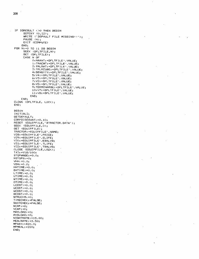
208
IF IORESULT <>C THEN BEGIN GOTOXY (0.22); WRITE ('DEFAULT FILE MISSING'!'); PAUSE (4); EXIT (COMPUTE)
END; FOR N:=0 TO 11 DO BEGIN
SEEK (DFLTFILE.N); GET (DFLTFILE); CASE N OF
0: MAXWT: DFLTFILE'. VALUE; TRACWT: =DFLTFILE. VALUE; TRLRWT: =DFLTFILE". VALUE; TRLRCUBE: =DFLTFILE'. VALUE; DENSITY: DFLTFILE... VALUE;
: V4: DFLTFILE. VALUE; V3: DFLTFILE.... VALUE; V2: =DFLTFILE'. VALUE; V!: DFLTFILE'. VALUE; TERMCHARGE: DFLTFILE'. VALUE; V7: DFLTFILE". VALUE;
11:V8:=DFLTFILE....VALUE; END;
END; CLOSE (DFLTFILE. LOCK); END;
BEGIN INITIAL2; (3ETDEFAULT; CORPDISCOUNT:=O. 10; RESET (EQUIPFILE, '*TRACTOR. DATA'); SEEK (EOUIPFILE.0) GET (EQUIPFILE); TRACTOR: =EOUIPFILE'. NAME; V28: EQUIPFILE'. PRICE; V29:EQIJIPFILE'.ELIFE; V30: =EOUIPFILE'. ESALVG; V31:=EOUIPFILE-'.,TLIFE; V32: =EOUIPFILE. TSALVG; CLOSE (EQUIPFILE,LOCK); TX3:=V18/100; STOPWAGE:'rO. C); NSTOPS: 0; VHH: 0 C); VDH:0.0; HHTIME: =0. C); DHTIME: 0. C); LTIME: =0.0; UTIME: 0. C); WTIME:0.0; OTIME: 0. 0; LCOST: =0. C); UCC)ST: C). C); WCOST: '0. C); OCOST: =0.):); NTRUCKS: =0; TIMECHEK: FALSE; SHIPCHEK: FAL5E; WCAP: =0; VCAP: 0; MAXLOAD:0; AVOLOAD: 'C); NIGHTRATE: =15.00; MEALRATE: 3. 50; MPDAY: '420. C); MPMEAL:200; END;
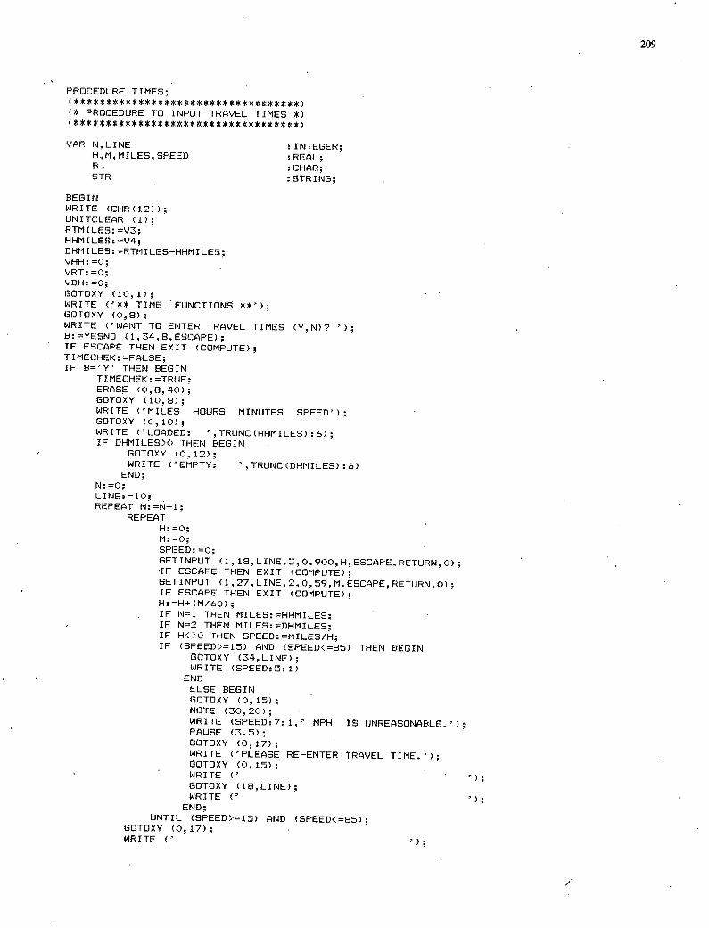
PROCEDURE TINES;
(* PROCEDURE TO INPUT TRAVEL TINES *)
VAR N.LINE :INTEGER; H,M,MILES..SPEED :REAL; B. : CHAR; STR :STRING;
BEGIN WRITE (CHR(12)); UNITCLEAR (1); RTMILES: V3; HHMILES: V4; DHMILES: RTMILES-HHMILES; VHH: 0; VRT: =0; VDH: =0; GOTOXY (10,1); WRITE ('** TINE FUNCTIONS GOTOXY (0,8); WRITE ('WANT TO ENTER TRAVEL TINES (Y,N)? B:YESNO (1,34,8.ESCAPE); IF ESCAPE THEN EXIT (COMPUTE); TIMECHEK: =FALSE; IF 8=' Y' THEN BEGIN
TIMECHEK: =TRUE; ERASE (0,8,40); GOTOXY (10,8); WRITE ('MILES HOURS MINUTES SPEED'); GOTOXY (0,10); WRITE ('LOADED: ', TRUNC (HHMILES) :6); IF DHNILES:>0 THEN BEGIN
GOTOXY (0,12); WRITE ('EMPTY: ',TRUNC(DHMILES):ó)
END; N: 0; LINE: REPEAT N:=N+1;
REPEAT H: =0;
SPEED: =0; GETINPUT (1.18,LINE,3,0,900,H,ESCAPE,RETtJRN,CJ); IF ESCAPE THEN EXIT (COMPUTE); GETINPUT (1,27,LINE,2,0,59,M,ESCAF'E,RETURN,o); IF ESCAPE THEN EXIT (COMPUTE); H:H+(M/60); IF N1 THEN MILESHHMILES; IF N=2 THEN MILES:DHMILES; IF H<)O THEN SPEED:MILE5/H; IF (SPEED>=15) AND (SPEED<=85) THEN BEGIN
GOTOXY (34,LINE); WRITE (SPEED:5:1)
END ELSE BEGIN GOTOXY (0,15); NOTE (30,20); WRITE (SPEED:7:1,' MPH IS UNREASONABLE.'); PAUSE (3.5); GOTOXY (0,17); WRITE ('PLEASE RE-ENTER TRAVEL TIME.'); GOTOXY (0,15); WRITE (' GOTOXY (18,LINE); WRITE ('
END; UNTIL (SPEED>=15) AND (SPEED<'85);
GOTOXY (0,17); WRITE (' ');
209
/
210
IF N=1 THEN VHH:SPEED; IF N=2 THEN VDH:=SPEED; LINE: 12; IF N=l THEN HHTIMEHHMILE5/VHH; IF N2 THEN DHTIME:=DHMILES/VDH; IF DHMILES=0 THEN N:=2; UNTIL N2;
END; PAGE (OUTPUT); RETURN: FALSE; END;
BEGIN INITIAL1; UNITCLEAR (1); REPEAT
WRITE (CHR(12)); GOTOXY (7,6); WRITE ('** DATA ENTRY OPTIONS GOTOXY (4,10); WRITE ('1. ENTER SHIPMENT DATA'); GOTOXY (4,12); WRITE ('2. ENTER STOP AND DELAY DATA');
- GOTOXY (0,23); WRITE ('<ESC)=RESTART <RETURN> TO CONTINUE'); REPLY:'*'; RETURN: FALSE; ESCAPE:FALSE; REPEAT
/ GOTOXY (0,21); WRITE ('ENTER NUMBER OF DESIRED OPTION: READIN (1,31,21, 1, S. ESCAPE. RETURN); REPLY: S[ 1]; UNTIL (REPLY IN E'1'..'2'1) OR (RETURN) OR (ESCAPE);
CASE REPLY OF SHIPMENT; STOPS;
END; UNTIL (RETURN) OR (ESCAPE);
WRITE (CHR(12)); IF ESCAPE THEN EXIT (COMPUTE)
ELSE BEGIN SCREEN; READDATA; TIMES; COSTCOMP
END; END;
THE TRANSPORTATION RESEARCH BOARD is an agency of the National Research Council, which serves the National Academy of Sciences and the National Academy of Engineering. The Board's purpose is to stimulate research concerning the nature and per-formance 9f transportation systems, to disseminate information that the research produces, and to encourage the application of appropriate research findings. The Board's program is carried out by more than 270 committees, task forces, and panels composed of more than 3,300 administrators, engineers, social scientists, attorneys, educators, and others concerned with transportation; they serve without compensation. The program is supported by state transpor-tation and highway departments, the modal administrations of the U.S. Department of Trans-portation, the Association of American Railroads, the National Highway Traffic Safety Administration, and other organizations and individuals interested in the development of transportation.
The Transportation Research Board operates within the National Research Council. The National Research Council was established by the National Academy of Sciences in 1916 to associate the broad community of science and technology with the Academy's purposes of furthering knowledge and of advising the Federal Government. The Council operates in ac-cordance with general policies determined by the Academy under the authority of its congres-sional charter of 1863, which establishes the Academy as a private, nonprofit, self-governing membership corporation. The Council has become the principal operating agency of both the National Academy of Sciences and the National Academy of Engineering in the conduct of their services to the government, the public, and the scientific and engineering communities. It is administered jointly by both Academies and the Institute of Medicine.
The National Academy of Sciences was established in 1863 by Act of Congress as a private, nonprofit, self-governing membership corporation for the furtherance of science and technology, and to advise the Federal Government upon request within its fields of competence. Under its corporate charter the Academy established the National Research Council in 1916, the National Academy of Engineering in 1964, and the Institute of Medicine in 1970.
NON-PROFIT ORG. U.S. POSTAGE
PAID WASHINGTON, D.C.
PERMIT NO. 42970
•L
1)
.j:: 'LJ -4 Z-4 o r- 0. Z-c) .)(
'-4'd4 0iU•
04W
TRANSPORTATION RESEARCH BOARD Naflonal Research Council
2101 ConstitutIon Avenue, N.W.
Washington, D.C. 20418
ADDRESS CORRECTION REQUESTED
Related Documents