arXiv:astro-ph/9903173v1 11 Mar 1999 Application of novel analysis techniques to Cosmic Microwave Background astronomy Aled Wynne Jones Mullard Radio Astronomy Observatory and King’s College, Cambridge. A dissertation submitted for the degree of Doctor of Philosophy in the University of Cambridge.

Welcome message from author
This document is posted to help you gain knowledge. Please leave a comment to let me know what you think about it! Share it to your friends and learn new things together.
Transcript
arX
iv:a
stro
-ph/
9903
173v
1 1
1 M
ar 1
999
Application of novelanalysis
techniques toCosmic Microwave Background
astronomy
Aled Wynne Jones
Mullard Radio Astronomy Observatory
andKing’s College, Cambridge.
A dissertation submitted for the degree of Doctorof Philosophy in the University of Cambridge.

i
Preface
This dissertation is the result of work undertaken at the Mullard Radio AstronomyObservatory, Cambridge between October 1994 and September 1997. The workdescribed here is my own, unless specifically stated otherwise. To the best of myknowledge it has not, nor has any similar dissertation, been submitted for a degree,diploma or other qualification at this, or any other university. This dissertation doesnot exceed 60 000 words in length.
Aled Wynne Jones
To Isabel and Ffion

ii
I am not sure how the universe was formed. But it knew how to do it, and that isthe important thing.
Anon. (child)
It is enough just to hold a stone in your hand. The universe would have beenequally incomprehensible if it had only consisted of that one stone the size of anorange. The question would be just as impenetrable: where did this stone come
from?Jostein Gaarder (in ‘Sophie’s World’)
Acknowledgements
Firstly I would like to thank the two people who have introduced me to theimmense field of microwave background anisotropies, Anthony Lasenby and StephenHancock. Without them I would not have begun to uncover the beauty at thebeginning of time. I would also like to thank Joss Bland-Hawthorn whose supervisionand enthusiasm during my time in Australia has made me more inquisitive in myfield. The many collaborations involved in this project have introduced me to manypeople without whom this thesis would not have been written; Graca Rocha andMike Hobson at MRAO, Carlos Gutierrez, Bob Watson, Roger Hoyland and RafaelRebolo at Tenerife, and Giovanna Giardino, Rod Davies and Simon Melhuish atJodrell Bank.

iii
I want to say a special thank you to the two women in my life that have keptme going for the last few years. Thanks to Ffion, my sister, whose insanity has keptme sane and thanks to Isabel whose support and encouragement I could not havedone without and whose love has made it all worth while.
Martina Wiedner, Marcel Clemens and Dave St. Jacques deserve a special men-tion for making my time in the department a little more bearable. Anna Moorefor putting up with me for three months in Australia. Cynthia Robinson, MartinGunthorpe, Nicholas Harrison, Liam Cox and Dafydd Owen for putting up with mefor the first years of my research.
I could not finish thanking people without mentioning Pam Hicks and DavidTitterington (special thanks for all the colour overhead transparencies) who havekept the department running smoothly.
I am also very grateful to PPARC for awarding me a research studentship. Maythey know better next time.
Yn olaf diolch yn fawr i fy rhieni sydd wedi rhoi i fyny efo fi am yr ugain mlynedddiwethaf.

iv
Contents
1 Introduction 1
1.0.1 Outline of thesis content . . . . . . . . . . . . . . . . . . . . . 2
2 The Universe and its evolution 5
2.1 Symmetry breaking and inflation . . . . . . . . . . . . . . . . . . . . 5
2.2 Dark matter . . . . . . . . . . . . . . . . . . . . . . . . . . . . . . . . 8
2.3 Coming of age . . . . . . . . . . . . . . . . . . . . . . . . . . . . . . . 9
2.3.1 The dipole . . . . . . . . . . . . . . . . . . . . . . . . . . . . . 10
2.3.2 Sachs-Wolfe effect . . . . . . . . . . . . . . . . . . . . . . . . . 10
2.3.3 Doppler peaks . . . . . . . . . . . . . . . . . . . . . . . . . . . 11
2.3.4 Defect anisotropies . . . . . . . . . . . . . . . . . . . . . . . . 11
2.3.5 Silk damping and free streaming . . . . . . . . . . . . . . . . . 12
2.3.6 Reionisation . . . . . . . . . . . . . . . . . . . . . . . . . . . . 12
2.3.7 The power spectrum . . . . . . . . . . . . . . . . . . . . . . . 13
2.4 The middle ages . . . . . . . . . . . . . . . . . . . . . . . . . . . . . . 14
2.4.1 Sunyaev–Zel’dovich effect . . . . . . . . . . . . . . . . . . . . 14
2.4.2 Extra–galactic sources . . . . . . . . . . . . . . . . . . . . . . 15
2.4.3 Galactic foregrounds . . . . . . . . . . . . . . . . . . . . . . . 17
2.5 Growing old . . . . . . . . . . . . . . . . . . . . . . . . . . . . . . . . 24
3 Microwave Background experiments 25
3.1 Atmospheric effect . . . . . . . . . . . . . . . . . . . . . . . . . . . . 26
3.2 General Observations . . . . . . . . . . . . . . . . . . . . . . . . . . . 27
3.2.1 Sky decomposition . . . . . . . . . . . . . . . . . . . . . . . . 27
3.2.2 The effect of a beam . . . . . . . . . . . . . . . . . . . . . . . 27
3.2.3 Sample and cosmic variance . . . . . . . . . . . . . . . . . . . 28
3.2.4 The likelihood function . . . . . . . . . . . . . . . . . . . . . . 28
3.3 Jodrell Interferometry . . . . . . . . . . . . . . . . . . . . . . . . . . 29
3.4 The Tenerife experiments . . . . . . . . . . . . . . . . . . . . . . . . . 31
3.5 The COBE satellite . . . . . . . . . . . . . . . . . . . . . . . . . . . . 32
3.6 The Planck Surveyor satellite . . . . . . . . . . . . . . . . . . . . . . 33
3.7 The MAP satellite . . . . . . . . . . . . . . . . . . . . . . . . . . . . 34
v
vi CONTENTS
4 The data 37
4.1 Jodrell Interferometry . . . . . . . . . . . . . . . . . . . . . . . . . . 374.1.1 Pre–processing . . . . . . . . . . . . . . . . . . . . . . . . . . 374.1.2 Calibration . . . . . . . . . . . . . . . . . . . . . . . . . . . . 384.1.3 Data processing . . . . . . . . . . . . . . . . . . . . . . . . . . 39
4.2 The Tenerife scans . . . . . . . . . . . . . . . . . . . . . . . . . . . . 414.2.1 Pre–processing . . . . . . . . . . . . . . . . . . . . . . . . . . 414.2.2 Stacking the data . . . . . . . . . . . . . . . . . . . . . . . . . 424.2.3 Calibration . . . . . . . . . . . . . . . . . . . . . . . . . . . . 424.2.4 Error bar enhancement . . . . . . . . . . . . . . . . . . . . . . 434.2.5 8.3 FWHM experiment . . . . . . . . . . . . . . . . . . . . . 434.2.6 5 experiments . . . . . . . . . . . . . . . . . . . . . . . . . . 46
5 Producing sky maps 55
5.1 CLEAN . . . . . . . . . . . . . . . . . . . . . . . . . . . . . . . . . . 565.2 Singular Value Decomposition . . . . . . . . . . . . . . . . . . . . . . 565.3 Bayes’ theorem . . . . . . . . . . . . . . . . . . . . . . . . . . . . . . 57
5.3.1 Pos/neg reconstruction . . . . . . . . . . . . . . . . . . . . . . 585.4 MEM in real space . . . . . . . . . . . . . . . . . . . . . . . . . . . . 59
5.4.1 Long period baseline drifts. . . . . . . . . . . . . . . . . . . . 595.4.2 The beam . . . . . . . . . . . . . . . . . . . . . . . . . . . . . 605.4.3 Implementation of MEM . . . . . . . . . . . . . . . . . . . . . 615.4.4 Errors on the MEM reconstruction . . . . . . . . . . . . . . . 645.4.5 Choosing α and m . . . . . . . . . . . . . . . . . . . . . . . . 655.4.6 Galactic extraction . . . . . . . . . . . . . . . . . . . . . . . . 66
5.5 MEM in Fourier space . . . . . . . . . . . . . . . . . . . . . . . . . . 675.5.1 Implementation of MEM in Fourier space . . . . . . . . . . . . 685.5.2 Updating the model . . . . . . . . . . . . . . . . . . . . . . . 685.5.3 Bayesian α calculation . . . . . . . . . . . . . . . . . . . . . . 695.5.4 Errors on the reconstruction . . . . . . . . . . . . . . . . . . . 70
5.6 The Wiener filter . . . . . . . . . . . . . . . . . . . . . . . . . . . . . 715.6.1 Errors on the Wiener reconstruction . . . . . . . . . . . . . . 735.6.2 Improvements to Wiener . . . . . . . . . . . . . . . . . . . . . 73
6 Testing the algorithms 75
6.1 CLEAN vs. MEM . . . . . . . . . . . . . . . . . . . . . . . . . . . . . 756.2 The Planck Surveyor simulations . . . . . . . . . . . . . . . . . . . . 77
6.2.1 The simulations . . . . . . . . . . . . . . . . . . . . . . . . . . 776.2.2 Singular Value Decomposition results . . . . . . . . . . . . . . 796.2.3 MEM and Wiener reconstructions . . . . . . . . . . . . . . . . 826.2.4 SZ reconstruction . . . . . . . . . . . . . . . . . . . . . . . . . 886.2.5 Power spectrum reconstruction . . . . . . . . . . . . . . . . . 89
6.3 The MAP simulations . . . . . . . . . . . . . . . . . . . . . . . . . . 906.3.1 MEM and Wiener results . . . . . . . . . . . . . . . . . . . . . 92
6.4 MEM and Wiener: the conclusions . . . . . . . . . . . . . . . . . . . 92
CONTENTS vii
6.5 Tenerife simulations . . . . . . . . . . . . . . . . . . . . . . . . . . . . 956.6 Discussion . . . . . . . . . . . . . . . . . . . . . . . . . . . . . . . . . 97
7 The sky maps 99
7.1 The Jodrell Bank 5GHz interferometer . . . . . . . . . . . . . . . . . 997.1.1 Wide–spacing data . . . . . . . . . . . . . . . . . . . . . . . . 997.1.2 Narrow–spacing data . . . . . . . . . . . . . . . . . . . . . . . 1037.1.3 Joint analysis . . . . . . . . . . . . . . . . . . . . . . . . . . . 104
7.2 The Tenerife experiments . . . . . . . . . . . . . . . . . . . . . . . . . 1087.2.1 Reconstructing the sky at 10.4 GHz with 8 FWHM . . . . . . 1087.2.2 Non-cosmological foreground contributions . . . . . . . . . . . 1107.2.3 The Dec 35 10 and 15 GHz Tenerife data. . . . . . . . . . . . 1117.2.4 The full 5 FWHM data set . . . . . . . . . . . . . . . . . . . 112
8 Analysing the sky maps 117
8.1 The power spectrum . . . . . . . . . . . . . . . . . . . . . . . . . . . 1178.2 Genus and Topology . . . . . . . . . . . . . . . . . . . . . . . . . . . 118
8.2.1 What is Genus? . . . . . . . . . . . . . . . . . . . . . . . . . . 1188.2.2 Simulations . . . . . . . . . . . . . . . . . . . . . . . . . . . . 1238.2.3 The Tenerife data . . . . . . . . . . . . . . . . . . . . . . . . . 1258.2.4 Extending genus: the Minkowski functionals . . . . . . . . . . 128
8.3 Correlation functions . . . . . . . . . . . . . . . . . . . . . . . . . . . 1298.3.1 Two point correlation function . . . . . . . . . . . . . . . . . . 1298.3.2 Three point correlation function . . . . . . . . . . . . . . . . . 1308.3.3 Four point correlation function . . . . . . . . . . . . . . . . . 131
9 Conclusions 135
9.1 Discussion . . . . . . . . . . . . . . . . . . . . . . . . . . . . . . . . . 1359.2 The future of CMB experiments . . . . . . . . . . . . . . . . . . . . . 137
References 139

viii CONTENTS
Chapter 1
Introduction
The Big Bang is the name given to the theory that describes how the Universe cameinto existence about 15 billion years ago at infinite density and temperature andthen expanded to its present form. The very early Universe was opaque due to theconstant interchange of energy between matter and radiation. About 300,000 yearsafter the Big Bang, the Universe cooled to a temperature of ∼ 3000C because ofits expansion. At this stage the matter does not have sufficient energy to remainionised. The electrons combine with the protons to form atoms and the cross sectionfor Compton scattering with photons is dramatically reduced. The radiation fromthis point in time has been travelling towards us for 15 billion years and has nowcooled to a blackbody temperature of 2.7 degrees Kelvin. At this temperature thePlanck spectrum has its peak at microwave frequencies (∼ 1 − 1000 GHz) and itsstudy forms a branch of astronomy called Cosmic Microwave Background astronomy(hereafter CMB astronomy). In 1965 Arno Penzias and Robert Wilson (Penzias &Wilson 1965) were the first to detect this radiation. It is seen from all directions inthe sky and is very uniform. This uniformity creates a problem. If the universe isso smooth then how did anything form? There must be some bumps in the earlyuniverse that could grow to create the structures we see today.
In 1992 the NASA Cosmic Microwave Background Explorer (COBE) satellitewas the first experiment to detect the bumps. These initial measurements werein the form of a statistical detection and no physical features could be identified.Today, experiments all around the world are finding these bumps that eventuallygrew into galaxies and clusters of galaxies. The required sensitivities called for newtechniques in astronomy. The main principle behind all of these experiments is that,instead of measuring the actual brightness, they measure the difference in brightnessbetween different regions of the sky. The experiments at Tenerife produced the firstdetection of the real, individual CMB fluctuations.
There are many different theories of how the universe began its life and how itevolved into the structures seen today. Each of these theories make slightly differentpredictions of how the universe looked at the very early stages which up until nowhave been impossible to prove or disprove. Knowing the structure of the CMB,within a few years it should be possible for astronomers to tell us where the universecame from, how it developed and where it will end up.
1
2 CHAPTER 1. INTRODUCTION
1.0.1 Outline of thesis content
This thesis covers four main topics: the detection of anisotropies of the CMB withdata taken by the Tenerife differencing experiments and Jodrell Bank interferome-ters, the analysis of this data to produce actual sky maps of the fluctuations, thepotential of future CMB experiments and subsequent analysis of the sky maps.
Chapter 2 introduces the processes involved in the formation of the fluctuationsand the resultant radiation we expect to see in our sky maps. This includes boththe CMB and other emission processes that operate at the frequencies covered byCMB experiments. These other processes are the Sunyaev–Zel’dovich effect, pointsource emissions and various Galactic foregrounds (namely dust, bremsstrahlungand synchrotron emission).
Chapters 3 and 4 present the experiments discussed in the thesis and the dataobtained from them. Preliminary analysis is done on the data to put constraintson Galactic emissions and point source contributions. The data discussed coversthe 5 GHz to 33 GHz frequency range which is at the lower end of the useful CMBspectral window. Lower frequency surveys are used to put constraints on the spectralindex of some of the Galactic foregrounds (the frequency range is not large enoughto put any useful constraints on dust emission which is expected to dominate athigher frequencies). The Tenerife experiments are used to put constraints on thelevel of the CMB anisotropy.
Chapter 5 introduces the concepts of the Maximum Entropy Method (MEM),the Wiener filter, CLEAN and Singular Value Decomposition. These four methodsoffer different alternatives to find the best underlying cosmological signal within thenoisy data. The usual approach of a positive–only Maximum entropy is enlarged tocover both positive and negative fluctuations, as well as multifrequency and multi-component observations. Simulations performed (Chapter 6) have shown that MEMis the best method of the four tested when attempting a reconstruction of the CMBsignal.
Chapter 7 presents the final sky maps of the CMB produced with the MaximumEntropy algorithm, as well as maps of the various contaminants that the experimentsare also sensitive to. The maps from a range of different experiments can be used toput constraints on various cosmological parameters such as the density parameter,Ω, Hubble’s constant, H, and the spectral index of the large scale CMB powerspectrum, n.
Chapter 8 presents subsequent analysis performed on the sky maps. These in-clude examining the topology using genus as well as looking at the power spectrumand correlation functions. The methods discussed are first applied to simulationsto test their usefulness at distinguishing between the origins of the fluctuations andthen applied to the reconstructed CMB sky maps.
New constraints on the power spectrum and some of the cosmological parameterswill be given in the final chapter. Here, the data and analysis described will bebrought together and the future of CMB experiments discussed.
Rhagarweiniad
3
O ble rydym ni i gyd yn dod? Pa brosesau wnaeth ddigwydd i greu popeth awelwn o’n cwmpas? I ateb y cwestiynau hyn byddai’n fanteisiol gallu teithio yn olmewn amser. Yn ol deddfau ffiseg mae hyn yn amhosibl, ond maent yn caniataurhywbeth sy’n ail orau i hynny. Gallwn edrych yn ol mewn amser. Mae golau’nteithio ar gyflymder penodol, felly os edrychwn yn ol ddigon pell gallwn weld yn oli ddechreuad y bydysawd. Er enghrifft, pan edrychwn ar yr haul mae mor bell felein bod yn edrych arno fel ag yr oedd wyth munud ynghynt.
Heddiw mae seryddwyr yn gallu gweld cyn belled yn ol mewn amser ag sy’nbosibl. Cymysegedd o fas ac ynni ymbelydrol yw’r bydysawd. Dros dymhereddarbennig (∼ 4000C), oherwydd ynni uchel yr ymbelydriad, mae’r rhyngweithiadrhwng mas ac ynni yn gwneud y bydysawd yn dywyll. Yn nechrau’r bydysawdroedd popeth wedi ei wasgu’n belen fechan poeth a ddechreuodd ehangu ac oeriwedyn. Felly, os, edrychwn yn ol mewn amser dylem weld y pwynt pryd y daethy bydysawd yn glir. Mae’r ymbelydriad o’r pwynt hwn mewn amser wedi bodyn teithio tuag atom am 15 biliwn o flynyddoedd ac mae wedi oeri i dymhereddo −270C erbyn hyn. Mae’r tymheredd hwn yn cyfateb i ymbelydriad microdon.Arno Penzias a Robert Wilson oedd y rhai cyntaf i ddarganfod yr ymbelydriad hwnyn 1965. Mae’n ymddangos o bob cyferiad yn yr awyr ac mae’n unffurf iawn. Mae’runffurfedd hwn yn achosi problem. Os yw’r bydysawd mor wastad sut y gwnaethunrhyw beth ffurfio? Mae’n rhaid fod yna rai gwrymiau yn y bydysawd cynnar igreu’r adeileddau a welwn heddiw.
Lloern Cosmic Microwave Background Explorer (COBE) NASA yn 1992 oedd yrarbrawf cyntaf i ddarganfod y gwrymiau. Ni llwyddod i dynnu lluniau o’r gwrymiaumewn gwirionedd oherwydd fod cymaint o swn yn gwneud hynny’n amhosibl. Daethar draws swn na’r arfer a’r unig eglurhad y gellid ei roi am hynny oedd presenoldebgwrymiau yn y bydysawd. Roedd hyn yn ffodus i seryddwyr neu byddent wedigorfod newid eu holl ddamcaniaethau. Erbyn heddiw mae mapiau o’r bydysawdcynnar hyd yn oed yn cael eu cynhyrchu. Led led y byd mae arbrofion yn darganfodgwrymiau a dyfodd yn y diwedd yn alaethau a chlystyrau o alaethau.
Roedd y gwaith hwn mor sensitif fel bod rhaid dyfeisio technegau newydd mewnseryddiaeth. Datblygwyd dulliau newydd o dynnu lluniau o’r awyr gyda thelegopaunewydd. Yr egwyddor sylfaenol y tu ol i’r holl arbrofion hyn oedd, yn hytrach na’ubod yn mesur y disgleirdeb gwirioneddol, eu bod yn mesur y gwahaniaeth mewndisgleirdeb rhwng gwahanol ranbarthau o’r awyr. Cynhyrchodd yr arbrofion ynTenerife y mapiau cyntaf o’r awyr. Mae Telesgop Anisotropy Caergrawnt hefyd yncynhyrchu mapiau o ranbarthau llai o’r awyr, gan weld gwrymiau llai na’r rhai awelwyd o Tenerife.
Bydd yr holl arbrofion hyn yn rhoi prawf ar ddamcaniaethau’r seryddwyr. Ceircannoedd o wahanol ddamcaniaethau ynglyn a’r modd y dechreuodd y bydysawd asut y datblygodd i’r adeileddau a welir heddiw. Mae pob un o’r damcaniaethau hynyn cynnig syniadau ychydig yn wahanol ynglyn a’r modd yr edrychai’r bydysawdyn gynnar yn ei hanes a hyd yma bu’n amhosibl eu profi neu eu gwrthbrofi.
O fewn ychydig flynyddoedd dylai fod yn bosibl i seryddwyr fedru dweud wrthymo ble y daeth y bydysawd, sut y datblygodd ac ym mhle y bydd yn gorffen. Mae’ngyfnod cyffrous i seryddwyr gyda holl gyfrinachau’r bydysawd yn disgwyl i gael eu

4 CHAPTER 1. INTRODUCTION
darganfod.
Chapter 2
The Universe and its evolution:
the origin of the CMB and
foreground emissions
In this chapter I summarise the various processes that go into forming the powerspectrum of fluctuations in the Cosmic Microwave Background. This includes pri-mordial effects as well as foreground effects like the Sunyaev-Zel’dovich effect. I alsodescribe the various foregrounds that have significant emissions at the frequenciesof interest to Microwave Background experiments.
The theory of the Big Bang stems from Edwin Hubble’s observations that everygalaxy is moving away from every other galaxy (providing they are not in gravita-tional orbit about each other). Hubble’s law tells us that the velocity of recessionaway from a point in the Universe is proportional to the distance to that point. To-day that constant of proportionality is called Hubble’s constant, H. If we extrapo-late this law back in time, there comes a point where everything in the Universe isvery close together. To get everything we see today into a very small region requiresan enormous amount of energy and this is where the Big Bang theory is born. Thishot, dense ‘soup’ expanded, cooled and eventually formed all the structures that wesee today.
2.1 Symmetry breaking and inflation
In physics, as things get hotter they generally get simpler. At a relatively lowtemperature (∼ 1015 K), compared to the Big Bang, the electromagnetic force andthe weak force, which binds the nucleus together, combine to form the electro–weakforce. At higher temperatures (∼ 1028 K) the strong force (described by QuantumChromo-Dynamics), which keeps the proton from splitting into its quarks, joins theelectro–weak force to become one force. This theory is called Grand Unification(GUT). It is hypothesised that the last force, the force of gravity, joins the otherforces in a theory of quantum gravity, at even higher temperatures (correspondingto the very earliest times in the Universe). At this stage everything in the Universe
5
6 CHAPTER 2. THE UNIVERSE AND ITS EVOLUTION
is indistinguishable from everything else. Matter and energy do not exist as separateentities and the Universe is very isotropic. To create structure in such a Universethere are two main theoretical models (or a combination of the two).
Starting from Newtonian physics and considering the effect of gravity on a unitmass at the edge of a sphere of radius R, then
R(t) = − GM
R2(t), (2.1)
where t is the time since the Big Bang and M is the mass inside the sphere, givenby
M =4
3πR3(t)ρ(t). (2.2)
In an expanding Universe, with no spontaneous particle creation, the amount ofmatter present does not change and so M is constant if we follow the motion of theedge of the sphere. Thus, if we write the present density of the Universe as ρ thenwe have
ρ(t) =R3(t)
R3(t)ρ, (2.3)
where t corresponds to now. The gravitational force per unit mass in Equation 2.1is therefore given by
R(t) = −4
3πGρR
−2(t) (2.4)
where R(t), the radius of the sphere today, is taken as unity. Integrating Equa-tion 2.4 gives
R2(t) =8
3πGρR
−1(t) − kc2. (2.5)
The constant of integration is found by including General Relativistic considerationswhere k is a measure of the curvature of space. So the equation of evolution of theUniverse is
(
R
R
)2
− 8πGρ
3= −kc
2
R2. (2.6)
We define Hubble’s constant, the rate of expansion of the Universe, as H = RR. In
General Relativity the Universe is said to be closed if the density is high enoughto prevent it from expanding forever. If the density is too low then the Universewill continue to expand forever and is called open. The point at which the densitybecomes critical (in between a closed and open Universe) corresponds to a flat space,or k = 0. This critical density is found from Equation 2.6 to be
ρcrit =3H2
8πG(2.7)
2.1. SYMMETRY BREAKING AND INFLATION 7
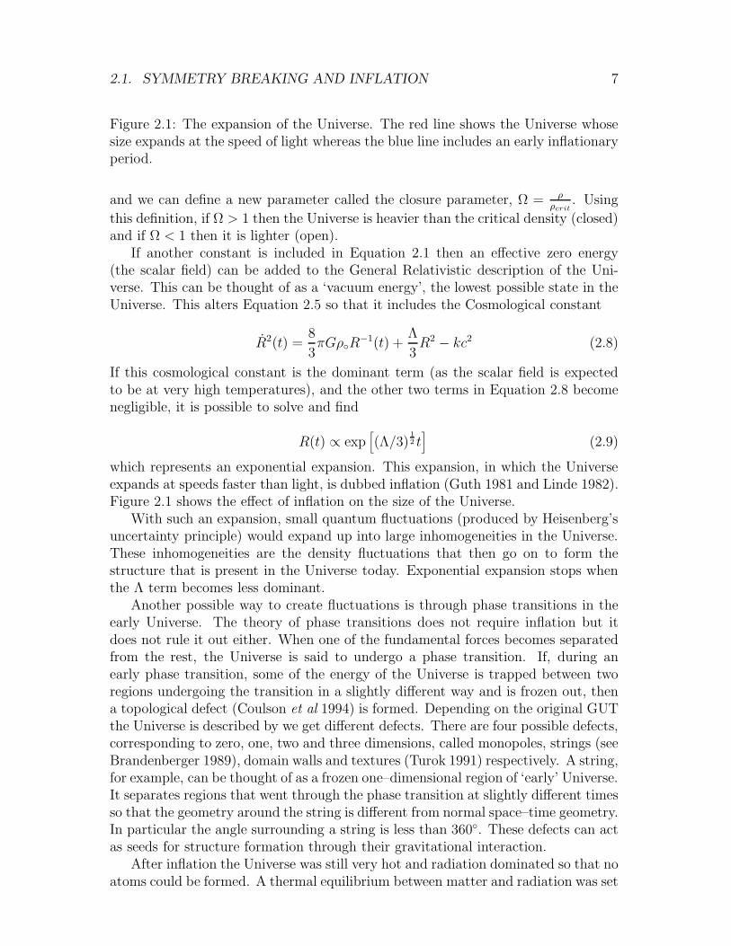
Figure 2.1: The expansion of the Universe. The red line shows the Universe whosesize expands at the speed of light whereas the blue line includes an early inflationaryperiod.
and we can define a new parameter called the closure parameter, Ω = ρρcrit
. Using
this definition, if Ω > 1 then the Universe is heavier than the critical density (closed)and if Ω < 1 then it is lighter (open).
If another constant is included in Equation 2.1 then an effective zero energy(the scalar field) can be added to the General Relativistic description of the Uni-verse. This can be thought of as a ‘vacuum energy’, the lowest possible state in theUniverse. This alters Equation 2.5 so that it includes the Cosmological constant
R2(t) =8
3πGρR
−1(t) +Λ
3R2 − kc2 (2.8)
If this cosmological constant is the dominant term (as the scalar field is expectedto be at very high temperatures), and the other two terms in Equation 2.8 becomenegligible, it is possible to solve and find
R(t) ∝ exp[
(Λ/3)12 t]
(2.9)
which represents an exponential expansion. This expansion, in which the Universeexpands at speeds faster than light, is dubbed inflation (Guth 1981 and Linde 1982).Figure 2.1 shows the effect of inflation on the size of the Universe.
With such an expansion, small quantum fluctuations (produced by Heisenberg’suncertainty principle) would expand up into large inhomogeneities in the Universe.These inhomogeneities are the density fluctuations that then go on to form thestructure that is present in the Universe today. Exponential expansion stops whenthe Λ term becomes less dominant.
Another possible way to create fluctuations is through phase transitions in theearly Universe. The theory of phase transitions does not require inflation but itdoes not rule it out either. When one of the fundamental forces becomes separatedfrom the rest, the Universe is said to undergo a phase transition. If, during anearly phase transition, some of the energy of the Universe is trapped between tworegions undergoing the transition in a slightly different way and is frozen out, thena topological defect (Coulson et al 1994) is formed. Depending on the original GUTthe Universe is described by we get different defects. There are four possible defects,corresponding to zero, one, two and three dimensions, called monopoles, strings (seeBrandenberger 1989), domain walls and textures (Turok 1991) respectively. A string,for example, can be thought of as a frozen one–dimensional region of ‘early’ Universe.It separates regions that went through the phase transition at slightly different timesso that the geometry around the string is different from normal space–time geometry.In particular the angle surrounding a string is less than 360. These defects can actas seeds for structure formation through their gravitational interaction.
After inflation the Universe was still very hot and radiation dominated so that noatoms could be formed. A thermal equilibrium between matter and radiation was set
8 CHAPTER 2. THE UNIVERSE AND ITS EVOLUTION
up by continual scattering. As the Universe cooled, processes not fully understoodas yet caused an excess of matter over anti-matter which started to form basic nuclei(deuterium, helium and lithium). This ‘soup’ of interacting particles and radiationhas a very high optical depth and so the radiation could not escape.
2.2 Dark matter
We have already defined the closure parameter of the Universe, Ω, as the ratio of theactual density of the Universe to the critical density. For Ω > 1 (a closed Universe)gravity will dominate and the Universe will collapse in on itself in a finite time.For Ω < 1 (an open Universe) the expansion will dominate and the Universe willcontinue growing forever. We can weigh the Universe by making observations of thestars and galaxies and estimating how heavy the objects are that we can see. In1978 observations were first reported of the rotation curve of galaxies and it wascalculated that there must be a lot more mass, unaccounted for by light (see Rubin,Ford & Thonnard, 1978). Later, observations were made of velocities of galaxiesin clusters and it was found that even more unseen mass was required to give thegalaxies their observed peculiar velocities. The Milky Way is in orbit around theVirgo cluster with a peculiar velocity of ∼ 600 kms−1 (see Gorenstein & Smoot 1981for the first measurement of this peculiar velocity, determined from the dipole in theCMB). The luminous mass in the Universe can account for Ωlum = 0.003h−1, whereh = H/100 km s−1 Mpc−1 and so, taking into account the non–luminous mass, ordark matter, this is a lower limit on Ω (see White 1989 for a review on dark matter).
It remains to be seen whether this dark matter can make Ω = 1 as simple inflationpredicts. The obvious question that comes to mind is – “In what form does thedark matter come?”. The most obvious candidate for dark matter is non–luminousbaryon matter. This can not exist as free hydrogen or dust clouds, otherwise wewould expect to see large black objects across the sky blocking out the starlight. Ifbaryonic, the dark matter must exist as gravitationally bound matter, either in theform of brown dwarfs (Carr 1990), planets, neutron stars or black holes. These mayexist in an extra–galactic halo around our galaxy and are called Massive CompactHalo Objects or MACHO’s for short (Alcock et al 1993). However, the amount ofbaryonic matter present in the Universe is constrained by the relative proportions ofhydrogen, helium, deuterium, lithium and beryllium that are observed as these wereformed together in the early Universe. This gives us 0.009 ≤ Ωbh
2 ≤ 0.02 (Copi etal 1995) and taking h = 0.5 then Ωb < 0.1 which means that 90% of the Universe ismade up of non–baryonic matter if it is spatially flat and closed (Ω = 1).
The non–baryonic matter must take the form of Weakly Interacting MassiveParticles (WIMPS; Turner 1991) which only interact with baryonic matter throughgravity (otherwise they would have been detected already). The theory of WIMPScan be subdivided into two categories; hot dark matter (HDM) and cold dark matter(CDM). Hot dark matter has large thermal velocities (for example, heavy neutrinos)and will wipe out structure on galactic scales in the early Universe due to stream-ing in the last scattering surface. This is a ‘top–down’ scenario. Cold dark matter
2.3. COMING OF AGE 9
has low thermal velocities (for example, axions and supersymmetric partners to thebaryonic matter) and will enhance the gravitational collapse of galactic size struc-tures. This is a ‘bottom–up’ scenario. The two theories are not mutually exclusiveand the combination of CDM and HDM is called mixed dark matter (MDM).
Constraints are already possible on some of the dark matter candidates. Forexample, in HDM if the dominant form of matter consists of heavy neutrinos, thenit can be shown (see Efstathiou 1989) that for a critical Universe (so Ω = 1) theneutrinos need to be about 30 eV in mass. With better measurements of the powerspectrum of the fluctuations seen in the CMB it will be possible to rule out orconfirm the existence of such particles. No candidate dark matter has yet beendetected.
2.3 Coming of age
At a redshift of z ∼ 1100, the Universe had cooled to a temperature of ∼ 3000 K.At this temperature electrons become coupled with protons and form atoms. Thisessentially increases the photon mean free path from close to zero to infinity ina very short time (∆z ∼ 80). So the furthest we can look back is to this lastscattering surface. This period is called the recombination era and is the originof the microwave background radiation studied in this thesis. By observing thisradiation the imprints of the fluctuations from the early part of the Universe canbe studied and hence cosmological models can be tested. The temperature of themicrowave background has now cooled down through the effects of cosmic expansionand has been measured to a very high degree of accuracy. It is found (see Mather,J.C. et al 1994) to be at
T = 2.726 ± 0.010K (95% confidence). (2.10)
The pattern of fluctuations in the radiation from the last scattering surfacewill tell us a lot about the early Universe. There are two models for how thematter fluctuations couple to the radiation fluctuations. These are adiabatic andisocurvature fluctuations. Inflation naturally produces the former but in specialconditions can produce the latter. Adiabatic fluctuations are perturbations in thedensity field which conserve the photon entropy of each particle species (the numberin a comoving volume is conserved). Isocurvature fluctuations are fluctuations inthe matter field with equal and opposite fluctuations in the photon field, keepingthe overall energy constant and therefore a constant curvature of space–time.
Due to the early coupling between matter and radiation, prior to the last scat-tering surface, an almost perfect blackbody would exist throughout the Universe atlast scattering. For blackbody emission, the spectrum (i.e. the CMB) is given bythe differential Planck spectrum
∆TA =∆Tx2ex
(ex − 1)2. (2.11)
Therefore the change in intensity is
10 CHAPTER 2. THE UNIVERSE AND ITS EVOLUTION
Figure 2.2: The dipole in the CMB as seen by the COBE satellite.
∆I(ν) =∆Tx4ex
(ex − 1)2, (2.12)
where x = hνkT
. The Universe progressively became more transparent and so thefluctuations seen at the last scattering surface are a superposition of fluctuationswithin a last scattering volume (comprising of the region between a totally opaqueand a totally transparent Universe). This can be expressed in terms of the opticaldepth, τ , as
∆T
T=∫ z
0
δT (z)
Te−τ(z)dτ
dzdz, (2.13)
where g(z) = e−τ(z) dτdz
is a Gaussian centred on z ∼ 1100 with ∆z ∼ 80, the widthof the last scattering surface (see, for example, Jones & Wyse 1985). Radiationfrom fluctuations smaller than the width of last scattering will add incoherentlyand therefore the radiation pattern of fluctuations will be erased on these small
scales. This corresponds to an angular size of θ = 3.8′Ω
12 on the sky today so all
anisotropies smaller than this will be heavily suppressed.
2.3.1 The dipole
The main source of anisotropy in the CMB is not intrinsic to the Universe. It isproduced by the peculiar velocity of the observer. Moving towards an object causesemitted light to appear blueshifted. As the Earth is not stationary with respectto the CMB (it is moving around the sun, the sun around the galaxy, the galaxyaround the Virgo cluster etc.) there will be a part of the CMB that the Earth movestowards and a part that it moves away from. Therefore, we expect to see a largedipole created by this Doppler effect. This dipole was clearly detected by the COBEsatellite (see Figure 2.2). It is necessary to remove this before attempting to studythe intrinsic fluctuations in the CMB.
2.3.2 Sachs-Wolfe effect
As the Universe grows older the observable Universe gets bigger, due to the finitespeed of light. The particle horizon of an observer is the distance to the furthestobject that could have affected that observer. Any objects further than this pointare not, and never have been, in causal contact with the observer. At the lastscattering surface the particle horizon corresponds to θ ∼ 2 as seen from Earthtoday. No physical processes will act on scales larger than this. Therefore, at theepoch of recombination fluctuations must have been produced by matter perturba-tions already present at this time. Inflation gives us a mechanism for the creationof these fluctuations. These matter perturbations give rise to perturbations in thegravitational potential. Radiation will experience different redshifts depending on
2.3. COMING OF AGE 11
Figure 2.3: The combined COBE maps showing the CMB over the full sky.
the potential and hence produce large angular scale anisotropies in the CMB. Thisprocess is called the Sachs–Wolfe effect (Sachs & Wolfe 1967).
It can be shown (see for example Padmanabhan 1993) that the angular depen-dence of the Sachs–Wolfe temperature fluctuations on scales greater than the horizonsize is given by
∆T
T∝ θ
(1−n)2 , (2.14)
where n is the spectral index of the initial power spectrum of fluctuations (P (k) =Akn). In inflation the natural outcome is a spectral index n = 1 because the fluctu-ations originate from quantum fluctuations that have no preferred scale (althoughrecently it has been shown that inflation does allow other possible values of n). Thisspecial case is called the Harrison–Zel’dovich (Harrison 1970 and Zel’dovich 1972)spectrum and leads to the ∆T
Tfluctuations being constant on all angular scales larger
than the horizon size. These fluctuations have been observed by the COBE satelliteat an angular scale of 7. The combined maps from the three observing frequenciesafter two years of COBE measurements at this angular scale are shown in Figure 2.3.
2.3.3 Doppler peaks
An overdensity in the early Universe does not collapse under the effect of self-gravityuntil it enters its own particle horizon when every point within it is in causal contactwith every other point. The perturbation will continue to collapse until it reachesthe Jean’s length, at which time radiation pressure will oppose gravity and set upacoustic oscillations. Since overdensities of the same size will pass the horizon sizeat the same time they will be oscillating in phase. These acoustic oscillations occurin both the matter field and the photon field and so will induce ‘Doppler peaks’ inthe photon spectrum.
The level of the Doppler peaks in the power spectrum depend on the numberof acoustic oscillations that have taken place since entering the horizon. For over-densities that have undergone half an oscillation there will be a large Doppler peak(corresponding to an angular size of ∼ 1). Other peaks occur at harmonics ofthis. As the amplitude and position of the primary and secondary peaks are intrin-sically determined by the number of electron scatterers and by the geometry of theUniverse, they can be used as a test of the density parameter of baryons and darkmatter, as well as other cosmological constants.
2.3.4 Defect anisotropies
The anisotropies produced by the various forms of defects arise from the effect thatthe defect has on the surrounding space–time (for example see Coulson et al 1994).Not only do they leave imprints on the CMB at the time of last scattering but a
12 CHAPTER 2. THE UNIVERSE AND ITS EVOLUTION
large proportion of the fluctuations due to defect anisotropies would be producedat latter times. As an example, consider the effect of cosmic strings (see Kaiser& Stebbins 1984). A string moving with velocity v will leave behind it a ‘gap’ inspace–time. The angle around the string is not 360 but is reduced by 8πGµ, whereµ is the energy density per unit length in the string. Therefore, photons travellingthrough space behind the string will experience a Doppler boost, with respect tophotons in front of the string, as they have less space to travel through. The valueof this boosting is
∆T
T= 8πGµ
v
c(2.15)
and is called the Kaiser–Stebbins effect. This results in a linear discontinuity in theCMB when the string passes in front and is easily discernible from the Gaussiananisotropies produced by the other processes. The higher dimensional defects willproduce more complicated discontinuities. Recently however, Magueijo et al 1996and Albrecht et al 1996 have shown that this discontinuity effect may be maskedby the defect interaction with the CMB prior to recombination. On large angularscales the discontinuities will also add together and mimic a Gaussian field (thecentral limit theorem). Therefore, only a high resolution (on the arcmin scale), highsensitivity, experiment will be able to distinguish between defect and inflationarysignatures on the CMB.
2.3.5 Silk damping and free streaming
Prior to the last scattering surface the photons and matter interact on scales smallerthan the horizon size. Through diffusion the photons will travel from high densityregions to low density regions ‘dragging’ the electrons with them via Compton in-teraction. The electrons are coupled to the protons through Coulomb interactionsand so the matter will move from high density regions to low density regions. Thisdiffusion has the effect of damping out the fluctuations and is more marked as thesize of the fluctuation decreases. Therefore, we expect the Doppler peaks to vanishat very small angular scales. This effect is known as Silk damping (Silk 1968).
Another possible diffusion process is free streaming. It occurs when collisionlessparticles (e.g. neutrinos) move from high density to low density regions. If theseparticles have a small mass then free streaming causes a damping of the fluctuations.The exact scale this occurs on depends on the mass and velocity of the particlesinvolved. Slow moving particles will have little effect on the spectrum of fluctuationsas Silk damping already wipes out the fluctuations on these scales, but fast moving,heavy particles (e.g. a neutrino with 30 eV mass), can wipe out fluctuations onlarger scales corresponding to 20 Mpc today (Efstathiou 1989).
2.3.6 Reionisation
Another process that will alter the power spectrum of the CMB is reionisation. If,for some reason, the Universe reheated to a temperature at which electrons and

2.3. COMING OF AGE 13
protons became ionised after recombination, then the interaction with the photonswould wipe out any small scale anisotropies expected. Today, there is reionisationaround quasars and high energy sources but this occurred too late in the historyof the Universe to have any large effect on the CMB. Little is known about theperiod between the last scattering surface and the furthest known quasar (z∼ 4) soreionisation cannot be ruled out.
2.3.7 The power spectrum
The usual approach to presenting CMB observations is through spherical harmonics.The expansion of the fluctuations over the sky can be written as
∆T
T(θ, φ) =
∑
ℓ,m
aℓmYℓm(θ, φ) (2.16)
where θ and φ are polar coordinates. Here aℓm represent the coefficients of theexpansion. For a random Gaussian field all of the statistical information can beobtained by considering the two–point correlation function, given by
C(β) =⟨
∆T
T(n1)
∆T
T(n2)
⟩
(2.17)
for the unit vectors n1 and n2 that define the directions such that n1.n2 = cos(β).Substituting Equation 2.16 into Equation 2.17 gives
C(β) =∑
ℓm
∑
ℓ′m′
< aℓma∗ℓ′m′ > Yℓm(θ, φ)Y ∗
ℓ′m′(θ′, φ′). (2.18)
If the CMB has no preferred direction, so that it is statistically rotationally sym-metric, then
C(β) =1
4π
∑
ℓ
(2ℓ+ 1)CℓPℓ(cosβ) (2.19)
defining < aℓmaℓ′m′ >= Cℓδℓℓ′δmm′ and the multiplication of spherical harmonicsgive the Legendre polynomials Pℓ(cosβ). If this is taken as a true indicator of theCMB then the Cℓ values can be used to give a complete statistical description ofthe fluctuations. These Cℓ values can be predicted from theory (normalised to anarbitrary value) and constitute the power spectrum of the CMB. For example, if astandard power law (P (k) = Akn) can be used to describe the fluctuations, as in thecase of the Sachs Wolfe effect, then Cℓ is given by (see Bond & Efstathiou, 1987)
Cℓ = C2Γ [ℓ + (n− 1)/2] Γ [(9 − n)/2]
Γ [ℓ+ (5 − n)/2] Γ [(3 + n)/2](2.20)
where Cℓ is now normalised to the quadrupole term C2 and Γ[x] are the Gammafunctions.
The power spectrum of the CMB is made up of a combination of all the competingprocesses already described. At large angular scales (corresponding to small ℓ valuesin the Fourier plane) the level of fluctuations (and hence ℓ(ℓ+1)Cℓ) will be constant
14 CHAPTER 2. THE UNIVERSE AND ITS EVOLUTION
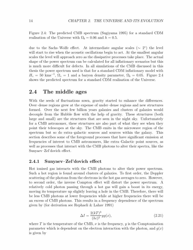
Figure 2.4: The predicted CMB spectrum (Sugiyama 1995) for a standard CDMrealisation of the Universe with Ωb = 0.06 and h = 0.5.
due to the Sachs–Wolfe effect. At intermediate angular scales (∼ 2) the levelwill start to rise when the acoustic oscillations begin to act. At the smallest angularscales the level will approach zero as the dissipative processes take place. The actualshape of the power spectrum can be calculated for all inflationary scenarios but thisis much more difficult for defects. In all simulations of the CMB discussed in thisthesis the power spectrum used is that for a standard CDM inflationary model withH = 50 kms−1, Ω = 1 and a baryon density parameter, Ωb = 0.05. Figure 2.4shows the predicted spectrum for a standard CDM realisation of the Universe.
2.4 The middle ages
With the seeds of fluctuations sown, gravity started to enhance the differences.Over–dense regions grew at the expense of under–dense regions and new structuresformed. Over the next few billion years galaxies and clusters of galaxies woulddecouple from the Hubble flow with the help of gravity. These structures (bothlarge and small) are the structures that are seen in the night sky. Unfortunatelyfor a CMB astronomer, these structures are also part of what they see when theypoint their telescopes at the sky. The CMB emits in the microwave region of thespectrum but so do extra–galactic sources and sources within the galaxy. Thissection describes some of the foreground processes that have significant emission atfrequencies of interest to CMB astronomers, like extra–Galactic point sources, aswell as processes that interact with the CMB photons to alter their spectra, like theSunyaev–Zel’dovich effect.
2.4.1 Sunyaev–Zel’dovich effect
Hot ionised gas interacts with the CMB photons to alter their power spectrum.Such a hot region is found around clusters of galaxies. To first order, the Dopplerscattering of the photons from the electrons in the hot gas averages to zero. However,to second order, the inverse Compton effect will distort the power spectrum. Arelatively cold photon passing through a hot gas will gain a boost in its energy,moving its temperature up slightly leaving a hole in the CMB. Therefore, there willbe less CMB photons at lower frequencies while at higher frequencies there will bean excess of CMB photons. This results in a frequency dependence of the spectrumgiven by (for derivation see Rephaeli & Lahav 1991)
∆I =2(kT )3
(hc)2yg(x), (2.21)
where T is the temperature of the CMB, ν is the frequency, y is the Comptonisationparameter which is dependent on the electron interaction with the photon, and g(x)is given by
2.4. THE MIDDLE AGES 15
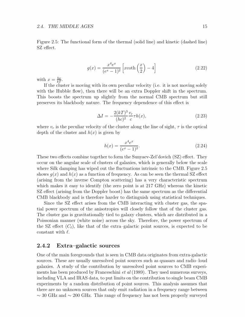
Figure 2.5: The functional form of the thermal (solid line) and kinetic (dashed line)SZ effect.
g(x) =x4ex
(ex − 1)2
[
xcoth(
x
2
)
− 4]
(2.22)
with x = hνkT
.If the cluster is moving with its own peculiar velocity (i.e. it is not moving solely
with the Hubble flow), then there will be an extra Doppler shift in the spectrum.This boosts the spectrum up slightly from the normal CMB spectrum but stillpreserves its blackbody nature. The frequency dependence of this effect is
∆I = −2(kT )3
(hc)2
vr
cτh(x), (2.23)
where vr is the peculiar velocity of the cluster along the line of sight, τ is the opticaldepth of the cluster and h(x) is given by
h(x) =x4ex
(ex − 1)2. (2.24)
These two effects combine together to form the Sunyaev-Zel’dovich (SZ) effect. Theyoccur on the angular scale of clusters of galaxies, which is generally below the scalewhere Silk damping has wiped out the fluctuations intrinsic to the CMB. Figure 2.5shows g(x) and h(x) as a function of frequency. As can be seen the thermal SZ effect(arising from the inverse Compton scattering) has a very characteristic spectrumwhich makes it easy to identify (the zero point is at 217 GHz) whereas the kineticSZ effect (arising from the Doppler boost) has the same spectrum as the differentialCMB blackbody and is therefore harder to distinguish using statistical techniques.
Since the SZ effect arises from the CMB interacting with cluster gas, the spa-tial power spectrum of the anisotropies will closely follow that of the cluster gas.The cluster gas is gravitationally tied to galaxy clusters, which are distributed in aPoissonian manner (white noise) across the sky. Therefore, the power spectrum ofthe SZ effect (Cℓ), like that of the extra–galactic point sources, is expected to beconstant with ℓ.
2.4.2 Extra–galactic sources
One of the main foregrounds that is seen in CMB data originates from extra-galacticsources. These are usually unresolved point sources such as quasars and radio–loudgalaxies. A study of the contribution by unresolved point sources to CMB experi-ments has been produced by Franceschini et al (1989). They used numerous surveys,including VLA and IRAS data, to put limits on the contribution to single beam CMBexperiments by a random distribution of point sources. This analysis assumes thatthere are no unknown sources that only emit radiation in a frequency range between∼ 30 GHz and ∼ 200 GHz. This range of frequency has not been properly surveyed
16 CHAPTER 2. THE UNIVERSE AND ITS EVOLUTION
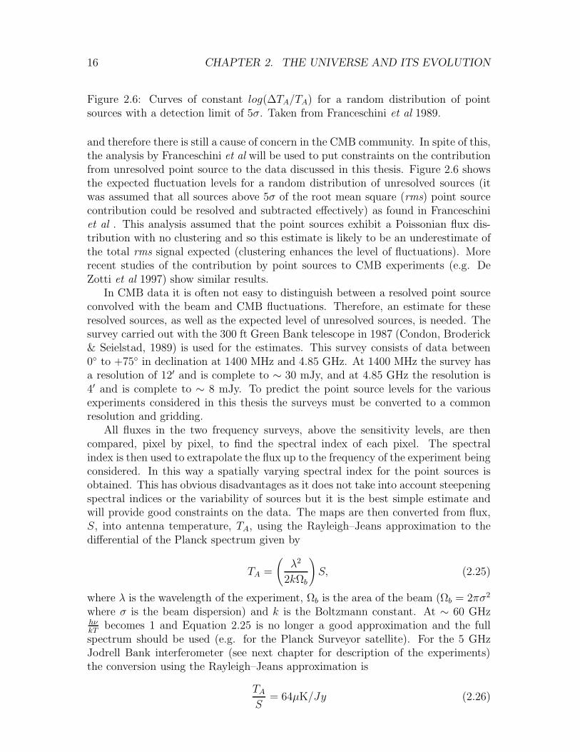
Figure 2.6: Curves of constant log(∆TA/TA) for a random distribution of pointsources with a detection limit of 5σ. Taken from Franceschini et al 1989.
and therefore there is still a cause of concern in the CMB community. In spite of this,the analysis by Franceschini et al will be used to put constraints on the contributionfrom unresolved point source to the data discussed in this thesis. Figure 2.6 showsthe expected fluctuation levels for a random distribution of unresolved sources (itwas assumed that all sources above 5σ of the root mean square (rms) point sourcecontribution could be resolved and subtracted effectively) as found in Franceschiniet al . This analysis assumed that the point sources exhibit a Poissonian flux dis-tribution with no clustering and so this estimate is likely to be an underestimate ofthe total rms signal expected (clustering enhances the level of fluctuations). Morerecent studies of the contribution by point sources to CMB experiments (e.g. DeZotti et al 1997) show similar results.
In CMB data it is often not easy to distinguish between a resolved point sourceconvolved with the beam and CMB fluctuations. Therefore, an estimate for theseresolved sources, as well as the expected level of unresolved sources, is needed. Thesurvey carried out with the 300 ft Green Bank telescope in 1987 (Condon, Broderick& Seielstad, 1989) is used for the estimates. This survey consists of data between0 to +75 in declination at 1400 MHz and 4.85 GHz. At 1400 MHz the survey hasa resolution of 12′ and is complete to ∼ 30 mJy, and at 4.85 GHz the resolution is4′ and is complete to ∼ 8 mJy. To predict the point source levels for the variousexperiments considered in this thesis the surveys must be converted to a commonresolution and gridding.
All fluxes in the two frequency surveys, above the sensitivity levels, are thencompared, pixel by pixel, to find the spectral index of each pixel. The spectralindex is then used to extrapolate the flux up to the frequency of the experiment beingconsidered. In this way a spatially varying spectral index for the point sources isobtained. This has obvious disadvantages as it does not take into account steepeningspectral indices or the variability of sources but it is the best simple estimate andwill provide good constraints on the data. The maps are then converted from flux,S, into antenna temperature, TA, using the Rayleigh–Jeans approximation to thedifferential of the Planck spectrum given by
TA =
(
λ2
2kΩb
)
S, (2.25)
where λ is the wavelength of the experiment, Ωb is the area of the beam (Ωb = 2πσ2
where σ is the beam dispersion) and k is the Boltzmann constant. At ∼ 60 GHzhνkT
becomes 1 and Equation 2.25 is no longer a good approximation and the fullspectrum should be used (e.g. for the Planck Surveyor satellite). For the 5 GHzJodrell Bank interferometer (see next chapter for description of the experiments)the conversion using the Rayleigh–Jeans approximation is
TA
S= 64µK/Jy (2.26)
2.4. THE MIDDLE AGES 17
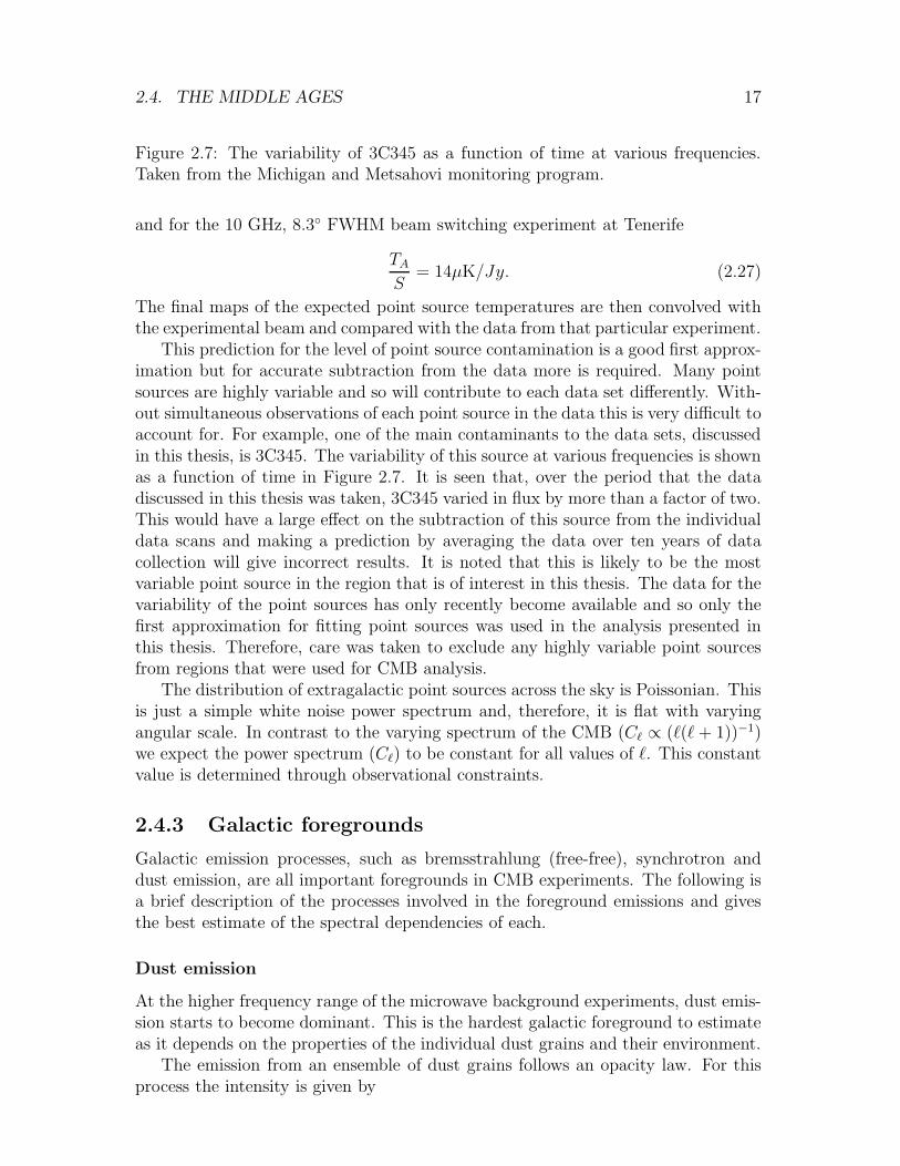
Figure 2.7: The variability of 3C345 as a function of time at various frequencies.Taken from the Michigan and Metsahovi monitoring program.
and for the 10 GHz, 8.3 FWHM beam switching experiment at Tenerife
TA
S= 14µK/Jy. (2.27)
The final maps of the expected point source temperatures are then convolved withthe experimental beam and compared with the data from that particular experiment.
This prediction for the level of point source contamination is a good first approx-imation but for accurate subtraction from the data more is required. Many pointsources are highly variable and so will contribute to each data set differently. With-out simultaneous observations of each point source in the data this is very difficult toaccount for. For example, one of the main contaminants to the data sets, discussedin this thesis, is 3C345. The variability of this source at various frequencies is shownas a function of time in Figure 2.7. It is seen that, over the period that the datadiscussed in this thesis was taken, 3C345 varied in flux by more than a factor of two.This would have a large effect on the subtraction of this source from the individualdata scans and making a prediction by averaging the data over ten years of datacollection will give incorrect results. It is noted that this is likely to be the mostvariable point source in the region that is of interest in this thesis. The data for thevariability of the point sources has only recently become available and so only thefirst approximation for fitting point sources was used in the analysis presented inthis thesis. Therefore, care was taken to exclude any highly variable point sourcesfrom regions that were used for CMB analysis.
The distribution of extragalactic point sources across the sky is Poissonian. Thisis just a simple white noise power spectrum and, therefore, it is flat with varyingangular scale. In contrast to the varying spectrum of the CMB (Cℓ ∝ (ℓ(ℓ+ 1))−1)we expect the power spectrum (Cℓ) to be constant for all values of ℓ. This constantvalue is determined through observational constraints.
2.4.3 Galactic foregrounds
Galactic emission processes, such as bremsstrahlung (free-free), synchrotron anddust emission, are all important foregrounds in CMB experiments. The following isa brief description of the processes involved in the foreground emissions and givesthe best estimate of the spectral dependencies of each.
Dust emission
At the higher frequency range of the microwave background experiments, dust emis-sion starts to become dominant. This is the hardest galactic foreground to estimateas it depends on the properties of the individual dust grains and their environment.
The emission from an ensemble of dust grains follows an opacity law. For thisprocess the intensity is given by
18 CHAPTER 2. THE UNIVERSE AND ITS EVOLUTION
I(ν) =∫
ǫ(ν)dl, (2.28)
where ǫ(ν) is the emissivity at frequency ν, and the integral is along the line of sight.The brightness temperature is found from the black body equation and is thereforea solution of
I(ν) =2hν3
c21
(ehνkT − 1)
. (2.29)
In the Rayleigh-Jeans approximation (where hν ≪ kT ).
Tb =c2I(ν)
2ν2k. (2.30)
This equation is used to convert between temperature and flux for all of the fore-ground emissions. Considering a constant line–of–site density of dust, it is possibleto combine Equations 2.30 and 2.28 to give
Tb ∝ ǫ(ν)ν−2. (2.31)
When modelling dust emission, it is therefore necessary to find the emissivity as afunction of frequency, as well as the flux level at a particular frequency.
From surveys of the dust emission (for example the COBE FIRAS results and theIRAS survey) it can be shown that low galactic latitude dust (dust in the galacticplane) is modelled well by a blackbody temperature of 21.3 K and an emissivity pro-portional to ν1.4, while at high galactic latitudes it is well modelled by a blackbodytemperature of 18 K and an emissivity proportional to ν2 (Bersanelli et al 1996).Since the observations discussed in this thesis are all at high galactic latitudes thedust models used have an assumed blackbody temperature of 18 K and a spectrawhich follows
∆I(ν) ∝ ∆Tx6ex
(ex − 1)2, (2.32)
where x = hνkT
. This equation is obtained by the differentiation of Equation 2.29with respect to T , multiplied by the dust emissivity.
As the dust emission comes from regions of warm interstellar clouds it is verylikely that there will also be ionised clouds associated with the neutral clouds(perhaps embedded within the neutral clouds or surrounding them, see McKee& Ostriker 1977 for an example of correlated features) and so we should expectbremsstrahlung from the same region (see below for description of bremsstrahlung).This results in an expected correlation between the dust and bremsstrahlung. Thiscorrelation has been detected (see for example Kogut et al 1996a or Oliveira-Costaet al 1997 who find a cross–correlation between the DIRBE dust maps and thelow frequency Saskatoon data which is contaminated by bremsstrahlung). In a fullanalysis of any data this correlation should be taken into account.
From IRAS observations of dust emission (Gautier et al 1992), it was found thatthe dust fluctuations have a power law that decreases as the third power of ℓ. This
2.4. THE MIDDLE AGES 19
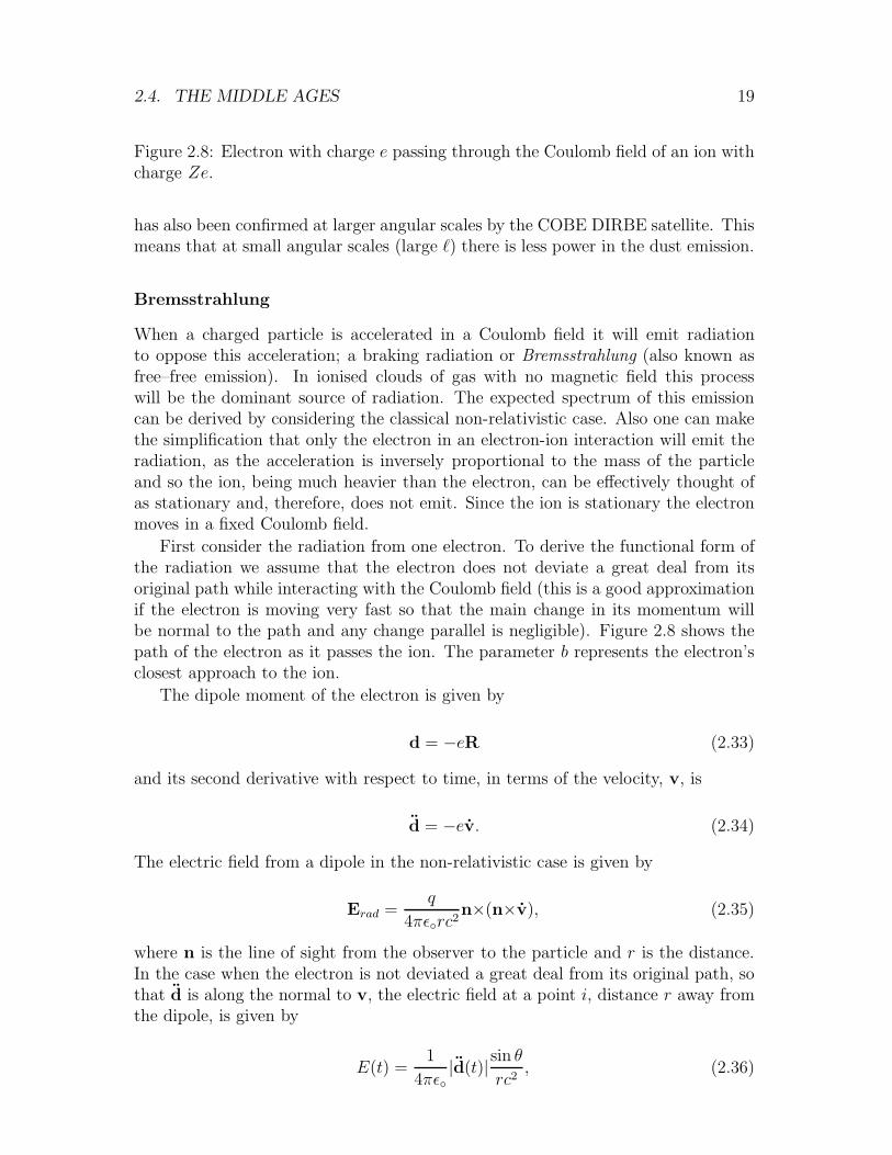
Figure 2.8: Electron with charge e passing through the Coulomb field of an ion withcharge Ze.
has also been confirmed at larger angular scales by the COBE DIRBE satellite. Thismeans that at small angular scales (large ℓ) there is less power in the dust emission.
Bremsstrahlung
When a charged particle is accelerated in a Coulomb field it will emit radiationto oppose this acceleration; a braking radiation or Bremsstrahlung (also known asfree–free emission). In ionised clouds of gas with no magnetic field this processwill be the dominant source of radiation. The expected spectrum of this emissioncan be derived by considering the classical non-relativistic case. Also one can makethe simplification that only the electron in an electron-ion interaction will emit theradiation, as the acceleration is inversely proportional to the mass of the particleand so the ion, being much heavier than the electron, can be effectively thought ofas stationary and, therefore, does not emit. Since the ion is stationary the electronmoves in a fixed Coulomb field.
First consider the radiation from one electron. To derive the functional form ofthe radiation we assume that the electron does not deviate a great deal from itsoriginal path while interacting with the Coulomb field (this is a good approximationif the electron is moving very fast so that the main change in its momentum willbe normal to the path and any change parallel is negligible). Figure 2.8 shows thepath of the electron as it passes the ion. The parameter b represents the electron’sclosest approach to the ion.
The dipole moment of the electron is given by
d = −eR (2.33)
and its second derivative with respect to time, in terms of the velocity, v, is
d = −ev. (2.34)
The electric field from a dipole in the non-relativistic case is given by
Erad =q
4πǫrc2n×(n×v), (2.35)
where n is the line of sight from the observer to the particle and r is the distance.In the case when the electron is not deviated a great deal from its original path, sothat d is along the normal to v, the electric field at a point i, distance r away fromthe dipole, is given by
E(t) =1
4πǫ|d(t)|sin θ
rc2, (2.36)
20 CHAPTER 2. THE UNIVERSE AND ITS EVOLUTION
where E(t) and |d(t)| represent the magnitudes of E(t) and d(t), and θ is the anglebetween the direction of d and the point i. From this electric field the radiationenergy per unit area per unit frequency is given by
dW
dAdω=ǫπ
∣
∣
∣E(ω)∣
∣
∣
2, (2.37)
where E(ω) is the Fourier transform of E(t). This follows from Parseval’s theoremfor Fourier transforms. When integrated over dA, after substitution for the Fouriertransform of Equation 2.36, it follows that
dW
dω=
2µω4
3c
∣
∣
∣d(ω)∣
∣
∣
2. (2.38)
The Fourier transform of Equation 2.34 is given by
− ω2d(ω) = − e
2π
∫ ∞
−∞veiωtdt, (2.39)
which will integrate to zero, because it oscillates, over long integration times. Forshort interaction times, however, the exponential is essentially unity and we have
d(ω) ∼ e
2πω2∆v, (2.40)
where ∆v is the change in electron velocity during the collision. With the assump-tion that the electron does not deviate from its path so that the change in velocity(∆v) is normal to the path,
∆v =Ze2
4πǫm
∫ ∞
−∞
b
(b2 + v2t2)32
dt =Ze2
2πǫbmv. (2.41)
Using Equations 2.38, 2.40 and 2.41 it follows that
dW
dω=
Z2µe6
6π4cǫ2m2b2v2, (2.42)
remembering that this result is only valid for the short interaction times, or equiv-alently, interactions that are within a certain distance.
Now expand this to include ne electrons per unit volume, interacting with ni
ions per unit volume. Integrating over all interactions results in
dW
dωdV dt= 2πvneni
∫ bmax
bmin
dW
dωbdb, (2.43)
where we have taken the velocity of each electron to be v so that the flux of electronsincident on an ion is nev (the element of area around an ion is given by 2πbdb). Bysubstituting from Equation 2.42 and integrating the final result it is found that
dW
dωdV dt=Z2µe
6neni
3π2cǫ2m2v
π√3gff(v, ω), (2.44)
2.4. THE MIDDLE AGES 21
where the bmax and bmin parameters have been absorbed into the gff(v, ω) Gauntfactor. This factor depends on the energy of the interaction and includes quantumcorrections when the full quantum analysis is considered. For the final part ofthe derivation consider a thermal ensemble of interacting pairs. Averaging over aMaxwellian distribution gives
dW (T, ω)
dωdV dt=
∫∞vmin
dWdωdV dt
v2exp(
−mv2
2kT
)
dv∫∞0 v2exp
(
−mv2
2kT
)
dv, (2.45)
where vmin is taking into account the photon discreteness as the electron’s kineticenergy must be at least as big as the photon energy that it is creating. The finalresult for the emissivity of bremsstrahlung is therefore
ǫ(ν) ∝ nineT− 1
2 e−hνkT gff (T, ν), (2.46)
where ν = ω2π
. This result has been tabulated on numerous occasions (see reviewarticle by Bressaard & van de Hulst, 1962). At the GHz frequency range of interestin this thesis, it is shown that ǫ(ν) ∝ ν−0.1 which, from Equation 2.31, in terms ofthe temperature fluctuations, gives Tb ∝ ν−2.1.
Kogut et al (1995) have made fits to bremsstrahlung and determined that itspower spectrum decreases as the third power of ℓ. This agrees with the assumedcorrelation of bremsstrahlung and dust, as the dust is found to have the same ℓdependence. To model this emission the IRAS templates, normalised to the appro-priate rms, were used as described in the dust emission section.
Synchrotron emission
When a relativistic particle interacts with a magnetic field B, it will radiate. Theequations of motion describing the motion of a charged particle are
d
dt(γmv) =
q
cv×B (2.47)
and
d
dt(γmc2) = qv·E = 0. (2.48)
Equation 2.48 implies that γ, the relativistic correction factor, is constant (themagnitude of the velocity is constant) and only the particles direction is altered.The velocity perpendicular to the field is therefore given by
dv
dt=
q
γmcv×B (2.49)
and its magnitude is constant. The velocity (magnitude and direction) parallel tothe field must be constant. In the non-relativistic case the power from a chargedparticle is given by the surface integral of the Poynting flux

22 CHAPTER 2. THE UNIVERSE AND ITS EVOLUTION
Figure 2.9: The emission cones of synchrotron radiation.
P =∫ ∫
1
µoE ×BdS, (2.50)
where µo is the permeability of free space. Using Equation 2.35 and B = 1c[n × E]
it is easily seen that
P =∫ ∫ µoq
2v2
6πcsin θdS, (2.51)
where v is the acceleration of the particle and θ is the angle between the line–of–sight from the observer to the particle and the acceleration. Transforming to therelativistic particle (v′‖ = γ3v‖ which is zero here and v′⊥ = γ2v⊥) the power emittedin synchrotron radiation is given by
P =
⟨
µq4γ2B2v⊥
2
6πcm2
⟩
. (2.52)
Due to the relativistic speed at which the electron spirals through the B field,the radiation will be beamed into a small cone. The electron emits radiation in onedirection over the angle ∆θ as seen in Figure 2.9. The frequency of rotation of theelectron is given by
ωB =qB
γmc(2.53)
(from Equation 2.48). The radius of the circle shown in Figure 2.9 is
a =v
ωB sinα, (2.54)
where the sinα term is the projection of the circle into a plane normal to the fieldand the angle ∆θ is 2
γ. The distance that the particle has travelled between the
start and finish of the pulse is
∆S = a∆θ =2v
γωB sinα(2.55)
and the duration of the pulse is
∆t =∆S
v=
2
γωB sinα. (2.56)
The time between the start and the finish of the pulse as seen by an observer is lessthan ∆t by a factor ∆S
c, which is the time taken for the radiation to travel across
∆S. So the observer sees a time difference between pulses of
∆t =2
γωB sinα
(
1 − v
c
)
(2.57)
2.4. THE MIDDLE AGES 23
and as
1 − v
c∼ 1
2γ2, (2.58)
the time interval is proportional to the inverse third power of γ. Let the inverse ofthe pulse delay be defined as the frequency
ωc =3
2γ3ωB sinα. (2.59)
The synchrotron emission is dominated by this frequency. If the full relativisticcalculation is performed, then it can be shown that the total power (from Equa-tion 2.52) is proportional to ω
ωc.
For an ensemble of electrons emitting synchrotron radiation, assuming an energydistribution of the form
N(E)dE = NE−pdE, (2.60)
the total radiation power is given by
Ptot(ω) = N
∫ Emax
Emin
P(
ω
ωc
)
E−pdE. (2.61)
ωc depends on energy (through γ in Equation 2.59) and it is possible to substitutein Equation 2.61 to give
ωc =3E2qB sinα
2m3c4. (2.62)
Substituting for x = ωωc
in Equation 2.61 the functional form of the power law isfound to be
Ptot(ω) ∝ ω−(p−1)
2
∫ x2
x1
P (x)x(p−3)
2 dx. (2.63)
If the energy limits are sufficiently wide then the integral is a constant and apower law in ω with spectral index α = p−1
2is obtained, so that Ptot(ω) ∝ ω−α.
As the electrons radiate they lose energy and so in the full treatment the energydistribution of the electron should be a function of time (N(E, T )). The electronswith the highest energy radiate faster than the ones with the lowest energy and sothe spectrum is expected to steepen at higher frequencies as the source grows older.In the galactic plane, where fairly young sources are found, the spectral index fora typical synchrotron source is α ∼ 0.75 resulting in the temperature fluctuationshaving a power law (Tb ∝ ν−2.75). At higher galactic latitudes the spectral index ofthe synchrotron steepens with energy (Lawson et al 1987) but due to the lack of fullsky surveys at the GHz frequency range it is very difficult to estimate the frequencydependence of this steepening.
To estimate the effect of synchrotron radiation on experiments in the GHz rangelow frequency maps are extrapolated using this form of power law. However, thereare inherent problems with this. Normally, the 408 MHz (Haslam et al 1982) and
24 CHAPTER 2. THE UNIVERSE AND ITS EVOLUTION
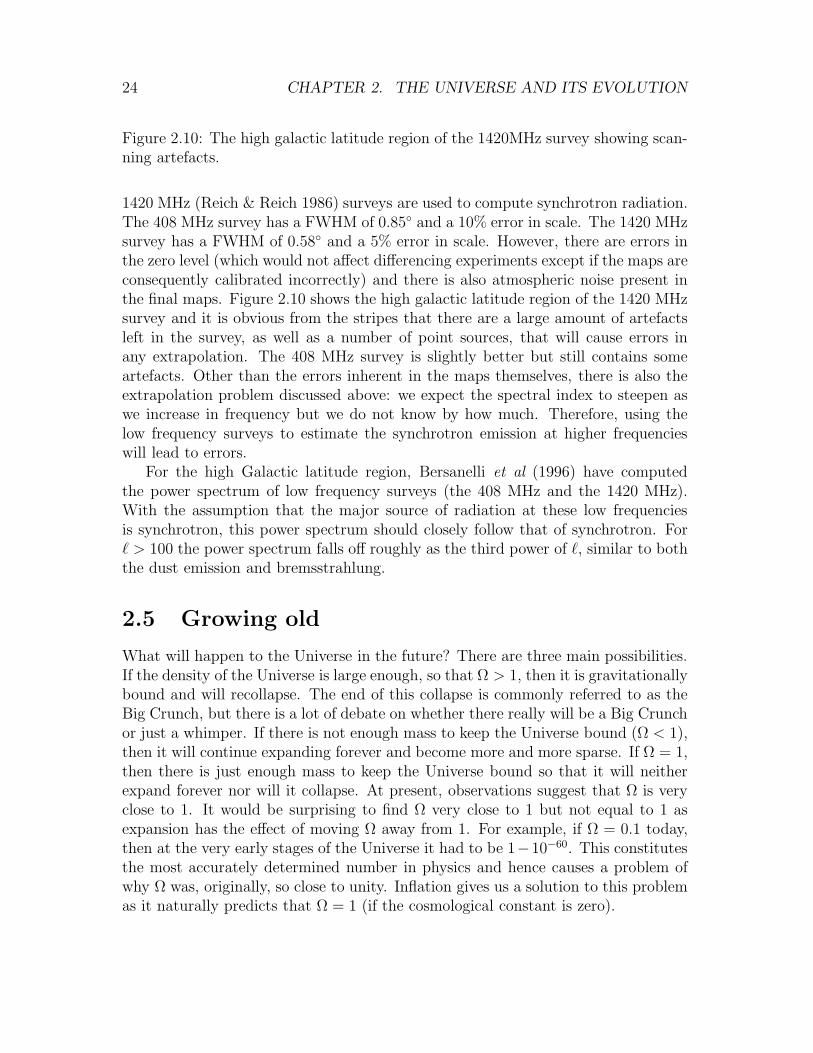
Figure 2.10: The high galactic latitude region of the 1420MHz survey showing scan-ning artefacts.
1420 MHz (Reich & Reich 1986) surveys are used to compute synchrotron radiation.The 408 MHz survey has a FWHM of 0.85 and a 10% error in scale. The 1420 MHzsurvey has a FWHM of 0.58 and a 5% error in scale. However, there are errors inthe zero level (which would not affect differencing experiments except if the maps areconsequently calibrated incorrectly) and there is also atmospheric noise present inthe final maps. Figure 2.10 shows the high galactic latitude region of the 1420 MHzsurvey and it is obvious from the stripes that there are a large amount of artefactsleft in the survey, as well as a number of point sources, that will cause errors inany extrapolation. The 408 MHz survey is slightly better but still contains someartefacts. Other than the errors inherent in the maps themselves, there is also theextrapolation problem discussed above: we expect the spectral index to steepen aswe increase in frequency but we do not know by how much. Therefore, using thelow frequency surveys to estimate the synchrotron emission at higher frequencieswill lead to errors.
For the high Galactic latitude region, Bersanelli et al (1996) have computedthe power spectrum of low frequency surveys (the 408 MHz and the 1420 MHz).With the assumption that the major source of radiation at these low frequenciesis synchrotron, this power spectrum should closely follow that of synchrotron. Forℓ > 100 the power spectrum falls off roughly as the third power of ℓ, similar to boththe dust emission and bremsstrahlung.
2.5 Growing old
What will happen to the Universe in the future? There are three main possibilities.If the density of the Universe is large enough, so that Ω > 1, then it is gravitationallybound and will recollapse. The end of this collapse is commonly referred to as theBig Crunch, but there is a lot of debate on whether there really will be a Big Crunchor just a whimper. If there is not enough mass to keep the Universe bound (Ω < 1),then it will continue expanding forever and become more and more sparse. If Ω = 1,then there is just enough mass to keep the Universe bound so that it will neitherexpand forever nor will it collapse. At present, observations suggest that Ω is veryclose to 1. It would be surprising to find Ω very close to 1 but not equal to 1 asexpansion has the effect of moving Ω away from 1. For example, if Ω = 0.1 today,then at the very early stages of the Universe it had to be 1−10−60. This constitutesthe most accurately determined number in physics and hence causes a problem ofwhy Ω was, originally, so close to unity. Inflation gives us a solution to this problemas it naturally predicts that Ω = 1 (if the cosmological constant is zero).
Chapter 3
Microwave Background
experiments
In this chapter I describe the various considerations that go into designing a Mi-crowave Background experiment. The experiments used to produce the data dis-cussed in this thesis will also be summarised.
When making measurements of the CMB fluctuations there are many techni-cal problems that need to be addressed. A basic CMB experiment must be ableto make high sensitivity observations while minimising both foreground and atmo-spheric emissions (see Section 3.1 for description of the atmospheric emission). Anestimate of the level of Galactic free-free and synchrotron emissions can be madeby using experiments at lower frequencies (100 MHz to 10 GHz), where these emis-sions are expected to be dominant, and then extrapolating to higher frequencies.The Jodrell Bank 5 GHz experiment is used for this purpose. Dust emission be-comes important at frequencies higher than ∼ 200 GHz and so is not consideredas a contaminant to the low frequency experiments in this thesis. Between 10 GHzand 200 GHz the CMB is expected to dominate over the Galactic foregrounds, al-though the contamination from the atmosphere increases with frequency. Therefore,a ground based experiment operating at frequencies between 10 GHz and 100 GHz,or a space based experiment operating at frequencies between 10 GHz and 200 GHz,should be used as a measure on the CMB. The ground based experiments chosenfor this purpose are the Tenerife experiments (10 GHz to 33 GHz). The results fromthese are compared to the COBE satellite results (30 GHz to 90 GHz) to check theconsistency of the two results (they both operate at similar angular scales) and theprimordial nature of the signal detected. As examples of the possible future CMBexperiments both the Planck Surveyor and MAP satellites are discussed.
When designing any experiment systematic errors need to be well understood sothat useful constraints can be made on the data. Today there are two types of re-ceivers that can reach high sensitivity and have well understood systematic errors atthe frequencies of interest to a CMB astronomer. At lower frequencies (< 100 GHz)High Electron Mobility Transistor (HEMT) devices are used, whereas at higher fre-quencies Bolometer devices are used. The HEMT devices work with an antennareceiver, the signal from which is then amplified with transistors. The bolometers
25
26 CHAPTER 3. MICROWAVE BACKGROUND EXPERIMENTS
are solid–state devices that increase in temperature with incoming radiation. Bothof these receiver systems need to be cooled to lower the noise signal.
3.1 Atmospheric effect
Another foreground that is seen with experiments looking at the microwave back-ground is closer to Earth than those already discussed. This is the atmosphere.Fluctuations in the atmosphere are hard to distinguish from actual extra–terrestrialfluctuations when limited frequency coverage is available. There are three waysto overcome this problem. The first method is to eliminate the atmospheric effectcompletely. Space missions are the best way to do this but their main problem iscost. High altitude sites (either at the top of a mountain or in a balloon) can re-duce the atmospheric contribution, as can moving the experiment to a region witha stable atmosphere. A cheaper alternative to physically moving the experiment isto observe with the experiment for a long time. As the atmospheric effects occuron a short time–scale, compared with the life-time of the experiment (typically oforder a few months for each data set taken with ground based CMB experiments),and the extra-terrestrial fluctuations are essentially constant, by integrating over along time the contribution from the extra–terrestrial fluctuations are increased withrespect to the atmospheric effects. Stacking together n data points (taken from nseparate observations) will reduce the variable atmospheric signal with respect tothe constant galactic or cosmological one by a factor of
√n (providing that they are
independent with respect to the atmospheric signal and any atmospheric effects onscales larger than the beam which affect the gain have been removed). The thirdway, which can also be combined with both the first and second way, is to designthe experiment to be as insensitive as possible to atmospheric variations.
An obvious design consideration is to make the telescope sensitive to frequenciesat which the atmospheric contribution is a minimum. By avoiding various bandsin the spectrum, where much emission is expected (for example water lines), theatmosphere becomes less of a problem. Above a frequency of about 100 GHz theatmospheric effect is too large to allow useful observations from a ground basedtelescope. Taken with the increasing foreground contamination from the Galaxy atlow frequencies (it is expected that the Galaxy dominates over the CMB signal atfrequencies below 10 GHz) this reduces the observable frequencies for ground basedCMB experiments to between 10 and 100 GHz. This narrow observable range resultsin the need for balloon or satellite experiments so that a larger frequency coveragecan be made to check the consistency of the results and to check the contaminationfrom the various foregrounds that are expected.
The largest atmospheric variations occur mainly on longer time scales than theintegration time of telescopes (typically of order a few minutes), as the variationsare produced by pockets of air moving over the telescope. If an experiment couldbe insensitive to these ‘long’ term variations then it should effectively see throughthe atmosphere. It is noted that these ‘long’ term variations are still on short timescales compared to the lifetime of the experiment. An interferometer extracts a small

3.2. GENERAL OBSERVATIONS 27
range of Fourier coefficients from the sky, reducing any incoherent signal (short timescale variations) or any signal that is coherent on large angular scales (long timescale variations), and so should see through the atmosphere very well. Similarly, anexperiment that switches between two positions on the sky relatively quickly willalso reduce the long term atmospheric variations. This technique is called beamswitching. Church (1995) modelled the atmosphere to predict the contribution thatatmospheric emission would make to interferometer and beam switching experimentsoperating at GHz frequencies. Church found that the level of atmospheric ‘snapshot’fluctuations expected was below 1 mK in favourable conditions for an interferometeroperating at sea level. After averaging over a relatively short time scale (muchshorter than the average lifetime of an experiment), the atmospheric noise was wellbelow the system noise and so negligible. A beam switching experiment is less wellable to eliminate the atmospheric emission but operating at high altitudes, wherethe atmosphere is drier, should allow good observations to be made with this typeof set up.
3.2 General Observations
Once the measurements of the CMB have been taken it is then necessary to presentdata in a way that is consistent between all experiments. In this section I willattempt to summarise the way in which most CMB data are presented.
3.2.1 Sky decomposition
The usual method of presenting the results from a CMB experiment is throughthe power spectrum of the spherical harmonic expansion discussed in the previouschapter. Another value often quoted is related to this analysis. The COBE grouppublished their data in terms of Qrms−ps which is given by
Qrms−ps = T
√
5C2
4π(3.1)
where C2 is related to the Cℓ values in the lower ℓ range (where the Sachs Wolfeeffect dominates) through Equation 2.20. The relative values of the Cℓs throughoutthe ℓ range depend mainly on the spectral index, n, Hubble’s constant, H, thedensity parameter, Ω, and, to a lesser extent, the other cosmological constants. Forexample, in the cold dark matter model of the Universe the height of the Dopplerpeak depends mainly on Hubble’s constant, whereas its position depends mainly onthe density parameter.
3.2.2 The effect of a beam
One important thing to note is that the observations from a particular experimentwill not generally measure the Cℓs directly. This is due to the effect of the beam onthe data. A different experiment will be sensitive to different angular scales (and so

28 CHAPTER 3. MICROWAVE BACKGROUND EXPERIMENTS
a different range of Cℓs). If an experiment has a Gaussian beam (most experimentsare not perfectly Gaussian but can be approximated by one) then it will measure
Cm(β) =1
4π
∑
ℓ
(2ℓ+ 1)CℓPℓ(cos β) exp[−(ℓ+1
2)2σ2] (3.2)
where σ is the dispersion of the Gaussian (see Scaramella & Vittorio, 1988). Thisexponential term follows through into the equation for temperature fluctuationsand must be taken into account when analysing the data if the results are to berepresented in this form.
3.2.3 Sample and cosmic variance
With the data presented like this and all systematic errors taken into account thereare still two errors which must be considered. In some cases these errors will belarger than those caused by the systematic or instrumental noise. The sample vari-ance of the data arises from an experiment that only measures a fraction of the sky.This is due to the uncertainty that the part of sky measured was a ‘special’ part.As the distribution of the CMB is expected to follow a Gaussian pattern there is aprobability that the level of fluctuations in the fraction of sky that one experimentmeasured is different to that in the fraction of sky measured by another experiment.This is sample variance and is inversely proportional to the sky area covered bythe experiment. The other error is sample variance on a cosmological scale. Theobservable Universe is just one realisation of the parameters (for example the Cℓsin the case of a Gaussian field) taken from a Gaussian distribution with the ensem-ble average described by the underlying theory. Therefore, at large angular scales,where there are less degrees of freedom (given by 2ℓ+ 1 for the Gaussian field), theuncertainty caused by having just one realisation is greatest. There is no way toreduce cosmic variance as this would require the study of another observable Uni-verse. Cosmic variance will dominate at large angular scales while sample variance,if present, dominates at small angular scales.
3.2.4 The likelihood function
If it is assumed that the CMB is described by a two–dimensional, random Gaussianfield then the properties of the fluctuations can be described completely by theirauto–correlation function C(β) (see Equation 2.17). The data can then be usedto find the most likely variables that describe the auto–correlation function (forexample n or C2, and hence QRMS−PS, in Equation 2.19 and 2.20).
In the case of the Tenerife experiments care must be taken to account for theswitch beam and it is possible to write the covariance matrix for two points i and jwith coordinates (αi, δi) and (αj , δj) as
Mij =<
∆T (αi, δi) −1
2[∆T (αi + β/ cos(δi), δi) + ∆T (αi − β/ cos(δi), δi)]
3.3. JODRELL INTERFEROMETRY 29
Figure 3.1: The 5 GHz interferometer at Jodrell Bank.
∆T (αj, δj) −1
2[∆T (αj + β/ cos(δj), δj) + ∆T (αj − β/ cos(δj), δj)]
>
(3.3)where ∆T (αi, δi) is the fluctuation in temperature at point (αi, δi) after convolutionwith the Gaussian beam pattern for a single antenna and β is the switching angle.With the noise ǫi on point i included the total covariance matrix is given by
Vij = Mij+ < ǫiǫj > (3.4)
where the noise term is non–zero only when i = j if it is uncorrelated from point topoint.
The likelihood function of this covariance matrix is defined as
L(∆T|pi) ∝1
(detV)12
exp(
−1
2∆TTV−1∆T
)
(3.5)
where pi are the parameters to be fitted in the covariance matrix and ∆T are thedata. The maximum value of this function corresponds to the most probable valuesof the parameters pi if we interpret the likelihood curves in a Bayesian sense with auniform a priori probability distribution. As the likelihood function calculates howprobable a set of parameters are given a data set, rather than trying to predict theparameters directly, both sample and cosmic variance are taken into account in theanalysis.
3.3 The Jodrell Bank 5 GHz interferometer
The CMB is dominant over the Galactic foreground emissions at frequencies higherthan ∼ 10 GHz (and below ∼ 200 GHz). Therefore, to obtain a good estimate ofthese foregrounds it is necessary to make observations at lower frequencies. Theseobservations can then be used to put constraints on the foreground contribution toother CMB experiments.
The 5 GHz interferometer located at Jodrell Bank, Manchester is a twin horn,broad–band, multiplying interferometer (see Figure 3.1). The horns are corrugatedand have a well defined beam with low side lobes to minimise ground spill–over.They have an aperture diameter of 0.56 m and a half power beam width of 8. Theprinciple of interferometry ensures that uncorrelated signals from the atmosphereare averaged down, whilst the astronomical signals, which are correlated betweenantennae, add coherently. Thus despite the relatively poor atmospheric conditionsprevalent at Jodrell Bank, an antenna temperature sensitivity of ∼ 100 µK per beamcan be attained in one good day of observing.
The antennae are arranged in an East–West configuration with a central fre-quency of 4.94 GHz and a variable baseline (the two baselines to be discussed in this
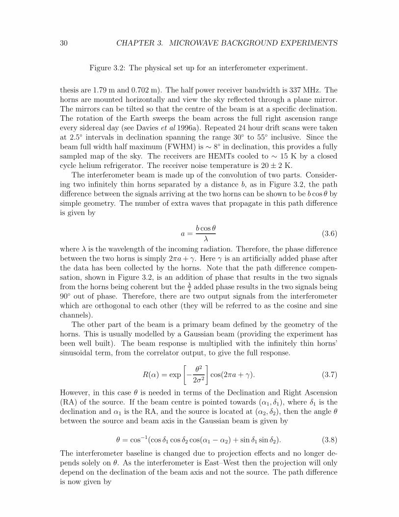
30 CHAPTER 3. MICROWAVE BACKGROUND EXPERIMENTS
Figure 3.2: The physical set up for an interferometer experiment.
thesis are 1.79 m and 0.702 m). The half power receiver bandwidth is 337 MHz. Thehorns are mounted horizontally and view the sky reflected through a plane mirror.The mirrors can be tilted so that the centre of the beam is at a specific declination.The rotation of the Earth sweeps the beam across the full right ascension rangeevery sidereal day (see Davies et al 1996a). Repeated 24 hour drift scans were takenat 2.5 intervals in declination spanning the range 30 to 55 inclusive. Since thebeam full width half maximum (FWHM) is ∼ 8 in declination, this provides a fullysampled map of the sky. The receivers are HEMTs cooled to ∼ 15 K by a closedcycle helium refrigerator. The receiver noise temperature is 20 ± 2 K.
The interferometer beam is made up of the convolution of two parts. Consider-ing two infinitely thin horns separated by a distance b, as in Figure 3.2, the pathdifference between the signals arriving at the two horns can be shown to be b cos θ bysimple geometry. The number of extra waves that propagate in this path differenceis given by
a =b cos θ
λ(3.6)
where λ is the wavelength of the incoming radiation. Therefore, the phase differencebetween the two horns is simply 2πa+ γ. Here γ is an artificially added phase afterthe data has been collected by the horns. Note that the path difference compen-sation, shown in Figure 3.2, is an addition of phase that results in the two signalsfrom the horns being coherent but the λ
4added phase results in the two signals being
90 out of phase. Therefore, there are two output signals from the interferometerwhich are orthogonal to each other (they will be referred to as the cosine and sinechannels).
The other part of the beam is a primary beam defined by the geometry of thehorns. This is usually modelled by a Gaussian beam (providing the experiment hasbeen well built). The beam response is multiplied with the infinitely thin horns’sinusoidal term, from the correlator output, to give the full response.
R(α) = exp
[
− θ2
2σ2
]
cos(2πa+ γ). (3.7)
However, in this case θ is needed in terms of the Declination and Right Ascension(RA) of the source. If the beam centre is pointed towards (α1, δ1), where δ1 is thedeclination and α1 is the RA, and the source is located at (α2, δ2), then the angle θbetween the source and beam axis in the Gaussian beam is given by
θ = cos−1(cos δ1 cos δ2 cos(α1 − α2) + sin δ1 sin δ2). (3.8)
The interferometer baseline is changed due to projection effects and no longer de-pends solely on θ. As the interferometer is East–West then the projection will onlydepend on the declination of the beam axis and not the source. The path differenceis now given by
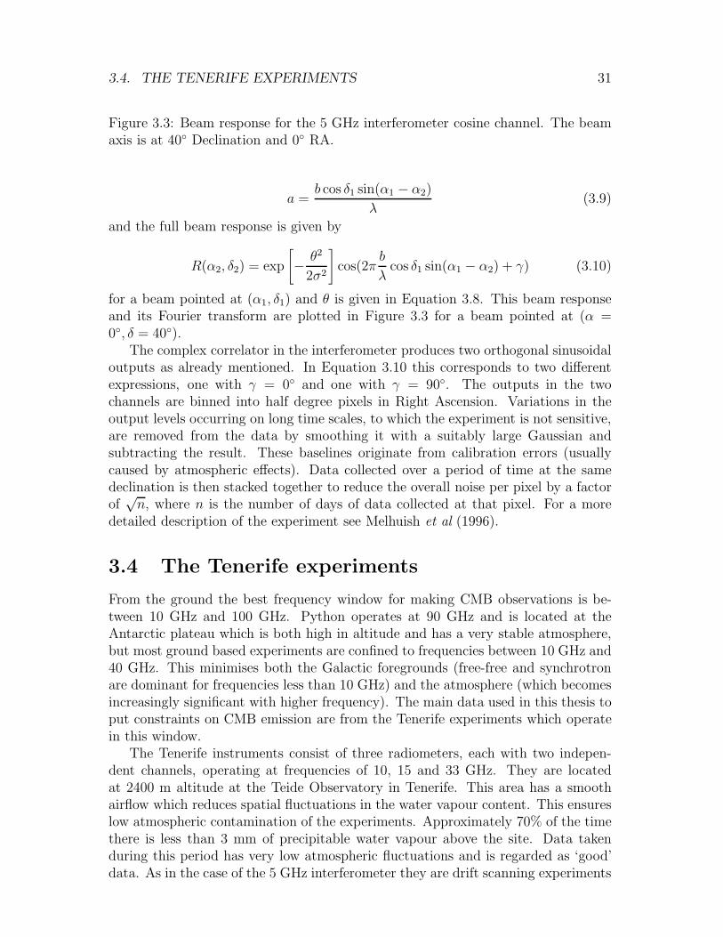
3.4. THE TENERIFE EXPERIMENTS 31
Figure 3.3: Beam response for the 5 GHz interferometer cosine channel. The beamaxis is at 40 Declination and 0 RA.
a =b cos δ1 sin(α1 − α2)
λ(3.9)
and the full beam response is given by
R(α2, δ2) = exp
[
− θ2
2σ2
]
cos(2πb
λcos δ1 sin(α1 − α2) + γ) (3.10)
for a beam pointed at (α1, δ1) and θ is given in Equation 3.8. This beam responseand its Fourier transform are plotted in Figure 3.3 for a beam pointed at (α =0, δ = 40).
The complex correlator in the interferometer produces two orthogonal sinusoidaloutputs as already mentioned. In Equation 3.10 this corresponds to two differentexpressions, one with γ = 0 and one with γ = 90. The outputs in the twochannels are binned into half degree pixels in Right Ascension. Variations in theoutput levels occurring on long time scales, to which the experiment is not sensitive,are removed from the data by smoothing it with a suitably large Gaussian andsubtracting the result. These baselines originate from calibration errors (usuallycaused by atmospheric effects). Data collected over a period of time at the samedeclination is then stacked together to reduce the overall noise per pixel by a factorof
√n, where n is the number of days of data collected at that pixel. For a more
detailed description of the experiment see Melhuish et al (1996).
3.4 The Tenerife experiments
From the ground the best frequency window for making CMB observations is be-tween 10 GHz and 100 GHz. Python operates at 90 GHz and is located at theAntarctic plateau which is both high in altitude and has a very stable atmosphere,but most ground based experiments are confined to frequencies between 10 GHz and40 GHz. This minimises both the Galactic foregrounds (free-free and synchrotronare dominant for frequencies less than 10 GHz) and the atmosphere (which becomesincreasingly significant with higher frequency). The main data used in this thesis toput constraints on CMB emission are from the Tenerife experiments which operatein this window.
The Tenerife instruments consist of three radiometers, each with two indepen-dent channels, operating at frequencies of 10, 15 and 33 GHz. They are locatedat 2400 m altitude at the Teide Observatory in Tenerife. This area has a smoothairflow which reduces spatial fluctuations in the water vapour content. This ensureslow atmospheric contamination of the experiments. Approximately 70% of the timethere is less than 3 mm of precipitable water vapour above the site. Data takenduring this period has very low atmospheric fluctuations and is regarded as ‘good’data. As in the case of the 5 GHz interferometer they are drift scanning experiments
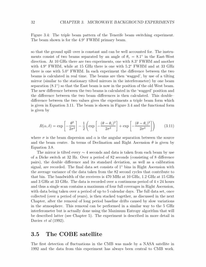
32 CHAPTER 3. MICROWAVE BACKGROUND EXPERIMENTS
Figure 3.4: The triple beam pattern of the Tenerife beam–switching experiment.The beam shown is for the 4.9 FWHM primary beam.
so that the ground spill–over is constant and can be well accounted for. The instru-ments consist of two beams separated by an angle of θ = 8.1 in the East-Westdirection. At 10 GHz there are two experiments, one with 8.3 FWHM and anotherwith 4.9 FWHM, while at 15 GHz there is one with 5.2 FWHM and at 33 GHzthere is one with 5.0 FWHM. In each experiment the difference between the twobeams is calculated in real time. The beams are then ‘wagged’, by use of a tiltingmirror (similar to the stationary tilted mirrors in the interferometer) by one beamseparation (8.1) so that the East beam is now in the position of the old West beam.The new difference between the two beams is calculated in the ‘wagged’ position andthe difference between the two beam–differences is then calculated. This double–difference between the two values gives the experiments a triple beam form whichis given in Equation 3.11. The beam is shown in Figure 3.4 and the functional formis given by
R(α, δ) = exp
[
− θ2
2σ2
]
− 1
2
(
exp
[
−(θ − θ)2
2σ2
]
+ exp
[
−(θ − θ)2
2σ2
])
(3.11)
where σ is the beam dispersion and α is the angular separation between the sourceand the beam centre. In terms of Declination and Right Ascension θ is given byEquation 3.8.
The mirror is tilted every ∼ 4 seconds and data is taken from each beam by useof a Dicke switch at 32 Hz. Over a period of 82 seconds (consisting of 8 differencepairs), the double–difference and its standard deviation, as well as a calibrationsignal, are recorded. The final data set consists of 1 bins in Right Ascension withthe average variance of the data taken from the 82 second cycles that contribute tothat bin. The bandwidth of the receivers is 470 MHz at 10 GHz, 1.2 GHz at 15 GHzand 3 GHz at 33 GHz. The data is recorded over a continuous period of 4×24 hoursand thus a single scan contains a maximum of four full coverages in Right Ascension,with data being taken over a period of up to 5 calendar days. The full data set, oncecollected (over a period of years), is then stacked together, as discussed in the nextChapter, after the removal of long period baseline drifts caused by slow variationsin the atmosphere. This removal can be performed in a similar way to the 5 GHzinterferometer but is actually done using the Maximum Entropy algorithm that willbe described latter (see Chapter 5). The experiment is described in more detail inDavies et al (1992).
3.5 The COBE satellite
The first detection of fluctuations in the CMB was made by a NASA satellite in1992 and the data from this experiment has always been central to CMB work.

3.6. THE PLANCK SURVEYOR SATELLITE 33
Figure 3.5: The COBE satellite showing the location of the main experiments onboard.
Therefore, a comparison between this data set and that from the Tenerife experimentwill provide a very useful check on the consistency of the two data sets.
The NASA Cosmic Microwave Background Explorer (COBE) satellite, launchedon November 18th 1989, had three experiments on board. The Diffuse InfraredBackground Experiment (DIRBE) measured fluctuations in high frequency emissionmainly produced by dust in our galaxy. The Far Infrared Absolute Spectrophotome-ter (FIRAS) measured the CMB spectrum between 1 cm and 100 µm. The resultsfrom FIRAS showed the CMB to have a black body spectrum that was correct to 1part in 104, the most accurate black body known to science. From this experimentthe temperature of the CMB was shown to be TCMB = 2.726±0.010 K at 95% confi-dence (see Mather et al 1994). The Differential Microwave Background Radiometer(DMR) maps the fluctuations in the CMB over the full sky. The satellite is shownin Figure 3.5.
The DMR experiment is made up of six radiometers, two at each frequencyof 31.5 GHz, 53 GHz and 90 GHz. The frequencies were chosen to overlap theexpected minimum in Galactic foreground emission. Each radiometer pair have twoindependent receivers (denoted by A and B) that measure the difference in the levelof CMB in beams of FWHM 7 separated by 60 in the sky. After removal of thedipole effect (see Chapter 2, Section 2.3.1) the sum and difference between the Aand B are calculated. The sum maps, which enhance any signal present in both Aand B, give an estimate of the fluctuations present in the CMB while the differencemaps, which remove any consistent signal, gives a measure of the instrumental noise.The data was calibrated by using a combination of an on–board calibration source,microwave emission from the Moon and the level of the dipole in the CMB (seeBennett et al 1992b). The first detection of fluctuations in the CMB was madeby COBE using data from one year of flight (Smoot et al 1992). The dipole andthe combined maps of the A+B channels from all three frequencies were shown inChapter 2. The data used in this thesis are the publicly available processed dataafter four years of flight.
3.6 The Planck Surveyor satellite
The Planck Surveyor satellite is due to be launched by ESA in 2006. The goalof Planck is to make full–sky maps of the CMB fluctuations on all angular scalesgreater than 4 arc minutes with an accuracy set by astrophysical limits. The satelliteand its proposed operation is described in detail in Bersanelli et al (1996). Since thepublication of Bersanelli et al (1996) substantial improvements have been made tothe telescope and the latest specifications (G. Efstathiou, private communication)will be used in the simulations performed in this thesis. The main improvementsinclude a change in frequencies and a substantial improvement in noise sensitivitiesfor the lower frequency channels and an additional 100 GHz channel which can be
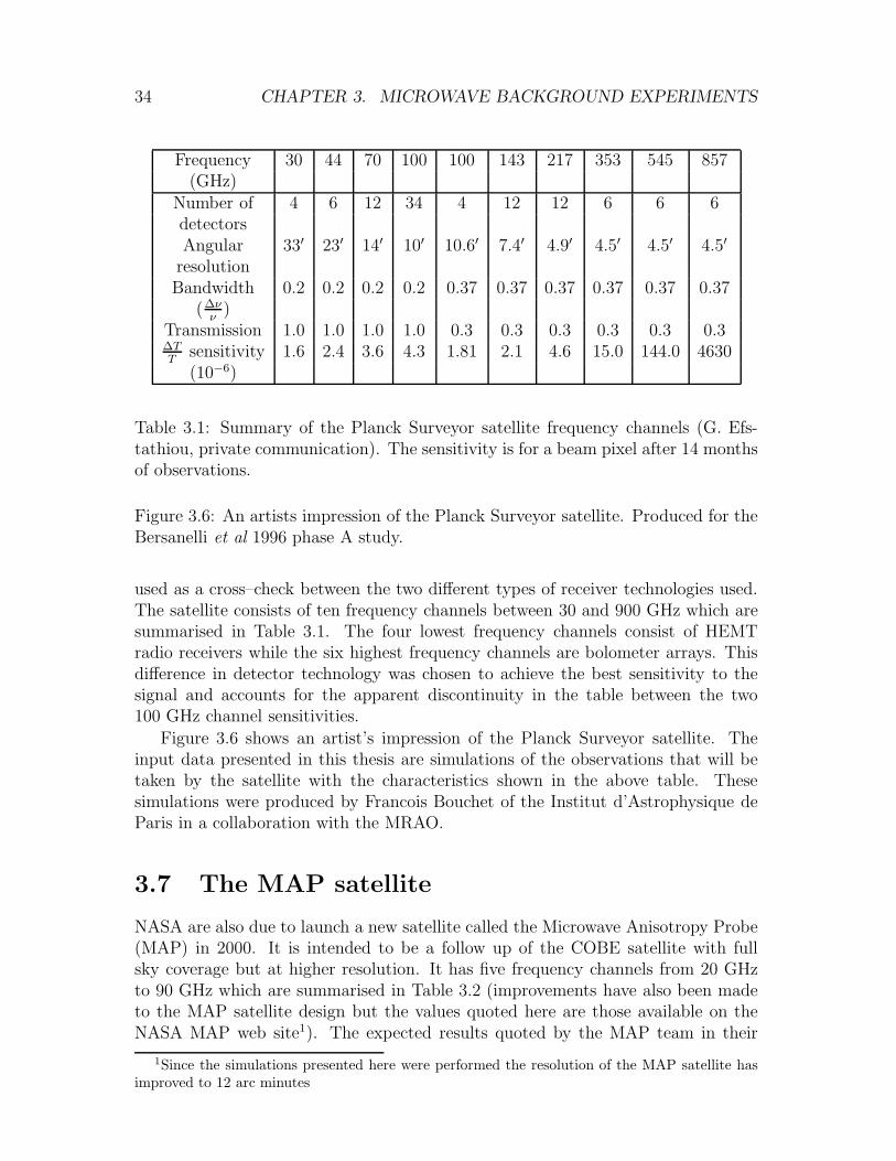
34 CHAPTER 3. MICROWAVE BACKGROUND EXPERIMENTS
Frequency 30 44 70 100 100 143 217 353 545 857(GHz)
Number of 4 6 12 34 4 12 12 6 6 6detectorsAngular 33′ 23′ 14′ 10′ 10.6′ 7.4′ 4.9′ 4.5′ 4.5′ 4.5′
resolutionBandwidth 0.2 0.2 0.2 0.2 0.37 0.37 0.37 0.37 0.37 0.37
(∆νν
)Transmission 1.0 1.0 1.0 1.0 0.3 0.3 0.3 0.3 0.3 0.3∆TT
sensitivity 1.6 2.4 3.6 4.3 1.81 2.1 4.6 15.0 144.0 4630(10−6)
Table 3.1: Summary of the Planck Surveyor satellite frequency channels (G. Efs-tathiou, private communication). The sensitivity is for a beam pixel after 14 monthsof observations.
Figure 3.6: An artists impression of the Planck Surveyor satellite. Produced for theBersanelli et al 1996 phase A study.
used as a cross–check between the two different types of receiver technologies used.The satellite consists of ten frequency channels between 30 and 900 GHz which aresummarised in Table 3.1. The four lowest frequency channels consist of HEMTradio receivers while the six highest frequency channels are bolometer arrays. Thisdifference in detector technology was chosen to achieve the best sensitivity to thesignal and accounts for the apparent discontinuity in the table between the two100 GHz channel sensitivities.
Figure 3.6 shows an artist’s impression of the Planck Surveyor satellite. Theinput data presented in this thesis are simulations of the observations that will betaken by the satellite with the characteristics shown in the above table. Thesesimulations were produced by Francois Bouchet of the Institut d’Astrophysique deParis in a collaboration with the MRAO.
3.7 The MAP satellite
NASA are also due to launch a new satellite called the Microwave Anisotropy Probe(MAP) in 2000. It is intended to be a follow up of the COBE satellite with fullsky coverage but at higher resolution. It has five frequency channels from 20 GHzto 90 GHz which are summarised in Table 3.2 (improvements have also been madeto the MAP satellite design but the values quoted here are those available on theNASA MAP web site1). The expected results quoted by the MAP team in their
1Since the simulations presented here were performed the resolution of the MAP satellite has
improved to 12 arc minutes
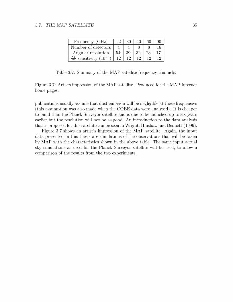
3.7. THE MAP SATELLITE 35
Frequency (GHz) 22 30 40 60 90Number of detectors 4 4 8 8 16Angular resolution 54′ 39′ 32′ 23′ 17′
∆TT
sensitivity (10−6) 12 12 12 12 12
Table 3.2: Summary of the MAP satellite frequency channels.
Figure 3.7: Artists impression of the MAP satellite. Produced for the MAP Internethome pages.
publications usually assume that dust emission will be negligible at these frequencies(this assumption was also made when the COBE data were analysed). It is cheaperto build than the Planck Surveyor satellite and is due to be launched up to six yearsearlier but the resolution will not be as good. An introduction to the data analysisthat is proposed for this satellite can be seen in Wright, Hinshaw and Bennett (1996).
Figure 3.7 shows an artist’s impression of the MAP satellite. Again, the inputdata presented in this thesis are simulations of the observations that will be takenby MAP with the characteristics shown in the above table. The same input actualsky simulations as used for the Planck Surveyor satellite will be used, to allow acomparison of the results from the two experiments.

36 CHAPTER 3. MICROWAVE BACKGROUND EXPERIMENTS
Chapter 4
The data from the 5 GHz
interferometer and Tenerife
experiments
In this chapter I will present the raw and processed data from the four Tenerifeexperiments and the Jodrell Bank interferometer. Brief analyses done on the rawdata itself and comparison with previous surveys are also presented. A furtheranalysis technique that obtains the best information from the data will be discussedin the next chapter and results from this are presented in Chapter 7.
4.1 The Jodrell Bank 5GHz interferometer
4.1.1 Pre–processing
From the complete data set a data subset that is useful must be selected and anydata that is obviously not due to real sky fluctuations discarded. The first processis to use an automatic program (developed by Simon Melhuish at Jodrell Bank, seeMelhuish et al 1997) that excises the regions in the data contaminated by the Sunand the Moon. The program looks at the time of observations and the position ofthe Sun and the Moon at that time. It deletes data that is within 47 and 17 of theSun and Moon respectively. Any abnormal signals that deviate from the mean ofthe data by more than 3σ are also deleted as these probably arise from noise withinthe telescope or bad atmospheric conditions.
The two output channels from the interferometer should be in quadrature -however, this is not always the case. Errors in the correlator output lead to anoutput that can be 80 out of phase rather than 90 and a difference in amplitudebetween the two channels of 1% was commonly observed. This is easily correctedby multiplying the channels with a suitably chosen matrix and the amplitude andquadrature is restored. Long term baseline drifts caused by instrumental driftswere removed by applying a high–pass filter of one hour (15 Gaussian) in RightAscension. The final results, binned in 0.5 pixels are stacked together to produce
37
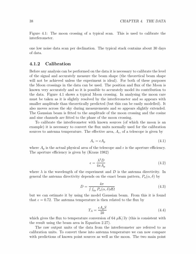
38 CHAPTER 4. THE DATA
Figure 4.1: The moon crossing of a typical scan. This is used to calibrate theinterferometer.
one low noise data scan per declination. The typical stack contains about 30 daysof data.
4.1.2 Calibration
Before any analysis can be performed on the data it is necessary to calibrate the levelof the signal and accurately measure the beam shape (the theoretical beam shapewill not be achieved unless the experiment is ideal). For both of these purposesthe Moon crossings in the data can be used. The position and flux of the Moon isknown very accurately and so it is possible to accurately model its contribution tothe data. Figure 4.1 shows a typical Moon crossing. In analysing the moon caremust be taken as it is slightly resolved by the interferometer and so appears withsmaller amplitude than theoretically predicted (but this can be easily modelled). Italso moves across the sky during measurements and so appears slightly extended.The Gaussian beam is fitted to the amplitude of the moon crossing and the cosineand sine channels are fitted to the phase of the moon crossing.
To calibrate the interferometer with known sources (of which the moon is anexample) it is necessary to convert the flux units normally used for the calibrationsources to antenna temperature. The effective area, Ae, of a telescope is given by
Ae = ǫAp (4.1)
where Ap is the actual physical area of the telescope and ǫ is the aperture efficiency.The aperture efficiency is given by (Kraus 1982)
ǫ =λ2D
4πAp(4.2)
where λ is the wavelength of the experiment and D is the antenna directivity. Ingeneral the antenna directivity depends on the exact beam pattern, Pn(α, δ) by
D =4π
∫ ∫
4π Pn(α, δ)dΩ(4.3)
but we can estimate it by using the model Gaussian beam. From this it is foundthat ǫ = 0.72. The antenna temperature is then related to the flux by
TA =ǫApS
2k(4.4)
which gives the flux to temperature conversion of 64 µK/Jy (this is consistent withthe result using the beam area in Equation 2.27).
The raw output units of the data from the interferometer are referred to ascalibration units. To convert these into antenna temperature we can now comparewith predictions of known point sources as well as the moon. The two main point
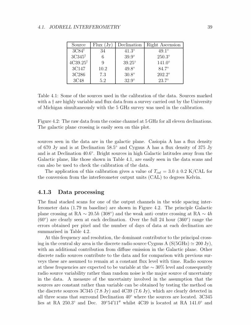
4.1. JODRELL INTERFEROMETRY 39
Source Flux (Jy) Declination Right Ascension3C84† 34 41.3 49.1
3C345† 6 39.9 250.3
4C39.25† 9 39.25 141.0
3C147 10.2 49.8 84.7
3C286 7.3 30.8 202.2
3C48 5.2 32.9 23.7
Table 4.1: Some of the sources used in the calibration of the data. Sources markedwith a † are highly variable and flux data from a survey carried out by the Universityof Michigan simultaneously with the 5 GHz survey was used in the calibration.
Figure 4.2: The raw data from the cosine channel at 5 GHz for all eleven declinations.The galactic plane crossing is easily seen on this plot.
sources seen in the data are in the galactic plane. Casiopia A has a flux densityof 670 Jy and is at Declination 58.5 and Cygnus A has a flux density of 375 Jyand is at Declination 40.6. Bright sources in high Galactic latitudes away from theGalactic plane, like those shown in Table 4.1, are easily seen in the data scans andcan also be used to check the calibration of the data.
The application of this calibration gives a value of Tcal = 3.0 ± 0.2 K/CAL forthe conversion from the interferometer output units (CAL) to degrees Kelvin.
4.1.3 Data processing
The final stacked scans for one of the output channels in the wide spacing inter-ferometer data (1.79 m baseline) are shown in Figure 4.2. The principle Galacticplane crossing at RA ∼ 20.5h (308) and the weak anti–centre crossing at RA ∼ 4h(60) are clearly seen at each declination. Over the full 24 hour (360) range theerrors obtained per pixel and the number of days of data at each declination aresummarised in Table 4.2.
At this frequency and resolution, the dominant contributor to the principal cross-ing in the central sky area is the discrete radio source Cygnus A (S(5GHz) ≃ 200 Jy),with an additional contribution from diffuse emission in the Galactic plane. Otherdiscrete radio sources contribute to the data and for comparison with previous sur-veys these are assumed to remain at a constant flux level with time. Radio sourcesat these frequencies are expected to be variable at the ∼ 30% level and consequentlyradio source variability rather than random noise is the major source of uncertaintyin the data. A measure of the uncertainty involved in the assumption that thesources are constant rather than variable can be obtained by testing the method onthe discrete sources 3C345 (7.8 Jy) and 4C39 (7.6 Jy), which are clearly detected inall three scans that surround Declination 40 where the sources are located. 3C345lies at RA 250.3 and Dec. 3954′11′′ whilst 4C39 is located at RA 141.0 and
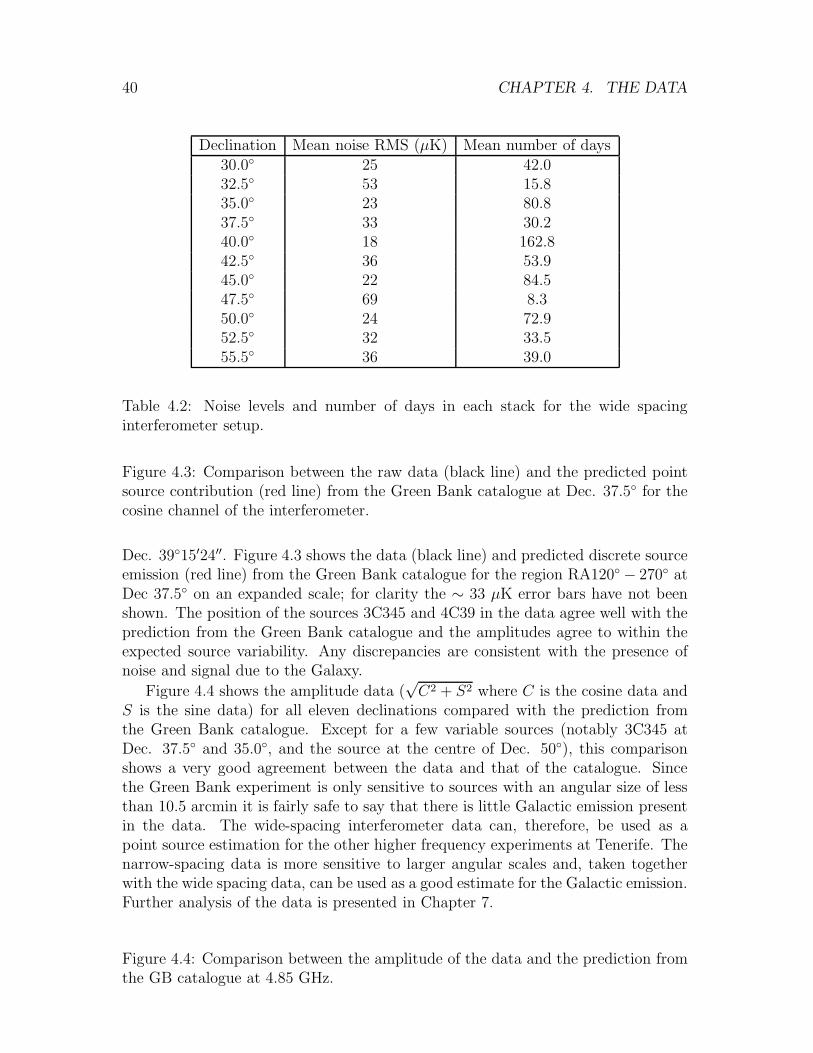
40 CHAPTER 4. THE DATA
Declination Mean noise RMS (µK) Mean number of days30.0 25 42.032.5 53 15.835.0 23 80.837.5 33 30.240.0 18 162.842.5 36 53.945.0 22 84.547.5 69 8.350.0 24 72.952.5 32 33.555.5 36 39.0
Table 4.2: Noise levels and number of days in each stack for the wide spacinginterferometer setup.
Figure 4.3: Comparison between the raw data (black line) and the predicted pointsource contribution (red line) from the Green Bank catalogue at Dec. 37.5 for thecosine channel of the interferometer.
Dec. 3915′24′′. Figure 4.3 shows the data (black line) and predicted discrete sourceemission (red line) from the Green Bank catalogue for the region RA120 − 270 atDec 37.5 on an expanded scale; for clarity the ∼ 33 µK error bars have not beenshown. The position of the sources 3C345 and 4C39 in the data agree well with theprediction from the Green Bank catalogue and the amplitudes agree to within theexpected source variability. Any discrepancies are consistent with the presence ofnoise and signal due to the Galaxy.
Figure 4.4 shows the amplitude data (√C2 + S2 where C is the cosine data and
S is the sine data) for all eleven declinations compared with the prediction fromthe Green Bank catalogue. Except for a few variable sources (notably 3C345 atDec. 37.5 and 35.0, and the source at the centre of Dec. 50), this comparisonshows a very good agreement between the data and that of the catalogue. Sincethe Green Bank experiment is only sensitive to sources with an angular size of lessthan 10.5 arcmin it is fairly safe to say that there is little Galactic emission presentin the data. The wide-spacing interferometer data can, therefore, be used as apoint source estimation for the other higher frequency experiments at Tenerife. Thenarrow-spacing data is more sensitive to larger angular scales and, taken togetherwith the wide spacing data, can be used as a good estimate for the Galactic emission.Further analysis of the data is presented in Chapter 7.
Figure 4.4: Comparison between the amplitude of the data and the prediction fromthe GB catalogue at 4.85 GHz.

4.2. THE TENERIFE SCANS 41
4.2 Structure in the Tenerife switched-beam scans
4.2.1 Pre–processing
Data within 50 of the Sun and 30 of the Moon were removed from the raw data ofall the Tenerife experiments with an automated process, similar to the interferom-eter. Data taken in poor atmospheric conditions (about 30% of all data) and anyindividual pixel that deviated by more than 3σ from the average were also removed.These individual pixels correspond to technical failures in the instrumental systemor anomalous sources (like butterflies flying into the horns). The data taken in pooratmospheric conditions was removed by looking at each scan individually. If dataappeared to be affected by atmospheric fluctuations then a portion of data aroundthe affected region was removed. Portions of bad data were eliminated by eye be-cause an automated analysis would prove too complicated due to the complexity ofthe data.
A similar technique to the pre–processing of data from the Jodrell Bank in-terferometer, by smoothing the data, could have been used to remove long termbaseline drifts caused by atmospheric offsets, but it was decided to leave the base-lines in and remove them simultaneously with the Maximum Entropy reconstructiondescribed in the next chapter. This method basically finds the best astronomicalsignal consistent with all the scans, subtracts this from each scan and then performsthe smoothing on the residual signal. The final stacked results shown below aretherefore after Maximum Entropy processing. However, problems arise when thebaseline variations in the raw data are so extreme that they prevent their successfulremoval in the MEM deconvolution analysis. As noted in Davies et al 1996, thisproblem is exaggerated at the higher frequencies where the water vapour emissionis higher. At these higher frequencies (the 33 GHz experiment in the case of Tener-ife observations) it is clear that the variations in baseline are, in certain cases, tooextreme for removal and will therefore result in artefacts in the final stacked scan.These artefacts result from poor observing conditions rather than being intrinsic tothe astronomy, because such problems occur only for days with severe baselines andappear in a randomly distributed fashion for different days. Removal of such datais essential if the necessary sensitivity to detect CMB fluctuations is to be obtained.This involves the task of examining each raw scan (the best covered declination forthe 5 FWHM data sets contains over 200 days of data) and its baseline and decid-ing if the data are usable. In such cases where the data is un-salvageable, then thedata for the full 360 observation are discarded. This ensures that there is no biasintroduced by selectively removing features in the scans. After this final stage ofediting, the baseline fitting must be repeated for the full remaining data set. TheMEM process will now be able to search for a more accurate solution and will pro-duce a new set of more accurate baselines. The coverages of a given declination cannow be stacked together and the process repeated until all artefacts of this type areremoved. This process is carried out for each of the Tenerife data sets discussed inthis thesis but will not be mentioned again.

42 CHAPTER 4. THE DATA
Declination 10 GHz 15 GHz 33 GHz30.0 - 104 -32.5 85 74 -35.0 82 191 4037.5 129 103 -40.0 134 134 9042.5 50 85 -45.0 51 67 -
Table 4.3: Number of independent measurements for the 5 FWHM Tenerife exper-iments.
4.2.2 Stacking the data
The data set consists of 1 bins in right ascension covering a range of declinationsand taken over a large number of days (the best scans have nearly 200 days of data).To reduce the amount of data it is necessary to stack all the data for each pointthat were taken at different days together. This is done after baseline subtraction toavoid addition of atmospheric effects. By taking a weighted mean over the ns scans(where ns is the number of days) the final data scan is obtained. The number of daysof data at each declination and frequency for the 5 FWHM Tenerife experiment issummarised in Table 4.3. If the data in each 1 bin is given by yir, where i is thebin and r is the day, and the error on yir is given by σir then the final stacked datais given by
Yi =
∑nsr=1wir (yir − bir)∑ns
r=1wir(4.5)
where bir represents any long term baselines that have to be subtracted from thedata before stacking and the weighting factor wir is given by
wir =1
σ2ir
. (4.6)
The error on the final stack is given by the scatter over the days contributing toeach point
σ2i =
(
∑nsr=1wir [(yir − bir) − Yi]
2
∑nsr=1wir(ns− 1)
)
. (4.7)
4.2.3 Calibration
The data was calibrated using a continuous online noise injection diode so that thedata amplitude response remains constant throughout the day’s observing. Theoutput is then in units of CAL (the calibration level). Moon observations and theGalactic plane crossing were then used to calibrate the signal and convert the output
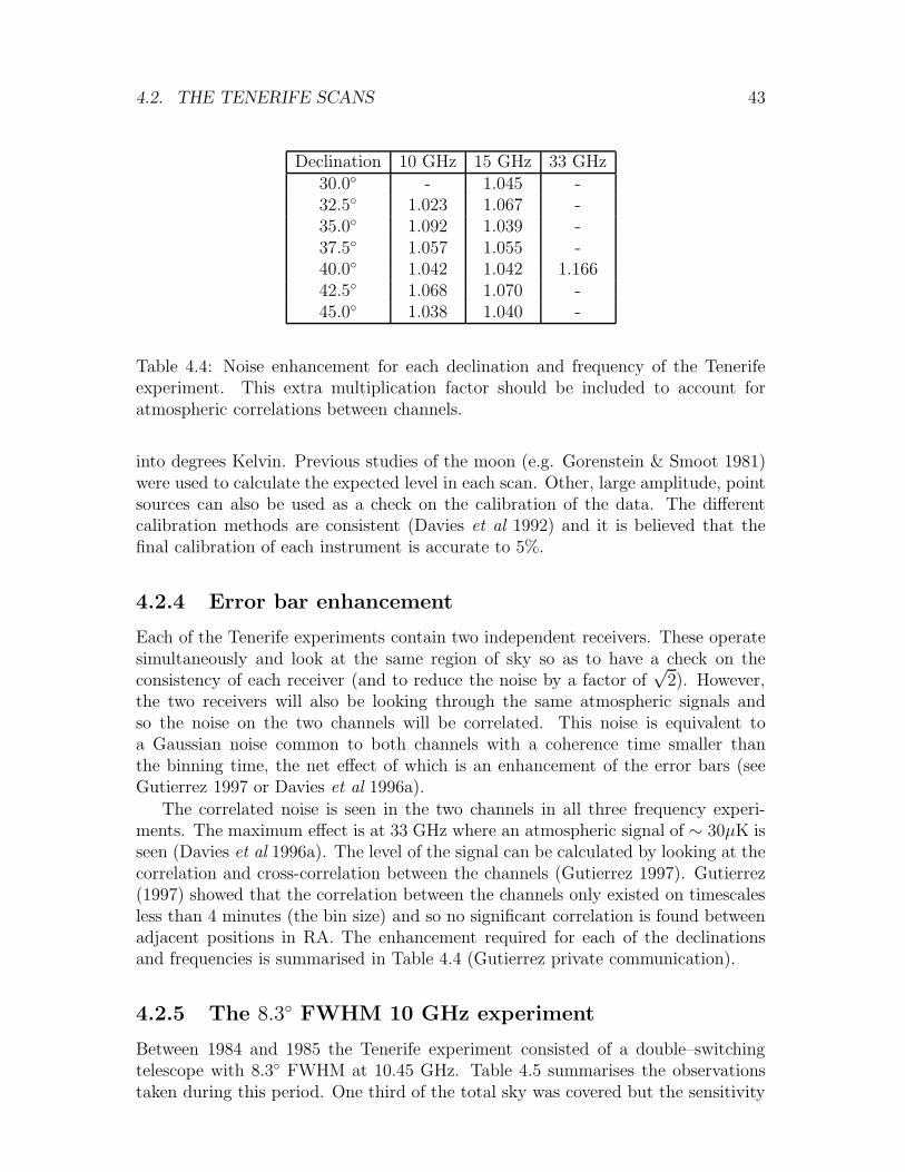
4.2. THE TENERIFE SCANS 43
Declination 10 GHz 15 GHz 33 GHz30.0 - 1.045 -32.5 1.023 1.067 -35.0 1.092 1.039 -37.5 1.057 1.055 -40.0 1.042 1.042 1.16642.5 1.068 1.070 -45.0 1.038 1.040 -
Table 4.4: Noise enhancement for each declination and frequency of the Tenerifeexperiment. This extra multiplication factor should be included to account foratmospheric correlations between channels.
into degrees Kelvin. Previous studies of the moon (e.g. Gorenstein & Smoot 1981)were used to calculate the expected level in each scan. Other, large amplitude, pointsources can also be used as a check on the calibration of the data. The differentcalibration methods are consistent (Davies et al 1992) and it is believed that thefinal calibration of each instrument is accurate to 5%.
4.2.4 Error bar enhancement
Each of the Tenerife experiments contain two independent receivers. These operatesimultaneously and look at the same region of sky so as to have a check on theconsistency of each receiver (and to reduce the noise by a factor of
√2). However,
the two receivers will also be looking through the same atmospheric signals andso the noise on the two channels will be correlated. This noise is equivalent toa Gaussian noise common to both channels with a coherence time smaller thanthe binning time, the net effect of which is an enhancement of the error bars (seeGutierrez 1997 or Davies et al 1996a).
The correlated noise is seen in the two channels in all three frequency experi-ments. The maximum effect is at 33 GHz where an atmospheric signal of ∼ 30µK isseen (Davies et al 1996a). The level of the signal can be calculated by looking at thecorrelation and cross-correlation between the channels (Gutierrez 1997). Gutierrez(1997) showed that the correlation between the channels only existed on timescalesless than 4 minutes (the bin size) and so no significant correlation is found betweenadjacent positions in RA. The enhancement required for each of the declinationsand frequencies is summarised in Table 4.4 (Gutierrez private communication).
4.2.5 The 8.3 FWHM 10 GHz experiment
Between 1984 and 1985 the Tenerife experiment consisted of a double–switchingtelescope with 8.3 FWHM at 10.45 GHz. Table 4.5 summarises the observationstaken during this period. One third of the total sky was covered but the sensitivity
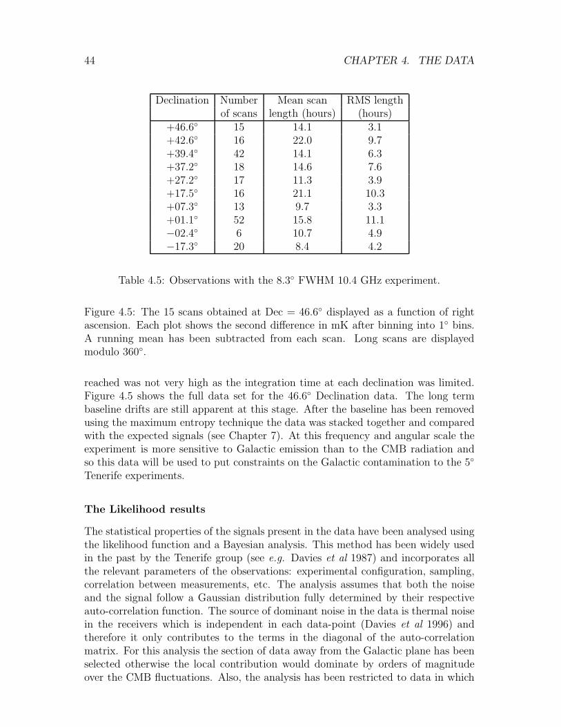
44 CHAPTER 4. THE DATA
Declination Number Mean scan RMS lengthof scans length (hours) (hours)
+46.6 15 14.1 3.1+42.6 16 22.0 9.7+39.4 42 14.1 6.3+37.2 18 14.6 7.6+27.2 17 11.3 3.9+17.5 16 21.1 10.3+07.3 13 9.7 3.3+01.1 52 15.8 11.1−02.4 6 10.7 4.9−17.3 20 8.4 4.2
Table 4.5: Observations with the 8.3 FWHM 10.4 GHz experiment.
Figure 4.5: The 15 scans obtained at Dec = 46.6 displayed as a function of rightascension. Each plot shows the second difference in mK after binning into 1 bins.A running mean has been subtracted from each scan. Long scans are displayedmodulo 360.
reached was not very high as the integration time at each declination was limited.Figure 4.5 shows the full data set for the 46.6 Declination data. The long termbaseline drifts are still apparent at this stage. After the baseline has been removedusing the maximum entropy technique the data was stacked together and comparedwith the expected signals (see Chapter 7). At this frequency and angular scale theexperiment is more sensitive to Galactic emission than to the CMB radiation andso this data will be used to put constraints on the Galactic contamination to the 5
Tenerife experiments.
The Likelihood results
The statistical properties of the signals present in the data have been analysed usingthe likelihood function and a Bayesian analysis. This method has been widely usedin the past by the Tenerife group (see e.g. Davies et al 1987) and incorporates allthe relevant parameters of the observations: experimental configuration, sampling,correlation between measurements, etc. The analysis assumes that both the noiseand the signal follow a Gaussian distribution fully determined by their respectiveauto-correlation function. The source of dominant noise in the data is thermal noisein the receivers which is independent in each data-point (Davies et al 1996) andtherefore it only contributes to the terms in the diagonal of the auto-correlationmatrix. For this analysis the section of data away from the Galactic plane has beenselected otherwise the local contribution would dominate by orders of magnitudeover the CMB fluctuations. Also, the analysis has been restricted to data in which
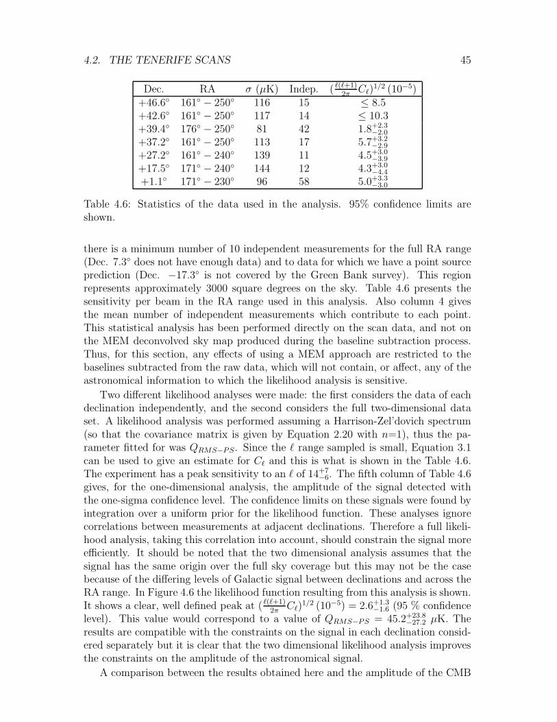
4.2. THE TENERIFE SCANS 45
Dec. RA σ (µK) Indep. ( ℓ(ℓ+1)2π
Cℓ)1/2 (10−5)
+46.6 161 − 250 116 15 ≤ 8.5+42.6 161 − 250 117 14 ≤ 10.3+39.4 176 − 250 81 42 1.8+2.3
−2.0
+37.2 161 − 250 113 17 5.7+3.2−2.9
+27.2 161 − 240 139 11 4.5+3.0−3.9
+17.5 171 − 240 144 12 4.3+3.0−4.4
+1.1 171 − 230 96 58 5.0+3.3−3.0
Table 4.6: Statistics of the data used in the analysis. 95% confidence limits areshown.
there is a minimum number of 10 independent measurements for the full RA range(Dec. 7.3 does not have enough data) and to data for which we have a point sourceprediction (Dec. −17.3 is not covered by the Green Bank survey). This regionrepresents approximately 3000 square degrees on the sky. Table 4.6 presents thesensitivity per beam in the RA range used in this analysis. Also column 4 givesthe mean number of independent measurements which contribute to each point.This statistical analysis has been performed directly on the scan data, and not onthe MEM deconvolved sky map produced during the baseline subtraction process.Thus, for this section, any effects of using a MEM approach are restricted to thebaselines subtracted from the raw data, which will not contain, or affect, any of theastronomical information to which the likelihood analysis is sensitive.
Two different likelihood analyses were made: the first considers the data of eachdeclination independently, and the second considers the full two-dimensional dataset. A likelihood analysis was performed assuming a Harrison-Zel’dovich spectrum(so that the covariance matrix is given by Equation 2.20 with n=1), thus the pa-rameter fitted for was QRMS−PS. Since the ℓ range sampled is small, Equation 3.1can be used to give an estimate for Cℓ and this is what is shown in the Table 4.6.The experiment has a peak sensitivity to an ℓ of 14+7
−6. The fifth column of Table 4.6gives, for the one-dimensional analysis, the amplitude of the signal detected withthe one-sigma confidence level. The confidence limits on these signals were found byintegration over a uniform prior for the likelihood function. These analyses ignorecorrelations between measurements at adjacent declinations. Therefore a full likeli-hood analysis, taking this correlation into account, should constrain the signal moreefficiently. It should be noted that the two dimensional analysis assumes that thesignal has the same origin over the full sky coverage but this may not be the casebecause of the differing levels of Galactic signal between declinations and across theRA range. In Figure 4.6 the likelihood function resulting from this analysis is shown.It shows a clear, well defined peak at ( ℓ(ℓ+1)
2πCℓ)
1/2 (10−5) = 2.6+1.3−1.6 (95 % confidence
level). This value would correspond to a value of QRMS−PS = 45.2+23.8−27.2 µK. The
results are compatible with the constraints on the signal in each declination consid-ered separately but it is clear that the two dimensional likelihood analysis improvesthe constraints on the amplitude of the astronomical signal.
A comparison between the results obtained here and the amplitude of the CMB
46 CHAPTER 4. THE DATA
Figure 4.6: The likelihood function from the analysis of the full data set. There isa clearly defined peak at ( ℓ(ℓ+1)
2πCℓ)
1/2 (10−5) = 2.6+1.3−1.6 (95% confidence level).
structure found in Hancock et al (1994) at higher frequencies can be made. Theyfound QRMS−PS ∼ 21 µK in an 5 FWHM switched beam and taking into accountthe extra dilution a slightly lower level is expected in an 8 FWHM switched beam,assuming a n = 1 power spectrum. It is seen that the majority of the signal inthe 10 GHz, FWHM=8 data is most likely due to Galactic sources. Assumingthat the majority of the signal found here is Galactic and using a spatial spectrumof Cℓ ∝ ℓ−3 (estimated from the Haslam et al 1982 maps) to predict the galacticcontamination in a 5 FWHM beam at 10 GHz, then using a full likelihood analysis,it is found that an rms signal of ∆Trms = 55+32
−26 µK is expected. It should benoted that this is an upper limit on the Galactic contribution to the 5 data as thevariability of the sources has been ignored when the subtraction was performed (thisresults in a residual signal from the point sources in the data during the likelihoodanalysis) and the analysis also includes regions where the Galactic signal is expectedto be higher (for example the North Polar Spur). The 5 FWHM Tenerife scans arecentred on Dec. 40 and it can be seen from Table 4.6 that this is the region withthe lowest Galactic contamination. The results reported in Gutierrez et al (1997),for the 5 FWHM, 10 GHz Tenerife experiment, show that the signal found wasQRMS−PS < 33.8 µK (corresponding to a signal of ∆T < 53 µK) which is consistentwith the prediction here (also taking into account the more significant contributionfrom the CMB at 5). This comparison allows a restriction on the maximum Galacticcontribution to the signal found in Hancock et al 1994 to be ∆Trms ∼ 18−23 µK at15 GHz and ∆Trms ∼ 2−4 µK at 33 GHz depending on whether the contaminationis dominated by synchrotron or free-free emission.
4.2.6 The 5 FWHM Tenerife experiments
The aim of the 5 FWHM experiments is to produce consistent maps at three operat-ing frequencies (10.45, 14.90 and 33.00 GHz) of the CMB fluctuations and using thefrequency coverage to put constraints on the levels of galactic foregrounds (namelysynchrotron and free–free which are expected to be the most important at thesefrequencies). The experiments cover a range between Declinations 27.5 and 45.The 10.45 GHz, 4.9 FWHM experiment, the 14.9 GHz, 5.2 FWHM experimentand the 33 GHz, 5.0 FWHM experiment have been taking data since 1985, 1990and 1992 respectively. Table 4.7 summarises the results up to July 1996 (the datapresented in this thesis is taken up to August 1997 which includes a new 15 GHzdeclination scan at 27.5). It is seen that the full area is not covered by all threeexperiments but they are continually taking new data to build up a well sampled,high sensitivity data set. Table 4.8 shows the noise levels per 1 bin achieved in thisdata set.
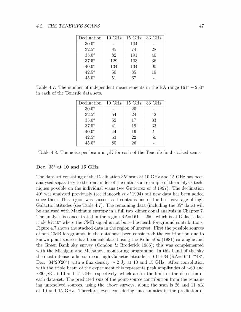
4.2. THE TENERIFE SCANS 47
Declination 10 GHz 15 GHz 33 GHz30.0 - 104 -32.5 85 74 2835.0 82 191 4037.5 129 103 3640.0 134 134 9042.5 50 85 1945.0 51 67 -
Table 4.7: The number of independent measurements in the RA range 161 − 250
in each of the Tenerife data sets.
Declination 10 GHz 15 GHz 33 GHz30.0 - 20 -32.5 54 24 4235.0 52 17 3337.5 41 19 3340.0 44 19 2142.5 63 22 5045.0 80 26 -
Table 4.8: The noise per beam in µK for each of the Tenerife final stacked scans.
Dec. 35 at 10 and 15 GHz
The data set consisting of the Declination 35 scan at 10 GHz and 15 GHz has beenanalysed separately to the remainder of the data as an example of the analysis tech-niques possible on the individual scans (see Gutierrez et al 1997). The declination40 was analysed previously (see Hancock et al 1994) but new data has been addedsince then. This region was chosen as it contains one of the best coverage of highGalactic latitudes (see Table 4.7). The remaining data (including the 35 data) willbe analysed with Maximum entropy in a full two–dimensional analysis in Chapter 7.The analysis is concentrated in the region RA=161− 250 which is at Galactic lat-itude b>∼ 40 where the CMB signal is not buried beneath foreground contributions.Figure 4.7 shows the stacked data in the region of interest. First the possible sourcesof non-CMB foregrounds in the data have been considered; the contribution due toknown point-sources has been calculated using the Kuhr et al (1981) catalogue andthe Green Bank sky survey (Condon & Broderick 1986); this was complementedwith the Michigan and Metsahovi monitoring programme. In this band of the skythe most intense radio-source at high Galactic latitude is 1611+34 (RA=16h11m48s,Dec.=3420′20′′) with a flux density ∼ 2 Jy at 10 and 15 GHz. After convolutionwith the triple beam of the experiment this represents peak amplitudes of ∼60 and∼30 µK at 10 and 15 GHz respectively, which are in the limit of the detection ofeach data-set. The predicted rms of the point-source contribution from the remain-ing unresolved sources, using the above surveys, along the scan is 26 and 11 µKat 10 and 15 GHz. Therefore, even considering uncertainties in the prediction of
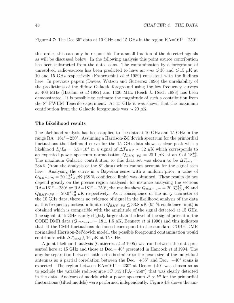
48 CHAPTER 4. THE DATA
Figure 4.7: The Dec 35 data at 10 GHz and 15 GHz in the region RA=161−250.
this order, this can only be responsible for a small fraction of the detected signalsas will be discussed below. In the following analysis this point source contributionhas been subtracted from the data scans. The contamination by a foreground ofunresolved radio-sources has been predicted to have an rms <∼ 30 and <∼ 15 µK at10 and 15 GHz respectively (Franceschini et al 1989) consistent with the findingshere. In previous papers (Davies, Watson and Gutierrez 1996) the unreliability ofthe predictions of the diffuse Galactic foreground using the low frequency surveysat 408 MHz (Haslam et al 1982) and 1420 MHz (Reich & Reich 1988) has beendemonstrated. It is possible to estimate the magnitude of such a contribution fromthe 8 FWHM Tenerife experiment. At 15 GHz it was shown that the maximumcontribution from the Galactic foregrounds was ∼ 20 µK.
The Likelihood results
The likelihood analysis has been applied to the data at 10 GHz and 15 GHz in therange RA=161−250. Assuming a Harrison-Zel’dovich spectrum for the primordialfluctuations the likelihood curve for the 15 GHz data shows a clear peak with alikelihood L/L0 = 5.5×10⁴ in a signal of ∆TRMS ∼ 32 µK which corresponds toan expected power spectrum normalisation QRMS−PS = 20.1 µK at an ℓ of 18+9
−7.The maximum Galactic contribution to this data set was shown to be ∆Trms =23µK (from the analysis of the 8 data) which cannot account for the signal seenhere. Analysing the curve in a Bayesian sense with a uniform prior, a value ofQRMS−PS = 20.1+7.1
−5.4 µK (68 % confidence limit) was obtained. These results do notdepend greatly on the precise region analysed; for instance analysing the sectionsRA=161− 230 or RA=181− 250, the results show QRMS−PS = 20.3+8.7
−7.3 µK andQRMS−PS = 20.0+8.0
−6.0 µK respectively. As a consequence of the noisy character ofthe 10 GHz data, there is no evidence of signal in the likelihood analysis of the dataat this frequency; instead a limit on QRMS−PS ≤ 33.8 µK (95 % confidence limit) isobtained which is compatible with the amplitude of the signal detected at 15 GHz.The signal at 15 GHz is only slightly larger than the level of the signal present in theCOBE DMR data (QRMS−PS = 18± 1.5 µK, Bennett et al 1996) and this indicatesthat, if the CMB fluctuations do indeed correspond to the standard COBE DMRnormalised Harrison-Zel’dovich model, the possible foreground contamination wouldcontribute with ∆TRMS
<∼ 16 µK at 15 GHz.
A joint likelihood analysis (Gutierrez et al 1995) was run between the data pre-sented here at 15 GHz and those at Dec.= 40 presented in Hancock et al 1994. Theangular separation between both strips is similar to the beam size of the individualantennas so a partial correlation between the Dec.=+35 and Dec.=+40 scans isexpected. The region between RA=161 − 230 at Dec.= +40 was chosen so asto exclude the variable radio-source 3C 345 (RA∼ 250) that was clearly detectedin the data. Analyses of models with a power spectrum P ∝ kn for the primordialfluctuations (tilted models) were performed independently. Figure 4.8 shows the am-
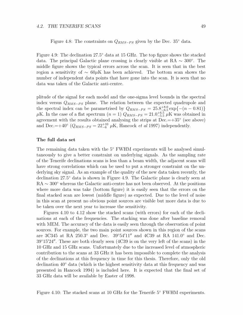
4.2. THE TENERIFE SCANS 49
Figure 4.8: The constraints on QRMS−PS given by the Dec. 35 data.
Figure 4.9: The declination 27.5 data at 15 GHz. The top figure shows the stackeddata. The principal Galactic plane crossing is clearly visible at RA ∼ 300. Themiddle figure shows the typical errors across the scan. It is seen that in the bestregion a sensitivity of ∼ 60µK has been achieved. The bottom scan shows thenumber of independent data points that have gone into the scan. It is seen that nodata was taken of the Galactic anti-centre.
plitude of the signal for each model and the one-sigma level bounds in the spectralindex versus QRMS−PS plane. The relation between the expected quadrupole andthe spectral index can be parametrised by QRMS−PS = 25.8+8.0
−6.5 exp−(n − 0.81)µK. In the case of a flat spectrum (n = 1) QRMS−PS = 21.0+6.5
−5.5 µK was obtained inagreement with the results obtained analysing the strips at Dec.=+35 (see above)and Dec.=+40 (QRMS−PS = 22+10
−6 µK, Hancock et al 1997) independently.
The full data set
The remaining data taken with the 5 FWHM experiments will be analysed simul-taneously to give a better constraint on underlying signals. As the sampling rateof the Tenerife declinations scans is less than a beam width, the adjacent scans willhave strong correlations which can be used to put a stronger constraint on the un-derlying sky signal. As an example of the quality of the new data taken recently, thedeclination 27.5 data is shown in Figure 4.9. The Galactic plane is clearly seen atRA ∼ 300 whereas the Galactic anti-centre has not been observed. At the positionswhere more data was take (bottom figure) it is easily seen that the errors on thefinal stacked scan are lowest (middle figure) as expected. Due to the level of noisein this scan at present no obvious point sources are visible but more data is due tobe taken over the next year to increase the sensitivity.
Figures 4.10 to 4.12 show the stacked scans (with errors) for each of the decli-nations at each of the frequencies. The stacking was done after baseline removalwith MEM. The accuracy of the data is easily seen through the observation of pointsources. For example, the two main point sources shown in this region of the scansare 3C345 at RA 250.3 and Dec. 3954′11′′ and 4C39 at RA 141.0 and Dec.3915′24′′. These are both clearly seen (4C39 is on the very left of the scans) in the10 GHz and 15 GHz scans. Unfortunately due to the increased level of atmosphericcontribution to the scans at 33 GHz it has been impossible to complete the analysisof the declinations at this frequency in time for this thesis. Therefore, only the olddeclination 40 data (which is the highest sensitivity data at this frequency and waspresented in Hancock 1994) is included here. It is expected that the final set of33 GHz data will be available by Easter of 1998.
Figure 4.10: The stacked scans at 10 GHz for the Tenerife 5 FWHM experiments.
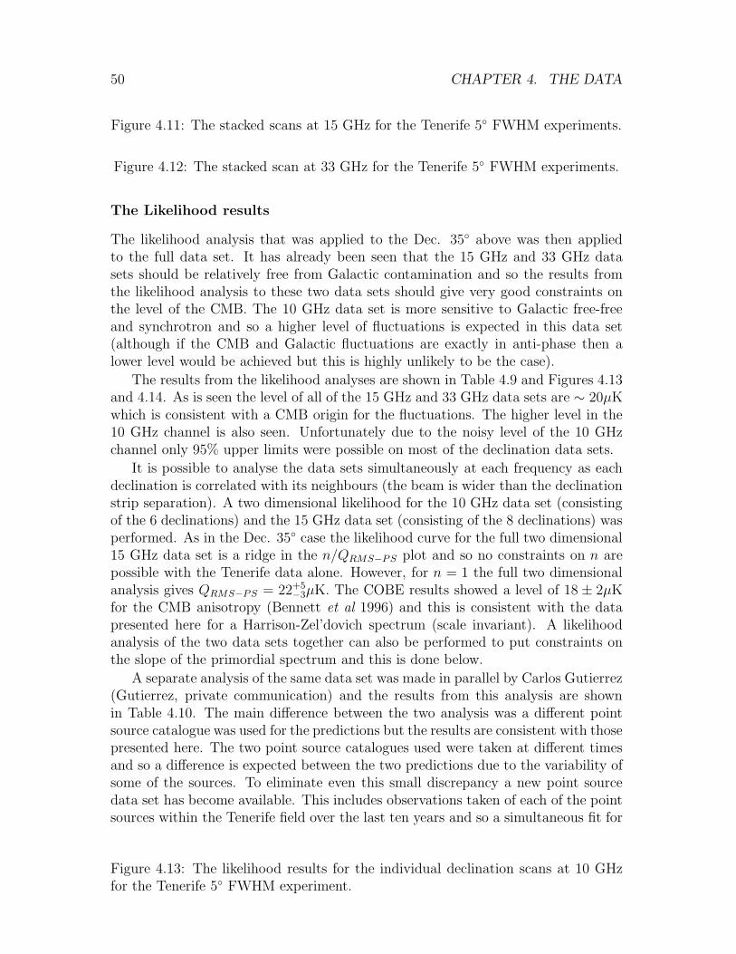
50 CHAPTER 4. THE DATA
Figure 4.11: The stacked scans at 15 GHz for the Tenerife 5 FWHM experiments.
Figure 4.12: The stacked scan at 33 GHz for the Tenerife 5 FWHM experiments.
The Likelihood results
The likelihood analysis that was applied to the Dec. 35 above was then appliedto the full data set. It has already been seen that the 15 GHz and 33 GHz datasets should be relatively free from Galactic contamination and so the results fromthe likelihood analysis to these two data sets should give very good constraints onthe level of the CMB. The 10 GHz data set is more sensitive to Galactic free-freeand synchrotron and so a higher level of fluctuations is expected in this data set(although if the CMB and Galactic fluctuations are exactly in anti-phase then alower level would be achieved but this is highly unlikely to be the case).
The results from the likelihood analyses are shown in Table 4.9 and Figures 4.13and 4.14. As is seen the level of all of the 15 GHz and 33 GHz data sets are ∼ 20µKwhich is consistent with a CMB origin for the fluctuations. The higher level in the10 GHz channel is also seen. Unfortunately due to the noisy level of the 10 GHzchannel only 95% upper limits were possible on most of the declination data sets.
It is possible to analyse the data sets simultaneously at each frequency as eachdeclination is correlated with its neighbours (the beam is wider than the declinationstrip separation). A two dimensional likelihood for the 10 GHz data set (consistingof the 6 declinations) and the 15 GHz data set (consisting of the 8 declinations) wasperformed. As in the Dec. 35 case the likelihood curve for the full two dimensional15 GHz data set is a ridge in the n/QRMS−PS plot and so no constraints on n arepossible with the Tenerife data alone. However, for n = 1 the full two dimensionalanalysis gives QRMS−PS = 22+5
−3µK. The COBE results showed a level of 18 ± 2µKfor the CMB anisotropy (Bennett et al 1996) and this is consistent with the datapresented here for a Harrison-Zel’dovich spectrum (scale invariant). A likelihoodanalysis of the two data sets together can also be performed to put constraints onthe slope of the primordial spectrum and this is done below.
A separate analysis of the same data set was made in parallel by Carlos Gutierrez(Gutierrez, private communication) and the results from this analysis are shownin Table 4.10. The main difference between the two analysis was a different pointsource catalogue was used for the predictions but the results are consistent with thosepresented here. The two point source catalogues used were taken at different timesand so a difference is expected between the two predictions due to the variability ofsome of the sources. To eliminate even this small discrepancy a new point sourcedata set has become available. This includes observations taken of each of the pointsources within the Tenerife field over the last ten years and so a simultaneous fit for
Figure 4.13: The likelihood results for the individual declination scans at 10 GHzfor the Tenerife 5 FWHM experiment.
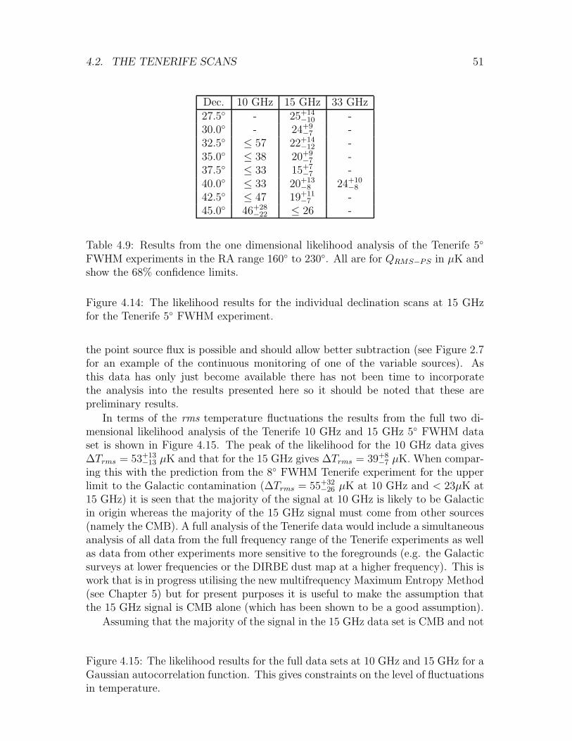
4.2. THE TENERIFE SCANS 51
Dec. 10 GHz 15 GHz 33 GHz27.5 - 25+14
−10 -30.0 - 24+9
−7 -32.5 ≤ 57 22+14
−12 -35.0 ≤ 38 20+9
−7 -37.5 ≤ 33 15+7
−7 -40.0 ≤ 33 20+13
−8 24+10−8
42.5 ≤ 47 19+11−7 -
45.0 46+28−22 ≤ 26 -
Table 4.9: Results from the one dimensional likelihood analysis of the Tenerife 5
FWHM experiments in the RA range 160 to 230. All are for QRMS−PS in µK andshow the 68% confidence limits.
Figure 4.14: The likelihood results for the individual declination scans at 15 GHzfor the Tenerife 5 FWHM experiment.
the point source flux is possible and should allow better subtraction (see Figure 2.7for an example of the continuous monitoring of one of the variable sources). Asthis data has only just become available there has not been time to incorporatethe analysis into the results presented here so it should be noted that these arepreliminary results.
In terms of the rms temperature fluctuations the results from the full two di-mensional likelihood analysis of the Tenerife 10 GHz and 15 GHz 5 FWHM dataset is shown in Figure 4.15. The peak of the likelihood for the 10 GHz data gives∆Trms = 53+13
−13 µK and that for the 15 GHz gives ∆Trms = 39+8−7 µK. When compar-
ing this with the prediction from the 8 FWHM Tenerife experiment for the upperlimit to the Galactic contamination (∆Trms = 55+32
−26 µK at 10 GHz and < 23µK at15 GHz) it is seen that the majority of the signal at 10 GHz is likely to be Galacticin origin whereas the majority of the 15 GHz signal must come from other sources(namely the CMB). A full analysis of the Tenerife data would include a simultaneousanalysis of all data from the full frequency range of the Tenerife experiments as wellas data from other experiments more sensitive to the foregrounds (e.g. the Galacticsurveys at lower frequencies or the DIRBE dust map at a higher frequency). This iswork that is in progress utilising the new multifrequency Maximum Entropy Method(see Chapter 5) but for present purposes it is useful to make the assumption thatthe 15 GHz signal is CMB alone (which has been shown to be a good assumption).
Assuming that the majority of the signal in the 15 GHz data set is CMB and not
Figure 4.15: The likelihood results for the full data sets at 10 GHz and 15 GHz for aGaussian autocorrelation function. This gives constraints on the level of fluctuationsin temperature.
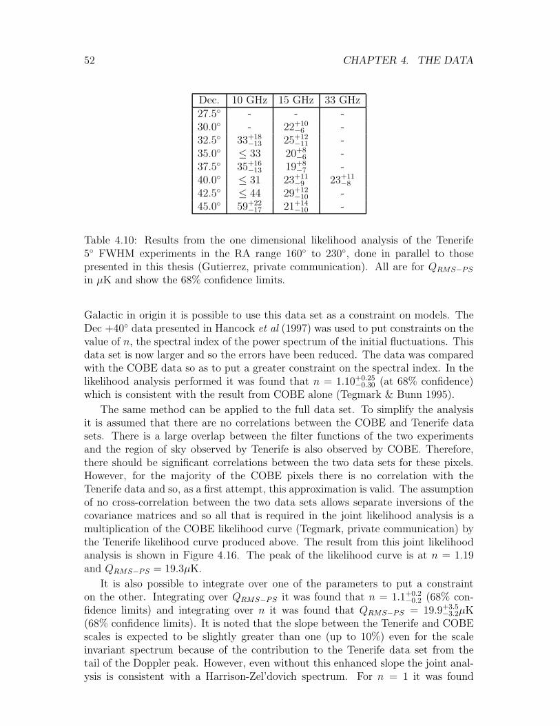
52 CHAPTER 4. THE DATA
Dec. 10 GHz 15 GHz 33 GHz27.5 - - -30.0 - 22+10
−6 -32.5 33+18
−13 25+12−11 -
35.0 ≤ 33 20+8−6 -
37.5 35+16−13 19+8
−7 -40.0 ≤ 31 23+11
−9 23+11−8
42.5 ≤ 44 29+12−10 -
45.0 59+22−17 21+14
−10 -
Table 4.10: Results from the one dimensional likelihood analysis of the Tenerife5 FWHM experiments in the RA range 160 to 230, done in parallel to thosepresented in this thesis (Gutierrez, private communication). All are for QRMS−PS
in µK and show the 68% confidence limits.
Galactic in origin it is possible to use this data set as a constraint on models. TheDec +40 data presented in Hancock et al (1997) was used to put constraints on thevalue of n, the spectral index of the power spectrum of the initial fluctuations. Thisdata set is now larger and so the errors have been reduced. The data was comparedwith the COBE data so as to put a greater constraint on the spectral index. In thelikelihood analysis performed it was found that n = 1.10+0.25
−0.30 (at 68% confidence)which is consistent with the result from COBE alone (Tegmark & Bunn 1995).
The same method can be applied to the full data set. To simplify the analysisit is assumed that there are no correlations between the COBE and Tenerife datasets. There is a large overlap between the filter functions of the two experimentsand the region of sky observed by Tenerife is also observed by COBE. Therefore,there should be significant correlations between the two data sets for these pixels.However, for the majority of the COBE pixels there is no correlation with theTenerife data and so, as a first attempt, this approximation is valid. The assumptionof no cross-correlation between the two data sets allows separate inversions of thecovariance matrices and so all that is required in the joint likelihood analysis is amultiplication of the COBE likelihood curve (Tegmark, private communication) bythe Tenerife likelihood curve produced above. The result from this joint likelihoodanalysis is shown in Figure 4.16. The peak of the likelihood curve is at n = 1.19and QRMS−PS = 19.3µK.
It is also possible to integrate over one of the parameters to put a constrainton the other. Integrating over QRMS−PS it was found that n = 1.1+0.2
−0.2 (68% con-fidence limits) and integrating over n it was found that QRMS−PS = 19.9+3.5
−3.2µK(68% confidence limits). It is noted that the slope between the Tenerife and COBEscales is expected to be slightly greater than one (up to 10%) even for the scaleinvariant spectrum because of the contribution to the Tenerife data set from thetail of the Doppler peak. However, even without this enhanced slope the joint anal-ysis is consistent with a Harrison-Zel’dovich spectrum. For n = 1 it was found
4.2. THE TENERIFE SCANS 53
Figure 4.16: The likelihood results for the combination of COBE and Tenerife datasets. This is very preliminary analysis as no cross-correlations between the two datasets have been taken into account.
Figure 4.17: The levels of fluctuations found from various CMB experiments. Thesolid line is a χ2 minimisation for the points. The two dashed lines correspond toaltering the Saskatoon results by ±14%. Evidence for a Doppler peak is clearlyvisible and it is seen that the Tenerife data is in agreement with the results fromother experiments. The vertical bars on each point correspond to the error on thelevels calculated and the horizontal bars correspond to the window function of theexperiments.
that QRMS−PS = 22.2+4.4−4.2µK. This can also be compared with the joint likeli-
hood analysis for the 15 GHz and 33 GHz Tenerife Dec. 40 data which givesQRMS−PS = 22.7+8.3
−5.7µK for n = 1 which is consistent with the joint COBE and15 GHz Tenerife likelihood analysis. Currently work is being done into calculat-ing the full likelihood results for the joint analysis incorporating all of the cross-correlations between the COBE and Tenerife data sets.
By placing the results from Tenerife for the level of the CMB onto the powerspectrum graph, along with the results from other experiments, it can be seen thatthe standard CDM model (with inflation) is consistent with the findings. Figure4.17 shows the levels of fluctuations found by various CMB experiments. The solidline is a polynomial fit to the points that minimises χ2 and the two dashed linescorrespond to altering the Saskatoon experiment calibration by 14% (the quoteduncertainty in the results). It is clearly seen that there is evidence for the Dopplerpeak in the spectrum (see Hancock et al 1996).

54 CHAPTER 4. THE DATA
Chapter 5
Producing sky maps
The purpose of any Microwave Background experiment is to produce a map of thefluctuations present on the last scattering surface. However, the methods used toobtain the sensitivity required involve scanning, beam switching and interferometryand so a way of working back from the data to the underlying real sky is needed.Similar problems occur when more than one component is present in the data anda method of separating out the different signals is required.
In this Chapter analysis techniques that can be used to find the best astronomicalsignals from a given data set are presented. The four methods to be described areCLEAN (Section 5.1), Singular Value Decomposition (Section 5.2), a new MaximumEntropy Method (Section 5.4) and the Wiener filter (Section 5.6). In the followingChapters the methods are used to analyse the data from each of the experimentsdescribed in Chapter 3.
The Maximum Entropy Method has been introduced previously in Hancock(1994). A fuller account of the method and the choice of parameters is given inthis chapter, as well as new error calculations and new applications to interferom-etry and multiple frequency observations. Therefore, the equations that appear inChapter 4 of Hancock (1994) are repeated here (Equations 5.9 to 5.22) so that thefull method can be followed.
In general, the data from a CMB experiment will take the form of the truesky convolved with the instrumental response matrix with any baseline variationsor noise terms added on. It is assumed that the observations obtained from aparticular experiment have been integrated into discrete bins. For the i-th row andthe j-th column, the data, y
(j)i , recorded by the instrument can be expressed as the
instrumental response matrix R(j)i (i′, j′) acting on the true sky x(i′, j′):
y(j)i =
∑
(i′,j′)
R(j)i (i′, j′)x(i′, j′) + ǫ
(j)i , (5.1)
where i′ and j′ label the true sky row and column position respectively. The ǫ(j)i
term represents a noise term, assumed to be random, uncorrelated Gaussian noise.It is immediately clear from Equation 5.1 that the inversion of the data y
(j)i to
obtain the two-dimensional sky distribution x(i′, j′), is singular. The inverse, R−1,of the instrumental response function does not exist, unless the telescope samples
55
56 CHAPTER 5. PRODUCING SKY MAPS
all of the modes on the sky. Consequently there is a set of signals, comprisingthe annihilator of R, which when convolved with R gives zero. Furthermore, thepresence of the noise term ǫ will effectively enlarge the annihilator of R allowingsmall changes in the data to produce large changes in the estimated sky signal. Itis, therefore, necessary to use a technique that will approximate this inversion.
5.1 CLEAN
The CLEAN technique is an operation which reduces the data into a set of pointsource responses. The point source responses are then convolved with the beamto obtain the ‘CLEAN’ map. For the two dimensional data a two dimensionalCLEAN was implemented. Firstly the algorithm looks for the peak value in the dataamplitude (in the case of the interferometer this is a complex amplitude) and notesits position, (i, j). It then subtracts the normalised beam centred on (i, j) multipliedby γ times the peak value, where γ is the loop gain (γ < 1) set by the user, fromthe data. This process is then repeated iteratively. If this is allowed to continuead–infinitum all the data would be fitted by the point source beam responses butthis has no advantage over the original data so a criterion must be set as to whento halt the iterations. Two methods can be used to halt the iterations. Either thenumber of iterations can be set (Niter) or the peak amplitude of the residual mapcan be set so that no points below this will be fitted. The final responses data setis then convolved with the beam to produce a cleaned map. The obvious problemwith this method is that it eliminates all fluctuations in the data below the thresholdlevel (or below the level set by Niter). However, it does reconstruct all large sourcesvery quickly.
5.2 Singular Value Decomposition
In singular value decomposition (SVD) the solution to Equation 5.1 can be approx-imated by solving
y(j)i =
∑
(i′,j′)
R(j)i (i′, j′)x(i′, j′) (5.2)
where x is the best estimate (given the noise and beam convolution) of the underlyingtrue sky x. The solution is found by minimising the residual
r =∑
(i,j)
∣
∣
∣
∣
∣
∣
y(j)i −
∑
(i′,j′)
R(j)i (i′, j′)x(i′, j′)
∣
∣
∣
∣
∣
∣
2
. (5.3)
To find an approximate inverse of the R matrix, so that the best x can be found, itis written as the product of three matrices.
R = UWVT (5.4)
5.3. BAYES’ THEOREM 57
where U and V are both orthogonal matrices and W is purely diagonal with ele-ments wk. The formal inverse of R is therefore easily found and is equal to
R−1 = V
[
diag(
1
wk
)]
UT . (5.5)
The singular values of R (comprising the annihilator) are easily seen as the valuesof wk that are zero. To overcome this problem the SVD analysis sets a conditionnumber which is defined as the ratio of the largest wk to the smallest wk. Any wk
below the minimum value set by the condition number (so that it is close to zeroand therefore represents a possible singular value) has the corresponding 1/wk setto zero. The condition number is usually set to machine precision and so roundingerrors and singularities are removed making the approximate inverse possible tocalculate.
The SVD analysis does not take into account the level of noise in the data vectorand so may have the tendency to amplify the noise. A method of regularising thisis required.
5.3 Bayes’ theorem and the entropic prior
There are many degenerate sky solutions that are consistent with the data but itis desired to assume as little as possible about the true sky so as to avoid biastowards any particular model. By considering the problem from a purely Bayesianviewpoint, the most probable sky distribution given our data set and some priorinformation is desired. Given a hypothesis H , data D and background informationI, then Bayes’ theorem states that the posterior probability distribution Pr(H|DI)is the product of the prior probability Pr(H|I) and the likelihood Pr(D|HI), withsome overall normalising factor called the evidence Pr(D|I):
Pr(H|DI) =Pr(H|I) Pr(D|HI)
Pr(D|I) . (5.6)
The likelihood Pr(D|HI) is fully defined by the data, but there is freedom to choosethe prior Pr(H|I). The most conservative prior assumption is to simply take thesky fluctuations to be small at some level. It is therefore desired to find the skythat contains the least amount of information, the one closest to being smooth,that is still consistent with the data set. This forms the basis of the so called“maximum entropy methods” (MEM) (Gull 1989, Gull & Skilling 1984) used in thereconstruction of images. If the class of sky models is restricted to those with thisproperty then this leads to a prior of form (Skilling 1989),
Pr(H|I) ∝ exp(αS(f,m)) (5.7)
for an image f(ξ) and prior information m(ξ), where ξ is the position on the sky.The regularising parameter, α, is a dimensional constant that depends on the scalingof the problem and S(f,m) is the cross entropy. For a positive, additive distribution(PAD), the cross entropy is given by (Skilling 1988):
58 CHAPTER 5. PRODUCING SKY MAPS
S(f,m) =∫
dξ
[
f(ξ) −m(ξ) − f(ξ) ln
(
f(ξ)
m(ξ)
)]
, (5.8)
where m(ξ) can also be considered a constraint on f(ξ) such that when the entropicprior dominates, the aposteriori sky map f(ξ) does not deviate significantly fromm(ξ). This form is chosen for the entropy to ensure that the global maximum ofthe entropy at f(ξ) = m(ξ) is zero and it is the only form of entropy consistentwith coordinate and scaling invariance (Skilling 1988) which does not introduce anybiases away from a small fluctuation model.
5.3.1 Positive and negative data reconstruction
Due to the log entropy term, this standard form is inapplicable in the more generalcase of an image x(ξ) that can take both positive and negative values. Various meth-ods in the past have been tried to reconstruct data containing negative peaks. Laue,Skilling and Staunton (1985) proposed a two channel MEM, which involved splittingthe data into positive and negative features and then reconstructing each separatelybut not taking into account any continuity constraint between the two. This methodis inappropriate for differencing experiments as the positive and negative featuresoriginate from the beam shape and not from separate sources. White and Bunn(1995) have proposed adding a constant onto the data to make it wholly positive.They use the Millimetre-wave Anisotropy Experiment (MAX) data to reconstruct a5×2 region of sky. As simulations performed show, this method introduces a biastowards positive (or negative if the data are inverted) reconstruction. The reasonfor this is that the added constant has to be small enough so that numerical errorsare not introduced into the calculations but a lower constant will give less range forthe reconstruction of negative features and so the most probable sky will be a morepositive one. A method to overcome both of these problems is proposed here (seeJones et al 1998 and Maisinger et al 1997).
Consider the image to be the difference between two PADS:
x(ξ) = u(ξ) − v(ξ),
so that the expression for the cross entropy becomes:
S(u, v,m) =∫
dξ
[
u(ξ) −mu(ξ) − u(ξ) ln
(
u(ξ)
mu(ξ)
)]
+
∫
dξ
[
v(ξ) −mv(ξ) − v(ξ) ln
(
v(ξ)
mv(ξ)
)]
. (5.9)
With the prior thus defined, it is possible to calculate the probability of obtainingthe reconstructed sky x (the hypothesis H) given y (the data D):
Pr(x|y) ∝ Pr(x) Pr(y|x), (5.10)
and then maximise Pr(x|y) to obtain the most likely 2-D image of the microwavesky.
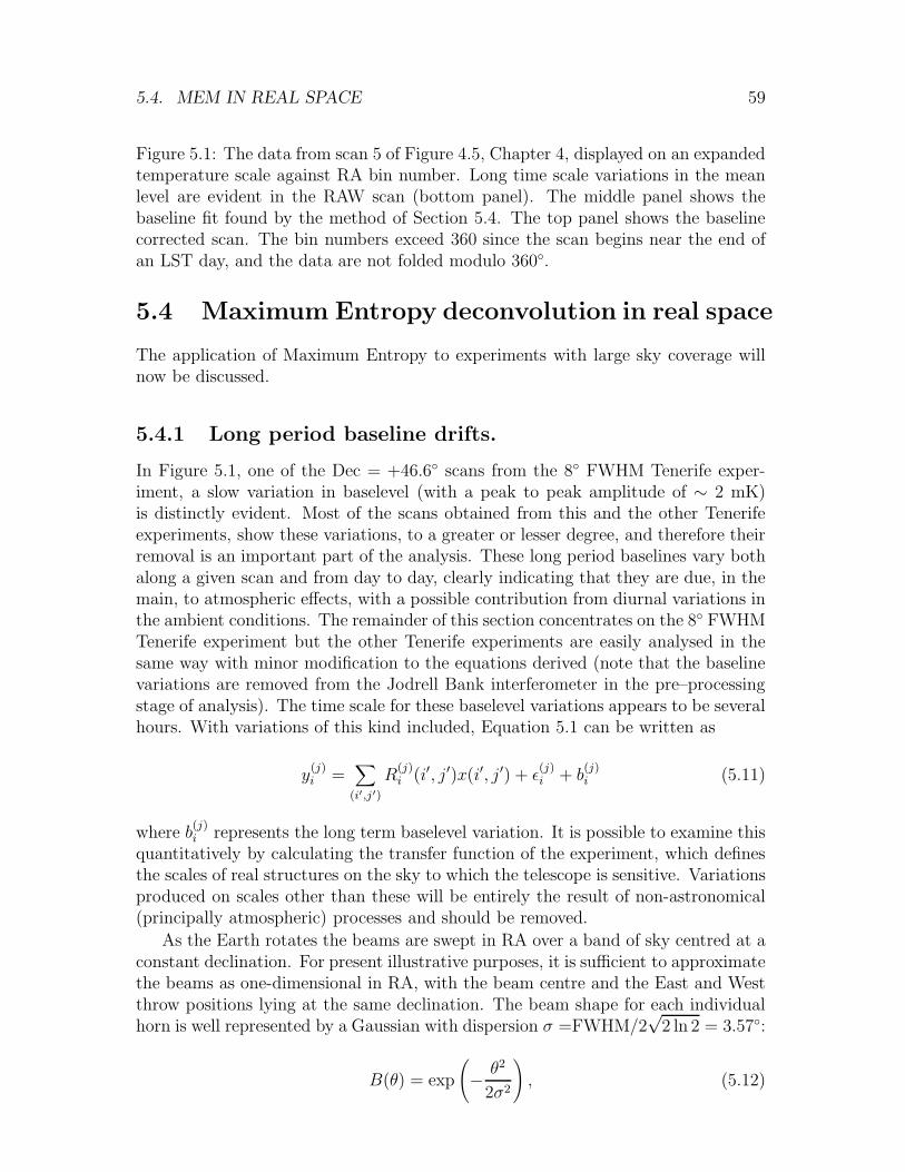
5.4. MEM IN REAL SPACE 59
Figure 5.1: The data from scan 5 of Figure 4.5, Chapter 4, displayed on an expandedtemperature scale against RA bin number. Long time scale variations in the meanlevel are evident in the RAW scan (bottom panel). The middle panel shows thebaseline fit found by the method of Section 5.4. The top panel shows the baselinecorrected scan. The bin numbers exceed 360 since the scan begins near the end ofan LST day, and the data are not folded modulo 360.
5.4 Maximum Entropy deconvolution in real space
The application of Maximum Entropy to experiments with large sky coverage willnow be discussed.
5.4.1 Long period baseline drifts.
In Figure 5.1, one of the Dec = +46.6 scans from the 8 FWHM Tenerife exper-iment, a slow variation in baselevel (with a peak to peak amplitude of ∼ 2 mK)is distinctly evident. Most of the scans obtained from this and the other Tenerifeexperiments, show these variations, to a greater or lesser degree, and therefore theirremoval is an important part of the analysis. These long period baselines vary bothalong a given scan and from day to day, clearly indicating that they are due, in themain, to atmospheric effects, with a possible contribution from diurnal variations inthe ambient conditions. The remainder of this section concentrates on the 8 FWHMTenerife experiment but the other Tenerife experiments are easily analysed in thesame way with minor modification to the equations derived (note that the baselinevariations are removed from the Jodrell Bank interferometer in the pre–processingstage of analysis). The time scale for these baselevel variations appears to be severalhours. With variations of this kind included, Equation 5.1 can be written as
y(j)i =
∑
(i′,j′)
R(j)i (i′, j′)x(i′, j′) + ǫ
(j)i + b
(j)i (5.11)
where b(j)i represents the long term baselevel variation. It is possible to examine this
quantitatively by calculating the transfer function of the experiment, which definesthe scales of real structures on the sky to which the telescope is sensitive. Variationsproduced on scales other than these will be entirely the result of non-astronomical(principally atmospheric) processes and should be removed.
As the Earth rotates the beams are swept in RA over a band of sky centred at aconstant declination. For present illustrative purposes, it is sufficient to approximatethe beams as one-dimensional in RA, with the beam centre and the East and Westthrow positions lying at the same declination. The beam shape for each individualhorn is well represented by a Gaussian with dispersion σ =FWHM/2
√2 ln 2 = 3.57:
B(θ) = exp
(
− θ2
2σ2
)
, (5.12)
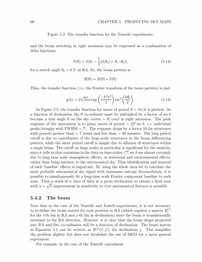
60 CHAPTER 5. PRODUCING SKY MAPS
Figure 5.2: The transfer function for the Tenerife experiments.
and the beam switching in right ascension may be expressed as a combination ofdelta functions:
S(θ) = δ(0) − 1
2(δ(θb) + δ(−θb)), (5.13)
for a switch angle θb = 8.3 in RA. So, the beam pattern is
R(θ) = B(θ) ∗ S(θ).
Thus, the transfer function, (i.e. the Fourier transform of the beam pattern) is just:
g(k) = 2√
2πσ exp
(
−k2σ2
2
)
sin2
(
kθb
2
)
. (5.14)
In Figure 5.2, the transfer function for waves of period θ = 2π/k is plotted. Asa function of declination the θ co-ordinate must be multiplied by a factor of sec δbecause a true angle θ on the sky covers ∼ θ/ cos δ in right ascension. The peakresponse of the instrument is to plane waves of period ∼ 22 sec δ, i.e. individualpeaks/troughs with FWHM ∼ 7. The response drops by a factor 10 for structureswith periods greater than ∼ 7 hours and less than ∼ 40 minutes. The long periodcutoff is due to cancellation of the large-scale structures in the beam differencingpattern, while the short period cutoff is simply due to dilution of structures withina single beam. The cutoff on large scales in particular is significant for the analysis,since it tells us that variations in the data on time scales >
∼7h sec δ are almost certainlydue to long time scale atmospheric effects, or terrestrial and environmental effects,rather than being intrinsic to the astronomical sky. Thus identification and removalof such ‘baseline’ effects is important. By using the whole data set to calculate themost probable astronomical sky signal with maximum entropy deconvolution, it ispossible to simultaneously fit a long-time scale Fourier component baseline to eachscan. Then a stack of n days of data at a given declination to obtain a final scanwith a ∼ √
n improvement in sensitivity to true astronomical features is possible.
5.4.2 The beam
Note that in the case of the Tenerife and Jodrell experiments, it is not necessaryto re-define the beam matrix for each position in RA (which requires a matrix R
(j)i
for the i-th bin in RA and j-th bin in declination) since the beam is translationallyinvariant in the RA direction. However, it is clear that the beam shape projectedinto RA and Dec co-ordinates will be a function of declination. The beam matrixin Equation 5.1 can be written as R(j)(i′, j′), for declination j. This simplifiesthe problem slightly but does not invalidate the use of MEM for a more generalexperiment.
For example, in the case of the Tenerife experiment
5.4. MEM IN REAL SPACE 61
R(j)(i′, j′) = C
[
exp
(
− θ2C
2σ2
)
− 1
2
(
exp
(
− θ2E
2σ2
)
+ exp
(
− θ2W
2σ2
))]
(5.15)
where θC , θE , and θW represent the true angular separation of the point (i′, j′)from the beam centre and the East and West throw positions respectively. Thenormalisation of the beam matrix is determined by C and is implemented withrespect to a single beam. The angles θC , θE , and θW can be calculated using sphericalgeometry. If the beam is centred at Dec. δ(j) and α0 is the (arbitrary) RA originfor the definition of all the beams, for a source at a general (α, δ) corresponding tothe grid point (i′, j′) the distance from the main beam centre is
θC = arccos(
sin δ(j) sin δ + cos(α0 − α) cos δ(j) cos δ)
. (5.16)
There are also two other beams (with half the amplitude of the central beam),due to the beamswitching and mirror wagging, a distance θb (the beamthrow) eitherside of the central peak. These have RA centres given by θE or θW as in Equation 5.15defined as
cos(θE or W − α0) =cos θb − sin2 δ(j)
cos2 δ(j),
and (fairly accurately for the beamthrow used in practice) Dec’s of δ(j) still. Thustheir angular distances from the source at (i′, j′) can be worked out from Equa-tion 5.16, yielding θE or W , and the final R(j) entry computed from Equation 5.15.
5.4.3 Implementation of MEM
If the assumption of random Gaussian noise if made, the likelihood is given by:
Pr(y|x) ∝ exp
(
−χ2
2
)
, (5.17)
where χ2 is the misfit statistic (Equation 5.22). Thus in order to maximise Pr(x|y)it is simply necessary to minimise the function
F = χ2 − αS (5.18)
where a factor of two has been absorbed into the constant α. Thus the process isto iterate to a minimum in F by consistently updating the 2-D reconstructed skyx(i′, j′). For the Tenerife data set long term baselines for each scan are also builtup simultaneously. The baselines are represented by a Fourier series
b(j)ir = C
(j)0r +
nmax∑
n=1
[
C(j)nr cos(
2nπi
l) +D(j)
nr sin(2nπi
l)]
(5.19)
for the r-th scan at the j-th declination with nmax baseline coefficients to be fitted.The basis data vector index i runs from 1 to l, the length of the data sets (3 × 24h
for the Tenerife 8 FWHM data set). Thus to obtain a minimum period solution >∼
62 CHAPTER 5. PRODUCING SKY MAPS
7h sec δ (Section 5.4.1) we must limit the number of baseline coefficients, nmax inEquation 5.19 to less than 9 (for the case δ = 40) for the Tenerife 8 FWHM dataset and less than 16 for the Tenerife 5 FWHM data set.
For the rth Tenerife scan, Equation 5.11 may be written as
y(j)ir = y
pred(j)i + b
(j)ir + ǫ
(j)ir , (5.20)
with the baseline variation b included and
ypred(j)i =
∑
i′,j′R(j)(i′, j′)x(i′ + i, j′) (5.21)
is the predicted signal produced by the telescope in the absence of noise and baselineoffsets. The beam matrix R is now defined with respect to an origin (which waschosen to be zero) in the i′ direction as it is translationally invariant in RA. Thisgives us the term x(i′ + i, j′) instead of x(i′, j′). So, the χ2 for the problem is
χ2 =ndecs∑
j=1
nra∑
i=1
w(j)i (y
pred(j)i − y
obs(j)i )2, (5.22)
for a total number of declinations ndecs, total number of RA bins nra and observedstacked data values y
obs(j)i with weighting factor w
(j)i , which are a weighted average
over the ns scans with the baseline b(j)ir subtracted from each of the scans y
(j)ir (r is
an index running over the ns scans). In the absence of data w(j)ir , for each individual
scan, is set to zero and when data is present it is given by the inverse of the variancefor the data point. It is a fairly simple task to compute y
pred(j)i , since it is possible
to use prior knowledge of the geometry of the instrument to calculate the expectedresponse function R(j)(i′, j′) for each i′, j′, at RA i and declination j, thus χ2 is fullydefined.
For the Jodrell Bank interferometer there are two orthogonal channels thatshould be included. As the entropy term depends on an unconvolved map thisdoes not change with the introduction of these two orthogonal terms. However, forthe i−th bin in right ascension and the j−th bin in declination the data, the χ2
term becomes
χ2 =ndecs∑
j=1
nra∑
i=1
w(j)ic (y
pred(j)ic − y
obs(j)ic )2 +
ndecs∑
j=1
nra∑
i=1
w(j)is (y
pred(j)is − y
obs(j)is )2, (5.23)
for a total number of declinations ndecs, total number of RA bins nra and observeddata value y
obs(j)ic/s with weighting factor w
(j)ic/s taken to be the inverse of the variance
of the pixel. The cosine and sine channels are given by
y(j)ic =
∑
(i′,j′)
C(j)(i′, j′)x(i′ + i, j′) + ǫ(j)ic , (5.24)
and
5.4. MEM IN REAL SPACE 63
y(j)is =
∑
(i′,j′)
S(j)(i′, j′)x(i′ + i, j′) + ǫ(j)is , (5.25)
where i′ and j′ label the true sky right ascension bin and declination bin respectively,and C and S are the beam matrices for the cosine and sine channel respectively.The beams are once more defined with respect to an arbitrarily chosen origin ofi = 0 as they are translationally invariant in RA. The ǫ
(j)ic/s term represents a noise
term, assumed to be random Gaussian noise.Applying the requirements of continuity in entropy with respect to x (so that
the partial gradients with respect to u and v are equal and opposite, which leads touv = m2) to Equation 5.9 implies an entropy term, S(x,m), of form:
∑
i′,j′
[
ψi′,j′ − 2mi′,j′ − xi′,j′ ln
(
ψi′,j′ + xi′,j′
2mi′,j′
)]
, (5.26)
where ψi′,j′ = ui′,j′ + vi′,j′ = (x2i′,j′ +4m2
i′,j′)1/2. Using our prior information that the
sky fluctuations have zero mean, mi′,j′ = mu = mv (from Equation 5.9) was chosen,
and the minima of the large entropy case corresponds to x =(
1−mu
mv
)
u = 0; mi′,j′
can therefore be considered as a level of ‘damping’ imposed on xi′,j′ rather than adefault model as in the positive-only MEM. A large value of m allows large noisyfeatures to be reconstructed whereas a small value of m will not allow the final skyto deviate strongly from the zero mean.
Thus, if the value of the regularising parameter α and the ‘damping’ term mis known then F is determined and the best sky reconstruction is that for which∂F/∂xij = 0, ∀xij . This is most easily implemented by applying one-dimensionalNewton-Raphson iteration simultaneously to each of the xij to find the zero of thefunction G(x) = ∂F/∂x. This means that x is updated from the n-th to the (n+1)-th iteration by
xn+1lm = xn
lm − γ
G(xnlm)
∂G∂xlm
∣
∣
∣
xnlm
. (5.27)
Convergence towards a global minimum is ensured by setting a suitable value forthe loop gain γ and updating xlm only if ∂G
∂xlm
∣
∣
∣
xnlm
is positive. The differential with
respect to the sky model is easily found analytically. For χ2 it is found that
∂χ2
∂xlm= 2
∑
k
∑
i
w(k)i
(
R(k)(l − i,m)(ypred(k)i − y
obs(k)i )
)
(5.28)
and, considering only the diagonal terms that are of concern here,
∂2χ2
∂xlm2
= 2∑
k
∑
i
w(k)i
(
R(k)(l − i,m))2
(5.29)
and for the entropy term, S, it is found that
64 CHAPTER 5. PRODUCING SKY MAPS
∂S
∂xlm= − ln
(
ulm
mlm
)
= − ln
(
ψlm + xlm
2mlm
)
(5.30)
and
∂2S
∂xlm2
= − 1
ulm + vlm= − 1
ψlm. (5.31)
In the case of the Tenerife data where the long-term baseline fluctuations areleft in the data to be analysed by MEM, it is possible to simultaneously fit forthe parameters of the baselines. The best reconstruction of the microwave skyis calculated and subtracted from each individual scan and then an atmosphericbaseline is fitted to each scan. To fit for the baseline parameters C
(j)0r , C(j)
nr andD(j)
nr as expressed in Equation 5.19 it is sufficient to implement a simultaneous butindependent χ2 minimisation on each of these to obtain the baseline for the r-th scan.From the Bayesian viewpoint minimising χ2 is just finding the maximum posteriorprobability by using a uniform prior. This is also done with a Newton-Raphsoniterative technique with a new loop gain, γb.
5.4.4 Errors on the MEM reconstruction
The posterior probability of the MEM reconstruction can be written as
Pr(H|DI) ∝ exp[
−(
χ2 − αS)]
(5.32)
and expanding the exponent around its minimum gives
χ2 − αS =(
χ2 − αS)
min+ x∇
(
χ2 − αS)
min+
1
2x†∇2
(
χ2 − αS)
minx. (5.33)
At the minima (the maximum probability) ∇ (χ2 − αS) = 0 and so, to second order,Equation 5.32 can be written as
Pr(H|DI) = Pr(HMP |DI)exp[
−1
2x†∇2
(
χ2 − αS)
minx]
(5.34)
where HMP is the most probable reconstruction ofH given the data,D, and informa-tion, I (i.e. it is the MEM solution). This is a Gaussian in x with covariance matrixgiven by the inverse Hessian, M−1 = (∇2 (χ2 − αS)min)
−1. For the reconstruction
of data from CMB experiments the Hessian is given by
Mlk = RilRik +α
xlkδlk (5.35)
where R is the beam and x is the sky reconstruction. This follows directly fromconsidering all of the terms, on and off the diagonal, in Equations 5.29 and 5.31.The second differential of the entropy is a diagonal matrix, however, the seconddifferential of the χ2 is not diagonal. The errors on the reconstruction, therefore,involve the inversion of a large matrix that is computationally intense. For the case
5.4. MEM IN REAL SPACE 65
of the Planck surveyor this would involve the inversion of a (400× 400× 5)2 matrix.For this reason the simpler method of performing Monte Carlo simulations was usedto obtain an estimate on the errors. However, in the Fourier plane the problem isdramatically simplified (see Section 5.5).
5.4.5 Choosing α and m
In this MEM approach the entropic regularising parameter, α, controls the competi-tion between the requirement for a smoothly varying sky and the noisy sky imposedby the data. The larger the value of α the more the data are ignored. The smallerthe value of α the more noise is reconstructed. A choice of α that will take maxi-mum notice of the data vectors containing information on the true sky distribution,while using the beam response shape to reject the noisy data vectors is required. Insome sense, the entropy term may be thought of as using the prior information thatthe sky is continuous at some level to fill in for the information not sampled by theresponse function, thereby allowing the inversion process to be implemented.
Here, m is chosen to be of similar size to the rms of the fluctuations so thatthe algorithm has enough freedom to reconstruct the expected features. Increas-ing/decreasing m by an order of magnitude from this value does not alter the finalresult significantly so that the absolute value of m is not important. This is differentto a positive–only MEM because in that case m is chosen to be the default model(the value of the sky reconstruction in the absence of data) and is therefore moreconstrained by the problem itself. In the case of positive/negative MEM, as m isthe default model on the two channels and not on the final sky, there is a greaterfreedom in its choice.
For a data set with independent data points, α is completely defined in a Bayesiansense (see Section 5.5.3). For data sets containing a large number of non-independentpoints (as in the case of real sky coverages that contain beam convolutions so thatthe data set is too large to allow inversion of the Hessian; see Section 5.5.3), theoptimum choice of α is somewhat controversial in the Bayesian community andwhile several methods exist (Gull 1989, Skilling 1989) it is difficult to select oneabove the others that is superior. The criterion that χ2 − αS = N , where N is thenumber of data points that are fitted in the convolved sky, is used here. If any ofthe data points are weighted to zero, as the galactic plane crossing is in the casesconsidered here, these points should not be included in N . Increasing/decreasing αby a factor of ten decreases/increases the amplitude of the fluctuations derived inthe final analysis by <
∼ 5 %. The value of α is decreased in stages until χ2−αS = N ;experience has shown that a convergent solution, for the 10 GHz, 5 FWHM Tenerifeexperiment, is best obtained with the typical parameter values given in Table 5.1.Below this value for α the noisy features in the data have a large effect and the scansare poorly fitted. This can be seen in Figure 5.3 where χ2−αS begins to flatten outas α is lowered further than the chosen value (shown as a cross). From this figureit is easy to chose the value of α. Note that any significance cannot be attached tothe absolute value of α, since it is a parameter that depends on the scaling of theproblem. Also shown in Figure 5.3 is the effect of varying m, the ‘damping’ term.
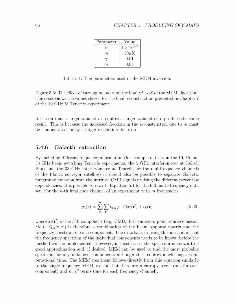
66 CHAPTER 5. PRODUCING SKY MAPS
Parameter Valueα 4 × 10⁻²
m 50µKγ 0.01γb 0.05
Table 5.1: The parameters used in the MEM inversion.
Figure 5.3: The effect of varying m and α on the final χ2−αS of the MEM algorithm.The cross shows the values chosen for the final reconstruction presented in Chapter 7of the 10 GHz 5 Tenerife experiment.
It is seen that a larger value of m requires a larger value of α to produce the sameresult. This is because the increased freedom in the reconstruction due to m mustbe compensated for by a larger restriction due to α.
5.4.6 Galactic extraction
By including different frequency information (for example data from the 10, 15 and33 GHz beam switching Tenerife experiments, the 5 GHz interferometer at JodrellBank and the 33 GHz interferometer at Tenerife, or the multifrequency channelsof the Planck surveyor satellite) it should also be possible to separate Galacticforeground emission from the intrinsic CMB signals utilising the different power lawdependencies. It is possible to rewrite Equation 5.1 for the full multi–frequency dataset. For the k-th frequency channel of an experiment with m frequencies
yk(r) =n∑
l=1
∑
r′
Qkl(r, r′)xl(r
′) + ǫk(r) (5.36)
where xl(r′) is the l-th component (e.g. CMB, dust emission, point source emission
etc.). Qkl(r, r′) is therefore a combination of the beam response matrix and the
frequency spectrum of each component. The drawback in using this method is thatthe frequency spectrum of the individual components needs to be known before themethod can be implemented. However, in most cases, the spectrum is known to agood approximation and, if desired, MEM can be used to find the most probablespectrum for any unknown components although this requires much longer com-putational time. The MEM treatment follows directly from this equation similarlyto the single frequency MEM, except that there are n entropy terms (one for eachcomponent) and m χ2 terms (one for each frequency channel).
5.5. MEM IN FOURIER SPACE 67
5.5 Maximum entropy in Fourier space
If the sky coverage of a particular experiment is not too large, so that the sphericityis negligible and a Fourier transform can be used, then the problem becomes sim-plified. This may also be possible with larger sky coverages but will require a moresophisticated decomposition of the sky harmonics (e.g. full sky spherical harmonicdecomposition, for which the main limitation is computational time). Therefore, inFourier space it is useful to look at the full Maximum Entropy problem again.
If the Fourier transform of Equation 5.36 is taken then we find
yk(k) =∑
l
Qkl(k,k′)xl(k
′) + ǫl(k) (5.37)
where k is the Fourier mode. The convolution between Q and x has been replacedby a multiplication. This in itself represents a substantial simplification of all ofthe calculations involved in implementing the MEM approach. It is seen that eachFourier mode is independent of each other Fourier mode and so the Maximum En-tropy algorithm can be implemented on a pixel by pixel basis (where each pixelis now a separate Fourier mode). However, it is also possible to include furtherinformation to MEM using this method.
If the correlation of x is known then it may be useful to use this extra informationto further constrain the image reconstruction. We define the Fourier transform ofthe signal covariance matrix as
Cll′(r) = 〈xl(r)xl′(r)〉 (5.38)
where Cll′ is real with dimensions n× n (the number of components). The diagonalelements of C contain the ensemble average power spectra of the different com-ponents at a reference frequency ν and the off-diagonal terms contain the crosspower spectra between components. The known correlations can be incorporatedinto MEM through the use of an intrinsic correlation function (ICF) and a set ofindependent hidden variables (Gull & Skilling 1990 and Hobson et al 1998a). Thisis most easily achieved by the inclusion of lower triangular matrix L such that
x = Lh. (5.39)
L is obtained by performing a Cholesky decomposition (Press et al 1992) of thematrix C such that LLT = C. Thus, the components of h are uncorrelated and ofunit variance and so
⟨
xx†⟩
=⟨
Lhh†LT⟩
= L⟨
hh†⟩
LT = LLT = C (5.40)
as required. Now the ‘default’ model in the MEM is a measure on h and not x andso the rms expected level is simply unity.
Equation 5.37 can now be written as
yk(k) =∑
l,m
Qkl(k,k′)Llm(k′)hm(k′) + ǫk(k) (5.41)
68 CHAPTER 5. PRODUCING SKY MAPS
and L can be absorbed into Q so that it now contains frequency and spatial infor-mation for each of the foregrounds and the CMB. Now the MEM problem becomesthe reconstruction of h. Equation 5.9 follows directly except that now the differencebetween u and v is used to reconstruct h.
5.5.1 Implementation of MEM in Fourier space
The problem is now exactly the same as before except all the terms are complex.The log term in the entropy does not allow for complex reconstructions but it isnoted that the real and imaginary parts of the sky are independent of each otherand so it is possible to split them up into two different PADS. Therefore, one complexreconstruction is split into a total of four channels; ureal, vreal, uimag and vimag. The
χ2 term is easily calculable from the reconstruction h as it depends linearly upon it(through the multiplication). Therefore, the reconstruction for each k-mode can befound separately.
If there is an initial guess for the distribution of h then it is possible to incorporatethis into the MEM algorithm in two different ways. The first way is to incorporatethe information into the covariance matrix and allow MEM to reconstruct the besthidden variables given the covariance matrix. In the absence of any initial guess atthe shape of the covariance matrix, it is set to a flat model with the total powerchosen to be the same as that in the input maps. If it is noted that the differencebetween mu and mv is the ‘default’ level for h (the real and imaginary parts of hneed to be considered separately here) then another method for taking into accountan initial guess is possible. Taking a uniform background common to both defaultvalues (this is taken as the rms of h) the initial guess at h is split into a positivepart (added onto mu) and a negative part (added onto mv) so that mu − mv isequal to the guess. Without the initial guess then it can be seen that h representsphase information and so both mu and mv are assigned with unit amplitude. In theabsence of data h will default to the original guess.
The function F is now fully defined and the maximum of the posterior probabilityis required. To find the minimum of F , which is now dependent on a very smallnumber of variables, a quick minimisation routine is required. The variable metricminimisation (Press et al 1992), which uses the first derivative of the function andestimates the second derivative, approaches the minimum quadratically. This provedto be the most efficient method of minimising in Fourier space (other methods weretried and comparison between the various minimisations showed that each methodwas consistent).
5.5.2 Updating the model
After the posterior probability has been maximised an estimate of the underlyingsky signal x is obtained. This could be used as the best sky reconstruction but itis also possible to use this estimate as the initial guess to MEM to find a betterreconstruction. The guess can either be used to update the covariance matrix orthe default sky models as described above. It is then possible to iterate until no
5.5. MEM IN FOURIER SPACE 69
significant change is observed between iterations (a 3% change in any pixel flux wasused as a measure of whether the image had converged or not in the simulations inthe following Chapter).
5.5.3 Bayesian α calculation
A common criticism of MEM has been the arbitrary choice of α, the Lagrangemultiplier. However, it is possible to completely define α using a Bayesian approach.If the problem is thought of as trying to find the maximum probability with respectto both h and α, given some background information I, it is possible to first integrateover all possible h values to find that
Pr(α|y, I) =1
Pr(α|I)∫
Pr(h, y, α|I) dN h
det[ψ]12
(5.42)
and maximise this in a similar way to maximising over h before. The metric on thespace of positive/negative distributions is given by −∇h∇hS(h,m) which leads tothe invariant volume, det[ψ]−1/2, in the integral (this can be derived by consideringthe difference between two Poisson distributions; see Hobson & Lasenby 1998).
The full posterior probability can be written as
Pr(h, y, α|I) = Pr(h|α, I) Pr(y|h, α, I) Pr(α|I) (5.43)
and expanding this one finds
Pr(h, y, α|I) =Pr(α|I)ZsZL
exp(
α(S1 + S2 + ....SN ) − 1
2χ2)
(5.44)
where Zs is the normalisation constant for the entropy term and ZL is that for thelikelihood term. The total entropy is the sum of the entropy for each of the separatemaps that go into h.
If one Taylor expands each term about its minimum (e.g. S = Smin+12h∇2Sminh+
...) then it is found that, to second order,
Zs = (2π)N2 α
N2 (5.45)
where N is the number of independent variables to be found. For example, N = 6 inthe case of a data set made from three input maps (i.e. h consists of three channels)if the calculation is performed on each Fourier mode separately (remembering thateach of the three channels is made up of a real and an imaginary channel) and N =6np, where np is the number of pixels in each map, if the calculation is performedon all Fourier modes simultaneously. The function to be minimised is given by
F (h) = F (h)min − 1
2h[ψ− 1
2 ]A[ψ− 12 ]h (5.46)
where A = [ψ12 ]M [ψ
12 ] and M is the Hessian and ψ = −∇2S. The probability
distribution for α is given by Equation 5.42 and so substituting in the expansions itis found that
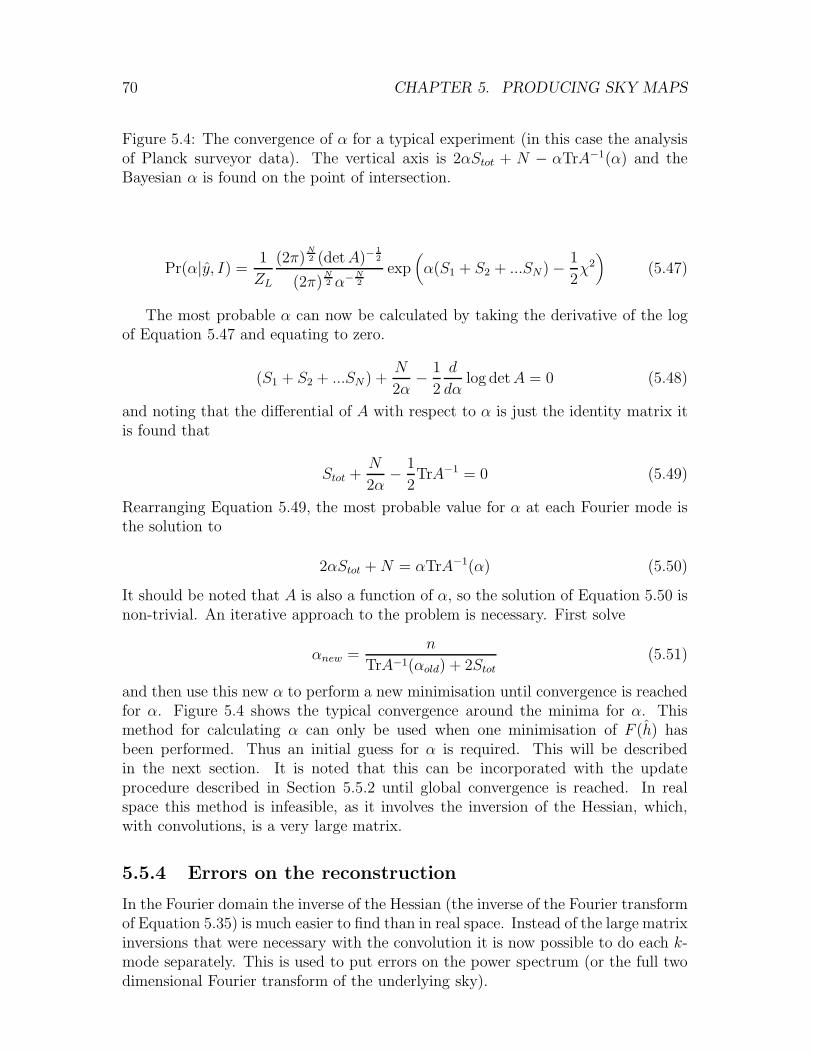
70 CHAPTER 5. PRODUCING SKY MAPS
Figure 5.4: The convergence of α for a typical experiment (in this case the analysisof Planck surveyor data). The vertical axis is 2αStot + N − αTrA−1(α) and theBayesian α is found on the point of intersection.
Pr(α|y, I) =1
ZL
(2π)N2 (detA)−
12
(2π)N2 α−N
2
exp(
α(S1 + S2 + ...SN) − 1
2χ2)
(5.47)
The most probable α can now be calculated by taking the derivative of the logof Equation 5.47 and equating to zero.
(S1 + S2 + ...SN ) +N
2α− 1
2
d
dαlog detA = 0 (5.48)
and noting that the differential of A with respect to α is just the identity matrix itis found that
Stot +N
2α− 1
2TrA−1 = 0 (5.49)
Rearranging Equation 5.49, the most probable value for α at each Fourier mode isthe solution to
2αStot +N = αTrA−1(α) (5.50)
It should be noted that A is also a function of α, so the solution of Equation 5.50 isnon-trivial. An iterative approach to the problem is necessary. First solve
αnew =n
TrA−1(αold) + 2Stot(5.51)
and then use this new α to perform a new minimisation until convergence is reachedfor α. Figure 5.4 shows the typical convergence around the minima for α. Thismethod for calculating α can only be used when one minimisation of F (h) hasbeen performed. Thus an initial guess for α is required. This will be describedin the next section. It is noted that this can be incorporated with the updateprocedure described in Section 5.5.2 until global convergence is reached. In realspace this method is infeasible, as it involves the inversion of the Hessian, which,with convolutions, is a very large matrix.
5.5.4 Errors on the reconstruction
In the Fourier domain the inverse of the Hessian (the inverse of the Fourier transformof Equation 5.35) is much easier to find than in real space. Instead of the large matrixinversions that were necessary with the convolution it is now possible to do each k-mode separately. This is used to put errors on the power spectrum (or the full twodimensional Fourier transform of the underlying sky).
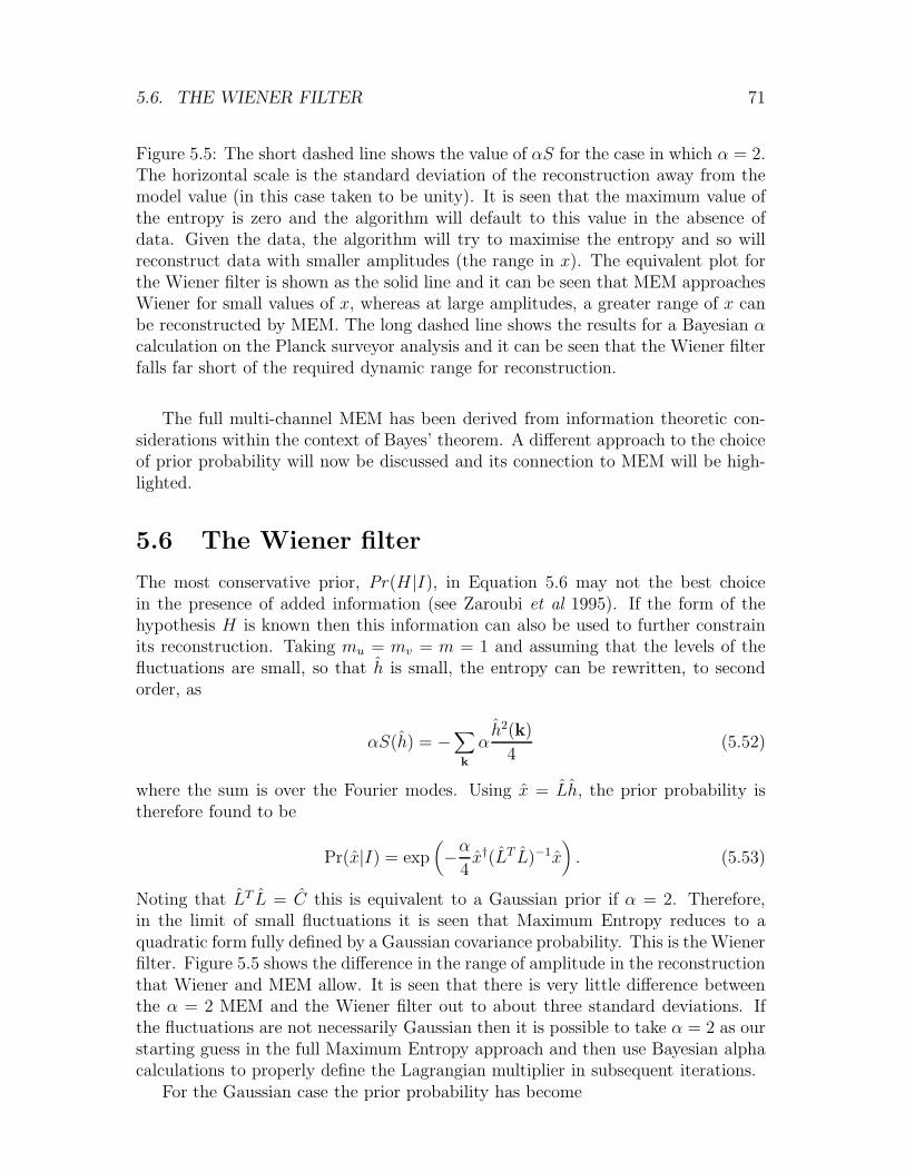
5.6. THE WIENER FILTER 71
Figure 5.5: The short dashed line shows the value of αS for the case in which α = 2.The horizontal scale is the standard deviation of the reconstruction away from themodel value (in this case taken to be unity). It is seen that the maximum value ofthe entropy is zero and the algorithm will default to this value in the absence ofdata. Given the data, the algorithm will try to maximise the entropy and so willreconstruct data with smaller amplitudes (the range in x). The equivalent plot forthe Wiener filter is shown as the solid line and it can be seen that MEM approachesWiener for small values of x, whereas at large amplitudes, a greater range of x canbe reconstructed by MEM. The long dashed line shows the results for a Bayesian αcalculation on the Planck surveyor analysis and it can be seen that the Wiener filterfalls far short of the required dynamic range for reconstruction.
The full multi-channel MEM has been derived from information theoretic con-siderations within the context of Bayes’ theorem. A different approach to the choiceof prior probability will now be discussed and its connection to MEM will be high-lighted.
5.6 The Wiener filter
The most conservative prior, Pr(H|I), in Equation 5.6 may not the best choicein the presence of added information (see Zaroubi et al 1995). If the form of thehypothesis H is known then this information can also be used to further constrainits reconstruction. Taking mu = mv = m = 1 and assuming that the levels of thefluctuations are small, so that h is small, the entropy can be rewritten, to secondorder, as
αS(h) = −∑
k
αh2(k)
4(5.52)
where the sum is over the Fourier modes. Using x = Lh, the prior probability istherefore found to be
Pr(x|I) = exp(
−α4x†(LT L)−1x
)
. (5.53)
Noting that LT L = C this is equivalent to a Gaussian prior if α = 2. Therefore,in the limit of small fluctuations it is seen that Maximum Entropy reduces to aquadratic form fully defined by a Gaussian covariance probability. This is the Wienerfilter. Figure 5.5 shows the difference in the range of amplitude in the reconstructionthat Wiener and MEM allow. It is seen that there is very little difference betweenthe α = 2 MEM and the Wiener filter out to about three standard deviations. Ifthe fluctuations are not necessarily Gaussian then it is possible to take α = 2 as ourstarting guess in the full Maximum Entropy approach and then use Bayesian alphacalculations to properly define the Lagrangian multiplier in subsequent iterations.
For the Gaussian case the prior probability has become
72 CHAPTER 5. PRODUCING SKY MAPS
Pr(x|I) ∝ exp(
−1
2x†C−1x
)
(5.54)
and the matrix C is the covariance matrix of the model given by
C =< x†x > . (5.55)
The problem then becomes the minimisation of
F = χ2 + x†C−1x (5.56)
This minimisation can be done in the same way as MEM through an iterative algo-rithm or it can be solved analytically. In full,
F = (y − Qx)†N−1(y − Qx) + x†C−1x (5.57)
where Q is the instrumental response matrix, from Equation 5.36 and N is thevariance matrix of the data. Minimising with respect to x, the solution is
x′ = CQ†(QCQ† + N)−1y. (5.58)
The Wiener filter, W , that finds the best linear approximation to xi(r) hasresulted:
x′i(r) = Wij(r, r′)yj(r
′) (5.59)
where i is now running over all the pixels in the component maps, j is over all thepixels in the data maps and the Wiener filter is given by
W = CQ†(QCQ† + N)−1. (5.60)
This can be easily written in the hidden variable space, as for MEM, but for illus-trative purposes it is left in Fourier space. The Bayesian probability can now bewritten in terms of this filter (completing the square of Equation 5.57 can also beused to find the Wiener filter):
Pr(x|yI) ∝ exp(
−1
2[x−Wy]† (C−1 + Q†N−1Q) [x−Wy]
)
(5.61)
which is seen to have the quadratic form of the simplified MEM approach. Fromthis it is easily seen that the covariance matrix on this reconstruction is given by
H−1w = (C−1 + Q†N−1Q)−1. (5.62)
The Wiener filter can now be considered as minimising the variance of the re-construction errors of the Fourier components given by
⟨
∆i(k)2⟩
=⟨
|x′i(k) − xi(k)|2⟩
. (5.63)
It is well known that the Wiener filter smoothes out the fluctuations at low fluxlevels (corresponding to levels below the noise). This has the effect of reducing the

5.6. THE WIENER FILTER 73
power in a map. Therefore, the Wiener filter cannot be used in an iterative fashionas it will tend to zero.
Both MEM and the Wiener filter (the quadratic approximation to MEM) inthe Fourier plane have a disadvantage over the real space MEM (Wiener in realspace involves the inversion of very large matrices and so is infeasible to run). Asthe calculations are done on a pixel by pixel basis in Fourier space, the numberof pixels at each frequency has to be the same. Due to the different pixelisationusually seen at different frequency experiments this requires an additional first stepof re-pixelisation. In real space the full MEM analysis does not require this extrapixelisation as all the separate pixelisations can be taken into account in the matrixQ which does not have to be square. Also, the Wiener filter requires the samenumber of pixels in the output maps as in the input maps and so cannot be usedto reconstruct a map in irregularly sampled data (as in the case of the Tenerife orJodrell Bank data).
5.6.1 Errors on the Wiener reconstruction
It has already been shown that the covariance matrix (the inverse Hessian) for theWiener reconstruction is given by Equation 5.62. Therefore, the assignment of errorson the Wiener filter reconstruction is straightforward. It should be noted however,that the simple propagation of errors in the Wiener filter are a direct result ofthe Gaussian assumption of the initial covariance structure. This differs from theMEM error calculation as the MEM approximates the peak of the probability to beGaussian to calculate the errors and not the whole probability distribution as in theWiener filter case.
5.6.2 Improvements to Wiener
An ‘improvement’ to the Wiener filter has been proposed by a number of authors(see, for example, Rybicki & Press 1992, Bouchet et al 1997, Tegmark 1997). Theypropose a rescaling of the power spectrum (either by dividing the power spectrumby a quality factor or by the introduction of a Lagrange multiplier into the priorprobability) so that the total reconstructed power is equal to the total input powerof the maps. It has been shown that the power spectrum reconstructed by the stan-dard Wiener filter is a biased estimation of the true power spectrum (for exampleBouchet et al 1997) in that it weights the reconstructed power spectrum by sig-nal/(signal+noise). This bias can be quantified by introducing a quality factor foreach component l, Sl(k), given by
Sl(k) = ΣmWlm(k)Qml(k) (5.64)
where Wlm(k) is the Wiener matrix at Fourier mode k, Qlm(k) is the instrumentalresponse matrix and the sum is over the frequencies of the experiment. The qualityfactor varies between unity (in the absence of noise) and zero. If x′l(k) is Wienerreconstruction of the lth component and kth Fourier mode and xl(k) is the exactvalue it can be shown (Bouchet et al 1997) that
74 CHAPTER 5. PRODUCING SKY MAPS
⟨
|x′l(k)|2⟩
= Sl(k)⟨
|xl(k)|2⟩
. (5.65)
It is seen that the power spectrum of the reconstruction is an underestimate of theactual power spectrum by the quality factor. By rescaling the Wiener matrix it caneasily be seen that the resulting power spectrum will be unbiased. However, it isfound that the variance of the reconstructed maps increases as they are noisier.
The other proposed variant on Wiener filter is the introduction of a Lagrangemultiplier into the prior probability that scales the input power spectrum. It hasbeen suggested (Tegmark 1997) that this parameter should be chosen to obtain adesired signal to noise ratio in the final reconstruction. However, if it is noted thatthis Lagrange multiplier has exactly the same role as the MEM α it is seen that thisparameter is completely defined in a Bayesian sense similarly to α. The inclusion ofthis Lagrange multiplier simply results in the Wiener filter becoming the quadraticapproximation to MEM without the automatic setting of α due to the absolute valueof the Gaussian probability covariance matrix.
In Wiener filtering the introduction of the quality factor results in noisier maps.The addition of the Lagrange multiplier just results in the quadratic approximationto MEM and as MEM and Wiener are indistinguishable in the Gaussian case thereis no need to perform both methods. Therefore, as the final product of the analysispresented in this thesis is intended to be the real sky maps, only classic Wiener andthe full MEM will be tested in the next chapter.
The methods discussed in this chapter will be applied to simulated data in thefollowing chapter to test their relative strengths at analysing data from CMB ex-periments. The best method(s) will then be used to analyse the data and produceactual CMB maps from the experiments discussed in Chapter 4 in Chapter 7.
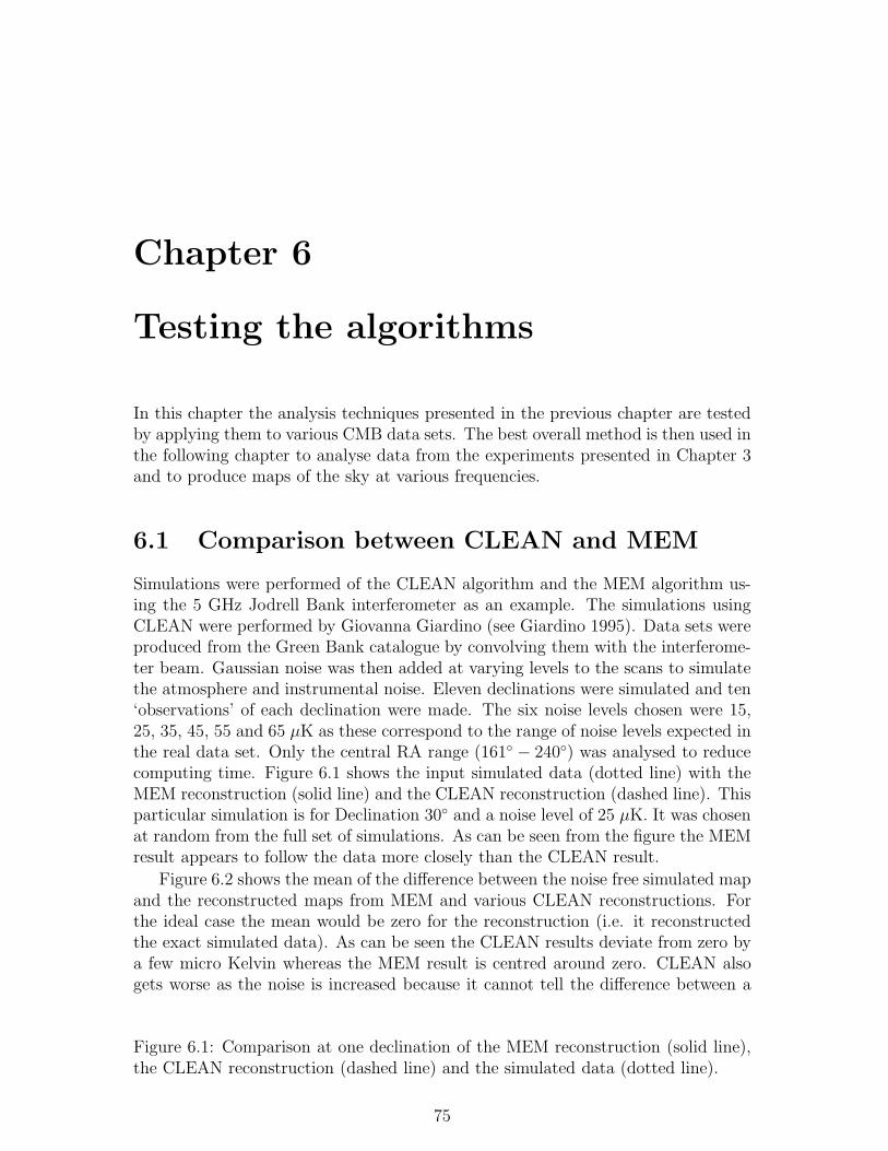
Chapter 6
Testing the algorithms
In this chapter the analysis techniques presented in the previous chapter are testedby applying them to various CMB data sets. The best overall method is then used inthe following chapter to analyse data from the experiments presented in Chapter 3and to produce maps of the sky at various frequencies.
6.1 Comparison between CLEAN and MEM
Simulations were performed of the CLEAN algorithm and the MEM algorithm us-ing the 5 GHz Jodrell Bank interferometer as an example. The simulations usingCLEAN were performed by Giovanna Giardino (see Giardino 1995). Data sets wereproduced from the Green Bank catalogue by convolving them with the interferome-ter beam. Gaussian noise was then added at varying levels to the scans to simulatethe atmosphere and instrumental noise. Eleven declinations were simulated and ten‘observations’ of each declination were made. The six noise levels chosen were 15,25, 35, 45, 55 and 65 µK as these correspond to the range of noise levels expected inthe real data set. Only the central RA range (161 − 240) was analysed to reducecomputing time. Figure 6.1 shows the input simulated data (dotted line) with theMEM reconstruction (solid line) and the CLEAN reconstruction (dashed line). Thisparticular simulation is for Declination 30 and a noise level of 25 µK. It was chosenat random from the full set of simulations. As can be seen from the figure the MEMresult appears to follow the data more closely than the CLEAN result.
Figure 6.2 shows the mean of the difference between the noise free simulated mapand the reconstructed maps from MEM and various CLEAN reconstructions. Forthe ideal case the mean would be zero for the reconstruction (i.e. it reconstructedthe exact simulated data). As can be seen the CLEAN results deviate from zero bya few micro Kelvin whereas the MEM result is centred around zero. CLEAN alsogets worse as the noise is increased because it cannot tell the difference between a
Figure 6.1: Comparison at one declination of the MEM reconstruction (solid line),the CLEAN reconstruction (dashed line) and the simulated data (dotted line).
75

76 CHAPTER 6. TESTING THE ALGORITHMS
Figure 6.2: Mean of difference between the noise free map and the reconstructedmaps. The MEM reconstructed differences are shown by the filled circles. CLEANhas been run for different values of the parameter Niter and γ. Niter = 10000 forall curves except for the hollow squares, for which Niter = 20000. Stars refer toγ = 0.02, hollow squares to γ = 0.06, filled triangles to γ = 0.1 and filled squares toγ = 0.25 (γ is the loop gain in each iteration of the CLEAN algorithm). The largeerror bars are due to the number of realisations per noise level being limited to 10.
Figure 6.3: Standard deviation of the difference between the amplitude of the noisefree map and the maps reconstructed with CLEAN and MEM. The symbols are asin the previous figure.
noise peak and a data peak whereas the MEM process does not get any better orworse.
The errors in the final map have also been calculated (by use of a Monte Carlotechnique) and these are shown in Figure 6.3. As can be seen the different CLEANprocesses all have a similar error in their reconstructions but MEM has a muchlower error. This means that the MEM reconstruction will also be more consistentbetween data sets with different noise realisations, which is essential when analysingdata that has many scans to be simultaneously analysed (as in the case of Tenerife).The MEM error line is also flatter than the CLEAN results (and also flatter than aline with unit gradient) which means that not only does MEM perform better thanCLEAN on all noise scales but MEM actually does relatively better at extractingsignals when the noise level is higher.
The final test of the algorithm is to check whether the fluctuations reconstructedby the two methods are present in the original map. It may be the case that theMEM method has reconstructed the correct amplitude of the signal but has put allof the features in the incorrect locations. To test this a correlation coefficient methodwhich correlates the levels of the fluctuations between the input and output mapswas used. Two maps will have a correlation coefficient of one if they are identical. Ascan be seen in Figure 6.4 the MEM reconstructions are very close to unity and so itis seen with confidence that MEM is reconstructing the simulations very accurately.The CLEAN results, however, shows that at low noise level it closely follows thesimulations but at high noise levels the correlation drops dramatically. From thisanalysis it is concluded that MEM out–performs a simple CLEAN routine on allreconstruction properties of the maps. The CLEAN technique is, therefore, notused in subsequent analysis.
Figure 6.4: The correlation coefficient between the noise free map and the recon-structions from MEM and CLEAN. The symbols are the same as in the previousfigures.
6.2. THE PLANCK SURVEYOR SIMULATIONS 77
6.2 The Planck Surveyor simulations
The MEM Galactic extraction algorithm was tested on simulated observations fromthe Planck Surveyor satellite (see Hobson et al 1998a). To constrain any of theforegrounds in CMB data it is necessary to have a large frequency coverage. ThePlanck Surveyor satellite covers a range from 31 GHz to 847 GHz and has a highangular resolution (see Chapter 3) so that it will sample all of the foregrounds thatwere mentioned in Chapter 2.
6.2.1 The simulations
The simulations described here include six different components as input for the ob-servations (see Bouchet, Gispert, Boulanger & Puget 1997 and Gispert & Bouchet1997). The main component ignored in these simulations are extra–galactic pointsources. Very little information is known about the distribution of point sources atthe observing frequencies of the Planck Surveyor. The usual method for predictingpoint source contamination is to use observations at IRAS frequencies (> 1000 GHz)or low frequency surveys (< 10 GHz) and extrapolate to intermediate frequencies.This has obvious problems and so predictions are unreliable. For small sky cov-erage point source subtraction is performed by making high–resolution, high–flux–sensitivity observations of the point sources at frequencies close to the CMB experi-ment (see for example, O’Sullivan et al 1995). For all sky observations, point sourceremoval is more complicated as it is difficult to make the required observations ofthe point sources. For the Planck satellite it is anticipated that the point sourcescan be subtracted to a level of 1 Jy at each observing frequency, and it may bepossible to subtract all sources brighter than 100 mJy at intermediate frequencieswhere the CMB emission peaks (De Zotti et al 1997). De Zotti et al (1997) findthat the number of pixels affected by point sources to be low and that the level offluctuations due to unsubtracted sources is also very low. Therefore, no modellingof extra–galactic point sources will be made here. Recently, surveys at 350 GHzand 660 GHz (Smail, Ivison & Blain, 1997) have confirmed previous estimates ofthe contribution made by point sources (De Zotti et al. 1997). However, these sur-veys were in specially selected regions (gravitationally lensed objects) and so maybe an over-estimate of the actual point source contribution. The MEM algorithmdescribed here has been applied to simulations with point sources (Hobson et al.1998b) and it was seen that their inclusion alters the conclusions reached here verylittle.
The six components used are the CMB, kinetic and thermal SZ, dust, bremsstrahlungand synchrotron. A detailed discussion of the simulations used is given by Bouchet etal (1997) and Gispert & Bouchet (1997). These have reasonably well defined spectralcharacteristics and this information can be used, together with the multifrequencyobservations, to distinguish between them. Both MEM and Wiener filtering areused to attempt a reconstruction of the components from simulated data taken with14 months of satellite observation. The simulations are constructed on 10 × 10
fields with 1.5′ pixels. Two models of the CMB are used. The first used is a stan-
78 CHAPTER 6. TESTING THE ALGORITHMS
dard CDM model with H = 50kms−1Mpc−1 and Ωb = 0.05. The second is a stringmodel produced by Francois Bouchet. The SZ component (thermal and kinetic)was produced by Aghanim et al (1997) using a Press-Schechter formalism (Press &Schechter 1974) which gives the number density of clusters per unit redshift, solidangle and flux density interval. The gas profiles of individual clusters were modelledas King β–model (King 1966), and their peculiar velocities were drawn at randomfrom an assumed Gaussian velocity distribution with a standard deviation at z = 0of 400 km s−1. Galactic dust emission and bremsstrahlung have been shown to havea component which is correlated with 21cm emission from HI (Kogut et al 1996,Boulanger et al 1996). To model this correlation two IRAS 100 µm maps were used;one for HI correlated emission and one for HI uncorrelated. The components arethen related by
HIcorr(ν) = A [0.95fD(ν) + 0.5fB(ν)] (6.1)
and
HIuncorr(ν) = B [0.05fD(ν) + 0.5fB(ν)] , (6.2)
where fD is the frequency dependence of the dust emission and fB is the frequencydependence of the bremsstrahlung. Therefore, the dust component was modelledby addition of 95% of the correlated HI IRAS map and 5% of the uncorrelatedmap and extrapolating to lower frequencies assuming a black body temperatureof 18 K and an emissivity of 2 for the dust. The bremsstrahlung (or free–free)component was modelled by using 50% of the HI correlated IRAS map and 50%of the uncorrelated IRAS map. The combined map was scaled so that the rmsamplitude of the bremsstrahlung at 53 GHz was 6.2 µK and a temperature spectralindex of β = 2.16 was assumed. No spatial template is available at sufficiently highresolution for the synchrotron maps. The simulations were modelled by using thelow frequency Haslam et al maps at 408 MHz, which have a resolution of 0.85 andadding small scale structure that follows a Cl ∝ l−3 power spectrum. A temperaturespectral index of β = 2.9 was assumed.
The components used were all converted to equivalent thermodynamic temper-ature, for comparison purposes, from flux using the equation
∆I(µ) =∆Tx4ex
(ex − 1)2(6.3)
where x = hv/kT and T = 2.726K. The flux is originally in units of Wm−2Hz−1sr−1
and all programs use flux units rather than temperature. The six input components(CMB, kinetic SZ, thermal SZ, dust, bremsstrahlung and synchrotron) are shownin Figures 6.5 (for the CDM simulation) and 6.6 (for the string simulation). Eachcomponent is plotted at 300 GHz and has been convolved with a Gaussian of 4.5′
FWHM, the highest resolution of the Planck Surveyor. It is noted that the IRAS100 µm maps used as templates for the Galactic dust and free–free emission appearquite non–Gaussian and the imposed correlation between these two foregrounds isclearly seen. The azimuthally averaged power spectra of the input maps (CDM
6.2. THE PLANCK SURVEYOR SIMULATIONS 79
realisation) are shown in Figure 6.7. It is easily seen that the power in the maps issuppressed for ℓ > 2000. This is due to the finite resolution.
The final design of the Planck Surveyor satellite is still to be decided and signifi-cant improvements have recently been made to the proposed sensitivities. Therefore,these recent improvements will be used here to simulate observations (see Table 3.1for full details on the frequency channels used). Simulated observations were pro-duced by integrating the emission due to each physical component across each wave-band, assuming the transmission is uniform across the band. At each frequency thebeam was assumed to be Gaussian with the appropriate FWHM. Care is needed toinclude the effect of the waveband integration in the MEM and Wiener algorithmsbut this can easily be done in the conversion matrix described in Section 5.4.6. Thefrequency channels now consist of a noise-free flux in Wm−2.
Isotropic Gaussian noise was added to each frequency channel with the typicalrms expected from 14 months of observations. Figure 6.8 shows the rms fluctuationsat each observing frequency due to each physical component after convolution withthe appropriate beam. The rms noise per pixel at each frequency is also plotted. Itis seen that only the dust and CMB emissions are above the noise level (although thethermal SZ is extremely non–Gaussian and has many peaks above the noise level).The kinetic SZ has the same spectral characteristics as the CMB, but the effect ofthe beam convolution at the different frequencies on a point source distribution ismore pronounced. The data was created on maps with pixels that assumed a spatialsampling of FWHM/2.4 at each frequency. That meant that for the 10 × 10 skyarea there were 320 × 320 pixels at the highest frequency and 44 × 44 pixels at thelowest frequency. As the calculations were performed in the Fourier plane it wasnecessary to repixelise the maps onto a common resolution although it is noted thatthis is not necessary for the MEM algorithm in real space. The final ten frequencychannels (now with pixel noise added) are shown in Figure 6.9.
6.2.2 Singular Value Decomposition results
The simple linear inversion of Singular Value Decomposition (S.V.D.) was used onthe two different data sets (one for the CDM realisation and one for the stringrealisation of the CMB) from the simulated Planck Surveyor data. The final recon-structed map for the CDM and strings simulations are shown in Figures 6.10 and6.11 and are summarised in Table 6.1. The grey scales of the reconstructions and theinput maps are the same. It was not possible to attempt a separate reconstructionof the CMB and kinetic SZ effect as these have the same frequency dependence.However, six plots are shown for easy comparison with the input maps. As can beseen from the figures and tables, the S.V.D. performs quite well on both the CMB(CDM and strings) and the dust channels but fails to reconstruct the other channels.As the input maps used are known it is possible to calculate the residuals for eachreconstruction. This is defined as
erms =
[
1
N
N∑
i=1
(
T irec − T i
true
)2]1/2
, (6.4)
80 CHAPTER 6. TESTING THE ALGORITHMS
Figure 6.5: The six input maps used in the simulations for the data taken by thePlanck Surveyor. This is for the CDM model of the CMB. They are shown at300 GHz in µK. a) CDM simulation, b) Kinetic SZ, c) Thermal SZ, d) Dust emissione) Free-free emission and f) Synchrotron emission.
Figure 6.6: The six input maps used in the simulations for the data taken by thePlanck Surveyor. This is for the string model of the CMB. They are shown at300 GHz in µK. a) String simulation, b) Kinetic SZ, c) Thermal SZ, d) Dust emissione) Free-free emission and f) Synchrotron emission.
Figure 6.7: The azimuthally-averaged power spectra of the input maps shown inFigure 6.5 at 300 GHz.
Figure 6.8: The rms thermodynamic temperature fluctuations at each Planck Sur-veyor observing frequency due to each physical component, after convolution withthe appropriate beam and using a sampling rate of FWHM/2.4. The rms noise perpixel at each frequency channel is also plotted.
Figure 6.9: The ten channels in the simulated data from the Planck Surveyor. Thenoise and lower resolution is clearly seen in the low frequency channels. The noiselevels represent an improvement for the LFI since Bersanelli et al 1996 was published.The units are in µK equivalent integrated over the band.
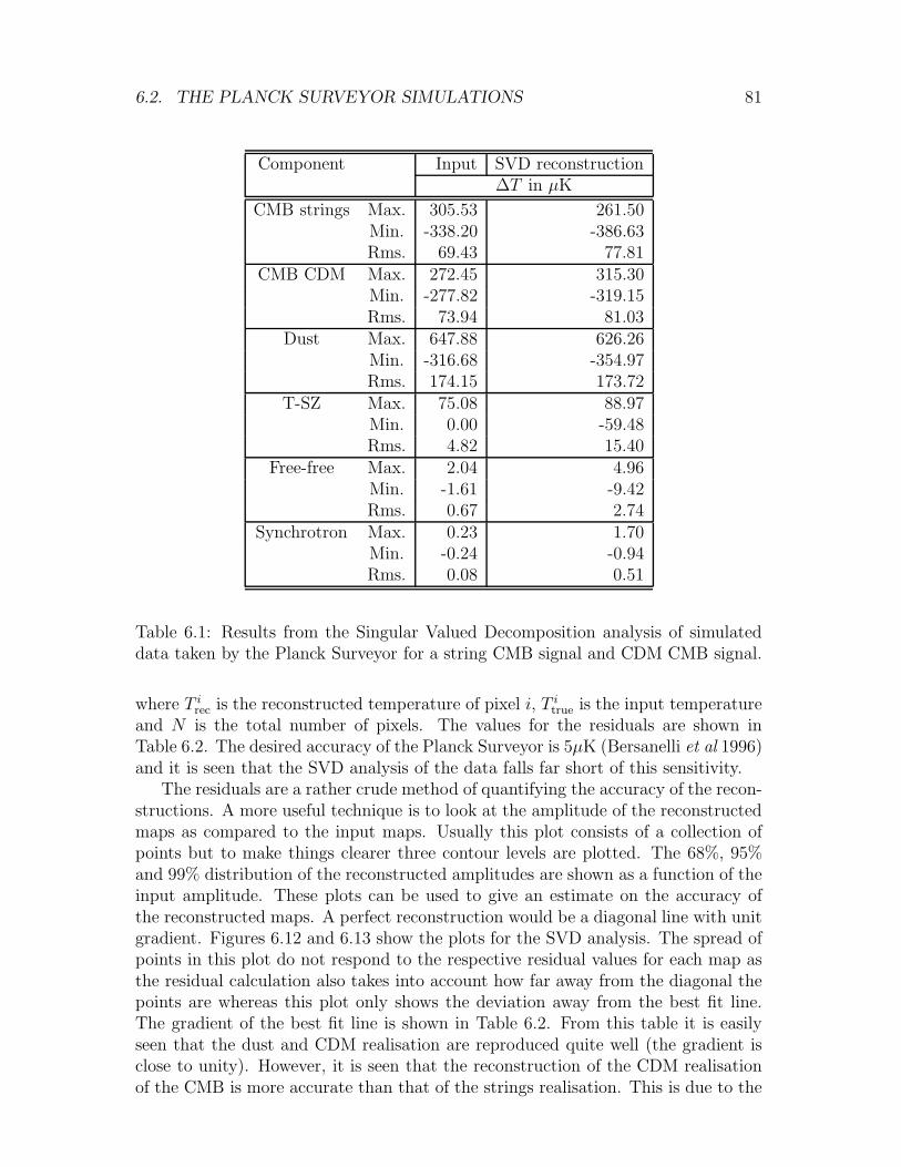
6.2. THE PLANCK SURVEYOR SIMULATIONS 81
Component Input SVD reconstruction∆T in µK
CMB strings Max. 305.53 261.50Min. -338.20 -386.63Rms. 69.43 77.81
CMB CDM Max. 272.45 315.30Min. -277.82 -319.15Rms. 73.94 81.03
Dust Max. 647.88 626.26Min. -316.68 -354.97Rms. 174.15 173.72
T-SZ Max. 75.08 88.97Min. 0.00 -59.48Rms. 4.82 15.40
Free-free Max. 2.04 4.96Min. -1.61 -9.42Rms. 0.67 2.74
Synchrotron Max. 0.23 1.70Min. -0.24 -0.94Rms. 0.08 0.51
Table 6.1: Results from the Singular Valued Decomposition analysis of simulateddata taken by the Planck Surveyor for a string CMB signal and CDM CMB signal.
where T irec is the reconstructed temperature of pixel i, T i
true is the input temperatureand N is the total number of pixels. The values for the residuals are shown inTable 6.2. The desired accuracy of the Planck Surveyor is 5µK (Bersanelli et al 1996)and it is seen that the SVD analysis of the data falls far short of this sensitivity.
The residuals are a rather crude method of quantifying the accuracy of the recon-structions. A more useful technique is to look at the amplitude of the reconstructedmaps as compared to the input maps. Usually this plot consists of a collection ofpoints but to make things clearer three contour levels are plotted. The 68%, 95%and 99% distribution of the reconstructed amplitudes are shown as a function of theinput amplitude. These plots can be used to give an estimate on the accuracy ofthe reconstructed maps. A perfect reconstruction would be a diagonal line with unitgradient. Figures 6.12 and 6.13 show the plots for the SVD analysis. The spread ofpoints in this plot do not respond to the respective residual values for each map asthe residual calculation also takes into account how far away from the diagonal thepoints are whereas this plot only shows the deviation away from the best fit line.The gradient of the best fit line is shown in Table 6.2. From this table it is easilyseen that the dust and CDM realisation are reproduced quite well (the gradient isclose to unity). However, it is seen that the reconstruction of the CDM realisationof the CMB is more accurate than that of the strings realisation. This is due to the
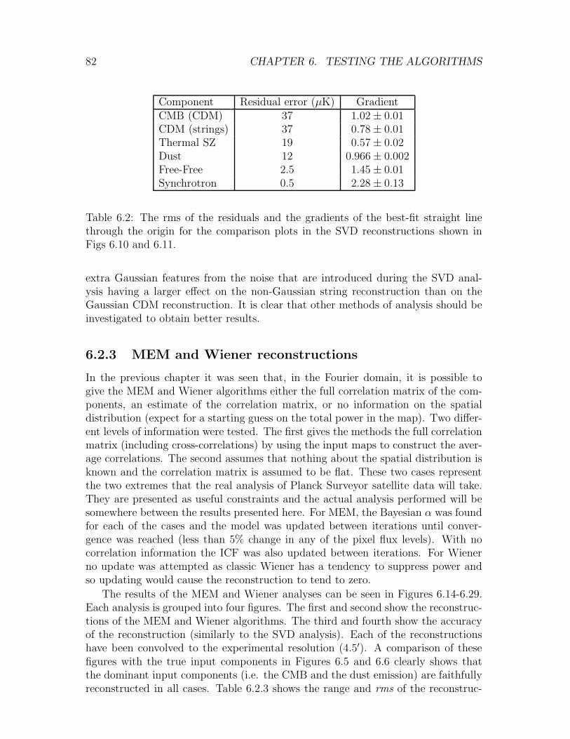
82 CHAPTER 6. TESTING THE ALGORITHMS
Component Residual error (µK) GradientCMB (CDM) 37 1.02 ± 0.01CDM (strings) 37 0.78 ± 0.01Thermal SZ 19 0.57 ± 0.02Dust 12 0.966 ± 0.002Free-Free 2.5 1.45 ± 0.01Synchrotron 0.5 2.28 ± 0.13
Table 6.2: The rms of the residuals and the gradients of the best-fit straight linethrough the origin for the comparison plots in the SVD reconstructions shown inFigs 6.10 and 6.11.
extra Gaussian features from the noise that are introduced during the SVD anal-ysis having a larger effect on the non-Gaussian string reconstruction than on theGaussian CDM reconstruction. It is clear that other methods of analysis should beinvestigated to obtain better results.
6.2.3 MEM and Wiener reconstructions
In the previous chapter it was seen that, in the Fourier domain, it is possible togive the MEM and Wiener algorithms either the full correlation matrix of the com-ponents, an estimate of the correlation matrix, or no information on the spatialdistribution (expect for a starting guess on the total power in the map). Two differ-ent levels of information were tested. The first gives the methods the full correlationmatrix (including cross-correlations) by using the input maps to construct the aver-age correlations. The second assumes that nothing about the spatial distribution isknown and the correlation matrix is assumed to be flat. These two cases representthe two extremes that the real analysis of Planck Surveyor satellite data will take.They are presented as useful constraints and the actual analysis performed will besomewhere between the results presented here. For MEM, the Bayesian α was foundfor each of the cases and the model was updated between iterations until conver-gence was reached (less than 5% change in any of the pixel flux levels). With nocorrelation information the ICF was also updated between iterations. For Wienerno update was attempted as classic Wiener has a tendency to suppress power andso updating would cause the reconstruction to tend to zero.
The results of the MEM and Wiener analyses can be seen in Figures 6.14-6.29.Each analysis is grouped into four figures. The first and second show the reconstruc-tions of the MEM and Wiener algorithms. The third and fourth show the accuracyof the reconstruction (similarly to the SVD analysis). Each of the reconstructionshave been convolved to the experimental resolution (4.5′). A comparison of thesefigures with the true input components in Figures 6.5 and 6.6 clearly shows thatthe dominant input components (i.e. the CMB and the dust emission) are faithfullyreconstructed in all cases. Table 6.2.3 shows the range and rms of the reconstruc-
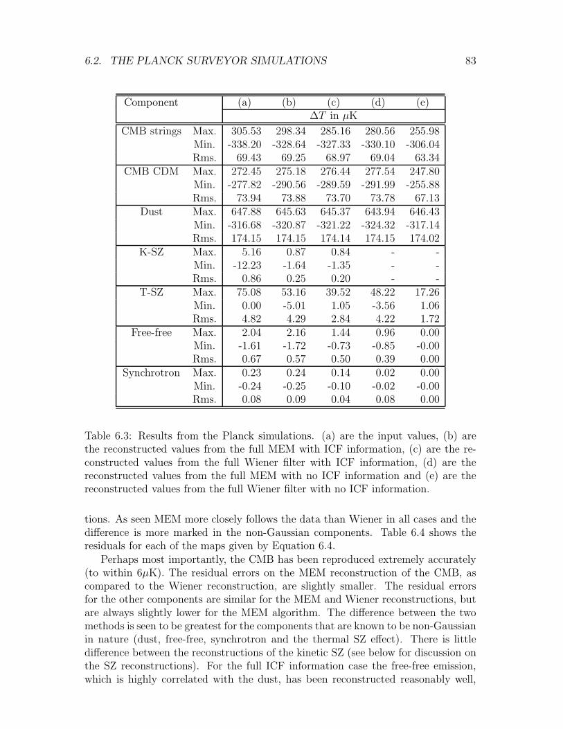
6.2. THE PLANCK SURVEYOR SIMULATIONS 83
Component (a) (b) (c) (d) (e)∆T in µK
CMB strings Max. 305.53 298.34 285.16 280.56 255.98Min. -338.20 -328.64 -327.33 -330.10 -306.04Rms. 69.43 69.25 68.97 69.04 63.34
CMB CDM Max. 272.45 275.18 276.44 277.54 247.80Min. -277.82 -290.56 -289.59 -291.99 -255.88Rms. 73.94 73.88 73.70 73.78 67.13
Dust Max. 647.88 645.63 645.37 643.94 646.43Min. -316.68 -320.87 -321.22 -324.32 -317.14Rms. 174.15 174.15 174.14 174.15 174.02
K-SZ Max. 5.16 0.87 0.84 - -Min. -12.23 -1.64 -1.35 - -Rms. 0.86 0.25 0.20 - -
T-SZ Max. 75.08 53.16 39.52 48.22 17.26Min. 0.00 -5.01 1.05 -3.56 1.06Rms. 4.82 4.29 2.84 4.22 1.72
Free-free Max. 2.04 2.16 1.44 0.96 0.00Min. -1.61 -1.72 -0.73 -0.85 -0.00Rms. 0.67 0.57 0.50 0.39 0.00
Synchrotron Max. 0.23 0.24 0.14 0.02 0.00Min. -0.24 -0.25 -0.10 -0.02 -0.00Rms. 0.08 0.09 0.04 0.08 0.00
Table 6.3: Results from the Planck simulations. (a) are the input values, (b) arethe reconstructed values from the full MEM with ICF information, (c) are the re-constructed values from the full Wiener filter with ICF information, (d) are thereconstructed values from the full MEM with no ICF information and (e) are thereconstructed values from the full Wiener filter with no ICF information.
tions. As seen MEM more closely follows the data than Wiener in all cases and thedifference is more marked in the non-Gaussian components. Table 6.4 shows theresiduals for each of the maps given by Equation 6.4.
Perhaps most importantly, the CMB has been reproduced extremely accurately(to within 6µK). The residual errors on the MEM reconstruction of the CMB, ascompared to the Wiener reconstruction, are slightly smaller. The residual errorsfor the other components are similar for the MEM and Wiener reconstructions, butare always slightly lower for the MEM algorithm. The difference between the twomethods is seen to be greatest for the components that are known to be non-Gaussianin nature (dust, free-free, synchrotron and the thermal SZ effect). There is littledifference between the reconstructions of the kinetic SZ (see below for discussion onthe SZ reconstructions). For the full ICF information case the free-free emission,which is highly correlated with the dust, has been reconstructed reasonably well,
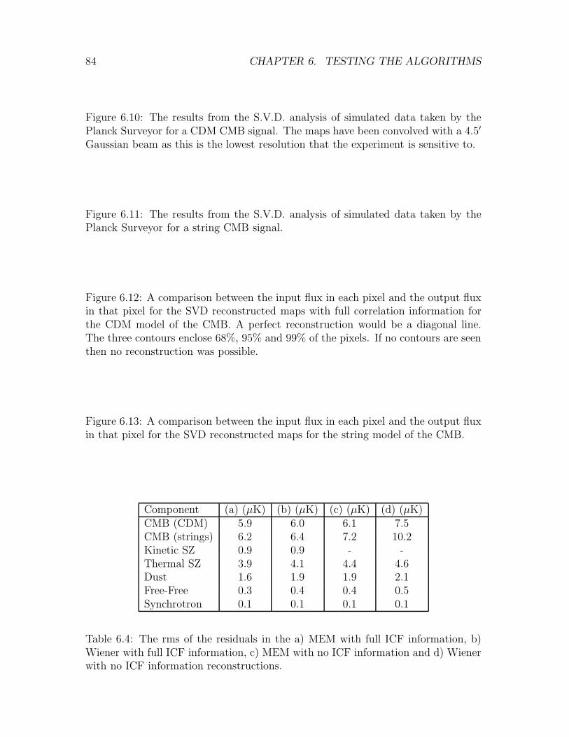
84 CHAPTER 6. TESTING THE ALGORITHMS
Figure 6.10: The results from the S.V.D. analysis of simulated data taken by thePlanck Surveyor for a CDM CMB signal. The maps have been convolved with a 4.5′
Gaussian beam as this is the lowest resolution that the experiment is sensitive to.
Figure 6.11: The results from the S.V.D. analysis of simulated data taken by thePlanck Surveyor for a string CMB signal.
Figure 6.12: A comparison between the input flux in each pixel and the output fluxin that pixel for the SVD reconstructed maps with full correlation information forthe CDM model of the CMB. A perfect reconstruction would be a diagonal line.The three contours enclose 68%, 95% and 99% of the pixels. If no contours are seenthen no reconstruction was possible.
Figure 6.13: A comparison between the input flux in each pixel and the output fluxin that pixel for the SVD reconstructed maps for the string model of the CMB.
Component (a) (µK) (b) (µK) (c) (µK) (d) (µK)CMB (CDM) 5.9 6.0 6.1 7.5CMB (strings) 6.2 6.4 7.2 10.2Kinetic SZ 0.9 0.9 - -Thermal SZ 3.9 4.1 4.4 4.6Dust 1.6 1.9 1.9 2.1Free-Free 0.3 0.4 0.4 0.5Synchrotron 0.1 0.1 0.1 0.1
Table 6.4: The rms of the residuals in the a) MEM with full ICF information, b)Wiener with full ICF information, c) MEM with no ICF information and d) Wienerwith no ICF information reconstructions.
6.2. THE PLANCK SURVEYOR SIMULATIONS 85
containing most of the main features present in the true input map. It is noted thatthe Wiener reconstruction of the free-free emission follows the dust emission moreclosely than the MEM reconstruction which has also reconstructed some free-freeemission that is uncorrelated with the dust. For the case of no prior ICF informationit is seen that no significant reconstruction of the free-free emission is made with theWiener analysis whereas a smooth version has been reconstructed by MEM. Therecovery of the synchrotron emission is less impressive. With full information MEMand Wiener can reconstruct the synchrotron to some degree but the significance ofthe features is not very high (this is seen in the very broad correlations betweeninput amplitude and reconstructed amplitude in Figure 6.16).
Again, the residual errors on the MEM and Wiener reconstructions do not showall of the information available about the reconstructions. The extent of the de-viation of the correlation plots away from the diagonal also contains information.Table 6.5 shows the gradients of the best fit lines for the MEM and Wiener recon-structions with full and no prior ICF information. From these best fit lines it is seenthat the CMB and dust emission are both reconstructed very well. However, it isseen that MEM always outperforms the Wiener on the CMB reconstruction whenno prior ICF information was given. This is due to Wiener underestimating thetemperature of each pixel in the CMB channel. It is clearly seen that the thermalSZ is consistently reconstructed with a lower amplitude than the true amplitude.Even though the Wiener filter has been given the full prior ICF information it is stilloutdone by MEM with no prior information in the case of this highly non-Gaussianeffect. The range of values reconstructed by Wiener is lower than that for MEM(the spread is smaller around the best fit line), however, the residual errors for theWiener are always larger than those for MEM because of the smaller amplitudesreconstructed. The fit for MEM and Wiener can be improved by assuming the re-construction is at a lower resolution (which is likely to be the case as there is littleinformation on the SZ at the highest frequencies where the resolution is highest). Forexample, the reconstruction of the thermal SZ effect has a much stronger correlationwith the input maps if it is assumed that the resolution of the data is 10.6′ (theresolution of the frequency channel where the thermal SZ effect is most dominantin the Planck Surveyor data). At this resolution the error is then 3µK.
Visually, the string realisation of the CMB appears to be reconstructed very ac-curately with all the non-Gaussian features still apparent in all cases. Comparingthe residual errors from the string realisation with that of the CDM realisation, it isseen that even when MEM is used the non-Gaussian process is reconstructed slightlyless accurately (a 10% increase in the residual errors in both cases considered). How-ever, when the Wiener filter is applied the difference is much more enhanced (a 10%and 50% increase in the residual errors for the case of full and no prior correlationinformation respectively). In all cases the gradient of the MEM reconstruction iscloser to unity than that of Wiener, but it is seen that the Gaussian realisation ismore accurately reconstructed.
As a test of the power of MEM the frequency dependence of various componentswas also checked. There was an obvious minimum in the value of χ2 for the actualvalues of the dust temperature and emissivity as there is a lot of information on the

86 CHAPTER 6. TESTING THE ALGORITHMS
Full prior ICF No prior ICFComponent MEM Wiener MEM WienerCMB (CDM) 1.00 1.00 1.00 0.97CDM (strings) 0.98 0.97 0.97 0.89Thermal SZ 0.55 0.27 0.50 0.24Kinetic SZ 0.07 0.05 - -Dust 1.00 1.00 1.00 1.00Free-Free 0.48 0.37 0.60 0.22Synchrotron 0.62 0.44 0.47 0.13
Table 6.5: The gradients of the best-fit straight line through the origin for thecorrelation plots of the reconstructions.
Figure 6.14: The six reconstructed channels from the MEM analysis of the Plancksimulated data for a CDM model of the CMB using full correlation information.
Figure 6.15: The six reconstructed channels from the Wiener analysis of the Plancksimulated data for a CDM model of the CMB using full correlation information.
Figure 6.16: A comparison between the input flux in each pixel and the output fluxin that pixel for the MEM reconstructed maps with full correlation information forthe CDM model of the CMB.
Figure 6.17: A comparison between the input flux in each pixel and the output fluxin that pixel for the Wiener reconstructed maps with full correlation information forthe CDM model of the CMB.
Figure 6.18: The six reconstructed channels from the MEM analysis of the Plancksimulated data for a strings model of the CMB using full correlation information.
Figure 6.19: The six reconstructed channels from the Wiener analysis of the Plancksimulated data for a strings model of the CMB using full correlation information.
Figure 6.20: A comparison between the input flux in each pixel and the output fluxin that pixel for the MEM reconstructed maps with full correlation information forthe strings model of the CMB.
Figure 6.21: A comparison between the input flux in each pixel and the output fluxin that pixel for the Wiener reconstructed maps with full correlation information forthe strings model of the CMB.
6.2. THE PLANCK SURVEYOR SIMULATIONS 87
Figure 6.22: The six reconstructed channels from the MEM analysis of the Plancksimulated data for a CDM model of the CMB using no correlation information. Theplot shows the kinetic SZ (figure (b)) for ease of comparison even though no attemptwas made to reconstruct this effect.
Figure 6.23: The six reconstructed channels from the Wiener analysis of the Plancksimulated data for a CDM model of the CMB using no correlation information.
Figure 6.24: A comparison between the input flux in each pixel and the output fluxin that pixel for the MEM reconstructed maps with no correlation information forthe CDM model of the CMB.
Figure 6.25: A comparison between the input flux in each pixel and the output fluxin that pixel for the Wiener reconstructed maps with no correlation information forthe CDM model of the CMB.
Figure 6.26: The six reconstructed channels from the MEM analysis of the Plancksimulated data for a strings model of the CMB using no correlation information.
Figure 6.27: The six reconstructed channels from the Wiener analysis of the Plancksimulated data for a strings model of the CMB using no correlation information.
Figure 6.28: A comparison between the input flux in each pixel and the output fluxin that pixel for the MEM reconstructed maps with no correlation information forthe strings model of the CMB.
Figure 6.29: A comparison between the input flux in each pixel and the output fluxin that pixel for the Wiener reconstructed maps with no correlation information forthe strings model of the CMB.
88 CHAPTER 6. TESTING THE ALGORITHMS
dust emission from the higher frequency channels. The free–free and synchrotronspectral indices were less tightly constrained as the χ2 depends mainly on the CMBand dust emissions. It should therefore be possible to constrain the spatial and fre-quency dependence of the dust emission but more assumptions, or higher sensitivity,is required to constrain the other Galactic components.
6.2.4 SZ reconstruction
The thermal SZ effect can be used to calculate the value of H (Grainge et al 1993,Saunders 1997 etc.). However, for this to be possible the shape of the cluster mustbe known. Any algorithm used to reconstruct the information about the thermalSZ effect must closely follow the true shape of the underlying cluster and not justreconstruct the rms or the amplitude. It was seen in the reconstructed maps that theMEM algorithm reconstructs the thermal SZ effect in more clusters than the Wienerfilter. With no information on the correlation function the Wiener filter performsvery badly in reconstructing the non-Gaussian emission. Figure 6.30 shows some ofthe typical thermal SZ profiles reconstructed by the MEM and Wiener algorithmswith full and no correlation information. They are compared with the input profilesconvolved with a Gaussian of size 10.6′, the resolution of the 100 GHz channel (thefrequency at which the fractional contribution of the thermal SZ effect is largest).It is easily seen that the full MEM analysis does reconstruct the cluster profilescloser to their truer shape than the Wiener filter. Thus, as expected, the Gaussianassumption of the Wiener filter leads to poor reconstructions of highly non-Gaussianfields as compared with MEM. It is also seen that even with no prior information onthe correlations, the MEM algorithm still reconstructs a reasonable approximationto the true profiles.
At first sight it appears that the MEM reconstructions contain some spuriousfeatures as compared to the input profiles. This is seen most dramatically in thetop panel of Figure 6.30 for the full prior ICF case. The central cluster appears tohave an extra feature on the right hand side. In fact, this phenomenon illustratesthe care that should be taken when interpreting SZ profiles found this way, sincethe feature is actually present in the input map, but has almost been smoothed outby the 10.6′ convolution. The reason it is still present in the reconstruction is thatthe effective resolution of the MEM and Wiener reconstructions can vary across themap, depending on the level of the pixel noise and the other components. Therefore,in some regions a degree of super-resolution is possible whereas in regions where thepixel noise, or emission from the other components, is large the super-resolutiondoes not occur. This was tested with different pixel noise realisations and it wasseen that the areas of super-resolution did indeed move across the map.
The kinetic SZ can be used to put constraints on the interactions of galaxyclusters through their velocity distributions. No reconstruction was attempted whenno information about the correlations was given, as the frequency spectrum of thekinetic SZ is the same as that for the CMB. Even in the case when full correlationinformation was given the kinetic SZ emission is not recovered particularly well. Thereconstruction as compared to the input kinetic SZ emission is shown in Figure 6.31.

6.2. THE PLANCK SURVEYOR SIMULATIONS 89
Figure 6.30: Typical reconstructions of SZ profiles. The solid line is the input clus-ter convolved to 10.6′ (the resolution at which the sensitivity to the SZ effect is amaximum). The dashed line is the reconstruction from the MEM analysis using (a)full correlation information and (b) no correlation information. The dotted line isthe reconstruction from the Wiener analysis using (a) full correlation informationand (b) no correlation information. As can be seen the Wiener result is a muchsmoother reconstruction than the MEM result, especially in the case with no cor-relation information when the Wiener does not reconstruct any significant featuresbut the MEM still follows the true profiles very well.
Figure 6.31: Comparison between the input simulation of the kinetic SZ effect con-volved to 23′ (the resolution at which the fractional contribution of the kinetic SZis highest in the data) and the MEM reconstruction of the effect.
Comparing the spatial location of the recovered kinetic SZ profiles to that of thethermal SZ it is seen that only the large kinetic SZ effects that occur on pixels alsoassociated with a large thermal SZ are reconstructed. Therefore, it is seen that therecovery of the kinetic SZ is highly dependent on the information given to the MEMalgorithm prior to the analysis and the data is not sufficiently sensitive to allowthe kinetic SZ to be extracted by itself. This is easily seen as the largest kineticSZ effect (in the lower right quadrant of the figures) is not reconstructed as it isnot associated with a large thermal SZ effect. For a better reconstruction extrainformation is required, as well as the frequency and average spatial spectra. Thismay come in the form of the positions of the clusters (through the thermal SZ effect)and then using the information that the SZ effect occurs mainly on angular scalesbelow any contribution from the CMB. However, this is very difficult to incorporatein an automatic algorithm and so no further analysis was attempted.
6.2.5 Power spectrum reconstruction
Figures 6.32 and 6.33 show the azimuthally averaged power spectra for the MEM andWiener reconstructions with full prior correlation information respectively. The 68%confidence intervals obtained from the inversion of the Hessian are also shown. It isseen that the 68% confidence intervals always encompass the input power spectra. Itshould be noted that the confidence intervals shown are for the reconstructed mapsgiven that the data is representative of the full sky and do not take into accountsample or cosmic variance. For the components with the most amount of information(namely the CMB and dust) the confidence intervals are correspondingly smallerwhereas for components with little information (as in the case of synchrotron) theconfidence intervals are much larger. It is seen that the MEM and Wiener confidenceintervals are fairly similar but this is to be expected as the Hessian calculation forboth comes from a Gaussian assumption.
The reconstruction of the CMB is very good out to an ℓ of about 1500 for bothMEM and Wiener. Beyond ℓ ∼ 1500 Wiener begins to visibly underestimate the true
90 CHAPTER 6. TESTING THE ALGORITHMS
power but MEM is still accurate to ℓ ∼ 2000. The dust emission is reconstructed verywell out to an ℓ of about 3000 for the MEM reconstruction and 2000 for the Wienerreconstruction, the extra information over the CMB coming from the increasedresolution at the higher frequencies. The white noise spectra of the thermal SZand kinetic SZ is much more closely followed by the MEM reconstruction althoughboth algorithms have lost some of the power from the free-free and synchrotronreconstructions.
For the case with no prior ICF information the difference between the MEM andWiener reconstruction is more easily seen. The power spectrum reconstructions forthis case are seen in Figure 6.34 and 6.35. Even in the CMB reconstruction it is seenthat the Wiener-produced power spectrum is consistently below the true spectrumeven at very low ℓ. The MEM reconstruction is accurate out to ℓ ∼ 1500 at whichpoint it drops rapidly to zero. This rapid drop, seen in most of the reconstructions,is a result of continually updating the ICF in an area for which there is little infor-mation in the data. For the thermal SZ it is seen that the MEM reconstruction isreasonably accurate out to ℓ ∼ 1000 but the Wiener filter is only reasonably accu-rate out to ℓ ∼ 200. No reconstruction of the kinetic SZ was attempted. The dustpower spectrum reconstruction is accurate out to ℓ ∼ 2000 for MEM and ℓ ∼ 3000for Wiener. However, it is seen that the Wiener reconstruction has a spurious bumpin the power spectrum at ℓ ∼ 2000 − 5000 which overestimates the power for theCMB and this is again seen for the dust. Thus it is unclear whether the reconstruc-tion from the Wiener filter beyond ℓ ∼ 2000 is accurate. Out to ℓ ∼ 70 the MEMreconstruction approximates the free-free true power spectrum but for Wiener, andthe two reconstructions of the synchrotron emission, the power spectrum is alwaysunderestimated.
6.3 The MAP simulations
Four years prior to the launch of the Planck Surveyor NASA is due to launch its MAPsatellite. This is a cheaper alternative to Planck, with less frequency coverage andlower angular resolution. As a test of the relative strength of the two experimentsthe same analysis that was performed on the Planck Surveyor was performed on theMAP satellite. The same simulations as the Planck analysis were used so that adirect comparison between the two satellites would be possible. The input maps forMAP were the same as those for the Planck, although the resolution of MAP is about4 times worse than that of Planck and so the results are expected to be smoother(see Figure 6.36). The resolution of the MAP satellite has improved considerablysince these simulations were performed and the latest design has a best resolutionof about 2 times that of Planck (see Jones, Hobson, Lasenby & Bouchet 1998 forsimulations with the current design). The true test of the sensitivity of MAP isagain in the flux reconstruction of features that it is sensitive to. A fit to the sixchannels was again attempted. Only the CDM model of the CMB is shown here asthe string simulations show very similar results.
6.3. THE MAP SIMULATIONS 91
Figure 6.32: The reconstructed power spectra (dark line) with errors compared tothe input power spectra (faint line) of the Planck Surveyor CDM CMB simulation.The errors are calculated using the Gaussian approximation for the peak of theprobability distribution. This reconstruction was produced by MEM with full ICFinformation.
Figure 6.33: The reconstructed power spectra (dark line) with errors compared tothe input power spectra (faint line) of the Planck Surveyor CDM CMB simulation.The errors are calculated using the Gaussian approximation for the full probabilitydistribution. This reconstruction was produced by Wiener filtering with full ICFinformation.
Figure 6.34: The reconstructed power spectra (dark line) with errors (dotted line)compared to the input power spectra (faint line) of the Planck Surveyor CDM CMBsimulation. The errors are calculated using the Gaussian approximation for the peakof the probability distribution. This reconstruction was produced by MEM with noICF information.
Figure 6.35: The reconstructed power spectra (dark line) with errors (dotted line)compared to the input power spectra (faint line) of the Planck Surveyor CDM CMBsimulation. The errors are calculated using the Gaussian approximation for the fullprobability distribution. This reconstruction was produced by Wiener filtering withno ICF information.
Figure 6.36: The six input maps convolved to the highest resolution of the MAPsatellite for comparison with the reconstructions. No reconstruction of the kineticSZ was attempted as the signal at this resolution is negligible but it is still plottedto allow easy comparison with the Planck results.
92 CHAPTER 6. TESTING THE ALGORITHMS
6.3.1 MEM and Wiener results
The MEM and Wiener analyses of the MAP simulations were carried out with thesame levels of information as the Planck analysis. The results of the analyses canbe seen in Figures 6.37-6.44. Again, each analysis is grouped into four figures. Thefirst and second show the reconstructions of the MEM algorithm and the Wienerfilter respectively. The third and fourth show the accuracy of the reconstruction.
It is easily seen that there is no information in the MAP data on any of theforegrounds that the Planck Surveyor is sensitive to. Table 6.6 shows the rms of thereconstructions from the simulations. The lower frequency coverage of MAP resultsin no information available on the dust emission (this is seen when no correlationinformation is given and the reconstruction is just set to zero by both MEM andWiener). Even though the low frequency channels should contain information onthe free-free and synchrotron emissions none is recovered. This is due to the lowerresolution and sensitivity that MAP has. MAP was never designed to extract in-formation on the SZ effect and does not contain channels near the critical 217 GHzfrequency. Hence, no information on either of the SZ effects was reconstructed.However, the CMB is reconstructed fairly well. There is a very strong correlationfor both the MEM and Wiener filter. Little difference is seen between these two re-constructions as the resolution is not large enough to pick them out and everythingappears Gaussian (this was true in both the CDM and string simulations; the levelof Gaussianity in the string simulation at this resolution is tested in Chapter 8).The 68% confidence intervals on the CMB reconstruction are 19µK and 29µK forthe reconstructions with full correlation information and no correlation informationrespectively. The gradient of the best-fit lines for the correlation plots are 0.97 and0.91 for the full prior ICF information and no prior ICF information respectively. Itis seen that the reconstructions with full prior correlation information are more ac-curate than those with no assumed correlations by 10µK. Therefore, a much betterreconstruction of the CMB can be achieved with added information on its spatialdistribution in contrast to the Planck Surveyor simulations where there was enoughinformation in the data to reconstruct the CMB at a high degree of accuracy (thefull and no prior correlation information reconstructions having a 68% confidenceinterval of 6µK and 7µK respectively). The Planck Surveyor appears to be threetimes more sensitive to the CMB than MAP (although the sensitivity and resolutionof both satellites is not finalised).
6.4 MEM and Wiener: the conclusions
The simulations of the Planck Surveyor and MAP satellite data were analysed byboth MEM and Wiener filtering. It was found that there were no differences betweenthe two in the case of a fully Gaussian data set (see the MAP analysis where all non-Gaussian effects were negligible). However, when there was a non-Gaussian effectpresent, whether in a foreground or in the map to be reconstructed, there was asignificant improvement when MEM was used as opposed to Wiener. The differencebetween the reconstructions using full and no prior information was less marked
6.4. MEM AND WIENER: THE CONCLUSIONS 93
Figure 6.37: The six reconstructed maps from the MEM analysis of the MAP sim-ulated data for a CDM model of the CMB using full correlation information.
Figure 6.38: The six reconstructed maps from the Wiener analysis of the MAPsimulated data for a CDM model of the CMB using full correlation information.
Figure 6.39: A comparison between the input flux in each pixel and the output fluxin that pixel for the MEM reconstructed maps with full correlation information forthe CDM model of the CMB. The contours are as before.
Figure 6.40: A comparison between the input flux in each pixel and the output fluxin that pixel for the Wiener reconstructed maps with full correlation information forthe CDM model of the CMB.
Figure 6.41: The six reconstructed maps from the MEM analysis of the MAP sim-ulated data for a CDM model of the CMB using no correlation information.
Figure 6.42: The six reconstructed maps from the Wiener analysis of the MAPsimulated data for a CDM model of the CMB using no correlation information.
Figure 6.43: A comparison between the input flux in each pixel and the output fluxin that pixel for the MEM reconstructed maps with no correlation information forthe CDM model of the CMB.
Figure 6.44: A comparison between the input flux in each pixel and the output fluxin that pixel for the Wiener reconstructed maps with no correlation information forthe CDM model of the CMB.
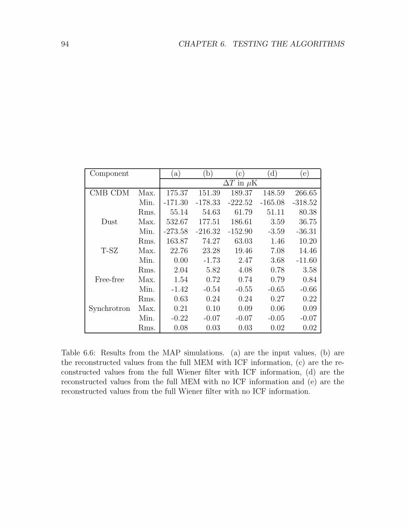
94 CHAPTER 6. TESTING THE ALGORITHMS
Component (a) (b) (c) (d) (e)∆T in µK
CMB CDM Max. 175.37 151.39 189.37 148.59 266.65Min. -171.30 -178.33 -222.52 -165.08 -318.52Rms. 55.14 54.63 61.79 51.11 80.38
Dust Max. 532.67 177.51 186.61 3.59 36.75Min. -273.58 -216.32 -152.90 -3.59 -36.31Rms. 163.87 74.27 63.03 1.46 10.20
T-SZ Max. 22.76 23.28 19.46 7.08 14.46Min. 0.00 -1.73 2.47 3.68 -11.60Rms. 2.04 5.82 4.08 0.78 3.58
Free-free Max. 1.54 0.72 0.74 0.79 0.84Min. -1.42 -0.54 -0.55 -0.65 -0.66Rms. 0.63 0.24 0.24 0.27 0.22
Synchrotron Max. 0.21 0.10 0.09 0.06 0.09Min. -0.22 -0.07 -0.07 -0.05 -0.07Rms. 0.08 0.03 0.03 0.02 0.02
Table 6.6: Results from the MAP simulations. (a) are the input values, (b) arethe reconstructed values from the full MEM with ICF information, (c) are the re-constructed values from the full Wiener filter with ICF information, (d) are thereconstructed values from the full MEM with no ICF information and (e) are thereconstructed values from the full Wiener filter with no ICF information.

6.5. TENERIFE SIMULATIONS 95
for the MEM analysis than for the Wiener analysis. This is a very useful propertybecause a smaller range of possible reconstructions means that the analysis is lesssensitive to the prior information (which may be incorrect in the real analysis).It has been shown that the Wiener approach can be considered as the quadraticapproximation to MEM and so even in the Gaussian case Wiener will be no betterthan MEM. Therefore, MEM will be used to analyse the Tenerife and Jodrell datain the next Chapter. The following section will test the power of MEM to analysethe Tenerife data set.
6.5 Testing the MEM algorithm on the Tenerife
data set
Before applying the MEM algorithm to the real data, simulations were carried outto test its performance. Two-dimensional sky maps were simulated using a stan-dard cold, dark matter model (Ho = 50 km s−1, Ωb = 0.1) with an rms signal of22µK per pixel (normalised to COBE second year data, Qrms−PS = 20.3µK, seeTegmark & Bunn 1995). Observations from the sky maps were then simulated byconvolving them with the Tenerife 8 FWHM beam. Before noise was added thepositive/negative algorithm was tested by analysing the data and then changing thesign of the data and reanalysing again. In both cases the same, but inverted, recon-struction was found for the MEM output and so it is concluded that this methodof two positive channels introduces no biases towards being positive or negative.Various noise levels were then added to the scans before reconstruction with MEM.The two noise levels considered here are 100µK and 25µK on the data scans, whichrepresent the two extrema of the data that are expected from the various Tenerifeconfigurations (100µK for the 10 GHz, FWHM=8 data and 25µK for the 15 and33 GHz, FWHM=5 data).
Figure 6.45 shows the convolution of one of the simulations with the Tenerifebeam and the result obtained from MEM with the two noise levels. The plotsare averaged over 30 simulations and the bounds are the 68% confidence limits(simulation to simulation variation). As seen, MEM recovers the underlying skysimulation to good accuracy for both noise levels, with the 25µK result the betterof the two as expected. Figure 6.46 shows the reconstructed intrinsic sky from twoof the simulations after 60 Newton–Raphson iterations of the MEM algorithm ascompared with the real sky simulations convolved in an 8 Gaussian beam. Variouscommon features are seen in the three scans like the maxima at RA 150, minimaat RA 170 and the partial ring feature between RA 200 and 260 with centralminima at RA 230, Dec. +35. All features larger than the rms are reconstructedin both the 25µK and 100µK noise simulations. However, there is a some freedom inthe algorithm to move these features within a beam width. This can cause spuriousfeatures to appear at the edge of the map when the guard region (about 5) aroundthe map contains a peak (this can be seen in the map as a decaying tail away fromthe edge). For example, the feature at RA 230, Dec 50 has been moved down bya few degrees out of the guard region in the 100µK noise simulation so it appears
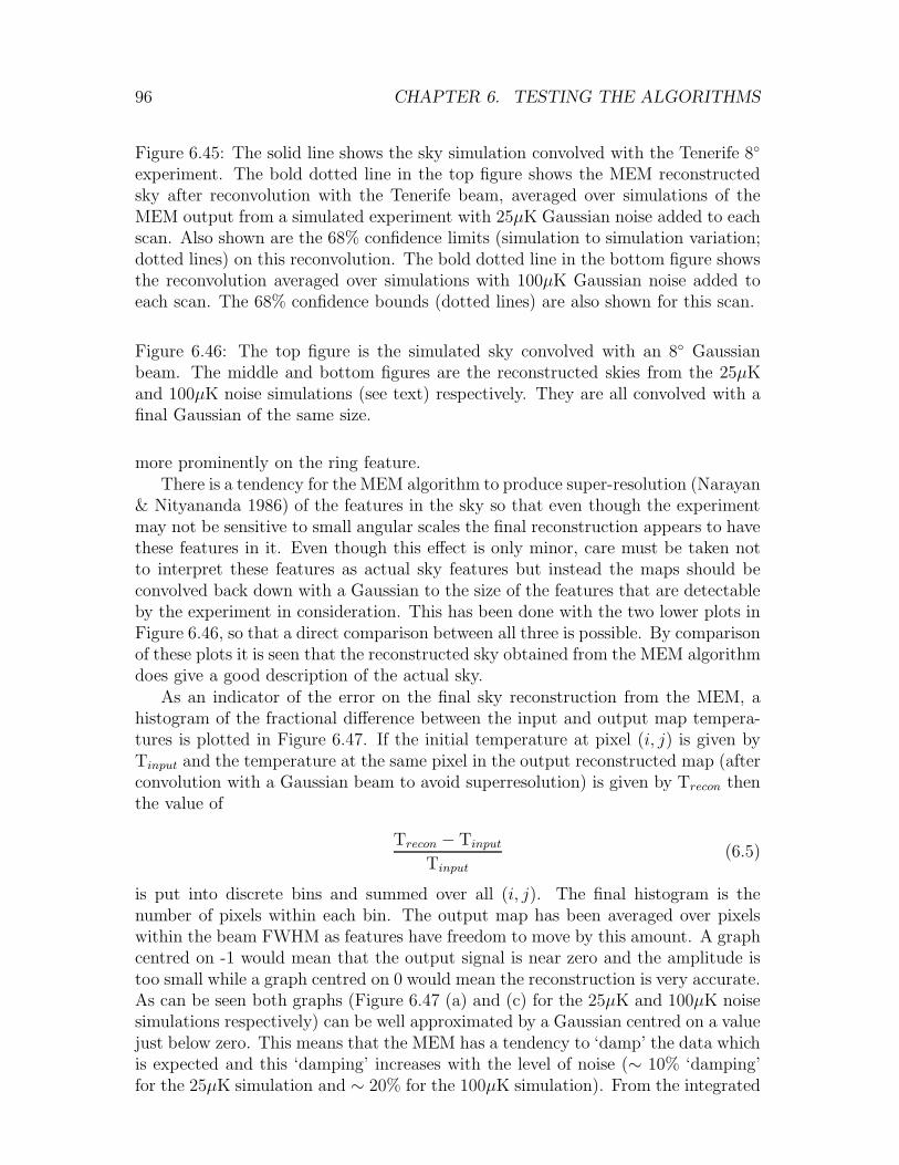
96 CHAPTER 6. TESTING THE ALGORITHMS
Figure 6.45: The solid line shows the sky simulation convolved with the Tenerife 8
experiment. The bold dotted line in the top figure shows the MEM reconstructedsky after reconvolution with the Tenerife beam, averaged over simulations of theMEM output from a simulated experiment with 25µK Gaussian noise added to eachscan. Also shown are the 68% confidence limits (simulation to simulation variation;dotted lines) on this reconvolution. The bold dotted line in the bottom figure showsthe reconvolution averaged over simulations with 100µK Gaussian noise added toeach scan. The 68% confidence bounds (dotted lines) are also shown for this scan.
Figure 6.46: The top figure is the simulated sky convolved with an 8 Gaussianbeam. The middle and bottom figures are the reconstructed skies from the 25µKand 100µK noise simulations (see text) respectively. They are all convolved with afinal Gaussian of the same size.
more prominently on the ring feature.There is a tendency for the MEM algorithm to produce super-resolution (Narayan
& Nityananda 1986) of the features in the sky so that even though the experimentmay not be sensitive to small angular scales the final reconstruction appears to havethese features in it. Even though this effect is only minor, care must be taken notto interpret these features as actual sky features but instead the maps should beconvolved back down with a Gaussian to the size of the features that are detectableby the experiment in consideration. This has been done with the two lower plots inFigure 6.46, so that a direct comparison between all three is possible. By comparisonof these plots it is seen that the reconstructed sky obtained from the MEM algorithmdoes give a good description of the actual sky.
As an indicator of the error on the final sky reconstruction from the MEM, ahistogram of the fractional difference between the input and output map tempera-tures is plotted in Figure 6.47. If the initial temperature at pixel (i, j) is given byTinput and the temperature at the same pixel in the output reconstructed map (afterconvolution with a Gaussian beam to avoid superresolution) is given by Trecon thenthe value of
Trecon − Tinput
Tinput
(6.5)
is put into discrete bins and summed over all (i, j). The final histogram is thenumber of pixels within each bin. The output map has been averaged over pixelswithin the beam FWHM as features have freedom to move by this amount. A graphcentred on -1 would mean that the output signal is near zero and the amplitude istoo small while a graph centred on 0 would mean the reconstruction is very accurate.As can be seen both graphs (Figure 6.47 (a) and (c) for the 25µK and 100µK noisesimulations respectively) can be well approximated by a Gaussian centred on a valuejust below zero. This means that the MEM has a tendency to ‘damp’ the data whichis expected and this ‘damping’ increases with the level of noise (∼ 10% ‘damping’for the 25µK simulation and ∼ 20% for the 100µK simulation). From the integrated
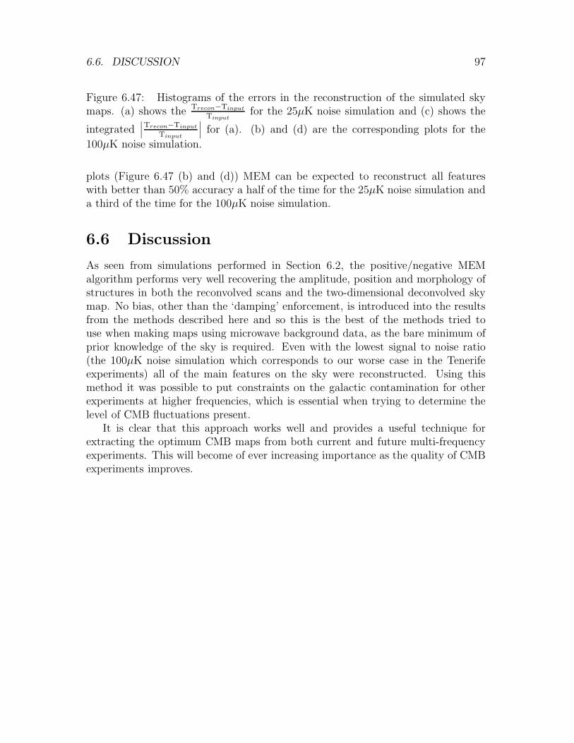
6.6. DISCUSSION 97
Figure 6.47: Histograms of the errors in the reconstruction of the simulated skymaps. (a) shows the
Trecon−Tinput
Tinputfor the 25µK noise simulation and (c) shows the
integrated∣
∣
∣
Trecon−Tinput
Tinput
∣
∣
∣ for (a). (b) and (d) are the corresponding plots for the
100µK noise simulation.
plots (Figure 6.47 (b) and (d)) MEM can be expected to reconstruct all featureswith better than 50% accuracy a half of the time for the 25µK noise simulation anda third of the time for the 100µK noise simulation.
6.6 Discussion
As seen from simulations performed in Section 6.2, the positive/negative MEMalgorithm performs very well recovering the amplitude, position and morphology ofstructures in both the reconvolved scans and the two-dimensional deconvolved skymap. No bias, other than the ‘damping’ enforcement, is introduced into the resultsfrom the methods described here and so this is the best of the methods tried touse when making maps using microwave background data, as the bare minimum ofprior knowledge of the sky is required. Even with the lowest signal to noise ratio(the 100µK noise simulation which corresponds to our worse case in the Tenerifeexperiments) all of the main features on the sky were reconstructed. Using thismethod it was possible to put constraints on the galactic contamination for otherexperiments at higher frequencies, which is essential when trying to determine thelevel of CMB fluctuations present.
It is clear that this approach works well and provides a useful technique forextracting the optimum CMB maps from both current and future multi-frequencyexperiments. This will become of ever increasing importance as the quality of CMBexperiments improves.

98 CHAPTER 6. TESTING THE ALGORITHMS
Chapter 7
Foregrounds and CMB features in
the sky maps
In this chapter I will use the maximum entropy method to produce maps of the skyat various frequencies from the data taken by the Jodrell Bank and Tenerife exper-iments. The possible origin of some of the features on the maps will be discussed.
7.1 The Jodrell Bank 5GHz interferometer
7.1.1 Wide–spacing data
The wide–spacing interferometer at Jodrell Bank has a baseline of 1.79m. Thetransfer function of the beam (i.e. the Fourier transform of the beam) is shown inFigure 7.1. It can be seen that in the RA direction it is sensitive to ∼ 1.5 scaleswhereas in the declination direction it is sensitive to ∼ 8 scales. At this frequency(5 GHz) the largest signals present will be those from extra–galactic point sources onthe smaller angular scales and galactic synchrotron emission on the larger angularscales. This data will therefore be used as a prediction for point source contributionin the results from the other experiments and as a possible constraint on galacticemission. Simulations performed for the level of the CMB fluctuations that are ex-pected in the data from a CDM dominated Universe with H = 50kms−1Mpc−1 andΩb = 0.03 give 3.0±1.1µK (the error is the standard deviation over 300 simulations).This is far below the noise and so it is ignored in the analysis presented here.
The MEM algorithm was used to extract the best information from the datausing both sine and cosine channels as constraints as described in the previouschapter. The full deconvolved map was not used as there is no simple consistentmethod to analyse the different scale dependencies in the two directions (the mapappears to be stripped in the RA direction due to the larger resolution) and thuscompare the result with other data from experiments such as Tenerife. The map
Figure 7.1: The cosine beam power sensitivity as a function of inverse degrees. Thesine beam has the same pattern but contains different phase information.
99
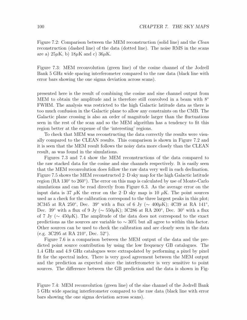
100 CHAPTER 7. THE SKY MAPS
Figure 7.2: Comparison between the MEM reconstruction (solid line) and the Cleanreconstruction (dashed line) of the data (dotted line). The noise RMS in the scansare a) 25µK, b) 18µK and c) 36µK.
Figure 7.3: MEM reconvolution (green line) of the cosine channel of the JodrellBank 5 GHz wide spacing interferometer compared to the raw data (black line witherror bars showing the one sigma deviation across scans).
presented here is the result of combining the cosine and sine channel output fromMEM to obtain the amplitude and is therefore still convolved in a beam with 8
FWHM. The analysis was restricted to the high Galactic latitude data as there istoo much confusion in the Galactic plane to allow any constraints on the CMB. TheGalactic plane crossing is also an order of magnitude larger than the fluctuationsseen in the rest of the scan and so the MEM algorithm has a tendency to fit thisregion better at the expense of the ‘interesting’ regions.
To check that MEM was reconstructing the data correctly the results were visu-ally compared to the CLEAN results. This comparison is shown in Figure 7.2 andit is seen that the MEM result follows the noisy data more closely than the CLEANresult, as was found in the simulations.
Figures 7.3 and 7.4 show the MEM reconstructions of the data compared tothe raw stacked data for the cosine and sine channels respectively. It is easily seenthat the MEM reconvolution does follow the raw data very well in each declination.Figure 7.5 shows the MEM reconstructed 2–D sky map for the high Galactic latituderegion (RA 130 to 260). The error on this map is calculated by use of Monte-Carlosimulations and can be read directly from Figure 6.3. As the average error on theinput data is 37 µK the error on the 2–D sky map is 10 µK. The point sourcesused as a check for the calibration correspond to the three largest peaks in this plot;3C345 at RA 250, Dec. 39 with a flux of 6 Jy (∼ 400µK); 4C39 at RA 141,Dec. 39 with a flux of 9 Jy (∼ 550µK); 3C286 at RA 200, Dec. 30 with a fluxof 7 Jy (∼ 450µK). The amplitude of the data does not correspond to the exactpredictions as the sources are variable to ∼ 30% but all agree to within this factor.Other sources can be used to check the calibration and are clearly seen in the data(e.g. 3C295 at RA 210, Dec. 52).
Figure 7.6 is a comparison between the MEM output of the data and the pre-dicted point source contribution by using the low frequency GB catalogues. The1.4 GHz and 4.9 GHz catalogues were extrapolated by performing a pixel by pixelfit for the spectral index. There is very good agreement between the MEM outputand the prediction as expected since the interferometer is very sensitive to pointsources. The difference between the GB prediction and the data is shown in Fig-
Figure 7.4: MEM reconvolution (green line) of the sine channel of the Jodrell Bank5 GHz wide spacing interferometer compared to the raw data (black line with errorbars showing the one sigma deviation across scans).
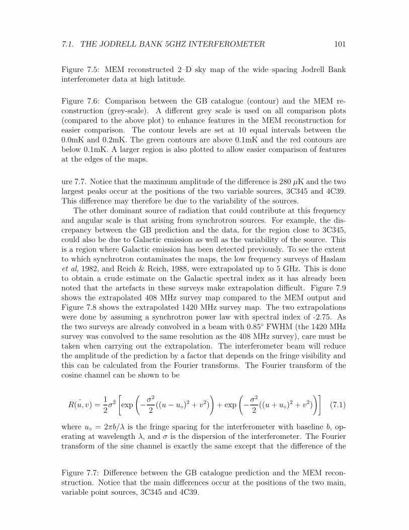
7.1. THE JODRELL BANK 5GHZ INTERFEROMETER 101
Figure 7.5: MEM reconstructed 2–D sky map of the wide–spacing Jodrell Bankinterferometer data at high latitude.
Figure 7.6: Comparison between the GB catalogue (contour) and the MEM re-construction (grey-scale). A different grey scale is used on all comparison plots(compared to the above plot) to enhance features in the MEM reconstruction foreasier comparison. The contour levels are set at 10 equal intervals between the0.0mK and 0.2mK. The green contours are above 0.1mK and the red contours arebelow 0.1mK. A larger region is also plotted to allow easier comparison of featuresat the edges of the maps.
ure 7.7. Notice that the maximum amplitude of the difference is 280 µK and the twolargest peaks occur at the positions of the two variable sources, 3C345 and 4C39.This difference may therefore be due to the variability of the sources.
The other dominant source of radiation that could contribute at this frequencyand angular scale is that arising from synchrotron sources. For example, the dis-crepancy between the GB prediction and the data, for the region close to 3C345,could also be due to Galactic emission as well as the variability of the source. Thisis a region where Galactic emission has been detected previously. To see the extentto which synchrotron contaminates the maps, the low frequency surveys of Haslamet al, 1982, and Reich & Reich, 1988, were extrapolated up to 5 GHz. This is doneto obtain a crude estimate on the Galactic spectral index as it has already beennoted that the artefacts in these surveys make extrapolation difficult. Figure 7.9shows the extrapolated 408 MHz survey map compared to the MEM output andFigure 7.8 shows the extrapolated 1420 MHz survey map. The two extrapolationswere done by assuming a synchrotron power law with spectral index of -2.75. Asthe two surveys are already convolved in a beam with 0.85 FWHM (the 1420 MHzsurvey was convolved to the same resolution as the 408 MHz survey), care must betaken when carrying out the extrapolation. The interferometer beam will reducethe amplitude of the prediction by a factor that depends on the fringe visibility andthis can be calculated from the Fourier transforms. The Fourier transform of thecosine channel can be shown to be
ˆR(u, v) =1
2σ2
[
exp
(
−σ2
2((u− u)
2 + v2)
)
+ exp
(
−σ2
2((u+ u)
2 + v2)
)]
(7.1)
where u = 2πb/λ is the fringe spacing for the interferometer with baseline b, op-erating at wavelength λ, and σ is the dispersion of the interferometer. The Fouriertransform of the sine channel is exactly the same except that the difference of the
Figure 7.7: Difference between the GB catalogue prediction and the MEM recon-struction. Notice that the main differences occur at the positions of the two main,variable point sources, 3C345 and 4C39.
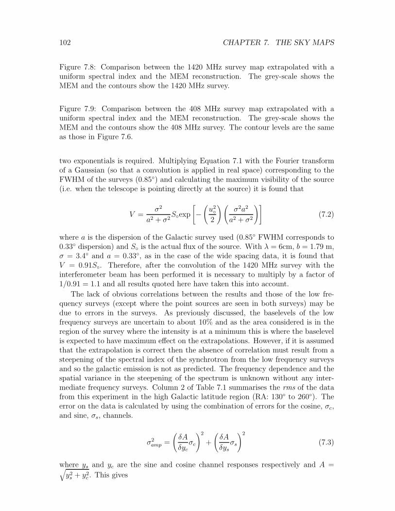
102 CHAPTER 7. THE SKY MAPS
Figure 7.8: Comparison between the 1420 MHz survey map extrapolated with auniform spectral index and the MEM reconstruction. The grey-scale shows theMEM and the contours show the 1420 MHz survey.
Figure 7.9: Comparison between the 408 MHz survey map extrapolated with auniform spectral index and the MEM reconstruction. The grey-scale shows theMEM and the contours show the 408 MHz survey. The contour levels are the sameas those in Figure 7.6.
two exponentials is required. Multiplying Equation 7.1 with the Fourier transformof a Gaussian (so that a convolution is applied in real space) corresponding to theFWHM of the surveys (0.85) and calculating the maximum visibility of the source(i.e. when the telescope is pointing directly at the source) it is found that
V =σ2
a2 + σ2Sexp
[
−(
u2
2
)(
σ2a2
a2 + σ2
)]
(7.2)
where a is the dispersion of the Galactic survey used (0.85 FWHM corresponds to0.33 dispersion) and S is the actual flux of the source. With λ = 6cm, b = 1.79 m,σ = 3.4 and a = 0.33, as in the case of the wide spacing data, it is found thatV = 0.91S. Therefore, after the convolution of the 1420 MHz survey with theinterferometer beam has been performed it is necessary to multiply by a factor of1/0.91 = 1.1 and all results quoted here have taken this into account.
The lack of obvious correlations between the results and those of the low fre-quency surveys (except where the point sources are seen in both surveys) may bedue to errors in the surveys. As previously discussed, the baselevels of the lowfrequency surveys are uncertain to about 10% and as the area considered is in theregion of the survey where the intensity is at a minimum this is where the baselevelis expected to have maximum effect on the extrapolations. However, if it is assumedthat the extrapolation is correct then the absence of correlation must result from asteepening of the spectral index of the synchrotron from the low frequency surveysand so the galactic emission is not as predicted. The frequency dependence and thespatial variance in the steepening of the spectrum is unknown without any inter-mediate frequency surveys. Column 2 of Table 7.1 summarises the rms of the datafrom this experiment in the high Galactic latitude region (RA: 130 to 260). Theerror on the data is calculated by using the combination of errors for the cosine, σc,and sine, σs, channels.
σ2amp =
(
δA
δycσc
)2
+
(
δA
δysσs
)2
(7.3)
where ys and yc are the sine and cosine channel responses respectively and A =√
y2s + y2
c . This gives
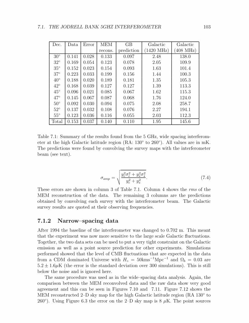
7.1. THE JODRELL BANK 5GHZ INTERFEROMETER 103
Dec. Data Error MEM GB Galactic Galacticrecons. prediction (1420 MHz) (408 MHz)
30 0.141 0.028 0.133 0.097 2.48 138.032 0.169 0.054 0.123 0.078 2.05 109.935 0.152 0.023 0.154 0.093 1.63 101.437 0.223 0.033 0.199 0.156 1.44 100.340 0.188 0.020 0.189 0.181 1.35 105.342 0.168 0.039 0.127 0.127 1.39 113.345 0.096 0.021 0.085 0.067 1.62 115.347 0.145 0.067 0.087 0.068 1.76 124.050 0.092 0.030 0.094 0.075 2.08 258.752 0.137 0.032 0.108 0.076 2.27 194.155 0.123 0.036 0.116 0.055 2.03 112.3
Total 0.153 0.037 0.140 0.110 1.95 145.6
Table 7.1: Summary of the results found from the 5 GHz, wide spacing interferom-eter at the high Galactic latitude region (RA: 130 to 260). All values are in mK.The predictions were found by convolving the survey maps with the interferometerbeam (see text).
σamp =
√
√
√
√
y2cσ
2c + y2
sσ2s
y2c + y2
s
. (7.4)
These errors are shown in column 3 of Table 7.1. Column 4 shows the rms of theMEM reconstruction of the data. The remaining 3 columns are the predictionsobtained by convolving each survey with the interferometer beam. The Galacticsurvey results are quoted at their observing frequencies.
7.1.2 Narrow–spacing data
After 1994 the baseline of the interferometer was changed to 0.702 m. This meantthat the experiment was now more sensitive to the large scale Galactic fluctuations.Together, the two data sets can be used to put a very tight constraint on the Galacticemission as well as a point source prediction for other experiments. Simulationsperformed showed that the level of CMB fluctuations that are expected in the datafrom a CDM dominated Universe with H = 50kms−1Mpc−1 and Ωb = 0.03 are5.2 ± 1.6µK (the error is the standard deviation over 300 simulations). This is stillbelow the noise and is ignored here.
The same procedure was used as in the wide–spacing data analysis. Again, thecomparison between the MEM reconvolved data and the raw data show very goodagreement and this can be seen in Figures 7.10 and 7.11. Figure 7.12 shows theMEM reconstructed 2–D sky map for the high Galactic latitude region (RA 130 to260). Using Figure 6.3 the error on the 2–D sky map is 8 µK. The point sources
104 CHAPTER 7. THE SKY MAPS
Figure 7.10: MEM reconvolution (green line) of the cosine channel of the JodrellBank 5 GHz narrow spacing interferometer compared to the raw data (black linewith error bars showing the one sigma deviation across scans).
Figure 7.11: MEM reconvolution (green line) of the sine channel of the Jodrell Bank5 GHz narrow spacing interferometer compared to the raw data (black line witherror bars showing the one sigma deviation across scans).
seen with the wide–spacing interferometer are again clearly visible in the narrow–spacing data. Figure 7.13 shows the comparison between the point source predictionand the MEM reconstruction. However, there are now larger sources that are notdue to point source contributions (e.g. the region about RA 170, Dec. 35). Theseare most likely produced by the extra sensitivity to large scale structure that thenarrow–spacing data has and are therefore most likely to be Galactic in origin. Thedilution of the beam given by Equation 7.2 becomes V = 0.56S. Therefore, afterthe convolution of the two low frequency surveys for comparison, it is necessary tomultiply by a factor of 1/0.56 = 1.8 and all results quoted here have taken this intoaccount.
Figure 7.14 and Figure 7.15 show the two low frequency surveys extrapolatedwith a synchrotron power law compared to the narrow–spacing MEM reconstruction.It is seen that there is little correlation between the 1420 MHz survey and the MEMreconstruction (ignoring the point source contributions that are seen in both maps)but there are some common features in the 408 MHz and the MEM reconstruction(although these are saturated in the contours). For example, there is a possibleGalactic feature at RA 170, Dec. 35 which is common to both the 408 MHzand MEM reconstruction but it appears at a higher level in the 408 MHz survey(the contour levels are saturated) which may be an indication that it is a steepenedsynchrotron source. The 1420 MHz survey is considered to be of poorer quality inthe low level Galactic emission (high Galactic latitude) than the 408 MHz survey asit suffers from more striping effects. This could account for the discrepancy betweenthe two predictions. Table 7.2 summarises the results for this experiment in thehigh Galactic latitude region (RA 130 to 260).
7.1.3 Joint analysis
It is possible to combine the two data sets to extract the most likely common un-derlying sky for both the narrow and wide spacings. This is a very good test of theconsistency of the experiment. The joint MEM analysis described in the Chapter 5can be used to combine the narrow and wide–spacing and extract the most likelyunderlying sky common to the two experiments. Table 7.3 summarises the results
Figure 7.12: MEM reconstructed 2–D sky map of the narrow–spacing Jodrell Bankinterferometer data at high latitude.
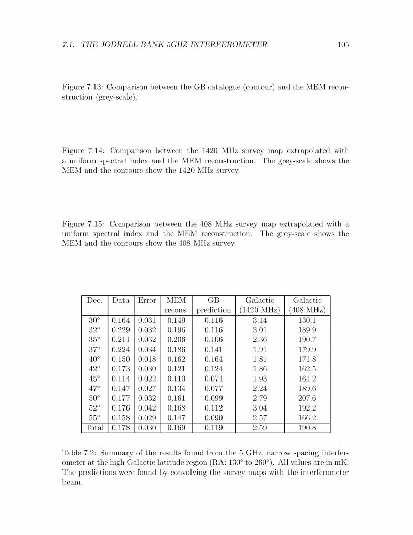
7.1. THE JODRELL BANK 5GHZ INTERFEROMETER 105
Figure 7.13: Comparison between the GB catalogue (contour) and the MEM recon-struction (grey-scale).
Figure 7.14: Comparison between the 1420 MHz survey map extrapolated witha uniform spectral index and the MEM reconstruction. The grey-scale shows theMEM and the contours show the 1420 MHz survey.
Figure 7.15: Comparison between the 408 MHz survey map extrapolated with auniform spectral index and the MEM reconstruction. The grey-scale shows theMEM and the contours show the 408 MHz survey.
Dec. Data Error MEM GB Galactic Galacticrecons. prediction (1420 MHz) (408 MHz)
30 0.164 0.031 0.149 0.116 3.14 130.132 0.229 0.032 0.196 0.116 3.01 189.935 0.211 0.032 0.206 0.106 2.36 190.737 0.224 0.034 0.186 0.141 1.91 179.940 0.150 0.018 0.162 0.164 1.81 171.842 0.173 0.030 0.121 0.124 1.86 162.545 0.114 0.022 0.110 0.074 1.93 161.247 0.147 0.027 0.134 0.077 2.24 189.650 0.177 0.032 0.161 0.099 2.79 207.652 0.176 0.042 0.168 0.112 3.04 192.255 0.158 0.029 0.147 0.090 2.57 166.2
Total 0.178 0.030 0.169 0.119 2.59 190.8
Table 7.2: Summary of the results found from the 5 GHz, narrow spacing interfer-ometer at the high Galactic latitude region (RA: 130 to 260). All values are in mK.The predictions were found by convolving the survey maps with the interferometerbeam.

106 CHAPTER 7. THE SKY MAPS
Dec. WS MEM result NS MEM result30 0.134 0.15032 0.122 0.19335 0.155 0.20437 0.198 0.18540 0.189 0.16242 0.127 0.12245 0.085 0.11147 0.087 0.13450 0.094 0.16152 0.108 0.16855 0.116 0.147
Total 0.140 0.168
Table 7.3: Summary of the results found from the joint MEM analysis of the two5 GHz interferometer data sets at the high Galactic latitude region (RA: 130 to260). All values are in mK.
from the combination of the two data sets. By comparing this to Table 7.1 and 7.2it can be seen that the results from the joint analysis are almost identical to thosefrom the individual analyses. This means that the narrow and wide–spacing datasets are consistent and can be used to put constraints on Galactic emission. Anydiscrepancies between the analysis are a result of the variability in the point sources.
To predict the level of Galactic fluctuations at higher frequencies the spectralindex dependence of the foregrounds is required. To calculate this it is possibleto compare the results from the joint analysis to the predictions from the lowerfrequency surveys. Firstly the point sources must be subtracted from the mapreconstruction to leave the Galactic contribution. The prediction from the GreenBank catalogue was subtracted from the narrow and wide–spacing data to leave theresidual signal. Due to the variability of the sources this residual will be an upperlimit on the Galactic contribution and only by having continuous source monitoringwould the results be better. We will use the residual signal for the narrow–spacingdata (where the Galactic signal is expected to be higher and so a smaller error willbe obtained). The rms of this signal is 73 ± 23µK (where the error on the MEMreconstruction comes from comparison with simulations and a 30% variability in themajor sources is assumed). When comparing this to the signal of 2.59 ± 0.26 mK(error from a 10% error in the survey) at 1420 MHz and 190.8± 19 mK at 408 MHzit is found that the average spectral index from 1420 MHz to 5 GHz is 2.8 ± 0.4and from 408 MHz to 5 GHz is 3.1 ± 0.4. These results are in agreement withprevious predictions of the Galactic spectral index at a range of angular scales.Bersanelli et al (1996) found that the spectral index between 1420 MHz and 5 GHzwas 2.9±0.3 on a 2 angular scale and Platania et al (1997) found that the spectralindex between 1420 MHz and a range of frequency data between 1 GHz and 10 GHz
7.1. THE JODRELL BANK 5GHZ INTERFEROMETER 107
Figure 7.16: The variation in the derived spectral index using the narrow–spacingdata and the 408 MHz survey. The contour level is at the rms of the map.
Figure 7.17: The variation in the derived spectral index using the narrow–spacingdata and the 1420 MHz survey. The contour level is at the rms of the map.
gave a spectral index of 2.8 ± 0.2 on an 18 angular scale. This is an indication ofa steepening synchrotron spectral index. To take the analysis one step further it ispossible to compare the surveys pixel by pixel to obtain a map of the spectral indexdependencies.
Figure 7.16 shows the spectral index variation as predicted by comparison be-tween the 408 MHz survey and the narrow–spacing data over the high Galacticregion. The rms spectral index is 3.3 ± 0.5 where the error is now the rms overthe map. This is consistent with the above result. Figure 7.17 shows the result forthe 1420 MHz survey prediction. The rms spectral index is 3.1 ± 0.9. The regionswhere there is a large deviation away from the rms spectral index (which results inthe large variance) are usually associated with variable point sources (e.g. 3C345)that have not been fully removed from the 5 GHz interferometer or Galactic surveydata. All the results so far are consistent with a steepened synchrotron source beingthe dominant contributor to the data. It is also possible that the shallower indexbetween 1420 MHz and 5 GHz than between 408 MHz and 5 GHz could be due tothe increasing importance of free–free emission, although further frequency measure-ments are necessary to confirm this. Therefore, the low frequency surveys should notbe used (especially the 1420 MHz survey) as a prediction for Galactic contributionwithout taking into account the synchrotron steepening. The new 5 GHz data pre-sented here represents an intermediate step in the frequency coverage between thelow frequency Galactic surveys and the higher frequency CMB experiments. It istherefore a very useful check on Galactic models and can be used to make estimatesof Galactic contamination in CMB experiments.
It should be noted that the level of Galactic emission predicted here may betoo large as the artefacts in the surveys may enhance the fluctuations. Also, the1420 MHz and 408 MHz surveys contain contributions from the point sources (forexample 3C295) and so the level of Galactic fluctuations predicted will be too large.If it is assumed that 50% of the 408 MHz survey rms is due to these effects (i.e.135 ± 20 mK at 408 MHz for the narrow spacing data) then the spectral indexconstraint is β = 3.0±0.4 which still corresponds to a steeping synchrotron spectrum.This does not take into account the residual effect from the point sources in the 5GHz prediction and so should be taken as a lower limit on the spectral index. Thisdoes not alter the conclusion that the low frequency surveys should not be used bythemselves as a prediction for galactic emission as these artefacts, or the presenceof point sources, only make the prediction worse.
If it is assumed that the signal remaining after subtracting the Green Bank pointsource prediction from the data is due to Galactic emission alone then it is possibleto make a prediction for the level of contamination in the Tenerife data. As the
108 CHAPTER 7. THE SKY MAPS
interferometer is only sensitive to a certain range of angular scales it is necessary toassume something about the spatial variation of the synchrotron source. A spectrumof l−3 is used spatially and the steepened synchrotron spectrum is assumed to holduntil the higher Tenerife frequencies. Therefore, considering the 5 FWHM Tenerifeexperiments, it is expected that the 10 GHz data will be contaminated by 30 µK ofsynchrotron emission, the 15 GHz data will be contaminated by 10 µK of synchrotronemission and the 33 GHz data will be contaminated by 1 µK of synchrotron emission.However, these figures are very approximate as the interferometer is sensitive to twodifferent scales in the RA and Dec. direction and this has not been taken into accountand will reduce the contamination level. Also the increasing importance of the free–free emission has been ignored which will increase the Galactic contamination level.
7.2 The Tenerife experiments
The MEM programs were applied to all Tenerife data described in Chapter 4. Thisis an ongoing process and the results shown here are not final but represent thecurrent iteration of the analysis.
7.2.1 Reconstructing the sky at 10.4 GHz with 8 FWHM
To apply the MEM deconvolution process described to the data from the 10.4 GHz,8 FWHM, Tenerife experiment it is necessary to select parameters that not onlyachieve convergence of the iterative scheme, but also make the fullest use of thedata. The amplitude of the fluctuations that are of interest is at least two ordersof magnitude smaller than the magnitude of the signal produced during the majorpassage through the Galactic plane region (∼ 45 mK at ∼ Dec. +40). Clearly, anybaseline fitting and reconstruction will be dominated by this feature at the expenseof introducing spurious features into the regions which are of interest. For thisreason the data (Table 7.4) corresponding to the principal Galactic plane crossingare not used in the reconstruction.
In contrast, the anti-centre crossing (∼ RA 60 at ∼ Dec. +40 ) correspondingto scanning through the Galactic plane, but looking out of the Galaxy, is at anacceptable level (<∼ 5 mK) and is a useful check on the performance and consistencyof the observations. With the parameters set as in Chapter 5, Table 5.1, χ2 demon-strates a rapid convergence. For example, the change in χ2 after 120 iterations ofMEM is ∆χ2/χ2 ≃ −9×10⁻⁴ while the change in χ2
base is ∆χ2base/χ
2base ≃ −2×10⁻⁴.
The fitted baselines are subtracted from the raw data set to provide data free frombaseline effects, allowing the scans for a given declination to be stacked together toprovide a single high sensitivity scan. Figure 7.18 shows the stacked results for the 8
experiment at each declination compared with the reconvolution of the MEM resultwith the beam. The weak Galactic crossing is clearly visible at RA=50 − 100. Atlower declinations this crossing shows a complex structure with peak amplitudes ∼a few mK. Only positions on the sky with more than ten independent measurementshave been plotted. The data with better sensitivities are those at Dec.=+39.4 and
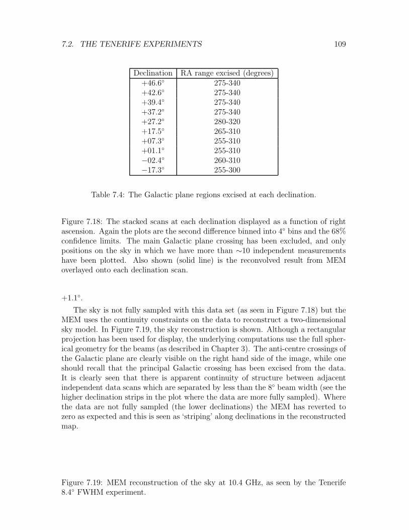
7.2. THE TENERIFE EXPERIMENTS 109
Declination RA range excised (degrees)+46.6 275-340+42.6 275-340+39.4 275-340+37.2 275-340+27.2 280-320+17.5 265-310+07.3 255-310+01.1 255-310−02.4 260-310−17.3 255-300
Table 7.4: The Galactic plane regions excised at each declination.
Figure 7.18: The stacked scans at each declination displayed as a function of rightascension. Again the plots are the second difference binned into 4 bins and the 68%confidence limits. The main Galactic plane crossing has been excluded, and onlypositions on the sky in which we have more than ∼10 independent measurementshave been plotted. Also shown (solid line) is the reconvolved result from MEMoverlayed onto each declination scan.
+1.1.
The sky is not fully sampled with this data set (as seen in Figure 7.18) but theMEM uses the continuity constraints on the data to reconstruct a two-dimensionalsky model. In Figure 7.19, the sky reconstruction is shown. Although a rectangularprojection has been used for display, the underlying computations use the full spher-ical geometry for the beams (as described in Chapter 3). The anti-centre crossings ofthe Galactic plane are clearly visible on the right hand side of the image, while oneshould recall that the principal Galactic crossing has been excised from the data.It is clearly seen that there is apparent continuity of structure between adjacentindependent data scans which are separated by less than the 8 beam width (see thehigher declination strips in the plot where the data are more fully sampled). Wherethe data are not fully sampled (the lower declinations) the MEM has reverted tozero as expected and this is seen as ‘striping’ along declinations in the reconstructedmap.
Figure 7.19: MEM reconstruction of the sky at 10.4 GHz, as seen by the Tenerife8.4 FWHM experiment.
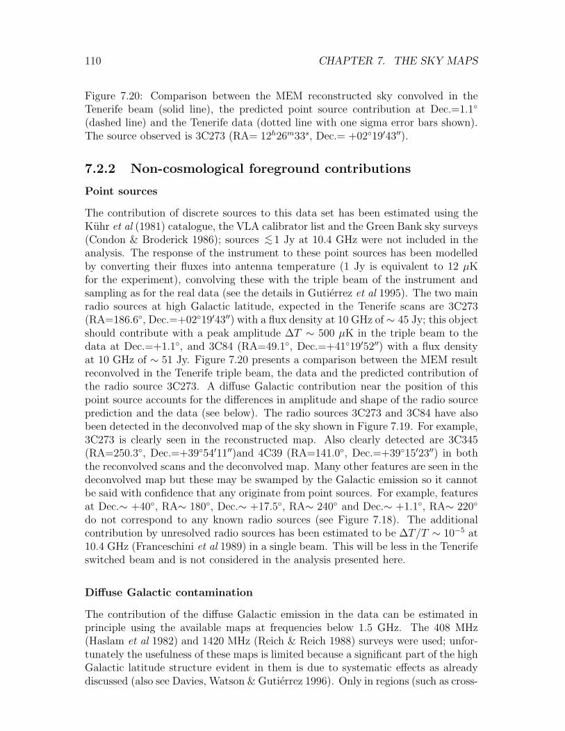
110 CHAPTER 7. THE SKY MAPS
Figure 7.20: Comparison between the MEM reconstructed sky convolved in theTenerife beam (solid line), the predicted point source contribution at Dec.=1.1
(dashed line) and the Tenerife data (dotted line with one sigma error bars shown).The source observed is 3C273 (RA= 12h26m33s, Dec.= +0219′43′′).
7.2.2 Non-cosmological foreground contributions
Point sources
The contribution of discrete sources to this data set has been estimated using theKuhr et al (1981) catalogue, the VLA calibrator list and the Green Bank sky surveys(Condon & Broderick 1986); sources <∼ 1 Jy at 10.4 GHz were not included in theanalysis. The response of the instrument to these point sources has been modelledby converting their fluxes into antenna temperature (1 Jy is equivalent to 12 µKfor the experiment), convolving these with the triple beam of the instrument andsampling as for the real data (see the details in Gutierrez et al 1995). The two mainradio sources at high Galactic latitude, expected in the Tenerife scans are 3C273(RA=186.6, Dec.=+0219′43′′) with a flux density at 10 GHz of ∼ 45 Jy; this objectshould contribute with a peak amplitude ∆T ∼ 500 µK in the triple beam to thedata at Dec.=+1.1, and 3C84 (RA=49.1, Dec.=+4119′52′′) with a flux densityat 10 GHz of ∼ 51 Jy. Figure 7.20 presents a comparison between the MEM resultreconvolved in the Tenerife triple beam, the data and the predicted contribution ofthe radio source 3C273. A diffuse Galactic contribution near the position of thispoint source accounts for the differences in amplitude and shape of the radio sourceprediction and the data (see below). The radio sources 3C273 and 3C84 have alsobeen detected in the deconvolved map of the sky shown in Figure 7.19. For example,3C273 is clearly seen in the reconstructed map. Also clearly detected are 3C345(RA=250.3, Dec.=+3954′11′′)and 4C39 (RA=141.0, Dec.=+3915′23′′) in boththe reconvolved scans and the deconvolved map. Many other features are seen in thedeconvolved map but these may be swamped by the Galactic emission so it cannotbe said with confidence that any originate from point sources. For example, featuresat Dec.∼ +40, RA∼ 180, Dec.∼ +17.5, RA∼ 240 and Dec.∼ +1.1, RA∼ 220
do not correspond to any known radio sources (see Figure 7.18). The additionalcontribution by unresolved radio sources has been estimated to be ∆T/T ∼ 10−5 at10.4 GHz (Franceschini et al 1989) in a single beam. This will be less in the Tenerifeswitched beam and is not considered in the analysis presented here.
Diffuse Galactic contamination
The contribution of the diffuse Galactic emission in the data can be estimated inprinciple using the available maps at frequencies below 1.5 GHz. The 408 MHz(Haslam et al 1982) and 1420 MHz (Reich & Reich 1988) surveys were used; unfor-tunately the usefulness of these maps is limited because a significant part of the highGalactic latitude structure evident in them is due to systematic effects as alreadydiscussed (also see Davies, Watson & Gutierrez 1996). Only in regions (such as cross-
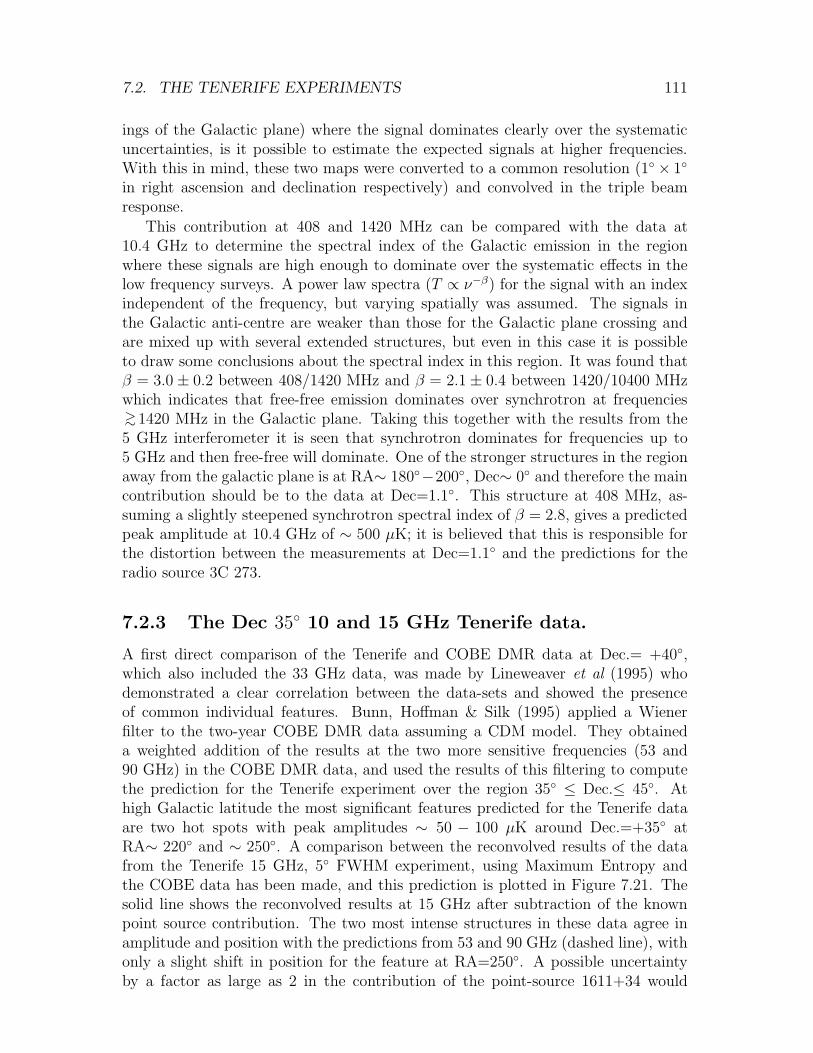
7.2. THE TENERIFE EXPERIMENTS 111
ings of the Galactic plane) where the signal dominates clearly over the systematicuncertainties, is it possible to estimate the expected signals at higher frequencies.With this in mind, these two maps were converted to a common resolution (1 × 1
in right ascension and declination respectively) and convolved in the triple beamresponse.
This contribution at 408 and 1420 MHz can be compared with the data at10.4 GHz to determine the spectral index of the Galactic emission in the regionwhere these signals are high enough to dominate over the systematic effects in thelow frequency surveys. A power law spectra (T ∝ ν−β) for the signal with an indexindependent of the frequency, but varying spatially was assumed. The signals inthe Galactic anti-centre are weaker than those for the Galactic plane crossing andare mixed up with several extended structures, but even in this case it is possibleto draw some conclusions about the spectral index in this region. It was found thatβ = 3.0 ± 0.2 between 408/1420 MHz and β = 2.1 ± 0.4 between 1420/10400 MHzwhich indicates that free-free emission dominates over synchrotron at frequencies>∼1420 MHz in the Galactic plane. Taking this together with the results from the5 GHz interferometer it is seen that synchrotron dominates for frequencies up to5 GHz and then free-free will dominate. One of the stronger structures in the regionaway from the galactic plane is at RA∼ 180−200, Dec∼ 0 and therefore the maincontribution should be to the data at Dec=1.1. This structure at 408 MHz, as-suming a slightly steepened synchrotron spectral index of β = 2.8, gives a predictedpeak amplitude at 10.4 GHz of ∼ 500 µK; it is believed that this is responsible forthe distortion between the measurements at Dec=1.1 and the predictions for theradio source 3C 273.
7.2.3 The Dec 35 10 and 15 GHz Tenerife data.
A first direct comparison of the Tenerife and COBE DMR data at Dec.= +40,which also included the 33 GHz data, was made by Lineweaver et al (1995) whodemonstrated a clear correlation between the data-sets and showed the presenceof common individual features. Bunn, Hoffman & Silk (1995) applied a Wienerfilter to the two-year COBE DMR data assuming a CDM model. They obtaineda weighted addition of the results at the two more sensitive frequencies (53 and90 GHz) in the COBE DMR data, and used the results of this filtering to computethe prediction for the Tenerife experiment over the region 35 ≤ Dec.≤ 45. Athigh Galactic latitude the most significant features predicted for the Tenerife dataare two hot spots with peak amplitudes ∼ 50 − 100 µK around Dec.=+35 atRA∼ 220 and ∼ 250. A comparison between the reconvolved results of the datafrom the Tenerife 15 GHz, 5 FWHM experiment, using Maximum Entropy andthe COBE data has been made, and this prediction is plotted in Figure 7.21. Thesolid line shows the reconvolved results at 15 GHz after subtraction of the knownpoint source contribution. The two most intense structures in these data agree inamplitude and position with the predictions from 53 and 90 GHz (dashed line), withonly a slight shift in position for the feature at RA=250. A possible uncertaintyby a factor as large as 2 in the contribution of the point-source 1611+34 would

112 CHAPTER 7. THE SKY MAPS
Figure 7.21: Comparison between the 15 GHz data (solid line) and the COBEprediction by Bunn et al 1995 (dashed line).
Figure 7.22: A multifrequency MEM reconstruction of the two fluctuations (whitespots on the bottom colour contour plot), which Bunn et al (1995) predicted shouldbe seen by the Tenerife experiments using COBE results, from the 10 GHz and15 GHz channels. 0 and 50 on the y–axis correspond to 65 and 15 in declinationrespectively. 0 and 50 on the x–axis correspond to 210 and 260 in right ascensionrespectively. The vertical axis is in arbitrary units. Only the Dec +35 data wasused to constrain this reconstruction so the fluctuations fall to zero away from thisdeclination.
change only slightly the shape and amplitude of this second feature. As a test themultifrequency MEM was applied to the 10 GHz and 15 GHz Tenerife data at thisdeclination. The program is currently in development and so it was not possibleto apply it to the full two dimensional data set in the time allowed. However, theapplication of multi-MEM to this declination can be used as a test of the powerthat it will have in analysing the full two dimensional data set. Figure 7.22 clearlyshows the two features predicted by Bunn, Hoffman & Silk (1995) at Dec +35 asreconstructed by the multifrequency MEM algorithm using the 10 GHz and 15 GHzdata simultaneously.
7.2.4 The full 5 FWHM data set
The MEM deconvolution was applied to the full data set at each frequency. Thisrepresents a large portion of the sky at the two lower frequencies and so it is possibleto produce sky maps covering a large area. Figures 7.23 and 7.24 show the MEMreconvolved data compared to the raw stacked data at each declination for the10 GHz and 15 GHz Tenerife experiments respectively. At both frequencies all ofthe declinations were analysed simultaneously utilising the continuity across the sky.As can be seen the MEM result falls within the one sigma confidence limits at eachdeclination. There are some discrepancies between declinations where, because thedata were taken at different times, the variability of the sources leads to a differentflux contribution. This can be seen clearly at RA 250 where the variable source(the predicted source contribution is shown as the red line) has become smaller inamplitude between the data acquisition of Dec. 37.5 and that of Dec. 40. Theonly way to allow for this is to make simultaneous observations of all sources andsubtract their flux from the raw data. This is work in progress (see Figure 2.7).
Figure 7.23: Comparison of the MEM reconvolved data (green line) and the rawstacked data (black line) for each of the declinations at 10 GHz. Also shown (redline) is the expected point source contribution from an extrapolation of the 1.4 GHzand 5 GHz Green Bank point source catalogue.
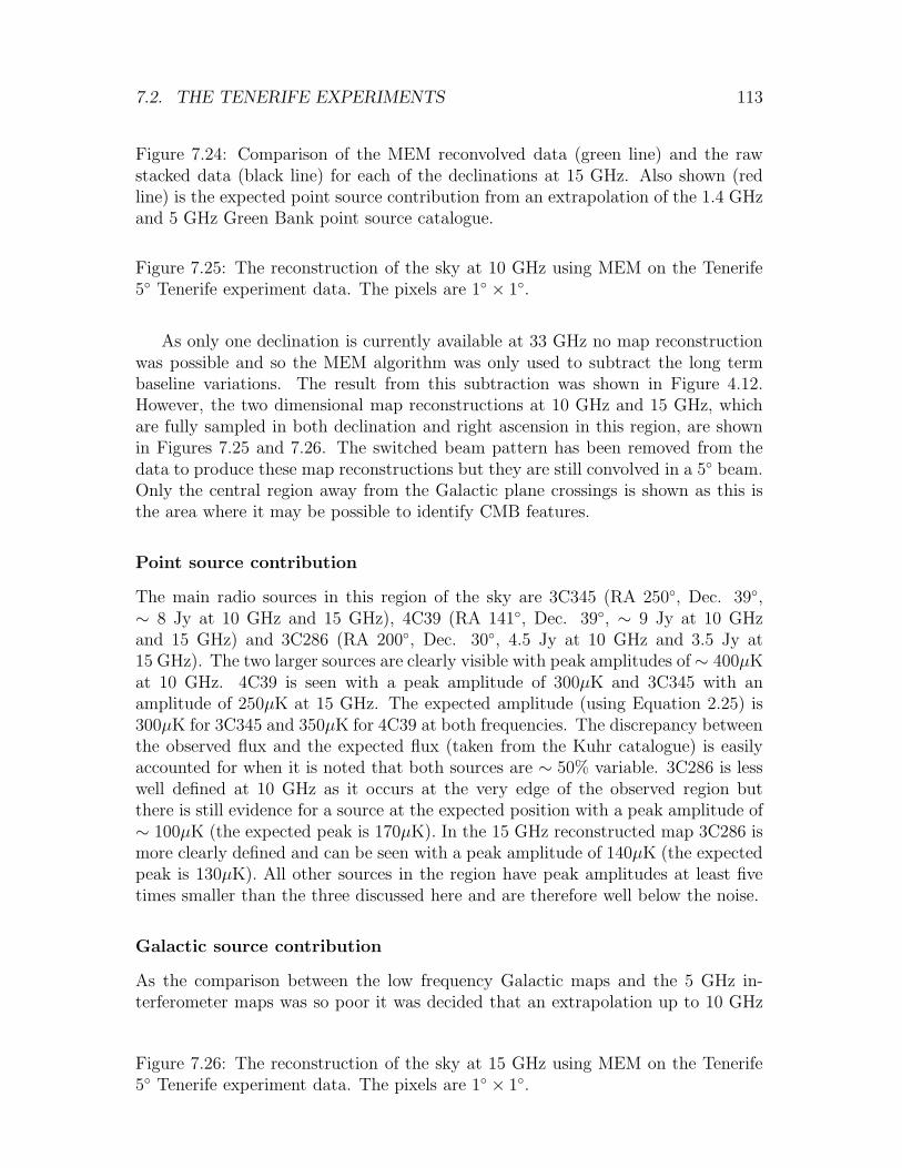
7.2. THE TENERIFE EXPERIMENTS 113
Figure 7.24: Comparison of the MEM reconvolved data (green line) and the rawstacked data (black line) for each of the declinations at 15 GHz. Also shown (redline) is the expected point source contribution from an extrapolation of the 1.4 GHzand 5 GHz Green Bank point source catalogue.
Figure 7.25: The reconstruction of the sky at 10 GHz using MEM on the Tenerife5 Tenerife experiment data. The pixels are 1 × 1.
As only one declination is currently available at 33 GHz no map reconstructionwas possible and so the MEM algorithm was only used to subtract the long termbaseline variations. The result from this subtraction was shown in Figure 4.12.However, the two dimensional map reconstructions at 10 GHz and 15 GHz, whichare fully sampled in both declination and right ascension in this region, are shownin Figures 7.25 and 7.26. The switched beam pattern has been removed from thedata to produce these map reconstructions but they are still convolved in a 5 beam.Only the central region away from the Galactic plane crossings is shown as this isthe area where it may be possible to identify CMB features.
Point source contribution
The main radio sources in this region of the sky are 3C345 (RA 250, Dec. 39,∼ 8 Jy at 10 GHz and 15 GHz), 4C39 (RA 141, Dec. 39, ∼ 9 Jy at 10 GHzand 15 GHz) and 3C286 (RA 200, Dec. 30, 4.5 Jy at 10 GHz and 3.5 Jy at15 GHz). The two larger sources are clearly visible with peak amplitudes of ∼ 400µKat 10 GHz. 4C39 is seen with a peak amplitude of 300µK and 3C345 with anamplitude of 250µK at 15 GHz. The expected amplitude (using Equation 2.25) is300µK for 3C345 and 350µK for 4C39 at both frequencies. The discrepancy betweenthe observed flux and the expected flux (taken from the Kuhr catalogue) is easilyaccounted for when it is noted that both sources are ∼ 50% variable. 3C286 is lesswell defined at 10 GHz as it occurs at the very edge of the observed region butthere is still evidence for a source at the expected position with a peak amplitude of∼ 100µK (the expected peak is 170µK). In the 15 GHz reconstructed map 3C286 ismore clearly defined and can be seen with a peak amplitude of 140µK (the expectedpeak is 130µK). All other sources in the region have peak amplitudes at least fivetimes smaller than the three discussed here and are therefore well below the noise.
Galactic source contribution
As the comparison between the low frequency Galactic maps and the 5 GHz in-terferometer maps was so poor it was decided that an extrapolation up to 10 GHz
Figure 7.26: The reconstruction of the sky at 15 GHz using MEM on the Tenerife5 Tenerife experiment data. The pixels are 1 × 1.
114 CHAPTER 7. THE SKY MAPS
would be impossible. Therefore, a comparison of the 5 GHz narrow spacing mapand the 10 GHz Tenerife map was made by eye to check for any possible commonfeatures. One feature which is clearly detected in both the 5 GHz (at 0.3mK in theinterferometer beam) and 10 GHz (at 0.2mK in the 5 Gaussian beam) maps liesjust above Dec. 35 at RA 170 (this feature is also detected in the 1420 MHz and408 MHz maps as well). This feature was assumed to be Galactic in origin in the5 GHz map and also seems to be Galactic in origin in the 10 GHz map (as it hasvanished in the 15 GHz map). Taking into account the different beam sizes (FWHMof the Jodrell interferometer is 8 and that of the 10 GHz Tenerife experiment is 5)it is possible to calculate an approximate spectral index for the feature. The peakamplitude at 5 GHz was ∼ 280µK and at 10 GHz was ∼ 140µK and so the spectralindex is β = 2.3 ± 0.5. This would indicate a Galactic origin and it is more likelythat the feature is free-free emission. This agrees with the findings of the 8 FWHMexperiment that the majority of Galactic emission between 5 GHz and 10 GHz wasfree-free emission in origin.
The 10 GHz map is generally expected to contain more Galactic features (indeedthe rms values of the 10 GHz data are larger than the 15 GHz data which wouldindicate additional emission processes are contributing to the data) but it is verydifficult to assign each feature to being Galactic or cosmological in origin withouta simultaneous analysis of the 10 GHz and 5 GHz (and possibly lower frequencydata). This is now work in progress with the new multi-MEM procedure but due tothe size and complexity of the problem it was not possible to produce any results intime for the publication of this thesis.
CMB features in the map
It is very difficult to decide whether a particular feature is cosmological in originor whether it originates from one of the foregrounds considered here. Without thecompletion of the full analysis now in progress it is only possible to speculate onthe origin of the features detected. By comparing the various frequencies from theTenerife experiments or by comparison with other experiments it is possible to makea good ‘guess’ at whether a particular feature is CMB or not. It was seen that the15 GHz Tenerife data set is expected to have a maximum Galactic contribution of10 µK which is well below the noise and so the 15 GHz reconstruction is predom-inantly CMB. The 15 GHz data can be used by itself, as a first approximation, toput constraints on CMB features. One example of a possible CMB feature is visibleat RA 180 and Dec. 40. This feature is detected at the same amplitude in the10 GHz, 15 GHz and 33 GHz data sets and so is a clear candidate for being CMBin origin (this was first reported in Hancock et al 1994). Another example are thefeatures at Dec. 35 between RA 210 and 250 at 15 GHz which appear as two pos-itive features separated by a large negative feature. These also appear in the COBE53 GHz and 90 GHz maps and were used for the prediction by Bunn et al (1995)which was shown in Figure 7.21. With such a large frequency coverage indicatingthat the features do have the correct spectral dependence to be CMB in origin theseare probably the best candidates in literature today for CMB features.
7.2. THE TENERIFE EXPERIMENTS 115
The following chapter introduces some of the techniques used to analyse the mapsproduced here in an attempt to automatically characterise the features without theneed for a comparison by eye.

116 CHAPTER 7. THE SKY MAPS
Chapter 8
Analysing the sky maps
In the preceding chapter the data were processed by MEM to produce a two dimen-sional partial sky map of the CMB fluctuations. In this chapter I will explore someof the main procedures that are in use to analyse CMB maps to get the maximumamount of information from them.
8.1 The power spectrum
A simple way of comparing maps is to look at their power spectra. By Fouriertransforming the temperature fluctuation distribution underlying theories can betested by comparing the predicted spectrum with the observed. However, thereare problems in implementing this. The main problem is the spherical nature ofthe sky. A simple Fourier transform is not possible unless the sky area is smallenough so that the spherical nature of the sky can be ignored. To overcome this,a high resolution experiment can be used to survey a small area of sky. The powerspectra from 10 × 10 patches of simulated Planck Surveyor data were plotted inChapter 6. As the sky area covered decreases sample variance will quickly dominatethe errors. Sample variance was not plotted in the power spectra of Chapter 6 asthe purpose of these plots was not to compare the result with theory but to comparethe reconstructed power spectra with the true, input power spectra. Otherwise, it isnecessary to use spherical harmonics to transform the map into ℓ space (see Chapter2). This has problems caused by the nature of data acquisition. Without full skycoverage (which is never possible because of the Galactic plane contamination ofthe data, which needs to be excluded when testing the CMB parameters) therewill always be artefacts present due to the absence of data. Window functions (forexample, the cosine bell) can be used to reduce their effects but they cannot becompletely eliminated. The window functions also have the effect of reducing thenumber of data points that are used in the analysis (the ones at the edge of themap are weighted down) and so have the effect of increasing the errors on the finalparameter estimation. So, instead of trying to predict what the theory looks likeusing the data, it is better to use the theory to try and predict what the datashould look like, as all artefacts can then be easily incorporated, and then comparethis prediction with the real data. This is done using the likelihood function (see
117
118 CHAPTER 8. ANALYSING THE SKY MAPS
Chapter 4 for likelihood results).The power spectrum is a useful test for the cosmological parameters in a given
theory. However, it is fairly straight-forward to construct a map with Gaussianfluctuations and one with non-Gaussian fluctuations (based on the string model forexample) that have the same power spectrum. Therefore, it is necessary to usefurther tests for non-Gaussianity and the remainder of this chapter attempts tosummarise some of these tests.
8.2 Genus and Topology
When presented with a map of any description the eye automatically searches forshapes within that image. It would therefore be logical to construct an algorithmthat will do this but in a statistical manner. By using the topology of an object itis possible to group together shapes with similar mathematical properties. Thereare many ways of defining the topological parameters of an object. The shapes in atwo dimensional map can be characterised by their area, circumference or curvature.The mean curvature of a map is also known as the Genus.
8.2.1 What is Genus?
In three dimensions (see Gott et al 1986) an object will have a genus of +1 if it issimilar to a torus and a genus of -1 if it is similar to a sphere. In two dimensions(see Gott et al 1990) an object will have a genus of +1 if it is similar to a coin anda genus of -1 if it is similar to a ring. The genus of a map is simply the sum ofthe genus of each of the shapes in that map. If a two dimensional map is a perfectsponge shape, so that there are an equal number of coin and ring shapes, then thetotal average genus is zero and we have a perfect Gaussian field. In one dimensionthe genus is simply taken as the number of up crossings above a certain threshold(see Coles & Barrow 1987).
Genus was first applied in cosmology to large scale structure surveys. Manysuch surveys (e.g. de Lapparent, Geller & Huchra 1986, Schectman et al 1992,Jones et al 1994) are presently being analysed in this manner and the results fromthese will be of great interest in their own right. However, topology offers a uniqueway for comparing the fluctuations present in the large scale structure with thosein the microwave background. This comparison between today’s anisotropies andtheir precursors will lead to information on the evolution of the universe throughgravitational interactions. I have developed algorithms to apply the genus statisticto pixellised CMB maps and the results from the application of these algorithmswill be presented here. Firstly, it is useful to derive the expected form of the genusfor the case of a purely Gaussian process.
In two dimensions the genus, G, of the surface is given by
G = No. isolated high density regions − No. isolated low density regions (8.1)
In the case of a CMB map this corresponds to setting a threshold temperature andcalculating the number of fluctuations above that threshold minus those below the

8.2. GENUS AND TOPOLOGY 119
threshold. The genus can also be defined in terms of the curvature of the contoursthat enclose the shapes.
Consider a contour, C, enclosing an excursion region (defined as the region in amap above, or below, the threshold) counterclockwise. The curvature of the contour,along its length s, is defined as
κ(s) =1
R(8.2)
where R is the radius of a circle which, when placed so that its perimeter lies ons, has the same curvature as the contour. The radius of curvature, R, is defined asbeing positive if the circle is on the same side of the contour as the enclosed regionand negative if the circle is on the other side. The total curvature is the integralalong s,
K =∫
Cκds (8.3)
The genus is then defined as
G =1
2π
∫
Cκds. (8.4)
For example, consider a contour enclosing a simple, circular, high temperature region(like a coin). The radius of curvature around the contour will always be equal tothe radius of the coin and, as the circle is on the same side of the contour as theenclosed region, it will be positive. Therefore, κ is a constant (1/R) and the integralaround s is equal to the perimeter of the coin (2πR). The genus is therefore equal to1. For a circular contour surrounded by a high temperature region (like the insideof a ring), the radius of curvature is still equal to the radius of the ring but nowit is defined as being negative (the enclosed region is on the outside of the circle).Therefore, the genus is now equal to -1. There will also be contours that cross theedge of the map being analysed and in this case the genus will be fractional.
The genus of an object is usually quoted as a function of the threshold levelset in computing the excursion region. There are many different methods to derivethe expected functional form for the genus of a two dimensional map. Adler (1981)derived the form of the genus for general geometrical problems and Bardeen etal (1986) and Doroshkevich (1970) use the Euler–Poincare statistic to derive thefrequency of high density peaks in Gaussian fields. All CMB maps are produced ona pixellised grid and so it is more advantageous to follow the derivation set out inHamilton et al (1986; hereafter HGW86) which applies the genus approach to threedimensional smoothed large scale structure surveys.
HGW86 use tessellated polyhedra to analyse large scale structure data. Bysmoothing the density function of the large scale structure they are able to calcu-late the mean density in octahedra. This gives the objects in their maps regular,repeating shapes that make it easier to calculate the genus. In two dimensions, asin CMB maps, the simplest form of tessellation to use are square pixels (althoughthis does lead to an ambiguity in assigning genus; see below). Each octahedron (orpixel in two dimensions) is then either above or below the threshold level set. The
120 CHAPTER 8. ANALYSING THE SKY MAPS
Figure 8.1: The 16 different configurations possible around a vertex in a pixellisedmap. The shaded region corresponds to pixels that are above the threshold leveland are, therefore, within a high density excursion region.
Figure 8.2: Case (d) in Figure 8.1 has two possible configurations around the vertexleading to two different genus.
surface of the excursion region is then the surface of the octahedra. As stated inHGW86, the curvature of any polyhedra is only non–zero at its vertices and so it isrelatively easy to find the total curvature by summing up the vertex contributions.As the number of polyhedra approaches infinity (so that they are infinitely small)then the genus calculated in this way approaches the true genus of the objects beinganalysed.
Consider a map, in two dimensions, made up of square pixels of size d× d. Eachpixel has four vertices which touch four other pixels. The number of vertices perunit volume, Nvol, is therefore
Nvol =Nvert
Area×Npixels=
1
d2. (8.5)
where Npixels is the number of pixels at each vertex. Now consider the possibleconfigurations about the vertices. Figure 8.1 shows the sixteen possibilities aroundeach vertex. The genus of the vertex in each case is easily calculated. For (a) thegenus is zero in both 4 low density and 4 high density cases. For (b) the genus is+1/4 for the 3 low density and 1 high density case, and -1/4 for the 3 high densityand 1 low density complimentary case. For (c) the genus is zero. For (d) the genusis slightly ambiguous. If we consider the two high density pixels to be connectedand separating the two low density pixels then the genus is -2/4 but if the two lowdensity regions are connected and they separate the two high density regions thenthe genus is +2/4. These two possibilities are shown in Figure 8.2. To account forthis ambiguity the genus is assigned randomly as ±2/4 for this case. For a CMBmap the density of a pixel is just the average temperature within that pixel andfrom now on will be referred to as such.
The genus defined above can be shown to be correct in the simplest cases: con-sider a single high temperature pixel in a sea of low temperature pixels. Each vertexwill then correspond to case (b) in Figure 8.1 and contribute +1/4 to the total genus.Summing over each of the vertices gives 4×+1/4 = +1 which is the expected resultfrom Equation 8.1. The total expected theoretical genus for any pixellised map canbe calculated by summing the genus contribution for each vertex multiplied by theprobability that the vertex has that configuration.
Assume that the temperature distribution in the CMB map is Gaussian anddefine fluctuations from the mean as
δ =T − T
T(8.6)
8.2. GENUS AND TOPOLOGY 121
where T is the average temperature in the full sky map. In the case of CMB mapsT = 2.73K, the temperature of the blackbody spectra, but this is already subtractedfrom the maps in most cases. The probability of each vertex configuration can nowbe calculated. Label the four pixels around a vertex in a clockwise direction as 1, 2,3 and 4 and define the correlation function as
ξij =< δiδj > (8.7)
where i and j are over the four pixels. Now define that probability function
f(δ1, δ2, δ3, δ4) =1
4π2(det[ξ])12
exp
−1
2
∑
ij
ξ−1ij δiδj
(8.8)
where det[ξ] is the determinant of the covariance matrix ξij . It is easily seen that,from symmetry the matrix ξ can be written as
ξ(0) ξ12 ξ13 ξ12ξ12 ξ(0) ξ12 ξ13ξ13 ξ12 ξ(0) ξ12ξ12 ξ13 ξ12 ξ(0)
. (8.9)
Note that ξii = ξ(0) which in turn is the square of the pixel temperature rms fromξii =< δ2
i >. In terms of the continuous correlation function over the map ξ12 = ξ(d)and ξ13 = ξ(d
√2). As the pixels become smaller and smaller a Taylor expansion can
be made for ξ(r)
ξ(r) = ξ(0) +r2
2!ξ(2) +
r4
4!ξ(4) + . . . (8.10)
where
ξ(n) =
∣
∣
∣
∣
∣
dnξ(r)
drn
∣
∣
∣
∣
∣
r=0
. (8.11)
It is now possible to derive the functional form of the genus.If the probability that pixel 1 is above the threshold temperature, δc, and pixels
2, 3 and 4 are below δc is equal to p1 then
p1 =∫ δc
−∞
∫ δc
−∞
∫ δc
−∞
∫ ∞
δc
f(δ1, δ2, δ3, δ4)dδ1dδ2dδ3dδ4. (8.12)
Similarly, the probability that pixels 1 and 2 are above δc and pixel 3 and 4 arebelow δc is given by
p12 =∫ δc
−∞
∫ δc
−∞
∫ ∞
δc
∫ ∞
δc
f(δ1, δ2, δ3, δ4)dδ1dδ2dδ3dδ4. (8.13)
The remaining probabilities follow in an analogous way. By symmetry p1 = p2 =p3 = p4, p12 = p14 = p23 = p34 = p13 = p24 and p123 = p234 = p341 = p124. Combiningthis with Equation 8.5 the genus per unit area is given by
122 CHAPTER 8. ANALYSING THE SKY MAPS
G =1
d2
∑
i
gipi (8.14)
where i runs over the vertices and gi is the genus of the pixel with configuration iand probability pi. Using the symmetry of the probabilities the genus is
G =1
d2(0 × pnone +
(
+1
4
)
× 4p1 + 0 × p12 +1
2×(
+2
4
)
× 2p12+
1
2×(−2
4
)
× 2p12 +(
−1
4
)
× 4p123 + 0 × p1234) =(p1 − p123)
d2(8.15)
and so only p1 and p123 need to be calculated. The algebra required in Equation8.12 is very long and in the past has been relegated to computer programs likeMACSYMA (see Melott et al 1986, hereafter MCHGW). MCHGW perform theanalysis for hexagon shaped pixels which eliminates the ambiguity in case (d), Figure8.1. However, hexagonal pixels are not used in general CMB experiments (althoughsee Tegmark 1996 for a recent hexagonal pixel projection of the COBE data) and sothe analysis here is restricted to square pixels. MCHGW quote the result for squarepixels to fourth order in pixel size after the Taylor expansion of all ξ terms havebeen performed. They find, to second order in pixel size,
G =1
(2π)32
(
− ξ(2)
ξ(0)
)
νe−ν2
2
(
1 +d2
24
(
− ξ(2)
ξ(0)
)
[3 − ν2 − ξ(4)ξ(0)
(ξ(2))2] + . . . .
)
(8.16)
where ν is given by
ν =δc
ξ(0)12
. (8.17)
and is the number of standard deviations of the temperature rms that δc is from themean of the map. As the pixel size approaches zero the genus approaches the resultfor a non–pixellised map which was shown by Adler (1981, p115) to be
G ∝ ν exp (−ν2
2). (8.18)
The term in d2 in Equation 8.16 can, therefore, be thought of as an error on thegenus calculated from a pixellised map due to the pixellisation.
For random Gaussian fluctuations the area fraction covered by fluctuations abovea certain threshold, δc, is given by
f =∫ ∞
ν
1√2πe−ν2/2dν =
1
2erfc
(
ν√2
)
, (8.19)
where erfc(x) is the complementary error function. This is an easier definition touse when implementing the algorithm in the case of a pixellised map, as it is trivialto set the f highest temperature pixels as the excursion region. It is this definitionwhich is used in the analysis to construct the contours, but all graphs will be plottedas a function of ν.
8.2. GENUS AND TOPOLOGY 123
Figure 8.3: Genus of CDM simulations (error bars are the rms over the simulations)compared with the theoretical expected genus for a Gaussian distributed function(dashed line).
Figure 8.4: Genus of string simulations (error bars are rms over the simulations)compared with the theoretical expected genus for a Gaussian distributed function(dashed line).
The expected form for a random Gaussian temperature map has been calculated.The genus from the data, calculated on pixellised maps using the definitions shownin Figure 8.1, can be compared to this and if it differs significantly from the expectedcurve then the underlying field is non–Gaussian.
8.2.2 Simulations
To test the genus algorithm and its power at distinguishing between the origin offluctuations, simulated data was used. This also tests the relative merit of each ofthe experiments for distinguishing between Gaussian and non–Gaussian origins forthe temperature fluctuations. Simulations for the Planck Surveyor experiment wereused. The genus of the full sky will closely follow that of the theoretical curve (towithin cosmic variance) if it is Gaussian distributed. However, most experimentsdo not have sufficient sky coverage to allow for this. Therefore, the simulationsperformed here are for a smaller patch of the sky. The simulations were made at300 GHz.
Figure 8.3 shows 9 regions analysed using genus for a Cold Dark Matter simula-tion compared to the theoretical curve for a Gaussian process. The regions used forthese plots are 50 × 50 pixels (a total of 1.25 × 1.25). Figure 8.4 shows 9 regionsanalysed for a string simulation. There is no significant difference to the eye betweenthese plots. Figure 8.5 shows the results for the SZ analysis. The SZ genus appearsto be shifted to the left of the theoretical genus. This shift implies that there aremore excursion regions above the rms of the map than below it (the area under thecurve in the positive v region is larger than that in the negative v region). The SZeffect is made up of point source features and so there are indeed more excursionregions above the rms.
To test the significance of the genus analysis a χ2 fit to the recovered genuswas performed. The χ2 level was minimised with respect to the amplitude of thetheoretical genus. Table 8.1 shows the results for each of the maps and whetherthat map is assigned to be Gaussian or not. As can be seen from the table eachchannel is assigned correctly to Gaussian or non-Gaussian for the full range of ν.
Figure 8.5: Genus of SZ simulations (error bars are the rms over the simulations)compared with the theoretical expected genus for a Gaussian distributed function(dashed line).

124 CHAPTER 8. ANALYSING THE SKY MAPS
Channel χ2 Gaussian?−1 < ν < 1 −2 < ν < 2 −3 < ν < 3
CDM 1.0 ± 0.5 1.1 ± 0.6 3.3 ± 2.6 YesStrings 1.3 ± 0.8 1.2 ± 0.5 30 ± 16 No
SZ 18 ± 4 60 ± 7 673 ± 89 No
Table 8.1: χ2 obtained from the calculated genus for each of the simulations com-pared to the predicted genus for a Gaussian distributed function.
Figure 8.6: One of the string simulations produced by Pedro Ferreira at a) 1.0′, b)4.5′, c) 10′ and d) 17′ resolution.
However, when the central range of ν is considered, the SZ effect is the only one tobe assigned as non-Gaussian. This is to be expected as the non-Gaussian featuresof the string simulations are on small angular scales (line discontinuities) and thesewill only show up in the genus at the extremities of the map where there are notenough fluctuations for the average effect to appear Gaussian (by the central limittheorem). Therefore, it is possible to say that for a highly non-Gaussian process (likethe SZ effect) the genus algorithm can easily distinguish the non-Gaussian effects,whereas for a process in which the central limit theorem dominates (a large area ofCMB anisotropies produced by strings) genus can only distinguish the non-Gaussianeffects in the peaks of the distribution.
As a further use of the genus algorithm, simulations of the CMB maps producedby strings were used to compare the proposed satellite experiments. Table 8.2 showsthe minimised χ2 for the genus from 50 string simulations produced by Pedro Ferreiraat different resolutions. One of the simulations is shown in Figure 8.6 at the fourdifferent resolutions considered here. The Planck Surveyor is expected to have amaximum resolution of 4.5 arc minutes and the MAP satellite will have a maximumresolution of 17 arc minutes1. From the table it can be seen that with a beam of 4.5′
the non-Gaussian nature of the strings is clearly seen at 15 times the expected χ2
for a Gaussian process, whereas at 17′ the non-Gaussian nature is still seen but at amuch reduced level. Again, it is seen that without a very high resolution experiment(∼ 1′) the non-Gaussian nature of the string simulation is only seen in the extremaof the temperature distribution. It should be noted that no noise was added tothese simulations so these represent the best scenario for any experiment with theseresolutions.
It is also possible to use the genus algorithm to check for differences between non-Gaussian theories. Three possible sources of non-Gaussian effects are monopoles,strings and textures. Simulations provided by Neil Turok were used to test thepower of the genus algorithm for distinguishing between these three theories of non-
1Since the simulations presented here were performed the resolution of the MAP satellite has
improved to 12 arc minutes
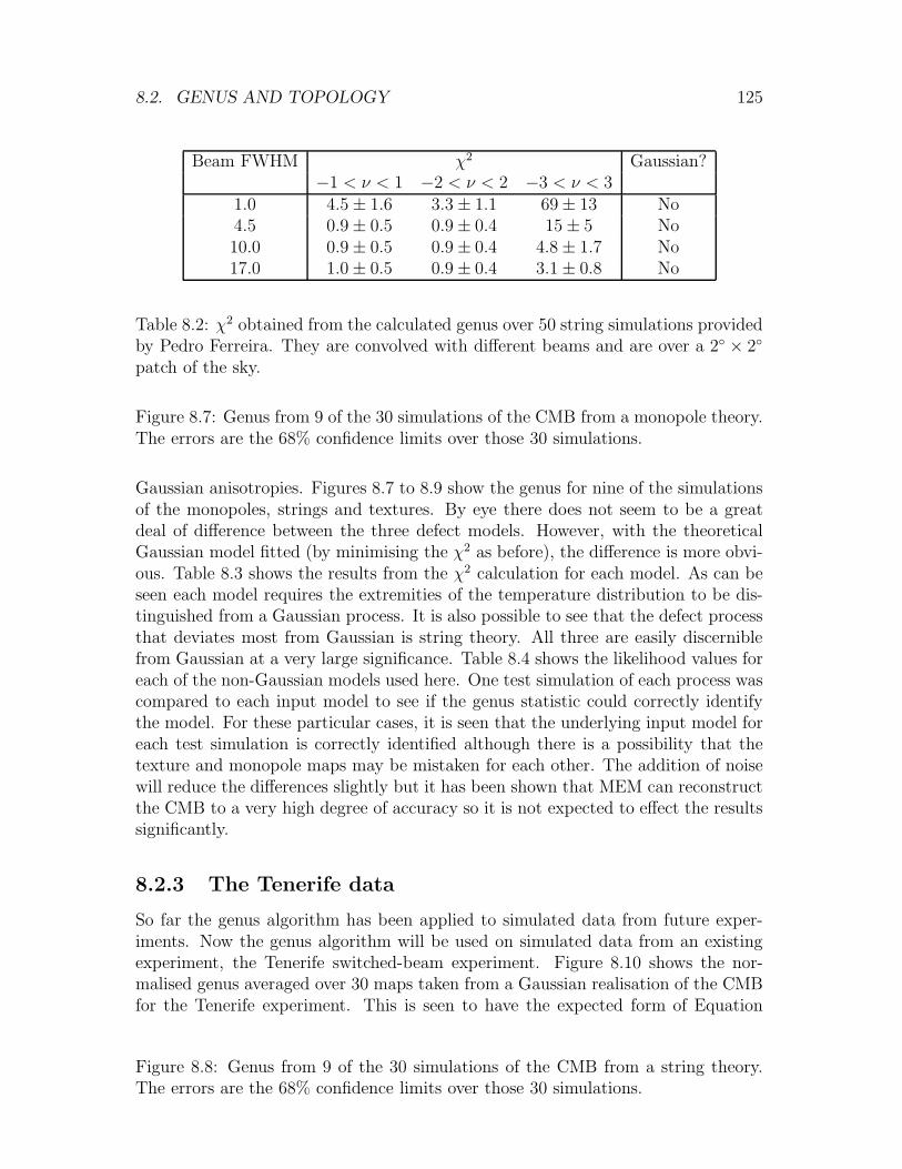
8.2. GENUS AND TOPOLOGY 125
Beam FWHM χ2 Gaussian?−1 < ν < 1 −2 < ν < 2 −3 < ν < 3
1.0 4.5 ± 1.6 3.3 ± 1.1 69 ± 13 No4.5 0.9 ± 0.5 0.9 ± 0.4 15 ± 5 No10.0 0.9 ± 0.5 0.9 ± 0.4 4.8 ± 1.7 No17.0 1.0 ± 0.5 0.9 ± 0.4 3.1 ± 0.8 No
Table 8.2: χ2 obtained from the calculated genus over 50 string simulations providedby Pedro Ferreira. They are convolved with different beams and are over a 2 × 2
patch of the sky.
Figure 8.7: Genus from 9 of the 30 simulations of the CMB from a monopole theory.The errors are the 68% confidence limits over those 30 simulations.
Gaussian anisotropies. Figures 8.7 to 8.9 show the genus for nine of the simulationsof the monopoles, strings and textures. By eye there does not seem to be a greatdeal of difference between the three defect models. However, with the theoreticalGaussian model fitted (by minimising the χ2 as before), the difference is more obvi-ous. Table 8.3 shows the results from the χ2 calculation for each model. As can beseen each model requires the extremities of the temperature distribution to be dis-tinguished from a Gaussian process. It is also possible to see that the defect processthat deviates most from Gaussian is string theory. All three are easily discerniblefrom Gaussian at a very large significance. Table 8.4 shows the likelihood values foreach of the non-Gaussian models used here. One test simulation of each process wascompared to each input model to see if the genus statistic could correctly identifythe model. For these particular cases, it is seen that the underlying input model foreach test simulation is correctly identified although there is a possibility that thetexture and monopole maps may be mistaken for each other. The addition of noisewill reduce the differences slightly but it has been shown that MEM can reconstructthe CMB to a very high degree of accuracy so it is not expected to effect the resultssignificantly.
8.2.3 The Tenerife data
So far the genus algorithm has been applied to simulated data from future exper-iments. Now the genus algorithm will be used on simulated data from an existingexperiment, the Tenerife switched-beam experiment. Figure 8.10 shows the nor-malised genus averaged over 30 maps taken from a Gaussian realisation of the CMBfor the Tenerife experiment. This is seen to have the expected form of Equation
Figure 8.8: Genus from 9 of the 30 simulations of the CMB from a string theory.The errors are the 68% confidence limits over those 30 simulations.

126 CHAPTER 8. ANALYSING THE SKY MAPS
Figure 8.9: Genus from 9 of the 30 simulations of the CMB from a texture theory.The errors are the 68% confidence limits over those 30 simulations.
Model χ2 Gaussian?−1 < ν < 1 −2 < ν < 2 −3 < ν < 3
Monopoles 1.0 ± 0.5 1.5 ± 0.6 274 ± 31 NoStrings 1.0 ± 0.5 0.9 ± 0.3 1558 ± 106 No
Textures 0.8 ± 0.4 1.1 ± 0.5 645 ± 85 No
Table 8.3: χ2 obtained from the calculated genus over 30 simulations provided byNeil Turok of the CMB expected from different defect models. They are convolvedwith a 4.5′ beam to simulate the best results possible from the Planck Surveyor.
Input model Monopole Strings TexturesTest modelMonopoles 0.16 2.3 × 10⁻¹¹ 0.11
Strings 2.0 × 10⁻¹⁵ 0.44 8.1 × 10⁻¹⁰
Textures 0.42 6.5 × 10⁻⁸ 0.63
Table 8.4: The likelihood results for the three different non-Gaussian simulations.A peak value of 1 is obtained if the test model has the exact genus of the inputmodel. The genus of the input model was found by averaging over 32 test modelsof each defect process. It is seen that the strings model is easily distinguished fromthe other two defect processes (see text).
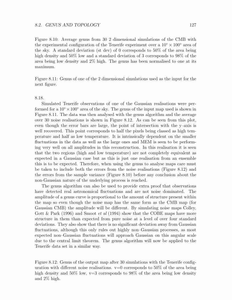
8.2. GENUS AND TOPOLOGY 127
Figure 8.10: Average genus from 30 2 dimensional simulations of the CMB withthe experimental configuration of the Tenerife experiment over a 10 × 100 area ofthe sky. A standard deviation (st dev) of 0 corresponds to 50% of the area beinghigh density and 50% low and a standard deviation of 3 corresponds to 98% of thearea being low density and 2% high. The genus has been normalised to one at itsmaximum.
Figure 8.11: Genus of one of the 2 dimensional simulations used as the input for thenext figure.
8.18.
Simulated Tenerife observations of one of the Gaussian realisations were per-formed for a 10×100 area of the sky. The genus of the input map used is shown inFigure 8.11. The data was then analysed with the genus algorithm and the averageover 30 noise realisations is shown in Figure 8.12. As can be seen from this plot,even though the error bars are large, the point of intersection with the y–axis iswell recovered. This point corresponds to half the pixels being classed as high tem-perature and half as low temperature. It is intrinsically dependent on the smallerfluctuations in the data as well as the large ones and MEM is seen to be perform-ing very well on all amplitudes in this reconstruction. In this realisation it is seenthat the two regions (high and low temperature) are not completely equivalent asexpected in a Gaussian case but as this is just one realisation from an ensemblethis is to be expected. Therefore, when using the genus to analyse maps care mustbe taken to include both the errors from the noise realisations (Figure 8.12) andthe errors from the sample variance (Figure 8.10) before any conclusion about thenon-Gaussian nature of the underlying process is reached.
The genus algorithm can also be used to provide extra proof that observationshave detected real astronomical fluctuations and are not noise dominated. Theamplitude of a genus curve is proportional to the amount of structure present withinthe map so even though the noise map has the same form as the CMB map (forGaussian CMB) the amplitude will be different. By simulating noise maps Colley,Gott & Park (1996) and Smoot et al (1994) show that the COBE maps have morestructure in them than expected from pure noise at a level of over four standarddeviations. They also show that there is no significant deviation away from Gaussianfluctuations, although this only rules out highly non–Gaussian processes, as mostexpected non–Gaussian fluctuations will approach Gaussian on this angular scaledue to the central limit theorem. The genus algorithm will now be applied to theTenerife data set in a similar way.
Figure 8.12: Genus of the output map after 30 simulations with the Tenerife config-uration with different noise realisations. v=0 corresponds to 50% of the area beinghigh density and 50% low, v=3 corresponds to 98% of the area being low densityand 2% high.
128 CHAPTER 8. ANALYSING THE SKY MAPS
Figure 8.13: Genus of the 15 GHz Tenerife MEM reconstructed map. The 68%confidence limits shown are calculated from the Monte-Carlo simulations (results inFigure 8.12).
The real data
As the 10 GHz data set is expected to be contaminated by Galactic emission only the15 GHz data set will be used here. The map shown in Figure 7.26 was used to test thepower of the genus algorithm. The region between RA 131 and 260 was analysedto test for Gaussianity. Figure 8.13 shows the result for this analysis. A preliminaryattempt at subtracting the effect of the two point sources in this region was madeprior to the genus analysis and it can be seen that the non-Gaussian behaviourexpected due to these sources does not show in this figure. The average χ2 for thedifference between the theoretical curve and the genus from the 15 GHz data is 0.38.It is seen that the MEM reconstruction of the Tenerife 15 GHz data is completelyconsistent with a Gaussian origin (less than one sigma deviation away from thetheoretical Gaussian curve). However, this does not mean that it is inconsistentwith a non-Gaussian origin. As in the COBE analysis only highly non-Gaussianprocesses can be ruled out as most expected non-Gaussian fluctuations will approachGaussian at the scales that Tenerife is sensitive to.
8.2.4 Extending genus: the Minkowski functionals
Recent advances (Schmalzing & Buchert 1997, Kerscher et al 1997, Mecke, Buchert& Wagner 1994, and references therein) in the analysis of Large Scale Structure datasets using integral geometry have led to an interest in this area of statistics in theCMB community (see Winitski & Kosowsky 1998 and Schmalzing & Gorski 1998).Large Scale Structure and CMB data sets both need the following requirements fora functional that can describe them: the functional must be independent of theorientation or position in space (motion invariance), must be additive (so that thefunctional of the combination of two data sets is the addition of the two separatefunctionals minus their intersection) and must have conditional continuity (the func-tional of a pixellised data set must approach the true functional of the underlyingprocess as the pixels are made smaller). These three requirements taken togetherwere shown by Hadwiger (1957) to lead to only d+ 1 functionals in a d-dimensionalspace that would completely describe the data set. These are the Minkowski func-tionals. For a CMB data set (in 2-dimensional space) there are three Minkowskifunctionals; surface area, boundary length and the Euler characteristic (or genus).
As has already been shown, the genus of the CMB maps holds a great deal ofinformation and so it is expected that the inclusion of the two other Minkowskifunctionals will allow further discrimination between theories. Tests on the three-dimensional Minkowksi functions applied to Large Scale Structure data sets (Jones,Hawthorn & Kaiser 1998) have shown that the addition of the other Minkowksifunctionals does indeed increase the power to discern between underlying theories.Other groups have already began to test the Minkowski functionals on CMB data

8.3. CORRELATION FUNCTIONS 129
sets (Schmalzing & Gorski 1998 apply them to the COBE data set). This is workin progress.
8.3 Correlation functions
Instead of looking at the morphology of the temperature distribution using Minkowskifunctionals (which include genus) it is possible to use statistical techniques to mea-sure the distribution in space of pixel fluxes. This is done using correlation functions.It has been shown that any correlation function can be expressed in terms of theMinkowksi functionals (for example, see Mecke, Buchert & Wagner 1994). However,the correlation functions do contain useful properties and so they will be discussedhere. I will summarise the two, three and four point correlation functions and applythe two and four point functions to various data sets.
8.3.1 Two point correlation function
The two point correlation function is a measure of the average product of tempera-ture fluctuations in two directions. For two pixels in a CMB map, i and j, separatedby an angle β, the two point correlation function is given by
V (β) =⟨(
∆Ti
T
)(
∆Tj
T
)⟩
(8.20)
and it is easily seen that when β = 0, so that i = j, V (0) is the variance of thedata. The variance is very easily calculated and is used as a check at each of thedata reduction stages. It is also fitted for in the likelihood function.
On the raw data the two point correlation function can be used as a test of theorigin of the emission detected in a CMB experiment. By applying the weightedtwo point correlation function to the Tenerife data it is possible to test whether thedata is consistent with noise or whether there is some underlying signal present.The weighted two point correlation function is given by
C(θ) =
∑
i,j ∆Ti∆Tjwiwj∑
i,j wiwj
(8.21)
where wi and ∆Ti are the weight (1/σ2i ) and double-differenced temperature of the
Tenerife data set. In this form the two point correlation function is also known asthe auto-correlation function.
Figure 8.14 presents the auto-correlation of the 15 GHz Tenerife data in the re-gion at RA=161−250. The error-bars were determined by Monte-Carlo techniques.The errors on each data point were estimated by assuming a random Gaussian pro-cess with the appropriate rms given by the Tenerife data set (i.e. the noise). Thedata point was then displaced by this amount and a new data set was constructed forwhich the auto-correlation function was found. This was done over 1000 noise reali-sations and the errors show the 68% confidence limits over these realisations. These

130 CHAPTER 8. ANALYSING THE SKY MAPS
Figure 8.14: The auto–correlation of the 15 GHz data in the region at RA=161 −250. The solid line is the best fit to the data, the short dashed line shows theexpected region of correlation for a Harrison-Zel’dovich spectrum CMB model andthe long dashed line shows the expected region of correlation for the case of purenoise. The errors are calculated using a Monte-Carlo technique. This figure wasproduced by Carlos Gutierrez.
techniques were also used to obtain the confidence bands in the case of pure uncor-related noise (long-dashed lines) and the expected correlation (short-dashed line)in the case of a Harrison-Zel’dovich spectrum for the primordial fluctuations withan amplitude corresponding to the signal of maximum likelihood (see Chapter 4).Clearly this model gives an adequate description of the observed correlation whilstthe results are incompatible with pure uncorrelated noise. The cross-correlationbetween the data at 10 GHz and 15 GHz is inconclusive as it is dominated by thenoisy character of the 10 GHz data.
A variation to the two point correlation function that is commonly used (see, forexample, Kogut et al 1995 and Kogut et al 1996) is the extrema correlation function.Instead of applying the two point correlation function to the full data set, the peaks(and troughs) of the data set are found. A peak is defined as any pixel ‘hotter’ thanthe neighbouring pixels and a trough is any pixel ‘colder’ than the neighbouringpixels. The correlation function between these peaks and troughs is then found. Itcan be separated into three different analyses; a) peak-peak auto-correlation (andtrough-trough auto-correlation), b) peak-trough cross-correlation and c) extremacross-correlation (the correlation between all extrema regardless of whether they area peak or trough). Kogut et al (1995) use the extrema two point correlation functionto analyse the COBE 53 GHz map and use the likelihood function to predict whetherthe peaks are from a Gaussian or non-Gaussian source. They find that the COBEresult is most likely to have originated from a Gaussian distribution of fluctuationsalthough the significance of their analysis is very difficult to compute.
The theoretical predictions for the two point and three point correlation functionscan be found in Bond & Efstathiou (1987) and Falk, Rangarajan & Srednicki (1993)show the predictions for the full two point correlation function and the collapsedthree point correlation function (see below) for inflationary cosmologies. The mainproblem with any of the correlation function analysis techniques is that they donot take into account any noise or foregrounds present. Therefore, it is necessaryto perform the analysis on the MEM processed map or simulations of the noiseand foregrounds must be performed to evaluate their effect. Kogut et al (1995) useMonte Carlo simulations of the noise added onto different models for the CMB (theydo not include foregrounds) to evaluate the significance of their result.
8.3.2 Three point correlation function
The three point correlation function is similar to the two point correlation functionexcept that it takes the product between three pixels. The angular separation be-
8.3. CORRELATION FUNCTIONS 131
tween pixels is now α (between i and j), β (between i and k) and γ (between j andk) which gives
S(α, β, γ) =⟨(
∆Ti
T
)(
∆Tj
T
)(
∆Tk
T
)⟩
(8.22)
and when α = β = γ = 0, so that i = j = k, S is defined as the skewness of thedata. The skewness of the data is slightly more sensitive to non-Gaussian featuresthan the two point correlation function.
The collapsed three point correlation function (β = α and γ = 0) was used byGangui & Mollerach (1996) to analyse the COBE results. They found that defectscould not be ruled out using the COBE data but a higher resolution experimentcould distinguish between Gaussian fluctuations and those arising from textures.Falk et al (1993) also show that the collapsed three point correlation function isnot sensitive enough to be detected by COBE for generic models (those withoutspecially chosen parameters to make the three point correlation function artificiallylarge).
8.3.3 Four point correlation function
The four point correlation function is very rarely used in full. Instead it is used inthe collapsed form when the separation between pixels is zero. This is defined asthe kurtosis (see, for example, Gaztanaga, Fosalba & Elizalde 1997) and is equal to
K =
⟨
(
∆TT
)4⟩
− 3⟨
(
∆TT
)2⟩2
⟨
(
∆TT
)2⟩2 (8.23)
The kurtosis is a good discriminatory test between Gaussian and non-Gaussianfeatures but it can only be applied effectively in data with little or no noise andminimal foregrounds. For the Gaussian case the kurtosis should tend to zero.
Gaztanaga et al (1997) use the kurtosis to analyse data from the MAX, MSAM,Saskatoon, ARGO and Python CMB experiments (all are sensitive to angular scalesaround the first Doppler peak). They find that there is a very large kurtosis foreach of the experiments and a Gaussian origin of the fluctuations is ruled out at theone sigma level. However, the analysis does not allow for any systematic errors orforeground effects and these could alter the results greatly.
Application to simulated data
The kurtosis was applied to the Planck simulation maps. Table 8.5 shows the kur-tosis values for the analysis. The kurtosis of the reconstructions is compared to thatof the input maps convolved with the highest resolution of the experiment. As canbe seen the kurtosis of the SZ effect is very high as expected for a strongly non-Gaussian feature. After the simulated observations and analysis was performed itcan be seen that the MEM result reconstructs the kurtosis very well. This implies
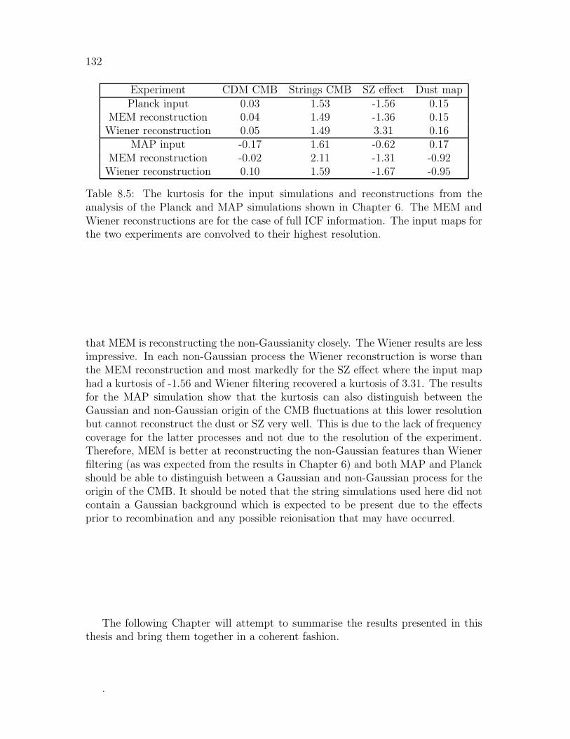
132
Experiment CDM CMB Strings CMB SZ effect Dust mapPlanck input 0.03 1.53 -1.56 0.15
MEM reconstruction 0.04 1.49 -1.36 0.15Wiener reconstruction 0.05 1.49 3.31 0.16
MAP input -0.17 1.61 -0.62 0.17MEM reconstruction -0.02 2.11 -1.31 -0.92Wiener reconstruction 0.10 1.59 -1.67 -0.95
Table 8.5: The kurtosis for the input simulations and reconstructions from theanalysis of the Planck and MAP simulations shown in Chapter 6. The MEM andWiener reconstructions are for the case of full ICF information. The input maps forthe two experiments are convolved to their highest resolution.
that MEM is reconstructing the non-Gaussianity closely. The Wiener results are lessimpressive. In each non-Gaussian process the Wiener reconstruction is worse thanthe MEM reconstruction and most markedly for the SZ effect where the input maphad a kurtosis of -1.56 and Wiener filtering recovered a kurtosis of 3.31. The resultsfor the MAP simulation show that the kurtosis can also distinguish between theGaussian and non-Gaussian origin of the CMB fluctuations at this lower resolutionbut cannot reconstruct the dust or SZ very well. This is due to the lack of frequencycoverage for the latter processes and not due to the resolution of the experiment.Therefore, MEM is better at reconstructing the non-Gaussian features than Wienerfiltering (as was expected from the results in Chapter 6) and both MAP and Planckshould be able to distinguish between a Gaussian and non-Gaussian process for theorigin of the CMB. It should be noted that the string simulations used here did notcontain a Gaussian background which is expected to be present due to the effectsprior to recombination and any possible reionisation that may have occurred.
The following Chapter will attempt to summarise the results presented in thisthesis and bring them together in a coherent fashion.
.
133
In the beginning there was only darkness, dust and water. The darkness wasthicker in some places than in others. In one place it was so thick that it mademan. The man walked through the darkness. After a while, he began to think.
Creation myth from the Pima tribe in Arizona

134
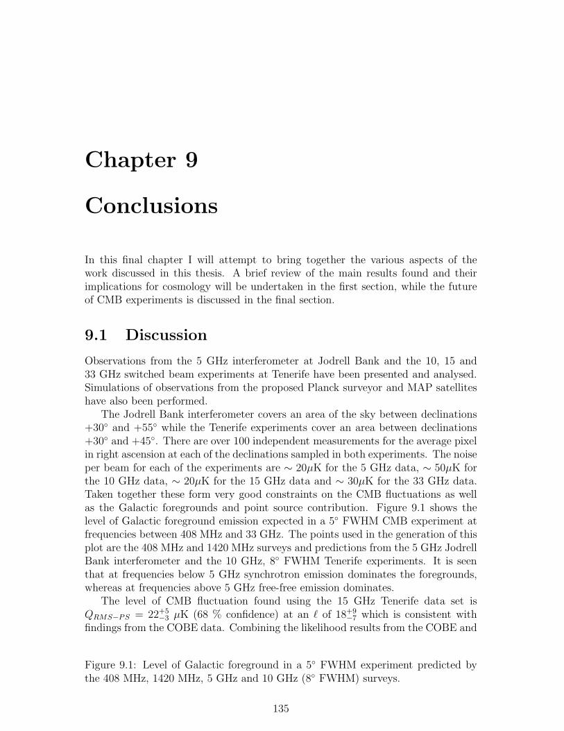
Chapter 9
Conclusions
In this final chapter I will attempt to bring together the various aspects of thework discussed in this thesis. A brief review of the main results found and theirimplications for cosmology will be undertaken in the first section, while the futureof CMB experiments is discussed in the final section.
9.1 Discussion
Observations from the 5 GHz interferometer at Jodrell Bank and the 10, 15 and33 GHz switched beam experiments at Tenerife have been presented and analysed.Simulations of observations from the proposed Planck surveyor and MAP satelliteshave also been performed.
The Jodrell Bank interferometer covers an area of the sky between declinations+30 and +55 while the Tenerife experiments cover an area between declinations+30 and +45. There are over 100 independent measurements for the average pixelin right ascension at each of the declinations sampled in both experiments. The noiseper beam for each of the experiments are ∼ 20µK for the 5 GHz data, ∼ 50µK forthe 10 GHz data, ∼ 20µK for the 15 GHz data and ∼ 30µK for the 33 GHz data.Taken together these form very good constraints on the CMB fluctuations as wellas the Galactic foregrounds and point source contribution. Figure 9.1 shows thelevel of Galactic foreground emission expected in a 5 FWHM CMB experiment atfrequencies between 408 MHz and 33 GHz. The points used in the generation of thisplot are the 408 MHz and 1420 MHz surveys and predictions from the 5 GHz JodrellBank interferometer and the 10 GHz, 8 FWHM Tenerife experiments. It is seenthat at frequencies below 5 GHz synchrotron emission dominates the foregrounds,whereas at frequencies above 5 GHz free-free emission dominates.
The level of CMB fluctuation found using the 15 GHz Tenerife data set isQRMS−PS = 22+5
−3 µK (68 % confidence) at an ℓ of 18+9−7 which is consistent with
findings from the COBE data. Combining the likelihood results from the COBE and
Figure 9.1: Level of Galactic foreground in a 5 FWHM experiment predicted bythe 408 MHz, 1420 MHz, 5 GHz and 10 GHz (8 FWHM) surveys.
135
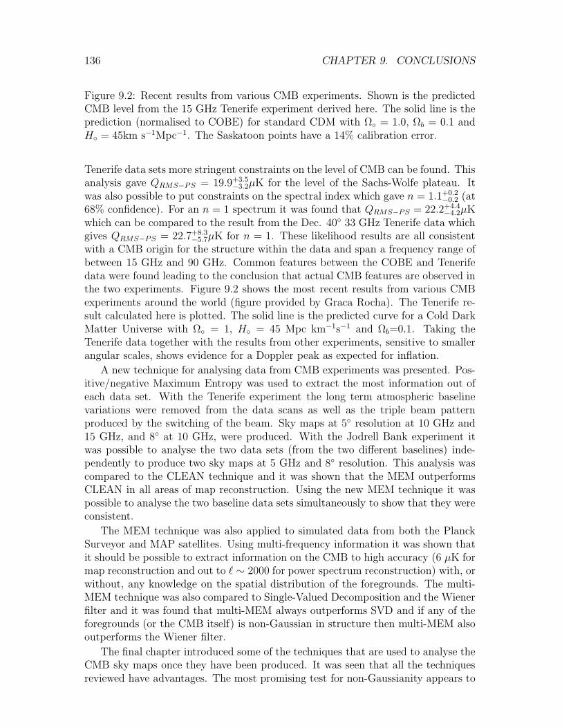
136 CHAPTER 9. CONCLUSIONS
Figure 9.2: Recent results from various CMB experiments. Shown is the predictedCMB level from the 15 GHz Tenerife experiment derived here. The solid line is theprediction (normalised to COBE) for standard CDM with Ω = 1.0, Ωb = 0.1 andH = 45km s−1Mpc−1. The Saskatoon points have a 14% calibration error.
Tenerife data sets more stringent constraints on the level of CMB can be found. Thisanalysis gave QRMS−PS = 19.9+3.5
−3.2µK for the level of the Sachs-Wolfe plateau. Itwas also possible to put constraints on the spectral index which gave n = 1.1+0.2
−0.2 (at68% confidence). For an n = 1 spectrum it was found that QRMS−PS = 22.2+4.4
−4.2µKwhich can be compared to the result from the Dec. 40 33 GHz Tenerife data whichgives QRMS−PS = 22.7+8.3
−5.7µK for n = 1. These likelihood results are all consistentwith a CMB origin for the structure within the data and span a frequency range ofbetween 15 GHz and 90 GHz. Common features between the COBE and Tenerifedata were found leading to the conclusion that actual CMB features are observed inthe two experiments. Figure 9.2 shows the most recent results from various CMBexperiments around the world (figure provided by Graca Rocha). The Tenerife re-sult calculated here is plotted. The solid line is the predicted curve for a Cold DarkMatter Universe with Ω = 1, H = 45 Mpc km−1s−1 and Ωb=0.1. Taking theTenerife data together with the results from other experiments, sensitive to smallerangular scales, shows evidence for a Doppler peak as expected for inflation.
A new technique for analysing data from CMB experiments was presented. Pos-itive/negative Maximum Entropy was used to extract the most information out ofeach data set. With the Tenerife experiment the long term atmospheric baselinevariations were removed from the data scans as well as the triple beam patternproduced by the switching of the beam. Sky maps at 5 resolution at 10 GHz and15 GHz, and 8 at 10 GHz, were produced. With the Jodrell Bank experiment itwas possible to analyse the two data sets (from the two different baselines) inde-pendently to produce two sky maps at 5 GHz and 8 resolution. This analysis wascompared to the CLEAN technique and it was shown that the MEM outperformsCLEAN in all areas of map reconstruction. Using the new MEM technique it waspossible to analyse the two baseline data sets simultaneously to show that they wereconsistent.
The MEM technique was also applied to simulated data from both the PlanckSurveyor and MAP satellites. Using multi-frequency information it was shown thatit should be possible to extract information on the CMB to high accuracy (6 µK formap reconstruction and out to ℓ ∼ 2000 for power spectrum reconstruction) with, orwithout, any knowledge on the spatial distribution of the foregrounds. The multi-MEM technique was also compared to Single-Valued Decomposition and the Wienerfilter and it was found that multi-MEM always outperforms SVD and if any of theforegrounds (or the CMB itself) is non-Gaussian in structure then multi-MEM alsooutperforms the Wiener filter.
The final chapter introduced some of the techniques that are used to analyse theCMB sky maps once they have been produced. It was seen that all the techniquesreviewed have advantages. The most promising test for non-Gaussianity appears to

9.2. THE FUTURE OF CMB EXPERIMENTS 137
be Minkowski functionals as these incorporate all of the other techniques togetherin just three functionals (for a two dimensional map). Using the auto-correlationfunction it was shown that there is an excess signal present in the 15 GHz Tenerifesky map that is not due to noise alone. The Genus analysis of this map showed thatit was consistent with a Gaussian process.
9.2 The future of CMB experiments
Within the next ten years a new generation of CMB experiments will be in opera-tion. These include both space based (like the Planck Surveyor and MAP), balloonbased (like TopHat and Boomerang) as well as ground based (like the Very SmallArray which is based on a similar design to the CAT interferometer). It has beenshown here that the Planck surveyor will produce very accurate maps of the CMBfluctuations. It will also allow very tight constraints on the level of Galactic fore-ground emissions which can be subtracted from other experiments. The recent ESAreport on the Planck Surveyor show that the sensitivity of the satellite has improvedsince the simulations presented here were performed and so the accuracy will be evenhigher.
Ground–based measurements have already proven to provide tight constraints onthe level of the CMB anisotropies and so the VSA (a 15 element interferometer thatwill measure the CMB anisotropy at high angular resolution) should also performvery well. In conjunction with existing ground based telescopes constraints on theCMB anisotropies will increase considerably prior to the launch of either satellite.The Tenerife experiment will continue to take measurements at all three frequencieswith the aim of having a final two dimensional map with very low noise and theJodrell Bank interferometer is currently taking data for a new baseline. With sucha wealth of data at many frequencies (5 - 900 GHz) conventional analysis techniqueswill have to be refined. The maximum entropy algorithm described here can copewith multiple frequencies, varying pixel size, multiple component fitting and a veryhigh level of noise. This ‘multi-MEM’ is now in the process of being applied to theTenerife and Jodrell Bank data described in this thesis. The data from the twoexperiments are also being combined with data from COBE and lower frequencysurveys (the 408 MHz, 1420 MHz and 2300 MHz surveys) using the multi-MEMin an analogous way to the Planck Surveyor analysis presented here, to put betterconstraints on the CMB at the large angular scales covered by Tenerife and COBE(ℓ < 30).
Another area of CMB research which is becoming increasingly of interest is thecomparison with large scale structure. All theories that explain the shape of thepower spectrum of CMB anisotropies also make predictions for the evolution ofthese anisotropies into the present large scale structure. By attempting to matchthe two power spectra on the different scales more constraints can be put on theexact form of the underlying matter. This is now being done by various groupsalthough research into this area is still in its very early stages.
With new high quality data and the ability to extract the CMB signal from the
138
foreground contamination, very tight constraints on the cosmological parametersshould be achievable.
.
Eureka?
C. Lineweaver on the COBE discovery
References
A
Adler, R.J. 1981, ‘The geometry of random fields’, Chichester:Wiley
Aghanim, N., De Luca, A., Bouchet, F.R., Gispert, R. & Puget, J.L. 1997, preprintin astro-ph/9705092
Albrecht, A., Coulson, D., Ferreira, P. & Magueijo, J. 1996, Phys. Rev. Lett., 76,1413
Alcock, C. et al 1993, Nature, 365, 621
B
Bardeen, J.M., Bond, J.R., Kaiser, N. & Szalay, A.S. 1986, ApJ, 304, 15
Bennett, C.L. et al. 1992a, ApJ, 396, L7
Bennett, C.L. et al. 1992b, ApJ, 391, 466
Bennett, C.L. et al. 1996, ApJ, 464, L1
Bersanelli, M. et al. 1996, COBRAS/SAMBA report on the phase A study, ESAdocument D/SCI(96)3
Bond, J.R. & Efstathiou, G. 1987, MNRAS, 226, 655
Bouchet, F.R., Gispert, R., Boulanger, F. & Puget, J.L. 1997, in Proc. XVI MoriondAstrophysics Meeting, ed. Bouchet, Gispert, Guiderdoni & Tran Thanh Van
Boulanger, F., Abergel, A., Bernard, J.P., Burton, W.B., Desert, F.X., Hartmann,D., Lagache, G. & Puget, J.L. 1996, Astr. Astrophys., 312, 256
Branenberger, R.H. 1989, in Peacock et al 1989, p. 281
Bressaard, P.J. & van de Hulst, H.C. 1962, Rev. Mod. Phys., 34, 507
Bunn, E.F., Hoffman, Y., & Silk, J. 1996, ApJ, 464, 1
139
140 REFERENCES
C
Carr, B.J. 1990 Comments in Astrophysics, 14, 257
Church, S.E. 1995, MNRAS, 272, 551
Coles, P. & Barrow, J.D. 1987, MNRAS, 228, 407
Colley, W.N., Gott, J.R. & Park, C. 1996, MNRAS, 281, L82
Condon, J.J., & Broderick, J.J. & Seielstad, G.A. 1989, AJ, 97, 1064
Copi, C.J., Olive, K.A. & Schramm, D.N. 1995, Science, 267, 192
Coulson, D., Ferreira, P., Graham, P. & Turok, N. 1994, Nature, 368, 27
D
Davies, R.D. Lasenby, A.N., Watson, R.A., Daintree, E.J., Hopkins, J., Beckman,J., Sanchez-Almeida, J. & Rebolo, R. 1987, Nature, 326, 462
Davies, R.D., Watson, R.A., Daintree, E.J., Hopkins, J., Lasenby, A.N., Sanchez-Almeida, J., Beckman, J.E. & Rebolo, R. 1992, MNRAS, 258, 605
Davies, R.D. et al. 1996a, MNRAS, 278, 883
Davies, R.D., Watson, R.A., & Gutierrez, C.M. 1996b, MNRAS, 278, 925
Doroshkevich, A.G. 1970, Astrophysics, 6, 320
E
Efstathiou, G. 1989, in Peacock et al. 1989
F
Falk, T., Rangarajan, R. & Srednicki, M. 1993, ApJ, 403, L1
Franceschini, A., Toffolatti, L., Danese, L., & De Zotti, G. 1989, ApJ, 344, 35
G
Gangui, A. & Mollerash, S. 1996, Phys. Rev. D., 54, 4750
REFERENCES 141
Gaztanaga, E., Fosalba, P. & Elizalde, E. 1997, preprint astro-ph/9705116
Gautier, T.N., Boulanger, F., Perault, J.L. 1992, AJ, 103, 1313
Giardino, G. 1995, MSc thesis, University of Manchester
Gispert, R. & Bouchet, F.R. 1997, in Proc. XVI Moriond Astrophysics Meeting, ed.Bouchet, Gispert, Guiderdoni & Tran Thanh Van
Gott III, J.R., Melott, A.L., & Dickinson, M. 1986, ApJ, 306, 341
Gott III, J.R., Park, C., Juszkiewicz, R., Bies, W.E., Bennett, D.P., Bouchet, F.R.& Stebbins, A. 1990, ApJ, 352, 1
Gorenstein, M.V. & Smoot, G.F. 1981, ApJ, 244, 361
Grainge, K., Jones, M.E., Pooley, G.G., Saunders, R.D.E. & Edge, A. 1993, MN-RAS, 256, 57
Gull, S.F. 1989 Maximum Entropy and Bayesian Methods, 53, ed. J. Skilling
Gull, S.F., Skilling, J. 1984, IEEE proc, 131(F), 646
Gull, S.F. & Skilling, J. 1990, The MEMSYS5 User’s Manual, Maximum EntropyData Consultants Ltd., Royston
Gutierrez de la Cruz, C. M., Davies, R. D., Rebolo, R., Watson, R. A., Hancock,S., & Lasenby, A. N. 1995, ApJ, 442, 10
Gutierrez, C.M., Hancock, S., Davies, R.D., Rebolo, R., Watson, R.A., Hoyland,R.J., Lasenby, A.N., & Jones, A.W. 1997, ApJ, 480, L83
Gutierrez, C.M. 1997, ApJ, 483, 51
Guth, A.H. 1981, Phys. Rev. D., 23, 347
H
Hadwiger, H. 1957, Vorlesungen uber Inhalt, Oberflache und Isoperimetrie (SpringerVerlag, Berlin).
Hamilton, A.J.S., Gott III, J.R. & Wienberg, D. ApJ, 1986, 309, 1
Hancock, S. 1994 ’Detections of structure in the CMB’, PhD thesis, MRAO, Cam-bridge
Hancock, S. et al. 1994, Nature, 367, 333
Hancock, S., Lasenby, A.N., Gutierrez de la Cruz, C.M., Davies, R.D., Watson,R.A.,& Rebolo, R. 1995, APLCOM, 32, 201

142 REFERENCES
Hancock, S., Rocha, G., Lasenby, A.N. & Gutierrez, C.M. 1996, MNRAS, submitted
Hancock, S., Gutierrez, C.M., Davies, R.D., Lasenby, A.N., Rocha, G., Rebolo, R.,Watson, R.A. & Tegmark, M. 1997, MNRAS, 289, 505
Harrison, E.R. 1970, Phys. Rev. D., 1, 2726
Haslam, C.G.T., Salter, C.J., Stoffel, H., & Wilson, W.E. 1982, A&AS, 47, 1
Hobson, M.P., Jones, A.W., Lasenby, A.N. & Bouchet, F. 1998a, MNRAS, in press
Hobson, M.P., Barreiro, R., Toffalati, L., Lasenby, A.N., Sanz, J.L., Jones, A.W. &Bouchet, F.R. 1998b, MNRAS, submitted
Hobson, M.P. & Lasenby, A.N. 1998, MNRAS, submitted
J
Jones, A.W., Bland-Hawthorn, J., & Kaiser, N. 1994, BAAS, 26, 1407
Jones, A.W., Hawthorn, J., & Kaiser, N. 1998, in prep.
Jones, A.W., Hobson, M.P., Lasenby, A.N. & Bouchet, F.R. 1998, MNRAS, submit-ted
Jones, A.W., Hancock, S., Lasenby, A.N., Davies, R.D., Gutierrez, C.M., Rocha,G., Watson, R.A., & Rebolo, R. 1998, MNRAS, 294, 582
Jones, B.J.T. & Wyse, R.F.G. 1985, Astron. Astroph., 149, 144
K
Kaiser, N. & Stebbins, A. 1984, Nature, 310, 391
Kerscher, M. et al 1997, MNRAS, 284, 73
King, I.R. 1966, Astr. J., 71, 64
Kogut, A., Banday, A.J., Bennett, C.L., Gorski, K.M., Hinshaw, G. & Reach, W.T.1996a, ApJ, 460, 1
Kogut, A., Banday, A.J., Bennett, C.L., Gorski, K.M., Hinshaw, G., Smoot, G.F.& Wright, E.L. 1996b, ApJ, 464, L29
Kogut, A., Banday, A.J., Bennett, C.L., Hinshaw, G., Lubin, P.M. & Smoot, G.F.1995, ApJ, 439, L29
Kraus, J.D. 1982, ‘Radio Astronomy’, ed. Mc Graw–Hill.
REFERENCES 143
Kuhr, H., Witzel, A., Pauliny-Toth, I.I.K., & Nauber, U. 1981, A&AS, 45, 367
L
de Lapparent, V., Geller, M.J. & Huchra, J.P. 1986, ApJ, 304, L585
Lasenby, A.N. 1992, in ‘Clusters and superclusters of galaxies’, ed. Fabian, A.C.,Kluwer Academic Press
Laue, E., Skilling, J., & Staunton, J. 1985, J. Mag. Res, 63, 418
Lawson, K.D., Mayer, C.J., Osborne, J.L. & Parkinson, M.L. 1987, MNRAS, 225,307
Linde, A.D. 1982, Phys. Lett., 108B, 389
Lineweaver, C.H. et al. 1995, ApJ, 448, 482
M
Magueijo, J., Albrecht, A., Coulson, D. & Ferreira, P. 1996, Phys. Rev. Lett., 76,2617
Maisinger, K., Hobson, M.P. & Lasenby, A.N. 1997, MNRAS, 290, 313
Mather, J.C. et al. 1994, ApJ, 420, 439
McKee, C.F. & Ostriker, J.P. 1977, ApJ, 218, 148
Mecke, K.R., Buchert, T. & Wagner, H. 1994, Astron. Astroph., 288, 697
Melhuish, S., Davies, R.D., Davis, R.J., Morgan, A., Daintree, E.J., Hernandez-Gonzales, P.J., Giardino, G. & Hopkins, J. 1997, MNRAS, 286, 48
Melott, A.L., Cohen, A.P., Hamilton, A.J.S., Gott III, J.R. & Weinberg, D.H. 1989,ApJ, 345, 618
N
Narayan, R. & Nityananda, R. 1986, Ann. Rev. Astron. Astrophys., 24, 127
O
de Oliveira-Costa, A., Kogut, A., Devlin, M.J., Netterfield, C.B., Page, L.A. &Wollack, E.J. 1997 ApJ, 482, L17
144 REFERENCES
O’Sullivan et al 1995, MNRAS, 274, 861
P
Padmanabhan, T. 1993, ‘Structure formation in the early universe’, Cambridge Uni-versity Press
Partridge, R.B. 1995, ‘3K: The Cosmic Microwave Background Radiation’, Cam-bridge Astrophysics Series; 25, Cambridge University Press
Peacock, J.A., Heavens, A.F. & Davies, A.T. 1989, ‘Physics of the early universe’,Proc. 36th Scottish Uni. Summer School, Adam Hilger, New York
Penzias, A., & Wilson, R. 1965, ApJ, 142, L419
Platania, P., Bensadoun, M., Bersanelli, M., De Amici, G., Kogut, A., Levin, S.,Maino, D., & Smoot, G. 1997, astro-ph/9707252
Press, W.H. & Schechter, P. 1974, ApJ, 187, 425
Press, W.H., Teukolsky, S.A, Vetterling, W.T. & Flannery, B.P. 1992 ‘NumericalRecipes’, Cambridge University Press
R
Reich, P., & Reich, W. 1988, A&AS, 74, 7
Rephaeli, Y. & Lahav, O. 1991, ApJ, 372, 21
Rubin, V.C., Ford, W.K. Jr. & Thonnard, N. 1978, ApJ, 225, L107
Rybicki, G.B., Lightman, A.P. ‘Radiative Processes in Astrophysics’, ed. John Wiley& Sons.
Rybicki, G.B. & Press W.H. 1992, ApJ, 398, 169
S
Sachs, R.K. & Wolfe, A.M. 1967, ApJ, 147, 73
Saunders, R. 1997, in Proc. XVI Moriond Astrophysics Meeting, ed. Bouchet, Gis-pert, Guiderdoni & Tran Thanh Van
Scaramella, R. & Vittorio, N. 1988, ApJ, 331, L53
Schectman et al 1992, ‘Clusters and Superclusters of Galaxies’, ed. Fabian
REFERENCES 145
Schmalzing, J. & Buchert, T. 1997, ApJ, 482, L1
Schmalzing, J. & Gorski, K.M. 1998, MNRAS submitted, astro-ph/9710185
Silk, J. 1968, ApJ, 151, 459
Skilling, J. 1988, Maximum Entropy and Bayesian Methods in Science and Engi-neering, Volume 1, 173, ed. Erickson, G.J. & Smith, C.R.
Skilling, J. 1989, Maximum Entropy and Bayesian Methods, 45, ed. J. Skilling
Smail, I., Ivison, R.J. & Blain, A.W. 1997, ApJ, 490, L5
Smoot, G.F. et al. 1992, ApJ, 396, L1
Smoot, G.F., Tenorio, L., Banday, A.J., Kogut, A., Wright, E.L., Hinshaw, G. &Bennett, C.L. 1994, ApJ, 437, 1
Smoot, G.F. 1993, ‘Wrinkles in Time’, Little, Brown & Company Ltd.
Sugiyama, N. 1995, ApJ Supp., 100, 281
T
Tegmark, M. 1995, in Proc. Enrico Fermi, Course CXXXII, Varenna
Tegmark, M., & Bunn, E.F. 1995, ApJ, 455, 1
Tegmark, M., & Efstathiou, G. 1996, MNRAS, 281, 1297
Tegmark, M. 1996, ApJ, 470, L81
Tegmark, M. 1997, Phys. Rev. D., 55, 5895
Turner, M.S. 1991, Physica Scripta, T36, 167
Turok, N. 1991, Physica Scripta, T36, 135
W
Watson, R.A., DeLaCruz, C.M.G., Davies, R.D., Lasenby, A.N., Rebolo, R., Beck-man, J.E. & Hancock S. 1992, Nature, 357, 660
White, M., & Bunn, E. 1995, ApJ, 443, L53
White, S.D.M. 1989, in Peacock et al. 1989
Winitzki, S. & Kosowsky, A. 1998, ApJ, submitted, astro-ph/9710164
146 REFERENCES
Wright, E.L., Hinshaw, G. & Bennett, C.L. 1996, ApJ, 458, L53
Z
Zaroubi, S., Hoffman, Y., Fisher, K.B. & Lahav, O. 1995, ApJ, 449, 446
Zel’dovich, Y. B. 1972, MNRAS, 160, 1P
De Zotti, G., Toffalatti, L., Argueso Gomez, F., Franceschini, A., Mazzei, P., Danese,L. & Burigana, C. 1997, in Proc. XVI Moriond Astrophysics Meeting, ed.Bouchet, Gispert, Guiderdoni & Tran Thanh Van
Related Documents