Tools for Cosmic Microwave Background Polarimetry

In Search of Inflation: Tools for

Cosmic Microwave Background

Polarimetry

Kevin Thomas Crowley

A Dissertation

Presented to the Faculty

of Princeton University

in Candidacy for the Degree

of Doctor of Philosophy

Recommended for Acceptance

by the Department of

Department of Physics

Adviser: Professor Suzanne T. Staggs

September 2018

c© Copyright by Kevin Thomas Crowley, 2018.

All rights reserved.

Abstract

The pursuit of knowledge of the early universe via the properties of the cosmic mi-

crowave background (CMB) has reached an inflection point. Nearly all information

about scalar perturbations in the primordial electron-photon plasma has now been

gleaned from the pattern of intensity anisotropies visible as part-per-million varia-

tions in the CMB. The measurement of large-scale polarization patterns at a part

in 100 million is the most promising path by which we may observe further in the

past of the early universe. In addition to confirming the ΛCDM concordance model

shaped by the CMB, polarization anisotropy studies pursue evidence of primordial

tensor perturbations, which themselves could elucidate a period of inflation in the

early universe. These tensor perturbations are imprinted on the CMB polarization

as divergence-free patterns, known as B-modes. In order to make these demanding

polarization measurements, increased instrumental sensitivity and control of system-

atics is required. As part of the Advanced ACTPol (AdvACT) project, we have

integrated and characterized high-density detector arrays of thousands of bolometers,

the state-of-the-art detection technique for mm-wave radiation, and deployed them on

the Atacama Cosmology Telescope (ACT). In addition, the Atacama B-mode Search

(ABS) instrument featured a polarization modulator system to control systematics

and gain access to large-scale anisotropy modes otherwise masked by changing signals

in the atmosphere.

In this thesis, I begin by presenting the standard model of the universe with an eye

to the role of inflation and discuss the promise of polarization measurements. This

motivates a discussion of the technology in use throughout the field of CMB polariza-

tion studies and progresses into an introduction of arrays of multiplexed bolometers.

I discuss generic bolometer models involving superconducting thermistors, known as

transition-edge sensors (TESes). These models are compared to data from the Ad-

vACT TES bolometers, particularly their sensitivities and characteristic response to

iii

changing signals. I next describe the principle of polarization modulation using a

continuously-rotating half-wave plate (HWP), including the signal injected into the

detectors by this optical component. I discuss a pipeline developed to investigate

and remove this signal and the related demodulation analysis of the cleaned data for

CMB and point source mapping. Initial results from the 2017 run of silicon metama-

terial HWPs on ACT are shown. Finally, I describe the maximum-likelihood pipeline

developed as part of the ABS collaboration to constrain the parameter describing

the power in primordial tensor perturbations, the tensor-to-scalar ratio r. The final

published results for ABS are discussed. I conclude by considering the future devel-

opment of high-sensitivity focal planes and control of systematics, especially detector

non-linearity, in the Simons Observatory set of instruments, which are in the design

phase.

iv

Acknowledgements

Many people, through their hard work, care, and support, are responsible for my

producing this set of pages. Thanking them all is a tall task, but also the least I can

do.

I’ll begin with those cosmology students and scientists with whom I was so fortu-

nate to share lab time and tight spaces in Jadwin. Sara Simon helped bring me on

board to the ABS project and was always ready to help with any questions; indeed,

she still is today, and I am tremendously grateful to her. Patty Ho filled a similar

role on the ACT side, but circumstances also conspired to demand some careful wafer

vacuum lowering, wafer pinning, and fridge mounting from us. Her positive attitude

and fearless affect in the lab has been crucial in seeing the ACT team through tricky

times. Yaqiong Li gets a special shoutout for her dedication and fortitude, especially

in some of the all-day bonder sessions, when the only sound besides thousands of

hydraulic swooshes was our conversation about old movies and Chinese sci-fi. Steve

Choi has always led with a forthrightness and sincere desire to make things better

that I appreciate. Maria Salatino, who has moved on, is remembered fondly (U2

playing in the lab less so!); new students, Sarah Marie Bruno, Erin Healy, and others,

I am looking forward to tracking all your exciting progress from afar. The original

runners of the lab that I interacted with, Emily Grace, Christine Pappas, and others,

I appreciate all your help in bringing me up to speed and teaching me most of what

I know about cryostats, readout, and the rest.

Outside collaborators in ACT and ABS are so numerous that to elaborate them

all here would double my page count! I wish to highlight the respect and affection

I feel for Brian Koopman, Jason Stevens, Nick Cothard, Pato Gallardo, and all of

the Cornell MUX team led by Mike Niemack (who also been a stalwart and appre-

ciated supporter of my detector work). Shawn Henderson deserves his own sentence

for reminding me that anything even getting close to working is something to cele-

v

brate, and for answering all my unceasing questions about MCE business. The team

I’ve been so fortunate to visit at NIST and see elsewhere, Jay Austermann (who

introduced me to Velma and hit the town with me in Kurume), Brad Dober (the

king of the unexpected and lucky invite), Shannon Duff, Doug Bennett, Joe Fowler,

Randy Doriese, and others made those trips to Boulder something to look forward to.

Matthew Hasselfield deserves a whole paean to himself, for training up myself, and

simultaneously a ton of other people, to do anything useful with field data, and for

being one of the sharpest eyes in the room when my misshapen plots got aired out

at telecons. A big thanks to you, man; sorry about that In-N-Out pepper challenge.

To the administrators and staff I was fortunate enough to work with regularly

in Jadwin: Ted Lewis, Darryl Johnson, Todd Antonakos, Julio Lopez, Stephanie

Rumphrey, Sumit Saluja (all those disks!), and others, thank you for all your hard

work. To Steve Lowe in the student shop, and Bill Dix, Glenn Atkinson, and the

pro shop team: thanks for being unfailingly on-time and supportive. Bert Harrop,

the whole ACT team owes you a debt of gratitude for all your work on our array

integration. I always enjoy coming round to your office. Angela Lewis, hauling

sandwiches was a great privilege, as was working with you.

A whole other stream of experiences took place in South America. Lucas Parker

is responsible for breaking me in to work at 17,000 feet, and for being a swell guy

to share the mountain with. Mark Devlin, watching you drop lightning rods from

20 m up is about as memorable an experience as I’ve ever had. Thanks for all your

support and candor. To the engineers who slog it out for many months to make our

work possible, and had to ferry my automatic transmission-only butt up the road, a

personal and permanent thanks: Felipe Rojas Aracena, Federico Nati, Felipe Carrero,

Max Fankhanel. Y’all are spectacular.

There are a whole bunch of friends to thank: to physics folks who never had to

see me drop screws all over the lab: Farzan, Stevie, Will, and others. Thanks for

vi

making Jadwin in general a fun place to be. My original Pton roommate Jordan

is now essentially an extension of my brain; you’re a gem buddy, never forget it.

The basement gang, and most especially Sama, Mattias, and Jamal, the music flows

through you and buoys us all. I’ll storm PREX or hit a drum with you guys anytime.

Summer softball plays are some of my sweetest memories of genteel guys and gals like

Kenan, Zach, Anne, and mon capitain Tom, all of whom I’m pretty grateful I got to

hang with outside the hall of physics.

And now, the incalculably big thank yous: to Lyman Page, who never said any-

thing about me falling asleep during my first ACT telecons and has unfailingly sup-

ported my efforts across all projects since then. To Akito Kusaka, who, despite my

first-year eagerness to quibble over every detail, remains an exceptionally thoughtful

and helpful mentor. To Hannes Hubmayr, who has always encouraged my efforts to

play around with these TESes, and who I am grateful to consider a friend and mentor.

And to my adviser Suzanne Staggs, who brought me into CMB work and has gently

pushed and pulled me into all that I’ve done, supported my efforts, given me food

for thought, caught out my errors and shown me how to do better, and been a great

person to work for and with: Thank you.

Finally, it’s down to the family. Cat, you may not care about this stuff, but you’re

a fantastic sister and maybe one day, an even better playwright. Mom and Dad, your

wisdom in grown-up matters shows itself more and more each day; you’ve never not

been around to talk things through, and I owe you everything. Noelle, my partner,

no matter how hairy things got on your end, you always made room in your heart

and mind to make me feel special and loved. I only hope I supported you nearly as

well as you’vde done for me. I’m as lucky as can be to have you with me. Thank

you.

vii

To Mom and Dad, for their support,

and Noelle, for everything. I love you.

viii

Contents

Abstract . . . . . . . . . . . . . . . . . . . . . . . . . . . . . . . . . . . . . iii

Acknowledgements . . . . . . . . . . . . . . . . . . . . . . . . . . . . . . . v

0.1 Related Work . . . . . . . . . . . . . . . . . . . . . . . . . . . . . . . 1

1 Introduction 19

1.1 The ΛCDM Model . . . . . . . . . . . . . . . . . . . . . . . . . . . . 19

1.2 The Cosmic Microwave Background . . . . . . . . . . . . . . . . . . 24

1.3 Instrumentation for CMB Polarimetry . . . . . . . . . . . . . . . . . 32

1.3.1 Telescope Designs . . . . . . . . . . . . . . . . . . . . . . . . . 33

1.3.2 Cold and Warm Optical Elements . . . . . . . . . . . . . . . . 33

1.3.3 Milllimeter-Wave Focal Planes . . . . . . . . . . . . . . . . . . 34

1.4 CMB Experiments in this Work . . . . . . . . . . . . . . . . . . . . . 36

1.4.1 Atacama Cosmology Telescope . . . . . . . . . . . . . . . . . 36

1.4.2 Atacama B-Mode Search . . . . . . . . . . . . . . . . . . . . 40

1.5 Structure of this Work . . . . . . . . . . . . . . . . . . . . . . . . . . 41

2 Electrothermal Models of Bolometers 43

2.1 Basic Model . . . . . . . . . . . . . . . . . . . . . . . . . . . . . . . . 43

2.2 Extensions to the Basic Model . . . . . . . . . . . . . . . . . . . . . . 46

2.3 Models for Transition-Edge Sensor Bolometers . . . . . . . . . . . . . 47

2.4 Verifying TES Bolometer Models and Parameters . . . . . . . . . . . 53

ix

2.4.1 Bias Steps . . . . . . . . . . . . . . . . . . . . . . . . . . . . . 53

2.4.2 TES Bolometer Impedance . . . . . . . . . . . . . . . . . . . . 55

2.4.3 TES Bolometer Noise . . . . . . . . . . . . . . . . . . . . . . . 57

2.4.4 Effects of Extended Models . . . . . . . . . . . . . . . . . . . 61

2.5 Conclusion . . . . . . . . . . . . . . . . . . . . . . . . . . . . . . . . 67

3 AdvACT Detector Testing 68

3.1 Experimental Setups . . . . . . . . . . . . . . . . . . . . . . . . . . . 68

3.1.1 AdvACT Array Architecture and Laboratory Testing . . . . . 69

3.1.2 NIST Laboratory Tests . . . . . . . . . . . . . . . . . . . . . . 78

3.1.3 AdvACT Field Tests . . . . . . . . . . . . . . . . . . . . . . . 80

3.2 AdvACT Array Data Acquisition . . . . . . . . . . . . . . . . . . . . 81

3.2.1 SQUID Tuning and I-V Curves . . . . . . . . . . . . . . . . . 81

3.2.2 Bath Temperature Ramp Data . . . . . . . . . . . . . . . . . 85

3.3 Dark Noise in the AdvACT Arrays . . . . . . . . . . . . . . . . . . . 88

3.4 AdvACT Bolometer Impedance . . . . . . . . . . . . . . . . . . . . . 95

3.5 Model Studies with Dark Noise Spectra . . . . . . . . . . . . . . . . 110

3.6 Field Performance of Arrays . . . . . . . . . . . . . . . . . . . . . . . 117

3.7 Conclusion . . . . . . . . . . . . . . . . . . . . . . . . . . . . . . . . 126

4 AdvACT Polarization Modulation Studies 127

4.1 CRHWP Modulation: An Overview . . . . . . . . . . . . . . . . . . 128

4.1.1 CRHWP Synchronous Signal . . . . . . . . . . . . . . . . . . 133

4.2 ABS CRHWP Results . . . . . . . . . . . . . . . . . . . . . . . . . . 135

4.3 AdvACT HWP Overview . . . . . . . . . . . . . . . . . . . . . . . . 138

4.3.1 AdvACT HWP Instrumentation . . . . . . . . . . . . . . . . 139

4.3.2 A(χ) Estimation, Decomposition, and Subtraction . . . . . . 143

4.4 A(χ) Fourier Mode Stability . . . . . . . . . . . . . . . . . . . . . . 150

x

4.5 Relative Calibration Using A(χ) Templates . . . . . . . . . . . . . . 154

4.6 Conclusion . . . . . . . . . . . . . . . . . . . . . . . . . . . . . . . . 158

5 Maximum-Likelihood Studies of CMB Results 160

5.1 ABS CMB Power Spectra Pipeline . . . . . . . . . . . . . . . . . . . 160

5.2 Probability Density Function Estimation . . . . . . . . . . . . . . . . 163

5.3 Bandpower and r Likelihoods . . . . . . . . . . . . . . . . . . . . . . 170

5.4 Conclusion . . . . . . . . . . . . . . . . . . . . . . . . . . . . . . . . 175

6 Future Work: Detector Nonlinearity 176

6.1 Direct Measurement of Nonlinearity . . . . . . . . . . . . . . . . . . 177

6.2 Simulations of Nonlinearity in Observations . . . . . . . . . . . . . . 180

6.3 TES Loop Gain from I-V Curves . . . . . . . . . . . . . . . . . . . . 185

6.4 TES Bolometer Systematics and Modeling in the Future . . . . . . . 187

A Impedance Data Acquisition and Analysis Code 189

A.1 Acquisition Scripts . . . . . . . . . . . . . . . . . . . . . . . . . . . . 189

A.2 Analysis Scripts . . . . . . . . . . . . . . . . . . . . . . . . . . . . . . 192

B Semiconductor Bolometer Tests for PIXIE 197

C Time-Varying Scan-Synchronous Signal in ABS 205

Bibliography 210

xi

0.1 Related Work

Some of the work in this dissertation has been presented at conferences and published.

The sections in this work that contain content from these conferences and publications

have been modified and/or expanded for this dissertation. I list all such presentations

and publications below, along with a description of my work with regard to these

public exhibition of results. I also indicate publications and presentations being drawn

from in the body of the dissertation where relevant. All publications and presentations

discussed below benefited from collaborative editing with the respective coauthors.

In the case of the following, the content in these presentations was only presented

at the conference.

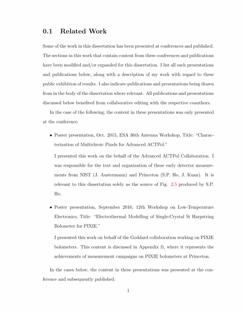
• Poster presentation, Oct. 2015, ESA 36th Antenna Workshop, Title: “Charac-

terization of Multichroic Pixels for Advanced ACTPol.”

I presented this work on the behalf of the Advanced ACTPol Collaboration. I

was responsible for the text and organization of these early detector measure-

ments from NIST (J. Austermann) and Princeton (S.P. Ho, J. Kuan). It is

relevant to this dissertation solely as the source of Fig. 2.5 produced by S.P.

Ho.

• Poster presentation, September 2016, 12th Workshop on Low-Temperature

Electronics, Title: “Electrothermal Modelling of Single-Crystal Si Harpstring

Bolometer for PIXIE.”

I presented this work on behalf of the Goddard collaboration working on PIXIE

bolometers. This content is discussed in Appendix B, where it represents the

achievements of measurement campaigns on PIXIE bolometers at Princeton.

In the cases below, the content in these presentations was presented at the con-

ference and subsequently published.

1

• Poster presentation, June 2016, SPIE Astronomical Telescopes and Instrumen-

tation, Title: “Data-Driven Electrothermal and Noise Modeling of TES Detec-

tors in Multichroic Arrays for Advanced ACTPol.”

I presented this work in concert with S. Choi on behalf of the Advanced ACTPol

collaboration. I produced about half of the figures and text.

• Proceeding, Title: “Characterization of AlMn TES Impedance, Noise, and Op-

tical Effciency in the First 150 mm Multichroic Array for Advanced ACTPol.”

Crowley, K.T.; Choi, S.K.; et al. 2016. [15].

This article is part of the conference proceedings showing in detail the work

presented in the poster. As co-first author, I produced all figures and text in

Section 3, and was responsible for the overall drafting of the article. This work

is expanded upon in Ch. 3.

• Poster presentation, July 2017, Low-Temperature Detectors (LTD) 17, Title:

“Advanced ACTPol TES Device Parameters & Noise Performance in Fielded

Arrays.”

I presented this work on behalf of the Advanced ACTPol collaboration. I was

responsible for all figures except where indicated, and all text. This work is

expanded upon in Ch. 3.

• Proceeding, Title: “Advanced ACTPol TES Device Parameters and Noise Per-

formance in Fielded Arrays.” Crowley, K.T. et al. [14]. 2017.

As sole first author, I produced all figures and text in this article. This article

contains some of the results on Advanced ACTPol array noise seen in Ch. 3,

where it is also expanded upon.

2

• Oral presentation, June 2018, SPIE Astronomical Telescopes and Instrumen-

tation, Title: “Characterizing AlMn Bolometers for Advanced ACTPol (Ad-

vACT).”

I presented my work on detailed characterization of TES bolometer data ac-

quired at NIST on behalf of the Advanced ACTPol collaboration. This presen-

tation was solely produced by myself except where indicated, and described the

work discuss in Ch. 3 on these data.

• Proceeding, Title: “Electrothermal Characterization of AlMn Transition Edge

Sensor Bolometers for Advanced ACTPol.” 2018.

This article is in preparation and about to be submitted as a conclusion to the

data presented in the oral presentation above. As sole first author, I contributed

all text and figures where not otherwise indicated in the article.

In the case of the ABS science results paper:

• Journal article, Title: ”Results from the Atacama B-Mode Experiment.”

Kusaka, A.; Appel, J.; Essinger-Hileman, T.; et al. 2018. [67]

My work was not previously presented at a conference. I drafted the text of

Sections 4, 6.1, and 6.5. My main contribution to the ABS results are in Sec.

6.5 of that paper and Ch. 5 of this dissertation, where they are presented in

more detail.

3

List of Tables

1.1 AdvACT array summaries . . . . . . . . . . . . . . . . . . . . . . . . 39

3.1 AdvACT bolometer properties by array/channel. . . . . . . . . . . . 71

3.2 Summary of TES parameters measured using complex impedance data

in the MF arrays for Tbath ∈ [120, 130] mK and fraction of RN =

0.5. These values come from 8 bolometers total, across both arrays

and frequency channels. With alternate probes, only the parameter

f3dB, eff is recovered at each operating condition. These results are to

be published in [14]. . . . . . . . . . . . . . . . . . . . . . . . . . . . 100

3.3 Contribution, in %, of the median array dark NEP 2 to the total esti-

mated NEP 2 for the arrays based on the fits in Fig. 3.24. . . . . . . 122

5.1 Estimated values for σ and ν when fitting Eq. 5.4 to the values of Cb

over the MC ensemble used in ABS science analysis. Bolded values in-

dicate PDFs estimated according to the single-parameter prescription,

where we set σ =√

2ν. . . . . . . . . . . . . . . . . . . . . . . . . . . 168

5.2 Results by band for measured ABS bandpower, asymmetric error bars

deduced from the likelihood given the single-parameter fit to the MC

ensemble of Cb, and the parameter ν, the single parameter used to

describe the scaled-χ2 fit. . . . . . . . . . . . . . . . . . . . . . . . . . 174

4

List of Figures

1.1 Current CBB` spectra measured by ground-based experiments. . . . . 30

1.2 Galactic polarized foreground brightness versus frequency. . . . . . . 32

1.3 Photographs of ACTPol dichroic and AdvACT HF dichroic arrays . . 38

1.4 Photograph of the ABS receiver. . . . . . . . . . . . . . . . . . . . . . 40

2.1 Thermal circuit diagram of the simplest bolometer model. A single

thermal element, or “block” with heat capacity C and temperature

T sees incoming power Pbias + Pγ. This is balanced by the outgoing

power flowing to the cold thermal bath, Pbath. . . . . . . . . . . . . . 45

2.2 Left: A schematic of the hanging electrothermal model for bolometers,

with parameters for the second block written with subindices i. Not

shown is the voltage source producing the power Pbias in the thermistor

with resistance R. Right: Electrothermal schematic for the intermedi-

ate electrothermal model. . . . . . . . . . . . . . . . . . . . . . . . . 47

2.3 TES bias circuit schematic. . . . . . . . . . . . . . . . . . . . . . . . 50

2.4 I-V curves takent at multiple bath temperatures for an example Ad-

vACT bolometer. . . . . . . . . . . . . . . . . . . . . . . . . . . . . . 54

2.5 Example fitting of line to f3dB recovered by bias steps. . . . . . . . . 55

5

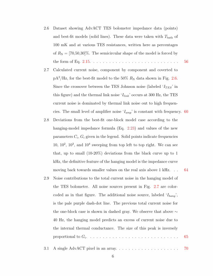
2.6 Dataset showing AdvACT TES bolometer impedance data (points)

and best-fit models (solid lines). These data were taken with Tbath of

100 mK and at various TES resistances, written here as percentages

of RN = [70,50,30]%. The semicircular shape of the model is forced by

the form of Eq. 2.15. . . . . . . . . . . . . . . . . . . . . . . . . . . . 56

2.7 Calculated current noise, component by component and coverted to

pA2/Hz, for the best-fit model to the 50% RN data shown in Fig. 2.6.

Since the crossover between the TES Johnson noise (labeled ‘ITES’ in

this figure) and the thermal link noise ‘Ilink’ occurs at 300 Hz, the TES

current noise is dominated by thermal link noise out to high frequen-

cies. The small level of amplifier noise ‘Iamp’ is constant with frequency. 60

2.8 Deviations from the best-fit one-block model case according to the

hanging-model impedance formula (Eq. 2.23) and values of the new

parameters Ci, Gi given in the legend. Solid points indicate frequencies

10, 102, 103, and 104 sweeping from top left to top right. We can see

that, up to small (10-20%) deviations from the black curve up to 1

kHz, the definitive feature of the hanging model is the impedance curve

moving back towards smaller values on the real axis above 1 kHz. . . 64

2.9 Noise contributions to the total current noise in the hanging model of

the TES bolometer. All noise sources present in Fig. 2.7 are color-

coded as in that figure. The additional noise source, labeled ‘Ihang’,

is the pale purple dash-dot line. The previous total current noise for

the one-block case is shown in dashed gray. We observe that above ∼

40 Hz, the hanging model predicts an excess of current noise due to

the internal thermal conductance. The size of this peak is inversely

proportional to Gi. . . . . . . . . . . . . . . . . . . . . . . . . . . . . 65

3.1 A single AdvACT pixel in an array. . . . . . . . . . . . . . . . . . . . 70

6

3.2 Schematic of “mux11d” design for time-division multiplexing. . . . . 74

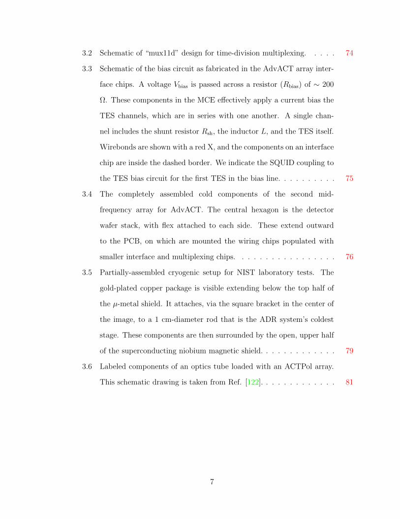
3.3 Schematic of the bias circuit as fabricated in the AdvACT array inter-

face chips. A voltage Vbias is passed across a resistor (Rbias) of ∼ 200

Ω. These components in the MCE effectively apply a current bias the

TES channels, which are in series with one another. A single chan-

nel includes the shunt resistor Rsh, the inductor L, and the TES itself.

Wirebonds are shown with a red X, and the components on an interface

chip are inside the dashed border. We indicate the SQUID coupling to

the TES bias circuit for the first TES in the bias line. . . . . . . . . . 75

3.4 The completely assembled cold components of the second mid-

frequency array for AdvACT. The central hexagon is the detector

wafer stack, with flex attached to each side. These extend outward

to the PCB, on which are mounted the wiring chips populated with

smaller interface and multiplexing chips. . . . . . . . . . . . . . . . . 76

3.5 Partially-assembled cryogenic setup for NIST laboratory tests. The

gold-plated copper package is visible extending below the top half of

the µ-metal shield. It attaches, via the square bracket in the center of

the image, to a 1 cm-diameter rod that is the ADR system’s coldest

stage. These components are then surrounded by the open, upper half

of the superconducting niobium magnetic shield. . . . . . . . . . . . . 79

3.6 Labeled components of an optics tube loaded with an ACTPol array.

This schematic drawing is taken from Ref. [122]. . . . . . . . . . . . . 81

7

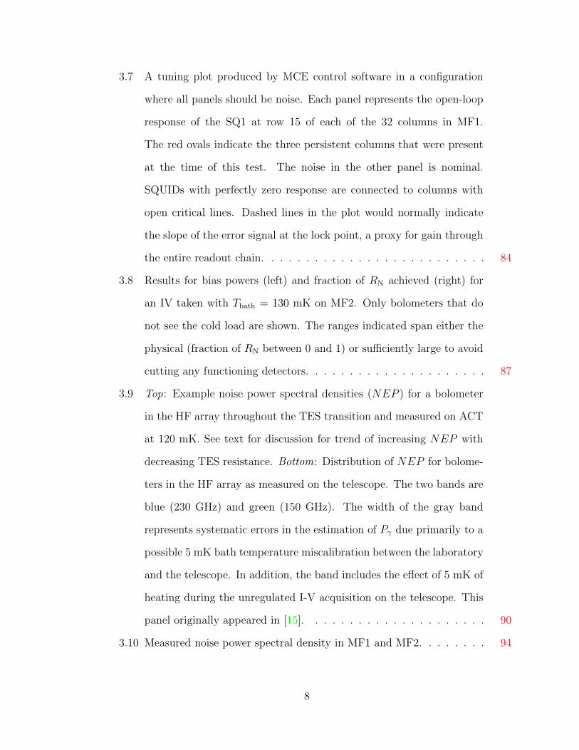
3.7 A tuning plot produced by MCE control software in a configuration

where all panels should be noise. Each panel represents the open-loop

response of the SQ1 at row 15 of each of the 32 columns in MF1.

The red ovals indicate the three persistent columns that were present

at the time of this test. The noise in the other panel is nominal.

SQUIDs with perfectly zero response are connected to columns with

open critical lines. Dashed lines in the plot would normally indicate

the slope of the error signal at the lock point, a proxy for gain through

the entire readout chain. . . . . . . . . . . . . . . . . . . . . . . . . . 84

3.8 Results for bias powers (left) and fraction of RN achieved (right) for

an IV taken with Tbath = 130 mK on MF2. Only bolometers that do

not see the cold load are shown. The ranges indicated span either the

physical (fraction of RN between 0 and 1) or sufficiently large to avoid

cutting any functioning detectors. . . . . . . . . . . . . . . . . . . . . 87

3.9 Top: Example noise power spectral densities (NEP ) for a bolometer

in the HF array throughout the TES transition and measured on ACT

at 120 mK. See text for discussion for trend of increasing NEP with

decreasing TES resistance. Bottom: Distribution of NEP for bolome-

ters in the HF array as measured on the telescope. The two bands are

blue (230 GHz) and green (150 GHz). The width of the gray band

represents systematic errors in the estimation of Pγ due primarily to a

possible 5 mK bath temperature miscalibration between the laboratory

and the telescope. In addition, the band includes the effect of 5 mK of

heating during the unregulated I-V acquisition on the telescope. This

panel originally appeared in [15]. . . . . . . . . . . . . . . . . . . . . 90

3.10 Measured noise power spectral density in MF1 and MF2. . . . . . . . 94

8

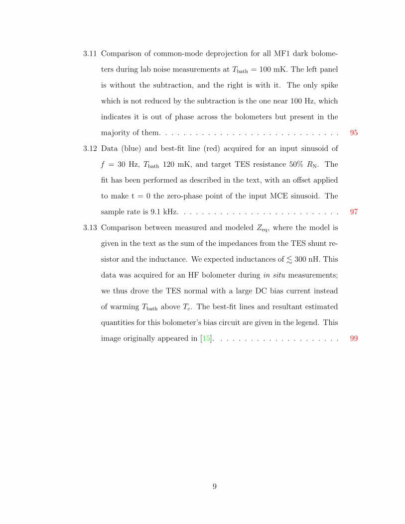
3.11 Comparison of common-mode deprojection for all MF1 dark bolome-

ters during lab noise measurements at Tbath = 100 mK. The left panel

is without the subtraction, and the right is with it. The only spike

which is not reduced by the subtraction is the one near 100 Hz, which

indicates it is out of phase across the bolometers but present in the

majority of them. . . . . . . . . . . . . . . . . . . . . . . . . . . . . . 95

3.12 Data (blue) and best-fit line (red) acquired for an input sinusoid of

f = 30 Hz, Tbath 120 mK, and target TES resistance 50% RN. The

fit has been performed as described in the text, with an offset applied

to make t = 0 the zero-phase point of the input MCE sinusoid. The

sample rate is 9.1 kHz. . . . . . . . . . . . . . . . . . . . . . . . . . . 97

3.13 Comparison between measured and modeled Zeq, where the model is

given in the text as the sum of the impedances from the TES shunt re-

sistor and the inductance. We expected inductances of . 300 nH. This

data was acquired for an HF bolometer during in situ measurements;

we thus drove the TES normal with a large DC bias current instead

of warming Tbath above Tc. The best-fit lines and resultant estimated

quantities for this bolometer’s bias circuit are given in the legend. This

image originally appeared in [15]. . . . . . . . . . . . . . . . . . . . . 99

9

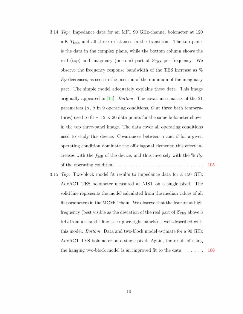
3.14 Top: Impedance data for an MF1 90 GHz-channel bolometer at 120

mK Tbath and all three resistances in the transition. The top panel

is the data in the complex plane, while the bottom column shows the

real (top) and imaginary (bottom) part of ZTES per frequency. We

observe the frequency response bandwidth of the TES increase as %

RN decreases, as seen in the position of the minimum of the imaginary

part. The simple model adequately explains these data. This image

originally appeared in [14]. Bottom: The covariance matrix of the 21

parameters (α, β in 9 operating conditions, C at three bath tempera-

tures) used to fit ∼ 12 × 20 data points for the same bolometer shown

in the top three-panel image. The data cover all operating conditions

used to study this device. Covariances between α and β for a given

operating condition dominate the off-diagonal elements; this effect in-

creases with the f3dB of the device, and thus inversely with the % RN

of the operating condition. . . . . . . . . . . . . . . . . . . . . . . . . 105

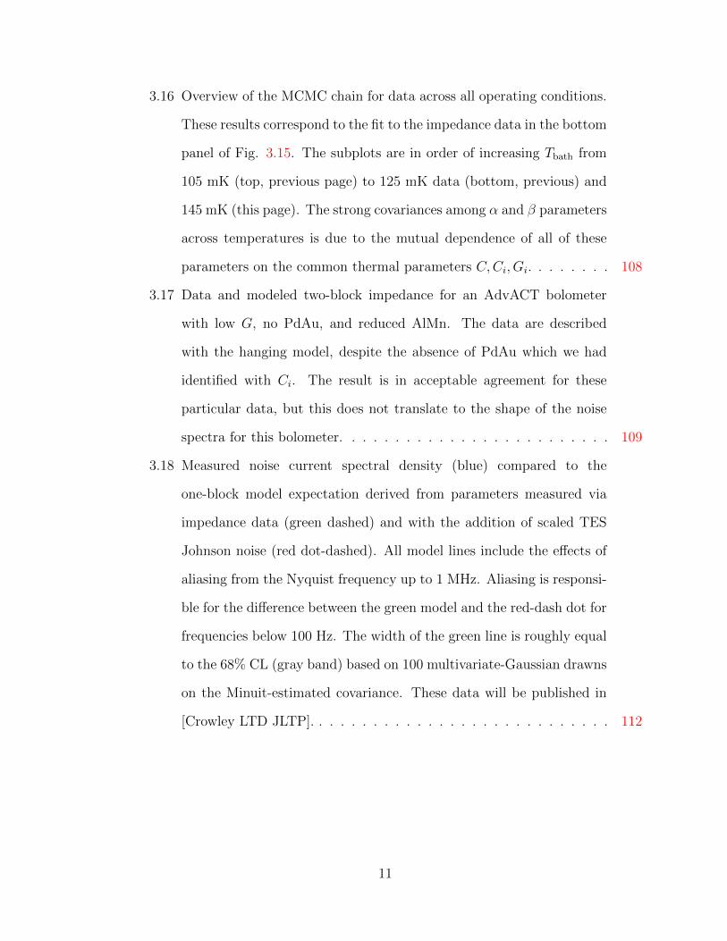
3.15 Top: Two-block model fit results to impedance data for a 150 GHz

AdvACT TES bolometer measured at NIST on a single pixel. The

solid line represents the model calculated from the median values of all

fit parameters in the MCMC chain. We observe that the feature at high

frequency (best visible as the deviation of the real part of ZTES above 3

kHz from a straight line, see upper-right panels) is well-described with

this model. Bottom: Data and two-block model estimate for a 90 GHz

AdvACT TES bolometer on a single pixel. Again, the result of using

the hanging two-block model is an improved fit to the data. . . . . . 106

10

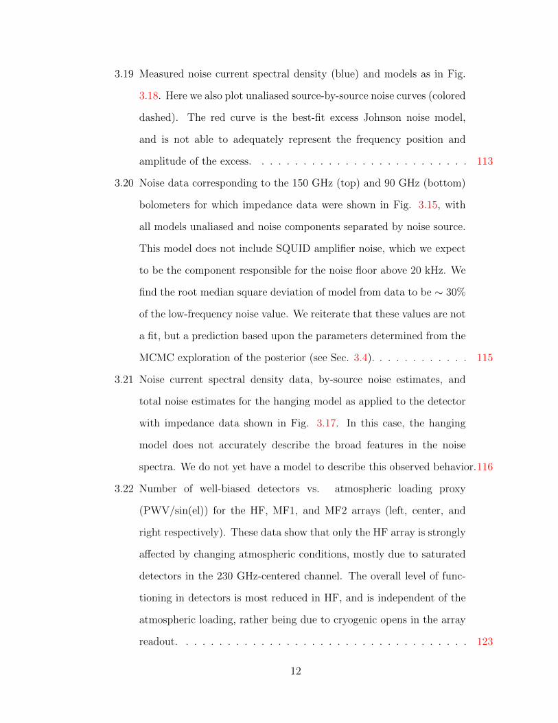
3.16 Overview of the MCMC chain for data across all operating conditions.

These results correspond to the fit to the impedance data in the bottom

panel of Fig. 3.15. The subplots are in order of increasing Tbath from

105 mK (top, previous page) to 125 mK data (bottom, previous) and

145 mK (this page). The strong covariances among α and β parameters

across temperatures is due to the mutual dependence of all of these

parameters on the common thermal parameters C,Ci, Gi. . . . . . . . 108

3.17 Data and modeled two-block impedance for an AdvACT bolometer

with low G, no PdAu, and reduced AlMn. The data are described

with the hanging model, despite the absence of PdAu which we had

identified with Ci. The result is in acceptable agreement for these

particular data, but this does not translate to the shape of the noise

spectra for this bolometer. . . . . . . . . . . . . . . . . . . . . . . . . 109

3.18 Measured noise current spectral density (blue) compared to the

one-block model expectation derived from parameters measured via

impedance data (green dashed) and with the addition of scaled TES

Johnson noise (red dot-dashed). All model lines include the effects of

aliasing from the Nyquist frequency up to 1 MHz. Aliasing is responsi-

ble for the difference between the green model and the red-dash dot for

frequencies below 100 Hz. The width of the green line is roughly equal

to the 68% CL (gray band) based on 100 multivariate-Gaussian drawns

on the Minuit-estimated covariance. These data will be published in

[Crowley LTD JLTP]. . . . . . . . . . . . . . . . . . . . . . . . . . . . 112

11

3.19 Measured noise current spectral density (blue) and models as in Fig.

3.18. Here we also plot unaliased source-by-source noise curves (colored

dashed). The red curve is the best-fit excess Johnson noise model,

and is not able to adequately represent the frequency position and

amplitude of the excess. . . . . . . . . . . . . . . . . . . . . . . . . . 113

3.20 Noise data corresponding to the 150 GHz (top) and 90 GHz (bottom)

bolometers for which impedance data were shown in Fig. 3.15, with

all models unaliased and noise components separated by noise source.

This model does not include SQUID amplifier noise, which we expect

to be the component responsible for the noise floor above 20 kHz. We

find the root median square deviation of model from data to be ∼ 30%

of the low-frequency noise value. We reiterate that these values are not

a fit, but a prediction based upon the parameters determined from the

MCMC exploration of the posterior (see Sec. 3.4). . . . . . . . . . . . 115

3.21 Noise current spectral density data, by-source noise estimates, and

total noise estimates for the hanging model as applied to the detector

with impedance data shown in Fig. 3.17. In this case, the hanging

model does not accurately describe the broad features in the noise

spectra. We do not yet have a model to describe this observed behavior.116

3.22 Number of well-biased detectors vs. atmospheric loading proxy

(PWV/sin(el)) for the HF, MF1, and MF2 arrays (left, center, and

right respectively). These data show that only the HF array is strongly

affected by changing atmospheric conditions, mostly due to saturated

detectors in the 230 GHz-centered channel. The overall level of func-

tioning in detectors is most reduced in HF, and is independent of the

atmospheric loading, rather being due to cryogenic opens in the array

readout. . . . . . . . . . . . . . . . . . . . . . . . . . . . . . . . . . . 123

12

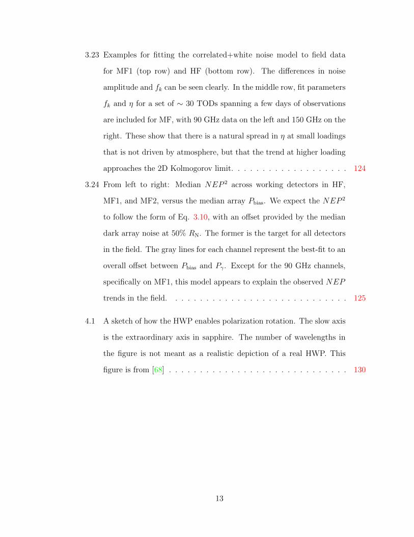
3.23 Examples for fitting the correlated+white noise model to field data

for MF1 (top row) and HF (bottom row). The differences in noise

amplitude and fk can be seen clearly. In the middle row, fit parameters

fk and η for a set of ∼ 30 TODs spanning a few days of observations

are included for MF, with 90 GHz data on the left and 150 GHz on the

right. These show that there is a natural spread in η at small loadings

that is not driven by atmosphere, but that the trend at higher loading

approaches the 2D Kolmogorov limit. . . . . . . . . . . . . . . . . . . 124

3.24 From left to right: Median NEP 2 across working detectors in HF,

MF1, and MF2, versus the median array Pbias. We expect the NEP 2

to follow the form of Eq. 3.10, with an offset provided by the median

dark array noise at 50% RN. The former is the target for all detectors

in the field. The gray lines for each channel represent the best-fit to an

overall offset between Pbias and Pγ. Except for the 90 GHz channels,

specifically on MF1, this model appears to explain the observed NEP

trends in the field. . . . . . . . . . . . . . . . . . . . . . . . . . . . . 125

4.1 A sketch of how the HWP enables polarization rotation. The slow axis

is the extraordinary axis in sapphire. The number of wavelengths in

the figure is not meant as a realistic depiction of a real HWP. This

figure is from [68] . . . . . . . . . . . . . . . . . . . . . . . . . . . . . 130

13

4.2 A cartoon of the ABS optical setup. Shown are the HWP in red at

the top aperture of the vacuum system, which holds the cryogenically

cooled mirrors (at 4K) as well as the feedhorns and detectors (at 300

mK when observing). The ray traces are not accurate, but meant to

guide the eye through the crossed-Dragone configuration and the fact

that detectors are mapped to plane waves arriving from infiinity at

various angles of incidence. These illuminate nearly the full HWP for

each detector. . . . . . . . . . . . . . . . . . . . . . . . . . . . . . . . 131

4.3 A ray-tracing simulation of the optics tube design for ACTPol, with the

rough position and diameter of the HWP overlaid in solid black. This

figure is meant to indicate how ACTPol detectors and ABS detectors

see their respective HWPs differently. Courtesy M. Niemack. . . . . . 132

4.4 Per-CES measurements (circles) of a2 and b2, defined in Eq. 4.4, for an

example ABS TES bolometer across the first season of observations.

The best-fit line (solid) is used to make a data-selection threshold for

CES which deviate excessively. The fit is restricted to the inner 95%

of the a2 and b2 distributions. Figure taken from [113]. . . . . . . . . 136

4.5 Calibrated A(χ) peak-to-peak amplitude of the sapphire CRHWP from

ABS for a special ACTPol TOD in which it was present in the optical

path for an ACTPol 150 GHz array. The median value of 0.74 K is

in reasonable agreement with measurements of the A(χ) amplitude of

the same CRHWP measured by ABS. . . . . . . . . . . . . . . . . . . 137

4.6 Example timestreams for CRHWP data on ACT across ABS sapphire

and AdvACT metamaterial HWPs . . . . . . . . . . . . . . . . . . . 139

4.7 CRHWP angle residuals and jitter estimate for an AdvACT TOD. . . 142

4.8 Example A(χ) data and model for MF1 and MF2. . . . . . . . . . . . 145

14

4.9 Results for A(χ) peak-to-peak values for single TOD with AdvACT

arrays. . . . . . . . . . . . . . . . . . . . . . . . . . . . . . . . . . . . 147

4.10 Power removal plots for MF1 and MF2 for example TOD. . . . . . . 148

4.11 Detector-averaged raw, subtracted, and demodulated noise spectra

(MF1, MF2) . . . . . . . . . . . . . . . . . . . . . . . . . . . . . . . . 149

4.12 PWV estimated from ALMA weather station data for the 2017

CRHWP run. . . . . . . . . . . . . . . . . . . . . . . . . . . . . . . . 151

4.13 A(χ) Harmonic dependence on loading ( PWV/sin(el) ) for two MF

detectors. . . . . . . . . . . . . . . . . . . . . . . . . . . . . . . . . . 152

4.14 1f r and 2f r harmonic amplitudes vs. time of day for MF1. . . . . . . 153

4.15 1f r and 2f r harmonic amplitudes vs. time of day for MF2. . . . . . . 155

4.16 Example transformed A(χ) values and estimated common mode. . . . 158

4.17 Estimated correlation to the A(χ) common mode. . . . . . . . . . . . 159

5.1 Left : Distribution of fiducal MC ensemble generated by ΛCDM simu-

lations for the EE bandpower covering ` in [101,130]. The two sets of

dotted points indicate the best-fit PDF functions for free σ, ν parame-

ters (red) and a reduced model, equivalent to a scaled χ2 translated to

have zero mean, achieved by setting σ =√

2/ν (green). The best-fit

parameters, and some statistics of the MC ensemble, are in the leg-

end, with the parameter Nb being estimated directly from the mean

of noise-only MC ensemble results for this bandpower. Right : Best-fit

results for the same models, matched to the same colors, for the BB

bandpower over the same range of `. Here the fiducial model is zero

bandpower input, hence the distribution being centered around zero. . 165

15

5.2 The same fiducial BB MC ensemble shown in the right panel of Fig.

5.1, but with Nb a free parameter. The constraint on Nb comes from

jointly fitting the model of Eq. 5.4 for two MC datasets: the BB

fiducial ensemble and an ensemble with r = 0.9. The recovered bias

on the bandpower Nb is 20% smaller when compared to the estimate

from noise-only simulations, Nb = 1.21. . . . . . . . . . . . . . . . . . 166

5.3 The minimum negative log-likelihood (colormap) when the PDF of the

fiducial MC ensemble of the fourth EE bandpower is minimized with

respect to σ for various values of√

2/ν. The σ values minimizing the

function are plotted on the y-axis. There is no minimum found above

the bottom-leftmost point closest to√

2/ν = 0. The shaded region

defines the 1-σ upper-limit on the√

2/ν parameter, while the dashed

line shows the estimated 1-σ error bar on the σ parameter. We do

not use this minimization in this case, but instead revert to fitting a

Gaussian PDF to the distribution (see text). . . . . . . . . . . . . . . 167

5.4 Left : Best-fit values and estimated errors for the PDF parameters σ

and√

2/ν across the first 9 EE bandpowers for ABS. See text for

discussion of the one-sided error bars. Right : Best-fit values for the

PDF parameters for the first 9 BB bandpowers. . . . . . . . . . . . . 168

5.5 Top row : Distributions of r and the best-fit parameter PDF using a

joint fit across the fiducial (left, r = 0) and signal (right, r = 0.9)

ensembles. Each ensemble has 400 MC realizations, where r for each

realization is estimated from fitting to the first three bandpowers, as

discussed in the text. We note that the bias, estimated from the dif-

ference between⟨r⟩

and r, is small in both cases, thus validating our

minimum-χ2 pipeline. Bottom row : The same as for the top row,

except the fit used to recover r uses the first four bins. . . . . . . . . 170

16

5.6 Correct likelihood for r (red) given r = 0 compared to the plotting the

PDF as a function of r when r = 0. The plot demonstrates the change

in the function shape depending on whether we study the PDF or Lr. 172

5.7 Left : ABS likelihood for r without (black) and with (green) the convo-

lution of a Gaussian term describing the calibration uncertainty. The

upper limits indicated are the points where ∆Lr = ln(L/Lmax = −4.

Previously published in [67]. Right : ABS data and the best-fit theory

spectrum for the first three bandpowers. This defines the r we assume

in the likelihood at left. . . . . . . . . . . . . . . . . . . . . . . . . . . 173

5.8 Left : Likelihood for the EE bandpower spanning ` ∈ [101, 130]. The

two curves show likelihoods with and without a final beam correction

based on cross-correlation of ABS spectra with Planck [67]. Our results

assume the green curve and dashed one-σ upper and lower error bars.

Right : BB bandpower likelihood for the same ` span as int he left panel.173

5.9 Left : ABS measured EE spectra with maximum-likelihood, asymmet-

ric error bars (green points) determined as in the text, and fiducial

error bars (blue) determined solely from the spread of the bandpower

values across the MC realizations. The first 13 bandpowers are shown,

with their values and errors, along with other details, in Tab. 5.2.

Right : ABS measured BB spectra, with error bars as at left, except

the blue points are now the full maximum-likelihood error bar points. 174

6.1 Example plot of second-harmonic pickup from a TES bolometer. . . . 178

6.2 Studying pickup vs. imput amplitude of a sine-wave excitation on the

TES bias lines. . . . . . . . . . . . . . . . . . . . . . . . . . . . . . . 183

6.3 CMB simulation results including nonlinearity effects. . . . . . . . . . 184

6.4 I-V curve-based measurement of loopgain L ; examples from MF1 . . 187

17

B.1 Diagram of a PIXIE detector. . . . . . . . . . . . . . . . . . . . . . . 198

B.2 Models used in PIXIE detector description. . . . . . . . . . . . . . . . 199

B.3 PIXIE optical testing results. . . . . . . . . . . . . . . . . . . . . . . 201

B.4 PIXIE thermistor AC-biased thermal transfer measurement. . . . . . 203

C.1 Example of ABS scan-synchronous signal discrete correlation function. 206

C.2 Histogram of selection criteria feq. . . . . . . . . . . . . . . . . . . . . 208

18

Chapter 1

Introduction

1.1 The ΛCDM Model

In modern physical cosmology, across the diverse landscape of measurement tech-

niques and objects of study, a common model has emerged to explain the energy

contents of the universe. The initiation of this model was the discovery of the

Friedmann-Lemaitre-Robertson-Walker solutions (FLRW) [36] [74] [106] [126] to Ein-

stein’s equations in general relativity (GR). Given the assumption of a homogeneous,

isotropic universe when coarse-grained on the largest (tens of megaparsecs (Mpc) to

gigaparsecs (Gpc)) scales, a concept now given the name the “cosmological princi-

ple,” the FLRW solutions describe dynamic universes whose evolution is described

by a scale factor a(t), where t is the coordinate time. This scale factor can be used

as the clock for all cosmological time, and it evolves according to the energy content

of the universe. In general, the FLRW solutions can be classified according to the

curvature of the space-time in the universe. All of this can be seen in the Friedman

equation for a in terms of the Hubble parameter, H(t) ≡ a/a, where a is the time

derivative of a:

H2 +K

a2=

8πG

3ρ. (1.1)

19

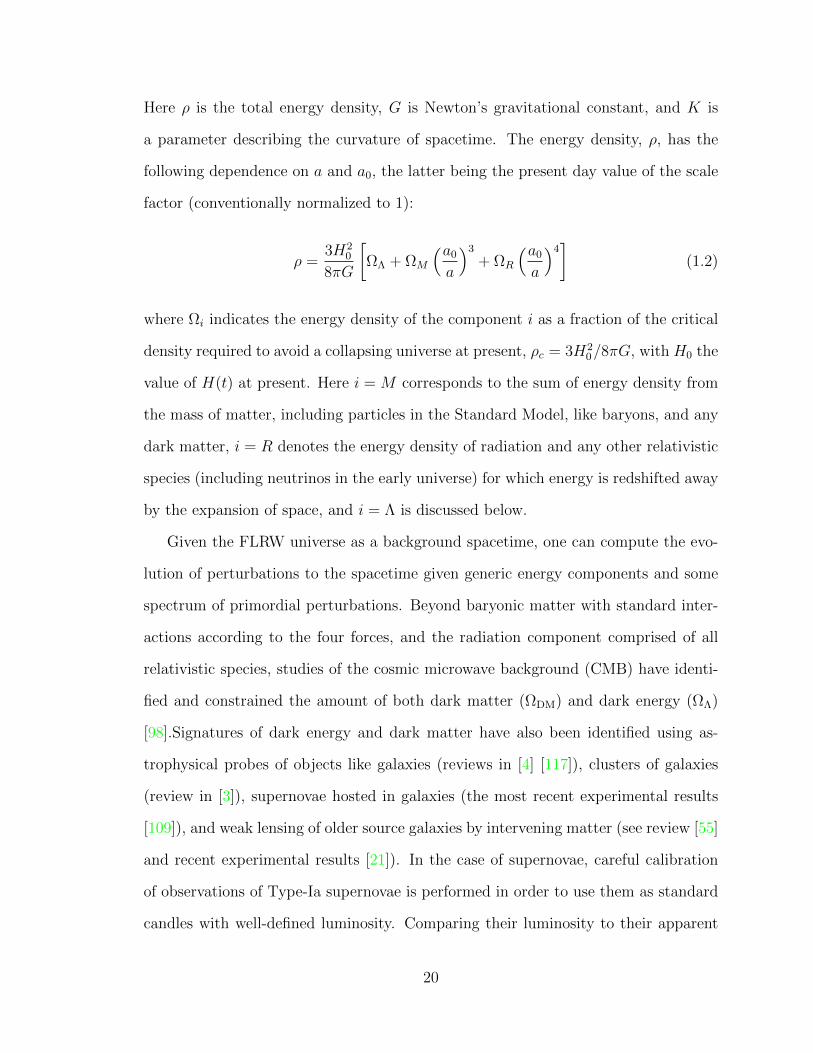
Here ρ is the total energy density, G is Newton’s gravitational constant, and K is

a parameter describing the curvature of spacetime. The energy density, ρ, has the

following dependence on a and a0, the latter being the present day value of the scale

factor (conventionally normalized to 1):

ρ =3H2

0

8πG

[ΩΛ + ΩM

(a0

a

)3

+ ΩR

(a0

a

)4]

(1.2)

where Ωi indicates the energy density of the component i as a fraction of the critical

density required to avoid a collapsing universe at present, ρc = 3H20/8πG, with H0 the

value of H(t) at present. Here i = M corresponds to the sum of energy density from

the mass of matter, including particles in the Standard Model, like baryons, and any

dark matter, i = R denotes the energy density of radiation and any other relativistic

species (including neutrinos in the early universe) for which energy is redshifted away

by the expansion of space, and i = Λ is discussed below.

Given the FLRW universe as a background spacetime, one can compute the evo-

lution of perturbations to the spacetime given generic energy components and some

spectrum of primordial perturbations. Beyond baryonic matter with standard inter-

actions according to the four forces, and the radiation component comprised of all

relativistic species, studies of the cosmic microwave background (CMB) have identi-

fied and constrained the amount of both dark matter (ΩDM) and dark energy (ΩΛ)

[98].Signatures of dark energy and dark matter have also been identified using as-

trophysical probes of objects like galaxies (reviews in [4] [117]), clusters of galaxies

(review in [3]), supernovae hosted in galaxies (the most recent experimental results

[109]), and weak lensing of older source galaxies by intervening matter (see review [55]

and recent experimental results [21]). In the case of supernovae, careful calibration

of observations of Type-Ia supernovae is performed in order to use them as standard

candles with well-defined luminosity. Comparing their luminosity to their apparent

20

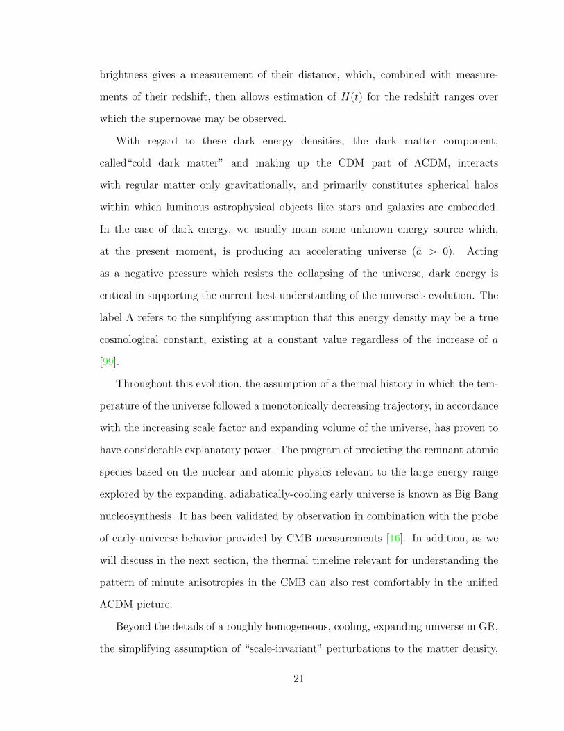
brightness gives a measurement of their distance, which, combined with measure-

ments of their redshift, then allows estimation of H(t) for the redshift ranges over

which the supernovae may be observed.

With regard to these dark energy densities, the dark matter component,

called“cold dark matter” and making up the CDM part of ΛCDM, interacts

with regular matter only gravitationally, and primarily constitutes spherical halos

within which luminous astrophysical objects like stars and galaxies are embedded.

In the case of dark energy, we usually mean some unknown energy source which,

at the present moment, is producing an accelerating universe (a > 0). Acting

as a negative pressure which resists the collapsing of the universe, dark energy is

critical in supporting the current best understanding of the universe’s evolution. The

label Λ refers to the simplifying assumption that this energy density may be a true

cosmological constant, existing at a constant value regardless of the increase of a

[99].

Throughout this evolution, the assumption of a thermal history in which the tem-

perature of the universe followed a monotonically decreasing trajectory, in accordance

with the increasing scale factor and expanding volume of the universe, has proven to

have considerable explanatory power. The program of predicting the remnant atomic

species based on the nuclear and atomic physics relevant to the large energy range

explored by the expanding, adiabatically-cooling early universe is known as Big Bang

nucleosynthesis. It has been validated by observation in combination with the probe

of early-universe behavior provided by CMB measurements [16]. In addition, as we

will discuss in the next section, the thermal timeline relevant for understanding the

pattern of minute anisotropies in the CMB can also rest comfortably in the unified

ΛCDM picture.

Beyond the details of a roughly homogeneous, cooling, expanding universe in GR,

the simplifying assumption of “scale-invariant” perturbations to the matter density,

21

velocity, particle species distributions, and other parameters has proven to be vali-

dated by most observational data. In fact, the perturbations exhibit a mild red tilt,

meaning their amplitudes decrease with decreasing spatial scale. This small devia-

tion appears to describe the behavior of the dominant density perturbations across

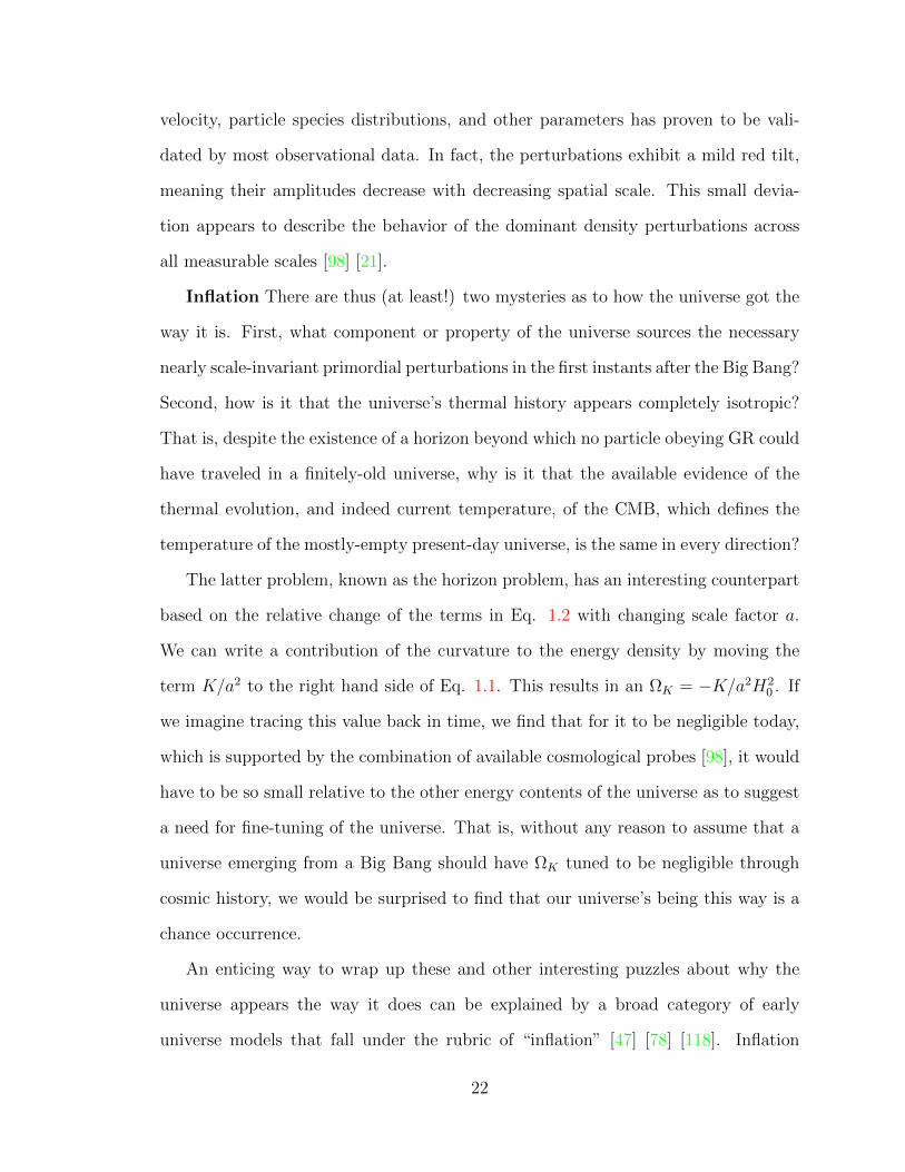
all measurable scales [98] [21].

Inflation There are thus (at least!) two mysteries as to how the universe got the

way it is. First, what component or property of the universe sources the necessary

nearly scale-invariant primordial perturbations in the first instants after the Big Bang?

Second, how is it that the universe’s thermal history appears completely isotropic?

That is, despite the existence of a horizon beyond which no particle obeying GR could

have traveled in a finitely-old universe, why is it that the available evidence of the

thermal evolution, and indeed current temperature, of the CMB, which defines the

temperature of the mostly-empty present-day universe, is the same in every direction?

The latter problem, known as the horizon problem, has an interesting counterpart

based on the relative change of the terms in Eq. 1.2 with changing scale factor a.

We can write a contribution of the curvature to the energy density by moving the

term K/a2 to the right hand side of Eq. 1.1. This results in an ΩK = −K/a2H20 . If

we imagine tracing this value back in time, we find that for it to be negligible today,

which is supported by the combination of available cosmological probes [98], it would

have to be so small relative to the other energy contents of the universe as to suggest

a need for fine-tuning of the universe. That is, without any reason to assume that a

universe emerging from a Big Bang should have ΩK tuned to be negligible through

cosmic history, we would be surprised to find that our universe’s being this way is a

chance occurrence.

An enticing way to wrap up these and other interesting puzzles about why the

universe appears the way it does can be explained by a broad category of early

universe models that fall under the rubric of “inflation” [47] [78] [118]. Inflation

22

posits a brief period of exponential evolution of the scale factor with constant H.

This is conceptually similar to the de Sitter cosmological solution for GR [20], which

corresponds to a universe with the only energy density being a positive cosmological

constant, and where spacetime has a constant positive curvature. While the Λ-like

expansion of the universe in the present day is thus analogous, the scale of the energies

needed to drive inflation, and to explain the current amount of accelerating expansion

in the universe, are extremely different. It is also not certaint whether dark energy is

fully described by a cosmological constant Λ.

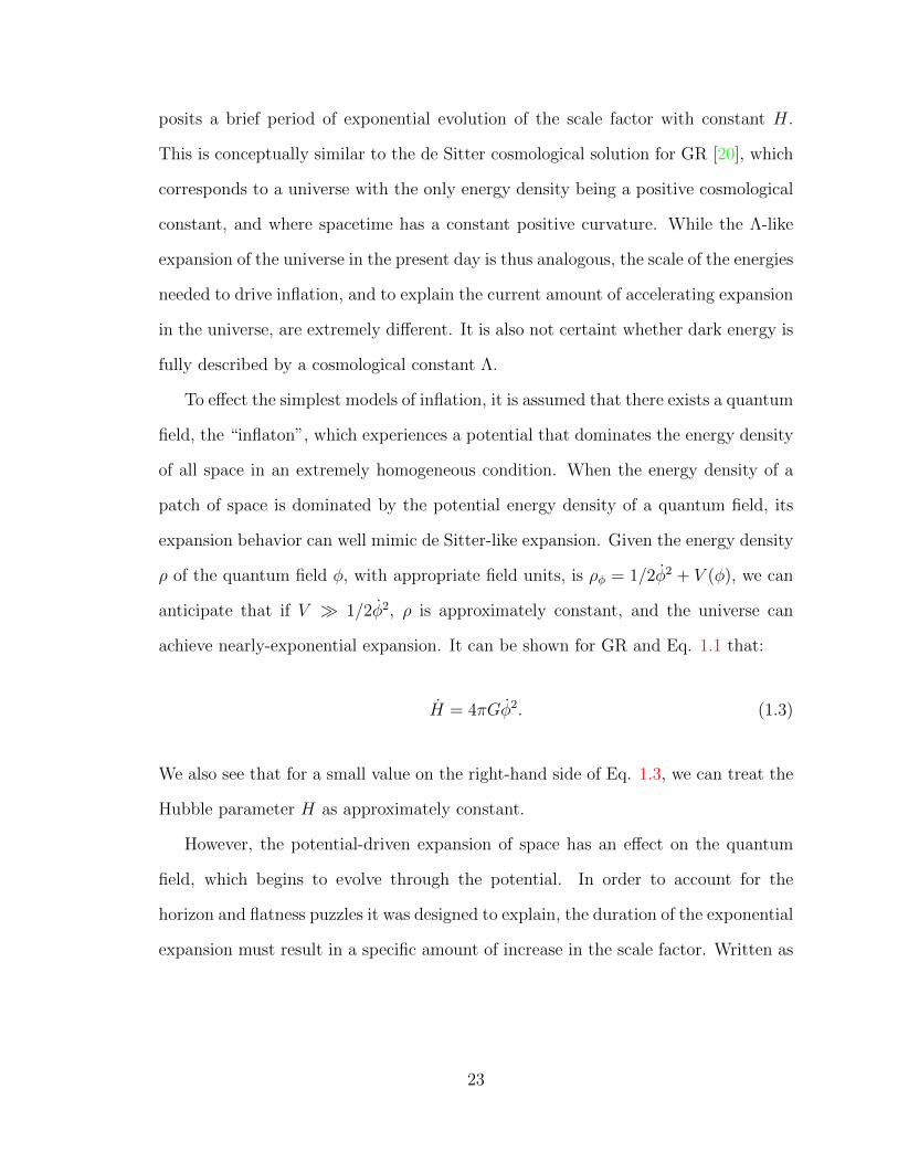
To effect the simplest models of inflation, it is assumed that there exists a quantum

field, the “inflaton”, which experiences a potential that dominates the energy density

of all space in an extremely homogeneous condition. When the energy density of a

patch of space is dominated by the potential energy density of a quantum field, its

expansion behavior can well mimic de Sitter-like expansion. Given the energy density

ρ of the quantum field φ, with appropriate field units, is ρφ = 1/2φ2 + V (φ), we can

anticipate that if V 1/2φ2, ρ is approximately constant, and the universe can

achieve nearly-exponential expansion. It can be shown for GR and Eq. 1.1 that:

H = 4πGφ2. (1.3)

We also see that for a small value on the right-hand side of Eq. 1.3, we can treat the

Hubble parameter H as approximately constant.

However, the potential-driven expansion of space has an effect on the quantum

field, which begins to evolve through the potential. In order to account for the

horizon and flatness puzzles it was designed to explain, the duration of the exponential

expansion must result in a specific amount of increase in the scale factor. Written as

23

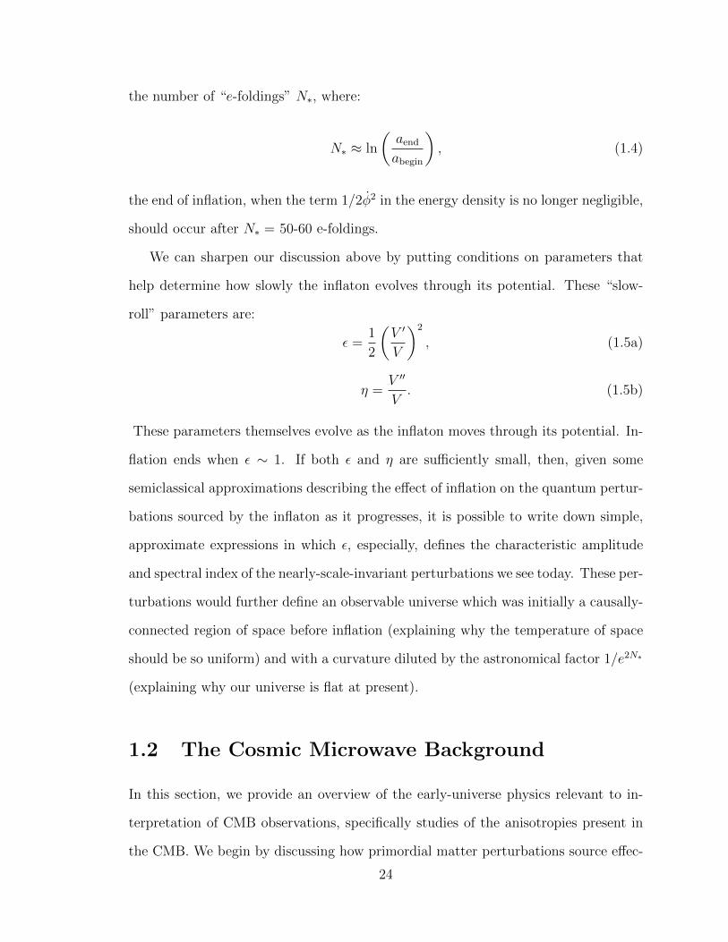
the number of “e-foldings” N∗, where:

N∗ ≈ ln

(aend

abegin

), (1.4)

the end of inflation, when the term 1/2φ2 in the energy density is no longer negligible,

should occur after N∗ = 50-60 e-foldings.

We can sharpen our discussion above by putting conditions on parameters that

help determine how slowly the inflaton evolves through its potential. These “slow-

roll” parameters are:

ε =1

2

(V ′

V

)2

, (1.5a)

η =V ′′

V. (1.5b)

These parameters themselves evolve as the inflaton moves through its potential. In-

flation ends when ε ∼ 1. If both ε and η are sufficiently small, then, given some

semiclassical approximations describing the effect of inflation on the quantum pertur-

bations sourced by the inflaton as it progresses, it is possible to write down simple,

approximate expressions in which ε, especially, defines the characteristic amplitude

and spectral index of the nearly-scale-invariant perturbations we see today. These per-

turbations would further define an observable universe which was initially a causally-

connected region of space before inflation (explaining why the temperature of space

should be so uniform) and with a curvature diluted by the astronomical factor 1/e2N∗

(explaining why our universe is flat at present).

1.2 The Cosmic Microwave Background

In this section, we provide an overview of the early-universe physics relevant to in-

terpretation of CMB observations, specifically studies of the anisotropies present in

the CMB. We begin by discussing how primordial matter perturbations source effec-

24

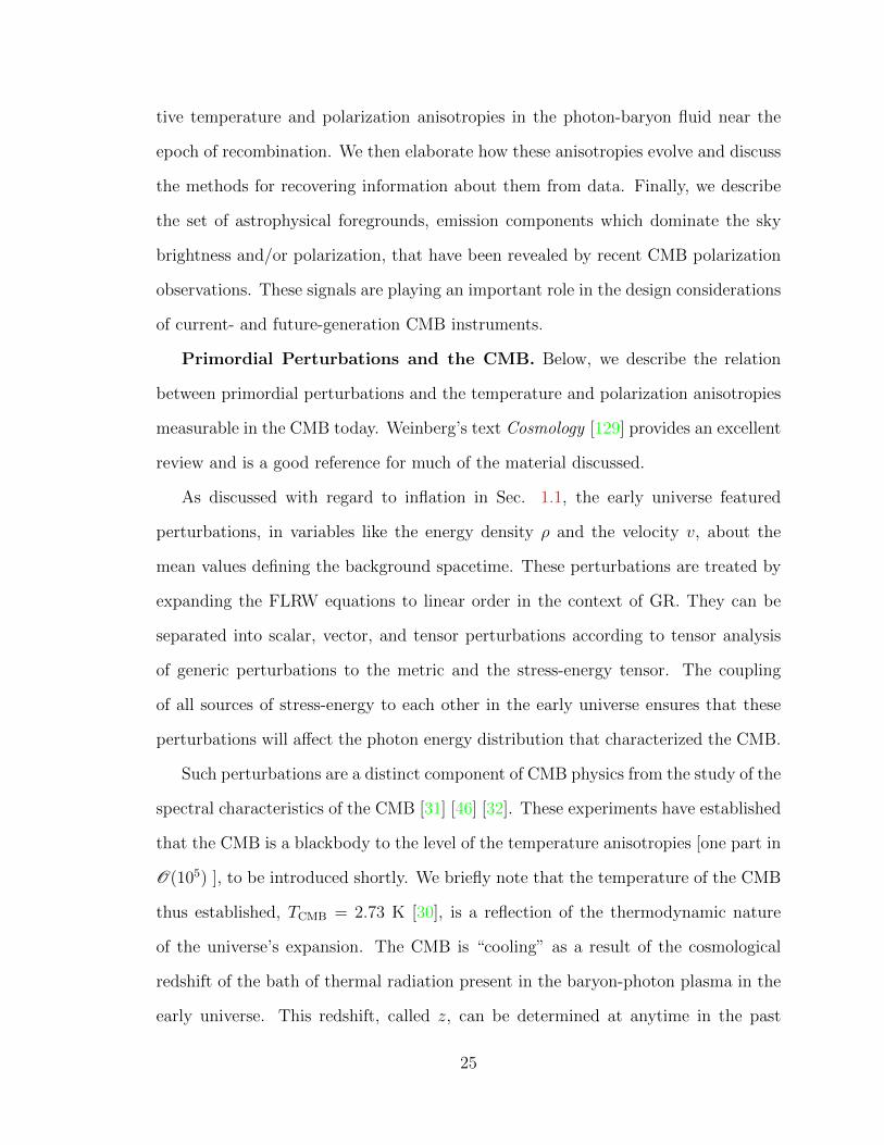
tive temperature and polarization anisotropies in the photon-baryon fluid near the

epoch of recombination. We then elaborate how these anisotropies evolve and discuss

the methods for recovering information about them from data. Finally, we describe

the set of astrophysical foregrounds, emission components which dominate the sky

brightness and/or polarization, that have been revealed by recent CMB polarization

observations. These signals are playing an important role in the design considerations

of current- and future-generation CMB instruments.

Primordial Perturbations and the CMB. Below, we describe the relation

between primordial perturbations and the temperature and polarization anisotropies

measurable in the CMB today. Weinberg’s text Cosmology [129] provides an excellent

review and is a good reference for much of the material discussed.

As discussed with regard to inflation in Sec. 1.1, the early universe featured

perturbations, in variables like the energy density ρ and the velocity v, about the

mean values defining the background spacetime. These perturbations are treated by

expanding the FLRW equations to linear order in the context of GR. They can be

separated into scalar, vector, and tensor perturbations according to tensor analysis

of generic perturbations to the metric and the stress-energy tensor. The coupling

of all sources of stress-energy to each other in the early universe ensures that these

perturbations will affect the photon energy distribution that characterized the CMB.

Such perturbations are a distinct component of CMB physics from the study of the

spectral characteristics of the CMB [31] [46] [32]. These experiments have established

that the CMB is a blackbody to the level of the temperature anisotropies [one part in

O(105) ], to be introduced shortly. We briefly note that the temperature of the CMB

thus established, TCMB = 2.73 K [30], is a reflection of the thermodynamic nature

of the universe’s expansion. The CMB is “cooling” as a result of the cosmological

redshift of the bath of thermal radiation present in the baryon-photon plasma in the

early universe. This redshift, called z, can be determined at anytime in the past

25

t < t0, when the scale factor was smaller, as:

1 + z = a0/a(t). (1.6)

From arguments based on the form for the number density of photons in equilib-

rium with matter at temperature T , we can recover that, when the CMB has ceased

interacting with matter, its spectrum retains the form of the Planck blackbody dis-

tribution, but with a temperature T (z) = TL1+z

1+zL, where the subscript L stands for

an idealized, instantaneous time of last scattering.

According to the above argument, CMB photons are thus distributed as a perfect

blackbody. However, the primordial perturbations affecting the energy density have

the small, one part in 100,000-level effect on the CMB mentioned above. In order

to fully calculate the perturbations to the CMB due to physics near the time of last

scattering, or “recombination” (referring to the universe becoming electrically neutral

due to the combining of electrons and protons into hydrogen atoms), a full treatment

of the perturbations to the CMB number density in phase space is required. In these

expressions, a natural decomposition arises where perturbations to the CMB energy

distribution are written as T (x, t) = T + ∆T (x, t) with T the average.

The temperature anisotropy, ∆T (x, t), effectively describes the number density

fluctuation at that position as a temperature fluctuation. Conceptually, it is positive

or negative depending on the presence of matter overdensities or underdensities, re-

spectively, for “adiabatic” perturbations, the dominant mode of perturbations. We

can consider this as due to the fact that the photons of the CMB are tightly coupled

to free electrons by Thomson scattering in this era. Recombination begins when the

timescale on which CMB photons scatter from ionized matter falls below the Hubble

expansion timescale ∼ 1/H(t).

26

We now prepare to describe how these temperature anisotropies are studied. Con-

sider that there is some “primordial power spectrum” of fluctuations, particularly for

scalar perturbations. These result in a power spectrum of temperature fluctuations,

which we can estimate in principle from the autocorrelation between the temperature

anisotropy ∆T (n) measured in some direction n on the celestial sphere, and some

∆T (n′). In terms of what has been previously discussed, ∆T (n) measured today is

T (n)− TCMB, and we can write its decomposition into spherical harmonics as:

∆T (n) =∑`m

a`mYm` (n), (1.7)

When we then take the covariance, we can define the angular power for a given

multipole moment `, C`, as:

〈∆T (n)∆T (n′)〉 =∑`m

C`Ym` (n)Y −m` (n′), (1.8)

where angle brackets indicate an ensemble average over all possible realizations of the

anisotropies given the ΛCDM cosmology. We can also write:

〈a`ma ∗ `′m′〉 = 〈a`ma`′−m′〉 = δ``′δmm′C`, (1.9)

with δ the Kronecker delta, and with the first equality following from the real-valued

nature of the anisotropies.

However, these averages cannot be performed, as they would require observing the

CMB from multiple positions in the universe. We thus form the measured quantity

Cmeas` as the average of the estimator in Eq. 1.9 over the spherical harmonic index

m, under the assumption that the CMB has no preferred direction, and thus can be

27

described by the 1-D spectrum C` independent of m.

Cmeas` =

1

2`+ 1

∑m

a`ma`−m. (1.10)

We can then see how the finite number of independent spherical-harmonic modes used

to form an estimate of Cmeas` for each multipole moment determines the signal vari-

ance on the measurement, known as “cosmic variance,” which goes as√

2/(2`+ 1)C`

assuming Gaussian distribution of the primordial perturbations [63].

This compression of the information in the anisotropies into a single 1-D power

spectrum has been extremely important for cosmology. From exploration of these data

alone, the ΛCDM model can be powerfully constrained. Given the many degeneracies

between parameters, a limited set of six free parameters describing our universe in

the ΛCDM framework has been used to nearly completely describe the structure of

Cmeas` [98]. The connection between CMB spectra and these parameters is provided

by numerical software [112] [75] [7] designed to output realizations of power spectra

given these parameters as input. The signal recovered in the power spectrum indicates

the presence of acoustic waves in the primordial baryon-photon plasma, arising from

the opposing forces of gravity, under which photons are dragged with matter towards

overdensities and away from underdensities, and radiation pressure, which resists the

aggregation of high numbers of photons.

If we assume a perfectly scale-invariant perturbation spectrum (i.e., flat in wave-

vector k space), we recover a spectrum C` which goes as C` ∝ (`(` + 1))−1. It is

therefore common to rescale C` by this factor, with an additional numerical constant,

to recover a spherical-harmonic power spectrum that is also flat with multipole mo-

ment [97]. The typical quantity to plot is C` = `(`+1)2π

C` and we use this convention

in Ch. 5.

28

CMB Polarization. Generation of linear polarization of the CMB via the same

spectrum of primordial perturbations falls naturally out of the study of the evolution

of these perturbations given the energy contents of the early universe. The results are

most easily expressed in terms of the components of linear polarization in the Stokes

vector I,Q, U, V , where linear polarization is defined by the two components Q

and U . Non-zero values of these components are sourced from scalar perturbations

according to local quadrupole moments of the CMB distribution around a free elec-

tron, according to Thomson scattering. The total amplitude of linear polarization

p =√Q2 + U2 has a ratio with the pure CMB intensity of p/I . 10 %. There

is expected to be no generation of circular polarization V of CMB photons due to

Thomson scattering in the early universe.

Since Q and U are related by a 45 rotation of the polarization, they can be

combined into two complex polarization quantities Q±iU , which admit of a spherical-

harmonic decomposition using spin-2 harmonics [61]:

(Q± iU)(n) =∑`m

a±2`m±2Y

m` (n). (1.11)

However, it is more common to form two scalar fields, labeled E(n) (since curl-free,

like a classical electric field) and B(n) (since divergence-free, like a magnetic field),

from the polarization quantities. This is done according to a global transformation,

most easily written according to the spin-2 a±2`m quantities [111]:

aE`m = −(a+2`m + a−2

`m)

2, (1.12a)

aB`m =(a+2`m − a

−2`m)

2. (1.12b)

It is the case that these coefficients can be recovered as the decomposition of a partic-

ular combination of Q and U according to the standard, spin-0 spherical harmonics.

29

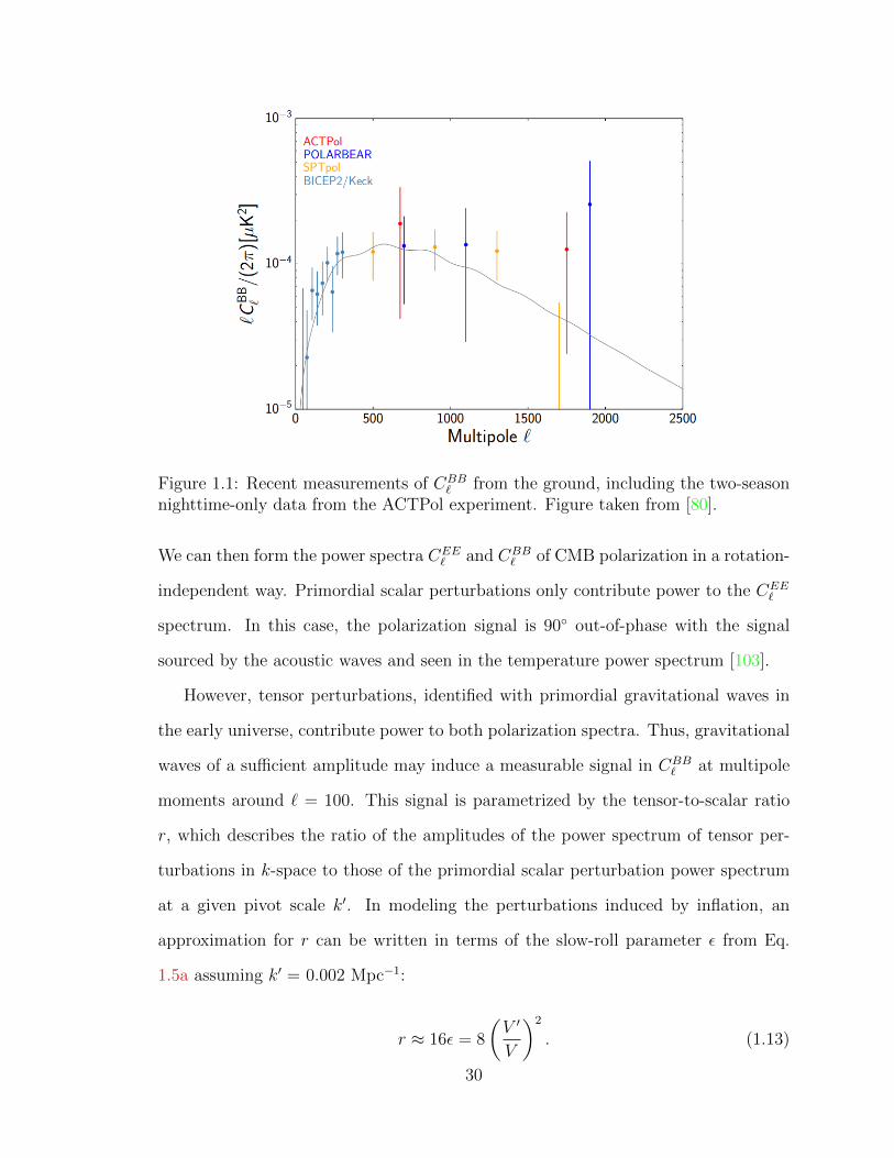
Figure 1.1: Recent measurements of CBB` from the ground, including the two-season

nighttime-only data from the ACTPol experiment. Figure taken from [80].

We can then form the power spectra CEE` and CBB

` of CMB polarization in a rotation-

independent way. Primordial scalar perturbations only contribute power to the CEE`

spectrum. In this case, the polarization signal is 90 out-of-phase with the signal

sourced by the acoustic waves and seen in the temperature power spectrum [103].

However, tensor perturbations, identified with primordial gravitational waves in

the early universe, contribute power to both polarization spectra. Thus, gravitational

waves of a sufficient amplitude may induce a measurable signal in CBB` at multipole

moments around ` = 100. This signal is parametrized by the tensor-to-scalar ratio

r, which describes the ratio of the amplitudes of the power spectrum of tensor per-

turbations in k-space to those of the primordial scalar perturbation power spectrum

at a given pivot scale k′. In modeling the perturbations induced by inflation, an

approximation for r can be written in terms of the slow-roll parameter ε from Eq.

1.5a assuming k′ = 0.002 Mpc−1:

r ≈ 16ε = 8

(V ′

V

)2

. (1.13)

30

Another mechanism for generating CBB` is gravitational lensing, which distorts E-

mode signal into B-mode. Recent ground-based measurements of the CBB` spectrum

consistent with lensing are summarized in Fig. 1.1, which includes the most recent

published results for the ACTPol experiment [80], to be discussed in Sec. 1.4.1. This

lensing signal represents an obstruction to measuring the primordial signal, but can

be “cleaned” given a measurement of the lensing potential sourcing the B-modes [82].

Polarized Foregrounds. The example of lensing of the CMB polarization sig-

nal described above gives an example of an inflation-confounding signal due to large-

scale structure in the universe. However, our existence within the Milky Way galaxy

presents its own serious challenges to performing studies of the polarization of the

CMB. Polarized signals at millimeter-wave frequencies arise from free-electron syn-

chroton radiation, the dominant foreground in both temperature and polarization

at long wavelength, and from thermal emission of dust in the galaxy. The role of

the latter in interfering with measurements of r has been highlighted by the neces-

sity of removing an expected signal sourced by dust in the analysis of data from the

BICEP2/Keck experiment [6].

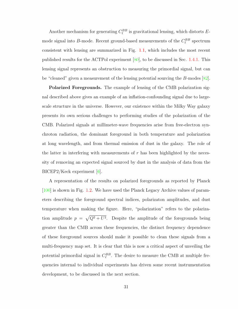
A representation of the results on polarized foregrounds as reported by Planck

[100] is shown in Fig. 1.2. We have used the Planck Legacy Archive values of param-

eters describing the foreground spectral indices, polarizaton amplitudes, and dust

temperature when making the figure. Here, “polarization” refers to the polariza-

tion amplitude p =√Q2 + U2. Despite the amplitude of the foregrounds being

greater than the CMB across these frequencies, the distinct frequency dependence

of these foreground sources should make it possible to clean these signals from a

multi-frequency map set. It is clear that this is now a critical aspect of unveiling the

potential primordial signal in CBB` . The desire to measure the CMB at multiple fre-

quencies internal to individual experiments has driven some recent instrumentation

development, to be discussed in the next section.

31

Figure 1.2: Brightness temperature in Raleigh-Jeans units of the two dominantsources of polarized foregrounds as measured by Planck [100]. “Polarization” hererefers to the polarization amplitude p =

√Q2 + U2. Here we assume a power law

index βs for synchrotron of -3, a greybody spectrum for thermal dust with dust tem-perature Td = 21 and index βd = 2.5, and a CMB temperature TCMB = 2.73 K. Thedust and synchrotron amplitudes come from Table 5 in Ref. [100]. We approximatethe RMS value of the CMB polarization anisotropies as 0.55 µK. It is apparent thatthe foregrounds dominate the overall CMB polarization signal across the entire rangeof frequencies, which span the Planck channels, but that the foregrounds have distinctfrequency dependence as compared to the CMB. This figure is inspired by Fig. 51from the reference.

1.3 Instrumentation for CMB Polarimetry

As elaborated above, the anisotropy signals we intend to study in the CMB are minute

when compared to the blackbody emission spectrum of the background at 2.73 K. Ad-

ditionally, they can be masked by astrophysical foregrounds that require sophisticated

analyses to remove. In order to recover the non-galactic anisotropy signal, extremely

sensitive receivers must be coupled to wide field-of-view, high-throughput telescope

optics, while also considering many types of complex instrumental systematic errors

32

in the design. In this section, we discuss developments in CMB instrumentation which

have enabled the ever-improving sensitivity of CMB instrumentation. As we proceed,

relevant instrumental systematics will be discussed.

1.3.1 Telescope Designs

High-throughput telescope designs, where throughput equals AΩ, with A the effective

area and Ω the solid angle over which the apertue illuminates the effective area, have

been devised for CMB telescopes from among a few fundamental designs. Reflector

designs can be well suited to experiments designed to be sensitive to small scales,

where refracting optical elements are often too large to be reliably fabricated. Off-

axis Gregorian designs avoid losing field-of-view to optical elements in the path of light

while maintaining good systematics [91]; crossed-Dragone designs satisfy conditions

which ensure minimal polarization systematics (mainly, the cross-polarization) [87]

[24]. Refractor designs are also in use for telescopes with larger beam size [1] [107] and

as part of reimaging optics in large-aperture telescopes [122]. Examples of instruments

using both reflector designs mentioned above will be discussed in Sec. 1.4.

1.3.2 Cold and Warm Optical Elements

The position of the focus and/or f#, where the latter is the ratio of the focal length

of the telescope to the aperture diameter, of a particular reflector design is often

not well-suited to coupling to the detector array. Reimaging optics are then used,

as these enable control of coupling between arrays of detectors and the telescope

itself. Making these elements cryogenic to reduce loss, and using high refractive-

index materials to make the receiver compact and reduce emission from the thinner

lenses thus designed, is a major focus of CMB instrumentation work. Development of

silicon [18] and alumina [1] lenses has enabled receiver designs which take advantage

of high-performing arrays and telescopes.

33

Additional optical elements in the cold stages of a receiver include IR-blocking fil-

ters, the most common being metal-mesh patterned onto millimeter wave-transparent

plastics [123]. These can be though of as optical low-pass filters. Additionally, this

technique can be used for band definition. A metal-mesh filter suspended in front of a

detector array can define the bandpass or the upper band edge to which the detector

will be sensitive. In the latter case, the lower band edge can then be defined by some

waveguide-like element, or by on-wafer transmission-line filters.

Finally, the use of polarization modulation as a systematic control element has be-

come an important consideration for CMB experiments in search of B-mode signals,

or other polarization signatures at degree angular scales and above. Once it is decided

to peform such modulation, the use of a half-wave plate (HWP), either stepped or

continuously-rotating, can be compared to other modulators, variable-delay polariza-

tion modulators (VPM) [49] or even rapid rotation of the telescope boresight [93].

We will discuss the use of continuously-rotating HWPs (CRHWPs) throughout Ch.

4. Without modulation, it is difficult to account for and deproject the contamina-

tion sourced by combinations of low-frequency signals in the instrument and in the

atmosphere.

1.3.3 Milllimeter-Wave Focal Planes

The use of cryogenic detectors to improve detector sensitivity has led to major ef-

forts in CMB instrumentation and its coupling to advancing cryogenic technologies.

When incoherent detectors like bolometers can be held at low temperatures to reach

sufficently good sensitivity, they present an attractive technique for recording the

signals of the CMB. The generic scheme for a bolometer is discussed in Sec. 2.1.

Initial devices were based on doped semiconductors [85], but these evolved with the

implementation of sensitive temperature-sensitive resistors (thermistors) based on su-

34

perconductors [56] [73]. These latter were more easily multiplexed [19] [71], and have

been highly developed over the last ∼20 years.

Improvements to detector sensitivity well below the photon noise background,

considered as the sum of shot noise and coherent wave noise, do not improve the

overall sensitivity of a CMB instrument. Once this limit began to be achieved, the

paramount improvement for CMB-instrument focal planes became to place as many

background-limited detectors in a focal plane as possible. On the detector side of the

instrumentation, this necessitated:

• dense fabricaton of millimeter-wave structures and highly-uniform detectors on

silicon substrates;

• multiplexing techniques able to scale to readout of these dense arrays without

overloading the cryogenic stages of the receivers;

• high-yield array assembly techniques to assure that the maximum number of

detectors are usable in the field.

Throughout this process, requirements on device sensitivity (i.e. reaching the

background limit of photon-induced noise) have been balanced against the need for

detectors to operate as stably and linearly as possible. As this work discusses, super-

conducting sensors in most CMB experiments today, especially ground-based experi-

ments, are in complex thermal environments and can only be treated as approximately

linear. Their electrical readout is also sensitive to possible oscillatory effects which

must be accounted for in the design.

Not yet discussed are the on-chip millimeter-wave transmission and filtering el-

ements, which have been critical in enabling more control over the definition of

millimeter-wave bands over which incoherent detectors like bolometers can absorb

power. In addition, such elements can be used to define multiple sub-bands after the

millimeter-wave signal is coupled to the detector arrays via superconducting anten-

35

nae [86] [92] [66]. Such “multichroic” designs have arisen in response to the enhanced

understanding of the strength and complexity of foreground signals, in addition to

their ability to maximize use of the limited focal plane area. These foregrounds, as

well as any time-varying sources of sky signal, are best constrained and removed by

simultaneous measurement across multiple frequency bands, which is most compactly

performed in instruments featuring multichroic focal planes.

1.4 CMB Experiments in this Work

In this section, we introduce the experiments that are studied in the body of this

work. Each features a millimeter-wave reflector-design telescope, but there are many

differencess in their design and history. We seek to provide the relevant background

for the chapters dealing with work on the Atacama Cosmology Telescope (ACT) [Chs.

3, 4] and the Atacama B-Mode Search (ABS) [Ch. 5]. We feature citations to the

main results achieved by these experiments where appropriate.

1.4.1 Atacama Cosmology Telescope

ACT is a two-reflector millimeter-wave telescope with an off-axis Gregorian design,

a ∼6 m primary mirror, and a 2 m secondary mirror. This gives a beam full-width

half-maximum of 1.4 arcmin at 150 GHz, and a field of view of 3 as defined by a cold

aperture stop inside the receiver. Details of the optical design can be found in Ref.

[34]. Sited at 5190 m in the Atacama Desert near Cerro Toco, Chile, the mirrors of

the telescope are fixed to a frame movable in azimuth and elevation, with a co-moving

metallic ground-screen also built on this frame. This robotic mount, fabricated by

Kuka Robotics1 allows the telescope to slew rapidly in azimuth, with a rate during

observations of 1.5/s [119].

1https://www.kuka.com/en-us

36

Since the first camera, the Millimeter Bolometric Array Camera (MBAC), was

mounted on the telescope in 2007, reimaging optics have been used in the cryogenic

receiver to maximize the number of sensors in the telescope focal plane. These reimag-

ing optics are placed in “optics tubes” within the body of a larger cryogenic receiver.

Elements in the optics tubes are cryogenically cooled, with IR-blocking and GHz low-

pass filters at warmer (40 K) stages cooled by pulse tube coolers, cryogenic lenses at

liquid helium temperature (4 K) or lower also cooled by closed-cycle coolers, and a

Lyot stop defining the illumination of the array from the telescope focus. In MBAC,

the cryogenic arrays of “pop-up” bolometers [83] were cooled by helium-3 sorption

fridges [72] [119] to a base temperature of 300 mK. These were single-color arrays

with bandpasses centered at 145, 217, and 265 GHz.

The MBAC arrays were not polarization-sensitive, but coupled to free space using

an absorber structure. In the ACT Polarimeter (ACTPol) receiver upgrade, a new

cryogenic receiver was designed to accomodate a custom dilution refrigerator (DR)

designed by Janis2. Details on this new cryogenic platform may be found in Ref. [122].

We emphasize that the three-tube configuration used for MBAC was maintained in

the ACTPol upgrade. New lenses featuring metamaterial AR coatings were developed

for these tubes [18].

In addition, given the greater base temperature and cooling power of the DR,

more detectors could be read out and run with lower bath temperatures, enhancing

their sensitivity. The resulting set of arrays featured pixels developed through the

TRUCE collaboration [131], which developed a planar orthomode transducer (OMT)

made from superconducting niobium fed by a corrugated silicon platelet feedhorn.

The OMT enabled the TRUCE pixels to define the polarization sensitivity of a given

bolometer. The TRUCE design was also used in science-grade arrays for SPTpol [2]

and ABS [28].

2225 Wildwood Ave, Woburn, MA 01801

37

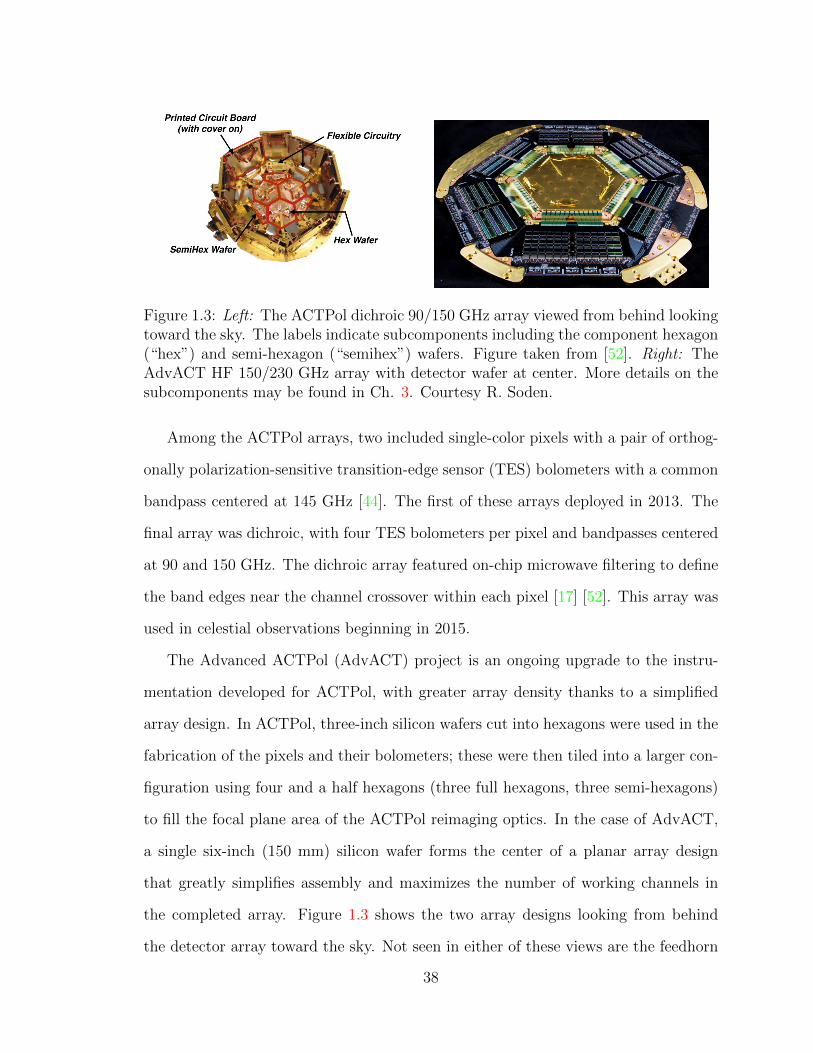
Figure 1.3: Left: The ACTPol dichroic 90/150 GHz array viewed from behind lookingtoward the sky. The labels indicate subcomponents including the component hexagon(“hex”) and semi-hexagon (“semihex”) wafers. Figure taken from [52]. Right: TheAdvACT HF 150/230 GHz array with detector wafer at center. More details on thesubcomponents may be found in Ch. 3. Courtesy R. Soden.

Among the ACTPol arrays, two included single-color pixels with a pair of orthog-

onally polarization-sensitive transition-edge sensor (TES) bolometers with a common

bandpass centered at 145 GHz [44]. The first of these arrays deployed in 2013. The

final array was dichroic, with four TES bolometers per pixel and bandpasses centered

at 90 and 150 GHz. The dichroic array featured on-chip microwave filtering to define

the band edges near the channel crossover within each pixel [17] [52]. This array was

used in celestial observations beginning in 2015.

The Advanced ACTPol (AdvACT) project is an ongoing upgrade to the instru-

mentation developed for ACTPol, with greater array density thanks to a simplified

array design. In ACTPol, three-inch silicon wafers cut into hexagons were used in the

fabrication of the pixels and their bolometers; these were then tiled into a larger con-

figuration using four and a half hexagons (three full hexagons, three semi-hexagons)

to fill the focal plane area of the ACTPol reimaging optics. In the case of AdvACT,

a single six-inch (150 mm) silicon wafer forms the center of a planar array design

that greatly simplifies assembly and maximizes the number of working channels in

the completed array. Figure 1.3 shows the two array designs looking from behind

the detector array toward the sky. Not seen in either of these views are the feedhorn

38

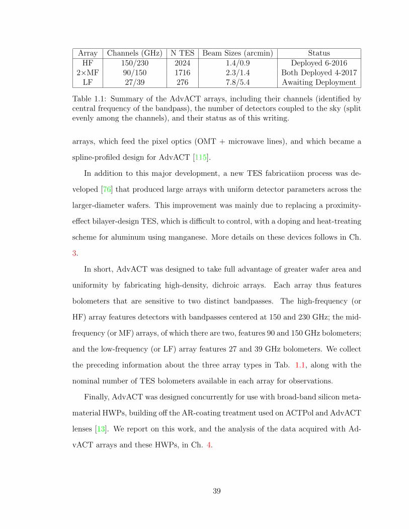
Array Channels (GHz) N TES Beam Sizes (arcmin) StatusHF 150/230 2024 1.4/0.9 Deployed 6-2016

2×MF 90/150 1716 2.3/1.4 Both Deployed 4-2017LF 27/39 276 7.8/5.4 Awaiting Deployment

Table 1.1: Summary of the AdvACT arrays, including their channels (identified bycentral frequency of the bandpass), the number of detectors coupled to the sky (splitevenly among the channels), and their status as of this writing.

arrays, which feed the pixel optics (OMT + microwave lines), and which became a

spline-profiled design for AdvACT [115].

In addition to this major development, a new TES fabricatiion process was de-

veloped [76] that produced large arrays with uniform detector parameters across the

larger-diameter wafers. This improvement was mainly due to replacing a proximity-

effect bilayer-design TES, which is difficult to control, with a doping and heat-treating

scheme for aluminum using manganese. More details on these devices follows in Ch.

3.

In short, AdvACT was designed to take full advantage of greater wafer area and

uniformity by fabricating high-density, dichroic arrays. Each array thus features

bolometers that are sensitive to two distinct bandpasses. The high-frequency (or

HF) array features detectors with bandpasses centered at 150 and 230 GHz; the mid-

frequency (or MF) arrays, of which there are two, features 90 and 150 GHz bolometers;

and the low-frequency (or LF) array features 27 and 39 GHz bolometers. We collect

the preceding information about the three array types in Tab. 1.1, along with the

nominal number of TES bolometers available in each array for observations.

Finally, AdvACT was designed concurrently for use with broad-band silicon meta-

material HWPs, building off the AR-coating treatment used on ACTPol and AdvACT

lenses [13]. We report on this work, and the analysis of the data acquired with Ad-

vACT arrays and these HWPs, in Ch. 4.

39

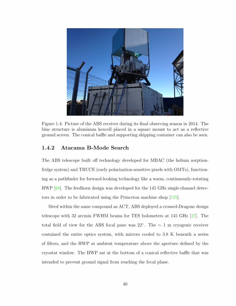
Figure 1.4: Picture of the ABS receiver during its final observing season in 2014. Theblue structure is aluminum hexcell placed in a square mount to act as a reflectiveground screen. The conical baffle and supporting shipping container can also be seen.

1.4.2 Atacama B-Mode Search

The ABS telescope built off technology developed for MBAC (the helium sorption-

fridge system) and TRUCE (early polarization-sensitive pixels with OMTs), function-

ing as a pathfinder for forward-looking technology like a warm, continuously-rotating

HWP [68]. The feedhorn design was developed for the 145 GHz single-channel detec-

tors in order to be fabricated using the Princeton machine shop [125].

Sited within the same compound as ACT, ABS deployed a crossed-Dragone design

telescope with 32 arcmin FWHM beams for TES bolometers at 145 GHz [27]. The

total field of view for the ABS focal pane was 22. The ∼ 1 m cryogenic receiver

contained the entire optics system, with mirrors cooled to 3.8 K beneath a series

of filters, and the HWP at ambient temperature above the aperture defined by the

cryostat window. The HWP sat at the bottom of a conical reflective baffle that was

intended to prevent ground signal from reaching the focal plane.

40

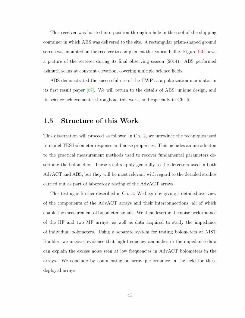
This receiver was hoisted into position through a hole in the roof of the shipping

container in which ABS was delivered to the site. A rectangular prism-shaped ground

screen was mounted on the receiver to complement the conical baffle. Figure 1.4 shows

a picture of the receiver during its final observing season (2014). ABS performed

azimuth scans at constant elevation, covering multiple science fields.

ABS demonstrated the successful use of the HWP as a polarization modulator in

its first result paper [67]. We will return to the details of ABS’ unique design, and

its science achievements, throughout this work, and especially in Ch. 5.

1.5 Structure of this Work

This dissertation will proceed as follows: in Ch. 2, we introduce the techniques used

to model TES bolometer response and noise properties. This includes an introducton

to the practical measurement methods used to recover fundamental parameters de-

scribing the bolometers. These results apply generally to the detectors used in both

AdvACT and ABS, but they will be most relevant with regard to the detailed studies

carried out as part of laboratory testing of the AdvACT arrays.

This testing is further described in Ch. 3. We begin by giving a detailed overview

of the components of the AdvACT arrays and their interconnections, all of which

enable the measurement of bolometer signals. We then describe the noise performance

of the HF and two MF arrays, as well as data acquired to study the impedance

of individual bolometers. Using a separate system for testing bolometers at NIST

Boulder, we uncover evidence that high-frequency anomalies in the impedance data

can explain the excess noise seen at low frequencies in AdvACT bolometers in the

arrays. We conclude by commenting on array performance in the field for these

deployed arrays.

41

As part of the season following the deployment of the two MF arrays, three HWPs

designed for the appropriate bands of each array were rotated continuously in order

to modulate incoming polarization to the AdvACT arrays. We describe the principle

of this technique, its history with ABS, and preliminary studies of its performance in

the AdvACT project. This concludes our look into AdvACT specifically.

With regard to ABS, we present the maximum-likelihood analysis implemented

to produce the final EE and BB bandpower error bars, as well as the published

likelihood on the tensor-to-scalar ratio r. We introduce the MASTER pipeline [51]

used in ABS to produce many Monte Carlo simulations that makes it possible to

accurately model the statistics of crucial variables like r by efficiently computing

hundreds of experimental simulations.

Finally, we conclude with a presentation of ongoing work on developing an un-

derstanding of, and tools for dealing with, the nonlinearity of TES bolometer signals

in response to slowly-varing, large amplitude fluctuations sourced by instrument 1/f

noise. These preliminary results include simulations indicating that this effect can

leak large-scale models, and excess noise, from intensity to polarization during CMB

observations. We point to ways to track the susceptibility of a given array of bolome-

ters over time using standard bolometer calibration procedures, and then conclude.

42

Chapter 2

Electrothermal Models of

Bolometers

In this chapter, we present the concepts and the first-order coupled differential equa-

tions describing the electrothermal behavior of their electrically-biased thermal sen-

sors. We begin with general concepts relevant to all bolometer thermal architectures,

then focus on the case relevant to AdvACT transition-edge sensor (TES) bolometers.

2.1 Basic Model

The bolometric detection concept [70] can be summarized as the detection of thermal

power produced by incident electromagnetic (EM), or optical, power. This process

is broadband and can easily record brightness temperatures, as compared to photon

fluxes.

Absorbing elements to convert optical power into thermal power can be designed

across much of the electromagnetic spectrum, though bolometers are most easily

optimized from millimeter-wave to infrared wavelengths [105], where the limiting

sources of noise arising in the bolometer have been well-understood for the past 35

years [84]. At high energies, measuring individual photon pulses and converting these

43

to photon energies may be more appropriate, and the bolometer becomes a calorimeter

[43] [62].

Regardless of the frequency band over which the bolometer is sensitive, these de-

vices can usually be fully described by i) their thermal architecture and ii) their elec-

trical architecture. The former is generated through a lumped-element represetation

of heat flow in the bolometer, with distinct thermal “blocks” representing isothermal

components of the bolometer with heat capacities Ci and temperatures Ti. The latter

generally applies to a distinct sensor, usually a thermistor (temperature-sensitive re-

sistor), which converts the bolometer thermal signal into an electrical signal. In both

cases, we use circuit diagrams to represent the relevant aspects of each architecture.

Figure 2.1 shows the simplest thermal circuit diagram, a single block with tem-

perature T and heat capacity C. The figure also shows a single resistive element (R)

schematically representing an unspecified electrical circuit. As this figure indicates,

the two circuits are coupled due to the thermal power Pbias produced by current flow

through the thermistor. In order to thermalize the sum of Pbias and the optical signal

Pγ, heat flows across the thermal impedance connecting the thermal block to a bath

at temperature Tbath < T . In the analysis of small transient signals, we will label this

thermal impedance as a thermal conductance G to the bath. However, for constant

Pγ and Pbias, we instead refer to a power to the bath Pbath related to G and satisfying

the following equation:

Pbath = Pγ + Pbias (2.1)

which we refer to as the “power balance equation.” This equation forms the basis for

the linear, small-signal model which allows us to describe the bolometer response to

electrical and optical excitations given a steady-state Pbias and predefined Pbath.

In essence, the bolometer always satisfies this equation. In the appropriate small-

signal limit, expansion of the nonlinearities hiding in terms like Pbias to first order

result in a set of coupled equations, where the coupling occurs due to the thermistor

44

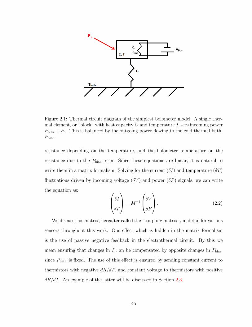
Figure 2.1: Thermal circuit diagram of the simplest bolometer model. A single ther-mal element, or “block” with heat capacity C and temperature T sees incoming powerPbias + Pγ. This is balanced by the outgoing power flowing to the cold thermal bath,Pbath.

resistance depending on the temperature, and the bolometer temperature on the

resistance due to the Pbias term. Since these equations are linear, it is natural to

write them in a matrix formalism. Solving for the current (δI) and temperature (δT )

fluctuations driven by incoming voltage (δV ) and power (δP ) signals, we can write

the equation as: δIδT

= M−1

δVδP

. (2.2)

We discuss this matrix, hereafter called the “coupling matrix”, in detail for various

sensors throughout this work. One effect which is hidden in the matrix formalism

is the use of passive negative feedback in the electrothermal circuit. By this we

mean ensuring that changes in Pγ an be compensated by opposite changes in Pbias,

since Pbath is fixed. The use of this effect is ensured by sending constant current to

thermistors with negative dR/dT , and constant voltage to thermistors with positive

dR/dT . An example of the latter will be discussed in Section 2.3.

45

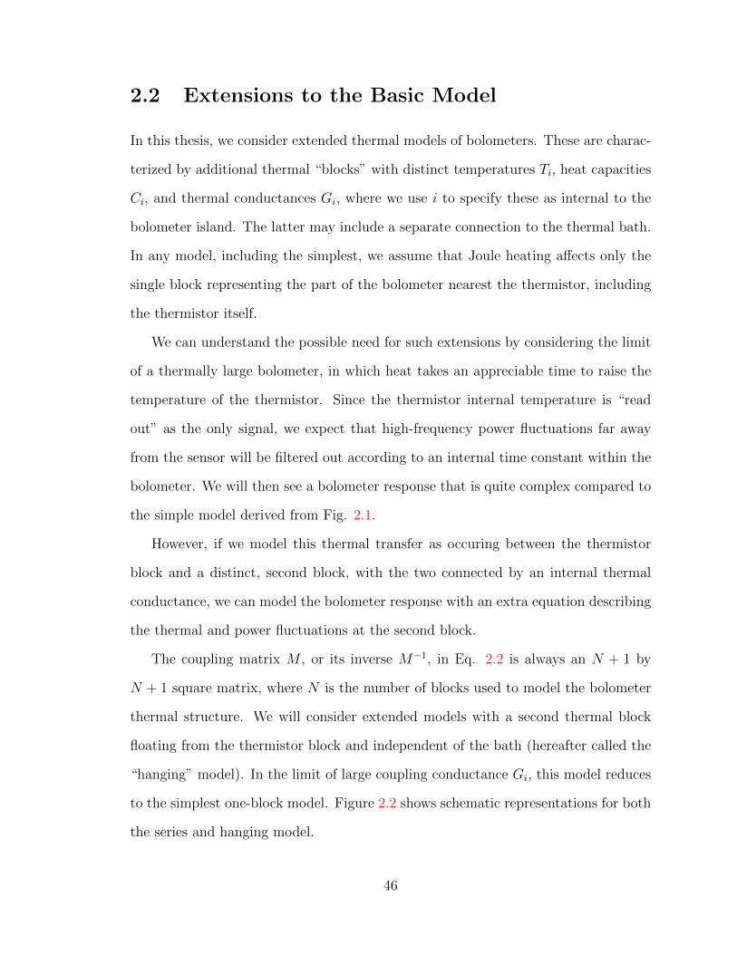
2.2 Extensions to the Basic Model

In this thesis, we consider extended thermal models of bolometers. These are charac-

terized by additional thermal “blocks” with distinct temperatures Ti, heat capacities

Ci, and thermal conductances Gi, where we use i to specify these as internal to the

bolometer island. The latter may include a separate connection to the thermal bath.

In any model, including the simplest, we assume that Joule heating affects only the

single block representing the part of the bolometer nearest the thermistor, including

the thermistor itself.

We can understand the possible need for such extensions by considering the limit

of a thermally large bolometer, in which heat takes an appreciable time to raise the

temperature of the thermistor. Since the thermistor internal temperature is “read

out” as the only signal, we expect that high-frequency power fluctuations far away

from the sensor will be filtered out according to an internal time constant within the

bolometer. We will then see a bolometer response that is quite complex compared to

the simple model derived from Fig. 2.1.

However, if we model this thermal transfer as occuring between the thermistor

block and a distinct, second block, with the two connected by an internal thermal

conductance, we can model the bolometer response with an extra equation describing

the thermal and power fluctuations at the second block.

The coupling matrix M , or its inverse M−1, in Eq. 2.2 is always an N + 1 by

N + 1 square matrix, where N is the number of blocks used to model the bolometer

thermal structure. We will consider extended models with a second thermal block

floating from the thermistor block and independent of the bath (hereafter called the

“hanging” model). In the limit of large coupling conductance Gi, this model reduces

to the simplest one-block model. Figure 2.2 shows schematic representations for both

the series and hanging model.

46

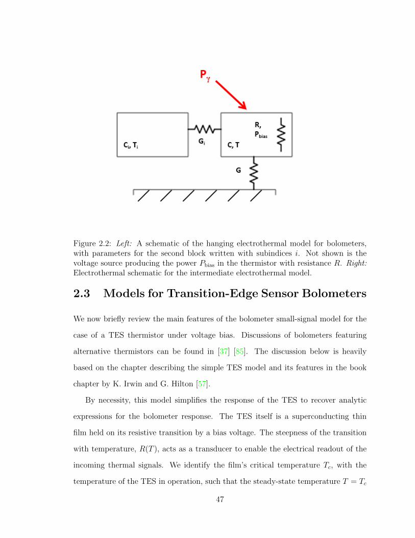
Figure 2.2: Left: A schematic of the hanging electrothermal model for bolometers,with parameters for the second block written with subindices i. Not shown is thevoltage source producing the power Pbias in the thermistor with resistance R. Right:Electrothermal schematic for the intermediate electrothermal model.

2.3 Models for Transition-Edge Sensor Bolometers

We now briefly review the main features of the bolometer small-signal model for the

case of a TES thermistor under voltage bias. Discussions of bolometers featuring

alternative thermistors can be found in [37] [85]. The discussion below is heavily

based on the chapter describing the simple TES model and its features in the book

chapter by K. Irwin and G. Hilton [57].

By necessity, this model simplifies the response of the TES to recover analytic

expressions for the bolometer response. The TES itself is a superconducting thin

film held on its resistive transition by a bias voltage. The steepness of the transition

with temperature, R(T ), acts as a transducer to enable the electrical readout of the

incoming thermal signals. We identify the film’s critical temperature Tc, with the

temperature of the TES in operation, such that the steady-state temperature T = Tc

47

in all bolometer equations involving TES thermistors. We are validated in doing

this due to the narrow range (O(1%) of Tc) of temperatures within the transition.

Another important value for these devices is their normal state resistance, RN, which

determines the scale of the thermistor resistance in operation R. We often write

achieved values of R in operation as fractions or percentages of RN.

When operating TESes in their transition, a stiff bias voltage provides the negative

feedback required to use these high open loop gain sensors without railing, which in

this case is termed “thermal runaway.” A heuristic to see how bias voltage provides

the correct feedback is to consider an increase in optical power, which increases the

sensor temperature. This increase in TES temperature increases the TES resistance,

which reduces the Joule heating Pbias since Pbias = V 2/R, where V is the constant

bias voltage.

For our purposes, the TES is represented by the following equation, describing the

resistance fluctuations δR induced by thermal fluctuations δT and current fluctuations

δI:

δR =R

TαδT +

R

IβδI. (2.3)

From the above one can see that α = dln(R)dln(T )

and β = dln(R)dln(I)

. These parameters, also

called the “sensitivites” of the TES to temperature and current fluctuations for α

and β respectively, are instrumental in determining the overall detector sensitivity

and stability within the coupled electrothermal equations.

We now discuss the expressions for the thermal and electrical architectures of a

simple TES bolometer. The first equation expands the power balance equation to

first order in δT , where the time-dependent temperature T (t) = Tc + δT (t). We also

add a term for power induced by the changing temperature of the heat capacity C:

CdδT

dt= V (2 + β)δI + (Pbiasα/Tc −G)δT + δPγ, (2.4)

48

where all δ terms are time-dependent, the conductance G = dPsat/dT |Tc , and Psat

is defined as the total power incident on the bolometer (the sum of Pbias and Pγ)

required to drive the detector into its normal state. Looking back at Eq. 2.1, we see

that Psat is then equal to the term Pbath. The labeling of Pbath as Psat will apply to all

discussions of TES bolometers. For definiteness, we specify the common power-law

model used to describe Psat that defines the parameters determining G:

Psat = κ(T nc − T nbath) (2.5)

so that G = nκT n−1c . We note, finally, that the sharpness of the resistive transition in

TES temperature also leads to a very sharp R(P ) curve. Therefore, the total power

on the TES during operation is usually within 10% Psat.

We now define an open loop gain under constant-current (hard current bias) con-

ditions using the term multiplying δT in Eq. 2.4: The result will be hereafter referred

to as “loop gain” L :

L =Pbiasα

GT. (2.6)

For large loop gains, the TES sensor has a faster and more linear response across a

wider range of signal amplitudes. This is not evident from the bare equations, but

results from considering some limiting cases of the equations above. For instance,

under hard current bias, δI goes to zero and the time-domain equation for the TES

temperature fluctuation is directly integrable. Instead of a bare thermal time constant

τ = C/G, which would occur for Pbias = L = 0, we define a new time constant:

τI =τ

(1−L ). (2.7)

Based on these equations, TES bolometers under electrothermal feedback have an

“effective conductance” equal to G(1−L ).

49

δV

V

RL

R

L

Figure 2.3: A schematic of the conceptual TES electrical bias circuit used in Eq. 2.8.Here, RL ∼ Rsh. A more detailed circuit appears in Fig. 3.3.

In the electrical circuit, we account for a TES under a voltage bias V with fluctu-

ations δV (t). The TES is in series with an impedance RL, the Thevenin-equivalent

impedance of other elements in the TES bias circuit, and an inductance L:

LdδI

dt= − [RL +R(1 + β)] δI − V α

TδT + δV. (2.8)

These components are schematically represented in Fig. 2.3.

This equation by itself can be used to define a new time constant in the sys-

tem when we set δT = 0. In this case, the equation for the time-domain behavior

of the current fluctations is independent of δT . We then define the time constant

determining the decay of current in the TES bias circuit as a response to some δV :

τel =L

RL +R(1 + β). (2.9)

With these equations, we can now define the coupling matrix M for the simple

model of the TES bolometer. We write these equations keeping the inductance L and

heat capacity C as coefficients of the first-derivative terms, as opposed to the format

50

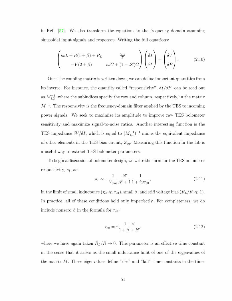
in Ref. [57]. We also transform the equations to the frequency domain assuming

sinusoidal input signals and responses. Writing the full equations:

iωL+R(1 + β) +RLV αT

−V (2 + β) iωC + (1−L )G

δIδT

=

δVδP

. (2.10)

Once the coupling matrix is written down, we can define important quantities from

its inverse. For instance, the quantity called “responsivity”, δI/δP , can be read out

as M−11,2 , where the subindices specify the row and column, respectively, in the matrix

M−1. The responsivity is the frequency-domain filter applied by the TES to incoming

power signals. We seek to maximize its amplitude to improve raw TES bolometer

sensitivity and maximize signal-to-noise ratios. Another interesting function is the

TES impedance δV/δI, which is equal to (M−11,1 )−1 minus the equivalent impedance

of other elements in the TES bias circuit, Zeq. Measuring this function in the lab is

a useful way to extract TES bolometer parameters.

To begin a discussion of bolometer design, we write the form for the TES bolometer

responsivity, sI , as:

sI ∼ −1

Vbias

L

L + 1

1

1 + iωτeff

, (2.11)

in the limit of small inductance (τel τeff), small β, and stiff voltage bias (RL/R 1).

In practice, all of these conditions hold only imperfectly. For completeness, we do

include nonzero β in the formula for τeff:

τeff = τ1 + β

1 + β + L. (2.12)

where we have again taken RL/R → 0. This parameter is an effective time constant

in the sense that it arises as the small-inductance limit of one of the eigenvalues of

the matrix M . These eigenvalues define “rise” and “fall” time constants in the time-

51

domain response of the TES current and temperature to a unit impulse. We skip

these details and direct interested readers once again to [57].

In the AdvACT project, we used the approximate expressions above describing

an “ideal” TES bolometer to understand trade-offs in design. We reiterate that our

idealization goes beyond assuming the simplest electrothermal architecture of the

bolometer, to assuming ideal bias conditions (i.e. no terms depending on RL) and

insensitivity to bias current fluctuations (setting β = 0). For such a device, designing

a bolometer proceeds roughly as the following:

• Determine the expected power background on the device Pload due to incoming

radiation and select a Psat target by multiplying Pload by a safety factor (∼ 2 to

3).

• Select a critical temperature for the TES that, for fixed Psat, optimizes the TES

sensitivity.

• Add a tunable-thickness metal film to the bolometer to control the heat capacity

of the TES and minimize the time constant τeff for fast TES response without

violating the bound τel < 5.8τeff required for TES electrical stability [45].

The above criteria then determine many of the crucial parameters for an array

of TES bolometers: their Psat values, their critical temperatures, and their time

constants. Though not mentioned above, the normal resistance RN is an important

overall calibration factor that determines the amplitude of the responsivity and plays

into expected TES noise behavior.

We conclude this section by providing the matrix equation describing the hanging

two-block electrothermal model from Section 2.2. In the 3×3 matrix below, the new

parameters Ci and Gi fully parametrize the new components of the extended model,

52

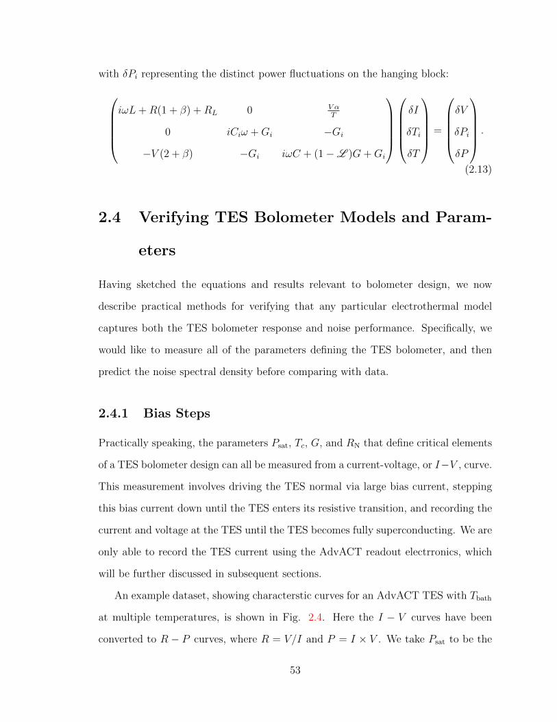
with δPi representing the distinct power fluctuations on the hanging block:

iωL+R(1 + β) +RL 0 V α

T

0 iCiω +Gi −Gi

−V (2 + β) −Gi iωC + (1−L )G+Gi

δI

δTi

δT

=

δV

δPi

δP

.

(2.13)

2.4 Verifying TES Bolometer Models and Param-

eters

Having sketched the equations and results relevant to bolometer design, we now

describe practical methods for verifying that any particular electrothermal model

captures both the TES bolometer response and noise performance. Specifically, we

would like to measure all of the parameters defining the TES bolometer, and then

predict the noise spectral density before comparing with data.

2.4.1 Bias Steps

Practically speaking, the parameters Psat, Tc, G, and RN that define critical elements

of a TES bolometer design can all be measured from a current-voltage, or I−V , curve.

This measurement involves driving the TES normal via large bias current, stepping

this bias current down until the TES enters its resistive transition, and recording the

current and voltage at the TES until the TES becomes fully superconducting. We are

only able to record the TES current using the AdvACT readout electrronics, which

will be further discussed in subsequent sections.

An example dataset, showing characterstic curves for an AdvACT TES with Tbath

at multiple temperatures, is shown in Fig. 2.4. Here the I − V curves have been

converted to R − P curves, where R = V/I and P = I × V . We take Psat to be the

53

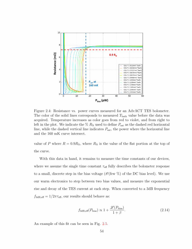
Pbias (pW)

Re

sist

ance

(mΩ

)0.9 RN

Psat at 160 mK

Figure 2.4: Resistance vs. power curves measured for an AdvACT TES bolometer.The color of the solid lines corresponds to measured Tbath value before the data wasacquired. Temperature increases as color goes from red to violet, and from right toleft in the plot. We indicate the % RN used to define Psat as the dashed red horizontalline, while the dashed vertical line indicates Psat, the power where the horizontal lineand the 160 mK curve intersect.

value of P where R = 0.9RN, where RN is the value of the flat portion at the top of

the curve.

With this data in hand, it remains to measure the time constants of our devices,

where we assume the single time constant τeff fully describes the bolometer response

to a small, discrete step in the bias voltage (O(few %) of the DC bias level). We use

our warm electronics to step between two bias values, and measure the exponential

rise and decay of the TES current at each step. When converted to a 3dB frequency

f3dB,eff = 1/2πτeff, our results should behave as:

f3dB,eff(Pbias) ∝ 1 +L (Pbias)

1 + β. (2.14)

An example of this fit can be seen in Fig. 2.5.

54

The constant of proportionality in the above is purely thermal f3dB,0 = 1/2πτ .

If we multiply through by this parameter, we find a line with intercept f3dB,0 and

a slope that depends on a combination of α, β, Tc, G, and C. We assume the last

three parameters have already been measured. In this case, the slope may be used

to measure the quantity α/(1 + β). However, this assumes that these parameters

are not themselves a function of Pbias, which we know to be false in principle. This

approximate expression is thus not able to distinguish the relative sizes of α and β,

nor do we expect it to be accurate across wide ranges of Pbias.

2.4.2 TES Bolometer Impedance

A more complete understanding of the TES response can be gleaned via measurements

of the electrical impedance, ZTES of the sensor. This general technique has been

applied before to studies of bolometer electrothermal models [37] [133] [81]. We

Figure 2.5: Example linear fit to f3dB versus Pbias for an early AdvACT test device.Figure courtesy S.P. Ho, and appeared as part of poster presentation at 36th ESAAntenna (see 0.1).

55

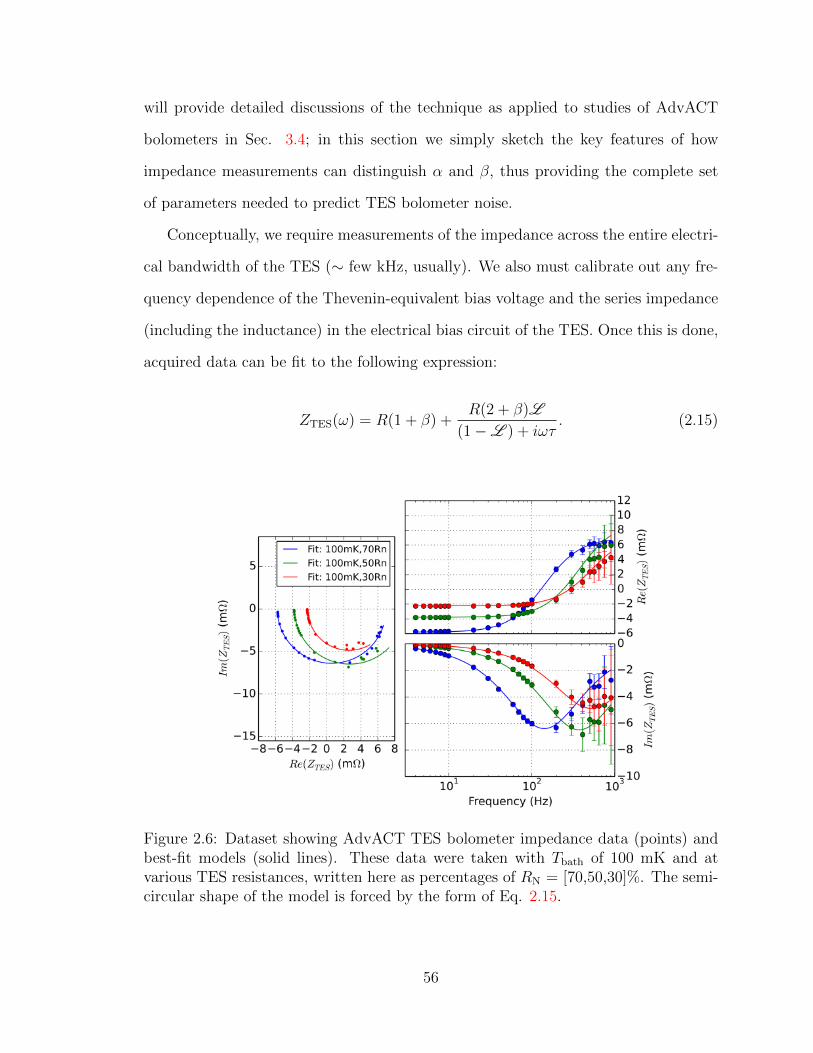
will provide detailed discussions of the technique as applied to studies of AdvACT

bolometers in Sec. 3.4; in this section we simply sketch the key features of how

impedance measurements can distinguish α and β, thus providing the complete set

of parameters needed to predict TES bolometer noise.

Conceptually, we require measurements of the impedance across the entire electri-

cal bandwidth of the TES (∼ few kHz, usually). We also must calibrate out any fre-

quency dependence of the Thevenin-equivalent bias voltage and the series impedance

(including the inductance) in the electrical bias circuit of the TES. Once this is done,

acquired data can be fit to the following expression:

ZTES(ω) = R(1 + β) +R(2 + β)L

(1−L ) + iωτ. (2.15)

Figure 2.6: Dataset showing AdvACT TES bolometer impedance data (points) andbest-fit models (solid lines). These data were taken with Tbath of 100 mK and atvarious TES resistances, written here as percentages of RN = [70,50,30]%. The semi-circular shape of the model is forced by the form of Eq. 2.15.

56

Derivation of this result in Ref. [57] proceeds, as mentioned above, by studying

the component M−11,1 component of the inverse of the simple model’s coupling matrix

M . Qualitatively, the resulting equation describes a semicircle in the lower half-plane

of the complex plane. In the ω → ∞ case, the TES responds as a resistor with its

dynamic resistance at constant temperature dV/dI|T = R(1 + β) instead of R. At

low frequencies ω → 0, in the limit of large L , we recover ZTES = −R From these

twin limits, the parameter β can be recovered. If R is known beforehand, from an

I − V curve for example, then only the high-frequency limit is required.

Once β is measured, we can extract the constant-current time constant τI by

recognizing that the imaginary part of the impedance has a minimum at the frequency

ωminτI = 1. This quantity is degenerate in the loop gain (or α if we assume the other

parameters have been measured via I−V curves) and the heat capacity C. However,

L also factors into the radius of the semicircle, a shape factor which is independent

of the way the semicircle is swept out versus frequency. So we may recover β, α, and

C separately, with some non-negligible covariance between them. As an example,

Fig. 2.6 shows an example impedance data set and best-fit simple-model curve for an

AdvACT bolometer. These data are acquired for a constant Tbath at various fractions

of RN.

By doing this for various bath temperatures, or equivalently various Pbias, and at

various points on the TES transition, we may study how these parameters vary. At

any given point, we should expect that our set of parameters completely define the

electrothermal model, and thus any other dataset acquired for the devices. We choose

to study the validity of this assumption using noise data.

2.4.3 TES Bolometer Noise

In this subsection, we describe how to estimate the total noise generated by the TES

bolometer in order to confirm that the electrothermal model captures the frequency

57

dependence of this noise. For a simple TES bolometer, the sources of noise are usually

enumerated as:

• Johnson noise from the TES resistor, with a correction to the standard expres-

sion due to the R(I) function of the sensor: SVTES= 4kBTR(1 + 2β), where

kB is Boltzmann’s constant and SV refers to a noise voltage spectral density in

units of V 2/Hz;

• Johnson noise from the load resistance in series with the TES, SVL = 4kBTLRL,

where we set TL is to Tbath;

• Current noise in the amplification circuit, which we discuss in Section 3.4;

• Phonon noise due to the conductance G at temperature T , SPlink= 4kBGT

2flink,

where the units here are W 2/Hz, or noise power spectral density.

In reference to the diagram in Fig. 2.3, the Johnson voltage noise terms arise in series

with the TES and load resistor, respectively; the current noise is incoherently summed

at readout; and the phonon noise generates some spurious δI within the TES that

is read out. Both the TES Johnson noise and phonon noise terms contain nonequi-

librium corrections to the equilibrium noise quantities. These arise from the current

bias present in the TES and the thermal power flowing through the conductance G

during noise measurements, coupled to the nonlinearity of the quantities R(I) and

G(T ) [57].

As stated above, we measure the TES current using our readout system, and can

calibrate this to power units using an estimate for the responsivity. When studying

the noise spectrum, we prefer to work in terms of each noise source’s contribution

to the current noise, comparing their incoherent sum to the measured noise current.

Any deviations are then due either to i) errors in the sizes and frequency dependence

of the terms which convert voltage and power noises to current noise or ii) additional,

unmodeled noise sources.

58

We will now briefly describe the terms that convert the above quantities to current

noise, excepting the amplifier noise, which we take to be a current noise in series

with noise arising from the bolometer. We have already mentioned the responsivity

sI = δI/δP . The current noise contribution from phonon noise in the conductance G

is then SIlink= |sI |2SPlink

.

In order to convert the voltage noise terms sourced by the load resistance and the

TES itself, we use the expressions for the internal and external admittance, where

admittance is the inverse of electrical impedance. The impedance matrix Z can be

derived directly from the coupling matrix M once the source fluctuations (δV, δP )

have been converted to the conjugate forces (δV, δP/T ) of the fluctuation-dissipation

theorem. This requires dividing the terms in the second row of M by T [57].

The matrix thus formed is Zext, and defines the external admittance Y ext =

(Zext)−1. It is important to distinguish this from the internal impedance and ad-

mittance matrices, in which we must account for the work done on a voltage source

internal to the TES. The resulting change only applies to the 2, 1 element of Zext,

which becomes:

Z int2,1 = [I(RL −R) + iωLI]

1

T. (2.16)

This results from accounting for the noise voltage present in the TES electrical circuit

when calculating the Joule power dissipated in the TES. Rather than assuming some

form for this voltage, we set the power at the TES Pbias = IVTES = I (IR + Vnoise),

but replace the TES voltage multiplying I to the sum of the other voltages in the bias

circuit:

Pbias = I

(Vbias − IRL − L

dI

dt

), (2.17)

where Vbias is the Thevenin-equivalent bias voltage supplying the TES. Following

this expression, equation 2.16 arises as an expansion of the above expression for

I(t) = I + δI(t).

59

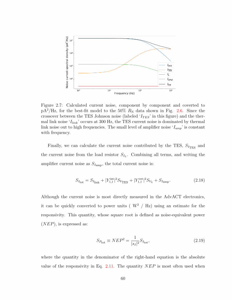
Figure 2.7: Calculated current noise, component by component and coverted topA2/Hz, for the best-fit model to the 50% RN data shown in Fig. 2.6. Since thecrossover between the TES Johnson noise (labeled ‘ITES’ in this figure) and the ther-mal link noise ‘Ilink’ occurs at 300 Hz, the TES current noise is dominated by thermallink noise out to high frequencies. The small level of amplifier noise ‘Iamp’ is constantwith frequency.

Finally, we can calculate the current noise contributed by the TES, SITESand

the current noise from the load resistor SIL . Combining all terms, and writing the

amplifier current noise as SIamp , the total current noise is:

SItot = SIlink+ |Y int

1,1 |2SVTES+ |Y ext

1,1 |2SVL + SIamp . (2.18)

Although the current noise is most directly measured in the AdvACT electronics,

it can be quickly converted to power units ( W2 / Hz) using an estimate for the

responsivity. This quantity, whose square root is defined as noise-equivalent power

(NEP ), is expressed as:

SPtot ≡ NEP 2 =1

|sI |2SItot , (2.19)

where the quantity in the denominator of the right-hand equation is the absolute

value of the responsivity in Eq. 2.11. The quantity NEP is most often used when

60

expressing the sensitivity of a TES. It expresses the EM signal size (in dimensions

of power) required to achieve a signal-to-noise ratio of 1. However, in the case when

the TES observes the sky, the photon noise term SPγ must be added to Eq. 2.19.

When we speak of a TES bolometer being “background-limited”, we mean that the

sum of terms in this equation is subdominant to the photon noise, so that the overall

detector NEP is dominanted by√SPγ .

To make the foregoing discussion more concrete, and to show the relative size of

these noise terms for AdvACT TES bolometers, Fig. 2.7 shows the individual current

noise terms as a function of frequency for all noise sources except photon shot noise,

which was not present for the dark measurements used to estimate these terms. The

parameters used to calculate the noise values, responsivity, and relevant components

of the admittance matrices are all taken from the best-fit results of the impedance

data shown in Fig. 2.6 for 50% RN.

We can see that the dominant term for dark noise data is SIlink, especially at

frequencies below f3dB,eff. We note that we have here set the nonlinear term flink = 1.

Johnson noise from the TES is relevant at higher frequencies, but is strongly reduced

by electrothermal feedback due to the the 1/L dependence hidden in |Y int1,1 |2.

To summarize, in this subsection we have introduced the noise sources contributing

to TES bolometer current and power noise. We have introduced the concepts of

internal and external admittances and how they differ, leading to different frequency

dependence in the current noise terms associated with internal TES voltage noise and

external load resistor voltage noise. We then showed an example of expected TES

noise for an AdvACT TES bolometer.

2.4.4 Effects of Extended Models

The effects of adding a second thermal block to our bolometer thermal models is

twofold: we add another noise source due to the finite conductance Gi between the

61

blocks, and we alter the form of the TES bolometer responsivity, impedance, both

admittances, and any other quantities derived from the coupling matrix M = Mhang.

In this section, we describe the effect of recalculating the bolometer impedance and

the total bolometer current noise for the hanging model, the latter also being the

focus (with generic number of additional blocks used to fit excess TES noise) in Ref.

[41].

With regard to the new noise source, which we call SPhang, its form in units

of power is the same as that of SPlink, except we do not anticipate a need for a

corresponding flink because the blocks are isothermal in the steady state. We write:

SPhang= 4kBGiT

2. (2.20)

Converting this quantity to a noise current at the TES requires a new function, which

can be calculated from the inverse of Mhang. Before doing so, we review the form of

M−1 and discuss the new function for TES bolometer impedance.

Recalling Eq. 2.13, we simplify the expression by defining the following functions,

each of them an entry on the diagonal of Mhang:

A(ω) ≡ iωL+R(1 + β) +RL; (2.21a)

B(ω) ≡ iωCi +Gi; (2.21b)

D(ω) ≡ iωC +Gi + (1−L )G, (2.21c)

62

where we use D(ω) to avoid confusion with the heat capacity C. Our expression for

Mhang then becomes:

A(ω) 0 V α

T

0 B(ω) −Gi

−V (2 + β) −Gi D(ω)

δI

δTi

δT

=

δV

δPi

δP

, (2.22)

where, again due to the assumption of the two blocks being isothermal in the steady

state, we have idential terms −Gi as the (2,3) and (3,2) elements in Mhang.

Now, we can calculate the impedance for the hanging model by calculating the

1, 1 entry of M−1hang, inverting it, and subtracting the series equivalent impedance. We

take the latter to be Zeq = RL + iωL. The result is:

ZTES,hang = R(1 + β) +R(2 + β)LGB(ω)

B(ω) D(ω)−G2i

. (2.23)

Using this equation, we can extract, or set limits on, the parameters Ci and Gi given

an impedance dataset. The effect of their inclusion on the shape of the TES bolometer

impedance curve can be seen in Fig. 2.8, which shows the impedance plotted in the

complex plane for one value of Ci (where Ci equals the measured best-fit C of the

one-block model for Fig. 2.6) and three values of Gi. The main effect is an elongation

of the semicircle towards high frequencies, which, because the functional forms for

the simple and hanging model have the same high-frequency limit, causes a kink in

the curve. We expect this kink to occur above ∼ 1 kHz.

We can now investigate the components of M−1hang that are relevant for converting

noise powers to noise currents. Assuming zero signal in the inputs δV , δP , and

δPi, and assuming no voltage noise (which we handle separately by recalculating

63

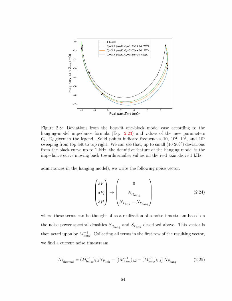
Figure 2.8: Deviations from the best-fit one-block model case according to thehanging-model impedance formula (Eq. 2.23) and values of the new parametersCi, Gi given in the legend. Solid points indicate frequencies 10, 102, 103, and 104

sweeping from top left to top right. We can see that, up to small (10-20%) deviationsfrom the black curve up to 1 kHz, the definitive feature of the hanging model is theimpedance curve moving back towards smaller values on the real axis above 1 kHz.

admittances in the hanging model), we write the following noise vector:

δV

δPi

δP

→

0

NPhang

NPlink−NPhang

(2.24)

where these terms can be thought of as a realization of a noise timestream based on

the noise power spectral densities SPhangand SPlink

described above. This vector is

then acted upon by M−1hang. Collecting all terms in the first row of the resulting vector,

we find a current noise timestream:

NIthermal= (M−1

hang)1,3NPlink+[(M−1

hang)1,2 − (M−1hang)1,3

]NPhang

(2.25)

64

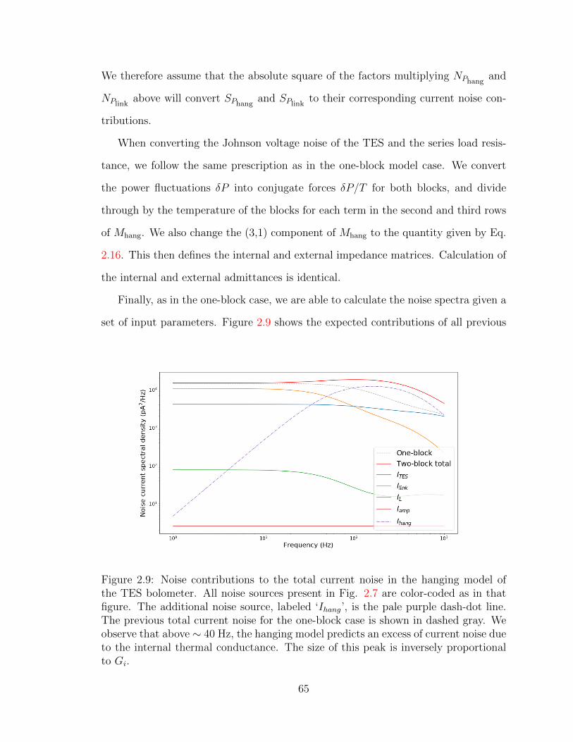
We therefore assume that the absolute square of the factors multiplying NPhangand

NPlinkabove will convert SPhang

and SPlinkto their corresponding current noise con-

tributions.

When converting the Johnson voltage noise of the TES and the series load resis-

tance, we follow the same prescription as in the one-block model case. We convert

the power fluctuations δP into conjugate forces δP/T for both blocks, and divide

through by the temperature of the blocks for each term in the second and third rows

of Mhang. We also change the (3,1) component of Mhang to the quantity given by Eq.

2.16. This then defines the internal and external impedance matrices. Calculation of

the internal and external admittances is identical.

Finally, as in the one-block case, we are able to calculate the noise spectra given a

set of input parameters. Figure 2.9 shows the expected contributions of all previous

Figure 2.9: Noise contributions to the total current noise in the hanging model ofthe TES bolometer. All noise sources present in Fig. 2.7 are color-coded as in thatfigure. The additional noise source, labeled ‘Ihang’, is the pale purple dash-dot line.The previous total current noise for the one-block case is shown in dashed gray. Weobserve that above ∼ 40 Hz, the hanging model predicts an excess of current noise dueto the internal thermal conductance. The size of this peak is inversely proportionalto Gi.

65

noise terms, and the additional noise arising from the added thermal link Gi, for

one of the parameter cases shown in Fig. 2.8. As described above, those examples

feature values of Ci that dominate the sum of the two blocks’ heat capacities. This

reflects the expected case for the AdvACT bolometers as designed, where the total

heat capacity target is tuned using a separate, electrically inert metal film.

We exaggerate the effect of the extra link noise term by making Gi only a factor

of 10 larger than G. This is smaller than expected for AdvACT, or in the majority of

measurements in [40]. In this reference, an excess heat capacity is placed between the

TES and the bath, which differs from the hanging model discussed here. However,

for large Gi, they reduce to the same equations [81].

The noise excess is worse for small Gi, despite the noise in power being reduced,

due to the coefficient of the power noise in the second term of Eq. 2.25. We expect

the actual performance of AdvACT bolometers to lie between this example and the

values in the reference.

From the figure, we can see that for this region of parameter space, the hanging

model predicts a noise excess caused by the peak of the current noise contribution

SIhang. There is also an enhancement of low-frequency Johnson noise as compared to

the one-block case due to the differences in the internal admittances for the TES in

each model.

To conclude, the effects of a possible hanging heat capacity in the bolometer

thermal architecture have been qualitatively described. The presence of such a heat

capacity can be observed via impedance measurements at fairly high frequencies, but

before the TES bolometer response is rolled off by τel. Once observed, the distinct

kink in the impedance curve can allow us to estimate Ci and Gi and then estimate

noise spectra accounting for their presence. The possible excess noise induced by Gi

is generally improved for tight coupling (i.e. large Gi), which we may expect given

66

that the equations for the hanging model exactly reduce to the one-block case for

large Gi.

2.5 Conclusion

In this chapter, we have presented an overview of bolometers, and the need for ex-

tended electrothermal models in order to fully model the response of bolometers to

changing signals. We specifically focused on the parameters and equations describing

TES thermistors in order to prepare the reader for the in-depth discussion of the

testing and analysis of AdvACT TES bolometers in the coming chapter. However,

much of the framework laid out in the preceding pages can be applied to different

sensor types; the full equations are still valid assuming we expand a given thermistor’s

R(T ) behavior in terms of α and β. The limits taken to arrive at simple expressions

for bolometer response functions like the responsivity are some of the only elements

requiring adjustment.

The expressions needed to describe the behavior of a TES bolometer with a sec-

ond, “hanging” block were reported within the context of measuring their effects on

quantities like impedance and noise spectra. Some of the assumptions underlying the

hanging block model and their relevance to the actual AdvACT bolometer design

have been mentioned; these will be more fully explored in the next chapter.

67

Chapter 3

AdvACT Detector Testing

In this chapter, we detail the impedance and noise studies performed on AdvACT

TES bolometer arrays both in the lab and in situ as the focal plane of ACT. Details

on the relationship of the AdvACT project to ACT is given in Sec. 1.4.1. We begin

by introducing the technologies used in the measurements, and describe the data

acquisition methods developed for AdvACT array testing. Our discussion of these

acquisitions progresses to providing results for AdvACT array noise. We then turn to

an overview of impedance data acquisition and results, and apply these to comparing

measured to expected noise spectra over a wide frequency band for impedance data at

high excitation frequency. Observed excess noise beyond the simple TES bolometer

electrothermal model is observed. Its possible causes are discussed, with the result

that the total noise appears to be adequately explained within the context of the

hanging electrothermal bolometer model.

3.1 Experimental Setups

In the course of the detector testing to be described in the body of this chapter, we

have used a variety of different experimental setups to produce data allowing us to

investigate the performance of the AdvACT TES bolometers. The majority of the

68

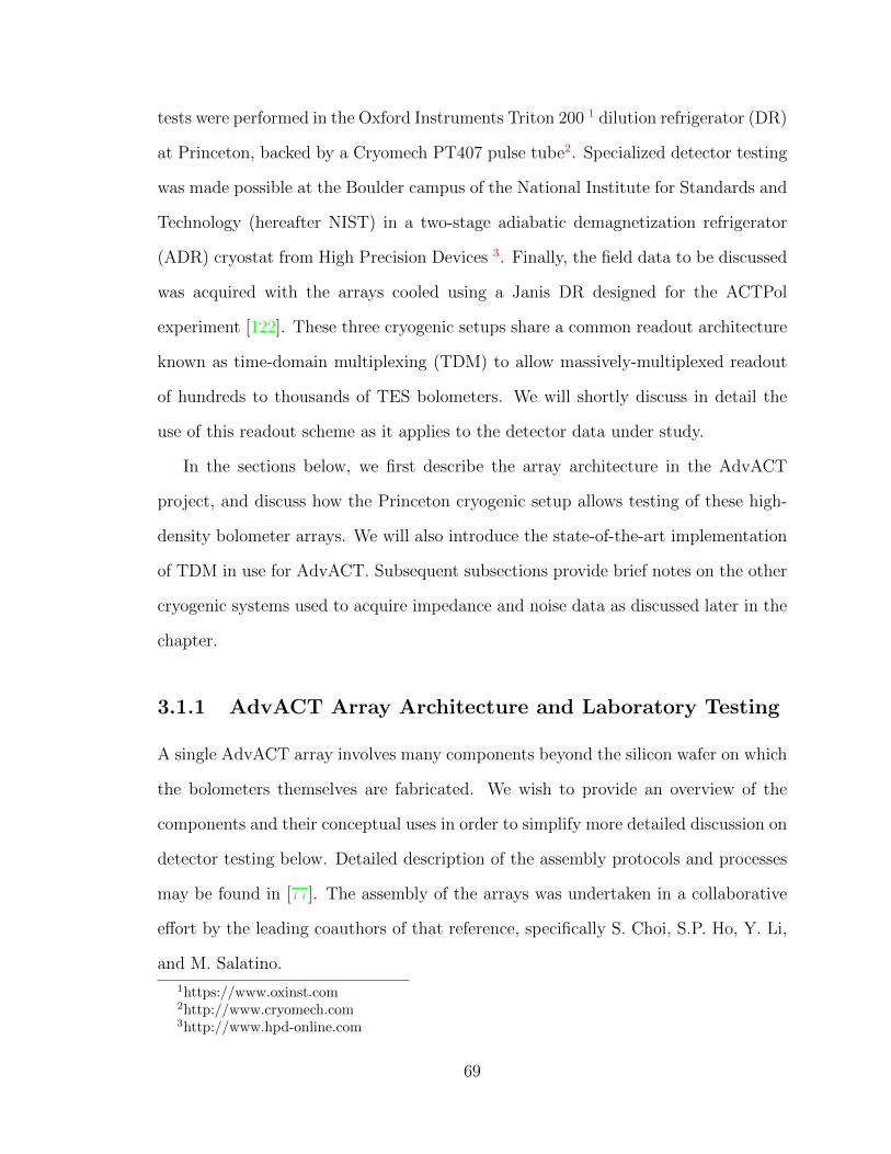
tests were performed in the Oxford Instruments Triton 200 1 dilution refrigerator (DR)

at Princeton, backed by a Cryomech PT407 pulse tube2. Specialized detector testing

was made possible at the Boulder campus of the National Institute for Standards and

Technology (hereafter NIST) in a two-stage adiabatic demagnetization refrigerator

(ADR) cryostat from High Precision Devices 3. Finally, the field data to be discussed

was acquired with the arrays cooled using a Janis DR designed for the ACTPol

experiment [122]. These three cryogenic setups share a common readout architecture

known as time-domain multiplexing (TDM) to allow massively-multiplexed readout

of hundreds to thousands of TES bolometers. We will shortly discuss in detail the

use of this readout scheme as it applies to the detector data under study.

In the sections below, we first describe the array architecture in the AdvACT

project, and discuss how the Princeton cryogenic setup allows testing of these high-

density bolometer arrays. We will also introduce the state-of-the-art implementation

of TDM in use for AdvACT. Subsequent subsections provide brief notes on the other

cryogenic systems used to acquire impedance and noise data as discussed later in the

chapter.

3.1.1 AdvACT Array Architecture and Laboratory Testing

A single AdvACT array involves many components beyond the silicon wafer on which

the bolometers themselves are fabricated. We wish to provide an overview of the

components and their conceptual uses in order to simplify more detailed discussion on

detector testing below. Detailed description of the assembly protocols and processes

may be found in [77]. The assembly of the arrays was undertaken in a collaborative

effort by the leading coauthors of that reference, specifically S. Choi, S.P. Ho, Y. Li,

and M. Salatino.

1https://www.oxinst.com2http://www.cryomech.com3http://www.hpd-online.com

69

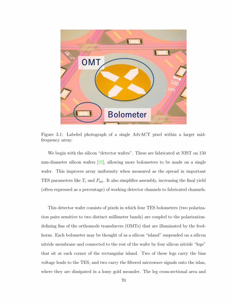
Figure 3.1: Labeled photograph of a single AdvACT pixel within a larger mid-frequency array.

We begin with the silicon “detector wafers”. These are fabricated at NIST on 150

mm-diameter silicon wafers [25], allowing more bolometers to be made on a single

wafer. This improves array uniformity when measured as the spread in important

TES parameters like Tc and Psat. It also simplifies assembly, increasing the final yield

(often expressed as a percentage) of working detector channels to fabricated channels.

This detector wafer consists of pixels in which four TES bolometers (two polariza-

tion pairs sensitive to two distinct millimeter bands) are coupled to the polarization-

defining fins of the orthomode transducers (OMTs) that are illuminated by the feed-

horns. Each bolometer may be thought of as a silicon “island” suspended on a silicon

nitride membrane and connected to the rest of the wafer by four silicon nitride “legs”

that sit at each corner of the rectangular island. Two of these legs carry the bias

voltage leads to the TES, and two carry the filtered microwave signals onto the islan,

where they are dissipated in a lossy gold meander. The leg cross-sectional area and

70

length determine the conductance G between the island and the bath. The TES itself

is an AlMn film deposted on top of niobium electrodes, which apply the bias voltage

to the superconducting film. Details of the process used to ensure repeatable, precise

control of the TES critical temperature Tc and normal resistance RN can be found in

[76]. Finally, an separate, normal metal film of PdAu is deposited on the entirety of

the island not covered by the Au meander and the TES. By controlling the thickness

and surface area (i.e. the total volume) of this PdAu film, it is possible to tune the

heat capacity C of the island when it is viewed as a single thermal block. We will in-

terrogate this assumption using the impedance and noise data of subsequent sections.

In Tab. 3.1, we provide details on the leg dimensions and PdAu volume used, in the

fabrication design, to target the listed G and C values, for all bolometer channels in

the AdvACT arrays. By bolometer “channel” we here mean the frequency band as

identified by nominal center frequency in simulations of the pixel microwave filters.

An example pixel, with components identified by text, can be seen in Fig. 3.1. The

long dimensions of the bolometer is ∼ 100µm, and the entire pixel is approximately

5 mm between the furthest-separated pair of vertices. The TES is the narrow bar

extending along the short dimension of the island. Its width is 12 µm, and its width

and length are in a 1:8 ratio. The TES aspect ratio is used to set RN.

Array Center Freq (GHz) Psat (pW) Leg Width (µm) Leg Length (µm) G (pW/K) PdAu Volume (µm3) C (pJ/K)HF 150 GHz 12.5 24 61 292 3.61×104 3.5HF 230 GHz 25 48 61 585 6.08×104 5.4MF 90 GHz 11.3 24 61 264 2.15×104 2.4MF 150 GHz 12.5 21.6 61 292 3.61×104 3.5LF 27 GHz 7.8 12.1 61 182 2.74×104 2.9LF 39 GHz 1.5 10 628 35.1 0 0.6

Table 3.1: Summary of bolometer island parameters (SiN leg dimensions, PdAu vol-ume) and their targeted design bolometer parameters Psat, G, and C. On all islands,an AlMn film defines the TES and is a base layer on the island above the Nb elec-trodes. For all bands except the LF 27 GHz, this AlMn film is expected to contribute0.8 pJ/K to the total heat capacity (rightmost column). For LF 27 GHz channel, thecontribution is 0.6 pJ/K.

71

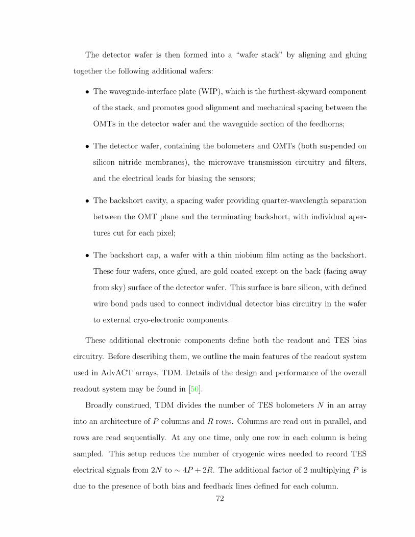
The detector wafer is then formed into a “wafer stack” by aligning and gluing

together the following additional wafers:

• The waveguide-interface plate (WIP), which is the furthest-skyward component

of the stack, and promotes good alignment and mechanical spacing between the

OMTs in the detector wafer and the waveguide section of the feedhorns;

• The detector wafer, containing the bolometers and OMTs (both suspended on

silicon nitride membranes), the microwave transmission circuitry and filters,

and the electrical leads for biasing the sensors;

• The backshort cavity, a spacing wafer providing quarter-wavelength separation

between the OMT plane and the terminating backshort, with individual aper-

tures cut for each pixel;

• The backshort cap, a wafer with a thin niobium film acting as the backshort.

These four wafers, once glued, are gold coated except on the back (facing away

from sky) surface of the detector wafer. This surface is bare silicon, with defined

wire bond pads used to connect individual detector bias circuitry in the wafer

to external cryo-electronic components.

These additional electronic components define both the readout and TES bias

circuitry. Before describing them, we outline the main features of the readout system

used in AdvACT arrays, TDM. Details of the design and performance of the overall

readout system may be found in [50].

Broadly construed, TDM divides the number of TES bolometers N in an array

into an architecture of P columns and R rows. Columns are read out in parallel, and

rows are read sequentially. At any one time, only one row in each column is being

sampled. This setup reduces the number of cryogenic wires needed to record TES

electrical signals from 2N to ∼ 4P + 2R. The additional factor of 2 multiplying P is

due to the presence of both bias and feedback lines defined for each column.

72

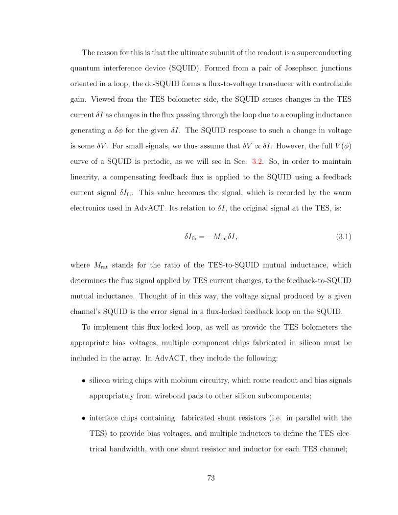
The reason for this is that the ultimate subunit of the readout is a superconducting

quantum interference device (SQUID). Formed from a pair of Josephson junctions

oriented in a loop, the dc-SQUID forms a flux-to-voltage transducer with controllable

gain. Viewed from the TES bolometer side, the SQUID senses changes in the TES

current δI as changes in the flux passing through the loop due to a coupling inductance

generating a δφ for the given δI. The SQUID response to such a change in voltage

is some δV . For small signals, we thus assume that δV ∝ δI. However, the full V (φ)

curve of a SQUID is periodic, as we will see in Sec. 3.2. So, in order to maintain

linearity, a compensating feedback flux is applied to the SQUID using a feedback

current signal δIfb. This value becomes the signal, which is recorded by the warm

electronics used in AdvACT. Its relation to δI, the original signal at the TES, is:

δIfb = −MratδI, (3.1)

where Mrat stands for the ratio of the TES-to-SQUID mutual inductance, which

determines the flux signal applied by TES current changes, to the feedback-to-SQUID

mutual inductance. Thought of in this way, the voltage signal produced by a given

channel’s SQUID is the error signal in a flux-locked feedback loop on the SQUID.

To implement this flux-locked loop, as well as provide the TES bolometers the

appropriate bias voltages, multiple component chips fabricated in silicon must be

included in the array. In AdvACT, they include the following:

• silicon wiring chips with niobium circuitry, which route readout and bias signals

appropriately from wirebond pads to other silicon subcomponents;

• interface chips containing: fabricated shunt resistors (i.e. in parallel with the

TES) to provide bias voltages, and multiple inductors to define the TES elec-

trical bandwidth, with one shunt resistor and inductor for each TES channel;

73

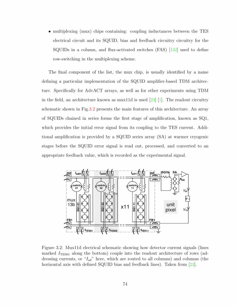
• multiplexing (mux) chips containing: coupling inductances between the TES

electrical circuit and its SQUID, bias and feedback circuitry circuitry for the

SQUIDs in a column, and flux-activated switches (FAS) [132] used to define

row-switching in the multiplexing scheme.

The final component of the list, the mux chip, is usually identified by a name

defining a particular implementation of the SQUID amplifier-based TDM architec-

ture. Specifically for AdvACT arrays, as well as for other experiments using TDM

in the field, an architecture known as mux11d is used [23] [1]. The readout circuitry

schematic shown in Fig.3.2 presents the main features of this architecture. An array

of SQUIDs chained in series forms the first stage of amplification, known as SQ1,

which provides the initial error signal from its coupling to the TES current. Addi-

tional amplification is provided by a SQUID series array (SA) at warmer cryogenic

stages before the SQUID error signal is read out, processed, and converted to an

appropriate feedback value, which is recorded as the experimental signal.

Figure 3.2: Mux11d electrical schematic showing how detector current signals (linesmarked ITES01 along the bottom) couple into the readout architecture of rows (ad-dressing currents, or “Iad” here, which are routed to all columns) and columns (thehorizontal axis with defined SQUID bias and feedback lines). Taken from [23].

74

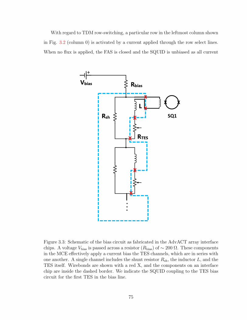
With regard to TDM row-switching, a particular row in the leftmost column shown

in Fig. 3.2 (column 0) is activated by a current applied through the row select lines.

When no flux is applied, the FAS is closed and the SQUID is unbiased as all current

X X

SQ1

X

X

Figure 3.3: Schematic of the bias circuit as fabricated in the AdvACT array interfacechips. A voltage Vbias is passed across a resistor (Rbias) of ∼ 200 Ω. These componentsin the MCE effectively apply a current bias the TES channels, which are in series withone another. A single channel includes the shunt resistor Rsh, the inductor L, and theTES itself. Wirebonds are shown with a red X, and the components on an interfacechip are inside the dashed border. We indicate the SQUID coupling to the TES biascircuit for the first TES in the bias line.

75

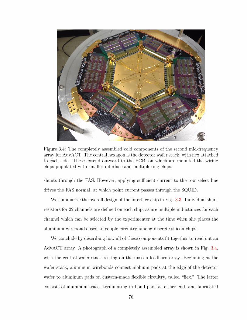
Figure 3.4: The completely assembled cold components of the second mid-frequencyarray for AdvACT. The central hexagon is the detector wafer stack, with flex attachedto each side. These extend outward to the PCB, on which are mounted the wiringchips populated with smaller interface and multiplexing chips.

shunts through the FAS. However, applying sufficient current to the row select line

drives the FAS normal, at which point current passes through the SQUID.

We summarize the overall design of the interface chip in Fig. 3.3. Individual shunt

resistors for 22 channels are defined on each chip, as are multiple inductances for each

channel which can be selected by the experimenter at the time when she places the

aluminum wirebonds used to couple circuitry among discrete silicon chips.

We conclude by describing how all of these components fit together to read out an

AdvACT array. A photograph of a completely assembled array is shown in Fig. 3.4,

with the central wafer stack resting on the unseen feedhorn array. Beginning at the

wafer stack, aluminum wirebonds connect niobium pads at the edge of the detector

wafer to aluminum pads on custom-made flexible circuitry, called “flex.” The latter

consists of aluminum traces terminating in bond pads at either end, and fabricated

76

on polyimide film to provide elastic mechanical coupling between the silicon array

and other parts. The flex mounts to a copper-trace printed-circuit board (PCB) that

surrounds the central detector wafer and is mounted to a gold-plated copper support

ring. Detector signals leave the flex to a wiring chip glued to the PCB using rubber

cement. This wiring chip, as described above, provides the appropriate routing for

these detector signals, as well as TES bias signals and all SQUID signals, to discrete

mux and interface chips. These smaller chips are stycasted to the wiring chips before

bonding proceeds. Additionally, we consider that wiring chips provide a layer of

modularity above the PCB, which contains signal traces for all of the lines running

from cryogenic stages to room temperature, known as “critical lines” since multiple

TES bolometers share each of them.

At the output of the PCB, all critical lines are routed, via ancillary PCBs, to sol-

dered MDM connectors. These connectors interface the complete array package [127]

with the warm-stage electronics via NbTi woven-loom cables from Tekdata 4. The

warm-stage electronics are known as Multi-Channel Electronics (MCE) [5]; through

this system the user controls all critical line bias values while feedback values are

recorded and the row switching is performed. We also use the MCE to generate the

sine-wave bias signals used for impedance measurements, as discussed in Sec. 3.4.

This description applies to readout of entire AdvACT arrays in both the Prince-

ton laboratory and field cryostats. In the laboratory specifically, we couple the array

package (feedhorn array, wafer stack, PCB, and all silicon chips) to the mixing cham-

ber of the DR. This is done via a copper interface plate and mounting brackets that

allow us to mechanically suspend the array from the mixing chamber [11]. One addi-

tional component, a metal-mesh millimeter low-pass filter, is mounted in front of the

sky-side horn aperture to cut any out-of-band radiation.

4https://www.tekdata-interconnect.com

77

The DR provides adequate cooling power to allow the array to reach base tem-

peratures of ∼ 30 mK. During measurements, we perform PID feedback control to

keep the array temperature between 100 and 150 mK. In addition to the array, a

cryogenic blackbody is suspended from the 4 K stage of the DR. It is used to illumi-

nate one-third of the feedhorns (and thus pixels) of the array for optical tests [12],

while the remaining bolometers can be assumed to have negligible millimeter-wave

loading. On the outside of the cryostat, a cylindrical µ-metal magnetic shield with

high aspect ratio (cylinder height to opening diameter) is lifted into place around the

outer vacuum jacket of the DR.

3.1.2 NIST Laboratory Tests

When performing TES bolometer testing at NIST in order to achieve high sinusoid

input frequencies for impedance studies, many aspects of the above description are

simplified. A single PCB supports individual wiring chips, interface and multiplexing

chips, and separate silicon die with the devices to be studied. All of these compo-

nents are rubber-cemented to the board, and connected via wirebonds to provide the

appropriate signal routing. This compact package is then mounted to the a rod in

the ADR that provides the cooling energy at base temperature. We note that the

mux chips used in this package are not mux11d, but a previous generation known as

mux11c. This architecture features two cold SQUID amplifier stages before the SA,

and row switching is provided not by a shunting FAS but by directly applying bias

voltage to SQ1s one at a time. A different Mrat is also defined. This technology is

identical to that used in previous generations of ACT focal planes, as in [45] [96].

In the NIST ADR used for these measurements, the use of strong magnetic fields in

the thermal cycling process has lead to two cryogenic radiation shields being places

around the TES bolometer package. The inner shield is a µ-metal shield in two

clamshell halves that are bolted together around the detector. The outer shield is

78

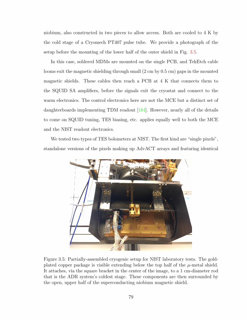
niobium, also constructed in two pieces to allow access. Both are cooled to 4 K by

the cold stage of a Cryomech PT407 pulse tube. We provide a photograph of the

setup before the mounting of the lower half of the outer shield in Fig. 3.5.

In this case, soldered MDMs are mounted on the single PCB, and TekEtch cable

looms exit the magnetic shielding through small (2 cm by 0.5 cm) gaps in the mounted

magnetic shields. These cables then reach a PCB at 4 K that connects them to

the SQUID SA amplifiers, before the signals exit the cryostat and connect to the

warm electronics. The control electronics here are not the MCE but a distinct set of

daughterboards implementing TDM readout [104]. However, nearly all of the details

to come on SQUID tuning, TES biasing, etc. applies equally well to both the MCE

and the NIST readout electronics.

We tested two types of TES bolometers at NIST. The first kind are “single pixels”,

standalone versions of the pixels making up AdvACT arrays and featuring identical

Figure 3.5: Partially-assembled cryogenic setup for NIST laboratory tests. The gold-plated copper package is visible extending below the top half of the µ-metal shield.It attaches, via the square bracket in the center of the image, to a 1 cm-diameter rodthat is the ADR system’s coldest stage. These components are then surrounded bythe open, upper half of the superconducting niobium magnetic shield.

79

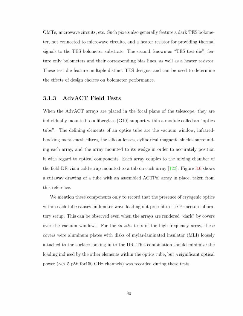
OMTs, microwave circuits, etc. Such pixels also generally feature a dark TES bolome-

ter, not connected to microwave circuits, and a heater resistor for providing thermal

signals to the TES bolometer substrate. The second, known as “TES test die”, fea-

ture only bolometers and their corresponding bias lines, as well as a heater resistor.

These test die feature multiple distinct TES designs, and can be used to determine

the effects of design choices on bolometer performance.

3.1.3 AdvACT Field Tests

When the AdvACT arrays are placed in the focal plane of the telescope, they are

individually mounted to a fiberglass (G10) support within a module called an “optics

tube”. The defining elements of an optics tube are the vacuum window, infrared-

blocking metal-mesh filters, the silicon lenses, cylindrical magnetic shields surround-

ing each array, and the array mounted to its wedge in order to accurately position

it with regard to optical components. Each array couples to the mixing chamber of

the field DR via a cold strap mounted to a tab on each array [122]. Figure 3.6 shows

a cutaway drawing of a tube with an assembled ACTPol array in place, taken from

this reference.

We mention these components only to record that the presence of cryogenic optics

within each tube causes millimeter-wave loading not present in the Princeton labora-

tory setup. This can be observed even when the arrays are rendered “dark” by covers

over the vacuum windows. For the in situ tests of the high-frequency array, these

covers were aluminum plates with disks of mylar-laminated insulator (MLI) loosely

attached to the surface looking in to the DR. This combination should minimize the

loading induced by the other elements within the optics tube, but a significant optical

power (∼> 5 pW for150 GHz channels) was recorded during these tests.

80

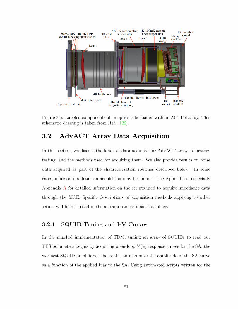
Figure 3.6: Labeled components of an optics tube loaded with an ACTPol array. Thisschematic drawing is taken from Ref. [122].

3.2 AdvACT Array Data Acquisition

In this section, we discuss the kinds of data acquired for AdvACT array laboratory

testing, and the methods used for acquiring them. We also provide results on noise

data acquired as part of the chaarcterization routines described below. In some

cases, more or less detail on acquisition may be found in the Appendices, especially

Appendix A for detailed information on the scripts used to acquire impedance data

through the MCE. Specific descriptions of acquisition methods applying to other

setups will be discussed in the appropriate sections that follow.

3.2.1 SQUID Tuning and I-V Curves

In the mux11d implementation of TDM, tuning an array of SQUIDs to read out

TES bolometers begins by acquiring open-loop V (φ) response curves for the SA, the

warmest SQUID amplifiers. The goal is to maximize the amplitude of the SA curve

as a function of the applied bias to the SA. Using automated scripts written for the

81

MCE [5], we perform a sweep of SA bias values and record the optimum bias for

subsequent tuning.

With the SA SQUIDs biased, we send a signal into each column sufficient to

bias the SQ1 amplifiers. Using the SA feedback loop to keep the output linear, we

drive current into the row addressing lines, thus driving flux into the FAS. We record

the values of the row bias signal at the minimum and maximum value of the SA

feedback. The median of these values across the columns becomes the “row-select”

and “row-deselect” values used to drive each row, as in Fig. 3.2.

We now proceed to driving current through the SQ1 feedback lines, while keeping

the SA SQUIDs at their lockpoints using feedback. By plotting SA feedback vs. SQ1

feedback, we can optimize the SQ1 response (i.e. maximize the SQ1 V (φ) curves)

independently of the SA response. However, our final operating mode is to operate on

the open-loop output of the SA, the error signal, in order to determine the appropriate

feedback to keep the SQ1 locked. Thus, the final amplifier gains and readout configu-

ration is best approximated by recording the open-loop signal generated by ramping

current through the SQ1 feedback circuit. This is the final component of the SQUID

tuning. Numbers relevant for performing the row switching, SQUID biasing, and

feedback calculations are all automatically stored in an experimental configuration

file read by the MCE.

As a first check of the detectors,we additionally ramp current through the TES

bias lines at the end of the automated SQUID tuning. We do so while recording the

open-loop error signal through the SQ1 and SA. Using this data, we can identify any

issues affecting single detectors (i.e. broken bonds somewhere between the input coil

to the SQUID on the mux chips and the detector wafer).

Such channels then have open SQUID inputs, and are known as dark SQUIDs.

To be very conservative, we have added such channels to dead lists, which are used

to specify channels for which the MCE should not apply feedback. This is because

82

channels that are not dead-listed can result in large, erroneous values of feedback

being sent in by the MCE. This latter scenario would induce leakage as the MCE

switches to subsequent rows. Other channels in the dead lists include SQUIDs that

cannot be biased or addressed by feedback; these latter are almost always due to

failures of critical line bonds, and thus come in groups of tens to hundreds.

Persistence. A second, and pernicious, failure mode involves the FAS in the

array readout circuitry being always normal. This induces so-called “persistence” in

the column that the FAS occupies. Since the FAS is always in its normal-metal state,

SQ1 bias current is always shunted to the SQ1 in parallel to the affected FAS. This

row then persists through all row switches, and its signals affect the readout of every

row in such a column. We expect that such issues are usually caused by magnetic

flux trapped in the FAS when it is cooled through its transition (for niobium, this is

∼ 7 K). However, fabrication failures which disconnect an FAS from its SQ1 would

produce the same effect.

Persistence in the AdvACT arrays is tested for taking a special set of tuning data,

in which the open-loop measurement of ramping current through the SQ1 feedback

lines is performed with all rows set to be always off. We do this by setting the row-

select value to the row-deselect value, which we expect will cause no signal to be read

at the SA output. If we see any V (φ)-like behavior, we label the column persistent;

the severity of the effect is qualitatively proportional to the amplitude of the response.

We do not always dead list these columns, though we note them and can attempt to

repair the column by replacing a mux chip containing a persistence candidate with

another. An example of a dataset in which three persistent columns appear can be

seen in Fig. 3.7.

Finally, as discussed in Sec. 2.4, I-V curves are used to study important character-

istics of the TES bolometers. These include measurements of RN and Psat across the

array. We work to achieve minimal scatter in values of the former across detectors in

83

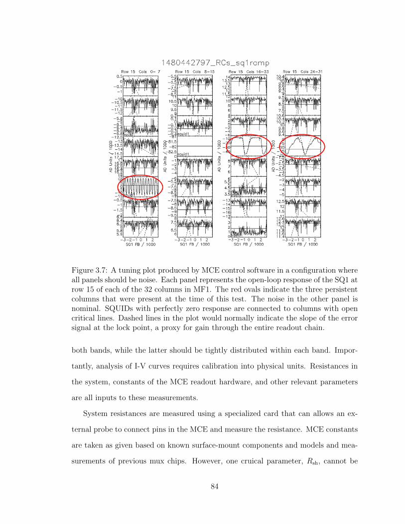
Figure 3.7: A tuning plot produced by MCE control software in a configuration whereall panels should be noise. Each panel represents the open-loop response of the SQ1 atrow 15 of each of the 32 columns in MF1. The red ovals indicate the three persistentcolumns that were present at the time of this test. The noise in the other panel isnominal. SQUIDs with perfectly zero response are connected to columns with opencritical lines. Dashed lines in the plot would normally indicate the slope of the errorsignal at the lock point, a proxy for gain through the entire readout chain.

both bands, while the latter should be tightly distributed within each band. Impor-

tantly, analysis of I-V curves requires calibration into physical units. Resistances in

the system, constants of the MCE readout hardware, and other relevant parameters

are all inputs to these measurements.

System resistances are measured using a specialized card that can allows an ex-

ternal probe to connect pins in the MCE and measure the resistance. MCE constants

are taken as given based on known surface-mount components and models and mea-

surements of previous mux chips. However, one cruical parameter, Rsh, cannot be

84

measured directly by probing. We record typical values of ∼ 200 µΩ. This per-

channel number thus forms the largest uncertainty in our estimates of Pbias, RN, and

other parameters. A brief description of how we estimate these values in AdvACT

studies is given in Sec. 3.3.

When acquiring I-V curves, we must account for the fact that the feedback values

in the MCE record relative changes in current at the TES. An overall offset is thus

accounted for when converting to physical units (which are generally linear transfor-

mations) by fitting a slope to normal part of an I-V curve, extrapolating this to zero

bias voltage, and removing the offset Previous reports on ACT [133] and ACTPol [45]

[96] describe this method in more detail.

We proceed now to describing how we acquire I-V curves, as well as other critical

characterization data, at various bath temperatures.

3.2.2 Bath Temperature Ramp Data

In order to stably control the bath temperature and move between temperature set-

points in the laboratory, we use a Lakeshore AC370 5 readout and control box. This

device features multiple readout channels, each using an AC resistance bridge for ac-

curate measurement of the ∼ kΩ resistances of ruthenium oxide (ROx) thermometers

at the coldest stages of the DR. These thermometers are calibrated from resistance to

temperature using measurements during a common cooldown with a pre-calibrated

thermometer at Cornell.

At each bath temperature, we acquire the following datasets:

• I-V curves, in order to recover Psat and measure Tc and G from fits to Psat vs

Tbath (see Eq. 2.5);

• bias step data, in order to measure f3dB,eff at various Pbias and fit these data to

Eq. 2.14;

5https://www.lakeshore.com

85

• DC-biased noise data, in order to determine noise current densities and esti-

mated NEP for all active bolometers.

For the last two items, it is also important to acquire data across the transition. In

laboratory testing of AdvACT arrays, we study devices between 0.2RN and 0.7RN,

which represents the approximate spread in achieved TES resistance when we bias

detectors in the field.

We write a master script to perform the acquisition by first taking an I-V curve,

then subsequently analyzing the output to optimize bias values for each bias line based

on the data from bolometers that share it. In the HF arrays, up to 110 bolometers

can share a bias line. These numbers fall to up to 99 bolometers per bias line for the

MF array, and 25 bolometers per bias line for LF. Choosing the best bias involves

taking the median of the bias value (in digital-analog converter, or DAC, units) for

which each bolometer is closest to the target fractional RN. For a single I-V data

acquisition, we change this target to span a large part of the transition, and record

these biases in output files.

Array Heating During testing of the HF array, we found that taking I-V curves

for all bias lines at once produced a heating spike of ∼ 5mK. This would produce

large systematics in our assumed Tbath values when fitting out the parameters Tc and

G. In order to reduce this, we chose to perform the I-V curve acquisition within a

single “quadrant” of the HF and MF arrays. The quadrants are defined as groups of

eight columns, contiguous in the MCE readout space, which share MDM cabling and

connectors in the completed array assemblies. There are six bias lines per quadrant in

the HF and MF arrays. With this method, we reduced the transient heating during

I-V acquisition to . 2 mK. In the field, conversely, we elected to run full-array I-V

acquisitions, and instead tune the high-voltage range of the I-V curve to the minimum

possible voltage for which we can still recover unbiased estimates for RN and apply

the offset correction of the I-V data described above.

86

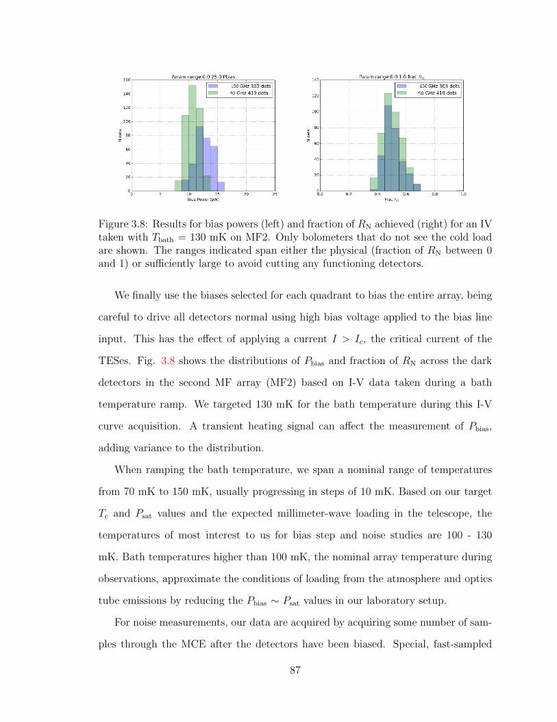
Figure 3.8: Results for bias powers (left) and fraction of RN achieved (right) for an IVtaken with Tbath = 130 mK on MF2. Only bolometers that do not see the cold loadare shown. The ranges indicated span either the physical (fraction of RN between 0and 1) or sufficiently large to avoid cutting any functioning detectors.

We finally use the biases selected for each quadrant to bias the entire array, being

careful to drive all detectors normal using high bias voltage applied to the bias line

input. This has the effect of applying a current I > Ic, the critical current of the

TESes. Fig. 3.8 shows the distributions of Pbias and fraction of RN across the dark

detectors in the second MF array (MF2) based on I-V data taken during a bath

temperature ramp. We targeted 130 mK for the bath temperature during this I-V

curve acquisition. A transient heating signal can affect the measurement of Pbias,

adding variance to the distribution.

When ramping the bath temperature, we span a nominal range of temperatures

from 70 mK to 150 mK, usually progressing in steps of 10 mK. Based on our target

Tc and Psat values and the expected millimeter-wave loading in the telescope, the

temperatures of most interest to us for bias step and noise studies are 100 - 130

mK. Bath temperatures higher than 100 mK, the nominal array temperature during

observations, approximate the conditions of loading from the atmosphere and optics

tube emissions by reducing the Pbias ∼ Psat values in our laboratory setup.

For noise measurements, our data are acquired by acquiring some number of sam-

ples through the MCE after the detectors have been biased. Special, fast-sampled

87

noise on individual detectors was acquired separately, as part of the impedance soft-

ware suite, and will be discussed further in Appendix A.

3.3 Dark Noise in the AdvACT Arrays

As measured, noise data are recorded as feedback values applied by the MCE for

individual bolometers identified by their column and row within the “readout array”.

Analysis of these data must begin by calibrating them into physical units.

First, the feedback voltage applied in DAC units is converted to volts using our

knowledge of the number of bits and maximum voltage for the DAC. We then use

the measured resistance of the feedback loop, very close to constant across columns,

to convert Vfb to Ifb. This number is ∼ 2 kΩ due to bias resistors within the MCE

circuitry. Finally, we use Eq. 3.1 to estimate the current fluctuations at the TES.

If we want to convert our measurements to TES voltage or power, we must calcu-

late the bias voltage V on the TES. We do so by assuming the following equation:

V ∼(Vbias

Rbias

)Rsh (3.2)

where Vbias has been converted from the bias DAC value recorded by the MCE, Rbias is

measured at DC through the bias line and is usually ∼ 200Ω, and Rsh is an estimated

shunt resistance on the interface chip. The parameter Rsh is not directly measurable

in the fully-assembled array. We estimate a per-channel Rsh , normally about 200±20

µΩ across groups of multiple interface chips by measuring the series resistance of ∼

100 shunt resistors and assigning the average value to all shunt resistors in the group

of interface chips. These values are logged and properly assigned to TES channels

once the interface chips have been fully assembled.

With the voltage estimated at the TES this way, we assume that the power at

the TES is then simply V × I. This differs from the actual responsivity of the TES

88

given in 2.11, which we should deconvolve from our current signals. However, in the

low-frequency limit and for L 1, our simplified power estimation is approximately

correct.

We note that, due to the different sizes of the feedback and bias resistances, the

latter requires more accuracy when we wish to calibrate TES signal into units of

power. At the same time, details of the bias circuit do not enter our estimates of

current noise. We thus generally prefer to compare expected to measured current

noise in some of the more detailed noise studies to be described below. However, the

more relevant parameter for determining dark array sensitivity relative to photon-

induced noise is NEP .

Our results for dark NEP of the HF array come from tests performed in situ on

the telescope. This is due partially to early drafts of the bath temperature acquisition

code not properly performing the detector biasing scheme, and partially to evidence

for excessive pickup. In the magnetically-shielded optics tube of the telescope, and

with solid aluminum covers over the windows, we anticipated a sufficiently dark mea-

surement to assume no photon noise. We then gathered data as in the lab, while

ramping the bath temperature, with the exception that there was no PID control

loop to regulate the bath temperature during the acquisition.

In Fig. 3.9, we give an example detector power spectral density in the top panel

and summarize our results for NEP , measured in a 2 Hz band (10 Hz ± 1 Hz) in the

array in the bottom panel. The rolloff near ∼ 115 Hz is the effect of an antialiasing

filter applied to AdvACT data when the ∼ 10 kHz readout rate is reduced to ∼

400 Hz in order not to exceed the maximum data transfer and storage rate of the

MCE hardware. All of these power spectral densities are estimated using the “welch”

function of the scipy scientific-computng package 6. This function implements the

Welch periodogram method of spectral density estimation [130]. It defines segments

6http://www.scipy.org

89

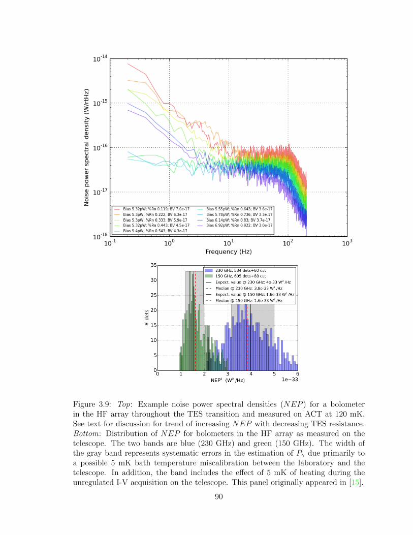
Figure 3.9: Top: Example noise power spectral densities (NEP ) for a bolometerin the HF array throughout the TES transition and measured on ACT at 120 mK.See text for discussion for trend of increasing NEP with decreasing TES resistance.Bottom: Distribution of NEP for bolometers in the HF array as measured on thetelescope. The two bands are blue (230 GHz) and green (150 GHz). The width ofthe gray band represents systematic errors in the estimation of Pγ due primarily toa possible 5 mK bath temperature miscalibration between the laboratory and thetelescope. In addition, the band includes the effect of 5 mK of heating during theunregulated I-V acquisition on the telescope. This panel originally appeared in [15].

90

of a specified length from the input timestream with 50% overlap between segments,

applying a Hanning window function, estimating the spectral density for each segment

after normalizing out the effect of the window function, and averaging the resultant

estimates accounting for the common data between segments.

In the top panel, the trend in estimated NEP as a function of different TES

resistances R (i.e. different points on the resistive transition) indicates a potential

calibration error that is affected by the TES resistance, or a source of constant current

noise that is being projected into power. We surmise that this effect is due to excess

current noise aliased into the low-frequency band of our devices, an effect which

we observe to be TES resistance-dependent in other datasets. This excess is then

calibrated into power.

However, when studying the distribution of NEP at 10 Hz across the array for a

given target resistance, we are able to qualitatively match the median of the measured

distribution to a model of the sum of noise contributions from thermal link and photon

noise, with no free parameters. We are able to estimate the photon noise using

the observed difference in Pbias for detectors in the laboratory and on the telescope,

for the same Tbath and fraction of RN. Using this technique, we are susceptible

to additional uncertainties introduced by heating the array during I-V acquisition

and miscalibration of thermometers between the lab and the telescope. These are

represented by the width of the gray band in the right panel.

Due to the presence of significant photon-sourced NEP , these data are not able to

confirm that detector-sourced noise is dominated by thermal link noise, as expected.

However, laboratory data from testing the two mid-frequency arrays gave us the

opportunity to compare measured NEP values to the expected values for the dark

detectors. Again, by “dark detectors” we mean bolometers in array pixels whose

feedhorns were covered by the metal-plated silicon mask.

91

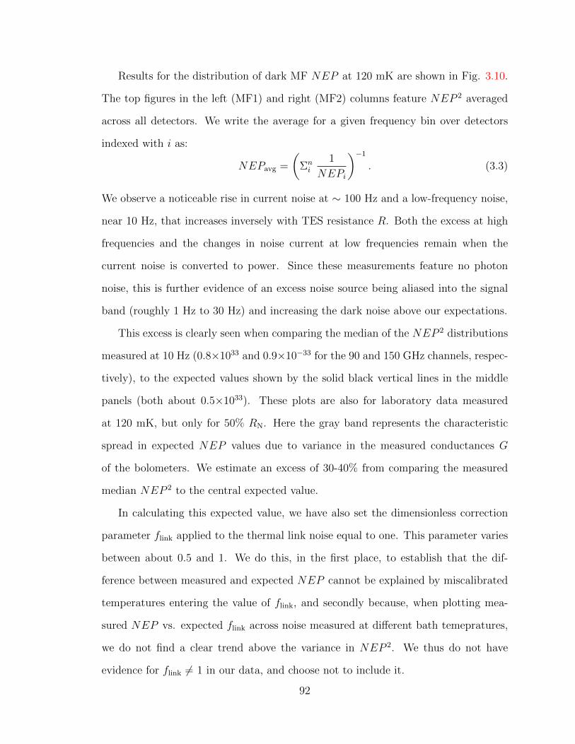
Results for the distribution of dark MF NEP at 120 mK are shown in Fig. 3.10.

The top figures in the left (MF1) and right (MF2) columns feature NEP 2 averaged

across all detectors. We write the average for a given frequency bin over detectors

indexed with i as:

NEPavg =

(Σni

1

NEPi

)−1

. (3.3)

We observe a noticeable rise in current noise at ∼ 100 Hz and a low-frequency noise,

near 10 Hz, that increases inversely with TES resistance R. Both the excess at high

frequencies and the changes in noise current at low frequencies remain when the

current noise is converted to power. Since these measurements feature no photon

noise, this is further evidence of an excess noise source being aliased into the signal

band (roughly 1 Hz to 30 Hz) and increasing the dark noise above our expectations.

This excess is clearly seen when comparing the median of the NEP 2 distributions

measured at 10 Hz (0.8×1033 and 0.9×10−33 for the 90 and 150 GHz channels, respec-

tively), to the expected values shown by the solid black vertical lines in the middle

panels (both about 0.5×1033). These plots are also for laboratory data measured

at 120 mK, but only for 50% RN. Here the gray band represents the characteristic

spread in expected NEP values due to variance in the measured conductances G

of the bolometers. We estimate an excess of 30-40% from comparing the measured

median NEP 2 to the central expected value.

In calculating this expected value, we have also set the dimensionless correction

parameter flink applied to the thermal link noise equal to one. This parameter varies

between about 0.5 and 1. We do this, in the first place, to establish that the dif-

ference between measured and expected NEP cannot be explained by miscalibrated

temperatures entering the value of flink, and secondly because, when plotting mea-

sured NEP vs. expected flink across noise measured at different bath temepratures,

we do not find a clear trend above the variance in NEP 2. We thus do not have

evidence for flink 6= 1 in our data, and choose not to include it.

92

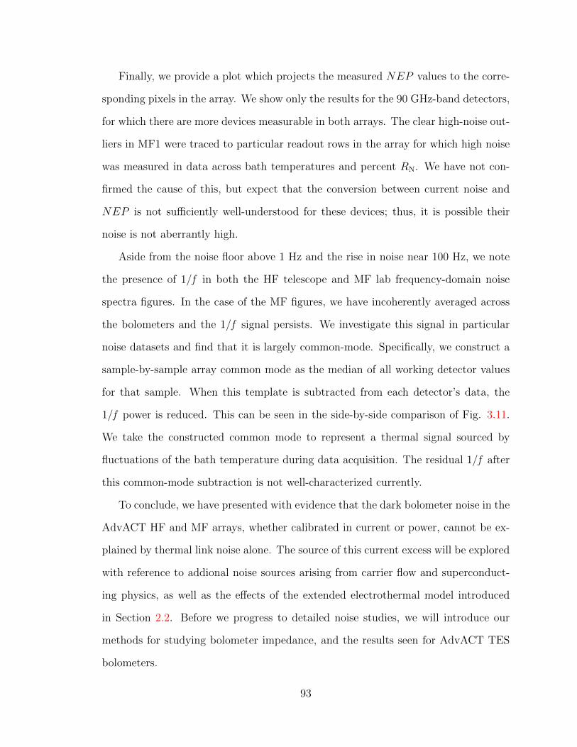
Finally, we provide a plot which projects the measured NEP values to the corre-

sponding pixels in the array. We show only the results for the 90 GHz-band detectors,

for which there are more devices measurable in both arrays. The clear high-noise out-

liers in MF1 were traced to particular readout rows in the array for which high noise

was measured in data across bath temperatures and percent RN. We have not con-

firmed the cause of this, but expect that the conversion between current noise and

NEP is not sufficiently well-understood for these devices; thus, it is possible their

noise is not aberrantly high.

Aside from the noise floor above 1 Hz and the rise in noise near 100 Hz, we note

the presence of 1/f in both the HF telescope and MF lab frequency-domain noise

spectra figures. In the case of the MF figures, we have incoherently averaged across

the bolometers and the 1/f signal persists. We investigate this signal in particular

noise datasets and find that it is largely common-mode. Specifically, we construct a

sample-by-sample array common mode as the median of all working detector values

for that sample. When this template is subtracted from each detector’s data, the

1/f power is reduced. This can be seen in the side-by-side comparison of Fig. 3.11.

We take the constructed common mode to represent a thermal signal sourced by

fluctuations of the bath temperature during data acquisition. The residual 1/f after

this common-mode subtraction is not well-characterized currently.

To conclude, we have presented with evidence that the dark bolometer noise in the

AdvACT HF and MF arrays, whether calibrated in current or power, cannot be ex-

plained by thermal link noise alone. The source of this current excess will be explored

with reference to addional noise sources arising from carrier flow and superconduct-

ing physics, as well as the effects of the extended electrothermal model introduced

in Section 2.2. Before we progress to detailed noise studies, we will introduce our

methods for studying bolometer impedance, and the results seen for AdvACT TES

bolometers.

93

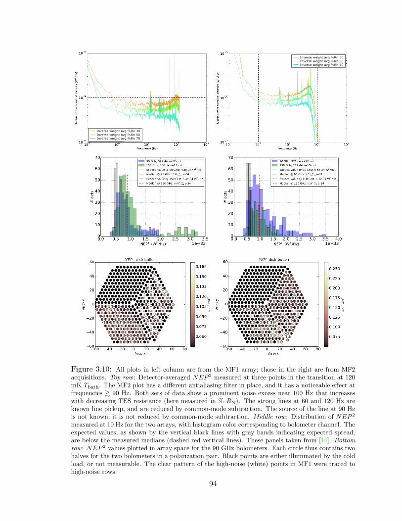
Inverse weight avg %Rn 30Inverse weight avg %Rn 50Inverse weight avg %Rn 70

Inverse weight avg %Rn 30Inverse weight avg %Rn 50Inverse weight avg %Rn 70

Figure 3.10: All plots in left column are from the MF1 array; those in the right are from MF2acquisitions. Top row : Detector-averaged NEP 2 measured at three points in the transition at 120mK Tbath. The MF2 plot has a different antialiasing filter in place, and it has a noticeable effect atfrequencies & 90 Hz. Both sets of data show a prominent noise excess near 100 Hz that increaseswith decreasing TES resistance (here measured in % RN). The strong lines at 60 and 120 Hz areknown line pickup, and are reduced by common-mode subtraction. The source of the line at 90 Hzis not known; it is not reduced by common-mode subtraction. Middle row : Distribution of NEP 2

measured at 10 Hz for the two arrays, with histogram color corresponding to bolometer channel. Theexpected values, as shown by the vertical black lines with gray bands indicating expected spread,are below the measured medians (dashed red vertical lines). These panels taken from [14]. Bottomrow : NEP 2 values plotted in array space for the 90 GHz bolometers. Each circle thus contains twohalves for the two bolometers in a polarization pair. Black points are either illuminated by the coldload, or not measurable. The clear pattern of the high-noise (white) points in MF1 were traced tohigh-noise rows.

94

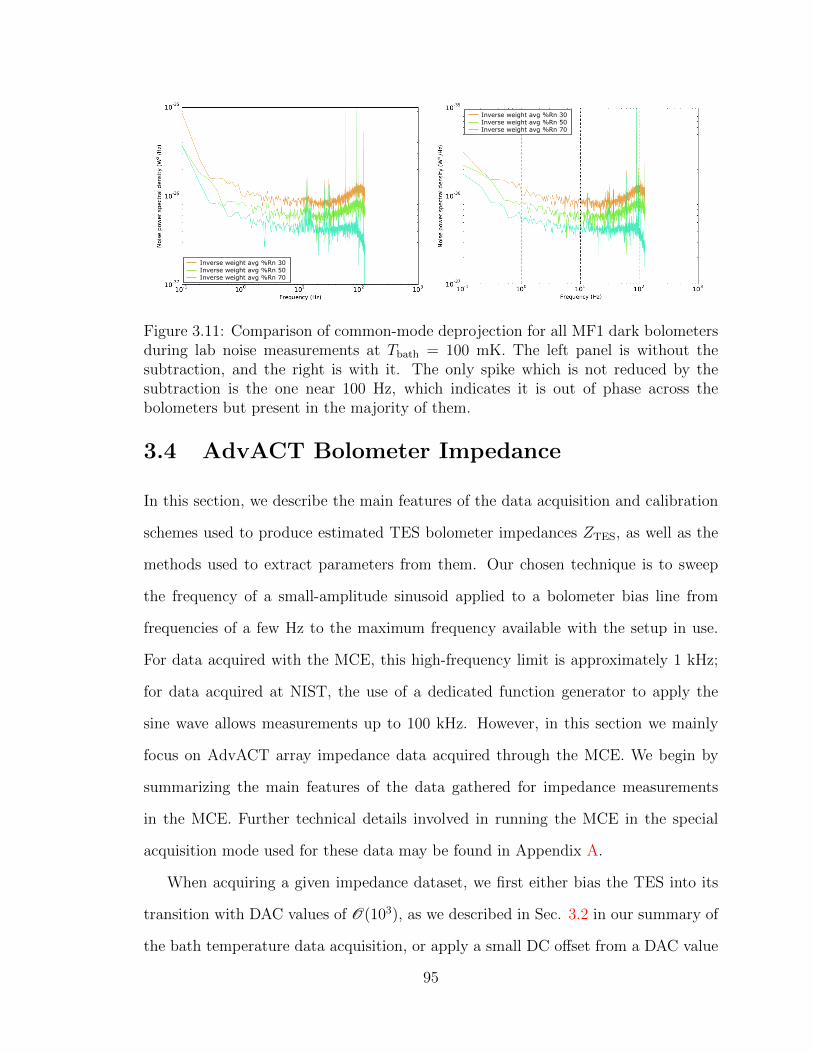
Inverse weight avg %Rn 30Inverse weight avg %Rn 50Inverse weight avg %Rn 70

Inverse weight avg %Rn 30Inverse weight avg %Rn 50Inverse weight avg %Rn 70

Figure 3.11: Comparison of common-mode deprojection for all MF1 dark bolometersduring lab noise measurements at Tbath = 100 mK. The left panel is without thesubtraction, and the right is with it. The only spike which is not reduced by thesubtraction is the one near 100 Hz, which indicates it is out of phase across thebolometers but present in the majority of them.

3.4 AdvACT Bolometer Impedance

In this section, we describe the main features of the data acquisition and calibration

schemes used to produce estimated TES bolometer impedances ZTES, as well as the

methods used to extract parameters from them. Our chosen technique is to sweep

the frequency of a small-amplitude sinusoid applied to a bolometer bias line from

frequencies of a few Hz to the maximum frequency available with the setup in use.

For data acquired with the MCE, this high-frequency limit is approximately 1 kHz;

for data acquired at NIST, the use of a dedicated function generator to apply the

sine wave allows measurements up to 100 kHz. However, in this section we mainly

focus on AdvACT array impedance data acquired through the MCE. We begin by

summarizing the main features of the data gathered for impedance measurements

in the MCE. Further technical details involved in running the MCE in the special

acquisition mode used for these data may be found in Appendix A.

When acquiring a given impedance dataset, we first either bias the TES into its

transition with DAC values of O(103), as we described in Sec. 3.2 in our summary of

the bath temperature data acquisition, or apply a small DC offset from a DAC value

95

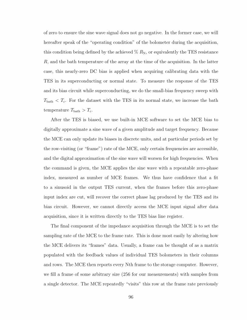
of zero to ensure the sine wave signal does not go negative. In the former case, we will

hereafter speak of the “operating condition” of the bolometer during the acquisition,

this condition being defined by the achieved % RN, or equivalently the TES resistance

R, and the bath temperature of the array at the time of the acquisition. In the latter

case, this nearly-zero DC bias is applied when acquiring calibrating data with the

TES in its superconducting or normal state. To measure the response of the TES

and its bias circuit while superconducting, we do the small-bias frequency sweep with

Tbath < Tc. For the dataset with the TES in its normal state, we increase the bath

temperature Tbath > Tc.

After the TES is biased, we use built-in MCE software to set the MCE bias to

digitally approximate a sine wave of a given amplitude and target frequency. Because

the MCE can only update its biases in discrete units, and at particular periods set by

the row-visiting (or “frame”) rate of the MCE, only certain frequencies are accessible,

and the digital approximation of the sine wave will worsen for high frequencies. When

the command is given, the MCE applies the sine wave with a repeatable zero-phase

index, measured as number of MCE frames. We thus have confidence that a fit

to a sinusoid in the output TES current, when the frames before this zero-phase

input index are cut, will recover the correct phase lag produced by the TES and its

bias circuit. However, we cannot directly access the MCE input signal after data

acquisition, since it is written directly to the TES bias line register.

The final component of the impedance acquisition through the MCE is to set the

sampling rate of the MCE to the frame rate. This is done most easily by altering how

the MCE delivers its “frames” data. Usually, a frame can be thought of as a matrix

populated with the feedback values of individual TES bolometers in their columns

and rows. The MCE then reports every Nth frame to the storage computer. However,

we fill a frame of some arbitrary size (256 for our measurements) with samples from

a single detector. The MCE repeatedly “visits” this row at the frame rate previously

96

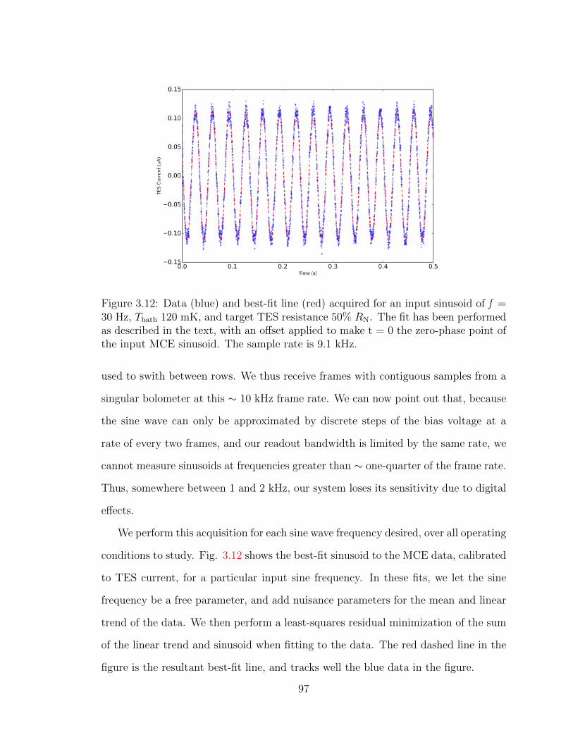
Figure 3.12: Data (blue) and best-fit line (red) acquired for an input sinusoid of f =30 Hz, Tbath 120 mK, and target TES resistance 50% RN. The fit has been performedas described in the text, with an offset applied to make t = 0 the zero-phase point ofthe input MCE sinusoid. The sample rate is 9.1 kHz.

used to swith between rows. We thus receive frames with contiguous samples from a

singular bolometer at this ∼ 10 kHz frame rate. We can now point out that, because

the sine wave can only be approximated by discrete steps of the bias voltage at a

rate of every two frames, and our readout bandwidth is limited by the same rate, we

cannot measure sinusoids at frequencies greater than ∼ one-quarter of the frame rate.

Thus, somewhere between 1 and 2 kHz, our system loses its sensitivity due to digital

effects.

We perform this acquisition for each sine wave frequency desired, over all operating

conditions to study. Fig. 3.12 shows the best-fit sinusoid to the MCE data, calibrated

to TES current, for a particular input sine frequency. In these fits, we let the sine

frequency be a free parameter, and add nuisance parameters for the mean and linear

trend of the data. We then perform a least-squares residual minimization of the sum

of the linear trend and sinusoid when fitting to the data. The red dashed line in the

figure is the resultant best-fit line, and tracks well the blue data in the figure.

97

We perform a data reduction from the raw TES current data at each frequency to

a voltage transfer function T (f) =VfbVbias

at each operating condition. This transfer

function is a complex value at each frequency describing the relative amplitude and

phase of the output sinusoid as compared to the input. This transfer function can be

converted to ZTES once the Thevenin-equivalent voltage and series impedance present

in the TES bias circuit. Following the work by [79] [133], we use the voltage transfer

functions measured in the superconducting and normal state of the TES to form a

quantity proportional to the Thevenin voltage Vth and equivalent series impedance

Zeq as follows:

Vth =RN

T −1N −T −1

sc

, (3.4a)

Zeq =RN

Tsc/TN − 1, (3.4b)

where Tsc and Tn are the transfer functions measured in the superconducting and

normal state, respectively. To be explicit, Vth is the Thevenin-equivalent voltage

divided by the input bias voltage amplitude at the MCE and a calibration factor

between TES current and feedback voltage. The latter can differ from the ideal value

δITES/δVfb = −Mrat/Rfb due to unmodeled parasitic impedances in the bias circuit.

Additionally, we note that the normal resistance is the calibrated physical value used

to convert the dimensionless voltage transfer functions back into physical units.

We can perform a check of the quality of our calibrating transfer functions by

plotting the real and imaginary parts of the Zeq as a function of circular frequency

ω. We expect the real part to be frequency-independent and equal the resistance

RL ∼ Rsh defined in the ideal bias circuit of the simple TES bolometer model of Ch.

2. The imaginary part, if dominated as we assume by the inductance L used to limit

the bandwidth of the TES noise, should be a straight line. Thus overall we expect

Zeq = Rsh + iωL. Fig. 3.13 shows the result of taking the average real part of Zeq and

98

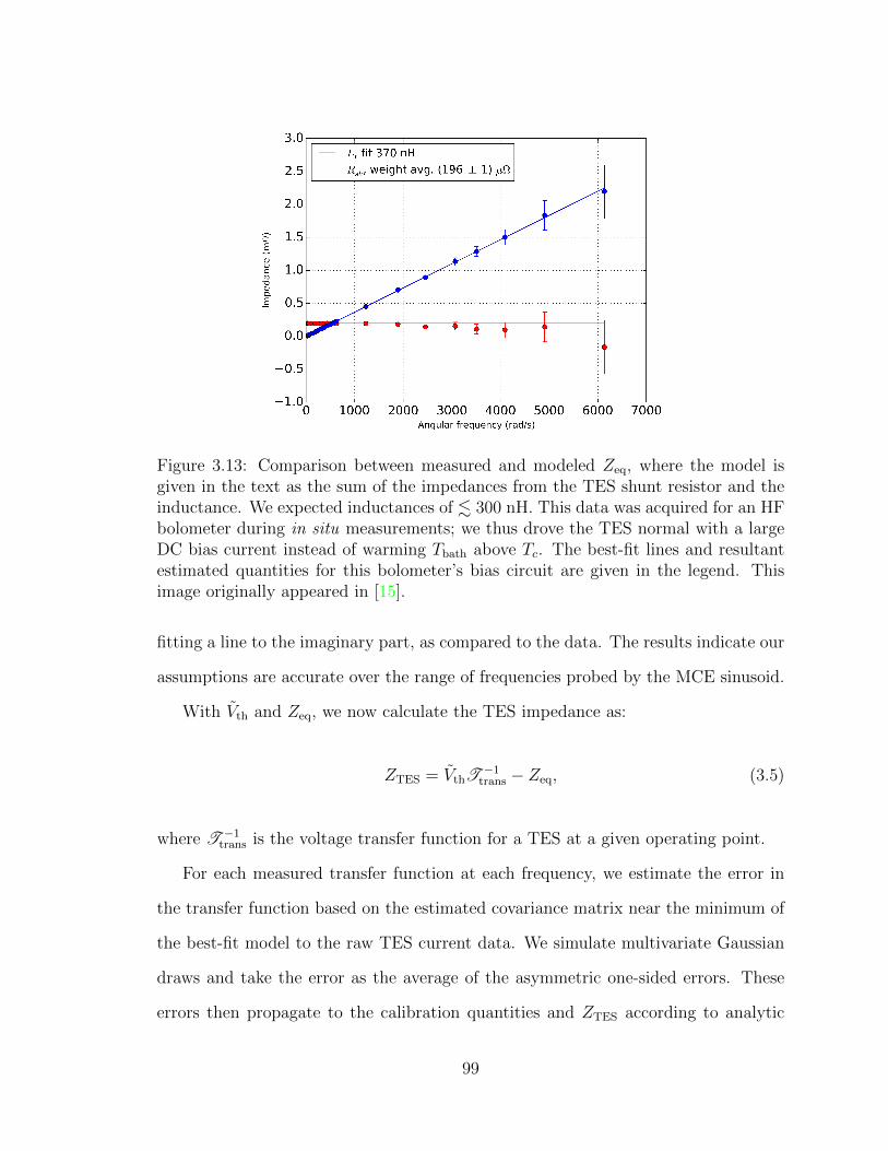
Figure 3.13: Comparison between measured and modeled Zeq, where the model isgiven in the text as the sum of the impedances from the TES shunt resistor and theinductance. We expected inductances of . 300 nH. This data was acquired for an HFbolometer during in situ measurements; we thus drove the TES normal with a largeDC bias current instead of warming Tbath above Tc. The best-fit lines and resultantestimated quantities for this bolometer’s bias circuit are given in the legend. Thisimage originally appeared in [15].

fitting a line to the imaginary part, as compared to the data. The results indicate our

assumptions are accurate over the range of frequencies probed by the MCE sinusoid.

With Vth and Zeq, we now calculate the TES impedance as:

ZTES = VthT−1

trans − Zeq, (3.5)

where T −1trans is the voltage transfer function for a TES at a given operating point.

For each measured transfer function at each frequency, we estimate the error in

the transfer function based on the estimated covariance matrix near the minimum of

the best-fit model to the raw TES current data. We simulate multivariate Gaussian

draws and take the error as the average of the asymmetric one-sided errors. These

errors then propagate to the calibration quantities and ZTES according to analytic

99

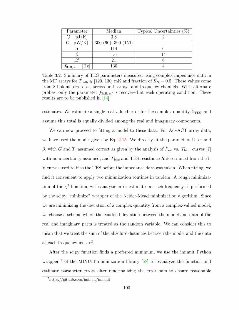
Parameter Median Typical Uncertainties (%)C [pJ/K] 3.8 2G [pW/K] 300 (90); 390 (150) –

α 114 6β 1.6 14L 21 6

f3dB, eff [Hz] 130 4

Table 3.2: Summary of TES parameters measured using complex impedance data inthe MF arrays for Tbath ∈ [120, 130] mK and fraction of RN = 0.5. These values comefrom 8 bolometers total, across both arrays and frequency channels. With alternateprobes, only the parameter f3dB, eff is recovered at each operating condition. Theseresults are to be published in [14].

estimates. We estimate a single real-valued error for the complex quantity ZTES, and

assume this total is equally divided among the real and imaginary components.

We can now proceed to fitting a model to these data. For AdvACT array data,

we have used the model given by Eq. 2.15. We directly fit the parameters C, α, and

β, with G and Tc assumed correct as given by the analysis of Psat vs. Tbath curves [?]

with no uncertainty assumed, and Pbias and TES resistance R determined from the I-

V curves used to bias the TES before the impedance data was taken. When fitting, we

find it convenient to apply two minimization routines in tandem. A rough minimiza-

tion of the χ2 function, with analytic error estimates at each frequency, is performed

by the scipy “minimize” wrapper of the Nelder-Mead minimization algorithm. Since

we are minimizing the deviation of a complex quantity from a complex-valued model,

we choose a scheme where the coadded deviation between the model and data of the

real and imaginary parts is treated as the random variable. We can consider this to

mean that we treat the sum of the absolute distances between the model and the data

at each frequency as a χ2.

After the scipy function finds a preferred minimum, we use the iminuit Python

wrapper 7 of the MINUIT minimization library [58] to reanalyze the function and

estimate parameter errors after renormalizing the error bars to ensure reasonable

7https://github.com/iminuit/iminuit

100

reduced χ2 values. Using the “minos” function in iminuit, we can fully explore any

nonlinearities near the minimum to ensure our parameter errors are conservative.

These errors are the basis of the results in Tab. 3.2. In that table, we record details

about the parameters recovered from fitting the impedance data of bolometers across

both MF arrays and both frequency channels, in various operating conditions. We

additionally include derived parameters like L and the f3dB,eff. The errors on the

former are scaled from the estimated error on the TES α, while for the latter we

draw realizations from the multivariate Gaussian described by the MINUIT-estimated

covariance and take the spread as an error estimate.

As an added consideration, we find it necessary to impose certain constraints

on the fit parameters in order to avoid a proliferation of degrees of freedom and

to break possible degeneracies. For these data, the main feature is that impedance

data at different % RN are fit with a common heat capacity C for the bolometer.

This improves the substantial degeneracy between C and α. Thus, only the TES

sensitivities α and β are fit for each operating condition. Unfortunately, the limits of

the sinusoid frequency (or equivalently, the sampling) mean that for fast devices, we

are not able to strongly constrain β from the high-frequency limit of the impedance.

In this case, α and β become strongly covariant.

We include an example covariance matrix for the same bolometer with example

impedance data shown in Fig. 3.14. The left panel shows the operating-condition

data for all % RN at 120 mK for an MF1 90 GHz bolometer, while the right shows

the estimated covariance when all datasets in 12 operating conditions (30%, 50%

and 70% RN at 100, 120, and 140 mK) are used to fit the 21 parameters describing

the impedance. Interestingly, covariance of α at the same bias points across bath

temperatures is similarly large when compared to the covariance between α and β

in the same operating condition. We note that all errors estimated using MINUIT

properly account for these covariances.

101

All of the above measurements have been interpreted in the context of the simple

bolometer electrothermal model. However, we expect a correlate in the impedance

data for the excess noise discussed above. This is observed using data acquired at

NIST, and most apparent in bolometers fabricated as part of MF single pixels in

2016. When fitting these data, we find it useful to perform the following processes in

our numerical studies:

• Select a break frequency fsplit, where for frequencies below fsplit we estimate

single-block model parameters as described above;

• Open the fitting regime to a wide range of frequencies up to ∼ 20-30 kHz, where

impedance data at these frequencies are acquired with optimized with SQUID

feedback parameters;

• Use these parameters as an initialization array for a Markov Chain Monte Carlo

(MCMC) sampler (implemented in the emcee [33] Python package), to be dis-

cussed further below;

• Take the median value sampled by the MCMC chain for each parameter as our

best-fit value, and estimate errors according to percentiles in the marginalized

parameter distributions.

We switch to MCMC sampling as we expand our possible degeneracies when fitting

the hanging model. When fitting this model, we alter our constraints such that all

thermal parameters Ci, Gi, and C are held constant across all operating conditions.

We find empirically that this improves the sampler performance.

In addition, due to the way the NIST data are acquired using a software lock-in,

we are not able to estimate errors in the same way as in the MCE measurement case.

We follow the analysis provided in Ref. [79], altering their error estimate to take as

input the RMS TES current fluctuations. Assuming a fiducial ∆ITES estimated from

102

thermal-link noise converted to current only by the bias voltage, and thus independent

of frequency, we write a real-valued error ∆ZTES representing the coadded real and

imaginary error as:

|∆ZTES| =

∣∣∣∣∣(ZTES + Zeq)2

Vthev

∣∣∣∣∣∆ITES, (3.6)

where we convert Vthev estimated from the function calculated in Eq. 3.4a to proper

voltage units using the ideal conversion −Mrat/Rfb. This equation applies at each

frequency.

As a final caveat, we have found it necessary to carefully tune the parameters

of the NIST SQUID feedback circuit to ensure good high-frequency response of the

feedback signal. Our focus was mainly on changing the P and I parameters of the

feedback together to ensure frequency-independent response of the superconducting

transfer data at frequencies above 10 kHz. Altering these numbers affect the shape of

the high-frequency impedance data, but we strongly expect that properly calibrating

these data as described above will not produce bias.

With the errors estimated and the minimization routine ready, it is now possible

to explore the results of fitting the two-block model to data up to tens of kilohertz.

Figure 3.15 shows the measured data and MCMC-preferred model results for two

MF single-pixel bolometers, the top panel a 150 GHz-channel bolometer and the

bottom a 90 GHz-channel bolometer. It is clear that the model is able to describe

the “turnover” in the data, and in doing so, recover a large Gi. For the bolometer in

the top panel, the ratio of Gi : G at 40% RN is 110; for the bottom, it is 120.

This behavior persists, in this case, across operating conditions, though the range

of the feature (i.e. the change in the real part of ZTES at high frequencies) is reduced

at higher Tbath, and thus lower Pbias and ITES. Due to the form of the equations

describing the hanging model, this is not necessarily a surprise – the severity of both

the distortion to the impedance and, as will be shown, the noise spectral densities, is

enhanced for large Pbias and large loop gain L .

103

In Fig. 3.16, we show the parameter distributions of the MCMC chain across all

parameter pairs, as well as the 1-D reduced distributions. The strong covariance of α

and β parameters across operating conditions, especially bath temperatures, is due to

their mutual covariance with the thermal parameters, especially in the case of α and

Gi. These results highlight that the equations describing TES bolometer impedance

feature strong parameter degeneracies. Nevertheless, we can place few-percent errors

on these parameters, and better understand how real devices perform with regard to

the models in use.

104

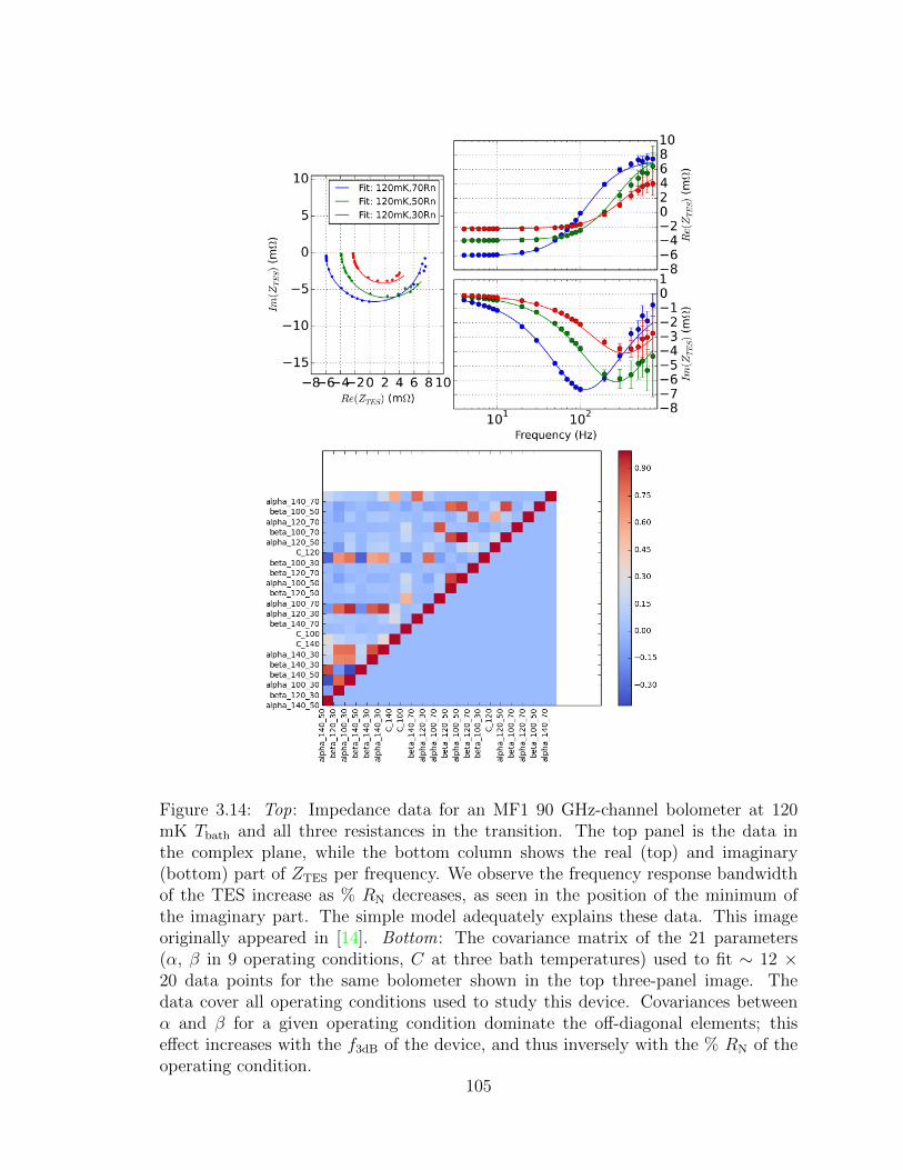
Figure 3.14: Top: Impedance data for an MF1 90 GHz-channel bolometer at 120mK Tbath and all three resistances in the transition. The top panel is the data inthe complex plane, while the bottom column shows the real (top) and imaginary(bottom) part of ZTES per frequency. We observe the frequency response bandwidthof the TES increase as % RN decreases, as seen in the position of the minimum ofthe imaginary part. The simple model adequately explains these data. This imageoriginally appeared in [14]. Bottom: The covariance matrix of the 21 parameters(α, β in 9 operating conditions, C at three bath temperatures) used to fit ∼ 12 ×20 data points for the same bolometer shown in the top three-panel image. Thedata cover all operating conditions used to study this device. Covariances betweenα and β for a given operating condition dominate the off-diagonal elements; thiseffect increases with the f3dB of the device, and thus inversely with the % RN of theoperating condition.

105

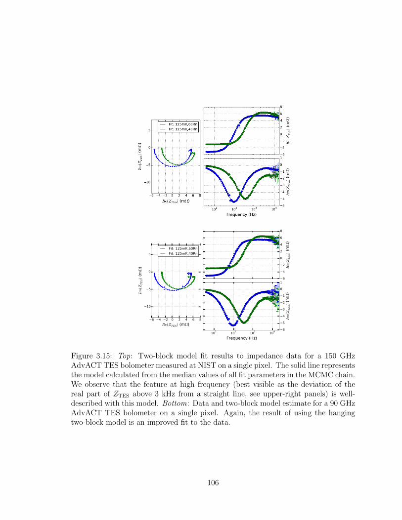
6 4 2 0 2 4 6 8Re(ZTES) (mΩ)

10

5

0

5

Im(Z

TES) (

mΩ

)

Fit: 125mK,60RnFit: 125mK,40Rn

6

4

2

0

2

4

6

8

Re(ZTES) (

mΩ

)

101 102 103 104

Frequency (Hz)

6

5

4

3

2

1

0

1Im

(ZTES) (

mΩ

)

Figure 3.15: Top: Two-block model fit results to impedance data for a 150 GHzAdvACT TES bolometer measured at NIST on a single pixel. The solid line representsthe model calculated from the median values of all fit parameters in the MCMC chain.We observe that the feature at high frequency (best visible as the deviation of thereal part of ZTES above 3 kHz from a straight line, see upper-right panels) is well-described with this model. Bottom: Data and two-block model estimate for a 90 GHzAdvACT TES bolometer on a single pixel. Again, the result of using the hangingtwo-block model is an improved fit to the data.

106

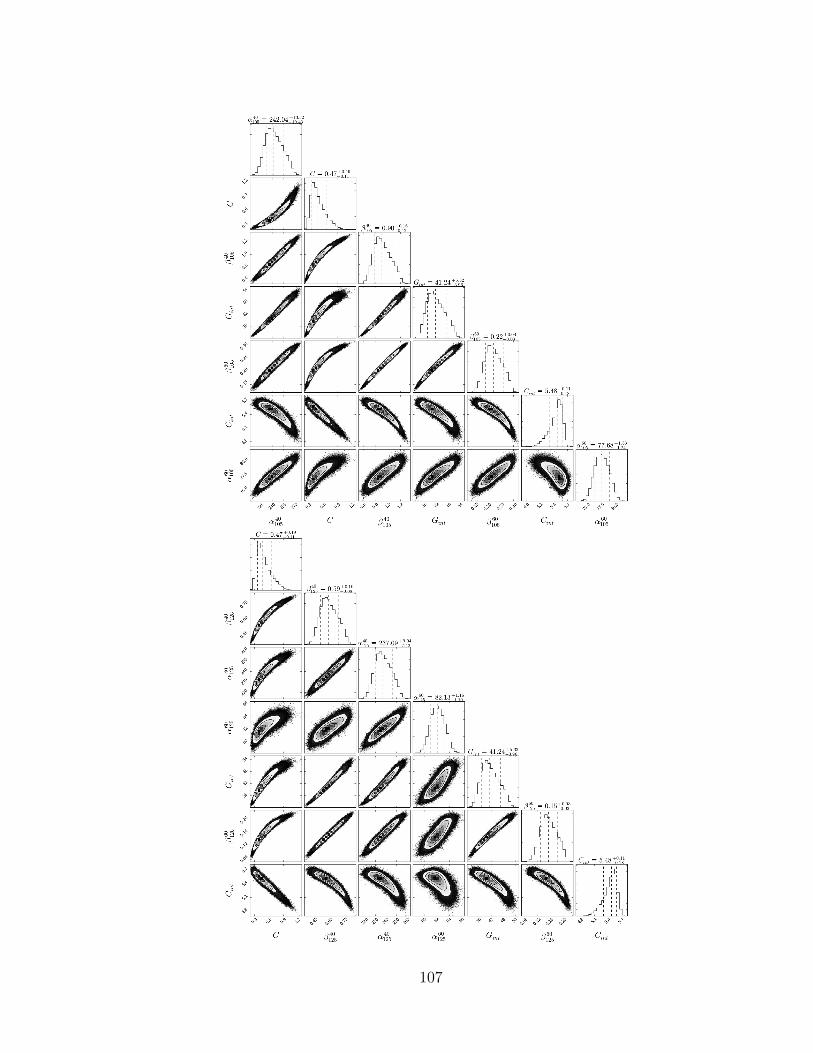
107

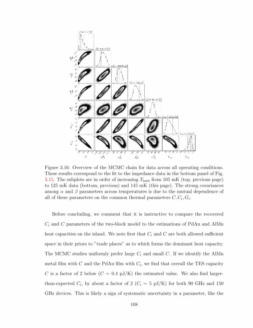
Figure 3.16: Overview of the MCMC chain for data across all operating conditions.These results correspond to the fit to the impedance data in the bottom panel of Fig.3.15. The subplots are in order of increasing Tbath from 105 mK (top, previous page)to 125 mK data (bottom, previous) and 145 mK (this page). The strong covariancesamong α and β parameters across temperatures is due to the mutual dependence ofall of these parameters on the common thermal parameters C,Ci, Gi.

Before concluding, we comment that it is instructive to compare the recovered

Ci and C parameters of the two-block model to the estimations of PdAu and AlMn

heat capacities on the island. We note first that Ci and C are both allowed sufficient

space in their priors to ”trade places” as to which forms the dominant heat capacity.

The MCMC studies uniformly prefer large Ci and small C. If we identify the AlMn

metal film with C and the PdAu film with Ci, we find that overall the TES capacity

C is a factor of 2 below (C ∼ 0.4 pJ/K) the estimated value. We also find larger-

than-expected Ci, by about a factor of 2 (Ci ∼ 5 pJ/K) for both 90 GHz and 150

GHz devices. This is likely a sign of systematic uncertainty in a parameter, like the

108

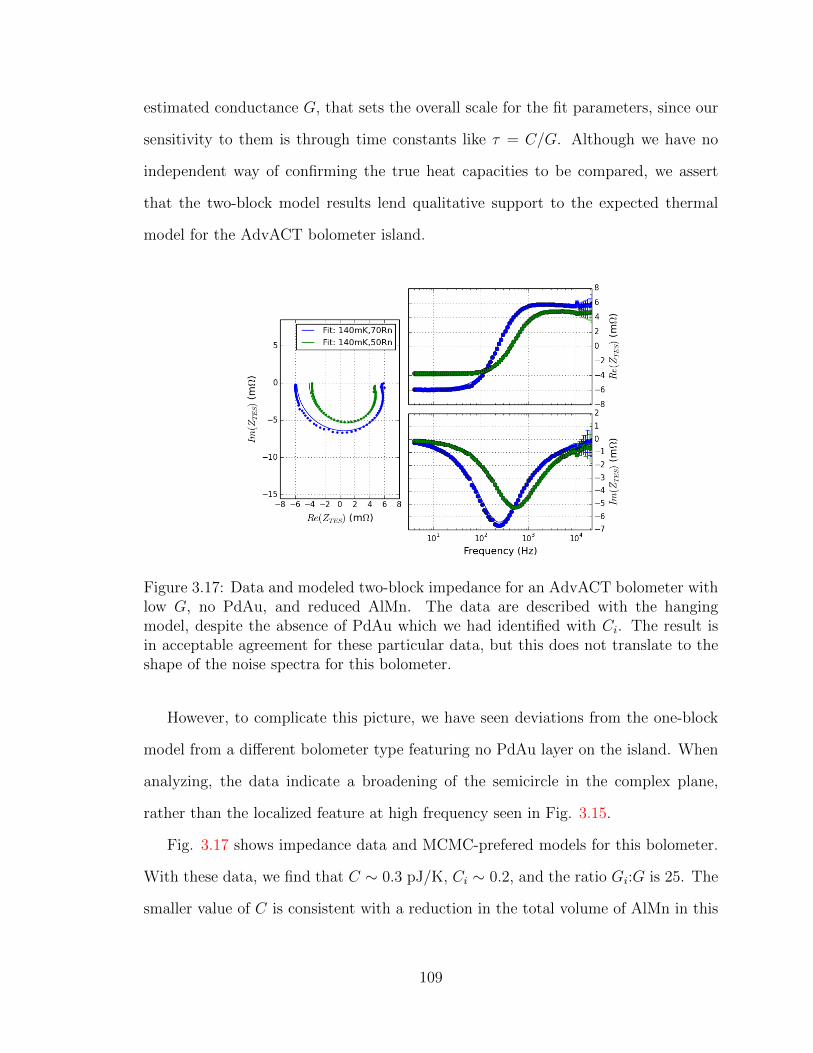
estimated conductance G, that sets the overall scale for the fit parameters, since our

sensitivity to them is through time constants like τ = C/G. Although we have no

independent way of confirming the true heat capacities to be compared, we assert

that the two-block model results lend qualitative support to the expected thermal

model for the AdvACT bolometer island.

Figure 3.17: Data and modeled two-block impedance for an AdvACT bolometer withlow G, no PdAu, and reduced AlMn. The data are described with the hangingmodel, despite the absence of PdAu which we had identified with Ci. The result isin acceptable agreement for these particular data, but this does not translate to theshape of the noise spectra for this bolometer.

However, to complicate this picture, we have seen deviations from the one-block

model from a different bolometer type featuring no PdAu layer on the island. When

analyzing, the data indicate a broadening of the semicircle in the complex plane,

rather than the localized feature at high frequency seen in Fig. 3.15.

Fig. 3.17 shows impedance data and MCMC-prefered models for this bolometer.

With these data, we find that C ∼ 0.3 pJ/K, Ci ∼ 0.2, and the ratio Gi:G is 25. The

smaller value of C is consistent with a reduction in the total volume of AlMn in this

109

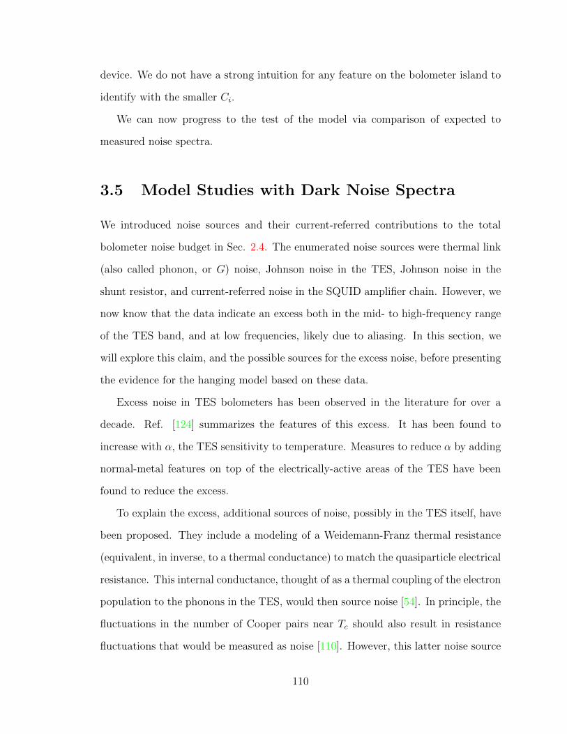
device. We do not have a strong intuition for any feature on the bolometer island to

identify with the smaller Ci.

We can now progress to the test of the model via comparison of expected to

measured noise spectra.

3.5 Model Studies with Dark Noise Spectra

We introduced noise sources and their current-referred contributions to the total

bolometer noise budget in Sec. 2.4. The enumerated noise sources were thermal link

(also called phonon, or G) noise, Johnson noise in the TES, Johnson noise in the

shunt resistor, and current-referred noise in the SQUID amplifier chain. However, we

now know that the data indicate an excess both in the mid- to high-frequency range

of the TES band, and at low frequencies, likely due to aliasing. In this section, we

will explore this claim, and the possible sources for the excess noise, before presenting

the evidence for the hanging model based on these data.

Excess noise in TES bolometers has been observed in the literature for over a

decade. Ref. [124] summarizes the features of this excess. It has been found to

increase with α, the TES sensitivity to temperature. Measures to reduce α by adding

normal-metal features on top of the electrically-active areas of the TES have been

found to reduce the excess.

To explain the excess, additional sources of noise, possibly in the TES itself, have

been proposed. They include a modeling of a Weidemann-Franz thermal resistance

(equivalent, in inverse, to a thermal conductance) to match the quasiparticle electrical

resistance. This internal conductance, thought of as a thermal coupling of the electron

population to the phonons in the TES, would then source noise [54]. In principle, the

fluctuations in the number of Cooper pairs near Tc should also result in resistance

fluctuations that would be measured as noise [110]. However, this latter noise source

110

is assumed to be below the noise floor sourced by the thermal link noise, for instance,

and thus is negligible.

Modeling of TESes as superconducting weak links [108] [65] has added the possi-

bility of noise sourced by the stochastic generation of “phase slips,” or 2π wrappings

of the superconducting order parameter within the TES between its superconducting

leads. Ref. [35] gives a detailed presentation of this concept, along with equations

useful for estimating the size of this noise source based on experimentally-accessible

TES parameters. In his work, the claim that phase-slip “shot noise” can replicate the

main qualitative features of TES excess noise seen in detailed device studies in the

literature.

However, the notion of extended electrothermal models sourcing excess noise [133]

[41] [42] has generally allowed sufficient freedom to reproduce the spectral and op-

erating condition-dependent features of excess TES noise. In both of the latter two

references, the notion of indefinite numbers of thermal blocks in series arises naturally

from studying the generic features of N block models. In the first reference, [133],

as in this reference, we prefer to extend the model to a definite number of blocks

and determine the validity of this extension, in order to elucidate the possible causes

for the excess in the detector architecture. Though this ambitious goal is not easily

accomplished, it is a strong desideratum to only extend the bolometer model to a

physically-motivated degree.

In initially investigating the excess noise, we proceeded along the lines of [59], in

which a similar excess is studied by assuming it is an enhancement of the TES Johnson

noise. In the regime of AdvACT detectors, with α well over 100 and large Pbias and

TES current at the sensor, we assumed that some element of the equilibrium form of

the Johnson noise may not be valid. This would be beyond the correction outlined

in [57] where a nonequilbrium factor of (1 + 2β) is a coefficient of the Johnson noise.

We have included that term throughout this work.

111

We found that this hypothesis is not satisfactory with respect to more than two

or three of the bolometers studied with impedance and noise acquisitions. However,

in the cases where some semblance of agreement is found, we were able to use the

modeled bolometer noise to predict the effect of aliased noise. To be explicit, our

noise model is written:

StotI = Sthermal

I + SshI + (1 +M2)SJ

I + SSQUIDI , (3.7)

where each of these terms is the current-referred noise associated with the noise source.

We choose this parameterization so that the factor multiplying SJI is positive-definite

and is significant if it deviates from zero.

10-2 10-1 100 101 102 103 104

Frequency (Hz)

10-23

10-22

10-21

10-20

10-19

10-18

10-17

Nois

e cu

rren

t spe

ctra

l den

sity

(A2

/Hz)

Temp 120, 50%Rn120mK, 50%RnASD = 1.66e-20±1.645e-21Best-fit excess noiseM2 =15.9ASD = 2.35e-20Estimated noiseASD = 1.346e-20thermalJohnsonshunt

Figure 3.18: Measured noise current spectral density (blue) compared to the one-blockmodel expectation derived from parameters measured via impedance data (greendashed) and with the addition of scaled TES Johnson noise (red dot-dashed). Allmodel lines include the effects of aliasing from the Nyquist frequency up to 1 MHz.Aliasing is responsible for the difference between the green model and the red-dash dotfor frequencies below 100 Hz. The width of the green line is roughly equal to the 68%CL (gray band) based on 100 multivariate-Gaussian drawns on the Minuit-estimatedcovariance. These data will be published in [Crowley LTD JLTP].

When we discuss “aliasing” in the TDM context relevant for AdvACT, we mean

that frequencies above the row-visit rate (7.5 kHz for HF, 9 kHZ for MF, 15 kHz

112

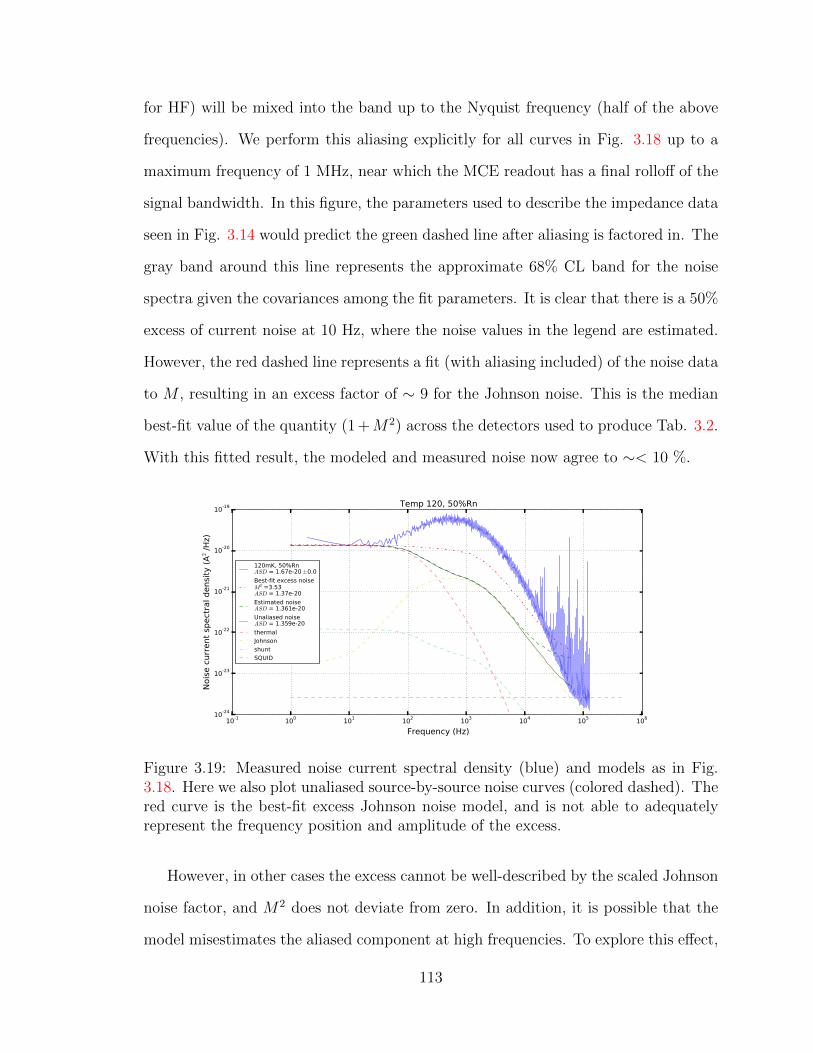
for HF) will be mixed into the band up to the Nyquist frequency (half of the above

frequencies). We perform this aliasing explicitly for all curves in Fig. 3.18 up to a

maximum frequency of 1 MHz, near which the MCE readout has a final rolloff of the

signal bandwidth. In this figure, the parameters used to describe the impedance data

seen in Fig. 3.14 would predict the green dashed line after aliasing is factored in. The

gray band around this line represents the approximate 68% CL band for the noise

spectra given the covariances among the fit parameters. It is clear that there is a 50%

excess of current noise at 10 Hz, where the noise values in the legend are estimated.

However, the red dashed line represents a fit (with aliasing included) of the noise data

to M , resulting in an excess factor of ∼ 9 for the Johnson noise. This is the median

best-fit value of the quantity (1 +M2) across the detectors used to produce Tab. 3.2.

With this fitted result, the modeled and measured noise now agree to ∼< 10 %.

10-1 100 101 102 103 104 105 106

Frequency (Hz)

10-24

10-23

10-22

10-21

10-20

10-19

Nois

e cu

rren

t spe

ctra

l den

sity

(A2

/Hz)

Temp 120, 50%Rn

120mK, 50%RnASD = 1.67e-20±0.0Best-fit excess noiseM2 =3.53ASD = 1.37e-20Estimated noiseASD = 1.361e-20Unaliased noiseASD = 1.359e-20thermalJohnsonshuntSQUID

Figure 3.19: Measured noise current spectral density (blue) and models as in Fig.3.18. Here we also plot unaliased source-by-source noise curves (colored dashed). Thered curve is the best-fit excess Johnson noise model, and is not able to adequatelyrepresent the frequency position and amplitude of the excess.

However, in other cases the excess cannot be well-described by the scaled Johnson

noise factor, and M2 does not deviate from zero. In addition, it is possible that the

model misestimates the aliased component at high frequencies. To explore this effect,

113

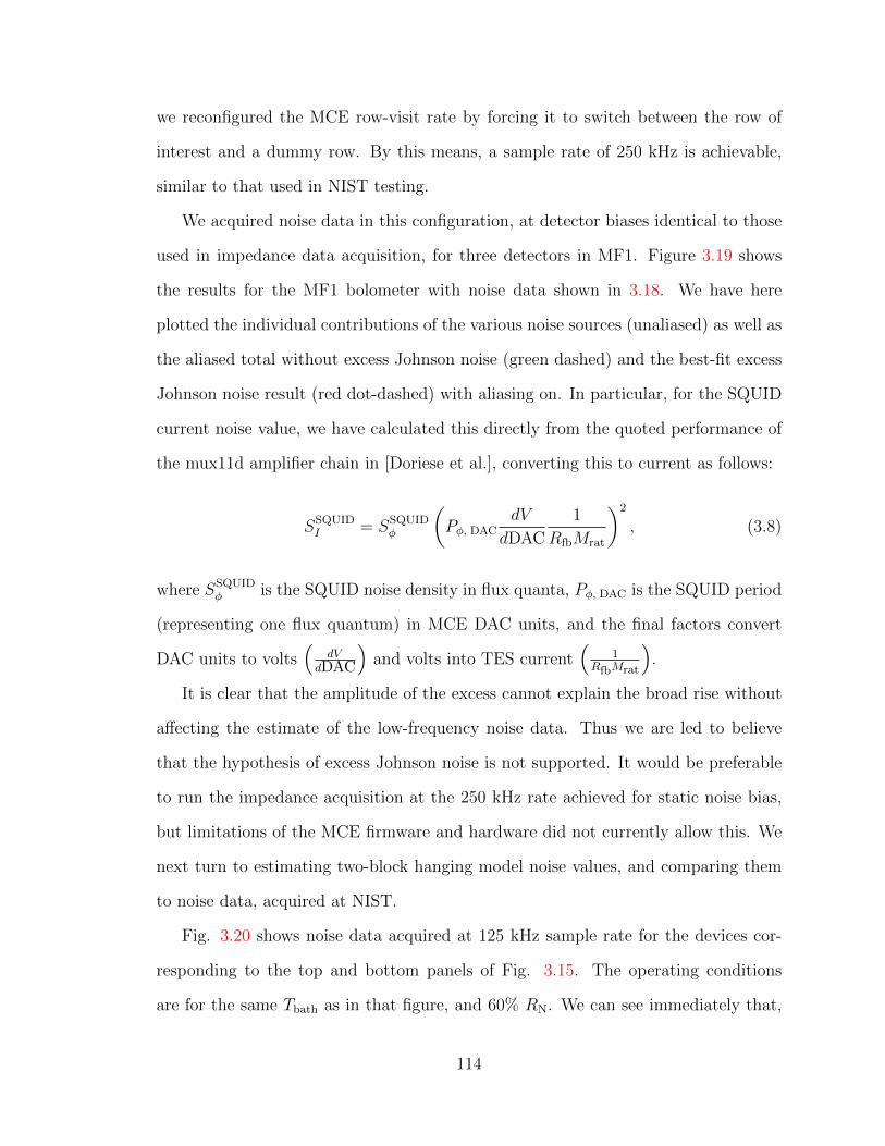
we reconfigured the MCE row-visit rate by forcing it to switch between the row of

interest and a dummy row. By this means, a sample rate of 250 kHz is achievable,

similar to that used in NIST testing.

We acquired noise data in this configuration, at detector biases identical to those

used in impedance data acquisition, for three detectors in MF1. Figure 3.19 shows

the results for the MF1 bolometer with noise data shown in 3.18. We have here

plotted the individual contributions of the various noise sources (unaliased) as well as

the aliased total without excess Johnson noise (green dashed) and the best-fit excess

Johnson noise result (red dot-dashed) with aliasing on. In particular, for the SQUID

current noise value, we have calculated this directly from the quoted performance of

the mux11d amplifier chain in [Doriese et al.], converting this to current as follows:

SSQUIDI = SSQUID

φ

(Pφ, DAC

dV

dDAC

1

RfbMrat

)2

, (3.8)

where SSQUIDφ is the SQUID noise density in flux quanta, Pφ, DAC is the SQUID period

(representing one flux quantum) in MCE DAC units, and the final factors convert

DAC units to volts(

dVdDAC

)and volts into TES current

(1

RfbMrat

).

It is clear that the amplitude of the excess cannot explain the broad rise without

affecting the estimate of the low-frequency noise data. Thus we are led to believe

that the hypothesis of excess Johnson noise is not supported. It would be preferable

to run the impedance acquisition at the 250 kHz rate achieved for static noise bias,

but limitations of the MCE firmware and hardware did not currently allow this. We

next turn to estimating two-block hanging model noise values, and comparing them

to noise data, acquired at NIST.

Fig. 3.20 shows noise data acquired at 125 kHz sample rate for the devices cor-

responding to the top and bottom panels of Fig. 3.15. The operating conditions

are for the same Tbath as in that figure, and 60% RN. We can see immediately that,

114

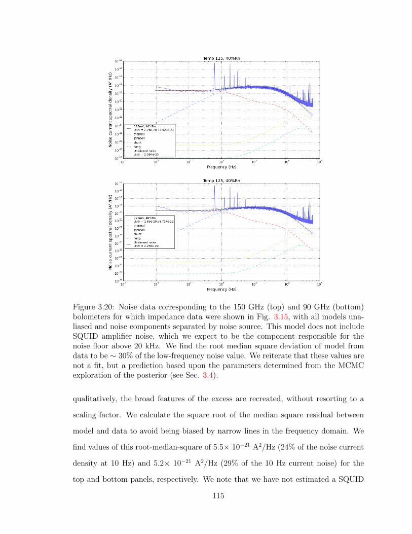
Figure 3.20: Noise data corresponding to the 150 GHz (top) and 90 GHz (bottom)bolometers for which impedance data were shown in Fig. 3.15, with all models una-liased and noise components separated by noise source. This model does not includeSQUID amplifier noise, which we expect to be the component responsible for thenoise floor above 20 kHz. We find the root median square deviation of model fromdata to be ∼ 30% of the low-frequency noise value. We reiterate that these values arenot a fit, but a prediction based upon the parameters determined from the MCMCexploration of the posterior (see Sec. 3.4).

qualitatively, the broad features of the excess are recreated, without resorting to a

scaling factor. We calculate the square root of the median square residual between

model and data to avoid being biased by narrow lines in the frequency domain. We

find values of this root-median-square of 5.5× 10−21 A2/Hz (24% of the noise current

density at 10 Hz) and 5.2× 10−21 A2/Hz (29% of the 10 Hz current noise) for the

top and bottom panels, respectively. We note that we have not estimated a SQUID

115

current noise for these data, partially explaining the deviation of the model below the

data at high frequencies.

Figure 3.21: Noise current spectral density data, by-source noise estimates, and totalnoise estimates for the hanging model as applied to the detector with impedance datashown in Fig. 3.17. In this case, the hanging model does not accurately describe thebroad features in the noise spectra. We do not yet have a model to describe thisobserved behavior.

According to this model, then, the Johnson noise of the AdvACT TES devices

is strongly suppressed, even with respect to the one-block model at these large (∼>

10) loop gains L . The important second source of noise, then, is that sourced by the

internal conductance Gi. Understanding how this noise excess varies under different

operating conditions then becomes critical. Instead of the large-L suppression of

Johnson noise, we find that for both larger α (smaller % RN) and larger Pbias (smaller

Tbath), the excess appears more clearly in the current noise. This is despite the cur-

rent noise induced by the smaller conductance to bath, which continues to dominate

at frequencies below ∼ 50 Hz, also increasing for smaller % RN. In general, then,

the behavior of this excess is as described by [Ullom], but we argue that it can be

completely attributed to a thermal noise source connecting to a hanging heat capac-

ity in an extended model. We note that this line of reasoning cannot be completely

proven, given issues seen in fitting the hanging model to data at 20% and 30% RN.

116

In general, concerns about TES instabilities near these resistances makes them less

likely to be used during normal observations.

As a final point of interest, we conclude this section by including the estimated

noise for the unique low-G bolometer studied in 3.17. Fig. 3.21 indicates that the

resulting total noise estimate cannot replicate the frequency-domain shape of the

data, as opposed to the MF case. This is more evidence that the hanging model may

not be applicable here, and moving to a new model is motivated.

3.6 Field Performance of Arrays

As a result of the array tests above and others described elsewhere [53] [12], the

first three AdvACT arrays were deemed ready for use in observations. The high-

frequency (HF) array was installed on the telescope in summer 2016, and observed

for six months along with the previously-installed ACTPol arrays. After an inter-

season break, telescope operations resumed in May 2017 after the installation of the

two MF arrays in April 2017. In this section, we describe the performance of the

three AdvACT arrays during their simultaneous observations throughout the 2017

season (referred to as “s17” hereafter).

Yield. Before celestial observations can begin, the arrays must be tuned and

studied to understand the presence of possible issues like open lines, persistence, etc.

This array commissioning in s17 proceeded by:

• Tuning the array and finding readout channels with problematic or no SQUID

response.

• Testing for persistence and noting for which columns and whether it can be

allayed.

• Taking I-V curves across the array to determine working detectors.

117

The response to each type of issue is, in the case of open SQUID response, to add

the channel to a “deadlist” for which the MCE feedback loop will not be applied.

This avoids the possibility of the MCE ramping the feedback DAC through its entire

dynamic range in search of a faulty lock point. For MF1 and MF2, the majority of

bad readout channels were isolated and seemingly random, with one broken column

in MF2. In HF, critical line electrical failures preventing signal passes has greatly

reduced the number of working detectors. We cannot ascertain the cause of these

failures until the array is removed from the field.

In the case of persistence, we found four weakly persistent and two strongly per-

sistent columns in MF2, and none in HF and MF1. We believe that, by underbiasing

the SQ1 in the affected columns, we have reduced the persistence to acceptable levels.

Detectors in the two persistent columns, which have now observed for a year, have not

been fully vetted, but it appears their I-V characteristics deviate from expectations

significantly.

Finally, for detector channels which do not respond to I-V curves, which we assume

indicates a failure of a wirebond somewhere in the TES readout circuit, we create lists

of non-working detectors in order to prevent their data from being used to determine

applied voltages to the TES bias lines. This is convenient with the MCE configuration

files describing each array’s bias line configuration.

We estimate our yields with respect to the number of optically-active TES bolome-

ters for the arrays (2024 in HF, 1716 in MF). Fig. 3.22 shows the trend of number

of well-biased detectors for each of ∼ 500 I-V datasets vs. the estimated precipitable

water vapor (PWV), a proxy for atmospheric loading in power, divided by sin(el),

where el is the elevation of the telescope during the observation. These results are

taken across the entirety of s17. The three plots cover each array (HF, MF1, MF2

from left to right). We observe that the MF arrays are fairly static with respect

to atmospheric brightness. This is partially due to the atmospheric loading on the

118

90 GHz detectors being minimal when compared to their Psat targets. In HF, the

more complex response is likely due to the dichroic nature of the arrays, with the 230

GHz-channel bolometers being especially sensitive to atmospheric loading, and some

saturating between 1 mm and 2 mm PWV.

Transforming these numbers into yields, we recover that at 1.5 mm loading, the

HF yield is 66% (1326 detectors), the MF1 yield is 94% (1612 detectors), and the

MF2 yield is 83% (1432 detectors).

1/f Noise. A major difference between detector studies in the laboratory and in

situ on ACT is the presence of additional sources of noise. We expect that thermal

fluctuations will be larger, due to the lack of focal plane temperature regulation. In

addition, it is believed that the motion (specifically the acceleration) of the telescope

can induce additional array heating through mechanical vibrations. As the telescope

scans, the harmonics of the scan frequency rise above the noise background, and can

play a significant role in determining the low-frequency noise properties of the arrays

in the field. Finally, the strong correlated noise induced by changing atmospheric

fluctuations, with spatial coherence lengths on the order of one-quarter to one-half of

the array, results in 1/f modes that must be understood.

Other ACT-related studies have described how array-scale common modes in-

duced by the atmosphere can be used to determine a flat field for the array [26] [80].

This flat field will partially prevent the correlated modes of the assumed-unpolarized

atmosphere from leaking into polarization. However, once this is done, we may be

concerned that other correlated noise sources, like bath temperature fluctuations, will

become the dominant mode.

In the ACTPol context, we explored trying to recover information about possible

correlations between timestreams from the thermometers used to record array tem-

peratures and the correlated noise in the TES bolometer timestreams. This has been

observed in other references for the ACTPol receiver [96]. The results of this study

119

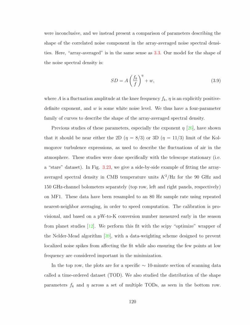
were inconclusive, and we instead present a comparison of parameters describing the

shape of the correlated noise component in the array-averaged noise spectral densi-

ties. Here, “array-averaged” is in the same sense as 3.3. Our model for the shape of

the noise spectral density is:

SD = A

(fkf

)η+ w, (3.9)

where A is a fluctuation amplitude at the knee frequency fk, η is an explicitly positive-

definite exponent, and w is some white noise level. We thus have a four-parameter

family of curves to describe the shape of the array-averaged spectral density.

Previous studies of these parameters, especially the exponent η [26], have shown

that it should be near either the 2D (η = 8/3) or 3D (η = 11/3) limit of the Kol-

mogorov turbulence expressions, as used to describe the fluctuations of air in the

atmosphere. These studies were done specifically with the telescope stationary (i.e.

a “stare” dataset). In Fig. 3.23, we give a side-by-side example of fitting the array-

averaged spectral density in CMB temperature units K2/Hz for the 90 GHz and

150 GHz-channel bolometers separately (top row, left and right panels, respectively)

on MF1. These data have been resampled to an 80 Hz sample rate using repeated

nearest-neighbor averaging, in order to speed computation. The calibration is pro-

visional, and based on a pW-to-K conversion number measured early in the season

from planet studies [12]. We perform this fit with the scipy “optimize” wrapper of

the Nelder-Mead algorithm [39], with a data-weighting scheme designed to prevent

localized noise spikes from affecting the fit while also ensuring the few points at low

frequency are considered important in the minimization.

In the top row, the plots are for a specific ∼ 10-minute section of scanning data

called a time-ordered dataset (TOD). We also studied the distribution of the shape

parameters fk and η across a set of multiple TODs, as seen in the bottom row.

120

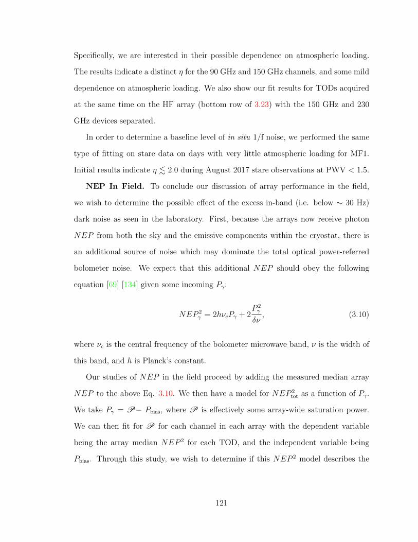
Specifically, we are interested in their possible dependence on atmospheric loading.

The results indicate a distinct η for the 90 GHz and 150 GHz channels, and some mild

dependence on atmospheric loading. We also show our fit results for TODs acquired

at the same time on the HF array (bottom row of 3.23) with the 150 GHz and 230

GHz devices separated.

In order to determine a baseline level of in situ 1/f noise, we performed the same

type of fitting on stare data on days with very little atmospheric loading for MF1.

Initial results indicate η . 2.0 during August 2017 stare observations at PWV < 1.5.

NEP In Field. To conclude our discussion of array performance in the field,

we wish to determine the possible effect of the excess in-band (i.e. below ∼ 30 Hz)

dark noise as seen in the laboratory. First, because the arrays now receive photon

NEP from both the sky and the emissive components within the cryostat, there is

an additional source of noise which may dominate the total optical power-referred

bolometer noise. We expect that this additional NEP should obey the following

equation [69] [134] given some incoming Pγ:

NEP 2γ = 2hνcPγ + 2

P 2γ

δν, (3.10)

where νc is the central frequency of the bolometer microwave band, ν is the width of

this band, and h is Planck’s constant.

Our studies of NEP in the field proceed by adding the measured median array

NEP to the above Eq. 3.10. We then have a model for NEP 2tot as a function of Pγ.

We take Pγ = P− Pbias, where P is effectively some array-wide saturation power.

We can then fit for P for each channel in each array with the dependent variable

being the array median NEP 2 for each TOD, and the independent variable being

Pbias. Through this study, we wish to determine if this NEP 2 model describes the

121

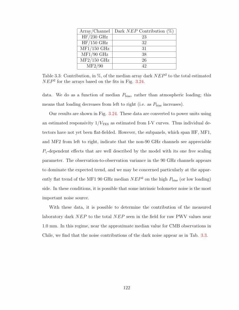
Array/Channel Dark NEP Contribution (%)HF/230 GHz 23HF/150 GHz 32

MF1/150 GHz 31MF1/90 GHz 38MF2/150 GHz 26

MF2/90 42

Table 3.3: Contribution, in %, of the median array dark NEP 2 to the total estimatedNEP 2 for the arrays based on the fits in Fig. 3.24.

data. We do as a function of median Pbias, rather than atmospheric loading; this

means that loading decreases from left to right (i.e. as Pbias increases).

Our results are shown in Fig. 3.24. These data are converted to power units using

an estimated responsivity 1/VTES as estimated from I-V curves. Thus individual de-

tectors have not yet been flat-fielded. However, the subpanels, which span HF, MF1,

and MF2 from left to right, indicate that the non-90 GHz channels see appreciable

Pγ-dependent effects that are well described by the model with its one free scaling

parameter. The observation-to-observation variance in the 90 GHz channels appears

to dominate the expected trend, and we may be concerned particularly at the appar-

ently flat trend of the MF1 90 GHz median NEP 2 on the high Pbias (or low loading)

side. In these conditions, it is possible that some intrinsic bolometer noise is the most

important noise source.

With these data, it is possible to determine the contribution of the measured

laboratory dark NEP to the total NEP seen in the field for raw PWV values near

1.0 mm. In this regime, near the approximate median value for CMB observations in

Chile, we find that the noise contributions of the dark noise appear as in Tab. 3.3.

122

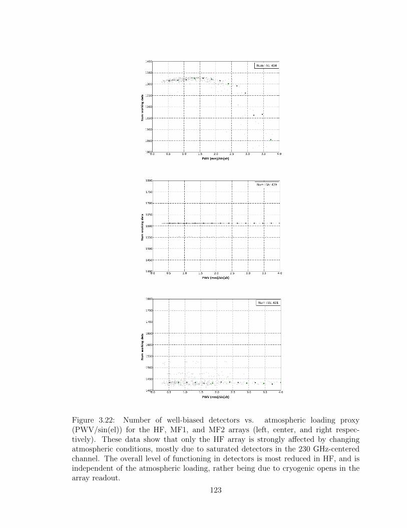
Figure 3.22: Number of well-biased detectors vs. atmospheric loading proxy(PWV/sin(el)) for the HF, MF1, and MF2 arrays (left, center, and right respec-tively). These data show that only the HF array is strongly affected by changingatmospheric conditions, mostly due to saturated detectors in the 230 GHz-centeredchannel. The overall level of functioning in detectors is most reduced in HF, and isindependent of the atmospheric loading, rather being due to cryogenic opens in thearray readout.

123

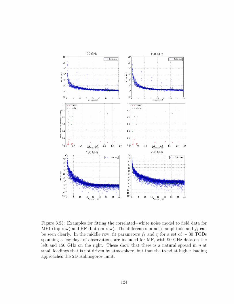
90 GHz 150 GHz

150 GHz 230 GHz

Figure 3.23: Examples for fitting the correlated+white noise model to field data forMF1 (top row) and HF (bottom row). The differences in noise amplitude and fk canbe seen clearly. In the middle row, fit parameters fk and η for a set of ∼ 30 TODsspanning a few days of observations are included for MF, with 90 GHz data on theleft and 150 GHz on the right. These show that there is a natural spread in η atsmall loadings that is not driven by atmosphere, but that the trend at higher loadingapproaches the 2D Kolmogorov limit.

124

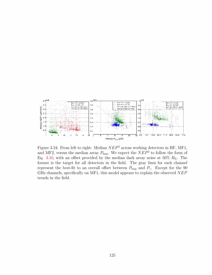
Median Pbias (pW)

Med

ian

NE

P2 (

aW2/H

z)

Figure 3.24: From left to right: Median NEP 2 across working detectors in HF, MF1,and MF2, versus the median array Pbias. We expect the NEP 2 to follow the form ofEq. 3.10, with an offset provided by the median dark array noise at 50% RN. Theformer is the target for all detectors in the field. The gray lines for each channelrepresent the best-fit to an overall offset between Pbias and Pγ. Except for the 90GHz channels, specifically on MF1, this model appears to explain the observed NEPtrends in the field.

125

3.7 Conclusion

In this chapter, we have presented an overview of the noise performance and bolometer

response characteristics of the three fielded AdvACT arrays as of summer 2018. In

these studies, it has been determined that a dark noise excess in the region of ∼ 100

Hz can be described according to the hanging two-block electrothermal model of a

TES bolometer. We further have initial evidence for the identification of the second

thermal lumped element with the layer of PdAu used to control the heat capacity of

the AdvACT bolometer island.

We have further described details of data acquisition with the MCE, which Ad-

vACT uses to implement its time-domain multiplexing in the laboratory and the

field. Complete studies of the TES bolometer impedance necessitated special data

acquired with an earlier, less-complex system that allowed for simple, fast (i.e. > 100

kHz) sampling of the TES response to sinusoid signals. It is these data that lend the

strongest support to the hypothesis that the two-block hanging model can adequately

describe the TES bolometers in AdvACT, especially in the MF arrays.

As a result of this excess, additional aliased noise is introduced into the frequency

band most relevant to CMB studies. This excess is seen when comparing the expected

dark noise in the arrays to measurements. However, we find that results in the field

indicate that AdvACT bolometers are dominated by photon noise induced by cryostat

loading and atmosphere, an important criterion for ensuring the detector arrays are

as sensitive as possible. Thus we believe that the AdvACT bolometer arrays, though

exhibiting interesting deviations from the simple bolometer model, are validated for

sensitive CMB observations.

126

Chapter 4

AdvACT Polarization Modulation

Studies

In this chapter, we describe the implementation of a continuously-rotating half-wave

plate (CRHWP) polarization modulator as part of the AdvACT project, and initial

analysis of the resulting detector data. We begin by providing a conceptual overview

of the modulation scheme, and the usefulness of modulation in general. We progress

to describing the HWP-synchronous signal that arises in detector timestreams, which

we henceforth refer to as A(χ). We then discuss the use of a warm CRHWP in

ABS, followed by the implementation in AdvACT and initial description of the A(χ)

signal seen in a special observing run during October 2017 during which all three

deployed AdvACT arrays had achromatic CRHWPs deployed in their optical paths.

We then progress to discussion of the HWP performance and usefulness of the data

from this special run, and conclude with a presentation of how A(χ) signals can be

used to inter-calibrate detectors and track changes in their complex-valued response

to incoming signals.

127

4.1 CRHWP Modulation: An Overview

As discussed in the last section of Ch. 3, the noise properties of the AdvACT TES

bolometers during observations differ from the white noise due to the presence of 1/f

noise derived from atmospheric brightness fluctuations in the detector optical band,

thermal drifts of the bath temperature of the arrays, and possibly other “noise”

sources. Here the quotes refer to the fact that these noise terms are in fact signals,

but ones that obscure the incoming CMB polarization and make understanding the

CMB at large scales from the ground a challenge.

We can understand the promise of modulating incoming polarization signals into

a frequency band where atmospheric signals do not dominate by considering the

following model for a TES timestream:

d(t) = s(t) + nwhite(t) + ncorr(t), (4.1)

where s(t) is the CMB signal we wish to recover, and the other two are noise terms,

with ncorr representing noise with a non-zero autocorrelation within d(t) on long

timescales and the characteristic frequency-domain shape of a power law, with ex-

ponent η, as given in Eq. 3.9. In addition, we expect ncorr to be correlated across

detectors in the focal plane due to the spatial coherence scale of the atmospheric

fluctuations.

If we take the Fourier transform of the above equation, which we will indicate

using s(ω), and assume that our polarization signal as measured at the detector has

been shifted to s(ω + ωmod), we can imagine filtering in a narrow band around ωmod

and demodulating our data at that frequency in order to recover a timestream that

is free of long-timescale correlated signals.

Multiple experiments spanning more than a decade [60] [121] [68] have used

CRHWPs to achieve this polarization signal modulation ahead of the detectors in the

128

optical path. Other experiments have used “stepped” HWPs in place of boresight

rotation in order to improve observing strategy relevant for polarimeter studies, and

to mitigate polarization systematics [9]. The signal description of a warm CRHWP

has been described in detail in Ref. [68], which we draw from broadly in the following.

First, we must introduce the concept of a HWP itself. A generic HWP can be con-

sidered as a disc, made of a birefringent material, in the x−y plane. We may imagine

that the HWP is positioned such that its strongly refracting (called “extraordinary”)

axis points along x and the orthogonal, more weakly refracting (“ordinary”) axis is

along y. A polarized plane wave traveling in the −z direction towards the HWP with

linear polarization angle θ from the x−axis will leave the HWP with polarization

angle −θ. This is because waves polarized along the different axes of the disc travel

at different speeds, producing an overall relative phase change between the x and y

components of the incoming wave’s polarization. This change is equivalent to the

polarization vector being rotated. Since the polarization is rotated by 2θ, for rotation

frequency θ/2π = f r, this effect and the spin-2 symmetry of polarization produces a

polarized signal at 4f r in the detector. This physical picture is summarized in Fig.

4.1.

We represent the CRHWP-modulated timestream as the following:

dm(t) = I + Iatmo + εRe[e2φ−4iχ (Q+ iU)

]+ A(χ), (4.2)

where we have suppressed the time dependence of χ, I, Iatmo, Q, and U . The expo-

nential factor multiplying the complex polarization value contains both a detector

polarization angle φ, which we take to zero for clarity in this case, and the time-

domain modulation as χ rotates. We write this as m = e−4iχ. The factor ε is termed

a “modulation efficiency”, the fraction of incoming polarized signal that is fully trans-

mitted to the detectors through the CRHWP and other optical components. Finally,

129

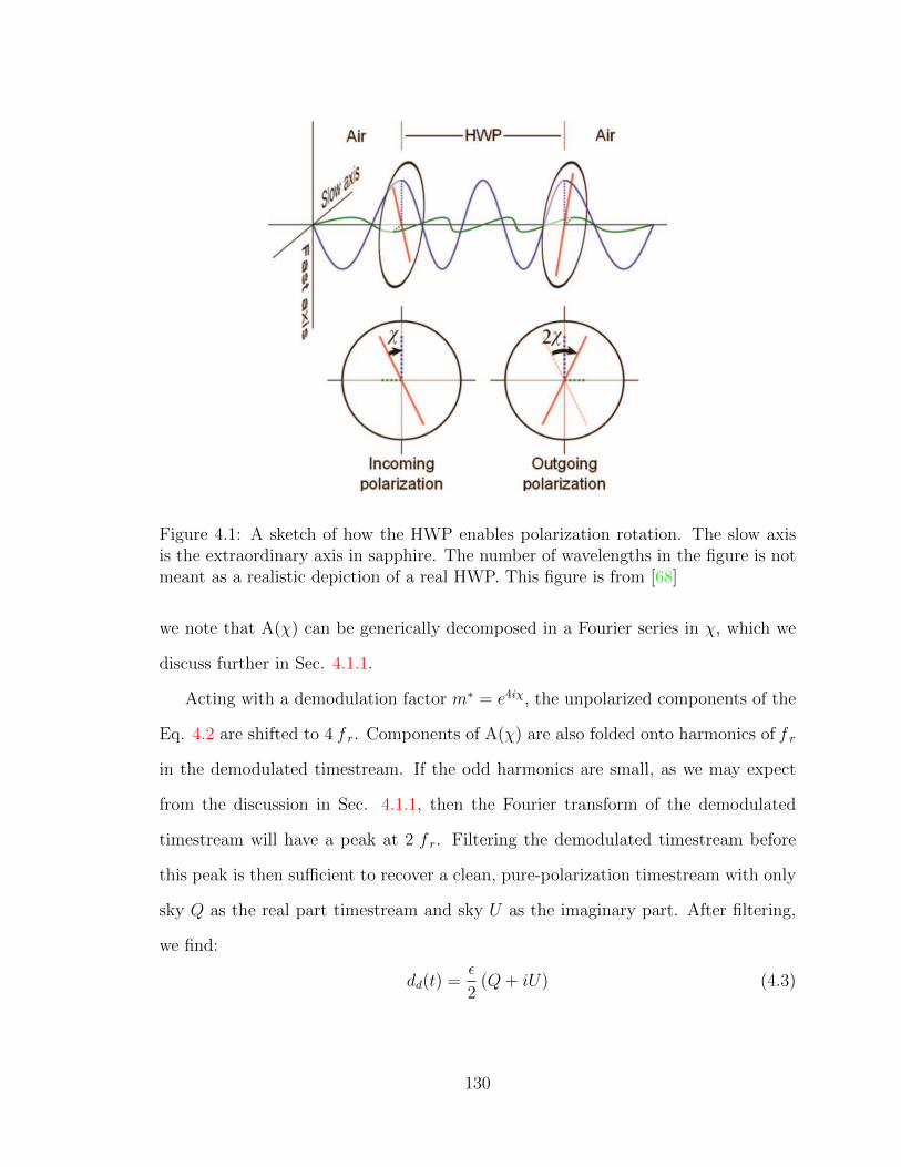
Figure 4.1: A sketch of how the HWP enables polarization rotation. The slow axisis the extraordinary axis in sapphire. The number of wavelengths in the figure is notmeant as a realistic depiction of a real HWP. This figure is from [68]

we note that A(χ) can be generically decomposed in a Fourier series in χ, which we

discuss further in Sec. 4.1.1.

Acting with a demodulation factor m∗ = e4iχ, the unpolarized components of the

Eq. 4.2 are shifted to 4 f r. Components of A(χ) are also folded onto harmonics of f r

in the demodulated timestream. If the odd harmonics are small, as we may expect

from the discussion in Sec. 4.1.1, then the Fourier transform of the demodulated

timestream will have a peak at 2 f r. Filtering the demodulated timestream before

this peak is then sufficient to recover a clean, pure-polarization timestream with only

sky Q as the real part timestream and sky U as the imaginary part. After filtering,

we find:

dd(t) =ε

2(Q+ iU) (4.3)

130

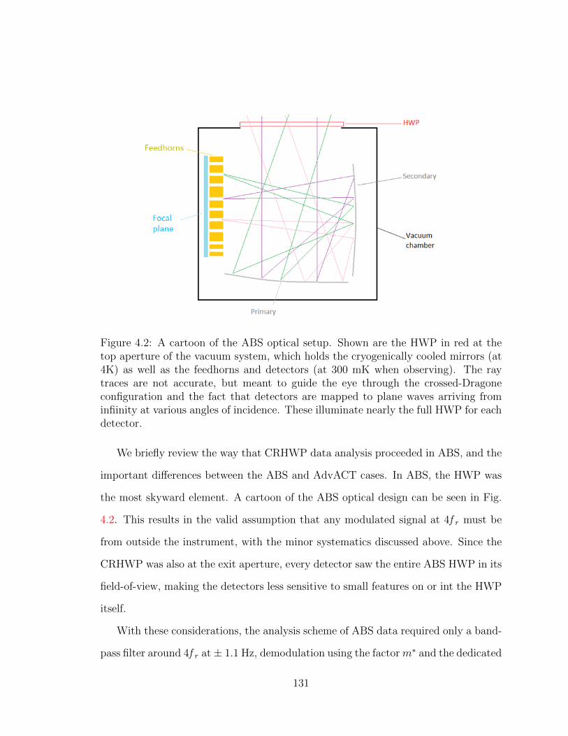
Figure 4.2: A cartoon of the ABS optical setup. Shown are the HWP in red at thetop aperture of the vacuum system, which holds the cryogenically cooled mirrors (at4K) as well as the feedhorns and detectors (at 300 mK when observing). The raytraces are not accurate, but meant to guide the eye through the crossed-Dragoneconfiguration and the fact that detectors are mapped to plane waves arriving frominfiinity at various angles of incidence. These illuminate nearly the full HWP for eachdetector.

We briefly review the way that CRHWP data analysis proceeded in ABS, and the

important differences between the ABS and AdvACT cases. In ABS, the HWP was

the most skyward element. A cartoon of the ABS optical design can be seen in Fig.

4.2. This results in the valid assumption that any modulated signal at 4f r must be

from outside the instrument, with the minor systematics discussed above. Since the

CRHWP was also at the exit aperture, every detector saw the entire ABS HWP in its

field-of-view, making the detectors less sensitive to small features on or int the HWP

itself.

With these considerations, the analysis scheme of ABS data required only a band-

pass filter around 4f r at± 1.1 Hz, demodulation using the factorm∗ and the dedicated

131

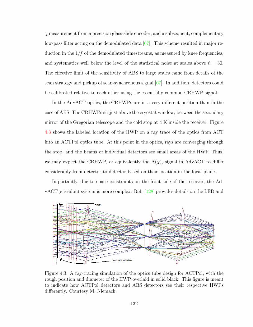
χmeasurement from a precision glass-slide encoder, and a subsequent, complementary

low-pass filter acting on the demodulated data [67]. This scheme resulted in major re-

duction in the 1/f of the demodulated timestreams, as measured by knee frequencies,

and systematics well below the level of the statistical noise at scales above ` = 30.

The effective limit of the sensitivity of ABS to large scales came from details of the

scan strategy and pickup of scan-synchronous signal [67]. In addition, detectors could

be calibrated relative to each other using the essentially common CRHWP signal.

In the AdvACT optics, the CRHWPs are in a very different position than in the

case of ABS. The CRHWPs sit just above the cryostat window, between the secondary

mirror of the Gregorian telescope and the cold stop at 4 K inside the receiver. Figure

4.3 shows the labeled location of the HWP on a ray trace of the optics from ACT

into an ACTPol optics tube. At this point in the optics, rays are converging through

the stop, and the beams of individual detectors see small areas of the HWP. Thus,

we may expect the CRHWP, or equivalently the A(χ), signal in AdvACT to differ

considerably from detector to detector based on their location in the focal plane.

Importantly, due to space constraints on the front side of the receiver, the Ad-

vACT χ readout system is more complex. Ref. [128] provides details on the LED and

Figure 4.3: A ray-tracing simulation of the optics tube design for ACTPol, with therough position and diameter of the HWP overlaid in solid black. This figure is meantto indicate how ACTPol detectors and ABS detectors see their respective HWPsdifferently. Courtesy M. Niemack.

132

photodiode apparatus, and the encoder ring that contains precisely-placed holes sepa-

rated by degree. These allow reconstruction of CRHWP position but require a careful

analysis of the fast-sampled voltage signal coming from the photodiode receptor.

With these differences in mind, we move to a discussion of the recovery of A(χ)

using a Fourier-series analysis.

4.1.1 CRHWP Synchronous Signal

When studying the signal injected by the CRHWP into the detector timestreams,

what we have called A(χ), we assume the following:

• The signal is periodic in χ;

• The shape of the signal may drift within or across TODs;

• The dominant harmonic of f r visible in A(χ) should be at 2f r.

In some sense, the first and the second are contradictory. What we mean is that

the A(χ) signal should be modeled as being periodic in χ, but its harmonic content

can change over sufficiently long timescales. The converse of this is that the signal we

care about is itself changes to the 4f r harmonic at all timescales. Thus, estimating

A(χ) and deprojecting or removing it is complicated by the desire to preserve all

information at 4f r.

Given the periodicity of the signal, we proceed in our study of A(χ) by decom-

posing it into its Fourier series components:

A(χ) =n∑m

am cos(mχ) + bm sin(mχ) =n∑m

Qmeimχ. (4.4)

The above equation schematically represents the Fourier series (or discrete Fourier

transform) of A(χ) in the variable χ. Here we use X to identify a complex number.

133

We can further decompose the complex amplitude of a given harmonic, Qm, into

a sum of terms:

Qm = Am + σm, (4.5)

where Am describes a roughly constant amplitude and phase for the mth harmonic

sourced by slowly-varying instrumental elements, and σm describes a more rapidly

time-varying complex amplitude, with a timescale of tens of seconds to minutes,

possibly driven by long-timescale fluctuations identical to those that source 1/f noise.

In general, we expect that different components of the instrument will source

nonzero A(χ) components at different harmonics. We do not a priori anticipate large

odd-harmonic components in A(χ). However, in the case of the term A2, we assume

that the differential emission along the axes of the CRHWP will dominate. A time-

varying component of σ2 is sourced by differential transmission of any intensity signals

arising skyward of the CRHWP. This term should be most strongly sourced by the

changing atmospheric loading.

At 4f r, a component of A4 arises from any I → P leakage of optical components

skyward of the CRHWP. These are usually induced by polarized emission of the

mirrors, a finite-conductance effect of any real metal. Any nonzero σ4 sourced by

the instrument is indistinguishable from signal on the relevant timescales. Concerns

about non-sky, or even non-optical, effects inducing a signal that survives filtering and

demodulation is a primary concern of CRHWP experiments. Averaging over many

scans to recover only the celestially-fixed signal can reduce the significance of these

leakages, but only if the variation is independent of telescope position. An important

effect that has recently been elucidated is the fact that any gain variations of the

detector or readout backend acting upon a nonzero A4 [120] [22] produce a signal in

the demodulated timestream. In the case of detector nonlinearity, this variation is

driven mainly by unpolarized 1/f . We discuss studies of TES bolometer nonlinearity

in Ch. 6.

134

Overall, these considerations demand that CRHWP experiments develop pipelins

to remove A(χ), including any non-zero Q contributions to the signal at 4f r. In

addition, the relative size of the static and time-varying terms can have important

effects on the required complexity of the removal pipeline.

4.2 ABS CRHWP Results

In this section, we will present a brief overview of the performance of a warm CRHWP

in ABS. We have already discussed some assumptions and features of the ABS science-

level analysis of demodulated CRHWP data. We now discuss aspects of A(χ) studies

that benefited the understanding of ABS data, as an example of the possible uses of

these concepts for both AdvACT and future experiments.

First, we describe the ABS CRHWP. The narrow-band design, meant to be op-

timum at the center of the ABS band ∼ 150 GHz, is fabricated from 31.5-cm thick

sapphire, and is 33 cm in diameter. A laminated anti-reflection (AR) coating was

used to improve the ABS sensitivity [68]. The CRHWP rotated at f r = 2.55 Hz, in

order for the 4f r signal to be at 10.2 Hz, a clean part of the frequency domain in ABS

observation noise spectra.

We now discuss the A(χ) subtraction pipeline implemented for ABS time-ordered

data. Over the course of a full ABS CES (∼ 1 hr of observation), each bolometer’s

timestream is binned by χ value. The resulting binned data is averaged within each

bin to produce an estimated A(χ) “template” for each ABS bolometer. This template

is then decomposed into a truncated Fourier series with components as in Eq. 4.4,

with the terms from m = 0 (the mean of the A(χ) signal, which was not removed

for the timestream before binning) to m = 19 being removed. In this description,

the majority of the A(χ) amplitude is found in the second harmonic, with a small

additional component at the fourth harmonic.

135

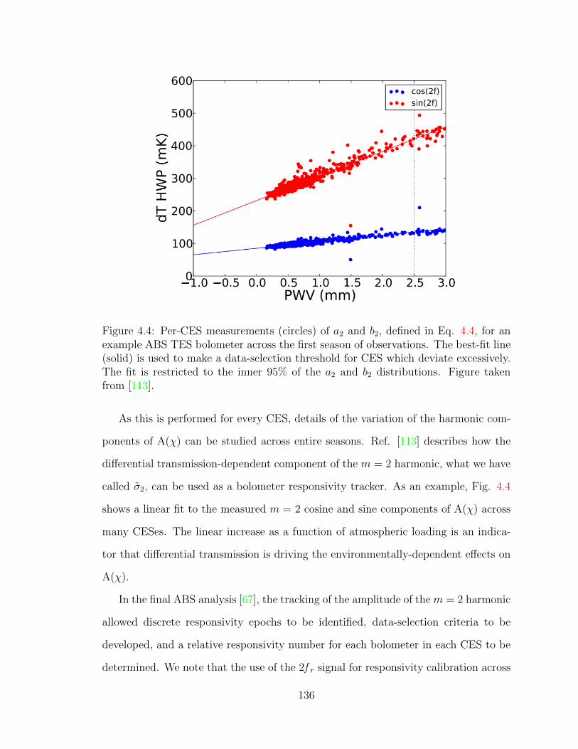
Figure 4.4: Per-CES measurements (circles) of a2 and b2, defined in Eq. 4.4, for anexample ABS TES bolometer across the first season of observations. The best-fit line(solid) is used to make a data-selection threshold for CES which deviate excessively.The fit is restricted to the inner 95% of the a2 and b2 distributions. Figure takenfrom [113].

As this is performed for every CES, details of the variation of the harmonic com-

ponents of A(χ) can be studied across entire seasons. Ref. [113] describes how the

differential transmission-dependent component of the m = 2 harmonic, what we have

called σ2, can be used as a bolometer responsivity tracker. As an example, Fig. 4.4

shows a linear fit to the measured m = 2 cosine and sine components of A(χ) across

many CESes. The linear increase as a function of atmospheric loading is an indica-

tor that differential transmission is driving the environmentally-dependent effects on

A(χ).

In the final ABS analysis [67], the tracking of the amplitude of the m = 2 harmonic

allowed discrete responsivity epochs to be identified, data-selection criteria to be

developed, and a relative responsivity number for each bolometer in each CES to be

determined. We note that the use of the 2f r signal for responsivity calibration across

136

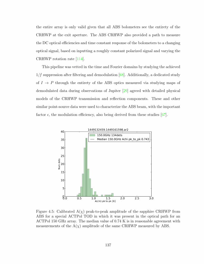
the entire array is only valid given that all ABS bolometers see the entirety of the

CRHWP at the exit aperture. The ABS CRHWP also provided a path to measure

the DC optical efficiencies and time constant response of the bolometers to a changing

optical signal, based on inputting a roughly constant polarized signal and varying the

CRHWP rotation rate [114].

This pipeline was vetted in the time and Fourier domains by studying the achieved

1/f suppression after filtering and demodulation [68]. Additionally, a dedicated study

of I → P through the entirety of the ABS optics measured via studying maps of

demodulated data during observations of Jupiter [29] agreed with detailed physical

models of the CRHWP transmission and reflection components. These and other

similar point-source data were used to characterize the ABS beam, with the important

factor ε, the modulation efficiency, also being derived from these studies [67].

Figure 4.5: Calibrated A(χ) peak-to-peak amplitude of the sapphire CRHWP fromABS for a special ACTPol TOD in which it was present in the optical path for anACTPol 150 GHz array. The median value of 0.74 K is in reasonable agreement withmeasurements of the A(χ) amplitude of the same CRHWP measured by ABS.

137

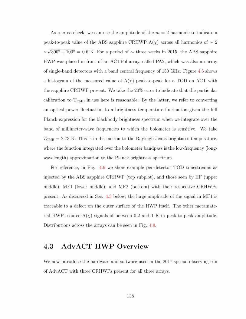
As a cross-check, we can use the amplitude of the m = 2 harmonic to indicate a

peak-to-peak value of the ABS sapphire CRHWP A(χ) across all harmonics of ∼ 2

×√

3002 + 1002 = 0.6 K. For a period of ∼ three weeks in 2015, the ABS sapphire

HWP was placed in front of an ACTPol array, called PA2, which was also an array

of single-band detectors with a band central frequency of 150 GHz. Figure 4.5 shows

a histogram of the measured value of A(χ) peak-to-peak for a TOD on ACT with

the sapphire CRHWP present. We take the 20% error to indicate that the particular

calibration to TCMB in use here is reasonable. By the latter, we refer to converting

an optical power fluctuation to a brightness temperature fluctuation given the full

Planck expression for the blackbody brightness spectrum when we integrate over the

band of millimeter-wave frequencies to which the bolometer is sensitive. We take

TCMB = 2.73 K. This is in distinction to the Rayleigh-Jeans brightness temperature,

where the function integrated over the bolometer bandpass is the low-frequency (long-

wavelength) approximation to the Planck brightness spectrum.

For reference, in Fig. 4.6 we show example per-detector TOD timestreams as

injected by the ABS sapphire CRHWP (top subplot), and those seen by HF (upper

middle), MF1 (lower middle), and MF2 (bottom) with their respective CRHWPs

present. As discussed in Sec. 4.3 below, the large amplitude of the signal in MF1 is

traceable to a defect on the outer surface of the HWP itself. The other metamate-

rial HWPs source A(χ) signals of between 0.2 and 1 K in peak-to-peak amplitude.

Distributions across the arrays can be seen in Fig. 4.9.

4.3 AdvACT HWP Overview

We now introduce the hardware and software used in the 2017 special observing run

of AdvACT with three CRHWPs present for all three arrays.

138

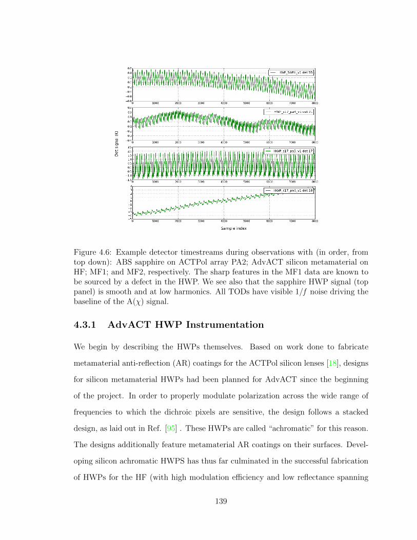
Figure 4.6: Example detector timestreams during observations with (in order, fromtop down): ABS sapphire on ACTPol array PA2; AdvACT silicon metamaterial onHF; MF1; and MF2, respectively. The sharp features in the MF1 data are known tobe sourced by a defect in the HWP. We see also that the sapphire HWP signal (toppanel) is smooth and at low harmonics. All TODs have visible 1/f noise driving thebaseline of the A(χ) signal.

4.3.1 AdvACT HWP Instrumentation

We begin by describing the HWPs themselves. Based on work done to fabricate

metamaterial anti-reflection (AR) coatings for the ACTPol silicon lenses [18], designs

for silicon metamaterial HWPs had been planned for AdvACT since the beginning

of the project. In order to properly modulate polarization across the wide range of

frequencies to which the dichroic pixels are sensitive, the design follows a stacked

design, as laid out in Ref. [95] . These HWPs are called “achromatic” for this reason.

The designs additionally feature metamaterial AR coatings on their surfaces. Devel-

oping silicon achromatic HWPS has thus far culminated in the successful fabrication

of HWPs for the HF (with high modulation efficiency and low reflectance spanning

139

over an octave in millimeter-wave frequency from ∼ 130 GHz to ∼ 280 GHz) and

for the MF (similarly broad, from 60 GHz to 170 GHz) arrays. More detail may be

found in Ref. [13].

We pass over the details of the air-bearing and drive system for the AdvACT

HWPs. Information on the ABS air bearing system may be found in [68]. Details

may be found in [128]. We wish to briefly review the main features of the readout

system that is used to recover the HWP position. We have not yet discussed the

importance of an accurate, relatively precise estimate of the χ timestream in order

for the estimated A(χ) template to be successfully used in removing the measured

signal in the TOD. If there as effective jitter σχ in the χ timestream, this can directly

add to the variance of both A(χ)-subtracted and demodulated timestreams as:

σA(χ) ∼dA(χ)

dχσχ, (4.6a)

σm∗ ∼ −4σχ, (4.6b)

where m∗ is the demodulation factor introduced in Sec. 4.1 that is applied to our

A(χ)-subtracted TODs in the pipeline to be described in Sec. 4.3.2. Though we can

reduce the effective jitter in our A(χ) estimate by binning, binning also has the effect

of introducing signal variance from any drifts of the A(χ) harmonics.

The hardware used for recording χ data in AdvACT first uses precisely-placed

holes on an encoder ring which is at the edge of the HWP rotor assembly. The holes

on this encoder ring are intended to be placed as accurately as possible on the same

diameter, with separation of exactly 2. A single hole, offset at a slightly larger radius,

is read out as the “home hole” and is used to indicate the direction of rotation of the

HWP, being slightly closer to a particular degree hole. It has been found that the

natural variance in their achieved separation can be an important template to remove

140

from the final angle solutions through a kind of remapping. However, we generally

work with an angle solution that ignores this effect.

The operating principle of the photointerruptor encoder is that a red light-emitting

diode (LED) sits below the encoder ring, at the edge of the HWP assembly and

safely removed from the moving parts. Above it is a well-aligned phodiode designed

to receive a strong signal when an encoder hole passes between the source and the

detector. The voltage signal of this photoreceptor is read out at a sample rate of 40

kHz; this data is multiplexed in order to be merged into the ACT TOD file format,

which includes critical housekeeping data as well as encoder positions for the telescope

boresight and the detector TOD. A digital design for this processing was led by M.

Hasselfield for the ACT collaboration, building from the previous-generation design

by J. Ward, who was also responsible for much of the mechanical design in the rotor

and bearing systems.

Usefully, an algorithm has been developed by M. Hasselfield and described in a

publication in preparation [Ward et al. in prep] whereby this signal can be used to esti-

mate χ. The raw encoder signal is first downsampled to 3.2 kHz, and then processed

to find the large-amplitude photodiode response to the LED using an empiricially

determined threshold. Timestamps for the degree-hole peaks are then analyzed to

produce an angle timestream, which accounts for the home hole by using its recorded

peak timestamp as the χ = 0 point. These timestamps are synchronous with the

“sync box” used to keep the detector data synchronized across all AdvACT arrays.

This analysis is performed in real time, and the estimated χ timestream is then stored

with the full AdvACT TOD for later access.

To characterize jitter, we analyze the χ timestream as follows:

• Bound full rotations of the HWP by finding large negative jumps (i.e. from

high to low χ);

141

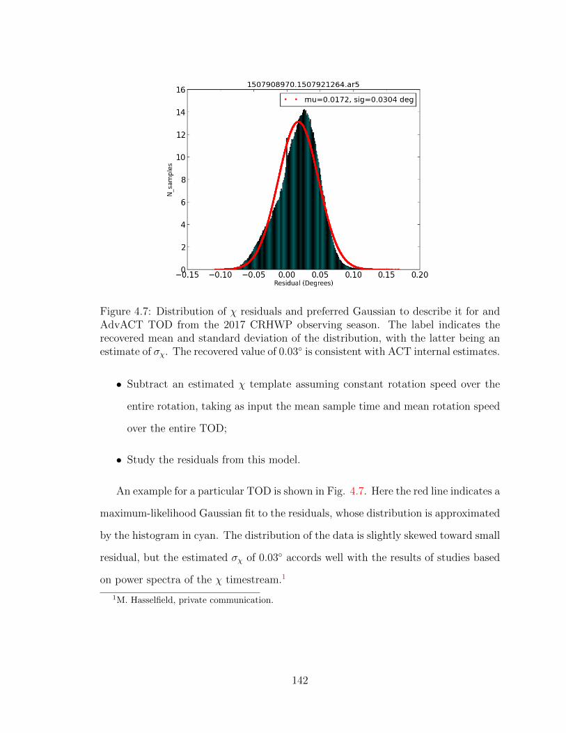
Figure 4.7: Distribution of χ residuals and preferred Gaussian to describe it for andAdvACT TOD from the 2017 CRHWP observing season. The label indicates therecovered mean and standard deviation of the distribution, with the latter being anestimate of σχ. The recovered value of 0.03 is consistent with ACT internal estimates.

• Subtract an estimated χ template assuming constant rotation speed over the

entire rotation, taking as input the mean sample time and mean rotation speed

over the entire TOD;

• Study the residuals from this model.

An example for a particular TOD is shown in Fig. 4.7. Here the red line indicates a

maximum-likelihood Gaussian fit to the residuals, whose distribution is approximated

by the histogram in cyan. The distribution of the data is slightly skewed toward small

residual, but the estimated σχ of 0.03 accords well with the results of studies based

on power spectra of the χ timestream.1

1M. Hasselfield, private communication.

142

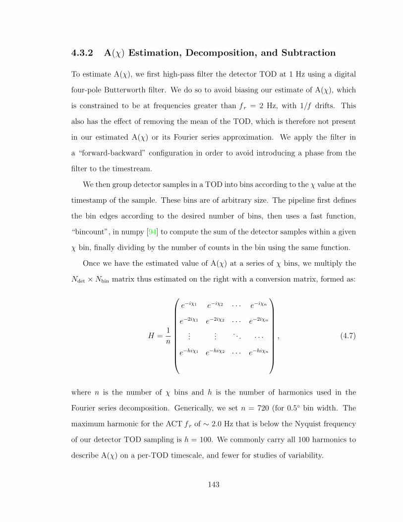
4.3.2 A(χ) Estimation, Decomposition, and Subtraction

To estimate A(χ), we first high-pass filter the detector TOD at 1 Hz using a digital

four-pole Butterworth filter. We do so to avoid biasing our estimate of A(χ), which

is constrained to be at frequencies greater than f r = 2 Hz, with 1/f drifts. This

also has the effect of removing the mean of the TOD, which is therefore not present

in our estimated A(χ) or its Fourier series approximation. We apply the filter in

a “forward-backward” configuration in order to avoid introducing a phase from the

filter to the timestream.

We then group detector samples in a TOD into bins according to the χ value at the

timestamp of the sample. These bins are of arbitrary size. The pipeline first defines

the bin edges according to the desired number of bins, then uses a fast function,

“bincount”, in numpy [94] to compute the sum of the detector samples within a given

χ bin, finally dividing by the number of counts in the bin using the same function.

Once we have the estimated value of A(χ) at a series of χ bins, we multiply the

Ndet ×Nbin matrix thus estimated on the right with a conversion matrix, formed as:

H =1

n

e−iχ1 e−iχ2 · · · e−iχn

e−2iχ1 e−2iχ2 · · · e−2iχn

......

. . . · · ·

e−hiχ1 e−hiχ2 · · · e−hiχn

, (4.7)

where n is the number of χ bins and h is the number of harmonics used in the

Fourier series decomposition. Generically, we set n = 720 (for 0.5 bin width. The

maximum harmonic for the ACT f r of ∼ 2.0 Hz that is below the Nyquist frequency

of our detector TOD sampling is h = 100. We commonly carry all 100 harmonics to

describe A(χ) on a per-TOD timescale, and fewer for studies of variability.

143

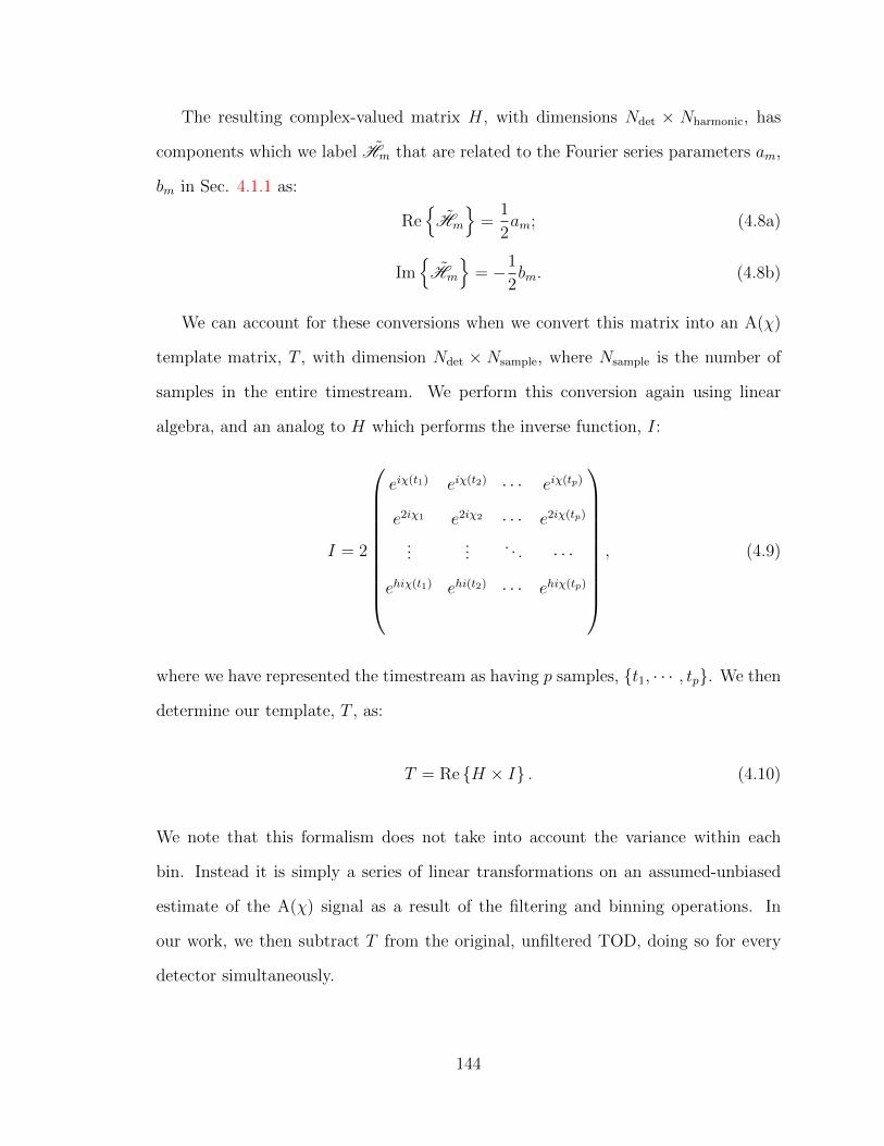
The resulting complex-valued matrix H, with dimensions Ndet × Nharmonic, has

components which we label Hm that are related to the Fourier series parameters am,

bm in Sec. 4.1.1 as:

Re

Hm

=

1

2am; (4.8a)

Im

Hm

= −1

2bm. (4.8b)

We can account for these conversions when we convert this matrix into an A(χ)

template matrix, T , with dimension Ndet × Nsample, where Nsample is the number of

samples in the entire timestream. We perform this conversion again using linear

algebra, and an analog to H which performs the inverse function, I:

I = 2

eiχ(t1) eiχ(t2) · · · eiχ(tp)

e2iχ1 e2iχ2 · · · e2iχ(tp)

......

. . . · · ·

ehiχ(t1) ehi(t2) · · · ehiχ(tp)

, (4.9)

where we have represented the timestream as having p samples, t1, · · · , tp. We then

determine our template, T , as:

T = Re H × I . (4.10)

We note that this formalism does not take into account the variance within each

bin. Instead it is simply a series of linear transformations on an assumed-unbiased

estimate of the A(χ) signal as a result of the filtering and binning operations. In

our work, we then subtract T from the original, unfiltered TOD, doing so for every

detector simultaneously.

144

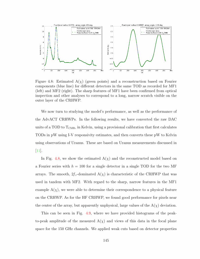
Figure 4.8: Estimated A(χ) (green points) and a reconstruction based on Fouriercomponents (blue line) for different detectors in the same TOD as recorded for MF1(left) and MF2 (right). The sharp features of MF1 have been confirmed from opticalinspection and other analyses to correspond to a long, narrow scratch visible on theouter layer of the CRHWP.

We now turn to studying the model’s performance, as well as the performance of

the AdvACT CRHWPs. In the following results, we have converted the raw DAC

units of a TOD to TCMB, in Kelvin, using a provisional calibration that first calculates

TODs in pW using I-V responsivity estimates, and then converts these pW to Kelvin

using observations of Uranus. These are based on Uranus measurements discussed in

[11].

In Fig. 4.8, we show the estimated A(χ) and the reconstructed model based on

a Fourier series with h = 100 for a single detector in a single TOD for the two MF

arrays. The smooth, 2f r-dominated A(χ) is characteristic of the CRHWP that was

used in tandem with MF2. With regard to the sharp, narrow features in the MF1

example A(χ), we were able to determine their correspondence to a physical feature

on the CRHWP. As for the HF CRHWP, we found good performance for pixels near

the center of the array, but apparently unphysical, large values of the A(χ) deviation.

This can be seen in Fig. 4.9, where we have provided histograms of the peak-

to-peak amplitude of the measured A(χ) and views of this data in the focal plane

space for the 150 GHz channels. We applied weak cuts based on detector properties

145

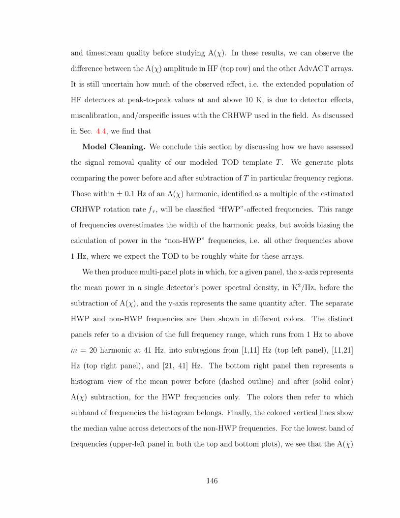
and timestream quality before studying A(χ). In these results, we can observe the

difference between the A(χ) amplitude in HF (top row) and the other AdvACT arrays.

It is still uncertain how much of the observed effect, i.e. the extended population of

HF detectors at peak-to-peak values at and above 10 K, is due to detector effects,

miscalibration, and/orspecific issues with the CRHWP used in the field. As discussed

in Sec. 4.4, we find that

Model Cleaning. We conclude this section by discussing how we have assessed

the signal removal quality of our modeled TOD template T . We generate plots

comparing the power before and after subtraction of T in particular frequency regions.

Those within ± 0.1 Hz of an A(χ) harmonic, identified as a multiple of the estimated

CRHWP rotation rate f r, will be classified “HWP”-affected frequencies. This range

of frequencies overestimates the width of the harmonic peaks, but avoids biasing the

calculation of power in the “non-HWP” frequencies, i.e. all other frequencies above

1 Hz, where we expect the TOD to be roughly white for these arrays.

We then produce multi-panel plots in which, for a given panel, the x-axis represents

the mean power in a single detector’s power spectral density, in K2/Hz, before the

subtraction of A(χ), and the y-axis represents the same quantity after. The separate

HWP and non-HWP frequencies are then shown in different colors. The distinct

panels refer to a division of the full frequency range, which runs from 1 Hz to above

m = 20 harmonic at 41 Hz, into subregions from [1,11] Hz (top left panel), [11,21]

Hz (top right panel), and [21, 41] Hz. The bottom right panel then represents a

histogram view of the mean power before (dashed outline) and after (solid color)

A(χ) subtraction, for the HWP frequencies only. The colors then refer to which

subband of frequencies the histogram belongs. Finally, the colored vertical lines show

the median value across detectors of the non-HWP frequencies. For the lowest band of

frequencies (upper-left panel in both the top and bottom plots), we see that the A(χ)

146

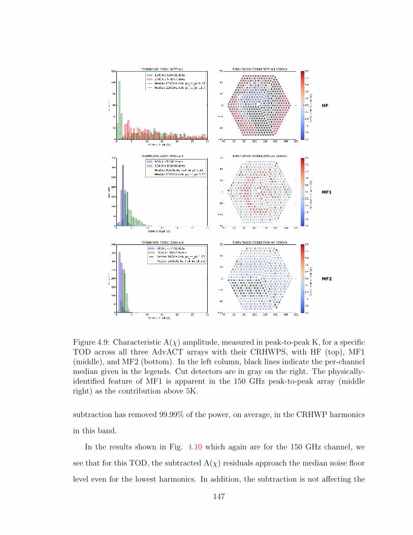
(K)

(K)

(K)

(K)

HF

MF1

(K)

(K)

MF2

Figure 4.9: Characteristic A(χ) amplitude, measured in peak-to-peak K, for a specificTOD across all three AdvACT arrays with their CRHWPS, with HF (top), MF1(middle), and MF2 (bottom). In the left column, black lines indicate the per-channelmedian given in the legends. Cut detectors are in gray on the right. The physically-identified feature of MF1 is apparent in the 150 GHz peak-to-peak array (middleright) as the contribution above 5K.

subtraction has removed 99.99% of the power, on average, in the CRHWP harmonics

in this band.

In the results shown in Fig. 4.10 which again are for the 150 GHz channel, we

see that for this TOD, the subtracted A(χ) residuals approach the median noise floor

level even for the lowest harmonics. In addition, the subtraction is not affecting the

147

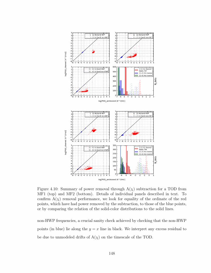
Figure 4.10: Summary of power removal through A(χ) subtraction for a TOD fromMF1 (top) and MF2 (bottom). Details of individual panels described in text. Toconfirm A(χ) removal performance, we look for equality of the ordinate of the redpoints, which have had power removed by the subtraction, to those of the blue points,or by comparing the relation of the solid-color distributions to the solid lines.

non-HWP frequencies, a crucial sanity check achieved by checking that the non-HWP

points (in blue) lie along the y = x line in black. We interpret any excess residual to

be due to unmodeled drifts of A(χ) on the timescale of the TOD.

148

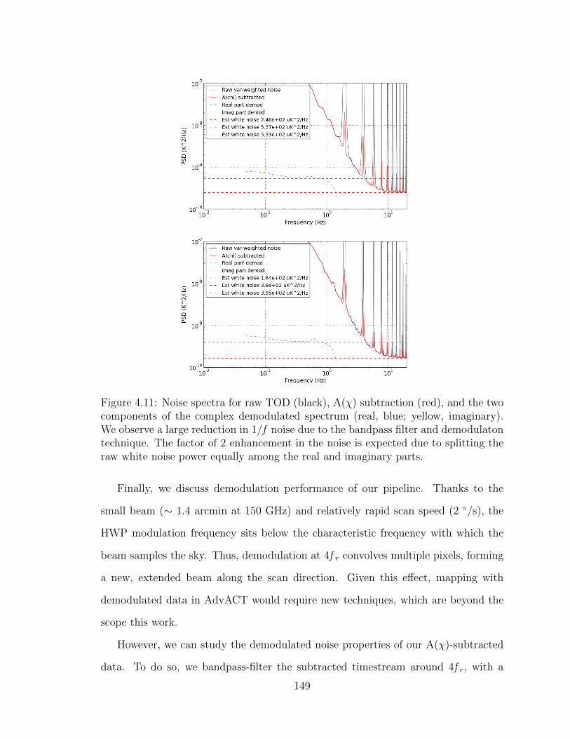
Figure 4.11: Noise spectra for raw TOD (black), A(χ) subtraction (red), and the twocomponents of the complex demodulated spectrum (real, blue; yellow, imaginary).We observe a large reduction in 1/f noise due to the bandpass filter and demodulatontechnique. The factor of 2 enhancement in the noise is expected due to splitting theraw white noise power equally among the real and imaginary parts.

Finally, we discuss demodulation performance of our pipeline. Thanks to the

small beam (∼ 1.4 arcmin at 150 GHz) and relatively rapid scan speed (2 /s), the

HWP modulation frequency sits below the characteristic frequency with which the

beam samples the sky. Thus, demodulation at 4f r convolves multiple pixels, forming

a new, extended beam along the scan direction. Given this effect, mapping with

demodulated data in AdvACT would require new techniques, which are beyond the

scope this work.

However, we can study the demodulated noise properties of our A(χ)-subtracted

data. To do so, we bandpass-filter the subtracted timestream around 4f r, with a

149

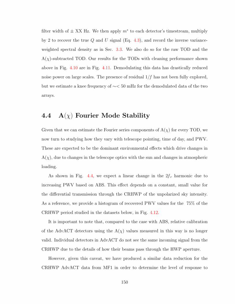
filter width of ± XX Hz. We then apply m∗ to each detector’s timestream, multiply

by 2 to recover the true Q and U signal (Eq. 4.3), and record the inverse variance-

weighted spectral density as in Sec. 3.3. We also do so for the raw TOD and the

A(χ)-subtracted TOD. Our results for the TODs with cleaning performance shown

above in Fig. 4.10 are in Fig. 4.11. Demodulating this data has drastically reduced

noise power on large scales. The presence of residual 1/f has not been fully explored,

but we estimate a knee frequency of ∼< 50 mHz for the demodulated data of the two

arrays.

4.4 A(χ) Fourier Mode Stability

Given that we can estimate the Fourier series components of A(χ) for every TOD, we

now turn to studying how they vary with telescope pointing, time of day, and PWV.

These are expected to be the dominant environmental effects which drive changes in

A(χ), due to changes in the telescope optics with the sun and changes in atmospheric

loading.

As shown in Fig. 4.4, we expect a linear change in the 2f r harmonic due to

increasing PWV based on ABS. This effect depends on a constant, small value for

the differential transmission through the CRHWP of the unpolarized sky intensity.

As a reference, we provide a histogram of recovered PWV values for the 75% of the

CRHWP period studied in the datasets below, in Fig. 4.12.

It is important to note that, compared to the case with ABS, relative calibration

of the AdvACT detectors using the A(χ) values measured in this way is no longer

valid. Individual detectors in AdvACT do not see the same incoming signal from the

CRHWP due to the details of how their beams pass through the HWP aperture.

However, given this caveat, we have produced a similar data reduction for the

CRHWP AdvACT data from MF1 in order to determine the level of response to

150

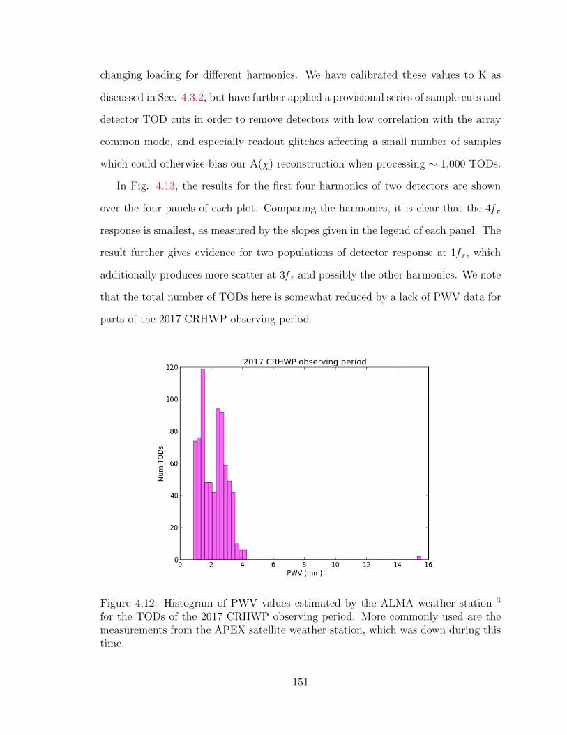
changing loading for different harmonics. We have calibrated these values to K as

discussed in Sec. 4.3.2, but have further applied a provisional series of sample cuts and

detector TOD cuts in order to remove detectors with low correlation with the array

common mode, and especially readout glitches affecting a small number of samples

which could otherwise bias our A(χ) reconstruction when processing ∼ 1,000 TODs.

In Fig. 4.13, the results for the first four harmonics of two detectors are shown

over the four panels of each plot. Comparing the harmonics, it is clear that the 4f r

response is smallest, as measured by the slopes given in the legend of each panel. The

result further gives evidence for two populations of detector response at 1f r, which

additionally produces more scatter at 3f r and possibly the other harmonics. We note

that the total number of TODs here is somewhat reduced by a lack of PWV data for

parts of the 2017 CRHWP observing period.

Figure 4.12: Histogram of PWV values estimated by the ALMA weather station 3

for the TODs of the 2017 CRHWP observing period. More commonly used are themeasurements from the APEX satellite weather station, which was down during thistime.

151

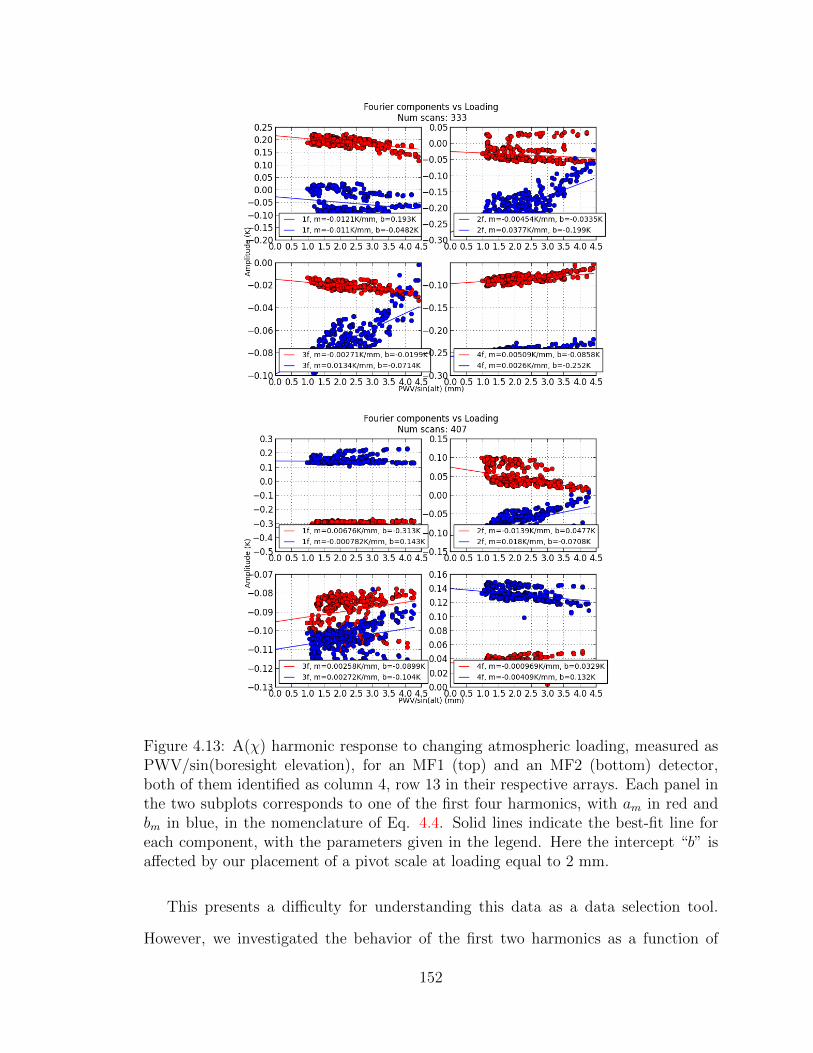
Figure 4.13: A(χ) harmonic response to changing atmospheric loading, measured asPWV/sin(boresight elevation), for an MF1 (top) and an MF2 (bottom) detector,both of them identified as column 4, row 13 in their respective arrays. Each panel inthe two subplots corresponds to one of the first four harmonics, with am in red andbm in blue, in the nomenclature of Eq. 4.4. Solid lines indicate the best-fit line foreach component, with the parameters given in the legend. Here the intercept “b” isaffected by our placement of a pivot scale at loading equal to 2 mm.

This presents a difficulty for understanding this data as a data selection tool.

However, we investigated the behavior of the first two harmonics as a function of

152

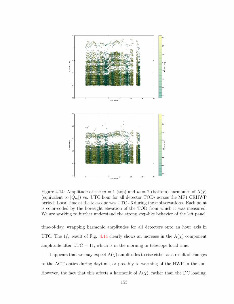
Figure 4.14: Amplitude of the m = 1 (top) and m = 2 (bottom) harmonics of A(χ)(equivalent to |Qm|) vs. UTC hour for all detector TODs across the MF1 CRHWPperiod. Local time at the telescope was UTC - 3 during these observations. Each pointis color-coded by the boresight elevation of the TOD from which it was measured.We are working to further understand the strong step-like behavior of the left panel.

time-of-day, wrapping harmonic amplitudes for all detectors onto an hour axis in

UTC. The 1f r result of Fig. 4.14 clearly shows an increase in the A(χ) component

amplitude after UTC = 11, which is in the morning in telescope local time.

It appears that we may expect A(χ) amplitudes to rise either as a result of changes

to the ACT optics during daytime, or possibly to warming of the HWP in the sun.

However, the fact that this affects a harmonic of A(χ), rather than the DC loading,

153

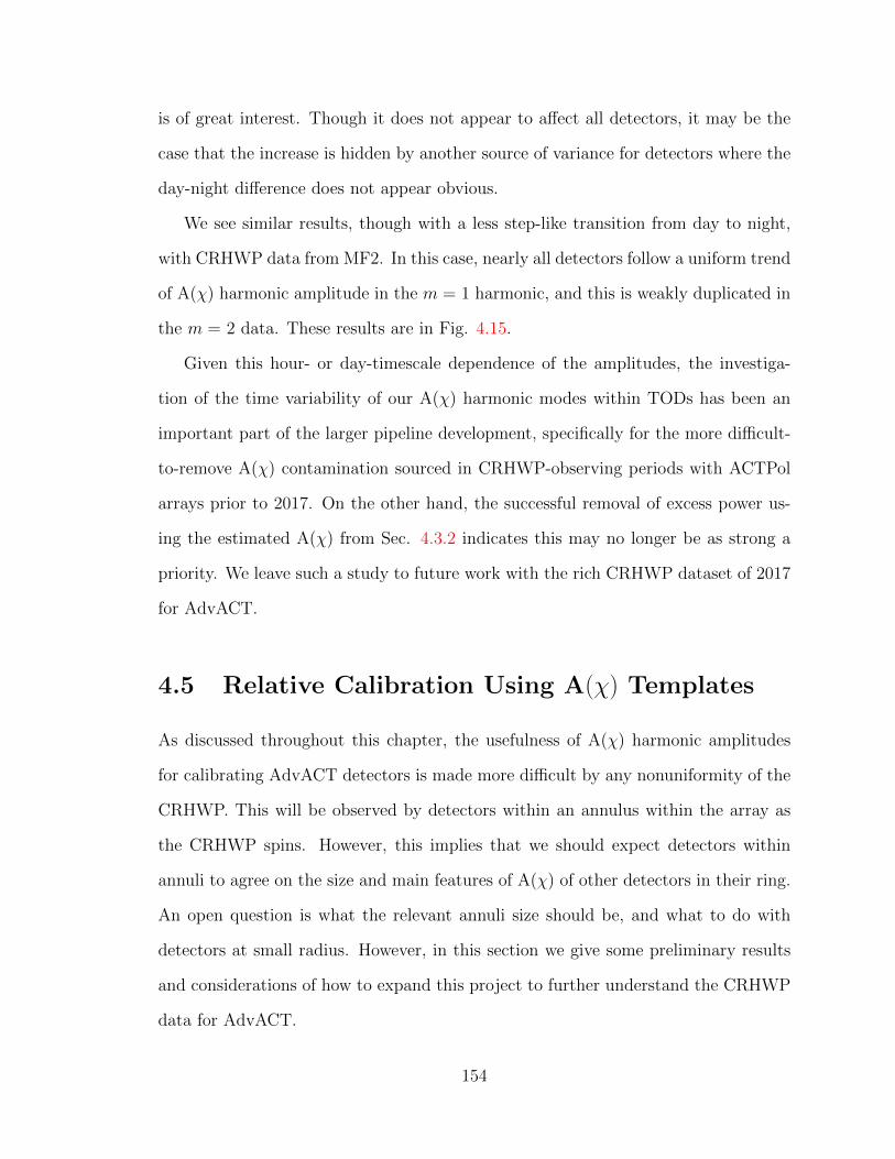
is of great interest. Though it does not appear to affect all detectors, it may be the

case that the increase is hidden by another source of variance for detectors where the

day-night difference does not appear obvious.

We see similar results, though with a less step-like transition from day to night,

with CRHWP data from MF2. In this case, nearly all detectors follow a uniform trend

of A(χ) harmonic amplitude in the m = 1 harmonic, and this is weakly duplicated in

the m = 2 data. These results are in Fig. 4.15.

Given this hour- or day-timescale dependence of the amplitudes, the investiga-

tion of the time variability of our A(χ) harmonic modes within TODs has been an

important part of the larger pipeline development, specifically for the more difficult-

to-remove A(χ) contamination sourced in CRHWP-observing periods with ACTPol

arrays prior to 2017. On the other hand, the successful removal of excess power us-

ing the estimated A(χ) from Sec. 4.3.2 indicates this may no longer be as strong a

priority. We leave such a study to future work with the rich CRHWP dataset of 2017

for AdvACT.

4.5 Relative Calibration Using A(χ) Templates

As discussed throughout this chapter, the usefulness of A(χ) harmonic amplitudes

for calibrating AdvACT detectors is made more difficult by any nonuniformity of the

CRHWP. This will be observed by detectors within an annulus within the array as

the CRHWP spins. However, this implies that we should expect detectors within

annuli to agree on the size and main features of A(χ) of other detectors in their ring.

An open question is what the relevant annuli size should be, and what to do with

detectors at small radius. However, in this section we give some preliminary results

and considerations of how to expand this project to further understand the CRHWP

data for AdvACT.

154

Figure 4.15: Amplitude of the m = 1 (left) and m = 2 (right) harmonics of A(χ)(equivalent to |Qm|) vs. UTC hour across the MF2 CRHWP observing period. Localtime at the telescope was UTC - 5 during these observations. Each point is color-coded by the boresight elevation of the TOD from which it was measured.

First, we anticipate the need to correct a given detector’s A(χ) signal for its

angular position in the array. We measure this angle from the horizontal axis when

looking through the array (i.e. from behind) or into it (i.e. from above, or the sky).

Angles increase counterclockwise when viewed from the sky. To correct for this, we

essentially shift the argument of A(χ) from χ to χ − γ, where we label the angular

position of the detector in the focal plane γ.

155

Second, we correct for the polarization angle of individual detectors being distinct.

This was a non-existent effect in the ABS relative calibration of detectors based on

harmonic amplitudes, where the different phases of polarization pairs were not a

factor.

We can do the above by multiplying element-wise the A(χ) Fourier series com-

ponents Hm, in an Ndet ×Nharmonic matrix, with a matrix of identical dimension, R.

In this matrix, for the detector in row i, with harmonic j+1 corresponding to each

column and with position angle and polarization angle γi and φi respectively, we write

the elements to multiply its coefficients by as:

Ri,j = [γi, 2γi + 2φi, 3γi, 4γi + 2φi, · · · ]. (4.11)

Only the even harmonics are acted by the polarization-angle correction. Again, this

correction is applied after the individual detector A(χ) bin values and coefficients

have been estimated, essentially when the A(χ) per-bin values are reconstructed from

a Fourier series using the coefficients.

A first test of this result is provided by plotting the rotated A(χ) estimates,

after calculating only the first 8 harmonics, in radial annuli. In this case, we have

calibrated these detectors using the same values as in previous sections. Since γi

requires information on the position of individual detectors in the array, e.g. as

γi = arctan(y/x), it is easy to divide the detector A(χ) into groups using the radius√x2 + y2. An example for an MF2 TOD is shown in Fig. 4.16 for a group of detectors

closest to the center.

After the transformation is performed, a common template can be formed from

the A(χ) of detectors in a radial bin. This is best done for detectors at exactly equal

radius. We define “equal radius” in this case as those detectors with equivalent radii

when rounded to 0.01 level. In Fig. 4.16, we show the transformed A(χ) for a set

156

of detectors in MF2 at a middle radius on the array (light colored lines), and the

common mode indicated in solid black. We have used the same color for polarization

pairs (detectors at identical array position in the same frequency channel). These

data have been transformed to equivalent optical power in pW, with this conversion

estimated from an I-V curve taken before the observation. This avoids pre-applying

a calibration through the conversion to Kelvin. However, we have assumed a nominal

direction for the detector response to optical changes, either positive or negative with

respect to incoming δPγ. The common mode here is determined by an average across

all detectors at each χ angle defined when generating the transformed A(χ).

In this figure, it appears to mainly recover unpolarized, odd harmonics. However,

we confirm visually that pairs have been corrected to agree on the sign of the large

m = 2 harmonic mode in individual detector A(χ). Thus, there must be a reason

that the even harmonics are not agreeing between pairs. This may require correction

by a sign parameter determined from the response of indivdiual detectors to changing

m = 2 amplitude with changing atmospheric loading, something we have access to

via the studies of Sec. 4.4.

We conclude this section by showing the measured correlation coefficient between

the common mode and the detectors at this radius in Fig. 4.17. We plot the coeffi-

cient as a scatter versus A(χ) peak-to-peak in pW (blue circles), with the common

mode indicated at 1 on the ordinate axis (black star). These results indicate that the

estimates of A(χ) coming from the largest peak-to-peak detectors are indeed domi-

nating the common mode. Scaling the detectors with smaller peak-to-peak values up,

or vice versa, should allow flat-fielding once we are confident in our transformation

and common-mode estiimation.

157

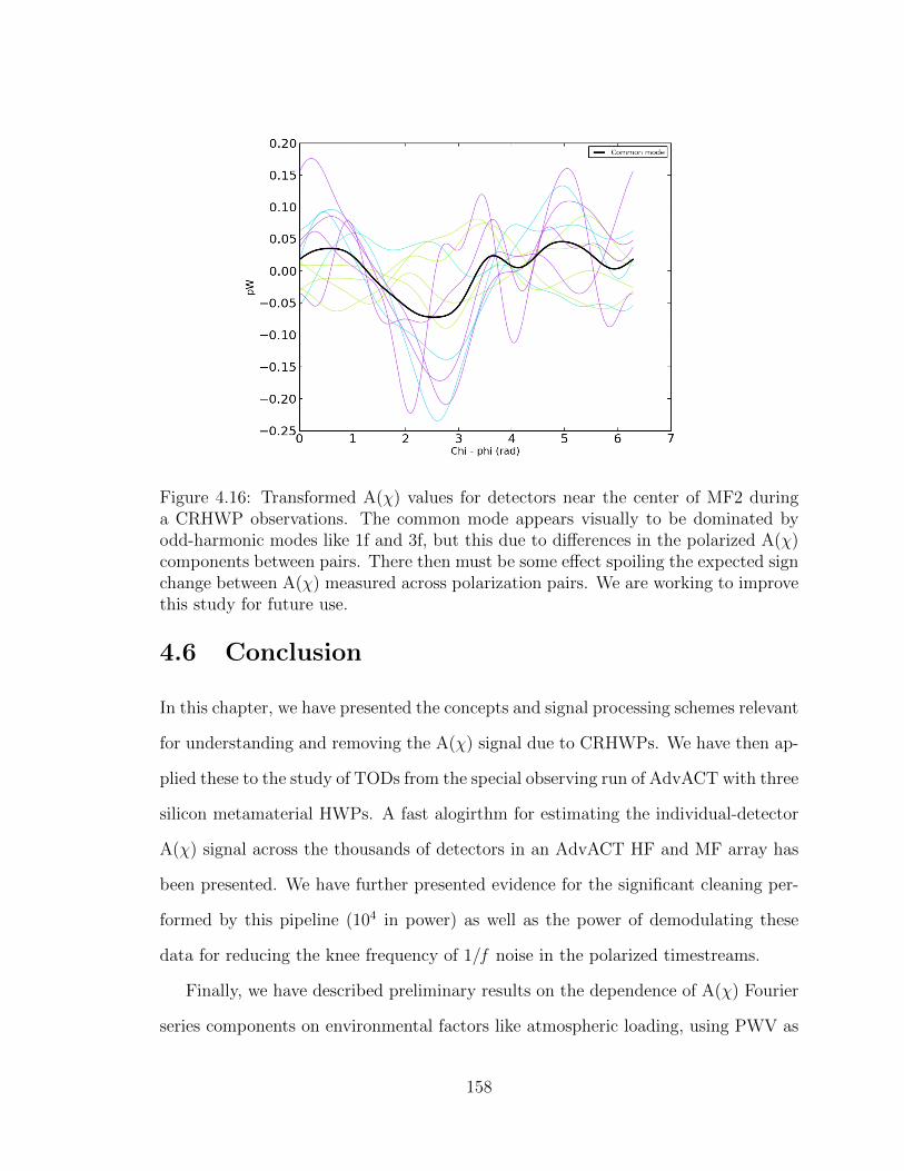
Figure 4.16: Transformed A(χ) values for detectors near the center of MF2 duringa CRHWP observations. The common mode appears visually to be dominated byodd-harmonic modes like 1f and 3f, but this due to differences in the polarized A(χ)components between pairs. There then must be some effect spoiling the expected signchange between A(χ) measured across polarization pairs. We are working to improvethis study for future use.

4.6 Conclusion

In this chapter, we have presented the concepts and signal processing schemes relevant

for understanding and removing the A(χ) signal due to CRHWPs. We have then ap-

plied these to the study of TODs from the special observing run of AdvACT with three

silicon metamaterial HWPs. A fast alogirthm for estimating the individual-detector

A(χ) signal across the thousands of detectors in an AdvACT HF and MF array has

been presented. We have further presented evidence for the significant cleaning per-

formed by this pipeline (104 in power) as well as the power of demodulating these

data for reducing the knee frequency of 1/f noise in the polarized timestreams.

Finally, we have described preliminary results on the dependence of A(χ) Fourier

series components on environmental factors like atmospheric loading, using PWV as

158

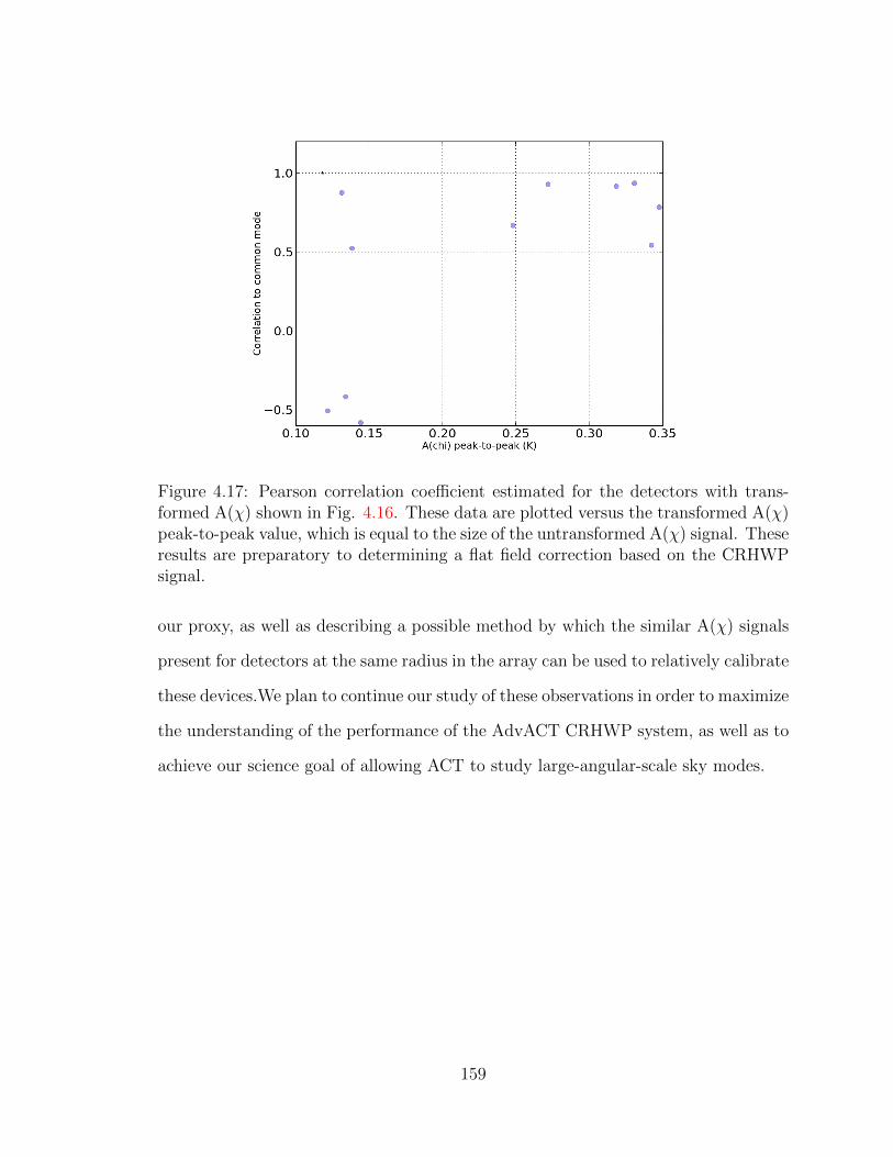
Figure 4.17: Pearson correlation coefficient estimated for the detectors with trans-formed A(χ) shown in Fig. 4.16. These data are plotted versus the transformed A(χ)peak-to-peak value, which is equal to the size of the untransformed A(χ) signal. Theseresults are preparatory to determining a flat field correction based on the CRHWPsignal.

our proxy, as well as describing a possible method by which the similar A(χ) signals

present for detectors at the same radius in the array can be used to relatively calibrate

these devices.We plan to continue our study of these observations in order to maximize

the understanding of the performance of the AdvACT CRHWP system, as well as to

achieve our science goal of allowing ACT to study large-angular-scale sky modes.

159

Chapter 5

Maximum-Likelihood Studies of

CMB Results

In this section, we describe the power spectrum estimation pipeline used in the reduc-

tion of data from ABS. The instrument was introduced in Sec. 1.4.2. Here we present

a brief introduction to the analysis scheme used by ABS to estimate power spectra,

based on the MASTER pipeline [51]. We then describe the construction of likeli-

hood functions based on parametric descriptions of the probability density functions

of polarization spectra bandpowers and the scalar-to-tensor ratio r. These results

are based on Monte Carlo simulations of ABS observations, which simulations are

critical to the pipeline. We conclude by presenting the errors on the measured ABS

bandpowers and the upper-limit determination on r derived from the likelihoods. A

final comment concerns the effect of estimated foreground power at large scales and

its possible effects on these results.

5.1 ABS CMB Power Spectra Pipeline

In the field of studies of the CMB, the mathematical operations involved in reducing

many channels of time-domain detector samples into sky signal maps and spherical

160

harmonic power spectra have been well-studied [101] [10] [88]. However, practial

considerations applying to real observations often introduce processing steps or ob-

servational constraints that complicate the reduction process. Generally, the most

critical effects are due to i) observation of a small patch of sky (“Field A” in [67] is

2400 deg2), and ii) filtering operations on the detector timestreams (for ABS, these

occur in the HWP demodulation scheme and in scan-synchronous signal subtrac-

tion, for instance). Accounting for the effects of these operations in the mapmaking

equation and power spectrum estimators often results in computationally-intensive

pipelines.

An alternative is to create a Monte Carlo (MC) simulation pipeline that can itself

feed into the data reduction pipeline of an experiment, just as the real field data does.

This requires drawing realizations of a CMB sky based on input power spectra, which

can represent a ΛCDM universe or a generic functional form. The simulated CMB sky

is then “observed” by a representation of the ABS instrument that must capture all

relevant details of the experiment, including, for example observation strategy, noise

properties, and bad samples. However, the simulated pipelines may then be treated

just as the real data is, and reduced using a simplified, compact pipeline that can

afford to be naive. By performing this operation hundreds of times, the statistical

properties of important quantities like the C` of the power spectra can be captured.

The use of this process to calibrate out the effects of naive reduction on real CMB

instrument data is discussed in detail in [51]. In ABS, the pipeline was designed by A.

Kusaka building from work on the QUIET experiment [102], with a power spectrum

estimation code used in studies of both simulation and data developed from the

QUIET pipeline by S. Choi [11]. As applied in ABS, the pipeline begins by making a

weighted-average map based on the value of each detector sample that is not cut due

to the data selection criteria. The weight applied is the assumed inverse variance,

taken from the white noise level of the relevant detector’s demodulated timestreams.

161

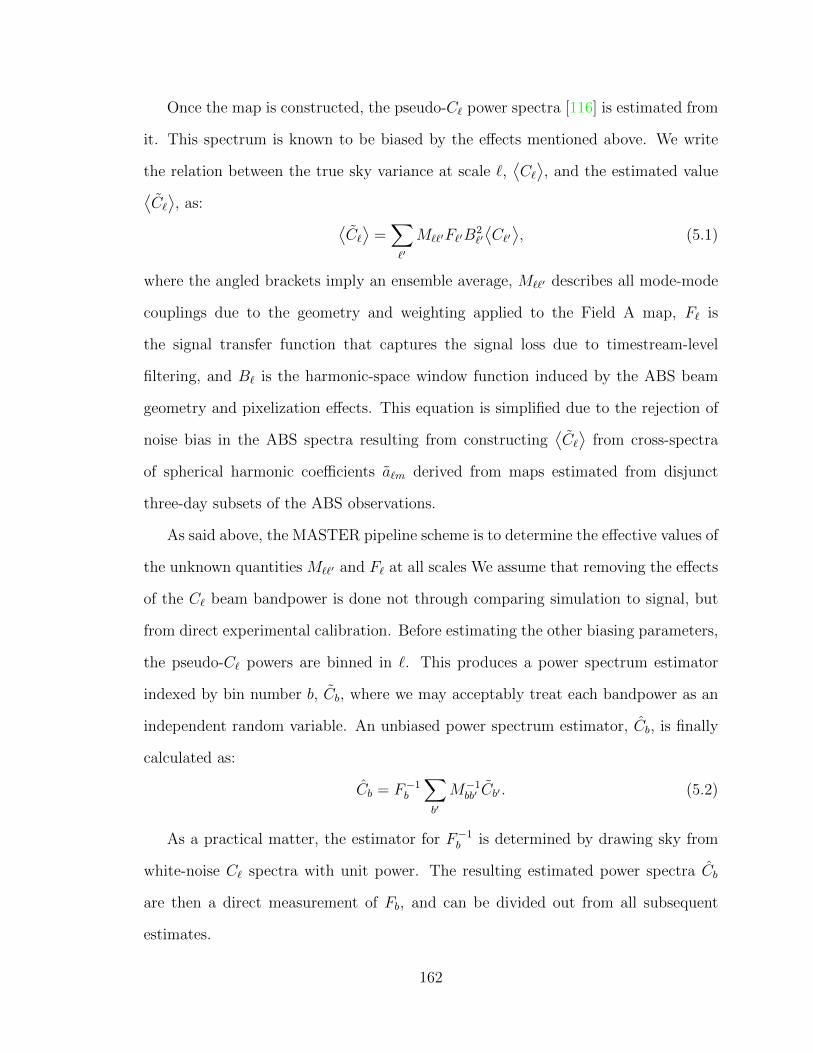
Once the map is constructed, the pseudo-C` power spectra [116] is estimated from

it. This spectrum is known to be biased by the effects mentioned above. We write

the relation between the true sky variance at scale `,⟨C`⟩, and the estimated value⟨

C`⟩, as: ⟨

C`⟩

=∑`′

M``′F`′B2`′

⟨C`′⟩, (5.1)

where the angled brackets imply an ensemble average, M``′ describes all mode-mode

couplings due to the geometry and weighting applied to the Field A map, F` is

the signal transfer function that captures the signal loss due to timestream-level

filtering, and B` is the harmonic-space window function induced by the ABS beam

geometry and pixelization effects. This equation is simplified due to the rejection of

noise bias in the ABS spectra resulting from constructing⟨C`⟩

from cross-spectra

of spherical harmonic coefficients a`m derived from maps estimated from disjunct

three-day subsets of the ABS observations.

As said above, the MASTER pipeline scheme is to determine the effective values of

the unknown quantities M``′ and F` at all scales We assume that removing the effects

of the C` beam bandpower is done not through comparing simulation to signal, but

from direct experimental calibration. Before estimating the other biasing parameters,

the pseudo-C` powers are binned in `. This produces a power spectrum estimator

indexed by bin number b, Cb, where we may acceptably treat each bandpower as an

independent random variable. An unbiased power spectrum estimator, Cb, is finally

calculated as:

Cb = F−1b

∑b′

M−1bb′ Cb′ . (5.2)

As a practical matter, the estimator for F−1b is determined by drawing sky from

white-noise C` spectra with unit power. The resulting estimated power spectra Cb

are then a direct measurement of Fb, and can be divided out from all subsequent

estimates.

162

We conclude this section by noting that, though ABS works with a pipeline that

requires careful, accurate simulations for debiasing, the quick processing of any needed

simulations (from fiducial ΛCDM signals, to mapping noise-only data, to turning on

and off systematic mitigation schemes and filters) gives the pipeline a large amount

of flexibility. This, and its relative computational cheapness, make it a very useful

tool for CMB data reduction. In addition, as described in the next section, we

can numerically estimate errors for power spectra bandpowers, and other quantities

derived from them, using ensembles of MC realizations generated by the pipeline.

This can be done by taking either the standard error over the ensemble, which is used

in ABS for null test studies, or by constructing a likelihood for the given quantity

assuming some parametrized form for the PDF. In the next section, we describe the

first part of the latter process: estimating the PDF of the quantity from the ensemble

results.

5.2 Probability Density Function Estimation

In this section, we describe the application of techniques developed for the QUIET

experiment [102] to the estimation of PDFs for i) the CMB spectral bandpowers mea-

sured by ABS for EE and BB, and ii) r, the scalar-to-tensor ratio.1 Since the former

is the canonical case, we introduce the formalism first with regard to bandpowers

before describing its application to estimating a PDF (and, thus, a likelihood) for r.

The functional form used to describe the bandpower PDF is a scaled χ2 distribu-

tion with number of degrees of freedom ν and an independent parameter, σ, defining

its standard deviation. This captures the known skewness in the bandpower PDFs,

which have also been studied by assuming a log-normal PDF [8]. In our case, we

1This work is also indebted to the QUIET internal study on maximum-likelihood analyses by A.Kusaka.

163

additionally shift the modified χ2 such that its mean is zero. We write it as:

PMχ2 (x|ν, σ) =

√2ν

σPχ2

(ν

[√2

νx/σ + 1

]| ν

). (5.3)

This general probability distribution can be used to define the conditional probability

of observing Cb given an input Cb:

P (Cb|Cb) = PMχ2

(Cb +Nb

Cb +Nb

− 1|ν, σ

)/(Cb +Nb). (5.4)

The random variable x of Eq. 5.3 is now a function of Cb, Cb, and a quantity termed

the “noise bias” Nb. Because the suite of MC ensembles run through the simulation

pipeline includes noise-only simulations, we are able to estimate Nb directly from the

bandpowers of the noise-only spectra. In order to estimate Nb from signal simula-

tions, we require simulations with two different Cb input values. This is a natural

requirement for the r pipeline, and therefore also for BB bandpowers. However, in

general, we take Nb as given.

We have written a script to perform a negative log-likelihood minimization over

ensembles of MC realizations produced using the CMB Boltzmann solver CAMB [75],

with each realization providing a value for Cb, in order to estimate the parameters σ

and ν for each bandpower. In fact, we choose to minimize the function with respect

to the parameter√

2/ν, which instead of diverging as the PDF function approaches

the normal disribution, trends smoothly to zero. We perform the minimization of the

negative log-likelihood with the iminuit Python wrapper of the “migrad” algorithm

in the C package Minuit [58]. Again, this assumes Cb and Nb are known.

Figure 5.1 shows the fit to the bandpower ensembles for the bandpower bin ` ∈

[101, 130] for the EE (left) and BB spectra over 400 fiducial realizations. For EE, the

fiducial model is a full ΛCDM sky realization. For BB, the fidcuial input spectra is

zero everywhere. Each dot represents a single MC realization, and the blue histogram

164

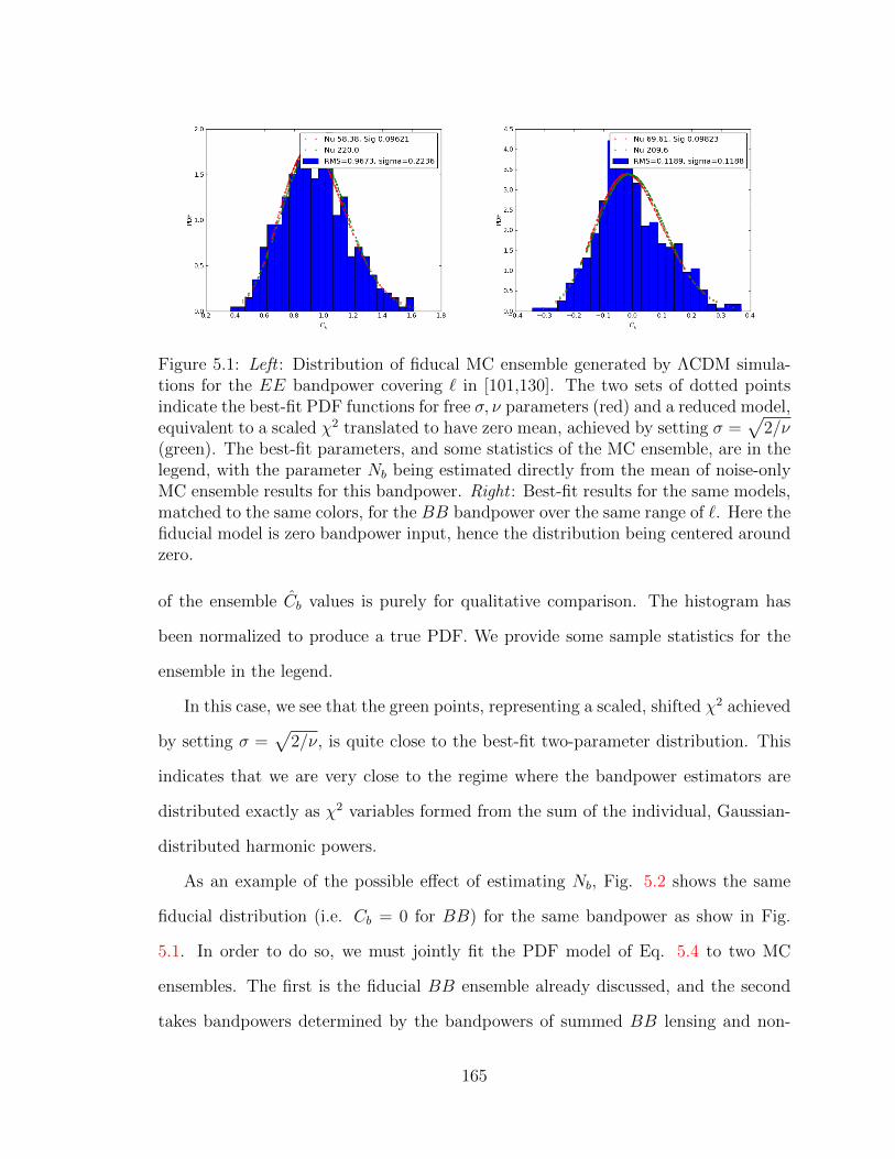
Figure 5.1: Left : Distribution of fiducal MC ensemble generated by ΛCDM simula-tions for the EE bandpower covering ` in [101,130]. The two sets of dotted pointsindicate the best-fit PDF functions for free σ, ν parameters (red) and a reduced model,equivalent to a scaled χ2 translated to have zero mean, achieved by setting σ =

√2/ν

(green). The best-fit parameters, and some statistics of the MC ensemble, are in thelegend, with the parameter Nb being estimated directly from the mean of noise-onlyMC ensemble results for this bandpower. Right : Best-fit results for the same models,matched to the same colors, for the BB bandpower over the same range of `. Here thefiducial model is zero bandpower input, hence the distribution being centered aroundzero.

of the ensemble Cb values is purely for qualitative comparison. The histogram has

been normalized to produce a true PDF. We provide some sample statistics for the

ensemble in the legend.

In this case, we see that the green points, representing a scaled, shifted χ2 achieved

by setting σ =√

2/ν, is quite close to the best-fit two-parameter distribution. This

indicates that we are very close to the regime where the bandpower estimators are

distributed exactly as χ2 variables formed from the sum of the individual, Gaussian-

distributed harmonic powers.

As an example of the possible effect of estimating Nb, Fig. 5.2 shows the same

fiducial distribution (i.e. Cb = 0 for BB) for the same bandpower as show in Fig.

5.1. In order to do so, we must jointly fit the PDF model of Eq. 5.4 to two MC

ensembles. The first is the fiducial BB ensemble already discussed, and the second

takes bandpowers determined by the bandpowers of summed BB lensing and non-

165

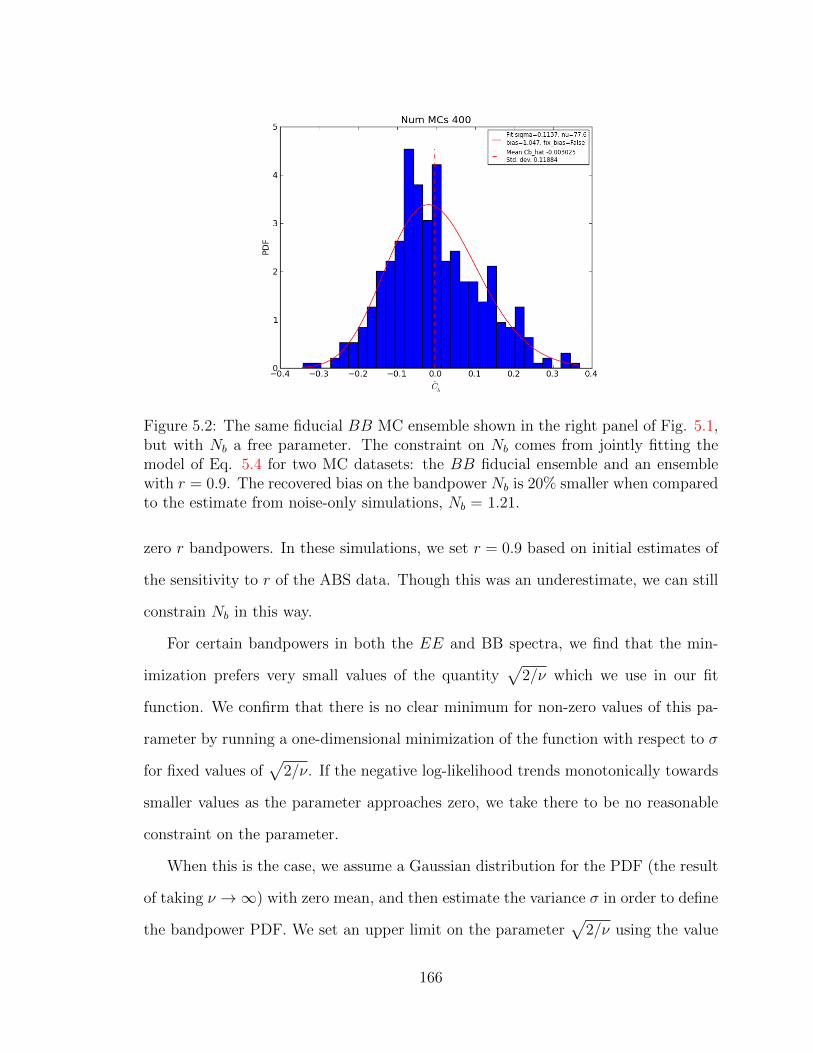
Figure 5.2: The same fiducial BB MC ensemble shown in the right panel of Fig. 5.1,but with Nb a free parameter. The constraint on Nb comes from jointly fitting themodel of Eq. 5.4 for two MC datasets: the BB fiducial ensemble and an ensemblewith r = 0.9. The recovered bias on the bandpower Nb is 20% smaller when comparedto the estimate from noise-only simulations, Nb = 1.21.

zero r bandpowers. In these simulations, we set r = 0.9 based on initial estimates of

the sensitivity to r of the ABS data. Though this was an underestimate, we can still

constrain Nb in this way.

For certain bandpowers in both the EE and BB spectra, we find that the min-

imization prefers very small values of the quantity√

2/ν which we use in our fit

function. We confirm that there is no clear minimum for non-zero values of this pa-

rameter by running a one-dimensional minimization of the function with respect to σ

for fixed values of√

2/ν. If the negative log-likelihood trends monotonically towards

smaller values as the parameter approaches zero, we take there to be no reasonable

constraint on the parameter.

When this is the case, we assume a Gaussian distribution for the PDF (the result

of taking ν →∞) with zero mean, and then estimate the variance σ in order to define

the bandpower PDF. We set an upper limit on the parameter√

2/ν using the value

166

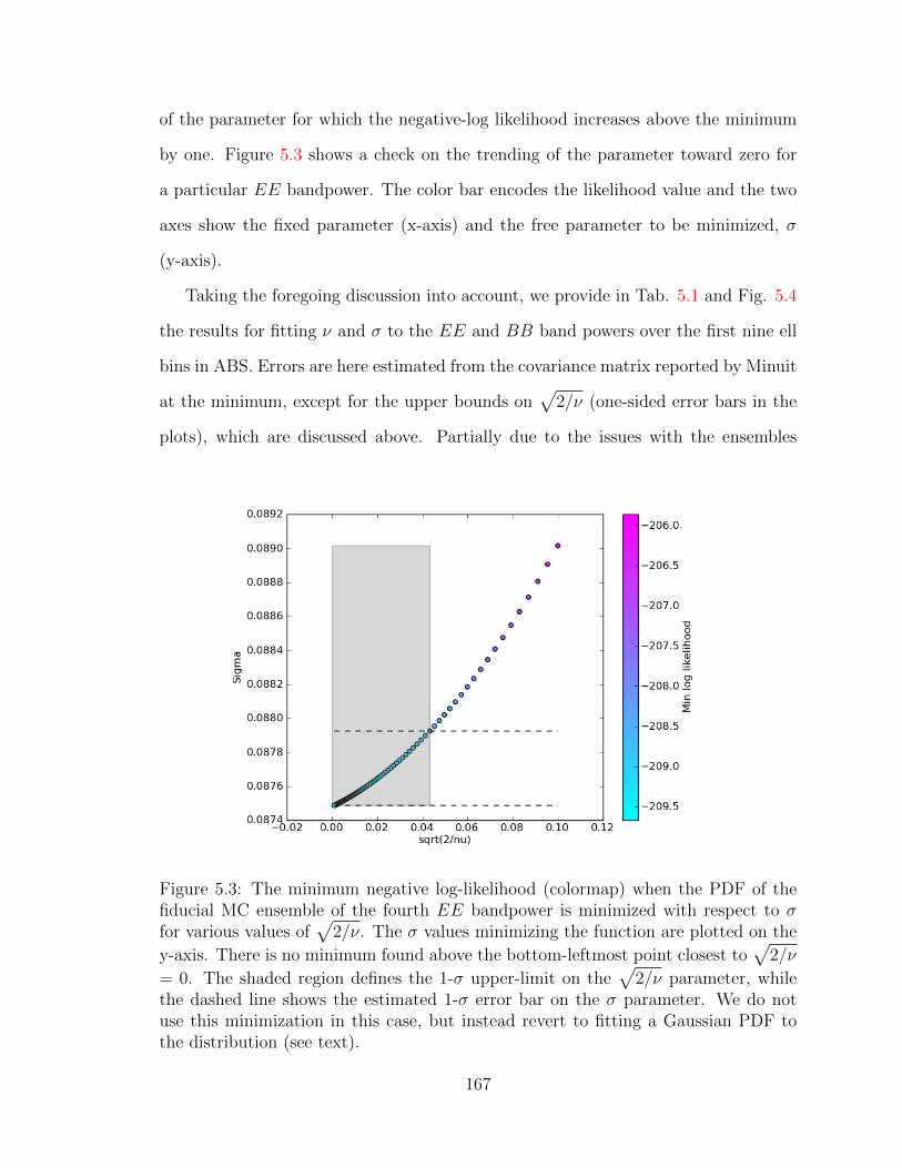
of the parameter for which the negative-log likelihood increases above the minimum

by one. Figure 5.3 shows a check on the trending of the parameter toward zero for

a particular EE bandpower. The color bar encodes the likelihood value and the two

axes show the fixed parameter (x-axis) and the free parameter to be minimized, σ

(y-axis).

Taking the foregoing discussion into account, we provide in Tab. 5.1 and Fig. 5.4

the results for fitting ν and σ to the EE and BB band powers over the first nine ell

bins in ABS. Errors are here estimated from the covariance matrix reported by Minuit

at the minimum, except for the upper bounds on√

2/ν (one-sided error bars in the

plots), which are discussed above. Partially due to the issues with the ensembles

Figure 5.3: The minimum negative log-likelihood (colormap) when the PDF of thefiducial MC ensemble of the fourth EE bandpower is minimized with respect to σfor various values of

√2/ν. The σ values minimizing the function are plotted on the

y-axis. There is no minimum found above the bottom-leftmost point closest to√

2/ν

= 0. The shaded region defines the 1-σ upper-limit on the√

2/ν parameter, whilethe dashed line shows the estimated 1-σ error bar on the σ parameter. We do notuse this minimization in this case, but instead revert to fitting a Gaussian PDF tothe distribution (see text).

167

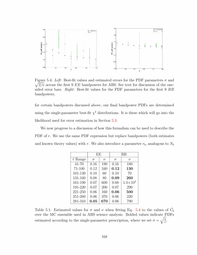
Figure 5.4: Left : Best-fit values and estimated errors for the PDF parameters σ and√2/ν across the first 9 EE bandpowers for ABS. See text for discussion of the one-

sided error bars. Right : Best-fit values for the PDF parameters for the first 9 BBbandpowers.

for certain bandpowers discussed above, our final bandpower PDFs are determined

using the single-parameter best-fit χ2 distributions. It is these which will go into the

likelihood used for error estimation in Section 5.3.

We now progress to a discussion of how this formalism can be used to describe the

PDF of r. We use the same PDF expression but replace bandpowers (both estimates

and known theory values) with r. We also introduce a parameter rb, analogous to Nb

EE BB` Range σ ν σ ν

41-70 0.16 190 0.16 18071-100 0.12 340 0.12 130101-130 0.10 60 0.10 70131-160 0.08 80 0.09 260161-190 0.07 600 0.08 1.0×105

191-220 0.07 200 0.07 290221-250 0.06 160 0.06 500251-280 0.06 370 0.06 220281-310 0.05 670 0.06 790

Table 5.1: Estimated values for σ and ν when fitting Eq. 5.4 to the values of Cbover the MC ensemble used in ABS science analysis. Bolded values indicate PDFs

estimated according to the single-parameter prescription, where we set σ =√

2ν.

168

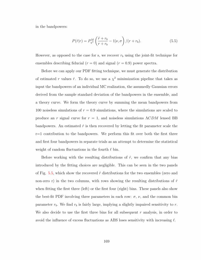
in the bandpowers:

P (r|r) = PMχ2

(r + rbr + rb

− 1|ν, σ)/(r + rb). (5.5)

However, as opposed to the case for s, we recover rb using the joint-fit technique for

ensembles describing fiducial (r = 0) and signal (r = 0.9) power spectra.

Before we can apply our PDF fitting technique, we must generate the distribution

of estimated r values r. To do so, we use a χ2 minimization pipeline that takes as

input the bandpowers of an individual MC realization, the assumedly Gaussian errors

derived from the sample standard deviation of the bandpowers in the ensemble, and

a theory curve. We form the theory curve by summing the mean bandpowers from

100 noiseless simulations of r = 0.9 simulations, where the simulations are scaled to

produce an r signal curve for r = 1, and noiseless simulations ΛCDM lensed BB

bandpowers. An estimated r is then recovered by letting the fit parameter scale the

r=1 contribution to the bandpowers. We perform this fit over both the first three

and first four bandpowers in separate trials as an attempt to determine the statistical

weight of random fluctuations in the fourth ` bin.

Before working with the resulting distributions of r, we confirm that any bias

introduced by the fitting choices are negligible. This can be seen in the two panels

of Fig. 5.5, which show the recovered r distributions for the two ensembles (zero and

non-zero r) in the two columns, with rows showing the resulting distributions of r

when fitting the first three (left) or the first four (right) bins. These panels also show

the best-fit PDF involving three parameters in each row: σ, ν, and the common bin

parameter rb. We find rb is fairly large, implying a slightly impaired sensitivity to r.

We also decide to use the first three bins for all subsequent r analysis, in order to

avoid the influence of excess fluctuations as ABS loses sensitivity with increasing `.

169

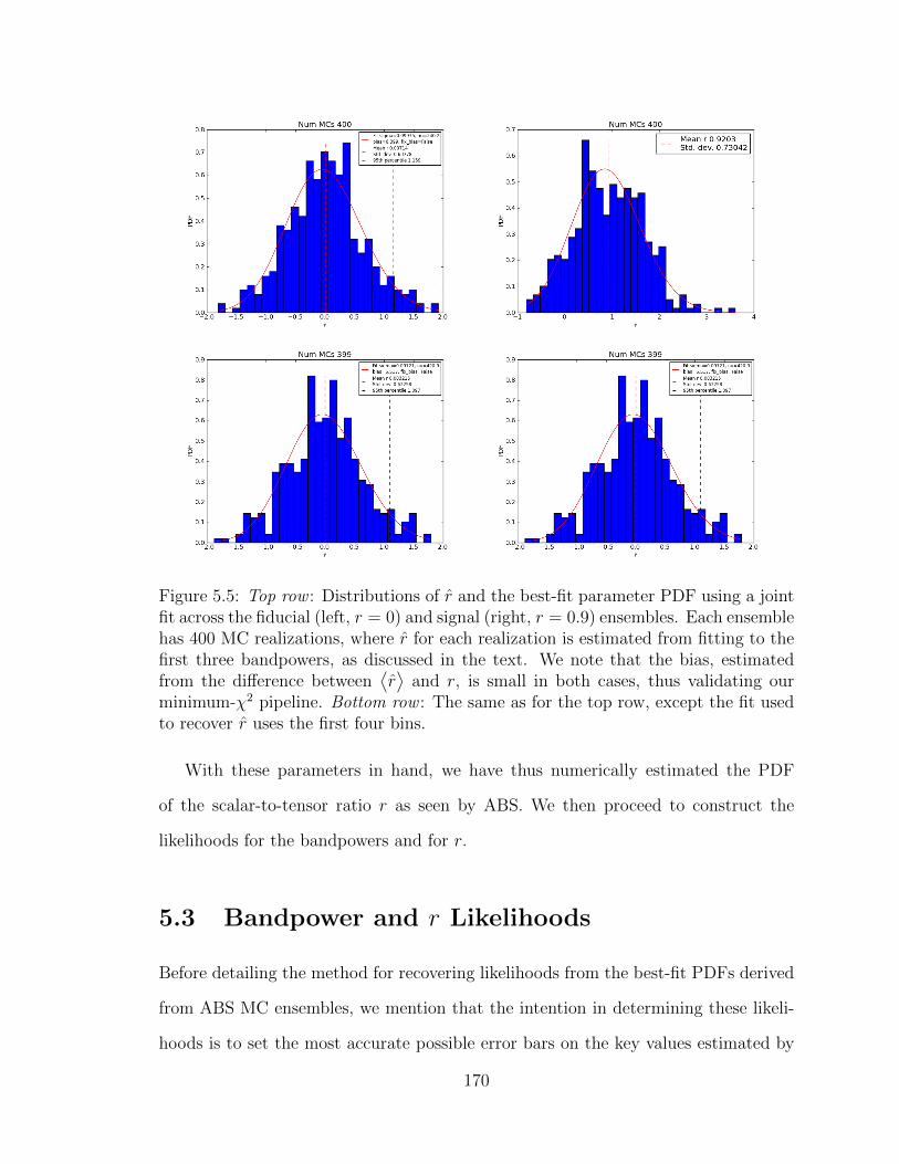
Figure 5.5: Top row : Distributions of r and the best-fit parameter PDF using a jointfit across the fiducial (left, r = 0) and signal (right, r = 0.9) ensembles. Each ensemblehas 400 MC realizations, where r for each realization is estimated from fitting to thefirst three bandpowers, as discussed in the text. We note that the bias, estimatedfrom the difference between

⟨r⟩

and r, is small in both cases, thus validating ourminimum-χ2 pipeline. Bottom row : The same as for the top row, except the fit usedto recover r uses the first four bins.

With these parameters in hand, we have thus numerically estimated the PDF

of the scalar-to-tensor ratio r as seen by ABS. We then proceed to construct the

likelihoods for the bandpowers and for r.

5.3 Bandpower and r Likelihoods

Before detailing the method for recovering likelihoods from the best-fit PDFs derived

from ABS MC ensembles, we mention that the intention in determining these likeli-

hoods is to set the most accurate possible error bars on the key values estimated by

170

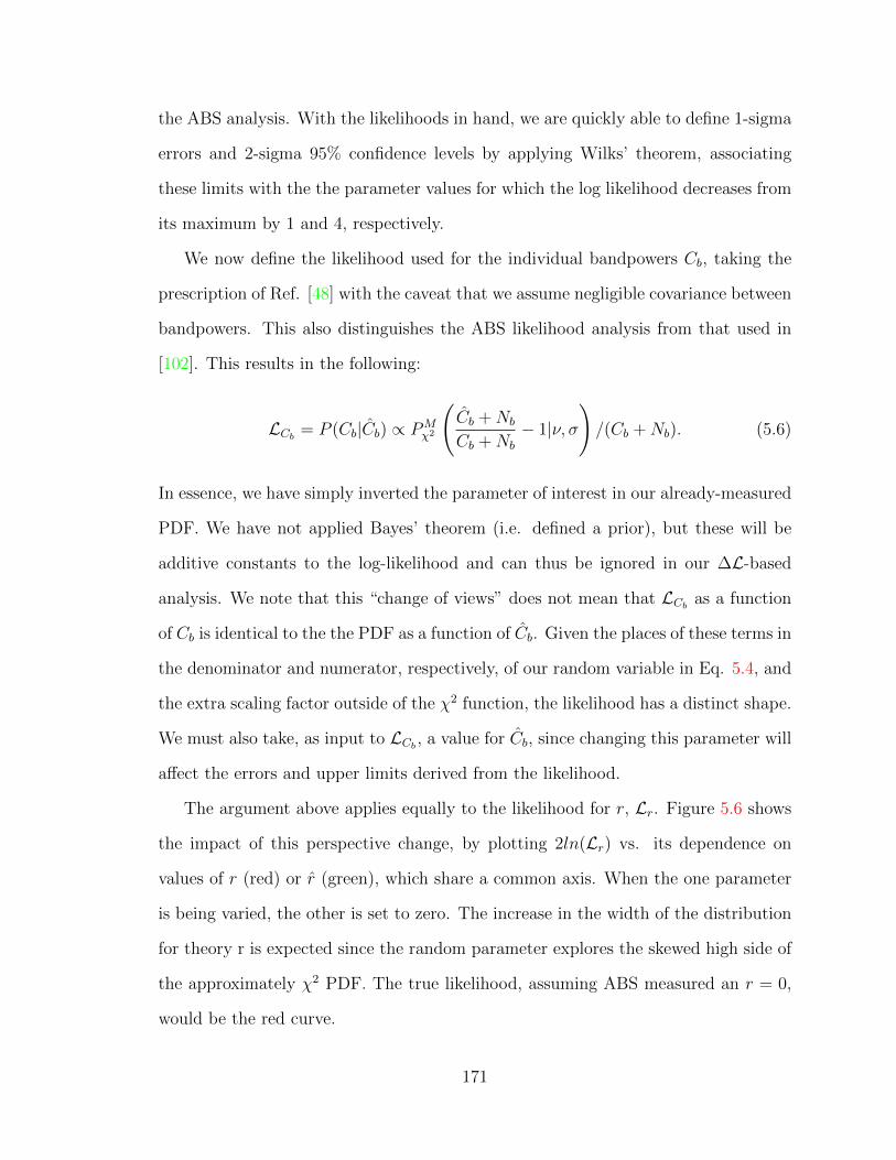
the ABS analysis. With the likelihoods in hand, we are quickly able to define 1-sigma

errors and 2-sigma 95% confidence levels by applying Wilks’ theorem, associating

these limits with the the parameter values for which the log likelihood decreases from

its maximum by 1 and 4, respectively.

We now define the likelihood used for the individual bandpowers Cb, taking the

prescription of Ref. [48] with the caveat that we assume negligible covariance between

bandpowers. This also distinguishes the ABS likelihood analysis from that used in

[102]. This results in the following:

LCb = P (Cb|Cb) ∝ PMχ2

(Cb +Nb

Cb +Nb

− 1|ν, σ

)/(Cb +Nb). (5.6)

In essence, we have simply inverted the parameter of interest in our already-measured

PDF. We have not applied Bayes’ theorem (i.e. defined a prior), but these will be

additive constants to the log-likelihood and can thus be ignored in our ∆L-based

analysis. We note that this “change of views” does not mean that LCb as a function

of Cb is identical to the the PDF as a function of Cb. Given the places of these terms in

the denominator and numerator, respectively, of our random variable in Eq. 5.4, and

the extra scaling factor outside of the χ2 function, the likelihood has a distinct shape.

We must also take, as input to LCb , a value for Cb, since changing this parameter will

affect the errors and upper limits derived from the likelihood.

The argument above applies equally to the likelihood for r, Lr. Figure 5.6 shows

the impact of this perspective change, by plotting 2ln(Lr) vs. its dependence on

values of r (red) or r (green), which share a common axis. When the one parameter

is being varied, the other is set to zero. The increase in the width of the distribution

for theory r is expected since the random parameter explores the skewed high side of

the approximately χ2 PDF. The true likelihood, assuming ABS measured an r = 0,

would be the red curve.

171

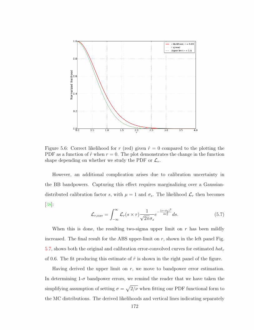
Figure 5.6: Correct likelihood for r (red) given r = 0 compared to the plotting thePDF as a function of r when r = 0. The plot demonstrates the change in the functionshape depending on whether we study the PDF or Lr.

However, an additional complication arises due to calibration uncertainty in

the BB bandpowers. Capturing this effect requires marginalizing over a Gaussian-

distributed calibration factor s, with µ = 1 and σs. The likelihood Lr then becomes

[38]:

Lr,corr =

∫ ∞−∞Lr(s× r)

1√2πσs

e− (s−σs)2

2σ2s ds. (5.7)

When this is done, the resulting two-sigma upper limit on r has been mildly

increased. The final result for the ABS upper-limit on r, shown in the left panel Fig.

5.7, shows both the original and calibration error-convolved curves for estimated hatr

of 0.6. The fit producing this estimate of r is shown in the right panel of the figure.

Having derived the upper limit on r, we move to bandpower error estimation.

In determining 1-σ bandpower errors, we remind the reader that we have taken the

simplifying assumption of setting σ =√

2/ν when fitting our PDF functional form to

the MC distributions. The derived likelihoods and vertical lines indicating separately

172

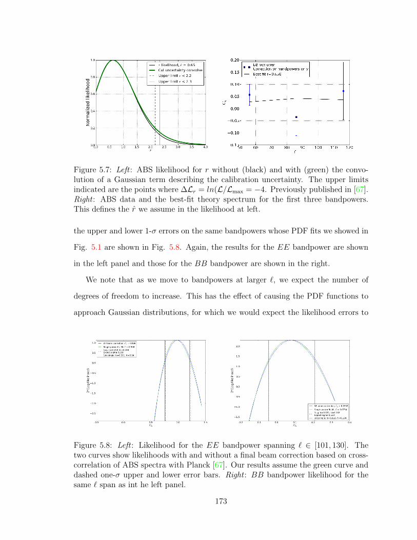
Figure 5.7: Left : ABS likelihood for r without (black) and with (green) the convo-lution of a Gaussian term describing the calibration uncertainty. The upper limitsindicated are the points where ∆Lr = ln(L/Lmax = −4. Previously published in [67].Right : ABS data and the best-fit theory spectrum for the first three bandpowers.This defines the r we assume in the likelihood at left.

the upper and lower 1-σ errors on the same bandpowers whose PDF fits we showed in

Fig. 5.1 are shown in Fig. 5.8. Again, the results for the EE bandpower are shown

in the left panel and those for the BB bandpower are shown in the right.

We note that as we move to bandpowers at larger `, we expect the number of

degrees of freedom to increase. This has the effect of causing the PDF functions to

approach Gaussian distributions, for which we would expect the likelihood errors to

Figure 5.8: Left : Likelihood for the EE bandpower spanning ` ∈ [101, 130]. Thetwo curves show likelihoods with and without a final beam correction based on cross-correlation of ABS spectra with Planck [67]. Our results assume the green curve anddashed one-σ upper and lower error bars. Right : BB bandpower likelihood for thesame ` span as int he left panel.

173

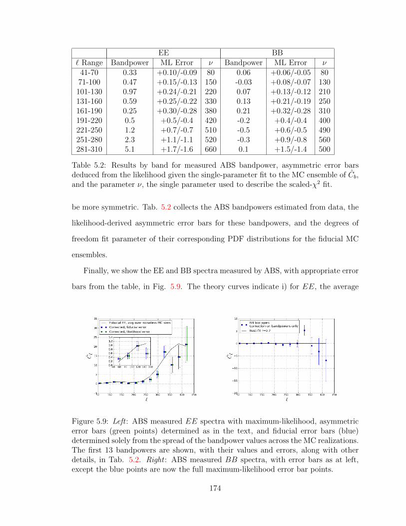
EE BB` Range Bandpower ML Error ν Bandpower ML Error ν

41-70 0.33 +0.10/-0.09 80 0.06 +0.06/-0.05 8071-100 0.47 +0.15/-0.13 150 -0.03 +0.08/-0.07 130101-130 0.97 +0.24/-0.21 220 0.07 +0.13/-0.12 210131-160 0.59 +0.25/-0.22 330 0.13 +0.21/-0.19 250161-190 0.25 +0.30/-0.28 380 0.21 +0.32/-0.28 310191-220 0.5 +0.5/-0.4 420 -0.2 +0.4/-0.4 400221-250 1.2 +0.7/-0.7 510 -0.5 +0.6/-0.5 490251-280 2.3 +1.1/-1.1 520 -0.3 +0.9/-0.8 560281-310 5.1 +1.7/-1.6 660 0.1 +1.5/-1.4 500

Table 5.2: Results by band for measured ABS bandpower, asymmetric error barsdeduced from the likelihood given the single-parameter fit to the MC ensemble of Cb,and the parameter ν, the single parameter used to describe the scaled-χ2 fit.

be more symmetric. Tab. 5.2 collects the ABS bandpowers estimated from data, the

likelihood-derived asymmetric error bars for these bandpowers, and the degrees of

freedom fit parameter of their corresponding PDF distributions for the fiducial MC

ensembles.

Finally, we show the EE and BB spectra measured by ABS, with appropriate error

bars from the table, in Fig. 5.9. The theory curves indicate i) for EE, the average

Figure 5.9: Left : ABS measured EE spectra with maximum-likelihood, asymmetricerror bars (green points) determined as in the text, and fiducial error bars (blue)determined solely from the spread of the bandpower values across the MC realizations.The first 13 bandpowers are shown, with their values and errors, along with otherdetails, in Tab. 5.2. Right : ABS measured BB spectra, with error bars as at left,except the blue points are now the full maximum-likelihood error bar points.

174

of the noiselessΛCDM simulations discussed in Sect. 5.2, and ii) for BB, the theory

curve used in our minimum-χ2 fitting pipeline.

5.4 Conclusion

We conclude this chapter, having provided the detailed prescription used to generate

the main results of this likelihood pipeline. The ABS upper limit on r is thus revealed

to be carefully estimated, but almost three times as large as the estimated r level

used in generating the non-zero r MC ensemble. We do not expect this to introduce

considerable issues unless an MC ensemble at r = 2 were to prefer much different

estimate for the PDF bias parameter rb.

175

Chapter 6

Future Work: Detector

Nonlinearity

We conclude this thesis by discussing additional possibilities for TES bolometer char-

acterization relevant to better understanding performance in the field. Particularly,

we focus on concerns about TES nonlinearity when coupled to A4 to produce a spu-

rious signal in the demodulated timestream of CRHWP experiments [120], [22]. We

also provide initial simulations used to study this effect in a generic time-domain sim-

ulation framework, s4cmb in a distinct case, where no CRHWP is present but the TES

nonlinearity sources leakage of atmospheric intensity signals due to intensity-driven

gain mismatch between detector polarization pairs.1

To be explicit, our model for TES nonlinearity can be written as a reobserving

function on the input data d(t). Assuming we are only interested in low frequencies

in our timestream, we choose to write the nonlinearly-distorted timestream d′(t) as

[120]:

d′(t) = [1 + g1d(t)]d(t− τ1d(t)), (6.1)

1J. Peloton, https://github.com/JulienPeloton/s4cmb.

176

where the parameters g1 and τ1 would be zero for an ideal detector. These parameters

can be estimated by expanding the ordinary differential equations outlined in Ch. 2

to second order. Expressions are recovered that depend on parameters like τ , L , and

other familiar components of the simple, and extended, TES bolometer models [120].

We are interested in constraining these parameters in a controlled, calibrated way,

preferably in situ on the telescope.

6.1 Direct Measurement of Nonlinearity

As a first attempt to probe nonlinearity in AdvACT TES bolometers, we performed

a test data acquisition in December 2017 during downtime from observations. We

use the MCE to send in digitally-approximated sinusoids of various frequencies to 10

TES bias lines on a common MCE “bias card” in use on the AdvACT HF and two

MF arrays. We then look for pickup at twice the input frequency, where if we label

this frequency f s, we expect to see a signal proprtional to g1, since:

d′(t) ∼ d(t) + g1d2(t), (6.2)

based on simplifying Eq. 6.1 for a measurement where we ignore the phase-lag effects

of nonzero τ1. Such a probe is provided by comparing the amplitude of the discrete

Fourier transform at f s to that at 2f s. Assuming a purely sinusoidal input, the ratio

of these two is an estimate of the g1 we wish to determine if we assume some input

signal size to convert the dimensionless ratio to something like %/K.

To see the effect of nonlinearity in the frequency domain, Fig. 6.1 shows three

current spectral densities (solid curves) measured at three separate input sinusoid

amplitudes, in DAC. This is an MF1 detector studied with a reflective cover over

the aperture of the receiver window. We can clearly see the increase of the height

of the largest peak from green (20 DAC amplitude) to red (160 DAC amplitude),

177

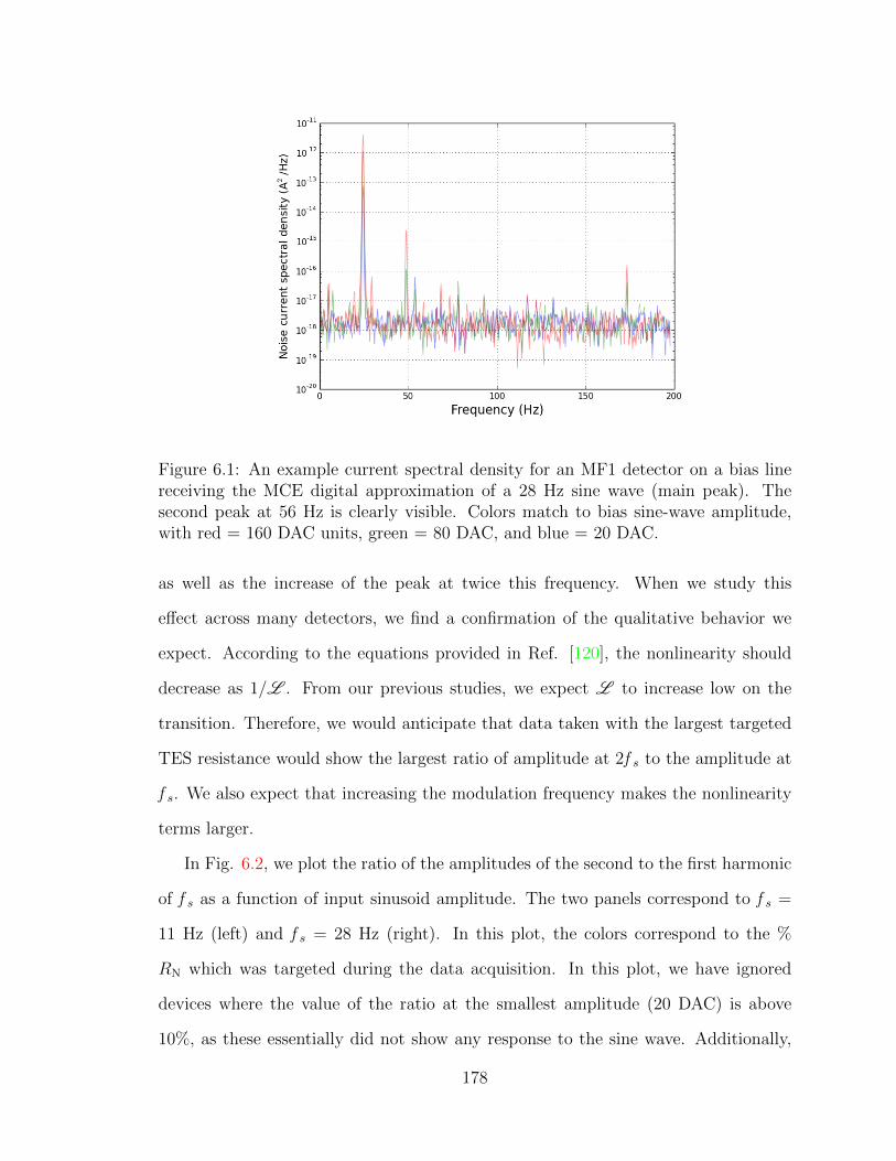
Figure 6.1: An example current spectral density for an MF1 detector on a bias linereceiving the MCE digital approximation of a 28 Hz sine wave (main peak). Thesecond peak at 56 Hz is clearly visible. Colors match to bias sine-wave amplitude,with red = 160 DAC units, green = 80 DAC, and blue = 20 DAC.

as well as the increase of the peak at twice this frequency. When we study this

effect across many detectors, we find a confirmation of the qualitative behavior we

expect. According to the equations provided in Ref. [120], the nonlinearity should

decrease as 1/L . From our previous studies, we expect L to increase low on the

transition. Therefore, we would anticipate that data taken with the largest targeted

TES resistance would show the largest ratio of amplitude at 2f s to the amplitude at

f s. We also expect that increasing the modulation frequency makes the nonlinearity

terms larger.

In Fig. 6.2, we plot the ratio of the amplitudes of the second to the first harmonic

of f s as a function of input sinusoid amplitude. The two panels correspond to f s =

11 Hz (left) and f s = 28 Hz (right). In this plot, the colors correspond to the %

RN which was targeted during the data acquisition. In this plot, we have ignored

devices where the value of the ratio at the smallest amplitude (20 DAC) is above

10%, as these essentially did not show any response to the sine wave. Additionally,

178

this cut ignores devices that were driven into unstable regimes of the transition due

to the excitation amplitude. This is an important effect that will likely determine

how usefully we may use this technique in the future. We were left with about 1/3

of the MF1 array available to study, those addressed by the 10 bias lines to which we

directed the sinusoid.

While our model would predict g1 to be independent of the input amplitude, we

find that for the 160 DAC amplitude, a signficant increase in this ratio is observed.

Of course, we may have expected that we were exercising a higher-order nonlinearity

given the presence of higher-order harmonics in Fig. 6.1.

If we take the middle amplitude, 80 DAC, and convert this to a bias voltage on

the TES, we recover 3 nV. This would then correspond to a current signal of 0.7

pA assuming a TES resistance of 4 mΩ (50% RN and RN = 8 mΩ). Finally, we

convert this to a power fluctuation by multiplying the two (equivalently, dividing

by the naive estimate of the responsivity), and convert to a brightness temperature

fluctuation assuming a rule-of-thumb found for ACTPol and AdvACT of ∼ 10 K/pW.

This results in assuming our input, if considered as a temperature difference, is ∼ 30

mTCMB, and we thus roughly estimate g1 ∼ 0.1 %/mTCMB.

This should be compared to the estimate in Ref. [120] of an expected range

for the absolute value of g1 from 0.2 to 0.4 %/K. There an assumed modulation

frequency of 8 Hz was input to the parameter estimates; higher modulation frequencies

should increase the terms, but not sufficiently to explain the discrepancy. This is also

concerning given the high expected loop gains for AdvACT devices. However, we

stress that this study is preliminary. We hope that this probe may be developed in

future to provide quick checks of device linearity in the field.

179

6.2 Simulations of Nonlinearity in Observations

Given the presence of nonlinearity in TES bolometers (Eq. 6.1), it is imperative to

understand how this simple model for signal-dependent gain effects may contribute

to spurious signal in upcoming CMB instruments. This model arose in Ref. [120] as

a way to explain leakage of an unpolarized atmosphere signal into the demodulated

timestream of the POLARBEAR experiment with a CRHWP. However, we also

expect that for telescopes without polarization modulators, differences between the

nonlinearity coupling values, especially g1, across different TES polarization pairs

may produce a significant leakage of general sky intensity (CMB + atmosphere) I

into recovered polarization P .

To get an upper bound on this effect size, we have begun running simulations

using a CMB instrument systematic error pipeline available publicly, s4cmb. Initial

results for this work are presented in Ref. [Crowley Simon SPIE]. As discussed in

that text, various aspects of the design of the Simons Observatory (SO), a project

which will span multiple telescopes to be sited near the Simons Array and AdvACT

in Chile, were included in the simulations. However, many aspects of the instrument

design and observing strategy have not been confirmed within the SO technical team.

Further, the simulation was made more tractable by taking only 32 detectors in 16

pairs, sampled at 32 Hz, and using an effective description of atmospheric noise power

as measured by the noise power spectra of existing ACTPol datasets. We modeled

the nonlinearity parameters g1 and τ1 by calculating them based on current optimum

bolometer design parameters for SO, then putting a 10% spread on these parameters,

a lower-bound estimate of expected fabrication variance of the bolometers. Finally,

the level of nonlinearity was varied between simulated observations by scaling these

numbers with estimated changes of Pbias, assuming a fiducial Psat and changing Pγ

due to changing PWV.

180

We wish to emphasize that these results were achieved with an explicit pair-

differencing pipeline, in which sky polarization is recovered at each pixel by sub-

tracting the timestream of one detector from its orthogonally-polarized pipeline. In

general, weighting of each detector’s sampling of a sky pixel by that detector’s po-

larization angle can more cleanly recover polarization in a map. However, as stated

above, pair-differencing represents a “worst-case” leakage, especially when nothing

has been done to attempt the mitigate the presence of the effects of nonlinearity.

Our results indicate that, in combination with large, long-timescale, unpolarized

signals, the differential nonlinearity of detector pairs can leak an appreciable signal

into the recovered maps of polarization (here in Stokes Q and U). We confirm that

this is due entirely to nonlinearity by:

• setting sky Q and U to zero so that any signal in these maps is due to noise or

systematic effects;

• comparing the result with nonlinearity (Case I) to that without, where 1/f noise

is still present (Case III), and to pure signal + white noise simulations (Case

II).

We include the results for a putative “deep” observing strategy, in which 1% of

the sky is mapped in a repeating 12-day pattern of observations. These observations

are four-hours azimuthal scans of the sky at constant elevation, and occur once a day,

to mimic having only 20% observing efficiency. This number is a convenience of the

split of 24 hours into four and 20; current experiments like ACT achieve higher (&

40%) during the active observing season.

The result for Case I (left column) for sky I (top row), Q (middle) and U (bottom)

indicates that including nonlinearity in the systematics of the telescope can produce

signals at the ∼ 1 µ K level. Case II and III (middle and left columns, respectively)

confirm that what is seen in Case I is not the result of issues with the simulation

181

of white or correlated noise. We thus confirm that the systematic defined and dis-

cussed in this chapter should be carefully considered, along with any unmodeled gain

drifts, out of concern for leakage of the bright atmopshere and CMB temperature

anisotropies into the low signal-to-noise-ratio channels of Q and U , which we trans-

form directly into the E- and B-modes discussed in Ch. 1.

182

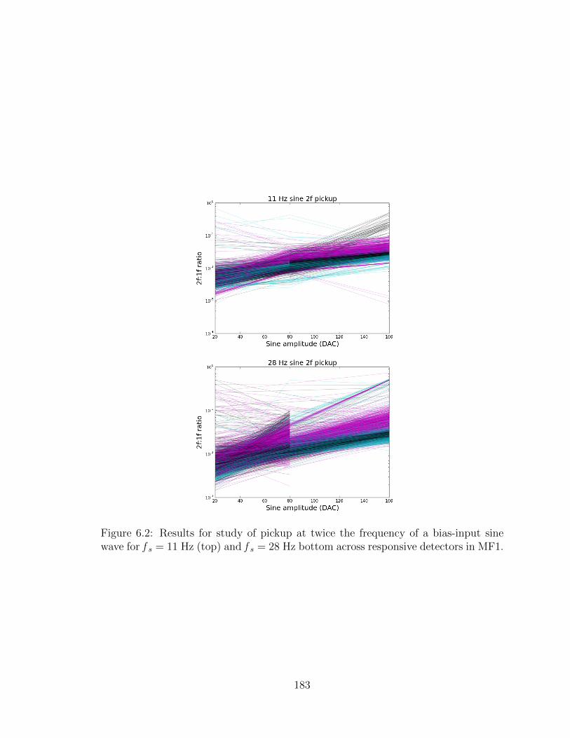
Figure 6.2: Results for study of pickup at twice the frequency of a bias-input sinewave for f s = 11 Hz (top) and f s = 28 Hz bottom across responsive detectors in MF1.

183

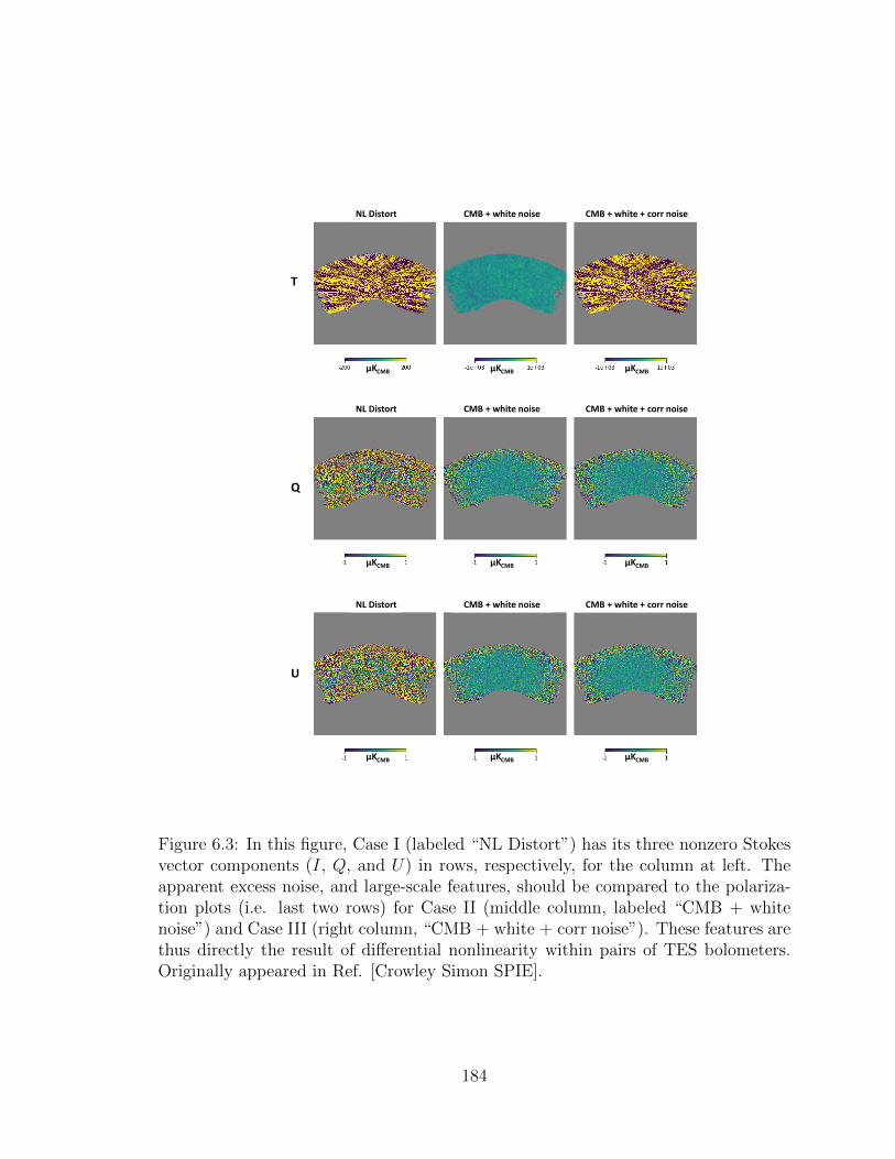
NL Distort CMB + white noise CMB + white + corr noise

NL Distort CMB + white noise CMB + white + corr noise

NL Distort CMB + white noise CMB + white + corr noise

T

Q

U

μKCMB μKCMB μKCMB

μKCMB μKCMB μKCMB

μKCMB μKCMB μKCMB

Figure 6.3: In this figure, Case I (labeled “NL Distort”) has its three nonzero Stokesvector components (I, Q, and U) in rows, respectively, for the column at left. Theapparent excess noise, and large-scale features, should be compared to the polariza-tion plots (i.e. last two rows) for Case II (middle column, labeled “CMB + whitenoise”) and Case III (right column, “CMB + white + corr noise”). These features arethus directly the result of differential nonlinearity within pairs of TES bolometers.Originally appeared in Ref. [Crowley Simon SPIE].

184

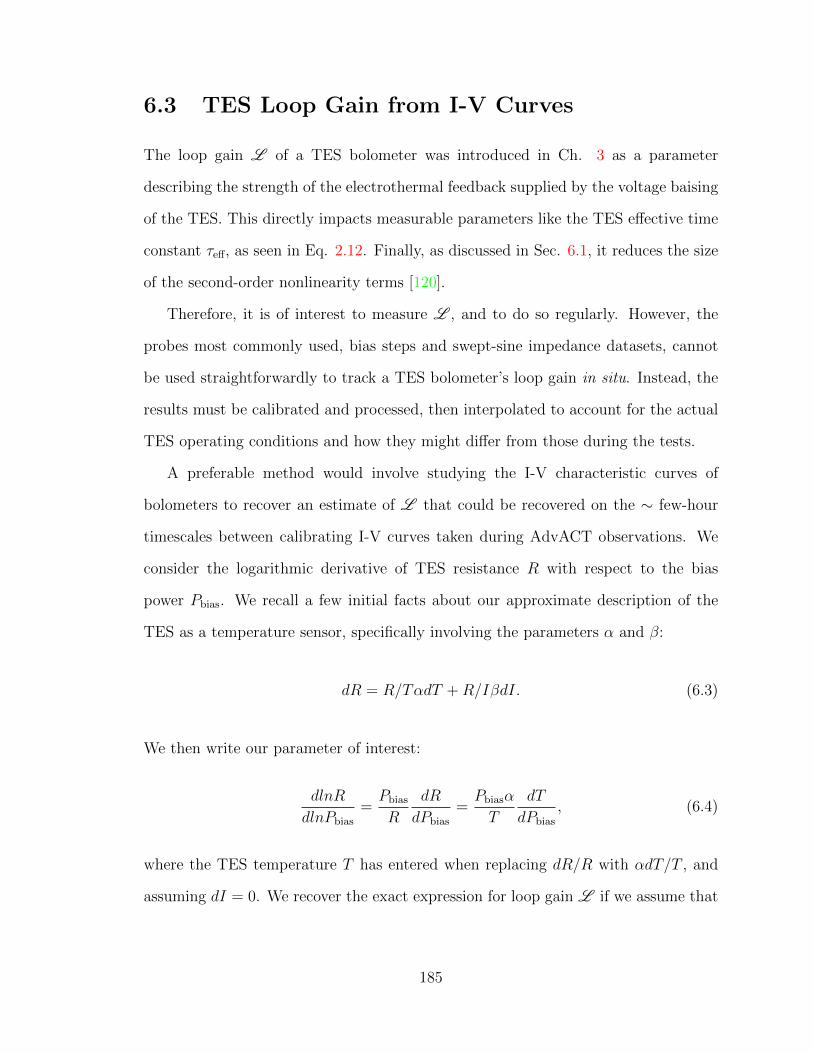
6.3 TES Loop Gain from I-V Curves

The loop gain L of a TES bolometer was introduced in Ch. 3 as a parameter

describing the strength of the electrothermal feedback supplied by the voltage baising

of the TES. This directly impacts measurable parameters like the TES effective time

constant τeff, as seen in Eq. 2.12. Finally, as discussed in Sec. 6.1, it reduces the size

of the second-order nonlinearity terms [120].

Therefore, it is of interest to measure L , and to do so regularly. However, the

probes most commonly used, bias steps and swept-sine impedance datasets, cannot

be used straightforwardly to track a TES bolometer’s loop gain in situ. Instead, the

results must be calibrated and processed, then interpolated to account for the actual

TES operating conditions and how they might differ from those during the tests.

A preferable method would involve studying the I-V characteristic curves of

bolometers to recover an estimate of L that could be recovered on the ∼ few-hour

timescales between calibrating I-V curves taken during AdvACT observations. We

consider the logarithmic derivative of TES resistance R with respect to the bias

power Pbias. We recall a few initial facts about our approximate description of the

TES as a temperature sensor, specifically involving the parameters α and β:

dR = R/TαdT +R/IβdI. (6.3)

We then write our parameter of interest:

dlnR

dlnPbias

=Pbias

R

dR

dPbias

=Pbiasα

T

dT

dPbias

, (6.4)

where the TES temperature T has entered when replacing dR/R with αdT/T , and

assuming dI = 0. We recover the exact expression for loop gain L if we assume that

185

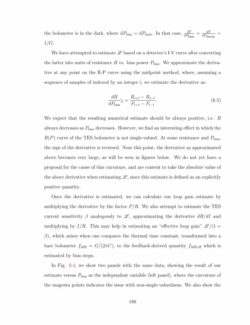
the bolometer is in the dark, where dPbias = dPbath. In that case, dTdPbias

= dTdPtherm

=

1/G.

We have attempted to estimate L based on a detector’s I-V curve after converting

the latter into units of resistance R vs. bias power Pbias. We approximate the deriva-

tive at any point on the R-P curve using the midpoint method, where, assuming a

sequence of samples of indexed by an integer i, we estimate the derivative as:

dR

dPbias

|i =Ri+1 −Ri−1

Pi+1 − Pi−1

. (6.5)

We expect that the resulting numerical estimate should be always positive, i.e. R

always decreases as Pbias decreases. However, we find an interesting effect in which the

R(P ) curve of the TES bolometer is not single-valued. At some resistance and Pbias,

the sign of the derivative is reversed. Near this point, the derivative as approximated

above becomes very large, as will be seen in figures below. We do not yet have a

proposal for the cause of this curvature, and are content to take the absolute value of

the above derivative when estimating L , since this estimate is defined as an explicitly

positive quantity.

Once the derivative is estimated, we can calculate our loop gain estimate by

multiplying the derivative by the factor P/R. We also attempt to estimate the TES

current sensitivity β analogously to L , approximating the derivative dR/dI and

multiplying by I/R. This may help in estimating an “effective loop gain” L /(1 +

β), which arises when one compares the thermal time constant, transformed into a

bare bolometer f3dB = G/(2πC), to the feedback-derived quantity f3dB,eff which is

estimated by bias steps.

In Fig. 6.4, we show two panels with the same data, showing the result of our

estimate versus Pbias as the independent variable (left panel), where the curvature of

the magenta points indicates the issue with non-single-valuedness. We also show the

186

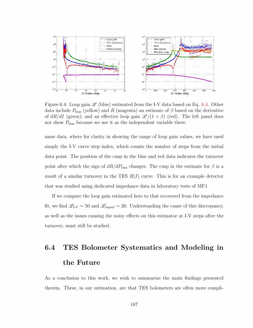
Figure 6.4: Loop gain L (blue) estimated from the I-V data based on Eq. 6.4. Otherdata include Pbias (yellow) and R (magenta) an estimate of β based on the derivativeof dR/dI (green); and an effective loop gain L /(1 + β) (red). The left panel doesnot show Pbias because we use it as the independent variable there.

same data, where for clarity in showing the range of loop gain values, we have used

simply the I-V curve step index, which counts the number of steps from the initial

data point. The position of the cusp in the blue and red data indicates the turnover

point after which the sign of dR/dPbias changes. The cusp in the estimate for β is a

result of a similar turnover in the TES R(I) curve. This is for an example detector

that was studied using dedicated impedance data in laboratory tests of MF1.

If we compare the loop gain estimated here to that recovered from the impedance

fit, we find LI-V ∼ 50 and Limped ∼ 20. Understanding the cause of this discrepancy,

as well as the issues causing the noisy effects on this estimator at I-V steps after the

turnover, must still be studied.

6.4 TES Bolometer Systematics and Modeling in

the Future

As a conclusion to this work, we wish to summarize the main findings presented

therein. These, in our estimation, are that TES bolometers are often more compli-

187

cated in their internal thermal (and electrothermal) architectures. As experiments

begin to push on maximizing the number of detectors to meet ambitious sensitivity

targets, it is important to not neglect attempts to detect excess noise, understand its

source, and control any possible enhancement in the CMB signal band.

Additionally, it is potentially dangerous to assume that these bolometers can

be treated as linear-gain devices for ground-based CMB observations. We empha-

size “ground-based”, since it is the pernicious presence of atmospheric fluctuation-

induced 1/f noise that generates spurious polarization signals. Mitigating this after

the fact using observed unmodulated timestreams to clean the estimated polarization

timestreams, as in Ref. [120] is one possible path. However, for experiments without

the presence of CRHWPs, and even for those using them, it is important to consider

that systematics control can be balanced against ambitious sensitivty gains. Given

that enhancing the loop gain parameter L by increasing the bias power Pbias applied

during observations is always a potential choice, we are also in need of a model for

the effect that can be usefully compared against enhancing noise levels by making

these bolometers as sensitive as possible. This will be the continuation of the work

presented in this chapter.

Finally, we presented multiple elements of a preliminary study of the performance

of a CRHWP at a part of the optics where the HWP-synchronous signal (A(χ)) may

alter between detectors and with time in complex ways. Producing science from this

data, when CRHWPs are used to observe on a telescope sensitive to small sales, can-

not proceed exactly as in previous experiments [68]. We will continue to explore this

rich dataset, taking advantage of the good sensitivity and performance of the Ad-

vACT bolometers as built, to attempt to push the sensitivity of the AdvACT project

to larger scales. TES bolometers reacting to these signals is a complex interplay be-

tween aspects of instrumentation that have enabled current progress on the study of

the CMB, and will continue to do so in future.

188

Appendix A

Impedance Data Acquisition and

Analysis Code

This appendix is meant to serve as a brief overview of the codebase used in the

impedance measurements reported in Ch. 3. We separate individual scripts or mod-

ules based on whether they are used for acquisition or analysis.

A.1 Acquisition Scripts

input sine.py This script initiates the data-taking for the impedance measurements.

It has the following argument format:

input sine.py -m <marker> -cr <col/row numbers> -bc <bias card> -adc

<adc offset> -rc <readout card> -f <frequencies> -o <offset> -a <amplitude> -t

<temperature> -fr <frames> -ramp <max frequency> -start <min frequency> -Rn

<percRN > -bl <bias line> -n <noise frames>

The “marker” argument ensures that data generated as part of a single call to

this script has a common prefix, for simpler analysis.

It instantiates a loop over detectors in the array, identified by MCE column and

row number. It then instantiates an inner loop over frequencies, either provided as a

189

command line argument (“frequencies” taken as a Python list) or given as a beginning

(“start”) and ending (“ramp”) frequency. If the script generates the frequencies

automatically, then the step size is the power of 10 of the previous frequency. We

have generally run the acquisition between 4 Hz and 1 kHz. Based on the frequencies

requested, the script requires some hard-coded information about the MCE frame (or

row-visit) rate in order to accurately estimate the true frequency of the sine wave as

approximated by the MCE.

This script is relatively informed about how to properly DC bias a TES bolometer.

Both an “offset” and a “percRN ” (or percent RN) parameter should be provided. If

the former is non-zero and the latter is 0 (i.e., superconducting), then no DC bias is

applied. For any other “percRN ” parameter, the TES is driven normal by the default

normal bias in the array.cfg file, before the DC bias is set to the value of the “offset”

argument. The script reads local configuration information (with hardcoded paths)

in order to determine which bias line on which bias card corresponds to the detector

under test. This functionality is provided by helper modules read bias lines.py and

bias card finder.py. With regard to determining the DC bias, we have used a sec-

ondary script (Psat script.py) to estimate this quantity for each target percent RN.

This secondary script reads I-V curve data in for the detector under test.

This script is also used to communicate with the MCE to set up the sine wave

input for later transmission to a particular target register. The argument “adc offset”

is a toggle which determines whether the sine wave signal will go to the TES bias

card specified by the argument “bias card,” or to the ADC register specified by the

argument. As mentioned above, the script determines the appropriate bias card and

bias line based on MCE column and row number. If the detector is not targeted by the

bias card requested in the argument, the script overrides the “bias card” argument.

Once the target is set, the script calls the MCE utility function “mce internal ramp setup.”

This function, and the general characteristics of an internal ramp, are described on

190

the public MCE wiki. 1 This ramp is hardcoded to update every two MCE frames,

where the timespan of a frame is set by the details of the multiplexing setup, and a

minimum step size of 1 DAC unit.

Once this internal ramp register is set aside by the MCE, we define the sine wave

using a second MCE utility function, “mce awg setup.” This script accepts arguments

defining the shape of the excitation (we specify “sine”), a DAC offset and amplitude

for the sine wave, and the number of ramp steps N to be used in defining the sinusoid

period. For each frequency, N is determined in order to most closely match the

frequency requested by the user. Once the two setup scripts have been run, the script

collect sine is called.

When this is complete, input sine.py assumes the sine wave bias is no longer

running. It then rebiases the detector, and takes a number “noise frames” of DC-

biased noise with the multiplexing set up in collect sine.

Throughout, individual log files for each acquisition are written to a specified

directory, and a running log of sine-wave data taken is written in the folder where

the data are stored.

collect sine This is a Bash executable script written to perform the actual MCE

acquisition commands needed to send the sine wave. It takes a series of arguments,

all generated inside input sine.py. The argument structure is:

collect sine<filename><column><row><frames><readout card><datarate>

<bias card> <bias line> <noise>

This script sends the bias sine wave to “bias line” on “bias card,” as determined by

input sine.py. It sets up a rectangle-mode acquisition on the MCE, in which a single

detector is sampled repeatedly, rather than switching between rows. This fills up a

dummy frame of some specified number of rows and columns (currently hardcoded

to be 32×8=256), which then is read out at the rate specified by the “datarate”

1https://e-mode.phas.ubc.ca/mcewiki/index.php/Main Page

191

argument. This argument should always equal the total number of samples in a

frame.

Although the “row” argument of a particular detector is unique, we note that

the “column” argument in this script is relative to the RC card specified by “read-

out card,” and thus can only span [0-7]. Thus, the global column 12 must be addressed

as column 4 on readout card 2. Similarly, the bias line of a particular detector in the

array must be mapped into the “bias line” index for the particular bias card set by

“bias card” in order for the sine wave to be properly addressed.

Once the rectangle mode is enabled and the sine wave bias is set to appear only

on the appropriate bias line (using MCE command “enbl bias mod”), the sine wave

is started, a number of rectangle-mode frames is acquired according to the argument

“frames,” and the sine wave is then turned off. If the argument “noise” equals the

string “y,” the sine wave bias is not enabled, and rectangle-mode noise is acquired

instead.

impedance noise acqscript.py Due to some of the need for secondary analysis

to feed to the acquisition scripts, we have written a set of wrapper scripts where

analysis of I-V curves can be performed, proper naming conventions for the different

kinds of data can be enforced, and a separate external loop over detector column and

row numbers can be performed. In this way, we can study each detector at bias values

that are closest to the target percent RN for each individual bolometer. This script

also ensures that any on-transition data are marked by the filename of the I-V curve

taken before the sine wave data was acquired.

A.2 Analysis Scripts

transfer function.py Raw data are read into this file, which searches according to

a regular-expression pattern-matching module in Python. An argument “marker”

192

identical to the one used in the acquisition of the data should be provided to ensure

all frequencies are found. Additional identification of specific files is performed by

specifying the MCE column and row numbers, and the target percent RN used in

determining the DC bias applied during the acquisition.

Once the files specifying a dataset are found, they are looped over. First, the

mce data module for Python is used to properly read the data (in feedback DAC

unnits) from binary flatfile in which they are stored. Information about the MCE

sample rate stored in the runfile (an auxiliary file associated with the data file) is used

to generate a vector of times assuming constant sample rate. The original vector of

MCE samples is also shifted so that the fiirst 262 samples are cut. We have found that

this precise sample index is the zero-phase point for the input sine wave, so in order

to recover phase information from our studies, we shift our output by this amount.

An “array” argument is used to specify a bias line configuration file, which is read to

determine if the feedback signal has positive or negative response to changing TES

current signals.

This data is then fit to a five-parameter model for the data:

yi = a+ b sin(c+ 2πdti) + eti. (A.1)

This fit is performed by the “curve fit” function in the scipy.optimize module. We

take the best-fit sinusoid frequency d to be the true frequency of the sine wave. This

function provides an estimated covariance matrix along with the best-fit parameters.

This matrix is used to generate error bars for the parameters of interest (amplitude

b and phase c) using 300 draws of a covariance matrix appropriately scaled such that

the best-fit parameters produce a reduced χ2 of 1. These errors are propagated to all

other quantities estimated from the best-fit amplitude and phase at each frequency.

193

The appropriately-scaled transfer function is then estimated using calibration con-

stants within the MCE, a command line argument specifying the sine wave amplitude

in bias DAC units, and the measured amplitude and phase of the feedback signal.

This data can either be plotted for inspection, or written to a file (with filename

specified by the “out” argument) for later use.

analyze transfer.py This script performs the calibration of the transfer function

into physical units, as well as the calculation of the complex calibration numbers Vth

and Zeq as in Ch. 3. Together, these values can be used to estimate ZTES. This is

usually done for a single detector, whose column and row number is specified on the

command line. The script has been designed to work with demodulated lock-in data

stored in the NIST Python dictionary format, or with the transfer functions saved as

Python Pickle files, as written by transfer function.py.

In order to perform the calibration in either case, an I-V curve or set of I-Vs must

be specified to be studied. The code must be told what set of operating conditions

(combinations of Tbath and % RN) to try to process. Then the number of I-Vs provided

as a command line argument should generally match the number of bath temperatures

to be studied. For each operating condition, a given I-V is studied to determine the

TES resistance at the applied bias, the bias power, and the normal resistance of

the device. The value of RN is required to calibrate the impedance data to Ohms

[79] [133], and relies on the shunt resistance assumed in its estimation. The TES

resistance in transition and the bias power are assumed to be exactly known, and

are required for extracting parameters in the fit. The TES thermal conductance G

estimated from I-V curve data at different Tbath is also necessary. Information on the

applied bias is stored either in the .info files written by input sine.py (MCE data) or

in the NIST-style dictionary for each frequency sweep. The user can specify a shunt

resistance mapping file to apply a particular shunt value for the detector studied.

194

I-V curves from MCE acquisitions are studied by a separate script, iv-

plot princeton.py. This code writes the physically-relevant quantities mentioned

above to a lcoal file, where analyze transfer knows to look for them. These numbers

are then loaded and used to perform the conversions (e.g., Eq. 3.5) needed to recover

ZTES. Errors are either estimated from the magnitude and phase errors estimated

by transfer function.py, or for NIST data, following Eq. 3.6. The resulting data and

errors are stored in a Python dictionary for passing to the final analysis module, to

be discussed below.

minuit contact.py As one may imagine, this module contains all connections

between the data provided by analyze transfer.py and the minimization algorithms

to be applied in fitting the model. An added layer of complexity comes from the choice

of total parameter numbers. Both analyze transfer.py and minuit contact.py need it

specified which parameters will be fit with unique values at all operating conditions,

and which will be held common across datasets. There are two categories of the

latter: those held constant across all percent RN studied (“rat hold”) and those held

in common across all data sets, and thus across bath temperatures (“temp hold”).

Initial values for the relevant parameters must be specified in analyze transfer.py in

order for minuit contact.py to generate the appropriate description of the parameters

to fit.

In addition, as discussed in Ch. 3, the simple and hanging bolometer models

were fit with differences in which parameters are held constant. Both the analysis

script and the fitting module refer to these models as “one block” and “two block,”

in reference to the number of electrothermal elements. Beyond these various levels

of customization, a call to instantiate a “minimizer”, an object class defined to de-

termine which parameters to define and to perform the fit, requires specifying which

minimization scheme to use. The options are: the SciPy minimization using Powell’s

method; Minuit; a combination scheme where Minuit is called after the SciPy min-

195

imization succeeds essentially in order to properly estimate errros; and the MCMC

implementation using Emcee.

In the two-block model fitting case of NIST data, we have implemented a hybrid

approach where certain parameters are first estimated for a reduced set of frequencies,

where the one-block model would appear valid. These estimates are then used to set

the initialization for the MCMC exploraton an extended frequency range using the

hanging model. In the one-block model fitting case, we tend to use the combination

of SciPy for initial minimization, and Minuit for robust error estimation.

The final parameters estimated by the minimization routines in the “minimizer”

class can then be plotted against the data using the “plot results” function of the

class. This function has many options for how to plot the impedance results, whether

and how to load noise data and process it, estimation of noise curves with and without

aliasing, etc. This code is fairly complicated since it must handle many choices with

regard to what is plotted. Writing a new, more modular version of these functions

would be a worthy follow-up to the initial establishment of this code base.

196

Appendix B

Semiconductor Bolometer Tests for

PIXIE

The PIXIE experiment [64] is a proposed Explorer-class satellite designed to accu-

rately measure any distortions of the CMB spectra arising from physics before and

after recombination. This science goal is served by an instrument design in which

various systematic contaminants in the timestream cancel at first order [90]. A two-

port Fourier Transform Spectrometer (FTS) is used to observe either the same sky

patch with two co-pointed beams, or to observe with one port filled by an isothermal,

highly emissive blackbody. The design for the optical components gives PIXIE sensi-

tivity to celestial emission over 2.5 decades in frequency, from 15 GHz to 6 THz. The

movable mirror component enables the time-dependent path length difference within

the spectrometer to sample this frequency range in bins of 15 GHz.

At the detection port for the interferometer, two single-polarization detectors are

placed back-to-back to record the signals from the interferometer. The individual

crystalline-silicon devices are optically and thermally large, with an optically-active

area of 13 mm×13 mm [89]. Thin, free-standing wires of silicon, called “harpstrings”,

are degenerately doped with phosphorous to be metallic. They are arrayed at reg-

197

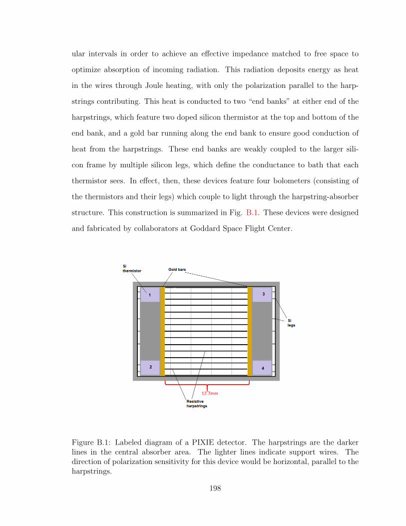
ular intervals in order to achieve an effective impedance matched to free space to

optimize absorption of incoming radiation. This radiation deposits energy as heat

in the wires through Joule heating, with only the polarization parallel to the harp-

strings contributing. This heat is conducted to two “end banks” at either end of the

harpstrings, which feature two doped silicon thermistor at the top and bottom of the

end bank, and a gold bar running along the end bank to ensure good conduction of

heat from the harpstrings. These end banks are weakly coupled to the larger sili-

con frame by multiple silicon legs, which define the conductance to bath that each

thermistor sees. In effect, then, these devices feature four bolometers (consisting of

the thermistors and their legs) which couple to light through the harpstring-absorber

structure. This construction is summarized in Fig. B.1. These devices were designed

and fabricated by collaborators at Goddard Space Flight Center.

Figure B.1: Labeled diagram of a PIXIE detector. The harpstrings are the darkerlines in the central absorber area. The lighter lines indicate support wires. Thedirection of polarization sensitivity for this device would be horizontal, parallel to theharpstrings.

198

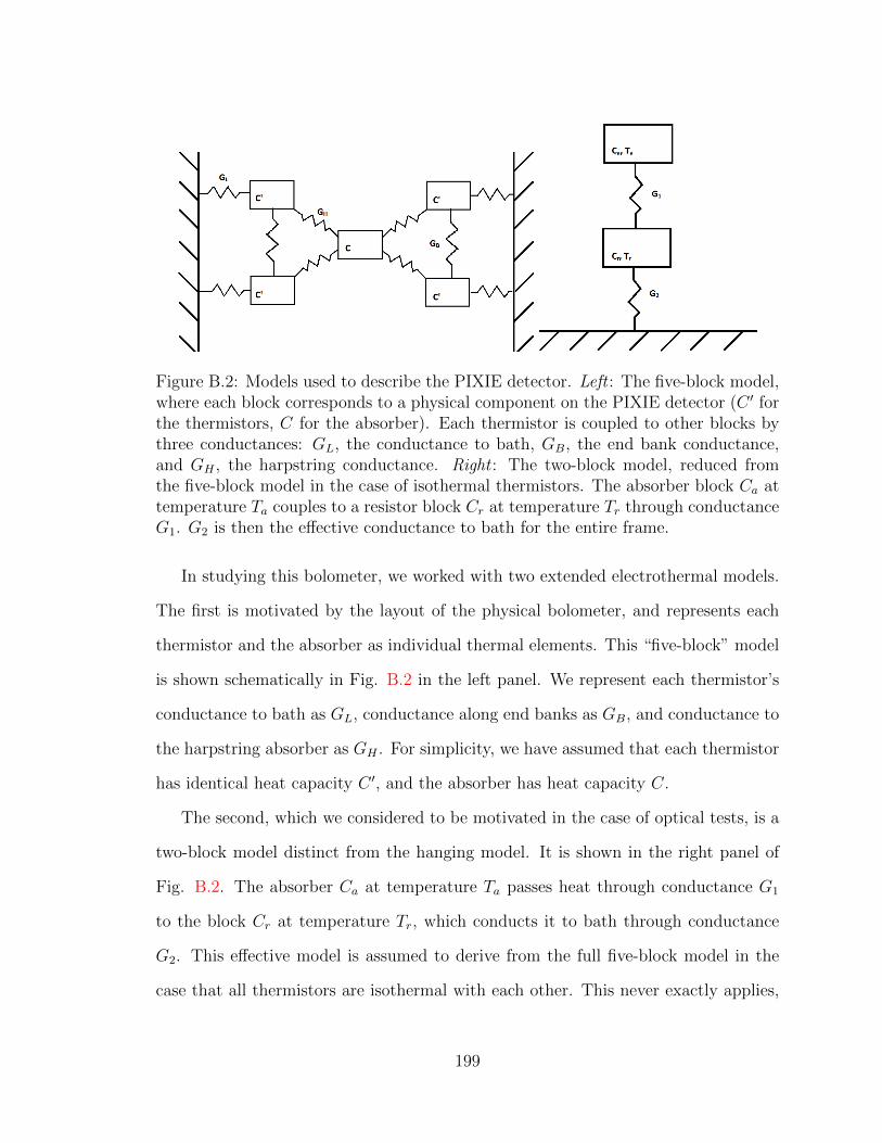
Figure B.2: Models used to describe the PIXIE detector. Left : The five-block model,where each block corresponds to a physical component on the PIXIE detector (C ′ forthe thermistors, C for the absorber). Each thermistor is coupled to other blocks bythree conductances: GL, the conductance to bath, GB, the end bank conductance,and GH , the harpstring conductance. Right : The two-block model, reduced fromthe five-block model in the case of isothermal thermistors. The absorber block Ca attemperature Ta couples to a resistor block Cr at temperature Tr through conductanceG1. G2 is then the effective conductance to bath for the entire frame.

In studying this bolometer, we worked with two extended electrothermal models.

The first is motivated by the layout of the physical bolometer, and represents each

thermistor and the absorber as individual thermal elements. This “five-block” model

is shown schematically in Fig. B.2 in the left panel. We represent each thermistor’s

conductance to bath as GL, conductance along end banks as GB, and conductance to

the harpstring absorber as GH . For simplicity, we have assumed that each thermistor

has identical heat capacity C ′, and the absorber has heat capacity C.

The second, which we considered to be motivated in the case of optical tests, is a

two-block model distinct from the hanging model. It is shown in the right panel of

Fig. B.2. The absorber Ca at temperature Ta passes heat through conductance G1

to the block Cr at temperature Tr, which conducts it to bath through conductance

G2. This effective model is assumed to derive from the full five-block model in the

case that all thermistors are isothermal with each other. This never exactly applies,

199

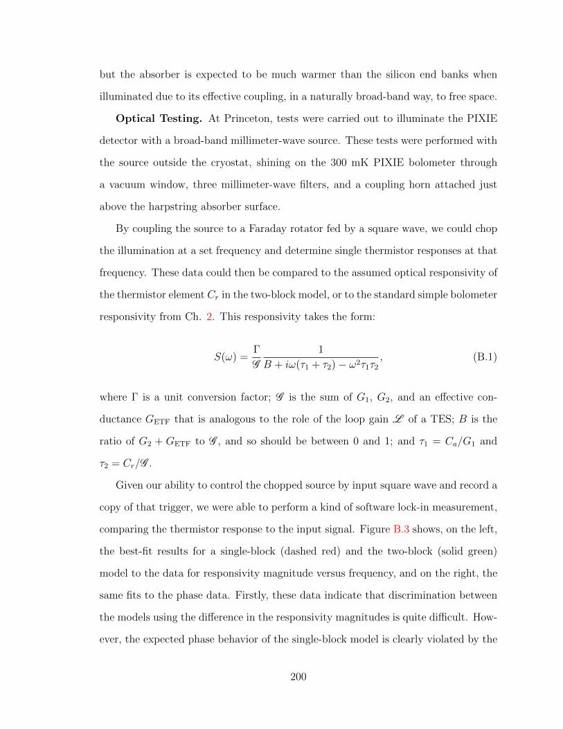
but the absorber is expected to be much warmer than the silicon end banks when

illuminated due to its effective coupling, in a naturally broad-band way, to free space.

Optical Testing. At Princeton, tests were carried out to illuminate the PIXIE

detector with a broad-band millimeter-wave source. These tests were performed with

the source outside the cryostat, shining on the 300 mK PIXIE bolometer through

a vacuum window, three millimeter-wave filters, and a coupling horn attached just

above the harpstring absorber surface.

By coupling the source to a Faraday rotator fed by a square wave, we could chop

the illumination at a set frequency and determine single thermistor responses at that

frequency. These data could then be compared to the assumed optical responsivity of

the thermistor element Cr in the two-block model, or to the standard simple bolometer

responsivity from Ch. 2. This responsivity takes the form:

S(ω) =Γ

G

1

B + iω(τ1 + τ2)− ω2τ1τ2

, (B.1)

where Γ is a unit conversion factor; G is the sum of G1, G2, and an effective con-

ductance GETF that is analogous to the role of the loop gain L of a TES; B is the

ratio of G2 + GETF to G , and so should be between 0 and 1; and τ1 = Ca/G1 and

τ2 = Cr/G .

Given our ability to control the chopped source by input square wave and record a

copy of that trigger, we were able to perform a kind of software lock-in measurement,

comparing the thermistor response to the input signal. Figure B.3 shows, on the left,

the best-fit results for a single-block (dashed red) and the two-block (solid green)

model to the data for responsivity magnitude versus frequency, and on the right, the

same fits to the phase data. Firstly, these data indicate that discrimination between

the models using the difference in the responsivity magnitudes is quite difficult. How-

ever, the expected phase behavior of the single-block model is clearly violated by the

200

0 10 20 30 40 50 60 70Chopper frequency in Hz

0.000000

0.000002

0.000004

0.000006

0.000008

0.000010

0.000012

0.000014

0.000016

0.000018

|V|

B = 0.6, t1 = 0.02354, t2 = 0.001786

2-pole fit to binned data1-pole fit: tau=0.0295193028817Data binned by frequency

0 10 20 30 40 50 60 70Chopper frequency in Hz

0.0

0.5

1.0

1.5

2.0

Arg

(V)

B = 0.6, t1 = 0.01567, t2 = 0.00114

2-pole fit to binned data1-pole fit: tau=0.0309550610245Data binned by frequency

Figure B.3: Tests of broad-band illumination of PIXIE detectors by a warm, choppedsource. Left : Best-fit model and parameters recovered for fitting the magnitude ofthe thermistor response to the chopped source versus frequency. The solid green fitsthe two-block form of Eq. B.1, the dashed red fits using the simple bolometer modelwhere the only degree of freedom aside from a normalization is the time constant.No strong preference is exhibited by the data. Right : Best-fit model and parametersfor fitting phase versus frequency. Solid green and dashed red lines correspond tomodels as in the right panel. The two-block model is able to handle the rise of thephase to values above π/2, and prefers a fast transfer of heat to the bath (small τ2),as compared to transfer between the absorber and thermistors (larger tau1).

data. Adding a second block has enabled us to fit the data out to much higher fre-

quency, and recover two time constants of very different order. Specifically, the slower

time constant here corresponds to heat transfer between the harpstring absorber and

the thermistors. This is supported by other measurements of the version of the PIXIE

detectors tested at Princeton at this time, with evidence to be discussed below.

Thermal Transfer. In order to explore the full set of conductances coupled to

each thermistor, we carried out a campaign of measurements to fully characterize

each thermistor on a different PIXIE detector than the one which was optically tests.

We began by estimating the parameters that define the R(T ) curve of semiconductor

thermistors, as well as the total conductance seen by each thermistor. The resistance

of these devices is understood in the context of a variable-range hopping model (for

201

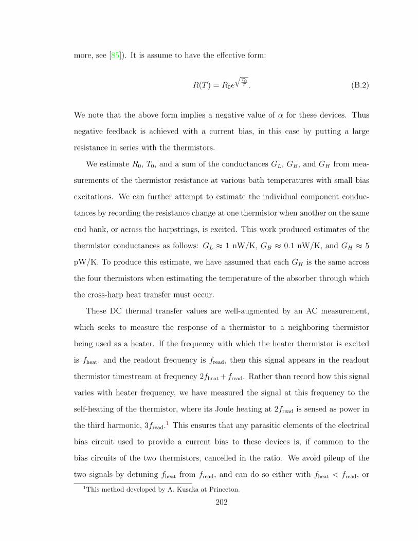
more, see [85]). It is assume to have the effective form:

R(T ) = R0e

√T0T . (B.2)

We note that the above form implies a negative value of α for these devices. Thus

negative feedback is achieved with a current bias, in this case by putting a large

resistance in series with the thermistors.

We estimate R0, T0, and a sum of the conductances GL, GB, and GH from mea-

surements of the thermistor resistance at various bath temperatures with small bias

excitations. We can further attempt to estimate the individual component conduc-

tances by recording the resistance change at one thermistor when another on the same

end bank, or across the harpstrings, is excited. This work produced estimates of the

thermistor conductances as follows: GL ≈ 1 nW/K, GB ≈ 0.1 nW/K, and GH ≈ 5

pW/K. To produce this estimate, we have assumed that each GH is the same across

the four thermistors when estimating the temperature of the absorber through which

the cross-harp heat transfer must occur.

These DC thermal transfer values are well-augmented by an AC measurement,

which seeks to measure the response of a thermistor to a neighboring thermistor

being used as a heater. If the frequency with which the heater thermistor is excited

is fheat, and the readout frequency is fread, then this signal appears in the readout

thermistor timestream at frequency 2fheat + fread. Rather than record how this signal

varies with heater frequency, we have measured the signal at this frequency to the

self-heating of the thermistor, where its Joule heating at 2fread is sensed as power in

the third harmonic, 3fread.1 This ensures that any parasitic elements of the electrical

bias circuit used to provide a current bias to these devices is, if common to the

bias circuits of the two thermistors, cancelled in the ratio. We avoid pileup of the

two signals by detuning fheat from fread, and can do so either with fheat < fread, or

1This method developed by A. Kusaka at Princeton.

202

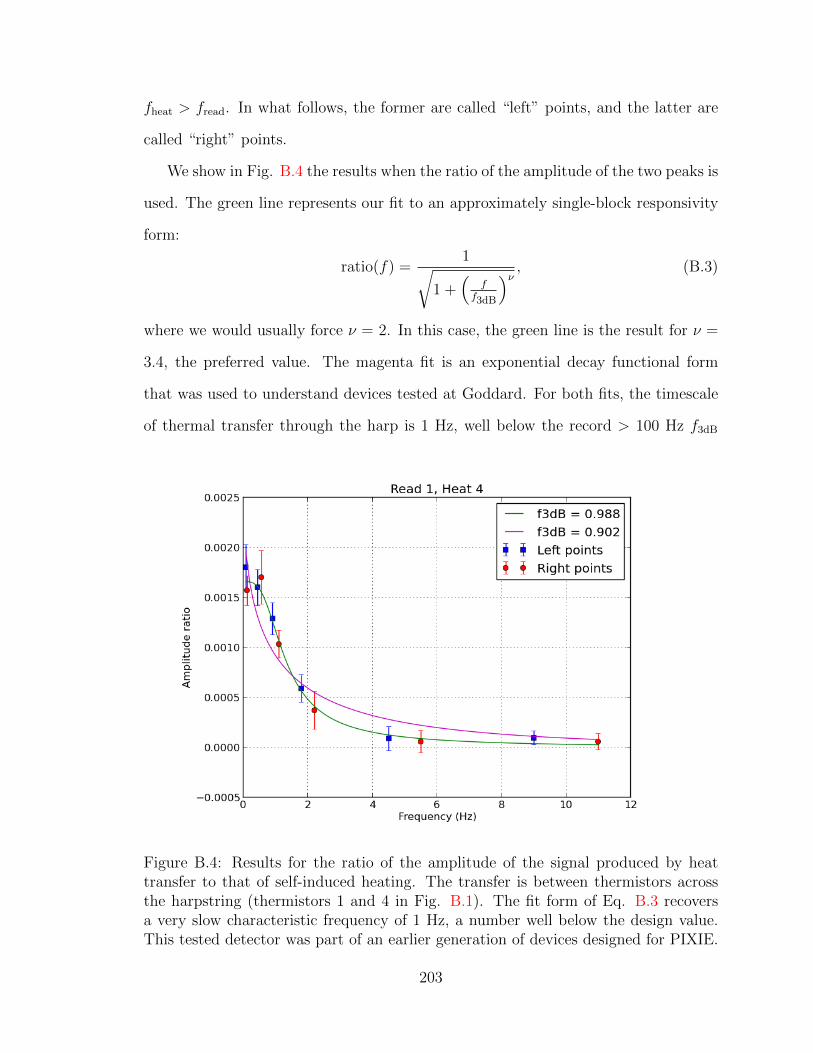
fheat > fread. In what follows, the former are called “left” points, and the latter are

called “right” points.

We show in Fig. B.4 the results when the ratio of the amplitude of the two peaks is

used. The green line represents our fit to an approximately single-block responsivity

form:

ratio(f) =1√

1 +(

ff3dB

)ν , (B.3)

where we would usually force ν = 2. In this case, the green line is the result for ν =

3.4, the preferred value. The magenta fit is an exponential decay functional form

that was used to understand devices tested at Goddard. For both fits, the timescale

of thermal transfer through the harp is 1 Hz, well below the record > 100 Hz f3dB

Figure B.4: Results for the ratio of the amplitude of the signal produced by heattransfer to that of self-induced heating. The transfer is between thermistors acrossthe harpstring (thermistors 1 and 4 in Fig. B.1). The fit form of Eq. B.3 recoversa very slow characteristic frequency of 1 Hz, a number well below the design value.This tested detector was part of an earlier generation of devices designed for PIXIE.

203

values measured at Goddard. This result should not be taken to represent the final

measurement on this aspect of PIXIE detector performance.

A new generation of PIXIE detectors has been designed and fabricated at God-

dard, and tests are in progress, with future plans including similar AC-biased studies

of thermistor heat transfer.

204

Appendix C

Time-Varying Scan-Synchronous

Signal in ABS

A major systematic error issue for ground-based observations of the CMB is pickup

of signals synchronous with the scan but not produced in the sky. Sources of such

signals may include scattering or far beam sidelobes in the instrument and magnetic

pickup by the cryogenic SQUID amplifiers. Though we expect that it will not add

coherently in maps produced from many scans, we prefer to remove an estimate for

this signal in order to avoid any artifacts. The baffle and ground screen for ABS were

designed to prevent this pickup, but additional methods to handle any such signals

were also instituted.

As part of the TOD processing for the ABS science analysis, a template of the per-

CES scan-synchronous signal (SSS) was estimated and removed. The template itself

refers to defining 1-wide bins in boresight azimuth and averaging detector samples

across the ∼ 1-hour CES within those bins. This template was removed using a model

built from a linear combination of the first 20 Legendre polynomials. The template

estimation and removal process was done separately for the real and imaginary parts

of the demodulated timestream.

205

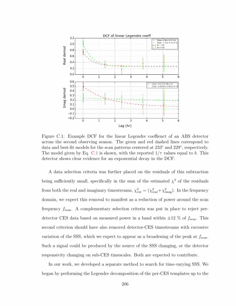
Lag (hr)

Real dem

od

Imag

dem

od

Figure C.1: Example DCF for the linear Legendre coeffienct of an ABS detectoracross the second observing season. The green and red dashed lines correspond todata and best-fit models for the scan patterns centered at 233 and 229, respectively.The model given by Eq. C.1 is shown, with the reported 1/τ values equal to b. Thisdetector shows clear evidence for an exponential decay in the DCF.

A data selection criteria was further placed on the residuals of this subtraction

being sufficiently small, specifically in the sum of the estimated χ2 of the residuals

from both the real and imaginary timestreams, χ2cut = (χ2

real+χ2imag). In the frequency

domain, we expect this removal to manifest as a reduction of power around the scan

frequency fscan. A complementary selection criteria was put in place to reject per-

detector CES data based on measured power in a band within ±12 % of fscan. This

second criterion should have also removed detector-CES timestreams with excessive

variation of the SSS, which we expect to appear as a broadening of the peak at fscan.

Such a signal could be produced by the source of the SSS changing, or the detector

responsivity changing on sub-CES timescales. Both are expected to contribute.

In our work, we developed a separate method to search for time-varying SSS. We

began by performing the Legendre decomposition of the per-CES templates up to the

206

fifth Legendre polynomial. Our early results indicated that the linear term, the first

Legendre polyomial, had the largest coefficients and varied the most. We thus elected

to focus our study on it.

Once we estimated the coefficient of this first-degree polynomial for the template

of each detector-CES, we calculated the discrete autocorrelation function (DCF) of

this set of coefficients ki as a function of time between CES, in hours, across the

entire first and second seasons of ABS observations. We defined the time of each

CES as the midpoint of the scanning period to define the set of times ti. Our DCF

estimator used binning individual DCF samples in bins of width 1.2 hours to reduce

variance. However, the reduced number of CESes in the first season resulted in a lack

of sensitivity to possible correlations due to fewer samples in the bins. We therefore

narrowed our analysis to the second observing season of ABS.

We did this separately for the four scanning patterns which ABS used to observe

the main field used for CMB science. We refer to them by their central azimuth, with

two in the west (centered at az = 229 and az = 233) and two in the east (centered

at az = 128 and az = 124). We then fit the DCF to the following decay function:

A(l) = cδ(l) + aebl, (C.1)

where l is the bin lag time in hours, a, b, and c are fit parameters, and b free to be

positive or negative. An example of a dataset for an ABS detector across the east set

of scans is shown in Fig. C.1. This detector shows evidence for an exponential decay

of the DCF in its real component with time constant τ = 1/b ∼ 0.5 hours.

In order to determine whether a given detector’s full-season DCF indicated possi-

ble variations on timescales shorter than a CES, we defined a frequency ωeq at which

the white noise of the SSS variation (estimated from the lag = 0 point of the DCF)

equals any 1/f -like noise from the fit parameters for the exponential decay. Taking

207

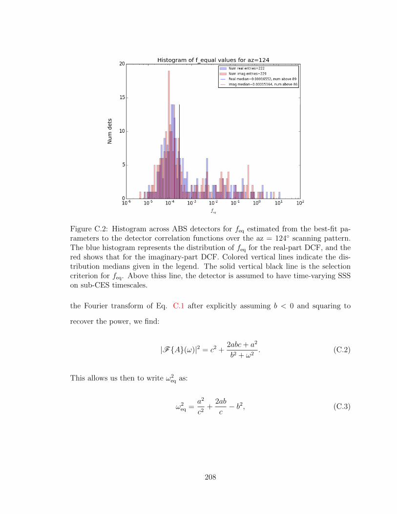
Numdets

Figure C.2: Histogram across ABS detectors for feq estimated from the best-fit pa-rameters to the detector correlation functions over the az = 124 scanning pattern.The blue histogram represents the distribution of feq for the real-part DCF, and thered shows that for the imaginary-part DCF. Colored vertical lines indicate the dis-tribution medians given in the legend. The solid vertical black line is the selectioncriterion for feq. Above thiss line, the detector is assumed to have time-varying SSSon sub-CES timescales.

the Fourier transform of Eq. C.1 after explicitly assuming b < 0 and squaring to

recover the power, we find:

|FA(ω)|2 = c2 +2abc+ a2

b2 + ω2. (C.2)

This allows us then to write ω2eq as:

ω2eq =

a2

c2+

2ab

c− b2, (C.3)

208

By calculating the quantity in Eq. C.3 for each detector’s DCF across all four

scanning patterns, we could determine if certain detectors could be considered to have

evidence for time-varying SSS on timescales shorter than a CES. We found it useful

to take the square root of ω2eq and divide by 2π, recovering an feq for each detector

for each scanning pattern. The histogram of feq for the az = 124 scanning pattern

is shown in Fig. C.2. We note that this analysis made use of all other data selection

criteria before the DCF were calculated, such that any additional criteria associated

with this analysis would not be affected by known problematic detectors. We find a

large (∼ 90) number of detectors with possible contamination on sub-CES timescales,

indicated here as frequencies greater than the vertical black line at feq > (1 hour)−1.

However, we found that fewer of those detectors had DCFs with possible sub-CES

contamination across multiple distributions. Eight totall distributions were defined:

the real and imaginary demodulated components across all four scanning patterns.

Our suggested criteria was to reject detectors that had feq > (1 hour)−1 for three

out of the possible eight distributions. This list of 55 detectors was studied in the

ABS systematic error tests [67] by running the ABS pipeline with and without these

detectors. The results indicate that their effect on the ABS results is negligible, and

any possible residual arising from including them is below the level of the statistical

noise in the BB power spectrum.

209

Bibliography

[1] Z. Ahmed, M. Amiri, S. J. Benton, J. J. Bock, R. Bowens-Rubin, I. Buder,E. Bullock, J. Connors, J. P. Filippini, J. A. Grayson, M. Halpern, G. C. Hilton,V. V. Hristov, H. Hui, K. D. Irwin, J. Kang, K. S. Karkare, E. Karpel, J. M.Kovac, C. L. Kuo, C. B. Netterfield, H. T. Nguyen, R. O’Brient, R. W. Og-burn, C. Pryke, C. D. Reintsema, S. Richter, K. L. Thompson, A. D. Turner,A. G. Vieregg, W. L. K. Wu, and K. W. Yoon. BICEP3: a 95GHz refractingtelescope for degree-scale CMB polarization. In Millimeter, Submillimeter, andFar-Infrared Detectors and Instrumentation for Astronomy VII, volume 9153 ofProc. SPIE, page 91531N, August 2014.

[2] J. E. Austermann, K. A. Aird, J. A. Beall, D. Becker, A. Bender, B. A. Benson,L. E. Bleem, J. Britton, J. E. Carlstrom, C. L. Chang, H. C. Chiang, H.-M.Cho, T. M. Crawford, A. T. Crites, A. Datesman, T. de Haan, M. A. Dobbs,E. M. George, N. W. Halverson, N. Harrington, J. W. Henning, G. C. Hilton,G. P. Holder, W. L. Holzapfel, S. Hoover, N. Huang, J. Hubmayr, K. D. Irwin,R. Keisler, J. Kennedy, L. Knox, A. T. Lee, E. Leitch, D. Li, M. Lueker, D. P.Marrone, J. J. McMahon, J. Mehl, S. S. Meyer, T. E. Montroy, T. Natoli, J. P.Nibarger, M. D. Niemack, V. Novosad, S. Padin, C. Pryke, C. L. Reichardt, J. E.Ruhl, B. R. Saliwanchik, J. T. Sayre, K. K. Schaffer, E. Shirokoff, A. A. Stark,K. Story, K. Vanderlinde, J. D. Vieira, G. Wang, R. Williamson, V. Yefremenko,K. W. Yoon, and O. Zahn. SPTpol: an instrument for CMB polarizationmeasurements with the South Pole Telescope. In Millimeter, Submillimeter, andFar-Infrared Detectors and Instrumentation for Astronomy VI, volume 8452 ofProc. SPIE, page 84521E, September 2012.

[3] N.A. Bahcall. Clusters and cosmology. Physics Reports, 333-334:233–244, 2000.

[4] E. Battaner and E. Florido. The Rotation Curve of Spiral Galaxies and itsCosmological Implications. Fundamentals of Cosmic Physics, 21:1–154, 2000.

[5] E. S. Battistelli, M. Amiri, B. Burger, M. Halpern, S. Knotek, M. Ellis, X. Gao,D. Kelly, M. Macintosh, K. Irwin, and C. Reintsema. Functional Description ofRead-out Electronics for Time-Domain Multiplexed Bolometers for Millimeterand Sub-millimeter Astronomy. Journal of Low Temperature Physics, 151:908–914, May 2008.

210

[6] BICEP2/Keck Collaboration, Planck Collaboration, and et al. Joint Anal-ysis of BICEP2/Keck Array and Planck Data. Physical Review Letters,114(10):101301, March 2015.

[7] D. Blas, J. Lesgourgues, and T. Tram. The Cosmic Linear Anisotropy SolvingSystem (CLASS). Part II: Approximation schemes. Journal of Cosmology andAstroparticle Physics, 7:034, July 2011.

[8] J. R. Bond, A. H. Jaffe, and L. Knox. Radical Compression of Cosmic MicrowaveBackground Data. Astrophysical Journal, 533:19–37, April 2000.

[9] S. Bryan, P. Ade, M. Amiri, S. Benton, R. Bihary, J. Bock, J. R. Bond, H. C.Chiang, C. Contaldi, B. Crill, O. Dore, B. Elder, J. Filippini, A. Fraisse,A. Gambrel, N. Gandilo, J. Gudmundsson, M. Hasselfield, M. Halpern,G. Hilton, W. Holmes, V. Hristov, K. Irwin, W. Jones, Z. Kermish, C. Lawrie,C. MacTavish, P. Mason, K. Megerian, L. Moncelsi, T. Montroy, T. Morford,J. Nagy, C. B. Netterfield, I. Padilla, A. S. Rahlin, C. Reintsema, D. C. Ri-ley, J. Ruhl, M. Runyan, B. Saliwanchik, J. Shariff, J. Soler, A. Trangsrud,C. Tucker, R. Tucker, A. Turner, S. Wen, D. Wiebe, and E. Young. A cryogenicrotation stage with a large clear aperture for the half-wave plates in the Spiderinstrument. Review of Scientific Instruments, 87(1):014501, January 2016.

[10] E. F. Bunn and B. Wandelt. Pure E and B polarization maps via Wienerfiltering. Phys. Rev. D, 96(4):043523, August 2017.

[11] K.H.S. Choi. Measuring the Cosmic Microwave Background from the AtacamaDesert. PhD thesis, Princeton University, 2018.

[12] S. K. Choi, J. Austermann, J. A. Beall, K. T. Crowley, R. Datta, S. M. Duff,P. A. Gallardo, S.-P. P. Ho, J. Hubmayr, B. J. Koopman, Y. Li, F. Nati, M. D.Niemack, L. A. Page, M. Salatino, S. M. Simon, S. T. Staggs, J. Stevens,J. Ullom, and E. J. Wollack. Characterization of the Mid-Frequency Arrays forAdvanced ACTPol. ArXiv e-prints, November 2017.

[13] K. P. Coughlin, J. J. McMahon, K. T. Crowley, B. J. Koopman, K. H. Miller,S. M. Simon, and E. J. Wollack. Pushing the Limits of Broadband and High-Frequency Metamaterial Silicon Antireflection Coatings. Journal of Low Tem-perature Physics, May 2018.

[14] K. T. Crowley, J. A. Austermann, S. K. Choi, S. M. Duff, P. A. Gallardo, S.-P. P.Ho, J. Hubmayr, B. J. Koopman, F. Nati, M. D. Niemack, M. Salatino, S. M.Simon, S. T. Staggs, J. R. Stevens, J. N. Ullom, E. M. Vavagiakis, and E. J.Wollack. Advanced ACTPol TES Device Parameters and Noise Performance inFielded Arrays. Journal of Low Temperature Physics.

[15] K. T. Crowley, S. K. Choi, J. Kuan, J. A. Austermann, J. A. Beall, R. Datta,S. M. Duff, P. A. Gallardo, M. Hasselfield, S. W. Henderson, S.-P. P. Ho, B. J.Koopman, M. D. Niemack, M. Salatino, S. M. Simon, S. T. Staggs, and E. J.

211

Wollack. Characterization of AlMn TES impedance, noise, and optical efficiencyin the first 150 mm multichroic array for Advanced ACTPol. In Millimeter,Submillimeter, and Far-Infrared Detectors and Instrumentation for AstronomyVIII, volume 9914 of Proc. SPIE, page 991431, July 2016.

[16] R. H. Cyburt, B. D. Fields, K. A. Olive, and T.-H. Yeh. Big bang nucleosynthe-sis: Present status. Reviews of Modern Physics, 88(1):015004, January 2016.

[17] R. Datta, J. Hubmayr, C. Munson, J. Austermann, J. Beall, D. Becker, H. M.Cho, N. Halverson, G. Hilton, K. Irwin, D. Li, J. McMahon, L. Newburgh,J. Nibarger, M. Niemack, B. Schmitt, H. Smith, S. Staggs, J. Van Lanen, andE. Wollack. Horn Coupled Multichroic Polarimeters for the Atacama Cosmol-ogy Telescope Polarization Experiment. Journal of Low Temperature Physics,176:670–676, September 2014.

[18] R. Datta, C. D. Munson, M. D. Niemack, J. J. McMahon, J. Britton, E. J.Wollack, J. Beall, M. J. Devlin, J. Fowler, P. Gallardo, J. Hubmayr, K. Ir-win, L. Newburgh, J. P. Nibarger, L. Page, M. A. Quijada, B. L. Schmitt,S. T. Staggs, R. Thornton, and L. Zhang. Large-aperture wide-bandwidthantireflection-coated silicon lenses for millimeter wavelengths. Applied Optics,52:8747, December 2013.

[19] P. A. J. de Korte, J. Beyer, S. Deiker, G. C. Hilton, K. D. Irwin, M. MacIntosh,S. W. Nam, C. D. Reintsema, L. R. Vale, and M. E. Huber. Time-divisionsuperconducting quantum interference device multiplexer for transition-edgesensors. Review of Scientific Instruments, 74:3807–3815, August 2003.

[20] W. de Sitter. Einstein’s theory of gravitation and its astronomical consequences.Third paper. Monthly Notices of the Royal Astronomical Society, 78:3–28,November 1917.

[21] DES Collaboration. Dark Energy Survey Year 1 Results: Cosmological Con-straints from Galaxy Clustering and Weak Lensing. ArXiv e-prints, August2017.

[22] J. Didier, A. D. Miller, D. Araujo, F. Aubin, C. Geach, B. Johnson, A. Ko-rotkov, K. Raach, B. Westbrook, K. Young, A. M. Aboobaker, P. Ade, C. Bac-cigalupi, C. Bao, D. Chapman, M. Dobbs, W. Grainger, S. Hanany, K. Helson,S. Hillbrand, J. Hubmayr, A. Jaffe, T. Jones, J. Klein, A. Lee, L. Levinson,M. Limon, K. MacDermid, M. Milligan, L. Moncelsi, E. Pascale, B. Reichborn-Kjennerud, I. Sagiv, C. Tucker, G. S. Tucker, and K. Zilic. Intensity-Coupled-Polarization in Instruments with a Continuously Rotating Half-Wave Plate.ArXiv e-prints, November 2017.

[23] W. B. Doriese, K. M. Morgan, D. A. Bennett, E. V. Denison, C. P. Fitzgerald,J. W. Fowler, J. D. Gard, J. P. Hays-Wehle, G. C. Hilton, K. D. Irwin, Y. I.Joe, J. A. B. Mates, G. C. O’Neil, C. D. Reintsema, N. O. Robbins, D. R.

212

Schmidt, D. S. Swetz, H. Tatsuno, L. R. Vale, and J. N. Ullom. Developmentsin Time-Division Multiplexing of X-ray Transition-Edge Sensors. Journal ofLow Temperature Physics, 184:389–395, July 2016.

[24] C. Dragone. Offset multireflector antennas with perfect pattern symmetry andpolarization discrimination. AT T Technical Journal, 57:2663–2684, September1978.

[25] S. M. Duff, J. Austermann, J. A. Beall, D. Becker, R. Datta, P. A. Gallardo,S. W. Henderson, G. C. Hilton, S. P. Ho, J. Hubmayr, B. J. Koopman, D. Li,J. McMahon, F. Nati, M. D. Niemack, C. G. Pappas, M. Salatino, B. L. Schmitt,S. M. Simon, S. T. Staggs, J. R. Stevens, J. Van Lanen, E. M. Vavagiakis, J. T.Ward, and E. J. Wollack. Advanced ACTPol Multichroic Polarimeter ArrayFabrication Process for 150 mm Wafers. Journal of Low Temperature Physics,184:634–641, August 2016.

[26] R. Dunner, M. Hasselfield, T. A. Marriage, J. Sievers, V. Acquaviva, G. E. Ad-dison, P. A. R. Ade, P. Aguirre, M. Amiri, J. W. Appel, L. F. Barrientos, E. S.Battistelli, J. R. Bond, B. Brown, B. Burger, E. Calabrese, J. Chervenak, S. Das,M. J. Devlin, S. R. Dicker, W. Bertrand Doriese, J. Dunkley, T. Essinger-Hileman, R. P. Fisher, M. B. Gralla, J. W. Fowler, A. Hajian, M. Halpern,C. Hernandez-Monteagudo, G. C. Hilton, M. Hilton, A. D. Hincks, R. Hlozek,K. M. Huffenberger, D. H. Hughes, J. P. Hughes, L. Infante, K. D. Irwin, J. Bap-tiste Juin, M. Kaul, J. Klein, A. Kosowsky, J. M. Lau, M. Limon, Y.-T. Lin,T. Louis, R. H. Lupton, D. Marsden, K. Martocci, P. Mauskopf, F. Menanteau,K. Moodley, H. Moseley, C. B. Netterfield, M. D. Niemack, M. R. Nolta, L. A.Page, L. Parker, B. Partridge, H. Quintana, B. Reid, N. Sehgal, B. D. Sherwin,D. N. Spergel, S. T. Staggs, D. S. Swetz, E. R. Switzer, R. Thornton, H. Trac,C. Tucker, R. Warne, G. Wilson, E. Wollack, and Y. Zhao. The AtacamaCosmology Telescope: Data Characterization and Mapmaking. AstrophysicalJournal, 762:10, January 2013.

[27] T. Essinger-Hileman. Probing Inflationary Cosmology: The Atacama B-ModeSearch (ABS). PhD thesis, Princeton University, 2011.

[28] T. Essinger-Hileman, J. W. Appel, J. A. Beal, H. M. Cho, J. Fowler, M. Halpern,M. Hasselfield, K. D. Irwin, T. A. Marriage, M. D. Niemack, L. Page, L. P.Parker, S. Pufu, S. T. Staggs, O. Stryzak, C. Visnjic, K. W. Yoon, and Y. Zhao.The Atacama B-Mode Search: CMB Polarimetry with Transition-Edge-SensorBolometers. In B. Young, B. Cabrera, and A. Miller, editors, American Instituteof Physics Conference Series, volume 1185 of American Institute of PhysicsConference Series, pages 494–497, December 2009.

[29] T. Essinger-Hileman, A. Kusaka, J. W. Appel, S. K. Choi, K. Crowley, S. P.Ho, N. Jarosik, L. A. Page, L. P. Parker, S. Raghunathan, S. M. Simon, S. T.

213

Staggs, and K. Visnjic. Systematic effects from an ambient-temperature, contin-uously rotating half-wave plate. Review of Scientific Instruments, 87(9):094503,September 2016.

[30] D. J. Fixsen. The Temperature of the Cosmic Microwave Background. Astro-physical Journal, 707:916–920, December 2009.

[31] D. J. Fixsen, G. Hinshaw, C. L. Bennett, and J. C. Mather. The Spectrumof the Cosmic Microwave Background Anisotropy from the Combined COBEFIRAS and DMR Observations. Astrophysical Journal, 486:623–628, September1997.

[32] D. J. Fixsen, A. Kogut, S. Levin, M. Limon, P. Lubin, P. Mirel, M. Seiffert,J. Singal, E. Wollack, T. Villela, and C. A. Wuensche. ARCADE 2 Measurementof the Absolute Sky Brightness at 3-90 GHz. Astrophysical Journal, 734:5, June2011.

[33] D. Foreman-Mackey, D. W. Hogg, D. Lang, and J. Goodman. emcee: TheMCMC Hammer. Publications of the Astronomical Society of the Pacific,125:306, March 2013.

[34] J. W. Fowler, M. D. Niemack, S. R. Dicker, A. M. Aboobaker, P. A. R. Ade, E. S.Battistelli, M. J. Devlin, R. P. Fisher, M. Halpern, P. C. Hargrave, A. D. Hincks,M. Kaul, J. Klein, J. M. Lau, M. Limon, T. A. Marriage, P. D. Mauskopf,L. Page, S. T. Staggs, D. S. Swetz, E. R. Switzer, R. J. Thornton, and C. E.Tucker. Optical design of the Atacama Cosmology Telescope and the MillimeterBolometric Array Camera. Applied Optics, 46:3444–3454, June 2007.

[35] G. W. Fraser. On the nature of the superconducting-to-normal transition intransition edge sensors. Nuclear Instruments and Methods in Physics ResearchA, 523:234–245, May 2004.

[36] A. Friedmann. On the Curvature of Space. General Relativity and Gravitation,31:1991, December 1999.

[37] M. Galeazzi and D. McCammon. Microcalorimeter and bolometer model. Jour-nal of Applied Physics, 93:4856–4869, April 2003.

[38] K. Ganga, B. Ratra, J. O. Gundersen, and N. Sugiyama. UCSB South Pole 1994Cosmic Microwave Background Anisotropy Measurement Constraints on Openand Flat-Λ Cold Dark Matter Cosmogonies. Astrophysical Journal, 484:7–30,July 1997.

[39] Fuchang Gao and Lixing Han. Implementing the nelder-mead simplex algo-rithm with adaptive parameters. Computational Optimization and Applications,51(1):259–277, Jan 2012.

214

[40] E. M. George, J. E. Austermann, J. A. Beall, D. Becker, B. A. Benson, L. E.Bleem, J. E. Carlstrom, C. L. Chang, H.-M. Cho, A. T. Crites, M. A. Dobbs,W. Everett, N. W. Halverson, J. W. Henning, G. C. Hilton, W. L. Holzapfel,J. Hubmayr, K. D. Irwin, D. Li, M. Lueker, J. J. McMahon, J. Mehl, J. Mont-gomery, T. Natoli, J. P. Nibarger, M. D. Niemack, V. Novosad, J. E. Ruhl, J. T.Sayre, E. Shirokoff, K. T. Story, G. Wang, V. Yefremenko, K. W. Yoon, andE. Young. A Study of Al-Mn Transition Edge Sensor Engineering for Stability.Journal of Low Temperature Physics, 176:383–391, August 2014.

[41] J. M. Gildemeister, A. T. Lee, and P. L. Richards. Model for excess noisein voltage-biased superconducting bolometers. Applied Optics, 40:6229–6235,December 2001.

[42] D. J. Goldie, M. D. Audley, D. M. Glowacka, V. N. Tsaneva, and S. Withing-ton. Thermal models and noise in transition edge sensors. Journal of AppliedPhysics, 105(7):074512–074512–7, April 2009.

[43] L. Gottardi, H. Akamatsu, M. P. Bruijn, R. den Hartog, J.-W. den Herder,B. Jackson, M. Kiviranta, J. van der Kuur, and H. van Weers. Development ofthe superconducting detectors and read-out for the X-IFU instrument on boardof the X-ray observatory Athena. Nuclear Instruments and Methods in PhysicsResearch A, 824:622–625, July 2016.

[44] E. Grace, J. Beall, J. R. Bond, H. M. Cho, R. Datta, M. J. Devlin, R. Dunner,A. E. Fox, P. Gallardo, M. Hasselfield, S. Henderson, G. C. Hilton, A. D. Hincks,R. Hlozek, J. Hubmayr, K. Irwin, J. Klein, B. Koopman, D. Li, M. Lungu,L. Newburgh, J. P. Nibarger, M. D. Niemack, L. Maurin, J. McMahon, S. Naess,L. A. Page, C. Pappas, B. L. Schmitt, J. Sievers, S. T. Staggs, R. Thornton,J. Van Lanen, and E. J. Wollack. ACTPol: on-sky performance and character-ization. In Millimeter, Submillimeter, and Far-Infrared Detectors and Instru-mentation for Astronomy VII, volume 9153 of Proc. SPIE, page 915310, August2014.

[45] E.A. Grace. Detector Characterization, Optimization, and Operation for ACT-Pol. PhD thesis, Princeton University, 2016.

[46] H. P. Gush, M. Halpern, and E. H. Wishnow. Rocket measurement of thecosmic-background-radiation mm-wave spectrum. Physical Review Letters,65:537–540, July 1990.

[47] A. H. Guth. Inflationary universe: A possible solution to the horizon andflatness problems. Phys. Rev. D, 23:347–356, January 1981.

[48] S. Hamimeche and A. Lewis. Likelihood analysis of CMB temperature andpolarization power spectra. Phys. Rev. D, 77(10):103013, May 2008.

[49] K. Harrington, T. Marriage, A. Ali, J. W. Appel, C. L. Bennett, F. Boone,M. Brewer, M. Chan, D. T. Chuss, F. Colazo, S. Dahal, K. Denis, R. Dunner,

215

J. Eimer, T. Essinger-Hileman, P. Fluxa, M. Halpern, G. Hilton, G. F. Hinshaw,J. Hubmayr, J. Iuliano, J. Karakla, J. McMahon, N. T. Miller, S. H. Mose-ley, G. Palma, L. Parker, M. Petroff, B. Pradenas, K. Rostem, M. Sagliocca,D. Valle, D. Watts, E. Wollack, Z. Xu, and L. Zeng. The Cosmology LargeAngular Scale Surveyor. In Millimeter, Submillimeter, and Far-Infrared Detec-tors and Instrumentation for Astronomy VIII, volume 9914 of Proc. SPIE, page99141K, July 2016.

[50] S. W. Henderson, J. R. Stevens, M. Amiri, J. Austermann, J. A. Beall,S. Chaudhuri, H.-M. Cho, S. K. Choi, N. F. Cothard, K. T. Crowley, S. M.Duff, C. P. Fitzgerald, P. A. Gallardo, M. Halpern, M. Hasselfield, G. Hilton,S.-P. P. Ho, J. Hubmayr, K. D. Irwin, B. J. Koopman, D. Li, Y. Li, J. McMa-hon, F. Nati, M. Niemack, C. D. Reintsema, M. Salatino, A. Schillaci, B. L.Schmitt, S. M. Simon, S. T. Staggs, E. M. Vavagiakis, and J. T. Ward. Read-out of two-kilopixel transition-edge sensor arrays for Advanced ACTPol. InMillimeter, Submillimeter, and Far-Infrared Detectors and Instrumentation forAstronomy VIII, volume 9914 of Proc. SPIE, page 99141G, July 2016.

[51] E. Hivon, K. M. Gorski, C. B. Netterfield, B. P. Crill, S. Prunet, and F. Hansen.MASTER of the Cosmic Microwave Background Anisotropy Power Spectrum:A Fast Method for Statistical Analysis of Large and Complex Cosmic MicrowaveBackground Data Sets. Astrophysical Journal, 567:2–17, March 2002.

[52] S. P. Ho, C. G. Pappas, J. Austermann, J. A. Beall, D. Becker, S. K. Choi,R. Datta, S. M. Duff, P. A. Gallardo, E. Grace, M. Hasselfield, S. W. Hender-son, G. C. Hilton, J. Hubmayr, B. J. Koopman, J. V. Lanen, D. Li, J. McMahon,F. Nati, M. D. Niemack, P. Niraula, M. Salatino, A. Schillaci, B. L. Schmitt,S. M. Simon, S. T. Staggs, J. R. Stevens, J. T. Ward, E. J. Wollack, and E. M.Vavagiakis. The First Multichroic Polarimeter Array on the Atacama Cosmol-ogy Telescope: Characterization and Performance. Journal of Low TemperaturePhysics, 184:559–567, August 2016.

[53] S.-P. P Ho, J. Austermann, J. A. Beall, S. K. Choi, N. F. Cothard, K. P.Coughlin, K. T. Crowley, R. D. Datta, S. M. Duff, M. D. Devlin, P. A. Gallardo,M. Hasselfield, S. W. Henderson, G. C. Hilton, J. Hubmayr, B. J. Koopman,Y. Li, J. J. McMahon, M. D. Niemack, M. Salatino, S. M. Simon, S. T. Staggs,J. N. Ullom, E. M. Vavagiakis, J. Ward, and E. J. Wollack. Highly uniform150 mm diameter multichroic polarimeter array deployed for CMB detection.volume 9914, pages 9914 – 9914 – 15, 2017.

[54] H. F. C. Hoevers, A. C. Bento, M. P. Bruijn, L. Gottardi, M. A. N. Korevaar,W. A. Mels, and P. A. J. de Korte. Thermal fluctuation noise in a voltagebiased superconducting transition edge thermometer. Applied Physics Letters,77:4422, December 2000.

[55] D. Huterer. Weak lensing, dark matter and dark energy. General Relativityand Gravitation, 42:2177–2195, September 2010.

216

[56] K. D. Irwin. An application of electrothermal feedback for high resolutioncryogenic particle detection. Applied Physics Letters, 66:1998–2000, April 1995.

[57] K.D. Irwin and G.C. Hilton. Cryogenic Particle Detection, chapter TransitionEdge Sensors, pages 63–150. Springer Verlag, Berlin, 2005.

[58] F. James and M. Roos. Minuit: A System for Function Minimization andAnalysis of the Parameter Errors and Correlations. Comput. Phys. Commun.,10:343–367, 1975.

[59] N. Jethava, J. N. Ullom, K. D. Irwin, W. B. Doriese, J. A. Beall, G. C. Hilton,L. R. Vale, and B. Zink. Dependence of Excess Noise on the Partial Deriva-tives of Resistance in Superconducting Transition Edge Sensors. In B. Young,B. Cabrera, and A. Miller, editors, American Institute of Physics ConferenceSeries, volume 1185 of American Institute of Physics Conference Series, pages31–33, December 2009.

[60] B. R. Johnson, J. Collins, M. E. Abroe, P. A. R. Ade, J. Bock, J. Borrill,A. Boscaleri, P. de Bernardis, S. Hanany, A. H. Jaffe, T. Jones, A. T. Lee,L. Levinson, T. Matsumura, B. Rabii, T. Renbarger, P. L. Richards, G. F.Smoot, R. Stompor, H. T. Tran, C. D. Winant, J. H. P. Wu, and J. Zuntz.MAXIPOL: Cosmic Microwave Background Polarimetry Using a Rotating Half-Wave Plate. Astrophysical Journal, 665:42–54, August 2007.

[61] M. Kamionkowski, A. Kosowsky, and A. Stebbins. Statistics of cosmic mi-crowave background polarization. Phys. Rev. D, 55:7368–7388, June 1997.

[62] R. L. Kelley, H. Akamatsu, P. Azzarello, T. Bialas, K. R. Boyce, G. V.Brown, E. Canavan, M. P. Chiao, E. Costantini, M. J. DiPirro, M. E. Eckart,Y. Ezoe, R. Fujimoto, D. Haas, J.-W. den Herder, A. Hoshino, K. Ishikawa,Y. Ishisaki, N. Iyomoto, C. A. Kilbourne, M. O. Kimball, S. Kitamoto, S. Kon-ami, S. Koyama, M. A. Leutenegger, D. McCammon, K. Mitsuda, I. Mitsuishi,H. Moseley, H. Murakami, M. Murakami, H. Noda, M. Ogawa, T. Ohashi,A. Okamoto, N. Ota, S. Paltani, F. S. Porter, K. Sakai, K. Sato, Y. Sato,M. Sawada, H. Seta, K. Shinozaki, P. J. Shirron, G. A. Sneiderman, H. Sugita,A. E. Szymkowiak, Y. Takei, T. Tamagawa, M. Tashiro, Y. Terada, M. Tsuji-moto, C. P. de Vries, S. Yamada, N. Y. Yamasaki, and Y. Yatsu. The Astro-Hhigh resolution soft x-ray spectrometer. In Space Telescopes and Instrumenta-tion 2016: Ultraviolet to Gamma Ray, volume 9905 of Proc. SPIE, page 99050V,July 2016.

[63] Lloyd Knox. Determination of inflationary observables by cosmic microwavebackground anisotropy experiments. Phys. Rev. D, 52:4307–4318, Oct 1995.

[64] A. Kogut, D. J. Fixsen, D. T. Chuss, J. Dotson, E. Dwek, M. Halpern, G. F.Hinshaw, S. M. Meyer, S. H. Moseley, M. D. Seiffert, D. N. Spergel, and E. J.Wollack. The Primordial Inflation Explorer (PIXIE): a nulling polarimeter for

217

cosmic microwave background observations. Journal of Cosmology and As-troparticle Physics, 7:025, July 2011.

[65] A. G. Kozorezov, A. A. Golubov, D. D. E. Martin, P. A. J. de Korte, M. A. Lin-deman, R. A. Hijmering, and J. K. Wigmore. Microscopic Model of a TransitionEdge Sensor as a Weak Link. IEEE Transactions on Applied Superconductivity,21:250–253, June 2011.

[66] C. L. Kuo, J. J. Bock, J. A. Bonetti, J. Brevik, G. Chattopadhyay, P. K.Day, S. Golwala, M. Kenyon, A. E. Lange, H. G. LeDuc, H. Nguyen, R. W.Ogburn, A. Orlando, A. Transgrud, A. Turner, G. Wang, and J. Zmuidzinas.Antenna-coupled TES bolometer arrays for CMB polarimetry. In Millimeterand Submillimeter Detectors and Instrumentation for Astronomy IV, volume7020 of Proc. SPIE, page 70201I, July 2008.

[67] A. Kusaka, J. Appel, T. Essinger-Hileman, J. A. Beall, L. E. Campusano, H.-M. Cho, S. K. Choi, K. Crowley, J. W. Fowler, P. Gallardo, M. Hasselfield,G. Hilton, S.-P. P. Ho, K. Irwin, N. Jarosik, M. D. Niemack, G. W. Nixon,M. Nolta, L. A. Page, Jr, G. A. Palma, L. Parker, S. Raghunathan, C. D.Reintsema, J. Sievers, S. M. Simon, S. T. Staggs, K. Visnjic, and K.-W. Yoon.Results from the Atacama B-mode Search (ABS) Experiment. ArXiv e-prints,January 2018.

[68] A. Kusaka, T. Essinger-Hileman, J. W. Appel, P. Gallardo, K. D. Irwin,N. Jarosik, M. R. Nolta, L. A. Page, L. P. Parker, S. Raghunathan, J. L.Sievers, S. M. Simon, S. T. Staggs, and K. Visnjic. Modulation of cosmic mi-crowave background polarization with a warm rapidly rotating half-wave plateon the Atacama B-Mode Search instrument. Review of Scientific Instruments,85(3):024501, March 2014.

[69] J. M. Lamarre. Photon noise in photometric instruments at far-infrared andsubmillimeter wavelengths. Applied Optics, 25:870–876, March 1986.

[70] S. P. Langley. The bolometer. Nature, 57:620–22, 1898.

[71] T. M. Lanting, H.-M. Cho, J. Clarke, W. L. Holzapfel, A. T. Lee, M. Lueker,P. L. Richards, M. A. Dobbs, H. Spieler, and A. Smith. Frequency-domainmultiplexed readout of transition-edge sensor arrays with a superconductingquantum interference device. Applied Physics Letters, 86(11):112511, March2005.

[72] J.M. Lau. CCAM: A Novel Millimeter-Wave Instrument Using a Close-PackedTES Bolometer Array. PhD thesis, Princeton University, 2007.

[73] A. T. Lee, P. L. Richards, S. W. Nam, B. Cabrera, and K. D. Irwin. A su-perconducting bolometer with strong electrothermal feedback. Applied PhysicsLetters, 69:1801–1803, September 1996.

218

[74] Georges Lemaıtre. Republication of: A homogeneous universe of constant massand increasing radius accounting for the radial velocity of extra-galactic nebulae.General Relativity and Gravitation, 45(8):1635–1646, Aug 2013.

[75] Antony Lewis, Anthony Challinor, and Anthony Lasenby. Efficient computationof CMB anisotropies in closed FRW models. Astrophys. J., 538:473–476, 2000.

[76] D. Li, J. E. Austermann, J. A. Beall, D. T. Becker, S. M. Duff, P. A. Gallardo,S. W. Henderson, G. C. Hilton, S.-P. Ho, J. Hubmayr, B. J. Koopman, J. J.McMahon, F. Nati, M. D. Niemack, C. G. Pappas, M. Salatino, B. L. Schmitt,S. M. Simon, S. T. Staggs, J. Van Lanen, J. T. Ward, and E. J. Wollack. AlMnTransition Edge Sensors for Advanced ACTPol. Journal of Low TemperaturePhysics, 184:66–73, July 2016.

[77] Y. Li, S. Choi, S.-P. Ho, K. T. Crowley, M. Salatino, S. M. Simon, S. T. Staggs,F. Nati, J. Ward, B. L. Schmitt, S. Henderson, B. J. Koopman, P. A. Gal-lardo, E. M. Vavagiakis, M. D. Niemack, J. McMahon, S. M. Duff, A. Schillaci,J. Hubmayr, G. C. Hilton, J. A. Beall, and E. J. Wollack. Assembly and integra-tion process of the first high density detector array for the Atacama CosmologyTelescope. In Millimeter, Submillimeter, and Far-Infrared Detectors and In-strumentation for Astronomy VIII, volume 9914 of Proc. SPIE, page 991435,July 2016.

[78] Andrei D. Linde. A New Inflationary Universe Scenario: A Possible Solution ofthe Horizon, Flatness, Homogeneity, Isotropy and Primordial Monopole Prob-lems. Phys. Lett., 108B:389–393, 1982.

[79] M. A. Lindeman, K. A. Barger, D. E. Brandl, S. G. Crowder, L. Rocks,and D. McCammon. Complex impedance measurements of calorimeters andbolometers: Correction for stray impedances. Review of Scientific Instruments,78(4):043105–043105, April 2007.

[80] T. Louis, E. Grace, M. Hasselfield, M. Lungu, L. Maurin, G. E. Addison,P. A. R. Ade, S. Aiola, R. Allison, M. Amiri, E. Angile, N. Battaglia, J. A.Beall, F. de Bernardis, J. R. Bond, J. Britton, E. Calabrese, H.-m. Cho,S. K. Choi, K. Coughlin, D. Crichton, K. Crowley, R. Datta, M. J. Devlin,S. R. Dicker, J. Dunkley, R. Dunner, S. Ferraro, A. E. Fox, P. Gallardo,M. Gralla, M. Halpern, S. Henderson, J. C. Hill, G. C. Hilton, M. Hilton, A. D.Hincks, R. Hlozek, S. P. P. Ho, Z. Huang, J. Hubmayr, K. M. Huffenberger,J. P. Hughes, L. Infante, K. Irwin, S. Muya Kasanda, J. Klein, B. Koopman,A. Kosowsky, D. Li, M. Madhavacheril, T. A. Marriage, J. McMahon, F. Menan-teau, K. Moodley, C. Munson, S. Naess, F. Nati, L. Newburgh, J. Nibarger,M. D. Niemack, M. R. Nolta, C. Nunez, L. A. Page, C. Pappas, B. Partridge,F. Rojas, E. Schaan, B. L. Schmitt, N. Sehgal, B. D. Sherwin, J. Sievers, S. Si-mon, D. N. Spergel, S. T. Staggs, E. R. Switzer, R. Thornton, H. Trac, J. Treu,C. Tucker, A. Van Engelen, J. T. Ward, and E. J. Wollack. The Atacama

219

Cosmology Telescope: two-season ACTPol spectra and parameters. Journal ofCosmology and Astroparticle Physics, 6:031, June 2017.

[81] I. J. Maasilta. Complex impedance, responsivity and noise of transition-edgesensors: Analytical solutions for two- and three-block thermal models. AIPAdvances, 2(4):042110, December 2012.

[82] A. Manzotti, K. T. Story, W. L. K. Wu, J. E. Austermann, J. A. Beall, A. N.Bender, B. A. Benson, L. E. Bleem, J. J. Bock, J. E. Carlstrom, C. L. Chang,H. C. Chiang, H.-M. Cho, R. Citron, A. Conley, T. M. Crawford, A. T. Crites,T. de Haan, M. A. Dobbs, S. Dodelson, W. Everett, J. Gallicchio, E. M. George,A. Gilbert, N. W. Halverson, N. Harrington, J. W. Henning, G. C. Hilton, G. P.Holder, W. L. Holzapfel, S. Hoover, Z. Hou, J. D. Hrubes, N. Huang, J. Hub-mayr, K. D. Irwin, R. Keisler, L. Knox, A. T. Lee, E. M. Leitch, D. Li, J. J.McMahon, S. S. Meyer, L. M. Mocanu, T. Natoli, J. P. Nibarger, V. Novosad,S. Padin, C. Pryke, C. L. Reichardt, J. E. Ruhl, B. R. Saliwanchik, J. T. Sayre,K. K. Schaffer, G. Smecher, A. A. Stark, K. Vanderlinde, J. D. Vieira, M. P.Viero, G. Wang, N. Whitehorn, V. Yefremenko, and M. Zemcov. CMB Polar-ization B-mode Delensing with SPTpol and Herschel. Astrophysical Journal,846:45, September 2017.

[83] T.M. Marriage. Detectors for the Atacama Cosmology Telescope. PhD thesis,Princeton University, 2006.

[84] J. C. Mather. Bolometer noise: nonequilibrium thoery. Applied Optics, 21:1125–1129, March 1982.

[85] D. McCammon. Cryogenic Particle Detection, chapter Semiconductor Ther-mistors, pages 35–62. Springer Verlag, Berlin, 2005.

[86] J. McMahon, J. W. Appel, J. E. Austermann, J. A. Beall, D. Becker, B. A.Benson, L. E. Bleem, J. Britton, C. L. Chang, J. E. Carlstrom, H. M. Cho,A. T. Crites, T. Essinger-Hileman, W. Everett, N. W. Halverson, J. W. Henning,G. C. Hilton, K. D. Irwin, J. Mehl, S. S. Meyer, S. Mossley, M. D. Niemack,L. P. Parker, S. M. Simon, S. T. Staggs, C. Visnjic, E. Wollack, K. U.-Yen,K. W. Yoon, and Y. Zhao. Planar Orthomode Transducers for Feedhorn-coupledTES Polarimeters. In B. Young, B. Cabrera, and A. Miller, editors, AmericanInstitute of Physics Conference Series, volume 1185 of American Institute ofPhysics Conference Series, pages 490–493, December 2009.

[87] Y. Mizugutch, M. Akagawa, and H. Yokoi. Offset Dual Reflector Antenna. ISAProceedings, pages 2–5, 1976.

[88] S. K. Næss and T. Louis. A fast map-making preconditioner for regular scanningpatterns. Journal of Cosmology and Astroparticle Physics, 8:045, August 2014.

220

[89] P. C. Nagler, K. T. Crowley, K. L. Denis, A. M. Devasia, D. J. Fixsen, A. J.Kogut, G. Manos, S. Porter, and T. R. Stevenson. Multimode bolometer de-velopment for the PIXIE instrument. In Millimeter, Submillimeter, and Far-Infrared Detectors and Instrumentation for Astronomy VIII, volume 9914 ofProc. SPIE, page 99141A, July 2016.

[90] P. C. Nagler, D. J. Fixsen, A. Kogut, and G. S. Tucker. Systematic Effects inPolarizing Fourier Transform Spectrometers for Cosmic Microwave BackgroundObservations. Astrophysical Journal Supplement, 221:21, November 2015.

[91] M.D. Niemack. Towards Dark Energy: Design, Development, and PreliminaryData from ACT. PhD thesis, Princeton University, 2008.

[92] R. O’Brient, J. Edwards, K. Arnold, G. Engargiola, W. Holzapfel, A. T. Lee,M. Myers, E. Quealy, G. Rebeiz, P. Richards, H. Spieler, and H. Tran. Sinuousantennas for cosmic microwave background polarimetry. In Millimeter andSubmillimeter Detectors and Instrumentation for Astronomy IV, volume 7020of Proc. SPIE, page 70201H, July 2008.

[93] S. Oguri, J. Choi, T. Damayanthi, M. Hattori, M. Hazumi, H. Ishitsuka, K. Ki-uchi, R. Koyano, H. Kutsuma, K. Lee, S. Mima, M. Minowa, M. Nagai, T. Na-gasaki, C. Otani, Y. Sekimoto, M. Semoto, J. Suzuki, T. Taino, O. Tajima,N. Tomita, E. Won, T. Uchida, and M. Yoshida. GroundBIRD: observations ofCMB polarization with fast scan modulation and MKIDs. In Ground-based andAirborne Telescopes VI, volume 9906 of Proc. SPIE, page 99063L, July 2016.

[94] T.E. Oliphant. A Guide to NumPy. Trelgol Publishing, 2006.

[95] S. Pancharatnam. Achromatic combinations of birefringent plates. Proceedingsof the Indian Academy of Sciences - Section A, 41(4):137–144, Apr 1955.

[96] C.G. Pappas. Assembly, Characterization, and Operation of Large-Scale TESDetector Arrays for ACTPol. PhD thesis, Princeton University, 2016.

[97] P. J. E. Peebles. Large-scale background temperature and mass fluctuationsdue to scale-invariant primeval perturbations. Astrophysical Journal Letters,263:L1–L5, December 1982.

[98] Planck Collaboration, P. A. R. Ade, N. Aghanim, M. Arnaud, M. Ashdown,J. Aumont, C. Baccigalupi, A. J. Banday, R. B. Barreiro, J. G. Bartlett, andet al. Planck 2015 results. XIII. Cosmological parameters. Astronomy & As-trophysics, 594:A13, September 2016.

[99] Planck Collaboration, P. A. R. Ade, N. Aghanim, M. Arnaud, M. Ashdown,J. Aumont, C. Baccigalupi, A. J. Banday, R. B. Barreiro, N. Bartolo, and et al.Planck 2015 results. XIV. Dark energy and modified gravity. Astronomy &Astrophysics, 594:A14, September 2016.

221

[100] Planck Collaboration and et al. Planck 2015 results. X. Diffuse componentseparation: Foreground maps. Astronomy & Astrophysics, 594:A10, September2016.

[101] D. Poletti, G. Fabbian, M. Le Jeune, J. Peloton, K. Arnold, C. Baccigalupi,D. Barron, S. Beckman, J. Borrill, S. Chapman, Y. Chinone, A. Cukierman,A. Ducout, T. Elleflot, J. Errard, S. Feeney, N. Goeckner-Wald, J. Groh,G. Hall, M. Hasegawa, M. Hazumi, C. Hill, L. Howe, Y. Inoue, A. H. Jaffe,O. Jeong, N. Katayama, B. Keating, R. Keskitalo, T. Kisner, A. Kusaka, A. T.Lee, D. Leon, E. Linder, L. Lowry, F. Matsuda, M. Navaroli, H. Paar, G. Puglisi,C. L. Reichardt, C. Ross, P. Siritanasak, N. Stebor, B. Steinbach, R. Stompor,A. Suzuki, O. Tajima, G. Teply, and N. Whitehorn. Making maps of cosmicmicrowave background polarization for B-mode studies: the POLARBEAR ex-ample. Astronomy & Astrophysics, 600:A60, April 2017.

[102] QUIET Collaboration, C. Bischoff, A. Brizius, I. Buder, Y. Chinone, K. Cleary,R. N. Dumoulin, A. Kusaka, R. Monsalve, S. K. Næss, L. B. Newburgh,R. Reeves, K. M. Smith, I. K. Wehus, J. A. Zuntz, J. T. L. Zwart, L. Bronf-man, R. Bustos, S. E. Church, C. Dickinson, H. K. Eriksen, P. G. Ferreira,T. Gaier, J. O. Gundersen, M. Hasegawa, M. Hazumi, K. M. Huffenberger,M. E. Jones, P. Kangaslahti, D. J. Kapner, C. R. Lawrence, M. Limon, J. May,J. J. McMahon, A. D. Miller, H. Nguyen, G. W. Nixon, T. J. Pearson, L. Pic-cirillo, S. J. E. Radford, A. C. S. Readhead, J. L. Richards, D. Samtleben,M. Seiffert, M. C. Shepherd, S. T. Staggs, O. Tajima, K. L. Thompson, K. Van-derlinde, R. Williamson, and B. Winstein. First Season QUIET Observations:Measurements of Cosmic Microwave Background Polarization Power Spectra at43 GHz in the Multipole Range 25 ≥ ` ≤ 475. Astrophysical Journal, 741:111,November 2011.

[103] A. C. S. Readhead, S. T. Myers, T. J. Pearson, J. L. Sievers, B. S. Mason, C. R.Contaldi, J. R. Bond, R. Bustos, P. Altamirano, C. Achermann, L. Bronfman,J. E. Carlstrom, J. K. Cartwright, S. Casassus, C. Dickinson, W. L. Holzapfel,J. M. Kovac, E. M. Leitch, J. May, S. Padin, D. Pogosyan, M. Pospieszalski,C. Pryke, R. Reeves, M. C. Shepherd, and S. Torres. Polarization Observationswith the Cosmic Background Imager. Science, 306:836–844, October 2004.

[104] C. D. Reintsema, J. Beyer, S. W. Nam, S. Deiker, G. C. Hilton, K. Irwin, J. Mar-tinis, J. Ullom, L. R. Vale, and M. Macintosh. Prototype system for supercon-ducting quantum interference device multiplexing of large-format transition-edge sensor arrays. Review of Scientific Instruments, 74:4500–4508, October2003.

[105] P. L. Richards. Bolometers for infrared and millimeter waves. Journal of AppliedPhysics, 76:1–24, July 1994.

[106] H. P. Robertson. Kinematics and World-Structure. Astrophysical Journal,82:284, November 1935.

222

[107] M. C. Runyan, P. A. R. Ade, M. Amiri, S. Benton, R. Bihary, J. J. Bock, J. R.Bond, J. A. Bonetti, S. A. Bryan, H. C. Chiang, C. R. Contaldi, B. P. Crill,O. Dore, D. O’Dea, M. Farhang, J. P. Filippini, L. Fissel, N. Gandilo, S. R. Gol-wala, J. E. Gudmundsson, M. Hasselfield, M. Halpern, G. Hilton, W. Holmes,V. V. Hristov, K. D. Irwin, W. C. Jones, C. L. Kuo, C. J. MacTavish, P. V.Mason, T. A. Morford, T. E. Montroy, C. B. Netterfield, A. S. Rahlin, C. D.Reintsema, J. E. Ruhl, M. A. Schenker, J. Shariff, J. D. Soler, A. Trangsrud,R. S. Tucker, C. E. Tucker, and A. Turner. Design and performance of the SPI-DER instrument. In Millimeter, Submillimeter, and Far-Infrared Detectors andInstrumentation for Astronomy V, volume 7741 of Proc. SPIE, page 77411O,July 2010.

[108] J.E. Sadleir. Superconducting transition-edge sensor physics. PhD thesis, Uni-versity of Illinois at Urbana-Champaign, 2016.

[109] D. M. Scolnic, D. O. Jones, A. Rest, Y. C. Pan, R. Chornock, R. J. Foley,M. E. Huber, R. Kessler, G. Narayan, A. G. Riess, S. Rodney, E. Berger, D. J.Brout, P. J. Challis, M. Drout, D. Finkbeiner, R. Lunnan, R. P. Kirshner,N. E. Sanders, E. Schlafly, S. Smartt, C. W. Stubbs, J. Tonry, W. M. Wood-Vasey, M. Foley, J. Hand, E. Johnson, W. S. Burgett, K. C. Chambers, P. W.Draper, K. W. Hodapp, N. Kaiser, R. P. Kudritzki, E. A. Magnier, N. Metcalfe,F. Bresolin, E. Gall, R. Kotak, M. McCrum, and K. W. Smith. The CompleteLight-curve Sample of Spectroscopically Confirmed SNe Ia from Pan-STARRS1and Cosmological Constraints from the Combined Pantheon Sample. Astrophys-ical Journal, 859:101, June 2018.

[110] G. M. Seidel and I. S. Beloborodov. Intrinsic excess noise in a transition edgesensor. Nuclear Instruments and Methods in Physics Research A, 520:325–328,March 2004.

[111] U. Seljak and M. Zaldarriaga. Signature of Gravity Waves in the Polarizationof the Microwave Background. Physical Review Letters, 78:2054–2057, March1997.

[112] Uros Seljak and Matias Zaldarriaga. A line of sight approach to cosmic mi-crowave background anisotropies. Astrophys. J., 469:437–444, 1996.

[113] S. M. Simon, J. W. Appel, L. E. Campusano, S. K. Choi, K. T. Crowley,T. Essinger-Hileman, P. Gallardo, S. P. Ho, A. Kusaka, F. Nati, G. A. Palma,L. A. Page, S. Raghunathan, and S. T. Staggs. Characterizing Atacama B-modeSearch Detectors with a Half-Wave Plate. Journal of Low Temperature Physics,184:534–539, August 2016.

[114] S. M. Simon, J. W. Appel, H. M. Cho, T. Essinger-Hileman, K. D. Irwin,A. Kusaka, M. D. Niemack, M. R. Nolta, L. A. Page, L. P. Parker, S. Raghu-nathan, J. L. Sievers, S. T. Staggs, and K. Visnjic. In Situ Time Constant andOptical Efficiency Measurements of TRUCE Pixels in the Atacama B-ModeSearch. Journal of Low Temperature Physics, 176:712–718, September 2014.

223

[115] S. M. Simon, J. Austermann, J. A. Beall, S. K. Choi, K. P. Coughlin, S. M.Duff, P. A. Gallardo, S. W. Henderson, F. B. Hills, S.-P. P. Ho, J. Hubmayr,A. Josaitis, B. J. Koopman, J. J. McMahon, F. Nati, L. Newburgh, M. D.Niemack, M. Salatino, A. Schillaci, B. L. Schmitt, S. T. Staggs, E. M. Vava-giakis, J. Ward, and E. J. Wollack. The design and characterization of widebandspline-profiled feedhorns for Advanced ACTPol. In Millimeter, Submillimeter,and Far-Infrared Detectors and Instrumentation for Astronomy VIII, volume9914 of Proc. SPIE, page 991416, July 2016.

[116] K. M. Smith. Pseudo-C estimators which do not mix E and B modes. Phys.Rev. D, 74(8):083002, October 2006.

[117] Y. Sofue and V. Rubin. Rotation Curves of Spiral Galaxies. Annual Review ofAstronomy and Astrophysics, 39:137–174, 2001.

[118] P. J. Steinhardt and Michael S. Turner. A Prescription for Successful NewInflation. Phys. Rev. D, 29:2162–2171, 1984.

[119] D. S. Swetz, P. A. R. Ade, M. Amiri, J. W. Appel, E. S. Battistelli, B. Burger,J. Chervenak, M. J. Devlin, S. R. Dicker, W. B. Doriese, R. Dunner, T. Essinger-Hileman, R. P. Fisher, J. W. Fowler, M. Halpern, M. Hasselfield, G. C. Hilton,A. D. Hincks, K. D. Irwin, N. Jarosik, M. Kaul, J. Klein, J. M. Lau, M. Limon,T. A. Marriage, D. Marsden, K. Martocci, P. Mauskopf, H. Moseley, C. B.Netterfield, M. D. Niemack, M. R. Nolta, L. A. Page, L. Parker, S. T. Staggs,O. Stryzak, E. R. Switzer, R. Thornton, C. Tucker, E. Wollack, and Y. Zhao.Overview of the Atacama Cosmology Telescope: Receiver, Instrumentation, andTelescope Systems. Astrophysical Journal Supplement, 194:41, June 2011.

[120] Satoru Takakura, Mario Aguilar, Yoshiki Akiba, Kam Arnold, Carlo Bacci-galupi, Darcy Barron, Shawn Beckman, David Boettger, Julian Borrill, ScottChapman, Yuji Chinone, Ari Cukierman, Anne Ducout, Tucker Elleflot, JosquinErrard, Giulio Fabbian, Takuro Fujino, Nicholas Galitzki, Neil Goeckner-Wald,Nils W. Halverson, Masaya Hasegawa, Kaori Hattori, Masashi Hazumi, CharlesHill, Logan Howe, Yuki Inoue, Andrew H. Jaffe, Oliver Jeong, Daisuke Kaneko,Nobuhiko Katayama, Brian Keating, Reijo Keskitalo, Theodore Kisner, Nico-letta Krachmalnicoff, Akito Kusaka, Adrian T. Lee, David Leon, LindsayLowry, Frederick Matsuda, Tomotake Matsumura, Martin Navaroli, HarukiNishino, Hans Paar, Julien Peloton, Davide Poletti, Giuseppe Puglisi, Chris-tian L. Reichardt, Colin Ross, Praween Siritanasak, Aritoki Suzuki, OsamuTajima, Sayuri Takatori, and Grant Teply. Performance of a continuously ro-tating half-wave plate on the POLARBEAR telescope. Journal of Cosmologyand Astro-Particle Physics, 2017:008, May 2017.

[121] The EBEX Collaboration, A. M. Aboobaker, P. Ade, D. Araujo, F. Aubin,C. Baccigalupi, C. Bao, D. Chapman, J. Didier, M. Dobbs, C. Geach,W. Grainger, S. Hanany, K. Helson, S. Hillbrand, J. Hubmayr, A. Jaffe,B. Johnson, T. Jones, J. Klein, A. Korotkov, A. Lee, L. Levinson, M. Limon,

224

K. MacDermid, T. Matsumura, A. D. Miller, M. Milligan, K. Raach,B. Reichborn-Kjennerud, I. Sagiv, G. Savini, L. Spencer, C. Tucker, G. S.Tucker, B. Westbrook, K. Young, and K. Zilic. The EBEX Balloon BorneExperiment - Optics, Receiver, and Polarimetry. ArXiv e-prints, March 2017.

[122] R. J. Thornton, P. A. R. Ade, S. Aiola, F. E. Angile, M. Amiri, J. A. Beall,D. T. Becker, H.-M. Cho, S. K. Choi, P. Corlies, K. P. Coughlin, R. Datta,M. J. Devlin, S. R. Dicker, R. Dunner, J. W. Fowler, A. E. Fox, P. A. Gallardo,J. Gao, E. Grace, M. Halpern, M. Hasselfield, S. W. Henderson, G. C. Hilton,A. D. Hincks, S. P. Ho, J. Hubmayr, K. D. Irwin, J. Klein, B. Koopman, D. Li,T. Louis, M. Lungu, L. Maurin, J. McMahon, C. D. Munson, S. Naess, F. Nati,L. Newburgh, J. Nibarger, M. D. Niemack, P. Niraula, M. R. Nolta, L. A.Page, C. G. Pappas, A. Schillaci, B. L. Schmitt, N. Sehgal, J. L. Sievers, S. M.Simon, S. T. Staggs, C. Tucker, M. Uehara, J. van Lanen, J. T. Ward, andE. J. Wollack. The Atacama Cosmology Telescope: The Polarization-sensitiveACTPol Instrument. The Astrophysical Journal Supplement Series, 227:21,December 2016.

[123] C. E. Tucker and P. A. R. Ade. Thermal filtering for large aperture cryogenicdetector arrays. In Society of Photo-Optical Instrumentation Engineers (SPIE)Conference Series, volume 6275 of Proc. SPIE, page 62750T, June 2006.

[124] J. N. Ullom, W. B. Doriese, G. C. Hilton, J. A. Beall, S. Deiker, K. D. Ir-win, C. D. Reintsema, L. R. Vale, and Y. Xu. Suppression of excess noise inTransition-Edge Sensors using magnetic field and geometry. Nuclear Instru-ments and Methods in Physics Research A, 520:333–335, March 2004.

[125] K. Visnjic. Data Characteristics and Preliminary Results from the AtacamaB-Mode Search (ABS). PhD thesis, Princeton University, 2013.

[126] A. G. Walker. On Milne’s Theory of World-Structure. Proceedings of the LondonMathematical Society, (Series 2) volume 42, p. 90-127, 42:90–127, 1937.

[127] J. T. Ward, J. Austermann, J. A. Beall, S. K. Choi, K. T. Crowley, M. J. Devlin,S. M. Duff, P. A. Gallardo, S. W. Henderson, S.-P. P. Ho, G. Hilton, J. Hubmayr,N. Khavari, J. Klein, B. J. Koopman, D. Li, J. McMahon, G. Mumby, F. Nati,M. D. Niemack, L. A. Page, M. Salatino, A. Schillaci, B. L. Schmitt, S. M.Simon, S. T. Staggs, R. Thornton, J. N. Ullom, E. M. Vavagiakis, and E. J.Wollack. Mechanical designs and development of TES bolometer detector arraysfor the Advanced ACTPol experiment. In Millimeter, Submillimeter, and Far-Infrared Detectors and Instrumentation for Astronomy VIII, volume 9914 ofProc. SPIE, page 991437, July 2016.

[128] J.T. Ward. Development of Technologies for the Atacama Cosmology Telescopeand Next Generation Cosmic Microwave Background Instruments. PhD thesis,University of Pennsylvania, 2018.

[129] S. Weinberg. Cosmology. Oxford University Press, 2008.

225

[130] P. Welch. The use of fast fourier transform for the estimation of power spectra:A method based on time averaging over short, modified periodograms. IEEETransactions on Audio and Electroacoustics, 15(2):70–73, Jun 1967.

[131] K. W. Yoon, J. W. Appel, J. E. Austermann, J. A. Beall, D. Becker, B. A. Ben-son, L. E. Bleem, J. Britton, C. L. Chang, J. E. Carlstrom, H.-M. Cho, A. T.Crites, T. Essinger-Hileman, W. Everett, N. W. Halverson, J. W. Henning,G. C. Hilton, K. D. Irwin, J. McMahon, J. Mehl, S. S. Meyer, S. Moseley, M. D.Niemack, L. P. Parker, S. M. Simon, S. T. Staggs, K. U-yen, C. Visnjic, E. Wol-lack, and Y. Zhao. Feedhorn-Coupled TES Polarimeters for Next-GenerationCMB Instruments. In B. Young, B. Cabrera, and A. Miller, editors, AmericanInstitute of Physics Conference Series, volume 1185 of American Institute ofPhysics Conference Series, pages 515–518, December 2009.

[132] H. Zappe. Josephson quantum interference computer devices. IEEE Transac-tions on Magnetics, 13:41–47, January 1977.

[133] Y. Zhao. Characterization of Transition-Edge Sensors for the MillimeterBolometer Array Camera on the Atacama Cosmology Telescope. PhD thesis,Princeton University, 2010.

[134] J. Zmuidzinas. Thermal noise and correlations in photon detection. AppliedOptics, 42:4989–5008, September 2003.

226