Application of multispectral LiDAR to automated virtual outcrop geology

ISPRS Journal of Photogrammetry and Remote Sensing 88 (2014) 147–155

Contents lists available at ScienceDirect

ISPRS Journal of Photogrammetry and Remote Sensing

journal homepage: www.elsevier .com/ locate/ isprs jprs

Application of multispectral LiDAR to automated virtual outcrop geology

0924-2716/$ - see front matter � 2013 International Society for Photogrammetry and Remote Sensing, Inc. (ISPRS) Published by Elsevier B.V. All rights reserved.http://dx.doi.org/10.1016/j.isprsjprs.2013.12.004

⇑ Corresponding author. Tel.: +1 832 842 8881.E-mail address: [email protected] (P. Hartzell).

Preston Hartzell a,⇑, Craig Glennie a, Kivanc Biber b, Shuhab Khan b

a Department of Civil and Environmental Engineering, University of Houston, Houston, TX 77204, United Statesb Department of Earth and Atmospheric Sciences, University of Houston, Houston, TX 77204, United States

a r t i c l e i n f o a b s t r a c t

Article history:Received 1 August 2013Received in revised form 13 December 2013Accepted 16 December 2013

Keywords:Laser scanningLIDARMultispectralCalibrationRadiometricClassification

Terrestrial laser scanning (TLS) is a valuable tool for creating virtual 3D models of geological outcrops toenable enhanced modeling and analysis of geologic strata. Application of TLS data is typically limited tothe geometric point cloud that is used to create the 3D structure of the outcrop model. Digital photogra-phy can then be draped onto the 3D model, allowing visual identification and manual spatial delineationof different rock layers. Automation of the rock type identification and delineation is desirable, and recentwork has investigated the use of terrestrial hyperspectral photography for this purpose. However, passivephotography, whether visible or hyperspectral, presents several complexities, including accurate spatialregistration with the TLS point cloud data, reliance on sunlight for illumination, and radiometric calibra-tion to properly extract spectral signatures of the different rock types. As an active remote sensingmethod, a radiometrically calibrated TLS system offers the potential to directly provide spectral informa-tion for each recorded 3D point, independent of solar illumination. Therefore, the practical application ofthree radiometrically calibrated TLS systems with differing laser wavelengths, thereby achieving a mul-tispectral dataset in conjunction with 3D point cloud data, is investigated using commercially availablehardware and software. The radiometric calibration of the TLS intensity values is investigated and theclassification performance of the multispectral TLS intensity and calibrated reflectance datasets evaluatedand compared to classification performed with passive visible wavelength imagery. Results indicate thatrock types can be successfully identified with radiometrically calibrated multispectral TLS data, withenhanced classification performance when fused with passive visible imagery.� 2013 International Society for Photogrammetry and Remote Sensing, Inc. (ISPRS) Published by Elsevier

B.V. All rights reserved.

1. Introduction

In the past decade, airborne and terrestrial LiDAR (Light Detec-tion and Ranging), also referred to as laser scanning, has gainedwidespread acceptance and use in measuring and documenting3D topographic conditions. Laser scanning is used extensively inthe private sector for site as-built conditions ranging from complexpiping networks in industrial environments to basic civil engineer-ing tasks such as measurements for volume computations.Academic and research organizations have also adopted laser scan-ning for a wide variety of applications. Examples include seismicevent change detection (Oskin et al., 2012), archeological and pale-ontological study and preservation (Bates et al., 2008; Chase et al.,2011), and forest biomass computations (Lefsky et al., 2002; Limet al., 2003). The use of high resolution terrestrial laser scanners(TLS) is also well suited for the field of virtual outcrop geology, inwhich high resolution 3D models of exposed outcrops and cliff sec-tions are analyzed to infer subsurface geology. These investigations

are especially prevalent in hydrocarbon reservoir studies whereexposed rock layers are used to create 3D models of subsurfacerock layers which serve as analogues for understanding fluid flowand storage in similarly deposited reservoirs around the world(Buckley et al., 2010; Pringle et al., 2006).

While laser scanning is very adept at capturing precise 3D mod-els of surface geometry, the highly accurate point clouds generatedby LiDAR systems contain little or no information regarding themineral or chemical composition of the reflecting surfaces. Amajority of LiDAR systems collect the strength of the return energy(often referred to as intensity), but this measure is normally un-calibrated and provided at a scale and resolution which varies be-tween instruments. Thus, it is an effective tool for characterizingrelative reflectance between materials, but does not directlyprovide a measure of absolute reflectance without calibration(Franceschi et al., 2009; Hartzell et al., 2013; Kaasalainen et al.,2011; Pfennigbauer and Ullrich, 2010). Even when radiometricallycalibrated to determine absolute reflectance, the LiDAR source isnominally from a single wavelength, which may be of limited valuewhen attempting to automatically determine material reflectionproperties.

148 P. Hartzell et al. / ISPRS Journal of Photogrammetry and Remote Sensing 88 (2014) 147–155

To augment the value of laser scanning products, passive digitalimagery is sometimes fused with the 3D point cloud data, such asin geological applications where very dense 3D point clouds havebeen draped with high resolution photography to create detailedvirtual rock outcrop representations for enhanced interpretationand analysis (Buckley et al., 2010; Enge et al., 2007; Kurtzmanet al., 2009; McCaffrey et al., 2005; Wilson et al., 2009). The colorinformation (RGB) can then be utilized in combination with the la-ser intensity to extract object properties as in Lichti (2005). Morerecent work has investigated combining target reflectance proper-ties from high dimensionality passive multispectral or hyperspec-tral imagery with 3D scan data for enhanced target materialidentification (Kurz et al., 2011). While this data fusion is promis-ing because it combines the accurate 3D models from the pointcloud with the high spectral content of the hyperspectral imagery,there are still a few remaining issues with the optimal combinationof these datasets. First, the viewpoint and field of view of thehyperspectral camera and laser scanner are not coincident, andtherefore a mapping or draping of the hyperspectral imagery ontothe laser point cloud is required, which, if not carefully calibrated,can produce misalignment between the spatial and spectral data-sets. Additionally, the hyperspectral datasets are passive, andtherefore rely upon the sun for illumination. As a result, calibrationfor the amount of radiant sunlight incident on the object of interestis required. This calibration for downwelling irradiance is normallyundertaken by either placing objects of known reflectance withinthe image scene, or taking in situ measurements of reflectance ofobjects within the scene in order to calibrate the hyperspectralimagery (Bachmann et al., 2010).

The requirements of passive hyperspectral imagery for illumi-nation by sunlight and in situ calibration can cause significantproblems for its use for virtual outcrop geology, where it is desir-able to determine both the structure and material properties ofan exposed rock outcrop (Buckley et al., 2010). Many rock outcropsof interest are inaccessible for in situ calibrations, and the verticalnature of a majority of rock outcrops do not provide ideal condi-tions for uniform illumination by sunlight across the entire out-crop, especially in the case of overhanging walls, or those with anorthern exposure (in the northern hemisphere). With these con-siderations in mind, an ideal tool for virtual outcrop geology wouldbe a hyperspectral laser scanner that afforded the ability to use ac-tive illumination to simultaneously spectrally and spatially samplea rock outcrop at high resolution. Recent advances in pulsed lasers,nonlinear fiber optics (Dudley et al., 2006) and avalanche photodiodes (APDs) have made the combination of active illuminationand ranging and hyperspectral channel reflectance a possibilitywith the creation of broadband directional light sources and small,high resolution photo detectors. However, currently availablebroadband light sources do not have the output power availableto allow ranging at longer distances. A number of organizationshave demonstrated hyperspectral lasers (Alexander et al., 2013;Hakala et al., 2012; Suomalainen et al., 2011) and multispectralsystems (Powers and Davis, 2012; Tan et al., 2005; Wallace et al.,2005; Woodhouse et al., 2011), although most are confined to alaboratory setting. Multiple laser wavelengths have also been usedfor distinguishing targets by their spectral properties in differentialabsorption LiDAR for atmospheric studies for several decades (Bro-well et al., 1998) as well as in bathymetric LiDAR where a nearinfrared laser is used to detect the water surface and a green laserto detect the benthic layer (Wang and Philpot, 2007).

While the concept of using radiometrically calibrated multi-spectral LiDAR observations for target identification is not new,only a few research organizations are using the method, often withone-of-a-kind experimental systems. Therefore, it would be advan-tageous to investigate whether multispectral LiDAR as a tool forvirtual outcrop geology can be accomplished using existing

commercial hardware. The objective of this study is to demon-strate a practical method of using terrestrial multispectral LiDARobservations, acquired and processed with readily available com-mercial hardware and software packages, for classification of lith-ological units in a rock outcrop. The performance of an empiricalradiometric calibration is investigated, and classification accura-cies achieved from raw and radiometrically calibrated TLS intensi-ties are compared to those obtained from passive visiblewavelength imagery, which is often collected in conjunction withTLS data.

2. Background

In addition to the 3D points computed from the combinedranges and angles measured by LiDAR systems, dimensionlessintensity values related to the amount of energy reflected by a tar-get from the incident laser energy are also reported. For a pulsedLiDAR system, assuming a collimated beam and diffusely reflectingsurface, the expected amount of reflected photoelectron energy de-tected can be expressed using a form of the LiDAR link equation(Cossio et al., 2010):

gs ¼ gqgrEt

hm� qk cos a

Ar

pR2 � ½expð�be;kRÞ�2 ð1Þ

where gq is the detector quantum efficiency, gr is the receiver opti-cal efficiency, Et is the transmitted energy of the pulse in joules, h isPlanck’s constant, m is the laser frequency in Hz, qk is the wave-length dependent surface reflectance, a is the angle of incidenceon the surface, Ar is the collection area of the receiver aperture,be,k is the atmospheric extinction coefficient, and R is the range tothe target surface. For a given laser system

C ¼ gqgrEt

hm� Ar

p� CONSTANT ð2Þ

and therefore the return energy is given by:

gs ¼ C � qk cos aR2 � ½expð�be;kRÞ�2 ð3Þ

This implies that for a given laser system the variation in returnsignal strength is directly influenced by atmospheric effects, rangeto target, surface reflectance, and target incidence angle of theincoming radiation. If we assume that the atmosphere is stableover the time period of a survey, and if the intensity values re-ported by a LiDAR system can be normalized for range and inci-dence angle, the normalized intensity should be correlated withthe reflectance properties of the targeted surface. In practice, how-ever, the relationship between normalized intensity and surfacereflectance is complicated by photocurrent amplification methodsemployed by LIDAR system manufacturers (Kaasalainen et al.,2011). This difficulty can be bypassed by using empirical methodsto radiometrically calibrate a LiDAR system where targets withknown reflectance properties are used to correlate LiDAR intensityto reflectance (Kaasalainen et al., 2009, 2005).

3. Methodology

3.1. Instrumentation

Three TLS systems with unique laser wavelengths were selectedfor use in the study: a Riegl VZ-400, a Leica HDS3000 and a Zol-ler + Fröhlich (Z + F) IMAGER 5003. Table 1 contains an overviewof the specifications for each laser system. For this study, the mostimportant characteristic is that each TLS utilizes a laser at a differ-ent wavelength: 0.532 lm (visible green) for the Leica, 0.785 lm(red) for the Z + F, and 1.550 lm (near infrared) for the Riegl.

Table 1Specifications of the three TLS systems used in this study.

Property Leica HDS3000 Z + F IMAGER 5003 Riegl VZ-400

Laser wavelength 0.532 lm 0.785 lm 1.550 lmMeasurement mode Time of flight Continuous wave Time of flightBeam divergence or spot size <6 mm at 50 m 0.22 mrad 0.3 mradMaximum range 300 m 53.5 m 400 mPulse repetition frequency 4 kHz 500 kHz 300 kHzRange accuracy 6 mm <5 mm 5 mm at 100 mHorizontal field of view 360� 360� 360�Vertical field of view 270� 310� 100�

P. Hartzell et al. / ISPRS Journal of Photogrammetry and Remote Sensing 88 (2014) 147–155 149

3.2. Radiometric calibration

If reported TLS intensity values scale linearly with respect to re-ceived power, then a series of observations to a near 100% reflectiv-ity standard at normal incidence, encompassing the expectedranges of future observations, is sufficient to accommodate theinfluence of range by computation of relative reflectance values.However, prior work by Hartzell et al. (2013) and Kaasalainenet al. (2011, 2009) illustrates that intensity linearity cannot be as-sumed for many TLS systems, particularly at near ranges. There-fore, reported intensity values cannot be assumed to beproportional to target reflectance. However, by storing intensityvalues observed from multiple targets of low and high reflectancevalues, an empirical model of the nonlinear relationship betweentarget reflectance and reported TLS intensity can be created. Sincerange must also be accommodated, intensity values from multiplereflectance standards must be stored for a series of ranges encom-passing expected future TLS observations.

Therefore, observations to Labsphere Spectralon (Labsphere,2013) panels of multiple reflectance values (99%, 50% and 20%nominal reflectance) were collected with each TLS at ranges from5 to 70 m in approximate 10 m increments. Reflectance values ofthe Spectralon panels at the laser wavelength of each TLS systemwere taken from the calibration report accompanying each panelthat lists the measured, rather than nominal, hemispherical reflec-tance for wavelengths from 0.25 to 2.5 lm. To accommodate mate-rials with very low reflectance values, an approximate 3%reflectance panel, created using flat black spray paint on cardboardwith a relative reflectance value measured with a spectroradiome-ter, was also observed. The set of range and average intensityobservations for each calibrated reflectance target was stored ina look up table (LUT) for each TLS. Note that each LUT contains datain three dimensions: TLS intensity, target range, and target reflec-tance. For any subsequent range and intensity measured by one ofthe TLS systems, a reflectance value can be estimated from theappropriate LUT via bi-linear interpolation. The MATLAB (MatrixLaboratory) computing language was used for all computations.This method accommodates nonlinear TLS intensity values as wellas the influence of range. Note that this method assumes a perpen-dicular incidence angle, so any corrections for incidence anglemust be performed separately.

It must be noted that neither the hemispherical reflectance val-ues reported by the Labsphere Spectralon calibration sheets northe relative reflectance values computed with the spectroradiome-ter account for the retroreflective peak, or hotspot, characteristicthat many materials, including Spectralon (Kaasalainen et al.,2005; Papetti et al., 2007), exhibit in the direct backscatter direc-tion. The impact of the hotspot effect on detected intensity valuescan approach a factor of 2 compared to an observation performedonly a few degrees out of direct backscatter geometry (Kaasalainenet al., 2005). As LiDAR instruments operate in direct backscattergeometry, the hotspot effect influences every intensity measure-ment. The empirical radiometric calibration described above

implicitly assumes that all observed materials have hotspot char-acteristics similar to those of the calibration targets. Althoughthe magnitude of the hotspot effect is roughly correlated with tar-get reflectance for some materials (Kaasalainen et al., 2005), thiscannot be assumed for all materials. Therefore, reflectance valuescomputed for targets with hotspot characteristics significantly dif-ferent than those of the calibration targets will be in error by anunknown amount. As noted by (Kaasalainen et al., 2009), the quan-tity obtained by a TLS radiometric calibration might be betterdescribed as ‘‘backscatter reflectance’’.

The performance of the empirical TLS calibration process de-scribed above was evaluated with a small proof of concept testprior to field deployment. The spectral signatures of several samplerocks (Fig. 1a) were measured with an ASD FieldSpec Pro FR spect-roradiometer. A foreoptic attachment with an artificial light sourcewas used for all measurements and a 99% reflectance LabsphereSpectralon panel was used for the spectroradiometer white refer-ence. The rock samples were then imaged at normal incidence withall three TLS systems. The observed intensity and range valueswere used to estimate reflectance values via interpolation of theLUTs as described above, and the average result for each samplecompared to the spectroradiometer data in Fig. 1b. If the calibratedTLS reflectance values agree with the spectroradiometer reflec-tance measurements, then the plotted points should lie along a lineat a 45� angle from either axis (indicated by the dashed line) inFig. 1b. While the general trend is correct, there are clear depar-tures between the calibrated TLS and measured reflectance values.In particular, the calibrated TLS reflectance values for the shale andgypsum samples are higher than the spectroradiometer measuredreflectance values. Both the shale and gypsum, which has a crystal-line structure, samples are smooth on a micro level (much smallerthan the laser spot size), which may contribute to partial specularreflectance, thereby increasing the calibrated TLS reflectance value.The calibrated TLS reflectance values for the sandstone andlimestone samples are lower than the measured reflectance values,except for the Leica (0.532 lm) TLS. These differences inreflectance values may be due to the influence of differing hotspoteffect characteristics of the rock samples. The differences betweenthe calibrated TLS and spectroradiometer reflectance values arequantified by R2 coefficient of determination values given onFig. 1b. The Z + F (0.785 lm) reflectance values exhibit thestrongest agreement with the spectroradiometer values. Note thatthe negative Leica (0.532 lm) R2 value, which indicates the varia-tion in the calibrated Leica TLS reflectance values is better de-scribed by their mean than by the spectroradiometer reflectancevalues, is caused in part by the small spread of reflectance valuesof the rock samples at the laser wavelength of the Leica TLS.

The results of the proof of concept test suggest that the effec-tiveness of direct identification of rock types by comparison of cal-ibrated TLS reflectance values with laboratory reflectance values,which are measured in non-backscatter geometry, may be limited.However, if the TLS radiometric calibration produces consistentreflectance values by normalization of range and TLS receiver

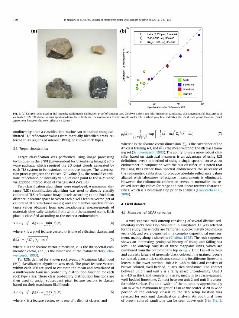
Fig. 1. (a) Sample rocks used in TLS intensity radiometric calibration proof of concept test. Clockwise, from top left: limestone, sandstone, shale, gypsum. (b) Scatterplot ofcalibrated TLS reflectance versus spectroradiometer reflectance measurements of the sample rocks. The dashed gray line indicates the ideal data point location (exactagreement between the two reflectance values).

150 P. Hartzell et al. / ISPRS Journal of Photogrammetry and Remote Sensing 88 (2014) 147–155

nonlinearity, then a classification routine can be trained using cal-ibrated TLS reflectance values from manually identified areas, re-ferred to as regions of interest (ROIs), of known rock types.

3.3. Target classification

Target classification was performed using image processingtechniques in the ENVI (Environment for Visualizing Images) soft-ware package, which required the 3D point clouds generated byeach TLS system to be rasterized to produce images. The rasteriza-tion process projects the chosen ‘‘Z’’-value (i.e., the actual Z coordi-nate, reflectance, or intensity value) of each point to the X–Y planevia gridded interpolation of triangulated Z-values.

Two classification algorithms were employed. A minimum dis-tance (MD) classification algorithm was used to directly classifycalibrated TLS reflectance image pixels according to the Euclideandistance in feature space between each pixel’s feature vector (set ofcalibrated TLS reflectance values) and endmember spectral reflec-tance values obtained from spectroradiometer measurements ofmaterials physically sampled from within the scanned scene. Eachpixel is classified according to the nearest endmember:

x*2 xi if diðx

*Þ ¼ min

t¼1;2;���;cdtðx

*Þ ð4Þ

where x*

is a pixel feature vector, xi is one of c distinct classes, and

diðx*Þ ¼

ffiffiffiffiffiffiffiffiffiffiffiffiffiffiffiffiffiffiffiffiffiffiffiffiffiffiffiffiffiRn

j¼1ðxj � eij Þ2

qð5Þ

where n is the feature vector dimension, ei is the ith spectral end-member vector, and j is the dimension of the feature vector (Scho-wengerdt, 1983).

For ROIs defined for known rock types, a Maximum Likelihood(ML) classification algorithm was used. The pixel feature vectorswithin each ROI are used to estimate the mean and covariance ofa multivariate Gaussian probability distribution function for eachrock type class. These class probability distribution functions arethen used to assign subsequent pixel feature vectors to classesbased on their maximum likelihood:

x*2 xi if piðx

*Þ ¼ max

t¼1;2;���;cptðx

*Þ ð6Þ

where x*

is a feature vector, xi is one of c distinct classes, and

piðx*Þ ¼ 1

ð2pÞd2jRij

12

exp �12ðx*�mi

*Þ

TR�1

i ðx*�mi

*Þ

� �ð7Þ

where d is the feature vector dimension,P

i is the covariance of theith class training set, and mi

*is the mean vector of the ith class train-

ing set (Schowengerdt, 1983). The ability to use a more robust clas-sifier based on statistical measures is an advantage of using ROIdefinitions over the method of using a single spectral curve as anendmember in conjunction with the MD classifier. It is noted thatby using ROIs rather than spectral endmembers the necessity ofthe radiometric calibration to produce absolute reflectance valuesaligned with laboratory reflectance measurements is eliminated.However, the radiometric calibration serves to normalize the re-ceived intensity values for range and non-linear receiver character-istics, which is a necessary step prior to analysis (Franceschi et al.,2009).

4. Field dataset

4.1. Multispectral LiDAR collection

A well-exposed rock outcrop consisting of several distinct sed-imentary rocks near Lion Mountain in Kingsland, TX was selectedfor the study. These rocks are Cambrian, approximately 540 millionyears old, and were deposited in a complex depositional environ-ment, mainly along a shoreline (Chafetz, 1978). The rock sequenceshows an interesting geological history of rising and falling sealevel. The outcrop consists of three mappable units, which arenumbered from the bottom to the top in Fig. 2. Unit 1 is �9 m thickand consists largely of greenish-black colored, fine grained, poorlycemented, glauconitic sandstone containing fossiliferous limestonelenses in the lower portion. Unit 2 is �2.5 m thick and consists ofbrown colored, well-bedded, quartz-rich sandstone. The contactbetween unit 1 and unit 2 is a fairly sharp unconformity. Unit 3is �4.5 m thick and consists of a gray, medium to coarse-grained,well-bedded limestone. Contact between unit 2 and unit 3 is a con-formable surface. The total width of the outcrop is approximately140 m with a maximum height of 17 m at the center. A 20 m wideportion of the outcrop closest to the TLS setup location wasselected for rock unit classification analysis. An additional layerof brown colored sandstone can be seen above unit 3 in Fig. 2,

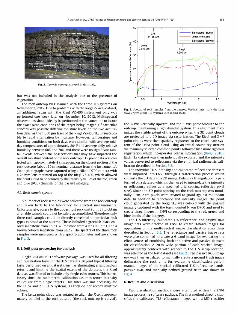
Fig. 2. Geologic outcrop analyzed in this study.

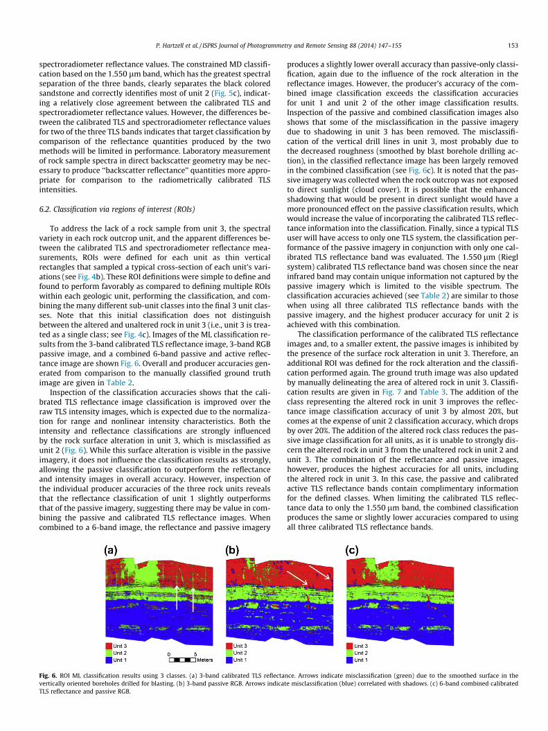
Fig. 3. Spectra of rock samples from the outcrop. Vertical lines mark the laserwavelengths of the TLS systems used in this study.

P. Hartzell et al. / ISPRS Journal of Photogrammetry and Remote Sensing 88 (2014) 147–155 151

but was not included in the analysis due to the presence ofvegetation.

The rock outcrop was scanned with the three TLS systems onNovember 3, 2012. Due to problems with the Riegl VZ-400 dataset,an additional scan with the Riegl VZ-400 instrument only wasperformed one week later on November 10, 2012. Multispectralobservations should ideally be performed at the same time to insurethe exact same conditions of the target being imaged. Of particularconcern was possible differing moisture levels on the two acquisi-tion days, as the 1.550 lm laser of the Riegl VZ-400 TLS is suscepti-ble to rapid attenuation by moisture. However, temperature andhumidity conditions on both days were similar, with average mid-day temperatures of approximately 80� F and average daily relativehumidity between 60% and 70%, and there were no significant rain-fall events between the observations that may have impacted theoverall moisture content of the rock outcrop. TLS point data was col-lected with approximately 1 cm spacing on the closest portion of therock outcrop (about 30 m nominal distance from the instruments).Color photographs were captured using a Nikon D700 camera witha 25 mm lens mounted on top of the Riegl VZ-400, which allowedthe point cloud to be colored by the intensity values of the red, greenand blue (RGB) channels of the passive imagery.

4.2. Rock sample spectra

A number of rock samples were collected from the rock outcropand taken back to the laboratory for spectral measurements.Unfortunately, access to the uppermost rock unit (unit 3) to obtaina reliable sample could not be safely accomplished. Therefore, onlythree rock samples could be directly correlated to particular rocktypes exposed at the outcrop. These included a greenish-black col-ored sandstone from unit 1, a limestone from a lens in unit 1, and abrown colored sandstone from unit 2. The spectra of the three rocksamples were measured with a spectroradiometer and are shownin Fig. 3.

5. LiDAR post processing for analysis

Riegl’s RiSCAN PRO software package was used for all filteringand registration tasks for the TLS datasets. Beyond typical filteringtasks performed on all datasets, such as eliminating errant mid-airreturns and limiting the spatial extent of the datasets, the Riegldataset was filtered to include only single-echo returns. This is nec-essary since the radiometric calibration assumes return intensityvalues are from single targets. This filter was not necessary forthe Leica and Z + F TLS systems, as they do not record multipleechoes.

The Leica point cloud was rotated to align the X-axis approxi-mately parallel to the rock outcrop (the rock outcrop is curved),

the Y-axis vertically upward, and the Z axis perpendicular to theoutcrop, maintaining a right-handed system. This alignment max-imizes the visible extent of the outcrop when the 3D point cloudsare projected to a 2D image via rasterization. The Riegl and Z + Fpoint clouds were then spatially registered to the coordinate sys-tem of the Leica point cloud using an initial coarse registrationvia manually selected common points, followed by a more rigorousregistration which incorporates planar information (Riegl, 2010).Each TLS dataset was then individually exported and the intensityvalues converted to reflectance via the empirical radiometric cali-bration described in Section 3.2.

The individual TLS intensity and calibrated reflectance datasetswere imported into ENVI through a rasterization process whichconverts the 3D data to a 2D image. Delaunay triangulation is per-formed on a dataset, which is then used to interpolate the intensityor reflectance values at a specified grid spacing (effective pixelsize). Since the 3D point spacing on the rock outcrop was nomi-nally 1 cm, 2 cm pixels were created to guard against redundantdata. In addition to reflectance and intensity images, the pointcloud generated by the Riegl TLS was colored with the passiveimagery captured with the top-mounted Nikon D700 and used tocreate three images in ENVI corresponding to the red, green, andblue bands of the imagery.

The TLS intensity, calibrated TLS reflectance, and passive RGBimage sets were stacked in ENVI to create 3-band images forapplication of the multispectral image classification algorithmsdescribed in Section 3.3. The reflectance and passive image setswere also combined to create a 6-band image for evaluating theeffectiveness of combining both the active and passive datasetsfor classification. A 20 m wide portion of each stacked image,approximately centered with respect to the TLS setup location,was selected as the test dataset (see Fig. 2). The passive RGB imag-ery was then visualized to manually create a ground truth imagedelineating the rock units for evaluating classification perfor-mance. Images of the stacked calibrated TLS reflectance bands,passive RGB, and manually defined ground truth are shown inFig. 4.

6. Results and discussion

Two classification methods were attempted within the ENVIimage processing software package. The first method directly clas-sifies the calibrated TLS reflectance images with a MD classifier

Fig. 4. (a) Stacked calibrated TLS reflectance image. (b) Stacked visible passive red, green, and blue bands. (c) Ground truth image. ROI definitions are shown as narrowcolored lines overlaid on the passive image in (b).

152 P. Hartzell et al. / ISPRS Journal of Photogrammetry and Remote Sensing 88 (2014) 147–155

using the spectral curves measured from the rock samples as end-members. Given the consistent departure of the calibrated TLSreflectance values from the spectroradiometer reflectance valuesin the proof of concept test (Section 3.2), the direct classificationis not expected to perform as robustly as classification using ROIdefinitions. However, it is still informative to examine the perfor-mance of the empirical TLS reflectance calibration, which obtains‘‘backscatter reflectance’’ quantities, versus spectroradiometerreflectance measurements of rock samples taken from the outcrop.The second method employs ROIs to train a ML classifier for appli-cation to the TLS intensity and calibrated TLS reflectance images.The classification performance of passive imagery alone and fusedwith the calibrated TLS reflectance images is also examined toevaluate the effectiveness of active multispectral TLS observationscompared to passive imagery observations. The goal of the classifi-cation is to correctly separate the rock outcrop into the threedistinct units described in Section 4.1.

6.1. Direct classification via known spectra

If the radiometric calibration described in Section 3.2 createdabsolute reflectance values in agreement with spectroradiometerreflectance measurements, the classification of the calibrated TLSreflectance images is straightforward since the spectral signaturesof several materials of interest are known. Spectral endmemberswere defined by importing the measured spectral curves of thethree previously described rock samples into ENVI and the MDclassification technique was applied. As discussed in Section 4.2,a reliable rock sample from unit 3 was not able to be obtained. Gi-ven the limited endmember collection, the results of the directclassification via known spectral values are assessed qualitativelyonly. The MD classification using all three reflectance bands is

Fig. 5. Calibrated TLS reflectance image MD classification results. (a) 0.532 lm, 0.785 lm(c) 1.550 lm band only with 0.05 maximum error constraint.

shown in Fig. 5a. The limestone lenses in the lower portion of unit1 are evident. The bands of black colored sandstone in unit 2 canalso be seen, and unit 2 is largely classified correctly. However,bright surface alterations in unit 1 are misclassified as limestoneor brown colored sandstone. This is not unexpected since the out-crop units are not uniform and only a limited number of rock spec-tra were used.

To better evaluate the agreement between the calibrated TLSand spectroradiometer reflectance measurements, a maximum dis-tance error constraint of 0.05 (5% reflectance) was imposed on aMD classification performed on each calibrated TLS reflectanceband individually. Any pixel feature vectors that are further than0.05 from the closest endmember will not be classified. The 0.05error value was based on the average standard deviation of the cal-ibrated TLS reflectance values (4.9%) of the test rock samples.When the constrained MD classifier was applied to the 0.785 lmband, the calibrated TLS reflectance values were found to be con-sistently low, with no pixels classified as limestone lens, whichhas the highest measured reflectance of the rock samples at0.785. Furthermore, approximately one-third of all pixels werenot classified. These findings indicate that the radiometrically cal-ibrated TLS reflectance values generated from the Z + F TLS intensi-ties are significantly different than the spectroradiometerreflectance values. The constrained MD classification based onthe 0.532 lm band produces results for most pixels, but onlyweakly separates the black colored sandstone from limestonelenses and brown colored sandstone (Fig. 5b). This can partly beexplained by the fact that the 0.532 lm band has the least spectralseparation of the three bands (see Fig. 3) for the rock samples.The classification of the limestone lens material and browncolored sandstone is also approximately inverted, again indicatinga consistent difference between the calibrated TLS and

, and 1.550 lm bands. (b) 0.532 lm band only with 0.05 maximum error constraint.

P. Hartzell et al. / ISPRS Journal of Photogrammetry and Remote Sensing 88 (2014) 147–155 153

spectroradiometer reflectance values. The constrained MD classifi-cation based on the 1.550 lm band, which has the greatest spectralseparation of the three bands, clearly separates the black coloredsandstone and correctly identifies most of unit 2 (Fig. 5c), indicat-ing a relatively close agreement between the calibrated TLS andspectroradiometer reflectance values. However, the differences be-tween the calibrated TLS and spectroradiometer reflectance valuesfor two of the three TLS bands indicates that target classification bycomparison of the reflectance quantities produced by the twomethods will be limited in performance. Laboratory measurementof rock sample spectra in direct backscatter geometry may be nec-essary to produce ‘‘backscatter reflectance’’ quantities more appro-priate for comparison to the radiometrically calibrated TLSintensities.

6.2. Classification via regions of interest (ROIs)

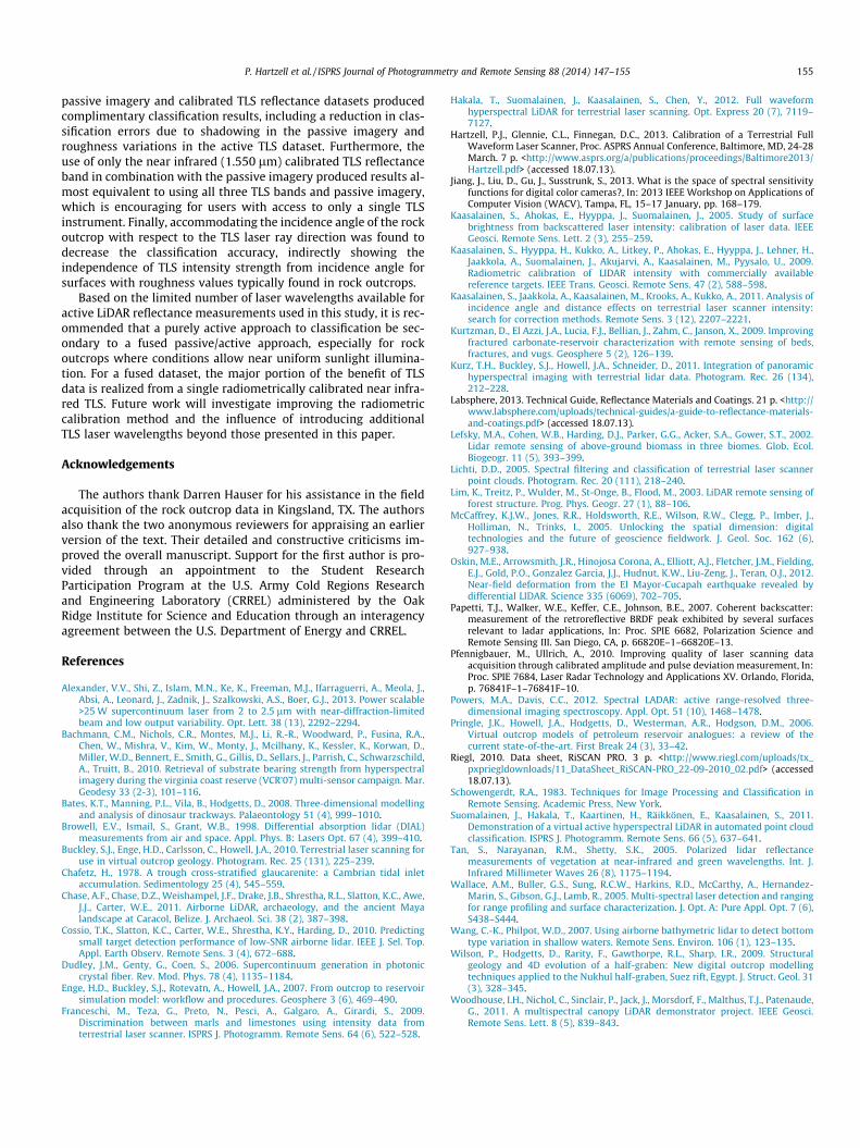
To address the lack of a rock sample from unit 3, the spectralvariety in each rock outcrop unit, and the apparent differences be-tween the calibrated TLS and spectroradiometer reflectance mea-surements, ROIs were defined for each unit as thin verticalrectangles that sampled a typical cross-section of each unit’s vari-ations (see Fig. 4b). These ROI definitions were simple to define andfound to perform favorably as compared to defining multiple ROIswithin each geologic unit, performing the classification, and com-bining the many different sub-unit classes into the final 3 unit clas-ses. Note that this initial classification does not distinguishbetween the altered and unaltered rock in unit 3 (i.e., unit 3 is trea-ted as a single class; see Fig. 4c). Images of the ML classification re-sults from the 3-band calibrated TLS reflectance image, 3-band RGBpassive image, and a combined 6-band passive and active reflec-tance image are shown Fig. 6. Overall and producer accuracies gen-erated from comparison to the manually classified ground truthimage are given in Table 2.

Inspection of the classification accuracies shows that the cali-brated TLS reflectance image classification is improved over theraw TLS intensity images, which is expected due to the normaliza-tion for range and nonlinear intensity characteristics. Both theintensity and reflectance classifications are strongly influencedby the rock surface alteration in unit 3, which is misclassified asunit 2 (Fig. 6). While this surface alteration is visible in the passiveimagery, it does not influence the classification results as strongly,allowing the passive classification to outperform the reflectanceand intensity images in overall accuracy. However, inspection ofthe individual producer accuracies of the three rock units revealsthat the reflectance classification of unit 1 slightly outperformsthat of the passive imagery, suggesting there may be value in com-bining the passive and calibrated TLS reflectance images. Whencombined to a 6-band image, the reflectance and passive imagery

Fig. 6. ROI ML classification results using 3 classes. (a) 3-band calibrated TLS reflectanvertically oriented boreholes drilled for blasting. (b) 3-band passive RGB. Arrows indicatTLS reflectance and passive RGB.

produces a slightly lower overall accuracy than passive-only classi-fication, again due to the influence of the rock alteration in thereflectance images. However, the producer’s accuracy of the com-bined image classification exceeds the classification accuraciesfor unit 1 and unit 2 of the other image classification results.Inspection of the passive and combined classification images alsoshows that some of the misclassification in the passive imagerydue to shadowing in unit 3 has been removed. The misclassifi-cation of the vertical drill lines in unit 3, most probably due tothe decreased roughness (smoothed by blast borehole drilling ac-tion), in the classified reflectance image has been largely removedin the combined classification (see Fig. 6c). It is noted that the pas-sive imagery was collected when the rock outcrop was not exposedto direct sunlight (cloud cover). It is possible that the enhancedshadowing that would be present in direct sunlight would have amore pronounced effect on the passive classification results, whichwould increase the value of incorporating the calibrated TLS reflec-tance information into the classification. Finally, since a typical TLSuser will have access to only one TLS system, the classification per-formance of the passive imagery in conjunction with only one cal-ibrated TLS reflectance band was evaluated. The 1.550 lm (Rieglsystem) calibrated TLS reflectance band was chosen since the nearinfrared band may contain unique information not captured by thepassive imagery which is limited to the visible spectrum. Theclassification accuracies achieved (see Table 2) are similar to thosewhen using all three calibrated TLS reflectance bands with thepassive imagery, and the highest producer accuracy for unit 2 isachieved with this combination.

The classification performance of the calibrated TLS reflectanceimages and, to a smaller extent, the passive images is inhibited bythe presence of the surface rock alteration in unit 3. Therefore, anadditional ROI was defined for the rock alteration and the classifi-cation performed again. The ground truth image was also updatedby manually delineating the area of altered rock in unit 3. Classifi-cation results are given in Fig. 7 and Table 3. The addition of theclass representing the altered rock in unit 3 improves the reflec-tance image classification accuracy of unit 3 by almost 20%, butcomes at the expense of unit 2 classification accuracy, which dropsby over 20%. The addition of the altered rock class reduces the pas-sive image classification for all units, as it is unable to strongly dis-cern the altered rock in unit 3 from the unaltered rock in unit 2 andunit 3. The combination of the reflectance and passive images,however, produces the highest accuracies for all units, includingthe altered rock in unit 3. In this case, the passive and calibratedactive TLS reflectance bands contain complimentary informationfor the defined classes. When limiting the calibrated TLS reflec-tance data to only the 1.550 lm band, the combined classificationproduces the same or slightly lower accuracies compared to usingall three calibrated TLS reflectance bands.

ce. Arrows indicate misclassification (green) due to the smoothed surface in thee misclassification (blue) correlated with shadows. (c) 6-band combined calibrated

Table 2ROI ML classification accuracies for 3 classes.

Image Overallaccuracy (%)

Producer’s accuracy (%)

Unit1

Unit2

Unit3

TLS Intensity 66.3 71.3 73.5 54.3TLS reflectance 75.7 87.4 70.0 60.1Passive 84.5 85.3 76.5 88.0Passive & TLS Refl. 83.5 88.2 82.9 76.4Passive & 1.550 lm TLS Refl.

Only82.6 86.5 84.2 75.5

Table 3ROI ML classification accuracies for 4 classes.

Image Overallaccuracy (%)

Producer’s accuracy (%)

Unit1

Unit2

Unit3

Unit3aa

TLS intensity 66.6 71.3 45.1 69.4 75.8TLS reflectance 76.7 87.4 46.0 78.2 73.5Passive 75.7 85.0 65.0 66.5 68.0Passive & TLS Refl. 84.1 88.2 68.3 89.4 79.9Passive & 1.550 lm TLS

Refl. Only82.0 86.4 67.4 86.3 75.9

a Area of rock surface alteration in Unit 3.

154 P. Hartzell et al. / ISPRS Journal of Photogrammetry and Remote Sensing 88 (2014) 147–155

An interesting visual difference between the passive and activeimage classification results is the pronounced increase in spatialhomogeneity in the passive classification results. It is believed thatthe broad spectral line widths employed for the RGB channels ofthe Nikon D700 (Jiang et al., 2013) are not as sensitive to subtlespatial variations in the spectral signature of the rock, leading tomore spatially homogeneous classification. The lasers used by theTLS systems have very narrow spectral line widths and produceclassification images with a greater amount of noise, or speckle,but also appear to better detect thin strata. See, for example, thethin layers of black colored sandstone within unit 2 in Fig. 7aand b. Both of these qualities may be desirable in situations whereminor variation in rock types are not of interest but detection ofthin rock layers and sharp boundaries between different strata orrock properties is desired to provide enhanced interpretation.The combination of the active and passive imagery appears blendsthese characteristics, although at reduced levels, into a single re-sult (Fig. 7c).

The LiDAR link equation (Eq. (1)) specifies that the amount ofenergy detected by a LiDAR system is proportional to cosine ofthe angle of incidence of the laser ray. However, consistent reflec-tance values and classification performance across the rock out-crop (Fig. 6 and 7) indicate that an incidence angle correctionmay not be necessary for most of the rock outcrop. In (Franceschiet al., 2009) it is stated that natural surfaces such as rock outcropswhich are characterized by roughness on the order of magnitude ofthe laser spot size, i.e., 1–10 mm for a laser spot size of 10–20 mm,exhibit LiDAR return intensity values that are independent of inci-dence angle. To confirm this, 2D reflectance images were createdthat were compensated for the incidence angle of the laser beamfor the three TLS datasets. This led to overly bright areas with highincidence angles which reduced overall classification accuracy byover 5% when using the ML classifier with the 3 ROI definitionsfor the 3 rock outcrop units. The bright patterns in the correctedreflectance images were visibly correlated to misclassification pat-terns. This result indirectly validates the independence of laser

Fig. 7. ROI ML classification results using 4 classes. (a) 3-band calibrated TLS reflectance.RGB.

intensity from incidence angle for rock outcrops previouslyreported.

7. Conclusions

A method for target classification based on multispectral LiDARobservations using commercially available hardware and softwarefor potential application to automated virtual outcrop geology wasdemonstrated. An empirical radiometric calibration of TLS inten-sity values that accommodated range and intensity non-linearitywas found to produce consistent reflectance values, but only clo-sely matched spectroradiometer reflectance values in a limitednumber of cases. The TLS intensity calibration model is expectedto be most effective for observed materials having similar scatter-ing and hotspot characteristics as the calibration targets. Materialsnot conforming to this requirement are assigned biased reflectancevalues by the calibration model, which limits the ability tocorrectly identify materials solely from a priori spectral libraryinformation. ROIs defining areas of known material type are there-fore required for maximum classification accuracy. Future perfor-mance improvement of the radiometric calibration model forrock outcrop classification may be attained by measuring thereflectance of multiple rock samples and subsequently using thesamples as the radiometric calibration targets, thereby achievinga closer relationship between the calibration model and materialsof interest.

Quantitative classification results based on ROI definitions re-vealed that while radiometrically calibrated TLS reflectance valueswere more effective than raw TLS intensities, RGB informationfrom passive digital photography was equally or more effectivein discriminating the rock outcrop units in this study, dependingon class selection. Compared to the narrow spectral bands of theTLS lasers, passive imagery RGB bands contain information froma broad spectrum of wavelengths. Additional TLS laser wave-lengths may therefore be necessary to outperform traditional pas-sive imagery classification results. When combined, however, the

(b) 3-band passive RGB. (c) 6-band combined calibrated TLS reflectance and passive

P. Hartzell et al. / ISPRS Journal of Photogrammetry and Remote Sensing 88 (2014) 147–155 155

passive imagery and calibrated TLS reflectance datasets producedcomplimentary classification results, including a reduction in clas-sification errors due to shadowing in the passive imagery androughness variations in the active TLS dataset. Furthermore, theuse of only the near infrared (1.550 lm) calibrated TLS reflectanceband in combination with the passive imagery produced results al-most equivalent to using all three TLS bands and passive imagery,which is encouraging for users with access to only a single TLSinstrument. Finally, accommodating the incidence angle of the rockoutcrop with respect to the TLS laser ray direction was found todecrease the classification accuracy, indirectly showing theindependence of TLS intensity strength from incidence angle forsurfaces with roughness values typically found in rock outcrops.

Based on the limited number of laser wavelengths available foractive LiDAR reflectance measurements used in this study, it is rec-ommended that a purely active approach to classification be sec-ondary to a fused passive/active approach, especially for rockoutcrops where conditions allow near uniform sunlight illumina-tion. For a fused dataset, the major portion of the benefit of TLSdata is realized from a single radiometrically calibrated near infra-red TLS. Future work will investigate improving the radiometriccalibration method and the influence of introducing additionalTLS laser wavelengths beyond those presented in this paper.

Acknowledgements

The authors thank Darren Hauser for his assistance in the fieldacquisition of the rock outcrop data in Kingsland, TX. The authorsalso thank the two anonymous reviewers for appraising an earlierversion of the text. Their detailed and constructive criticisms im-proved the overall manuscript. Support for the first author is pro-vided through an appointment to the Student ResearchParticipation Program at the U.S. Army Cold Regions Researchand Engineering Laboratory (CRREL) administered by the OakRidge Institute for Science and Education through an interagencyagreement between the U.S. Department of Energy and CRREL.

References

Alexander, V.V., Shi, Z., Islam, M.N., Ke, K., Freeman, M.J., Ifarraguerri, A., Meola, J.,Absi, A., Leonard, J., Zadnik, J., Szalkowski, A.S., Boer, G.J., 2013. Power scalable>25 W supercontinuum laser from 2 to 2.5 lm with near-diffraction-limitedbeam and low output variability. Opt. Lett. 38 (13), 2292–2294.

Bachmann, C.M., Nichols, C.R., Montes, M.J., Li, R.-R., Woodward, P., Fusina, R.A.,Chen, W., Mishra, V., Kim, W., Monty, J., Mcilhany, K., Kessler, K., Korwan, D.,Miller, W.D., Bennert, E., Smith, G., Gillis, D., Sellars, J., Parrish, C., Schwarzschild,A., Truitt, B., 2010. Retrieval of substrate bearing strength from hyperspectralimagery during the virginia coast reserve (VCR’07) multi-sensor campaign. Mar.Geodesy 33 (2-3), 101–116.

Bates, K.T., Manning, P.L., Vila, B., Hodgetts, D., 2008. Three-dimensional modellingand analysis of dinosaur trackways. Palaeontology 51 (4), 999–1010.

Browell, E.V., Ismail, S., Grant, W.B., 1998. Differential absorption lidar (DIAL)measurements from air and space. Appl. Phys. B: Lasers Opt. 67 (4), 399–410.

Buckley, S.J., Enge, H.D., Carlsson, C., Howell, J.A., 2010. Terrestrial laser scanning foruse in virtual outcrop geology. Photogram. Rec. 25 (131), 225–239.

Chafetz, H., 1978. A trough cross-stratified glaucarenite: a Cambrian tidal inletaccumulation. Sedimentology 25 (4), 545–559.

Chase, A.F., Chase, D.Z., Weishampel, J.F., Drake, J.B., Shrestha, R.L., Slatton, K.C., Awe,J.J., Carter, W.E., 2011. Airborne LiDAR, archaeology, and the ancient Mayalandscape at Caracol, Belize. J. Archaeol. Sci. 38 (2), 387–398.

Cossio, T.K., Slatton, K.C., Carter, W.E., Shrestha, K.Y., Harding, D., 2010. Predictingsmall target detection performance of low-SNR airborne lidar. IEEE J. Sel. Top.Appl. Earth Observ. Remote Sens. 3 (4), 672–688.

Dudley, J.M., Genty, G., Coen, S., 2006. Supercontinuum generation in photoniccrystal fiber. Rev. Mod. Phys. 78 (4), 1135–1184.

Enge, H.D., Buckley, S.J., Rotevatn, A., Howell, J.A., 2007. From outcrop to reservoirsimulation model: workflow and procedures. Geosphere 3 (6), 469–490.

Franceschi, M., Teza, G., Preto, N., Pesci, A., Galgaro, A., Girardi, S., 2009.Discrimination between marls and limestones using intensity data fromterrestrial laser scanner. ISPRS J. Photogramm. Remote Sens. 64 (6), 522–528.

Hakala, T., Suomalainen, J., Kaasalainen, S., Chen, Y., 2012. Full waveformhyperspectral LiDAR for terrestrial laser scanning. Opt. Express 20 (7), 7119–7127.

Hartzell, P.J., Glennie, C.L., Finnegan, D.C., 2013. Calibration of a Terrestrial FullWaveform Laser Scanner, Proc. ASPRS Annual Conference, Baltimore, MD, 24-28March. 7 p. <http://www.asprs.org/a/publications/proceedings/Baltimore2013/Hartzell.pdf> (accessed 18.07.13).

Jiang, J., Liu, D., Gu, J., Susstrunk, S., 2013. What is the space of spectral sensitivityfunctions for digital color cameras?, In: 2013 IEEE Workshop on Applications ofComputer Vision (WACV), Tampa, FL, 15–17 January, pp. 168–179.

Kaasalainen, S., Ahokas, E., Hyyppa, J., Suomalainen, J., 2005. Study of surfacebrightness from backscattered laser intensity: calibration of laser data. IEEEGeosci. Remote Sens. Lett. 2 (3), 255–259.

Kaasalainen, S., Hyyppa, H., Kukko, A., Litkey, P., Ahokas, E., Hyyppa, J., Lehner, H.,Jaakkola, A., Suomalainen, J., Akujarvi, A., Kaasalainen, M., Pyysalo, U., 2009.Radiometric calibration of LIDAR intensity with commercially availablereference targets. IEEE Trans. Geosci. Remote Sens. 47 (2), 588–598.

Kaasalainen, S., Jaakkola, A., Kaasalainen, M., Krooks, A., Kukko, A., 2011. Analysis ofincidence angle and distance effects on terrestrial laser scanner intensity:search for correction methods. Remote Sens. 3 (12), 2207–2221.

Kurtzman, D., El Azzi, J.A., Lucia, F.J., Bellian, J., Zahm, C., Janson, X., 2009. Improvingfractured carbonate-reservoir characterization with remote sensing of beds,fractures, and vugs. Geosphere 5 (2), 126–139.

Kurz, T.H., Buckley, S.J., Howell, J.A., Schneider, D., 2011. Integration of panoramichyperspectral imaging with terrestrial lidar data. Photogram. Rec. 26 (134),212–228.

Labsphere, 2013. Technical Guide, Reflectance Materials and Coatings. 21 p. <http://www.labsphere.com/uploads/technical-guides/a-guide-to-reflectance-materials-and-coatings.pdf> (accessed 18.07.13).

Lefsky, M.A., Cohen, W.B., Harding, D.J., Parker, G.G., Acker, S.A., Gower, S.T., 2002.Lidar remote sensing of above-ground biomass in three biomes. Glob. Ecol.Biogeogr. 11 (5), 393–399.

Lichti, D.D., 2005. Spectral filtering and classification of terrestrial laser scannerpoint clouds. Photogram. Rec. 20 (111), 218–240.

Lim, K., Treitz, P., Wulder, M., St-Onge, B., Flood, M., 2003. LiDAR remote sensing offorest structure. Prog. Phys. Geogr. 27 (1), 88–106.

McCaffrey, K.J.W., Jones, R.R., Holdsworth, R.E., Wilson, R.W., Clegg, P., Imber, J.,Holliman, N., Trinks, I., 2005. Unlocking the spatial dimension: digitaltechnologies and the future of geoscience fieldwork. J. Geol. Soc. 162 (6),927–938.

Oskin, M.E., Arrowsmith, J.R., Hinojosa Corona, A., Elliott, A.J., Fletcher, J.M., Fielding,E.J., Gold, P.O., Gonzalez Garcia, J.J., Hudnut, K.W., Liu-Zeng, J., Teran, O.J., 2012.Near-field deformation from the El Mayor-Cucapah earthquake revealed bydifferential LIDAR. Science 335 (6069), 702–705.

Papetti, T.J., Walker, W.E., Keffer, C.E., Johnson, B.E., 2007. Coherent backscatter:measurement of the retroreflective BRDF peak exhibited by several surfacesrelevant to ladar applications, In: Proc. SPIE 6682, Polarization Science andRemote Sensing III. San Diego, CA, p. 66820E–1–66820E–13.

Pfennigbauer, M., Ullrich, A., 2010. Improving quality of laser scanning dataacquisition through calibrated amplitude and pulse deviation measurement, In:Proc. SPIE 7684, Laser Radar Technology and Applications XV. Orlando, Florida,p. 76841F–1–76841F–10.

Powers, M.A., Davis, C.C., 2012. Spectral LADAR: active range-resolved three-dimensional imaging spectroscopy. Appl. Opt. 51 (10), 1468–1478.

Pringle, J.K., Howell, J.A., Hodgetts, D., Westerman, A.R., Hodgson, D.M., 2006.Virtual outcrop models of petroleum reservoir analogues: a review of thecurrent state-of-the-art. First Break 24 (3), 33–42.

Riegl, 2010. Data sheet, RiSCAN PRO. 3 p. <http://www.riegl.com/uploads/tx_pxpriegldownloads/11_DataSheet_RiSCAN-PRO_22-09-2010_02.pdf> (accessed18.07.13).

Schowengerdt, R.A., 1983. Techniques for Image Processing and Classification inRemote Sensing. Academic Press, New York.

Suomalainen, J., Hakala, T., Kaartinen, H., Räikkönen, E., Kaasalainen, S., 2011.Demonstration of a virtual active hyperspectral LiDAR in automated point cloudclassification. ISPRS J. Photogramm. Remote Sens. 66 (5), 637–641.

Tan, S., Narayanan, R.M., Shetty, S.K., 2005. Polarized lidar reflectancemeasurements of vegetation at near-infrared and green wavelengths. Int. J.Infrared Millimeter Waves 26 (8), 1175–1194.

Wallace, A.M., Buller, G.S., Sung, R.C.W., Harkins, R.D., McCarthy, A., Hernandez-Marin, S., Gibson, G.J., Lamb, R., 2005. Multi-spectral laser detection and rangingfor range profiling and surface characterization. J. Opt. A: Pure Appl. Opt. 7 (6),S438–S444.

Wang, C.-K., Philpot, W.D., 2007. Using airborne bathymetric lidar to detect bottomtype variation in shallow waters. Remote Sens. Environ. 106 (1), 123–135.

Wilson, P., Hodgetts, D., Rarity, F., Gawthorpe, R.L., Sharp, I.R., 2009. Structuralgeology and 4D evolution of a half-graben: New digital outcrop modellingtechniques applied to the Nukhul half-graben, Suez rift, Egypt. J. Struct. Geol. 31(3), 328–345.

Woodhouse, I.H., Nichol, C., Sinclair, P., Jack, J., Morsdorf, F., Malthus, T.J., Patenaude,G., 2011. A multispectral canopy LiDAR demonstrator project. IEEE Geosci.Remote Sens. Lett. 8 (5), 839–843.