Application Note Hall Sensors - Lake Shore · Revision F 2F075-00-00 3 August 2017 . Model HGA Axial Hall Sensors . Model HGT Transverse Hall Sensors . Model HGCA/CT Cryogenic Hall

Revision F F075-00-00 23 August 2017

Model HGA Axial Hall Sensors Model HGT Transverse Hall Sensors

Model HGCA/CT Cryogenic Hall Sensors

Lake Shore Cryotronics, Inc. 575 McCorkle Blvd. Westerville, Ohio 43082-8888 USA

[email protected] [email protected]

www.lakeshore.com

Fax: (614) 891-1392 Telephone: (614) 891-2243

Methods and apparatus disclosed and described herein have been developed solely on company funds of Lake Shore Cryotronics, Inc. No government or other contractual support or relationship whatsoever has existed which in any way affects or mitigates proprietary rights of Lake Shore Cryotronics, Inc. in these developments. Methods and apparatus disclosed herein may be subject to U.S. Patents existing or applied for. Lake Shore Cryotronics, Inc. reserves the right to add, improve, modify, or withdraw functions, design modifications, or products at any time without notice. Lake Shore shall not be liable for errors contained herein or for incidental or consequential damages in connection with furnishing, performance, or use of this material.

Application Note

Hall Sensors Magnetic Field Sensors

Lake Shore Hall Sensor Application Guide

E

©2014 – 2017 Lake Shore Cryotronics, Inc. All rights reserved. No portion of this manual may be reproduced, stored in a retrieval system, or transmitted, in any form or by any means, electronic, mechanical, photocopying, recording, or otherwise, without the express written permission of Lake Shore.

Lake Shore Hall Sensor Application Guide

Specifications 1-1

CHAPTER 1 SPECIFICATIONS

1.0 SPECIFICATIONS Full specifications about Hall sensors are provided on our website. Please see: http://www.lakeshore.com/products/Hall-Magnetic-Sensors/pages/Specifications.aspx

Lake Shore Hall Sensor Application Guide

Theory of Operation 2-1

CHAPTER 2 THEORY OF OPERATION

2.0 GENERAL This chapter provides a history of the Hall effect in Section 2.1 and Hall sensor theory of operation in Section 2.2.

2.1 HISTORY The Hall Effect was discovered in 1879 by Edwin H. Hall (1855 to 1938), a graduate student at Johns Hopkins University in Baltimore. Hall had studied Maxwell’s book about electricity and magnetism in which appears the following statement: “It must be carefully remembered that the mechanical force which urges a conductor carrying a current across the lines of magnetic forces acts, not on the electric current, but on the conductor which carries it.” Since no force is exerted by a magnetic field on a conductor without a current, Hall had discovered a contradiction to Maxwell’s arguments. Together with Professor Henry A. Rowland, Hall attempted to find a way to prove the influence of the magnetic field on the current in a conductor. Their theory was that the magnetic field forces the current in the conductor to one side. In experiments performed between 7 and 11 October 1879, attempts to prove this displacement by changing the resistance in a silver layer were unsuccessful. Finally, an attempt was made to prove the existence of a current displacement by detecting lateral charging of the conductor, in the direction perpendicular to the current flow and the magnetic field. On 28 October 1879, it was possible unambiguously to measure a cross-current in a thin gold layer on glass which, with reversal of magnetic polarity, likewise changed its sign. This day marks the birthday of the Hall effect. Suppose you have an electric current in a copper strip. You place the strip in a magnetic field perpendicular to the strip. The magnetic field will deflect the drifting electrons to one side of the strip. The electrons piling up on one side of the strip creates a constant transverse electric field which pushes the electrons in the opposite direction. A balance is achieved. The electric field is associated with a Hall potential difference which can be measured. In most of classical electrodynamics, it would not make any difference if the current were caused by positive charge carriers moving in the opposite direction. The Hall effect is an exception to this. If there were positive charge carriers, the polarity of the Hall potential difference would be reversed. In addition, with the Hall effect, you can measure the number of charge carriers per unit volume of the conductor. Hall performed his experiments at room temperature and with moderate magnetic fields of less than one tesla. A century later, in the 1970’s, researchers were studying the Hall effect at extremely low temperatures, only a few degrees from absolute zero, and very high magnetic fields, as high as 30 T. Much early work was performed on metals which make inefficient Hall sensors. During the late 1940’s and 1950’s, Russian and German scientists formulated semiconductors from columns III and V of the periodic chart. These materials provided the ideal combination of high mobility and high resistivity necessary for good Hall sensors. These III-V compounds are still superior Hall effect materials today.

Lake Shore Hall Sensor Application Guide

2-2 Theory of Operation

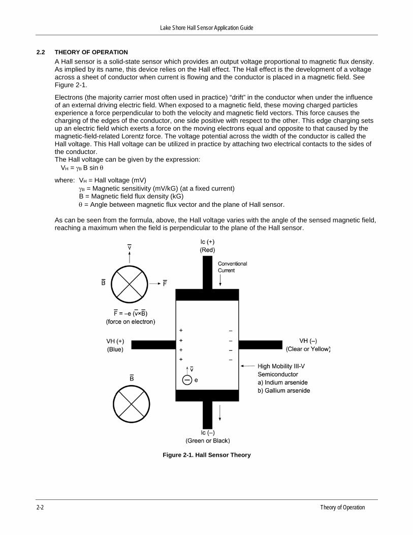
2.2 THEORY OF OPERATION A Hall sensor is a solid-state sensor which provides an output voltage proportional to magnetic flux density. As implied by its name, this device relies on the Hall effect. The Hall effect is the development of a voltage across a sheet of conductor when current is flowing and the conductor is placed in a magnetic field. See Figure 2-1.

Electrons (the majority carrier most often used in practice) “drift” in the conductor when under the influence of an external driving electric field. When exposed to a magnetic field, these moving charged particles experience a force perpendicular to both the velocity and magnetic field vectors. This force causes the charging of the edges of the conductor, one side positive with respect to the other. This edge charging sets up an electric field which exerts a force on the moving electrons equal and opposite to that caused by the magnetic-field-related Lorentz force. The voltage potential across the width of the conductor is called the Hall voltage. This Hall voltage can be utilized in practice by attaching two electrical contacts to the sides of the conductor.

The Hall voltage can be given by the expression:

VH = γΒ B sin θ

where: VH = Hall voltage (mV) γΒ = Magnetic sensitivity (mV/kG) (at a fixed current) B = Magnetic field flux density (kG) θ = Angle between magnetic flux vector and the plane of Hall sensor. As can be seen from the formula, above, the Hall voltage varies with the angle of the sensed magnetic field, reaching a maximum when the field is perpendicular to the plane of the Hall sensor.

Figure 2-1. Hall Sensor Theory

Lake Shore Hall Sensor Application Guide

Installation 3-1

CHAPTER 3 INSTALLATION

3.0 GENERAL Installation details for the Hall sensor are provided as follows. Handling is provided in Section 3.1. Lead configurations are detailed in Section 3.2. Leads are discussed in Section 3.3. Polarity is discussed in Section 3.4. Mounting considerations are discussed in Section 3.5. Potting is discussed in Section 3.6. Finally, electrostatic discharge is discussed in Section 3.7.

3.1 HANDLING

CAUTION: Care must be exercised when handling the Hall sensor. The Hall sensor is very fragile. Stressing the Hall sensor can alter its output. Any excess force can easily break the Hall sensor. Broken Hall sensors are not repairable.

CAUTION: Refer to the specifications on our website for the type of solder used to tin the ends of the

sensor leads you may have. If you intend to use a solder that does not match what was used to tin the sensor lead wires, you will need to cut the ends and re-tin them with your desired solder. SAC305 lead-free solder and Sn63Pb37 solder should never be used together due to the unsuitability of the alloy that is formed when they mix. http://www.lakeshore.com/products/Hall-Magnetic-Sensors/pages/Specifications.aspx

Hall sensors are very fragile and require delicate handling. The ceramic substrate used to produce the Hall sensor is very brittle. Use the leads to move the Hall sensor. Do not handle the substrate. The strength of the lead-to-substrate bond is about 7 ounces, so avoid tension on the leads and especially avoid bending them close to the substrate. The Hall sensor is also susceptible to bending and thermal stresses, as will be discussed in further detail later in this application guide.

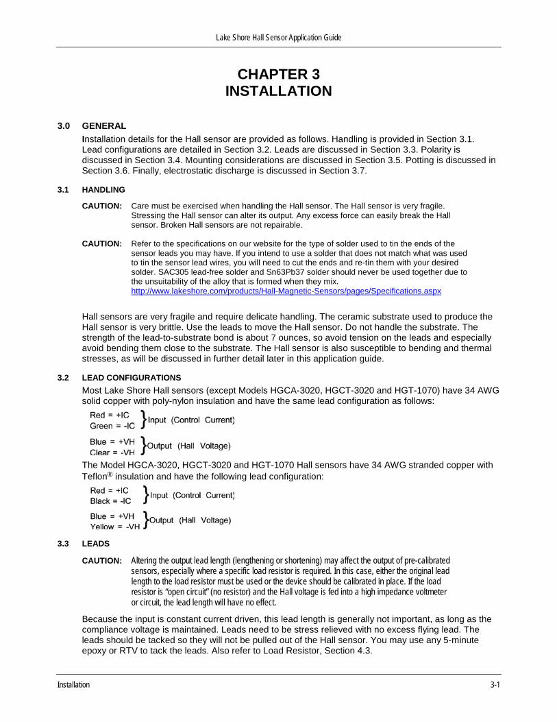
3.2 LEAD CONFIGURATIONS Most Lake Shore Hall sensors (except Models HGCA-3020, HGCT-3020 and HGT-1070) have 34 AWG solid copper with poly-nylon insulation and have the same lead configuration as follows:

The Model HGCA-3020, HGCT-3020 and HGT-1070 Hall sensors have 34 AWG stranded copper with Teflon® insulation and have the following lead configuration:

3.3 LEADS

CAUTION: Altering the output lead length (lengthening or shortening) may affect the output of pre-calibrated sensors, especially where a specific load resistor is required. In this case, either the original lead length to the load resistor must be used or the device should be calibrated in place. If the load resistor is “open circuit” (no resistor) and the Hall voltage is fed into a high impedance voltmeter or circuit, the lead length will have no effect.

Because the input is constant current driven, this lead length is generally not important, as long as the compliance voltage is maintained. Leads need to be stress relieved with no excess flying lead. The leads should be tacked so they will not be pulled out of the Hall sensor. You may use any 5-minute epoxy or RTV to tack the leads. Also refer to Load Resistor, Section 4.3.

Lake Shore Hall Sensor Application Guide

3-2 Installation

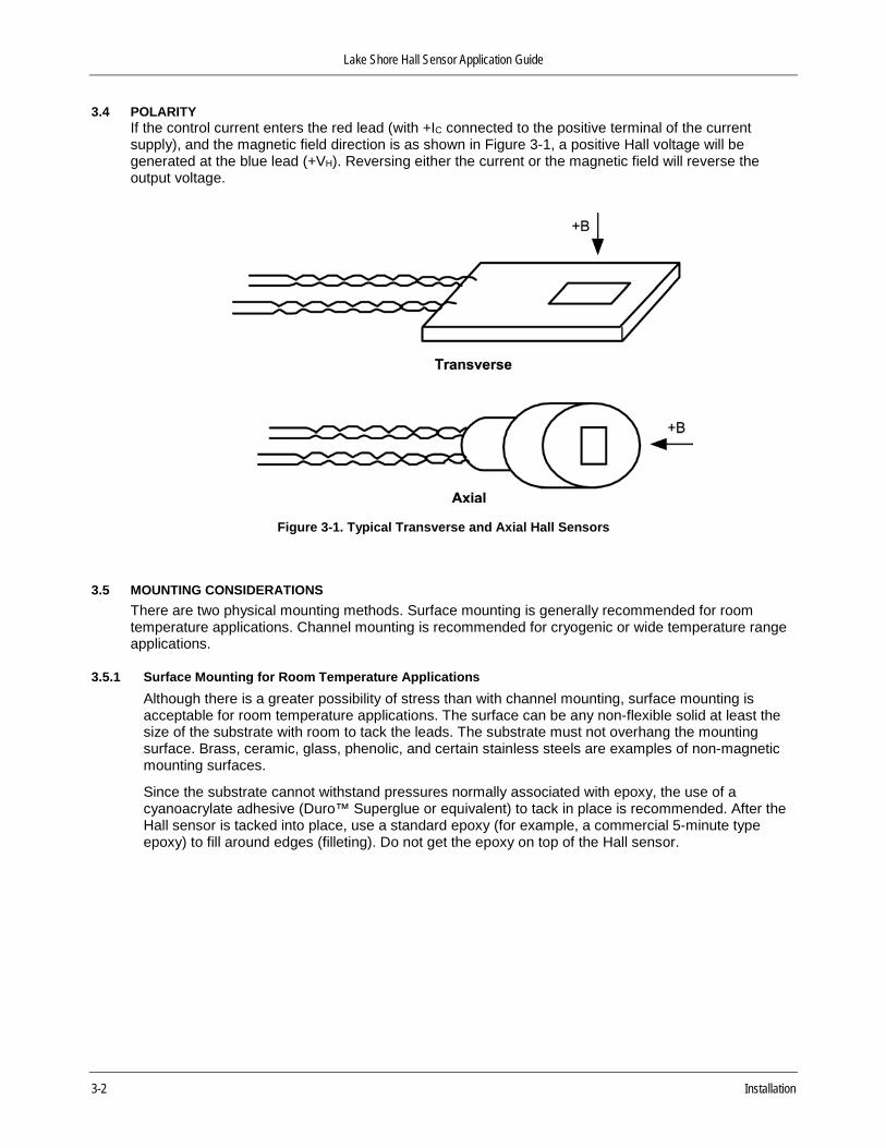
3.4 POLARITY If the control current enters the red lead (with +IC connected to the positive terminal of the current supply), and the magnetic field direction is as shown in Figure 3-1, a positive Hall voltage will be generated at the blue lead (+VH). Reversing either the current or the magnetic field will reverse the output voltage.

Figure 3-1. Typical Transverse and Axial Hall Sensors

3.5 MOUNTING CONSIDERATIONS There are two physical mounting methods. Surface mounting is generally recommended for room temperature applications. Channel mounting is recommended for cryogenic or wide temperature range applications.

3.5.1 Surface Mounting for Room Temperature Applications Although there is a greater possibility of stress than with channel mounting, surface mounting is acceptable for room temperature applications. The surface can be any non-flexible solid at least the size of the substrate with room to tack the leads. The substrate must not overhang the mounting surface. Brass, ceramic, glass, phenolic, and certain stainless steels are examples of non-magnetic mounting surfaces.

Since the substrate cannot withstand pressures normally associated with epoxy, the use of a cyanoacrylate adhesive (Duro™ Superglue or equivalent) to tack in place is recommended. After the Hall sensor is tacked into place, use a standard epoxy (for example, a commercial 5-minute type epoxy) to fill around edges (filleting). Do not get the epoxy on top of the Hall sensor.

Lake Shore Hall Sensor Application Guide

Installation 3-3

3.5.2 Channel Mounting for Wide Temperature Range Applications Channel mounting is best where high thermal expansion stresses will be encountered. Mounting must be accomplished in such a way to minimize mechanical strains. Use a formed or machined channel in a non-magnetic material (like phenolic) for Hall sensor mounting.

Failure rates approaching 10% have occurred on initial cool down with cryogenic Hall sensors that have not been properly installed (Hall sensors surviving the initial cool down generally experience no problems on subsequent cycles.) Avoid applying tension to the leads (i.e., allow plenty of slack) and avoid bending the leads close to the substrate. The leads may be bent at any angle as long as the bend is at least 0.125 in away from the substrate connection. The device should be mounted to a non-flexible, smooth surface that has a coefficient of thermal expansion that is no greater than a factor of three different from that of the ceramic substrate (which is about 7 × 10-6 K-1).

The preferred mounting procedure is to locate the device in a cavity that is at least 0.003 in larger in all dimensions than the substrate. The depth of the cavity should be the same or slightly greater than the thickness of the package. See Figure 3-2. The suggested mounting sequence is as follows:

1. Carefully place sensor into the slot.

2. Use Kapton® tape or a mechanical cover over the top of the sensor to keep it in place. The tape or cover should apply only light pressure to the sensor.

3. For strain relief, use GE-7031 varnish (or equivalent) to tack leads. If this cannot be done, an alternate mounting sequence is as follows:

1. Sparingly apply corner- or side-dots of Stycast® 2850-FT epoxy (or equivalent) to the sensor to hold it in place. Avoid getting the mounting substance on top of the sensor.

2. For strain relief, use GE-7031 varnish (or equivalent) to tack leads.

Figure 3-2. Typical Sensor Channel Mounting

Lake Shore Hall Sensor Application Guide

3-4 Installation

3.6 POTTING Potting is not recommended. It puts too much stress on the Hall sensor. However, if potting is the only choice, a silicone barrier layer should be placed around the sensor. The thickness of the barrier layer is application dependent, and can be as thin as 3 mil or up to 0.0625 in thick.

3.7 ELECTROSTATIC DISCHARGE Electrostatic discharge (ESD) may damage electronic parts, assemblies, and equipment. ESD is a transfer of electrostatic charge between bodies at different electrostatic potentials caused by direct contact or induced by an electrostatic field. The low-energy source that most commonly destroys electrostatic discharge sensitive (ESDS) devices is the human body, which generates and retains static electricity. Simply walking across a carpet in low humidity may generate up to 35,000 V of static electricity.

Current technology trends toward greater complexity, increased packaging density, and thinner dielectrics between active elements, which results in electronic devices with even more ESD sensitivity. Some electronic parts are more ESDS than others. ESD levels of only a few hundred volts may damage electronic components such as semiconductors, thick and thin film resistors, and piezoelectric crystals during testing, handling, repair, or assembly. Discharge voltages below 4000 V cannot be seen, felt, or heard.

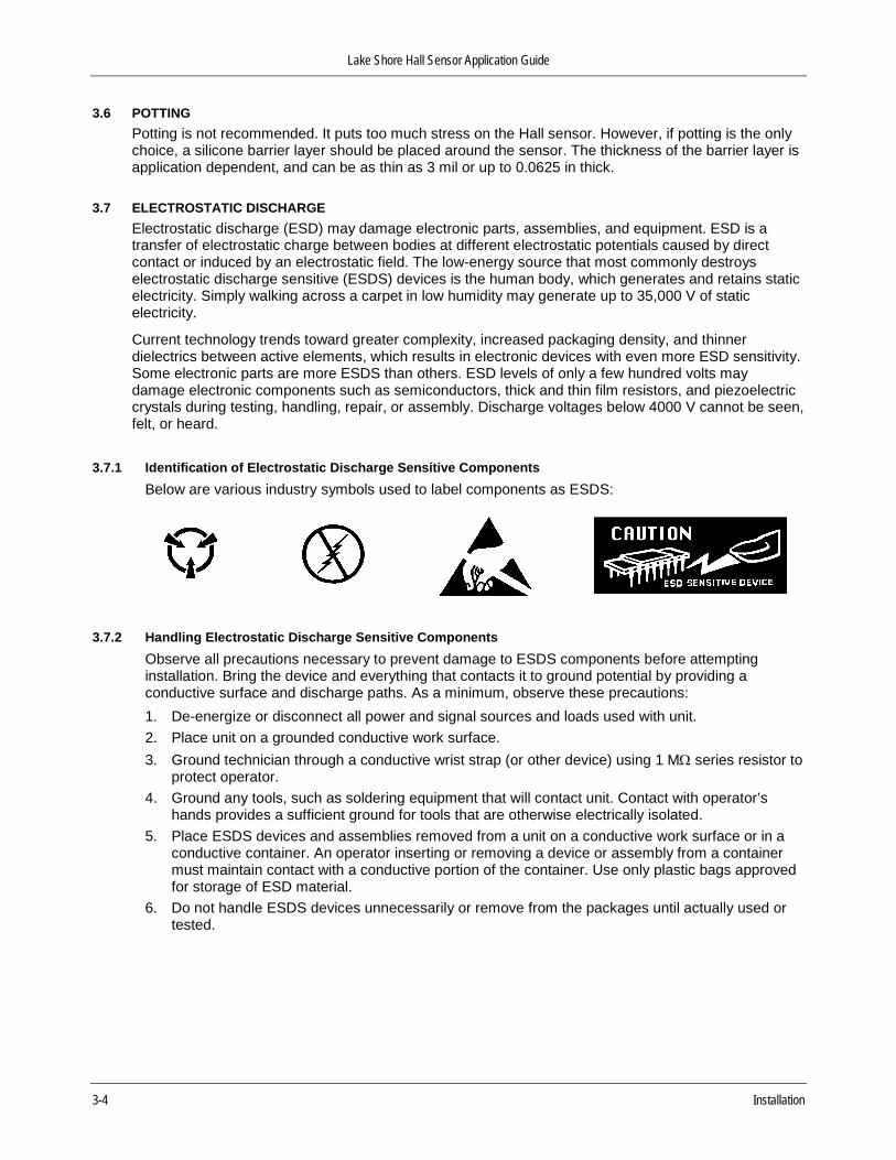
3.7.1 Identification of Electrostatic Discharge Sensitive Components Below are various industry symbols used to label components as ESDS:

3.7.2 Handling Electrostatic Discharge Sensitive Components Observe all precautions necessary to prevent damage to ESDS components before attempting installation. Bring the device and everything that contacts it to ground potential by providing a conductive surface and discharge paths. As a minimum, observe these precautions:

1. De-energize or disconnect all power and signal sources and loads used with unit. 2. Place unit on a grounded conductive work surface. 3. Ground technician through a conductive wrist strap (or other device) using 1 MΩ series resistor to

protect operator. 4. Ground any tools, such as soldering equipment that will contact unit. Contact with operator’s

hands provides a sufficient ground for tools that are otherwise electrically isolated. 5. Place ESDS devices and assemblies removed from a unit on a conductive work surface or in a

conductive container. An operator inserting or removing a device or assembly from a container must maintain contact with a conductive portion of the container. Use only plastic bags approved for storage of ESD material.

6. Do not handle ESDS devices unnecessarily or remove from the packages until actually used or tested.

Lake Shore Hall Sensor Application Guide

Operation 4-1

CHAPTER 4 OPERATION

4.0 GENERAL This chapter provides operation instructions for the Lake Shore Hall sensor. A Hall sensor generic hookup is provided in Section 4.1. Sensitivity versus current control is discussed in Section 4.2. Load resistor details are provided in Section 4.3. Other accuracy considerations are discussed in Section 4.4. Finally, the Error Data Report provided with each Hall sensor is described in Section 4.5. CAUTION: Care must be exercised when handling the Hall sensor. The Hall sensor is very fragile. Stressing

the Hall sensor can alter its output. Any excessive force can easily break the Hall sensor. Broken Hall sensors are not repairable.

4.1 HALL SENSOR GENERIC HOOKUP The Hall voltage leads may also be connected directly to a readout instrument, such as a high impedance voltmeter, or can be attached to electronic circuitry for amplification or conditioning. Device signal levels will be in the range of microvolts to hundreds of millivolts. In this case, a separate precision current source (Lake Shore Model 121 or equivalent) is necessary. See Figure 4-1. CAUTION: The four Hall sensor leads connect to four points on a sheet of semiconductor material having

different potentials. No two leads can be connected together without adversely affecting operation. Therefore, the current source and the output indicator cannot have a common connection, but must be isolated from each other. One, the other, but not both, may be grounded.

CAUTION: Do not exceed the maximum continuous control current given in the specifications.

Figure 4-1. Typical Hall Sensor Hookup

4.2 SENSITIVITY VERSUS CONTROL CURRENT Control currents (input) can be raised or lowered from the “Nominal” value given in the specifications (Chapter 1). The sensitivity given will very accurately follow the current value (i.e., doubling the current will double the sensitivity). However, it must be realized that the other parameters such as offset voltage and offset voltage drift with temperature also alter with the control current.

Lake Shore Hall Sensor Application Guide

4-2 Operation

4.3 LOAD RESISTOR (RL) To attain their rated linearity and sensitivity, some Hall sensors require that a load resistor (RL) be part of the installation. Load resistors (not included) are often specified. For example, this is true of, but not limited to, the Series 3010, 3020, and 3030 devices. Since every Hall sensor is slightly different, a unique value of load resistor may be required for each. Metal film resistors with 1% or better accuracy are recommended. The power rating of the resistor is not critical. Since those Hall sensors requiring a load resistor are calibrated at Lake Shore with the resistor placed at the end of the leads supplied, it is imperative that the user does the same. Any variation from this condition may affect the calibration, determined sensitivity, and linearity. For critical applications, consult the factory for assistance. For applications where the factory-calibrated sensitivity is not of prime importance, the load resistor can be placed some distance from the Hall sensor. This may be especially helpful where the Hall device is in a cryogenic environment, and it is desired to keep the load resistor at room temperature. Because the extension leads act as part of a voltage divider in series with the device output resistance and the load resistor, it is always suggested that the extension leads be as low impedance as possible to maintain maximum Hall voltage. Remember, the above requirement applies mainly where a load resistor is positioned at the end of a long set of extension leads. If no load resistor is required, and the receiving instrumentation has high input impedance, then no drop in Hall voltage occurs.

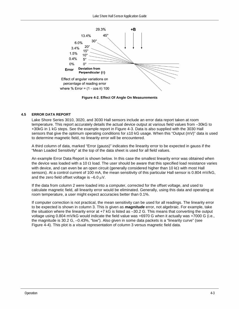
4.4 OTHER ACCURACY CONSIDERATIONS In addition to maintaining an accurate constant current input drive and properly loading the Hall sensor output, as mentioned above, the user must be aware that other factors can affect the accuracy of measurement. Linearity Error: The Hall sensor output is not perfectly linear with magnetic field. This non-linearity is given in the specifications (Chapter 1). This full error may be realized when using a single sensitivity value. On certain device models, data is supplied which can be used to nullify this error, or at least be used to indicate what the error is (Section 4.5). Zero Field Offset Voltage: Hall sensors exhibit an output voltage even when there is no magnetic field. This offset voltage must be accounted for mathematically in any field calculation. The offset can be positive or negative, and could be substantial in value, especially when measuring low field values. Temperature Effects: Temperature affects Hall sensors in two separate ways. First, the magnetic sensitivity of the device changes with temperature (see specification “Mean temperature Coefficient of Magnetic Sensitivity”). This change is a percent of the reading, and becomes greater in gauss (or tesla) error as the measured field increases. Totally separate is a drift in the Zero Field Offset Voltage. This is usually given as a specific voltage (i.e., gauss) change per temperature change. This offset error can be much greater than the sensitivity error at low field readings. However, if the user can measure the offset at temperature, then this can be adjusted for and is of no effect. Field Orientation: Hall sensor output varies with the angle of the field vector to the plane of the sensor. The output is maximum when the magnetic field is perpendicular to the device. It should be noted that all Hall sensors are calibrated with the field vector 90° to the sensor active area. Thus, every effort must be made to duplicate this condition in use. See Figure 4-2 for errors encountered when the sensor is not perpendicular to the magnetic field.

Lake Shore Hall Sensor Application Guide

Operation 4-3

Figure 4-2. Effect Of Angle On Measurements

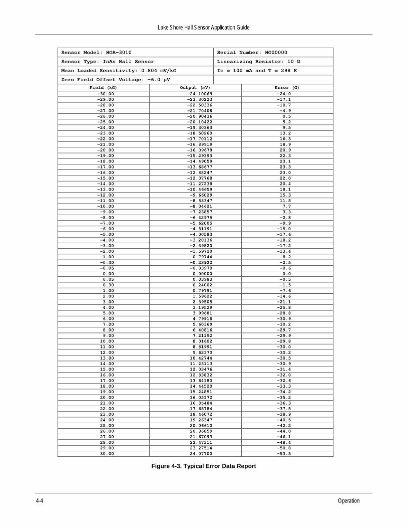
4.5 ERROR DATA REPORT Lake Shore Series 3010, 3020, and 3030 Hall sensors include an error data report taken at room temperature. This report accurately details the actual device output at various field values from –30kG to +30kG in 1 kG steps. See the example report in Figure 4-3. Data is also supplied with the 3030 Hall sensors that give the optimum operating conditions for ±10 kG usage. When this “Output (mV)” data is used to determine magnetic field, no linearity error will be encountered. A third column of data, marked “Error (gauss)” indicates the linearity error to be expected in gauss if the “Mean Loaded Sensitivity” at the top of the data sheet is used for all field values. An example Error Data Report is shown below. In this case the smallest linearity error was obtained when the device was loaded with a 10 Ω load. The user should be aware that this specified load resistance varies with device, and can even be an open circuit (generally considered higher than 10 kΩ with most Hall sensors). At a control current of 100 mA, the mean sensitivity of this particular Hall sensor is 0.804 mV/kG, and the zero field offset voltage is –6.0 µV. If the data from column 2 were loaded into a computer, corrected for the offset voltage, and used to calculate magnetic field, all linearity error would be eliminated. Generally, using this data and operating at room temperature, a user might expect accuracies better than 0.1%. If computer correction is not practical, the mean sensitivity can be used for all readings. The linearity error to be expected is shown in column 3. This is given as magnitude error, not algebraic. For example, take the situation where the linearity error at +7 kG is listed as –30.2 G. This means that converting the output voltage using 0.804 mV/kG would indicate the field value was +6970 G when it actually was +7000 G (i.e., the magnitude is 30.2 G, –0.43%, “low”). Also given in some data packets is a “linearity curve” (see Figure 4-4). This plot is a visual representation of column 3 versus magnetic field data.

Lake Shore Hall Sensor Application Guide

4-4 Operation

Sensor Model: HGA-3010 Serial Number: HG00000

Sensor Type: InAs Hall Sensor Linearizing Resistor: 10 Ω

Mean Loaded Sensitivity: 0.804 mV/kG Ic = 100 mA and T = 298 K

Zero Field Offset Voltage: -6.0 µV Field (kG) Output (mV) Error (G)

-30.00 -24.10069 -24.0 -29.00 -23.30223 -17.1 -28.00 -22.50336 -10.7 -27.00 -21.70408 -4.9 -26.00 -20.90436 0.5 -25.00 -20.10422 5.2 -24.00 -19.30363 9.5 -23.00 -18.50260 13.2 -22.00 -17.70112 16.3 -21.00 -16.89919 18.9 -20.00 -16.09679 20.9 -19.00 -15.29393 22.3 -18.00 -14.49059 23.1 -17.00 -13.68677 23.3 -16.00 -12.88247 23.0 -15.00 -12.07768 22.0 -14.00 -11.27238 20.4 -13.00 -10.46659 18.1 -12.00 -9.66029 15.3 -11.00 -8.85347 11.8 -10.00 -8.04621 7.7 -9.00 -7.23857 3.3 -8.00 -6.42975 -2.8 -7.00 -5.62005 -9.9 -6.00 -4.81191 -15.0 -5.00 -4.00583 -17.6 -4.00 -3.20136 -18.2 -3.00 -2.39820 -17.2 -2.00 -1.59720 -13.4 -1.00 -0.79744 -8.2 -0.30 -0.23922 -2.5 -0.05 -0.03970 -0.6 0.00 0.00000 0.0 0.05 0.03983 –0.5 0.30 0.24002 -1.5 1.00 0.79791 -7.6 2.00 1.59622 -14.6 3.00 2.39505 -21.1 4.00 3.19529 -25.8 5.00 3.99681 -28.8 6.00 4.79918 -30.9 7.00 5.60369 -30.2 8.00 6.40816 -29.7 9.00 7.21192 -29.9

10.00 8.01602 -29.8 11.00 8.81991 -30.0 12.00 9.62370 -30.2 13.00 10.42744 -30.5 14.00 11.23113 -30.9 15.00 12.03476 -31.4 16.00 12.83832 -32.0 17.00 13.64180 -32.6 18.00 14.44520 -33.3 19.00 15.24851 -34.2 20.00 16.05172 -35.2 21.00 16.85484 -36.3 22.00 17.65784 -37.5 23.00 18.46072 -38.9 24.00 19.26347 -40.5 25.00 20.06610 -42.2 26.00 20.86859 -44.0 27.00 21.67093 -46.1 28.00 22.47311 -48.4 29.00 23.27514 -50.8 30.00 24.07700 -53.5

Figure 4-3. Typical Error Data Report

Lake Shore Hall Sensor Application Guide

Operation 4-5

Figure 4-4. Typical Linearity Error Data Plot

Lake Shore Hall Sensor Application Guide

Glossary of Terminology A-1

APPENDIX A GLOSSARY OF TERMINOLOGY

accuracy. The degree of correctness with which a measured value agrees with the true value.2

electronic accuracy. The accuracy of an instrument independent of the sensor. sensor accuracy. The accuracy of a temperature sensor and its associated calibration or its ability to match a standard curve.

active area. The Hall sensor assembly contains the sheet of semiconductor material to which the four contacts are made. This entity is normally called a “Hall plate.” The Hall plate is, in its simplest form, a rectangular shape of fixed length, width and thickness. Due to the shorting effect of the current supply contacts, most of the sensitivity to magnetic fields is contained in an area approximated by a circle, centered in the Hall plate, whose diameter is equal to the plate width.

ampere. The constant current that, if maintained in two straight parallel conductors of infinite length, of negligible circular cross section, and placed one meter apart in a vacuum, would produce between these conductors a force equal to 2 × 10–7 newton per meter of length.2 This is one of the base units of the SI.

ampere-turn. A MKS unit of magnetomotive force equal to the magnetomotive force around a path linking one turn of a conducting loop carrying a current of one ampere; or 1.26 gilberts.

ampere/meter (A/m). The SI unit for magnetic field strength (H). 1 ampere/meter = 4π/1000 oersted ≈ 0.01257 oersted. bipolar magnet. A permanent magnet that has been magnetized in two different field directions, with one side being designated north

and the other south. calibration. To determine, by measurement or comparison with a standard, the correct (accurate) value of each scale reading on a

meter or other device, or the correct value for each setting of a control knob.1 cgs system of units. A system in which the basic units are the centimeter, gram, and second.2 coercive force (coercive field). The magnetic field strength (H) required to reduce the magnetic induction (B) in a magnetic material

to zero. coercivity. generally used to designate the magnetic field strength (H) required to reduce the magnetic induction (B) in a magnetic

material to zero from saturation. The coercivity would be the upper limit to the coercive force. compliance voltage. See current source. current source. A type of power supply that supplies a constant current through a variable load resistance by automatically varying

its compliance voltage. A single specification given as “compliance voltage” means the output current is within specification when the compliance voltage is between zero and the specified voltage.

demagnetization. when a sample is exposed to an applied field (Ha), poles are induced on the surface of the sample. Some of the returned flux from these poles is inside of the sample. This returned flux tends to decrease the net magnetic field strength internal to the sample yielding a true internal field (Hint) given by: Hint = Ha – DM ,where M is the volume magnetization and D is the demagnetization factor. D is dependent on the sample geometry and orientation with respect to the field.

deviation. The difference between the actual value of a controlled variable and the desired value corresponding to the setpoint.1 differential permeability. The slope of a B versus H curve: µd = dB/dH. differential susceptibility. The slope of a M versus H curve: χd = dM/dH. dimensionless sensitivity. Sensitivity of a physical quantity to a stimulus, expressed in dimensionless terms. The dimensionless

temperature sensitivity of a resistance temperature sensor is expressed as Sd = (T/R)(dR/dT) which is also equal to the slope of R versus T on a log-log plot, that is Sd = d lnR / d lnT. Note that absolute temperature (in kelvin) must be used in these expressions.

electromagnet. A device in which a magnetic field is generated as the result of electrical current passing through a helical conducting coil. It can be configured as an iron-free solenoid in which the field is produced along the axis of the coil, or an iron-cored structure in which the field is produced in an air gap between pole faces. The coil can be water cooled copper or aluminum, or superconductive.

electron. An elementary particle containing the smallest negative electric charge. Note: The mass of the electron is approximately equal to 1/1837 of the mass of the hydrogen atom.2

electrostatic discharge (ESD). A transfer of electrostatic charge between bodies at different electrostatic potentials caused by direct contact or induced by an electrostatic field.

error. Any discrepancy between a computed, observed, or measured quantity and the true, specified, or theoretically correct value or condition.2

flux (φ). The electric or magnetic lines of force in a region.1 flux density (B). Any vector field whose flux is a significant physical quantity; examples are magnetic flux density, electric

displacement, and gravitational field.1

Lake Shore Hall Sensor Application Guide

A-2 Glossary of Terminology

gamma. A cgs unit of low-level flux density, where 100,000 gamma equals one oersted, or 1 gamma equals 10–5 oersted. gauss (G). The cgs unit for magnetic flux density (B). 1 gauss = 10–4 tesla = 1 Mx/cm2 = line/cm2. Named for Karl Fredrich Gauss

(1777 – 1855) a German mathematician, astronomer, and physicist. gaussian system (units). A system in which centimeter-gram-second units are used for electric and magnetic qualities. gilbert (Gb). A cgs electromagnetic unit of the magnetomotive force required to produce one maxwell of magnetic flux in a magnetic

circuit of unit reluctance. One gilbert is equal to 10/4π ampere-turn. Named for William Gilbert (1540 – 1603), an English physicist; hypothesized that the earth is a magnet.

gilbert per centimeter. Practical cgs unit of magnet intensity. Gilberts per cm are the same as oersteds. Greek alphabet. The Greek alphabet is defined as follows:

Alpha α Α Iota ι Ι Rho ρ Ρ Beta β Β Kappa κ Κ Sigma σ Σ Gamma γ Γ Lambda λ Λ Tau τ Τ Delta δ ∆ Mu µ Μ Upsilon υ Υ Epsilon ε Ε Nu ν Ν Phi φ Φ Zeta ζ Ζ Xi ξ Ξ Chi χ Χ Eta η Η Omicron ο Ο Psi ψ Ψ Theta θ Θ Pi π Π Omega ω Ω

ground. A conducting connection, whether intentional or accidental, by which an electric circuit or equipment is connected to the earth, or to some conducting body of large extent that serves in place of the earth. Note: It is used for establishing and maintaining the potential of the earth (or of the conducting body) or approximately that potential, on conductors connected to it, and for conducting ground current to and from the earth (or of the conducting body).2

Hall effect. The generation of an electric potential perpendicular to both an electric current flowing along a thin conducting material and an external magnetic field applied at right angles to the current. Named for Edwin H. Hall (1855 – 1938), American physicist.

Hall mobility. The quantity µH in the relation µH = Rσ, where R = Hall coefficient and σ = conductivity.2 Helmholtz coils. A pair of flat, circular coils having equal numbers of turns and equal diameters, arranged with a common axis, and

connected in series; used to obtain a magnetic field more nearly uniform than that of a single coil.1 hole. A mobile vacancy in the electronic valence structure of a semiconductor that acts like a positive electron charge with a positive

mass.2 hysteresis. The dependence of the state of a system on its previous history, generally in the form of a lagging of a physical effect

behind its cause.1 Also see magnetic hysteresis. initial permeability. The permeability determined at H = 0 and B = 0. initial susceptibility. The susceptibility determined at H = 0 and M = 0. international system of units (SI). A universal coherent system of units in which the following seven units are considered basic:

meter, kilogram, second, ampere, kelvin, mole, and candela. The International System of Units, or Système International d'Unités (SI), was promulgated in 1960 by the Eleventh General Conference on Weights and Measures. For definition, spelling, and protocols, see Reference 3 for a short, convenient guide.

interpolation table. A table listing the output and sensitivity of a sensor at regular or defined points which may be different from the points at which calibration data was taken.

intrinsic coercivity. The magnetic field strength (H) required to reduce the magnetization (M) or intrinsic induction in a magnetic material to zero.

intrinsic induction. The contribution of the magnetic material (Bi) to the total magnetic induction (B). Bi = B – µoH (SI) Bi = B – H (cgs)

line of flux. An imaginary line in a magnetic field of force whose tangent at any point gives the direction of the field at that point; the lines are spaced so that the number through a unit area perpendicular to the field represents the intensity of the field. Also known as a Maxwell in the cgs system of units.

magnetic air gap. The air space, or non-magnetic portion, of a magnetic circuit. magnetic field strength (H). The magnetizing force generated by currents and magnetic poles. For most applications, the magnetic

field strength can be thought of as the applied field generated, for example, by a superconducting magnet. The magnetic field strength is not a property of materials. Measure in SI units of A/m or cgs units of oersted.

magnetic flux density (B). Also referred to as magnetic induction. This is the net magnetic response of a medium to an applied field, H. The relationship is given by the following equation: B = µo (H + M) for SI, and B = H + 4πM for cgs, where H = magnetic field strength, M = magnetization, and µo = permeability of free space = 4π × 10–7 H/m.

magnetic hysteresis. The property of a magnetic material where the magnetic induction (B) for a given magnetic field strength (H) depends upon the past history of the samples magnetization.

magnetic induction (B). See magnetic flux density.

Lake Shore Hall Sensor Application Guide

Glossary of Terminology A-3

magnetic moment (m). This is the fundamental magnetic property measured with dc magnetic measurements systems such as a vibrating sample magnetometer, extraction magnetometer, SQUID magnetometer, etc. The exact technical definition relates to the torque exerted on a magnetized sample when placed in a magnetic field. Note that the moment is a total attribute of a sample and alone does not necessarily supply sufficient information in understanding material properties. A small highly magnetic sample can have exactly the same moment as a larger weakly magnetic sample (see Magnetization). Measured in SI units as A·m2 and in cgs units as emu. 1 emu = 10–3 A·m2.

magnetic scalar potential. The work which must be done against a magnetic field to bring a magnetic pole of unit strength from a reference point (usually at infinity) to the point in question. Also known as magnetic potential.1

magnetic units. Units used in measuring magnetic quantities. Includes ampere-turn, gauss, gilbert, line of force, maxwell, oersted, and unit magnetic pole.

magnetization (M). This is a material specific property defined as the magnetic moment (m) per unit volume (V). M = m/V. Measured in SI units as A/m and in cgs units as emu/cm3. 1 emu/cm3 = 103 A/m. Since the mass of a sample is generally much easier to determine than the volume, magnetization is often alternately expressed as a mass magnetization defined as the moment per unit mass.

magnetostatic. Pertaining to magnetic properties that do not depend upon the motion of magnetic fields.1 Maxwell (Mx). A cgs electromagnetic unit of magnetic flux, equal to the magnetic flux which produces an electromotive force of

1 abvolt in a circuit of one turn link the flux, as the flux is reduced to zero in 1 second at a uniform rate.1 neutral zone. The area of transition located between areas of a permanent magnet which have been magnetized in opposite

directions. MKSA System of Units. A system in which the basic units are the meter, kilogram, and second, and the ampere is a derived unit

defined by assigning the magnitude 4π × 10–7 to the rationalized magnetic constant (sometimes called the permeability of space). noise (electrical). Unwanted electrical signals that produce undesirable effects in circuits of control systems in which they occur.2 normalized sensitivity. For resistors, signal sensitivity (dR/dT) is geometry dependent; i.e., dR/dT scales directly with R;

consequently, very often this sensitivity is normalized by dividing by the measured resistance to give a sensitivity, sT, in percent change per kelvin. sT = (100/R) (dR/dT) %K, where T is the temperature in kelvin and R is the resistance in Ωs.

oersted (Oe). The cgs unit for the magnetic field strength (H). 1 oersted = 10¾π ampere/meter ≈ 79.58 ampere/meter. Ω (Ω). The SI unit of resistance (and of impedance). The Ω is the resistance of a conductor such that a constant current of one

ampere in it produces a voltage of one volt between its ends.2 permeability. Material parameter which is the ratio of the magnetic induction (B) to the magnetic field strength (H): µ = B/H.

Also see Initial Permeability and Differential Permeability. polynomial fit. A mathematical equation used to fit calibration data. Polynomials are constructed of finite sums of terms of the form

aixi, where ai is the ith fit coefficient and xi is some function of the dependent variable. precision. Careful measurement under controlled conditions which can be repeated with similar results. See repeatability. prefixes. SI prefixes used throughout this manual are as follows:

Factor Prefix Symbol 1024 yotta Y 1021 zetta Z 1018 exa E 1015 peta P 1012 tera T 109 giga G 106 mega M 103 kilo k 102 hecto h 101 deka da

Factor Prefix Symbol 10–1 deci d 10–2 centi c 10–3 milli m 10–6 micro µ 10–9 nano n 10–12 pico p 10–15 femto f 10–18 atto a 10–21 zepto z 10–24 yocto y

probe. A long, thin body containing a sensing element which can be inserted into a system in order to make measurements. Typically,

the measurement is localized to the region near the tip of the probe. remanence. The remaining magnetic induction in a magnetic material when the material is first saturated and then the applied field is

reduced to zero. The remanence would be the upper limit to values for the remanent induction. Note that no strict convention exists for the use of remanent induction and remanence and in some contexts the two terms may be used interchangeably.

remanent induction. The remaining magnetic induction in a magnetic material after an applied field is reduced to zero. Also see remanence.

repeatability. The closeness of agreement among repeated measurements of the same variable under the same conditions.2 See precision.

Lake Shore Hall Sensor Application Guide

A-4 Glossary of Terminology

resolution. The degree to which nearly equal values of a quantity can be discriminated.2 display resolution. The resolution of the physical display of an instrument. This is not always the same as the measurement

resolution of the instrument. Decimal display resolution specified as “n digits” has 10n possible display values. A resolution of n and one-half digits has 2 × 10n possible values.

measurement resolution. The ability of an instrument to resolve a measured quantity. For digital instrumentation this is often defined by the analog-to-digital converter being used. A n-bit converter can resolve one part in 2n. The smallest signal change that can be measured is the full scale input divided by 2n for any given range. Resolution should not be confused with accuracy.

scalar. A quantity which has magnitude only and no direction, in contrast to a vector.1 semiconducting material. A conducting medium in which the conduction is by electrons, and holes, and whose temperature

coefficient of resistivity is negative over some temperature range below the melting point.2 semiconductor. An electronic conductor, with resistivity in the range between metals and insulators, in which the electric charge

carrier concentration increases with increasing temperature over some temperature range. Note: Certain semiconductors possess two types of carriers, namely, negative electrons and positive holes.2

sensitivity. The ratio of the response or change induced in the output to a stimulus or change in the input. Temperature sensitivity of a resistance temperature detector is expressed as S = dR/dT.

SI. Système International d'Unités. See International System of Units. stability. The ability of an instrument or sensor to maintain a constant output given a constant input. susceptance. In electrical terms, susceptance is defined as the reciprocal of reactance and the imaginary part of the complex

representation of admittance: [suscept(ibility) + (conduct)ance]. susceptibility (χ). Parameter giving an indication of the response of a material to an applied magnetic field. The susceptibility is the

ratio of the magnetization (M) to the applied field (H). χ = M/H. In both SI units and cgs units the volume susceptibility is a dimensionless parameter. Multiply the cgs susceptibility by 4π to yield the SI susceptibility. See also Initial Susceptibility and Differential Susceptibility. As in the case of magnetization, the susceptibility is often seen expressed as a mass susceptibility or a molar susceptibility depending upon how M is expressed.

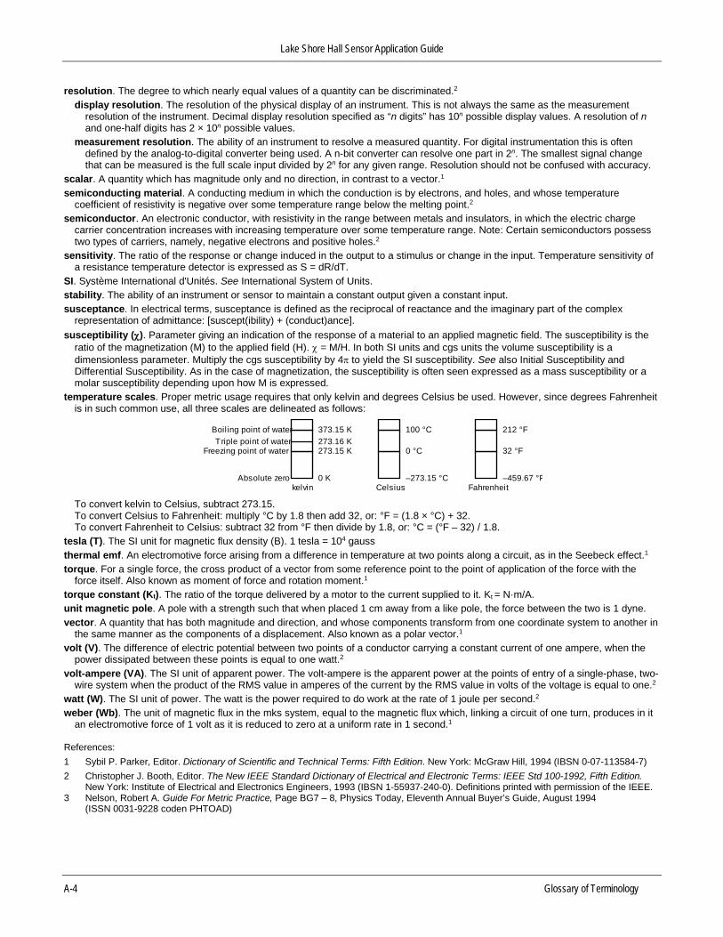
temperature scales. Proper metric usage requires that only kelvin and degrees Celsius be used. However, since degrees Fahrenheit is in such common use, all three scales are delineated as follows:

To convert kelvin to Celsius, subtract 273.15. To convert Celsius to Fahrenheit: multiply °C by 1.8 then add 32, or: °F = (1.8 × °C) + 32. To convert Fahrenheit to Celsius: subtract 32 from °F then divide by 1.8, or: °C = (°F – 32) / 1.8.

tesla (T). The SI unit for magnetic flux density (B). 1 tesla = 104 gauss thermal emf. An electromotive force arising from a difference in temperature at two points along a circuit, as in the Seebeck effect.1 torque. For a single force, the cross product of a vector from some reference point to the point of application of the force with the

force itself. Also known as moment of force and rotation moment.1 torque constant (Kt). The ratio of the torque delivered by a motor to the current supplied to it. Kt = N·m/A. unit magnetic pole. A pole with a strength such that when placed 1 cm away from a like pole, the force between the two is 1 dyne. vector. A quantity that has both magnitude and direction, and whose components transform from one coordinate system to another in

the same manner as the components of a displacement. Also known as a polar vector.1 volt (V). The difference of electric potential between two points of a conductor carrying a constant current of one ampere, when the

power dissipated between these points is equal to one watt.2 volt-ampere (VA). The SI unit of apparent power. The volt-ampere is the apparent power at the points of entry of a single-phase, two-

wire system when the product of the RMS value in amperes of the current by the RMS value in volts of the voltage is equal to one.2 watt (W). The SI unit of power. The watt is the power required to do work at the rate of 1 joule per second.2 weber (Wb). The unit of magnetic flux in the mks system, equal to the magnetic flux which, linking a circuit of one turn, produces in it

an electromotive force of 1 volt as it is reduced to zero at a uniform rate in 1 second.1 References: 1 Sybil P. Parker, Editor. Dictionary of Scientific and Technical Terms: Fifth Edition. New York: McGraw Hill, 1994 (IBSN 0-07-113584-7) 2 Christopher J. Booth, Editor. The New IEEE Standard Dictionary of Electrical and Electronic Terms: IEEE Std 100-1992, Fifth Edition.

New York: Institute of Electrical and Electronics Engineers, 1993 (IBSN 1-55937-240-0). Definitions printed with permission of the IEEE. 3 Nelson, Robert A. Guide For Metric Practice, Page BG7 – 8, Physics Today, Eleventh Annual Buyer’s Guide, August 1994

(ISSN 0031-9228 coden PHTOAD)

Boiling point of water

Freezing point of water

Absolute zerokelvin Celsius Fahrenheit

0 K

273.15 K

373.15 K

–273.15 °C

0 °C

100 °C

–459.67 °F

32 °F

212 °FTriple point of water 273.16 K