Welcome message from author
This document is posted to help you gain knowledge. Please leave a comment to let me know what you think about it! Share it to your friends and learn new things together.
Transcript


i
Antenna Bandwidth Improvement by Using Indirect
Coaxial Probe Feeding Method
By
Mohanad Basem Qraiqea
Supervisors
Prof. Dr. Mohamed Ouda
Dr. Mustfa Abu Nasar
A Thesis Submitted in Partial Fulfillment of Requirements for the Degree of Master in
Electrical Engineering-Communication Systems.
Faculty of Electrical Engineering
Islamic University of Gaza
February 2015


ii
الملخص
تستخدم هوائيات مغير التصحيح بكثرة لما لها من مزايا عديدة, مثل أنها خفيفة الوزن. ومع ذلك فان لها بعض العيوب حيث ان
عرض نطاق ترددي ضيق. مما جعل الباحثين لبذل كثير من الجهد للتغلب على هذه المشكلة, من خالل تقديم الكثير من لها
التكوينات لتوسيع عرض النطاق.
ومثال على هوائيات مغير التصحيح من الترددي النطاق عرض لتعزيز معينة تقنيات تطوير بالفعل تم قد في الفترات السابقة
. parasitic patch, U-slot patch, L-probe couplingذلك
من خالل تغذية الهوائي باساليب مختلفة. وسوف يتم اختبار (return lossالهدف من هذا البحث هو تحسين خسارة العودة )
(. سوف يتم اختبارPIFAمجموعة من الهوائيات المختلفة مثل هوائي مغير التصحيح و الهوائي ذو المستوى المقلوب )
الهوائيات في حالتين: االولى باعتبار ان الهوائي ومصدر التغذية ككتلة واحدة, اما االختبار الثاني سوف يتم التعامل مع كل من
الهوائي ومصدر التغذية كجزئين منفصلين.
الرنين عن تعمل علي زيادة مكاسب مقاومه مدخالت ير المباشرة للهوائي تعمل علي تحسين النطاق الترددي و غالتغذية ال
طريق مزامنه المكثف و الهوائي .

1
Abstract
Microstrip patch antennas are widely used because of their many advantages, such as the
low profile, light weight, and conformity. However, patch antennas have a main disadvantage
which is the narrow bandwidth. Researchers have made many efforts to overcome this problem
and many configurations have been presented to broaden the bandwidth.
Certain techniques for enhancing the bandwidth of microstrip antennas have already been
developed, e.g., parasitic patch either in stacked or coplanar geometries, U-slot patch, L-probe
coupling, aperture coupling and increasing the thickness of the antenna.
The goal of this research is to improve the return loss bandwidth by using different feeding
techniques. This technique will be tested for various planner antenna types such as microstrip
antenna and Planar Inverted F Antenna (PIFA). The research will consider the antenna and its
feeder in two modes. The first one will consider them as the one part and the second will separate
them in treatment.
Indirect Probe Feeding gains large band of impedance resonance obtained by adjusting the
capacitance and the inductance of feeder part.

2
Dedication
edicated to my soul brothers, Dr. Monther (Abu-Basem), Moatz (Abu-Islam) and my
soul nephew Islam, and to all my brother and sisters ( Ezzedeen , Sultan , Mohammed , Mazin,
Sheymaa, Shreen, Karem and Shams. Finally, to my parents (Abu-Monther, Om-Monther).
D

3
Acknowledgment
would like to start by thanking ALLAH, without his graciousness the completion of this
work would not have been possible. Allah the Almighty has entrusted me with the
abilities and provided me with the courage to complete a long journey.
My advisors, Prof. Mohamed Ouda, and Dr. Mustfa Abu Nasar, deserve a special word of
appreciation. They have always been there with support and guidance throughout the duration of
my graduate studies. My deepest thanks and feeling of gratitude should go to Eng. Basel O. Al-
Wadia and Eng. Yousef A. Shaban for their help, software development, and for all their time and
assistance with the construction of antenna prototypes and many antenna measurements.
My parents, family and friends definitely deserve a special word of thanks for always being
there to support and encourage me. They have always showed a great deal of interest in my
studies.
Finally, I must express my sincere gratitude to my wife, Madlen. She knows more than
anyone else about the sacrifices that had to be made. I would like to thank her for her love,
encouragement, patience and understanding throughout all of my studies. It is much appreciated.
I

4
TABLE OF COTENTS
Abstract ........................................................................................................................................... 1
Acknowledgment ............................................................................................................................. 3
List of Figures ................................................................................................................................. 7
List of Table .................................................................................................................................. 10
Chapter 1 Introduction ................................................................................................................. 12
1.1 Introduction ................................................................................................................................. 12
1.2 Theoretical background ............................................................................................................. 12
1.3 Problem Statement ...................................................................................................................... 15
1.4 Literature Review ....................................................................................................................... 16
1.5 References .................................................................................................................................... 18
Chapter 2 Antenna Theory & Concepts ........................................................................................ 20
2.1 Antenna Types ............................................................................................................................ 20
2.1.1 Wire antennas ...................................................................................................................... 20
2.1.2 Horn Antennas .................................................................................................................... 27
2.1.3 MICROSTRIP PATCH ANTENNA ................................................................................. 28
2.1.4 Array Antenna..................................................................................................................... 29
2.1.5 FRACTAL Antenna ............................................................................................................ 32
2.1.6 Reflector Antenna ............................................................................................................... 33
2.1.7 Lens Antennas ..................................................................................................................... 34
2.2 Antenna Parameter ..................................................................................................................... 34
2.2.1 Radiation pattern ................................................................................................................ 34
2.2.2 Gain ...................................................................................................................................... 36
2.2.3 Bandwidth ............................................................................................................................ 37
2.2.4 Beamwidth ........................................................................................................................... 37
2.2.5 Polarization .......................................................................................................................... 38
2.2.6 Return Loss .......................................................................................................................... 39
2.2.7 Antenna Efficiency .............................................................................................................. 39
2.2.8 Input Impedance ................................................................................................................ 40
2.2.9 Directivity ............................................................................................................................ 40
2.3 Small Antenna ............................................................................................................................. 41

5
2.3.1 Definition of a Small Antenna ............................................................................................ 41
2.3.2 Significance of small antennas ........................................................................................... 42
2.3.3 Small antenna Parameters ................................................................................................ 43
2.4 Bandwidth Enhancement Techniques ....................................................................................... 44
2.4.1 Wideband Impedance-Matching Networks ............................................................................. 44
2.4.2 Edge-Coupled Patches ........................................................................................................ 45
2.4.3 Stacked Patches .................................................................................................................. 46
2.4.4 Shaped Probes ..................................................................................................................... 47
2.4.5 Capacitive Coupling and Slotted Patches ......................................................................... 49
2.4.6 Capacitive Feed Probes ...................................................................................................... 51
2.5 Feed Techniques .......................................................................................................................... 52
2.5.1 Coaxial Feed ........................................................................................................................ 52
2.5.2 Microstrip Feed line ............................................................................................................ 53
2.5.3 Aperture Coupled Feed ..................................................................................................... 54
2.5.4 Proximity Coupled Feed ..................................................................................................... 55
2.6 OVERVIEW OF MODELLING TECHNIQUES.................................................................... 56
2.6.1 Approximate Methods ....................................................................................................... 56
2.7 Finite element method ................................................................................................................ 60
2.8 HFSS............................................................................................................................................ 62
References ................................................................................................................................................ 64
Bandwidth enhancement of Microstrip Patch Antenna using New Feeding Technique (indirect
probe feed) ............................................................................................................................................... 70
3.1: Introduction to Antenna design .................................................................................................. 70
3.2: MSP antenna with parasitic ....................................................................................................... 74
3.3: Bandwidth enhancement of antenna using new feeding technique IPF. ................................ 76
3.4: Change the position of with indirect probe feeding .................................................................. 78
3.5: Change the position of probe feed indirect probe feeding ....................................................... 89
3.6: Changing the inner radius of probe feed. .................................................................................. 97
3.7: Changing the length of stripline ................................................................................................ 99
3.8: Hexagonal MSP antenna with probe feed patch ..................................................................... 103
3.9: Hexagonal MSP antenna with indirect probe feed patch ...................................................... 105
Chapter 4 .................................................................................................................................... 109

6
CONCLUSION AND FUTURE PROSPECTS ............................................................................ 109

7
List of Figures
Figure 1. 1: Microstrip antennas and their feeds (a) a microstrip antenna with its coordinates, (b) three
feeding configuration: coupling feed, microstrip feed and coaxial feed [7] ................................................. 13
Figure 1. 2: Structure of the planar inverted-F antenna. ............................................................................... 14
Figure 1. 3: Illustrative performance trends of a microstrip patch antenna. (a) Impedance bandwidth. (b)
surface-wave efficiency. ............................................................................................................................... 15
Figure 1. 4: probe feed (a) direct (b) indirect. ............................................................................................... 16
Figure 2. 1: A configuration for a general Yagi antenna ............................................................................... 21
Figure 2. 2: A typical radiation pattern of a Yagi antenna (13 elements. Right: E-Plane. Left: H-plane). ... 22
Figure 2. 3: Half Wave Dipole. ..................................................................................................................... 22
Figure 2. 4: Radiation pattern for Half wave dipole. .................................................................................... 23
Figure 2. 5: Monopole Antenna .................................................................................................................... 23
Figure 2. 6: Radiation pattern for the Monopole Antenna. ........................................................................... 24
Figure 2. 7: Loop Antenna. ........................................................................................................................... 24
Figure 2. 8: Radiation Pattern of Small and Large Loop Antenna. ............................................................... 25
Figure 2. 9: Helix Antenna. ........................................................................................................................... 26
Figure 2. 10: Radiation Pattern of Helix Antenna......................................................................................... 27
Figure 2. 11: Types of Horn Antenna. .......................................................................................................... 27
Figure 2. 12: Structure of a Microstrip Patch Antenna. ................................................................................ 28
Figure 2. 13: Common shapes of microstrip patch elements. ....................................................................... 29
Figure 2. 14: Different types of antenna array structures.............................................................................. 31
Figure 2. 15: Comparison of array pattern for different numbers of antenna array elements. ...................... 31
Figure 2. 16: Types of fractal geometries. .................................................................................................... 33
Figure 2. 17: Lens antenna configuration. .................................................................................................... 34
Figure 2. 18: Radiation pattern of a generic directional antenna. ................................................................. 35
Figure 2. 19: Antenna classification based on the radiation pattern............................................................ 36
Figure 2. 20: Types of Polarization. ............................................................................................................... 38
Figure 2. 21: Geometry of a probe-fed microstrip patch antenna with a wideband impedance-matching
network. ........................................................................................................................................................ 45
Figure 2. 22: Geometry of a probe-fed microstrip patch element that is edge-coupled to the parasitic
patches. ......................................................................................................................................................... 46
Figure 2. 23: Geometry of a probe-fed stacked microstrip patch antenna. ................................................... 47
Figure 2. 24: Geometries of microstrip patch antennas with shaped probes. (a) Stepped probe. (b) L-shaped
probe. ............................................................................................................................................................ 49
Figure 2. 25: Geometries of probe-fed microstrip patch antennas where capacitive coupling and slots are
used. (a) Capacitive coupling. (b) Annular slot in the surface of the patch. ................................................. 50
Figure 2. 26: Geometries of the microstrip patch antennas employing capacitive feed probes. (a) Circular
capacitor patch. (b) Rectangular capacitor patch. ......................................................................................... 51

8
Figure 2. 27: Rectangular Microstrip antenna coaxial feed ......................................................................... 53
Figure 2. 28: Rectangular Microstrip antenna of Microstrip Line feeding. .................................................. 54
Figure 2. 29: Rectangular Microstrip antenna Aperture coupled feed. ......................................................... 54
Figure 2. 30: Proximity-coupled Feed. ......................................................................................................... 55
Figure 2. 31: Plane view of rectangular patch antenna and its equivalent circuit. ........................................ 57
Figure 2. 32: Flow chart for the design procedure of a rectangular patch antenna. ...................................... 60
Figure 2. 33: Full-wave EM analysis in the FEM. ........................................................................................ 61
Figure 3. 1: The proposed microstrip patch in HFSS 15 environment in 3D. .............................................. 72
Figure 3. 2: Return loss of microstrip patch antenna. ................................................................................... 72
Figure 3. 3: Gain of microstrip patch antenna. ............................................................................................. 73
Figure 3. 4: Input impedance of microstrip patch antenna. ........................................................................... 73
Figure 3. 5: The proposed MSP antenna with parasitic. ............................................................................... 74
Figure 3. 6:Return loss of MSP antenna with parasitic. ............................................................................. 75
Figure 3. 7: Gain of MSP antenna with parasitic. ......................................................................................... 76
Figure 3.8: Input impedance of MSP antenna with parasitic. ....................................................................... 76
Figure 3. 9: MSP antenna with IPF at stripline position = 0cm. ................................................................... 77
Figure 3. 10: Return loss of MSP antenna with IPF position = 0cm. ........................................................... 77
Figure 3. 11: Input impedance of gain MSP antenna with IPF position = 0cm. ........................................... 78
Figure 3. 12: MSP antenna with IPF position = y cm. .................................................................................. 79
Figure 3. 13: Return loss of MSP antenna with IPF position =y cm. ........................................................... 79
Figure 3. 14: Gain of MSP antenna with IPF position = y cm. ..................................................................... 80
Figure 3. 15: Input impedance of MSP antenna with IPF position = y cm. .................................................. 80
Figure 3. 16: MSP antenna with IPF position = 2y cm. ................................................................................ 81
Figure 3. 17: Return loss of MSP antenna with IPF position = 2y cm. ........................................................ 81
Figure 3. 18: Gain of MSP antenna with IPF position = 2y cm. ................................................................ 82
Figure 3. 19: Input impedance of MSP antenna with IPF position = 2y cm. ................................................ 82
Figure 3. 20: MSP antenna with IPF position = 3y cm. ................................................................................ 83
Figure 3. 21: Return loss of MSP antenna with IPF position = 3y cm. ........................................................ 83
Figure 3. 22: Gain of MSP antenna with IPF position = 3y cm. ................................................................... 84
Figure 3. 23: Input impedance of MSP antenna with IPF position = 3y cm. ................................................ 84
Figure 3. 24: MSP antenna with IPF position = 4y cm. ................................................................................ 85
Figure 3. 25: Return loss of MSP antenna with IPF position = 4y cm. .................................................... 85
Figure 3. 26: Gain of MSP antenna with IPF position = 4y cm. ................................................................... 86
Figure 3. 27: Input impedance of MSP antenna with IPF position = 4y cm. ................................................ 86
Figure 3. 28: MSP antenna with IPF position = 5y cm. ................................................................................ 87
Figure 3. 29: Return loss of MSP antenna with IPF position =5y cm. ......................................................... 87
Figure 3. 30: Gain of MSP antenna with IPF position = 5y cm. ................................................................... 88
Figure 3. 31: Input impedance of MSP antenna with IPF position 5ycm. .................................................... 88
Figure 3. 32: Return loss Results compared by varying indirect probe feed positions. ................................ 89
Figure 3. 33: MSP antenna with probe feed position = x cm. ....................................................................... 90

9
Figure 3. 34: Return loss of MSP antenna at probe feed position = x cm. ................................................... 90
Figure 3. 35: Gain MSP antenna with probe feed position = x cm. .............................................................. 91
Figure 3. 36: Input impedance of MSP antenna with probe feed position = x cm. ....................................... 91
Figure 3. 37: MSP antenna with probe feed position = 2x cm. ..................................................................... 92
Figure 3. 38:Return loss of MSP antenna at probe feed position = 2x cm.................................................... 92
Figure 3. 39: MSP antenna with probe feed position = 3x cm. ..................................................................... 93
Figure 3. 40: Return loss of MSP antenna at probe feed position = 3x cm................................................... 93
Figure 3. 41: MSP antenna with probe feed position = 4x cm. ..................................................................... 94
Figure 3. 42: Return loss of MSP antenna at probe feed position = 4x cm................................................... 94
Figure 3. 43: MSP antenna with probe feed position = 5x cm. ..................................................................... 95
Figure 3. 44: Return loss of MSP antenna at probe feed position = 5x cm................................................... 95
Figure 3. 45: Return loss for this parametric solution comparing the results obtained by varying Feed feed
position. ......................................................................................................................................................... 96
Figure 3. 46: MSP antenna with change inner radius of probe feed to 0.073cm. ......................................... 97
Figure 3. 47: Return loss of MSP antenna with inner radius of probe feed at 0.073cm. .............................. 98
Figure 3. 48: Gain of MSP antenna with inner probe feed radius at 0.073cm. ............................................. 98
Figure 3. 49: Input impedance of MSP antenna with inner probe feed radius at 0.073cm. .......................... 99
Figure 3. 50: MSP antenna with the length of IPF on x axis in order to be smallest. ................................... 99
Figure 3. 51: Return loss if MSP antenna with the length of IPF on x axis in order to be smallest. .......... 100
Figure 3. 52: Gain MSP antenna with the length of IPF on x axis in order to be smallest. ........................ 100
Figure 3. 53: Input impedance of MSP antenna with the length of IPF on x axis in order to be smallest. . 101
Figure 3. 54: MSP antenna with IPF with the same length of the patch. .................................................... 102
Figure 3. 55: Return loss of MSP antenna with the length of IPF on x axis the same length of the patch.
.................................................................................................................................................................... 102
Figure 3. 56: Gain of MSP antenna with the length of IPF on x axis the same length of the patch. .......... 103
Figure 3. 57: Input impedance of MSP antenna with the length of IPF on x axis the same length of the
patch. ........................................................................................................................................................... 103
Figure 3. 58: Hexagonal MSP antenna with probe feed patch. ................................................................... 104
Figure 3. 59: Return loss hexagonal MSP antenna with probe feed. .......................................................... 104
Figure 3. 60: Gain hexagonal MSP antenna with probe feed. .................................................................... 105
Figure 3. 61: Hexagonal MSP antenna with indirect probe feed patch....................................................... 105
Figure 3. 62: Return loss Hexagonal MSP antenna with indirect probe feed patch.................................... 106
Figure 3. 63: Gain of Hexagonal MSP antenna with indirect probe feed patch. ........................................ 106

10
List of Table
Table 2. 1: Comparing the Different Feed Techniques[68]. ......................................................................... 55
Table 3. 1: Results of MSP antenna. ............................................................................................................. 73
Table 3. 2: Results of MSP antenna with parasitic ....................................................................................... 75
Table 3. 3: Results of MSP antenna with IPF. .............................................................................................. 77
Table 3. 4: MSP antenna parameters with IPF position = 0cm. .................................................................... 78
Table 3. 5: MSP antenna parameters with IPF position = y cm. ................................................................... 79
Table 3. 6: MSP antenna parameters with IPF position = 2y cm. ................................................................. 81
Table 3. 7: MSP antenna parameters with IPF position = 3y cm. ................................................................. 83
Table 3. 8: MSP antenna parameters with IPF position = 4y cm. ................................................................. 85
Table 3. 9: MSP antenna parameters with PF position = x cm. .................................................................... 90
Table 3. 10: Simulated results for different probe feed positions for microstrip patch antenna. .................. 96
Table 3. 11: Parameters of MSP antennas with radius of inner probe feed is 0.073cm. ............................... 98

11
Abbreviation
PIFA Planar Inverted F Antenna
MMICs Monolithic Microwave Integrated Circuits
WLAN Wireless Local Networks
IPF Indirect Probe Feeding
VSWR Voltage Standing Wave Ratio
ESA Electrically Small Antenna
PCSA Physically Constrained Small Antenna
FSA Functionally Small Antenna
PSA Physically Small Antenna
NFC Near Field Communication systems
RFID Radio Frequency Identification
UWB Ultra-Wide Band
WLAN Wireless Local Area Networks
WiMAX Worldwide Interoperability for Microwave Access
FEM Finite Element Method
PDE partial differential equation
MSP microstrip patch antenna
LHM Left-handed meta-material
12
Chapter 1 Introduction
1.1 Introduction
Communication can be broadly defined as the transfer of information from one point to
another [1]. Communication between human beings was first done through voice. With the desire
to increase the distance of communication, devices such as Drums, signal flags and smoke were
used. These optical communication devices of course utilized the light part of the electromagnetic
spectrum. It has been of recent in human history that the electromagnetic spectrum, outside the
visible region has been employed for communication, through the use of Radio. One of the
greatest human scientific evolutions is the emergence of electromagnetic spectrum and antenna
has been instrumental in harnessing the resource [2].
Antennas are a very important component of communication systems. By definition, an
antenna is a device used to transform an RF signal, traveling on a conductor, into an
electromagnetic wave in free space [3]. Another explanation says that an antenna can be defined
usually metallic device, which radiates and receives electromagnetic waves more specifically,
radio waves. Antennas demonstrate a property known as reciprocity, which means that an antenna
will maintain the same characteristics regardless if it is transmitting or receiving. Most antennas
are resonant devices, which operate efficiently over a relatively narrow frequency band [4].
There are several types of antennas were developed since the past times due nowadays.
Such as wire antennas; aperture antennas; microstrip antennas; Array Antennas; reflector
antennas; and lens antennas [4].
1.2 Theoretical background
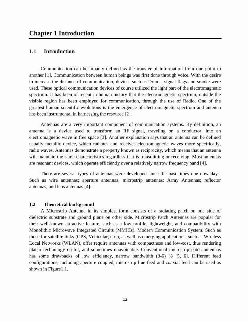
A Microstrip Antenna in its simplest form consists of a radiating patch on one side of
dielectric substrate and ground plane on other side. Microstrip Patch Antennas are popular for
their well-known attractive feature, such as a low profile, lightweight, and compatibility with
Monolithic Microwave Integrated Circuits (MMICs). Modern Communication System, Such as
those for satellite links (GPS, Vehicular, etc.), as well as emerging applications, such as Wireless
Local Networks (WLAN), offer require antennas with compactness and low-cost, thus rendering
planar technology useful, and sometimes unavoidable. Conventional microstrip patch antennas
has some drawbacks of low efficiency, narrow bandwidth (3-6) % [5, 6]. Different feed
configurations, including aperture coupled, microstrip line feed and coaxial feed can be used as
shown in Figure1.1.
13
Figure 1. 1: Microstrip antennas and their feeds (a) a microstrip antenna with its coordinates, (b) three feeding
configuration: coupling feed, microstrip feed and coaxial feed [7]
Planar inverted-F antennas (PIFAs):
PIFAs have received much attention because their size makes them suitable for integration
into portable communication devices. For instance, Ogawa et al. designed a PIFA suitable for
shoulder mounting, [8] Virga and Rahmat-Samii [9] included a PIFA on a handset, and Ng et al.
developed a PIFA for inclusion on a laptop computer chassis [10].
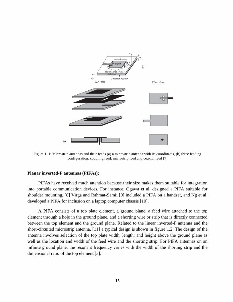
A PIFA consists of a top plate element, a ground plane, a feed wire attached to the top
element through a hole in the ground plane, and a shorting wire or strip that is directly connected
between the top element and the ground plane. Related to the linear inverted-F antenna and the
short-circuited microstrip antenna, [11] a typical design is shown in figure 1.2. The design of the
antenna involves selection of the top plate width, length, and height above the ground plane as
well as the location and width of the feed wire and the shorting strip. For PIFA antennas on an
infinite ground plane, the resonant frequency varies with the width of the shorting strip and the
dimensional ratio of the top element [3].

14
Figure 1. 2: Structure of the planar inverted-F antenna.
Rectangular and circular patches are most common, but any shape that possesses a
reasonably well-defined resonant mode can be used [1]. These include, for example, annular
rings, ellipses and triangles. The patch is a resonant element and therefore one of its dimensions
must be approximately one half of the guided wavelength in the presence of the dielectric
substrate. There are four fundamental techniques to feed or excite the patch. These are presented
in chapter 3 and include the microstrip-line feed, the probe feed, the aperture-coupled feed and the
proximity-coupled feed. The main drawback associated with microstrip patch antennas in general
is that they inherently have a very narrow impedance bandwidth (due to their multilayered
configuration, aperture-coupled feeds and proximity-coupled feeds tend to have a slightly wider
bandwidth than probe feeds and microstrip-line feeds). In most cases, the impedance bandwidth is
not wide enough to handle the requirements of modern wireless communications systems [2]. The
narrow impedance bandwidth of microstrip patch antennas can be referred to the thin substrates
that are normally used to separate the patch and the ground plane. The general performance trends
of a microstrip patch antenna are illustrated in Figure 1.3. Here, Figure 1.3(a) shows the typical
trend for impedance bandwidth versus substrate thickness, as a function of the substrate’s
dielectric constant, while Figure 1.3(b) shows the typical trend for surface-wave efficiency versus
substrate thickness, also as a function of the substrate's dielectric constant. From these it can be
seen that, in order to increase the bandwidth, the substrate thickness has to be increased, while the
dielectric constant has to be kept as low as possible. A low dielectric constant is also required to
keep surface-wave losses as low as possible. Therefore, in order to obtain a wideband microstrip
patch antenna with good surface-wave efficiency, the performance trends of Figure 1.3 point to a
thick substrate with a very low dielectric constant.

15
Figure 1. 3: Illustrative performance trends of a microstrip patch antenna. (a) Impedance bandwidth. (b) surface-wave
efficiency.
1.3 Problem Statement
Practically bandwidth of Microstrip Patch Antenna is narrow but today wireless
communication systems require higher operating bandwidth. Such as about 7.6% for a global
system for mobile communication (GSM; 890-960 MHz), 9.5% for a digital communication
system (DCS; 1710-1880 MHz), 5% for a personal communication system (PCS; 1850–
1990MHz) and 12.2% for a universal mobile telecommunication system (UMTS;1920-2170
MHz) [12].
Narrow bandwidth available from printed microstrip patches has been recognized as one of
the most significant factors limiting the widespread applications of this class of antennas.
Various techniques used to increase the bandwidth of microstrip patch antenna maybe
classified as follows:
1- Decreasing the Q-factor of the patch by increasing the substrate height and lowering
the dielectric constant.

16
2- Use the multiple resonators located in one plane.
3- Use the multilayer configurations with multiple resonators stacked vertically.
4- Use impedance matching networks.
One of these techniques is the indirect probe feeding. Indirect Probe Feeding gains large
band of impedance resonant obtained by adjusting the capacitance and the inductance of feeder
part.
The feeder part can be considered as small loaded dipole antenna.
The ordinary feeder
The proposed feeder
Figure 1. 4: probe feed (a) direct (b) indirect.
1.4 Literature Review
The inherently narrow impedance bandwidth is the major weakness of a microstrip antenna.
Techniques for bandwidth enhancement have been intensively studied in past decades. Several
methods including the utilization of parasitic patches [14] and thick substrates [15] have been
suggested in the literature.
Certain techniques for enhancing the bandwidth of planar antennas have already been
developed, e.g., parasitic patch either in stacked or coplanar geometries, U-slot patch [16], L-
probe coupling [17], aperture coupling and increasing the thickness of the antenna. In this
research, a novel simple alternative for enhancing the impedance bandwidth of a conventional
quarter-wave patch antenna is proposed.

17
Methodology
Different method and technique related to enhance the bandwidth of microstrip antenna.
This research was divided into different phases which:
1. Design basic microstrip antenna.
2. Redesign the microstrip antenna using IPF to enhance the bandwidth.
3. Design new shape of microstrip antenna with IPF technique to get new result.
4. Examine different attempt to find the mathematical and physical explanations techniques
of IPF.
5. Simulation and Testing of the results.
Researches on this type of science should be performed using electromagnetic modeling and
simulation programs, so I will apply my work using HFSS simulation program.

18
1.5 References
[1] K.T Ahmed, M. B Hossain and M.J Hossain, “Designing a high bandwidth patch Antenna
comparison with the former patch Antenna,” Canadian journal on multimedia and wireless
network, Vol.2, No. 2 April,2011.
[2] S.K Behera, “Novel Tuned Rectangular Patch Antenna as a load for phase power
combining,” Ph.D Thesis, Jadavpur University, Kolkata, India.
[3] J. D. Kraus, "Basic Antenna Concepts," in Antennas, pp. 17 – 82, 2nd
ed., NewYork:
McGraw-Hill, 1988.
[4] C. A. Balanis, "Antennas," in Antenna theory : analysis and design, pp. 1 – 10, 3rd
ed.,
New York: Wiley, 2005.
[5] R.G.Voughan.“Two-port higher mode circular microstrip antennas. IEEE,Trrans.Antenna
Propagation,”.36(3):309-321, 1988.
[6] A.K.Bhattacharjee, S.R.Bhadra, D.R.Pooddar,“Equivalence of Impedance and radiation
properties of square and circular microstrip patches antennas”.
IEEProc.1365(Pt,H,no.4):338-342.
[7] Y. Huang and K. Boyle, Antennas: From Theory to Practice,1st ed., John Wiley & Sons,
2008.
[8] Ogawa, K., Uwano, T., and Takahashi, M. “A shoulder-mounted planar antenna for
mobile radio applications,” IEEE Trans. Veh. Technol., vol. 49, No. 3, May 2000, pp.
1041–1044.
[9] Virga, K. L. and Rahmat-Samii, Y. “Low-profile enhanced-bandwidth PIFA antennas for
wireless communications packaging,” IEEE Trans. Microwave Theory Tech., vol. 45, No.
10, Oct. 1997, pp. 1879–1888
[10] Ng, A. K. P. Lau, J., and Murch, R. D. “2.4 GHz ISM band antenna for PC cards,” IEEE
Antennas and Propagation Society International Symposium. 1999 Digest. vol.3, 1999, pp.
2066–2069
[11] Sanford, G. and Klein, L. “Increasing the beamwidth of a microstrip radiating element,”
IEEE AP-S Int. Symp. Digest, June 1979, pp. 126–129.

19
[12] Kin-Lu Wong; Yi-Fang Lin, "Microstrip-line-fed compact microstrip antenna with
broadband operation," Antennas and Propagation Society International Symposium, 1998.
IEEE , vol.2, no., pp.1120,1123 vol.2, 21-26 June 1998.
[13] Pozar, D. M., Schaubert, D, H., “Microstrip Antennas: The Design and Analysis of
Microstrip Antennas”, IEEE Press, New York, 1995.
[14] R. Q. Lee, K. F. Lee, and J. Bobinchak, “Characteristics of a two-layer
electromagnetically coupled rectangular patch antenna,” Electron. Lett., vol. 23, pp. 1070–
1072, 1987.
[15] E. Chang, S. A. Long, and W. F. Richards, “Experimental investigation of electrically
thick rectangular microstrip antennas,” IEEE Trans. Antennas Propagat., vol. AP-43, pp.
767–772, 1986.
[16] T. Huynh and K. F. Lee, “Single-layer single-patch wideband microstrip antenna,”
Electron. Lett., vol. 31, pp. 1310–1312, Aug. 1995.
[17] Y. X. Guo, K. M. Luk, and K. F. Lee, “U-slot circular patch antennas with L-probe
feeding,” Electron. Lett., vol. 35, pp. 1694–1695, Sept. 1999.
[18] Ansoft Corporation, “user’s guide – High Frequency Structure Simulator,” 225 West
Station Square Dr. Suite 200, Pittsburgh, PA 15219-1119, 2005.

20
Chapter 2 Antenna Theory & Concepts
Antennas exist in different forms; here is a list of the different types of antennas classified
so that each group possesses a number of features that are specific to it:
1- Wire antennas: include monopoles, dipoles, Yagi-Uda arrays,
2- Aperture antennas: include Horn antennas…
3- Reflector antennas: parabolic reflector antenna, dish antennas …
4- Microstrip antennas: include patch antennas …
5- Array antennas; linear, planar and circular.
2.1 Antenna Types
Antennas come in different shapes and sizes to suit different types of wireless applications.
The characteristics of an antenna are very much determined by its shape, size and the type of
material that it is made of. Some of the commonly used antennas are briefly described below.
2.1.1 Wire antennas
Wire antennas are the oldest and still the most prevalent of all antenna forms. They can be
made from either solid or tubular conductors. A wire is defined as a conductor (e.g., a piece of
metal) whose length is much greater than its diameter. Thus, an antenna is a wire antenna if it is
composed primarily of one or more wires.
The wires do not have to be connected. Unconnected elements are called parasitic, and act
as passive antennas that receive radiation from the surrounding connected elements and re-radiate
them in different directions [1]. Such parasitic can produce excellent results, as the Yagi-Uda
antennas.
To compute the electromagnetic properties of wire antennas accurately, it is necessary to
solve Maxwell’s equations subject to boundary conditions imposed by the wires and their
surrounding environment. This approach gives rise to an integral equation (integral equations)
that is are complicated and for which approximate solutions have been reported for many years.
However, modern numerical methods implemented on powerful digital computers led to
sophisticated results and are applicable to many wire antenna configurations.
Array wire antennas are composed of many wires arranged in a way to produce a directional
radiation pattern. These may have all the elements or parts of them driven (fed). An array of
parallel wires where not all the elements are driven is called a YagiUda antenna [2]. This is going
to be dealt with in what follows.

21
1. Yagi-Uda antenna
Yagi-Uda (or simply Yagi) antennas are very popular because of their simplicity and
relatively high gain. They are widely used in the HF, VHF and UHF frequency ranges. The first
research on the Yagi-Uda antennas was performed by Shintaro Uda at Tohoku University in
Sendai, Japan, in 1926 and was published in Japanese in 1926 and 1927. The work of Uda was
reviewed in an article written in English by Uda's professor, H.Yagi, in 1928. [7]
The basic unit of a Yagi antenna consists of three elements: a driven element or driver, a
reflector and one or more directors. The driver is the element fed by the input signal. The reflector
acts as a mirror to reflect radiation from the driver. The directors are those parasitic elements
which receive the signal and direct it back in the same direction of reception [7]. Figure 2.1
illustrates a configuration of a general Yagi antenna.
Figure 2. 1: A configuration for a general Yagi antenna
Yagi antennas are termed to be endfire traveling-wave antennas. The currents on the
director elements farther out from the driver have decreasing current amplitudes. This causes a
smaller gain increase for each director added to the end of the Yagi array. In fact, adding up to
five directors provides a significant increase in gain. But further addition gives relatively little
gain improvement [7].
The characteristics of the Yagi are affected by the geometric parameters of the array: the
lengths of the elements, the spacing and the element diameter. The radiation pattern of a Yagi
antenna is shown in figure 2.2.
To sum up, the Yagi antenna has the following general features [9]
- High gain
- Low weight
- Low cost
- Relatively narrow bandwidth.

22
Although the last property is a drawback for the Yagi, this property is not of great
significance, it is the gain that is more important in any Yagi antenna design. On the other hand, if
a folded dipole is used as a driver, the electrical performance of the antenna will remain stable
over a wider bandwidth. This is besides increasing the input impedance of the driver [7].
Figure 2. 2: A typical radiation pattern of a Yagi antenna (13 elements. Right: E-Plane. Left: H-plane).
The second type of antennas that is of great importance is the group of linear and planar
array antennas. These are widely used in modern wireless communications and radar systems.
2. Half Wave Dipole
The length of this antenna is equal to half of its wavelength as the name itself suggests.
Dipoles can be shorter or longer than half the wavelength [6], but a tradeoff exists in the
performance and hence the half wavelength dipole is widely used.
Figure 2. 3: Half Wave Dipole.

23
The dipole antenna is fed by a two wire transmission line, where the two currents in the
conductors are of sinusoidal distribution and equal in amplitude, but opposite in direction. Hence,
due to canceling effects, no radiation occurs from the transmission line. As shown in figure 2.3,
the currents in the arms of the dipole are in the same direction and they produce radiation in the
horizontal direction. Thus, for a vertical orientation, the dipole radiates in the horizontal direction.
The typical gain of the dipole is 2dB and it has a bandwidth of about 10%. The half power
beamwidth is about 78 degrees in the E plane and its directivity is 1.64 (2.15dB) with a radiation
resistance of 73Ω [4]. Figure 2.4 shows the radiation pattern for the half wave dipole.
Figure 2. 4: Radiation pattern for Half wave dipole.
3. Monopole Antenna
The monopole antenna, shown in figure 2.5, results from applying the image theory to the
dipole. According to this theory, if a conducting plane is placed below a single element of length
2/L carrying a current, then the combination of the element and its image acts identically to a
dipole of length L except that the radiation occurs only in the space above the plane.
Figure 2. 5: Monopole Antenna

24
For this type of antenna, the directivity is doubled and the radiation resistance is halved
when compared to the dipole. Thus, a half wave dipole can be approximated by a quarter wave
monopole (L/2= λ/4).The monopole is very useful in mobile antennas where the conducting plane
can be the car body or the handset case. The typical gain for the quarter wavelength monopole is
2-6dB and it has a bandwidth of about 10%. Its radiation resistance is 36.5 Ω and its directivity is
3.28 (5.16dB) [5]. The radiation pattern for the monopole is shown below in figure 2.6.
Figure 2. 6: Radiation pattern for the Monopole Antenna.
4. Loop Antennas
The loop antenna is a conductor bent into the shape of a closed curve such as a circle or a
square with a gap in the conductor to form the terminals as shown in figure 2.7. There are two
types of loop antennas-electrically small loop antennas and electrically large loop antennas. If the
total loop circumference is very small as compared to the wavelength (L λ), then the loop
antenna is said to be electrically small. An electrically large loop antenna typically has its
circumference close to a wavelength. The far-field radiation patterns of the small loop antenna are
insensitive to shape [5].
Figure 2. 7: Loop Antenna.

25
As shown in figure 2.8, the radiation patterns are identical to that of a dipole despite the
fact that the dipole is vertically polarized whereas the small circular loop is horizontally polarized.
Figure 2. 8: Radiation Pattern of Small and Large Loop Antenna.
The performance of the loop antenna can be increased by filling the core with ferrite. This
helps in increasing the radiation resistance. When the perimeter or circumference of the loop
antenna is close to a wavelength, then the antenna is said to be a large loop antenna.
The radiation pattern of the large loop antenna is different than that of the small loop
antenna. For a one wavelength square loop antenna, radiation is maximum normal to the plane of
the loop (along the z axis). In the plane of the loop, there is a null in the direction parallel to the
side containing the feed (along the x axis), and there is a lobe in a direction perpendicular to the
side containing the feed (along the y axis). Loop antennas generally have a gain from -2dB to 3dB
and a bandwidth of around 10%. The small loop antenna is very popular as a receiving antenna
[2]. Single turn loop antennas are used in pagers and multiturn loop antennas are used in AM
broadcast receivers.

26
5. Helical Antennas
A helical antenna or helix is one in which a conductor connected to a ground plane, is
wound into a helical shape. Figure 2.9 illustrates a helix antenna. The antenna can operate in a
number of modes, however the two principal modes are the normal mode (broadside radiation)
and the axial mode (endfire radiation). When the helix diameter is very small as compared to the
wavelength, then the antenna operates in the normal mode [8]. However, when the circumference
of the helix is of the order of a wavelength, then the helical antenna is said to be operating in the
axial mode.
Figure 2. 9: Helix Antenna.
In the normal mode of operation, the antenna field is maximum in a plane normal to the
helix axis and minimum along its axis. This mode provides low bandwidth and is generally used
for hand-portable mobile applications [8].

27
Figure 2. 10: Radiation Pattern of Helix Antenna.
In the axial mode of operation, the antenna radiates as an endfire radiator with a single
beam along the helix axis. This mode provides better gain (up to 15dB) [4], and high bandwidth
ratio (1.78:1) as compared to the normal mode of operation. For this mode of operation, the beam
becomes narrower as the number of turns on the helix is increased. Due to its broadband nature of
operation, the antenna in the axial mode is used mainly for satellite communications. Figure 2.10
above shows the radiation patterns for the normal mode as well as the axial mode of operations.
2.1.2 Horn Antennas
Horn antennas are used typically in the microwave region (gigahertz range) where
waveguides are the standard feed method, since horn antennas essentially consist of a waveguide
whose end walls are flared outwards to form a megaphone like structure [1].
Figure 2. 11: Types of Horn Antenna.

28
Horns provide high gain, low Voltage Standing Wave Ratio (VSWR), relatively wide
bandwidth, low weight, and are easy to construct [2]. The aperture of the horn can be rectangular,
circular or elliptical. However, rectangular horns are widely used. The three basic types of horn
antennas that utilize a rectangular geometry are shown in figure 2.11. These horns are fed by a
rectangular waveguide which have a broad horizontal well as shown in the figure 2.11. For
dominant waveguide mode excitation, the E-plane is vertical and H-plane horizontal. If the broad
wall dimension of the horn is flared with the narrow wall of the waveguide being left as it is, then
it is called an H-plane sectorial horn antenna as shown in the figure 2.11. If the flaring occurs
only in the E-plane dimension, it is called an E-plane sectorial horn antenna. A pyramidal horn
antenna is obtained when flaring occurs along both the dimensions. The horn basically acts as a
transition from the waveguide mode to the free-space mode and this transition reduces the
reflected waves and emphasizes the traveling waves which lead to low VSWR and wide
bandwidth [2]. The horn is widely used as a feed element for large radio astronomy, satellite
tracking, and communication dishes.
2.1.3 MICROSTRIP PATCH ANTENNA
In its most basic form, a Microstrip patch antenna consists of a radiating patch on one side
of a dielectric substrate which has a ground plane on the other side as shown in figure 2.12. The
patch is generally made of conducting material such as copper or gold and can take any possible
shape [10]. The radiating patch and the feed lines are usually photo etched on the dielectric
substrate.
Figure 2. 12: Structure of a Microstrip Patch Antenna.

29
In order to simplify analysis and performance prediction, the patch is generally square,
rectangular, circular, triangular, and elliptical or some other common shape as shown in figure
2.13. For a rectangular patch, the length L of the patch is usually 0.3333 λ0 < L < 0.5 λ0, where λ0
is the free-space wavelength. The patch is selected to be very thin such that t << λ0, where t is the
patch thickness). The height h of the dielectric substrate is usually 0.003 λ0 ≤h≤0.05 λ0 .The
dielectric constant of the substrate (εr ) is typically in the range 2.2≤ εr ≤12.
Figure 2. 13: Common shapes of microstrip patch elements.
Microstrip patch antennas radiate primarily because of the fringing fields between the patch
edge and the ground plane. For good antenna performance, a thick dielectric substrate having a
low dielectric constant is desirable since this provides better efficiency, larger bandwidth and
better radiation [11]. However, such a configuration leads to a larger antenna size. In order to
design a compact Microstrip patch antenna, higher dielectric constants must be used which are
less efficient and result in narrower bandwidth [13]. Hence a compromise must be reached
between antenna dimensions and antenna performance.
Microstrip patch antennas are increasing in popularity for use in wireless applications due
to their low-profile structure. Therefore they are extremely compatible for embedded antennas in
handheld wireless devices such as cellular phones, pagers etc... The telemetry and communication
antennas on missiles need to be thin and conformal and are often Microstrip patch antennas.
Another area where they have been used successfully is in Satellite communication.
2.1.4 Array Antenna
In many applications, it is necessary to design antennas with very directive characteristics,
beam scanning and/or steering capability to meet the demand of long distance communication.
This can only be accomplished by increasing the electrical size of the antenna. However,
achieving this can be done, without necessarily paying the price of large elemental antennas.
Instead, we can just form an assembly of the radiating elements termed an array. In most cases the
elements of an array are identical. However, this is not necessary but it is simpler and more
practical [9].

30
The total field of an array is determined by the vector addition of the fields radiated by the
elements. This assumes that the current in each element is the same as that of the isolated element.
This is usually not the case and depends on the separation between the elements. To provide very
directive patterns, it is necessary that the fields from the elements of the array interfere
constructively (add) in the desired directions and interfere destructively (cancel each other) in the
remaining space [14]. In an array of identical elements, there are five controls that can be used to
shape the overall pattern of the antenna. These are:
1- The geometrical configuration of the overall array (linear, circular, rectangular, spherical,
etc…).
2- The relative displacement between the elements.
3- The excitation amplitude of the individual elements.
4- The excitation phase of the individuals elements.
5- The relative pattern of the individual elements.
Antenna arrays may be classified in many ways. The spatial distribution of the elements is a
common classification: arrays may be linear, planar or volume. Other classification involve
scanning method-phase scanned, time delay scanned, frequency scanned- or antenna structure,
conformal or not.
An antenna array is a combination of antennas arranged in one, two or three dimensional
planes that can provide the following advantages (Alexiou & Haardt 2004) over a single antenna:
- Increase the overall gain of the system;
- Determine the direction of arrival of desired and interfering signals;
- Cancel interference from particular directions by combining antenna array data;
- Steer array in a particular direction by electronically varying the antenna array radiation
pattern (or simply array pattern);
- Maximize signal-to-interference-plus-noise ratio by performing advanced signal
processing on the antenna array data.
Antenna arrays can be structured as linear, planar or circular arrays as shown in figure 2.14
to provide the above advantages. Linear arrays form a one dimensional pattern providing a single
degree of freedom thus their pattern can be modified in either the elevation or azimuth plane. On
the other hand, planar arrays provide array pattern control in both elevation and azimuth plane.
Planar arrays are a combination of linear arrays in a two dimensional plane. Circular arrays are a
special form of planar array [15].

31
Figure 2. 14: Different types of antenna array structures. There are several independent factors that can be controlled to modify the array pattern
effectively that include:
- Type of array structure (linear or planar)
- Number of antennas ( m=1,2,…M)
- Antenna array spacing (relative positioning between r)
- Individual antenna radiation pattern (isotropic or directional)
Sample radiation patterns for a linear array are shown in figure 2.15 .The array patterns are
obtained by varying the number of antennas and antenna array spacing.
Figure 2. 15: Comparison of array pattern for different numbers of antenna array elements.

32
2.1.5 FRACTAL Antenna
In modern wireless communication systems wider bandwidth, multiband and low profile
antennas are in great demand for both commercial and military applications. This has initiated
antenna research in various directions; one of them is using fractal shaped antenna elements.
Traditionally, each antenna operates at a single or dual frequency bands, where different antennas
are needed for different applications. Fractal shaped antennas have already been proved to have
some unique characteristics that are linked to the various geometry and properties of fractals.
Fractals were first defined by Benoit Mandelbrot in 1975 as a way of classifying structures whose
dimensions were not whole numbers. Fractal geometry has unique geometrical features occurring
in nature. It can be used to describe the branching of tree leaves and plants, rough terrain,
jaggedness of coastline, and many more examples in nature. Fractals have been applied in various
field like image compression, analysis of high altitude lightning phenomena, and rapid studies are
apply to creating new type of antennas. Fractals are geometric forms that can be found in nature,
being obtained after millions of years of evolution, selection and optimization [16].
There are many benefits when we applied these fractals to develop various antenna
elements. By applying fractals to antenna elements:
• We can create smaller antenna size.
• Achieve resonance frequencies that are multiband.
• May be optimized for gain.
• Achieve wideband frequency band.
Most fractals have infinite complexity and detail that can be used to reduce antenna size and
develop low profile antennas. For most fractals, self-similarity concept can achieve multiple
frequency bands because of different parts of the antenna are similar to each other at different
scales. The combination of infinite complexity and self-similarity makes it possible to design
antennas with various wideband performances [17].
We need fractal antenna due to the following facts:
- Very broadband and multiband frequency response that derives from the inherent
properties of the fractal geometry of the antenna.
- Compact size compared to antennas of conventional designs, while maintaining good
to excellent efficiencies and gains.
- Mechanical simplicity and robustness; the characteristics of the fractal antenna are
obtained due to its geometry and not by the addition of discrete components.
- Design to particular multi frequency characteristics containing specified stop bands as
well as specific multiple pass bands.

33
There are many fractal geometries [18] that have been found to be useful in developing new
and innovative design for antennas. Figure 2.16, below shows some of these unique geometries.
Figure 2. 16: Types of fractal geometries. 2.1.6 Reflector Antenna
Reflector antennas are very attractive candidates for use at high frequencies, because they
have high gain and low losses. However, the size of a high gain Reflector antenna can sometimes
be too big to be practical in short range communication applications such as backhaul. There are
quite a few companies worldwide that manufacture Reflector antennas in the E-band. Most of
their products are front-fed parabolic Reflector or cassegrain antennas and their dimensions
depend on the gain [18].
The elliptic aperture reflector has the lowest side lobe level and the highest gain, thus the
best performance in comparison with the others. The feeding source of the reflector is an ideal
conical horn antenna [19].
Another design would be a cylindrical linear fed parabolic reflector whose feed is
illuminated by a parallel plate structure. Inside the parallel plate could be an enclosed parabolic
reflector, similar to [20] and this could be illuminated by a horn antenna or another type of feed,
such as a hat feed. The parallel plate structure makes the antenna compact and the cylindrical
shape of the reflector makes it easier to be manufactured than the one with the parabolic shape.
A cylindrical parabolic reflector fed by a printed antenna array is designed at [20] in the
frequency range of 57 - 64 GHz. The measured gain at 60 GHz is 34 dBi and the length of the
cylindrical parabolic reflector is 100 mm.

34
Reflector antennas are strongly recommended to be used at high frequencies, due to their
excellent performance characteristics in gain and efficiency.
2.1.7 Lens Antennas
Lenses are primarily used to collimate incident divergent energy to prevent it from
spreading in undesired directions. By properly shaping the geometrical configuration and
choosing the appropriate material of the lenses, they can transform various forms of divergent
energy into plane waves [21].
The use of lens antennas in millimeter wave applications has become more popular, because
the dimensions of the lenses become smaller and they can be easily integrated with other
components. Lens antennas have similar function as reflector antennas, because they have to be
fed by a source which is usually a horn or a microstrip antenna or even an open waveguide.
In [22]. They can be used in most of the applications in which the parabolic reflectors are
implemented, especially at higher frequencies. One major disadvantage of these antennas is that
their dimensions and weight become exceedingly large at low frequencies. Lens antennas are
classified according to the material from which they are constructed, or according to their
geometrical shape. A convex-plane and concave-plane lens antenna configurations are shown in
figure 2.17.
Figure 2. 17: Lens antenna configuration.
2.2 Antenna Parameter
2.2.1 Radiation pattern
One of the most common descriptors of an antenna is its radiation pattern. Radiation
pattern can easily indicate an application for which an antenna will be used. For example, cell
phone use would necessitate a nearly omnidirectional antenna, as the user location is not known.
Therefore, radiation power should be spread out uniformly around the user for optimal reception.
However, for satellite applications, a highly directive antenna would be desired such that the
majority of radiated power is directed to a specific, known location. According to the IEEE
Standard Definitions of Terms for Antennas [8], an antenna radiation pattern (or antenna pattern)
is defined as follows:
35
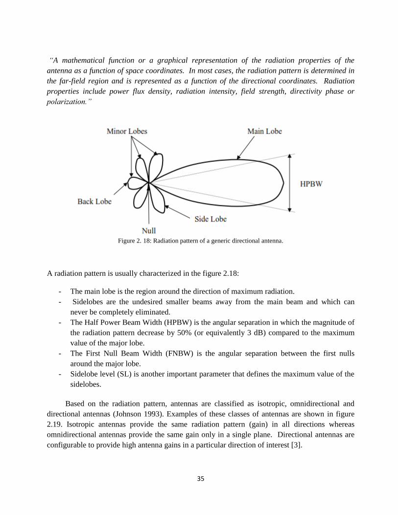
“A mathematical function or a graphical representation of the radiation properties of the
antenna as a function of space coordinates. In most cases, the radiation pattern is determined in
the far-field region and is represented as a function of the directional coordinates. Radiation
properties include power flux density, radiation intensity, field strength, directivity phase or
polarization.”
Figure 2. 18: Radiation pattern of a generic directional antenna.
A radiation pattern is usually characterized in the figure 2.18:
- The main lobe is the region around the direction of maximum radiation.
- Sidelobes are the undesired smaller beams away from the main beam and which can
never be completely eliminated.
- The Half Power Beam Width (HPBW) is the angular separation in which the magnitude of
the radiation pattern decrease by 50% (or equivalently 3 dB) compared to the maximum
value of the major lobe.
- The First Null Beam Width (FNBW) is the angular separation between the first nulls
around the major lobe.
- Sidelobe level (SL) is another important parameter that defines the maximum value of the
sidelobes.
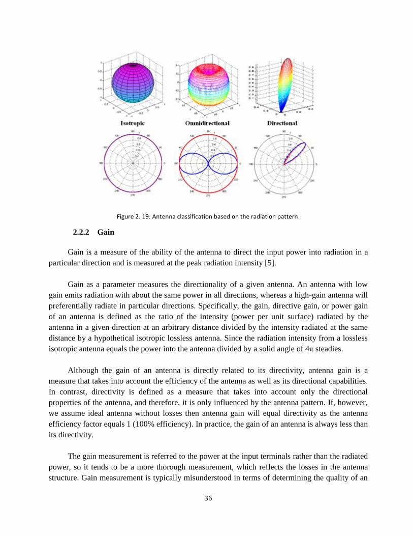
Based on the radiation pattern, antennas are classified as isotropic, omnidirectional and
directional antennas (Johnson 1993). Examples of these classes of antennas are shown in figure
2.19. Isotropic antennas provide the same radiation pattern (gain) in all directions whereas
omnidirectional antennas provide the same gain only in a single plane. Directional antennas are
configurable to provide high antenna gains in a particular direction of interest [3].
36
Figure 2. 19: Antenna classification based on the radiation pattern. 2.2.2 Gain
Gain is a measure of the ability of the antenna to direct the input power into radiation in a
particular direction and is measured at the peak radiation intensity [5].
Gain as a parameter measures the directionality of a given antenna. An antenna with low
gain emits radiation with about the same power in all directions, whereas a high-gain antenna will
preferentially radiate in particular directions. Specifically, the gain, directive gain, or power gain
of an antenna is defined as the ratio of the intensity (power per unit surface) radiated by the
antenna in a given direction at an arbitrary distance divided by the intensity radiated at the same
distance by a hypothetical isotropic lossless antenna. Since the radiation intensity from a lossless
isotropic antenna equals the power into the antenna divided by a solid angle of 4π steadies.
Although the gain of an antenna is directly related to its directivity, antenna gain is a
measure that takes into account the efficiency of the antenna as well as its directional capabilities.
In contrast, directivity is defined as a measure that takes into account only the directional
properties of the antenna, and therefore, it is only influenced by the antenna pattern. If, however,
we assume ideal antenna without losses then antenna gain will equal directivity as the antenna
efficiency factor equals 1 (100% efficiency). In practice, the gain of an antenna is always less than
its directivity.
The gain measurement is referred to the power at the input terminals rather than the radiated
power, so it tends to be a more thorough measurement, which reflects the losses in the antenna
structure. Gain measurement is typically misunderstood in terms of determining the quality of an

37
antenna. A common misconception is that the higher the gain, the better the antenna. This is only
true if the application requires a highly directive antenna. Since gain is linearly proportional to
directivity, the gain measurement is a direct indication of how directive the antenna is (provided
the antenna has adequate radiation efficiency) [7].
2.2.3 Bandwidth
Bandwidth is a fundamental antenna parameter. It describes the range of frequencies over
where the antenna parameters, such as input impedance, radiation patterns, polarization, sidelobes
level and gain is within an acceptable value from those at the center frequency.
Often, the desired bandwidth is one of the determining parameters used to decide upon an a
ntennaThe bandwidth of a broadband antenna can be defined as the ratio of the upper to lower
frequencies of acceptable operation. The bandwidth of a narrowband antenna can be defined as
the percentage of the frequency difference over the center frequency [6]. According to [9] these
definitions can be written in terms of equations as follows:
𝐵𝑊𝑏𝑟𝑜𝑎𝑑𝑏𝑎𝑛𝑑 =𝑓𝐻𝑓𝐿
𝐵𝑊𝑛𝑎𝑟𝑟𝑜𝑤𝑏𝑎𝑛𝑑(%) = [𝑓𝐻−𝑓𝐿
𝑓𝐶] 100
where 𝑓𝐻 = upper frequency
𝑓𝐿 = lower frequency
𝑓𝐶 = center frequency
2.2.4 Beamwidth
The beamwidth of the antenna is usually considered to be the angular width of the half
power radiated within a certain cut through the main beam of the antenna where most of the
power is radiating. From the peak radiation intensity of the radiation pattern, which is the peak of
the main beam, the half power level is 3 dB below such a peak where the two points on the main
beam are located; these points are on two sides of the peak, which separate the angular width of
the half power. The angular distance between the half power points is defined as the beamwidth.
Half the power expressed in decibels is 3 dB, so the half-power beamwidth is sometimes referred
to as the 3-dB beamwidth. Both horizontal and vertical beamwidths are usually considered [1].

38
2.2.5 Polarization
Polarization of a radiated wave is defined as the property of an electromagnetic wave
describing the time-varying direction and relative magnitude of the electric-field vector. It is
described by the geometric figure traced by the electric field vector upon a stationary plane
perpendicular to the direction of propagation, as the wave travels through that plane. The three
different types of antenna polarizations are shown in Figure 2.20. Vertical, and horizontal
polarizations are the simplest forms of antenna polarization and they both fall into a category
known as linear polarization. It is also possible that antennas can have a circular polarization.
Circular polarization occurs when two or more linearly polarized waves add together, such that
the E-field of the net wave rotates. Circular polarization has a number of benefits for areas such as
satellite applications where it helps overcome the effects of propagation anomalies, ground
reflections and the effects of the spin that occur on many satellites [3]. Another form of
polarization is known as elliptical polarization. It occurs when there is a mix of linear and circular
polarization. This can be visualized by the tip of the electric field vector tracing out an elliptically
shaped corkscrew. It is possible for linearly polarized antennas to receive circularly polarized
signals and vice versa. But, there is a 3 dB polarization mismatch between linearly and circularly
polarized antennas [8].
Figure 2. 20: Types of Polarization. When a wave is travelling in space the property that describes its electric field rotation at a
fixed point as a function of time is called wave polarization. It is a parameter which remains
constant over the antenna main beam but may vary in the minor loops. Since the electric and
magnetic field vectors are always related according to Maxwell’s equation, it is enough to specify
the polarization of one of them. And generally it is specified by the electric field. Polarization
should be defined in its transmitting mode with reference to IEEE Standards. The polarization
plane is the plane containing the electric and magnetic field vectors and it is always perpendicular
to the plane of propagation. The contour drawn by the tip of the electric field vector describes the
wave polarization. This contour is an ellipse, circle or a line. The polarization direction is
assumed in the direction of the main beam unless otherwise stated. There are 2 kinds of
polarization co-and cross-polarizations.

39
Co-polarization is the polarization radiated/received by the antenna, while the cross-
polarization is perpendicular to it. Polarization is a very important factor in wave propagation
between the transmitting and receiver antennas. Having the same kind of polarization and sense is
important so that the receiving antenna can extract the signal from the transmitted wave.
Maximum power transfer will take place when the receiving antenna has the same direction, axial
ratio, spatial orientation and the same sense of polarization as incident wave, otherwise there will
be polarization mismatch. If polarization mismatch occurs it will add more losses. Polarization is
very important when considering wave reflection [2].
2.2.6 Return Loss
Return loss is traditionally expressed as the ratio between incident and reflected power
expressed in dB, however, this report will in accordance with common practice within antenna
engineering report return loss with a negative sign that is the fraction of reflected power divided
by incident power in dB [8].
𝑅𝐿 = 10 log10𝑃𝑟𝑃𝑖
Return loss evaluated at different frequencies of an antenna usually give a good
representation of its radiating properties. For example, if the return loss is close to 0 dB, it means
that the antenna isn't radiating at that frequency and if the return losses around -10 dB or lower, it
means that at least 99% of power either is radiated or absorbed and converted into heat inside the
antenna. Microstrip antennas usually have rather poor efficiency, of those 99% typically 70-80%
would be radiated power. The reason small antennas have low efficiency is due to the fact that
they are working in resonance, allowing the wave to travel through the antenna many times and
thereby lose more power [1].
For systems with more than one antenna low return loss and low losses inside the antenna
won't necessarily mean the energy is radiated to the far field, it might also get absorbed by other
antennas. Hence, it is important to also consider the energy absorbed by the diversity antenna
when simulating and measuring MIMO configurations. Simulation software can give direct
information about radiation efficiency, but since return loss is much faster to calculate, it is the
most common parameter to use as guidance during the design. This is true since calculating
radiation efficiency requires knowledge about the radiated far field, while calculating return loss
only requires knowledge of the lumped element circuits and the antenna [6].
2.2.7 Antenna Efficiency
Efficiency of an antenna can be divided into radiation efficiency which depends on the
antenna structure or the radiation resistance, while the other is the total efficiency which includes
the matching of an antenna to the power source or the return loss S11, where the expected value is
usually -6dB.
η𝑡𝑜𝑡𝑎𝑙 = η𝑟𝑎𝑑⌈1 − (|𝑆11|)2⌉

40
2.2.8 Input Impedance
The input impedance of an antenna is defined by as “the impedance presented by an antenna
at its terminals or the ratio of the voltage to the current at the pair of terminals or the ratio of the
appropriate components of the electric to magnetic fields at a point”. Hence the impedance of the
antenna can be written as:
Zin = Rin + jXin
Where Z in is the antenna impedance at the terminals
R in is the antenna resistance at the terminals
X in is the antenna reactance at the terminals
The imaginary part, X in of the input impedance represents the power stored in the near field
of the antenna. The resistive part, Rin of the input impedance consists of two components, the
radiation resistance in Rr and the loss resistance RL. The power associated with the radiation
resistance is the power actually radiated by the antenna, while the power dissipated in the loss
resistance is lost as heat in the antenna itself due to dielectric or conducting losses [5].
2.2.9 Directivity
The Directivity of an antenna is defined as the ratio of the radiation intensity in a given
direction from the antenna to the radiation intensity averaged over all directions. The average
radiation intensity is equal to the total power radiated by the antenna divided by 4π. If the
direction is not specified, the direction of maximum radiation intensity is implied. The directivity
of a non-isotropic source is equal to the ratio of its radiation intensity in a given direction over
that of an isotropic source [7]. In a mathematical form, it can be written as
𝐷 =𝑈
𝑈𝑜=4𝜋𝑈
𝑃𝑟𝑎𝑑
Where
D = directivity (dimensionless)
U = radiation intensity (W/unit solid angle)
Uo = radiation intensity of isotropic source (W/unit solid angle)
Many times it is desirable to express the directivity in decibels (dB) instead of dimensionless
quantities. The expressions for converting the dimensionless quantities of directivity and
maximum directivity to decibels (dB) is D (dB) = 10 log10 [D (dimensionless)].

41
2.3 Small Antenna
2.3.1 Definition of a Small Antenna
Small antennas are referred to as “electrically small antennas” or ESAs. The name is an
implication that their physical size is much smaller than a wavelength at the operational
frequency. The first definition was proposed by Wheeler [24] as an antenna whose maximum
dimension is less than λ/2π (radian length). Where λ is the wavelength. Another common and an
equivalent definition, ESA is an antenna that satisfies the condition
ka < 0.5,
where k is the wave number = (2πa /λ) <1.
and ‘a’ is the radius of the minimum size sphere that encloses the antenna. The sphere is termed
as ‘Chu sphere’. Another definition given by Hansen is
ka < 1
This is interpreted as an antenna enclosed inside a sphere of radius equal to one radian
length and the sphere is called ‘radian sphere’. This represents the boundary between the near and
far field radiation for a Hertzian dipole.
Small antennas are treated with a concept that embraces not only electrically small
antennas, but also other types of small antennas. Categories used to classify small antennas
include functions as well as dimensions, because small antennas being used practically are not
only what we call “Electrically Small Antennas,” but also simply physically small antennas –
antennas of partly electrically small dimensions and antennas equivalently small in terms of
functions [23].
Conventionally, Electrically Small Antenna ESA has been the main subject when small
antennas are discussed; however, other types of small antenna have comparable significance with
the ESA, depending on the situation of the practical applications. The categories used here are
ESA, Physically Constrained Small Antenna (PCSA), Functionally Small Antenna (FSA), and
Physically Small Antenna (PSA) [28].
A PCSA is an antenna, not having dimensions of ESA, but a part of which has dimensions
corresponding to the ESA. A low-profile antenna, for example, with the height over the ground
plane or the thickness of say λ/50 or so, like an Inverted-L antenna, planar antennas such as a
patch antenna, a microstrip antenna (MSA), and so forth, can be classified into “Physically
Constrained Small Antenna” (PCSA) [25].

42
Another classification of small antennas relates to antenna functions. When an antenna can
attain either additional functions or enhanced performances with the dimensions being kept
unchanged, it can be said to have an equivalent reduction in the antenna size, because with normal
antennas such enhanced function or improved performance could result only from enlargement of
dimensions. An example is an antenna designed to have wideband, multiband performance,
radiation pattern shaping, and array thinning without any change in the dimensions. This class of
antenna is referred to as “Functionally Small Antenna” (FSA) [26].
A PSA is an antenna, which differs from any of the above, but has physically small
dimensions as measured. When the volume of an antenna is bounded by 30 cm or less, we may
call the antenna a PSA. There is not any strict physical meaning in the definition, but only a
sensual measure based on the common understanding of “smallness” in physical size. An example
is a millimeter-wave horn antenna with an aperture size of, say 5 cm approximately. Many of the
MSAs may be classified into either PCSA or PSA [27].
2.3.2 Significance of small antennas
The significance of the small antenna is recognized from its important role in various
wireless systems, where small antennas are indispensable. In the early days of communications,
when electronic devices such as thermionic vacuum tubes were not yet available, antenna
technology was essential to extend the communication range. Development of tuning and
matching concepts gave impetus to promote further increase in communication capability.
Meanwhile, mobile communications drove development of small antennas, as mobile
terminals needed small equipment, for which small-sized, compact, and lightweight antennas
were required. So far, creation and invention of small antennas have accelerated rapidly in
response to worldwide demands raised urgently by the growth of mobile phone systems. Recent
trends are increasing demands arising particularly for newly deployed wireless mobile systems
Near Field Communication systems (NFC), including Radio Frequency Identification (RFID),
Ultra-Wide Band (UWB), and wireless broadband systems such as Wireless Local Area Networks
(WLAN) and Worldwide Interoperability for Microwave Access (WiMAX). Small antennas have
already played an obscure but key role in such wireless mobile systems, as the systems do not
work without these devices. Antennas in these systems have acted as a key component, since they
almost determine the system performance, especially in small wireless equipment, because the
systems are designed to exhibit almost the highest achievable electronic performance, and only
the antenna can further improve the system performance. Since downsizing of electronic devices
and their design technology as well has expedited progress in small wireless equipment, small
antennas have become inevitable for these systems. As such, it can also be said that such newly
deployed wireless systems owe much in their development to small antennas, and in turn small-
antenna technology has advanced by being employed in these wireless systems. Recent urgent

43
demand is application of small antennas to the Multi-Input Multi-Output (MIMO) systems.
WiMAX already employs the MIMO system in order to transmit high data rate to the 4G (4th
Generation) mobile systems, and other wireless broadband systems where high data rates will be
needed will adopt the MIMO system. Small antennas are suitable for small MIMO equipment,
where space to install antennas is limited to small areas, and close proximity of antenna elements
is unavoidable [23].
2.3.3 Small antenna Parameters
The following characteristic parameters are the most important for a small antenna.
1. Directivity
Small antennas are often believed to have doughnut shaped Omni directional pattern of a
Hertzian dipole of directivity D=1.5. The pattern is due to the radiation of TE10 or TM10
spherical modes. But Harrington, Kwon and Pozar have demonstrated unidirectional and bi
directional patterns with D from 1 to 3 theoretically. Antennas with higher spherical TEmn and
TMnm radiations are not of the small type. Small antennas are also termed super directive, since
the directivity D remains unaltered with decrease in size ka [24].
2. Radiation Efficiency
Antenna radiation efficiency factor η is the ratio of power radiated to the power delivered to
an antenna. The losses other than radiation are modeled as a resistor of value R loss
Mathematically is given as:
η = 𝑅𝑟𝑎𝑑
𝑅𝑟𝑎𝑑 + 𝑅𝑙𝑜𝑠𝑠= 𝑅𝑟𝑎𝑑𝑅𝐴
The efficiency gets reduced as the antenna dimension ka is reduced for the fact that R loss
dominates. The reduction can be attributed to frequency dependent conduction and dielectric
losses [23].
3. Quality factor
The Quality factor Q is used to describe the high input reactance and narrow bandwidth of small
antennas [29] and is defined as
𝑄 =2𝜔0max (𝑊𝐸 ,𝑊𝑀)
𝑃𝐴

44
WE and WM are the time average stored electric and magnetic energies and PA is the
received antenna power. The Q value the quantity of our interest is inversely proportional to the
antenna bandwidth [29].
Many times, the bandwidth (BW) of an antenna is not clearly defined; therefore the quality
factor (Q) has more interest. Q is usually expressed in terms of the VSWR or related to the return
loss at the input terminals.
2.4 Bandwidth Enhancement Techniques
The impedance bandwidth of microstrip patch antennas is usually much smaller than the
pattern bandwidth [30]. This discussion on bandwidth enhancement techniques will therefore
focus on input impedance rather than radiation patterns. There are a number of ways in which the
impedance bandwidth of probe-fed microstrip patch antennas can be enhanced. According to
Wong [31], the various bandwidth-enhancement techniques can be categorized into three broad
approaches:
- Impedance matching.
- The use of multiple resonances.
- The use of lossy materials.
For the purpose of this overview, it has been decided to rather categorize the different
approaches in terms of the antenna structures that are normally used. These include:
Wideband impedance-matching networks.
Edge-coupled patches.
Stacked patches.
Shaped probes.
Capacitive coupling and slotted patches.
Capacitive feed probes.
Overlapped patches which represents the new antenna element that forms the basis of this
study.
In terms of Wong’s categories, all these approaches can be identified as making use of
either impedance matching or multiple resonances. In practice, lossy materials are not frequently
used as it limits the radiation efficiency of the antenna. It will therefore not be considered here.
2.4.1 Wideband Impedance-Matching Networks
One of the most direct ways to improve the impedance bandwidth of probe-fed microstrip
antennas, without altering the antenna element itself, is to use a reactive matching network that
compensates for the rapid frequency variations of the input impedance. As shown in Figure 2.21,
this can typically be implemented in microstrip form below the ground plane of the antenna
element. The method is not restricted to antenna elements on either thin or a thick substrates, but
the thick substrate will of course add some extra bandwidth.

45
Pues and Van de Capelle [32] implemented the method by modelling the antenna as a
simple resonant circuit. A procedure, similar to the design of a bandpass filter, is then used to
synthesize the matching network. With this approach, they have managed to increase the
bandwidth from 4.2% to 12% for a VSWR of 2:1. Subsequently to that, C.Nauwelaers [33] used
the simplified real frequency technique in order to design the matching network for a probe-fed
microstrip patch antenna. They have managed to increase the bandwidth of one antenna element
from 5.7% to 11.1% for a VSWR of 1.5:1, and that of another from 9.4% to 16.8% for a VSWR
of 2:1. Recently, V. Gupta and S. Sinha [34] have shown how a dielectric-resonator loaded
suspended microstrip patch antenna can increase the bandwidth from
3.2% to 18% for a VSWR of 1.5:1.
The advantages of using impedance-matching networks are that the antenna elements do not
get altered and that the matching network can be placed behind the antenna's ground plane. As
such, the radiation characteristics of the antenna element stay unchanged, while radiation from the
matching network is also minimized.
Figure 2. 21: Geometry of a probe-fed microstrip patch antenna with a wideband impedance-matching network.
The drawback of this method is that the matching network can potentially take up
space that is very limited when microstrip feed networks are used to excite the individual
elements in an antenna array. Another drawback is that, for single-element antennas, more than
one substrate layer is required to support the antenna element and the matching network.
2.4.2 Edge-Coupled Patches
The basic idea behind edge-coupled patches, is to increase the impedance bandwidth of a
microstrip patch through the introduction of additional resonant patches. By doing so, a few
closely-spaced resonances can be created. Only one of the elements is driven directly. The other
patches are coupled through proximity effects. An example of such an arrangement is shown in
Figure 2.22.
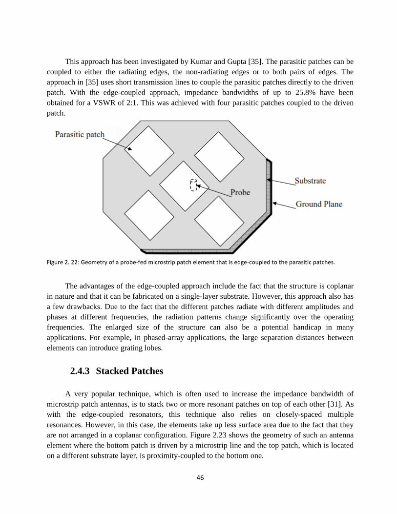
46
This approach has been investigated by Kumar and Gupta [35]. The parasitic patches can be
coupled to either the radiating edges, the non-radiating edges or to both pairs of edges. The
approach in [35] uses short transmission lines to couple the parasitic patches directly to the driven
patch. With the edge-coupled approach, impedance bandwidths of up to 25.8% have been
obtained for a VSWR of 2:1. This was achieved with four parasitic patches coupled to the driven
patch.
Figure 2. 22: Geometry of a probe-fed microstrip patch element that is edge-coupled to the parasitic patches.
The advantages of the edge-coupled approach include the fact that the structure is coplanar
in nature and that it can be fabricated on a single-layer substrate. However, this approach also has
a few drawbacks. Due to the fact that the different patches radiate with different amplitudes and
phases at different frequencies, the radiation patterns change significantly over the operating
frequencies. The enlarged size of the structure can also be a potential handicap in many
applications. For example, in phased-array applications, the large separation distances between
elements can introduce grating lobes.
2.4.3 Stacked Patches
A very popular technique, which is often used to increase the impedance bandwidth of
microstrip patch antennas, is to stack two or more resonant patches on top of each other [31]. As
with the edge-coupled resonators, this technique also relies on closely-spaced multiple
resonances. However, in this case, the elements take up less surface area due to the fact that they
are not arranged in a coplanar configuration. Figure 2.23 shows the geometry of such an antenna
element where the bottom patch is driven by a microstrip line and the top patch, which is located
on a different substrate layer, is proximity-coupled to the bottom one.

47
Figure 2. 23: Geometry of a probe-fed stacked microstrip patch antenna.
In practice, the patches are usually very close in size so that the generation of two
distinct resonances can be avoided. Different shapes of patches can be used. These commonly
include rectangular patches [36], circular patches [37] and annular-ring patches [38]. Waterhouse
[36] reported a 26% 10 dB return-loss bandwidth for rectangular patches, Mitchell [37] reported a
33% 10 dB return-loss bandwidth for circular patches, while Kokotoff [38] reported a 22% 10 dB
return-loss bandwidth for annular-ring patches.
These bandwidths were all obtained for two patches stacked on top of each other. It is
possible to stack more patches, but the performance may not be much better than with only two
patches [31]. Instead of aligning the patches vertically, some researchers have also used a
horizontal offset between the patches [39]. However, due to the structural asymmetry, these
configurations exhibit beam dispersion.
The stacked-patch configuration has a number of advantages over the edge-coupled
configuration. Since it does not increase the surface area of the element, it can be used in array
configurations without the danger of creating grating lobes. Its radiation patterns and phase center
also remains relatively constant over the operating frequency band. It has a large number of
parameters that can be used for optimization. However, due to this, the design and optimization
process can also be very complex. Another drawback of stacked patches, is that it requires more
than one substrate layer to support the patches.
2.4.4 Shaped Probes
As was shown in Chapter 1, a thick substrate can be used to enhance the impedance
bandwidth of microstrip patch antennas. However, the input impedance of probe-fed microstrip
patch antennas become more inductive as the substrate thickness is increased. In order to offset
this inductance, some capacitance is needed in the antenna's feeding structure. One way to

48
implement such a capacitive feed is to alter the shape of the probe. There are basically two
approaches. In one approach, the probe is connected directly to the patch [40], while in the other
approach, the probe is not connected to the patch at all [41].
The direct feed can be implemented as shown in Figure 2.24(a), where the feeding structure
consists of a stepped probe. The horizontal part of the probe couples capacitive to the patch. Chen
and Chia [40] reported an impedance bandwidth of 19.5% for a VSWR of 2:1. Another option is
to add a stub to one of the radiating edges of the patch and to feed the stub directly with a probe.
For such an approach, Chen and Chia [42] reported an impedance bandwidth of 25%, once again
for a VSWR of 2:1. The proximity-coupled probe is implemented as shown in Figure 2.24(b),
where the probe is bent into a L-shape. The horizontal part of the probe runs underneath the patch
and also couples capacitive to it. This solution has been implemented for a variety of patch
shapes. Maketal. Reported an impedance bandwidth of 36% for a rectangular patch in [43] and
42% for a triangular patch in [44], while Guo et al. reported an impedance bandwidth of 27% for
an annular-ring patch in [45]. These bandwidth figures were all quoted for a VSWR of 2:1.
Instead of a L-shaped probe. A microstrip patch antenna with a shaped probe, be it directly driven
or not, can usually be supported on a single substrate layer. This makes it extremely suitable for
antenna arrays where cost has to be minimized.

49
Figure 2. 24: Geometries of microstrip patch antennas with shaped probes. (a) Stepped probe. (b) L-shaped probe.
Most of these elements have radiation patterns with a slight squint in the E-plane and
slightly high cross-polarization levels in the H-plane. These are characteristics of probe-fed
microstrip patch antennas on thick substrates. The stepped probe, though, exhibits somewhat
lower cross-polarization levels. The patches that are directly driven should be more robust that
those with the proximity coupled probes. For the latter ones, care has to be taken with respect to
the proper alignment of the paths and probes. Another advantage of both approaches is that, since
they do not increase the surface area of the element, they can be used in array configurations
without the danger of creating grating lobes.
2.4.5 Capacitive Coupling and Slotted Patches
There are two alternative approaches that can also be used to overcome the inductive nature
of the input impedance associated with a probe-fed patch on a thick substrate. These are
capacitive coupling or the use of slots within the surface of the patch element. Examples of such
approaches are shown in Figures 2.25(a) and (b) respectively. It can be argued that these two
approaches are structurally quite similar. The approach in Figure 2.25(a) has a small probe-fed
capacitor patch, which is situated below the resonant patch [46]. The gap between them acts as a
series capacitor. Similarly, the annular slot in Figure 2.25(b) separates the patch into a small
probe-fed capacitor patch and a resonant patch. In this case, the slot also acts as a series capacitor.
In principle, both of these approaches employ some sort of capacitive coupling and are
functionally also, to some degree, equivalent to the L-probe and T–probe.
Liu and kooi [47] combined the capacitive-coupled feed probe with stacked patches and
reported a impedance bandwidth of 25.7% for a VSWR of 2:1. To achieve this, they used two
stacked patches with a small probe-fed patch below the bottom resonant patch. In another
approach, Gonzalez [48] placed a resonant patch, together with the small probe-fed capacitor
patch just below it, into a metallic cavity. With this configuration, they managed to obtain a
impedance bandwidth of 35.3% for a VSWR of 2:1. Chen and Chia [49] used a small rectangular

50
probe-fed capacitor patch, located within a notch that was cut into the surface of the resonant
patch. They managed to obtain an impedance bandwidth of 36% for a VSWR of 2:1.
Some authors also used a rectangular resonant patch with a U-slot in its surface. The
metallic area inside the slot is then driven directly with a probe. Here, Tong [50] reported a
impedance bandwidth of 27% for a VSWR of 2:1, while Weigand [51] reported an impedance
bandwidth of 39 %, also for a VSWR of 2:1. In yet another approach, Nie and Chew [52]
placed a circular probe-fed patch within a annular-ring patch, with the circular patch exciting
higher-order modes on the annular-ring patch.
Figure 2. 25: Geometries of probe-fed microstrip patch antennas where capacitive coupling and slots are used. (a)
Capacitive coupling. (b) Annular slot in the surface of the patch.
They managed to obtain 8 dB return-loss bandwidth of 20%. Kokotoff [53] placed a small
shorted circular probe-fed patch within a annular-ring patch, but with the circular patch exciting
the dominant TM11 mode on the annular-ring patch. They reported a 10 dB return-loss of 6.6%.
The advantage of the approach where the capacitor patch is located below the resonant
patch, is that the cross-polarization levels in the H-plane are lower than what can be achieved with
the approach where the capacitor patch is located within the surface of the resonant patch.
However, in order to support the capacitor patch below the resonant patch, an additional substrate
layer might be required. In contrast, only one substrate layer is required to support the
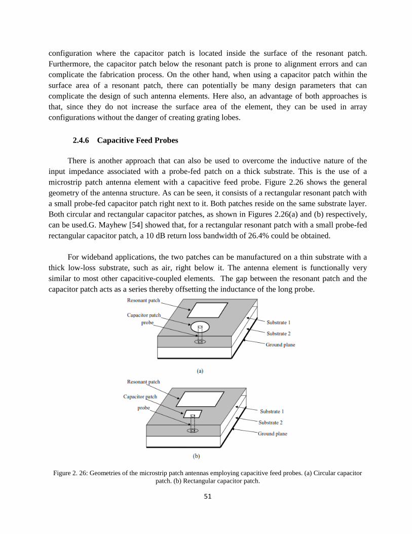
51
configuration where the capacitor patch is located inside the surface of the resonant patch.
Furthermore, the capacitor patch below the resonant patch is prone to alignment errors and can
complicate the fabrication process. On the other hand, when using a capacitor patch within the
surface area of a resonant patch, there can potentially be many design parameters that can
complicate the design of such antenna elements. Here also, an advantage of both approaches is
that, since they do not increase the surface area of the element, they can be used in array
configurations without the danger of creating grating lobes.
2.4.6 Capacitive Feed Probes
There is another approach that can also be used to overcome the inductive nature of the
input impedance associated with a probe-fed patch on a thick substrate. This is the use of a
microstrip patch antenna element with a capacitive feed probe. Figure 2.26 shows the general
geometry of the antenna structure. As can be seen, it consists of a rectangular resonant patch with
a small probe-fed capacitor patch right next to it. Both patches reside on the same substrate layer.
Both circular and rectangular capacitor patches, as shown in Figures 2.26(a) and (b) respectively,
can be used.G. Mayhew [54] showed that, for a rectangular resonant patch with a small probe-fed
rectangular capacitor patch, a 10 dB return loss bandwidth of 26.4% could be obtained.
For wideband applications, the two patches can be manufactured on a thin substrate with a
thick low-loss substrate, such as air, right below it. The antenna element is functionally very
similar to most other capacitive-coupled elements. The gap between the resonant patch and the
capacitor patch acts as a series thereby offsetting the inductance of the long probe.
Figure 2. 26: Geometries of the microstrip patch antennas employing capacitive feed probes. (a) Circular capacitor
patch. (b) Rectangular capacitor patch.

52
Once the size of the resonant patch and the thickness of the substrate have been fixed for a
certain operating frequency and impedance bandwidth, there are basically two parameters that can
be used to control the input impedance of the antenna element. These are the size of the capacitor
patch and the size of the gap between the two patches.
The structural properties of this antenna element can be viewed in context. First of all, this
antenna element can be manufactured on a single substrate layer due to both the resonant patch
and the capacitor patch residing on the same layer. This is very important for large antenna arrays
where lamination can be very expensive. The fact that the capacitor patch is driven directly by a
probe, gives the structure some rigidity. The structure is also less prone to alignment errors, which
can be a factor of merit for antenna elements where the probe does not make physical contact with
any of the resonant patches or where the capacitor patch is located on a different layer than the
resonant patch. The surface area of the element is not much larger than that of a resonant patch
and therefore it is very suitable for use within antenna arrays. An advantage that might not be
very obvious at first, is that the antenna element, as opposed to slotted antenna elements, consists
of parts that are regular in shape, it has huge benefits for the analysis of such antennas, especially
for large antenna arrays. Finally, the design of such an antenna element, as well as tuning of the
input impedance, is very straightforward due to the few parameters that have to be adjusted.
2.5 Feed Techniques
There are different techniques available to feed or transmit electromagnetic energy to a
microstrip antenna. The four most popular feeding methods are the Microstrip line, coaxial probe,
aperture coupling and proximity coupling.
2.5.1 Coaxial Feed
The Coaxial feed or probe feed is a very common technique used for feeding Microstrip
patch antennas. As seen from Figure 2.27, the inner conductor of the coaxial connector extends
through the dielectric and is soldered to the radiating patch, while the outer conductor is
connected to the ground plane.

53
Figure 2. 27: Rectangular Microstrip antenna coaxial feed
The main advantage of this type of feeding scheme is that the feed can be placed at any
desired location inside the patch in order to match with its input impedance. This feed method is
easy to fabricate and has low spurious radiation. However, a major disadvantage is that it provides
narrow bandwidth and is difficult to model since a hole has to be drilled in the substrate and the
connector protrudes outside the ground plane, thus not making it completely planar for thick
substrates (h > 0.02λo). Also, for thicker substrates, the increased probe length makes the input
impedance more inductive, leading to matching problems. It is seen above that for a thick
dielectric substrate, which provides broad bandwidth [58].
2.5.2 Microstrip Feed line
In this type of feed technique, a conducting strip is connected directly to the edge of the
Microstrip patch as shown in Figure 2.28. The conducting strip is smaller in width as compared to
the patch and this kind of feed arrangement has the advantage that the feed can be etched on the
same substrate to provide a planar structure The purpose of the inset cut in the patch is to match
the impedance of the feed line to the patch without the need for any additional matching element.
This is achieved by properly controlling the inset position. Hence this is an easy feeding scheme,
since it provides ease of fabrication and simplicity in modeling as well as impedance matching.
However as the thickness of the dielectric substrate being used, increases, surface waves and
spurious feed radiation also increases, which hampers the bandwidth of the antenna [57]. The feed
radiation also leads to undesired cross polarized radiation.

54
Figure 2. 28: Rectangular Microstrip antenna of Microstrip Line feeding.
2.5.3 Aperture Coupled Feed
In this type of feed technique, the radiating patch and the Microstrip feed line are separated
by the ground plane as shown in Figure 2.29. Coupling between the patch and the feed line is
made through a slot or an aperture in the ground plane. The coupling aperture is usually centered
under the patch, leading to lower cross polarization due to symmetry of the configuration. The
amount of coupling from the feed line to the patch is determined by the shape, size and location of
the aperture. Since the ground plane separates the patch and the feed line, spurious radiation is
minimized. Generally, a high dielectric material is used for the bottom substrate and a thick, low
dielectric constant material is used for the top substrate to optimize radiation from the patch [59].
The major disadvantage of this feed technique is that it is difficult to fabricate due to
multiple layers, which also increases the antenna thickness. This feeding scheme also provides
narrow bandwidth (up to 21%).
Figure 2. 29: Rectangular Microstrip antenna Aperture coupled feed.

55
2.5.4 Proximity Coupled Feed
This type of feed technique is also called as the electromagnetic coupling scheme. As
shown in Figure 2.30, two dielectric substrates are used such that the feed line is between the two
substrates and the radiating patch is on top of the upper substrate [60]. The main advantage of this
feed technique is that it eliminates spurious feed radiation and provides very high bandwidth (as
high as 13%), due to overall increase in the thickness of the microstrip patch antenna. This
scheme also provides choices between two different dielectric media, one for the patch and one
for the feed line to optimize the individual performances.
Figure 2. 30: Proximity-coupled Feed.
Matching can be achieved by controlling the length of the feed line and the width-to-line
ratio of the patch. The major disadvantage of this feed scheme is that it is difficult to fabricate
because of the two dielectric layers which need proper alignment. Also, there is an increase in the
overall thickness of the antenna. Table 2.1 below summarizes the characteristics of the different
feed techniques [56].
Table 2. 1: Comparing the Different Feed Techniques[68].
Characteristics Microstrip Line
Feed Coaxial Feed
Aperture
Coupled Feed
Proximity
Coupled Feed
Spurious feed
radiations More more Less minimum
Ease of fabrication Easy
Soldering and
drilling needed
Alignment
required
Alignment
required
impedance matching Easy Easy Easy Easy
Bandwidth (achieved
with impedance
matching)
2-5% 2-5% 2-5% 13%
reliability better Poor due to
soldering Good Good

56
2.6 OVERVIEW OF MODELLING TECHNIQUES
There are a number of methods that can be used for the analysis of microstrip patch
antennas. Most of these methods fall into one of two broad categories: approximate methods and
full-wave methods [56]. The approximate methods are based on simplifying assumptions and
therefore they have a number of limitations and are usually less accurate. They are usually used to
analyze single antenna elements as it is very difficult to model coupling between elements with
these methods. However, where applicable, they normally do provide good physical insight and
the computation time is usually very small. The full-wave methods include all relevant wave
mechanisms and rely heavily upon the use of efficient numerical techniques [61]. When applied
properly, the full-wave methods are reasonably accurate and can be used to model a wide variety
of antenna configurations, including antenna arrays. These methods tend to be much more
complex than the approximate methods and also provide less physical insight. Very often they
also require vast computational resources and extensive solution times. In the remainder of this
section, an overview of both approximate and full-wave methods will be given.
2.6.1 Approximate Methods
Some of the popular approximate models include the transmission-line model, the cavity
model and the segmentation model. These models usually treat the microstrip patch as a
transmission line or as a cavity resonator.
3.6.1.1 Transmission-Line Model
The transmission-line model leads to results that are adequate for most engineering
purposes and entail less computation. Although this method has its shortcomings, particularly in
that it is applicable only to rectangular or square patch geometries, the model offers a reasonable
interpretation of the radiation mechanism, while simultaneously giving a simple expression of the
antenna’s characteristics [62].
The basic concept of the transmission-line model is shown in Figure 2.31. This model is for
a rectangular patch fed at the center of the radiating edge. The patch is characterized as a
microstrip transmission-line with a length L, width W, and thickness h. Each radiating edge, with
length equal to W, is modeled as a narrow slot radiating into a half-space. The width of the slot is,
for the sake of convenience, assumed to be equal to the substrate thickness h, As a result, the
rectangular patch antenna can be represented by two admittance connected by an equivalent
microstrip transmission line as shown in the lower half of Figure 2.31, where the characteristic
impedance Z and the propagation constant ß for the fundamental mode in the microstrip line are
approximated by [63] as:

57
Figure 2. 31: Plane view of rectangular patch antenna and its equivalent circuit.
𝑍𝑜 = 1
𝑌𝑜≈
η
√𝜀𝑟𝑒𝑓𝑓
ℎ
𝑊 (2.1)
𝛽𝑔 ≈ 𝐾𝑜√𝜀𝑟𝑒𝑓𝑓 (2.2)
where
ηo = The wave impedance in free space.
Ko = The propagation constant in free space.
𝜀𝑟𝑒𝑓𝑓 = Effective dielectric constant.
𝜀𝑟𝑒𝑓𝑓 is related to the intrinsic dielectric constant 𝜀𝑟 of the substrate as follows [58]:
𝜀𝑟𝑒𝑓𝑓 =𝜀𝑟+1
2+
𝜀𝑟−1
2[1 + 12
ℎ
𝑊] ^(−
1
2) (2.3)
Notice that the value of 𝜀𝑟𝑒𝑓𝑓 is slightly less then𝜀𝑟 because the fringing fields around the
periphery of the patch are not confined in the dielectric substrate but are also spread in the air.
The capacitive component, B, and the conductive component, Gr, which form each
admittance, are related to the fringing field and the radiation loss, and are respectively
approximated by [64] as:
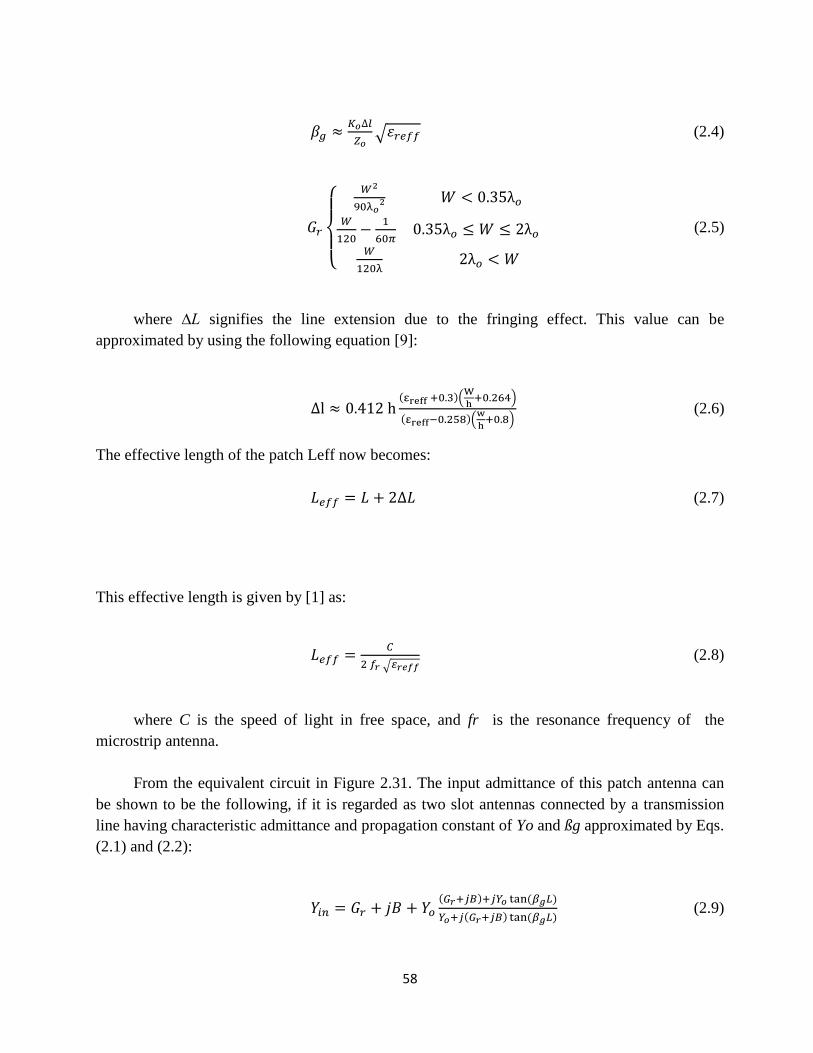
58
𝛽𝑔 ≈𝐾𝑜∆𝑙
𝑍𝑜√𝜀𝑟𝑒𝑓𝑓 (2.4)
𝐺𝑟
𝑊2
90λ𝑜2 𝑊 < 0.35λ𝑜
𝑊
120−
1
60𝜋 0.35λ𝑜 ≤ 𝑊 ≤ 2λ𝑜
𝑊
120λ 2λ𝑜 < 𝑊
(2.5)
where ∆L signifies the line extension due to the fringing effect. This value can be
approximated by using the following equation [9]:
∆l ≈ 0.412 h(εreff +0.3)(
W
h+0.264)
(εreff−0.258)(w
h+0.8)
(2.6)
The effective length of the patch Leff now becomes:
𝐿𝑒𝑓𝑓 = 𝐿 + 2∆𝐿 (2.7)
This effective length is given by [1] as:
𝐿𝑒𝑓𝑓 =
𝐶
2 𝑓𝑟 √𝜀𝑟𝑒𝑓𝑓 (2.8)
where C is the speed of light in free space, and fr is the resonance frequency of the
microstrip antenna.
From the equivalent circuit in Figure 2.31. The input admittance of this patch antenna can
be shown to be the following, if it is regarded as two slot antennas connected by a transmission
line having characteristic admittance and propagation constant of Yo and ßg approximated by Eqs.
(2.1) and (2.2):
𝑌𝑖𝑛 = 𝐺𝑟 + 𝑗𝐵 + 𝑌𝑜(𝐺𝑟+𝑗𝐵)+𝑗𝑌𝑜 tan(𝛽𝑔𝐿)
𝑌𝑜+𝑗(𝐺𝑟+𝑗𝐵) tan(𝛽𝑔𝐿) (2.9)

59
In this case, the resonance condition is given by
ImYin = 0 (2.10)
Where ImYin represents the imaginary part of Yin. From Equation (2.10), the following
condition can be derived:
tan(𝛽𝑔 𝐿) = 2𝑌𝑜𝐵
𝐺𝑟2+ 𝐵2−𝑌𝑜
2 (2.11)
The condition above is used to determine the resonant frequency when the patch length L is
given. The input admittance at resonance can be found by substituting Eq. (2.11) into (2.9):
Yin = 2 Gr (2.12)
This result is, of course, easily deduced from the equivalent circuit of Figure 2.7. For an
efficient radiation, a practical width that leads to good radiation efficiencies is given in [4] as:
𝑊 =𝐶
2 𝑓𝑟 √
2
𝜀𝑟+1 (2.13)
In the typical design procedure of a rectangular patch antenna, the thickness and dielectric
constant of the substrate must be known. Once they are given or determined, a patch antenna that
operates at the required resonance frequency can be designed by following the flow chart shown
in Figure 2.32 [57].
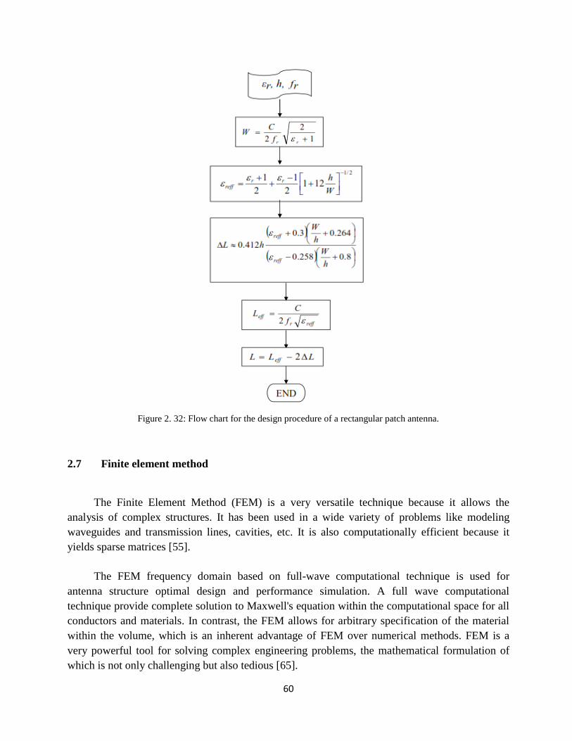
60
Figure 2. 32: Flow chart for the design procedure of a rectangular patch antenna.
2.7 Finite element method
The Finite Element Method (FEM) is a very versatile technique because it allows the
analysis of complex structures. It has been used in a wide variety of problems like modeling
waveguides and transmission lines, cavities, etc. It is also computationally efficient because it
yields sparse matrices [55].
The FEM frequency domain based on full-wave computational technique is used for
antenna structure optimal design and performance simulation. A full wave computational
technique provide complete solution to Maxwell's equation within the computational space for all
conductors and materials. In contrast, the FEM allows for arbitrary specification of the material
within the volume, which is an inherent advantage of FEM over numerical methods. FEM is a
very powerful tool for solving complex engineering problems, the mathematical formulation of
which is not only challenging but also tedious [65].

61
It was introduced to the electromagnetic community towards the end of the 1960's. Since
then, a great progress has been made in terms of its application to electromagnetic problems. In
addition, the FEM is a well-known frequency-domain technique which is highly capable of
modeling 3D complex structures within homogeneities. Typical full wave EM analyzes in the
FEM is shown in Figure 2.31.
Figure 2. 33: Full-wave EM analysis in the FEM.
When using the FEM for electromagnetic problems, the electric field is the unknown
variable that has to be solved for, the method is implemented by discrediting the entire volume
over which the electric field exists, together with its bounding surface, into small elements. In
which triangular elements are used for surface meshes and tetrahedron elements for volumetric
meshes. Simple linear or higher-order functions on the nodes, along the edge or on faces of the
elements, are to model the electric field. For antenna problems, the volume over which the electric
field exists will have one boundary on the antenna and another boundary some distance away
from the antenna [65].
The latter boundary is an absorbing boundary, which is needed to truncate the volume. One
view point from which the FEM can be derived is that of variation analyze. The method starts
with the partial differential equation (PDE) from Maxwell's equations and finds a variation
functional from which the minimum (or external point) corresponds with the solution of the PDE,
subject to the boundary conditions. An example of such a functional is the energy functional,
which is an expression describing all the energy associated with the configuration being analysis,
in terms of the electric field. After the boundary conditions have been enforced, a matrix equation
is obtained. This equation can then be solved to yield the amplitudes that are associated with the
functions on the elements used to model the electric field. The matrix associated with the FEM is
a sparse matrix due to the fact that every element only interacts with the elements in its own
neighborhood. Other parameters, such as the magnetic field, induced currents and power loss, can
be obtained from the electric field. The major advantage of the FEM is that the electrical and
geometrical properties of each element can be defined independently. Therefore, very
complicated geometries and in homogenous materials can be treated with relative ease. This
implies that the analysis of microstrip antennas with finite ground plane and layers is also possible
[66].

62
2.8 HFSS
Ansys’s electromagnetic computer modeling software, High Frequency Structure Simulator
(HFSS), has become an industry standard. Its user friendly graphical user’s interface is intuitive
enough to help even the most novice RF, microwave, and electromagnetic engineers create
anything that starts in the deepest recesses of their imaginations. The software opens up and gives
its user free reign to draw, scale, and measure whatever his heart and needs dictate. Once
designed, the software offers a myriad of simulation options; ranging from power based solutions
to incident wave modeling. Then the simulations can be conducted thoroughly or quickly and
with as much data across as many frequencies as warranted. Once all of the data has been
generated, HFSS allows the user to process and analyze it in any way that satisfies its user’s
requirements. HFSS is an extremely versatile software package that has played no small part in
assisting the world’s engineers and scientists to advance the field of electromagnetism.
Ansys designed HFSS to use the FEM for solving complex microwave structures. This
method will divide a structure into smaller pieces and define a “finite element.” HFSS breaks
objects down into many tetrahedrons and the combination of the separate tetrahedrons is called a
mesh. Each individual tetrahedral is solved using Maxwell’s equations while keeping each piece
connected at its boundaries. A field solution is obtained for the entire structure by constructing
the solutions from each piece. Once the field solution has been obtained for the entire form, an S-
parameter matrix is generated. Because Maxwell’s equations are the basis of the simulator, HFSS
does not solve objects by using electric circuit parameters like voltages and currents; instead it
uses electric and magnetic fields. These fields must be able to exist within the evaluated structures
in order for HFSS to work properly.
HFSS does not just spit out information after a user presses “run,” it forms a mesh and
iteratively constructs and refines it, particularly in the areas where the fields are most
complicated, to ensure it is computing the correct results. This process of redefining and updating
meshes to approach the most correct solution is called an adaptive solution. The user can
determine how much room for error will be allowed in the HFSS solution by defining the
program’s adaptive sweep settings.
Before HFSS begins to adaptively solve anything and after the user creates the model, the
kind of solution the solver should work toward, the boundaries, and the excitations all have to be
set. There are three solution types available in HFSS: driven modal, driven terminal, and
eigenmode. The driven modal solution is the most common and is used when evaluating simple
transmission line, microstrip, and waveguide structures. It presents its data in a conventional S-
matrix. Driven terminal is similar to driven modal, but it is mainly used to solve transmission
lines with multiple signals for Signal Integrity (SI) purposes. It also presents an S-matrix, but it is
based on voltages and currents. The last solution type is the eigenmode solution. It provides a
detailed report on the resonances in a structure and the fields at those resonant points.

63
Boundaries in HFSS are used to either create an electromagnetic model or to simplify and
contain a geometric model. There are twelve boundary options to choose from, depending on the
needs of the user. The most relevant one to this thesis is the Radiation boundary. This boundary
type will create an open model and is applied to the outer surfaces of the user-defined area which
is a quarter of a wavelength away from the simulated model. The radiation boundary is intended
to set a point at which waves that will radiate to infinity will be truncated in order to keep the
simulation as simple as possible.
There are seven excitation options in HFSS and they allow the user to indicate field,
voltage, charge, and/or current sources to drive the simulation. Only two will be presented here.
The wave port excitation is one of the most commonly used with transmission lines and is used in
this thesis. It provides S, Y, and Z parameters and will also relay port impedance information.
Because the wave port is seen as a waveguide when energy enters it, the port’s size is an
important consideration to take into account.
Drawing a structure, initializing “simulation rules,” and determining how something should
be solved are all it takes to use the electromagnetic solving capabilities of HFSS. The rendered
solution can be as exact or approximate as the user wishes. The exact options and choices that
were made concerning this thesis topic will be discussed as the project is presented [67].
In this work, the MSPA have been simulated by using the software Ansoft-HFSS based on
Finite Element Method (FEM). The simulation technique was used to calculate the three
dimensional electromagnetic fields inside a structure. The principle of this method is to divide the
study area into many small regions (tetrahedrons), then calculating the local electromagnetic field
in each element. The local fields tetrahedron elements from the following equations [55].
To validate the proposed structure, Ansoft HFSS was used to simulate the performance of
the antenna. The commercial EM software version HFSS 15 is used for simulation and
optimization. HFSS automatically generates field solutions, port characteristics, and s-parameters.
It is able to quickly calculate antenna metrics such as gain, directivity, far-field pattern cuts, far
field 3D plots, and 3dB beamwidth. The main advantage of the FEM is that, because the volume
is discredited in tetrahedral, the shape of the antenna can be more accurately represented [55].

64
References
[1] Warren L. Strutzman and Gary A. Thiele, “Antenna theory and design”, John
Wiely & Sons, Inc, 1981.
[2] Constantine A. BALANIS, “Antenna theory: analysis and design” Third edition,
John Wiley & sons Inc., 2005.
[3] Rappaport, Theodore S., Wireless Communications: Principles and Practice, Prentice Hall
Communications Engineering and Emerging Technologies Series, 1999.
[4] Derek S. Linden, “Automated design and optimization of wire antennas using genetic
algorithms”, PhD thesis, Massachusetts institute of technology, 1997.
[5] Sophocles J. Orfanidis, “Electromagnetic waves and antennas”, ECE department,
Rutgers University. Greece. (www.ece.rutgers.edu/~orfanidis/ewa)
[6] C. A. Balanis, Antenna Theory: Analysis and Design, 2 nded., John Wiley and Sons:
` New York, 1997.
[7] A. W. Rudge, K. Milne, A. D. Olver, P. Knight, The Handbook of Antenna Design:
Volume I, Peter Peregrinus Ltd.: London, 1982.
[8] T. A. Milligan, Modern Antenna Design, McGraw Hill: New York, 1985.
[9] L. V. Blake, Antennas, John Wiley and Sons: New York, 1966.
[10] Garg, R., Bhartia, P., Bahl, I., Ittipiboon, A., Microstrip Antenna Design Handbook,
Artech House, Inc, 2001.
[11] K. Wong, Compact and Broadband Microstrip Antennas, John Wiley and
Sons, New York, 2002.
[12] Kumar, G. and Ray, K.P., Broadband Microstrip Antennas, Artech House, Inc, 2003.
[13] James, J.R., and P.S. Hall, Handbook of Microstrip Antennas, Vol. 1,
London: Peter Peregrines Ltd., 1989.
[14] Mailloux R. J. (1994), Phased Array Antenna Handbook, Artech House.
[15] Schelkunoff S. A. (1943), “A Mathematical Theory of Linear Arrays,” Bell System
Technical Jour-nal, Vol. 22, pp. 80–107.
[16] D. H. Werner and S. Gangul. An overview of fractal antenna engineering research. IEEE
Antennas and Propagolion, 45, February 2003.

65
[17] P. Simedrea. Design and implementation of compact microstrip fractal antennas. Master’s
thesis, The University of Western Ontario, March 2004.
[18] Nathan Cohen. Fractal antenna applications in wireless telecommunications. Electronic
Industries Forum of New England, Professional Program Proceedings, May 1997.
[19] G. Aulisio, H. Palacios, J. Vassallo, A 70 GHz Cassegrain antenna using a Fresnel
reflector.
[20] M. Enlund, M. Sadrai, A. Derneryd, U. Engstrom, M. Johansson, B. Svensson, Parallel
plate waveguide antenna for point - to - multipoint communication at millimeter-wave
frequencies, Electronics letters Vol. 41.
[21] T. Komljenovic, Lens antennas - Analysis and synthesis at mm-waves.
[22] A. Neto, I. E. Lager, Non. dispersive, UWB leaky lens antenna for millimeter and
sub-millimeter wave frequencies.
[23] K.Fujimoto et al.,Small Antenna, Research Studies Press, UK, 1987, p. 4.
[24] H. A. Wheeler, Fundamental Limitatioms of Small Antenna, Proceedings of IRE, vol. 35,
Dec. 1947. Pp. 1479-1484.
[25] S. A. Schelkunoff and H. T. Friis,Antennas and Theory, John Wiley and Sons, 1952,
chapter 10.
[26] R. W. P. King, the theory of Linear Antennas, Haravard University Press, 1956, p. 184.
[27] H. R. Stuart and A. Pilwerbetsky, Electrically Small Antenna Elements Using Negative
Permittivity Resonator, IEEE Transactions on Antennas and Propagation, vol. 54, 2006,
no. 6, pp. 1644–1653.
[28] J. L. Volakis, C.-C. Chen, and K. Fujimoto, Small Antennas, Miniaturization Techniques
and Applications, McGraw-Hill, 2010, chapter 6.

66
[29] H. D. Folts and J. S. McLean, Limits on the Radiation Q of Electrically Small Antennas
Re-Estimated to Oblong Bounding Regions, IEEE Antennas and Propagation Society
International Symposium, July 1999, vol. 4, pp. 2702–2705.
[30] Sanchez-Hernandez, D., Robertson, I. D., “A survey of broadband microstrip patch
antennas,” Microwave Journal, pp. 60-82, Sept. 1996.
[31] K. Wong, Compact and Broadband Microstrip Antennas, John Wiley and Sons, New
York, 2002.
[32] H. F. Pues and A. R. Van de Capelle, “Impedance-matching technique for increasing the
bandwidth of microstrip antennas,” IEEE Transactions on Antennas and Propagat., vol.
AP-37, no. 11, pp. 1345-1354, Nov. 1989.
[33] H. An., B. K. J. C. Nauwelaers, and A. R. Van de Capelle, “Broadband microstrip antenna
design with the simplified real frequency technique,” IEEE Transactions on Antennas and
Propagat., vol. 42, no. 2, pp. 129-136,Feb. 1994.
[34] Vijay Gupta, Sumit Sinha, Shiban K. Koul, and Bharathi Bhat,“Wideband dielectric-
resonator loaded suspended microstrip patch antennas,” Microwave and Optical
Technology Letters, vol. 37, no. 4, pp. 300-302, May 2003.
[35] G. Kumar and K. C. Gupta, “Directly coupled multiple resonator wideband microstrip
antenna,” IEEETrans. Antennas Propagat., vol. AP-33, pp. 588–593, June 1985.
[36] R. B. Waterhouse, “Design of probe-fed stacked patches,” IEEE Transactions on
Antennas and Propagation, vol. 47, no. 12, pp. 17801784, Dec. 1999.
[37] A. Mitchell, M. Lech, D. M. Kokotoff, and R. B. Waterhouse, “Search for high-
performance probe-fed stacked patches using optimization,” IEEE Transactions on
Antennas and Propagation, vol. 51, no. 2, pp. 249-255, Feb. 2003.
[38] D. M. Kokotoff, J. T. Aberle, and R. B. Waterhouse, “Rigorous analysis of probe-fed
printed annular ring antennas,” IEEE Transactions on Antennas and Propagation, vol. 47,
no. 2, pp. 384-388, Feb. 1999.
[39] H. R. Hassani and D. Mirshekar-Syahkal, “Analysis of stacked rectangular patch antennas
with nonaligned patches or unequal patch sizes,” IEEE Transactions on Antennas and
Propagation, vol. 42, no. 9, pp. 1333-1336, Sept. 1994.

67
[40] Z. N. Chen and M. Y. W. Chia, “Broad-band suspended probe-fed plate antenna with low
cross-polarization levels,” IEEE Transactions on Antennas and Propagation, vol. 51, no.
2, pp. 345-346, Feb. 2003.
[41] Y.-X. Guo, C. L. Mak, K. M. Luk, and K. F. Lee, “Analysis and design ofL-probe
proximity-fed patch antennas,” IEEE Transactions on Antennas for designing broad-band
microstrip antennas in multilayered planar structures,” IEEE Transactions on Antennas
and Propagation, vol. 47, no. 9, pp. 1416-1420, Sept. 1999.
[42] Z. N. Chen and M. Y. W. Chia, “Design of broadband probe-fed plate antenna with stub,”
IEE Proceedings on Microwaves, Antennas and Propagation, vol. 148, no. 4, pp. 221-226,
Aug. 2001.
[43] C. L. Mak, K. M. Luk, K. F. Lee, and Y. L. Chow, “Experimental study of a microstrip
patch antenna with a L-shaped probe," IEEE Transactions on Antennas and Propagation,
vol. 48, no. 5, pp. 777-783, May 2000.
[44] C. L. Mak, K. M. Luk, and K. F. Lee, “Wideband triangular patch antenna,” IEE
Proceedings on Microwaves, Antennas and Propagation, vol. 146, no. 2, pp. 167-168,
Apr. 1999.
[45] Y.-X. Guo, K.-M. Luk, and K.-F. Lee, “L-probe proximity-fed annular ring microstrip
antennas,” IEEE Transactions on Antennas and Propagation, vol. 49, no. 1, pp. 19-21,
Jan.2001.
[46] G. A. E. Vandenbosch and A. R. Van de Capelle, “Study of the capacitively fed microstrip
antenna element,” IEEE Transactions on Antennas and Propagation, vol. 42, no. 12, pp.
1648-1652, Dec. 1994.
[47] Z. F. Liu, P. S. Kooi, L. W. Li, M. S. Leong, and T. S. Yeo, “A method for designing
broad-band microstrip antennas in multilayered planar structures,” IEEE Transactions on
Antennas and Propagation, vol. 47, no. 9, pp. 1416-1420, Sept. 1999.
[48] M. A. Gonzalez de Aza, J. Zapata, and J. A. Encinar, “Broad-band cavity backed and
capacitively probe-fed microstrip patch arrays,” IEEETransactionson Antennas and
Propagation,vol. 48, no. 5, pp.784-789,May2000.
[49] Z. N. Chen and M. Y. W. Chia, “Broadband suspended plate antenna with probe-fed
strip,” IEE Proceedings on Microwaves, Antennas and Propagation, vol. 148, no. 1, pp.
37-40, Feb. 2001.

68
[50] K. F. Tong, K. M. Luk, K. F. Lee, and R. Q. Lee, “A broad-band U-slot rectangular patch
antenna on a microwave substrate,” IEEE Transactions on Antennas and Propagation,
vol. 48, no. 6, pp. 954-960, June 2000.
[51] S. Weigand, G. H. Huff, K. H. Pan, and J. T. Bernhard, “Analysis and design of broad-
band single-layer rectangular U-slot microstrip patch antennas,” IEEE Transactions on
Antennas and Propagation, vol. 51, no. 3, pp. 457-468, Mar. 2003.
[52] Z. Nie, W. C. Chew, and Y. T. Lo, “Analysis of the annular-ring-loaded circular-disk
microstrip antenna,” IEEE Transactions on Antennas and Propagation, vol. 38, no. 6,
pp.806-813, June 1990.
[53] D. M. Kokotoff, R. B. Waterhouse, and J. T. Aberle, “An annular-ring coupled to a
shorted patch,” IEEE Transactions on Antennas and Propagation, vol. 45, no. 5, pp. 913-
914, May1997.
[54] Gordon Mayhew-Ridgers, “Development and modeling of new wideband microstrip patch
antennas with capacitive feed probes,” Ph. D. thesis, Dept. of Elect. and Comp. Eng.,
University of Pretoria, July 2004.
[55] A. Hoorfar and V. Jamnejad, “electromagnetic modeling and analysis of wireless
communiation antennas,” IEEE Microwave Magazine, vol. 4, no.1, p. 51, 2003.
[56] J. R. James, and P. S. Hall, Handbook of Microstrip Antennas, Peter eregrinus Ltd.
London United Kingdom 1989.
[57] I. J. Bahl, and P. Bhartia, Microstrip Antennas, Artech House, Dedham, MA, 1980.
[58] S. Weigand, G. H. Huff, K. H. Pan, and J. T. Bernhard, “Analysis and design of broad-
band single-layer rectangular U-slot microstrip patch antennas,” IEEE Transactions on
Antennas and Propagation, vol. 51, no. 3, pp. 457-468, Mar. 2003.
[59] S. D. Targonski, R. B. Waterhouse, and D. M. Pozar, “Design of wideband aperture-
stacked patch microstrip antennas,” IEEE Trans. Antennas Propagat., vol. 46, no. 9,
pp.1245-1251, September 1998.
[60] S. Gao, and A. Sambell, “Broadband dual-polarized proximity coupled circular patch
antenna,” Microwave and optical Technology Letters, vol. 47, no. 3, pp. 298-302,
November 2005.

69
[61] Gordon Mayhew-Ridgers, Johann W. Odendaal, and Johan Joubert, “Entire-domain versus
subdomain attachment modes for the spectral domain method of moments analysis of
probe-fed microstrip patch antennas,” IEEE Trans. Antennas Propagat., vol. 52, no. 6,
pp.1616-1620, June 2004.
[62] Kazuhiro Hirasawa, Misao Haneishi, Analysis, Design, and measurement of small and
low-profile Antennas, Artech House, Inc., Boston, London, 1992.
[63] E. O. Hammerstad, “Equations for microstrip circuit design,” proc. 5 European
Microwave Conf., pp. 268-272, 1975.
[64] A. G. Derneryd, “Linearly polarized microstrip antennas,” IEEE Transactions on
Antennas and Propagation, vol. Ap-24, pp. 846-850, Th November 1976.
[65] M. A. Gonzalez de Aza, J. Zapata, and J. A. Encinar, “Broad-band cavity backed and
capacitive probe-fed microstrip patch arrays,” IEEE Transactions on Antennas and
Propagation, vol. 48, no. 5, pp. 784-789,May 2000.
[66] David. B. D. (Ed.). (2011). Computational electromagnetics for RF and microwave
engineering. Cambridge University press,
[67] Ansys Corporation, HFSS Online Help.
[68] http://www.slideshare.net/totitarek/microstrip-antenna-15491076

70
Chapter 3
Bandwidth enhancement of Microstrip Patch Antenna using New Feeding
Technique (indirect probe feed)
3.1: Introduction to Antenna design
The design parameters and results for a rectangular microstrip patch antenna in HFSS
software is explained and the results obtained from the simulations are demonstrated. The
microstrip patch design is achieved by using probe and use new technique is indirect feed
technique will be demonstrated later. It offers high bandwidth and consistency gain where
parametric solutions were proved it.
For conventional probe-fed microstrip antennas with a thick substrate, the major problem
associated with impedance matching is the large probe reactance owing to the required long probe
pin in the thick substrate layer. To solve this problem, a variety of designs with modified probe
feeds have been reported [1].
The geometries of antenna design are shown in figure 3.1 in three dimensions, the air-
based substrate having r = 1 is h = 5 mm in thickness, 12 cm along the x-axis and 11 cm along
the y-axis. The feed probe (coaxial) has a characteristic impedance of 50 ohms. The patch is a
rectangle of 6 cm along the x-axis and 5.31 cm along the y-axis. The rectangular part of the
ground plane is (12 cm×11 cm). A coaxial probe is connected to the patch at a location (0.6cm,
2.19cm).
In this thesis, the proposed antenna is designed using HFSS software, whose dimensions
were calculated according to the transmission line model equations as mentioned in chapter 2
equations. After simulation and optimization, the final dimensions are shown in the figure 3.1.
The essential parameters for the design of a rectangular microstrip Patch Antenna are:
• Patch length along the X axis (lx): The length along the X axis was adjusted to be 6 cm in
order to obtain better results.
• Patch length along the Y axis (ly): The length along the Y axis was adjusted to be 5.31 cm
in order to obtain better results.
• Frequency of operation (fo): The resonant frequency of the antenna must be selected
appropriately. The resonant frequency selected for our design is 2.5 GHz.

71
• Dielectric constant of the substrate ( r ): The dielectric material selected for our design
has a dielectric constant of 1.
• Height of dielectric substrate (h): For the microstrip patch antenna to be used in cellular
phones, it is essential that the antenna is not bulky. Hence, the height of the dielectric
substrate is 5 mm.
• Length of substrate (l): The dielectric material selected for our design has a the length
along the X axis was adjusted to be 12 cm
• Width of substrate (w): The dielectric material selected for our design has a the width
along the Y axis was adjusted to be 11 cm
• Length of probe feed (Lf):The length of probe feed selected for our design has a the length
along Z axis was adjusted to be 2 cm
• Radius of probe feed (Rf): The radius of probe feed selected for our design was adjusted
to be 1 mm
• Position of probe feed (Pf): The position of probe feed selected for our design was
adjusted to be (0.6cm, 2.19cm)
Hence, the essential parameters for the design are:
• l x= 6 cm
• l y== 5.31 cm
• f o = 2.5 GHz
• r = 1
• h = 5 cm
• l = 12 cm
• w = 11 cm
• Lf= 2 cm
• Rf = 0.34 cm
• Pf = (0.6cm, 2.19cm)
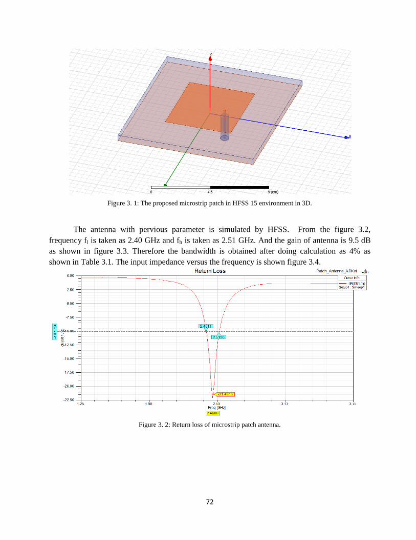
72
Figure 3. 1: The proposed microstrip patch in HFSS 15 environment in 3D.
The antenna with pervious parameter is simulated by HFSS. From the figure 3.2,
frequency fl is taken as 2.40 GHz and fh is taken as 2.51 GHz. And the gain of antenna is 9.5 dB
as shown in figure 3.3. Therefore the bandwidth is obtained after doing calculation as 4% as
shown in Table 3.1. The input impedance versus the frequency is shown figure 3.4.
Figure 3. 2: Return loss of microstrip patch antenna.

73
Figure 3. 3: Gain of microstrip patch antenna.
Figure 3. 4: Input impedance of microstrip patch antenna.
Table 3. 1: Results of MSP antenna.
1.25 1.88 2.50 3.13 3.75Freq [GHz]
-1000.00
-500.00
0.00
500.00
1000.00
1500.00
2000.00
2500.00
Y1
Patch_Antenna_ADKv1XY Plot 1 ANSOFT
Curve Info
im(Zt(coax_pin_T1,coax_pin_T1))Setup1 : Sw eep1
mag(Zt(coax_pin_T1,coax_pin_T1))Setup1 : Sw eep1
Parameters Value
fh 2.5 GH
fl 2.4 GHz
fo 2.46 GHz
BW= fh – fl 100 MHz
BWr%=BW
fo * 100 4 %

74
3.2: MSP antenna with parasitic
In this section we used parasitic patch with the same parameter of basic antenna and we
used parasitic patch dimensions 1 cm x 2.5 cm as shown in figure 3.5.
Figure 3. 5: The proposed MSP antenna with parasitic.

75
Figure 3. 6:Return loss of MSP antenna with parasitic.
Return loss results shown in figure 3.6 at resonance frequency (fo) are very bad. In table
3.2 we find the height and low frequency are shifted and the bandwidth ratio increased 0.5 %.
Parameters Value
fh 2.13 GHz
fl 2.24 GHz
fo 2.20 GHz
BW= fh – fl 100 MHz
BWr%=BW
fo * 100 4.5 %
Table 3. 2: Results of MSP antenna with parasitic
Also in figure 3.7 we find that the gain decreased from 9.5 dB to 8.6 dB. By comparing
between Input impedance in basic antenna at figure 3.1 and the input impedance in parasitic patch
antenna at figure 3.8 we find that a parasitic was worse.
1.00 1.50 2.00 2.50 3.00 3.50 4.00 4.50 5.00 5.50 6.00 6.50 7.00 7.50Freq [GHz]
-15.00
-12.50
-10.00
-7.50
-5.00
-2.50
0.00
dB
(St(
co
ax_
pin
_T
1,c
oa
x_
pin
_T
1))
Patch_Antenna_ADKv1XY Plot 6 ANSOFT
Curve Info
dB(St(coax_pin_T1,coax_pin_T1))Setup1 : Sw eep1

76
Figure 3. 7: Gain of MSP antenna with parasitic.
Figure 3.8: Input impedance of MSP antenna with parasitic.
3.3: Bandwidth enhancement of antenna using new feeding technique IPF.
The goal of this section is to enhance bandwidth of microstrip antenna by trying connect
the probe feed and patch indirectly by using stripline connecting between the patch and probe
feed.
Dimensions of indirect probe feed length is 0.5 cm and width is 1 cm and position is 0cm
form edge of the patch on Y-axis and dimension of stripline is 2.5 cm x 1 cm as shown in the
figure 3.9.
1.00 2.00 3.00 4.00 5.00 6.00 7.00Freq [GHz]
-250.00
-125.00
0.00
125.00
250.00
Y1
Patch_Antenna_ADKv1XY Plot 19 ANSOFT
Curve Info
im(Zt(coax_pin_T1,coax_pin_T1))Setup1 : Sw eep1
re(Zt(coax_pin_T1,coax_pin_T1))Setup1 : Sw eep1
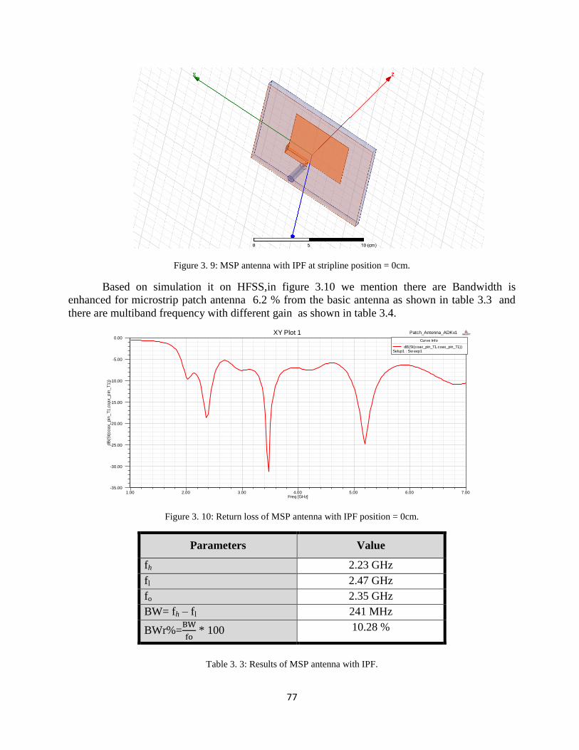
77
Figure 3. 9: MSP antenna with IPF at stripline position = 0cm.
Based on simulation it on HFSS,in figure 3.10 we mention there are Bandwidth is
enhanced for microstrip patch antenna 6.2 % from the basic antenna as shown in table 3.3 and
there are multiband frequency with different gain as shown in table 3.4.
Figure 3. 10: Return loss of MSP antenna with IPF position = 0cm.
Parameters Value
fh 2.23 GHz
fl 2.47 GHz
fo 2.35 GHz
BW= fh – fl 241 MHz
BWr%=BW
fo * 100 10.28 %
Table 3. 3: Results of MSP antenna with IPF.
1.00 2.00 3.00 4.00 5.00 6.00 7.00Freq [GHz]
-35.00
-30.00
-25.00
-20.00
-15.00
-10.00
-5.00
0.00
dB
(St(
co
ax_
pin
_T
1,c
oa
x_
pin
_T
1))
Patch_Antenna_ADKv1XY Plot 1 ANSOFT
Curve Info
dB(St(coax_pin_T1,coax_pin_T1))Setup1 : Sw eep1

78
IPF position= 0 cm Fr (GHz) S11(dB) BW (MHz) Gain
dB
First band 2.35 -18.72 241 9.6
Second band 3.47 -31.29 300 8.17
Third band 5.19 -24.65 500 9.5
Table 3. 4: MSP antenna parameters with IPF position = 0cm.
The input impedance was also within the range from 32Ω to 35Ω at resonance frequencies
as illustrate in the figure 3.11.
Figure 3. 11: Input impedance of gain MSP antenna with IPF position = 0cm.
3.4: Change the position of with indirect probe feeding
In this section we want to change the position of stripline on Y-axis to find the optimum
result where this change factor is y=.86 cm.
At IPF position on y As shown in figure 3.12
We find the return loss change as shown in figure 3.13 also from table 3.5 we find that the
return loss worse than the previous position and the gain 9.6 dB as shown in figure 3.14 also the
input impedance versus with resonance frequencies shown in figure 3.15 .
1.00 2.00 3.00 4.00 5.00 6.00 7.00Freq [GHz]
-250.00
-125.00
0.00
125.00
250.00
Y1
Patch_Antenna_ADKv1XY Plot 2 ANSOFT
Curve Info
im(Zt(coax_pin_T1,coax_pin_T1))Setup1 : Sw eep1
re(Zt(coax_pin_T1,coax_pin_T1))Setup1 : Sw eep1

79
Figure 3. 12: MSP antenna with IPF position = y cm.
Figure 3. 13: Return loss of MSP antenna with IPF position =y cm.
IPF position = y cm Fr (GHz) S11 (dB) BW (MHz)
First band 2.02 -13.41 335
Second band 3.11 -28.25 624
Third band 4.97 -21.39 523
Table 3. 5: MSP antenna parameters with IPF position = y cm.
1.00 2.00 3.00 4.00 5.00 6.00 7.00Freq [GHz]
-30.00
-25.00
-20.00
-15.00
-10.00
-5.00
0.00
dB
(St(
coa
x_p
in_
T1
,co
ax_
pin
_T
1))
Patch_Antenna_ADKv1XY Plot 1 ANSOFT
Curve Info
dB(St(coax_pin_T1,coax_pin_T1))Setup1 : Sw eep1

80
Figure 3. 14: Gain of MSP antenna with IPF position = y cm.
Figure 3. 15: Input impedance of MSP antenna with IPF position = y cm.
At IPF position on 2y cm as shown in figure 3.16
From figure 3.17 we find that the return loss change by change the position and the
multiband decreased to be two multiband comparing the return loss to the basic position 0 cm
show that better than but the bandwidth decreased as shown in table 3.6 , figure 3.18 show that
the gain decrease. The input impedance show in figure 3.18 show that versus with the frequencies
within 50 Ω to 75 Ω.
1.00 2.00 3.00 4.00 5.00 6.00 7.00Freq [GHz]
-250.00
-125.00
0.00
125.00
250.00
Y1
Patch_Antenna_ADKv1XY Plot 2 ANSOFT
Curve Info
im(Zt(coax_pin_T1,coax_pin_T1))Setup1 : Sw eep1
re(Zt(coax_pin_T1,coax_pin_T1))Setup1 : Sw eep1
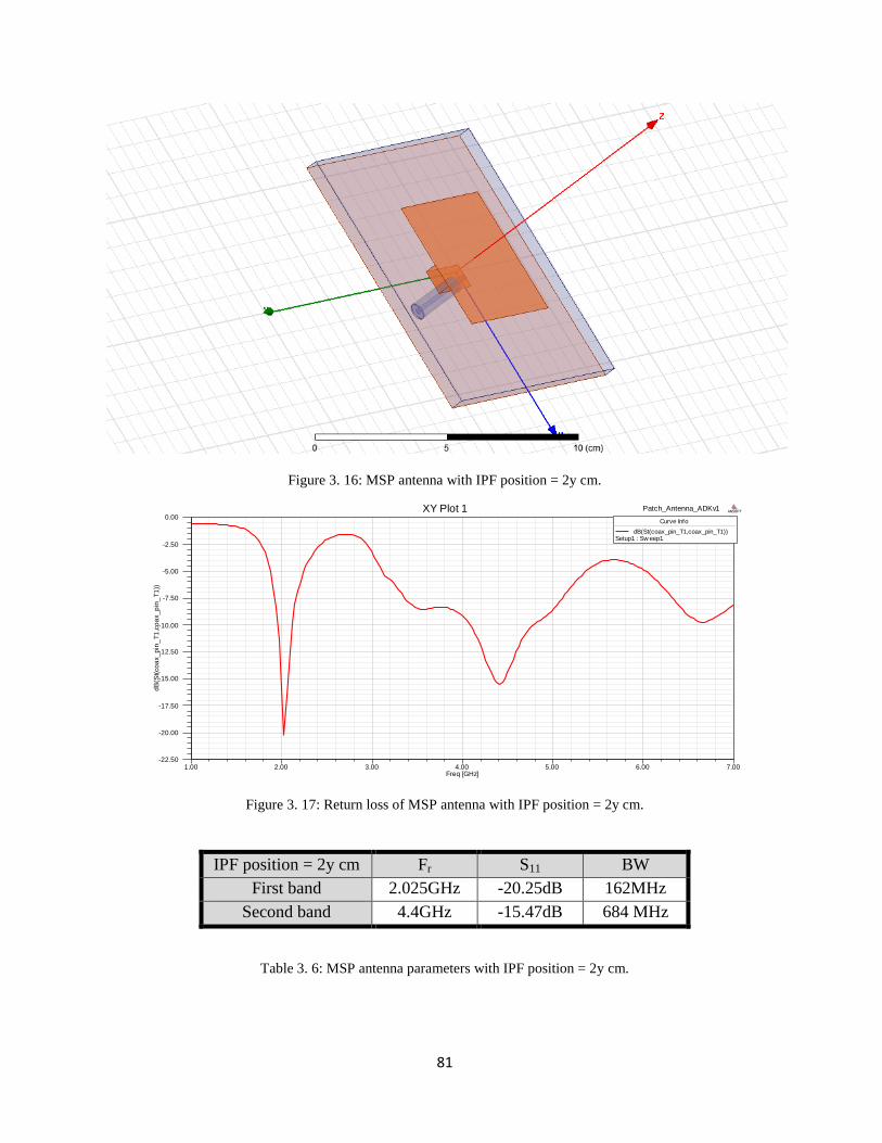
81
Figure 3. 16: MSP antenna with IPF position = 2y cm.
Figure 3. 17: Return loss of MSP antenna with IPF position = 2y cm.
IPF position = 2y cm Fr S11 BW
First band 2.025GHz -20.25dB 162MHz
Second band 4.4GHz -15.47dB 684 MHz
Table 3. 6: MSP antenna parameters with IPF position = 2y cm.
1.00 2.00 3.00 4.00 5.00 6.00 7.00Freq [GHz]
-22.50
-20.00
-17.50
-15.00
-12.50
-10.00
-7.50
-5.00
-2.50
0.00
dB
(St(
co
ax_
pin
_T
1,c
oa
x_
pin
_T
1))
Patch_Antenna_ADKv1XY Plot 1 ANSOFT
Curve Info
dB(St(coax_pin_T1,coax_pin_T1))Setup1 : Sw eep1

82
Figure 3. 18: Gain of MSP antenna with IPF position = 2y cm.
Figure 3. 19: Input impedance of MSP antenna with IPF position = 2y cm.
At IPF position on 3y cm as shown in figure 3.20
From figure 3.21 show that the return loss of the antenna it be two multi band and two
resonant frequencies it be the nearly the same value compare with the previous position of IPF =-
1.72. Gain and input impedance from figure 3.22, 3.23 as shown below there are nearly the same
value of previous position
1.00 2.00 3.00 4.00 5.00 6.00 7.00Freq [GHz]
-250.00
-125.00
0.00
125.00
250.00
Y1
Patch_Antenna_ADKv1XY Plot 2 ANSOFT
Curve Info
im(Zt(coax_pin_T1,coax_pin_T1))Setup1 : Sw eep1
re(Zt(coax_pin_T1,coax_pin_T1))Setup1 : Sw eep1

83
Figure 3. 20: MSP antenna with IPF position = 3y cm.
Figure 3. 21: Return loss of MSP antenna with IPF position = 3y cm.
IPF position = 3y cm Fr S11 BW
First band 2.025GHz -18.61dB 180MHz
Second band 4.4GHz -15.46dB 644 MHz
Table 3. 7: MSP antenna parameters with IPF position = 3y cm.
1.00 2.00 3.00 4.00 5.00 6.00 7.00Freq [GHz]
-20.00
-17.50
-15.00
-12.50
-10.00
-7.50
-5.00
-2.50
0.00
dB
(St(
coa
x_p
in_
T1
,co
ax_
pin
_T
1))
Patch_Antenna_ADKv1XY Plot 1 ANSOFT
Curve Info
dB(St(coax_pin_T1,coax_pin_T1))Setup1 : Sw eep1
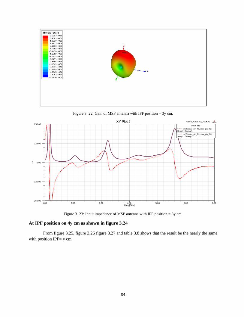
84
Figure 3. 22: Gain of MSP antenna with IPF position = 3y cm.
Figure 3. 23: Input impedance of MSP antenna with IPF position = 3y cm.
At IPF position on 4y cm as shown in figure 3.24
From figure 3.25, figure 3.26 figure 3.27 and table 3.8 shows that the result be the nearly the same
with position IPF= y cm.
1.00 2.00 3.00 4.00 5.00 6.00 7.00Freq [GHz]
-250.00
-125.00
0.00
125.00
250.00
Y1
Patch_Antenna_ADKv1XY Plot 2 ANSOFT
Curve Info
im(Zt(coax_pin_T1,coax_pin_T1))Setup1 : Sw eep1
re(Zt(coax_pin_T1,coax_pin_T1))Setup1 : Sw eep1

85
Figure 3. 24: MSP antenna with IPF position = 4y cm.
Figure 3. 25: Return loss of MSP antenna with IPF position = 4y cm.
IPF position = 4y cm Fr S11 BW
First band 2.14 -10.37 334
Second band 3.11 -27.39 611
Third band 4.97 -20.42 523
Table 3. 8: MSP antenna parameters with IPF position = 4y cm.
1.00 2.00 3.00 4.00 5.00 6.00 7.00Freq [GHz]
-30.00
-25.00
-20.00
-15.00
-10.00
-5.00
0.00
dB
(St(
co
ax_
pin
_T
1,c
oa
x_
pin
_T
1))
Patch_Antenna_ADKv1XY Plot 1 ANSOFT
Curve Info
dB(St(coax_pin_T1,coax_pin_T1))Setup1 : Sw eep1
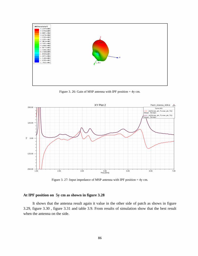
86
Figure 3. 26: Gain of MSP antenna with IPF position = 4y cm.
Figure 3. 27: Input impedance of MSP antenna with IPF position = 4y cm.
At IPF position on 5y cm as shown in figure 3.28
It shows that the antenna result again it value in the other side of patch as shows in figure
3.29, figure 3.30 , figure 3.31 and table 3.9. From results of simulation show that the best result
when the antenna on the side.
1.00 2.00 3.00 4.00 5.00 6.00 7.00Freq [GHz]
-250.00
-125.00
0.00
125.00
250.00
Y1
Patch_Antenna_ADKv1XY Plot 2 ANSOFT
Curve Info
im(Zt(coax_pin_T1,coax_pin_T1))Setup1 : Sw eep1
re(Zt(coax_pin_T1,coax_pin_T1))Setup1 : Sw eep1
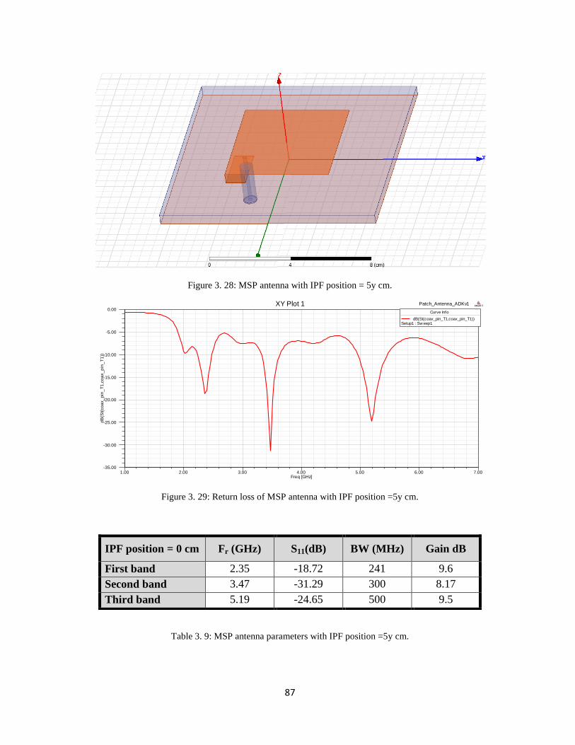
87
Figure 3. 28: MSP antenna with IPF position = 5y cm.
Figure 3. 29: Return loss of MSP antenna with IPF position =5y cm.
Table 3. 9: MSP antenna parameters with IPF position =5y cm.
1.00 2.00 3.00 4.00 5.00 6.00 7.00Freq [GHz]
-35.00
-30.00
-25.00
-20.00
-15.00
-10.00
-5.00
0.00
dB
(St(
co
ax_
pin
_T
1,c
oa
x_
pin
_T
1))
Patch_Antenna_ADKv1XY Plot 1 ANSOFT
Curve Info
dB(St(coax_pin_T1,coax_pin_T1))Setup1 : Sw eep1
IPF position = 0 cm Fr (GHz) S11(dB) BW (MHz) Gain dB
First band 2.35 -18.72 241 9.6
Second band 3.47 -31.29 300 8.17
Third band 5.19 -24.65 500 9.5

88
Figure 3. 30: Gain of MSP antenna with IPF position = 5y cm.
Figure 3. 31: Input impedance of MSP antenna with IPF position 5ycm.
The analysis of the antenna for different indirect probe feed positions values has been done
by varying and keeping others as constant. It is carried out here to parametric study the flexibility
in designing this of single layer patch antenna with indirect probe feed. The return loss of the
different indirect probe feed positions in the antenna design is shown in figure 3.32, which clearly
clarifies the explanation of the proposed antenna. By changing the IPF position on Y-axis give the
same result at the side of axis like a mirror.
1.00 2.00 3.00 4.00 5.00 6.00 7.00Freq [GHz]
-250.00
-125.00
0.00
125.00
250.00
Y1
Patch_Antenna_ADKv1XY Plot 2 ANSOFT
Curve Info
im(Zt(coax_pin_T1,coax_pin_T1))Setup1 : Sw eep1
re(Zt(coax_pin_T1,coax_pin_T1))Setup1 : Sw eep1

89
Figure 3. 32: Return loss Results compared by varying indirect probe feed positions.
Table 3. 10: S-parameter Study by varying indirect probe feed rectangular patch by varying probe feed point position.
3.5: Change the position of probe feed indirect probe feeding
In this section we want to change the probe feed position over the IPF static at the side of
patch on IPF=0 cm because the result in this location is the best, so we change the probe feed over
X-axis to get the optimum result and values to the antenna this change factor is x=.45 cm.
At probe feed x cm as shown in figure 3.33.
The return loss as shown in figure 3.34 the return loss is very good as shown in table 3.11
and bandwidth enhance than the basic antenna and the gain not change when probe feed = -0.45
cm as shown in figure 3.35 , from figure 3.36 we can see that the input impedance versus within
the frequencies (35 Ω -50Ω).
1.00 2.00 3.00 4.00 5.00 6.00 7.00Freq [GHz]
-50.00
-40.00
-30.00
-20.00
-10.00
0.00d
B(S
t(co
ax_
pin
_T
1,c
oa
x_
pin
_T
1))
Ansoft LLC Patch_Antenna_ADKv1XY Plot 1 ANSOFT
Curve Info
dB(St(coax_pin_T1,coax_pin_T1))Setup1 : Sw eep1zf='-4.3cm'
dB(St(coax_pin_T1,coax_pin_T1))Setup1 : Sw eep1zf='-3.44cm'
dB(St(coax_pin_T1,coax_pin_T1))Setup1 : Sw eep1zf='-2.58cm'
dB(St(coax_pin_T1,coax_pin_T1))Setup1 : Sw eep1zf='-1.72cm'
dB(St(coax_pin_T1,coax_pin_T1))Setup1 : Sw eep1zf='-0.86cm'
dB(St(coax_pin_T1,coax_pin_T1))Setup1 : Sw eep1zf='0cm'
in.feed position freq1 re.loss b.w freq2 re.loss b.w ferq3 re.loss b.w ferq4 re.loss b.w
0 2.3789 -19.219 0.2282 3.4888 -34.9879 0.3152 5.2175 -22.0345 0.4642 0 0 0
-0.86 2.042 -13.2284 0.3361 3.1323 -30.7858 0.6047 4.3363 -11.2616 0.3251 5 -19.7569 0.4931
-1.72 2.0291 -21.2049 0.1552 4.3969 -15.5593 0.6782 0 0 0 0 0 0
-2.58 2.0291 -21.2049 0.1552 4.3969 -15.5593 0.6782 0 0 0 0 0 0
-3.44 2.0291 -14.1173 0.3348 3.1121 -26.3818 0.6201 4.3161 -11.3507 0.3402 4.9821 -20.2754 0.5
-4.3 2.3587 -20.0113 0.24 3.4616 -36.3933 0.2942 5.1906 -24.6752 0.4932 0 0 0
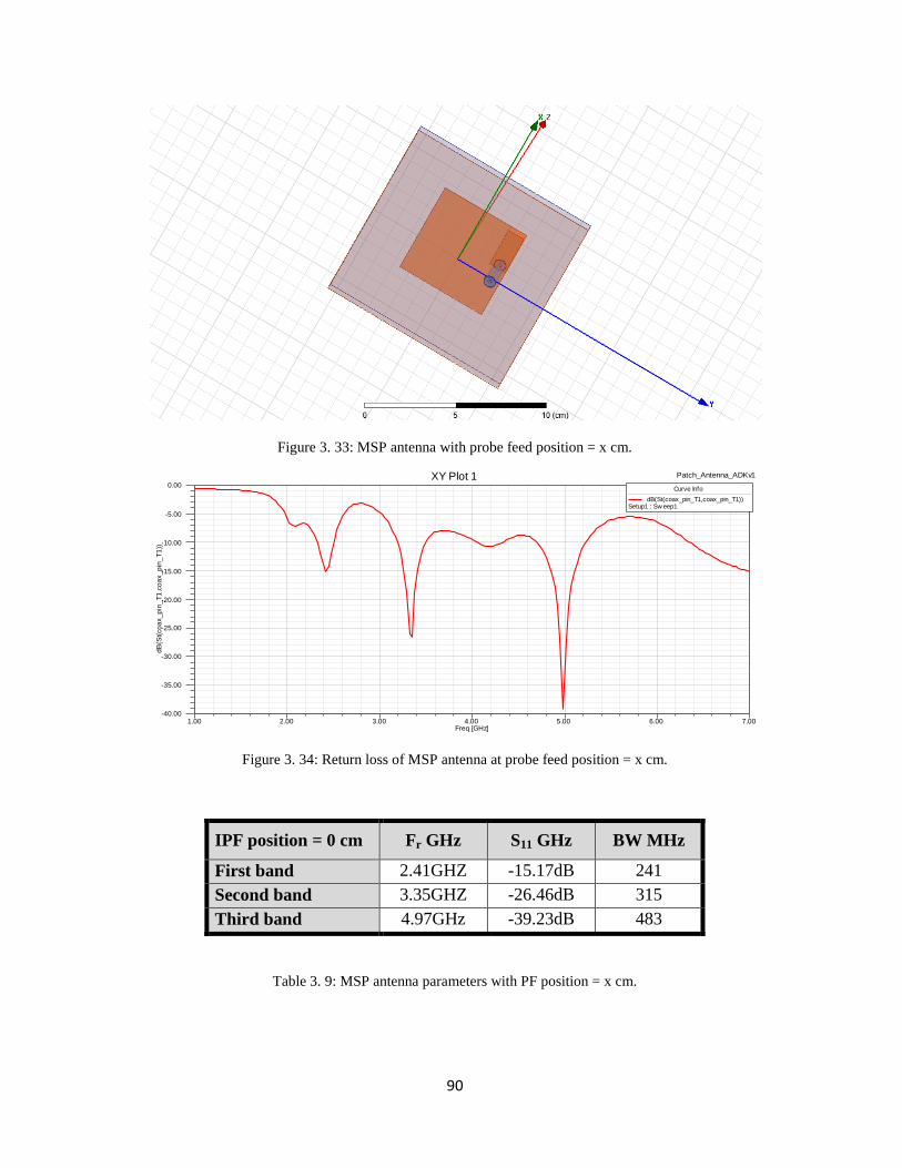
90
Figure 3. 33: MSP antenna with probe feed position = x cm.
Figure 3. 34: Return loss of MSP antenna at probe feed position = x cm.
IPF position = 0 cm Fr GHz S11 GHz BW MHz
First band 2.41GHZ -15.17dB 241
Second band 3.35GHZ -26.46dB 315
Third band 4.97GHz -39.23dB 483
Table 3. 9: MSP antenna parameters with PF position = x cm.
1.00 2.00 3.00 4.00 5.00 6.00 7.00Freq [GHz]
-40.00
-35.00
-30.00
-25.00
-20.00
-15.00
-10.00
-5.00
0.00
dB
(St(
co
ax_
pin
_T
1,c
oa
x_
pin
_T
1))
Patch_Antenna_ADKv1XY Plot 1Curve Info
dB(St(coax_pin_T1,coax_pin_T1))Setup1 : Sw eep1

91
Figure 3. 35: Gain MSP antenna with probe feed position = x cm.
Figure 3. 36: Input impedance of MSP antenna with probe feed position = x cm.
At probe feed 2x cm as shown in figure 3.37.
From figure 3.38 shows that the return loss very worth than the previous result and not
necessary to get gain and input impedance.
.
1.00 2.00 3.00 4.00 5.00 6.00 7.00Freq [GHz]
-250.00
-125.00
0.00
125.00
250.00
Y1
Patch_Antenna_ADKv1XY Plot 2 ANSOFT
Curve Info
im(Zt(coax_pin_T1,coax_pin_T1))Setup1 : Sw eep1
re(Zt(coax_pin_T1,coax_pin_T1))Setup1 : Sw eep1

92
Figure 3. 37: MSP antenna with probe feed position = 2x cm.
Figure 3. 38:Return loss of MSP antenna at probe feed position = 2x cm.
At probe feed 3x cm as shown in figure 3.39.
Like a previous position that the return loss shown in figure 3.40 .
1.00 2.00 3.00 4.00 5.00 6.00 7.00Freq [GHz]
-10.00
-8.00
-6.00
-4.00
-2.00
0.00
dB
(St(
co
ax_
pin
_T
1,c
oa
x_
pin
_T
1))
Patch_Antenna_ADKv1XY Plot 1Curve Info
dB(St(coax_pin_T1,coax_pin_T1))Setup1 : Sw eep1

93
Figure 3. 39: MSP antenna with probe feed position = 3x cm.
Figure 3. 40: Return loss of MSP antenna at probe feed position = 3x cm.
At probe feed 4x cm as shown in figure 3.41.
From figure 3.42 show that the return loss above -10 dB.
1.00 2.00 3.00 4.00 5.00 6.00 7.00Freq [GHz]
-9.00
-8.00
-7.00
-6.00
-5.00
-4.00
-3.00
-2.00
-1.00
0.00
dB
(St(
co
ax_
pin
_T
1,c
oa
x_
pin
_T
1))
Patch_Antenna_ADKv1XY Plot 1Curve Info
dB(St(coax_pin_T1,coax_pin_T1))Setup1 : Sw eep1

94
Figure 3. 41: MSP antenna with probe feed position = 4x cm.
Figure 3. 42: Return loss of MSP antenna at probe feed position = 4x cm.
At probe feed 5x cm as shown in figure 3.43.
Finally the last position of previous probe feed shown in figure 3.44 give the same result
of previous position .
1.00 2.00 3.00 4.00 5.00 6.00 7.00Freq [GHz]
-9.00
-8.00
-7.00
-6.00
-5.00
-4.00
-3.00
-2.00
-1.00
0.00
dB
(St(
co
ax_
pin
_T
1,c
oa
x_
pin
_T
1))
Patch_Antenna_ADKv1XY Plot 1Curve Info
dB(St(coax_pin_T1,coax_pin_T1))Setup1 : Sw eep1
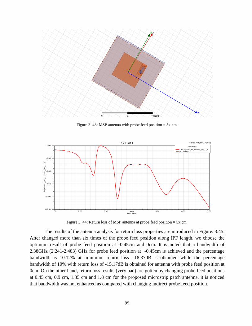
95
Figure 3. 43: MSP antenna with probe feed position = 5x cm.
Figure 3. 44: Return loss of MSP antenna at probe feed position = 5x cm.
The results of the antenna analysis for return loss properties are introduced in Figure. 3.45.
After changed more than six times of the probe feed position along IPF length, we choose the
optimum result of probe feed position at -0.45cm and 0cm. It is noted that a bandwidth of
2.38GHz (2.241-2.483) GHz for probe feed position at -0.45cm is achieved and the percentage
bandwidth is 10.12% at minimum return loss –18.37dB is obtained while the percentage
bandwidth of 10% with return loss of -15.17dB is obtained for antenna with probe feed position at
0cm. On the other hand, return loss results (very bad) are gotten by changing probe feed positions
at 0.45 cm, 0.9 cm, 1.35 cm and 1.8 cm for the proposed microstrip patch antenna, it is noticed
that bandwidth was not enhanced as compared with changing indirect probe feed position.
1.00 2.00 3.00 4.00 5.00 6.00 7.00Freq [GHz]
-12.50
-10.00
-7.50
-5.00
-2.50
0.00
dB
(St(
co
ax_
pin
_T
1,c
oa
x_
pin
_T
1))
Patch_Antenna_ADKv1XY Plot 1Curve Info
dB(St(coax_pin_T1,coax_pin_T1))Setup1 : Sw eep1
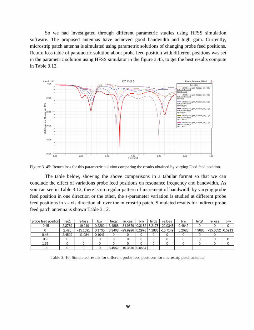
96
So we had investigated through different parametric studies using HFSS simulation
software. The proposed antennas have achieved good bandwidth and high gain. Currently,
microstrip patch antenna is simulated using parametric solutions of changing probe feed positions.
Return loss table of parametric solution about probe feed position with different positions was set
in the parametric solution using HFSS simulator in the figure 3.45, to get the best results compute
in Table 3.12.
Figure 3. 45: Return loss for this parametric solution comparing the results obtained by varying Feed feed position.
The table below, showing the above comparisons in a tabular format so that we can
conclude the effect of variations probe feed positions on resonance frequency and bandwidth. As
you can see in Table 3.12, there is no regular pattern of increment of bandwidth by varying probe
feed position in one direction or the other, the s-parameter variation is studied at different probe
feed positions in x-axis direction all over the microstrip patch. Simulated results for indirect probe
feed patch antenna is shown Table 3.12.
Table 3. 10: Simulated results for different probe feed positions for microstrip patch antenna.
1.00 2.00 3.00 4.00 5.00 6.00 7.00Freq [GHz]
-50.00
-40.00
-30.00
-20.00
-10.00
0.00
dB
(St(
co
ax_
pin
_T
1,c
oa
x_
pin
_T
1))
Ansoft LLC Patch_Antenna_ADKv1XY Plot 1 ANSOFT
Curve Info
dB(St(coax_pin_T1,coax_pin_T1))Setup1 : Sw eep1fm='-0.45cm'
dB(St(coax_pin_T1,coax_pin_T1))Setup1 : Sw eep1fm='0cm'
dB(St(coax_pin_T1,coax_pin_T1))Setup1 : Sw eep1fm='0.45cm'
dB(St(coax_pin_T1,coax_pin_T1))Setup1 : Sw eep1fm='0.9cm'
dB(St(coax_pin_T1,coax_pin_T1))Setup1 : Sw eep1fm='1.35cm'
dB(St(coax_pin_T1,coax_pin_T1))Setup1 : Sw eep1fm='1.8cm'
probe feed position freq1 re.loss b.w freq2 re.loss b.w ferq3 re.loss b.w ferq4 re.loss b.w
-0.45 2.3789 -19.219 0.2282 3.4888 -34.9879 0.3152 5.2175 -22.0345 0.4642 0 0 0
0 2.426 -15.1591 0.1735 3.3408 -29.9926 0.2976 4.1883 -10.7149 0.2628 4.9888 -35.6552 0.5213
0.45 2.4529 -11.984 0.1041 0 0 0 0 0 0 0 0
0.9 0 0 0 0 0 0 0 0 0 0 0 0
1.35 0 0 0 0 0 0 0 0 0 0 0 0
1.8 0 0 0 3.4552 -10.3376 0.0534

97
3.6: Changing the inner radius of probe feed.
In this section we try to change the inner radius probe feed to the standard inner radius
from 1mm to 0.73 mm to shows the change in result we chose the position of IPF over Y-axis 0
cm and the probe feed position over X-axis is -0.45 cm because that is the best result of pervious
simulations, as shown in figure 3.45 the new design of antenna with new inner radius.
The return loss of the antenna can be seen on figure 3.46 show that new value multiband
antenna this value better than the previous design. From table 3.13 show that the bandwidth
enhance over the previous enhancement.
Gain enhancement in the broadside direction as shown in figure 3.47. The maximum gain
of proposed antenna with changing radius of inner probe feed is achieved at resonance frequency
2.44 GHz with 9.68 dBi in the broadside direction. The input impedance was also within the
range from 37Ω to 59Ω at resonance frequencies as illustrate in the figure 3.48.
Figure 3. 46: MSP antenna with change inner radius of probe feed to 0.073cm.
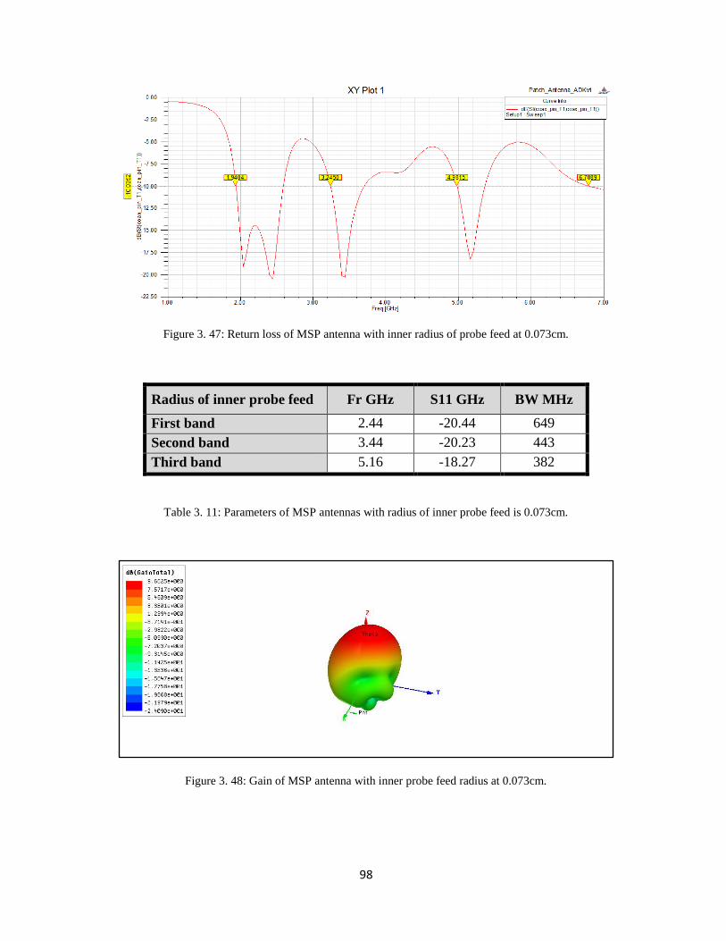
98
Figure 3. 47: Return loss of MSP antenna with inner radius of probe feed at 0.073cm.
Radius of inner probe feed Fr GHz S11 GHz BW MHz
First band 2.44 -20.44 649
Second band 3.44 -20.23 443
Third band 5.16 -18.27 382
Table 3. 11: Parameters of MSP antennas with radius of inner probe feed is 0.073cm.
Figure 3. 48: Gain of MSP antenna with inner probe feed radius at 0.073cm.
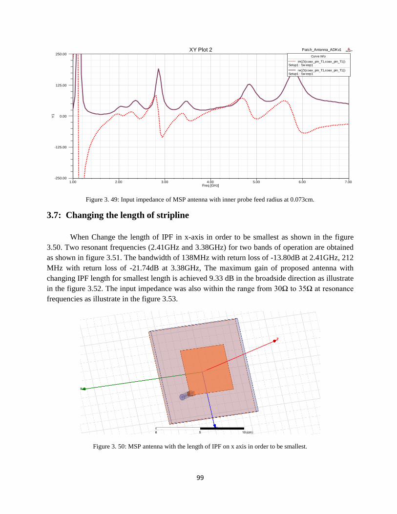
99
Figure 3. 49: Input impedance of MSP antenna with inner probe feed radius at 0.073cm.
3.7: Changing the length of stripline
When Change the length of IPF in x-axis in order to be smallest as shown in the figure
3.50. Two resonant frequencies (2.41GHz and 3.38GHz) for two bands of operation are obtained
as shown in figure 3.51. The bandwidth of 138MHz with return loss of -13.80dB at 2.41GHz, 212
MHz with return loss of -21.74dB at 3.38GHz, The maximum gain of proposed antenna with
changing IPF length for smallest length is achieved 9.33 dB in the broadside direction as illustrate
in the figure 3.52. The input impedance was also within the range from 30Ω to 35Ω at resonance
frequencies as illustrate in the figure 3.53.
Figure 3. 50: MSP antenna with the length of IPF on x axis in order to be smallest.
1.00 2.00 3.00 4.00 5.00 6.00 7.00Freq [GHz]
-250.00
-125.00
0.00
125.00
250.00Y
1Patch_Antenna_ADKv1XY Plot 2 ANSOFT
Curve Info
im(Zt(coax_pin_T1,coax_pin_T1))Setup1 : Sw eep1
re(Zt(coax_pin_T1,coax_pin_T1))Setup1 : Sw eep1

100
Figure 3. 51: Return loss if MSP antenna with the length of IPF on x axis in order to be smallest.
Figure 3. 52: Gain MSP antenna with the length of IPF on x axis in order to be smallest.
1.00 2.00 3.00 4.00 5.00 6.00 7.00Freq [GHz]
-22.50
-20.00
-17.50
-15.00
-12.50
-10.00
-7.50
-5.00
-2.50
0.00d
B(S
t(co
ax_
pin
_T
1,c
oa
x_
pin
_T
1))
Patch_Antenna_ADKv1XY Plot 6 ANSOFT
Curve Info
dB(St(coax_pin_T1,coax_pin_T1))Setup1 : Sw eep1

101
Figure 3. 53: Input impedance of MSP antenna with the length of IPF on x axis in order to be smallest.
Moreover, changing the length of IPF on x-axis in order to be the same length of the patch
as shown in the figure 3.54. Many resonant frequencies are appeared for multi-bands of operation
are obtained as shown in figure 3.55. The bandwidth of 137MHz with return loss of -12.13dB at
2.35GHz, 219 MHz with return loss of -14.61dB at 3.38GHz and 319 MHz with return loss of -
28.36dB at 3.80GHz and 543 MHz with return loss of -33.14dB at 5.16GHz. The maximum gain
of proposed antenna with changing IPF length in order to be the same length the patch is achieved
8.49 dBi in the broadside direction as shown in the figure 3.56. The input impedance was also
within the range from 37Ω to 50Ω at resonance frequencies as illustrate in the figure 3.57.
1.00 2.00 3.00 4.00 5.00 6.00 7.00Freq [GHz]
-250.00
-125.00
0.00
125.00
250.00Y
1Patch_Antenna_ADKv1XY Plot 14 ANSOFT
Curve Info
im(Zt(coax_pin_T1,coax_pin_T1))Setup1 : Sw eep1
re(Zt(coax_pin_T1,coax_pin_T1))Setup1 : Sw eep1

102
Figure 3. 54: MSP antenna with IPF with the same length of the patch.
Figure 3. 55: Return loss of MSP antenna with the length of IPF on x axis the same length of the patch.
1.00 2.00 3.00 4.00 5.00 6.00 7.00Freq [GHz]
-40.00
-30.00
-20.00
-10.00
0.00
dB
(St(
co
ax_
pin
_T
1,c
oa
x_
pin
_T
1))
Ansoft LLC Patch_Antenna_ADKv1XY Plot 1 ANSOFT
Curve Info
dB(St(coax_pin_T1,coax_pin_T1))Setup1 : Sw eep1

103
Figure 3. 56: Gain of MSP antenna with the length of IPF on x axis the same length of the patch.
Figure 3. 57: Input impedance of MSP antenna with the length of IPF on x axis the same length of the patch.
3.8: Hexagonal MSP antenna with probe feed patch
Where an additional case is considered to enhance the bandwidth, hexagonal patch
technique has been applied over the antenna design using probe feed which dimension of each
length is 3cm calculated by using design equations in chapter 2, the feed location is center of
hexagon antenna as shown in the figure 3.58. Hence, resonance frequency is generated bandwidth
up to 5.49% (2.69 to 2.81) GHz as shown in figure 3.59.however, maximum gain 8.89 dB was
attained at the frequency of 2.5 GHz as shown in the figure 3.60.
1.00 2.00 3.00 4.00 5.00 6.00 7.00Freq [GHz]
-500.00
-250.00
0.00
250.00
500.00
Y1
Patch_Antenna_ADKv1XY Plot 2 ANSOFT
Curve Info
im(Zt(coax_pin_T1,coax_pin_T1))Setup1 : Sw eep1
re(Zt(coax_pin_T1,coax_pin_T1))Setup1 : Sw eep1
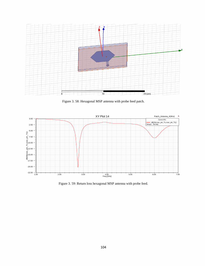
104
Figure 3. 58: Hexagonal MSP antenna with probe feed patch.
Figure 3. 59: Return loss hexagonal MSP antenna with probe feed.
1.00 2.00 3.00 4.00 5.00 6.00 7.00Freq [GHz]
-22.50
-20.00
-17.50
-15.00
-12.50
-10.00
-7.50
-5.00
-2.50
0.00
dB
(St(
co
ax_
pin
_T
1,c
oa
x_
pin
_T
1))
Patch_Antenna_ADKv1XY Plot 14Curve Info
dB(St(coax_pin_T1,coax_pin_T1))Setup1 : Sw eep

105
Figure 3. 60: Gain hexagonal MSP antenna with probe feed.
3.9: Hexagonal MSP antenna with indirect probe feed patch
By using an indirect probe feed for hexagonal patch antenna as shown in the figure 3.61,
while, three resonant modes are produced. The first resonant mode increases with return losses of
-28.50dB that is generated bandwidth up to 12.45%, the second resonance mode decreases with
return loss of -14.34dB that is generated bandwidth up to 9.69%, and the third resonance mode
decreases with return loss of -13.50dB that is generated bandwidth up to 9.9%,. The indirect
probe feed for hexagonal patch antenna enhance bandwidth as shown in the figure 3.62. It has a
band range of 2 GHz to 5 GHz with total gain approximately of 9.41 dBi as shown in the figure
3.63.
Figure 3. 61: Hexagonal MSP antenna with indirect probe feed patch.

106
Figure 3. 62: Return loss Hexagonal MSP antenna with indirect probe feed patch.
Figure 3. 63: Gain of Hexagonal MSP antenna with indirect probe feed patch.
Finally, I had design MSP antenna with different indirect probe feed positions for
wideband applications. We chose the optimum results of indirect probe feed positions. We use a
substrate (air) have relative permittivity (1), thickness of (h=5mm) and dimensions L × W (12cm
× 11cm). All microstrip patch simulated by software name HFSS which basis on finite element
method. A series of parameters of the MSP should be carefully selected. In this section, the
effects of several key parameters on the proposed antennas were discussed and simulated using
the Ansoft HFSS. In the process of analysis, it is also found that in comparison with the probe
feed and indirect probe feed effects on the bandwidth and resonant frequency. The resonant
frequency slightly decreases and bandwidth increase with changing indirect probe feed. To meet
these improvements, an extensive-simulation study has been carried out to determine the optimal
dimensions of the rectangular patch shapes, by maximizing the bandwidth and results are shown.
1.00 2.00 3.00 4.00 5.00 6.00 7.00Freq [GHz]
-30.00
-25.00
-20.00
-15.00
-10.00
-5.00
0.00d
B(S
t(co
ax_
pin
_T
1,c
oa
x_
pin
_T
1))
Patch_Antenna_ADKv1XY Plot 14Curve Info
dB(St(coax_pin_T1,coax_pin_T1))Setup1 : Sw eep

107
The improvement of bandwidth, resonance frequency, returns loss, and gain are illustrated.
The largest improvement is provided by indirect probe feed position. It is clear that the antenna
design with indirect probe feed displays the best performance compared with the others. It is
noted that a bandwidth of probe feed position at -0.45cm is achieved the percentage bandwidth is
10.12% at minimum return loss –18.37dB is obtained while the percentage bandwidth of 10%
with return loss of -15.17dB is obtained for antenna with probe feed position at 0cm. we observe
that for the proposed antenna, when the position of the probe feed is changed along stripline
length, we obtain a greater bandwidth at -0.45cm and 0cm in comparison with the bandwidth
obtained when the probe feed position is changed.
However, note that the inner radius of probe feed is changed to 0.073cm of these MSP
antenna, we can improve the bandwidth by up to 26.59% when compared with the probe feed
radius is 0.1cm.Thus, a considerable improvement in bandwidth can be obtained for the same
indirect probe feed position.
Now, it is clear that the antenna with indirect probe feed gives a good performance of
bandwidth compared with bandwidth of the antenna without indirect probe feed.

108
References
[1] K. L. Wong a nd W. H. Hsu, “Broadband triangular microstrip antenna with U-shaped s
lot, ” Electron. Lett. 33, 2085–2087, Dec. 4, 1997.

109
Chapter 4
CONCLUSION AND FUTURE PROSPECTS
During recent years, much effort has gone into bandwidth enhancement techniques for
microstrip antennas in general. As such, there is a great amount of information in the open
literature and it covers a very broad range of solutions that have been proposed. The entire
spectrum of approaches that have been suggested is too comprehensive to discuss here and
therefore the discussion in this chapter will be restricted to techniques that have been applied to
enhance the bandwidth of probe-fed microstrip patch antennas in particular .In this thesis, a broad
overview will be given in terms of the various techniques that are currently available to enhance
the bandwidth of microstrip patch antennas.
The performance, advantages and disadvantages of the most practical approaches will also
be discussed which there has been a tremendous amount of activity during recent years, is that of
computational electromagnetics. These tools are essential for an accurate analysis and design of
complex antenna. Although probe-fed microstrip patch antennas are structurally quite simple, an
accurate analysis of their various characteristics proves to be rather intricate. A major advantage
of the new feeding mechanism is that only a single substrate is required to support the antenna.
This implies cost savings when compared to other approaches, as well as simplified
manufacturing techniques and light weight.
The principal contributions of this study include the development of a new probe feeding
mechanism for probe-fed MSP that is called indirect feed insert between substrate material and
patch. The characteristics of proposed antennas have been investigated through different
parametric studies using HFSS simulation software. Indirect probe feed microstrip patch antenna
has been successfully designed having a center frequency of 2.5 GHz.
One of the problems in this thesis is related with the numerical modelling techniques and
theoretical formulation this makes micorstrip patch antenna with indirect probe feed much more
efficient to analyze that was implemented for the purposes of this study
The method of changing the indirect probe feed position and dimension W or L,
reasonable return loss S11 values will be obtained, however. S11 values are acceptable, but the
microstrip antenna still suffers from low gain and small bandwidth, because there is a tradeoff
between antenna dimension and bandwidth.
The drawback in such antenna design is that the relative permittivity value of the
substrate, if high 𝜀𝑟 material is assigned, the antenna will suffer from poor S11 but will have a
nice gain, and just the opposite will happen when you assign low 𝜀𝑟. Because of this, the FR4

110
epoxy substrate has low gain. However, there are many steps to solve this issue. This could be
done by changing in the shape of the antenna or assigning different material properties like Left-
handed meta-material (LHM), which is a material whose permeability and permittivity are
simultaneously negative, but in this thesis assigned the air.
Then, in simulation result for return loss S11 of original antenna which the resonant
frequency has been 2.5 GHz, the bandwidth is 4.4% and gain is 9.58dBi, after many steps in
simulation more than indirect probe feed dimensions, the trouble was solved, being about
changing the indirect probe feed positions. Most of these steps have been described in chapter
three.
The proposed indirect probe feed microstrip patch antennas have improved bandwidth that
is 26.91% and achieved good impedance matching, stable gain, and radiation patterns.
The indirect probe feed antenna can be used for Wireless system application that operate
quad and triple (multiband) frequencies. In addition, the proposed antenna is 12 cm by 11 cm.so
the designed antenna is suitable for wireless system devices.
In future work, one may modify any antenna shape to a specific application. Future work
will concentrate on how to tackle size and performance of this type of antennas. Triple band with
high gain will be a good idea to continue studies in this field. As is the case with all research,
there are always more aspects that can be investigated than what is practically possible. Here also,
there are some aspects of both the new antenna and the numerical formulation that can be
extended.
Although the new antenna have been characterized to some extent, it would be useful to
have more comprehensive guidelines to design such antenna. This should include geometrical
parameters as well as the optimum choice of material properties, especially dielectric constants
and substrate thicknesses, fabrication and verification of simulated results can be carried out in
future
Related Documents
![BANDWIDTH IMPROVEMENT OF MICROSTRIP AN- TENNA … · 2018. 1. 10. · bandwidth of a patch antenna [18{22]. Bandwidth of small size microstrip antennas has been improved by the use](https://static.cupdf.com/doc/110x72/60f7db4f8ad6da2c602a0426/bandwidth-improvement-of-microstrip-an-tenna-2018-1-10-bandwidth-of-a-patch.jpg)