Antarctic ice sheet fertilises the Southern Ocean

Biogeosciences, 11, 2635–2643, 2014www.biogeosciences.net/11/2635/2014/doi:10.5194/bg-11-2635-2014© Author(s) 2014. CC Attribution 3.0 License.

Biogeosciences

Open A

ccess

Antarctic ice sheet fertilises the Southern Ocean

R. Death1, J. L. Wadham1, F. Monteiro1, A. M. Le Brocq2, M. Tranter 1, A. Ridgwell1, S. Dutkiewicz3, and R. Raiswell4

1School of Geographical Sciences, University of Bristol, BS81SS, UK2Geography, College of Life and Environmental Sciences, University of Exeter, EX4 4RJ, UK3Department of Earth, Atmosphere and Planetary Sciences, Massachusetts Institute of Technology, MA 02139, USA4School of Earth and Environment, University of Leeds, LS2 9JT, UK

Correspondence to:J. L. Wadham ([email protected])

Received: 7 June 2013 – Published in Biogeosciences Discuss.: 30 July 2013Revised: 19 March 2014 – Accepted: 25 March 2014 – Published: 19 May 2014

Abstract. Southern Ocean (SO) marine primary productiv-ity (PP) is strongly influenced by the availability of iron insurface waters, which is thought to exert a significant controlupon atmospheric CO2 concentrations on glacial/interglacialtimescales. The zone bordering the Antarctic Ice Sheet ex-hibits high PP and seasonal plankton blooms in response tolight and variations in iron availability. The sources of ironstimulating elevated SO PP are in debate. Established con-tributors include dust, coastal sediments/upwelling, icebergsand sea ice. Subglacial meltwater exported at the ice marginis a more recent suggestion, arising from intense iron cyclingbeneath the ice sheet. Icebergs and subglacial meltwater maysupply a large amount of bioavailable iron to the SO, esti-mated in this study at 0.07–0.2 Tg yr−1. Here we apply theMIT global ocean model (Follows et al., 2007) to determinethe potential impact of this level of iron export from the icesheet upon SO PP. The export of iron from the ice sheet raisesmodelled SO PP by up to 40 %, and provides one plausibleexplanation for seasonally very high in situ measurements ofPP in the near-coastal zone. The impact on SO PP is great-est in coastal regions, which are also areas of high measuredmarine PP. These results suggest that the export of Antarcticrunoff and icebergs may have an important impact on SO PPand should be included in future biogeochemical modelling.

1 Introduction

Primary production in the Southern Ocean (SO) accounts for5–10 % of total global oceanic primary production (Mooreand Abbott, 2000; Arrigo et al., 2008) and has an importantimpact on climate via its regulatory effect upon atmospheric

CO2 concentrations (Sigman and Boyle, 2000). The SO isa high-nutrient–low-chlorophyll (HNLC) region, where ironis the main limiting nutrient, preventing phytoplankton fromusing the available N and P (Martin, 1990). Hence, changesin the supply of iron are hypothesised to cause variationsin SO PP, and hence CO2 drawdown (Sarmiento and Orr,1991). Well-established iron sources include coastal sedi-ments/upwelling (Tagliabue et al., 2009), sea ice (Edwardsand Sedwick, 2001) and dust (Martin, 1990; Jickells et al.,2005), and more recently, iceberg-rafted debris (Raiswell etal., 2008; Raiswell and Canfield, 2012). Subglacial meltwa-ter discharged from the ice sheet has received comparativelylittle attention to date (Statham et al., 2008; Wadham et al.,2013). The impacts of both these glacial sources of iron uponSO PP have not yet been quantified and form the focus of thispaper. The significance of glacial iron sources is heightenedby predictions of rising meltwater and iceberg fluxes in fu-ture decades (Vaughan, 2006; Pritchard et al., 2012).

Debris entombed in icebergs and meltwater from beneathglaciers has been shown to be rich in bioavailable iron, aris-ing from intense iron cycling in subglacial environments(Statham et al., 2008; Raiswell et al., 2009; Wadham et al.,2010; Bhatia et al., 2013). Sulfide oxidation produces Fe(III)(in the form of Fe(OH)3) under oxic conditions and Fe(II) bymicrobial mediation under anoxic conditions (Eqs. (1) and(2), respectively) (Wadham et al., 2010). It is enhanced bythe continual exposure of fresh and reactive sulfide mineralsby glacial erosion:

4FeS2 + 15O2 + 14H2O ⇒ 8SO24 + 4Fe(OH)3 + 16H+ (1)

FeS2 + 14Fe3++ 8H2O ⇒ 2SO2−

4 + 15Fe2++ 16H+. (2)

Published by Copernicus Publications on behalf of the European Geosciences Union.

2636 R. Death et al.: Antarctic ice sheet fertilises the Southern Ocean

Table 1. Annual iron fluxes modelled in this paper for aeolian dust, icebergs and subglacial meltwater and in comparison to previouslycalculated values for these and other hypothesised iron sources to the Southern Ocean.

Fe Source Flux (Tg yr−1)

Input to modelAntarctic subglacial meltwater∗ 0.009–0.090Icebergs (aqueous and nanoparticulate) 0.065Aeolian dust 0.075

Previously calculated fluxesIcebergs (aqueous); Raiswell et al., 2008 0.001–0.005Icebergs (aqueous+nanoparticulate); Raiswell et al., 2008 0.06–0.120Sea ice; Edwards and Sedwick, 2001 3× 10−4

Aeolian dust; Raiswell et al,. 2008 0.01–0.130Benthic recycling from sediments; Raiswell and Canfield, 2012 0.013–0.032Hydrothermal iron; Taglaibue et al., 2010 0.021

∗ This assumes that all the SGM Fe flux is delivered to the MIT ocean cell adjacent to the coast.

Subglacial meltwaters are generated at the bed of the icesheet by geothermal heating of basal ice layers (Pattyn,2010). They are driven toward the margin via the dynamicfilling and draining of subglacial lakes and/or via subglacialrivers (Fricker et al., 2007; Wingham et al., 2006), where theyare exported via channels or as groundwater (Supplement 2).Solute fluxes associated with this water export are likely tobe high and of a similar magnitude to those from some of theplanet’s largest rivers (Wadham et al., 2010). We would ex-pect iron concentrations in subglacial meltwaters (SGM-Fe,i.e. aqueous+nanoparticulate+some colloidal Fe,< 0.4 µm)to be at the higher end of the reported range for glacial runoff(e.g. µM Fe, Supplement Table 1), consistent with the pre-vailing elevated rock:water ratios, prolonged water residencetimes and anoxic conditions. In support of this are high con-centrations of sulfate ions in porewaters from the Kamb andBindschadler ice streams (West Antarctica) and frozen lakeice from subglacial Lake Vostok (East Antarctica) (Skidmoreet al., 2010; Christner et al., 2006). The highest dissolvediron concentrations in Antarctic coastal waters have also re-cently been measured in the Pine Island Polynya, thought tobe associated with the release of iron-rich meltwater fromPine Island Glacier (Gerringa et al., 2012). Glacial ice andsea ice are relatively dilute in comparison (nM Fe, Supple-ment Table 1). We calculate that the potential iron export insubglacial meltwater is∼ 0.009–0.09 Tg a−1 (where SGM-Fe concentrations= 3 and 30 µM, respectively. We note thatthis assumes a 100 % export efficiency from the ice mar-gin to coastal waters for SGM iron, since the proportion ofiron which is removed from the water column beneath iceshelves is unknown. This flux of SGM iron is of a similarorder of magnitude to Fe sources from icebergs, aeolian dust(Raiswell et al., 2008) and benthic recycling from sediments(Raiswell and Canfield, 2012; Table 1).

The potential impact of iron in iceberg-rafted debris uponSO PP has received greater consideration in the litera-

ture (Raiswell et al., 2009; Schwarz and Schodlok, 2009;Smith et al., 2011). Nanoparticulate iron oxyhydroxide isproduced originally by sulfide oxidation in regelation wa-ters and by the diffusion and subsequent oxidation of dis-solved Fe(II). Fe(II) is generated under anoxic conditionsin subglacial sediment porewaters which on entry into oxicmicro-environments at the ice-bed interface rapidly oxidiseto Fe(III) (Raiswell et al., 2009). This nanoparticulate ironis bioavailable and is preserved within the debris-rich icesections of icebergs which may be exported large distancesacross the SO (Raiswell et al., 2008). It has been shown byone modelling study to have an impact on SO Chlorophylla

concentrations that substantially exceeds that of aeolian dust(Lancelot et al., 2009).

2 Methods

2.1 Numerical model

We evaluate the potential impact of iron fluxes via icebergsand subglacial meltwater on SO PP for the present day usingthe MIT global ocean model (Follows et al., 2007; Monteiroet al., 2010), and compare these impacts with those from ae-olian dust iron inputs. The MIT global ocean biogeochemi-cal/ecological has a 1◦ × 1◦ horizontal resolution and 23 ver-tical levels, and uses the ECCO-GODAE state estimates ofocean circulation (Wunsch and Heimbach, 2007). We ini-tialised the model with nutrient fields of WOA01 (Conkrightet al., 2002) for consistency with previous simulations (Mon-teiro et al., 2010). The model simulations are run for 10years, which is sufficient to attain surface iron steady statein the SO whilst maintaining other nutrient fields close to ob-servations. The modelled ocean ecosystem represents a rangeof phytoplankton and two zooplankton types. The ecosystemstructure of the modelled phytoplankton is self-assembledfrom an initialised random population of 78 phytoplankton

Biogeosciences, 11, 2635–2643, 2014 www.biogeosciences.net/11/2635/2014/

R. Death et al.: Antarctic ice sheet fertilises the Southern Ocean 2637

which includes different types of diatoms, nitrogen fixers,other small cyanobacteria and large eukaryotes (Monteiro etal., 2010). In addition to phytoplankton activity and grazing,the model accounts explicitly for ocean dynamics of Dis-solved Organic matter (DOM) and Particulate Organic Mat-ter (POM). The ocean biogeochemical cycles of phosphorus,nitrogen, silica and iron are represented in the model.

Within the model framework, geochemical and biologicalprocesses interact via the uptake of nutrients, phytoplanktongrowth and decay and remineralisation of organic matter atdepth. Of particular interest to this study is the manner inwhich the model deals with iron cycling and how the mod-elled surface ocean phytoplankton community responds tochanges in iron bioavailability. The parameterisation of theiron cycle within the MIT model is prescribed (Parekh et al.,2004, 2005), with iron existing in a “free” state or complexedto an organic ligand with binding strength ofKFeL (2× 105

µM−1). The amount of iron that exists in an organic com-plex is determined by the total ligand concentration (1 nM)and the stability of the ligand complex (KFeL). Removal ofiron occurs either via biological uptake, which is describedin Dutkiewicz et al. (2005) or by scavenging of free ironto particles, with a scavenging rate of 1.1× 10−3 d−1. Therate at which iron is removed from the surface ocean wa-ters and transported to depth is controlled by the sinking rateof particulate organic matter (POM) (10 m d−1). The rate atwhich dissolved iron is returned to the water column throughremineralisation depends on whether it is in an organic ornanoparticulate form. The organic matter remineralisationrate is 0.01 d−1, while the particulate matter rate is 0.02 d−1.Therefore, the vertical profile of dissolved iron in the watercolumn is determined by the balance between the rate of ironacquisition and mineralisation versus the rate of iron lossesvia biological uptake and/or scavenging.

2.2 Iron input fluxes to the model

We model five scenarios for iron inputs to the SO (seeTable 1): (a) dust-only; (b) icebergs and dust; (c) sub-glacial meltwater and dust (where [Fe]= 3µM); (d) sub-glacial meltwater and dust (where [Fe]= 30 µM) (Supple-ment Table 1) and (e) subglacial meltwater, icebergs anddust (where [Fe]= 3 µM]). We assume that the Fe inputvia subglacial meltwater is in the dissolved phase. Whilewe acknowledge that other iron sources may be importantwithin the SO, for example benthic recycling from sediments(Lancelot et al., 2009; Tagliabue et al., 2010; Raiswell andCanfield, 2012) as well as hydrothermal contributions (Tagli-abue et al., 2010, 2014), we do not include these sourceswithin the model due to uncertainties regarding their param-eterisation at present. However, we acknowledge that addi-tional iron sources would increase primary production com-pared to our existing model scenarios. Hence, we considerthe latter to yield minimum estimates of SO primary pro-ductivity. The following sections detail how iron fluxes from

dust, subglacial meltwater and icebergs are calculated and in-put to the model as forcing fields for primary productivity ofthe SO. Other glacially sourced nutrient inputs (e.g. Si) arenot included in these scenarios.

2.2.1 Dust fluxes

The standard run uses the MIT model, where the aeolian dustflux (Mahowald et al., 2005) is the only source of iron to theocean. The solubility of dust iron is set in the MIT model at2.0 % (considered a higher estimate; Boyd et al., 2010) whichis assumed to be bioavailable to phytoplankton.

2.2.2 Subglacial meltwater Fe fluxes

Meltwater beneath the ice sheet is generated using theGLIMMER model (Rutt et al., 2009), with the modificationsdescribed in Le Brocq et al. (2011). Meltwaters are suppliedfrom the ice sheet to the coastal cells around the ice sheetperimeter using a flow routing scheme that apportions theflow downstream based on the surrounding local slope angle.The slopes are derived from the basal topography providedby the BEDMAP data set (Lythe et al., 2001). The total sub-glacial meltwater output from the Antarctic Ice Sheet calcu-lated using this method is 52.8 Gt a−1, which is similar toa previous estimate of 65 Gt a−1 (Pattyn, 2010). The differ-ence between these two estimates arises because the GLIM-MER method applies a constant geothermal heat flux (GHF),in contrast to Pattyn (2010) who uses a spatially distributedfield for GHF. The fluxes to the coastal cells are summedonto a latitude/longitude grid which is concordant with theMIT model grid. In the current configuration the meltwateris released to the surface ocean layer of the MIT model. Weare aware that these waters are more likely to be releasedfrom the base of the ice sheet, which may be at some depth.However, since this water will be fresh compared to seawa-ter, it is likely to upwell close to the coast and in< 1 grid cell(100 km) as has been indicated by recent work (Le Brocq etal., 2013; Gladish et al., 2012). Hence, assuming water inputwithin the surface layer of the coastal grid cells of the MITmodel is a reasonable approximation of the real-world situa-tion. We recognise that we have not allowed for loss of ironthrough scavenging and mixing during this upwelling, andhence, the iron delivered to the surface may be a maximumestimate in each scenario.

Iron fluxes in subglacial meltwater are calculated as theproduct of the water input (in m3) within each coastal celland a representative iron concentration value. We employlower and upper boundary concentrations (in this case 3or 30 µM: see Supplement 1) based upon field observationsof typical iron concentrations in subglacial meltwaters (seeSupplement Table 1). These iron fluxes associated with sub-glacial meltwater are added to the aeolian dust iron input fielddeposition, and used in combination as iron input forcing tothe model.

www.biogeosciences.net/11/2635/2014/ Biogeosciences, 11, 2635–2643, 2014

2638 R. Death et al.: Antarctic ice sheet fertilises the Southern Ocean

0

60 E

120 E

180

120 W

60 W

(A)

(B)

0-60 E 61-120 E 121-180 E 120-179 W 61-119 W 0-60 W

Mel

twat

er F

lux

109 m

3 yr-1

Longitudinal Sectors

0

2

4

6

8

10

12

14

16

18

0 3.6

109 m3yr-1

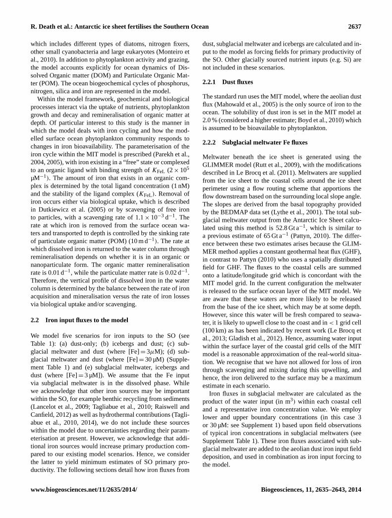
Fig. 1. (a) Distribution of ice-sheet-derived iron fluxes showingmodelled subglacial meltwater fluxes and iceberg tracks from theAntarctic Ice Sheet. Both of these ice-sheet-derived mass flux dis-tributions are controlled principally by the location of major icestream complexes and ocean circulation.(b) Regionally integratedcoastal subglacial meltwater fluxes indicating which regions aroundAntarctica are most influenced by subglacial meltwater input.

2.2.3 Iceberg Fe fluxes

The release of meltwater from icebergs accounts for 60–80 %of the freshwater flux from Antarctica (Martin and Adcroft,2010). The calving locations, number and size of icebergs arecalculated from balance fluxes along the coastal margins. Theiceberg flux is calculated at a 1◦

× 1◦ resolution to match theresolution of the MIT model. A statistical distribution (Glad-stone et al., 2001) is used to partition this iceberg mass fluxleaving the coast into ten different size classes. This allows usto generate the number of icebergs within each size class foreach coastal cell. We employ an iceberg model (Bigg et al.,1997) previously applied to the SO (Gladstone et al., 2001)to model the iceberg flow paths. The modelled iceberg trackscompare well with observations, and are discussed in Sup-plementary Information (Supplement Fig. 1).

Table 2. Summary statistics (mean, RMS, standard deviation) forobserved (Tagliabue et al., 2012) and modelled surface ocean (0–100 m) iron concentrations.

Mean StandardScenario (nM) Deviation RMS

Observations 0.47 0.66 n/aA – Dust only 0.26 0.06 0.65B – Icebergs 0.60 0.70 0.87C – SGM (3 µM) 0.35 0.14 0.63D – SGM (30 µM) 1.05 0.89 0.90E – Icebergs+SGM (3 µM) 0.81 0.92 1.03

The bioavailable iron released from melting icebergs in themodel is based upon a number of assumptions since there islittle observational data of the sediment loading within ice-bergs from Antarctica. We assume that the sediment distri-bution within icebergs comprises a basal debris layer (thesize of which has been reported between 1 to 10 m; Ander-son et al., 1980; Syvitski et al., 1996), with the remainderof the iceberg containing a sediment concentration that re-flects the aeolian dust flux to the Antarctic Ice Sheet. Thedust flux is derived from observations of dust deposition overAntarctica (Mahowald et al., 2009) (0.01 g m−2 yr−1). Forthis study we assume that the icebergs have a debris layerdepth of 5 m, which is approximately the median of valuesreported in the literature (Anderson et al., 1980; Syvitski etal., 1996; Dowdeswell et al., 1995). The sediment contentof the icebergs is estimated at 5 %. Field observations fromAntarctic icebergs (Anderson et al., 1980) suggest a debriscontent of between 4 to 8 % by weight. For comparison, sam-ples from 20 icebergs around Spitsbergen contained a rangeof sediment concentrations (0.02 to 28 % by weight) withinthe basal debris layer (Dowdeswell and Dowdeswell, 1989).Photographic evidence suggests that icebergs may also carrytheir sediment in englacial layers (Raiswell, 2011) which isnot accounted for in the current model configuration. Ne-glecting the englacial component of iceberg-rafted debriswill only serve to minimise the quantity and spatial distribu-tion of iron delivery from icebergs to the SO, making modelresults conservative.

The form and reactivity of the iron within the glacial de-bris and the dust fraction is also considered in order to modelthe fate of the iron held within icebergs. For the ice contain-ing only aeolian dust, we assume the same solubility (2 %)as the direct dust flux to the ocean (see Sect. 2.2.1). The re-activity of the debris in the basal layer is calculated as fol-lows. There are few direct measurements of the iron con-tent of free-drifting icebergs (Shaw et al., 2011), but esti-mates exist for sediment in grounded icebergs in Antarctica(Raiswell et al., 2008). Nanoparticles of iron oxyhydroxidesare found within the iceberg-hosted sediment in significantquantities, and the iron content in the reactive phases of fer-rihydrite and nanogoethite is 0.10± 0.11 %. We assume that

Biogeosciences, 11, 2635–2643, 2014 www.biogeosciences.net/11/2635/2014/

R. Death et al.: Antarctic ice sheet fertilises the Southern Ocean 2639

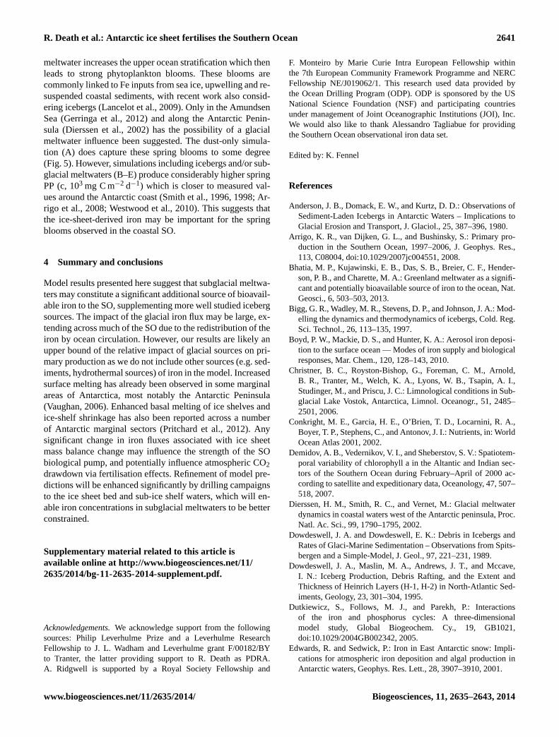
Fig. 2. The geographical distribution of the impact of iron in-puts upon modelled surface (0–100 m) ocean iron concentrationsis shown for(A) Scenario A (dust only) and(B) Scenario E (dust,subglacial meltwater (where [Fe]= 3 µM) and icebergs). Observedsurface ocean iron concentrations are shown as coloured circles, andare derived from (Tagliabue et al., 2012) with data from the Amund-sen Sea from (Gerringa et al., 2012).

the proportion of this iron that is bioavailable is 10 %, andhence, that 0.01 % of the basal sediment is bioavailable iron(Raiswell et al., 2008). The bioavailable iron that is releasedby each iceberg into the MIT ocean grid cell is summed andoverlaid onto the dust deposition field to produce an overallmap of iron input to the SO from icebergs and aerosol dustinput.

Observations Dust only Icebergs + dust SGM (3µm)+ dust

SGM (30µm)+ dust

SGM (3µm),icebergs + dust

Dis

solv

ed Ir

on (n

M)

-0.5

0.0

0.5

1.0

1.5

2.0

2.5

Scenario

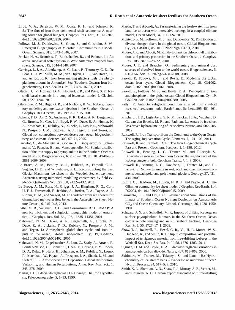
Fig. 3. Summary statistics (mean and standard deviation) for ob-served (Tagliabue et al., 2012) and modelled surface ocean (0–100 m) iron concentrations, illustrating the differences between themodelled scenarios.

3 Results and discussion

3.1 Modelled iron fluxes to the Southern Ocean

Iron fluxes in subglacial meltwaters are distributed along theAntarctic coast, in accordance with the pattern of subglacialwater export (Fig. 1a, Supplement 3), with the highest totalfluxes around the East Antarctic margin (Fig. 1b). Iceberg-derived iron fluxes follow iceberg tracks (Fig. 1a), which alsocorrespond approximately to spatial patterns of subglacialmeltwater release, since ice stream dynamics control thefluxes of both iron sources. Modelled mean annual surfaceocean iron concentrations are enhanced in zones of high sub-glacial meltwater and iceberg iron input, most prominentlyaround the coast (Fig. 2, Supplement Fig. 2). Many of thesezones of iron enhancement in the model correspond withareas of high measured iron concentrations, such as in theRoss Sea (Moore and Braucher, 2008) and Amundsen Sea(Gerringa et al., 2012) (Fig. 2a and b, Supplement Fig. 2).Dust fluxes of iron (Fig. 2a) cannot explain some of the highmeasured iron concentrations in surface coastal ocean wa-ters pointing towards an additional iron source. One possiblesource for this iron is the ice sheet.

A more quantitative analysis of these results is presentedin Fig. 3, with the data provided in Table 2. Because of thelimitations of the data, we are not able to make a judgmentthat any single model scenario does a better job. However,the magnitude and variability of iron concentrations in theSouthern Ocean are best matched by those scenarios whichinclude additional iron inputs, as opposed to the dust-onlyrun. The latter shows a very limited range and generallylower iron concentrations in surface ocean waters than thosewith a glacial iron source as prescribed in scenarios B, D andE (Table 2).

www.biogeosciences.net/11/2635/2014/ Biogeosciences, 11, 2635–2643, 2014

2640 R. Death et al.: Antarctic ice sheet fertilises the Southern Ocean

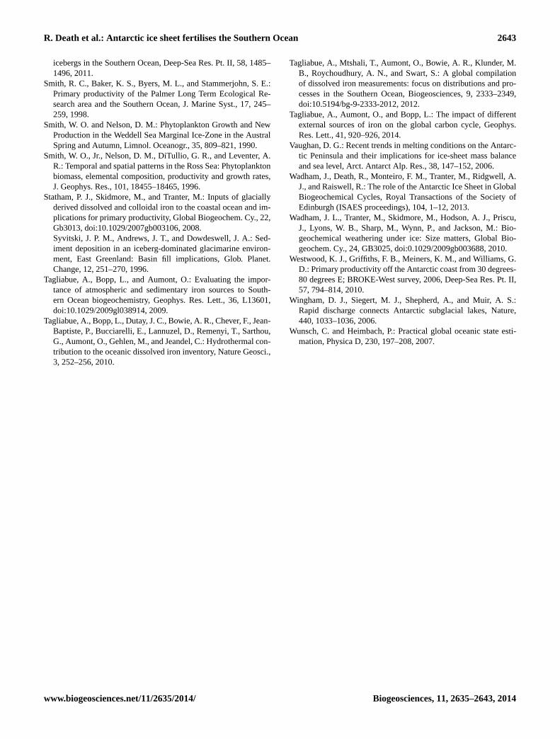
Fig. 4. Modelled sensitivity of annual primary productivity of theSouthern Ocean to external iron inputs. Tabulated total PP generatedby the different model scenarios and polar stereographic images ofannual primary productivity for model scenarios,(A) aeolian dust,(B) icebergs,(C) subglacial meltwater, SMW, where [Fe]= 3 µM,(D) SMW, where [Fe]= 30 µM and(E) aeolian dust+ icebergs+SMW (where [Fe]= 3 µM).

3.2 Impact upon SO wide primary productivity

Iceberg, subglacial meltwater (B–D) and combined ice-berg/meltwater (E) iron inputs have a pronounced (10–40 %)impact on total Southern Ocean PP (Fig. 4) above that gener-ated by dust-only simulations (A). A fourfold difference be-tween SO PP enhancement associated with subglacial melt-water with an [Fe] of 3 µM and 30 µM also indicates a sensi-tivity to meltwater Fe concentrations. The geographical dis-tribution of ice sheet iron impacts on ocean-wide SO PP re-flect (a) the location of iron inputs from major ice streamsor iceberg melting, (b) the redistribution of this iron viaocean circulation and (c) the geographical distribution of SOiron limitation. Many regions of elevated mean annual PPin both subglacial meltwater and iceberg iron input scenar-ios (Fig. 4) match to zones of high runoff or iceberg calv-ing fluxes around the Antarctic margin (Fig. 1). These in-clude large parts of East Antarctica, such as Prydz Bay, andthe Ross, Weddell and Amundsen Seas, which are all areasof high measured summer PP (Demidov et al., 2007; Smithand Nelson, 1990; Smith et al., 1996; Gerringa et al., 2012).The similarities in the spatial distribution of annual PP en-hancement in iceberg and subglacial meltwater flux simula-tions (Fig. 4) arises from the fact that the surface ocean cur-rents that transport the icebergs also convey the subglacialmeltwater away from the ice margin. Northward advection ofice-sheet-derived iron by ocean currents is evident from theelevated PP values at lower latitudes relative to dust sourcesalone, with an effect that extends as far as 50◦ S in scenar-ios B–E (Fig. 4). For example, along the western margin ofthe Antarctic Peninsula (B–E) where runoff fluxes are lowand the enhanced PP is stimulated by glacially derived Fe

Fig. 5. Modelled mean seasonal primary productivity (Decem-ber, January, February) of the Southern Ocean in response todust and glacial iron inputs for model scenarios(A) aeolian dust,(B) icebergs,(C) SMW, where [Fe]= 3 µM, (D) SMW, where[Fe]= 30 µM and(E) Aeolian dust+ icebergs+ SMW (where[Fe]= 3 µM).

advected north from the Ross Sea and Amundsen Sea. Theseresults highlight the importance of ocean circulation in pro-moting iron fertilisation from subglacial runoff and icebergsover a large proportion of the SO.

3.3 Impact upon coastal primary productivity

In addition to ocean-wide effects on SO PP, glacial sourcesof iron also have the potential to drive strong enhancementof PP in the near-coastal zone in spring/summer. Springblooms, where primary productivity attains values of the or-der of 103 mg C m−2 d−1, are commonly measured at the iceedge in early summer (Arrigo et al., 2008) along the Antarc-tic Peninsula (Smith et al., 1998) in the Ross Sea (Smith etal., 1996), Weddell Sea (Smith and Nelson, 1990), Amund-sen Sea (Gerringa et al., 2012) and Prydz Bay (Westwoodet al., 2010). This reflects the melting of sea ice duringthe austral spring, allowing sunlight to reach the nutrient-rich surface ocean waters. Additionally, the input of fresh

Biogeosciences, 11, 2635–2643, 2014 www.biogeosciences.net/11/2635/2014/

R. Death et al.: Antarctic ice sheet fertilises the Southern Ocean 2641

meltwater increases the upper ocean stratification which thenleads to strong phytoplankton blooms. These blooms arecommonly linked to Fe inputs from sea ice, upwelling and re-suspended coastal sediments, with recent work also consid-ering icebergs (Lancelot et al., 2009). Only in the AmundsenSea (Gerringa et al., 2012) and along the Antarctic Penin-sula (Dierssen et al., 2002) has the possibility of a glacialmeltwater influence been suggested. The dust-only simula-tion (A) does capture these spring blooms to some degree(Fig. 5). However, simulations including icebergs and/or sub-glacial meltwaters (B–E) produce considerably higher springPP (c, 103 mg C m−2 d−1) which is closer to measured val-ues around the Antarctic coast (Smith et al., 1996, 1998; Ar-rigo et al., 2008; Westwood et al., 2010). This suggests thatthe ice-sheet-derived iron may be important for the springblooms observed in the coastal SO.

4 Summary and conclusions

Model results presented here suggest that subglacial meltwa-ters may constitute a significant additional source of bioavail-able iron to the SO, supplementing more well studied icebergsources. The impact of the glacial iron flux may be large, ex-tending across much of the SO due to the redistribution of theiron by ocean circulation. However, our results are likely anupper bound of the relative impact of glacial sources on pri-mary production as we do not include other sources (e.g. sed-iments, hydrothermal sources) of iron in the model. Increasedsurface melting has already been observed in some marginalareas of Antarctica, most notably the Antarctic Peninsula(Vaughan, 2006). Enhanced basal melting of ice shelves andice-shelf shrinkage has also been reported across a numberof Antarctic marginal sectors (Pritchard et al., 2012). Anysignificant change in iron fluxes associated with ice sheetmass balance change may influence the strength of the SObiological pump, and potentially influence atmospheric CO2drawdown via fertilisation effects. Refinement of model pre-dictions will be enhanced significantly by drilling campaignsto the ice sheet bed and sub-ice shelf waters, which will en-able iron concentrations in subglacial meltwaters to be betterconstrained.

Supplementary material related to this article isavailable online athttp://www.biogeosciences.net/11/2635/2014/bg-11-2635-2014-supplement.pdf.

Acknowledgements.We acknowledge support from the followingsources: Philip Leverhulme Prize and a Leverhulme ResearchFellowship to J. L. Wadham and Leverhulme grant F/00182/BYto Tranter, the latter providing support to R. Death as PDRA.A. Ridgwell is supported by a Royal Society Fellowship and

F. Monteiro by Marie Curie Intra European Fellowship withinthe 7th European Community Framework Programme and NERCFellowship NE/J019062/1. This research used data provided bythe Ocean Drilling Program (ODP). ODP is sponsored by the USNational Science Foundation (NSF) and participating countriesunder management of Joint Oceanographic Institutions (JOI), Inc.We would also like to thank Alessandro Tagliabue for providingthe Southern Ocean observational iron data set.

Edited by: K. Fennel

References

Anderson, J. B., Domack, E. W., and Kurtz, D. D.: Observations ofSediment-Laden Icebergs in Antarctic Waters – Implications toGlacial Erosion and Transport, J. Glaciol., 25, 387–396, 1980.

Arrigo, K. R., van Dijken, G. L., and Bushinsky, S.: Primary pro-duction in the Southern Ocean, 1997–2006, J. Geophys. Res.,113, C08004, doi:10.1029/2007jc004551, 2008.

Bhatia, M. P., Kujawinski, E. B., Das, S. B., Breier, C. F., Hender-son, P. B., and Charette, M. A.: Greenland meltwater as a signifi-cant and potentially bioavailable source of iron to the ocean, Nat.Geosci., 6, 503–503, 2013.

Bigg, G. R., Wadley, M. R., Stevens, D. P., and Johnson, J. A.: Mod-elling the dynamics and thermodynamics of icebergs, Cold. Reg.Sci. Technol., 26, 113–135, 1997.

Boyd, P. W., Mackie, D. S., and Hunter, K. A.: Aerosol iron deposi-tion to the surface ocean — Modes of iron supply and biologicalresponses, Mar. Chem., 120, 128–143, 2010.

Christner, B. C., Royston-Bishop, G., Foreman, C. M., Arnold,B. R., Tranter, M., Welch, K. A., Lyons, W. B., Tsapin, A. I.,Studinger, M., and Priscu, J. C.: Limnological conditions in Sub-glacial Lake Vostok, Antarctica, Limnol. Oceanogr., 51, 2485–2501, 2006.

Conkright, M. E., Garcia, H. E., O’Brien, T. D., Locarnini, R. A.,Boyer, T. P., Stephens, C., and Antonov, J. I.: Nutrients, in: WorldOcean Atlas 2001, 2002.

Demidov, A. B., Vedernikov, V. I., and Sheberstov, S. V.: Spatiotem-poral variability of chlorophyll a in the Altantic and Indian sec-tors of the Southern Ocean during February–April of 2000 ac-cording to satellite and expeditionary data, Oceanology, 47, 507–518, 2007.

Dierssen, H. M., Smith, R. C., and Vernet, M.: Glacial meltwaterdynamics in coastal waters west of the Antarctic peninsula, Proc.Natl. Ac. Sci., 99, 1790–1795, 2002.

Dowdeswell, J. A. and Dowdeswell, E. K.: Debris in Icebergs andRates of Glaci-Marine Sedimentation – Observations from Spits-bergen and a Simple-Model, J. Geol., 97, 221–231, 1989.

Dowdeswell, J. A., Maslin, M. A., Andrews, J. T., and Mccave,I. N.: Iceberg Production, Debris Rafting, and the Extent andThickness of Heinrich Layers (H-1, H-2) in North-Atlantic Sed-iments, Geology, 23, 301–304, 1995.

Dutkiewicz, S., Follows, M. J., and Parekh, P.: Interactionsof the iron and phosphorus cycles: A three-dimensionalmodel study, Global Biogeochem. Cy., 19, GB1021,doi:10.1029/2004GB002342, 2005.

Edwards, R. and Sedwick, P.: Iron in East Antarctic snow: Impli-cations for atmospheric iron deposition and algal production inAntarctic waters, Geophys. Res. Lett., 28, 3907–3910, 2001.

www.biogeosciences.net/11/2635/2014/ Biogeosciences, 11, 2635–2643, 2014

2642 R. Death et al.: Antarctic ice sheet fertilises the Southern Ocean

Elrod, V. A., Berelson, W. M., Coale, K. H., and Johnson, K.S.: The flux of iron from continental shelf sediments: A miss-ing source for global budgets, Geophys. Res. Lett., 31, L12307,doi:10.1029/2004gl020216, 2004.

Follows, M. J., Dutkiewicz, S., Grant, S., and Chisholm, S. W.:Emergent Biogeography of Microbial Communities in a ModelOcean, Science, 315, 1843–1846, 2007.

Fricker, H. A., Scambos, T., Bindschadler, R., and Padman, L.: Anactive subglacial water system in West Antarctica mapped fromspace, Science, 315, 1544–1548, 2007.

Gerringa, L. J. A., Alderkamp, A. C., Laan, P., Thuroczy, C. E., DeBaar, H. J. W., Mills, M. M., van Dijken, G. L., van Haren, H.,and Arrigo, K. R.: Iron from melting glaciers fuels the phyto-plankton blooms in Amundsen Sea (Southern Ocean): Iron bio-geochemistry, Deep-Sea Res. Pt. II, 71/76, 16–31, 2012.

Gladish, C. V., Holland, D. M., Holland, P. R., and Price, S. F.: Ice-shelf basal channels in a coupled ice/ocean model, J. Glaciol.,58, 1227–1244, 2012.

Gladstone, R. M., Bigg, G. R., and Nicholls, K. W.: Iceberg trajec-tory modeling and meltwater injection in the Southern Ocean, J.Geophys. Res.-Oceans, 106, 19903–19915, 2001.

Jickells, T. D., An, Z. S., Andersen, K. K., Baker, A. R., Bergametti,G., Brooks, N., Cao, J. J., Boyd, P. W., Duce, R. A., Hunter, K.A., Kawahata, H., Kubilay, N., laRoche, J., Liss, P. S., Mahowald,N., Prospero, J. M., Ridgwell, A. J., Tegen, I., and Torres, R.:Global iron connections between desert dust, ocean biogeochem-istry, and climate, Science, 308, 67–71, 2005.

Lancelot, C., de Montety, A., Goosse, H., Becquevort, S., Schoe-mann, V., Pasquer, B., and Vancoppenolle, M.: Spatial distribu-tion of the iron supply to phytoplankton in the Southern Ocean: amodel study, Biogeosciences, 6, 2861–2878, doi:10.5194/bg-6-2861-2009, 2009.

Le Brocq, A. M., Bentley, M. J., Hubbard, A., Fogwill, C. J.,Sugden, D. E., and Whitehouse, P. L.: Reconstructing the LastGlacial Maximum ice sheet in the Weddell Sea embayment,Antarctica, using numerical modelling constrained by field ev-idence, Quaternary Sci. Rev., 30, 2422–2432, 2011.

Le Brocq, A. M., Ross, N., Griggs, J. A., Bingham, R. G., Corr,H. F. J., Ferraccioli, F., Jenkins, A., Jordan, T. A., Payne, A. J.,Rippin, D. M., and Siegert, M. J.: Evidence from ice shelves forchannelized meltwater flow beneath the Antarctic Ice Sheet, Na-ture Geosci., 6, 945–948, 2013.

Lythe, M. B., Vaughan, D. G., and Consortium, B.: BEDMAP: Anew ice thickness and subglacial topographic model of Antarc-tica, J. Geophys. Res.-Sol. Ea., 106, 11335–11351, 2001.

Mahowald, N. M., Baker, A. R., Bergametti, G., Brooks, N.,Duce, R. A., Jickells, T. D., Kubilay, N., Prospero, J. M.,and Tegen, I.: Atmospheric global dust cycle and iron in-puts to the ocean, Global Biogeochem. Cy., 19, Gb4025,doi:10.1029/2004gb002402, 2005.

Mahowald, N. M., Engelstaedter, S., Luo, C., Sealy, A., Artaxo, P.,Benitez-Nelson, C., Bonnet, S., Chen, Y., Chuang, P. Y., Cohen,D. D., Dulac, F., Herut, B., Johansen, A. M., Kubilay, N., Losno,R., Maenhaut, W., Paytan, A., Prospero, J. A., Shank, L. M., andSiefert, R. L.: Atmospheric Iron Deposition: Global Distribution,Variability, and Human Perturbations, Annu. Rev. Mar. Sci., 1,245–278, 2009.

Martin, J. H.: Glacial-Interglacial CO2 Change: The Iron Hypothe-sis, Paleoceanography, 5, 1–13, 1990.

Martin, T. and Adcroft, A.: Parameterizing the fresh-water flux fromland ice to ocean with interactive icebergs in a coupled climatemodel, Ocean Model, 34, 111–124, 2010.

Monteiro, F. M., Follows, M. J., and Dutkiewicz, S.: Distribution ofdiverse nitrogen fixers in the global ocean, Global Biogeochem.Cy., 24, GB3017, doi:10.1029/2009gb003731, 2010.

Moore, J. K. and Abbott, M. R.: Phytoplankton chlorophyll distribu-tions and primary production in the Southern Ocean, J. Geophys.Res., 105, 28709–28722, 2000.

Moore, J. K. and Braucher, O.: Sedimentary and mineral dustsources of dissolved iron to the world ocean, Biogeosciences, 5,631–656, doi:10.5194/bg-5-631-2008, 2008.

Parekh, P., Follows, M. J., and Boyle, E.: Modeling the globalocean iron cycle, Global Biogeochem. Cy., 18, Gb1002,doi:10.1029/2003gb002061, 2004.

Parekh, P., Follows, M. J., and Boyle, E. A.: Decoupling of ironand phosphate in the global ocean, Global Biogeochem. Cy., 19,Gb2020, doi:10.1029/2004gb002280, 2005.

Pattyn, F.: Antarctic subglacial conditions inferred from a hybridice sheet/ice stream model, Earth Planet. Sc. Lett., 295, 451–461,2010.

Pritchard, H. D., Ligtenberg, S. R. M., Fricker, H. A., Vaughan, D.G., van den Broeke, M. R., and Padman, L.: Antarctic ice-sheetloss driven by basal melting of ice shelves, Nature, 484, 502–505,2012.

Raiswell, R.: Iron Transport from the Continents to the Open Ocean:The Aging-Rejuvenation Cycle, Elements, 7, 101–106, 2011.

Raiswell, R. and Canfield, D. E.: The Iron Biogeochemical CyclePast and Present, Geochem. Perspect, 1, 1–186, 2012.

Raiswell, R., Benning, L. G., Tranter, M., and Tulaczyk, S.:Bioavailable iron in the Southern Ocean: the significance of theiceberg conveyor belt, Geochem Trans., 7, 1–9, 2008.

Raiswell, R., Benning, L. G., Davidson, L., Tranter, M., and Tu-laczyk, S.: Schwertmannite in wet, acid, and oxic microenviron-ments beneath polar and polythermal glaciers, Geology, 37, 431–434, 2009.

Rutt, I. C., Hagdorn, M., Hulton, N. R. J., and Payne, A. J.: TheGlimmer community ice sheet model, J Geophys Res-Earth, 114,F02004, doi:10.1029/2008jf001015, 2009.

Sarmiento, J. L. and Orr, J. C.: 3-Dimensional Simulations of theImpact of Southern-Ocean Nutrient Depletion on AtmosphericCO2 and Ocean Chemistry, Limnol. Oceanogr., 36, 1928–1950,1991.

Schwarz, J. N. and Schodlok, M. P.: Impact of drifting icebergs onsurface phytoplankton biomass in the Southern Ocean: Oceancolour remote sensing and in situ iceberg tracking, Deep-SeaRes. Pt. I, 56, 1727–1741, 2009.

Shaw, T. J., Raiswell, R., Hexel, C. R., Vu, H. P., Moore, W. S.,Dudgeon, R., and Smith, K. L.: Input, composition, and potentialimpact of terrigenous material from free-drifting icebergs in theWeddell Sea, Deep-Sea Res. Pt. II, 58, 1376–1383, 2011.

Sigman, D. M. and Boyle, E. A.: Glacial/interglacial variations inatmospheric carbon dioxide, Nature, 407, 859–869, 2000.

Skidmore, M., Tranter, M., Tulaczyk, S., and Lanoil, B.: Hydro-chemistry of ice stream beds – evaporitic or microbial effects?,Hydrol. Process., 24, 517–523, 2010.

Smith, K. L., Sherman, A. D., Shaw, T. J., Murray, A. E., Vernet, M.,and Cefarelli, A. O.: Carbon export associated with free-drifting

Biogeosciences, 11, 2635–2643, 2014 www.biogeosciences.net/11/2635/2014/

R. Death et al.: Antarctic ice sheet fertilises the Southern Ocean 2643

icebergs in the Southern Ocean, Deep-Sea Res. Pt. II, 58, 1485–1496, 2011.

Smith, R. C., Baker, K. S., Byers, M. L., and Stammerjohn, S. E.:Primary productivity of the Palmer Long Term Ecological Re-search area and the Southern Ocean, J. Marine Syst., 17, 245–259, 1998.

Smith, W. O. and Nelson, D. M.: Phytoplankton Growth and NewProduction in the Weddell Sea Marginal Ice-Zone in the AustralSpring and Autumn, Limnol. Oceanogr., 35, 809–821, 1990.

Smith, W. O., Jr., Nelson, D. M., DiTullio, G. R., and Leventer, A.R.: Temporal and spatial patterns in the Ross Sea: Phytoplanktonbiomass, elemental composition, productivity and growth rates,J. Geophys. Res., 101, 18455–18465, 1996.

Statham, P. J., Skidmore, M., and Tranter, M.: Inputs of glaciallyderived dissolved and colloidal iron to the coastal ocean and im-plications for primary productivity, Global Biogeochem. Cy., 22,Gb3013, doi:10.1029/2007gb003106, 2008.Syvitski, J. P. M., Andrews, J. T., and Dowdeswell, J. A.: Sed-iment deposition in an iceberg-dominated glacimarine environ-ment, East Greenland: Basin fill implications, Glob. Planet.Change, 12, 251–270, 1996.

Tagliabue, A., Bopp, L., and Aumont, O.: Evaluating the impor-tance of atmospheric and sedimentary iron sources to South-ern Ocean biogeochemistry, Geophys. Res. Lett., 36, L13601,doi:10.1029/2009gl038914, 2009.

Tagliabue, A., Bopp, L., Dutay, J. C., Bowie, A. R., Chever, F., Jean-Baptiste, P., Bucciarelli, E., Lannuzel, D., Remenyi, T., Sarthou,G., Aumont, O., Gehlen, M., and Jeandel, C.: Hydrothermal con-tribution to the oceanic dissolved iron inventory, Nature Geosci.,3, 252–256, 2010.

Tagliabue, A., Mtshali, T., Aumont, O., Bowie, A. R., Klunder, M.B., Roychoudhury, A. N., and Swart, S.: A global compilationof dissolved iron measurements: focus on distributions and pro-cesses in the Southern Ocean, Biogeosciences, 9, 2333–2349,doi:10.5194/bg-9-2333-2012, 2012.

Tagliabue, A., Aumont, O., and Bopp, L.: The impact of differentexternal sources of iron on the global carbon cycle, Geophys.Res. Lett., 41, 920–926, 2014.

Vaughan, D. G.: Recent trends in melting conditions on the Antarc-tic Peninsula and their implications for ice-sheet mass balanceand sea level, Arct. Antarct Alp. Res., 38, 147–152, 2006.

Wadham, J., Death, R., Monteiro, F. M., Tranter, M., Ridgwell, A.J., and Raiswell, R.: The role of the Antarctic Ice Sheet in GlobalBiogeochemical Cycles, Royal Transactions of the Society ofEdinburgh (ISAES proceedings), 104, 1–12, 2013.

Wadham, J. L., Tranter, M., Skidmore, M., Hodson, A. J., Priscu,J., Lyons, W. B., Sharp, M., Wynn, P., and Jackson, M.: Bio-geochemical weathering under ice: Size matters, Global Bio-geochem. Cy., 24, GB3025, doi:0.1029/2009gb003688, 2010.

Westwood, K. J., Griffiths, F. B., Meiners, K. M., and Williams, G.D.: Primary productivity off the Antarctic coast from 30 degrees-80 degrees E; BROKE-West survey, 2006, Deep-Sea Res. Pt. II,57, 794–814, 2010.

Wingham, D. J., Siegert, M. J., Shepherd, A., and Muir, A. S.:Rapid discharge connects Antarctic subglacial lakes, Nature,440, 1033–1036, 2006.

Wunsch, C. and Heimbach, P.: Practical global oceanic state esti-mation, Physica D, 230, 197–208, 2007.

www.biogeosciences.net/11/2635/2014/ Biogeosciences, 11, 2635–2643, 2014