FMCW Radar Signal Processing for Antarctic Ice Shelf Profiling and Imaging Samiur Rahman Thesis submitted for the degree of Doctor of Philosophy University College London Sensors, Systems and Circuits Group Department of Electronic and Electrical Engineering University College London April 2016

Welcome message from author
This document is posted to help you gain knowledge. Please leave a comment to let me know what you think about it! Share it to your friends and learn new things together.
Transcript

FMCW Radar Signal Processing for Antarctic Ice
Shelf Profiling and Imaging
Samiur Rahman
Thesis submitted for the degree of
Doctor of Philosophy
University College London
Sensors, Systems and Circuits Group
Department of Electronic and Electrical Engineering
University College London
April 2016

1
I, Samiur Rahman, confirm that the work presented in this thesis is my own. Where
information has been derived from other sources, I confirm that this has been indicated
in the thesis.
29/04/2016

2
Abstract
This thesis contains details of all the signal processing work being done on FMCW
Radar (operating at VHF-UHF band) for the Antarctic Ice Shelf monitoring project
that has been carried out at UCL. The system developed at UCL was based on a novel
concept of phase-sensitive FMCW radar with low power consumption, thus allowing
data collection for long period of time with millimetre range precision. Development
of new signal processing method was required in order to process the large amount of
data, along with the signal processing technique for obtaining the high precision range
values. This was achieved during the first stage of the thesis, providing accurate ice
shelf basal layer melt rate values. Properties of the FMCW radar system and
experimental scenarios posed further signal processing challenges. Those challenges
were met by developing number of novel algorithms. A novel shape matching
algorithm was developed to detect internal layers underneath the ice shelf. Range
migration correction method was developed to compensate for the defocusing of the
image in large angles due to high fractional bandwidth of the radar system. Vertical
error correction method was developed to compensate for any vertical displacement
of the radar antenna during field experiment. Finally, a novel 3-D MIMO imaging
algorithm for the Antarctic ice shelf base study was developed. This was done to
process the 8x8 MIMO radar (developed at UCL) data. The radars have been deployed
in the Antarctica during the Austral summer of each year from 2011-2014. The field
experiments were done in the Ronne, Larsen-C, Larsen North, George VI and Ross
ice shelves. The novel signal processing techniques have been successfully applied on
the real data, allowing better understanding of the Antarctic ice shelf features.

3
Acknowledgements
First and foremost, I would like to thank and express my gratitude to my supervisor
Professor Paul Brennan, for accepting me as his PhD student. Throughout my PhD, he
has always been very helpful. His guidance was the main factor that enabled me to
complete my research work. He made it very easy for me to structure my whole thesis
work, by always clearly explaining and updating me about the research goal. He has
always been very easily accessible. Whenever I went to his room to discuss a problem
even without an appointment, he has always given me time to provide suggestion to
solve the problem. For this professional and friendly attitude towards me, I am grateful
to him. Along with him, I am also very grateful to Dr. Lai Bun Lok. He is an
immensely talented scientist and engineer. All the signal processing work I did during
my PhD, was based on the system parameters and the data obtained from the radars
that he built. Special thanks to Dr. Keith Nicholls and Dr. Hugh Corr from British
Antarctic Survey, for letting me to work on their project of the Antarctic Ice Shelf.
A very special thanks to the Ministry of Science and Information Technology,
Bangladesh, for funding my entire PhD. I would also like to thank Dr. Kenneth Tong
and Professor Hugh Griffiths, for their valuable feedback during my transfer viva.
I would like to thank my former and current colleagues of the UCL radar group;
namely Shashi, Arvind, Ajmal, Jian Ling, Allann, Hashir and Mandana. I consider
myself very lucky to be part of this tightly knit research group.
I am forever grateful to my parents and siblings (Rusmila, Salman, Safwan) for
providing the constant support in my life. Finally, I would like to thank my wife Tina,
for all her encouragement and compassion. She has always made sure that I am in
proper physical and mental state to complete my PhD smoothly.
4
List of Publications
[1] Samiur Rahman, Paul V. Brennan, Lai Bun Lok, ‘Millimetre-precision range
profiling and cross-sectional imaging of ice shelves in Polar regions using phase-
sensitive FMCW radar’, Radar Conference, 2013 IEEE, April 29- 3 May 2013,
Ottawa, Canada, DOI: 10.1109/RADAR.2013.6586055.
[2] Samiur Rahman, Paul V. Brennan, Lai Bun Lok, ‘Shape matching algorithm for
detecting radar hidden targets to determine internal layers in Antarctic ice shelves’,
Radar Conference, 2014 IEEE, 19-23 May 2014, Cincinnati, Ohio, USA, DOI:
10.1109/RADAR.2014.6875824.
[3] Paul V. Brennan, Samiur Rahman, Lai Bun Lok, ‘Range migration compensation
in static digital-beamforming-on-receive radar’, IET Radar, Sonar and Navigation
Journal, DOI: 10.1049/iet-rsn.2014.0355.
[4] Samiur Rahman, Paul V. Brennan, ‘3-D FMCW MIMO Radar imaging of
Antarctic Ice Shelf Base’, Cold Regions Science and Technology Journal (accepted).

5
Contents 1 Introduction ........................................................................................ 19
1.1 Aim of the Thesis .............................................................................. 19
1.2 Thesis Outline ................................................................................... 21
2 Theoretical Background .................................................................... 23
2.1 Fundamentals of Radar ..................................................................... 23
2.1.1 Basic Concept of Radar ................................................................. 23
2.1.2 Radar Equations............................................................................. 25
2.1.3 Radar application for remote sensing of the environment ............ 28
2.2 FMCW Radar .................................................................................... 29
2.2.1 Linear FM Signal ........................................................................... 30
2.2.2 Basic FMCW Radar Operation Principle ..................................... 31
2.2.3 Advantages of using FMCW radar ................................................ 34
2.3 Overview of Antarctic Ice Shelf Research ........................................ 35
2.3.1 Ice Shelves in Antarctica ................................................................ 36
2.3.2 Use of remote sensing for Ice Shelf Monitoring ............................ 38
2.3.3 Motivation for the radar system upgrade ...................................... 44
2.3.4 Phase sensitive FMCW radar for Ice Shelf Monitoring built at UCL ......................................................................................................... 45
3 Signal Processing Algorithms for the Antarctic Data Analysis ..... 50
3.1 Phase Sensitive Range Profiling ....................................................... 51
3.1.1 Phase sensitive processing steps .................................................... 52
3.1.2 Time delay error correction ........................................................... 56
3.1.3 Range calibration with two reference values ................................ 56
3.2 Phased Array Processing ................................................................... 57
3.2.1 Developments in Phased Array Radar ........................................... 57
3.2.2 Beamforming .................................................................................. 58
3.2.3 Grating Lobes................................................................................. 63
3.2.4 Phased array imaging simulation .................................................. 63
3.3 Synthetic Aperture Radar (SAR) Processing .................................... 65
3.3.1 SAR geometry and Parameters ...................................................... 65
3.3.2 SAR Doppler History ..................................................................... 68

6
3.3.3 SAR Image Processing Algorithms ................................................ 69
3.3.4 Range Migration Algorithm ........................................................... 71
3.3.5 SAR simulation Results .................................................................. 77
3.4 MIMO Processing ............................................................................. 80
3.4.1 MIMO Virtual Array ...................................................................... 81
3.4.2 MIMO Beamforming ...................................................................... 83
4 Novel Signal Processing Techniques for Antarctic Data Analysis 84
4.1 Shape Matching Algorithm to Detect Internal Layers ...................... 84
4.1.1. Defining the reference signal from range profile ......................... 87
4.1.2. Amplitude scaling .......................................................................... 87
4.1.3. Point by point difference calculation and ranking ....................... 88
4.1.4. Integration for overall rank .......................................................... 89
4.2 Range Migration Processing in FMCW Phased Array Radar .......... 90
4.2.1. Criterion for significant range migration in phased array radar 90
4.2.2. Mitigation of range migration in phased array radar .................. 94
4.2.3 Simulation results ........................................................................... 97
4.3 Vertical Error Correction by Phase Calibration .............................. 101
4.4 3-D MIMO Imaging Algorithm for Ice Shelf Basal Layer ............. 107
4.4.1 3-D Beamforming ......................................................................... 109
4.4.2 Range Migration Compensation .................................................. 111
4.4.3 Selecting the range bin corresponding to zero degree return ..... 112
4.4.4 Compensating for the curvature of the range slice ...................... 112
4.4.5 Image sidelobe suppression by 2-D correlation .......................... 113
4.4.6 Simulation results ......................................................................... 115
5 Processed Results from Antarctic Ice Shelf Experiments ............ 119
5.1 Loop Test results at UCL ................................................................ 119
5.2 Range Profiling ............................................................................... 122
5.3 Foundation Ice Stream Imaging ...................................................... 129
5.4 Larsen North Imaging ..................................................................... 134
5.5 3-D MIMO Imaging of Ice Shelf Base ........................................... 140

7
Conclusions and Future Work ........................................................... 145
6.1 Conclusions ..................................................................................... 145
6.2 Future Works ................................................................................... 148
Appendix A .......................................................................................... 151
Simulation for MIMO Snow Avalanche Imaging ................................ 151
References ............................................................................................ 155
8
List of Figures
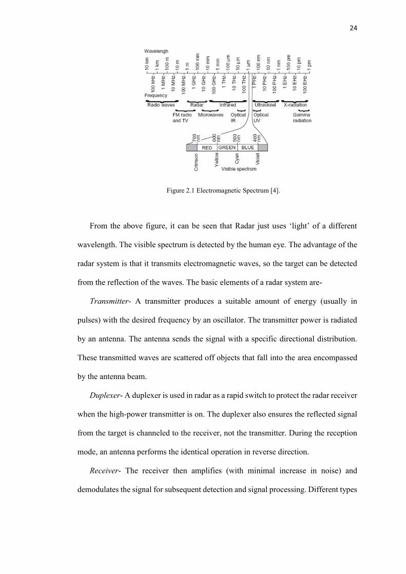
Figure 2.1: Electromagnetic Spectrum.
Figure 2.2: (a) Rectangular pulse in time domain; (b) Spectral density of that
rectangular pulse first null occurring at 1/T.
Figure 2.3: Linear FM (chirp) Signal.
Figure 2.4: Plot of FMCW chirp transmit and receive signal to calculate the deramped
frequency, fd.
Figure 2.5: Plot of triangular FMCW transmit signal (blue) and return echo from a
moving target (red) along with corresponding deramped frequency (black).
Figure 2.6: Map of Antarctica. The colored parts are various ice shelves, several of
those have been used as experimental locations in this project. (Credit: Ted Scambos,
NSIDC)
Figure 2.7: Ice sheets in both Polar Regions (Credit: NSIDC)
Figure 2.8: Simplified diagram of ice formation in Polar Regions showing the
fragmentation from ice sheet to ice shelf and then to iceberg. Grounding line is the
boundary between floating and grounded ice. (Credit: Mark R. Drinkwater; European
Space Agency, ESA-ESTEC)
Figure 2.9: A map created from ICESat data demonstrating the extent of ice sheet
thinning in Greenland and Antarctica [29]. (Credit: British Antarctic Survey/NASA)
Figure 2.10: An example of GPR profile showing underneath the ice cored esker near
Carat Lake, N.W. T. Canada.
Figure 2.11: Logarithmically scaled amplitude plot after processing pRES data from
George VI ice shelf, showing basal layer at around 450 meters.
Figure 2.12: Prototype phase sensitive FMCW radar built at UCL.
Figure 3.1: High precision range processing method for the phase-sensitive FMCW
radar.
Figure 3.2: Visual depiction of the zero padding and rotating process for FMCW radar
data processing.
Figure 3.3: Diagram of the phase sensitive FMCW radar range measurement process.
Figure 3.4: Illustration of basic concept for beamforming utilizing the constructive
interference properties of waveforms.

9
Figure 3.5: Geometric representation of a linear phased array system to calculate the
time (hence phase) difference among array elements when arriving signal has an angle
with normal to the array.
Figure 3.6: Beampattern for 25 degrees, without cross range windowing (above) and
with cross range windowing (below). Blackman windowing has been used in both
cases.
Figure 3.7: Illustration of grating lobe where on a beampattern for steering vector at
25 degrees, another strong signal appears at -38 degrees due to element spacing being
more than half the signal wavelength.
Figure 3.8: Image formation for a point target at 1500 metres range and 15 degree
angular distance from the array: above one is without implementing beamforming and
below one shows the image after applying phased array beamforming.
Figure 3.9: SAR operation geometry.
Figure 3.10: SAR integration angle and point target.
Figure 3.11: SAR range calculation geometry.
Figure 3.12: SAR signal history stored in a two dimensional memory and the
corresponding range migration curve.
Figure 3.13: Block diagram of the Range Migration Algorithm.
Figure 3.14: Far field radar antenna radiation pattern and its straight line
approximation within minute area.
Figure 3.15: SAR signal energy in 2-dimensional frequency domain and Stolt
interpolation’s effect on it.
Figure 3.16: SAR signal history of a point target return before implementing focusing
algorithm showing the characteristic hyperbolic curve (image is zoomed in).
Figure 3.17: SAR point target image after implementing Range Migration Algorithm
with 30 degree integration angle (image is zoomed in).
Figure 3.18: SAR point target image after implementing Range Migration Algorithm
with 3.6 degree integration angle (image is zoomed in).
Figure 3.19: Comparison of (a) MIMO radar and (b) Phased array radar.
Figure 3.20: Illustration of MIMO virtual array positioning by convolution of real and
receive array.
Figure 4.1: Range profile of Antarctic ice shelf illustrating basal layer return and
strong return in short range.

10
Figure 4.2: Construction used to determine the degree of range migration in a fixed
phased array radar.
Figure 4.3: Illustration of maximum acceptable limit of range migration variation of
range resolution, ±ΔR or 2ΔR.
Figure 4.4: Point target simulation of a 64 element phased array radar operating with
66.7% fractional bandwidth without implementing range migration correction (target
has a 330 angle array normal).
Figure 4.5: Point target simulation of a 64 element phased array radar operating with
66.7% fractional bandwidth after implementing range migration correction (target has
a 330 angle from array normal).
Figure 4.6: Phased array radar image of a target scene comprising a reflecting layer
parallel to array at 1500 m range, without range migration processing.
Figure 4.7: Phased array radar image of a target scene comprising a reflecting layer
parallel to array at 1500 m range, after range migration processing but without phase
correction.
Figure4.8: Phased array radar image of a target scene comprising a reflecting layer
parallel to array at 1500 m range, after range migration processing.
Figure 4.9: Geometry of vertical displacement of element from the array baseline.
Figure 4.10: Phased array processed image of a reflecting layer at 1500 metres range
without accounting for vertical spacing error of antennas.
Figure 4.11: Phased array processed image of a reflecting layer at 1500 metres range
where vertical spacing error of antennas has been taken into account.
Figure 4.12: Range profile of one of the array elements showing the zero degree signal
return at range bin number 4001.
Figure 4.13: Plot of phase response for the zero degree return across the entire array.
Figure 4.14: Plot of phase response for the zero degree return across the entire array
where vertical displacement of the elements have been imposed.
Figure 4.15: Phased array processed image of a reflecting layer at 1500 metres range
where vertical spacing error of antennas has been compensated by phase calibration
with reference to zero degree return.
Figure 4.16: 3-D MIMO beamforming geometry for planar array.
Figure 4.17: Two dimensional representation of the 3-D MIMO beamforming
geometry for the purpose of Pythagorean calculation.
11
Figure 4.18: Surface curvature correction for 3-D MIMO imaging of one range slice.
Figure 4.19: Sample demonstration of 2-D correlation method used for sidelobe
suppression in 3-D MIMO image.
Figure 4.20: Simulated result of a defocused 3-D MIMO image for a point target
(single range slice at 1500 m) with ±25º scan angle in azimuth and elevation; for large
array length and without applying range migration correction.
Figure 4.21: Simulated result of a focused 3-D MIMO image for a point target (single
range slice at 1500 m) with ±25º scan angle in azimuth and elevation; for large array
length and after applying range migration correction.
Figure 4.22: Simulated result of 3-D MIMO image of very closely spaced targets
covering ± 15º area in both direction without sidelobe suppression hence showing the
ring pattern (scan angle in both direction is ±20º).
Figure 4.23: Simulated result of 3-D MIMO image of very closely spaced targets
covering ± 15º area in both direction after applying hence removing the ring pattern
(scan angle in both direction is ±20º).
Figure 5.1: Figure 5.1: Raw received deramped signals of the FMCW phase sensitive
radar with 4 alternating attenuator settings.
Figure 5.2: Range plots of the 240 meter round trip path through the cable for all 4
gain settings of the radar, without time error correction (above) and with time error
correction (below).
Figure 5.3: (a) Larsen-C range profile showing the ice shelf base at 362 metres (b) Plot
of difference between measured ice shelf base and the internal layer over 6 days.
Figure 5.4: George VI Ice Shelf basal layer range (at 386 metres) plot for 130
continuous measurements, corresponding to 64.5 hours.
Figure 5.5: Larsen Ice Shelf basal layer plot for 495 continuous measurements (1 in
every 10 minutes), corresponding to 82 hours and 20 minutes.
Figure 5.6: Larsen South Ice Shelf basal layer range (at 361 metres) plot for 495
continuous measurements (1 in every 10 minutes) after averaging of 9 chirps of each
attenuator setting.
Figure 5.7: George VI range profile without cross-correlation (above) and with cross-
correlation (below) having almost no impact.
Figure 5.8: George VI range profile without shape matching algorithm implemented
(above) and with the algorithm implemented (below) reducing the clutter/noise.
12
Figure 5.9: Normal Larsen ice shelf range profile (above) and the same profile after
implementing shape matching algorithm showing a more than 50% match at around
77 metres.
Figure 5.10: Normal Foundation ice stream range profile (above) and the same profile
after implementing shape matching algorithm.
Figure 5.11: Foundation Ice Stream imaging experiment setup, comprising six
transmitters and six receivers, creating 36 linear virtual array elements.
Figure 5.12: Measured result taken from Foundation Ice Stream, Antarctica showing
range profile.
Figure 5.13: Measured phase of the range bin corresponding to the basal layer across
each of the 36 array elements, to act as an array phase calibration.
Figure 5.14: MIMO image of the Foundation Ice Stream, without range migration
processing or vertical error correction; the basal layer return echo is at 1285 metres.
Figure 5.15: MIMO image of the Foundation Ice Stream, using range migration
processing and phase calibration, showing consistent image intensity at the basal layer
and better-defined clutter structure.
Figure 5.16: Differential phase interferometry image of Foundation ice stream to
observe the basal layer melt within 6 days using the detected internal layer for
calibration.
Figure 5.17: SAR processed 2D cross-sectional image of Larsen North ice shelf.
Figure 5.18: Measured result taken from Larsen North Ice Shelf, Antarctica showing
range profile.
Figure 5.19: Measured phase to the basal layer across each of the 109 array elements,
to act as an array phase calibration.
Figure 5.20: Phased array image of the Larsen North Ice Shelf, without any correction;
the basal layer return echo is at 370 metres.
Figure 5.21: Phased array image of the Larsen Ice Shelf, using range migration
processing and phase calibration, showing consistent image intensity at the basal layer
and better-defined clutter structure.
Figure 5.22: Phased array image of the Larsen North Ice Shelf showing the thin line
showing the double bounce return coming from twice the basal layer range.
Figure 5.23: Planar MIMO antenna array geometry for 3-D imaging of Antarctic Ice
Shelf.

13
Figure 5.24: 3-D MIMO image of Ronne Ice Shelf (site1) basal layer at 566 metres
(without 2-D correlation).
Figure 5.25: 3-D MIMO image of Ronne Ice Shelf (site1) basal layer at 566 metres
(after 2-D correlation).
Figure 5.26: 3-D MIMO image of Ronne Ice Shelf (site2) basal layer at 514 metres
(without 2-D correlation).
Figure 5.27: 3-D MIMO image of Ronne Ice Shelf (site2) basal layer at 514 metres
(after 2-D correlation).
Figure 5.28: 3-D MIMO image of Greenland Ice Sheet basal layer at 638 metres
(without 2-D correlation).
Figure 5.29: 3-D MIMO image Greenland Ice Sheet basal layer at 638 metres (after2-
D correlation).
Figure 6.1: Plot of change in range values with respect to the temperature change in
the radar system
Figure app.1: Range profile for point target at 1000 metres without any spreading code
applied.
Figure app.2: Point target image (at 1000 metres range) of a MIMO radar without any
spreading code applied.
Figure app.3: Range profile for point target at 1000 metres after applying spreading
code.
Figure app.4: Point target image (at 1000 metres range) of a MIMO radar after
applying spreading code.

14
List of Tables
Table 1: Parameters of phase sensitive FMCW radar.
Table 2: Parameters of pRES radar.
15
Symbols
A Physical area of the receiving antenna
Ae Effective area of the receiving antenna
B Bandwidth
B(ϴ) Beamforming function
c Speed of light
d Element spacing within the antenna array
dB Decibel
Δϕ Phase delay
ΔL Path length variation across antenna array
Δr, ΔR Range resolution
Δt Time delay
εr Dielectric constant
fc, fo Centre frequency
fd Deramped frequency
fd,down Deramped frequency for down chirp
fd,up Deramped frequency for up chirp
fstep Step frequency
ϕ Elevation angle for 3-D MIMO beamforming
φd(t) Deramped signal phase
φr(t) Instantaneous phase of linear chirp (receive side)
φt(t) Instantaneous phase of linear chirp (transmit side)
G Antenna gain
K Chirp rate
kx, kr Spatial frequency

16
λ Signal wavelength
N Noise figure
p Pad factor
pr Radar receiver power
pt Radar transmitter power
ρa Efficiency of the antenna aperture
R Range of the target
Rcoarse Coarse range
Rf Fine range
Ro Reference range
Rmax Maximum range of the radar
sIF(t) Deramped signal of the FMCW radar
sr(t) Receive signal of the FMCW radar
str(t) Transmitted signal of the FMCW radar
Smin Minimum detectable signal
sc Scaling factor for the shape matching algorithm
σ Radar cross section
T Chirp duration
Tp Pulse width
τ Pulse duration
ϴ Azimuth frequency for beamforming
v, vpl Velocity
wn Weighting coefficient for the beamforming
ωt(t) Instantaneous transmitted frequency of the linear chirp
z Vertical displacement of the array antenna element

17
Abbreviations
ADC Analog to Digital Converter
CPG Coherent processing gain
CSA Chirp Scaling Algorithm
CW Continuous Wave
DDS Direct Digital Synthesizer
FBP Fast Backprojection Algorithm
FFBP Fast Factorized Backprojection Algorithm
FFT Fast Fourier Transform
FM Frequency Modulation
FMCW Frequency Modulated Continuous Wave
GBP Global Backprojection Algorithm
GPR Ground penetrating Radar
IF Intermediate Frequency
InSAR Interferometric SAR
MIMO Multiple Input Multiple Output
PN Pseudo Random Noise
pRES Phase-sensitive Radio Echo Sounder
PRF Pulse Repetition Frequency
PSLR Peak to Sidelobe Ratio
Radar Radio Detection and Ranging
RCS Radar Cross Section
RDA Range Doppler Algorithm
RMA Range Migration Algorithm
SAR Synthetic Aperture Radar
SCR Signal to Clutter Ratio
SNR Signal to Noise Ratio

18
UHF Ultra High Frequency
VHF Very High Frequency

19
Chapter 1
Introduction
Accurate prediction of sea level rise is very important in the field of climate change
research. Ice shelves in the Polar Regions have direct correlation with sea level rise.
An ice shelf is a floating extension of ice sheet. Presence of an ice shelf limits the ice
flow into the ocean. As ice shelves are already floating in the ocean, a major collapse
in ice shelf can enhance the level of fresh water into the sea indirectly by speeding up
the flow of land ice into the ocean [1]. A lot of ice shelves collapsed in the Antarctica
in the last few decades [1]. Scientists reasoned that this phenomena is due to warmer
climate [1]. It is therefore of great importance to analyze the pattern of the thickness
change of the ice shelf over the year with respect to oceanographic data. This would
give geoscientists an accurate idea about whether the melting of ice shelves from the
bottom is due to a natural cycle or because of the climate change.
1.1 Aim of the Thesis
A purpose-built phase-sensitive FMCW radar has been developed at UCL. The
radar uses phase sensitivity to determine range to high precision. This high precision
is achieved by using a Vernier-like process that accounts for the fine range
measurement of the target along with its coarse range. This fine range is attained by
measuring the phase of the signal in the particular range bin where the coarse range is
obtained. In order to obtain this, challenges have to be met for both hardware and
signal processing. A similar phase-sensitive radar system (pRES) had been developed
20
before which also produced satisfactory results [2] [3]. The motivation for this project
work was to develop an upgraded radar system capable of year-long operation with
low power consumption while providing high precision data. Link budget modelling
of the FMCW radar built for this project shows that with very low transmit power (0.1
W), 3 mm RMS precision at 1800 m range is achievable. The main features of this
radar are low power consumption, low noise figure (6 dB), lightweight and suitable
for low temperature operation. For these advantages, it can be used for long term
continuous data collection in contrast to the pRES system (ice-penetrating radar built
by British Antarctic Survey, predecessor of the current FMCW radar system), which
is restricted to operation only during Austral summers and to provide a series of
snapshots (because the pRES system is based on a general purpose network analyser,
which has a high power consumption and requires a heavy petrol-generator, thus
making it impractical for long term data collection).
The Antarctic Ice Shelf monitoring project involved novel radar hardware
development as well as novel signal processing algorithm development for Ice Shelf
profiling and imaging. This thesis work has dealt with the signal processing algorithm
development part of the project. The main objective is to produce ice shelf range
profiles of millimetre precision as well as imaging the features underneath the ice
shelf. The signal processing challenges were to develop suitable algorithms for phase
sensitive range profiling as well as imaging techniques. As is often the case, specific
applications require customized techniques for data analysis. This has been the case
during this thesis as well, as novel radar hardware system required newly developed
signal processing algorithms. So, along with developing processing algorithms for
data analysis by using conventional methods (for phased array, SAR, MIMO), new
techniques have to be developed as well for accurate data processing. The aim of the

21
thesis is to obtain data from both Polar Regions and produce significant results (images
and profiles) that would help geoscientists to better understand the melting pattern and
other properties of ice shelves.
1.2 Thesis Outline
Chapter 1: This chapter gives a brief outline of the thesis by giving an overview of
the project aim.
Chapter 2: Theoretical background of the whole research work has been described in
this chapter along with reviewing the research work done so far for remote sensing of
ice.
Chapter 3: This chapter describes the specifics of the thesis work; the main signal
processing algorithms that are required for polar data analysis. The theory of phased
array radar, SAR and MIMO signal processing has been discussed in this chapter along
with theoretical description of the phase sensitive range profiling method. MIMO
signal processing has been described very briefly as newly developed 3-D MIMO
imaging technique has been broadly discussed in Chapter 4.
Chapter 4: This chapter discusses the novel signal processing techniques developed
for this thesis work. These include: range migration correction for phased array, shape
matching algorithm for detecting hidden layers, vertical error correction by phase
calibration and 3 dimensional MIMO imaging algorithm; these four techniques that
have been developed for FMCW radar data analysis have been thoroughly discussed.
Chapter 5: Experimental results are shown in this chapter. All the algorithms that
have been developed and simulated during this thesis were also put to the test by
applying them to real data. The results are then analyzed and compared with the
modelled results in this chapter.

22
Chapter 6: Along with concluding remarks, the overall contribution of the thesis is
described in this chapter. Achievements and improvements made over the existing
techniques has been discussed. Also, future work and scope for improvements of the
developed algorithms are discussed.

23
Chapter 2
Theoretical Background
This chapter provides a basic theoretical outline of the whole research work
starting from the fundamentals of radar. The majority of the discussion on the radar
basics are based on [6] and [7]. After discussing these basics, FMCW radar theory is
reviewed as it is the main experimental instrument for this research work. Theoretical
discussion of Antarctic ice shelves is provided within the context of this particular
research along with a review of previous research work in this field. This leads to a
discussion of the need for updating the current technology and a description of the
FMCW radar that was built at UCL for this particular project. A broad description of
this Ice Shelf monitoring radar system is provided in the last section of this chapter.
2.1 Fundamentals of Radar
2.1.1 Basic Concept of Radar
After the formulation of electromagnetic radiation theory, the basic foundation of
radio technology was established. The possibility of wireless communication was
realized by the scientists, as electromagnetic waves propagate at the speed of light.
‘Radar’ (Radio Detection and Ranging) is a device that uses electromagnetic
waves for the purpose of acquiring information at a distant location from that device.
This operation is commonly known as ‘Remote Sensing’. Different bands of the
electromagnetic spectrum are used in different applications of radar.
24
Figure 2.1 Electromagnetic Spectrum [4].
From the above figure, it can be seen that Radar just uses ‘light’ of a different
wavelength. The visible spectrum is detected by the human eye. The advantage of the
radar system is that it transmits electromagnetic waves, so the target can be detected
from the reflection of the waves. The basic elements of a radar system are-
Transmitter- A transmitter produces a suitable amount of energy (usually in
pulses) with the desired frequency by an oscillator. The transmitter power is radiated
by an antenna. The antenna sends the signal with a specific directional distribution.
These transmitted waves are scattered off objects that fall into the area encompassed
by the antenna beam.
Duplexer- A duplexer is used in radar as a rapid switch to protect the radar receiver
when the high-power transmitter is on. The duplexer also ensures the reflected signal
from the target is channeled to the receiver, not the transmitter. During the reception
mode, an antenna performs the identical operation in reverse direction.
Receiver- The receiver then amplifies (with minimal increase in noise) and
demodulates the signal for subsequent detection and signal processing. Different types
25
of filter, attenuator, mixer and amplifier are used to achieve the desired signal. During
the signal processing, with the information regarding antenna directivity, the time
delay and phase/frequency change (with respect to the transmitted signal), the target
position and/or speed can be determined.
A radar system includes a transmitter emitting electromagnetic radiation, in the
form of a radio wave. The radio wave propagates through a medium (i.e. air, ice) and
gets reflected from a target. The radar receiver collects the reflected wave. This
reflected wave helps detect the presence of the target. As the speed of the wave
propagation is known, the time of flight determines the range of the target (distance
between the radar and the target). A moving target would produce a Doppler shift in
the received signal, which can be used to calculate the velocity of the target. By using
directional antennas, the direction of the target with respect to the radar (bearing) can
also be determined.
The selection of wavelength for radar operation depends on the application. For
instance, radar technology was mainly developed during World War II. The main
objective at that time was to detect airplanes, combat ships or enemy vessels located
beyond visual range [5]. The main advantage of such a technology is that no one has
to rely on sunlight, or clear sky. Radar itself is the source of the emitted waves reflected
by a target. So, radars mainly emit electromagnetic waves at such frequencies which,
unlike visible light, easily pass through clouds, fogs with attenuation as less as possible
(some radars use mm wave for high resolution, but signals get highly attenuated at that
frequency).
2.1.2 Radar Equations
One of the most basic aspects of radar theory is the radar range equation, derived
from the equation for receiver power in relation to transmitted power and antenna gain.
26
A typical radar signal will have a two-way path propagation from transmitter to target
and then reflected back from target to receiver. Due to this propagation through 3-
dimensional space, the received signal power will depend on the reflectivity of the
target, directivity of the signal, distance travelled by the signal and the gain of the
antenna. So, it is very important to calculate the receiver power before performing any
radar operation. The Radar receiver power equation [6] is as follows:
𝑃𝑟 = 𝑃𝑡𝐺𝐴𝑒𝜎
(4𝜋)2𝑟4 (2.1)
In the above equation, Pt is the transmitted power, G is the maximum gain of
antenna, Ae is effective area of the receiving antenna, σ is the radar cross section (RCS)
of the target and r is the distance of the target from the radar receiver or target range.
Ae is directly related to the physical area of the antenna aperture A where Ae =ρaA,
where ρa is the efficiency of antenna aperture [6]. To determine the maximum range
Rmax of the radar, Pr needs to be at least equal to the minimum detectable signal Smin.
Hence, rearranging Equation (2.1) gives the radar range equation [7]:
𝑅𝑚𝑎𝑥 = [𝑃𝑡𝐺𝐴𝑒𝜎
(4𝜋)2𝑆𝑚𝑖𝑛]
14⁄
(2.2)
The above equation is also referred as the radar equation or range equation. During
a radar design for any specific application, target RCS is taken into account to
determine the choice of parameters, such as operating frequency and transmit power,
since the reflectivity directly depends on frequency. After determining those, the
power budget is calculated.
Another basic factor in radar operation is the range resolution. It determines the
ability of the radar to distinguish between two targets. Before formulating the range
resolution, it is necessary to first determine the range of the radar. By considering τ as
the two-way propagation delay time (time between the emission of the
27
electromagnetic wave from the receiver and the reflected wave coming back to the
receiver). The propagation delay then can be written as,
𝜏 =2𝑟
𝑐 (2.3)
The above equation enables calculation of the radar range, r, where c is the speed
of light in free space, 3x10⁸ ms-1. In a different medium, the speed of light changes
which is compensated by taking the dielectric constant of that medium into account.
In its simplest form, range resolution can be calculated [7] as follows:
∆𝑟 = 𝑐𝜏
2 (2.4)
In order to obtain two distinct signal returns from two separate targets, the targets
have to be separated in range by at least half the distance corresponding to the pulse
width. In most cases, radars send a modulated signal. So, it is more useful to determine
range resolution in terms of signal bandwidth. That formula can be achieved by using
the spectral density of the transmitted pulse.
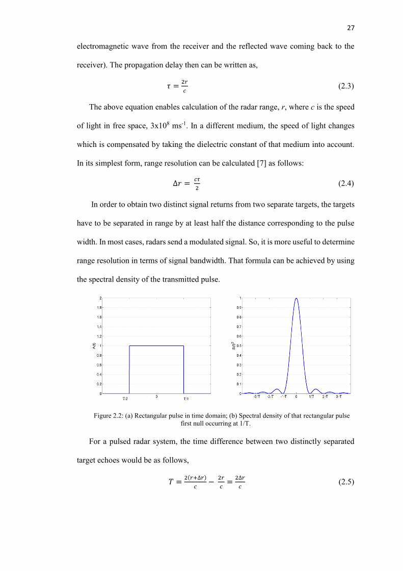
Figure 2.2: (a) Rectangular pulse in time domain; (b) Spectral density of that rectangular pulse
first null occurring at 1/T.
For a pulsed radar system, the time difference between two distinctly separated
target echoes would be as follows,
𝑇 =2(𝑟+∆𝑟)
𝑐−
2𝑟
𝑐=
2∆𝑟
𝑐 (2.5)

28
Because of the two-way propagation of the signal, the minimum range resolution
would vary proportionally with one half of the pulse length, T. From the above figure,
the bandwidth of the pulse can be determined with respect to the location of the first
null (for a non-modulated signal, bandwidth would be the smallest positive frequency
where the power spectral density is zero). According to the above figure, where a
rectangular pulse is considered, the first null occurs at 1/T. So, bandwidth can be
written as:
𝐵 ≈ 1
𝑇 (2.6)
Using Equation (2.5) and (2.6), range resolution can be re-written as:
∆𝑟 = 𝑐
2𝐵 (2.7)
In order to calculate the maximum unambiguous range, the Pulse Repetition
Frequency (PRF) needs to be considered. This is the rate at which the radar transmitter
emits signal (in the case of pulsed radar system). If a signal is reflected from a target
after the transmitter has sent another pulse, then the range of the target cannot be
unambiguously determined, as the corresponding transmitted pulse is not defined with
absolute certainty. This maximum unambiguous range, ru, can be mathematically
expressed as,
𝑟𝑢 =𝑐
2𝑃𝑅𝐹 (2.8)
2.1.3 Radar application for remote sensing of the environment
Even though radar was originally developed for military purpose during wars, it
serves as a very important tool for civilian applications as well. The most commonly
known civilian application for radar is air-traffic control [7]. The widely used Air
Traffic Control (ATC) radar beacon system and the microwave landing system are
mainly based on radar technology [7]. Radar is also widely used nowadays for
29
environmental monitoring. For weather observation, the Nexrad system is widely
known [6]. It is a network of 160 S-band Doppler radars. Along with climatology, the
precipitation data from Nexrad is used in the field of meteorology and hydrology as
well [8]. Various SAR systems (both spaceborne and airborne) have been used for
earth and climate monitoring as SAR images help imaging of the ocean current pattern,
glacier motion pattern, volcanic movement, geological studies and so on. Examples
include Magellan (NASA/JPL), RADARSAT-1(Canadian Space Agency), ERS-1/2
(European Remote Sensing satellite), J-ERS (Japanese Earth Remote Sensing
satellite), SEASAT (performing first civilian SAR application), and CARABAS [9].
Radars are also used for ship safety [7]. In adverse weather conditions when
visibility is poor, radars can be used for collision avoidance (with other naval vehicles,
navigation buoys). Automated radar systems with detection and tracking capacity for
collision avoidance are commercially available and usually small in size and not costly
[7].
Another significant contribution of radar for remote sensing is the measurement of
the earth’s mean sea level (geoid- global mean sea level model to precisely measure
the surface elevations of the earth) [10]. Downward looking spaceborne altimeters
such as the ERS-1/2 have been used for this purpose [10].
2.2 FMCW Radar
Generally, the transmitted radar signal is either a single pulse at a time or it is a
continuous wave. Radar that uses the first technique is known as pulsed radar. Radar
that uses the latter technique is known as Continuous Wave radar or CW radar for
short. Frequency Modulated Continuous Wave (FMCW) radar is a type of CW radar
that transmits frequency modulated waves, usually with linear frequency modulation.
30
The advantage obtained by modulating the frequency is the ability to determine range
without requiring a short pulse. Modulation of the transmitted signal provides the
timing mark which can be used to extract range information. For instance, a frequency
modulated signal would have various frequency components. So, when a target echo
is received, those different frequency components will arrive in different time thus
creating the option for range measurement. The operation principle for FMCW is
discussed below.
2.2.1 Linear FM Signal
The application and operation of FM signals is widespread in radio broadcasting.
One advantage can be found in radar over radio broadcasting is that radar does not
transmit any meaningful message. It just sends a signal in order to get a reflection. So,
there is no need for complicated manipulation to decode any audio-visual message
from the signal. A simple pulse containing numerous frequency components would
suffice. One such simple FM signal is a chirp signal (or sweep signal, both terms are
used interchangeably). It is basically an FM signal where the frequency is increased
or decreased with time, just like the chirping noise of birds, or bats. It is simple in
concept and easy to generate. A chirp signal can be generated in ascending order (up
chirp) or descending order (down chirp). Also, the frequency differences can be linear
or exponential. In order to maintain simplicity, most radars use a linear chirp signal.
The transmitted signal equation is,
𝑠(𝜏) = 𝑟𝑒𝑐𝑡 (𝜏
𝑇𝑝) 𝑒(𝑖2𝜋𝑓𝑐+𝑖𝜋𝐾𝜏2) (2.9)
K is the chirp rate which is the ratio of the bandwidth and pulse width 𝐵⁄𝑇𝑝, fc is the
center frequency and τ is pulse duration.

31
Figure 2.3 Linear FM (chirp) Signal.
2.2.2 Basic FMCW Radar Operation Principle
A linear FM chirp signal is used for transmission in FMCW radar. After receiving
a target echo, the received signal is mixed with the transmit signal. The resultant
frequency is known as a beat frequency of deramped frequency. This deramped
frequency is used for calculating the target range. The mathematical depiction of
FMCW radar operation is given in [11]. For a stationary target, the deramped
frequency would be a constant value. In order to get an expression for the deramped
frequency, the mathematical form of the instantaneous FM chirp transmitted signal in
sinusoidal form can be written as:
𝑠𝑡𝑟(𝑡) = 𝑎𝑜 sin 2𝜋 [𝑓𝑜𝑡 + 𝐾𝑡2
2] (2.10)
where K is the chirp rate and fo is the centre frequency. The received signal will be a
time delayed version of the above equation most likely with different amplitude due
32
to attenuation. If the time delay between transmit and receive is τ, then the equation
for the received signal becomes:
𝑠𝑟(𝑡) = 𝑏𝑜 sin 2𝜋 [𝑓𝑜(𝑡 − 𝜏) + 𝐾(𝑡−𝜏)2
2] (2.11)
The deramped signal sIF(t) is the resultant of the mixing of these two signals:
𝑠𝐼𝐹(𝑡) = 𝑠𝑡𝑟(𝑡) . 𝑠𝑟(𝑡) (2.12)
The deramped signal will consist of both the sum of and difference of two signal
phases. For FMCW operation, only the difference is required thus the sum is ignored
or filtered out. Simplification after substituting values from Equation (2.10) and (2.11)
to Equation (2.12) gives the following equation for the deramped signal:
𝑠𝐼𝐹(𝑡) = 𝑐𝑜 cos 2𝜋 [𝑓𝑜𝜏 + 𝐾𝑡𝜏 − 𝐾𝜏2
2] (2.13)
Here, the second term is the time linear phase term corresponding to the instantaneous
frequency difference between the transmit signal and receive signal.
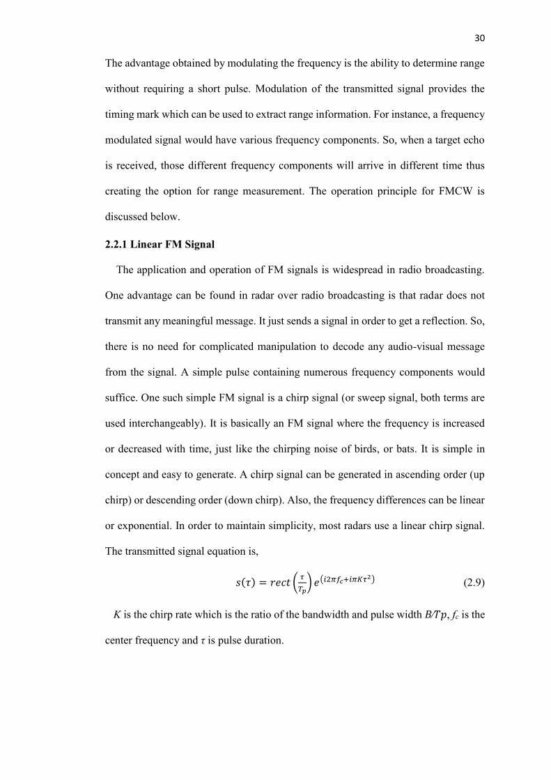
Figure 2.4: Plot of FMCW chirp transmit and receive signal to calculate the deramped frequency,
fd.
From the above figure, the equation for fd can be obtained easily by using simple
geometry. Here, the blue line is the transmitted chirp and the red line is the received
signal, which is equal to the transmitted one but delayed by the round trip delay τ. It
can be seen that the triangle consisting of sides equal to bandwidth B and chirp
duration T is similar to the triangle consisting of sides fd and τ (they have equal angles).

33
So, the ratio of their corresponding sides will be equal (fd/B = τ/T). Hence, equation
for the deramped signal can be written as:
𝑓𝑑 = 𝐵𝜏
𝑇 (2.14)
The round trip delay τ can be written in terms of range R as τ = 2R/c. So, Equation
(2.14) then becomes:
𝑓𝑑 = 2𝐵𝑅
𝑇𝑐 (2.15)
It should be noted that in Figure (2.4), only the up-chirp has been used. In FMCW
operation, it should be sufficient if Doppler information is of no concern. In order to
extract Doppler information, both up and down chirps would be required. Otherwise,
range-Doppler cross coupling will occur which can be mathematically seen by
modifying Equation (2.13) for a moving target. If the target is moving with velocity
v, then range becomes function of time (R(t) = Ro+vt). So, the equation for round trip
delay becomes:
𝜏 = 2(𝑅𝑜+𝑣𝑡)
𝑐 (2.16)
The last term is Equation (2.13), which is a small phase offset, is neglected (as τ
<< T). Combining Equation (2.13) and (2.16):
𝑠𝐼𝐹(𝑡) = 𝑐𝑜 cos 2𝜋 [2𝑓𝑜𝑅𝑜
𝑐+ (
2𝑓𝑜𝑣
𝑐+
2𝐾𝑅𝑜
𝑐) 𝑡 +
2𝐾𝑣𝑡2
𝑐] (2.17)
In the above equation, the third term corresponds to range-Doppler coupling.
So, when the FMCW radar application consists of a moving target, it uses chirps
in both directions. The method can be understood from Figure (2.5). It can be seen that
the deramped frequency will have different values depending on the chirp direction.
For up and down chirps, equation for deramped frequencies would be as follows:
𝑓𝑑,𝑑𝑜𝑤𝑛 = 2𝐵𝑅
𝑇𝑐−
2𝑓𝑜𝑣
𝑐 (2.18)

34
𝑓𝑑,𝑢𝑝 = 2𝐵𝑅
𝑇𝑐+
2𝑓𝑜𝑣
𝑐 (2.19)
Figure 2.5: Plot of triangular FMCW transmit signal (blue) and return echo from a moving target
(red) along with corresponding deramped frequency (black) [12].
It should be noted from Figure (2.5) that the deramped frequency of a moving
target (assuming constant velocity) becomes an oscillating wave. The actual range will
be the average of these two frequency values. Target velocity can also be obtained by
substitution.
2.2.3 Advantages of using FMCW radar
FMCW radar has the advantage of achieving better range resolution for a given peak
output power as it is easier to increase the bandwidth of a FMCW radar than to shorten
the pulse width of a pulse radar. Another very important factor when deramp
processing is used is that even though FMCW radar operates with a large bandwidth,
after mixing, the frequency resolution becomes much smaller (1/T). This is the
equivalent processing gain often known as the time-bandwidth product [12]. The
application for this specific project requires high precision through a lossy medium in
order to measure the ice shelf melting rate precisely along with the need for yearlong
data collection (which means low power transmission is desired). Also, as this is not

35
a military application, there is no concern with jamming or interference as is often the
case with FMCW radar. Considering these factors, FMCW radar has been chosen for
this project.
From a hardware perspective, the advantage of FMCW radar over conventional
linear FM pulse compression radar is worth mentioning. In the latter one, good range
resolution is also achieved by using wider bandwidth. But pulse compression is a time
domain operation. So, data acquisition hardware is required to be quick enough to
sample the whole transmit signal bandwidth. FMCW radar systems are able to mitigate
this hardware constraint. This is because of the use of the deramped signal bandwidth
instead of the entire transmission bandwidth. In a sense, Fourier transformation of
deramped signal is equivalent to the matched filtering operation during pulse
compression. Also, to compensate for the r4 attenuation (r3 for distributed targets),
conventional pulse radars use gain controls to make sure the dynamic range of the IF
signal stays within limit. Due to the linear relationship between range and deramped
frequency, this can be achieved in the frequency domain in FMCW radars.
2.3 Overview of Antarctic Ice Shelf Research
Antarctic ice shelf research is a part of environmental monitoring research work.
One of the main research topics in modern science is the climate change research,
which has escalated the need for research on worldwide environmental surveillance.
One of the possible effects due to climate change is sea level rise across the world.
The repercussion is quite alarming for areas close to oceans and sea shores [13]. So, it
is of great importance that geoscientists are able to make accurate predictions of the
sea level rise, as these calculations will have direct social, economic and political
consequences. In the last 100 years, sea level rise has been approximately 4 to 8 inches
36
[13] which has been at least partly attributed to global warming [14] [15]. The average
global surface temperature is also rising, which the scientific community attributes to
man-made causes, such as increase in greenhouse gas. Due to this, polar ice caps and
glaciers worldwide are showing a rapid melting rate hence contributing directly to sea
level rise. This is the main incentive for scientific monitoring of Antarctic ice shelves.
Proper quantification of the role of ice shelves in sea level rise is thus necessary.
Before discussing the research work performed so far in this field, it would be
appropriate to describe the basic theory of the ice shelves.
2.3.1 Ice Shelves in Antarctica
Ice shelves are floating extensions of ice sheets that link the ocean to the landmass.
Even though there are ice shelves in the northern hemisphere, most of the ice shelves
are on the Antarctica.
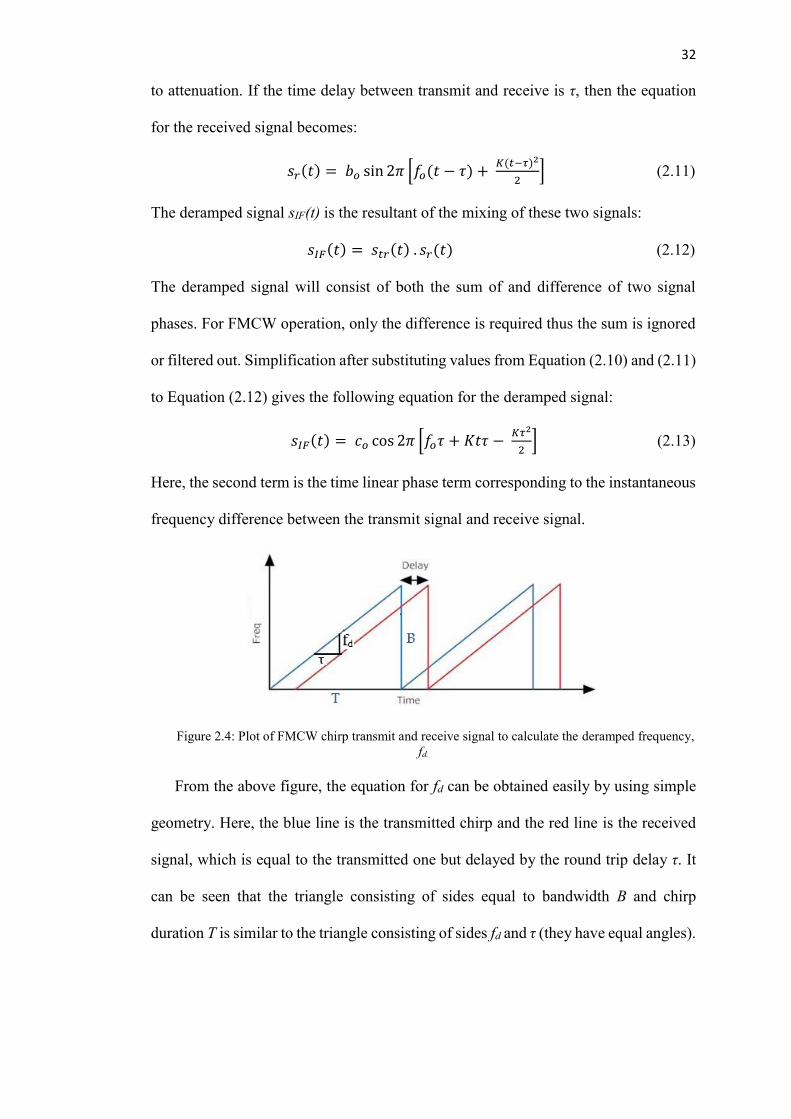
Understanding the formation of an ice shelf requires a brief description of an ice
sheet. An ice sheet is a large chunk of land ice covering most of the Polar Regions.
Figure 2.6: Map of Antarctica. The colored parts are various ice shelves, several of those have
been used as experimental locations in this project. (Credit: Ted Scambos, NSIDC).
37
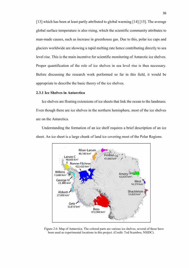
Figure 2.7 Ice sheets in both Polar Regions (Credit: NSIDC).
Large parts of North America and Scandinavia were also covered by ice sheets
during the last ice age. The ice sheets in Antarctica and Greenland contain 99% of the
freshwater ice of the whole world [16]. The Antarctic ice sheet extends over almost
5.4 million square miles, which is the largest single mass of ice in the world containing
7.2 cubic miles of ice [16]. The ice sheet in Greenland extends almost 656,000 square
miles [16].
Ice shelves are basically floating extensions of ice sheets [1]. They are formed
when the ice sheet extends to the coast and over the ocean. Through ice streams and
glaciers, ice from the ice sheet gradually oozes into the sea. Due to differences in
temperature, newly arrived ice does not melt into water straight away. It starts floating
like an iceberg. But it also gains size as more ice gets added from behind before the
small chunk gets the chance to dissolve into the ocean. The very important feature of
these ice shelves is that they act as the interface between the huge ice sheet and the
ocean. So, they are able to act as a bottleneck to slow down the ice flow into the ocean.
This is very important in terms of sea level rise study because the implication is that
ice shelves are very useful to limit the amount of water in the ocean by inhibiting the
land ice (glacier and ice sheet) flow into the ocean. If these ice shelves are melting

38
rapidly or collapsing, that would have direct effect on sea level rise. There have been
studies regarding ice shelf collapses and melting which even gives alarming prediction
that the ice shelves may disappear within next 200 years [17] [18] [19].
Figure 2.8: Simplified diagram of ice formation in Polar Regions showing the fragmentation from
ice sheet to ice shelf and then to iceberg. Grounding line is the boundary between floating and
grounded ice. (Credit: Mark R. Drinkwater; European Space Agency, ESA-ESTEC).
2.3.2 Use of remote sensing for Ice Shelf Monitoring
In 1933, it was discovered that high frequency radio signals can penetrate snow and
ice, the foundation for use of remote sensing to study ice was then built [20]. It was
24 years later though when the first experiment was performed (by Amory Waite) that
used radio echo-sounder (RES) for measuring ice thickness [20]. In 1963, a VHF
system for echo sounding was built [21]. That pioneered the research field of RES
systems for ice measurements. Radars built for this purpose were mostly pulse radars
operating in the VHF and UHF frequency ranges. These instruments achieved quite
good success in calculating ice thicknesses in Polar Regions [22]. After a decade, use
of FMCW radar in this field also started. In 1980, an FMCW system [23] was used to

39
detect and measure water equivalence (amount of water contained in the snowpack)
and snow stratigraphy (different layers of snow).
The current research on ice shelf monitoring is a major collaboration between
government research organizations from various countries. Following are the names
of few organizations that are leading the research work: British Antarctic Survey
(BAS) from UK, National Snow and Ice Data Center (NSIDC) from USA, National
Institute of Polar Research (NIPR) from Japan, Australian Antarctic Division (AAD)
from Australia and Canadian Ice Service (CIS) from Canada.
Different kinds of radar have been used for ice monitoring. NSIDC have used a
combination of satellite techniques (Interferometric Synthetic Aperture Radar
(InSAR), visible-band imagery, and repeat-track laser altimetry) to map ice shelves
[24]. They mapped the grounding line location of the entire Amery ice shelf. Results
shown in [24] helped improve the understanding of the dynamic state of the ice shelf.
Various other papers have been published encompassing analysis of data obtained
from Ice Shelf measurements [25] [26]. In [27], Wilkins Ice Shelf break-up events that
occurred in 28 February to 6 March, 27 May to 31 May, and 28 June to mid-July of
2008, are analyzed with the help of satellite remote sensing observation. The data
provided great detail of the ice shelf calving while the break up was occurring. It was
discovered that the break up was due to a unique type of ice shelf calving, referred to
as ‘disintegration’. The paper also goes into further details of this disintegration
process. In [28], NSIDC used FMCW radar for ice measurements to study the
discontinuities in the snowpack. C-Band (2-6 GHz), X-Band (8-12 GHz), and Ku-
Band (14-18 GHz) frequencies were used for measurements (as the snow structure is
not uniform, reflectivity from different sections of the snowpack for a single frequency
band will vary. Hence, different frequency bands are used and the results are
40
compared). The magnitude and location of snow pack discontinuities have been
calculated as function of frequencies to precisely determine snow cover properties
from monostatic and bistatic radar systems. The experiments revealed that when radar
operates at 14-18 GHz, it gives better information about the internal features of a dry
snow pack. On the other hand, due to the high absorption loss in water, in wet snow
areas, high frequency transmission provides very poor result. For the latter case, lower
frequencies (2-6 GHz) were required to penetrate wet snow without significant
attenuation. In [29], Landsat-7 ETM+ images had been used to map blue ice areas in
Antarctica. In [30], IceBridge Ku-Band Radar altimeter data provides measurements
from Polar Regions of both hemispheres. Time, latitude, longitude, elevation, and
surface measurements, as well as flight path charts and echograms images were
obtained from this radar system. The Ice, Cloud and Elevation Satellite (ICESat) [31]
is another major project of NSIDC, for studying polar ice. This satellite performs
operation based on Geoscience Laser Altimeter System (GLAS), a space-based laser-
ranging instrument (LIDAR). It provides year-long data to determine ice sheet mass
balance along with data of stratospheric clouds (clouds in the winter polar
stratosphere) that are widespread over polar areas. The second version, ICESat-2, is
expected to start operation in 2017.

41
Figure 2.9: A map created from ICESat data demonstrating the extent of ice sheet thinning in
Greenland and Antarctica [32]. (Credit: British Antarctic Survey/NASA).
Besides satellite based systems, numerous ground based systems are also used for
ice monitoring in polar areas. An elaborate description of ground penetrating radar
(GPR) systems can be found in [33]. Further details of the operating principles of GPR
may be found in [33]. Figure (2.10) gives an example of processed data from GPR.
An eskers are long ridges found in the glaciated regions of the northern hemisphere
(Europe and North America). From Figure (2.10), properties underneath the esker can
be seen from the GPR data. As it is seen, radar signal passes through the ice easily but
gets reflected back from others (different types of rocks). Near the surface, reflection
is coming from boulder and gravel (different classes of rock according to particle size).
Below the ice, hyperbolic shaped reflections are due to sediment and bedrock. Most
of the GPR operations are in VHF/UHF frequencies. Even though higher resolution
can be achieved by using high frequency signals, for ice shelf thickness analysis where
the depth of ice can be as long as 2 km, high frequency signals can be severely
attenuated while propagating through the snow and ice [35]. In [36] [37], it was studied
that ice shelf depth change measured by using satellite altimeters does not directly

42
correspond to the mass imbalance. Mass imbalance is the offset from the net balance
between the accumulation and ablation of ice. This imbalance was measured by
satellite altimeters to calculate the change in depth.
Figure 2.10: An example of GPR profile showing underneath the ice cored esker near Carat Lake,
N.W. T. Canada [34].
Instead, thickness change can be attributed to other meteorological conditions that
affect snow compaction such as densification process that changes snow morphology.
In [37], GPR was used to measure snow compaction in two Antarctic Ice Shelves
(McMurdo and Ross), which would compensate for the uncertainties from the
altimeter data. The GPR operated at UHF band. In [38], GPR was used for crevasse
detection across the Ross Ice Shelf. Here, the radar transmission frequency was also
in UHF (400 MHz). In [39], debris characteristics (along with dynamics in the ablation
region) of McMurdo Ice Shelf were studied using GPR data.
The British Antarctic Survey (BAS) have pioneered the use of phase sensitive radar
for measuring ice shelf thicknesses with millimeter precision. As the image processing
from the radar data is mainly done by the processing of the received signals, phase
accuracy of the signals allows for more accurate imaging, hence enhancing the image
quality. In [3], the potential was first shown of phase sensitive radar for precise
43
measurement of ice shelf basal layer melt rate. The pRES was first deployed at the
George VI ice shelf to study ice-ocean interaction. The incentive for high precision
melt rate measurement was that this event plays a major role on Antarctic ice mass
balance, accounting for more than 20% ice discharge from the ice sheet [40]. Accurate
study of the melting of the ice shelf basal layer also helps to understand the evolution
cycle of water mass around polar areas, consequently having an effect on entire global
water mass [41]. But many of the previous basal layer depth estimations had errors
even by margins of 50% [42]. The pRES system helped to narrow down the error
margin significantly. The radar system developed at BAS, known as pRES system,
was based on the stepped-frequency principle. Stepped-frequency continuous wave
radars are also FMCW radars where instead of a continuous frequency band sweep,
the frequency is increased in discrete steps [33]. Advantages and disadvantages of
stepped frequency radar have been detailed in [42]. Step frequency radars are used in
glaciology mainly because of high bandwidth, which means high resolution, as well
as for better signal-to-noise ratio (SNR) [43]. Other main factor is the radar systems
capture not only amplitude, but also phase information. The amplitude was measured
directly where the phase was calculated by comparing the reflected signal with the
output of a precision reference oscillator. The carrier waveform was demodulated in
both side bands from the centre frequency to the baseband [44]. The pRES system
consists of a network analyzer (HP8751A). Transmit and receive antennas were
identical broadband antennas with 10 dBi gain. The system operated at 305 MHz
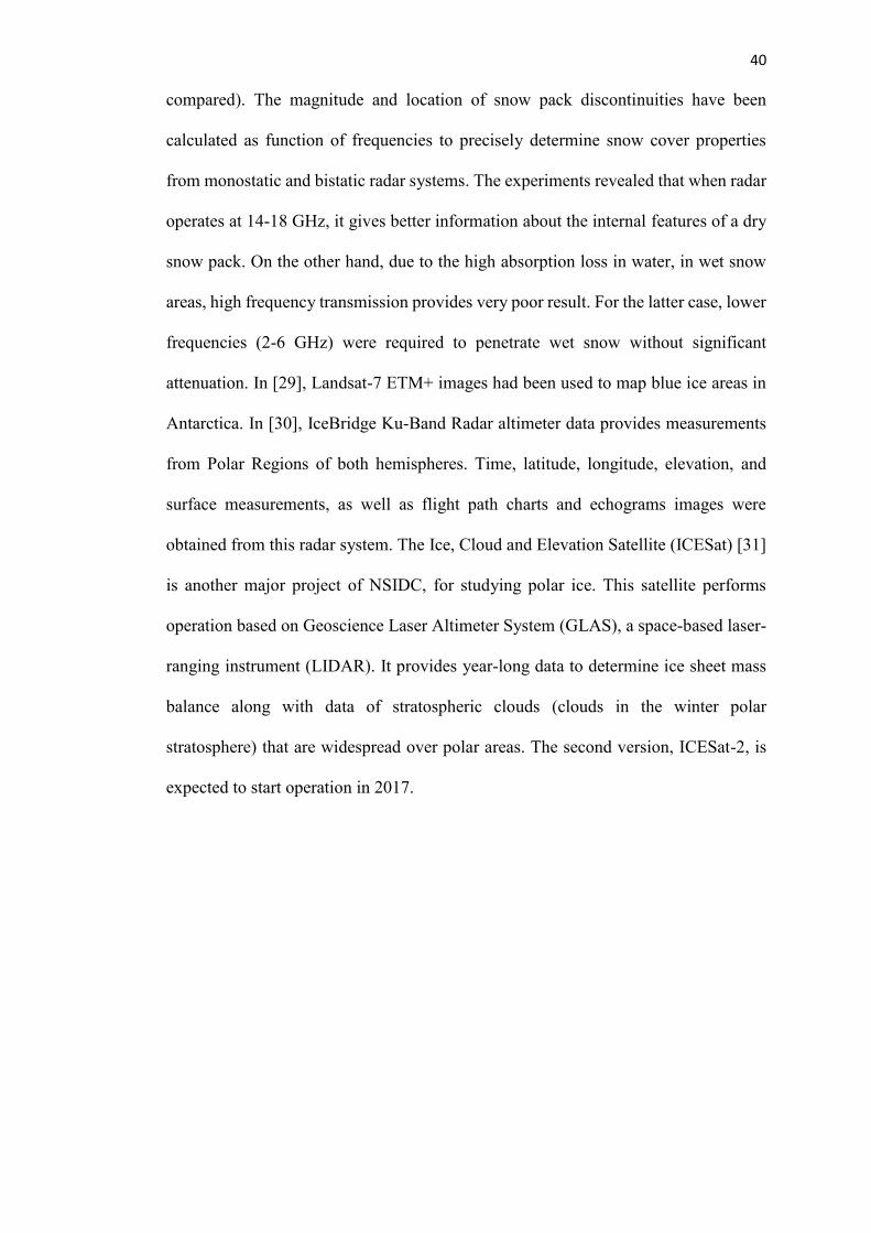
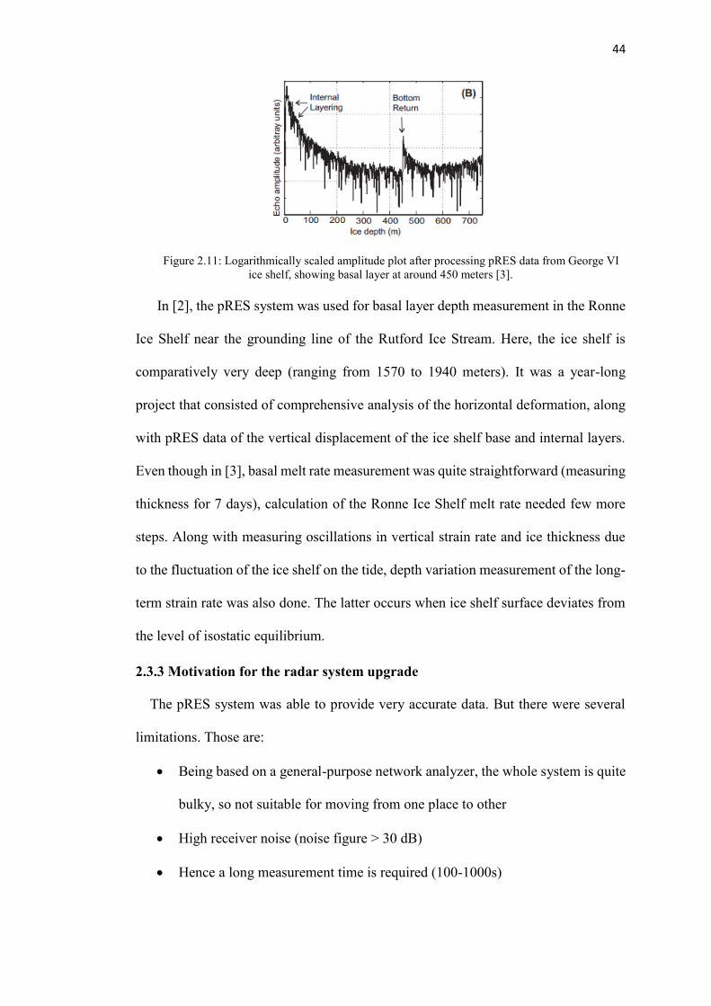
centre frequency where bandwidth being 160 MHz. The range plot from radar data is
the Fourier transformed result of the return signal (in logarithmic scale) shown in
Figure (2.11).
44
Figure 2.11: Logarithmically scaled amplitude plot after processing pRES data from George VI
ice shelf, showing basal layer at around 450 meters [3].
In [2], the pRES system was used for basal layer depth measurement in the Ronne
Ice Shelf near the grounding line of the Rutford Ice Stream. Here, the ice shelf is
comparatively very deep (ranging from 1570 to 1940 meters). It was a year-long
project that consisted of comprehensive analysis of the horizontal deformation, along
with pRES data of the vertical displacement of the ice shelf base and internal layers.
Even though in [3], basal melt rate measurement was quite straightforward (measuring
thickness for 7 days), calculation of the Ronne Ice Shelf melt rate needed few more
steps. Along with measuring oscillations in vertical strain rate and ice thickness due
to the fluctuation of the ice shelf on the tide, depth variation measurement of the long-
term strain rate was also done. The latter occurs when ice shelf surface deviates from
the level of isostatic equilibrium.
2.3.3 Motivation for the radar system upgrade
The pRES system was able to provide very accurate data. But there were several
limitations. Those are:
Being based on a general-purpose network analyzer, the whole system is quite
bulky, so not suitable for moving from one place to other
High receiver noise (noise figure > 30 dB)
Hence a long measurement time is required (100-1000s)

45
High power consumption, requiring a petrol generator
Bulky and not suitable for low temperature operation
Restricted to operation only during Austral summers and to a series of
snapshots (due to the factors mentioned above, it is impractical to use the
system for whole year)
The need for a new system that would be lightweight, consume low power and
most importantly, be able to collect data throughout the year on its own has become
apparent. Also, there was an ever-growing need for making numerous copies of the
system to deploy simultaneously in various experimental sites. Copying a bulky and
high power consuming pRES system would be very impractical. Hence, the project
started by collaboration between BAS and UCL where first objective was to build a
modified FMCW radar prototype with lower noise figure and power consumption
along with all the radar components suitable for low temperature operation, hence
making a year-long operation possible.
2.3.4 Phase sensitive FMCW radar for Ice Shelf Monitoring built at UCL
The FMCW radar built at UCL has the capacity to measure melt rates to mm/year
precision. The radar is built to maintain this precision up to 1800 metres depth [45].
The main features of this radar are low power consumption, low noise figure and hence
a short measurement time, lightweight and suitable for low temperature operation. The
radar system is discussed below by using [45] as the main reference.
As seen from the Figure (2.12), the phase-sensitive FMCW radar is based on a
Direct Digital Synthesizer (DDS) linear FM chirp generator. It consists of a low noise
receiver/downconverter chain. A master clock is used to synchronize the DDS chirp
generator and the data logger (Analog to Digital Converter (ADC)). This
synchronization allows for precise phase measurement during processing and the

46
Figure 2.12: Simplified block diagram of the UCL built phase-sensitive FMCW radar [45]
achieved phase precision exceeds the standard range resolution. It is a low power
consumption device with 5 W power needed during operation and 1 mW during
standby. As the noise figure is far less than the pRES system, the signal collection time
is also much smaller (1 s, as opposed to 100-1000 s for the pRES system). It should
be noted that, as different gain settings are used during field test and to have the option
for pulse-to-pulse averaging, the signal collection time is set to 1 min. If one minute
of data is collected in every six hours (common operating mode), the mean power
consumption is around 31 mW. So, to collect data for a whole winter, a modest
accumulator of 40 Ah capacity would suffice. All the RF components of the radar
system are able to work to temperatures as low as -40o C. The radar system is designed
for VHF-UHF band operation. The bandwidth is 200 MHz with centre frequency at
300 MHz. So, for a 1 s pulse duration, the deramped frequency is 2.35 Hz/m (using
Equation (2.14)). The range resolution becomes 43 cm by considering the dielectric
constant of the Antarctic ice as 3.1 (value provided by the British Antarctic Survey).
Measuring the phase of the deramped pulses carefully, millimetre range precision is

47
achieved (discussed more in Chapter 3). Considering the maximum range as 2 km, the
deramped frequency at this point would be 4.7 kHz. So, a simple data logger with a
sampling rate of 12 ksamples/s or higher would be sufficient.
Table 1: Parameters of phase sensitive FMCW radar
Operating frequency (centre), fc 300 MHz
FM sweep bandwidth, B 200 MHz
RF power, Pt 20 dBm
Antenna gains, Gt, Gr 10 dBi
Noise figure, N 6 dB (F = 4)
Associated standard range resolution, ΔR 43 cm with εr = 3.1
Depth precision in phase-sensitive mode 3 mm RMS, provided SNR>21 dB
Pulse duration, T 1 s
Total acquisition time Total acquisition time 60 s. Ten pulses each with four RF gain
values
ADC sampling rate >12 ksamples/s
Ice attenuation 0.015 dB/m
Maximum operating range, R 2 km
Reflection coefficient between internal layers −60 to −90 dB
Reflection coefficient at ice sheet base −2 dB
Figure 2.13 Prototype phase sensitive FMCW radar built at UCL [45].

48
Figure (2.13) shows the prototype radar system for the Antarctic ice shelf monitoring
developed at UCL. The system is based on the block diagram shown in Figure (2.12),
including added front-end filtering and digital clock generation and synchronization.
The DDS synthesizer used for the system is an Analog Device AD9910. It generates
a sweep signal of 200-400 MHz with a 1 GHz clock. The radar system is designed to
provide good performance on data processing for reflections coming from both near
and far from the radar. Different gain settings have been used for this purpose. A pair
of Mini-Circuits ZX76-31-PP+ digital step attenuators are used to achieve this. These
step attenuators have four combinations that set the RF gain values to 4, 16, 28 and 40
dB. During operation, the gain settings are changed in this sequence for successive
chirps. A second-order high pass filter in the baseband path is also used in order to
compensate for the signal attenuation in the ice. Considering the attenuation
coefficient in the ice as 0.015 dB/m, the reflected signal degrades at a rate of 30
dB/decade within first 100 m range [45], then degrades more rapidly. The high-pass
filter has 0 dB gain at frequencies under 50 Hz and the maximum gain is 80 dB at 5
kHz. It has a fixed slope of +40 dB/decade, over compensating at short ranges but
undercompensating at longer ranges. This is an acceptable trade off, where the 60 dB
or greater dynamic range of the ADC should work, which means effective number of
bits of 10 should be enough. During operation, the system consumes 750 mA at 6 V.
It consumes 0.24 mA during standby. This is a very low power consumption when
compared to the pRES system which required hundreds of watts and a petrol generator.
The reduced noise figure (6 dB) means shorter signal collection time, which saves
energy consumption even more. During the link budget modelling for the system [45],
the expected SNR was calculated as greater than 75 dB for ice shelf basal layer not
exceeding 500 m. After that the SNR drops rapidly due to the inverse-cube dependence

49
and also the ice attenuation. At maximum range (2 km), the SNR is around 14 dB. The
loop test results of the prototype system are discussed in Chapter 5.

50
Chapter 3
Signal Processing Algorithms for the Antarctic Data
Analysis
This chapter concerns with the details of signal processing algorithms that have
been used for analysing the FMCW radar data. The first part discusses the phase
sensitive signal processing method. This method would be used to achieve the
millimetre precision range values while measuring the ice shelf thickness. The FMCW
radar has also been used for imaging of ice shelf base. Different experiments have
been set up at Antarctic sites for imaging the layers underneath ice shelf surface. Three
different algorithms have been used for image processing; phased array processing,
SAR processing and MIMO processing. Discussions regarding the basics of all three
algorithms have been done in this chapter. Along with the basics, simulation results
for all the algorithms are shown and discussed. Instead of using some open source
codes for simulation, MATLAB codes were written for all the conventional imaging
algorithms, along with writing new code for the precision range profiling. One of the
reasons for this is the received signal characteristics of the FMCW radar built at UCL.
Usually conventional algorithms process the received signal (i.e. beamforming
operation in phased array) in time domain. Meanwhile, in the FMCW radar, the
received signal is mixed with the transmitted signal before the data logger saves it. So,
the output from the data logger is the deramped signal, which is in frequency domain.
Most of the open source codes use matched filtering operation to produce the range
history, which is not the case for this system. A conventional SAR system simulation
51
scenario requires a platform in constant motion for a specific amount of time (which
determines the Synthetic Aperture length). This constant motion creates the SAR
Doppler history. The experimental setup used in the Antarctica was not a pure SAR
system, but a simulated SAR system. The radar was mounted on a sledge and then
moved in to different positions in a straight line to collect data. SAR signal history is
obtained by the assumption of an entirely stationary targets within the period of data
collection (a very assumption in the Antarctic Ice Shelves), so the Doppler information
is extrapolated by using the phase information and the total data collection time. In
case of MIMO processing, a conventional MIMO system transmits different
transmitted signals (usually orthogonal to each other). In case of the Antarctic ice shelf
monitoring, all the transmitters send same signal. MIMO system scenario is achieved
by using time switching method. Considering all these factors, along with the need to
ensure that the algorithms work properly with the FMCW radar system parameters,
simulations for the conventional algorithms were performed by newly written
MATLAB codes.
3.1 Phase Sensitive Range Profiling
In [45] [46], techniques for millimetre precision range measurement with FMCW
radar, along with the hardware design to achieve this, have been discussed. In [45], a
processing technique for unambiguous range measurement with the newly built phase
sensitive radar has been thoroughly discussed. The FMCW radar uses phase sensitivity
to determine the high precision range. This high precision is achieved by using a
Vernier-like process that accounts for the fine range measurement of the target along
with its coarse range. The operation principle of a Vernier scale is using a major and
a minor scale. The major scale gives the coarse length and combining it with the value
obtained from the minor scale, precise length is measured. Similar approach is used

52
by the phase-sensitive FMCW radar system. This fine range is attained by measuring
the phase of the signal in the particular range bin where the coarse range is obtained.
3.1.1 Phase sensitive processing steps
The mathematical description of the processing method [45] is given below:
The instantaneous frequency of the linear chirp transmission can be written as:
𝜔𝑡(𝑡) = 𝜔𝑐 + 𝐾(𝑡 − 𝑇/2) 0 ≤ 𝑡 ≤ 𝑇 (3.1)
where ωc is the centre frequency, T is the pulse duration and K is the chirp rate. It
should be noted that chirp rate is signal bandwidth divided by time (should be
multiplied with 2π to get the value in radians). By integrating Equation (3.1), equation
for instantaneous phase can be obtained:
𝜑𝑡(𝑡) = 𝜔𝑐𝑡 + 𝐾(𝑡−𝑇/2)2
2+ 𝑐𝑜𝑛𝑠𝑡 0 ≤ 𝑡 ≤ 𝑇 (3.2)
The equation for the phase of the received signal arriving from range R will be:
𝜑𝑟(𝑡) = 𝜔𝑐(𝑡 − 𝜏) + 𝐾(𝑡−𝜏−𝑇/2)2
2+ 𝑐𝑜𝑛𝑠𝑡 (3.3)
Here, τ is the round trip delay which for any range R, τ = 2R√εr/c.
Deramped signal phase can be mathematically obtained by subtracting the receive
signal phase from the transmitted signal phase. So, from Equation (3.2) and (3.3):
𝜑𝑑(𝑡) = 𝜑𝑡 − 𝜑𝑟 = 𝜔𝑐𝜏 + 𝐾𝜏 (𝑡 −𝑇
2) − 𝐾𝜏2/2 (3.4)
The first term of the phase is the important phase term used for high precision range
calculation. Second term is the linear phase term and third one is the phase offset
(generally negligible). It can be noted that equation for the deramped frequency can
be obtained by differentiating Equation (3.4), which will be exactly the same as the
deramped frequency derived in Chapter 2 (Equation (2.12)).
The range profile is obtained by Fourier transforming the deramped signal. The
range bins will have resolution defined in Equation (2.5). The separation of range bins

53
will be 1/T in frequency. The purpose-built radar uses Vernier-like process to obtain
high resolution range. Along with measuring the coarse range of a target return, it also
measures the phase of the range bin where target is located. Cumulating this fine range
measurement within the range bin with the coarse range provides the millimetre range
precision. In order to measure the accurate phase, the FM waveform and ADC need to
be precisely synchronized.
Figure 3.1: High precision range processing method for the phase-sensitive FMCW radar.
The synchronization is achieved by generating the FM signal with a frequency
divided version of the ADC signal. Figure (3.1) shows the basic idea behind the range
calculation method of this radar. At first, peak amplitude is searched within the range
bins in the proximity of the expected target range. As can be seen in Figure (3.1), it is
the range bin ‘b’. Coarse range value with respect to range bin (b-1) is calculated by
using the generic range formula, Rcoarse = (b-1) c /2B. After that, fine range within the
range bin ‘b’ is attained from the phase of that range bin. The equation relating the
instantaneous phase within the range bin and the range value can be found, as follows:
𝜑𝑑 = 2𝜋
𝜆 2𝑅𝑓
54
=> 𝑅𝑓 =𝜑𝑑𝜆
4𝜋 (3.5)
Here is the instantaneous deramped signal and is the fine range. The factor 2
accommodates for the two-way travel of the radar signal. So, the final range output by
this radar of a certain target is,
𝑅 = (𝑏−1)𝑐
2𝐵√𝜀𝑟+
𝜑𝑑𝜆
4𝜋 (3.6)
εr is the dielectric constant. There are some modifications required during signal
processing. For instance, the phase variation of the deramped pulse from a target as it
moves across the total range bin can be defined as:
∆(𝜔𝑐𝜏) = 𝜔𝑐(2∆𝑅√𝜀𝑟/𝑐) =𝜔𝑐
𝐵= 2𝜋𝑓𝑐/𝐵 (3.7)
To ensure phase unambiguously, the phase variation cannot exceed 2π. Equation (3.7)
shows that for unambiguous phase and hence range indication, the chirp bandwidth
needs to be at least equal to the carrier frequency. Which means ultra-wideband
operation would be necessary for the desired performance. But instead of putting strain
on hardware design, the problem can be easily solved by signal processing. Before
obtaining the range profile by Fourier transformation, the deramped signal can be zero
padded, which decreases the range bin spacing by a factor of p to ΔR/p (where ΔR is
the range resolution and p is the pad factor). A pad factor of 2 would be adequate for
the current radar, reducing the phase variation from 3π to 1.5π.
One other observation can be made from the Equation (3.4). The phase centre of the
deramped signal is at the centre of the sample, at t = T/2. But after Fourier transform,
it would be at t=0. So, before calculating the range profile, the deramped signal needs
to be rotated to align the waveform centre with the starting point of the sample. Figure
(3.2) provides a visual understanding of the zero padding and rotating process.

55
Figure 3.2: Visual depiction of the zero padding and rotating process for FMCW radar data
processing [45].
Figure 3.3: Diagram of the phase sensitive FMCW radar range measurement process [45].
When a point target return phase is at the centre of the range bin, it would be
convenient if it is normalized to zero phase. By multiplying the deramped signal with
the phase conjugate of the estimated phase at the centre of the range bin, return phase
is normalized. The reference phase would be:
56
𝑟𝑒𝑓 = 𝑒(−𝑗(𝜔𝑐𝜏−𝐾𝜏2/2)) (3.8)
3.1.2 Time delay error correction
One important factor that has to be taken into account is the correction due to mis-
synchronization of the ADC and the FM signal. This will cause a time delay which
would correspond to a certain phase delay. The quantitative value of the phase delay
Δϕ is, 2πfdΔt, where fd is the deramped frequency of the target return and Δt is the time
delay. fd can be expressed in terms of range bin and pulse duration as (𝑏−1)𝑇. The
threshold of time delay is ±0.75 μs while taking the desired range precision and
maximum range into account. The value can be calculated by using Equation (3.5).
The estimated range error due to the delay becomes as follows:
𝑅𝑒 =𝜆∆∅𝑑
4𝜋=
𝐵𝑅∆𝑡
𝑓𝑐𝑇 (3.9)
The value of Δt can be obtained from the above equation by considering maximum
range for the radar application as 2 km and accepted range accuracy as 1 mm, which
then becomes 0.75 μs.
3.1.3 Range calibration with two reference values
During field operation, the radar will cycle through each 1 minute burst in every
few hours. Due to the behaviour of the DDS development board, it was discovered
that the precise timing of the initiation of the DDS chirp was subject to a small
variation when the radar is turned on again from stand by. This causes a small error in
timing that cannot be compensated by the time delay correction. The way to get around
this is performing calibration by using two reference range values in order to correct
both the timing errors that are independent of range (represented by a) and the phase
errors that result in range errors linearly-proportional to range (represented by b). This
method is practically plausible as many ice shelves have internal layers above the base

57
which are always constant in terms of depth. These internal layers (R1 and R2) can be
taken as references and the range offset for calibration can be calculated as follows:
∆𝑅1 = 𝑎 + 𝑏𝑅1, ∆𝑅2 = 𝑎 + 𝑏𝑅2
𝑏 =∆𝑅2−∆𝑅1
𝑅2−𝑅1, 𝑎 =
∆𝑅1 𝑅2− ∆𝑅2 𝑅1
𝑅2−𝑅1 (3.10)
−(∆𝑅) = −(𝑎 + 𝑏𝑅)
3.2 Phased Array Processing
Array processing deals with the processing of signals carried out by propagating
wave phenomena [47]. The radar echo from a target is received by numerous sensors
collectively referred to as an array. These sensors have a predefined spacing with
respect to each other. The main goal of array processing is to extrapolate expedient
features of the received signal field (its signature, direction, speed of transmission)
[48].
The different sensors are expected to receive different but coherent signals from a
target, although that may not be always the case. Receive signals can be non-coherent
if those are independent of each other. The basic idea for array processing is to use the
knowledge of sensor spacing and then synthesize the coherent signals from different
sensors to obtain a combined result. According to the application, arrays are formed
in different shapes [49] [50]. The simplest and widely used is the linear array, which
is a collection of sensors in a straight line.
3.2.1 Developments in Phased Array Radar
Phased array radar uses the coherent phase change among the array elements of
the received signal coming from a particular point target. Background on phased array
radar system development can be found in [51]. The earliest development of phased
array can be dated back to 1905, when Nobel laureate Karl Ferdinand Braun

58
experimentally proved the use of multiple antennas to dictate the direction of the
transmitted wave [52]. The first phased array radar was built by Germany during
World War II, which was named FuMG 41/42 Mammut [53]. It consisted of six or
eight Freya [54] antennas and operated at VHF band (116-146 MHz). It had a range
of around 325 metres and was deployed for detecting aerial vehicles of the enemy.
Research on phased array theory became mainstream in the radar community in 1960s
[6]. By the 1980s, due to advancement on antenna technology, phased array systems
were being widely used for various applications and many research works had been
published describing its working principle [55] [56] [57]. The main feature of a phased
array system is the ability to electronically steer the beam. As mentioned above,
phased array systems use antenna spacing information. This information is combined
with the interference property of electromagnetic waves, eventually providing the
ability to control the wave direction. It has the obvious advantage over any operation
that requires to steer the antenna mechanically. Phased array radar has military
applications as it is used by naval warships. The navies use it for finding ships on
water and aircrafts and missiles on the air [58]. Phased array radars are also used for
obtaining weather data [59] and even space research [60]. In this chapter the main
focus would be on the signal processing aspect of phased array radar. The process
phased array radar system uses for transmission or reception of signals from a certain
desired direction, is known as beamforming.
3.2.2 Beamforming
The beamforming technique is used to obtain information from a particular angle.
It works according to the principle of constructive and destructive interference of
electromagnetic waves. Due to antenna element spacing, each element will receive a
signal coming from a certain direction at a slightly different time. This directly
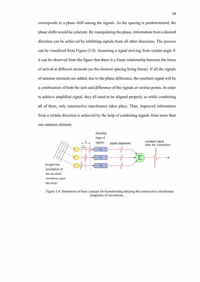
59
corresponds to a phase shift among the signals. As the spacing is predetermined, the
phase shifts would be coherent. By manipulating the phase, information from a desired
direction can be achieved by inhibiting signals from all other directions. The process
can be visualized from Figure (3.4). Assuming a signal arriving from certain angle θ,
it can be observed from the figure that there is a linear relationship between the times
of arrival at different elements (as the element spacing being linear). If all the signals
of antenna elements are added, due to the phase difference, the resultant signal will be
a combination of both the sum and difference of the signals at various points. In order
to achieve amplified signal, they all need to be aligned properly so while combining
all of them, only constructive interference takes place. Thus, improved information
from a certain direction is achieved by the help of combining signals from more than
one antenna element.
Figure 3.4: Illustration of basic concept for beamforming utilizing the constructive interference
properties of waveforms.

60
Figure 3.5: Geometric representation of a linear phased array system to calculate the time (hence
phase) difference among array elements when arriving signal has an angle with normal to the array.
Figure (3.5) helps to quantify the phase difference between adjacent elements in a
linear array. In this figure, N is the total number of elements in the array and
n=0,1,2,3,…,N-1 where d is the spacing between adjacent array elements. As all the
elements are equally spaced, distance from any element from the reference (the first
element) can be quantified as nd. Then, from the triangle drawn on Figure (3.5), extra
path that a signal has to travel at each element due to the incident angle θ, can be
calculated. Converting the spatial value into phase gives the equation for phase delay:
∅𝑠ℎ𝑖𝑓𝑡 = 2𝜋
𝜆 𝑛𝑑 sin 𝜃 (3.11)
During beamforming, this equation is used for aligning the signals coming from
angle θ. 4π should be used instead of 2π to account for the two way signal propagation.
It is obvious from Equation (3.11) that if the incident signal is parallel to the array
(θ=0), there is no phase delay, hence just adding the original receive signals would
give the resultant signal from that angle.
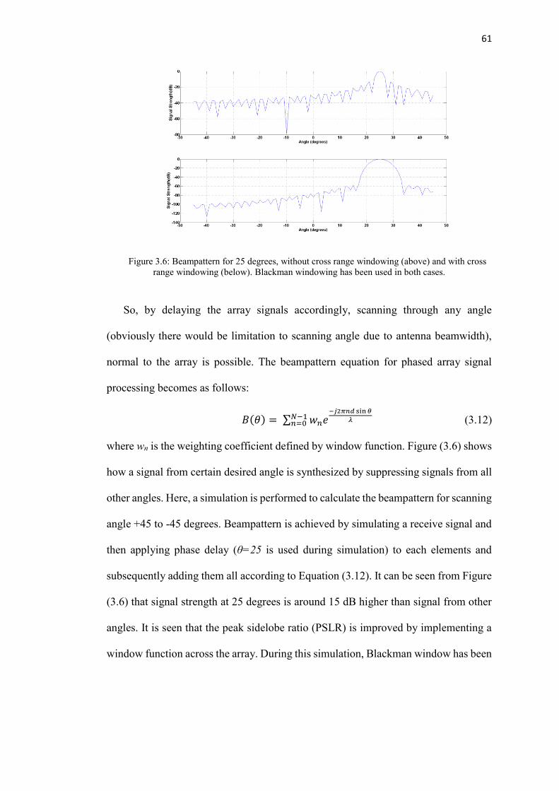
61
Figure 3.6: Beampattern for 25 degrees, without cross range windowing (above) and with cross
range windowing (below). Blackman windowing has been used in both cases.
So, by delaying the array signals accordingly, scanning through any angle
(obviously there would be limitation to scanning angle due to antenna beamwidth),
normal to the array is possible. The beampattern equation for phased array signal
processing becomes as follows:
𝐵(𝜃) = ∑ 𝑤𝑛𝑒−𝑗2𝜋𝑛𝑑 sin 𝜃
𝜆𝑁−1𝑛=0 (3.12)
where wn is the weighting coefficient defined by window function. Figure (3.6) shows
how a signal from certain desired angle is synthesized by suppressing signals from all
other angles. Here, a simulation is performed to calculate the beampattern for scanning
angle +45 to -45 degrees. Beampattern is achieved by simulating a receive signal and
then applying phase delay (θ=25 is used during simulation) to each elements and
subsequently adding them all according to Equation (3.12). It can be seen from Figure
(3.6) that signal strength at 25 degrees is around 15 dB higher than signal from other
angles. It is seen that the peak sidelobe ratio (PSLR) is improved by implementing a
window function across the array. During this simulation, Blackman window has been

62
used. The main lobe width has increased but this is the usual trade off while using
window function.
Other important implication of Equation (3.11) and (3.12) is that the phase delay
is a function of signal wavelength, hence frequency. So, using phase delay would not
work properly in a wideband operation where this beam steering vector will not be a
function of single frequency. So, beamforming in this process makes the beam
squinted as perfect constructive interference is not achieved due to large number of
frequency components. To resolve this issue, beamforming can be obtained by time
delay instead of frequency delay. To convert the phase delay for beam steering into
time delay one, relation between phase angle φ and time delay Δt can be used which
is φ=2πf * Δt. Here, f is the signal frequency. Substituting this value with Equation
(3.10) gives the time delay factor and subsequently the time delay steering vector as
follows:
∆𝑡 = 𝑛𝑑 sin 𝜃
𝑐 (3.13)
𝐵(𝜃) = ∑ 𝑤𝑛𝑒−𝑗𝑛𝑑 sin 𝜃
𝑐𝑁−1𝑛=0 (3.14)
It can be seen that there are no frequency parameters in Equation (3.13) and (3.14).
Figure 3.7: Illustration of grating lobe where on a beampattern for steering vector at 25 degrees,
another strong signal appears at -38 degrees due to element spacing being more than half the signal
wavelength.
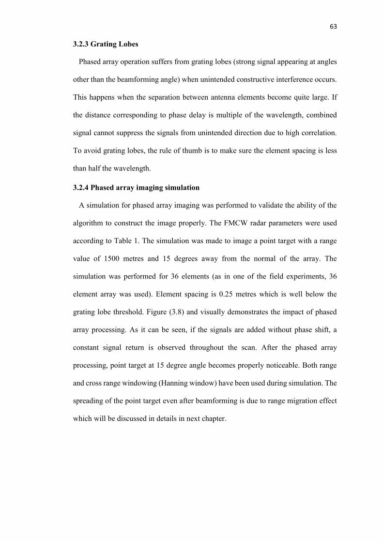
63
3.2.3 Grating Lobes
Phased array operation suffers from grating lobes (strong signal appearing at angles
other than the beamforming angle) when unintended constructive interference occurs.
This happens when the separation between antenna elements become quite large. If
the distance corresponding to phase delay is multiple of the wavelength, combined
signal cannot suppress the signals from unintended direction due to high correlation.
To avoid grating lobes, the rule of thumb is to make sure the element spacing is less
than half the wavelength.
3.2.4 Phased array imaging simulation
A simulation for phased array imaging was performed to validate the ability of the
algorithm to construct the image properly. The FMCW radar parameters were used
according to Table 1. The simulation was made to image a point target with a range
value of 1500 metres and 15 degrees away from the normal of the array. The
simulation was performed for 36 elements (as in one of the field experiments, 36
element array was used). Element spacing is 0.25 metres which is well below the
grating lobe threshold. Figure (3.8) and visually demonstrates the impact of phased
array processing. As it can be seen, if the signals are added without phase shift, a
constant signal return is observed throughout the scan. After the phased array
processing, point target at 15 degree angle becomes properly noticeable. Both range
and cross range windowing (Hanning window) have been used during simulation. The
spreading of the point target even after beamforming is due to range migration effect
which will be discussed in details in next chapter.

64
Figure 3.8: Image formation for a point target at 1500 metres range and 15 degree from the array:
above one is without implementing beamforming and below one shows the image after applying
phased array beamforming.
65
3.3 Synthetic Aperture Radar (SAR) Processing
SAR signal processing is a 2-dimensional image processing operation. The
fundamental difference between the conventional optical image processing and
radar/SAR image processing is the latter one uses distances between the objects and
the sensor to form an image. On the other hand, optical imaging systems such as
cameras or optical telescopes use the angular differences of the signals incident upon
the sensor to create an image. In the Antarctic Ice Shelf application that this thesis
work concerns, no physical SAR system was deployed. But during the data collection,
a SAR like experiment was performed by mounting the ice penetrating radar on a
sledge and moving the sledge in a straight line while the radar collected data. This
emulated the synthetic aperture. The idea was to analyse and compare the ice shelf
images obtained from different processing methods (i.e. phased array and SAR).
3.3.1 SAR geometry and Parameters
SAR data acquisition method is similar to normal Radar when each transmitted pulse
and corresponding reception is considered individually. After all, it is a standard Radar
that is attached to the platform. However, there is one little assumption that is
commonly made. Radar signal travels in the speed of light and the platform speed is
extremely slow compared to light speed. So, during the time the Radar receives the
reflection from the ground, platform’s movement can be neglected. This is known as
the ‘start-stop’ assumption [61].

66
Figure 3.9: SAR operation geometry.
As mentioned, SAR typically requires precise positional information of the
platform during its data gathering period. Method of SAR processing which is
independent of platform position has also been researched [62]. With the platform
information, it can calculate the necessary factors that determine the relationship
between the platform and the target at each moment. These parameters that are
obtained from the geometry along with the terms that are essential during computation
are discussed below.
Platform velocity: All along the flight path, platform velocity is tried to be kept
constant. In practical cases, the platform velocity does not remain the same for the
whole flight. This causes error in computation and has to be accounted for, which is
known as ‘motion compensation’.
Integration angle: It is basically the angle measured from the two endpoints of the
flight path. It determines the eventual synthetic aperture length. The angle is
determined by the lines drawn from two ends of the flight path joining the point target.
Thus, Synthetic aperture length (L) can be calculated from the integration angle.

67
Figure 3.10: SAR integration angle and point target.
Ground range: This is the two dimensional measurement of the distance between
the point target and a point from the flight path line’s projection on the ground plane
(Figure (3.9)).
Slant range: In the simplest of ways, it is the length of the straight line drawn
between the platform and the target at each given moment during the flight. This is the
evident distance travelled by the transmitted pulse from platform to target. As seen
from Figure (3.9), it is a three dimensional measurement. At each
transmission/reception period during flight, slant range is been determined. The
measurement is done by simple Pythagorean geometry.
Figure 3.11: SAR range calculation geometry.

68
While calculating range, along with the known platform parameters, the minimum
range to the target (ro) is known. An important fact should be known about monostatic
SAR in terms of minimum range. The target and the platform should be separated by
at least a distance defined by the time duration of switch of the radar from transmission
to reception mode. The radar cannot detect target closer to this value as that target
echo will reach the radar before it is switched into receiving mode. This time delay
depends on the transmission pulse width as radar cannot switch before the whole pulse
is been transmitted. From Figure (3.11), the point target has coordinate values in x and
y axis. As seen from the geometry, xo is just the displacement in x axis from the origin
and 𝑦𝑜 = √𝑟𝑜2 − ℎ2. Having vpl and h as the platform velocity and altitude
respectively, the equation becomes,
𝑅(𝑡) = √(𝑣𝑝𝑙𝑡 − 𝑥𝑜)2
+ 𝑦𝑜2 + ℎ2 (3.15)
3.3.2 SAR Doppler History
For a single platform position, SAR signal return is collected. This recording is
continued throughout the flight. For a given aperture length, the number of recorded
sample depends on PRF. They are placed in the two dimensional memory of azimuth
and range. This is the raw SAR signal history which is used for image processing by
applying suitable algorithms. This is also called as SAR phase history. During the
flight, range between the platform and target is changed. The range equation is
hyperbolic, thus SAR signal history is the hyperbolic curve shown in the right side of
Figure (3.12). The inherent Doppler Effect on SAR signal is apparent from the figure.
The hyperbolic nature of the range migration curve depends in the integration angle.
Larger integration angle makes the hyperbolic nature more obvious. During SAR
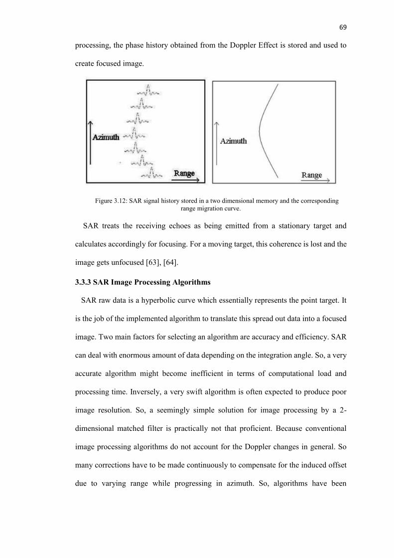
69
processing, the phase history obtained from the Doppler Effect is stored and used to
create focused image.
Figure 3.12: SAR signal history stored in a two dimensional memory and the corresponding
range migration curve.
SAR treats the receiving echoes as being emitted from a stationary target and
calculates accordingly for focusing. For a moving target, this coherence is lost and the
image gets unfocused [63], [64].
3.3.3 SAR Image Processing Algorithms
SAR raw data is a hyperbolic curve which essentially represents the point target. It
is the job of the implemented algorithm to translate this spread out data into a focused
image. Two main factors for selecting an algorithm are accuracy and efficiency. SAR
can deal with enormous amount of data depending on the integration angle. So, a very
accurate algorithm might become inefficient in terms of computational load and
processing time. Inversely, a very swift algorithm is often expected to produce poor
image resolution. So, a seemingly simple solution for image processing by a 2-
dimensional matched filter is practically not that proficient. Because conventional
image processing algorithms do not account for the Doppler changes in general. So
many corrections have to be made continuously to compensate for the induced offset
due to varying range while progressing in azimuth. So, algorithms have been

70
developed to perform SAR image focusing distinctively. All the developed algorithms
can be grouped into two main categories in terms of their working domains, Time
domain algorithms and Frequency domain algorithms. As the signal history is
obviously in time domain it can very easily be converted into frequency domain by
performing two-dimensional Fourier transform. Actually, it is quite common in image
processing field to manipulate images in frequency domain. The reason is its
mathematical advantages as different features of an image correspond to different
frequency elements.
Time domain algorithms by and large are based on the back-projection principle
[65]. The concept is very simple. Each signal is back-projected onto the image plane
according to their direction vector. Same value is assigned throughout that direction.
The process is carried out for every sample and the summation gives out the final
image. The most widely used such algorithm is Global Backprojection (GBP)
algorithm [66]. It provides accurate image but it has high computational cost due to its
large number of required operation to produce an image. Other algorithms such as Fast
Backprojection (FBP) [66] or Fast Factorized Backprojection (FFBP) [9] have taken
mainly developed to reduce this cost.
Meanwhile, frequency domain algorithms rely quite understandably on Fourier
transformation. In fact, they use the Fast Fourier transform (FFT) technique. This
feature brings the opportunity for speedy computation. These algorithms generally try
to nullify the Doppler Effect by performing interpolation or complex multiplications
in frequency domain. Prominent algorithms of this kind are Range Doppler algorithm
(RDA) [5], Chirp Scaling Algorithm (CSA) [67] and Range Migration Algorithm
(RMA) [61]. RDA was the first developed algorithm for SAR processing. In this
algorithm, SAR data is converted into range Doppler domain by azimuth FFT

71
operation. Ensuing operations are performed in this domain to achieve the image. CSA
is applied in a two-dimensional frequency domain that avoids the use of interpolation.
This is an advantage because other frequency domain algorithms often require a very
sophisticated interpolation procedure that inflicts computational cost on the processor.
RMA on the other hand has the ability to operate with large integration angles and
does not discard any phase term unlike CSA or RDA. Although, motion compensation
in frequency domain is not that convenient, especially for large integration angle as it
further increases the computational cost. In essence, algorithms of both domains
inherit different features in terms of image quality and processing time [65] [66]. The
selection of one algorithm will entirely depend on the integration angle, threshold for
acceptable resolution, and platform parameters.
3.3.4 Range Migration Algorithm
The Range Migration Algorithm (RMA) has been used for SAR data processing
during the period of the work presented in this thesis. RMA originated from seismic
signal processing [61]. Seismic data processing can be considered strongly analogous
to SAR. For seismic data processing, some numbers of geophones are placed along a
straight line on the ground and a charge is detonated along that straight line. Every
single geophones uses the received sound echo and the combined results are analyzed
to figure out ground characteristics. This placement of geophones is similar to specific
SAR platform positions at any given instance. During the processing of seismic
received data, the phase function is hyperbolic just like SAR phase data.
RMA is a frequency domain algorithm where frequency conversion is applied in
both azimuth and range axes. The technique that RMA uses to focus the image is based
on downward continuation i.e. the downward propagation of the wave equation [61].
This property has also been drawn from seismic migration. The key feature of RMA

72
is the change of variable in the range axis. This method was developed by Stolt. He
developed this variable swap method in frequency domain which is commonly known
as ‘Stolt mapping’ or ‘Stolt interpolation’ [68]. He implemented this method to
provide a proper solution for the wave equation for seismic data processing [5].
RMA has four major segments in terms of its functionality. Each has distinct features
and purposes that sequentially lead to create a focused image of the area viewed by
the radar aperture during the SAR flight.
Figure 3.13: Block diagram of the Range Migration Algorithm.
The first and last steps are just domain converters. The main algorithm is applied
to the signal data by the two steps in the middle. It is seen from the Figure (3.13) that
those steps are performed in frequency domain. Just to set the premise before going
into comprehensive discussion on these two steps in the middle, the image formation
process of a single stationary point target will be the basis for the explanation of the
algorithm. This will elucidate the algorithm at its core. When more point targets are
added, the algorithm works exactly the same way on each of those point targets in
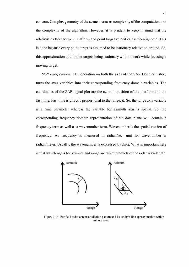
73
concern. Complex geometry of the scene increases complexity of the computation, not
the complexity of the algorithm. However, it is prudent to keep in mind that the
relativistic effect between platform and point target velocities has been ignored. This
is done because every point target is assumed to be stationary relative to ground. So,
this approximation of all point targets being stationary will not work while focusing a
moving target.
Stolt Interpolation: FFT operation on both the axes of the SAR Doppler history
turns the axes variables into their corresponding frequency domain variables. The
coordinates of the SAR signal plot are the azimuth position of the platform and the
fast time. Fast time is directly proportional to the range, R. So, the range axis variable
is a time parameter whereas the variable for azimuth axis is spatial. So, the
corresponding frequency domain representation of the data plane will contain a
frequency term as well as a wavenumber term. Wavenumber is the spatial version of
frequency. As frequency is measured in radian/sec, unit for wavenumber is
radian/meter. Usually, the wavenumber is expressed by 2π/𝜆. What is important here
is that wavelengths for azimuth and range are direct products of the radar wavelength.
Figure 3.14: Far field radar antenna radiation pattern and its straight line approximation within
minute area.

74
Figure (3.14) illustrates the wavelength concept of SAR signal. The radar
wavelength 𝜆 projects to the direction of the wave propagation while 𝜆r is related to
the ground range. 𝜃 is the squint angle. As wavefronts are parallel to each other, the
relationship among these three wavelengths can be evaluated from this above simple
geometry [5].
𝜆𝑥 =𝜆
sin 𝜃 (3.16)
𝜆𝑟 =𝜆
cos 𝜃 (3.17)
Now, if the frequency domain representation of the azimuth axis spatial variable x
is denoted as kx, ground range variable r as kr then,
𝑘𝑥 =2𝜋
𝜆𝑥 (3.18)
𝑘𝑟 =2𝜋
𝜆𝑟 (3.19)
The frequency domain representation for the remaining plane, the slant range plane,
is merely the angular frequency of the signal as it changes proportionally with the fast
time. Substituting the values of Equation (3.16) and (3.17) into Equation (3.18) and
(3.19),
𝑘𝑥 =2𝜋
𝜆sin 𝜃 (3.20)
𝑘𝑟 =2𝜋
𝜆cos 𝜃 (3.21)
Squaring the above two equations and adding them together,
𝑘𝑥2 + 𝑘𝑟
2 = (2𝜋
𝜆)
2
(3.22)
Substituting the value of 𝜆 with wavelength ω,
𝜔 =𝑐
2√𝑘𝑥
2 + 𝑘𝑟2 (3.23)

75
Equation (3.23) demonstrates the relationship between the frequency domain variable
of the ground range with the frequency domain variables of the SAR signal history.
Stolt interpolation uses this equation to change the variable of the range axis. Since
the phase reference is assigned in closest approach point (between platform and
target), the Doppler shift at that point is evidently zero. The main goal is to eradicate
the Doppler shifts of other points taking the closest approach point as reference. In
zero Doppler position, azimuth spatial frequency kx=0. So, in zero Doppler, a
relationship exclusively between kr and 𝜔 becomes kr= 2ω/c. This can be exploited to
make the interpolation more efficient. For every kx, the phase corrected value for 𝜔
can be found by shifting it with respect to the center frequency. It gives the new value,
𝜔´ = 𝜔 – 𝜔c (𝜔c is the centre frequency). This new value can be calculated from
Equation (3.23) where kr is measured according to the new value of kr (with respect to
reference phase). This whole manipulation produces the new equation:
𝜔′ =𝑐
2√𝑘𝑥
2 + 𝑘𝑟2 − 𝜔𝑐 (3.24)
By means of the above equation, the effect of the variable change is achieved.
Interpolation operation is imposed to rectify the values of 𝜔 with corresponding values
of 𝜔´. What is to observe here is that the Stolt interpolation basically transforms the
azimuth slant range plane of the raw SAR data into azimuth ground range plane. From
the geometrical point of view, it can be said that the intrinsic Doppler Effect within
the signal arises from the non-orthogonality of the two plains comprising the signal
history. Since azimuth and ground range are orthogonal to each other, the deformation
gets canceled out and so as the phase shift along the flight path [5] [69].

76
Figure 3.15: SAR signal energy in 2-dimensional frequency domain and Stolt interpolation’s
effect on it.
One interesting observation can be made from Figure (3.15) is the circular nature of
the signal strength after the Stolt interpolation. Recalling Equation (3.23) helps to
explain this matter. That is a rearranged version of the circle equation. This gives the
visual representation of how frequency component replacement in range corrects the
entire image spectrum. In practical cases, this nature hardly becomes apparent in
narrowband SAR operation [61], but UWB SAR makes this property visually more
evident because of its large integration angle.
Azimuth Compression: Before taking the signal data back into its original domain,
azimuth compression needs to be performed to create the focused image. The signal
information of a single point target which is spread out throughout the signal history
has been taken care of by the Stolt interpolation in terms of phase shift correction.
Still, the data needs to be converged in azimuth. This step is actually quite simple and
does not possess any lengthy concept like the Stolt interpolation. An azimuth reference
function [61] is multiplied with the signal spectrum to congregate the signal data
smeared along the azimuth axis into the zero Doppler point. This is nothing but a
matched filtering operation where the signal is correlated with the matched filter

77
function corresponding to the closest approach point. So, this multiplication just
funnels in all the smeared data into the closest approach point or minimum range, for
that is the ultimate position considered for the point target. After this compression, all
the signal energy gets concentrated into this point hence creating the focused image
(when it is transformed back to time domain). The azimuth reference function is as
follows,
𝑟𝑒𝑓(𝑘𝑥,𝑘𝑟) =|𝑘𝑟|
√𝑘𝑥2+𝑘𝑟
2𝑒
−𝑗(𝑟𝑜√𝑘𝑥2+𝑘𝑟
2−𝑟𝑜𝑘𝑟) (3.25)
The first part of the function is the magnitude which has little effect if integration angle
is small. Combining the two operations, Stolt interpolation and azimuth compression,
the raw SAR data is synchronized with the reference point phase, both in azimuth and
range. In other words, the signal energy is entirely compressed. Now, the focused
image with its full resolution can be seen simply by performing 2-D inverse Fourier
transform of the signal spectrum.
3.3.5 SAR simulation Results
Before implementing SAR processing to real data, simulation of the range migration
algorithm to focus point target was performed to ensure the algorithm was accurately
translated into software routine (in this thesis work, MATLAB was used). Again, radar
parameters were set according to Table 1. The simulation was performed to focus a
point target with a range value of 350 metres (as the target return from SAR field
experiment was from around that distance). Even though the integration angle in the
field experiment was quite low (total SAR platform length was 22 metres only),
simulation was performed for larger integration angle as well to visually observe its
affect. Platform velocity was assumed to be very slow (1 m/sec.), as that would be the
case during Antarctic experiment. Figure (3.16) shows the SAR signal history which

78
illustrates the conventional hyperbolic pattern. Figure (3.17) shows the focused point
target after implementing RMA. Here, the integration angle is 30 degrees. Figure
(3.18) shows the focused image of the same point target when the integration angle is
very small (corresponding to 22 metres of synthetic aperture length only). The
degradation of target focusing quality due to low integration angle can be easily
compared from Figure (3.17) and (3.18).
Figure 3.16: SAR signal history of a point target return before implementing focusing algorithm
showing the characteristic hyperbolic curve (image is zoomed in).
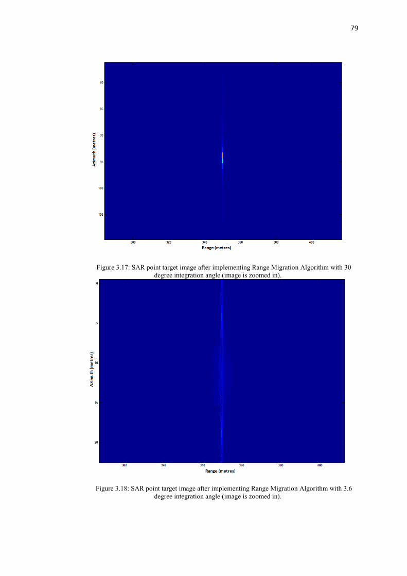
79
Figure 3.17: SAR point target image after implementing Range Migration Algorithm with 30
degree integration angle (image is zoomed in).
Figure 3.18: SAR point target image after implementing Range Migration Algorithm with 3.6
degree integration angle (image is zoomed in).

80
3.4 MIMO Processing
Multiple-input-multiple-output (MIMO) radar is a relatively new technology in the
radar field. The basic idea is to add waveform diversity to the conventional phased
array system, obtaining enhanced performance. According to [70], the definition of
waveform diversity is the ability to adapt and diversify dynamically the waveform to
the surrounding environment which would deliver enhanced performance compared
to a non-adaptive system. In [71] [72] [73], the prospect of using multiple signals in
an array system has been studied. The waveform diversity is also achieved by utilizing
the antenna element spacing [74]. In various research papers, superiority of MIMO
radars has been discussed (ability to obtain better resolution [73] [75], better capability
for slowly moving target detection [76], ability to identify more targets than phased
array [74], better application for adaptive array techniques [74] [77] [78]).
Figure 3.19: Comparison of (a) MIMO radar and (b) Phased array radar [79].

81
Figure (3.19) illustrates the fundamental geometric principle of MIMO radar
compared to conventional phased array radar. It can be seen that MIMO radar uses
waveform optimization by transmitting different signals from different elements.
When compared to phased array, the potential to extract more information by MIMO
can be intuitively understood. As a return echo from a target received by phased array
system is essentially the same signal with a phase difference, signals on the receive
side cannot be distinguished in terms of the parent transmitter. On the other hand, in
MIMO, it can be easily achieved because each individual transmitter emits signals
unique from the others. This information can be used for obtaining better angular
information as well as for improved detection performance, resolution and SINR
(signal to interference plus noise ratio) [80]. MIMO receivers use matched filtering to
obtain information coming from each individual transmit antennas. The transmitted
signals in MIMO radar are orthogonal even though it’s not a strict requirement. The
orthogonality is usually achieved by time or frequency division multiplexing. Also, in
terms of antenna spacing, MIMO radar system can be collocated or sparse. For further
details on those can be found in [79].
3.4.1 MIMO Virtual Array
The unique concept of MIMO system is the virtual array configuration. Here, a
brief understanding of this concept is provided. More elaborate studies on this can be
found in [75] [76] [81].
Virtual array in MIMO is achieved by utilizing its waveform diversity property. The
advantage of using virtual array is that during processing, the MIMO array consists of
elements more than the number of elements that are physically in operation. MIMO

82
virtual array positions are determined by convoluting transmit and receive antenna
element positions.
Figure 3.20: Illustration of MIMO virtual array positioning by convolution of real and receive
array.
It can be seen from the above figure that the convolution process increases the
number of array elements to 9 where there are 6 elements present physically.
Assuming there are M number of transmit elements and N number of receive elements.
The signal transmitted by mth antenna is denoted as φm(t). Each transmitting signals
are orthogonal. At each receive element, M number of matched filters are used to
extract all orthogonal signals. Which corresponds to total number of receive signals
equal to product of M and N. This is the total number of virtual array element which
is NM produced by using N+M number of physical elements. According to the
geometric position of the real array elements, equation for the target response at nth
receiver for the signal coming from mth transmitter can be written as [80]:
𝑦𝑛,𝑚(𝑡) = 𝑎 𝑒(𝑗
2𝜋
𝜆𝐮𝐭
𝑇(𝐱𝑇,𝑚+𝐱𝑅,𝑛)) (3.26)
where ut is a unit vector pointing toward the target from the array. xT,m and xR,n are
the positional vectors for mth transmitter and nth receiver respectively where a is the
signal amplitude. It should be noted that location of transmission and receive elements
attribute directly to the obtained phase difference.

83
3.4.2 MIMO Beamforming
For a uniform linear array, the location vectors can be defined according to
Equation (3.11). So, the Equation (3.26) can be written as:
𝑦𝑛,𝑚(𝑡) = 𝑎 𝑒(𝑗
2𝜋
𝜆(𝑛𝑑𝑟 sin 𝜃+𝑚𝑑𝑡 sin 𝜃))
(3.27)
where dr and dt are the element spacing for transmit and receive antennas respectively.
This equation is used to create steering vector for MIMO. One basic difference of
beamforming in MIMO from phased array beamforming is unlike phased array, virtual
beamforming can only be achieved in receive side. During the thesis work, MIMO
imaging simulation was performed to analyze the possibility of using MIMO radar for
snow Avalanche imaging in Alps. Simulation results concluded that SNR would be
too low to create any meaningful signal by MIMO transmission, hence the project
stuck with its previous conventional phased array system. The simulation results are
added in the appendix. MIMO beamforming and imaging technique developed for
three-dimensional imaging of Ice Shelf base is described in Chapter 4.

84
Chapter 4
Novel Signal Processing Techniques for Antarctic
Data Analysis
This chapter consists of the signal processing techniques that were developed
during this thesis work for the Antarctic data analysis. The development of these
techniques was motivated by the practical necessity stemmed from Antarctic ice shelf
experiments. The first section describes the Shape matching algorithm that has been
developed to detect internal layers underneath ice shelves. The second section
describes the range migration correction for fixed phased array radar. The range
migration within the array is caused by the high fractional signal bandwidth, which is
the case with the FMCW radar that has been deployed in Antarctica. Also, adverse
weather conditions in Antarctica make it very hard to maintain the geometric
parameters of the experiments accurately. Hence, vertical antenna spacing error
correction method by using reference phase has been developed. The final section
encompasses the 3-D MIMO imaging algorithm that has been developed for 3-D
imaging of the Antarctic Ice Shelf basal layer.
4.1 Shape Matching Algorithm to Detect Internal Layers
Due to unavoidable practical reasons, it is very difficult to take precise radar
measurements in the challenging conditions in Antarctica. Events such as snowfall,
heavy wind can change the vertical position of the radar antennas. When the expected
accuracy is within millimeter range, slightest change of the radar position can become

85
significant. So, it is always desired to have some fixed reference that can be used for
calibration and to compensate due to the displacement error.
The internal layer is a feature of the ice shelf that can be used for this calibration
purpose. Internal layers can be detected by radio waves. Mainly, these are sections
underneath the ice shelves where there is a contrast in the ice dielectric property [82].
Due to this contrast, an ice crystal fabric is formed that reflects radar transmitted
signal. Most importantly, these layers are prone to have fixed coordinate. They usually
do not drift vertically hence can be used as a very good reference point. If the radar
shifts from its initial position, it can be easily determined by the presence of an internal
layer. By adjusting for these discrepancies using internal layer, very high precision
results can be achieved from the radar data. Not only for radar data calibration, but
internal layers also have great interest among geoscientists in their field of study of
ice in Polar Regions. Even though it is desirable to get an internal layer while profiling
an ice shelf, it is not that straightforward to detect. Generally, internal layers are
located close to the ice shelf surface (within 100 meter). Due to antenna direct
coupling, radar range profiles consist of large returns in close range. These high signals
tend to obscure return radar signal from any actual ice shelf feature (i.e. internal layer).
In radar signal processing, it is always a big challenge to detect the presence of a
target with low signal to noise ratio (SNR) or signal to clutter ratio (SCR). A number
of research works have been performed to solve these problems [83] [84]. In most
cases, the problems are application specific, each requiring different modelling and
assumption of the target scenario.

86
Figure4.1: Range profile of Antarctic ice shelf illustrating basal layer return and strong return in
short range.
Figure (4.1) illustrates a typical FMCW radar range profile of Antarctic ice shelf.
In Antarctic ice shelf measurement, the strongest return is expected from the basal
layer. As it is seen in Figure (4.1), even though the basal layer is quite apparent, the
profile encompasses high amplitude signals at very close range. These close range
signals can be attributed to antenna direct coupling and/or clutter in the vicinity of the
ice shelf surface. Usually, internal layers are expected to be present in that close range
region. For radar target detection, a cross-correlation method is usually used when
there is a known target [85]. In the particular case of ice shelves, the assumption is that
both basal layer and internal layer will give out specular reflections. Hence, intuitively,
cross-correlation method ought to work for internal layer detection. Meanwhile, it is
obvious that cross-correlation will be ineffective when the antenna direct coupling
signals are significantly higher than the actual basal layer return.
A proposed method to overcome this problem is described below. This shape
matching algorithm works in following four steps-

87
Defining the reference signal from the range profile.
Amplitude scaling.
Point by point difference calculation and ranking.
Integration for overall rank
4.1.1. Defining the reference signal from range profile
In shape matching algorithm, the first task is to determine the signal portion that
is to be matched throughout the profile. In general case, a known expected pattern can
be used or a copy of the transmitted signal (used in matched filtering). The idea is to
slide this reference signal over the whole profile just like conventional correlation. In
this case, the mathematical operation during the sliding would be entirely different. In
the specific case of ice shelf, return signal from the ice shelf base will be the obvious
reference. As mentioned before, internal layers are likely to have similar signal shape
due to same reflection property. So, a portion of the signal from the profile that
corresponds to basal return is chosen as a reference. Care is needed while selecting the
reference cut, as that chunk would be the main reference. The more similar a signal
portion in any other part of the profile is to this reference, the more likely that portion
would be a radar target rather than clutter/noise. For the derivation, radar received
signal is defined as s(n) having N number of samples (n=1,2,….,N). Reference signal
is defined as ref(m) consisting of M number of samples (m=1,2,….,M).
4.1.2. Amplitude scaling
The main reason that the generic cross-correlation weighting does not work for
hidden feature detection is high amplitude values in close range. Amplitude scaling is
thus performed to eradicate that problem. When ref(m) is being slid over s(n), the
portion of s(n) that ref(m) is covering will be scaled with respect to ref(m) amplitude.

88
It can be implemented in terms of average amplitude of the signal portion or the
maximum amplitude. As the eventual goal of the algorithm is to determine whether
the compared signal portion matches with the reference, using the maximum
amplitude would be just fine. The portion of s(n) covered at a moment by ref(n) is
defined as g(m). It should be noted that g(m) will have less than M samples while
ref(m) is crossing the edges. This will not hamper the scaling as only the maximum
value is used. The scaling would be linear hence the scaling factor would be the
difference between the maximum amplitudes. Thus, the scaling factor sc is,
sc = maximum(ref(m)) – maximum(g(m)) (4.1)
Then, ssc(m), which is the scaled version of g(m) would become:
ssc(m) = g(m) + sc (4.2)
4.1.3. Point by point difference calculation and ranking
After the amplitude scaling, the difference between the overlapping points will be
calculated. This will be done for all the overlapping points (M number of points except
when ref(m) is at the edge). When the difference is calculated, it should be then ranked
in terms of likelihood. For instance, if the difference is zero, then it will get highest
ranking point (1 for normalized calculation). For determining ranking value as zero, a
threshold will be required. Zero would mean the points do not match at all. Choosing
the threshold value is quite critical and would depend on the overall amplitude
distribution of the actual signal. While defining threshold, it is better to calculate the
amplitude ratio between overall maximum signal amplitude and maximum amplitude
of the reference. A common case during specifying threshold is the tradeoff. Large
threshold is likely to help revealing more features but also unwanted signals. On the
other hand, very small threshold may lead to failed detection of a desired target.
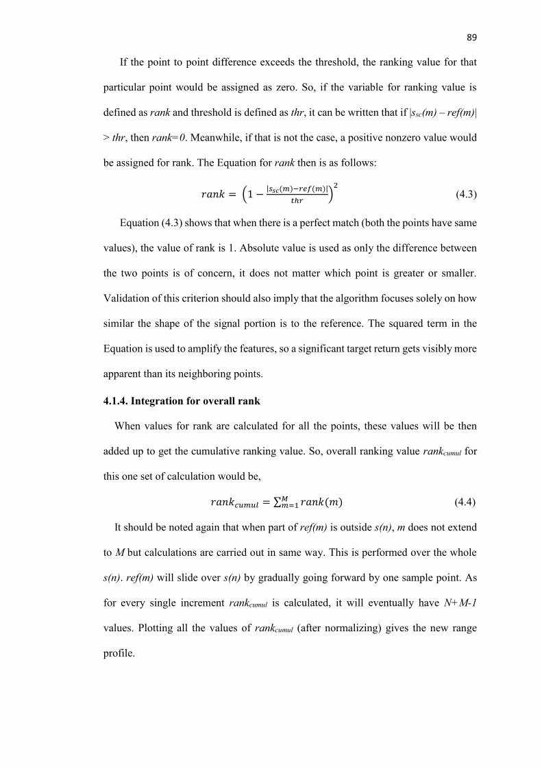
89
If the point to point difference exceeds the threshold, the ranking value for that
particular point would be assigned as zero. So, if the variable for ranking value is
defined as rank and threshold is defined as thr, it can be written that if |ssc(m) – ref(m)|
> thr, then rank=0. Meanwhile, if that is not the case, a positive nonzero value would
be assigned for rank. The Equation for rank then is as follows:
𝑟𝑎𝑛𝑘 = (1 −|𝑠𝑠𝑐(𝑚)−𝑟𝑒𝑓(𝑚)|
𝑡ℎ𝑟)
2
(4.3)
Equation (4.3) shows that when there is a perfect match (both the points have same
values), the value of rank is 1. Absolute value is used as only the difference between
the two points is of concern, it does not matter which point is greater or smaller.
Validation of this criterion should also imply that the algorithm focuses solely on how
similar the shape of the signal portion is to the reference. The squared term in the
Equation is used to amplify the features, so a significant target return gets visibly more
apparent than its neighboring points.
4.1.4. Integration for overall rank
When values for rank are calculated for all the points, these values will be then
added up to get the cumulative ranking value. So, overall ranking value rankcumul for
this one set of calculation would be,
𝑟𝑎𝑛𝑘𝑐𝑢𝑚𝑢𝑙 = ∑ 𝑟𝑎𝑛𝑘(𝑚)𝑀𝑚=1 (4.4)
It should be noted again that when part of ref(m) is outside s(n), m does not extend
to M but calculations are carried out in same way. This is performed over the whole
s(n). ref(m) will slide over s(n) by gradually going forward by one sample point. As
for every single increment rankcumul is calculated, it will eventually have N+M-1
values. Plotting all the values of rankcumul (after normalizing) gives the new range
profile.

90
The shape matching algorithm has been implemented on real Antarctic ice shelf
data for internal layer location. The processed results are shown and discussed in the
next chapter.
4.2 Range Migration Processing in FMCW Phased Array Radar
As discussed in the previous chapter, range migration is a very common feature in
SAR. This is due to the fact that SAR would usually have a very long synthetic
aperture [86]. Methods for range migration correction are therefore an essential part
of SAR research [61] [87]. In SAR, the radar moves along the aperture, so the range
of particular target keeps changing. This creates migration and also Doppler shift.
While processing the SAR image, this is taken into account (as the platform velocity
is known) to create the resultant focused SAR image [88].
Meanwhile, in phased array/MIMO radar, the aperture length is very small
compared to SAR. Also, there is no Doppler shift as the radar is stationary. This is
why the range migration factor is generally neglected. Even though range migration is
usually attributed to radar motion or very long aperture (in case of number of
geophones placed for seismic activity measurement), phased array radar can also face
range migration effect under certain conditions related to radar system parameters.
Here, those conditions will be discussed. Along with that, the compensation process
for range migration in phased array radar system, for instance an FMCW radar with
deramped processing [11], is comprehensively described.
4.2.1. Criterion for significant range migration in phased array radar
A phased array radar system is considered comprising a receive array with N
elements of uniform spacing d arranged on a linear baseline, receiving an echo from
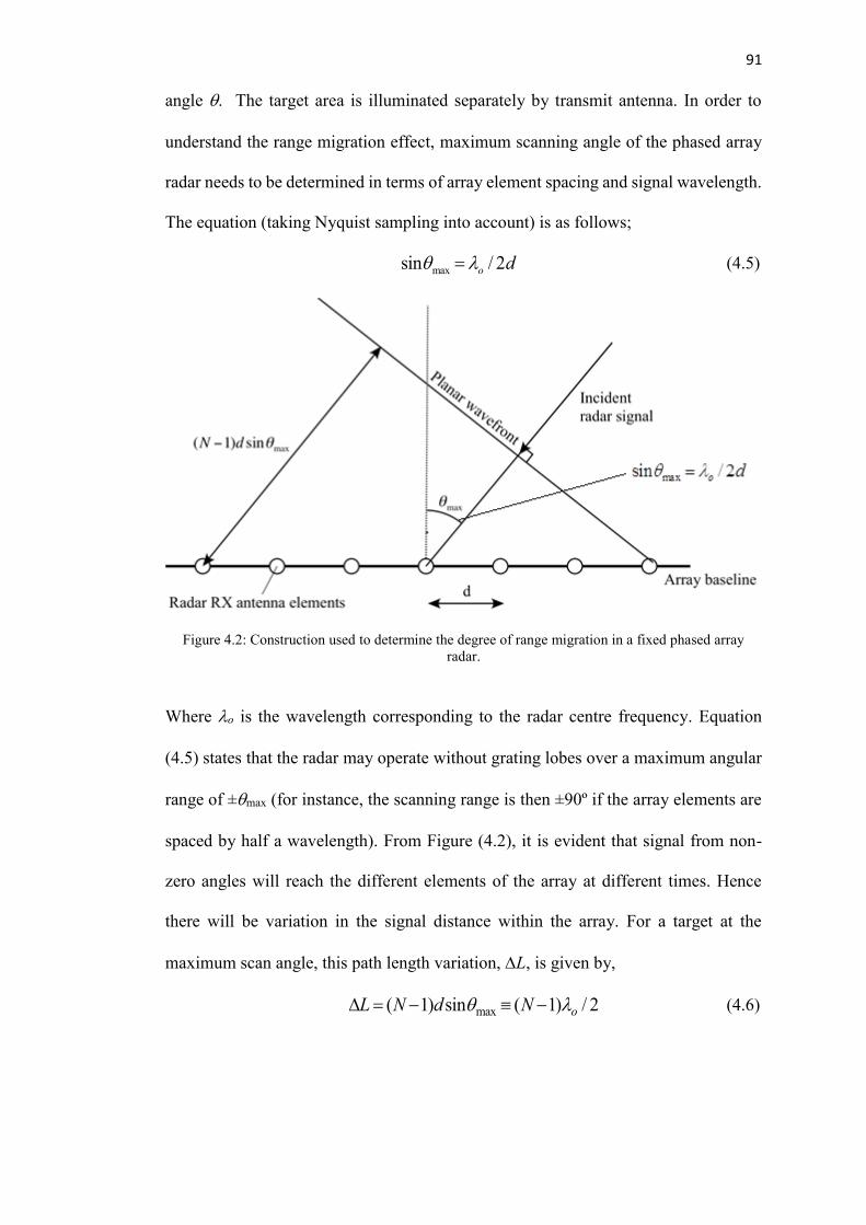
91
angle . The target area is illuminated separately by transmit antenna. In order to
understand the range migration effect, maximum scanning angle of the phased array
radar needs to be determined in terms of array element spacing and signal wavelength.
The equation (taking Nyquist sampling into account) is as follows;
sinqmax = lo / 2d (4.5)
Figure 4.2: Construction used to determine the degree of range migration in a fixed phased array
radar.
Where o is the wavelength corresponding to the radar centre frequency. Equation
(4.5) states that the radar may operate without grating lobes over a maximum angular
range of ±max (for instance, the scanning range is then ±90º if the array elements are
spaced by half a wavelength). From Figure (4.2), it is evident that signal from non-
zero angles will reach the different elements of the array at different times. Hence
there will be variation in the signal distance within the array. For a target at the
maximum scan angle, this path length variation, L, is given by,
DL = (N -1)dsinqmax º (N -1)lo / 2 (4.6)
92
The range migration within the array will be equivalent to this (after compensating for
two-way path). So,
𝑟𝑎𝑛𝑔𝑒_𝑚𝑖𝑔𝑟𝑎𝑡𝑖𝑜𝑛 =±∆𝐿
2= (𝑁 − 1)𝜆𝑜/4 (4.7)
Where the expression for L is valid and accurate considering the target range is much
greater than the array baseline. In cases where this does not apply, the signal distance
variation within the array should be calculated in terms of exact geometry instead of
using a sinmax approximation.
By considering the general radar resolution, R = c/2B, range migration threshold
will be twice R (as explained below).
The limit on array size beyond which range migration is significant may be
established,
bandwidthfractionalB
f
B
cN
BcRN
o
o
o
_
41
41
41 hence,
/24/)1(
max
max
(4.8)
The above Equation determines the criteria of range migration correction for a
particular phased array system. It can be seen that a system with high fractional
bandwidth is prone to suffer from range migration within the array.
This gives a very simple expression to determine whether range migration
processing needs to be applied. It indicates that a phased array radar with a higher
fractional bandwidth and/or a larger number of elements is more likely to require range
migration compensation. For instance, a radar with 20% fractional bandwidth may
have up to 21 elements before range migration will have any effect. On the other hand,
a phased array radar with 50% fractional bandwidth will cross the threshold if element

93
number is more than 9. Equation (4.8) does not have element spacing as a variable
because it has direct correlation to the maximum scan angle.
To justify the assumption of maximum tolerable range migration being twice the
range resolution, a point target response of a linear-FMCW range radar is considered,
[89], with no windowing from a target at range, Ro along the x-axis. This gives the
familiar result, [6], based on a sinc function:
R
RxAV o )(
sinc
(4.9)
Figure 4.3: Illustration of maximum acceptable limit of range migration variation of range resolution,
±ΔR or 2ΔR.
Equation (4.9) implies that the point target response signal amplitude will fluctuate
through the array. This is due to change in range, x. As can be seen from Figure (4.3),
the value is maximum at the array centre of the sinc function and comparatively very
low at the edges.
Therefore, the mean array output can be determined by taking an average across the
array of the sinc function in Equation (4.9). The average is calculated by considering
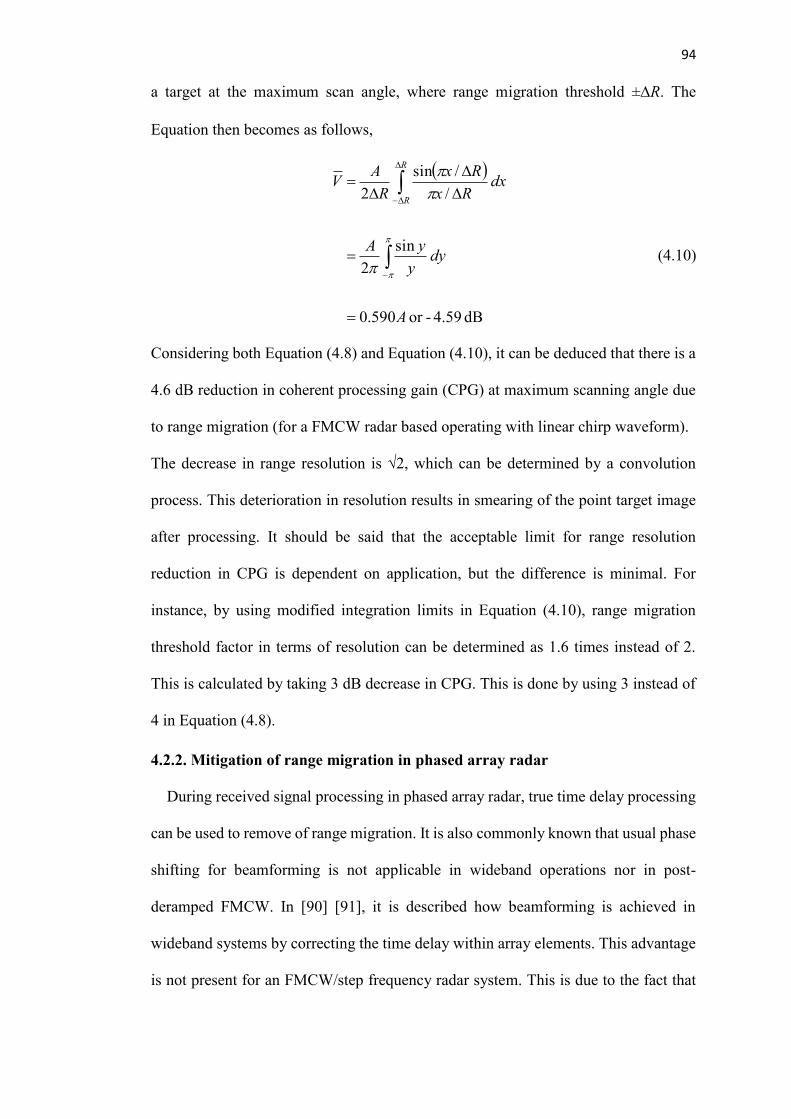
94
a target at the maximum scan angle, where range migration threshold ±R. The
Equation then becomes as follows,
dB 4.59-or 590.0
sin
2
/
/sin
2
A
dyy
yA
dxRx
Rx
R
AV
R
R
(4.10)
Considering both Equation (4.8) and Equation (4.10), it can be deduced that there is a
4.6 dB reduction in coherent processing gain (CPG) at maximum scanning angle due
to range migration (for a FMCW radar based operating with linear chirp waveform).
The decrease in range resolution is √2, which can be determined by a convolution
process. This deterioration in resolution results in smearing of the point target image
after processing. It should be said that the acceptable limit for range resolution
reduction in CPG is dependent on application, but the difference is minimal. For
instance, by using modified integration limits in Equation (4.10), range migration
threshold factor in terms of resolution can be determined as 1.6 times instead of 2.
This is calculated by taking 3 dB decrease in CPG. This is done by using 3 instead of
4 in Equation (4.8).
4.2.2. Mitigation of range migration in phased array radar
During received signal processing in phased array radar, true time delay processing
can be used to remove of range migration. It is also commonly known that usual phase
shifting for beamforming is not applicable in wideband operations nor in post-
deramped FMCW. In [90] [91], it is described how beamforming is achieved in
wideband systems by correcting the time delay within array elements. This advantage
is not present for an FMCW/step frequency radar system. This is due to the fact that

95
the received signals in these systems are mixed with replica chirp to obtain the
deramped signal. As it is known that deramped signal corresponds to frequency shift,
time delay compensation for raw digitized received data cannot be achieved. Hence,
time delay processing is not applicable. Instead, the range migration correction needs
to be implemented by using the frequency shift.
There are number of papers that deal with the range migration correction. In [92],
range migration correction is performed in frequency-wavenumber domain for 2-D
wideband MIMO array where in [93], it is done for FMCW SAR system. In [94], range
migration correction is also performed in frequency-wavenumber domain for ground
penetrating radar system. In this thesis work, the range migration correction process
has been developed for an FMCW/deramped phased array radar system that has been
built for Antarctic Ice Shelf imaging. The radar system has quite large aperture due
to low operating frequency and a wide fractional bandwidth.
For a phased array radar system that exceeds the criterion given in Equation (4.8)
and therefore suffers from significant range migration, the obvious remedy is to re-
align the returns from the elements in order to compensate for their displacement due
to range migration, prior to cross-range processing. This may be achieved by time
delay equalization in many cases, with the necessary delays easily calculated from
basic geometry. From inspection of Figure (4.2), the necessary time delay equalization
can be obtained from Equation (3.12). In the case of an FMCW radar with full-
deramped processing, which is the basis of the experimental system in this thesis work,
the frequencies of the deramped signals will be shifted by range migration and so it
will instead be necessary to re-align the signals in the frequency domain. This may be
affected by frequency-translating the signals from the nth element by the following
amount:

96
∆𝑓 =𝐵
𝑇∆𝜏 =
𝑛𝐵𝑑 sin 𝜃
𝑐𝑇 (4.11)
The FFT resolution and range bin spacing is 1/T (or 1/Tp if zero-padding is used
to increase the sample length by a factor of p) and so it may be convenient to translate
the signals at each element by appropriate increments of 1/Tp, which is effectively
nearest-neighbour interpolation. A pad factor, p, of two or more has been found to
yield good results.
In addition to re-aligning the range profiles derived from elements across the array,
attention must be paid to the relative phases of the signals that have been re-aligned,
which is considered as follows. From Equation (3.4), deramped phase term, which is
compensated by normal phased array processing is:
𝜓 = 𝜔𝑐𝜏 −𝑘𝜏2
2 (4.12)
Equation (3.4) shows that the stationary phase point of the deramped FMCW radar
signal is in the centre of the pulse, at t = T/2, at which point the signal phase is
independent of the sweep parameters. An FFT function would normally indicate the
phase at the beginning of the signal, t = 0, which depends strongly on the sweep
parameters and will vary if the signal is frequency-shifted to achieve re-alignment in
order to mitigate range migration. To consider the degree of phase change as a result
of this re-alignment process, from Equation (3.4) the deramped signal from a given
point target may be represented as a sinusoid within but not necessarily in the centre
of a frequency bin, of frequency nωo + Δω, where ωo is the FFT frequency resolution,
which is equal to 2π/T, with an instantaneous phase as follows,
𝜃𝑑(𝑡) = (𝑛𝜔𝑜 + ∆𝜔)(𝑡 − 𝑇/2) + 𝜓 (4.13)
Where 𝜔𝑜 =2𝜋
𝑇 and |∆𝜔| < 𝜋/𝑇
The FFT (or DFT) term relating to the nth range bin is given by

97
𝐹𝑛(𝑛𝜔𝑜) = ∫ 𝑒(−𝑗𝑛𝜔𝑜𝑡) . 𝑒𝑗(𝑛𝜔𝑜+∆𝜔)(𝑡−𝑇/2) . 𝑒(𝑗𝜓)𝑑𝑡𝑇
0 (4.14)
which reduces to the following expression,
𝐹𝑛(𝑛𝜔𝑜) = 𝑇 𝑒(𝑗𝜓) . 𝑒(−𝑛𝜋) . sinc(∆𝜔𝑇/2) (4.15)
The sinc function factor in this expression is always positive, for |Δω| < 2π/T (a
condition that is easily satisfied), and so this result shows that the phases of the FFT
components obtained from sinusoids in adjacent range bins will alternate. Thus it is
crucial that this phase change is corrected when the signals are translated to effect
range migration mitigation. If zero-padding is used to sinc-interpolate the range profile
by increasing the length of the time-domain sample by a factor of p, then the FFT
resolution will be increased by a factor of p and the phase change between adjacent
range bins will be correspondingly reduced, giving a more general result for the phase
indicated by the nth range bin:
⦟𝐹𝑛(𝑛𝜔𝑜) = 𝜓 −𝑛𝜋
𝑝 (4.15)
Thus, in addition to re-alignment of the signals to mitigate range migration it is
also necessary to correct the phases, in the case of an FMCW radar with full-deramped
processing. As an alternative, from Equation (3.4) it is clear that rotating the time
domain signal by –T/2 prior to taking the FFT will allow the phase reference to be
moved to the centre of the pulse and yield a similar effect. This may be achieved by
applying the standard Matlab FFTshift function.
4.2.3 Simulation results
Simulation was performed to validate the range migration correction. Simulation
parameters were used according to Table 1. It should be noted that the FMCW radar
has a high fractional bandwidth (66.7%). Using Equation (4.8), range migration
processing will be required if the array contains more than 7 elements (which would

98
always be the case during Antarctic experiments). At first, the simulation was
performed for a single point target to demonstrate the effect of range migration
processing. Then, contiguous point targets parallel to the base line were simulated and
imaging results have been shown here. During simulation, 64 elements were used and
target range was 1500 metres.
Figure (4.4) shows the processed point target without applying range migration
correction. It can be seen the image is smeared out (defocused). Figure (4.5) shows
the immediate effect of the correction process as the image is now far better focused.
It should be noted that if the point target is located at normal of the array, then image
will be focused in the first place as no range migration will occur. Figure (4.6) shows
the processed image of point targets with same range but instead of one, number of
closely spaced point targets throughout the scanning angle has been imaged to
simulate a basal layer return from ice shelf. It can be seen that as the scanning angle
increases, the image becomes more defocused. Figure (4.7) shows the same image
after range migration processing but without correcting the phase. It shows even
though signal energies have converged, the overall image still has not been focused
properly due to phases not being properly modified. Figure (4.8) shows the processed
image after fully applying the correction process. Now, the target return looks like a
straight line parallel to array, exactly the way target locations were defined during
simulation.
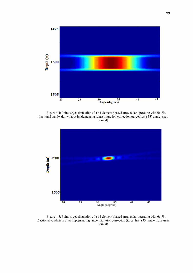
99
Figure 4.4: Point target simulation of a 64 element phased array radar operating with 66.7%
fractional bandwidth without implementing range migration correction (target has a 330 angle array
normal).
Figure 4.5: Point target simulation of a 64 element phased array radar operating with 66.7%
fractional bandwidth after implementing range migration correction (target has a 330 angle from array
normal).
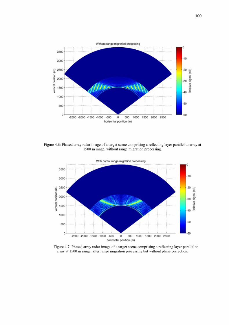
100
Figure 4.6: Phased array radar image of a target scene comprising a reflecting layer parallel to array at
1500 m range, without range migration processing.
Figure 4.7: Phased array radar image of a target scene comprising a reflecting layer parallel to
array at 1500 m range, after range migration processing but without phase correction.

101
Figure 4.8: Phased array radar image of a target scene comprising a reflecting layer parallel to
array at 1500 m range, after range migration processing.
4.3 Vertical Error Correction by Phase Calibration
As mentioned in the previous section, the vertical error in the Antarctic data signal
processing occurs during experiments. An internal layer is hence very useful to resolve
this but there is no guarantee of an internal layer being present all the time. In that
case, some other means is required to correct the error to get a properly focused image.
Radar motion compensation techniques have been well developed in the field of SAR
[95] [96], or in case where Doppler shift is present due to moving target [97]. In this
particular scenario of Antarctic Ice Shelf study, everything (radar and the target) is
assumed to be stationary. So, an appropriate method needed to be developed which
would enable minimization of the effect of vertical antenna displacement. This
correction will also compensate for phase error occurred due to near-field effect, as it
is an exact geometric correction. The main problem is antenna displacement errors
cannot be determined in post processing if there is no reference present. But what can
be done is the vertical displacement can be accommodated into the phased

102
array/MIMO beamforming equation. The previous figure shows the geometry of the
vertical error and simple trigonometry to quantify it. If the vertical displacement is z,
then by recalling Figure (3.5), extra distance travelled by the signal can be calculated
as it is shown in Figure (4.9). It can be seen that the offset distance is zcosθ. The total
extra distance corresponding to phase delay then becomes ndsinθ+zcosθ. So, by
modifying Equation (3.11), the new beamforming equation becomes:
𝐵(𝜃) = ∑ 𝑤𝑛𝑒−𝑗2𝜋(𝑛𝑑 𝑠𝑖𝑛 𝜃+𝑧 cos 𝜃)
𝜆𝑁−1𝑛=0 (4.16)
Figure 4.9: Geometry of vertical displacement of element from the array baseline.
The above figure illustrates the effect of vertical errors. Here, the same simulation
was performed that obtained Figure (4.8), only difference being vertical spacing of the
array elements has been imposed. 36 array elements are used here as that many
elements were used during one of the experiments in Antarctica. The resultant image
is totally defocused as during beamforming, zcosθ has not been taken into account.
So, the signal phases lost coherence.
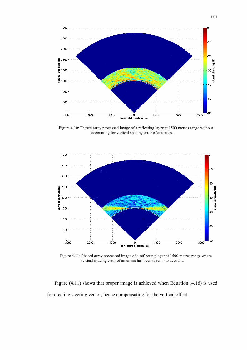
103
Figure 4.10: Phased array processed image of a reflecting layer at 1500 metres range without
accounting for vertical spacing error of antennas.
Figure 4.11: Phased array processed image of a reflecting layer at 1500 metres range where
vertical spacing error of antennas has been taken into account.
Figure (4.11) shows that proper image is achieved when Equation (4.16) is used
for creating steering vector, hence compensating for the vertical offset.
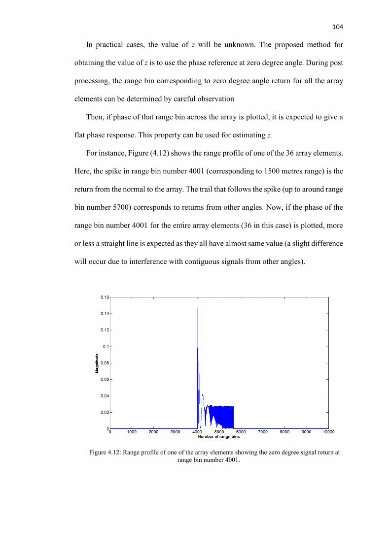
104
In practical cases, the value of z will be unknown. The proposed method for
obtaining the value of z is to use the phase reference at zero degree angle. During post
processing, the range bin corresponding to zero degree angle return for all the array
elements can be determined by careful observation
Then, if phase of that range bin across the array is plotted, it is expected to give a
flat phase response. This property can be used for estimating z.
For instance, Figure (4.12) shows the range profile of one of the 36 array elements.
Here, the spike in range bin number 4001 (corresponding to 1500 metres range) is the
return from the normal to the array. The trail that follows the spike (up to around range
bin number 5700) corresponds to returns from other angles. Now, if the phase of the
range bin number 4001 for the entire array elements (36 in this case) is plotted, more
or less a straight line is expected as they all have almost same value (a slight difference
will occur due to interference with contiguous signals from other angles).
Figure 4.12: Range profile of one of the array elements showing the zero degree signal return at
range bin number 4001.

105
It can be seen that phase is quite constant throughout (varying from only 1.95 to
1.65 radians). If there is any vertical displacement at the antenna elements, this flat
phase response will not be seen. So, observing the phase response for this range bin
somewhat gives an idea about the error.
Figure (4.14) demonstrates exactly that where due to antenna displacement, flat
phase response is lost. The idea for determining z is using this arbitrary phase response
and making it flat (assuming vertical displacement is the only/main cause for the phase
offsets.). During simulation, the first value is taken as reference.
Figure 4.13: Plot of phase response for the zero degree return across the entire array.
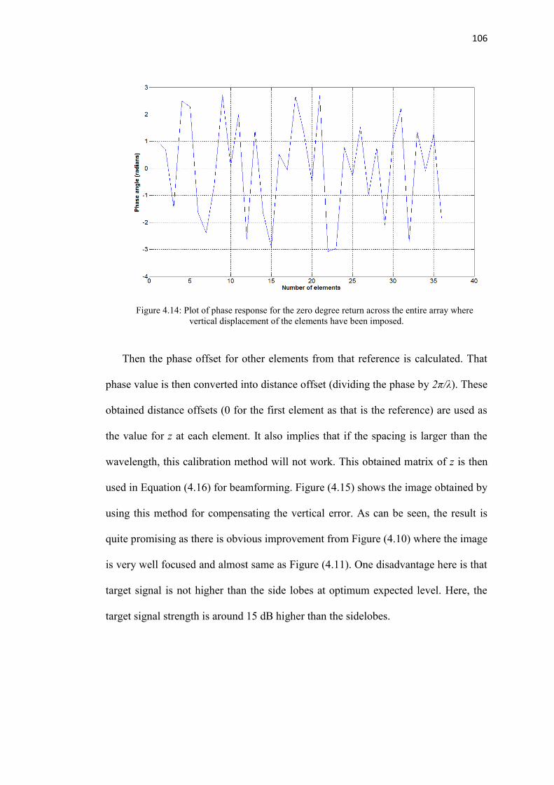
106
Figure 4.14: Plot of phase response for the zero degree return across the entire array where
vertical displacement of the elements have been imposed.
Then the phase offset for other elements from that reference is calculated. That
phase value is then converted into distance offset (dividing the phase by 2π/λ). These
obtained distance offsets (0 for the first element as that is the reference) are used as
the value for z at each element. It also implies that if the spacing is larger than the
wavelength, this calibration method will not work. This obtained matrix of z is then
used in Equation (4.16) for beamforming. Figure (4.15) shows the image obtained by
using this method for compensating the vertical error. As can be seen, the result is
quite promising as there is obvious improvement from Figure (4.10) where the image
is very well focused and almost same as Figure (4.11). One disadvantage here is that
target signal is not higher than the side lobes at optimum expected level. Here, the
target signal strength is around 15 dB higher than the sidelobes.

107
Figure 4.15: Phased array processed image of a reflecting layer at 1500 metres range where
vertical spacing error of antennas has been compensated by phase calibration with reference to zero
degree return.
4.4 3-D MIMO Imaging Algorithm for Ice Shelf Basal Layer
The last signal processing algorithm developed during this thesis work was to create
a 3-D image of basal layer of the Antarctic Ice Shelves. As the previous signal
processing with linear phased array radar gave sectoral plots, 3-D image of the base
would give more opportunity for more in depth analysis of the ice shelves. For this
purpose, an 8x8 MIMO radar with 2-D array has been built at UCL, which have been
deployed in Antarctica. It should be noted that no orthogonal waveform for MIMO
transmission is used in this system (all transmitting antennas emit same waveform).
The spatial diversity is obtained by time switching the antenna elements. New
processing method needed to be developed to create proper 3-D images from the radar
data.

108
There are research articles studying the 3-D MIMO beamforming technique. In
[98], a beamforming equation for 2-D MIMO array has been illustrated. In [99] [100],
3-D imaging techniques have been described by combining MIMO and Synthetic
Aperture Radar (SAR) geometry. In [101], imaging techniques for FMCW MIMO
system have been shown, applicable to conventional two-dimensional imaging. In
[102], a 3-D imaging technique has been described for co-located MIMO radar
configuration. The paper proposes a 3-D imaging technique by taking one snapshot of
a moving target, hence evading the need for motion compensation. But as the focus of
the paper is to image a moving target, beamforming vector corresponds to only one
direction (as opposed to both in azimuth and elevation). For the purpose of Ice Shelf
Imaging, where the signal processing is done solely in terms of receive array, two
dimensional steering vector is required to map the ice shelf base. So, it was necessary
to create an algorithm for the entire 3-D MIMO image processing (based on FMCW
radar receive array and focused on imaging base of ice shelf/sheet), which will include
all the required operations. The steps for 3-D MIMO imaging algorithm developed for
Antarctic Ice Shelf basal layer imaging are as follows:
Range profile for all virtual elements.
Applying 2-D window over the planar array.
3-D Beamforming (by compensating for phase offset at each elements
according to azimuth and elevation angles).
Range Migration compensation (if required).
Selecting the range bin corresponding to zero degree return (using that range
slice throughout the scan for 3-D basal layer imaging).
Compensating for the curvature of the range slice.
109
Image sidelobe suppression by 2-D correlation
The first two steps are quite straightforward, which basically deal with preparing the
raw data before beginning the imaging process. As the algorithm is developed for
FMCW based radar system, range profile should be obtained by simple FFT of the
deramped signals (after applying range window to minimize range sidelobes). Also,
in order to suppress cross range sidelobes, windowing over the arrays should be
performed which is quite usual in phased array/MIMO processing. As the array is
planar, the windowing operation needs to be performed on both axes. For instance, for
an 8x8 array, windowing has to be applied on eight elements of each row as well as
on each column.
4.4.1 3-D Beamforming
The main objective of a beamforming operation is to find out the signal path offset
in each element of the array, for every angle. It is determined with respect to a
reference where the offset is zero. 3-D beamforming process for the imaging here is
the same as described in Chapter 3, only with an added dimension, hence an added
angle (instead of one incident angle, in this case both azimuth and elevation angles
will be taken into account). So, even though the geometry requires a bit more
visualization, the basic idea here for beamforming is the same as it is for a linear array.
Figure (4.16) illustrates a geometrical representation of the 3-D beamforming process.
The red line represents the offset signal distance incident upon X and Y plane
(corresponding to the X and Y axes of the planar array). ‘θ’ and ‘ϕ’ in the above figure
define azimuth and elevation angles respectively. So, the beamforming matrix will
contain a total number of elements equal to the product of azimuth and elevation angle
sample numbers.

110
Figure 4.16: 3-D MIMO beamforming geometry for planar array.
Figure 4.17: Two dimensional representation of the 3-D MIMO beamforming geometry for the
purpose of Pythagorean calculation.

111
In order to determine the value of the signal offset, it will be convenient to draw a two
dimensional representative diagram of the area of interest from Figure (4.16). As it
can be seen in Figure (4.17), the red line corresponds to the same offset signal path
from Figure (4.16). Similarly, the green lines in both figures correspond to same Ysinϕ.
The green line is simply the path offset at Y axis (where azimuth angle is 0 degree).
Now, the signal direction would tilt by θ degree when azimuth angle is present. This
can be visualized from Figure (4.17). The horizontal blue line then would correspond
to X distance. By using Pythagorean geometry, the values of lines can be defined
which would lead to the calculation of the eventual distance required for beamforming
(the red line). Those values are also shown in Figure (4.17). The calculation for
beamforming distance then becomes as follows:
𝐵𝑑(𝜃, ∅) = (𝑋 − 𝑌 sin ∅ tan 𝜃) sin 𝜃 + 𝑌 sin ∅
cos 𝜃
= 𝑋 sin 𝜃 + 𝑌sin ∅
cos 𝜃(1 − sin2 𝜃)
= 𝑋 sin 𝜃 + 𝑌 sin ∅ cos 𝜃 (4.17)
This can be now easily translated into equation for phase compensation during
beamforming, which is as follows,
𝐵(𝜃, ∅) =4𝜋
𝜆(𝑋 sin 𝜃 + 𝑌 sin ∅ cos 𝜃) (4.18)
4π/λ has been used as the distance to phase conversion factor instead of 2π/λ here, due
to two way wave propagation (the beamforming is only performed in receive array).
4.4.2 Range Migration Compensation
The effect of range migration has been discussed earlier in this chapter. Equation
(4.8) gives a proper indication whether a receive array processing would require the
112
migration correction. In order to implement the correction process for planar 2-D
array, array length actually gets reduced. For instance, a 64 element linear array would
have 8 times more length than an 8x8 planar array (considering same element spacing
in both cases), even though in both cases there are there are 64 array elements. So, in
later case, the condition check from equation (4.8) should be performed for 8 elements,
instead of 64.
4.4.3 Selecting the range bin corresponding to zero degree return
In 3-D MIMO imaging, the obtained result would be a three dimensional form of the
usual sectoral image achieved in 2-D phased array/MIMO processing. Imaging the
whole 3-D image in such a way would be inconvenient for visual representation. So,
instead of plotting the image for the entire range limit, single range slice is chosen. A
3-D image of that specific slice is then plotted (in terms of azimuth axis, elevation axis
and signal strength at each point). In case of Antarctic Ice Shelf study, the range slice
is chosen by determining the distance of basal layer from the surface. As the surface
may not be plane (hence the reason for 3-D imaging), a reference point is chosen.
Simplest way to choose the reference range bin is finding the range return from zero
degree angle. During post processing, it is quite easy to find the range bin
corresponding to zero degree return, as the signal strength would be usually quite
higher. This is due to signal attenuation with distance increased and zero degree return
being the closest distance. The corresponding range bin is found the same way it has
been described in section 4.3.
4.4.4 Compensating for the curvature of the range slice
After the selection of the zero degree return range bin, range bins for other angles
corresponding to the same range from the radar need to be identified. The range
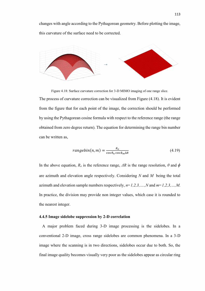
113
changes with angle according to the Pythagorean geometry. Before plotting the image,
this curvature of the surface need to be corrected.
Figure 4.18: Surface curvature correction for 3-D MIMO imaging of one range slice.
The process of curvature correction can be visualized from Figure (4.18). It is evident
from the figure that for each point of the image, the correction should be performed
by using the Pythagorean cosine formula with respect to the reference range (the range
obtained from zero degree return). The equation for determining the range bin number
can be written as,
𝑟𝑎𝑛𝑔𝑒𝑏𝑖𝑛(𝑛, 𝑚) =𝑅𝑜
cos 𝜃𝑛 cos ∅𝑚∆𝑅 (4.19)
In the above equation, Ro is the reference range, ΔR is the range resolution, θ and ϕ
are azimuth and elevation angle respectively. Considering N and M being the total
azimuth and elevation sample numbers respectively, n=1,2,3,….,N and m=1,2,3,…,M.
In practice, the division may provide non integer values, which case it is rounded to
the nearest integer.
4.4.5 Image sidelobe suppression by 2-D correlation
A major problem faced during 3-D image processing is the sidelobes. In a
conventional 2-D image, cross range sidelobes are common phenomena. In a 3-D
image where the scanning is in two directions, sidelobes occur due to both. So, the
final image quality becomes visually very poor as the sidelobes appear as circular ring

114
patterns (as will be shown in simulation results). To minimize that, 2-D correlation is
performed over the image. It is done by taking the maximum value as reference in
each row and column and performing correlation operation on each row and column
with those references.
Figure 4.19: Sample demonstration of 2-D correlation method used for sidelobe suppression in 3-D
MIMO image
Figure (4.19) can be used to visualize the concept being used during reducing the
circular rings from the image. The table corresponds to the image plane where each
block represents a specific azimuth and elevation angle combination. The arbitrary
numbers in the figure represent signal strength corresponding to that block. The blue
box encases the first row in which 3 is the maximum value. That will be taken as a
reference and the correlation would be performed over the entire row (within the blue
box) with respect to the reference. Same thing will be repeated for all the rows. After
that, this correlation process is applied on all the columns using the same method. In
practice, instead of taking one value as reference, several values on both sides of the
maximum value are also included to make a reference for correlation consisting of
more than one sample. Also, due to correlation process, number of samples in each
row and column will increase. To have same number of values in all the rows and all
the columns for processing purpose, interpolation is used to scale that. In real case, the

115
surplus samples are very few in numbers compared to total samples in a row or column
(as the reference signal size is comparatively very small). So, the change in image due
to interpolation is negligible.
4.4.6 Simulation results
In order to verify the image processing method, a simulation has been performed in
MATLAB. The parameters during simulation have been chosen according to the
specification of the 8x8 FMCW based MIMO radar built at UCL. The radar operates
at 300 MHz central frequency with 200 MHz bandwidth. The virtual array spacing is
0.64λ in both axes. For the basic visual understanding of the images, the simulation
has been performed for point targets. Also, from Equation (4.8), it is found that range
migration is not going to have much of an effect on an 8x8 array. So, during simulation
longer array length has been chosen just to validate the need of range migration
correction for 3-D MIMO image processing algorithm.
Figure (4.20) shows the point target image at 1500 metre range and -8 degree angle
from the array normal (both in azimuth and elevation). The scanning is performed for
±25º in both directions. It can be seen that the point target image has wide spreading
due to range migration. In Figure (4.21), the same point target can be seen after
applying the range migration correction.
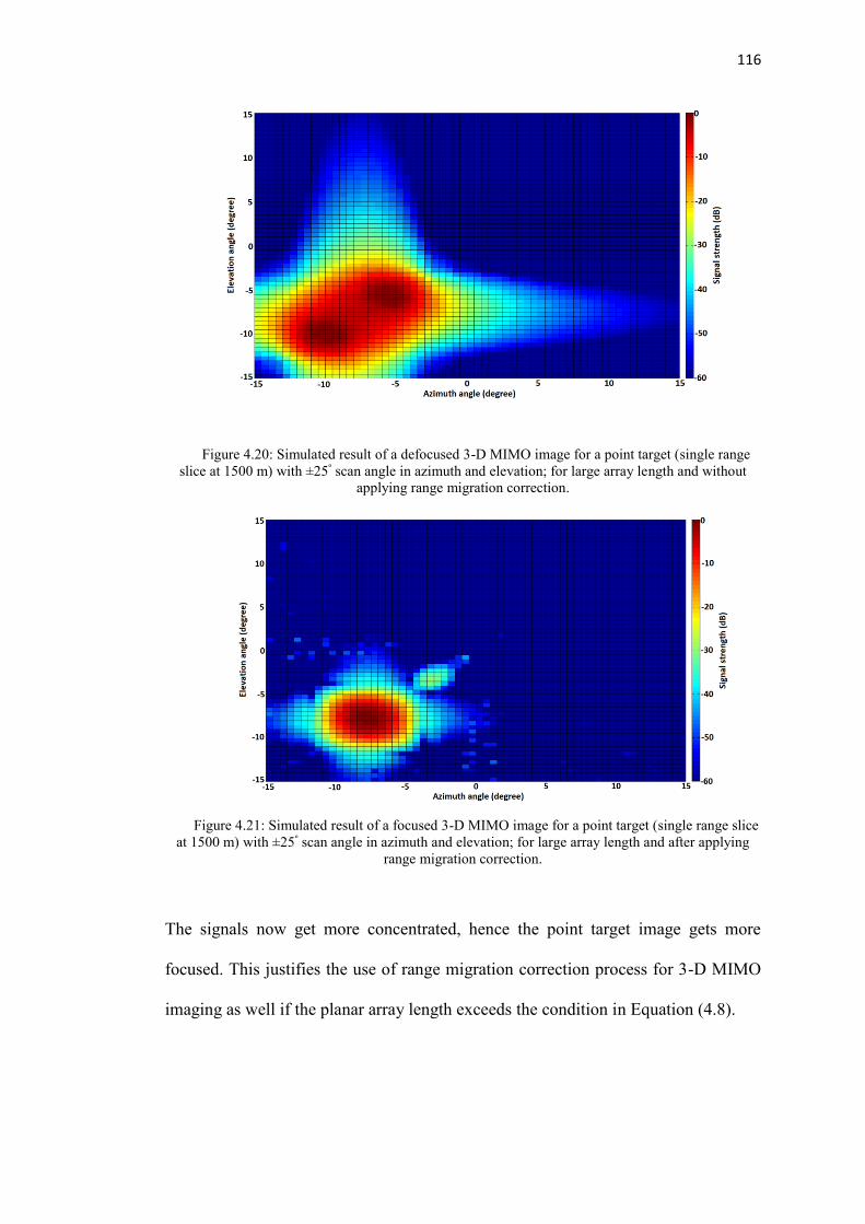
116
Figure 4.20: Simulated result of a defocused 3-D MIMO image for a point target (single range
slice at 1500 m) with ±25º scan angle in azimuth and elevation; for large array length and without
applying range migration correction.
Figure 4.21: Simulated result of a focused 3-D MIMO image for a point target (single range slice
at 1500 m) with ±25º scan angle in azimuth and elevation; for large array length and after applying
range migration correction.
The signals now get more concentrated, hence the point target image gets more
focused. This justifies the use of range migration correction process for 3-D MIMO
imaging as well if the planar array length exceeds the condition in Equation (4.8).
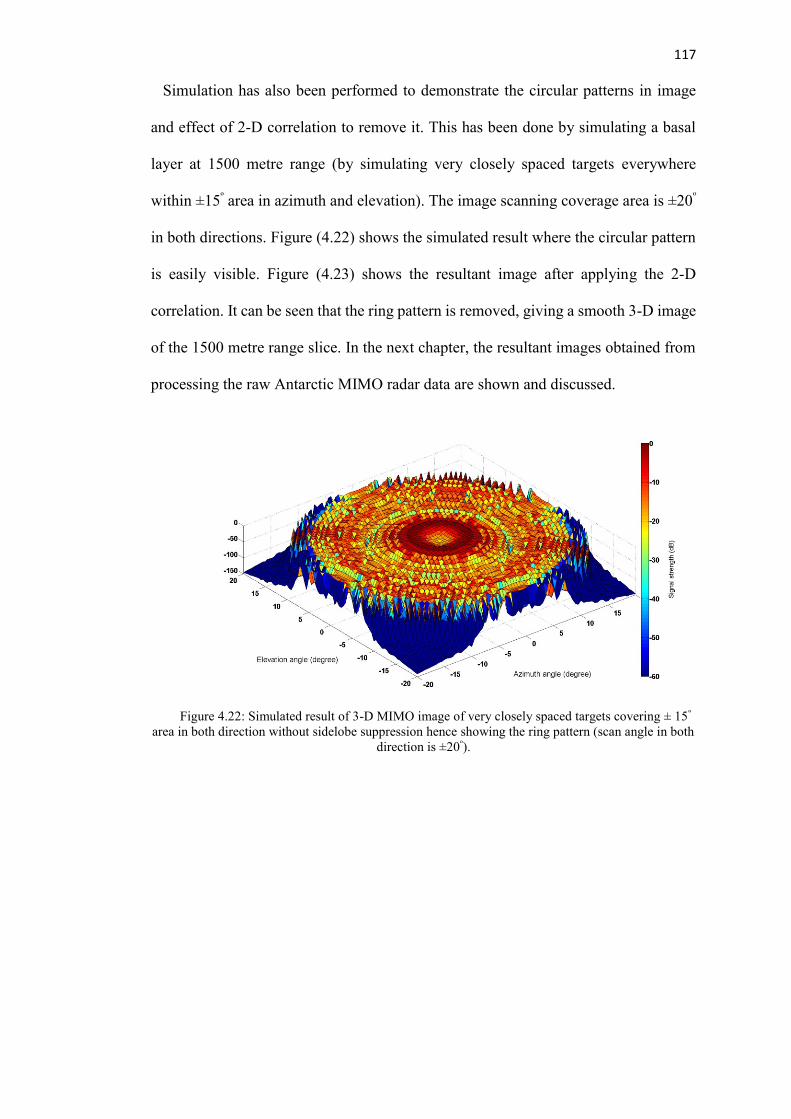
117
Simulation has also been performed to demonstrate the circular patterns in image
and effect of 2-D correlation to remove it. This has been done by simulating a basal
layer at 1500 metre range (by simulating very closely spaced targets everywhere
within ±15º area in azimuth and elevation). The image scanning coverage area is ±20º
in both directions. Figure (4.22) shows the simulated result where the circular pattern
is easily visible. Figure (4.23) shows the resultant image after applying the 2-D
correlation. It can be seen that the ring pattern is removed, giving a smooth 3-D image
of the 1500 metre range slice. In the next chapter, the resultant images obtained from
processing the raw Antarctic MIMO radar data are shown and discussed.
Figure 4.22: Simulated result of 3-D MIMO image of very closely spaced targets covering ± 15º
area in both direction without sidelobe suppression hence showing the ring pattern (scan angle in both
direction is ±20º).

118
Figure 4.23: Simulated result of 3-D MIMO image of very closely spaced targets covering ± 15º
area in both direction after applying hence removing the ring pattern (scan angle in both direction is
±20º).
119
Chapter 5
Processed Results from Antarctic Ice Shelf
Experiments
This chapter demonstrates all the results obtained from processing Antarctic data. The
signal processing techniques that have been discussed in Chapter 3 and 4, have been
applied for real data processing. The data was obtained during field expedition
organized by BAS in Austral summer of 2011-12. During this expedition, BAS
deployed both their pRES system as well as the phase sensitive FMCW radar built at
UCL. The FMCW radar was deployed in Larsen–C, Larsen South, Larsen North and
George VI ice shelves. The pRES system made measurements in Foundation ice
stream of Ronne Ice Shelf. Along with range profiling of the basal layer of these ice
shelves, various imaging experiments were also carried out by constructing the array
geometry. Generally, the radar was mounted on a sledge and then moved around
carefully according to the specific geometry. Also, the radar performance was tested
at UCL to validate radar performance, which is shown here. Finally, the 3-D imaging
results from the Ronne Ice Shelf are also shown. The FMCW based 8x8 MIMO radar
was deployed in the location in 2014-15 Austral summer. The radar was also taken to
Greenland by BAS. Raw data from there has also been processed and the resultant
images have been shown here.
5.1 Loop Test results at UCL
A trial had been conducted at UCL to verify the radar performance with a 240
meter cable (connecting the two endpoints to the transmitter and receiver). The

120
dielectric constant of the cable is 2.1. Phase sensitive FMCW radar signal processing
algorithm [45] was implemented in MATLAB during the thesis to analyze the raw
radar data. The codes were written in such a way so it would be able to segment the
signals from different attenuator settings automatically and process the whole data file
at one go. Figure (5.1) shows the received deramped signals for four different
attenuator settings of the radar (which is to get optimum dynamic range while
acquiring field data). Figure (5.2) shows the range plots.
Figure 5.1: Raw received deramped signals of the FMCW phase sensitive radar with 4 alternating
attenuator settings.
The above figure shows the MATLAB plot of the received signal from the FMCW
radar. It shows 8 chirps (most of the 9th chirp is clipped off). As discussed in Chapter
2, each successive chirps correspond to four different gain values that change
sequentially. The alternating attenuator setting allows to achieve the different gains (4,
16, 28 and 40 dB). The effect of time delay error correction (discussed in Chapter 3)

121
Figure 5.2: Range plots of the 240 meter round trip path through the cable for all 4 gain settings
of the radar, without time error correction (above) and with time error correction (below).

122
can be visualized as the standard deviation decreases when the correction is applied.
Even though the pulse duration is 1s, the radar runs for 1 minute as it switched over
to the 4 attenuator settings. For each attenuator setting, it records 9 pulses as can be
seen from Figure (5.2).
5.2 Range Profiling
The phase sensitive FMCW radar signal processing method described in Chapter
3 has been used for obtaining range profiles of radar. Figure (5.3(a)) shows the range
profile of the Larsen-C ice shelf where the reflection from the basal layer can be seen
at 362 metres. The high amplitude signal observed at close range is mainly due to
antenna direct coupling or other features creating reflections. As can be seen from the
range profile, there is a trail after the sharp peak from the basal layer. This trail
corresponds to the returns coming from the non-zero angles. This trail is desired as it
will provide more information about the basal layer when beamforming is applied. A
shape matching algorithm is used to determine the presence of any feature among this.
But in this case for Larsen-C ice shelf, a presence of an internal layer at around 77
metres is known from previous measurements (information obtained from BAS). So,
the performance of the algorithm can be tested by applying it to the Larsen-C profile
to see if it can detect the internal layer, which is shown later. Figure (5.3(b)) shows
the differential plot of the basal layer and the internal layer over 6 days. The radar took
continuous measurements from 28th November 2011 (10 pm) to 5th December 2011
(4am). The figure contains plots for measured results from all four attenuator settings.
The gap seen in the plot is due to data loss during that period (data logger did not
record any data). Even though there are fluctuations seen on the plot, the overall trend
is clearly downward which infers the melting of the base. The average gives a melting

123
rate of around 3.3 mm/day. It should be considered that the data was collected for six
days and during Austral summer, when melting of the ice shelf base is expected. So,
the melt rate should not be used to calculate the total melting over the year. In order
to do that, the year-long data needs to be processed. Only then the overall melting
pattern of the ice shelf can be properly demonstrated. Figure (5.4) shows a continuous
range plot for a single attenuator. A Total of 130 measurements were taken for 64.5
hours (1 in every 30 minutes). In the middle of the figure, there is an approximately 5
mm instant slump in range. That was due to a cable fault during measurement. The
range return is from 386 metres. It can be seen that there has been a cyclic pattern in
the range plot indicating ice accumulation and melt both occurring during the
measurement period. Figure (5.5) shows range plot of Larsen South Ice Shelf where
495 continuous measurements were taken (1 in every 10 minutes). Within this 82
hours and 20 minutes, 1.6 mm melting is recorded. It should be noted that this is the
first time a phase precision radar system is deployed in this area. So, there is no means
for cross checking the data unless some other researchers take measurement at the
same place at the same time. The confidence on the radar performance is achieved
from the loop test results in the lab as it is not possible to place a known target deep
under the ice shelf. A corner reflector can be used for a ground measurement, but that
will not validate the radar performance underneath the ice shelf due to the dielectric
constant factor. As the main goal is to measure the melt rate, the result should be valid
anyways as long as the offset in measured range (if there is any) is constant. Two
abrupt plunges in the plot are most probably due to wrong data recording of two
samples as those two data points clearly seem to be an anomaly. The data is plotted
for all four attenuator settings.

124
Figure 5.3: (a) Larsen-C range profile showing the ice shelf base at 362 metres (b) Plot of
difference between measured ice shelf base and the internal layer over 6 days.

125
Figure 5.4: George VI Ice Shelf basal layer range (at 386 metres) plot for 130 continuous
measurements, corresponding to 64.5 hours.
Figure 5.5: Larsen Ice Shelf basal layer plot for 495 continuous measurements (1 in every 10
minutes), corresponding to 82 hours and 20 minutes.

126
Figure 5.6: Larsen South Ice Shelf basal layer range (at 361 metres) plot for 495 continuous
measurements (1 in every 10 minutes) after averaging of 9 chirps of each attenuator setting.
Figure (5.6) shows the same plot but with chirp averaging (averaging nine pulses of
each attenuator settings). As it can be seen, no significant difference is observed.
Hence, chirp averaging can be applied during range profiling.
Figure (5.7) shows a range profile of George VI ice shelf (basal layer return from
386 metres) along with the profile after conventional cross correlation is performed
upon it. It can be seen that correlation does not help in terms of clutter/antenna direct
coupling suppression or hidden feature detection. . Figure (5.8) shows the same profile
but this time with shape matching algorithm implemented plot. The improvement can
be very clearly observed. The base now has a very sharp high peak as that was the
main reference (so rank (equation (4.4)) was maximum at that point).

127
Figure 5.7: George VI range profile without cross-correlation (above) and with cross-correlation
(below) having almost no impact.
Figure 5.8: George VI range profile without shape matching algorithm implemented (above) and
with the algorithm implemented (below) reducing the clutter/noise.

128
Figure 5.9: Normal Larsen ice shelf range profile (above) and the same profile after
implementing shape matching algorithm showing a more than 50% match at around 77 metres.
Also, the algorithm successfully suppresses the antenna direct coupling/near surface
clutter that is present throughout first 30 meters or so. However, no hidden feature is
revealed from the plot. The straightforward implication of this is that there is perhaps
no internal layer present in this ice shelf (or at least in the region that was covered by
the antenna beam). Figure (5.9) shows the range profile of the Larsen ice shelf along
with the profile with the shape matching algorithm processing. Along with close range
signal attenuation, at around 77 metres, a feature is detected. As mentioned before, it
is known that an internal layer exists around this region. Without the implementation
of the algorithm, it is almost impossible to detect with just normal range processing.
This justifies the algorithms’ application as the processed result by using the shape
matching algorithm agrees with the previously known result from the Larsen ice shelf.

129
Figure 5.10: Normal Foundation ice stream range profile (above) and the same profile after
implementing shape matching algorithm.
Figure (5.10) demonstrates a similar profile plot, this time for the Foundation ice
stream. The basal layer return is coming from 1285 metres underneath the surface.
Here, the algorithm also suppresses the high amplitude signals, but a feature is
revealed around 23 meter. This internal layer is used for calibrating the radar data for
melt rate measurement.
5.3 Foundation Ice Stream Imaging
For imaging Foundation Ice Stream, pRES radar was used. As mentioned earlier, it
is similar to FMCW radar but during modulation it uses stepped frequency increase
method. The parameters for the pRES system are given in Table 2. The imaging
experiment done in this location was a MIMO experiment. Figure (5.11) shows the

130
MIMO array configuration, which is a 6x6 MIMO creating a 36 element linear virtual
array (virtual array spacing being 0.14 metres).
Table 2: Parameters of pRES radar
Parameters Value
Centre frequency, fc 305 MHz
Step frequency, fstep 32 KHz
Bandwidth, B 160 MHz
Pulse duration, T 1s
Ice dielectric constant, 𝜀𝑟 3.1
Figure 5.11: Foundation Ice Stream imaging experiment setup, comprising six transmitters and
six receivers, creating 36 linear virtual array elements.
Both range migration algorithm (according to equation (4.8), it needs to be
applied) and vertical error correction have been implemented during image
processing. The effects of those on final image are demonstrated here as well. Figure
(5.12) is the log plot of the range profile showing the basal return from 1285 metres.
Phases of the corresponding range bin for all 36 elements (shown in figure (5.13))
have been used for vertical displacement correction. Figure (5.14) shows the processed
MIMO image without any correction. As the virtual array is linear, the processing was
the same as a conventional phased array image processing with ±60 degree scanning.
The basal layer can be seen from the image clearly. There is another return visible at

131
around 70 metres below the layer which is due to reflections from cables that are
feeding the antenna. Figure (5.11) shows the image after applying range migration and
phase correction. Comparing of Figure (5.14) and (5.15) demonstrates the effect of
correction process for image quality improvement. It can be seen that after the
correction process, the basal layer feature is now better defined showing more
consistent intensity across the entire scan. Which means the signal energy has been
more concentrated than it was before. Same conclusion can also be made by observing
the clutter structure. In Figure (5.14), clutter is smeared out where in Figure (5.15), it
is sharper which means energy is not smeared out anymore. As it was discussed in
Chapter 4, image defocusing due to range migration becomes worse as scanning angle
increases. Here in Figure (5.15), it is seen that image is better focused at wider angles
as well where basal layer signal strength is around 15-20 dB higher compared to Figure
(5.14). By observing Figure (5.12), it can be seen that there is another peak beyond 50
m from the basal return. This might suggest that there is a sharp slope present in that
area causing another return, but no such slope is seen on Figure (5.14) and (5.15). This
may be due to the fact that the antenna beam width was not sharp enough, so after
beamforming this physical phenomena could not be observed. It can also be an
artefact, in which case the beamforming will not show any slope which is not present.
Also, the region between the surface and the base is quite plain, suggesting a
homogenous ice structure throughout that area.
During the Foundation Ice Stream expedition, the MIMO experimentation was
performed twice with a six day time gap. Both measurements were made in exactly
the same location. So, phase differential was calculated by measuring the phases of
the two processed images. The idea was to obtain a differential phase interferometry
like information to observe minute changes in the basal layer during that 6 days. Figure
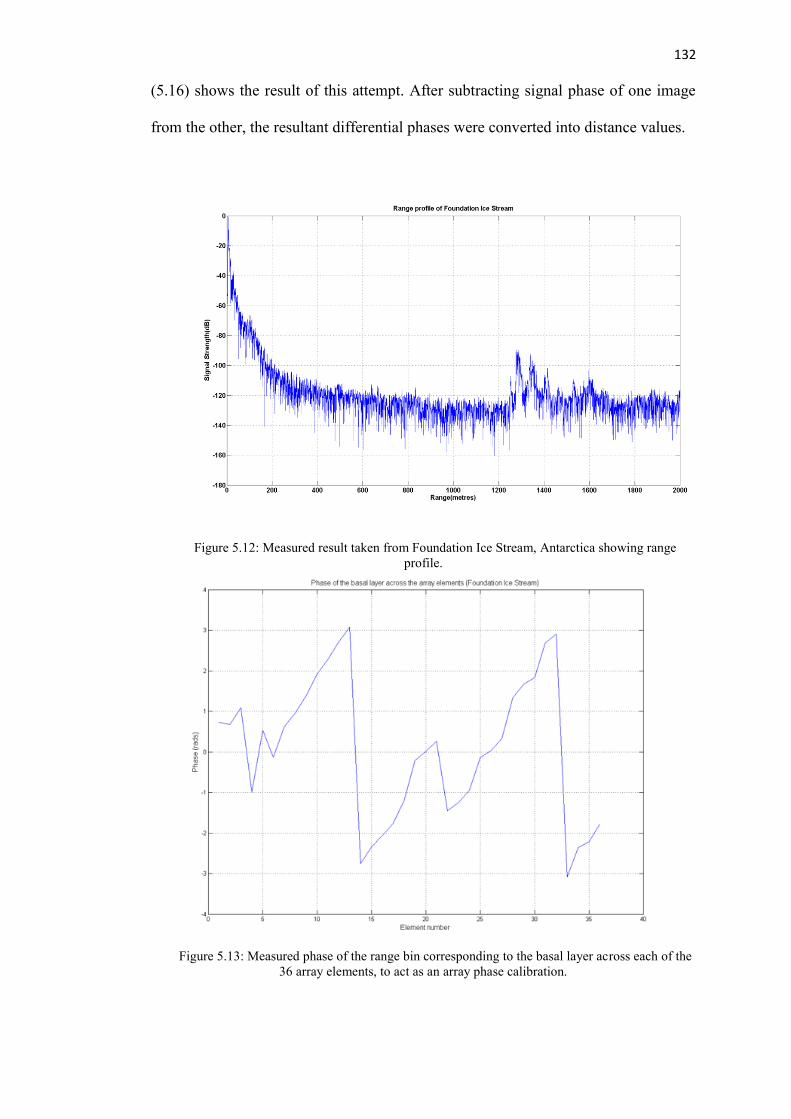
132
(5.16) shows the result of this attempt. After subtracting signal phase of one image
from the other, the resultant differential phases were converted into distance values.
Figure 5.12: Measured result taken from Foundation Ice Stream, Antarctica showing range
profile.
Figure 5.13: Measured phase of the range bin corresponding to the basal layer across each of the
36 array elements, to act as an array phase calibration.

133
Figure 5.14: MIMO image of the Foundation Ice Stream, without range migration processing or
vertical error correction; the basal layer return echo is at 1285 metres.
Figure 5.15: MIMO image of the Foundation Ice Stream, using range migration processing and
phase calibration, showing consistent image intensity at the basal layer and better-defined clutter
structure.
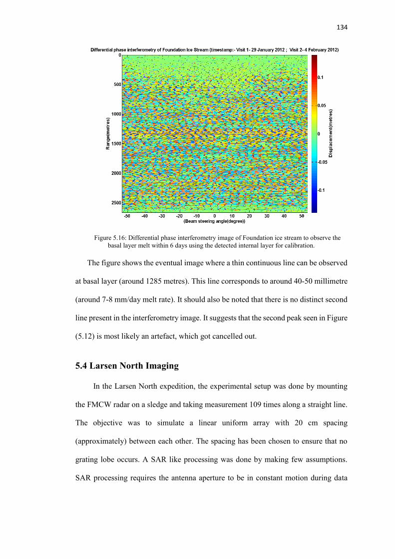
134
Figure 5.16: Differential phase interferometry image of Foundation ice stream to observe the
basal layer melt within 6 days using the detected internal layer for calibration.
The figure shows the eventual image where a thin continuous line can be observed
at basal layer (around 1285 metres). This line corresponds to around 40-50 millimetre
(around 7-8 mm/day melt rate). It should also be noted that there is no distinct second
line present in the interferometry image. It suggests that the second peak seen in Figure
(5.12) is most likely an artefact, which got cancelled out.
5.4 Larsen North Imaging
In the Larsen North expedition, the experimental setup was done by mounting
the FMCW radar on a sledge and taking measurement 109 times along a straight line.
The objective was to simulate a linear uniform array with 20 cm spacing
(approximately) between each other. The spacing has been chosen to ensure that no
grating lobe occurs. A SAR like processing was done by making few assumptions.
SAR processing requires the antenna aperture to be in constant motion during data

135
acquisition. This assumption can be made for the Larsen North processing as well.
The fact that the radar was stationary during each element position can be related to
the usual ‘stop and go’ assumption for the SAR processing. The Range Migration
Algorithm (RMA) for SAR processing discussed in Chapter 3 is quite suitable for this
scenario as it stems from seismic data processing technique [53].
Figure 5.17: SAR processed 2D cross-sectional image of Larsen North ice shelf.
For seismic data processing, some numbers of geophones are placed along a straight
line on the ground and a charge is detonated along that straight line. Every single
geophone uses the received sound echo and the combined results are analyzed to figure
out ground characteristics. This placement of geophones is similar to specific SAR
platform positions at any given instance, as well as the experimental arrangement of
Larsen North.
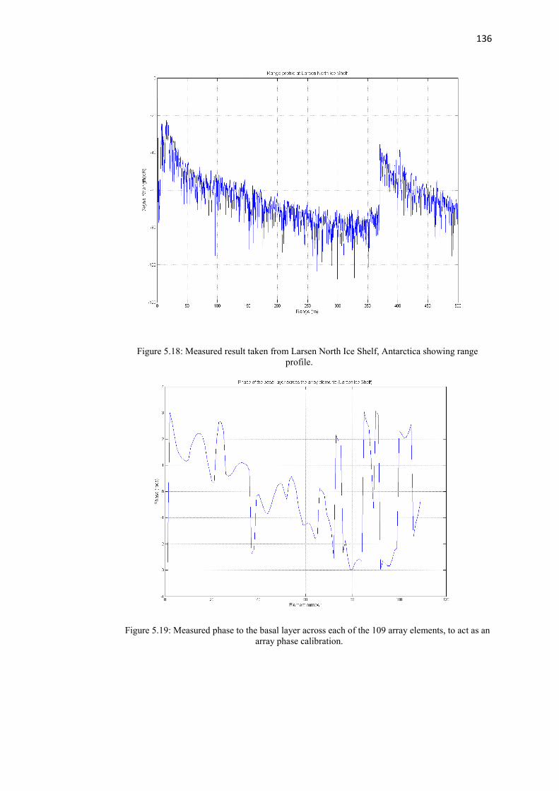
136
Figure 5.18: Measured result taken from Larsen North Ice Shelf, Antarctica showing range
profile.
Figure 5.19: Measured phase to the basal layer across each of the 109 array elements, to act as an
array phase calibration.
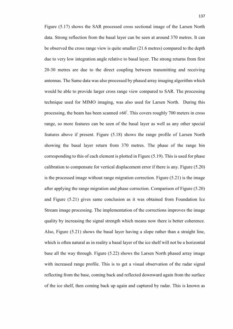
137
Figure (5.17) shows the SAR processed cross sectional image of the Larsen North
data. Strong reflection from the basal layer can be seen at around 370 metres. It can
be observed the cross range view is quite smaller (21.6 metres) compared to the depth
due to very low integration angle relative to basal layer. The strong returns from first
20-30 metres are due to the direct coupling between transmitting and receiving
antennas. The Same data was also processed by phased array imaging algorithm which
would be able to provide larger cross range view compared to SAR. The processing
technique used for MIMO imaging, was also used for Larsen North. During this
processing, the beam has been scanned ±60º. This covers roughly 700 meters in cross
range, so more features can be seen of the basal layer as well as any other special
features above if present. Figure (5.18) shows the range profile of Larsen North
showing the basal layer return from 370 metres. The phase of the range bin
corresponding to this of each element is plotted in Figure (5.19). This is used for phase
calibration to compensate for vertical displacement error if there is any. Figure (5.20)
is the processed image without range migration correction. Figure (5.21) is the image
after applying the range migration and phase correction. Comparison of Figure (5.20)
and Figure (5.21) gives same conclusion as it was obtained from Foundation Ice
Stream image processing. The implementation of the corrections improves the image
quality by increasing the signal strength which means now there is better coherence.
Also, Figure (5.21) shows the basal layer having a slope rather than a straight line,
which is often natural as in reality a basal layer of the ice shelf will not be a horizontal
base all the way through. Figure (5.22) shows the Larsen North phased array image
with increased range profile. This is to get a visual observation of the radar signal
reflecting from the base, coming back and reflected downward again from the surface
of the ice shelf, then coming back up again and captured by radar. This is known as

138
the double bounce affect. As the signal propagates more distance, it gets attenuated
quite a lot through ice, which is evident by the lower signal strength of the double
bounce from the basal return.
Figure 5.20: Phased array image of the Larsen North Ice Shelf, without any correction; the basal
layer return echo is at 370 metres.
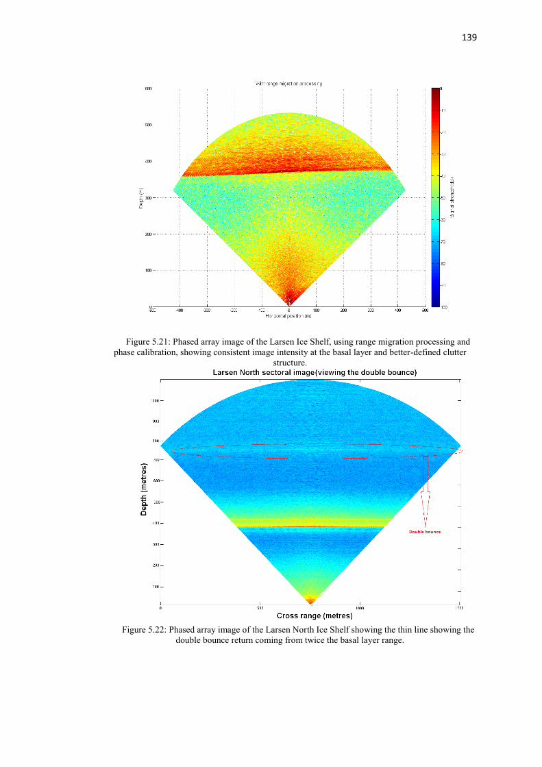
139
Figure 5.21: Phased array image of the Larsen Ice Shelf, using range migration processing and
phase calibration, showing consistent image intensity at the basal layer and better-defined clutter
structure.
Figure 5.22: Phased array image of the Larsen North Ice Shelf showing the thin line showing the
double bounce return coming from twice the basal layer range.

140
5.5 3-D MIMO Imaging of Ice Shelf Base
The 8x8 MIMO radar was deployed in the Ronne Ice Shelf during 2014-15 Austral
summer. The MIMO array configuration can be seen at Figure (5.23). The physical
length of the array is 6.42 x 6.47 metres. The 1.08 m gap between the adjacent
transmitter and the receiver on the top left of the geometry is to get proper antenna
isolation. As trenches were made to mount each antenna element, some were 5 metres
deep and some were 10 metres. This has been taken into account during processing.
The antennas used are bow tie antennas operating at 300 MHz centre frequency with
200 MHz bandwidth. The radar operation is based on FMCW principle where it
transmits up-chirp signals (with time switching) and the receiver outputs deramped
signal after mixing with reference chirp. The radar measurement was taken in two
different sites in Ronne Ice Shelf, as well as in Greenland.
Figure 5.23: Planar MIMO antenna array geometry for 3-D imaging of Antarctic Ice Shelf.

141
Figure (5.24) shows the processed image of the ice shelf base at 566 metres depth.
Range slice corresponding to that depth has been imaged here. Scan angle is ±25º both
in azimuth and elevation. At 566 metres deep, this corresponds to 653.5 x 653.5 square
metres. Array baseline length is not large enough for range migration to take effect, so
no correction has been applied. But the image is processed without 2-D correlation.
The ring patterns in the image are very apparent, which makes it very hard to properly
visualize and analyze the result. Figure (5.25) shows the same image after the
correlation is applied. The significant change in the image quality is easily noticeable.
The curves within the curvature of the basal layer can now be visualized. The image
shows high signal strength in the middle region and reduced signal strength elsewhere,
which is expected as the scanning angle increases. The basal layer is not plain and
regular bumps are observed throughout the scanning area. This suggests that there is
mass imbalance in the ice shelf causing deformation [103]. Mass imbalance occurs
when there is a difference between amount of ice accumulation and ablation, causing
ice flow underneath.
Figure (5.26) illustrates the processed image at a different site in the same ice shelf
without the 2-D correction. Here the basal layer is at 514 metres. The scanning angle
is the same as it was for the previous site, which corresponds to coverage area of 593.5
x 593.5 square metres. Figure (5.27) shows the same image after suppressing the
circular rings. Figure (5.28) and (5.29) shows image processed in same method and
parameters, but with data obtained from Greenland. The basal layer here is at 638
metres, which means the coverage area is approximately 736.72 x 736.72 square
metres. Figure (5.29) shows a very plain basal layer compared to the images from the
Antarctica. This is expected as this is an ice sheet base instead of an ice shelf. Ice
sheets are more stable than ice shelves which melts rapidly compared to an ice sheet.

142
Figure 5.24: 3-D MIMO image of Ronne Ice Shelf (site1) basal layer at 566 metres (without 2-D
correlation).
Figure 5.25: 3-D MIMO image of Ronne Ice Shelf (site1) basal layer at 566 metres (after 2-D
correlation).
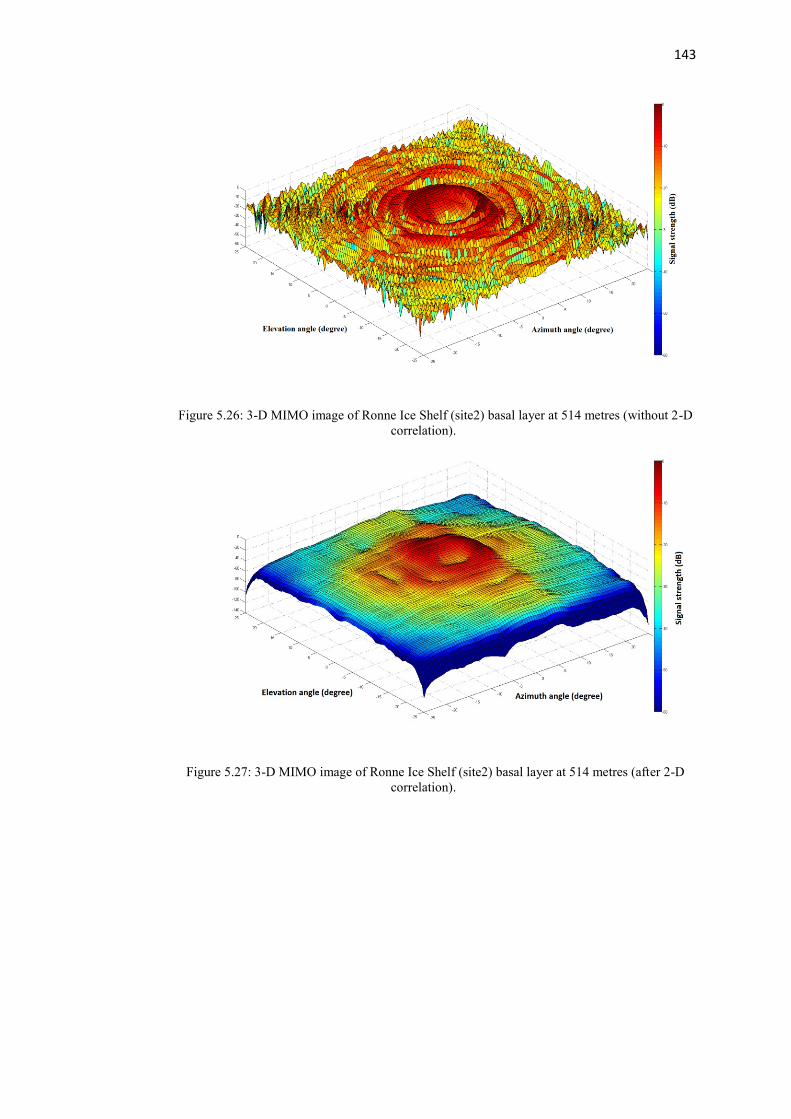
143
Figure 5.26: 3-D MIMO image of Ronne Ice Shelf (site2) basal layer at 514 metres (without 2-D
correlation).
Figure 5.27: 3-D MIMO image of Ronne Ice Shelf (site2) basal layer at 514 metres (after 2-D
correlation).
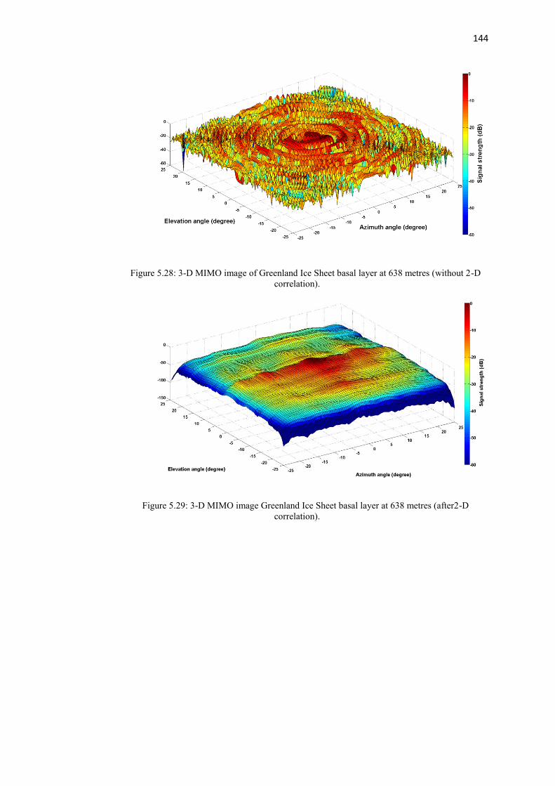
144
Figure 5.28: 3-D MIMO image of Greenland Ice Sheet basal layer at 638 metres (without 2-D
correlation).
Figure 5.29: 3-D MIMO image Greenland Ice Sheet basal layer at 638 metres (after2-D
correlation).
145
Chapter 6
Conclusions and Future Work
6.1 Conclusions
The main goal of the thesis work was to develop novel signal processing algorithms
for phase-sensitive FMCW radar data to profile and image Antarctic Ice Shelves.
Along with developing new processing techniques, conventional processing methods
also had to be learned and used for data processing, which are phased
array/SAR/MIMO imaging and FMCW radar range profiling. The first part of the
thesis encompassed mostly studying and implementing those algorithms on raw radar
data from Antarctica. The algorithms had been implemented in MATLAB in a way
that they would accommodate the nature of the FMCW radar data. While processing
the real data, new signal processing challenges had been faced which motivated to
develop new processing techniques. These techniques had been simulated in terms of
Antarctic ice shelf experiment scenario at first to validate the principle. The results
obtained by processing the Antarctic data have validated the use of developed methods
towards better analysis of the ice shelves.
The list of achievements and advances made over the existing techniques during the
thesis are as follows-
Millimetre precision range profiling of the Antarctic dataset- The phase-sensitive
FMCW radar built for the year-long Antarctic ice shelf monitoring is a novel system.
In [46], FMCW radar has been used for similar purpose but with no phase processing
and with reduced resolution (1 m) compared to the radar built at UCL. In [104] [105],

146
large area of the Antarctic ice shelves have been mapped by using satellite radar
altimeter. The precision achieved from this system is not satisfactory (around 20 cm).
Also, these are pulsed radar systems which are not favourable for high precision
measurement in a lossy medium like ice with low power requirements. Hence, new
signal processing techniques to process the large amount of data at once to obtain the
ice shelf melt rate over a long period was required. The first achievement during this
PhD thesis was the MATLAB code written to process the large dataset from the
Antarctica, which outputs the range profile by calculating the fine range and adding it
with the coarse range, to get the millimetre range precision.
Shape matching algorithm development- Detection of internal layers has been a big
challenge during the monitoring of the Antarctic ice shelves. There is no literature
present which deals with this particular issue. The conventional method for finding
any hidden target is to take some known signal as reference and performing a cross-
correlation along the range profile. Due to the nature of the FMCW radar data, this
conventional method does not work, as in close range antenna direct coupling
produces larger amplitudes than the reference signal. So, to solve this problem, shape
matching algorithm was developed which uses a point by point ranking system instead
of multiplication, so the amplitude does not have any affect. The validation of this
developed algorithm could only be made by applying it on a real data obtained from a
place where there is a presence of a known internal layer. The algorithm was applied
on such dataset from the Larsen ice shelf and was successfully able to detect the
internal layer which was not visible from the normal range profile plot.
Range migration algorithm for FMCW phased array radar- Range migration
problem is not usually faced in a phased array system, but due to the system parameters
of the FMCW radar and the nature of the received data (deramped signal, so time delay

147
beamforming is not possible) for the ice shelf monitoring, this became an issue. The
system operates with a very high fractional bandwidth, so range migration is occurred
when beamforming is applied on the received signal at large angles. New
mathematical concept was developed that shows the relationship between the number
of array elements and the fractional bandwidth. Also, it was mathematically shown
how the range migration compensation relates to the signal phase and how to
compensate for it. This algorithm was applied on the field data from the Antarctica
and it was successfully able to enhance the phased array image quality at wide angles.
Vertical error correction by phase calibration- A very practical consideration in the
Antarctic field test is the adverse weather, which is disadvantageous to precise radar
measurement. As this Antarctic ice shelf monitoring radar system was built for
measuring the melt rate with very high precision, it was a big challenge to compensate
for any experimental errors. The error correction method was developed that would
not require any prior knowledge of the vertical displacements of the antenna. The
method is based on by using phase of the zero degree return from the ice shelf base as
reference. Applying this method compensated for any ambiguity in range calculation.
By doing this, it allowed for the accurate calculation of the ice shelf melt rate and
improved the processed image quality.
3-D MIMO imaging of the ice shelf- A planer array MIMO radar system was
developed at UCL for the 3-D imaging purpose. Considering its application and the
radar system parameter, an entirely new processing technique was required. During
the last period of the thesis, this was achieved. There are 3-D MIMO imaging
techniques developed by other researchers which have been discussed in the previous
chapters, but those are not suitable for this application, where a large area underneath
the ice shelf will be imaged, which would create serious sidelobe issues by

148
conventional processing. So, a step by step method was developed which would take
into account all the factors regarding the radar system parameters and the experimental
scenario. The beamforming technique with the 3-D geometry, range migration
correction requirements, surface curvature correction and sidelobe suppression; all of
these are sequentially applied to obtain the final image. This algorithm was not only
successfully applied on the Antarctic ice shelf data, but also on the Greenland ice sheet
data to visualize the image of the base.
6.2 Future Works
The phase-sensitive radar system requires very rigorous stability in phase. In
practice, it was observed that the temperature variation within the components in the
RF chain has effect on eventual range values.
Figure 6.1: Plot of change in range values with respect to the temperature change in the radar
system
The above figure shows the variation in range values when temperature of the radar
unit is varied. This plot was created by using the data from one of the loop tests with
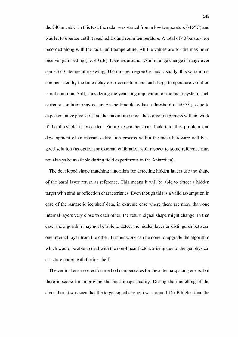
149
the 240 m cable. In this test, the radar was started from a low temperature (-15o C) and
was let to operate until it reached around room temperature. A total of 40 bursts were
recorded along with the radar unit temperature. All the values are for the maximum
receiver gain setting (i.e. 40 dB). It shows around 1.8 mm range change in range over
some 35o C temperature swing, 0.05 mm per degree Celsius. Usually, this variation is
compensated by the time delay error correction and such large temperature variation
is not common. Still, considering the year-long application of the radar system, such
extreme condition may occur. As the time delay has a threshold of ±0.75 μs due to
expected range precision and the maximum range, the correction process will not work
if the threshold is exceeded. Future researchers can look into this problem and
development of an internal calibration process within the radar hardware will be a
good solution (as option for external calibration with respect to some reference may
not always be available during field experiments in the Antarctica).
The developed shape matching algorithm for detecting hidden layers use the shape
of the basal layer return as reference. This means it will be able to detect a hidden
target with similar reflection characteristics. Even though this is a valid assumption in
case of the Antarctic ice shelf data, in extreme case where there are more than one
internal layers very close to each other, the return signal shape might change. In that
case, the algorithm may not be able to detect the hidden layer or distinguish between
one internal layer from the other. Further work can be done to upgrade the algorithm
which would be able to deal with the non-linear factors arising due to the geophysical
structure underneath the ice shelf.
The vertical error correction method compensates for the antenna spacing errors, but
there is scope for improving the final image quality. During the modelling of the
algorithm, it was seen that the target signal strength was around 15 dB higher than the

150
sidelobe. This was good enough during simulation as the modelled basal layer was
clearly visible. Also, it is expected to provide good results in a relatively low noise
scenario which is the case in the Antarctica. Further improvement of the sidelobe can
still be practical, as then it will allow the algorithm to be used in a much noisier
scenario.
In the case of 3-D MIMO imaging, only one range slice was taken as the result was
supposed to be interpreted on a 2-D plane. As the signal processing results contain
images of all range slices, a 3-D interpretation method of the whole set can be
developed. Also, a slice by slice comparison method can be modelled which would
enable to find out about other features (if present) within the ice shelf. In this way,
there is opportunity to study the entire ice shelf from surface to base (the volume
covered by the radar), instead of just the basal layer. By comparing the 3-D data taken
at different time, the characteristics of the ice between the surface and the base can be
better understood. It will provide the geoscientists an improved understanding of the
whole ice shelf underneath the surface. It should be noted that to achieve this, very
large dataset have to be processed. So, the computational load will be quite heavy
which should be taken into account.
Finally, after the successful operation with the prototype system in the Antarctica,
the system has been replicated and number of radars have been placed at various ice
shelves in the Antarctica to obtain data covering the whole year. Processing of a year-
long data will give more in depth knowledge about the melting pattern of the ice
shelves with respect to the seasonal change in the temperature and the ocean current.
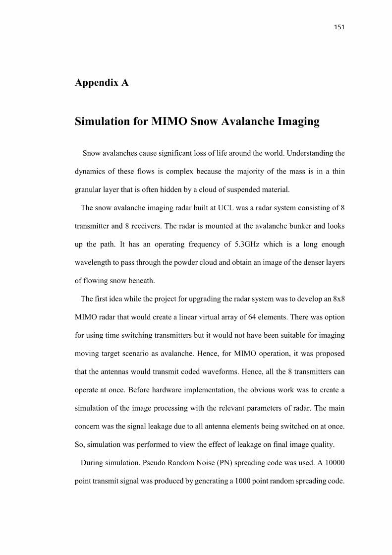
151
Appendix A
Simulation for MIMO Snow Avalanche Imaging
Snow avalanches cause significant loss of life around the world. Understanding the
dynamics of these flows is complex because the majority of the mass is in a thin
granular layer that is often hidden by a cloud of suspended material.
The snow avalanche imaging radar built at UCL was a radar system consisting of 8
transmitter and 8 receivers. The radar is mounted at the avalanche bunker and looks
up the path. It has an operating frequency of 5.3GHz which is a long enough
wavelength to pass through the powder cloud and obtain an image of the denser layers
of flowing snow beneath.
The first idea while the project for upgrading the radar system was to develop an 8x8
MIMO radar that would create a linear virtual array of 64 elements. There was option
for using time switching transmitters but it would not have been suitable for imaging
moving target scenario as avalanche. Hence, for MIMO operation, it was proposed
that the antennas would transmit coded waveforms. Hence, all the 8 transmitters can
operate at once. Before hardware implementation, the obvious work was to create a
simulation of the image processing with the relevant parameters of radar. The main
concern was the signal leakage due to all antenna elements being switched on at once.
So, simulation was performed to view the effect of leakage on final image quality.
During simulation, Pseudo Random Noise (PN) spreading code was used. A 10000
point transmit signal was produced by generating a 1000 point random spreading code.

152
It is basically phase coding as the values were randomly either +1 or -1. Then, this
1000 point code was applied on a sine wave and finally was spread into a 10000 point
coded signal. All the 8 transmitters had unique codes. In receive side, matched filtering
(according to the code) was applied to extract signal for every transmitter receiver
combination.
Figure app.1: Range profile for point target at 1000 metres without any spreading code applied.
Figure app.2: Point target image (at 1000 metres range) of a MIMO radar without any spreading
code applied.
The above two figures demonstrate the results of a point target image without any
spreading code. Basically, there is no leakage between elements. As it can be seen, the
153
target mainlobe is around 70 dB higher than the sidelobe level, indicating very good
image quality.
Figure app.3: Range profile for point target at 1000 metres after applying spreading code.
Figure app.4: Point target image (at 1000 metres range) of a MIMO radar after applying
spreading code.
The above two figures show the effect of using spreading code signal leakage
while all array elements are operating at once. It can be seen from the range profile
that mainlobe is only around 20 dB higher than the sidelobe level and the sidelobe
level throughout the range is quite visible on the resultant image. Even after the
matched filtering, the leakage from the other elements attribute to increased sidelobe
level. It should be noted that this simulation was only performed for a stationary point

154
target. In practical case, the target will be snow avalanche which would be moving
and distributed. So, it was concluded that MIMO radar development with coded signal
transmission may become a big risk for snow avalanche imaging as it takes huge
amount of time and effort to build the hardware. The final decision was to resort to a
conventional phased array radar development.

155
References
[1] http://nsidc.org/cryosphere/quickfacts/iceshelves.html
[2] JENKINS, A., CORR, H.F.J., NICHOLLS, K.W., STWART, C.L., DOAKE,
C.S.M., ‘Interactions between ice and ocean observed with phase-sensitive radar near
an Antarctic ice-shelf grounding line’, Journal of Glaciology, Vol. 52, No. 178, 2006,
pp. 325-346.
[3] CORR, H.F.J., JENKINS, A., NICHOLLS, K.W., DOAKE, C.S.M., ‘Precise
measurement of changes in ice-shelf thickness by phase-sensitive radar to determine
basal melt rates’, Geophysical Research Letters, Vol. 29, No. 8, 1232,
10.1029/2001GL014618, 2002.
[4] http://edatoly.opx.pl/usesof-the-electromagnetic-spectrum.php
[5] Cumming I. G., and Wong F.H., ‘Digital Processing of Synthetic Aperture Radar
Data: Algorithms and Implementation’, Artech House Inc.,Norwood, MA, 2005.
[6] Skolnik, M. (1990), ‘Radar Handbook’, McGraw-Hill.
[7] Skolnik, M. (2001), ‘Introduction to Radar systems’, McGraw-Hill.
[8]Young, C. B., B. R. Nelson, A. A. Bradley, J. A. Smith, C. D. Peters-Lidard, A.
Kruger, and M. L. Baeck (1999), ‘An evaluation of NEXRAD precipitation estimates
in complex terrain’, J. Geophys. Res., 104, 19691–19703.
[9] SAAB, CARABAS Foliage Penetration Radar Brochure.
[10] Caporali, A. (1993), ‘Combined regional geoid determination for the ERS-1 radar
altimeter calibration’, J. Geod., 67, 139–147, DOI:10.1007/BF00806253.
[11] Stove, A. (1992), ‘Linear FMCW radar techniques’, Radar and Signal Processing,
IEE Proceedings F 139(5), 343 –350.
[12] Griffiths, H. (1990), ‘New ideas in FM radar’, Electronics Communication
Engineering Journal 2(5), 185–194.
[13] ‘Warming to Cause Catastrophic Rise in Sea Level?’
http://news.nationalgeographic.com/news/2004/04/0420_040420_earthday.html
[14] Etkins, R., and E.S. Epstein, ‘The Rise of Global Mean Sea Level as an Indication
of Climate Change’, Science, vol. 215, pp. 287-289, 15 January, 1982.
[15] Bogorodsky, V.V., V.I. Pozdnynak, G.V. Trepov, and A.M. Shremetyev, ‘Radar
Sounding Measurements of the Thickness of Annual Snow Strata in the Antarctic,,
Doklady of the Academy of Sciences of the U.S.S.R. Earth science sections, vol. 264,
no. 4, pp. 909-911, 1982.

156
[16] http://nsidc.org/cryosphere/quickfacts/icesheets.html
[17] Peter Kuipers Munneke, Stefan R.m. Ligtenberg, Michael R. Van Den Broeke,
David G. Vaughan, ‘Firn air depletion as a precursor of Antarctic ice-shelf collapse’,
Journal of Glaciology,2014; 60 (220): 205.
[18] Rignot, E., Bamber, J. L., van den Broeke, M. R., Davis, C., Li, Y., Van de Berg,
W. J., van Meijgaard, E. (2008), ‘Recent Antarctic ice mass loss from radar
interferometry and regional climate modelling’, Nature Geoscience, 1(2), 106-110.
[19] Scambos, T. A., Hulbe, C., Fahnestock, M., & Bohlander, J. (2000), ‘The link
between climate warming and break-up of ice shelves in the Antarctic Peninsula’.
Journal of Glaciology, 154), 516-530.
[20] Petri Pellikka, W. Gareth Rees (2009), ’Remote Sensing of Glaciers: Techniques
for Topographic, Spatial and Thematic Mapping of Glaciers’, CRC Press.
[21] Evans, S.1966, ‘Progress report on radio echo sounding’, PolarRec, Vol.13,
No.85, p.413-420.
[22] Gogineni, S., T. Chuah, C. Allen, K. Jezek, and R.K. Moore, “An Improved
Coherent Radar Depth Sounder”, Journal of Glaciology, vol. 44, no. 148, 1998.
[23] Ellerbruch, D.A., and H.S. Boyne, ‘Snow stratigraphy and water equivalence
measured with an active microwave system’, Journal of Glaciology, vol. 26, no. 94,
pp. 225-233, 1980.
[24] Fricker, HA, R Coleman, L Padman, TA Scambos, J Bohlander and KM Brunt
(2009), ‘Mapping the grounding zone of the Amery Ice Shelf, East Antarctica using
InSAR, MODIS and ICESat’, Antarct. Sci. 21 (5) 515-532, issn: 0954-1020, ids:
509RD.
[25] Raup, BH, TA Scambos and T Haran (2005), ‘Topography of streaklines on an
antarctic shelf from photoclinometry applied to a single advanced land imager (ALI)
image’, IEEE Trans. Geosci. Remote Sensing 43 (4) 736-742, issn: 0196-2892, ids:
909TB.
[26] McGrath, D, K Steffen, PR Holland, T Scambos, H Rajaram, W Abdalati and E
Rignot 2014), ‘The structure and effect of suture zones in the Larsen C Ice Shelf,
Antarctica’, J. Geophys.Res.-Earth Surf. 119 (3) 588-602, issn: 2169-9003, ids:
AE9WR.
[27] Scambos, T, HA Fricker, CC Liu, J Bohlander, J Fastook, A Sargent, R Massom
and AM Wu (2009), ‘Ice shelf disintegration by plate bending and hydro-fracture:
Satellite observations and model results of the 2008 Wilkins ice shelf break-ups’,
Earth Planet. Sci. Lett. 280 (4-Jan) 51-60.

157
[28] Marshall, H.P., G. Koh, and R. Forster, ‘Ground-Based FMCW radar
measurements: a summary of the NASA CLPX data’, EOS Trans, AGU, 84(46), Fall
Meet.
[29] Cavalieri, D. J. and A. Ivanoff. 2009. ‘AMSRIce03 Landsat-7 ETM+ Imagery’,
Boulder, Colorado USA: NASA DAAC at the National Snow and Ice Data Center.
[30] Leuschen, C., P. Gogineni, F. Rodriguez-Morales, J. Paden, and C. Allen. 2010,
updated 2013. ‘IceBridge Ku-Band Radar L1B Geolocated Radar Echo Strength
Profiles’, Boulder, Colorado USA: NASA DAAC at the National Snow and Ice Data
Center.
[31] Schutz, B. E., Zwally, H. J., Shuman, C. A., Hancock, D., & DiMarzio, J. P.
(2005). Overview of the ICEsat Mission’, Geophysical Reasearch Letters, 32.
[32] H. Pritchard, R. J. Arthern, D. G. Vaughan, L. A. Edwards, ‘Extensive dynamic
thinning the margins of the Greenland and Antarctic ice sheets’, Nature 461, 971
(2010).
[33] Harry M. Jol, ‘Ground Penetrating Radar: Theory and Applications’, ISBN: 978-
0-444-53348-7.
[34] Moorman BJ, Robinson SD, Burgess MM.2003. ‘Imaging periglacial conditions
with ground-penetrating radar’, Permafrost and Periglacial Processes 14:319–329.
DOI:10.1002/ppp.463.
[35] Daniels DJ (ed.) (2004). ‘Ground Penetrating Radar (2nd Ed.)’, Knoval
(Institution of Engineering and Technology). pp. 1–4. ISBN 978-0-86341-360-5.
[36] Brenner, A.C., R.A. Bindschadler, R.H. Thomas and H.J. Zwally. 1983. ‘Slope-
induced errors in radar altimetry over continental ice sheets’ J. Geophys. Res., 88(C3),
1617–1623.
[37] Kruetzmann, N. C., W. Rack, A. J. McDonald, and S. E. George(2011), ‘Snow
accumulation and compaction derived from GPR data near Ross Island, Antarctica’,
Cryosphere, 391–404, doi:10.5194/tc-5-391-2011.
[38] Delaney, A., S. A. Arcone, A. O’Bannon, and J. Wright (2004), ‘Crevasse
detection with GPR across the Ross Ice Shelf, Antarctica’, paper presented at 10th
International Conference on GPR, Delft, Netherlands, 21–24 June.
[39] Glasser, N., B. Goodsell, L. Copland and W. Lawson. (2006), ‘Debris
characteristics and ice-shelf dynamics in the ablation region of the McMurdo Ice Shelf,
Antarctica’, J. Glaciol., 52 177), 223–234.
[40] Jacobs, S. S., H. H. Hellmer, C. S. M. Doake, A. Jenkins, and R. M. Frolich,
‘Melting of shelves and the mass balance of Antarctica’, J. Glaciol., 38, 375–387,
1992.

158
[41] Foldvik, A., and T. Gammelsrød, ‘Notes on southern ocean hydrography, sea-ice
and bottom water formation’, Palaeogeogr. Paleoclimatol. Palaeoecol. , 67, 3–17,
1998.
[42] Mensa, D. L., ‘High resolution radar cross-section imaging’, Artech House, Inc.,
Norwood, MA, 1991.
[43] Hamran, S. E., and E. Aarholt, ‘Glacier study using wavenumber domain
synthetic aperture radar’, Radio Science, 28, 559–570, 1993.
[44] Walford, M. E. R., P. C. Holdorf, and R. G. Oakberg, ‘Phase-sensitive radio-echo
sounding at the Devon Island Ice Cap’, Canada, J. Glaciol. , 18, 217–229, 1977.
[45] P.V Brennan,, L.Lok., H. Corr, K. Nicholls, ‘Phase-sensitive FMCW radar
imaging system for high precision Antarctic ice shelf profile monitoring (2014)’, IET
Radar, Sonar and Navigation journal. doi:10.1049/iet-rsn.2013.0053.
[46] Cardenas, C.A., Jenett, M., Schunemann, K., Winkelmann, J., ‘Sub-ice
topography in Patriot Hills, West Antarctica: first results of a newly developed high-
resolution FM-CW radar system’, J. Glaciol., 2009,55, pp. 162–166.
[47] D.E. Dudgeon, ‘Fundamentals of Digital Array Processing’, Proc. IEEE, Vol. 65,
pp. 898-904, June 1977.
[48] S. Haykin, ‘Array Signal Processing’(1985), Pretince-Hall Inc.
[49] R. E. Collins and F.J. Zucker (1969), ‘Antenna Theory’, Part I, Mcgraw-Hill.
[50] R. S. Elliott (1981), ‘Antenna Theory and Design’, Pretince-Hall.
[51] A. J. Fenn, D. H. Temme, W. P. Delaney, and W. E. Courtney, ‘The development
of phased-array radar technology’, Lincoln Lab. J. , vol. 12, no. 2, pp. 321–340, 2000.
[52] W H Wee and J B Pendry, ‘Super phase array’, New Journal of Physics 12 (2010).
[53] Swords, Sean S. (1986), ‘Technical History of the Beginnings of Radar’, London:
IEE/Peter Peregrinus. ISBN 0-86341-043-X.
[54] Price, Alfred., ‘Instruments of Darkness: The History of Electronic Warfare’, St
Albans, UK: Granada, 1979. ISBN 0-586-04834-0.
[55] R. J. Maillous, ‘Phased array theory and technology’, Proc. IEEE, vol. 70, pp.
246–291, 1982.
[56] E. Brookner, ‘A review of array radars’, Microwave J. Vol. 24, pp. 25-114,
October 1981.
[57] E. Brookner, ‘Radar of the 80’s and beyond’, IEEE Electro 84, May 1984.

159
[58] Jane's Information Group, ‘AEGIS Weapon System MK-7’, 2001-04-25.
Archived from the original on 2006-07-01.
[59] http://www.noaa.gov/about-noaa.html
[60] R. E. Wallis and S. Cheng, ‘Phased-Array Antenna System for the MESSENGER
Deep Space Mission’, IEEE Aerospace Conference Technical Digest, March 2001.
[61] Cafforio C., Prati C., and Rocca F., ‘SAR data focusing using seismic migration
techniques’, IEEE Transactions on Aerospace and Electronic Systems, Vol. 27, pp.
194–207, Mar. 1991.
[62] Sanz, J.; Prats, P.; Mallorqui, J.J., ‘Platform and mode independent SAR data
processor based on the extended chirp scaling algorithm’, Geoscience and Remote
Sensing Symposium, 2003. IGARSS '03. Proceedings. 2003 IEEE International.
[63] M.I. Pettersson, ‘Detection of moving targets in wideband SAR’, IEEE Trans. on
Aerospace and Electron. Syst., vol. 40, pp. 780-796, July 2004.
[64] Jen King Jao, ‘Theory of SAR imaging of a moving target’, IEEE Trans. on
Geosci. And Remote Sensing ,vol. 39, pp. 1984–1992, Sept. 2001.
[65] V. Vu, T. Sjögren, M. Pettersson, and A. Gustavsson, ‘Definition on SAR image
quality measurements for UWB SAR in Remote Sensing’, Cardiff: SPIE, 2008.
[66] V. T. Vu, T. K Sjögren, and M. I. Pettersson, ‘A comparison between fast
factorized backprojection and frequency-domain algorithms in UWB low frequency
SAR’, Proc. IEEE Internl. Geosci. and Remote Sensing Symp. IGARSS, July 2008.
[67] Carrara W. G., Goodman R. S. and Majewski R. M., `Spotlight synthetic aperture
radar: Signal processing algorithms’, Artech House, Norwood, MA, 1995.
[68] R. H. Stolt., `Migration by Fourier transform’, Geophysics, 43:23-48, 1978.
[69] Bamler, R., 'A Comparison of Range-Doppler And Wavenumber Domain SAR
Focusing Algorithms', IEEE Trans. on Geoscience and Remote Sensing, Special
IGARSS'91.
[70] A. D. Maio and A. Farina, ‘Waveform Diversity: Past, Present, and Future’, A
Lecture Series on Waveform Diversity for Advanced Radar Systems, July 2009.
[71] E. Fishler, A. Haimovich, R. Blum, D. Chizhik, L. Cimini, and R. Valenzuela,
‘MIMO radar: An idea whose time has come’, Proc. IEEE Radar Conf. April 2004,
pp. 71–78.
[72] E. Fishler, A. Haimovich, R. Blum, L. Cimini, D. Chizhik, and R. Valenzuela,
‘Spatial diversity in radars —models and detection performance’, IEEE Trans. Signal
Process.54(3):823–838 (March 2006).

160
[73] I. Bekkerman and J. Tabrikian, ‘Spatially coded signal model for active arrays’,
Proc. 2004 IEEE Int. Conf. Acoustics, Speech, and Signal Processing, Montreal,
Quebec, Canada, March 2004, Vol. 2, pp. ii/209–ii/212.
[74] J. Li and P. Stoica, ‘MIMO radar—diversity means superiority’, in Proceedings
of the 14th Adaptive Sensor Array Processing Workshop (ASAP ’06), Lincoln Lab,
Mass, USA, December 2006.
[75] D. W. Bliss and K. W. Forsythe, ‘Multiple-input multiple-output (MIMO) radar
and imaging: Degrees of freedom and resolution’, Proc. 37th Asilomar Conf. Signals,
Systems and Computers, Pacific Grove, CA, Nov. 2003, Vol. 1, pp. 54–59.
[76] K. W. Forsythe, D. W. Bliss, and G. S. Fawcett, ‘Multiple-input multiple-output
(MIMO) radar: Performance issues’, Proc. 38th Asilomar Conf. Signals, Systems and
Computers, Pacific Grove, CA, Nov. 2004, Vol. 1, pp. 310–315.
[77] L. Xu, J. Li, and P. Stoica, ‘Target detection and parameter estimation for MIMO
radar Systems’, IEEE Trans. Aerospace Electron. Syst. (in press).
[78] L. Xu, J. Li, and P. Stoica, ‘Adaptive techniques for MIMO radar’, Proc. 4th IEEE
Workshop on Sensor Array and Multi-channel Processing, Waltham, MA, July 2006.
[79] Jian Li, Petre Stoica (2008), ‘MIMO Radar Signal Processing’, Wiley-IEEE
Press.
[80] Chun-Yang Chen, ‘Signal processing algorithms for MIMO radar’, Ph.D. thesis,
California Institute of Technology, 2009.
[81] F. C. Robey, S. Coutts, D. Weikle, J. C. McHarg, and K. Cuomo, ‘MIMO Radar
Theory and Experimental Results’, Proc. 38th IEEE Asilomar Conf. on Signals,
Systems, and Computers, vol. 1, pp. 300–304, Nov. 2004.
[82] John W. Clough, ‘Radio echo sounding: reflections from internal layers in ice
sheets’, Journal of Glaciology, Vol. 18, No. 78, 1977.
[83] D. MacDonald, J. Isenman, and J. Roman, ‘Radar detection of hidden targets’,
Proc. IEEE 1997 National Aerospace and Electronics Conf., vol. 2, pp. 846–855, 1997.
[84] Tugac, S. and M. Efe, ‘Radar target detection using hidden Markov models,’
Progress in Electromagnetics Research B, Vol. 44, 241{259, 2012.
[85] D.Kandar et al, ‘Clutter rejection in outdoor radar operation by correlation
method for known target’, Journal of Information Systems and Communication, ISSN:
0976-8742& E-ISSN: 0976-8750, Volume 3, Issue 1, 2012, pp.-332-334.
[86] WANG, J., LIU, X., ‘Automatic correction of range migration in SAR imaging’,
IEEE Geoscience and Remote Sensing Letters, Vol. 7, No. 2, April 2010, pp. 256-260.

161
[87] Munson, D.C., Visentin, R.L.: ‘A signal processing view of strip-mapping
synthetic aperture radar’, IEEE Trans. Acoust. Speech Signal Process., 1989, 37, pp.
2131–2147.
[88] Dewit, J.J.M., Meta, A., Hoogeboom, P.: ‘Modified range-Doppler processing for
FMCW synthetic aperture radar’, IEEE Geosci. Remote Sens. Lett., 2006, 3, (1), pp.
83–87.
[89] Chen, W., Xu, S., Wang, D., Liu, F., ‘Range performance analysis in linear
FMCW radar,, Int. Conf. on Microwave and Millimeterwave Technology,
ICMMT2000, China, 2000, pp. 654–657.
[90] Toughlian, E.N., Zmuda, H., Carter, C.A., ‘True-time-delay transmit/receive
optical beam-forming system for phased arrays and other signal processing
applications’, Proc. SPIE 2155, Optoelectronic Signal Processing for Phased-Array
Antennas IV, 10 June 1994, vol. 181.
[91] Chen, Y., Wu, K., Zhao, F., Chen, R.T., ‘Reconfigurable true-time delay for
wideband phased-array antennas’, Proc. SPIE, 2004, vol. 5363, pp. 125–130.
[92] Zhuge, X., Yarovoy, A.G., ‘Three-dimensional near-field MIMO array imaging
using range migration techniques’, IEEE Trans. Image Process., 2012, 21, (6), pp.
3026–3033.
[93] Xue, G.Y., Yang, J., Liu, P., ‘Modified range migration algorithm integrated with
motion compensation for FMCW SAR’, IET Radar Conf. 2013, 2013, pp. 1–4.
[94] Xu, X., Miller, G.L., ‘Optimization of migration method to locate buried object
in lossy medium’, IEEE Int. Geoscience and Remote Sensing Symp., IGARSS 2002,
2002, vol. 1, pp. 337–339.
[95] J. Kirk, ‘Motion compensation for synthetic aperture radar’, IEEE Trans. Aerosp.
Electron. Syst., vol. 11, no. 3, pp. 338–348, May 1975.
[96] M. Xing, X. Jiang , R. Wu , F. Zhou and Z. Bao, ‘Motion compensation for UAV
SAR based on raw radar data’, IEEE Trans. Geosci. Remote Sens., vol. 47, no.
8, pp.2870 -2883 2009.
[97] B. Liu and W. Chang, ‘Range alignment and motion compensation for missile-
borne frequency stepped chirp radar’, Progr. Electromagn. Res., vol. 136, pp.523 -542
2013.
[98] P. Vaidyanathan, P. Pal, and C. Chen, ‘MIMO Radar with Broadband
Waveforms: Smearing Filter Banks and 2D Virtual Arrays’, in 42nd Asilomar
Conference on Signals, Systems and Computers, pp. 188-192, October 2008.
[99] J. Klare, ‘Digital beamforming for 3D MIMO SAR—Improvements through
frequency and waveform diversity’, Proc. IEEE Geosci. Remote Sens. Symp., pp.V-
17 -V-20 2008

162
[100] C. Ma, T. S. Yeo, C. S. Tan, J.-Y. Li and Y. Shang, ‘Three-dimensional imaging
using colocated MIMO radar and ISAR technique’, IEEE Trans. Geosci. Remote
Sens., vol. 50, no. 8, pp.3189 -3201 2012.
[101] Huang, Y. and P. V. Brennan, ‘FMCW based MIMO imaging radar for maritime
navigation’, Progress In Electromagnetics Research, Vol. 115, 327-342, 2011.
[102] C. Ma , T. S. Yeo , C. S. Tan and Z. Liu, ‘Three-dimensional imaging of targets
using colocated MIMO radar’, IEEE Trans. Geosci. Remote Sens., vol. 49, no.
8, pp.3009 -3021 2011.
[103] Greve, R., Blatter, H (2009), ‘Dynamics of Ice Sheets and Glaciers’, Springer,
DOI: 10.1007/978-3-642-03415-2.
[104] Griggs, J.A., Bamber, J.L, ‘Antarctic ice shelf thickness from satellite radar
altimetry’, J. Glaciol., 2011, 57, (203), pp. 485–498.
[105] Laxon, S., ‘Sea ice extent mapping using the ERS-1 radar altimeter’, EARSeL
Adv. Remote Sens., 1994, 3, (2 – X11), pp. 112–116.
Related Documents