The Annals of Statistics 2002, Vol. 30, No. 4, 962–1030 ANCESTRAL GRAPH MARKOV MODELS 1 BY THOMAS RICHARDSON AND PETER SPIRTES University of Washington and Carnegie Mellon University This paper introduces a class of graphical independence models that is closed under marginalization and conditioning but that contains all DAG independence models. This class of graphs, called maximal ancestral graphs, has two attractive features: there is at most one edge between each pair of vertices; every missing edge corresponds to an independence relation. These features lead to a simple parameterization of the corresponding set of distributions in the Gaussian case. Contents 1. Introduction 2. Basic definitions and concepts 2.1. Independence models 2.2. Mixed graphs 2.3. Paths and edge sequences 2.4. Ancestors and anterior vertices 3. Ancestral graphs 3.1. Definition of an ancestral graph 3.2. Undirected edges in an ancestral graph 3.3. Bidirected edges in an ancestral graph 3.4. The pathwise m-separation criterion 3.5. The augmentation m ∗ -separation criterion 3.6. Equivalence of m-separation and m ∗ -separation 3.7. Maximal ancestral graphs 3.8. Complete ancestral graphs 4. Marginalizing and conditioning 4.1. Marginalizing and conditioning independence models (I[ S L ) 4.2. Marginalizing and conditioning for ancestral graphs 5. Extending an ancestral graph 5.1. Extension of an ancestral graph to a maximal ancestral graph 5.2. Extension of a maximal ancestral graph to a complete graph 6. Canonical directed acyclic graphs 6.1. The canonical DAG D(G) associated with G 6.2. The independence model I m (D(G)[ S D(G) L D(G) ) Received October 2000; revised October 2001. 1 Supported by NSF Grants DMS-99-72008 and DMS-98-73442, the Office of Naval Research, the Isaac Newton Institute, Cambridge, UK and the Environmental Protection Agency. AMS 2000 subject classifications. Primary 62M45, 60K99; secondary 68R10, 68T30. Key words and phrases. Directed acyclic graph, DAG, ancestral graph, marginalizing and con- ditioning, m-separation, path diagram, summary graph, MC-graph, latent variable, data-generating process. 962

Welcome message from author
This document is posted to help you gain knowledge. Please leave a comment to let me know what you think about it! Share it to your friends and learn new things together.
Transcript
The Annals of Statistics2002, Vol. 30, No. 4, 962–1030
ANCESTRAL GRAPH MARKOV MODELS1
BY THOMAS RICHARDSON AND PETER SPIRTES
University of Washington and Carnegie Mellon University
This paper introduces a class of graphical independence models thatis closed under marginalization and conditioning but that contains all DAGindependence models. This class of graphs, called maximal ancestral graphs,has two attractive features: there is at most one edge between each pairof vertices; every missing edge corresponds to an independence relation.These features lead to a simple parameterization of the corresponding setof distributions in the Gaussian case.
Contents
1. Introduction2. Basic definitions and concepts
2.1. Independence models2.2. Mixed graphs2.3. Paths and edge sequences2.4. Ancestors and anterior vertices
3. Ancestral graphs3.1. Definition of an ancestral graph3.2. Undirected edges in an ancestral graph3.3. Bidirected edges in an ancestral graph3.4. The pathwise m-separation criterion3.5. The augmentation m∗-separation criterion3.6. Equivalence of m-separation and m∗-separation3.7. Maximal ancestral graphs3.8. Complete ancestral graphs
4. Marginalizing and conditioning4.1. Marginalizing and conditioning independence models (I[SL)4.2. Marginalizing and conditioning for ancestral graphs
5. Extending an ancestral graph5.1. Extension of an ancestral graph to a maximal ancestral graph5.2. Extension of a maximal ancestral graph to a complete graph
6. Canonical directed acyclic graphs6.1. The canonical DAG D(G) associated with G
6.2. The independence model Im(D(G)[SD(G)
LD(G))
Received October 2000; revised October 2001.1Supported by NSF Grants DMS-99-72008 and DMS-98-73442, the Office of Naval Research,
the Isaac Newton Institute, Cambridge, UK and the Environmental Protection Agency.AMS 2000 subject classifications. Primary 62M45, 60K99; secondary 68R10, 68T30.Key words and phrases. Directed acyclic graph, DAG, ancestral graph, marginalizing and con-
ditioning, m-separation, path diagram, summary graph, MC-graph, latent variable, data-generatingprocess.
962
ANCESTRAL GRAPH MARKOV MODELS 963
7. Probability distributions7.1. Marginalizing and conditioning distributions7.2. The set of distributions obeying an independence model [P (I)]7.3. Relating P (Im(G)) and P (Im(G[SL))7.4. Independence models for ancestral graphs are probabilistic
8. Gaussian parameterization8.1. Parameterization8.2. Gaussian independence models8.3. Equivalence of Gaussian parameterizations and independence models for maxi-
mal ancestral graphs8.4. Gaussian ancestral graph models are curved exponential families8.5. Parameterization via recursive equations with correlated errors8.6. Canonical DAGs do not provide a full parameterization
9. Relation to other work9.1. Summary graphs9.2. MC-graphs9.3. Comparison of approaches9.4. Chain graphs
10. DiscussionAppendix: Definition of a mixed graph
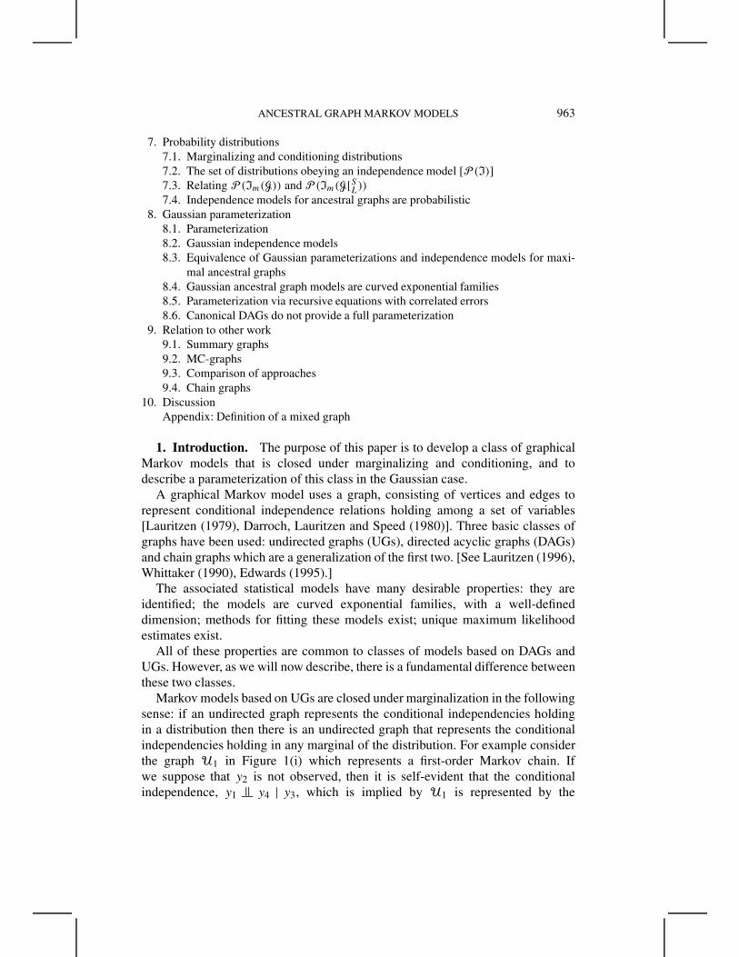
1. Introduction. The purpose of this paper is to develop a class of graphicalMarkov models that is closed under marginalizing and conditioning, and todescribe a parameterization of this class in the Gaussian case.
A graphical Markov model uses a graph, consisting of vertices and edges torepresent conditional independence relations holding among a set of variables[Lauritzen (1979), Darroch, Lauritzen and Speed (1980)]. Three basic classes ofgraphs have been used: undirected graphs (UGs), directed acyclic graphs (DAGs)and chain graphs which are a generalization of the first two. [See Lauritzen (1996),Whittaker (1990), Edwards (1995).]
The associated statistical models have many desirable properties: they areidentified; the models are curved exponential families, with a well-defineddimension; methods for fitting these models exist; unique maximum likelihoodestimates exist.
All of these properties are common to classes of models based on DAGs andUGs. However, as we will now describe, there is a fundamental difference betweenthese two classes.
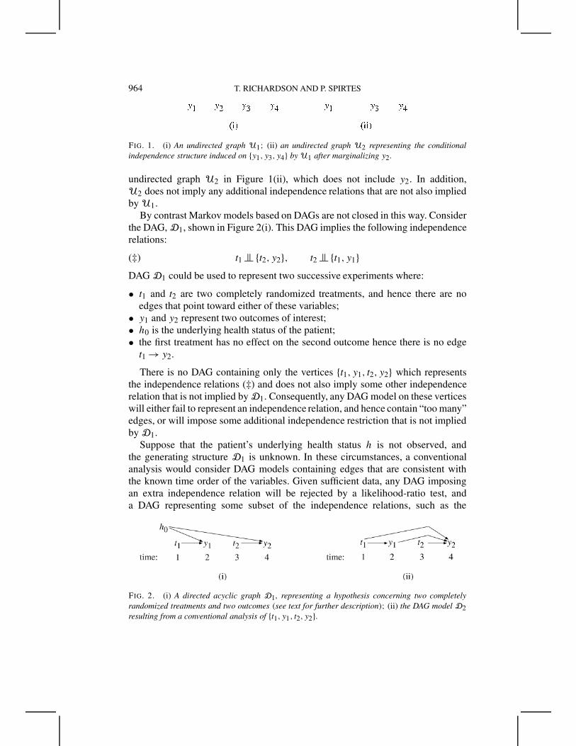
Markov models based on UGs are closed under marginalization in the followingsense: if an undirected graph represents the conditional independencies holdingin a distribution then there is an undirected graph that represents the conditionalindependencies holding in any marginal of the distribution. For example considerthe graph U1 in Figure 1(i) which represents a first-order Markov chain. Ifwe suppose that y2 is not observed, then it is self-evident that the conditionalindependence, y1 |= y4 | y3, which is implied by U1 is represented by the
964 T. RICHARDSON AND P. SPIRTES
FIG. 1. (i) An undirected graph U1; (ii) an undirected graph U2 representing the conditionalindependence structure induced on {y1, y3, y4} by U1 after marginalizing y2.
undirected graph U2 in Figure 1(ii), which does not include y2. In addition,U2 does not imply any additional independence relations that are not also impliedby U1.
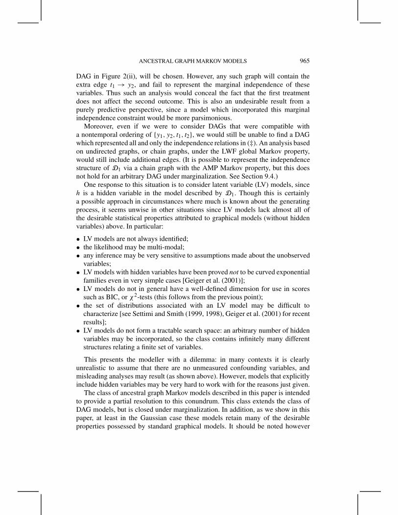
By contrast Markov models based on DAGs are not closed in this way. Considerthe DAG, D1, shown in Figure 2(i). This DAG implies the following independencerelations:
t1 |= {t2, y2}, t2 |= {t1, y1}(‡)
DAG D1 could be used to represent two successive experiments where:
• t1 and t2 are two completely randomized treatments, and hence there are noedges that point toward either of these variables;
• y1 and y2 represent two outcomes of interest;• h0 is the underlying health status of the patient;• the first treatment has no effect on the second outcome hence there is no edge
t1 → y2.
There is no DAG containing only the vertices {t1, y1, t2, y2} which representsthe independence relations (‡) and does not also imply some other independencerelation that is not implied by D1. Consequently, any DAG model on these verticeswill either fail to represent an independence relation, and hence contain “too many”edges, or will impose some additional independence restriction that is not impliedby D1.
Suppose that the patient’s underlying health status h is not observed, andthe generating structure D1 is unknown. In these circumstances, a conventionalanalysis would consider DAG models containing edges that are consistent withthe known time order of the variables. Given sufficient data, any DAG imposingan extra independence relation will be rejected by a likelihood-ratio test, anda DAG representing some subset of the independence relations, such as the
FIG. 2. (i) A directed acyclic graph D1, representing a hypothesis concerning two completelyrandomized treatments and two outcomes (see text for further description); (ii) the DAG model D2resulting from a conventional analysis of {t1, y1, t2, y2}.
ANCESTRAL GRAPH MARKOV MODELS 965
DAG in Figure 2(ii), will be chosen. However, any such graph will contain theextra edge t1 → y2, and fail to represent the marginal independence of thesevariables. Thus such an analysis would conceal the fact that the first treatmentdoes not affect the second outcome. This is also an undesirable result from apurely predictive perspective, since a model which incorporated this marginalindependence constraint would be more parsimonious.
Moreover, even if we were to consider DAGs that were compatible witha nontemporal ordering of {y1, y2, t1, t2}, we would still be unable to find a DAGwhich represented all and only the independence relations in (‡). An analysis basedon undirected graphs, or chain graphs, under the LWF global Markov property,would still include additional edges. (It is possible to represent the independencestructure of D1 via a chain graph with the AMP Markov property, but this doesnot hold for an arbitrary DAG under marginalization. See Section 9.4.)
One response to this situation is to consider latent variable (LV) models, sinceh is a hidden variable in the model described by D1. Though this is certainlya possible approach in circumstances where much is known about the generatingprocess, it seems unwise in other situations since LV models lack almost all ofthe desirable statistical properties attributed to graphical models (without hiddenvariables) above. In particular:
• LV models are not always identified;• the likelihood may be multi-modal;• any inference may be very sensitive to assumptions made about the unobserved
variables;• LV models with hidden variables have been proved not to be curved exponential
families even in very simple cases [Geiger et al. (2001)];• LV models do not in general have a well-defined dimension for use in scores
such as BIC, or χ2-tests (this follows from the previous point);• the set of distributions associated with an LV model may be difficult to
characterize [see Settimi and Smith (1999, 1998), Geiger et al. (2001) for recentresults];
• LV models do not form a tractable search space: an arbitrary number of hiddenvariables may be incorporated, so the class contains infinitely many differentstructures relating a finite set of variables.
This presents the modeller with a dilemma: in many contexts it is clearlyunrealistic to assume that there are no unmeasured confounding variables, andmisleading analyses may result (as shown above). However, models that explicitlyinclude hidden variables may be very hard to work with for the reasons just given.
The class of ancestral graph Markov models described in this paper is intendedto provide a partial resolution to this conundrum. This class extends the class ofDAG models, but is closed under marginalization. In addition, as we show in thispaper, at least in the Gaussian case these models retain many of the desirableproperties possessed by standard graphical models. It should be noted however
966 T. RICHARDSON AND P. SPIRTES
that two different DAG models may lead to the same ancestral graph, so in thissense information is lost.
Up to this point we have considered closure under marginalization. There isa similar notion of closure under conditioning that is motivated by consideringselection effects [see Cox and Wermuth (1996), Cooper (1995)]. UG Markovmodels are closed under conditioning, DAG models are not. The class of Markovmodels described here is also closed under conditioning.
The remainder of the paper is organized as follows:We introduce basic graphical notation and definitions in Section 2. Section 3
introduces the class of ancestral graphs and the associated global Markov property.We also define the subclass of maximal ancestral graphs, which obey a pairwiseMarkov property.
In Section 4 we formally define the operation of marginalizing and conditioningfor independence models, and a corresponding graphical transformation. Theo-rem 4.18 establishes that the independence model associated with the transformedgraph is the same as the model resulting from applying the operations of marginal-izing and conditioning to the independence model given by the original graph. Itis also shown that the graphical transformations commute (Theorem 4.20).
Two extension results are proved in Section 5. First, it is shown that by addingedges a nonmaximal graph may be made maximal and this extension is unique(Theorem 5.1). Second, it is demonstrated that a maximal graph may be madecomplete (so that there is an edge between every pair of vertices) by a sequenceof edge additions that preserve maximality (Theorem 5.6). In Section 6 it isshown that every maximal ancestral graph may be obtained by transforminga DAG, the structure of which bears a simple relation to the original ancestralgraph (Theorem 6.4). Consequently, every independence model associated withan ancestral graph may be obtained by applying the operations of marginalizingand conditioning to some independence model given by a DAG.
Section 7 relates the operations of marginalizing and conditioning that havebeen defined for independence models to probability distributions. Theorem 7.6then shows that the global Markov property for ancestral graphs is complete.
In Section 8 we define a Gaussian parameterization of an ancestral graph. It isshown in Theorem 8.7 that each parameter is either a concentration, a regressioncoefficient, or a residual variance or covariance. Theorem 8.14 establishes that ifthe graph is maximal then the set of Gaussian distributions associated with theparameterization is exactly the set of Gaussian distributions which obey the globalMarkov property for the graph.
Section 9 contrasts the class of ancestral graphs to summary graphs, introducedby Wermuth, Cox and Pearl (1994), and MC-graphs introduced by Koster (1999a).Finally, Section 10 contains a brief discussion.
2. Basic definitions and concepts. In this section we introduce notation andterminology for describing independence models and graphs.
ANCESTRAL GRAPH MARKOV MODELS 967
2.1. Independence models. An independence model I over a set V is a setof triples 〈X,Y | Z〉 where X, Y and Z are disjoint subsets of V ; X and Y arenonempty. The triple 〈X,Y | Z〉 is interpreted as saying that X is independentof Y given Z. In Section 7 we relate this definition to conditional independencein a probability distribution. (As defined here, an “independence model” neednot correspond to the set of independence relations holding in any probabilitydistribution.)
2.1.1. Graphical independence models. A graph G is an ordered pair (V,E)
where V is a set of vertices and E is a set of edges. A separation criterion C
associates an independence model IC(G) with graph G:
〈X,Y | Z〉 ∈ IC(G) ⇐⇒ X is separated from Y by Z in G under criterion C.
Such a criterion C is also referred to as a global Markov property. The d-separationcriterion introduced by Pearl (1988) is an example of such a criterion.
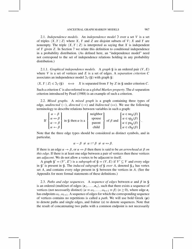
2.2. Mixed graphs. A mixed graph is a graph containing three types ofedge, undirected (−), directed (→) and bidirected (↔). We use the followingterminology to describe relations between variables in such a graph:
If
α − β
α ↔ β
α → β
α ← β
in G then α is a
neighborspouseparentchild
of β and
α ∈ neG(β)
α ∈ spG(β)
α ∈ paG(β)
α ∈ chG(β)
.
Note that the three edge types should be considered as distinct symbols, and inparticular,
α − β �= α � β �= α ↔ β.
If there is an edge α → β , or α ↔ β then there is said to be an arrowhead at β onthis edge. If there is at least one edge between a pair of vertices then these verticesare adjacent. We do not allow a vertex to be adjacent to itself.
A graph G′ = (V ′,E′) is a subgraph of G = (V,E) if V ′ ⊆ V and every edgein G′ is present in G. The induced subgraph of G over A, denoted GA has vertexset A, and contains every edge present in G between the vertices in A. (See theAppendix for more formal statements of these definitions.)
2.3. Paths and edge sequences. A sequence of edges between α and β in Gis an ordered (multi)set of edges 〈ε1, . . . ,εn〉, such that there exists a sequence ofvertices (not necessarily distinct) 〈α ≡ ω1, . . . ,ωn+1 ≡ β〉 (n ≥ 0), where edge εihas endpoints ωi,ωi+1. A sequence of edges for which the corresponding sequenceof vertices contains no repetitions is called a path. We will use bold Greek (µ)to denote paths and single edges, and fraktur (s) to denote sequences. Note thatthe result of concatenating two paths with a common endpoint is not necessarily
968 T. RICHARDSON AND P. SPIRTES
a path, though it is always a sequence. Paths and sequences consisting of a singlevertex, corresponding to a sequence of no edges, are permitted for the purpose ofsimplifying proofs; such paths will be called empty as the set of associated edgesis empty.
We denote a subpath of a path π , by π(ωj ,ωk+1) ≡ 〈εj , . . . ,εk〉, and likewisefor sequences. Unlike a subpath, a subsequence is not uniquely specified by thestart and end vertices, hence the context will also make clear which occurrence ofeach vertex in the sequence is referred to.
We define a path as a sequence of edges rather than vertices because the latterdoes not specify a unique path when there may be two edges between a given pairof vertices. (However, from Section 3 on we will only consider graphs containingat most one edge between each pair of vertices.) A path of the form α → · · · → β ,on which every edge is of the form →, with the arrowheads pointing toward β , isa directed path from α to β .
2.4. Ancestors and anterior vertices. A vertex α is said to be an ancestor ofa vertex β if either there is a directed path α → · · · → β from α to β , or α = β .
A vertex α is said to be anterior to a vertex β if there is a path µ on which everyedge is either of the form γ − δ, or γ → δ with δ between γ and β , or α = β; thatis, there are no edges γ ↔ δ and there are no edges γ ← δ pointing toward α. Sucha path is said to be an anterior path from α to β .
We apply these definitions disjunctively to sets:
an(X) = {α | α is an ancestor of β for some β ∈ X};ant(X) = {α | α is anterior to β for some β ∈ X}.
Our usage of the terms “ancestor” and “anterior” differs from Lauritzen (1996),but follows Frydenberg (1990a).
PROPOSITION 2.1. In a mixed graph G,
(i) if X ⊆ Y then ant(X) ⊆ ant(Y ) and an(X) ⊆ an(Y );(ii) X ⊆ ant(X) = ant(ant(X)) and X ⊆ an(X) = an(an(X));
(iii) ant(X ∪ Y ) = ant(X) ∪ ant(Y ) and an(X ∪ Y ) = an(X) ∪ an(Y ).
PROOF. These properties follow directly from the definitions of an(·) andant(·). �
PROPOSITION 2.2. If X and Y are disjoint sets of vertices in a mixed graph Gthen:
(i) ant(ant(X) \ Y ) = ant(X);(ii) an(an(X) \ Y ) = an(X).
ANCESTRAL GRAPH MARKOV MODELS 969
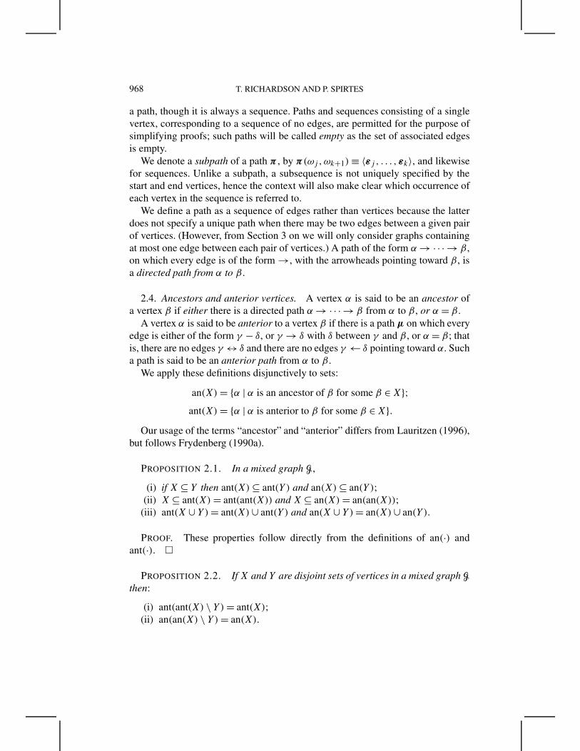
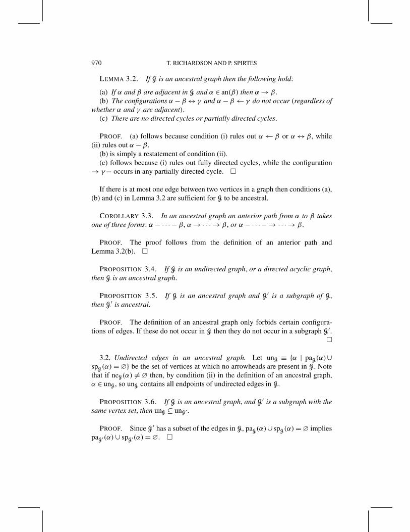
FIG. 3. (a) Mixed graphs that are not ancestral; (b) ancestral mixed graphs.
PROOF. (i) Since X and Y are disjoint, X ⊆ ant(X)\Y . By Proposition 2.1(i),ant(X) ⊆ ant(ant(X) \ Y ). Conversely, ant(X) \ Y ⊆ ant(X) so ant(ant(X) \ Y ) ⊆ant(ant(X)) = ant(X), by Proposition 2.1(i) and (ii).
The proof of (ii) is very similar. �
A directed path from α to β together with an edge β → α is called a (fully)directed cycle. An anterior path from α to β together with an edge β → α is calleda partially directed cycle. A directed acyclic graph (DAG) is a mixed graph inwhich all edges are directed, and there are no directed cycles.
3. Ancestral graphs. The class of mixed graphs is much larger than requiredfor our purposes, in particular, under natural separation criteria, it includesindependence models that do not correspond to DAG models under marginalizingand conditioning. We now introduce the subclass of ancestral graphs.
3.1. Definition of an ancestral graph. An ancestral graph G is a mixed graphin which the following conditions hold for all vertices α in G:
(i) α /∈ ant(pa(α) ∪ sp(α));(ii) if ne(α) �= ∅ then pa(α) ∪ sp(α) = ∅.
In words, condition (i) requires that if α and β are joined by an edge with anarrowhead at α, then α is not anterior to β . Condition (ii) requires that there beno arrowheads present at a vertex which is an endpoint of an undirected edge.Condition (i) implies that if α and β are joined by an edge with an arrowhead at α,then α is not an ancestor of β . This is the motivation for terming such graphs“ancestral.” (See also Corollary 3.10.) Examples of ancestral and nonancestralmixed graphs are shown in Figure 3.
LEMMA 3.1. In an ancestral graph for every vertex α the sets ne(α), pa(α),ch(α) and sp(α) are disjoint, thus there is at most one edge between any pair ofvertices.
PROOF. ne(α), pa(α) and ch(α) are disjoint by condition (i). ne(α)∩sp(α) = ∅ by (ii) since at most one of these sets is nonempty. Finally (i) impliesthat sp(α) ∩ pa(α) ⊆ sp(α) ∩ ant(α) = ∅, and likewise sp(α) ∩ ch(α) = ∅. �
970 T. RICHARDSON AND P. SPIRTES
LEMMA 3.2. If G is an ancestral graph then the following hold:
(a) If α and β are adjacent in G and α ∈ an(β) then α → β .(b) The configurations α − β ↔ γ and α − β ← γ do not occur (regardless of
whether α and γ are adjacent).(c) There are no directed cycles or partially directed cycles.
PROOF. (a) follows because condition (i) rules out α ← β or α ↔ β , while(ii) rules out α − β .
(b) is simply a restatement of condition (ii).(c) follows because (i) rules out fully directed cycles, while the configuration
→ γ− occurs in any partially directed cycle. �
If there is at most one edge between two vertices in a graph then conditions (a),(b) and (c) in Lemma 3.2 are sufficient for G to be ancestral.
COROLLARY 3.3. In an ancestral graph an anterior path from α to β takesone of three forms: α − · · · − β , α → · · · → β , or α − · · · − → · · · → β .
PROOF. The proof follows from the definition of an anterior path andLemma 3.2(b). �
PROPOSITION 3.4. If G is an undirected graph, or a directed acyclic graph,then G is an ancestral graph.
PROPOSITION 3.5. If G is an ancestral graph and G′ is a subgraph of G,then G′ is ancestral.
PROOF. The definition of an ancestral graph only forbids certain configura-tions of edges. If these do not occur in G then they do not occur in a subgraph G′.
�
3.2. Undirected edges in an ancestral graph. Let unG ≡ {α | paG(α)∪spG(α) = ∅} be the set of vertices at which no arrowheads are present in G. Notethat if neG(α) �= ∅ then, by condition (ii) in the definition of an ancestral graph,α ∈ unG, so unG contains all endpoints of undirected edges in G.
PROPOSITION 3.6. If G is an ancestral graph, and G′ is a subgraph with thesame vertex set, then unG ⊆ unG′ .
PROOF. Since G′ has a subset of the edges in G, paG(α)∪ spG(α) = ∅ impliespaG′(α) ∪ spG′(α) = ∅. �
ANCESTRAL GRAPH MARKOV MODELS 971
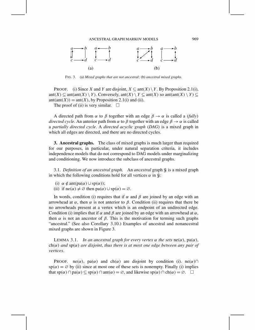
FIG. 4. Schematic showing decomposition of an ancestral graph into an undirected graph anda graph containing no undirected edges.
LEMMA 3.7. If G is an ancestral graph with the vertex set V ,
and
α ↔ β
α − β
α → β
in G then
α,β ∈ V \ unG
α,β ∈ unG
β ∈ V \ unG
.
PROOF. The proof follows directly from the definition of unG and Lem-ma 3.2(b). �
Lemma 3.7 shows that any ancestral graph can be split into an undirectedgraph GunG , and an ancestral graph containing no undirected edges GV \unG ; anyedge between a vertex α ∈ unG and a vertex β ∈ V \ unG takes the form α → β .See Figure 4. This result is useful in developing parameterizations for the resultingindependence models (see Section 8).
LEMMA 3.8. For an ancestral graph G,
(i) if α ∈ unG then β ∈ antG(α) ⇒ α ∈ antG(β);(ii) if α and β are such that α �= β , α ∈ antG(β) and β ∈ antG(α) then
α,β ∈ unG, and there is a path joining α and β on which every edge is undirected;(iii) antG(α) \ anG(α) ⊆ unG.
PROOF. (i) follows from Lemma 3.2(b) and Corollary 3.3. (ii) follows sinceby Lemma 3.2(c) there are no partially directed cycles and thus the anterior pathsbetween α and β consist only of undirected edges, so α,β ∈ unG by Lemma 3.7.(iii) follows because if a vertex β is anterior to α, but not an ancestor of α, thenby Corollary 3.3 any anterior path starts with an undirected edge, and the resultfollows from Lemma 3.7. �
LEMMA 3.9. If G is an ancestral graph, and α, β are adjacent vertices in Gthen:
(i) α − β ⇔ α ∈ antG(β), β ∈ antG(α);(ii) α → β ⇔ α ∈ antG(β), β /∈ antG(α);
(iii) α ↔ β ⇔ α /∈ antG(β), β /∈ antG(α).

972 T. RICHARDSON AND P. SPIRTES
FIG. 5. Two pairs of graphs that share the same adjacencies and anterior relations betweenadjacent vertices, and yet are not equivalent.
PROOF. (i)(⇒) follows by the definition of anterior; (i)(⇐) by Lemma 3.8(ii)and Lemma 3.2(b). Claim (ii)(⇒) follows by the definition of anterior andproperty (i) of an ancestral graph; (ii)(⇐) follows because from Lemma 3.8(i),β /∈ unG, and so by Lemma 3.7 and property (i) of an ancestral graph, α → β .(iii)(⇒) follows by property (i) of an ancestral graph. (iii)(⇐) follows by definitionof anterior. �
A direct consequence of Lemma 3.9 is that an ancestral graph is uniquelydetermined by its adjacencies (or “skeleton”) and anterior relations. Moreformally:
COROLLARY 3.10. If G1 and G2 are two ancestral graphs with the samevertex set V , and adjacencies, then if ∀α,β ∈ V , adjacent in G1 and G2,
α ∈ antG1(β) ⇐⇒ α ∈ antG2(β)
then G1 = G2.
PROOF. The proof follows directly from Lemma 3.9. �
Note that this does not hold in general for nonancestral graphs. See Figure 5 foran example.
3.3. Bidirected edges in an ancestral graph. The following lemma showsthat the ancestor relation induces a partial ordering on the bidirected edges in anancestral graph.
LEMMA 3.11. Let G be an ancestral graph. The relation ≺ defined by
α ↔ β ≺ γ ↔ δ if α,β ∈ an({γ, δ}) and {α,β} �= {γ, δ}defines a strict (irreflexive) partial order on the bidirected edges in G.
PROOF. Transitivity of the relation ≺ follows directly from transitivity of theancestor relation. Suppose for a contradiction that α ↔ β ≺ γ ↔ δ ≺ α ↔ β , but{α,β} �= {γ, δ}. Either α /∈ {γ, δ} or β /∈ {γ, δ}. Without loss of generality, suppose
ANCESTRAL GRAPH MARKOV MODELS 973
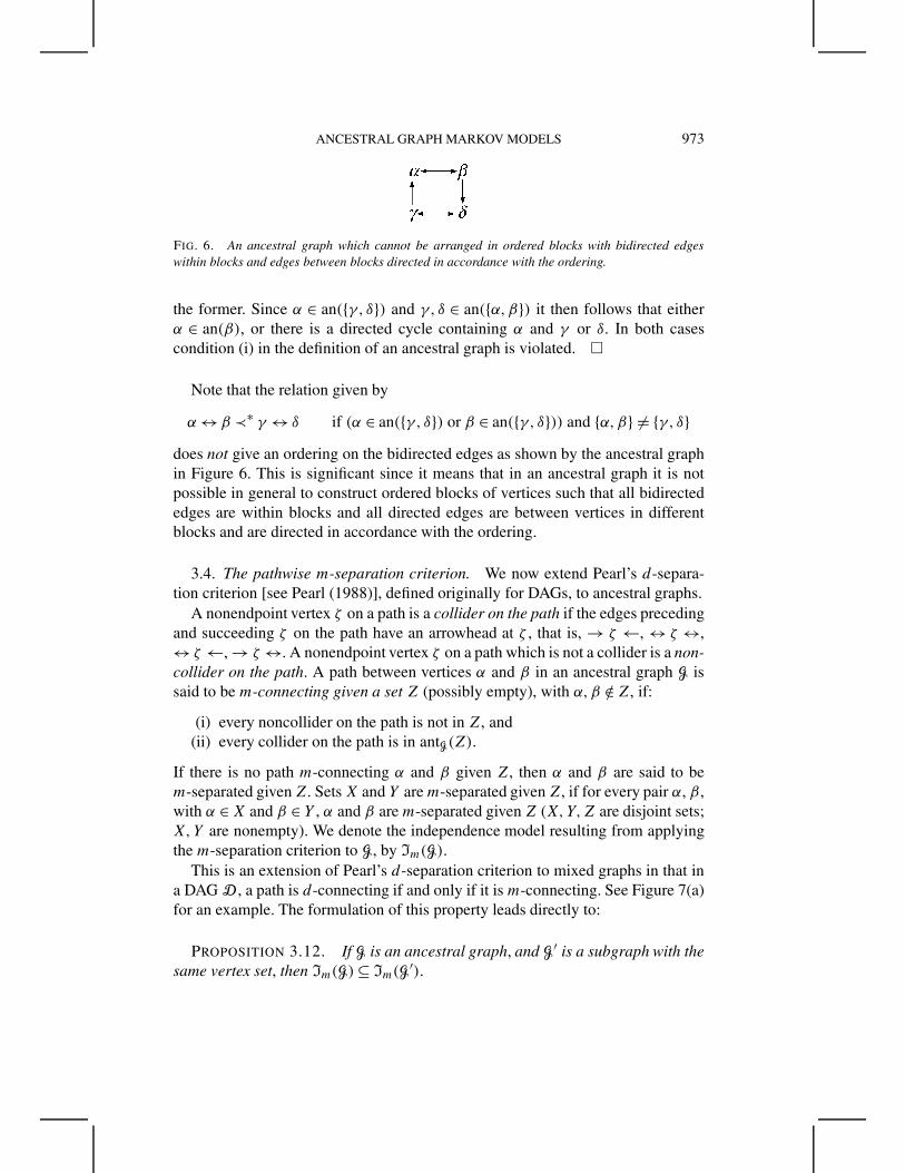
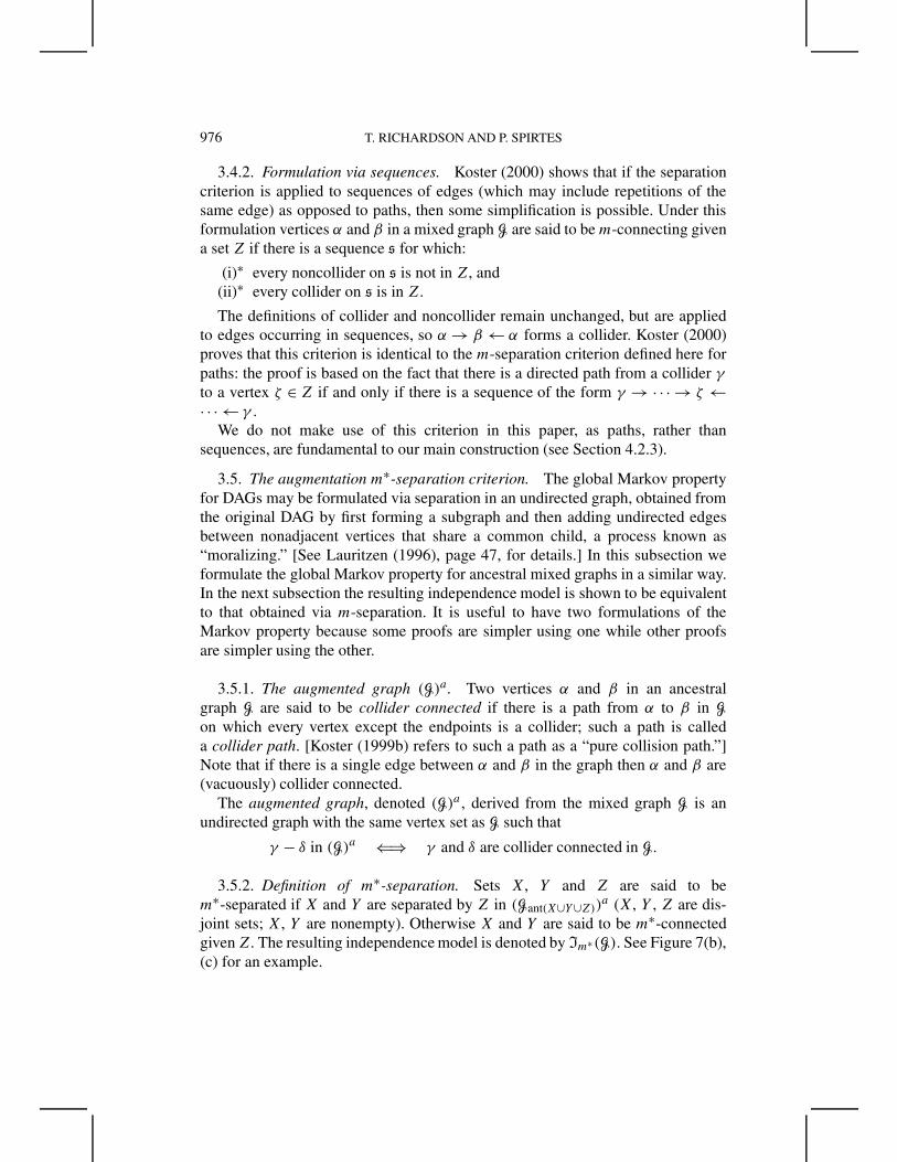
FIG. 6. An ancestral graph which cannot be arranged in ordered blocks with bidirected edgeswithin blocks and edges between blocks directed in accordance with the ordering.
the former. Since α ∈ an({γ, δ}) and γ, δ ∈ an({α,β}) it then follows that eitherα ∈ an(β), or there is a directed cycle containing α and γ or δ. In both casescondition (i) in the definition of an ancestral graph is violated. �
Note that the relation given by
α ↔ β ≺∗ γ ↔ δ if (α ∈ an({γ, δ}) or β ∈ an({γ, δ})) and {α,β} �= {γ, δ}does not give an ordering on the bidirected edges as shown by the ancestral graphin Figure 6. This is significant since it means that in an ancestral graph it is notpossible in general to construct ordered blocks of vertices such that all bidirectededges are within blocks and all directed edges are between vertices in differentblocks and are directed in accordance with the ordering.
3.4. The pathwise m-separation criterion. We now extend Pearl’s d-separa-tion criterion [see Pearl (1988)], defined originally for DAGs, to ancestral graphs.
A nonendpoint vertex ζ on a path is a collider on the path if the edges precedingand succeeding ζ on the path have an arrowhead at ζ , that is, → ζ ←, ↔ ζ ↔,↔ ζ ←, → ζ ↔. A nonendpoint vertex ζ on a path which is not a collider is a non-collider on the path. A path between vertices α and β in an ancestral graph G issaid to be m-connecting given a set Z (possibly empty), with α,β /∈ Z, if:
(i) every noncollider on the path is not in Z, and(ii) every collider on the path is in antG(Z).
If there is no path m-connecting α and β given Z, then α and β are said to bem-separated given Z. Sets X and Y are m-separated given Z, if for every pair α, β ,with α ∈ X and β ∈ Y , α and β are m-separated given Z (X,Y,Z are disjoint sets;X,Y are nonempty). We denote the independence model resulting from applyingthe m-separation criterion to G, by Im(G).
This is an extension of Pearl’s d-separation criterion to mixed graphs in that ina DAG D , a path is d-connecting if and only if it is m-connecting. See Figure 7(a)for an example. The formulation of this property leads directly to:
PROPOSITION 3.12. If G is an ancestral graph, and G′ is a subgraph with thesame vertex set, then Im(G) ⊆ Im(G
′).
974 T. RICHARDSON AND P. SPIRTES
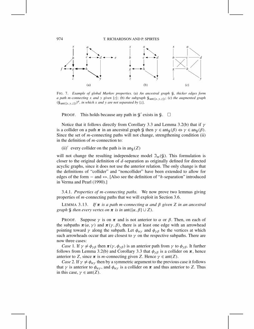
FIG. 7. Example of global Markov properties. (a) An ancestral graph G, thicker edges forma path m-connecting x and y given {z}; (b) the subgraph Gant({x,y,z}); (c) the augmented graph(Gant({x,y,z}))a , in which x and y are not separated by {z}.
PROOF. This holds because any path in G′ exists in G. �
Notice that it follows directly from Corollary 3.3 and Lemma 3.2(b) that if γ
is a collider on a path π in an ancestral graph G then γ ∈ antG(β) ⇔ γ ∈ anG(β).Since the set of m-connecting paths will not change, strengthening condition (ii)in the definition of m-connection to:
(ii)′ every collider on the path is in anG(Z)
will not change the resulting independence model Im(G). This formulation iscloser to the original definition of d-separation as originally defined for directedacyclic graphs, since it does not use the anterior relation. The only change is thatthe definitions of “collider” and “noncollider” have been extended to allow foredges of the form − and ↔. [Also see the definition of “h-separation” introducedin Verma and Pearl (1990).]
3.4.1. Properties of m-connecting paths. We now prove two lemmas givingproperties of m-connecting paths that we will exploit in Section 3.6.
LEMMA 3.13. If π is a path m-connecting α and β given Z in an ancestralgraph G then every vertex on π is in ant({α,β} ∪ Z).
PROOF. Suppose γ is on π and is not anterior to α or β . Then, on each ofthe subpaths π(α, γ ) and π(γ,β), there is at least one edge with an arrowheadpointing toward γ along the subpath. Let φαγ and φγβ be the vertices at whichsuch arrowheads occur that are closest to γ on the respective subpaths. There arenow three cases:
Case 1. If γ �= φγβ then π(γ,φγβ) is an anterior path from γ to φγβ . It furtherfollows from Lemma 3.2(b) and Corollary 3.3 that φγβ is a collider on π , henceanterior to Z, since π is m-connecting given Z. Hence γ ∈ ant(Z).
Case 2. If γ �= φαγ then by a symmetric argument to the previous case it followsthat γ is anterior to φαγ , and φαγ is a collider on π and thus anterior to Z. Thusin this case, γ ∈ ant(Z).
ANCESTRAL GRAPH MARKOV MODELS 975
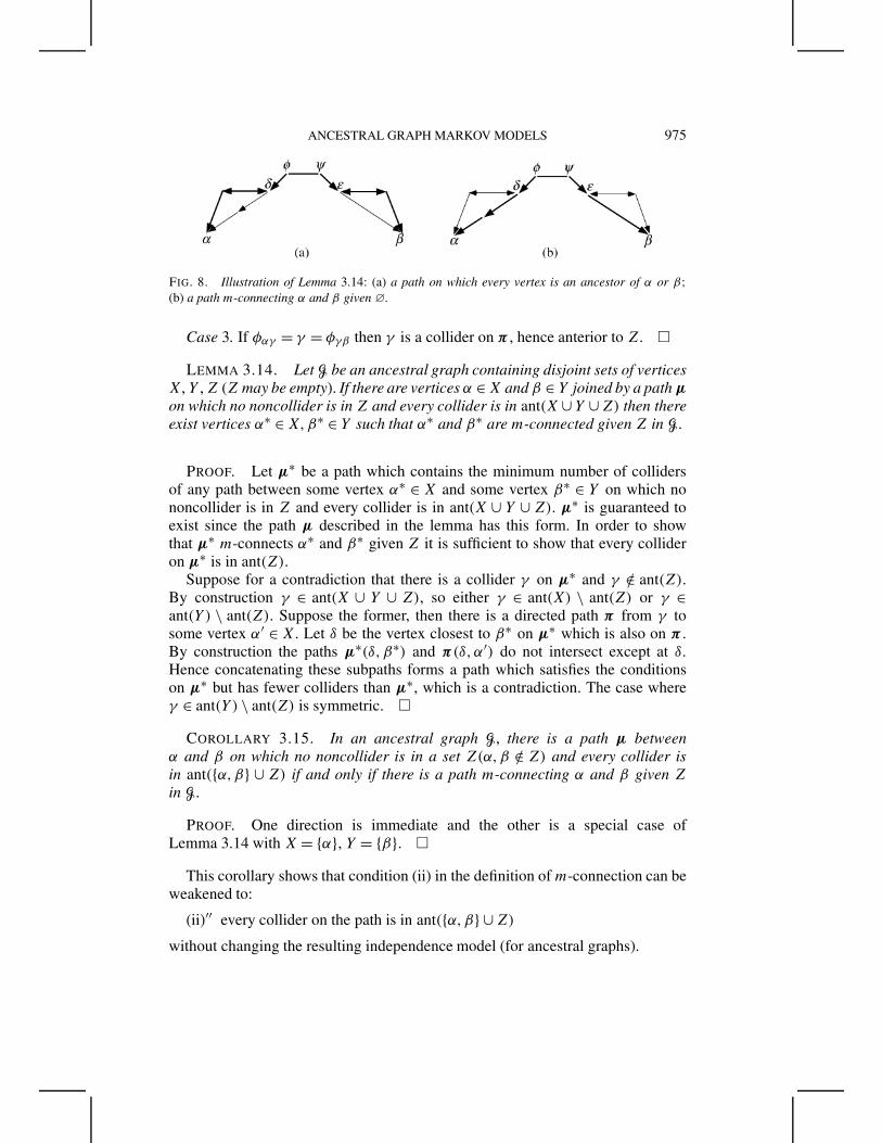
FIG. 8. Illustration of Lemma 3.14: (a) a path on which every vertex is an ancestor of α or β;(b) a path m-connecting α and β given ∅.
Case 3. If φαγ = γ = φγβ then γ is a collider on π , hence anterior to Z. �
LEMMA 3.14. Let G be an ancestral graph containing disjoint sets of verticesX, Y , Z (Z may be empty). If there are vertices α ∈ X and β ∈ Y joined by a pathµon which no noncollider is in Z and every collider is in ant(X ∪ Y ∪Z) then thereexist vertices α∗ ∈ X,β∗ ∈ Y such that α∗ and β∗ are m-connected given Z in G.
PROOF. Let µ∗ be a path which contains the minimum number of collidersof any path between some vertex α∗ ∈ X and some vertex β∗ ∈ Y on which nononcollider is in Z and every collider is in ant(X ∪ Y ∪ Z). µ∗ is guaranteed toexist since the path µ described in the lemma has this form. In order to showthat µ∗ m-connects α∗ and β∗ given Z it is sufficient to show that every collideron µ∗ is in ant(Z).
Suppose for a contradiction that there is a collider γ on µ∗ and γ /∈ ant(Z).By construction γ ∈ ant(X ∪ Y ∪ Z), so either γ ∈ ant(X) \ ant(Z) or γ ∈ant(Y ) \ ant(Z). Suppose the former, then there is a directed path π from γ tosome vertex α′ ∈ X. Let δ be the vertex closest to β∗ on µ∗ which is also on π .By construction the paths µ∗(δ, β∗) and π(δ,α′) do not intersect except at δ.Hence concatenating these subpaths forms a path which satisfies the conditionson µ∗ but has fewer colliders than µ∗, which is a contradiction. The case whereγ ∈ ant(Y ) \ ant(Z) is symmetric. �
COROLLARY 3.15. In an ancestral graph G, there is a path µ betweenα and β on which no noncollider is in a set Z(α,β /∈ Z) and every collider isin ant({α,β} ∪ Z) if and only if there is a path m-connecting α and β given Z
in G.
PROOF. One direction is immediate and the other is a special case ofLemma 3.14 with X = {α}, Y = {β}. �
This corollary shows that condition (ii) in the definition of m-connection can beweakened to:
(ii)′′ every collider on the path is in ant({α,β} ∪ Z)
without changing the resulting independence model (for ancestral graphs).
976 T. RICHARDSON AND P. SPIRTES
3.4.2. Formulation via sequences. Koster (2000) shows that if the separationcriterion is applied to sequences of edges (which may include repetitions of thesame edge) as opposed to paths, then some simplification is possible. Under thisformulation vertices α and β in a mixed graph G are said to be m-connecting givena set Z if there is a sequence s for which:
(i)∗ every noncollider on s is not in Z, and(ii)∗ every collider on s is in Z.
The definitions of collider and noncollider remain unchanged, but are appliedto edges occurring in sequences, so α → β ← α forms a collider. Koster (2000)proves that this criterion is identical to the m-separation criterion defined here forpaths: the proof is based on the fact that there is a directed path from a collider γto a vertex ζ ∈ Z if and only if there is a sequence of the form γ → · · · → ζ ←· · · ← γ .
We do not make use of this criterion in this paper, as paths, rather thansequences, are fundamental to our main construction (see Section 4.2.3).
3.5. The augmentation m∗-separation criterion. The global Markov propertyfor DAGs may be formulated via separation in an undirected graph, obtained fromthe original DAG by first forming a subgraph and then adding undirected edgesbetween nonadjacent vertices that share a common child, a process known as“moralizing.” [See Lauritzen (1996), page 47, for details.] In this subsection weformulate the global Markov property for ancestral mixed graphs in a similar way.In the next subsection the resulting independence model is shown to be equivalentto that obtained via m-separation. It is useful to have two formulations of theMarkov property because some proofs are simpler using one while other proofsare simpler using the other.
3.5.1. The augmented graph (G)a . Two vertices α and β in an ancestralgraph G are said to be collider connected if there is a path from α to β in Gon which every vertex except the endpoints is a collider; such a path is calleda collider path. [Koster (1999b) refers to such a path as a “pure collision path.”]Note that if there is a single edge between α and β in the graph then α and β are(vacuously) collider connected.
The augmented graph, denoted (G)a , derived from the mixed graph G is anundirected graph with the same vertex set as G such that
γ − δ in (G)a ⇐⇒ γ and δ are collider connected in G.
3.5.2. Definition of m∗-separation. Sets X, Y and Z are said to bem∗-separated if X and Y are separated by Z in (Gant(X∪Y∪Z))
a (X, Y , Z are dis-joint sets; X, Y are nonempty). Otherwise X and Y are said to be m∗-connectedgiven Z. The resulting independence model is denoted by Im∗(G). See Figure 7(b),(c) for an example.
ANCESTRAL GRAPH MARKOV MODELS 977
When applied to DAGs, or UGs, the augmentation criterion presented hereis equivalent to the Lauritzen–Wermuth–Frydenberg moralization criterion. (SeeSection 9.4 for a discussion of chain graphs.)
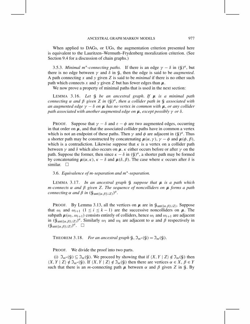
3.5.3. Minimal m∗-connecting paths. If there is an edge γ − δ in (G)a , butthere is no edge between γ and δ in G, then the edge is said to be augmented.A path connecting x and y given Z is said to be minimal if there is no other suchpath which connects x and y given Z but has fewer edges than µ.
We now prove a property of minimal paths that is used in the next section:
LEMMA 3.16. Let G be an ancestral graph. If µ is a minimal pathconnecting α and β given Z in (G)a , then a collider path in G associated withan augmented edge γ − δ on µ has no vertex in common with µ, or any colliderpath associated with another augmented edge on µ, except possibly γ or δ.
PROOF. Suppose that γ − δ and ε − φ are two augmented edges, occurringin that order on µ, and that the associated collider paths have in common a vertexwhich is not an endpoint of these paths. Then γ and φ are adjacent in (G)a . Thusa shorter path may be constructed by concatenating µ(α, γ ), γ − φ and µ(φ,β),which is a contradiction. Likewise suppose that κ is a vertex on a collider pathbetween γ and δ which also occurs on µ. κ either occurs before or after γ on thepath. Suppose the former, then since κ − δ in (G)a , a shorter path may be formedby concatenating µ(α, κ), κ − δ and µ(δ, β). The case where κ occurs after δ issimilar. �
3.6. Equivalence of m-separation and m∗-separation.
LEMMA 3.17. In an ancestral graph G suppose that µ is a path whichm-connects α and β given Z. The sequence of noncolliders on µ forms a pathconnecting α and β in (Gant({α,β}∪Z))
a .
PROOF. By Lemma 3.13, all the vertices on µ are in Gant({α,β}∪Z). Supposethat ωi and ωi+1 (1 ≤ i ≤ k − 1) are the successive noncolliders on µ. Thesubpath µ(ωi,ωi+1) consists entirely of colliders, hence ωi and ωi+1 are adjacentin (Gant({α,β}∪Z))
a . Similarly ω1 and ωk are adjacent to α and β respectively in(Gant({α,β}∪Z))
a . �
THEOREM 3.18. For an ancestral graph G, Im∗(G) = Im(G).
PROOF. We divide the proof into two parts.
(i) Im∗(G) ⊆ Im(G). We proceed by showing that if 〈X,Y | Z〉 /∈ Im(G) then〈X,Y | Z〉 /∈ Im∗(G). If 〈X,Y | Z〉 /∈ Im(G) then there are vertices α ∈ X, β ∈ Y
such that there is an m-connecting path µ between α and β given Z in G. By
978 T. RICHARDSON AND P. SPIRTES
Lemma 3.17 the noncolliders on µ form a path µ∗ connecting α and β in(Gant(X∪Y∪Z))
a . Since µ is m-connecting, no noncollider on µ is in Z hence novertex on µ∗ is in Z. Thus 〈X,Y | Z〉 /∈ Im∗(G).
(ii) Im(G) ⊆ Im∗(G). We show that if 〈X,Y | Z〉 /∈ Im∗(G) then 〈X,Y | Z〉 /∈Im(G). If 〈X,Y | Z〉 /∈ Im∗(G) then there are vertices α ∈ X, β ∈ Y such thatthere is a minimal path π connecting α and β in (Gant(X∪Y∪Z))
a on whichno vertex is in Z. Our strategy is to replace each augmented edge on π witha corresponding collider path in Gant(X∪Y∪Z) and replace the other edges on πwith the corresponding edge in G. It follows from Lemma 3.16 that the resultingsequence of edges forms a path from α to β in G, which we denote ν. Further, anynoncollider on ν is a vertex on π and hence not in Z. Finally, since all verticesin ν are in Gant(X∪Y∪Z) it follows that every collider is in ant(X ∪ Y ∪ Z). Thusby Lemma 3.14 there are vertices α∗ ∈ X and β∗ ∈ Y such that α∗ and β∗ arem-connected given Z in G. Thus 〈X,Y | Z〉 /∈ Im(G). �
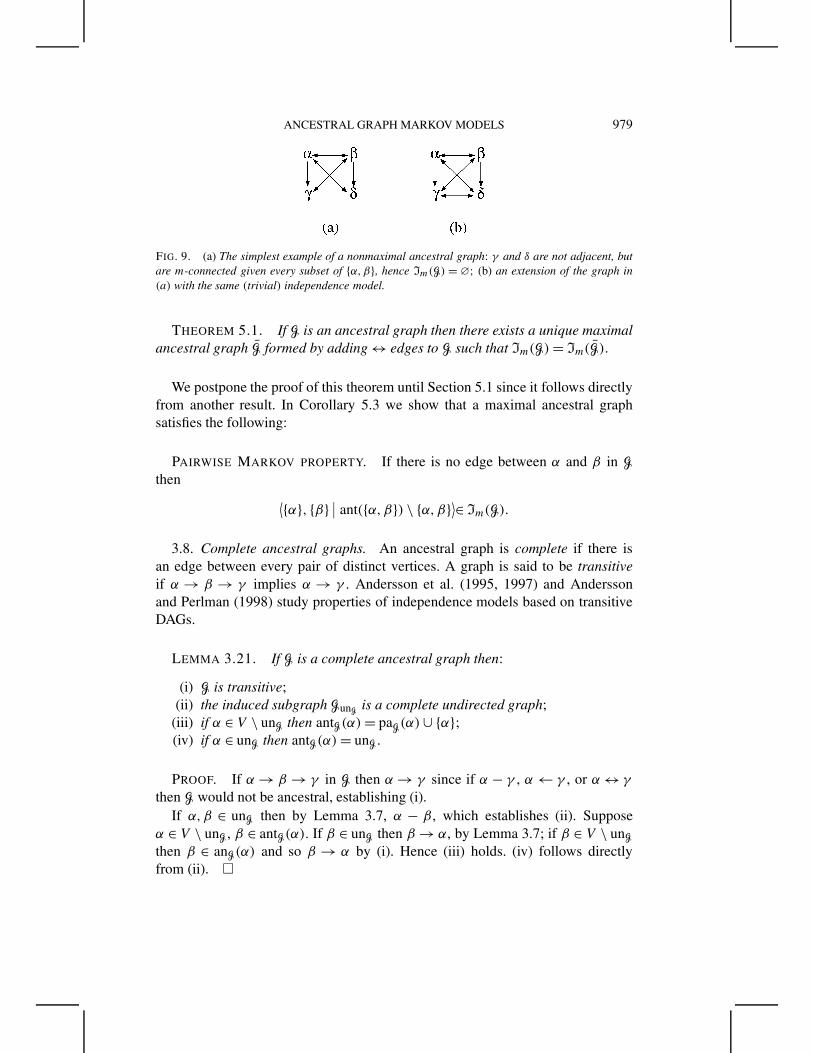
3.7. Maximal ancestral graphs. Independence models described by DAGsand undirected graphs satisfy pairwise Markov properties with respect to thesegraphs, hence every missing edge corresponds to a conditional independence [seeLauritzen (1996), page 32]. This is not true in general for an arbitrary ancestralgraph, as shown by the graph in Figure 9(a).
This motivates the following definition: an ancestral graph G is said to bemaximal if for every pair of vertices α, β if α and β are not adjacent in G then thereis a set Z (α,β /∈ Z), such that 〈{α}, {β} | Z〉 ∈ Im(G). Thus a graph is maximal ifevery missing edge corresponds to at least one independence in the correspondingindependence model.
PROPOSITION 3.19. If G is an undirected graph, or a directed acyclic graphthen G is maximal.
PROOF. The proof follows directly from the existence of pairwise Markovproperties for DAGs and undirected graphs. �
The use of the term “maximal” is motivated by the following:
PROPOSITION 3.20. If G = (V,E) is a maximal ancestral graph, and G isa subgraph of G∗ = (V,E∗), then Im(G) = Im(G
∗) implies G = G∗.
PROOF. If some pair α,β are adjacent in G∗ but not G, then in G∗, α and β arem-connected by any subset of V \ {α,β}. Hence Im(G) �= Im(G
∗). �
Hence maximal ancestral graphs are maximal in the sense that no additionaledge may be added to the graph without changing the independence model. Thefollowing theorem gives the converse.
ANCESTRAL GRAPH MARKOV MODELS 979
FIG. 9. (a) The simplest example of a nonmaximal ancestral graph: γ and δ are not adjacent, butare m-connected given every subset of {α,β}, hence Im(G) = ∅; (b) an extension of the graph in(a) with the same (trivial) independence model.
THEOREM 5.1. If G is an ancestral graph then there exists a unique maximalancestral graph G formed by adding ↔ edges to G such that Im(G) = Im(G).
We postpone the proof of this theorem until Section 5.1 since it follows directlyfrom another result. In Corollary 5.3 we show that a maximal ancestral graphsatisfies the following:
PAIRWISE MARKOV PROPERTY. If there is no edge between α and β in Gthen ⟨{α}, {β} ∣∣ ant({α,β}) \ {α,β}⟩∈ Im(G).
3.8. Complete ancestral graphs. An ancestral graph is complete if there isan edge between every pair of distinct vertices. A graph is said to be transitiveif α → β → γ implies α → γ . Andersson et al. (1995, 1997) and Anderssonand Perlman (1998) study properties of independence models based on transitiveDAGs.
LEMMA 3.21. If G is a complete ancestral graph then:(i) G is transitive;
(ii) the induced subgraph GunG is a complete undirected graph;(iii) if α ∈ V \ unG then antG(α) = paG(α) ∪ {α};(iv) if α ∈ unG then antG(α) = unG.
PROOF. If α → β → γ in G then α → γ since if α − γ , α ← γ , or α ↔ γ
then G would not be ancestral, establishing (i).If α,β ∈ unG then by Lemma 3.7, α − β , which establishes (ii). Suppose
α ∈ V \ unG, β ∈ antG(α). If β ∈ unG then β → α, by Lemma 3.7; if β ∈ V \ unG
then β ∈ anG(α) and so β → α by (i). Hence (iii) holds. (iv) follows directlyfrom (ii). �
980 T. RICHARDSON AND P. SPIRTES
4. Marginalizing and conditioning. In this section we first introduce mar-ginalizing and conditioning for an independence model. We then define a graph-ical transformation of an ancestral graph. We show that the independence modelcorresponding to the transformed graph is the independence model obtained bymarginalizing and conditioning the independence model of the original graph. Inthe remaining subsections we derive several useful consequences.
4.1. Marginalizing and conditioning independence models (I[SL). An inde-pendence model I with vertex set V after marginalizing out a subset L is simplythe subset of triples which do not involve any vertices in L. More formally wedefine
I[L≡ {〈X,Y | Z〉 ∣∣ 〈X,Y | Z〉 ∈ I; (X ∪ Y ∪ Z) ∩ L = ∅}.
If I contains the independence relations present in a distribution P , thenI[L contains the subset of independence relations remaining after marginalizingout the “Latent” variables in L; see Theorem 7.1. (Note the distinct uses of thevertical bar in 〈·, · | ·〉 and {· | ·}.)
An independence model I with vertex set V after conditioning on a subset S isthe set of triples defined as follows:
I[S≡ {〈X,Y | Z〉 ∣∣ 〈X,Y | Z ∪ S〉 ∈ I; (X ∪ Y ∪ Z) ∩ S = ∅}.
Thus if I contains the independence relations present in a distribution P thenI[S constitutes the subset of independencies holding among the remainingvariables after conditioning on S; see Theorem 7.1. (Note that the set S issuppressed in the conditioning set in the independence relations in the resultingindependence model.) The letter S is used because Selection effects represent onecontext in which conditioning may occur.
Combining these definitions we obtain
I[SL≡ {〈X,Y | Z〉 ∣∣ 〈X,Y | Z ∪ S〉 ∈ I; (X ∪ Y ∪ Z) ∩ (S ∪ L) = ∅}.
PROPOSITION 4.1. For an independence model I over V containing disjointsubsets S1, S2, L1, L2:
(i) I[∅∅= I,
(ii) (I[S1L1
)[S2L2
= I[S1∪S2L1∪L2
.
4.1.1. Example. Consider the following independence model:
I∗ = {〈{a, x}, {b, y} | {t}〉, 〈{a, x}, {b} | ∅〉, 〈{b, y}, {a} | ∅〉, 〈{a, b}, {t} | ∅〉}.
In fact, I∗ ⊂ Im(D), where D is the DAG in Figure 10(i). In this case,
I∗[∅{t}=
{〈{a, x}, {b} | ∅〉, 〈{b, y}, {a} | ∅〉}, I∗[{t}∅ = {〈{a, x}, {b, y} | ∅〉}.
ANCESTRAL GRAPH MARKOV MODELS 981
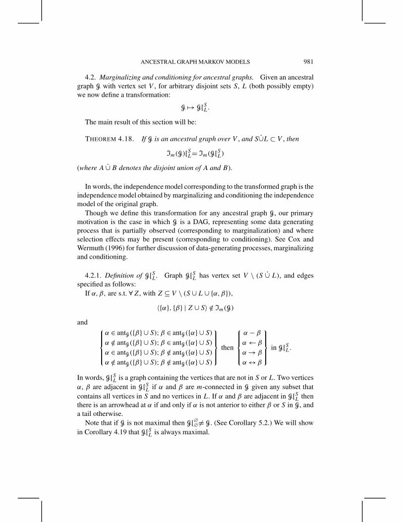
4.2. Marginalizing and conditioning for ancestral graphs. Given an ancestralgraph G with vertex set V , for arbitrary disjoint sets S, L (both possibly empty)we now define a transformation:
G $→ G[SL.The main result of this section will be:
THEOREM 4.18. If G is an ancestral graph over V , and S∪L ⊂ V , then
Im(G)[SL= Im(G[SL)(where A ∪ B denotes the disjoint union of A and B).
In words, the independence model corresponding to the transformed graph is theindependence model obtained by marginalizing and conditioning the independencemodel of the original graph.
Though we define this transformation for any ancestral graph G, our primarymotivation is the case in which G is a DAG, representing some data generatingprocess that is partially observed (corresponding to marginalization) and whereselection effects may be present (corresponding to conditioning). See Cox andWermuth (1996) for further discussion of data-generating processes, marginalizingand conditioning.
4.2.1. Definition of G[SL. Graph G[SL has vertex set V \ (S ∪ L), and edgesspecified as follows:
If α,β, are s.t. ∀Z, with Z ⊆ V \ (S ∪ L ∪ {α,β}),〈{α}, {β} | Z ∪ S〉 /∈ Im(G)
and α ∈ antG({β} ∪ S);β ∈ antG({α} ∪ S)
α /∈ antG({β} ∪ S);β ∈ antG({α} ∪ S)
α ∈ antG({β} ∪ S);β /∈ antG({α} ∪ S)
α /∈ antG({β} ∪ S);β /∈ antG({α} ∪ S)
then
α − β
α ← β
α → β
α ↔ β
in G[SL.
In words, G[SL is a graph containing the vertices that are not in S or L. Two verticesα, β are adjacent in G[SL if α and β are m-connected in G given any subset thatcontains all vertices in S and no vertices in L. If α and β are adjacent in G[SL thenthere is an arrowhead at α if and only if α is not anterior to either β or S in G, anda tail otherwise.
Note that if G is not maximal then G[∅∅ �= G. (See Corollary 5.2.) We will showin Corollary 4.19 that G[SL is always maximal.
982 T. RICHARDSON AND P. SPIRTES
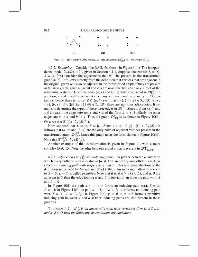
FIG. 10. (i) A simple DAG model, D; (ii) the graph D[∅{t}; (iii) the graph D[{t}∅
.
4.2.2. Examples. Consider the DAG, D , shown in Figure 10(i). The indepen-dence model Im(D) ⊃ I∗, given in Section 4.1.1. Suppose that we set L = {t},S = ∅. First consider the adjacencies that will be present in the transformedgraph D[∅{t}. It follows directly from the definition that vertices that are adjacent inthe original graph will also be adjacent in the transformed graph, if they are presentin the new graph, since adjacent vertices are m-connected given any subset of theremaining vertices. Hence the pairs (a, x) and (b, y) will be adjacent in D[∅{t}. Inaddition, x and y will be adjacent since any set m-separating x and y in D con-tains t , hence there is no set Z ⊆ {a, b} such that 〈{x}, {y} | Z〉 ∈ Im(D). Since〈{a}, {b, y} | ∅〉, 〈{b}, {a, x} | ∅〉 ∈ Im(D) there are no other adjacencies. It re-mains to determine the types of these three edges in D[∅{t}. Since x /∈ antD(y), andy /∈ antD(x), the edge between x and y is of the form x ↔ y. Similarly the otheredges are a → x and b → y. Thus the graph D[∅{t} is as shown in Figure 10(ii).
Observe that I∗[∅{t}⊂ Im(D[∅{t}).Now suppose that L = ∅, S = {t}. Since 〈{a, x}, {b, y} | {t}〉 ∈ Im(D), it
follows that (a, x) and (b, y) are the only pairs of adjacent vertices present in thetransformed graph D[{t}∅ , hence this graph takes the form shown in Figure 10(iii).
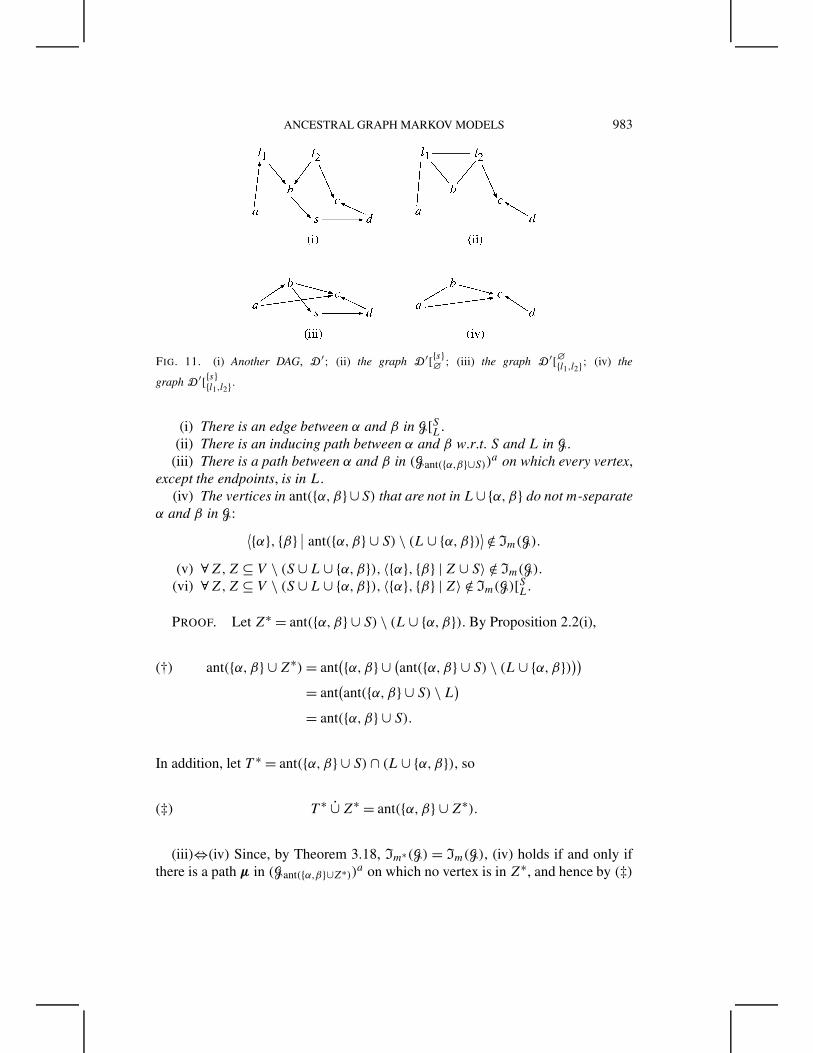
Note that I∗[{t}∅ ⊂ Im(D[{t}∅ ).Another example of this transformation is given in Figure 11, with a more
complex DAG D ′. Note the edge between a and c that is present in D ′[{s}{l1,l2}.
4.2.3. Adjacencies in G[SL and inducing paths. A path π between α and β onwhich every collider is an ancestor of {α,β} ∪ S and every noncollider is in L, iscalled an inducing path with respect to S and L. This is a generalization of thedefinition introduced by Verma and Pearl (1990). An inducing path with respectto S = ∅,L = ∅ is called primitive. Note that if α,β ∈ V \ (S ∪ L), and α,β areadjacent in G then the edge joining α and β is (trivially) an inducing path w.r.t. Sand L in G.
In Figure 10(i) the path x ← t → y forms an inducing path w.r.t. S = ∅,L = {t}; in Figure 11(i) the path a → l1 → b ← l2 → c forms an inducing pathw.r.t. S = {s}, L = {l1, l2}; in Figure 9(a), γ ↔ β ↔ α ↔ δ forms a primitiveinducing path between γ and δ. (Other inducing paths are also present in thesegraphs.)
THEOREM 4.2. If G is an ancestral graph, with vertex set V = O ∪ S ∪ L,and α,β ∈ O then the following six conditions are equivalent:
ANCESTRAL GRAPH MARKOV MODELS 983
FIG. 11. (i) Another DAG, D ′; (ii) the graph D ′[{s}∅
; (iii) the graph D ′[∅{l1,l2}; (iv) the
graph D ′[{s}{l1,l2}.
(i) There is an edge between α and β in G[SL.(ii) There is an inducing path between α and β w.r.t. S and L in G.
(iii) There is a path between α and β in (Gant({α,β}∪S))a on which every vertex,
except the endpoints, is in L.(iv) The vertices in ant({α,β} ∪S) that are not in L∪ {α,β} do not m-separate
α and β in G: ⟨{α}, {β} ∣∣ ant({α,β} ∪ S) \ (L ∪ {α,β})⟩ /∈ Im(G).
(v) ∀Z,Z ⊆ V \ (S ∪ L ∪ {α,β}), 〈{α}, {β} | Z ∪ S〉 /∈ Im(G).(vi) ∀Z,Z ⊆ V \ (S ∪ L ∪ {α,β}), 〈{α}, {β} | Z〉 /∈ Im(G)[SL.
PROOF. Let Z∗ = ant({α,β} ∪ S) \ (L ∪ {α,β}). By Proposition 2.2(i),
ant({α,β} ∪ Z∗) = ant({α,β} ∪ (
ant({α,β} ∪ S) \ (L ∪ {α,β})))(†)
= ant(ant({α,β} ∪ S) \ L
)= ant({α,β} ∪ S).
In addition, let T ∗ = ant({α,β} ∪ S) ∩ (L ∪ {α,β}), so
T ∗ ∪ Z∗ = ant({α,β} ∪ Z∗).(‡)
(iii)⇔(iv) Since, by Theorem 3.18, Im∗(G) = Im(G), (iv) holds if and only ifthere is a path µ in (Gant({α,β}∪Z∗))a on which no vertex is in Z∗, and hence by (‡)
984 T. RICHARDSON AND P. SPIRTES
every vertex is in T ∗. Further, by (†), Gant({α,β}∪Z∗) = Gant({α,β}∪S), hence by thedefinition of T ∗, µ satisfies the conditions given in (iii).
(ii)⇒(iv) If there is an inducing path π in G w.r.t. S and L, then no noncollideron π is in Z∗, since Z∗ ∩ L = ∅, and any collider on π is in an({α,β} ∪ S) ⊆ant({α,β} ∪ S) = ant({α,β} ∪ Z∗) by (†). Hence by Corollary 3.15 there isa path π∗ which m-connects α and β given Z∗ in G as required.
(iv)⇒(ii) Let ν be a path which m-connects α and β given Z∗. By Lemma 3.13and (†), every vertex on ν is in ant({α,β} ∪ S), hence by Lemma 3.2(b)and Corollary 3.3, every collider is in an({α,β} ∪ S). Every noncollider is inant({α,β} ∪ S) \ Z∗ ⊆ L ∪ {α,β}, so every noncollider is in L. Hence ν is aninducing path w.r.t. S and L in G.
(iii)⇒(v) Every edge present in (Gant({α,β}∪S))a is also present in
(Gant({α,β}∪Z∪S))a . The implication then follows since every nonendpoint vertex
on the path is in L.(v)⇒(iv) This follows trivially taking Z = Z∗ \ S.(v)⇔(i) Definition of G[SL.(v)⇔(vi) Definition of Im(G)[SL. �
An important consequence of condition (iv) in this theorem is that a single testof m-separation in G is sufficient to determine whether or not a given adjacencyis present in G[SL; it is not necessary to test every subset of V \ (S ∪ L ∪{α,β}). Likewise properties (ii) and (iii) provide conditions that can be tested inpolynomial time.
4.2.4. Primitive inducing paths and maximality.
COROLLARY 4.3. If G is an ancestral graph, then there is no set Z,(α,β /∈ Z), such that 〈{α}, {β} | Z〉 ∈ Im(G) if and only if there is a primitiveinducing path between α and β in G.
PROOF. The result follows from (ii)⇔(v) in Theorem 4.2 with S = ∅, L = ∅.�
COROLLARY 4.4. Every nonmaximal ancestral graph contains a primitiveinducing path between a pair of nonadjacent vertices.
PROOF. Immediate by the definition of maximality and Corollary 4.3. �
Primitive inducing paths with more than one edge take a very special form, asdescribed in the next lemma, and illustrated by the inducing path γ ↔ β ↔ α ↔ δ
in Figure 9(a).
LEMMA 4.5. Let G be an ancestral graph. If π is a primitive inducing pathbetween α and β in G, and π contains more than one edge, then:
ANCESTRAL GRAPH MARKOV MODELS 985
(i) every nonendpoint vertex on π is a collider and in antG({α,β});(ii) α /∈ antG(β) and β /∈ antG(α);
(iii) every edge on π is bidirected.
PROOF. Part (i) is a direct consequence of the definition of a primitiveinducing path. Consider the vertex γ which is adjacent to α on π . By (i), γ isa collider on π , so γ ∈ spG(α)∪chG(α), so γ /∈ antG(α) as G is ancestral. Hence by(i) γ ∈ antG(β). If β ∈ antG(α) then γ ∈ antG(α), but this is a contradiction. Thusβ /∈ antG(α). By a similar argument α /∈ antG(β), establishing (ii). (iii) followsdirectly from (i) and (ii), since G is ancestral. �
Lemma 4.5 (ii) has the following consequence:
COROLLARY 4.6. In a maximal ancestral graph G, if there is a primitiveinducing path between α and β containing more than one edge, then there is anedge α ↔ β in G.
PROOF. Since G is maximal, by Corollary 4.3, α and β are adjacent in G. ByLemma 4.5(ii), α /∈ antG(β) and β /∈ antG(α), hence by Lemma 3.9, it follows thatα ↔ β in G. �
Note that if G is a maximal ancestral graph and G′ is a subgraph formed byremoving an undirected or directed edge from G then G′ is also maximal.
4.2.5. Anterior relations in G[SL. The next lemma characterizes the verticesanterior to α in G[SL.
LEMMA 4.7. For an ancestral graph G with vertex set V = O ∪ S ∪ L, ifα ∈ O then
antG(α) \ (antG(S) ∪ L) ⊆ antG[SL(α) ⊆ antG({α} ∪ S) \ (S ∪ L).
In words, if β , α are in G[SL and β is anterior to α but not S in G, then β is alsoanterior to α in G[SL. Conversely, if β is anterior to α in G[SL then β is anterior toeither α or S in G.
PROOF OF LEMMA 4.7. Letµ be an anterior path from a vertex β ∈ antG(α)\(L∪antG(S)) to α in G. Note that no vertex on µ is in S. Consider the subsequence〈β ≡ ωm, . . . ,ωi, . . . ,ω1 ≡ α〉 of vertices on µ that are in V \ (S ∪ L). Now thesubpathµ(ωi+1,ωi) is an anterior path on which every vertex except the endpointsis in L. Hence ωi and ωi+1 are adjacent in G[SL. Further since ωi+1 ∈ antG(ωi)
it follows that either ωi+1 − ωi or ωi+1 → ωi , hence β ≡ ωm ∈ antG[SL(α), asrequired.
986 T. RICHARDSON AND P. SPIRTES
To prove the second assertion, let ν ≡ 〈φn, . . . , φ1 ≡ α〉 be an anterior path froma vertex φn ∈ antG[SL(α) to α in G[SL. For 1 ≤ i < n, either φi+1 − φi or φi+1 → φi
on ν. By definition of G[SL, in either case φi+1 ∈ antG({φi} ∪ S) \ (S ∪ L). Thusφn ∈ antG({α} ∪ S) \ (S ∪ L). �
Taking S = ∅ in Lemma 4.7 we obtain the following:
COROLLARY 4.8. In an ancestral graph G = (V,E) if α ∈ V \ L thenantG(α) \ L = antG[∅L (α).
4.2.6. The undirected subgraph of G[SL.
LEMMA 4.9. If G is an ancestral graph with vertex set V = O ∪ S ∪ L, then(unG ∪ antG(S)
) \ (S ∪ L) ⊆ unG[SL .
In words, any vertex in the undirected subgraph of G which is also present in G[SLwill also be in the undirected subgraph of G[SL. Likewise any vertex anterior to S
in G will be in the undirected component of G[SL if present in this graph.
PROOF OF LEMMA 4.9. Suppose for a contradiction that α ∈ (unG ∪ antG(S))\(S ∪ L), but α /∈ unG[SL . Hence there is a vertex β such that either β ↔ α or
β → α in G[SL. In both cases α /∈ antG({β} ∪ S). Thus α /∈ antG(S). Since α andβ are adjacent in G[SL by Theorem 4.2(ii) there is an inducing path π between α
and β w.r.t. S and L, hence every vertex on π is in antG({α,β} ∪S). If there are nocolliders on π then since α ∈ unG, π is an anterior path from α to β so α ∈ antG(β),which is a contradiction. If there is a collider on π then let γ be the collider on πclosest to α. Now π(α, γ ) is an anterior path from α to γ so α ∈ antG(γ ) butγ /∈ unG, hence by Lemma 3.8(ii), γ /∈ antG(α). Thus γ ∈ antG({β} ∪ S), and thusα ∈ antG({β} ∪ S), again a contradiction. �
COROLLARY 4.10. If G is an ancestral graph with V = O ∪S ∪L and α ∈ O
then
antG(α) \ (S ∪ L) ⊆ unG[SL ∪ antG[SL(α).
Thus the vertices anterior to α ∈ G that are also in G[SL either remain anterior toα ∈ G[SL, or are in unG[SL (or both).
PROOF OF COROLLARY 4.10.(antG(α)) \ (S ∪ L) ⊆ (
antG(α) \ (antG(S) ∪ L)) ∪ (
antG(S) \ (S ∪ L))
(∗) ⊆ antG[SL(α) ∪ unG[SL .
The step marked (∗) follows from Lemmas 4.7 and 4.9. �
ANCESTRAL GRAPH MARKOV MODELS 987
LEMMA 4.11. In an ancestral graph G, if α ∈ antG[SL(β) and α /∈ unG[SL thenα ∈ anG(β), and α /∈ antG(S).
PROOF. If α /∈ unG[SL , but α ∈ V \ (S ∪ L) then by Lemma 4.9, α /∈ unG ∪antG(S). Since α ∈ antG[SL(β) it follows from Lemma 4.7 that α ∈ antG({β} ∪ S).So α ∈ antG(β). Further, since α /∈ unG, by Lemma 3.8(iii), α ∈ anG(β). �
Consequently, if in G[SL α is anterior to β and there is an arrowhead at α thenα is an ancestor of β in G.
4.2.7. G[SL is an ancestral graph.
THEOREM 4.12. If G is an arbitrary ancestral graph, with vertex set V =O ∪ S ∪ L, then G[SL is an ancestral graph.
PROOF. Clearly G[SL is a mixed graph. Suppose for a contradiction that α ∈antG[SL(paG[SL(α)∪spG[SL(α)). Suppose α ∈ antG[SL(β) with β ∈ paG[SL(α)∪spG[SL(α).Then by Lemma 4.7, α ∈ antG({β} ∪ S). However if β ∈ paG[SL(α) ∪ spG[SL(α) then
α /∈ antG(β ∪S) by definition of G[SL, which is a contradiction. Hence G[SL satisfiescondition (i) for an ancestral graph.
Now suppose that neG[SL(α) �= ∅. Let β ∈ neG[SL(α). Then by the definition
of G[SL, α ∈ antG({β} ∪ S) and β ∈ antG({α} ∪ S). Thus either α ∈ antG(S) or,by Lemma 3.8(ii), α ∈ unG. It follows by Lemma 4.9 that α ∈ unG[SL , hence
paG[SL(α)∪ spG[SL(α) = ∅. So G[SL satisfies condition (ii) for an ancestral graph. �
We will show in Section 4.2.10 that G[SL is a maximal ancestral graph.
4.2.8. Introduction of undirected and bidirected edges. As stated earlier, weare particularly interested in considering the transformation G $→ G[SL in thecase where G is a DAG, and hence contains no bidirected or undirected edges.The following results show that the introduction of undirected edges is naturallyassociated with conditioning, while bidirected are associated with marginalizing.
PROPOSITION 4.13. If G is an ancestral graph which contains no undirectededges, then neither does G[∅L .
PROOF. If α − β in G[∅L then, by construction, α ∈ antG(β), β ∈ antG(α).Hence by Lemma 3.8(ii) there is a path composed of undirected edges which joinsα and β in G, which is a contradiction. �
In particular, if we begin with a DAG, then undirected edges will only be presentin the transformed graph if S �= ∅; likewise it follows from the next Propositionthat bidirected edges will only be present if L �= ∅.
988 T. RICHARDSON AND P. SPIRTES
PROPOSITION 4.14. If G is an ancestral graph which contains no bidirectededges then neither does G[S
∅.
PROOF. If α ↔ β in G[S∅
then α /∈ antG({β} ∪S) and β /∈ antG({α} ∪S). Sincethere are no bidirected edges in G it follows that α and β are not adjacent in G.Since L = ∅, it further follows that any inducing path has the form α → σ ← β ,where σ ∈ antG(S), contradicting α,β /∈ antG(S). �
4.2.9. The independence model Im(G[SL). The following lemmas and corol-lary are required to prove Theorem 4.18.
LEMMA 4.15. If G is an ancestral graph with V = O ∪ S ∪ L, and β ∈paG[SL(α)∪ spG[SL(α) then α is not anterior to any vertex on an inducing path (w.r.t.S and L) between α and β in G.
PROOF. If β ∈ paG[SL(α) ∪ spG[SL(α), then α /∈ unG[SL . It then follows by
Lemma 4.9 that α /∈ unG, and by construction of G[SL that α /∈ antG({β} ∪ S).A vertex γ on an inducing path between α and β is in antG({α,β} ∪ S). Ifα ∈ antG(γ ) then by Lemma 3.8(ii) γ /∈ antG(α), since α /∈ unG. Thus γ ∈antG({β} ∪ S) but then α ∈ antG({β} ∪ S), which is a contradiction. �
COROLLARY 4.16. If α ↔ β or α ← β in G[SL and 〈α,φ1, . . . , φk, β〉 is aninducing path (w.r.t. S and L) in G then φ1 ∈ paG(α) ∪ spG(α).
PROOF. By Lemma 4.15, α /∈ antG(φ1), hence φ1 ∈ paG(α) ∪ spG(α). �
The next lemma forms the core of the proof of Theorem 4.18.
LEMMA 4.17. If G is an ancestral graph with V = O ∪S ∪L, Z ∪ {α,β} ⊆ O
then the following are equivalent:
(i) There is an edge between α and β in ((G[SL)antG[S
L({α,β}∪Z))
a .
(ii) There is a path between α and β in (GantG({α,β}∪Z∪S))a on which every
vertex, except the endpoints, is in L.(iii) There is a path which m-connects α and β in G given
antG({α,β} ∪ Z ∪ S) \ (L ∪ {α,β}).Figure 12 gives an example of this lemma, continued below, to illustrate the
constructions used in two of the following proofs.
PROOF OF LEMMA 4.17. (i)⇒(ii) By (i) there is a path π between α and β
in G[SL on which every nonendpoint vertex is a collider and an ancestor of
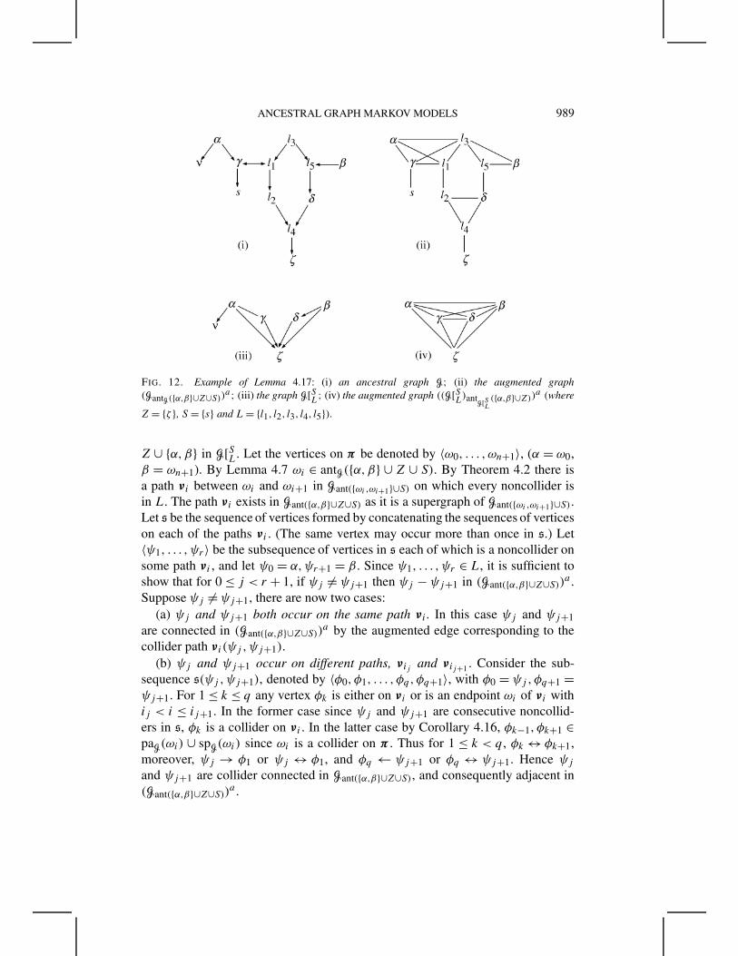
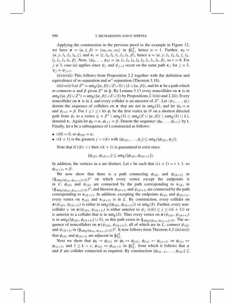
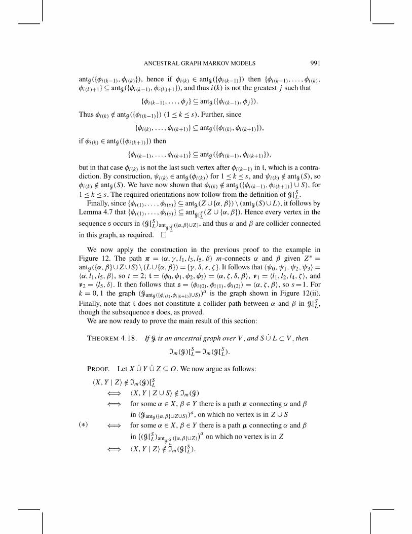
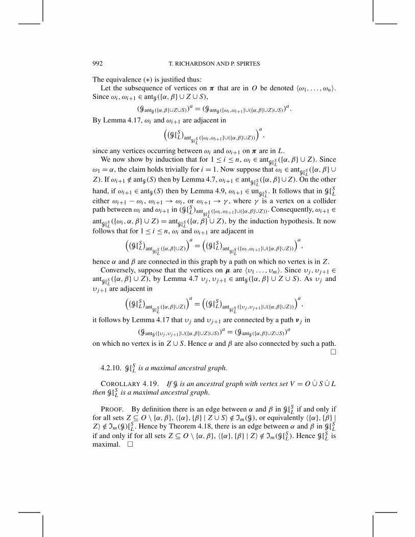
ANCESTRAL GRAPH MARKOV MODELS 989
FIG. 12. Example of Lemma 4.17: (i) an ancestral graph G; (ii) the augmented graph(GantG({α,β}∪Z∪S))
a ; (iii) the graph G[SL; (iv) the augmented graph ((G[SL)antG[S
L({α,β}∪Z))
a (where
Z = {ζ }, S = {s} and L = {l1, l2, l3, l4, l5}).
Z ∪ {α,β} in G[SL. Let the vertices on π be denoted by 〈ω0, . . . ,ωn+1〉, (α = ω0,β = ωn+1). By Lemma 4.7 ωi ∈ antG({α,β} ∪ Z ∪ S). By Theorem 4.2 there isa path νi between ωi and ωi+1 in Gant({ωi ,ωi+1}∪S) on which every noncollider isin L. The path νi exists in Gant({α,β}∪Z∪S) as it is a supergraph of Gant({ωi ,ωi+1}∪S).Let s be the sequence of vertices formed by concatenating the sequences of verticeson each of the paths νi . (The same vertex may occur more than once in s.) Let〈ψ1, . . . ,ψr〉 be the subsequence of vertices in s each of which is a noncollider onsome path νi , and let ψ0 = α,ψr+1 = β . Since ψ1, . . . ,ψr ∈ L, it is sufficient toshow that for 0 ≤ j < r + 1, if ψj �= ψj+1 then ψj − ψj+1 in (Gant({α,β}∪Z∪S))
a .Suppose ψj �= ψj+1, there are now two cases:
(a) ψj and ψj+1 both occur on the same path νi . In this case ψj and ψj+1
are connected in (Gant({α,β}∪Z∪S))a by the augmented edge corresponding to the
collider path νi(ψj ,ψj+1).(b) ψj and ψj+1 occur on different paths, νij and νij+1 . Consider the sub-
sequence s(ψj ,ψj+1), denoted by 〈φ0, φ1, . . . , φq,φq+1〉, with φ0 = ψj ,φq+1 =ψj+1. For 1 ≤ k ≤ q any vertex φk is either on νi or is an endpoint ωi of νi withij < i ≤ ij+1. In the former case since ψj and ψj+1 are consecutive noncollid-ers in s, φk is a collider on νi . In the latter case by Corollary 4.16, φk−1, φk+1 ∈paG(ωi) ∪ spG(ωi) since ωi is a collider on π . Thus for 1 ≤ k < q , φk ↔ φk+1,moreover, ψj → φ1 or ψj ↔ φ1, and φq ← ψj+1 or φq ↔ ψj+1. Hence ψj
and ψj+1 are collider connected in Gant({α,β}∪Z∪S), and consequently adjacent in(Gant({α,β}∪Z∪S))
a .
990 T. RICHARDSON AND P. SPIRTES
Applying the construction in the previous proof to the example in Figure 12,we have π = 〈α, ζ,β〉 = 〈ω0,ω1,ω2〉 in G[SL, hence n = 1. Further, ν0 =〈α,γ, l1, l2, l4, ζ 〉 and ν1 = 〈ζ, l4, l2, l1, l3, l5, β〉, hence s = 〈α,γ, l1, l2, l4, ζ, l4,l2, l1, l3, l5, β〉. Now, 〈ψ0, . . . ,ψ9〉 = 〈α, l1, l2, l4, l4, l2, l1, l3, l5, β〉, so r = 8. Forj �= 3, case (a) applies since ψj and ψj+1 occur on the same path νi ; for j = 3,ψj = ψj+1.
(ii)⇔(iii) This follows from Proposition 2.2 together with the definition andequivalence of m-separation and m∗-separation (Theorem 3.18).
(iii)⇒(i) Let Z∗ = antG({α,β}∪Z∪S)\ (L∪{α,β}), and let π be a path whichm-connects α and β given Z∗ in G. By Lemma 3.13 every noncollider on π is inantG({α,β} ∪Z∗) = antG({α,β} ∪Z∪S) by Propositions 2.1(iii) and 2.2(i). Everynoncollider on π is in L and every collider is an ancestor of Z∗. Let 〈ψ1, . . . ,ψt〉denote the sequence of colliders on π that are not in antG(S), and let ψ0 = α
and ψt+1 = β . For 1 ≤ i ≤ t let φi be the first vertex in O on a shortest directedpath from ψi to a vertex ζi ∈ Z∗ \ antG(S) ⊂ antG(Z ∪ {α,β}) \ (antG(S) ∪ L),denoted νi . Again let φ0 = α, φt+1 = β . Denote the sequence 〈φ0, . . . , φt+1〉 by t.Finally, let s be a subsequence of t constructed as follows:
• i(0) = 0, so φi(0) = α;• i(k + 1) is the greatest j > i(k) with {φi(k), . . . , φj } ⊆ antG({φi(k), φj }).
Note that if i(k) < t then i(k + 1) is guaranteed to exist since
{φi(k), φi(k)+1} ⊆ antG({φi(k), φi(k)+1}).In addition, the vertices in s are distinct. Let s be such that i(s + 1) = t + 1, soφi(s+1) = β .
We now show that there is a path connecting φi(k) and φi(k+1) in(GantG({φi(k),φi(k+1)}∪S))
a on which every vertex except the endpoints isin L: φi(k) and ψi(k) are connected by the path corresponding to νi(k) in(GantG({φi(k),φi(k+1)}∪S))
a , and likewise φi(k+1) and ψi(k+1) are connected by the pathcorresponding to νi(k+1). In addition, excepting the endpoints φi(k) and φi(k+1),every vertex on νi(k) and νi(k+1) is in L. By construction, every collider onπ(ψi(k),ψi(k+1)) is either in antG({φi(k), φi(k+1)}) or antG(S). Further, every non-collider γ on π(ψi(k),ψi(k+1)) is either anterior to ψj (i(k) ≤ j ≤ i(k + 1)) oris anterior to a collider that is in antG(S). Thus every vertex on π(ψi(k),ψi(k+1))
is in antG({φi(k), φi(k+1)} ∪ S), so this path exists in GantG({φi(k),φi(k+1)}∪S). The se-quence of noncolliders on π(ψi(k),ψi(k+1)), all of which are in L, connect ψi(k)
and ψi(k+1) in (GantG({φi(k),φi(k+1)}∪S))a . It now follows from Theorem 4.2 (iii)⇔(i)
that φi(k) and φi(k+1) are adjacent in G[SL.Next we show that φ0 → φi(1) or φ0 ↔ φi(1), φi(s) ← φi(s+1) or φi(s) ↔
φi(s+1) and 1 ≤ k < s, φi(k) ↔ φi(k+1) in G[SL, from which it follows that α
and β are collider connected as required. By construction {φi(k−1), . . . , φi(k)} ⊆
ANCESTRAL GRAPH MARKOV MODELS 991
antG({φi(k−1), φi(k)}), hence if φi(k) ∈ antG({φi(k−1)}) then {φi(k−1), . . . , φi(k),
φi(k)+1} ⊆ antG({φi(k−1), φi(k)+1}), and thus i(k) is not the greatest j such that
{φi(k−1), . . . , φj } ⊆ antG({φi(k−1), φj }).Thus φi(k) /∈ antG({φi(k−1)}) (1 ≤ k ≤ s). Further, since
{φi(k), . . . , φi(k+1)} ⊆ antG({φi(k), φi(k+1)}),if φi(k) ∈ antG({φi(k+1)}) then
{φi(k−1), . . . , φi(k+1)} ⊆ antG({φi(k−1), φi(k+1)}),but in that case φi(k) is not the last such vertex after φi(k−1) in t, which is a contra-diction. By construction, ψi(k) ∈ antG(φi(k)) for 1 ≤ k ≤ s, and ψi(k) /∈ antG(S), soφi(k) /∈ antG(S). We have now shown that φi(k) /∈ antG({φi(k−1), φi(k+1)} ∪ S), for1 ≤ k ≤ s. The required orientations now follow from the definition of G[SL.
Finally, since {φi(1), . . . , φi(s)} ⊆ antG(Z ∪ {α,β})\ (antG(S)∪L), it follows byLemma 4.7 that {φi(1), . . . , φi(s)} ⊆ antG[SL(Z ∪ {α,β}). Hence every vertex in the
sequence s occurs in (G[SL)antG[S
L({α,β}∪Z), and thus α and β are collider connected
in this graph, as required. �
We now apply the construction in the previous proof to the example inFigure 12. The path π = 〈α,γ, l1, l3, l5, β〉 m-connects α and β given Z∗ =antG({α,β}∪Z∪S)\(L∪{α,β}) = {γ, δ, s, ζ }. It follows that 〈ψ0,ψ1,ψ2,ψ3〉 =〈α, l1, l5, β〉, so t = 2; t = 〈φ0, φ1, φ2, φ3〉 = 〈α, ζ, δ,β〉, ν1 = 〈l1, l2, l4, ζ 〉, andν2 = 〈l5, δ〉. It then follows that s = 〈φi(0), φi(1), φi(2)〉 = 〈α, ζ,β〉, so s=1. Fork = 0,1 the graph (GantG({φi(k),φi(k+1)}∪S))
a is the graph shown in Figure 12(ii).Finally, note that t does not constitute a collider path between α and β in G[SL,though the subsequence s does, as proved.
We are now ready to prove the main result of this section:
THEOREM 4.18. If G is an ancestral graph over V , and S ∪ L ⊂ V , then
Im(G)[SL= Im(G[SL).
PROOF. Let X ∪ Y ∪ Z ⊆ O. We now argue as follows:
〈X,Y | Z〉 /∈ Im(G)[SL⇐⇒ 〈X,Y | Z ∪ S〉 /∈ Im(G)
⇐⇒ for some α ∈ X, β ∈ Y there is a path π connecting α and β
in (GantG({α,β}∪Z∪S))a , on which no vertex is in Z ∪ S
⇐⇒ for some α ∈ X, β ∈ Y there is a path µ connecting α and β
in((G[SL)ant
G[SL({α,β}∪Z)
)a on which no vertex is in Z
⇐⇒ 〈X,Y | Z〉 /∈ Im(G[SL).
(∗)
992 T. RICHARDSON AND P. SPIRTES
The equivalence (∗) is justified thus:Let the subsequence of vertices on π that are in O be denoted 〈ω1, . . . ,ωn〉.
Since ωi,ωi+1 ∈ antG({α,β} ∪ Z ∪ S),
(GantG({α,β}∪Z∪S))a = (GantG({ωi ,ωi+1}∪({α,β}∪Z)∪S))
a.
By Lemma 4.17, ωi and ωi+1 are adjacent in((G[SL
)ant
G[SL({ωi,ωi+1}∪({α,β}∪Z))
)a,
since any vertices occurring between ωi and ωi+1 on π are in L.We now show by induction that for 1 ≤ i ≤ n, ωi ∈ antG[SL({α,β} ∪ Z). Since
ω1 = α, the claim holds trivially for i = 1. Now suppose that ωi ∈ antG[SL({α,β} ∪Z). If ωi+1 /∈ antG(S) then by Lemma 4.7, ωi+1 ∈ antG[SL({α,β} ∪Z). On the other
hand, if ωi+1 ∈ antG(S) then by Lemma 4.9, ωi+1 ∈ unG[SL . It follows that in G[SLeither ωi+1 − ωi , ωi+1 → ωi , or ωi+1 → γ , where γ is a vertex on a colliderpath between ωi and ωi+1 in (G[SL)ant
G[SL({ωi ,ωi+1}∪({α,β}∪Z)). Consequently, ωi+1 ∈
antG[SL({ωi,α,β} ∪ Z) = antG[SL({α,β} ∪ Z), by the induction hypothesis. It nowfollows that for 1 ≤ i ≤ n, ωi and ωi+1 are adjacent in((
G[SL)ant
G[SL({α,β}∪Z)
)a =((
G[SL)ant
G[SL({ωi,ωi+1}∪({α,β}∪Z))
)a,
hence α and β are connected in this graph by a path on which no vertex is in Z.Conversely, suppose that the vertices on µ are 〈υ1 . . . , υm〉. Since υj ,υj+1 ∈
antG[SL({α,β} ∪ Z), by Lemma 4.7 υj ,υj+1 ∈ antG({α,β} ∪ Z ∪ S). As υj andυj+1 are adjacent in((
G[SL)ant
G[SL({α,β}∪Z)
)a =((
G[SL)ant
G[SL({υj ,υj+1}∪({α,β}∪Z))
)a,
it follows by Lemma 4.17 that υj and υj+1 are connected by a path νj in
(GantG({υj ,υj+1}∪({α,β}∪Z)∪S))a = (GantG({α,β}∪Z∪S))
a
on which no vertex is in Z ∪ S. Hence α and β are also connected by such a path.�
4.2.10. G[SL is a maximal ancestral graph.
COROLLARY 4.19. If G is an ancestral graph with vertex set V = O ∪ S ∪ L
then G[SL is a maximal ancestral graph.
PROOF. By definition there is an edge between α and β in G[SL if and only iffor all sets Z ⊆ O \ {α,β}, 〈{α}, {β} | Z ∪ S〉 /∈ Im(G), or equivalently 〈{α}, {β} |Z〉 /∈ Im(G)[SL. Hence by Theorem 4.18, there is an edge between α and β in G[SLif and only if for all sets Z ⊆ O \ {α,β}, 〈{α}, {β} | Z〉 /∈ Im(G[SL). Hence G[SL ismaximal. �
ANCESTRAL GRAPH MARKOV MODELS 993
4.2.11. Commutativity.
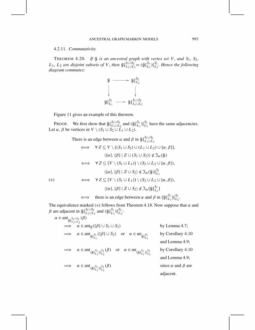
THEOREM 4.20. If G is an ancestral graph with vertex set V , and S1, S2,L1, L2 are disjoint subsets of V , then G[S1∪S2
L1∪L2= (G[S1
L1)[S2
L2. Hence the following
diagram commutes:
G G[S2L2
G[S1L1
G[S1∪S2L1∪L2
Figure 11 gives an example of this theorem.
PROOF. We first show that G[S1∪S2L1∪L2
and (G[S1L1
)[S2L2
have the same adjacencies.Let α, β be vertices in V \ (S1 ∪ S2 ∪ L1 ∪ L2).
There is an edge between α and β in G[S1∪S2L1∪L2
⇐⇒ ∀Z ⊆ V \ ((S1 ∪ S2) ∪ (L1 ∪ L2) ∪ {α,β}),〈{α}, {β} | Z ∪ (S1 ∪ S2)〉 /∈ Im(G)
⇐⇒ ∀Z ⊆ (V \ (S1 ∪ L1)
) \ (S2 ∪ L2 ∪ {α,β}),〈{α}, {β} | Z ∪ S2〉 /∈ Im(G)[S1
L1
⇐⇒ ∀Z ⊆ (V \ (S1 ∪ L1)
) \ (S2 ∪ L2 ∪ {α,β}),〈{α}, {β} | Z ∪ S2〉 /∈ Im
(G[S1
L1
)⇐⇒ there is an edge between α and β in
(G[S1
L1
)[S2L2
.
(∗)
The equivalence marked (∗) follows from Theorem 4.18. Now suppose that α andβ are adjacent in G[S1∪S2
L1∪L2and (G[S1
L1)[S2
L2:
α ∈ antG[S1∪S2
L1∪L2
(β)
'⇒ α ∈ antG({β} ∪ S1 ∪ S2) by Lemma 4.7;
'⇒ α ∈ antG[S1
L1
({β} ∪ S2) or α ∈ unG[S1
L1
by Corollary 4.10
and Lemma 4.9;
'⇒ α ∈ ant(G[S1
L1)[S2
L2
(β) or α ∈ un(G[S1
L1)[S2
L2
by Corollary 4.10
and Lemma 4.9;
'⇒ α ∈ ant(G[S1
L1)[S2
L2
(β) since α and β are
adjacent.
994 T. RICHARDSON AND P. SPIRTES
Arguing in the other direction,
α ∈ ant(G[S1
L1)[S2
L2
(β)
'⇒ α ∈ antG[S1
L1
({β} ∪ S2) by Lemma 4.7;
'⇒ α ∈ antG({β} ∪ S1 ∪ S2) by Lemma 4.7;
'⇒ α ∈ antG[S1∪S2
L1∪L2
(β) or α ∈ unG[S1∪S2
L1∪L2
by Corollary 4.10and Lemma 4.9;
'⇒ α ∈ antG[S1∪S2
L1∪L2
(β) since α and β areadjacent.
It then follows from Corollary 3.10 that G[S1∪S2L1∪L2
= (G[S1L1
)[S2L2
as required. �
5. Extending an ancestral graph. In this section we prove two extensionresults. We first show that every ancestral graph can be extended to a maximalancestral graph, as stated in Section 3.7. We then show that every maximalancestral graph may be extended to a complete ancestral graph, and that the edgeadditions may be ordered so that all the intermediate graphs are also maximal. Thislatter result parallels well known results for decomposable undirected graphs [seeLauritzen (1996), page 20].
5.1. Extension of an ancestral graph to a maximal ancestral graph.
THEOREM 5.1. If G is an ancestral graph then there exists a unique maximalancestral graph G formed by adding bidirected edges to G such that Im(G) =Im(G).
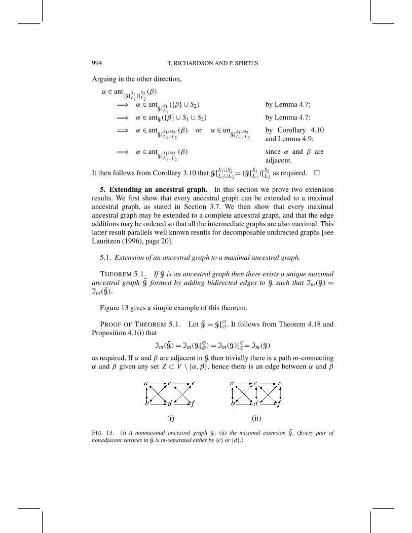
Figure 13 gives a simple example of this theorem.
PROOF OF THEOREM 5.1. Let G = G[∅∅. It follows from Theorem 4.18 andProposition 4.1(i) that
Im(G) = Im(G[∅∅) = Im(G)[∅
∅= Im(G)
as required. If α and β are adjacent in G then trivially there is a path m-connectingα and β given any set Z ⊂ V \ {α,β}, hence there is an edge between α and β
FIG. 13. (i) A nonmaximal ancestral graph G; (ii) the maximal extension G. (Every pair ofnonadjacent vertices in G is m-separated either by {c} or {d}.)
ANCESTRAL GRAPH MARKOV MODELS 995
in G[∅∅. Now, by Corollary 4.8, antG(α) = antG[∅∅
(α). Hence by Lemma 3.9 every
edge in G is inherited by G = G[∅∅. By Corollary 4.19 G[∅∅ is maximal. Thisestablishes the existence of a maximal extension of G.
Let G be a maximal supergraph of G. Suppose α and β are adjacent in G but arenot adjacent in G. By Corollary 4.3 there is a primitive inducing path π betweenα and β in G, containing more than one edge. Since π is present in G, and thisgraph is maximal, it follows by Corollary 4.6 that α ↔ β in G, as required. Thisalso establishes uniqueness of G. �
Three corollaries are consequences of this result:
COROLLARY 5.2. G is a maximal ancestral graph if and only if G = G[∅∅.
PROOF. Follows directly from the definition of G[∅∅ and Theorem 5.1. �
The next corollary establishes the pairwise Markov property referred to inSection 3.7.
COROLLARY 5.3. If G is a maximal ancestral graph and α, β are not adjacentin G, then 〈{α}, {β} | antG({α,β}) \ {α,β}〉 ∈ Im(G).
PROOF. By Corollary 5.2, G = G[∅∅. The result then follows by contrapositionfrom Theorem 4.2 and properties (i) and (iv). �
COROLLARY 5.4. If G is an ancestral graph, α ∈ antG(β), and α, β are notadjacent in G then 〈{α}, {β} | antG({α,β}) \ {α,β}〉 ∈ Im(G).
PROOF. If α ∈ antG(β) then by Corollary 4.8, α ∈ antG[∅∅
(β). Hence there is
no edge α ↔ β in G[∅∅, since by Theorem 4.12, G[∅∅ is ancestral. It follows fromTheorem 5.1 that α and β are not adjacent in G[∅∅. The conclusion then followsfrom Corollary 5.3. �
5.2. Extension of a maximal ancestral graph to a complete graph. For anancestral graph G = (V,E), the associated complete graph, denoted G, is definedas follows:
G has vertex set V and an edge between every pair of distinct vertices α, β ,specified as:
α − β if α,β ∈ unG,
α → β if α ∈ unG ∪ antG(β) and β /∈ unG,
α ↔ β otherwise.
996 T. RICHARDSON AND P. SPIRTES
Thus between each pair of distinct vertices in G there will be exactly one edge.Note that although G is unique as defined, in general there will be other completeancestral graphs of which a given graph G is a subgraph.
LEMMA 5.5. If G = (V,E) is an ancestral graph, then: (i) G is a subgraphof G; (ii) unG = unG; (iii) for all ν ∈ V , antG(ν) = antG(ν) ∪ unG; (iv) G is anancestral graph.
PROOF. (i) This follows from the construction of G, Lemma 3.7, and paG(ν) ⊆antG(ν).
(ii) By construction, if α ∈ unG then paG(α) ∪ spG(α) = ∅ hence α ∈ unG.Conversely, if α /∈ unG then paG(α) ∪ spG(α) �= ∅. By (i), paG(α) ∪ spG(α) �= ∅,so α /∈ unG. Thus unG = unG as required.
(iii) By (i), antG(ν) ⊆ antG(ν), further, by construction, unG ⊆ antG(ν), thusantG(ν) ∪ unG ⊆ antG(ν). Conversely, if α ∈ antG(ν0) then either α ∈ unG = unG
by (ii) or α /∈ unG. In the latter case, by construction of G there is a directed pathα → νn → · · · → ν0 in G, and every vertex on the path is in V \ unG. Henceα ∈ antG(νn), and νi ∈ antG(νi−1) (i = 1, . . . , n), so α ∈ antG(ν0).
(iv) If β → α in G then, by the construction of G, α /∈ unG and β ∈ antG(α) ∪unG. Hence, by Lemma 3.8(ii), α /∈ antG(β) and thus α /∈ antG(β), by (iii).Similarly, if β ↔ α in G then by construction, α /∈ unG ∪ antG(β), hence againby (iii), α /∈ antG(β). Thus α /∈ antG(paG(α) ∪ spG(α)), so (i) in the definition of
an ancestral graph holds. By the construction of G, if neG(α) �= ∅ then α ∈ unG,and thus, again by construction, spG(α) ∪ paG(α) = ∅, hence (ii) in the definitionholds as required. �
THEOREM 5.6. If G is a maximal ancestral graph with r pairs of vertices thatare not adjacent, and G∗ is any complete supergraph of G with unG = unG∗ thenthere exists a sequence of maximal ancestral graphs
G∗ ≡ G0, . . . ,Gr ≡ G
where Gi+1 is a subgraph of Gi containing one less edge εi than Gi , and unGi+1 =unGi
.The sequence of edges removed, 〈ε0, . . . ,εr−1〉, is such that no undirected edge
is removed after a directed edge and no directed edge is removed after a bidirectededge.
Two examples of this theorem are shown in Figure 14. (The existence of at leastone complete ancestral supergraph G∗ of G is guaranteed by the previous lemma.)
PROOF OF THEOREM 5.6. Let E be the set of edges that are in G0 ≡ G∗ butnot G. Place an ordering ≺ on E as follows:
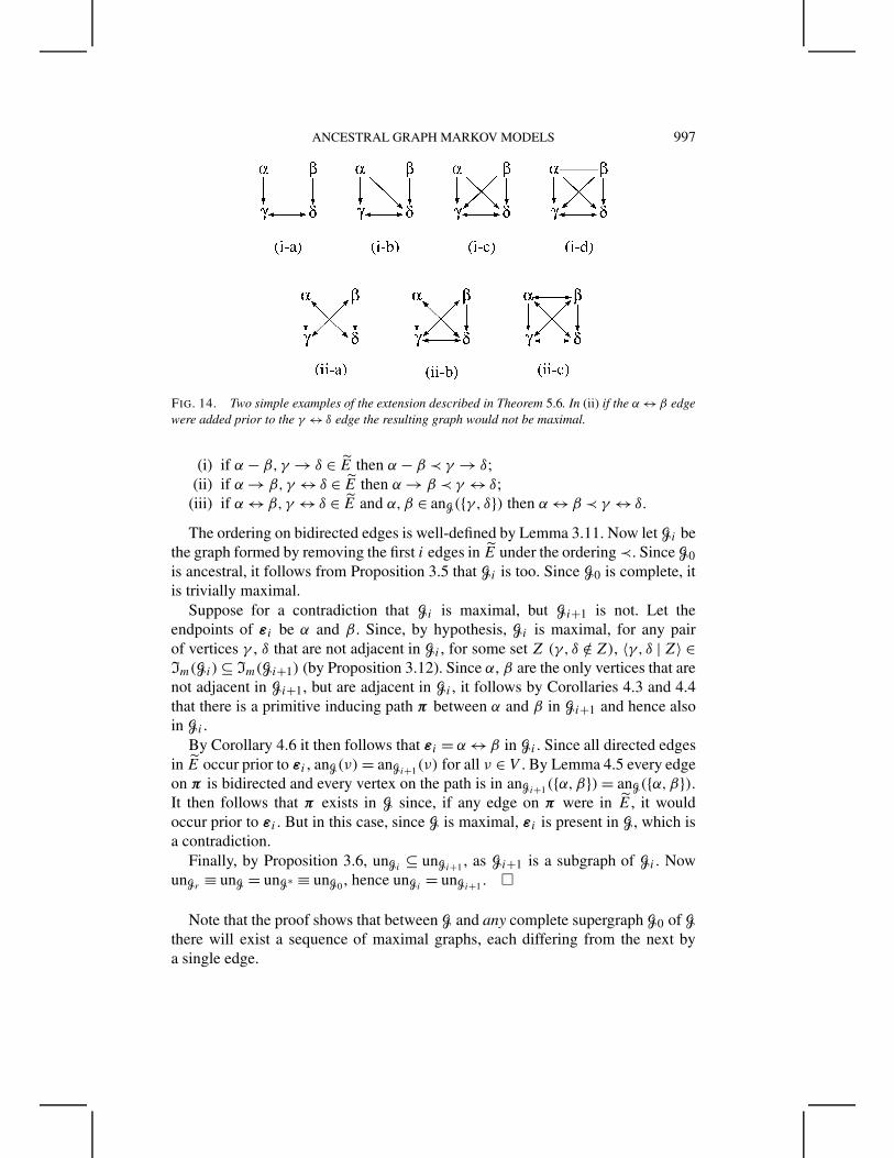
ANCESTRAL GRAPH MARKOV MODELS 997
FIG. 14. Two simple examples of the extension described in Theorem 5.6. In (ii) if the α ↔ β edgewere added prior to the γ ↔ δ edge the resulting graph would not be maximal.
(i) if α − β,γ → δ ∈ E then α − β ≺ γ → δ;(ii) if α → β,γ ↔ δ ∈ E then α → β ≺ γ ↔ δ;
(iii) if α ↔ β,γ ↔ δ ∈ E and α,β ∈ anG({γ, δ}) then α ↔ β ≺ γ ↔ δ.
The ordering on bidirected edges is well-defined by Lemma 3.11. Now let Gi bethe graph formed by removing the first i edges in E under the ordering ≺. Since G0is ancestral, it follows from Proposition 3.5 that Gi is too. Since G0 is complete, itis trivially maximal.
Suppose for a contradiction that Gi is maximal, but Gi+1 is not. Let theendpoints of εi be α and β . Since, by hypothesis, Gi is maximal, for any pairof vertices γ , δ that are not adjacent in Gi , for some set Z (γ, δ /∈ Z), 〈γ, δ | Z〉 ∈Im(Gi) ⊆ Im(Gi+1) (by Proposition 3.12). Since α, β are the only vertices that arenot adjacent in Gi+1, but are adjacent in Gi , it follows by Corollaries 4.3 and 4.4that there is a primitive inducing path π between α and β in Gi+1 and hence alsoin Gi .
By Corollary 4.6 it then follows that εi = α ↔ β in Gi . Since all directed edgesin E occur prior to εi , anG(ν) = anGi+1(ν) for all ν ∈ V . By Lemma 4.5 every edgeon π is bidirected and every vertex on the path is in anGi+1({α,β}) = anG({α,β}).It then follows that π exists in G since, if any edge on π were in E, it wouldoccur prior to εi . But in this case, since G is maximal, εi is present in G, which isa contradiction.
Finally, by Proposition 3.6, unGi⊆ unGi+1 , as Gi+1 is a subgraph of Gi . Now
unGr ≡ unG = unG∗ ≡ unG0 , hence unGi= unGi+1 . �
Note that the proof shows that between G and any complete supergraph G0 of Gthere will exist a sequence of maximal graphs, each differing from the next bya single edge.
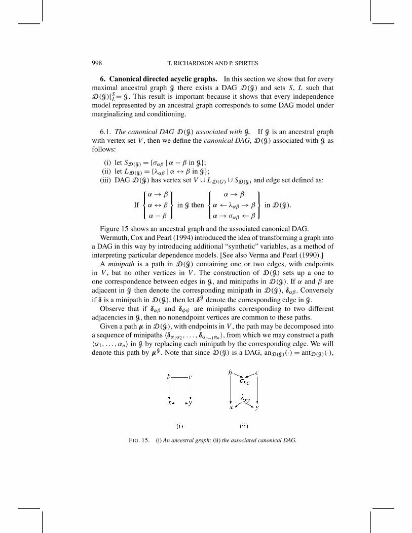
998 T. RICHARDSON AND P. SPIRTES
6. Canonical directed acyclic graphs. In this section we show that for everymaximal ancestral graph G there exists a DAG D(G) and sets S, L such thatD(G)[SL= G. This result is important because it shows that every independencemodel represented by an ancestral graph corresponds to some DAG model undermarginalizing and conditioning.
6.1. The canonical DAG D(G) associated with G. If G is an ancestral graphwith vertex set V , then we define the canonical DAG, D(G) associated with G asfollows:
(i) let SD(G) = {σαβ | α − β in G};(ii) let LD(G) = {λαβ | α ↔ β in G};
(iii) DAG D(G) has vertex set V ∪ LD(G) ∪ SD(G) and edge set defined as:
If
α → β
α ↔ β
α − β
in G then
α → β
α ← λαβ → β
α → σαβ ← β
in D(G).
Figure 15 shows an ancestral graph and the associated canonical DAG.Wermuth, Cox and Pearl (1994) introduced the idea of transforming a graph into
a DAG in this way by introducing additional “synthetic” variables, as a method ofinterpreting particular dependence models. [See also Verma and Pearl (1990).]
A minipath is a path in D(G) containing one or two edges, with endpointsin V , but no other vertices in V . The construction of D(G) sets up a one toone correspondence between edges in G, and minipaths in D(G). If α and β areadjacent in G then denote the corresponding minipath in D(G), δαβ . Converselyif δ is a minipath in D(G), then let δG denote the corresponding edge in G.
Observe that if δαβ and δφψ are minipaths corresponding to two differentadjacencies in G, then no nonendpoint vertices are common to these paths.
Given a path µ in D(G), with endpoints in V , the path may be decomposed intoa sequence of minipaths 〈δα1α2, . . . , δαn−1αn〉, from which we may construct a path〈α1, . . . , αn〉 in G by replacing each minipath by the corresponding edge. We willdenote this path by µG. Note that since D(G) is a DAG, anD(G)(·) = antD(G)(·),
FIG. 15. (i) An ancestral graph; (ii) the associated canonical DAG.
ANCESTRAL GRAPH MARKOV MODELS 999
and by definition a path µ is m-connecting if and only if it is d-connecting. Sinceit helps to make clear that we are referring to a path in a DAG, we will onlyuse the term “d-connecting” when referring to a path which is m-connecting (andd-connecting) in D(G).
6.1.1. Graphical properties of D(G).
LEMMA 6.1. Let G be an ancestral graph with vertex set V .
(i) If β ∈ V then anD(G)(β) ∩ V = anG(β).(ii) anD(G)(SD(G)) = paD(G)(SD(G)) ∪ SD(G), so anD(G)(SD(G)) ⊆ SD(G) ∪
unG.(iii) anD(G)(SD(G)) ∩ LD(G) = ∅.
PROOF. (i) If α,β ∈ V and α ∈ anD(G)(β) then there is a directed path δ fromα to β in D(G). Every nonendpoint vertex on δ has at least one parent and at leastone child in D(G), hence every vertex on δ is in V [since chD(G)(SD(G)) = ∅ =paD(G)(LD(G))]. It then follows from the construction of D(G) that δ exists in G,so α ∈ anG(β). It also follows from the construction of D(G) that any directedpath in G exists in D(G).
(ii) By construction, paD(G)(σαβ) = {α,β} ⊆ unG (by Lemma 3.7). Butagain, by construction, paD(G)(unG) = ∅. Hence anD(G)(σαβ) = {α,β,σαβ} ⊆unG ∪ {σαβ}, so anD(G)(SD(G)) ⊆ unG ∪SD(G).
(iii) This follows from the previous property:
anD(G)(SD(G)) ∩ LD(G) ⊆ (unG ∪SD(G)) ∩ LD(G)
⊆ (V ∪ SD(G)) ∩ LD(G) = ∅. �
Note that antG(β) �= antD(G)(β) for β ∈ V , because an undirected edge α − β
in G is replaced by α → σαβ ← β in D(G).
LEMMA 6.2. G is a subgraph of D(G)[SD(G)
LD(G).
PROOF. First recall that anD(G)(·) = antD(G)(·) since D(G) is a DAG. We nowconsider each of the edges occurring in G:
(i) If α − β in G then α → σαβ ← β in D(G), so α,β ∈ antD(G)(SD(G)). It
then follows that α − β in D(G)[SD(G)
LD(G).
(ii) If α → β in G then α → β in D(G), so α ∈ antD(G)(β). By Lemma 6.1(i),β /∈ antD(G)(α), and since further, β /∈ SD(G) ∪ unG, by Lemma 6.1(ii), β /∈antD(G)(SD(G)). It then follows from the definition of the transformation that
α → β in D(G)[SD(G)
LD(G).
1000 T. RICHARDSON AND P. SPIRTES
(iii) Likewise, if α ↔ β in G then α ← λαβ → β in D(G). By Lemma 6.1(i)and (ii), it follows as in case (ii) that β /∈ antD(G)({α} ∪ SD(G)), and by symmetry,
α /∈ antD(G)({β} ∪ SD(G)). Hence α ↔ β in D(G)[SD(G)
LD(G). �
6.2. The independence model Im(D(G)[SD(G)
LD(G)).
THEOREM 6.3. If G is an ancestral graph then
Im(G) = Im
(D(G)
)[SD(G)
LD(G)= Im
(D(G)[SD(G)
LD(G)
).
It follows from this result that the global Markov property for ancestral graphsmay be reduced to that for DAGs: X is m-separated from Y given Z in G if andonly if X is d-separated from Y given Z ∪ SD(G). (However, see Section 8.6 forrelated comments concerning parameterization.)
It also follows from this result that the class of independence models associatedwith ancestral graphs is the smallest class that contains the DAG independencemodels and is closed under marginalizing and conditioning.
PROOF OF THEOREM 6.3. We break the proof into three parts:
Part 1. Im(D(G))[SD(G)
LD(G)= Im(D(G)[SD(G)
LD(G)) by Theorem 4.18.
Part 2. Im(G) ⊆ Im(D(G))[SD(G)
LD(G). Suppose G has vertex set V , containing
vertices α, β , and set Z (α,β /∈ Z). It is sufficient to prove that if there is a path µwhich d-connects α and β given Z ∪ SD(G) in D(G) then µG m-connects α and β
given Z in G.Suppose that γ is a collider on µG. In this case γ is a collider on µ since
the corresponding minipaths collide at γ in D(G). Since µ is d-connecting givenZ ∪ SD(G) and γ ∈ V ,
γ ∈ (anD(G)(Z ∪ SD(G))
) ∩ V = (anD(G)(Z) ∩ V
) ∪ (anD(G)(SD(G)) ∩ V
),
by Proposition 2.1. But γ /∈ unG, so by Lemma 6.1(ii), γ /∈ anD(G)(SD(G)). Henceγ ∈ (anD(G)(Z) ∩ V ) = anG(Z), the equality following from Lemma 6.1(i).
If γ is a noncollider on µG then γ is a noncollider on µ, so γ /∈ Z ∪ SD(G), thusγ /∈ Z as required.
Part 3. Im(D(G)[SD(G)
LD(G)) ⊆ Im(G). By Lemma 6.2 G is a subgraph of
D(G)[SD(G)
LD(G), and the result then follows by Proposition 3.12. �
6.2.1. If G is maximal then D(G)[SD(G)
LD(G)= G. We now prove the result
mentioned at the start of this section:
THEOREM 6.4. If G is a maximal ancestral graph then
D(G)[SD(G)
LD(G)= G.
ANCESTRAL GRAPH MARKOV MODELS 1001
PROOF. By Lemma 6.2 G is a subgraph of D(G)[SD(G)
LD(G), while by Theorem 6.3
these graphs correspond to the same independence model. It then follows from the
maximality of G that D(G)[SD(G)
LD(G)= G. �
7. Probability distributions. In this section we relate the operations ofmarginalizing and conditioning that have been defined for independence modelsand graphs to probability distributions.
7.1. Marginalizing and conditioning distributions. For a graph G with vertexset V we consider collections of random variables (Xν)ν∈V taking values inprobability spaces (Xν)ν∈V . In all the examples we consider, the probability spacesare either real finite-dimensional vector spaces or finite discrete sets. For A ⊆ V
we let XA ≡ ×v∈A(Xν), X ≡ XV and XA ≡ (Xν)ν∈A.If P is a probability measure on XV then as usual we define the distribution after
marginalizing over XL, here denoted P [XLor PXV \L , to be a probability measure
on XV \L, such that
P [XL(E) ≡ PXV \L(E) = P (〈XV \L,XL〉 ∈ E × XL).
We will assume the existence of a regular conditional probability measure, denotedP [XS=xS (·) or P (· | XS = xS), for all xS ∈ XS so that∫
FP [XS=xS (E)dPXS
(xS) = P(〈XV \S,XS〉 ∈ E × F
).
This defines P [XS=xS (·) up to almost sure equivalence under PXS. Likewise we
define
P [XS=xSXL
(·) ≡ (P [XS=xS )[XL(·).
7.2. The set of distributions obeying an independence model [P (I)]. Wedefine conditional independence under P as follows:
A |= B | C[P ] ⇐⇒ P [XC=xCXV \(A∪C)
(·) = P [XB=xB,XC=xCXV \(A∪B∪C)
(·) (PXB∪Ca.e.)
where we have used the usual shorthand notation: A denotes both a vertex set andthe random variable XA.
For an independence model I over V let P (I) be the set of distributions P on X
such that for arbitrary disjoint sets A, B , Z (Z may be empty),
if 〈A,B | Z〉 ∈ I then A |= B | Z[P ].Note that if P ∈ P (I) then there may be independence relations that are not in I
that also hold in P .A distribution P is said to be faithful or Markov perfect with respect to an
independence model I if
〈A,B | Z〉 ∈ I if and only if A |= B | Z[P ].An independence model I is said to be probabilistic if there is a distribution P thatis faithful to I.
1002 T. RICHARDSON AND P. SPIRTES
7.3. Relating P (Im(G)) and P (Im(G[SL)).
THEOREM 7.1. Let I be an independence model over V with S ∪ L ⊂ V . IfP ∈ P (I) then
P [XS=xsXL
∈ P(I[SL
)(PXS
a.e.).
PROOF. Suppose 〈X,Y | Z〉 ∈ I[SL. It follows that 〈X,Y | Z ∪ S〉 ∈ I and(X ∪ Y ∪ Z) ⊆ V \ (S ∪ L). Hence, if P ∈ P (I) and 〈X,Y | Z〉 ∈ I[SL then
X |= Y | Z ∪ S [P ],hence
X |= Y | Z [P [XS=xs
XL
](PXS
a.e.).
[The last step follows from the assumption that regular conditional probabilitymeasures exist. See Koster (1999a), Appendix A and B.] Since there are finitelymany triples 〈X,Y | Z〉 ∈ I[SL, it follows that
P [XS=xSXL
∈ P(I[SL
)(PXS
a.e.),
as required. �
Two corollaries follow from this result:
COROLLARY 7.2. If G is an ancestral graph and P ∈ P (Im(G)) then
P [XS=xSXL
∈ P(Im(G)[SL
) = P(Im
(G[SL
))(PXS
a.e.).
PROOF. This follows directly from Theorem 7.1 and Theorem 4.18. �
COROLLARY 7.3. If N is a normal distribution, faithful to an independencemodel I over vertex set V then N [XS=xs
XLis faithful to I[SL.
PROOF. Since N ∈ P (I), by normality and Theorem 7.1, N [XS=xsXL
∈ P (I[SL).Now suppose 〈X,Y | Z〉 /∈ I[SL where X ∪ Y ∪ Z ⊆ V \ (S ∪ L). Hence 〈X,Y |Z ∪ S〉 /∈ I. Since N is faithful to I
X /|= Y | Z ∪ S [N ] which implies X /|= Y | Z [N [XS=xs
XL
]for any xS ∈ R
|S|, by standard properties of the normal distribution. �
Note that the analogous result is not true for the multinomial distribution ascontext-specific (or asymmetric) independence relations may be present.
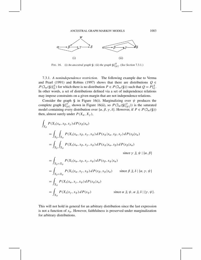
ANCESTRAL GRAPH MARKOV MODELS 1003
FIG. 16. (i) An ancestral graph G; (ii) the graph G[∅{ψ} . (See Section 7.3.1.)
7.3.1. A nonindependence restriction. The following example due to Vermaand Pearl (1991) and Robins (1997) shows that there are distributions Q ∈P (Im(G)[SL) for which there is no distribution P ∈ P (Im(G)) such that Q = P [SL.In other words, a set of distributions defined via a set of independence relationsmay impose constraints on a given margin that are not independence relations.
Consider the graph G in Figure 16(i). Marginalizing over ψ produces thecomplete graph G[∅{ψ} shown in Figure 16(ii), so P (Im(G[∅{ψ})) is the saturatedmodel containing every distribution over {α,β, γ, δ}. However, if P ∈ P (Im(G))
then, almost surely under P (Xα,Xγ ),∫Xβ
P (Xδ|xα, xβ, xγ ) dP (xβ |xα)
=∫Xβ
∫Xψ
P (Xδ|xα, xβ, xγ , xψ) dP(xψ |xα, xβ, xγ ) dP (xβ |xα)
=∫Xβ
∫Xψ
P (Xδ|xα, xβ, xγ , xψ) dP(xψ |xα, xβ) dP (xβ |xα)
since γ |= ψ | {α,β}=
∫Xβ×Xψ
P (Xδ|xα, xβ, xγ , xψ) dP(xβ, xψ |xα)
=∫Xβ×Xψ
P (Xδ|xα, xγ , xψ) dP (xβ, xψ |xα) since β |= δ | {α,γ,ψ}
=∫Xψ
P (Xδ|xα, xγ , xψ) dP (xψ |xα)
=∫Xψ
P (Xδ|xγ , xψ) dP(xψ) since α |= ψ , α |= δ | {γ,ψ}.
This will not hold in general for an arbitrary distribution since the last expressionis not a function of xα . However, faithfulness is preserved under marginalizationfor arbitrary distributions.
1004 T. RICHARDSON AND P. SPIRTES
7.4. Independence models for ancestral graphs are probabilistic. The exis-tence of distributions that are faithful to Im(G) for an ancestral graph G followsfrom the corresponding result for DAGs:
THEOREM 7.4 [Building on results of Geiger (1990), Geiger and Pearl (1990),Frydenberg (1990b), Spirtes et al. (1993) and Meek (1995b)]. For an arbitraryDAG, D , Im(D) is probabilistic, in particular there is a normal distribution thatis faithful to Im(D).
THEOREM 7.5. If G is an ancestral graph then Im(G) is probabilistic, inparticular there is a normal distribution which is faithful to Im(G).
PROOF. By Theorem 6.3 there is a DAG D(G) such that
Im(G) = Im
(D(G)[SD(G)
LD(G)
).
By Theorem 7.4 there is a normal distribution N that is faithful to Im(D(G)). By
Corollary 7.3,N [XS=xSXL
is faithful to Im(D(G))[SD(G)
LD(G)= Im(D(G)[SD(G)
LD(G)) = Im(G).
�
7.4.1. Completeness of the global Markov property. A graphical separationcriterion C is said to be complete if for any graph G and independence model I∗,
if IC(G) ⊆ I∗ and P (IC(G)) = P (I∗) then IC(G) = I∗.
In other words, the independence model IC(G) (see Section 2.1.1) cannot beextended without changing the associated set of distributions P (IC(G)).
THEOREM 7.6. The global Markov property for ancestral graphs is complete.
PROOF. The existence of a distribution that is faithful to Im(G) is clearlya sufficient condition for completeness. �
8. Gaussian parameterization. There is a natural parameterization of theset of all nonsingular normal distributions satisfying the independence relationsin Im(G). In the following sections we first introduce the parameterization, thendefine the set of normal distributions satisfying the relations in the independencemodel, and then prove equivalence.
Let Np(µ,<) denote a p-dimensional multivariate normal distribution withmean µ and covariance matrix <. Likewise let Np be the set of all suchdistributions, with nonsingular covariance matrices.
Throughout this section we find it useful to make the following convention:<−1
AA = (<AA)−1, where <AA is the submatrix of < restricted to A.
ANCESTRAL GRAPH MARKOV MODELS 1005
8.1. Parameterization. A Gaussian parameterization of an ancestral graph G,with vertex set V and edge set E is a pair 〈µ,>〉, consisting of a mean function
µ :V → R
which assigns a number to every vertex, together with a covariance function
> :V ∪ E → R
which assigns a number to every edge and vertex in G, subject to the restrictionthat the matrices ?, @ defined below are positive definite (p.d.):
(?)αβα,β∈unG
= λαβ =>(α), if α = β,
>(α − β), if α − β in G,
0, otherwise;
(@)αβα,β∈V \unG
= ωαβ =>(α), if α = β,
>(α ↔ β), if α ↔ β in G,
0 otherwise.
Let �(G) be the set of all such parameterizations 〈µ,>〉 for G. We further define:
(B)αβα,β∈V
= bαβ =
1, if α = β,>(α ← β), if α ← β in G,0, otherwise.
PROPOSITION 8.1. If ? and @ are given by a parameterization of G then:
(i) ?, @ are symmetric;(ii) for ν ∈ unG, λνν > 0 and for ν ∈ V \ unG, ωνν > 0.
PROOF. Both properties follow from the requirement that ?, @ be positivedefinite. �
PROPOSITION 8.2. Let G be an ancestral graph with vertices V , edges E. Thevalues taken by >(·) on the sets, unG ∪{α −β ∈ E}, (V \ unG)∪ {α ↔ β ∈ E} and{α → β ∈ E} are variation independent as >(·) varies in �(G). Likewise, µ(·)and >(·) are variation independent.
PROOF. The proof follows directly from the definition of a parameterization.�
LEMMA 8.3. Let G be an ancestral graph with vertex set V . Further, let ≺ bean arbitrary ordering of V such that all vertices in unG precede those in V \ unG,
1006 T. RICHARDSON AND P. SPIRTES
and α ∈ an(β) \ {β} implies α ≺ β . Under such an ordering, the matrix B givenby a parameterization of G has the form:
B =(
I 0Bdu Bdd
)and B−1 =
(I 0
−B−1dd Bdu B−1
dd
),
where Bdd is lower triangular, with diagonal entries equal to 1. Hence B is lowertriangular and nonsingular, as is B−1.
Note that we use u,d as abbreviations for unG,V \ unG respectively.
PROOF OF LEMMA 8.3. If α,β ∈ unG then since G is ancestral, α /∈ chG(β)
and vice versa. Hence by definition of B , bαβ = δ(α,β) (where δ is Kronecker’sdelta function). If α ∈ unG, β ∈ V \ unG then α /∈ chG(β), since G is ancestral,hence bαβ = 0. If α,β ∈ V \ unG, and α = β then bαβ = 1 by definition. If α �= β ,and bαβ �= 0 then α ∈ chG(β), so β ≺ α. Finally, since G is ancestral, β /∈ chG(α),so bβα = 0 as required. �
8.1.1. Definition of the Gaussian model [N (G)]. A parameterization 〈µ,>〉of G specifies a Gaussian distribution as follows:
NGµ> = N|V |(µ,<G>)
where
(µ)α = µ(α) and <G> = B−1(?−1 0
0 @
)B−).(1)
The Gaussian model, N (G) associated with G is the set of normal distributionsobtained from parameterizations of G:
N (G) = {NGµ> | 〈µ,>〉 ∈�(G)}.Note that it follows from the conditions on B , ? and @ that <G> is positive
definite. The mean function µ does not play a significant role in what follows.
LEMMA 8.4. If 〈µ,>〉 is a parameterization of an ancestral graph G then
<G> =(
?−1 −?−1B)duB
−)dd
−B−1dd Bdu?
−1 B−1dd (Bdu?
−1B)du + @)B−)
dd
),
<−1G> =
(? + B)
du@−1Bdu B)
du@−1Bdd
B)dd@
−1Bdu B)dd@
−1Bdd
).
PROOF. The proof is immediate from the definition of <G> and Lemma 8.3.�
ANCESTRAL GRAPH MARKOV MODELS 1007
8.1.2. Parameterization of a subgraph.
LEMMA 8.5. Let 〈µ,>〉 be a parameterization of an ancestral graph G =(V,E). If A ⊂ V such that ant(A) = A, and 〈µA,>A〉 is the parameterizationof the induced subgraph GA, obtained by restricting µ to A and > to A ∪ E∗,where E∗ is the set of edges in GA, then
?−1A = (?−1)A∩uA∩u, @A = (@)A∩d A∩d, B−1
A = (B−1)AA,
hence
<GA>A= (<G>)AA,
where ?A,@A,BA are the matrices associated with >A.
In words, if all vertices that are anterior to a set A in G are contained in A
then the covariance matrix parameterized by the restriction of > to the inducedsubgraph GA is just the submatrix (<G>)AA.
Note the distinction between matrices indexed by two subsets which indicatesubmatrices in the usual way (e.g., <AA) and matrices indexed by one subset whichare obtained from a parameterization of an induced subgraph on this set of vertices(e.g., BA).
PROOF OF LEMMA 8.5. For @ there is nothing to prove. Since A = ant(A),no vertex in unG ∩A is adjacent to a vertex in unG \A. Thus
? =(?A∩u A∩u 0
0 ?u\A u\A
),
so (?−1)A∩uA∩u = ?−1A as required.
Since A is anterior,
B =(BAA 0BAA BAA
),
where A = V \ A. The result then follows by partitioned inversion since BA =(B)AA = BAA. �
If G = (V,E) is a subgraph of an ancestral graph G∗ = (V,E∗), then there isa natural mapping 〈µ,>〉 $→ 〈µ∗,>∗〉 from �(G) to �(G∗), defined by
µ∗(·) = µ(·), >∗(x) ={>(x), if x ∈ V ∪ E,
0, if x ∈ E∗ \ E.
>∗ simply assigns 0 to edges in G∗ that are not in G (both graphs have the samevertex set). It is simple to see that
NGµ> = NG∗µ∗>∗ .
The next proposition is an immediate consequence.
1008 T. RICHARDSON AND P. SPIRTES
PROPOSITION 8.6. If G = (V,E) is a subgraph of an ancestral graph G∗ =(V,E∗) then N (G) ⊆ N (G∗).
8.1.3. Interpretation of parameters.
THEOREM 8.7. If G = (V,E) is an ancestral graph, 〈µ,>〉 ∈ �(G), and< = <G>, then for all vertices α for which pa(α) �= ∅,
B{α} pa(α) = −<{α} pa(α)<−1pa(α)pa(α); further,
(?−1 0
0 @
)= B<B).(2)
Regarding < as the covariance matrix for a (normal) random vector XV , thetheorem states that >(α ← ν) is −1 times the coefficient of Xν in the regressionof Xα on Xpa(α). @ is the covariance matrix of the residuals from this set ofregressions. ? is just the inverse covariance matrix for XunG . Hence if < isobtained from some unknown covariance function > for an ancestral graph G,then equation (2) allows us to reconstruct > from G and <.
PROOF OF THEOREM 8.7. Suppose that < = <G> for some parameterization〈µ,>〉. If every vertex has no parents then B is the identity matrix and the claimholds trivially.
Suppose that α is a vertex with pa(α) �= ∅, hence by definition α ∈ V \ unG. LetA = ant(α), e = ant(α) \ (pa(α) ∪ {α}), p = pa(α). By Lemma 8.5,
<AA = B−1A
(?−1
A 00 @A
)B−)A .(3)
Since G is ancestral, neG(α)∩A = ∅. Thus partitioning A into e,p, {α}, we obtain
BA = Bee 0 0
Bpe Bpp 0
0 Bαp 1
and @A =@e∩d e∩d @e∩d p∩d 0
@p∩d e∩d @p∩d p∩d 0
0 0 ωαα
.
The expression for B{α} pa(α) = Bαp then follows from (3) by routine calculation.The second claim is an immediate consequence of (1). �
8.1.4. Identifiability.
COROLLARY 8.8. If G is an ancestral graph, >1,>2 are two covariancefunctions for G and <G>1 = <G>2 then >1(·) = >2(·). Hence the mapping> $→ <G> is one-to-one.
PROOF. This follows directly from Theorem 8.7: both >1 and >2 satisfyequation (2) and hence are identical. �
ANCESTRAL GRAPH MARKOV MODELS 1009
8.1.5. N (G) for a complete ancestral graph is saturated.
THEOREM 8.9. If G = (V,E) is a complete ancestral graph then N (G)=N|V |.
In words, a complete ancestral graph parameterizes the saturated Gaussianmodel of dimension |V |.
PROOF OF THEOREM 8.9. Let < be an arbitrary p.d. matrix of dimension |V |.It is sufficient to show that there exists a covariance function > for G, such that< = <G>. We may apply equation (2) to obtain matrices B , ? and @ from <.However, it still remains to show that (a) whenever there is a nonzero off-diagonalentry in ?, @ or B , there is an edge of the appropriate type in G to associate withit, and (b) ? and @ are positive definite.
By Lemma 3.21(ii), GunG is complete, hence in ? all off-diagonal entries arepermitted to be nonzero.
It follows directly from the construction of B given by (2) that if (B)αβ �= 0 andα �= β then β ∈ pa(α).
Now suppose α,β ∈ V \ unG, and there is no edge α ↔ β in G. Since G iscomplete, it follows from Lemma 3.21(iii) that either α ← β , or α → β . Withoutloss of generality suppose the former, and let A = ant(α) = pa(α) ∪ {α} since G iscomplete. Then
(B<B))αβ = (BA<AAB)A )αβ
=[(
Bpp 0−<αp<
−1pp 1
)(<pp <pα
<αp <αα
)(B)pp −<−1
pp <pα
0 1
)]αβ
= 0
as required. The same argument applies in the case where β ∈ unG, α ∈ V \ unG,and hence α ← β , thus establishing that B<B) is block-diagonal with blocks?−1 and @. This establishes (a).
Since, by hypothesis, < is p.d. and B is nonsingular, by construction, it followsthat ? and @ are also p.d. hence (b) holds. We now have
<G> = B−1(?−1 0
0 @
)B−) = B−1B<B)B−) = <. �
8.1.6. Entries in @−1 and G↔. If G = (V,E) is an ancestral graph then wedefine G↔ to be the induced subgraph with vertex set V , but including only thebidirected edges in E.
LEMMA 8.10. If α,β ∈ V \ unG and α is not adjacent to β in (G↔)a then
(@−1)αβ = 0,
for any @ obtained from a covariance function > for G.
1010 T. RICHARDSON AND P. SPIRTES
PROOF [Based on the proof of Lemma 3.1.6 in Koster (1999a)]. First recallthat α and β are adjacent in (G↔)a if and only if α and β are collider connected inG↔. The proof is by induction on |d| = |V \ unG |.
If |d| = 2 then (@−1)αβ = −(@)αβ |@|−1 = 0 as there is no edge α ↔ β in G.For |d| > 2, note that by partitioned inversion:
(@−1)αβ = −(ωαβ − @{α}c@−1cc @c{β})|@{α,β}.c|−1(4)
= −(ωαβ − ∑
γ,δ∈c
ωαγ (@−1cc )γ δωδβ
)|@{α,β}.c|−1(5)
where c = d \ {α,β}, @−1cc = (@cc)
−1, and
@{α,β}.c = @{α,β}{α,β} − @{α,β}c@−1cc @c{α,β}.
Since α and β are not adjacent in (G↔)a there is no edge α ↔ β in G, henceωαβ = 0. Now consider each term in the sum (5). If there is no edge α ↔ γ orno edge δ ↔ β then ωαγ (@
−1cc )ωδβ = 0. If there are edges α ↔ γ and δ ↔ β in G
then γ �= δ as otherwise α and β would be collider connected in G↔, and furtherγ and δ are not collider connected in (Gc)↔. Hence by the inductive hypothesis,(@−1
cc )γ δ = 0. Thus every term in the sum is zero and we are done. �
An alternative proof follows from the Markov properties of undirected graphicalGaussian models [see Lauritzen (1996)]: view the specification of @ formally asif it were an inverse covariance matrix for a model represented by an undirectedgraph U. Then α and β are not collider connected in G if and only if α and β arenot connected in U. Hence by the global Markov property for undirected graphs,α and β are marginally independent, so (@−1)αβ = 0. (We thank S. Lauritzen forthis observation.)
It also follows directly from the previous lemma (and this discussion) that @−1
will be block diagonal. (We thank N. Wermuth for this observation.)
COROLLARY 8.11. Let G be an ancestral graph with α ↔ β in G. Let G′ bethe subgraph formed by removing the α ↔ β edge in G. If α and β are not adjacentin (G′↔)a then
(@−1)αβ = −>(α ↔ β)|@{α,β}.c|−1,
where c = d \ {α,β}, > is a covariance function for G, and @ is the associatedmatrix.
Note that we adopt the convention: @{α,β}.c = @{α,β} when c = ∅.
PROOF OF COROLLARY 8.11. By the argument used in the proof ofLemma 8.10, it is clear that the sum in equation (5) is equal to 0. The result thenfollows since, by definition, ωαβ = >(α ↔ β). �
ANCESTRAL GRAPH MARKOV MODELS 1011
8.2. Gaussian independence models. A Gaussian independence model, N (I),is the set of nonsingular normal distributions obeying the independence relationsin I:
N (I) ≡ N|V | ∩ P (I)
where V is the set of vertices in I. As noted in Section 7, normal distributions inN (I) may also satisfy other independence relations.
PROPOSITION 8.12. If G′ is a subgraph of G then N (Im(G′)) ⊆ N (Im(G)).
PROOF. The proof follows directly from Proposition 3.12. �
THEOREM 8.13. If G1,G2 are two ancestral graphs then
N(Im(G1)
) = N(Im(G2)
)if and only if Im(G1) = Im(G2).
PROOF. If Im(G1) = Im(G2), then N (Im(G1)) = N (Im(G2)) by definition.By Theorem 7.5 there is a normal distribution N1 that is faithful to Im(G1).
Hence
〈A,B | Z〉 ∈ Im(G1) ⇐⇒ A |= B | Z [N1].Since N (Im(G1)) = N (Im(G2)), N1 ∈ N (Im(G2)), hence Im(G2) ⊆ Im(G1).The reverse inclusion may be argued symmetrically. �
8.3. Equivalence of Gaussian parameterizations and independence models formaximal ancestral graphs. The main result of this section is the following:
THEOREM 8.14. If G is a maximal ancestral graph then
N (G) = N(Im(G)
).
In words, if G is a maximal ancestral graph then the set of normal distributionsthat may be obtained by parameterizing G is exactly the set of normal distributionsthat obey the independence relations in Im(G).
Note that Wermuth, Cox and Pearl (1994) refer to a “parameterization” of anindependence model when describing a parameterization of a (possibly proper)subset of N (I). To distinguish their usage from the stronger sense in which theterm is used here, we may say that a parameterization is full if all distributions inN (I) are parameterized. In these terms Theorem 8.14 states that if G is maximalthen the parameterization of G described in Section 8.1 is a full parameterizationof N (Im(G)).
1012 T. RICHARDSON AND P. SPIRTES
8.3.1. N (G) when G is not maximal. If G is not maximal then N (G) isa proper subset of N (Im(G)), as the following example illustrates: considerthe nonmaximal ancestral graph G shown in Figure 9(a). Since Im(G) = ∅,N (Im(G)) = N4, the saturated model. However, there are 10 free parameters inN4 and yet there are only 5 edges and 4 vertices, giving 9 parameters in N (G).Direct calculation shows that
σγ δ − σγασαδ
σαα
− σγβσβδ
σββ
+ σγασαβσβδ
σαασββ
= 0
where σφψ = (<G>)φψ . This will clearly not hold for all distributions in N4.
8.3.2. If G is maximal then N (Im(G)) ⊆ N (G). We first require two lemmas.
LEMMA 8.15. Let G = (V,E) be an ancestral graph, ε an edge in E withendpoints (α,β) and V = antG({α,β}). If G′ = (V,E \ {ε}) is maximal, then foran arbitrary covariance function > for G, (<−1
G>)αβ = 0 implies >(ε) = 0.
In words, if in a graph G, removing an edge, ε, between α and β resultsin a graph that is still maximal, then in any distribution NGµ> obtained froma parameterization 〈µ,>〉 of G, if the partial correlation between α and β givenV \ {α,β} is zero, then > assigns zero to the edge ε.
PROOF OF LEMMA 8.15. There are three cases, depending on the type of theedge ε:
Case 1. ε is undirected. In this case α,β ∈ unG. Then by Lemma 8.4,
(<−1)αβ = (? + B)d u@
−1Bd u)αβ.
However, since V = antG({α,β}), d = ∅, hence (<−1)αβ = (?)αβ = >(α − β),so >(α − β) = 0 as required.
Case 2. ε is directed. Without loss, suppose α ← β . It now follows fromLemma 8.4, that
(<−1)αβ = B)d{α}@−1Bd{β}
= ∑γ,δ∈d
bγα(@−1)γ δbδβ.
Now, bγα = 0 for α �= γ since chG(α) = ∅, and bαα = 1 by definition. Hence
(<−1)αβ = ∑δ∈d
(@−1)αδbδβ.
Since β → α, β ∈ antG(α), so V = antG(α). Thus if δ ∈ V , α �= δ, andα and δ are connected by a path π in G↔, containing more than one edge (seeSubsection 8.1.6), then π is a primitive inducing path between α and δ in G. But
ANCESTRAL GRAPH MARKOV MODELS 1013
this is a contradiction, since δ ∈ antG(α), and yet by Lemma 4.5(ii), δ /∈ antG(α).Hence by Lemma 8.10, (@−1)αδ = 0 for δ �= α. Consequently,
(<−1)αβ = (@−1)ααbαβ = (@−1)αα>(α → β).
As @ is positive definite, (@−1)αα > 0, hence >(α → β) = 0.Case 3. ε is bidirected. Again it follows from Lemma 8.4, that
(<−1)αβ = B)d{α}@−1Bd{β}
= ∑γ,δ∈d
bγα(@−1)γ δbδβ.
As chG({α,β}) = ∅, bγα = 0 for γ �= α, and likewise bδβ = 0 for δ �= β . Bydefinition, bββ = bαα = 1. Since, by hypothesis, G′ is maximal, α and β are notadjacent in (G′↔)a , so
(<−1)αβ = (@−1)αβ = −>(α ↔ β)|@{α,β}.c|−1,
the second equality following by Corollary 8.11. Hence >(α ↔ β) = 0 asrequired. �
Note that case 2 could alternatively have been proved by direct appeal to theinterpretation of >(α ← β) as a regression coefficient, as shown by Theorem 8.7.However, such a proof is not available in Case 3, and we believe that the currentproof provides greater insight into the role played by the graphical structure.
The next lemma provides the inductive step in the proof of the claim whichfollows.
LEMMA 8.16. Let G = (V,E) be an ancestral graph and ε an edge in E. IfG′ = (V,E \ {ε}) is maximal, and unG = unG′ , then
N (G) ∩ N (Im(G′)) ⊆ N (G′).
PROOF. Let N ∈ N (G) ∩ N (Im(G′)), with covariance matrix <, and para-
metrization >G. Let ε have endpoints α, β . Since unG = unG′ it is sufficient toshow that >G(ε) = 0, because in this case, the restriction of >G to the edges (andvertices) in G′ is a parameterization of G′, hence N ∈ N (G′).
Let A = antG′({α,β}) = antG({α,β}). Since α, β are not adjacent in G′ and G′is maximal, it follows from Corollary 5.3 that⟨{α}, {β} | ant({α,β}) \ {α,β}⟩ ∈ Im(G
′).
Since N ∈ N (Im(G′)), it then follows from standard properties of the Normal
distribution that (<−1AA)αβ = 0. By Lemma 8.5 <−1
AA is parameterized by >A, therestriction of >G to the edges and vertices in the induced subgraph GA. The resultthen follows by applying Lemma 8.15 to GA, giving >A(ε) = >G(ε) = 0. �
1014 T. RICHARDSON AND P. SPIRTES
We are now in a position to prove that if G is maximal then all distributionsin N (Im(G)) may be obtained by parametrizing G. This constitutes one half ofTheorem 8.14.
CLAIM. If G is maximal then N (Im(G)) ⊆ N (G).
PROOF. Suppose N ∈ N (Im(G)). Let G be the completed graph defined inSection 5.2. By Theorem 8.9, N|V | = N (G), hence N ∈ N (G). By Theorem 5.6,there exists a sequence of maximal ancestral graphs G ≡ G0, . . . ,Gr ≡ G wherer is the number of nonadjacent vertices in G and unG0 = · · · = unGr . Now byProposition 8.12,
N (Im(Gr )) ⊂ · · · ⊂ N (Im(G0)) = N|V |hence N ∈ N (Im(Gi )), for 0 ≤ i ≤ r . We thus may apply Lemma 8.16 r-times toshow successively
N ∈ N (Gi ) ∩ N (Im(Gi+1)) implies N ∈ N (Gi+1)
for i = 0 to r − 1. Hence N ∈ N (Gr ) = N (G) as required. �
8.3.3. N (G) obeys the global Markov property for G. The following lemmaprovides a partial converse to Lemma 8.15.
LEMMA 8.17. If > is a covariance function for an ancestral graph G =(V,E), and α,β ∈ V are not adjacent in (G)a then (<−1
G>)αβ = 0.
PROOF. There are two cases to consider:Case 1. α /∈ unG or β /∈ unG. By Lemma 8.4,(
<−1G>
)αβ = ∑
γ,δ∈d
bγα(@−1)γ δbδβ.(6)
If bγα �= 0 and bδβ �= 0 then there are edges α → γ , β → δ in G, hence γ �= δ,β �= γ and α �= δ since otherwise α and β are adjacent in (G)a . Further, there isno path between γ and δ in G↔ since if there were, α and β would be colliderconnected in G, hence adjacent in (G)a . Thus γ and δ are not adjacent in (G↔)a
and so by Lemma 8.10 (@−1)γ δ = 0. Consequently every term in the sum in (6) iszero as required.
Case 2. α,β ∈ unG. Again by Lemma 8.4:(<−1
G>
)αβ = λαβ + ∑
γ,δ∈d
bγα(@−1)γ δbδβ.(7)
If α, β are not adjacent in (G)a then α and β are not adjacent in G. Hence λαβ = 0.The argument used in case (1) may now be repeated to show that every term in thesum in (7) is zero. �
ANCESTRAL GRAPH MARKOV MODELS 1015
The next lemma proves the second half of Theorem 8.14. It does not require Gto be maximal, so we state it as a separate lemma.
LEMMA 8.18. If G is an ancestral graph then N (G) ⊆ N (Im(G)).
In words, any normal distribution obtained by parametrizing an ancestralgraph G obeys the global Markov property for G.
PROOF OF LEMMA 8.18. Suppose that 〈X,Y | Z〉 ∈ Im(G). If ν ∈ antG(X ∪Y ∪ Z) \ (X ∪ Y ∪ Z) then in (Gant(X∪Y∪Z))
a either ν is separated from X by Z,or from Y by Z. Hence X and Y may always be extended to X∗, Y ∗ respectively,such that 〈X∗, Y ∗ | Z〉 ∈ Im(G) and X∗ ∪ Y ∗ ∪ Z = antG(X ∪ Y ∪ Z). Since themultivariate normal density is strictly positive, for an arbitrary N ∈ N|V |,
A |= B | C ∪ D and A |= C | B ∪ D implies A |= B ∪ C | D(C5)
[see Dawid (1980)]. By repeated application of C5 it is sufficient to show that foreach pair α, β with α ∈ X∗, β ∈ Y ∗,
α |= β | (Z ∪ X∗ ∪ Y ∗) \ {α,β} [N ],or equivalently (<−1
AA)αβ = 0, where A = X∗ ∪ Y ∗ ∪ Z. Since 〈X∗, Y ∗ | Z〉 ∈Im(G), α and β are not adjacent in (GA)
a . The result then follows from Lemma 8.5and Lemma 8.17. �
Lemmas 8.17 and 8.18 are based on Lemma 3.1.6 and Theorem 3.1.8 in Koster(1999a), though these results concern a different class of graphs (see Section 9.2).An alternative proof of Lemma 8.18 for ancestral graphs without undirected edgesis given in Spirtes et al. (1996, 1998).
8.3.4. Distributional equivalence of Markov equivalent models. The follow-ing corollary states that two maximal ancestral graphs are Markov equivalent ifand only if the corresponding Gaussian models are equivalent.
COROLLARY 8.19. For maximal ancestral graphs, G1,G2,
Im(G1) = Im(G2) if and only if N (G1) = N (G2).
PROOF.
N (G1) = N (G2) ⇐⇒ N (Im(G1)) = N (Im(G2)) by Theorem 8.14;
⇐⇒ Im(G1) = Im(G2) by Theorem 8.13.
1016 T. RICHARDSON AND P. SPIRTES
COROLLARY 8.20. If G = (V,E) is an ancestral graph and S ∪ L ⊂ V ,
if N ∈ N (G) then N [XS=xSXL
∈ N(G[SL
)for all xS ∈ R
|S|.
PROOF. By Lemma 8.18, N (G) ⊆ N (Im(G)). Hence by normality andTheorem 7.1 N [XS=xS
XL∈ N (Im(G)[SL). Finally, by Corollary 4.19 G[SL is maximal,
hence
N(Im(G)[SL
) = N(Im
(G[SL
)) = N(G[SL
),
by Theorems 4.18 and 8.14. �
Suppose that we postulate a Gaussian model N (G) with complex structure,such as a DAG containing latent variables and/or selection variables. Thiscorollary is significant because it guarantees that if N (G) contains the “true”distribution N∗, and we then simplify G to a model for the observed variables,N (G[SL), then the new model will contain the true “observable” distributionobtained by marginalizing the unobserved variables and conditioning on theselection variables, N [XS=xS
XL. [The distribution N [XS=xS
XLis termed “observable”
because it is the distribution over the observed variables (V \ (S ∪ L)) in the“selected” subpopulation for which XS = xS . In general this will obviously notbe the distribution observed in a finite sample.]
8.4. Gaussian ancestral graph models are curved exponential families. LetS be a full regular exponential family of dimension m with natural parameterspace E ⊆ R
m, so S = {Pθ | θ ∈ E}. If U is an open neighborhood in E, thenSU = {Pθ | θ ∈ U }. Let S0 be a subfamily of S, with E0 the corresponding subsetof E.
If A is open in Rm then a function f :A → R
m is a diffeomorphism of A ontof (A) if f (·) is one-to-one, smooth (infinitely differentiable), and of full rankeverywhere on A. Corollary A.3 in Kass and Vos (1997) states that a function f isa diffeomorphism if it is smooth, one-to-one, and the inverse f −1 :f (A) → A isalso smooth.
Theorem 4.2.1 in Kass and Vos (1997) states that a subfamily S0 of anm-dimensional regular exponential family S is a locally parameterized curvedexponential family of dimension k if for each θ0 ∈ E0 there is an openneighborhood U in E containing θ0 and a diffeomorphism f :U → R
k × Rm−k ,
and
SU0 = {
Pθ ∈ SU | f (θ) = (ψ,0)}.
We use the following fact in the next lemma.
ANCESTRAL GRAPH MARKOV MODELS 1017
PROPOSITION 8.21. If f is a rational function defined everywhere on a set Dthen f (n) is a rational function defined everywhere on D.
PROOF. The proof is by induction on n. Suppose f (n) = gn/hn, where gn,hn
are polynomials, and hn > 0 on D. Then f (n+1) = (hng′n − gnh
′n)/h
2n from which
the conclusion follows (since h2n > 0 on D). �
Let �+|V | denote the cone of positive definite |V | × |V | matrices.
LEMMA 8.22. If G is a complete ancestral graph then the mapping
fG :�(G) → R|V | ×�+
|V | given by 〈µ,>〉 $→ 〈µ,<G>〉is a diffeomorphism from �(G) to R
|V | �+|V |.
PROOF. Corollary 8.8 establishes that fG is one-to-one. Further, by Theo-rem 8.9, N (G) = N|V | hence
f (�(G)) = R|V | �+
|V |.
It remains to show that fG, f −1G are smooth. It follows from equation (1) that the
components of fG are rational functions of 〈µ,>〉, defined for all 〈µ,>〉 ∈�(G).Hence, by Proposition 8.21, fG is smooth. Similarly, equation (2) establishes thatf −1
G is smooth. �
THEOREM 8.23. For an ancestral graph G(V,E), N (G) is a curvedexponential family, with dimension 2|V | + |E|.
PROOF. This follows from the definition of N (G), the existence of a completeancestral supergraph of G (Lemma 5.5), Lemma 8.22 and Theorem 4.2.1 of Kassand Vos (1997), referred to above. �
The BIC criterion for the model N (G) is given by
BIC(G) = −2 lnLG(θ) + ln(n)(2|V | + |E|),where n is the sample size, LG(·) is the likelihood function and θ is the cor-responding MLE for N (G). A consequence of Theorem 8.23 is that BIC(·) is anasymptotically consistent criterion for selecting among Gaussian ancestral graphmodels [see Haughton (1988)].
By contrast, Geiger et al. (2001) have shown that simple discrete DAG modelswith latent variables do not form curved exponential families.
1018 T. RICHARDSON AND P. SPIRTES
8.5. Parameterization via recursive equations with correlated errors. TheGaussian model N (G) can alternatively be parameterized in two pieces via thefactorization of the density
f (xV ) = f (xunG)f (xV \unG|xunG).(8)
The undirected component f (xunG) may be parameterized via an undirectedgraphical Gaussian model also known as a covariance selection model [seeLauritzen (1996) and Dempster (1972)].
The directed component, f (xV \unG | xunG), may be parameterized via a set ofrecursive equations as follows:
(i) Associate with each ν in V \unG a linear equation, expressing Xν as a linearfunction of the variables for the parents of ν plus an error term:
Xν = µν + ∑π∈pa(ν)
b∗νπXπ + εν.
(ii) Specify a nonsingular multivariate normal distribution over the errorvariables (εν)ν∈V \unG (with mean zero) satisfying the condition that
if there is no edge α ↔ β in G, then Cov(εα, εβ) = 0,
but otherwise unrestricted.
Note that b∗αβ = −bαβ under the parameterization specified in Section 8.1. The
conditional distribution, f (xV \unG | xunG), is thus parameterized via a simultaneousequation model, of the kind used in econometrics and psychometrics since the1940s. We describe the system as “recursive” because the equations may bearranged in upper triangular form, possibly with correlated errors. (Note that someauthors only use this term if, in addition, the errors are uncorrelated.) As shownin Theorem 8.7 the set of recursive equations described here also has the specialproperty that the linear coefficients may be consistently estimated via regression ofeach variable on its parents. This does not hold for recursive equations in general.
8.5.1. Estimation procedures. The parameterization described above thusbreaks N (G) into an undirected graphical Gaussian model and a set of recursiveequations with correlated errors. This result is important for the purposes ofstatistical inference because software packages exist for estimating these models:MIM Edwards (1995) fits undirected Gaussian models via the IPS algorithm;AMOS Arbuckle (1997), EQS Bentler (1986), Proc CALIS SAS Publishing(1995) and LISREL Jöreskog and Sörbom (1995) are packages which fitstructural equation models via numerical optimization. Fitting the two componentsseparately is possible in view of the factorization of the likelihood given byequation (8) and the variation independence of the parameters in these pieces (seeProposition 8.2).
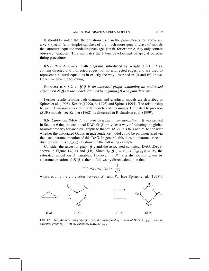
ANCESTRAL GRAPH MARKOV MODELS 1019
It should be noted that the equations used in the parameterization above area very special (and simple) subclass of the much more general class of modelsthat structural equation modelling packages can fit, for example, they only containobserved variables. This motivates the future development of special purposefitting procedures.
8.5.2. Path diagrams. Path diagrams, introduced by Wright (1921, 1934),contain directed and bidirected edges, but no undirected edges, and are used torepresent structural equations in exactly the way described in (i) and (ii) above.Hence we have the following:
PROPOSITION 8.24. If G is an ancestral graph containing no undirectededges then N (G) is the model obtained by regarding G as a path diagram.
Further results relating path diagrams and graphical models are described inSpirtes et al. (1998), Koster (1999a, b; 1996) and Spirtes (1995). The relationshipbetween Gaussian ancestral graph models and Seemingly Unrelated Regression(SUR) models [see Zellner (1962)] is discussed in Richardson et al. (1999).
8.6. Canonical DAGs do not provide a full parameterization. It was provedin Section 6 that the canonical DAG D(G) provides a way of reducing the globalMarkov property for ancestral graphs to that of DAGs. It is thus natural to considerwhether the associated Gaussian independence model could be parameterized viathe usual parameterization of this DAG. In general, this does not parameterize alldistributions in N (Im(G)) as shown in the following example.
Consider the ancestral graph G1, and the associated canonical DAG, D(G1)
shown in Figure 17(i-a) and (i-b). Since Im(G1) = ∅, N (Im(G1)) = N3 thesaturated model on 3 variables. However, if N is a distribution given bya parameterization of D(G1), then it follows by direct calculation that
min{ρab, ρbc, ρac} < 1√2
where ρvw is the correlation between Xv and Xw [see Spirtes et al. (1998)].
FIG. 17. (i-a) An ancestral graph G1; (i-b) the corresponding canonical DAG, D(G1); (ii-a) anancestral graph G2; (ii-b) the canonical DAG, D(G2).
1020 T. RICHARDSON AND P. SPIRTES
Since this does not hold for all distributions in N3, there are normal distributionsN ∈ N (Im(G1)) for which there is no distribution N∗ ∈ N (D(G1)) such thatN = N∗[{λab,λbc,λac}.
Lauritzen [1998, page 12] gives an analogous example for conditioning, byconsidering the graph G2, with canonical DAG, D(G2), shown in Figure 17(ii-a)and (ii-b). Lauritzen shows that there are normal distributions N ∈ N (Im(G2)), forwhich there is no distribution N∗ ∈ N (D(G2)) such that N = N∗[{σxy ,σxz,σzw,σyw}.
These negative results are perhaps surprising given the very simple nature of thestructure in D(G), but serve to illustrate the complexity of the sets of distributionsrepresented by such models.
9. Relation to other work. The problem of constructing graphical represen-tations for the independence structure of DAGs under marginalizing and condi-tioning was originally posed by Wermuth in 1994 in a lecture at CMU. Wermuth,Cox and Pearl developed an approach to this problem based on summary graphs[see Wermuth et al. (1994, 1999), Cox and Wermuth (1996), Wermuth and Cox(2000)]. More recently Koster has introduced another class of graphs, called MC-graphs, together with an operation of marginalizing and conditioning. [See Koster(2000), Koster (1999a, b).]
In Figure 18 we show two examples of data generating processes, togetherwith the maximal ancestral graph, summary graph and MC-graphs resulting aftermarginalizing (i) and conditioning (ii).
Simple representations for DAGs under marginalization alone were proposedby Verma (1993), who defined an operation of projection which transforms a DAGwith latent variables to another DAG in which each latent variable has exactlytwo children both of which are observed (called a “semi-Markovian model”). Theoperation is defined so that the DAG and its projection are Markov equivalentover the common set of observed variables. This approach does not lead toa full parameterization of the independence model for the reasons discussed inSection 8.6.
In this section we will briefly describe the classes of summary graphs andMC-graphs. We then outline the main differences and similarities to the class ofmaximal ancestral graphs. Finally we discuss the relation between ancestral graphsand chain graphs.
9.1. Summary graphs. A summary graph is a graph containing three types ofedge →, −, - - - - . Directed cycles may not occur in a summary graph, but it ispossible for there to be a dashed line (α - - - -β) and at the same time a directedpath from α to β . Thus there may be two edges between a pair of vertices, thatis, α - - - -−→ β . This is the only combination of multiple edges that is permitted.The separation criterion for summary graphs is equivalent to m-separation aftersubstituting bidirected edges (↔) for dashed edges (- - - -).
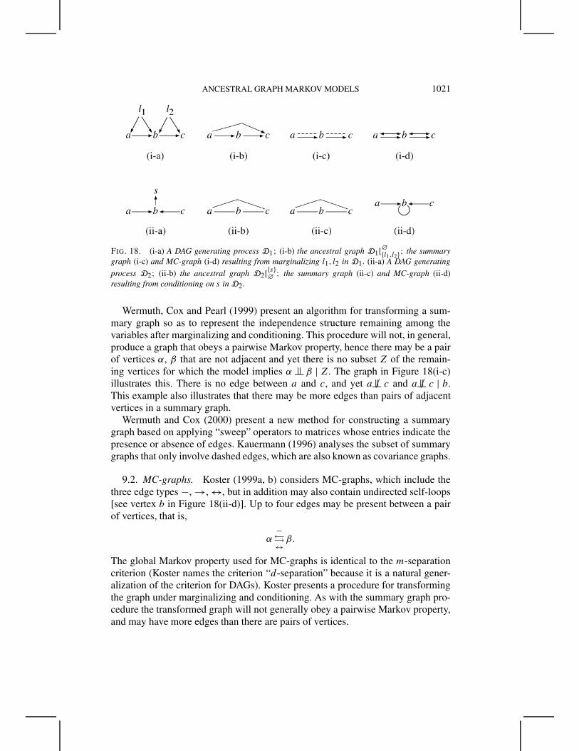
ANCESTRAL GRAPH MARKOV MODELS 1021
FIG. 18. (i-a) A DAG generating process D1; (i-b) the ancestral graph D1[∅{l1,l2}; the summarygraph (i-c) and MC-graph (i-d) resulting from marginalizing l1, l2 in D1. (ii-a) A DAG generating
process D2; (ii-b) the ancestral graph D2[{s}∅
; the summary graph (ii-c) and MC-graph (ii-d)resulting from conditioning on s in D2.
Wermuth, Cox and Pearl (1999) present an algorithm for transforming a sum-mary graph so as to represent the independence structure remaining among thevariables after marginalizing and conditioning. This procedure will not, in general,produce a graph that obeys a pairwise Markov property, hence there may be a pairof vertices α, β that are not adjacent and yet there is no subset Z of the remain-ing vertices for which the model implies α |= β | Z. The graph in Figure 18(i-c)illustrates this. There is no edge between a and c, and yet a /|= c and a /|= c | b.This example also illustrates that there may be more edges than pairs of adjacentvertices in a summary graph.
Wermuth and Cox (2000) present a new method for constructing a summarygraph based on applying “sweep” operators to matrices whose entries indicate thepresence or absence of edges. Kauermann (1996) analyses the subset of summarygraphs that only involve dashed edges, which are also known as covariance graphs.
9.2. MC-graphs. Koster (1999a, b) considers MC-graphs, which include thethree edge types −, →, ↔, but in addition may also contain undirected self-loops[see vertex b in Figure 18(ii-d)]. Up to four edges may be present between a pairof vertices, that is,
α−�↔
β.
The global Markov property used for MC-graphs is identical to the m-separationcriterion (Koster names the criterion “d-separation” because it is a natural gener-alization of the criterion for DAGs). Koster presents a procedure for transformingthe graph under marginalizing and conditioning. As with the summary graph pro-cedure the transformed graph will not generally obey a pairwise Markov property,and may have more edges than there are pairs of vertices.
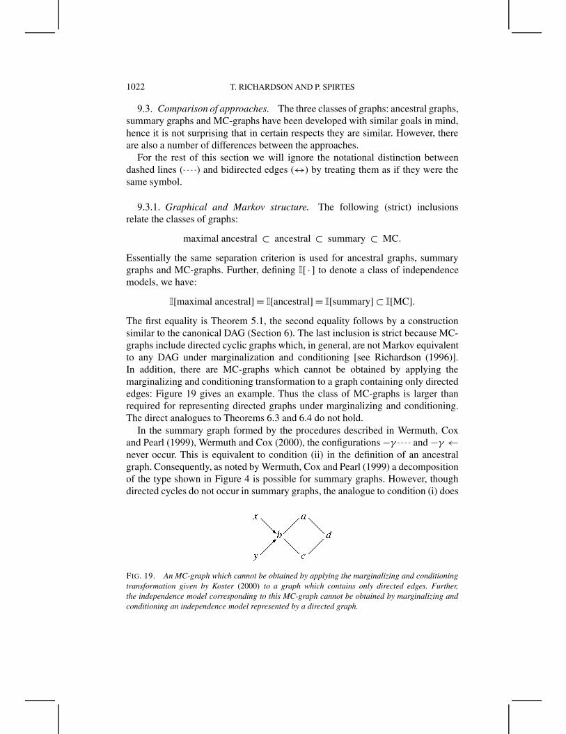
1022 T. RICHARDSON AND P. SPIRTES
9.3. Comparison of approaches. The three classes of graphs: ancestral graphs,summary graphs and MC-graphs have been developed with similar goals in mind,hence it is not surprising that in certain respects they are similar. However, thereare also a number of differences between the approaches.
For the rest of this section we will ignore the notational distinction betweendashed lines (- - - -) and bidirected edges (↔) by treating them as if they were thesame symbol.
9.3.1. Graphical and Markov structure. The following (strict) inclusionsrelate the classes of graphs:
maximal ancestral ⊂ ancestral ⊂ summary ⊂ MC.
Essentially the same separation criterion is used for ancestral graphs, summarygraphs and MC-graphs. Further, defining I[ · ] to denote a class of independencemodels, we have:
I[maximal ancestral] = I[ancestral] = I[summary] ⊂ I[MC].The first equality is Theorem 5.1, the second equality follows by a constructionsimilar to the canonical DAG (Section 6). The last inclusion is strict because MC-graphs include directed cyclic graphs which, in general, are not Markov equivalentto any DAG under marginalization and conditioning [see Richardson (1996)].In addition, there are MC-graphs which cannot be obtained by applying themarginalizing and conditioning transformation to a graph containing only directededges: Figure 19 gives an example. Thus the class of MC-graphs is larger thanrequired for representing directed graphs under marginalizing and conditioning.The direct analogues to Theorems 6.3 and 6.4 do not hold.
In the summary graph formed by the procedures described in Wermuth, Coxand Pearl (1999), Wermuth and Cox (2000), the configurations −γ - - - - and −γ ←never occur. This is equivalent to condition (ii) in the definition of an ancestralgraph. Consequently, as noted by Wermuth, Cox and Pearl (1999) a decompositionof the type shown in Figure 4 is possible for summary graphs. However, thoughdirected cycles do not occur in summary graphs, the analogue to condition (i) does
FIG. 19. An MC-graph which cannot be obtained by applying the marginalizing and conditioningtransformation given by Koster (2000) to a graph which contains only directed edges. Further,the independence model corresponding to this MC-graph cannot be obtained by marginalizing andconditioning an independence model represented by a directed graph.
ANCESTRAL GRAPH MARKOV MODELS 1023
not hold, since it is possible to have an edge α - - - -β and a directed path from α
to β .The marginalizing and conditioning transformation operations for summary
graphs and MC-graphs are “local” in that they make changes to triples ofadjacent vertices. In contrast the transformation G $→ G[SL requires pairwise tests ofm-separation to be carried out in order to determine the adjacencies present in G[SL.This may make the transformation harder for a human to carry out. On theother hand the transformation given by Wermuth is recursive, and tests for theexistence of an m-connecting path can be performed by a recursive procedure thatonly examines triples of adjacent vertices. It can be said that the MC-graph andsummary graph transformations may in general be performed in fewer steps thanthe ancestral graph transformation.
However, a price is paid for not performing these tests of m-separation:whereas G[SL always obeys a pairwise Markov property (Corollary 4.19), thesummary graphs and MC graphs resulting from the transformations do not do soin general. This is a disadvantage in a visual representation of an independencemodel insofar as it conflicts with the intuition, based on separation in undirectedgraphs, that if two vertices are not connected by an edge then they are not directlyconnected and hence may be made independent by conditioning on an appropriatesubset of the other vertices.
9.3.2. Gaussian parameterization. For summary graphs, as for ancestralgraphs, the Gaussian parameterization consists of a conditional distribution anda marginal distribution. Once again, the marginal parameterization is specified viaa covariance selection model and the conditional distribution via a system of struc-tural equations of the type used in econometrics and psychometrics as describedin Section 8.5 [see Cox and Wermuth (1996)]. Under this parameterization oneparameter is associated with each edge and vertex in the graph.
As described above, it is possible for a summary graph to contain moreedges than there are pairs of adjacent vertices. Consequently, the Gaussianmodel associated with a summary graph will not be identified in general, andthe analogous result to Corollary 8.8 will not hold. Thus the summary graphmodel will sometimes contain more parameters than needed to parameterize thecorresponding Gaussian independence model.
On the other hand, as mentioned in the previous section, summary graphsdo not satisfy a pairwise Markov property, and hence the associated model willnot parameterize all Gaussian distributions satisfying the Markov property forthe graph. In particular, the comments concerning nonmaximal ancestral graphsapply to summary graphs (see Section 8.3.1). In other words, parameterizationof a summary graph does not, in general, lead to a full parameterization of theindependence model (see Theorem 8.14). In this sense the summary graph modelsometimes contains too few parameters.
1024 T. RICHARDSON AND P. SPIRTES
As a consequence, two Markov equivalent summary graphs may representdifferent sets of Gaussian distributions, so the analogue to Corollary 8.19 doesnot hold. Thus for the purpose of parameterizing Gaussian independence models,the class of maximal ancestral graphs has advantages over summary graphs (andnonmaximal ancestral graphs).
It should be stressed, however, that the fact that a summary graph model mayimpose additional non-Markovian restrictions can be seen as an advantage insofaras it may lead to more parsimonious models. For this purpose ideally one wouldwish to develop a graphical criterion that would also allow the nonindependencerestrictions to be read from the graph. In addition, one would need to showthat the analogue to Corollary 8.20 held for the transformation operation, sothat any non-Markovian restrictions imposed by the model associated with thetransformed summary graph were also imposed by the original model. Otherwisethere is the possibility that while the original model contained the true populationdistribution, by introducing an additional non-Markovian constraint, the modelafter transformation no longer contains the true distribution. The approach inWermuth and Cox (2000) considers the parameterization as derived from theoriginal DAG in the manner of structural equation models with latent variables.Under this scheme the same summary graph may have different parameterizations.An advantage of this scheme is that the strengths of the associations may becalculated if we know the parameters of the generating DAG.
Finally, note that the linear coefficients occurring in the equations in a summarygraph model do not always have a population interpretation as regressioncoefficients. This is because there may be an edge α - - - -β and a directed path fromα to β . [However, coefficients associated with edges υ → δ where υ is a vertexin the undirected subgraph do have this interpretation, as noted by Wermuth andCox (2000).] Hence the analogue to Theorem 8.7 does not hold for all summarygraphs.
Koster (1999a, b) does not discuss parameterization of MC-graphs, however allof the above comments will apply to any parameterization which associates oneparameter with each vertex and edge. Indeed, under such a scheme identifiabilitywill be more problematic than for summary graphs because MC-graphs permitmore edges between vertices in addition to self-loops.
9.4. Chain graphs. A mixed graph containing no partially directed cycles, andno bidirected edges is called a chain graph. (Recall that a partially directed cycle isan anterior path from α to β , together with an edge β → α.) There is an extensivebody of work on chain graphs. [See Lauritzen (1996) for a review.]
As was shown in Lemma 3.2(c) an ancestral graph does not contain partiallydirected cycles, hence we have the following:
PROPOSITION 9.1. If G is an ancestral graph containing no bidirected edgesthen G is a chain graph.
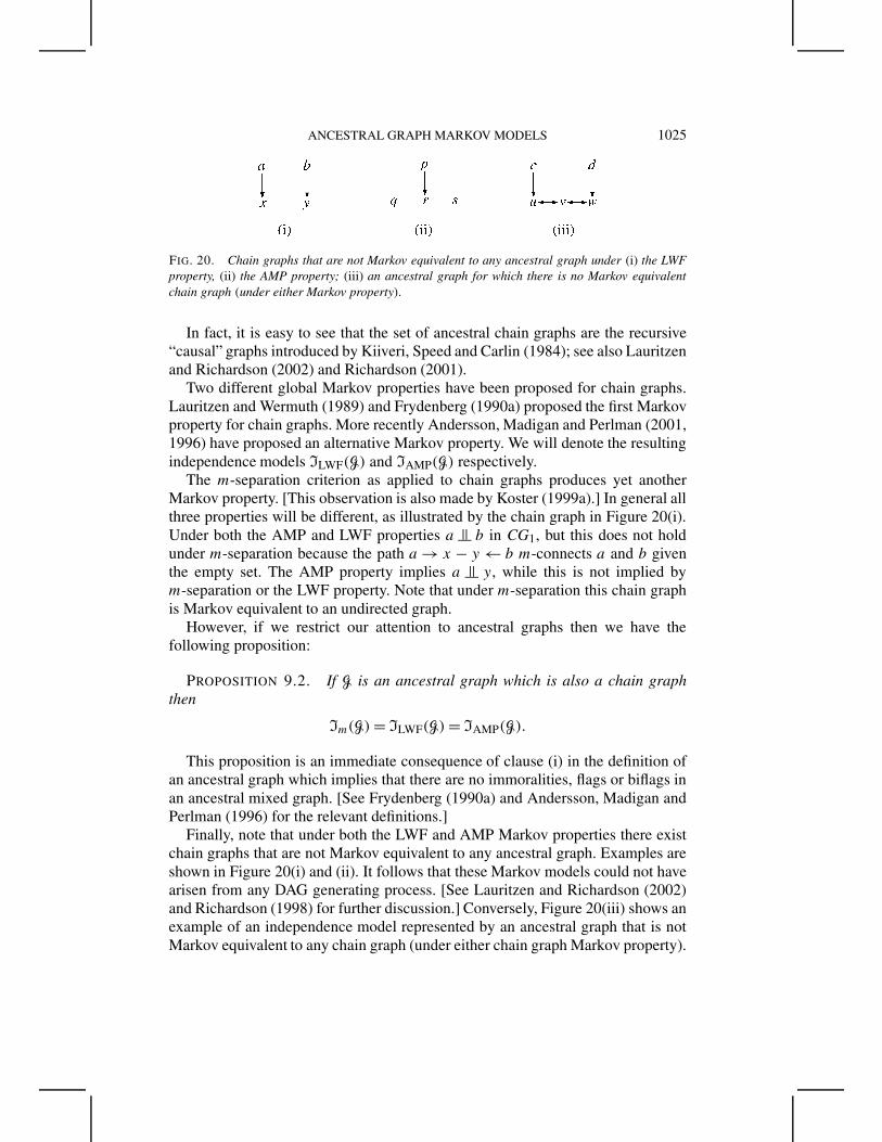
ANCESTRAL GRAPH MARKOV MODELS 1025
FIG. 20. Chain graphs that are not Markov equivalent to any ancestral graph under (i) the LWFproperty, (ii) the AMP property; (iii) an ancestral graph for which there is no Markov equivalentchain graph (under either Markov property).
In fact, it is easy to see that the set of ancestral chain graphs are the recursive“causal” graphs introduced by Kiiveri, Speed and Carlin (1984); see also Lauritzenand Richardson (2002) and Richardson (2001).
Two different global Markov properties have been proposed for chain graphs.Lauritzen and Wermuth (1989) and Frydenberg (1990a) proposed the first Markovproperty for chain graphs. More recently Andersson, Madigan and Perlman (2001,1996) have proposed an alternative Markov property. We will denote the resultingindependence models ILWF(G) and IAMP(G) respectively.
The m-separation criterion as applied to chain graphs produces yet anotherMarkov property. [This observation is also made by Koster (1999a).] In general allthree properties will be different, as illustrated by the chain graph in Figure 20(i).Under both the AMP and LWF properties a |= b in CG1, but this does not holdunder m-separation because the path a → x − y ← b m-connects a and b giventhe empty set. The AMP property implies a |= y, while this is not implied bym-separation or the LWF property. Note that under m-separation this chain graphis Markov equivalent to an undirected graph.
However, if we restrict our attention to ancestral graphs then we have thefollowing proposition:
PROPOSITION 9.2. If G is an ancestral graph which is also a chain graphthen
Im(G) = ILWF(G) = IAMP(G).
This proposition is an immediate consequence of clause (i) in the definition ofan ancestral graph which implies that there are no immoralities, flags or biflags inan ancestral mixed graph. [See Frydenberg (1990a) and Andersson, Madigan andPerlman (1996) for the relevant definitions.]
Finally, note that under both the LWF and AMP Markov properties there existchain graphs that are not Markov equivalent to any ancestral graph. Examples areshown in Figure 20(i) and (ii). It follows that these Markov models could not havearisen from any DAG generating process. [See Lauritzen and Richardson (2002)and Richardson (1998) for further discussion.] Conversely, Figure 20(iii) shows anexample of an independence model represented by an ancestral graph that is notMarkov equivalent to any chain graph (under either chain graph Markov property).
1026 T. RICHARDSON AND P. SPIRTES
10. Discussion. In this paper we have introduced the class of ancestralgraph Markov models. The purpose in introducing this class was to be ableto characterize the Markov structure of a DAG model under marginalizing andconditioning. To this end we defined a graphical transformation, G $→ G[SL, whichcorresponded to marginalizing and conditioning the corresponding independencemodel (Theorem 4.18).
If a DAG model containing latent or selection variables is hypothesized asthe generating mechanism for a given system then this transformation will allowa simple representation of the Markov model induced on the observed variables.
However, often graphical models are used for exploratory data analysis, wherelittle is known about the generating structure. In such situations the existence ofthis transformation provides a guarantee: if the data were generated by an unknownDAG containing hidden variables then we are ensured that there exists an ancestralgraph which can represent the resulting Markov structure over the observedvariables. Hence the problem of additional and misleading edges encounteredin the introduction may be avoided. In this context the transformation providesa justification for using the class of ancestral graphs.
However, any interpretation of the types of edge present in an ancestral graphwhich was arrived at via an exploratory analysis should take into account thatthere may exist (many) different graphs that are Markov equivalent. Spirtesand Richardson (1997) present a polynomial-time algorithm for testing Markovequivalence of two ancestral graphs. Spirtes et al. (1995, 1999) describe analgorithm for inferring structural features that are common to all maximal ancestralgraphs in a Markov equivalence class. For instance, there are Markov equivalenceclasses in which every member contains a directed path from some vertex α
to a second vertex β; likewise in other Markov equivalence classes no membercontains a directed path from α to β . At the time of writing there is not yet a fullcharacterization of common features, such as exists for DAG Markov equivalenceclasses [see Andersson, Madigan and Perlman (1997), Meek (1995a)].
Finally, we showed that maximal ancestral graphs lead to a natural para-metrization of the set of Gaussian distributions obeying the global Markovproperty for the graph. Conditions for the existence and uniqueness of maximumlikelihood estimates for these models is currently an open question.
Development of a parameterization for discrete distributions is another areaof current research. Richardson (2003) describes a local Markov property fora class of graphs that includes all ancestral graphs without undirected edges. Thislocal Markov property is equivalent to the global Markov property, and may thusfacilitate the development of a discrete parameterization.
APPENDIX
Definition of a mixed graph. Let E = {−,←,→,↔} be the set of edges. LetP(E) denote the power set of E . Formally, a mixed graph G = (V,E) is an ordered
ANCESTRAL GRAPH MARKOV MODELS 1027
pair consisting of a finite set V , and a mapping E :V × V → P(E), subject to thefollowing restrictions:
E(α,α) = ∅,
− ∈ E(α,β) ⇐⇒ − ∈ E(β,α),
← ∈ E(α,β) ⇐⇒ → ∈ E(β,α),
↔ ∈ E(α,β) ⇐⇒ ↔ ∈ E(β,α).
The induced subgraph, GA of G on A ⊆ V , is (A,E|A) where E|A is the naturalrestriction of E to A × A.
Acknowledgments. The work presented here has benefited greatly from thefrequent interaction that the authors have had with Nanny Wermuth and JanKoster during the last five years. In particular, as mentioned, the idea of studyingindependence models under conditioning was first raised by Wermuth, as was thenotion of a canonical DAG. The proof techniques employed by Koster in lecturenotes originally prepared for a course at the Fields Institute [Koster (1999a)]had a considerable influence on the development of Sections 7 and 8. Much ofthis interaction took place at workshops that were part of the European ScienceFoundation program on Highly Structured Stochastic Systems.
The authors are also grateful to Ayesha Ali, Steen Andersson, Heiko Bailer,Moulinath Banerjee, Sir David Cox, Clark Glymour, David Heckerman, SteffenLauritzen, David Madigan, Chris Meek, Michael Perlman, Jamie Robins, TamasRudas, Richard Scheines, Jim Q. Smith, Milan Studený, Larry Wasserman andJacob Wegelin for stimulating conversations and helpful comments on earlierdrafts.
REFERENCES
ANDERSSON, S. A., MADIGAN, D. and PERLMAN, M. D. (1996). An alternative Markov propertyfor chain graphs. In Uncertainty in Artificial Intelligence (F. V. Jensen and E. Horvitz,eds.) 40–48. Morgan Kaufmann, San Francisco.
ANDERSSON, S. A., MADIGAN, D. and PERLMAN, M. D. (1997). A characterization of Markovequivalence classes for acyclic digraphs. Ann. Statist. 25 505–541.
ANDERSSON, S. A., MADIGAN, D. and PERLMAN, M. D. (2001). Alternative Markov propertiesfor chain graphs. Scand. J. Statist. 28 33–86.
ANDERSSON, S. A., MADIGAN, D., PERLMAN, M. D. and TRIGGS, C. (1995). On the relationbetween conditional independence models determined by finite distributive lattices andby directed acyclic graphs. J. Statist. Plann. Inference 48 25–46.
ANDERSSON, S. A., MADIGAN, D., PERLMAN, M. D. and TRIGGS, C. (1997). A graphicalcharacterization of lattice conditional independence models. Ann. Math. Artif. Intell. 2127–50.
ANDERSSON, S. A. and PERLMAN, M. D. (1998). Normal linear regression models with recursivegraphical Markov structure. J. Multivariate Anal. 66 133–187.
ARBUCKLE, J. L. (1997). AMOS User’s Guide. Version 3.6. SPSS, Chicago.
1028 T. RICHARDSON AND P. SPIRTES
BENTLER, P. M. (1986). Theory and implementation of EQS: A structural equations program.BMDP Statistical Software, Los Angeles.
COOPER, G. F. (1995). Causal discovery from data in the presence of selection bias. In PreliminaryPapers of the Fifth International Workshop on AI and Statistics (D. Fisher, ed.) 140–150.
COX, D. R. and WERMUTH, N. (1996). Multivariate Dependencies: Models, Analysis andInterpretation. Chapman and Hall, London.
DARROCH, J., LAURITZEN, S. and SPEED, T. (1980). Markov fields and log-linear interactionmodels for contingency tables. Ann. Statist. 8 522–539.
DAWID, A. (1980). Conditional independence for statistical operations. Ann. Statist. 8 598–617.DEMPSTER, A. P. (1972). Covariance selection. Biometrics 28 157–175.EDWARDS, D. M. (1995). Introduction to Graphical Modelling. Springer, New York.FRYDENBERG, M. (1990a). The chain graph Markov property. Scand. J. Statist. 17 333–353.FRYDENBERG, M. (1990b). Marginalization and collapsibility in graphical interaction models. Ann.
Statist. 18 790–805.GEIGER, D. (1990). Graphoids: A qualitative framework for probabilistic inference. Ph.D.
dissertation, UCLA.GEIGER, D., HECKERMAN, D., KING, H. and MEEK, C. (2001). Stratified exponential families:
Graphical models and model selection. Ann. Statist. 29 505–529.GEIGER, D. and PEARL, J. (1990). On the logic of causal models. In Uncertainty in Artificial
Intelligence IV (R. D. Shachter, T. S. Levitt, L. N. Kanal and J. F. Lemmer, eds.) 136–147.North-Holland, Amsterdam.
HAUGHTON, D. (1988). On the choice of a model to fit data from an exponential family. Ann. Statist.16 342–355.
JÖRESKOG, K. and SÖRBOM, D. (1995). LISREL 8: User’s Reference Guide. Scientific SoftwareInternational, Chicago.
KASS, R. E. and VOS, P. W. (1997). Geometrical Foundations of Asymptotic Inference. Wiley, NewYork.
KAUERMANN, G. (1996). On a dualization of graphical Gaussian models. Scand. J. Statist. 23 105–116.
KIIVERI, H., SPEED, T. and CARLIN, J. (1984). Recursive causal models. J. Austral. Math. Soc.Ser. A 36 30–52.
KOSTER, J. T. A. (1996). Markov properties of non-recursive causal models. Ann. Statist. 24 2148–2177.
KOSTER, J. T. A. (1999a). Linear structural equations and graphical models. Lecture Notes, TheFields Institute, Toronto.
KOSTER, J. T. A. (1999b). On the validity of the Markov interpretation of path diagrams of Gaussianstructural equation systems with correlated errors. Scand. J. Statist. 26 413–431.
KOSTER, J. T. A. (2000). Marginalizing and conditioning in graphical models. Technical report,Erasmus Univ.
LAURITZEN, S. L. (1979). Lectures on contingency tables. Technical report, Inst. Math. Statist.,Univ. Copenhagen.
LAURITZEN, S. (1996). Graphical Models. Clarendon, Oxford.LAURITZEN, S. L. (1998). Generating mixed hierarchical interaction models by selection. Technical
Report R-98-2009, Dept. Mathematics, Univ. Aalborg.LAURITZEN, S. L. and RICHARDSON, T. S. (2002). Chain graph models and their causal
interpretations (with discussion). J. Roy. Statist. Soc. Ser. B 64 321–361.LAURITZEN, S. L. and WERMUTH, N. (1989). Graphical models for association between variables,
some of which are qualitative and some quantitative. Ann. Statist. 17 31–57.
ANCESTRAL GRAPH MARKOV MODELS 1029
MEEK, C. (1995a). Causal inference and causal explanation with background knowledge. InUncertainty in Artificial Intelligence: Proceedings of the 11th Conference (P. Besnardand S. Hanks, eds.) 403–410. Morgan Kaufmann, San Francisco.
MEEK, C. (1995b). Strong completeness and faithfulness in Bayesian networks. In Uncertainty inArtificial Intelligence (P. Besnard and S. Hanks, eds.) 411–418. Morgan Kaufmann, SanFrancisco.
PEARL, J. (1988). Probabilistic Reasoning in Intelligent Systems. Morgan Kaufmann, San Francisco.RICHARDSON, T. S. (1996). Models of feedback: interpretation and discovery. Ph.D. dissertation,
Carnegie Mellon Univ.RICHARDSON, T. S. (1998). Chain graphs and symmetric associations. In Learning in Graphical
Models (M. Jordan, ed.) 231–260. Kluwer, Drodrecht.RICHARDSON, T. S. (2001). Chain graphs which are maximal ancestral graphs are recursive causal
graphs. Technical Report 387, Dept. Statistics, Univ. Washington.RICHARDSON, T. S. (2003). Markov properties for acyclic directed mixed graphs. Scand. J. Statist.
To appear.RICHARDSON, T. S., BAILER, H. and BANERJEE, M. (1999). Tractable structure search in the
presence of latent variables. In Preliminary Papers of the Seventh International Workshopon AI and Statistics (D. Heckerman and J. Whittaker, eds.) 142–151. Morgan Kaufmann,San Francisco.
ROBINS, J. (1997). Causal inference from complex longitudinal data. In Latent Variable Modellingand Applications to Causality. Lecture Notes in Statist. 120 69–117. Springer, New York.
SAS Publishing (1995). SAS/STAT User’s Guide. Version 6, 4th ed. SAS Publishing, Cary, NC.SETTIMI, R. and SMITH, J. Q. (1998). On the geometry of Bayesian graphical models with hidden
variables. In Uncertainty in Artificial Intelligence (G. Cooper and S. Moral, eds.) 472–479. Morgan Kaufmann, San Francisco.
SETTIMI, R. and SMITH, J. Q. (1999). Geometry, moments and Bayesian networks with hiddenvariables. In Preliminary Papers of the Seventh International Workshop on AI andStatistics (D. Heckerman and J. Whittaker, eds.) 293–298. Morgan Kaufmann, SanFrancisco.
SPIRTES, P. (1995). Directed cyclic graphical representations of feedback models. In Uncertainty inArtificial Intelligence (P. Besnard and S. Hanks, eds.) 491–498. Morgan Kaufmann, SanFrancisco.
SPIRTES, P., GLYMOUR, C. and SCHEINES, R. (1993). Causation, Prediction and Search. LectureNotes in Statist. 81. Springer, New York.
SPIRTES, P., MEEK, C. and RICHARDSON, T. S. (1995). Causal inference in the presence oflatent variables and selection bias. In Uncertainty in Artificial Intelligence (P. Besnardand S. Hanks, eds.) 449–506. Morgan Kaufmann, San Francisco.
SPIRTES, P., MEEK, C. and RICHARDSON, T. S. (1999). An algorithm for causal inference in thepresence of latent variables and selection bias. In Computation, Causation and Discovery(C. Glymour and G. F. Cooper, eds.) 211–252. MIT Press.
SPIRTES, P. and RICHARDSON, T. S. (1997). A polynomial-time algorithm for determining DAGequivalence in the presence of latent variables and selection bias. In Preliminary Papersof the Sixth International Workshop on AI and Statistics (D. Madigan and P. Smyth, eds.)489–501.
SPIRTES, P., RICHARDSON, T. S., MEEK, C., SCHEINES, R. and GLYMOUR, C. (1996). Usingd-separation to calculate zero partial correlations in linear models with correlated errors.Technical Report CMU-PHIL-72, Dept. Philosophy, Carnegie Mellon Univ.
SPIRTES, P., RICHARDSON, T. S., MEEK, C., SCHEINES, R. and GLYMOUR, C. (1998). Using pathdiagrams as a structural equation modelling tool. Sociological Methods and Research 27182–225.
1030 T. RICHARDSON AND P. SPIRTES
VERMA, T. (1993). Graphical aspects of causal models. Technical Report R-191, Cognitive SystemsLaboratory, UCLA.
VERMA, T. and PEARL, J. (1990). Equivalence and synthesis of causal models. In Uncertainty inArtificial Intelligence (M. Henrion, R. Shachter, L. Kanal and J. Lemmer, eds.) 220–227.Association for Uncertainty in AI.
VERMA, T. and PEARL, J. (1991). Equivalence and synthesis of causal models. Technical ReportR-150, Cognitive Systems Laboratory, UCLA.
WERMUTH, N. and COX, D. (2000). A sweep operator for triangular matrices and its statisticalapplications. Technical Report 00-04, ZUMA Institute, Mannheim, Germany.
WERMUTH, N., COX, D. and PEARL, J. (1994). Explanations for multivariate structures derivedfrom univariate recursive regressions. Technical Report 94-1, Univ. Mainz, Germany.
WERMUTH, N., COX, D. and PEARL, J. (1999). Explanations for multivariate structures derivedfrom univariate recursive regressions. Technical Report Revision of 94-1, Univ. Mainz,Germany.
WHITTAKER, J. (1990). Graphical Models in Applied Multivariate Statistics. Wiley, Chichester.WRIGHT, S. (1921). Correlation and causation. J. Agricultural Research 20 557–585.WRIGHT, S. (1934). The method of path coefficients. Ann. Math. Statist. 5 161–215.ZELLNER, A. (1962). An efficient method of estimating seemingly unrelated regression and tests for
aggregation bias. J. Amer. Statist. Assoc. 57 348–368.
DEPARTMENT OF STATISTICS
UNIVERSITY OF WASHINGTON
SEATTLE, WASHINGTON 98195E-MAIL: [email protected]
INSTITUTE FOR HUMAN & MACHINE
COGNITION
40 SOUTH ALCANIZ
PENSACOLA, FLORIDA 32501E-MAIL: [email protected]
Related Documents