ANALYSIS OF TRACER DATA FROM URBAN DISPERSION EXPERIMENTS Akula Venkatram and Vlad Isakov Motivation for Field Experiments Field Studies Conducted.

ANALYSIS OF TRACER DATA FROM URBAN DISPERSION EXPERIMENTS

Akula Venkatram and Vlad Isakov

Motivation for Field Experiments Field Studies Conducted in Barrio

Logan Results from Current Models New Modeling Approach Results Future Work

Motivation Few experiments conducted for

ground-level releases in urban areas.– St Louis Experiment in 1968

Little data for near source dispersion

Data set is specific to Barrio Logan

Urban Effects on Dispersion

Stable air from the rural area becomes unstable when it flows over warmer urban area

Roughness increases turbulence and decreases wind speed

Field Experiments

Tracer studies designed to study dispersion at scales of meters to kilometers in urban areas.– Near source experiment at Memorial High,

April 2001– CE-CERT parking lot study, April-May 2001 – Summer and winter Barrio Logan field

studies– Dugway Proving Grounds Model Study

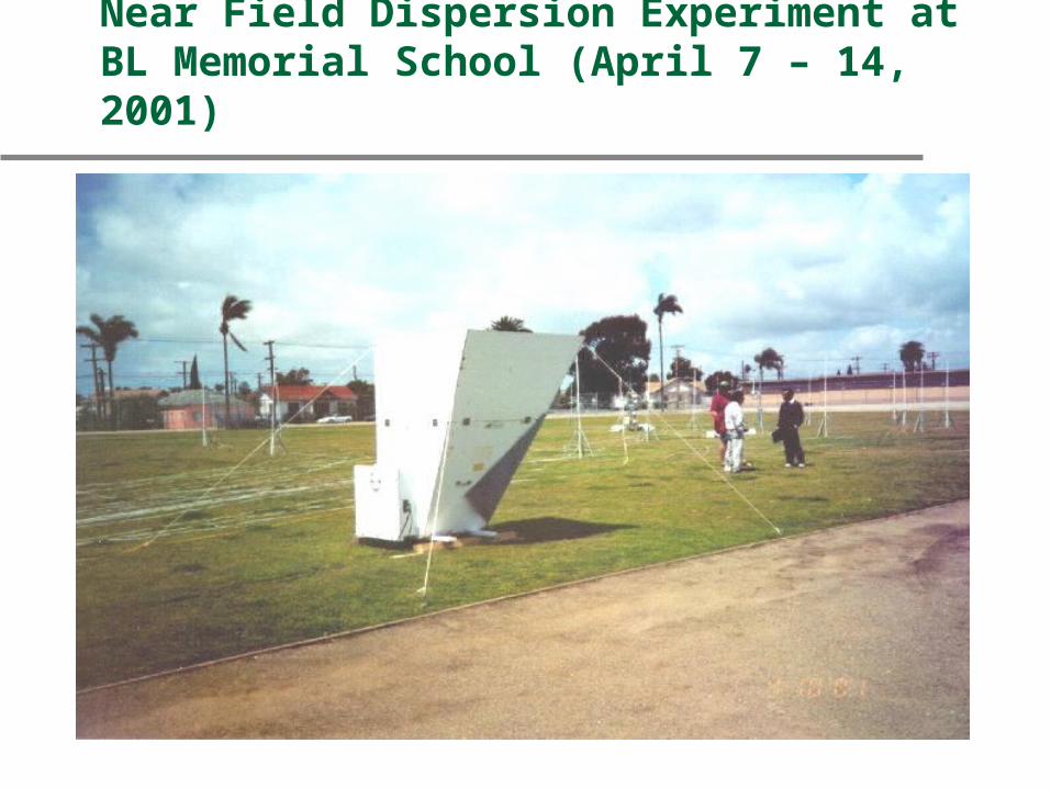
Near Field Dispersion-tens of meters

SF6 released at ground level in a school playground in an urban area

Source surrounded by two arcs at 10 and 20 meters

Flow measured with sonics, propeller anemometers, and mini-sodar

Real time analysis of data

Near source dispersion

v is comparable to effective wind speed transporting plume

Upwind dispersion becomes important

Plume model might not be applicable

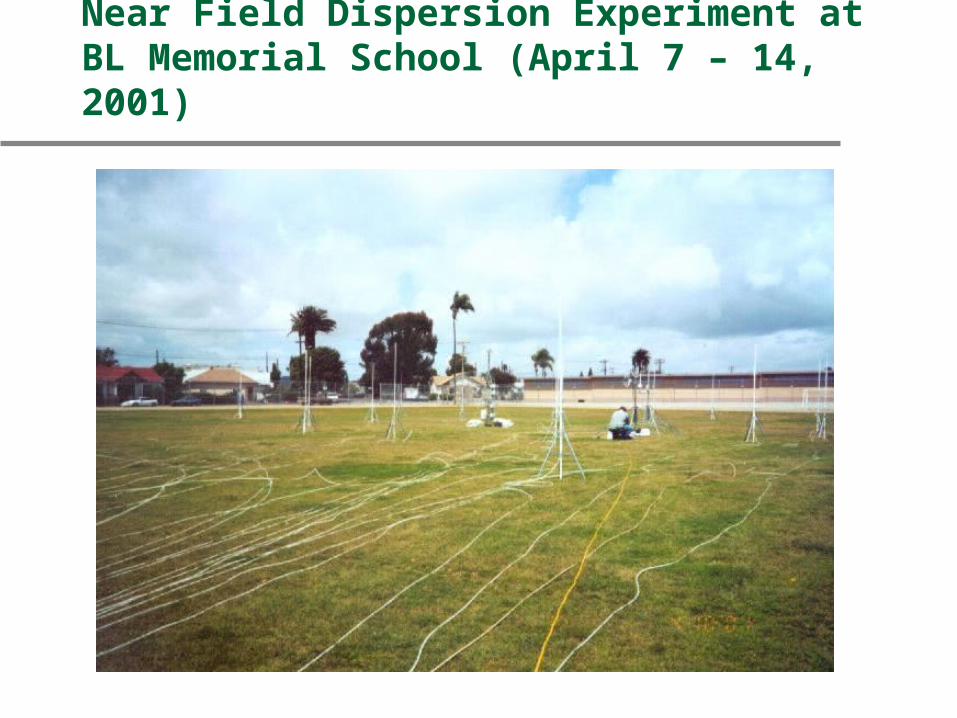
Near Field Dispersion Experiment at BL Memorial School (April 7 – 14, 2001)

Near Field Dispersion Experiment at BL Memorial School (April 7 – 14, 2001)

Near Field Dispersion Experiment at BL Memorial School (April 7 – 14, 2001)

Near Field Dispersion Experiment at BL Memorial School (April 7 – 14, 2001)

Concentration Pattern on 4/14/01

-25 -20 -15 -10 -5 0 5 10 15 20 25-25

-20

-15

-10

-5

0

5

10

15

20

25

853

105

1319

142

176

122

Concentrations(ppt) for half hour ending 4/14/01 14:30

X

4

8

123

5

7

141

Y

u = (1.2815)i+ (1.1118)jDirection Vector

Concentration Pattern on 4/14/01

-25 -20 -15 -10 -5 0 5 10 15 20 25-25

-20

-15

-10

-5

0

5

10

15

20

25

0

76

1

108

123

83

Concentrations for half hour ending 4/14/01 05:30

X

0

63

330

0

436

221

Y

u = (-0.73455)i+ (-0.10971)j

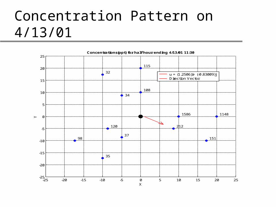
Concentration Pattern on 4/13/01

-25 -20 -15 -10 -5 0 5 10 15 20 25-25

-20

-15

-10

-5

0

5

10

15

20

25

1148

151

1586

212

115

108

Concentrations(ppt) for half hour ending 4/13/01 11:30

X

34

37

120

32

35

98

Y

u = (1.2506)i+ (-0.83009)jDirection Vector

Concentration Pattern on 4/12/01

-25 -20 -15 -10 -5 0 5 10 15 20 25-25

-20

-15

-10

-5

0

5

10

15

20

25

19

709

9

610

339

448

Concentrations for half hour ending 4/12/01 20:00

X

2

58

639

0

0

399

Y

u = (1.8729)i+ (-0.38128)j

CE-CERT Parking Lot

CE-CERT Parking Lot

CE-CERT Parking Lot

CE-CERT Model Comparison

Low Wind Speed Model

The horizontal distribution is written as:

2y

2m

2v

2v

ran

2y

2

yranran

x2

u22

f

2y

exp21

)f1(r2

1f)y,x(H

Tracer Experiment at Barrio LoganTracer Experiment at Barrio Logan

Tracer Experiment conducted in August and December of 2001

Hourly SF6 concentrations sampled at 50 sites Tracer released at NASSCO during daytime

from 10 a.m. to 10 p.m.

Mobile van sampled continuously to measure crosswind SF6 concentrations

Mini-sodar to measure vertical winds up to 200m at 5m resolution

Six sonic anemometers to measure surface level winds and turbulence

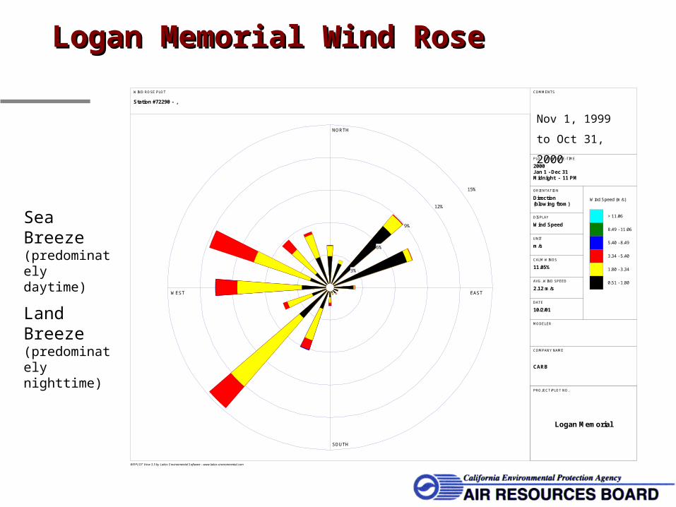
WIND ROSE PLOT

Station #72290 - ,

NORTH

SOUTH

WEST EAST

3%

6%

9%

12%

15%

Wind Speed (m/s)

> 11.06

8.49 - 11.06

5.40 - 8.49

3.34 - 5.40

1.80 - 3.34

0.51 - 1.80

UNIT

m/s

DISPLAY

Wind Speed

CALM WINDS

11.05%

MODELER

DATE

10/2/01

COMPANY NAME

CARB

COMMENTS

WRPLOT View 3.5 by Lakes Environmental Software - www.lakes-environmental.com

PLOT YEAR-DATE-TIME

2000 Jan 1 - Dec 31Midnight - 11 PM

AVG. WIND SPEED

2.12 m/s

ORIENTATION

Direction(blowing from)

PROJECT/PLOT NO.

Logan Memorial

Logan Memorial Wind RoseLogan Memorial Wind Rose

Nov 1, 1999 to

Oct 31, 2000

Sea Breeze (predominately daytime)

Land Breeze (predominately nighttime)

Map of Barrio Logan tracer experimentAugust 2001

yellow dotd -stationarysamplersblack lines - mobile vanlocations

Model Performance at 200m on 08/21/2001

Model Performance at 500m on 08/21/2001

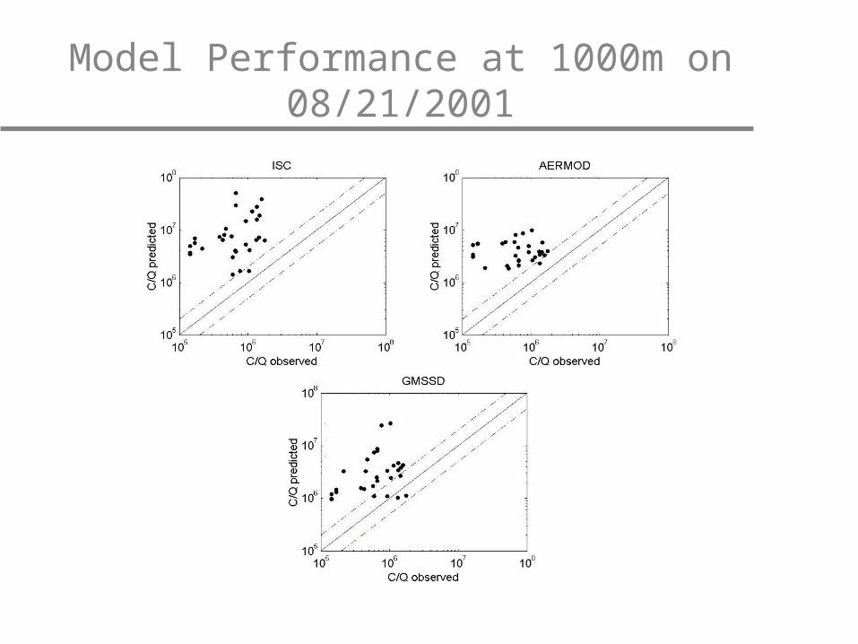
Model Performance at 1000m on 08/21/2001

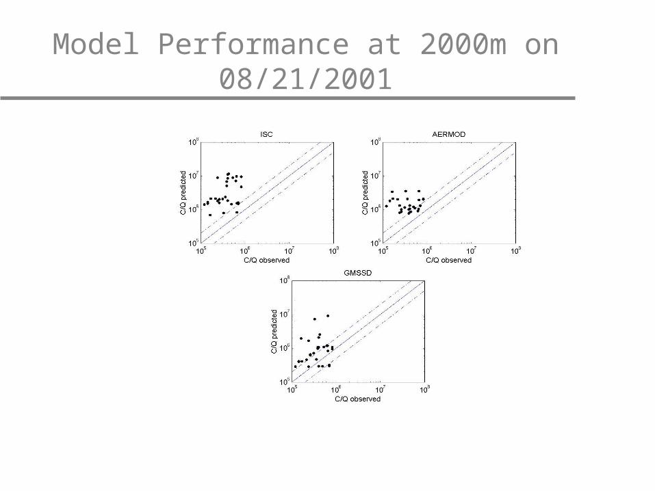
Model Performance at 2000m on 08/21/2001

Model Performance at 200m on 08/25/2001

Model Performance at 500m on 08/25/2001

Model Performance at 1000m on 08/25/2001

Model Performance at 2000m on 08/25/2001

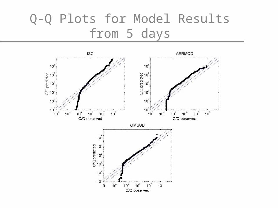
Q-Q Plots for Model Results from 5 days

Model for Urban Areas

Micrometeorological variables used to describe flat terrain dispersion do not apply to urban areas

Formulate model that uses measured turbulence and velocity profiles

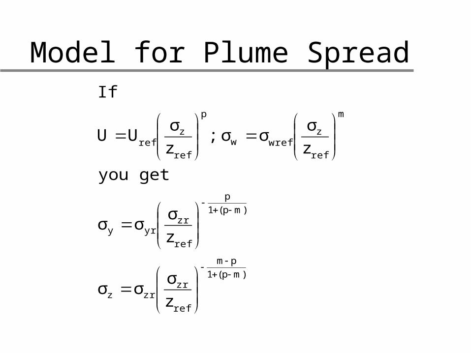
Model for Plume Spread

)mp(1pm

ref

zrzrz

)mp(1p

ref

zryry

m

ref

zwrefw

p

ref

zref

zσ

σσ

zσ

σσ

get you

zσ

σσ ;zσ

UU

If

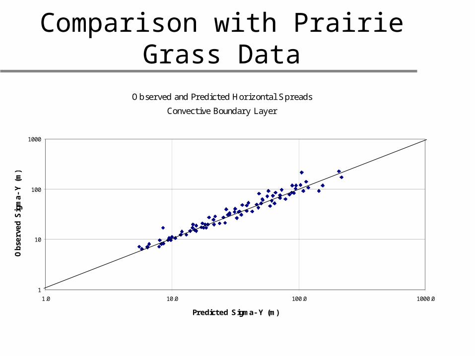
Comparison with Prairie Grass Data

Observed and Predicted Horizontal Spreads

Convective Boundary Layer

1

10

100

1000

1.0 10.0 100.0 1000.0

Predicted Sigma- Y (m)

Obse

rved S

igm

a-Y (

m)

Comparison with Prairie Grass Data

Observed versus Predicted Concentrations

Convective Boundary layer- Prairie Grass

1

10

100

1000

10000

1.0 10.0 100.0 1000.0 10000.0

Modeled Concentration (us/m3)

Obs

erve

d Con

cent

rati

on (

us/m

3)

Comparison with Prairie Grass Data

Observed versus Predicted Horizontal Spreads

Stable Boundary Layer- Prairie Grass

1

10

100

1.0 10.0 100.0

Predicted Sigma- y (m)

Obs

erve

d S

igm

a-y

(m)

Comparison with Prairie Grass DataObserved Versus Modeled Concentrations

Stable Boundary Layer- Prairie Grass

1

10

100

1000

10000

100000

1.0 10.0 100.0 1000.0 10000.0 100000.0

Modeled Concentration (us/m3)

Obs

erve

d Co

ncen

trat

ion

(us/

m3)

Model Field Study

Understand dispersion in flat terrain at distances of less than 50 m

Examine the effect of increasingly complicated building structures on– Turbulence– Dispersion

Model Field Study

Conducted at Dugway Proving Ground, Utah July 17,18,19,26 2001

13.5 hours under a variety of stability conditions

Velocity and turbulence measured with sonic anemometers

Buildings simulated with barrels

Model Urban Area 59 array of 45 barrels H=0.91 m and D=0.57 m at spacing

of 1.8 m- frontal area/plan area=16% Propylene released at z=0 and z=H 6 different configurations to examine

the effect of release height and source structure

Concentration Measurements

Tracer measured with 43 PIDs arranged in 3, 50 degree arcs

Arcs at 1.5S, 2.5S, and 4.5S PIDs at 5o spacing PIDs located at z=0.23 m Four 2 m towers were used to

measure vertical profiles Concentrations measured at 50 Hz

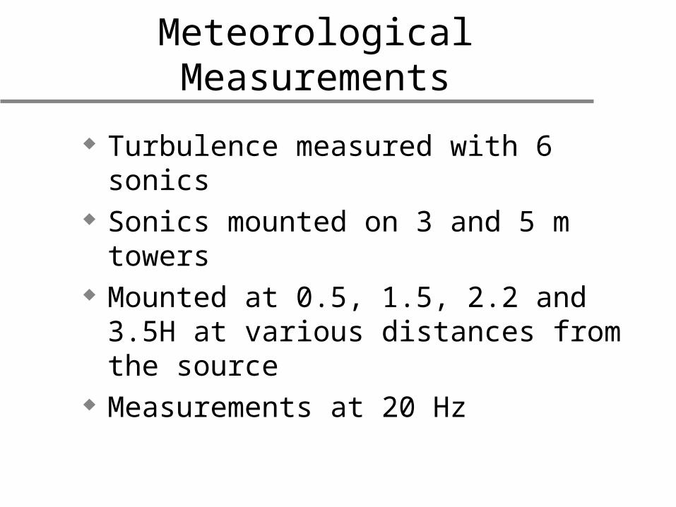
Meteorological Measurements

Turbulence measured with 6 sonics Sonics mounted on 3 and 5 m

towers Mounted at 0.5, 1.5, 2.2 and 3.5H

at various distances from the source

Measurements at 20 Hz

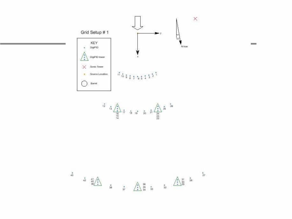
Figure 2. Observed versus Predicted concentration using model plume spreads without obstacle for ground level release

1.0E-02

1.0E-01

1.0E+00

1.0E-02 1.0E-01 1.0E+00

Pred. Conc. (gm/m3)

Obs.

Con

c. (

gm/m

3)

Figure 3. Observed versus Predicted concentration using linear plume spreads with one obstacle in array for ground level release

1.0E-03

1.0E-02

1.0E-01

1.0E+00

1.0E-03 1.0E-02 1.0E-01 1.0E+00

Pred. Conc. (gm/m3)

Obs

. Co

nc.

(gm

/m3)

Figure 4. Observed versus Predicted concentration using model plume spreads with one obstacle in array for ground level release

1.0E-03

1.0E-02

1.0E-01

1.0E+00

1.0E-03 1.0E-02 1.0E-01 1.0E+00

Pred. Conc. (gm/m3)

Obs

. Co

nc.

(gm

/m3)

Figure 6. Observed versus Predicted concentration using model plume spreads with two obstacles in array for ground level release

1.0E-03

1.0E-02

1.0E-01

1.0E+00

1.0E-03 1.0E-02 1.0E-01 1.0E+00

Pred. Conc. (gm/ m3)

Obs

. Co

nc.

(gm

/m3)

Future Work

Model might require modification to account for source effects

Need to account for plume meandering-upwind dispersion

Need to evaluate model with CE-CERT data and Barrio Logan winter data