Analysis of rainfall and temperature time series to detect ...

J. Earth Syst. Sci. (2018) 127:25 c© Indian Academy of Scienceshttps://doi.org/10.1007/s12040-018-0926-3

Analysis of rainfall and temperature time series to detectlong-term climatic trends and variability over semi-aridBotswana

Jimmy Byakatonda1,3,*, B P Parida1, Piet K Kenabatho2 and D B Moalafhi2

1Department of Civil Engineering, University of Botswana, P/Bag 0061, Gaborone, Botswana.2Department of Environmental Science, University of Botswana, P/Bag 00704, Gaborone, Botswana.3Department of Biosystems Engineering, Gulu University, P.O. Box 166, Gulu, Uganda.*Corresponding author. e-mail: [email protected]

MS received 14 December 2016; revised 23 May 2017; accepted 24 July 2017; published online 6 March 2018

Arid and semi-arid environments have been identified with locations prone to impacts of climatevariability and change. Investigating long-term trends is one way of tracing climate change impacts.This study investigates variability through annual and seasonal meteorological time series. Possibleinhomogeneities and years of intervention are analysed using four absolute homogeneity tests. Trendsin the climatic variables were determined using Mann–Kendall and Sen’s Slope estimator statistics.Association of El Nino Southern Oscillation (ENSO) with local climate is also investigated throughmultivariate analysis. Results from the study show that rainfall time series are fully homogeneouswith 78.6 and 50% of the stations for maximum and minimum temperature, respectively, showinghomogeneity. Trends also indicate a general decrease of 5.8, 7.4 and 18.1% in annual, summer and winterrainfall, respectively. Warming trends are observed in annual and winter temperature at 0.3 and 1.5%for maximum temperature and 1.7 and 6.5% for minimum temperature, respectively. Rainfall reporteda positive correlation with Southern Oscillation Index (SOI) and at the same time negative associationwith Sea Surface Temperatures (SSTs). Strong relationships between SSTs and maximum temperatureare observed during the El Nino and La Nina years. These study findings could facilitate planning andmanagement of agricultural and water resources in Botswana.

Keywords. Correlation; El Nino; homogeneity test; intervention analysis; persistence; trend analysis.

1. Introduction

Increasing concentrations of atmospheric carbon-dioxide (CO2) over the recent past has been sin-gled out as the main cause of global warming(Shifteh Some’e et al. 2012; Stocker et al. 2013).The fifth assessment report (AR5) of the intergov-ernmental panel on climate change (IPCC) showsa close positive association between CO2 concen-tration and global temperature rise (Stocker et al.

2013). It is reported that the first decade of the 21stcentury has been the warmest ever, coincidingwith the strongest El Nino in 100 years (Stockeret al. 2013; Hansen et al. 2016; Rahman andLateh 2017). Also climate change projections haverevealed a global temperature rise of about 2◦Cin the near future and 4−6◦C in the long run(Pachauri and Reisinger 2007). These climaticchanges could lead to a shift in meteorological vari-ables such as rainfall and temperature (Yue and

1

0123456789().,--: vol V

25 Page 2 of 20 J. Earth Syst. Sci. (2018) 127:25

Hashino 2003; Costa and Soares 2009b; Hanselet al. 2016). Besides, these anticipated changesare not uniformly spread globally, with differentregions experiencing impacts at varying degrees.It is further projected that arid and semi-aridregions could experience higher than global averagewarming levels (Modarres and da Silva 2007; Khanet al. 2016). Hence, there is need to shift focustowards semi-arid locations where adaptation mea-sures to these extreme weather conditions are a bigchallenge. Studies on long-term changes in rainfalland temperature are necessary for sustainable landand water resources planning and managementespecially under climate variability and change(Shahid 2010; Tabari and Talaee 2011). Therefore,for any meaningful study on climate variability andchange, these meteorological variables may not beignored. Of recent, interest has increased in investi-gating long-term trends in rainfall and temperaturein quest of tracing the climate change signal (Men-zel et al. 2006; Giorgi and Lionello 2008; Kenabathoet al. 2012).

Several studies have since been conductedglobally and regionally to investigate climate vari-ability by analyzing trends in rainfall and tem-perature time series. Such of these investigationshave been conducted in semi-arid locations in Iranby Shifteh Some’e et al. (2012) and Tabari andTalaee (2011). Results from their studies indicateboth increasing and decreasing trends in meteoro-logical variables for a period of 1966–2006, withsignificant trends mainly observed during winterperiod. In Nigeria, Akinsanola and Ogunjobi (2015)reported decreasing trends in both annual andwinter seasonal rainfall while using the Mann–Kendal (MK) test statistic. In Portugal, Costa andSoares (2009a) reported high rainfall variabilityby examining trends in aridity and standardizedprecipitation index (SPI). Their study found highclimatic uncertainty in the south of the country.In Turkey, Partal and Kahya (2006) applied theMK test and Sen’s Slope estimator to study thedirection and magnitude of trends in meteorologi-cal variables. Their study identified the months ofJanuary, February and September to be exhibit-ing decreasing trends especially in the south andwest of Turkey for the period from 1929 to 1993.Climatic changes for a period of 1980–2010 wereinvestigated in Serbia by Gocic and Trajkovic(2013) using the MK trend analysis and Sen’s Slopeestimator. The results indicated increasing trendsin both annual and seasonal temperature with nosignificant trends in rainfall.

Climate variability has also been closely linkedwith El Nino Southern Oscillation (ENSO) thatis attributed to hydro-climatic extremes in formof droughts and floods. ENSO is the main sourceof climate variability in the Equatorial Pacific(Moran-Tejeda et al. 2016). This climate variabilityhas tele-connections with the Indian and AtlanticOceans (Nicholson et al. 2001; Nyenzi and Lefale2006). Influences of ENSO on the local climate maynot be ignored since a number of studies over south-ern Africa have reported its close association withrainfall patterns and onset of droughts (Nichol-son et al. 2001; Usman and Reason 2004; Edossaet al. 2014). This study, thus proposes to investi-gate the association between ENSO and the localclimate.

To investigate the temporal and spatial extent ofclimate variability and change, Botswana, which islocated in the mid-latitudes and classified as semi-arid, is selected as a study area. Botswana’s econ-omy is heavily dependent on the climatic regimesince majority of her water resources are derivedfrom rainfall stored in surface reservoirs (Statis-tics Botswana 2009). Also 80% of the dwellersin the study area are engaged in rain fed agri-culture, which is heavily moderated by the localclimate (Batisani 2012; Statistics Botswana 2015).It is therefore necessary to investigate climatevariability and change in Botswana since any neg-ative impacts may propagate to other sectors ofthe economy. Some attempts have been made tostudy climate variability and change in Botswanaby Parida and Moalafhi (2008) and Batisani andYarnal (2010), who both reported decreasing rain-fall and increasing incidences of drought over thestudy area. However, these studies only analysedrainfall as the only precursor of climate variabilityand change. With reported global warming, tem-perature will require inclusion if any conclusive cli-mate change studies are to be conducted. Besides,it is prudent to periodically monitor climate vari-ability and change using location specific mete-orological data in order to achieve sustainablemanagement of water and agricultural resourcessince the climatic regime could change dependingon prevailing circumstances. It is on these premisesthat this study investigates climate variability andchange in Botswana. The variability will be studiedby investigating homogeneity and trends in rainfall,minimum and maximum temperature from 14 syn-optic stations spread across the study area. Alsothe study intends to determine the degree of asso-ciation between local climatic variables and ENSO.

J. Earth Syst. Sci. (2018) 127:25 Page 3 of 20 25

The analysis is proposed to be conducted for bothannual and seasonal scales.

2. Data and methods

2.1 Data

Data used in this study comprises locally observedmonthly rainfall, maximum and minimum tem-perature. The second dataset is from large-scaleclimatic predictors in the form of sea surface tem-peratures (SSTs) and southern oscillation index(SOI) elements of ENSO activities in the equatorialPacific.

2.1.1 Local meteorological data

Local meteorological data recorded at 14 synopticstations as shown in figure 2, was obtained fromthe Department of Meteorological Services (DMS)of Botswana. The records were of varying lengthwith the longest record being 1960–2014 and theshortest spanning 2000–2014. Details of the sta-tions, annual rainfall coefficient of variations (Cvs)and data record length are presented in table 1.Stations are selected based on the availability ofcomplete data that include rainfall, maximum andminimum temperature with < 5% missing values.

2.1.2 Sea surface temperatures and southernoscillation index

Records of SSTs from El Nino in region 3.4were obtained from the climatic prediction center

of NOAA (NOAA-NCEP 2016). The data recordlength corresponded to the locally observedmeteorological records. Similarly, data on SOI wasobtained from the national climate data center ofNOAA (NOAA-NCDC 2016). Climatic data anal-ysis is done at annual and seasonal scales. Annualand seasonal averages were obtained from climaticdata arranged at monthly scale for the case oftemperature time series, while annual and seasonaltotals are used for rainfall time series. Seasons con-sidered in this study are summer (October–March)and winter (May–August).

2.2 Methods

For analysis of long-term climate variability overthe study area, a number of statistical proceduresare employed in this study. The steps of anal-ysis involve: (i) applying four absolute tests forhomogeneity in the time series; (ii) applying theMann–Kendall (MK) trend analysis test and Sen’sSlope estimator; (iii) detection of persistence andtesting its effect on the MK trend statistics, and(iv) assessing the influence of ENSO on local cli-matic variables.

2.2.1 Tests for homogeneity

Data used in long-term climatological studies arerequired to be homogeneous in that, they shouldbelong to the same population with mean ofno temporal variation (Akinsanola and Ogun-jobi 2015). Data is considered homogeneous ifany changes are only attributed to natural

Table 1. Station locations and length of meteorological variable record.

Station

ID

Station

name

Latitude◦S

Longitude◦E

Elevation

amsl (m)

Rainfall

CV (%)

Period of record

Sl. no. Rainfall Max temp Min temp

1 033-FRAN Francistown 21.2 27.5 968 36.7 1960–2014 1960–2014 1960–2014

2 039-GANT Ghanzi 21.7 21.6 1131 39.6 1960–2014 1961–2014 1960–2014

3 053-JWAN Jwaneng 24.6 24.8 935 29.8 1988–2014 1989–2014 1989–2014

4 064-KASA Kasane 17.8 25.2 960 26.0 1968–2014 1983–2014 1983–2014

5 093-LET2 Letlhakane 21.3 25.3 991 35.9 1993–2014 1994–2014 1994–2014

6 106-MAHA Mahalapye 23.1 26.8 1005 33.5 1960–2013 1971–2014 1971–2014

7 130-MAUN Maun 19 23.4 945 38.6 1960–2014 1965–2014 1965–2014

8 183-PAN2 Pandamatenga 17.8 28.6 1071 29.4 1998–2014 1998–2014 1998–2014

9 213-SEL2 Selibe-Phikwe 23.1 37.8 892 34.5 1998–2014 2000–2014 2000–2014

10 223-SHAK Shakawe 18.4 21.9 1030 31.5 1960–2014 1965–2014 1965–2014

11 035-SSKA SSKA 24.7 25.9 975 34.2 1985–2014 1985–2014 1985–2014

12 033-SUAP Sowa Pan 20.6 26 908 40.4 1992–2010 2000–2014 2000–2014

13 244-TSAB Tsabong 26 22.4 960 42.4 1960–2011 1961–2014 1961–2014

14 251-TSHA Tshane 24 21.6 1118 42.0 1960–2014 1961–2014 1960–2014

25 Page 4 of 20 J. Earth Syst. Sci. (2018) 127:25

occurrences. Homogeneity testing in this studyinvolves a number of stages. The first stage com-prises data quality checks to identify recordingerrors both visual and graphical techniques. Thesecond stage involves applying of absolute homo-geneity testing techniques that include the Stan-dard Normal Homogeneity Test (SNHT; Alexan-dersson 1986), Pettit test (Pettit 1979), Buishandrange test (Buishand 1982) and the Von Neu-mann ratio test (Von Neumann 1941). Wijngaardet al. (2003), in a comprehensive study of Euro-pean climate systems, recommended no discardingof stations with suspected inhomogeneities, butrather classify them. Absolute tests were selectedover relative tests due to the somewhat sparse andskewed towards the east (figure 2) meteorologicalnetwork across the study area. Stations are catego-rized as ‘useful’, ‘doubtful’, or ‘suspect’ following aclassification suggested by Wijngaard et al. (2003)and Hansel et al. (2016). This classification wasapplied at 1% level of statistical significance. A sta-tion is classified as ‘useful’ if it is homogeneous inat least three of the tests, ‘doubtful’ if homogene-ity is reported for two tests and ‘suspect’ whenstation fails in three or more of the tests (Wijn-gaard et al. 2003; Costa and Soares 2009b; Hanselet al. 2016). For further studies of variability andtrend analysis, complete data record is used for thestations classified as ‘useful’. If a station is labeled‘doubtful’, the whole data record is used, but trendin the data is further scrutinized by comparingwith trends before and after the suspected yearof intervention. For stations classified as ‘suspect’,the record before the suspected year of interventionwas excluded from the analysis. The null hypoth-esis for the four absolute tests assumes that thetime series are homogeneous. For the alternativehypothesis, the SNHT, Pettit and Buishand testssuppose an intervention in the time series. Thesetests are able to locate the year of intervention andits statistical significance. The Von Neumann testunder the alternative hypothesis assumes persis-tence in the time series. Formulations of the fourtests are presented below.

Standard normal homogeneity test (SNHT).The SNHT as presented by Alexandersson (1986)and (Alexandersson and Moberg 1997) gives astatistic that compares the means of the first mseries with the last (n−m) series of meteorologicalvariable at an annual scale. If Wi denotes meteo-rological time series for i = 1, 2, 3, . . ., n, then thetest statistic is given by

T (m)=my12 + (n − m) y2

2 for m = 1, 2, . . . , n

(1)

where

y1 =1m

m∑

i=1

(Wi − W

)

σ(2)

and

y2 =1

(n − m)

n∑

i=m+1

(Wi − W

)

σ, (3)

W and σ are the expected value and standard devi-ation of the time series, respectively. A plot of T (m)against m reaches its maximum at the suspectedyear of intervention. The test statistic at the sus-pected point is given by

T0 = Max︸ ︷︷ ︸1≤m≤n

T (m) . (4)

The null hypothesis is rejected, if T0 exceeds a giventhreshold, which is a function of the sample size ata given level of significance. A table of critical T0

values is presented in Wijngaard et al. (2003).

Pettit test. This is a non-parametric rank basedtest presented by Pettit (1979) and applied in Akin-sanola and Ogunjobi (2015) and Wijngaard et al.(2003). It states that if r1, r2, . . ., rn are ranks ofa given meteorological variable Wi, then the orderstatistic is given by

Xm = 2m∑

i=1

ri −m (n + 1) for m = 1, 2, . . . , n (5)

If intervention is suspected to occur at year K, theplot of Xm against time will exhibit a minimum ormaximum at m = K and

XK = Max︸ ︷︷ ︸1≤m≤n

|Xm| . (6)

The significant values of XK are provided in tablesas a function of sample size at a given significantlevel.

Buishand test. The Buishand test as presentedby Buishand (1982) utilizes adjusted partial sumsgiven by

J. Earth Syst. Sci. (2018) 127:25 Page 5 of 20 25

S∗0 = 0

andS∗m=

∑m

i=1

(Wi−W

)for m=1, 2, . . . , n. (7)

The null hypothesis is accepted, if the plot of S∗m

against time fluctuates around S∗0. Gradual rise or

fall in the plot is an indication of suspected point ofintervention corresponding to a particular year M .The test of significance is achieved through rescaledrange R given by

R =

⎛

⎜⎜⎝

Max︸ ︷︷ ︸1≤m≤n

S∗m − Min︸︷︷︸

1≤m≤n

S∗m

σ

⎞

⎟⎟⎠ . (8)

The critical values of R/√

n are given in Buis-hand (1982). If the computed R/

√n is greater than

the tabulated value, then the null hypothesis isrejected.

Von Neumann test. The Von Neumann test is acomplementary test to the three preceding homo-geneity tests characterized by ratios of successivemean square difference to the variance of the timeseries (Von Neumann 1941; Wijngaard et al. 2003).It is given by

N =∑n−1

i=1 (Wi − Wi+1)2

∑ni=1

(Wi − W

)2 . (9)

The test gives no information on the point of inter-vention even though it exists. Significant values ofN are tabulated in Von Neumann (1941).

2.2.2 Trend analysis of meteorological time series

Following classification of meteorological stationsas ‘useful’, ‘doubtful’, and ‘suspect’ in section 2.1.1,analysis of trend is made. This study applies twonon-parametric statistics, the Mann–Kendall todetermine the direction of the trend and Sen’sSlope for the magnitude of the trend. The Sen’sSlope is also used to determine the percentagechange in the variable for the period of analysis.

Mann–Kendall (MK) trend statistic. TheMK statistic as presented by Mann (1945) and

Kendall (1975), applied in Tabari et al. (2011) andAkinsanola and Ogunjobi (2015) and is given by:

S=n−1∑

i

n∑

k=i+1

Sgn(Wk−Wi) for k > i (10)

where Sgn is the sign function given by

Sgn (xj − xi) =

⎧⎨

⎩

+1 if (Wk − Wi) > 00 if (Wk − Wi) = 0

−1 if (Wk − Wi) < 0. (12)

The statistical significance of the trend is testedusing the Z-statistic which is obtained from

Zw =

⎧⎪⎪⎨

⎪⎪⎩

S−1√Var(S)

if S > 0

0 if S = 0S+1√Var(S)

if S < 0(13)

where Var(S) is the variance of the S statisticobtained from equation 10. The Var(S) is com-puted from

Var(S)

=n (n−1) (2n + 5)−∑q

i=1 pi (pi−1) (2pi+5)18

(14)

where q and pi are the total number of tied groupsand ties of extend i, respectively. Positive values ofZw designate upward trends, while negative valuesotherwise. The null hypothesis assumes that notrend exists in the time series and the alternativehypothesis assumes trend exists. The significanceof the trend is tested by comparing the resultingp-value with a significant value α. When the com-puted p-value is greater than α, the null hypothesisis accepted. For this study, α = 0.05 is used. TheMK test has successfully been applied in a numberof hydro-climatic studies (Shifteh Some’e et al.2012; Gocic and Trajkovic 2013; Sabzevari et al.2015).

Trend slope magnitude estimation. The Sen’sSlope method is used to test the magnitude ofthe MK trend. This method examines whether theregression slope between ordered pairs is signifi-cantly different from zero. The slope is estimatedfrom the procedure proposed by Thiel (1950) andSen (1968). The slope of N ordered pairs of datapoints is given by

25 Page 6 of 20 J. Earth Syst. Sci. (2018) 127:25

Qi =(Wk − Wi)

k − ifor i = 1, 2, . . ., N. (15)

The median slope of Qi arranged in ascendingorder gives the Sen’s Slope and computed from

Qmed =

⎧⎨

⎩

Q (N+1)2

, if N is oddQ(N

2 )+Q [N+2]2

2 , if N is even. (16)

For trend comparison among different meteorolog-ical locations, the percentage change in slope ispreferred as proposed by Yue and Hashino (2003)and applied in Akinsanola and Ogunjobi (2015) isgiven by

ΔS =Qmed × T

W× 100. (17)

For regionalization, the total change over the studyarea is obtained from

ΔSR =1b

b∑

i=1

ΔS (18)

where ΔS is the percentage change over a periodof record T , b is the total number of stations overthe study area and ΔSR is the regionalized changein a given meteorological variable.

2.2.3 Detection of persistence

Parametric trend tests of climatological data seriesrequire that it is serially independent and randomin nature (Tabari et al. 2011; Gocic and Trajkovic2013). An auto-correlation is applied to detectnon-randomness in data. Presence of persistencein the time series increases chances of acceptingthe null hypothesis even when trend exists (Yueet al. 2002; Tabari and Talaee 2011). For meteo-rological time series that exhibits significant serialcorrelation at α = 0.05, the effective sample size(ESS) method suggested by Lettenmaier (1976)and used in Tabari and Talaee (2011) and Akin-sanola and Ogunjobi (2015) to correct the influenceof the serial correlation on the Mann–Kendall testis applied.

The auto-correlation lag-1 is used in this study,since the main interest is to examine the possibilityof none randomness in the data series. Possibility ofstatistically significant correlations in sample dataseries W1 + W2 + W3 + · · · + Wn is tested usingthe following procedures as stated in Gocic andTrajkovic (2013)

• The lag-1 serial correlation coefficient of sampledata Wi is computed as applied in Croakin andTobias (2006)

r1 =1

n−1

∑n−1i=1

(Wi − W

) (Wi+1 − W

)

1n

∑ni=1

(Wi − W

)2 (19)

• If the computed r1 in (i) above is not significantat α = 0.05, the variance of the Mann–Kendallis used as earlier determined in equation (14).

• Should the calculated r1 be significant atα = 0.05, the variance of the Mann–Kendallstatistic is modified using ESS.

The modified variance Var∗(s) is given by

Var∗(s) = var(s) .n

n∗ (20)

where n is the actual sample size of the timeseries and n∗ is the ESS. The ratio of n/n∗ isthe correction factor. Matalas and Langbein (1962)and Akinsanola and Ogunjobi (2015) proposed aformula to determine n∗ for the lag-1 serialcorrelation

n∗ =n

1 + 2(

rn+11 −nr21+(n−1)r1

n(r1−1)2

) (21)

by replacing the Var∗(s) with Var(s) in the Mann–Kendall’s equation, a modified test statistic Zw iscomputed by

Z∗w = Zw

√n∗

n. (22)

The null hypothesis being tested is that, thesequence was produced in a random manner.

2.3 Influence of ENSO on local climatic variables

El Nino southern oscillation (ENSO) definesclimatic patterns in the Equatorial Pacific. ENSOis comprised of two components: El Nino and LaNina. El Nino is associated with warm SSTs inthe Equatorial Pacific that coincide with nega-tive SOI, whereas La Nina is closely linked tocool SSTs and positive SOI (Rojas et al. 2014).The degree of association between ENSO and localclimatic variables is investigated using multivariateanalysis. Monthly SSTs and SOI data are averagedat annual and seasonal scales using the same crite-ria as that of meteorological variables. Correlationsbetween SSTs and climatic variables on one handand SOI, on the other hand, are performed.

J. Earth Syst. Sci. (2018) 127:25 Page 7 of 20 25

0

0.2

0.4

0.6

0.8

1

Francistown

Ghanzi

Jwaneng

Kasane

Letlhakane

Mahalapye

Maun

Pandamatenga

Selibe-Phikwe

Shakawe

SSKA

Sowa Pan

Tsabong

TshaneP-

Val

ues

Stations

Pettit SNHT BHD Von

Figure 1. p-values from four homogeneity tests on annual rainfall time series.

Table 2. P-values from four homogeneity tests and probable year of intervention for maximum temperature.

Station

Pettit’s

test

Change

year SNHT

Change

year

BHD’s

test

Change

year

Von’s

test Classification

Francistown 0.00 1980/81 0.00 1980/81 0.00 1980/81 0.04 Suspect

Ghanzi 0.05 Homo 0.09 Homo 0.04 Homo 0.26 Useful

Jwaneng 0.79 Homo 0.84 Homo 0.92 Homo 0.45 Useful

Kasane 0.04 Homo 0.02 Homo 0.02 Homo 0.18 Useful

Letlhakane 0.78 Homo 0.87 Homo 0.70 Homo 0.43 Useful

Mahalapye 0.05 Homo 0.02 Homo 0.04 Homo 0.20 Useful

Maun 0.00 1980/81 0.00 1980/81 0.00 1980/81 0.04 Suspect

Pandamatenga 0.75 Homo 0.81 Homo 0.81 Homo 0.75 Useful

Selibe-Phikwe 0.42 Homo 0.55 Homo 0.53 Homo 0.71 Useful

Shakawe 0.00 1980/81 0.00 1980/81 0.00 1980/81 0.00 Suspect

SSKA 0.23 Homo 0.26 Homo 0.18 Homo 0.18 Useful

Sowa Pan 0.76 Homo 0.72 Homo 0.58 Homo 0.45 Useful

Tsabong 0.15 Homo 0.36 Homo 0.15 Homo 0.44 Useful

Tshane 0.10 Homo 0.13 Homo 0.05 Homo 0.33 Useful

Statistically significant at α = 0.01, Homo = Homogeneous.

3. Results

Results from the four absolute homogeneity tests,trend analysis test, tests for persistence and influ-ence of ENSO on local climate are presented inthis section. The results are for both annual andseasonal (summer and winter) timescales.

3.1 Tests for homogeneity

3.1.1 Annual rainfall time series

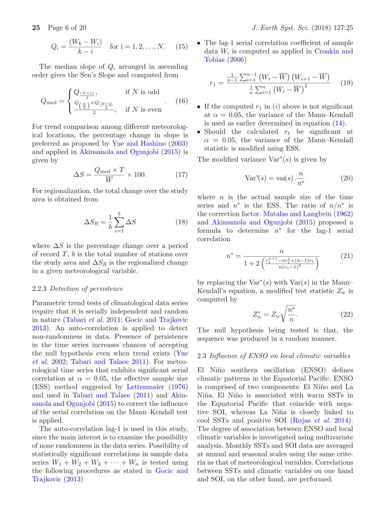
Figure 1 presents homogeneity test results onannual rainfall totals. The p-values are compared

with a value of α = 0.01. The results reveal that thep-values at all stations in the study area are abovethe significant value and hence homogeneous. Theyare all classified as ‘useful’ to be used for furthertrend and variability analysis.

3.1.2 Annual maximum temperature time series

P -values from homogeneity tests of maximum tem-perature series are presented in table 2. Resultsreveal that majority of the stations are homoge-neous except for three stations that failed three outof the four tests and hence classified as ‘suspect’.These stations include Francistown, in the east;

25 Page 8 of 20 J. Earth Syst. Sci. (2018) 127:25

Table 3. P-values from four homogeneity tests and probable year of intervention for minimum temperature.

Station

Pettit’s

test

Change

year SNHT Year

BHD’s

test

Change

year

Von’s

test Classification

Francistown 0.07 Homo 0.04 Homo 0.02 Homo 0.00 Useful

Ghanzi 0.00 1984/85 0.06 Homo 0.00 1984/85 0.01 Suspect

Jwaneng 0.07 Homo 0.13 Homo 0.01 Homo 0.03 Useful

Kasane 0.00 1992/93 0.00 1992/93 0.00 1992/93 0.00 Suspect

Letlhakane 0.01 Homo 0.12 Homo 0.01 Homo 0.01 Useful

Mahalapye 0.00 1981/82 0.00 1981/82 0.00 1981/82 0.00 Suspect

Maun 0.00 1983/84 0.00 1983/84 0.00 1983/84 0.00 Suspect

Pandamatenga 0.87 Homo 0.06 Homo 0.42 Homo 0.12 Useful

Selibe-Phikwe 0.32 Homo 0.22 Homo 0.51 Homo 0.05 Useful

Shakawe 0.01 Homo 0.02 Homo 0.01 Homo 0.00 Useful

SSKA 0.35 Homo 0.00 1986/87 0.18 Homo 0.01 Doubtful

Sowa Pan 0.20 Homo 0.41 Homo 0.37 Homo 0.05 Useful

Tsabong 0.00 1996/97 0.00 1997/98 0.00 1996/97 0.00 Suspect

Tshane 0.00 1988/89 0.00 1988/89 0.00 1988/89 0.00 Suspect

Statistically significant at α = 0.01, Homo = Homogeneous.

Maun in the north and Shakawe, in the northwest.At all the stations, the suspected year of interven-tion is 1980/81.

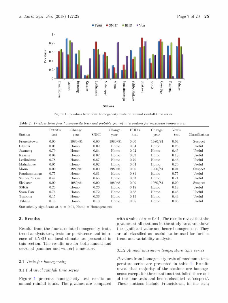
3.1.3 Annual minimum temperature time series

Results from tests of homogeneity in minimumtemperature are presented in table 3. These resultsreveal that at 50% of the stations minimum tem-perature series are homogeneous. At SSKA, theminimum temperature series failed two tests andhence classified as ‘doubtful’. The change yearreported at this station is 1986/87. Forty-threepercent of the stations failed in at least three ofthe tests and are classified as suspect. These sta-tions are Ghanzi with a change year of 1984/85,Kasane with a change at 1992/93 and Maha-lapye at 1981/82. The Other stations are Maunat 1983/84, Tsabong at 1996/97 and Tshane at1988/89.

3.2 Mann–Kendall (MK) trend analysis andpercentage change

Trend statistics in annual, summer and wintertrends for rainfall, maximum and minimum tem-perature are presented in tables 4–6. The periodof trend analysis is indicated especially for sta-tions classified as ‘doubtful’ or ‘suspect’, whereall the data record length were not used in theanalysis.

3.2.1 Rainfall trends and percentage changes

Trends in annual rainfall. Results from the MKtrends and Sen’s Slope estimator are presentedin table 4. Both increasing and decreasing trendsare experienced over the study area though nonewas significant at α = 0.05. Increasing trends areobserved at Francistown, Ghanzi, Mahalapye, SowaPan and Tsabong. The highest percentage increasein rainfall during the study period was 23.6% atFrancistown. No trend in annual rainfall is reportedat Jwaneng. However 57% of the stations indicatedecreasing trends though not significant. The high-est decrease in rainfall of 33.5% is observed at Pan-damatenga. The regionalized annual percentagechange over the study area indicates a 5.8%decrease in rainfall. This indicates overall rainfallhas decreased across the study area during theperiod of analysis.

Summer rainfall trends. The summer rainfallexhibits the same trend direction as the annualrainfall with increasing trends reported at Fran-cistown, Ghanzi, Mahalapye and Tsabong. Thehighest increase in seasonal rainfall of 23.1% isrecorded at Francistown. 71.4% of the stationsshow decreasing rainfall trends though none issignificant at α = 0.05. Selibe-Phikwe presentedwith the highest percentage increase of 35.9%. Thestudy area generally experienced 7.4% decrease insummer rainfall during the period of study. Spa-tial distribution of summer rainfall in figure 2(a)indicates decreasing trends in the northern, central

J. Earth Syst. Sci. (2018) 127:25 Page 9 of 20 25

Table 4. MK trend and Sen’s Slope estimator results for rainfall.

Station Season p-value MK-Z Sen’s S Change (%) Period of trend analysis

Francistown Annual 0.13 1.52 2.12 23.6 1960/61−2013/14

Summer 0.12 1.55 1.86 23.1 1960/61−2013/14

Winter 0.98 −0.02 0.00 0.0 1960/61−2013/14

Ghanzi Annual 0.70 0.39 0.48 5.8 1960/61−2013/14

Summer 0.70 0.39 0.53 7.2 1960/61−2013/14

Winter 0.16 −1.41 −0.04 −26.1 1960/61−2013/14

Jwaneng Annual 1.00 0.00 0.60 7.1 1988/89−2013/14

Summer 0.97 −0.04 −0.30 −4.0 1988/89−2013/14

Winter 0.91 −0.11 −0.03 −7.4 1988/89−2013/14

Kasane Annual 0.08 −1.78 −3.30 −25.0 1968/69−2013/14

Summer 0.07 −1.84 −3.31 −26.1 1968/69−2013/14

Winter 0.23 1.23 0.00 0.0 1968/69−2013/14

Letlhakane Annual 0.70 −0.39 −1.28 −6.8 1993/94−2013/14

Summer 0.39 −0.88 −3.22 −18.7 1993/94−2013/14

Winter 0.03* −2.16 −0.46 −58.9 1993/94−2013/14

Mahalapye Annual 0.85 0.19 0.29 3.4 1960/61−2012/13

Summer 0.88 0.15 0.17 2.3 1960/61−2012/13

Winter 0.60 −0.52 −0.02 −6.4 1960/61−2012/13

Maun Annual 0.69 −0.40 −0.61 −7.2 1960/61−2013/14

Summer 0.95 −0.07 −0.16 −2.0 1960/61−2013/14

Winter 0.52 −0.64 0.00 0.0 1960/61−2013/14

Pandamatenga Annual 0.17 −1.40 −10.84 −33.5 1998/99−2013/14

Summer 0.27 −1.13 −8.70 −28.6 1998/99−2013/14

Winter 1.00 −0.05 0.00 0.0 1998/99−2013/14

Selibe-Phikwe Annual 0.35 −0.95 −8.01 −34.1 1998/99−2013/14

Summer 0.27 −1.13 −7.52 −35.9 1998/99−2013/14

Winter 0.03* −2.13 −0.67 −96.6 1998/99−2013/14

Shakawe Annual 0.65 −0.45 −0.40 −4.1 1960/61−2013/14

Summer 0.73 −0.34 −0.40 −4.4 1960/61−2013/14

Winter 0.25 −1.15 0.00 0.0 1960/61−2013/14

SSKA Annual 0.59 −0.54 −2.10 −12.7 1985/86−2013/14

Summer 0.29 −1.07 −3.25 −22.8 1985/86−2013/14

Winter 0.55 0.64 0.23 29.1 1985/86−2013/14

Sowa Pan Annual 0.96 0.06 0.39 1.9 1992/93−2009/10

Summer 0.96 −0.06 −1.39 −7.4 1992/93−2009/10

Winter 0.06 −1.85 −0.51 −53.4 1992/93−2009/10

Tsabong Annual 0.59 0.54 0.71 11.8 1960/61−2010/11

Summer 0.46 0.73 0.99 19.9 1960/61−2010/11

Winter 0.19 −1.30 −0.13 −34.3 1960/61−2010/11

Tshane Annual 0.13 −0.56 −0.71 −11.2 1960/61−2013/14

Summer 0.72 −0.36 −0.37 −6.7 1960/61−2013/14

Winter 1.00 0.00 0.00 0.0 1960/61−2013/14

Statistically significant at α = 0.05, *significant trends.

and southern locations with a north to southdecreasing gradient. There is marginally increas-ing trends in the west at Ghanzi and southwest atTshane. Increasing trends are also observed in theeast at Francistown.

Winter rainfall trends. Winter rainfall alsopresents both increasing and decreasing trends.

Increasing trends are reported at Kasane andSSKA, though none was significant. No trend isobserved at Tshane during the period of analy-sis. Decreasing trends are reported in 78.6% of thestations over the study area with significantlydecreasing trends at Letlhakane and Selibe-Phikwe.The percentage decrease at these locations was59.9 and 96.6%, respectively. The regionalizeddecrease in winter rainfall over the study area

25 Page 10 of 20 J. Earth Syst. Sci. (2018) 127:25

Table 5. MK trend and Sen’s Slope estimator results for maximum temperature.

Station Season p-value MK-Z Sen’s S Change (%) Period of trend analysis

Francistown Annual 0.50 0.67 0.01 0.93 1980/81−2013/14

Summer 0.08 1.77 0.02 2.91 1960/61−2013/14

Winter 0.19 1.05 0.02 2.83 1984/85−2013/14

Ghanzi Annual 0.20 1.28 0.01 1.53 1961/62−2013/14

Summer 0.72 0.35 0.00 0.33 1961/62−2013/14

Winter 0.01* 2.60 0.02 3.46 1961/62−2013/14

Jwaneng Annual 0.50 0.68 0.01 1.11 1989/90−2013/14

Summer 0.73 0.35 0.01 0.61 1989/90−2013/14

Winter 0.37 0.91 0.02 1.91 1989/90−2013/14

Kasane Annual 0.07 −1.84 −0.02 −2.49 1983/84−2013/14

Summer 0.01* −2.65 −0.03 −3.10 1983/84−2013/14

Winter 0.34 −0.95 −0.01 −1.49 1983/84−2013/14

Letlhakane Annual 0.50 −0.68 −0.02 −1.05 1994/95−2013/14

Summer 0.59 −0.55 −0.01 −0.85 1994/95−2013/14

Winter 0.39 0.88 0.02 1.87 1994/95−2013/14

Mahalapye Annual 0.03* 2.12 0.02 3.80 1971/72−2013/14

Summer 0.10 1.62 0.03 3.68 1971/72−2013/14

Winter 0.04* 2.04 0.02 3.16 1971/72−2013/14

Maun Annual 0.60 −0.53 −0.01 −0.74 1980/81−2013/14

Summer 0.16 1.41 0.02 2.48 1965/66−2013/14

Winter 0.19 1.30 0.01 1.82 1980/81−2013/14

Pandamatenga Annual 0.76 0.32 0.02 0.93 1998/99−2013/14

Summer 0.69 −0.41 −0.02 −1.06 1998/99−2013/14

Winter 0.96 0.05 0.00 0.18 1998/99−2013/14

Selibe-Phikwe Annual 0.59 −0.55 −0.03 −1.24 2000/01−2013/14

Summer 0.45 −0.77 −0.07 −3.03 2000/01−2013/14

Winter 0.33 0.99 0.05 2.73 2000/01−2013/14

Shakawe Annual 0.53 0.62 0.01 0.85 1980/81−2013/14

Summer 0.62 −0.49 −0.01 −0.64 1980/81−2013/14

Winter 0.53 0.63 0.01 1.19 1985/86−2013/14

SSKA Annual 0.16 −1.41 −0.03 −2.71 1985/86−2013/14

Summer 0.26 −1.14 −0.03 −3.08 1985/86−2013/14

Winter 0.12 −1.56 −0.03 −3.29 1985/86−2013/14

Sowa Pan Annual 1.00 0.00 0.00 0.22 1961/62−2013/14

Summer 0.82 0.23 0.02 0.87 1961/62−2013/14

Winter 0.37 0.91 0.03 2.23 1961/62−2013/14

Tsabong Annual 0.18 1.33 0.01 1.66 1961/62−2013/14

Summer 0.90 −0.13 0.00 −0.31 1961/62−2013/14

Winter 0.00* 3.09 0.02 5.02 1961/62−2013/14

Tshane Annual 0.22 1.23 0.01 1.31 1961/62−2013/14

Summer 0.62 −0.50 −0.01 −0.86 1961/62−2013/14

Winter 0.89 −0.14 0.00 −0.23 1983/84−2013/14

Statistically significant at α = 0.05, *significant trends.

is reported at 18.1%. Spatial representation infigure 2(b) indicates a general decrease in win-ter rainfall with progression from east to west.The highest decrease is concentrated in the cen-tral region around Letlhakane. The northeast atKasane and south at SSKA, increasing trends areobserved with no particular gradient to describethe patterns.

3.2.2 Trends in maximum temperature andpercentage changes

Results showing trends in annual, summer andwinter periods are presented in table 5.

Trends in annual maximum temperature.Results from annual maximum temperature time

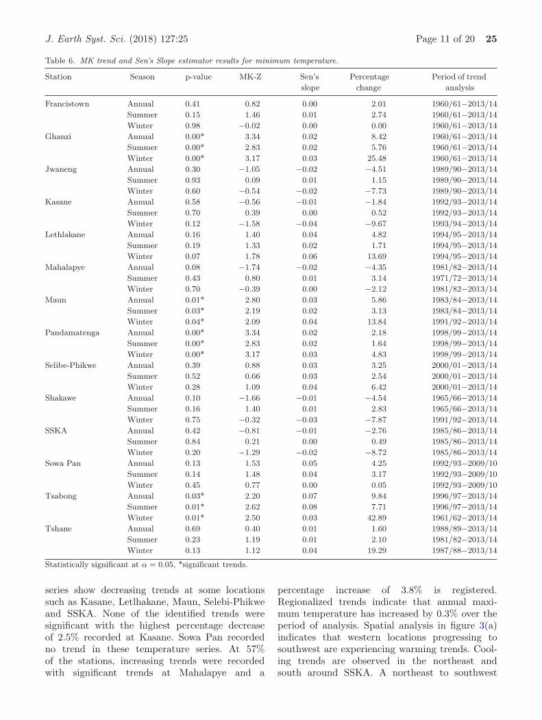
J. Earth Syst. Sci. (2018) 127:25 Page 11 of 20 25

Table 6. MK trend and Sen’s Slope estimator results for minimum temperature.

Station Season p-value MK-Z Sen’s

slope

Percentage

change

Period of trend

analysis

Francistown Annual 0.41 0.82 0.00 2.01 1960/61−2013/14

Summer 0.15 1.46 0.01 2.74 1960/61−2013/14

Winter 0.98 −0.02 0.00 0.00 1960/61−2013/14

Ghanzi Annual 0.00* 3.34 0.02 8.42 1960/61−2013/14

Summer 0.00* 2.83 0.02 5.76 1960/61−2013/14

Winter 0.00* 3.17 0.03 25.48 1960/61−2013/14

Jwaneng Annual 0.30 −1.05 −0.02 −4.51 1989/90−2013/14

Summer 0.93 0.09 0.01 1.15 1989/90−2013/14

Winter 0.60 −0.54 −0.02 −7.73 1989/90−2013/14

Kasane Annual 0.58 −0.56 −0.01 −1.84 1992/93−2013/14

Summer 0.70 0.39 0.00 0.52 1992/93−2013/14

Winter 0.12 −1.58 −0.04 −9.67 1993/94−2013/14

Lethlakane Annual 0.16 1.40 0.04 4.82 1994/95−2013/14

Summer 0.19 1.33 0.02 1.71 1994/95−2013/14

Winter 0.07 1.78 0.06 13.69 1994/95−2013/14

Mahalapye Annual 0.08 −1.74 −0.02 −4.35 1981/82−2013/14

Summer 0.43 0.80 0.01 3.14 1971/72−2013/14

Winter 0.70 −0.39 0.00 −2.12 1981/82−2013/14

Maun Annual 0.01* 2.80 0.03 5.86 1983/84−2013/14

Summer 0.03* 2.19 0.02 3.13 1983/84−2013/14

Winter 0.04* 2.09 0.04 13.84 1991/92−2013/14

Pandamatenga Annual 0.00* 3.34 0.02 2.18 1998/99−2013/14

Summer 0.00* 2.83 0.02 1.64 1998/99−2013/14

Winter 0.00* 3.17 0.03 4.83 1998/99−2013/14

Selibe-Phikwe Annual 0.39 0.88 0.03 3.25 2000/01−2013/14

Summer 0.52 0.66 0.03 2.54 2000/01−2013/14

Winter 0.28 1.09 0.04 6.42 2000/01−2013/14

Shakawe Annual 0.10 −1.66 −0.01 −4.54 1965/66−2013/14

Summer 0.16 1.40 0.01 2.83 1965/66−2013/14

Winter 0.75 −0.32 −0.03 −7.87 1991/92−2013/14

SSKA Annual 0.42 −0.81 −0.01 −2.76 1985/86−2013/14

Summer 0.84 0.21 0.00 0.49 1985/86−2013/14

Winter 0.20 −1.29 −0.02 −8.72 1985/86−2013/14

Sowa Pan Annual 0.13 1.53 0.05 4.25 1992/93−2009/10

Summer 0.14 1.48 0.04 3.17 1992/93−2009/10

Winter 0.45 0.77 0.00 0.05 1992/93−2009/10

Tsabong Annual 0.03* 2.20 0.07 9.84 1996/97−2013/14

Summer 0.01* 2.62 0.08 7.71 1996/97−2013/14

Winter 0.01* 2.50 0.03 42.89 1961/62−2013/14

Tshane Annual 0.69 0.40 0.01 1.60 1988/89−2013/14

Summer 0.23 1.19 0.01 2.10 1981/82−2013/14

Winter 0.13 1.12 0.04 19.29 1987/88−2013/14

Statistically significant at α = 0.05, *significant trends.

series show decreasing trends at some locationssuch as Kasane, Letlhakane, Maun, Selebi-Phikweand SSKA. None of the identified trends weresignificant with the highest percentage decreaseof 2.5% recorded at Kasane. Sowa Pan recordedno trend in these temperature series. At 57%of the stations, increasing trends were recordedwith significant trends at Mahalapye and a

percentage increase of 3.8% is registered.Regionalized trends indicate that annual maxi-mum temperature has increased by 0.3% over theperiod of analysis. Spatial analysis in figure 3(a)indicates that western locations progressing tosouthwest are experiencing warming trends. Cool-ing trends are observed in the northeast andsouth around SSKA. A northeast to southwest

25 Page 12 of 20 J. Earth Syst. Sci. (2018) 127:25

(a) (b)

Figure 2. Rainfall MK-Z trends (a) summer and (b) winter.

(b)(a)

Figure 3. Maximum temperature MK-Z trends (a) annual and (b) summer.

warming gradient is evident from the spatialpatterns.

Trends in summer maximum temperature.This climatic variable shows both increasing anddecreasing trends. Decreasing trends are observedin 57% of the stations, but only significant atKasane with a percentage increase of 3.1%. Thereare no reported significantly increasing trends overthe study area for summer season maximum tem-perature. The highest percentage increase recordedfor summer maximum temperature is 3.7% atMahalapye. Overall percentage change shows areduction by 0.15% over the study period.

Spatial presentation in figure 3(b) shows thenorthern and eastern locations present withwarming trends. The northeastern locations aroundKasane and Pandamatenga show decreasingtrends in maximum temperature. The southernlocations are generally present with marginalcooling trends. No particular gradient can beestablished from the spatial patterns which showisolated warming around Maun, Francistown andMahalapye.

Winter maximum temperature. Decreasingtrends in winter maximum temperature arereported at Kasane, SSKA and Tshane though

J. Earth Syst. Sci. (2018) 127:25 Page 13 of 20 25

(b) (a)

Figure 4. Minimum temperature MK-Z trends (a) summer and (b) winter.

none is significant. The highest percentagedecrease of 3.3% is recorded at SSKA. 78.6% ofthe stations recorded generally increasing trendswith significant trends registered at Ghanzi andTsabong. The reported increase at these stationsis 3.5% at Ghanzi and 5.0% at Tsabong. Over-all regional trend indicates an increase of 1.5%in winter maximum temperature over the studyperiod.

3.2.3 Trends in minimum temperature andpercentage changes

Results from investigations of long-term trendsin minimum temperature at annual and seasonalscales are presented in table 6.

Trends in annual minimum temperature.Similarly both increasing and decreasing trendsare reported in minimum temperature time seriesat annual scale over the study area. Decreasingtrends are observed at Jwaneng, Kasane, Maha-lapye and Shakawe though none are significant. Thehighest decrease of 4.5% is recorded at Shakawe.71.4% of the stations recorded increasing trendswith significant trends registered at Ghanzi, Maun,Pandamatenga and Tsabong. The highest increaseof 9.8% is recorded at Tsabong. Regionalized trendindicates an overall increase in annual minimumtemperature of 1.7% across the study area duringthe period of analysis.

Trends in summer minimum temperature.Summer temperature showed only increasingtrends across the study area at all the stations. Sig-nificant increase was recorded at Ghanzi, Maun,Pandamatenga and Tsabong. The trends followsimilar patterns as those of annual minimum tem-perature. The highest recorded change in increas-ing minimum temperature was 7.7% at Tsabongin the southwest. The regionalized temperaturechange over the study area indicates increase of2.7% during the period of analysis. Spatial rep-resentation in figure 4(a) shows increased warm-ing at most locations with large parts in thenorth, west and east all presenting with warm-ing trends. Marginal trends are observed in thesouth at SSKA and Jwaneng. A clear warminggradient from east to west is observed from the spa-tial distribution of summer minimum temperaturetrends.

Trends in winter minimum temperature.Winter minimum temperature trends equallypresent with both increasing and decreasing trends.No significantly decreasing trends are registeredover the study area. The highest change in decreas-ing trends is 9.7% registered at Kasane. 57%of the stations showed increasing trends in win-ter minimum temperature. Significantly increasingtrends are registered at Ghanzi, Maun, Panda-matenga and Tsabong. The highest change in

25 Page 14 of 20 J. Earth Syst. Sci. (2018) 127:25

-0.8

-0.6

-0.4

-0.2

0

0.2

0.4

0.6

Francistow

n

Ghanzi

Jwaneng

Kasane

Letlhakane

Mahalapye

Maun

Pandam

atenga

Selibe-P

hikwe

Shakaw

e

Sow

a Pan

SS

KA

Tsabong

Tshane

Lag

1- C

orr

Stations

Figure 5. Serial correlation effect on annual rainfall time series.

-0.8

-0.6

-0.4

-0.2

0

0.2

0.4

0.6

Francistow

nG

hanziJw

anengK

asaneLetlhakaneM

ahalapyeM

aunP

andamatenga

Selibe-P

hikwe

Shakaw

eS

owa P

anS

SK

AT

sabongT

shane

Lag-

1 co

rr

Stations -0.2

0

0.2

0.4

0.6

0.8

Francistow

n

Ghanzi

Jwaneng

Kasane

Letlhakane

Mahalapye

Maun

Pandam

atenga

Selibe-P

hikwe

Shakaw

e

Sow

a Pan

SS

KA

Tsabong

Tshane

(a) (b)

Figure 6. Serial correlation on effect annual (a) maximum and (b) minimum temperature series.

increasing trends was 43% at Tsabong. Regionally,the trends in minimum temperature are increasingwith overall change of 6.5% during the period ofanalysis.

Spatial presentation in figure 4(b) indicateswarming trends across the study area except forlocations in the northeast and northwest at Kasaneand Shakawe, respectively. Southern locations ofSSKA, Jwaneng and Mahalapye are also show-ing tendencies of cooling trends. Central, eastto west and southwest are showing increasingtrends in winter minimum temperature. There arewarming gradients observed at three fronts, a gra-dient is observed from southeast towards the west.Another gradient originates from the northeast,progresses southwards to the west. The final gra-dient originates from the north progressing south-west. Warming trends are generally concentratedin the west to southwest.

3.3 Detection of persistence in meteorologicaltime series

The lag-1 serial correlation of for annual rain-fall, maximum and minimum temperature arepresented in this section. For the rainfall timeseries, all the lag-1 serial correlations were non-significant at α=0.05. Positive serial correlationswere obtained at Tsabong, Mahalapye, Selibe-Phikwe and Jwaneng. Stations with their lag-1correlations are plotted in figure 5. Maximumtemperatures recorded mainly positive correlationswith the only negative correlation registered atPandamatenga and Selibe-Phikwe. Stations pre-sented with mostly none significant lag-1 serialcorrelations in maximum temperature accept atShakawe as shown in figure 6(a). The minimumtemperature recorded positive correlations at allstations except Pandamentanga. Most of the lag-1

J. Earth Syst. Sci. (2018) 127:25 Page 15 of 20 25

correlations were significant at α = 0.05 except forPandamatenga, Selibe-Phikwe, Jwaneng, Ghanziand Sowa Pan. The distribution of these stationsis shown in figure 6(b).

3.4 Influence of ENSO on local climatic variables

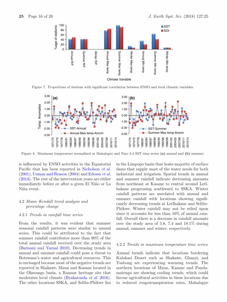
Positive correlations resulted from the analysis ofrainfall and southern oscillation index (SOI) atboth annual and seasonal scales. Significant corre-lations at annual scale were recorded at 50% of thestations. During analysis of summer rainfall timeseries, 43% of the stations reported significant pos-itive correlations. Winter rainfall registered weakcorrelations and none are significant.

Negative correlations were observed betweenrainfall and sea surface temperatures (SSTs) forannual and seasonal time series. Significant neg-ative correlations for both annual and summerseries are reported in 43% of the stations. Winterrainfall time series did not register any significantcorrelation with SOI in the study area. Correla-tions between maximum temperature and SOI inannual and seasonal time series were negative atall the stations used in this study. For annualseries, significant negative correlations are recordedin 86% of the stations. The number of stations withsignificant correlations increased in summer to93%. During the winter season, most stations didnot record significant correlations except at Maun.

Correlations between maximum temperature andSSTs returned positive correlations for both annualand seasonal series. Significant correlations are reg-istered at 78.5% of the stations in annual series.From analysis of summer time series, the associa-tion is significant at all stations in the study area.Associations with winter maximum time seriesare not significant most of the time except atKasane and Mahalapye. Correlations between min-imum temperature and SOI over the study areareveal weakly negative associations at annual andwinter time scales. The annual minimum tem-perature associations with SOI are significant atFrancistown, Jwaneng and Mahalapye. Associa-tions with winter minimum temperature are sig-nificant only at Tsabong. Summer correlations arealso significant at 43% of the stations. Investiga-tions of association between minimum temperatureand SSTs reveal significant association at 36%of the stations at annual scale. During summerseason, the number of stations with significantcorrelations increased to 64%. Winter season cor-relations are generally not significant except at

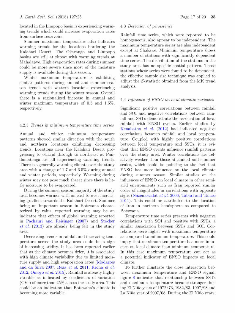
Tsabong in southwest. Distribution of stationswith significant correlations is presented in fig-ure 7. To further illustrate the influence of ENSOon the local climate, relationships between maxi-mum temperature anomalies and SST from Nino3.4 are presented in figure 8. The relations arefound to be strongest particularly during the yearsof 1972/73, 1982/83, 1997/98 and 2007/08 forboth cases of annual and summer season timeseries.

4. Discussions

4.1 Tests for homogeneity

The four absolute homogeneity tests demonstratedtheir ability in detecting inconsistencies and breaksin meteorological time series. The results fromthese tests have enabled categorization of mete-orological stations as ‘useful’, ‘doubtful’ and‘suspect’. This is particularly helpful for futureclimatic studies over the region as station clas-sified as suspect may be excluded from furthertrend analysis. Results indicated that rainfall timeseries are fully homogeneous. Similarly, 78.6% ofthe stations for maximum temperature and 50%for minimum temperature time series were foundhomogeneous. These results of homogenous rain-fall series are consistent with findings of Wijngaardet al. (2003) and Hansel et al. (2016), who indi-cated difficulties in identifying breaks in rainfalltime series with high variability, which is the casefor semi-arid climates (Modarres and da Silva2007). It was easier to detect breaks in temper-ature time series due to their lower variabilityas compared to rainfall series. However, in theabsence of metadata it was difficult to conclu-sively state if the reported interventions or lackof them are as a result of climatic changes orinhomogeneities in the time series. For the fore-going reason it was not possible to discard anystation, but consciously examine the data beforeand after the suspected year of intervention. Inthose stations classified as ‘suspect’, only thoseseries after the intervention were used in trendanalysis.

El Nino years of 1986/87, 1991/92, 1997/98and 2004/05 at the same time La Nina years of1983/84 and 1984/85 were also identified as yearsof intervention in the temperature time series. Thisrevelation may further strengthen the assertionthat inter-annual variability over southern Africa

25 Page 16 of 20 J. Earth Syst. Sci. (2018) 127:25

0

20

40

60

80

100

Annual R

/F

Sum

mer R

/F

Winter R

/F

Annual M

ax temp

Sum

mer M

ax temp

Winter M

ax temp

Annual M

in temp

Sum

mer M

in temp

Winter M

in temp

%ag

e of

sta

tions

Climate Variable

SSTSOI

Figure 7. Proportions of stations with significant correlation between ENSO and local climatic variables.

-3.00

-2.00

-1.00

0.00

1.00

2.00

3.00

1971

/72

1974

/75

1977

/78

1980

/81

1983

/84

1986

/87

1989

/90

1992

/93

1995

/96

1998

/99

2001

/02

2004

/05

2007

/08

2010

/11

2013

/14

Tem

p. A

nom

alie

s

SST-Annual

Annual Max temp-Anorm -3.00

-2.00

-1.00

0.00

1.00

2.00

3.00

1971

/72

1974

/75

1977

/78

1980

/81

1983

/84

1986

/87

1989

/90

1992

/93

1995

/96

1998

/99

2001

/02

2004

/05

2007

/08

2010

/11

2013

/14

SST-SummerSummer Max temp-Anorm

(a) (b)

Figure 8. Maximum temperature normalized at Mahalapye and Nino 3.4 SST time series (a) annual and (b) summer.

is influenced by ENSO activities in the EquatorialPacific that has been reported in Nicholson et al.(2001), Usman and Reason (2004) and Edossa et al.(2014). The rest of the intervention years are eitherimmediately before or after a given El Nino or LaNina event.

4.2 Mann–Kendall trend analysis andpercentage change

4.2.1 Trends in rainfall time series

From the results, it was evident that summerseasonal rainfall patterns were similar to annualseries. This could be attributed to the fact thatsummer rainfall contributes more than 90% of thetotal annual rainfall received over the study area(Batisani and Yarnal 2010). Decreasing trends inannual and summer rainfall could pose a threat toBotswana’s water and agricultural resources. Thisis envisaged because most of the negative trends arereported in Shakawe, Maun and Kasane located inthe Okavango basin, a Ramsar heritage site thatmoderates local climate (Byakatonda et al. 2016).The other locations SSKA, and Selibe-Phikwe lies

in the Limpopo basin that hosts majority of surfacedams that supply most of the water needs for bothindustrial and irrigation. Spatial trends in annualand summer rainfall indicate decreasing amountsfrom northeast at Kasane to central around Letl-hakane progressing southward to SSKA. Winterrainfall patterns are unrelated with annual andsummer rainfall with locations showing signifi-cantly decreasing trends at Letlhakane and Selibe-Phikwe. Winter rainfall may not be relied uponsince it accounts for less than 10% of annual rain-fall. Overall there is a decrease in rainfall amountsover the study area of 5.8, 7.4 and 18.1% duringannual, summer and winter, respectively.

4.2.2 Trends in maximum temperature time series

Annual trends indicate that locations borderingKalahari Desert such as Shakawe, Ghanzi, andTsabong are experiencing warming trends. Thenorthern locations of Maun, Kasane and Panda-matenga are showing cooling trends, which couldfavour agricultural activities in these locations dueto reduced evapotranspiration rates. Mahalapye

J. Earth Syst. Sci. (2018) 127:25 Page 17 of 20 25

located in the Limpopo basin is experiencing warm-ing trends which could increase evaporation ratesfrom surface reservoirs.

Summer maximum temperature also indicateswarming trends for the locations bordering theKalahari Desert. The Okavango and Limpopobasins are still at threat with warming trends atMahalapye. High evaporation rates during summercould be more severe since most of the moisturesupply is available during this season.

Winter maximum temperature is exhibitingsimilar patterns during annual and summer sea-son trends with western locations experiencingwarming trends during the winter season. Overallthere is a regionalized increase in annual andwinter maximum temperature of 0.3 and 1.5%,respectively.

4.2.3 Trends in minimum temperature time series

Annual and winter minimum temperaturepatterns showed similar direction with the southand northern locations exhibiting decreasingtrends. Locations near the Kalahari Desert pro-gressing to central through to northeast at Pan-damatenga are all experiencing warming trends.There is a generally warming climate over the studyarea with a change of 1.7 and 6.5% during annualand winter periods, respectively. Warming duringwinter may not pose much threat since there is lit-tle moisture to be evaporated.

During the summer season, majority of the studyarea becomes warmer with an east to west increas-ing gradient towards the Kalahari Desert. Summerbeing an important season in Botswana charac-terized by rains, reported warming may be anindicator that effects of global warming reportedin Pachauri and Reisinger (2007) and Stockeret al. (2013) are already being felt in the studyarea.

Decreasing trends in rainfall and increasing tem-perature across the study area could be a signof increasing aridity. It has been reported earlierthat as the climate becomes drier, it is associatedwith high climate variability due to limited mois-ture supply and high evaporation rates (Modarresand da Silva 2007; Reza et al. 2011; Recha et al.2012; Omoyo et al. 2015). Rainfall is already highlyvariable as indicated by coefficients of variation(CVs) of more than 25% across the study area. Thiscould be an indication that Botswana’s climate isbecoming more variable.

4.3 Detection of persistence

Rainfall time series, which were reported to behomogeneous, also appear to be independent. Themaximum temperature series are also independentexcept at Shakawe. Minimum temperature showsa number of stations with significantly dependenttime series. The distribution of the stations in thestudy area has no specific spatial pattern. Thosestations whose series were found to be dependent,the effective sample size technique was applied toadjust the Z-statistic obtained from the MK trendanalysis.

4.4 Influence of ENSO on local climatic variables

Significant positive correlations between rainfalland SOI and negative correlations between rain-fall and SSTs demonstrate the association of localrainfall with ENSO events. Earlier studies byKenabatho et al. (2012) had indicated negativecorrelations between rainfall and local tempera-ture. Coupled with highly positive correlationsbetween local temperature and SSTs, it is evi-dent that ENSO events influence rainfall patternsover the study area. Winter correlations are rel-atively weaker than those at annual and summerscales, which could be pointing to the fact thatENSO has more influence on the local climateduring summer season. Similar studies on theinfluences of ENSO on local climate in other semi-arid environments such as Iran reported similarorder of magnitudes in correlations with oppositesigns (Nazemosadat et al. 2006; Tabari and Talaee2011). This could be attributed to the locationof Iran in northern hemisphere as compared toBotswana.

Temperature time series presents with negativecorrelations with SOI and positive with SSTs, asimilar association between SSTs and SOI. Cor-relations were higher with maximum temperatureas compared to minimum temperature. This couldimply that maximum temperature has more influ-ence on local climate than minimum temperature.In this case maximum temperature can act asa potential indicator of ENSO impacts on localclimate.

To further illustrate the close interaction bet-ween maximum temperature and ENSO signal,figure 8 indicates that relationship between SSTsand maximum temperature became stronger dur-ing El Nino years of 1972/73, 1982/83, 1997/98 andLa Nina year of 2007/08. During the El Nino years,

25 Page 18 of 20 J. Earth Syst. Sci. (2018) 127:25

positive anomalies, which are responsible fordroughts conditions over southern Africa are evi-dent and during the La Nina years, negativeanomalies are observed on the plot accounting forwet conditions over the region.

The ENSO phenomenon has been known topropagate climate variability due to uncertaintiesassociated with these events (Kandji et al. 2006;Dai 2013; Moran-Tejeda et al. 2016). DuringEl Nino events, rains in the southern Africa regiondip to below long-term mean leading to severe andprolonged droughts (Nicholson et al. 2001; Usmanand Reason 2004), whereas during the La Ninaepisodes, flood causing heavy rains that lead todestruction of infrastructure are recorded as abovenormal. These fluctuations resulting from anoma-lies in SSTs coupled with local feedbacks haveincreased climate variability and global aridity(Dai 2011a; Huang et al. 2016). With high corre-lations reported and close relationships observedduring the period of study, this could be anotherpointer towards high variable climate across thestudy area. The local feedbacks are mainly linkedwith warming of the Indian Ocean in telecom-munication with positive SST anomalies in theEquatorial Pacific, especially during austral sum-mer (Nicholson et al. 2001; Jury 2002). It isduring the summer season that more than 90%of the stations showed significant correlations withENSO. The plots in figure 8 have demonstratedclose relationships between ENSO and local cli-matic variables during years for which extremeevents were recorded in the southern Africanregion. One of such events is the severe El Ninodrought of 1982/83 with SST anomalies rais-ing above 6◦ that affected economies of regionalmember states (Dai 2011b; Jury 2013). Anotherevent is the La Nina heavy rains of 1999/2000,which caused devastating floods in Mozambiquewith pests and disease outbreak in Botswana thatresulted in 50% crop yield decline in that year(Kandji et al. 2006). This study has demonstratedthat local climate is still influenced by the largeclimatic predictors associated with high climatevariability.

5. Conclusions and summary

Climate variability and change in Botswana wasinvestigated through annual and seasonal timeseries of rainfall, maximum and minimum tem-perature for a period 1960–2014. Four absolutehomogeneity tests were used to check any

possible inhomogeneities and interventions in thetime series. The Mann–Kendall and Sen’s Slopeestimator were used to detect trends and absolutechanges over the period of study at 14 synopticstations. The association of local climatic vari-ables with ENSO was also investigated throughmultivariate correlation analysis. The followingsummary has been deduced from the study.

• The rainfall time series are fully homogeneousacross the study period at all the stations.78.6% of the stations for maximum temperatureand 50% of the stations for minimum temper-ature were homogeneous, classifying as ‘useful’.Due to absence of metadata, it was not possi-ble to conclude if the presence of homogeneoustime series or lack of them was as a resultof inhomogeneities or normal climate regimeshift. Most of the years of intervention identi-fied also either coincided with El Nino/La Ninaor closely followed and at times preceded ENSOepisodes.

• Trends in rainfall indicate a general decrease of5.8, 7.4 and 18.1% during annual, summer andwinter seasons over the study area, respectively.There is a regionalized warming trend of 0.3 and1.5% in annual and winter maximum temper-ature, respectively. Minimum temperature alsoreported warming trends of 1.7 and 6.5% dur-ing annual and winter season in the study area.The decreasing trends in rainfall and warm-ing trends across Botswana could lead to moreclimate variability.

• The rainfall time series were completely randomwith only temperature series showing some per-sistence at some stations. Maximum temperaturetime series are found to be random except atShakawe. 57% of the stations showed persistencetendencies in minimum temperature. The effec-tive sample size technique was used to adjustthe Z-statistic from the MK analysis for stationswith persistence.

• Significant positive correlations exist betweenrainfall and SOI, at the same time rainfall isnegatively associated with SSTs. More signifi-cant positive associations are identified betweenSST and maximum temperature. The associa-tions were particularly strong during the summerseason with very close relationships establishedbetween local climatic variables and ENSO dur-ing El Nino years of 1972/73, 1982/83, 1997/98and La Nina years of 2007/08. The significantcorrelations between local climate and ENSO

J. Earth Syst. Sci. (2018) 127:25 Page 19 of 20 25

could further be linking Botswana’s climate withhigh variability due to uncertainties that areassociated with ENSO events.

In general, the study reveals decreasing rainfallamounts and warming trends across the studyarea. The influence of ENSO on local climate hasbeen established linking Botswana to high cli-mate variability. Information generated by thisstudy could be beneficial to agricultural andwater resources planning and management espe-cially in semi-arid environments, where adapt-ability to climate variability and change is stilllow.

Acknowledgements

This study was supported by the Mobility forEngineering Graduates in Africa (METEGA) andCarnegie Cooperation of New York throughRUFORUM in the form of research funds. Theclimatic data used were provided by Departmentof Meteorological Services (DMS) of Botswana.The authors are grateful for the support from thetwo entities. Gulu University is highly appreciatedfor granting study leave to the first author. Theyalso wish to thank the two anonymous review-ers for their valuable comments that enriched thisstudy.

References

Akinsanola A A and Ogunjobi K O 2015 Recent homogeneityanalysis and long-term spatio-temporal rainfall trends inNigeria; Theor. Appl. Climatol. 128 275–289, https://doi.org/10.1007/s00704-015-1701-x.

Alexandersson H 1986 A homogeneity test applied to precip-itation data; J. Climatol. 6 661–675.

Alexandersson H and Moberg A 1997 Homogenization ofSwedish temperature data. Part I: Homogeneity test forlinear trends; Int. Int. J. Climatol. 17 25–34.

Batisani N 2012 Climate variability, yield instability andglobal recession: The multi-stressor to food security inBotswana; Clim. Dev. 4 129–140.

Batisani N and Yarnal B 2010 Rainfall variability and trendsin semi-arid Botswana: Implications for climate changeadaptation policy; Appl. Geogr. 30 483–489.

Buishand T A 1982 Some methods for testing the homogene-ity of rainfall records; J. Hydrol. 58 11–27.

Byakatonda J, Parida B P, Kenabatho P K and Moalafhi DB 2016 Modeling dryness severity using artificial neuralnetwork at the Okavango Delta, Botswana; Glob. Nest. J.18 463–481.

Costa A C and Soares A 2009a Trends in extreme precipita-tion indices derived from a daily rainfall database for thesouth of Portugal; Int. J. Climatol. 29 1956–1975.

Costa A C and Soares A 2009b Homogenization of climatedata: Review and new perspectives using geostatistics;Math. Geosci. 41 291–305, https://doi.org/10.1007/s11004-008-9203-3.

Croakin C and Tobias P 2006 NIST/SEMATECH e-Handbook of Statistical Methods, National Institute ofStandards and Technology/SEMATECH; US CommerceDepartment’s Technology Administration.

Dai A 2013 Increasing drought under global warming inobservations and models; Nat. Clim. Change 3 52–58.

Dai A 2011a Drought under global warming: A review; WileyInterdiscip. Rev. Clim. Change 2 45–65, https://doi.org/10.1002/wcc.81.

Dai A 2011b Characteristics and trends in various forms ofthe Palmer Drought Severity Index during 1900–2008.

Edossa D C, Woyessa Y E and Welderufael W A 2014 Anal-ysis of droughts in the central region of South Africa andtheir association with SST anomalies; Int. J. Atmos. Sci.,https://doi.org/10.1155/2014/508953.

Giorgi F and Lionello P 2008 Climate change projectionsfor the Mediterranean region; Global Planet. Change 6390–104.

Gocic M and Trajkovic S 2013 Analysis of changes in mete-orological variables using Mann–Kendall and Sen’s slopeestimator statistical tests in Serbia; Global Planet. Change100 172–182, https://doi.org/10.1016/j.gloplacha.2012.10.014.

Hansel S, Medeiros D M and Matschullat J et al. 2016 Assess-ing homogeneity and climate variability of temperatureand precipitation series in the capitals of north-easternBrazil; Front. Earth Sci. 4 1–21, https://doi.org/10.3389/feart.2016.00029.

Hansen J, Sato M and Ruedy R et al. 2016 Global Temper-ature in 2015; Colomb. Univ., pp. 1–6.

Huang J, Ji M and Xie Y et al. 2016 Global semi-arid climatechange over last 60 years; Clim. Dyn. 46 1131–1150.

Jury M R 2002 Economic impacts of climate variabilityin South Africa and development of resource predictionmodels; J. Appl. Meteorol. 41 46–55.

Jury M R 2013 Climate trends in southern Africa; S. Afr. J.Sci. 109 1–11.

Kandji S T, Verchot L and Mackensen J 2006 Climatechange climate and variability in southern Africa: Impactsand adaptation in the agricultural sector; World Agro-forestry Centre (ICRAF), United Nations EnvironmentProgramme (UNEP), Africa.

Kenabatho P K, Parida B P and Moalafhi D B 2012 Thevalue of large-scale climate variables in climate changeassessment: The case of Botswana’s rainfall; Phys. Chem.Earth 50-52 64–71, https://doi.org/10.1016/j.pce.2012.08.006.

Kendall M G 1975 Rank Correlation Methods; 4th edn,London.

Khan M I, Liu D and Fu Q et al. 2016 Recent climate trendsand drought behavioral assessment based on precipitationand temperature data series in the Songhua River Basinof China; Water Resour. Manag. 30 4839–4859.

Lettenmaier D P 1976 Detection of trends in water qual-ity data from records with dependent observations; WaterResour. Res. 12 1037–1046.

Mann H B 1945 Nonparametric tests against trend; Econom.J. Econom. Soc. 13(3) 245–259.

25 Page 20 of 20 J. Earth Syst. Sci. (2018) 127:25

Matalas N C and Langbein W B 1962 Information contentof the mean; J. Geophys. Res. 67 3441–3448.

Menzel A, Sparks T H and Estrella N et al. 2006 Euro-pean phenological response to climate change matchesthe warming pattern; Glob. Change Biol. 12 1969–1976.

Modarres R and da Silva V de P R 2007 Rainfall trends inarid and semi-arid regions of Iran; J. Arid Environ. 70344–355.

Moran-Tejeda E, Bazo J and Lopez-Moreno J I et al. 2016Climate trends and variability in Ecuador (1966–2011);Int. J. Climatol.https://doi.org/10.1002/joc.4597.

Nazemosadat M J, Samani N, Barry D A and Niko M M2006 ENSO forcing on climate change in Iran: Precipi-tation analysis; Iran. J. Sci. Technol. Trans. B Eng. 301–11.

Nicholson S E, Leposo D and Grist J 2001 The relationshipbetween El Nino and drought over Botswana; J. Clim. 14323–335.

NOAA-NCDC 2016 Southern Oscillation Index (SOI); www.ncdc.noaa.gov/teleconnections/enso/indicators/soi/data.csv.

NOAA-NCEP 2016 Average sea surface temperature(SST) anormalies in region 3.4 of the Equato-rial Pacific. http://www.cpc.ncep.noaa.gov/products/analysis monitoring/ensostuff/ONI change.shtml.

Nyenzi B and Lefale P F 2006 El Nino Southern Oscillation(ENSO) and global warming; Adv. Geosci. 6 95–101.

Omoyo N N, Wakhungu J and Oteng’i S 2015 Effects ofclimate variability on maize yield in the arid and semiarid lands of lower eastern Kenya; Agric. Food Secur. 4 8,https://doi.org/10.1186/s40066-015-0028-2.

Pachauri R K and Reisinger A 2007 IPCC fourth assessmentreport; IPCC, Geneva.

Parida B P and Moalafhi D B 2008 Regional rainfall fre-quency analysis for Botswana using L-Moments and radialbasis function network; Phys. Chem. Earth 33 614–620,https://doi.org/10.1016/j.pce.2008.06.011.

Partal T and Kahya E 2006 Trend analysis in Turkish pre-cipitation data; Hydrol. Process. 20 2011–2026, https://doi.org/10.1002/hyp.5993.

Pettit A N 1979 A non-parametric approach to the change-point detection; Appl. Stat. 28 126–135.

Rahman M R and Lateh H 2017 Climate change inBangladesh: A spatio-temporal analysis and simulation ofrecent temperature and rainfall data using GIS and timeseries analysis model; Theor. Appl. Climatol. 128 27–41,https://doi.org/10.1007/s00704-015-1688-3.

Recha C W, Makokha G L and Traore P S et al. 2012Determination of seasonal rainfall variability, onset andcessation in semi-arid Tharaka district, Kenya; Theor.Appl. Climatol. 108 479–494.

Reza Y M, Javad K D, Mohammad M and Ashish S 2011Trend detection of the rainfall and air temperature datain the Zayandehrud basin; J. Appl. Sci. 11 2125–2134.

Rojas O, Li Y and Cumani R 2014 An assessment usingFAO’s Agricultural Stress Index (ASI): Understandingthe drought impact of El Nino on the global agriculturalareas.

Sabzevari A A, Zarenistanak M, Tabari H and Moghimi S2015 Evaluation of precipitation and river discharge vari-ations over southwestern Iran during recent decades; J.Earth Syst. Sci. 124 335–352, https://doi.org/10.1007/s12040-015-0549-x.

Sen P K 1968 Estimates of the regression coefficient basedon Kendall’s tau; J. Am. Stat. Assoc. 63 1379–1389.

Shahid S 2010 Rainfall variability and the trends of wet anddry periods in Bangladesh; Int. J. Climatol. 30 2299–2313,https://doi.org/10.1002/joc.2053.

Shifteh Some’e B, Ezani A and Tabari H 2012 Spatio-temporal trends and change point of precipitation inIran; Atmos. Res. 113 1–12, https://doi.org/10.1016/j.atmosres.2012.04.016.

Statistics Botswana 2009 Botswana water statistics;Gaborone, Botswana.

Statistics Botswana 2015 Statistics Botswana Annual Agri-cultural Survey Report 2013, Gaborone, Botswana.

Stocker T F, Qin D and Plattner G K et al. 2013 Climatechange 2013: The physical science basis; Intergovernmen-tal panel on climate change, working group I contributionto the IPCC fifth assessment report (AR5).

Tabari H, Somee B S and Zadeh M R 2011 Testing forlong-term trends in climatic variables in Iran; Atmos.Res. 100 132–140, https://doi.org/10.1016/j.atmosres.2011.01.005.

Tabari H and Talaee P H 2011 Temporal variability of pre-cipitation over Iran: 1966–2005; J. Hydrol. 396 313–320,https://doi.org/10.1016/j.jhydrol.2010.11.034.

Thiel H 1950 A rank-invariant method of linear and poly-nomial regression analysis, Part 3. In: Proceedings ofKoninalijke Nederlandse Akademie van WeinenschatpenA, pp. 1397–1412.

Usman M T and Reason C J C 2004 Dry spell frequenciesand their variability over southern Africa; Clim. Res. 26199–211, https://doi.org/10.3354/cr026199.

Von Neumann J 1941 Distribution of the ratio of the meansquare successive difference to the variance; Ann. Math.Stat. 12 367–395.

Wijngaard J B, Klein Tank A M G and Konnen G P 2003Homogeneity of 20th century European daily tempera-ture and precipitation series; Int. J. Climatol. 23 679–692,https://doi.org/10.1002/joc.906.

Yue S and Hashino M 2003 Long Term Trends of Annualand Monthly Precipitation in Japan; JAWRA J. Am.Water. Resour. Assoc. 39 587–596, https://doi.org/10.1111/j.1752-1688.2003.tb03677.x.

Yue S, Pilon P, Phinney B and Cavadias G 2002 The influ-ence of autocorrelation on the ability to detect trendin hydrological series; Hydrol. Process 16 1807–1829,https://doi.org/10.1002/hyp.1095.

Corresponding editor: Subimal Ghosh