Analysis of Modeling Assumptions used in Production Cost ... · Aaron Townsend, and Aaron Bloom National Renewable Energy Laboratory ... Abstract Published renewable energy integration

NREL is a national laboratory of the U.S. Department of Energy Office of Energy Efficiency & Renewable Energy Operated by the Alliance for Sustainable Energy, LLC

This report is available at no cost from the National Renewable Energy Laboratory (NREL) at www.nrel.gov/publications.

Contract No. DE-AC36-08GO28308

Analysis of Modeling Assumptions used in Production Cost Models for Renewable Integration Studies Brady Stoll, Gregory Brinkman, Aaron Townsend, and Aaron Bloom National Renewable Energy Laboratory

Technical Report NREL/TP-6A20-65383 January 2016

NREL is a national laboratory of the U.S. Department of Energy Office of Energy Efficiency & Renewable Energy Operated by the Alliance for Sustainable Energy, LLC


Contract No. DE-AC36-08GO28308

National Renewable Energy Laboratory 15013 Denver West Parkway Golden, CO 80401 303-275-3000 • www.nrel.gov

Analysis of Modeling Assumptions used in Production Cost Models for Renewable Integration Studies Brady Stoll, Gregory Brinkman, Aaron Townsend, and Aaron Bloom National Renewable Energy Laboratory

Prepared under Task No. SA12.0373

Technical Report NREL/TP-6A20-65383 January 2016

NOTICE

This report was prepared as an account of work sponsored by an agency of the United States government. Neither the United States government nor any agency thereof, nor any of their employees, makes any warranty, express or implied, or assumes any legal liability or responsibility for the accuracy, completeness, or usefulness of any information, apparatus, product, or process disclosed, or represents that its use would not infringe privately owned rights. Reference herein to any specific commercial product, process, or service by trade name, trademark, manufacturer, or otherwise does not necessarily constitute or imply its endorsement, recommendation, or favoring by the United States government or any agency thereof. The views and opinions of authors expressed herein do not necessarily state or reflect those of the United States government or any agency thereof.


Available electronically at SciTech Connect http:/www.osti.gov/scitech

Available for a processing fee to U.S. Department of Energy and its contractors, in paper, from:

U.S. Department of Energy Office of Scientific and Technical Information P.O. Box 62 Oak Ridge, TN 37831-0062 OSTI http://www.osti.gov Phone: 865.576.8401 Fax: 865.576.5728 Email: [email protected]

Available for sale to the public, in paper, from:

U.S. Department of Commerce National Technical Information Service 5301 Shawnee Road Alexandria, VA 22312 NTIS http://www.ntis.gov Phone: 800.553.6847 or 703.605.6000 Fax: 703.605.6900 Email: [email protected]

Cover Photos by Dennis Schroeder: (left to right) NREL 26173, NREL 18302, NREL 19758, NREL 29642, NREL 19795.

NREL prints on paper that contains recycled content.

http://www.osti.gov/scitech

http://www.osti.gov/

mailto:[email protected]

http://www.ntis.gov/

mailto:[email protected]

iii

This report is available at no cost from the National Renewable Energy Laboratory (NREL) at www.nrel.publications.

Table of Contents Introduction .................................................................................................................................................. 1 Background .................................................................................................................................................. 2

Study Characteristics .............................................................................................................................. 4 Motivation ............................................................................................................................................... 4

Methods ........................................................................................................................................................ 5 Model Assumptions ................................................................................................................................ 5 Model Implementation ............................................................................................................................ 7 Evaluation Metrics .................................................................................................................................. 9

Results ........................................................................................................................................................ 10 Impact of Linear (LP) vs. Integer (MIP) Optimization ......................................................................... 10

Model Run Time .......................................................................................................................... 10 Generation by Generator Type .................................................................................................... 10 Total Production Cost .................................................................................................................. 11 Curtailment .................................................................................................................................. 12 CO2 Emissions ............................................................................................................................. 13 Starts and Ramps ......................................................................................................................... 13

Impact of Hourly vs Five-minute Dispatch Temporal Resolution ........................................................ 17 Model Run Time .......................................................................................................................... 17 Generation by Generator Type .................................................................................................... 17 Total Production Cost .................................................................................................................. 18 Curtailment .................................................................................................................................. 19 CO2 Emissions ............................................................................................................................. 20 Starts and Ramps ......................................................................................................................... 20

Comparison of WECC and CO-Test Systems ...................................................................................... 23 Model Run Time .......................................................................................................................... 23 Comparison of Generation by Generator Type ............................................................................ 23 Total Production Cost .................................................................................................................. 24 Curtailment .................................................................................................................................. 24 CO2 Emissions ............................................................................................................................. 24 Starts and Ramps ......................................................................................................................... 25

Effects of Four-Hour-Ahead Commitment ........................................................................................... 29 Generation by Generator Type .................................................................................................... 29 Total Production Cost .................................................................................................................. 30 Curtailment .................................................................................................................................. 30 CO2 Emissions ............................................................................................................................. 30 Starts and Ramps ......................................................................................................................... 32

Impact of Overbuilt Systems ................................................................................................................ 34 Generation by Generator Type .................................................................................................... 35 Total Production Cost .................................................................................................................. 36 Curtailment .................................................................................................................................. 36 CO2 Emissions ............................................................................................................................. 36 Starts and Ramps ......................................................................................................................... 37

Conclusions ............................................................................................................................................... 41 References ................................................................................................................................................. 42

iv


List of Figures Figure 1. Capacity mix by system ................................................................................................................. 8 Figure 2. Step time for MIP and LP optimization ....................................................................................... 10 Figure 3. Generation by model and system ................................................................................................. 11 Figure 4. Total production cost ................................................................................................................... 12 Figure 5. Carbon emissions by generator type ............................................................................................ 13 Figure 6. Capacity started, LP vs MIP ........................................................................................................ 14 Figure 7. Average on-time per start ............................................................................................................. 15 Figure 8. Number of ramps ......................................................................................................................... 16 Figure 9. Step time required for hourly and sub-hourly dispatch ................................................................ 17 Figure 10. Generation by generator type ..................................................................................................... 18 Figure 11. Total production cost ................................................................................................................. 19 Figure 12. Carbon emissions by generator type .......................................................................................... 20 Figure 13. Capacity started, temporal resolution ......................................................................................... 21 Figure 14. Average on-time per start, temporal resolution .......................................................................... 21 Figure 15. Number of ramps ....................................................................................................................... 22 Figure 16. Run time per step for CO-Test and WECC ................................................................................ 23 Figure 17. Difference in generation by generator type and system ............................................................. 24 Figure 18. Carbon emissions by generator type .......................................................................................... 25 Figure 19. Capacity started, GW ................................................................................................................. 26 Figure 20. Average on-time per start ........................................................................................................... 27 Figure 21. Number of ramps ....................................................................................................................... 28 Figure 22. Difference in generation when including four-hour-ahead market ............................................ 29 Figure 23. Carbon emissions for CO-Test and WECC when including four-hour

ahead commitment .................................................................................................................. 31 Figure 24. Change in CO2 emissions when including four-hour ahead commitment period ...................... 31 Figure 25. Capacity started, 4HA commitment ........................................................................................... 32 Figure 26. Average on-time per start, including 4-HA commitment .......................................................... 33 Figure 27. Number of ramps, including four-hour ahead commitment ....................................................... 34 Figure 28. Difference in generation by generator type and system when including retirements ................ 35 Figure 29. Change in carbon emissions when including retirements .......................................................... 37 Figure 30. Capacity started (GW), including retirements............................................................................ 38 Figure 31. Average on-time per start, including retirements ....................................................................... 39 Figure 32. Number of ramps, including retirements ................................................................................... 40

v


List of Tables Table 1. Comparison of LP and MIP Optimization Results .......................................................................... 6 Table 2. Renewable Penetration for Each System ......................................................................................... 7 Table 3. Curtailment of Renewable Energy ................................................................................................ 12 Table 4. Percent Difference in Started Capacity, Optimization .................................................................. 14 Table 5. Percent Difference in Average On-Time, Optimization ................................................................ 15 Table 6. Percent Difference in Number of Ramps, Optimization ............................................................... 16 Table 7. Curtailment of Renewable Energy ................................................................................................ 19 Table 8. Percent Difference in Number of Ramps, Temporal Resolution ................................................... 22 Table 9. Percent Difference in Started Capacity, Optimization .................................................................. 26 Table 10. Percent Difference in Average On-time per Start, Temporal Resolution .................................... 27 Table 11. Percent Difference in Number of Ramps, System Comparison .................................................. 28 Table 12. Curtailment of Renewable Energy, 4HA Commitment ............................................................... 30 Table 13. Capacity Started, 4HA Commitment ........................................................................................... 32 Table 14. Average On-Time per Start, 4-HA Commitment ........................................................................ 33 Table 15. Number of Ramps, 4-HA Commitment ...................................................................................... 34 Table 16. Generator Fleet, before and after retirements .............................................................................. 35 Table 17. Curtailment of Renewable Energy, including Retirements ......................................................... 36 Table 18. Capacity Started, including Retirements ..................................................................................... 38 Table 19. Average On-Time per Start, including Retirements .................................................................... 39 Table 20. Number of Ramps, including Retirements .................................................................................. 40

vi


Abstract Published renewable energy integration studies of many regions have explored how higher penetration of renewable energy will impact the electric grid. These studies make assumptions about the systems they are analyzing; however, the effect of many of these assumptions has not yet been examined or published. In this paper, we analyze the impact of modeling assumptions in renewable integration studies, including the optimization method used (linear or mixed-integer programming) and the temporal resolution of the dispatch stage (hourly or sub-hourly). We analyze each of these assumptions on a large and a small system, and we determine the impact of each assumption on key metrics, including the total production cost, curtailment of renewables, carbon dioxide (CO2) emissions, and generator starts and ramps. Additionally, we identify the impacts on these metrics of (1) including a four-hour ahead commitment step before the dispatch step and (2) retiring generators to reduce the degree to which the system is overbuilt. We found that the largest effect of these assumptions is at the unit level on starts and ramps, particularly for the temporal resolution, and we saw a smaller impact at the aggregate level on system costs and emissions. For each fossil fuel generator type, we measured the average capacity started, average run time per start, and average number of ramps. Linear programming results saw up to a 20% difference in number of starts and average run time of traditional generators, and up to a 4% difference in the number of ramps when compared to mixed-integer programming. Using hourly dispatch instead of sub-hourly dispatch, we saw no difference in coal or gas combined-cycle (CC) units for either start metric, while gas combustion turbine (CT) units had a 5% increase in the number of starts and 2% increase in the average on-time per start. The number of ramps decreased by as much as 44%. The smallest effect seen is on the CO2 emissions and total production cost, with 0.8% and 0.9% reductions respectively when using linear programming compared to mixed-integer programming and 0.07% and 0.6% reduction respectively in the hourly dispatch compared to sub-hourly dispatch.

1


Introduction Renewable energy, in particular wind and solar, has experienced a large increase in installed capacity in recent years. The global installed capacity of solar power has increased by more than 40% each year between 2008 and 2012, and the global capacity of wind power was 318 gigawatts (GW) at the end of 2013 [1]. In the United States, the installed capacity of wind increased by 28% in 2012 alone, and solar power increased 83% in the same year [1].

Many states and countries have also set renewable energy targets via renewable portfolio standards or have encouraged further renewable energy growth by implementing feed-in tariffs. These include renewable portfolio standards in 29 states of up to 40% renewables, energy efficiency measures in 20 states, and net metering policies in 43 states. These policies will lead to a further increase of the amount of both wind and solar energy on the electric grid in the coming years [2].

As the fraction of wind and solar energy incorporated in the electric grid increases, so do concerns about reliability. Wind and solar energy are not dispatchable resources and can vary on time scales of minutes. This can potentially present problems for grid reliability operators, who must provide an adequate supply of alternative sources to meet demand even as renewable sources vary. It is of concern that high penetrations of variable energy sources may lead to grid security issues or significant curtailment of these sources if traditional generators, such as coal and natural gas plants cannot meet rapidly changing net loads. Grid operators are also interested in whether the variability of renewable sources may lead to different use patterns for traditional power sources and whether these use patterns negatively impact the efficiencies and maintenance costs of traditional facilities.

Many studies have analyzed these operational challenges to determine the impacts of integrating renewable energy on existing or future electric grids, as well as to identify potential benefits of such integration. These benefits potentially include reducing the production costs for the overall system due to lower fuel and operational costs, as well as reducing greenhouse gas emissions.

Studies analyzing these trade-offs have investigated renewable integration at a multitude of spatial resolutions for specific regions or renewable energy capacities. The electric system is a very large and complex system, and for this reason, these studies make many assumptions to create computationally tractable models or to reduce the computation time of the model. Each assumption will have an effect on the results, but the impact of many of these assumptions has not been evaluated. This report examines two assumptions—the optimization method used and the temporal resolution used in the real-time dispatch market—as well as an additional commitment stage and the retirement of generators with low capacity factors. The impacts of these assumptions on the production cost, curtailment, carbon dioxide (CO2) emissions, and the use patterns of fossil fuel generators, as measured by starting and ramping of these generators, are determined for two different system sizes.

2


Background Numerous integration studies have been conducted for electric grids ranging in size from the island of Oahu, Hawaii to the entire European grid. While each study has a specific focus, they typically investigate the impact of increasing penetrations of renewable energy and whether a specific system will be able to accommodate increasing levels of renewable energy. These studies illustrate the range of entities interested in renewable integration, and also the variety of ways these problems are modeled.

For this report, we examine the modeling methods and assumptions used in nine renewable integration studies:

• Eastern Wind Integration & Transmission Study (EWITS)

• Western Wind and Solar Integration Study Phase 1 (WWSIS-1)

• Western Wind and Solar Integration Study Phase 2 (WWSIS-2)

• Eastern Interconnection Planning Committee Study, Phase 2 (EIPC Phase 2)

• European Wind Integration study (EWIS)

• Investigating a Higher Renewables Portfolio Standard in California (California RPS study)

• Duke Energy Photovoltaic Integration Study: Carolinas Service Areas (DPIS)

• PJM Renewable Integration Study (PRIS)

• Manitoba-Hydro Wind Synergy Study (MHWSS)

These nine studies represent a sample of key studies performed, and they cover a variety of locations and renewable technologies. Each of these studies is concerned with the challenges associated with increasing the amount of renewable energy on the grid and any operational costs associated with this increase. Below is a brief overview of each study.

Eastern Wind Integration & Transmission Study [3] Published in 2011, this study’s goal is to determine the costs and impacts of large increases in wind resources on the North American Eastern Interconnection, up to 20%–30% penetration, and potential new transmission needs due to these increases. The study models most of the U.S. portion of the Eastern Interconnection in the year 2024, excluding portions of the Southeastern Electric Reliability Council (SERC) and the Florida Reliability Coordinating Council (FRCC).

Western Wind and Solar Integration Study Phase 1 [4] Published in 2010 by GE Energy, this study analyzes the Western Electricity Coordinating Council (WECC) system in 2017. The study goal is to identify operational impacts of up to 35% renewable penetration in the WestConnect region; determine how geography, cooperation, and location of renewable resources affect these operational impacts; and identify potential mitigation strategies for challenges that arise. The study

3


uses on-shore wind, distributed photovoltaics (PV), and concentrating solar power (CSP) with six hours of storage to meet the renewable energy targets.

Western Wind and Solar Integration Study Phase 2 [5] The National Renewable Energy Lab (NREL) published this study in 2013 as a follow-up study to WWSIS-1. The study focuses on the cycling cost and emissions impacts on fossil fuel generators—from the perspectives of both the generator and the system operator—of penetrations of 8%–25% wind and 4%–25% solar on the Western Interconnection in 2020. Technologies used to meet this requirement include on-shore wind, rooftop PV, utility-scale PV, and CSP with six hours of storage.

Eastern Interconnection Planning Committee Study, Phase 2 [6] This study analyzes three potential future scenarios of increased wind generation in the year 2030 in the entire Eastern Interconnection to identify transmission needs and costs associated with this new wind generation. These scenarios include a national carbon constraint, increased efficiency measures to reduce total demand as well as a 30% regionally-implemented national renewable portfolio standard, and finally a business-as-usual scenario. On-shore wind is the predominant technology used to meet these standards, with 7% of other renewables in a second scenario.

European Wind Integration study [7] This study was published in 2010. It analyzes the European Network of Transmission System Operators for Electricity (ENTSO-E) portions of the European electric grid in 2015. The study includes 70–185 GW of on- and off-shore wind, as well as one scenario with additional transmission capacity. The study’s goals are to (1) identify the challenges and network issues associated with meeting the European 2020 renewable energy targets of providing 20% renewable energy by year 2020 and (2) determine the best way to accommodate the expected increase of wind power due to these regulations.

Investigating a Higher Renewables Portfolio Standard in California [8] This study, published in 2014, examines the ability of California’s generation fleet to meet a renewable portfolio standard (RPS) of up to 50% given operational constraints such as minimum generation requirements. The study identifies the expected costs and carbon emission reductions associated with the RPS for California in 2030. It includes references cases of 33%–40% penetration and four scenarios representing different ways of providing 50% renewable penetration. Wind, CSP, utility-scale solar, and distributed solar are used to meet the RPS requirement.

Duke Energy Photovoltaic Integration Study: Carolinas Service Areas [9] Published in 2014, this study examines reliability challenges in the Carolinas with the goal of determining whether meeting grid stability compliance metrics with large amounts of distributed solar power will be possible given expected growth in solar power in response to North Carolina Senate Bill 3 (SB3). The study analyzes every other year from 2014 to 2022, increasing the amount of solar PV in the region each year. Three scenarios are examined: meeting the requirements of SB3, a mid-level penetration of PV

4


based on current expectations, and a rapid penetration of PV supplying up to 20% of peak load.

PJM Renewable Integration Study [10] This study, published in 2014, models the Eastern Interconnection, with a strong focus on the PJM independent system operator area, with a goal of identifying the operational and cost impacts of increasing renewable energy in PJM, as well as mitigation strategies for these impacts. The study year is 2026, and it includes 10 scenarios: business as usual, a 14% RPS to meet existing mandates, and four scenarios each with 20% and 30% penetration of renewables. These scenarios include different combinations of on- and off-shore wind and centralized and distributed solar technologies.

Manitoba-Hydro Wind Synergy Study [11] Published in 2013, the goal of this study is to identify the costs and benefits of coupling the wind resources of the Midcontinent Independent System Operator (MISO) with Manitoba-Hydro’s hydroelectric resources either by using high voltage transmission lines or allowing bi-directional sales of resources on DC ties instead of only sales from Manitoba-Hydro to MISO. Most of the Eastern Interconnection is modeled, except Florida, ISO-NE and eastern Canada, in the year 2027. Various transmission upgrades are considered, as is the use of a bidirectional “external asynchronous resource” or EAR. Wind is the predominant renewable technology studied.

Study Characteristics These eight studies represent a wide variety of study sizes, renewable technologies, and renewable energy penetrations. They also use a variety of assumptions in their models regarding both input parameters and model setup. For example, gas prices in the studies range from $2.61 per million British thermal units (MMBTU) to $10.23/MMBTU. Many of the studies also perform a sensitivity analysis on the price of natural gas as part of their analysis. Carbon pricing is included in the reference case in several studies and as a sensitivity analysis in other studies, with prices ranging from $20 to $140/ton of CO2.

Transmission is also a topic addressed by many of the studies, including additional transmission, analyzing how much additional transmission is needed in the study, or modeling where this transmission should be included. Most studies aggregate transmission constraints to a zonal representation.

Forecasting of load and renewables also varies between studies. The studies include perfect load and renewables forecasts between commitment and dispatch stages, a perfect load forecast but an imperfect forecast for renewables, or an imperfect forecast for both. Some studies also perform a sensitivity analysis on the cost impact of improving the forecasting of renewables.

Motivation Many of these studies perform sensitivity analyses on the effects of gas prices, forecasting, and other characteristics of the studies themselves. However, there has not yet been an analysis of the sensitivity of results to the methodologies and inputs used in

5


the studies. Many renewable integration studies choose different methodologies in performing their analysis that can affect the results obtained. We are interested in identifying the degree to which important differences in methodology—such as optimization technique, temporal resolution, and inclusion of intra-day commitment, differ between studies—and we perform a sensitivity analysis on key results based on these differing methods. We further perform an analysis of the impact of using an overbuilt system in these studies.

It is important to note that this study analyzes the impact of several inputs on model outputs. In many cases, renewable integration studies compare several scenarios and analyze the differences between these scenarios. Systematic changes due to input choice might not impact scenario comparisons; however, large systematic differences may obscure differences between scenarios. This study helps analysts understand which input parameters may have an impact on the studied output parameters, and the degree to which those impacts may be significant, so that choices in model design may be well informed.

Methods Model Assumptions For each of the eight studies we examine, we identify the study methodology and the assumptions made. These assumptions include the generation mix in the study year, transmission fidelity, temporal resolution of dispatch, forecasting techniques for renewables and load, and optimization techniques used. We focus on two of these assumptions: the optimization technique used in solving the scheduling problem for both the commitment and dispatch stages, and the temporal resolution used in the dispatch stage.

For the eight studies we examine, the optimization method varies and included linear optimization (e.g., EWIS), integer optimization for commitment and linear optimization for dispatch (e.g., California RPS), and full integer optimization (e.g., WWSIS-2). The choice of optimization impacts the results by relaxing some of the constraints of the problem in a linear solution, such as minimum generation, by allowing partial commitment of generators. An integer solution does not allow relaxing of any constraints in the problem, making it more precise; however, it requires more computational time. In this study we utilize the unit commitment and dispatch software PLEXOS, which allows for use of either a mixed-integer optimization or a linear optimization.

The following is an example of the formulation of common constraints seen in these models. The equations listed include constraints on the minimum generation, generator capacity, and commitment of a generator.

𝑢𝑢𝑢𝑢_𝑜𝑢𝑖 × 𝑚𝑢𝑢𝑢𝑚𝑢𝑚_𝑔𝑔𝑢𝑔𝑔𝑔𝑢𝑢𝑜𝑢 ≤ 𝑔𝑔𝑢𝑔𝑔𝑔𝑢𝑢𝑜𝑢𝑖

𝑔𝑔𝑢𝑔𝑔𝑔𝑢𝑢𝑜𝑢𝑖 ≤ 𝑢𝑢𝑢𝑢_𝑜𝑢𝑖 × 𝑚𝑔𝑚_𝑐𝑔𝑐𝑔𝑐𝑢𝑢𝑐

𝑢𝑢𝑢𝑢_𝑜𝑢𝑖 = 𝑢𝑢𝑢𝑢_𝑜𝑢𝑖−1 + 𝑢𝑢𝑢𝑢_𝑠𝑢𝑔𝑔𝑢𝑢𝑐𝑖 − 𝑢𝑢𝑢𝑢_𝑠ℎ𝑢𝑢𝑢𝑜𝑢𝑢𝑖

6


A simple two-generator example can illustrate the difference between linear (LP) and integer (MIP) optimization. In this case, a less expensive unit is running at 75 megawatts (MW), and a second more expensive unit is needed to start up and serve 100 MW of load. For each generator, Table 1 shows the values for unit commitment (unit_oni) and startups (unit_startupi) that result if the optimal generation level is 25 MW for the second generator but its minimum generation level is 50 MW. The LP optimization allows partial commitment and startup of this particular generator, which in turn skews resulting values for generation, startup costs, and other metrics for this system.

Table 1. Comparison of LP and MIP Optimization Results LP optimization can give nonsensical values for commitment and startups and can skew other metrics, such as generation and startup costs.

Variable Optimal Value with Integers Relaxed (LP)

Optimal Value with Integers Enforced (MIP)

Unit 1 Unit 2 Unit 1 Unit 2

Unit_on 1 0.5 1 1

Unit_startup 1 0.5 1 1

Generation (MW) 75 25 50 50

It is important to note that the LP solution in the software PLEXOS is a true LP, which does not respect any integer variables such as startup costs or minimum generation levels. However, some commercial production cost models that use LP optimization have ways to respect those constraints. For example, the GE MAPS [12] model uses an LP as an iterative process to identify the optimum commitment while respecting minimum up and down time constraints and start-up costs.

The studies we examine also vary in the temporal resolution of the dispatch schedule. Current operational practice typically includes sub-hourly dispatch in the United States. However, solving sub-hourly problems requires significantly more time, particularly at five-minute resolution. While many studies, such as EWITS, do indeed perform full sub-hourly dispatch models, others perform hourly dispatch models, as in EWIS. Some studies, such as PRIS, perform an hourly dispatch but further investigated specific days by computing sub-hourly dispatch for those days. The use of hourly dispatch will affect the results by masking sub-hourly phenomena, such as high ramping requirements and rapid changes in renewable generation or load.

We next identify the evaluation metrics used by each study and how these variables factor into the study’s conclusions. Most of the studies evaluate four metrics: total production cost, curtailment of renewable energy, total CO2 emissions, and the operational impact metrics of ramping and starting of traditional generators. We use these four metrics to evaluate the different assumptions analyzed in our study.

7


Model Implementation We model two regions in PLEXOS to evaluate the impact of the size of the model. The models are both run for one year. We use existing NREL models from previous studies. The larger model is the Western Interconnection model (WECC) as used by WWSIS-2 [5], and the smaller model is a Colorado-based test system (CO-Test) used in “Impact of Generator Flexibility on Electric System Costs and Integration of Renewable Energy” [13]. Reserves for all models are co-optimized with the dispatch model. Reserves include both spinning-up contingency reserves and regulation-up reserves. Regulation-down reserves re also included in CO-Test. Reserve requirements are determined by a combination of percentage of load and forecast error. The sub-hourly and hourly reserves are consistent; the total reserve requirement is identical in both cases. In both of the systems the transmission is modeled zonally.

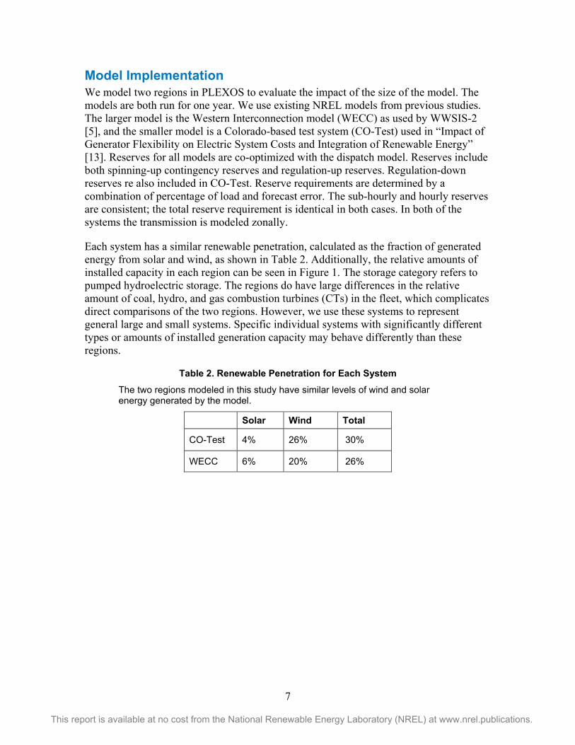
Each system has a similar renewable penetration, calculated as the fraction of generated energy from solar and wind, as shown in Table 2. Additionally, the relative amounts of installed capacity in each region can be seen in Figure 1. The storage category refers to pumped hydroelectric storage. The regions do have large differences in the relative amount of coal, hydro, and gas combustion turbines (CTs) in the fleet, which complicates direct comparisons of the two regions. However, we use these systems to represent general large and small systems. Specific individual systems with significantly different types or amounts of installed generation capacity may behave differently than these regions.

Table 2. Renewable Penetration for Each System

The two regions modeled in this study have similar levels of wind and solar energy generated by the model.

Solar Wind Total

CO-Test 4% 26% 30%

WECC 6% 20% 26%

8


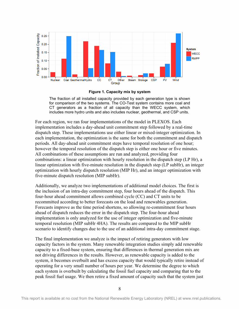
Figure 1. Capacity mix by system

The fraction of all installed capacity provided by each generation type is shown for comparison of the two systems. The CO-Test system contains more coal and CT generators as a fraction of all capacity than the WECC system, which includes more hydro units and also includes nuclear, geothermal, and CSP units.

For each region, we ran four implementations of the model in PLEXOS. Each implementation includes a day-ahead unit commitment step followed by a real-time dispatch step. These implementations use either linear or mixed-integer optimization. In each implementation, the optimization is the same for both the commitment and dispatch periods. All day-ahead unit commitment steps have temporal resolution of one hour; however the temporal resolution of the dispatch step is either one hour or five minutes. All combinations of these assumptions are run and analyzed, providing four combinations: a linear optimization with hourly resolution in the dispatch step (LP Hr), a linear optimization with five-minute resolution in the dispatch step (LP subHr), an integer optimization with hourly dispatch resolution (MIP Hr), and an integer optimization with five-minute dispatch resolution (MIP subHr).

Additionally, we analyze two implementations of additional model choices. The first is the inclusion of an intra-day commitment step, four hours ahead of the dispatch. This four-hour ahead commitment allows combined cycle (CC) and CT units to be recommitted according to better forecasts on the load and renewables generation. Forecasts improve as the time period shortens, so allowing re-commitment four hours ahead of dispatch reduces the error in the dispatch step. The four-hour ahead implementation is only analyzed for the use of integer optimization and five-minute temporal resolution (MIP subHr 4HA). The results are compared to the MIP subHr scenario to identify changes due to the use of an additional intra-day commitment stage.

The final implementation we analyze is the impact of retiring generators with low capacity factors in the system. Many renewable integration studies simply add renewable capacity to a fixed-base system, ensuring that differences in thermal generation mix are not driving differences in the results. However, as renewable capacity is added to the system, it becomes overbuilt and has excess capacity that would typically retire instead of operating for a very small number of hours per year. We determine the degree to which each system is overbuilt by calculating the fossil fuel capacity and comparing that to the peak fossil fuel usage. We then retire a fixed amount of capacity such that the system just

9


meets capacity reliability standards. We use data from the MIP hourly analyses for both the WECC and the CO-Test systems to identify the generators with the lowest capacity factor, and we assume the generators with the lowest capacity factors will retire. Results could be quite different if baseload units such as coal plants are retired instead of these low capacity factor units; however, for this analysis, we are analyzing the impacts of operating with a smaller planning reserve margin, not completely restructuring the thermal fleet. For this analysis MIP optimization and hourly temporal resolution are used.

Evaluation Metrics For each implementation in PLEXOS we compute the total production cost, curtailment of both wind and solar, total emissions by fuel type, the number of starts and ramps of each generator type, and the average on-time per start of these generators. These metrics are used to identify how the studied input variables, optimization, temporal resolution, and intra-day commitment can affect the output variables of a study.

The total production cost includes the fuel cost, startup cost, and variable operation and maintenance cost for each generator. The total production costs are summed for each generator category for comparison. Curtailment of wind and solar power are also computed by PLEXOS and summed for each renewable energy type.

The total CO2 emissions are computed as the total fuel used by each generator multiplied by the emissions factor of the fuel used. The CO2 emissions are then aggregated for comparison between models.

Operational impacts are a frequent topic of interest or concern in systems with high renewable penetrations. To illustrate these impacts, we examine the capacity started by generator type, the average on-time per start, and the number of ramps by generator type for each model. The capacity started is computed as the sum of all times a generator began operation, multiplied by the capacity of that generator. The linear model solutions allow partial operation of generators, so in these cases some generators would operate at very low levels (e.g., thousandths or millionths of a megawatt). We only account for starts in these cases if a generator operates at a level greater than 0.01 MW.

We then compute the time that each generator is operated, or the on-time, per start for that generator. The result is then averaged for each generator type to find the average on-time for each type. We omit must-run generators, which are typically co-generation facilities, from this metric. It provides an indication of how a generator’s operation is affected by each of our studied assumptions.

Ramping is a large concern for coal generators, which anticipate very different use patterns than their traditional operation when there is high penetration of renewable energy. We comput the number of ramps as the total number of times that a generator must increase its generation by an amount more than 30% of its installed capacity (as is done in WWSIS-2). We compute only the up-ramps for each generator, assuming that each up-ramp will be mirrored later by a corresponding down-ramp. The ramp rate of each ramp is not computed, only the total number of ramping events.

10


Results Impact of Linear (LP) vs. Integer (MIP) Optimization Model Run Time The main reason an LP solution is utilized over a MIP solution is the run time required. If a study examines many potential future scenarios or renewable penetrations, the model must be run several times, which requires significantly more time. For example, the unit commitment stage required 94 hours for the MIP optimization and 66 hours for the LP optimization. The dispatch stage also requires more time; LP solution in the WECC system has a run time of 50 hours whereas the MIP solution has a run time of 65 hours when solving one year of the dispatch solution. This time savings however comes at a cost of a less realistic model solution, as the LP scenario will be able to start partial generators in order to relax minimum generation level constraints, and other such partial operation, which is not feasible for actual generators.

Figure 2 shows the distribution of step times for the LP and MIP dispatch examined. Both scenarios have the same number of steps (105,120 for one year), but the MIP solution required an average of 2.2 seconds per step, whereas the LP required 1.7 seconds per step. For each scenario, there are many outlier steps, taking as long as 12.5 seconds each to solve.

Figure 2. Step time for MIP and LP optimization

Solving the economic dispatch equations with an LP solution requires less time per step on average than does the MIP solution.

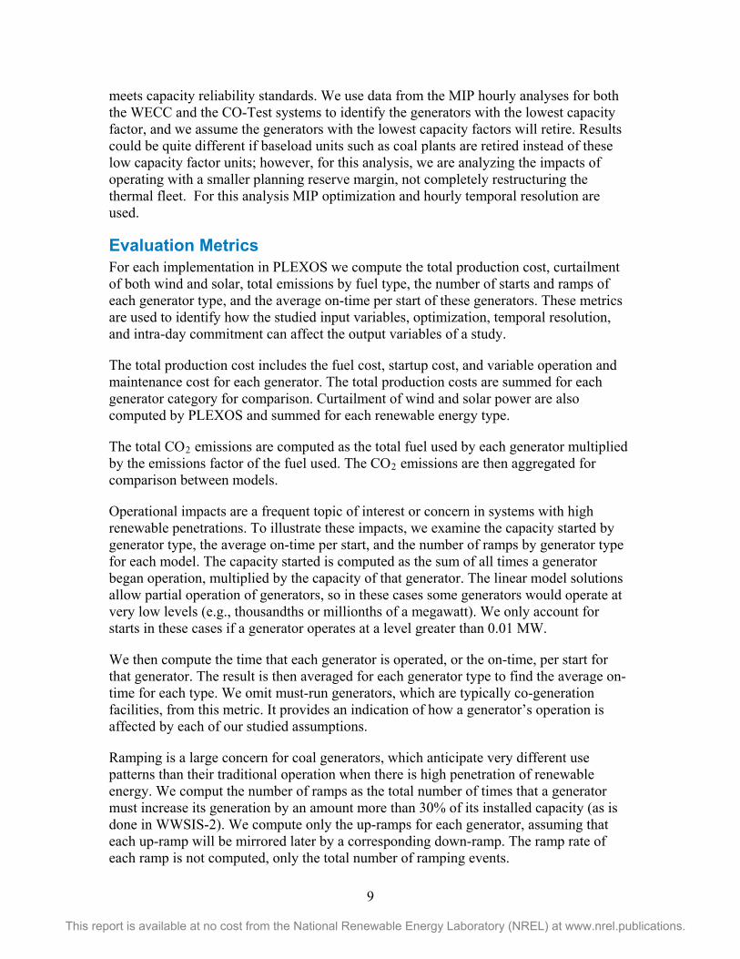
Generation by Generator Type A comparison of the relative amount of generation by generator type for the sub-hourly scenario for the WECC system is shown in Figure 3. This comparison illustrates the different choices made under the each optimization technique to meet the total demand. In particular, a model using linear optimization uses 0.5% more wind generation and 2.4% less gas CC generation because minimum generation constraints are never binding when using LP optimization.

11


Figure 3. Generation by model and system

The LP and MIP models use different generation types to meet demand. These differences can particularly be seen in the use of CC generators and wind. The results are shown for WECC with sub-hourly temporal resolution.

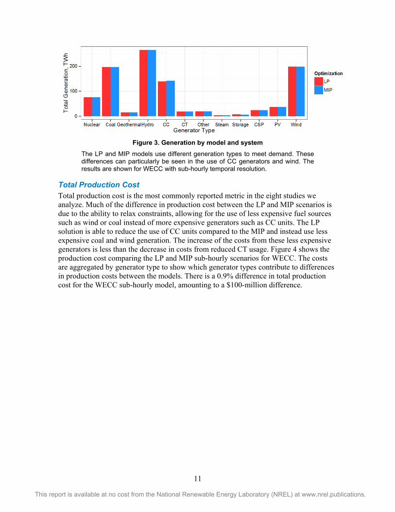
Total Production Cost Total production cost is the most commonly reported metric in the eight studies we analyze. Much of the difference in production cost between the LP and MIP scenarios is due to the ability to relax constraints, allowing for the use of less expensive fuel sources such as wind or coal instead of more expensive generators such as CC units. The LP solution is able to reduce the use of CC units compared to the MIP and instead use less expensive coal and wind generation. The increase of the costs from these less expensive generators is less than the decrease in costs from reduced CT usage. Figure 4 shows the production cost comparing the LP and MIP sub-hourly scenarios for WECC. The costs are aggregated by generator type to show which generator types contribute to differences in production costs between the models. There is a 0.9% difference in total production cost for the WECC sub-hourly model, amounting to a $100-million difference.

12


Figure 4. Total production cost

The total production cost is shown for the WECC sub-hourly model implementation, by generator type. The LP optimization technique leads to a total production cost that is 0.9% lower.

Curtailment Curtailment of renewable energy is another important quantity, and it is measured in seven of the nine studies we examine. High curtailment of renewables is undesirable, as it reduces the capacity factor of the renewable sources and leads to the use of higher cost generation sources. The total curtailment of wind and solar and the percent difference from the MIP solution are shown in Table 3.

Table 3. Curtailment of Renewable Energy

The total curtailment of both wind and solar is shown aggregated by optimization result. The percent difference is given from the MIP solution.

Energy Curtailed Percent Difference

LP 5,500 gigawatt-hours (GWh) -24%

MIP 7,200 GWh n/a

Using LP optimization leads to a large change in curtailment, with a reduction in total curtailment in the system of 24%. Curtailment in WECC amounts to 2.7% of available renewable energy for the MIP case, and 2.1% of available renewable energy for the LP case.

13


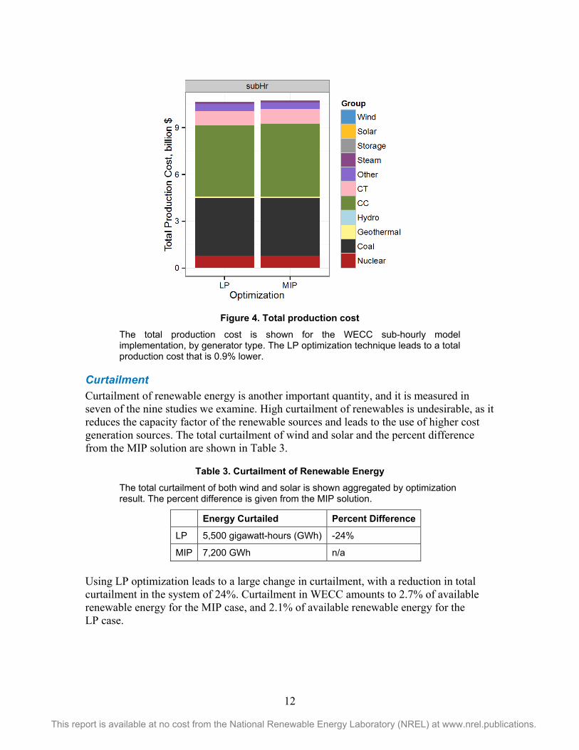
CO2 Emissions The large increase in renewable energy use described above leads to lower CO2 emissions, as these sources displace higher carbon sources such as coal. As carbon policies begin to be implemented, this will increasingly become a more important metric. The results for CO2 emissions are shown in Figure 5. We find a 0.8% reduction, amounting to a difference of three million tons of CO2 between the MIP and LP models with sub-hourly temporal resolution for WECC.

Figure 5. Carbon emissions by generator type

The total emissions are shown for each system analyzed, grouped according to generator type.

Starts and Ramps To understand the day-to-day impact of increased renewable energy on the electric grid, system operators need to understand operational impacts. For this reason, we use three metrics for evaluating these operational impacts, focusing on starts, ramps and generator on-time of fossil fuel and storage facilities. For each of these metrics there is a large difference between the linear optimization and integer optimization. For storage technologies, starting metrics refer to only generation from the storage facility and do not include pumping.

For each fossil fuel generator type, the LP optimization sees an increase in the started capacity over the MIP solution (Figure 6). A large contributor to this increase is the ability of an LP solution to partially start units in the optimization (which are then counted as full starts in the post-processed capacity started metric); in contrast, a MIP solution does not allow partial starts. This leads to a large increase in starts for some generators; in particular, coal units see a 23% increase in their started capacity in the LP solution over the MIP, and storage capacities see a 27% decrease (Table 4).

14


Figure 6. Capacity started, LP vs MIP

This figure shows the total capacity started, in GW, for gas CC, coal, and gas CT generators as well as for pumped hydro storage.

Table 4. Percent Difference in Started Capacity, Optimization

The percent difference in started capacity in GW is calculated from the MIP solution for four technologies.

Technology Percent Difference

Gas CC 1%

Coal 23%

Gas CT 9%

Storage -27%

The average on-time per start provides insight into how different generator types are being used. Coal units are used for less time during each start in the LP model, whereas both gas CC and gas CT technologies are used for longer time periods. The largest relative difference, as seen in Figure 7, is the gas CT units, which has an average on-time per start of 20% more in the LP solution than in the MIP.

15


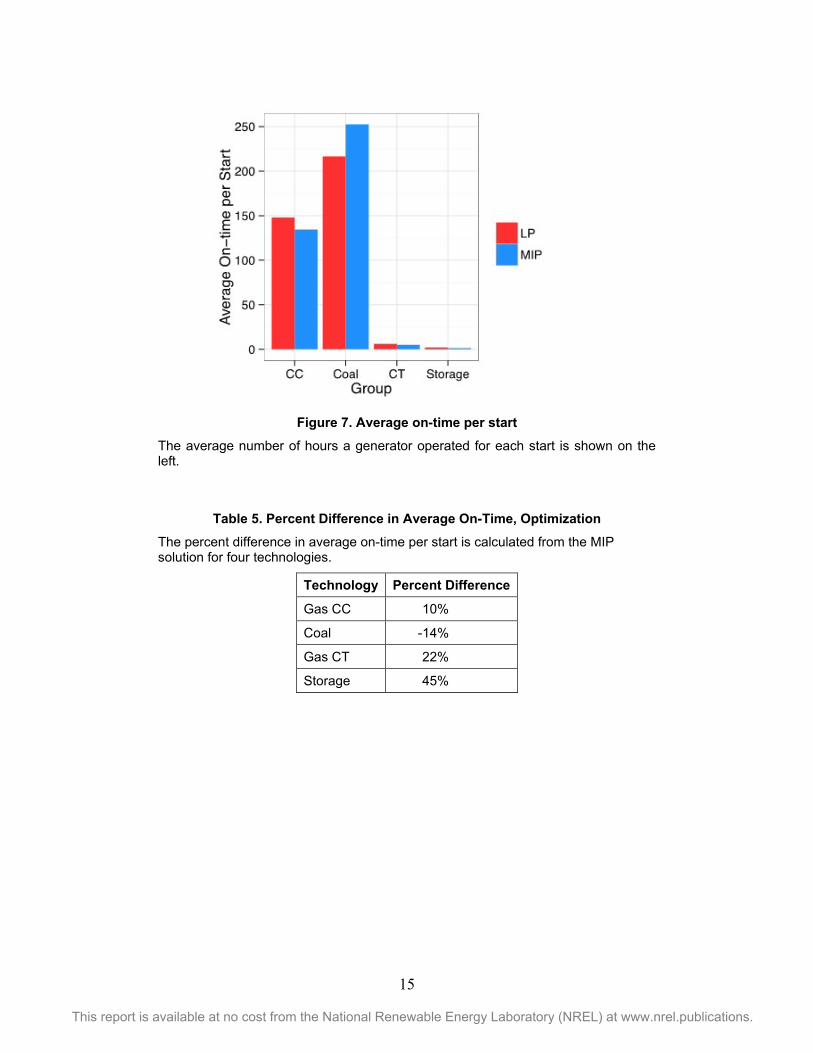
Figure 7. Average on-time per start

The average number of hours a generator operated for each start is shown on the left.

Table 5. Percent Difference in Average On-Time, Optimization

The percent difference in average on-time per start is calculated from the MIP solution for four technologies.


Gas CC 10%

Coal -14%

Gas CT 22%

Storage 45%

16


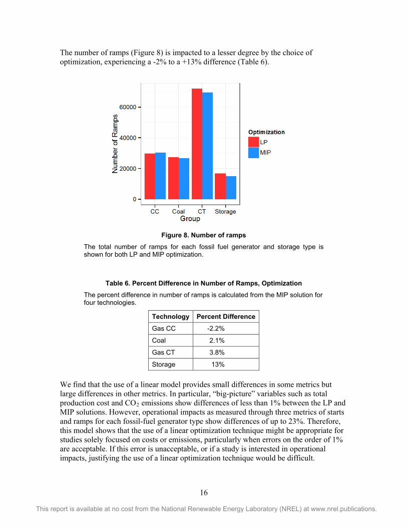
The number of ramps (Figure 8) is impacted to a lesser degree by the choice of optimization, experiencing a -2% to a +13% difference (Table 6).

Figure 8. Number of ramps

The total number of ramps for each fossil fuel generator and storage type is shown for both LP and MIP optimization.

Table 6. Percent Difference in Number of Ramps, Optimization

The percent difference in number of ramps is calculated from the MIP solution for four technologies.


Gas CC -2.2%

Coal 2.1%

Gas CT 3.8%

Storage 13%

We find that the use of a linear model provides small differences in some metrics but large differences in other metrics. In particular, “big-picture” variables such as total production cost and CO2 emissions show differences of less than 1% between the LP and MIP solutions. However, operational impacts as measured through three metrics of starts and ramps for each fossil-fuel generator type show differences of up to 23%. Therefore, this model shows that the use of a linear optimization technique might be appropriate for studies solely focused on costs or emissions, particularly when errors on the order of 1% are acceptable. If this error is unacceptable, or if a study is interested in operational impacts, justifying the use of a linear optimization technique would be difficult.

17


Impact of Hourly vs Five-minute Dispatch Temporal Resolution Model Run Time Using hourly dispatch instead of sub-hourly dispatch has a very significant impact on the total run time of the model. For the WECC system we analyzed, the hourly dispatch model requires 3.6 hours to run, compared to 65 hours for the sub-hourly (five-minute dispatch) dispatch model. The average step time of the hourly dispatch is 1.5 seconds compared to 2.2 seconds for the sub-hourly dispatch. The distribution of time steps is shown in Figure 9. The large difference in run time is due to the inclusion of fewer steps in the hourly dispatch case and also likely issues of memory usage with the larger model. Only 8,760 steps are required in the hourly dispatch case while 105,120 steps are required for the sub-hourly dispatch. Many outliers in both cases require up to 12.5 seconds for one step in the sub-hourly dispatch and one case in the hourly-dispatch step required as much as 32 seconds.

The cost of this shortened run time is a less precise representation of the grid operations. Much of the uncertainty and variability of load and renewable generation happens at time scales of minutes, and a model operating on hourly time scales will not see this variability.

Figure 9. Step time required for hourly and sub-hourly dispatch

The time required is for each step using a MIP optimization and either hourly or sub-hourly dispatch. The hourly dispatch has 8,760 steps and the sub-hourly dispatch has 105,120 steps.

Generation by Generator Type A comparison of the relative amount of generation by fuel type for the sub-hourly scenario for the WECC system is shown in Figure 10. There are only small differences between these scenarios in terms of total generation. Gas CC units has the highest absolute difference of 383 GWh, which amounted to a difference of 0.3% in total generation between the scenarios. In terms of percent difference, storage technologies are used 5% more in the sub-hourly case to help account for short-term variability in

18


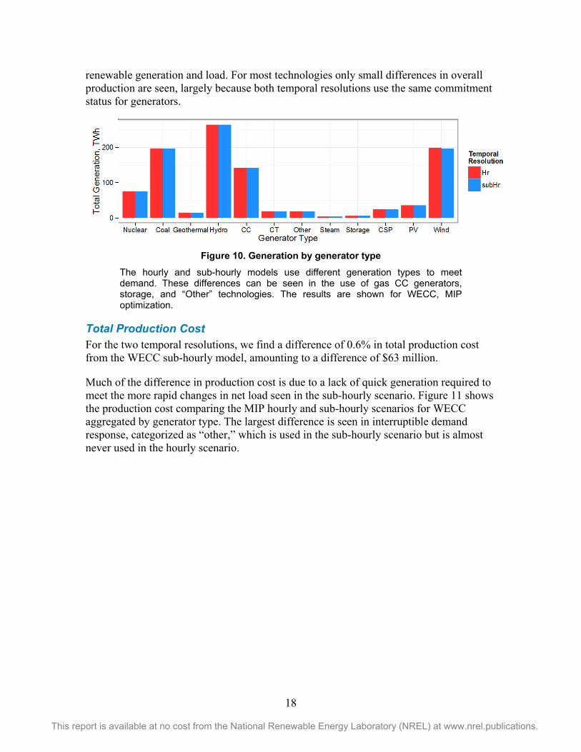
renewable generation and load. For most technologies only small differences in overall production are seen, largely because both temporal resolutions use the same commitment status for generators.

Figure 10. Generation by generator type

The hourly and sub-hourly models use different generation types to meet demand. These differences can be seen in the use of gas CC generators, storage, and “Other” technologies. The results are shown for WECC, MIP optimization.

Total Production Cost For the two temporal resolutions, we find a difference of 0.6% in total production cost from the WECC sub-hourly model, amounting to a difference of $63 million.

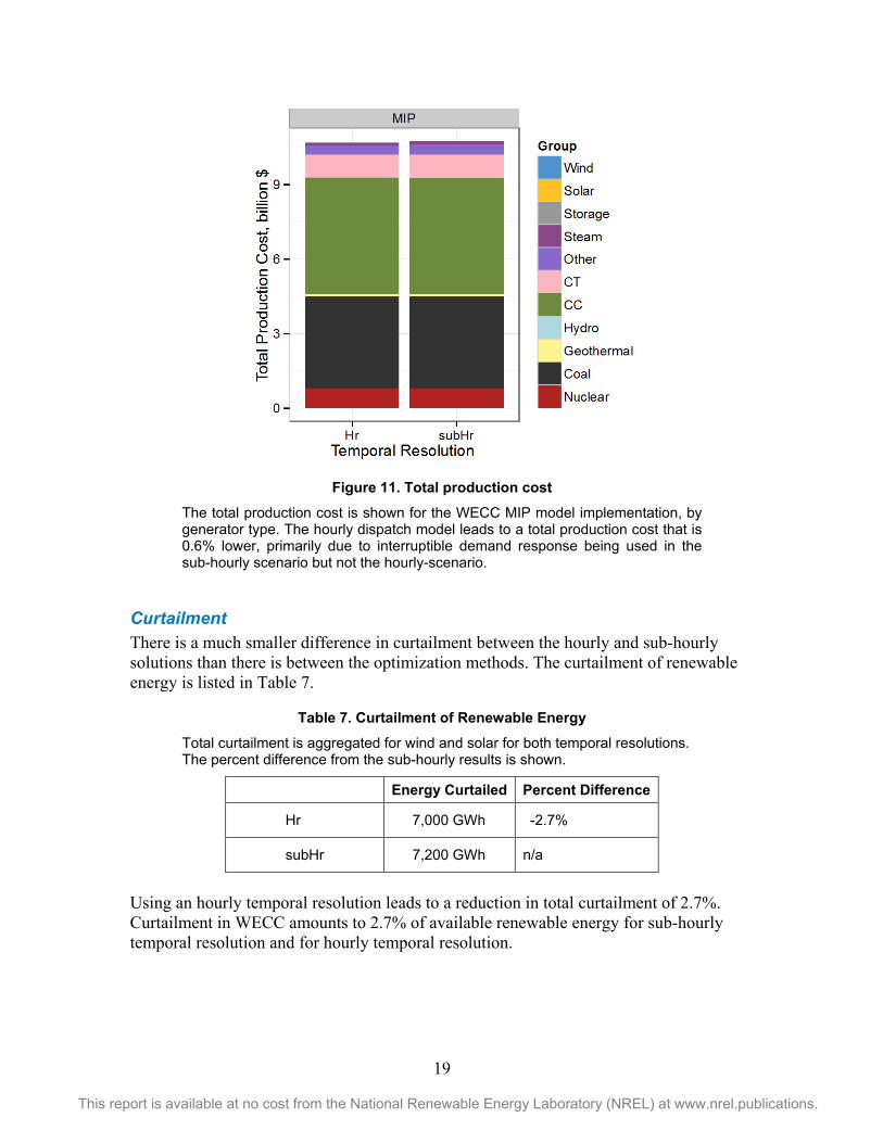
Much of the difference in production cost is due to a lack of quick generation required to meet the more rapid changes in net load seen in the sub-hourly scenario. Figure 11 shows the production cost comparing the MIP hourly and sub-hourly scenarios for WECC aggregated by generator type. The largest difference is seen in interruptible demand response, categorized as “other,” which is used in the sub-hourly scenario but is almost never used in the hourly scenario.

19


Figure 11. Total production cost

The total production cost is shown for the WECC MIP model implementation, by generator type. The hourly dispatch model leads to a total production cost that is 0.6% lower, primarily due to interruptible demand response being used in the sub-hourly scenario but not the hourly-scenario.

Curtailment There is a much smaller difference in curtailment between the hourly and sub-hourly solutions than there is between the optimization methods. The curtailment of renewable energy is listed in Table 7.

Table 7. Curtailment of Renewable Energy

Total curtailment is aggregated for wind and solar for both temporal resolutions. The percent difference from the sub-hourly results is shown.

Energy Curtailed Percent Difference

Hr 7,000 GWh -2.7%

subHr 7,200 GWh n/a

Using an hourly temporal resolution leads to a reduction in total curtailment of 2.7%. Curtailment in WECC amounts to 2.7% of available renewable energy for sub-hourly temporal resolution and for hourly temporal resolution.

20


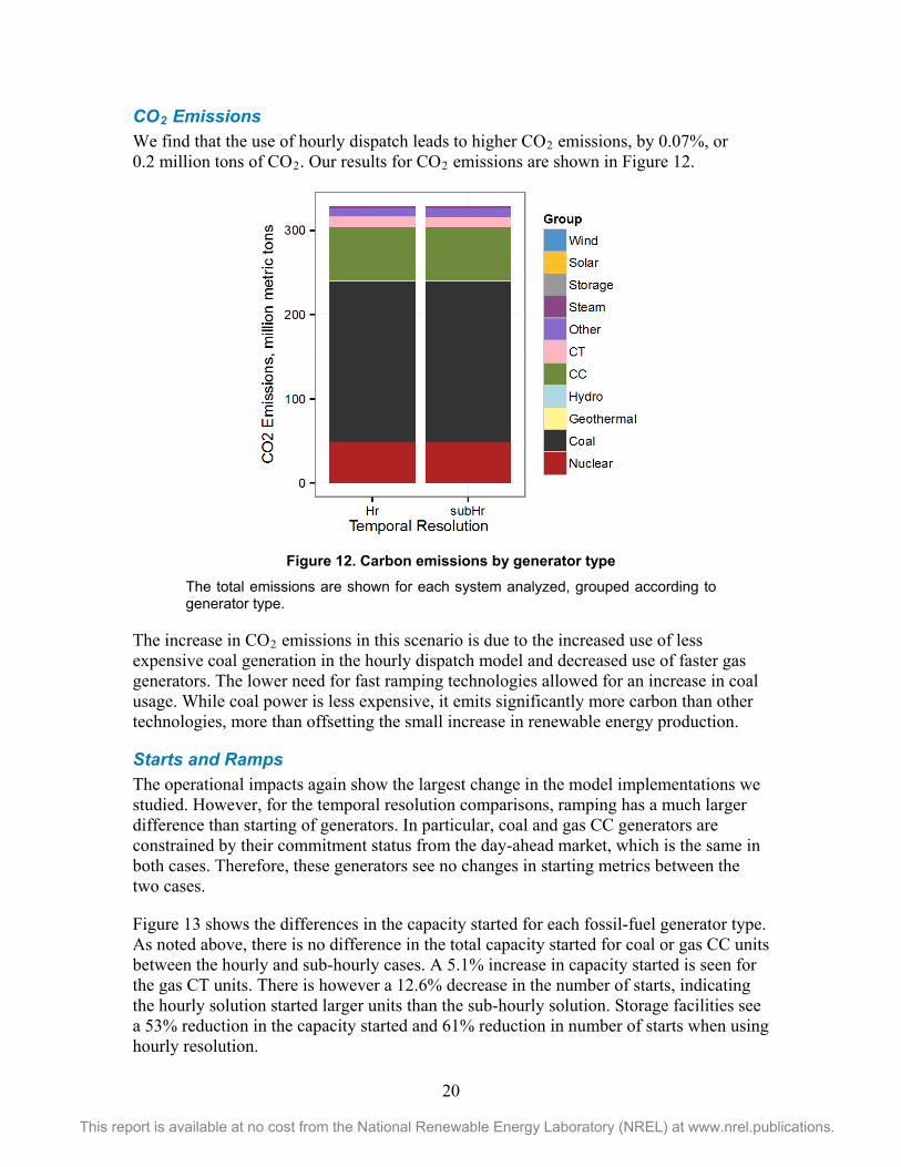
CO2 Emissions We find that the use of hourly dispatch leads to higher CO2 emissions, by 0.07%, or 0.2 million tons of CO2. Our results for CO2 emissions are shown in Figure 12.


The total emissions are shown for each system analyzed, grouped according to generator type.

The increase in CO2 emissions in this scenario is due to the increased use of less expensive coal generation in the hourly dispatch model and decreased use of faster gas generators. The lower need for fast ramping technologies allowed for an increase in coal usage. While coal power is less expensive, it emits significantly more carbon than other technologies, more than offsetting the small increase in renewable energy production.

Starts and Ramps The operational impacts again show the largest change in the model implementations we studied. However, for the temporal resolution comparisons, ramping has a much larger difference than starting of generators. In particular, coal and gas CC generators are constrained by their commitment status from the day-ahead market, which is the same in both cases. Therefore, these generators see no changes in starting metrics between the two cases.

Figure 13 shows the differences in the capacity started for each fossil-fuel generator type. As noted above, there is no difference in the total capacity started for coal or gas CC units between the hourly and sub-hourly cases. A 5.1% increase in capacity started is seen for the gas CT units. There is however a 12.6% decrease in the number of starts, indicating the hourly solution started larger units than the sub-hourly solution. Storage facilities see a 53% reduction in the capacity started and 61% reduction in number of starts when using hourly resolution.

21


Figure 13. Capacity started, temporal resolution

This figure shows the total capacity started, in GW, for gas CC, coal, and gas CT generators. Results are for the WECC system with MIP optimization.

The average on-time per start only varies for different temporal resolutions for gas CT units and storage, again due to the commitment status of the gas CC and coal units. Gas CT units see a 2% increase in the average on-time per start in the hourly dispatch compared to the sub-hourly dispatch, and storage units see a 96% increase compared to sub-hourly dispatch (Figure 14).

Figure 14. Average on-time per start, temporal resolution

The average number of hours a generator operated for each start is shown; results are for the WECC system with MIP optimization.

22


We find that ramping is impacted to the greatest degree for the temporal resolution comparison (Figure 15). All generator types see a decrease in the number of ramps when using an hourly dispatch model of up to 55% for gas CT generators and 86% for storage facilities (Table 8).


The figure shows the total number of ramps for each fossil fuel generator type.

Table 8. Percent Difference in Number of Ramps, Temporal Resolution



Gas CC -26%

Coal -44%

Gas CT -56%

Storage -87% As we find with the comparison of optimization technique used, we see again that the effect of using an hourly dispatch model rather than a sub-hourly dispatch model is much greater when examining operational impact metrics compared to production cost or emissions metrics. This might be expected for a temporal resolution comparison, as hourly modeling is unable to accurately measure the variability seen on a five-minute time scale. This variability requires generators to change their output more often, leading to an increase in the ramping performed by traditional generators.

As with our conclusions from the optimization technique used, this model shows that future studies interested in operational impacts should use a sub-hourly dispatch model, but studies interested in total costs or emissions may, depending on the acceptable error level, could use an hourly dispatch model.

23


Comparison of WECC and CO-Test Systems We next perform our analysis on both a large system and a small system to identify any differences that may have arisen due to specific systems. We are interested in whether any of our assumptions have different effects on systems of different sizes and generator fleet compositions. While some of the differences are present due to the different installed capacity of the two systems, we see similar behavior in all metrics between the systems.

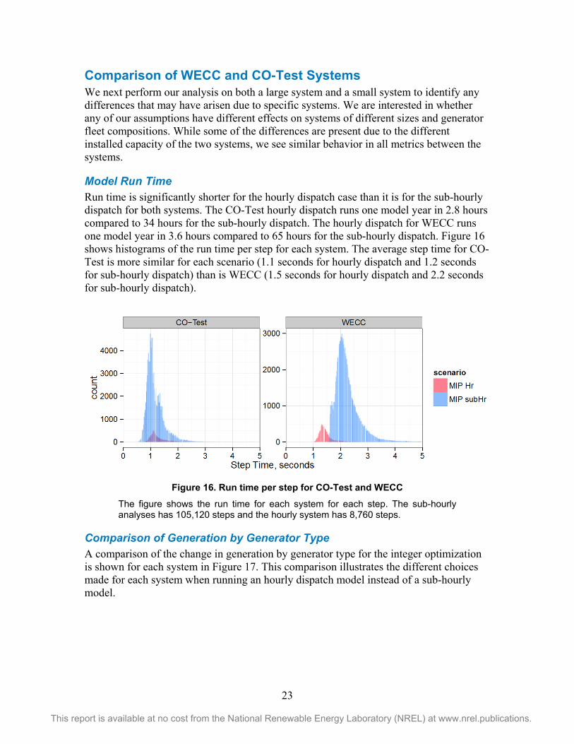
Model Run Time Run time is significantly shorter for the hourly dispatch case than it is for the sub-hourly dispatch for both systems. The CO-Test hourly dispatch runs one model year in 2.8 hours compared to 34 hours for the sub-hourly dispatch. The hourly dispatch for WECC runs one model year in 3.6 hours compared to 65 hours for the sub-hourly dispatch. Figure 16 shows histograms of the run time per step for each system. The average step time for CO-Test is more similar for each scenario (1.1 seconds for hourly dispatch and 1.2 seconds for sub-hourly dispatch) than is WECC (1.5 seconds for hourly dispatch and 2.2 seconds for sub-hourly dispatch).

Figure 16. Run time per step for CO-Test and WECC

The figure shows the run time for each system for each step. The sub-hourly analyses has 105,120 steps and the hourly system has 8,760 steps.

Comparison of Generation by Generator Type A comparison of the change in generation by generator type for the integer optimization is shown for each system in Figure 17. This comparison illustrates the different choices made for each system when running an hourly dispatch model instead of a sub-hourly model.

24


Figure 17. Difference in generation by generator type and system

The WECC and CO-Test systems have different generation mixes, which influences the choices made for each model. These differences can particularly be seen in the use of CT and coal generators in CO-Test. The results are shown for the MIP optimization, comparing the difference between the hourly and sub-hourly temporal resolution.

TWh = terawatt-hours

We find that CO-Test has a much more drastic change in which types of generators are used when moving to an hourly dispatch model. This is likely because more generator types are used in the WECC while only a few generator types are used in CO-Test.

Total Production Cost Both systems we examine experience a drop in production cost when using an hourly dispatch model instead of a sub-hourly dispatch model. The CO-Test system however experiences a much higher drop, of 6.5% compared to 0.9%. This represents a savings of $75 million for CO-Test compared to the MIP sub-hourly dispatch model. For the CO-Test system, this difference is in large part due to a significantly higher use of gas CT generators in place of coal in the sub-hourly dispatch model. The CO-Test system is dominated by wind and coal, so displacement of these technologies in the sub-hourly model leads to a higher change in cost than otherwise might be seen.

Curtailment CO-Test also experiences a higher percent difference in curtailment than is seen in WECC; CO-Test has a 21% reduction in total curtailment compared to a 2.7% reduction in WECC. Curtailment in the CO-Test system is approximately 0.1% of all renewable energy. In WECC, 2.7% of all renewable energy is curtailed.

CO2 Emissions We find that the use of hourly dispatch leads to higher CO2 emissions, an increase in WECC of 0.07%, or 0.2 million tons of CO2 and in CO-Test of a 0.4% increase in emissions, or 0.2 million tons of CO2. Our results for CO2 emissions are shown in Figure 18.

25



Total emissions are shown for each system analyzed, grouped according to generator type.

The increase in CO2 emissions in these scenarios is due to the increased use of less expensive coal generation in the hourly dispatch model. Though coal power is less expensive, it leads to higher emissions despite the increased use of renewables in the model.

Starts and Ramps The operational impacts of each system are in most cases similar despite differences in the generation mix of each system. The differences in generation mix are reflected in the relative magnitudes of each fossil fuel generation type.

The started capacity (Figure 19) slightly increases for WECC gas CT generators, discussed above, and it decreases by 65% in CO-Test. The number of starts however decreases for both of these systems, indicating that WECC started higher capacity CT units in the hourly dispatch scenario. The started capacity decreases significantly for storage facilities in both systems.

26


Figure 19. Capacity started, GW

The total started capacity can be seen on the left for the CO-Test system and on the right for WECC. Integer optimization is used for both systems.

Table 9. Percent Difference in Started Capacity, Optimization

The percent difference in started capacity in GW is calculated from the MIP solution for four technologies.

Technology Percent Difference WECC

Percent Difference CO-Test

Gas CC 0% 0%

Coal 0% 0%

Gas CT 5% -65%

Storage -53% -34%

27


The average on-time for each system is shown in Figure 20. Both systems see an increase in the gas CT generators’ average on-time in the hourly scenario and no difference in the coal and gas CC generators; this is again because the same commitment status is used.

Figure 20. Average on-time per start

The average on-time per generator of each type can be seen for CO-Test on the left and WECC on the right. The results are shown for integer optimization

Table 10. Percent Difference in Average On-time per Start, Temporal Resolution

The percent difference in average on-time per start is calculated from the MIP solution for four technologies.



Gas CC 0% 0%

Coal 0% 0%

Gas CT 21% 2%

Storage 40% 96%

28


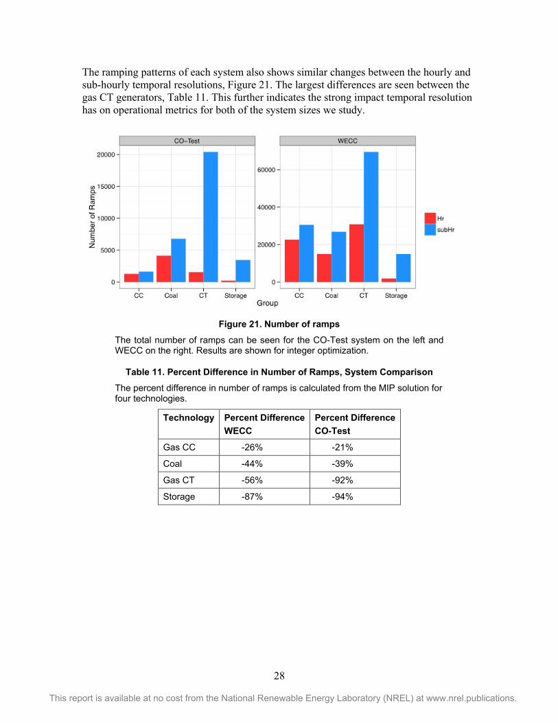
The ramping patterns of each system also shows similar changes between the hourly and sub-hourly temporal resolutions, Figure 21. The largest differences are seen between the gas CT generators, Table 11. This further indicates the strong impact temporal resolution has on operational metrics for both of the system sizes we study.


The total number of ramps can be seen for the CO-Test system on the left and WECC on the right. Results are shown for integer optimization.

Table 11. Percent Difference in Number of Ramps, System Comparison




Gas CC -26% -21%

Coal -44% -39%

Gas CT -56% -92%

Storage -87% -94%

29


Effects of Four-Hour-Ahead Commitment In addition to testing the two model assumptions described above, we analyze the addition of a four-hour ahead commitment schedule between the day-ahead and dispatch markets. While this is not a modeling assumption, the impacts of additional commitment on these same metrics may be of interest to policymakers and may be used in future models. Specifically, the following results can be used to understand the impact of additional commitment on the production cost, emissions, and operational impacts. We perform this analysis for both the CO-Test and WECC systems with an integer optimization at sub-hour temporal resolution. Including an additional commitment step does require more time to run the model. We found for WECC the total commitment and dispatch time increased from 160 hours to 209 hours, a 30% increase. The CO-Test system increased from 38 hours to 43 hours, a 12% increase.

Generation by Generator Type A comparison of the generation provided by generator type when a four-hour ahead commitment period is included is shown in Figure 22. During this commitment period, commitment levels may change, impacting the ultimate dispatch of these generators. Generators with long startup periods, such as coal and nuclear generators are not allowed to be re-committed during this phase; however, gas CC units are allowed to change their commitment. Figure 22 shows the absolute difference in generation for each system, by generator type.

Figure 22. Difference in generation when including four-hour-ahead market

Both systems make difference choices for dispatch in the real-time market when a four-hour ahead commitment period is utilized. The results are shown for integer optimization and sub-hourly temporal resolution.

The largest difference seen is in the commitment of gas CC and gas CT units, whereby gas CC units are used at a higher rate when a four-hour commitment period is included. In terms of percent differences, CO-Test has a higher percent difference in most cases than WECC, and it see high changes in CC and CT units.

30


Total Production Cost The total production cost decreases a small amount in the CO-Test system and is effectively unchanged in the WECC system when four-hour ahead commitment is used. CO-Test sees a 0.6% decrease in production cost, which amounts to a difference in total production cost of -$7.0 million.

Curtailment Total curtailment shows different behaviors between the small system and large system when a four-hour ahead commitment period is included. For the CO-Test region, total curtailment decreases by 12%; for the WECC system, total curtailment increases by 0.4% when the four-hour ahead dispatch period is added. Table 12 shows the curtailment for each scenario and system as well as the percentage change.

Table 12. Curtailment of Renewable Energy, 4HA Commitment The total curtailment is shown for each system when including an additional commitment step.

Includes 4HA Energy Curtailed Percent Difference

WECC No 7,200 GWh 0.4%

Yes 7,300 GWh n/a

CO-Test No 25 GWh -12%

Yes 22 GWh n/a

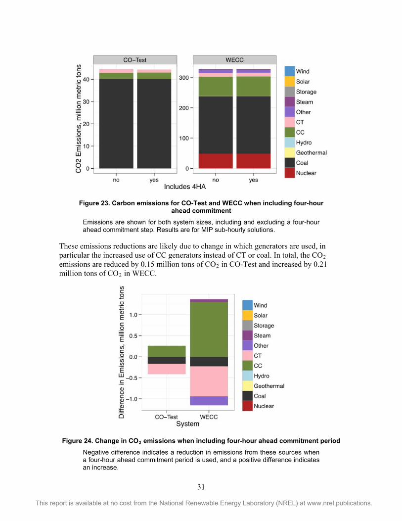
CO2 Emissions As is the case in our previous analyses, the effect of including a four-hour commitment step on CO2 emissions is small. When a four-hour ahead commitment period is included, the emissions are reduced by 0.3% in CO-Test and increased by 0.07% in WECC. Figure 23 shows the emissions by type for each system and commitment scenario, and Figure 24 shows the difference in emissions by generator type.

31


Figure 23. Carbon emissions for CO-Test and WECC when including four-hour

ahead commitment Emissions are shown for both system sizes, including and excluding a four-hour ahead commitment step. Results are for MIP sub-hourly solutions.

These emissions reductions are likely due to change in which generators are used, in particular the increased use of CC generators instead of CT or coal. In total, the CO2 emissions are reduced by 0.15 million tons of CO2 in CO-Test and increased by 0.21 million tons of CO2 in WECC.

Figure 24. Change in CO2 emissions when including four-hour ahead commitment period

Negative difference indicates a reduction in emissions from these sources when a four-hour ahead commitment period is used, and a positive difference indicates an increase.

32


Starts and Ramps When including a four-hour ahead commitment step, the operation of fossil fuel units is seen to change in different ways for CO-Test and WECC, particularly for gas CC and gas CT units. We find that both systems see a reduction in the capacity started for gas CT units when a four-hour ahead commitment step is included. However, CO-Test also sees a reduction in the use of gas CC units, while WECC sees an increase in these units. Figure 25 shows the total capacities started and Table 13 shows the percent change when the four-hour ahead is included. Coal generators see no change, as these generators are unable to change their commitment in the four-hour ahead step.

Figure 25. Capacity started, 4HA commitment

Results are shown for both the CO-Test system and WECC, including and excluding a 4-HA commitment step for MIP sub-hourly solutions.

Table 13. Capacity Started, 4HA Commitment The percent difference in capacity started when a four-hour ahead commitment step is included is shown for each system studied.

Technology Percent Difference CO-Test

Percent Difference WECC

Gas CC -2% 14%

Coal 0% 0%

Gas CT -10% -33%

Storage -3% -5%

The average on-time per start varies greatly between the two systems. Figure 26 shows the average-on time seen for both systems, and Table 14 shows the percent differences from the solution without the additional commitment step. Differences in these systems

33


are likely due to the generation mixes of the systems and their relative proportions of each generator type.

Figure 26. Average on-time per start, including 4-HA commitment

The average on-time per start for each generator type is shown by system, with and without a four-hour ahead commitment step. Results are shown for MIP sub-hourly solutions.

Table 14. Average On-Time per Start, 4-HA Commitment The percent difference in on-time per start when a four-hour ahead commitment step is shown for each system studied.



Gas CC 24% -0.4%

Coal 0% 0%

Gas CT -4.8% 2.5%

Storage 2.4% 3.4%

The number of ramps by each generator class see similar changes between the systems (Figure 27). Gas CT units see the highest percent change (Table 15), and Gas CC unit ramping decreases in both systems. The addition of an intra-day commitment step and better forecasting allows the use of less expensive coal and CC units to match variability in load and renewables instead of the more expensive CT units.

34


Figure 27. Number of ramps, including four-hour ahead commitment

The number of ramps for the CO-Test system and WECC is shown for solutions using MIP optimization and sub-hourly time resolution.

Table 15. Number of Ramps, 4-HA Commitment The percent difference in number of ramps when a four-hour ahead commitment step is shown for each system studied.



Gas CC 19% 13%

Coal 3.1% 4.2%

Gas CT -8.7% -6.4%

Storage 7.3% -0.4%

Impact of Overbuilt Systems We perform an analysis of the impact of retirements of generators to reduce the overbuilt degree of each system. We retire fossil fuel generators until the system fossil fuel capacity is 1.2 times the peak fossil fuel usage in the MIP hourly runs to account for reliability requirements. Retirements are made based on generators with the lowest yearly capacity factors. The capacity of fossil fuel generators on the system before and after retirements is shown in Table 16.

35


Table 16. Generator Fleet, before and after retirements

The installed capacity of each system is shown before and after retirements are taken into account. The category of “Other” includes coal, steam, and other fossil fuel generators.

Capacity Type Before Retirements After Retirements Difference

WECC

Gas CC 70.8 GW 59.8 GW 11.0 GW

Gas CT 29.1 GW 16.3 GW 12.7 GW

Other 54.0 GW 50.9 GW 3.1 GW

CO-Test

Gas CC 4.7 GW 4.1 GW 0.6 GW

Gas CT 4.6 GW 3.1 GW 1.5 GW

Other 6.5 GW 6.4 GW 0.1 GW

The following results are dependent upon the exact makeup of retirements, and they are likely to change based on which generators are retired. In particular, major changes in these results would be expected if base-load generators are retired instead of units used predominantly for peaking. However, these results demonstrate the general impacts that may be seen from using a more constrained system in a renewable integration study.

Generation by Generator Type The retirements in each system lead to some changes in use patterns of the generation fleet. Figure 28 shows the change in generation from each generator category before and after the retirements are performed. The differences are impacted to a high degree by the changes in generator make up after the retirements, and also by the more highly constrained nature of the system.

Figure 28. Difference in generation by generator type and system when

including retirements

The WECC and CO-Test systems both predominantly retired gas CT generators. WECC retired more gas CC generators than did the CO-Test system. Both systems see differing use patterns after the retirements.

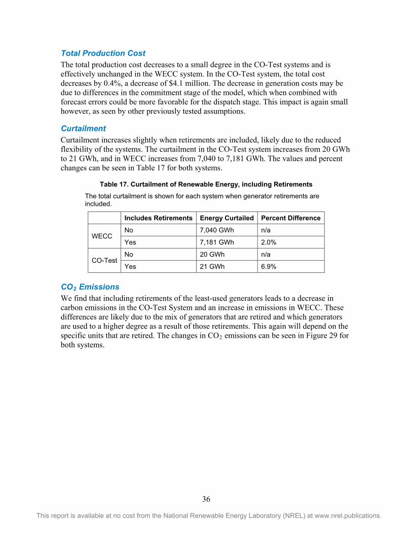
36


Total Production Cost The total production cost decreases to a small degree in the CO-Test systems and is effectively unchanged in the WECC system. In the CO-Test system, the total cost decreases by 0.4%, a decrease of $4.1 million. The decrease in generation costs may be due to differences in the commitment stage of the model, which when combined with forecast errors could be more favorable for the dispatch stage. This impact is again small however, as seen by other previously tested assumptions.

Curtailment Curtailment increases slightly when retirements are included, likely due to the reduced flexibility of the systems. The curtailment in the CO-Test system increases from 20 GWh to 21 GWh, and in WECC increases from 7,040 to 7,181 GWh. The values and percent changes can be seen in Table 17 for both systems.

Table 17. Curtailment of Renewable Energy, including Retirements The total curtailment is shown for each system when generator retirements are included.

Includes Retirements Energy Curtailed Percent Difference

WECC No 7,040 GWh n/a

Yes 7,181 GWh 2.0%

CO-Test No 20 GWh n/a

Yes 21 GWh 6.9%

CO2 Emissions We find that including retirements of the least-used generators leads to a decrease in carbon emissions in the CO-Test System and an increase in emissions in WECC. These differences are likely due to the mix of generators that are retired and which generators are used to a higher degree as a result of those retirements. This again will depend on the specific units that are retired. The changes in CO2 emissions can be seen in Figure 29 for both systems.

37


Figure 29. Change in carbon emissions when including retirements

The systems see variable changes in carbon emissions due to the differences in which capacity types were retired.

The CO-Test system sees a 0.3% reduction in carbon emissions, which represents approximately 0.14 million metric tons of CO2. The WECC system sees an increase of 0.2%, approximately 0.7 million metric tons. These effects are again small changes, as seen in the other studied assumptions.

Starts and Ramps The operational impacts are affected in inconsistent ways. The specific changes in these metrics are to a large degree impacted by the specific units retired; however, they demonstrate the types of effects that may be seen when generators are retired from the system.

The capacity started shows small changes due to the retirements, Figure 30. The direction of these changes varies for each system; however, the changes are small in all cases except for gas CT units in the CO-Test system which has a high degree of retirements of gas CT units. Table 18 shows the percent changes seen for each system and generator type.

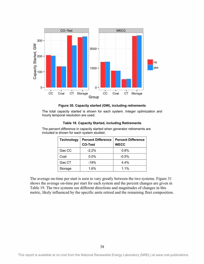
38


Figure 30. Capacity started (GW), including retirements

The total capacity started is shown for each system. Integer optimization and hourly temporal resolution are used.

Table 18. Capacity Started, including Retirements

The percent difference in capacity started when generator retirements are included is shown for each system studied.



Gas CC -2.2% 0.8%

Coal 0.0% -0.5%

Gas CT -19% 4.4%

Storage 1.6% 1.1%

The average on-time per start is seen to vary greatly between the two systems. Figure 31 shows the average on-time per start for each system and the percent changes are given in Table 19. The two systems see different directions and magnitudes of changes in this metric, likely influenced by the specific units retired and the remaining fleet composition.

39


Figure 31. Average on-time per start, including retirements

The average on-time per start is shown for each system when retirements are included.

Table 19. Average On-Time per Start, including Retirements

The percent difference in on-time per start when generator retirements are included is shown for each system studied.



Gas CC 24% 3%

Coal 0% 1%

Gas CT -10% 12%

Storage -8% -1%

The ramping impacts also show differences between the systems, as seen in Figure 32. The CO-Test system sees a fairly high degree of variance between the different generator types, while WECC sees all units increase in the number of ramps when generators are retired. Table 20 shows the percent changes in ramps for each system and generator type.

40


Figure 32. Number of ramps, including retirements

The number of ramps is shown with and without retirements for both the CO-Test system and WECC. The ramping capabilities are impacted by the retired generation mix.

Table 20. Number of Ramps, including Retirements The percent difference in number of ramps when generator retirements are included is shown for each system studied.



Gas CC 29% 8%

Coal 2% 9%

Gas CT -28% 5%

Storage -15% 20%

41


Conclusions We analyze the impacts of optimization technique, temporal resolution, and intra-day commitment on several key metrics for integration studies. We perform this analysis for two system sizes to ensure our results are not specific to a particular system, and we also study the impact of using overbuilt systems when performing these studies. We analyze the total production cost, curtailment, CO2 emissions, and operational impacts for each of our model implementations.

Our results indicate that of the metrics we studied, the smallest effect from either optimization technique, temporal resolution, intra-day commitment, or retirements of overbuilt generation is found on the “big-picture” variables of total production cost and CO2 emissions. These variables see a less than 1% change for the WECC system. The CO-Test system experiences larger changes for these variables, though they are still small (up to 6.5% difference in total production cost). This error may be acceptable depending on the intent of a particular study, but it should be noted that using either a linear optimization or an hourly dispatch model will lead to a difference in the results. The use of intra-day commitment is found to impact some systems to a higher degree than others, with almost no difference in total production cost or emissions for the WECC system studied.

We find larger effects on the operational impact metrics for both the different optimization techniques and the temporal resolution of the dispatch model. The optimization technique shows a higher impact on the starting and operational time of generators (an increase of more than 20% in some cases) and less of an impact on the ramping of generators. The temporal resolution has a high impact on the ramping metrics studied (a 55% increase for gas CT generators) but a lower impact on starting of generators due to the commitment of coal and CC generators in the day-ahead commitment step. If operational questions are being answered in a renewables integration study, use of linear optimization or hourly temporal resolution would be difficult to justify. Incorporating intra-day commitment has the greatest impact on ramping, changing the degree to which all fossil fuel generators ramp for both systems. The degree to which gas CC and gas CT generators are used varied between the CO-Test and WECC systems. Retiring overbuilt generators also shows higher effects on the operational impact metrics, particularly ramping and average on-time per start of gas CT generators. However, the specific differences seen in a model will be affected by which generators are retired.

42


References [1] National Renewable Energy Laboratory. (2013) 2012 Renewable Energy Data Book, Report DOE/GO-102013-4291

[2] Database of State Incentives for Renewable Energy. (2014) Accessed December 11, 2014, from <http://www.dsireusa.org/summarymaps/index.cfm?ee=1&RE=1>

[3] EnerNex Corporation. (2010). Eastern Wind Integration and Transmission Study, NREL Report No. SR-550-47078. http://www.nrel.gov/docs/fy11osti/47078.pdf.

[4] GE Energy (2010). Western Wind and Solar Integration Study. NREL/SR-550-47434. Golden, CO: NREL. http://www.nrel.gov/docs/fy10osti/47434.pdf.

[5] D. Lew, G. Brinkman, E. Ibanez, A. Florita, M. Heaney, B.-M. Hodge, M. Hummon, and G. Stark. (2013). Western Wind and Solar Integration Study Phase 2. NREL/TP-5500-55588. Golden, CO: NREL. http://www.nrel.gov/docs/fy13osti/55588.pdf.

[6] Eastern Interconnection Planning Collaborative. (2012). Phase 2 Report: Interregional Transmission Development and Analysis for Three Stakeholder Scenarios. DOE Award Project: DE-OE0000343. http://www.eipconline.com/uploads/20130103_Phase2Report_Part2_Final.pdf

[7] Transpower stromübertragungs gmbh. (2010). European Wind Integration Study. Ed. Wilhelm Winter. TREN/07/FP6EN/S07.70123/038509. http://www.energinet.dk/SiteCollectionDocuments/Danske%20dokumenter/Forskning/EWIS_Final%20Report.pdf.

[8] Energy and Environmental Economics, Inc. (2014). Investigating a Higher Renewables Portfolio Standard in California. https://ethree.com/documents/E3_Final_RPS_Report_2014_01_06_with_appendices.pdf

[9] Lu S., N. Samaan, D. Meng, F. Chassin, Y. Zhang, B. Vyakaranam, M. Warwick, J. Fuller, R. Diao, T. Nguyen, C. Jin. (2014). Duke Energy Photovoltaic Integration Study: Carolinas Service Areas. PNNL-23226. http://www.pnnl.gov/main/publications/external/technical_reports/PNNL-23226.pdf.

[10] GE Energy. (2013). PJM Renewable Integration Study. http://www.pjm.com/committees-and-groups/task-forces/irtf/pris.aspx

[11] MISO and Manitoba Hydro. (2013). Manitoba Hydro Wind Synergy Study. https://www.misoenergy.org/_layouts/MISO/ECM/Download.aspx?ID=160821

[12] GE Energy (2013) MAPS. http://www.geenergyconsulting.com/practice-area/software-products/maps

[13] Palchak, D. and P. Denholm. (2014). Impact of generator flexibility on electric system costs and integration of renewable energy. NREL/TP-6A20-62275. http://www.nrel.gov/docs/fy14osti/62275.pdf