An MRI digital brain phantom for validation of segmentation methods

This article appeared in a journal published by Elsevier. The attachedcopy is furnished to the author for internal non-commercial researchand education use, including for instruction at the authors institution

and sharing with colleagues.

Other uses, including reproduction and distribution, or selling orlicensing copies, or posting to personal, institutional or third party

websites are prohibited.

In most cases authors are permitted to post their version of thearticle (e.g. in Word or Tex form) to their personal website orinstitutional repository. Authors requiring further information

regarding Elsevier’s archiving and manuscript policies areencouraged to visit:

http://www.elsevier.com/copyright

Author's personal copy

An MRI digital brain phantom for validation of segmentation methods

Bruno Alfano a,⇑, Marco Comerci a, Michele Larobina a, Anna Prinster a,b, Joseph P. Hornak c, S. Easter Selvan a,Umberto Amato d, Mario Quarantelli a, Gioacchino Tedeschi e, Arturo Brunetti a,f, Marco Salvatore b,f

a Biostructure and Bioimaging Institute, National Research Council, Naples, Italyb SDN Foundation, Institute of Diagnostic and Nuclear Development, Naples, Italyc Magnetic Resonance Laboratory, Center for Imaging Science, Rochester Institute of Technology, Rochester, NY, USAd Institute for Applications of Calculation ‘‘Mauro Picone’’ National Research Council, Naples, Italye Department of Neurological Sciences, Second University, Naples, Italyf Department of Biomorphological and Functional Sciences, University ‘‘Federico II’’, Naples, Italy

a r t i c l e i n f o

Article history:Received 19 July 2010Received in revised form 29 December 2010Accepted 18 January 2011Available online 28 January 2011

Keywords:Brain phantomMRISegmentationTissue inhomogeneityMultiple sclerosis

a b s t r a c t

Knowledge of the exact spatial distribution of brain tissues in images acquired by magnetic resonanceimaging (MRI) is necessary to measure and compare the performance of segmentation algorithms. Cur-rently available physical phantoms do not satisfy this requirement. State-of-the-art digital brain phan-toms also fall short because they do not handle separately anatomical structures (e.g. basal ganglia)and provide relatively rough simulations of tissue fine structure and inhomogeneity. We present a soft-ware procedure for the construction of a realistic MRI digital brain phantom. The phantom consists ofhydrogen nuclear magnetic resonance spin–lattice relaxation rate (R1), spin–spin relaxation rate (R2),and proton density (PD) values for a 24 � 19 � 15.5 cm volume of a ‘‘normal’’ head. The phantom includes17 normal tissues, each characterized by both mean value and variations in R1, R2, and PD. In addition, anoptional tissue class for multiple sclerosis (MS) lesions is simulated. The phantom was used to createrealistic magnetic resonance (MR) images of the brain using simulated conventional spin-echo (CSE)and fast field-echo (FFE) sequences. Results of mono-parametric segmentation of simulations ofsequences with different noise and slice thickness are presented as an example of possible applicationsof the phantom. The phantom data and simulated images are available online at http://lab.ibb.cnr.it/.

� 2011 Elsevier B.V. All rights reserved.

1. Introduction

Brain image segmentation is a useful tool for in vivo quantita-tive evaluation of both normal aging and neurodegenerative dis-eases. Ideally, segmentation results should be precise andaccurate enough to measure volumetric abnormalities and changesassociated with different pathophysiological phenomena, and tomonitor the effects of therapy. Many brain segmentation methodshave been proposed, validated, and used (Bermel and Bakshi, 2006;Bezdek et al., 1993; Pelletier et al., 2004), but the evaluation oftheir relative performance remains an open issue, although severalsuitable comprehensive evaluation frameworks have been intro-duced. Repetition studies have been proposed to assess the preci-sion of segmentation methods (Hartmann et al., 1999; Kovacevicet al., 2002; Wie et al., 2002), while subjective evaluation of accu-racy based on visual inspection of segmented images, or compari-son with manual segmentation, has often been reported (Han and

Fischl, 2007; Rex et al., 2004). Alternatively, Udupa et al. (2006)proposed a framework consisting of metrics, image data, groundtruth, standard segmentation algorithms, and a global softwaresystem to attain precision, accuracy, and efficiency. In addition,by using Bayesian statistical indicators, Warfield et al. (2008) haveproposed a method to derive both a reference estimate and perfor-mance levels of different raters, independently of the segmentationmethods (manual and automated ones). Bouix et al. (2007) havetaken advantage of this approach measuring the consistency of dif-ferent automated segmentation approaches and comparing theevaluations obtained with and without including expert manualsegmentations. Their results suggest that common agreementalone may not represent a sufficient basis for a complete evalua-tion of the performance of segmentation methods.

A robust evaluation of accuracy of brain segmentation algo-rithms needs a ground truth, wherein an exact classification ofeach voxel is given ‘‘a priori’’ by a realistic phantom. However, aphysical phantom is not suited for this task as it suffers from thefollowing shortcomings: a restricted number of tissues, the inabil-ity to reproduce tissue inhomogeneity because the tissues are sim-ulated by chemical solutions, and the presence of physical wallsseparating the solution compartments. On the other hand digital

1361-8415/$ - see front matter � 2011 Elsevier B.V. All rights reserved.doi:10.1016/j.media.2011.01.004

⇑ Corresponding author. Address: Istituto di Biostrutture e Bioimmagini, CNR, ViaPansini 5 (Ed. 10) 80131 Napoli, Italy. Tel.: +39 0812203187x403; fax: +390812296117.

E-mail address: [email protected] (B. Alfano).

Medical Image Analysis 15 (2011) 329–339

Contents lists available at ScienceDirect

Medical Image Analysis

journal homepage: www.elsevier .com/locate /media

Author's personal copy

brain phantoms simulating tissue morphology, topology, and MRrelaxometric characteristics could represent more accurate mod-els, useful to simulate MRI studies of ‘‘ideal’’ physical phantomsand could be used as ground truth for testing performances of seg-mentation methods.

In particular digital phantoms should be ‘‘anatomically’’ realistic,to reproduce the characteristics of real subjects which may misleadclassification. In principle this can be achieved by modeling tissueanatomy on real MRI studies using expert supervised segmentation.In fact, a real MRI study segmentation from experts, which repre-sents a good approximation of tissue spatial distribution of thescanned subject, although not suitable as ground truth to evaluatesegmentation performance, can be used as ‘‘a priori’’ spatial defini-tion of tissue classes to build an anthropomorphic phantom.

To date, the design of digital MRI brain phantoms for imageanalysis evaluation has been accomplished and reported in litera-ture by few research groups. A digital phantom of an ‘‘adult’’ brainis provided by Brainweb (www.bic.mni.mcgill.ca/brainweb Collinset al., 1998; Aubert-Broche et al., 2006a,b), a digital brain phantomwhich is probably the most used tool to simulate MR acquisitionand to test processing tools. Despite its good spatial resolution,the phantom suffers from a limit in the representation of tissueinhomogeneities, as it take into account only receiver coil inhomo-geneities. Most brain tissues are not homogeneous all over thebrain but have different MRI intensities due to different relaxationtimes in different brain regions (Wansapura et al., 1999), so far notsimulated by phantoms. These pose a major challenge for segmen-tation methods.

Furthermore, a greater number of tissue classes would be desir-able to better simulate the real data and it is essential for testingsegmentation algorithms that classify these tissues.

Other phantoms designed for more specific purposes includethe one proposed by Rexilius et al. (2005), which incorporates real-istic multiple sclerosis (MS) lesions into an MR scan for quantita-tive assessment of lesion volumetry accuracy, and by Kazemi etal. (2007), who presented the construction of a phantom of theneonatal brain derived from MR images of newborns.

Our goal was to build a digital brain phantom and a softwareprocedure simulating their MRI examinations, providing a goldstandard for testing segmentation methods. The phantom repli-cates real anatomy and tissue inhomogeneities derived from a realnormal subject MRI to provide a realistic model. To build the phan-tom we assigned each voxel to one of 17 or 18 tissue compart-ments (including 12 intra-cranial, 5 extra-cranial and an optionaldemyelinated white matter compartment), simulating real headtissues in terms of relaxation rate mean values and intrinsic inho-mogeneities. The software procedure simulating an MRI examina-tion allowes to select several acquisition features (e.g. k-spacesampling and filtering), and is currently restricted to simulationof conventional spin-echo (CSE) and three-dimensional (3D) T1weighted (T1w) fast field-echo (FFE) pulse sequences.

2. Materials and methods

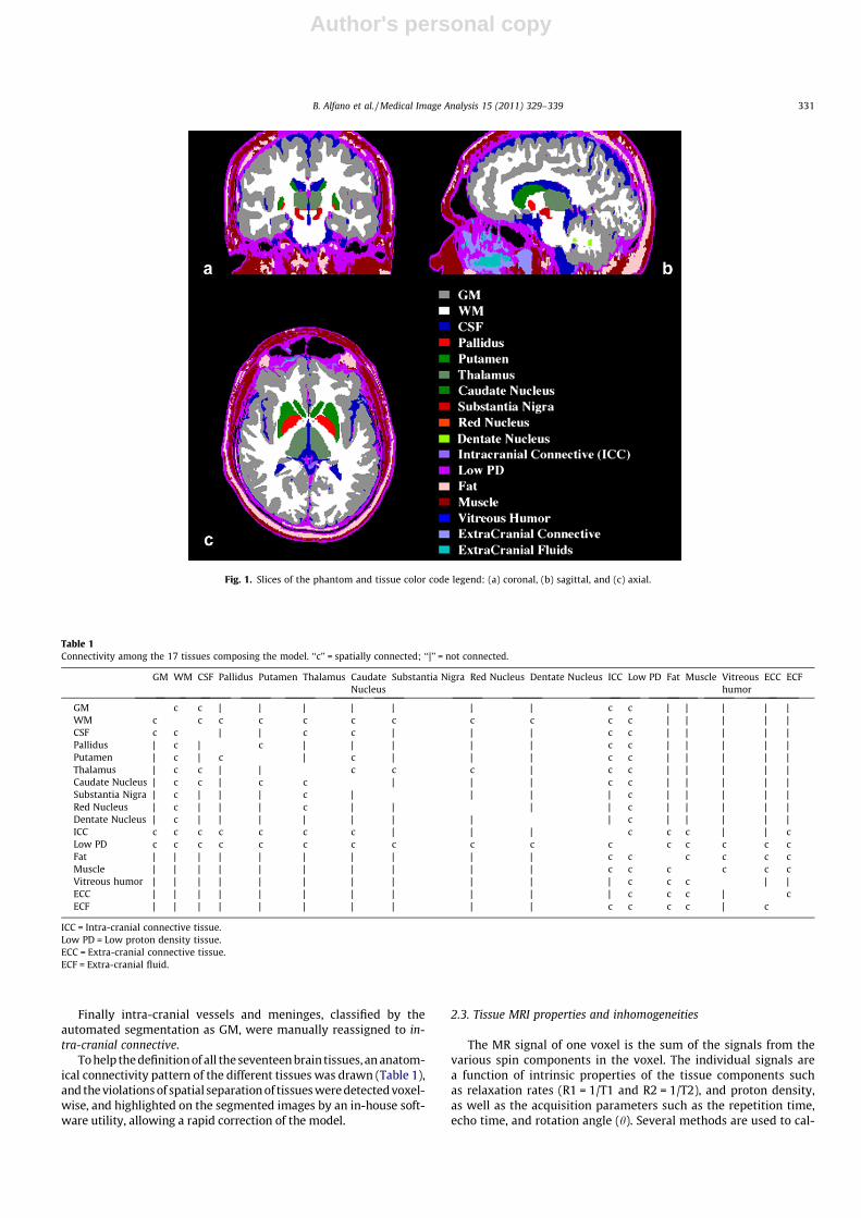
Similar to physical phantoms, the presented digital phantomconsists of a set of compartments representing the anatomical dis-tribution of different tissues. These compartments are filled withvirtual tissues solutions simulating the tissue characteristics as de-tected by the scanner. In contrast to a physical phantom, the vir-tual tissues are inhomogeneous to simulate the variability of thenormal and pathological tissues in terms of their principal mag-netic resonance characteristics of relaxation times and proton den-sity. The compartments and virtual tissues constitute the 3Danatomical model (phantom), which provides the basis of theMRI simulation.

The phantom (Fig. 1), was built starting from an MRI study of anormal volunteer preliminarily segmented using a multi-paramet-ric method based on a relaxometric approach (Alfano et al., 1997).Subsequently, both manual and semi-automated editing proce-dures were carried out to enhance the quality of the anatomicalmodel using both commercial (Photoshop, Adobe Systems, Inc.)and in-house (IDL, Research Systems, Inc. and Matlab, The Math-Works, Inc.) software. Additionally, a separate optional set of MSlesions is provided. The MRI simulation procedure allows to definethe position of the phantom in the field of view and a large series ofacquisition parameters which can be either manually imposed orautomatically extracted from a real MRI study (target study).

2.1. Model acquisition

MRI images were acquired on a 1.5T scanner (Marconi MedicalSystems, Cleveland, United States), using a quadrature head birdcagecoil from a 38 years old male normal volunteer. The MRI data con-sisted of 150 axial slices, obtained from five acquisition groups cover-ing the entire brain. Each group consists of 30 interleaved slices, 3 mmthickness, and is shifted of 1 mm down from the previous one. Thechoice of the slice thickness being 3 mm is due to the limitation ofthe two-dimensional (2D) CSE acquisition, which was used to calcu-late the relaxation rates. Each of the 5 sets included two conventionalspin-echo sequences providing T1weigthed (958/15 ms TR/TE) andproton density-T2 weighted (PD-T2w) (3446/15–90 ms TR/TE) axialslices with an in-plane resolution of 0.9375 � 0.9375 mm(256 � 256 acquisition matrix). The five groups of 30 T1w, T2w, andPDw images covering a total sampled volume of 24 � 19� 15.5 cm,were co-registered, re-sliced at 1 mm, and averaged, to obtain a lownoise, near-isotropic voxel (0.9375� 0.9375� 1 mm3) data set. De-spite 1 mm sampling along the caudal–cranial direction (z-axis), wehave chosen this reconstruction strategy which causes a full widthhalf maximum (FWHM) of about 5.8 mm along z-axis to reduce thenoise by a factor greater than 2.6.

2.2. Tissue compartment definition

By implementing a multi-parametric segmentation algorithm(Alfano et al., 1997), a preliminary distribution of eight tissues(GM, WM, CSF, globus pallidus, putamen, muscle, fat, and low pro-ton density tissues) was obtained. The segmentation was performedon the isotropic sampled data (�1 � 1 � 1 mm) with non isotropicresolution due to the thickness of the original slices. The 3D outputdata of the automated segmentation procedure was then verifiedand manually refined by some of the authors helped by two expertneurologists. Editing was performed using an in-house software(written using IDL) which allowed iterative modifications on trans-verse as well as on coronal and sagittal reformatted planes. Thethalamus, caudate nucleus, substantia nigra, red nucleus, and den-tate nucleus, which were typically classified by the automated seg-mentation algorithm as WM or GM, were also manually defined.All basal ganglia were refined to improve their shape with a Matlabscript, which performed a 5 mm FWHM smoothing of their binary3D masks, retaining for each structure the voxels with a valueabove 0.5 and assigning to WM voxels below 0.5, if they had notbeen previously manually assigned. The application order of thescript were: Putamen, Pallidus, Caudate Nucleus, Thalamus, Sub-stantia Nigra, Red Nucleus and Dentate Nucleus.

Extra-cranial connective and nasal mucosa, generally classifiedby the automated segmentation as extra-cranial GM-like tissues,were also reassigned manually to the correct classes.

The extra-cranial fluids (e.g. the thin CSF layer surrounding theoptic nerves, and vitreous humor) were reclassified manually sincethe automated segmentation could not distinguish between themand the intra-cranial CSF.

330 B. Alfano et al. / Medical Image Analysis 15 (2011) 329–339

Author's personal copy

Finally intra-cranial vessels and meninges, classified by theautomated segmentation as GM, were manually reassigned to in-tra-cranial connective.

To help the definition of all the seventeen brain tissues, an anatom-ical connectivity pattern of the different tissues was drawn (Table 1),and the violations of spatial separation of tissues were detected voxel-wise, and highlighted on the segmented images by an in-house soft-ware utility, allowing a rapid correction of the model.

2.3. Tissue MRI properties and inhomogeneities

The MR signal of one voxel is the sum of the signals from thevarious spin components in the voxel. The individual signals area function of intrinsic properties of the tissue components suchas relaxation rates (R1 = 1/T1 and R2 = 1/T2), and proton density,as well as the acquisition parameters such as the repetition time,echo time, and rotation angle (h). Several methods are used to cal-

Fig. 1. Slices of the phantom and tissue color code legend: (a) coronal, (b) sagittal, and (c) axial.

Table 1Connectivity among the 17 tissues composing the model. ‘‘c’’ = spatially connected; ‘‘|’’ = not connected.

GM WM CSF Pallidus Putamen Thalamus CaudateNucleus

Substantia Nigra Red Nucleus Dentate Nucleus ICC Low PD Fat Muscle Vitreoushumor

ECC ECF

GM c c | | | | | | | c c | | | | |WM c c c c c c c c c c c | | | | |CSF c c | | c c | | | c c | | | | |Pallidus | c | c | | | | | c c | | | | |Putamen | c | c | c | | | c c | | | | |Thalamus | c c | | c c c | c c | | | | |Caudate Nucleus | c c | c c | | | c c | | | | |Substantia Nigra | c | | | c | | | | c | | | | |Red Nucleus | c | | | c | | | | c | | | | |Dentate Nucleus | c | | | | | | | | c | | | | |ICC c c c c c c c | | | c c c | | cLow PD c c c c c c c c c c c c c c c cFat | | | | | | | | | | c c c c c cMuscle | | | | | | | | | | c c c c c cVitreous humor | | | | | | | | | | | c c c | |ECC | | | | | | | | | | | c c c | cECF | | | | | | | | | | c c c c | c

ICC = Intra-cranial connective tissue.Low PD = Low proton density tissue.ECC = Extra-cranial connective tissue.ECF = Extra-cranial fluid.

B. Alfano et al. / Medical Image Analysis 15 (2011) 329–339 331

Author's personal copy

culate the properties of the tissue components, each one having itsown pros and cons. These include the mono-exponential two-point(Alfano et al., 1997), multi-point (Fletcher et al., 1993), multi-expo-nential principal component analysis (Antalek et al., 1998; Windiget al., 1998), and inverse Laplace transform (Labadie et al., 1994)methods. We have adopted the mono-exponential two-pointmethod because it simulates the relaxation behavior reasonablywell, can be applied to routinely available pulse sequences, anduses a speed of image acquisition that results in minimal scan-to-scan displacements due to subject motion, thus requiring mini-mal post-registration.

The fine structure of all the tissues was determined in terms ofrelaxation rate and PD variability from the voxel values of the low-noise normal volunteer study (NVS). For each of the compartmentsdetailed in the previous section, the PD and relaxation rates werecalculated voxel-wise from the PD, T1- and T2-weighted imagesusing a mono-exponential two-point method described elsewhere(Alfano et al., 1995), obtaining PD, R1 and R2 mean values anddeviations.

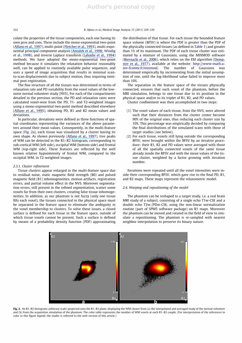
In particular, deviations were defined as three functions of spa-tial coordinates representing the variances of the above parame-ters around their mean values. Consequently, in the multi-featurespace (Fig. 2a), each tissue was visualized by a cluster having itsown shape. As shown previously (Alfano et al., 1997), tree peaksof WM can be detected in the R1–R2 histogram, corresponding tosub-cortical WM (left side), occipital WM (bottom side) and frontalWM (top-right side). These features are reflected by the wellknown relative hypointensity of frontal WM, compared to theoccipital WM, in T2-weighted images.

2.3.1. Cluster refinementTissue clusters appear enlarged in the multi-feature space due

to residual noise, static magnetic field strength (B0) and pulsedmagnetic field (B1) inhomogeneities, motion artifacts, registrationerrors, and partial volume effect in the NVS. Moreover segmenta-tion errors, still present in the refined segmentation, scatter somevoxels far from their own clusters, creating false tissue inhomoge-neities. In addition, as our phantom is not fuzzy (only one tissuefills each voxel), the tissues connected in the physical space mustbe separated in the feature space to eliminate the ambiguity inthe voxel membership to clusters. To solve these issues, a closedsurface is defined for each tissue in the feature space, outside ofwhich tissue voxels cannot be present. Such a surface is definedby means of a probability density function (PDF) approximating

the distribution of that tissue. For each tissue the bounded featurespace volume (BFSV) is where the PDF is greater than the PDF ofthe physically connected tissues (as defined in Table 1) and greaterthan 1% of its maximum. The PDF of each tissue cluster was esti-mated by a mixture of Gaussians, using the MIXMOD software(Biernacki et al., 2006), which relies on the EM algorithm (Demp-ster et al., 1977), available at the website: http://www-math.u-niv-fcomte.fr/mixmod/. The number of Gaussians wasdetermined empirically by incrementing from the initial assump-tion of one, until the log-likelihood value failed to improve morethan 10%.

The separation in the feature space of the tissues physicallyconnected, ensures that each voxel of the phantom, before theMRI simulation, belongs to one tissue due to its position in thephysical space and/or to its triplet of R1, R2, and PD values.

Cluster confinement was then accomplished in two steps:

(1) The voxel values of each tissue, from the NVS, were alteredsuch that their distances from the cluster center become90% of the original ones, thus reducing each cluster size by10%. This percentage was empirically decided by comparingthe final distributions of the simulated scans with those oftarget studies (see below).

(2) For each tissue, voxels still lying outside the correspondingBFSV, were brought within the BFSV by an iterative proce-dure: their R1, R2 and PD values were averaged with thoseof all the spatially connected voxels of the same tissuealready inside the BFSV and with the mean values of the tis-sue cluster, weighted by a factor growing with iterationnumber.

Iterations were repeated until all the voxel intensities were in-side their corresponding BFSV, which gave rise to the final PD, R1,and R2 maps. These maps represent the relaxometric model.

2.4. Warping and repositioning of the model

The phantom can be reshaped to a target study, i.e. a real brainMRI study of a subject, consisting of a single echo T1w-CSE and adouble echo T2w-/PDw-CSE, using the non-linear normalizationroutine (part of SPM5 software package) on R1 maps. Moreoverthe phantom can be moved and rotated in the field of view to sim-ulate a repositioning. The phantom is re-sampled with nearestneighbor interpolation to preserve its binary nature.

Fig. 2. An R1–R2 histogram (arbitrary scale) projected onto the R1–R2 plane, displaying the WM cluster from (a) the interpolated and averaged study of the normal volunteerand (b) from the acquisition simulation of the phantom. The color table represents the number of WM voxels at each R1–R2 couple. (For interpretation of the references tocolor in this figure legend, the reader is referred to the web version of this article.)

332 B. Alfano et al. / Medical Image Analysis 15 (2011) 329–339

Author's personal copy

2.5. Procedure for simulating conventional spin-echo MRI acquisitions

The above-detailed tissue compartments and inhomogeneitiesconstitute the anatomical model of the phantom, which must befilled by the tissues with their mean values and then must undergothe MRI simulation process.

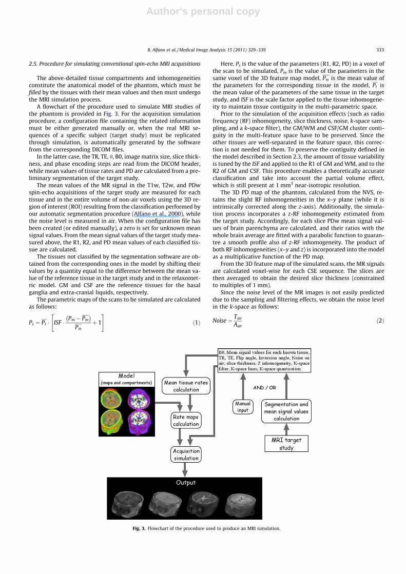
A flowchart of the procedure used to simulate MRI studies ofthe phantom is provided in Fig. 3. For the acquisition simulationprocedure, a configuration file containing the related informationmust be either generated manually or, when the real MRI se-quences of a specific subject (target study) must be replicatedthrough simulation, is automatically generated by the softwarefrom the corresponding DICOM files.

In the latter case, the TR, TE, h, B0, image matrix size, slice thick-ness, and phase encoding steps are read from the DICOM header,while mean values of tissue rates and PD are calculated from a pre-liminary segmentation of the target study.

The mean values of the MR signal in the T1w, T2w, and PDwspin-echo acquisitions of the target study are measured for eachtissue and in the entire volume of non-air voxels using the 3D re-gion of interest (ROI) resulting from the classification performed byour automatic segmentation procedure (Alfano et al., 2000), whilethe noise level is measured in air. When the configuration file hasbeen created (or edited manually), a zero is set for unknown meansignal values. From the mean signal values of the target study mea-sured above, the R1, R2, and PD mean values of each classified tis-sue are calculated.

The tissues not classified by the segmentation software are ob-tained from the corresponding ones in the model by shifting theirvalues by a quantity equal to the difference between the mean va-lue of the reference tissue in the target study and in the relaxomet-ric model. GM and CSF are the reference tissues for the basalganglia and extra-cranial liquids, respectively.

The parametric maps of the scans to be simulated are calculatedas follows:

Ps ¼ Pt � ISF �Pm � Pm� �

Pmþ 1

" #ð1Þ

Here, Ps is the value of the parameters (R1, R2, PD) in a voxel ofthe scan to be simulated, Pm is the value of the parameters in thesame voxel of the 3D feature map model, Pm is the mean value ofthe parameters for the corresponding tissue in the model, Pt isthe mean value of the parameters of the same tissue in the targetstudy, and ISF is the scale factor applied to the tissue inhomogene-ity to maintain tissue contiguity in the multi-parametric space.

Prior to the simulation of the acquisition effects (such as radiofrequency (RF) inhomogeneity, slice thickness, noise, k-space sam-pling, and a k-space filter), the GM/WM and CSF/GM cluster conti-guity in the multi-feature space have to be preserved. Since theother tissues are well-separated in the feature space, this correc-tion is not needed for them. To preserve the contiguity defined inthe model described in Section 2.3, the amount of tissue variabilityis tuned by the ISF and applied to the R1 of GM and WM, and to theR2 of GM and CSF. This procedure enables a theoretically accurateclassification and take into account the partial volume effect,which is still present at 1 mm3 near-isotropic resolution.

The 3D PD map of the phantom, calculated from the NVS, re-tains the slight RF inhomogeneities in the x–y plane (while it isintrinsically corrected along the z-axis). Additionally, the simula-tion process incorporates a z-RF inhomogeneity estimated fromthe target study. Accordingly, for each slice PDw mean signal val-ues of brain parenchyma are calculated, and their ratios with thewhole brain average are fitted with a parabolic function to guaran-tee a smooth profile also of z-RF inhomogeneity. The product ofboth RF inhomogeneities (x–y and z) is incorporated into the modelas a multiplicative function of the PD map.

From the 3D feature map of the simulated scans, the MR signalsare calculated voxel-wise for each CSE sequence. The slices arethen averaged to obtain the desired slice thickness (constrainedto multiples of 1 mm).

Since the noise level of the MR images is not easily predicteddue to the sampling and filtering effects, we obtain the noise levelin the k-space as follows:

Noise ¼ Tair

Aairð2Þ

Fig. 3. Flowchart of the procedure used to produce an MRI simulation.

B. Alfano et al. / Medical Image Analysis 15 (2011) 329–339 333

Author's personal copy

Tair is the mean value of the signal in air in the target study. Aair

is the mean value of the signal in air after synthesizing the noise-only images, having unit variance in the k-space, both for the realand imaginary part. The noise-only image is the simulation of anempty acquisition with unit variance, complex Gaussian noise.After quantization and filtering, the absolute value of the noise-only images is calculated to yield a Rician noise image. This simu-lation estimates the variance of the complex noise in the k-space toobtain the same mean signal value in air as that of the target study,using (2).

A filter is usually applied by most scanner software to k-spaceMR data to reduce noise and/or enhance detail. Different equationsare reported for different scanners (Lowe and Sorenson, 1997),with a pass-band behavior. For the purpose of our simulation,the filter is approximated by a simple pass-band function whit alinear rising term multiplied by a negative exponential term. A firstsimulation without the filter is generated, followed by slice averag-ing, and calculation of its one-dimensional frequency spectrum(FS). The FS was constructed by assuming radial symmetry span-ning 360� (i.e., averaging along a radius centered at the DC coeffi-cient). The same FS calculation procedure is repeated for the targetstudy. The ratio between the two FS values is fitted by the follow-ing function representing the above filter shape in the k-spacedomain:

f ðmÞ ¼ ðaþ b � mÞ � e�ðm=cÞd ð3Þ

where m is the frequency, a is determined by the ratio of signal inte-grals, b is the rising coefficient, c modulates the filter width, and d isthe filter order.

The parameters are stored in the configuration file. Finally, forthe fast Fourier transform (FFT) of each slice in a series, complexpseudo-random Gaussian noise with a standard deviation definedin (2) and a user-defined seed is added. Subsequently, k-space sam-pling and k-space filtering is performed, and the magnitude of theinverse FFT is calculated. An example of the WM cluster from asimulation is illustrated by the multi-feature space in Fig. 2b.

2.6. Multiple sclerosis simulation

To allow for multiple sclerosis (MS) studies simulation, a newmodel with MS lesions was produced by inserting a set of MS le-sions into the original model, as an additional brain compartment(abnormal white matter – AWM).

To construct the anatomical MS model, an MS patient study waspreliminarily segmented using a modification (Alfano et al., 2000)of the software used for the segmentation of the NVS describedabove, providing automated definition of the MS lesions, whichwere verified and manually refined. The brain parenchyma(GM + WM) of the patient, generated by the segmentation method,was spatially warped to the parenchyma of the normal phantommodel, using the non-linear normalization routine (part of the Sta-tistical Parametric Mapping - SPM5 software package – Fristonet al., 1995) on smoothed PDw images (8 mm FWHM) with20 mm cutoff, 32 non-linear iterations and light regularization.The resulting normalization parameters were used with the near-est neighbor interpolation to re-slice the relaxation rate maps ofthe segmented AWM of the patient. The warped AWM was thenmasked with the WM of the model, before its insertion into theWM compartment. To fill up the lesion (l) compartment, the voxelsin the relaxation rate maps of the MS model were obtained fromthe corresponding voxels of the warped patient lesions, with thefollowing linear transformation:

Pml ¼ PmCSF þPpl � PpCSF� �

� PmWM � PmCSF� �

PpWM � PpCSF� � ; ð4Þ

where P is the parameter (R1, R2, or PD in turn), �P is its mean value,the subscript m refers to a voxel in the model, the subscript p refersto the corresponding voxel values in the patient.

To avoid an abrupt transition between the lesion and thesurrounding WM, the voxels at the border of the lesions were aver-aged with the corresponding voxels of the normal relaxometricmodel. Finally, the voxel values of lesions, WM, and CSF were con-fined to the feature space using the procedure described in Step 2of Section 2.3.

It should be noted that by this procedure relaxation rate valuesof normal–appearing tissues are also comparable to those found inMS patient studies, as are derived from a target study of an MSpatient.

2.7. Procedure for simulating T1w-fast field-echo MRI acquisitions

The 3D FFE acquisitions are frequently used for mono-paramet-ric segmentation. To simulate this type of sequences, an estimateof the R2�, which includes also contributions from inhomogeneitiesin the magnetic field, present only outside the normal brain, is alsoneeded to better simulate extra-cranial tissues.

To obtain a map of R2�, the same volunteer who was imaged toobtain the anatomical model, was imaged using two magnetiza-tion-prepared FFE sequences (196 echo-train-length with first fourechoes discarded, TR = 9.9 ms, flip angle = 10�, and TE1,2 = 2.2 and3.5 ms, respectively), on a Philips Achieva scanner. The acquiredvolume is 256 � 256 � 124 voxels of size 0.9375 � 0.9375 � 1.2mm3.

The two sequences were registered to the R1 map of the modelwith an affine registration (SPM5 – J., Ashburner et al., 1997) totake in account also possible differences in gradient calibrationand re-sliced at 256 � 256 � 150 voxels of size0.9375 � 0.9375 � 1 mm3. Registration results has been visuallyverified using chromatic superimposition of corresponding slices.From these two sequences R2� was calculated for the entire vol-ume. Since water and fat are in phase opposition at the echo time(2.2 ms) of the first sequence, the signal at the boundary of fatareas is lower compared to the estimated value based on the echotime. Accordingly, the R2� map voxel intensities were zeroedwhere the signal in the second sequence was more than in the firstone.

From the resulting very noisy R2� map we modeled a syntheticR2� map with a simple 3D function SR�2, which was constant insidethe brain and took into account the principal sources of the mag-netic field inhomogeneities present in extra-cranial tissues and atthe border of tissues. This function is defined as the Gaussian con-volution (FWHM = 2 mm) of a function Ki constant within each tis-sue and in the one-voxel-thick-layer at the edge of each tissue (allintra-cranial tissues were treated as a single tissue). The values Ki

were obtained using the Nelder–Mead optimization process, min-imizing the mean square differences between the synthetic mapand the calculated one. The simulation of the 3D T1w-FFE was per-formed using the following expression:

S¼ k �q � VSS �cosN a �e�N�TR=T1þXN

i¼1

cosi a � e�ði�1Þ�TR=T1�e�i�TR=T1� � !�����

�sina �e�TE=T2� �OPðf;TEÞ�� ð5Þ

where S is the voxel value; k is an arbitrary scale factor; q, R1, andR2� are from the corresponding maps; N is the number of pulses be-tween the inversion pulse and central echo of the k-space; andOP(f, TE) is the following function describing the loss of signal dueto water-fat dephasing:

OPðf; TÞ ¼ffiffiffiffiffiffiffiffiffiffiffiffiffiffiffiffiffiffiffiffiffiffiffiffiffiffiffiffiffiffiffiffiffiffiffiffiffiffiffiffiffiffiffiffiffiffiffiffiffiffiffiffiffiffiffiffiffiffiffiffiffiffiffiffiffiffiffiffiffiffiðf � sin bÞ2 þ ðð1� fÞ þ f � cos bÞ2

qð6Þ

334 B. Alfano et al. / Medical Image Analysis 15 (2011) 329–339

Author's personal copy

Here, f is the ratio between the fat-proton density and the(fat + water)-proton density, expressed as f = qf/(qf + qw); b is thedephasing angle, given by b = 3.5 � 10�6 � 2p�TE�Larmor frequency;and VSS is the steady-state value of magnetization along the z-axis,as follows:

VSS ¼�PN’

i¼1cosi a � ðe�ði�1Þ�TR=T1 � e�i�TR=T1Þ

1þ cosN0 a � e�N0 �TR=T1ð7Þ

where N0 is the echo-train-length, defined as the total number ofechoes including the discarded ones, plus one.

3. Results

3.1. Similarity between simulated and real data

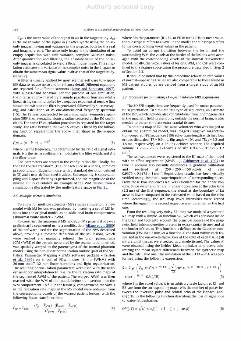
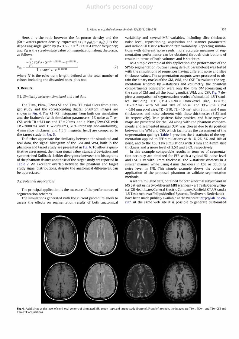
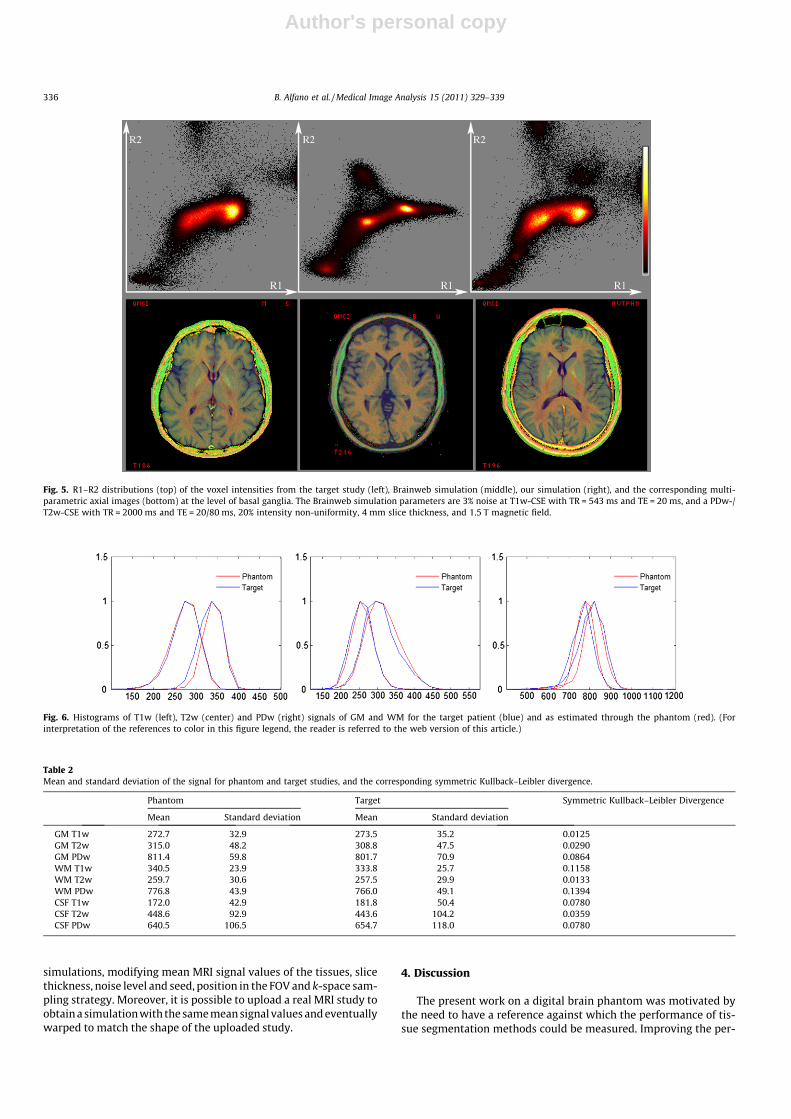
The T1w-, PDw-, T2w-CSE and T1w-FFE axial slices from a tar-get study and the corresponding digital phantom images areshown in Fig. 4. The R1–R2 histograms from both our simulationand the Brainweb (with simulation parameters: 3% noise at T1w-CSE with TR = 543 ms and TE = 20 ms, and a PDw-/T2w-CSE withTR = 2000 ms and TE = 20/80 ms, 20% intensity non-uniformity,4 mm slice thickness, and 1.5 T magnetic field) are compared tothe target study in Fig. 5.

To further appreciate the similarity between the simulated andreal data, the signal histogram of the GM and WM, both in thephantom and target study are presented in Fig. 6. To allow a quan-titative assessment, the mean signal value, standard deviation, andsymmetrized Kullback–Leibler divergence between the histogramsof the phantom tissues and those of the target study are reported inTable 2. An excellent overlap between the phantom and targetstudy signal distributions, despite the anatomical differences, canbe appreciated.

3.2. Potential applications

The principal application is the measure of the performances ofsegmentation schemes.

The simulations generated with the current procedure allow toassess the effects on segmentation results of both anatomical

variability and several MRI variables, including slice thickness,noise level, repositioning, acquisition and scanner parameters,and individual tissue relaxation rate variability. Repeating simula-tions with different noise seeds, more accurate measures of seg-mentation performance can be obtained through distributions ofresults in terms of both volumes and k-statistics.

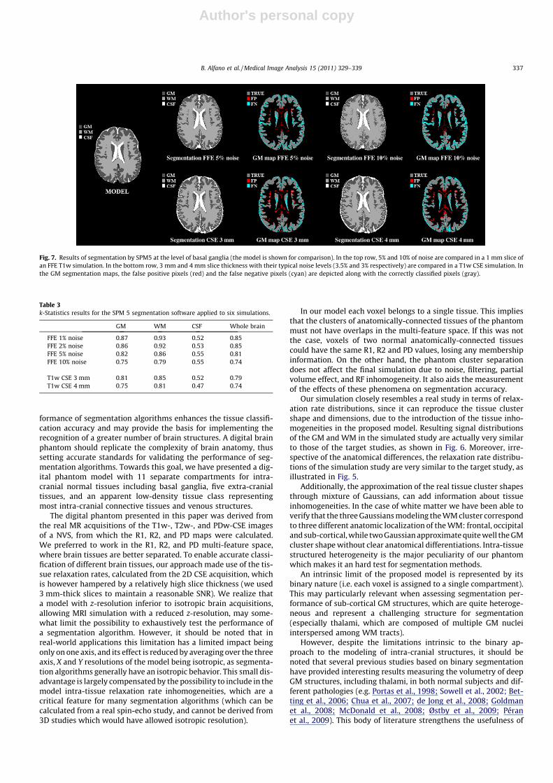
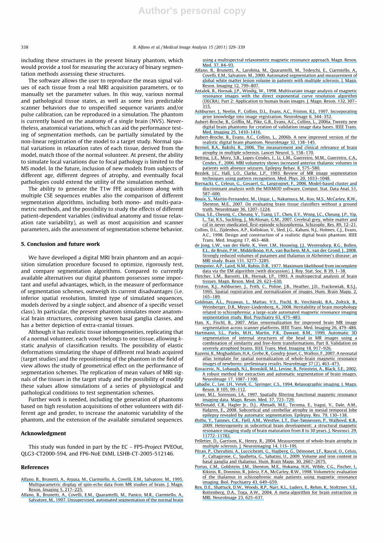
As a simple example of this application, the performance of theSPM5 segmentation routine (using default parameters) was testedwith the simulations of sequences having different noise and slicethickness values. The segmentation outputs were processed to ob-tain the binary masks of the GM, WM, and CSF. To evaluate the seg-mentation schemes by k-statistics and volumetry, the phantomcompartments considered were only the total GM (consisting ofthe sum of GM and all the basal ganglia), WM, and CSF. Fig. 7 de-picts a comparison of segmentation results of simulated 1.5 T stud-ies including FFE (0.94 � 0.94 � 1 mm voxel size, TR = 9.9,TE = 2.2 ms) with 5% and 10% of noise, and T1w CSE (0.94� 0.94 mm pixel size, TR = 510, TE = 15 ms) with 3 mm and 4 mmthicknesses, and noise coherent with these thicknesses (3.5% and3% respectively). True positive, false positive, and false negativemaps are presented for the GM along with the phantom compart-ments and segmented images (GM was chosen due to its positionbetween the WM and CSF, which facilitates the assessment of thesegmentation quality). Table 3 provides the k-statistics of the seg-mentation applied to FFE simulations with 1%, 2%, 5%, and 10% ofnoise, and to the CSE T1w simulations with 3 mm and 4 mm slicethickness and a noise level of 3.5% and 3.0%, respectively.

In this example comparable results in term so of segmenta-tion accuracy are obtained for FFE with a typical 5% noise leveland CSE T1w with 3 mm thickness. The k-statistic worsens in asimilar manner while using 4 mm thickness in CSE or doublingnoise level in FFE. This simple example shows the potentialapplication of the proposed phantom to validate segmentationmethods.

A set of simulated data, obtained for both a normal subject and anMS patient using two different MRI scanners – a 1 Tesla Genesys Sig-na (GE Healthcare, General Electric Company, Fairfield, CT, US) and a1.5 Tesla Achieva (Philips Medical Systems, Eindhoven, Nederland) –have been made publicly available at the web site: http://lab.ibb.cn-r.it/. At the same web site it is possible to generate customized

Fig. 4. Axial slices at the level of semi-oval centers of simulated MRI study (top) and target study (bottom). From left to right, the images are T1w-, PDw-, and T2w-CSE andT1w-FFE acquisitions.

B. Alfano et al. / Medical Image Analysis 15 (2011) 329–339 335

Author's personal copy

simulations, modifying mean MRI signal values of the tissues, slicethickness, noise level and seed, position in the FOV and k-space sam-pling strategy. Moreover, it is possible to upload a real MRI study toobtain a simulation with the same mean signal values and eventuallywarped to match the shape of the uploaded study.

4. Discussion

The present work on a digital brain phantom was motivated bythe need to have a reference against which the performance of tis-sue segmentation methods could be measured. Improving the per-

Fig. 5. R1–R2 distributions (top) of the voxel intensities from the target study (left), Brainweb simulation (middle), our simulation (right), and the corresponding multi-parametric axial images (bottom) at the level of basal ganglia. The Brainweb simulation parameters are 3% noise at T1w-CSE with TR = 543 ms and TE = 20 ms, and a PDw-/T2w-CSE with TR = 2000 ms and TE = 20/80 ms, 20% intensity non-uniformity, 4 mm slice thickness, and 1.5 T magnetic field.

Fig. 6. Histograms of T1w (left), T2w (center) and PDw (right) signals of GM and WM for the target patient (blue) and as estimated through the phantom (red). (Forinterpretation of the references to color in this figure legend, the reader is referred to the web version of this article.)

Table 2Mean and standard deviation of the signal for phantom and target studies, and the corresponding symmetric Kullback–Leibler divergence.

Phantom Target Symmetric Kullback–Leibler Divergence

Mean Standard deviation Mean Standard deviation

GM T1w 272.7 32.9 273.5 35.2 0.0125GM T2w 315.0 48.2 308.8 47.5 0.0290GM PDw 811.4 59.8 801.7 70.9 0.0864WM T1w 340.5 23.9 333.8 25.7 0.1158WM T2w 259.7 30.6 257.5 29.9 0.0133WM PDw 776.8 43.9 766.0 49.1 0.1394CSF T1w 172.0 42.9 181.8 50.4 0.0780CSF T2w 448.6 92.9 443.6 104.2 0.0359CSF PDw 640.5 106.5 654.7 118.0 0.0780

336 B. Alfano et al. / Medical Image Analysis 15 (2011) 329–339

Author's personal copy

formance of segmentation algorithms enhances the tissue classifi-cation accuracy and may provide the basis for implementing therecognition of a greater number of brain structures. A digital brainphantom should replicate the complexity of brain anatomy, thussetting accurate standards for validating the performance of seg-mentation algorithms. Towards this goal, we have presented a dig-ital phantom model with 11 separate compartments for intra-cranial normal tissues including basal ganglia, five extra-cranialtissues, and an apparent low-density tissue class representingmost intra-cranial connective tissues and venous structures.

The digital phantom presented in this paper was derived fromthe real MR acquisitions of the T1w-, T2w-, and PDw-CSE imagesof a NVS, from which the R1, R2, and PD maps were calculated.We preferred to work in the R1, R2, and PD multi-feature space,where brain tissues are better separated. To enable accurate classi-fication of different brain tissues, our approach made use of the tis-sue relaxation rates, calculated from the 2D CSE acquisition, whichis however hampered by a relatively high slice thickness (we used3 mm-thick slices to maintain a reasonable SNR). We realize thata model with z-resolution inferior to isotropic brain acquisitions,allowing MRI simulation with a reduced z-resolution, may some-what limit the possibility to exhaustively test the performance ofa segmentation algorithm. However, it should be noted that inreal-world applications this limitation has a limited impact beingonly on one axis, and its effect is reduced by averaging over the threeaxis, X and Y resolutions of the model being isotropic, as segmenta-tion algorithms generally have an isotropic behavior. This small dis-advantage is largely compensated by the possibility to include in themodel intra-tissue relaxation rate inhomogeneities, which are acritical feature for many segmentation algorithms (which can becalculated from a real spin-echo study, and cannot be derived from3D studies which would have allowed isotropic resolution).

In our model each voxel belongs to a single tissue. This impliesthat the clusters of anatomically-connected tissues of the phantommust not have overlaps in the multi-feature space. If this was notthe case, voxels of two normal anatomically-connected tissuescould have the same R1, R2 and PD values, losing any membershipinformation. On the other hand, the phantom cluster separationdoes not affect the final simulation due to noise, filtering, partialvolume effect, and RF inhomogeneity. It also aids the measurementof the effects of these phenomena on segmentation accuracy.

Our simulation closely resembles a real study in terms of relax-ation rate distributions, since it can reproduce the tissue clustershape and dimensions, due to the introduction of the tissue inho-mogeneities in the proposed model. Resulting signal distributionsof the GM and WM in the simulated study are actually very similarto those of the target studies, as shown in Fig. 6. Moreover, irre-spective of the anatomical differences, the relaxation rate distribu-tions of the simulation study are very similar to the target study, asillustrated in Fig. 5.

Additionally, the approximation of the real tissue cluster shapesthrough mixture of Gaussians, can add information about tissueinhomogeneities. In the case of white matter we have been able toverify that the three Gaussians modeling the WM cluster correspondto three different anatomic localization of the WM: frontal, occipitaland sub-cortical, while two Gaussian approximate quite well the GMcluster shape without clear anatomical differentiations. Intra-tissuestructured heterogeneity is the major peculiarity of our phantomwhich makes it an hard test for segmentation methods.

An intrinsic limit of the proposed model is represented by itsbinary nature (i.e. each voxel is assigned to a single compartment).This may particularly relevant when assessing segmentation per-formance of sub-cortical GM structures, which are quite heteroge-neous and represent a challenging structure for segmentation(especially thalami, which are composed of multiple GM nucleiinterspersed among WM tracts).

However, despite the limitations intrinsic to the binary ap-proach to the modeling of intra-cranial structures, it should benoted that several previous studies based on binary segmentationhave provided interesting results measuring the volumetry of deepGM structures, including thalami, in both normal subjects and dif-ferent pathologies (e.g. Portas et al., 1998; Sowell et al., 2002; Bet-ting et al., 2006; Chua et al., 2007; de Jong et al., 2008; Goldmanet al., 2008; McDonald et al., 2008; Østby et al., 2009; Péranet al., 2009). This body of literature strengthens the usefulness of

Fig. 7. Results of segmentation by SPM5 at the level of basal ganglia (the model is shown for comparison). In the top row, 5% and 10% of noise are compared in a 1 mm slice ofan FFE T1w simulation. In the bottom row, 3 mm and 4 mm slice thickness with their typical noise levels (3.5% and 3% respectively) are compared in a T1w CSE simulation. Inthe GM segmentation maps, the false positive pixels (red) and the false negative pixels (cyan) are depicted along with the correctly classified pixels (gray).

Table 3k-Statistics results for the SPM 5 segmentation software applied to six simulations.

GM WM CSF Whole brain

FFE 1% noise 0.87 0.93 0.52 0.85FFE 2% noise 0.86 0.92 0.53 0.85FFE 5% noise 0.82 0.86 0.55 0.81FFE 10% noise 0.75 0.79 0.55 0.74

T1w CSE 3 mm 0.81 0.85 0.52 0.79T1w CSE 4 mm 0.75 0.81 0.47 0.74

B. Alfano et al. / Medical Image Analysis 15 (2011) 329–339 337

Author's personal copy

including these structures in the present binary phantom, whichwould provide a tool for measuring the accuracy of binary segmen-tation methods assessing these structures.

The software allows the user to reproduce the mean signal val-ues of each tissue from a real MRI acquisition parameters, or tomanually set the parameter values. In this way, various normaland pathological tissue states, as well as some less predictablescanner behaviors due to unspecified sequence variants and/orpulse calibration, can be reproduced in a simulation. The phantomis currently based on the anatomy of a single brain (NVS). Never-theless, anatomical variations, which can aid the performance test-ing of segmentation methods, can be partially simulated by thenon-linear registration of the model to a target study. Normal spa-tial variations in relaxation rates of each tissue, derived from themodel, match those of the normal volunteer. At present, the abilityto simulate local variations due to focal pathology is limited to theMS model. In the future, inclusion of new models from subjects ofdifferent age, different degrees of atrophy, and eventually focalpathologies could extend the utility of the simulation method.

The ability to generate the T1w FFE acquisitions along withmultiple CSE sequences enables also the comparison of differentsegmentation algorithms, including both mono- and multi-para-metric methods, and the possibility to study the effects of differentpatient-dependent variables (individual anatomy and tissue relax-ation rate variability), as well as most acquisition and scannerparameters, aids the assessment of segmentation scheme behavior.

5. Conclusion and future work

We have developed a digital MRI brain phantom and an acqui-sition simulation procedure focused to optimize, rigorously test,and compare segmentation algorithms. Compared to currentlyavailable alternatives our digital phantom possesses some impor-tant and useful advantages, which, in the measure of performanceof segmentation schemes, outweigh its current disadvantages (i.e.inferior spatial resolution, limited type of simulated sequences,models derived by a single subject, and absence of a specific vesselclass). In particular, the present phantom simulates more anatom-ical brain structures, comprising seven basal ganglia classes, andhas a better depiction of extra-cranial tissues.

Although it has realistic tissue inhomogeneities, replicating thatof a normal volunteer, each voxel belongs to one tissue, allowing k-static analysis of classification results. The possibility of elasticdeformations simulating the shape of different real heads acquired(target studies) and the repositioning of the phantom in the field ofview allows the study of geometrical effect on the performance ofsegmentation schemes. The replication of mean values of MRI sig-nals of the tissues in the target study and the possibility of modifythese values allow simulations of a series of physiological andpathological conditions to test segmentation schemes.

Further work is needed, including the generation of phantomsbased on high resolution acquisitions of other volunteers with dif-ferent age and gender, to increase the anatomic variability of thephantom, and the extension of the available simulated sequences.

Acknowledgment

This study was funded in part by the EC – FP5-Project PVEOut,QLG3-CT2000-594, and FP6-NoE DiMI, LSHB-CT-2005-512146.

References

Alfano, B., Brunetti, A., Arpaia, M., Ciarmiello, A., Covelli, E.M., Salvatore, M., 1995.Multiparametric display of spin-echo data from MR studies of brain. J. Magn.Reson. Imaging 5, 217–225.

Alfano, B., Brunetti, A., Covelli, E.M., Quarantelli, M., Panico, M.R., Ciarmiello, A.,Salvatore, M., 1997. Unsupervised, automated segmentation of the normal brain

using a multispectral relaxometric magnetic resonance approach. Magn. Reson.Med. 37, 84–93.

Alfano, B., Brunetti, A., Larobina, M., Quarantelli, M., Tedeschi, E., Ciarmiello, A.,Covelli, E.M., Salvatore, M., 2000. Automated segmentation and measurement ofglobal white matter lesion volume in patients with multiple sclerosis. J. Magn.Reson. Imaging 12, 799–807.

Antalek, B., Hornak, J.P., Windig, W., 1998. Multivariate image analysis of magneticresonance images with the direct exponential curve resolution algorithm(DECRA). Part 2: Application to human brain images. J. Magn. Reson. 132, 307–315.

Ashburner, J., Neelin, P., Collins, D.L., Evans, A.C., Friston, K.J., 1997. Incorporatingprior knowledge into image registration. NeuroImage 6, 344–352.

Aubert-Broche, B., Griffin, M., Pike, G.B., Evans, A.C., Collins, L., 2006a. Twenty newdigital brain phantoms for creation of validation image data bases. IEEE Trans.Med. Imaging 25, 1410–1416.

Aubert-Broche, B., Evans, A.C., Collins, L., 2006b. A new improved version of therealistic digital brain phantom. NeuroImage 32, 138–145.

Bermel, R.A., Bakshi, R., 2006. The measurement and clinical relevance of brainatrophy in multiple sclerosis. Lancet Neurol. 5, 158–170.

Betting, L.E., Mory, S.B., Lopes-Cendes, I., Li, L.M., Guerreiro, M.M., Guerreiro, C.A.,Cendes, F., 2006. MRI volumetry shows increased anterior thalamic volumes inpatients with absence seizures. Epilepsy Behav. 8, 575–580.

Bezdek, J.C., Hall, L.O., Clarke, L.P., 1993. Review of MR image segmentationtechniques using pattern recognition. Med. Phys. 20, 1033–1048.

Biernacki, C., Celeux, G., Govaert, G., Langrognet, F., 2006. Model-based cluster anddiscriminant analysis with the MIXMOD software. Comput. Stat. Data Anal. 51,587–600.

Bouix, S., Martin-Fernandez, M., Ungar, L., Nakamura, M., Koo, M.S., McCarley, R.W.,Shenton, M.E., 2007. On evaluating brain tissue classifiers without a groundtruth. NeuroImage 36, 1207–1224.

Chua, S.E., Cheung, C., Cheung, V., Tsang, J.T., Chen, E.Y., Wong, J.C., Cheung, J.P., Yip,L., Tai, K.S., Suckling, J., McAlonan, G.M., 2007. Cerebral grey, white matter andcsf in never-medicated, first-episode schizophrenia. Schizophr. Res. 89, 12–21.

Collins, D.L., Zijdenbos, A.P., Kollokian, V., Sled, J.G., Kabani, N.J., Holmes, C.J., Evans,A.C., 1998. Design and construction of a realistic digital brain phantom. IEEETrans. Med. Imaging 17, 463–468.

de Jong, L.W., van der Hiele, K., Veer, I.M., Houwing, J.J., Westendorp, R.G., Bollen,E.L., de Bruin, P.W., Middelkoop, H.A., van Buchem, M.A., van der Grond, J., 2008.Strongly reduced volumes of putamen and thalamus in Alzheimer’s disease: anMRI study. Brain 131, 3277–3285.

Dempster, A.P., Laird, N.M., Rubin, D.B., 1977. Maximum likelihood from incompletedata via the EM algorithm (with discussion). J. Roy. Stat. Soc. B 39, 1–38.

Fletcher, L.M., Barsotti, J.B., Hornak, J.P., 1993. A multispectral analysis of braintissues. Magn. Reson. Med. 29, 623–630.

Friston, K.J., Ashburner, J., Frith, C., Poline, J.B., Heather, J.D., Frackowiak, R.S.J.,1995. Spatial registration and normalization of images. Hum. Brain Mapp. 2,165–189.

Goldman, A.L., Pezawas, L., Mattay, V.S., Fischl, B., Verchinski, B.A., Zoltick, B.,Weinberger, D.R., Meyer-Lindenberg, A., 2008. Heritability of brain morphologyrelated to schizophrenia: a large-scale automated magnetic resonance imagingsegmentation study. Biol. Psychiatry 63, 475–483.

Han, X., Fischl, B., 2007. Atlas renormalization for improved brain MR imagesegmentation across scanner platforms. IEEE Trans. Med. Imaging 26, 479–486.

Hartmann, S.L., Parks, M.H., Martin, P.R., Dawant, B.M., 1999. Automatic 3Dsegmentation of internal structures of the head in MR images using acombination of similarity and free-form transformations. Part II. Validation onseverely atrophied brains. IEEE Trans. Med. Imaging 18, 917–926.

Kazemi, K., Moghaddam, H.A., Grebe, R., Gondry-Jouet, C., Wallois, F., 2007. A neonatalatlas template for spatial normalization of whole-brain magnetic resonanceimages of newborns: preliminary results. NeuroImage 37 (2), 463–473.

Kovacevic, N., Lobaugh, N.J., Bronskill, M.J., Levine, B., Feinstein, A., Black, S.E., 2002.A robust method for extraction and automatic segmentation of brain images.NeuroImage 17, 1087–1100.

Labadie, C., Lee, J.H., Vetek, G., Springer, C.S., 1994. Relaxographic imaging. J. Magn.Reson. B 105, 99–112.

Lowe, M.J., Sorenson, J.A., 1997. Spatially filtering functional magnetic resonanceimaging data. Magn. Reson. Med. 37, 723–729.

McDonald, C.R., Hagler Jr., D.J., Ahmadi, M.E., Tecoma, E., Iragui, V., Dale, A.M.,Halgren, E., 2008. Subcortical and cerebellar atrophy in mesial temporal lobeepilepsy revealed by automatic segmentation. Epilepsy. Res. 79, 130–138.

Østby, Y., Tamnes, C.K., Fjell, A.M., Westlye, L.T., Due-Tønnessen, P., Walhovd, K.B.,2009. Heterogeneity in subcortical brain development: a structural magneticresonance imaging study of brain maturation from 8 to 30 years. J. Neurosci. 29,11772–11782.

Pelletier, D., Garrison, K., Henry, R., 2004. Measurement of whole-brain atrophy inmultiple sclerosis. J. Neuroimaging 14, 11S–19S.

Péran, P., Cherubini, A., Luccichenti, G., Hagberg, G., Démonet, J.F., Rascol, O., Celsis,P., Caltagirone, C., Spalletta, G., Sabatini, U., 2009. Volume and iron content inbasal ganglia and thalamus. Hum. Brain Mapp. 30, 2667–2675.

Portas, C.M., Goldstein, J.M., Shenton, M.E., Hokama, H.H., Wible, C.G., Fischer, I.,Kikinis, R., Donnino, R., Jolesz, F.A., McCarley, R.W., 1998. Volumetric evaluationof the thalamus in schizophrenic male patients using magnetic resonanceimaging. Biol. Psychiatry 43, 649–659.

Rex, D.E., Shattuck, D.W., Woods, R.P., Narr, K.L., Luders, E., Rehm, K., Stoltzner, S.E.,Rottenberg, D.A., Toga, A.W., 2004. A meta-algorithm for brain extraction inMRI. NeuroImage 23, 625–637.

338 B. Alfano et al. / Medical Image Analysis 15 (2011) 329–339

Author's personal copy

Rexilius, J., Hahn, H., Schlüter, M., Bourquain, H., Peitgen, H.O., 2005. Evaluation ofaccuracy in MS lesion volumetry using realistic lesion phantoms. Acad. Radiol.12, 17–24.

Sowell, E.R., Trauner, D.A., Gamst, A., Jernigan, T.L., 2002. Development of corticaland subcortical brain structures in childhood and adolescence: a structural MRIstudy. Dev. Med. Child Neurol. 44, 4–16.

Udupa, J.K., LeBlanc, V.R., Ying, Z.G., Imielinska, C., Schmidt, H., Currie, L.M., Hirsch,B.E., Woodburn, J., 2006. A framework for evaluating image segmentationalgorithms. Comput. Med. Imaging Graph 30, 75–87.

Wansapura, J.P., Holland, S.K., Dunn, R.S., Ball Jr., W.S., 1999. NMR relaxation timesin the human brain at 3.0 tesla. J. Magn. Reson. Imaging 9 (4), 531–538.

Warfield, S.K., Zou, K.H., Wells, W.M., 2008. Validation of image segmentation byestimating rater bias and variance. Philos. Trans. Roy. Soc. London Ser. A 366,2361–2375.

Wie, X., Warfield, S.K., Zou, K.H., Wu, Y., Li, X., Guimond, A., Mugler 3rd, J.P., Benson,R.R., Wolfson, L., Weiner, H.L., Guttmann, C.R., 2002. Quantitative analysis ofMRI signal abnormalities of brain white matter with high reproducibility andaccuracy. J. Magn. Reson. Imaging 15, 203–209.

Windig, W., Antalek, B., Hornak, J.P., 1998. Multivariate image analysis of magneticresonance images with the direct exponential curve resolution algorithm(DECRA). Part 1: Algorithm and model study. J. Magn. Reson. 32, 298–306.

B. Alfano et al. / Medical Image Analysis 15 (2011) 329–339 339