A hybrid Harmony Search algorithm to MRI brain segmentation

A Hybrid Harmony Search Algorithm to MRI BrainSegmentation

Osama Moh’d Alia, Rajeswari Mandava

CVRG - School of Computer Sciences,

University Sains Malaysia,

11800 USM, Penang, Malaysia

Email: sm [email protected], [email protected]

Mohd Ezane Aziz

Department of Radiology - Health Campus,

Universiti Sains Malaysia,

16150 K.K, Kelantan, Malaysia

[email protected]

Abstract—Automatic brain MRI image segmentation is achallenging problem and received significant attention in the fieldof medical image processing. In this paper, we present a newdynamic clustering algorithm based on the Harmony Search (HS)hybridized with Fuzzy C-means called DCHS to automaticallysegment the brain MRI image in an intelligent manner. Inthis algorithm, the capability of standard HS is modified toautomatically evolve the appropriate number of clusters as wellas the locations of cluster centers. By incorporating the conceptof variable length in each harmony memory vector, DCHS isable to encode variable numbers of candidate cluster centersat each iteration. Furthermore, a new HS operator, called the‘empty operator’ is introduced to support the selection of emptydecision variables in the harmony memory vector. The PBMFcluster validity index is used as an objective function to validatethe clustering result obtained from each harmony memory vector.The proposed algorithm is applied on several simulated T1-weighted normal and MS lesion magnetic resonance brain images.The experimental results show the ability of DCHS to find the ap-propriate number of naturally occurring regions in brain images.Furthermore, superiority of the proposed algorithm over differentclustering-based algorithms is demonstrated quantitatively. Allthe segmented results obtained by DCHS are also compared withthe available ground truth images.

Index Terms—Automatic Brain MRI segmentation, dynamicfuzzy clustering, harmony search, PBMF index

I. INTRODUCTION

The segmentation of Magnetic Resonance Imaging (MRI)

brain images is a fundamental process for medical research and

clinical applications such as quantification of tissue volume,

diagnose illnesses, aid in computer-guided surgery, treatment

planning, surgical simulation, therapy evaluation, functional

brain mapping, and also study of anatomical structure.

In general, the attractive tissues in brain are white matter

(WM), gray matter (GM), and cerebrospinal fluid (CSF).

Changes in these tissues even in the whole volume or within

specific regions can be used to characterize physiological

processes and disease entities or to characterize tumor tissues

(viable tumor, edema, and necrotic tissues).

Basically the MRI brain image segmentation is the task of

subdividing this image into constituent regions, in which each

region shares similar feature properties. In other words, it is

the process of specifying the tissue type for each pixel or voxel

in 2D or 3D data set based on information available from both

MRI images and the prior knowledge of brain. Actually, MRI

sequences such as T1-weighted (T1), T2-weighted (T2) and

the proton density (PD) can provide rich information about

brain tissues as can be seen in Fig. 1. This information appears

in a form of multispectral images, where each image can

provide different intensity information for a given anatomical

region and subject [1]. However, the process of automatically

segmenting the brain images is a complicated and challenging

task [2]. This complexity is inherited from the intrinsic nature

of the image. The brain image has a particularly complicated

structure and it always contains artifacts such as noise, partial

volume effect and intensity inhomogeneity [3]. This leads to

many different approaches for automatic brain image segmen-

tation [3], each of which uses different induction principles

such as classification-based methods [1], [4]–[12], region-

based methods [13]–[16], boundary-based methods [17]–[20],

and others [21]–[25]. For further information see [3], [26] and

references therein.

Among these algorithms, clustering-based approaches are

considered as one of the most popular [27], [28]. Clustering is a

very powerful technique whereby data is grouped together with

other data sharing particular similarities. It has many useful

characteristics which has made it one of the most popular

machine learning algorithms not only from the image seg-

mentation, but also for other fields such as machine learning,

artificial intelligence, pattern recognition, web mining, data

mining, biology, remote sensing, marketing, etc [29], [30].

During the last several decades, clustering algorithms have

proven to be very reliable, especially in categorization tasks

that call for semi or full automation [27], [31]. This is a

very promising fact as image segmentation also falls into such

categorization tasks.

In general, clustering is a typical unsupervised learning

technique used to group similar data points according to some

measurement of similarity. In image segmentation, clustering

algorithms consider the image pixels as data objects and

each pixel is assigned to a cluster (image region) based on

some feature similarity [32]. This measurement will seek to

minimize the inter-cluster similarity while maximizing the

intra-cluster similarity [29].

Clustering algorithms can generally be categorized into

two groups; hierarchical, and partitional [29]. The former

basically produces a nested series of partitions whereas the

Proc. 9th IEEE Int. Conf. on Cognitive Informatics (ICCI’10) F. Sun, Y. Wang, J. Lu, B. Zhang, W. Kinsner & L.A. Zadeh (Eds.) 978-1-4244-8040-1/10/$26.00 ©2010 IEEE

���

(a) (b)

(c)

Fig. 1. Simulated brain MRI image (slice 70) obtained from BrainWeb. (a)T1-Wieghted image. (b) T2-Wieghted image. (c) Proton Density image (PD).

latter does clustering with one partitioning result. According

to Jain et al [33] partitional clustering is more popular in

pattern recognition applications because it does not suffer from

drawbacks such as static-behavior (i.e. data points assigned to

a cluster cannot move to another cluster), and the probability

of failing to separate overlapping clusters, problems which are

prevalent in hierarchical clustering. Partitional clustering can

further be divided into two: 1) Crisp (or hard) clustering where

each data point belongs to only one cluster, and 2) Fuzzy or

Soft clustering where data points can simultaneously belong to

more than one cluster at the same time, based on some fuzzy

membership grade. Fuzzy is considered more appropriate than

crisp clustering for image datasets, as images exhibit unclear

boundaries between clusters or regions [27], [28], [31].

Partitional clustering algorithms however suffer from some

weakness such as: the proneness to get trapped in local optima

and the requirement of prior knowledge about the number of

clusters in dataset. A considerable amount of research effort

in the last few decades is reported in the literature to solve

the local optima problem, where the number of clusters is

known or set in advance by the user, as an optimization

problem such as [34]–[39]. While fewer efforts have been

reported to solve the second problem where finding the optimal

number of clusters is desired [40] such as Das and Konar [41]

proposed Deferential Evolution algorithm for fuzzy clustering

(AFDE), Saha and Bandyopadhyay proposed fuzzy variable

string length genetic point symmetry (Fuzzy-VGAPS) algo-

rithm [42], [43], Campello et al. proposed evolutionary-based

algorithm (EAC-FCM) [44], while the researchers in [45], [46]

used genetic algorithm as a clustering algorithm (FVGA). For

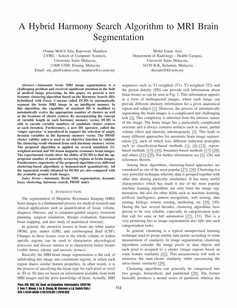
(a) (b)

Fig. 2. (a) original normal T1- brain image in z1 plane (b) segmented resultobtained by DCHS (6 clusters).

further information see [47]–[49] and references therein.

In this paper, we present a new approach called Dy-

namic fuzzy Clustering using the Harmony Search algorithm

(DCHS). This approach takes advantage of the search capa-

bilities of the metaheuristic Harmony Search (HS) algorithm

[50] to automatically determine the appropriate number of

clusters (without any prior knowledge), as well as the appro-

priate locations of cluster centers. A modification to the HS

is proposed in this study to tackle the two aforementioned

problems. The effectiveness of the proposed algorithm is

shown in segmenting a simulated MRI images of the normal

brain and MRI brain images with affected tissues by mul-

tiple sclerosis lesions obtained from BrainWeb [51]. DCHS

is used to automatically segment the brain images without

any determination of number of naturally occurring tissue

types. Then the segmentation results are compared with the

available ground truth information for validation purposes. A

comparison with other well known clustering-based algorithms

such as Fuzzy C-means algorithm (FCM) [52], Expectation

Maximization (EM) [53], and dynamic clustering-based fuzzy

variable string length genetic algorithm (FVGA) [45], [46] and

fuzzy variable string length genetic point symmetry (FVGAPS)

[42], [43], is conducted to show the superiority of our proposed

algorithm.

The rest of this paper is organized as follows. In Section

II, we present the fundamentals of fuzzy clustering with the

standard FCM clustering algorithm. Our proposed algorithm

DCHS is described in Section III. Experimental and compar-

ison results are presented in Section IV and we conclude this

paper in Section V.

II. FUNDAMENTALS OF FUZZY CLUSTERING

Clustering algorithm classically is performed on a set of

n patterns or objects X = {x1, x2, . . . , xn}, each of which,

xi ∈ �d, is a feature vector consisting of d real-valued

measurements describing the features of the object represented

by xi.

Two types of clustering algorithms are available hard and

fuzzy. In hard clustering, the goal would be to partition the data

set X into non-overlapping non-empty partitions G1, · · · , Gc.

While in fuzzy clustering algorithms the goal would be to

partition the data set X into partitions that allowed the data

��4

(a) (b)

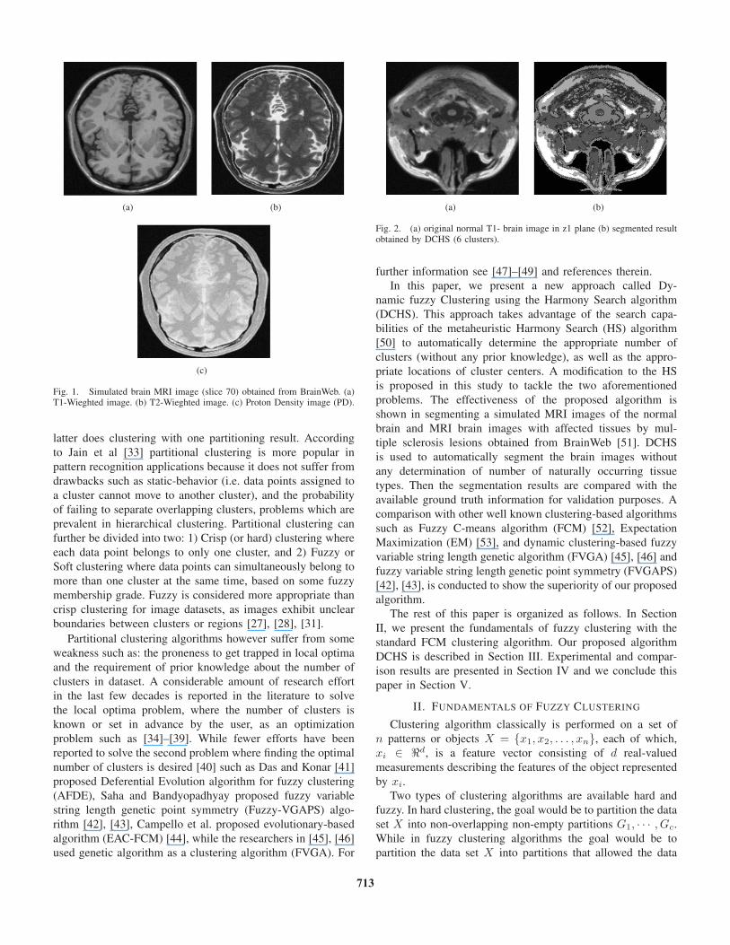
Fig. 3. (a) original normal T1- brain image in z36 plane (b) segmented resultobtained by DCHS (9 clusters).

object to belong in a particular (possibly null) degree to every

fuzzy cluster. The clustering output is a membership matrix

called a fuzzy partition matrix U = [uij ](c×n) as in Eq (1).

Where uij ∈ [0, 1] represents the fuzzy membership of the ithobject to the jth fuzzy cluster.

Mfcn ={

U ∈ �c×n|∑cj=1 Uij = 1, 0 <

∑ni=1 Uij < n

, and Uij ∈ [0, 1] ; 1 ≤ j ≤ c; 1 ≤ i ≤ n

}(1)

Fuzzy C-means algorithm (FCM) [52] is considered as one

of the most popular fuzzy partitioning algorithms. FCM is

an iterative procedure which is able to locally minimize the

following objective function:

Jm =c∑

j=1

n∑i=1

umij‖xi − vj‖2 (2)

where {vj}cj=1 are the centroids of the clusters c and ‖.‖

denotes an inner-product norm (e.g. Euclidean distance) from

the data point xi to the jth cluster center, and the parameter

m ∈ [1,∞), is a weighting exponent on each fuzzy member-

ship that determines the amount of fuzziness of the resulting

classification.

FCM algorithm starts with random initial c cluster centers,

and then at every iteration it finds the fuzzy membership of

each data point to every cluster using the following equation:

uij =1∑c

k=1

( ‖xi−vj‖‖xi−vk‖

) 2m−1

(3)

Based on the membership values, the cluster centers are

recomputed using the following equation:

vj =

∑ni=1 um

ij · xi∑ni=1 um

ij

(4)

The algorithm terminates when there is no further change in

the cluster centers.

III. HARMONY SEARCH-BASED FUZZY CLUSTERING -

DCHS ALGORITHM

Harmony Search is a relatively new stochastic metaheuristic

algorithm, which was developed by Geem et al. in 2001 [50]

and successfully applied to different optimization problems

(see [54] and references therein). It is a very successful

metaheuristic algorithm through its ability to exploit the new

suggested solution (harmony) synchronizing with exploring

the search space in both intensification and diversification

parallel optimization environment [55]. This algorithm imitates

the natural phenomenon of musicians’ behavior when they

cooperate the pitches of their instruments together to achieve

a fantastic harmony as measured by aesthetic standards. In the

following sections we describe a model of HS that represents

our proposed algorithm DCHS.

A. Initialization of DCHS Parameters

The DCHS algorithm parameters are same as the standard

HS parameters except the new operator ‘empty operator’ that

will be describing later. These parameters are:

1) Harmony Memory Size (HMS) (i.e. number of solution

vectors in harmony memory);

2) Harmony Memory Considering Rate (HMCR), where

HMCR ∈ [0, 1] ;

3) Pitch Adjusting Rate (PAR), where PAR ∈ [0, 1];4) Stopping Criteria (i.e. number of improvisation (NI));

5) Empty Operator Rate (EOR) ∈ [0, 1].

B. Initialization of Harmony Memory

Each harmony memory (HM) vector encodes the cluster

centers of the given data set. Since the number of these clusters

are unknown a priori, a possible range of number of clusters

that the given data set may possess is tested. Consequently,

each harmony memory vector can vary in length according to

the randomly generated number of clusters for each vector.

To initialize the HM with feasible solutions, each harmony

memory vector initially encodes a number of cluster centers,

denoted by ‘ClustNo’, such that:

clustNo = (rand() ×(clustMaxNo − clustMinNo))+ clustMinNo (5)

The number of clusters ‘clustNo’ is picked at random between

‘clustMinNo’ and ‘clustMaxNo’, where ‘clustMaxNo’ is an

estimate of the maximum number of clusters (upper bound),

while ‘clustMinNo’ is the minimum number of clusters (lower

bound). The values of upper and lower bounds are set depend-

ing on the data sets used.

Even though the vector length is allowed to vary, for a

matrix representation, each vector length in HM must be made

equal to the maximum number of clusters (‘clustMaxNo’).

Consequently, for d-dimensional space, the length of the vector

is (clustMaxNo × d), where the first d-locations correspond

to the first cluster center, the next d-locations correspond to

the second cluster centers and so forth.

In case of encoding a vector with a number of clusters less

than the ‘clustMaxNo’, the vector is occupied by these cluster

centers in random positions, while the remaining unused vector

elements (referred to as “ don’t care ” as in ( [45])) are

represented with ‘#’ sign. To illustrate the idea, let d = 2and clustMaxNo = 6, i.e. the feature space is 2-dimensional

and the maximum number of clusters is equal to 6. Now let

���

one of the HM vector has only 3-candidate cluster centers such

as: {(25.1, 13.2), (14, 6.3), (8.3, 3)}Then these 3 centers will be set in the vector in arbitrary

order while the rest of the vector’s elements are set to “don’t

care” with the ‘#’ sign as illustrated in Eq. (6)

HM = {25.1 13.2 # # # # 14 6.3 # # 8.3 3}(6)

The last step in harmony memory initialization process is to

calculate the fitness function for each harmony vector and

saved in harmony memory as explained in section (III-F).

C. Improvisation of a New Harmony Vector

In each iteration of HS, a new harmony vector is generated

based on the HS’s improvisation rules mentioned in [56]. These

rules are HM consideration; pitch adjustment; or random con-

sideration. In HM consideration, the value of the component

(i.e. decision variable) of the new vector is inherited from the

possible range of the harmony memory vectors stored in HM.

This is the case when a random number ∈ [0, 1] is within the

probability of HMCR; otherwise, the value of the component

of the new vector is selected from the possible data range with

a probability of (1-HMCR).

Furthermore, the new vector components which are selected

out of memory consideration operator are examined to be pitch

adjusted with the probability of (PAR). If it is, then the value

of this component becomes:

(aNEWi ) = (aNEW

i ) ± rand() ∗ bw (7)

here, bw is an arbitrary distance bandwidth used to im-

prove the performance of HS and its value is set to

bw=0.001*maxValue(n). The other important issue worth men-

tioning is when the inherited components of the new vector

have don’t care values ‘#’. In this case, no pitch adjustment

will take place.

D. Empty Operator

To further enhance the concept of variable-length of the

harmony memory vectors, a new HS operator called the ‘emptyoperator’ is proposed. This new operator is introduced mainly

to add the empty (don’t care) decision variables in the newly

generated harmony vector with a particular rate, namely Empty

Operator Rate (EOR) ∈ [0, 1]. The main rationale behind

the new operator is so that DCHS works in a more stable

manner. In other words, the new operator is introduced to

minimize the variation of the results (i.e. number of clusters)

that may obtained from DCHS in case of multiple runs. Where

the inconsistent results from multiple runs can be due to

the dominating effect of a number of solution vectors of the

HM through the improvisation process (premature convergence

problem). Therefore, the ability of generating of a new vector

with different number of cluster centers is very poor. For that,

the new operator is introduced to add a new method of having

empty ’don’t care’ decision variables in the newly generated

harmony vector. This is done in parallel with the normal way

(i.e. inherited from HM) of having the empty components in

the new vector.

The empty operator works as follows:

1) If the generated random number is within the probability

of HMCR, the value of the new decision variable is

randomly inherited from the historical values which are

stored in the HM.

2) Otherwise, if the generated random number is within

the probability of (1-HMCR), a new random number

between 0 and 1 is generated. If this random number

within the probability of EOR, then the new decision

variable is assigned a random number within the possible

data range. Otherwise, a don’t care (‘#’) value is assigned

to the new decision variable.

Furthermore, If the value of this rate is too low, only a

few random values from the visible data range are selected

and it may converge too slowly. If this rate is extremely high

(approaching 1), the addition of don’t care elements into the

new harmony vector rarely happens which may lead to an

unstable clustering results. The value of this operator is indeed

subject to the givin data set. According to this added operator,

the DCHS algorithm still has the ability to generate a new

harmony vector with varying lengths of number of clusters,

even in the final stages of the DCHS algorithm search process.

In other words, this new operator increases the diversity of

don’t care components in DCHS.

E. Update the Harmony Memory

Once the new harmony vector is generated, a count is

done on the generated number of cluster centers in the new

vector. If it is less than the minimum number of cluster centers

(clustMinNo), the new vector will be rejected. Otherwise, the

new vector will be accepted and a fitness function is computed

using a cluster validity measurement described in Section

(III-F). Then, the new vector is compared with the worst

harmony memory solution in terms of the fitness function. If

it is better, the new vector is included in the harmony memory

and the worst harmony is excluded.

F. Evaluation of Solutions

The evaluation (fitness value) of each harmony memory

vector indicates the degree of goodness of the solution it

represents. In order to evaluate the goodness of each harmony

memory vector, the empty components that may appear in

the harmony vector is removed and the remaining components

which represent the cluster centers are used to cluster the given

dataset (e.g. image). DCHS performs clustering based on pixels

of an image in the gray-scale intensity space, where each data

point (e.g. pixel) in the given data set (image) is assigned to

one or more clusters (regions) with a membership grade. The

membership value for each data point is calculated based on

Eq.(3).

After that, the goodness of the clustering result (i.e. U

matrix) is measured using a cluster validity index. Therefore,

the validity index measurement is used as the fitness function

in this study. In this paper, a recently developed index, which

exhibits a good trade-off between efficacy and computational

concern, is used. This index is named PBMF-index which is

��C

the fuzzy version of PBM-index [57]. PBMF-index is defined

as follows:

PBMF (c) =(

1c× E1

Ec× Dc

)p

(8)

where c is the number of clusters. Here

Ec =c∑

j=1

n∑i=1

umij ‖xi − vj‖ (9)

and

Dc = maxi,l‖vi − vl‖ (10)

where the power p is used to control the contrast between the

different cluster configurations and it is set to be 2. E1 is a

constant term for a particular data set and it is used to avoid

the index value from approaching zero. The value of m , which

is the fuzziness weighting exponent, is experimentally set to

1. Dc measures the maximum separation between two clusters

over all possible pairs of clusters, while Ec measures the sum

of c within-cluster distances (i.e., compactness).

The main goal of PBMF-index is to maximize the inter-

cluster distances (separation) while minimizing the intra-

cluster distances (compactness). Hence, the maximization of

PBMF-index indicates accurate clustering results and conse-

quently, accurate number of clusters could be achieved.

G. Check the Stopping Criterion

This process is repeated until the maximum number of

iterations (NI) is reached. In the end, the best solution among

the maximum value of fitness function of each HM solution

vectors is selected to be the best solution vector.

H. Hybridization with FCM

A hybridizing step with FCM is introduced to increase the

quality of the DCHS clustering results. This step is introduced

to DCHS by calling the FCM algorithm just one time to fine

tuning the best solution that have been optimized by DCHS.

The solution vector with highest fitness value is selected from

harmony memory and considered as initial values for FCM’s

cluster centers. In this case, FCM through its mechanism

modifies the cluster centers values until the variance of the

clusters are minimum, thus yielding more compact clusters.

Consequently, the clustering results achieved by DCHS will

decrease the variation within each cluster members (intra-

cluster variation) and at a same time increase the variation

between clusters (inter-cluster variation).

IV. EXPERIMENTAL RESULTS AND DISCUSSION

A. Experiment Setting

The proposed DCHS clustering algorithm is used as an

image segmentation algorithm to automatically segment the

given image into naturally occurring regions. DCHS uses the

intensity value for each pixel as a feature space to perform

the segmentation. DCHS is applied to automatically segment

a set of simulated MRI images of the normal brain and

MRI brain images with multiple sclerosis lesions obtained

from BrainWeb [51]. The simulated MRI volumes provided

(a) (b)

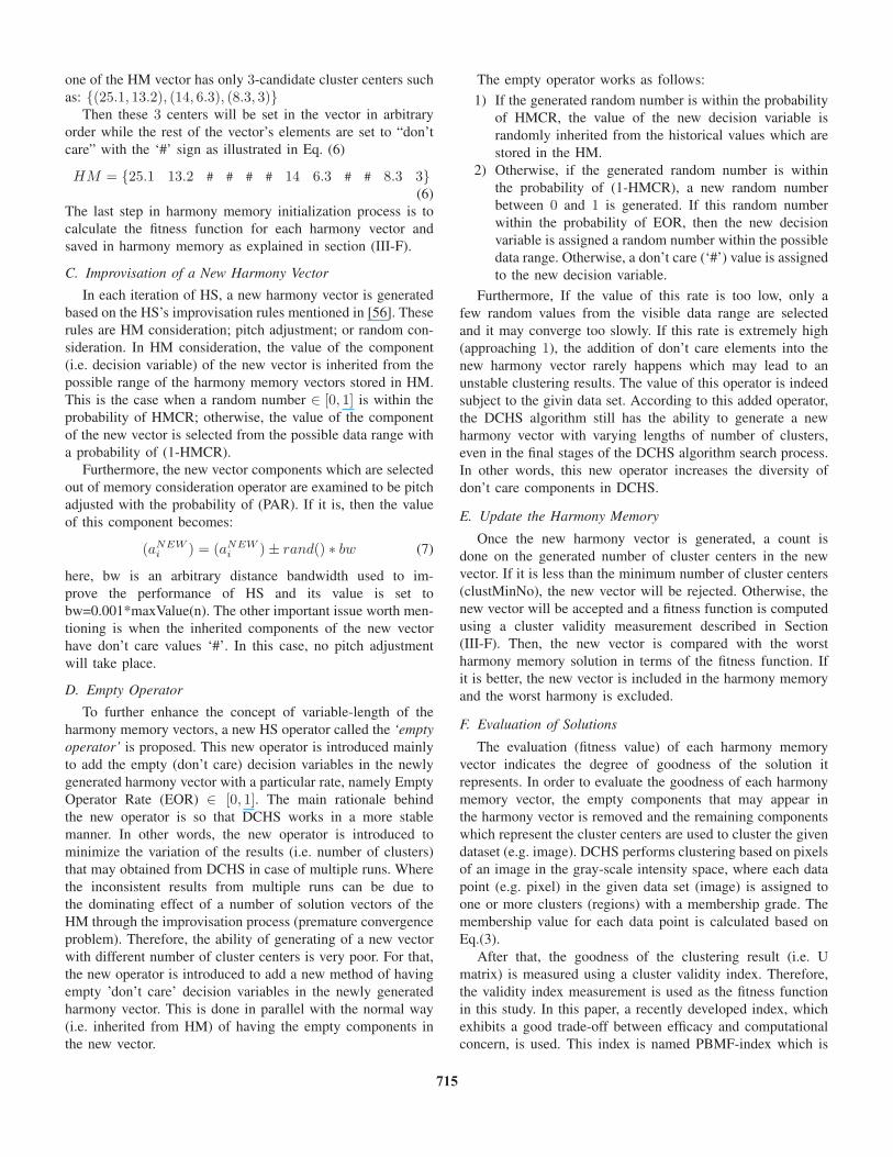
Fig. 4. (a) original normal T1- brain image in z72 plane (b) segmented resultobtained by DCHS (9 clusters).

by BrainWeb [51] are full 3D data volumes that have been

simulated using three sequences T1-weighted, T2-weighted,

and Proton Density (PD)-weighted with a variety of slice

thicknesses, noise levels, and levels of intensity non-uniformity

(intensity inhomogeneity) [51]. In this study, the experiments

were conducted only for some of T1-weighted images with

1 mm slice thickness, 3% noise and with 20% intensity non-

uniformity.

Each volume consists of 181 images with size 217 × 181for each. Each image in this volume may contain different

tissue types based on the axial location of the image in the

brain. In normal brain images, 10 classes of brain tissues

are presented where the number of classes varies along the

different z planes. These classes are Background, CSF, Grey

Matter, White Matter, Fat, Muscle/Skin, Skin, Skull, Glial

Matter and Connective tissues. While in multiple sclerosis

lesions brain images, 11 classes of brain tissues are presented

where the number of classes varies along the different z planes.

These classes are same as normal volumes except the MS

Lesion. It is worth mentioning here that some of these tissues

show same intensity level in MRI images such as background

and skull, WM and Connective tissues, CSF and skin.

Since the ground truth information is available and provided

by BrainWeb [51], a quantization index was used to evaluate

the performance of segmentation based on the accuracy of

the classification. The accuracy rate is calculated based on

the matching between the ground truth reference image and a

segmented image obtained from the proposed DCHS automatic

segmentation method. The quantization index used in this

study is Minkowski Score (MS) [58] that is calculated as

follows:

MS(T, S) =√

n01 + n10

n11 + n10(11)

Where T represents the partitioning matrix of the ground

truth image and S represents the partitioning matrix of the

segmented image. The n11 denotes the number of pairs of

elements that are in the same cluster in both S and T. The

n01 denotes the number of pairs that are in the same cluster

only in S, and the n10 denotes the number of pairs that are

in the same cluster in T. The minimum value of MS means

that the best matching between the ground truth image and the

��B

(a) (b)

Fig. 5. (a) original normal T1- brain image in z144 plane (b) segmentedresult obtained by DCHS (9 clusters).

segmented image is gained. The optimal value for MS is 0.

The parameters of the DCHS algorithm are experimen-

tally set as follows: HM size=30, HMCR=0.90, PAR=0.30,

EOR=0.85 and the maximum number of iteration NI=30000.

Furthermore, and based on the possible number of tissue

types that the brain images have, the minimum value for

the number of clusters (lower bound) is set to 2, while the

maximum number of clusters (upper bound) is set to 20. All

the experiments are performed on an Intel Core2Duo 2.66 GHz

machine, with 2GB of RAM; while the codes are written using

Matlab 2008a.

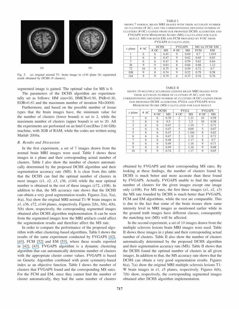
B. Results and Discussion

In the first experiment, a set of 7 images drawn from the

normal brain MRI images were used. Table I shows these

images in z plane and their corresponding actual number of

clusters. Table I also show the number of clusters automati-

cally determined by the proposed DCHS algorithm and their

segmentation accuracy rate (MS). It is clear from this table

that the DCHS can find the optimal number of clusters in

most images (z1, z2, z3, z36, z144) while the near optimal

number is obtained in the rest of these images (z72, z108). In

addition to that, the MS accuracy rate shows that the DCHS

can obtain a very good segmentation results. Figures 2(a), 3(a),

4(a), 5(a) show the original MRI normal T1-W brain images in

z1, z36, z72, z144 planes, respectively. Figures 2(b), 3(b), 4(b),

5(b) show, respectively, the corresponding segmented images

obtained after DCHS algorithm implementation. It can be seen

from the segmented images how the MRI artifacts could affect

the segmentation results and therefore affect the MS rate.

In order to compare the performance of the proposed algo-

rithm with other clustering-based algorithms, Table I shows the

results of the same experiment conducted by FVGAPS [42],

[43], FCM [52] and EM [53], where these results reported

in [42], [43]. FVGAPS algorithm is a dynamic clustering

algorithm that can automatically determine number of clusters

with the appropriate cluster center values. FVGAPS is based

on Genetic Algorithm combined with point symmetry-based

index as an objective function. Table I shows the number of

clusters that FVGAPS found and the corresponding MS rates.

For the FCM and EM, since they cannot find the number of

cluster automatically, they had the same number of clusters

TABLE ISHOWS 7 NORMAL BRAIN MRI IMAGES WITH THEIR ACCURATE NUMBER

OF CLUSTERS (# AC) AND THE CORRESPONDING OBTAINED NUMBER OF

CLUSTERS (# OC) GAINED FROM OUR PROPOSED DCHS ALGORITHM AND

FVGAPS WITH MINKOWSKI SCORE (MS) CALCULATED FOR EACH

RESULT. MS FOR BOTH EM AND FCM PROVIDED BY # OC FROM

FVGAPS IS CALCULATED.

z plane # ACDCHS FVGAPS MS for FCM/ EM

# OC MS # OC MS FCM EM1 6 6 0.45 9 0.69 0.7 1.0192 6 6 0.47 9 0.62 0.65 0.833 6 6 0.47 8 0.59 0.62 0.64

36 9 9 0.83 8 0.84 0.88 1.1272 10 9 0.75 8 0.59 0.72 0.7

108 9 8 0.74 9 0.52 0.79 0.58144 9 9 0.79 6 0.33 0.34 0.76

TABLE IISHOWS 10 MULTIPLE SCLEROSIS LESIONS BRAIN MRI IMAGES WITH

THEIR ACCURATE NUMBER OF CLUSTERS (# AC) AND THE

CORRESPONDING OBTAINED NUMBER OF CLUSTERS (# OC) GAINED FROM

OUR PROPOSED DCHS ALGORITHM, FVGA AND FVGAPS WITH

MINKOWSKI SCORE (MS) CALCULATED FOR EACH RESULT.

z plane # ACDCHS FVGA FVGAPS

# OC MS # OC MS # OC MS1 6 6 0.39 2 1.21 10 0.582 6 6 0.5 2 1.2 10 0.583 6 6 0.47 2 1.19 7 0.714 6 6 0.47 5 0.69 5 0.675 6 6 0.47 2 1.184 8 0.626 6 6 0.47 2 1.18 3 0.717 6 6 0.48 2 1.17 8 0.78 6 6 0.49 2 1.16 9 0.719 6 6 0.49 2 1.16 9 0.68

10 9 9 0.74 2 1.17 9 0.65

obtained by FVGAPS and their corresponding MS rates. By

looking at these findings, the number of clusters found by

DCHS is much better and more accurate than these found

by FVGAPS. Actually, FVGAPS unable to find the optimal

number of clusters for the given images except one image

only (z108). For MS rates, the first three images (z1, z2, z3)

the MS rate founded by DCHS is much better than FVGAPS,

FCM and EM algorithms, while the rest are comparable. This

is due to the fact that some of the brain tissues show same

intensity level in MRI images as mentioned earlier while in

the ground truth images have different classes, consequently

the matching test (MS) will be affected.

In the second experiment, a set of 10 images drawn from the

multiple sclerosis lesions brain MRI images were used. Table

II shows these images in z plane and their corresponding actual

number of clusters. Table II also show the number of clusters

automatically determined by the proposed DCHS algorithm

and their segmentation accuracy rate (MS). Table II shows that

the DCHS found the optimal number of clusters in all given

images. In addition to that, the MS accuracy rate shows that the

DCHS can obtain a very good segmentation results. Figures

6(a), 7(a) show the original MRI multiple sclerosis lesions T1-

W brain images in z1, z5 planes, respectively. Figures 6(b),

7(b) show, respectively, the corresponding segmented images

obtained after DCHS algorithm implementation.

���

(a) (b)

Fig. 6. (a) original multiple sclerosis lesions T1- brain image in z1 plane (b)segmented result obtained by DCHS (6 clusters).

In order to compare the performance of the proposed algo-

rithm with other dynamic clustering-based algorithms, Table

II shows the results of the same experiment conducted by

FVGAPS [42], [43] and FVGA [45], [46], where these results

reported in [42], [43]. FVGA algorithm also is a dynamic

clustering algorithm that can automatically determine number

of clusters with the appropriate cluster center values. FVGA

is based on Genetic Algorithm combined with XB index as

an objective function. Table II shows the number of clusters

that FVGAPS found and the corresponding MS rates. Also

the number of clusters found by FVGA for the given images

and their corresponding MS rates are shown in the same table.

By looking at these findings, the number of clusters found

by DCHS is much better and more accurate than these found

by FVGAPS and FVGA. FVGAPS unable to find the optimal

number of clusters for all given images except image z10 only.

While FVGA failed to find the optimal number of clusters

for all given images. The MS rates also show the superiority

of the proposed DCHS algorithm compared with the other

algorithms.

V. CONCLUSION

We have presented in this paper a novel dynamic clustering

algorithm called DCHS based on Harmony Search algorithm

hybridized with Fuzzy C-means algorithm. DCHS has the

ability to cluster the given data set automatically without any

prior knowledge of number of clusters that may the given

data set has. DCHS have been used as an image segmentation

algorithm to dynamically segment a simulated normal and

multiple sclerosis lesions brain MRI images.

The numbers of clusters found by DCHS for the brain im-

ages were the best among other dynamic clustering algorithms

(FVGAPS and FVGA). The accuracy rates of segmentation

results were the highest for multiple sclerosis lesions images

while comparable in the normal brain images.

Regarding the MRI artifacts such as noise and intensity non-

uniformity, the upcoming research will focus on how to im-

prove the segmentation results of DCHS algorithm and how to

incorporate the spatial information to reduce the effectiveness

of these artifacts. Furthermore, another study of how to reduce

the impact of the problem of non-similar brain tissue types

(a) (b)

Fig. 7. (a) original multiple sclerosis lesions T1- brain image in z5 plane (b)segmented result obtained by DCHS (6 clusters).

with similar intensity appearance will be also the upcoming

research interest.

ACKNOWLEDGMENT

The authors thank Dr. Dhanesh Ramachandram and Dr. Sri-

parna Saha for their comments regarding this manuscript. This

research is supported by Universiti Sains Malaysia, USM’s

fellowship scheme and ’Universiti Sains Malaysia Research

University Grant’ grant titled ’Delineation and visualization of

Tumour and Risk Structures - DVTRS’ under grant number

1001/PKOMP/817001.

REFERENCES

[1] W. Dou, S. Ruan, Y. Chen, D. Bloyet, and J.-M. Constans, “A frameworkof fuzzy information fusion for the segmentation of brain tumor tissueson mr images,” Image and Vision Computing, vol. 25, no. 2, pp. 164–171,2007.

[2] J. Wang, J. Kong, Y. Lu, M. Qi, and B. Zhang, “A modified fcmalgorithm for mri brain image segmentation using both local and non-local spatial constraints,” Computerized Medical Imaging and Graphics,vol. 32, no. 8, pp. 685–698, 2008.

[3] A. W.-C. Liew and H. Yan, “Current methods in the automatic tissuesegmentation of 3d magnetic resonance brain images,” Current medicalimaging reviews, vol. 2, pp. 91–103, 2006.

[4] I. Wells, W. M., W. E. L. Grimson, R. Kikinis, and F. A. Jolesz, “Adaptivesegmentation of mri data,” Medical Imaging, IEEE Transactions on,vol. 15, no. 4, pp. 429–442, 1996.

[5] T. Kapur, W. E. L. Grimson, W. M. Wells, and R. Kikinis, “Segmen-tation of brain tissue from magnetic resonance images,” Medical ImageAnalysis, vol. 1, no. 2, pp. 109–127, 1996.

[6] J. Zhou and J. C. Rajapakse, “Fuzzy approach to incorporate hemo-dynamic variability and contextual information for detection of brainactivation,” Neurocomputing, vol. 71, no. 16-18, pp. 3184–3192, 2008.

[7] L. Szilagyi, Z. Benyo, S. M. Szilagyi, and H. S. Adam, “Mr brainimage segmentation using an enhanced fuzzy c-means algorithm,” inProceedings of the 25th Annual International Conference of the IEEEEngineering in Medicine and Biology Society,, vol. 1, 2003, pp. 724–726.

[8] H. A. Mokbel, M. E.-S. Morsy, and F. E. Z. Abou-Chadi, “Automaticsegmentation and labeling of human brain tissue from mr images,” inSeventeenth National Radio Science Conference, 17th NRSC ’, 2000, pp.1–8.

[9] L. Xiaohe, Z. Taiyi, and Q. Zhan, “Image segmentation using fuzzyclustering with spatial constraints based on markov random field viabayesian theory,” IEICE Trans. Fundam. Electron. Commun. Comput.Sci., vol. E91-A, no. 3, pp. 723–729, 2008.

[10] K. Van Leemput, F. Maes, D. Vandermeulen, and P. Suetens, “Automatedmodel-based tissue classification of mr images of the brain,” IEEETransactions on Medical Imaging, vol. 18, no. 10, pp. 897–908, 1999.

[11] K. Van Leemput, F. Maes, D. Vandermeulen, and P. Suetens, “Automatedmodel-based bias field correction of mr images of the brain,” IEEETransactions on Medical Imaging, vol. 18, no. 10, pp. 885–896, 1999.

���

[12] J. C. Bezdek, L. O. Hall, and L. P. Clarke, “Review of mr imagesegmentation techniques using pattern recognition,” Medical Physics,vol. 20, no. 4, pp. 1033–1048, 1993.

[13] Y. L. Chang and X. Li, “Adaptive image region-growing,” IEEE Trans-actions on Image Processing, vol. 3, no. 6, pp. 868–872, 1994.

[14] R. Adams and L. Bischof, “Seeded region growing,” IEEE Transactionson pattern analysis and machine intelligence, vol. 16, no. 6, pp. 641–647,1994.

[15] R. Pohle and K. D. Toennies, “Segmentation of medical images usingadaptive region growing,” in Proceedings of SPIE (Medical Imaging),vol. 4322, San Diego, 2001, pp. 1337–1346.

[16] J. Sijbers, P. Scheunders, M. Verhoye, A. Van der Linden, D. van Dyck,and E. Raman, “Watershed-based segmentation of 3d mr data for volumequantization,” Magnetic Resonance Imaging, vol. 15, no. 6, pp. 679–688,1997.

[17] M. S. Atkins and B. T. Mackiewich, “Fully automatic segmentation ofthe brain in mri,” IEEE Transactions on Medical Imaging,, vol. 17, no. 1,pp. 98–107, 1998.

[18] M. Ashtari, J. L. Zito, B. I. Gold, J. A. Lieberman, M. T. Borenstein, andP. G. Herman, “Computerized volume measurement of brain structure,”Investigative Radiology, vol. 25, no. 7, pp. 798–805, 1990.

[19] L. Ji and H. Yan, “Attractable snakes based on the greedy algorithm forcontour extraction,” Pattern Recognition, vol. 35, no. 4, pp. 791–806,2002.

[20] T. McInerney and D. Terzopoulos, “Deformable models in medical imageanalysis: a survey,” Medical Image Analysis, vol. 1, no. 2, pp. 91–108,1996.

[21] Y. Zhou and J. Bai, “Atlas-based fuzzy connectedness segmentationand intensity nonuniformity correction applied to brain mri,” IEEETransactions on Biomedical Engineering,, vol. 54, no. 1, pp. 122–129,2007.

[22] M. C. Clark, “Knowledge-guided processing of magnetic resonanceimages of the brain,” Ph.D. dissertation, University of South Florida,Department of Computer Science and Engineering, South Florida USA,1998.

[23] M. Clark, L. Hall, D. Goldgof, and M. Silbiger, “Using fuzzy informationin knowledge guided segmentation of brain tumors,” in Fuzzy Logic inArtificial Intelligence Towards Intelligent Systems, 1997, pp. 167–181.

[24] M. Sonka, S. K. Tadikonda, and S. M. Collins, “Knowledge-basedinterpretation of mr brain images,” IEEE Transactions on MedicalImaging,, vol. 15, no. 4, pp. 443–452, 1996.

[25] S. Shen, W. Sandham, M. Granat, and A. Sterr, “Mri fuzzy seg-mentation of brain tissue using neighborhood attraction with neural-network optimization,” IEEE Transactions on Information Technologyin Biomedicine, vol. 9, no. 3, pp. 459–467, 2005.

[26] D. L. Pham, C. Xu, and J. L. Prince, “Current methods in medical imagesegmentation,” Annual Review of Biomedical Engineering, vol. 2, no. 1,pp. 315–337, 2000.

[27] P. Hore, L. O. Hall, D. B. Goldgof, Y. Gu, A. A. Maudsley, andA. Darkazanli, “A scalable framework for segmenting magnetic reso-nance images,” Journal of Signal Processing Systems, vol. 54, no. 1-3,pp. 183–203, 2008.

[28] J. Kang, L. Min, Q. Luan, X. Li, and J. Liu, “Novel modified fuzzy c-means algorithm with applications,” Digital Signal Processing, vol. 19,no. 2, pp. 309–319, 2009.

[29] A. K. Jain, M. N. Murty, and P. J. Flynn, “Data clustering: a review,”ACM Comput. Surv., vol. 31, no. 3, pp. 264–323, 1999.

[30] S. E. Brian, L. Sabine, and L. Morven. Wiley Publishing, 2009.[31] H. Zhou, “Fuzzy c-means and its applications in medical imaging,”

in Computational Intelligence in Medical Imaging: Techniques andApplications, 2009, p. 213.

[32] A. Rosenfeld and A. C. Kak, Digital Picture Processing. AcademicPress, Inc. New York, NY., 1982, vol. 2nd.

[33] A. K. Jain, R. P. W. Duin, and M. Jianchang, “Statistical patternrecognition: a review,” IEEE Transactions on Pattern Analysis andMachine Intelligence,, vol. 22, no. 1, pp. 4–37, 2000.

[34] O. M. Alia, R. Mandava, D. Ramachandram, and M. E. Aziz, “Harmonysearch- based cluster initialization for fuzzy c-means segmentation ofmr images.” in International Technical Conference of IEEE Region 10(TENCON), Singapore, 2009, pp. 1–6.

[35] O. M. Alia, R. Mandava, D. Ramachandram, and M. E. Aziz, “Anovel image segmentation algorithm based on harmony fuzzy searchalgorithm,” in International Conference of Soft Computing and PatternRecognition, SOCPAR ’09., Malacca, Malaysia, 2009, pp. 335–340.

[36] J. C. Bezdek and R. J. Hathaway, “Optimization of fuzzy clusteringcriteria using genetic algorithms,” in Proceedings of the First IEEEConference on Evolutionary Computation,IEEE World Congress onComputational Intelligence, vol. 2, Orlando, FL, USA, 1994, pp. 589–594.

[37] U. Maulik and I. Saha, “Modified differential evolution based fuzzyclustering for pixel classification in remote sensing imagery,” PatternRecognition, vol. 42, no. 9, pp. 2135–2149, 2009.

[38] P. M. Kanade and L. O. Hall, “Fuzzy ants and clustering,” IEEETransactions on Systems, Man and Cybernetics,Part A,, vol. 37, no. 5,pp. 758–769, 2007.

[39] K. S. Al-Sultan and C. A. Fedjki, “A tabu search-based algorithm forthe fuzzy clustering problem,” Pattern Recognition, vol. 30, no. 12, pp.2023–2030, 1997.

[40] S. Das, A. Abraham, and A. Konar, “Metaheuristic pattern clustering -an overview,” in Metaheuristic Clustering. Springer, 2009, pp. 1–62.

[41] S. Das and A. Konar, “Automatic image pixel clustering with animproved differential evolution,” Applied Soft Computing, vol. 9, no. 1,pp. 226–236, 2009.

[42] S. Saha and S. Bandyopadhyay, “A new point symmetry based fuzzygenetic clustering technique for automatic evolution of clusters,” Infor-mation Sciences, vol. 179, no. 19, pp. 3230–3246, 2009.

[43] S. Saha and S. Bandyopadhyay, “Mri brain image segmentation by fuzzysymmetry based genetic clustering technique,” in IEEE Congress onEvolutionary Computation, CEC, 2007, pp. 4417–4424.

[44] R. Campello, E. Hruschka, and V. Alves, “On the efficiency of evolution-ary fuzzy clustering,” Journal of Heuristics, vol. 15, no. 1, pp. 43–75,2009.

[45] M. K. Pakhira, S. Bandyopadhyay, and U. Maulik, “A study of somefuzzy cluster validity indices, genetic clustering and application to pixelclassification,” Fuzzy Sets and Systems, vol. 155, no. 2, pp. 191–214,2005.

[46] U. Maulik and S. Bandyopadhyay, “Fuzzy partitioning using a real-coded variable-length genetic algorithm for pixel classification,” IEEETransactions on Geoscience and Remote Sensing., vol. 41, no. 5, pp.1075–1081, 2003.

[47] E. R. Hruschka, R. J. G. B. Campello, A. A. Freitas, and A. C. P. L. F. d.Carvalho, “A survey of evolutionary algorithms for clustering,” IEEETransactions on Systems, Man and Cybernetics, Part C: Applicationsand Reviews, vol. 39, pp. 133–155, 2009.

[48] D. Horta, M. Naldi, R. Campello, E. Hruschka, and A. de Carvalho,“Evolutionary fuzzy clustering: An overview and efficiency issues,” inFoundations of Computational Intelligence, 2009, pp. 167–195.

[49] S. Das, A. Abraham, and A. Konar, Metaheuristic Clustering. SpringerVerlag, Germany, 2009.

[50] Z. W. Geem, J. H. Kim, and G. Loganathan, “A new heuristic opti-mization algorithm: harmony search.” SIMULATION, vol. 76, no. 2, pp.60–68, 2001.

[51] “Brain web: Simulated brain database. mcconnell brain imagingcentre. montreal neurological institute, mcgill university,http://www.bic.mni.mcgill.ca/brainweb.”

[52] J. C. Bezdek, Pattern Recognition with Fuzzy Objective Function Algo-rithms. Kluwer Academic Publishers, 1981.

[53] A. P. Dempster, N. M. Laird, and D. B. Rubin, “Maximum likelihoodfrom incomplete data via the em algorithm,” Journal of the RoyalStatistical Society. Series B (Methodological), vol. 39, no. 1, pp. 1–38,1977.

[54] G. Ingram and T. Zhang, in Music-Inspired Harmony Search Algorithm.Springer Berlin / Heidelberg, 2009, pp. 15–37.

[55] Z. W. Geem, Harmony Search Algorithms for Structural Design Opti-mization. Springer Berlin / Heidelberg, 2009.

[56] Z. W. Geem, C.-L. Tseng, and Y. Park, “Harmony search for generalizedorienteering problem: Best touring in china,” in Advances in NaturalComputation. Springer Berlin / Heidelberg, 2005, pp. 741–750.

[57] M. K. Pakhira, S. Bandyopadhyay, and U. Maulik, “Validity index forcrisp and fuzzy clusters,” Pattern Recognition, vol. 37, no. 3, pp. 487–501, 2004.

[58] A. Ben-Hur and I. Guyon, “Detecting stable clusters using principal com-ponent analysis,” Methods in Molecular Biology-Clifton then Totowa,vol. 224, pp. 159–182, 2003.

��

further investigation. Since our goal is to improve the AUC

metric of the evolved classifiers, we may use the AUC as

fitness directly. We refer to such a fitness function as fA.

In Li’s method [12], the cost-sensitive fitness function fCgiven in Equation 6 is chosen:

fC = w1 ∗ Accuracy− w2 ∗RF − w3 ∗RMC (6)

w1, w2 and w3 are the weights of the metrics. Since our

target is to find the classifier with the maximum AUC, we

may instead take the AUC measure as fitness function. On

the other hand, we wish to explore the use of the entropy

similar to C4.5, since it has a positive correlation with AUC

but is much easier to compute.

H(X) = −n∑

i=0

p(xi) log2 p(xi) (7)

Equation 7 gives the definition of the information gain [23]

for a random variable X with n outcomes {xi : i = 1....n}.The Shannon entropy, a measure of uncertainty is denoted

by H(X) and p(xi) is the probability mass function of the

outcomes xi.

pi =Pi

1∑j=0

Pj

(8)

fE =

NL∑k=0

(1 +

1∑i=0

pi log2 pi

)(1∑

j=0

(Pj − 1)

)

Ntr −NL(9)

We can easily introduce a fitness function very similar

to Shannon’s formula as given in Equation 9.It’s a novel

decision tree structure. In a decision tree T as used in our

EDDIE-102 system, two numbers are assigned to each of

the NL leaf node: P0 is used to record how many negative

instances arrive at it and the other (P1) is used to record how

many positive instances arrived. The range of the entropy-

based fitness fE is from 0 to 1. When fE = 1, the classifier

has the best training result, fE = 0 means the classifier is a

random one.

IV. THE IMPROVED ALGORITHM: EDDIE-102

The main routine of our improved approach (called

EDDIE-102) is given in 2. It is a version of standard Genetic

Programming process extended with a local search and an

ensemble approach.

A. Crossover Steered by Badfitness

We use the badfitness bf of an individual T applied to the

training data D as guide for parent selection as the candidate

individuals for crossover or mutation. This idea stems from

[11]. According to 10, the badfitness of an individual here

stands for how far away it is from achieving the best fitness.

bf = 1− fE (10)

Algorithm EDDIE-102(M , N )

M is the maximum generation

N is the size of the ensemble

BEGIN

Let gen = 0Initialize the population using the grow method

while (gen < M )

Evaluate fitness(fE) of each individual

Update archive of Best N individuals

Survival Selection : Tournament Selection by fECrossover and Mutation

Adjust Individuals with Hill-Climbing

gen = gen+ 1end while

Ensemble the Best N individuals on test data set

ENDFigure 2. The EDDIE-102 Algorithm

We also utilize some of the ideas from [11]. Crossover

plays important role in genetic programming. We produce

offspring according to a given crossover rate. All candidate

parents to be made crossover on are selected via another

tournament which is one by the participating individual

with the highest badfitness. This will give more chance

for decision tree with lager badfitness to be changed, i.e.,

to likely be improved. The crossover operation swaps two

subtrees from the two different individuals.

B. Modified Mutation

Subsequently, individuals are selected for mutation ac-

cording to the mutation rate pm. The mutation operation

is usually a destructive process. Since we do not want to

destroy the good parts of a decision tree, we create several

mutated offspring of an individual in order to find one whose

fitness is better than the one of the parent. Many mutation

operations, however, cost much training time. In [11], a

strategy to reduce computation time is adopted: 50% of

the training cases are used to evaluate the fitness fm of

the mutated individual and the fitness fo of the original

individual. If fm equals fo, the remaining 50% of the

training cases are used to get fm. If the mutated individual is

equally good or better than its parent, it is kept. Otherwise,

the mutation operation is ignored with the probability pt. In

our experiments, we set pt = 0.5.

C. Ensemble

Our system does not only return a single classifier as result

of the optimization process, but instead uses the aggregated

knowledge in the population by combining the N best

classifiers to an ensemble. In this section, we describe an

ensemble method to give scores to training and test cases

as needed for computing the AUC metric and ROC graphs.

The decision trees used by us are different from traditional

decision trees, as already mentioned in the discussion of 9.

���

In Figure 3 we sketch such a tree where every leaf node

records how many positive cases (in P1) and negative cases

(in P0) arrive at it. The leaf nodes will then return a score

Sc= P1/(P1+P0).

Figure 3. Decision Tree

Our ensemble method is using several individuals to

decide the final score for one training or test case C, here

we describe a strategy to obtain the scores as follows, where

N is the number of individuals in the ensemble and Si(C)is the score achieved by the ith individual classifier.

Score(C) =Si(C) : i = arg maxj∈1..N

abs(Sj − 0.5) (11)

V. EXPERIMENTS

A. Data sets

To conduct our experiments we use four examples and

four datasets defined as follows:

S&P-500 -2700 cases. This dataset stems from the Heng

Seng Index. Available to us were data from the 2nd April

1963 to the 25th January 1974 (2700 data cases). The

attributes of each case are composed by indicators which are

derived from financial technical analysis. The indicators are

based on the daily closing price. We tried to find classifiers

which detect an increase of stock value of 4% in a horizon

of 63 days. We divided the data into 1800 cases for training

and put 900 cases into the test data set.

DJIA -2800 cases. We obtain this dataset from the closing

prices of the Dow Jones Industrial Average. We choose two

ranges in DJIA to our experiments. One has 2800 cases

(from 7th of April 1969 to the 5th May 1980), the other

consists of 3035 cases (from the 7th April 1969 to the 9th

April 1981). In the first dataset (called D1), we on one hand,

again aim to detect an increase of 4% in a horizon of 63 days

(setup D11). On the other hand, we try to classify according

to an increase of 2.2% in a horizon of 21 days (setup D12).

In the second datasets, we target an increase of 2.2% in an

horizon of 21 days (setting D2).

It’s difficult to find patterns in the financial data sets

because of its timeliness. Li used FGP-1 to find some

patterns in above data sets [12], and this work is the extend

of FGP-1, so we adopt these data sets to examine EDDIE-

102 working in financial data sets. A horizon of 21 days is a

short-term prediction and 63 days is a middle-term perdition.

B. Parameters

We adopt the three different fitness functions (fA, fC , and

fE as defined in Section III-C) in FGP and run it on the four

data sets. First, we run FGP with the cost sensitive fitness

function (fC , FGP-1), second we use AUC as the fitness

function (fA, FGP-AUP), and third, we applied Equation 9,

i.e., fE (FGP-E). Besides FGP, we also tested our new

approach EDDIE-102 which is based on the entropy fitness

as well. In Table , we provide the parameters of the four

algorithm configurations used.

Table IIPARAMETERS FOR FOUR ALGORITHMS

Objective Find decision treeswhich has the higher AUC

Terminals 0,1with 1 representing ”Positive”;0 representing ”Negative”

Function set If-then-else , And, Or, Not, >, < , =.Data sets S&P500 D11 D12 D2

Algorithms FGP-1 ,FGP-AUC ,FGP-E ,EDDIE-102Crossover rate 0.9Mutation rate 0.1

Parameters for GP P(Population size) = 1000;G (Maximum generation) = 50

Number of Runs = 10Termination criterion Maximum of G of

generation has been reachedSelection strategy Tournament selection, Size = 4

Max depth ofindividual program 17

Max depth ofinitial individual program 3

C. Results

We compare the algorithms using four indicators,

1) the AUC on training data,

2) the AUC on the test datasets,

3) the training time, and

4) the final decision tree’s size.

In all diagrams we provide as evaluation results, the blue line

with the plus markers stand for the performance of FGP-1,

the green line with star markers represent FGP-AUC, the red

line with circle markers belongs to FGP-E, and cyan lines

with dots are results obtained with EDDIE-102.

The incentive to apply all four GP algorithms to stock

price prediction was to get a clear, unbiased understanding

of their performance and of the hardness of the problem.

��4

more and more researchers [10, 11, 15, 17, 18] adopt the

Area under an ROC Curve (AUC) for measuring their final

results. This measure is considered to be more reasonable

than accuracy in comparing learning algorithms [19]. In this

work, we will introduce AUC into FGP in order to improve

its performance and result quality.

The C4.5 algorithm by Quinlan [8] is a famous tool

for classification. Because of its greedy tree construction

algorithm, it is faster than most other classification ap-

proaches. It utilizes entropy as heuristic which costs much

less computation time than AUC. We will therefore also

test how using entropy as classifier fitness influences the

performance of our Genetic Programming system.

EDDIE-1 and FGP-1 adopt a standard EA and simple

operators in the algorithms. Besides the two mentioned

novelties, we also introduce the unfitness method discussed

by Muni et al. [11] and a modified mutation operator into

EDDIE-3.

III. CLASSIFIER METRICS AND FITNESS FUNCTION

A classifier performance metric is a value which rates the

utility of the classifier. The larger (or smaller) this value is,

the better classifier. There are various metrics for measuring

classifiers and we describe the ones relevant to our work in

the following.

A. Confusion Matrix and Metrics

Table ICONFUSION MATRIX TO CLASSIFY TWO CLASSES

TN FP TN + FPFN TP FN + TP

TN + FN FP + TP Ntr.

Table I sketches the blueprint of a confusion matrix for

a binary classification problem. Here, true positive (TP) is

the number of instances which are positive and which have

also been classified as positive, false negatives (FN) are the

instance which belong to class positive but are classified as

negative, and the meaning of false positives (FP) and true

negative (TN) are analogous. Ntr is the total number of

instances in the data set. From the confusion matrix, the

following metrics can be extracted:

Accuracy =TP + TN

Ntr(1)

True-Positive Rate(Recall) =TP

FN + TP(2)

False-Positive Rate (FPR) =FP

TN + FP(3)

Rate of Failure(RF ) =FP

FP + TP(4)

Rate of Missing chance(RMC) =FN

FN + TP(5)

Accuracy focuses on the rate of correct classification in

the whole data set but does not consider the balance [20,

21] of the data set. Assume, for example, that there is a

dataset with 90 positive instances and 10 negative instances.

A classifier always classifying an instance as positive will

then have an accuracy rating of 0.9. Although this rating is

high, it is meaningless.

B. Receiver Operating Characteristics (ROC)

Receiver operating characteristics (ROC) can be used

to illustrate the performance of a classifier. ROC graphs

are increasingly used in machine learning and data mining

research [15]. Figure 1 by Garcia-Almanza et al. [22] shows

an example ROC graph. ROC graphs depict relative tradeoffs

between benefits (true positives) and costs (false positives)

[15]. The area under an ROC curve (AUC) [15, 17, 18] is

a metric for classifier performance on binary classification

considered more objective than accuracy [19]. A perfect

classifier has an AUC equal to 1, a random classifier achieves

around 0.5 and a classifier with an AUC less than 0.5 is a

bad classifier. In the ROC graph, the top-left area denotes

good performance.

For each classifier/ensemble, not only one point in the

ROC graph exists but a whole curve. The idea is that a

classifier returns a score when classifying an instance of

the available data. The higher the score of the instance, the

more likely it should be classified as positive. If there are

M different scores, we can define M different thresholds t.If the score of an instance is higher than t, it is classified as

positive. This way, we can create up to M different points in

the ROC graph for a classifier or ensemble. The area under

the curve defined by these points then is the AUC measure.

Details on how AUC is computed can be found in [15].

0 0.1 0.2 0.3 0.4 0.5 0.6 0.7 0.8 0.9 10

0.2

0.4

0.6

0.8

1

False Positive Rate

True

Pos

itive

Rat

e

AUC =0.75

PerfectClassification

ConservativeClassification

LiberalClassification

RandomperformanceClassification

Figure 1. Receiver Operating Characteristic (ROC) space [22]

C. Fitness Function

Evolutionary algorithms use fitness functions in order

to determine which candidate solutions are promising for

���