An investigation into the winner-loser and momentum anomalies in four medium-sized European markets Cormac O’ Keeffe BBS, MEconSc A Dissertation Submitted for the Degree of Doctor of Philosophy Dublin City University Supervisor: Prof. Liam Gallagher School of Business Dublin City University January 2013

Welcome message from author
This document is posted to help you gain knowledge. Please leave a comment to let me know what you think about it! Share it to your friends and learn new things together.
Transcript
An investigation into the winner-loser and
momentum anomalies in four medium-sized
European markets
Cormac O’ Keeffe
BBS, MEconSc
A Dissertation Submitted for the Degree of Doctor of Philosophy
Dublin City University
Supervisor:
Prof. Liam Gallagher
School of Business
Dublin City University
January 2013

ii
DECLARATION
I hereby certify that this material, which I now submit for assessment on the
programme of study leading to the award of Doctor of Philosophy is entirely
my own work, and that I have exercised reasonable care to ensure that the
work is original, and does not to the best of my knowledge breach any law of
copyright, and has not been taken from the work of others save and to the
extent that such work has been cited and acknowledged within the text of my
work.
Signed: (Candidate) ID No.: 54150281. Date:

iii
ACKNOWLEDGEMENTS
I wish to thank Professor Liam Gallagher for his guidance, encouragement, and expertise
throughout the process of completing this dissertation.
I am appreciative of the support of my colleagues at Waterford Institute of Technology.
I am grateful to my parents and family for all of their love and encouragement.
Finally, I wish to express my gratitude to my wife Sinéad for her unwavering love, support,
patience, and selflessness throughout the preparation of this thesis.

iv
TABLE OF CONTENTS
Declaration ii
Acknowledgements iii Table of Contents iv Abstract viii List of Abbreviations and Acronyms ix List of Appendices x
List of Tables xi List of Figures xiii
Chapter One - Introduction 1 1.1 Introduction 1 1.2 Background to the study 1 1.3 Rationale 7 1.4 Research objectives 9
1.4.1 Contribution 10 1.5 Research design 11 1.6 Structure of the thesis 13
Chapter Two - Momentum 15 2.1 Introduction 15
2.2 The momentum anomaly 15 2.3 Causes of momentum 21
2.4 Rational explanations 23 2.4.1 Data mining 24
2.4.2 Model mis-specification 25 2.4.3 Liquidity risk 27
2.4.4 Transaction costs and short-selling constraints 28 2.5 Macroeconomic variables 31 2.6 Behavioural theories 32 2.6.1 Noise traders 33
2.6.2 Positive feedback trading and technical analysis 38 2.6.3 Underreaction to news 43 2.6.4 Conservatism bias 49
2.6.5 Anchoring bias 49
2.6.6 Prospect theory and the disposition effect 51 2.6.7 Myopic loss aversion 53 2.6.8 Overconfidence 54
2.7 Breakdown of returns 57 2.7.1 Industry and style momentum 57 2.7.2 Firm-specific attributes 60 2.7.3 Country vs. firm level 62 2.7.4 Seasonality, tax loss-selling, and window dressing 63
2.8 The role of brokers/analysts/investment houses 64 2.9 Summary and conclusions 65

v
Chapter Three – The Winner-Loser Anomaly 66 3.1 Introduction 66 3.2 The winner-loser anomaly 66 3.3 Additional evidence of long-run reversals 68 3.4 Short-run reversals 70
3.5 Causes of return reversals 72 3.6 Behavioural biases 73 3.6.1 Overreaction to news 73 3.6.2 Noise traders 83 3.6.3 Herding, conservatism bias, and anchoring 84
3.7 Rational explanations 85 3.7.1 The role of risk 86
3.7.2 Measurement errors 89 3.7.3 Survivorship and selection bias 96 3.7.4 Mean reversion and the business cycle 98 3.7.5 Seasonality and data mining 100 3.7.6 Size effect and firm-specific attributes 103
3.8 The role of analysts 106 3.9 Summary and conclusions 106
Chapter Four – The Role of Security Analysts 108 4.1 Introduction 108 4.2 The role of security analysts 110 4.3 The accuracy of analysts’ forecasts 112
4.4 Impact of brokers’ recommendations 119
4.5 Conflicts of interest 126 4.5.1 Causes of conflicts of interest 126 4.5.2 Earnings guidance and management 130
4.5.3 Optimism/pessimism 132 4.5.4 Regulatory efforts 139
4.6 Herding 140 4.7 Momentum trading by institutions/analysts 141 4.8 Cognitive biases 143
4.8.1 Overconfidence 144 4.9 Geographical considerations 145
4.9.1 The Irish market 148 4.10 Summary and conclusions 150
Chapter Five – Data and Methodology 152 5.1 Introduction 152 5.2 Data 152 5.2.1 Return reversal and continuation 152
5.2.2 Brokers’ recommendations and forecasts 156 5.3 Contrarian and strength rule methodology 159 5.3.1 Return-generating models 160 5.3.2 Portfolios 162

vi
5.3.3 Statistical significance 164 5.3.4 Robustness tests 165 5.4 Brokers’ output methodology 165 5.4.1 Analysts’ views 169 5.4.2 Momentum 170
5.4.3 Firm size 171 5.4.4 Dispersion 171 5.4.5 Past volume 171 5.4.6 Book-to-market 172 5.4.7 Earnings-price ratio 173
5.4.8 Future returns and volume 173 5.5 Limitations 174
Chapter Six – Momentum and Reversal Findings and Discussion 175 6.1 Introduction 175 6.2 Results 175 6.3 Alternative specifications 183
6.3.1 Alternative rank and holding periods 183 6.3.2 Portfolio size 191
6.4 Seasonal effects 194 6.5 Robustness of results 200
6.5.1 Out-of-sample returns 201 6.5.2 Macroeconomic cycle 209 6.5.3 Sub-period analysis 213
6.5.4 Firm-level dynamics 214
6.6 Conclusion 218
Chapter Seven – Broker Findings and Discussion 221 7.1 Introduction 221 7.2 Findings 222
7.2.1 Recommendation categories 222 7.2.2 Optimism index 225 7.2.3 Recommendation revisions 227
7.3 Target price 229 7.3.1 Forecast accuracy 230
7.3.2 Recommendation level vs. target price 231 7.4 EPS forecasts 237
7.5 Firm-specific attributes of recommended stocks 238 7.5.1 Ratings vs. firm-specific attributes 239 7.5.2 Future returns 242 7.5.3 Abnormal volume 247 7.6 Micro-level analysis 250
7.6.1 Price effects 251 7.6.2 Volume effects 262 7.7 Conclusion 264

vii
Chapter Eight - Conclusions 266 8.1 Introduction 266 8.2 Objectives 266 8.3 Findings 267 8.3.1 Anomalies 267
8.3.2 Brokers’ recommendations 269 8.4 Implications 270 8.5 Contribution 272 8.6 Limitations 273 8.7 Recommendations for future research 274
References 277

viii
ABSTRACT
An investigation into the winner-loser and momentum anomalies in four medium-sized
European markets
Cormac O’ Keeffe
The allocative efficiency of financial markets is of central importance to academics,
investors, and regulators. However, there is a dearth of research relating to the efficiency of
medium-sized European markets. This thesis addresses this research gap by examining the
winner-loser and momentum anomalies in Ireland, Greece, Norway, and Denmark. The
profitability of contrarian and strength rule strategies is examined using a variety of models
and rank and holding periods of differing lengths. Existing research establishes a strong link
between the two anomalies under review and the behaviour of brokers. Therefore, this study
also analyses the economic value and impact of brokers’ recommendations and forecasts in
the Irish market.
There is substantial evidence of market inefficiency with significant return continuation in
Ireland and reversals in the other three markets. Risk-adjusted returns are significantly higher
when portfolios are comprised of extreme winners and losers. There is evidence of
momentum followed by reversal in two of the four markets. Average monthly momentum
returns peak after approximately two months in Ireland, while the optimum approach in the
other three markets involves skipping one year before implementing the contrarian strategy.
Brokers’ recommendations earn modest abnormal returns by exploiting the superior
performance of small firms with positive momentum. However, such returns are
significantly reduced by the relatively poor performance of stocks with low book-to-market
and high earnings-to-price ratios that brokers favourably recommend. Recommendation
revisions are of greater value but fail to outperform relatively straightforward trading
strategies based on momentum, size, book-to-market, and price-earnings ratios. Brokers’
recommendations do not induce a significant increase in trading activity. Taken together, this
suggests that brokers follow momentum strategies but are not a key driver of momentum.

ix
LIST OF ABBREVIATIONS AND ACRONYMS
ARCH: Autoregressive Conditional Heteroscedasticity
BHAR: Buy-and-Hold Abnormal Returns
B/M: Book-to-Market ratio
CAPM: Capital Asset Pricing Model
CAR: Cumulative Abnormal Returns
CFO: Chief Financial Officer
CRSP: Center for Research and Stock Prices
DISP: Dispersion
E/P: Earnings-to-Price ratio
EMH: Efficient Market Hypothesis
EPS: Earnings Per Share
GARCH: Generalised Autoregressive Conditional Heteroscedasticity
IPO: Initial Public Offering
ln: Natural logarithm
MM: Market Model
NASD: National Association of Securities Dealers (NASD)
OLS: Ordinary Least Squares
P/E: Price/Earnings ratio
PEAD: Post-Earnings Announcement Drift
VOL: Volume
Reg FD: Regulation Fair Disclosure
SV: Standardised Volume

x
LIST OF APPENDICES
Appendix A Markets studied in multi-country momentum studies 320
Appendix B Markets studied in multi-country reversal studies 323
Appendix C Details of key broker studies 334
Appendix D Analyst coverage by firm 324
Appendix E Coverage by broker 326
Appendix F Buy-to-sell ratios in existing literature 327
Appendix G Revisions by market in existing studies 328
Appendix H Summary statistics on firm-specific attributes 329
Appendix I Pre- and post-revision abnormal returns 330
Appendix J Standardised volume 333

xi
LIST OF TABLES
Table 2.1 Findings in multi-market studies 20
Table 5.1 Number of companies analysed 155
Table 5.2 Analyst following 158
Table 5.3 Summary statistics for brokers’ output 159
Table 5.4 Market indices 160
Table 5.5 Rating system used to code recommendations 168
Table 6.1 Returns to contrarian investment and strength rule strategies (1989-2006) 176
Table 6.2 Average annualised returns to contrarian investment strategy 180
Table 6.3 Contribution of winner and loser portfolios 181
Table 6.4 Alternative contrarian returns 184
Table 6.5 Alternative strength rule returns 187
Table 6.6 Returns to portfolios of varying sizes 192
Table 6.7 Statistically significant monthly returns 198
Table 6.8 Out-of-sample abnormal returns (2007-09) 202
Table 6.9 Alternative strength rule returns (2007-09) 205
Table 6.10 Relationship between anomalous returns and market returns 211
Table 6.11 Movement of shares between winner and loser portfolios 214
Table 6.12 Contingency table and cross-product ratios 216
Table 6.13 Average rank correlation coefficient 217
Table 7.1 Percentage of recommendations by category 223
Table 7.2 Details of unique recommendations 224
Table 7.3 Recommendation revisions 227
Table 7.4 Recommendation runs 228
Table 7.5 Average sequences following upgrades and downgrades 229
Table 7.6 Consensus recommendation levels and price targets 232
Table 7.7 Comparison of common price forecasts and recommendation categories 234
Table 7.8 Comparison of recommendation levels and target prices 235
Table 7.9 Comparison of price forecasts and recommendations (Irish brokers) 236
Table 7.10 Relationship between market returns and analyst recommendations 239

xii
Table 7.11 Ratings level and firm-specific characteristics 240
Table 7.12 Returns to quintile trading strategies 243
Table 7.13 Abnormal volume 247
Table 7.14 Summary of relationships 249
Table 7.15 Number of recommendation revisions by category 254
Table 7.16 Abnormal returns to revisions 254

xiii
LIST OF FIGURES
Figure 2.1 Causes of momentum 22
Figure 2.2 Prospect theory value function 52
Figure 4.1 Anatomy of the information dissemination process 108
Figure 6.1 Average excess abnormal returns (1989-2006) 179
Figure 6.2 Returns to alternative rank and holding period strategies 185
Figure 6.3 Returns to alternative rank and holding periods 189
Figure 6.4 Average monthly momentum returns (Ireland) 190
Figure 6.5 Average aggregate monthly abnormal returns 195
Figure 6.6 Average excess abnormal returns by month 197
Figure 6.7 Out-of-sample abnormal returns (2007-09) 203
Figure 6.8 Excess abnormal returns to strength rule strategies 206
Figure 6.9 Average monthly momentum returns (2007-09) 207
Figure 6.10 Average monthly abnormal returns (2006-09) 208
Figure 6.11 Aggregate market performance (1989-2009) 210
Figure 7.1 Percentage of recommendations by category 223
Figure 7.2 Average rating (Irish vs. non-Irish brokers) 226
Figure 7.3 Expected price change vs. recommendation category 233
Figure 7.4 Average forecasted and actual EPS 237
Figure 7.5 Abnormal returns vs. firm-specific characteristics 244
Figure 7.6 Future abnormal volume 248
Figure 7.7 Abnormal returns to revisions 256
Figure 7.8 Abnormal returns to key upgrades and downgrades 261
Figure 7.9 Standardised volume 263

1
Chapter One
Introduction
1.1 Introduction
This thesis examines the winner-loser and momentum anomalies in four medium-sized
European markets (Ireland, Greece, Norway, and Denmark) and also analyses the economic
value and impact of brokers’ recommendations and forecasts in the Irish market. The study
represents a test of the efficiency of four medium-sized European markets with an emphasis
on the role of behavioural factors and brokers in explaining the two anomalies. This chapter
outlines the background and rationale to the research and provides an overview of the
research objectives and design and the structure of the remaining chapters.
1.2 Background to the study
Valuing shares is a complex decision-making process. Standard finance theory asserts that
‘economic man’ correctly assesses the probability of each outcome and reaches a rational
valuation. The expected utility theorem (von Neumann and Morgenstern 1947 cited in
Tversky and Kahneman 1984, p.343) posits that the ‘representative agent’ acts rationally by
choosing between risky outcomes on the basis of expected utility alone. Furthermore, the
theory states that agents adhere to the axioms of choice (transitivity, completeness,
convexity/continuity, and independence), are assumed to be risk averse (Bernoulli 1738 cited
in Tversky and Kahneman 1984, p.341), and update their beliefs according to Bayes’ rule.
An implicit assumption of this traditional theory is that cognitive biases and investor
sentiment cannot affect asset prices. The actions of any irrational agents are either self-
cancelling or offset by the process of arbitrage, thereby preventing them from impacting
share prices.
However, in reality people are often risk seekers and make decisions predicated on heuristics
and mental frames that are often capricious and inflexible (Kahneman and Tversky, 1979).

2
Furthermore, people regularly buy both insurance policies and lottery tickets (Friedman and
Savage, 1948), overreact and underreact in violation of Bayes’ rule and exhibit a vast array of
other cognitive biases. A number of observed paradoxes (for example, Allais, St Petersburg,
and Ellsberg) have cast a further shadow over the validity of expected utility theory.
Observed levels of trading volume are incongruous with standard theory; as such excessive
volume requires heterogeneous beliefs. Furthermore, the trades of irrational individuals will
not be self-cancelling in the presence of herding behaviour and noise traders may impact
prices due to limits to arbitrage.
A major tenet of standard finance theory is the Efficient Market Hypothesis (EMH). A
financial market is said to be informationally efficient if current prices fully reflect all
available information. Fama (1970) identified three levels of market efficiency: weak; semi-
strong; and strong, each differing with respect to the relevant definition of ‘information’1.
The concept of a random walk is central to the EMH. Bachelier (1900 cited in Dimson and
Mussavian 1998, p.92) incorporated the concept of Brownian motion in finance theory,
stating that “past, present and even discounted future events are reflected in market price, but
often show no apparent relation to price changes”. Fama (1965, p.34) states that the random
walk implies that “successive price changes are independent, identically distributed random
variables”.
One of the challenges that any study of market efficiency faces is the appropriate definition
of ‘efficiency’. The definition has gradually evolved over time and critics of the EMH
suggest that these constant refinements constitute a moving of the goalposts in response to
mounting evidence of anomalies.
Originally, Fama (1965) defined an ‘efficient’ market as one:
where there are large numbers of rational, profit-maximisers actively
competing, with each trying to predict future market values of individual
securities, and where important current information is almost freely available
to all participants (p.76).
1 Past price, publicly available information, and all information, respectively.

3
In such a market “stock prices follow random walks and at every point in time actual prices
represent good estimates of intrinsic values” and prices will over-adjust as often as they will
under-adjust (Fama, 1965, p.40).
Shiller (1984, p.459) states that the argument that share prices represent good estimates of
intrinsic values at every point in time “represents one of the most remarkable errors in the
history of economic thought”. The quixotic view of the market that Shiller (1984) attacks has
been supplanted by the less stringent requirement that an efficient market does not permit
investors to consistently and predictably make economic profits after accounting for
transaction costs and risk. Fama (1991) acknowledges that information and trading costs are
clearly positive and thus rejects the strong version of the EMH, which suggests that such
costs should be zero. Fama (1991, p.1575) presents a “weaker and economically more
sensible version of the efficiency hypothesis”, where security prices “reflect information to
the point where the marginal benefits of acting on information do not exceed the marginal
costs”. It is this definition that this study uses in order to test market efficiency.
The EMH implies that brokers do not have an informational advantage and that their
recommendations do not generate abnormal returns on average. However, Grossman and
Stiglitz (1980) assert that perfect market efficiency is impossible as the concept represents an
immutable paradox. If information is costly to gather and prices always fully reflect
information then investors have no incentive to spend time and money collecting information
and trading on it. In this case markets cannot be informationally efficient as information is
not impounded into prices. There must be a marginal reward to incentivise research and trade
and prices must only partly reflect private information.
The empirical validity of the EMH has been called into question by a series of anomalies. An
anomaly refers to evidence that is incongruous with the predictions of standard finance
theory. Such anomalous evidence violates at least one of the principles of market efficiency,
the random walk hypothesis, or investor rationality as defined by the axioms of choice. The
financial literature is replete with such anomalous evidence. For example, the existence of
bubbles is at odds with the idea of efficient markets as standard theory postulates that

4
informed rational investors arbitrage prices back to their correct level. Furthermore, equity
returns are excessively high and volatile2 and a catalogue of anomalies suggests that returns
are predictable.
Such anomalies are broadly categorised as calendar (seasonal) or fundamental. Calendar
anomalies refer to the existence of systematic abnormal returns at certain calendar times;
whereas fundamental anomalies refer to systematic divergences between the expected and
actual returns of stocks with certain firm-specific characteristics. The key calendar anomalies
include the January, day-of-the-week, Halloween, turn-of-the-month, and holiday effects3;
the principal fundamental anomalies are the size, price-earnings, winner-loser and momentum
effects.4 There is also a considerable body of evidence linking stock returns to mood-related
variables such as the weather, lunar cycles, sports results, biorhythms, Seasonal Affective
Disorder, and superstitions5.
Many of the above anomalies disappeared when subjected to out-of-sample testing or
alternative econometric specifications. The anomalous returns may have been time- or
model-specific, or the process of arbitrage may have caused abnormal returns to subside after
the anomaly was publicised. However, two interrelated fundamental anomalies have largely
defied explanation and remain two of the most pervasive and enduring puzzles in financial
economics.
The momentum and winner-loser anomalies refer to the observation that abnormal returns are
positively and negatively serially correlated, respectively. It is these two anomalies that are
the principal focus of this thesis. There is strong evidence in support of both strategies in the
form of return continuation followed by reversal due to the different holding periods typically
associated with each anomaly.
2 See Mehra and Prescott (1985) and Shiller (1981), respectively.
3 See for example, Rozeff and Kinney (1976); Cross (1973); Bouman and Jacobsen (2002); Ariel (1987); and
Fields, (1934), respectively. 4 See for example, Banz (1981); Basu (1977); De Bondt and Thaler (1985); and Jegadeesh and Titman (1993),
respectively. 5 See for example, Hirshleifer and Shumway (2003); Yuan et al. (2006); Edmans et al. (2007); and Dowling and
Lucey (2005).

5
The winner-loser (overreaction) effect refers to the tendency for stocks that have performed
poorly (well) over a specified period to perform well (poorly) in the subsequent period. The
effect implies a reversal of fortunes that manifests itself in negative serial correlation in
abnormal returns. A contrarian investment strategy attempts to exploit return reversals by
buying past losers and contemporaneously short-selling past winners. The winner-loser
anomaly is inextricably linked to the influential work of De Bondt and Thaler (1985).
However, research on overreaction and value investing dates back at least to Keynes (1936)
and Graham (1949 cited in De Bondt and Thaler, 1985), respectively.
Power and Lonie (1993, p.326) state that “the overreaction effect has a claim to be regarded
as one of the most important anomalies investigated during the 1980s”. The authors posit
three reasons why the anomaly merits extensive examination. First, contrarian investment
strategies are associated with significantly larger returns and lower transaction costs than
other anomalies. Second, the anomaly is more intuitively appealing than other stock market
puzzles; and finally, the anomaly is built on a solid foundation of evidence from cognitive
psychology documenting individuals’ tendency to overreact.
The momentum (underreaction) effect is the opposite of the overreaction effect and manifests
itself in return continuation (positive serial correlation). Strength rule strategies attempt to
profit from momentum by longing past winners and shorting past losers in the anticipation of
a continuation of past performance. The concept of return momentum is synonymous with
Jegadeesh and Titman (1993). However, research into positive serial correlation in returns
can be traced back to the seminal work of Cowles and Jones (1937), Levy (1967), and Ball
and Brown (1968).
Fama (1998, p.304) concedes that the post-earnings-announcement drift is an anomaly that is
“above suspicion” and labels short-term continuation as an “open puzzle”. Such is the broad
consensus regarding the existence of return continuation that a momentum factor is
commonly included in return-generating models, most notably in Carhart’s (1997) four-factor
model.

6
The above violations of standard theory and a burgeoning catalogue of anomalies that
contradict the EMH led to the development of prospect theory (Kahneman and Tversky,
1979) and the incorporation of cognitive biases and heuristics into an alternative paradigm
known as Behavioural Finance (BF).
Barber and Odean (1999) state that:
Behavioral finance relaxes the traditional assumptions of financial
economics by incorporating … observable, systematic, and very human
departures from rationality into standard models of financial markets
(p.41).
BF replaces the quixotic view of the market as described by standard theory with the notion
that agents often use time-saving heuristics, are influenced by psychological factors such as
affect, regret, greed, fear, and overconfidence and make systematic errors that render share
prices predictable. Two of the most important cognitive biases are over- and underreaction
and these are the key focus of this study. Brokers are not immune to making such errors and
their behaviour may lead to investors acting in a more co-ordinated fashion, thereby
amplifying any biases and in turn affecting share prices in a material and predictable manner.
For at least two decades criticism of EMH was viewed as heretical and the ideas of BF were
accordingly received with scepticism and controversy. However, BF has garnered favour
over the last three decades and the school of thought is accepted as the dominant paradigm in
many quarters. Indeed, the alternative to BF, where psychology and sentiment have no part
to play in financial decision making and all prices are set by rational agents, is difficult to
countenance. As Statman (1999, p.26) states “people are ‘rational’ in standard finance; they
are ‘normal’ in behavioral finance”. Thaler (1999, p.16) proclaims the “end of behavioural
finance” as he asks “what other sort of finance is there?”
Although Thaler’s proclamation may have proven somewhat premature, the growing
catalogue of anomalies means that a set of theories that incorporate investor irrationality is
becoming the accepted paradigm, rather than ‘anomalous’. The term ‘anomaly’ is itself a
loaded term, suggesting that any evidence consistent with a violation of the EMH is merely

7
an ‘exception that proves the rule’. Instead of being viewed as anomalous to the EMH,
behaviouralists may prefer to refer to such evidence as confirmatory, as it is consistent with
BF models. This thesis will examine the role of behavioural factors, such as underreaction,
overreaction, and herding, in explaining the two anomalies under review and the impact of
the behaviour of brokers.
Brokers and analysts perform an important intermediary role in financial markets; issuing
advice, facilitating trades, and transferring information from companies to investors. Starting
with Cowles (1933), there has been extensive research on the economic value and impact of
brokers’ recommendations; however, a consensus on these issues remains elusive. There is
abundant evidence to suggest that brokers play a pivotal role in explaining the momentum
and reversal anomalies6.
1.3 Rationale
This study is motivated by a desire to gain a greater understanding of the functioning of
financial markets by examining two of the most important anomalies in financial economics
and analysing the role of a key financial participant – brokers. The research is driven by a
strong personal interest in the topics under review and perceived gaps in the existing
literature.
The allocative and informational efficiency of financial markets are of central importance to
practitioners, investors, corporations, and regulators. Financial theory is fundamentally based
on the assumption that financial agents and markets are rational. Evidence to the contrary
may indicate the need for alterations to existing models, or in extreme cases, the need for a
new paradigm that more accurately reflects the observed patterns of behaviour.
Practitioners rely heavily on contrarian and value investment strategies that are a key focus of
this study. The considerable success of Benjamin Graham, George Soros, and Warren
Buffett possibly represents the most immutable contradiction of standard theory’s assertion
6 See for example Moshirian et al. (2009); Jegadeesh et al. (2004); Aitken et al. (2000); and Womack (1996).

8
that returns are unpredictable. Furthermore, the overreaction phenomenon has implications
beyond financial economics. Dreman and Lufkin (2000, p.61) state that overreaction “can be
the major cause of financial bubbles and panics”.
Brokers and analysts play an important intermediary role in financial markets; facilitating
trade and providing investment advice. The earnings forecasts of analysts are a key input into
equity valuation models and their behaviour can have a significant impact on the allocation of
scarce financial resources. Bernard (1990 cited in Olsen, 1996) shows that earnings forecasts
affect stock prices and returns, while De Bondt and Thaler (1990) assert that brokers are key
contributors to market overreaction.
Schipper (1991) outlines the motivations for the predominant use of analysts’ forecasts as a
proxy for market expectations. On average, analysts’ forecasts of earnings are more accurate
and forecast errors elicit a greater trading response than those of statistical models based on
realised earnings. Brown and Caylor (2005) outline the increased importance of security
analysts in financial markets. The authors document a significant increase in the number of
analysts, the number of covered firms, media attention paid to analysts’ forecasts, and the
accuracy of such forecasts.
Proponents of the standard theory argue that the presence of a small number of irrational
investors does not necessarily pose a significant challenge to the EMH. However, market
efficiency is unlikely to persist if analysts are prone to irrationalities. The output of brokers
may contribute to the interrelated phenomena of return continuation and reversal. Brokers
may have the effect of co-ordinating the actions of individual investors, thereby leading to
herding and overreaction. This is particularly germane if brokers follow momentum
strategies. If a sufficient number of investors follow the recommendations of such brokers
then this advice may constitute a self-fulfilling prophecy, leading to return continuation.
These factors are accentuated by analysts’ observed reluctance to revise forecasts and
recommendations and by the finding that they are prone to cognitive biases that contribute to
momentum returns such as overconfidence, biased self-attribution, and underreaction. If

9
these factors cause prices to overshoot their fundamental value a subsequent reversal may
ensue. Therefore, it is worth devoting considerable attention to the role of analysts and their
impact on the functioning of financial markets and their role in explaining documented
anomalies.
1.4 Research objectives
This study aims to fill a number of perceived gaps in the literature. The overarching goal is
to examine the profitability of contrarian and momentum investment strategies on a number
of medium-sized European bourses. Any significant profits arising from either strategy
would seem to violate the EMH. The thesis aims to explore the theories postulated to explain
the two anomalies, with particular emphasis on behavioural causes and the role of brokers. In
essence, the principal goal is to take a significant step towards answering the call to action of
Michaely et al. (1995, p.606), who state that “we hope future research will help us understand
why the market appears to overreact in some circumstances and underreact in others”.
The overarching objectives vis-à-vis brokers are to ascertain whether they follow momentum
strategies, are prone to cognitive biases and conflicts of interest, and whether their output has
predictive power and induces trading activity. Affirmative answers to these questions would
imply a strong link between the behaviour of brokers and the momentum and reversal
anomalies.
A number of specific research questions will be addressed in this study. These include:
1. Is it possible to make economically and statistically significant risk-adjusted returns
by following strength rule and contrarian strategies in the four markets under review?
2. Is it possible to ameliorate returns by employing alternative rank and holding periods
and hybrid strategies?
3. Are any abnormal returns due to rational or behavioural factors?
4. Do Irish brokers appear to be more prone to conflicts of interest than their
international counterparts?
5. To what extent do brokers follow momentum and contrarian strategies?

10
6. Do brokers’ recommendations have predictive power and what are the volume and
price impacts of their output?
1.4.1 Contribution
This study makes a number of important contributions to the body of research relating to the
momentum and reversal anomalies and the value and impact of brokers’ recommendations.
Above all, it fills an important research gap and minimses data-snooping bias by using
relatively under-utilised markets. Existing research is predominantly centred on large
developed markets such as the US and UK and the emerging and recently liberalised markets
of Asia. There is a dearth of research on small- to medium-sized European markets, which
this study aims to address by focussing on Ireland, Greece, Norway, and Denmark. The
market structure in these countries differs from those of the more developed markets that are
often the focus of existing studies. The possible links between positive feedback trading and
bubbles merits a closer examination of share price dynamics in two markets that experienced
dramatic crashes (Greece and Ireland).
The study is of interest to investors and academics alike and aims to give a better
understanding of the return-generating process and volatility of price movements in equities
and provides further evidence on the efficiency of the four markets under review. An
understanding of whether share prices on these stock exchanges overreact or underreact will
provide valuable insights into the information content of earnings announcements and the
effect of news. While previous studies have examined the two trading strategies separately,
few have attempted to combine them in recognition of their shared causes and differing
holding periods.
A number of models are employed, with varying degrees of sophistication in terms of their
treatment of risk, in order to assess whether any excess abnormal returns are merely a rational
reward for extra risk or whether they point towards market inefficiency. The inclusion of a
number of hybrid strategies provides a broader perspective on the potential trading profits
that can be generated by exploiting continuation followed by reversal.

11
The economic value of brokers’ output and their susceptibility towards conflicts of interest
are of great interest to investors and regulators alike. Considerable funds are expended on the
research conducted by financial analysts. It is important to ascertain whether such an
investment is a worthwhile undertaking or whether it constitutes an economic loss to
investors. This study also makes an important contribution by focussing on the relationship
between brokers’ output and the two anomalies.
The oligopolistic nature of the Irish brokerage industry and the traditional ties between Irish
brokerage firms and banks merit close examination as they may accentuate conflicts of
interest and herding. This is of interest to regulators as efforts to tackle conflicts of interest in
Europe have lagged behind those in the US.
This study also implements a number of novel methodological approaches. First, cross-
product ratios and rank correlation coefficients are frequently employed to evaluate the
persistence of fund managers’ performance. However, to the best of the author’s knowledge
they have never been used to analyse return dynamics in relation to the momentum and
reversal anomalies. Second, excluding overlapping observations mitigates potential cross-
sectional dependence issues and provides a clearer picture of the price impact of brokers’
recommendations. Third, including a small-firm asset helps to minimise microstructure bias
without reducing the number of stocks analysed. Fourth, the use of rank and holding periods
of varying lengths for both strategies offers valuable insights into the dynamics of returns.
Finally, this study measures analysts’ opinions on the prospects of firms using expected price
change as a percentage of current price, in addition to the traditional recommendation levels.
The former is a continuous variable, which provides a greater scope for differentiating
between the strength of each observation. Furthermore, a comparison of the two variables
sheds light on potential inconsistencies in brokers’ output.
1.5 Research design
This thesis employs a quantitative approach to answer the research questions outlined in
section 1.4. It should be noted that tests of market efficiency run into the joint-hypothesis

12
problem in that any abnormal excess return found may not be an indication of market
inefficiency but instead may be indicative of inefficiencies in the models used. Fama (1991,
p.1576) stresses that “… when we find anomalous evidence on the behavior of returns, the
way it should be split between market inefficiency or a bad model of market equilibrium is
ambiguous”. Similarly, Statman (1999, p.21) argues that “the problem of jointly testing
market efficiency and asset-pricing models dooms us to futile attempts to determine two
variables with only one equation”. In light of this, a suite of models is employed in order to
increase the robustness of all findings and conclusions.
The momentum and reversal anomalies are tested on each of the four markets by measuring
the profitability of the contrarian and strength rule strategies using three models; the adjusted
market model; market model; and the Capital Asset Pricing Model (CAPM).
The value, veracity, and impact of brokers’ output are tested on the Irish market by analysing
panel data relating to three forms of projections; Earnings Per Share (EPS) forecasts; target
prices; and overall recommendation category. A combination of event- and calendar-based
strategies is employed in conjunction with a number of models and holding periods.
The data relating to brokers is analysed along three temporal dimensions. First, brokers’
recommendations are compared to historic variables, such as momentum, trading volume,
size, and earnings-to-price ratios, in order to ascertain the characteristics of stocks that
brokers favour and to assess whether they follow momentum or contrarian strategies.
Second, the contemporaneous price targets and recommendations of each broker are analysed
in order to determine whether the output of brokers paints a consistent picture of their
opinions of the prospects of each firm. Third, the value and impact of brokers’ output is
scrutinised by examining the relationship between recommendations and future returns and
trading volume.

13
1.6 Structure of the thesis
The remainder of this thesis is organised as follows. Chapters two and three provide the
theoretical framework underpinning this research by synthesising the literature on the
momentum and reversal anomalies respectively. A discussion of the abundant evidence
across geographic and temporal dimensions is presented and a distinction is drawn between
rational and behavioural explanations for the putative anomalies. The evidence in favour of
the anomalies is pervasive and persistent and attempts to reconcile the evidence with rational
explanations have proven to be largely futile.
Chapter four discusses the literature on the relationship between the behaviour of brokers
and the two anomalies under review. Three key broad themes emerge. First, brokers are
prone to conflicts of interest, causing them to issue overly optimistic forecasts and
recommendations. They also herd and recommend stocks that have existing momentum.
Second, investors tend to take brokers’ advice at face value and such recommendations and
forecasts thus impact share prices. Third, brokers’ advice is often of insignificant economic
value to investors but they trade on it nonetheless, thereby pushing share prices beyond their
fundamental values, leading to a subsequent reversal. Taken together, this strongly suggests
that brokers play a central role in the dynamics of the momentum and reversal anomalies.
Chapter five discusses the data and methodology pertaining to this thesis, outlining the data
collection process and the models employed to address the research objectives detailed in
section 1.4.
Chapter six presents the findings relating to the momentum and reversal anomalies. There is
substantial evidence of market inefficiency with significant return continuation in Ireland and
reversals in the other three markets. Risk-adjusted returns are significantly higher when
portfolios are comprised of extreme winners and losers. There is evidence of momentum
followed by reversal in two of the four markets and in general the optimum contrarian
strategy involves skipping the first post-ranking year before implementing the contrarian
investment strategy for one year. The optimum momentum strategy in Ireland involves

14
ranking stocks over a nine-month period and holding them for a period of approximately two
months.
Chapter seven analyses the value, veracity, and impact of brokers’ output. The most notable
conclusion is the consistent and robust tendency for brokers to tilt their recommendations
towards firms with positive momentum. The long-term relationship between brokers’
recommendations and abnormal returns and volume strongly suggests that brokers are
principally followers, rather than leaders, in terms of momentum. Investors could generate
greater abnormal returns by simply focusing on small firms with high momentum and book-
to-market (B/M) ratios, rather than by following analysts’ advice. Irish brokers are
considerably more optimistic than their international counterparts and their recommendations
generate larger abnormal returns. This superior performance is attributable to the
performance of upgrades, which exploit momentum in returns. Finally, there is a marked
lack of consistency between the recommendations and price forecasts of brokers.
Chapter eight concludes the thesis by synthesising the key findings and discussing their
implications. It also outlines the contributions and limitations of the study and provides
recommendations for further research.

15
Chapter Two
Momentum
2.1 Introduction
This chapter synthesises the literature pertaining to the momentum anomaly. It commences
with the background to the momentum effect, followed by a discussion of the causes that
have been postulated to elucidate its existence and persistence. The hypothesised causes are
split into two broad schools of thought. Section 2.4 summarises the explanations for the
apparent anomaly that are consistent with market efficiency. Behavioural theories are
outlined in section 2.6, while the breakdown of momentum returns along a number of
dimensions is analysed in section 2.7. Section 2.8 introduces the important role of brokers in
explaining the anomaly, while conclusions are drawn in section 2.9.
2.2 The momentum anomaly
The momentum effect is possibly the most puzzling and persistent anomaly financial
economics. There is a broad consensus on the existence of a momentum (or post-earnings-
announcement drift) effect. It provides the most stern and stubborn test to the efficiency and
rationality of financial markets. Fama (1998, p.304) concedes that the post-earnings-
announcement drift is an anomaly that is “above suspicion” and labels short-term
continuation as an “open puzzle”. There is considerably less agreement on what the causes of
such an anomaly, or indeed whether it is an anomaly at all. This chapter outlines the
empirical evidence pertaining to the momentum effect and discusses the theories postulated
to explain its persistence.
Levy (1967, p.609) concludes that “superior profits can be achieved by investing in securities
which have historically been relatively strong in price movement”. Jegadeesh and Titman
(1993) find that a strength rule strategy, which involves buying stocks that have performed
well in the past three to twelve months (‘winners’) and short selling those that have

16
underperformed in the same period (‘losers’), generates significant risk-adjusted returns in
the US.
Jegadeesh and Titman (1993) examine 16 strategies based on rank and holding periods of
three, six, nine, and 12 months. The authors analyse a further 16 strategies where a week is
skipped between the rank and holding period in order to minimise microstructure biases. The
optimum strategy ranks stocks on the basis of their performance over the past 12 months and
holds winners and short sells losers for three months. This strategy generates 1.31% per
month, rising to 1.49% when a week is skipped. Return continuation is only present for past
winners, as past losers register positive abnormal returns for all 32 strategies. Continuation in
returns over the first year is followed by a partial reversal in the subsequent two years.
The profitability of a strength rule has been confirmed in international markets and for out-of-
sample time periods. Jegadeesh and Titman (2001) update their earlier study and find that
momentum returns persist. Further evidence of momentum in US stocks is provided by, inter
alios, Lee and Swaminathan (2000), Grundy and Martin (2001), Lewellen (2002), and Ji
(2012), in addition to a host of studies that examine the US in conjunctions with other
markets. Notably, Gutierrez and Kelley (2008) find evidence of momentum in the short run,
as well as the traditional holding period of 6-12 months deployed by the majority of studies.
Long before the seminal paper by Jegadeesh and Titman (1993) or the work of Levy (1967),
Cowles and Jones (1937) examined the return continuation when estimating a posteriori
probabilities in stock prices. By measuring the frequency of reversals and sequences
(consecutive movements of opposite and same signs respectively), Cowles and Jones (1937)
measure the probability of the market increasing over a period of one hour, day, week, month
or year, following an increase over the previous period of equal length.
A probability of one-half would be consistent with a random walk, whereas a probability
sufficiently less than or greater than one-half would be suggestive of the profitability of a
contrarian investment strategy and strength rule, respectively. However, it should be noted

17
that this initial examination is very crude, as it says nothing about the size of subsequent
movements, just the direction of such movements.
Cowles and Jones (1937) find that sequences outnumbered reversals with a resulting
probability of 0.625, suggesting a random walk with drift and thus some structure in stock
price movements. However, the authors find that the daily and weekly intervals are too short
for movements to cover transaction costs. One month is found to be the optimum period but
profits are modest. The evidence of structure in stock prices is perhaps the most important
contribution of the paper.
Davidson and Dutia (1989) also find that there is a statistically significant positive
relationship between abnormal returns earned in one year and the next. This pattern of
winners keep on winning and losers keep on losing (‘momentum’ or ‘continuation’) forms
the basis of the strength rule and poses a significant threat to the EMH, since the information
content of performance in one period is not instantly and fully reflected in share prices before
the next period (underreaction).
Evidence of return continuation is not confined to the US. Rouwenhorst (1998) finds that a
medium-term momentum strategy executed on a diversified portfolio from 12 European
equity markets over the period 1978-1995 generates an excess return of 1% per month
(continuation is present in all 12 countries). Returns are robust to adjustment for risk and size
and there is evidence that European and US momentum strategies have a common
component. Further evidence of strong return momentum in developed European markets is
provided by Doukas and McKnight (2005), Pan and Hsueh (2007) and Nijman et al. (2004).
Rouwenhorst (1999) finds that emerging European markets also exhibit significant
momentum.
There is abundant evidence of significant abnormal returns to momentum trading strategies in
many other markets – both developed and emerging. For example, Hou and McKnight
(2004), Kan and Kirikos (1996), and Kyrzanowski and Zhang (1992) present evidence of
significant momentum returns in Canada.

18
Evidence of momentum in European markets has also been unearthed on an individual
country basis for Italy (Mengoli, 2004), Sweden (Parmler and Gonzalez, 2007), Spain (Muga
and Santamaria, 2009; Forner and Marhuenda, 2003) Switzerland (Rey and Schmid, 2007)
and Germany (Schiereck et al. 1999; Glaser and Weber, 2003). Significant momentum
returns are discovered in the UK by, inter alios, Siganos (2010); Galariotis et al. (2007); and
Aarts and Lehnert (2005).
Studies that unearth evidence of momentum in a number of other developed markets include
Huang (2006), Patro and Wu (2004), Bird and Whitaker (2003), Balvers and Wu (2006),
Fong et al. (2004) and Griffin et al. (2005). Momentum in emerging markets is documented
by Naranjo and Porter (2007), Muga and Santamaria (2007b), and van der Hart et al. (2003);
while Shen et al. (2005) and Bhojraj and Swaminathan (2006) find strong evidence of
momentum for both developed and emerging markets. Appendix A details the markets
analysed by each of the above studies.
Researchers such as Schneider and Gaunt (2012), Phua et al. (2010), and Hurn and Pavlov
(2003) document momentum in Australia, while Gunasekarage and Kot (2007) find
supportive evidence for continuation in New Zealand. Significant strength rule returns are
also documented in India (Ansari, 2012), China (Kang et al., 2002), Iran (Foster and Kharzai,
2008), Egypt (Ismail, 2012) and South Africa (Cubbin et al., 2006).
The evidence of momentum is Asia is relatively weak with the positive momentum returns
unearthed by Ramiah et al. (2011), Brown et al. (2008) and Naughton et al. (2008)
contrasting with the findings of Hameed and Kusnadi (2002) and Ryan and Curtin (2006) that
momentum is not profitable in a number of Asian markets. Furthermore, Cheng and Wu
(2010) find that momentum profits are insignificant in Hong Kong; while Griffin et al. (2005)
find that evidence of momentum is weak in East Asian markets. Du et al. (2009) and Fu and
Wood (2010) show that momentum profits are weak or negative in Thailand and Taiwan,
respectively.

19
Evidence of momentum is not confined to stock returns. Continuation has been documented
in commodities markets (Miffre and Rallis, 2007) and currency markets (Okunev and White,
2003). Moskowitz et al. (2012) present evidence of momentum in equity index, currency,
commodity, and bond futures. The authors document continuation over the 1-12 month time-
frame followed by partial reversal over longer horizons consistent with behavioural theories
of initial underreaction and delayed overreaction.
It is clear that the momentum anomaly is not unique to the US and unlikely to arise due to
data mining. However, there is a shortage of research into the momentum anomaly in the
four markets under review in this thesis. Several studies include stocks from the four markets
but the majority construct portfolios using stocks from numerous markets. It is therefore not
possible to adduce the returns at the country level in such studies. Table 2.1 presents the
findings of studies that report separate results pertaining to one or more of the four markets in
question.

20
Table 2.1
Findings in multi-market studies
The table provides a summary of the key findings relating to the four markets that are the
focus of this thesis. Monthly (pm) or annual (pa) excess abnormal returns (with t-statistics in
parentheses) and details of the rank and holding periods (in months) are presented where such
details are reported in the relevant study.
Author(s) Market(s) Rank,
holding
Abnormal returns
Doukas and McKnight
(2005)
Denmark 6,6 0.0098 pm (3.30)
Norway 6,6 0.0065 pm (1.40)
Griffin et al. (2005) Denmark
Greece
Ireland
Norway
6,6
High
High
No details
Low
Liu et al. (2011) Denmark
Norway
12,6 0.77 pa (2.89)
0.51 pa (1.33)
Naranjo and Porter (2007) Denmark
Ireland
Norway
Greece
11,1
0.73 pm (1.78)
1.01 pm (1.87)
0.61 pm (1.15)
1.46 pm (2.43)
Patro and Wu (2004) Denmark
Norway
Various Positive serial correlation
Weaker evidence
Rouwenhorst (1998) Denmark
Norway
6,6 0.0109 pm (3.16)
0.0099 pm (2.09)
Van der Hart et al. (2003) Greece 6,6 0.91 pm (2.30)
Historically, there has been a dearth of research into the momentum effect in Ireland. Two
recent studies attempt to fill this void and document mixed evidence of momentum in returns.
O’Sullivan and O’Sullivan (2010) show that momentum strategies with various numbers of
stocks and rank and holding periods of varying lengths yield insignificant abnormal returns
on Irish stocks.
O’Donnell and Baur (2009) also show that a momentum strategy does not outperform the
market index on the Irish market. However, a strategy of buying past winners alone yields
economically and statistically significant abnormal returns. The most successful strategy
involves ranking stocks over the past six months and holding the winners for the subsequent
12 months. Such a strategy generates 9.6% per month in excess of the market return. This

21
shows that even investors without the ability to short sell can profit from momentum in
returns.
2.3 Causes of momentum
While there is general agreement of the existence of a significant momentum effect there is
considerable debate on the causes of such positive serial correlation in returns. Explanations
can be broadly split into two camps; those that argue the effect is more apparent than real and
can be explained by rational means, such as model mis-specification (Wu and Wang, 2005),
transaction costs (Lesmond et al., 2004), etc.; and those that argue that the effect is caused by
irrational behaviour such as underreaction (Jegadeesh and Titman, 1993), overconfidence
(Daniel et al., 1998), etc. This highlights the joint-hypothesis problem, as excess abnormal
returns for a particular investment strategy may not be an indication of market inefficiency or
irrational behaviour but instead may be indicative of inefficiencies in the model used to
compute abnormal returns. Figure 2.1 shows the main causes postulated to explain the
momentum anomaly.

Figure 2.1
Causes of momentum
Momentum Behavioural Explanations
Rational Explanations
Breakdown of
Returns
Brokers/ Analysts
Model Mis-specification
Liquidity Risk
Time-
varying
Risk
Inadequate Measure of
Risk
Transaction Costs
Data Mining Herding
Conflicts of Interest
Overconfidence
Momentum Trading
Small
Stocks
Industry
versus Firm
Style Momentum
Underreaction
Gradual Diffusion of Information
Herding
Positive
Feedback
Trading
Chartism
Prospect
Theory
Mental Accounting
Disposition Effect
Overconfidence
Biased Self-attribution
Short-Selling
Constraints
Seasonal effects
22

23
2.4 Rational explanations
Proponents of standard finance theory argue that the apparently anomalous evidence of return
continuation is principally attributable to methodological flaws in research design. For
example, Conrad and Kaul (1998) assert that momentum profits are attributable to cross-
sectional variation in expected returns, rather than to predictable time-series variations in
returns. Bulkley and Nawosah (2009) confirm this hypothesis by showing that momentum
returns vanish when de-meaned returns are used.
In contrast, Jegadeesh and Titman (2001) argue that if Conrad and Kaul’s hypothesis were
true momentum profits should be similar in any post-ranking period. This is because Conrad
and Kaul (1998) argue that stock prices follow random walks with drifts and that it is this
(unconditional) drift that varies across stocks. Grundy and Martin (2001) test Conrad and
Kaul’s assertion and find that the momentum strategy generates excess returns of 9.24% per
annum over the period 1966-1995 (using each stock as its own risk control).
When Jegadeesh and Titman (2001) extend their test period to five years they find that
momentum returns increase monotonically for approximately one year and then decline for
the following four years. The momentum strategy generates an average profit of 1.01% per
month in the first year but registers losses ranging from 0.23 to 0.31% in years 2-5. Such
findings are incongruous with the Conrad and Kaul (1998) hypothesis and are more
consistent with the behavioural explanation that momentum profits will eventually reverse7
(see Barberis et al., 1998; Daniel et al., 1998; and Hong and Stein, 1999).
Jegadeesh and Titman (2002) argue that Conrad and Kaul’s (1998) results are driven by
sample biases, as they use bootstrap methods with replacement leading to the possibility that
the same extreme returns are drawn in the rank and holding period, thereby suggesting
momentum in returns. Jegadeesh and Titman (2002) show that cross-sectional differences in
expected returns explain very little, if any, of the momentum profits.
7 Grundy and Martin (2001), and Megoli (2004) find similar results for the US and Italian markets, respectively.

24
2.4.1 Data mining
A criticism typically aimed at any study that claims to have unearthed a profitable trading
strategy is that the results are attributable to data mining. Fama (1998, p.287) argues that
“splashy results get more attention, and this creates an incentive to find them”. Fama (1998)
further states that an equal occurrence of overreaction and underreaction in entirely consistent
with market efficiency as investors would be unable to determine which anomaly is more
likely to prevail ex ante.
Furthermore, it is unlikely that cumulative excess returns to the momentum and contrarian
strategies will always be zero. Therefore, if a momentum strategy generates large negative
abnormal returns one could conclude that the contrarian investment strategy would be
profitable. What is important from a market efficiency standpoint is that there is an equal
chance of either one being successful in any given period.
Jegadeesh and Titman (2001) update their previous study by including the period 1990-98 in
order to assess the out-of-sample validity of their findings. They also examine the
momentum returns generated by small and large firms in order to assess whether the effect is
unique to small illiquid shares. They find that the momentum strategy continues to generate
positive excess abnormal returns of approximately 1.4% per month over the more recent
period and momentum is not unique to small stocks. Thus, their original results do not seem
to be attributable to data mining. The momentum profits are equally attributable to the buy
(past winners) and sell (past losers) side of the strategy, contrary to the argument of Hong et
al. (2000)8.
Ji (2012) provides further evidence that momentum returns cannot be attributed to data
mining by documenting significant strength rule returns using pre-CRSP data covering the
period 1815-1925. As with much of the more recent evidence, Ji (2012) reports that
momentum returns are negative in January and positive in all other months.
8 Hong et al. (2000) argue that most of the profits to the momentum strategy come from selling the past losers.

25
2.4.2 Model mis-specification
The principal mode of attack for proponents of EMH to any research that finds profitable
strategies is on the methodological front. It is usually the treatment of risk that comes under
the greatest scrutiny. It is argued that the anomaly is more apparent than real, as excess
abnormal returns are a rational reward for risk or are a manifestation of the size and book-to-
market effects.
However, Fama and French (1996) concede that their unconditional three-factor model
cannot explain momentum profits. Their three factors proxy for risk (beta), firm distress
(high minus low book-to-market) and the higher risk and lower liquidity of small firms (small
minus large firm). Grundy and Martin (2001) run rolling regressions using the Fama-French
three-factor model and find that risk-adjusted momentum returns are very close to, or actually
higher than, raw returns. Thus, the Fama-French model does not seem to account for the
excess returns to the momentum strategy. Indeed, Ahn et al. (2003) find that the Fama-
French model actually magnifies raw returns.
Wu and Wang (2005) argue that the conventional procedure of running Fama-French three-
factor regressions over the full sample period is inappropriate as it fails to account for the
systematic dynamics of momentum portfolio factor loadings. Wu and Wang (2005) argue
that using constant factor betas leads to an underestimation of the contribution of common
risk factors to momentum profits. When the authors correct for this they find that 40% of the
excess returns generated by individual stocks and almost 100% of those generated by style
portfolios can be explained by the Fama-French three factors.
Carhart (1997) attempts to improve on the Fama-French three-factor model by adding a
factor to capture the momentum anomaly and finds that his four-factor model is better able to
explain time-series variation. Carhart (1997) evaluates the persistence in mutual fund returns
(a test of the ‘smart money’ hypothesis) and finds that the majority of abnormal returns can
be explained by one-year momentum (rather than stock picking abilities).

26
A failure to account for time-varying risk can explain apparently anomalous momentum
returns. Li et al. (2008) find that good news and bad news have asymmetric effects on stock
returns and on the conditional variance of stock returns (bad news increases the volatility of
losers but has no significant impact on the volatility of winners). Failure to account for this
would result in an under-estimation (over-estimation) of the volatility of losers (winners). Li
et al. (2008) also document the strong impact of old news and the persistence of volatility for
losers (half-life of over three years) and argue that it is due to managers’ reluctance to release
bad news (especially those of companies with low analyst coverage). The opposite is true for
winner stocks. Thus, not only does bad news travel slowly, as argued by Hong et al. (2000),
but good news travels quickly9.
Li et al. (2008) conclude that momentum ‘profits’ are merely a compensation for time-
varying unsystematic risks (common to both winner and loser stocks); thus the EMH holds.
The ‘profits’ disappear when a Generalised Autoregressive Conditional Heteroscedasticity
(GARCH) model is used; largely because of an increase in the returns of the loser portfolio.
This suggests that the poor performance of the loser portfolio using models based on static
risk was in part due to their sluggish and asymmetric reaction to bad news.
Du and Denning (2005) also assert that standard models, such as the CAPM and the Fama–
French three-factor model, fail to fully measure the common factor risk due to the delayed
reaction to common factors. By including the lagged Fama–French factors the authors find
that industry momentum is mainly due to the common factors, not industry-specific
idiosyncratic risk. However, Lewellen and Nagel (2006) find that the conditional CAPM
cannot explain asset-pricing anomalies such as momentum. The authors find little evidence
that betas covary with the market risk premium in such a way as to explain the alphas of the
momentum portfolio and find that conditional alphas are large, statistically significant, and
close to the unconditional alphas.
Karolyi and Kho (2004) use bootstrap techniques to examine whether a number of return-
generating models that allow for time-varying expected returns can explain momentum.
9 In contrast, McQueen et al. (1996) find that stocks react slowly to good news but quickly to bad news.

27
Although none of the models used are capable of generating returns as large as the actual
momentum profits, Karolyi and Kho (2004) find that 75-80% of such profits can be explained
by market-wide and macroeconomic instrumental variables.
Blitz et al. (2011) argue that conventional momentum strategies simply bet on the
continuation of the reward to Fama-French factors, as in market upturns winner stocks are
likely to have high betas and book-to-market ratios. Ranking stocks on residual returns
neutralises such dynamic factor exposures. Blitz et al. (2011) show that momentum
strategies formed conditional on residual returns earn risk-adjusted returns of approximately
twice the order of those formed on total returns. Residuals are calculated using the Fama-
French three-factor model, suggesting that the profits are not driven by risk factors.
Furthermore, Blitz et al. (2011) show that residual momentum profits are consistent over
different time periods and economic states, and are not driven by small-firm or seasonal
effects that often plague conventional momentum strategies. This suggests that momentum
returns are not driven by microstructure biases, data mining, and risk.
Similarly, Fong et al. (2005) examine the momentum strategy at country level for 24 nations
and find that the momentum strategy generates positive excess abnormal returns after
accounting for risk and transaction costs regardless of the economic state and sub-period
analysed. The authors conclude that momentum profits are more likely to be attributable to
irrational behaviour than to omitted risk factors.
2.4.3 Liquidity risk
It is possible that the superior returns to momentum strategies are merely a reward for
additional liquidity risk. Sadka (2006) finds that up to 83% of the cross-sectional variation in
momentum portfolios can be accounted for by liquidity risk. Sadka (2006, p.311) argues that
since the variable component of liquidity risk can be associated with private information then
a significant proportion of momentum profits can be attributed to “compensation for the
unexpected variations in the aggregate ratio of informed traders to noise traders and the
quality of information possessed by the informed traders”.

28
Pástor and Stambaugh (2003) find that a liquidity risk factor accounts for over half of the
profits of the momentum strategy, while Chang (2005) finds that liquidity risk (primarily that
of losers) accounts for up to 82% of the cross-sectional variation in momentum portfolios and
subsumes the momentum magnifying effects. Similarly, Bhootra (2011) shows that
momentum profits significantly decrease when stocks priced less than $5 are excluded.
2.4.4 Transaction costs and short-selling constraints
Momentum strategies involve high portfolio turnover, often in small stocks; thus transaction
costs can often be prohibitive. Furthermore, short selling is not always possible. Thus,
apparently profitable investing opportunities can survive the process of arbitrage. Lesmond
et al. (2004) assert that previous studies documenting significant momentum profits (such as
Jegadeesh and Titman, 1993) under-estimate transaction costs. Lesmond et al. (2004) argue
that momentum strategies require frequent trading in particularly costly stocks to such an
extent that most ‘profits’ found in previous studies would be swamped by transaction costs if
such costs were measured correctly.
Lesmond et al. (2004) re-assess the returns to the momentum strategy documented by
Jegadeesh and Titman (1993 and 2001) and Hong et al. (2000), albeit for a different time
period (1980-1998). The strategy is found to produce significant ‘paper profits’ ranging from
0.45% to 1.30% per month. The majority of the trading returns (ranging from 53% to 70%)
are generated by short selling the loser portfolio. Lesmond et al. (2004) characterise such
stocks as small, low price, high beta, and off-NYSE stocks. It is also found that such stocks
have low liquidity. It can thus be expected that the trading costs involved with these stock
would be high.
Lesmond et al. (2004) use four methods to estimate trading costs and find that in almost all
cases such costs exceed the paper profits of the relative strength rule strategy. The authors
find that trading costs for large capitalisation stocks generally vary from 1% to 2%, whereas

29
for small capitalisation stocks trading costs are between 5% and 9%10
. The momentum
strategy produced significant profits after trading costs on only one occasion. Furthermore,
the standard deviation of returns of the Jegadeesh and Titman (1993) strategy is 7.8%, with
returns varying from -49% to +32%. Thus, the EMH holds in the sense that it is not possible
to consistently make excess abnormal returns (after accounting for transaction costs) using
past information.
However, Jegadeesh and Titman (2001) conclude that the argument that momentum profits
should disappear for larger stocks (but not for smaller ones due to transaction stocks) is not
supported by their data. The profits from trading in past winners are not eliminated to a
greater degree than those of past losers11
.
The probability of the momentum strategy generating positive post-cost abnormal returns
increases when one uses a relatively long holding period and focuses on low transaction
shares. Agyei-Ampomah (2007) shows that only momentum strategies with holding periods
greater than six months are capable of generating statistically and economically significant
post-cost returns, while Li et al. (2009) generate similar returns when concentrating on low
transaction-cost shares. Rey and Schmid (2007) show that significant post-cost returns can
be generated by focusing solely on large capitalisation companies.
Siganos (2010) finds that even small investors can profit from momentum in shares after
accounting for transaction costs. This is achieved by using a relatively small number of firms
to form the winner and loser portfolios and by utilising a relatively long holding period (at
least six months) in order to minimise transaction costs. Siganos (2010) finds that it is
optimum for an investor to hold 20 winners and 20 losers. Hanna and Ready (2005) also
show that momentum profits are robust to austere specfications of transaction costs. In
contrast, Trethewey and Crack (2010) show that transaction costs swamp momentum returns
in New Zealand.
10
However, Chan and Lakonishok (1995) estimate the trading costs for small firms to be only 3%. 11
Similar findings can be found in Korajczyk and Sadka (2004).

30
Li et al. (2009) find that round-trip transactions costs for selling loser firms are
approximately double those of buying winners and this is even more pronounced for low-
volume stocks. The costs of buying winners and losers are more similar, irrespective of
volume levels. However, in net terms momentum strategies remain more profitable when
based on low volume stocks.
In addition to restrictive transaction costs, the need to short sell securities can prevent
individual investors from exploiting any anomaly. Short-sale constraints are particularly
salient in view of the dominant contribution of the loser portfolio to momentum returns in the
majority of studies. Alexander (2000) shows that many studies that use ‘zero investment’
strategies are biased towards rejecting market efficiency as they ignore such constraints.
Barber and Odean (2008) find that only 0.29% of individual traders take short positions,
while Chen et al. (2002) find that the majority of stocks have virtually no short interest
outstanding at any given point of time and Sadka and Scherbina (2007) and Jones and
Lamont (2002) find that overpriced stocks tend to be expensive to short. Ali and Trombley
(2006) find that momentum returns are dominated by the loser portfolio but short-sale
constraints prevent arbitrage of these returns.
Market frictions such as bid-ask spreads, short-selling constraints and illiquidity are more
pronounced in small and emerging markets. De Roon et al. (2001) find that anomalous
returns in recently liberalised emerging markets cannot be exploited due to short-sale
constraints and transaction costs. Ghysels and Cherkaoui (2003) find that transaction costs
are prohibitively high on the Casablanca stock exchange.
However, short-sale constraints and transaction costs do not necessarily prevent investors for
exploiting return continuation. Griffin et al. (2005) investigate momentum in 40 countries
and show that small investors can profit from momentum without the need to take short
positions. Fong et al. (2005) reach the same conclusion when studying momentum in 24
countries, finding that buying past winners generates significant abnormal returns after

31
transaction costs12
. Muga and Santamaria (2007b) show that transaction costs and risk are
incapable of explaining the significant momentum returns in four South American markets
(Argentina, Brazil, Chile, and Mexico); while Phua et al. (2010) show that momentum
returns in Australia are mainly attributable to past winners. Boynton and Oppenheimer
(2006) show that momentum returns increase when survivorship bias and bid-ask spreads are
accounted for.
2.5 Macroeconomic variables
Chordia and Shivakumar (2002) find that momentum profits can be explained by lagged
macroeconomic variables linked to the business cycle, such as inflation. The authors argue
that momentum returns may be attributable to time-varying expected returns as opposed to
behavioural explanations. Karolyi and Kho (2004) find that 75-80% of momentum profits
can be explained by market-wide and macroeconomic instrumental variables. O’Sullivan and
O’Sullivan (2010) and O’ Donnell and Baur (2009) find that momentum strategies in Ireland
generate more significant returns in periods of higher market growth.
Cheng and Wu (2010) show that momentum profits in Hong Kong become insignificant
when macroeconomic variables are taken into account. However, Griffin et al. (2003) find
that macroeconomic risk cannot explain momentum profits and show that such profits are
large and significant in good and bad economic states. The finding of Griffin et al. (2003)
that momentum profits reverse over one- to five-year horizons is more consistent with
behavioural rather than risk-based explanations of momentum.
Griffin et al. (2003) find that momentum profits tend to be larger in bear markets in the US,
while Rey and Schmid (2007) reach a similar conclusion using Swiss data. However, these
findings are contradicted by Ismail (2012), Avramov et al. (2007), and Bird and Whitaker
(2003), who show that momentum strategies only generate economically significant results in
bull markets. Cooper et al. (2004) find that mean monthly momentum profits are 0.93% after
12
These findings may explain the results of Lakonishok et al. (1991) and Wermers (1999) who report that fund
managers and mutual funds buy past winners but do not sell past losers.

32
positive market returns, compared to -0.37% following down markets. Huang (2006) largely
confirms the findings of Cooper et al. (2004) using Morgan Stanley Capital International
(MSCI) index monthly returns for 17 countries. Du et al. (2009) show that momentum
profits are negative in Thailand after down markets.
In contrast, Siganos and Chelley-Steeley (2006) find that momentum returns are stronger
following bear markets in the UK. Muga and Santamaria (2009) find that momentum returns
are significantly positive in Spain following both up and down market states. Furthermore,
momentum was stronger for long holding periods following down markets. Thus, one cannot
necessarily draw a conclusive link between momentum returns and market state.
2.6 Behavioural theories
The failure of rational models to fully account for momentum profits has led many
researchers to turn to behavioural explanations of the anomaly. Behavioural Finance (BF)
represents an eclectic approach where finance collaborates with social sciences such as
psychology and sociology. BF has gained increasing favour over recent decades as an
alternative paradigm to standard finance theory. In essence, BF relaxes the assumptions of
rationality employed by standard theory, in light of a considerable body of evidence from the
field of cognitive psychology suggesting that agents are irrational and systematically make
errors in processing information. As Albert Einstein said: “Two things are infinite: the
universe and human stupidity; and I'm not sure about the universe.”
BF recognises the importance of ‘greed and fear’ and ‘animal spirits’ and shows that
investors are influenced by a myriad of psychological factors such as mood, affect, previous
gains, loss and regret aversion, anchoring, framing, overconfidence, optimism, and herding.
Crucially, BF has adduced evidence that such biased behaviour has a material impact on
share prices, often in a systematic manner, in violation of the standard finance theory. One of
the main tenets of behavioural finance is the theory of noise traders.

33
2.6.1 Noise traders
Shefrin and Statman (1985) assert that noise traders are the drivers of all stock market
anomalies. The theory of ‘noise traders’ was principally developed by Poterba and Summers
(1988), building on the work of Shiller (1984) and Black (1986). De Long et al. (1990b,
p.706) describe noise traders as individuals who “falsely believe that they have special
information about the future price of risky assets”. In essence, noise traders are individuals
whose demand for shares is determined by factors other than their expected return. It is of
great interest to establish whether such traders can affect stock prices and market efficiency.
Long before the term ‘noise trader’ was coined, Keynes clearly recognised the predilection of
individuals to act on impulse rather than information. Keynes (1936, p.161-162) states that
“a large proportion of our positive activities depend on spontaneous optimism rather than
mathematical expectations” and further argues that prices are driven by ‘animal spirits’ rather
than “as the outcome of a weighted average of quantitative benefits multiplied by quantitative
probabilities”. Keynes (1936, p.154) also states that prices may be influenced by the “mass
psychology of a large number of ignorant individuals” and may fluctuate suddenly due to
“waves of optimistic and pessimistic sentiment” caused by “factors which do not really make
much difference to the prospective yield”.
The theory of noise traders attempts to explain the excessive volatility puzzle as it posits that
investors trade even if they lack any pertinent information relating to a company’s
fundamental value. Cutler et al. (1989) show that there is only a weak relationship between
news and trading volume. Black (1986) explores the impact of ‘noise’ on finance,
econometrics, and macroeconomics and concludes that trading in financial markets is made
possible by noise. Furthermore, noise results in markets being somewhat inefficient but can
simultaneously prevent investors taking advantage of such inefficiencies. Shiller (1984)
develops a model of investor sentiment where the interaction between ‘smart-money
investors’ and ‘ordinary investors’ (who overreact to news or are vulnerable to fads) leads to
overreaction.

34
In relation to financial markets, Black (1986) uses the word ‘noise’ as being the opposite of
information. Some investors trade on information, whereas others trade on noise (in the
mistaken belief that it is information). Noise trading is essential if markets are to be liquid, as
if every investor had perfect information no two investors would take opposing positions.
This is linked to the Grossman-Stiglitz paradox (1980), as Black (1986) explains that not only
must noise traders exist but/or investors who trade on information must think that there are
noise traders and be able to identify them. If they are contemplating trading on information
then they will need to examine the counterparty trader. If the counterparty is an information
trader then the original trader may not be willing to trade, as they cannot be confident as to
whose information is more accurate. On the other hand, an information trader would be
much more confident of ‘out-smarting’ a noise trader.
The above suggests that noise traders should not trade (apart from perhaps with other noise
traders). However, Black (1986) assumes that they will trade in the belief that they do
actually possess information. Noise trading may cause share prices to move away from their
fundamental values (the price that is based on perfect information with no noise); thereby
leading to market inefficiency. On most occasions information traders will make money at
the expense of noise traders.
Perhaps the most important argument put forward by Black (1986) is that information traders
will not trade to the extent that they drive noise traders from the market and thus ensure
efficiency. This conclusion is reached because information traders have an edge on noise
traders but no guarantee that their information is correct (how is their ex-ante belief that they
are information traders different from that of noise traders?). Taking larger positions
involves taking greater risks and traders can never be certain that their ‘information’ is not
‘noise’.
Furthermore, the information that they possess may be incorporated into share prices already
due to the trading of equally-informed traders. Afterall, they do not necessarily have a
monopoly on any piece of information. Trading on such information has the same effect as
trading on noise and may explain apparent investor overreaction (Arrow, 1982). However,

35
Black (1986) argues that, over time, information traders become aware that share prices are
moving away from their fundamental values and will thus trade aggressively to bring them
back. Thus, prices will be mean-reverting in nature.
Black (1986) concludes that noise traders create the opportunity for information traders to
make profits by trading but equally make it difficult for them to do so. This is accentuated by
the fact that in calculating the fundamental value of a firm, investors usually multiply
earnings by a suitable price-earnings ratio. Since price may have a noise component in it
then so too will the value of the firm through the price-earnings component of the valuation
The perils facing rational investors in betting against noise traders were clearly outlined by
Keynes (1936, p.157), who argued that investors who attempt to rationally forecast the long-
term value of securities “run greater risks than he who tries to guess better than the crowd
how the crowd will behave”. Keynes (1936, p.157) also outlined the limits of arbitrage
when arguing that “markets can remain irrational longer than you can remain solvent” as “an
investor who proposes to ignore near-term market fluctuations needs greater resources for
safety and must not operate on so large a scale, if at all, with borrowed money”.
Shleifer and Summers (1990) base their ‘noise trader approach to finance’ on two
assumptions. First, some investors (‘noise traders’) are not fully rational and their beliefs are
not completely explained or justified by fundamental news. The remaining investors
(‘arbitrageurs’) form rational expectations about security returns. Second, arbitrage is both
risky and limited because of principal-agent problems. The combination of the two
assumptions implies that changes in investor sentiment is not fully countered by arbitrageurs
and thus affects security returns. Therefore, there is no guarantee that a rational-expectations
equilibrium will result.
Shleifer and Summers (1990) posit that the opinions and trading patterns of noise traders may
be subject to systematic biases. In the absence of limits to arbitrage the actions of
arbitrageurs would correct any noise introduced into stock prices and ensure that they return
to their fundamental value as argued by Friedman (1953) and Fama (1970). However, in

36
reality there are two types of risk that may limit arbitrage and thus provide an alternative to
the efficient market hypothesis approach to finance.
The first is fundamental risk. In essence short selling ‘overvalued’ stocks is risky because
there is always a chance that the market will increase, thereby driving prices even higher.
Fear of this prevents an arbitrageur from short selling and driving prices down to their
fundamental values. The second risk stems from the unpredictability of the future resale
price of the stock in question. Future mispricing may become even more extreme and the
fear of this puts a limit on arbitrage. No trader wants to be the first to sell a stock for fear that
it will increase even further.
Furthermore, arbitrageurs have short horizons, as the performance of most money managers
is periodically evaluated. This results in a myopic perspective and the structure of transaction
costs also induces a bias towards short horizons because arbitrageurs have to borrow to
implement their trades and fees cumulate over time. Thus, long-term arbitrage opportunities
may persist (Shleifer and Summers, 1990).
Crucially, the above limits of arbitrage are actually understated as it is assumed that the
arbitrageur knows the fundamental value of the security. It has been shown that a time series
of share prices that deviate from fundamental values looks extremely like a random walk and
thus an arbitrageur may not be able to identify/quantify any mispricing.
Shleifer and Vishny (1997) focus on the ‘limits of arbitrage’ caused by the agency problem.
Arbitrageurs (agents) are less likely to receive funds from investors (principals) when prices
deviate substantially from their fundamental values since in such a situation arbitrageurs
would have performed poorly. Thus, arbitrage is limited and in situations where there is the
greatest opportunity for an arbitrageur to profit from mis-pricing the arbitrageur is least able
to obtain the necessary funds to do so. Pontiff (1996) confirms this theory empirically.
Gallagher and Taylor (2001) examine the speed of reversion of the market log dividend-price
ratio for U.S data and find that Shleifer and Summers’ (2000) theory of risky arbitrage is

37
better able to explain the lack of arbitrage than the limits of arbitrage model of Shleifer and
Vishny (1997).
Russell and Thaler (1985) conclude that if there are some ‘quasi-rational’ agents in an
economy, then a rational-expectations equilibrium is not guaranteed despite the existence of
some rational agents. Market efficiency is less likely when noise traders are continually
entering the market and prices may diverge from their fundamental values, at least for short
periods. Palomino (1996) shows that noise traders are more likely to survive in small
markets.
De Long et al. (1990b) develop a model where noise traders not only affect share prices but
also earn higher expected returns than rational investors. Noise traders introduce additional
pricing risk and the inability of arbitrageurs with short horizons to predict noise traders’
beliefs deters them from trading aggressively against such traders. Noise traders thus make
returns from the risk that they create and they survive the process of arbitrage.
Changes in investor demand for securities are not always rational. Sometimes they are
caused by changes in expectations or sentiment unrelated to information. They may also be
caused by trend chasing and other trading strategies. Subjects in psychological experiments
tend to make systematic as opposed to random mistakes. If all people make the same
predictable mistakes then such mistakes become cumulative rather than self-cancelling.
Furthermore, technical analysis (or ‘chartism’) is based on noise, rather than on information.
Friedman (1953) argues that such noise traders will not survive as they will lose money and
their reduced wealth will mean they have a smaller effect on demand. It has also been argued
that noise traders will learn from their errors and transform themselves into rational
arbitrageurs over time. Shleifer and Summers (1990) disagree with both of these arguments.
First, noise traders can earn higher expected returns if they take on more risk and this risk is
rewarded by the market. Second, if noise traders get ‘lucky’ and make a positive return this
may both encourage them to take even more risks believing their success was due to skill

38
rather than luck and may also encourage new traders to imitate their strategies, thereby
increasing the number of noise traders in the market. In effect, most noise traders can be
expected to lose money but a small proportion may win and thus influence share prices even
in the long run. Furthermore, Kogan et al. (2006) show that irrational traders can have a
significant effect on prices even as their wealth falls towards zero in the long run.
Shleifer and Summers (1990) further state that when arbitrageurs bet against noise traders
they begin to look like noise traders themselves. Often, they do not pick stocks on the basis
of fundamentals or for diversification purposes but simply bet against noise traders.
Arbitrageurs often follow contrarian strategies and it can become difficult to differentiate
between noise traders and arbitrageurs.
Hirshleifer et al. (2006) develop a model in which the trading activity of noise traders affects
prices and cash flows. Hirshleifer et al. (2006) argue that all such investors are eventually
endowed with the same sentiment. What is important is the timing of such an endowment.
Some irrational traders are endowed with it earlier and thus able to trade before others giving
them a first-mover advantage. In this setting, momentum is likely as irrational investors buy
(or sell) shares for a number of consecutive trading days. The early traders are able to make a
profit at the expense of the slow starters.
It may be expected that this momentum will be followed by a reversal of a similar magnitude.
However, if there is feedback from share prices to cash flows (as argued by Hirshleifer et al.,
2006) then the effect is not completely negated and irrational traders as a group can make
excess returns from trading. This is because the gains of the early irrational traders outweigh
the losses of the late traders.
2.6.2 Positive feedback trading and technical analysis
Noise traders often engage in positive feedback trading. This is a form of trend chasing
where investors buy stocks after they rise and sell stocks after they fall. Such a strategy may
be pursued in the belief of the existence of underreaction or as a way of initiating a

39
bandwagon effect or speculative bubble. Goetzmann and Massa (2001) analyse the trading
patterns of 91,000 investors and find that investors tend to habitually behave as positive
feedback traders or contrarians and rarely shift from one category to the other.
It should be remembered that in order to make profits from trading, investors should not be
overly concerned with predicting the fundamental value of a stock but rather in predicting the
behaviour of other investors. It may thus be in their interest to act like a noise trader, as
forecasting share prices is analogous to forecasting the winner of a Keynesian ‘beauty
contest’13
. Graham and Dodd (1934) cogently capture the essence of the price discovery
process when arguing that:
The market is not a weighing machine, on which the value of each issue is
recorded by an exact and impersonal mechanism. Rather the market is a
voting machine, whereon countless individuals register choices which are the
product partly of reason and partly of emotion (p.23).
When a sufficient number of investors follow positive feedback strategies it may become
beneficial for arbitrageurs to jump on the bandwagon rather than attempt to buck the trend.
The effect of arbitrage in this case is to stimulate the interest of other investors and thus have
a destabilising effect, as prices move even further away from their fundamental values.
This kind of attitude (‘if you can’t beat them, join them’) may explain the overreaction
phenomenon. Prices will eventually go so far out of line with fundamentals that they will
begin to reverse. It could be argued that when arbitrageurs get involved in this way it may
increase the positive feedback that noise traders receive. In believing that their views were
correct, they may increase their trades. The prophecies of noise traders in that sense may
become self-fulfilling in nature.
Although the approach and conclusions of Black (1986) and Shleifer and Summers (1990)
are similar they differ in one important respect. Black (1986) feels that share prices are mean
13
According to Keynes (1936, p.154), professional investors should be concerned “not with what an investment
is really worth to a man who buys it 'for keeps', but with what the market will value it at, under the influence of
mass psychology, three months or a year hence.”

40
reverting in the long run, whereas Shleifer and Summers (1990) feel that sufficient resources
will not be put into stocks to bring them back to their fundamental values in the long run.
However, it should be noted that fundamental value and mean reversion are not necessarily
the same thing. The mean of a stock is not necessarily its fundamental value, although the
terms are often used interchangeably.
The noise trader approach provides an alternative explanation of the phenomenon of
continuation followed by subsequent reversal as found by, inter alios, Poterba and Summers
(1988) and Jegadeesh and Titman (1993). Such findings may not arise as a result of
underreaction and overreaction but instead may be rooted in deeper psychological causes
such as overconfidence, recency hypothesis, hot-hand hypothesis, loss aversion, regret, and
bandwagon effects. In effect, arbitrageurs may be inclined to originally act like noise traders,
thus accentuating positive autocorrelation before eventually acting like true arbitrageurs and
initiating reversal in accordance with the mean-reversion hypothesis (De Long et al., 1990a).
Brozynski et al. (2003) present survey evidence on the use of contrarian, momentum, and
buy-and-hold strategies by fund managers in Germany. The authors find that the momentum
strategy is widely used (more than 90% of respondents use it to some degree) due to its
excess returns (in a relatively short period compared to the contrarian investment strategy), in
addition to its avoidance of positions that are against market trends. Grinblatt et al. (1995)
report a similar finding for American fund managers and additionally show that managers
only use momentum strategies after good news, buying past winners but not short selling past
losers.
Keim and Madhavan (1995) find that the number of institutional traders acting like
contrarians and momentum traders is approximately equal and suggest that the effect may
thus be offsetting. Similarly, Brozynski et al. (2003) find that fund managers do not tend to
use either strategy exclusively; the correlation coefficient on the use of the two strategies is
0.344, suggesting that many fund managers use both methods.

41
Gutierrez and Prinsky (2007) assert that the incentives of trading institutions induce them to
chase relative returns and underreact to firm-specific abnormal returns. They show that
momentum persists for a number of years without reversing, consistent with underreaction.
They find that institutions aggressively buy stocks with the highest prior returns and avoid
stocks with the lowest prior returns.
Keim and Madhavan (1995) show that institutional traders behave asymmetrically with
respect to buy and sell orders. Traders take longer to execute buy orders than equivalent-
sized sell orders. Furthermore, the duration of trading increases with order size, liquidity, and
market capitalisation. This delayed execution of trades may explain short-term momentum in
past winning stocks. Traders may appear to be momentum traders but may in fact be trading
sequentially on their own private information. Furthermore, Keim and Madhavan (1995)
show that contrarian investors in some institutions focus solely on buying past losers.
He and Shen (2010) show that investors form extrapolative return and earnings expectations
based on past market and price returns. Such expectations appear to be over-optimistic
(over-pessimistic) for stocks with extremely high (low) returns in the previous year. These
findings remain after controlling for risk and analyst optimism and lend support, using real
market data, to the findings from experimental research14
. This evidence of a positive
relationship between past and expected returns suggests that investors trade based on
momentum, driving prices beyond their fundamental value; thereby necessitating a reversal in
order to realign prices with their fundamental values.
The idea that overreaction is caused by self-fulfilling prophesis and positive feedback trading
is examined by Lynch (2000) in the context of ‘thought contagion’. Thought contagion
builds on the idea of memes as developed by Richard Dawkins and is a theoretical paradigm
that focuses on the evolutionary epidemiology of ideas. It refers to ideas that stimulate their
host to proselytise their worth, thereby propagating their re-transmission. The theory of how
14
See, for example, Shefrin (2005), Caginalp et al. (2000), and De Bondt (1993), who document a strong
positive correlation between investors’ expected returns and past returns.

42
some ideas become widely accepted, regardless of their accuracy, is of importance to the
behaviour of stock prices.
Lynch (2000) argues that momentum in returns may occur because of such thought
contagion. If a share performs well over a specified period current investors in the share are
more likely to talk about their holdings in the share as they are proud of their success and/or
may want to encourage others to buy the share to further inflate its price. Potential investors
may jump on the bandwagon and push the share price beyond its fundamental value.
Investors need not believe that their share purchase is rational in terms of the fundamental
value of the share. Instead, they may hope that the current positive contagion (bubble)
attached to the share facilitates a subsequently profitable sale to a ‘greater fool’. The speed
of on-line communications and the role of brokers in co-ordinating public opinion have
increased the importance of such thought contagion in recent decades. Such contagion was
concisely observed in the Internet bubble and the doomsday prophecy surrounding the Y2K
computer bug. Rumours regarding potential takeovers and stock recommendations can also
fuel such overreactions, which manifest themselves in herding behaviour15
.
Shi et al. (2012) show that positive feedback trading, and consequently momentum returns,
are higher for firms with extreme past returns. Such feedback trading is approximately twice
as pronounced in the case of past losers than winners. The link between positive feedback
trading and momentum returns is higher for stocks with high information uncertainty,
consistent with noise trading models.
The effects of positive feedback trading may be accentuated by herding, which co-ordinates
the actions of investors (see for example Hwang and Salmon, 2004). In the presence of
intentional herding investors ignore their private information16
. Accordingly, share prices
15
For a more detailed discussion on the importance of fads, information cascades, and bubbles, see for example,
Shiller and Pound (1989); Welch (1992); and Bikhchandani et al. (1998). 16
It is important to distinguish between intentional herding and what Bikhchandani and Sharma (2001) refer to
as ‘spurious’ herding. The former arises when individuals choose to follow the actions of others, whereas the
latter refers to a situation where individuals act independently but take similar actions based on fundamentals.
Whether herding is coincidental or correlated has important implications for market efficiency.

43
may not accurately reflect all available information and may move away from their
fundamental values. This can result in momentum followed by reversal (bubbles and
subsequent crashes), as information gradually cascades and prices revert towards their means.
Herding by analysts is particularly important and will be examined in section 4.6.
2.6.3 Underreaction to news
A prominent school of thought suggests that momentum is caused by investors underreacting
to news, causing prices to drift rather than instantly adjust towards their fundamental values.
The terms ‘underreaction’ and ‘overreaction’ are synonymous with return momentum and
reversal, respectively. However, the momentum anomaly may arise as a result of either of
the two information-processing errors. The dynamics of share price vis-à-vis the stock’s
fundamental value are of seminal importance in correctly labelling the anomaly.
Underreaction occurs when prices react insufficiently to company-specific news causing
positive serial correlation that gradually results in the share price adjusting towards its
fundamental value.
Alternatively, if prices exhibit positive serial correlation but overshoot their fundamental
value, one can say that the market has overreacted. This is observed when overreaction
occurs sequentially due to the delayed response of, and/or the asynchronous release of
brokers’ recommendations to, various groups of investors. When overreaction occurs in this
manner one observes positive serial correlation in returns and this is often interpreted as
underreaction. If overreaction occurs in a more contemporaneous manner then it will be
correctly interpreted, ex post, as an overreaction if and when prices revert. Naturally, one
can also observe underreaction followed by overreaction; however, the automatic labelling of
positive serially correlated returns as evidence of underreaction is flawed.
Additionally, momentum in stock prices may occur from a rational and prompt response to a
series of news events of the same category. Outside a laboratory setting, it is impossible to
isolate one key news event. Consequently, momentum in returns can be misinterpreted as
44
underreaction. In the presence of sequentially conflicting news, the labelling of contrarian
returns as overreaction may represent a similar misnomer.
However, the above rational explanation may not be apposite if one unearths consistent
evidence of momentum or reversal, as one may expect that good and bad news are serially
independent. A notable exception is when companies engage in earnings management in
order to continually beat EPS targets. In the presence of such manipulation of earnings, good
news may be serially correlated, thereby rendering positive serial correlation in returns
rational. It can also be argued that a vicious or virtuous cycle of news can be propagated by
the two-way link between share prices and fundamentals. Changes in share price can affect a
company’s credit rating, collateral, gearing, and cost of capital, which can have reinforcing
effects on share price, thereby increasing the likelihood of good (bad) news in successive
periods (Soros, 1998).
Jegadeesh and Titman (1993) decompose the profitability of the strength rule and find that it
is not explained by systematic risk, which would be consistent with efficient markets or
delayed stock price reactions to common factors. They find that the profits are best explained
by delayed price reactions to firm-specific information (market underreaction), implying
market inefficiency, as prices are not quickly and fully adjusting to new information.
Jegadeesh and Titman (1993) find that returns reverse in the longer term, with approximately
half of the momentum profits earned in the past six months dissipating over the subsequent
24 months.
Lee and Swaminathan (2000) and Jegadeesh and Titman (2001) confirm these findings.
However, Nagel (2001) shows that these apparent long-term reversals can be accounted for
by a book-to-market effect. Chan and Kot (2002) argue that the time frame that defines past
losers and winners is a key determinant of the extent of momentum profits. They find that a
momentum strategy that buys stocks that are short-term winners but long-term losers and
sells stocks that are short-term losers but long-term winners produces increasing profits for
up to 60 months. Their adjusted momentum strategy in essence attempts to combine the
returns from the documented short-term momentum and long-term reversal in stocks.
45
A key example of market underreaction is the phenomenon of post-earnings announcement
drift (PEAD), which Fama (1998, p.286) labels the “granddaddy of underreaction events”.
Ball and Brown (1968) find that after an earnings announcement the abnormal returns of
good (bad) news firms tend to remain positive (negative) for a period of time greater than that
predicted by the EMH. Returns tend to drift rather than rapidly adjust to their new levels
after an earnings announcement.
In one of the earliest documented event studies, Ashley (1962) shows that stock prices react
more quickly to bad news than good news. Ashley (1962) also presents evidence of drift
after earnings and dividends announcements. Bernard and Thomas (1989) find that PEAD is
more likely to be caused by delayed response to new information than by model mis-
specification or transaction costs. Such a finding is supported by Chan et al. (1996), who
show that a portion of momentum profits in the US can be attributed to underreaction to
earnings information, but price momentum is not subsumed by earnings momentum.
Chan et al. (1996) show that sorting stocks by their prior six-month returns (earnings
revisions) generates excess returns of 8.8% (7.7%) over the subsequent six months.
Momentum returns are not explained by market risk, size, and book-to-market effects but are
more likely caused by analysts’ sluggish response to news. If the market is surprised by an
earnings announcement it tends to be surprised in the same direction for at least the next two
earnings announcements; thus forecasts are revised sluggishly and new information is
assimilated slowly. Analysts are particularly slow to revise estimates downwards, possibly
due to conflicts of interest.
Van Dijk and Huibers (2002) confirm the results of Chan et al. (1996) for European markets,
finding that analysts underreact to new earnings information and are slow to revise their
earnings forecasts. Such undereaction causes positive autocorrelation in earnings revisions,
which in turn causes positive autocorrelation (momentum) in prices. Van Dijk and Huibers
(2002) find that the momentum strategy generates an average excess abnormal return of more
than 10% per annum in the 15 countries studied. Consistent with Chan et al. (1996), the
momentum effect is shown to be distinct from the value and size effects.

46
Hong and Stein (1999) examine the gradual diffusion of information by assuming that there
are two types of investors; news watchers and momentum traders. The former group are only
interested in fundamental information and ignore past prices, whereas the latter behave in the
opposite manner. The authors argue that it is the gradual diffusion of information among the
news watchers that leads to market underreaction and thus momentum profits. The
momentum traders (technical analysts) then extrapolate based on past prices, pushing the
prices of past winners above their fundamental values. Both sets of investors in this model
update their expectations in a rational manner but only use partial information, thereby
leading to return predictability. Investors are unable to extract the private information of
others from prices.
Hong et al. (2000) test this gradual information diffusion model using firm size and analyst
coverage as proxies for the rate of information diffusion and find that the momentum effect is
only present for smaller firms and is more prevalent for firms with low analyst coverage
(especially for past losers). Verardo (2009) also shows that momentum returns are positively
correlated with dispersion in analysts’ forecasts and Doukas and McKnight (2005) provide
out-of-sample confirmation of the negative relationship between momentum returns and
analyst coverage. Such findings are consistent with the gradual diffusion of firm-specific
information, especially negative information. These findings are confirmed for emerging
markets (Wen, 2005) and European markets (Doukas and McKnight, 2005). Furthermore,
Hou and McKnight (2004) find that analyst coverage is the main driver of momentum profits
in Canada, while size plays no significant role.
Chan (2003) documents a material difference between the prevalence of momentum in firms
with public news and those with no news (but similar past returns). The drift in prices, which
lasts for up to 12 months, is more pronounced for firms with bad public news, consistent with
an underreaction to bad news. The prices of firms with no conspicuous news tend to reverse
in the subsequent month, suggesting that the original price change was an overreaction to
spurious price movements, possibly caused by positive feedback traders17
. Pritamani and
17
The effect may also be caused by bid-ask bounce, transaction costs, short-sale constraints and limits to
arbitrage, as drifts are more common among smaller, low-priced, and illiquid loser stocks.

47
Singal (2001) also show that large price changes coupled with public announcements display
momentum, while price changes with no accompanying news do not (and display evidence of
reversal). Momentum in returns is more pronounced when news is related to earnings or
analyst recommendations.
The results are entirely consistent with the models of Hong and Stein (1999) and Daniel et al.
(1998), which predict underreaction to public information and overreaction to private
information. In a similar vein, Cohen et al. (2002) show that expected cash flow changes
account for momentum. Cohen et al. (2002) show that institutional investors trade with, and
profit from, individual investors who underreact to cash-flow driven price rises and overreact
to spurious price movements (i.e. those unrelated to cash flows).
Jackson and Johnson (2006) show that momentum and PEAD are manifestations of the same
underlying phenomena. Both anomalies are caused by changes in expected earnings (or
growth thereof) and momentum only exists because investors attempt to predict future
changes in earnings. PEAD occurs not because of delayed reaction to reported earnings but
because of the manner in which reported earnings alter expectations of future earnings.
Expected earnings (proxied by analysts’ forecasts) are shown to underreact to prices and
corporate actions, thereby leading to continuation. Momentum is merely the aggregate effect
of PEAD across time and various news events (both observable and less conspicuous).
Battalio and Mendenhall (2005) show that small investors base their earnings expectations on
simplistic random walk models, which are less accurate than analysts’ forecasts. Such traders
thus underreact to the information contained in current earnings, consistent with the
hypothesis of Bernard and Thomas (1989). Investors who initiate large trades incorporate
analysts’ forecast errors into their expectations and respond in a more timely and complete
fashion.
Continuation can also result from the delayed reaction of investors to news. Ho and
Michaely (1988) and Huberman and Regev (2001) find that investors sometimes react to the
republication of information. It may appear to the econometrician that the investor is

48
following a positive feedback trading strategy when in fact they are responding to news in a
delayed fashion. If the price-sensitive information contained in the news has already been
priced into the share then this delayed reaction could cause continuation followed by reversal.
Evidence of continuation followed by reversal is consistent with the underreaction
hypothesis. Alwathaninani (2012) documents significant evidence of momentum (year 1)
followed by reversal (years 2-5) that is robust to the four-factor model and consistent with the
behavioural models of Barberis et al. (1998) and Daniel et al. (1998). Similarly, Schneider
and Gaunt (2012) document momentum followed by reversals in Australia.
Hong et al. (2007) find that industry returns predict individual stock returns and such
predictability is linked to the ability of an industry to forecast various indicators of economic
activity. Hong et al. (2007) conclude that this suggests that stocks markets react in a delayed
fashion to the information contained in industry returns i.e. gradual diffusion of information.
Zhang (2008) finds that stock prices react slowly to news and momentum returns are higher
when there is greater information uncertainty surrounding an announcement. Zhang (2008)
uses firm size, firm age, analyst coverage, dispersion in analyst earnings forecasts, stock
volatility, and cash flow volatility to proxy for information uncertainty. Mikhail et al. (2003)
find that PEAD is lower for firms that are followed by more experienced analysts.
Furthermore, Hvidkjaer (2006) uses transactions data to show that small investors in the US
react in a sluggish manner to past returns, thereby potentially causing momentum.
Berggrun and Rausch (2011) find that momentum returns have disappeared in Columbia and
attribute this to greater information diffusion. Barros and Haas (2008) reach a similar
conclusion when evaluating 15 emerging markets. This suggests that the paucity of evidence
for momentum returns in Asian markets may be driven by the later sample period employed
in many of such studies.
Hirshleifer et al. (2009) show that underreaction is caused by investors’ limited attention.
They find that the immediate price and volume reaction to earnings surprises are much

49
weaker, and post-announcement drifts are much stronger, when there is a significant number
of other firms announcing earnings on the same day. Peng and Xiong (2006) show that
limited investor attention leads to category-learning behavior, whereby investors tend to
process more market-wide information than firm-specific information.
2.6.4 Conservatism bias
Underreaction may occur due to investors’ conservatism. Edwards (1968, cited in Doukas
and McKnight, 2005) identified the phenomenon of conservatism, whereby investors do not
update their beliefs adequately in terms of strength and weight of new information in
violation to Bayes’ rule. As J.K. Galbraith notes, “faced with the choice between changing
one's mind and proving that there is no need to do so, almost everyone gets busy on the
proof”. Barberis et al. (1998) argue that momentum results from conservatism bias combined
with the ‘representative heuristic’, as described by Tversky and Kahneman (1974).
Representativenss means that investors ignore the laws of probability and behave as if recent
events are typical of the return-generating process.
Barberis et al. (1998) argue that frequency of over- or underreaction depends on investors’
beliefs about mean reversion. If investors feel that share prices are mean-reverting and a new
signal suggests that they are not, investors react to this information with conservatism
(believing that at least part of the effect of the information will be reversed in the next period)
and thus underreaction will result. Doukas and McKnight (2005) find that momentum can be
explained by conservatism (and gradual information diffusion), as investors do not place
adequate emphasis on the statistical weight of new information.
2.6.5 Anchoring bias
Judgements are comparative in nature and even when subjects have all the relevant
information at hand they tend to use a benchmark for comparison purposes (anchoring).
Mussweiler and Schneller (2003) argue that this is all the more prevalent in investing
decisions since the information is more difficult to obtain or process.

50
Mussweiler and Schneller (2003) show that participants provide higher (lower) target prices
when basing their estimates on charts with clear highs (lows) at their mid-point. This
suggests that investors tend to go against the trend in that they expect share prices to revert
towards the recent high or low. However, if the recent high or low is at the end of the series
then investors expect share prices to continue and thus adopt a strength rule strategy. This is
consistent with the finding of De Bondt (1993) that investors tend to extrapolate current
trends into the future. Kaustia et al. (2008) show that financial market professionals exhibit a
strong anchoring effect, which does not tend to dissipate with experience.
George and Hwang (2004) find that a large proportion of momentum profits are explained by
the 52-week high price. The authors find that returns generated by sorting based on 52-week
highs are approximately twice as large as those based on past returns to individual stocks or
industries. Furthermore, returns using the 52-week high price do not tend to reverse in the
long run, suggesting that short-term momentum and long-term reversals are largely separate
phenomena. However, Du (2008) finds that the 52-week high momentum profits reverse in
the long run using 18 stock market indices suggesting that the two phenomena are strongly
linked.
George and Hwang (2004) posit that investors use the 52-week high as a reference point and
are reluctant to push shares over that high when new positive information becomes available.
This anchor-and-adjust bias causes a delayed reaction (continuation) when the information
prevails and the price pushes through the barrier of its previous high. Similarly, investors are
disinclined to sell when current prices are significantly distanced from their 52-week high.
The authors argue that underreaction to news peaks at or near 52-week highs. Marshall and
Cahan (2005) present evidence of significant abnormal returns to the 52-week high
momentum strategy in the Australian market and conclude that such returns are robust to
adjustments for size, liquidity, and risk.
Using a sample of 20 major stock markets, Liu et al. (2011) show that the 52-week high
momentum effect is robust in international markets. Profits to such a positive feedback
trading strategy are positive in 18 of 20 markets analysed, ten of which are statistically

51
significant. Liu et al. (2011) show that the 52-week high returns exist independently from the
individual and industry momentum returns of Jegadeesh and Titman (1993) and Moskowitz
and Grinblatt (1999), respectively. Consistent with George and Hwang (2004), Liu et al.
(2011) find that momentum returns do not reverse in the longer term.
Li and Yu (2012) conjecture that overreaction to bad news will be at its peak when the
current price is far from its historical high, as at this level it is likely that there has been a
series of bad news and traders overreact to prolonged news. As expected, Li and Yu (2012)
find that nearness to the Dow 52-week high positively predicts future aggregate market
returns, while proximity to the historical high negatively predicts future market returns. In
other words, nearness to 52-week (all-time) highs is a proxy for underreaction (overreaction).
Li and Yu (2012) also show that the value premium is much weaker among firms for which
overreaction is less likely, that is, for which the 52-week high equals the historical high.
Furthermore, momentum is about three times stronger for stocks for which the 52-week high
equals the historical high. In summary, they provide strong evidence that behavioral-bias-
motivated variables have strong power to forecast future aggregate market returns.
2.6.6 Prospect theory and the disposition effect
Another possible explanation of the momentum effect is derived from prospect theory
(Kahneman and Tversky, 1979) and mental accounting (Thaler, 1980). Prospect theory is an
alternative to standard expected utility theory, which evaluates people’s choices in terms of
gains and losses rather than final outcomes (levels of wealth). Mental accounting refers to
the ways in which people aggregate and evaluate choices over time, i.e. how they are framed.
Using experimental choices, Kahneman and Tversky (1979) find that people tend to
overweight outcomes that are considered certain over probable ones – the certainty effect.
Subjects are found to be risk averse in the domain of gains and risk seeking in the domain of
losses. This is because in the domain of gains the certainty effect leads subjects to a risk-
averse preference for a sure gain over a larger but merely probable gain. Conversely, in the

52
domain of losses the certainty effect leads to a risk-seeking preference for a probable rather
than a lower certain loss. Thus, the utility function is concave for gains, convex for losses,
and is steeper for losses than for gains, as illustrated in figure 2.2.
Figure 2.2
Prospect theory value function
A combination of prospect theory and mental accounting generates a disposition effect, a term
introduced by Shefrin and Statman (1985). This is the tendency for investors to sell winners
too quickly and hold on to losers for too long. Odean (1998a) finds that investors prefer to
sell winners than losers. Such behaviour does not seem consistent with a desire to rebalance
portfolios, avoid high trading costs and does not seem to lead to superior subsequent
performance (the winners that are sold outperform the losers that are retained in subsequent
periods).
The disposition effect may appear consistent with contrarian investment strategies. Indeed,
Andreassen (1987) finds that subjects behave as if expecting short-term mean reversion when
buying and selling stocks in an experimental setting. However, it could also explain return
Gains Losses
Value (Utility)
Source: Kahneman and Tversky (1979)
53
continuation. If price goes up but is then stabilised by the disposition effect, more investors
may continue to buy the stock in the belief that the disposition effect selling has caused the
price to fall short of its fundamental value. Thus, there will be continuation (positive
autocorrelation) of returns. Barber and Odean (1999) infer that investors’ reluctance to sell
losing stocks leads to underreaction to news as bad news is slowly incorporated into share
prices.
Grinblatt and Han (2005) formally examine the link between prospect theory, mental
accounting, and momentum. The authors find that a proxy for aggregate unrealised capital
gains is the key driver of momentum returns. Frazzini (2006) shows that the disposition
effect can lead to underreaction to news. Bad news travels particularly slowly for stocks
trading at large capital losses as investors are reluctant to realise their losses. In contrast to
the assertion that investors sell winners too quickly, Frazzini (2006) finds that goods news
also travels slowly among stocks trading at large capital gains. Phua et al. (2010) test
behavioural theories relating to momentum in Australia and conclude that the anomalous
returns are more consistent with the disposition effect than the overreaction effect.
Muga and Santamaria (2009) argue that the disposition effect may lead to momentum in both
up and down market states, contradicting the findings of Cooper et al. (2004), as outlined in
section 2.5. The authors stress the importance of the magnitude of unrealised gains and
losses relative to the reference price. The case for an important role for the disposition effect
is enhanced by the finding that reference price portfolios predict returns as well as past
returns and the 52-week high loser portfolio has greater predictive power in down markets
than past returns. Furthermore, momentum returns following up markets reverse suggesting
an overreaction. However, there is no such reversal following down markets, which suggests
that the disposition effect leads to underreaction (as argued by Grinblatt and Han, 2005).
2.6.7 Myopic loss aversion
The combination of loss-aversion and mental accounting is central to the concept of myopic
loss aversion (MLA), as outlined by Benartzi and Thaler (1995). MLA refers to a situation

54
where an investor evaluates gains and losses in the short run, rather than aggregating returns
into a lifetime portfolio. As Kahneman and Tversky (1979, p.287) state “a person who has
not made peace with his losses is likely to accept gambles that would be unacceptable to him
otherwise”.
Barber and Odean (1999) assert that loss aversion drives the disposition effect. In examining
trades randomly selected from 10,000 brokerage accounts the authors discount alternative
explanations such as taxation, rebalancing, and transaction cost considerations or a belief in
mean reversion.
Researchers such as Thaler et al. (1997), Gneezy and Potters (1997) and Gneezy et al. (2003)
find evidence of MLA, albeit predominantly with inexperienced traders (such as students).
However, MLA is not exclusive to such traders. Haigh and List (2005) find that professional
traders (from the Chicago Board of Exchange) exhibit behaviour consistent with MLA to a
greater extent than students. Shavit et al. (2010) provide physical evidence of the importance
of mental accounting and loss aversion in an experimental setting using eye tracking
techniques. Subjects spend more time looking at the final value of an asset than the
portfolio’s final value. Furthermore, subjects tend to spend more time looking at changes in
an asset’s value than its final value and nominal changes receive more attention than
percentage changes.
Menkhoff and Schmeling (2006) show that momentum returns can survive the process of
arbitrage because MLA requires substantial returns even with modest transaction costs.
Momentum strategies only become worthwhile for evaluation periods of one year and
beyond. This may explain why momentum persists for periods of approximately one year but
is practically non-existent for longer periods in existing momentum studies.
2.6.8 Overconfidence
De Bondt and Thaler (1995, cited in Daniel and Titman 1999, p.28) state that
“overconfidence is perhaps the most robust finding in psychology of judgement”. Studies on

55
the overconfidence of professionals can be traced back to Oskamp (1965), who examines the
overconfidence biases of clinical psychologists. Overconfident security analysts and
economic forecasters were first studied by Ahlers and Lakonishok (1983) and Froot and
Frankel (1989). Overconfidence can lead to PEAD or momentum as investors and analysts
fail to update their beliefs adequately in the face of earnings surprises (or other information
that contradicts their opinions), thereby causing prices to drift.
Benos (1998) and Hirshleifer and Luo (2001) argue that overconfident traders can earn higher
profits by bidding more aggressively than rational traders; thereby causing momentum in
returns by pushing prices beyond their fundamental values. This is consistent with the
finding that overconfidence increases with experience (Van de Venter and Michayluk, 2008).
A further theoretical link between overconfidence and momentum is provided by Odean
(1998a), who finds that market returns may display positive serial correlation when
overconfident traders underreact to information from rational traders.
Barber and Odean (1999) find that overconfident investors sell winners prematurely, hold
losers for too long, trade more frequently, and make bigger losses. Overconfidence leads
investors to believe that they have greater information or ability than is actually the case.
Barber and Odean (1999) show that the stocks that traders buy underperform those that they
sell, even when transaction costs are ignored.
De Bondt (1998) shows that surveyed investors are overconfident about the shares that they
bought but not overconfident about the market as a whole. Furthermore, investors provide
overly narrow confidence intervals on the variability of security prices and underestimate the
covariation in returns between their own portfolio and the market index. This shows that
investors are susceptible to all four sources of overconfidence, i.e. unrealistic optimism,
illusion of control, miscalibration, and better-than-average effect.

56
Daniel et al. (1998) argue that momentum may be caused by continuing overreaction by
overconfident traders, reinforced by self-attribution bias rather than by underreaction18
. This
arises because overconfident investors put too much weight on their own private information
and underweight public information. Thus, investors overreact to private information and
underreact to public information. However, because of self-attribution bias investors adjust
slowly when public information contradicts their private beliefs and continue to overreact if
the information confirms their beliefs. Thus, there is an on-going overreaction with share
prices moving away from their fundamental value.
In a theoretical setting, Odean (1998b) shows that the presence of a many overconfident
traders leads to markets underreacting to the information of rational traders. Odean (1998b)
shows that markets underreact to abstract, statistical, and highly relevant information, and
overreact to salient, anecdotal, and less relevant information. Daniel and Titman (1999) also
show that overconfidence can generate momentum in returns.
Chui et al. (2010) find that momentum returns are positively correlated to an individualism
index, as developed by Hofstede (2001 cited in Chui et al., 2010), which measures
overconfidence and biased self-attribution. According to Chui et al. (2010), it is thus cultural
differences that explain the varying momentum returns across countries. In nations with low
levels of individualism (such as Asian nations), investors are less likely to act like the
overconfident/self-attribution biased investors that can cause momentum as described in this
section.
Scott et al. (1999) argue that investor underreaction is caused by overconfidence that leads
investors to overweight their own valuation of a share and underweight news that contradicts
their views. Scott et al. (2003) show that investors underreact to analysts’ forecast revisions
for high-growth stocks only. The authors argue that news affects the share price of such
companies as there is greater uncertainty surrounding their prospects. This is of particular
18
Self-attribution bias, as identified by Bem (1965), refers to the tendency for people to attribute success to their
own abilities and failure to external factors (such as bad luck) or to place too much significance on signals that
confirm their beliefs and ignore signals that contradict them.

57
relevance to momentum strategies as companies with rapid growth are more likely to be
classified as winners.
Cooper et al. (2004) explain how the models of Daniel et al. (1998) and Barberis et al. (1998)
predict that momentum returns should be larger following up markets due to the increased
overconfidence and reduced risk aversion that accompany greater wealth. In both models, a
correction of this mispricing should manifest itself in long-term reversals. Therefore,
momentum and reversals should be larger following bull markets. The authors find that these
behavioural models cannot fully explain the momentum and reversal anomalies in the US, as
short-term continuation does not tend to precede long-run reversals following market
downturns. Momentum profits exclusively follow bull markets but reversals occur after both
market types and are more significant following down markets. Thus, reversals are not solely
corrections of previous mispricings due to momentum.
2.7 Breakdown of returns
Considerable research has examined whether the momentum effect is present at the firm-,
industry-, or country-level in order to gain an insight into the causes of return continuation.
The firm-specific attributes of momentum stocks such as size, book-to-market ratios, and
value versus growth stocks are also of interest.
2.7.1 Industry and style momentum
Individuals have a tendency to group similar items together in order to simplify problems of
choice and economically evaluate large amounts of information (Rosch and Lloyd 1978 cited
in Barberis and Shleifer, 2003). Investors tend to classify stocks as being small-cap/large-
cap, value/growth, etc. and investing on this basis is referred to as ‘style investing’
(Bernstein, 1995 cited in Barberis and Shleifer, 2003). Sharpe (1992) shows that 97% of a
leading fund’s superior performance in the 1980s is attributable to correct investment style
allocation rather than superior stock picking.

58
Barberis and Shleifer (2003) postulate that style-based momentum strategies are more
profitable than their traditional individual-firm counterparts. Chan et al. (2002) find that
value/growth and size are important components of style. Different styles are more useful in
different periods – no single style dominates. Style momentum strategies involve buying
stocks that are currently in favour and selling those out of favour.
Chen and De Bondt (2004) argue that pressure from clients may force fund managers to
pursue such a strategy despite their own personal beliefs. If a sufficient number of fund
managers invest in style momentum then its success can become a self-fulfilling prophecy. If
this is the case the strategy should succeed only in the short- to medium-term and be followed
by a reversal in the long-run19
. Chen and De Bondt (2004) find that stocks with favourable
style characteristics outperform those with unfavourable style characteristics by 20 to 60
basis points per month and assert that style momentum is distinct from price and industry
momentum.
Investing in particular industries is another popular method of grouping stocks. Moskowitz
and Grinblatt (1999) find that industry momentum accounts for the vast majority of
individual stock momentum. The authors find that the profitability of industry momentum
strategies are significant and remain unaffected after controlling for size, book-to-market
equity, individual stock momentum, the cross-sectional dispersion in mean returns, and
potential microstructure influences. Furthermore, contrary to the findings of other studies,
the strategy seems to be profitable when used on large, liquid stocks and abnormal returns are
largely accounted for by the buy side profits. The optimum period for investing in industry
momentum strategies is the short term (one-month horizon). Profits tend to fall after the 12-
month horizon and reversal is often found, as is the case with individual momentum
strategies.
It should not be thought that the argument that industry momentum is the main cause of the
profitability of a strength rule is in conflict with the behavioural explanations. Moskowitz
and Grinblatt (1999) argue that the two explanations are not mutually exclusive. If an
19
Teo and Woo (2001) provide evidence of style-related return reversals.

59
investor is to profit from momentum they will attempt to set up an arbitrage position by
longing past winners and shorting past losers (weighted so that it has a similar factor beta
configuration as the winner portfolio). They will attempt to diversify away firm-specific risk.
However, firms within an industry tend to be more highly correlated than stocks across
industries. Therefore, momentum strategies will not be arbitrage opportunities as firm-
specific risk cannot be diversified away. This expounds why apparent arbitrage opportunities
persist.
Scowcroft and Sefton (2005) also show that industry momentum is the main driver of price
momentum in the MSCI World Index of developed countries; while O’Neal (2000) presents
evidence of significant abnormal returns to industry momentum strategies in the US. Nijman
et al. (2004) find that the momentum strategy for large European stock generates an excess
return of approximately 12% per annum. Individual stocks account for 60% of the total
momentum effect, with industries and countries only accounting for 30% and 10%,
respectively. The results are robust to the inclusion of value and size effects. Grundy and
Martin (2001) find that momentum returns cannot be fully explained by industry risk or
cross-sectional differences in returns.
Pan et al. (2004) find that the industry momentum effect is mainly attributable to the own-
correlation in industry returns as opposed to return cross-autocorrelations (as argued by Lo
and MacKinlay 1990a) or cross-sectional differences in mean returns (as argued by Conrad
and Kaul, 1998). This is consistent with the behavioural models of Hong and Stein (1999),
Barberis et al. (1998), and Daniel et al. (1998). This finding also supports Moskowitz and
Grinblatt’s (1999) assertion that industry momentum is driven by serial correlation in
industry returns. Lewellen (2002) and Wu and Wang (2005) find that the industry
momentum profits produced by portfolios sorted by size and/or book-to-market ratio can be
explained by the Fama-French three-factor model.
Du (2009) also reports evidence of short-run momentum in US industry portfolio returns and
finds that serial correlations are the main driver of such anomalous returns when long-run
momentum is mainly due to cross-serial correlations. Muga and Santamaria (2007a) find that

60
it is solely new economy stocks that exhibit momentum in Spain, while Aarts and Lehnert
(2005) find that style momentum strategies fail to outperform traditional momentum
strategies in the UK.
2.7.2 Firm-specific attributes
The firm-specific characteristics of stocks that comprise the winner portfolio often
systematically differ from those of the loser portfolio on dimensions other than past returns.
Sagi and Seasholes (2007) find that momentum strategies based on firm-specific attributes
such as high revenue growth, low costs, and valuable growth options outperform traditional
strength rule strategies by approximately 5% per annum. Firms with high revenue volatility
(a proxy for high information uncertainty) earn momentum profits 6-14 percentage points
higher than those with low revenue-volatility. Momentum profits are 2-9 percentage points
higher for firms with low costs of sales; are higher in up markets, and are approximately 10
percentage points higher for high book-to-market firms.
Lee and Swaminathan (2000) find that past trading volume is a key predictor of momentum
returns. They find that firms with high past turnover earn lower future returns and have more
negative earnings surprises over the next eight quarters. The opposite is the case for low
turnover stocks. High (low) volume stocks are associated with glamour (value)
characteristics and high-turnover stocks experience a subsequent reversal quicker than low-
turnover stocks. The authors find that a strategy of buying past winners with low trading
volume and selling past losers with high trading volume outperforms standard momentum
strategies by 2–7 percentage points per annum.
Arena et al. (2008) show that momentum returns are higher for stocks (especially losers) with
high idiosyncratic volatility. The authors conclude that this implies that momentum is caused
by underreaction to firm-specific news and idiosyncratic volatility represents a limit to
arbitrage as suggested by Shleifer and Vishny (1997). Arena et al. (2008) also document a
positive relationship between aggregate idiosyncratic volatility and momentum returns, which
may explain the persistence of the anomaly as such volatility has increased over time.
61
Lo and MacKinlay (1988) present evidence of significant positive serial correlation in weekly
and monthly returns. Although the effect is more pronounced for smaller stocks, the authors
show that it is not solely attributable to infrequent trading. Similarly, Glaser and Weber
(2003) find that momentum strategies on the German market are more profitable among high-
turnover stocks.
Hong et al. (2000) find that there are no significant momentum profits when very small
stocks are excluded. Rouwenhorst (1999) finds that momentum in emerging markets is
mainly driven by small stocks and value stocks. However, Rouwenhorst (1999) finds that
there is no correlation between expected returns and turnover in emerging markets and Phua
et al. (2010) show that momentum returns in Australia are more significant for larger firms.
Furthermore, Fama and French (2008, p.1653) show that the anomaly is pervasive, with
abnormal returns present for all size groups.
Eisdorfer (2008) finds that approximately 40% of momentum returns are accounted for by
delisted firms. It is primarily bankrupt firms that contribute to this delisting profit, with
merged firms having only a minimal effect. Furthermore, ex-ante momentum returns can be
increased by focussing on firms with a higher probability of bankruptcy and excluding firms
that are likely to merge. Notably, Eisdorfer (2008) shows that the momentum returns are
almost exclusively accounted for by the delisting returns. This suggests that a significant
proportion of momentum profits do not accrue during the normal day-to-day trading of firms
but occur in the final throes of the delisting process. The limitations around short selling in
the run up to a delisting may make it impractical or impossible for an investor to harvest any
momentum returns.
Avramov et al. (2007) highlight the link between momentum profits and credit ratings. They
find that firms with low bond-ratings exhibit significant return momentum, while momentum
is absent for high-grade firms. The low-grade firms account for less than 4% of the market
capitalisation and excluding this small group of firms renders momentum profits
insignificant. Avramov et al. (2007) also find that firms with high bankruptcy risk exhibit

62
strong momentum, while Agarwal and Taffler (2008) conclude that momentum in the UK is
driven by underreaction to financial distress (bankruptcy) risk.
2.7.3 Country vs. firm level
The majority of momentum studies examine returns at the firm level. More recently, research
has examined whether there is momentum in stock market indices. Chan et al. (2000) find
evidence of a six-month momentum effect at the country index level and find that momentum
profits are positively correlated with past trading volume.
Shen et al. (2005) test the momentum strategy at the country level on both growth and value
indices. Shen et al. (2005) put forward two reasons as to why momentum strategies may
work when used in conjunction with growth stocks. First, analysts tend to underestimate
earnings growth for past winners (see Chan et al., 1996). Furthermore, Skinner and Sloan
(2002) show that growth stocks tend to be more sensitive to earnings surprises (thus positive
earnings surprises will also have a greater impact on winner stocks that are also growth
stocks). Second, there is a greater level of uncertainty surrounding the valuation of growth
stocks. Furthermore, Miller (1977) argues that in the absence of total access to short selling,
the most optimistic investors will have a disproportionate impact on share prices and thus the
greater the uncertainty about a stock's value, the more it will be overvalued.
Shen et al. (2005) find that momentum profits are concentrated in growth industries and
there is evidence of short-term overreaction that is subsequently corrected. The return
pattern found by Shen et al. (2005) is similar to those of Jegadeesh and Titman (1993) in
that the momentum strategy is profitable six-nine months into the test period, after which
they become negative (and thus the contrarian investment strategy is profitable for such a
period) until the end of the 36-month extended test period. In fact, all of the strategies
regardless of the formation period earn negative profits in every six-month period after the
first year.
The above findings (continuation followed by reversal) are consistent with many studies,

63
such as Conrad and Kaul (1998) whereby the contrarian investment strategy is profitable in
the short-term (1-3 months), and the long-term (2-5 years), whereas the momentum strategy
is profitable over the medium-term (3-12 months). If momentum profits were mainly
attributable to cross-sectional differences in mean returns (as argued by Conrad and Kaul,
1998) then past winners should continue to outperform past losers indefinitely. Since this is
not the case it cannot fully explain the persistence of the continuation phenomenon. Bhojraj
and Swaminathan (2006), Asness et al. (1997) and Chan et al. (2000) also document
evidence of momentum using data from stock market indices.
Menzly and Ozbas (2006) present evidence of cross-industry momentum as industries related
to each other through the supply chain exhibit significant momentum. A strategy of buying
(selling) firms whose upstream counterparts experienced large positive (negative) returns
yields excess abnormal returns of 6% per annum.
2.7.4 Seasonality, tax loss-selling, and window dressing
It may be expected that a momentum strategy would perform poorly in January, as the tax-
loss selling and window-dressing hypotheses imply that investors sell past losers and small
stocks at the end of the tax year and re-purchase them in the following month. Jegadeesh and
Titman (1993) confirm this by finding that the momentum strategy registers mean losses of
7% in January and positive returns in all other months. Similarly, Grundy and Martin (2001)
report a mean loss to the strategy of 5.85% in January, with only 15 out of the 69 periods
registering positive January returns20
.
Jegadeesh and Titman (1993) and Grinblatt and Moskowitz (2004) show that momentum
profits tend to be highest in December. Furthermore, Grinblatt and Moskowitz (2004) show
that momentum and seasonal effects tend to be more pronounced for small stocks with high
turnover and low institutional ownership. They also show that seasonality in momentum
20
Grundy and Martin (2001) report a mean return to non-January months of 1.01%.

64
profits is only evident in high-tax years. Taken together, this seems to support the tax-loss
selling hypothesis as an explanation for the January effect21
.
In light of these findings, a momentum strategy that excludes January may be superior to one
which holds stock for the full year. Sias (2007) finds that this is the case for US stocks and
also concludes that momentum strategies tend to be considerably more effective for quarter-
ending months, especially December, suggesting that window dressing or tax-loss selling is
prevalent. Sias (2007) further recommends focussing on stocks that have high levels of
institutional trading. Fu and Wood (2010) show that momentum returns in Taiwan are
confined to months following the deadline for annual statements, suggesting that momentum
returns are linked to earnings surprises.
2.8 The role of brokers/analysts/investment houses
In addition to being overconfident the behaviour of brokers/analysts can explain the
momentum anomaly in three ways. First, brokers’ have conflicts of interest and are thus
more likely to issue buy recommendations (Michaely and Womack, 2004) and are slow to
revise their earnings forecasts downwards (Erturk, 2006). Second, herding behaviour can
cause stocks to deviate from their fundamental value (Caparrelli et al., 2004) and finally,
analysts often follow momentum strategies and are prone to underreaction (Bhaskar and
Morris, 1984).
If the majority of shares are held by institutions, any positive feedback trading by such
institutions may directly induce momentum in returns. Similarly, the recommendations of
brokers may indirectly cause positive serial correlation in returns as brokers tend to
recommend stocks with recent positive performance and such recommendations are taken at
face value by investors; thereby materially impacting share prices. The impact of momentum
trading by these key financial participants is magnified by their observed tendency to herd.
These issues are examined in greater detail in chapter four.
21
For evidence of these explanations of the January effect see, inter alios, Sias and Starks (1997); Gultekin and
Gultekin (1983); and Reinganum (1983).

65
2.9 Summary and conclusions
This chapter synthesised the evidence relating to the momentum anomaly and discussed the
theories that have been postulated to explain the emergence and persistence of the anomaly.
Momentum returns were categorised on the basis of several firm-specific characteristics such
as size, book-to-market, trading volume, costs, revenue volatility and a key distinction was
made between the evidence pertaining to value and growth stocks and country and industry,
as opposed to, firm-level momentum.
Overall, the chapter presented convincing evidence of the existence of a strong and pervasive
momentum effect across geographical and temporal dimensions. It was also shown that there
is a dearth of evidence pertaining to the four markets that are the focus of this study. While
the existence of return continuation is widely accepted, one can conclude that the cause of
such an apparent violation of the EMH is an open issue.
Rational explanations, such as transaction costs, risk, model mis-specification and short-
selling constraints, were shown to only partially account for the vast body of evidence in
favour of significant momentum returns. The evidence suggests that brokers play a
significant role in explaining momentum returns, while behavioural explanations continue to
gain acceptance. The behavioural and brokerage views should not be seen as rival theories in
accounting for the momentum anomaly but are very much interrelated areas that warrant
further attention and this will be given in chapter four.

66
Chapter Three
The Winner-Loser Anomaly
3.1 Introduction
The winner-loser anomaly remains one of the most puzzling anomalies in finance. The
existence of return reversals is axiomatic; however, the cause of such negative serial
correlation in returns is considerably more contentious. Significant evidence of return
reversals persists in many capital markets despite relentless attacks from proponents of the
EMH. This chapter examines the evidence relating to the anomaly and discusses the causes
that have been postulated to elucidate its persistence. Given the inter-related nature of the
momentum and reversal anomalies, it is natural that many of the causes of return reversals are
similar to those discussed in the previous chapter. This chapter focuses on additional
explanations and evidence specific to the winner-loser anomaly in order to avoid repetition.
It also emphasises the seminal distincion between short- and long-term return reversals.
The remainder of this chapter is organised as follows. Section 3.2 provides a backgroud to
the winner-loser effect, with particular emphasis on the early evidence adduced in favour of
the anomaly. Additional evidence is presented in section 3.3, while section 3.4 discusses the
evidence relating to short-term return reversals. Section 3.4 introduces the causes that have
been postulated to explain the putative anomaly; the behavioural and rational explanations are
discussed in sections 3.6 and 3.7, respectively. The potentially important contribution of
brokers to the winner-loser effect is highlighted in section 3.8 and section 3.9 concludes.
3.2 The winner-loser anomaly
The 'winner-loser' effect is an anomaly that seems to point to the rejection of market
efficiency, highlighting a potential trading strategy with which it may be possible to make
abnormal profits on a systematic basis. The anomaly refers to the phenomenon whereby
stocks that have performed relatively poorly (losers) over a specified period tend to perform
relatively well in the subsequent period and vice versa for winners. Thus, there is a reversal
of fortunes with stock prices displaying negative serial correlation and being mean reverting

67
in nature. Work on the winner-loser anomaly is motivated by Graham (1949 cited in De
Bondt and Thaler, 1985), who advocated the purchase of stocks whose prices appeared low
relative to their fundamental value.
A contrarian investment strategy attempts to profit from the vicissitudes of the market by
buying (long) stocks that have been losers and selling (short) those that have been winners. It
is based on the belief that stock prices revert to their means (‘what goes up, must come down’
and vice versa) and is similar to a filter rule. The holding period for a contrarian strategy is
usually longer than that implied by a filter rule and thus transaction costs are less prohibitive
than with the frequent buying and selling involved in a filter rule. Empirical support for the
strategy suggests that investors can make potentially profitable use out of past price
information and thus poses a significant challenge to the EMH.
The phrase ‘contrarian strategy’ generally refers to the purchase of past losers and the
simultaneous short-sale of past winners. However, past stock price performance is not the
only measure of firm value/performance that investors can use to select stocks for a
contrarian strategy. ‘Value’ strategies use variables such as book value, cash flow, earnings,
and dividends to form portfolios that are long in value stocks and short in growth stocks.
Although most of the evidence in this chapter refers to the contrarian strategies based on
price, the term is also used to refer to value strategies. There is considerable overlap
beyween the two concepts as stocks that have performed poorly over a specified period are,
ceteris paribus, also likely to have lower measures of value such as size and earnings.
In two papers central to the anomaly, De Bondt and Thaler (1985 and 1987) argue that
investors tend to overreact to moving share prices. Accordingly, stocks that have fallen most
in price during the previous three to five years (‘losers’) will tend to yield excess returns over
the following three to five years and vice versa for stocks performing well over the same
period (‘winners’). De Bondt and Thaler (1985) use monthly data from the New York Stock
Exchange for the period 1926-1982 and find that loser portfolio outperforms the market by an
average of 19.6% in the 16 non-overlapping three-year test periods. The winner portfolio
earns approximately 5% less than the market, giving a difference in cumulative average

68
residuals between the extreme portfolios (and thus a profit form a contrarian investment
strategy) of 24.6%.
The overreaction phenomenon primarily occurs during the second and third year of the test
period, with a small reversal in the first year. This is partly consistent with the phenomenon
of ‘continuation followed by reversal’. Furthermore, the overreaction effect is asymmetric,
being much larger for losers than for winners. The excess returns are predominantly realised
in January; however, the authors show that the overreaction effect is not merely a
manifestation of the January effect but is an important anomaly in its own right. The results
of De Bondt and Thaler (1985) represent a prima facie rejection of the EMH.
3.3 Additional evidence of long-run reversals
The findings of De Bondt and Thaler (1985) spawned a plethora of related research, resulting
in a burgeoning body of evidence consistent with return reversals across temporal and
geographical partitions, using a varierty of methodoglical approaches. This section outlines a
cross-section of the key evidence adduced in favour of long-term return reversals. The
equivalent evidence in favour of short-term reversals is examined in the subsequent section.
Richards (1997) finds that a contrarian investment strategy executed on national indices
yields average excess abnormal returns of more than 6%, with such returns tending to be
larger on smaller markets22
. Mun et al. (2000) document significant contrarian returns in the
US and Canada, while Baytas and Cakici (1999) document large reversals in Canada. Further
evidence of significant long-term contrarian returns in the US market is documented by, inter
alios, Balvers and Wu (2006), Larson and Madura (2003), and Conrad et al. (1997).
Mazouz and Li (2007) find economically and statistically significant contrarian returns in the
UK, which persist after accounting for seasonality, firm size, and time-varying risk.
Significant long-term return reversals are also documented for the UK by Dissanaike (2002),
Campbell and Limmack (1997), Capstaff et al. (1995), and Power et al. (1991).
22
Appendix B details the markets analysed in the multi-country studies outlined in this chapter.

69
Bird and Whitaker (2003) document evidence of contrarian returns in a number of major
European markets. Further evidence of return reversal in European markets is documented
for Germany (Schiereck et al. 1999; Stock, 1990), France (Bacmann and Dubois, 1998; Mai,
1995), Spain (Alonso and Rubio, 1990; Forner and Marhuenda, 2003), Lithuania
(Paškevičius and Mickevičiūtė, 2011); by Brouwer et al. (1997) for France, Germany, The
Netherlands, and the UK, and by Baytas and Cakici (1999) in France, UK, Germany, and
Italy.
Schaub et al. (2008) examine daily price changes in Korea, Hong Kong and Japan and find
that overreaction is limited to past losers. The three indices reversed by 35 to 45% following
days of excessive decline. No such reversal was documented for previous winners. Further
evidence of significant abnormal contrarian returns in the rest of the world is fournished for
Australia (Lo and Coggins, 2006), China (Wang and Xie, 2010; Kang et al., 2002), Japan
(McInish et al, 2008; Chou et al., 2007), Egypt (Ismail, 2012), India (Locke and Gupta,
2009), Brazil (da Costa, 1994), New Zealand (Chin et al., 2002; Bowman and Iverson, 1998),
Malaysia (Lai et al., 2003; Ahmad and Hussain, 2001), Tunisia (Trabelsi, 2010), Hong Kong
(Leung and Li, 1998), Turkey (Bildik and Gulay, 2007), and South Africa (Gilbert and
Strugnell, 2010; Cubbin et al., 2006; Bailey and Gilbert, 2007). Finally, Barros and Haas
(2008) document evidence of significant contrarian returns in a sample of 15 emerging
markets.
There is a conspicuous dearth of research on the four markets that are the focus of this thesis.
Only one of the studies in appendix B that covers one or more of these markets provides
details on the market-specific profitability of the contrarian strategy in any of the four
markets. Richards (1997) reports that the contrarian returns in Denmark and Norway are the
largest of the 16 markets analysed at 23.5 and 16.8% per annum respectively. Antoniou et al.
(2006a) report that abnormal returns are insignificant in Greece when time-varying risk
measures are employed.
Evidence on the profitability of contrarian investing is not limited to academic circles.
Highly successful investors such as Benjamin Graham, Warren Buffett and George Soros

70
attribute their success to value/contrarian strategies. Naturally, the evidence relating to return
reversals is not entirely supportive of the anomaly. Subadar and Hossenbaccus (2010) show
that there is no significant evidence of return reversals in Mauritius. Value strategies based on
size, P/E ratios, and book-to-market ratios are also shown to be of no economic value.
Brailsford (1992) and Allen and Prince (1995) find no evidence of the winner-loser anomaly
in Australia, while Kyrzanowski and Zhang (1992) reach the same conclusion for Canada.
The argument of Fama (1998) regarding data mining, as outlined in chapter two, may explain
why the volume of such findings is dwarfed by the more ‘splashy’ results that give investors
hope that large profits can be realised using a relatively straightforward strategy.
3.4 Short-run reversals
The literature often fails to distinguish between short- and long-term return reversals23
.
However, such a distinction is crucial, as the divergent causes that have been postulated to
explain the two putative anomalies suggest that they may be largely separate phenomena.
This section outlines the evidence adduced in favour of short-run negative serial correlation
in returns (contrary to standard theory’s assertion that returns follow of a random walk or
martingale process).
Significant return reversals have been documented over daily (Bremer and Sweeney, 1988),
weekly (Lehmann, 1990), and monthly (Howe, 1986) holding periods. Short-term negative
feedback trading is often based on filter rules and can be less profitable in net terms due the
increased impact of transaction costs, illiquidity and nonsynchronous trading. However, the
short event-window means that return reversals are considerably less compromised by
changes in risk levels and lead-lag effects. At first glance, bid-ask spreads would appear to
be more relevant for short-term contrarian strategies (as bid-ask bounce is more relevant
when prices remain relatively stable). However, the short-term nature of such negative
feedback strategies means that such spreads are not cumulated to the same degree as with
longer-term equivalents (see Conrad and Kaul, 1993). As Fama (1998, p.283) points out,
short event windows allow for cleaner analysis as expected returns are close to zero and thus
23
Power and Lonie (1993) is a notable exception.

71
“the model for expected returns does not have a big effect on inferences about abnormal
returns”.
Niederhoffer and Osborne (1966) analyse consecutive price movements and report that
reversals are three times as likely as continuations. However, after two consecutive price
changes in the same direction, further continuation is almost twice as likely as is the case
after a reversal. Furthermore, large changes tend to be followed by large changes. Similar
evidence is furnished for third- and fourth-order movements. These results are in stark
contrast with findings of Cowles and Jones (1937) that continuations are more likely than
reversals, as outlined in chapter two. The results of both studies are incongruous with the
predictions of the random walk model, as consecutive price changes do not appear to be
independent.
Bremer and Sweeney (1988) find that stocks that have fallen in value by more than 10% earn
returns of 3.95% over the subsequent five days. The authors only use large firms in order to
minimise bid-ask spreads and the small-firm effect. Similar evidence is furnished by Brown
and Harlow (1988). Bremer and Sweeney (1991) show that firms with large negative ten-day
returns generate positive returns for the subsequent two days. Cox and Peterson (1994) also
find reversals in the first three days after extreme price declines, while Larson and Madura
(2003) document evidence of significant overreaction to events that cause extreme one-day
returns.
Chang et al. (1995) report profits to a short-term contrarian strategy in Japan that are robust
to risk, firm size, and seasonality, with losers outperforming winners by approximately 2% in
the month following portfolio formation. Contrarian returns disappear and become negative
over the subsequent months consistent with the stylised pattern of short-term reversal,
medium-term momentum and long-term reversal as discussed in chapter two. Iihara et al.
(2004) also document significant one-month return reversals in Japan that are robust to risk,
firm characteristics, and industry classification. Bremer and Hiraki (1999) document similar
one-week return reversals in Japan.

72
Howe (1986) shows that stocks that register extreme declines in the rank week earn
significant abnormal returns in the susequent 50-week period, with the majoirty of the
abnormal returns concentrated in the first week of the holding period and cumulative returns
peaking in week five. Past winners perform poorly over the subsequent 50-week period.
Increases in loser betas are negligible, suggesting that overreaction to news, as opposed to
risk, is the main driver of return reversal24
.
Lehmann (1990) presents evidence of significant one-week reversals in stock returns that
persist after accounting for transaction costs and bid-ask spreads. Lehmann (1990) finds that
a one-week contrarian strategy registers a profit 90% of the time and cites investor
overreaction or short-run illiquidity as the most plausible explanations for the anomalous
returns.
French and Roll (1986) find evidence of significant negative serial correlation in daily
returns. Jegadeesh (1990), Rosenberg et al. (1985) and Rosenberg and Rudd (1982) confirm
these findings using monthly data. Further evidence of the profitability of a short-term
negative feedback strategy is documented for the US (Ma et al., 2005; Peterson, 1995;
Ketcher and Jordan, 1994; Niederhoffer, 1971), Canada (Assoe and Sy, 2003), the UK
(Antoniou et al., 2006b), China (Chen et al., 2012; Kang et al., 2002), Malaysia (Hameed and
Ting, 2000) and Australia (Lee et al., 2003).
3.5 Causes of return reversals
There is much disagreement on the causes of the winner-loser anomaly. As with the
momentum anomaly discussed in chapter two, there are two distinct schools of thought on the
causes of the winner-loser anomaly. The first school argues that anomalous returns are more
apparent than real and are compatible with rational explanations. The chief line of attack
taken by such defenders of the EMH is that apparently anomalous returns are primarily
attributable to model mis-specification; particularly casued by an inadequate quantification of
the risks and costs involved in executing a contrarian strategy.
24
Howe (1986) also shows that the January effect does not explain the anomalous returns.

73
In stark contrast, advocates of the behavioural paradigm contend that return reversals exist
and persist because of investor irrarionality that stems from cognitive biases such as
overreaction, overconfidence, noise trading, and herding. Return reversals may also be a
manifestation of previously documented anomalies such as January and size effects.25
As outlined earlier, some of the following posited causes of return reversals are primarily
relvelant for short- or long-term return reversals. For example, bid-ask bounce, lead-lag
effects, and transaction costs are more germane for short-term reversals, whereas changes in
risk, mean reversion, survivorship bias, and seasonalities are more apposite for negative serial
correlation in long-run returns.
3.6 Behavioural biases
All financial transactions emanate from a human decision-making process. Concomitantly,
any irrationalities or biases in this process on the part of investors or analysts will manifest
themselves in biased share prices, unless such biases are self-cancelling. Mounting evidence
from behaviouralists suggests that the evidence of behavioural biases documented in the
psychological literature manifests itself in the behaviour of investors and analysts, aggregates
to the market level, and has a pervasive and persistent impact on share prices due to limits to
arbitrage. The behavioural finance paradigm thus asserts that anomalous returns are caused
by systematic psychological biases such as overreaction, overconfidence, noise trading, and
herding. A number of these were discussed in chapter two; therefore this section focuses on
additional evidence that relates specifically to the winner-loser anomaly.
3.6.1 Overreaction to news
Research in experimental psychology finds that, in violation of Bayes’ rule, people overreact
to unexpected and dramatic news. The initial study by De Bondt and Thaler (1985) is, they
state, an extension into financial circles of this finding. The winner-loser anomaly is often 25
This explanation does not fit precisely into either the ‘rational’ or ‘behavioural’ camp. Although it may
suggest that investor overreaction is not the key driver of return predictability, the fact that returns are
predictable is nonetheless inconsistent with the idea of an efficient market.
74
referred to as the 'overreaction effect' - a term borrowed form applied psychology. Previous
research primarily focuses on either past prices or past earnings as the most conspicuous
forms of ‘news’.
De Bondt and Thaler (1985) argue that overreaction occurs because investors place too much
weight on recent news (especially bad news) and prices are thus based too much on current
earning power and too little on long-term dividend-paying power (the ‘recency effect’).
Investors extrapolate too far into the future on the basis of the present, consistent with the
representativeness heuristic (Tversky and Kahneman, 1982, p.31). In other words, naïve
investors become excessively pessimistic (optimistic) about the prospects of firms that
experienced some form of bad (good) news.
Overreaction is consistent with the so-called ‘bandwagon effect’ and ‘speculative bubbles’.
It may also be explained by the ‘hot-hand hypothesis’, which states that traders attempt to
unearth trends in stock prices and thereby overestimate the autocorrelation in the series. In an
experimental setting, Offerman and Sonnemans (2004) show that overreaction is more
consistent with the hot-hand hypothesis than the recency hypothesis.
Realisation of the overreaction effect occurred decades before the ground-breaking studies by
De Bondt and Thaler (1985 and 1987). In fact, Keynes (1930, p.360) clearly recognised the
bias when he suggested that unexpexted news “will often cause the capital value of the shares
to fluctuate by an amount which far exceeds any possible change in its profits due to the
event in question”. Keynes (1936) also asserted that:
… day-to-day fluctuations in the profits of existing investments, which are
obviously of an ephemeral and non-significant character, tend to have an
altogether excessive, and even an absurd, influence on the market (pp.153-
154).
Similarly, Williams (1938, cited in De Bondt and Thaler 1989, p.190) notes that “prices have
been based too much on current earning power, too little on long-run dividend paying
power.” Dreman (1979 cited in De Bondt and Thaler, 1989) argued that investors

75
systematically overvalue the prospects of the best investments and undervalue those of the
worst; thereby extrapolating prices too far into the future causing an overreaction. Ackley
(1983, p.5) recognised that “price movements may develop a cumulative momentum in one
direction, which can easily overshoot the current long-run equilibrium price.” Childs (1984
cited in Power and Lonie 1993, p.330) provides a succinct analogy of the overreaction
phenomenon:
Investors are irrational. They overreact. In boom periods when everyone is
optimistic, they act like the guys who are going down to Atlantic City on the
bus to beat the gambling houses. And when things turn pessimistic, they act
like the guys coming back.
In one of the earliest tests of overreaction, Merrill (1966 cited in Niederhoffer 1971, p.194),
tests the market’s reaction to five tragic events involving to US presidents and reports that
“selling drives prices down to a surprising degree. However, when a day has passed, the
market recovers from its panic, and sometimes works upward to a higher level.”
Niederhoffer (1971) extends the work of Merrill (1966) by examining the overall stock-
market reaction to world events, as measured by content analysis of headlines in the New
York Times. Niederhoffer (1971) presents evidence of continuation in the first day after bad
news headlines, followed by reversals in the following four days26
. The evidence of
continuation need not necessarily imply underreaction, as Niederhoffer (1971) reports that
there is a strong tendency for runs of good and bad news on consecutive days. Thus, the
market may be reacting rationally to consecutive unique pieces of news. In contrast, good
news rarely follows bad news; therefore reversals appear consistent with the correction for an
initial overreaction.
Additionally, Niederhoffer (1971) specifically examines the short-term market reaction to
bad news relating to presidential illnesses and deaths using a data period that commences
with the headline reporting Wilson’s dysentery in 1919 and ending with the reporting of
26
Niederhoffer (1971) also presents evidence of positive serial correlation for large price changes that are
unaccompanied by world events but shows that large changes in share prices are considerably more likely
following world events than on other days.

76
Kennedy’s assassination in 1963. Niederhoffer (1971) presents evidence of significant
declines (averaging 2.8%) on day one of the event window, with reversals consistently
registered between days two and five (a combined average of 2.3%). This evidence of
market-wide overreaction to dramatic events paved the way for studies of investor reaction to
firm-specific news.
Soros (1998) argues that the parabolic price patterns that facilitate profitable contrarian
strategies arise due to the virtuous and vicious cycles between price, perception, and
fundamentals caused by ‘reflexivity’. It is this interactive two-way feedback loop that results
in overreaction to news as investors act like positive feedback traders by reacting to the price
changes caused by their (or other investors’) trades27
. Eventually, sentiment changes and
prices reverse for a sustained period and overreact in the opposite direction. Reflexivity may
explain the boom-bust cycle in markets and speculative bubbles, such as the tulip bulb craze
of the 1630s. Reversals in the shorter term may be seen as microcosms of such bubbles.
Dreman and Lufkin (2000) conclude that no explanation other than psychological influences
can account for the evidence of overreaction that they furnish28
. The authors also provide
evidence that over- and underreaction are possibly part of the same process, as overreaction
takes places before portfolio formation, driving prices beyond their fundamental values, after
which returns revert towards a more appropriate level. Iihara et al. (2004) conclude that
short-term contrarian returns in Japan are caused by investor overreaction to news as
reversals are more pronounced at the turn of the fiscal year when more news is disclosed.
Dreman and Berry (1995a) show that a correction for previous overreaction occurs when
firm-specific news contradicts existing opinions on the companies in question. When good
(bad) news arrives for companies that are considered good (bad), investors’ perceptions
remain unaltered and share prices remain unchanged. However, when contradictory news
27
Fundamentals alter the thinking of market participants, which in turn affect fundamentals due to the
relationship between share price and fundamentals via credit ratings, cost of capital, etc. Reflexivity leads to
self-reinforcing effects that cause markets to constantly move away from equilibrium, thereby causing prices to
display positive serial correlation followed by a reversal when sentiment changes. 28
This overreaction is evidenced by large changes in returns that are associated with relatively modest changes
in fundamental values.

77
arrives, i.e. good (bad) news for unfavoured (favoured) companies, investors react strongly
due to a change in perception. Consequently, if favoured and unfavoured firms experience
the same amount of good and bad news, the net effect will be a markedly superior
performance of unfavoured firms.
De Bondt and Thaler (1990) note that laboratory studies in psychology typically rely on non-
finance professionals and argue that it is plausible to expect that experienced fianance
professionals may not be prone to the same psychological biases. However, the authors show
that security analysts are no less prone to overreaction than naïve undergraduates, thereby
lending support to behavioural explanations of market anomalies such as the winner-loser
effect.
The concept of contrarian investing is inextricably linked to the theory of value investing.
According to Graham and Dodd (1934), investors and analysts tend to overemphasise near-
term prospects and therefore overprice (underprice) favourable (unfavourable) companies.
Stock market participants extrapolate too far into the future, thereby driving stock prices too
far in either direction. The reversal of share prices is thus symptomatic of share prices
returning closer to fundamental values and is consistent with the mean-reversion hypothesis.
Such a reversal should be predictable form past price data alone (thus violating the weak-
form EMH). Contrarian strategies based on past stock returns fit into the class of value
strategies that advocate buying stocks that are under-priced relative to relative to book value,
cash flow, earnings, dividends, sales, or any other measure of a firm’s fundamental value.
For example, the price-earnings (P/E) effect by Basu (1977) is consistent with the
overreaction effect, as Basu (1977) asserts that the anomaly exists due to temporary excessive
pessimism surrounding low-P/E companies. De Bondt and Thaler (1985) argue that
overreaction may explain the P/E effect as loser firms are seen to be temporarily undervalued
as a result of investor pessimism after bad earnings reports and price falls proportionally
more than earnings. When better than expected earnings are announced, investors are
surprised and price adjusts upwards. The opposite is the case for winner firms with high
price-earnings ratios.

78
Lakonishok et al. (1994) show that returns to value strategies arise because investors naïvely
extrapolate past sales or earnings growth. Investors overestimate the future growth of such
variables (and underestimate risk) for glamour stocks relative to value stocks. Such
systematic bias in expectations persists due to limits to arbitrage and is accentuated by key
financial professionals, as outlined by Lakonishok et al. (1992), who show that institutional
money managers have a tendency to focus on glamour stocks for career prospects, window
dressing, and the perceived lower risk of financial distress attached to such firms. Superior
returns to value stocks are thus not attributable to risk but are caused by the unwinding of the
past biases of naïve investors with extrapolative expectations. Lakonishok et al. (1994), La
Porta (1996), and La Porta et al. (1997) confirm this thesis empirically.
Clayman (1987) shows that firms identified as ‘excellent’ considerably underperform a
matched sample of ‘non-excellent’ companies in terms of growth and profitability over the
subsequent five years29
. A portflio of the latter outperformes the former by approximately 11
percentage points per annum, with no apparent increase in risk. Clayman (1987) concludes
that the market becomes overly optimistic in its valuation of excellent companies, thereby
overestimating their growth, return, and market-to-book values. The opposite is the case for
‘non-excellent’ companies, with significant evidence that accounting measures and returns
for both groups revert towards mean values.
Clayman (1987) argues that survivor bias is unlikely to account for the dramatic reversal of
fortunes of ‘excellent’ and ‘non-excellent’ companies as mergers and acquisitions were
equally as prevalent as bankruptcies in the stock selection period in question. Bannister
(1990) shows that the findings of Clayman are exploitable by fund managers. Bannister
(1990) includes companies that subsequently dropped out of the S&P 500 and restricts the
sample to relatively large companies in order to reduce survivorship and firm size biases.
‘Unexcellent’ companies outperform their more illustrious counterparts by more than 25
percetange points. Furthermore, takeovers were more frequent among unexcellent companies
29
Excellence is defined according to the sample and criteria used by Peters and Waterman’s (1982) In Search of
Excellence.

79
and bankruptcies were extremely rare, and occurred with equal frequency in each group.
This suggests that the results are not driven by survivorship bias.
It is often difficult to distinguish between the above causes, i.e. investors’ naïve extrapolating
of past financial indicators or biased analysts’ earnings forecasts. La Porta et al. (1997) and
Levis and Liodakis (2001) adduce further evidence that the surperiority of value strategies are
attributable to erroneous earnings expectations of investors and analysts. The greater
frequency of earnings surprises for value stocks shows that analysts extrapolate past
performance in a naïve manner that results in an underestimation of the prospects of value
firms. La Porta et al. (1997) show that the majority of the difference in the returns of value
and growth stocks occur arounds earnings annoucements as investors revise their
expectations in recognition of their expectation errors.
La Porta (1996) uses analysts’ forecasts of growth as a proxy for investors’ expectations and
finds that expectations are too extreme, thereby supporting the extrapolative expectations
hypothesis30
. La Porta (1996) finds that the returns of a portfolio of stocks with low growth
expectations exceed those with high growth forecasts by 20 percentage points. Furthermore,
there is no evidence to suggest that such stocks carry additional risk compared to stocks that
are more highly regarded.
Bauman et al. (1999) examine 21 stock markets and show that value strategies yield excess
returns because investors overreact to past growth rates in EPS, as both investors and
research analysts assume that past growth rates in EPS will continue into the future. The
crucial role played by analysts in explaining anomalous returns is discussed further in chapter
four.
Gregory et al. (2001) show that value strategies generate significant abnormal returns after
accounting for size and risk. Similarly, Gregory et al. (2003) show that returns to value
strategies are not due to the additional risk of value stocks or macroeconomic risk, i.e.
compensation for unobserved risk factors. Badrinath and Kini (2001) and Daniel and Titman
30
La Porta (1996) acknowledges that analysts’ forecasts may be a noisy proxy due to conflicts of interest

80
(1997) also show that the returns to value strategies are robust to various sophisticated risk-
adjustment procedures.
Haugen and Baker (1996) report that a value strategy based on more than 50 security
attributes, such as size, book-to-market, and past returns, generates excess returns of
approximately 3% per month31
. Haugen and Baker (1996) show that the strong correlation
between firm characteristics and expected returns is common across different time periods
and markets and find no evidence that the superior returns are risk related. Further
international evidence on the profitability of value strategies is provided by Gilbert and
Strugnell (2010); Arshanapalli et al. (1998); and Bauman et al. (1998).
The above findings relating to value strategies appear to run contrary to efficient market and
asset pricing theories, which suggest that the difference in expected returns should be soley
determined by risk differentials. If non-risk factors are shown to play an important role then it
appears that pricing is biased. However, it can always be argued that the asset pricing model
inadequately captures risk or that other biases materially affect the results.
Using more recent data, Hanna and Ready (2005) show that the strategies of Haugen and
Baker (1996) fail to outperform the relatively straightforward strategies based on book-to-
market and momentum after accounting for transaction costs. The majority of the returns to
the value strategy are attributable to momentum returns. Thus, the high turnover and
associated trading costs of the strategy mean that it is of no marginal benefit.
Larson and Madura (2003) examine extreme price movements and sub-divide them into
‘informed’ events, where relevant information is released in the Wall Street Journal, and
‘uninformed’ events, which are not publicised. Larson and Madura (2003) show that
investors only overreact to information when trading based on private information (i.e.
uninformed events), consistent with the self-attribution bias outlined by Daniel et al. (1998).
31
The 50 measures are classified under the headings risk, liquidity, price level (relative to accounting numbers),
growth potential, and price history.

81
Larson and Madura (2001) reach the same conclusion when evaluating overreaction in
currency markets.
Wongchoti and Pyun (2005) find that the excess contrarian returns to non-S&P 500 NYSE
shares are only significant for high-volume stocks. Such returns cannot be explained by
time-varying risk and are dominated by winner (glamour) stocks. Such evidence is consistent
with the overreaction hypothesis, as stocks whose prices have overreacted to the greatest
degree should experience the highest trading volumes. Contrary to the findings of De Bondt
and Thaler (1985) and many others, the findings of Wongchoti and Pyun (2005) suggest that
investors only overreact to good news.
Dissanaike (1997) concludes that contrarian returns in the UK are consistent with the
overreaction hypothesis. Dissanaike (1997) controls for time-varying risk and restricts his
sample to large and better-known companies in order to minimise bid-ask bias and the small-
firm phenomenon as drivers of reversals. Dissanaike (1999) confirms these findings using a
cross-sectional analysis of the UK's Top-500 firms. Similarly, Kang et al. (2002) show that
short-term contrarian returns in China are predominantly driven by overreaction to firm-
specific information.
Ketcher and Jordan (1994) and Liang and Mullineaux (1994) report significant negative
abnormal returns following abrupt changes in value/returns, consistent with short-term
market overreaction. Fabozzi et al. (1995) document significant reversals following large
intraday price movements consistent with the preference reversal hypothesis32
. Reversals are
more pronounced following price declines, for small and low volume firms, on Mondays, and
in January.
Jegadeesh and Titman (1995) find that short-term contrarian profits are predominantly caused
by investors overreacting to firm-specific information. Lai et al. (2003) find that contrarian
returns on the Kuala Lumpur market are due to overreaction rather than firm size or time-
32
The preference reversal hypothesis, as postulated by Grether and Plott (1979), constitutes a violation of the
axiom of transitivity.
82
varying risk. Bowman and Iverson (1998) show that contrarian returns in New Zealand are
most likely attributable to overreaction as returns are robust to risk, size, seasonals, and bid-
ask bounce. Antoniou et al. (2006b) reach a similar conclusion when assessing the UK
market.
De Bondt and Thaler (1987) argue that overreaction is caused by the market’s overreaction to
earnings information. Investors exhibit extrapolative expectations by interpreting extreme
earnings as being permanent. The prices of firms with extremely good (bad) earnings are
pushed too high (low). When earnings mean revert the market recognises its error and prices
follow suit. De Bondt and Thaler (1987) show that the earnings and share prices of firms
with extreme prior price performance subsequently reverse
Zarowin (1989b, p.1386) criticises the methodology of De Bondt and Thaler (1987), asserting
that one can only test overreaction to earnings by examining “share returns subsequent to
earnings realisations but not prior to them”. The results of De Bondt and Thaler (1987) are
thus “consistent with, but not evidence of, ‘earnings myopia’”. Zarowin (1989b) shows that a
portfolio of shares with the worst earnings history outperforms that of the best performing
firms by an average of 16.6% over the subsequent three years. However, the effect is
attributable to the size effect. When firms with extremely poor earnings are matched with
commensurate high earners evidence of reversals becomes insignificant33
. The importance of
firm size to the winner-loser anomaly is examined in more detail in section 3.7.6.
Empirical evidence consistent with overreaction is not restriced to share price data. Vergin
(2001) shows that individuals betting on NFL games overreact significantly to unusually
positive past performance. Grant et al. (2005), Fung and Lam (2004), Fung et al. (2000), and
Lin et al. (1999) find evidence of contrarian profits in futures market, while Parikakis and
Syriopoulos (2008) and Larson and Madura (2001) document reversals in currency markets
in both emerging and developed markets.
33
Furthermore, Zarowin (1989b) shows that among poor performing stocks, smaller winners outperform larger
losers.

83
3.6.2 Noise traders
Chapter two outlined evidence of investors engaging in positive feedback strategies. If such
trading drives price beyond their fundamental values, it is natural to expect a subsequent
reversal. In essence, the presence of noise traders and the limits to arbitrage can result in an
overreaction that is not immediately corrected. After a certain point, sentiment reverses and
prices revert towards, and often overshoot, their mean values.
De Long et al. (1990) argue that mean reversion is caused by the temporary errors of noise
traders. De Long et al. (1990) and Chopra et al. (1992) argue that the opportunities presented
by the winner-loser anomaly may persist because of arbitrageurs’ preference for short-term
arbitrage opportunities and the fact that contrarian investment strategies require capital
commitments over extended periods, usually in smaller firms.
According to Shleifer and Vishny (1990), this preference arises because arbitrageurs are
exposed to opportunity costs if there is no certainty that mispricing will be corrected in a
timely fashion. Due to the periodic evaluation of money managers by their clients,
arbitrageurs flock to short-term arbitrage opportunities. Bloomfield et al. (2009) find that in
laboratory experiments uninformed traders behave largely as irrational contrarian noise
traders, reducing the market’s ability to accurately and quickly incorporate new information
into prices.
Behavioural biases are not unique to uninformed traders. Covel and Shumway (2005) show
that Chicago Board of Trade proprietary traders are prone to loss aversion that results in the
assumption of elevated risk levels in the afternoon in an attempt to recoup morning losses.
The afternoon prices set by such traders reverse to a much great degree than those of traders
with morning gains.
Barros and Haas (2008) postulate that the prevalence of return reversals in place of the
momentum returns documented in much of the previous research on emerging markets is
driven by the increased amount of information available to investors and the advent of
Internet trading. These innovations led to greater information diffusion, overreaction,

84
overconfidence, and a greater influence of small investors, who are more likely to use
contrarian strategies34
.
3.6.3 Herding, conservatism bias, and anchoring
Kang et al. (2002) show that herding plays an important role in explaining short-term
contrarian returns in the Chinese market. The authors state that there is a dominance of
individual investors in the relatively young capital market of China. There is a lack of
reliable information on firms (particularly small firms) and thus investors tend to rely on
technical analysis and rumour. This is accentuated by syndicate speculators who create
bullish sentiment on small stocks. These factors combine to create a speculative
environment, which leads to herding and causes the prices of small stocks to temporarily
overshoot their fundamental values before reverting towards their mean.
Power and Lonie (1993, p.333) argue that stereotyping and inappropriate anchoring prevent
investors from fully and impartially recognising changing trends in performance, thereby
causing an inertia that prevents prices reaching equilibrium. The bias is gradually eliminated
by the accumulation of conflicting evidence and share prices thus reverese. This is analogous
to the conservatism bias as postulated by Edwards (1968, cited in Doukas and McKnight,
2005), and discussed in chapter two.
In a laboratory experiment, Cirpirani and Guarino (2005) endow subjects with information on
the fundamental value of an asset and the history of past trades. Subjects trade sequentially
with a market maker who updates the market price in response to trades received. The study
tests for herding behaviour but shows that investors do not tend to mimick the trades of
others. Instead, investors often choose to ignore the information that they have been imbued
with and either decide not to trade or trade in a contrarian way by trading against the market.
In a similar experimental setting, Drehmann et al. (2005) also show that herding is rarely
observed when pricing is flexible. There is also ample evidence of contrarian behaviour that
34
See, for example, Grinblatt and Keloharju (2001a).

85
prevents prices from converging to their fudamental value. Drehmann et al. (2005)
rationalise contrarian trading at relatively high or low prices when agents doubt the
rationality of other traders.
The disposition effect, as outlined in chapter two, can also explain the phenomenon of return
reversal as it describes the tendency for investors to sell winners and hold losers (as purchase
price is used as a reference point and investors are reluctant to realise losses). Barber and
Odean (1999) assert that the tendency for investors to buy stocks with extreme performance
leads to overreaction. Weber and Camerer (1998) present confirmatory evidence of a
disposition effect in experimental security trading. Similar evidence is provided by Barber
and Odean (1999), Andreassen (1987), and Shefrin and Statman (1985). In the absence of
individuals’ complete trading records it is difficult to disentangle the disposition effect and
negative feedback trading that attempts to exploit mean reversion.
3.7 Rational explanations
This section discusses the explanations that have been postulated to explain ‘abnormal’
contrarian returns in a manner that is consistent with standard finance theory rather than
behavioural biases. The results of De Bondt and Thaler (1985) were controversial and did
not go unchallenged. Ardent defenders of market efficiency assert that contrarian returns are
more apparent than real, as they result from various model mis-specification and
measurement error sources such as inadequate risk measurement, bid-ask spread, illiquidity,
transaction costs, survivorship bias, data mining and lead-lag effects. It is also suggested that
evidence of return reversals does not constitute a separate anomaly but is merely a
manifestation of existing anomalies such as the size effect and the January effect.
Fama (1998) maintains that the approximately equal occurrence of momentum and reversal
returns in emprical work is consistent with market efficiency; furthermore, such anomalies
are generally not robust to reasonble changes in research methodology. However, if such
anomalous returns systematically occur over specific holding periods, i.e. short-term
reversals, medium-term continuation, and long-term reversal, then market efficiency is

86
clearly violated. The following sub-sections outline the various rational explanations that
have been proposed to explain apparently anomalous returns in a manner that is consistent
with market efficiency.
3.7.1 The role of risk
Fama (1998, p.285) asserts that “apparent anomalies are methodological illusions”. The main
criticism of De Bondt and Thaler’s (1985) study is that it assumes that risk levels do not
change between the portfolio formation and test periods. Researchers such as Fama and
French (1988), Chan (1988), and Ball et al. (1995) argue that ‘abnormal’ returns could be a
rational reward for assuming additional risk. In other words, anomalous returns reflect a
rejection of asset pricing models such as the CAPM, as opposed to a violation of the EMH.
The risk of both losers and winners is not constant and thus the estimation of the return from
a contrarian investment strategy is sensitive to the estimation methods employed.
Chan (1988) uses the CAPM and adjusts for changes in risk by calculating a distinct beta for
the rank and test periods. Chan (1988) finds that the contrarian strategy earns a very small
abnormal return, which is probably economically insignificant and is likely to be a normal
compensation for the additional risk involved in such an investment strategy. This is because
losers’ betas increase between the rank and test period and vice versa for winners. It is
argued that losers are safer in the beginning but become more risky as their financial leverage
becomes larger as stock price falls. Additionally, risk increases because of the loss of
economies of scale and increases in operating leverage. These effects reduce the risk of
winner stocks as their values increase during the rank period (Chan, 1988).
Fama and French (1992) show that beta alone does not sufficiently explain the cross-sectional
variation in stock returns. The inclusion of a firm size and book-to-market (B/M)
significantly improve explanatory power. Fama and French (1992) argue that size and B/M
are proxies for unobservable common risk factors and conclude that their evidence is
consistent with rational assets pricing.

87
Fama and French (1996) show that contrarian returns are explained by the increased risk of
the loser portfolio and can be captured by a multifactor asset pricing model. Galariotis et al.
(2007) show that contrarian returns in the UK are explained by the Fama–French three factor
model. This suggests that reversal returns are driven by size and value rather than
behavioural biases and investors are merely rewarded for assuming additional risk.
Clements et al. (2009) provide confirmatory evidence of De Bondt and Thaler’s (1985) return
reversals in out-of-sample testing that augments the seminal study with two decades of return
data. Indeed, cumulative excess returns on a risk-unadjusted basis increase to almost 58% for
the updated time period, with the loser portfolio contributing all but four percentage points of
the returns to the contrarian strategy. The addition of the updated period would increase the
overall returns documented by De Bondt and Thaler (1985) by 50%, suggesting that the
anomaly is “alive and well” (Clements et al. 2009, p.77).
However, Clements et al. (2009) show that the above returns disappear when risk is
appropraitely accounted for. Consistent with the findings of Chan (1988) for the earlier
dataset, Clements et al. (2009) show that the beta of losers (winners) increases (decreases)
between the portfolio formation and test periods. The three-factor Fama and French model
(incorporating the test period betas) shows that size and value drive contrarian returns. Such
returns thus appear to be merely a compensation for the additonal portfolio risk that must be
assumed by buying losers that tend to be small, distressed stocks.
However, Agarwal and Taffler (2008) find no evidence of a link between financial distress
and size and book-to-market factors. Similarly, Richards (1997) finds no evidence that losers
are riskier than winners for a contrarian investment strategy on national market indices.
Furthermore, reversals are not unique to small markets, although they are generally larger in
smaller markets. Similarly, several studies, including Nam et al. (2001), Balvers et al.
(2000), and De Bondt and Thaler (1987) show that risk differentials are incapable of fully
accounting for contrarian returns.

88
Mun et al. (2001) argue that a nonparametric approach with time-varying risk in conjunction
with a multi-factor CAPM is more appropriate when errors may not be normally distributed.
Mun et al. (2001) show that contrarian returns are significantly reduced (but remain non-
trivial) when such an approach is adopted as parametric tests tend to overstate contrarian
returns.
Chopra et al. (1992) estimate event-varying betas for the CAPM in computing abnormal
returns for winners and losers and show that an adjustment for beta risk explains a large
proportion, but not all, of the overreaction effect. Their results are still consistent with a
substantial overreaction effect. Using annual (monthly) return intervals, they find that
extreme losers outperform extreme winners by 6.5% (9.5%) per annum. They also show that
the overreaction effect is distinct from the size effect.
Ball and Kothari (1989) confirm Chan’s (1988) assertion that the superior returns to past
losers are attributable to elevated risk levels. However, Jones (1993) argues that the beta
measuresments of Chan (1998) may be biased as they are only suitable for a one-factor
return-generating process. Allen and Prince (1995) find that beta changes between rank and
holding periods are trivial in Australia. Similarly, Braun et al. (1995) contradict the assertion
of Chan (1988) by showing that leverage effects do not lead to a significant change in
conditional betas.
Antoniou et al. (2006a) use a Kalman filter algorithm (Kalman, 1960) to calculate time-
varying systematic risk measures in Greece and find that ‘abnormal’ returns can be fully
explained in the long run by changes in systematic risk. Accordingly, failing to account for
the effect of time-varying risk may lead to biased and false evidence against the EMH.
Jordan (2012) considerably extends the dataset employed in previous studies using
international indices and shows that the reversal anomaly disappears when a time-varying
CAPM and moderate transaction costs are utilised. Jordan (2012) employs conditional alphas
in addition to the more commonly utilised time-varying betas. The author finds that time-
varying betas alone are incapable of capturing long-tern return reversals; however, the

89
addition of conditional alphas accounts for such reversals even when transaction costs are
ignored. Furthermore, even in the absence of risk adjustment, contrarian profits disappear
when moderate transaction costs are included. Jordan (2012) concludes that markets appear
to be efficient and previously documented long-run return reversals are attributable to
transaction costs and time-varying risk.
In contrast, La Porta et al. (1997), La Porta (1996) and Lakonishok et al. (1994) show that the
significantly higher returns to buying value stocks are not merely compensation for bearing
additional risk but are due to the unwinding of the naïvely extrapolative expectations or
investors.
3.7.2 Measurement errors
There are a number of measurement errors that can result in the discovery of spurious
reversals. This sub-section outlines the importance of three such errors, namely; the lead-lag
effect, bid-ask bias, and illiquidity. Returns may also be overstated by underestimating
transaction costs, as outlined in section 2.4.4.
Lo and MacKinlay (1990a) find that overreaction accounts for less than half of the contrarian
profits in the US market. Lo and MacKinlay (1990a) find that part of the excess abnormal
returns to the short-term contrarian investment strategy are due to the positive serial
correlation in portfolio returns. However, negative serial correlation in individual returns still
accounts for a significant portion of the excess abnormal returns. Lo and MacKinlay (1990a)
find that the returns of large stocks tend to lead those of smaller stocks but not vice versa.
This lead-lag effect may be interpreted as evidence of the delayed reaction of smaller firms to
news. McQueen et al. (1996) show that small stocks display a delayed reaction to common
good, but not bad, news, consistent with Keim and Madhavan’s (1995) observation that
traders take longer to execute buy orders than equivalent-sized sell orders.
Niederhoffer and Osborne (1966, p.905) argue that short-term reversals may be largely driven
by bid-ask spread and limit orders, which “act as a barrier to continued price movement in

90
either direction”. When buy and sell orders occur with equal incidence, transaction prices
will fluctuate between the bid and offer price until the highest bid and lowest offer are
executed. Amihud and Mendelson (1986) show that expected return is an increasing function
of bid-ask spread. The bias is particularly pertinent for the small firms that are often central
to the generation of contrarian profits and has a greater bearing on short-term reversals.
Chou et al. (2007) find that contrarian returns in Japan are due to the lead-lag effect rather
than investor overreaction or other behavioural explanations. More specifically, excess
abnormal returns are primarily attributable to cross-autocorrelations among firm-specific
error components of the Fama-Frech three-factor model. Boudoukh et al. (1994) argue that
the lead-lag effect may simply be a proxy for the short-term autocorrelation patterns of small
stocks. Similarly, Jegadesh and Titman (1993) show that the lead-lag effect is a attributable
to investors’ delayed reaction to common factors.
Conrad et al. (1997) and Boudoukh et al. (1994) argue that short-term contrarian profits are
due to measurement errors and market microstructure biases such as non-synchronous
trading, price discreteness and the bid–ask bounce. Conrad et al. (1997) show that when bid
prices are used only a small level of profits remain to the strategy and these are subsumed by
even trivial levels of transaction costs (generally less than 0.2%). Similarly, Rosenberg and
Rudd (1982) show that transaction costs may prevent investors from profiting from negative
serial correlation in monthly returns.
Mech (1993) shows that portfolio autocorrelation is due to transaction costs slowing price
adjustment. Boudoukh et al. (1994) assert that nonsynchronous trading is the main cause of
autocorrelation in short-term returns. The authors argue that studies such as Lo and
MacKinlay (1990b) understate the effect of nonsynchronous trading as they assume an equal
probability of trading in any period and assume that if a stock trades it does so at the closing
price. Lo and MacKinlay (1990b) also fail to account for the heterogenity of stocks, i.e. the
fact that the probability of non-trading may vary greatly for different stocks. However,
McQueen et al. (1996) find that nonsynchronous trading accounts for an insignificant portion
of autocorrelation in long-run returns.

91
Cox and Peterson (1994) find evidence of significant short-run reversals in the US. However,
they show that such reversals are primarily driven by bid-ask bounce, firm size, and market
liquidity rather than overreaction. Stocks with large one-day price declines continue to
perform poorly over an extended period. Similarly, Park (1995) shows that short-term price
reversals disappear when the average of bid-ask prices is employed and transaction costs are
accounted for.
Bremer and Sweeney (1991) speculate that the reversals of low-priced stocks can be caused
by the oscillation between bid and ask prices. Kaul and Nimalendran (1990) show that there
is a negative relationship between stock price and bid-ask spread and find that short-run
reversals in the US are attributable to bid-ask bias and a lead-lag effect. Kaul and
Nimalendran (1990) show that evidence of market overreaction disappears when bid-to-bid
prices are used to calculate weekly returns.
Bid-ask bounce is a related but separate phenomenon to bid-ask spread. It refers to the
situtation where successive prices bounce between bid and ask (or vice versa) giving the
illusion of a price change (or exaggerating actual price changes). It is particualry relevant for
small, illiquid stocks. If a stock price remains unchanged over a specified period after light
trading, there is a 50% chance of returns appearing to be negatively autocorrelated as returns
are measured using closing prices.
Conrad and Kaul (1993) also assert that contrarian profits may be overstated because of bid-
ask errors, nonsynchronous trading and price discreteness35
. The authors argue that the
method of cumulating single-period returns over long intervals upwardly biases the results of
long-term overreaction studies as it involves cumulating measurement errors. Using almost
identical data to De Bondt and Thaler (1985), Conrad and Kaul (1993) show that contrarian
returns disappear for all months except January when average cumulated abnormal returns
are replaced with the average holding period abnormal returns.
35
Conrad and Kaul (1993) show that measurement biases are more pronounced if, as is primarily the case,
losers are small stocks and winners are large stocks as there is a nonlinearity in the relation between bias and
price.

92
Conrad and Kaul (1993) conclude that evidence of overreaction is thus driven by
measurement errors and the January effect. The main source of the measurement error is an
upward bias in the return of past losers. Furthermore, this bias is correlated to price as
opposed to firm size. Conrad and Kaul (1993) show that loser stocks have an average
(minimum) price of $11.48 ($1.62), while winners register equivalents of $38.58 and $9.32,
respectively. Furthermore, over 10% of loser firms had average prices less than $136
.
Conrad and Kaul (1993) find that the returns to a strategy based on price (buying low-priced
stocks and short-selling high priced stocks) are two to four times larger than those to a
contrarian strategy based on prior returns. However, such returns are limited to January,
suggesting that the January effect is a low-price phenomenon (perhaps due to tax-loss
selling). Galariotis et al. (2007) show that failing to account for non-synchronous trading and
the bid-ask spread leads to the number of profitable contrarian strategies increasing by more
than 100%.
However, Loughran and Ritter (1996) suggest that the concerns of Conrad and Kaul (1993)
may have been overstated due to survivorship bias and long-term mean reversion. The
authors find that the difference between cumulative abnormal returns and buy-and-hold
returns and the influence of low-priced stock are both limited. Loughran and Ritter (1996)
assert that bid-ask spread biases are not compounded over time and argue that price proxies
for prior returns (and possibly risk) as well as bid-ask spread percentages. Furthermore,
Mazouz and Li (2007) document substantial reversal returns in the UK using both buy-and-
hold returns (BHAR) and cumulative abnormal returns (CAR).
Similarly, Power and Lonie (1993) argue that recording errors in bid and ask prices are more
pronounced for high-frequency data than for the monthly data typically employed in long-
term overreaction studies. Furthermore, the biases outlined by Conrad and Kaul (1993) “may
offset rather than reinforce each other” (Power and Lonie, 1993, p.334). Power and Lonie
(1993) also point out that it is the exclusion of January, as opposed to the attempted
36
Conrad and Kaul (1993) show that a $1 stock has a measurement bias of 56.25%. The equivalent for a $3
stock is only 6.25%.

93
correction for bid-ask bias, that materially alters the returns to the contrarian strategy37
.
Boynton and Oppenheimer (2006) find that controlling for survivorship bias and bid-ask
spreads results in substantial reductions in contrarian returns. However, such returns remain
economically significant.
Additionally, Power and Lonie (1993) assert that bid-ask bias may be specific to US studies
that utilise the CRSP database. The Datastream resource used in other studies (such as Power
et al., 1993) uses mid-market share prices, thereby reducing the spread bias. In fact, Power
et al. (1991) show that contrarian returns in the UK are more impressive when the alternative
cumulating procedure of Conrad and Kaul is used than the equivalent returns generated using
De Bondt and Thaler’s (1985) methodology. Similarly, Schiereck et al. (1999) present
evidence of economically and statistically significant contrarian returns in Germany, a market
which they claim has no explicit bid-ask spreads.
Fama (1998) states that bad-model problems are more pronounced in tests of long-term
returns as expected returns are an increasing function of time. In contrast to Conrad and Kaul
(1993), Fama (1998) argues that such returns should be calculated using sums or averages of
short-term abnormal returns rather than buy-and-hold abnormal returns, as compounding
returns to obtain the latter can result in exaggerated returns and cause statistical problems
such as extreme skewness38
. Fama (1998) further advocates the use of value-weight returns,
as equally-weighted returns give relatively more weight to small stocks, which poses more
significant problems to asset-pricing models. Furthermore, value-weighted returns more
accurately reflect the total wealth effects of investors.
Fluck et al. (1997) focus on large companies in order make transaction cost estimates more
reliable and to minimise the problem of survivorship bias. Fluck et al. (1997) show that a
low P/E contrarian strategy yields sizeable risk-adjusted excess returns after accounting for
37
The alternative cumulating procedure results in a decrease in returns from 37.5% to 27.1%. On the other
hand, returns for non-January months fall from 12.2% to -1.7% when Conrad and Kaul’s cumulating procedure
is employed. 38
Fama (1998) points out that many asset pricing models assume normally distributed returns. Short-term
returns are more likely to exhibit normality as skewness is more pervasive in longer-term returns.

94
transaction costs and bid-ask spreads. The results are robust to out-of-sample testing and are
not driven by investors overestimating the future earnings of glamour stocks, as suggested by
Lakonishok et al. (1994).
Ball et al. (1995) show that contrarian strategies rely heavily on past losers that are generally
low-priced small firms. The returns of such firms are skewed and the success of the strategy
is sensitive to the effects of microstructure effects such as bid-ask spreads, liquidity, and
brokerage fees. Furthermore, abnormal returns may be due to model mis-specification as
low-priced losers are generally purchased after bear markets and are thus subject to expected-
return effects as highlighted by Jones (1993). Ball et al. (1995, p. 55) report that “... bid–ask
bias explains approximately two-thirds of the following-week profits from a contrarian
strategy.”
Several studies show that such microstructure biases are most severe at the turn of the year,
which is the time of portfolio formation for the majoirty of contrarain studies39
. In light of
this, Ball et al. (1995) use June-end investment periods and report that contrarian returns are
31% lower that those for their December-end equivalents. These findings call into question
the robusteness of the contrarian returns documented by, inter alios, De Bondt and Thaler
(1985).
Akhigbe et al. (1998) find no significant profits from a short-term contrarian strategy on the
NYSE. The authors analyse the returns to shares in the five days following their appearance
in the Wall Street Journal gainers and losers list. The authors use bid-ask spread to control
for transaction costs and find significant reversals during the post-announcement period.
However, any profits from exploiting this reversal are eroded by transaction costs, thereby
supporting the weak-form efficiency of the NYSE.
Atkins and Dyl (1990) find that the average bid-ask spreads are larger than reversals and thus
the market is efficient. They use the average of the May and December bid-ask spreads
surrounding the date the stock experienced the large price change. Akhigbe et al. (1998)
39
See, for example, Roll (1983); Lakonishok and Smidt (1984); and Keim (1989).

95
improve on this methodology by using contemporaneous trade and quote date (i.e. bid-ask
spreads from the days immediately following the announcements). Akhigbe et al. (1998)
find that losers make positive abnormal returns on each of the two days immediately
following the event. Winners increase in value on the first day after the announcement but
experience a reversal on days two through four. This is similar to the pattern of continuation
followed by reversal found in studies of a longer-term contrarian investment strategy (De
Bondt and Thaler, 1985), or in Poterba and Summers’ (1988) study of mean reversion, albeit
over a short-term horizon.
Lee et al. (2003) unearth similar results to Akhigbe et al. (1998) for the Australian market.
The authors examine weekly share prices and find structure in returns; however transaction
costs eliminate any potential profits. However, the authors argue that the strategy may still
be of use to fund managers as an overlay on their existing portfolio strategy as they
effectively face a zero incremental transaction cost. The predictability in stock prices is
primarily caused by an overreaction to firm-specific information. Furthermore, the size of
any contrarian profit is negatively related to company size, highlighted by the fact that
contrarian profits are lower when the value-weighted portfolio methodology was used. The
authors argue that their results are not explained by time-varying risk, seasonality factors, or
trading volume.
Returns reversals may also persist due a lack of liquidity, particularly in loser stocks, which
tend to be small stocks on average. Chordia et al. (2002) report a strong positive relationship
between order imbalances (buy orders less sell orders) and market declines, which suggests
that investors are contrarians on aggregate. Order imbalances reduce liquidity and have a
significant impact on market-wide returns. The authors also present evidence of reversals
following large market declines and continuation following postive returns.
Lo and Coggins (2006) test this hypothesis by examining whether order imbalances following
large price changes are the cause of short-term return reversals and find that return reversals
are positively related to the level of order imbalance. Gaunt (2000) finds that modest

96
contrarian returns in Australia are dominated by the a loser portfolio that mainly contains
small stocks and that such returns cannot be exploited due to a lack of liquidity.
Surprisingly, Hameed and Ting (2000) show that the profits to a short-term contrarian
strategy in Malaysia are greater for stocks that are more actively and frequently traded40
.
Bailey and Gilbert (2007) show that a value strategy, as presented by Cubbin et al. (2006),
remains profitable in South Africa after accounting for liquidity concerns by showing that the
value strategy produced lower, yet still economically significant, returns when applied to
more liquid shares alone.
Conrad et al. (1994) examine the link between lagged trading volume and short-term
autocovariance in returns and show that high-volume (low-volume) stocks experience price
reversals (continuations). The effects are shown to be more pronounced for small stocks.
Bremer and Hiraki (1999) present assenting evidence for Japanese stocks.
3.7.3 Survivorship and selection bias
The problem of survivorship bias is acute in any study of return reversals as past losers, in
particular small firms, are more likely to disappear from the sample. The missing test-period
returns of firms that delist due to bankruptcy are thus likely to upwardly bias the returns to a
contrarian strategy. Of course, the opposite may be the case for firms that disappear due to
merger or acquisition activity. Indeed, Galariotis et al. (2007) shows that survivorship bias
reduces the number of profitable contrarian strategies in the UK.
The sample of firms that are available in the databases used in many studies can introduce
considerable bias, especially when the characteristics of delisted firms differ systematically
from those that survive. This bias is of particular relevance for studies of long-term market
behaviour. Brown et al. (1995) show that tests of serial autocorrelation in returns are biased
towards the rejection of a random walk due to survivorship bias. Banz and Breen (1986) and
Kothari et al. (1995) claim that the value returns documented in many studies may be
40
However, the authors note that even modest transaction costs would erode the profits to the strategy.

97
attributable to survivorship and look-ahead bias associated with the COMPUSTAT
database41
.
If the majority of firms delist because of financial distress, it follows that returns will be
biased upwards. Firms in financial distress are likely to be small, risky firms that have
relatively poor recent returns. By excluding such firms from a sample the average returns
(risk) of the remaining risky firms will be overstated (understated). As Bain (1972, p.104)
asserts: “the use of ex-post sampling will invariably produce an upward bias in the
measurement of returns on risky securities”. Since the delisted firms are more likely to be
classified as past losers, the returns to the contrarian strategy are likely to be overstated due to
this survivorship bias.
Davis (1996), Kothari et al. (1995), and Banz and Breen (1986) confirm that the returns on
shares excluded from the COMPUSTAT database are lower that those of survivors. Davis
(1996) further shows that delisted firms tend to be smaller than those that remain in the
database. However, it is noteworthy that McElreath and Wiggins (1984) find that 55% of the
delistings from the New York Stock Exchange (NYSE) between 1970 and 1979 were due to
mergers, with a mere 6% being attributable to bankruptcy and liquidations. Accordingly, the
authors conclude that the importance of survivorship bias may be overstated. Similarly, Ball
and Watts (1979) show that survival bias had little effect on EPS data as there is no
significant difference between the EPS of surviving and delisted firms.
Selection and survivor bias is more relevant for contrarian strategies based on accounting
measures than those based on past price performance as the COMPUSTAT database, which
is primarily used to collect accounting information, is prone to greater biases than the CRSP
database that is used to collect prices42
.
41
However, significant returns to value strategies have been documented by studies that use databases that are
not subject to the same biases (for example La Porta, 1996) and those that carefully minimise such biases (for
example La Porta et al., 1997). 42
For a discussion of the biases associated with the COMPUSTAT database, see Gilbert and Strugnell (2010);
McElreath and Wiggins (1984); and Ball and Watts (1979).

98
The profitability of the the value strategy in South Africa, as presented by Bailey and Gilbert
(2007) and Cubbin et al. (2006), cannot be attributed to survivorship bias as both studies
include delisted shares. Gilbert and Strugnell (2010) extend the time period used by those
studies and test whether the expensive and time-consuming efforts of those two South
African studies in collecting data on delisted shares was justified. Gilbert and Strugnell
(2010) show that survivorship bias has a material impact on the returns to value strategies.
Although mean reversion remains present, it is more significant for a sample of currently
listed shares than a portfolio of all shares. It thus seems crucial that every effort is made to
minimise survivorship bias and this study aims to do so by including delisted firms.
3.7.4 Mean reversion and the business cycle
There is a considerable body of evidence suggesting that share prices revert towards a mean
value over the medium term. It is thus plausible that contrarian returns are not driven by
overreaction but are attributable to returns synchronsing with this pattern and portfolios being
formed near or at the turning points in returns. Forbes (1996) strongly advocates a synthesis
of the literatures relating to mean reversion and return reversal given the interrelated nature of
the two phenomena. If returns follow a mean-reverting trend it is evident that the chance of
not finding return reversals is minimal as it would require commencing the test at
approximate mid-point of an up or down state (so that the holding and test period returns are
insignificant as the returns within each period largely cancel each other out).
Poterba and Summers (1988) examine share prices in 18 countries and find that in most
countries, share prices are mean reverting with significant negative serial correlation of
returns in the long run, i.e, poor performance over a specific period is generally followed by
good performance and vice versa. The authors find that in the short-term, i.e., less than one
year, there is positive serial correlation of returns. Poterba and Summers (1988) find a large
transitory component in stock prices, most likely caused by noise traders. Fama and French
(1988) document similar evidence of the long-term mean-reverting nature of returns but
argue that mean reversion is due to time-varying expected returns, consistent with EMH. In
terms of a contrarian investment strategy, the key for an investor is to know the optimal

99
length of formation and holding period so that losers are purchased as their prices reach a
trough and sold when their share price has peaked.
Gallagher and Taylor (2000) provide further robust evidence of mean reversion in US stock
prices. Renshaw (1984) shows that companies that suffer large back-to-back declines tend to
subsequently outperform the market, consistent with mean reversion. Hirschey (2003)
presents further evidence of mean reversion in the S&P 500 and NASDAQ indices.
Reversals are considerably more pronounced following bear markets. Similarly, Ismail
(2012) and Chen et al. (2012) find that contrarian returns are larger following down markets
in Egypt and China respectively.
Gallagher et al. (1997) and Gallagher (1999) provide further evidence of mean reversion, in
the form of a transitory component in stock price, in sixteen markets. Kim et al. (1991) show
that mean reversion is mainly a pre-war phenomenon and may be due to the assumption of
normally distributed returns. However, McQueen and Thorley (1991) use Markov chains to
show that low (high) returns tend to follow sequences of high (low) returns in post-war years.
Balvers et al. (2000) find similar results when examining mean reversion in 18 countries for
the period 1969-1996; mean reversion having a half-life of three to three-and-a-half years.
The authors conclude that contrarian investment strategies that fully exploit such mean
reversion across national indices outperform buy-and-hold strategies. Gropp (2004) reaches
the same conclusion using the 1926-1998 time period.
It is thus often argued that return reversals are merely a manifestation of the mean-reverting
nature of stock returns. If returns are normally distributed, then one would expect that a
sample of extreme performing stocks (an asymmetric sample) is more likely to be followed
by sample of stocks with returns closer to the population mean. Such a reversion towards the
mean may be misinterpreted as evidence of overreaction to news. However, although the
terms ‘mean reversion’ and ‘return reversals’ are often used interchangably, the terms are not
necessarily synonymous. The empirical evidence shows that returns are manifestly above the
population mean in the portfolio holding period. In other words, returns tend to

100
systematically overshoot the population mean, switching from the extreme losers to winner
group, rather than merely falling back in line with the average return.
Afterall, if returns merely reverted closer to the population mean, a contrarian investment
strategy would not generate abnormal returns, regardless of the magnitude of the reversal.
The absence of an observed mean reversion, ex post, would naturally require an improbable
level of continuation. If one observes the worst performing stock over a specific period, it is
highly unlikely that the same stock will maintain such a poor performance. A reversal
towards the mean is thus almost inevitable. However, the stylised finding that returns
overshoot the mean is suggestive of overreaction rather than mean reverison.
To conclude, mean reversion and return reversals are inextricably linked. Mean reversion
tends to define aggregate market trends, while contrarian strategies succesfully sort stocks on
an individual basis and often over a shorter time period. Noise traders often prevent the
timely reversion to mean values, thereby presenting contrarian profit opportunities.
Evidence of short-term contrarian returns are unlikely to be explained by mean reversion as
the probability that such short-term strategies are executed at the turning point of a long-term
mean reverting cycle is minimal.
3.7.5 Seasonality and data mining
This section outlines the importance of seasonality in explaining contrarian returns and also
examines the consistency of return reversals over time in light of data-mining issues. It is
axiomatic that January returns contribute disproportionally to the overall profits of long-term
contrarian strategies. It is therefore a matter of interest to examine whether the winner-loser
anomaly merely constitutes a repackaging of the January effect.
Several studies, such as Bildik and Gulay (2007), Conrad and Kaul (1993), and Zarowin
(1990), show that contrarian returns are largely confined to January. Jegadeesh (1991) shows
that the mean reversion phenomenon is entirely unique to January. The majority of the
contrarian returns unearthed by De Bondt and Thaler (1985) are confined to January

101
(especially for loser stocks); however, overreaction is also prevalent in non-January months.
De Bondt and Thaler (1985) suggest that tax-loss selling is the most plausible explanation for
their sizeable January returns as the relative returns to the loser portfolio decline between
October and December. However, the price rebound in January is more pronounced than the
preceding declines and elevated January returns persist for five years.
Johnston and Cox (1996) argue that tax status may be more pertinent than behavioural bias in
structure of ownership, as argued by Chopra et al. (1992). Tax-loss selling can be of
significant use to individual investors but is not relevant to institutional investors.
Consequently, if small firms have a greater proportion of individual investors it follows that
small firms are more likely to earn elevated January returns.
Zarowin (1990) shows that contrarian returns disappear for all months except January for
size-matched portfolios. Zarowin (1990) argues that the tax-loss selling hypothesis may
explain the uniqueness of the January returns. Johnston and Cox (1996) empirically confirm
that tax-loss selling in January is a key contributor to long-term price reversals. In contrast,
Bremer and Sweeney (1991), De Bondt and Thaler (1985, 1987) and others show that the
overreaction effect is a separate phenomenon by documenting significant non-January
returns.
Jegadeesh (1991) concludes that tax-loss selling cannot fully explain elevated January returns
as mean reversion is only observed in January in the UK, where the tax year ends at the
beginning of April. However, contradictory evidence is provided by Campbell and Limmack
(1997), who show that return reversals are dominated by the January and April returns of
small loser stocks, consistent with the tax-loss selling hypothesis. Ahmad and Hussain
(2001) find that February plays a key role in contributing to long-run reversals in Malaysia43
.
Since the tax year does not end in February the authors postulate that the effect may be
caused by window dressing, menal accounting, or the spending of Ang Pows (cash gifts
43
Ho (1990) and Wong et al. (1990) provide evidence of a February (Chinese New Year) effect for Asian
markets.

102
tradionally exchanged at the turn of the Chinese new year), as Chinese investors are the
dominant investors in the Malaysian market.
The accusation of data mining is often the first port of call for propoents of the EMH when
attempting to explain away apparently anomalous returns44
. Black (1993, p.37) outlines the
perils of data mining and states that anomalies may be “nuggets from a gold mine, found by
one of the thousands of miners all over the world”. Fama (1998, p.287) claims that “chance
generates apparent anomalies that split randomly between overreaction and underreaction”.
The majority of studies report average contrarian returns over extended periods of time,
commonly in excess of 50 years. It is possible that these averages are driven by a small
number of sub periods.
Chen and Sauer (1997) examine the stability and persistence of the overreaction anomaly and
find that past losers outperform past winners by approximately 11% annually over a 66-year
period. Abnormal returns decline as one moves from the extreme loser portfolio to the
extreme winner portfolio. When the returns are broken into sub-periods, the authors find
positive profits in the pre-war period, negative profits in the Great Depression era, and no
abnormal profits from 1940s to mid-1950s. Negative abnormal returns are also documented
after the mid-1980s and overall the lack of consistency in contrarian returns calls into
question the robustness of reversals returns. Furthermore, the majoirty of the returns
disappear after risk is taken into account.
Bird and Whitaker (2003) show that contrarian returns are only present in major European
markets during the market correction at the turn of the 21st century, with momentum profits
dominating in the preceeding rising market conditions. In contrast, Paškevičius and
Mickevičiūtė (2011) show that a contrarian strategy executed on Lithuanian stocks are only
viable in pre-financial crisis periods of rapid economic expansion. Contrarian returns are
non-existent in the wake of the financial crisis.
44
For discussions on the importance of data mining see, for example, Lovell (1983) and Lo and MacKinlay
(1990).

103
3.7.6 Size effect and firm-specific attributes
As outlined in section 3.7.1, Fama and French (1992) show that size plays an important role
in explaining cross-sectional differences in expected returns. Accordingly, any return
reversals documented in studies that fail to adjust for size may merely represent a
manifestation of the size effect.
Archival evidence strongly suggests that the overreaction effect is not homogeneous across
size groups. Zarowin (1990) argues that losers outperform winners because they tend to be
smaller sized firms than winners at the end of the rank period. Zarowin (1990) shows that
losers only consistently outperform winners when they are smaller and the opposite is the
case when past winners are smaller. Return differentials between winners and losers
disappear for all non-January months when portfolios are matched on size. Hence, evidence
of long-run overreaction may be merely a manifestation of the size effect as documented by
Banz (1981). However, Zarowin (1989a and 1990) shows that risk-adjusted short-run return
reversals are not subsumed by the January or size effect and concludes that the anomaly
appears to be genuine and unique45
.
For proponents of the EMH, declaring that an anomaly is attributable to the size effect as
opposed to overreaction, underreaction, or any other behavioural bias may appear analogous
to rearranging the deckchairs on the Titanic. From the point of view of those who are opposed
the idea of efficient markets, an anomaly by any other name would smell as sweet. However,
the size effect can be neatly accounted for with reference to risk, bid-ask spread, illiquidity,
etc. Accordingly, removing an anomaly from a behavioural dossier to one based on size
aligns it more closely to rational explanations consistent with standard finance theory. As
Zarowin (1989b, p.1386) argues, “… stock market overreaction is an efficient markets
anomaly, the size phenomenon is more likely a CAPM anomaly.”
Locke and Gupta (2009) find that firm size plays a crucial role in explaining the substantial
abnormal returns to the contrarian strategy in India. Clare and Thomas (1995) also find that
the overreaction effect in the UK is subsumed by the size effect; while Wang and Xie (2010)
45
However, Zarowin (1989a) does caution that the results may be driven by bid-ask bounce.

104
show that contrarian returns on the Chinese equity market are a decreasing function of firm
size. Jegadeesh and Titman (2001) also report significant reversals for small firms only in the
US.
Albert and Henderson (1995) argue that there is a bias in the ranking technique used by
Zarowin (1990). After correcting for this bias, Albert and Henderson (1995) find that the
overreaction effect is distinct from the size effect. Similarly, Dissanaike (1997, 1999, 2002)
finds that the winner-loser anomaly could not be explained by the size effect in the UK.
Many studies now attempt to control for the size effect by using the Fama-French three-factor
model.
Assoe and Sy (2003) show that short-term contrarian returns in Canada are primarily driven
by small firms’ January returns and do not remain economically profitable after accounting
for transaction costs. Bildik and Gulay (2007) find significant contrarian returns in Turkey
but conclude that such returns are due to the January effect and the additional risk associated
with buying small loser stocks Baytas and Caciki (1999) show that portfolios constructed on
the basis of average price significantly outperform those based on size and the traditional
contrarian strategy. This may be a manifestation of the size effect as price can be viewed as a
proxy for size. Indeed, Kaul and Nimalendran (1990) document a strong positive correlation
between market value (size), share price and volume. Chopra et al. (1992) find that
contrarian returns are much more pronounced for small firms. They posit that small firms are
mainly held by individuals while large firms are predominantly held by institutional investors
and that the former are more prone to overreaction than the latter. In contrast, Pettengill and
Jordan (1990) show that reversals are most pronounced in large firms and are largely
confined to January.
De Bondt and Thaler (1987, p.579) show that, although loser firms tend to be smaller than
winners, they are nonetheless medium- to large-size firms on average and “the winner-loser
effect is not primarily a size effect”. Fama and French (1988) corroborate these findings,
suggesting that return reversal is not purely a small-firm phenomenon. Ahmad and Hussain
(2001) show that the contrarian returns on the Malaysian stock market are not merely a

105
manifestation of the size effect. Campbell and Limmack (1997) provide supportive evidence
for the UK market and Chang et al. (1995) show that short-term reversals in Japan are not
explained by firm size or seasonality.
Peterson (1995) shows that reversals in the three days subsequent to a large one-day stock
price decline are significantly lower for firms with exchange-traded options. Such options
appear to speed up the price-adjustment process and dampen overreaction, thereby enhancing
market efficiency and/or liquidity. Firm size may be viewed as a proxy for option listing as
larger firms are more likely to have listed options.
Ibbotson et al. (1997) argue that the betas of small firms are underestimated by the standard
estimation procedure. The authors posit that it takes longer for market-wide information to
be incorporated in their stock prices. It is thus more apposite to estimate beta using the sum
of the regression coefficients of the stock’s return regressed on the current and one-period
lagged market return. Ibbotson et al. (1997) present empirical evidence of a negative
correlation between this measure of beta (‘sum beta’) and firm size and conclude that
traditional beta measurements fail to capture size risk, thereby partially explaining the small
firm effect.
Documented long-term return reversals tend to be primarily driven by the positive returns to
past losers. For example, De Bondt and Thaler (1985) show that the returns to losers are
three times larger than the winners’ equivalent. Similar results are reported by, inter alios,
Campbell and Limmack (1997), Pettengill and Jordan (1990), Clements et al. (2009), and
Chopra et al. (1992). Indeed, Brailsford (1992) is the only notable study that reports
reversals for past winners only. However, short-term reversals are most often observed for
both winners and losers (see, for example, Zarowin 1989a).
The stylised dominance of the loser portfolio is consistent with many of the explanations
postulated in this chapter. For example, the overreaction literature suggests that agents
overreact more to bad news. Additonaly, the size effect, illiquidity, lead-lag effect and bid-
ask bias are more pertinent as, ceteris paribus, past losers are more likely to be small firms at

106
the end of the rank period. Furthermore, seasonailties such as the January effect tend to be
more pronounced for small stocks and survivorship bias is also more pertinent to past losers.
Finally, model mis-specification whereby risk is underestimated (or is assumed to be
stationary) is more relevant to past losers.
The dominant role that past losers play in driving contrarian returns renders short-selling
constraints virtually irrelevant as the strategy involves buying such poor performing stocks
and the inability to short sell past winners will often have a neglible (and even positive)
influence on trading returns.
3.8 The role of analysts
Contrarian returns can be explained by financial professionals’ tendancy to overreact (De
Bondt and Thaler, 1990), as outlined in section 3.3. Furthermore, Bauman and Dowen
(1988) show that contrarian returns result from prices reflecting analysts’ biased long-term
earnings growth forecasts. Similarly, Dechow and Sloan (1997) show that over half of
contrarian returns are attributable to investors’ naïve reliance on analysts’ biased forecasts of
earnings growth. In light of the fundamental role that analysts play in forming expectations
and influencing trading behaviour, chapter four is devoted to examining the link between the
behaviour of analysts and the two anomalies under review in this thesis.
3.9 Summary and conclusions
This chapter outlined the evidence relating to the pervasive winner-loser anomaly. The
crucial distinction between short- and long-term overreaction was highlighted and rational
and behavioural explanations for the apparantly anomalous returns to contrarian stretegies
were outlined. The evidence in favour of the anomaly is consistent across geographical,
temporal, and methodoglical partitions. Rational explanations are incapable of sufficiently
and consistently accounting for the burgeoning body of evidence documenting return
reversals.

107
This chapter has shown how the behavioural biases documented in the psychological
literature manifest themselves in the behaviour of investors and analysts, aggregate to the
market level and survive due to limits to arbitrage. Stock market participants are particularly
prone to the phenomenon of overreaction that is also witnessed in experimental psychology
and betting, futures, and currency markets. Overreaction is more prevalent and pronounced
in response to bad news and is the most plausible single explanation of long-run reversals,
whereas short-run reversals are more attributable to by microstructure biases.
As with momentum returns, there is no single cause that consistently accounts for return
reversals and many of the causes are inextricably intertwined. In the same manner that Fama
(1998) argues that an approximately equal occurrence of evidence in favour of momentum
and reversal is consistent with market efficiency, the inability of any one theory to
consistently account for contrarian returns may suggest the that opposite is true. The analysis
of contrarian returns for the four markets under review in this study will aim to incorporate as
many of the postulated casues as is practical.

108
Chapter Four
The Role of Security Analysts
4.1 Introduction
Brokers and analysts play an important intermediary role in financial markets; facilitating
trade and providing investment advice. The earnings forecasts of analysts are a key input into
equity valuation models and their behaviour can have a significant impact on the allocation of
scarce financial resources. There are four main steps in the dissemination of information
from companies to shareholders and consequently to share prices, as shown in figure 4.1.
First, analysts must garner information from firms; second, they must analyse this
information and quantify its impact on earnings and share prices; third, they must
communicate this to their clients; and finally these investors must process the information
and decide on an appropriate trading response.
Figure 4.1
Anatomy of the information dissemination process
The diagram presents the circular information dissemination process from brokers to
investors.
Information Gathering
Information Proessing
Recommendation
Investor Response

109
The process is cyclical in nature, as the actions of investors influence the companies followed
and the recommendations made by analysts, due to analysts’ tendency to follow firms with
existing momentum (see section 4.7). During each of these steps different characteristics,
behaviours and biases of market participants have a significant impact on the dissemination
process and the dynamics of any stock price reaction.
The transfer of information from firm to analyst is affected by the proximity of the analyst to
the covered company and any underwriting relationship that may exist between the company
and the brokerage house in question. There is also great scope for variation in how the
analyst processes the information that is garnered from the covered firm, as analysts are
subject to numerous cognitive biases such as overconfidence; overreaction; herding; biased
self-attribution; and framing46
. At the third stage conflicts of interest may result in analysts
releasing overoptimistic forecasts and recommendations in order to curry favour with the
companies that they cover. Furthermore, the timing of the release of information has
important implications for the dynamics of investors’ trading responses. Finally, investors
respond to the output of analysts in various ways, resulting in an inconsistent impact on share
prices. Investors may not be aware of analysts’ conflicts of interest, may react in a delayed
fashion, and are subject to the same range of cognitive biases that alter the behaviour of
analysts.
While there is mixed evidence on the accuracy of the output of brokers, there is consensus
that their actions have a significant effect on share prices. The evidence shows that brokers’
recommendations induce trading and that their earnings forecasts not only affect share prices
as earnings are announced, but also affect the behaviour of covered companies. Thus,
brokers have an important role in explaining any stock market anomaly, in particular the
momentum anomaly, as there is abundant evidence that brokers follow momentum strategies.
If investors follow brokers’ recommendations that are based purely on momentum then it is
reasonable to expect that share prices may be pushed beyond their fundamental values,
thereby leading to reversal in the longer term. This chapter primarily outlines the role of
brokers in contributing towards the momentum anomaly. In most cases, the argument can be
46
See, for example, Welch (2000); Stotz and von Nitzsch (2005); and De Bondt and Forbes (1999).

110
extrapolated to explain contrarian returns that result from the unwinding of momentum
returns that overshoot fundamental values.
The behaviour of sell-side analysts/brokers can ‘explain’ the momentum anomaly in three
ways. First, brokers have conflicts of interest and are more likely to issue buy
recommendations (Michaely and Womack, 2004) and are slow to revise their earnings
forecasts downwards (Erturk, 2006). Second, herding behaviour can cause stocks to deviate
from their fundamental value (Caparrelli et al., 2004). Finally, like all investors, brokers’
behaviour can be subject to cognitive biases that contribute to momentum returns such as
overconfidence, biased self-attribution, and underreaction (see, for example, Stotz and von
Nitzsch, 2005). In order for these behaviours to impact share prices and potentially cause
momentum investors must take the output of brokers at face value and trade in such a manner
that causes the continuation of past performance. This chapter provides an extensive body of
evidence consistent with such behaviour by brokers and the requisite response from investors.
The remainder of this chapter is organised as follows. Section 4.2 examines the role of
security analysts; section 4.3 examines the accuracy of their forecasts; and section 4.4
outlines the volume and share price implications of the output of brokers. Section 4.5 details
the conflicts of interest that analysts and firms face and the regulatory efforts intended to
mitigate such conflicts. The propensity of brokers to engage in herding and momentum
trading are examined in sections 4.6 and 4.7 respectively, while section 4.8 examines the role
of cognitive biases in explaining analysts’ behaviour. Section 4.9 discusses the importance of
geographical considerations and section 4.10 draws some conclusions.
4.2 The role of security analysts
Security analysts and brokers47
provide valuable intermediary services such as trade
facilitation, information gathering, and investment advice at cost savings to individual
investors due to economies of scale and privileged access to pertinent information. Schutte
47
The terms ‘analyst’ and ‘broker’ are generally used interchangeably in this chapter. However, in sections
where underwriting fee incentives are pertinent, a distinction is made between buy- and sell-side analysts.

111
and Unlu (2009) find that greater analyst coverage results in less noise in stock prices,
thereby increasing market efficiency and creating a more certain environment for firms to
make decisions relating to dividends, investment, capital structure, and corporate
acquisitions. Brennan and Subrahmanyam (1995) show that increased analyst coverage
improves market depth, consequentially reducing the adverse selection costs of trading, while
Brennan et al. (1993) show that stocks with greater analyst coverage react more rapidly to
common information, thereby enhancing the informational efficiency of the market. Alford
and Berger (1999) also show that greater analyst coverage is associated with higher forecast
accuracy; while Anand et al. (2006) and Irvine (2003) show that recommendation changes
and initiations enhance liquidity.
Jensen and Meckling (1976) argue that security analysts have a role in mitigating the agency
problem that stems from a separation of ownership and control by reducing informational
asymmetries between managers and outside investors. Chung and Jo (1996) posit that analyst
coverage reduces agency costs as the public nature of analysts’ output motivates and
disciplines corporate managers. Thus, increased analyst coverage should result in prices
trading close to their fundamental values. Moyer et al. (1989) empirically confirm that
analysts’ monitoring role reduces agency costs; while Merton (1987) shows that a firm’s
market value is an increasing function of investor cognisance, i.e. the number of investors
who are aware of the firm.
However, these findings may be the result of spurious correlation or reverse causation. In
light of brokerage pressures, analysts have incentives to follow high quality companies as the
stock of such firms is more marketable. Furthermore, Lang and Lundholm (1996) show that
analysts tend to follow firms with informative disclosure policies. Thus, the observed
reduction in the noise component of covered firms may be attributable to a selection bias
rather than analysts playing a pivotal role in disentangling complex financial data.
Naturally, analysts are not rewarded for reducing agency and transaction costs but are
compensated for generating underwriting fees. However, increased market efficiency and
reduced agency costs may be a by-product of the information that analysts gather and
112
disseminate. Hong et al. (2000) confirm this to a certain degree by showing that momentum
returns are greater for firms with low analyst coverage, confirming the gradual information-
diffusion model of Hong and Stein (1999). Moreover, Wang and Xie (2010) show that
contrarian returns in China are only significant for firms with low analyst coverage (a proxy
for the speed of information diffusion).
However, there is an extensive body of literature that suggests that analysts are not impartial
observers of financial markets who judiciously issue unbiased forecasts that inform investors
and result in an efficient allocation of scarce resources. Instead, there is voluminous evidence
that brokers are prone to overconfidence bias and optimism that are, to some extent, caused
by conflicts of interest. In contrast to the arguments of Jensen and Meckling (1976), Doukas
et al. (2005) find that these biases result in greater analyst coverage being associated with
increased divergence of prices from their fundamental values.
Furthermore, there is evidence that companies manipulate investors’ expectations by guiding
analysts towards their expected earnings and ensuring that they meet or marginally beat such
forecasts through earnings manipulation. Overall, the evidence on the role of brokers in
financial markets is mixed. The subsequent sections examine the veracity and impact of
brokers’ output, with particular focus on whether the conflicts of interest and cognitive biases
prevent brokers from conveying the true economic value of their information to the public.
4.3 The accuracy of analysts’ forecasts
Research on the effects of brokers’ recommendations has primarily focussed on two key
questions. First, do brokers’ recommendations have predictive power (a test of the strong-
form leg of the EMH) and second, do they induce trading activity? The answers to these
questions are of great importance to understanding the source of any profits to contrarian or
strength rule strategies. This section examines the information content of analysts’ forecasts
and recommendations; while section 4.4 discusses the volume and price impact of brokers’
recommendations.

113
Grossman and Stiglitz (1980) assert that market prices cannot be perfectly efficient as this
would result in information gatherers having no incentive to undertake their costly activities.
However, this need not imply that analysts’ forecasts are of economic value as sell-side
analysts are compensated via alternative channels, such as underwriting fees and
commissions. In contrast, the recommendations of buy-side analysts must be of economic
value in order to justify their expense. Accordingly, the principal set of profitable
recommendations may be the one that is not issued to the general investing public48
.
The output of analysts generally appears in four forms and research has focussed on the
accuracy and impact of each of these four categories. The three most commonly analysed
measures are target prices, EPS forecasts, and the overall recommendation category (buy,
sell, hold, etc.). A fourth, often overlooked, measure is the written justification of an
analyst’s advice. Empirical work has focussed on the information content of the absolute
level and revisions of each of the above four measures.
There is much debate surrounding the value of investment advice issued by financial
professionals such as brokers, analysts, and money managers. Cowles (1933) was the first to
examine the accuracy of analysts’ recommendations, finding that, on average, the
recommendations of financial services firms, Wall Street Journal editorials, and other
‘experts’ underperformed the market. Furthermore, the returns of superior analysts were
probably due to chance49
. Cowles (1944) confirms these findings when extending the dataset
for 11 of the 14 financial publications examined in the original study.
The profitability of recommendations collected from the institutional research departments of
brokerage firms was first examined by Diefenbach (1972), who found that, on aggregate,
there was little value in following such recommendations. Studies such as Logue and Tuttle
(1973), Fitzgerald (1975), and Bidwell (1977) reach similar conclusions. Colker (1963)
48
Buy-side analysts work for private equity, pension, or mutual funds and issue their recommendations
exclusively to their money managers. Their performance is evaluated purely on the basis of the profitability of
their recommendations as they do not generate fees. 49
However, Michaely and Womack (2004) assert that the period of study in Cowles’ work was biased at it
included the stock market crash of 1929.
114
concludes that recommendations (published in the Wall Street Journal’s ‘Market Views-
Analysis’) only marginally outperform the market and that either professional securities
dealers could not accurately quantify their superior information or their best projections do
not become public knowledge. In contrast, Bjerring et al. (1983) find that investors
following the recommendations of Canadian brokers could make significant abnormal
returns, even after allowing for transaction costs.
Crichfield et al. (1978) find that there is no systematic bias in the earnings forecasts of
analysts50
. It should be noted that accurate earnings forecasts need not necessarily facilitate
profitable recommendations as there may be a disconnect between earnings and share
prices51
. Bradshaw (2004) shows that analysts’ recommendations are associated with
heuristic models more than present values; thereby broadening the disconnect between
earnings forecasts and share prices. Bradshaw (2004) concludes that investors can
outperform analysts’ recommendations by discounting the earnings forecasts of analysts
using simple present value models. Dreman and Berry (1995b) assess 66,100 consensus
earnings estimates and document significant forecast errors on average.
In contrast, Ertimur et al. (2007) show that analysts with low conflicts of interest are capable
of translating accurate forecasts into profitable buy recommendations by isolating cases
where earnings are value relevant. Loh and Mian (2006) similarly document a positive
correlation between accurate earnings forecasts and profitable recommendations.
Cragg and Malkiel (1968) and Elton and Gruber (1972) find that analysts’ forecasts fail to
outperform those of time series and regression models. This would suggest that security
analysis does not add value and thus the resources committed to such research constitute an
economic loss. However, Brown and Rozeff (1978) question the experimental and
parametric techniques used in these studies and find that analysts’ forecasts outperform time-
series models. Similarly, Hussain (1996), Patz (1989), and Capstaff et al. (1995), show that
50
For further early evidence documenting the information content of analysts’ earnings forecasts and
recommendations see, inter alios, Cheney (1969); Lloyd-Davies and Canes (1978); and Elton et al. (1986). 51
See, for example, Barth et al. (1998).

115
UK brokers outperform naïve forecasting models for forecasting periods of shorter than three,
12, and 16 months ahead, respectively.
Aitken et al. (2000) find that recommending brokers do have stock picking ability in that buy
and sell recommendations result in abnormal returns in the predicted directions.
Furthermore, there is a positive relationship between the strength of the recommendation and
the size of the abnormal return. Interestingly, returns in the pre-recommendation period are
higher than those after the announcement. This implies that brokers’ timing may not be fully
accurate, brokers may be reactive rather than proactive, or that there is some type of leakage
to certain clients (or front-running). Alternatively, some recommendations may be based on
technical analysis and by the time the recommendation is released the trend may have largely
exhausted itself. Groth et al. (1979) also find that the excess returns prior to a positive
recommendation are much larger than those that could have been earned after the
recommendation.
This implies that recommendations are somewhat dated by the time of issue. Accordingly, if
investors act as prescribed an overreaction may be expected to occur whereby the share price
is driven above its fundamental value. As explained earlier, a reversal may follow. Aitken et
al. (2000) confirm this to a certain degree by finding a partial reversal subsequent to the
recommendation day. However, the authors find that sell recommendations have a more
permanent impact on prices, suggesting that analysts may engage in momentum trading (or
recommending) for past winners but not for losers.
Dugar and Nathan (1995) and Clarke et al. (2006) find that the returns to following the
advice of affiliated brokers do not differ significantly from those to other analysts. Dugar and
Nathan (1995) find that market participants are cognisant of potential conflicts of interest and
utilise the output of non-affiliated analysts to a greater degree in forming their earnings
expectations. However, differences in trading volumes to the advice of each type of analyst
are insignificant. Clarke et al. (2006) also find that market reaction does not depend on
affiliation.

116
Dimson and Marsh (1984) find that the forecasts of institutional (buy-side) analysts are
disseminated quicker than those of other analysts. This is to be expected as institutional
analysts participate in trading and thus their views should be reflected in stock prices more
instantly. Accordingly, investors must react in a rapid fashion in order to take advantage of
any profits.
This is supported by Womack (1996), who finds that the majority of the price impacts to buy
recommendations are observed in the three-day period surrounding the recommendation.
However, abnormal returns persist for up to six months for sell recommendations. Mean
reversion is observed for buy recommendations but not for sell recommendations, suggesting
that buy recommendations are overly-optimistic and contribute to continuation followed by
reversal. Womack (1996) views the greater returns to sell recommendations as a reward to
compensate for the additional ‘costs’ involved in issuing negative recommendations (as will
be discussed in section 4.5).
Naturally, not all analysts are created equally and there is evidence that the recommendations
of certain groups of analysts yield positive abnormal returns. Stickel (1992) shows that the
forecasts of the Institutional Investor All-American Research Team52
are more accurate, less
biased, more frequent, and their forecast revisions have a greater impact on prices, than the
forecasts of other analysts.
Desai et al. (2000) find that stocks recommended by Wall Street Journal All-Star analysts
outperform the market, while Sinha et al. (1997) find evidence of superior performance for
analysts who were marked out as superior in the previous period. There is also extensive
evidence of the investment value contained in the recommendations published in the ‘Heard
on the Street’ and ‘Dartboard’ columns published in the Wall Street Journal53
. Similarly,
Mikhail et al. (2004) find that an analyst’s superior performance tends to continue from one
52
Each year the Institutional Investor asks approximately 2,000 money managers to evaluate analysts based on
four criteria: stock picking, earnings forecasts, written reports, and overall service. Being one of the select ‘All-
Americans’ can be viewed as a proxy for reputation and pay, as membership of this list is one of the three main
criteria for determining pay (Stickel, 1992). 53
See, inter alios, Lloyd-Davies and Canes (1978); Beneish (1991); and Bauman et al. (1995).

117
period to the next. In contrast, Conroy et al. (1997) find that there is no significant link
between a broker’s forecast errors in subsequent years, while Elton et al. (1986) and O’Brien
(1990) find no evidence of significant differences in the forecast accuracy of individual
analysts.
Hendricks et al. (1993) provide evidence of short-run persistence in mutual fund
performance, suggesting that some fund managers have ‘hot hands’. Performance
continuation is more pronounced for underperforming funds (‘icy hands’). Goetzmann and
Ibbotson (1994) also provide evidence of persistence in the performance of fund managers.
However, Carhart (1997) argues that the results of Hendricks et al. (1993) can be explained
by investment fees, transaction costs, risk, and one-year momentum in returns. Carhart
(1997) concludes that there is no evidence consistent with the existence of skilled or informed
mutual fund portfolio managers54
.
Fletcher and Forbes (2002) further highlight the importance of using Carhart’s four-factor
model in order to separate a mutual fund’s stock picking ability from its ability to profit from
momentum in returns. The authors document evidence of persistence in mutual fund
performance in the UK when using traditional return-generating models, such as the CAPM.
However, there is also evidence of continuation in the performance of portfolios based on
past performance and mutual fund persistence disappears when Carhart’s model
incorporating momentum is employed.
Ferreira and Smith (2003) analyse the information content of the recommendations of
panellists on the television show ‘Wall $treet Week with Louis Rukeyser’. They find
statistically significant abnormal returns of 0.65% in the first day after the show was aired.
Such recommendations appear to have significant information content as recommended
stocks outperform industry and size matched stocks in the subsequent eight quarters.
However, even the recommendations of top-performing analysts often fail to generate excess
returns after accounting for transaction costs. Desai and Jain (1995) show that the
performance of ‘superstar’ money managers at the Barron's Annual Roundtable is
54
Carhart (1997) does, however, present evidence of momentum in the performance of underperforming funds.

118
insufficient to cover transaction costs55
. The authors find that the market response to sell
recommendations is considerably stronger than that for buy recommendations.
Clement (1999) and Jacob et al. (1999) find that forecast accuracy is greatest for experienced
analysts who work for large brokerage houses and focus on a relatively small number of
firms and industries. Sorescu and Subrahmanyam (2006) provide confirming evidence of the
superior forecasting ability of analysts of large and prestigious banks respectively. On the
other hand, Richards (1976) finds insignificant cross-sectional variation in the forecasting
ability of analysts and thus suggests that, ceteris paribus, investors should source the least
expensive analyst.
The majority of the above studies examine the recommendation levels. One may expect that
there should be a more pronounced market response to changes in an analyst’s
recommendation level for a covered firm, particularly for downgrades. The paltry number of
recommendation categories used by analysts combined with their reluctance to downgrade
suggests that it must take significant information to elicit a downgrade. Ho and Harris (1998)
confirm that downgrades elicit a greater price response.
Elton et al. (1986) find that brokers’ upgrades and downgrades contain significant
information and the abnormal returns to trading on these revisions persist for two months
after the revision. There is abundant evidence of the information content of revisions to
earnings forecasts (for example, Lys and Sohn, 1990; Mikhail et al., 1997), recommendation
levels (Azzi and Bird, 2005; Chan et al., 2006), and target prices (Brav and Lehavy, 2003;
Bradshaw, 2002).
Givoly and Lakonishok (1979) show that analysts’ forecast revisions are informative.
Notably, the authors show that the market responds in a delayed fashion, causing post-
revision announcement drift. Dische (2002) similarly shows that prices drift in the direction
of a forecast revision in a predictable manner and the strength of the market’s reaction is
55
Barron's Annual Roundtable is a gathering of top-performing money managers and analysts organised by the
American financial newspaper Barron.

119
positively correlated to the level of analyst agreement. It takes up to six months for the
majority of the information to be incorporated into share prices. Thus, there is a negative
relationship between momentum returns and analyst dispersion.
This finding is in stark contrast with the predictions of the models of Daniel et al. (1998) and
Hong and Stein (1999), which suggest that momentum returns should be greater for high
dispersion firms due to their higher level of information asymmetries. Instead, the evidence
is consistent with the conservatism model postulated by Barberis et al. (1998), which posits
that investors are slow to update their beliefs as they underweight new information. Notably,
Mear and Firth (1987) find that surveyed financial analysts overestimate (underestimate) the
weight placed on minor (major) cues. This can be viewed as early evidence of a
conservatism bias that may lead to underreaction and concomitantly to momentum in stock
returns.
This section has outlined the mixed evidence on the accuracy of brokers’ forecasts and some
evidence on the linkages between the output of brokers and the two anomalies under review
in this thesis. The next section provides further evidence of these linkages by examining the
impact of brokers’ prognostications.
4.4 Impact of brokers’ recommendations
The output of brokers can have significant volume and price impacts and is thus central to
understanding the information and price efficiencies of financial markets. This is particularly
apposite when investors do not react immediately to the recommendations of analysts.
Consider the situation where a leading broker issues a strong buy recommendation on a stock.
If some investors react more slowly than others then a strength rule strategy may prove to be
profitable as a result of underreaction. However, if the recommendation proves to be over-
optimistic then a reversal may be observed over the longer term. Thus, brokers may
contribute to the parabolic pattern in prices that facilitate profitable short-term strength rule
and long-term contrarian investment strategies.

120
The buying and selling actions of the brokerage firm’s proprietary traders is also of vital
importance. It is normal for a considerable period of time to elapse before a broker’s
recommendation is made public. If the brokerage firm trades before making the buy
recommendation public then a large part of the advice may be redundant. The stock price
may rise beyond its fundamental value and subsequently reverse if a sufficient number of
investors act on such advice. Such information leakages and front-running may occur despite
the existence of Chinese Walls and may explain the evidence discussed in section 4.3 that
abnormal returns are highest in the pre-recommendation phase.
The above parabolic pattern of returns may also be explained with reference to speculative
bubbles or self-fulfilling prophecies that may be accentuated by herding and thought
contagion. If a broker recommends a stock (without justification) and some investors buy the
stock, more investors may jump on the bandwagon causing a speculative bubble. This bubble
may eventually burst with stocks returning to their fundamental values. Jegadeesh et al.
(2004) show that analysts often focus on stocks with high positive price momentum, while
Welsh (2000) finds that herding is common among analysts. These issues are examined in
greater detail in sections 4.7 and 4.8, respectively.
The link between analysts’ output and momentum is strengthened by the vast archival
evidence that brokers are much more likely to issue ‘buy’ recommendations than advice to
sell. Rajan and Servaes (1997) and Michaely and Womack (2004) find that the ratio of buy-
to-sell recommendations was approximately 10-to-1 up to the early 1990s, but became even
more weighted towards buy recommendations thereafter. Barber et al. (2006) state that by
mid-2000 the percentage of buy recommendations rose to 74% of total outstanding
recommendations, dwarfing the 2% of sell recommendations. Furthermore, analysts’
reluctance to revise their forecasts (Erturk, 2006) results in prolonged runs of consecutive buy
recommendations. If investors interpret such recommendations sequentially (or believe that
they constitute new information), share prices will exhibit momentum.
Aitken et al. (2000) find that recommendations cause increased trading and more business for
the advice-issuing brokers. Buy recommendations are found to affect trading in a more
121
pronounced manner than sell recommendations. Womack (1996) finds that stocks typically
appreciate by two per cent or more on the day of buy recommendation initiations; while
trading volume doubles. Michaely and Womack (2004) show that trading increases in the
pre-recommendation stage but is not as pronounced as the post-recommendation increase.
Such post-recommendation increases in trading activity can persist for a significant number
of days suggesting that some investors do not react instantaneously. This may point to the
profitability of a short-term strength rule.
Stickel (1992) and Clement and Tse (2005) show that the market responds to a greater degree
to the forecasts of top-rated analysts and those employed by large banks respectively. Bonner
et al. (2007) and Sorescu and Subrahmanyam (2006) show that the market reacts more
acutely to the forecasts of analysts of high repute. Gleason and Lee (2003) show that the
market responds more rapidly and completely to the forecast revisions of high-profile
analysts.
Using an extensive sample from Zacks Investment database, Stickel (1995) shows that buy
and sell recommendations (and revisions) have a significant short-run impact on share prices
in the prescribed direction. The magnitude of the price impact is positively correlated with
the strength of the recommendation, the magnitude of change, the presence of
contemporaneous earnings forecast revisions, the reputation of the analyst, and the size and
marketing ability of the brokerage house and is negatively correlated with firm size.
Similarly, Jegadeesh and Kim (2006) provide evidence of significant abnormal volume on the
day of upgrades and downgrades, as well as the day before and after such recommendation
changes.
Asquith et al. (2005) argue that the traditional discrete stock recommendation categories
(strong buy, buy, hold, sell, strong sell) are too limited; a problem accentuated by the findings
that analysts are reluctant to use the two negative ratings. Asquith et al. (2005) show that
only 0.5% of recommendations are sell or strong sell; possibly due to the underwriting
relationship between firms and brokerage houses observed in more than half of the cases
reviewed.

122
Asquith et al. (2005) incorporate gradations in the analysts’ price targets as well as the
contents of analyst reports in order to get a more accurate picture of the information content
of analyst reports. The authors find that changes in earnings forecasts, stock
recommendations, and price targets all provide independent information signals to capital
markets. Furthermore, stronger justifications given in an analyst’s report result in a more
pronounced market reaction. Finally, investors tend to react more to an analyst report when it
is a downgrade, perhaps because the relatively high frequency of upgrades and analysts’
conflict of interest lead investors to be sceptical of positive recommendations.
Kerl and Walter (2008) also show that there is valuable information contained in the earnings
forecast and target price revisions of German analysts. Interestingly, they find that there is
independent information contained in the justifications of such published advice contained in
the written reports of such analysts. The market reacts most significantly to the written
justifications and investors do not account for any relationship between a brokerage firm and
the company that it covers.
Michaely and Womack (2004) explain the dynamics associated with the dissemination of
brokers’ recommendations prior to Regulation Fair Disclosure (Reg FD). Recommendations
can be classed as urgent, timely, or routine. It is the mechanics of the delivery of routine
brokers’ reports that is of most importance to the analysis of the strength rule and contrarian
investment strategies. Urgent information is immediately disseminated to relevant interested
parties; first to the sales-force of the brokerage firm; and subsequently via the sales-force to
clients. Alternatively, the broker may contact important customers directly once the
salespeople have been informed. Timely information is customarily disseminated to large
buy-side traders and portfolio managers via morning conference calls before markets open.
Thus, both of the above sets of information are made available relatively quickly and to a
relatively large amount of investors. Therefore, it can be expected that investors will react in
a timely fashion. An agency, such as Reuters, may also transmit any recommendations or
reports, thus in theory further unifying and accelerating the market’s response. For routine
reports the time-frame involved in the dissemination of information is somewhat more

123
elongated. Large clients may receive reports sooner, whereas smaller clients may have to
wait for such reports to arrive in the mail. Thus, the market’s reaction to a routine
recommendation (or update) may occur consecutively rather than contemporaneously,
thereby leading to a chain reaction and drift.
Furthermore, Malmendier and Shanthikumar (2007) find that small investors react to the
reiteration of previously released buy and strong buy recommendations. This may explain
why share prices overshoot their fundamental values. Similarly, Syed et al. (1989) find that
the publication of recommendations in the Wall Street Journal’s ‘Heard on the Street’
column elicits significant market reactions, even in cases where such recommendations are
leaked prior to publication.
Han and Suk (1996) examine the trading impact of the release of analyst recommendations in
Barron’s ‘Research Reports’ column. Such advice is previously released by investment firms
and is thus effectively old information by the time it appears in Barron’s column. However,
investors appear to trade as if constitutes new information and this causes momentum, as a
similar response was registered when the information was first released. The fact that returns
reverse within five trading days of the initial recommendation is consistent with investors
reacting in a delayed fashion and trading on old information.
Palmon et al. (2009) find that the buy recommendations of columnists in Business Week,
Forbes and Fortune magazines are associated with increased share prices prior to, and on, the
day of publication. However, it would not be possible for investors to make consistent long-
term abnormal returns by following such recommendations.
Barber and Loeffler (1993) find evidence of abnormal returns for stocks recommended in the
Wall Street Journal’s ‘Dartboard’ column. They argue that such recommendations constitute
second-hand information, consistent with the delayed-response hypothesis. However,
Beneish (1991) argues that such information is, in many cases, first-hand information as
analysts have an incentive to publish information via the media before revealing it to their
clients in order to establish their reputation. Beneish (1991) argues that the positive returns
124
in the days prior to publication are caused by insiders trading on information before it is
published, rather than investors trading on publicly released information.
The delayed reaction of investors to the output of analysts constitutes only one of the two
potential strains on the diffusion process between news and prices. Analysts may also delay
updating their recommendations in light of news. Zhang (2008) finds that analysts’
responsiveness to earnings announcements varies significantly. Analysts that respond earlier
tend to make more accurate forecasts, mitigating the extent of the PEAD. Zhang (2008)
concludes that the results are consistent with the delayed-response hypothesis, as argued by
Bernard and Thomas (1989).
Specifically, Zhang (2008) finds that 44% of sell-side security analysts issue forecast
revisions within two trading days of an earnings announcement, with the remaining analysts
taking an average of 34 days to revise their forecasts. The absolute forecast errors of the non-
responsive analysts are significantly larger than those of the responsive analysts, suggesting
that the earnings announcements contain new information. Zhang (2008) finds that this
underreaction, as measured by serial correlation in forecast errors, is twice that of the
responsive analysts. Finally, Zhang (2008) finds that the PEAD is approximately one-third
lower for firms followed by responsive analysts only than for those followed by non-
responsive analysts alone. Jegadeesh and Livnat (2006) also find that analysts are slow to
incorporate the information in revenue and earnings surprises into their earnings forecasts,
taking up to six months to do so.
Unsurprisingly, Michaely and Womack (2004) show that the returns to be made from
following analysts’ recommendations are negatively correlated with investors’ reaction time.
However, the window of opportunity is not restrictively narrow. Share prices are found to
drift for a number of weeks or months. It is a matter of debate whether markets are thus
reacting in an inefficient manner to the news incorporated in these recommendations or
whether brokers are manipulating stock prices by temporarily pushing them away from their
fundamental values through issuing self-fulfilling prophesies. Jegadeesh and Kim (2006)
similarly show that stock prices drift for two to six months after recommendations are issued.

125
Brown et al. (2007) find that the share-price response to initiating recommendations by
Australian brokers is greater than that for continuing recommendations, especially for the
more negative recommendation categories. The response to positive initiating
recommendations is more muted, perhaps due to investors discounting such
recommendations in light of potential conflicts of interest or bandwagon effects. In contrast,
Chan et al. (2006) find no significant difference between returns to initiating and continuing
recommendations of Australian brokers.
In the US, Peterson (1987), Womack (1996), and McNichols and O’Brien (1997) show that
initiating recommendations produce positive abnormal stock returns at the time that the
recommendation is released. Irvine (2003) shows that the price impact of an initiation is one
percentage point greater than that of a continuing recommendation. Bauman et al. (1995) and
Lloyd-Davies and Canes (1978) find significant announcement-date returns for
recommendations made in the Wall Street Journal’s ‘Heard on the Street’ column. Bauman
et al. (1995) show that investors appear to overreact to such recommendations as returns
reverse over the subsequent days. Pre-recommendation returns are significantly positive
(negative) for buy (sell) recommendations. Similarly, Lin et al. (2009) show that the
information contained in analysts’ recommendations published in the printed press in Taiwan
is leaked prior to publication as the major price response occurs prior to the publication date.
Busse and Green (2002) provide evidence of the immediacy with which analysts’ forecasts
are factored into share prices. The authors show that prices respond within seconds of being
positively recommended on CNBC’s Morning and Midday Call reports56
. Trading volume
and intensity increase and positive reports are fully incorporated within one minute. Traders
must respond within 15 seconds in order to make small but significant profits. Similarly,
Green (2006) shows that investors can generate two-day returns in excess of one per cent if
they have early access to recommendation revisions. Such opportunities persist for two hours
following the pre-market release of the upgrade or downgrade to clients.
56
There is a larger but more gradual response to sell recommendations, possibly due to short-selling constraints
(Busse and Green, 2002).

126
It thus appears that brokerage houses provide valuable information to their clients, the
majority of which is redundant by the time it reaches remaining market participants. One can
surmise that if such recommendations are reprinted at a later date, any resulting trades would
causes an overreaction as the information content has already been efficiently incorporated
into share prices.
In summary, it is clear that brokers’ recommendations and forecasts have a significant impact
on share prices and volume and can thus explain the two anomalies under review. The next
section examines whether this link is strengthened by potential conflicts of interest on the part
of brokers and covered companies.
4.5 Conflicts of interest
It is important to note that any evidence showing that analysts’ recommendations are of
insignificant economic value does not necessarily imply that analysts do not possess superior
information. Anecdotal and academic evidence suggests that analysts’ conflicts of interest
often prevent them from communicating the true content of their information to the public.
This section focuses predominantly on the behaviour of sell-side analysts, who by definition
have more potential conflicts of interest, as their compensation is generally based on
commission and underwriting fees generated rather than fund performance (as is the case for
buy-side analysts)57
. It also examines the incentives of companies to manage earnings and
guide analysts and the concomitant earnings-guidance game.
4.5.1 Causes of conflicts of interest
Analysts are conflicted between the desire for accuracy and the incentive-driven need to
produce optimistic forecasts. Empirical and anecdotal evidence suggests that the financial
and career incentives of the latter dominate the reputational and financial incentives of the
57
The clients of brokerage firms do not generally pay directly for investment advice but pay indirectly in the
form of commissions on the trades that are triggered by such advice (Kerl and Walter, 2008).

127
former. The trade-off is particularly pertinent when an analyst forms a negative view on the
prospects of a firm but the need to generate underwriting fees and maintain access to the
covered firm’s non-public information clouds the analyst’s thinking. It is also more germane
when there is greater uncertainly over the future earnings of a firm, thereby increasing the
value of non-public information.
Lim (2001) models this trade off and shows that utility-maximising behaviour involves the
issuance of over-optimistic forecasts. Paradoxically, analysts can improve long-term
forecasting accuracy by deliberately biasing forecasts upwards. The marginal (short-term)
error in doing so is more than offset by the access to non-public information that it facilitates.
Thus, the trade-off between accuracy and reward may be more apparent than real. Lim
(2001) confirm the model’s predictions empirically58
.
Conflicts of interests arise from three main sources. First, analysts who work for investment
houses aim to please clients by issuing favourable recommendations due to the pressure to
generate investment banking fee revenue (from equity offerings and M&A deals)59
.
Kolasinski and Kothari (2004) label this the ‘bribery’ hypothesis. Second, there is pressure to
generate brokerage commissions and it is argued that positive research/recommendations
stimulate trading (the ‘underwriting’ or ‘marketing’ hypothesis’)60
. Finally, analysts may
want to keep the management of covered companies satisfied by issuing favourable
recommendations in order to ensure they have access to senior management and to timely
information (the ‘information hypothesis’)61
.
The ‘bribery’ hypothesis is supported by Hayward and Boeker (1998), who show that
analysts working for investment banks are more optimistic about the prospects of stocks
owned by their clients than other analysts. This optimism is more pronounced for large
58
This suggests that the documented evidence of a positive association between analyst experience and accuracy
may be attributable to greater access to information as a reward for compliant analysts, as opposed to learning
on the part of such analysts. 59
See Michaely and Womack (1999); Carleton et al. (1998); and Dugar and Nathan (1995). 60
See Cowen et al. (2006); Irvine (2004); and Jackson (2005). 61
See Lim (2001); Das et al. (1998); and Francis and Philbrick (1993).

128
clients, who are more likely to engage in large capital offerings and M&A deals, and
increases as the date of such deals approaches.
Michaely and Womack (1999) show that the buy recommendations of analysts covering firms
whose Initial Public Offering (IPO) was managed by the analyst’s investment bank
underperform those of unaffiliated brokers. In the long-run, underwriting analysts
underperform their unaffiliated counterparts by more than 50%. However, the market fails to
fully discount this underwriting bias as the authors document short-run excess returns of
2.7% for underwriter analyst recommendations; compared to 4.4% for unaffiliated analysts.
Michaely and Womack (1999) show that the poor performance of underwriting analysts is
not due to ability, as such analysts are more accurate when evaluating the prospects of firms
for whom they were not the lead underwriter. Conflicts of interest appear to overwhelm
underwriting analysts’ informational advantage, which should arise from information
gathered during the due-diligence process prior to the IPO.
In a theoretical setting, Hayes (1998) finds that analysts have greater commission-driven
incentives to collect information on firms that they expect to perform well, as argued by
McNichols and O’Brien (1997). Short-sale constraints may further incentivise analysts to
issue buy recommendations and generally focus on stocks that are expected to perform well62
.
Hayes (1998) posits that analysts’ earnings forecasts for such firms should be accurate as
their optimism is justified.
Irvine (2004) shows that firms can generate greater brokerage commissions by optimistically
biasing their forecasts, as buy recommendations stimulate trading to the greatest extent.
Dorfman (1991) notes that analysts’ bonuses are often tied to the commissions that their
recommendations generate for the brokerage firm. Brennan and Hughes (1991) and Alford
and Berger (1999) show that analysts tend to follow firms that generate greater brokerage
commissions, such as those that announce stock splits. Chung (2000) also provides evidence 62
If short-sales are prohibited or excessively costly, sell recommendations can only generate commission from
the current holders of a stock. On the other hand, buy recommendations can generate commissions from a wider
pool of investors.
129
consistent with the marketing hypothesis of analyst following, as analysts are attracted to
high-quality firms in response to investors’ preference for such firms.
Chan et al. (2007) assert that analysts are now cheerleaders for the firms they cover, rather
than impartial providers of information. The authors argue that the correlation between the
surge in non-negative earnings surprises in the 1990s and the increase in underwriting
activity is not coincidental and can perhaps be explained by the conflicts of interest that
analysts face. Chan et al. (2007) show that non-negative earnings surprises are more likely in
growth firms as opposed to value firms, as the former are more likely to be involved in
mergers and acquisitions and need to raise fresh capital. Furthermore, earnings surprises tend
to display less positive bias in countries with weaker links between investment banking and
analyst research.
The financial press is replete with anecdotal evidence documenting the perils of issuing
unfavourable reports on a firm. Chen and Matsumoto (2006) summarise a number of such
reports of firms closing the lines of communication to analysts following downgrades63
. A
Reuters survey indicates that 88% of analysts fear negative consequences from the companies
they cover if they were to issue negative opinions on the companies (NIRI, 2003b).
Erturk (2006) argues that analysts’ reluctance to revise their earnings forecasts downwards
due to conflicts of interest leads to market underreaction to bad news. Erturk (2006) finds
that a strategy of buying low-dispersion stocks and short selling high-dispersion stocks earns
0.75% in one month (but monotonically decreases with longer holding periods). O'Brien et
al. (2005) provide supportive evidence of this thesis by showing that analysts affiliated with
underwriter banks are slower to downgrade and quicker to upgrade than other analysts.
Conrad et al. (2006) find that analysts are reluctant to downgrade recommendations and show
that there is a greater chance of an analyst upgrading a stock when their brokerage house has
an investment banking relationship with the company under review. Elton et al. (1986),
63
For further anecdotal evidence see, for example, Doukas et al. (2005); Hayward and Boeker (1998); and
Michaely and Womack (1996 and 1999).
130
provides cogent evidence of the inertia in recommendations, reporting that only
approximately 12% of a sample of 10,000 recommendations are revised to a different level.
4.5.2 Earnings guidance and management
In addition to inducing trading and following momentum strategies, analysts can have a
significant impact on stock prices via earnings surprises. Lopez and Rees (2002) find that the
market premium for meeting forecasts is less than the market penalty for missing forecasts.
Managers’ incentives to reach or surpass earnings targets are also driven by bonuses,
stakeholder motivations, bond covenants, career and reputational concerns, and the use of
elevated share prices as a method of defending against hostile takeovers.
It is thus unsurprising that there is abundant evidence that firms go to extensive lengths to
avoid negative earnings shocks64
. Companies can avoid negative earnings surprises through
earnings management or via guidance management. The former involves the company taking
actions to alter their reported earnings in order to meet or beat an earnings forecast, while the
latter involves manipulating the forecast in order to align it with the expected actual earnings.
Matsumoto (2002) finds that firms manage their earnings upwards and guide analysts’
forecasts downwards in order to avoid negative earnings surprises.
Earnings management is used to avoid negative earnings surprises and smooth earnings65
. If
earnings are artificially prevented from following their naturally erratic path in favour of a
smooth but increasing time-series of earnings, then a clear link exists between earnings
management and long-term momentum returns. If there is a strong relationship between
reported earnings and share prices then, ceteris paribus, steadily increasing earnings will
result in positive serial correlation in share prices. Any subsequent unwinding of earnings
management may result in reversal.
64
See, for example, Burgstahler and Dichev (1997). 65
Graham et al. (2005) find that 96.9% of surveyed Chief Financial Officers (CFOs) have a preference for a
smooth earnings path as the market values predictable earnings.

131
The manipulation of accounting information is not the only method that firms use to meet
earnings forecasts. The myopic quest to meet earnings expectations can distract a firm from
its long-term objectives and result in sub-optimal behaviour. Graham et al. (2005) find that
78% of Chief Financial Officers (CFOs) admit to sacrificing long-term value in order to
smooth earnings. Managers prefer to take actions that may have negative long-term
consequences, such as delaying maintenance or advertising expenditure or sacrificing
positive NPV projects, than making within-GAAP accounting choices to manage earnings,
such as accrual management.
The second method of avoiding negative earnings surprises involves manipulating the
market’s forecasted earnings figure in order to increase the company’s chances of meeting or
beating such a projection. This method is often referred to as ‘guidance management’ or
‘expectations management’. The ‘earnings guidance game’ involves analysts issuing an
optimistic forecast for firm and then ‘walking down’ their prediction to a more achievable
(pessimistic) level, due in part to guidance from managers (Richardson et al., 2004).
Graham et al. (2005) find that more than 80% of surveyed CFOs admit to guiding analysts to
some degree. CFOs state that they guide analysts in order to reduce forecast dispersion and
often guide analysts to a figure below the internally generated target in order to increase the
probability of beating such a forecast. One CFO described their guidance policy as “under-
promise and over-deliver” (Graham et al. 2005, p.42). Furthermore, survey evidence
suggests that earnings and guidance management are pervasive. In the US, a National
Investor Relations Institute (NIRI) survey finds that 77% of firms surveyed indicate that they
provide guidance to analysts and 98% said they believe analysts want guidance (NIRI,
2003a).
In the absence of cooperation from analysts, companies can manage earnings expectations by
talking down earnings as the announcement date approaches. The walking down of earnings,
either via analysts or directly by the company, will result in serial correlation in share prices,
thereby facilitating the profitability of a momentum strategy.
132
4.5.3 Optimism/pessimism
The conflicts of interest and earnings-management game outlined above tend to manifest
themselves in initially optimistic forecasts followed by downward revisions to a pessimistic
level as the earnings announcement date approaches. This sub-section examines the evidence
relating to analyst optimism in more detail.
Cowles (1944) was the first to cogently show that analysts’ forecasts have a tendency to be
over-optimistic. Cowles (1944) shows that bullish recommendations outnumber bearish
forecasts by a factor of four, despite more than half of the period under review being
characterised by bear market conditions and the observation that stocks lost approximately
one-third of their value on average.
Brav and Lehavy (2003) find that the average target price for one year hence is 28% higher
than the current market price. This suggests an excessive level of optimism as the dataset
used covers an extensive range of firms; thus expected returns should closely mirror that of a
market index. Chopra (1998) finds that Wall Street analysts forecast average EPS growth of
17.7%, which is more than twice the actual ensuing growth rate. Analysts consistently ‘walk
down’ forecasts throughout the year as a result of their overoptimistic initial estimates.
Jegadeesh et al. (2004) show that sell recommendations account for less than five per cent of
US analysts’ recommendations between 1985 and 1998. Jegadeesh and Kim (2006) find that
the equivalent figure for the period 1993-2001 is 3.3%66
. Lloyd-Davies and Canes (1978),
Stickel (1995), Ho and Harris (1998) and Womack (1996) find buy-to-sell ratios of 3.2:1,
4.6:1, 5.2:1, and 7:1, respectively for the US. Elton et al. (1986) examine 10,000 brokerage
recommendations and find a buy-to-sell ratio of 3.5:1, with the most negative rating being
used in only approximately two per cent of cases.
There has been a significant decrease in the predominance of buy recommendations in the US
since the introduction of NASD Rule 2711 (see section 4.5.4). However, Irish brokers are
66
This contrasts with an average proportion of sells of 15.3% for the G7 nations excluding the US.

133
not covered by this rule and Ryan (2006) reports a ratio of 7.2:1 for Irish brokerage houses67
.
Moshirian et al. (2009) document a ratio of positive-to-negative recommendations of
approximately 1.4:1 for a sample of emerging markets and show that the proportion of sell
recommendations issued by analysts in such markets is considerably less than their
counterparts in developed markets.
Excessive optimism can be explained by the conflicts of interest outlined in section 4.5. The
‘information hypothesis’ states that as the forecasting task becomes more complex, analysts
have a greater incentive to bias their forecasts upwards in order maintain access to
information of the covered company as the marginal benefit of such information increases
(Das et al., 1998).
Similarly, Ke and Yu (2006) show that analysts that engage in the earnings-guidance game
with covered firms produce more accurate forecasts and are less likely to lose their job. This
finding is particularly strong for firms with more uncertain earnings and heavier insider
selling. The results do not vary significantly for affiliated and unaffiliated analysts, thereby
suggesting that it is information, rather than brokerage fees, that encourage analysts to
compromise their forecasts.
Ivković and Jegadeesh (2004) find no evidence that analysts possess a superior ability to
process publicly available information as their revisions are least informative in the week
following earnings announcements. In contrast, the authors document a significant increase
in the information content of positive revisions in the week before earnings announcements.
This suggests that any superior forecasting ability may be attributable to access to private
information as the covered company’s accounts would be completed, but not publicly
released, in the period immediately prior to the earnings announcement.
Optimistic forecasts may also stem from analysts’ desire to generate trading and underwriting
fees. Lin and McNichols (1998) find that stock recommendations and earnings forecasts tend
67
This thesis performs an out-of-sample test of Ryan’s findings using the updated time period 2007-10 and
focuses on the differences between brokers working for Irish and non-Irish brokerage houses.
134
to be more favourable when an analyst is affiliated with underwriters, while Carleton et al.
(1998) and Hussain (1996) show that brokerage firms tend to issue more optimistic
recommendations than their non-brokerage counterparts. Dechow et al. (2000) show that the
forecasts of affiliated sell-side analysts at the time of equity offerings are over-optimistic and
report a positive relationship between the level of optimism and the fees paid to the brokerage
house by the issuing company.
Jackson (2005) shows that optimistic analysts in Australia generate higher trading volumes
(and thus commissions), giving them an incentive to bias forecasts upwards. The power of
such incentives is partially reduced by long-term reputational concerns. Jackson (2005)
shows that analysts with better reputations tend to generate more commissions for their
brokerage firms. Thus, there may be incentives for analysts to forego the short-term
incentive of increased commissions at the beginning of their careers in order to build up their
reputation, which can be used to generate larger commissions in the long run.
Bartov et al. (2002) find that the proportion of companies meeting or beating analysts’
estimates has increased considerably in recent years. This may seem inconsistent with the
prevalence of optimistic forecasts. However, the two are not mutually exclusive due to the
dynamics of the earnings-guidance game. Actual earnings are typically compared with the
most recent earnings forecast. Therefore, it is possible for analysts to issue optimistic
forecasts on average and walk down forecasts to a beatable level, thereby explaining the co-
existence of optimistic forecasts and non-negative earnings surprises68
.
Beckers et al. (2004) examine how the optimism bias of consensus forecasts of European
brokers is affected by a number of company characteristics. Beckers et al. (2004) find that
there is a positive relationship between the dispersion in analyst forecasts and both consensus
forecast error and forecast optimism. Bias and optimism are also an increasing function of
past stock return volatility.
68
Bartov et al. (2002) show that firms that beat revised earnings forecasts enjoy a higher return, despite the
expense of dampening expectations prior to the earnings announcement. Perhaps the reported earnings figure is
more observable by a greater number of investors.

135
Mest and Plummer (2003) show that sales forecasts are less optimistically biased than
earnings forecasts. The authors argue that the former are less important to the managers of
the covered firm; therefore, an analyst has less incentive to intentionally bias such a forecast
in order to improve/maintain access to management. The results of Chandra and Ro (2008)
appear to confirm this assertion, as they document the increasing importance of revenue (as
opposed to earnings) growth in explaining changes in firm valuation.
McNichols and O’Brien (1997) argue that the predominance of positive recommendations is
due to analysts’ self-selection bias as they tend to predominantly cover stocks for which they
have positive views. The authors find that the covered stocks outperform dropped stocks,
suggesting that this selection strategy is based on real information rather than conflicts of
interest.
It is worth noting that evidence of excessively optimistic forecasts is not necessarily
suggestive of analysts’ conflicts of interest. Cognitive biases may affect analysts in the same
manner that they affect other investors leading to over-optimistic forecasts. Thus, analysts
may act like Voltaire’s Dr Pangloss or Porter’s Pollyanna of their own accord, rather than at
the behest of the management of covered firms. Easterwood and Nutt (1999) assert that
cognitive biases lead analysts to overreact (underreact) to good (bad) earnings information,
thereby biasing forecasts upwards.
However, there is considerable evidence that the cross-sectional variation in optimism bias is
dependent on the gains that an analyst can derive from doing so in terms of underwriting fees
and access to information. For example, Michaely and Womack (1999) find that optimism
bias is caused by conflicts of interest rather than other explanations, such as cognitive or
selection bias. The authors find that optimism is more pronounced for brokerage houses that
have a banking relationship with the recommended firm. Similarly, Rajan and Servaes
(1997) show that analysts’ optimism is more significant for recent IPO firms than a matched
sample of firms in the same industry, while Hong and Kubik (2003) show that optimistic
analysts are more likely to be rewarded (in terms of career prospects) by their brokerage
houses.
136
Kwag and Stephens (2007) find that Asian-Pacific analysts tend to underreact to negative
news, while reacting rationally to positive news, thus issuing systematically optimistic
forecasts. Furthermore, analysts tend to underreact (overreact) to recent (old) earnings
information. Bhaskar and Morris (1984) and O’Hanlon and Whiddett (1991) find that UK
analysts are prone to underreaction when predicting earnings forecasts. Jackson and Johnson
(2006) show that analysts underreact to stock returns and corporate actions. This body of
evidence may explain short-term momentum and long-term reversal in returns.
Kwag and Shrieves (2010) find that investors are aware of broker bias and incorporate
previous forecasts errors when interpreting new earnings announcements69
. Furthermore, the
market reacts to a greater degree to forecast errors when forecasts are historically more
optimistic. The authors show that extreme optimistic (pessimistic) errors tend to persist and
result in negative (positive) post-announcement drifts over the 60 days following an
announcement.
If all forecasts are optimistically biased to a similar degree then such forecasts may be
informative if investors discount them in recognition of the optimism bias or analyse
forecasts in a relative sense. Wallmeier (2005) finds that the consensus forecasts of German
analysts during the market boom of the 1990s were excessively optimistic. However, once
the optimism bias is removed such forecasts can be used to generate significant abnormal
returns. Ertimur et al. (2007) similarly show that significant returns can be generated by
interpreting the hold recommendations of conflicted analysts as ‘sells’ and find that buy
recommendations are only profitable for ‘non-conflicted’ analysts. Similarly, Barber et al.
(2006) show that upgrades to buy of brokers with a smaller percentage of buys outperform
those of brokers with a greater percentage of such optimistic recommendations.
If investors downgrade analysts’ recommendations by one degree to correct for bias then it
follows that investors would never interpret information as ‘strong buy’. This suggests that
stock prices will not be informationally efficient as investors’ scepticism would prevent them
69
Agrawal and Chen (2008) and Forbes and Skerratt (1992) also show that investors downgrade brokers’
recommendations in recognition of conflicts of interest.
137
from acting on the occasions where brokers have genuine (unbiased) positive information.
Brokers would thus assume the role of Aesop’s fabled ‘boy who cried wolf’’. Morgan and
Stocken (2003) confirm this by showing that analysts are unable to convey the full
information content of favourable information but can credibly convey the unfavourable
information. The evidence suggests that investors rather crudely discount recommendations,
as they do so even for analysts whose incentives are aligned with those of investors.
Malmendier and Shanthikumar (2007) find that large traders revise their trading response to
analysts’ forecasts downwards in recognition of conflict of interest issues. However, small
investors take analysts’ recommendations at face value, thereby pushing share prices upward
beyond their true values (assuming that analysts’ recommendations are indeed biased
upwards). Upward bias in stock recommendations is found to be more pronounced when the
analyst has an affiliation with the underwriter of the stock (Ljungqvist et al., 2007)70
.
Ferreira and Smith (2006) find that investors have not altered the manner in which they
respond to changes in analysts’ recommendations in the aftermath of the recent regulation.
Further evidence that investors are wary of taking analysts’ buy recommendations at face
value is provided by McKnight and Todd (2006), who find that European investors attach
greater significance to negative earnings forecasts revisions and are sceptical about positive
forecast revisions. Investors adopt a ‘wait-and-see’ approach, causing a delayed reaction and
return continuation for stocks with upward revisions. Analysts’ upward revisions contain
valuable information but investors may lose out by being over-cynical and only reacting in a
delayed fashion.
Barber et al. (2007) show that the average daily abnormal return to following the buy
recommendations of independent research firms exceeds that of following investment bank
recommendations by 3.1 basis points (8% on an annualised basis) during a bear market. The
opposite is true with regard to hold and sell recommendations. This suggests that analysts’
recommendations are subject to severe conflicts of interest leading to over-optimistic
recommendations which are of little economic value, particularly in market downturns.
70
See also, Bradley et al. (2003); Chen (2004); and Barber et al. (2006).

138
There is significant information content in negative recommendations as the analyst must
have strong information in order to overcome their reluctance to issue negative advice on an
affiliated company.
Moshirian et al. (2009) show that the recommendations and revisions of analysts in emerging
markets are more positively biased (and are upgraded more often) than those of analysts in
developed markets. Furthermore, there is a strong positive relationship between the market-
to-book ratio and the issuance of positive recommendations. It appears that analysts favour
high growth (glamour) stocks, possibly due to conflicts of interest. Moshirian et al. (2009)
find that stock prices react strongly, albeit with a lag, to the output of analysts and abnormal
returns are possible due to the greater informational asymmetries present in emerging
markets.
Abarbanell and Lehavy (2003) attempt to reconcile the apparently contradictory co-existence
of vast evidence of analyst optimism, pessimism, and unbiasedness. Abarbanell and Lehavy
(2003) find that analysts’ forecast errors have a median value of zero and there is a greater
prevalence of positive earnings surprises, suggesting pessimism. The authors argue that prior
evidence of analyst optimism can be attributed to the greater incidence and magnitude of
extreme negative earnings surprises (‘tail asymmetry’), combined with the contrary finding
for small earnings surprises (‘middle asymmetry’). Furthermore, 12% of earnings forecasts
exhibit zero forecast error.
Cowen et al. (2006) show that the level of analyst optimism is dependent on the methods
used to fund research. The authors find that optimism is driven more by incentives to
generate trading fees than the quest for underwriting fees. Somewhat surprisingly, the
authors find that firms that fund their research through underwriting fees issue less
optimistically biased forecasts.
Additionally, Cowen et al. (2006) show that optimism is more significant for analysts
employed by retail brokerage firms than their counterparts who issue advice solely to

139
institutional investors. The most optimistic forecasts are issued by brokerage firms who rely
on trading revenues but do not generate underwriting fees.
4.5.4 Regulatory efforts
At the turn of the millennium it was widely accepted that the practice of brokers altering their
output in the face of conflicts of interest was pervasive. Regulators in the US enacted six key
interrelated regulations in an attempt to mitigate conflicts of interest and earnings
management, improve the veracity of brokers’ recommendations, and reduce information
asymmetries by improving the information flow from firms to investors71
. Efforts to mitigate
conflicts of interest in Europe have been less austere and have tended to emphasise guidance
towards codes of ethics and self-regulation more than the issuance of concrete rules as is the
case in the US (Forbes, 2011).
Several authors report increased informational efficiency in share prices and reduced
optimism bias after the regulations were introduced (see, for example, de Jong, 2011; Ertimur
et al., 2007; and Barber et al., 2006). However, critics of the regulations assert that they will
result in higher information costs and concomitant asymmetries, as analysts will commit
fewer resources to following companies. This is confirmed empirically by Irani and
Karamanou (2003), Agrawal and Chadha (2002), and Mokoaleli-Mokoteli et al. (2009).
Furthermore, Graham et al. (2005) posit that the Sarbanes–Oxley Act (2002) has resulted in
companies switching their focus from accounting-based to real-based earnings management
techniques. The act may thus have a negative impact on shareholder value as accounting
measures may be seen to simply alter the timing of earnings; whereas real measures may
result in reduced earnings72
.
71
The six regulations are Regulation Fair Disclosure (2000); NASD Rule 2711 (2002); NYSE Rule 472 (2002);
Sarbanes-Oxley Act (2002); Global Research Analysts Settlement (2003); and Regulation Analyst Certification
(2003). 72
This is empirically supported by Cohen et al. (2008).
140
On balance, it appears that the combination of regulations has reduced conflicts of interest
and informational asymmetries to a degree; however, analysts’ recommendations remain
overoptimistic and fail to fully incorporate their private information. It is noteworthy that,
the majority of these regulations are limited to analysts operating in the US. It is thus of great
interest to compare the output of Irish brokers to those working for American brokerage
firms. The results of such an analysis are presented in chapter seven.
4.6 Herding
Since investment decisions involve the processing of large amounts of information investors
and brokers may choose to follow the actions of others. Such herding may cause momentum
(followed by reversal), as when investors herd they ignore their own private information and
prices may thus move away from their fundamental values. Investors may trade excessively
as they misinterpret the low dispersion in analysts’ forecasts caused herding as indicative of
reduced risk. The impact of brokers’ herding may be accentuated by investors’
commensurate tendency to herd and the phenomenon of ‘thought contagion’ (Lynch, 2000)
as outlined in chapter two.
Welch (2000) finds that analysts are influenced by the prevailing consensus of other analysts
as well as the two most recent forecast revisions. This herding behaviour, which Welch
(2000) finds to be more prevalent when such a consensus is optimistic and past returns are
relatively high, can cause momentum in stock returns. If such herding is irrational (i.e. it is
based on mimicry rather than analysts independently following the same fundamental
information and arriving at the same forecast), it should be followed by reversal. If analysts
are mimicking other analysts then, essentially, they behave like noise traders. Volume levels
are higher than those merited by news and the lack of disagreement leads to momentum.
Gleason and Lee (2003) find that investors fail to sufficiently distinguish revisions that
contain new information from those that simply move an analyst towards the consensus.
Therefore, momentum in returns may be driven by investors reacting to the latter type of
revision despite its lack of new information.
141
Olsen (1996) suggests that the positive bias and poor accuracy of analysts’ forecasts stems
from herding caused by the human desire for consensus. Keynes (1936, pp.157) outlined the
perils of standing out from the crowd when stating that the behaviour of a long-term
contrarian trader will be seen as “eccentric, unconventional and rash in the eyes of average
opinion”. Olsen (1996) shows that herding leads to an increase in the mean because analysts
tend to herd their optimistic forecasts more often, as high forecasts lead to greater investment
business, and a reduction in the dispersion of analyst forecasts. Investors can misinterpret
these two effects as reduced risk and increased future returns. Du and McEnroe (2011)
confirm this using experimental data showing that investors are more confident when they
receive multiple earnings forecasts with no variability.
De Bondt and Forbes (1999) present evidence of herding among UK analysts. Even as the
forecast horizon lengthens (and thus the accuracy of forecast diminishes) herding remains
prevalent. Dische (2002) and Liang (2003) find that earnings momentum is more prevalent
in stocks with high levels of analyst agreement (low dispersion). In contrast, Verardo (2009)
shows that momentum returns in the US are significantly larger for firms with a large
dispersion in analysts’ forecasts. Bernhardt et al. (2006) contradict the above evidence by
finding that analysts tend to issue biased contrarian forecasts (‘anti-herding’), i.e. forecasts
that overshoot the consensus forecast in the direction of their private information.
4.7 Momentum trading by institutions/analysts
Positive feedback trading is not limited to noise traders. There is substantial evidence that
professional or institutional traders are trend chasers rather than news watchers. The
behaviour of institutional investors is crucial, as in many countries the majority of shares are
held by institutions. If such institutions also herd then their effect on the price-setting
mechanism will be significant and momentum returns may be largely attributable to
institutions engaging in positive feedback trading. Correspondingly, if brokers tend to
recommend the purchase of stocks with existing momentum and investors follow this advice,
such investors are (perhaps unwittingly) acting as positive feedback traders.
142
Bange and Miller (2004) find that the behaviour of investment houses is consistent with
momentum trading, as recommendations for equity allocation tend to increase for stocks and
countries that have performed well over the previous period. Similarly, Doyle et al. (2006)
show that analyst coverage increases for firms that experienced positive earnings surprises. If
investors follow this advice believing it to be based on economic variables then stocks will
exhibit momentum that cannot be explained by risk or macroeconomic variables. Doyle et al.
(2006) confirm this hypothesis by showing that the share prices of such firms tend to drift and
a momentum trading strategy that buys (sells) firms with positive (negative) earnings
surprises generates significant abnormal returns.
Badrinath and Wahal (2002) show that institutions act as momentum traders when they enter
stocks (take new positions) and as contrarian traders when they exit (close) or make
adjustments to existing positions. Nofsinger and Sias (1999), Wermers (1999), and Grinblatt
et al. (1995) also find that institutional investors engage in positive feedback trading.
Sorescu and Subrahmanyam (2006) report that approximately half of the abnormal returns to
the recommendations of experienced analysts can be explained by momentum, suggesting
that such analysts chase trends to some degree. Desai et al. (2000) also show that analysts
follow momentum strategies.
The task of predicting stock returns that confronts a broker is analogous to a Keynesian
‘beauty contest’. Access to relevant information is no guarantee of success in forecasting
share prices and issuing recommendations. Instead, analysts must be cognisant of how the
majority of investors view the company’s prospects. There is little point in an analyst
stubbornly swimming against the crowd even if they believe that they have superior
information73
. In fact, Keynes (1936) suggests that predicting the winner of a beauty contest
requires one to predict what the average person expects the average opinion to be, rather than
predicting what the average opinion will actually be. Analysts are in a unique position in that
their output frames the expectations of the public and are often used as a proxy for
expectations.
73
As J.K. Galbraith says, “In any great organization it is far, far safer to be wrong with the majority than to be
right alone.”

143
If the majority of traders follow positive feedback strategies then it may be beneficial for
analysts to jump on the bandwagon, even if their information suggests that prices are
overvalued. Assuming that the analyst has the informational advantage, share prices will be
pushed further away from their fundamental values. This also explains analysts’ tendency to
herd, as argued by Caparrelli et al. (2004) – brokers do not necessarily recommend stocks
that they find beautiful but pick stocks that they think will please the majority. Further
evidence that analysts’ penchant for stocks with existing momentum is provided by Desai and
Jain (1995), Womack (1996), Jegadeesh et al. (2004), and Jegadeesh and Kim (2006). Azzi
and Bird (2005) show that analysts tend to recommend high-momentum growth stocks in bull
market conditions and high-momentum value stocks in bear markets.
Bradshaw (2004) shows that analysts rely heavily on long-term growth forecasts in forming
recommendations, even when such growth is impounded into share prices. If such
recommendations are taken at face value, share prices may display momentum followed by
reversal. Bradshaw (2004) partially supports this thesis by showing that recommendations
based on long-term growth are negatively correlated with future returns.
The above dynamics do not apply to the forecasting of earnings per share as these are
reported on a specific date and should not contain any noise as they are more objective in
nature. Thus, one may expect to see inconsistencies in the forecasting of share prices and
earnings per share as the connection between the two variables can break down due to the
noise component in share prices.
4.8 Cognitive biases
Naturally, analysts are not emotionless machines that process vast amounts of information in
an efficient and unbiased manner. The literature shows that analysts underreact to
information in the same way as other market participants. Conservatism, biased self-
attribution, overconfidence and other cognitive biases mean that analysts are slow to update
their beliefs. Failure to react fully to the information content of news leads to momentum in
stock returns.

144
The substantial evidence suggesting that investors underreact to news was outlined in chapter
two. A more substantial market underreaction can be posited if analysts also underestimate
the serial correlation in earnings as their forecasts have a more direct and uniform impact on
share prices than the actions of disparate investors acting on their own beliefs. Mendenhall
(1991) shows that analysts tend to underestimate the persistence of earnings forecast errors.
Investors fail to account for this when processing analysts’ earnings revisions, thereby
explaining the well-documented PEAD and momentum. Similarly, Shane and Brous (2001)
confirm the conjecture of Abarbanell and Bernard (1992) that PEAD is driven by the
forecasting behaviour of analysts. The authors show that drift in stock returns is attributable
to the market correcting for the underreaction of analysts and investors to earnings
announcements and analysts’ forecast revisions.
However, Abarbanell and Lehavy (2003) show that the asymmetries outlined in section 4.5.3
are responsible for driving the serial correlation in analyst forecast errors. Mean forecast
errors following good and bad news are negative suggesting overreaction to good, and
underreaction to bad, news. However, Abarbanell and Lehavy (2003) find that forecast errors
that follow prior good (bad) news are more likely to fall in the middle (tail) asymmetry. In
other words, analysts tend to be optimistic (pessimistic) following bad (good) news, cogently
suggesting that analysts underreact to both forms of news. Therefore, evidence consistent
with both irrational reactions may be attributable to the extreme nature of optimistic forecast
errors and the greater incidence of pessimistic errors.
4.8.1 Overconfidence
Chapter two summarised the considerable body of evidence documenting the psychological
bias of overconfidence. This sub-section presents evidence that analysts are equally prone to
this bias. Analyst overconfidence (combined with biased self-attribution) may result in
momentum as it may contribute to a reluctance to revise forecasts in the face of evidence that
contradicts analysts’ prior beliefs.

145
Stotz and von Nitzsch (2005) state that people tend to be more overconfident when they have
a stronger perception of control. The authors argue that analysts often have close contact
with a company and have earnings forecasts to work with, leading to a greater perception of
control and confidence in their ability to forecast earnings. Share price forecasts are more
problematic since the price and the discount factor are influenced by investors’ behaviour,
leading to a perception of less control.
Stotz and von Nitzsch (2005) find that approximately 68% (61%) of analysts feel that their
earnings (price) forecasts are superior to their colleagues. Analysts are thus overconfident
with regard to both earnings and price forecasts and, as predicted, are more overconfident
about the earnings forecasts, about which they feel that they have greater control. This
feeling of greater control is confirmed when Stotz and von Nitzsch (2005, p.126) examine
some of the analysts’ opinions on the difference between earnings and forecasts. Some
analysts felt that prices sometimes “happen by chance”, are influenced by “irrational
investors”, and are affected by “general market movements” and “luck”. Conversely,
superior earnings forecasts are based on “detailed knowledge of the company and the sector”
and the “experience” and “hard work” of the analyst (biased self-attribution).
De Bondt and Forbes (1999) also find evidence of overconfidence in analysts’ forecasts using
UK data. Chen and Jiang (2006) find that analysts tend to overweight their private
information when they forecast earnings, especially when issuing forecasts that are more
favourable than the consensus. This overweighting increases when the benefits from doing
so increase (i.e. incentives to generate commissions). Chen and Jiang (2006) conclude that
overweighting may be more attributable to analysts’ incentives rather than to cognitive bias
(overconfidence and biased self-attribution).
4.9 Geographical considerations
The geographic proximity of a broker to the firms that it covers is an important determinant
of the veracity of a broker’s forecasts and recommendations in addition to the conflicts of
interest that they may face. Coval and Moskowitz (1999) posit an inverse relationship

146
between geographic proximity and the cost of information acquisition. Local analysts are
better placed to assess local market conditions, visit the firm and talk to its suppliers,
employers, competitors, etc. Malloy (2005) suggests that face-to-face meetings may offer a
greater opportunity to obtain valuable private information than is afforded by conference
calls. Local analysts focussing solely on companies in their own jurisdiction also avoid the
problem of varied accounting standards muddying the waters when forecasting earnings.
Malloy (2005) shows that there is a close relationship between the geographic proximity of
analysts to the covered companies and the accuracy of their forecasts. Furthermore, the
actions of local analysts have a greater impact on prices, especially when analysts are located
in small cities and remote areas. Malloy (2005) asserts that such local analysts tend to have
an informational advantage and are not as prone to conflicts of interest caused by a thirst for
underwriting fees74
. Malloy’s (2005) study focuses purely on the relationship between
distance and forecast accuracy as it focuses on analysts within the US. Thus, the effect of
exchange rates, differing accounting standards and other inter-country factors are irrelevant.
In contrast, this thesis examines brokers covering Irish shares from a diverse range of
countries.
Bolliger (2004) analyses the accuracy of analysts’ forecasts in 14 European markets and finds
that analysts at small and medium-sized brokerage houses produce more accurate forecasts.
Bolliger (2004) finds that forecasting accuracy is negatively correlated with the number of
countries covered by analysts, suggesting that large brokerage houses spread themselves too
thinly, thereby failing to reap the gains of national specialisation and access to local
information. This is consistent with the findings of Desai et al. (2000), who show that stocks
recommended by Wall Street Journal all-star analysts who cover a single industry outperform
those of analysts covering multiple industries. Similarly, Boni and Womack (2006) show
that any informational edge that analysts can garner is derived from their ability to rank
stocks within industries.
74
The majority of underwriting services are provided by a small number of large banks who are located in major
financial centres. Thus, in most cases, analysts in small population centres tend to be unaffiliated to any
brokerage houses. However, Malloy (2005) finds that even local affiliated analysts tend to issue less biased
recommendations.

147
This suggest that the forecast accuracy of European analysts may deteriorate over time as
there is a continuing trend towards industry specialising, which leads to analysts covering
stocks from a greater number of countries (Bolliger, 2004). Surprisingly, Bollinger (2004)
finds that forecast accuracy does not appear to improve with experience or for analysts
working for large brokerage houses and that the labour market does not reward superior
forecast performance75
. Orpurt (2002) finds that home-country analysts covering German-
headquartered firms outperform their foreign-based contemporaries in terms of the accuracy
of their earnings forecasts. However, Hendricks et al. (2010) find only limited evidence that
German banks have superior forecasting abilities to their international counterparts.
Conroy et al. (1997) find that local brokerage houses in Japan produce more accurate
earnings forecasts than Western brokers operating in Japan, even for firms with which they
have no investment banking relationship. Japanese brokers’ forecasts are optimistic, but less
so than their Western counterparts. It would thus seem that the informational advantage of
being local outweighs the conflicts of interest that stem from the desire to generate
underwriting fees. This informational advantage stems from local knowledge rather than
from access to insider information, as there is no difference in the accuracy of forecasts of
affiliated and non-affiliated brokers.
Using a sample of 32 countries, Bae et al. (2008) also find that local analysts have a
significant information advantage over non-resident analysts. This advantage is greater when
there is low volatility in earnings, firms disclose less information to the public, and holdings
by insiders are high. This informational advantage is driven by distance rather than the close
relationship between local brokerage houses and firms. Foreign analysts become more
accurate when they move closer to covered firms and local analysts do not lose precision
when they move away, possibly because they maintain superior access to information from
the erstwhile proximate firms that they cover.
75
This is in stark contrast to the findings of Mikhail et al. (1997), who document the superior accuracy of the
earnings forecasts of more experienced analysts.
148
Bae et al. (2008) find that local analysts have a greater information advantage when covering
firms who engage in earnings management and when firms are ranked as having low
transparency and poor disclosure. This suggests that the ability of a local analyst to directly
contact the firm to quantify the impact of certain information and possibly to engage in the
earnings-guidance game facilitates the greater accuracy enjoyed by proximate analysts.
Lai and Teo (2008) find that any informational advantage that analysts in emerging markets
possess is overwhelmed by their excessive optimism, which is caused by the pressure to
generate investment-banking fees. This home bias results in local analysts’ upgrades
underperforming those of non-resident analysts, while downgrades outperform their foreign
colleagues. Investors fail to account for this bias, resulting in biased recommendations
having a significant impact on share prices. This underwriting bias may be more salient for
local firms in light of the evidence that investors favour local equities76
.
Salva and Sonney (2011) find that European brokerage research organised along country
lines conveys more information than that arranged on a sector basis. The authors show that
‘country specialists’ produce more valuable forecasts regardless of their proximity to the
covered firm. However, it is unclear whether geographical location affects the informational
advantage of brokers. Jegadeesh and Kim (2006) show that US analysts are superior at
identifying mis-priced stocks than their international counterparts.
4.9.1 The Irish market
There is a dearth of research on the investment advice of analysts in Ireland. Ryan (2006)
constitutes the first notable effort to fill this research gap by examining the information
content of the written circulars of the four leading Irish-based sell-side analysts. The Irish
market differs notably from the major markets that are the focus of the majority of existing
studies on brokers. The Irish market has significantly fewer sell-side analysts per quoted
company and individual analysts tend to cover more sectors than their US or UK counterparts
(Ryan, 2006).
76
See, for example, Grinblatt and Keloharju (2001b).
149
The oligopolistic nature of the Irish market may result in a greater prevalence of many of the
aforementioned causes of momentum. For example, herding is more likely when there are
fewer brokers, while a lack of competition may reduce the importance attached to accurate
forecasts and divert the attention towards the numerous conflicts of interest discussed in
section 4.5. This is accentuated by the strong historical links between the principal Irish
brokers and banks.
Ryan (2006) confirms the findings relating to larger markets by showing that the advice of
analysts has a significant impact on share prices and also confirms the propensity for analysts
to issue optimistic forecasts. Ryan (2006) documents buy-to-sell ratios of 7.17, or 5.91:1
when similar recommendations made by more than one brokerage house are excluded. The
Irish market also displays behaviour consistent with the gradual-information hypothesis and
disposition effect as postulated by Hong et al. (2000) and Shefrin and Statman (1985)
respectively, and there is important information contained in recommendation revisions.
Ryan (2006) finds scant evidence of price-following behaviour for buy recommendations.
Ryan (2006) concludes that the relatively high frequency of buy recommendations and the
significant market reaction to sell recommendations are caused by analysts’ reluctance to
issue negative advice in the face of conflicts of interest. There is evidence that hold
recommendations may be thinly veiled sell recommendations as such neutral advice elicits a
negative market response (-0.91% in the recommending month).
There are high costs to issuing sell recommendations; therefore the benefits from doing so
must be sufficiently large. Ryan (2006) finds that the sell recommendations of Irish brokers
elicit a far greater market response than buy recommendations. The average return to sell
recommendations is -6.45% in the month of recommendation; while the equivalent for buy
recommendations is 1.68%. The level of response to sell recommendations in the Irish
market seems to be greater than that documented in the US (see, for example, Groth et al.,
1979; Elton et al., 1986; Stickel, 1995; Womack, 1996). The market responds to a lesser
degree and with less lag to buy recommendations, perhaps because investors discount such
recommendations in recognition of conflicts of interest.

150
Ryan (2006) finds that returns in each of the six months prior to sell and hold
recommendations initiations are negative, suggesting that analysts are reluctant to downgrade
stocks or that analysts are price traders rather than information traders. The largest negative
returns to sell recommendations are recorded in the month prior to the public issuing of the
advice; potentially suggesting a leakage of information prior to publication or momentum
trading.
Returns to sell recommendations are also negative in the three months following the
recommendation suggesting a post recommendations announcement drift caused by delayed
reaction. This drift is only present for sell and hold recommendations, consistent with the
evidence outlined earlier that investors underreact to bad news (possibly due to the loss
aversion driven disposition effect). Ryan (2006) posits that it may take investors some time
to realise that hold recommendations are in fact disguised advice to sell. This explains the
finding that hold recommendations result in negative returns for ten consecutive months, the
largest of which is recorded two months after the recommendation is issued.
4.10 Summary and conclusions
There are two major pillars that must exist in order to support the theory that brokers are to
some extent responsible for the stylised anomalies of momentum and reversal in share prices.
First, conflicts of interest, cognitive biases, herding, momentum trading or some other
underlying motivation must cause brokers to issue forecasts and recommendations that are
excessively optimistic and are consistent with the continuation of past performance. Second,
investors must interpret such recommendations at face value, failing to account for cognitive
biases and conflicts of interest, and trade in such a way that causes continuation, pushing
share prices beyond their fundamental values. Momentum is more probable if such investors
overreact to the advice of brokers and react in a delayed fashion.
This chapter has outlined the rich body of evidence that strongly suggests that these two
pillars are firmly embedded in financial markets, despite extensive regulatory efforts,
principally in the US. Brokers are prone to conflicts of interest causing them to issue overly

151
optimistic forecasts and recommendations. They also herd and recommend stocks that have
existing momentum. Investors tend to take brokers’ advice at face value and such
recommendations and forecasts thus impact share prices. This often occurs in a delayed
fashion, as the output is disseminated to investors at different intervals and investors often
trade on old information and have a tendency to herd and overreact to information. Brokers’
advice is often of insignificant economic value but investors trade on it nonetheless, thereby
pushing share prices beyond their fundamental values, leading to a subsequent reversal.
Taken together, the evidence presented in this chapter paints a vivid picture of brokers
playing a central role in the dynamics of the momentum and reversal anomalies.
The anomalies may also be driven by companies and brokers engaging in an earning-
guidance game that not only deteriorates the quality of reported accounting information but
also compromises the real activities of companies resulting in an inefficient use of scarce
resources and thus an economic loss to society. Recent regulatory efforts to tackle this
problem may have merely altered the channel through which companies manage earnings.
This may have resulted in a greater pervasiveness of myopic value-destroying efforts to
manipulate the real activities of a company. Future efforts to improve the output of brokers
and the behaviour of companies may be better served by addressing the incentive structures
that drive the behaviour of both parties rather than attempting to close the avenues of such
behaviour.
The chapter shows that research is almost exclusively restricted to large developed markets
such as the US and the UK, with a conspicuous dearth of research on small markets. There is
also a paucity of research pertaining to the impact of competition levels in the market for
brokerage advice. Chapter seven attempts to fill this void by analysing the oligopolistic
brokerage market in Ireland.

152
Chapter Five
Data and Methodology
5.1 Introduction
This chapter outlines the data and methodology employed in testing the existence of
momentum and reversal in returns and the accuracy and impact of brokers’ recommendations
and forecasts. Section 5.2 presents details of the datasets that are constructed for these tests.
Sections 5.3 and 5.4 discuss the methodological approaches relating to the anomalies and
brokers respectively, while the limitations of the data and methodology are outlined in section
5.5.
5.2 Data
This section presents details of the data used for the two principal strands of the thesis.
Section 5.2.1 outlines the dataset employed to estimate the returns to the contrarian and
momentum strategies; section 5.2.2 discusses the data pertaining to the output of brokers.
5.2.1 Return reversal and continuation
This study employs data from four medium-sized European markets; Ireland, Greece,
Norway, and Denmark in order to examine the reversal and momentum anomalies. Share-
price and market-index data is obtained from Thomson One Banker’s Datastream online data
service. One Banker is a widely used and accepted database. The period of study is 1989-
2006, with the period 2007-09 being used to test the out-of-sample validity of the results.
Stock prices are taken as the closing price on the Friday of each week77
. The year 1989 was
chosen so as to avoid the effects of the stock-market crash in October 1987. Datastream uses
mid-market prices, thereby reducing bid-ask spread bias.
77
The use of monthly share prices did not alter the results significantly.

153
The study examines the top stocks by market capitalisation at the beginning of each portfolio
formation period as well as an asset that is an average of a selection of smaller stocks listed at
that date. Stocks that delist during a holding period are sold and the proceeds are divided
equally among the remaining stocks. Including stocks that delist avoids problems of
survivorship bias and is more representative of the ex-ante decisions faced by an investor.
Furthermore, there was an approximately equal spilt between firms delisting due to mergers
and acquisitions and those due to financial distress. On average, the abnormal returns of
delisted firms were not statistically different to surviving firms in the year prior to delising.
Therefore, one can conclude that there is no systematic bias introduced.
By examining the top assets quoted on each stock exchange, as ranked by market
capitalisation, this study will make it easier to distinguish between the winner-loser and
momentum effects and the size effect and reduce problems of ‘thin trading’, as it will only be
relatively large companies that are used. Furthermore, Siganos (2010) recommends that
investors should focus on a small number of large companies in order to minimise transaction
costs.
The number of stocks used to form the winner and loser portfolios is small relative to much
of the existing research in this area. The number of shares in each portfolio ranges from six
to 15 with an average of 11 shares being held78
. Thus, the transaction costs will be relatively
low since most investors pay a flat fee for each trade. Furthermore, holding periods are non-
overlapping meaning that round-trip transaction costs are only incurred once every three
years for the contrarian strategy and once a year for the momentum strategy (excluding re-
balancing for delisted stocks). Although the use of non-overlapping periods results in fewer
holding periods, it maintains return independence, as stated by Schiereck et al. (1999). This
ensures that there is no need to adjust standard errors for serial dependence.
It is felt that these results will be of more relevance to small investors as well as fund
managers, as Goetzmann and Kumar (2008 cited in Siganos, 2010) find that the average
78
Siganos (2010) finds that it is optimum for an investor to hold 20 winners and 20 losers.

154
shareholding of a US investor is $35,629, with most investors only holding three or four
stocks. Thus, a momentum strategy that buys and sells small quantities of a diverse range of
stocks would not be exploitable for the majority of small investors.
The ISEQ index, KFX, Athens Comp, and OSEBX, which are value-weighted indices, will
be used as a market index in order to estimate abnormal returns. The four stock exchanges
are similar in terms of market capitalisation as of May 2010. Norway is the largest with a
market capitalisation of €136bn, followed by Greece (€63bn). Denmark is the third largest
(€48bn), narrowly larger than Ireland (€44bn). These relatively small differences in size
allow for a sensible comparison but also facilitate an investigation into any correlation
between the size of the market and the extent of any anomalous returns discovered.
The sample in two of the markets is highly concentrated in a small number of industries. In
Norway, oil and shipping firms account for in excess of 50% of market capitalisation, while
pharmaceuticals and biotechnology firms account for almost 50% of market capitalisation in
Denmark. There is no dominant industry in Ireland or Greece.
Table 5.1 presents summary statistics on the companies analysed in each market. Panel A
lists the total number of companies in the dataset. Naturally, not all companies are listed for
the entire sample period. Thus, Panel B presents summary statistics on the number of stocks
analysed for the contrarian investment strategy79
. Panel C presents summary statistics on
firm-specific attributes of the average and median firm. Such statistics are computed over the
entire sample period (1989-2009) and those from Norway and Denmark are converted to
euros using exchange rates from the end of each calendar year.
79
The statistics for the strength rule portfolios are virtually identical.

155
Table 5.1
Number of companies analysed
Panel A shows the total number of companies analysed in each country. The main list refers
to the large companies that are bought or sold as individual stocks, while the remaining
companies are grouped into a portfolio of small firms in order to overcome problems
associated with thin trading. The figures represent an upper limit on the number of
companies used in each holding period as not all companies are listed for the entire sample
period. Thus, Panel B reports summary statistics on the number of companies used in each
holding period. The small company index is counted as one stock and the figures reported
are for the contrarian investment strategy. Panel C reports the mean (median) value of a
number of firm-specific variables.
Panel A: Number of firms
Ireland Greece Norway Denmark
Main list 32 34 36 27
Small company portfolio 24 28 11 14
Panel B: Number of stocks per holding period
Market Mean Median Minimum Maximum
Ireland 24.2 25.5 18 26
Greece 19.0 18 12 28
Norway 22.7 23.5 16 28
Denmark 21.7 22 18 26
Panel C: Firm-specific attributes
Variable Ireland Greece Norway Denmark
Size (€m) 3257 (1354) 626 (289) 4705 (1180) 6785 (2424)
P/E 25.6 (14.4) 12.8 (8.3) 21.4 (14.0) 26.0 (19.3)
B/M 0.1 (0.6) 1.4 (2.0) 0.6 (0.7) 0.3 (0.6)
Share price (€) 15.9 (4.9) 8.6 (8.4) 11.2 (8.5) 174.5 (24.6)80
Beta 0.89 (0.82) 0.97 (0.91) 0.89 (0.93) 0.81 (0.88)
80 The high average share price in Denmark is largely attributable to AP Moller; the average price of the
remaining firms is €29.10.

156
5.2.2 Brokers’ recommendations and forecasts
The output of brokers is analysed using panel data relating to publicly-traded Irish firms. The
panel is comprised of time-series data along the cross-sectional dimensions of brokers’ output
and firm-specific characteristics. Brokers’ opinions on covered firms are measured with
reference to price forecasts, recommendation levels, and EPS forecasts. Revisions to the
former two measures are also analysed. Firm-specific variables include past momentum and
volume and accounting ratios, such as book-to-market and earnings-price.
All data is sourced from the Thomson ONE Banker database for the time period July 1999 to
July 2009. This period incorporates various economic states, which increases the robustness
of the findings. In times of extreme unexpected economic growth (decline) previous
forecasts will appear to be extremely pessimistic (optimistic) ex post, but at the time of
forecasting this may not have been the case. Weekly data is used for all variables, yielding a
maximum of 520 observations per company for each broker.
The sample is limited to firms that are followed by at least three brokers and have matching
accounting data. The resulting dataset includes the output of 77 brokers, covering 26
companies listed on the Irish stock exchange. A total of 45,918 price forecasts, 16,560 EPS
forecasts, and 70,794 recommendations are analysed. In addition, 2,262 target price and
1,094 recommendation revisions are examined.
To the author’s knowledge this is the largest dataset used in a study of the Irish brokerage
industry. Ryan (2006) obtains a total of 398 recommendations from the written circulars of
four brokerage houses for an 18-month period. The sample size also compares favourably to
those of studies examining larger markets where the number of publicly traded companies is
significantly larger than is the case for Ireland.81
The Irish brokerage industry is oligopolistic in nature and is dominated by Goodbody and
Davy stockbrokers. The remainder of the market is largely divided between NCB and
Merrion stockbrokers. Such a concentrated industry is of great interest, as oligopolistic
81
See appendix C for details of the sample sizes of some key studies.

157
practices and implicit collusion may lead to a greater level of herding than in more
competitive markets. The problem of overconfidence and positive bias may also be more
prevalent in the Irish market as all major players in the market have traditional links to banks,
potentially making conflicts of interest more prevalent. Furthermore, Irish brokers are not
subject to same regulatory framework as their American counterparts. This thesis
investigates whether this results in conflict of interest driven bias remaining high for Irish
brokers.
The summary statistics relating to the brokerage data are presented in table 5.2 along the
dimensions of brokerage firms and covered companies. Coverage is dominated by the output
of a small number of Irish brokers, covering a relatively small number of firms. The top
decile of brokers account for 45, 54, and 50% of the total number of price forecasts, earnings
forecasts, and recommendations respectively. The two lowest deciles account for 1% of
output. This level of concentration is greater than that reported in other markets82
. Detailed
breakdowns of the following statistics by firm and broker are contained in appendix D and E
respectively.
Coverage in also dominated by a small number of the 26 covered companies. The two (five)
most covered companies account for approximately one-quarter (half) of all brokers’ output.
The five-firm concentration ratios for price forecasts, earnings forecasts, and
recommendations are 51, 40, and 53% respectively. The most covered company is followed
by almost two-thirds of the brokers, while the mean (median) coverage is approximately 20%
(14%).
82
For example, the top ten brokers account for almost 74% of all output, compared to approximately two-thirds
in the UK as reported in De Bondt and Forbes (1999).
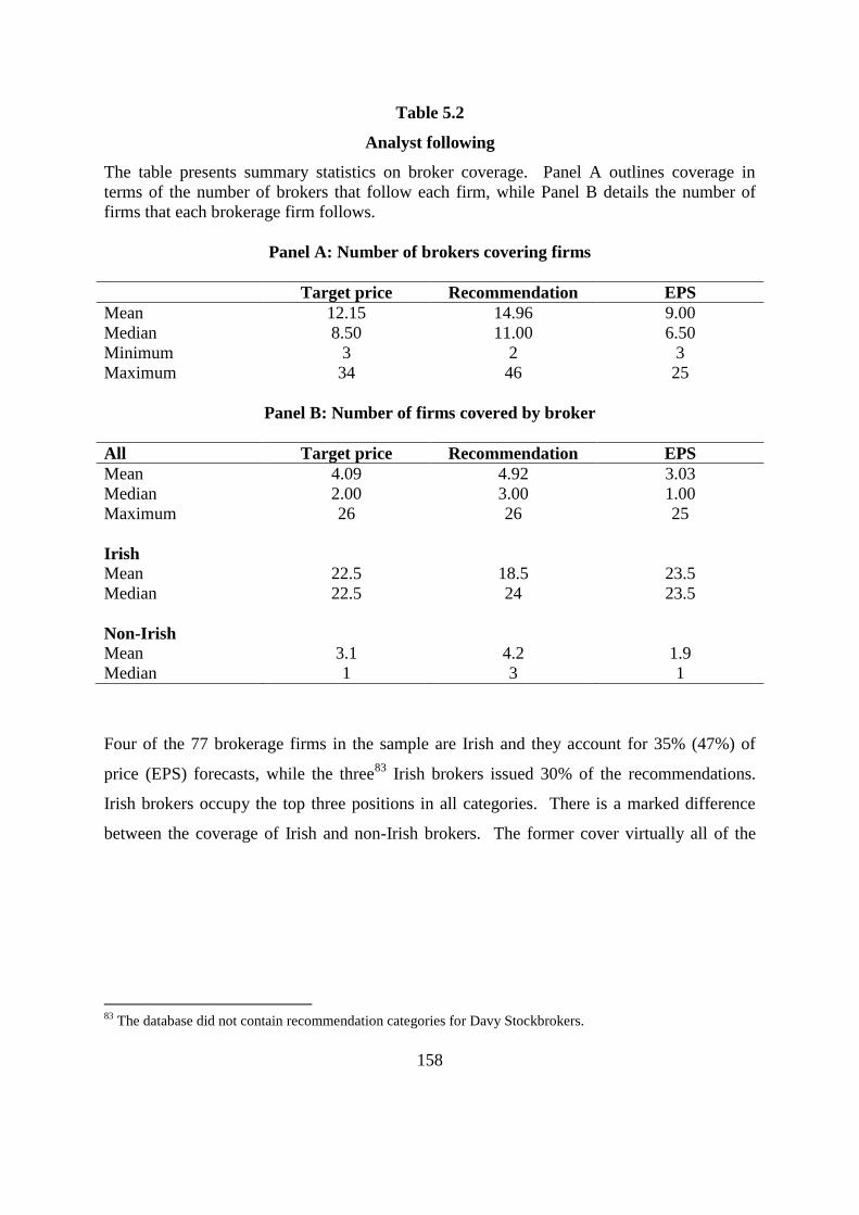
158
Table 5.2
Analyst following
The table presents summary statistics on broker coverage. Panel A outlines coverage in
terms of the number of brokers that follow each firm, while Panel B details the number of
firms that each brokerage firm follows.
Panel A: Number of brokers covering firms
Target price Recommendation EPS
Mean 12.15 14.96 9.00
Median 8.50 11.00 6.50
Minimum 3 2 3
Maximum 34 46 25
Panel B: Number of firms covered by broker
All Target price Recommendation EPS
Mean 4.09 4.92 3.03
Median 2.00 3.00 1.00
Maximum 26 26 25
Irish
Mean 22.5 18.5 23.5
Median 22.5 24 23.5
Non-Irish
Mean 3.1 4.2 1.9
Median 1 3 1
Four of the 77 brokerage firms in the sample are Irish and they account for 35% (47%) of
price (EPS) forecasts, while the three83
Irish brokers issued 30% of the recommendations.
Irish brokers occupy the top three positions in all categories. There is a marked difference
between the coverage of Irish and non-Irish brokers. The former cover virtually all of the
83
The database did not contain recommendation categories for Davy Stockbrokers.

159
companies in the sample, while the latter focus on a relatively small number of firms84
. Table
5.3 presents summary statistics on the output of brokers.85
Table 5.3
Summary statistics for brokers’ output
Price forecasts EPS forecast Recommendations
Mean 792 359 306
Median 260 94 931
Maximum 6,085 2,843 8,090
Total 45,918 16,153 70,794
Consistent with the underwriting hypothesis, bivariate analysis shows that there is a strong
relationship (r = 0.90) between the number of recommendations issued for a company and the
value of that company’s traded stock.
5.3 Contrarian and strength rule methodology
This section discusses the methodology employed in the two overarching strands of the
research. This study employs Cumulative Abnormal Returns (CARs) to calculate the returns
to the two trading strategies under investigation. CARs employ natural logarithms of prices
in order to obtain continuously compounded (as opposed to simple) returns. The
continuously compounded return, Rit, is calculated as the natural logarithm of the ratio of the
share price for the current and previous time period (pt and pt-1 respectively):
(
) (5.1)
84
This does not necessarily imply that Irish brokers are less specialised in terms of the industries that they
follow. One would expect that there are more analysts in the Irish brokerage houses focusing on Irish firms.
Hence, one would expect that a greater number of firms will be followed. In the absence of data on individual
brokers one cannot comment on industry specialisation. 85
The average number of forecasts/recommendations is limited by the fact that a number of companies under
review were not listed for the entire sample period.

160
An analogous equation is used for calculating market returns using index data. Log returns
are favoured in many event studies due to their time-additive86
nature and because they are
shown to more closely resemble a normal distribution than simple returns. Corrado and
Truong (2008) show that returns calculated using logarithms produce superior test
specifications than those calculated using arithmetic returns. For all models abnormal returns
are measured with reference to market returns. Details of the index used from each of the
four markets are presented below.
Table 5.4
Market indices
The table presents details of the market indices employed for the purpose of calculating
market returns. All index data is sourced from Thomson One Banker.
Ireland Greece Denmark Norway
Index ISEQ overall ASE KFX OBX
Number of stocks All stocks 60 largest
companies
20 most
traded stocks
All stocks
Weighting Value Value Value Value
5.3.1 Return-generating models
This study uses three models in order to measure abnormal returns; the market model; the
Capital Asset Pricing Model (CAPM); and the market adjusted model, as with De Bondt and
Thaler (1985). The CAPM is an equilibrium model developed by Sharpe (1964) and Lintner
(1965). It models expected return in terms of undiversifiable (systematic) risk. The standard
ex-ante and ex-post equations for the CAPM are respectively:
E(Ri) = R* + i [ E(Rm) - R*] (5.2)
Rit = Rt* + i (Rmt - Rt*) + it (5.3)
86
Consider the case where a stock price increases from €1 to €1.25 and then falls back to €1. The sum of the
simple returns will be 5% (the sum of +25% and -20%) even though the overall return is zero. Calculating
cumulative returns (1+r1)(1+r2) -1 gives the correct return of zero ([1.25*0.8] – 1). Similarly, the sum of the log
returns (0.2231 – 0.2231) will also be zero.

161
Where:
Rit is the rate of return on security i at time t;
Rmt is the rate of return on the market at time t;
Rt* is the rate of return on the risk-free asset at time t;
i is a measure of systematic risk = Cov(Ri,Rm)/Var(Rm) and
it is a random error.
The three-month inter-bank rate is used for the risk-free rate of return87
. In using the CAPM
one must keep in mind, inter alia, Roll’s critique, where in practice using broad-based market
indices such as the ISEQ index may not be theoretically sound (Cuthbertson, 1996, pp.73-
74).
Two variants of the market model are also used in order to estimate abnormal returns; the
market model and the market-adjusted model. The market model developed by Sharpe
(1963) was the first attempt to simplify portfolio theory by arguing that shares move to
varying degrees in line with the market itself. Unlike the CAPM, the market model looks not
only at the pricing of undiversifiable market risk but at total risk i.e. market risk plus specific
company risk (Pilbeam, 1998, pp.146-148). Sharpe (1963) postulates a linear relationship
between the return on a security and that of the market as a whole. The ex-post equation is
given by:
Rit = i + i Rmt + it (5.4)
Where i is a constant factor that varies between securities and measures the return to a stock
when there is no movement in the market. The market-adjusted model imposes a restriction
in (5.4) that i is zero and that i is equal to one.
Rit - Rmt = it (5.5)
87
In order to calculate the geometric weekly interest rate, rW, from the annual rate, rA, the formula
rW ={[1+rA]1/52
-1}*100 was used.

162
This study uses equations (5.2)-(5.4) in modelling equity returns. In each case the error term
(it) is interpreted as the abnormal return. The profitability of this contrarian investment
strategy is calculated as the difference between the cumulative average excess returns of the
loser portfolio and that of the winner portfolio, as the strategy involves buying the former and
short-selling the latter. The opposite is the case for the strength rule. The market model uses
a single beta for the whole dataset, whereas a separate beta is calculated for each rank and
holding period for the CAPM. The CAPM thus deals with risk more thoroughly than the two
market models.
The Fama-French three-factor model is not used as the factors are not available for the four
markets under review. Fama and French (2011) include all four markets in their European
portfolios. However, there is still an absence of loading factors and portfolio returns for each
of the four markets analysed in this study at the individual-country level. It is reasonable to
expect that the average factors are dominated by stocks from larger markets, such as
Germany, UK, and France. Furthermore, Griffin (2002) shows that country-specific factors
are superior to global factors.
5.3.2 Portfolios
For the contrarian strategy, three-year samples of share prices are taken, as with De Bondt
and Thaler’s (1985) study. The first three-year period in which winners and losers are
identified is known as the rank period. The following three-year period in which the
performance of these stocks is analysed is known as the test (holding) period. Two equally-
weighted portfolios are set up, one comprising former winners and the other comprising
former losers and the cumulative abnormal returns (CAR) for each portfolio for each non-
overlapping test period will be calculated to test the profitability of a contrarian investment
strategy.
For the contrarian strategy, the period 1989-1991 is formation period number one, 1992-1994
is formation period number two and test period number one. This process is repeated until
the final holding period (2004-06). For the strength rule, each year from 1989 to 2005 is a

163
portfolio formation periods and each year between 1990 and 2006 is a test period. The period
2007-09 is used to test the out-of-sample forecasting power of the results. This period allows
for one (three) holding period(s) for the contrarian (strength rule) strategy.
Small firms are grouped together into a separate portfolio that represents one asset. The
returns on this portfolio are evaluated in the same manner as other (individual) stocks. This
portfolio is used in order to minimise the risk that the results are skewed by the returns of
small thinly traded (and illiquid) securities, which would be expected to have higher bid-ask
spreads. Companies are classified as ‘small’ if their market capitalisation accounts for less
than 0.1% of the overall market capitalisation. The total number of companies analysed is
206. Of these, 77 qualify for the small company portfolio.
The relatively small number of stocks on the four markets under review negates the use of
deciles, as employed in studies on larger markets. In examining momentum on the Irish
market, O’Sullivan and O’Sullivan (2010) utilise portfolios based on the top and bottom
30%, 10%, and five stocks, while O’ Donnell and Baur (2009) construct portfolios based on
the top and bottom third of stocks. Similarly, Naranjo and Porter (2007), whose sample
includes all four markets that form the basis of this study, construct portfolios using the top
and bottom three deciles.
This study classifies winners (losers) as the top (bottom) half of stocks88
and will also form
extreme portfolios comprised of the top and bottom two and four stocks. Returns are
calculated using equally-weighted portfolios89
. Cumulative abnormal returns for a portfolio
(CARpt) are calculated by averaging the abnormal returns for n stocks for each period T, i.e:
∑∑
88
Where there is an odd number of stocks, the middle stock is omitted. 89
The use of value-weighted portfolios did not alter the results materially.

164
The profitability of the contrarian investment strategy is calculated as the difference between
the cumulative average abnormal returns of the loser portfolio and that of the winner portfolio
(CARL-CARW), as the strategy involves buying the former and selling short the latter. These
excess abnormal returns are averaged for the five three-year holding periods to give the
overall average profitability of the strategy. An analogous process is followed for the
strength rule strategy; excess abnormal returns (CARW-CARL) are averaged over the 17 non-
overlapping one-year holding periods.
5.3.3 Statistical significance
The statistical significance of abnormal returns to the contrarian and strength rule strategies is
estimated using the approach of De Bondt and Thaler (1985). The following equations
describe the process employed for obtaining test statistic relating to the contrarian strategy.
De Bondt and Thaler (1985) estimate the t-statistic of the excess abnormal return (i.e. loser
minus winner returns) as:
[ ] √ (5.7)
Where ACARW,t and ACARL,t are the average abnormal returns of the winner and loser
portfolios, respectively, and is the pooled estimate of population variance in CARt and is
estimated as:
[∑ ( )
∑ ( )
] (5.8)
Assuming samples of equal size, N, the sample standard deviation for the winner portfolio is
estimated as:
√∑( )

165
The standard error is then calculated as the standard deviation divided by the square root of N
and the t-statistic is the abnormal return of the winner portfolio divided by the standard error.
The equivalent statistic for the loser portfolio is calculated using the same approach. The test
statistics for the strength rule are estimated in a similar manner with equation 5.7 being
modified to:
[ ] √ (5.10)
The test statistics will follow Student’s t-distribution if abnormal returns are normally
distributed. A number of tests of normality were conducted and confirmed that this was the
case.
5.3.4 Robustness tests
This study conducts three general tests in order to assess the robustness of any abnormal
returns. First, the out-of-sample robustness of the key findings is examined by analysing the
pattern of returns in the period 2007-09. Second, an analysis of sub-period returns is
conducted, in order to assess whether any positive average abnormal returns are largely
attributable to the extremely profitable performance of the strategy in a small number of sub-
periods. Finally, a number of methods are employed to ascertain whether any abnormal
returns are driven by the dynamics of a relatively small number of stocks. Further details of
each of these procedures are outlined in section 6.5.
5.4 Brokers’ output methodology
The accuracy and impact of brokers’ output are analysed using both calendar and event based
strategies. The first part of the analysis represents a calendar-time study, where the output of
analysts is examined at the consensus level at the end of each calendar quarter. The
remaining analysis constitutes an event study, where the initiation and revisions of broker
measures are analysed at the level of individual brokers in event time.

166
Various test periods are employed, ranging from a minimum of one week to a maximum of
six months before, and one year after, the event date. Such an extended event window is
employed due to possible leakages and delayed reactions, as discussed in chapter four.
Furthermore, recommendations are often republished in the financial press. Thus, it is often
difficult to ascertain a precise date that the market becomes aware of an event.
A disadvantage of employing an extended test period is that there is a greater probability of
encountering multiple events within the same test period. This can result in cross-sectional
dependence problems, which understate standard errors and inflate test statistics. This issue
is overcome with a novel approach, which excludes overlapping observations, as will be
discussed in section 7.6.
Abnormal returns are measured using the adjusted-market model (equation 5.5) and buy-and-
hold returns, in order to facilitate comparisons with existing studies relating to brokers’
recommendations. Furthermore, the percentage of recommendations falling into each
category is calculated, in order to assess whether analysts are biased (possibly due to conflicts
of interest) towards positive recommendations. The subsequent performance of
recommendations is examined in order to ascertain whether any biases lead to inaccurate and
overoptimistic forecasts.
Brokers use a myriad of terms and a varying number of categories in order to communicate
their opinions on the prospects of the firms that they follow. In order to analyse these
recommendations it is necessary to convert them into a standard format. The key dimension
along which existing studies differ is the number of categories employed. Several studies
(for example, Stickel, 1995; Welch, 2000; Jegadeesh et al., 2004; Barber et al., 2007) utilise
separate categories for strong buy and strong sell and merge both add and buy and reduce and
sell, as they rely on the categories reported by the Zacks Investment Research, First Call, and
IBES90
databases. In contrast, Ryan (2006) uses three discrete categories; buy, hold, and sell.
90
IBES categorises recommendations as strong buy, buy, hold, underperform, sell and strong sell. However,
studies often amalgamate these into broader categories (see, for example, Moshirian et al., 2009).

167
This study differs from the above two approaches by using buy, add, hold, reduce, and sell
for three reasons. First, it is felt that the inclusion of separate categories for ‘strong buy’ and
‘strong sell’ is of limited use. In a dataset of 70,794 recommendations, there are only 419
observed ‘strong buy’ recommendations (less than 0.6% of the overall sample) and no ‘strong
sells’. Therefore, no distinction is made between strong buys and buys, as the former group
would not be sufficiently populated to merit a separate category. This approach is similar to
that adopted by Jegadeesh and Kim (2006), who merge ‘sell’ and ‘strong sell’
recommendations.
Second, the above approaches merge the ‘add’ and ‘buy’ and ‘reduce’ and ‘sell’ categories.
It is felt that doing so would truncate the data into a restrictively small number of categories
and result in the loss of a key distinction between the information content of each category. It
is strongly felt that the five categories are necessary in order to distinguish between the
27,309 buy and 16,868 add recommendations and between the 3,597 reduce and 1,958 sell
recommendations. A distinction between the 27,309 buy and 419 strong buy
recommendations is seen as less illuminating and there are no strong sells to isolate from the
sell recommendations.
Third, the five-point rating system most closely represents the scales used by brokers in this
sample, with its users accounting for in excess of three-quarters of recommendations. In
order to populate each of the five categories a manual coding was conducted by analysing the
recommendations of each broker and assigning it into the appropriate category. Table 5.5
details the interpretation of the various terms used by brokers in their final recommendation,
ranging from positive (bullish) to negative (bearish). Rakings of 1-5 (sell =1, … buy = 5) are
attached to these categories and will be used to calculate an optimism index91
.
91
The above approach may bias the average recommendation value upwards for brokers who only use sell, hold,
buy. However, the results were not materially affected when a value of 4.5 (1.5) was attached to buy (sell)
recommendations.

168
Table 5.5
Rating system used to code recommendations
5 4 3 2 1
Buy Add Hold Reduce Sell
Strong buy Accumulate Neutral Underperform
Buy on weakness Market perform Underweight
Outperform Equalweight
Overweight In-line
Peer perform
In order to gain an understanding of the characteristics of the stocks that brokers recommend
favourably, quintiles are formed based on recommendation levels and the firm-specific
characteristics of the constituents of each quintile is analysed. The future abnormal returns
and volume associated with each quintile are also examined in order to assess the price and
volume impact of brokers’ recommendations. Rank correlation coefficients are also
calculated for all pairs of variables. This will provide an insight into whether brokers follow
momentum or value strategies and whether their output is influenced by conflicts of interest.
The price and volume effects to quintiles sorted on each of the other firm-specific variables is
also estimated in order to evaluate whether brokers add incremental value above what is
contained in publicly available information such as momentum, firm size, and book-to-
market. The approach largely follows that of Jegadeesh et al. (2004) with a number of minor
adjustments. Due to a lack of data, several variables, such as sales growth, total assets, and
standardised unexpected earnings, are omitted, while measures for dispersion and future
volume are added to the suite of variables. Furthermore, analysts’ views on the prospects of a
firm are measured using the expected price change variable in addition to ratings levels.
This above approach employs calendar-time tests by forming quintiles for each of the 36
quarters in the sample period, which runs from July 2000 to June 200992
. Fama and French
(2008) state that decile approaches can be unreliable as extreme portfolios often contain
92
Stocks are added to the quintiles in such a way that the extreme quintiles always contain the same number of
stocks as each other. In other words, if there is an odd (even) number of additional stocks they are placed in the
middle (extreme) quintile(s). The results are not materially affected by the omission of these observations.

169
extremely small stocks. Such stocks are overrepresented relative to their share of market
value when equal-weight portfolios are employed. By using quintiles and limiting the sample
to relatively large firms, this study minimises this potential problem. The following sub-
sections provide details of the variables that are analysed. For all variables, time t refers to
the three months to the end of the calendar quarter.
5.4.1 Analysts’ views
Four variables are used in order to capture analysts’ views of the prospects of each firm.
Consensus recommendation levels and the expected price changes are examined, along with
changes in these two measures. The hypothesised relationship between all four measures and
future abnormal returns is positive.
Rating refers to the consensus forecast ( for each firm and is calculated as the mean of the
most recent recommendation ( for each broker in the three months prior to each calendar
quarter end. Recommendations are coded from sell =1 to buy =5 as detailed in table 5.5.
Ratings changes
Jegadeesh et al. (2004) find that recommendations changes provide more valuable
information than recommendation levels. The recommendation change (∆ Rating) is the
change in the mean level between the end of the prior calendar quarter and the current
calendar quarter.

170
Expected price change
Analysts’ views on a firm’s prospects are also measured using the anticipated percentage
price change implied by price forecasts. The continuous nature of this variable provides a
superior basis for analysis to the discrete recommendation level as it facilitates a more precise
assignment of stocks to the relevant quintiles.
EXP takes the difference between the most recent forecast prior to the end of the calendar
quarter and the price at that date and scales by that price.
Revisions are measured by ∆EXP, which is the change in EXP between consecutive quarters.
In terms of quintile formation, ∆ EXP is a superior measure to ∆ Rating, as price forecasts
are revised more often than recommendation levels. On average, there is one revision for
every 65 recommendations; the equivalent figure for price forecasts is 2093
. This reluctance
of analysts to revise their recommendations leads to a relatively large proportion of instances
where ∆ Rating is zero. Assigning such observations to quintiles becomes subjective and
accordingly, non-extreme quintiles must be interpreted with caution.
5.4.2 Momentum
Several authors, such as Womack (1996) and Jegadeesh and Kim (2006), find that analysts
tilt their recommendations towards stocks with high momentum in light of the findings of
Jegadeesh and Titman (1993) that future returns are positively correlated with past returns.
Momentum is captured using past returns over three- and six-month periods. MOM(3)
measures momentum before the calendar time t and is calculated as the cumulative market-
adjusted returns for each firm from week t-13 to t-1.
93
There are 2,262 (1,094) revisions in 45,918 (70,794) forecasts (recommendations).

171
∏
∏
MOM(6) follows the same approach with returns cumulated between week -1 and -26.
5.4.3 Firm size
Banz (1981) documents a negative relationship between firm-size and returns. SIZE
measures the natural logarithm of the number of shares outstanding (Nit) for each firm
multiplied by the corresponding share price at the end of the quarter (Pit).
(5.15)
5.4.4 Dispersion
Erturk (2006) reports a negative relationship between dispersion and future abnormal returns.
DISP is measured by the coefficient of variation, which is calculated by scaling the cross-
sectional standard deviation of price forecasts by the mean forecast (see, for example, Dische,
2002).
(5.16)
5.4.5 Past volume
According to Jegadeesh et al. (2004), analysts may be more likely to favourably recommend
low-volume stocks in light of the finding of Lee and Swaminathan (2000) that such stocks
exhibit value characteristics and earn higher future returns than high-volume (growth) stocks.
However, Jegadeesh et al. (2004) find that stocks with higher trading volume receive more
favourable recommendations and revisions, despite subsequently earning lower abnormal

172
returns. The relationship between volume and ratings may be clouded by any strong
relationship between high volume and high momentum94
.
Abnormal volume, VOL, is a measure of standardised volume and is calculated as the ratio
of average weekly volume for the current quarter volume to the average of the preceding
three quarters.
Where Vit is the average weekly volume over 13 weeks before the end of calendar quarter.
5.4.6 Book-to-market
Fama and French (1992) document a positive relationship between book-to-market (B/M)
ratios and abnormal returns. If brokers follow value (growth) strategies then one would
expect to observe a positive (negative) relationship between B/M and recommendation levels.
B/M divides the book value at the end of each calendar quarter by the firm’s market
capitalisation.
Book value is calculated as the net assets of each firm at the end of the calendar quarter.
Market capitalisation is calculated as the number of shares outstanding at the end of the
calendar quarter multiplied by the contemporaneous share price. Negative book-to-market
ratios are omitted as failing to do so would result in skewed averages.
94
However, Jegadeesh et al. (2004) show that the relationship between volume and ratings is robust to
adjustments that account for this correlation.

173
5.4.7 Earnings-price ratio
Basu (1977) documents the superior performance of firms with high earnings-to-price (E/P)
ratios. Jegadeesh et al. (2004) find that analysts follow value (contrarian) strategies by
favourably recommending such firms. E/P takes the earnings per share before extraordinary
items for each firm divided by its share price at the end of the quarter. Firm quarters with
non-positive EPS are excluded.
5.4.8 Future returns and volume
Chapter four outlined some of the numerous studies that have documented a positive
relationship between analysts’ output and future abnormal returns and volume. The value
and impact of brokers’ output is analysed by measuring the relation between ratings and
future abnormal returns and volume. In order to evaluate whether analysts add incremental
value the relationship between each of the firm-specific variables and returns and volume is
also examined.
Market-adjusted returns (Rit-Rmt) over the three and six months following the quarter end are
calculated in order to assess the abnormal returns to each quintile95
. These are labelled
RET(3) and RET(6), respectively, and are calculated using the approach detailed in equation
5.14, with returns running from week one to week 13 and 26 for three- and six-month returns,
respectively.
If brokers exhibit a strong tendency to favourably recommend low (high) volume stocks then
measuring future volume relative to the previous three quarters would overstate (understate)
the volume impact of brokers’ recommendations. Hence, abnormal volume for the next
quarter, VOL(F), is estimated by scaling the average weekly volume for each stock
95
The results are robust to the use of the market model and CAPM. The role of risk is less important over
relatively short event windows, as outlined in section 3.4.

174
subsequent to the end of the previous quarter by the average volume of the three quarters
preceding the recommendation quarter.
5.5 Limitations
There are a number of limitations to the methodology adopted in this chapter. All event
studies suffer from the joint-hypothesis problem, as they represent joint tests of market
efficiency and the return-generating models employed to estimate abnormal returns.
Although, this problem is mitigated by employing three models, it is unlikely that any of the
models perfectly capture expected returns.
The relatively small number of companies on the Irish market represents another potential
limitation. This problem is accentuated by the dominance of a small number of companies.
Furthermore, the data collected from One Banker specifies the output of each broker at the
end of each week. Thus, it is not possible to identify the exact date of each initiation and
revision. Accordingly, the designation of week 0 for estimating abnormal returns and volume
is somewhat arbitrary. However, the severity of this problem diminishes significantly as the
test period increases. Finally, the data on brokers’ output relates to brokerage houses; there is
no data on the recommendations of individual brokers.

175
Chapter Six
Momentum and Reversal Findings and Discussion
6.1 Introduction
This chapter summarises the key findings relating to the contrarian and momentum strategies
in the four markets under review. The remainder of this chapter is organised as follows.
Section 6.2 presents the key findings pertaining to the two strategies in the main data period
(1989-2006); alternative strategies based on various rank and holding periods and portfolio
sizes are examined in section 6.3. Seasonal effects are discussed in section 6.4 and the
robustness of the findings is examined in section 6.5 in the form of out-of-sample testing and
analysis by period and firm. Conclusions are drawn in section 6.6.
6.2 Results
This section presents the findings pertaining to both strategies for the main data period (1989-
2006) using the three models discussed in section 5.3. To begin with, the customary three-
and one-year holding periods are used for the contrarian and strength rule strategies
respectively, in order to get a broad picture of the underlying pattern of returns.
Subsequently, more bespoke rank and holding periods and hybrid strategies are examined in
light of previous findings that momentum is present for three months to one year before
return reversals occur. The use of portfolios with extreme winners and losers is also
examined.
Table 6.1 presents the returns to the two strategies for the four markets analysed. The results
are obtained using the three models discussed in section 5.3 and are the average cumulative
abnormal returns of five (17) holding periods for the contrarian (strength rule) strategy over
the period 1989-2006. The period 2007-09 is reserved to test the out-of-sample validity of
the results in section 6.5.
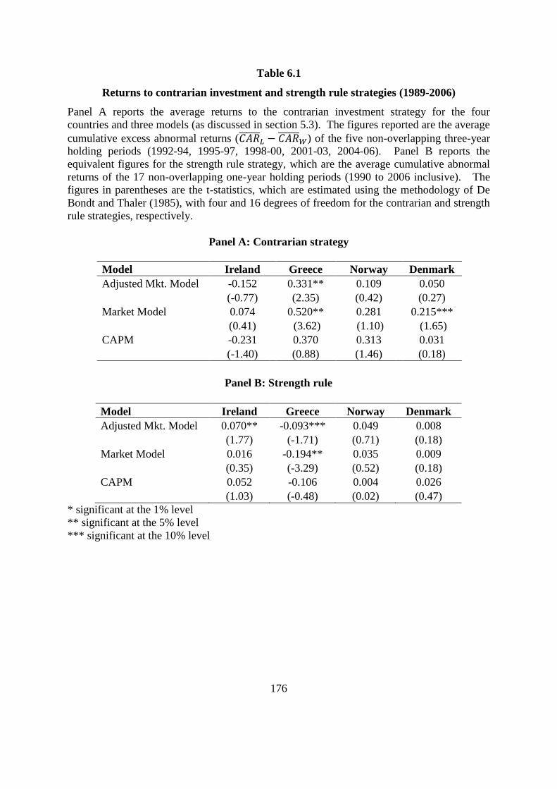
176
Table 6.1
Returns to contrarian investment and strength rule strategies (1989-2006)
Panel A reports the average returns to the contrarian investment strategy for the four
countries and three models (as discussed in section 5.3). The figures reported are the average
cumulative excess abnormal returns (
) of the five non-overlapping three-year
holding periods (1992-94, 1995-97, 1998-00, 2001-03, 2004-06). Panel B reports the
equivalent figures for the strength rule strategy, which are the average cumulative abnormal
returns of the 17 non-overlapping one-year holding periods (1990 to 2006 inclusive). The
figures in parentheses are the t-statistics, which are estimated using the methodology of De
Bondt and Thaler (1985), with four and 16 degrees of freedom for the contrarian and strength
rule strategies, respectively.
Panel A: Contrarian strategy
Model Ireland Greece Norway Denmark
Adjusted Mkt. Model -0.152 0.331** 0.109 0.050
(-0.77) (2.35) (0.42) (0.27)
Market Model 0.074 0.520** 0.281 0.215***
(0.41) (3.62) (1.10) (1.65)
CAPM -0.231 0.370 0.313 0.031
(-1.40) (0.88) (1.46) (0.18)
Panel B: Strength rule
Model Ireland Greece Norway Denmark
Adjusted Mkt. Model 0.070** -0.093*** 0.049 0.008
(1.77) (-1.71) (0.71) (0.18)
Market Model 0.016 -0.194** 0.035 0.009
(0.35) (-3.29) (0.52) (0.18)
CAPM 0.052 -0.106 0.004 0.026
(1.03) (-0.48) (0.02) (0.47)
* significant at the 1% level
** significant at the 5% level
*** significant at the 10% level

177
The contrarian investment strategy generates positive excess abnormal returns in all countries
except Ireland. This provides further out-of-sample confirmation of the findings of De Bondt
and Thaler (1985). The highest returns are generated in Greece, which is the only market
with statistically significant returns at the five per cent level. There are also economically
significant returns in Norway, with more modest returns generated in Denmark. The
contrarian investment strategy generates negative returns in Ireland as there is continuation of
past returns. Such momentum in Irish returns can be seen over a one-year holding period in
panel B. The positive strength rule returns in Ireland directly contradict the findings of
O’Sullivan and O’Sullivan (2010) and O’ Donnell and Baur (2009).
The excess abnormal returns in Greece are significantly larger than the 24.6% reported by De
Bondt and Thaler (1985) for the US using the adjusted market model. The results confirm
the findings of Richards (1997), who reports that in a 16-market study the largest reversals
are observed in Denmark and Norway (23.5% and 16.8% respectively).
Contrarian returns in Greece become statistically insignificant when the CAPM is used. The
returns remain economically significant but are considerably lower than market model
abnormal returns. The average beta of losers increases by 27% between the rank and holding
period, whereas that of the winners is relatively constant. However, the difference in mean
betas is not statistically significant (t = 1.39). This suggests that risk accounts for some, but
not all, of the excess abnormal returns found in Greece. This result partially confirms the
finding of Antoniou et al. (2006a) that abnormal returns are insignificant in Greece when
time-varying risk measures are employed. Contrarian returns are also less economically and
statistically significant in Denmark when the CAPM is employed.
In contrast, abnormal contrarian returns in Norway increase monotonically with model
sophistication in contrast to the findings of Chan (1988), who argues that the beta of losers
(winners) should increase (decrease) between the rank and holding period, thus reducing
returns when the CAPM is used. In Norway the average beta of losers decreases marginally,
while that of the winners remains stable. This is consistent with the findings of De Bondt and
Thaler (1985), who report statistically significantly larger betas for winners than losers.

178
The statistically significant negative strength rule returns in Greece add further weight to the
evidence of return reversals. One-year holding periods are typically associated with return
continuation. However, such is the pervasive nature of reversals in Greece that past losers
outperform past winners over one-year holding periods. Excess abnormal strength rule
returns are not statistically significant in the other two markets, although returns are
economically significant in Norway using two of the three models. The lack of statistically
significant positive momentum returns in Greece, Norway, and Denmark contradicts studies
such as Liu et al. (2011); Naranjo and Porter (2007); Griffin et al. (2005); Doukas and
McKnight (2005); and Rouwenhorst (1998), as detailed in table 2.1. Figure 6.1 presents the
evolution of cumulative excess abnormal returns over the holding periods for each strategy96
.
96
For ease of interpretation, the order of the legend in each graph coincides with the order of the lines at the end
of the time period.
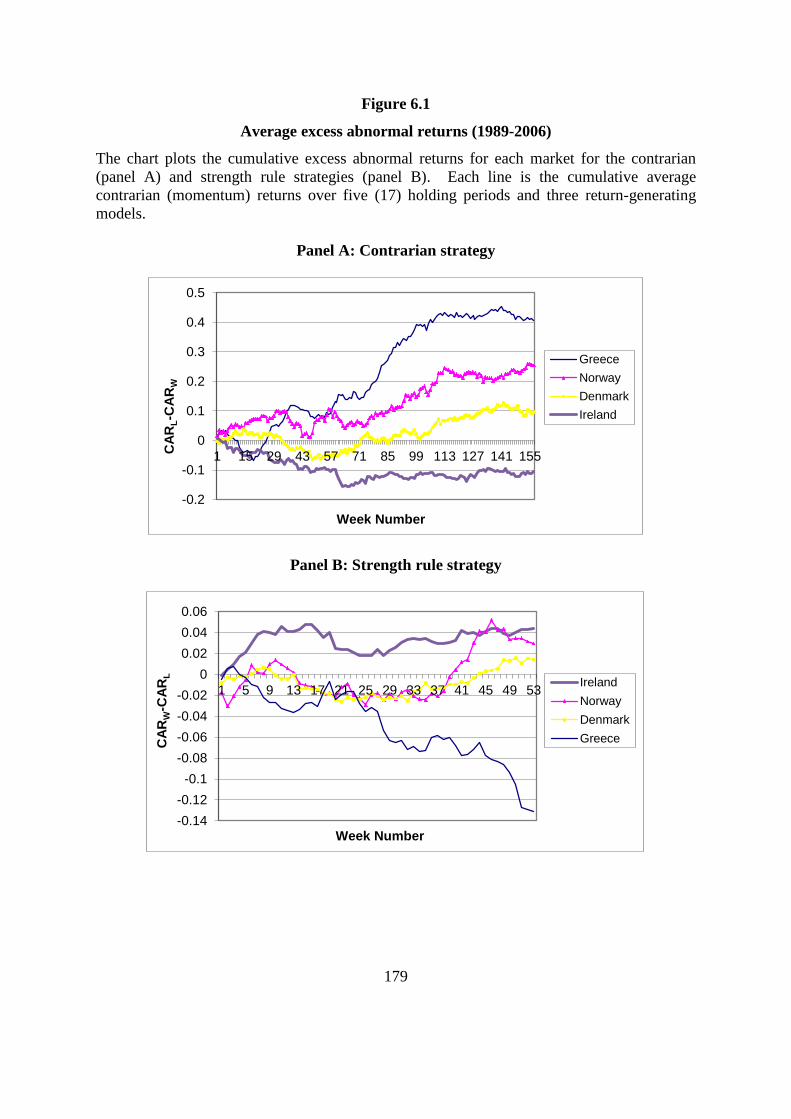
179
Figure 6.1
Average excess abnormal returns (1989-2006)
The chart plots the cumulative excess abnormal returns for each market for the contrarian
(panel A) and strength rule strategies (panel B). Each line is the cumulative average
contrarian (momentum) returns over five (17) holding periods and three return-generating
models.
Panel A: Contrarian strategy
Panel B: Strength rule strategy
-0.2
-0.1
0
0.1
0.2
0.3
0.4
0.5
1 15 29 43 57 71 85 99 113 127 141 155
CA
RL-C
AR
W
Week Number
Greece
Norway
Denmark
Ireland
-0.14
-0.12
-0.1
-0.08
-0.06
-0.04
-0.02
0
0.02
0.04
0.06
1 5 9 13 17 21 25 29 33 37 41 45 49 53
CA
RW
-CA
RL
Week Number
Ireland
Norway
Denmark
Greece

180
There are two important points to bear in mind when analysing the above findings. First, the
figures ignore transaction costs. As stated previously the strategies are self-financing; thus,
only round-trip transaction costs merit consideration. It is assumed that excess abnormal
returns of 2% per annum are sufficient to cover transaction costs. Second, the contrarian
returns are earned over a three-year period; thus annualised returns are presented in table 6.2
in order to facilitate a direct comparison with the strength rule returns97
.
Table 6.2
Average annualised returns to contrarian investment strategy
The table reports the average annualised excess abnormal returns to the contrarian investment
strategy (
) for the five non-overlapping three-year holding periods.
Model Ireland Greece Norway Denmark
Adjusted Mkt. Model -0.053 0.100 0.035 0.016
Market Model 0.024 0.150 0.086 0.067
CAPM -0.084 0.111 0.095 0.010
In annualised terms, the average abnormal returns of Greece and Norway are economically
significant, while it seems unlikely that the returns in Denmark would be sufficient to cover
moderate transaction costs for two of the three models. The returns to the strategy in Greece
are striking, with double-digit average annualised returns using all three models. The results
suggest that reversals are not evident in Ireland. Accordingly, the analysis pertaining to
return reversals in the remainder of this chapter is limited to the other three markets; whereas
strength rule returns are examined for Ireland.
The returns in table 6.1 may not accurately reflect the profits available to many investors as
both strategies involve short-selling. Barber and Odean (2008) find that only 0.29% of
individual traders take short positions. However, this does not necessarily imply that small
investors cannot take advantage of return continuation and reversal. Table 6.3 details the
contribution of the winner and loser portfolios to the overall excess abnormal returns detailed
earlier.
97
Annualised returns (ra) are obtained using the formula ra = (1+rt)1/3
-1, where rt is the three-year return.

181
Table 6.3
Contribution of winner and loser portfolios
The table presents the contribution of the winner and loser portfolios to overall excess
abnormal returns (t-statistics in parentheses). The returns for each model represent the
average of five (17) holding periods for the contrarian (strength rule) strategy. For the
contrarian strategy, the returns in the winner column are the negative of the winner returns as
the contrarian strategy (Greece, Norway, and Denmark) involves short-selling past winners.
The opposite is true for strength rule returns (Ireland).
Excess
Ireland
Adjusted Market Model 0.025 0.045*** 0.070**
(0.83) (1.56) (1.77)
Market Model 0.017 -0.001 0.016
(0.47) (-0.02) (0.35)
CAPM -0.003 0.055** 0.052
(0.08) (1.75) (1.03)
Greece
Adjusted Market Model 0.359** -0.028 0.331**
(3.12) (0.35) (2.35)
Market Model 0.231*** 0.289* 0.520**
(1.76) (4.91) (3.62)
CAPM 0.557 -0.187 0.370
(1.51) (0.93) (0.88)
Norway
Adjusted Market Model 0.045 0.063 0.109
(0.19) (0.73) (0.42)
Market Model 0.114 0.167 0.281
(0.50) (1.47) (1.10)
CAPM 0.363*** 0.050 0.313
(2.02) (0.43) (1.46)
Denmark
Adjusted Market Model 0.103 -0.053 0.050
(0.65) (-0.57) (0.27)
Market Model 0.140** 0.074 0.215***
(2.45) (0.64) (1.65)
CAPM 0.031 0.001 0.031
(0.28) (0.01) (0.18)
* significant at the 1% level
** significant at the 5% level
*** significant at the 10% level

182
It is clear that the loser portfolio dominates in all three countries with return reversals. On
average, the loser portfolio accounts for approximately 88% of the excess abnormal returns.
This is similar to the equivalent figure of 80% reported by De Bondt and Thaler (1985) for
three-year rank and holding periods. If the contrarian investment strategy returns are due to
overreaction then this suggests that investors overreact to bad news to a greater degree than
they do for good news. Table 6.3 shows that it is possible for an investor to generate
significant returns even if they cannot engage in short-selling. This is of particular
importance, as restrictions or bans were been placed on short selling in all four markets in the
aftermath of the eurozone crisis. A strategy of buying past losers would generate average
abnormal returns of 38.2, 17.4 and 9.1% in Greece, Norway, and Denmark respectively.
Such a strategy would also reduce transaction costs by eradicating the need for costly short-
selling.
The same is true of the strength rule strategy in Ireland, where the winner portfolio
contributes approximately 72% to the average excess abnormal returns of 4.6%. An investor
without the ability to short sell could generate excess abnormal returns of 3.3% by simply
buying past winners. This finding contrasts with the assertion of Hong et al. (2000) that the
majority of the profits to the momentum strategy arise from selling the past losers. However,
it is consistent with previous findings pertaining to Ireland. Recall that O’ Donnell and Baur
(2009) show that a strategy of buying past winners alone yields economically and statistically
significant abnormal returns.

183
6.3 Alternative specifications
This section examines variations of the contrarian and strength rule strategies along two
dimensions. The first approach examines rank and holding periods of various lengths,
following approaches similar to De Bondt and Thaler (1985) and Jegadeesh and Titman
(1993). The second alternative specification varies the number of stocks in the winner and
loser portfolio, as abnormal returns are frequently shown to be more pronounced for stocks
experiencing extreme past returns (see, for example, De Bondt and Thaler, 1985).
6.3.1 Alternative rank and holding periods
The contrarian returns in the previous section are derived using a three-year rank and holding
period, as originally employed by De Bondt and Thaler (1985). It is of interest to examine
alternative rank and holding periods, as panel A of figure 6.1 presents evidence of
continuation followed by reversal. Table 6.4 presents the average monthly excess abnormal
contrarian returns for a number of alternative rank and holding periods ranging from six to 36
months98
.
Twelve-month rank periods generate economically significant abnormal returns in Greece
and Norway over long holding periods. Furthermore, six-month rank periods generate
economically and statistically significant abnormal returns in Greece for all holding periods
of at least 12 months. These results contrast starkly with the results of De Bondt and Thaler
(1985), who report that there is no reversal for one-year portfolio formation periods in the
US. The positive, albeit statistically insignificant, abnormal returns to the 6,6 strategy
contradict the findings of Van der Hart et al. (2003), who report that a 6,6 momentum
strategy generates abnormal returns of 0.91% per month. There is evidence of short-term
reversals in Norway, with significant abnormal returns to six-month holding periods99
.
98
For the sake of brevity the table reports excess abnormal returns derived from the market model. The results
are broadly similar for all three models. 99
The majority of alternative rank and holding periods generate insignificant or negative abnormal returns in
Denmark as a result of return continuation in the first year of the holding period. The 36,36 strategy, which
generates 0.54% per month (t = 1.65), is the only combination of rank and holding periods with economically
significant excess abnormal returns.
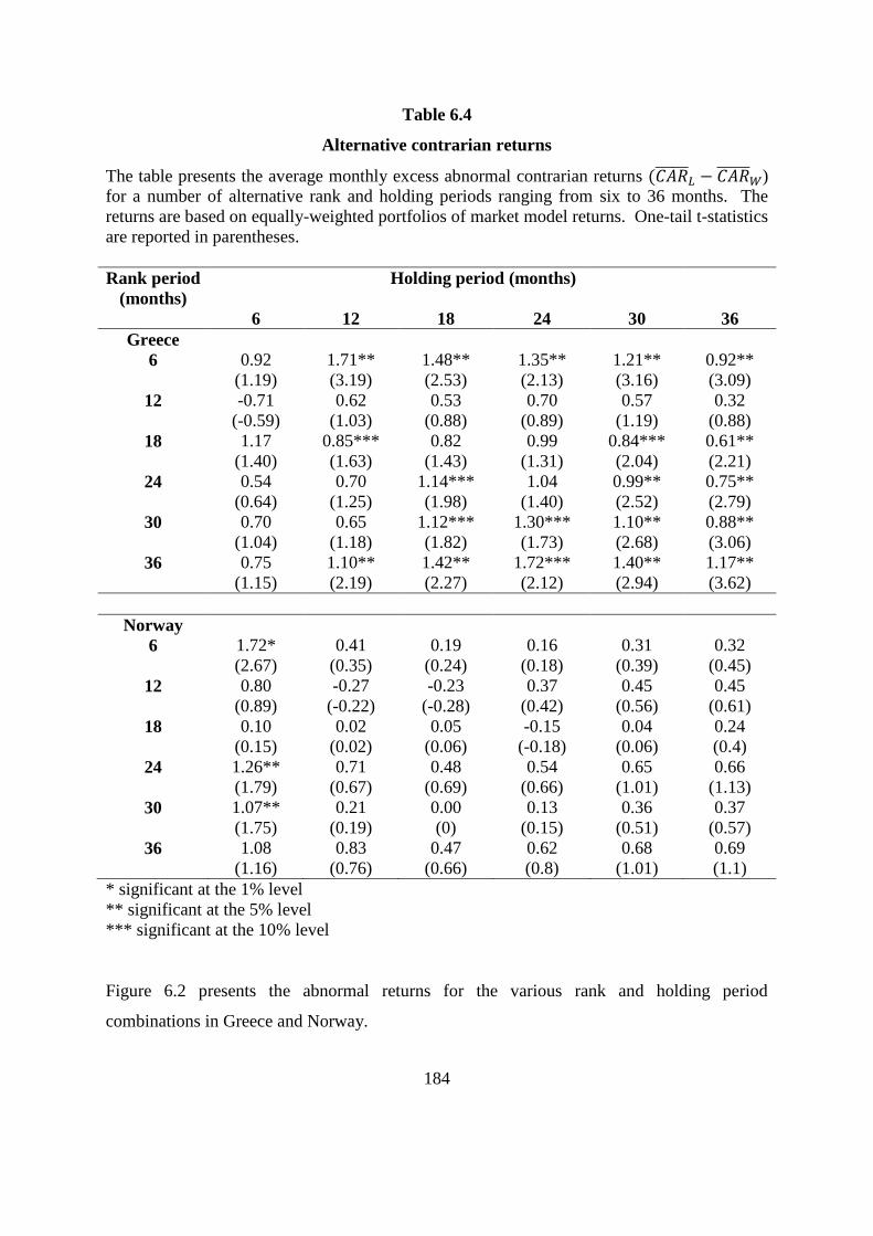
184
Table 6.4
Alternative contrarian returns
The table presents the average monthly excess abnormal contrarian returns
)
for a number of alternative rank and holding periods ranging from six to 36 months. The
returns are based on equally-weighted portfolios of market model returns. One-tail t-statistics
are reported in parentheses.
Rank period
(months)
Holding period (months)
6 12 18 24 30 36
Greece
6 0.92 1.71** 1.48** 1.35** 1.21** 0.92**
(1.19) (3.19) (2.53) (2.13) (3.16) (3.09)
12 -0.71 0.62 0.53 0.70 0.57 0.32
(-0.59) (1.03) (0.88) (0.89) (1.19) (0.88)
18 1.17 0.85*** 0.82 0.99 0.84*** 0.61**
(1.40) (1.63) (1.43) (1.31) (2.04) (2.21)
24 0.54 0.70 1.14*** 1.04 0.99** 0.75**
(0.64) (1.25) (1.98) (1.40) (2.52) (2.79)
30 0.70 0.65 1.12*** 1.30*** 1.10** 0.88**
(1.04) (1.18) (1.82) (1.73) (2.68) (3.06)
36 0.75 1.10** 1.42** 1.72*** 1.40** 1.17**
(1.15) (2.19) (2.27) (2.12) (2.94) (3.62)
Norway
6 1.72* 0.41 0.19 0.16 0.31 0.32
(2.67) (0.35) (0.24) (0.18) (0.39) (0.45)
12 0.80 -0.27 -0.23 0.37 0.45 0.45
(0.89) (-0.22) (-0.28) (0.42) (0.56) (0.61)
18 0.10 0.02 0.05 -0.15 0.04 0.24
(0.15) (0.02) (0.06) (-0.18) (0.06) (0.4)
24 1.26** 0.71 0.48 0.54 0.65 0.66
(1.79) (0.67) (0.69) (0.66) (1.01) (1.13)
30 1.07** 0.21 0.00 0.13 0.36 0.37
(1.75) (0.19) (0) (0.15) (0.51) (0.57)
36 1.08 0.83 0.47 0.62 0.68 0.69
(1.16) (0.76) (0.66) (0.8) (1.01) (1.1)
* significant at the 1% level
** significant at the 5% level
*** significant at the 10% level
Figure 6.2 presents the abnormal returns for the various rank and holding period
combinations in Greece and Norway.
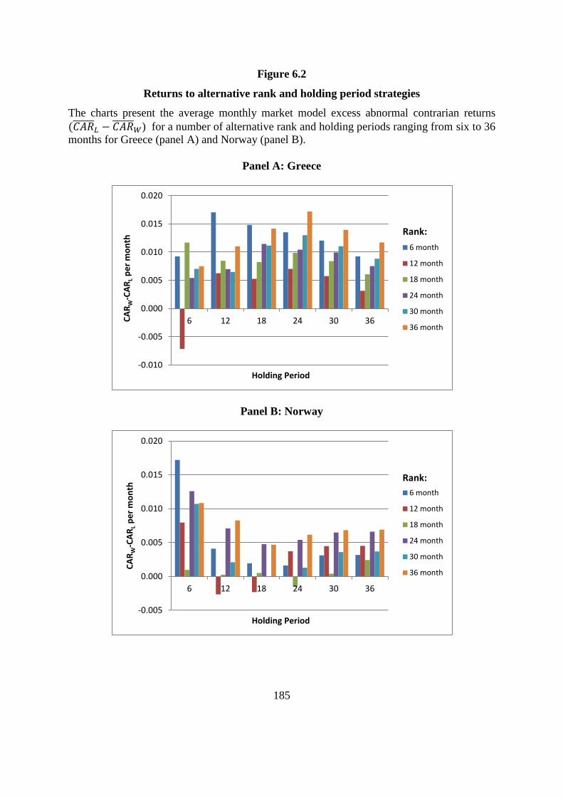
185
Figure 6.2
Returns to alternative rank and holding period strategies
The charts present the average monthly market model excess abnormal contrarian returns
) for a number of alternative rank and holding periods ranging from six to 36
months for Greece (panel A) and Norway (panel B).
Panel A: Greece
Panel B: Norway
-0.010
-0.005
0.000
0.005
0.010
0.015
0.020
6 12 18 24 30 36CA
RW
-CA
RL
pe
r m
on
th
Holding Period
6 month
12 month
18 month
24 month
30 month
36 month
-0.005
0.000
0.005
0.010
0.015
0.020
6 12 18 24 30 36
CA
RW
-CA
RL
pe
r m
on
th
Holding Period
6 month
12 month
18 month
24 month
30 month
36 month
Rank:
Rank:

186
It can be seen that the increase in average monthly returns in Greece with longer rank periods
would be monotonic in many instances if not for the high returns to the strategies based on
six-month rank periods. The returns to six-month rank periods decrease monotonically for
holding periods of 18 months or beyond. Returns also tend to increase with longer holding
periods. However, 36-month holding periods are sub-optimal.
The hitherto analysis has examined rank and holding periods of differing lengths. However,
each strategy commenced one week after the end of the rank period. Figure 6.1 suggests that
this may not be optimum as continuation followed by reversal is evident in two of the three
markets (Greece and Denmark). Abnormal returns are economically significant in year two
in all three markets. This is consistent with the findings of De Bondt and Thaler (1985), who
report abnormal returns in each of the three holding years of 5.4, 12.7, and 6.5%,
respectively.
Contrarian returns in Greece are 8.0, 31.6, and 1.1% respectively in years one, two and three.
However, the strategy generates negative or insignificant abnormal returns in the first six
months of year one due to continuation followed by reversal. It thus appears that the
optimum strategy in Greece would involve skipping the first six months of the holding
period. In order to maximise annualised returns it is also advisable to omit the third year of
the holding period, where abnormal returns are insignificant. This alternative contrarian
strategy generates average excess abnormal returns of 38.7% over the 18-month holding
period, which is the equivalent of 1.83% per month. The relatively poor performance of the
strategy in year three represents further evidence of reversal, as the superior performance of
the erstwhile losers itself begins to reverse.
The contrarian strategy generates a significant loss in year one in Denmark, suggesting that
investors could profit from a hybrid strategy, which profits from the observed pattern of
continuation followed by reversal by engaging in strength-rule trading in year one and
contrarian trading in years two and three. Such a hybrid strategy generates average abnormal
returns of 34% (1.22% per month). The standard three-year holding period is optimum in

187
Norway as the contrarian strategy generates consistent and significant positive excess
abnormal returns in each of the three holding years.
Alternative holding periods for the strength rule strategy are motivated by the approach of
Jegadeesh and Titman (1993), who examine 16 strategies based on combinations of rank and
holding periods of three, six, nine, and 12 months100
. The principal focus here is on returns
for Ireland as strength rule returns were not statistically significant in the other three markets.
Table 6.5 reports the average monthly strength rule returns for ranking and holding periods
ranging from three to 12 months in Ireland. With space considerations in mind, the table
details the excess abnormal returns derived from the CAPM. The results are broadly similar
for the other two models.
Table 6.5
Alternative strength rule returns
The table presents the average monthly excess abnormal strength rule returns for a number of
alternative rank and holding periods ranging from three to 12 months. The returns are based
on equally-weighted portfolios of CAPM returns. One-tail t-statistics are reported in
parentheses.
Holding period (months)
Rank period
(months)
3 6 9 12
3 1.21** 0.11 0.04 0.33
(1.83) (0.27) (0.10) (0.81)
6 1.52** 0.36 0.30 0.32
(2.46) (0.83) (0.62) (0.79)
9 2.04* 0.74** 0.58*** 0.52***
(3.56) (1.95) (1.34) (1.36)
12 1.09** 0.05 0.03 0.14
(1.80) (0.14) (0.07) (0.35)
* significant at the 1% level
** significant at the 5% level
*** significant at the 10% level
100
Jegadeesh and Titman (1993) examine an additional 16 strategies where a week is skipped between the rank
and holding period. The results for Ireland in this study are virtually identical when this approach is adopted.
Therefore, such results are not reported for every holding period.

188
The 9,3 (rank, hold) strategy is optimum, generating average returns of 2.04% per month
when the CAPM is employed101
. It thus appears that momentum in Irish returns is largely a
short- to medium-term phenomenon. The returns to the 9,3 strategy are consistent, with
positive excess abnormal returns in more than three-quarters of the three-month holding
periods.
These results provide further out-of-sample confirmation of the findings of Jegadeesh and
Titman (1993) and Rouwenhorst (1998), which show that 9,3 strategies are profitable.
However, both studies find that the 12,3 strategy is optimum, with average monthly returns of
1.31% and 1.35% respectively.
The breakdown of abnormal returns by portfolio contrasts with the findings of Jegadeesh and
Titman (1993) and Rouwenhorst (1998) in one important respect. In those two studies the
winner and loser portfolios generated positive abnormal returns for every rank and holding
period combination. Thus, a strategy of simply buying past winners would have generated
larger abnormal returns.102
In contrast, the evidence of underreaction in this study is more
symmetrical, as the loser portfolio generates negative abnormal returns for 11 of the 16 rank
and holding period combinations. This appears to contradict the findings of McQueen et al.
(1996) and Ashley (1962) that stocks react slowly to good news but quickly to bad news. The
winner portfolio accounts for approximately 84% of the abnormal returns. Thus, short-
selling constraints cannot explain the persistence of such anomalous returns.
Consistent with Jegadeesh and Titman (1993) and Rouwenhorst (1998), the economic and
statistical significance of average monthly returns generally increases with shorter holding
periods and longer rank periods. This pattern can be seen in figure 6.3. Three-month holding
periods and nine-month holding periods are optimum for all combinations; whereas 12-month
rank periods generate the lowest abnormal returns for all holding periods. The profitability of
momentum strategies with relatively short holding periods also confirms the results of
101
The average returns for the 9,3 strategy using the market model and adjusted market model are 1.81% (t =
3.37) and 1.98% (t = 3.56) respectively. 102
It seems that the only advantage of short selling past losers is that the strength rule strategy becomes self-
financing.
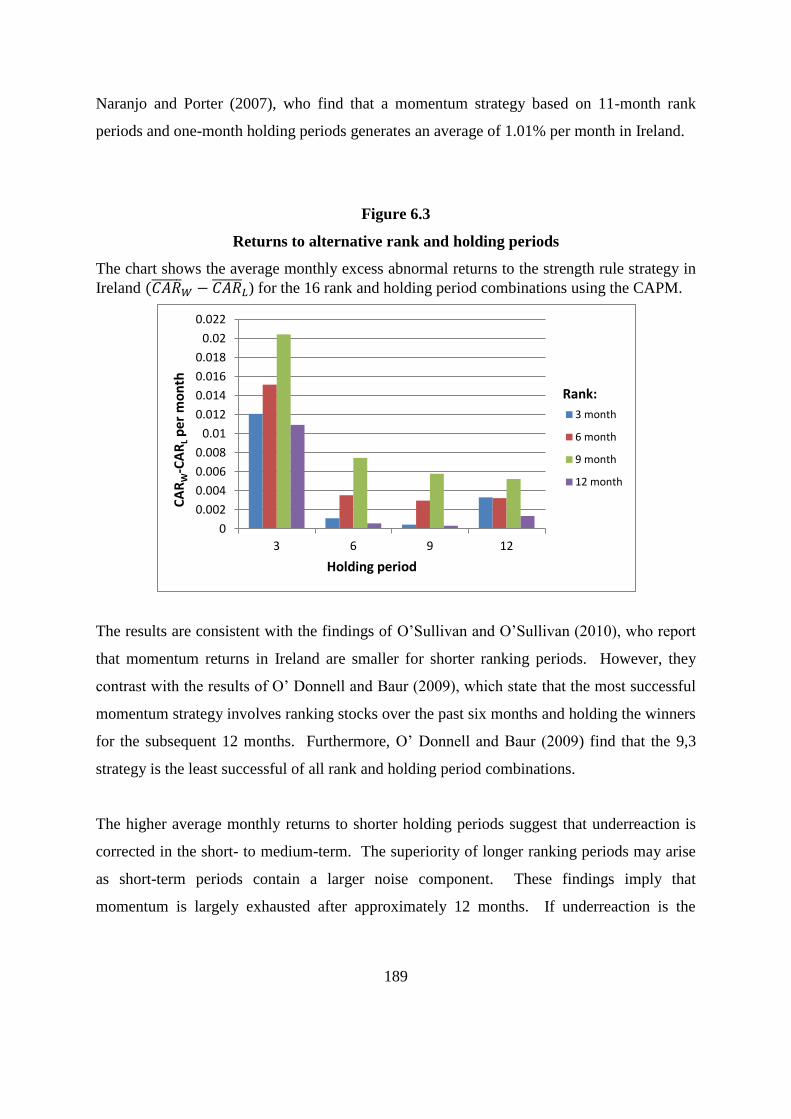
189
Naranjo and Porter (2007), who find that a momentum strategy based on 11-month rank
periods and one-month holding periods generates an average of 1.01% per month in Ireland.
Figure 6.3
Returns to alternative rank and holding periods
The chart shows the average monthly excess abnormal returns to the strength rule strategy in
Ireland
) for the 16 rank and holding period combinations using the CAPM.
The results are consistent with the findings of O’Sullivan and O’Sullivan (2010), who report
that momentum returns in Ireland are smaller for shorter ranking periods. However, they
contrast with the results of O’ Donnell and Baur (2009), which state that the most successful
momentum strategy involves ranking stocks over the past six months and holding the winners
for the subsequent 12 months. Furthermore, O’ Donnell and Baur (2009) find that the 9,3
strategy is the least successful of all rank and holding period combinations.
The higher average monthly returns to shorter holding periods suggest that underreaction is
corrected in the short- to medium-term. The superiority of longer ranking periods may arise
as short-term periods contain a larger noise component. These findings imply that
momentum is largely exhausted after approximately 12 months. If underreaction is the
0
0.002
0.004
0.006
0.008
0.01
0.012
0.014
0.016
0.018
0.02
0.022
3 6 9 12
CA
RW
-CA
RL p
er m
on
th
Holding period
3 month
6 month
9 month
12 month
Rank:
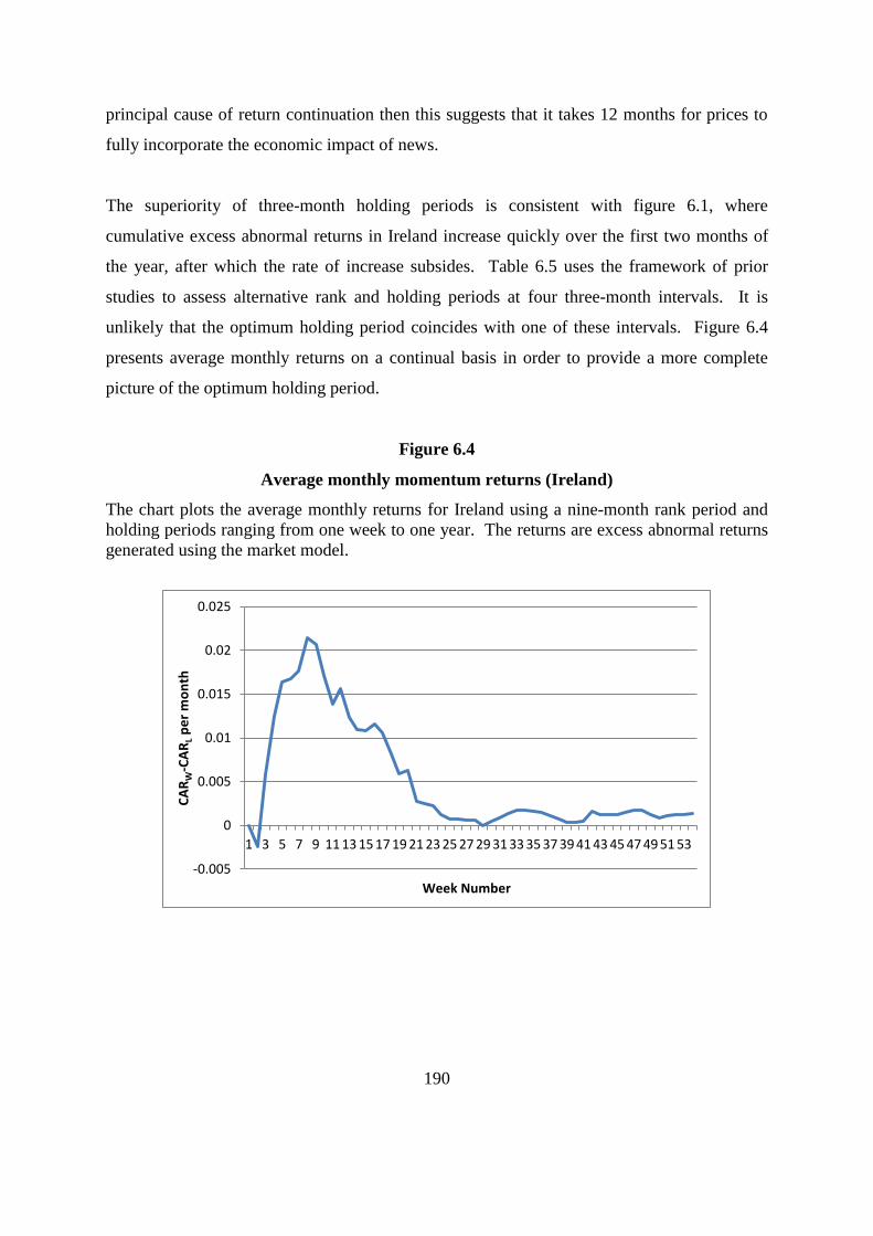
190
principal cause of return continuation then this suggests that it takes 12 months for prices to
fully incorporate the economic impact of news.
The superiority of three-month holding periods is consistent with figure 6.1, where
cumulative excess abnormal returns in Ireland increase quickly over the first two months of
the year, after which the rate of increase subsides. Table 6.5 uses the framework of prior
studies to assess alternative rank and holding periods at four three-month intervals. It is
unlikely that the optimum holding period coincides with one of these intervals. Figure 6.4
presents average monthly returns on a continual basis in order to provide a more complete
picture of the optimum holding period.
Figure 6.4
Average monthly momentum returns (Ireland)
The chart plots the average monthly returns for Ireland using a nine-month rank period and
holding periods ranging from one week to one year. The returns are excess abnormal returns
generated using the market model.
-0.005
0
0.005
0.01
0.015
0.02
0.025
1 3 5 7 9 11 13 15 17 19 21 23 25 27 29 31 33 35 37 39 41 43 45 47 49 51 53
CA
RW
-CA
RL
pe
r m
on
th
Week Number

191
A holding period of approximately seven weeks is optimum, with average monthly returns of
2.1%, rising to 2.54% when a week is skipped between the holding and rank period103
.
Although Jegadeesh and Titman (1993) recommend skipping a week to minimise
microstructure biases, it also has the effect of increasing average monthly returns for the
majority of the 16 strategies that they examine. The same effect is observed in this study due
to the negative strength rule returns in week one. It is noteworthy that even the least effective
holding periods generate abnormal returns in excess of 0.5% per month.
The returns to alternative rank and holding periods in Greece are also of interest given the
statistically significant negative returns to the strength rule on the Greek market. Such
evidence is consistent with short-term reversals and reinforces the patterns presented in table
6.4 relating to longer holding periods. The 12,3 contrarian strategy in Greece would generate
average excess abnormal returns of 1.21% per month. It is interesting to note that the
economic and statistical significance of average monthly returns increase as the holding
period increases. This is the opposite of the findings in relation to continuation and suggests
that overreaction is corrected in a more delayed fashion. Average monthly abnormal
momentum returns are insignificant in the other two markets, regardless of the rank and
holding period utilised.
6.3.2 Portfolio size
De Bondt and Thaler (1985) find that reversals are more pronounced for stocks with extreme
past performance. The benefits of using extreme stocks may be twofold to an investor, as
doing so could simultaneously increase returns and decrease transaction costs104
. This
supposition is tested by altering the number of winner and loser stocks held for the three
markets that displayed evidence of reversal. The average number of stocks held in each
portfolio in the original dataset was 11. The relatively small number of stocks listed in the
four markets studied renders the use of deciles impractical. Instead, portfolios of extreme
103
The average monthly returns to the strategy using nine-month rank periods and seven-week holding periods
are 2.57% and 2.56% for adjusted market model and CAPM respectively. 104
However, it should be noted that the use of extreme stocks will typically be accompanied by an increase in
the variance of portfolio returns.
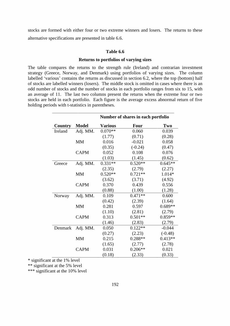
192
stocks are formed with either four or two extreme winners and losers. The returns to these
alternative specifications are presented in table 6.6.
Table 6.6
Returns to portfolios of varying sizes
The table compares the returns to the strength rule (Ireland) and contrarian investment
strategy (Greece, Norway, and Denmark) using portfolios of varying sizes. The column
labelled ‘various’ contains the returns as discussed in section 6.2, where the top (bottom) half
of stocks are labelled winners (losers). The middle stock is omitted in cases where there is an
odd number of stocks and the number of stocks in each portfolio ranges from six to 15, with
an average of 11. The last two columns present the returns when the extreme four or two
stocks are held in each portfolio. Each figure is the average excess abnormal return of five
holding periods with t-statistics in parentheses.
Number of shares in each portfolio
Country Model Various Four Two
Ireland Adj. MM. 0.070** 0.060 0.039
(1.77) (0.71) (0.28)
MM 0.016 -0.021 0.058
(0.35) (-0.24) (0.47)
CAPM 0.052 0.108 0.076
(1.03) (1.45) (0.62)
Greece Adj. MM. 0.331** 0.520** 0.645**
(2.35) (2.79) (2.27)
MM 0.520** 0.721** 1.014*
(3.62) (3.71) (4.92)
CAPM 0.370 0.439 0.556
(0.88) (1.00) (1.28)
Norway Adj. MM. 0.109 0.471** 0.600
(0.42) (2.39) (1.64)
MM 0.281 0.597 0.689**
(1.10) (2.81) (2.79)
CAPM 0.313 0.501** 0.859**
(1.46) (2.83) (2.79)
Denmark Adj. MM. 0.050 0.122** -0.044
(0.27) (2.23) (-0.48)
MM 0.215 0.288** 0.413**
(1.65) (2.77) (2.78)
CAPM 0.031 0.206** 0.021
(0.18) (2.33) (0.33)
* significant at the 1% level
** significant at the 5% level
*** significant at the 10% level

193
The pattern of returns in table 6.6 generally confirms the stylised finding of previous research
that reversals are more pronounced for firms with more extreme past price movements. In
the case of Greece, returns increase monotonically with the use of more extreme stocks. The
average return increases from 41% when all stocks are used, to 57% and 74% when four and
two stocks are used in each portfolio, respectively. The prospect of making a 74% excess
abnormal return by buying two shares and short-selling two shares should be particularly
appealing to small investors. It also suggests that fund managers should focus on a small
number of extreme stocks (ignoring diversification benefits).
The excess abnormal returns increase to an average of 66.8% when the first six months and
last year of the three year test period are skipped and each portfolio contains two stocks. This
is the equivalent of 2.76% per month over the modified 18-month holding period.
Implementing the contrarian strategy in the second year alone on such extreme stocks would
generate abnormal returns of 55.2% (3.73% per month).
A similar pattern is uncovered in Norway where excess abnormal returns increase from 25%
to 53% and 72% when four and two stocks are respectively used in each portfolio. The
results for Denmark are less emphatic, which is not surprising as there is less evidence of
return reversals in Denmark. The general tendency is for returns to increase as more extreme
stocks are used but they do not increase with same monotonic regularity as with Greece and
Norway. Returns increase using all three models when moving to four stocks per portfolio.
All of the above contrarian strategies remain profitable after the omission of the winner
returns and cannot thus be explained by short-selling constraints.
The increase in returns in Ireland is not as consistent and significant as is the case for the
contrarian strategies in the other three markets. Indeed, the use of extreme stocks results in
lower momentum returns to the 9,3 strategy. This is not surprising as, ceteris paribus, one
would expect that the prices of stocks with extreme past performance are more likely to be
nearer their turning points than other stocks. Mean reversion implies that reversals may be
more likely than continuation for such stocks. In other words, it is more plausible to expect
that the prices of extreme stocks have overreacted rather than underreacted. This finding is

194
consistent with O’Sullivan and O’Sullivan (2010), who report that momentum returns in
Ireland are smaller for portfolios of extreme stocks.
The above results show that there is considerable structure in share price returns in three of
the four stock markets. Of course, an investor would not know the optimum holding period
and portfolio size ex ante. The out-of-sample forecasting period (2007-09) is used to test the
robustness of the optimum strategies for each market. The results of these tests are presented
in section 6.5.1.
6.4 Seasonal effects
This section examines the seasonality of any abnormal returns in order to ascertain whether
such returns are merely a manifestation of another effect, such as the January effect. Of
course, an investor is not too concerned whether any returns are caused by overreaction,
mean reversion, the January effect, or any other effect. However, for academics it is
important to understand the source of any anomalous returns. Before examining the role of
seasonal patterns in explaining anomalous returns a general flavour of any seasonal patterns
is gauged by charting monthly aggregate returns in figure 6.5.
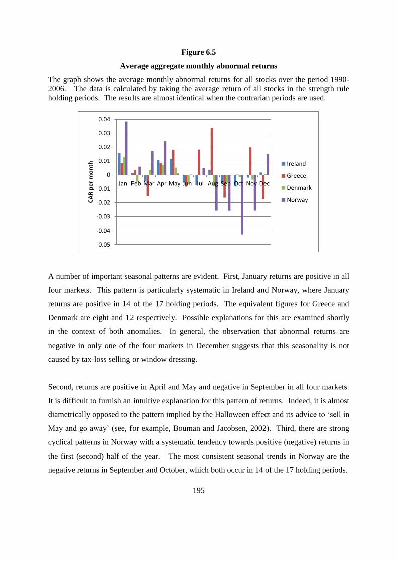
195
Figure 6.5
Average aggregate monthly abnormal returns
The graph shows the average monthly abnormal returns for all stocks over the period 1990-
2006. The data is calculated by taking the average return of all stocks in the strength rule
holding periods. The results are almost identical when the contrarian periods are used.
A number of important seasonal patterns are evident. First, January returns are positive in all
four markets. This pattern is particularly systematic in Ireland and Norway, where January
returns are positive in 14 of the 17 holding periods. The equivalent figures for Greece and
Denmark are eight and 12 respectively. Possible explanations for this are examined shortly
in the context of both anomalies. In general, the observation that abnormal returns are
negative in only one of the four markets in December suggests that this seasonality is not
caused by tax-loss selling or window dressing.
Second, returns are positive in April and May and negative in September in all four markets.
It is difficult to furnish an intuitive explanation for this pattern of returns. Indeed, it is almost
diametrically opposed to the pattern implied by the Halloween effect and its advice to ‘sell in
May and go away’ (see, for example, Bouman and Jacobsen, 2002). Third, there are strong
cyclical patterns in Norway with a systematic tendency towards positive (negative) returns in
the first (second) half of the year. The most consistent seasonal trends in Norway are the
negative returns in September and October, which both occur in 14 of the 17 holding periods.
-0.05
-0.04
-0.03
-0.02
-0.01
0
0.01
0.02
0.03
0.04
Jan Feb Mar Apr May Jun Jul Aug Sep Oct Nov Dec
CA
R p
er
mo
nth
Ireland
Greece
Denmark
Norway

196
It should be noted that the returns in the figure 6.5 are aggregate figures, while those of the
two trading strategies under review are net figures (winners minus losers and vice versa).
Accordingly, seasonalities may not manifest themselves in the returns to the two strategies if
both winners and losers experience extreme performance in the same direction and of a
similar magnitude. Alternatively, aggregate returns may understate the effect of seasonalities
on anomalous returns if the returns to winners and losers are of the opposite sign. Figure 6.6
presents the average excess abnormal returns to the contrarian (panel A) and strength rule
(panel B) strategies for each month.
It appears that the January effect partially explains the anomalous returns outlined in this
chapter105
. January returns are positive using contrarian rankings in the three markets that
displayed return reversals (Greece, Denmark, and Norway) and using strength rule rankings
in the market that exhibited continuation to the greatest extent (Ireland). January returns in
Ireland, Greece, Denmark, and Norway account for 50, 18, 35, and 40% of anomalous returns
respectively. However, in all four markets excess abnormal returns remain significant when
January returns are omitted, suggesting that the two anomalies are distinct phenomena to the
turn-of-the-year effect106
.
105 Recall that it is expected that the January effect would be evinced by positive (negative) returns in January
(December) for the contrarian strategy and vice versa for the strength rule if tax-loss selling or window dressing
are the principal drivers of the January anomaly. 106
For example, omitting January returns in Greece only reduces average monthly contrarian returns from 1.1%
to 1% per month.
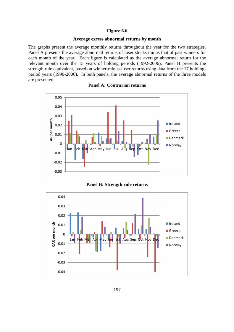
197
Figure 6.6
Average excess abnormal returns by month
The graphs present the average monthly returns throughout the year for the two strategies.
Panel A presents the average abnormal returns of loser stocks minus that of past winners for
each month of the year. Each figure is calculated as the average abnormal return for the
relevant month over the 15 years of holding periods (1992-2006). Panel B presents the
strength rule equivalent, based on winner-minus-loser returns using data from the 17 holding-
period years (1990-2006). In both panels, the average abnormal returns of the three models
are presented.
Panel A: Contrarian returns
Panel B: Strength rule returns
-0.03
-0.02
-0.01
0
0.01
0.02
0.03
0.04
0.05
Jan Feb Mar Apr May Jun Jul Aug Sep Oct Nov Dec
AR
pe
r m
on
th
Ireland
Greece
Denmark
Norway
-0.04
-0.03
-0.02
-0.01
0
0.01
0.02
0.03
0.04
Jan Feb Mar Apr May Jun Jul Aug Sep Oct Nov Dec
CA
R p
er
mo
nth
Ireland
Greece
Denmark
Norway

198
There are a number of monthly returns that stand out in the above graphs. However, there are
relatively few instances where an average monthly return is significantly different to the
average monthly return for the entire year. Table 6.7 presents details of such cases.
Table 6.7
Statistically significant monthly returns
The table presents the cases where average monthly abnormal returns are significantly
different to average returns for the entire year using a two-tail t-test. The final column shows
the percentage of holding periods where abnormal returns are of the same sign as the average
return as presented in figure 6.6.
Market Month Strategy Portfolio Monthly
return
t-statistic %
Norway October Strength rule Loser -6.22 -2.52* 77
Norway October Strength rule Winner-loser 3.91 1.76*** 100
Norway January Contrarian Loser 5.23 2.29** 100
Norway January Strength rule Loser 4.31 1.94*** 82
Norway January Strength rule Winner 3.38 1.84*** 82
Ireland January Strength rule Winner 2.69 1.83*** 88
Greece March Contrarian Loser-winner -2.49 -1.88*** 60
Greece March Contrarian Loser -3.45 -2.29** 80
* Significant at the 2% level
** Significant at the 5% level
*** Significant at the 10% level
The most significant abnormal return is the 6.2% that the loser portfolio contributes to
momentum returns in Norway in October. In most cases the winner and loser returns cancel
each other out to some extent so that seasonal patterns do not permeate to the level of the
excess abnormal returns. Indeed, there is no case where the excess abnormal returns are
significantly positive at the five per cent level. Therefore, one can conclude that the
anomalous returns presented in this chapter are more than mere manifestations of seasonal
anomalies.
Perhaps the most striking seasonal pattern is the dramatic increase in excess abnormal returns
in Greece in the middle third of the year. There is no apparent reason for this seasonality and

199
it represents a potentially fruitful area for future research. However, contrarian returns in
Greece remain significant after the omission of the returns from June-September.
The findings for Ireland are consistent with the results of Lucey and Whelan (2004), who
report that returns are elevated in Ireland in January and April. The positive momentum
returns in January are quite surprising as the tax-loss selling and window-dressing hypotheses
imply that strength rule returns should be negative in January as explained in section 2.7.4.
The positive abnormal returns of 2.25% in January are in sharp contrast with the negative
returns of 7% and 5.85% reported in Jegadeesh and Titman (1993) and Grundy and Martin
(2001), respectively. Remarkably, January abnormal returns for the winner portfolio are
positive in 15 of the 17 holding periods.
However, the high January returns for the strength rule must be interpreted with caution vis-
à-vis the tax-loss selling hypothesis. In 2002, the start of the tax year in Ireland was moved
from April to January. Aggregate returns are elevated in April and May, implying that tax-
loss selling may be driving seasonal returns. However, there are at least three reasons why
this may not be the case.
First, January returns were higher prior to 2002 and are not statistically significant from 2002
onwards. Second, excess abnormal returns are of the opposite sign than expected in January
pre-2002; the January effect would imply negative January returns to the strength rule as past
losers outperform past winners. Excess returns are of the prescribed sign in April but are not
statistically significant. Third, excess abnormal returns are close to zero in December. The
tax-loss selling hypothesis suggests that returns at the end of the year should be positive for
the strength rule, as investors sell past losers in order to realise tax losses.
The tax year commences in January in the other three markets. Thus, it is tempting to
conclude that the high January contrarian returns are consistent with tax-loss selling.
However, December returns are positive or close to zero in these markets, suggesting that
there is no significant selling of past losers at the end of the tax year. The trivial December
returns also invalidate the window-dressing explanation for the turn-of-the-year effect. If

200
fund managers sold small stocks at the end of the year and re-purchased them at the
beginning of January, one would expect to see a negative December effect.
The high strength rule returns in Ireland in January and February raise an important question.
Are the large returns to the 9,3 strategy outlined in section 6.2.1 caused by short-term
continuation or is it simply that the three-month holding period coincides with the beginning
of the calendar year? To answer this question the strategy is re-examined with rank and
holding periods, commencing in each month outside the first quarter. The findings show that
abnormal returns are consistently large for all three-month holding periods. Thus, it seems
that short-term continuation is a systematic feature of the Irish market and is not confined to
the turn of the year.
In summary, the evidence of anomalous returns documented in this chapter cannot be
explained by seasonal variations in returns. Although seasonal patterns exist in all four
markets, excess abnormal returns are rarely significantly different from average returns for
the entire year. This is partially because seasonalities tend to affect winners and losers to a
broadly similar extent.
6.5 Robustness of results
The robustness of the above results is examined in three ways. First, the out-of-sample
robustness of the key findings is analysed by examining the pattern of returns in the period
2007-09. Second, an analysis of sub-period returns is conducted in order to assess whether
any positive average abnormal returns are largely attributable to the extremely profitable
performance of the strategy in a small number of sub-periods. Third, a number of methods
are employed to ascertain whether any abnormal returns are driven by the dynamics of a
relatively small number of stocks.

201
6.5.1 Out-of-sample returns
The above results suggest that the contrarian investment strategy is profitable in three of the
four countries examined. It is optimum for an investor to focus on extreme stocks and to skip
certain portions of holding periods in two of the markets. Significant evidence of momentum
is documented for Ireland. These findings are tested in the out-of-sample holding period
(2007-09) in order to ascertain the out-of-sample validity of the results107
. This section also
examines the relationship between the returns to the two anomalies and market returns.
Table 6.8 and figure 6.7 present the excess abnormal returns to the basic contrarian and
momentum strategies in each of the four countries using three- and one-year holding periods
respectively108
.
107
Note that for the contrarian strategy it is assumed that the market model alpha and beta are the same for
2007-09 as they were for the period 1989-2006. 108
In order to save space, the data in figure 6.7 is the average return in each market over the three models
employed.
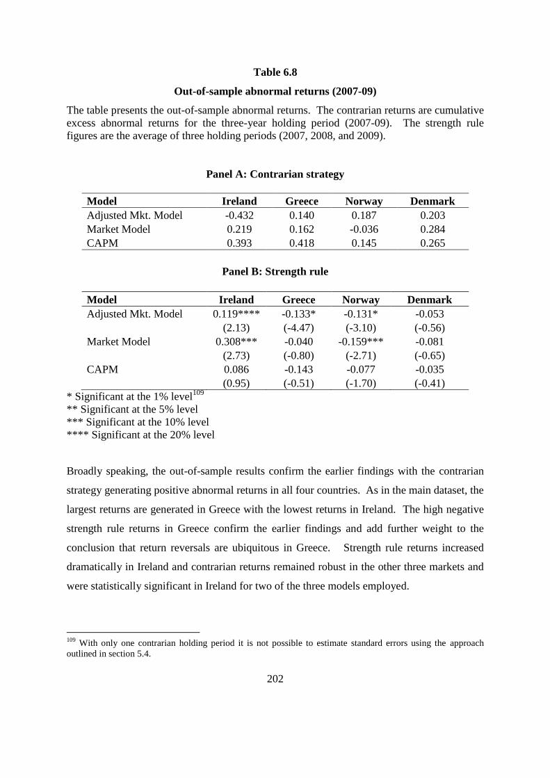
202
Table 6.8
Out-of-sample abnormal returns (2007-09)
The table presents the out-of-sample abnormal returns. The contrarian returns are cumulative
excess abnormal returns for the three-year holding period (2007-09). The strength rule
figures are the average of three holding periods (2007, 2008, and 2009).
Panel A: Contrarian strategy
Model Ireland Greece Norway Denmark
Adjusted Mkt. Model -0.432 0.140 0.187 0.203
Market Model 0.219 0.162 -0.036 0.284
CAPM 0.393 0.418 0.145 0.265
Panel B: Strength rule
Model Ireland Greece Norway Denmark
Adjusted Mkt. Model 0.119**** -0.133* -0.131* -0.053
(2.13) (-4.47) (-3.10) (-0.56)
Market Model 0.308*** -0.040 -0.159*** -0.081
(2.73) (-0.80) (-2.71) (-0.65)
CAPM 0.086 -0.143 -0.077 -0.035
(0.95) (-0.51) (-1.70) (-0.41)
* Significant at the 1% level109
** Significant at the 5% level
*** Significant at the 10% level
**** Significant at the 20% level
Broadly speaking, the out-of-sample results confirm the earlier findings with the contrarian
strategy generating positive abnormal returns in all four countries. As in the main dataset, the
largest returns are generated in Greece with the lowest returns in Ireland. The high negative
strength rule returns in Greece confirm the earlier findings and add further weight to the
conclusion that return reversals are ubiquitous in Greece. Strength rule returns increased
dramatically in Ireland and contrarian returns remained robust in the other three markets and
were statistically significant in Ireland for two of the three models employed.
109
With only one contrarian holding period it is not possible to estimate standard errors using the approach
outlined in section 5.4.
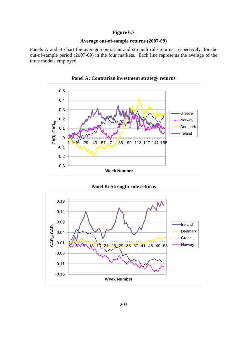
203
Figure 6.7
Average out-of-sample returns (2007-09)
Panels A and B chart the average contrarian and strength rule returns, respectively, for the
out-of-sample period (2007-09) in the four markets. Each line represents the average of the
three models employed.
Panel A: Contrarian investment strategy returns
Panel B: Strength rule returns
-0.3
-0.2
-0.1
0
0.1
0.2
0.3
0.4
0.5
1 15 29 43 57 71 85 99 113 127 141 155CA
RL-C
AR
W
Week Number
Greece
Norway
Denmark
Ireland
-0.16
-0.11
-0.06
-0.01
0.04
0.09
0.14
0.19
1 5 9 13 17 21 25 29 33 37 41 45 49 53CA
RW
-CA
RL
Week Number
Ireland
Denmark
Greece
Norway

204
Over the out-of-sample period both past winners and losers experienced substantial losses as
a result of the global financial crisis. Consistent with the overreaction hypothesis, past
winners declined to a greater extent than past losers, resulting in positive returns to the
contrarian investment strategy in all four markets. It appears that the ability to short sell is
crucial to the contrarian strategy in times of economic downturn. Further analysis of the role
of macroeconomic growth rates is presented in section 6.5.2.
The pattern of returns in figure 6.7 validates the earlier findings relating to Greece as
abnormal returns are insignificant in the first six months and final year of the three-year test
period. When these months are excluded the contrarian strategy generates average excess
abnormal returns of 1.6% per month, rising to 1.77% when portfolios are constructed using
the two extreme past winners and losers.
The pattern of returns in Denmark is replicated in the out-of-sample period, with significantly
negative returns in year one and positive returns thereafter. The contrarian strategy generates
average abnormal returns of 1.22% per month in years two and three when applied to all
stocks, and 0.7% per month when implemented on extreme portfolios of four winners and
losers.
The contrarian strategy generates average abnormal returns of 0.3% per month over the
standard three-year holding period in Norway. However, the use of extreme stocks results in
negative contrarian returns on average. This is entirely attributable to the large negative
abnormal returns in the third holding year.
Perhaps the most cogent conclusion from the preceding analysis is that returns reversals are
pervasive in the second year after portfolio formation in all three markets. A relatively
straightforward approach of implementing a contrarian investment strategy in year two alone
generates average excess abnormal returns of 0.6, 2.8, and 1.2% per month in Greece,
Denmark, and Norway, respectively, rising to 1.8, 4.6, and 1.8%, respectively when extreme
portfolios are used.

205
It can thus be seen that the anomalous returns to the contrarian strategy are robust to out-of-
sample testing. The remainder of this section focuses on the strength rule strategy. Recall
that Ireland was the only market with significant momentum returns. Table 6.9 and figure 6.8
present the excess abnormal returns to various rank and holding periods for the out-of-sample
period110
.
Table 6.9
Alternative strength rule returns (2007-09)
The table presents the average monthly excess abnormal strength rule returns for a number of
alternative rank and holding periods ranging from three to 12 months. The returns are based
on equally-weighted portfolios of market model returns. One-tail t-statistics are reported in
parentheses.
Holding period (months)
Rank period
(months)
3 6 9 12
3 4.31*** 1.60*** 0.16 1.23
(2.63) (2.29) (0.20) (1.51)
6 3.65*** 1.61 1.11 1.91***
(2.83) (1.87) (1.28) (2.13)
9 4.99** 2.28** 1.32 2.16***
(3.55) (2.93) (1.56) (2.50)
12 4.37*** 2.50** 1.35 2.26***
(2.87) (3.39) (1.70) (2.73)
* significant at the 1% level
** significant at the 5% level
*** significant at the 10% level
110
Recall that the use of extreme stocks did not increase momentum returns in Ireland. Thus, winner and loser
portfolios are formed using the top and bottom half of stocks respectively.

206
Figure 6.8
Excess abnormal returns to strength rule strategies
The figure charts the excess abnormal market model returns to strength rule strategies based
on alternative rank and holding periods, as outlined in table 6.9.
As with the main dataset, returns are generally larger for shorter holding periods and longer
rank periods and the 9,3 strategy is optimum in terms of the 16 rank and holding period
combinations. Figure 6.9 plots the average monthly market model excess abnormal returns
for nine-month ranking periods and holding periods ranging from one week to one year.
0.000
0.005
0.010
0.015
0.020
0.025
0.030
0.035
0.040
3 6 9 12
CA
RW
-CA
RL p
er m
on
th
Holding period
3 month
6 month
9 month
12 month
Rank:
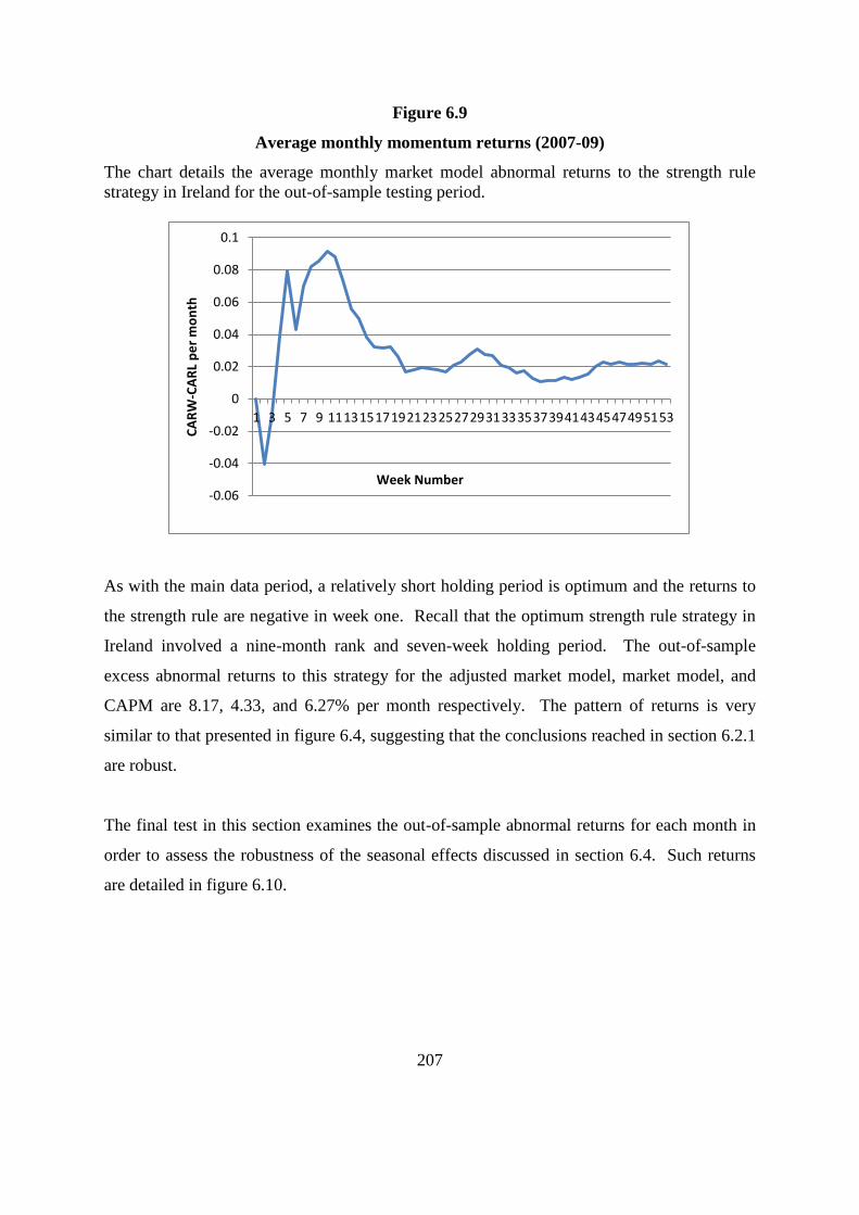
207
Figure 6.9
Average monthly momentum returns (2007-09)
The chart details the average monthly market model abnormal returns to the strength rule
strategy in Ireland for the out-of-sample testing period.
As with the main data period, a relatively short holding period is optimum and the returns to
the strength rule are negative in week one. Recall that the optimum strength rule strategy in
Ireland involved a nine-month rank and seven-week holding period. The out-of-sample
excess abnormal returns to this strategy for the adjusted market model, market model, and
CAPM are 8.17, 4.33, and 6.27% per month respectively. The pattern of returns is very
similar to that presented in figure 6.4, suggesting that the conclusions reached in section 6.2.1
are robust.
The final test in this section examines the out-of-sample abnormal returns for each month in
order to assess the robustness of the seasonal effects discussed in section 6.4. Such returns
are detailed in figure 6.10.
-0.06
-0.04
-0.02
0
0.02
0.04
0.06
0.08
0.1
1 3 5 7 9 11131517192123252729313335373941434547495153
CA
RW
-CA
RL
pe
r m
on
th
Week Number
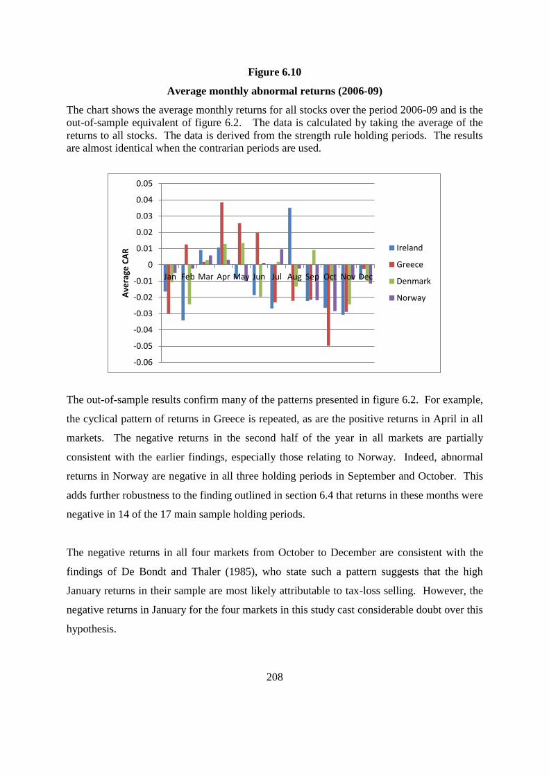
208
Figure 6.10
Average monthly abnormal returns (2006-09)
The chart shows the average monthly returns for all stocks over the period 2006-09 and is the
out-of-sample equivalent of figure 6.2. The data is calculated by taking the average of the
returns to all stocks. The data is derived from the strength rule holding periods. The results
are almost identical when the contrarian periods are used.
The out-of-sample results confirm many of the patterns presented in figure 6.2. For example,
the cyclical pattern of returns in Greece is repeated, as are the positive returns in April in all
markets. The negative returns in the second half of the year in all markets are partially
consistent with the earlier findings, especially those relating to Norway. Indeed, abnormal
returns in Norway are negative in all three holding periods in September and October. This
adds further robustness to the finding outlined in section 6.4 that returns in these months were
negative in 14 of the 17 main sample holding periods.
The negative returns in all four markets from October to December are consistent with the
findings of De Bondt and Thaler (1985), who state such a pattern suggests that the high
January returns in their sample are most likely attributable to tax-loss selling. However, the
negative returns in January for the four markets in this study cast considerable doubt over this
hypothesis.
-0.06
-0.05
-0.04
-0.03
-0.02
-0.01
0
0.01
0.02
0.03
0.04
0.05
Jan Feb Mar Apr May Jun Jul Aug Sep Oct Nov Dec
Ave
rage
CA
R Ireland
Greece
Denmark
Norway

209
In two respects the results contrast starkly with the findings from the main data period. First,
there is a manifest reversal in the pattern of January returns, with negative returns in the first
month of the year in all four markets. Second, the positive abnormal returns in Norway have
disappeared or reversed.
It is important to note that the returns in the above chart are the average of three year’s
returns, while the main period data is computed as the average of 17 years. Furthermore, the
recession resulted in negative returns in the majority of months. It would be of interest to
reassess the robustness of the patterns outlined in section 6.4 in a period of greater economic
stability.
6.5.2 Macroeconomic cycle
The positive returns to the contrarian strategy in Ireland detailed in the previous section
contradict the findings for the main dataset. The out-of-sample period coincided with a time
of intense market downturn caused by the global financial crisis and the resultant prolonged
recessions in the four markets under review. Over a period of approximately 18 months,
starting in mid-to-late 2007, market indices fell from their peaks by 80, 72, 65, and 58% in
Ireland, Greece, Norway, and Denmark, respectively.
It is expected that past winners (whose prices may be seen as overvalued) would decline to a
greater degree than past losers. Thus, one may expect to find increased (decreased) returns to
a contrarian investment (momentum) strategy during such periods. Figure 6.11 charts the
market indices over the entire sample period (1989-2009).
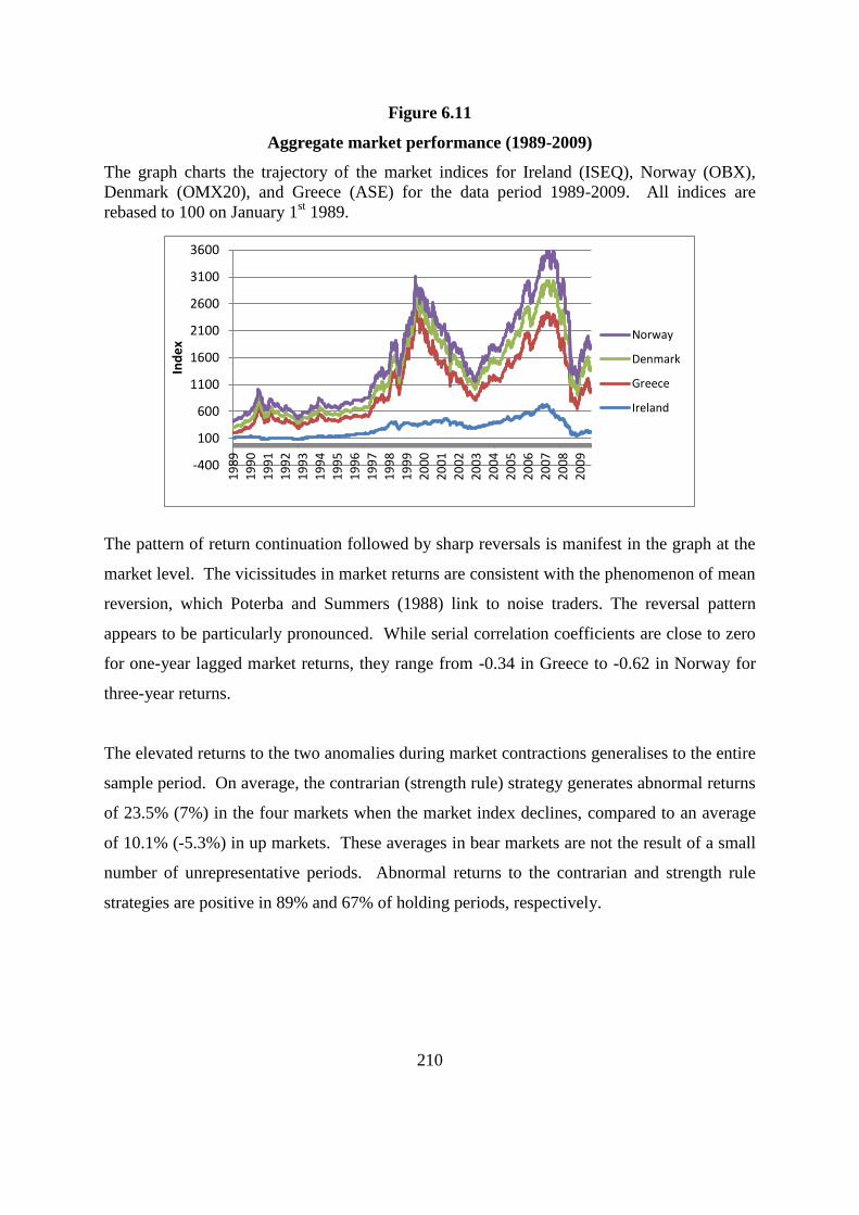
210
Figure 6.11
Aggregate market performance (1989-2009)
The graph charts the trajectory of the market indices for Ireland (ISEQ), Norway (OBX),
Denmark (OMX20), and Greece (ASE) for the data period 1989-2009. All indices are
rebased to 100 on January 1st 1989.
The pattern of return continuation followed by sharp reversals is manifest in the graph at the
market level. The vicissitudes in market returns are consistent with the phenomenon of mean
reversion, which Poterba and Summers (1988) link to noise traders. The reversal pattern
appears to be particularly pronounced. While serial correlation coefficients are close to zero
for one-year lagged market returns, they range from -0.34 in Greece to -0.62 in Norway for
three-year returns.
The elevated returns to the two anomalies during market contractions generalises to the entire
sample period. On average, the contrarian (strength rule) strategy generates abnormal returns
of 23.5% (7%) in the four markets when the market index declines, compared to an average
of 10.1% (-5.3%) in up markets. These averages in bear markets are not the result of a small
number of unrepresentative periods. Abnormal returns to the contrarian and strength rule
strategies are positive in 89% and 67% of holding periods, respectively.
-400
100
600
1100
1600
2100
2600
3100
3600
19
89
19
90
19
91
19
92
19
93
19
94
19
95
19
96
19
97
19
98
19
99
20
00
20
01
20
02
20
03
20
04
20
05
20
06
20
07
20
08
20
09
Ind
ex
Norway
Denmark
Greece
Ireland

211
Table 6.10 presents further details on the relationship between the abnormal returns to the
two trading strategies and market returns. Annual (three-year) market returns are regressed
on the returns for the strength rule (contrarian) strategy for each period.
Table 6.10
Relationship between anomalous returns and market returns
The table presents the coefficients in each country arising from regressions of market returns
on the contemporaneous abnormal returns to each strategy. Each coefficient is calculated
using returns from 20 (six) holding periods for the strength rule (contrarian strategy).
Strategy Ireland Greece Denmark Norway
Strength Rule -0.240 -0.099 -0.126 -0.557
R -0.45 -0.18 -0.15 -0.54
t-statistic -2.14** -0.78 -0.66 -2.71**
Contrarian -0.513 0.286 -0.300 0.105
R -0.96 0.51 -0.75 0.14
t-statistic -7.29* 1.19 -2.3** 0.28
* significant at the 1% level
** significant at the 5% level
*** significant at the 10% level
There is a negative correlation between strength rule returns and market returns in all four
markets. However, the relationship is only statistically significant in Ireland and Norway.
There is a high negative correlation between contrarian and market returns in Ireland and
Denmark, with a strong positive correlation in Greece and no distinct relationship in Norway.
In three of the four markets the results are similar when GNP or GDP is used instead of
market returns as there is a high correlation between these variables and market returns.
However, in Greece the correlation between market returns and economic growth is virtually
zero. The correlation between contrarian returns and GDP growth is -0.65, compared to
+0.51 in the case of market index returns.
The results pertaining to Ireland are in stark contrast with those of O’Sullivan and O’Sullivan
(2010) and O’ Donnell and Baur (2009), who find that momentum strategies in Ireland
generate more significant returns in periods of higher market growth. In general, the findings

212
relating to momentum are consistent with studies in international markets, such as, Griffin et
al. (2003) and Rey and Schmid (2007). However, they contradict the findings of researchers
such as Ismail (2012), Du et al. (2009), Cooper et al. (2004), who show that momentum
strategies only generate economically significant results in bull markets.
It is also of interest to examine the relationship between anomalous returns and lagged market
returns, following the approach of Cooper et al. (2004), as outlined in section 2.5. It is found
that contrarian returns are generally higher following bull markets in all countries except
Norway. The average correlation between contrarian returns and lagged market returns in
these three markets is 0.43 and average returns following bull and bear markets are 15.5%
and -16.6%, respectively111
. These findings directly contrast with those of Hirschey (2003),
Ismail (2012) and Chen et al. (2012), who find that contrarian returns are larger following
down markets in the US, Egypt, and China respectively. The results imply that investors
overreact to a greater extent to good news.
In contrast, there is no discernible pattern for momentum returns and lagged market returns in
any of the four markets. This suggests that behavioural models such as those developed by
Daniel et al. (1998) and Barberis et al. (2001) cannot fully explain momentum followed by
reversal, as such models predict that the returns to both momentum and contrarian strategies
will be larger following bull markets due to the increased overconfidence and reduced risk
aversion that accompany greater wealth.
In one important respect the results of this study differ from those of Cooper et al. (2004) and
lend support to the behavioural explanations of the two anomalies. There is a strong positive
relationship between contrarian returns and lagged momentum returns in two of the three
markets that exhibit significant return reversals (Greece and Denmark). It thus seems that
return reversals may be the result of an unwinding of previous momentum, consistent with
the overreaction hypothesis.
111
The dichotomy in the relationships between anomalous returns and contemporaneous and lagged market
returns is to be expected given the negative serial correlation in market returns, as outlined earlier in this section.

213
6.5.3 Sub-period analysis
The out-of-sample returns are derived from a relatively small number of holding periods.
Thus, the results from the main data period may be more robust. In addition to analysing the
average returns to each strategy, it is instructive to examine number of sub-periods in which
each strategy generates positive excess abnormal returns.
This is the second test for the robustness of the results. It is of importance because although a
strategy may perform well on average, such a result may be skewed by one sub-period in
which the strategy performs extremely well. It could be expected that by pure chance alone,
in an efficient market, each strategy would succeed 50% of the time112
. A significantly
higher percentage than this may provide further evidence of a violation of the EMH.
The contrarian strategy generates positive abnormal returns in 89% of holding periods in
Greece, with success rates of 67% in Denmark and Norway. The contrarian strategy
implemented in the second holding year generates positive returns in 78, 72, and 72% of the
holding periods in Greece, Denmark, and Norway, respectively. The strategy generates
abnormal returns in less than two-fifths of holding periods in Ireland, providing further
evidence of the propensity for return continuation in Ireland.
The 9,3 momentum strategy in Ireland generates positive abnormal returns in approximately
83% of holding periods. The strength rule generates positive returns in Greece in only 28%
of holding periods, adding further weight to the findings outlined in section 6.2. The
propensity towards reversals is so pronounced that a contrarian strategy generates positive
abnormal returns in the majority of one-year holding periods, a time-frame over which
continuation is more generally observed. These results show that the anomalous evidence
presented in section 6.2 is not attributable to a small number of unusually high and
unrepresentative sub-periods.
112
Recall that for the market to be efficient it is not necessary that no strategy is profitable; merely that one
cannot predict ex ante which strategy will succeed.

214
6.5.4 Firm-level dynamics
The final robustness test examines abnormal returns at the firm level. In theory, the
contrarian investment strategy could be profitable because one stock switches from being a
winner to a loser and vice versa. The opposite is true for strength rule returns. This section
thus tests whether any positive excess abnormal returns are due to the dynamics of a small
number of stocks. This gives an insight into whether one would expect the strategy to be
profitable in the future or whether large returns are caused by events unlikely to be repeated.
The results that follow relate to the basic strategy in each market.
It may be expected that each stock has a 50% chance of remaining within the winner or loser
portfolio over successive ranking periods. Table 6.11 details the percentage of stocks that
move from (remain within) portfolios when examining contrarian (strength rule) strategy,
with the associated z-score in parentheses for the one-tailed test that the average proportion is
significantly greater than the hypothesised value of 50%.
Table 6.11
Movement of shares between winner and loser portfolios
The table reports the percentage of shares switching (remaining within) portfolios for the
contrarian strategy (strength rule). The figures are the average of five (17) holding periods
with z-scores in parentheses.
Contrarian Ireland Greece Norway Denmark
Percentage moving 49.2 64.9* 54.8** 49.8
(-0.22) (5.34) (1.85) (-0.06)
Strength rule Ireland Greece Norway Denmark
Percentage staying 53.9* 44.6* 50.2 50.5
(2.63) (-2.94) (0.11) (0.24)
* significant at the 1% level
** significant at the 5% level
The results show that the significant contrarian returns in Greece are not driven by the
dynamics of a small number of stocks. Instead, there is a marked tendency for stocks to
switch portfolio, even with the strength rule and its one-year rank periods. There is also

215
evidence of a tendency for stocks to switch portfolios in Norway over three-year holding
periods and evidence of return persistence in Ireland. In all other cases, the proportion of
stocks moving or staying is not statistically different from the hypothesised value of 50%.
The robustness of the above results can be further examined using a non-parametric
technique based on 2x2 contingency tables and the cross-product (or log-odds) ratio, as
employed by Brown and Goetzmann (1995) in measuring persistence in mutual fund
performance113
.
Stocks are ranked as winners (W) or losers (L) in consecutive periods, giving four possible
combinations over each pair of periods. Continuation exists when a stock is a winner or loser
in consecutive periods (WW and LL respectively), while reversal occurs when a stock
alternates between being a winner and loser (WL and LW). The number of stocks falling into
each category is recorded and the cross-product ratio calculated as:
Cross-product ratio =
(6.1)
The inverse of the above equation is used when testing the contrarian investment strategy and
the propensity of stocks to move from one portfolio to another. In both cases, under the null
hypothesis of no serial correlation in returns the cross-product ratio will equal one. A ratio
significantly greater than one rejects the null hypothesis, thereby suggesting significant
structure (serial correlation) in the ranking of returns.
The statistical significance is estimated by scaling the log of the cross-product ratio by its
standard error, which is estimated as:
√(
) (
) (
) (
)
113
Building on the work of Brown et al. (1992) and Goetzmann and Ibbotson (1994).
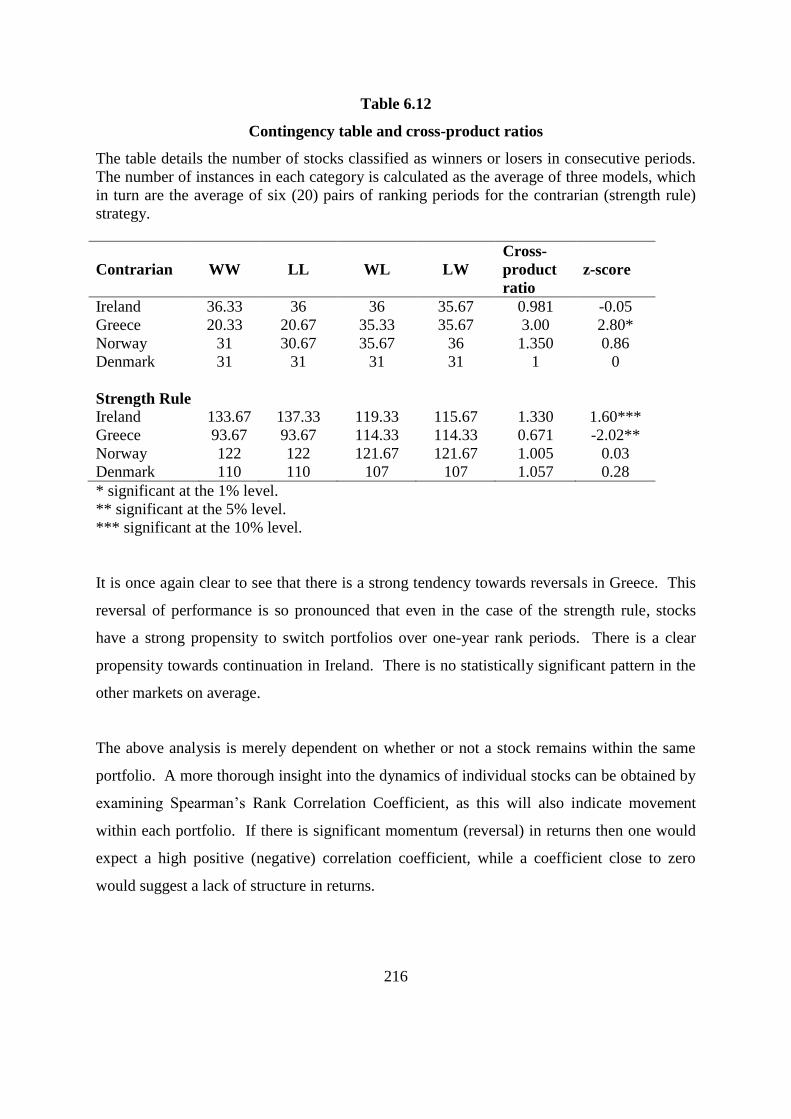
216
Table 6.12
Contingency table and cross-product ratios
The table details the number of stocks classified as winners or losers in consecutive periods.
The number of instances in each category is calculated as the average of three models, which
in turn are the average of six (20) pairs of ranking periods for the contrarian (strength rule)
strategy.
Contrarian WW LL WL LW
Cross-
product
ratio
z-score
Ireland 36.33 36 36 35.67 0.981 -0.05
Greece 20.33 20.67 35.33 35.67 3.00 2.80*
Norway 31 30.67 35.67 36 1.350 0.86
Denmark 31 31 31 31 1 0
Strength Rule
Ireland 133.67 137.33 119.33 115.67 1.330 1.60***
Greece 93.67 93.67 114.33 114.33 0.671 -2.02**
Norway 122 122 121.67 121.67 1.005 0.03
Denmark 110 110 107 107 1.057 0.28
* significant at the 1% level.
** significant at the 5% level.
*** significant at the 10% level.
It is once again clear to see that there is a strong tendency towards reversals in Greece. This
reversal of performance is so pronounced that even in the case of the strength rule, stocks
have a strong propensity to switch portfolios over one-year rank periods. There is a clear
propensity towards continuation in Ireland. There is no statistically significant pattern in the
other markets on average.
The above analysis is merely dependent on whether or not a stock remains within the same
portfolio. A more thorough insight into the dynamics of individual stocks can be obtained by
examining Spearman’s Rank Correlation Coefficient, as this will also indicate movement
within each portfolio. If there is significant momentum (reversal) in returns then one would
expect a high positive (negative) correlation coefficient, while a coefficient close to zero
would suggest a lack of structure in returns.

217
Table 6.13 details the average rank correlation coefficient for each country and model. The
average for each model is derived from six (20) pairs of rank periods for the contrarian
(momentum) strategy. As correlation coefficients are not additive, it is necessary to
transform the coefficients into Fisher Z values using equation (6.3).
[
]
These Z values are then averaged and the Fisher Weighted Mean Correlation Coefficient, is
computed as:
The statistical significance of can be estimated using:
√
Table 6.13
Average rank correlation coefficient
The table details the average rank correlation coefficient for both strategies with t-statistics in
parentheses. The figure for each model and country represents the mean coefficient of six
(20) pairs of rank periods for the contrarian (momentum) strategy after converting
coefficients to Fisher Z values.
Ireland Greece Norway Denmark
Contrarian 0.095 -0.385** -0.181 -0.064
(0.47) (-2.05) (-0.91) (-0.32)
Strength Rule 0.121 -0.146 0.043 0.052
(0.59) (-0.73) (0.21) (0.25)
** significant at the 5% level

218
The large and significant negative coefficient in Greece violates the null hypothesis that
consecutive rankings are independent of each other. In Greece the rank correlation
coefficient was of the expected sign in 17 of the 18 contrarian paired rank periods and was
also negative in 35 of the 60 paired rank periods for the momentum strategy. There is no
distinct and significant pattern in the other markets.
Taken together, the results in this section provide a clearer picture of the robustness of return
reversals. For each of the three measures, the evidence is consistent with the ranking of
reversals outlined in the preceding sections. The most robust evidence relates to Greece,
where there is a marked tendency for stocks to move from one portfolio to another. The
strength rule returns in Ireland are also robust. The evidence in Norway is less robust, while
the results suggest that the contrarian returns in Denmark are driven by extreme reversals of a
relatively small group of stocks.
Further analysis shows that the firms that comprise the winner and loser portfolios do not
systematically and significantly differ on key firm-specific characteristics such as firm size,
share price, and beta. This suggests that the anomalous returns in this chapter are not driven
by risk, or microstructure biases, such as bid-ask spread and illiquidity.
6.6 Conclusion
This chapter examines the returns to contrarian investment and strength rule strategies in four
medium-sized European markets using three models with varying degrees of sophistication in
their treatment of risk. Significant and robust evidence of structure in returns is presented in
violation of the null hypothesis of market efficiency.
The contrarian strategy generates positive excess abnormal returns in three of the four
markets. The most economically and statistically significant returns are in Greece, where
return reversals result in average excess abnormal contrarian returns of 40.7% over a three-
year holding period. It is shown that excess abnormal returns can be enriched via the use of
various holding periods and by focusing on extreme stocks. In general, average monthly

219
abnormal returns increase with longer rank and holding periods. The high returns to the
strategy using six-month rank periods in Greece and Norway are notable exceptions and
contradict the characteristic finding of medium-term continuation in the literature.
Perhaps the most robust and lucid finding is the tendency towards return reversals in the
second year following portfolio formation. A contrarian investment strategy implemented in
year two alone generates consistent and economically significant excess abnormal returns, as
it profits from stylised finding of momentum followed by reversal. The returns to such a
strategy are particularly striking when portfolios are constructed with extreme stocks.
Ireland is the only country where significant strength rule returns are consistently observed.
The optimum strategy involves ranking stocks over nine months and implementing the
momentum strategy for approximately two months. The superiority of a relatively short
holding period is consistent with the findings of key momentum studies such as Jegadeesh
and Titman (1993) and Rouwenhorst (1998). However, the nine-month rank period contrasts
with the 12-month period that is found to be optimal in such studies. The negative returns to
the portfolio of past losers suggest that return continuation in Ireland is not confined to past
winners.
The role of risk does not appear to be as important as stated in previous research, such as
Chan (1988). Although in some cases the use of the CAPM reduces abnormal returns it does
not do so to such an extent that it can be cited as a major explanatory variable in the large
returns. Furthermore, the abnormal returns cannot be explained by microstructure biases,
macroceconomic risk, and short-selling constraints. Moreover, the anomalous evidence is
robust to out-of-sample testing, is not attributable to the dynamics of a small number of
stocks, and is not limited to a small number of holding periods with disproportionately large
abnormal returns.
A number of noteworthy seasonal patterns emerged in this chapter. Abnormal returns are
positive in January, April and May and negative in September in all four markets. However,
in all markets excess abnormal returns remain significant when such months are omitted.

220
Therefore, one can conclude that the anomalous returns presented in this chapter are more
than mere manifestations of seasonal anomalies. Both strategies generate particularly
elevated abnormal returns during economic downturns and contrarian returns tend to be more
significant following market upturns. The latter finding presents a potentially useful ex ante
trading strategy.
It is noteworthy that the most significant anomalous returns are observed in Greece and
Ireland. These are the two smaller markets in the sample and they suffered to the greatest
extent in the stock market crashes at the time of the global financial crisis. This finding may
support the assertion of Dreman and Lufkin (2000, p.61) that overreaction “can be the major
cause of financial bubbles and panics”. The finding may also point towards an important role
for noise traders, as Palomino (1996) shows that such traders are more likely to survive in
small markets. As there was no dominant industry in Ireland or Greece (see section 5.2.1), it
appears that the anomalous returns are not attributable to industry momentum or reversal, or
cross-sectional dependence in firm’s returns.
In summary, the evidence in this chapter provides out-of-sample confirmation of the validity
of return continuation and reversal and casts further doubt on standard finance theory’s
assumption of market efficiency. Rational explanations are incapable of fully accounting for
the significant abnormal returns presented in this chapter. The next chapter examines
whether brokers play an important role in explaining this anomalous evidence.

221
Chapter Seven
Broker Findings and Discussion
7.1 Introduction
This chapter discusses the findings of tests relating to brokers’ output. Three principal forms
of such output are analysed; price forecasts, EPS forecasts, and the overall recommendation
category. It is important at the outset to a make a clear distinction between the terms used to
describe these three forms of prognostication made by brokers. The term ‘forecast’
specifically refers to EPS forecasts, while ‘target’ is used for brokers’ price target and
‘recommendation’ is used to describe the overall recommendation category. Existing
research tends to focus on one of the above three variables. This thesis examines the
interaction between the variables in order to obtain a more complete picture of the value,
veracity, and impact of brokers’ output. There is also a sharp focus on the relationship
between brokers’ output and return momentum.
The output of brokers is examined along three temporal dimensions. First, contemporaneous
targets and recommendations are analysed in order to ascertain whether brokers’ advice is
consistent with their predictions. Measures of herding and optimism are also examined.
Second, brokers’ output is compared to past variables, such as momentum, size, and book-to-
market value, in order to provide an insight into whether brokers follow momentum or value
strategies. Finally, the value and impact of brokers’ output is examined by comparing targets
and recommendations with future abnormal returns and volume. The absolute level of
brokers’ output is analysed, along with revisions to target prices and recommendation levels.
Furthermore, a comparison is drawn between Irish and non-Irish brokerage firms, as it is
hypothesised that the former are more prone to conflicts of interest.
The remainder of this chapter is structured as follows. Section 7.2 examines recommendation
levels; price and EPS forecasts are analysed in sections 7.3 and 7.4, respectively. Section 7.5
examines the firm-specific characteristics of stocks that analysts recommend favourably. The

222
price and volume impacts of brokers’ output are discussed in section 7.6 and section 7.7
draws conclusions.
7.2 Findings
This section presents the findings relating to the nature of recommendations. The number of
recommendations falling into each of the five categories is analysed and measures that
capture the level of analyst optimism and herding are presented. The responsiveness of
analysts in terms of recommendation revisions is also examined and any differences between
Irish brokers and their international counterparts are highlighted.
7.2.1 Recommendation categories
Table 7.1 and figure 7.1 present statistics on the frequency of recommendations by category.
Each of the 70,794 recommendations is assigned to one of the five categories using the
coding system outlined in table 5.5. It is clear that there is a significant positive bias in
recommendations and Irish brokers are considerably more optimistic in their outlook than
non-Irish brokers.
The overall level of optimism is significantly higher for brokers covering Irish stocks than in
the existing literature covering a variety of markets. However, the most striking aspect of
table 7.1 is the stark contrast between Irish brokers and their international counterparts. As
predicted by the conflicts of interest literature, the home-based analysts exhibit a higher level
of optimism. Remarkably, one Irish broker issued 8,088 recommendations with only 83
‘reduce’ and zero ‘sell’ recommendations.

223
Table 7.1
Percentage of recommendations by category
Panel A reports the percentage of recommendations falling into each of the five categories (N
= 70,794). Panel B reports the ratio of positive (buy and add) to negative (reduce and sell)
recommendations and the ratio of buy-to-sell recommendations.
Panel A: Recommendations by category
Category All % Irish % Non-Irish %
Buy 27,321 38.58 11,724 55.70 15,597 31.35
Add 16,868 23.83 5,271 25.04 11,597 23.31
Hold 21,050 29.74 3,348 15.91 17,702 35.58
Reduce 3,597 5.08 652 3.10 2945 5.92
Sell 1,958 2.77 53 0.25 1905 3.83
Total 70,794 100 21,048 100 49,746 100
Panel B: Recommendation ratios
Broker Positive-to-negative Buy-to-Sell
All 7.95 13.95
Irish 24.10 221.21
Others 5.61 8.19
Figure 7.1
Percentage of recommendations by category
The chart shows the breakdown of recommendations by category using the coding system
outlined in table 5.5.
0.00
10.00
20.00
30.00
40.00
50.00
60.00
70.00
80.00
90.00
100.00
Irish Non-Irish
%
Buy
Add
Hold
Reduce
Sell
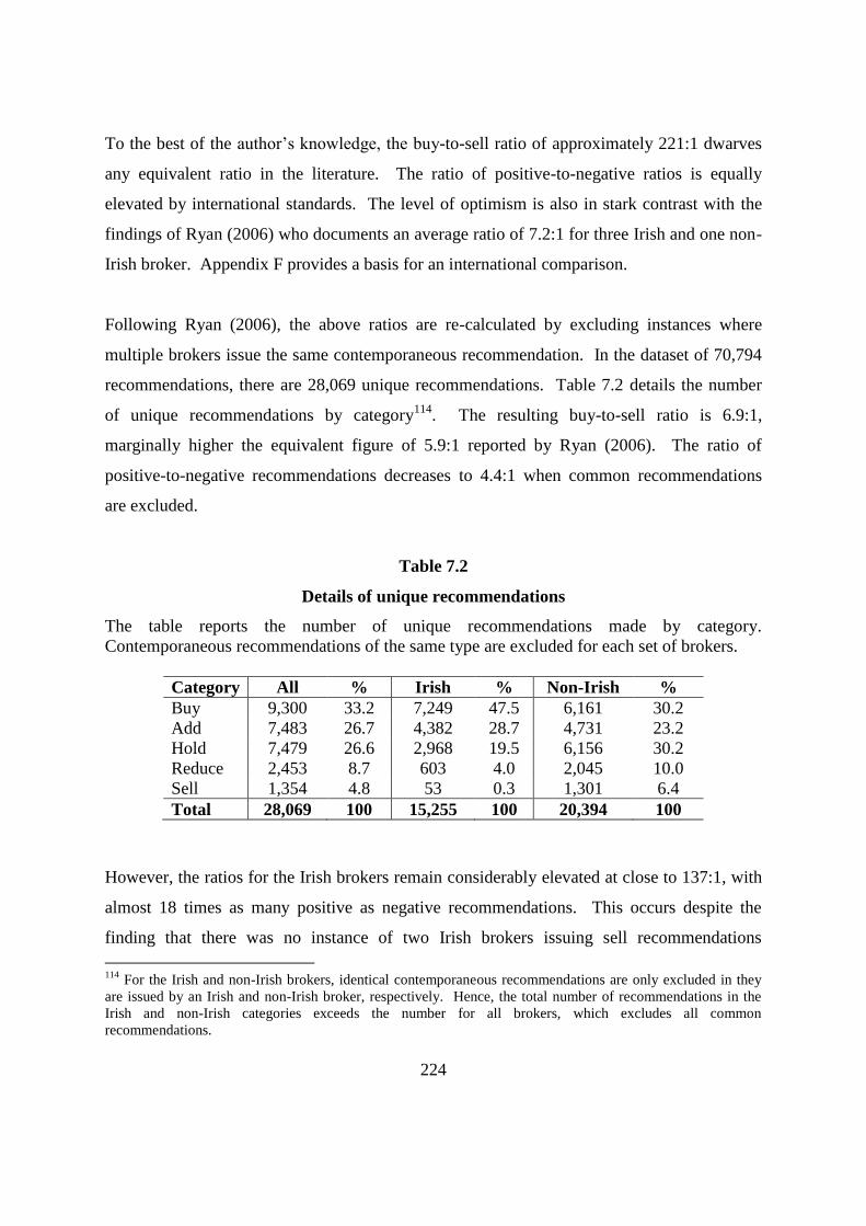
224
To the best of the author’s knowledge, the buy-to-sell ratio of approximately 221:1 dwarves
any equivalent ratio in the literature. The ratio of positive-to-negative ratios is equally
elevated by international standards. The level of optimism is also in stark contrast with the
findings of Ryan (2006) who documents an average ratio of 7.2:1 for three Irish and one non-
Irish broker. Appendix F provides a basis for an international comparison.
Following Ryan (2006), the above ratios are re-calculated by excluding instances where
multiple brokers issue the same contemporaneous recommendation. In the dataset of 70,794
recommendations, there are 28,069 unique recommendations. Table 7.2 details the number
of unique recommendations by category114
. The resulting buy-to-sell ratio is 6.9:1,
marginally higher the equivalent figure of 5.9:1 reported by Ryan (2006). The ratio of
positive-to-negative recommendations decreases to 4.4:1 when common recommendations
are excluded.
Table 7.2
Details of unique recommendations
The table reports the number of unique recommendations made by category.
Contemporaneous recommendations of the same type are excluded for each set of brokers.
Category All % Irish % Non-Irish %
Buy 9,300 33.2 7,249 47.5 6,161 30.2
Add 7,483 26.7 4,382 28.7 4,731 23.2
Hold 7,479 26.6 2,968 19.5 6,156 30.2
Reduce 2,453 8.7 603 4.0 2,045 10.0
Sell 1,354 4.8 53 0.3 1,301 6.4
Total 28,069 100 15,255 100 20,394 100
However, the ratios for the Irish brokers remain considerably elevated at close to 137:1, with
almost 18 times as many positive as negative recommendations. This occurs despite the
finding that there was no instance of two Irish brokers issuing sell recommendations
114
For the Irish and non-Irish brokers, identical contemporaneous recommendations are only excluded in they
are issued by an Irish and non-Irish broker, respectively. Hence, the total number of recommendations in the
Irish and non-Irish categories exceeds the number for all brokers, which excludes all common
recommendations.

225
contemporaneously. Thus, the number of unique sell recommendations equals the total
number of sell recommendations. The equivalent ratios for international brokers decrease to
4.7 and 3.3 respectively.
Another aspect of the advice given by brokers is their reluctance to use the word ‘sell’. In the
sample used in this study 26 out of 77 (34%) brokers do not explicitly use the word ‘sell’ for
their lowest recommendation category. Instead phrases such as ‘underperform’, ‘reduce’ and
‘underweight’ are attached to the most negative ratings. This is similar to the 30% reported
by Ho and Harris (1998). The above figure is biased downwards, as 30 of the brokers (40%)
did not issue any negative recommendations. It is thus not possible to ascertain the exact
terminology that such brokers use to communicate their most negative rating.
7.2.2 Optimism index
The statistics on the number of recommendations in each category can be used to calculate an
optimism index for Irish and non-Irish brokers. The index is calculated as the average value
of all recommendations for each set of brokers. Recommendations are coded from sell =1 to
buy =5 as detailed in table 5.5. The overall average optimism index is 3.90 for all brokers
and 4.32 (3.73) for Irish (non-Irish) brokers. The t-statistic for the difference in means of
Irish and non-Irish brokers is 3.67, suggesting that Irish brokers are considerably more
optimistic than their international counterparts.
It appears that regulations in Europe have not resulted in a marked decrease in optimism bias.
This contrasts with the evidence relating to the US. For example, Barber et al. (2006) report
a significant decline in the percentage of buy recommendations after the introduction of
NASD rule 2711. The figures reported here for non-Irish brokers are in line with those
reported in Jegadeesh et al. (2004) for the U.S, where the mean consensus level ranges from
3.21 to 3.97 and averages 3.67. Figure 7.2 plots the weekly optimism index for Irish and
non-Irish brokers.
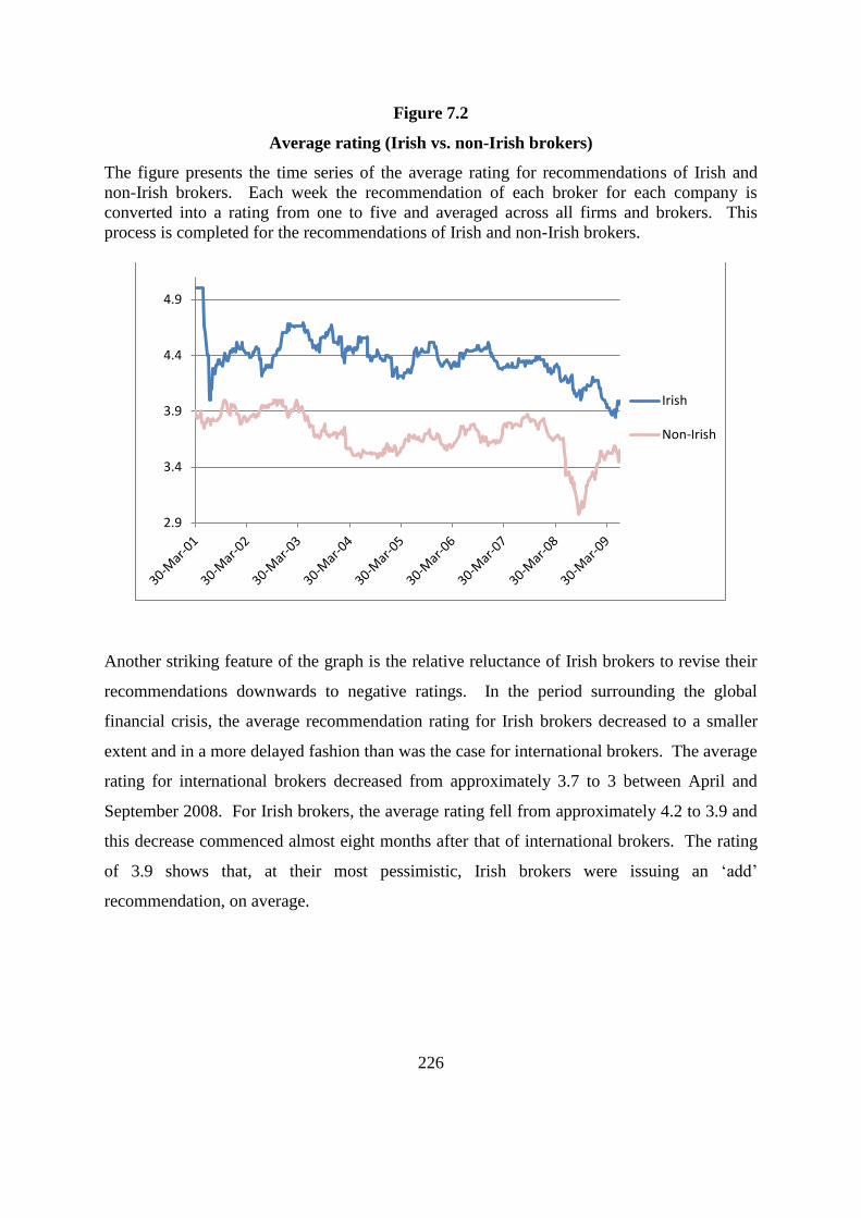
226
Figure 7.2
Average rating (Irish vs. non-Irish brokers)
The figure presents the time series of the average rating for recommendations of Irish and
non-Irish brokers. Each week the recommendation of each broker for each company is
converted into a rating from one to five and averaged across all firms and brokers. This
process is completed for the recommendations of Irish and non-Irish brokers.
Another striking feature of the graph is the relative reluctance of Irish brokers to revise their
recommendations downwards to negative ratings. In the period surrounding the global
financial crisis, the average recommendation rating for Irish brokers decreased to a smaller
extent and in a more delayed fashion than was the case for international brokers. The average
rating for international brokers decreased from approximately 3.7 to 3 between April and
September 2008. For Irish brokers, the average rating fell from approximately 4.2 to 3.9 and
this decrease commenced almost eight months after that of international brokers. The rating
of 3.9 shows that, at their most pessimistic, Irish brokers were issuing an ‘add’
recommendation, on average.
2.9
3.4
3.9
4.4
4.9
Irish
Non-Irish

227
7.2.3 Recommendation revisions
The previous sub-section tentatively suggests that Irish analysts are slow to revise their
recommendations downwards. Table 7.3 outlines the number of revisions based on the
original and new recommendation category. In total, there were 582 downgrades (53%) and
512 upgrades (47%)115
. Approximately 1.5% of recommendations are revisions, suggesting
that analysts covering Irish stocks are considerably more reluctant to revise their
recommendations than those covering stocks in the US. For example, Elton et al. (1986)
report 3,433 revisions in 30,391 recommendations, yielding a revision rate of approximately
11.3%. With five recommendation categories there are 20 possible revision combinations.
Any revisions to the left (right) of the main diagonal are upgrades (downgrades).
Table 7.3
Recommendation revisions
The table outlines the number of revisions based on the original and new recommendation
category.
New
Buy Add Hold Reduce Sell Total %
Buy 160 185 10 7 362 33
Add 161 103 21 2 287 26
Original Hold 160 82 45 40 327 30
Reduce 9 19 31 9 68 6
Sell 6 1 38 5 50 5
Total 336 262 357 81 58 1,096 -
% 31 24 33 7 5 - 100
The above table reiterates the clear reluctance of analysts to revise recommendations
downwards to the two negative ratings. The majority of revisions (55%) are of one degree,
with 42% of revisions moving by two degrees and 2% and 1% moving by three and four
degrees, respectively. These percentages are the same for upgrades and downgrades. The
proportion of multi-level changes is considerably higher than the 10 and 30% reported in Ho
and Harris (1998) and Stickel (1995), respectively. The significantly larger proportion of
115
See appendix G for comparable statistics from other studies.

228
downgrades from hold to sell compared to reduce to sell may be consistent with prospect
theory. If a broker risks antagonising a covered company by downgrading their stock to a
negative rating, then prospect theory (hedonic framing) suggests that such bad news should
be released in one step rather than drip fed to the market.
The reluctance to revise recommendations manifests itself in extended runs of consecutive
recommendations of the same category. Table 7.4 presents statistics on the number of weeks
over which recommendations remained unchanged.
Table 7.4
Recommendation runs
The table contains summary statistics on the number of consecutive weeks during which
recommendation levels remained unchanged, i.e. the length of recommendation runs. All
measures are in weeks except for ‘runs’, which details the number of runs for each category.
Sell Reduce Hold Add Buy Overall
Runs 76 110 531 435 591 1743
Maximum 156 158 262 297 305 305
Mean 25.9 33.2 24.8 38.7 46.2 40.6
Median 18 25 26 25 30 27
SD 27.8 32.0 39.8 40.9 48.8 42.8
It can be seen that recommendation levels are sticky, and this inertia tends to increase as
recommendation levels become more positive, where the maximum unbroken sequence is
almost six years116
. The overall mean run of 40.6 weeks connotes a conspicuous reluctance
to revise forecasts on the part of brokers. It presages that analysts do not believe that news is
quickly impounded into prices, unless there is a remarkable run of positive serial correlation
in news. The long sequence of unchanged recommendations may imply that analysts follow
momentum strategies. This will be examined in greater detail in section 7.5. Table 7.5
presents the mean (median) number of weeks over which recommendations remained
unchanged following revisions of different types.
116
The minimum run is one week for all recommendation categories.

229
Table 7.5
Average sequences following upgrades and downgrades
The table presents the mean (median) number of weeks of consecutive recommendations of
the same type following upgrades and downgrades of various degrees.
New
Buy Add Hold Reduce Sell
Buy 34.4 (19) 38.8 (23) 18.8 (19.5) 18.1 (20)
Add 44.4 (25) 42.3 (29) 47 (26) 8.5 (8.5)
Original Hold 37.9 (25) 41.6 (29.5) 28.4 (21) 21.6 (16.5)
Reduce 18.2 (20) 29.2 (25) 34 (24) 17 (8)
Sell 26.8 (26) 3 (3) 23.3 (17.5) 25.6 (24)
The table shows that revisions to negative categories are generally left unchanged for a
shorter period of time. In general, Irish brokers are more responsive than international
brokers. This result is entirely driven by their tendency to leave negative ratings unchanged
for shorter periods of time. On average, recommendations remain unchanged for 38 weeks
following upgrades and 36 weeks subsequent to downgrades. The difference is larger for
Irish brokers (37 versus 30 weeks) than non-Irish brokers (39 versus 38 weeks).
In summary, it appears that Irish brokers are considerably more optimistic than their
international counterparts. They are more reluctant to downgrade recommendations to
negative ratings and leave such recommendations unchanged for a relatively short time.
These findings represent more concrete evidence than Ryan’s (2006) interpretation of the
significant negative pre-revision abnormal returns to sell recommendations as evidence of
Irish analysts’ reluctance to downgrade recommendations, possibly due to conflicts of
interest.
7.3 Target price
The target price issued by brokers is the second form of output analysed. This variable is
examined in three ways. First, the accuracy of the forecasts is analysed by calculating
forecast errors. Second, the dispersion of forecasts is examined in order to measure analyst
herding. Finally, target prices are compared to recommendation levels in order to ascertain

230
whether brokers’ messages are consistent in terms of these two measures of their opinions of
a firm’s prospects.
The elevated optimism of Irish brokers is evidenced again. On average, the target price
issued by Irish brokers is 12.5% higher than the forecast of international brokers. The
average target price for Irish brokers exceeds the international average for 17 of the 22
companies for which both sets of brokers issue forecasts.
7.3.1 Forecast accuracy
Following the customary approach of existing studies of brokers’ output, the accuracy of
price forecasts is analysed by calculating the forecast error of each analyst i, for firm j, at
time t (FEijt) as:
1jt
1jtijt
ijtP
P - FFE
* 100 (7.1)
where: Fijt is the forecast of analyst i, for firm j, at time t.
Pjt+1 is the actual price of firm j, one year later.
On average, consensus forecasts are almost 89% higher than the resulting price, implying
strikingly unjustified optimism on the part of brokers. Irish brokers are more optimistic than
international analysts with the average price one year after forecasts being 95% lower than
the forecasted price. These figures are considerably higher than the equivalent figure of 28%
reported in Brav and Lehavy (2003). An analysis of price forecasts also shows that Irish
brokers have a greater tendency to herd than their international counterparts. The average
coefficient of variation for Irish and non-Irish brokers are 0.115 and 0.158, respectively (t-stat
for differences in means = 4.06).
The high level of herding by Irish brokers may explain the optimistic nature of their forecasts
and the significant momentum returns in Ireland, as outlined in section 6.2. Olsen (1996)

231
shows that herding leads to an increase in the mean forecast, as analysts tend to herd their
optimistic forecasts more often. Furthermore, Du and McEnroe (2011) show that investors
are more confident when they receive multiple earnings forecasts with no variability and
Welch (2000) shows that herding leads to momentum.
7.3.2 Recommendation level vs. target price
This section examines whether analysts’ recommendations and target prices present a
consistent picture of their opinions of the prospects of a firm. Kerl and Walter (2008) discuss
the recent change in the recommendation categories used by brokers. Banks generally tended
to use a five-category scheme for their recommendations, i.e., strong buy, buy, hold, sell, and
strong sell. However, in 2002, Lehman Brothers, Morgan Stanley and Goldman Sachs
changed to a three-category rating; (overweight, equal-weight, underweight) and most
investment banks followed suit (Bradley et al., 2003).
Having a limited number of discrete recommendation categories reduces the degrees of
freedom. Naturally, the strength of recommendations relating to stocks that fall into the same
category may differ significantly before the point at which one crosses the boundary into the
next recommendation category. This limitation is accentuated by the fact that the negative
recommendation categories are rarely used, as outlined in section 7.2.1.
In order to overcome this, an index is calculated measuring the expected change in share
price implied by a price forecast. This continuous data allows more scope for analysing
cross-sectional variation in the strength of the recommendation and its impact on share prices.
The anticipated percentage change in share price is calculated as the difference between the
forecasted and current share price divided by the current price and multiplied by 100.
100*P
P - FE
jt
jt1ijt ijt (7.2)
where: E∆ijt is the anticipated change in price forecast by analyst i, for firm j, at time t.

232
Fijt+1 is the forecast of analyst i, for firm j, for the next period.
Pjt is the current price of firm j.
The precise meaning of each category in terms of the associated expected change in price
varies by broker. This study adopts the most common approach of brokers in this dataset, as
detailed in table 7.6.
Table 7.6
Consensus recommendation levels and price targets
The table presents the average expected price change calculated by comparing brokers’ target
prices with the current price of each firm. The expected changes are allocated to bands and
compared to the overall recommendation categories.
Expected
price change
# % Recommendation
category
# %
15%+ 3,739 47.52 Buy 27,321 38.59
5 to 15% 1,553 19.74 Add 16,868 23.83
-5 to 5% 1,273 16.18 Hold 21,050 29.73
-5 to -15% 420 5.34 Reduce 3,597 5.08
-15% + 883 11.22 Sell 1,958 2.77
Total 7,868 100 Total 70,794 100
The general pattern is that price forecasts tend to fall into the extreme ratings more often than
recommendation levels. In terms of negative forecasts, one may suspect that forecasted
prices are more reflective of the broker’s view on the firm’s prospects. Perhaps brokers are
more willing to issue a forecast that implies selling a stock than they are to issue a report
explicitly containing the word ‘sell’. Figure 7.3 presents a graphical comparison of price
forecasts and recommendation categories.
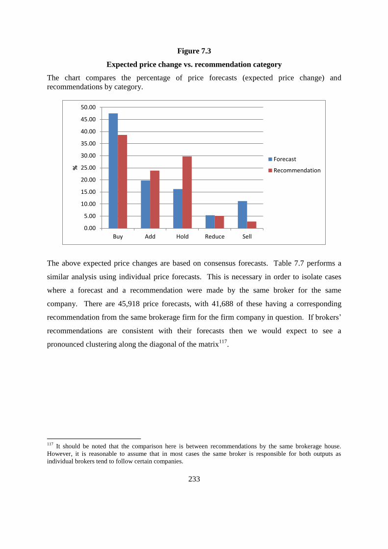
233
Figure 7.3
Expected price change vs. recommendation category
The chart compares the percentage of price forecasts (expected price change) and
recommendations by category.
The above expected price changes are based on consensus forecasts. Table 7.7 performs a
similar analysis using individual price forecasts. This is necessary in order to isolate cases
where a forecast and a recommendation were made by the same broker for the same
company. There are 45,918 price forecasts, with 41,688 of these having a corresponding
recommendation from the same brokerage firm for the firm company in question. If brokers’
recommendations are consistent with their forecasts then we would expect to see a
pronounced clustering along the diagonal of the matrix117
.
117
It should be noted that the comparison here is between recommendations by the same brokerage house.
However, it is reasonable to assume that in most cases the same broker is responsible for both outputs as
individual brokers tend to follow certain companies.
0.00
5.00
10.00
15.00
20.00
25.00
30.00
35.00
40.00
45.00
50.00
Buy Add Hold Reduce Sell
%
Forecast
Recommendation
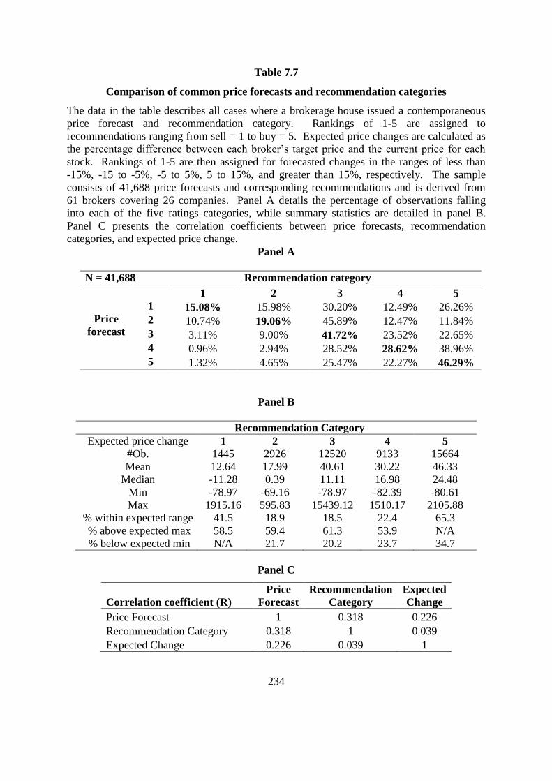
234
Table 7.7
Comparison of common price forecasts and recommendation categories
The data in the table describes all cases where a brokerage house issued a contemporaneous
price forecast and recommendation category. Rankings of 1-5 are assigned to
recommendations ranging from sell = 1 to buy = 5. Expected price changes are calculated as
the percentage difference between each broker’s target price and the current price for each
stock. Rankings of 1-5 are then assigned for forecasted changes in the ranges of less than
-15%, -15 to -5%, -5 to 5%, 5 to 15%, and greater than 15%, respectively. The sample
consists of 41,688 price forecasts and corresponding recommendations and is derived from
61 brokers covering 26 companies. Panel A details the percentage of observations falling
into each of the five ratings categories, while summary statistics are detailed in panel B.
Panel C presents the correlation coefficients between price forecasts, recommendation
categories, and expected price change.
Panel A
N = 41,688 Recommendation category
1 2 3 4 5
Price
forecast
1 15.08% 15.98% 30.20% 12.49% 26.26%
2 10.74% 19.06% 45.89% 12.47% 11.84%
3 3.11% 9.00% 41.72% 23.52% 22.65%
4 0.96% 2.94% 28.52% 28.62% 38.96%
5 1.32% 4.65% 25.47% 22.27% 46.29%
Panel B
Recommendation Category
Expected price change 1 2 3 4 5
#Ob. 1445 2926 12520 9133 15664
Mean 12.64 17.99 40.61 30.22 46.33
Median -11.28 0.39 11.11 16.98 24.48
Min -78.97 -69.16 -78.97 -82.39 -80.61
Max 1915.16 595.83 15439.12 1510.17 2105.88
% within expected range 41.5 18.9 18.5 22.4 65.3
% above expected max 58.5 59.4 61.3 53.9 N/A
% below expected min N/A 21.7 20.2 23.7 34.7
Panel C
Correlation coefficient (R)
Price
Forecast
Recommendation
Category
Expected
Change
Price Forecast 1 0.318 0.226
Recommendation Category 0.318 1 0.039
Expected Change 0.226 0.039 1

235
Table 7.8 provides a brief summary of the relationship between ratings and target prices for
Irish and non-Irish brokers.
Table 7.8
Comparison of recommendation levels and target prices
The table presents the average of the 1-5 ratings attached to target prices (μT) and the average
of the 1-5 ratings obtained by coding the overall recommendations (μR). The sample
comprises the 41,688 pairs of contemporaneous target prices and recommendations. The z-
scores relate to the difference in means with p-values in parentheses.
Broker # Obs μT μR z-score
Irish 12,622 3.97 4.34 39.2 (0.00)
Non-Irish 29,066 3.97 3.61 19.5 (0.00)
All 41,688 3.97 3.83 29.7 (0.00)
The evidence suggests that there is a pronounced disconnect between what brokers forecast
and what they recommend. The difference in means is significant for all sets of brokers and
it is clear that Irish brokers’ recommendations tend to be more positive than their price
forecasts. Overall, only approximately 38% of recommendations are in the category implied
by the brokers’ price forecast, with 36% (26%) above (below) the implied category.
The number of recommendations falling within the correct category is skewed upwards as
both forms of output are biased upwards. There is also a bias in the number of
recommendations falling below the minimum threshold of the implied category, as the top
category contains approximately 37.5% of all recommendations. Any recommendation that
incorrectly lies in this category must, by definition, be below the expected minimum price
change. When the top category is excluded, only approximately 21% of recommendations
fall into the ‘correct’ category based on the expected price change implied by brokers’ price
forecasts and 58% (21%) are above (below) the implied category118
. The contrast between
forecasts and recommendations is all the more stark when the output of Irish brokers alone is
analysed, as can be seen in Table 7.9.
118
The opposite bias is present in the lowest rating. However, there is such a small number of recommendations
in this category (3.4% of the total) that omitting it does not materially alter the above results.
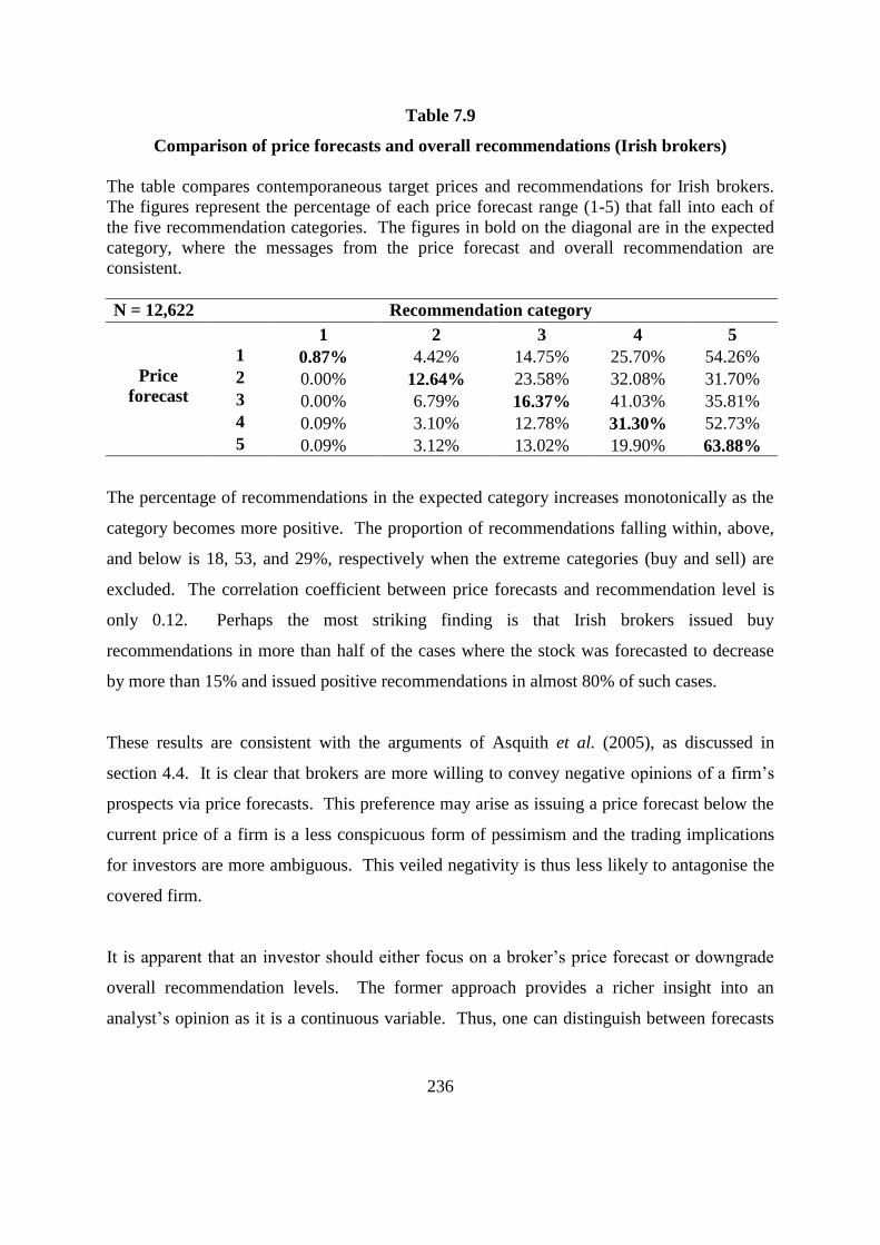
236
Table 7.9
Comparison of price forecasts and overall recommendations (Irish brokers)
The table compares contemporaneous target prices and recommendations for Irish brokers.
The figures represent the percentage of each price forecast range (1-5) that fall into each of
the five recommendation categories. The figures in bold on the diagonal are in the expected
category, where the messages from the price forecast and overall recommendation are
consistent.
N = 12,622 Recommendation category
1 2 3 4 5
Price
forecast
1 0.87% 4.42% 14.75% 25.70% 54.26%
2 0.00% 12.64% 23.58% 32.08% 31.70%
3 0.00% 6.79% 16.37% 41.03% 35.81%
4 0.09% 3.10% 12.78% 31.30% 52.73%
5 0.09% 3.12% 13.02% 19.90% 63.88%
The percentage of recommendations in the expected category increases monotonically as the
category becomes more positive. The proportion of recommendations falling within, above,
and below is 18, 53, and 29%, respectively when the extreme categories (buy and sell) are
excluded. The correlation coefficient between price forecasts and recommendation level is
only 0.12. Perhaps the most striking finding is that Irish brokers issued buy
recommendations in more than half of the cases where the stock was forecasted to decrease
by more than 15% and issued positive recommendations in almost 80% of such cases.
These results are consistent with the arguments of Asquith et al. (2005), as discussed in
section 4.4. It is clear that brokers are more willing to convey negative opinions of a firm’s
prospects via price forecasts. This preference may arise as issuing a price forecast below the
current price of a firm is a less conspicuous form of pessimism and the trading implications
for investors are more ambiguous. This veiled negativity is thus less likely to antagonise the
covered firm.
It is apparent that an investor should either focus on a broker’s price forecast or downgrade
overall recommendation levels. The former approach provides a richer insight into an
analyst’s opinion as it is a continuous variable. Thus, one can distinguish between forecasts

237
that fall into the same overall recommendation category. Furthermore, there are two
problems with downgrading ratings. First, one cannot downgrade sell recommendations by
one degree and second, if all ratings are downgraded it is no longer possible for brokers to
communicate a buy recommendation.
7.4 EPS forecasts
This section analyses the accuracy of EPS forecasts. Figure 7.4 presents a comparison
between actual and forecasted EPS for Irish and non-Irish brokers.
Figure 7.4
Average forecasted and actual EPS
The chart compares the EPS forecasts of Irish and non-Irish brokers with the subsequent
actual EPS. The average EPS forecast for all firms with forecasts by both groups of brokers
is calculated for each calendar year and compared to the realised EPS.
.
In stark contrast to the findings in relation to target prices and ratings, the average EPS
forecast of Irish brokers is 5% lower than the non-Irish brokers. Irish brokers issued more
optimistic EPS forecasts for only three of the 22 companies covered by both groups of
broker. On average, Irish brokers revise EPS forecasts downwards by 6.6% of the current
-0.2
0
0.2
0.4
0.6
0.8
1
1.2
1.4
2010 2009 2008 2007
EPS
(€)
Year
Irish
Non-Irish
Actual
238
price, compared to a revision of 5.4% in the same direction for non-Irish brokers (t-statistic
for difference in means = 3.72)119
.
The disconnect between price and earnings may suggest that Irish brokers use different
valuation models than the other brokers. Alternatively, the findings are consistent with
potential conflicts of interest. Irish brokers may issue more favourable price forecasts and
recommendations in order to stimulate trading, while pitching their EPS forecasts at beatable
levels in order to curry favour with covered firms and generate trading volume when earnings
are announced. This may result in return continuation, as outlined in chapter four.
Furthermore, in contrast with the findings relating to price forecast, Irish brokers do not
exhibit a tendency to herd their EPS forecasts to a significantly greater degree than non-Irish
brokers. The coefficient of variation is calculated as the standard deviation of EPS forecasts
scaled by the absolute value of mean forecasts (following Dische, 2002). The average
dispersion for Irish brokers (0.54) is marginal lower than that of international brokers (0.59);
however, the t-statistic for the difference in means is only 0.18.
7.5 Firm-specific attributes of recommended stocks
This section presents the findings relating to the relationship between recommendations and
firm-specific variables and market returns. Jegadeesh and Kim (2006) document a positive
relationship between current recommendations and lagged market returns. In order to assess
whether this finding holds for the Irish market, the average recommendation rating ( ) is
regressed against six-month lagged market returns ( ) as follows:
The regression results are presented in table 7.10. It can be seen that Irish brokers tend to
become more optimistic following good market performance to a greater extent than
119
EPS revisions are scaled by price due to the relatively high frequency of negative EPS forecasts.

239
international brokers. The relationship was not significant at the 15% level in the case of
non-Irish brokers. This suggests that Irish brokers may follow momentum strategies.
Table 7.10
Relationship between market returns and analyst recommendations
The table presents the regression coefficients (α and β) and correlation coefficient (r) with t-
statistics in parentheses. The 432 average consensus weekly recommendation ratings are
regressed against lagged six-month market returns. Significance at the 1% level is denoted
by *.
Broker α. β. p-value (β) r
Irish 4.375 (481.9) 0.73* (2.80) 0.005 0.14 (2.80)
Non-Irish 3.683 (397.8) 0.38 (1.43) 0.152 0.07 (1.43)
The above approach uses market returns and provides a broad perspective on the relationship
between analysts’ output and macroeconomic indicators. The focus is narrowed in the
following sub-sections by examining the firm-specific characteristics of stocks that analysts
recommend favourably120
. Subsequently, the relationship between each variable and future
abnormal returns and volume is analysed. Appendix H presents summary statistics on each
of the measures analysed.
7.5.1 Ratings vs. firm-specific attributes
Table 7.11 outlines the firm-specific attributes of stocks that analysts favour, based on the
quintles discussed in section 5.4. Panel A details the averages for each variable sorted on the
basis of ratings quintiles, while panel B presents average Spearman’s rank correlation
coefficients between each pair of variables.
120
This section examines consensus recommendations. Individual recommendations are analysed in section 7.6.
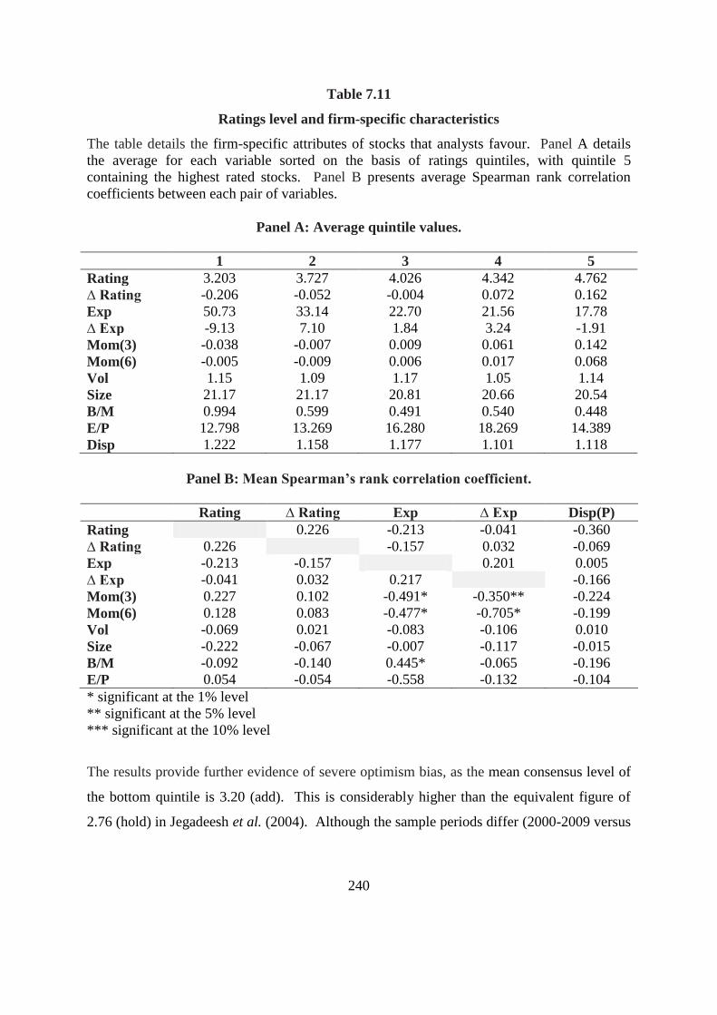
240
Table 7.11
Ratings level and firm-specific characteristics
The table details the firm-specific attributes of stocks that analysts favour. Panel A details
the average for each variable sorted on the basis of ratings quintiles, with quintile 5
containing the highest rated stocks. Panel B presents average Spearman rank correlation
coefficients between each pair of variables.
Panel A: Average quintile values.
1 2 3 4 5
Rating 3.203 3.727 4.026 4.342 4.762
∆ Rating -0.206 -0.052 -0.004 0.072 0.162
Exp 50.73 33.14 22.70 21.56 17.78
∆ Exp -9.13 7.10 1.84 3.24 -1.91
Mom(3) -0.038 -0.007 0.009 0.061 0.142
Mom(6) -0.005 -0.009 0.006 0.017 0.068
Vol 1.15 1.09 1.17 1.05 1.14
Size 21.17 21.17 20.81 20.66 20.54
B/M 0.994 0.599 0.491 0.540 0.448
E/P 12.798 13.269 16.280 18.269 14.389
Disp 1.222 1.158 1.177 1.101 1.118
Panel B: Mean Spearman’s rank correlation coefficient.
Rating ∆ Rating Exp ∆ Exp Disp(P)
Rating 0.226 -0.213 -0.041 -0.360
∆ Rating 0.226 -0.157 0.032 -0.069
Exp -0.213 -0.157 0.201 0.005
∆ Exp -0.041 0.032 0.217 -0.166
Mom(3) 0.227 0.102 -0.491* -0.350** -0.224
Mom(6) 0.128 0.083 -0.477* -0.705* -0.199
Vol -0.069 0.021 -0.083 -0.106 0.010
Size -0.222 -0.067 -0.007 -0.117 -0.015
B/M -0.092 -0.140 0.445* -0.065 -0.196
E/P 0.054 -0.054 -0.558 -0.132 -0.104
* significant at the 1% level
** significant at the 5% level
*** significant at the 10% level
The results provide further evidence of severe optimism bias, as the mean consensus level of
the bottom quintile is 3.20 (add). This is considerably higher than the equivalent figure of
2.76 (hold) in Jegadeesh et al. (2004). Although the sample periods differ (2000-2009 versus
241
1985-1998), it would be difficult to argue that the sample period employed in this thesis was
one that justified such an elevated level of optimism.
The apparent inconsistency between analysts’ recommendations and target prices, as outlined
in section 7.2, is clearly in evidence again. Indeed, the expected price change suggested by
analysts’ price forecasts decreases monotonically as ratings become more favourable. The
rank correlation coefficient between the two variables is -0.213. It seems that analysts attach
higher ratings to stocks that they expect to increase to a smaller extent.
The firm-specific characteristics that are most highly correlated to analysts’ recommendations
are past returns (positive), size (negative), dispersion (negative) and book-to-market
(negative). The positive correlation between ratings and past returns implies that analysts
follow momentum strategies. Indeed, recommendations become monotonically more
positive as past returns increase. This is the case for both past three- and six-month returns.
This is consistent with the findings of Womack (1996), Jegadeesh et al. (2004), and
Jegadeesh and Kim (2006). Separate analysis shows that the relationship between past
returns and ratings is considerably stronger for Irish brokers.
There is a strong negative relationship between momentum and the expected price change
implied by an analysts’ target price. At first, this may appear surprising, as one would expect
that analysts following momentum strategies will attach a higher target price to firms with
higher momentum. However, if analysts do not revise their price targets then the expected
price appreciation (and the revision thereof) will decrease as price increases.
There are strong negative relationships between size and dispersion and the four prediction
measures. Ratings are a monotonically decreasing function of firm size and analyst
disagreement. The dispersion variable shows that analysts tend to agree more about the
prospects of high-rated stocks with existing positive momentum and smaller firms with low
trading volume.
242
The negative correlation between past performance and dispersion may be caused by the non-
synchronous response of analysts to bad news. Inertia in revising forecasts is likely to be
more pronounced for poor performing stocks due to conflicts of interest and over-optimism
of brokers as discussed in section 4.5. Such reluctance manifests itself in a high dispersion of
forecasts.
Analysts also tilt towards firms with low volume and book-to-market ratios. However, these
relationships are not as significant as those relating to momentum, size, and dispersion. The
latter is consistent with the findings of Moshirian et al. (2009), who argue that conflicts of
interest cause analysts to tilt their recommendations towards growth firms. Brokers appear to
follow value strategies with reference to earning-to-price ratios, with ratings generally
becoming more favourable as E/P ratios increase. However, the relationship is not
monotonic, as the E/P ratio of the top rated stocks (quintile 5) is lower than that of quintiles 3
and 4. It seems somewhat contradictory that analysts appear to be momentum traders vis-à-
vis past returns and book-to-market ratios but are contrarian (value) investors in relation to
price-earnings ratios and volume.
7.5.2 Future returns
This section examines the value of brokers’ output by estimating the future abnormal returns
to quintiles based on the four measures of analysts’ opinions. For comparison purposes,
abnormal returns to quintiles sorted on each of the firm-specific characteristics are also
computed. Table 7.12 presents the three-month (panel A) and six-month (panel B) abnormal
returns to each quintile. The final column in each panel shows the average correlation
coefficient between each variable and future market-adjusted abnormal returns.
The returns in the penultimate column represent the difference between the abnormal returns
of the two extreme quintiles. The strategies adopted by brokers, as outlined in the previous
section, are used to determine whether such abnormal returns are calculated as high-minus-
low or vice versa. In other words, the table tests the effectiveness of the strategies that
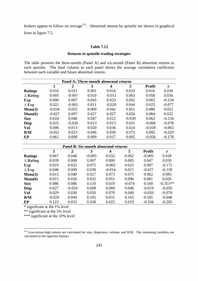
243
brokers appear to follow on average121
. Abnormal returns by quintile are shown in graphical
form in figure 7.5.
Table 7.12
Returns to quintile trading strategies
The table presents the three-month (Panel A) and six-month (Panel B) abnormal returns to
each quintile. The final column in each panel shows the average correlation coefficient
between each variable and future abnormal returns.
Panel A: Three-month abnormal returns
1 2 3 4 5 Profit r
Ratings 0.016 0.021 0.001 0.016 0.033 0.016 0.030
∆ Rating 0.005 -0.007 0.010 -0.011 0.063 0.058 0.036
Exp 0.000 0.007 0.045 0.023 0.002 0.002 -0.134
∆ Exp 0.021 -0.001 0.011 -0.020 0.044 0.023 -0.077
Mom(3) -0.034 0.025 0.009 0.042 0.051 0.086 0.052
Mom(6) -0.027 0.007 0.027 0.027 0.056 0.084 0.032
Size 0.024 0.046 0.047 0.012 -0.039 0.063 -0.234
Disp 0.025 -0.020 0.013 0.013 0.031 -0.006 -0.078
Vol 0.006 0.013 0.020 0.036 0.024 -0.018 -0.065
B/M -0.021 0.023 0.046 0.030 0.072 0.092 -0.029
EP 0.061 0.008 0.009 0.017 0.005 -0.056 -0.178
Panel B: Six-month abnormal returns
1 2 3 4 5 Profit r
Ratings 0.067 0.046 -0.003 0.032 0.062 -0.005 0.028
∆ Rating 0.039 0.008 0.007 0.000 0.085 0.047 0.030
Exp 0.019 0.032 0.072 -0.002 0.025 0.007 -0.171
∆ Exp 0.048 0.009 0.039 -0.014 0.021 -0.027 -0.159
Mom(3) 0.013 0.040 0.027 0.073 0.075 0.062 0.085
Mom(6) 0.015 0.026 0.032 0.051 0.096 0.081 0.026
Size 0.086 0.086 0.110 0.019 -0.074 0.160 -0.351**
Disp 0.027 -0.024 0.008 0.069 0.046 -0.019 -0.050
Vol 0.029 0.036 0.050 0.070 0.049 -0.020 -0.070
B/M -0.020 0.044 0.105 0.031 0.165 0.185 -0.046
EP 0.123 0.033 0.038 0.025 0.019 -0.104 -0.205
* significant at the 1% level
** significant at the 5% level
*** significant at the 10% level
121
Low-minus-high returns are calculated for size, dispersion, volume, and B/M. The remaining variables are
calculated in the opposite manner.
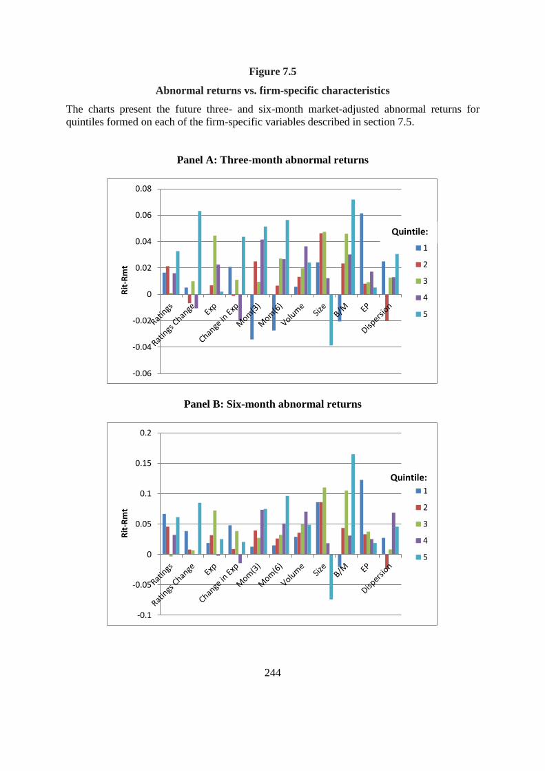
244
Figure 7.5
Abnormal returns vs. firm-specific characteristics
The charts present the future three- and six-month market-adjusted abnormal returns for
quintiles formed on each of the firm-specific variables described in section 7.5.
Panel A: Three-month abnormal returns
Panel B: Six-month abnormal returns
-0.06
-0.04
-0.02
0
0.02
0.04
0.06
0.08
Rit
-Rm
t
1
2
3
4
5
-0.1
-0.05
0
0.05
0.1
0.15
0.2
Rit
-Rm
t
1
2
3
4
5
Quintile:
Quintile:

245
Future returns are generally an increasing function of ratings, with the top-rated stocks
earning the highest market-adjusted returns over the next three and six months. However, a
strategy of buying (short selling) the highest (lowest) rated stocks only generates moderate
abnormal returns and the quintile of the lowest rated stocks outperforms top-rated stocks over
a six-month period. The correlation between past and future returns suggests that the
correlation between ratings and future returns may simply be due to momentum rather than
skill, as analysts lean towards stocks with positive momentum. The high momentum returns
are consistent with the findings presented in the previous chapter. Abnormal returns over six
months monotonically increase for quintiles based on existing six-month momentum and
future abnormal returns are highest to quintile 5 for all four combinations of past and future
returns. However, consistent with the findings reported in section 6.3, a three-month holding
period generates higher abnormal returns.
Consistent with Jegadeesh et al. (2004), there is a marked difference between the abnormal
returns to recommendation levels and revisions, with the latter generating abnormal returns of
5.8% in the three months following the quarter end, compared to 1.6% for recommendation
levels. The superior performance of revisions is entirely derived from the returns of extreme
upgrades. In fact, short selling stocks with the most extreme downgrades would result in
losses, as such stocks outperform the market over the next quarter, as was the case with
ratings levels. However, such losses are greater when rating levels are used122
.
It is not surprising that recommendation changes outperform recommendation levels as the
latter are more likely to be stale at the end of the quarter when they are evaluated using the
above framework due to the lack of revisions. As discussed in section 7.2, recommendations
remain unchanged for an average of 41 weeks. In contrast, recommendation changes cannot
be more than 13 weeks old and the average change will be approximately seven weeks old,
ceteris paribus.
122
It is not clear than an investor would short sell the lowest rated stocks as only a small proportion of such
stocks attracted sell ratings. A more straightforward strategy of buying top-rated stocks generates more
significant abnormal returns.

246
Although brokers exhibit greater selection and timing ability when changes in
recommendations are evaluated, it still appears that they fail to outperform growth strategies
based on momentum, B/M, and size. The abnormal returns to the high book-to-market
quintile are the highest of any of the 55 quintiles. Furthermore, the returns to quintile 1 are
negative, adding further weight to the validity of a growth strategy based on this ratio.
Size, B/M, and the two momentum measures are the only indicators where the returns to both
of the extreme quintiles are of the hypothesised sign for three-month abnormal returns. The
negative relationship between size and future returns is the only statistically significant
relationship at the five per cent level. Value strategies based on B/M and size generate
abnormal returns of 18.5 and 16% respectively in the six months following the end of the
calendar quarter. These results are consistent with the findings of Banz (1981) and Fama and
French (1992). However, they directly contrast with the results of Jegadeesh et al. (2004),
who report that large firms outperformed small firms and that value firms did not outperform
growth firms.
Recall that brokers follow value strategies in terms of E/P ratios. However, there is a strong
negative correlation between such ratios and abnormal returns; in other words,
growth/momentum strategies are profitable. This contrasts starkly with the findings of Basu
(1977) and Jegadeesh et al. (2004). As outlined above, the relationship between analysts’
ratings and past returns, price-earnings ratios, and book-to-market ratios paints an
inconsistent picture in terms of whether analysts favour value or growth strategies. There is
also some discrepancy in the relationships between these three variables and future returns;
value (growth) strategies are profitable when formed on the basis of B/M ratios (momentum
and E/P ratios).
The finding that returns are generally an increasing function of past volume is diametrically
opposed to the results of Jegadeesh et al. (2004). Recall that Lee and Swaminathan (2000)
argue that low (high) volume stocks are exhibit value (glamour) characteristics. Accordingly,
the superior returns to high-volume stocks can be viewed as consistent with

247
momentum/glamour returns and contradict the finding of Lee and Swaminathan (2000) that
firms with high past turnover earn lower future returns.
The negative correlation between dispersion and future returns is consistent with the findings
of Erturk (2006) and Dische (2002) but starkly contrast with Verardo (2009) and Doukas and
McKnight (2005). The results suggest that momentum is partially attributable to analyst
herding. However, the relationship is not statistically significant and the quintile of high-
dispersion stocks outperforms the low-dispersion quintile.
7.5.3 Abnormal volume
It is of interest to examine whether analysts’ output is correlated with future abnormal
volume in order to assess whether analysts induce trading activity. Table 7.13 presents
details of abnormal volume for quintiles sorted on recommendation levels and presents
analogous statistics for all other firm-specific variables.
Table 7.13
Abnormal volume
The table details the abnormal volume ratios for quintiles formed on each of the first-specific
characteristics. Abnormal volume is calculated by scaling the volume for the quarter
following recommendations by the average volume for three quarters prior to the
recommendation quarter. The last column shows the average correlation coefficient (r)
between each variable and future abnormal volume.
Quintiles
1 2 3 4 5 r
Rating 1.223 1.158 1.177 1.101 1.118 -0.048
∆ Rating 1.148 1.009 1.159 1.123 1.178 -0.029
Exp 1.006 0.958 0.994 0.986 1.070 -0.075
∆ Exp 0.931 0.901 0.922 0.989 1.028 0.014
Mom(3) 1.370 1.114 1.116 1.180 1.344 -0.106
Mom(6) 1.123 1.200 1.072 1.182 1.524 -0.091
Size 1.338 1.228 1.198 1.173 1.094 -0.037
Disp 1.113 1.027 1.078 1.232 1.178 -0.040
Vol 0.807 1.025 1.150 1.376 1.735 0.407
B/M 1.165 1.032 1.088 1.211 1.580 -0.095
E/P 1.047 1.039 0.834 0.828 0.997 -0.149

248
There is no discernible relationship between the four prediction measures and future volume,
suggesting that analysts’ recommendations do not generate abnormal volume. Surprisingly,
it is the lowest rated stocks that generate the highest level of abnormal volume. This would
be expected if investors acted on such relatively negative ratings by selling stocks in greater
quantities than would be the case for purchases of high-rated stocks, in recognition of
analysts’ conflicts of interest. However, such stocks earn the highest return of any quintile of
stocks over the subsequent six months. Figure 7.6 presents the future standardised volume to
quintiles based on each of the firm-specific variables described in section 7.5.1.
Figure 7.6
Future abnormal volume
The chart presents the future standardised volume to quintiles based on each of the firm-
specific variables. Abnormal volume is calculated by scaling the volume for the quarter after
recommendations by the average volume for three quarters prior to the recommendation
quarter.
Abnormal volume decreases monotonically with firm size. This is consistent with the finding
that smaller firms generate higher abnormal returns. Abnormal volume is generally an
increasing function of past momentum and is a monotonically increasing function of past
volume. The latter relationship may be driven by the former; in other words, high past
0
0.2
0.4
0.6
0.8
1
1.2
1.4
1.6
1.8
Rit
-Rm
t
1
2
3
4
5
Quintile:

249
returns are associated with high past volume. Momentum means that past and future returns
are related and this in turn induces a positive relationship between past and future volume.
Taken together, the above evidence strongly indicates that analysts favour small firms with
high momentum and low book-to-market ratios. It appears that brokers are vindicated in the
use of momentum strategies but not in their use of value strategies vis-à-vis B/M and EP,
which underperform stocks at the opposite end of the valuation spectrum by 10.4 and 18.5%,
respectively, over the six months subsequent to the calendar quarter end. It is also clear that
recommendation revisions add greater incremental value than recommendation levels.
All forms of brokers’ output generate lower returns than relatively straightforward strategies
based on size, momentum, and book-to-market. The finding that analysts fail to add
significant value confirms the results of Jegadeesh et al. (2004) for the US. Table 7.14
summarises the hypothesised and actual relationships between each firm-specific variable and
future abnormal returns and volume.
Table 7.14
Summary of relationships
The table presents the hypothesised and actual relationships between each of the firm-specific
variables and brokers’ ratings and abnormal returns. The second column details the
hypothesised direction of the relationship between each variable and abnormal returns based
on existing literature. The third column shows the relationship between each variable and the
brokers’ ratings and the last column lists the direction of the relationship between each firm-
specific attribute and future abnormal returns.
Variable Hypothesised
relationship
Ratings Abnormal
returns
Momentum + + +
Size - - -
Dispersion - - -
Volume - - -
Book-to-market + - -
Earnings-to-price + + -

250
7.6 Micro-level analysis
The above sections examine consensus ratings at the start of each quarter. In contrast, this
section examines recommendation revisions on a continual basis and does so at the level of
each broker rather than at the consensus level. In other words, we move from a calendar-time
to an event-time approach. The latter has the advantage of increasing the number of
observations and thus the power of statistical tests. However, the approaches tested here may
not represent implementable strategies due to the need for frequent rebalancing123
.
Another key difference is that this section examines portfolios that are clearly defined in
terms of the recommendation level. The extreme portfolios in the previous section could not
be interpreted as ‘buys’ or ‘sells’, as they were formed on the basis of quintiles. Given the
dominance of buy recommendations the top-rated quintile almost exclusively contains buy
recommendations. However, the lowest quintile could not be exclusively comprised of sell
recommendations, as such recommendations accounted for less than 3% of all advice.
Furthermore, this section allows one to differentiate between the market response to different
types of revisions. The hypothesised direction of any market reaction is not straightforward
as the implications of some revisions are unclear. For example, downgrades from buy to add
are included as a downgrade in the quintile-based approach. However, the new
recommendation level remains positive124
.
This section focuses on recommendation revisions, as opposed to levels, for a number of
reasons. First, as outlined in section 7.2, recommendation levels remain unchanged for
extended periods of time. Second, analysts display a marked tendency to herd. These
characteristics of the data increase the likelihood of encountering problems associated with
cross-sectional dependence and serial correlation. This problem is largely caused by
123
However, it seems more plausible that investors would implement trades as close as possible to the
announcement of recommendations or revisions rather than at the end of each calendar quarter. It also seems
more likely that investors would follow a small number of brokers rather than the consensus recommendation
level. 124
Furthermore, the theoretical impact of revisions to the hold category is questionable as the destination
category does not recommend any action on the part of the investor. However, it may be suspected that a
downgrade to hold may have a greater impact if holds are thinly-veiled sell recommendations.

251
overlapping observations and becomes more germane when extended test periods are
employed. Such problems are largely alleviated by using recommendation revisions. A
novel approach is adopted to mitigate the remaining problems caused by overlapping
observations, as discussed in the next sub-section. Third, as reported in section 7.5,
recommendation revisions have more predictive power than recommendation levels. It is
probable that recommendation levels are less profitable as a large proportion of such ratings
are stale as brokers leave recommendation levels unchanged for extended periods.
Recommendations are favoured over price and EPS forecasts. Recommendation ratings
provide a clear signal to the market and represent the principal form of communication
between brokers and investors in this sample, accounting for in excess of half of brokers’
output. Furthermore, it is not possible to accurately calculate EPS revisions when such
forecasts take a negative value. A significant number of forecasts fall into this category in
the later years of the sample.
7.6.1 Price effects
This section examines the stock picking and timing abilities of brokers by measuring the
price impact of revisions for each of the revision categories based on the original and new
recommendation. Existing research tends to examine a small number of revision categories
and holding periods. This study examines 20 revision categories and tracks abnormal returns
on a continual basis.
A central task in any event study is to strike a balance between accurately representing an
investor’s trading experience and statistical-significance considerations. Independence
assumes that the abnormal returns of firms are independent in time-series and cross-section
(Kothari and Warner, 2006). Cross-sectional and serial dependence are often encountered
when dealing with panel data and can result in biased test statistics125
. This study accounts
125
For a discussion of the impact of such dependence, see, for example, Brown and Warner, (1980); Mitchell
and Stafford, (2000).

252
for overlapping revisions in a manner that more accurately reflects an investor’s experience
and minimises cross-sectional dependence.
Robustness tests in this study show that failing to account for overlapping revisions results in
considerably inflated abnormal returns and test statistics, as the number of independent
observations is overstated. Accordingly, abnormal returns and volume will be calculated
using non-overlapping returns in order to minimise cross-sectional dependence issues.
Overlapping revisions are accounted for in two principal ways. First, contemporaneous
revisions of the same type that are made by multiple brokers for a particular company are
treated as one observation. Second, if there is a further revision before the end of an event
period over which abnormal returns are measured returns are curtailed so that they do not
overlap126
. Returns are calculated for the entire test period only if there are no subsequent
revisions during this time.
It is felt that this approach strikes the optimum balance between investor-experience and
statistical-significance concerns. For example, it seems reasonable to expect that if a stock
experiences a subsequent reversal by the same broker before the end of the event window, an
investor will revise their trading strategy. Similarly, if multiple brokers issue contiguous
revisions to buy the same stock it seems implausible that an investor would buy the same
stock multiple times over a short space of time and sell each holding in consecutive weeks
one year hence.
Market-adjusted buy-and-hold abnormal returns are estimated as the difference between the
product of one plus the company returns (Rit) over various time periods minus the equivalent
market return (Rmt), as is the conventional approach in studies of brokers’ advice (for
example, Ryan, 2006; Jegadeesh et al., 2004)127
.
126
This also facilitates a comparison with previous research relating to the Irish market, as Ryan (2006)
excludes from further analysis firms that incur a reverse revision after the recommendation month. 127
Several studies (for example, Desai et al., 2000) measure abnormal returns with reference to a control firm.
However, this approach is not deemed appropriate for this study, as the small number of companies on the Irish
market means that it not always possible to find a non-event control firm for any reasonably long test period.

253
∏
∏
The number of overlapping revisions increases for longer test periods. Accordingly,
equation 7.14 is recalculated for holding periods of increasing lengths, commencing at week
-26 and terminating at week +52 relative to the revision date. Abnormal returns are averaged
across n unique revisions of a specific type experienced over the sample period of
approximately ten years to give the equally-weighted portfolio abnormal return ( ):
∑
This procedure is repeated for each of the 20 revision categories i.e. add to buy, hold to add,
etc. The statistical significance of average abnormal returns is estimated by:
Where SET is the cross-sectional standard error of abnormal returns. Table 7.15 presents
details of the number of recommendations in each of the 20 revision categories after
overlapping revisions are excluded.

254
Table 7.15
Number of recommendation revisions by category
The table details the number of revisions sorted by the pre- and post-revision categories. The
original sample of 1,094 was reduced to 1,043 after cases where simultaneous revisions of the
same type and revisions without the necessary return and volume data were excluded.
New
N = 1,043 Buy Add Hold Reduce Sell Total %
Buy 152 174 10 7 343 33
Add 153 97 21 2 273 26
Original Hold 155 77 44 38 314 30
Reduce 9 18 31 9 67 7
Sell 6 1 34 5 46 4
Total 323 248 336 80 56 1,043 -
% 31 24 32 8 5 - 100
The sample contains 489 (47%) upgrades and 554 (53%) downgrades. Table 7.16 details the
average abnormal returns to each of the revision categories.
Table 7.16
Abnormal returns to revisions
Panel A presents the cumulative buy-and-hold market-adjusted abnormal returns for each of
the 20 revision categories for week 0-4. Panel B details the returns to upgrades and
downgrades for various holding periods relative to week 0.
Panel A
New
Buy Add Hold Reduce Sell
Buy -0.002 -0.011 -0.150 0.031
Add 0.024* -0.036* -0.016 -0.126
Original Hold 0.024* 0.038* -0.063* -0.029
Reduce -0.018 0.014 0.009 0.021
Sell 0.059 0.059* -0.002 0.009
Panel B
Category -26 to 0 0 0-26 0-52
Upgrades 0.022** 0.007 0.038* 0.071*
Downgrades 0.020 -0.021* -0.008 -0.002
* significant at the 1% level
** significant at the 5% level
*** significant at the 10% level

255
Table 7.16 shows that there is a generally a stronger response to upgrades. This is not
surprising, as short-sale constraints may limit the market response to negative ratings.
Surprisingly, the market response is less pronounced for revisions of larger degrees. It is
found that 64.5% (53.4%) of upgrades (downgrades) generate positive (negative) abnormal
returns over the 0-52 week period. The percentage for upgrades is larger than the equivalent
figure of 54% reported in Desai et al. (2000). It should be noted that the relatively low
number of revisions to sell reduces the statistical significance of abnormal returns to such
downgrades. For example, the -12.6% generated by revisions from add to sell is the average
of only two such revisions.
The returns to various revision categories are analysed on a week-by-week basis in graphical
form. These graphs plot cumulative abnormal returns from 26 weeks before to 52 weeks
after revisions as it is of interest to compare pre- and post-revision returns. Appendix I
contains separate graphs for the pre- and post-revision stage for some of the key revision
categories. The analysis commences with the general cases of upgrades and downgrades,
before focusing on some of the specific revision categories with significant abnormal returns.
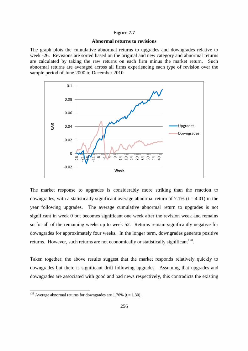
256
Figure 7.7
Abnormal returns to revisions
The graph plots the cumulative abnormal returns to upgrades and downgrades relative to
week -26. Revisions are sorted based on the original and new category and abnormal returns
are calculated by taking the raw returns on each firm minus the market return. Such
abnormal returns are averaged across all firms experiencing each type of revision over the
sample period of June 2000 to December 2010.
The market response to upgrades is considerably more striking than the reaction to
downgrades, with a statistically significant average abnormal return of 7.1% (t = 4.01) in the
year following upgrades. The average cumulative abnormal return to upgrades is not
significant in week 0 but becomes significant one week after the revision week and remains
so for all of the remaining weeks up to week 52. Returns remain significantly negative for
downgrades for approximately four weeks. In the longer term, downgrades generate positive
returns. However, such returns are not economically or statistically significant128
.
Taken together, the above results suggest that the market responds relatively quickly to
downgrades but there is significant drift following upgrades. Assuming that upgrades and
downgrades are associated with good and bad news respectively, this contradicts the existing
128
Average abnormal returns for downgrades are 1.76% (t = 1.30).
-0.02
0
0.02
0.04
0.06
0.08
0.1
-26
-21
-16
-11 -6 -1 4 9
14
19
24
29
34
39
44
49
CA
R
Week
Upgrades
Downgrades

257
information-diffusion literature (for example, Frazzini, 2006; Hong et al., 2000), which
implies that bad news travels slowly and good news travels fast. Indeed, it could also be said
that the market overreacts to downgrades, as abnormal returns following such revisions
rebound after an initial period of negative returns.
These findings are thus consistent with McQueen et al. (1996) and Ashley (1962), who show
that stock prices react more quickly to bad news than good news. However, they contrast
with those of Womack (1996), who finds that the majority of the price impacts to buy
recommendations are observed in the three-day period surrounding the recommendation;
whereas abnormal returns persist for up to six months for sell recommendations. The
findings also starkly contrast with those of Jegadeesh and Kim (2006) and Moshirian et al.
(2009), who report that long-term abnormal returns to upgrades are insignificant, while
returns to downgraded stocks drift in the majority of the markets in their sample of G7 and
emerging markets, respectively.
Alternatively, the drift in upgrades may arise as investors are sceptical about such positive
revisions in light of analysts’ conflicts of interest. Downgrades are acted upon much quicker,
as investors assume that analysts must have strong information in order to overcome the
negative reaction of the covered firm that may ensue. This is consistent with the findings of
McKnight and Todd (2006), Malmendier and Shanthikumar (2007), and Morgan and Stocken
(2003), who report that investors downgrade recommendations in recognition of conflicts of
interest, as outlined section 4.5.3.
There are significant abnormal returns for upgrades in the four to five months prior to
revisions. This is consistent with the findings of Aitken et al. (2000), and Bauman et al.
(1995) and connotes that brokers either follow momentum strategies or react in an extremely
delayed fashion to the good news that may have driven such positive returns. However, the
positive drift in the returns of upgraded stocks persists for such an extended period that
brokers’ revisions contain value, although the timing of their revisions is imprecise.
258
Similarly, downgrades experience large negative abnormal returns prior to the revision date.
However, such abnormal returns persist for a shorter period prior to revision when compared
to upgrades. It appears that brokers downgrade stocks in a more timely fashion. However,
the negative drift in returns persists for a relatively short time in the post-revision period.
Therefore, the relatively short delay in brokers revising their forecasts renders such revisions
largely unprofitable. It appears that it requires more stock-picking and timing ability to
profitably revise recommendations downwards as the window of opportunity to profit is
considerably narrower.
To some extent, these findings contradict Ryan (2006), who reports that returns are
significantly negative in the six months prior to the initiation of sell recommendations.
Furthermore, Ryan (2006) finds that there is no drift for buy recommendations but a
significant drift for sell recommendations. Such findings directly contrast with the pattern of
cumulative returns presented in figure 7.7. However, the sharp decline in the cumulative
returns of downgraded stocks shortly prior to the revision week is consistent with Ryan
(2006), who finds that largest negative returns to sell recommendations occur in the month
before initiation.
The large abnormal returns to upgrades relative to downgrades are largely attributable to the
economic value of upgrades issued by Irish brokers. Such revisions generate average
abnormal returns of 4.2% (t = 2.06) over the 0-26 week period, compared to 1.6% (t = 1.43)
for non-Irish analysts. The abnormal returns to downgrades are insignificant for both broker
groups. Further analysis shows that abnormal returns are higher for brokerage firms that
follow more firms129
and for firms that are relatively neglected. The superior performance of
Irish brokers may thus be partially explained by the finding of Ryan (2006) that individual
analysts at Irish brokerage firms tend to cover more sectors than their US or UK counterparts.
129 This contradicts the findings of Clement (1999) and Jacob et al. (1999), as outlined in section 4.3. However,
the correlation may be spurious as it may capture the superior performance of Irish brokers, who tend to issue a
disproportionately large proportion of recommendations.

259
The more persistent drift in upgrades is consistent with the findings reported in section 6.2
that the momentum returns in Ireland were dominated by the winner portfolio. Upgraded
stocks are more likely to be past winners given analysts’ tendency to follow momentum
strategies. Again, this suggests that the superior performance of Irish brokers principally
arises from the exploitation of return continuation. Indeed, the abnormal returns to upgrades
are similar to the returns to the winner portfolio, as outlined in section 6.2.
It is of interest to further examine the dynamics of returns following revisions by examining
the share-price reaction to specific categories of revision based on the pre- and post-revision
recommendation levels. As expected, the market reacts to the greatest degree to revisions
that move the recommendation category to or from positive or negative ratings. For example,
downgrades from hold to reduce elicit a greater response to those from buy to add.
Consistent with the existing literature, the market reaction of downgrades from positive to
negative ratings is considerably larger and more statistically significant than that of revisions
from negative to positive ratings. However, the opposite is the case when the sample is
limited to revisions to the extreme ratings. As expected, there is virtually no reaction to
upgrades to hold. Consistent with Ryan (2006), there is some evidence that a hold may be a
negative recommendation by another name, as revisions from buy and add to hold yield
negative post-revision abnormal returns. Figure 7.8 plots the cumulative abnormal returns to
a number of key revision categories.
Consistent with figure 7.7, the abnormal returns to each type of upgrade drift to a greater
extent than those of downgrades. The returns to downgrades from add are all negative and
statistically significant in the four weeks prior to such revisions. Subsequent returns are
negative for all three revision categories for approximately six months after such
recommendation changes. The pattern for downgrades from buy to the other four categories
is less clear, and somewhat surprisingly, the only statistically significant returns are the
positive returns to downgrades from buy to sell.

260
There is also a marked dichotomy between upgrades from the extreme rating and those from
other ratings. The most statistically and economically significant returns are generated for
upgrades from hold and add. The returns prior to the revision dates also tend to be more
significant for such upgrades. Surprisingly, none of the four categories where ratings are
upgraded from negative to positive generate economically and statistically significant
abnormal returns in the post-revision period.
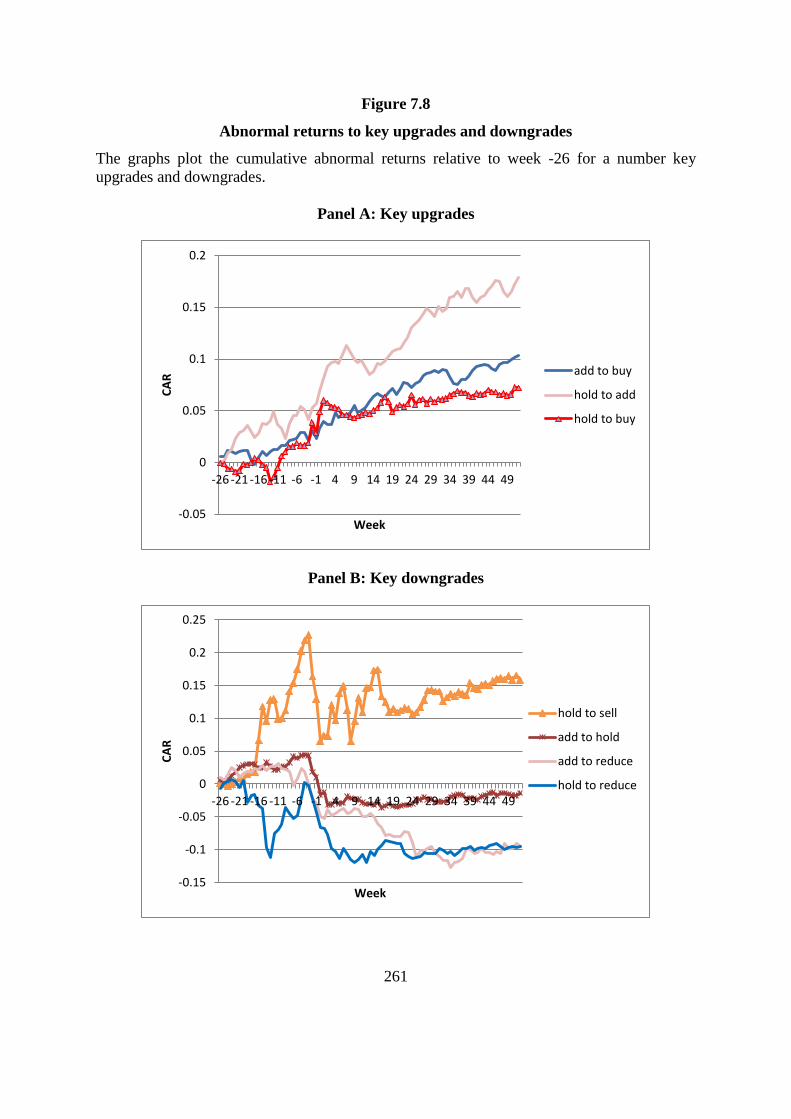
261
Figure 7.8
Abnormal returns to key upgrades and downgrades
The graphs plot the cumulative abnormal returns relative to week -26 for a number key
upgrades and downgrades.
Panel A: Key upgrades
Panel B: Key downgrades
-0.05
0
0.05
0.1
0.15
0.2
-26 -21 -16 -11 -6 -1 4 9 14 19 24 29 34 39 44 49
CA
R
Week
add to buy
hold to add
hold to buy
-0.15
-0.1
-0.05
0
0.05
0.1
0.15
0.2
0.25
-26 -21 -16 -11 -6 -1 4 9 14 19 24 29 34 39 44 49
CA
R
Week
hold to sell
add to hold
add to reduce
hold to reduce

262
Revisions of smaller degrees generate more significant abnormal returns, in direct contrast
with the findings of Ho and Harris (1998) and Stickel (1995). This finding may be explained
by return continuation. If momentum plays a central role in predicting future returns then it
is less likely that larger revisions will be prophetic as they are swimming against the tide of
momentum (assuming that the original recommendation category was informative).
7.6.2 Volume effects
Section 7.5 concluded that brokers’ output did not induce significant trading volume.
However, the earlier findings were derived using consensus forecasts at the end of each
calendar quarter. This section allows for a more precise assessment of any volume impact by
examining revisions in event time. Furthermore, the analysis is conducted at the level of
individual brokers and a distinction is made between revisions to and from each of the five
recommendation categories.
Following Jegadeesh and Kim (2006), abnormal volume is analysed by calculating
standardised volume (SV), which is the ratio of volume in an event week to the average
volume over an extended period before and after the event window. The event window runs
from eight weeks before to eight weeks after a recommendation revision, while average
volume is calculated using data from 26 weeks before and after the event window.
∑
∑
Where is the number of shares traded in week t. Standardised volume is calculated
for each of the 20 revision categories for each week of the event window. Abnormal volume
is indicated by a standardised volume figure that is significantly different from one130
. Figure
7.9 plots the standardised volume for upgrades and downgrades for eight weeks before and
after the revision date.
130
Following Jegadeesh and Kim (2006), observations with standardised volume in excess of 30 are excluded.

263
Figure 7.9
Standardised volume
The figure charts standardised volume for each of the 17 event weeks. Standardised volume
is computed as the ratio of volume in each event week to average long-term volume.
Standardised volume for upgrades is statistically different to one in weeks -1 to +1.
Abnormal volume for downgrades is significant for an additional week (t +2). This
contradicts the findings in section 7.6, as it suggests that investors react in a more delayed
fashion to bad news. However, the event window in equation 7.7 may be overly restrictive,
as abnormal returns persist for upgrades for up to one year. Accordingly, the denominator
may be inflated by the associated increase in volume, thereby dampening the extent of
abnormal volume.
The standardised volume for upgrades and downgrades in week 0 is 1.31 (t = 6.58) and 1.32
(t = 7.96), respectively. These levels of abnormal volume are significantly lower than those
reported in Jegadeesh and Kim (2006) for the US (1.67 and 2.3, respectively). The abnormal
volume for revisions to extreme ratings is also considerably lower than in the existing
literature. For example, Womack (1996) reports ratios of 1.9 and 3 for revisions to buy and
0.8
0.9
1
1.1
1.2
1.3
1.4
-8 -7 -6 -5 -4 -3 -2 -1 0 1 2 3 4 5 6 7 8
S
V
Week Number
Upgrades
Downgrades

264
sell revisions, respectively. The equivalent figures for this dataset are somewhat lower at
1.26 and 1.33, respectively131
.
Abnormal volume is statistically significant for both upgrades and downgrades prior to the
revision date. It might be tempting to conclude that this suggests that details of upcoming
revisions are leaked to certain clients prior to the revision date. However, there is another
possible explanation for this finding. Brokers may be slow to revise their recommendation
levels after firms release price-sensitive news. Investors may trade aggressively on such
news in advance of the broker’s revision. This appears more plausible as the abnormal
volume response to downgrades is more significant in the pre-revision phase. Conflicts of
interest may cause brokers to be more reluctant to revise their recommendations following
bad news.
A detailed breakdown of standardised volume by revision category is provided in appendix J.
In general, abnormal volume is more significant for revisions to positive categories. There is
no statistically significant abnormal volume in week 0 for approximately half of the revision
categories, the majority of which are downgrades. This confirms the findings in the previous
section that analysts’ output does not have a significant impact on volume.
7.7 Conclusion
This chapter analysed the value, veracity, and impact of brokers’ output. The most notable
conclusion is the consistent and robust tendency for brokers to tilt their recommendations
towards firms with positive momentum. The long-term relationship between brokers’
recommendations and abnormal returns and volume strongly suggests that brokers are
principally followers, rather than leaders, in terms of momentum. Investors could generate
greater abnormal returns by simply focusing on small firms with high momentum and B/M
ratios than by following analysts’ advice.
131
However, these results are not directly comparable, as Jegadeesh and Kim (2006) and Womack (1996) use
daily volume data.

265
The returns that analysts generate by exploiting momentum and size are reduced by the losses
to their B/M and E/P strategies. Analysts tilt their recommendations towards value (growth)
stocks in terms of B/M (E/P) ratios. However, such stocks significantly underperform stocks
at the opposite end of the valuation spectrum over the six months subsequent to the calendar
quarter end.
Recommendation revisions are more informative than recommendation levels and upgrades
generate considerably larger abnormal returns than downgrades. This result is largely driven
by the economic value contained in the upgrades of Irish brokers. The information content of
downgrades is quickly impounded into share prices. Indeed, the negative returns to such
revisions reverse in the longer term, implying a market overreaction. In contrast, the returns
to upgraded stocks drift in the prescribed direction for a number of months, implying an
underreaction to good news. Alternatively, these patterns may be driven by investors’
cognisance of the conflicts of interest that analysts face.
Abnormal volume effects are broadly similar for these two revision categories. In stark
contrast with prior research, revisions of smaller degrees generate more significant abnormal
returns. Further analysis shows that abnormal returns are higher for brokers that follow more
firms and for firms that are relatively neglected.
Irish brokers are considerably more optimistic and herd to a greater extent than their
international counterparts and their recommendations generate larger abnormal returns. This
superior performance is attributable to the performance of upgrades, which exploit
momentum in returns. The superior performance of home-based analysts confirms the
findings of Bae et al. (2008), Orpurt (2002), and Conroy et al. (1997). The co-existence of
more optimistic and accurate forecasts by Irish brokers may be consistent with the
information hypothesis. The finding that Irish brokers produce lower EPS forecasts adds
further weight to this possibility, given the dynamics of the earning-guidance game, as
outlined in section 4.5.

266
Chapter Eight
Conclusions
8.1 Introduction
This chapter completes the dissertation and commences by reiterating the objectives of the
study in section 8.2. The key findings are summarised and accompanied with a brief
discussion of their implications in sections 8.3 and 8.4, respectively. Sections 8.5 and 8.6
outline the contributions and limitations of the research, respectively, while recommendations
for future research are provided in section 8.7.
8.2 Objectives
This study aimed to fill a number of apparent gaps in the literature. The overarching
objective was to examine the profitability of contrarian and strength rule strategies in four
medium-sized European markets, with particular emphasis on the role of brokers. The
review of the literature identified a dearth of research on the two anomalies in the four
markets in question. Furthermore, the literature on the value and impact of brokers’
recommendations is ambiguous and there is limited research relating to the Irish market.
The objectives, as presented in section 1.4, were to answer the following questions:
1. Is it possible to make economically and statistically significant risk-adjusted returns
by following strength rule and contrarian strategies in the four markets under review?
2. Is it possible to ameliorate returns by employing alternative rank and holding periods
and hybrid strategies?
3. Are apparently abnormal returns more attributable to rational or behavioural factors?
4. Do Irish brokers appear to be more prone to conflicts of interest than their
international counterparts?
5. To what extent do brokers follow momentum and contrarian strategies?
6. Do brokers’ recommendations have predictive power and what are the volume and
price impacts of their output?

267
These questions were addressed using a quantitative approach. The profitability of the
contrarian and strength rule strategies was measured using three asset-pricing models, while
the value, veracity, and impact of brokers’ output were tested on the Irish market by
analysing panel data relating to three forms of projections; EPS forecasts; target prices; and
overall recommendation category. A combination of event- and calendar-based strategies
was employed in conjunction with a number of models and holding periods. An analysis was
also conducted on the firm-specific characteristics of stocks that are favourably
recommended by brokers.
8.3 Findings
This section summarises the key findings that emerged from the two principal strands of the
research and outlines the implications of these findings for academics, investors, brokers, and
regulators. The overarching findings suggest the rejection of the null hypothesis of market
efficiency and also call into question whether analysts’ recommendations add value.
8.3.1 Anomalies
Chapter six presented the findings pertaining to the momentum and reversal anomalies. The
contrarian investment strategy was found to be profitable in three of the four countries. The
returns are robust to a number of tests and are particularly consistent in the case of Greece. It
is shown that contrarian returns can be enriched via the use of various holding periods, hybrid
strategies, and by focusing on extreme stocks.
There is robust evidence that the relatively straightforward strategy of implementing the
contrarian investment strategy in year two alone generates consistent and economically
significant excess abnormal returns, as it profits from stylised finding of momentum followed
by reversal. The returns to such a strategy are particularly striking when portfolios are
constructed with extreme stocks.

268
The role of risk does not appear to be as important as stated in previous research. Although
in some cases the use of the CAPM reduces abnormal returns it does not do so to such an
extent that it can be cited as a major explanatory variable in the large returns. Furthermore,
the abnormal returns cannot be explained by seasonalities, microstructure biases,
macroceconomic risk, and short-selling constraints. Moreover, the anomalous evidence is
robust to out-of-sample testing, is not attributable to the dynamics of a small number of
stocks, and is not limited to a small number of holding periods with disproportionately large
abnormal returns.
Ireland is the only country where significant strength rule returns were consistently observed.
The optimum strategy involved ranking stocks over nine months and implementing the
momentum strategy for approximately two months. The superiority of a relatively short
holding period is consistent with the findings of key momentum studies such as Jegadeesh
and Titman (1993) and Rouwenhorst (1998). However, the nine-month rank period contrasts
with the 12-month period that is found to be optimal in such studies.
The persistent and robust evidence of return continuation leads to a rejection of the null
hypothesis of market efficiency in Ireland. It is clear that past performance, especially good
performance, is not quickly impounded into share prices. In contrast with key momentum
studies, such as Jegadeesh and Titman (1993) and Rouwenhorst (1998), past winners and
losers both contribute positively to the strength rule returns. This suggests that the Irish
market may underreact to both good and bad news, contradicting the assertion of McQueen et
al. (1996) that stocks react slowly to good news but quickly to bad news
The significant anomalous returns documented in chapter six may suggest that the actions of
noise traders have a material impact on share prices. Paradoxically, the efforts of individual
countries and the European Union (Short Selling) Regulations 2012 (236/20012), which aim
to co-ordinate efforts to tackle the potentially de-stabilising effects of short selling, may
increase the limits to arbitrage, and concomitantly, the noise component in stocks prices.

269
There is evidence of systematic seasonalities in returns. However, such seasonal patterns
tend to affect the winner and loser portfolios to a similar extent. Accordingly, they do not
permeate to the level of excess abnormal returns and one can conclude that seasonalities
cannot account for the anomalous evidence documented in this thesis. The returns to both
strategies tend to be more significant during bear markets. Contrarian returns are higher
following market upturns, while there is no relationship between momentum returns and
lagged market returns.
There is mixed evidence relating to the validity of behavioural explanations for continuation
followed by reversal. The finding that momentum profits are not positively correlated with
lagged market returns runs counter to the predictions of models relating to overconfidence
and loss aversion. However, the positive relationship between contrarian returns and lagged
momentum returns suggests that the two anomalies are related phenomena and reversals may
be the consequence of the unwinding of previous overreactions.
In summary, the anomalous returns documented in this thesis cannot be accounted for by
rational explanations such as risk, seasonalities, short-selling constraints, firm size, and
macroeconomic risk. Furthermore, abnormal returns are not driven by the dynamics of a
small number of stocks or holding periods and are robust to out-of-sample testing.
8.3.2 Brokers’ recommendations
Chapter seven analysed the value, veracity, and impact of brokers’ output. The most robust
finding is brokers’ tendency to tilt their recommendations towards small firms with positive
price momentum. The evidence adduced relating to abnormal returns and volume suggests
that brokers are principally followers of, rather than contributors to, return continuation.
Brokers’ recommendations and forecasts do not provide a basis for generating abnormal
returns above the level attainable by exploiting relatively easily observable variables such as
past momentum and firm size. This is largely the result of brokers incorrectly tilting their
recommendations towards value (growth) stocks in terms of B/M (E/P) ratios. Irish brokers

270
are more optimistic and exhibit a greater tendency to herd and follow momentum strategies
than international brokers.
Consistent with existing research (for example, Jegadeesh and Kim, 2006; Brav and Lehavy,
2003), revisions provide a superior basis for investment than recommendation levels.
Upgrades generate considerably larger abnormal returns than downgrades but the abnormal
volume effects are broadly similar for both revision categories. In stark contrast with prior
research, revisions of smaller degrees generate more significant abnormal returns.
The asymmetric market reaction to upgrades and downgrades suggests that investors
underreact to good news and overreact to bad news. This is consistent with the findings
presented in chapter six, where the majority of the momentum and contrarian returns were
generated by past winners and losers, respectively. This suggests that the anomalous returns
are principally attributable to underreaction to good news and overreaction to bad news,
respectively.
Alternatively, the divergent responses are driven by conflicts of interest, as investors
downgrade the recommendations of analysts, thereby delaying (accelerating) the market
response to upgrades (downgrades). Brokers react in a similar fashion to other investors, as
they downgrade poor performing stocks rapidly but respond in a more delayed fashion to
stocks with positive return momentum.
8.4 Implications
The above findings have a number of implications for academics, investors, brokers, and
regulators. The implications for investors relate to the trading strategies examined in chapter
six and the findings pertaining to brokers discussed in chapter seven. Investors in the Irish
market could profit from momentum trading strategies. Return continuation appears to be a
short- to medium-term phenomenon and investors can maximise average monthly returns by

271
employing nine-month rank and seven-week holding periods. Furthermore, momentum
returns can be increased by skipping a week between the portfolio rank and holding periods.
Contrarian investment strategies dominate in the other three markets and the Greek market
appears to offer the most fertile ground for profiting from return reversals. Furthermore,
investors are advised to form winner and loser portfolios using stocks with extreme past
returns. A relatively straightforward strategy of implementing a contrarian investment
strategy in year two alone represents a potentially profitable approach with the added benefit
of reduced transaction costs relative to three-year holding periods. Hybrid strategies that
combine the two strategies in recognition of their differing holding periods are capable of
successfully exploiting continuation followed by reversal.
Recall that both strategies generated particularly elevated abnormal returns during economic
downturns. This may not be of practical investment value as it is difficult to predict market
or economic growth rates. In contrast, the finding that contrarian returns tend to be more
significant following market upturns does present an ex ante implementable strategy.
The second set of implications pertaining to investors relates to the value of brokers’ output.
It is questionable whether the funds expended on the research conducted by financial analysts
represent a worthwhile undertaking or whether it constitutes an economic loss, which is
largely funded by investors through fees. Investors could generate greater abnormal returns
by simply focusing on small firms with high momentum and B/M ratios than by following
analysts’ advice. If investors are to follow brokers, it is prudent to focus on revisions. The
returns to upgrades are more significant and the window of opportunity is not as restrictively
narrow as is the case for downgrades due to the asymmetric market response to good and bad
news documented in both strands of the research.
There are four significant implications for academics. First, the use of non-overlapping
returns can provide a clearer insight the value of brokers’ recommendations by eliminating
cross-sectional dependence. Second, focussing on target prices, rather than recommendation
levels, provides greater scope for differentiating between the strength of analysts’ output.

272
Third, it is important to test the robustness of any apparently anomalous returns by employing
a number of models and out-of-sample testing periods. Finally, studies of contrarian returns
should utilise alternative rank and holding periods, as the standard three-year rank and
holding periods are typically sub-optimal. The abnormal returns to six-month rank periods
are particularly elevated and merit further examination.
Brokers should continue to tilt their recommendations towards small stocks with positive
price momentum. However, it would appear that a reversal of their strategy vis-à-vis book-
to-market and earnings-to-price ratios may be judicious. Brokers could also benefit from
following more stocks, particularly those that are relatively neglected132
. This study lends
further weight to the assertion of Carhart (1997) that brokers and fund managers should not
be rewarded for exploiting momentum and size, as such variables are easily observable.
The findings of this research also have a number of potential implications for regulators. If
optimism is a proxy for conflicts of interest then it would appear that Irish analysts are
considerably more conflicted than their international counterparts. Analysts may be
cheerleaders for the firms that they follow, as argued by Chan et al. (2007), rather than
impartial observers whose advice should be taken at face value.
8.5 Contribution
This study makes a number of important contributions to the literature pertaining to the
continuation and reversal anomalies. Above all, it fills an important research gap by
analysing four markets that have largely been neglected in the existing literature. The results
provide out-of-sample confirmation of the findings relating to more widely scrutinised
markets.
The study also adopts a number of novel methodological approaches and unearths some
findings that contradict existing research. For example, the use of hybrid strategies,
132
This implication is with the goal of improving forecast accuracy in mind; it ignores any other motivations
such as those relating to underwriting fees, commissions, access to information, etc.

273
alternative rank periods, and cross-product ratios and the significant contrarian returns to six-
month rank periods contribute to the understanding of share price dynamics.
The inclusion of data incorporating the global financial crisis facilitates a more complete
analysis of the relationship between anomalous returns and market states. The use of a small
stock portfolio and non-overlapping returns reduces microstructure bias and cross-sectional
dependence problems. Furthermore, the use of expected price change as a percentage of
current price, instead of recommendation levels, allows for analysts’ views to be examined on
a continual scale. Finally, the analysis of an oligopolistic market for investment advice
illuminates the importance of conflicts of interest and may be of interest to regulators.
8.6 Limitations
The conclusions from this research should be interpreted within the context of a number of
limitations. This study relies exclusively on a quantitative approach. While this facilitated a
broad dataset across temporal and cross-sectional dimensions, it comes at the loss of the
greater detail that accompanies a qualitative approach.
Given the nature of the markets analysed, the sample size and time period employed were
limited relative to those used in much of the existing literature that focusses on larger stock
markets. This study does not explicitly account for transaction costs. Returns are only
considered significant if they exceed a reasonably high threshold suggested by existing
research into trading costs. However, it is likely that such costs are higher in the small
markets used in this study.
Although a suite of models was employed, statistical inferences must be interpreted with
caution in light of the joint-hypothesis problem. As outlined in section 5.3.1, Fama-French
factors are not available on an individual basis for the four markets under review. The lack of
such factors is overcome to some degree by including size, B/M, and E/P in the quintile
approach in conjunction with brokers’ recommendations. However, this does not constitute a

274
perfect substitute for the robustness that would be gained by employing the Fama-French
three-factor or Carhart four-factor models.
Although there is no systematic survivorship bias, as outlined in section 5.2, there is a
possible bias introduced as some firms had to be excluded from the analysis pertaining to
brokers’ recommendations due to missing historic accounting data.
The out-of-sample period (2007-09) coincided with the global financial crisis. While this
facilitated a comparison between the returns to the two anomalies in differing economic
states, the period is far from representative. The impact of the acute market downturn is
particularly germane in the analysis of brokers’ forecasts as it manifests itself in exaggerated
ex post analyst optimism.
8.7 Recommendations for future research
The findings of this thesis initiate a number of suggestions for the trajectory of future
research. It would be valuable to re-examine the findings of this research using a larger
sample over an extended time period. It would also be enlightening to test whether the
results generalise to other markets or are specific to the four markets under review.
The high excess abnormal returns to the contrarian strategy using six-month rank periods
contrasts starkly with the findings in the literature and merits further examination. It would
also be interesting to examine the profitability contrarian strategies in the second holding
period year in other markets. It would also be illuminating to examine whether the
asymmetric response to the news contained in past returns and analysts’ revisions is also
present in the case of earnings announcements, thereby leading to PEAD.
Future research could also investigate the link between brokers’ output and commissions and
investment banking fees in order to illuminate the conflicts of interest that analysts face.
Furthermore, interviews with brokers may complement the insights gained from the cross-

275
sectional analysis undertaken in this research by facilitating a greater understanding of the
motives and strategies pertaining to these pivotal players in the financial market.
It may take a number of years for the nascent regulatory efforts at tackling conflicts of
interest to manifest themselves in a pronounced change in analyst behaviour; this provides a
potentially fruitful area for future research.
Recall that the forecasts of Irish brokers were simultaneously more optimistic and more
accurate than their international counterparts. It would be instructive to examine whether this
superior performance is attributable to an informational advantage that may stem from a
closer relationship with covered firms. An analysis of the trading activities of brokerage
firms and investment houses would also be potentially informative to this end.
The creation of a dataset of Fama-French factors for individual markets would represent a
meritorious exercise. Such an undertaking is proving to be a fruitful endeavour for the UK
market and it would ameliorate research in smaller markets in many areas of financial
analysis.
Although seasonalities could not account for the anomalous returns documented in this study,
there were a number of robust seasonal patterns in returns that merit closer examination. The
observed positive returns in April and May and negative returns in September in all four
markets possibly represent the most interesting grounds for future research. In addition, the
finding that returns are negative in Norway in September and October in 17 of the 20 years
demands further investigation.
The finding that the largest anomalous returns were observed in the countries that
subsequently experienced the most significant stock market crashes as a result of the global
financial crisis suggests that research should continue to investigate the link between
overreaction and bubbles.

276
Thaler’s (1999) claim that the term ‘behavioural finance’ would soon become redundant has
proven somewhat premature. However, although the search for a unifying model of investor
sentiment may be quixotic, future research should continue to focus on developing
behavioural models that incorporate investor sentiment and cognitive errors. Qualitative
studies that aim to further understand the cognitive forces that motivate investors would thus
represent a valuable path for future research.
277
References
Aarts, F. and Lehnert, T. 2005. On style momentum strategies. Applied Economic Letters,
12(13), pp.795-799.
Abarbanell, J.S. and Bernard, V.L. 1992. Tests of analysts’ overreaction/underreaction to
earnings information as an explanation for anomalous stock price behaviour. Journal of
Finance, 47(3), pp.1181-1207.
Abarbanell, J. and Lehavy, R. 2003. Biased forecast or biased earnings? The role of reported
earnings in explaining apparent bias and over/underreaction in analysts' earnings forecasts.
Journal of Accounting and Economics, 36(1-3), pp.105-146.
Ackley, G. 1983. Commodities and capital: Prices and quantities. American Economic
Review, 73(1), pp.1-16.
Agarwal, V. and Taffler, R. 2008. Does financial distress risk drive the momentum anomaly?
Financial Management, 37(3), pp.461-484.
Akhigbe, A., Gosnell, T. and Harikumar, T. 1998. Winners and losers on NYSE: A
reexamination using daily closing bid-ask spreads. Journal of Financial Research, 21(1),
pp.53-64.
Agrawal, A. and Chen, M.A. 2008. Do analyst conflicts matter? Evidence from stock
recommendations. Journal of Law and Economics, 51(3), pp.503-537.
Agyei-Ampomah, S. 2007. The post-cost profitability of momentum trading strategies:
Further evidence from the UK. European Financial Management, 13(4), pp.776–802.
Ahlers, D. and Lakonishok, J. 1983. A study of economists’ consensus forecasts,
Management Science, 29(10), pp.1113–25.
Ahmad, Z. and Hussain, S. 2001. KLSE long run overreaction and the Chinese New Year
effect. Journal of Business Finance and Accounting, 28(1), pp.63-105.
Ahn, D., Conrad, J. and Dittmar, R.F. 2003. Risk adjustment and trading strategies. Review of
Financial Studies, 16(2), pp. 459-485.
Aitken, M.J., Muthuswamy, J. and Wong, K.L. 2000. The impact of brokers’
recommendations: Australian evidence. University of New South Wales. PACAP/FMA
conference paper, Melbourne. Available at: www.sirca.org.au.
Albert, R.L. and Henderson, G.V. 1995. Firm size, overreaction, and return reversals.
Quarterly Journal of Business and Economics, 34(4), pp.60–80.

278
Alexander, G.J. 2000. On back-testing ‘‘zero-investment’’ strategies. Journal of Business,
73(2), pp. 255–278.
Alford, A. and Berger, P. 1999. A simultaneous equations analysis of forecast accuracy,
analyst following, and trading volume. Journal of Accounting, Auditing and Finance, 14(3),
pp.219–240.
Ali, A. and Trombley, M.A. 2006. Short-selling costs and momentum in stock returns.
Journal of Business Finance and Accounting, 33(3/4), pp.587-615.
Allen, D.E. and Prince, R. 1995. The winner/loser hypothesis: Some preliminary Australian
evidence on the impact of changing risk. Applied Economics Letters, 2(8), pp.280–283.
Alonso, A. and Rubio, G. 1990. Overreaction in the Spanish equity market. Journal of
Banking and Finance, 14(3), pp.469–481.
Alwathaninani, A.M. 2012. Consistent winners and losers. International Review of
Economics and Finance, 21(1), pp.210-220.
Amihud, Y. and Mendelson, H. 1986. Asset pricing and the bid-ask spread. Journal of
Financial Economics, 17(2), pp.223-249.
Anand, A., Badrinath, S., Chakravarty, S. and Wood, R. 2006. Is it prudent to trade around
analyst recommendation changes? An analysis of transaction costs. Journal of Trading, 1(4),
pp.22-37.
Andreassen, P. 1987. On the social psychology of the stock market: Aggregate attributional
effects and the regressiveness of prediction. Journal of Personality and Social Psychology,
53(3), pp.490-496.
Ansari, V.A. 2012. Momentum anomaly: evidence from India. Managerial Finance, 38(2),
pp.206-226.
Antoniou, A., Galariotis E.C., and Spyrou S.I. 2006a. The effect of time-varying risk on the
profitability of contrarian investment strategies in a thinly traded market: a Kalman filter
approach. Applied Financial Economics, 16(18), pp.1317-1329.
Antoniou, A., Galariotis E.C., and Spyrou S.I. 2006b. Short-term contrarian strategies in the
London Stock Exchange: Are they profitable? Which factors affect them? Journal of
Business Finance and Accounting, 33(5/6), pp.839-867.
Arena, M., Haggard, S. and Yan, X. 2008. Price momentum and idiosyncratic volatility. The
Financial Review, 43(2), pp.159-190.

279
Ariel, R.A. 1987. A monthly effect in stock returns. Journal of Financial Economics, 18(1),
pp.161–174.
Arshanapalli, B., Coggin, T.D. and Doukas, J. 1998. Multifactor asset pricing analysis of
international value investment strategies. Journal of Portfolio Management, 24(4), pp.10-23.
Ashley, J. 1962. Stock prices and changes in earnings and dividends: Some empirical results.
Journal of Political Economy, 70(1), pp.82–85.
Asness, C.S., Liew, J.M. and Stevens, R. 1997. Parallels between the cross-sectional
predictability of stock and country returns. Journal of Portfolio Management, 23(3), pp.79–
87.
Asquith, P., Mikhail, M.B. and Au, A.S. 2005. Information content of equity analyst reports.
Journal of Financial Economics, 75(2), pp.245-282.
Assoe, K. and Sy, O. 2003. Profitability of the short-run contrarian strategy in Canadian
stock markets. Canadian Journal of Administrative Sciences, 20(4), pp.311-319.
Atkins, A.B. and Dyl, E.A. 1990. Price reversals, bid-ask spreads, and market efficiency.
Journal of Financial and Quantitative Analysis, 25(4), 535-547.
Avramov, D., Chordia, T., Jostova, G. and Philipov, A. 2007. Momentum and credit rating.
Journal of Finance, 62(5), pp.2503–2520.
Azzi, S. and Bird, R. 2005. Prophets during gloom and doom downunder. Global Finance
Journal, 15(3), pp.337–367
Bacmann, J.F. and Dubois M. 1998. Contrarian strategies and cross-autocorrelations in stock
returns: Evidence from France. Working paper. Available at: www.ssrn.com.
Badrinath, S.G. and Wahal, S. 2002. Momentum trading by institutions. Journal of Finance,
57(6), pp.2449-2478.
Badrinath, S.G. and Kini, O. 2001. The robustness of abnormal returns from the earnings
yield contrarian investment strategy. Journal of Financial Research, 24(3), pp.385-401.
Bae, K.-H., Stulz, R.M. and Tan, H. 2008. Do local analysts know more? A cross-country
study of the performance of local analysts and foreign analysts. Journal of Financial
Economics, 88(3), pp.581–606.
Bailey, G. and Gilbert, E. 2007. The impact of liquidity on mean reversion of share returns of
the JSE. Investment Analysts Journal, 66, pp.1-11.

280
Bain, J.S. 1972. Diversification and risk: Comment. Financial Analysts Journal, 28(6),
pp.104-106.
Ball, R. and Brown, P. 1968. An empirical evaluation of accounting income numbers.
Journal of Accounting Research, 6(2), pp.159-178.
Ball, R. and Kothari, S.P. 1989. Nonstationary expected returns: Implications for tests of
market efficiency and serial correlation in returns. Journal of Financial Economics, 25(1),
pp.51-74.
Ball, R. and Watts, R. 1979. Some additional evidence on survival biases. Journal of
Finance, 34(1), pp.197-206.
Ball, R., Kothari, S.P. and Shanken, J. 1995. Problems in measuring portfolio performance:
an application to contrarian investment strategies. Journal of Financial Economics, 38(1),
pp.79–107.
Balvers, R., Wu Y. and Gilliland E. 2000. Mean reversion across national stock markets and
parametric contrarian investment strategies. Journal of Finance, 55(2), pp.745-771.
Balvers, R.J. and Wu, Y. 2006. Momentum and mean reversion across national equity
markets. Journal of Empirical Finance, 13(1), pp.24-48.
Bange, M.M. and Miller, T.W. 2004. Return momentum and global portfolio allocations.
Journal of Empirical Finance, 11(4), pp.429-459.
Bannister, B. 1990. In search of excellence: A portfolio management perspective. Financial
Analysts’ Journal, 46(2), pp.68-73.
Banz, R. 1981. The relationship between return and market value of common stock. Journal
of Financial Economics, 9(1), pp.3-18.
Banz, R.W. and Breen, W.J. 1986. Sample dependent results using accounting and market
data: Some evidence, Journal of Finance, 41(4), pp.779-793.
Barber, B. and Loeffler, D. 1993. The Dartboard Column: Second-hand information and price
pressure. Journal of Financial and Quantitative Analysis, 28(2), pp.273-284.
Barber, B. and Odean, T. 2008. All that glitters: The effect of attention and news on the
buying behaviour of individual and institutional investors. Review of Financial Studies. 21(2),
pp.785–818.
Barber, B., Lehavy, R. and Trueman, B. 2007. Comparing the stock recommendation
performance of investment banks and independent research firms. Journal of Financial
Economics, 85(2), pp.490-517.

281
Barber, B.M. and Odean, T. 1999. The courage of misguided convictions. Financial Analysts
Journal, 55(6), pp.41–55.
Barber, B.M., Lehavy, R., McNichols, M. and Trueman, B. 2006. Buys, holds, and sells: The
distribution of investment banks’ stock ratings and the implications for the profitability of
analysts’ recommendations. Journal of Accounting and Economics, 41(1-2), pp.87-117.
Barberis, N. and Shleifer, A. 2003. Style investing. Journal of Financial Economics, 68(2),
pp.161-199.
Barberis, N., Shleifer, A. and Vishny, R. 1998. A model of investor sentiment, Journal of
Financial Economics, 49(3), pp.307-343.
Barros, J.L. and Haas, J.R. 2008. Momentum and reversal puzzle in emerging markets. ICFAI
Journal of Behavioral Finance, 5(3), pp.54–71.
Barth, M.E., Beaver, W.H. and Landsman, W.R. 1998. Relative valuation roles of equity
book value and net income as a function of financial health. Journal of Accounting &
Economics 25(1), pp.1–34.
Bartov, E., Givoly, D. and Hayn, C. 2002. The rewards to meeting or beating earnings
expectations. Journal of Accounting and Economics 33(2), pp.173-204.
Basu, S. 1977. Investment performance of common stocks in relation to their price earnings
ratios: A test of the efficient market hypothesis. Journal of Finance, 33(3), pp.663-682.
Battalio, R.H. and Mendenhall, R.R. 2005. Earnings expectations, investor trade size, and
anomalous returns around earnings announcements. Journal of Financial Economics, 77(2),
pp.289–319.
Bauman, W.S. and Dowen, R. 1988. Growth projections and common stock returns.
Financial Analysts Journal, 44(4), pp.79-80.
Bauman, W.S., Conover, C.M. and Miller, R.E. 1998. Growth stocks versus value stocks and
large versus small cap stocks in international markets. Financial Analysts Journal, 54(2),
pp.75-89.
Bauman, W.S., Conover, C.M. and Miller, R.E. 1999. Investor overreaction in international
stock markets. Journal of Portfolio Management, 25(4), pp.102-110.
Bauman, W.S., Datta, S. and Iskander-Datta, M.E. 1995. Investment analyst
recommendations: A test of the "announcement effect" and the "valuable information effect".
Journal of Business Finance and Accounting, 22(5), pp.659-670.

282
Baytas, A. and Cakici, N. 1999. Do markets overreact: International evidence. Journal of
Banking and Finance, 23(7), pp.1121-1144.
Beckers, S., Steliaros, M. and Thomson, A. 2004. Bias in European analysts’ earnings
forecasts. Financial Analysts Journal, 60(2), pp.74–85.
Bem, D.J. 1965. An experimental analysis of self-persuasion. Journal of Experimental Social
Psychology, 1(3), pp.199-218.
Benartzi, S. and Thaler, R. 1995. Myopic loss aversion and the equity premium puzzle.
Quarterly Journal of Economics, 110(1), pp.73–92.
Beneish, M. 1991. Stock prices and the dissemination of analysts’ recommendations. Journal
of Business, 64(3), pp.393-416.
Benos, A. 1998. Aggressiveness and survival of overconfident traders. Journal of Financial
Markets, 1 (3/4), pp.353-383.
Berggrun, L. and Rausch, O. 2011. Momentum in the Colombian stock market. Latin
American Business Review, 12(1), pp.1-23.
Bernard, V.L. and Thomas, J.K. 1989. Post-earnings-announcement drift: Delayed price
response or risk premium? Journal of Accounting Research, 27(3), pp.1-36.
Bernhardt, D., Campello, M. and Kutsoati, E. 2006. Who herds? Journal of Financial
Economics, 80(3), pp.657-675.
Bhaskar, K.N. and Morris, R.C. 1984. The accuracy of brokers’ profit forecasts in the UK.
Accounting and Business Research, 14(54), pp.113-124.
Bhojraj, S. and Swaminathan, B. 2006. Macromomentum: Returns predictability in
international equity indices. Journal of Business, 79(1), pp.429-451.
Bhootra, A. 2011. Are momentum profits driven by the cross-sectional dispersion in expected
stock returns? Journal of Financial Markets, 14(3), pp.494-513.
Bidwell III, C.M. 1977. How good is institutional brokerage research. Journal of Portfolio
Management, 3(2), pp.26-31.
Bikhchandani, S. and Sharma, S. 2001. Herd behavior in financial markets. IMF Staff Papers,
47(3), pp.279– 310.
Bikhchandani, S., Hirshleifer, D. and Welch, I. 1998. Learning from the behavior of others:
Conformity, fads, and informational cascades. Journal of Economic Perspectives, 12(3),
pp.151–170.

283
Bildik, R. and Gulay, G. 2007. Profitability of contrarian vs. momentum strategies: Evidence
from the Istanbul stock exchange. International Review of Finance, 7(1-2), pp.61-87.
Bird, R. and Whitaker, J. 2003. The performance of value and momentum investment:
portfolios: recent experience in the major European markets. Journal of Asset Management,
4(4), pp.221–246.
Bjerring, J.H., Lakonishok, J. and Vermaelen, T. 1983. Stock price and financial analysts'
recommendations, Journal of Finance, 38(1), pp.187-204.
Black, F. 1993. Estimating expected return. Financial Analysts Journal, 9(5), pp.36-38.
Black, F. 1986. Noise. Journal of Finance, 41(3), pp.529-543.
Blitz, D., Huij, J. and Martens, M. 2011. Residual momentum. Journal of Empirical Finance
18(3), pp.506–521.
Bloomfield, R., O'Hara, M. and Saar, G. 2009. How noise trading affects markets: an
experimental analysis. Review of Financial Studies, 22(6), pp.2275-2302.
Bolliger, G. 2004. The characteristics of individual analysts’ forecasts in Europe. Journal of
Banking and Finance, 28(9), pp.2283–2309.
Boni, L. and Womack, K.L. 2006. Analysts, industries, and price momentum. Journal of
Financial and Quantitative Analysis, 41(1), pp.85–109.
Bonner, S.E., Hugon, A. and Walther, B.R. 2007. Investor reaction to celebrity analysts: the
case of earnings forecast revisions. Journal of Accounting Research, 45(3), pp.481–512.
Boudoukh, J., Richardson, M., and Whitelaw, R. 1994. A tale of three schools: Insights on
auto-correlations of short-horizon stock returns. The Review of Financial Studies, 7(3),
pp.539–573.
Bouman, S. and Jacobsen, B. 2002. The Halloween indicator: Sell in May and go away.
American Economic Review, 92(5), pp.1618−1635.
Bowman, R.G. and Iverson, D. 1998. Short-run overreaction in the New Zealand stock
Market. Pacific-Basin Finance Journal, 6(5), pp.475-491.
Boynton, W. and Oppenheimer, O.H. 2006. Anomalies in stock market pricing: Problems in
return measurements. Journal of Business, 79(5), pp.2617-2631.
Bradley, D.J., Jordan, B.D. and Ritter, J.R. 2003. The quiet period goes out with a bang.
Journal of Finance, 58(1), pp.1–36.

284
Bradshaw, M.T. 2002. The use of target prices to justify sell-side analysts’ stock
recommendations. Accounting Horizons, 16(1), pp.27–41.
Bradshaw, M.T. 2004. How do analysts use their earnings forecasts in generating stock
recommendations? Accounting Review 79(1), pp.25–50.
Brailsford, T. 1992. A test for the winner–loser anomaly in the Australian equity market:
1958–1987. Journal of Business Finance and Accounting, 19(2), pp.225–241.
Braun, P.A., Nelson, D.B. and Sunier, A.M. 1995. Good news, bad news, volatility, and
betas. Journal of Finance, 50(5), pp.1575–1603.
Brav, A. and Lehavy, R. 2003. An empirical analysis of analysts’ target prices: Short-term
informativeness and long-term dynamics. Journal of Finance, 58(5), pp.1933–1967.
Bremer, M. and Hiraki, T. 1999. Volume and individual security returns on the Tokyo Stock
Exchange. Pacific Basin Finance Journal, 7(3-4), pp.351–370.
Bremer, M. and Sweeney, R. 1991. The reversal of large stock-price decreases. Journal of
Finance, 46(2), pp.747-754.
Bremer, M.A. and Sweeney, R.J. 1988. The information content of extreme negative rates of
return. Working paper, Clarement McKenna College.
Brennan, M. and Hughes, P. 1991, Stock prices and the supply of information. Journal of
Finance, 46(5), pp.1665-169.
Brennan, M. and Subrahmanyam, A. 1995. Investment analysis and price formation in
security markets. Journal of Financial Economics, 38(3), pp.361-381.
Brennan, M.J., Jegadeesh, N. and Swaminathan, B. 1993. Investment analysis and the
adjustment of stock prices to common information, Review of Financial Studies, 6(4),
pp.799-824.
Brouwer, I., Van Der Put, J. and Veld C. 1997. Contrarian investment strategies in a
European context. Journal of Business Finance & Accounting, 24(9), pp.1353-1366.
Brown, K.C. and Harlow, W.V. 1988. Market overreaction: Magnitude and intensity. Journal
of Portfolio Management, 14(2), pp.6-13.
Brown, L. and Caylor, M. 2005. A temporal analysis of quarterly earnings thresholds:
propensities and valuation consequences. Accounting Review, 80(2), pp.423–440.
Brown, L. and Rozeff, M. 1978. The superiority of analyst forecasts as measures of
expectations: evidence from earnings. Journal of Finance, 33(1), pp.1–16.

285
Brown, R., Chan, H.W.H. and Ho, Y.K. 2007. Initiating coverage, broker reputation and
management earnings forecasts in Australia. Accounting and Finance, 47(3), pp.401-421.
Brown, S.J. and Warner, J.B. 1980. Measuring security price performance. Journal of
Financial Economics, 8(3), pp.205-258.
Brown, S., Du, D.Y., Rhee, S.G., and Zhang, L. 2008. The returns to value and momentum
in Asian Markets. Emerging Markets Review, 9(2), pp.79–88.
Brown, S.J. and Goetzmann, W. 1995. Performance persistence. Journal of Finance, 50(2),
pp.679–698.
Brown, S.J., Goetzmann, W.N. and Ross, S.A. 1995, Survival, Journal of Finance, 50(3),
pp.853-873.
Brown, S.J., Goetzmann, W.N., Ibbotson, R.G. and Ross, S.A. 1992. Survivorship bias in
performance studies. Review of Financial Studies, 5(4), pp.553-580.
Brozynski, T., Menkhoff, L. and Schmidt, U. 2003. The use of momentum, contrarian and
buy-&-hold strategies: Survey evidence from fund managers, Diskussionspapiere der
Wirtschaftswissenschaftlichen Fakultät der Universität Hannover dp-290, Universität
Hannover, Wirtschaftswissenschaftliche Fakultät.
Bulkley, G. and Nawosah, V. 2009. Can the cross-sectional variation in expected stock
returns explain momentum? Journal of Financial and Quantitative Analysis, 44(4), pp.777-
794.
Burgstahler, D. and Dichev, I. 1997. Earnings management to avoid earnings decreases and
losses. Journal of Accounting and Economics, 24(1), pp.99-126.
Busse, J.A. and Green, T.C. 2002. Market efficiency in real-time. Journal of Financial
Economics, 65(3), pp.415-437.
Caginalp, G., Porter, D. and Smith, V.L. 2000. Overreactions, momentum, liquidity, and
price bubbles in laboratory and field asset markets. Journal of Psychology and Financial
Markets, 1(1), pp.24-48.
Campbell, K. and Limmack, R.J. 1997. Long-term over-reaction in the UK stock market and
size adjustments. Applied Financial Economics, 7(5), pp.537–549.
Caparrelli, F., D’Arcangelis, A.M., and Cassuto, A. 2004. Herding in the Italian stock
market: A case of behavioral finance. Journal of Behavioral Finance, 5(4), pp.222-230.
Capstaff, J., Paudyal, K. and Rees, W. 1995. The accuracy and rationality of earnings
forecasts by UK analysts. Journal of Business Finance and Accounting, 22(1), pp.67-85.

286
Carhart, M. 1997. On persistence in mutual fund performance. Journal of Finance, 52(1),
pp.57-82.
Carleton, W.T., Chen, C.R. and Steiner, T.L. 1998. Optimism biases among brokerage and
non-brokerage firms’ equity recommendations: Agency costs in the investment industry.
Financial Management, 27(1), pp.17–30.
Chan, H., Brown, R. and Ho, Y.K. 2006. Initiation of brokers’ recommendations, market
predictors and stock returns. Journal of Multinational Financial Management, 16(3), pp.213-
231.
Chan, K, Hameed, A., and Tong, W. 2000. Profitability of momentum strategies in the
international equity markets. Journal of Financial and Quantitative Analysis, 35(2), pp.153–
72.
Chan, K. and Kot, H.W. 2006. Price reversal and momentum Strategies. Journal of
Investment Management, 4(1), pp.1-20.
Chan, K.C. 1988. On the contrarian investment strategy. Journal of Business, 61(2), pp.147-
164.
Chan, L.K.C. and Lakonishok, J. 1995. A cross-market comparison of institutional equity
trading costs. NBER Working Paper, No. 5374.
Chan, L.K.C., Chen, H.-L. and Lakonishok, J. 2002. On mutual fund investment styles.
Review of Financial Studies, 15(5), pp.1407–1437.
Chan, L.K.C., Jegadeesh, N. and Lakonishok, J. 1996. Momentum strategies. Journal of
Finance, 51(5), pp.1681-1713.
Chan, L.K.C., Karceski, J. and Lakonishok, J. 2007. Analysts’ conflict of interest and biases
in earnings forecasts. Journal of Financial and Quantitative Analysis, 42(4), pp.893–913.
Chan, W.S. 2003. Stock price reaction to news and no-news: drift and reversal after
headlines. Journal of Financial Economics, 70(2), pp.223-260.
Chandra, U. and Ro, B. 2008. The role of revenue in firm valuation, Accounting Horizons,
22(2), pp.199–222.
Chang, R.P. and McLeavey, D.W. and Rhee, S.G. 1995. Short-term abnormal returns of the
contrarian strategy in the Japanese stock market. Journal of Business Finance and
Accounting, 22(7), pp.1035--1048.
Chang, Y-C 2005. What drives momentum: Behavioral bias, or liquidity risk? Working
Paper, University of Washington Business School.

287
Chen, C.R. and Sauer, C.A. 1997. Is stock market overreaction persistent over time? Journal
of Business Finance & Accounting, 24(1), pp.51-66.
Chen, H.-L. and De Bondt, W.F.M. 2004. Style momentum within the S&P-500 Index.
Journal of Empirical Finance, 11(4), pp.483– 507.
Chen, J., Hong, H. and Stein, J. 2002. Breadth of ownership and stock returns. Journal of
Financial Economics, 66(2), pp.171-205.
Chen, Q. and Jiang, W. 2006. Analysts’ weighting of private and public information. Review
of Financial Studies, 19(1), pp.319-355.
Chen, Q., Jiang, Y. and Li, Y. 2012. The state of the market and the contrarian strategy:
Evidence from China’s stock market. Journal of Chinese Economic and Business Studies,
10(1), pp.89-108.
Chen, S. and Matsumoto, D. 2006. Upgrades vs downgrades: The impact on access to
information and analysts’ forecast accuracy. Journal of Accounting Research, 44(4), pp.657–
89.
Cheney, H. 1969. How good are investment advisory services? Financial Executive, 37(11),
pp.30-35.
Cheng, J.W. and Wu, H. 2010. The profitability of momentum trading strategies: Empirical
evidence from Hong Kong. International Review of Economics & Finance. 19(4), pp.527-
538.
Chin, J.Y.F., Prevost, A.K. and Gottesman, A.A. 2002. Contrarian investing in a small
capitalization market: Evidence from New Zealand. Financial Review, 37(3), pp.421-446.
Chopra, N., Lakonishok J. and Ritter J. 1992. Measuring abnormal performance: Do stocks
overreact? Journal of Financial Economics, 31(2), pp.235-268.
Chopra, V.K. 1998. Why so much error in analysts' earnings forecasts? Financial Analysts
Journal, 54(6), pp.35-42.
Chordia, R., Roll R. and Subrahmanyam A. 2002. Order imbalance, liquidity, and market
returns. Journal of Financial Economics, 65(1), pp.111–130.
Chordia, T. and Shivakumar, L. 2002. Momentum, business cycle and time-varying expected
returns. Journal of Finance, 57(2), pp.985-1019.
Chou, P-H., Wei K.C.J. and Chung H. 2007. Sources of contrarian profits in the Japanese
stock market. Journal of Empirical Finance, 14(3), pp.261-286.

288
Chui, A.C.W., Titman, S. and Wei, K.C. J. 2010. Individualism and momentum around the
world. Journal of Finance, 65(1), pp.361-392.
Chung, K.H. 2000. Marketing of stocks by brokerage firms: The role of financial analysts.
Financial Management, 29(2), pp.78-54.
Chung, K.H. and Jo, H. 1996. The impact of security analysts' monitoring and marketing
Functions on the market value of firms. Journal of Financial and Quantitative Analysis,
31(4), pp.493-512.
Cirpirani, M. and Guarino, A. 2005. Herd behaviour in a laboratory financial market.
American Economic Review, 95(5), pp.1427-1443.
Clare, A. and Thomas S. 1995. The overreaction hypothesis and the UK stock Market.
Journal of Business Finance and Accounting, 22(7), pp.961-973.
Clarke, J., Ferris, S.P., Jayaraman, N. and Lee, J. 2006. Are analyst recommendations biased?
Evidence from corporate bankruptcies. Journal of Financial and Quantitative Analysis,
41(1), pp.169–196.
Clayman, M. 1987. In search of excellence: The investor's viewpoint. Financial Analysts
Journal, 43(3), pp.54-63.
Clement, M. and Tse, S. 2005. Financial analyst characteristics and herding behaviour in
forecasting. Journal of Finance, 60(1), pp.307-341.
Clement, M.B. 1999. Analyst forecast accuracy: Do ability, resources, and portfolio
complexity matter? Journal of Accounting and Economics, 27(3), pp.285–303.
Clements, A., Drew, M.E., Reedman, E.M. and Veeraraghavan, M. 2009. The death of the
overreaction anomaly? A multifactor explanation of contrarian returns. Investment
Management and Financial Innovations, 6(1), pp.76-85.
Cohen, D. A., Dey, A. and Lys, T. Z. 2008. Real and accrual based earnings management in
the pre- and post-Sarbanes-Oxley periods. Accounting Review, 83(3), pp.757–787.
Cohen, R., Gompers, P. and Vuolteenaho, T. 2002. Who underreacts to cashflow news?
Evidence from trading between individuals and institutions. Journal of Financial Economics,
66(2-3), pp.409–62.
Colker, S.S. 1963. An analysis of security recommendations by brokerage houses. Quarterly
Review of Economics and Business, 3(1), pp.19-28.
Conrad, J. and Kaul, G. 1993. Long-term overreaction or biases in computed returns. Journal
of Finance, 48(1), pp.39-63.

289
Conrad, J. and Kaul, G. 1998. An anatomy of trading strategies. Review of Financial
Studies, 11(3), pp.489-519.
Conrad, J., Cornell, B., Landsman, W.R. and Rountree B.R. 2006. How do analyst
recommendations respond to major news? Journal of Financial and Quantitative Analysis,
41(1), pp.25-49.
Conrad, J., Gultekin M.N. and Kaul G. 1997. Profitability of short-term contrarian strategies:
implications for market efficiency. Journal of Business and Economic Statistics, 15(3),
pp.379–386.
Conrad, J., Hameed, A. and Niden, C. 1994. Volume and autocovariances in short-horizon
individual security returns. Journal of Finance, 49(4), pp.1305–1329.
Conroy, R.M., Fukuda, Y. and Harris, R.S. 1997. Securities houses and earnings forecasts in
Japan: what makes for an accurate prediction? Financial Analysts Journal, 53(4), pp.29–40.
Cooper, M. J., Gutierrez, R. C., and Hameed, A. 2004. Market states and momentum. Journal
of Finance, 59(3), pp.1345–1365.
Corrado, C.J. and Truong, C. 2008. Conducting event studies with Asia-Pacific security
market data. Pacific-Basin Finance Journal, 16(5), pp.493–521.
Coval, J.D. and Moskowitz, T.J. 1999. Home bias at home: Local equity preference in
domestic portfolios. Journal of Finance, 54(6), pp.2045-2073.
Covel, J.D. and Shumway, T. 2005. Do behavioural biases affect prices? Journal of Finance,
60(1), pp.1-34.
Cowen, A., Groysberg, B. and Healy, P.M. 2006. Which types of analyst firms are more
optimistic? Journal of Accounting and Economics, 41(1-2), pp.119–146.
Cowles, A. and Jones, H.E. 1937. Some a posteriori probabilities in stock market action.
Econometrica, 5(3), pp.280-294.
Cowles, A. 1933. Can stock market forecasters forecast? Econometrica, 1(3), pp.309-324.
Cowles, A. 1944. Stock market forecasting. Econometrica, 12(3/4), pp.206-214.
Cox, D.R. and Peterson, D.R. 1994. Stock returns following large one-day declines:
Evidence on short-term reversals and longer-term performance. Journal of Finance, 49(1),
pp.255-267.
Cragg, J.G. and Malkiel, B.G. 1968. The consensus and accuracy of some predictions of the
growth of corporate earnings, Journal of Finance, 23(1), pp.67-84.

290
Crichfield, T., Dyckman, T. and Lakonishok, J. 1978. An evaluation of security analysts'
forecasts. Accounting Review, 53(3), pp.651-668.
Cross, F. 1973. The behaviour of stock prices on Fridays and Mondays. Financial Analysts
Journal, 29(6), pp.67–69.
Cubbin, E., Eidne, M., Firer, C. and Gilbert, E. 2006. Mean reversion on the JSE. Investment
Analysts Journal, 63, pp.1-17.
Cutler, D., Poterba, J. and Summer, L. 1989. What moves stock prices? Moves in stock prices
reflect something other than news about fundamental values. Journal of Portfolio
Management, 15(3), pp.4-12.
da Costa, N. Jr. 1994. Overreaction in the Brazilian stock market. Journal of Banking and
Finance, 18(4), pp.633–642.
Daniel, K. and Titman, S. 1997. Evidence on the characteristics of cross-sectional variation in
stock returns, Journal of Finance, 52(1), pp.1-34.
Daniel, K. and Titman, S. 1999. Market efficiency in an irrational world. Financial Analysts
Journal, 55(6), pp.28-40.
Daniel, K., Hirshleifer, D. and Subrahmanyan, A. 1998. Investor psychology and security
market under- and overreactions. Journal of Finance, 53(6), pp.1839-1886.
Das, S., Levine, C.B. and Sivaramakrishnan, K. 1998. Earnings predictability and bias in
analysts’ earnings forecasts. The Accounting Review, 73(2), pp.277–294.
Davidson, W.N. and Dutia, D 1989. A note on the behaviour of security returns: A test of
stock market overreaction and efficiency. Journal of Financial Research, 12(3), pp.245-252.
Davis, J.L. 1996. The cross-section of stock returns and survivorship bias: Evidence from
delisted stocks. Quarterly Review of Economics and Finance, 36(3), pp.365-375.
De Bondt, W.F. 1998. A portrait of the individual investor. European Economic Review,
42(3-5), pp.831–844.
De Bondt, W.F.M. 1993. Betting on trends: Intuitive forecasts of financial risk and return.
International Journal of Forecasting, 9(3), pp.355-371.
De Bondt, W. and Forbes, W. 1999. Herding in analyst earnings forecasts: Evidence from the
United Kingdom. European Financial Management, 5(2), pp.143–163.
De Bondt, W.F.M. and Thaler R.H. 1985. Does the stock market overreact? Journal of
Finance, 40(3), pp.793-805.

291
De Bondt, W.F.M. and Thaler, R.H. 1987. Further evidence on investor overreaction and
stock market seasonality. Journal of Finance, 42(3), pp.557-581.
De Bondt, W.F.M. and Thaler, R.H. 1990. Do security analysts overreact. American
Economic Review, 80(2), pp.52-57.
de Jong, P.J. 2011. Are revenue forecasts rational? Evidence surrounding Reg FD. Applied
Economics Letters, 18(2), pp.153-160.
De Long, B.J., Shleifer, A., Summers, L.H. and Waldmann, R., 1990a. Positive feedback
investment strategies and destabilizing rational speculation. Journal of Finance, 45(2), pp.
379-395.
De Long, B.J., Shleifer, A., Summers, L.H. and Waldmann, R., 1990b. Noise trader risk in
financial markets. Journal of Political Economy, 98(4), pp.703-738.
De Roon, F.A., Nijman, T.E. and Werker, B.J.M., 2001. Testing for mean–variance spanning
with short sales constraints and transaction costs: the case of emerging markets. Journal of
Finance, 56(2), pp.721–742.
Dechow, P., Hutton, A. and Sloan, R. 2000. The relation between analysts’ forecasts of long-
term earnings growth and stock performance following equity offerings. Contemporary
Accounting Research, 17(1), pp.1–32.
Dechow, P.M. and Sloan, R.G. 1997. Returns to contrarian investment strategies: Tests of
naive expectations hypotheses. Journal of Financial Economics, 43(1), pp.3–27.
Desai, H. and Jain, P.C. 1995. An analysis of the recommendations of the 'superstar' money
managers at Barron's Annual Roundtable. Journal of Finance, 50(4), pp.1257-73
Desai, H., Liang, B. and Singh, K. 2000. Do all-stars shine. Evaluation of analyst
recommendations. Financial Analysts Journal, 56(3), pp.20–29.
Diefenbach, R.E. 1972. How good is institutional brokerage research. Financial Analysts
Journal, 28(1), pp.54-60.
Dimson, E. and Marsh, P. 1984. An analysis of brokers’ and analysts’ unpublished forecasts
of UK stock returns. Journal of Finance, 39(5), pp.1257-1292.
Dimson, E. and Mussavian, M. 1998. A brief history of market efficiency. European
Financial Management, 4(1), pp.91-103.
Dische, A. 2002. Dispersion in analyst forecasts and the profitability of earnings momentum
strategies. European Financial Management, 8(2), pp.211-228.

292
Dissanaike, G. 1997. Do stock market investors overreact? Journal of Business Finance &
Accounting, 24(1), p.27-49.
Dissanaike, G. 1999. Long-term stock price reversals in the UK: Evidence from regression
tests. British Accounting Review, 31(4), p.373-385.
Dissanaike, G. 2002. Does the size effect explain the UK winner loser effect? Journal of
Business Finance and Accounting. 29(1/2), pp.139-154.
Dorfman, J. 1991. Heard on the street: Analysts devote more time to selling as firms keep
scorecard on performance. Wall Street Journal, 29th
October, C1.
Doukas, J. and McKnight, P. 2005. European momentum strategies, information diffusion,
and investor conservatism. European Financial Management, 11(3), pp.313–338.
Doukas, J.A., Kim, C. and Pantzalis, C. 2005. The two faces of analyst coverage. Financial
Management, 34(2), pp. 99–125.
Dowling, M. and Lucey, B.M. 2005. Weather, biorhythms, beliefs and stock returns - some
preliminary Irish evidence. International Review of Financial Analysis, 14(3), pp.337–355.
Doyle, J.T., Lundholm, R.J. and Soliman, M.T. 2006. The extreme future stock returns
following I/B/E/S earnings surprises. Journal of Accounting Research, 44(5), pp.849-887.
Drehmann, M., Oechssler, J. and Roider, A. 2005. Herding and contrarian behavior in
financial markets: an internet experiment. American Economic Review, 95(5), pp.1403-1426.
Dreman, D. 1979. Contrarian Investment Strategy. New York: Random House.
Dreman, D. and Berry, M. 1995a. Overreaction, underreaction and the low P/E Effect.
Financial Analysts Journal, 51(4), pp.21-30.
Dreman, D.N. and Berry, M.A. 1995b. Analyst forecasting errors and their implications for
security analysis. Financial Analysts Journal, 51(3), pp.30-41.
Dreman, D.N. and Lufkin, E.A. 2000. Investor overreaction: Evidence that its basis is
psychological. Journal of Psychology and Financial Markets, 1(1), pp.61–75.
Du, D., Huang, Z. and Liao, B. 2009. Why is there no momentum in the Taiwan stock
market? Journal of Economics and Business, 61(2), pp.140-152.
Du, D. 2008. The 52-week high and momentum investing in international stock indexes,
Quarterly Review of Economics and Finance, 48(1), pp.61–77.

293
Du, D. 2009. Momentum and reversals in industry portfolio returns. International Research
Journal of Finance and Economics, 33, pp.50-63.
Du, D. and Denning, K. 2005. Industry momentum and common factors. Finance Research
Letters, 2(3), pp.107–124.
Du, N. and McEnroe, J.E. 2011. Are multiple analyst earnings forecasts better than the single
forecast? Journal of Behavioral Finance, 12(1), pp.1-8.
Dugar, A. and Nathan, S. 1995. The effect of investment banking relationships on financial
analysts’ earnings forecasts and investment recommendations, Contemporary Accounting
Research, 12(1), pp.131–160.
Easterwood, J.C. and Nutt, S.R. 1999. Inefficiency in analysts’ earnings forecasts: Systematic
Misreaction or systematic optimism? Journal of Finance, 54(5), pp.1777–1797.
Edmans, A., Garcia, D. and Norlin, Ø. 2007. Sports sentiment and stock returns. Journal of
Finance, 62(4), pp.1967-1998.
Eisdorfer, A. 2008. Delisted firms and momentum profits. Journal of Financial Markets,
11(2), pp.160–179.
Elton, E., Gruber, M. and Grossman, S. 1986. Discrete expectational data and portfolio
performance. Journal of Finance, 41(3), pp.699–713.
Elton, E.J. and Gruber, M.J. 1972. Earnings estimates and the accuracy of expectational data,
Management Science, 18(8), pp.409-424.
Ertimur, Y., Sunder, J. and Sunder, S.V. 2007. Measure for measure: The relation between
forecast accuracy and recommendation profitability of analysts. Journal of Accounting
Research, 45(3), pp.567–606.
Erturk, B. 2006. Dispersion of forecasts and stock returns, AFA 2007 Chicago Meetings
Paper. Available at SSRN: http://ssrn.com/abstract=891583.
Fabozzi, F.J., Ma, C.K., Chittenden, W.T. and Pace, R.D., 1995. Predicting intraday price
reversals. Journal of Portfolio Management, 21(2), pp.42-53.
Fama, E. 1965. The behaviour of stock-market prices. Journal of Business, 38(1), pp.34-
105.
Fama, E. 1970. Efficient capital markets: A review of theory and empirical work. Journal of
Finance, 25(2), pp.383-417.
Fama, E. 1991. Efficient capital markets: II. Journal of Finance, 46(5), pp.1575-1617.

294
Fama, E. 1998. Market efficiency, long-term returns, and behavioural finance. Journal of
Financial Economics, 49(3), pp.283-306.
Fama, E. and French, K.R. 1988. Dividend yields and expected stock returns, Journal of
Financial Economics, 22(1), pp.3–25.
Fama, E.F. and French, K.R 1992. The cross section of expected stock returns, Journal of
Finance, 47(2), pp.427-465.
Fama, E.F. and French, K.R. 1996. Multifactor explanations of asset pricing anomalies.
Journal of Finance, 5(1), pp.55-84.
Fama, E.F. and French, K.R. 2008. Dissecting anomalies. Journal of Finance, 63(4),
pp.1653-1678.
Fama, E.F. and French, K.R. 2011. Size, value, and momentum in international stock returns.
Journal of Financial Economics, 105(3), pp.457-472.
Ferreira, E.J. and Smith, S.D. 2003. “Wall $treet Week”: Information or entertainment?
Financial Analysts Journal, 59(1), pp.45–53.
Ferreira, E.J. and Smith, S.D. 2006. Effect of Reg FD on information in analysts’ rating
changes. Financial Analysts Journal, 62(3), pp.44–57.
Fields, M.J. 1934. Security Prices and Stock Exchange Holidays in Relation to Short Selling.
Journal of Business of the University of Chicago, 7(4), pp.328-338.
Fitzgerald, M.D. 1975. A proposed characterisation of U.K. brokerage firms and their effects
on market prices and returns, In Elton E.J. and Gruber M.J. (eds) International Capital
Markets, NY: North Holland, pp.87-113.
Fletcher, J. and Forbes, D. 2002. An exploration of the persistence of UK unit trust
performance. Journal of Empirical Finance, 9(5), pp.475–493.
Fluck, Z., Malkiel, B.G. and Quandt, R.E. 1997. The predictability of stock returns: A cross-
sectional simulation. Review of Economics and Statistics, 79(2), pp.176-183.
Fong, W.M., Wong, W.K., and Lean, H.H. 2005. International momentum strategies: A
stochastic dominance approach. Journal of Financial Markets, 8(1), pp.89-109.
Forbes, W. 2011. No conflict, no interest: On the economics of conflicts of interest faced by
analysts. European Journal of Law and Economics, forthcoming.
Forbes, W.P. 1996. Picking winners? A survey of the mean reversion and overreaction of
stock prices literature. Journal of Economic Surveys, 10(2), pp.123-158.

295
Forbes, W.P. and Skerralt, L.C.L. 1992. Analysts' forecast revisions and stock price
movements. Journal of Business Finance & Accounting, 19(4), pp.555-569.
Forner, C. and Marhuenda, J. 2003. Contrarian and momentum strategies in the Spanish stock
market, European Financial Management, 9(1), pp.67-88.
Foster, K. R. and Kharazi, A. 2008. Contrarian and momentum returns on Iran’s Tehran stock
exchange. Journal of International Financial Markets, Institutions and Money, 18(1), pp.16-
30.
Francis, J. and Philbrick, D. 1993. Analysts’ decisions as products of multi-task environment.
Journal of Accounting Research, 31(2), pp.216–230.
Frazzini, A. 2006. The disposition effect and under-reaction to news. Journal of Finance,
61(4), pp.2017-2046.
French, K. and Roll, R. 1986. Stock return variances: The arrival of information and the
reaction of traders. Journal of Financial Economics, 17(1), pp.5-27.
Friedman, M. and Savage, L.J. 1948. The utility analysis of choices involving risk. Journal
of Political Economy, 56(4), pp.279-304.
Froot, K. and Frankel, J.A. 1989. Forward discount bias: Is it an exchange risk premium?
Quarterly Journal of Economics, 104(1), pp.139–161.
Fu, H-P. and Wood, A. 2010. Momentum in Taiwan: seasonality matters! Applied
Economics Letters, 17(13), pp.1247-1253.
Fung, A.K-W. and Lam, K. 2004. Overreaction of index futures in Hong Kong. Journal of
Empirical Finance, 11(3), pp.331–351
Fung, A.K-W., Mok, D.M.Y. and Lam, K. 2000. Intraday price reversals for futures in the US
and Hong Kong. Journal of Banking & Finance, 24(7), pp.1179–1201.
Galariotis, E.C., Holmes, P. and Ma, C.X. 2007. Contrarian and momentum profitability
revisited: Evidence from the London Stock Exchange 1964-2005. Journal of Multinational
Financial Management, 17(5), pp.432-447.
Gallagher, L.A. 1999. A Multi-country analysis of temporary and permanent components in
stock prices. Applied Financial Economics, 9(2), pp.129-142.
Gallagher, L.A. and Taylor, M.P. 2000. Measuring the temporary component of stock prices:
Robust multivariate analysis. Economics Letters, 67(2), pp.193-200.
Gallagher, L.A. and Taylor, M.P. 2001. Risky arbitrage, limits to arbitrage, and non-linear
adjustment in the dividend-price ratio. Economic Inquiry, 39(4), pp.524-536.

296
Gallagher, L.A., Sarno, L. and Taylor, M.P. 1997. Estimating the mean-reverting component
in stock prices: A cross-country comparison. Scottish Journal of Political Economy, 44(5),
pp.566-582.
Gaunt, C. 2000. Overreaction in Australian equity market: 1974 to 1997. Pacific Basin
Finance Journal, 8(3), pp.375-398.
George, T.J. and Hwang, C. 2004. The 52-week high and momentum investing. Journal of
Finance, 59(5), pp.2145–2176.
Ghysels, E. and Cherkaoui, M. 2003. Emerging markets and trading costs: lessons from
Casablanca. Journal of Empirical Finance, 10(1), pp.169-198.
Gilbert, E and Strugnell, D. 2010. Does survivorship bias really matter? An empirical
investigation into its effects on the mean reversion of share returns on the JSE (1984-2007).
Investment Analysts Journal, 72, pp.31-42.
Givoly, D. and Lakonishok, J. 1979. The information content of financial analysts' forecasts
of earnings: Some evidence on semi-strong inefficiency. Journal of Accounting and
Economics, 1(3), pp.165-185.
Glaser, M. and Weber, M. 2003. Momentum and turnover: Evidence from the German Stock
Market. Schmalenbach Business Review, 55(2), pp.108-135.
Gleason, C. and Lee, C. 2003. Analyst forecast revisions and market price formation. The
Accounting Review, 78(1), pp.193–226.
Gneezy, U. and Potters, J. 1997. An experiment on risk taking and evaluation periods,
Quarterly Journal of Economics, 112(2), pp.631–645.
Gneezy, U., Kapteyn, A. and Potters, J. 2003. Evaluation periods and asset prices in a market
experiment. Journal of Finance, 58(2), pp.821–838.
Goetzmann, W.N. and Massa, M. 2001. Dispersion of opinions and stock returns. Evidence
from index fund investors. Yale ICF Working Paper, No. 00-28. Available at:
http://papers.ssrn.com/paper.taf?abstract_id=258761.
Goetzmann, W.N. and Ibbotson, R.G. 1994. Do winners repeat? Patterns in mutual fund
performance. Journal of Portfolio Management, 20(2), pp.9-17.
Graham, B. and Dodd, D. 2008. Security Analysis. 6th
ed. New York: McGraw-Hill.
Graham, J.R., Harvey, C.R. and Rajgopal, S. 2005. The economic implications of corporate
financial reporting. Journal of Accounting & Economics, 40(1-3), pp.3–73.

297
Grant, J.L., Wolf, A. and Yu, S. 2005. Intraday price reversals in the US stock index futures
market: a 15-year study. Journal of Banking & Finance, 29(5), pp.1311–1327.
Green, T.C. 2006. The value of client access to analyst recommendations. Journal of
Financial and Quantitative Analysis, 41(1), pp.1-24.
Gregory, A., Harris, R.D.F. and Michou, M. 2001. An analysis of contrarian investment
strategies in the UK. Journal of Business Finance and Accounting, 28 (9/10), pp.1192-1228.
Gregory, A., Harris, R.D.F. and Michou, M. 2003. Contrarian investment and
macroeconomic risk. Journal of Business Finance & Accounting, 30(1/2), pp.213-255.
Grether, D.M. and Plott, C.R. 1979. Economic theory of choice and the preference reversal
phenomenon. American Economic Review, 69(4), pp.623-638.
Griffin, J.M. 2002. Are the Fama and French factors global or country specific? Review of
Financial Studies, 15(3), pp.783-803.
Griffin J., Ji, S., and Martin J.S. 2005. Global momentum strategies. Journal of Portfolio
Management, 31(2), pp.23–39.
Griffin, J., Ji, S. and Martin, J.S. 2003. Momentum investing and business cycle risk:
evidence from pole to pole. Journal of Finance, 58(6), pp.2515–2547.
Grinblatt, M. and Han, B. 2005. Prospect theory, mental accounting, and momentum.
Journal of Financial Economics, 78(2), pp.311-339.
Grinblatt, M. and Keloharju, M. 2001a. What makes investors trade? Journal of Finance,
56(2), pp.589-615.
Grinblatt, M. and Keloharju, M. 2001b. Distance, language, and culture bias: The role of
investor sophistication, Journal of Finance, 56(3), pp.1053-1073.
Grinblatt, M. and Moskowitz, T. 2004. Predicting stock price movements from past returns;
the role of consistency and tax-loss selling. Journal of Financial Economics, 71(3), pp.541-
579.
Grinblatt, M., Titman, S. and Wermers, R. 1995. Momentum investment strategies, portfolio
performance, and herding: A study of mutual fund behaviour. American Economic Review,
85(5), pp.1088-1105.
Gropp, J. 2004. Mean reversion of industry stock returns in the U.S., 1926-1998. Journal of
Empirical Finance, 11(4), pp.537–551.

298
Grossman, S. and Stiglitz, J. 1980. On the impossibility of informationally efficient markets.
American Economic Review, 70(3), pp.393-408.
Groth, J.C., Lewellen, W.G., Schlarbaum, G.G. and Lease, R.C. 1979. An analysis of
brokerage house securities recommendations. Financial Analysts Journal, 35(1), pp.32-40.
Grundy, B.D. and Martin, J.S. 2001. Understanding the nature of the risks and the source of
the rewards to momentum investing. Review of Financial Studies, 14(1), pp.29–78.
Gunasekarage, A. and Kot, H.W. 2007. Return-based investment strategies in the New
Zealand stock market: momentum wins. Pacific Accounting Review, 19(2), pp.108-124.
Gutierrez, R. and Kelley, E. 2008. The long-lasting momentum in weekly returns, Journal of
Finance, 63(1), pp.415-447.
Gutierrez, R.C. and Prinsky, C.A. 2007. Momentum, reversal, and the trading behaviors of
institutions. Journal of Financial Markets, 10(1), pp.48–75.
Haigh, M.S. and List, J.A. 2005. Do professional traders exhibit myopic loss aversion? An
experimental analysis. Journal of Finance, 60(1), pp.523-534.
Hameed, A. and Kusnadi, Y. 2002. Momentum strategies: Evidence from Pacific Basin stock
markets. Journal of Financial Research, 25(3), pp.383-397.
Hameed, A. and Ting, S. 2000. Trading volume and short-horizon contrarian profits:
Evidence from Malaysian stock market. Pacific-Basin Finance Journal, 8(1), pp.67–84.
Han, K.C. and Suk, D.Y. 1996. Stock prices and the Barron’s ‘research reports’ column.
Journal of Financial and Strategic Decisions, 9(3), pp. 27-32.
Hanna, J.D. and Ready, M.J. 2005. Profitable predictability in the cross section of stock
returns. Journal of Financial Economics, 78(3), pp.463–505.
Haugen, R. and Baker, N. 1996. Commonality in the determinants of expected stock returns.
Journal of Financial Economics, 41(3), pp.401–440.
Hayes, R.M. 1998. The impact of trading commissions incentives on analysts’ stock coverage
decisions and earnings forecasts. Journal of Accounting Research, 36(2), pp.299-320.
Hayward, M. and Boeker, W. 1998. Power and conflicts of interest in professional firms:
Evidence from investment banking. Administrative Science Quarterly, 43(1), pp.1-22.
He, W. and Shen, J. 2010. Investor extrapolation and expected returns. Journal of Behavioral
Finance, 11(3), pp.150-160.

299
Hendricks, D., Patel, J. and Zeckhauser, R. 1993, Hot hands in mutual funds: Short-run
persistence of performance, 1974-88. Journal of Finance, 48(1), pp.93-130.
Hendricks, T., Kempa, B. and Pierdzioch, C. 2010. Do local analysts have an informational
advantage in forecasting stock returns? Evidence from the German DAX30. Financial
Markets and Portfolio Management, 24(2), pp.137-158.
Hirschey, M. 2003. Extreme return reversal in the stock market. Journal of Portfolio
Management 29(3), pp.78-90.
Hirshleifer, D, Subrahmanyam, A. and Titman, S. 2006. Feedback and the success of
irrational investors. Journal of Financial Economics, 81(2), pp.311-338.
Hirshleifer, D. and Luo, G.Y. 2001. On the survival of overconfident traders in a competitive
securities market. Journal of Financial Markets, 4(1), pp.73–84.
Hirshleifer, D. and Shumway, T. 2003. Good day sunshine: Stock returns and the weather.
Journal of Finance, 58(3), pp.1009-1032.
Hirshleifer, D., Lim, S.S. and Teoh, S.H. 2009. Driven to distraction: Extraneous events and
underreaction to earnings news. Journal of Finance, 64(5), pp.2289-2325.
Ho, M.J. and Harris, R.S. 1998. Market reactions to messages from brokerage ratings
systems. Financial Analysts Journal, 54(1), pp.49-57.
Ho, T. and Michaely, R. 1988. Information quality and market efficiency. Journal of
Financial and Quantitative Analysis, 5(3), pp.357–386.
Ho, Y.K. 1990. Stock return seasonalities in Asia Pacific markets. Journal of International
Financial Management and Accounting, 2(1), pp.47-77.
Hong, H. and Kubik, J. 2003. Analyzing the analysts: Career concerns and biased earnings
forecasts. Journal of Finance, 58(1), pp.312–351.
Hong, H. and Stein, J.C. 1999. A unified theory of underreaction, momentum trading and
overreaction in asset markets, Journal of Finance, 54(6), pp.2143-2184.
Hong, H., Kubik, J.D. and Solomon, A. 2000. Security analysts' career concerns and the
herding of earnings forecasts. RAND Journal of Economics, 31(1), pp.121-144.
Hong, H., Torous, W. and Valkanov, R. 2007. Do industries lead stock markets? Journal of
Financial Economics, 83(2), pp.367-396.
Hong. H., Lim, T. and Stein, J.C. 2000. Bad news travels slowly: size, analyst coverage, and
the profitability of momentum strategies. Journal of Finance, 55(1), pp.265-295.

300
Hou, T.C.T. and McKnight, P.J. 2004. An explanation of momentum in Canadian stocks.
Canadian Journal of Administrative Sciences, 21(4), pp.334-343.
Howe, J.S. 1986. Evidence on stock market overreaction. Financial Analysts Journal, 42(4),
pp.74-77.
Huang, D. 2006. Market states and international momentum strategies. Quarterly Review of
Economics and Finance, 46(3), pp.437–446.
Huberman, G. and Regev, T. 2001. Contagious speculation and a cure for cancer. Journal of
Finance, 56(1), pp.387–396.
Hunton, J. E. and McEwen, R.A. 1997. An assessment of the relation between analysts'
earnings forecast accuracy, motivational incentives and cognitive information search strategy.
Accounting Review, 72(4), pp.497-515.
Hurn, S. and Pavlov, V. 2003. Momentum in Australian stock returns. Australian Journal of
Management, 28(2), pp.141-156.
Hussain, S. 1996. Over-reaction by security market analysts: the impact of broker status and
firm size. Journal of Business Finance and Accounting, 23(9/10), pp.1223-1244.
Hvidkjaer, S. 2006. A trade-based analysis of momentum. Review of Financial Studies,
19(1), pp.457–91.
Hwang, S. and Salmon, M. 2004. Market stress and herding. Journal of Empirical Finance,
11(4), pp.585–616.
Ibbotson, R.G., Kaplan, P.D. and Peterson, J.D. 1997. Estimates of small-stock betas are
much too low. Journal of Portfolio Management 23(4), pp.104-111.
Iihara, Y., Kato, H.K. and Tokunaga, T. 2004. The winner–loser effect in Japanese stock
returns. Japan and the World Economy, 16(4), pp.471–485.
Irani, A. and Karamanou, I., 2003. Regulation Fair Disclosure, analyst following, and
forecast dispersion. Accounting Horizons, 17(1), pp.15–28.
Irvine, P. 2004. Analysts’ forecasts and brokerage-firm trading. Accounting Review, 79(1),
pp.125–150.
Irvine, P. A. 2003. The incremental impact of analysts’ initiation of coverage. Journal of
Corporate Finance 9(4), pp.431–451.
Ismail, E.A. 2012. Do momentum and contrarian profits exist in the Egyptian stock market?
International Research Journal of Finance and Economics, 87, pp.48-72.

301
Ivković, Z. and Jegadeesh, N. 2004. The timing and value of forecast and recommendation
revisions. Journal of Financial Economics, 73(3), pp.433–463.
Jackson, A. 2005. Trade generation, reputation, and sell-side analysts. Journal of Finance,
60(2), pp.673–717.
Jackson, A. and Johnson, T. 2006. Unifying underreaction anomalies. Journal of Business,
79(1), pp.75-114.
Jacob, J., Lys, T. and Neale, M. 1999. Expertise in forecasting performance of security
analysts. Journal of Accounting and Economics, 28(1), pp.27–50.
Jegadeesh, N. 1990. Evidence of predictable behavior of security returns. Journal of Finance,
45(3), pp.881–898.
Jegadeesh, N. 1991. Seasonality in stock price mean reversion: Evidence from the U.S. and
the U.K. Journal of Finance, 46(4), pp.1427-1444.
Jegadeesh, N. and Livnat, J. 2006. Revenue surprises and stock returns. Journal of
Accounting and Economics, 41(1-2), pp.147–171.
Jegadeesh, N. and Titman S. 1995. Overreaction, delayed reaction, and contrarian profits.
Review of Financial Studies, 8(4), pp.973–993.
Jegadeesh, N. and Titman, S. 1993. Returns to buying winners and selling losers:
Implications for stock market efficiency. Journal of Finance, 48(1), pp.65-91.
Jegadeesh, N. and Titman, S. 2001. Profitability of momentum strategies: An evaluation of
alternative explanations. Journal of Finance, 56(2), pp.699–720.
Jegadeesh, N. and Titman, S. 2002. Cross-sectional and time-series determinants of
momentum returns. Review of Financial Studies, 15(1), p.143-157.
Jegadeesh, N. and Kim, W.J. 2006. Value of analyst recommendations: International
evidence. Journal of Financial Markets, 9(3), pp.274−309.
Jegadeesh, N.J., Kim, J., Krische, S.D. and Lee, C.M.C. 2004. Analyzing the analysts:
When do recommendations add value? Journal of Finance, 59(3), pp.1083-1124.
Jensen, M.C. and Meckling, W.H. 1976. Theory of the firm: Managerial behavior, agency
costs and ownership structure. Journal of Financial Economics, 3(4), pp.305-360.
Ji, X. 2012. Momentum profitability: the pre-CRSP evidence. Applied Economics Letters,
19(13), pp.1223-1226.

302
Johnston, K. and Cox, D.R. 1996. Tax loss selling and the contrarian investment strategy.
Journal of Economics and Finance, 20(2), pp.87-94.
Jones, C.M. and Lamont, O.A. 2002. Short-sale constraints and stock returns. Journal of
Financial Economics, 66(2), pp.207-239.
Jones, S.L. 1993. Another look at time-varying risk and return in a long-horizon contrarian
strategy. Journal of Financial Economics, 33(1), pp.119–144.
Jordan, S.J. 2012. Time-varying risk and long-term reversals: A re-examination of the
international evidence. Journal of International Business Studies, 43(2), pp.123-142.
Kahneman, D. and Tversky, A. 1979. Prospect theory: An analysis of decision under risk,
Econometrica, 47(2), pp.263–291.
Kalman, R. E. 1960. A new approach to linear filtering and prediction problems. Journal of
Basic Engineering, Transactions of the ASME, Series D, 82, pp.35–45.
Kan, R. and Kirikos, G. 1996. Now you see them, then you don’t. Canadian Investment
Review, 9(2), pp.9-18.
Kang, J., Liu, M. and Ni, S. 2002. Contrarian and momentum strategies in the China stock
market: 1993–2000. Pacific-Basin Finance Journal, 10(3), pp.243−265.
Karolyi, G.A. and Kho, B-C. 2004. Momentum strategies: some bootstrap tests. Journal of
Empirical Finance, 11(4), pp.509–536.
Kaul, G. and Nimalendran, M. 1990. Price reversals: bid-ask errors or market overreaction?
Journal of Financial Economics, 28(1-2), pp.67-93.
Kaustia, M., Alho, E. and Puttonen, V. 2008. How much does expertise reduce behavioral
biases? The case of anchoring effects in stock return estimates. Financial Management,
37(3), pp.391-412.
Ke, B. and Yu, Y. 2006. The effect of issuing biased earnings forecasts on analysts’ access to
management and survival. Journal of Accounting Research, 44(5), pp.965–999.
Keim, D. and Madhavan, A. 1995. Anatomy of the trading process: Empirical evidence on
the behaviour of institutional traders. Journal of Financial Economics, 37(3), pp.371-398.
Keim, D.B. 1989. Trading patterns, bid-ask spreads, and estimated security returns: The case
of common stocks at calendar turning points. Journal of Financial Economics, 25(1), pp.75-
98.

303
Keim, D.B. and Madhavan, A., 1997. Transactions costs and investment style: an inter-
exchange analysis of institutional equity trades. Journal of Financial Economics, 46(3),
pp.265–292.
Kerl, A.G. and Walter, A. 2008. Never judge a book by its cover: What security analysts have
to say beyond recommendations. Financial Markets and Portfolio Management, 22(4),
pp.289–321.
Ketcher, D.N. and Jordan, B.D. 1994. Short-term price reversals following major price
innovations: Additional evidence on market overreaction. Journal of Economics and
Business, 46(4), pp.307-323.
Keynes, J.M. 1964. The General Theory of Employment, Interest and Money. Harcourt
Brace, London: pp.153-154. Reprint of the 1936 edition.
Keynes, J.M. 1930. A Treatise on Money, Vol 2, London, Macmillan.
Kim, M., Nelson, C. and Startz, R. 1991. Mean reversion in stock prices? A reappraisal of the
empirical evidence. Review of Economic Studies, 58(3), pp.515-528.
Kogan, L., Ross, S.A., Wang, J. and Westerfield M.M. 2006. The price impact and survival
of irrational traders. Journal of Finance, 51(1), pp.195-229.
Kolasinski, A. and Kothari, S.P. 2004. Investment banking and analyst objectivity: evidence
from forecasts and recommendations of analysts affiliated with M&A advisors. Working
paper, Massachusetts Institute of Technology, Cambridge, MA.
Korajczyk, R.A. and Sadka, R. 2004. Are momentum profits robust to trading costs? Journal
of Finance, 59(3), pp.1039-1082.
Kothari, S. P. and Warner, J.B. 2006. Econometrics of event studies, in: Eckbo Espen, B.
(ed). Handbook of Corporate Finance: Empirical Corporate Finance Volume I. Amsterdam:
Elsevier/North-Holland, pp.1-54.
Kothari, S.P., Shanken, J. and Sloan, R. 1995. Another look at the cross-section of expected
returns. Journal of Finance, 50(1), pp.185-224.
Kwag, S. and Shrieves, R.E. 2010. Investors' use of historical forecast bias to adjust current
expectations. Financial Review, 45(1), pp.129-152.
Kwag, S. and Stephens, A.A. 2007. Serial correlation of analyst forecast errors in 12 Asia-
Pacific markets. Journal of Applied Finance, 17(1), pp.29-39.
Kyrzanowski, L. and Zhang, H. 1992. The contrarian investment strategy does not work in
Canadian markets. Journal of Financial and Quantitative Analysis, 27(3), pp.383-395.

304
La Porta, R. 1996. Expectations and the cross-section of stock returns. Journal of Finance,
51(5), pp.1715-1742.
La Porta, R., Lakonishok, J., Shleifer, A. and Vishny, R. 1997. Good news for value stocks:
Further evidence on market efficiency. Journal of Finance, 52(2), pp.859-874.
Lai, M.M., Guru B.K. and Nor, F.M. 2003. Do Malaysian investors overreact? Journal of
American Academy of Business, 2(2), pp.602–609.
Lai, S. and Teo, M. 2008. Home biased analysts in emerging markets. Journal of Financial
and Quantitative Analysis, 43(3), pp.685–716.
Lakonishok, J. A. Shleifer, and Vishny, R. 1992. The structure and performance of the money
management industry. Brookings Papers on Economic Activity: Microeconomics, 2, pp.339-
391.
Lakonishok, J. and Smidt, S. 1984. Volume and turn-of-the-year behavior, Journal of
Financial Economics, 13(3), pp.435-455.
Lakonishok, J., Shleifer A. and Vishny R.W. 1994. Contrarian investment, extrapolation, and
risk. Journal of Finance, 49(5), pp.1541–1578.
Lakonishok, J., Shleifer, A., Thaler, R., and Vishny, R. 1991. Window dressing by pension
fund managers. American Economic Review, 81(2), pp.227-231.
Lang, M. and Lundholm, R. 1996. Corporate disclosure policy and analyst behavior.
Accounting Review, 71(4), pp.467-491.
Larson, S.J. and Madura, J. 2001. Overreaction and under-reaction in the foreign exchange
market. Global Finance Journal, 12(2), pp.153-77.
Larson, S.J. and Madura, J. 2003. What drives stock price behavior following extreme one-
day returns. Journal of Financial Research, 26(1), pp.113-128.
Lee, C.M.C. and Swaminathan, B. 2000. Price, momentum and trading volume. Journal of
Finance, 55(5), pp.2017–2069.
Lee, D.D., Chan, H., Faff, R.W. and Kalev, P.S. 2003. Short-term contrarian investing -/is it
profitable? . . . Yes and No. Journal of Multinational Financial Management, 13(4-5),
pp.385-404.
Lehmann, B.N. 1990. Fads, martingales, and market efficiency. Quarterly Journal of
Economics, 105(1), pp.1-28.

305
Lesmond, D.A., Schill, M.J. and Zhou, C. 2004. The illusory nature of momentum profits.
Journal of Financial Economics, 71(2), pp.349-380.
Leung, R.W.T. and Li, M. 1998. Does the Hong Kong stock market overreact? Asian Review
of Accounting, 6(2), pp.101–116.
Levis, M. and Liodakis, M. 2001. Contrarian strategies and investor expectations: The U.K.
evidence. Financial Analysts Journal, 57(5), pp.43-56.
Levy, R.A. 1967. Relative strength as a criterion for investment selection. Journal of
Finance, 22(4), pp.595–610.
Lewellen, J. 2002. Momentum and autocorrelation in stock returns. Review of Financial
Studies, 15(2), pp.533-563.
Lewellen, J. and Nagel, S. 2006. The conditional CAPM does not explain asset-pricing
anomalies. Journal of Financial Economics, 82(2), pp.289-314.
Li, J. and Yu, J. 2012. Investor attention, psychological anchors, and stock return
predictability. Journal of Financial Economics, 104(2), pp.401-419.
Li, X., Brooks, C. and Miffre, J. 2009. Low-cost momentum strategies. Journal of Asset
Management, 9(6), pp.366–379.
Li, X., Miffre, J., Brooks, C. and O’Sullivan, N. 2008. Momentum profits and time-varying
unsystematic risk. Journal of Banking & Finance, 32(4), pp.541-558.
Liang, L. 2003. Post-earnings announcement drift and market participants’ information
processing biases. Review of Accounting Studies, 8(2/3), pp.321–345.
Liang, Y. and Mullineaux, D.J. 1994. Overreaction and reverse anticipation: Two related
puzzles? Journal of Financial Research, 17(1), pp.31-43.
Lim, T. 2001. Rationality and analysts’ forecast bias. Journal of Finance, 56(1), pp.369–385.
Lin, C-C., Lin, F-T. and Wang, Y-H. 2009. Can investors profit from the stock
recommendations on the journalism? Testing conditional heteroscedasticity in the market
model. International Research Journal of Finance and Economics, 33, pp.111-119.
Lin, H. and McNichols, M. 1998. Underwriting relationships, analysts’ earnings forecasts and
investment recommendations. Journal of Accounting and Economics, 25(1), pp.101–127.
Lin, J.B., Onochie, J.I. and Wolf, A.S. 1999. Weekday variations in short-term contrarian
profits in futures markets. Review of Financial Economics, 8(2), pp.139-148.

306
Lintner, J. 1965. The valuation of risky assets and the selection of risky investments in stock
portfolios and capital budgets. The Review of Economics and Statistics, 47(1), pp.13-37.
Liu, M., Liu, Q. and Ma, T. 2011. The 52 week high momentum strategy in international
stock markets. Journal of International Money and Finance, 30(1), pp.180-204.
Ljungqvist, A., Marston, F., Starks, L.T., Wei, K.D. and Yan, H. 2007. Conflicts of interest in
sell-side research and the moderating role of institutional investors. Journal of Financial
Economics, 85(2), pp.420-456.
Lloyd-Davies, P.L. and Canes, J. 1978. Stock prices and the publication of second-hand
information. Journal of Business, 51(1), pp.43-56.
Lo, A. and MacKinlay, A. 1988. Stock market prices do not follow random walks: Evidence
from a simple specification test. Review of Financial Studies, 1(1), pp.41-66.
Lo, A.W. and MacKinlay, A.C. 1990a. When are contrarian profits due to stock market
overreaction? Review of Financial Studies, 3(2), pp.175-205.
Lo, A.W. and MacKinlay, A.C. 1990b. An econometric analysis of nonsynchronous trading.
Journal of Econometrics, 45(1-2), pp.181-211.
Lo, K. and Coggins, R. 2006. Effects of order flow imbalance on short-horizon contrarian
strategies in the Australian equity market. Pacific-Basin Finance Journal, 14(3), pp.291-310.
Locke, S. and Gupta, K. 2009. Applicability of contrarian strategy in the Bombay stock
exchange. Journal of Emerging Market Finance, 8(2), pp.165-189.
Logue, D.E. and Tuttle, D.L. 1973. Brokerage house investment advice. Financial Review,
8(1), pp.38-54.
Loh, R K. and Mian, G.M. 2006. Do accurate earnings forecasts facilitate superior investment
recommendations? Journal of Financial Economics, 80(2), pp.455-483.
Lopez, T. and Rees, L. 2002. The effect of meeting analyst forecasts and systematic positive
forecast errors on the information content of unexpected earnings. Journal of Accounting,
Auditing, and Finance, 17(2), pp.155-184.
Loughran, T. and Ritter, J.R. 1996. Long-term market overreaction: The effect of low-priced
stocks. Journal of Finance. 51(5), pp.1959-70.
Lovell, M.C. 1983. Data mining. Review of Economics and Statistics, 65(1), pp.1-12.
Lucey, B.M. and Whelan, S. 2004. Monthly and semi-annual seasonality in the Irish equity
market 1934–2000, Applied Financial Economics, 14(3), pp.203–208.

307
Lynch, A. 2000. Thought contagions in the stock market. Journal of Psychology and
Financial Markets, 1(1), pp.10-23.
Ma, Y., Tang A.P., and Hasan T. 2005. The stock price overreaction effect: Evidence on
NASDAQ stocks. Quarterly Journal of Business and Economics, 44(3/4), pp.113-127.
Mai, H.M. 1995. Sur-reaction sur le marche francais des actions au Reglement Mensuel
1977-1990. Finance, 16(1), pp.113-136.
Malloy, C.J. 2005. The geography of equity analysis. Journal of Finance, 60(2), pp.719–755.
Malmendier, U. and Shanthikumar, D. 2007. Are small investors naïve about incentives?
Journal of Financial Economics, 85(2), pp.457-489.
Marshall, B.R. and Cahan, R.M., 2005. Is the 52-week high momentum strategy profitable
outside the US? Applied Financial Economics, 15(18), p.1259–1267.
Matsumoto, D. A. 2002. Management's incentives to avoid negative earnings surprises.
Accounting Review, 77(3), pp.483-514.
Mazouz, K. and Li, X. 2007. The overreaction hypothesis in the UK market: Empirical
analysis. Applied Financial Economics, 17(13), pp.1101-1111.
McElreath, R.B. and Wiggins, C.D. 1984. Using the COMPUSTAT tapes in financial
research: problems and solutions. Financial Analysts Journal, 40(1), pp.71-76.
McInish, T.H., Ding D.K., Pyun C.S. and Wongchoti U. 2008. Short-horizon contrarian and
momentum strategies in Asian markets: An integrated analysis. International Review of
Financial Analysis, 17(2), pp.312-329.
McKnight, P.J. and Todd, S.K. 2006. Analyst forecasts and the cross section of European
stock returns. Financial Markets, Institutions & Instruments, 15(5), pp.201-224.
McNichols, M. and O’Brien, P.C. 1997. Self-selection and analyst coverage. Journal of
Accounting Research, 35(3), pp.167-199.
McQueen, G. and Thorley, S. 1991. Are stock returns predictable? A test using Markov
chains. Journal of Finance, 46(1), pp.75–109.
McQueen, G., Pinegar, M. and Thorley, S. 1996. Delayed reaction to good news and the
cross-autocorrelation of portfolio returns. Journal of Finance, 51(3), pp.889-919.
Mear, R. and Firth, M. 1987. Cue usage and self-insight of financial analysts. Accounting
Review, 62(1), pp.176-182.

308
Mech, T.S. 1993. Portfolio autocorrelation. Journal of Financial Economics, 34(3), pp.307-
344.
Mehra, R. and Prescott, E. 1985. The equity premium: A puzzle. Journal of Monetary
Economics, 15(2), pp.145-161.
Mendenhall, R.R. 1991. Evidence on the possible underweighting of earnings-related
information. Journal of Accounting Research, 29(1), pp.170-179.
Mengoli, S. 2004. On the source of contrarian and momentum strategies in the Italian equity
market. International review of Financial Analysis, 13(3), pp.301-331.
Menkhoff, L. and Schmeling, M. 2006. A prospect-theoretical interpretation of momentum
returns. Economics Letters, 93(3), pp.360-366.
Menzly, L. and Ozbas, O. 2006. Cross-industry momentum. Working Paper, University of
South California.
Merton, R. 1987. A simple model of capital market equilibrium with incomplete information.
Journal of Finance, 42(3), 483-510.
Mest, D. and Plummer, E. 2003. Analysts’ rationality and forecast bias: Evidence from sales
forecasts. Review of Quantitative Finance and Accounting, 21(2), pp.103–122.
Michaely, R. and Womack, K.L 1999. Conflict of interest and the credibility of underwriter
analyst recommendations. Review of Financial Studies, 12(4), pp.653-686.
Michaely, R. and Womack, K.L 2004. Brokerage recommendations: Stylized characteristics,
market responses, and biases. In Advances in Behavioural Finance Volume II edited by
Richard Thaler. Princeton: Princeton University Press.
Michaely, R., Thaler, R. and Womack, K. 1995. Price reactions to dividend initiations and
omissions. Journal of Finance, 50(2), pp.573-608.
Miffre, J. and Rallis, G. 2007. Momentum strategies in commodity futures markets. Journal
of Banking and Finance, 31(6), pp.1863-1886.
Mikhail, M., Walther, B. and Willis, R. 2004. Do security analysts exhibit persistent
differences in stock picking ability? Journal of Financial Economics, 74(1), pp.67-91.
Mikhail, M., Walther, B.R. and Willis, R.H. 2003. Security analyst experience and post-
earnings announcement drift, Journal of Accounting, Auditing and Finance, 18(4), pp.529-
548.

309
Mikhail, M.; B. Walther; and R. Willis. 1997. Do security analysts improve their
performance with experience? Journal of Accounting Research, 35(3), pp.131-157.
Miller, E. M. 1977. Risk, uncertainty, and divergence of opinion, Journal of Finance 32(4),
pp.1151-1168.
Mitchell, M. and E. Stafford, E. 2000. Managerial decisions and long-term stock price
performance, Journal of Business, 73(3), pp.287-329.
Mokoaleli-Mokoteli, T., Taffler, R.J. and Agarwal, V. 2009. Behavioural bias and conflicts
of interest in analyst stock recommendations. Journal of Business Finance and Accounting,
36(3/4), pp.384–418.
Morgan, J. and Stocken, P. 2003. An analysis of stock recommendations, RAND Journal of
Economics, 34(1), pp.183-203.
Moshirian, F., Ng, D. and Wu, E. 2009. The value of stock analysts' recommendations:
Evidence from emerging markets. International Review of Financial Analysis, 18(1-2),
pp.74-83.
Moskowitz, T.J. and Grinblatt, M. 1999. Do industries explain momentum. Journal of
Finance, 54(4), pp.1249-1290.
Moskowitz, T.J., Ooi, Y.H. and Pedersen, L.H. 2012. Time series momentum. Journal of
Financial Economics, 104(2), pp.228-250.
Moyer, R., Chatfield, R. and Sisneros, P. 1989. Security analyst monitoring activity: Agency
costs and information demands. Journal of Financial and Quantitative Analysis, 24(4),
pp.503-512.
Muga, L. and Santamaria, R. 2007a. New economy firms and momentum. Journal of
Behavioral Finance, 8(2), pp.109-120.
Muga, L. and Santamaria, R. 2007b. The momentum effect in Latin American emerging
markets. Emerging Markets Finance and Trade, 43(4), pp.24-45.
Muga, L. and Santamaria, R. 2009. Momentum, market states and investor behaviour.
Empirical Economics, 37(1), pp.105-130.
Mun, J.C., Kish, R.J. and Vasconcellos, G.M. 2001. The contrarian investment strategy:
Additional evidence. Applied Financial Economics, 11(6), pp.619-640.
Mun, J.C., Vasconcellos G.M. and Kish R. 2000. The contrarian/overreaction hypothesis: An
analysis of the US and Canadian stock markets. Global Finance Journal, 11(1), pp.53-72.

310
Mussweiler, T. and Schneller, K. 2003. “What goes up must go down” – How charts
influence decisions to buy and sell stocks. The Behavioral Finance, 4(3), pp.121-130.
Nam, K., Pyun, C.S. and Avard, S.L. 2001. Asymmetric reverting behavior of short-horizon
stock returns: An evidence of stock market overreaction. Journal of Banking and Finance,
25(4), pp.807-824.
Naranjo, A. and Porter, B. 2007. Including Emerging Markets in International Momentum
Investment Strategies, Emerging Markets Review, 8(2), pp.147-166.
National Investor Relations Institute (NIRI). NIRI Survey Results on Earnings Guidance
Practices, April 8, 2003a.
National Investor Relations Institute (NIRI). Analyst and IR Associations Form Joint Task
Force on Corporate Issuer-Analyst Relations, Business wire, May 12, 2003b.
Naughton, T., Truong, C. and Veeraraghavan, M. 2008. Momentum strategies and stock
returns: Chinese evidence. Pacific-Basin Finance Journal, 16(4), pp.476-492.
Niederhoffer, V. 1971. The analysis of world events and stock prices. Journal of Business,
44(2), pp.193-219.
Niederhoffer, V. and Osborne, M.F.M. 1966. Market making and reversal on the stock
exchange. Journal of the American Statistical Association, 61(316), pp.897-916.
Nijman, T., Swinkels, L. and Verbeek, M. 2004. Do countries or industries explain
momentum in Europe? Journal of Empirical Finance, 11(4), pp.461-481.
Nofsinger, J. and Sias, R. 1999. Herding and feedback trading by institutional and individual
investors. Journal of Finance, 54(6), pp.2263-2295.
O’Brien, P.C. 1990. Forecast accuracy of individual analysts in nine industries. Journal of
Accounting Research, 28(2), pp.286-304.
O’Brien, P.C., McNichols, M.F. and Lin, H. 2005. Analyst impartiality and investment
banking relationships. Journal of Accounting Research, 43(4), pp.623-650.
O’Donnell, D.J. and Baur, D.G. 2009. Momentum in the Irish stock market. Applied
Economics Letters, 16(11), pp.1133-1138.
O’Sullivan, F. and O’Sullivan, N. 2010. The profitability of momentum trading in the Irish
equity market. Irish Accounting Review, 17(1), pp.55-68.
Odean, T. 1998a. Are investors reluctant to realize their losses? Journal of Finance, 53(5),
pp.1775–1798.

311
Odean, T. 1998b. Volume, volatility, price and profit when all traders are above average.
Journal of Finance, 53(6), pp.1887-1934.
Offerman, T. and Sonnemans, J. 2004. What’s causing overreaction? An experimental
investigation of recency and the hot-hand Effect. Scandinavian Journal of Economics,
106(3), pp.533-554.
O'Hanlon, J. and Whiddett, R. 1991. Do UK security analysts overreact? Accounting and
Business Research, 22(85), pp.63-74.
Okunev, K. and White, D. 2003. Do momentum-based strategies still work in foreign
currency markets? Journal of Financial and Quantitative Analysis, 38(2), pp.425–447.
Olsen, R.A. 1996. Implications of herding behavior for earnings estimation, risk assessment,
and stock returns. Financial Analysts Journal, 52(4), pp.37-41.
O'Neal, E.S. 2000. Industry momentum and sector mutual funds. Financial Analysts Journal,
56(4), pp.37-46.
Orpurt, S. 2002. Analyst location and forecast accuracy: International evidence about expert
analysts and asymmetric information, Working paper, University of Chicago.
Oskamp, S. 1965. Overconfidence in case-study judgments. Journal of Consulting
Psychology, 29(3), pp.261-265.
Palmon, D., Sudit, E.F. and Yezegel, A. 2009. The value of columnists’ stock
recommendations: an event study approach. Review of Quantitative Finance and Accounting,
33(3), pp.209-232.
Palomino, F. 1996. Noise trading in small markets. Journal of Finance, 51(4), pp.1537-1550.
Pan, M-S. and Hsueh, L.P. 2007. International momentum effects: a reappraisal of empirical
evidence. Applied Financial Economics, 17(17), pp.1409–1420.
Pan, M-S, Liano, K. and Huang, G-C. 2004. Industry momentum strategies and
autocorrelations in stock returns. Journal of Empirical Finance, 11(2), pp.185-202.
Parikakis, G.S. and Syriopoulos, T. 2008. Contrarian Strategy and Overreaction in Foreign
Exchange Markets. Research in International Business and Finance, 22(3), pp.319-324.
Park, J. 1995. A market microstructure explanation for predictable variations in stock returns
following large price changes. Journal of Financial and Quantitative Analysis, 30(2),
pp.241–256.

312
Parmler, J. and Gonzalez, A. 2007. Is momentum due to data-snooping? European Journal
of Finance, 13(4), pp.301–318.
Paškevičius, A. and Mickevičiūtė, R. 2011. Applicability of contrarian investment strategies
in small capitalization markets: Evidence from NASDAQ OMX Vilnius. Ekonomika, 90(1),
pp.101-114.
Pástor, L. and Stambaugh, R.F. 2003. Liquidity risk and expected stock returns. Journal of
Political Economy, 111(3), pp.642–685.
Patro, D.K. and Wu, Y. 2004. Predictability of short-horizon returns in international equity
markets. Journal of Empirical Finance, 11(4), pp.553-584
Patz, D.H. 1989. UK analysts’ earnings forecasts, Accounting and Business Research, 19(75),
pp.267-75.
Payne, J. and Robb, S. 2000. Earnings management. The effect of ex ante earnings
expectations. Journal of Accounting, Auditing and Finance, 15(4), pp.371-392.
Peng, L and Xiong, W. 2006. Investor attention, overreaction and category learning. Journal
of Financial Economics, 80(3), pp.563-603.
Peters, T.J. and Waterman, R.H. 1982. In search of excellence. New York: Harper & Roe.
Peterson, D.R. 1987. Security price reactions to initial reviews of common stock by the Value
Line investment survey. Journal of Financial and Quantitative Analysis, 22(4), pp.483-494.
Peterson, D.R. 1995. The influence of organized options trading on stock price behaviour
following large one-day stock price declines. Journal of Financial Research, 18(1), pp.33-44.
Pettengill, G. and Jordan, B. 1990. The overreaction hypothesis, firm size, and stock market
seasonality, Journal of Portfolio Management, 16(3), pp.60-64.
Phua, V., Chan, H., Faff, R. and Hudon, R. 2010. The influence of time, seasonality and
market states on momentum: Insights from the Australian stock market. Applied Financial
Economics, 20(20), pp.1547-1563.
Pontiff, J. 1996. Costly arbitrage: Evidence from closed-end funds. Quarterly Journal of
Economics, 111(4), pp.1135–1151.
Poterba, J. and Summers, L.H. 1988. Mean reversion in stock prices: Evidence and
implications. Journal of Financial Economics, 22(2), pp.27-59.
Power, D.M. and Lonie, A. 1993. The overreaction effect - An anomaly of the 1980's. British
Accounting Review, 25(4), pp.325-366.

313
Power, D.M., Lonie, A.A. and Lonie, R. 1991. The overreaction effect: Some UK evidence.
British Accounting Review, 23(2), pp.149-170.
Pritamani, M. and Singal, V. 2001. Return predictability following large price changes and
information releases. Journal of Banking and Finance, 25(4), pp.631–656.
Rajan, R. and Servaes, H. 1997. Analyst following of initial public offerings. Journal of
Finance, 52(2), pp.507-529.
Ramiah, V., Cheng, Y.K., Orriols, J., Naughton, T. and Hallahan, T. 2011. Contrarian
investment strategies work better for dually-traded stocks: Evidence from Hong Kong,
Pacific-Basin Finance Journal, 19(1), pp.140-156.
Reinganum, M. 1983. The anomalous stock market behaviour of small firms in January:
Empirical tests for tax-loss selling effects. Journal of Financial Economics, 12(1), pp.89-
104.
Renshaw, E.F. 1984. Stock market panics: A test of the efficient market hypothesis.
Financial Analysts Journal, 40(3), p.48-51.
Rey, D., and Schmid, M. 2007. Feasible momentum strategies: Evidence from the Swiss
stock market. Financial Markets and Portfolio Management, 21(3), pp.325–352.
Richards, A.J. 1997. Winner–loser reversals in national stock market indices: Can they be
explained? Journal of Finance, 52(5), pp.2129–2144.
Richards, R.M. 1976. Analysts' performance and the accuracy of corporate earnings
forecasts. Journal of Business, 49(3), pp.350-357.
Richardson, S., Teoh, S. and Wysocki, P. 2004. The walk-down to beatable analyst forecasts:
The roles of equity issuance and insider trading incentives. Contemporary Accounting
Research, 21(4), pp.885–924.
Roll, R. 1983. Vas ist das? The turn-of-the-year effect and the return premia of small firms,
Journal of Portfolio Management, 9(2), pp.18-28.
Rosenberg, B, and Rudd, A. 1982. Factor-related and specific returns of common stocks:
Serial correlation and market inefficiency. Journal of Finance, 37(2), pp.543-554.
Rosenberg, B., Reid, K. and Lanstein, R. 1985. Persuasive evidence of market inefficiency.
Journal of Portfolio Management, 11(3), pp.9-16.
Rouwenhorst, K.G. 1998. International momentum strategies. Journal of Finance, 53(1),
pp.267–284.

314
Rouwenhorst, K.G. 1999. Local return factors and turnover in emerging stock markets.
Journal of Finance, 54(4), pp.1439–1464.
Rozeff, M. S., and Kinney, W. R., Jr. 1976. Capital market seasonality: The case of stock
returns. Journal of Financial Economics, 3(4), pp.379-402.
Russell, T. and Thaler, R. 1985. The relevance of quasi rationality in competitive markets.
American Economic Review, 75(5), pp.1071-1082.
Ryan, P. 2006. Value of analysts' investment recommendations: Evidence from the Irish
stock market. Irish Journal of Management, 26(2), pp.149-164.
Ryan, P. and Curtin, R. 2006. Profitability of price momentum strategies: Surprising
evidence from Pacific-Basin countries. Journal of Investing, 15(4), pp.38-45.
Sadka, R. 2006. Momentum and post-earnings-announcement drift anomalies: The role of
liquidity risk. Journal of Financial Economics, 80(2), pp.309-349.
Sadka, R. and Scherbina, A. 2007. Analyst disagreement, mispricing, and liquidity. Journal
of Finance, 62(5), pp.2367-2403.
Sagi, J.S. and Seasholes, M.S. 2007. Firm-specific attributes and the cross-section of
momentum. Journal of Financial Economics, 84(2), pp.389-434.
Salva, C. and Sonney, F. 2011. The value of analysts’ recommendations and the organization
of financial research. Review of Finance, 15(2), pp.397–440.
Schaub, M. Lee, B.S. and Chun, S.E. 2008. Overreaction and seasonality in Asian stock
indices: Evidence from Korea, Hong Kong and Japan. Research in Finance, 24, pp.169-208.
Schiereck, D., De Bondt, W. and Weber, M. 1999. Contrarian and momentum strategies in
Germany, Financial Analysts Journal, 55(6), pp.104-116.
Schipper, K. 1991. Commentary on analysts’ forecasts. Accounting Horizons, 5(4), pp.105–
121.
Schneider, P. and Gaunt, C. 2012. Price and earnings momentum in Australian stock returns.
Accounting and Finance, 52(2), pp.495-517.
Schutte, M. and Unlu, E. 2009. Do security analysts reduce noise? Financial Analysts
Journal, 65(3), pp.1-15.
Scott, J., Stump, M. and Xu, P. 1999. Behavioral bias, valuation, and active management.
Financial Analysts Journal, 55(4), pp.49-57.

315
Scott, J., Stump, M. and Xu, P. 2003. Overconfidence bias in international stock prices:
consistent across countries and trading environments. Journal of Portfolio Management,
29(2), pp.80-89.
Scowcroft, A. and Sefton, J. 2005. Understanding momentum, Financial Analysts Journal,
61(2), pp.64–82.
Shane, P. and Brous, P. 2001. Investor and (value line) analyst underreaction to information
about future earnings: the corrective role of non-earnings-surprise information. Journal of
Accounting Research, 39(2), pp.387-415.
Sharpe, W.F. 1963. A simplified model for portfolio analysis. Management Science, 9(2),
pp.277-293.
Sharpe, W.F. 1964. Capital asset prices: A theory of market equilibrium under conditions of
risk. Journal of Finance, 19(3), pp.425-442.
Sharpe, W.F. 1992. Asset allocation: Management style and performance measurement.
Journal of Portfolio Management, 18(2), pp.7-19.
Shavit, T., Giorgetta, C., Shani, Y. and Ferlazzo, F. 2010. Using an eye tracker to examine
behavioral biases in investment tasks: An experimental study. Journal of Behavioral
Finance, 11(4), pp.185-194.
Shefrin, H. and Statman, M. 1985. The disposition to sell winners too early and ride losers
too long: Theory and evidence. Journal of Finance, 40(3), pp.777-790.
Shefrin, H. 2005. A Behavioral Approach to Asset Pricing Theory. Burlington, MA: Elsevier.
Shen, Q., Szakmary, A.C. and Sharma, S.C. 2005. Momentum and contrarian strategies in
international stock markets: Further evidence. Journal of Multinational Financial
Management, 15(3), pp.235-255.
Shi, J., Chiang, T.C. and Liang, X. 2012. Positive-feedback trading activity and momentum
profits. Managerial Finance, 38(5), pp.1-38.
Shiller, R. 1981. Do stock prices move too much to be justified by subsequent changes in
dividends? American Economic Review, 71(3), pp.421-443.
Shiller, R. and Pound, J. 1989. Survey evidence on diffusion of interest and information
among investors. Journal of Economic Behavior and Organization, 12(1), pp.47–66.
Shiller, R. J., Fischer, S. and Friedman, B.M. 1984. Stock prices and social dynamics.
Brookings Papers on Economic Activity, 2, pp.457-510.

316
Shleifer, A. and Summers, L.H. 1990. The noise trader approach to finance. Journal of
Economic Perspectives, 4(2), pp.19-33
Shleifer, A. and Vishny R.W. 1990. Equilibrium short horizons of investors and firms.
American Economic Review Papers and Proceedings, 80(2), pp.148-153.
Shleifer, A. and Vishny, R.W. 1997. The limits of arbitrage. Journal of Finance, 52(1),
pp.35-55.
Sias, R. 2007. Causes and seasonality of momentum profits. Financial Analysts Journal,
63(2), pp.48-54.
Sias, R. and Starks, L. 1997. Institutions and individuals at the turn-of-the-year. Journal of
Finance, 52(4), pp.1543-1562.
Siganos, A. 2010. Can small investors exploit the momentum effect? Financial Markets and
Portfolio Management, 24(2), pp.171-192.
Siganos, A. and Chelley-Steeley, P. 2006. Momentum profits following bull and bear
markets. Journal of Asset Management, 6(5), pp.381-388.
Sinha, P., Brown, L.D. and Das, S., 1997. A re-examination of financial analysts’ differential
earnings forecast accuracy. Contemporary Accounting Research, 14(1), pp.1-42.
Skinner, D.J. and Sloan, R.G. 2002. Earnings surprises, growth expectations, and stock
returns or don’t let an earnings torpedo sink your portfolio. Review of Accounting studies,
7(2), pp.289-312.
Sorescu, S. and Subrahmanyam, A. 2006. The cross section of analyst recommendations.
Journal of Financial and Quantitative Analysis, 41(1), pp.139–168.
Soros, G. 1998. The Crisis of Global Capitalism: Open Society Endangered. New York:
Public Affairs.
Statman, M. 1999. Behavioral finance: Past battles and future engagements. Financial
Analysts Journal, 55(6), pp.18-27.
Stickel, S.E. 1992. Reputation and performance among security analysts. Journal of Finance,
47(5), pp.1811–1836.
Stickel, S.E. 1995. The anatomy of the performance of buy and sell recommendations.
Financial Analysts Journal, 51(5), pp.25-39.
Stock, D. 1990. Winner and loser anomalies in the German stock market. Journal of
Institutional and Theoretical Economics, 146(3), pp.518-529.

317
Stotz, O. and von Nitzsch, R. 2005. The perception of control and the level of
overconfidence: Evidence from analyst earnings estimates and price targets. Journal of
Behavioral Finance, 6(3), pp.121-128.
Subadar, U.A. and Hossenbaccus, M.A 2010. Profitability of contrarian strategies: Evidence
from the stock exchange of Mauritius. Organizations and Markets in Emerging Economies,
1(2), pp.123-139.
Syed, A.A., Liu, P. and Smith, S.D. 1989. The exploitation of inside information at the Wall
Street Journal: A test of strong form efficiency. Financial Review, 24(4), pp. 567-579.
Teo, M. and Woo, S.-J. 2001. Style effects. Working paper, Department of Economics,
Harvard University.
Thaler, R. 1980. Toward a positive theory of consumer choice. Journal of Economic
Behavior and Organization, 1(1), pp.39–60.
Thaler, R.H. 1999. The end of behavioral finance. Financial Analysts Journal, 55(6), pp.12-
17.
Thaler, R. H., Tversky, A. Kahneman, D. and Schwartz, A. 1997. The effect of myopia and
loss aversion on risk taking: An experimental test. Quarterly Journal of Economics, 112(2),
pp.647-661.
Trabelsi, M.A. 2010. Overreaction and portfolio-selection strategies in the Tunisian stock
market. The Journal of Risk Finance, 11(3), pp.310-322.
Trethewey, S. and Crack, T.F. 2010. Price momentum in the New Zealand stock market: a
proper accounting for transactions costs and risk. Accounting and Finance, 50(4), pp.941-
965.
Tversky, A. and Kahneman, D. 1982. Judgement under Uncertainty: Heuristics and Biases.
Cambridge University Press, London.
Tversky, A. and Kahneman, D. 1974. Judgement under uncertainty: Heuristics and biases.
Science, 185(4157), pp.1124-1131.
Tversky, A. and Kahneman, D. 1984. Choice, values, and frames. American Psychologist,
39(4), pp.341-350.
Van de Venter, G. and Michayluk, D. 2008. An insight into overconfidence in the
forecasting abilities of financial advisors. Australian Journal of Management, 32(3), pp.545-
557.

318
van der Hart, J., Slagter, E. and van Dijk, D. 2003. Stock selection strategies in emerging
markets. Journal of Empirical Finance, 10(1), pp.105-132.
Van Dijk, R. and Huibers, F. 2002. European price momentum and analysts behaviour.
Financial Analysts Journal, 58(2), pp.96-105.
Verardo, M. 2009. Heterogeneous beliefs and momentum profits. Journal of Financial and
Quantitative Analysis, 44(4), pp.795–822.
Vergin, C. R. 2001. Overreaction in the NFL point spread market. Applied Financial
Economics, 11(5), pp.497–509.
Wallmeier, M. 2005. Analysts’ earnings forecasts for DAX100 firms during the stock market
boom of the 1990s. Financial Markets and Portfolio Management, 19(2), pp.131–151.
Wang, C and Xie, L. 2010. Information diffusion and overreaction: Evidence from the
Chinese stock market. Emerging Markets, Finance and Trade. 46(2), pp.80-100.
Weber, M. and Camerer, C.F. 1998. The disposition effect in securities trading: An
experimental analysis. Journal of Economic Behavior and Organization, 33(2), pp. 167–184.
Welch, I. 1992. Sequential sales, learning and cascades. Journal of Finance, 47(2), pp.695–
732.
Welch, I. 2000. Herding among security analysts. Journal of Financial Economics, 58(3),
pp.369-396.
Wen, H. 2005. Analyst and momentum in emerging markets. Thirteenth Annual Conference
on Pacific Basic finance, Economics, and Accounting.
Wermers, R. 1999. Mutual fund herding and the impact on stock prices. Journal of Finance
54(2), pp.581-622.
Womack, K. 1996. Do brokerage analysts’ recommendations have investment value? Journal
of Finance, 51(1), pp.137-168.
Wong, P. L., Neoh, S.K., Lee, K.H. and Thong, T.S. 1990. Seasonality in the Malaysian stock
market. Asia Pacific Journal of Management, 7(3), pp.43-62.
Wongchoti, U. and Pyun, C.S. 2005. Risk-adjusted long-term contrarian profits: Evidence
from non-S&P 500 high-volume stocks. Financial Review, 40(3), pp.335-359.
Wu, Y. and Wang, J. 2005. Risk Adjustment and Momentum Sources. 2005 Financial
Management Association Conference.

319
Yuan, K., Zheng, L. and Zhu, Q. 2006. Are investors moonstruck? Lunar phases and stock
returns. Journal of Empirical Finance 13(1), pp.1-23.
Zarowin, P. 1990. Size, seasonality and stock market overreaction. Journal of Financial and
Quantitative Analysis, 25(1), pp.113-125.
Zarowin, P. 1989a. Short-run market overreaction: size and seasonality effects. Journal of
Portfolio Management, 15(3), pp.26-29.
Zarowin, P. 1989b. Does the stock market overreact to corporate earnings information?
Journal of Finance, 44(5), pp.1385-1399.
Zhang, Y. 2008. Analysts’ responsiveness and market underreaction to earnings
announcements. Journal of Accounting and Economics, 46(1), pp.201-15.

320
Appendix A
Markets studied in multi-country momentum studies
Balvers and Wu
(2006)
Australia, Austria, Belgium, Canada, Denmark, France, Germany,
Hong Kong, Italy, Japan, Netherlands, Norway, Singapore, Spain,
Sweden, Switzerland, UK, US.
Bhojraj and
Swaminathan (2006)
Argentina, Australia, Austria, Belgium, Brazil, Canada, Chile,
Denmark, Finland, France, Germany, Greece, Hong Kong,
Indonesia, Ireland, Italy, Japan, Korea, Malaysia, Mexico,
Morocco, Netherlands, New Zealand, Norway, Philippines,
Poland, Portugal, Singapore, South Africa, Spain, Sweden,
Switzerland, Taiwan, Thailand, Turkey, UK, US, Venezuela.
Bird and Whitaker
(2003)
France, Germany, Italy, The Netherlands, Spain, Switzerland,
UK.
Brown et al. (2008) Hong Kong, Korea, Singapore, Taiwan.
Doukas and
McKnight (2005)
Austria, Belgium, Denmark, Finland, France, Germany, Italy,
Netherlands, Norway, Spain, Sweden, Switzerland, UK.
Du (2008) Australia, Austria, Belgium, Canada, Denmark, France, Germany,
Hong Kong, Italy, Japan, the Netherlands, Norway, Singapore,
Spain, Sweden, Switzerland, UK, US.
Fong et al. (2004) Australia, Austria, Belgium, Canada, Denmark, France, Germany,
Hong Kong, Indonesia, Italy, Japan, Korea, Malaysia,
Netherlands, Norway, Singapore, South Africa, Spain, Sweden,
Switzerland, Taiwan, Thailand, UK, US.
Griffin et al. (2005) Argentina, Australia, Austria, Belgium, Brazil, Canada, Chile,
China, Denmark, Egypt, Finland, France, Germany, Greece, Hong
Kong, India, Indonesia, Ireland, Italy, Japan, Malaysia, Mexico,
Netherlands, New Zealand, Norway, Pakistan, Peru, Philippines,
Portugal, Singapore, South Africa, South Korea, Spain, Sweden,
Switzerland, Taiwan, Thailand, Turkey, UK, US.
Hameed and
Kusnadi (2002)
Hong Kong, Malaysia, Singapore, South Korea, Taiwan, and
Thailand.
Huang (2006)
Australia, Austria, Belgium, Denmark, France, Germany, Hong
Kong, Italy, Japan, Netherlands, Norway, Singapore, Spain,
Sweden, Switzerland, the UK and the US.

321
Liu et al. (2011) Australia, Austria, Belgium, Canada, Denmark, France, Germany,
Hong Kong, Italy, Japan, the Netherlands, Norway, Russia,
Singapore, South Korea, Spain, Sweden, Switzerland, Taiwan,
UK.
Muga and
Santamaria (2007b)
Argentina, Brazil, Chile, Mexico.
Naranjo and Porter
(2007)
Developed:
Australia, Austria, Belgium, Canada, Denmark, Finland, France,
Germany, Hong Kong, Ireland, Italy, Japan, Luxembourg,
Netherlands, New Zealand, Norway, Singapore, Spain, Sweden,
Switzerland, UK, USA.
Emerging:
Argentina, Brazil, Chile, Greece, India, Indonesia, Israel, Korea,
Malaysia, Mexico, Philippines, Poland, Portugal, Russia, South
Africa, Taiwan, Thailand, Turkey.
Nijman et al. (2004) Italy, Denmark, Ireland, France, Sweden, Finland, UK, Spain,
Switzerland, Netherlands, Norway, Germany, Portugal, Belgium,
Austria.
Pan and Hsueh
(2007)
Austria, Belgium, Denmark, France, Germany, Italy, The
Netherlands, Norway, Spain, Sweden, Switzerland, UK, US.
Patro and Wu (2004) Australia, Austria, Belgium, Canada, Denmark, France, Germany,
Hong Kong, Italy, Japan, Netherlands, Norway, Singapore, Spain,
Sweden, Switzerland, UK.
Rouwenhorst (1998) Austria, Belgium, Denmark, France, Germany, Italy, Norway,
Spain, Sweden, Switzerland, Netherlands, UK.
Rouwenhorst (1999) Argentina, Brazil, Chile, Columbia, Greece, Indonesia, India,
Jordan, Korea, Malaysia, Mexico, Nigeria, Pakistan, Philippines,
Portugal, Taiwan, Thailand, Turkey, Venezuela, Zimbabwe.
Ryan and Curtin
(2006)
India, Indonesia, Hong Kong, Malaysia, Singapore, South Korea,
and Taiwan
Shen et al. (2005) Developed:
Australia, Austria, Belgium, Canada, France, Germany, Hong
Kong, Italy, Japan, Netherlands, Norway, Singapore, Spain,
Sweden, Switzerland, UK, US.
Emerging:
Argentina, Brazil, Chile, Greece, Indonesia, Korea, Malaysia,

322
Mexico, The Philippines, Portugal, Taiwan, Thailand, and
Turkey.
Van der Hart et al.
(2003)
China, India, Indonesia, Korea, Malaysia, Pakistan, Philippines,
Sri Lanka, Taiwan, Thailand, Czech Republic, Egypt, Greece,
Hungary, Israel, Jordan, Morocco, Nigeria, Poland, Portugal,
Russia, Slovakia, South Africa, Turkey Zimbabwe, Argentina,
Brazil, Chile, Colombia, Mexico, Peru, and Venezuela.
Van Dijk and
Huibers (2002)
Austria, Belgium, Denmark, Finland, France, Germany, Ireland,
Italy, the Netherlands, Norway, Portugal, Spain, Sweden,
Switzerland, and the UK.

323
Appendix B
Markets studied in multi-country reversal studies
Balvers et al. (2000);
Balvers and Wu
(2006)
Australia, Austria, Belgium, Canada, Denmark, France, Germany,
Hong Kong, Italy, Japan, Netherlands, Norway, Singapore, Spain,
Sweden, Switzerland, UK, US.
Bird and Whitaker
(2003)
France, Germany, Italy, Netherlands, Spain, Switzerland, UK.
Barros and Haas
(2008)
Brazil, Chile, Czech Republic, Hungary, Indonesia, Malaysia,
Mexico, Pakistan, Philippines, Poland, Romania, South Africa,
Singapore, Thailand, Turkey.
Bauman et al. (1999) Australia, Austria, Belgium, Canada, Denmark, Finland, France,
Germany, Hong Kong, Ireland, Italy, Japan, Malaysia,
Netherlands, New Zealand, Norway, Singapore, Spain, Sweden,
Switzerland, UK.
Baytas and Cakici
(1999)
France, UK, Germany, Italy, Canada, Japan
Brouwer et al.(1997) France, Germany, Netherlands, UK.
Haugen and Baker
(1996)
France, Germany, Japan, UK, US.
Jordan (2012) Main Dataset (1924-2005):
Australia, France, Germany, Italy, Japan, Sweden, UK, US.
Secondary Dataset (1969-2005):
Austria, Canada, Denmark, Finland, Hong Kong, the Netherlands,
Spain, and Switzerland.
Larson and Madura
(2001)
Emerging currency markets:
Hong Kong, Israel, Malaysia, Singapore, South Korea.
Industrial currency markets:
Belgium, Britain, Canada, France, Germany, Italy, Japan, Spain,
Sweden, Switzerland.
McInish et al. (2008) Japan, Taiwan, Korea, Hong Kong, Malaysia, Thailand, and
Singapore.
Richards (1997) Australia, Austria, Canada, Denmark, France, Germany, Hong
Kong, Italy, Japan, the Netherlands, Norway, Spain, Sweden,
Switzerland, the UK, US.
Schaub et al. (2008) Korea, Hong Kong, Japan.

324
Appendix C
Details of key broker studies
Author(s) Market(s) Sample size
Elton et al. (1986) US 9,977 recommendations (1,156 changes)
Stickel (1995) US 16,957 buy and sell recommendations
(21,387 changes)
Womack (1996) US 1,573 changes
Ho and Harris (1998) US 4,436 revisions
De Bondt and Forbes (1999) UK 168,307 EPS forecasts
Desai et al. (2000) US 1,158 buy recommendations
Aitken et al. (2000) Australia 115,720 recommendations
Jegadeesh et al. (2004) US 54,400 recommendations
Bernhardt et al. (2006) US 387,756 observations
Jegadeesh and Kim (2006) US, UK, Canada,
France, Germany,
Italy, Japan
172,125 firm-years (191,174 changes)
Moshirian et al. (2009) Argentina, Brazil,
China, Chile,
Hungary, India,
Indonesia, Israel,
Korea, Mexico,
South Africa.
111,770 revisions
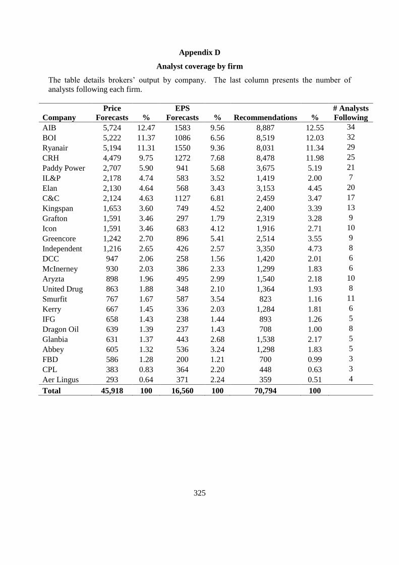
325
Appendix D
Analyst coverage by firm
The table details brokers’ output by company. The last column presents the number of
analysts following each firm.
Company
Price
Forecasts %
EPS
Forecasts % Recommendations %
# Analysts
Following
AIB 5,724 12.47 1583 9.56 8,887 12.55 34
BOI 5,222 11.37 1086 6.56 8,519 12.03 32
Ryanair 5,194 11.31 1550 9.36 8,031 11.34 29
CRH 4,479 9.75 1272 7.68 8,478 11.98 25
Paddy Power 2,707 5.90 941 5.68 3,675 5.19 21
IL&P 2,178 4.74 583 3.52 1,419 2.00 7
Elan 2,130 4.64 568 3.43 3,153 4.45 20
C&C 2,124 4.63 1127 6.81 2,459 3.47 17
Kingspan 1,653 3.60 749 4.52 2,400 3.39 13
Grafton 1,591 3.46 297 1.79 2,319 3.28 9
Icon 1,591 3.46 683 4.12 1,916 2.71 10
Greencore 1,242 2.70 896 5.41 2,514 3.55 9
Independent 1,216 2.65 426 2.57 3,350 4.73 8
DCC 947 2.06 258 1.56 1,420 2.01 6
McInerney 930 2.03 386 2.33 1,299 1.83 6
Aryzta 898 1.96 495 2.99 1,540 2.18 10
United Drug 863 1.88 348 2.10 1,364 1.93 8
Smurfit 767 1.67 587 3.54 823 1.16 11
Kerry 667 1.45 336 2.03 1,284 1.81 6
IFG 658 1.43 238 1.44 893 1.26 5
Dragon Oil 639 1.39 237 1.43 708 1.00 8
Glanbia 631 1.37 443 2.68 1,538 2.17 5
Abbey 605 1.32 536 3.24 1,298 1.83 5
FBD 586 1.28 200 1.21 700 0.99 3
CPL 383 0.83 364 2.20 448 0.63 3
Aer Lingus 293 0.64 371 2.24 359 0.51 4
Total 45,918 100 16,560 100 70,794 100
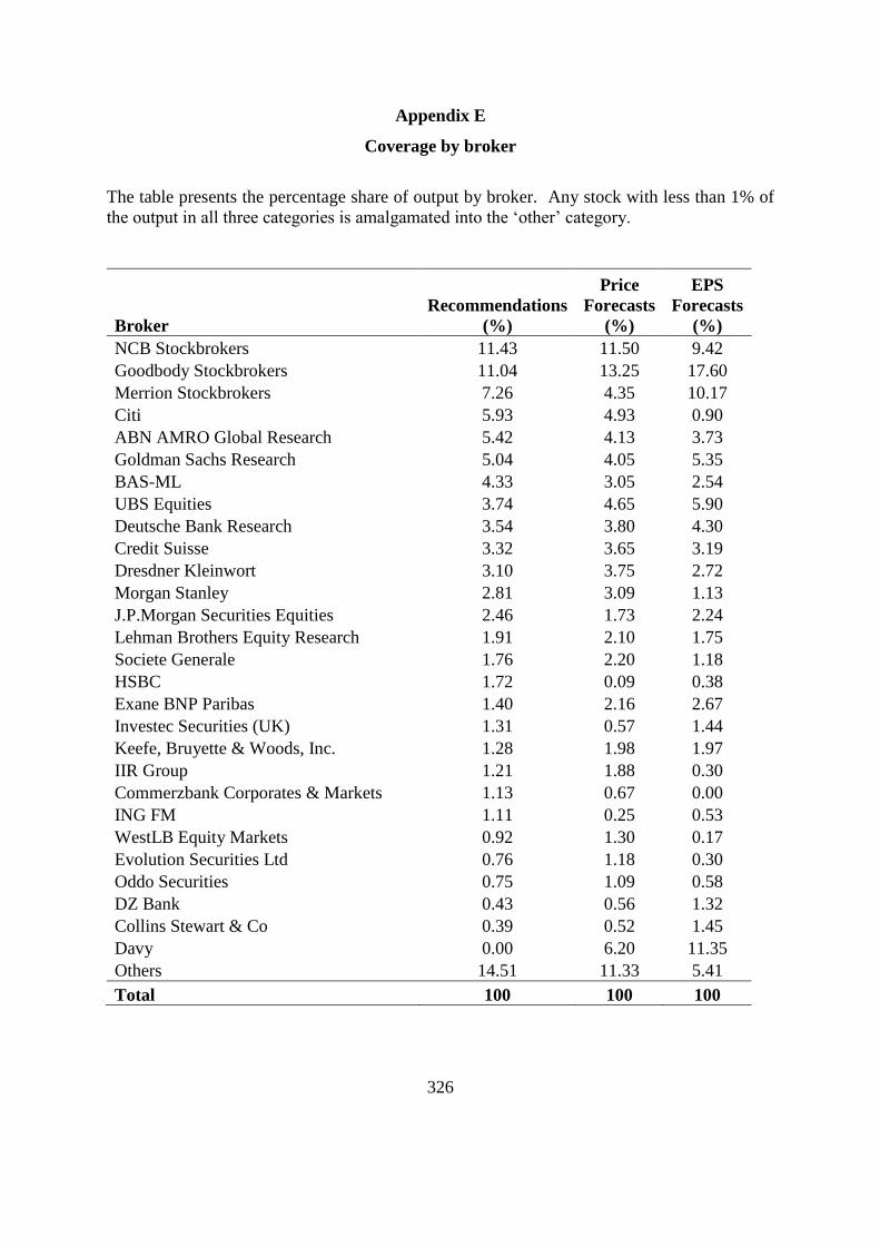
326
Appendix E
Coverage by broker
The table presents the percentage share of output by broker. Any stock with less than 1% of
the output in all three categories is amalgamated into the ‘other’ category.
Broker
Recommendations
(%)
Price
Forecasts
(%)
EPS
Forecasts
(%)
NCB Stockbrokers 11.43 11.50 9.42
Goodbody Stockbrokers 11.04 13.25 17.60
Merrion Stockbrokers 7.26 4.35 10.17
Citi 5.93 4.93 0.90
ABN AMRO Global Research 5.42 4.13 3.73
Goldman Sachs Research 5.04 4.05 5.35
BAS-ML 4.33 3.05 2.54
UBS Equities 3.74 4.65 5.90
Deutsche Bank Research 3.54 3.80 4.30
Credit Suisse 3.32 3.65 3.19
Dresdner Kleinwort 3.10 3.75 2.72
Morgan Stanley 2.81 3.09 1.13
J.P.Morgan Securities Equities 2.46 1.73 2.24
Lehman Brothers Equity Research 1.91 2.10 1.75
Societe Generale 1.76 2.20 1.18
HSBC 1.72 0.09 0.38
Exane BNP Paribas 1.40 2.16 2.67
Investec Securities (UK) 1.31 0.57 1.44
Keefe, Bruyette & Woods, Inc. 1.28 1.98 1.97
IIR Group 1.21 1.88 0.30
Commerzbank Corporates & Markets 1.13 0.67 0.00
ING FM 1.11 0.25 0.53
WestLB Equity Markets 0.92 1.30 0.17
Evolution Securities Ltd 0.76 1.18 0.30
Oddo Securities 0.75 1.09 0.58
DZ Bank 0.43 0.56 1.32
Collins Stewart & Co 0.39 0.52 1.45
Davy 0.00 6.20 11.35
Others 14.51 11.33 5.41
Total 100 100 100

327
Appendix F
Buy-to-sell ratios in existing literature
Author Country Buy-to-sell
ratio
Lloyd-Davies and Canes (1978) US 3.2:1
Elton et al. (1986) US 3.5:1
Stickel (1995) US 4.6:1
Ho and Harris (1998) US 5.2:1
Womack (1996) US 7:1
Rajan and Servaes (1997) US
Aitken et al. (2000) Australia 3.25*
Jegadeesh et al. (2004) US 18.8:1
Britain 3.9:1
Canada 4.8:1
France 3.3:1
Germany 1.9:1
Italy 2.8:1
Japan 2.5:1
Michaely and Womack (2004)
Jegadeesh and Kim (2006) US 3.6:1
Ryan (2006) Ireland 7.2:1
Moshirian et al. (2009) Emerging markets 1.4:1* * denotes a ratio of positive-to-negative recommendations.
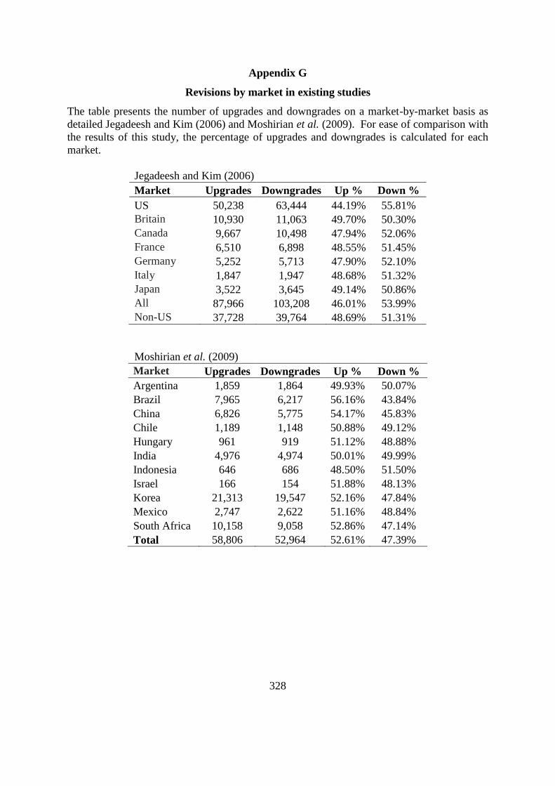
328
Appendix G
Revisions by market in existing studies
The table presents the number of upgrades and downgrades on a market-by-market basis as
detailed Jegadeesh and Kim (2006) and Moshirian et al. (2009). For ease of comparison with
the results of this study, the percentage of upgrades and downgrades is calculated for each
market.
Jegadeesh and Kim (2006)
Market Upgrades Downgrades Up % Down %
US 50,238 63,444 44.19% 55.81%
Britain 10,930 11,063 49.70% 50.30%
Canada 9,667 10,498 47.94% 52.06%
France 6,510 6,898 48.55% 51.45%
Germany 5,252 5,713 47.90% 52.10%
Italy 1,847 1,947 48.68% 51.32%
Japan 3,522 3,645 49.14% 50.86%
All 87,966 103,208 46.01% 53.99%
Non-US 37,728 39,764 48.69% 51.31%
Moshirian et al. (2009)
Market Upgrades Downgrades Up % Down %
Argentina 1,859 1,864 49.93% 50.07%
Brazil 7,965 6,217 56.16% 43.84%
China 6,826 5,775 54.17% 45.83%
Chile 1,189 1,148 50.88% 49.12%
Hungary 961 919 51.12% 48.88%
India 4,976 4,974 50.01% 49.99%
Indonesia 646 686 48.50% 51.50%
Israel 166 154 51.88% 48.13%
Korea 21,313 19,547 52.16% 47.84%
Mexico 2,747 2,622 51.16% 48.84%
South Africa 10,158 9,058 52.86% 47.14%
Total 58,806 52,964 52.61% 47.39%

329
Appendix H
Summary statistics on firm-specific attributes
The table presents summary statistics on the value of each firm-specific variable and the
number of firms for which data is available in each quarter.
Variable
Value Number of firms
Mean Median Mean Median
Rating 4.01 4.00 23 23
6 month returns 0.04 0.01 24 24
3 month returns 0.02 0.00 24 24
Volume 1.16 1.04 24 24
Size 20.81 20.78 22 21
Book-market 0.61 0.41 21 21
Expected price change 31.09 13.50 22 24
Rating change -0.01 0.00 21 22
Change in expected price change 0.96 -0.02 22 23
Future 3 month return 0.02 0.00 24 24
Future 6 month return 0.05 0.01 24 24
Dispersion 0.14 0.09 21 22
Future Volume 1.21 1.06 24 24
Earnings/Price 15.04 12.95 19 20
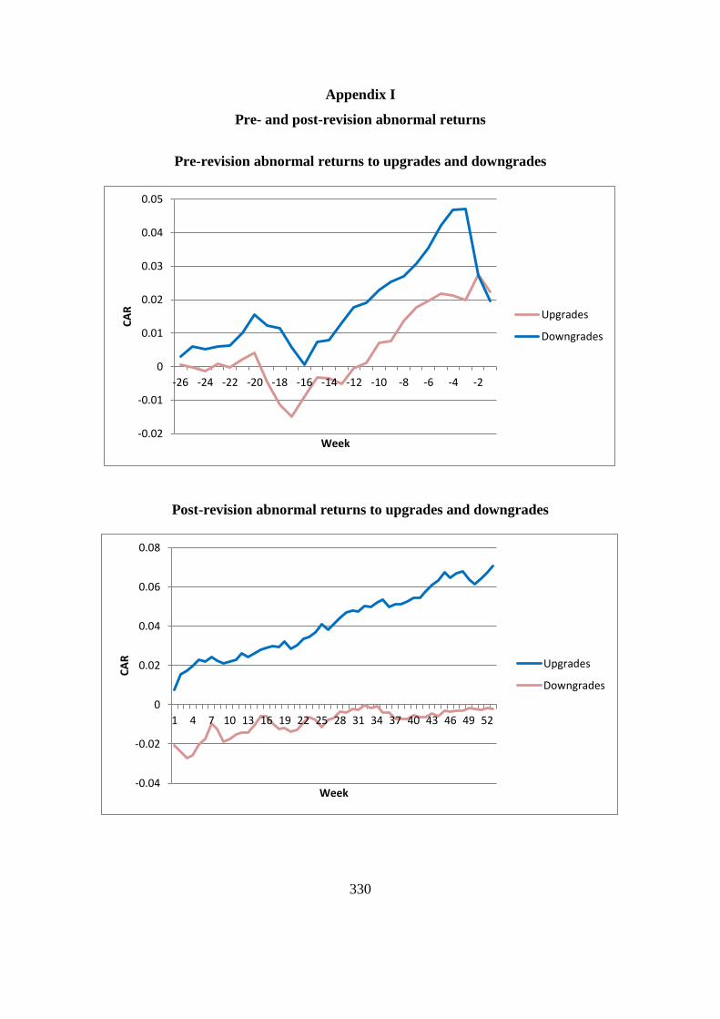
330
Appendix I
Pre- and post-revision abnormal returns
Pre-revision abnormal returns to upgrades and downgrades
Post-revision abnormal returns to upgrades and downgrades
-0.02
-0.01
0
0.01
0.02
0.03
0.04
0.05
-26 -24 -22 -20 -18 -16 -14 -12 -10 -8 -6 -4 -2
CA
R
Week
Upgrades
Downgrades
-0.04
-0.02
0
0.02
0.04
0.06
0.08
1 4 7 10 13 16 19 22 25 28 31 34 37 40 43 46 49 52
CA
R
Week
Upgrades
Downgrades

331
Pre-revision abnormal returns to key upgrades
Post-revision abnormal returns to key upgrades
-0.03
-0.02
-0.01
0
0.01
0.02
0.03
0.04
0.05
0.06
-26 -24 -22 -20 -18 -16 -14 -12 -10 -8 -6 -4 -2
CA
R
Week
hold to add
hold to buy
add to buy
0
0.02
0.04
0.06
0.08
0.1
0.12
0 3 6 9 12 15 18 21 24 27 30 33 36 39 42 45 48 51
CA
R
Week
hold to add
add to buy
hold to buy
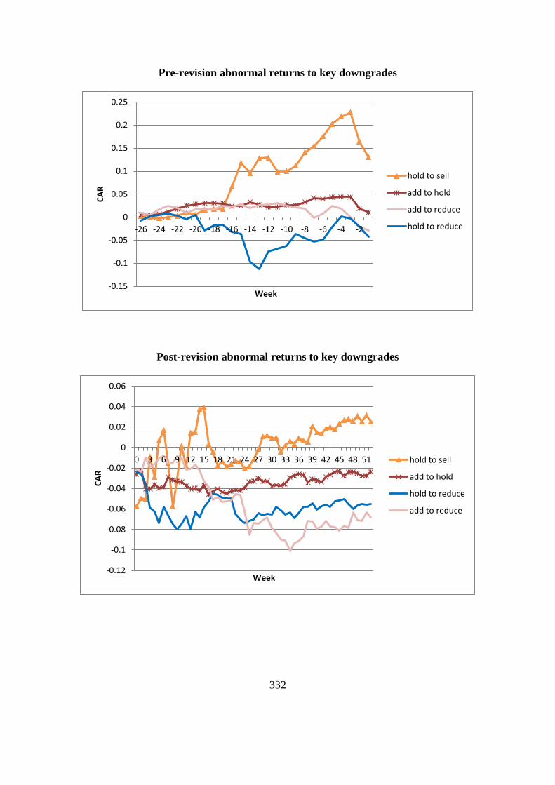
332
Pre-revision abnormal returns to key downgrades
Post-revision abnormal returns to key downgrades
-0.15
-0.1
-0.05
0
0.05
0.1
0.15
0.2
0.25
-26 -24 -22 -20 -18 -16 -14 -12 -10 -8 -6 -4 -2
CA
R
Week
hold to sell
add to hold
add to reduce
hold to reduce
-0.12
-0.1
-0.08
-0.06
-0.04
-0.02
0
0.02
0.04
0.06
0 3 6 9 12 15 18 21 24 27 30 33 36 39 42 45 48 51
CA
R
Week
hold to sell
add to hold
hold to reduce
add to reduce

333
Appendix J
Standardised volume
The table presents the standardised volume for each revision category from week -2 to +2.
Standardised volume is insignificant for all categories outside of this window. One-sided
statistical significance at the 1, 5, and 10% level is indicated by *, **, and *** respectively.
Revision
category
Week relative to revision
-2 -1 0 1 2
add to buy 1.11 1.05 1.32* 1.37* 1.16
add to hold 1.13*** 1.11 1.39* 1.15 1.02
add to reduce 1.21 1.17 1.22 0.92 1.27
add to sell 1.04 0.67 0.75 1.07 1.01
buy to add 0.91 1.21 1.33* 1.24* 1.11***
buy to hold 1.02 1.11 1.22* 1.09 1.12
buy to reduce 1.02 1.13 1.80 1.80* 1.25
buy to sell 0.96 1.06 1.13 1.08 0.75
hold to add 0.91 1.02 1.49* 1.00 0.96
hold to buy 0.96 1.13 1.20* 0.97 0.96
hold to reduce 0.87 1.32* 1.48* 1.22** 1.11
hold to sell 0.94 1.14 1.42* 1.20 1.30
reduce to add 1.25 1.91 1.24** 1.44 1.02
reduce to buy 0.82 0.95 1.18 0.85 0.92
reduce to hold 1.06 0.91 1.32* 0.88 1.01
reduce to sell 0.83 0.87 1.22 3.03 1.35
sell to add 1.55 1.37 1.18 1.64 0.57
sell to buy 0.90 1.06 1.35 1.31 1.07
sell to hold 0.95 1.33 1.38** 1.06 1.01
sell to reduce 0.80 2.21 1.46 1.03 0.64
Upgrades 1.01 1.13* 1.31* 1.12** 1.03
Downgrades 1.00 1.15* 1.32* 1.20* 1.12*
Related Documents