an integrative secondary life science curriculum using select

AN INTEGRATIVE SECONDARY LIFE SCIENCE CURRICULUM USING SELECT

ECOLOGICAL TOPICS PERTAINING TO FOREST ECOSYSTEMS OF NORTH

COAST CALIFORNIA

by

Melinda Bailey

A Project Presented to

The Faculty of Humboldt State University

In Partial Fulfillment of the Requirements of the Degree

Master of Science in Biology

Committee Membership

Dr. Jeffrey White, Chair

Dr. Sean Craig, Committee Member

Dr. Erik Jules, Committee Member

Dr. Susan Edinger Marshall, Committee Member

Dr. Michael Mesler, Graduate Coordinator

December 2014

ABSTRACT

AN INTEGRATIVE SECONDARY LIFE SCIENCE CURRICULUM USING SELECT

ECOLOGICAL TOPICS PERTAINING TO FOREST ECOSYSTEMS OF NORTH COAST CALIFORNIA

Melinda Bailey

Place-based education is an instructional approach that engages students with their

local environment, which can enrich the educational experience and improve scientific

literacy. This project is a place-based secondary-level life science curriculum incorporating

important ecological concepts using select forest types of the North Coast of California,

USA. The North Coast has a rich natural history and many schools are situated near forests.

This curriculum is multidimensional and includes structured units for middle school and

high school students presented in three thematic modules: general forest ecology, coast

redwoods, and oak woodlands. Units are preceded by a companion piece for each module

that embeds some of the latest scientific research intended to broaden a teachers’ previous

knowledge. Information is approached from different spatial and temporal scales and

designed for flexibility in order to fit the needs of local educators. Information was routinely

sourced from primary scientific literature and professional reports, which often can be

difficult to obtain and comprehend by the non-specialist. Components include figures and

select data, which are integrated into student lessons that offer a unique conduit between

scientists, science teachers, and science students. Evidence reveals students learn best when

actively engaged and presented with relevant information. By developing a challenging

ii

place-based curriculum aligned to new standards that incorporate scientific skills and

interdisciplinary connections, both formal and informal science educators will have a useful,

informative resource pertaining to local forest types that can enrich the learning experience

of their students while connecting them to the place in which they live.

iii

ACKNOWLEDGMENTS I would like to give special thanks to my husband, Mark Bailey; a lover of science

and information, who offered continued support for my project including a keen eye,

valuable feedback, and computer generated graphics. A special thank you to Marie Antoine,

who edited all of my rough draft manuscripts and to Dr. Stephen Sillett who, as a friend and

a scientist, reminded me of the rigor it takes to produce a non-biased, well-researched paper.

I extend further thanks to Dr. Sillett for letting me use field data collected in Prairie Creek

State Park. I would like to extend a special thank you to my advisor, Dr. Jeffrey White, for

his ongoing support since the initial stages of this project. He gave me valuable feedback

throughout the process and kept me on the right track. I would also like to extend my

appreciation to my committee: Dr. Sean Craig, Dr. Susan Edinger Marshall, and Dr. Erik

Jules, for their willingness to support me in this endeavor and for their time and effort.

Furthermore, I’d like to acknowledge the Redwood Science Project for providing funds to

pay for an editor at the final stages of my project. In addition, I would like to thank all of the

other people who contributed to this project. Thanks go out to Michael Kauffmann and

Melody Hjerpe, who created either custom maps or a specific drawing to use in my project.

Thanks to Lynn Webb, Jim Wheeler, and Jason Teraoka for working with me on appropriate

data sets to use in my lessons. Thanks to Deborah Zierten for sharing the latest information

on redwood species and for editing one of my teacher keys. Thanks to Andrea Pickart, who

gave me permission to use her botanical drawings, and to the following people that allowed

me to use their photos or figures in my project: Matt Cocking, Kevin Cole, Thomas Dunklin,

iv

Shayne Green, Greg Giusti, William Selby, and Robert Van Pelt. I would also like to thank

my close friends and family, who had faith in me for finishing such a monumental project

and for reminding me of its potential value.

v

PROJECT SUMMARY The primary purpose of this forest series is to offer both science education

professionals and informal educators involved in secondary science education (grades 7-12)

a stimulating, place-based, natural history curriculum, strongly steeped in ecological

concepts and principles. The targeted region is centered in Mendocino and Humboldt

Counties located on the North Coast of California, USA. Throughout this curriculum

project, a spectrum of ecological concepts and scientific skills are woven together pertaining

to many different ecological themes including: general ecology, population and community

ecology, landscape ecology, fire ecology, restoration ecology, and conservation biology.

Effort has been made to integrate often difficult to obtain information sourced from peer-

reviewed scientific journals and professional reports in order to add depth and improve

scientific skills. Science by its nature is an interdisciplinary field and much of the material

has students observing, describing, manipulating, and modeling variables. This project

integrates many different learning strategies useful in enriching both the classroom and

outdoor learning experiences. All lessons contained within each unit are aligned with the

disciplinary core ideas of the Next Generation Science Standards (NGSS) and apply to the

interdisciplinary approach set forth by the Common Core Skills and Standards (CCSS).

The entire curriculum series includes three main sections. The first section is an

introduction to the curriculum. This is followed by a prelude, which gives a brief overview

of California’s natural history, as well as the positive and negative influences humans have

had on the landscape. It presents information from a biogeographical perspective intended to

vi

provide a geographical template useful in gaining a wider perspective about the natural

world. Three subsequent thematic units follow the prelude: Module 1: Integrative Forest

Ecology, Module 2: Behind the Redwood Curtain, and Module 3: Our Disappearing Oak

Woodlands.

Each module is multidimensional and comes in two main parts. Part I is a teacher

companion, written to expand the background information of local educators wanting to

learn more about the forests of the North Coast. It integrates physical and biological science

concepts that shape a particular forest type and focuses on the life sciences in particular. Part

II encompasses two units of study; one pertaining to 7th grade life science and the other to

10th grade biology. All lessons within each unit include any necessary student worksheets

along with answer keys in order to make each lesson useful and time saving for the

instructor. The first few pages of each lesson include a unit overview that clearly states the

focal learning objectives of each lesson. Each lesson gives a lesson overview that highlights

key concepts, required materials, time needed, and interdisciplinary connections. A

suggested structured procedure is outlined for the instructor that includes preliminary

questions and answers in order to connect students to their prior understanding. Potential

links to relevant online information are given and each lesson includes a list of needed

materials as well a wide assortment of ideas to use as extension activities. At the end of each

module is a comprehensive glossary of key terms useful for building vocabulary and

references useful for further research.

Real world data are incorporated into several lessons within each module to improve

the educational experience and to allow students an engaging lens into the world of

vii

scientists. By analyzing real world data, students can use quantitative reasoning while

integrating many skills and principles relating to Science Technology Engineering and

Mathematics (STEM) education, a program widely recognized for preparing students for

technology-based careers and becoming well-informed citizens. Evidence shows students

learn best when actively engaged and presented with relevant material. By incorporating the

latest science, students can be engaged in an important and challenging science curriculum

appropriate for learning in the 21st century.

In summary, this curriculum project uses forest ecology as a framework for learning

scientific concepts and integrates many different lessons at various grade levels to complete

various learning objectives. This project is intended to act as a bridge between scientists and

science students, and therefore can be pertinent to improving scientific literacy, careers in

science, and other science related endeavors. Most of the North Coast is covered by

abundant and mixed forest types, which can provide a perfect place for students to explore

firsthand where they live while giving relevancy and meaning to scientific concepts.

Whether a teacher utilizes a unit in its entirety or hand-picks particular lessons within a

particular grade appropriate unit, each lesson is designed to add meaning and enrichment to

primary resources used in the classroom and beyond.

viii

TABLE OF CONTENTS ABSTRACT ……………………………………………………………….…..… ii

ACKNOWLEDGMENTS …………………………………………….….…...… iv

PROJECT SUMMARY ……………………………………………………..….. vi

APPENDICES

APPENDIX A: INTRODUCTION TO THE FOREST ECOLOGY 101 SERIES List of Figures 1I. Targeted area for the Forest Ecology 101 series ……………………………… 5 2I. Major components of each thematic module …………………………………. 5 3I. Potential integration of thematic units ……………………………………….. 6 Curriculum Series Overview……………………………………………………… 1 How to Use This Series ………………………………………………………….. 2 Forest Ecology 101 Thematic Modules …………………….………………….… 3 Figures ………………………………..……………………………………...…... 5 Literature Cited ……………………………………………………………….…. 6 APPENDIX B: PRELUDE List of Figures 1P. Bioregions of California ……………………………………………………. 14 2P. Simplified vegetation types across California’s landscape west to east. Plant communities common to northern California are situated above the transect and several communities common to southern California are located below the transect ………………………………………………………………………….. 14 Introduction …………………………………………………………..….…..…. 7 Climate …………………………………………………………..…………..…. 7 Geology …………………………………………………………..……..……… 8 Soils …………………………………………………………….…………..…... 9 Topography and Associated Vegetation ………………………………..…….... 9 Biodiversity ………………………………………………………………...…... 11 Human Influence ……………………………………………………….…..….. 12 Conservation ………………………………………………………….…….….. 13 Figures ………………………………………………..………….……….….… 14 Literature Cited ……………………………………………………….……..…. 15

ix

(Table of Contents continued) APPENDIX C: MODULE 1: INTEGRATIVE FOREST ECOLOGY ………….. 17 APPENDIX D: MODULE 2: BEHIND THE REDWOOD CURTAIN……….… 149 APPENDIX E: MODULE 3: OUR DISAPPEARING OAK WOODLANDS .… 276 APPENDIX F: GOING FURTHER …………………………………………….. 423

x

APPENDIX A

INTRODUCTION TO THE FOREST ECOLOGY 101 SERIES

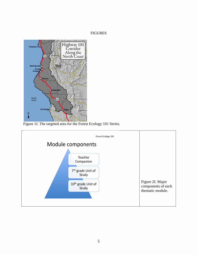
Curriculum Series Overview The primary purpose of this forest series (e.g., Forest Ecology 101) is to offer both science education professionals and informal educators involved in secondary science education (grades 7-12) a stimulating, place-based, natural history curriculum, strongly steeped in ecological concepts and conservation biology. It is centered on the North Coast of California, covering most of Humboldt and Mendocino Counties along the Highway 101 corridor (Fig. 1I). It integrates many different learning strategies useful in enriching both the classroom and outdoor learning experiences. All lessons contained within each unit are aligned with the disciplinary core ideas of the Next Generation Science Standards (NGSS) and apply to the interdisciplinary approach set forth by the Common Core Skills and Standards (CCSS). Throughout this series a spectrum of ecological concepts and scientific skills are woven together pertaining to many different ecological themes including general ecology, population and community ecology, landscape ecology, fire ecology, restoration ecology, and conservation biology. Effort has been made to integrate information obtained directly from peer-reviewed scientific journals and professional reports. By incorporating the latest science, students can be engaged in a relevant and challenging curriculum appropriate for learning in the 21st century. The entire series includes three modules discussed in greater detail below as follows: Module 1: Integrative Forest Ecology, Module 2: Behind the Redwood Curtain, and Module 3: Our Disappearing Oak Woodlands. All three modules are preceded by a prelude, which gives a brief overview of California’s natural history, as well as the positive and negative influences humans have had on the landscape. It presents information from a broad biogeographical perspective intended to provide a geographical template useful to gain a wider perspective regarding the limiting factors controlling vegetative types found throughout the state. It can be useful in integrating earth science, language arts, and mathematics as well as to the cross-cutting concepts set forth in the NGSS, such as cause and effect. All modules include lessons that attempt to utilize students’ critical thinking skills, while gaining a deeper understanding of our natural world. Each module is arranged in a clear, consistent, and useful format designed to incorporate a wide variety of skills used in science learning, including reading, writing, measuring, interpreting, predicting, observing, questioning, analyzing, modeling, and reaching conclusions. Real-world data are incorporated into several lessons within each module to improve the educational experience and allow students an engaging lens into the world of scientists. By analyzing real-world data, students can use quantitative reasoning while integrating many skills and principles relating to Science Technology Engineering and Mathematics (STEM) education, a program widely recognized for preparing students for technology-based careers and becoming well-informed citizens. A wide use of technology can be easily incorporated into various lessons including computer-generated graphing and modeling and the use of hand-held data collecting devices, as well as digital apps. In addition to providing challenging, high quality lessons, this series (e.g. Forest Ecology 101) is intended to act as a bridge between scientists and science students, and therefore can be

pertinent to improving scientific literacy, careers in science, and other science related endeavors. Science is by nature an interdisciplinary field; much of the material has students observing, describing, manipulating, and modeling variables. Lessons engage prior understanding and are intended to increase the sophistication of student thinking. Whether a teacher utilizes a unit in its entirety or hand-picks particular lessons within a particular grade-appropriate unit, each lesson is designed to add meaning and enrichment to primary resources used in the classroom and beyond. The information presented here uses forest ecology as a framework for learning scientific concepts and integrates many different lessons at various grade levels to complete different learning objectives. Forests provide many ecosystem services and have an intricate place in the human world. Most of the North Coast is covered by abundant and mixed forest types, which provide a perfect place for students to explore firsthand where they live while giving relevancy and meaning to scientific concepts. Evidence shows students learn best when actively engaged and presented with relevant material (Archie 2003). I decided to include information from a variety of temporal and spatial scales to obtain a wide-ranging natural history perspective pertaining to the North Coast, while maintaining a broad connection to the complexity and unmatched diversity of the state as a whole. Studying forested systems at different spatial scales can elucidate important mechanisms regarding watersheds, forest structure and function, and maintenance of biodiversity. I have chosen North Coast California as the setting for this place-based curriculum because of its rich natural history, proximity to many forested ecosystems, and the fact that I have spent over 20 years intimately exploring and living within this particular landscape. The focal area includes Mendocino and Humboldt Counties; however, most units can be easily modified for use throughout other forested landscapes within California’s NCR (Fig.1I). This targeted region corresponds most closely to the Outer North Coast Ranges described in the Jepson Manual (Hickman 1993) and the North Coast region as described by Sawyer (2006) in Northwest California: A Natural History. In this remote part of the state, educators can find abundant places for students to explore, perhaps even directly on or adjacent to their school site. A wide choice of alternative locations to choose from include city, county, state, and federal parks, as well as other federal lands, such as designated wilderness, national forests, and Bureau of Land Management (BLM) conservation areas and preserves, offering abundant, publically accessible places to enrich the learning experiences in the field.

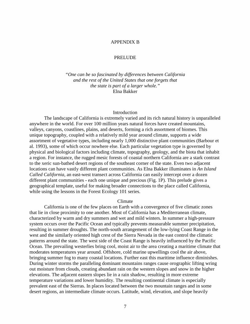
How to Use This Series This project is multidimensional and comes in two main parts presented in three modules. Each module has a teacher companion (Part I) and subsequent lessons (Part II) for two different grade levels referred to as units (Fig. 2I). Each Teacher Companion is written as useful background information for all educators regardless of grade level wanting to learn more about the forests of the North Coast. As previously mentioned, it disseminates information obtained from a wide variety of sources, including professional reports and primary scientific literature. It integrates physical and biological science concepts that shape a particular forest type, focusing on the life sciences in particular. The forest series is also designed so that different portions can be integrated into existing curriculum and/or within selected lessons found in a particular unit (Fig. 3I). For instance, teachers may want their students to understand the importance of keystone species by using both coast redwood (Module 2) and oaks (Module 3). The knowledge presented in each corresponding Teacher Companion goes beyond the specific realm of each lesson. The information is intended to add richness and depth to an

2

educator’s existing knowledge about the North Coast and to provide a window into some of the latest scientific findings. All lessons within each unit include any necessary student worksheets, along with answer keys in order to make each lesson useful and time saving for the instructor. The individual units (Part II) are geared towards two different grade levels: middle school life science (7th grade), and high school life science (10th grade). The two targeted grades levels should not be regarded as restrictive. Instead, they are intended to act only as a guide: useful for the alignment of particular life science standards and student ability levels. The middle school units are aligned to the preferred integrated NGSS standards arranged by disciplinary core ideas. Each unit has been designed for teacher flexibility. Each lesson within each unit can be used as a stand-alone lesson, a unit focusing on one particular module or theme, or together as a six-to eight-week comprehensive forest ecology series. For simplification and organization all pages used in a particular lesson are abbreviated to denote the module, lesson, and grade at a glance. A particular module is identified with a capital M, grade with a capital G, and lesson with a capital L. For example, M2.G10.L3 refers to lesson 3 in module 2 at the high school level or grade 10. Reference sheets, student worksheets, reading assignments, and teacher keys follow the same abbreviated pattern. In addition to being aligned with the NGSS, when relevant, every lesson makes connections to California’s Education and Environment Initiative (EEI) curriculum, which includes free, high-quality resources available online. The first few pages of each lesson include a unit overview that clearly states the focal learning objectives, key concepts, and topic and interdisciplinary connections. A suggested structured procedure is outlined for the instructor that includes preliminary questions and answers, in order to connect students to their prior understanding. Potential links to relevant online information are given and each lesson includes a list of needed materials, as well as a wide assortment of ideas to use as extension activities. At the end of each module teachers will find a comprehensive glossary of key terms useful for building vocabulary and references (literature cited) useful for further research. Several ideas and suggestions for field explorations ranging from one class period to an all day field trip are given throughout each Teacher Companion (Part I) and as extension ideas in Part II. Additionally at the end of each Teacher Companion assorted figures and tables are given including maps, pictures, and a list of scientific names referred to throughout each module. Lastly, an out-of-doors culminating experience (e.g., a field trip) to a local forest is encouraged during or after completing an entire unit within a particular module. Additional information for planning purposes is provided in the Going Further section, found at the end of the series in Appendix F. This section gives helpful tips for making outside activities a successful and rewarding experience for all participants, while maintaining good land stewardship practices.

Forest Ecology 101 Thematic Modules Module 1: Integrative Forest Ecology begins with a bioregional perspective to provide a geographic scaffold for the various components that shape a particular bioregion. It starts by outlining how climate, geology, and topography have shaped the ecology of the North Coast. From there, it moves to concepts intended to instill a deeper understanding of trees and their importance to humans and wildlife. Students learn about tree growth, local conifer species, competitive advantages, and how to take forest measurements. Lessons explore ecosystem dynamics and functioning and integrate concepts relevant to all forested ecosystems, such as providing ecosystems services, maintaining biodiversity, and cycling carbon in a terrestrial system.

3

Module 2: Behind the Redwood Curtain focuses on the quintessential forest species of the North Coast, the coast redwood (Sequoia sempervirens). Information about redwoods’ evolutionary history, distribution, size, and importance is presented, including some of the latest scientific data revealing why these forests store more above-ground carbon compared to any other forest type. Students will learn why these climax forests are true rainforests and will understand how old-growth forest structure can lead to greater ecological functioning. Lessons have students integrating scientific skills by graphically representing tree size, biomass, and effects of forest thinning. They will explore issues regarding how humans have impacted these environments and how natural disturbances can enhance biodiversity. Module 3: Our Disappearing Oak Woodlands attempts to reveal the various factors responsible for supporting and altering these exceptionally diverse landscapes unique to California. Oaks are highly variable and widely distributed. Eight species are emphasized here, including tanoak, which is not a true oak. Lessons in this unit have students understanding competitive dynamics, learning about Sudden Oak Death (SOD), and exploring interconnected relationships between oaks - a keystone species - and other organisms. Students will analyze data regarding oak response to conifer thinning, will sequence the evolutionary history of oaks, and will draw conclusions regarding the abiotic and biotic factors influential in acorn mast events and oak regeneration.

4

FIGURES

Figure 1I. The targeted area for the Forest Ecology 101 Series.

Figure 2I. Major components of each thematic module.

5

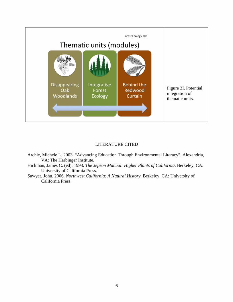
Figure 3I. Potential integration of thematic units.

LITERATURE CITED Archie, Michele L. 2003. “Advancing Education Through Environmental Literacy”. Alexandria,

VA: The Harbinger Institute. Hickman, James C. (ed). 1993. The Jepson Manual: Higher Plants of California. Berkeley, CA:

University of California Press. Sawyer, John. 2006. Northwest California: A Natural History. Berkeley, CA: University of

California Press.

6

APPENDIX B

PRELUDE

“One can be so fascinated by differences between California and the rest of the United States that one forgets that

the state is part of a larger whole.” Elna Bakker

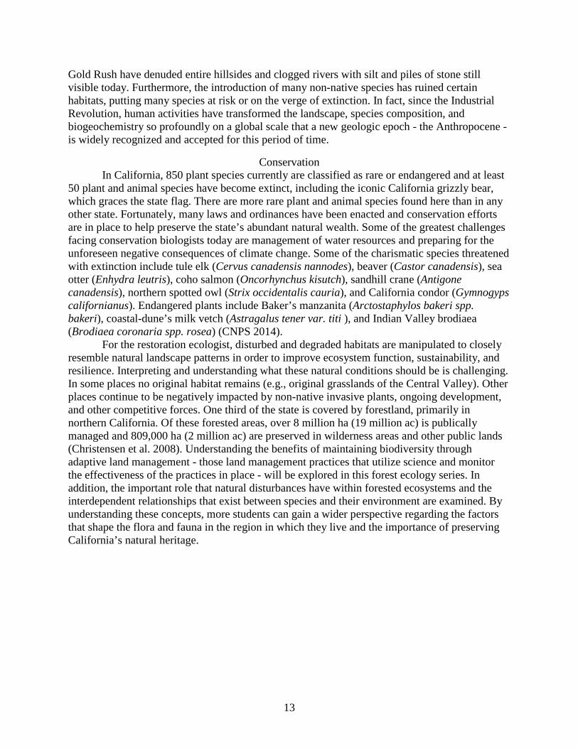
Introduction The landscape of California is extremely varied and its rich natural history is unparalleled anywhere in the world. For over 100 million years natural forces have created mountains, valleys, canyons, coastlines, plains, and deserts, forming a rich assortment of biomes. This unique topography, coupled with a relatively mild year around climate, supports a wide assortment of vegetative types, including nearly 1,000 distinctive plant communities (Barbour et al. 1993), some of which occur nowhere else. Each particular vegetation type is governed by physical and biological factors including climate, topography, geology, and the biota that inhabit a region. For instance, the rugged mesic forests of coastal northern California are a stark contrast to the xeric sun-bathed desert regions of the southeast corner of the state. Even two adjacent locations can have vastly different plant communities. As Elna Bakker illuminates in An Island Called California, an east-west transect across California can easily intercept over a dozen different plant communities - each one unique and precious (Fig. 1P). This prelude gives a geographical template, useful for making broader connections to the place called California, while using the lessons in the Forest Ecology 101 series.

Climate California is one of the few places on Earth with a convergence of five climatic zones that lie in close proximity to one another. Most of California has a Mediterranean climate, characterized by warm and dry summers and wet and mild winters. In summer a high-pressure system occurs over the Pacific Ocean and typically prevents measurable summer precipitation, resulting in summer droughts. The north-south arrangement of the low-lying Coast Range in the west and the similarly oriented high crest of the Sierra Nevada in the east control the climatic patterns around the state. The west side of the Coast Range is heavily influenced by the Pacific Ocean. The prevailing westerlies bring cool, moist air to the area creating a maritime climate that moderates temperatures year around. Offshore, cold marine upwellings cool the air above, bringing summer fog to many coastal locations. Further east this maritime influence diminishes. During winter storms the paralleling dominant mountains ranges cause orographic lifting wring out moisture from clouds, creating abundant rain on the western slopes and snow in the higher elevations. The adjacent eastern slopes lie in a rain shadow, resulting in more extreme temperature variations and lower humidity. The resulting continental climate is especially prevalent east of the Sierras. In places located between the two mountain ranges and in some desert regions, an intermediate climate occurs. Latitude, wind, elevation, and slope heavily

7

influence climate variations, and cool air flowing down mountains in the summer can help cool regions. Low-lying places lacking mountains can receive less than 12.5 cm (5 in) of rain per year (WRCC 2014). Another important climatic factor influencing many plant communities in California is fire. Dry vegetation associated with summer, coupled with low humidity, set up ideal conditions for lightning generated fire, especially in the Sierra Nevada. Certain plant communities are fire-dependent including closed pine forests, giant sequoia, and chaparral. Others are fire neutral or are stimulated by fire but not necessarily dependent upon it. In the North Coast, regular fire prevents conifers from overtopping and suppressing oak trees, which in some cases can lead to oak mortality. Even coast redwood, a forest type associated with fog and high humidity, can benefit from fire. Fire can promote seed germination, expose mineral soils, and benefit wildlife. For the last 50 years active fire suppression has resulted in a build up of fuels periodically creating catastrophic fires that can alter landscapes dramatically and kill native species. Regular fire (10-100 years) prevents these catastrophic fires by reducing the fuel load. Thus, allowing some fires to burn can be beneficial (Stuart and Stephens 2006). In some places anthropogenic fire regimes set by Native Americans over thousands of years have had a strong influence on vegetative composition and distribution, a topic to be discussed in greater detail below. The benefits of fire as they pertain to different forest types will be discussed further in Modules 2 and 3. Climate and fire are not the only limiting factors controlling the type and distribution of vegetation, however. Topography, geology, soil chemistry, and biological factors also play major roles.

Geology The geology of California is a complex mosaic of different types of bedrock derived from several sources and is only briefly reviewed here. Virtually every place in California has been influenced by tectonic activity. The state is crisscrossed with active faults and geothermal activity adding a degree of complexity to most terrains. The deepest rocks are products of several ancient subduction events dating back further than 300 million years. For instance the Sierra Nevada, a relatively young mountain range, sits upon much older rocks from the Mesozoic era. These rocks were part of a much older mountain range, since eroded, that formed atop an even older volcanic arc. Their rocky origin comes from deep magma that crystallized slowly from many different batches of magma, forming granitic rocks. The majority of gold that spurred the Gold Rush was found here. Coastward, the famous San Andreas Fault extends from the Gulf of California to near the Oregon border, marking the boundary between the Pacific and North American Plates. Along the northwest side of the San Andreas, millions of years of subduction have created a confusing matrix of different rock terrains, often referred to as the Franciscan mélange, which will be discussed in greater detail in Module 1. Most of the Franciscan complex consists of oceanic sediments scraped off the bottom of the ocean, mixed with deep-sea volcanism. Most lava was erupted over roughly 100 million years as the Farallon Plate was being subducted. Other parts of this mostly consumed plate were plastered or accreted along the western edge of the continent. The Franciscan formation lies west of the Great Valley Sequence, a thick accumulation of sediments partly formed from an inland sea millions of years ago (Harden 2004). Near Cape Mendocino, where the San Andreas Fault enters the sea, a junction of three tectonic plates occurs making this region one of the most earthquake prone areas in the world. Associated thrust faults continue to form an emergent or rising coastline lined with marine terraces or coastal bluffs. Near San Diego, even older ancient marine terraces and beach ridges

8

are evident, which over the ages have accumulated deep sand. Although most of the shoreline along the California coast is emergent, in some places (e.g., San Francisco Bay) the coastline is submerging and sea level continues to rise. The southern reach of the Sierra Nevada joins the Transverse Range, which is oriented east-west, breaking the primary north-south topographic pattern. Many faults in this area are ancient, buried, and non-active. The active fault systems occurring here are predominately caused by compressional forces, resulting in highly folded terrain that continues to twist and buckle today. Large areal basins now filled with thick sediment were formed by similar uplifting events occurring on all sides. Further south, the Peninsular Range has rocks of a similar age and origin to those in the Sierra Nevada, originating by ancient subduction along a volcanic arc. Granitic rocks near the Mohave Desert are some of the oldest found in the state being over one billion years old (Harden 2004). Other rocks in southern California were formed in shallow marine waters or by early volcanism. Given such a complex geological history, deciphering the complete story of California’s creation is far from complete and research continues to add new information.

Soils Geophysical processes such as mountain building, erosion, and glaciation, combined with water and organic material, produce different soil properties and a wide assortment of them are found in California. Examples of nearly all of the world’s 12 soil orders can be found contributing substantially to the high degree of biological diversity. Soils often are classified by color, texture, composition, and parent material. Even though soils can be deterministic of the type of flora and fauna found in a particular area, they will not be discussed in detail here. Several rare soil types occur in California. One in particular is worth mentioning because of its prevalence in the Coast Ranges - serpentine soil. Serpentinite or serpentine is a unique metamorphic rock associated with the upper mantle. These unusual soils are very low in calcium and high in magnesium. Many in- depth studies of the geology-plant linkage have been conducted on them. They can be high in heavy metals, including nickel, and at a glance, serpentine barrens and sparsely growing vegetation can easily be witnessed. Whereas serpentine soils would be considered toxic to most plant communities, many specialized ones are associated with them, including serpentine chaparral and serpentine fens (Kruckeberg 2006; Ornduff et al. 2003). Unique rock types, such as serpentine and limestone, create azonal habitats, since their associated soil chemistry can override the influence of climate and topography.

Topography and Associated Vegetation The topography of California resembles that of a bathtub where the central portion is occupied by the Great Central Valley. The north-south oriented coastal mountains flank the west side of the expansive Central Valley and the east side is lined by Sierra-Cascade axis, also oriented north-south. Most mountainous regions above 1,100 m (3,500 ft) begin to be covered by coniferous forests with lower elevations occupied by grasslands and oak woodlands, except in desert regions. The nearly flat interior portion is drained by two principal rivers: the Sacramento, which flows south, and the San Joaquin, which flows north, with the two meeting east of San Francisco Bay. These two impressive rivers drain 40% of the state (Josselyn 1983). In the Central Valley, soil types vary from deep alluvial soils, formed from frequent flooding, to hard soils associated with the oil-producing areas of the San Joaquin Valley (Ornduff et al. 2003). Deep rich loamy soils caused by frequent flooding (once covered by expansive grasslands and riparian forests) have been converted to one of the most productive agricultural regions of the

9

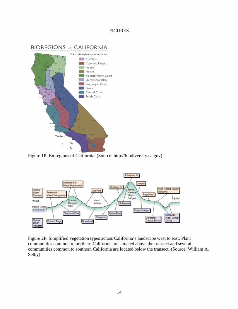
world. In fact, so much food is produced in the Central Valley that John McPhee (1993) describes it as the “North American fruit forests”. The Coast Range extends from Santa Barbara north to southern Alaska. In California this low-lying mountain range stretches across two thirds of the state. Bordering the Pacific Ocean, it is separated into the North and South Coast Ranges by the interruption of San Francisco Bay. This curriculum focuses on the northwestern corner of the NCR, home to the tallest and some of the largest trees in the world, the coast redwood (covered in more detail in Module 2). These awe-inspiring forests are unique; people often use similar language to describe them as they would religious cathedrals. Their lineage dates back to the Cretaceous period approximately 150 million years ago and thus are sometimes referred to as a relic or paleoendemic species. Module 3 highlights the ecological importance of oak woodlands, which are considered a keystone species. Although California is not the center of oak diversity, 20 tree species are found here, 16 of which are endemic, meaning they are found no where else in the world. The NCR is linked to the Sierra-Cascade axis by the Klamath and Siskiyou Mountains, forming the Klamath/North Coast bioregion, discussed further in Module 1 (Fig. 2P). Northeast of this bioregion lies the Modoc Plateau. It is a high plateau with a dry, cool, interior climate that marks the northern end of the Basin and Range Province, which extends eastward across Nevada. This northeastern corner is virtually treeless and is dominated by sagebrush steppe. Between the Modoc Plateau and the Klamath Mountains is the southern extent of the volcanically active Cascade Range, which extends north into Washington. These majestic volcanic cones form a backbone down central Washington and Oregon. In northern California two impressive volcanoes, Mt. Shasta and Mt. Lassen, tower above the grassy foothills underlain by lava. Eastward of the Central Valley is the “spine” of California - the Sierra Nevada. This uplifted granitic series extends continuously over 640 km (400 mi), reaching elevations of over 4267 m (14,000 ft) in the higher southern portion. This dramatic mountain range is approximately 64-97 km (40-80 mi) wide with the western edge rising gradually from the valley floor, in sharp contrast with steeply descending east side. The gradual elevation gain transects several different ecotones, beginning with foothill woodland in lower elevations to the wind-swept alpine zone, with several different forests types in between, including chaparral, yellow pine (lower montane forest, including Pinus jeffreyi and P. ponderosa), lodgepole pine (P. contorta spp. murrayana), and red fir (Abies magnifica). Some of the most dramatic landscapes in California occur here, including King and Yosemite Canyons. Every winter snow accumulates in the higher elevations acting as water reservoirs, slowly releasing moisture into the ground and rivers during the dry season. Today all the major rivers flowing from the Sierra Nevada westward are dammed with artificial reservoirs used to regulate water flow to the valley below. The Smith River, located primarily in the Six Rivers National Forest covering much of Humboldt County, is the last major free-flowing river in the state. The juxtaposition of the Sierra Nevada to the Central Valley and the eastward continent is partly responsible for some of the high degree of endemism found in California, including several trees species. The voluminous giant sequoia (Sequoiadendron giganteum) grows between 1,525 m (5,000 ft) and 2,300 m (7,500 ft) in small mixed groves and is a sight to behold. The biggest ones can have trunk diameters exceeding 8 m (27 ft) and stand over 80 m (260 ft) tall (Earle 2013). Because they are related to coast redwood giant sequoia will be discussed further in Module 2. In the subalpine zone lives the oldest known plant in the world, the bristlecone pine (Pinus longaeva). These trees, which have little competition, have adapted to a harsh

10

environment with little rain and poor dolomite soils. Record trees exceed 3,000 years old and partially decayed remnants mark a past timberline higher in elevation, suggesting an earlier time period of greater moisture. Over a dozen conifer species in California are endemic, including Monterey pine (Pinus radiata), foxtail pine (P. balfouriana), ghost pine (P. sabiniana) and Sargent cypress (Cupressus sargentii) (Lanner 1999). Adjacent to the Sierra Nevada is the heavily faulted Basin and Range Province, marking a transition zone between the coniferous forests of the Sierra Nevada and the steppe of the Great Basin. The steppe climate, associated with the southern portion of the Central Valley, gives way to low-lying desert environments, separated from the ocean by the Transverse Range (discussed briefly above). These geologically complicated mountains mark the northern border of the Los Angeles Basin. Off the mainland coast of Central and Southern California are the California Islands. Now isolated remnants of a once-larger contiguous coastal region, these continental islands host many endemic species and include the Farallon Islands in the north and the Channel Islands in the south. Inland, the Mohave Desert covers a large portion of the arid southeastern portion of the state. Lacking good drainage, salinity can be high. Here, plants compete for moisture and along most slopes the hardy creosote bush dominates. Average precipitation in the low-desert regions can measure less than 5 cm (2 in) annually. Occasionally in Death Valley, the lowest point in North America, no precipitation falls within a given year (Schoenherr 1992). Finally, south of the Mohave is the Colorado Desert with its rich diversity of plant and animal life. This low- elevation desert extends south into northern Mexico and east into Arizona. As aforementioned, the barriers created by the ocean, mountains, and deserts, together with the patterns of water and climate, render California a unique bioregion.

Biodiversity California ranks number one among the 50 states for its plant and animal diversity with new species still being discovered. The Golden State’s unmatched richness accounts for 25% of the overall diversity in the continental United States. At least 1,000 native vertebrate species and over 5,000 native vascular plant species currently live here (Barbour et al.1993; Raven 1988). Over 1,400 of these plant species and 65 vertebrate species are endemic (Keeler-Wolf 2003; Schoenherr 1992). Most of California belongs to a physiographic unit referred to as the California Floristic Province (hereafter CFP). It covers 75% of the state excluding a few xeric places in the north, south, and east (Hickman 1993). In 1996 it was identified as a world biodiversity hotspot, joining the ranks of 33 other identified regions in the world. The CFP contains more native vascular plant species than the entire central and northeastern United States and Canada combined! This superabundance of flora and fauna extends beyond the state’s boundaries, reaching into southern Oregon and northwestern Baja (Hogan 2009). The abundant natural wealth of California can be supported by the historically numerous Native American tribes that once lived here. In pre-European times, California was the most densely populated place of any equally sized area in North America (Anderson et al. 2013). Approximately 10% of all Native Americans on the continent lived in California. Although there is no good census of present population figures, some estimates exceed 200,000 spread over more than 100 tribes (Barbour et al. 1993; Heizer and Whipple 1971; Heizer and Elsasser 1980). Original tribal territories often encompassed many different elevations, thereby offering a wide assortment of plant and animal foods (Anderson 2005; Anderson et al. 2013). Survival depended on an intimate relationship with the seasonal cycles of food availability, including fish spawning

11

and bird migrations. As many anthropologists would agree, the indigenous people of California were not just living in California, they were an integral part of the landscape (Anderson et al. 2013; Heizer and Elsasser 1980).

Human Influences In an attempt to more accurately understand the human-nature relationship of California’s Native Americans, many scholars are no longer using the stereotypical “hunter-gatherer” to describe the indigenous cultures that lived here. Instead, research has revealed a more intense connection - they were land managers, or as Kat Anderson (2005) puts it - they “tended the wild”. For over 10,000 years, indigenous tribes intentionally introduced disturbances to the landscape (Anderson 2005; Anderson et al. 2013). Through burning, weeding, digging, sowing, pruning, and thinning, they encouraged certain plant, animal, algal, and fungal species. Their management practices were constantly refined and derived from collective knowledge, gained over thousands of years through direct experience with the natural world. These traditional management techniques have influenced the size, pattern, structure, and genetics of certain vegetative types found across the California landscape. Today, not only are the imprints of their past management practices found in shell middens, on fire scars on trees, and within soil, but they are also noted in many dusty diaries (Anderson 2005). A common tool used by Native Americans with the intended purpose of resource manipulation was fire. Regular low-intensity fire regimes benefit many ecosystems, including oak woodlands, coniferous forests, and freshwater marshes. For some vegetative types, studies reveal regular low-intensity anthropogenic fires were set every 1-40 years, depending on locale and conditions (Keeley 2002; McCreary 2004; Sawyer 2006; Van de Water and Safford 2011). After the extirpation of most Native Americans, sheepherders and cattlemen continued to burn in order to keep meadows open and reduce the risk of nearby forest fires (Anderson et al. 2013; Johnston 1994). In the past many natural areas (e.g., oak woodland, yellow pine forest) were so extensively managed by fire and clearing that early explorers described them as park-like, with large trees spaced far apart (Anderson 2005; Anderson et al. 2013). The benefits of regular burning include creating better habitat for game, eliminating brush, reducing the potential for catastrophic fires, diminishing many plant diseases, and encouraging a wider diversity of food crops (McCreary 2004). Fire increases the number of palatable grasses and forbs for grazing animals. Today, fire suppression has upset the natural balance in many ecosystems. Managed forests frequently have clogged understory and high fuel loads, which can lead to catastrophic wildfires (Van de Water and Safford 2011). Today, California is one of the most populated and fastest growing regions of the country. Most of the natural landscape has been severely altered by more-recent human impact. Since European contact, intensive exploitation of natural resources has had devastating effects on many ecosystems, resulting in severe habitat loss. The rich, loamy soils of the Central Valley have been converted to prime agricultural land. As a result, enormous freshwater marsh systems and lush riparian zones have been seriously degraded. To increase land area to accommodate grazing, agriculture, and urban growth, huge sections of salt marshes and other wetlands have been drained or filled. Diversion projects have redirected water away from rivers and deltas, decimating salmon populations and other wetland habitats and reducing water flows in some places to a mere trickle (de Nevers et al. 2013; Sawyer 2006). Much of the oak woodland and valley grasslands have been removed to make room for housing tracts, shopping malls, and orchards. Most forests have been logged extensively, reducing habitat, increasing siltation in streams, and fragmenting the landscape. Destructive hydraulic mining practices used during the

12

Gold Rush have denuded entire hillsides and clogged rivers with silt and piles of stone still visible today. Furthermore, the introduction of many non-native species has ruined certain habitats, putting many species at risk or on the verge of extinction. In fact, since the Industrial Revolution, human activities have transformed the landscape, species composition, and biogeochemistry so profoundly on a global scale that a new geologic epoch - the Anthropocene -is widely recognized and accepted for this period of time.

Conservation In California, 850 plant species currently are classified as rare or endangered and at least 50 plant and animal species have become extinct, including the iconic California grizzly bear, which graces the state flag. There are more rare plant and animal species found here than in any other state. Fortunately, many laws and ordinances have been enacted and conservation efforts are in place to help preserve the state’s abundant natural wealth. Some of the greatest challenges facing conservation biologists today are management of water resources and preparing for the unforeseen negative consequences of climate change. Some of the charismatic species threatened with extinction include tule elk (Cervus canadensis nannodes), beaver (Castor canadensis), sea otter (Enhydra leutris), coho salmon (Oncorhynchus kisutch), sandhill crane (Antigone canadensis), northern spotted owl (Strix occidentalis cauria), and California condor (Gymnogyps californianus). Endangered plants include Baker’s manzanita (Arctostaphylos bakeri spp. bakeri), coastal-dune’s milk vetch (Astragalus tener var. titi ), and Indian Valley brodiaea (Brodiaea coronaria spp. rosea) (CNPS 2014). For the restoration ecologist, disturbed and degraded habitats are manipulated to closely resemble natural landscape patterns in order to improve ecosystem function, sustainability, and resilience. Interpreting and understanding what these natural conditions should be is challenging. In some places no original habitat remains (e.g., original grasslands of the Central Valley). Other places continue to be negatively impacted by non-native invasive plants, ongoing development, and other competitive forces. One third of the state is covered by forestland, primarily in northern California. Of these forested areas, over 8 million ha (19 million ac) is publically managed and 809,000 ha (2 million ac) are preserved in wilderness areas and other public lands (Christensen et al. 2008). Understanding the benefits of maintaining biodiversity through adaptive land management - those land management practices that utilize science and monitor the effectiveness of the practices in place - will be explored in this forest ecology series. In addition, the important role that natural disturbances have within forested ecosystems and the interdependent relationships that exist between species and their environment are examined. By understanding these concepts, more students can gain a wider perspective regarding the factors that shape the flora and fauna in the region in which they live and the importance of preserving California’s natural heritage.

13

FIGURES

Figure 1P. Bioregions of California. (Source: http://biodiversity.ca.gov)

Figure 2P. Simplified vegetation types across California’s landscape west to east. Plant communities common to northern California are situated above the transect and several communities common to southern California are located below the transect. (Source: William A. Selby)

14

LITERATURE CITED Anderson, M. Kat, Michael G. Barbour, and Valerie Whitworth. 2013. “A World of Balance and

Plenty: Land, Plants, Animals and Humans in a Pre-European California.” In Contested Eden: California Before the Gold Rush, edited by Ramon A. Gutierrez and Richard J. Orsi., Berkeley, CA: University of California Press.

Anderson, M. Kat. 2005. Tending the Wild: Native American Knowledge and the Management of California’s Natural Resources. Berkeley, CA: University of California Press.

Bakker, Elna. 1971. An Island Called California: An Ecological Introduction to its Natural Communities. Berkeley, CA: University of California Press.

Barbour, Michael G., Bruce M. Pavlik, Frank Drysdale, and Susan Lindstrom. 1993. California’s Changing Landscapes. Edited by Phyllis Faber. 2nd ed., Sacramento, CA: California Native Plant Society.

Christensen, Glenn A., Sally J. Campbell, Jeremy S. Fried, and Technical Editors. 2008. California’s Forest Resources, 2001 – 2005 Five-Year Forest Inventory and Analysis Report., Portland, OR: USDA Forest Service PNW-GTR-763.

California Native Plant Societ (CNPS). 2014. “Rare and Endangered Plant Inventory.” http://www.rareplants.cnps.org/.

De Nevers, Greg, Deborah Stranger Edelman, and Adina Merenlender. 2013. The California Naturalist Handbook. Berkeley, CA: University of California Press.

Earle, Christopher. 2013. “The Gymnosperm Database.” http://www.conifers.org. Harden, Deborah R. 2004. California Geology. 2nd ed., Upper Saddle River, NJ: Pearson

Education, Inc. Heizer, Robert F., and Albert B. Elsasser. 1980. The Natural World of the California Indians.

Berkeley, CA: University of California Press. Heizer, Robert F., and M.A. Whipple. 1971. “Number and Condition of California Indians

Today.” In The Californian Indians: A Source Book, 2nd ed., Berkeley, CA: University of California Press.

Hickman, James C. (ed). 1993. The Jepson Manual: Higher Plants of California. Berkeley, CA: University of California Press.

Hogan, Michael C. 2009. “Biological Diversity in the California Floristic Province.” The Encyclopedia of Earth. http://www.eoearth.org/view/article/150634/.

Johnston, Verna R. 1994. California Forests and Woodlands. Berkeley, CA: University of California Press.

Josselyn, Michael. 1983. The Ecology of San Francisco Bay Tidal Marshes: A Community Profile. Washington D.C: U.S. Fish and Wildlife Service FSW/OBS-83/23.

Keeler-Wolf, Todd. 2003. “Geography and Vegetation.” In Atlas of the Biodiversity of California, 3rd printing., California Department of Fish and Game.

Keeley, Jon E. 2002. “Native American Impacts on Fire Regimes of the California Coastal Ranges.” Journal of Biogeography 29: 303–320.

Kruckeberg, Arthur R. 2006. Introduction to California Soils and Plants: Serpentine, Vernal Pools, and Other Geobotanical Wonders. Berkeley, CA: University of California Press.

Lanner, Ronald. M. 1999. Conifers of California. Edited by Majorie Popper and John Evarts. Los Olivos, CA: Cachuma Press, Inc.

15

McCreary, Douglas D. 2004. Fire in California’s Oak Woodlands. Brown Valley, CA: Publication for University of California Integrated Hardwood Range Management Program.

McPhee, John. 1993. Assembling California. New York, NY: Farrar, Straus and Giroux. Ornduff, Robert, Phyllis M. Faber, and Todd Keeler-Wolf. 2003. Introduction to California

Plant Life. Berkeley, CA: University of California Press. Raven, Peter H. 1988. “The California Flora.” In Terrestrial Vegetaion of California, edited by

Michael G. Barbour and Major Jack, 2nd ed., p.109–115. California Native Plant Society. Sawyer, John. 2006. Northwest California: A Natural History. Berkeley, CA: University of

California Press. Schoenherr, Allan A. 1992. A Natural History of California. Berkeley, CA: Berkeley, CA:

University of California Press. Stuart, John, and Scott L. Stephens. 2006. “North Coast Bioregion.” In Fire in California’s

Ecosystems, p.147–169. Berkeley, CA: University of California Press. Van de Water, Kip M., and Hugh D. Safford. 2011. “A Summary of Fire Frequency Estimates

for California Vegetation before Euro-American Settlement.” Fire Ecology 7 (3) (December): 26–58.

Western Regional Climate Center (WRCC). 2014. “Climate of California.” http://www.wrcc.dri.edu/narratives/CALIFORNIA.htm.

16

APPENDIX C

MODULE 1: INTEGRATIVE FOREST ECOLOGY

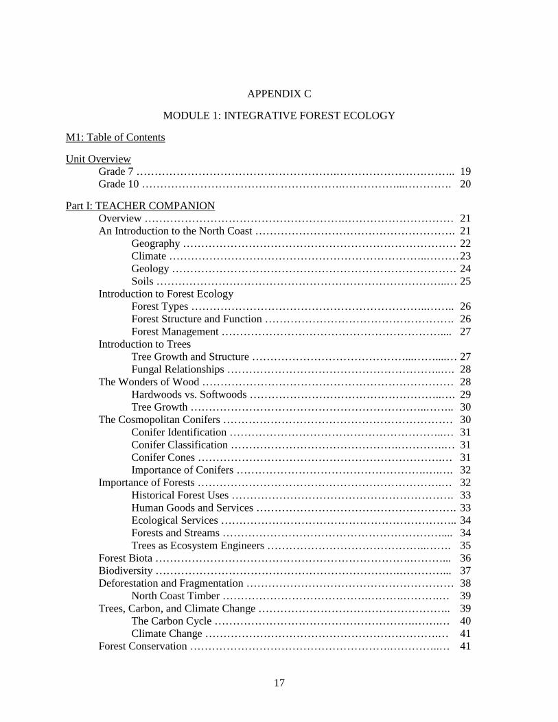
M1: Table of Contents

Unit Overview Grade 7 ……………………………………………….……………………. …….. 19 Grade 10 ……………………………………………….……………...…………. 20

Part I: TEACHER COMPANION Overview ……………………………………………….………………………… 21

An Introduction to the North Coast ………………………………………………. 21 Geography ………………………………………………………………… 22 Climate ……………………………………………………………..……… 23 Geology …………………………………………………………………… 24 Soils ……………………………………………………………………..… 25 Introduction to Forest Ecology Forest Types ………………………………………………………..…….. 26 Forest Structure and Function ……………………………………………. 26 Forest Management …………………………………………………….... 27 Introduction to Trees Tree Growth and Structure ……………………………………...……....… 27 Fungal Relationships …………………………………………………..…. 28 The Wonders of Wood …………………………………………………………… 28 Hardwoods vs. Softwoods ……………………………………………..…. 29 Tree Growth ………………………………………………………..…….. 30 The Cosmopolitan Conifers ……………………………………………………… 30 Conifer Identification …………………………………………………..… 31 Conifer Classification ……………………………………….………….… 31 Conifer Cones ………………………………………………………….… 31 Importance of Conifers …………………………………………….….…. 32 Importance of Forests ………………………………………………………….… 32 Historical Forest Uses ……………………………………………………. 33 Human Goods and Services ………………………………………………. 33 Ecological Services ……………………………………………………….. 34 Forests and Streams …………………………………………………….... 34 Trees as Ecosystem Engineers ……………………………………..……. 35 Forest Biota …………………………………………………………….………... 36 Biodiversity ………………………………………………………….…………... 37 Deforestation and Fragmentation ………………………………………………… 38 North Coast Timber ………………………………….……….……….… 39 Trees, Carbon, and Climate Change …………………………………………….. 39 The Carbon Cycle ……………………………………………….…….… 40 Climate Change ……………………………………………………….… 41

Forest Conservation ……………………………………………….…………..… 41

17

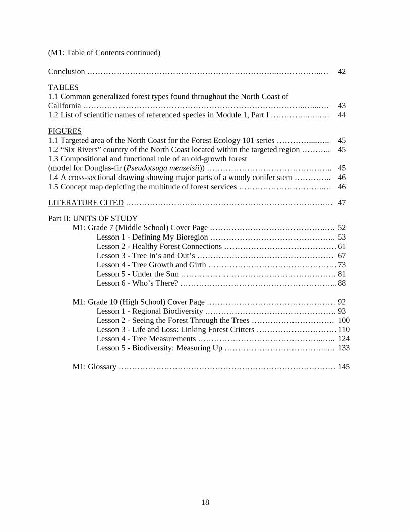
(M1: Table of Contents continued) Conclusion ……………………………………………………………..……………..… 42

TABLES 1.1 Common generalized forest types found throughout the North Coast of California ………………………………………………………………………..…...…. 43 1.2 List of scientific names of referenced species in Module 1, Part I …………..…..…. 44

FIGURES 1.1 Targeted area of the North Coast for the Forest Ecology 101 series …………....….. 45 1.2 “Six Rivers” country of the North Coast located within the targeted region ……….. 45 1.3 Compositional and functional role of an old-growth forest (model for Douglas-fir (Pseudotsuga menzeisii)) ……………………………………….. 45 1.4 A cross-sectional drawing showing major parts of a woody conifer stem ………….. 46 1.5 Concept map depicting the multitude of forest services …………………………..… 46

LITERATURE CITED ……………………..………………………………………….… 47

Part II: UNITS OF STUDY M1: Grade 7 (Middle School) Cover Page …………………………………….…. 52 Lesson 1 - Defining My Bioregion ……………………………………….. 53 Lesson 2 - Healthy Forest Connections …………………………………… 61 Lesson 3 - Tree In’s and Out’s …………………………………………… 67 Lesson 4 - Tree Growth and Girth ………………………………………… 73 Lesson 5 - Under the Sun …………………………………………………. 81 Lesson 6 - Who’s There? ………………………………………………….. 88 M1: Grade 10 (High School) Cover Page ………………………………………… 92 Lesson 1 - Regional Biodiversity …………………………………………. 93 Lesson 2 - Seeing the Forest Through the Trees …………………………. 100 Lesson 3 - Life and Loss: Linking Forest Critters ………………………… 110 Lesson 4 - Tree Measurements ………………………………………..….. 124 Lesson 5 - Biodiversity: Measuring Up ………………………………...… 133 M1: Glossary ……………………………………………………………………… 145

18

Forest Ecology 101 Series (M1: Part I)

MODULE1: INTEGRATIVE FOREST ECOLOGY

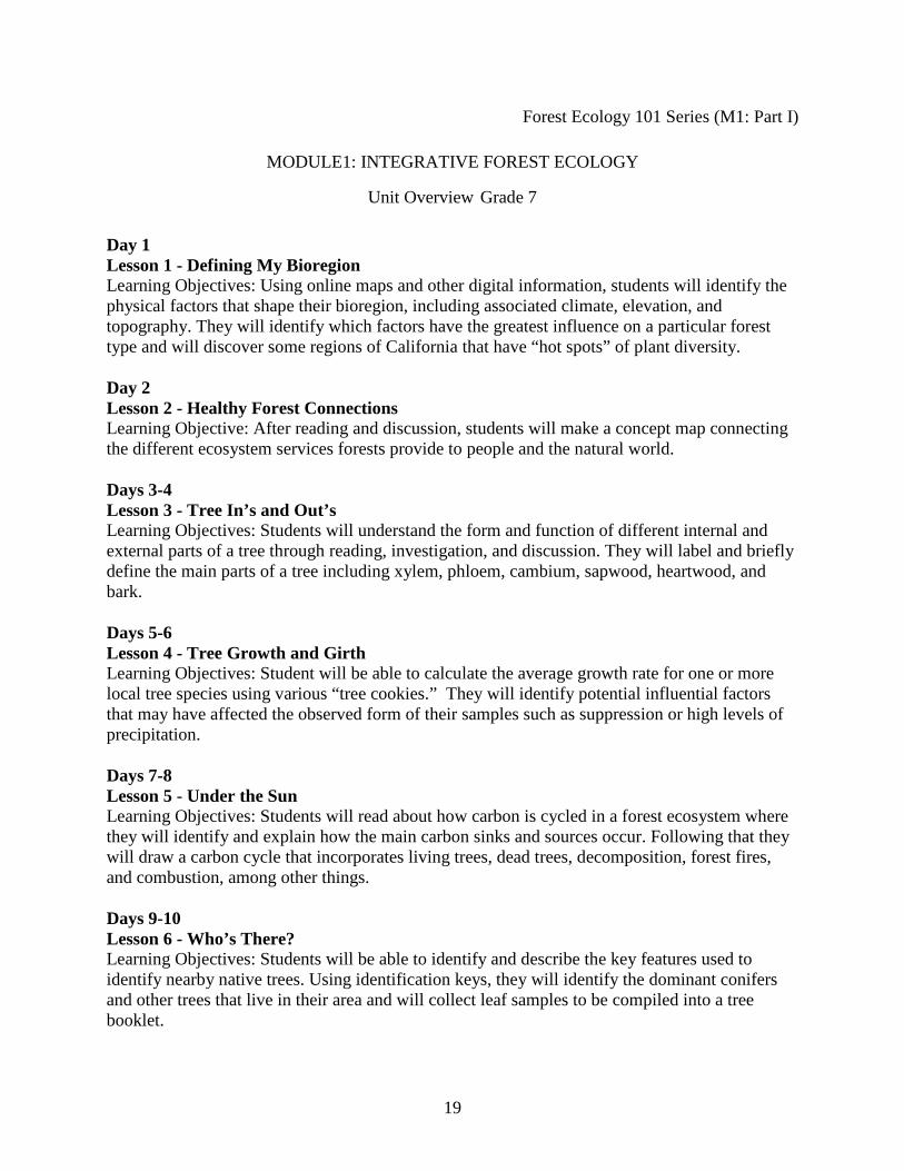
Unit Overview Grade 7 Day 1 Lesson 1 - Defining My Bioregion Learning Objectives: Using online maps and other digital information, students will identify the physical factors that shape their bioregion, including associated climate, elevation, and topography. They will identify which factors have the greatest influence on a particular forest type and will discover some regions of California that have “hot spots” of plant diversity. Day 2 Lesson 2 - Healthy Forest Connections Learning Objective: After reading and discussion, students will make a concept map connecting the different ecosystem services forests provide to people and the natural world. Days 3-4 Lesson 3 - Tree In’s and Out’s Learning Objectives: Students will understand the form and function of different internal and external parts of a tree through reading, investigation, and discussion. They will label and briefly define the main parts of a tree including xylem, phloem, cambium, sapwood, heartwood, and bark. Days 5-6 Lesson 4 - Tree Growth and Girth Learning Objectives: Student will be able to calculate the average growth rate for one or more local tree species using various “tree cookies.” They will identify potential influential factors that may have affected the observed form of their samples such as suppression or high levels of precipitation. Days 7-8 Lesson 5 - Under the Sun Learning Objectives: Students will read about how carbon is cycled in a forest ecosystem where they will identify and explain how the main carbon sinks and sources occur. Following that they will draw a carbon cycle that incorporates living trees, dead trees, decomposition, forest fires, and combustion, among other things. Days 9-10 Lesson 6 - Who’s There? Learning Objectives: Students will be able to identify and describe the key features used to identify nearby native trees. Using identification keys, they will identify the dominant conifers and other trees that live in their area and will collect leaf samples to be compiled into a tree booklet.

19

Forest Ecology 101 Series (M1: Part I)

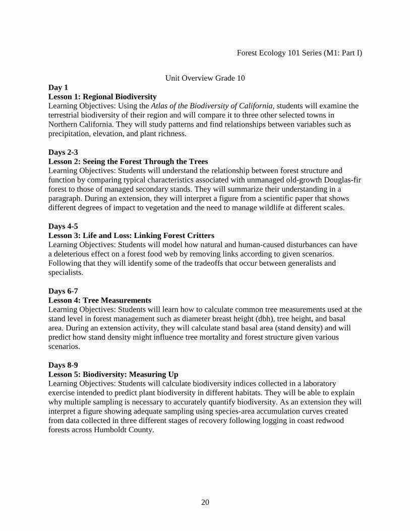
Unit Overview Grade 10 Day 1 Lesson 1: Regional Biodiversity Learning Objectives: Using the Atlas of the Biodiversity of California, students will examine the terrestrial biodiversity of their region and will compare it to three other selected towns in Northern California. They will study patterns and find relationships between variables such as precipitation, elevation, and plant richness. Days 2-3 Lesson 2: Seeing the Forest Through the Trees Learning Objectives: Students will understand the relationship between forest structure and function by comparing typical characteristics associated with unmanaged old-growth Douglas-fir forest to those of managed secondary stands. They will summarize their understanding in a paragraph. During an extension, they will interpret a figure from a scientific paper that shows different degrees of impact to vegetation and the need to manage wildlife at different scales. Days 4-5 Lesson 3: Life and Loss: Linking Forest Critters Learning Objectives: Students will model how natural and human-caused disturbances can have a deleterious effect on a forest food web by removing links according to given scenarios. Following that they will identify some of the tradeoffs that occur between generalists and specialists. Days 6-7 Lesson 4: Tree Measurements Learning Objectives: Students will learn how to calculate common tree measurements used at the stand level in forest management such as diameter breast height (dbh), tree height, and basal area. During an extension activity, they will calculate stand basal area (stand density) and will predict how stand density might influence tree mortality and forest structure given various scenarios. Days 8-9 Lesson 5: Biodiversity: Measuring Up Learning Objectives: Students will calculate biodiversity indices collected in a laboratory exercise intended to predict plant biodiversity in different habitats. They will be able to explain why multiple sampling is necessary to accurately quantify biodiversity. As an extension they will interpret a figure showing adequate sampling using species-area accumulation curves created from data collected in three different stages of recovery following logging in coast redwood forests across Humboldt County.

20

APPENDIX C

MODULE 1: TEACHER COMPANION

INTEGRATIVE FOREST ECOLOGY

“Look deep into nature, and then you will understand everything better”

Albert Einstein

Overview Studying forest ecology can link students to their surrounding environment with the intention of providing a richer scientific program while making connections to potential careers and land stewardship. The availability of forestland in the North Coast region provides abundant opportunity for students to explore the natural world while applying scientific inquiry, skills, and concepts. This particular portion of the teacher’s companion serves as supplemental information to be used in conjunction with the student lessons found in Module 1: Part II. It is intended to provide general and relevant information for secondary science educators and resource specialists regarding forested ecosystems and to be useful in a wide variety of applications. All lessons in this module are aligned to Next Generation Science Standards (NGSS) and apply to the interdisciplinary approach set forth by the Common Core Skills and Standards (CCSS). This chapter does not focus on one particular forest type. Instead, it gives a synthesis of fundamental knowledge to offer a broad-scale approach to understanding forest ecology. All lessons incorporate key life science concepts linked to the NGSS. These include interdependent relationships, cycling of matter and energy, ecosystem functioning and resilience, and the biodiversity that exists in a complex community. Certain lessons strive to reinforce the importance of the ecological services forests provide and the critical need to enhance and conserve the biological integrity of these places. To foster students’ understanding of forested habitats, some lessons make connections between physical and biological factors that govern a tree species, a forest stand, or a particular bioregion. The information contained herein can be easily integrated into Module 2 (coast redwoods) and Module 3 (oak woodlands), furnishing useful knowledge concerning forest measurements, biodiversity, forest structure and function, and the role of forests in the carbon cycle.

An Introduction to the North Coast Module 1 begins by having students take a broad look at the North Coast region. In lesson G7.L1, they will describe some of the different physical factors that shape the Klamath/North Coast bioregion. In lesson G10.L1, students will compare the vegetative richness and endemism of selected areas of the north state and will find relationships between vegetation types and physical factors such as soil type, climate, and topography that govern them. By reviewing some of the primary influential factors, students can develop a greater understanding of the interrelatedness organisms have to the places they inhabit and how human interference such as urbanization has changed the landscape of a given region.

21

Geography The targeted region in this series is centered on the North Coast of California, which includes large portions of Humboldt and Mendocino Counties (Sawyer 2006) (Fig. 1.1). It lies within the broader geographical subunit, the North Coast Range of California (hereafter NCR), which extends coastward from San Francisco Bay to the southern Oregon border (Hickman 1993; Sawyer 2006). This isolated region of the state is relatively unknown due to its rugged terrain and sparse population. The majority of the NCR has been significantly shaped by the San Andreas Fault and subduction off the coast, forming a series of north-south oriented mountains, resulting in many ridges and valleys that follow various fault lines. The mountains form an important climatic and geographic barrier from the Sacramento Valley and foothills to the east. The entire Coast Range is a much larger physiographic unit that hugs a large portion of the West Coast of North America, extending from Baja to southeast Alaska. Bordered by the Pacific Ocean on the west and the Central Valley on the east side, the NCR has distinctive geology, microclimates, soils, and vegetative types that have been changing throughout geologic history. It is adjacent to the Greater Redding metropolis east of the Trinity River watershed, which merges into the Klamath Mountains, forming a distinct bioregion commonly referred to as the Klamath/North Coast bioregion. The Klamath-Siskiyou Mountains have been identified as a Global 2000 Ecoregion by the World Wildlife Fund for their outstanding biological values, which include a high degree of endemism (Kauffmann 2012; Sawyer 2006; Strittholt et al. 2006). Endemism refers to plants and animals found nowhere else. Many of the rare and endemic plants found here can be partly attributed to an extremely complex geology coupled with a wide variety of soil types. Folded and faulted terrain, combined with relatively high precipitation, results in an extensive network of rivers and streams throughout the area. Most drain into a coastal mosaic of bays, lagoons, and deltas, creating important wetland habitats. Much of the region lies within the “Six Rivers” area; major watersheds include those of the Eel and Mattole Rivers in the south and the Mad River, portions of the Lower Klamath, and Redwood Creek in the north (Fig. 1.2). The Eel River system, the third largest in California, covers the majority of the area south of the Eureka-Arcata region as far as the town of Willits. Geologic compression left only one large inland valley, Round Valley, northeast of Willits (Sawyer 2006). The most remote region of the North Coast is commonly referred to as the “Lost Coast.” This 37 km (23 mi) of uninterrupted coastline is found about 110 km (70 mi) southwest of Eureka along the King Range (Schoenherr, 1992). To the south, San Francisco Bay is an important gateway for the North Coast, which lies behind the well-known Golden Gate Bridge. It is by far the largest bay-estuary system in California and continues to be central to the transportation of commodities to and from the North Coast. This nine-county region has the highest human population density in Northern California, with approximately seven million people. Humboldt Bay lies about 400 km (250 mi) north and is the second largest bay-estuary in the state. It is central to the Eureka-Arcata region, the main area of commerce, where approximately 70,000 live (Barnhart et al. 1992). Willits, with approximately 5,000 people, roughly delineates the southern extent of the targeted region along the Highway 101 corridor. All of the North Coast region has a lengthy history of modification from logging, grazing, agriculture, and fire, leading to high disturbance regimes that have resulted in high levels of habitat degradation in many areas (discussed in greater detail below). Much of the area is covered by coniferous forests, which provide much timber. Humboldt and Del Norte Counties

22

represent the southern extension of the great forests of the Pacific Northwest. The magnificent coast redwood forests are indigenous to the area. Coast redwood (Sequoia sempervirens) is the quintessential forest type along the coast where moisture is retained through frequent fog. These forests are protected in a string of parks and preserves that serve as a main tourist destination and are important to the economy of the area. (Coast redwoods are covered in more detail in Module 2.) Douglas-fir (Pseudotsuga menziesii) is the most common conifer and also produces high- quality lumber. It is often mixed with hardwood species such as madrone, tanoak, and California black oak forming a mixed evergreen forest (for scientific names refer to Table 1.2). Directly adjacent to the coastline, on southwest facing slopes and along low montane ridgetops, lie grasslands or prairies, adding to the rich mosaic of vegetation. They are frequently associated with oak woodlands, which are covered in Module 3. Oaks are the most common hardwoods in California. Many are endemic, including valley oak (Quercus lobata) and blue oak (Quercus douglasii).

Climate Similar to other regions of the state the climate of the NCR differs substantially between the rugged coastline and the interior mountains and valleys. A gradient of precipitation moves down the coast with Crescent City receiving close to six feet of rain (1800 mm or 70 in), while San Francisco may only receive one and a half feet (460 mm or 18 in) annually (Major, 1988). The majority of precipitation falls between October and April. Summers can be hot and dry, especially inland, with the length and intensity of the summer dry season increasing as one moves south. Although perhaps not as severe as other regions of the state, the North Coast can experience periodic drought. Another gradient extends from west to east as the Mediterranean climate changes from a moist maritime climate to a drier continental one. Offshore, frigid air originating in Alaska meets subtropical moisture from the south, creating a cool mesic climate along the coast. Here, cold upwelling in the Pacific creates summer fog. In coastal regions, fog drip can substantially contribute to soil moisture and significant amounts of water to vegetation. Northwest-facing streams (e.g., Eel River) channel some of the maritime air inland; however, these inland regions are typically much warmer and drier. As mentioned in the Prelude, orographic lifting caused by steep coastal mountains forces moisture out of water-laden clouds, creating a third gradient based on elevation. Locations near the highest point in the King Range at 1,246 m (4,090 ft) can have annual precipitation exceeding 2,540 mm (100 in). About 80 km (50 mi) further north, Eureka, at an elevation of 61 m (200 ft), has a yearly average of 1,015 mm (40 in) (Schultz, 1990). In winter, snow is common in the mountains, but doesn’t last long in the lower elevations. On some of the higher peaks such as Snow Mountain at 2,144 m (7,035ft) and South Yolla Bolly (formally Mt. Linn) at 2467 m (8,090 ft), snow can persist until early summer (Sawyer 2006). The eastern side of the NCR experiences a classic rain shadow effect caused by the taller coastal mountains to the west. It borders the Sacramento Valley and is not covered in this forest series, aside from comparing climatic variables and other factors useful for understanding associated vegetative types. Further from the coast, these areas experience hot, dry summers and wet, mild winters. Foothills on the leeward side receive one-fourth the precipitation by comparison. Lower elevations may only receive 380-500 mm (15-20 in) of rain annually (de Nevers et al. 2013). The climate and biota found on this drier, warmer side is more similar to the arid foothills of the Sierra Nevada and even parts of Southern California (Sawyer 2006). The microclimates and moisture gradients that occur across the North state can offer a learning

23

opportunity for students to compare weather histories of nearby areas and how they influence vegetative types found there. Having them collect microclimate data can also be a valuable exercise for finding relationships regarding plant and animal adaptations.

Geology The boundary between the Klamath Province and the North Coast is typically defined by South Fork Mountain, located northwest of Red Bluff. South Fork Mountain is associated with a major fault zone separating two major rock groups: the Franciscan complex to the west and the Great Valley sequence to the east (Alt and Hyndman 2001; Sawyer 2006). The Franciscan Complex might be described as a jumbled-up geologic mess. The rocks are a highly complicated mix of different ages and are poorly exposed, making analysis of the geomorphology challenging. Sawyer (2006) likens this highly altered mosaic to ice cream containing many different kinds of nuts. Much of the confusing geology comes from a conglomerate of mixed-aged mélanges embedded in a matrix of soft clay. Most of the Franciscan complex consists of oceanic sediments mixed with deep-sea volcanism. Igneous rocks that intermittently protrude in places are associated with spreading centers dating back 60 million years or more (Alt and Hyndman 2001; Hickman 1993; Sawyer 2006). On top of these older rocks are younger outcrops, some with shallow marine fossils embedded in them. Common rock types include shale, schist, sandstone, serpentinite, and basalt. When taking students into a forest, you may want to discuss why it is often difficult to see the geology or rocks upon which a forest sits. The high degree of moisture associated with the area results in rapid weathering, decomposition, soil accumulation, and large sediment loads, which can often cloak the underlying rock type. The geologic complexity associated with the NCR is compounded and enhanced by the fact that this region is considered “earthquake country”! In the last 115 years, over 40 earthquakes with a magnitude of 6.0 or greater have occurred north of Santa Rosa, including the adjacent offshore areas (Dengler et al. 2011). The largest earthquake in the recorded history of the area was the Great San Francisco Earthquake of 1906. It is estimated to have measured 8.3 on the Richter scale and caused extensive damage to the city proper and surrounding towns (Starr 2005). During this one epic earthquake, a section of the Pt. Reyes Peninsula shifted 5 m (16 ft) northwestward (Schultz, 1990). Further north, megaearthquakes - defined as those with magnitudes exceeding 9.0 - are associated with the Mendocino Triple Junction north of Cape Mendocino where the San Andreas Fault meets the sea. Here the Cascadia Subduction Zone occurs as the Gorda Plate is forced below the North American Plate. This region and the adjacent offshore area is one of the most seismically active areas of the world. Geologists estimate megaearthquakes there to occur every 300-500 years (Sawyer 2006). In 1992, an earthquake centered off the coast of Petrolia raised 20 km (12 mi) of coastline over 1m (3.2 ft) exposing tidepools to the air (Carver et al.1994). The effects of these megathrusts are dramatic; some of the marine terraces that can be seen along the shoreline are the result of such events. The various mountain ranges north of San Francisco can be traced to ancient volcanism and folded sediments along fault zones. Basins (e.g., Napa Valley, Cotati Valley, Alexander Valley, Eel River Basin) were mostly formed from fault movement. Further evidence of subterranean friction near the center of the NCR is the geothermal field near the town of Geyserville, generally referred to as “The Geysers.” Although this particular region lies southeast of the targeted region, it is worthy of mention here. From Highway 101 looking east (near Geyserville) along the ridges, geysers are clearly visible. Their existence is likely due to recent volcanism in the nearby Clear Lake area and today the subterranean heat is used to generate

24

electricity. Clear Lake is the largest natural lake in California and was partly formed by a lava dam. Molten lava underneath the Clear Lake Field is indicated to be near the surface because volcanism dates back as recently as 500,000 years (Alt and Hyndman 2001; Schoenherr 1992).

Soils The physical properties of soils are connected to the raw bedrock, sand, or lava from which they were originated. They are classified by color, texture, depth, chemical composition, and associated parent rock. The varied topography of the landscape influences erosion rates, as water and gravity move sediment downward. Unstable soils, such as those surrounding the Eel Basin, erode easily, so sedimentation tends to be the most significant factor affecting water quality. Erosion can be further accelerated by activities such as timber harvesting, grazing, and development. Soils provide water and important nutrients for plants and can dictate the establishment of distinctive vegetative communities. The amount of water and nutrients available for plants depends on certain variables, such as the amount of clay present, soil chemistry, and the availability of organic matter. Although none of the lessons in this forest series look at soils directly, understanding the connection between soils and plants is important. As students observe the abiotic and biotic factors shaping a forested ecosystem, soils cannot be ignored. Certain studies show a strong relationship between forest production and the depth and position of soil on slopes, as well as other soil characteristics (Fowells and Means 2008). Generally chaparral, a plant community adapted to dry conditions, tends to grow on younger soils that are coarse and shallow; trees and shrubs tend to prefer young unweathered soils; grassland occupies some of the deepest and riches soils; the soils of riparian woodlands are rich due to frequent flooding; and coastal marshes grow on anaerobic soils (Anderson et al. 2013; Barbour et al. 1993; Keeler-Wolf 2003a). An added natural hazard associated with the North Coast is landslides. The Eel river watershed is more prone to landslides than any other region in the state (Sawyer 2006). Understanding how land movement may alter the dynamics of a forest makes discussion relevant here. Most of the landslides are minor; evidence can be seen along most roadways in the form of folded and rumbled land surfaces. The dominate rock types within the Franciscan complex are sedimentary in origin and fracture easily, especially serpentine. Large landslides can occur when weak soils give way after being triggered by heavy rainfall or an earthquake. These events can be very destructive to infrastructure such as railroads, roads, and buildings and can overload streams and rivers with sediment. For example, exorbitant amounts of sediment caused by the 1959 and 1964 floods, exacerbated by clearcut logging and roads, continue to move down the Eel River (EPA 2007). Forests play a key role in reducing sedimentation. These two flooding events and associated salmon restoration efforts in the Bull Creek watershed will be discussed further in Module 2.

Introduction to Forest Ecology

Forest Types Vegetative types such as forests, woodlands, chaparral, and grasslands often are separated into easily identifiable groups based on the communities of plants occupying a particular environment. How vegetation composition and structure differs quantitatively and spatially in regard to the physical environment and disturbance history is fundamental to understanding

25

forest ecology and conservation planning. Forests are utilized by billions of people around the world and are central to quality of life. They are critical habitat for a variety of species and vary greatly in their form and function. A forest type is an association of trees, shrubs, and forbs (e.g., herbs) that form a forested community. Most forest managers agree that a forest is a vegetative type where the predominant life forms are trees creating a canopy that minimally covers 10-40% of the ground (de Nevers et al. 2013; Shvidenko et al. 2007). Forests have been defined in many ways and for different purposes. Woodlands are sometimes described as separate communities, apart from forests, because they have an interrupted tree canopy, creating open patches. In many cases they are referred to separately because they tend to be approached from a different managerial perspective. In California generally woodlands are not classified as timberland (Bernhardt and Swiecki 2001). For practical purposes, and because of the similar ecological role these two vegetative types share, woodlands will be included in the term forests throughout this curriculum series. A list of the most common forest types found in the North Coast appears in Table 1.1.

Forest Structure and Function From an ecological perspective forests are unique because of their high rates of primary productivity, vital ecosystem functioning, and unprecedented biodiversity. The structure and complexity of forests are a consequence of succession, the current plant community, various disturbances, and other environmental factors. Forest composition is the proportion and arrangement of different species occupying a particular ecosystem and is a major aspect of biodiversity. In lesson G10.L5, students will model how biodiversity can be measured using a simplified index. During this exercise, they will make connections between the biodiversity of different plots, ecological functioning, and alterations to the landscape. The different layers of a forest from the ground to the canopy provide vastly different habitats for a variety of organisms, each one interconnected to an entire ecosystem. Forests are often grouped into different age classes: old-growth (195-200 years old), mature (80-195 years old), and young (40-80 years) (Spies and Franklin 1991). Studies conducted in the Pacific Northwest show a greater diversity of species occupying old-growth forest ecosystems, compared to those that have had high disturbance regimes, including the removal of large trees (Franklin et al. 2002; Mazurek and Zielinski 2004; Strittholt et al. 2006). Large trees contribute disproportionally to the rate and pattern of tree regeneration, forest succession, and soil development (Lutz et al. 2012). Old-growth Douglas-fir forest (as well as other forest types) will characteristically include forest gaps, different aged trees, and woody debris in the form of snags and logs. The resulting spatial and structural heterogeneity found in old-growth forests can aid in management strategies that strive to increase habitat suitability in managed forests. In lesson G10.L2, students will look at the relationships of forest structure and function by comparing characteristics typically associated with unmanaged old-growth Douglas-fir forest to those of managed secondary stands (Fig. 1.3). Large tree crowns support unique epiphyte communities and collect greater amounts of moisture. Many vertebrates (e.g., red tree vole and northern spotted owl) are dependent on old-growth canopy structures for nesting, feeding, and protection (Franklin et al. 1981). The American marten (Martes americana) and fisher (Martes pennanti), members of the weasel family or mustelids, are habitat sensitive. The marten prefers late- successional forests with large diameter trees and logs for hiding, resting, and denning (Kirk and Zielinski 2009). Dense, structurally diverse mixed conifer/hardwood forests are important habitat

26

for fishers (Zielinski et al. 2010). Because of the affinity for old-growth forest structure these species possess, they are sometimes used as indicator species. In 1990, the northern spotted owl (Strix occidentalis caurina) was the first old-growth dependent species to be officially designated as threatened by the federal government and a major conflict over forest preservation vs. the economic value of timber harvest quickly ensued. Today the northern spotted owl continues to be used as an index for assessing forest habitat quality (Franklin et al. 2000). Some of the more common and closely connected organisms associated with local coniferous forests are described in the Forest Biota section below.

Forest Management Across the North Coast, secondary forests or those managed for large-scale timber production have been highly modified. Since the late 20th century, the primary objective in silviculture or timber management has been to promote high levels of timber productivity resulting in even-aged stands with a dense uniform canopy and little understory (Sawyer et al. 2000). These homogeneous forests become little more than tree farms, with 40-80 year rotations leaving a high density of equal-aged trees. The most common practice has been to clearcut, burn the slash left over from logging, and plant genetically improved seedlings. In addition, herbicides may be applied to kill or reduce competing vegetation, such as red alder and blue blossom (Swanson 2005). This degradation has reduced ecological functioning, severely altering wildlife habitat and decreasing ecological sustainability. After clear-cutting, virtually no remnant large trees are left, increasing the amount of solar radiation and resulting in evaporative stress and a change in species composition (Spies & Franklin, 1991). In mixed evergreen forest where Douglas-fir typically dominates, Douglas-fir does not have the ability to resprout and hardwoods such as tanoak and madrone frequently dominate after logging (Barbour et al. 1993). More discussion on logging in Northern California is found below. Measuring the structural attributes of a forest system can be much easier than quantifying productivity or organism diversity (Franklin et al. 2002). Outdoors students can be introduced to the spatial structure and quality of a forest patch or stand by taking tree measurements, including tree height, diameter at breast height (dbh), and stand density. In lesson G10.L4, they will learn how to accurately measure trees and how tree measurement (also known as mensuration) applies to forest management, discussed above. Densely growing trees can increase competition and reduce light availability resulting in little understory vegetation. Before applying broader aspects of forest ecology, it can be worthwhile to have students understand the nature of trees, the wood they produce, and the various types growing in the North Coast.

Introduction to Trees

Tree Growth and Structure A mature tree in its entirety is complex and is shaped by physical and biological factors. Trees are woody vascular plants that usually grow over 4 m (12 ft) high, with the dominant form having a single main stem. Like all vascular plants, trees have roots, leaves, and stems. Leaves produce food by converting carbon dioxide and water into sugars using sunlight, which enables plants to reproduce, grow, and repair as needed. Leaves make up the majority of a tree’s crown, which is a significant structural feature in a forest. The forest canopy or the extent of the height and tree crown closure can be important determinants for habitat quality in some species. Canopies cast shade that can stifle the growth of other plants, decreasing competition. Tree

27

shape, along with leaf type, can be used to quickly sort trees into groups such as conifers or hardwoods. Generally conifers are taller, have narrow crowns, and evergreen needle-like leaves. They have a conical shape, whereas hardwoods tend to have broad crowns or a rounded shape. In addition, hardwoods are slower growing, typically have broad leaves, and are mostly deciduous. Roots are the foundation on which a tree is built anchoring it to the ground. Because roots are difficult to see, they are poorly understood. Most roots have tiny roots hairs that increase the surface area and contact with the soil. They absorb water, oxygen, and dissolved nutrients, which are transported to the rest of the tree. Some trees (e.g., oaks) develop a strong taproot that can penetrate the ground as far as 20 m (65 ft) (Howard 2014). Over time this taproot will atrophy as lateral roots develop, spreading outward in search of water. Other trees (e.g., redwoods) lack a taproot, instead having a shallow root system consisting of lateral roots. The trunk of a tree is made of wood and supports the crown and houses the conducting tissues that distribute food and water. Vascular plants have two types of conducting tissues: xylem, which transports water and nutrients upward to the leaves and other photosynthetic parts of a plant, and phloem, which transports sugars downward and outward. These conducting tissues are located within the vascular cambium. Cambium is stem-cell tissue that allows trees and woody shrubs to grow thicker and stronger through time. Wood, a highly durable and flexible substance, is described in more detail below.

Fungal Relationships As a tree spreads it not only develops a larger crown but also a larger root system. Similar to most plants, the majority of trees have a mutualistic relationship between their roots and mycorrhizal fungi. The word mycorrhiza comes from the Greek words mykes and rhiza, which literally mean fungus root. Fungi and plants are co-evolutionary partners and fossil evidence shows an early relationship between them. Having a fungal partner may have been critical in the successful colonization of plants into new environments. Fungi do not have the capability to gain sugars through photosynthesis and most are considered decomposers. The most conspicuous or above-ground example of a fungus in many forests is a mushroom. Mushrooms are fruiting bodies that ultimately release spores. The underground portion has a much greater role in assisting trees. It is composed of mycelia, which are made of long filaments called hyphae. These penetrating fibers increase a tree’s ability to capture soil, nutrients, and water. In exchange, the fungus obtains sugars and a place to live. Some mycelia penetrate into the roots while others only grow around the roots. They can appear white and fuzzy. Fungi can also promote plant growth, assist in seed germination, and help fight pathogens. Not all fungus has a beneficial role, however, and many trees ultimately die of fungal diseases. Although fungal diseases are described often as negative factors in forest health, they can have beneficial effects such as the formation of pockets in living and dead trees, which provide important habitat for cavity-nesting birds and mammals (Molina 1994). Be sure to use caution when exploring mushrooms with students because some are highly poisonous. Bringing in samples from a forest and making spore prints can be interesting to students and useful in fungi identification (pers. observation).

The Wonders of Wood Wood is an amazing substance that aids in tree support and structure. It is a major defining feature that separates trees from many other plants. The largest proportion of wood lies in the trunk or bole of a tree. Without manufacturing wood, trees would not be able to grow big

28

and tall. In lesson G7.L4, students will study the internal anatomy of a tree and will learn the names and functions of the visible components of a trunk’s cross-section or “tree cookie.” The primary cell walls of plants are made of cellulose molecules grouped together in long microfibrils, which form a primary structural unit. In many tree species, lignin (a complex polymer) fills in the spaces between cellulose microfibrils, where it provides strength and serves to resist compression forces present under hydraulic tension. As a tree ages, wood can become clogged with tannins and fortified with lignin, making the tree more solid (Myburg et al. 2013). Besides adding strength, lignin also helps protects trees from attacking pathogens and consumption by herbivores. The presence of lignin inside cell walls of woody plants is believed by many evolutionists to have been critical in the adaptation of plants to a terrestrial environment. When trees grow they add girth every year by accumulating wood, which originates from the inner vascular cambium but is no longer living (Fig. 1.4). The outer vascular cambium produces phloem vessels. Secondary xylem or wood is produced in greater quantities than phloem. Both originate from this relative thin living cambium layer located just beneath the inner bark. Part of the inner bark contain sieve cells and is part of the conducting phloem and therefore is still living. During growth, phloem cells become crushed and are incorporated into the bark, which provides essential protection from the outside. After the first year, a periderm (an outer protective tissue) usually develops outward from the primary phloem. The periderm replaces the epidermis and manufactures cork cells, which are integrated into the thickening bark. Outer bark is composed of accumulated periderm and is also dead. In order to move food and water laterally between xylem and phloem, axial vascular rays develop in secondary tissue. These vascular rays can also store substances such as starch, lipids, and proteins (Evert and Eichhorn 2013). Because trees grow large and tall, the addition of lignin and tannins help to withstand the forces of wind, rain, and time.

Hardwoods vs. Softwoods “True wood” originates only from conifers (softwoods) and hardwoods. Wood differs between species based on different characteristics such as specific gravity and the collection of different intercellular spaces, rays, and vessels. Conifers typically have a lower specific gravity or density compared to hardwoods because they have more air space. They generally lack vessels and their axial cells are dominated by tracheids (a type of xylem cell), which are characterized by large pits. Many species are used as lumber because they grow quickly, have straight trunks, and develop wood that doesn’t easily warp. Trees such as pines and maples are famous for their resins. Within the main trunk and primary branches secondary xylem develops large resin ducts in trees with high sap content. Hardwoods are usually deciduous trees such as oak, maple, beech, and chestnut. Their wood is used in flooring, cabinetry, and furniture. Common local hardwoods include tanoak, Pacific madrone, California black oak, and canyon live oak (for scientific names, refer to Table 1.2). In California, hardwoods such as oak and madrone are not milled on a large scale and are utilized mostly for firewood. Hardwoods possess more complex wood consisting of vessels, tracheids, and many different fibers. Looking at a cross section, the color difference between heartwood and sapwood may not be as distinct, compared to conifers. Hardwoods develop larger, thicker rays than conifers. In oak trees, rays can account for 17% of the wood volume on average compared to 8% in conifers (Evert and Eichhorn 2013). The oak species found on the North Coast are discussed further in Module 3. Conifers are discussed in greater detail below with coast

29

redwood highlighted in Module 2. A worthwhile activity is to have students compare the characteristics of wood between different tree species.

Tree Growth As trees age older reinforced xylem cells lose conducting potential completely, becoming dense heartwood. Coast redwood is highly prized for its ability to manufacture rot-resistant heartwood. Younger xylem cells remain functional and form sapwood. In a tree round, heartwood can be easily distinguished from sapwood by its position and color. Typically every year a tree grows a new ring of secondary xylem is added creating annual rings. Counting rings can be used to determine the age of a tree; students will calculate tree age and growth rate in lesson G7.L5. These concentric annual growth rings of wood form the basis of dendro- chronology, the study of tree rings. Within an annual ring of a fast growing tree, two types of wood can usually be observed. During the peak growing season in temperate regions (spring) large amounts of early wood are added. As growth wanes, typically during the summer, late wood is added. Generally when observing cross-sections of wood, students usually can distinguish late wood from early wood, can see the thin living cambium layer, and can observe changes in growth rate from year to year (pers. observation). The width of an annual growth ring will vary with climatic factors and is a fairly accurate index of rainfall in a particular year. Abrupt changes in the availability of water and other environmental factors can produce more than one ring in a year, called a false ring. In this module, conifers will be examined in more detail than hardwoods, partly because they tend to be the dominant trees of the North Coast. For online resources for local tree identification, refer to lesson G7.L3. To enhance the learning experience in the field, have students observe wood sources up close. Along trails where large trees have been cut, closely spaced rings can be counted with a hand lens. On the forest floor students can look for downed trees and within partially decayed wood, they can usually see a host of different organisms utilizing this source of carbon as food or shelter. Downed wood offers shade, moisture, and a place to hide with snags commonly used as nesting sites by many birds and bats.

The Cosmopolitan Conifers In many cultures conifers are symbols of immortality and spiritual powers. The classification of conifers can be challenging and is blurred by a large amount of parallel evolution of the morphological features used in identification. Characteristics include simple, narrow attenuated (unnaturally thin) leaves or needles and seeds that are produced in woody or fleshy cones. Many conifers live in harsh conditions where water is scarce. Needles are an adaptation that reduces leaf surface area, thereby reducing water loss during evaporation and transpiration. However, some conifers found in the Southern Hemisphere have broad leaves and belong to the Araucariaceae family. This group as well - as another widespread tropical group, the Podocarps - used to be widely distributed over the southern part of the ancient continent Gondwanaland. Conifers are cosmopolitan and are currently found on all continents except Antarctica. The evolutionary history of conifers dates back to the Carboniferous period. The earliest fossils of progymnosperms (pre-conifers) date back more than 290 million years (Earle 2013; Evert and Eichhorn 2013). Modern day families can be traced back to the Mesozoic and are most widespread across temperature regions of western North America and eastern Asia. In North America commonly known conifers include pine, spruce, hemlock, and fir. California has a

30

greater diversity of conifers than any other state (Lanner 1999) and the highest diversity of temperate conifers in the world is located in the Klamath/North Coast bioregion. Excellent information covering every aspect of conifers can be found in the Gymnosperm Database online.

Conifer Identification In lesson G7.L3, students will identify different local conifer species using keys. Most conifers are evergreen and produce numerous leaves that develop on long shoots or branches. They usually form straight trunks with horizontal branches and range in size from the largest living things to small prostrate shrubs. Additionally the leaves of many species of conifers have a thick cuticle and sunken stomata. Aside from observing the leaves, bark, and cones of conifers for identification purposes, students can also observe different characteristics on a cellular level using a microscope. Learning a little bit about their evolutionary history and being able to place certain species within their associated family adds depth to understanding and a brief overview of their classification is discussed below.

Conifer Classification Conifers are the most conspicuous gymnosperms and are sometimes grouped into the large order Coniferales (Gifford and Foster 1988) or subclass Pinidae (Earle 2013). Worldwide there are seven families of conifers, the largest being Pinaceae. A distinguishing feature of the pine family is a needle arrangement in bundles or fascicles that dehisce (fall off) as one unit. The number of needles per bundle can be useful in identification. On the North Coast, common native trees in this family are: Douglas-fir, grand fir, gray pine, ponderosa pine, shore pine, Sitka spruce, and western hemlock (Lanner, 1999). For a list of scientific names of these trees and other noted organisms referenced in this module, refer to Table 1.2. Many other notable native conifers of the North Coast belong to the Cupressaceae family, which is the most widespread of all conifer families (Earle 2013). Local species include coast redwood, junipers, cedars, and cypress trees, which tend to have very small, scale-like leaves. These trees frequently grow with other conifers, including Sitka spruce and western hemlock. Three native cedar species include incense cedar, western red cedar, and Port Orford cedar. Narrowly avoiding extinction, the latter species is suffering from the parasitic Phytophthora fungus. In an attempt to curb the spread of Port Orford root disease, some national forest roads are closed over fall and winter and the tires of trucks and heavy machinery used in forestry must be cleaned before moving on to other areas. The last relevant family of conifers occupying the North Coast is Taxaceae. There are only two local species belonging to this group: pacific yew, which can be an inconspicuous understory member of closed-canopy, late-successional conifer forests, and the lesser known torreya or California nutmeg (Lanner 1999). Torreya is rare in California and can be found in moist canyons, protected slopes, and creek bottoms (Earle 2013). A good online site connecting students to many concepts and activities pertaining to conifers is called the Conifer Connection, written by Mike Roa and managed by California State Parks (www.parks.ca.gov).

Conifer Cones The term gymnosperm literally means “naked seed.” Conifers seeds, similar to other gymnosperms, are not produced and protected inside the ovary of a flower like true flowering plants. Instead, they are produced inside a reproductive structure called a cone. Although no lessons look at the reproductive cycle of conifers directly, their reproductive cycle and cone structure is relevant to conifer identification. Most conifers are monoecious, meaning they

31

develop both male and female cones on the same individual. Pollination occurs between a megagametophye (female gametophyte) within a female ovule, located on a scale of female cone, and a pollen grain or microgametophyte (male gametophyte), which originates on a separate and smaller male cone. During pollination the pollen tube, a pollen outgrowth, deposits the sperm directly to the egg. Conifers are notorious for producing large amounts of pollen; the reproductive life cycle can take one or two years, depending on the species. Yews produce their seeds in fleshy, fruit-like arils found on the ends of short shoots or branches. No matter where the pollen and seeds are produced, having students observe cones from different species and/or try to delineate male from female cones of the same conifer species can be a rewarding endeavor. For instance, the female cone of Douglas-fir is indicative to the species and is an identifying feature because it has distinctive three-prong bracts (sometimes likened to pigs’ feet) protruding outwardly. Female cones are the ones we generally associate conifers with. They can grow very large and remain attached to the tree until shed. Some cones open when dry, dispersing mature seeds via wind or animals. Other cones remain closed for years, especially those associated with the closed-cone pine group (Vogl et al.1988). Like the giant sequoia, closed-pines have serotinous cones, whose shape and reproduction has been influenced by the presence of fire. These cones require heat to stimulate them to open and release seeds. While pine needles are indigestible to most species, the seeds of conifers are an important food source for a variety of animals, including shrews, squirrels, and seed eating birds. The needles of Douglas-fir are the primary food and water source for the red tree vole (Arborinus pomo) and in winter sooty grouse (Dendragapus fuliginosus) (formerly blue grouse) depend on them (EMSWCD 2013).

Importance of Conifers Conifers are not only important to wildlife but also have been valued by humans for millennia. Because of their growth pattern and sheer size, conifers are some of the world’s most important renewable resources. The most economically exploited members in the North Coast belong to the Pinaceae and Cupressaceae families (Earle 2013). Douglas-fir and redwood respectively are prime examples and more information concerning these species is found throughout the forest series. Douglas-fir is the most common conifer throughout the North Coast. It is usually associated with other conifers such as redwood and mixed hardwood forests. It was so prized for its lumber that virtually none of the original forest remains in California outside wilderness areas and reserves (Halpern and Spies 1995). Other than travelling into northern Oregon and Washington, some of the most accessible remnant old-growth Douglas-fir forests can be found southeast of Laytonville in the Angelo State Reserve and is well worth a visit (pers. observation). This is a pristine ecosystem and is managed by UC Berkeley. Today logging remains one of the most important economic industries in the North Coast and is covered in more detail in the North Coast Timber section below.

Importance of Forests Forests have many important attributes. Among them are composition, structure and function, and habitat values (Fig. 1.5). The function of a forest is tied to the work it carries out, such as conservation of nutrients, regulation of the hydrological cycle, and wood productivity. Forest structure includes both the structure of individual trees and their remains in the form of snags and logs. The spatial arrangement of an old-growth forest includes canopy gaps and multi-

32

aged trees. The interrelatedness and importance of all of these factors have been known for many decades (Franklin et al. 2002). In lesson G7.L2, students will construct a concept map connecting the different ecological services forests provide to wildlife, the planet, and humankind.

Historical Forest Uses Historically, forests have had a profound effect on human civilization. Trees are intimately tied to human evolution; controlling fire has had major impacts on human survival. Wood was the first widely used fuel and is still an important energy resource. Using trees as resources goes back to the beginning of the human race. Not only have trees supplied wood necessary for heating, cooking, construction, and making containers, parts of trees have been used as musical instruments, drugs, boats, weapons, glues, resins, and industrial oils, to name but a few uses (Tudge 2005; Wilson 2013). As human population has expanded over time, technological advancement has enabled trees to be turned into timber, a resource used for economic gain and political power. Almost without exception, the rise of ancient kingdoms can be connected to the conversion of forests to agricultural land. Two thousand years ago, forest covered 80% of the land in Europe. The quest for power utilized available resources, and vast forests were removed in order to build intimidating forts and large fleets. Alexander the Great, for example, exploited the abundant oak forests on the island of Cyprus for a remote shipbuilding outpost. Today, Cyprus remains barren without its former oak woodlands. Romans cleared forests to open land on either side of a vast network of roads to help prevent ambush by enemies. Europe and northern Africa cleared forests so thoroughly that the quest for wood is partly what drove westward expansion.

Human Goods and Services About half of the world’s forests are found within six countries, including Canada, China, and the United States. How humans have interacted with these forest systems has changed over time. Millions of people from developed nations continue to benefit from industrial forest products such as, timber, fuel, and fiber. Amongst the world’s poor, at least 60 million indigenous people remain directly dependent on forest resources for food, wood, charcoal, and building materials (Shvidenko et al. 2007). To the Native Americans and other tribes, trees were intimately tied to everyday life. Many forests were managed to promote conditions favorable for food, clothing, basketmaking, and canoes (Peattie 1981). Changes to forested landscapes of early California are not as well documented as the more easily managed grasslands (Bartolome 1989). To the first Europeans, the forests of California appeared pristine and endless and were heavily exploited. Aside from economics and resource use, forests have an important societal role and offer many amenities important to human well-being and spiritual growth. Many people marvel at the beauty of forests. In many cultures forests have been put aside as sacred sites. Forests and trees have inspired works of literature, art, and architecture; and much symbolism is attached to trees, such as the cycle of life, death, and rebirth. By their nature, forests are scenic and provide open spaces, creating abundant recreational opportunities such as hiking, hunting, and mushroom collecting. People also use trees for windbreaks, shade, shelter, and aesthetics. Sometimes, trees inspire environmental advocacy, such as the case when Julia Butterfly spent two years living in the branches of a 1,000-year-old redwood tree outside the town of Stafford in order to draw attention to clear-cutting in nearby forests (Wilson 2013). People are continuing to learning about the critical role forests have in supporting a sustainable future. In many communities,

33

large-scale efforts are in place to preserve their integrity. As students go outside and admire trees, they should be reminded of their importance.

Ecological Services The benefits people receive from nature are part of an emerging concept referred to as ecosystem services, which is used to frame and describe the important connection people have to the natural world (Smith et al. 2011). Because of inherent functions, such as nutrient cycling and photosynthesis, forests are a central component of Earth’s biogeochemical systems. If you were to look down on Earth from space, you would see over 30% of the world’s landmass, or 41 billion ha (100 billion ac) covered by forests (FAO 2012). These vital ecosystems provide important refuges for terrestrial biodiversity and are mediators in global climate. The world’s forests provide critical habitat for at least half of the known terrestrial plant and animal species. Availability and water quality can be directly linked to forest health, because forests store and purify water. Forest catchments supply water to domestic, agricultural, industrial and ecological needs; more than three quarters of the world’s accessible freshwater comes from forested catchments (Calder et al. 2013; Shvidenko et al. 2007). During photosynthesis, forests absorb carbon dioxide and release oxygen in vast amounts. Because of the significant contribution of oxygen production on a global scale, forests have been described as the lungs of the planet. On a more regional scale, forests help moderate local climates, provide resources to the forest community, support soil formation, and protect and purify water sources (FAO 2012). Protecting and restoring aquatic systems is a critical need and is a primary consideration in forest management.

Forests and Streams Although they are not highlighted in more detail in this forest series, aquatic ecosystems in the western U.S. are some of the most valued yet threatened ecosystems that are being destroyed at a faster rate than terrestrial ecosystems (Kauffman et al. 2011). Logging activities have increased erosion and evapotranspiration rates and have altered stream flow regimes. On the North Coast, grazing, logging, road building, diversion projects, and dams have contributed substantially to diminished water quality an issue of high concern due to threatened anadromous fish populations and sensitive amphibian species that inhabit many areas (Brown et al. 1964; Yoshiyama and Moyle 2010). Understanding the connection between vegetation, hydrology, and geomorphic features at a regional level can assist in protecting and restoring these important systems. Rivers and streams are typically bordered by riparian forest, which is a loosely described habitat often consisting of deciduous trees such as alder, maple, willow, and cottonwood. These communities have a very high value for many wildlife species and are given special protection because of their importance in maintaining water quality. Leaf litter accumulates in water and contributes substantially to the primary levels of aquatic food webs, supporting a wide group of microorganisms and invertebrates (Brown et al. 1964). Having students survey macro- invertebrate populations in local streams is a popular and valuable field study. Good online information is available from the Watershed Stewards and the California Coastal Commission (www.coastal.ca.gov), among other places. Riparian habitat aids in the prevention of soil erosion and good water quality is important for the survival of salmonid species, which can have an intimate link to the forest system. Shade from trees decreases water temperature and reduces evaporation, maintaining cool water, higher oxygen levels, and deep pools necessary for supporting anadromous fish

34

populations. Anadromous fish are those that are hatched in freshwater streams, grow to adulthood in the ocean, and then return to their natal (relating to its birth) river to spawn and die. This group includes salmon, sturgeon, lamprey, and striped bass. Of all species occupying the forested landscape, it is probably the salmon that most epitomizes the North Coast area. Historically fishing along the Pacific Northwest and the coast of California has been an integral part of both the natural and human communities. Most rivers were once packed with fish during seasonal salmon migrations. For example, back in the late 1800s, the Eel River was one of the most productive fisheries in the state and supported an active cannery until 1912 (Yoshiyama and Moyle 2010). Now in the Pacific Northwest, almost 85% of the historical anadromous fish populations are extinct, endangered, threatened, or of special concern (Kauffman et al. 2011). Pacific salmon species that normally inhabit the rivers of the North Coast include steelhead trout, coho salmon, Chinook salmon, and coastal cutthroat trout from the mouth of the Eel River north (for scientific names, refer to table 1.2). Research suggests that salmonid populations, along with green sturgeon and lamprey, are on a trajectory of extinction in the rivers of the North Coast (Yoshiyama and Moyle 2010). Understanding the direct and indirect roles forests play in maintaining healthy aquatic habitats is now a key challenge in land, forest, and water management. Many factors account for the decline, including loss of riparian habitat, dams, pollution, and non-native species. The degradation of river quality and the continual decline of salmonid populations have spurred active stream restoration in most local rivers. Getting students to help with local restoration efforts is a worthy field trip that can give long lasting rewards. Students not only improve habitat for wildlife, but they are also more likely to become better stewards of the land. The addition of large woody debris (especially > 30 cm or 12 in) creates critical salmonid habitat. Studies reveal debris from large conifers does not enter streams in significant amounts until the stand reaches 120-150 years of age (Preston 1991). Smaller woody debris can decay quickly, supporting the need to retain large trees along waterways. The benefits and relationships between forests of the North Coast and salmon are not unidirectional. Salmon have a unique role in moving nutrients against the flow of water to upland forest regions. After leaving the ocean and migrating upstream to spawn and die, their carcasses deposit measurable amounts of nutrients, such as nitrogen and phosphorous, which have been detected in forest soil and the foliage of terrestrial vegetation. This addition of nitrogen may have important effects on riparian forests and may serve as a positive feedback loop (Helfield and Naiman 2001). The continual loss of these fish species has undoubtedly changed soil nutrients and the aquatic system at large. In review, large trees don’t just supply provide shade, shelter, and resting places for fish, amphibians, and aquatic invertebrates, but they also serve as important structures for other organisms. Snags, fallen trees, perching branches, and vegetative cover are essential for supporting a wide diversity of terrestrial wildlife, plants, and salmonids. As a matter of fact, in many ways mature trees are ecosystem engineers.

Trees as Ecosystem Engineers In a tree’s crown water and decay can accumulate in branch crotches creating habitat for epiphytes and small animals. Leaves and branches can moderate temperatures and reduce the impact of rain and wind. Roots aerate the soil and can bind around rocks, stabilizing the substrate. Air pockets around roots can provide places for animals to live and cache food. Once a tree falls, the deadwood creates habitat for numerous organisms and is consumed by certain animals and microorganisms (Clive et al. 1997). Furthermore, a treefall creates what is called a

35

canopy gap, generating a microclimate that is warmer and drier than the surrounding forest. As previously discussed, a diverse forest structure that includes gaps and large woody debris promotes a greater diversity of plant and animal species. In lesson G10.L2, students will compare the structural characteristics and associated functions of old-growth forest compared to secondary forests and will learn that ecologically they are not the same (Barbour et al. 1993).

Forest Biota The temperate forests of the North Coast are diverse in their flora and fauna. In lesson G10.L3, students will model the interconnectedness of certain plants and animals within a coniferous forest. In this lesson they will build a food web where each student represents a particular organism and is attached to others it depends on with string. Using scenario cards, certain species will be removed, revealing different degrees of dependency to the overall ecological balance or forest integrity. Following this activity, students will learn about tradeoffs between generalist and specialist species, a topic discussed further in the Climate Change section below. Of course the dominant vegetation in a forest are trees. Some forests are composed of a few ubiquitous trees, while others include over a dozen species. Growing through the leaf litter assorted ferns and forbs are widespread in healthy forests. In woodland habitats, grasses are likely to grow where the canopy is open. During spring and summer, many different flowering plants can be observed under the canopy, along forest edges, and on hillsides. Above the forest floor an understory of mixed shrubs usually exist, its composition and density dependent on many factors, including soil type and microclimate. A host of lichens and bryophytes typically inhabit branches, downed wood, and rocks, where competition with vascular plants is much reduced. The variety of vegetation is intimately linked to the assorted fauna that live in the various forest layers. For sake of brevity, this section will only introduce some of the common animals found in a typical North Coast coastal forest. (For a list of scientific names, refer to Table 1.2 below). A large array of invertebrates such as mollusks, termites, mites, millipedes, ants, moths, and beetles exploit forest resources from the ground up (Schultz 1990). Many of these animals are herbivores and depend directly on the types of plants found. These invertebrates are consumed by a host of birds, mammals, reptiles, and amphibians. Some species - such as the brightly colored banana slug - have a more significant role in a forest as detritivores. These animals aid in processing organic materials and are forest recyclers, a niche mostly occupied by fungi and bacteria. Fungi play important roles in the life and death of trees because they form mutualistic relationships with host plants. They lace the forest floor with nutrients; many are pathogenic or disease causing. Many small mammals such as squirrels have an intimate link to various forest fungi by spreading spores. Observing wildlife can be challenging and encounters will often be brief and unexpected. Those commonly encountered include squirrels, deer, and a variety of birds (pers. observation). Common squirrels are the Douglas squirrel (chickaree), western gray squirrel, and Townsend’s chipmunk. Black-tailed deer, Roosevelt elk, squirrels, rabbits, and rodents are among the primary herbivores (excluding invertebrates). Predators include bobcat, mountain lion, fox, coyote, skunks, and several members of the weasel family. These animals tend to be solitary and elusive. Black bears and raccoons are common omnivores and are considered opportunists. These two will upturn rocks and logs and probe waterways for fish and other species. Nocturnal animals include over seven species of bat, the northern flying squirrel, and several owl species, including

36

the great-horned owl, northern spotted owl, and western screech owl. The largest terrestrial mammal in the region is the Roosevelt elk or Wapiti. Fragmented populations can be found in the King Range and in the redwood parks north of Trinidad. Due to habitat destruction, this species is no longer common in California (Schoenherr 1992). It should not be confused with the tule elk often visible from Highway 101 south of Laytonville. Both populations of Roosevelt and tule elk are rebounding after nearly becoming extinct. Birds occupy all layers of a forest and feed on a host of smaller organisms, including seeds, foliage, and a myriad of insects, small mammals, and reptiles. They are typically the most reliable animal to observe and include woodpeckers, jays, quail, ravens, thrushes, chickadees, warblers, wrens, and the occasional hawk (J. Sawyer 2006; Ralph et al. 1988). Many reptiles and amphibians are scattered throughout the forest floor. The most commonly distributed snake is the northwestern garter snake (Kozloff 1976), which is often spotted along streams. In drier places, alligator lizards, rattlesnakes, and gopher snakes may be encountered. Moisture-loving amphibians (e.g., salamanders, frogs, and toads) find refuge in damp places and along streams and lakes. The largest amphibian is the coastal giant salamander (Dicamptodon tenabrosus), which can reach upwards of one foot long (Nafis 2013). The wandering salamander (Aneides vagrans) can live in an unlikely place: the coast redwood canopy. It can find suitable habitat inside rotted wood and fern mats along with a whole suite of organisms, including epiphytes, crickets, earthworms, mollusks, and millipedes (Sawyer et al. 2000; Spickler et al. 2006). Every organism has a specialized niche and takes advantage of available resources, and the combined forest community adds to the diversity and integrity of the entire ecosystem.

Biodiversity According to U.N. figures, about 40% of the remaining global forests are relatively undisturbed and are predicted to be large enough to maintain biodiversity (UNEP 2009), meaning over half are no longer able to do so. Biodiversity is a broad concept and applies to the variety of life found in an ecological system at different scales, including genetic, species, ecosystems, and biomes. Genetic biodiversity describes the variability of genes in a population or a species and will not be discussed here. Ecosystem and biome diversities quantify the number and kind of different habitats and ecosystems present in an area (Baker 2011). Species diversity is commonly a measure of the number of plants, animals, and other organisms found in an area and is the type most commonly used in conservation biology. The number of species found in a given area is more accurately defined as species richness, which will be emphasized in lesson G10.L5. The relationship between diversity and ecosystem stability is complex. Evidence supports the supposition that greater species diversity (richness) enhances stability (Hooper et al. 2005; Lindenmayer et al. 2000). This higher level of ecosystem resilience is connected to species sharing a functional group. A functional group is an assemblage of species performing a similar role within an ecosystem, such as pollination or decomposition. By having multiple species filling a particular niche, a safeguard or insurance policy is built into the ecosystem in case of extinction or reduction of a particular species. The different functional characteristics that occur in an ecosystem operate in a variety of contexts, including effects of keystone species, ecosystem engineers, competition, facilitation, and predation. For instance, if an ecosystem is relatively stable, some ecosystem properties initially may be insensitive to the loss of a species because multiple species carry out a similar function (Hooper et al. 2005). Often the degradation of a

37

particular ecosystem, such as excess sediment in streams or deforestation, decreases species diversity.

Deforestation and Fragmentation Clearing forests is one of the most widespread and important changes people have made to the surface of the Earth. Deforestation is the clearing of forests to non-forested land for an intended purpose. It is closely tied to human population growth and the continual need for new resources and services. Today, many forested areas have been reduced substantially from historic levels through urbanization, agricultural development, and industrial-scale logging. Over the course of 5,000 years, it is estimated that forestland has been reduced by 1.8 billion hectares (acres) or 10-20% of the land surface globally (FAO 2012). Although forest cover is increasing in some temperate regions of the world, such as Europe, Russia, and parts of North America through replanting, 25 countries have lost their forests completely and 29 countries have lost nearly 90% of their forest cover. Worldwide over 10 million ha (24 million ac) of tropical forests, the most diverse ecosystems on the planet, are lost annually. The continual degradation and fragmentation of the world’s forests further impair ecosystem functioning and decrease habitat suitability, resulting in a loss of biodiversity. Increased flooding and landsliding in certain areas can be directly linked to deforestation. In fact, human alteration of global ecosystems and landform patterns has reached such an extent that we are now influencing global climate patterns, thereby changing fundamental controls over ecosystem processes around the planet. In California, almost one third or approximately 13,500,000 ha (33 million ac) is forestland. Hardwood forests account for 40%, with approximately 810,000 ha (2 million ac) in protected areas. Even though some old-growth forests find refuge in parks, preserves, and wilderness areas, old-growth coniferous forests of the North Coast are rare. Unprotected forests have been under increasing pressure and stress by climate change, disease, non-native species, urban growth, and resource extraction (Christensen et al. 2008). In the Pacific Northwest, 72% of the original forest has been lost to timber harvest and land conversion, resulting in a cohort (a grouping of trees) less than 100 years old (Franklin et al. 2002; Strittholt et al. 2006). The high demand for timber, accelerated after mechanized logging practices came into use, has resulted in forest fragmentation, habitat loss, and decreased forest quality and integrity. In recent decades forest fragmentation and habitat loss are the most likely causes of accelerated extinction rates. Fragmentation involves altering habitat until it becomes separated from a previous state of greater continuity. It is mostly caused by anthropogenic changes to the landscape, such as commercial logging and clearing forests for agriculture (Jensen et al. 1993; Swanson 2005). In coniferous forests, fragmentation caused by logging has resulted in a checkerboard landscape pattern, creating isolated islands of forest or patches surrounded by clearings devoid of trees and woody debris. These patches support less wildlife than their combined acreage would if connected because many are too small to provide the minimum area requirements for some species. Edges of patches differ from the interior regions, receiving more sunlight and wind, reducing humidity, and increasing the chances of fire and windthrow. This “edge effect” typically supports more weedy species and may allow the entry of more predators and parasites. Furthermore, the distance between fragments may be too great for the successful passage of certain species, which can prevent or interrupt the flow of seed dispersal, seasonal migration patterns, and genetic and reproductive success of populations. The recognition of habitat loss due to changes in land use has spurred a large growth of scientific research and the adoption of new

38

approaches furthering our understanding about species survival in fragmented landscapes (Henle et al. 2004).

North Coast Timber Timber harvest can be divided into three categories: industrial timberland, nonindustrial private forestland, and public lands. Although not considered deforestation, an active history of industrial-scale logging across the north state has had a profound effect on these forests and their watersheds and thus cannot be ignored when studying forest ecology. The forests of Humboldt, Trinity, and Mendocino Counties have traditionally produced the highest volume of timber for the state, mostly Douglas-fir, true firs (Abies spp.), and ponderosa pine (Pinus pondersosa). The most significant hardwoods are black oak (Quercus kelloggii) and tanoak (Notholithocarpus densiflora) (Laaksonen-Craig et al. 2001). Following World War II, timber harvest volumes increased. In the 1960s and 1970s, a reduction of timber availability on private lands moved key sources of timber to national forests. Since the 1990s, overall timber volume in California has fallen sharply as more legal constraints have been enforced on harvesting. During the housing boom of the late 1990s, many logs were imported from Canada, Oregon, and Washington to keep up with demand (Morgan et al. 2012). Historically, before any laws were enacted, timber was extracted from most North Coast communities with all of the major harbors from Crescent City to Ft. Bragg used as logging ports. In the 1930s, a regular practice was to remove entire watersheds, beginning with easily accessed coastal forests then moving inland to harder-to-reach places (Laaksonen-Craig et al. 2001). During this time, Humboldt Bay was repeatedly dredged to accommodate ships to transport logs to the San Francisco Bay Area. Waterways were damned to use the force of water to flush logs downstream. In almost every watershed in northern California today, evidence of historic logging practices can be observed (pers. observation). Every forest is different and each one has its own history. Deciphering the history of the forest near you can be a worthwhile research project for students and a good integrating of local history. Today timber production is still important to the economies of Humboldt and Mendocino Counties as well as other rural counties. In 1999, almost 13% of all personal income was generated from forest sector jobs (Laaksonen-Craig et al. 2001). In 2006, Humboldt County had the most timber mills in the state (Morgan et al. 2012). Today land managers are looking at trees beyond their ability to make timber. Contemporary forest uses include recreation, non-timber resources (such as floral products), and using wood in bioenergy facilities. Because forests store large amounts of carbon, management strategies are shifting towards methods that enable forests to sequester more carbon, such as thinning projects and afforestation: the planting of trees in places where no forests traditionally existed.

Trees, Carbon, and Climate Change Although no single management approach will fit all situations, maintaining diverse heterogeneous forests, which are more biologically productive and therefore sequester more carbon, is a worthy goal (Thompson et al. 2009). Recently the role of forests in carbon sequestration and their importance in mitigating climate change has become more widely understood and accepted (FAO 2012). Under the auspices of climate change, the most commonly suggested management option is to improve forest defenses to make them more resilient to direct and indirect effects of rapid environmental change (Millar et al. 2007). Resilient forests are those

39

that not only can accommodate gradual changes but also those that can return towards a more stable regime and structure in which processes and interactions function as before. The amount of carbon a forest can sequester is based largely on biomass. Biomass is a value given to the accumulation of living and dead organisms that comprises the available organic material both above and below ground (Thompson et al. 2009) and usually refers to the assimilation of one element: carbon. The coniferous forests of western North America grow faster than any other trees in the world, absorbing large amounts of atmospheric carbon, which over time is converted to high volumes of wood. Currently global forests contain nearly over 50% of the global terrestrial carbon stocks (Shvidenko et al. 2007; Thompson et al. 2009; Woodbury et al. 2007). Aside from forests, other main reservoirs of carbon are the atmosphere, oceans, sediment, and other terrestrial ecosystems, such as grasslands. In lesson G7.L6, students will draw a carbon cycle that incorporates several components regarding the cycling of carbon in forests, including the absorption of carbon dioxide (CO2) during tree growth and from the soil and the release of carbon from decomposition and cellular respiration. In addition, they will show the release of CO2 in the form of forest fires and human caused disturbances such as combustion and deforestation.

The Carbon Cycle Trees play a vital role in the movement of water, carbon, nitrogen and other essential nutrients. As they live and die these substances get cycled from one form to another. All autotrophs can assimilate carbon through the process of photosynthesis. Chlorophyll, contained in tissues, is able to absorb solar energy beginning a biochemical process that manufactures glucose from water and CO2. Carbon dioxide is absorbed through pores called stomata, which remain open during the day. If glucose is not utilized directly, it is converted into other carbohydrates such as starch, cellulose, or other necessary compounds. As plants grow and develop they break down molecules through respiration offsetting net carbon gain. Often the proportion of carbon gained in a system is measured as net primary production or NPP. NPP is the balance between the overall fixation of carbon by plants through photosynthesis and what is lost through respiration and other means (e.g., decomposition, burning). The amount of carbon sequestered by forests, or the net ecosystem carbon balance (NECB), is offset by many factors, such as fossil fuel emissions, decomposition, land management practices, and forest fires (UNEP 2009; Woodbury et al. 2007). Most estimates for total stocks of carbon include live and dead trees, understory vegetation, leafy and woody debris on the forest floor, and soil up to 1 m (3.2 ft) deep (Woodbury et al. 2007). The carbon pool is largest in old-growth forests. Deforestation and degradation of these forests remain a significant source of annual greenhouse gas emissions into the atmosphere (Thompson et al. 2009; UNEP 2009). In 2005, net carbon sequestration by forested land was estimated to offset 10% of U.S. carbon emissions (Woodbury et al. 2007). Because of the role forests have in carbon sequestration, there is great interest across the international community, including federal organizations, such as the U.S. Forest Service, in this particular ecosystem service (Thompson et al. 2009; Woodbury et al. 2007). Having students understand and measure biomass and how it relates to carbon sequestration is a concept incorporated into Module 2, since coast redwood forests have the largest above-ground biomass of any terrestrial ecosystem.

Climate Change Many feedbacks occur between climate and modern anthropogenic stressors such as pollution, habitat fragmentation, and land use changes. Humans are forcing the global carbon

40

cycle into disequilibrium by increasing the amounts of atmospheric carbon faster than it can be absorbed through natural processes, resulting in a warmer planet. The continual study of forest health and integrity due to factors such as climate change remains a difficult task and is steeped in political controversy (Simberloff 1999). Generally U.S. forests are becoming more vulnerable by increased temperatures, drought stress, insect and disease outbreaks, and megafires (fires resulting from abnormally high-fuel loads). Fuels have built up through repeated fire suppression and much of the understory is now clogged with dead trees, thick shrubs, and other fuels resulting in more intense and destructive wildfires. The benefits that regular, low-intensity fire can have on oak forests are discussed further in Module 3. The rate of change in biophysical forest processes could reach a threshold or tipping point, leading some species to extinction (Thompson et al. 2009). Different species have different ranges of tolerance. Some plants and animals are generalists and can survive in a variety of conditions while others are specialists and can only thrive in a narrow range of environmental conditions. Various species are more at risk than others, especially those that are rare or endangered, have narrow physiological tolerances, or are specialists. As the climate changes, the composition and distribution of plant communities can also change. Studies reveal that many species will be forced to move to higher latitudes or elevations (Vose et al. 2012). How climate change affects forested ecosystems is important and difficult to model. In the end, many factors will dictate the future survival and distribution of forested landscapes in California. As students study various aspects of forest ecology, they should be made aware of the concern climate change and other stressors pose to the health and resilience of these important ecosystems.

Forest Conservation Conservation biology is a fundamental component of sustainable forest management. It can occur on many spatial scales, from a small plot to an entire landscape. Adequate conservation requires maintenance of habitats in order to support viable populations of native plant and animal species thus ensuring their long-term survival. Public awareness and concern over forest loss has grown substantially over the last several decades. Historically, deforestation was more intensive in temperate forests; however, now forests in tropical regions are being removed at the greatest rates (UNEP 2009). Many countries do not have estimates of deforestation and when estimates do exist, different methodologies are used, leaving these estimates with a high degree of uncertainty. Much research has been done on the state of the world’s forests; however, there are gaps in information, especially in developing countries, and few practical solutions exist regarding many of the issues facing global forest decline. New technologies have emerged improving how data are collected and analyzed, such as remote sensing and computer modeling. However, data remain spotty and assessments of forest quality questionable. In attempts to restore and enhance forestland, Europe and North America have aligned management objectives towards ecological sustainability and resilience (Motroni et al. 1991) through a wide variety of means, including stricter regulations and different managerial approaches. Struggles over how forests should be managed from social, political, and economic viewpoints continue to be controversial. Monitoring objectives and practices vary, depending on different management goals (Tierney et al. 2009). Previous forest conservation efforts mostly targeted conservation based on a focal species, such as the northern spotted owl (Strix occidentalis cauria). Today, much effort and discussion is pointed towards an ecosystem management approach. Ecosystem management considers all organisms, including those that

41

have previously been ignored such as fungi and worms. Given the complexity of a forest ecosystem, managing on a landscape level provides greater biological sustainability (Galindo-Leal and Bunnel 1995; Lindenmayer et al. 2000; Lindenmayer et al. 2006). To better understand the complex world of a forest, some ecological monitoring programs attempt to use the range of historical data in order to restore and improve forest function (Millar et al. 2007). No matter what methods are used, land managers today face a difficult and growing task. Explaining the importance of land management and conservation to students may have the greatest effect by taking students outside to see first hand how natural and human disturbance have altered the landscape. Depending on the severity of the observed impact in a forest plot, there may be an opportunity to begin a discussion and/or a debate about the most appropriate action a land manager could take to enhance the ecological function of a particular forest stand.

Conclusion Forests are closely tied to the welfare of people and wildlife. A particular forest type is dictated by many factors, including climate, soil, and geology. The forests of the North Coast are varied. Some are dominated by a few conifer species while others are a mix of more than a dozen hardwood and softwood species. The wood that trees provide has been used as lumber, fiber, and fuel for millennia and timber remains an important economic commodity to the North Coast. Besides having economic importance, forestland provides many social and ecological benefits, especially old-growth forest systems. They sequester tons of carbon, regulate the hydrological cycle, and provide important habitat to hundreds of species. Today’s forests are under increasing pressures from climate change, pollution, disease, non-native species, and urban growth. Habitat loss and fragmentation have resulted in the most significant cumulative impacts, leading to the extinction of plant and animals species. How forests are managed can influence the integrity and resilience of these valuable ecosystems. Overall the Klamath/North Coast bioregion is one of the most ecologically diverse areas in the world. By understanding how unique this region is and how critically important forests are on both a global and local scale, students can not only gain a deeper understanding of ecological concepts but may also become better stewards of the land.

42

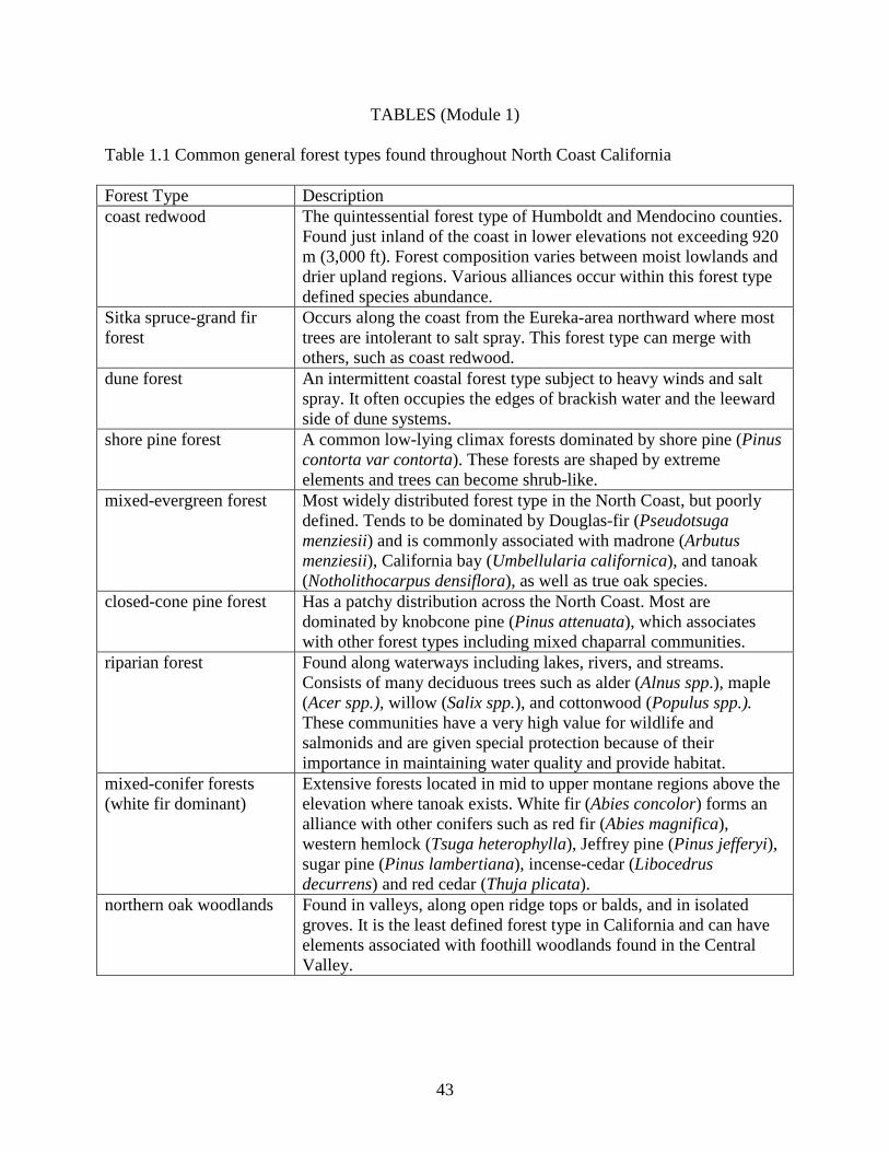
TABLES (Module 1) Table 1.1 Common general forest types found throughout North Coast California Forest Type Description coast redwood The quintessential forest type of Humboldt and Mendocino counties.

Found just inland of the coast in lower elevations not exceeding 920 m (3,000 ft). Forest composition varies between moist lowlands and drier upland regions. Various alliances occur within this forest type defined species abundance.

Sitka spruce-grand fir forest

Occurs along the coast from the Eureka-area northward where most trees are intolerant to salt spray. This forest type can merge with others, such as coast redwood.

dune forest An intermittent coastal forest type subject to heavy winds and salt spray. It often occupies the edges of brackish water and the leeward side of dune systems.

shore pine forest A common low-lying climax forests dominated by shore pine (Pinus contorta var contorta). These forests are shaped by extreme elements and trees can become shrub-like.

mixed-evergreen forest Most widely distributed forest type in the North Coast, but poorly defined. Tends to be dominated by Douglas-fir (Pseudotsuga menziesii) and is commonly associated with madrone (Arbutus menziesii), California bay (Umbellularia californica), and tanoak (Notholithocarpus densiflora), as well as true oak species.

closed-cone pine forest Has a patchy distribution across the North Coast. Most are dominated by knobcone pine (Pinus attenuata), which associates with other forest types including mixed chaparral communities.

riparian forest Found along waterways including lakes, rivers, and streams. Consists of many deciduous trees such as alder (Alnus spp.), maple (Acer spp.), willow (Salix spp.), and cottonwood (Populus spp.). These communities have a very high value for wildlife and salmonids and are given special protection because of their importance in maintaining water quality and provide habitat.

mixed-conifer forests (white fir dominant)

Extensive forests located in mid to upper montane regions above the elevation where tanoak exists. White fir (Abies concolor) forms an alliance with other conifers such as red fir (Abies magnifica), western hemlock (Tsuga heterophylla), Jeffrey pine (Pinus jefferyi), sugar pine (Pinus lambertiana), incense-cedar (Libocedrus decurrens) and red cedar (Thuja plicata).

northern oak woodlands Found in valleys, along open ridge tops or balds, and in isolated groves. It is the least defined forest type in California and can have elements associated with foothill woodlands found in the Central Valley.

43

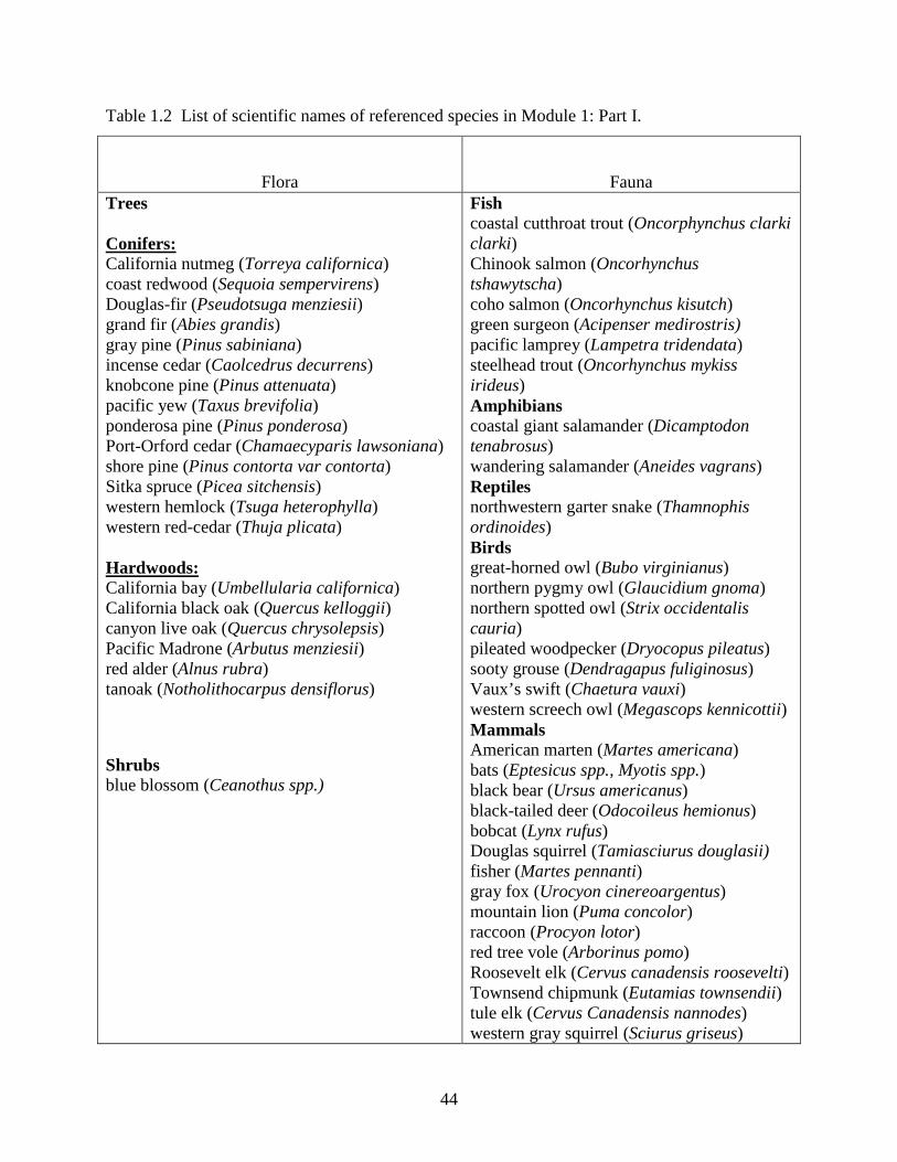
Table 1.2 List of scientific names of referenced species in Module 1: Part I.

Flora Fauna Trees Conifers: California nutmeg (Torreya californica) coast redwood (Sequoia sempervirens) Douglas-fir (Pseudotsuga menziesii) grand fir (Abies grandis) gray pine (Pinus sabiniana) incense cedar (Caolcedrus decurrens) knobcone pine (Pinus attenuata) pacific yew (Taxus brevifolia) ponderosa pine (Pinus ponderosa) Port-Orford cedar (Chamaecyparis lawsoniana) shore pine (Pinus contorta var contorta) Sitka spruce (Picea sitchensis) western hemlock (Tsuga heterophylla) western red-cedar (Thuja plicata) Hardwoods: California bay (Umbellularia californica) California black oak (Quercus kelloggii) canyon live oak (Quercus chrysolepsis) Pacific Madrone (Arbutus menziesii) red alder (Alnus rubra) tanoak (Notholithocarpus densiflorus)

Shrubs blue blossom (Ceanothus spp.)

Fish coastal cutthroat trout (Oncorphynchus clarki clarki) Chinook salmon (Oncorhynchus tshawytscha) coho salmon (Oncorhynchus kisutch) green surgeon (Acipenser medirostris) pacific lamprey (Lampetra tridendata) steelhead trout (Oncorhynchus mykiss irideus) Amphibians coastal giant salamander (Dicamptodon tenabrosus) wandering salamander (Aneides vagrans) Reptiles northwestern garter snake (Thamnophis ordinoides) Birds great-horned owl (Bubo virginianus) northern pygmy owl (Glaucidium gnoma) northern spotted owl (Strix occidentalis cauria) pileated woodpecker (Dryocopus pileatus) sooty grouse (Dendragapus fuliginosus) Vaux’s swift (Chaetura vauxi) western screech owl (Megascops kennicottii) Mammals American marten (Martes americana) bats (Eptesicus spp., Myotis spp.) black bear (Ursus americanus) black-tailed deer (Odocoileus hemionus) bobcat (Lynx rufus) Douglas squirrel (Tamiasciurus douglasii) fisher (Martes pennanti) gray fox (Urocyon cinereoargentus) mountain lion (Puma concolor) raccoon (Procyon lotor) red tree vole (Arborinus pomo) Roosevelt elk (Cervus canadensis roosevelti) Townsend chipmunk (Eutamias townsendii) tule elk (Cervus Canadensis nannodes) western gray squirrel (Sciurus griseus)

44

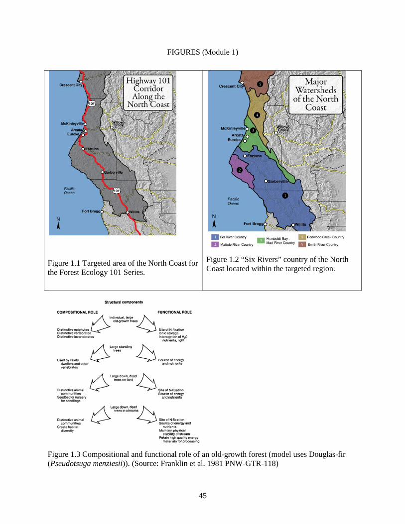
FIGURES (Module 1)

Figure 1.1 Targeted area of the North Coast for the Forest Ecology 101 Series.

Figure 1.2 “Six Rivers” country of the North Coast located within the targeted region.

Figure 1.3 Compositional and functional role of an old-growth forest (model uses Douglas-fir (Pseudotsuga menziesii)). (Source: Franklin et al. 1981 PNW-GTR-118)

45

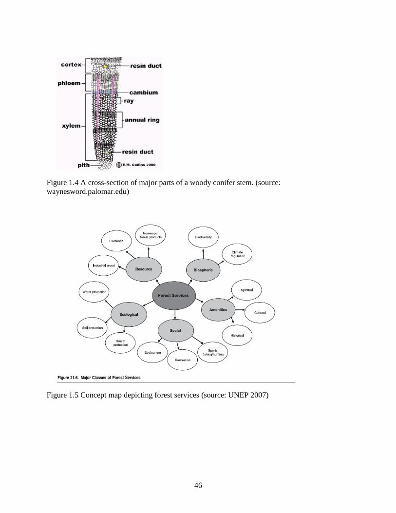
Figure 1.4 A cross-section of major parts of a woody conifer stem. (source: waynesword.palomar.edu)

Figure 1.5 Concept map depicting forest services (source: UNEP 2007)

46

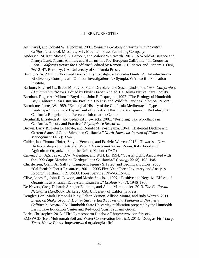
LITERATURE CITED Alt, David, and Donald W. Hyndman. 2001. Roadside Geology of Northern and Central

California. 2nd ed. Missolua, MT: Mountain Press Publishing Company. Anderson, M. Kat, Michael G. Barbour, and Valerie Whitworth. 2013. “A World of Balance and

Plenty: Land, Plants, Animals and Humans in a Pre-European California.” In Contested Eden: California Before the Gold Rush, edited by Ramon A. Gutierrez and Richard J. Orsi, 76:12–47. Berkeley, CA: University of California Press .

Baker, Erica. 2011. “Schoolyard Biodiversity Investigator Educator Guide: An Introduction to Biodiversity Concepts and Outdoor Investigations.”, Olympia, WA: Pacific Education Institute.

Barbour, Michael G., Bruce M. Pavlik, Frank Drysdale, and Susan Lindstrom. 1993. California’s Changing Landscapes. Edited by Phyllis Faber. 2nd ed. California Native Plant Society.

Barnhart, Roger A., Milton J. Boyd, and John E. Pequegnat. 1992. “The Ecology of Humboldt Bay, California: An Estuarine Profile.”, US Fish and Wildlife Service Biological Report 1.

Bartolome, James W. 1989. “Ecological History of the California Mediterraean-Type Landscape.”, Summary Department of Forest and Resource Management, Berkeley, CA: California Rangeland and Research Information Center.

Bernhardt, Elizabeth A., and Tedmund J. Swiecki. 2001. “Restoring Oak Woodlands in California: Theory and Practice.” Phytosphere Research.

Brown, Larry R., Peter B. Moyle, and Ronald M. Yoshiyama. 1964. “Historical Decline and Current Status of Coho Salmon in California.” North American Journal of Fisheries Management 14 (2): 37–41.

Calder, Ian, Thomas Hofer, Sibylle Vermont, and Patrizio Warren. 2013. “Towards a New Understanding of Forests and Water.” Forests and Water. Rome, Italy: Food and Agriculture Organization of the United Nations (FAO).

Carver, J.O., A.S. Jayko, D.W. Valentine, and W.H. Li. 1994. “Coastal Uplift Associated with the 1992 Cape Mendocino Earthquake in California.” Geology 22 (3): 195–198.

Christensen, Glenn A., Sally J. Campbell, Jeremy S. Fried, and Technical Editors. 2008. “California’s Forest Resources, 2001 – 2005 Five-Year Forest Inventory and Analysis Report.”, Portland, OR: USDA Forest Service PNW-GTR-763.

Clive, Jones G., John H. Lawton, and Moshe Shachak. 1997. “Positive and Negative Effects of Organisms as Physical Ecosystem Engineers.” Ecology 78 (7): 1946–1957.

De Nevers, Greg, Deborah Stranger Edelman, and Adina Merenlender. 2013. The California Naturalist Handbook. Berkeley, CA: University of California Press.

Dengler, Lori, Mark Hemphil-Haley, Felton Vernon, Allison Monro, and Judy Warren. 2011. Living on Shaky Ground: How to Survive Earthquakes and Tsunamis in Northern California, Arcata, CA: Humboldt State University publication prepared by the Humboldt Earthquake Education Center and Redwood Coast Tsunami Group.

Earle, Christopher. 2013. “The Gymnosperm Database.” http://www.conifers.org. EMSWCD (East Multnomah Soil and Water Conservation District). 2013. “Douglas-Fir.” Large

Trees, Native Plants. http://emswcd.org/douglas-fir/.

47

Environmental Protection Agency (EPA). 2007. “Lower Eel River Total Maximum Daily Loads for Temperature and Sediment.”, Report by U.S. Environmental Protection Agency Region IX.

Evert, Ray F., and Susan E. Eichhorn. 2013. pgs 617-635. Raven Biology of Plants. Edited by Sally Anderson. 8th ed. New York, NY: W.H. Freeman and Company.

FAO. 2012. “State of the World’s Forests 2012”. Rome, Italy: Report by U.N Food and Agriculture Organization.

Fowells, H.A., and Joseph E. Means. 2008. “The Tree and Its Environment.” http://www.na.fs.fed.us.

Franklin, Alan B., David R. Anderson, R.J. Gutierrez, and Kenneth P. Burnham. 2000. “Climate, Habitat Quality, and Fitness in Northern Spotted Owl Populations in Northwestern California.” Ecological Monographs 70 (4): 539–590.

Franklin, Jerry F., Thomas A. Spies, Robert Van Pelt, Andrew B. Carey, Dale A. Thornburgh, Dean Rae Berg, David B. Lindenmayer, et al. 2002. “Disturbances and Structural Development of Natural Forest Ecosystems with Silvicultural Implications, Using Douglas-Fir Forests as an Example.” Forest Ecology and Management 155: 399–423.

Franklin, Jerry F., Kermit Cromack, William Jr. Denison, Arthur Mckee, Chris Maser, James Sedell, Fred Swanson, and Glen Juday. 1981. “Ecological Characteristics of Old-Growth Douglas-Fir Forests.”, Portland, OR: USDA Forest Service PNW-GTR-118.

Galindo-Leal, Carlos, and Fred L. Bunnel. 1995. “Ecosystem Management : Implications and Opportunities of a New Paradigm.” The Forestry Chronicle 71 (5): 601–606.

Gifford, Ernest M., and Adriance S. Foster. 1988. “Coniferophyta.” In Morphology and Evolution of Vascular Plants, 3rd ed., 401–453. New York: W.H. Freeman and Company.

Halpern, Charles B., and Thomas A. Spies. 1995. “Plant Species Diversity in Natural and Managed Forests of the Pacific Northwest.” Ecological Applications 5 (4): 913–934.

Helfield, James M., and Robert J. Naiman. 2001. “Effects of Salmon-Derived Nitrogen on Riparian Forest Growth and Implications for Stream Productivity.” Ecology 82 (9): 2403–2409.

Henle, Klaus, David B. Lindenmayer, R. Chris, Denis A. Saunders, and Christian Wissel. 2004. “Species Survival in Fragmented Landscapes: Where Are We Now ?” Biodiversity and Conservation (13): 1–8.

Hickman, James C. (ed). 1993. The Jepson Manual: Higher Plants of California. Berkeley, CA: University of California Press .

Hooper, D.U., F.S. Chapin III, J.J. Ewel, A. Hector, P. Inchausti, S. Lavorel, J.H. Lawton, et al. 2005. “Effects of Biodiversity on Ecosystem Functioning: A Consensus on Current Knowledge.” Ecological Monographs 75 (1): 3–35.

Howard, Janet L. 2014. “Quercus Lobata.” Fire Effects Information Systems. http://www.fs.fed.us/database/feis/plants/tree/quelob/all.html.

Jensen, Deborah B., Margaret S. Torn, and Harte John. 1993. In Our Own Hands: A Strategy for Conserving California’s Biological Diversity. Berkeley, CA: University of California Press.

Kauffman, J. Boone, Robert L. Beschta, Nick Otting, and Danna Lytjen. 2011. “An Ecological Perspective of Riparian and Stream Restoration in the Western United States.” Fisheries: Special Issue on Watershed Restoration (October 2013): 37–41.

Kauffmann, Michael. 2012. Conifer Country: A Natural History and Hiking Guide to 35 Conifers of the Klamath Mountain Region. Kneeland, CA: Backcountry Press.

48

Keeler-Wolf, Todd. 2003. “Geography and Vegetation.” In Atlas of the Biodiversity of California, 3rd printing, 18. California Department of Fish and Game.

Kirk, Thomas A., and William J. Zielinski. 2009. “Developing and Testing a Landscape Habitat Suitability Model for the American Marten (Martes Americana ) in the Cascades Mountains of California.” Landscape Ecology 24: 759–773. Kozloff, Eugene N. 1976. Plants and Animals of the Pacific Northwest. Seattle, WA: University of Washington Press.

Laaksonen-Craig, Susanna, George E. Goldman, and William McKillop. 2001. “Forestry, Forest Industry, and Forest Products Consumption.”, UC Extension ANR pub 8070.

Lanner, Ronald. M. 1999. Conifers of California. Edited by Majorie Popper and John Evarts. Los Olivos, CA: Cachuma Press, Inc.

Lindenmayer, D.B., J.F. Franklin, and J. Fischer. 2006. “General Management Principles and a Checklist of Strategies to Guide Forest Biodiversity Conservation.” Biological Conservation 131 (3) (August): 433–445.

Lindenmayer, David B., Chris R. Margules, and Daniel B. Botkin. 2000. “Indicators of Biodiversity for Ecologically Sustainable Forest Management.” Conservation Biology: Essays 14 (4) (August 15): 941–950.

Lutz, James a, Andrew J. Larson, Mark E. Swanson, and James A. Freund. 2012. “Ecological Importance of Large-Diameter Trees in a Temperate Mixed-Conifer Forest.”, PloS One (7)5:e36131.

Major, Jack. 1988. “California Climate in Relation to Vegetation.” In Terrestrial Vegetaion of California, edited by Michael Barbour and Jack Major, 11–74. Davis, CA: California Native Plant Society.

Mazurek, M.J, and William J Zielinski. 2004. “Individual Legacy Trees Influence Vertebrate Wildlife Diversity in Commercial Forests.” Forest Ecology and Management 193 (3) (June): 321–334.

Millar, Constance I., Nathan L. Stephenson, and Scott L. Stephens. 2007. “Climate Change and Forests of the Future: Managing in the Face of Uncertainty.” Ecological Applications : A Publication of the Ecological Society of America 17 (8) (December): 2145–51.

Molina, Randy. 1994. “The Role of Mycorrhizal Symbioses in the Health of Giant Redwoods and Other Forest Ecosystems.”, Albany, CA: USDA Forest Service PSW-GTR-151.

Morgan, Todd A., Jason P. Brandt, Kathleen E. Songster, Charles E. Keegan III, and Glenn A. Christensen. 2006. “California’s Forest Products Industry and Timber Harvest, 2006.”, Portland, OR: USDA Forest Service PNW-GTR-866.

Motroni, Robert S., Daniel A. Airola, Robin K. Marose, and Nancy D. Tosta. 1991. “Using Wildlife Species Richness to Identify Land Protection Priorities in California’s Hardwood Woodlands.” Berkeley, CA: USDA Forest Service PSW-GTR-126.

Myberg, Alexander A. , Simcha Lev-Yadun, and Ronald Serdeoff. 2013. Xylem Structure and Function. In: eLS. Chichester: John Wiley & Sons Ltd. http://www.els.net.

Nafis, Gary. 2013. “Identifying California Salamanders.” California Herps. http://www.californiaherps.com/identification/salamandersid/salamanders.id2.html.

Peattie, Donald Culross. 1981. A Natural History of Western Trees. 2nd ed. Boston, MA: Houghton Miffline Company.

Preston, Larry. 1991. “A Cursory Evaluation of Salmonid Spawning and Rearing Conditions on Mattole River, Humboldt County”. Redding, CA.

49

Ralph, C John, Peter W C Paton, Cathy A Taylor, Coconino National Forest, and Happy Jack. 1988. “Habitat Association Patterns of Breeding Birds and Small Mammals in Douglas-Fir/ Hardwood Stands in Northwestern California and Southwestern Oregon.”

Sawyer, John. 2006. Northwest California: A Natural History. Berkeley, CA: University of California Press.

Sawyer, John O., Jane Gray, James G. West, Dale A. Thornburg, Reed F. Noss, Joseph H. Engbeck, Bruce G. Marcot, and Roland Raymond. 2000. “History of Redwood and Redwood Forests.” Ch 2. In The Redwood Forest: History, Ecology, and Conservation of the Coast Redwoods, edited by Reed F. Noss, 7–38. Covelo, CA: Island Press.

Sawyer, John O., Stephen C. Sillett, James H. Popenoe, Dale A. Thornburg, Anthony LaBanca, Teresa Sholars, David L. Largent, Fred Euphrat, Reed F. Noss, and Robert Van Pelt. 2000. “Characteristics of Redwood Forests.” Ch 3. In The Redwood Forest: History, Ecology, and Conservation of the Coast Redwoods, edited by Reed F. Noss, 39–80. Covelo, CA: Island Press.

Schoenherr, Allan A. 1992. A Natural History of California. Berkeley, CA: University of California Press.

Schultz, Stewart T. 1990. The Northwest Coast: A Natural History. Portland, OR: Timber Press, Inc.

Shvidenko, Anatoly, Charles V. Barber, and Reidar Persson. 2007. “Forest and Woodland Systems.” In Ecosystems and Human Well-Being: Current State and Trends, 585–621. Washington D.C.: Island Press.

Sillett, Stephen C., and Robert Van Pelt. 2007. “Trunk Reiteration Promotes Ephiphytes and Water Storage in an Old-Growth Redwood Forest Canopy.” Ecological Monographs 77 (3): 335–359.

Simberloff, Daniel. 1999. “The Role of Science in the Preservation of Forest Biodiversity.” Forest Ecology and Management 115 (2-3) (March): 101–111.

Smith, Nikola, Robert Deal, Jeff Kline, Blahna Dale, Trista Patterson, Thomas A. Spies, and Karen Bennett. 2011. “Ecosystem Services as a Framework for Forest Stewardship: Deschutes National Forest Overview.” Portland, OR: USDA Forest Service PNW-GTR-852.

Spickler, James C., Stephen C. Sillett, Sharyn B. Marks, and Hartwell H. Welsh. 2006. “Evidence of a New Niche for a North American Salamander: Aneides Vagrans Resising in the Canopy of Old-Growth Redwood Forest.” Herpetological Conservation and Biology 1 (1): 16–27.

Spies, Thomas A., and Jerry F. Franklin. 1991. “The Structure of Natural Young, Mature, and Old-Growth Douglas Fir Forests in Oregon and Washington.” Portland, OR: USDA Forest Service PNW-GTR-285.

Starr, Kevin. 2005. California: A History. New York, NY: Modern Library Chronicles. Strittholt, James R., Dominick a. Dellasala, and Hong Jiang. 2006. “Status of Mature and Old-

Growth Forests in the Pacific Northwest.” Conservation Biology 20 (2) (April): 363–374. Swanson, Mark. 2005. “Centuries of Change in Pacific Northwest Forests: Ecological Effects of

Forest Simplification and Fragmentation”. Seattle, WA: Paper presented for Saving Washington's Working Forest Land Base forum, University of Washington.

Thompson, Ian, Brendan Mackey, Steven McNulty, and Alex Mosseler. 2009. “Forest Resilience, Biodiversity, and Climate Change.”, CBD Technical Series #43, Canadian Forest Service.

50

Tierney, Geraldine L., Don Faber-Langendoen, Brian R. Mitchell, W. Gregory Shriver, and James P. Gibbs. 2009. “Monitoring and Evaluating the Ecological Integrity of Forest Ecosystems.” Frontiers in Ecology and the Environment 7 (6) (August): 308–316.

Tudge, Colin. 2005. The Tree: A Natural History of What Trees Are, How They Live, and Why They Matter. New York, NY: Three Rivers Press.

UNEP. 2009. “Vital Forest Graphics”. Scotland, UK: Report by United Nations Environment Programme.

Vogl, Richard J., Wayne P. Armstrong, Keith L. White, and Kenneth L. Cole. 1988. “The Closed-Cone Pine and Cypress.” In Terrestrial Vegetation of California, edited by Michael G. Barbour and Jack Major, 295–358. Davis, CA: California Native Plant Society.

Vose, James M., David L. Peterson, and Toral Patel-Weynand. 2012. “Effects of Climatic Variability and Change on Forest Ecosystems: A Comprehensive Science Synthesis for the U. S. Forest Sector.” Portland, OR: USDA Forest Service PNW-GTR-870.

Wilson, Ruth. 2013. “People and Trees: An Intimate Connection.” American Forests: Protecting and Restoring Forests. http://www.americanforests.org.

Woodbury, Peter B., James E. Smith, and Linda S. Heath. 2007. “Carbon Sequestration in the U.S. Forest Sector from 1990 to 2010.” Forest Ecology and Management 241 (1-3) (March): 14–27.

Yoshiyama, Ronald M., and Peter B. Moyle. 2010. “Historical Review of Eel River Anadromous Salmonids, with Emphasis on Chinook Salmon, Coho Salmon and Steelhead”. Davis, CA: A report commissioned by California Trout.

Zielinski, William J., Jeffrey R. Dunk, J. Scott Yaeger, and David W. Laplante. 2010. “Forest Ecology and Management Developing and Testing a Landscape-Scale Habitat Suitability Model for Fisher (Martes Pennanti) in Forests of Interior Northern California.” Forest Ecology and Management 260 (9): 1579–1591.

51

Forest Ecology 101 Series (M1: Part II)

Module 1: Integrative Forest Ecology Part II

UNIT OF STUDY COVER PAGE

7th Grade Unit of Study Lesson 1 - Defining My Bioregion

Lesson 2 - Healthy Forest Connections Lesson 3 - Tree In’s and Out’s

Lesson 4 - Tree Growth and Girth Lesson 5 - Under the Sun Lesson 6 - Who’s There?

52

M1.G7 Lesson 1: Defining My Bioregion Unit Overview: Integrative Forest Ecology Grade 7 Key Concepts:

• Interdependent relationships between populations and their environment

• Using patterns to identify cause and effect

• Adaptation Time: 60 - 90 minutes Materials for the Teacher: Access to computers Student worksheet

M1.7.1a Online resources (see

links) PowerPoint of

bioregions (optional) M1.7.1b: extension:

Blank map of California (optional)

Connections: Earth Science, geography, climatology, geology, climate change, evolution, plant science, soils, adaptation, vegetation Forest Ecology Series integration: M2: Coast Redwoods M3: Oak Woodlands

Learning Objectives: Using online maps and other digital information, students will identify the physical factors that shape their bioregion, including associated climate, elevation, and topography. They will identify which factors have the greatest influence on a particular forest type and will discover some regions of California that have “hot spots” of plant diversity. Background information: Refer to the appropriate section in Part I - Ch 1: Teacher Companion for Module 1 and online information regarding your local bioregion. Suggested procedure: The purpose of this lesson is to introduce forest ecology by having students look at the “big picture” and getting a sense of what physical factors influence vegetation type. Begin with a slide show depicting various vegetative communities and some of the organisms found there (see online resources). This can be done the day before students begin the main online investigation. During the slide show you may want to focus on forested communities or show them different bioregions of California. Note that different sources identify bioregions slightly differently. The Atlas of Biodiversity, which identifies the North Coast area as the Klamath/North Coast bioregion is recommended. Be sure to mention that California is the most diverse state in the nation and places with high levels of biologically diversity are considered “hot spots”. After the slide show, ask the students which environmental factors influence the type of vegetation found in a particular area the most (see preliminary questions below). List their answers on the board. You may want students to do this introductory activity with a partner using white boards or another method. Explain to them that in order to better understand the interrelatedness of organisms and the environment, places are often defined by general vegetative type, such as deserts, chaparral, forests, and grasslands. After a brief discussion, define what a bioregion is. Prepare them for their independent investigation by clearly outlining which websites they will be using. During their investigation, have them fill out student worksheet M1.7.1a where they have access to online information (refer to the online resources below). Follow up by having students complete M1.7.1b, where they will color and label the different bioregions of California.

53

M1.G7.L1 Unit Overview (continued) Preliminary questions:

• What does the word diverse mean? • What state is the most biologically diverse in the entire country? • We all know what town, county, and state we live in, but do you know what bioregion

you live in? • What does the word bioregion mean to you? • What factors do you think are used to define a particular bioregion? (show them a map) • Give me an example of a vegetative type you have heard of. (you may need to help them

with this by giving an example first) • What main factors do you think influence a particular forest type (or vegetative type) the

most? Critical Thinking: A particular bioregion is shaped by both abiotic and biotic factors. If our bioregion became hotter and drier, how might these factors change how plant and animals need to adapt in order to survive? Keywords: adaptation, abiotic, biodiversity, bioregion, climate, dominant, elevation, geology, hot spot, soil, topography, vegetative type NGSS alignment: MS-LS2 Ecosystem: Interactions, Energy, and Dynamics LS1.A: Interdependent Relationships in Ecosystems MS-LS4 Biological Evolution: Unity and Diversity LS4.C: Adaptation Online resources: Atlas of the Biodiversity of California sample pages http://www.dfg.ca.gov/biogeodata/atlas/pdf/Clim_12b_web.pdf This is an excellent resource to use when discussing the biodiversity of California. It includes nicely colored maps depicting topography, climate, elevation, and high and low temperatures of California for free. The entire atlas is for sale through California Department of Fish and Game. If you want students to color in the bioregions on worksheet M1.7.1b, I recommend using the map available at this site. CNRA -Klamath/Northcoast Bioregion Overview http://ceres.ca.gov/geo_area/bioregions/Klamath/about.html Although it has limited information, this is the primary website to use for exploring the Klamath/Northcoast bioregion and answering questions on student worksheet M1.7.1a. Bioregions of California lesson from UC Berkeley http://gk12calbio.berkeley.edu/lessons/less_bioregions.htmlHumboldt State Although this lesson is limited there is a nice PowerPoint slide show available that covers the main bioregions of California. It could be a nice introduction to what bioregions are and how species adapt to various bioregions. HSU (Humboldt State) Library: Northwestern California maps site: http://library.humboldt.edu/infoservices/staff/rls/geospatial/nwcalmaps.htm For further in-depth information about the geography of northwestern California, a variety of maps are available through this HSU site.

54

M1:G7:L1 Unit Overview (continued) EEI Connection: 7.3.1e Responding to Environmental Change B.6.a Biodiversity: The Keystone to life on Earth. Lesson 1 in this module describes all ten bioregions of California and has accompanied worksheets. B.6.b Ecosystem Change in California B.8.b Biological Diversity: The World’s Riches Answers to preliminary questions: - What does the word diverse mean? (diverse means very different or having a great deal of variety) -What state is the most biologically diverse in the entire country? (California) - What does biodiversity mean? (Biodiversity is a term given to describe the richness (number) and variety of species in a particular area. A biological hot spot has an usually rich variety of organisms or exceptional biodiversity living there due to factors such as a moderate climate and a variety of soil types). -We all know what town, county, and state we live in, but do you know what bioregion you live in? (Klamath/North Coast bioregion). - What does the word bioregion mean to you? (Answers will vary. A bioregion is an area with characteristic flora and fauna. It is a region defined not by man-made structures such as county lines, but by features related to the natural world.) - What factors do you think are used to define a particular bioregion (show them a map)? (Answers will vary. Students may come up with factors such as similar climate, temperature, latitude, geology, etc.) - Give me an example of a vegetative type you have heard of. (Answers will vary. Vegetative types include woodland, redwood forest or coastal evergreen forest, desert, grassland or savanna, pine forest, chaparral, coastal scrub, etc.) - What main factors do you think influence a particular forest type (or vegetative type) the most? (Again answers will vary. Main factors are moisture and temperature or climate. Other factors include topography, rock or soil type, elevation, etc.) Suggested follow up questions:

• After this investigation, what factors had the greatest influence on the vegetation found in a particular place? (broadly speaking temperature and moisture)

• What other factors influence the type of vegetation found in a particular place? • Who wants to share a fact you learned about during this investigation that was

unexpected or surprising to you. • Around what region is there a “hot spot” for plant diversity? • What are some rare plant and animals that live in the Klamath/North Coast bioregion? • Who can name a type of tree found in our bioregion? • What factors are probably the most important in determining what type of forest or tree

grows in a particular region? • How does our bioregion compare with other bioregions of the state?

Suggested extensions:

55

• Have students make a poster of their bioregion. Have them use descriptive words including the main factors that influence the vegetation.

• Conduct a microclimate study of the school campus or of a nearby forested area, where students record physical factors such as temperature, rainfall, humidity, and wind direction and speed. During this investigation, compare the north and south sides of a place or other areas with known varying microclimates.

• Have the students map different vegetative communities you have defined as a class in a nearby natural area.

• Start a photo collection of the different types of vegetation found in your local area. Pictures can be mounted on the wall or collected digitally as a group project. This could also be done as an extra credit project.

M1.7.1a Student worksheet and teacher key M1.7.1b Student extension (optional)

56

Student worksheet M1.G7.1a Name___________________________ Date _____________ Period ________

Defining My Bioregion Directions: Answer the following questions to the best of your ability. Answer questions 1 - 3 using the website: http://www.dfg.ca.gov/biogeodata/atlas/pdf/Clim_12b_web.pdf 1. What is the name of our bioregion? 2. According to this map, how many bioregions are there in California? ________ 3. The next series of questions are specific to where we live. Using different maps and their legends find: a. Approximate elevation_________________________________________ b. What map did you use to find elevation? _________________________ c. Average precipitation ________________________________________ d. Average range of high temperatures for the warmest months _____________________________________________________ e. Average range of low temperatures for the coldest months. ____________________________________________________ f. The name and symbol used for our climate type. ____________________________________________________ Answer questions 4-13 using the website - http://ceres.ca.gov/geo_area/bioregions/Klamath/about.html 4. Describe the Klamath/North Coast bioregion. Include information about the boundaries, population, and main highways found here. __________________________________________________________________

__________________________________________________________________

__________________________________________________________________

__________________________________________________________________

57

__________________________________________________________________

__________________________________________________________________

5. Name a nearby mountain range.______________________________________ 6. Give two counties that join the one you live in. __________________________________________________________________ 7. Name three types of trees. ____________________________________________________________________________________________________________________________________ 8. Name three types of rare animals. ____________________________________________________________________________________________________________________________________ 9. Name three types of rare plants. ____________________________________________________________________________________________________________________________________ 10. Where is there a “hot spot” of plant diversity? ____________________________________________________________________________________________________________________________________ 11. What are some tourist attractions? ____________________________________________________________________________________________________________________________________

Extension:

12. Give the name of a nearby forested park or other public place.

13. Give the name of a nearby national forest.

14. What are some factors affecting the biodiversity found in your bioregion?

58

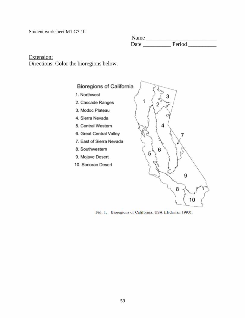
Student worksheet M1.G7.1b Name _________________________

Date __________ Period __________ Extension: Directions: Color the bioregions below.

59

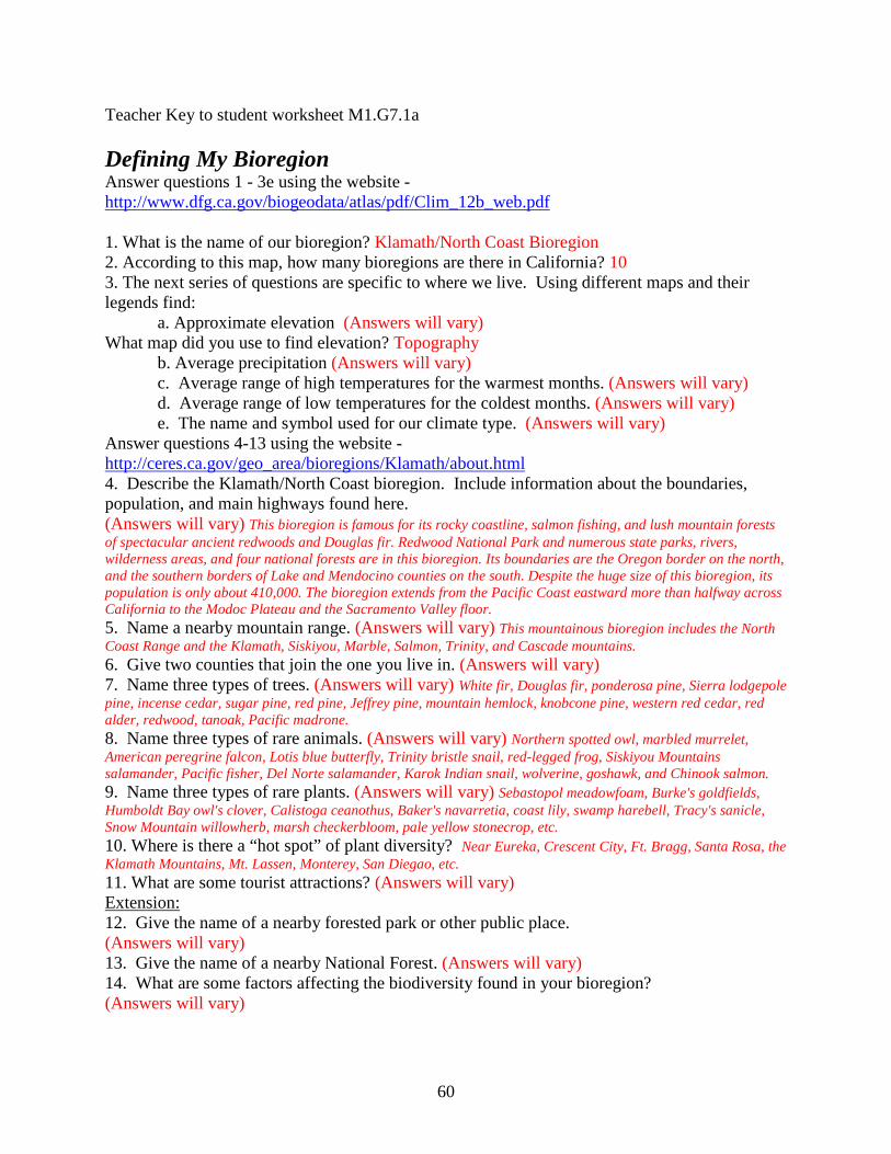
Teacher Key to student worksheet M1.G7.1a Defining My Bioregion Answer questions 1 - 3e using the website - http://www.dfg.ca.gov/biogeodata/atlas/pdf/Clim_12b_web.pdf 1. What is the name of our bioregion? Klamath/North Coast Bioregion 2. According to this map, how many bioregions are there in California? 10 3. The next series of questions are specific to where we live. Using different maps and their legends find: a. Approximate elevation (Answers will vary) What map did you use to find elevation? Topography b. Average precipitation (Answers will vary) c. Average range of high temperatures for the warmest months. (Answers will vary) d. Average range of low temperatures for the coldest months. (Answers will vary) e. The name and symbol used for our climate type. (Answers will vary) Answer questions 4-13 using the website - http://ceres.ca.gov/geo_area/bioregions/Klamath/about.html 4. Describe the Klamath/North Coast bioregion. Include information about the boundaries, population, and main highways found here. (Answers will vary) This bioregion is famous for its rocky coastline, salmon fishing, and lush mountain forests of spectacular ancient redwoods and Douglas fir. Redwood National Park and numerous state parks, rivers, wilderness areas, and four national forests are in this bioregion. Its boundaries are the Oregon border on the north, and the southern borders of Lake and Mendocino counties on the south. Despite the huge size of this bioregion, its population is only about 410,000. The bioregion extends from the Pacific Coast eastward more than halfway across California to the Modoc Plateau and the Sacramento Valley floor. 5. Name a nearby mountain range. (Answers will vary) This mountainous bioregion includes the North Coast Range and the Klamath, Siskiyou, Marble, Salmon, Trinity, and Cascade mountains. 6. Give two counties that join the one you live in. (Answers will vary) 7. Name three types of trees. (Answers will vary) White fir, Douglas fir, ponderosa pine, Sierra lodgepole pine, incense cedar, sugar pine, red pine, Jeffrey pine, mountain hemlock, knobcone pine, western red cedar, red alder, redwood, tanoak, Pacific madrone. 8. Name three types of rare animals. (Answers will vary) Northern spotted owl, marbled murrelet, American peregrine falcon, Lotis blue butterfly, Trinity bristle snail, red-legged frog, Siskiyou Mountains salamander, Pacific fisher, Del Norte salamander, Karok Indian snail, wolverine, goshawk, and Chinook salmon. 9. Name three types of rare plants. (Answers will vary) Sebastopol meadowfoam, Burke's goldfields, Humboldt Bay owl's clover, Calistoga ceanothus, Baker's navarretia, coast lily, swamp harebell, Tracy's sanicle, Snow Mountain willowherb, marsh checkerbloom, pale yellow stonecrop, etc. 10. Where is there a “hot spot” of plant diversity? Near Eureka, Crescent City, Ft. Bragg, Santa Rosa, the Klamath Mountains, Mt. Lassen, Monterey, San Diegao, etc. 11. What are some tourist attractions? (Answers will vary) Extension: 12. Give the name of a nearby forested park or other public place. (Answers will vary) 13. Give the name of a nearby National Forest. (Answers will vary) 14. What are some factors affecting the biodiversity found in your bioregion? (Answers will vary)

60

M1.G7 Lesson 2: Healthy Forest Connections Unit Overview: Integrative Forest Ecology Grade 7 Key Concepts:

• Concept mapping • Systematic

organization • Energy and matter • Ecosystems:

Interactions, energy, and dynamics

• Biodiversity and humans

Time: 50 - 80 minutes Materials for the Teacher: Student reading

M1.7.2 Reference sheet

M1.7.R2 Paper and pencils

Connections: STEM, Language Arts, Social Studies, Earth Science, humans and society, engineering, forestry, biodiversity, wildlife, carpentry, textiles, population growth, carbon cycle, careers Forest Ecology Series integration: M2: Coast Redwoods M3: Oak Woodlands

Learning Objective: After reading and discussion, students will make a concept map connecting the different ecosystem services forests provide to people and the natural world. Background information: Refer to the appropriate section in Part I: Teacher Companion for Module 1 and online information. Possible headings to use for organizational purposes are: A: Ecological - Forests provide: 1) wildlife habitat 2) cycle nutrients 3) control sedimentation 4) food for animals 5) microclimates. B: Human Goods and Services - Forest provide: 1) materials (wood and fiber) 2) shelter 3) food 4) energy 5) recreation 6) spiritual growth 7) inspiration. C: Global - Forests provide: 1) oxygen 2) catchment of water 3) critical habitat 4) sequester carbon and 5) purify water. You may also refer to reference sheet M1.7.R2 for an example and possible headings to use. Suggested procedure: This lesson requires students to have some general knowledge about the many positive attributes forests have at different scales. As homework, have students read M1.7.2, which discusses many of the products and services forests provide as well as their ability to absorb carbon and clean water. The next day, have them review what they have learned by brainstorming and/or reviewing with a partner. During this preliminary activity have them make a list of the different ways forests are important. You may want to give them broad categories under which to organize their topics such as: ecological, historical, cultural, and global. Some subcategories might include 1) food and fiber 2) air and water 3) plant and animals 4) economic and 5) social. See the concept map given in reference M1.7.R2 below for more ideas. If students have not created concept maps before, have them practice using a more familiar example first (refer to your text). After listing their information, give students time to draw a rough sketch of their concept map before making a final version. Once they have finished, post their product around the classroom or offer another way to share their creation. To conclude the lesson, ask several follow up questions (see below) to instigate a discussion where students weigh human uses vs. ecological effects. Another possible extension is to have them rank which services are most at risk by climate change.

61

M1.G7.L2 (Unit Overview continued) Preliminary questions:

• Are forests important to wildlife? Why/Why not? • Are forests important to people? Why/Why not? • What types of products come from trees? • What important functions does a forest have on a global scale?

Critical Thinking: How do temperate forests differ from tropical forests in regards to yearly growth, levels of biodiversity, and food sources? Keywords: forest, habitat, greenhouse effect, macroinvertebrate, photosynthesis, salmonid, sedimentation, snag NGSS alignment: MS-LS1-2: Systems and system models MS-LS2-5 Evaluate competing design solutions for maintaining biodiversity and ecosystem services MS-LSC Ecosystem dynamics, functioning, and resilience LS2-A: Interdependent relationships in ecosystems LS4-D: Biodiversity and Humans Online resources: Oregon Forest Institute - Learning Library http://oregonforests.org/content/ofri-resources This institution has a wide variety of information regarding management of forests of Oregon for environmental, recreational, and economic needs. Other links supply information on the carbon cycle, forest sounds, and wildlife guides. The Parks: Conifer Connection. Section 2: Humans in California’s Coniferous Forests http://www.parks.ca.gov/?page_id=26781 There are several chapters to choose from. Chapter 2 discusses how the Spanish and the Russians utilized California’s North Coast forests. PLT: Forests are More Than Trees - Student Page https://www.plt.org/stuff/contentmgr/files Project Learning Tree has great information about forests. This particular section discusses many aspects regarding trees such as ecosystem services, life cycle, succession, and forest stand development. EEI Connections: E.5.e Rainforests and Deserts: Distribution, Uses, and Human Influences 6.6.b Energy and Material Resources: Renewable or Not? 6.6.c Made From Earth: How Natural Resources Become Things we Use 8.12.5 Industrialization, Urbanization, and the Conservation Movement (California Connection).

62

M1.G7.L2 (Unit Overview continued) Answers to preliminary questions: - Are forests important to wildlife? Why/Why not? (Answers will vary. Forests provide protection, food, and habitat) - Are forests important to people? Why/Why not? (Answers will vary. Forests provide food, fiber, and materials for building homes, furniture, and other implements. Wood is burned for fuel and warmth. Trees provide shade and privacy. The timber industry produces jobs and forests are places people recreate and unwind.) - What types of products come from trees? (food, furniture, flooring, cabinets, buildings, musical instruments, utensils, paper, cardboard, books, rubber, latex, drugs, syrup, and many other items.) - What important functions does a forest have on a global scale? (Answers will vary. Forests sequester carbon, produce oxygen, protect watersheds, and enrich soil.) Follow Up Questions (for discussion):

• What types of human activities are the most destructive to forest health and integrity? • Are any of the ecological services you listed more important than the others? If so, why? • Can humans live in a sustainable way where forests are no longer destroyed? If so, how? • What continued threats do forests face by human disturbances? • How have people attempted to reverse the destruction done to forest ecosystems?

Suggested extensions:

• Have students make a poster or a promotional flyer of one of the main ecological services forests provide.

• Increase awareness of forest products by beginning a classroom forest collection where students bring in examples of things made of wood and wood fiber.

• Assign a writing project where students have to support how forests are important to them and society.

• Begin a student campaign for forest conservation such as recycling paper, using cloth bags, and buying products that don’t come from tropical forests.

• Play the forest families game at talkabouttrees.org • Begin a class list showing how the innovation of new products has reduced the use of

wood throughout historical times. • Plant trees in your community.

M1.G7.2 Student reading M1.G7.2R Reference sheet

63

Student reading M1.G7.2 Importance of Forests If you could look down on Earth form space you would see that over 30% of

all land is covered by forests. These key ecosystems play a large role on our planet

by cycling water and nutrients. Because forests contain the largest plants on earth,

trees, they are able to absorb large amounts of carbon in the form of carbon dioxide

(CO2). This helps reduce the greenhouse effect, which is responsible for the steady

increase in global temperatures. During photosynthesis, forests produce tons of

oxygen. Throughout the day they can even make their own clouds.

Healthy forests provide important habitat for a diverse set of animal, plant,

and fungal species. Various leaves, flowers, nuts, and fruits from trees and other

forest plants are important foods for many different animals. Large trees, snags,

and logs offer plenty of hiding places and nesting sites for different critters such as

the owls, bats, and amphibians. Downed wood in rivers and streams offer hiding

places for fish. Fallen leaves are converted into food for insects and other

macroinvertebrates contributing to the aquatic food chain. Tree roots reduce

sedimentation by holding soil in place and the canopies of trees cool water by

supplying shade. The resulting clean, cool water is important for young salmonids

before they make it out to sea and clean gravel is important for the successful

hatching of salmon eggs.

64

Historically, forests have been closely tied to human health and welfare.

People use wood for timber, fuel, and fiber. Milled timber is used for building

structures, fences, and furniture. Furthermore, wood can be pulped and turned into

paper, cardboard, and cellophane. Other objects made from trees are tires, latex,

and adhesives. Wood is an important energy source and some people use charcoal

for cooking and heating. Nuts, fruit, and seeds from certain trees offer humans rich

sources of food. Forest shrubs are often full of tasty berries and many forest plants

are used as medicine.

Using forests for fuel, fiber, and wood, supports local economies; however,

leaving the forests standing does too. Many people come to visit forests because

they offer solitude and beauty. Forests offer many recreational opportunities such

as camping, biking, hiking, and bird watching. The amount of money from tourism

exceeds that from timber production in many places. In short, forests provide many

services for people, the planet, and wildlife. They are not only interconnected to

other global systems but are important socially and economically.

Written by Melinda Bailey

2

65

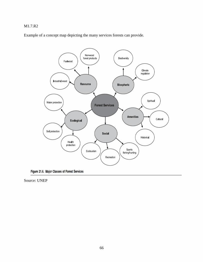
M1.7.R2 Example of a concept map depicting the many services forests can provide.

Source: UNEP

66

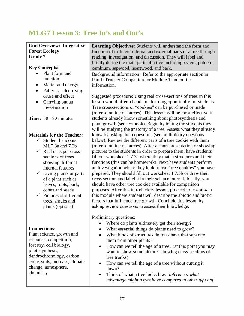
M1.G7 Lesson 3: Tree In’s and Out’s Unit Overview: Integrative Forest Ecology Grade 7 Key Concepts:

• Plant form and function

• Matter and energy • Patterns: identifying

cause and effect • Carrying out an

investigation Time: 50 - 80 minutes Materials for the Teacher: Student handouts

M1.7.3a and 7.3b Real or paper cross

sections of trees showing different internal features

Living plants or parts of a plant such as leaves, roots, bark, cones and seeds

Pictures of different trees, shrubs and plants (optional)

Connections: Plant science, growth and response, competition, forestry, cell biology, photosynthesis, dendrochronology, carbon cycle, soils, biomass, climate change, atmosphere, chemistry

Learning Objectives: Students will understand the form and function of different internal and external parts of a tree through reading, investigation, and discussion. They will label and briefly define the main parts of a tree including xylem, phloem, cambium, sapwood, heartwood, and bark. Background information: Refer to the appropriate section in Part I: Teacher Companion for Module 1 and online information. Suggested procedure: Using real cross-sections of trees in this lesson would offer a hands-on learning opportunity for students. Tree cross-sections or “cookies” can be purchased or made (refer to online resources). This lesson will be most effective if students already know something about photosynthesis and plant growth (see textbook). Begin by telling the students they will be studying the anatomy of a tree. Assess what they already know by asking them questions (see preliminary questions below). Review the different parts of a tree cookie with them (refer to online resources). After a short presentation or showing pictures to the students in order to prepare them, have students fill out worksheet 1.7.3a where they match structures and their functions (this can be homework). Next have students perform an investigation where they look at real “tree cookies” you have prepared. They should fill out worksheet 1.7.3b or draw their cross section and label it in their science journal. Ideally, you should have other tree cookies available for comparison purposes. After this introductory lesson, proceed to lesson 4 in this module where students will describe the abiotic and biotic factors that influence tree growth. Conclude this lesson by asking review questions to assess their knowledge. Preliminary questions:

• Where do plants ultimately get their energy? • What essential things do plants need to grow? • What kinds of structures do trees have that separate

them from other plants? • How can we tell the age of a tree? (at this point you may

want to show some pictures showing cross-sections of tree trunks)

• How can we tell the age of a tree without cutting it down?

• Think of what a tree looks like. Inference: what advantage might a tree have compared to other types of

67

Forest Ecology Series integration: M2: Coast Redwoods M3: Oak Woodlands

plants? • Does anyone know of a molecule or tissue that trees

make? • What are the two types of vascular tissues plants have?

Critical Thinking: Assume two different aged trees are the same height. What abiotic factors could explain why a 400 year old tree is of equal height to one only 40 years old? Keywords: bark, cambium, cellulose, heartwood, lignin, phloem, sapwood, spring wood (early wood), summer wood (late wood), wood, xylem NGSS alignment: MS-LS1 From Molecules to Organisms: Structures and Processes LS1.A: Structure and Function LS1.B: Growth and Development LS1.C: Organization for Matter and Energy Flow in Organisms MS-LS2 Ecosystem: Interactions, Energy, and Dynamics LS1.A: Interdependent Relationships in Ecosystems Online resources: The science of tree rings: http://web.utk.edu/~grissino/. This is an excellent website about anything relating to the science of tree rings. Idaho Forest Products: A quick guide to the different parts of a tree cookie: http://www.idahoforests.org/cookie1.htm If you don’t want to your own student guide to the different parts of a tree cookie, this site offers a simple explanation of the most of the different layers referenced in this lesson. Project Learning Tree’s (PLT) site: How to make a tree cookie: http://files.dnr.state.mn.us/education_safety/education/plt/activity_sheets/treeCookie.pdf. This site has several sections including how to how make a “tree cookie” and information about trees. Conifer Country: Lesson- Anatomy of a Giant: http://www.parks.ca.gov/pages/735/files/lessons%20and%20activ.pdf This site is full of activities to have students learn about our local conifers. The activity on pages 167-171, relates directly to this lesson and has students look at the anatomy of redwood trees specifically. It ends with a crossword puzzle reviewing key terms. EEI Connection: B.6.b Ecosystem Change in California - Lesson 3: Climate Clues in Rings and Pollen Cores 8.12.1 Agricultural and Industrial Development in the United States (1877-1914)

68

(M1.G7.L3 Unit Overview continued) Answers to preliminary questions: -Where do plants ultimately get their energy? (from the sun or a grow light) -What essential things do plants need to grow? (light, water, nutrients, carbon dioxide) -What structures do trees have that separate them from other plants? (answers will vary. A dominant trunk, wood, bark, sap, large branches, fruit, cones, etc.) -How can we tell the age of a tree? (count the rings, although this doesn’t work in all trees) -How can we tell the age of a tree without cutting it down? (bore into a tree and get a core which shows the rings without killing the tree; estimate based on size) -Think of what a tree looks like. What advantage might a tree have compared to other types of plants? (answers will vary. Some responses might be: it is taller so it can get more light; it is more sturdy to withstand wind and snow; it has more leaves so it can gain more energy and grow fast, it has large roots to pull more water) -Does anyone know of a molecule or tissue that trees produce? (cellulose, lignin, sugar, etc.) -What are the two types of vascular tissues plants have? (xylem - which transports water throughout a plant and phloem - which transports nutrients) Suggested follow up questions:

• What is the living tissue layer within a tree’s trunk called? • Where does the cambium layer lie compared to the rest of the tree? • As a tree grows two types of wood are produced within the rings. What are these two

different types of wood called? • What is heartwood? How does it differ from sapwood? • What environmental factors might produce rings close together? Far apart? • What is the purpose of bark? Ask for at least three different purposes. • What is the function of xylem?

Suggested extensions:

• Have students conduct a dendrochronology investigation in order to better understand how trees grow and respond to a particular environment over time.

• Increase awareness about the value of forests by having students bring in items from home that are made from trees.

• Walk through a local forest comparing different trees species, male and female cones, bark textures, and other identifying characteristics.

• Have students go on a structured “treasure hunt” in a nearby forest area. • Invite a wood worker or a forester to talk about trees and wood. • Have students calculate tree growth using “tree cookies”. See lesson M1.L7.L4.

M1.G7.L3a Student worksheet and teacher key M1.G7.L3b Laboratory investigation

69

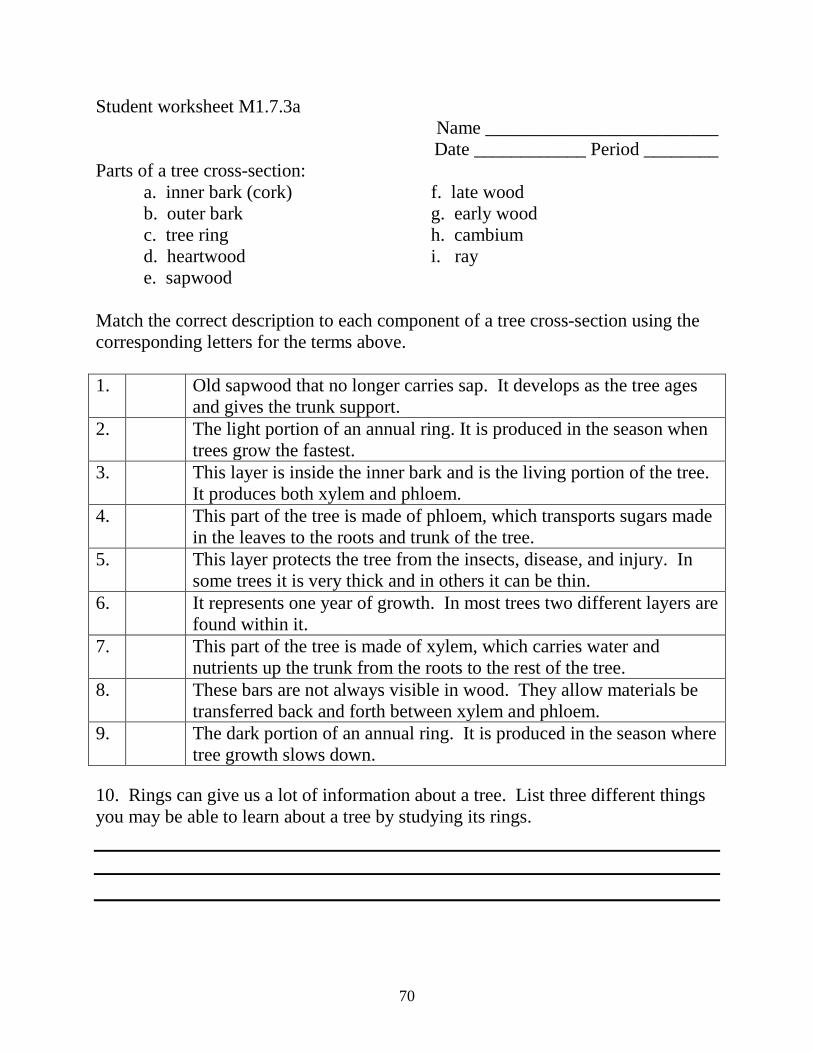
Student worksheet M1.7.3a Name _________________________

Date ____________ Period ________ Parts of a tree cross-section: a. inner bark (cork) f. late wood b. outer bark g. early wood c. tree ring h. cambium d. heartwood i. ray e. sapwood Match the correct description to each component of a tree cross-section using the corresponding letters for the terms above. 1. Old sapwood that no longer carries sap. It develops as the tree ages

and gives the trunk support. 2. The light portion of an annual ring. It is produced in the season when

trees grow the fastest. 3. This layer is inside the inner bark and is the living portion of the tree.

It produces both xylem and phloem. 4. This part of the tree is made of phloem, which transports sugars made

in the leaves to the roots and trunk of the tree. 5. This layer protects the tree from the insects, disease, and injury. In

some trees it is very thick and in others it can be thin. 6. It represents one year of growth. In most trees two different layers are

found within it. 7. This part of the tree is made of xylem, which carries water and

nutrients up the trunk from the roots to the rest of the tree. 8. These bars are not always visible in wood. They allow materials be

transferred back and forth between xylem and phloem. 9. The dark portion of an annual ring. It is produced in the season where

tree growth slows down. 10. Rings can give us a lot of information about a tree. List three different things you may be able to learn about a tree by studying its rings.

70

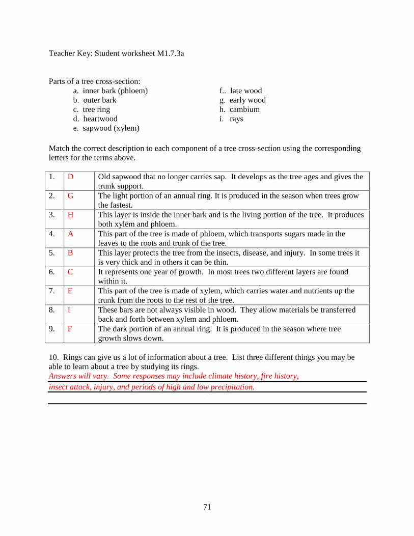
Teacher Key: Student worksheet M1.7.3a Parts of a tree cross-section: a. inner bark (phloem) f.. late wood b. outer bark g. early wood c. tree ring h. cambium d. heartwood i. rays e. sapwood (xylem) Match the correct description to each component of a tree cross-section using the corresponding letters for the terms above. 1. D Old sapwood that no longer carries sap. It develops as the tree ages and gives the

trunk support. 2. G The light portion of an annual ring. It is produced in the season when trees grow

the fastest. 3. H This layer is inside the inner bark and is the living portion of the tree. It produces

both xylem and phloem. 4. A This part of the tree is made of phloem, which transports sugars made in the

leaves to the roots and trunk of the tree. 5. B This layer protects the tree from the insects, disease, and injury. In some trees it

is very thick and in others it can be thin. 6. C It represents one year of growth. In most trees two different layers are found

within it. 7. E This part of the tree is made of xylem, which carries water and nutrients up the

trunk from the roots to the rest of the tree. 8. I These bars are not always visible in wood. They allow materials be transferred

back and forth between xylem and phloem. 9. F The dark portion of an annual ring. It is produced in the season where tree

growth slows down. 10. Rings can give us a lot of information about a tree. List three different things you may be able to learn about a tree by studying its rings. Answers will vary. Some responses may include climate history, fire history, insect attack, injury, and periods of high and low precipitation.

71

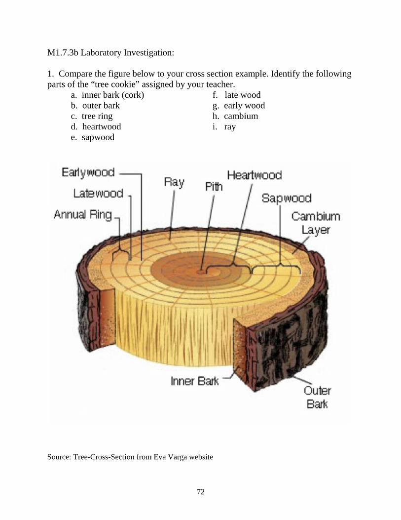
M1.7.3b Laboratory Investigation: 1. Compare the figure below to your cross section example. Identify the following parts of the “tree cookie” assigned by your teacher. a. inner bark (cork) f. late wood b. outer bark g. early wood c. tree ring h. cambium d. heartwood i. ray e. sapwood

Source: Tree-Cross-Section from Eva Varga website

72

M1.G7 Lesson 4: Tree Growth and Girth Unit Overview: Integrative Forest Ecology Grade 7 Key Concepts:

• Plant form and function

• Matter and energy • Identifying cause and

effect • Carrying out an

investigation • Interpreting data

Time: 50 - 80 minutes Materials for the Teacher: Rulers Calculators Different tree cookie

samples Sample picture of a

cross section Student investigation

M1.7.L4a Student extension and

teacher key M1.7.L4b (optional)

Pictures of tree cross sections showing special features such as suppression and fire scars (optional)

Connections: STEM, mathematics, plant science, growth and response, competition, forestry, cell biology, photosynthesis, dendrochronology, carbon cycle, biomass, climate change, chemistry, social science

Learning Objectives: Students will be able to calculate the average growth rate for one or more local tree species using various “tree cookies”. They will identify potential influential factors that may have affected the observed form of their samples such as suppression or high levels of precipitation. Background information: Refer to the appropriate section in Part I: Teacher Companion for Module 1, online resources, and other resources to assist you. Suggested procedure: This activity requires that you have a class set of tree crosssections or “tree cookies” unlike the previous lesson where they are only encouraged for use. Begin this lesson by reviewing tree anatomy (refer to M1.G7.L3). Show some pictures of tree cross sections and ask some of the preliminary questions below. Explain to the students they will be performing an activity where they will find the average rate growth for different trees using prepared samples or “tree cookies”. Directions for how to make “tree cookies” are found in the online links section below. Before they begin this activity, model how to find average growth using the example given. Decide how accurate you would like the students to be. Stress the need for them to use centimeters and to write their answer using the correct units (mm or cm/yr). Once they are finished, have them observe samples more closely and take further measurements in order to observe the nature of their sample (see M1.7.4a for suggestions). Is their “tree cookie” even all the way across? Is there evidence of branches, fire scars, or suppression? An optional follow up activity is given, where students find the average diameter breast height (dbh) of a stand using a real data set (refer to M1.G7.4b). Conclude this lesson by asking review questions to assess their knowledge and to make extensions. As an additional assessment tool, it may be helpful to compare student final answers to see how they varied. If answers varied substantially, discuss probable causes of error. Preliminary questions:

• What can the rings of a tree tell us? • What main factors or variables control the growth rate of

a plant or a tree? • How will tree growth respond to a year of high

precipitation? Low precipitation? • During which season will a tree grow the fastest? The

slowest?

73

Forest Ecology Series integration: M2: Coast Redwoods M3: Oak Woodlands

• What types of trees have the capacity to grow year around?

• What two things do you need to know before finding the average growth rate of a tree? (show them a picture of a cross section and model how to find growth rate)

• What unit of measurement will you be using for this activity?

Critical Thinking: Assume two trees are of the same age but have very different circumferences. What environmental factors might contribute to one tree having a very large diameter versus one with a very small diameter? Keywords: centimeter, circumference, conifer, cross section, dendrochronology, diameter, dbh, girth, precipitation, radius, suppression NGSS alignment: MS-LS1 From Molecules to Organisms: Structures and Processes LS1.A: Structure and Function LS1.B: Growth and Development LS1.C: Organization for Matter and Energy Flow in Organisms MS-LS2 Ecosystem: Interactions, Energy, and Dynamics LS1.A: Interdependent Relationships in Ecosystems Online resources: The Ultimate Tree Ring Site - The science of tree rings: http://web.utk.edu/~grissino/. This is an excellent website about anything relating to the science of tree rings. It is the best source for tree ring images. PLT’s site: How to make a tree cookie: http://files.dnr.state.mn.us/education_safety/education/plt/activity_sheets/treeCookie.pdf. This site has several sections including how to how make a “tree cookie” and information about trees. Dendrochronology Web Pages (Lectures): http://isu.indstate.edu/jspeer/dendro/ This site is one of a kind. It has several PowerPoint presentations that can be easily downloaded and modified to fit your needs. EEI Connection: B.6.b Ecosystem Change in California - Lesson 3: Climate Clues in Rings and Pollen Cores 8.12.1 Agricultural and Industrial Develoment in the United States (1877-1914)

74

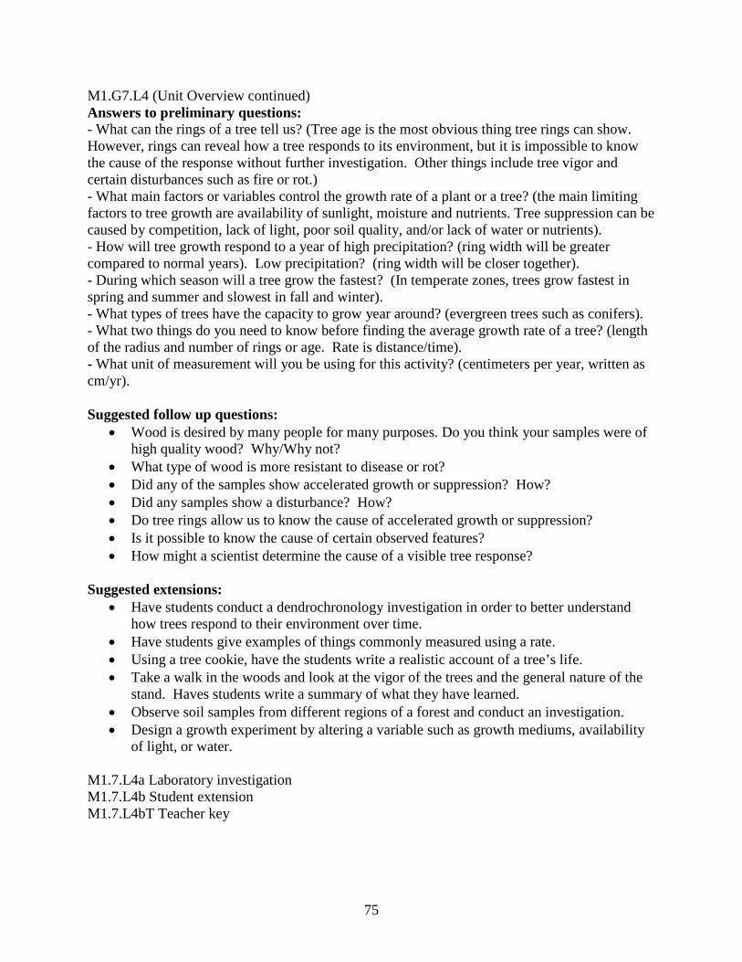
M1.G7.L4 (Unit Overview continued) Answers to preliminary questions: - What can the rings of a tree tell us? (Tree age is the most obvious thing tree rings can show. However, rings can reveal how a tree responds to its environment, but it is impossible to know the cause of the response without further investigation. Other things include tree vigor and certain disturbances such as fire or rot.) - What main factors or variables control the growth rate of a plant or a tree? (the main limiting factors to tree growth are availability of sunlight, moisture and nutrients. Tree suppression can be caused by competition, lack of light, poor soil quality, and/or lack of water or nutrients). - How will tree growth respond to a year of high precipitation? (ring width will be greater compared to normal years). Low precipitation? (ring width will be closer together). - During which season will a tree grow the fastest? (In temperate zones, trees grow fastest in spring and summer and slowest in fall and winter). - What types of trees have the capacity to grow year around? (evergreen trees such as conifers). - What two things do you need to know before finding the average growth rate of a tree? (length of the radius and number of rings or age. Rate is distance/time). - What unit of measurement will you be using for this activity? (centimeters per year, written as cm/yr). Suggested follow up questions:

• Wood is desired by many people for many purposes. Do you think your samples were of high quality wood? Why/Why not?

• What type of wood is more resistant to disease or rot? • Did any of the samples show accelerated growth or suppression? How? • Did any samples show a disturbance? How? • Do tree rings allow us to know the cause of accelerated growth or suppression? • Is it possible to know the cause of certain observed features? • How might a scientist determine the cause of a visible tree response?

Suggested extensions:

• Have students conduct a dendrochronology investigation in order to better understand how trees respond to their environment over time.

• Have students give examples of things commonly measured using a rate. • Using a tree cookie, have the students write a realistic account of a tree’s life. • Take a walk in the woods and look at the vigor of the trees and the general nature of the

stand. Haves students write a summary of what they have learned. • Observe soil samples from different regions of a forest and conduct an investigation. • Design a growth experiment by altering a variable such as growth mediums, availability

of light, or water. M1.7.L4a Laboratory investigation M1.7.L4b Student extension M1.7.L4bT Teacher key

75

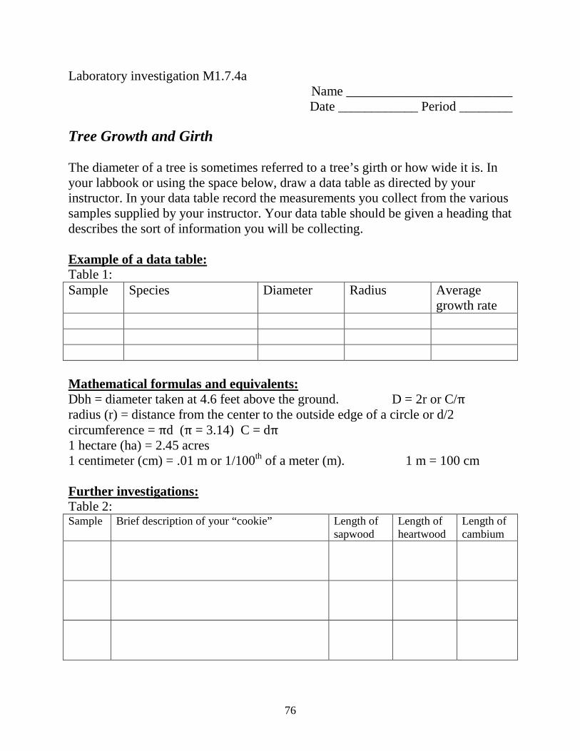
Laboratory investigation M1.7.4a Name _________________________

Date ____________ Period ________ Tree Growth and Girth The diameter of a tree is sometimes referred to a tree’s girth or how wide it is. In your labbook or using the space below, draw a data table as directed by your instructor. In your data table record the measurements you collect from the various samples supplied by your instructor. Your data table should be given a heading that describes the sort of information you will be collecting. Example of a data table: Table 1: Sample Species Diameter Radius Average

growth rate Mathematical formulas and equivalents: Dbh = diameter taken at 4.6 feet above the ground. D = 2r or C/π radius (r) = distance from the center to the outside edge of a circle or d/2 circumference = πd (π = 3.14) C = dπ 1 hectare (ha) = 2.45 acres 1 centimeter (cm) = .01 m or 1/100th of a meter (m). 1 m = 100 cm Further investigations: Table 2: Sample Brief description of your “cookie” Length of

sapwood Length of heartwood

Length of cambium

76

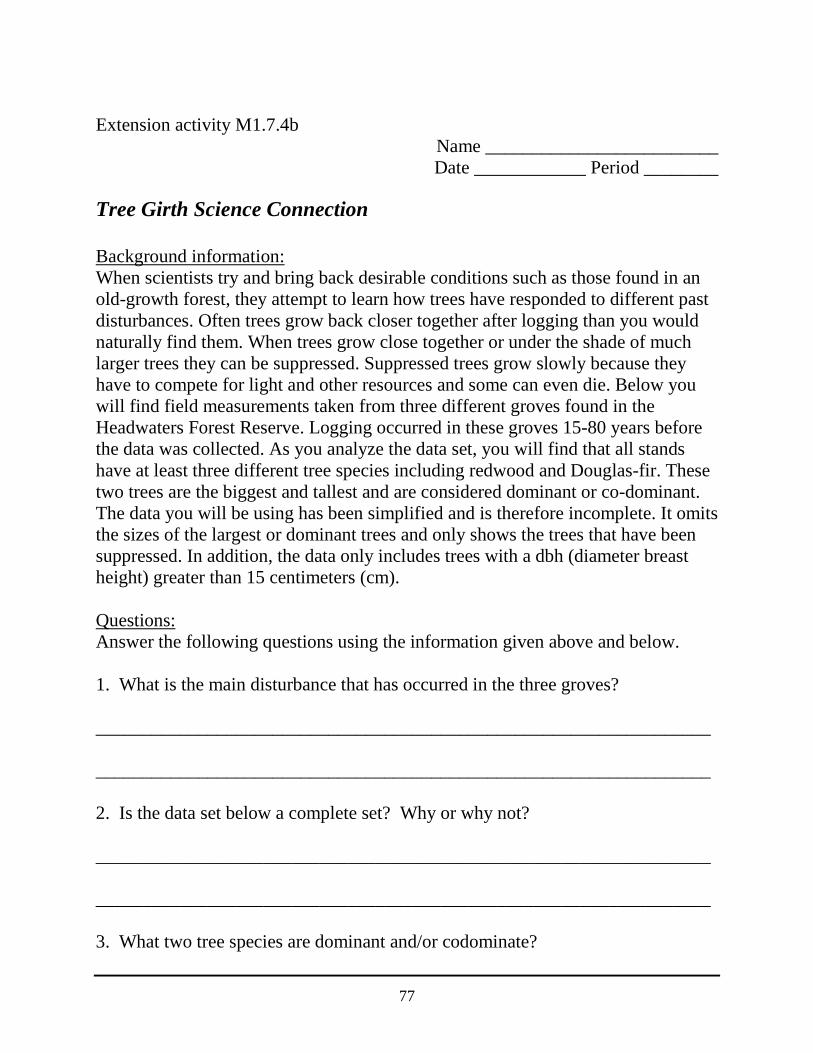
Extension activity M1.7.4b

Name _________________________ Date ____________ Period ________ Tree Girth Science Connection Background information: When scientists try and bring back desirable conditions such as those found in an old-growth forest, they attempt to learn how trees have responded to different past disturbances. Often trees grow back closer together after logging than you would naturally find them. When trees grow close together or under the shade of much larger trees they can be suppressed. Suppressed trees grow slowly because they have to compete for light and other resources and some can even die. Below you will find field measurements taken from three different groves found in the Headwaters Forest Reserve. Logging occurred in these groves 15-80 years before the data was collected. As you analyze the data set, you will find that all stands have at least three different tree species including redwood and Douglas-fir. These two trees are the biggest and tallest and are considered dominant or co-dominant. The data you will be using has been simplified and is therefore incomplete. It omits the sizes of the largest or dominant trees and only shows the trees that have been suppressed. In addition, the data only includes trees with a dbh (diameter breast height) greater than 15 centimeters (cm). Questions: Answer the following questions using the information given above and below. 1. What is the main disturbance that has occurred in the three groves?

__________________________________________________________________

__________________________________________________________________

2. Is the data set below a complete set? Why or why not?

__________________________________________________________________

__________________________________________________________________

3. What two tree species are dominant and/or codominate?

77

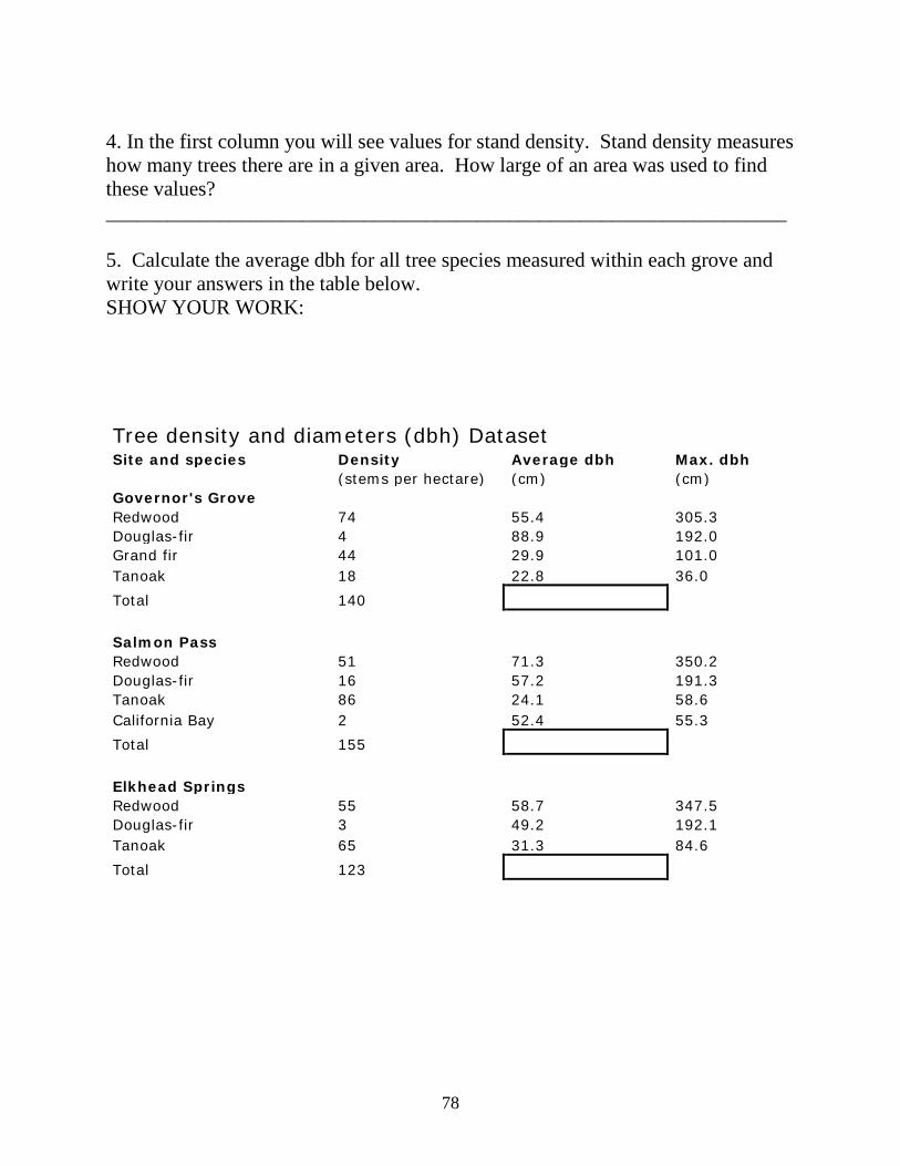
4. In the first column you will see values for stand density. Stand density measures how many trees there are in a given area. How large of an area was used to find these values? __________________________________________________________________ 5. Calculate the average dbh for all tree species measured within each grove and write your answers in the table below. SHOW YOUR WORK:

Tree density and diameters (dbh) Dataset Site and species Density Average dbh Max. dbh (stems per hectare) (cm) (cm) Governor's Grove Redwood 74 55.4 305.3 Douglas-fir 4 88.9 192.0 Grand fir 44 29.9 101.0 Tanoak 18 22.8 36.0 Total 140 Salmon Pass Redwood 51 71.3 350.2 Douglas-fir 16 57.2 191.3 Tanoak 86 24.1 58.6 California Bay 2 52.4 55.3 Total 155 Elkhead Springs Redwood 55 58.7 347.5 Douglas-fir 3 49.2 192.1 Tanoak 65 31.3 84.6 Total 123

78

6a. Which grove has the tree with the largest girth? ___________________.

b. How big is this tree (give dbh)? ______________ cm _______________ m.

c. Using dbh, find r (radius) ___________ and C (circumference). __________.

6d. What kind of tree is the largest tree? ________________________________.

7a. Which grove has the highest tree density overall? ______________________.

7b. Which grove has the lowest tree density overall? _______________________.

8. Which grove has the highest average dbh for:

a. Douglas-fir? _________________________________

b. Redwood? __________________________________

c. Tanoak? _____________________________________

9. Using this data, can the average rate for tree growth be calculated? ________

Why or why not?

_________________________________________________________________

Source: ANR Pub 8239 US Dept. of Agriculture page 3

79

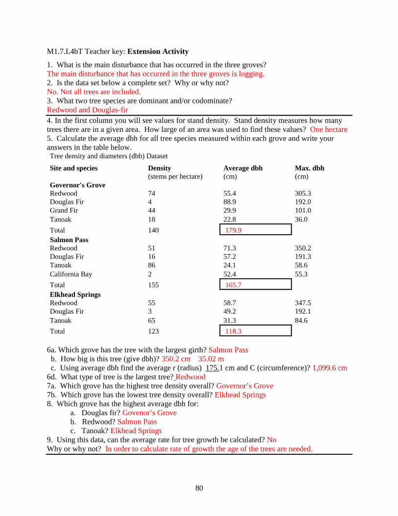
M1.7.L4bT Teacher key: Extension Activity 1. What is the main disturbance that has occurred in the three groves? The main disturbance that has occurred in the three groves is logging. 2. Is the data set below a complete set? Why or why not? No. Not all trees are included. 3. What two tree species are dominant and/or codominate? Redwood and Douglas-fir 4. In the first column you will see values for stand density. Stand density measures how many trees there are in a given area. How large of an area was used to find these values? One hectare 5. Calculate the average dbh for all tree species measured within each grove and write your answers in the table below. Tree density and diameters (dbh) Dataset

Site and species Density Average dbh Max. dbh (stems per hectare) (cm) (cm) Governor's Grove Redwood 74 55.4 305.3 Douglas Fir 4 88.9 192.0 Grand Fir 44 29.9 101.0 Tanoak 18 22.8 36.0 Total 140 179.9 Salmon Pass Redwood 51 71.3 350.2 Douglas Fir 16 57.2 191.3 Tanoak 86 24.1 58.6 California Bay 2 52.4 55.3 Total 155 165.7 Elkhead Springs Redwood 55 58.7 347.5 Douglas Fir 3 49.2 192.1 Tanoak 65 31.3 84.6 Total 123 118.3

6a. Which grove has the tree with the largest girth? Salmon Pass b. How big is this tree (give dbh)? 350.2 cm 35.02 m c. Using average dbh find the average r (radius) 175.1 cm and C (circumference)? 1,099.6 cm 6d. What type of tree is the largest tree? Redwood 7a. Which grove has the highest tree density overall? Governor’s Grove 7b. Which grove has the lowest tree density overall? Elkhead Springs 8. Which grove has the highest average dbh for: a. Douglas fir? Govenor’s Grove b. Redwood? Salmon Pass c. Tanoak? Elkhead Springs 9. Using this data, can the average rate for tree growth be calculated? No Why or why not? In order to calculate rate of growth the age of the trees are needed.

80

M1.G7 Lesson 5: Under the Sun Unit Overview: Integrative Forest Ecology Grade 7 Key Concepts:

• Developing and using models

• Cycling of matter • Conservation of

energy • Systems and system

models • Earth and human

activity Time: 60 - 80 minutes Materials for the Teacher: Visual examples of the

carbon cycle Student reading

M1.G7.L5a Student worksheet

M1.G7.5b Teacher reference

sheet M1.7.5T Drawing paper Pencils and pens

Connections: Plant science, earth science, social studies, cycling of matter, decomposition, soils, global warming, energy, energy conservation, resource management, carbon cycle, art Forest Ecology Series integration: M2: Coast Redwoods M3: Oak Woodlands

Learning Objectives: Students will read about how carbon is cycled in a forest ecosystem where they will identify and explain how main carbon sinks and sources occur. Following that they will draw a carbon cycle that incorporates living trees, dead trees, decomposition, forest fires, and combustion, among other things. Background information: Refer to the appropriate section in Part I: Teacher Companion for Module 1 and online resources. Suggested procedure: This lesson will be most appropriate once students become familiar with photosynthesis, respiration, and decomposition. Large quantities of carbon are stored in pools or reservoirs such as the ocean, soil, and forests. Any movement of carbon between these reservoirs is referred to as a carbon flux. Fluxes together with large pools create a carbon cycle. The entire global carbon cycle is much too complex to study simultaneously so individual cycles are created. All cycles are linked together and range in varying spatial and temporal scales. For instance, it only takes minutes for plants to absorb carbon dioxide through the atmosphere during photosynthesis and release it back into the atmosphere during cellular respiration. It takes much longer for dead plant material to decay where it is incorporated into the soil and longer still for plant material to be buried where it is converted to oil or coal. To begin this lesson, have students read about how carbon moves through a forest by assigning student reading M1.7.5a below. After they complete the reading, they should refer to reference sheet M1.7.5R where they will identify where and how carbon is stored (acting as a sink) and where and how it is released (acting as a source). Students should fill out student worksheet M1.7.5b as they proceed. Once students have completed worksheet M1.7.5b, test their knowledge by asking some follow up questions below. Next, have them draw a carbon cycle according to your directions. See the example given on teacher reference sheet M1.7.5T. Suggested items to incorporate into their drawing are: one or more living trees, wildfire, decomposition of wood, soil, fossil fuels, wood products, combustion of wood waste, coal, and/or oil, and tree planting. When appropriate they should depict how carbon moves through the system using arrows and label processes such as photosynthesis, combustion, and decomposition. Once they have finished, display some of the better examples.

81

Critical Thinking: Why is your model of the carbon cycle incomplete when considering the global carbon cycle? Explain your answer. Key words: carbon dioxide, carbon sequestration, carbon sink, carbon source, decomposition, deforestation, flux, fossil fuels, photosynthesis NGSS Standards alignment: MS-LS1 From Molecules to Organisms: Structures and Processes LS1.A: Structure and Function LS1.B: Growth and Development LS1.C: Organization for Matter and Energy Flow in Organisms Online resources: The Wilderness Society’s page on the Carbon Cycle: http://wilderness.org/sites/default/files/legacy/Primer-Carbon-Cycling.pdf This is the source of information used in the student reading for this lesson. It is a good overview of the carbon cycle relative to forests, forest fires, and climate change. EEI Curriculum E.7.b: The Life and Times of Carbon http://www.californiaeei.org/curriculum/ You will need to navigate down to the Earth Science section of the EEI curriclum to find this unit. Here there are good activities and great information relating to the carbon cycle from finding carbon in every day things to the global carbon cycle. California Forest Foundation: Forests and the Carbon Cycle curriculum http://www.calforestfoundation.org This site has several lessons pertaining to forests, carbon, and the carbon cycle. Realize, however, that it tends to be biased towards forestry and encourages people to use wood. GLOBE Carbon Cycle: An Introduction to the Global Carbon Cycle http://globecarboncycle.unh.edu/CarbonCycleBackground.pdf This pdf file is a good overview of the global carbon cycle for more in-depth reading. It is published by the University of New Hampshire and includes a nice glossary of terms. EEI Connection: E.5.e. Rainforests and Deserts: Distribution, Uses and Human Influences, Lesson 5 E.7.b Earth Sciences: The Life and Times of Carbon Answers to follow up questions: - What types of things are made of carbon? (all organic material or living things are made of carbon and some inorganic material such as rocks, oil, coal, and natural gas) - How long does carbon stay in a tree? (It depends. Some carbon is released immediately during respiration. As a tree grows carbon is assimilated into a tree and stays there as long as it lives) - What is the difference between respiration and photosynthesis in regards to carbon stored and released? (respiration releases carbon dioxide and photosynthesis absorbs or stores carbon dioxide)

82

(Answers to preliminary questions continued) - Does combustion release or absorb carbon dioxide? (combustion releases carbon dioxide and water and other trace elements) - What is an example of a carbon sink or the sequestration of carbon? (carbon is sequestered in soil, the ocean, the atmosphere and trees - therefore these are examples of carbon sinks) - Does decomposition release carbon quickly or slowly? (slowly) - What stable form of carbon persists after a forest fire? (charcoal) - Where is most carbon stored in a forest ecosystem? (in the soil) - What effect does deforestation have in regards to the global carbon cycle? (deforestation increases the amount of carbon dioxide in the atmosphere and thus accelerates global warming) Suggested extensions:

• Teach about deforestation of the tropical forests in order for students to make a connection to forests on a global scale.

• Have students play a card game where they identify what things contain carbon and what things don’t. This is available at the EEI site.

• Have students measure the density of different wood samples. Discuss how different wood types are used for different applications. Examples include wood used in musical instruments compared to wood used in furniture or housing.

• Connect the carbon cycle to the oceans by showing a video and/or talking about ocean acidification.

• Find a carbon calculator and have the students calculate their own carbon footprint. A good one can be found at the epa.gov, however for middle school, the one available at www.ei.lehigh.edu may be easier to use.

• Perform an energy audit at your school to see where energy can best be saved. • Begin a tree planting campaign in your area.

M1.7.5a Student reading M1.7.5b Student worksheet M1.7.5T Teacher reference sheet

83

Student Reading M1.7.5a Source: *The Wilderness Society 6/5/2008 (http://wilderness.org) CLIMATE CHANGE FACTS: A PRIMER ON CARBON CYCLING The Earth’s climate is changing. In the past, the climate warmed and cooled due to natural processes. Now humans are changing the climate by burning fossil fuels and permanently deforesting landscapes. Many of our wildlands are being stressed beyond their natural ability to adapt to these dramatic changes, and the full extent of how to deal with these changes remains unclear. What is clear, however, is that a better understanding of the carbon cycle and the role forests play will help us better manage forests and fire in a future marked by climate change. The Carbon Cycle Carbon is an element found in all forms of life. Carbon makes up 18 percent of our bodies and is a major component of trees and plants. It also exists in the environment in non-living things like rocks, oil, natural gas, coal, and air. In short, it is the basic building block of all life and the environment we live in. Carbon, in its many forms, is exchanged among the atmosphere, oceans, and land. This is called the carbon cycle. In simple terms, plants take carbon dioxide (CO2) from the atmosphere and turn it into biomass (wood, leaves, fruits etc.) through a process called “photosynthesis.” Some of the carbon taken in by plants is returned to the atmosphere through respiration by the plant or by other living organisms, including humans that use it for food or fuel. This renews the carbon cycle. By extracting fossil fuels (oil, gas and coal) from deep in the Earth, we are overloading the atmosphere with carbon, and changing our climate in irreversible ways. The Forest Carbon Cycle One critical part of the carbon cycle takes place in forests. Forests exchange large amounts of CO2 and other gases with the atmosphere and store carbon, in various forms, in trees and soils. Carbon stored in plants or soils is called “sequestered carbon.” Carbon returned to the atmosphere when it has been used by trees or other organisms as energy for life is called “respired carbon.” If we follow the fate of carbon in a forest, many processes are occurring. Much of the CO2 in the air above a forest is taken in by trees through the process of photosynthesis, where it becomes one of the building blocks for tree growth or energy for life. • How long does carbon stay in a tree? Some carbon goes right back into the atmosphere as the tree respires (breathes out); but, if it stays, then it may remain sequestered in the tree throughout its life—whether that is 10 or 500 years. When a tree dies or loses a leaf or branch containing carbon, it generally falls to the forest floor where it will be decomposed by bacteria and fungi, and either be respired back into the atmosphere or made into soil carbon. M1.7.5a (Student Reading continued)

84

• How long does carbon remain in the soil? Carbon is returned daily to the atmosphere when it is decomposed and respired by soil organisms. But, much of it remains in complex chemical forms that resist decomposition and persist for hundreds to thousands of years. Soil carbon is an important carbon storehouse. It accounts for as much carbon as is presently found in plants and the atmosphere combined. Figure 2: The forest carbon cycle • Fire plays an important role in the forest carbon cycle. When a fire occurs, a portion of the trees, plants, grasses and other biomass are consumed and converted to CO2 and other gases, and another portion is converted to charcoal, an essentially permanent form of storage. Only 10 to 30 percent of the biomass in a forest is actually consumed by a fire; the majority remains on-site. Live trees will continue their role in the carbon cycle. Dead trees will slowly decompose and release carbon to the atmosphere or make new soil carbon. Regrowth after a fire will recapture carbon from the atmosphere, reversing the fire’s emissions. About one to 10 percent of biomass killed in a fire is converted to charcoal, a uniquely stable form of carbon that will persist for thousands of years. Forest Carbon, Elevated CO2 and Climate Change Until humans began burning fossil fuels, the carbon cycle was closed to new inputs of carbon and carbon was continually recycled. Earth’s plants and animals evolved over thousands of years under this level of CO2 and a slowly changing climate, creating the forest ecosystems we know today. Now we are extracting billions of tons of fossil fuels each year to meet the energy demands of a growing global population, adding new carbon to the atmosphere and changing our climate. Prior to fossil fuel use, this carbon was locked underground for millions of years and was not part of the carbon cycle. Current levels of CO2 are 25 percent higher than before the Industrial Revolution. As a result of these elevated levels of carbon, our forest ecosystems are changing. They are changing the way they grow in response to elevated CO2, and they are changing in response to new climate patterns, including warmer temperatures and different levels of precipitation. These changes also affect the way that they store and release carbon, sometimes reducing the amount that goes into tree carbon or soil carbon. Conclusions Elevated levels of CO2 in the atmosphere are changing the carbon cycle and the climate. Because forests have evolved under a climate that has changed at slow rates over the past several thousand years, they cannot be expected to function in the same way or provide the same habitat under elevated CO2 levels and rapidly changing climatic conditions. As such, our forest management goals should include preserving healthy forest ecosystems and the natural role of forest fires and restoring forests toward resilient conditions when they have been depleted. *Figures 1 and 2 were deleted to save space. Go to the website above to read a color version. 2

85

Student worksheet M1.7.5b Name _________________________

Modified from: calforestfoundation.org Date __________ Period _________ Carbon Cycle Sinks and Sources Directions: Choose different carbon sinks and sources from your reading assignment and discussion. You can select these from the list below. In the table explain how carbon can enter a sink or be sequestered and how it can be emitted or become a carbon source. Carbon Sinks Carbon Sources Atmosphere Decomposition Plant biomass Respiration Soil Burning fossil fuels Rock Wildfires Fossil fuels (fossil pools) Wood burning stove Surface ocean Ocean exchange Deep ocean Deforestation Wood products Carbon Sink

How does it get there? Carbon Source

How is it emitted?

86

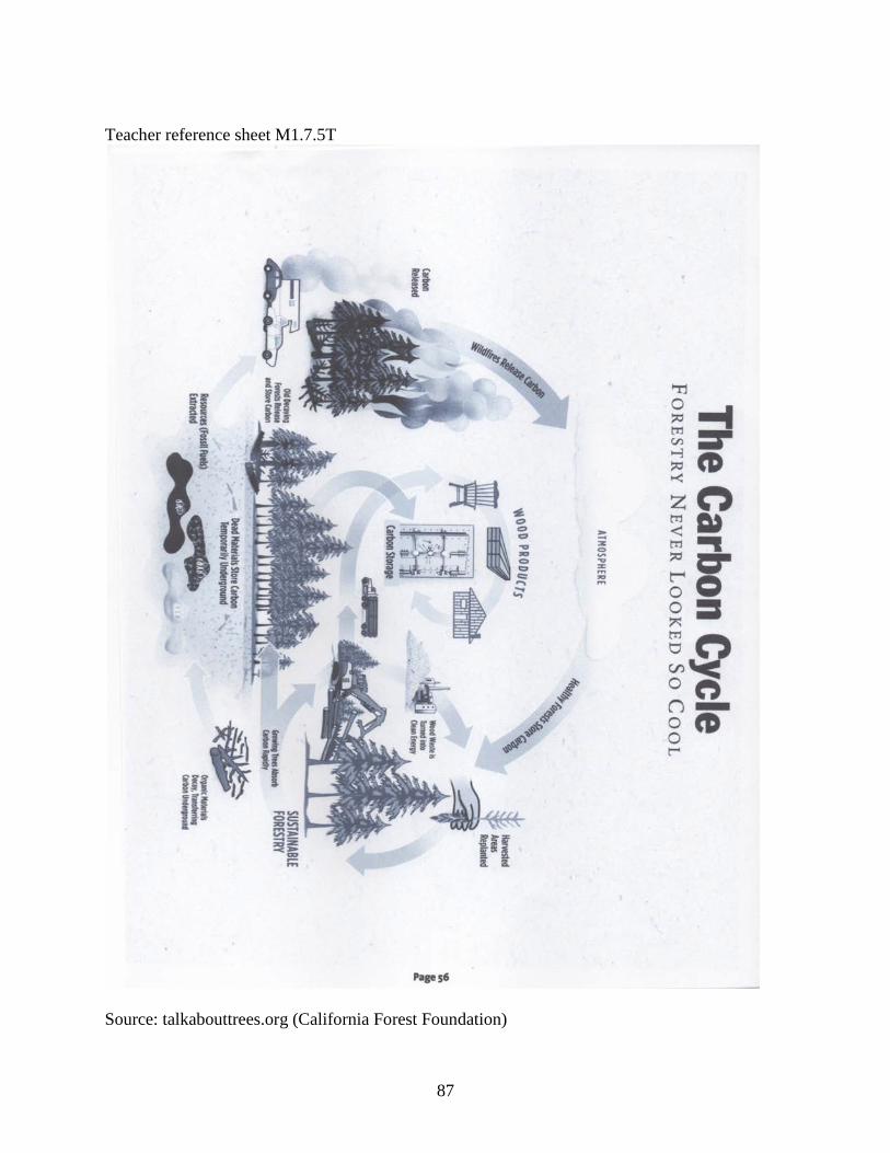
Teacher reference sheet M1.7.5T

Source: talkabouttrees.org (California Forest Foundation)

87

M1.G7 Lesson 6: Who’s There? Unit Overview: Integrative Forest Ecology Grade 7 Key Concepts:

• Identifying organisms • Growth and

development • Variation in and

between species • Compare and contrast

Time: 120 - 180 minutes Materials for the Teacher: Tree identification

references or keys Reference sheet

M1.7.6R Magnifying glasses

(optional) Tree foliage from

different species or pictures (enough for each student to have a small sample)

Garden clippers (for collecting)

Index cards and clear packaging tape

String or clasps Connections: Plant science, genetics, growth and development, reproduction, seasons, adaptation, resource management, soils, biogeography, art, carbon cycle Forest Ecology Series

Learning Objectives: Students will be able to identify and describe the key features used to identify nearby native trees. Using identification keys, they will identify the dominant conifers and other trees that live in their area and will collect leaf samples to be compiled into a tree booklet. Background information: Refer to the appropriate section in Part I: Teacher Companion for Module 1. Suggested procedure: This lesson focuses on native tree species, especially conifers, to add continuity to the previous lessons. You will need to decide what trees you want to use and whether you will be using live samples or botanical drawings. Collected samples can last several days in plastic bags left in a refrigerator. Samples can also be pressed ahead of time, but this tends to make them brittle if not used immediately. Begin this lesson by telling the students they will be identifying different local tree species using a key as they look at samples (shrubs can also be used). There are many ways this activity can be done. You will need to direct the students about how to obtain their samples and assemble their booklets. It is recommended that after they identify a particular species they place a small sample (about the size of a sand dollar) on an index card and label it with the common name in pencil. Cards can also include the scientific name, family, and any other information you would like them to know. Information could include key features such as needles in bundles of 3 or leaves alternate. Before they begin you will need to make sure they are familiar with some of the vocabulary used in plant identification (see M1.7.6R reference sheet). Copies of the reference sheet should be made available to them. Many other features such as smell can be used in addition to morphology. Once they have identified all of their species they should begin to assemble their tree (plant) booklet. Allow more than one day for this depending on how many plant specimen they have. An easy way to make a card is to place packaging tape over the plant sample. This method can preserve their specimens for months in order to use them later. It is important to have students identify their specimen first before taping it onto a card so they can observe all parts of it closely. Before beginning this activity you may want to find out what they already know about local trees by asking them the preliminary questions below. While doing so write down two headings on the board: “species” and “key

88

integration: M2: Coast Redwoods M3: Oak Woodlands

features” and list the student responses in the appropriate column. This questioning can also be done as an assessment tool especially if they are going to be held accountable for knowing their local tree species by sight. If you are having students use a dichotomous key, you may want to practice a few examples with them until they get the hang of it. A dichotomous key for hardwoods can be found in lesson 2 (G7) in Module 3. Note: there are many different references available for identifying plants. You will want to use something relatively simple. Find your own tree identification keys or use the one available online (see online resources below).

Preliminary or follow-up questions: • Who can tell me a type of tree that grows around here? (Ask for several different species) • What differences have you observed between different tree species? (Get several

responses related to morphology) • Which differences clearly set species apart from one another? (These are called key

features). • If you wanted to identify a certain tree species, what key features would you look for?

(Continue to ask for “what else” until you get a list of key features).

Critical Thinking: Assume you planted a tree species that naturally grows in the Sierra Mountains in your backyard. You give it adequate sun, space, and water, but it slowly dies. What are some possible factors that may have caused your tree to die? Key words: see reference sheet M1.7.6R below NGSS alignment: MS-LS1 From Molecules to Organisms: Structures and Processes LS1.A: Structure and Function LS1.B: Growth and Development LS1.C: Organization for Matter and Energy Flow in Organisms Online resources: OSU (Oregon State University) Common Trees of the Pacific Northwest: http://oregonstate.edu/trees/index.html Click on the dichotomous key link from this home page. This has an easy to use dichotomous key for identifying local trees. If you use this key, it assumes you are in the state of Oregon, but many of the trees are the same in northern California. The Gymnosperm Database: The gymnosperms of Alta California http://www.conifers.org/topics/caltrees.php The information in this database is too advanced for most middle school students to use, however it has a wealth of information about all gymnosperms and is a great resource for educators to use to brush up on their own knowledge of trees.

89

(online resources continued) Western Native Trees Society http://www.nativetreesociety.org/wnts/index_wnts.html This website has a comprehensive list of links associated with anything involving trees of western North America including tree identification apps and where to find inexpensive pocket guides. About Forestry: Using Anatomy and Habitat to Identify a Tree http://forestry.about.com/od/thecompletetree/u/tree_anatomy.htm This site has a host of guides, diagrams and illustrations to aid in tree and plant identification. It tends to focus on eastern tree species however. EEI Connection: E.7.b Earth Sciences: The Life and Times of Carbon Answers to preliminary questions: - Who can tell me a type of tree that grows around here? (this depends on a particular area. Common conifers include beach or shore pine, Sitka spruce, Douglas-fir, coast redwood, western red cedar, ponderosa pine, and grand fir. Hardwoods include black oak, Oregon white oak, tanoak, madrone, red alder, and California bay) -What differences have you observed between different tree species? (Answers will vary. Examples include differences in leaves, cones, and bark.) - Which differences clearly set species apart from one another? (Answer will vary. Refer to a plant identification guide or reference sheet M1.L7.R1) -If you want to identify a certain tree species, what key features would you look for? (Most trees can be identified by their size and shape combined with observing leaf shape, color, and arrangement. Conifers have needle-leaves and hardwoods have broad leaves. Additional key features include color and texture of bark and what type of seeds or cones they have.) Suggested extensions:

• Have students use their plant booklets outside in a nearby natural area to practice identifying trees.

• Have students read and discuss the importance of trees including their role in agriculture, commerce, timber, and habitat for wildlife.

• Use trees to connect to other important life science concepts such as genetics, evolution, or cellular transport.

• Use thin cross-sections to have students observe a leaf using a microscope. • Connect identification of plants to plant taxonomy or other genetic associations.

M1.7.6R Reference sheet - Plant identification

90

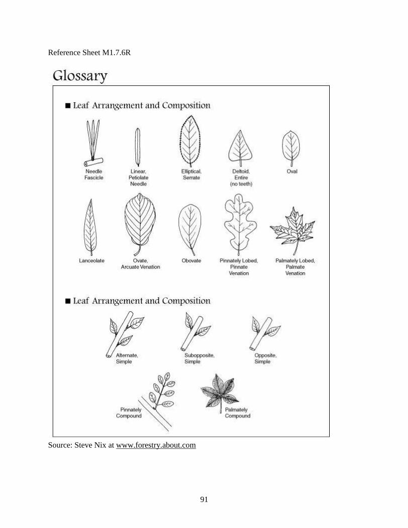
Reference Sheet M1.7.6R

Source: Steve Nix at www.forestry.about.com

91

Forest Ecology 101 Series (M1: Part II)

Module 1: Integrative Forest Ecology Part II

UNIT OF STUDY COVER PAGE

10th Grade Unit of Study Lesson 1 - Regional Biodiversity

Lesson 2 - Seeing the Forest Through the Trees Lesson 3 - Life and Loss: Linking Forest Critters

Lesson 4 - Tree Measurements Lesson 5 - Biodiversity: Measuring Up

92

M1.G10 Lesson 1: Regional Biodiversity Unit Overview: Integrative Forest Ecology Grade 10 Key Concepts:

• Ecosystem dynamics and resilience

• Using patterns to observe cause and effect

• Analyzing and interpreting

• Stability and change within a region

Time: 60 - 90 minutes Materials for the Teacher: Atlas of the

Biodiversity of California booklet (1 per student pair)

Short lecture on biodiversity

Student worksheet and teacher key M1.10.1a

Connections: Geography, earth science, genetics, botany, zoology, land management, wildlife, forestry, human population growth, conservation, economics, land use, climate change Forest Ecology Series integration: M2: Coast Redwood M3: Oak Woodlands

Learning Objective: Using the Atlas of the Biodiversity of California, students will examine the terrestrial biodiversity of their region and will compare it to three other selected towns in Northern California. They will study patterns and find relationships between variables such as precipitation, elevation, and plant richness. Background information: Refer to the appropriate sections in Part 1: Teacher Companion for Module 1 and the Atlas of the Biodiversity of California, published by the California Department of Fish and Game (see online resources). Every major subject area in the booklet has a short explanation giving interesting and useful information. Suggested procedure: This lesson uses an atlas that will need to be acquired ahead of time. Begin the lesson by asking some of the preliminary questions below to assess what students already know about biodiversity. There are many types of biodiversity including genetic, ecosystem, and species. This exercise focuses on species biodiversity, otherwise known as richness. After questioning, show a few pictures of varying habitats throughout California to add depth to their understanding (see online resources). During this short presentation, discuss some of the main factors influencing the biodiversity found in a given area such as climate, water availability, temperature, elevation, and soil type. For instance, why might the biodiversity of reptiles be greater in the desert regions? Certainly more than one factor is responsible for the noted differences. Once a short discussion is over, separate students into pairs and have them use the atlas to fill out student worksheet M1.10.1a. You will need to direct how you want them to fill out their worksheet since there is some flexibility built into the lesson. Go over at least one page with them to model how they will compare the four selected locations. Based on the skill level of your students, you may want to do the first one together. Depending on how many copies of the atlas you have, students can work independently or in pairs. Some pages of the atlas are available online. Two comparisons are not given and need to be chosen by you or the students from the atlas. Here they need to observe patterns and relationships and write a supportive sentence explaining the relationship between factors. Lastly, they will apply the concept of cause and effect to California as a whole after flipping through the booklet and will write another hypothesis.

93

Preliminary questions: • What types of landscapes or bioregions exist in California? • What does biodiversity mean? • What are some places you are aware of with high levels of biodiversity? (You may need

to give examples to prompt students). Low levels? • Why do you suppose some places have higher biodiversity than others? (You may want

to show a page from the biodiversity atlas) • Give me an example of a local habitat with high levels of biodiversity. (get at least 3

examples) Low levels? • Why does an ecologist or a land manager care about biodiversity?

Critical Thinking: California is one of the most diverse places on the planet as well as one of the fastest growing places in America. What challenges will future land managers face while attempting to preserve biodiversity? Keywords: abiotic, biodiversity, bioregion, biotic, climate, endemism, rarity, richness, variable NGSS alignment: HS-LS2.2: Ecosystems: Interactions, Energy and Dynamics HS2.C: Ecosystem dynamics, functioning, and resilience HS4.D: Biodiversity and humans ETS1.B: Developing possible solutions M1.G10.L1 (Unit Overview continued) Online resources: California Biodiversity: Lesson from calbio.berkeley http://gk12calbio.berkeley.edu/lessons/less_cabiodiv.htmld This site has a lesson where students learn about factors relating to extraordinary diversity of California. It also has a useful online Power Point presentation fitting as an overview for this lesson. It attempts to show repeated patterns between influential factors such as topography and climate. National Geographic: Biodiversity (in Reference and News section) http://education.nationalgeographic.com/education/encyclopedia/biodiversity This site has clear definitions of the different types of biodiversity, emphasizes the value of biodiversity, and describes some of the threats to global biodiversity. Biodiversity Hotspots Case Study: California - from KhanAcademy http://www.khanacademy.org/partner-content/CAS-biodiversity/where-biodiversity-is-found/biodiversity-hotspots-cas Several good short videos on biodiversity are available on this site along with questions and answers students can use to test their knowledge. California Academy of Sciences: Connect Experiences: Threatened Biodiversity http://www.calacademy.org/teachers/resources/lessons/threatened-biodiversity/ Mainly targeting treats to biodiversity in tropical areas, this site has lessons for 9th-12th grades and teacher background information that could be useful for extension activities.

94

EEI Connections: B.8.b Biological Diversity: The World’s Riches B.8.d The Isolation of Species 12.2.2 and 12.2.5 This Land is Our Land (Social Studies connection) Answers to preliminary questions: - What types of landscapes or bioregions exist in California? (California is one of the most diverse places in the world. It has deserts, mountains, wetlands, forests, savannas, and a rich marine habitat off the coast) - What does biodiversity mean? (biodiversity has several different meanings. It most commonly means the number of different species living in a particular place but can also reflect the variability between organisms) - What are some places you are aware of with high levels of biodiversity? (Answers will vary. Answers might include tropical rainforests, coral reefs, wetlands, etc.) Low levels? (arid regions, polar regions, and high elevations) - Why do you suppose some places have higher biodiversity than others? (places with high levels of biodiversity tend to be places where it is warm and moist all year, such as the tropics) - What do you think the main factors are that allow for an area to have high levels of biodiversity? (factors include mild temperatures, adequate rainfall, and rich soil types) - Give me an example of a local habitat with high levels of biodiversity. (Answers will vary. Local forests, shorelines, wetlands, and grasslands are all examples of places with high biodiversity. Low levels could be places like lawns, tree plantations, and towns) - Why does an ecologist or land manager care about biodiversity? (Answers will vary. Biodiversity can be an indicator of a healthy habitat able to support a large number of species. Places with high levels of biodiversity are storehouses of genetic information, potential sources of drugs, food, and other helpful products, and are the life line to life on earth. If a place has low levels of biodiversity it could signal environmental stressors such as pollution, disease, or heavy impact) Suggested extensions:

• Explore the biodiversity of a particular family of organisms in your area such as insects, birds, vascular plants, or mammals.

• Design a field study comparing the biodiversity of a square meter area between two or more nearby sites.

• Have students make a poster or collage depicting the biodiversity of a given place. • Classify pictures of organism into various taxonomic families or orders. • Perform a local bioblitz and have students in teams record all of the living things that

they observe in a given amount of time. • Let students explain to a partner the importance of avoiding species extinction. • Watch Becoming California a video about geological, biological and social change

throughout California. It can found on the calegacy website calegacy.org.

Student worksheet and teacher key M1.10.1a

95

Student worksheet M1.10.1a Name__________________________________ Date_______________ Period ______________ COMPARING BIOLOGICAL RICHNESS PART 1: Begin by identifying and locating your region on a map. Read pages 2-4 in the Atlas of the Biodiversity of California to review the layout and information contained within this booklet. For each section, read the accompanied information as you fill out the data for each variable below. For the Redding location, you might want to note the immediate area and the surrounding area. Once you have completed the table, follow your teacher’s instruction before you proceed to the next page. My region is _________________________________________________________. Information and/or biodiversity values for: Abiotic factors (pages)

A: Your region

B: Redding/nearby

C: Fort Bragg

D: Sacramento

Elevation (pgs 12-13)

Climate Classification (pgs 14-15)

Avg. Annual Precipitation (pgs 14-15)

Avg. High and Low Temperatures (pgs 14-15)

High: Low:

High: Low:

High: Low:

High: Low:

Biodiversity Vegetation (pgs 18-19)

Plant Richness (pgs 24-25)

Plant Rarity (index) (pgs 26-27)

Amphibian richness (pgs 28-29)

Mammal richness (pgs 38-39)

96

PART 2: Student worksheet M1.10.1a Instructions: 1. Once you have finished entering the data, look for patterns by flipping through the booklet. Select two variables you would like to compare and write them below for comparisons 3 and 4. Predict what factors are most influential between the selected variables and write a supporting statement for each. This is your hypothesis. In science this prediction would be tested. For instance, you might find a lack of mammals where human development or urbanization exists. Only two regions need to be compared at a time. 2. Look at California as a whole and find other relationships or patterns between abiotic and biotic factors and write a statement explaining your observations. Comparison 1: Elevation and Climate Region 1 ___________________________ Region 2 ___________________________ Supportive statement: ______________________________________________________________________________ ________________________________________________________________________________________________________________________________________________________________________________________________________________________________________________________________________________________________________________________ Comparison 2: Annual Precipitation Region 1 ___________________________ and Plant Richness Region 2___________________________ Supportive statement: ______________________________________________________________________________ ________________________________________________________________________________________________________________________________________________________________________________________________________________________________________________________________________________________________________________________ Comparison 3______________________ Region 1 _____________________________ (your choice) Region 2 ____________________________ Supportive statement: ______________________________________________________________________________ ________________________________________________________________________________________________________________________________________________________________________________________________________________________________________________________________________________________________________________________

page 2

97

Comparison 4: ___________________________ Region 1 ____________________________ (your choice) Region 2 ___________________________ Supportive statement: ______________________________________________________________________________ __________________________________________________________________________________________________________________________________________________________________________________________________________________________________________ General pattern of the California landscape: What patterns do you observe after flipping through the atlas? Make a hypothesis. Key concept: cause and effect Supportive statement: ______________________________________________________________________________ ________________________________________________________________________________________________________________________________________________________________________________________________________________________________________________________________________________________________________________________________________________________________________________________________________________________________________________________________________________________________________________________________________________________________________________________________________________________________________________

page 3

98

Teacher Key: Student worksheet M1.10.1a COMPARING BIOLOGICAL RICHNESS PART 1: My region is ____________________________________________________. Information and/or biodiversity values for: Abiotic factors (pages)

A: Your region

B: Redding/nearby

C: Fort Bragg

D: Sacramento

Elevation (pgs 12-13)

500-1,000 ‘

100-500 ‘

0-100 ‘

Climate Classification (pgs 14-15)

Mediterranean Hot summer

Mediterranean Summer fog

Mediterranean Hot summer

Avg. Annual Precipitation (pgs 14-15)

15-25”

40-60”

15 - 25”

Avg. High and Low Temperatures (F) (pgs 14-15)

High: Low:

High: 75.2-84.2 Low: 39.2-46

High:37-59 Low: 46.1-58

High:75.2-84.2 Low: 39.2-46

Biodiversity Vegetation (pgs 18-19)

Urban/ Woodland

Conifer Forest

Urban

Plant Richness (pgs 24-25)

839-1,108 1,409-1,704

1,253-1,408

719-838

Plant Rarity (index) (pgs 26-27)

Medium Low

Medium High

Low

Amphibian richness (pgs 28-29)

7-10

11-17

4-6

Mammal richness (pgs 38-39)

40-47

56-73

22-39

PART 2: Answers will vary.

99

M1.G10 Lesson 2: Seeing the Forest Through the Trees Unit Overview: Integrative Forest Ecology Grade 10 Key Concepts:

• Ecosystem dynamics and resilience

• Cause and effect relationship

• Structure and function regarding an ecosystem

• Analyzing and interpreting data

• Obtaining, evaluating, and communicating information

Time: 60 - 120 minutes Materials for the Teacher: Pictures of different

age classes of forests (optional)

Student reading M1.10.2a

Student worksheet M1.10.2b

Student worksheet M1.10.2c (optional)

Pictures of the wildife presented (optional)

Connections: STEM, forestry, botany, land management, forest function and structure, ecosystem resilience, conservation, economics, zoology, wildlife, land stewardship

Learning Objectives: Students will understand the relationship between forest structure and function by comparing typical characteristics associated with unmanaged old-growth Douglas- fir forest to those of managed secondary stands. They will summarize their understanding in a paragraph. During an extension, they will interpret a figure from a scientific paper that shows different degrees of impact to vegetation and the need to manage wildlife at different spatial scales. Background information: Refer to the appropriate sections in Part 1: Teacher Companion for Module 1 and referenced scientific papers below found in Part I: Franklin, J.F. et al. 2002. Disturbances and structural development of natural forest ecosystems with silvicultural implications, using Douglas-fir forests as an example, Forest Ecology and Management 155:399-423. Hansen et al. 1991. Conserving biodiversity in managed forests - Lessons from natural forests, Bioscience 41:6. Stritthold et al. 2006. Status of mature and old-growth forests in the Pacific Northwest, Conservation Biology 20:2. Suggested procedure: Begin the lesson by having students read M1.10.2a discussing how forest function and structure often differs between mature unmanaged Douglas-fire forest and young managed forests. Most of this information was modified from the Teacher Companion for Module 1. It can be assigned for homework the night before or read in groups. Next, have them complete Part I on student worksheet M1.10.2b. Here they will match the typical features and corresponding ecological functions frequently associated with the two forest classes (old-growth vs. young secondary forests) and describe how the ecological functioning is enhanced in old-growth forests. Before they fill out this worksheet, it is optional to add depth to their understanding by showing pictures of different modified forest and the corresponding features found in them. Once they have completed this page, it is suggested that you take time to correct it in class so they can learn instantly whether they have mastered the information or not. Review any commonly missed items. An optional extension follows on worksheet M1.10.2c. Here students will interpret Figure 1 from Wilson and Puettmann 2007. This figure graphically shows degrees of disturbance to understory vegetation from different

100

Forest Ecology Series integration: M2: Coast Redwood M3: Oak Woodlands

silvicultural methods and shows the different habitat utilization by five different forest animals from a fine scale to a large scale. If they are unfamiliar with any of these species, they should research them on their own time.

Critical Thinking: The structure and integrity of a managed forest is related to the management strategies imposed on the stand. Explain how two similarly aged forests of similar composition can end up different based on two different applied management strategies. Keywords: biological legacy, cohort, composition, degradation, diversified, epiphyte, forest succession, heterogeneous, homogenous, silviculture NGSS alignment: HS-LS2.2: Ecosystems: Interactions, Energy and Dynamics HS-LS2:A Interdependent Relationships in Ecosystems HS2.C: Ecosystem dynamics, Functioning, and Resilience HS4.D: Biodiversity and Humans Online resources: Project Learning Tree - Focus on Forests https://www.plt.org/focus-on-forests Abundant resources relating to forest healthy, succession, and management is available here. Most lessons are designed for K-8 but can be modified for high school. Tarleton College - Pacific Northwest forests page. http://www.tarleton.edu/Departments/range/Woodlands%20and%20Forest/Pacific%20Northwest%20Forests/PacificNorthwestForests.html Pictures of various stages of coastal Douglas-fir forests can be found here including virgin forests, second growth, and clear cuts. We Save Trees http://www.wesavetrees.org This site has good links to local resources regarding forest conservation and activism. EEI Connections: B.8.b Biological Diversity: The World’s Riches 10.4.1 World History- New Imperialism: The search for Natural Resources 11.5.7 U.S. History - Mass production, Marketing, and Consumption in the Roaring Twenties

101

M1.G10.L2 (Unit Overview continued) Suggested extensions:

• Have students write a report on a keystone species or an indicator species used in forestry management.

• Introduce a controversial subject relating to forest management and lead a discussion about it.

• Invite a forester to talk about current land management objectives and practices. • Measure trees in a forest stand to find density, height, and dbh (see M1.G10.L4). • Visit a local sawmill • Count the biodiversity of forest plants or other organisms in a nearby area. • Calculate the area of light that reaches a particular place on the forest floor by having

students trace where light and shadow are on a piece of laid out graph paper. M1.10.2a Student reading M1.10.2b Student worksheet and teacher key M1.10.2c Student worksheet and teacher key

102

Student reading M1.10.2a Forest Structure and Function

Read the passage below discussing the differences found between forest structure and related function based on two alternative forest systems: an old-growth forest (>180 years old) and a young managed secondary forest (40-80 years old). The structure and complexity of forests are a consequence of succession, the current plant

community, variable disturbances, and other environmental factors. Forest composition is the

proportion and arrangement of different species occupying a particular ecosystem and is a major

aspect of biodiversity. The different layers of a forest from the ground to the canopy provide

vastly different habitats for a variety of organisms; each one interconnected to an entire

ecosystem. Forests are often grouped into different age classes: old growth (195-200 years old),

mature (80-195 years old), and young (40-80 years).

Studies conducted in the Pacific Northwest show there is a greater diversity of species

occupying old-growth forest ecosystems compared to those that have had a high degree of

disturbance, including the removal of large trees. Large trees are sometimes referred to as

biological legacies because they can contribute disproportionally to the rate and pattern of tree

regeneration, forest succession, and soil development. Old-growth forests will characteristically

include a more diverse structural pattern that includes features like forest gaps, different-aged

trees, and large amounts woody debris in the form of snags and logs.

The resulting spatial and structural heterogeneity old-growth forests have can aid in

management strategies that strive to increase habitat suitability in managed forests. The crowns

of certain trees support unique epiphyte communities and collect greater amounts of moisture

compared to smaller sized trees. Threatened species, such as the red tree vole and northern

spotted owl, are dependent on old-growth canopy structures for nesting, feeding, and protection.

Frequently, there is a greater variety of understory plants in a mature or old-growth forest, which

can provide greater food sources and hiding places for animals. Since mature Douglas-fir and

redwood trees are long-lived, they continue to be modified over hundreds of years. During this

time, trees endure many disturbances such as tree falls, fire, and disease; adding to the degree of

complexity. In addition, large, old, living and dead trees allow for the accumulation of large

103

amounts of biomass. Large snags and logs are one of the most important features found in

mature forests often lacking in younger ones.

Across the North Coast, secondary forests (those managed for large-scale timber

production) have been highly modified. This human-caused disturbance does not duplicate

natural disturbances. Since the late 20th century, the primary objective in managing forests for

timber (also known as silviculture) has been to promote high tree productivity. Managing forests

strictly for rapid tree growth has resulted in even-age stands with more similarly sized trees

spaced uniformly apart. Because there is less diversity in these forests, they are often described

as homogeneous and basically form tree farms with 40-year to 80-year rotations. The most

common forestry practice is clear-cutting followed by burning left over slash and removing large

woody debris. This practice can cause habitat degradation, meaning it is altered from its original

nature. The lack of structurally diversity found in cut-over forests commonly reduces habitat and

nutrient cycling, which in turn reduces ecological functioning. A secondary forest typically has

no remnant large trees. Thus, the amount of incoming solar radiation increases, which can cause

plant-stress, a change in forest composition, and the establishment of non-native species. An

increase in tree density often occurs because so much light penetrates the forest floor. A high

density of trees can increase competition and many trees can become suppressed or diseased.

The end result is a forest with reduced understory vegetation, which often decreases habitat and

food sources for wildlife.

----------------------------------------------------- Written by Melinda Bailey

page 2

104

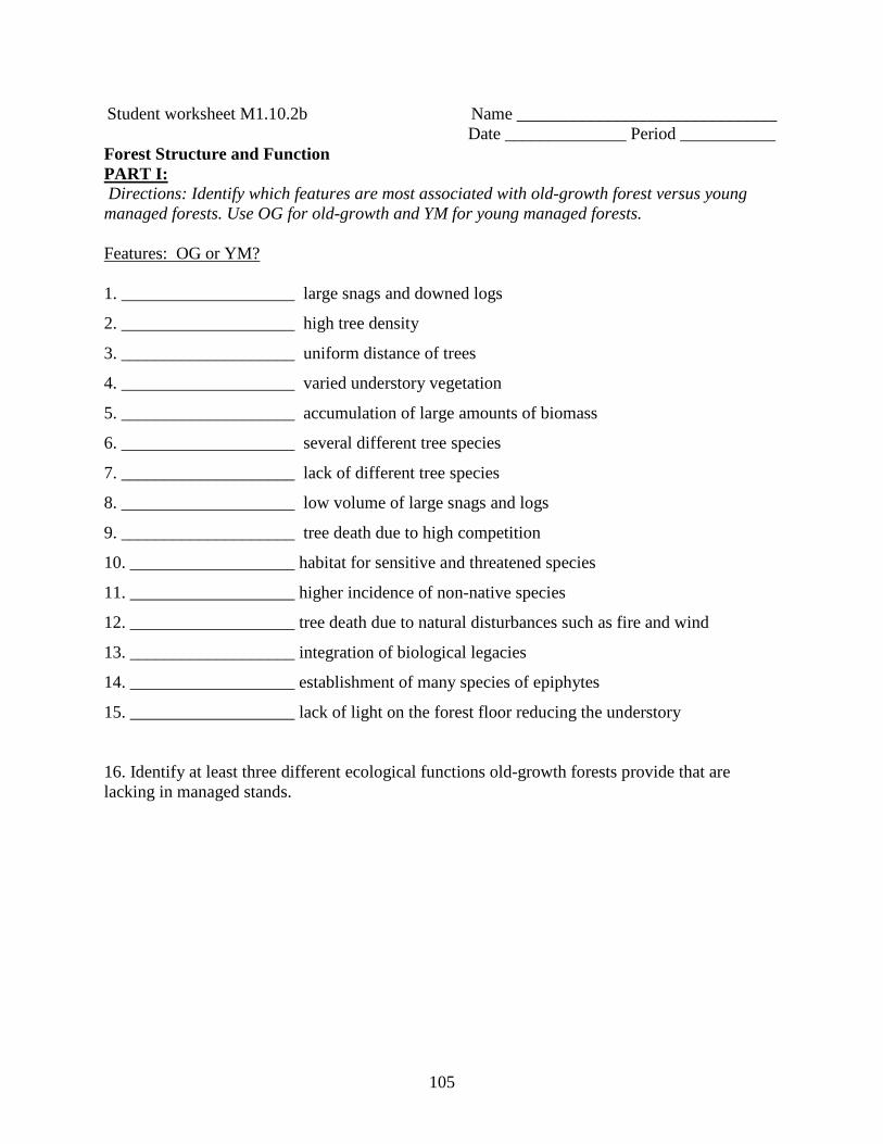
Student worksheet M1.10.2b Name ______________________________ Date ______________ Period ___________ Forest Structure and Function PART I: Directions: Identify which features are most associated with old-growth forest versus young managed forests. Use OG for old-growth and YM for young managed forests. Features: OG or YM? 1. ____________________ large snags and downed logs

2. ____________________ high tree density

3. ____________________ uniform distance of trees

4. ____________________ varied understory vegetation

5. ____________________ accumulation of large amounts of biomass

6. ____________________ several different tree species

7. ____________________ lack of different tree species

8. ____________________ low volume of large snags and logs

9. ____________________ tree death due to high competition

10. ___________________ habitat for sensitive and threatened species

11. ___________________ higher incidence of non-native species

12. ___________________ tree death due to natural disturbances such as fire and wind

13. ___________________ integration of biological legacies

14. ___________________ establishment of many species of epiphytes

15. ___________________ lack of light on the forest floor reducing the understory

16. Identify at least three different ecological functions old-growth forests provide that are lacking in managed stands.

105

Student worksheet M1.10.2c Name ______________________________ Date ______________ Period ___________ A Glimpse into Managing for Forest Density and Biodiversity Introduction: Forests provide habitat for many species, however, not all species have the same requirements. Certain species may live in the forest canopy while another may seek out moist places on the forest floor. Some birds and large mammals are can travel far and are thus able to utilize larger areas than amphibians or small mammals. How forests are managed will determine habitat suitability for different wildlife species. Evidence shows that certain species are affected by the size of forests stands as well as the structurally components discussed previously. For instance, larger animals often requiring large territories may be negatively affected by forest fragmentation because they will resist crossing large open patches or highly disturbed sites thereby reducing reproductive success. Directions: Study the figure below and then answer the questions below.

Fig 1. Different silvicultural methods and management decisions impact the structure of the understory vegetation at various levels of the landscape (top). Wildlife both utilizes and responds to species-specific scales that may not correspond to the size of a particular stand (bottom). (Source: Fig 1. Pg 126 Wilson and Puettmann, 2007. Forest Eco. and Mgmt. p.246) page 1

106

Student worksheet M1.10.L2c (continued) NOTE: Additional information: The hierarchical habitat selections referred to in the bottom graphic corresponds to another paper (Johnson 1980) where 1st order = the entire geographic range of an organism, 2nd order = home range, 3rd order = habitat used within a range, 4th order = a discrete feeding site. Directions: Answer the following questions based on Fig. 1 above. 1. What does the gray vertical stripe represent? 2. What title does the top graphic use to show the effects of silvicultural practices? 3. List at least three causes of light damage to understory vegetation (regardless of area). 4. List at least three causes of heavy damage to understory vegetation (regardless of area). 5. Which species uses the smallest area? 6. Which species uses the largest area? 7. What two species have a broad home range? 8. What portion of the Pacific fishers habitat does traditional management strategies focus on? 9. Identify several species that traditional management strategies tend to ignore. 10. What level of impact do the following have on understory vegetation? a. skid roads __________________________________________________ b. clear cuts ___________________________________________________ c. light thinning _______________________________________________ d. shrub removal (release) __________________________________

page 2

107

Teacher key M1.10.2b Forest Structure and Function PART I: Directions: Identify which features are most associated with old-growth forest versus young managed forests. Use OG for old-growth and YM for young managed forests. Features: OG or YM? 1. ________OG_______ large snags and downed logs

2. ________YM_______ high tree density

3. ________YM_______ uniform distance of trees

4. ________OG_______ varied understory vegetation

5. ________OG_______ accumulation of large amounts of biomass

6. ________OG_______ several different tree species

7. ________YM_______ lack of different tree species

8. ________YM_______ low volume of large snags and logs

9. ________YM________ tree death due to high competition

10. _______OG________ habitat for sensitive and threatened species

11. _______YM________ higher incidence of non-native species

12. _______OG________ tree death due to natural disturbances such as fire and wind

13. _______OG________ integration of biological legacies

14. _______OG________ establishment of many species of epiphytes

15. _______YM_________ lack of light on the forest floor reducing the understory vegetation

16. Identify at least three different ecological functions old-growth forests provide that are lacking in managed stands. Answers will vary. Correct responses include: - more habitat for a variety of species - higher degree of nutrient cycling - higher amounts of biomass (carbons sequestration) - conservation of water and nutrients - more food sources - maintain soil

108

Teacher key M1.10.2b: Extension 1. What does the gray vertical stripe represent? The scale of traditional management focus 2. What title does the top graphic use to show the effects of silvicultural practices? Disturbance severity 3. List at least three causes of light damage to understory vegetation (regardless of area). Gap edges, snag creation, shrub release, soft edges, variable density, late-successional reserves 4. List at least three causes of heavy damage to understory vegetation (regardless of area). Slash piles, skid roads, landings, clearcuts, short-rotation tree farms 5. Which species uses the smallest area? Red tree vole 6. Which species uses the largest area? Pacific fisher 7. What two species have a broad home range? Pileated woodpecker and Pacific fisher 8. What portion of the Pacific fishers habitat does traditional management strategies focus on? Feeding site 9. Identify several species that traditional management strategies tend to ignore. Red tree vole, Pacific giant salamander, and Northern flying squirrel 10. What level of impact do the following have on understory vegetation? a. skid roads _____heavy to moderate damage______________ b. clear cuts _______heavy damage____________________________ c. light thinning ______________light damage__________________ d. shrub removal (release) ______ light damage_____________

109

M1.G10 Lesson 3: Life and Loss: Linking Forest Critters Unit Overview: Integrative Forest Ecology Grade 10 Key Concepts:

• Energy and matter in an ecosystem

• Systems and system models

• Interactions between species

• Stability and change within a region

• Biological tradeoffs

Time: 50 - 80 minutes Materials for the Teacher: 2-3 balls of string Scissors 30 pieces of string 24 -

26 inches long or safety pins

Critter Cards Reference sheet

M1.10.3R Teacher directions

M1.10.3T Student worksheet

M1.10.3a (optional) Connections: Wildlife, forest conservation, ecosystem resilience, biodiversity, forestry, genetics, human population, global warming, social studies, mathematics Forest Ecology Series integration: M2: Coast Redwood M3: Oak Woodlands

Learning Objectives: Students will model how natural and human caused disturbances can have a deleterious effect on a forest food web by removing links according to given scenarios. Following that they will identify some of the tradeoffs that occur between generalists and specialists. Background information: Refer to the appropriate sections in Part I: Teacher Companion for Module 1, your textbook, and online resources. Suggested procedure: This lesson requires some advanced preparation (refer to M1.10.3T). Begin by showing a short video or lecturing about ecosystem ecology to introduce students to food webs (see online resources). Discuss what a food web attempts to convey and explain some of the shortcomings models can have (refer to your textbook). During this introduction, show students an example of a local forest food web (see reference sheet M1.10.3R). Warn them that if they end up being a generalist in this activity, they will need to hang onto many different strands of string. This activity is based on thirty students and you will need to adjust the number of cards so every student represents one species. In nature there are always more producers than consumers, however, because students tend to associated better with animals, there is a disproportionate number here compared to real-life. Furthermore, for simplicity bacteria and scavengers have been omitted from this exemplary food web. Once you have finished with the introduction, proceed to the activity. You will need to have at least one large ball of string. The full directions are given in M1.10.3T. If you have more than thirty students it is recommend that you add a few more plants and perhaps a bark beetle, spider, shrew, or coyote. Decrease the number by removing a few of the birds and/or mammals. Critter Cards: Huckleberry, California hazelnut, lichen, Douglas-fir needles, conifer seeds, tanoak, detritus, mushroom, Jerusalem cricket, bark beetle, banana slug, varied thrush, western screech owl, pileated woodpecker, northern spotted owl, red-tail hawk, tree frog, coastal giant salamander, western garter snake, rattle snake, deer mouse, red tree vole, woodrat, Douglas squirrel, black-tailed deer, black bear, raccoon, bobcat, and cougar. These organisms can be deleted and more can be added depending on your group size.

110

Critical Thinking: Models are useful in many scientific applications. How can a model of a food web be designed so it more accurately interprets what happens in nature? Keywords: detritus, food web, generalist, keystone species, specialist NGSS alignment: HS-LS2.2: Ecosystems: Interactions, Energy and Dynamics HS2.C: Ecosystem dynamics, functioning, and resilience HS4.D: Biodiversity and humans ETS1.B: Developing possible solutions Online resources: Virtual School video on You Tube - Generalists vs. Specialists. https://www.youtube.com/watch?v=bswS-Ooe4iQ This site is used for student worksheet M1.G10.3a. It shows a good short video describing the tradeoffs between generalists and specialists. Students can easily follow the ideas and it ends with a nice summary of both types of strategies. Crash Course Ecology by Hank Green (Khan Academy) https://www.khanacademy.org/partner-content/crash-course1/cc-ecologyBiology Several videos are available at this site including a Crash Course in Ecosystem Ecology: Link in a Food Chain. He explains the relationships between species in an ecosystem and discusses the connection to energy and the important role of decomposers. Biology Corner - Ecology lessons http://www.biologycorner.com/lesson-plans/ecology/ This site has many good lessons that explore the realm of a food web including interaction and dependence between species, experimentation, and random sampling (see extensions below). Cougar or Human? - Lessons and Guides to accompany PBS films on cougars http://www.pbs.org/wnet/nature/lesson_plans/cougar1.html This site lists several learning objectives connected to the topic of living with a top predator. Among objectives are how humans can upset the natural equilibrium that has been established over thousands of years. EEI Connections: B.8.a Differential Survival of Organisms B.8.b Biological Diversity: The World’s Riches B.8.d The Isolation of Species 11.8.6 Postwar Industries and the Emerging Environmental Movement (Social Studies)

111

M1.G10.L3 (Unit Overview continued) Suggested follow-up questions:

• Is this food web a realistic model? Why/Why not? • What are some examples of scenarios that had a larger than normal impact on the overall

food web? • Could any organism be removed without causing an impact somewhere done the line? • Were you surprised by any of the results? If so which ones? Why? • Are there any rare or threatened species in our food web? Which ones? • Are there any keystone species in this activity? • What differences did you observe in the eating strategies of certain animals? (generalists

vs. specialists) • Why does the field of ecology place a lot of emphasis on saving all species within a

particular ecosystem? Suggested extensions:

• Draw the forest food web using the organisms in this lesson and have students identify the primary producers, primary consumers, secondary consumers, tertiary consumers, and decomposers.

• Show a film on cougars and integrate some of the controversies related to living with a top predator (see online resources above).

• Make a food web for another ecosystem such as a marsh or a river. • Discuss the importance of keystone species and/or indicator species and how they can be

used to dictate forest management objectives. • Assign an endangered species report. This could pertain to a particular place such as the

ocean, a tropical rainforest, or California. • Graph the population growth of r-strategists and k-strategists • Conduct a random sampling activity such as the amount of English daisies growing in a

lawn. • Dissect owl pellets and have students identify how many species and individuals the owl

consumed. M1.G10.3R Reference sheet M1.G10.3T Teacher directions M1.G10.3a Student worksheet (optional)

112

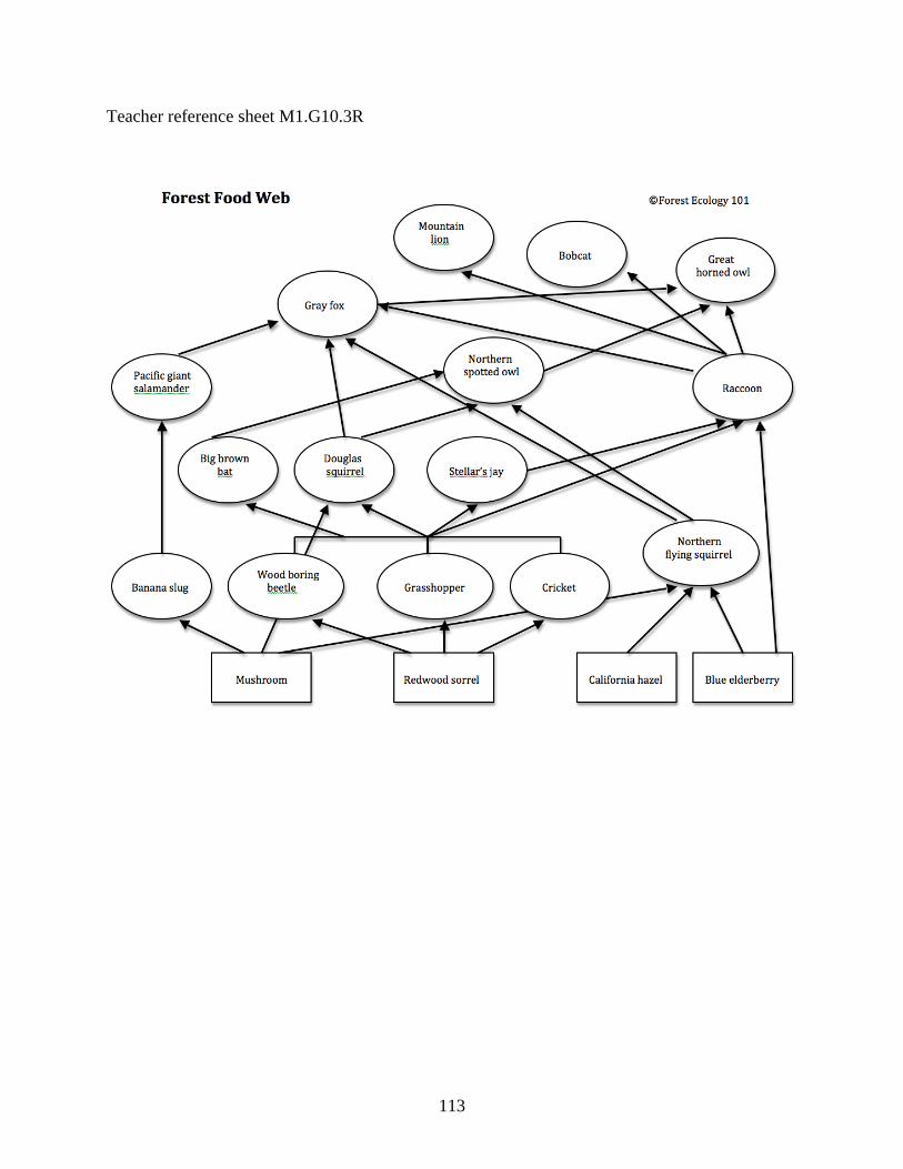
Teacher reference sheet M1.G10.3R

113

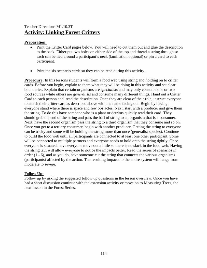
Teacher Directions M1.10.3T Activity: Linking Forest Critters Preparation:

• Print the Critter Card pages below. You will need to cut them out and glue the description to the back. Either put two holes on either side of the top and thread a string through so each can be tied around a participant’s neck (lamination optional) or pin a card to each participant.

• Print the six scenario cards so they can be read during this activity.

Procedure: In this lessons students will form a food web using string and holding on to critter cards. Before you begin, explain to them what they will be doing in this activity and set clear boundaries. Explain that certain organisms are specialists and may only consume one or two food sources while others are generalists and consume many different things. Hand out a Critter Card to each person and read the description. Once they are clear of their role, instruct everyone to attach their critter card as described above with the name facing out. Begin by having everyone stand where there is space and few obstacles. Next, start with a producer and give them the string. To do this have someone who is a plant or detritus quickly read their card. They should grab the end of the string and pass the ball of string to an organism that is a consumer. Next, have the second organism pass the string to a third organism that they consume and so on. Once you get to a tertiary consumer, begin with another producer. Getting the string to everyone can be tricky and some will be holding the string more than once (generalist species). Continue to build the food web until all participants are connected to at least one other participant. Some will be connected to multiple partners and everyone needs to hold onto the string tightly. Once everyone is situated, have everyone move out a little so there is no slack in the food web. Having the string taut will allow everyone to notice the impacts better. Read the series of scenarios in order (1 - 6), and as you do, have someone cut the string that connects the various organisms (participants) affected by the action. The resulting impacts to the entire system will range from moderate to severe. Follow Up: Follow up by asking the suggested follow up questions in the lesson overview. Once you have had a short discussion continue with the extension activity or move on to Measuring Trees, the next lesson in the Forest Series.

114

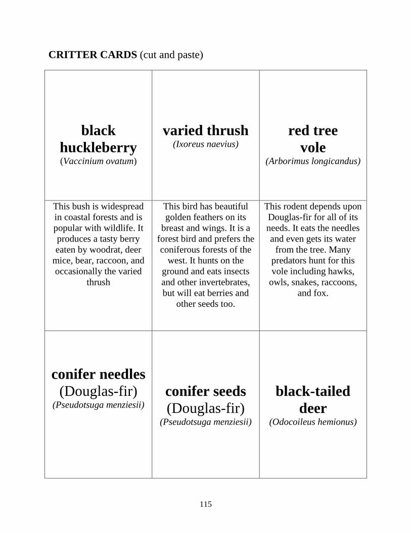
CRITTER CARDS (cut and paste)

black huckleberry (Vaccinium ovatum)

varied thrush (Ixoreus naevius)

red tree vole

(Arborimus longicandus)

This bush is widespread in coastal forests and is popular with wildlife. It produces a tasty berry eaten by woodrat, deer

mice, bear, raccoon, and occasionally the varied

thrush

This bird has beautiful golden feathers on its

breast and wings. It is a forest bird and prefers the coniferous forests of the

west. It hunts on the ground and eats insects and other invertebrates, but will eat berries and

other seeds too.

This rodent depends upon Douglas-fir for all of its needs. It eats the needles and even gets its water

from the tree. Many predators hunt for this vole including hawks,

owls, snakes, raccoons, and fox.

conifer needles (Douglas-fir)

(Pseudotsuga menziesii)

conifer seeds (Douglas-fir)

(Pseudotsuga menziesii)

black-tailed deer

(Odocoileus hemionus)

115

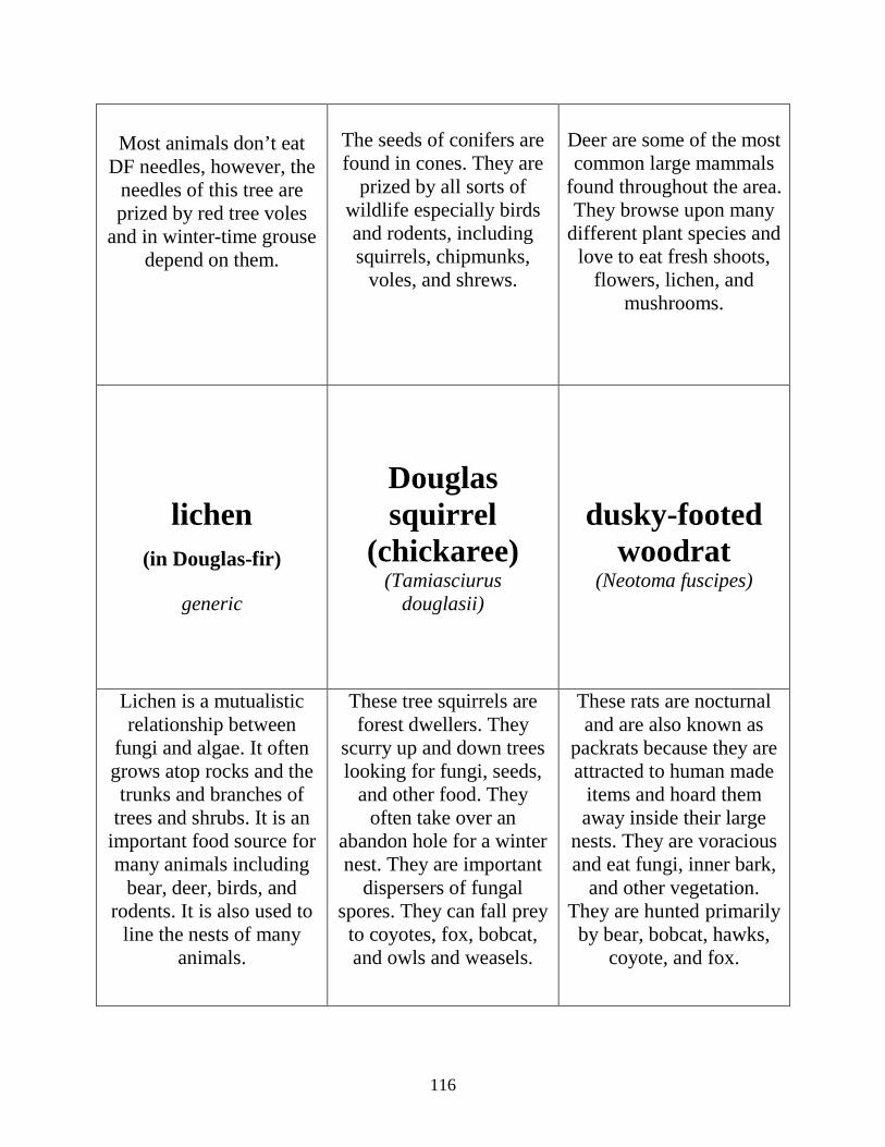
Most animals don’t eat

DF needles, however, the needles of this tree are prized by red tree voles

and in winter-time grouse depend on them.

The seeds of conifers are found in cones. They are

prized by all sorts of wildlife especially birds and rodents, including squirrels, chipmunks,

voles, and shrews.

Deer are some of the most common large mammals

found throughout the area. They browse upon many

different plant species and love to eat fresh shoots,

flowers, lichen, and mushrooms.

lichen (in Douglas-fir)

generic

Douglas squirrel

(chickaree) (Tamiasciurus

douglasii)

dusky-footed woodrat

(Neotoma fuscipes)

Lichen is a mutualistic relationship between

fungi and algae. It often grows atop rocks and the trunks and branches of

trees and shrubs. It is an important food source for many animals including

bear, deer, birds, and rodents. It is also used to

line the nests of many animals.

These tree squirrels are forest dwellers. They

scurry up and down trees looking for fungi, seeds,

and other food. They often take over an

abandon hole for a winter nest. They are important

dispersers of fungal spores. They can fall prey

to coyotes, fox, bobcat, and owls and weasels.

These rats are nocturnal and are also known as

packrats because they are attracted to human made

items and hoard them away inside their large

nests. They are voracious and eat fungi, inner bark,

and other vegetation. They are hunted primarily

by bear, bobcat, hawks, coyote, and fox.

116

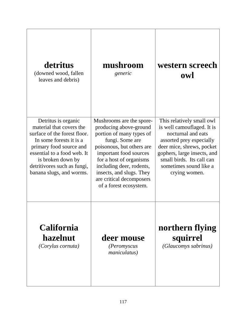
detritus (downed wood, fallen

leaves and debris)

mushroom generic

western screech owl

Detritus is organic material that covers the

surface of the forest floor. In some forests it is a

primary food source and essential to a food web. It

is broken down by detritivores such as fungi, banana slugs, and worms.

Mushrooms are the spore-producing above-ground portion of many types of

fungi. Some are poisonous, but others are important food sources for a host of organisms including deer, rodents, insects, and slugs. They are critical decomposers

of a forest ecosystem.

This relatively small owl is well camouflaged. It is

nocturnal and eats assorted prey especially

deer mice, shrews, pocket gophers, large insects, and

small birds. Its call can sometimes sound like a

crying women.

California hazelnut

(Corylus cornuta)

deer mouse (Peromyscus maniculatus)

northern flying squirrel

(Glaucomys sabrinus)

117

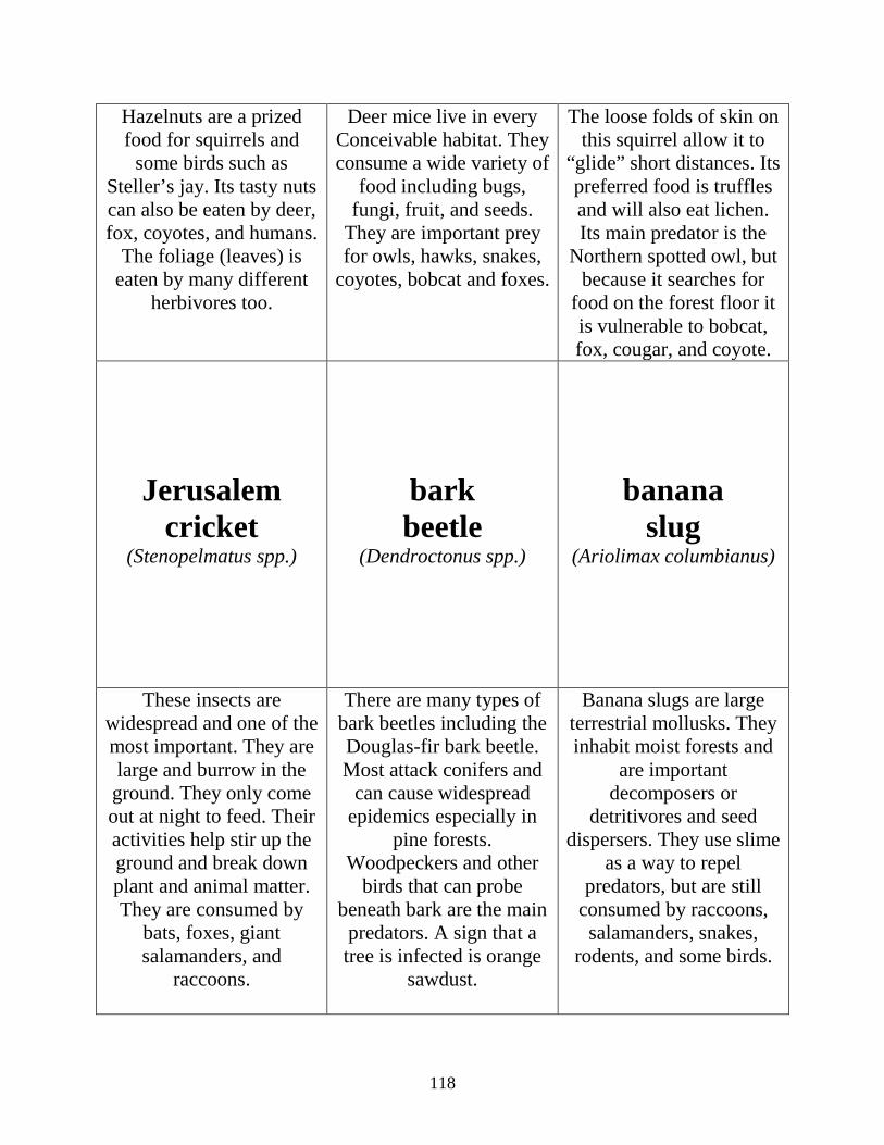
Hazelnuts are a prized food for squirrels and

some birds such as Steller’s jay. Its tasty nuts can also be eaten by deer, fox, coyotes, and humans.

The foliage (leaves) is eaten by many different

herbivores too.

Deer mice live in every Conceivable habitat. They consume a wide variety of

food including bugs, fungi, fruit, and seeds.

They are important prey for owls, hawks, snakes,

coyotes, bobcat and foxes.

The loose folds of skin on this squirrel allow it to

“glide” short distances. Its preferred food is truffles and will also eat lichen. Its main predator is the

Northern spotted owl, but because it searches for

food on the forest floor it is vulnerable to bobcat, fox, cougar, and coyote.

Jerusalem cricket

(Stenopelmatus spp.)

bark beetle

(Dendroctonus spp.)

banana slug

(Ariolimax columbianus)

These insects are widespread and one of the most important. They are large and burrow in the ground. They only come out at night to feed. Their activities help stir up the ground and break down plant and animal matter. They are consumed by

bats, foxes, giant salamanders, and

raccoons.

There are many types of bark beetles including the Douglas-fir bark beetle. Most attack conifers and

can cause widespread epidemics especially in

pine forests. Woodpeckers and other

birds that can probe beneath bark are the main

predators. A sign that a tree is infected is orange

sawdust.

Banana slugs are large terrestrial mollusks. They inhabit moist forests and

are important decomposers or

detritivores and seed dispersers. They use slime

as a way to repel predators, but are still

consumed by raccoons, salamanders, snakes,

rodents, and some birds.

118

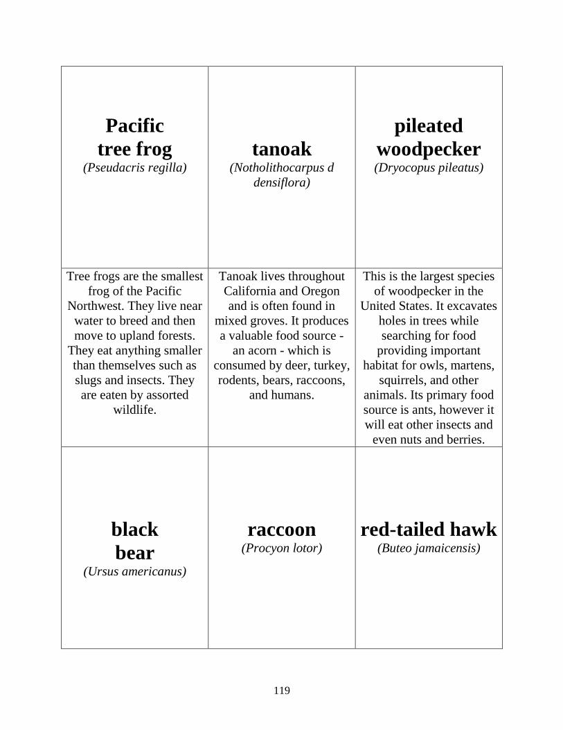
Pacific tree frog

(Pseudacris regilla)

tanoak (Notholithocarpus d

densiflora)

pileated woodpecker (Dryocopus pileatus)

Tree frogs are the smallest frog of the Pacific

Northwest. They live near water to breed and then move to upland forests.

They eat anything smaller than themselves such as slugs and insects. They are eaten by assorted

wildlife.

Tanoak lives throughout California and Oregon and is often found in

mixed groves. It produces a valuable food source -

an acorn - which is consumed by deer, turkey, rodents, bears, raccoons,

and humans.

This is the largest species of woodpecker in the

United States. It excavates holes in trees while searching for food

providing important habitat for owls, martens,

squirrels, and other animals. Its primary food source is ants, however it will eat other insects and

even nuts and berries.

black bear

(Ursus americanus)

raccoon (Procyon lotor)

red-tailed hawk (Buteo jamaicensis)

119

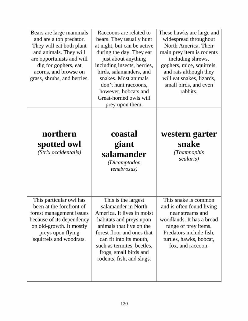
Bears are large mammals and are a top predator.

They will eat both plant and animals. They will

are opportunists and will dig for gophers, eat

acorns, and browse on grass, shrubs, and berries.

Raccoons are related to bears. They usually hunt at night, but can be active during the day. They eat

just about anything including insects, berries, birds, salamanders, and snakes. Most animals don’t hunt raccoons, however, bobcats and

Great-horned owls will prey upon them.

These hawks are large and widespread throughout North America. Their

main prey item is rodents including shrews,

gophers, mice, squirrels, and rats although they will eat snakes, lizards, small birds, and even

rabbits.

northern spotted owl (Strix occidentalis)

coastal giant

salamander (Dicamptodon

tenebrosus)

western garter snake

(Thamnophis scalaris)

This particular owl has been at the forefront of

forest management issues because of its dependency on old-growth. It mostly

preys upon flying squirrels and woodrats.

This is the largest salamander in North

America. It lives in moist habitats and preys upon animals that live on the

forest floor and ones that can fit into its mouth,

such as termites, beetles, frogs, small birds and

rodents, fish, and slugs.

This snake is common and is often found living

near streams and woodlands. It has a broad

range of prey items. Predators include fish, turtles, hawks, bobcat,

fox, and raccoon.

120

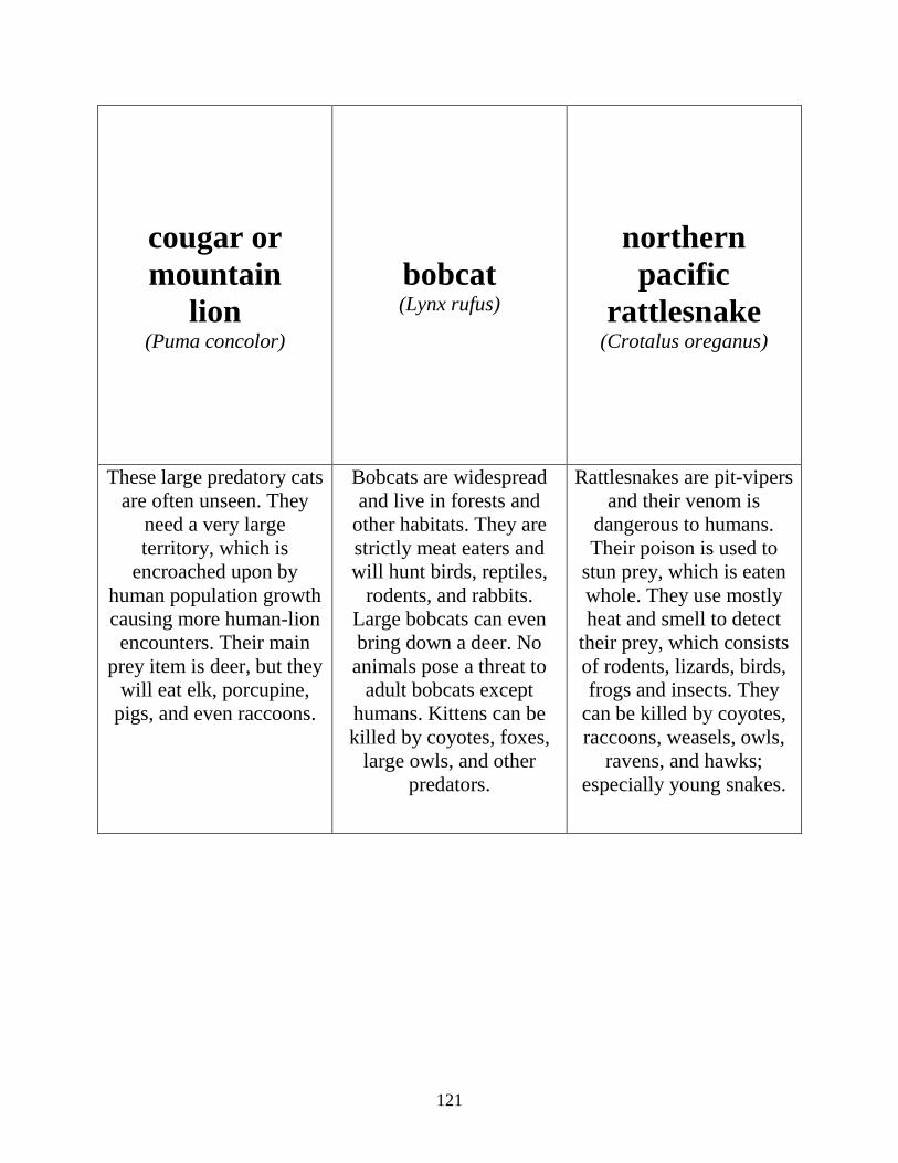
cougar or mountain

lion (Puma concolor)

bobcat (Lynx rufus)

northern pacific

rattlesnake (Crotalus oreganus)

These large predatory cats are often unseen. They

need a very large territory, which is

encroached upon by human population growth causing more human-lion encounters. Their main

prey item is deer, but they will eat elk, porcupine,

pigs, and even raccoons.

Bobcats are widespread and live in forests and

other habitats. They are strictly meat eaters and will hunt birds, reptiles,

rodents, and rabbits. Large bobcats can even bring down a deer. No animals pose a threat to

adult bobcats except humans. Kittens can be killed by coyotes, foxes,

large owls, and other predators.

Rattlesnakes are pit-vipers and their venom is

dangerous to humans. Their poison is used to

stun prey, which is eaten whole. They use mostly heat and smell to detect

their prey, which consists of rodents, lizards, birds, frogs and insects. They

can be killed by coyotes, raccoons, weasels, owls,

ravens, and hawks; especially young snakes.

121

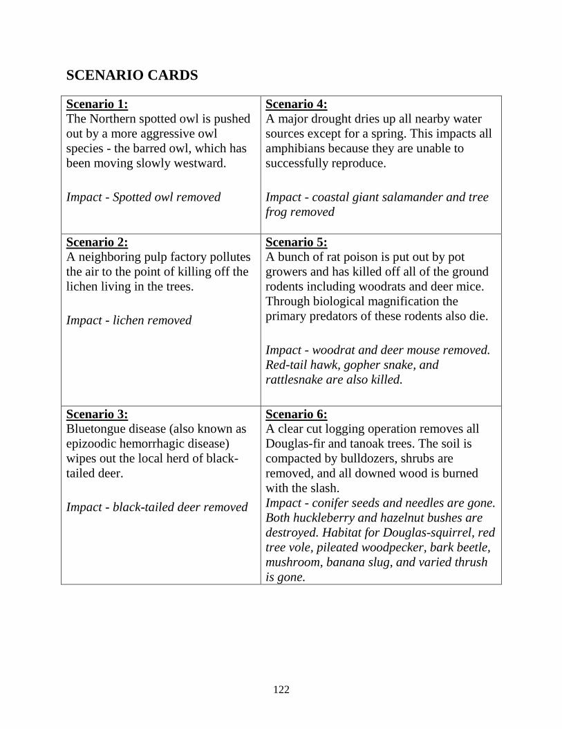
SCENARIO CARDS Scenario 1: The Northern spotted owl is pushed out by a more aggressive owl species - the barred owl, which has been moving slowly westward. Impact - Spotted owl removed

Scenario 4: A major drought dries up all nearby water sources except for a spring. This impacts all amphibians because they are unable to successfully reproduce. Impact - coastal giant salamander and tree frog removed

Scenario 2: A neighboring pulp factory pollutes the air to the point of killing off the lichen living in the trees. Impact - lichen removed

Scenario 5: A bunch of rat poison is put out by pot growers and has killed off all of the ground rodents including woodrats and deer mice. Through biological magnification the primary predators of these rodents also die. Impact - woodrat and deer mouse removed. Red-tail hawk, gopher snake, and rattlesnake are also killed.

Scenario 3: Bluetongue disease (also known as epizoodic hemorrhagic disease) wipes out the local herd of black-tailed deer. Impact - black-tailed deer removed

Scenario 6: A clear cut logging operation removes all Douglas-fir and tanoak trees. The soil is compacted by bulldozers, shrubs are removed, and all downed wood is burned with the slash. Impact - conifer seeds and needles are gone. Both huckleberry and hazelnut bushes are destroyed. Habitat for Douglas-squirrel, red tree vole, pileated woodpecker, bark beetle, mushroom, banana slug, and varied thrush is gone.

122

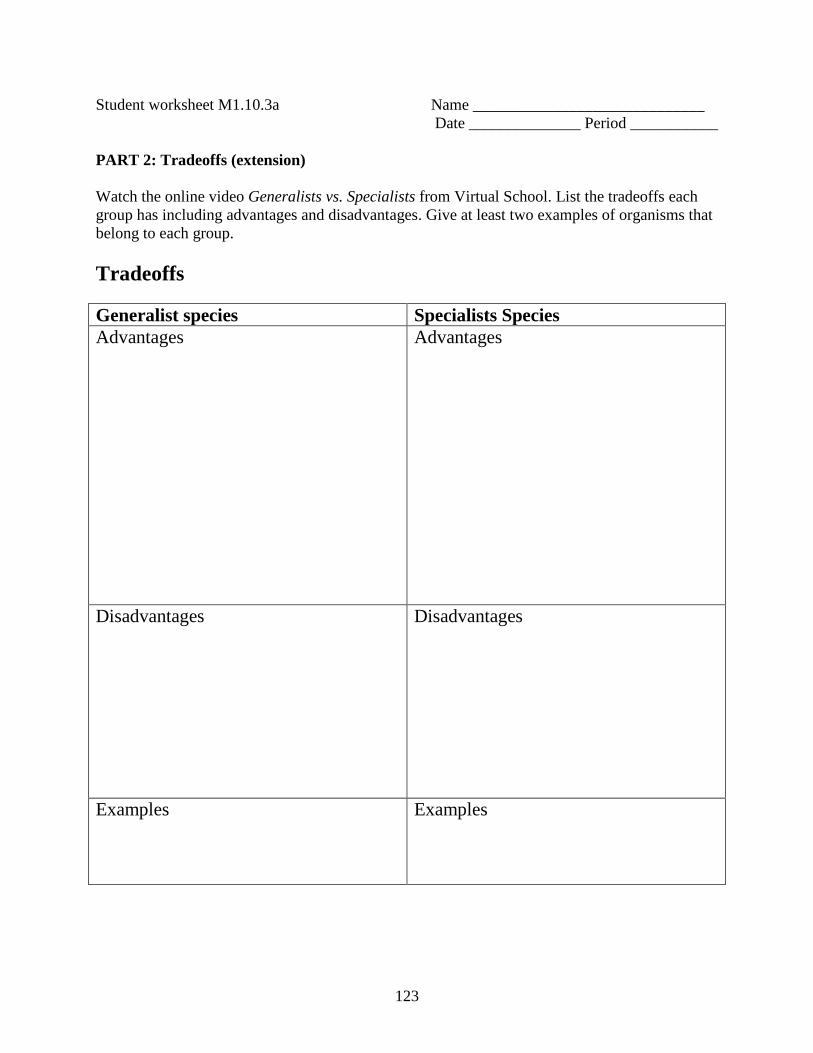
Student worksheet M1.10.3a Name _____________________________ Date ______________ Period ___________

PART 2: Tradeoffs (extension) Watch the online video Generalists vs. Specialists from Virtual School. List the tradeoffs each group has including advantages and disadvantages. Give at least two examples of organisms that belong to each group. Tradeoffs Generalist species Specialists Species Advantages

Advantages

Disadvantages

Disadvantages

Examples

Examples

123

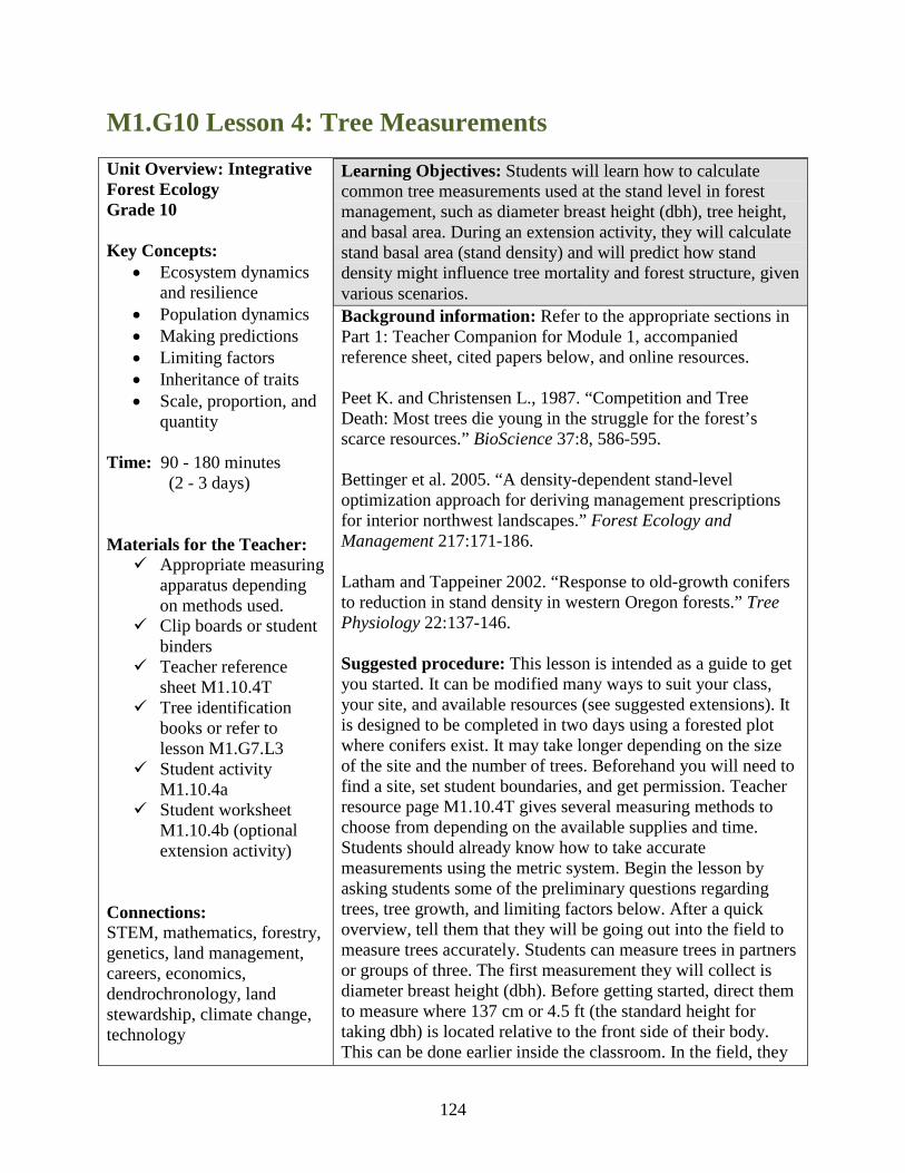
M1.G10 Lesson 4: Tree Measurements Unit Overview: Integrative Forest Ecology Grade 10 Key Concepts:

• Ecosystem dynamics and resilience

• Population dynamics • Making predictions • Limiting factors • Inheritance of traits • Scale, proportion, and

quantity Time: 90 - 180 minutes (2 - 3 days) Materials for the Teacher: Appropriate measuring

apparatus depending on methods used.

Clip boards or student binders

Teacher reference sheet M1.10.4T

Tree identification books or refer to lesson M1.G7.L3

Student activity M1.10.4a

Student worksheet M1.10.4b (optional extension activity)

Connections: STEM, mathematics, forestry, genetics, land management, careers, economics, dendrochronology, land stewardship, climate change, technology

Learning Objectives: Students will learn how to calculate common tree measurements used at the stand level in forest management, such as diameter breast height (dbh), tree height, and basal area. During an extension activity, they will calculate stand basal area (stand density) and will predict how stand density might influence tree mortality and forest structure, given various scenarios. Background information: Refer to the appropriate sections in Part 1: Teacher Companion for Module 1, accompanied reference sheet, cited papers below, and online resources. Peet K. and Christensen L., 1987. “Competition and Tree Death: Most trees die young in the struggle for the forest’s scarce resources.” BioScience 37:8, 586-595. Bettinger et al. 2005. “A density-dependent stand-level optimization approach for deriving management prescriptions for interior northwest landscapes.” Forest Ecology and Management 217:171-186. Latham and Tappeiner 2002. “Response to old-growth conifers to reduction in stand density in western Oregon forests.” Tree Physiology 22:137-146. Suggested procedure: This lesson is intended as a guide to get you started. It can be modified many ways to suit your class, your site, and available resources (see suggested extensions). It is designed to be completed in two days using a forested plot where conifers exist. It may take longer depending on the size of the site and the number of trees. Beforehand you will need to find a site, set student boundaries, and get permission. Teacher resource page M1.10.4T gives several measuring methods to choose from depending on the available supplies and time. Students should already know how to take accurate measurements using the metric system. Begin the lesson by asking students some of the preliminary questions regarding trees, tree growth, and limiting factors below. After a quick overview, tell them that they will be going out into the field to measure trees accurately. Students can measure trees in partners or groups of three. The first measurement they will collect is diameter breast height (dbh). Before getting started, direct them to measure where 137 cm or 4.5 ft (the standard height for taking dbh) is located relative to the front side of their body. This can be done earlier inside the classroom. In the field, they

124

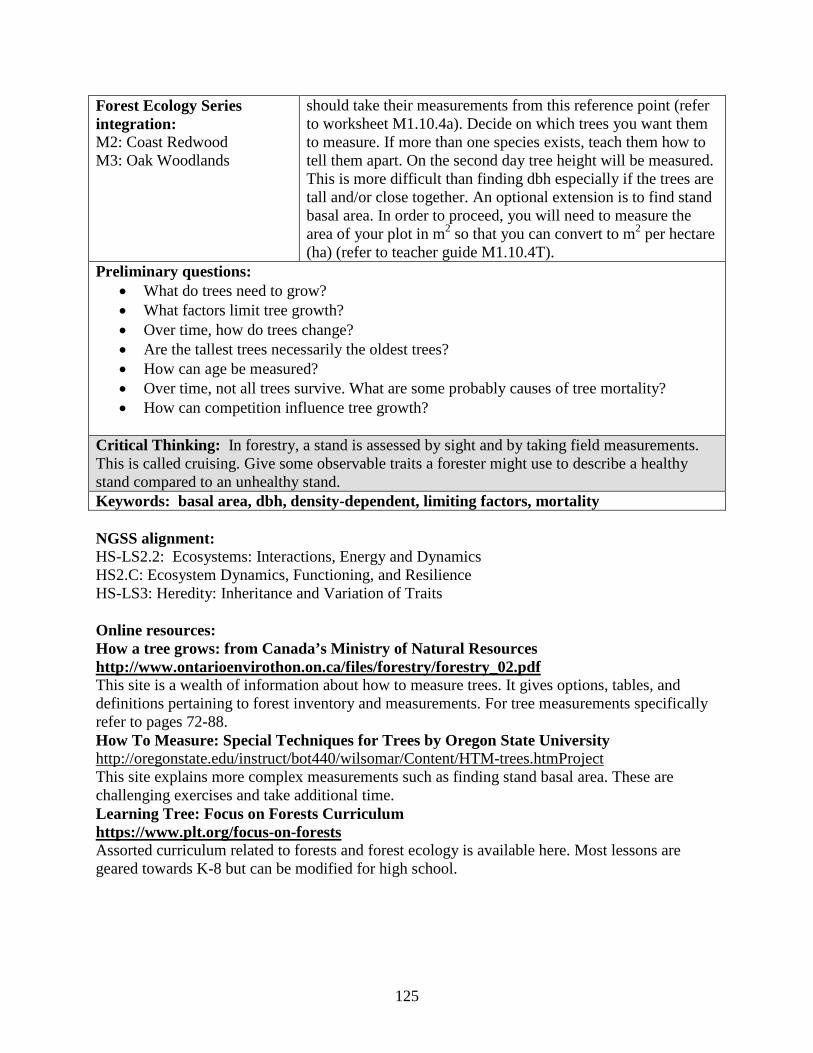
Forest Ecology Series integration: M2: Coast Redwood M3: Oak Woodlands

should take their measurements from this reference point (refer to worksheet M1.10.4a). Decide on which trees you want them to measure. If more than one species exists, teach them how to tell them apart. On the second day tree height will be measured. This is more difficult than finding dbh especially if the trees are tall and/or close together. An optional extension is to find stand basal area. In order to proceed, you will need to measure the area of your plot in m2 so that you can convert to m2 per hectare (ha) (refer to teacher guide M1.10.4T).

Preliminary questions: • What do trees need to grow? • What factors limit tree growth? • Over time, how do trees change? • Are the tallest trees necessarily the oldest trees? • How can age be measured? • Over time, not all trees survive. What are some probably causes of tree mortality? • How can competition influence tree growth?

Critical Thinking: In forestry, a stand is assessed by sight and by taking field measurements. This is called cruising. Give some observable traits a forester might use to describe a healthy stand compared to an unhealthy stand. Keywords: basal area, dbh, density-dependent, limiting factors, mortality NGSS alignment: HS-LS2.2: Ecosystems: Interactions, Energy and Dynamics HS2.C: Ecosystem Dynamics, Functioning, and Resilience HS-LS3: Heredity: Inheritance and Variation of Traits Online resources: How a tree grows: from Canada’s Ministry of Natural Resources http://www.ontarioenvirothon.on.ca/files/forestry/forestry_02.pdf This site is a wealth of information about how to measure trees. It gives options, tables, and definitions pertaining to forest inventory and measurements. For tree measurements specifically refer to pages 72-88. How To Measure: Special Techniques for Trees by Oregon State University http://oregonstate.edu/instruct/bot440/wilsomar/Content/HTM-trees.htmProject This site explains more complex measurements such as finding stand basal area. These are challenging exercises and take additional time. Learning Tree: Focus on Forests Curriculum https://www.plt.org/focus-on-forests Assorted curriculum related to forests and forest ecology is available here. Most lessons are geared towards K-8 but can be modified for high school.

125

(online resources continued) Oregon Forest Book: Ecology, Economics and Society http://oregonforests.org/sites/default/files/publications/pdf/Or_Forest_Book_K12.pdf This pamphlet is full of graphics and information regarding forests. It comes from Oregon and tends to promote the use of wood, however the information is clearly written and incorporates nice graphics. It can be used as a good summary and is appropriate for high school. Answers to preliminary questions: - What do trees need to grow? (water, light, and nutrients) - What factors limit tree growth? (water, light, space, and nutrients) - Over time, how do trees change? (as trees mature they get taller, wider, thicker bark, gain branches, and get more complex crown structure such as dead tops and broken branches) - Are the tallest trees necessarily the oldest trees? (answers will vary. It depends. The tallest trees are not necessarily the oldest. Some trees can grow fast and gain height quickly and are not that old. Others such as oak trees, never get very tall but they can live hundreds of years. -How can age be measured? (Trees are aged using increment borers or counting the rings of a cut tree or stump). - Over time, not all trees survive. What are some probably causes of tree mortality? (direct and indirect consequences will determine longevity such as genetics, disease, herbivory, and competition for resources) - How can competition influence tree growth? (trees compete mostly for light and water in dry regions. Usually survival rates are high with low competition and low with high competition). Suggested extensions:

• Have students estimate sizes of objects at school, including height of buildings, volume of water, and sizes of populations.

• Using some of the tree measurement results to find equivalents using every day objects such as lengths of hallways and tables and heights of people.

• Calculate board feet of certain trees using a volume table. • Design an experiment that compares competition and plant growth. • Relate limiting factors such as food and space to populations of animals. • Study relationships among species such as mutualism, predation, and parasitism.

M1.10.4R Teacher guide M1.10.L4a Student worksheet (activity) M1.10.L4b Student worksheet (optional extension)

126

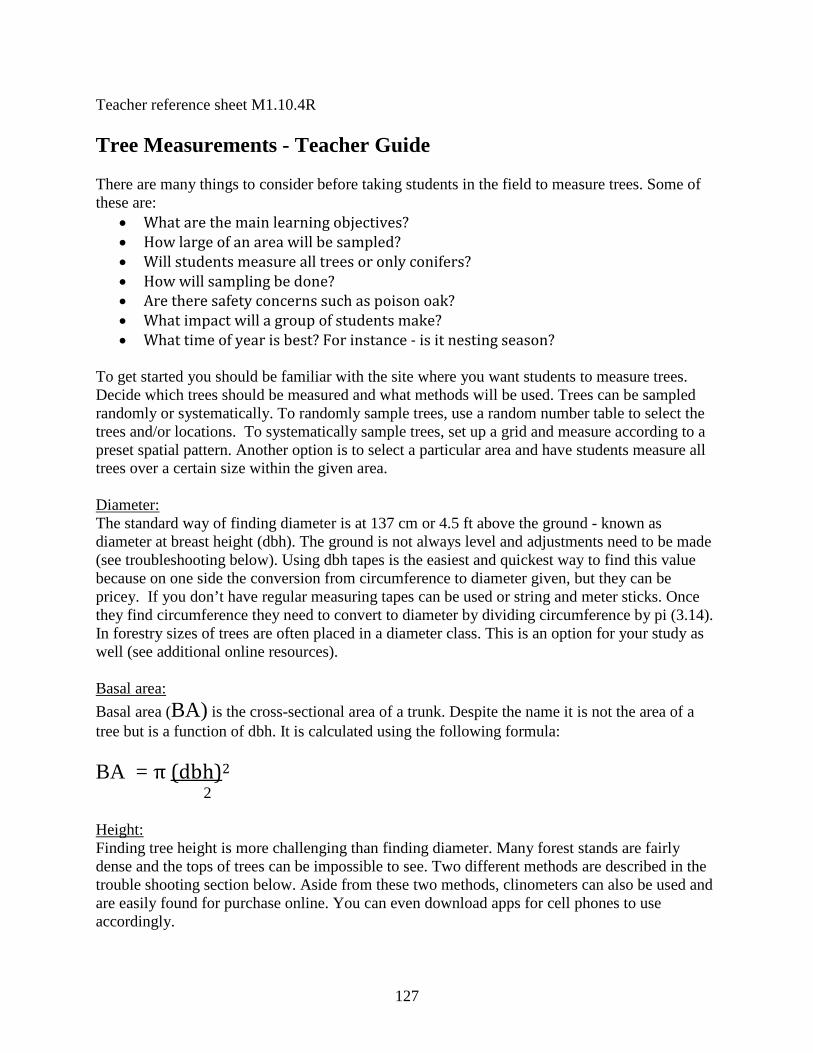
Teacher reference sheet M1.10.4R Tree Measurements - Teacher Guide There are many things to consider before taking students in the field to measure trees. Some of these are:

• What are the main learning objectives? • How large of an area will be sampled? • Will students measure all trees or only conifers? • How will sampling be done? • Are there safety concerns such as poison oak? • What impact will a group of students make? • What time of year is best? For instance - is it nesting season?

To get started you should be familiar with the site where you want students to measure trees. Decide which trees should be measured and what methods will be used. Trees can be sampled randomly or systematically. To randomly sample trees, use a random number table to select the trees and/or locations. To systematically sample trees, set up a grid and measure according to a preset spatial pattern. Another option is to select a particular area and have students measure all trees over a certain size within the given area. Diameter: The standard way of finding diameter is at 137 cm or 4.5 ft above the ground - known as diameter at breast height (dbh). The ground is not always level and adjustments need to be made (see troubleshooting below). Using dbh tapes is the easiest and quickest way to find this value because on one side the conversion from circumference to diameter given, but they can be pricey. If you don’t have regular measuring tapes can be used or string and meter sticks. Once they find circumference they need to convert to diameter by dividing circumference by pi (3.14). In forestry sizes of trees are often placed in a diameter class. This is an option for your study as well (see additional online resources). Basal area: Basal area (BA) is the cross-sectional area of a trunk. Despite the name it is not the area of a tree but is a function of dbh. It is calculated using the following formula: BA = π (dbh)2 2 Height: Finding tree height is more challenging than finding diameter. Many forest stands are fairly dense and the tops of trees can be impossible to see. Two different methods are described in the trouble shooting section below. Aside from these two methods, clinometers can also be used and are easily found for purchase online. You can even download apps for cell phones to use accordingly.

127

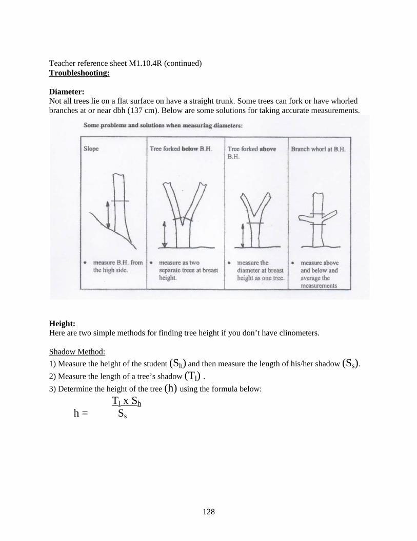
Teacher reference sheet M1.10.4R (continued) Troubleshooting: Diameter: Not all trees lie on a flat surface on have a straight trunk. Some trees can fork or have whorled branches at or near dbh (137 cm). Below are some solutions for taking accurate measurements.

Height: Here are two simple methods for finding tree height if you don’t have clinometers. Shadow Method: 1) Measure the height of the student (Sh) and then measure the length of his/her shadow (Ss). 2) Measure the length of a tree’s shadow (Tl) . 3) Determine the height of the tree (h) using the formula below: Tl x Sh h = Ss

128

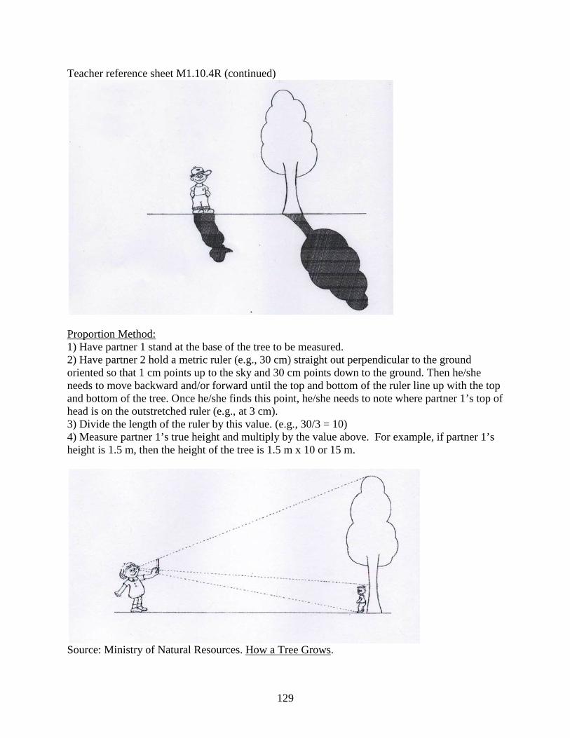
Teacher reference sheet M1.10.4R (continued)

Proportion Method: 1) Have partner 1 stand at the base of the tree to be measured. 2) Have partner 2 hold a metric ruler (e.g., 30 cm) straight out perpendicular to the ground oriented so that 1 cm points up to the sky and 30 cm points down to the ground. Then he/she needs to move backward and/or forward until the top and bottom of the ruler line up with the top and bottom of the tree. Once he/she finds this point, he/she needs to note where partner 1’s top of head is on the outstretched ruler (e.g., at 3 cm). 3) Divide the length of the ruler by this value. (e.g., 30/3 = 10) 4) Measure partner 1’s true height and multiply by the value above. For example, if partner 1’s height is 1.5 m, then the height of the tree is 1.5 m x 10 or 15 m.

Source: Ministry of Natural Resources. How a Tree Grows.

129

Teacher reference sheet M1.10.4R (continued) Part 2: Stand basal area (extension activity): The area that the trunks of trees occupy in a given stand is also referred to as stand density or stand basal area (SBA). You will need to know the entire area students work in square meters (m2) (A). To find (SBA) add up the initial values for basal area (BAi )and divide by the total area A. To use a common value convert to meters squared per hectare (SBA2). The ∑ symbol means to sum. See the following formulas: SBA1 = ∑ BAi SBA2 = SBA1 A ha Below is an example showing how to make proper calculations:

Source: Oregon State For more information on tree measurements refer to: http://oregonstate.edu/instruct/bot440/wilsomar/Content/HTM-trees.htm

130

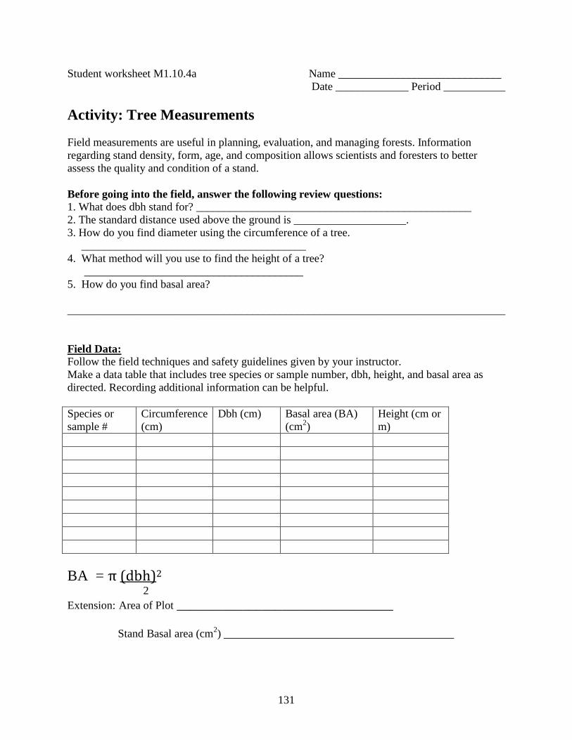
Student worksheet M1.10.4a Name _____________________________ Date _____________ Period ___________

Activity: Tree Measurements Field measurements are useful in planning, evaluation, and managing forests. Information regarding stand density, form, age, and composition allows scientists and foresters to better assess the quality and condition of a stand. Before going into the field, answer the following review questions: 1. What does dbh stand for? _________________________________________________ 2. The standard distance used above the ground is ____________________. 3. How do you find diameter using the circumference of a tree. ________________________________________ 4. What method will you use to find the height of a tree? _______________________________________ 5. How do you find basal area? ______________________________________________________________________________ Field Data: Follow the field techniques and safety guidelines given by your instructor. Make a data table that includes tree species or sample number, dbh, height, and basal area as directed. Recording additional information can be helpful. Species or sample #

Circumference (cm)

Dbh (cm) Basal area (BA) (cm2)

Height (cm or m)

BA = π (dbh)2 2 Extension: Area of Plot _________________________________ Stand Basal area (cm2) _________________________________________

131

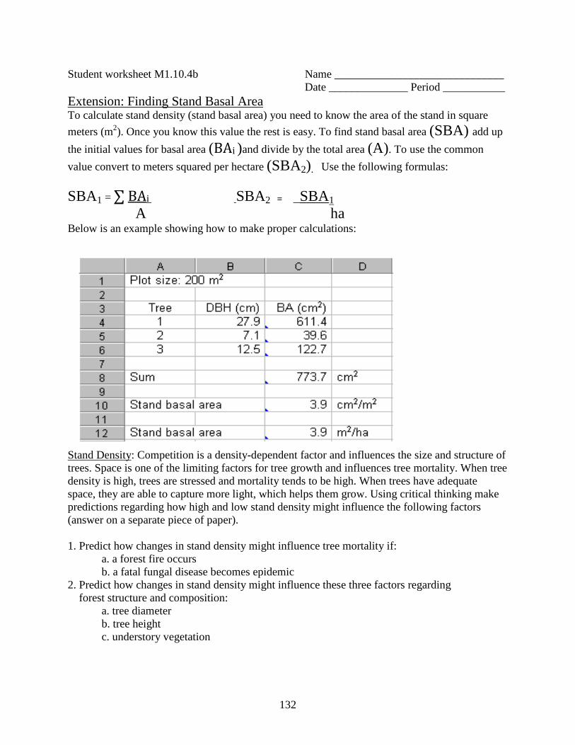
Student worksheet M1.10.4b Name ______________________________ Date ______________ Period ___________ Extension: Finding Stand Basal Area To calculate stand density (stand basal area) you need to know the area of the stand in square meters (m2). Once you know this value the rest is easy. To find stand basal area (SBA) add up the initial values for basal area (BAi )and divide by the total area (A). To use the common value convert to meters squared per hectare (SBA2). Use the following formulas: SBA1 = ∑ BAi SBA2 = SBA1 A ha Below is an example showing how to make proper calculations:

Stand Density: Competition is a density-dependent factor and influences the size and structure of trees. Space is one of the limiting factors for tree growth and influences tree mortality. When tree density is high, trees are stressed and mortality tends to be high. When trees have adequate space, they are able to capture more light, which helps them grow. Using critical thinking make predictions regarding how high and low stand density might influence the following factors (answer on a separate piece of paper). 1. Predict how changes in stand density might influence tree mortality if: a. a forest fire occurs b. a fatal fungal disease becomes epidemic 2. Predict how changes in stand density might influence these three factors regarding forest structure and composition: a. tree diameter b. tree height c. understory vegetation

132

M1.G10 Lesson 5: Biodiversity: Measuring Up Unit Overview: Integrative Forest Ecology Grade 10 Key Concepts:

• Analyzing and interpreting data

• Ecosystem dynamics and resilience

• Stability and change • Use mathematical

representation to support factors affecting biodiversity

• Ecosystem interrelationships

• Biodiversity and humans

Time: 90 - 120 minutes Materials for the Teacher: Assorted beads and

containers (refer to Teacher instructions M1.10.5T)

Teacher instructions M1.10.5T

Student laboratory M1.10.5a

Student worksheet M1.10.5b (optional)

Connections: STEM, mathematics, statistics, botany, succession, genetics, ecosystem resilience, forestry, land management, social studies, technology, engineering Forest Ecology Series integration: M2: Coast Redwood

Learning Objective: Students will calculate biodiversity indices collected in a laboratory exercise intended to predict plant biodiversity in different habitats. They will be able to explain why multiple sampling is necessary to accurately quantify biodiversity. As an extension they will interpret a figure showing adequate sampling using species-area accumulation curves created from data collected in three different stages of recovery following logging in coast redwood forests across Humboldt County. Background information: Refer to the appropriate sections in Part 1: Teacher Companion for Module 1, teacher instructions M1.10.5T, and online resources. Suggested procedure: This lab requires about an hour of prep time. Begin this lesson by having students come up with a definition of biodiversity with a partner (species biodiversity). Have students share their definitions. Choose some of the best examples and write them on the board. Briefly explain the different types of biodiversity and tell them the one most generally used is species biodiversity. This type of diversity commonly measures species richness and abundance. Define both species richness and evenness and give them an example of both. Refer to teacher instructions M1.10.5T. The most commonly used index by ecologists for measuring diversity is the Shannon Index. It applies the natural logarithm of species abundance. The one used in this activity has been simplified. At this point it is optional to give a short lecture on biodiversity and have students take notes. Both of these introductory elements can be done the day before. Once you are ready, organize students into groups so all seven habitats are sampled. Go over the most important steps before they begin and assist where necessary. It is important they sample randomly and don’t look at the colored beads to avoid bias. Once they are finished sampling, they should calculate the biodiversity indices and answer the questions on worksheet M1.10.5a. When they are done take time to ask follow up questions. In a suggested extension, students will look at a figure from a study that compares vascular plant richness across four different forest stages (initiation, closure, mature, and old-growth) in coast redwood forest. This figure shows species-area accumulation curves useful in determine sampling effectiveness (refer to worksheet M1.10.5b).

133

Critical Thinking: Explain the challenges an ecologist might face if she is attempting to quantify or predict the biodiversity of a region. Keywords: abundance, biodiversity, evenness, flora, richness, quantitative, sample, species-area curve NGSS alignment: HS-LS2.2: Ecosystems: Interactions, Energy and Dynamics HS2.C: Ecosystem Dynamics, Functioning, and Resilience HS4.D: Biodiversity and Humans Online resources: Schoolyard Biodiversity: Investigation Educator Guide (Washington Biodiversity Council) http://www.fishwildlife.org/files/ConEd-Schoolyard-Biodiversity-Guide.pdf Here there are many good activities applicable to a school site including how to sample local biodiversity along a transect line and how to conduct a simple vegetation survey (see extensions below). EELINK - from NAAEE http://eelink.net/pages/EE+Activities+-+Endangered+Species If you are not familiar with the North American Association for Environmental Education then glancing at this page on their website could be valuable. This association is up-to-date on the latest environmental science education. This particular link gives assorted activities relating to endangered species and saving biodiversity. Saving Species - 35 top biodiversity films http://savingspecies.org/2011/top-35-biodiversity-videos/ Here you will find top selections of the best videos for different concepts relating to biodiversity (see extensions below). Links to videos go straight to You Tube and are free. Most videos range from 2 minutes to one hour long. Invaders of the Forest: Invasive Species (Wisconsin) http://dnr.wi.gov/org/caer/ce/eek/teacher/invasivesguide/Invaders%20of%20the%20Forest.pdf This is an educator’s guide to the invasive plants of Wisconsin, however, it includes many innovative and hands-on activities appropriate for high school relating to ecosystems, which can be modified for your local area. EEI Connections: B.8.a Differential Survival of Organisms B.8.b Biological Diversity: The World’s Riches B.8.d The Isolation of Species

134

M1.G10.L5 (Unit Overview continued) Suggested follow-up questions:

• How did the results compare between groups? (have student record results as they complete their calculations).

• What are some reasons why variation exists between groups? • Were you surprised by any of the results? If so which ones? Why? • How could the sampling techniques used be improved? • Why does quantifying biodiversity prove to be difficult? •

Suggested extensions:

• Sample the biodiversity of a nearby natural area along a transect line. • Find the species biodiversity of your school site. • Collect pond water and have students identify as many species as they can. • Conduct a macroinvertebrate survey of a local waterway to assess the health of the

particular habitat. • Assign an endangered species report focusing on a particular region or biome. • Have students find and summarize an article regarding the biodiversity of a local park or

protected area. • Have students learn about the endangered species act and why it is important to

preserving biodiversity. • Make a wanted poster of an invasive plant or animal that is negatively impacting local

floral and fauna. M1.10.5T Teacher instructions M1.10.5a Student laboratory exercise M1.10.5b Student worksheet (optional)

135

Teacher instruction sheet M1.10.5T Biodiversity - Measuring Up lab Overview: The difference in the biodiversity between communities can differ widely and quantifying it is complex. Exhaustive measuring is impractical and expensive, and therefore sampling is used. Statistical analysis is necessary to determine how much sampling is enough to adequately predict. The most common measure of biodiversity is species diversity, which incorporates two factors: species richness and species evenness (see definitions below). Quantifying richness exclusively is limiting and by including evenness one can better gauge the overall health of an ecosystem (refer to fig. 1 below). For instance there could be thirty species found in an area, however, if 70% of the coverage is occupied by only one species, then the overall biodiversity is relatively low. This activity gives several options for quantifying biodiversity depending on the amount of time available and the skill level of your students. Part 1 is a lab exercise that attempts to simulate a hypothetical situation where students from Humboldt High attempt to measure plant diversity in different habitats located near their site. Instead of sampling once, they want to avoid pseudoreplication (one treatment or one sample in a site) and decide to set up three different plots within each habitat type. Surveying takes place in the spring when plants tend to be at their greatest abundance. The index used here has been simplified and only requires students to count richness or how many unique species they randomly sample. Part 2 (extension) uses a figure showing species-area accumulation curves. These curves show the average number of unique species included in random samples of different habitats. Plots were chosen based on similar ages since logging occurred in managed sites (initiation, closure, and mature) and were compared to old-growth forests (unmanaged) to determine where the highest diversity of plants occur. In this study 79 plots were sampled. Plots were spread across an area of 1,347 km2 and included sites on both private and public lands. Interestingly results showed the lowest plant richness in old growth forests, however, many sites included plants not found anywhere else suggesting that certain plants take a long time to recover or some plants may never recover from logging. Highest plant richness was found in the initiation plots (recently logged), however these sites had the highest number of non-native plants. In this short exercise, students will plot two different data sets. The first data set will show continued growth and no leveling off. The second data set will show growth and eventual leveling off. Sampling is not adequate unless leveling off occurs (zero growth). Since all species-area curves in this study reach an asymptote (point where no growth occurs) they reveal sampling was adequate. For more information refer to the original paper (Loya D. and Jules E. 2008) cited on the last page. Teacher Preparation: Each container represents a different habitat (habitats 1 - 7 below). The different colors represent different plant species (richness) living in these different habitats. The amount of each color represents species evenness or the relative abundance of each. As students sample each container, they will remove 20 beads (20% of overall plant community) each time. Many other items can be used instead of beads. This value is used in the diversity indices below and can be adjusted if necessary. Collect at least 20 different colored beads enough to fill seven different containers in the proportions given in the table below. Notice only 1 container has all 20 colors and you will need to fill each container with 100 beads representing 100% of the plant

136

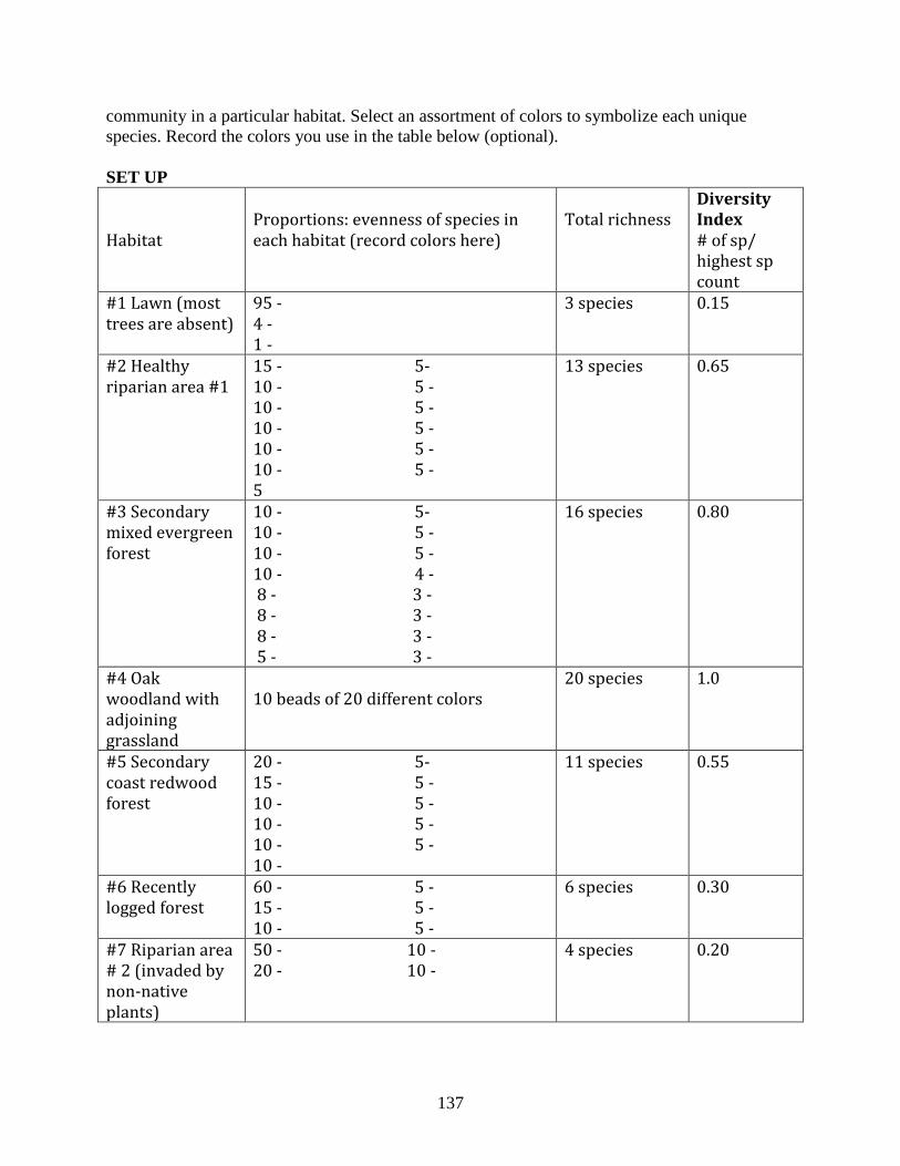
community in a particular habitat. Select an assortment of colors to symbolize each unique species. Record the colors you use in the table below (optional). SET UP Habitat

Proportions: evenness of species in each habitat (record colors here)

Total richness

Diversity Index # of sp/ highest sp count

#1 Lawn (most trees are absent)

95 - 4 - 1 -

3 species 0.15

#2 Healthy riparian area #1

15 - 5- 10 - 5 - 10 - 5 - 10 - 5 - 10 - 5 - 10 - 5 - 5

13 species 0.65

#3 Secondary mixed evergreen forest

10 - 5- 10 - 5 - 10 - 5 - 10 - 4 - 8 - 3 - 8 - 3 - 8 - 3 - 5 - 3 -

16 species 0.80

#4 Oak woodland with adjoining grassland

10 beads of 20 different colors

20 species 1.0

#5 Secondary coast redwood forest

20 - 5- 15 - 5 - 10 - 5 - 10 - 5 - 10 - 5 - 10 -

11 species 0.55

#6 Recently logged forest

60 - 5 - 15 - 5 - 10 - 5 -

6 species 0.30

#7 Riparian area # 2 (invaded by non-native plants)

50 - 10 - 20 - 10 -

4 species 0.20

137

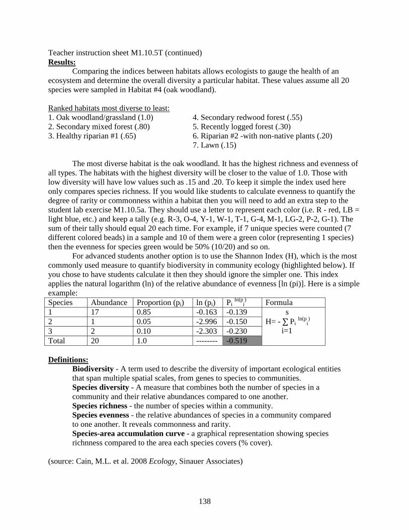
Teacher instruction sheet M1.10.5T (continued) Results: Comparing the indices between habitats allows ecologists to gauge the health of an ecosystem and determine the overall diversity a particular habitat. These values assume all 20 species were sampled in Habitat #4 (oak woodland). Ranked habitats most diverse to least: 1. Oak woodland/grassland (1.0) 4. Secondary redwood forest (.55) 2. Secondary mixed forest (.80) 5. Recently logged forest (.30) 3. Healthy riparian #1 (.65) 6. Riparian #2 -with non-native plants (.20) 7. Lawn (.15) The most diverse habitat is the oak woodland. It has the highest richness and evenness of all types. The habitats with the highest diversity will be closer to the value of 1.0. Those with low diversity will have low values such as .15 and .20. To keep it simple the index used here only compares species richness. If you would like students to calculate evenness to quantify the degree of rarity or commonness within a habitat then you will need to add an extra step to the student lab exercise M1.10.5a. They should use a letter to represent each color (i.e. R - red, LB = light blue, etc.) and keep a tally (e.g. R-3, O-4, Y-1, W-1, T-1, G-4, M-1, LG-2, P-2, G-1). The sum of their tally should equal 20 each time. For example, if 7 unique species were counted (7 different colored beads) in a sample and 10 of them were a green color (representing 1 species) then the evenness for species green would be 50% (10/20) and so on. For advanced students another option is to use the Shannon Index (H), which is the most commonly used measure to quantify biodiversity in community ecology (highlighted below). If you chose to have students calculate it then they should ignore the simpler one. This index applies the natural logarithm (ln) of the relative abundance of evenness [ln (pi)]. Here is a simple example: Species Abundance Proportion (pi) ln (pi) Pi ln(p

i) Formula

1 17 0.85 -0.163 -0.139 s H= - ∑ Pi ln(p

i)

i=1 2 1 0.05 -2.996 -0.150 3 2 0.10 -2.303 -0.230 Total 20 1.0 -------- -0.519 Definitions: Biodiversity - A term used to describe the diversity of important ecological entities that span multiple spatial scales, from genes to species to communities. Species diversity - A measure that combines both the number of species in a community and their relative abundances compared to one another. Species richness - the number of species within a community. Species evenness - the relative abundances of species in a community compared to one another. It reveals commonness and rarity. Species-area accumulation curve - a graphical representation showing species richnness compared to the area each species covers (% cover). (source: Cain, M.L. et al. 2008 Ecology, Sinauer Associates)

138

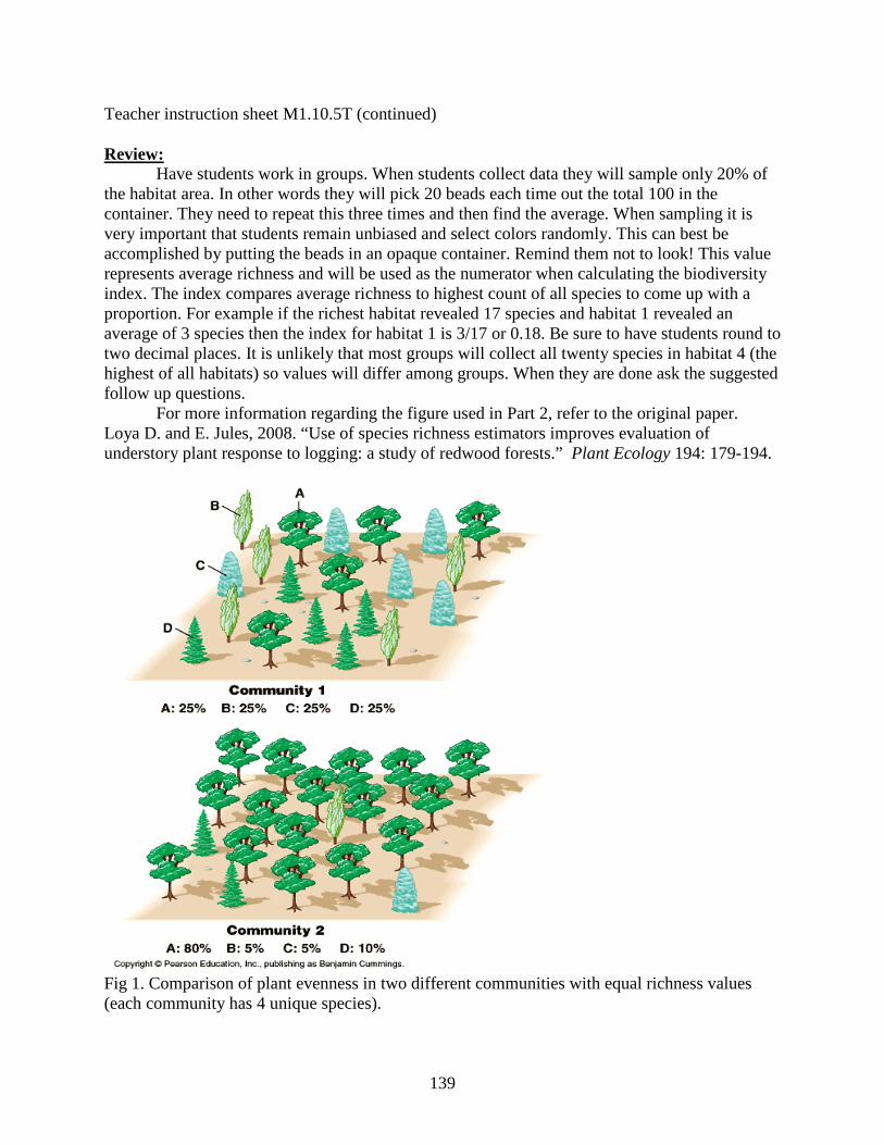
Teacher instruction sheet M1.10.5T (continued) Review: Have students work in groups. When students collect data they will sample only 20% of the habitat area. In other words they will pick 20 beads each time out the total 100 in the container. They need to repeat this three times and then find the average. When sampling it is very important that students remain unbiased and select colors randomly. This can best be accomplished by putting the beads in an opaque container. Remind them not to look! This value represents average richness and will be used as the numerator when calculating the biodiversity index. The index compares average richness to highest count of all species to come up with a proportion. For example if the richest habitat revealed 17 species and habitat 1 revealed an average of 3 species then the index for habitat 1 is 3/17 or 0.18. Be sure to have students round to two decimal places. It is unlikely that most groups will collect all twenty species in habitat 4 (the highest of all habitats) so values will differ among groups. When they are done ask the suggested follow up questions. For more information regarding the figure used in Part 2, refer to the original paper. Loya D. and E. Jules, 2008. “Use of species richness estimators improves evaluation of understory plant response to logging: a study of redwood forests.” Plant Ecology 194: 179-194.

Fig 1. Comparison of plant evenness in two different communities with equal richness values (each community has 4 unique species).

139

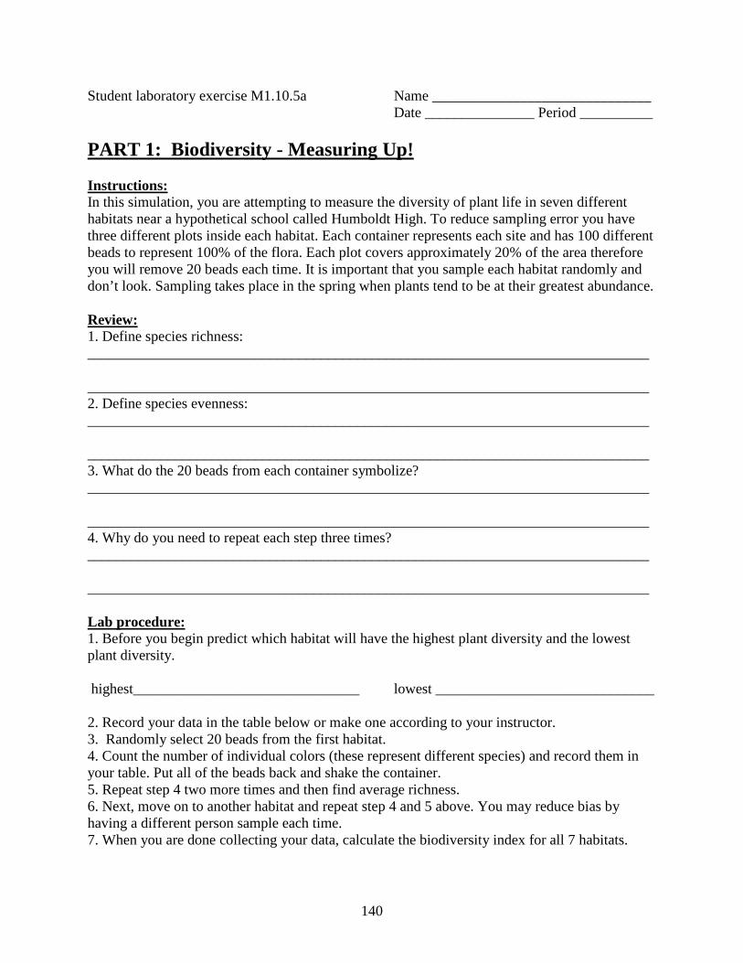
Student laboratory exercise M1.10.5a Name ______________________________ Date _______________ Period __________ PART 1: Biodiversity - Measuring Up! Instructions: In this simulation, you are attempting to measure the diversity of plant life in seven different habitats near a hypothetical school called Humboldt High. To reduce sampling error you have three different plots inside each habitat. Each container represents each site and has 100 different beads to represent 100% of the flora. Each plot covers approximately 20% of the area therefore you will remove 20 beads each time. It is important that you sample each habitat randomly and don’t look. Sampling takes place in the spring when plants tend to be at their greatest abundance. Review: 1. Define species richness: _____________________________________________________________________________ _____________________________________________________________________________ 2. Define species evenness: _____________________________________________________________________________ _____________________________________________________________________________ 3. What do the 20 beads from each container symbolize? _____________________________________________________________________________ _____________________________________________________________________________ 4. Why do you need to repeat each step three times? _____________________________________________________________________________ _____________________________________________________________________________ Lab procedure: 1. Before you begin predict which habitat will have the highest plant diversity and the lowest plant diversity. highest_______________________________ lowest ______________________________ 2. Record your data in the table below or make one according to your instructor. 3. Randomly select 20 beads from the first habitat. 4. Count the number of individual colors (these represent different species) and record them in your table. Put all of the beads back and shake the container. 5. Repeat step 4 two more times and then find average richness. 6. Next, move on to another habitat and repeat step 4 and 5 above. You may reduce bias by having a different person sample each time. 7. When you are done collecting your data, calculate the biodiversity index for all 7 habitats.

140

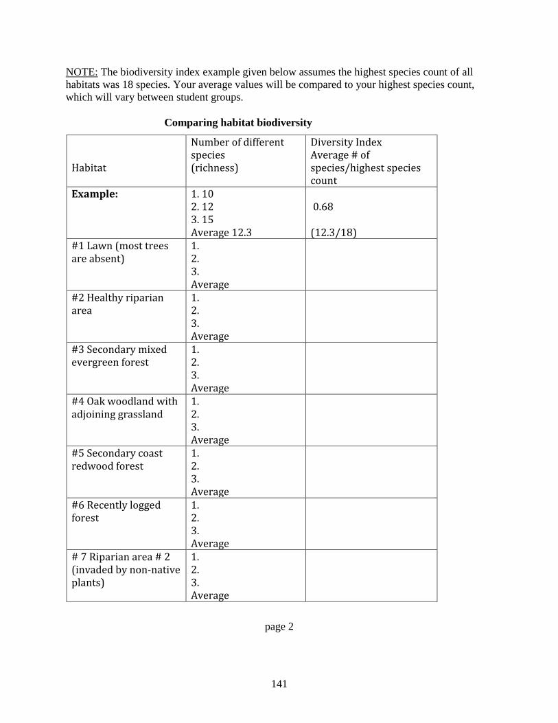
NOTE: The biodiversity index example given below assumes the highest species count of all habitats was 18 species. Your average values will be compared to your highest species count, which will vary between student groups. Comparing habitat biodiversity

page 2

Habitat

Number of different species (richness)

Diversity Index Average # of species/highest species count

Example:

1. 10 2. 12 3. 15 Average 12.3

0.68 (12.3/18)

#1 Lawn (most trees are absent)

1. 2. 3. Average

#2 Healthy riparian area

1. 2. 3. Average

#3 Secondary mixed evergreen forest

1. 2. 3. Average

#4 Oak woodland with adjoining grassland

1. 2. 3. Average

#5 Secondary coast redwood forest

1. 2. 3. Average

#6 Recently logged forest

1. 2. 3. Average

# 7 Riparian area # 2 (invaded by non-native plants)

1. 2. 3. Average

141

Student laboratory exercise M1.10.5a (continued) Results: 1. Rank the habitats from highest to lowest diversity using the calculated indices. __________________________________________________________________________________________________________________________________________________________ 2. How did this ranking compare with your predictions above? 3. Was sampling three times adequate enough to effectively predict the plant diversity of each habitat? 4. How could the sampling techniques used be improved? 5. Why is it important for researchers to collect samples from more than one plot?

142

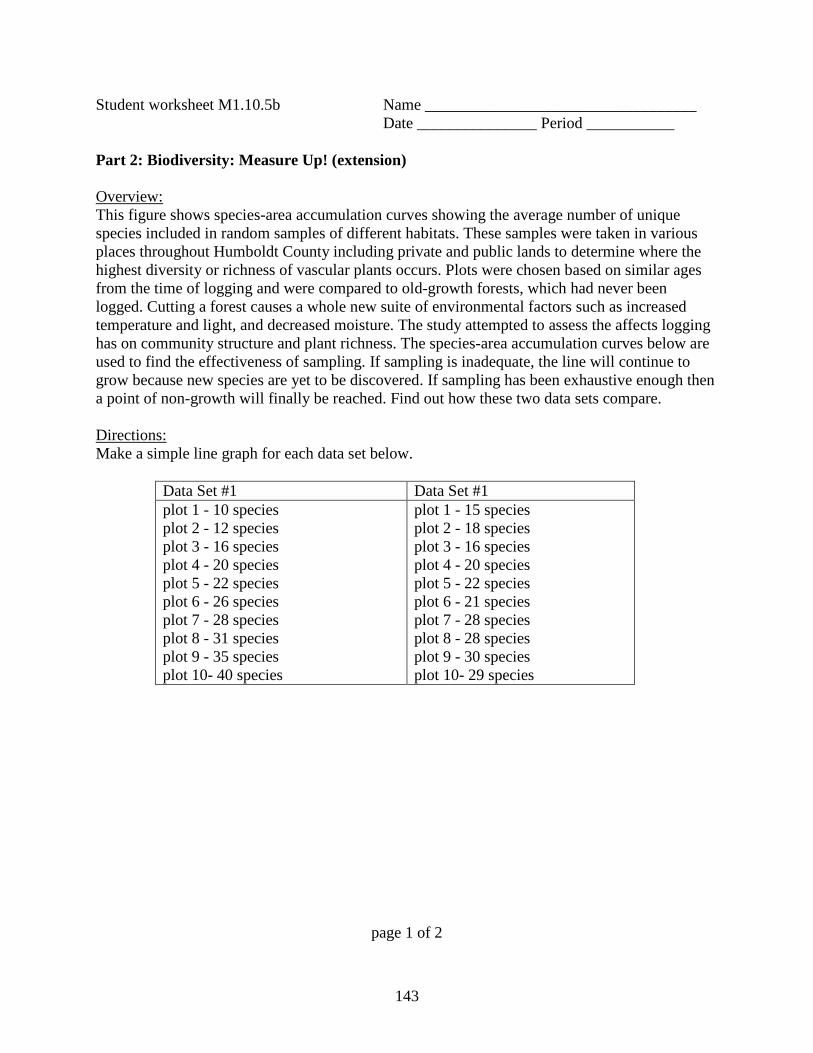
Student worksheet M1.10.5b Name __________________________________ Date _______________ Period ___________ Part 2: Biodiversity: Measure Up! (extension) Overview: This figure shows species-area accumulation curves showing the average number of unique species included in random samples of different habitats. These samples were taken in various places throughout Humboldt County including private and public lands to determine where the highest diversity or richness of vascular plants occurs. Plots were chosen based on similar ages from the time of logging and were compared to old-growth forests, which had never been logged. Cutting a forest causes a whole new suite of environmental factors such as increased temperature and light, and decreased moisture. The study attempted to assess the affects logging has on community structure and plant richness. The species-area accumulation curves below are used to find the effectiveness of sampling. If sampling is inadequate, the line will continue to grow because new species are yet to be discovered. If sampling has been exhaustive enough then a point of non-growth will finally be reached. Find out how these two data sets compare. Directions: Make a simple line graph for each data set below.

Data Set #1 Data Set #1 plot 1 - 10 species plot 2 - 12 species plot 3 - 16 species plot 4 - 20 species plot 5 - 22 species plot 6 - 26 species plot 7 - 28 species plot 8 - 31 species plot 9 - 35 species plot 10- 40 species

plot 1 - 15 species plot 2 - 18 species plot 3 - 16 species plot 4 - 20 species plot 5 - 22 species plot 6 - 21 species plot 7 - 28 species plot 8 - 28 species plot 9 - 30 species plot 10- 29 species

page 1 of 2

143

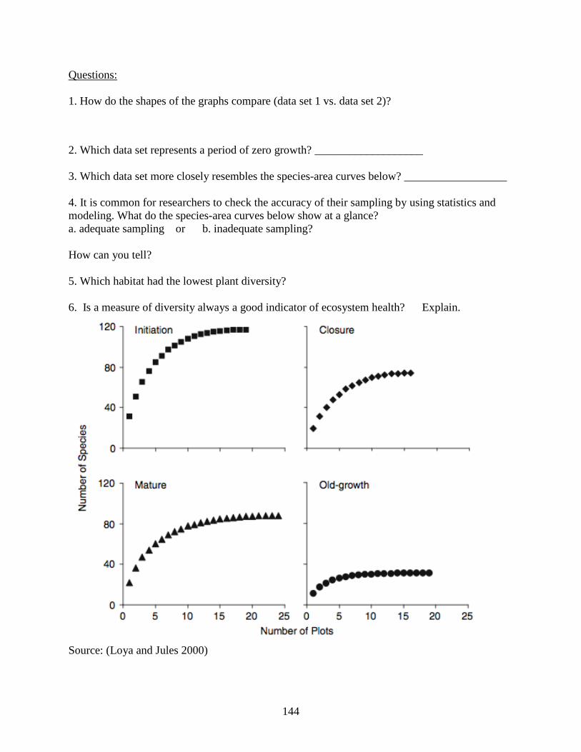
Questions: 1. How do the shapes of the graphs compare (data set 1 vs. data set 2)?

2. Which data set represents a period of zero growth? ___________________ 3. Which data set more closely resembles the species-area curves below? __________________ 4. It is common for researchers to check the accuracy of their sampling by using statistics and modeling. What do the species-area curves below show at a glance? a. adequate sampling or b. inadequate sampling? How can you tell? 5. Which habitat had the lowest plant diversity? 6. Is a measure of diversity always a good indicator of ecosystem health? Explain.

Source: (Loya and Jules 2000)

144

MODULE 1: GLOSSARY OF TERMS abiotic not directly caused or induced by organisms; non-living. abundance the number of individuals in a species that are found in a given area. adaptation

any change in the structure or functioning of an organism that makes it better suited to its environment.

bark

the protective layer of mostly dead cells that covers the outside of woody stems and roots.

basal area

the cross-sectional area of the trunk 4 1/2 feet above the ground; (per acre) the sum of the basal areas of the trees on an acre; used as a measure of forest density.

biodiversity

the full range of variety and variability within and among all organisms (plants and animals), and the ecological complexities in which they occur.

biodiversity (species)

the existence of a wide variety of species (species diversity) or other taxa of plants, animals, or microorganisms in a natural community or habitat.

biological legacies

features of a previous forest that are retained at timber harvest or left after natural disturbances, including large old-growth or other snags, stumps, live trees, logs, soil communities, hardwood trees, and shrubs.

bioregion

a region defined by characteristics of its natural environment, such as flora, fauna, climate, habitat type and topography.

biotic of or relating to life. cambium

a plant tissue consisting of actively dividing cells that is responsible for increasing the girth of the plant (i.e. it causes secondary growth).

carbon dioxide

a colorless odorless gas, which dissolves in water to give "carbonic acid". It occurs in the atmosphere but has a short residence time in this phase as it is both consumed by plants during photosynthesis and produced by respiration and by combustion.

carbon sequestration

the process of removing carbon from the atmosphere and depositing it in a reservoir. Carbon sequestration naturally occurs during photosynthesis.

carbon sink

a phenomenon, such as a forest or ocean, which can absorb atmospheric carbon dioxide.

carbon source

any part or reservoir of the carbon cycle that releases carbon to some other part of the cycle. Examples include the burning of fossil fuels, decomposition of organic waste,

cellulose

a polysaccharide that consists of a long unbranched chain of glucose units. It is the main constituent of the cell walls of all plants, many algae, and some fungi and is responsible for providing the rigidity of the cell wall.

centimeter a metric unit of length, equal to one hundredth of a meter. circumference the distance around something. climate

the long-term description of weather, based on averages and variation measured over decades.

cohort a group of individuals of the same age. composition

the nature of something's ingredients or constituents; the way in which a whole or mixture is made up.

145

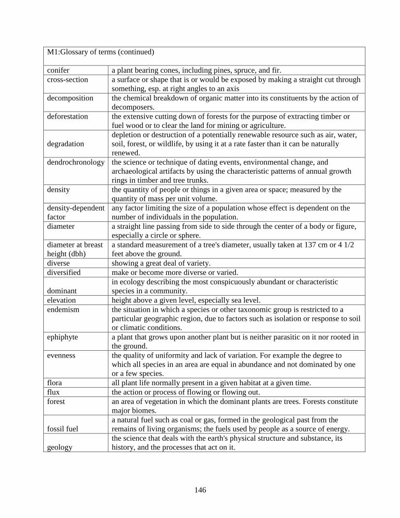
M1:Glossary of terms (continued) conifer a plant bearing cones, including pines, spruce, and fir. cross-section

a surface or shape that is or would be exposed by making a straight cut through something, esp. at right angles to an axis

decomposition

the chemical breakdown of organic matter into its constituents by the action of decomposers.

deforestation

the extensive cutting down of forests for the purpose of extracting timber or fuel wood or to clear the land for mining or agriculture.

degradation

depletion or destruction of a potentially renewable resource such as air, water, soil, forest, or wildlife, by using it at a rate faster than it can be naturally renewed.

dendrochronology

the science or technique of dating events, environmental change, and archaeological artifacts by using the characteristic patterns of annual growth rings in timber and tree trunks.

density

the quantity of people or things in a given area or space; measured by the quantity of mass per unit volume.

density-dependent factor

any factor limiting the size of a population whose effect is dependent on the number of individuals in the population.

diameter

a straight line passing from side to side through the center of a body or figure, especially a circle or sphere.

diameter at breast height (dbh)

a standard measurement of a tree's diameter, usually taken at 137 cm or 4 1/2 feet above the ground.

diverse showing a great deal of variety. diversified make or become more diverse or varied.

dominant in ecology describing the most conspicuously abundant or characteristic species in a community.

elevation height above a given level, especially sea level. endemism

the situation in which a species or other taxonomic group is restricted to a particular geographic region, due to factors such as isolation or response to soil or climatic conditions.

ephiphyte

a plant that grows upon another plant but is neither parasitic on it nor rooted in the ground.

evenness

the quality of uniformity and lack of variation. For example the degree to which all species in an area are equal in abundance and not dominated by one or a few species.

flora all plant life normally present in a given habitat at a given time. flux the action or process of flowing or flowing out. forest

an area of vegetation in which the dominant plants are trees. Forests constitute major biomes.

fossil fuel a natural fuel such as coal or gas, formed in the geological past from the remains of living organisms; the fuels used by people as a source of energy.

geology the science that deals with the earth's physical structure and substance, its history, and the processes that act on it.

146

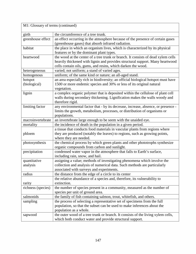
M1: Glossary of terms (continued) girth the circumference of a tree trunk. greenhouse effect

an effect occurring in the atmosphere because of the presence of certain gases (greenhouse gases) that absorb infrared radiation.

habitat

the place in which an organism lives, which is characterized by its physical features or by the dominant plant types.

heartwood

the wood at the center of a tree trunk or branch. It consists of dead xylem cells heavily thickened with lignin and provides structural support. Many heartwood cells contain oils, gums, and resins, which darken the wood.

heterogeneous varied; not uniform; a stand of varied ages. homogenous uniform; of the same kind or nature; an all-aged stand. hotspot (biological)

an area especially rich in biodiversity; an official biological hotspot must have 1500 or more endemic species and 30% or less of its original natural vegetation.

lignin

a complex organic polymer that is deposited within the cellulose of plant cell walls during secondary thickening. Lignification makes the walls woody and therefore rigid.

limiting factor

any environmental factor that - by its decrease, increase, absence, or presence - limits the growth, metabolism, processes, or distribution of organisms or populations.

macroinvertebrate an invertebrate large enough to be seem with the unaided eye. mortality the incidence of death in the population in a given period.

phloem

a tissue that conducts food materials in vascular plants from regions where they are produced (notably the leaves) to regions, such as growing points, where they are needed.

photosynthesis

the chemical process by which green plants and other phototrophs synthesize organic compounds from carbon and sunlight.

precipitation

condensed water vapor in the atmosphere that falls to Earth’s surface, including rain, snow, and hail.

quantitative analysis

assigning a value; methods of investigating phenomena which involve the collection and analysis of numerical data. Such methods are particularly associated with surveys and experiments.

radius the distance from the edge of a circle to its center

rarity the relative abundance of a species and, therefore, its vulnerability to extinction.

richness (species)

the number of species present in a community, measured as the number of species per unit of ground area.

salmonids the family of fish containing salmon, trout, whitefish, and others. sampling

the process of selecting a representative set of specimens from the full population, so that the subset can be used to make inferences about the population as a whole.

sapwood

the outer wood of a tree trunk or branch. It consists of the living xylem cells, which both conduct water and provide structural support.

147

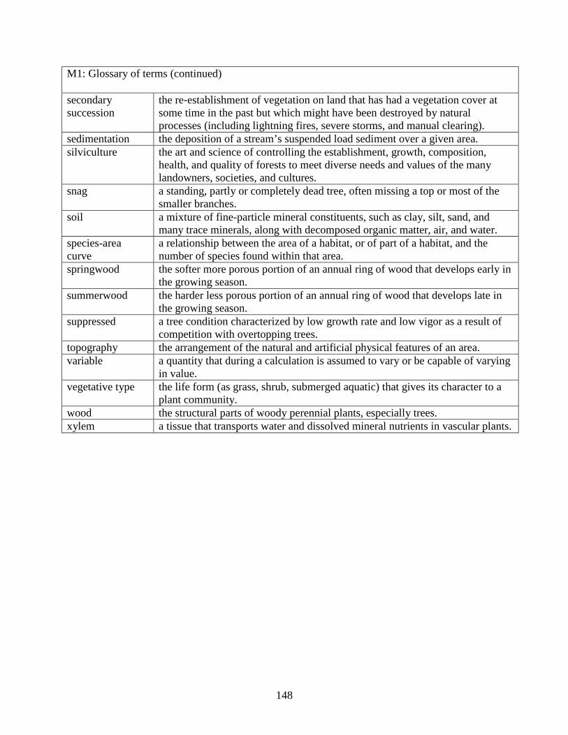
M1: Glossary of terms (continued) secondary succession

the re-establishment of vegetation on land that has had a vegetation cover at some time in the past but which might have been destroyed by natural processes (including lightning fires, severe storms, and manual clearing).

sedimentation the deposition of a stream’s suspended load sediment over a given area. silviculture

the art and science of controlling the establishment, growth, composition, health, and quality of forests to meet diverse needs and values of the many landowners, societies, and cultures.

snag

a standing, partly or completely dead tree, often missing a top or most of the smaller branches.

soil

a mixture of fine-particle mineral constituents, such as clay, silt, sand, and many trace minerals, along with decomposed organic matter, air, and water.

species-area curve

a relationship between the area of a habitat, or of part of a habitat, and the number of species found within that area.

springwood

the softer more porous portion of an annual ring of wood that develops early in the growing season.

summerwood

the harder less porous portion of an annual ring of wood that develops late in the growing season.

suppressed

a tree condition characterized by low growth rate and low vigor as a result of competition with overtopping trees.

topography the arrangement of the natural and artificial physical features of an area. variable

a quantity that during a calculation is assumed to vary or be capable of varying in value.

vegetative type

the life form (as grass, shrub, submerged aquatic) that gives its character to a plant community.

wood the structural parts of woody perennial plants, especially trees. xylem a tissue that transports water and dissolved mineral nutrients in vascular plants.

148

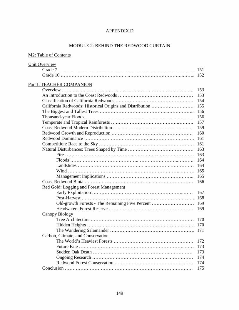
APPENDIX D

MODULE 2: BEHIND THE REDWOOD CURTAIN

M2: Table of Contents

Unit Overview Grade 7 ……………………………………..………………..…………………… 151 Grade 10 ……………………………………..……………………………..…….. 152

Part I: TEACHER COMPANION Overview ……………………………………..………………………………….. 153

An Introduction to the Coast Redwoods ………………………………………… 153 Classification of California Redwoods ………………………………………….. 154 California Redwoods: Historical Origins and Distribution ……………………… 155 The Biggest and Tallest Trees ……………………………………..…………….. 156 Thousand-year Floods ……………………………………..…………………..… 156 Temperate and Tropical Rainforests …………………………………….………. 157 Coast Redwood Modern Distribution …………………………………..……..… 159 Redwood Growth and Reproduction ……………………………………………. 160 Redwood Dominance ……………………………………..……………………… 161 Competition: Race to the Sky …………………………………….……………… 161 Natural Disturbances: Trees Shaped by Time …………………………………… 163 Fire ……………………………………..………………………………… 163 Floods ……………………………………..……………………..………. 164 Landslides ……………………………………..…………….…………… 164 Wind ……………………………………..………………………..……… 165 Management Implications ………………………………………………... 165 Coast Redwood Biota ……………………………………..……………………… 166 Red Gold: Logging and Forest Management Early Exploitation …………………………………………………..…… 167 Post-Harvest ……………………………………………………………… 168 Old-growth Forests - The Remaining Five Percent ……………………… 169 Headwaters Forest Reserve ……………………………………………… 169 Canopy Biology Tree Architecture ………………………………………………………… 170 Hidden Heights …………………………………………………………… 170 The Wandering Salamander ……………………………………………… 171 Carbon, Climate, and Conservation The World’s Heaviest Forests …………………………………………… 172 Future Fate …………………………………………………………..…… 173 Sudden Oak Death ………………………………………….…………… 173 Ongoing Research …………………………………………..…………… 174 Redwood Forest Conservation ……………………………………...…… 174 Conclusion ………………………………………………………………………. 175

149

TABLES 2.1 A list of scientific names of referenced species in Module 2, Part I …………………. 176

FIGURES 2.1 Comparison of leaf and cone morphology for A) coast redwood (Sequoia sempervirens) B) giant sequoia (Sequoiadendron giganteum), and C) dawn redwood (Metasequoia glyptostroboide)……………………………………………………………………………. 177 2.2 Generalized comparison of size and distribution of coast redwood (S. sempervirens) and giant sequoia (S. giganteum) .………………………………………………………..……. 177 2.3 Annual precipitation values for Northern California …………………………………. 178 2.4 Three major regional sections and twenty-five subsections for the natural distribution of Coast Redwood (S. sempervirens) …………………………………..……………….... 178 2.5 Similar-sized trunks of coast redwood (S. sempervirens) (left) and Douglas-fir (Pseudotsuga menzeisii) (right) occupying the same area in a secondary forest ………... 179 2.6 A) upper image is a profile of a generic heterogeneous old-growth forest with high compositional diversity B) lower image is a profile of a generic homogenous secondary forest lacking in compositional diversity ……………………………………………….... 179 2.7 Photos of coast redwood. A) upper left shows large trees with burn scars on trunks, B) upper right shows silt on trunks, evidence of large-scale flooding, C) lower left shows a large nurse log, and D) lower right is a large fern mat composed of leather fern (Polypodium scouleri) ……………………………………………………………………. 180

LITERATURE CITED …………………………………………………………………… 181

Part II: M2: UNITS OF STUDY Grade 7 (Middle School) Unit of Study Cover Page …………………………….. 187 Lesson 1 - Teasing Temperate Rainforests ……………………….……… 188 Lesson 2 - Comparing Cousins …………………………………..……… 197 Lesson 3 - Tree-Thinning Dynamics …………………………………..… 203 Lesson 4 - Measuring Up to the Tallest Trees …………………..……..… 211 Lesson 5 - Hidden Heights …………………………………..…………… 218 Grade 10 (High School) Unit of Study Cover Page ………………………….….. 227 Lesson 1 - Biggest Trees on the Block …………………………..……… 228 Lesson 2 - Shaking Up the Giants …………………………………..…… 237 Lesson 3 - Race to the Sky …………………………………..………..…. 250 Lesson 4 - Scaling the Tallest Trees …………………………………..…. 261 Lesson 5 - A Canopy Conundrum …………………………………..…… 267 Module 2 Glossary …………………………………………………..…………… 273

150

Forest Ecology 101 Series (M2: Part I)

MODULE 2: BEHIND THE REDWOOD CURTAIN

Unit Overview Grade 7 Day 1: Lesson 1 - Teasing Temperate Rainforests Learning Objectives: Students will understand why the northernmost coastal forests of California are referred to as a temperate rainforest. They will compare factors between temperate and tropical rainforests, including latitude, average rainfall, soils, canopy heights, biomass, and biodiversity, in order to understand how and why these two biomes differ. Day 2: Lesson 2 - Comparing Cousins Learning Objectives: Students will compare and contrast similarities and differences between the three members of the redwood subfamily in order to understand the concept of common ancestry and species diversity. Students will compare distribution, size, longevity, morphology, adaptations, and other notable features. By doing so they will understand that many organisms are classified based on shared similar traits. Days 3 and 4: Lesson 3 - Tree-Thinning Dynamics Learning Objectives: Students will analyze and graphically represent data from a tree-thinning project using a graphing program to see how young redwood trees respond to various levels of thinning. They will understand that ecosystems are dynamic and different management strategies produce different results. Following their data analysis, they will briefly summarize the results of the study in a short written paragraph. Days 5 and 6: Lesson 4 - Measuring Up to the Tallest Trees Learning Objectives: After reading about the world’s tallest redwood trees, students will conduct a short series of athletic challenges to find various lengths. They will use these base measurements to calculate equivalences compared to height of some of the world’s tallest trees. Optionally, students will write out their calculations using algebraic expression. Days 7 and 8: Lesson 5 - Hidden Heights Learning Objectives: Students will be able to define biomass and will understand that old- growth redwood forests have the highest above-ground biomass of any ecosystem on the planet. They will graphically illustrate the dry weights of different fern mats sampled in the old-growth canopy. These proportions are taken from a fern mat study conducted in coast redwood and Sitka spruce trees. Afterward, they will interpret the data and answer follow up questions.

151

Forest Ecology 101 Series (M2: Part I)

Unit Overview Grade 10 Days 1 and 2: Lesson 1 - Biggest Trees on the Block Learning Objectives: Students will review the concept of biomass. They will identify the life history strategies of the coast redwood that allows them to live 2,000 years and grow over 320 feet tall. They will understand that through the process of photosynthesis, water and carbon dioxide are converted into carbohydrates such as cellulose. Students will estimate the biomass of their classroom using the estimated dry weight of themselves and will compare their estimate to the biomass of some of largest redwood trees. Days 3 and 4: Lesson 2 - Shaking Up the Giants Learning Objectives: Students will understand how natural disturbances are critical to maintaining proper forest function and increasing biodiversity. They will learn how old-growth forest ecosystems respond to various disturbances (e.g., fire, flood, landslides, wind) and will summarize positive and negative effects. In an extension activity, they will illustrate a human- caused disturbance to a redwood forest ecosystem and will list potential post-disturbance responses and conditions. Days 5 and 6: Lesson 3 - Race to the Sky Learning Objectives: Students will graphically illustrate the results of a tree-thinning project conducted in Redwood National Park that reduced Douglas-fir and other competitive species in order to restore and enhance redwood dominance. Students will use their graphs to assist with an analysis to evaluate whether two different thinning regimes support current management objectives 35 years since the stand was clearcut. Days 7 and 8: Lesson 4 - Scaling the Tallest Trees Learning Objective: Students will create one or more scale models of some of the largest redwood trees using selected data collected from a one-hectare plot located in Prairie Creek State Park. Measurements include tree height, trunk volume, and diameter breast height (dbh) of some of the largest and most complex trees known. Day 9: Lesson 5 - A Canopy Conundrum Learning Objective: Students will interpret a figure showing summarized data from one of the most complex forest canopies of the world. They will write summaries about what the data attempts to reveal and will show their understanding through questioning.

152

APPENDIX D

MODULE 2: TEACHER COMPANION

BEHIND THE REDWOOD CURTAIN

“…From them comes silence and awe. It's not only their unbelievable stature, nor the color which seems to shift

and vary under your eyes, no, they are not like any trees we know, they are ambassadors from another time.”

John Steinbeck

Overview The following information is intended to provide a synthesis of interesting and relevant information for science educators and resource specialists regarding the much admired redwood forests of California’s North Coast. The information herein is intended as a companion guide to accompanying lessons found in Part II and as useful background information for field trips to the redwood region. Much of the information incorporates the latest scientific discoveries found within these complex forests and explores current land management practices intended to improve forest conditions in cut-over land. All lessons in this module are aligned to Next Generation Science Standards (NGSS) and apply to the interdisciplinary approach set forth by the Common Core Skills and Standards (CCSS). They integrate information regarding forest function and structure, biological interactions, and ecosystem processes using a wide variety of spatial and temporal scales. Knowledge regarding natural and anthropogenic disturbances, growth and reproduction, and tree size and complexity are included, as well as brief accounts of redwood classification, distribution, biota, and the future fate of redwoods in a changing environment. Implementing the lessons in this module will have students investigating life history strategies, exploring the canopies of old-growth redwood forests, analyzing actual field data, and constructing useful models, among other things. Throughout these pages suggestions are given for potential field trips to specific redwood parks and preserves, including various outdoor activities that will further enhance the learning experience behind the “Redwood Curtain.”

An Introduction to the Coast Redwoods No tree better epitomizes the North Coast of California than the coast redwood (Sequoia sempervirens). If Californians haven't seen this species of tree, they have no doubt heard about it. The longevity of redwood trees allows them to reach a gargantuan size so that walking among them can be an inspirational and humbling experience. The largest trees can commonly reach heights of 60-100 m (196-328 ft) and can have trunks over 6 m wide (20 ft) (Earle 2013; Van Pelt 2001). The redwood forest floor is laden with bryophytes (mosses, liverworts, hornworts), downed logs, and woody debris. The understory is typically a mix of ferns, redwood sorrel, assorted shrubs, hardwoods, and other conifers. The ability of trees to reach tremendous height and have large full canopies allows them to dominate the forest community. Old-growth forests provide vital ecosystem functions and services. They provide a wide array of habitats, enhance

153

air and water quality, and store incredible amounts of carbon. Complex tree structure and abundant snags and logs provide essential habitat for many threatened species (Franklin et al. 2002; Sawyer et al. 2000; Thornburgh et al. 2000). These primeval forests are the product of millions of years of evolution and serve as places of refuge for plants, animals, and humans. Most old-growth stands have been severely impacted by logging so that much of the redwood range now consists of secondary forest (forest that has been logged).The decay-resistant, high-quality heartwood these trees produce not only enables them to live long, but also produces some of the most highly prized timber. The desirability and economic importance of redwood has influenced much of the infrastructure we see in northern California today, such as the "redwood highway" and the Northwestern Pacific Railroad, largely constructed to transport redwood logs. Logging of old-growth redwood forest accelerated during the post-World War II boom of the 1940s and 50s and another surge of cutting occurred in the 1980s. Not long after, 95% of the old-growth redwoods had been felled (Russell 2000; Sawyer et al. 2000;). The magnificence of coast redwood forests has been acknowledged by many people. Preservationists began saving ancient redwood groves as early as 1901. Because of their economic and aesthetic importance many aspects of these forests have been widely studied (Chittick and Keyes 2004; Johnstone and Dawson 2010; Lorimer et al. 2009; Madej 2010; Sillett and Van Pelt 2000). After recognizing the value and rarity of these primeval forests, most counties within the redwood range set aside redwood parks and preserves that offer abundant opportunities for students to perform field studies and visit these unique ecosystems. The northernmost groves in California are extensions of the true rainforests of the Pacific Northwest and contain some of the largest and most complex tree structures known (Sillett and Van Pelt 2007). The best examples of pristine old-growth redwood forests are found in Humboldt and Del Norte Counties. For a list of redwood parks and preserves in North Coast California, refer to Appendix F.

Classification of California Redwoods Redwood, juniper, cedar, and cypress trees belong to the cypress family or Cupressaceae, which is the most widespread group of conifers. Members of this aromatic family characteristically have fibrous bark, relatively short scale-like leaves, and solitary seed cones that hang terminally on branches. Although taxonomists and botanists continue to update the phylogeny of this family, approximately 28 genera are represented, occupying diverse habitats on all continents except Antarctica (Earle 2013). Members of this family grow to be some of the oldest, largest, and tallest trees on Earth. The two landmark species (coast redwood and giant sequoia) existing in California are compared below. Since the early 1800s, botanists have had a challenging time classifying redwoods. Redwood species used to be considered members of the bald cypress genus (Taxodium) based on comparisons of leaf morphology and other characteristics, which can be unreliable (Fig. 2.1). The coast redwood was the first to be included in this group and received its specific epithet - sempervirens - because it remained evergreen while all other species of Taxodium were deciduous. In the mid-1800s, the classification was changed and its current scientific name was finalized. Until the 1930s, the giant sequoia (Sequoiadendron giganteum) was included in the Sequoia genus with coast redwood. Upon closer inspection at least nine notable differences in embryo development (noted by Buchholz) and other distinguishing characteristics separated them into two distinct genera (Barbour et al. 2001). The two California redwoods are often confused by name; however, since they occupy different regions of the state, they are rarely

154

confused in the field. An interesting side note is Sequoia is hexaploid (having six sets of chromosomes) and therefore has a much larger genome compared to other redwoods (Ahuja 2008). A third type of redwood, the dawn redwood (Metasequoia glyptostroboides), was considered extinct by western botanists until found in 1944. Until this time, it was only known in the fossil record until several live specimens were discovered in two providences of central China. These isolated groves remain vulnerable and in attempts to preserve the only deciduous redwood, seeds were distributed for planting. Today many trees are well-established in parks and arboreta around the world. The life span of this genus ranges from 300-600 years and it reaches heights of 50 m (164 ft) (Barbour et al. 2001), small compared to its two larger cousins whose proportions are discussed further below. Other species closely related to redwoods with impressive stature and longevity live elsewhere. For instance, a species that occupies forested areas of southern Chile and Argentina, called alerce or Patagonian cypress, can reach diameters reach of 4 m (13 ft) and heights over 50 m (164 ft) (Earle 2013). This species is presumed to live longer than giant sequoia and crossdating has revealed at least one tree older than 3,500 years (Earle 2013). Crossdating trees using dendrochronological techniques is useful beyond just dating trees. Tree cores and crossdating can be used to record past climatic changes specific to a particular area and can provide insight into forest dynamics. Preliminary results from recent dendrochronological studies for coast redwood are discussed further below in the climate change section. Lesson G7.L2 has students compare the classification, distribution, size, longevity, and other characteristics of the three “redwood cousins”: coast redwood, giant sequoia, and dawn redwood. Each is restricted to a small range and is a single representative of their genus. All three share several phenotypic traits, including red wood and fibrous bark (Ahuja 2008). Locally planted specimens can be observed outside the visitor center at Humboldt Redwoods State Park (hereafter HRSP) located near Weott and on the grounds of Humboldt State University (hereafter HSU) in Arcata California (pers. observation).

California Redwoods: Historical Origins and Distribution Coast redwood is considered paleoendemic, meaning it has an ancient lineage and is only found in one region: in this case the coast ranges of California and the southeastern corner of Oregon. The redwoods of California have been shaped throughout time by shifting climates and coastlines, environmental changes, and the evolution and dispersal of other organisms. The leaf and bark morphology of coast redwood has gone virtually unchanged since the Cretaceous, approximately 65-150 million years ago, making them living fossils. These imposing, tall, dark forests have served as the backdrops in several Hollywood films, including Jurassic Park and the Return of the Jedi, often depicting the age of the dinosaurs, because dinosaurs would have walked among the ancestors of these trees. It is likely that coast redwood did not reach its epic proportions until much later (Barbour et al., 2001; Noss 2000) and current assemblages associated with this forest community may only be 4,000 years or younger (Sawyer et al. 2000). Redwoods reached their most extensive distribution approximately 65-90 million years ago during the late Cretaceous. Ancestral species were once established across much of the temperate and sub-tropical regions. Approximately 30 million years ago, their distribution began to shrink due to climatic changes and geologic uplift events. During this time some redwood species became extinct, while others emerged (Ahuja 2008). In North America, different glacial episodes of contraction and expansion further altered the redwood range. Isolated pockets along

155

the coast acted as refuges for coast redwood, which is frost intolerant and prefers a moist coastal climate. Giant sequoia were once much more widespread within a larger matrix of mixed conifer forests covering eastern California and Nevada. As their range shrank they migrated to lower elevations where they are found today (Barbour et al. 2001; Sawyer et al. 2000) (Fig. 2.2). For those seeking to see nearby fossils of redwood, excellent examples dating back 30 million years can be found in The Petrified Forest outside of Calistoga (pers. observation).

The Biggest and Tallest Trees Redwood is the state tree of California and includes both the giant sequoia and the coast redwood because at the time of designation both were placed in the Sequoia genus. Giant sequoias are the biggest trees by volume living today, although coast redwoods may have been bigger historically. Giant sequoia can live over 3,200 years and reach basal diameters exceeding 8 m (26 ft) (Barbour et al., 2001; Sawyer et al., 2000). The record tree by volume is the General Sherman, recognized as the world's largest living terrestrial organism. The trunk alone weighs 1,400 tons and its above-ground dry mass is 582 Mg (metric tons). It has a diameter breast height (hereafter dbh) of 8.2 m (27 ft), a height just under 84 m (274 ft), and a total volume of 1,591 m3 (56,200 ft3) (Sillett et al. unpublished). By comparison, 15 adult blue whales or 21,800 150 pound humans would be equivalent in size (SRL 2013). The amount of wood contained in its trunk could build 120 average-sized houses (Armstrong 2013). The coast redwoods have the distinction of being the world's tallest living trees. They are an exceptionally long-lived species due to their fire-resistant bark and rot-resistant heartwood. The tallest, biggest, and most complex trees grow in the forests of the North Coast. Researchers recently discovered the oldest redwood on record, which is at least 2,510 years old (Sillett et al. unpublished). The tallest trees were discovered in 2006, well after most other giant trees had been discovered. The tallest is approximately 115 m (379 ft) and is still growing vigorously. The world’s tallest grove of trees is found in HRSP along lower Bull Creek, a tributary of the Eel River, in the Rockefeller Forest. Here along alluvial terraces, 70% of the redwood trees reach heights over 107 m (350 ft) (Sillett et al. 2010). No other tree species normally reach heights of even 100 m. This stand is a model grove and serves as a reference condition for old-growth redwoods occupying alluvial flats (Dagley and Berrill 2012). Old-growth redwood groves, such as the Rockefeller Forest serve only as icons of their former glory, however, since most have been logged (information about the impact of logging is discussed below). In lesson G7.L4, students will compare different lengths they obtain through athletic challenges to some of the tallest trees on the planet.

Thousand-year Floods The Rockefeller Forest may have been spared the chainsaw; however, over 300 large trees exceeding 1.5 m (4 ft) in dbh were lost in the catastrophic flood of 1955. Severe undercutting of the riverbank caused by a torrent of water, logs, and debris was the source of this massive destruction. The aftermath of this flood and the following megaflood of 1964 took a heavy toll on many groves throughout HRSP including Stephens Grove, Williams Grove, and Richardson Grove. Bull Creek and its tributaries were particularly hard hit because of rampant upslope logging, unstable slopes, and wet winter weather. In some places more than 7 m (23 ft) of sediment were deposited after both episodes, which completely buried the stream (Lorimer et al. 2009). So much damage was done that both conservationists and biologists began to shift

156

their thinking to whole watershed protection: soon after the entire Bull Creek watershed was incorporated into HRSP (Barbour et al. 2001). Rock levies and assorted salmon restoration efforts (some performed by local school children) are clearly visible along portions of this river above Rockefeller Forest. With the erection of willow walls and weirs, along with constant vigilance, deep pools able to support salmon and other aquatic organisms have returned (pers. observation). Because of its ecological, economical, and social importance, salmon restoration at various levels of intensity has been conducted on virtually all watersheds within the North Coast. A field trip to Bull Creek is recommended to view the exemplary trees and clear examples of watershed restoration nearby. In addition, the HRSP visitor center will gladly show the 1964 flood video in its movie room (The above information on floods is also relevant to the section below on natural disturbances that shape the redwood landscape, which is the focus of lesson G10.L2).

Temperate and Tropical Rainforests Although the coniferous forests associated with the North Coast are characterized by coast redwood, these forests are mainly a southern extension of the great temperate rainforests of the Pacific Northwest (hereafter PNW) (Franklin et al. 2006; Van Pelt 2001), especially the northernmost stands of Humboldt and Del Norte Counties. Stretching south from Alaska's Kodiak Island to northern California, the PNW supports an unusual diversity and abundance of fish, wildlife, and forest resources. Abundant rainfall and a nearly snow-free climate sets ideal conditions for the growth of large, long-lived trees. Instead of the deciduous hardwoods associated with many other temperate forests of North America, the PNW is dominated by large evergreen conifers, many obtaining world record size (Schultz 1990; Van Pelt 2001; Wolf et al. 1995). Aside from coast redwood, other dominant tree species include Douglas-fir, Sitka spruce, western red cedar, grand fir, and western hemlock (Van Pelt 2001; Schultz 1990; Barbour et al. 2001; Zinke 1988) (For a list of scientific names, refer to Table 2.1). This bioregion originally covered approximately 10 million ha (25 million ac) and today represents the largest contiguous coastal temperate rain forest (hereafter CTRF) in the world (Peattie 1981; Van Pelt 2001; Wolf et al. 1995). CTRFs were once found on all continents except Africa and Antarctica. The current PNW area accounts for more CTRF than all other areas combined. Besides those found in the PNW, significant stands include the coastal areas of Chile, the island of Tasmania, and the west coast of New Zealand. All have suffered from a high degree of exploitation for their timber and today the remaining area represents 2-3% of the overall temperate rain forests of the world (Wolf et al. 1995). Because of its high moisture content, rich biodiversity, and high amounts of biomass, this forest type can be compared to tropical rainforests on many levels, which is the main objective in lesson G7.L1. Rainforests are distinctive because they receive high levels of precipitation. Tropical rainforests receive anywhere from 150 cm (60 in) to 1,000 cm (400 in) of precipitation annually, with a mean temperature above 24°C (75°F) (Pwnet 2013). Tropical forests typically only have two pronounced seasons: wet and dry. Because of their proximity to the equator, these forests receive the most direct solar energy year round. Warm conditions accelerate decomposition and abundant rainfall causes heavy leaching, so soils tend to be nutrient poor and acidic. Most trees are broadleaved evergreens averaging 23-35 m (25 -155 ft) tall with large buttressed roots to help support their shallow root systems (Weir n.d.) however, these forests and the trees they contain vary substantially by location.

157

By comparison, CTRFs generally receive over 2,500 mm (100 in) of annual rainfall, most occurring between October and March (Pwnet 2013) (Fig 2.3). CTRFs experience four seasons, although not as distinctive as other temperate regions. The moderating influence of the ocean prevents frequent freezing and soils usually remain unfrozen throughout the year. Large accumulations of leaf litter and woody debris create fertile soils because cool temperatures and acidic conditions slow down decomposition (Thompson et al. 2009). Over time, long-lived stands of trees undergo high landscape-level disturbance, including wind-throws and landslides, creating a mixed-aged forest with structurally complex crowns (Franklin et al. 2002; Sawyer et al. 2000; Van Pelt 2001). Tropical forests are noted for their high levels of biodiversity unmatched anywhere else in the world. They may contain up to 60 % of all known species on the planet (Myers 1988; Wolf et al. 1995). A one square kilometer forest can support an alpha diversity (diversity at the local level) of 100-300 different tree species. Regional richness or gamma diversity can exceed 4,000 plant and animal species, not to mention countless smaller organisms (Thompson et al. 2009). Branches support numerous species of epiphytes (plants that live on other plants) such as orchids, bromeliads, ferns, mosses, and vines. However, overall biomass is surpassed by CTRF (Franklin et al. 2006; Sillett and Van Pelt 2007; Wolf et al. 1995). The long-lived trees in the CTRF of the PNW accumulate more organic matter or biomass compared than any other forest type (discussed further below), especially old-growth redwood forests in prime habitat (Sillett and Van Pelt 2007). In the PNW, individual trees can live over 1,000 years and can surpass 6 m (20 ft) in diameter (Wolf et al. 1995). Average tree height varies by species; however, it is not unusual to have trees over 80 m (262 ft) (Van Pelt 2001). Old trees with large branches can literally hold tons of epiphytes, including mosses, lichens, ferns, shrubs, and even other trees (Sillett and Van Pelt 2007; Van Pelt 2001). They can support approximately 300 bird and mammal species (Hagar 2007) and only a dozen or so tree species. The sheer size certain conifers can obtain often make them dominant. Many animals are heavily dependent on old-growth characteristics and species diversity can be seriously reduced in second-growth habitats (Cooperrider et al. 2000; Hagar 2007; Schultz 1990). (More information on redwood forest biota can be found below.) Both rainforest types have been highly reduced by land clearing and logging with tropical rainforests in particular being reduced and fragmented faster than any other ecological zone. This broad-scale clearing and degradation of the world's tropical forests is the primary cause of species extinctions (Myers 1988). Many tropical species live nowhere else, so once their habitat is destroyed, they are gone forever. The CTRF of the PNW were among the first landscapes to be logged when Euro-Americans settled along the Pacific Coast (Wolf et al. 1995). Due to the availability and high-quality timber found there, this area was destined to become the lumber capital of the world. Today, only one third of these forests are protected (Galindo-Leal and Bunnel 1995). Logging continues and many of the tallest and largest trees are gone (Van Pelt 2001; Wolf et al. 1995). Most of the last remaining champion trees, aside from coast redwood, can be found in isolated regions of the Olympic Peninsula and Vancouver Island. Similar to the northernmost stands of the coast redwood, their isolated locations spared them from intensive logging (Van Pelt 2001).

158

Coast Redwood Modern Distribution In attempts to better understand its distribution and habitat associations, the entire range of coast redwood has been divided into three major sections (north, central, south) and 25 subsections (Sawyer et al. 2000) (refer to Fig. 2.4). The information in this module predominately focuses on the northern section. All coast redwood forests lie within 60 km (37 mi) of the Pacific Ocean and most grow below 760 m (2,500 ft) in elevation. Because of their intolerance to salt spray, they tend to grow just inland from the immediate shoreline (Olson et al. 1990). Coast redwood stands of all ages are still found throughout their entire range in a variety of ecological settings despite severe human caused impacts, creating a patchy distribution (Schoenherr 1992). Particularly large stands of mixed ages occur in the central region, which ranges from HRSP to San Francisco Bay (Busing and Fujimori 2002). South of Sonoma County, redwood distribution becomes patchy and fragmented, and in the southern region, some groves are reduced to small isolated pockets sheltered in narrow valleys (Lorimer et al. 2009; Sawyer et al. 2000). About half of the remaining old-growth redwood forest can be found in Redwood National and State Parks (hereafter RNSP), north of Trinidad, California. Because of the uniqueness of these old-growth forests, RNSP has been designated as a U.N. World Heritage Site and an International Biosphere Reserve. Moisture and moderate temperatures seem to be the most important factors limiting coast redwood’s distribution, although topography and edaphic conditions (those related to soil) should not be ignored. Evidence suggests redwoods are sensitive to ambient moisture, which could be attributed to their high transpiration rates and inability to efficiently regulate water use (Johnstone and Dawson 2010). Coast redwood performs best where there is abundant moisture during the driest months, which in their home range comes mostly from summer fog. When air cools, water coalesces and falls to the ground as fog drip, some of which is intercepted by plant foliage. In redwood forests, 80% of the dominant species (including redwoods) exhibit a foliar uptake water acquisition strategy (Johnstone and Dawson 2010; Keppeler 2007; Limm et al. 2009). Moisture from fog can range from 0-37 mm (1.5 in) per day and contributions by fog may account for as much as 10-45% of the total water input to coastal redwood forest (Dawson 1998). The absence of redwood in some low lying places along the North Coast (e.g., the Mattole) may be mostly attributed to the lack of summer fog (Keppeler 2007, Sawyer et al. 2000). As the environment changes, particularly from human influenced climate change, models for the continued persistence of coast redwood across its entire range vary from pessimistic to positive. As a paleoendemic species, the resilience of coast redwood is acknowledged from a historical perspective. Thorough mapping and classification of redwood forests reveals many associated vegetation types, including mixed conifers, coastal fens, evergreen hardwoods, chaparral shrubs, and coastal prairie grasslands. The densest and purest stands live on alluvial flats. In general, coast redwoods are found living on moderately acidic to alkaline soils, with soil textures ranging from sandy-loam to clay (Lorimer et al. 2009; Sawyer et al. 2000). Redwood establishment often stops abruptly where serpentine or high-pH heavy clay soils occur. These trees prefer to grow on sedimentary rock and prairies can form in places where this type of rock is absent (Johnston 1994). An exemplary prairie well worth a visit is Elk Prairie in Prairie Creek State Park, north of Orick. This prairie is aptly named, since one has a good chance of seeing the charismatic Roosevelt elk (Cervus canadensis roosevelti) here (pers. observation). It is the largest North American elk species and has been brought back from near extinction.

159

Redwoods differ along a north-south gradient and between upland and lowland sites (Fritschle 2009; Sawyer et al. 2000). This information is relevant when considering management goals and conservation priorities. Average precipitation ranges from 1270-2286 mm (50-90 in) in the north region and 600-1020 (24-40 in) in the south. In the northern section, yearly temperatures normally range from 10-21°C (50-70 °F) (Barbour et al. 2001). Trees living in the north appear to be more frost-tolerant compared to the south. Studies comparing cloned trees and trees planted by seeds from different regions reveal disparities in genetic potential and changes in foliage, shape, root depth, chemical composition, and resistance to frost. Occasionally southern trees are exposed to salt spray and more regular intensive fires so these trees can develop a much different structure from their larger northern counterparts; some will even take on a shrub-like character (Barbour et al. 2001; Sawyer et al. 2000). Understanding these differences reveals the plasticity of coast redwoods or its ability to adapt to wide-ranging environmental conditions. As students investigate biological interactions and redwood forest structure, considering these different factors can be important. The variability of climate between the north and south range is fairly dramatic (Barbour et al. 2001; Veirs Jr. 1996). The modern restrictive range of coast redwood suggests these forests have a narrow envelope of climatic conditions within which they can live. Redwoods’ preference for moderate temperatures and moist places can be witnessed by their ability to reach their peak size where these preferable conditions occur. It is likely their range is restrained southward due to lack of winter precipitation and northward by low temperatures and frost (Lanner 1999), although no one knows with certainty. Although mortality caused by fire is rare, it can be another limiting factor, and the southern region has a greater incidence of natural wildfires. These factors only partly account for redwood’s limited distribution; another reason is they do not establish themselves well from seed (Barbour et al. 2001; O’Hara and Berrill 2009). A relatively low dispersal rate may be one of the main reasons why they cannot compete as well with other conifers, such as Douglas-fir and grand fir in some places. Thus, redwoods tend to be the dominant conifer where they are already established. This is supported by the fact that when planted in other parts of the world, such as Europe, New Zealand, or certain urban settings, coast redwood trees can flourish.

Redwood Growth and Reproduction Redwood regeneration can occur through seed germination or clonal growth (resprouting). Redwood seeds are small and lightweight. Lacking efficient wings to slow them down, they fall quickly to the ground, which can limit their dispersal (Olson et al. 1990). Even though a tree might release millions of seeds, the majority are not viable (Barbour et al. 2001). Successful germination tends to occur on freshly exposed mineral soils, such as recently deposited silt along river terraces, where competition is much reduced. Seeds have been known to successfully germinate on many surfaces, such as organic litter and surfaces of fallen logs, but do not seem to do as well on top of their own leaf litter (Veirs 1996). They are just viable for one year or less and germination appears to be most successful following 127-200 mm (5-8 in) of gentle rain. Once a young sapling becomes established, it is extraordinarily shade tolerant. A young redwood tree can survive in low light conditions, lying semi-dormant for decades, until its moment in the sun when it will respond quickly to increasing light levels (Barbour et al. 2001; Sawyer et al. 2000). Some small trees may be suppressed for hundreds of years yet maintain the ability to accelerate growth when favorable conditions occur (Olson et al.1990).

160

Unlike most conifers, redwoods harbor dormant basal or adventitious buds (those that sprout of unusual locations) that sprout profusely under stressful conditions even after they have been cut. Vegetative sprouts can form just about anywhere on a tree. Thus, in commercial forestry stump sprouts are often taken advantage of and relied heavily upon for restocking the forest (Burns 1983; O’Hara et al. 2007). Stump sprouts can occur at multiple ages and the growth, vigor, and mortality of sprouts are influenced by many factors (O’Hara and Berrill 2009). The useful carbohydrates stored within a large tree trunk, and the ability to resprout, is also taken advantage of by white or albino foliage, which grows on certain trees. These albino redwoods are difficult to find, and parks usually keep their locations secret in order to preserve them. Sprouts can come from burls, which are wart-like outgrowths of the trunk. They originate from meristimatic tissues and are used in artisan woodworking, such as burl tables and clocks. When a branch or part of a tree trunk is injured or snapped off, trees can respond quickly by resprouting. This is important when considering the complex structures some trees have, which is discussed further in the redwood canopy section. Redwood trees clone themselves so readily that it is difficult to know their true age. Sometimes when a tree dies, buds sprout around the old parent tree or trunk in a circular pattern, forming a "fairy ring" that when larger, forms a circle of trees called a cathedral tree. Sometimes evidence of the original parent tree can be clearly visible and having students note the different ages can be worthwhile (pers. observation).

Redwood Dominance The ability to sprout profusely, live in low light conditions, and grow big and tall allows the coast redwood to dominate the landscape unlike most other conifers. Redwoods are some of the fastest growing trees in the world under the right conditions and their ability to accumulate wood volume supersedes all other species (Jones and O’Hara 2011; Sillett et al. 2010; Veirs 1996). In general, dominant species have a tremendous impact on ecosystem processes and, if removed, can directly impact nutrient flow, microclimates, and biomass, among other factors. From this perspective, redwoods are truly a keystone species. Even after death, large diameter trees continue to contribute to the forest ecosystem persisting as snags and logs and adding to wildlife habitat. The overwhelming size of an old-growth grove has a heavy influence over moisture and light regimes. The forest floor is usually laden with a thick mat of fallen leaves and branches. Young redwoods are extremely shade tolerant and can persist for decades with no apparent growth. Forbs, shrubs, and other trees living underneath these giants have adapted to low-light conditions as well. Of course, no two redwood groves are the same, and they range from pure stands to scattered individual trees in upland vegetation where other trees dominate.

Competition: Race to the Sky Many variables discussed thus far have revealed important components influencing the age, size, distribution, and adaptations of coast redwood. Trees like most organisms compete for resources. Redwoods often grow alongside other trees such as tan oak, California bay, Douglas-fir, grand fir, Sitka spruce, and western hemlock. These trees compete for light, space, water, and other resources and, in some circumstances, are considered co-dominant. Co-dominant tree species have their crowns at the highest level of the forest canopy and receive full sunlight from above. In the North Coast and elsewhere, co-dominance regularly occurs between Douglas-fir and coast redwood, especially in upland stands (Fig. 2.5). Both are fast growing conifers and

161

approach records for the largest and tallest trees across the PNW. When it comes to attack by insects and fungal pathogens, redwood usually wins. Decay-resistant bark, loaded with chemicals such as tannins and other phenolics (a group of organic compounds), give redwood an excellent resistance to fungal and insect attack. Even though insects are known to feed on redwood leaves and cones, none are known to attack and kill a tree. Douglas-fir is more susceptible to insect and fungal attack and can host many more harmful insects, such as bark beetles, which is one of the reasons why they do not live as long as redwood. Some animals (beside humans) can harm redwood. Banana slugs and wood rats eat seedlings; black-tailed deer eat foliage; and black bears eat inner bark. Black bears are especially damaging (Giusti 1988). In some places, they favor the inner bark of redwood trees over Douglas-fir, especially young trees with 51-127 cm (20-50 in) diameters (Burns 1983; Sawyer et al. 2000). This is problematic in certain places, such as RNSP, where this learned behavior is causing redwood tree mortality in some secondary forests and young Douglas-fir are becoming dominant (Teraoka and Keyes 2011). This undesired competitive advantage is one of the challenges facing forest managers in Redwood National Park (hereafter RNP). In some secondary forests, precommercial treatments have removed portions of Douglas- fir to reduce overcrowding and to more rapidly set redwood stands towards a trajectory of desired conditions. Reference conditions are established from nearby old-growth forest (Berrill et al. 2009; Teraoka and Keyes 2011). In some logged areas, such as upland sites in RNP, hillsides once dominated by redwoods were aerially reseeded with Douglas-fir seed and other conifer species with the intention of future logging. Part of the rationale for this practice is that Douglas-fir can be a pioneer species and seedlings perform better in cut-over areas compared to redwood. Douglas-fir is a shade-intolerant species and unlike redwood, can produce numerous viable seeds. Germination is most successful after fire or clearing; however Douglas-fir cannot vegetatively reproduce or resprout like redwood can. The fact that Douglas-fir seeds were cast over logged areas, coupled with management strategies that alter forest composition and a predicted warmer and drier climate, may be giving Douglas-fir an advantage over redwoods in some places (Teraoka and Keyes 2011). On the other hand, Douglas-fir can occupy a disturbed site first and by doing so, may help facilitate establishment of redwood. Furthermore, some climate-forecasting models using general circulation patterns predict a warmer and wetter climate for California (Lenihan et al. 2003). Studying this competitive relationship is the main objective in lesson G10.L3. In this lesson, students will analyze data from the Whiskey 40 thinning project intended to restore the competitive advantage of coast redwood. This thinning project is unique because it occurred within a national park and can be easily accessed. Before the expansion of RNP in 1978, many upslope areas were clear-cut then burned, altering forest composition and function. The Whiskey 40 plot lies on a ridge and is representative of other poorly developed second growth stands. Tree density is high and biodiversity is relatively low. In some places Douglas-fir is more numerous and in other areas young grand fir and Sitka spruce (both exotic to the site from aerial seeding) are becoming established. The project thus far has three general prescriptions to be implemented over 40 years. The first prescription began in 1995, when 16.2 ha (36 ac) were thinned. All exotic species and trees less than 11.4 cm (4.5 in) were removed. Low-intensity thinning is sometimes prescribed to mimic the natural thinning that occurs during succession. Plots were measured immediately, then again in 2002. In 2005, a second prescription was conducted and 30% of the smaller trees were removed. Fourteen acres from the previous prescription were set

162

aside for comparison purposes. Results thus far reveal a basal area increase in both Douglas-fir and redwood. Continued low-level thinning is planned to reach desired objectives. This project reinforces the importance of continued management in RNP (Teraoka and Keyes 2011). As an interesting side note, RNP is the only national park in the country that manages its forests because the 1978 park expansion incorporated areas that had been previously logged. Students will analyze data from pre-thinning, post-thinning, and seven years after post- thinning. Trees per hectare, basal area, and the mean diameter of the tree species measured can be easily converted to a graphical representation. Following this unit, a field trip to RNSP, including a ride up to Whiskey 40 is highly recommended. Here students could directly observe the effects of mixed management strategies in secondary forests (pers. observation). In this same area, the park manages over 1,200 ha (3,000 ac) of oak woodland and grasslands. This is relevant to many lessons in Module 3, where different management techniques attempting to preserve oak woodlands are discussed in greater detail. Some speculate that shade-tolerant species may eventually out-compete redwood without substantial stand-level disturbance (Berrill et al. 2013; Sawyer 2001).

Natural Disturbances - Trees Shaped by Time A mature or old-growth coast redwood forest is structurally complex and diverse and is shaped by many forces over centuries. Disturbances are a critical factor in stand-level dynamics in most forest ecosystems. Low levels of disturbance tend to increase biodiversity by breaking up dominance and providing new opportunities for the establishment of other species. This has relevance to how past fire regimes managed by Native Americans may have influenced forest productivity and composition, an issue discussed in greater detail in the prelude and in Module 3. Disturbances also have beneficial effects on nutrient cycling, modification of fuel loads, formation of tree cavities and promotion of complex crown structures (Lorimer et al. 2009; Sillett and Van Pelt 2007). Additionally, long-lasting woody debris is an important component for streams supporting anadromous fish species (e.g., salmon, steelhead). Higher levels of disturbance, such as those associated with Euro-American settlement, can upset the equilibrium of a mature forest a topic discussed in the upcoming section on logging and management. This section covers regular natural disturbances and specifically includes fire (both natural and human caused), floods, wind, and landslides. In lesson G10.L2, students will identify and describe the potential positive and negative consequences each disturbance type can have on the structure and function of an old-growth redwood forest.

Fire The exact nature of historical fire regimes in coast redwood forest is uncertain (Veirs 1996). Fire has certainly shaped the redwood forest ecosystem for millennia, but investigating the effects of this phenomenon on the forest system has proven difficult. The fact that these forests grow in relatively humid, fog-shrouded coastal locations makes regular or widespread fires in the wettest forests unlikely. The effects fires may have on forest composition can vary widely depending on location. A growing body of evidence from analyzing fire scars documents that frequent, episodic, low-intensity fires were a dominant fire regime in many coast redwood forests (Brown 2007; Lorimer et al. 2009). Most fires prior to 1850 were probably ignited by Native Americans. For example, a study site near the Klamath River, with a Yurok village nearby, revealed a mean fire interval of 21 years. In southern regions, general patterns of fire frequency have intervals between 8 and 50 years while more moist sites have intervals extending

163

over centuries (Lorimer et al. 2009; Sawyer et al. 2000). Many redwood stands, especially those inside parks, have not experienced fire since the early 1930s. Observations done in old-growth redwood canopies note dead treetops that have most likely been caused by crown fires (Sillett and Van Pelt 2007). Lack of regular fire leads to questions concerning which management approaches are best for maintaining redwoods in managed forests. Regular fires would deter the establishment of fire-intolerant species that can compete with redwood, such as grand fir, Douglas-fir, and western hemlock (Brown 2007; Schoenerr 1998). In addition, the density of shrubs, forest duff, and woody debris would have been reduced under low-intensity fire, and as a consequence, forest composition and structure may have been quite different. It is likely that the loss of surface fires has occurred mostly in response to the loss of Native American ignition sources, active fire suppression, and other changes brought about by Euro-American settlement and land use. When fire does occur the thick, fibrous bark characteristic of mature redwood trees acts as a good retardant. Many large trees can survive moderate to intense ground fires (Fig. 2.7a). Even a casual observer can see signs of past fires by the charred bark on lower trunk surfaces and large burned-out cavities called "goose pens" (pers. observation). Along the lower trunks “goose pens” can serve as nesting sites for birds and bats. Intensive fires and crown fires can kill trees, especially young ones. One simple way students can infer when a fire likely occurred in an area is to compare the sizes of trees with and without signs of fire (pers. observation). In HRSP, the Canoe Fire, started by lighting in 2003, has provided information on fire intensity, duration, and behavior in different aged groves. It began in old-growth and moved into second-growth forest, behaving differently in the two settings. The effects of this fire on the trees and surrounding area will continue to be monitored (Scanlon 2007). A field trip to portions of this easily accessible fire-burned area offers a great opportunity for further investigation into the fire ecology of the coast redwoods.

Floods Flooding occurs in many areas across the North Coast and particularly affects stands of redwood along alluvial flats. One study conducted in the Bull Creek area revealed nearly 15 major floods have occurred there over the last 1,000 years (Barbour et al. 2001; Zinke 1988). Along Redwood Creek, the Tall Trees Grove has experienced at least seven different floods over 810 years, depositing over a meter (3 ft) of silt and sand. In this same area, 12 floods have deposited over 3 m (9 ft) of sediment over the last 3,250 years (Zinke 1988). The post-flood response of redwood trees varies. Sometimes so much sediment is deposited that root systems suffocate from inadequate oxygen supply and redwoods die. Other times adventitious roots are sent towards the surface, which the tree temporarily depends on, while a more permanent, multi-layered root system develops. Overall, redwoods seem to adapt well to flooding events. Floods can have a positive effect on both the health and re-establishment of redwoods (Busing and Fujimori 2002; Lorimer et al. 2009). In some places new sediment deposits set up ideal conditions for successful seed germination and survival. The timing of seed fall relative to deposition of alluvial sediments may be an important factor to stand-level dynamics. Clumps of river silt deposited during the 1964 flood can be clearly observed on the trunks of many trees, sometimes 6 m (20 ft) or more high, in several groves located in HRSP (pers. observation) (2.7b).

164

Landslides Coast redwoods live in loosely structured soils and in a highly active tectonic zone. The intensity of landslides depends on many factors, including the geology and topography (Lorimer et al. 2009; Madej 2010). These factors combined with high rainfall result in some of the highest erosion rates in the continental United States. Erosion is further accelerated through the removal of topsoil and forest duff associated with logging, grazing, and development. Certain redwood stands are exceptionally vulnerable to landsliding, especially those in narrow stream channels or on steep inner hillsides adjacent to large streams. Historically, erosion and deposition have helped create some of the preferred landforms coast redwoods grow on, such as broad, upraised alluvial flats built over time (Lorimer et al. 2009; Sawyer et al. 2000). The largest, densest stands of coast redwood tend to occupy alluvial flats. Landslides also can cause tree toppling. When a tree falls it adds to the amount of dead wood on the forest floor and along rivers. Large woody debris is an essential component in healthy aquatic systems (more information on the connection between forests and streams can be found in Module 1). Other times landslides can have detrimental effects on watersheds by overloading them with sediment, as noted earlier in the section on Bull Creek.

Wind The North Coast can experience severe windstorms. Winds are responsible for shaping trees and can damage crowns of redwoods. Large branches or parts of a tree trunk can calve off, leaving entry points for fungus and disease. Wind is one of the primary causes of coarse woody debris found resting on the forest floor (Madej 2010). The crushing damage caused by falling debris can reduce potential suppression and stimulate succession in some forests (Lutz and Halpern 2006). When a tree falls, a canopy gap is created. Canopy gaps allow higher light levels to penetrate to the forest floor, encouraging new plant growth and establishment, thereby producing a more diverse plant community. Redwood trees do not have a taproot and their shallow root systems become disadvantageous when the ground is saturated and winds are high, especially for trees that lean. Many heavy and tall mature redwood trees, unable to withstand this strong force, have toppled over in winter storms (Sawyer et al. 2000). Wind-caused tree casualties are abundant in many local redwood groves and can be easily observed. One of the more famous examples is the Dyerville Giant, which fell in 1991, located in Founders Grove in HRSP, north of Weott. This tree, taller than the Statue of Liberty, crashed with such force that it registered on a nearby seismograph. A visit here and elsewhere to see large fallen trees can provide students an alternative perspective of the sheer size redwood trees obtain because they can be observed lying horizontally (pers. observation). When a large tree is lost during a windstorm, the large downed tree becomes a valuable forest commodity. Once on the forest floor, a huge log may take centuries to decompose. In the process, it produces shade, traps moisture, and provides habitat for moisture-loving plants and animals. Large downed logs are often called nurse logs because they support a wide diversity of living things and are an important addition to the forest ecosystem (Fig. 2.7c). Having students find nurse logs at various stages of decay and coverage can be a valuable and rewarding exercise.

Management Implications Maintaining ecosystems for various disturbances is a challenge in many management settings. Understanding the role of historical disturbances in redwood forests has been something of an enigma and has been debated over many years (Busing and Fugimori 2002; Lorimer et al. 2009). Some raise the question whether coast redwood need periodic flooding and/or fire to

165

encourage reproduction. Small-scale disturbances such as canopy gaps and forest edges seem to promote regeneration (Busing and Fujimori 2002). The heterogeneity associated with old-growth coniferous forests in large part can be contributed to low levels of disturbance. As mentioned in other sections of this series, this heterogeneity is often used as a reference condition to guide ecological restoration and to address issues regarding biodiversity and forest integrity (Berrill et al. 2013; Giusti 2012; Millar et al. 2007) (Fig 2.6 a and b). Further research is needed to evaluate fully how various disturbances in redwood forests and adjacent communities influence stand dynamics and how they may promote desired forest functioning (Zinke 1988).

Coast Redwood Biota An old-growth redwood forest is more than tall domineering trees, downed logs, and woody debris. A mature forest can have distinct horizontal layers providing a diverse array of habitats for a variety of plant, animal, and fungal species (Russell 2000; Sawyer et al. 2000). Although none of the following lessons directly focus on the plants and animals of the forest floor, having students observe and understand biological interactions between different components of a forest ecosystem can be valuable. The forest floor is a complex community of organisms, including mushrooms, lichens, bryophytes (mosses and liverworts), ferns, and forbs (herbs). Occupying space above the forest floor are woody shrubs, conifers, and hardwoods. There are over 300 species of fungus, many having complex mutualistic relationships with different plant species, associated with the redwood forest. Some are saprophytic and help recycle nutrients, while others are pathogenic and can cause diseases such as heart rot and needle blight (Barbour et al. 2001; Sawyer et al. 2000). Common forest plants (not including trees) include California rhododendron, sword fern, evergreen huckleberry, salal, redwood sorrel, trillium, and redwood violet (Barbour et al. 2001). Sometimes hardwoods, such as tanoak and California bay, establish themselves underneath the taller redwood trees in thick stands and can form a clearly defined secondary canopy. Among the assorted vegetation live many animals; a few are endemic and others have highly restrictive ranges within the redwood region (Barbour et al. 2001; Cooperrider et al. 2000) (Refer to Table 2.1 for a list of scientific names.) On and within the moist forest floor live many invertebrates, including earthworms, mites, spiders, beetles, millipedes, and mollusks. These small animals are important detritivores and break down woody material, in the process changing it into usable forms for plants. They also sustain much of the fauna living in the forest including herpetofauna (amphibians and reptiles) and birds (Cooperrider et al. 2000). The shady environment attracts more amphibians than reptiles. At least four species of frog and one toad, as well as the western pond turtle, utilize aquatic habitats. Some of the more distinctive salamanders are lungless and breathe through their moist skin. One lungless salamander is a good climber and seeks refuge in complex canopies that have accumulated canopy soils (Barbour et al. 2001). This arboreal salamander is briefly discussed below. The largest salamander, the coastal giant salamander, is found in Sonoma County and northward. Adults can reach 25 cm (10 in) in length. This species not only has lungs, it also is the only salamander with vocal chords. Commonly seen are the slender salamander and the rough-skinned and red-bellied newts. The latter species migrates from upland forests down to aquatic sites during the breeding season (Cooperrider et al. 2000). Birds are the most diverse group of vertebrates with at least 100 species utilizing redwood forests during parts of the year. In the darker inner reaches of the forest most birds become inconspicuous. Common birds include common raven, varied thrush, Steller’s jay, and winter wren. Rare forest birds include two threatened species: the northern spotted owl and the

166

marbled murrelet (Brachyramphus marmoratus). The marbled murrelet is a pelagic bird that spends most of its time at sea until breeding season. During spring and summer, these birds use large, wide branches in dark regions of the forest to make cryptic nests. An individual might travel over 80 km (50 mi) inland to find a suitable nesting site (Raphael 2006). Both bird species are inextricably linked to old-growth forests and have been instrumental in shaping forest management policy and protection. Northern spotted owl populations are declining more rapidly in areas where larger and more aggressive barred owls have moved in. The barred owl is a recent arrival to the West and directly competes with spotted owls for food. In order to see if reducing barred owl numbers will improve spotted owl populations, an unusual management option to shoot barred owls has been implemented in some places. Not surprisingly this strategy is rife with controversy. Another animal group instrumental in shaping forest management and watershed restoration are the threatened anadromous fish species: coho and Chinook salmon (Russell 2009). (More information regarding connections between forests, streams, and fish are discussed in Module 1.) Over 60 mammals are closely tied to redwoods, including Townsend chipmunk, Douglas squirrel, northern flying squirrel, spotted skunk, black-tailed deer, Roosevelt elk, gray fox, black bear, bobcat, raccoon, marten, mountain lion, and several bat species (Barbour et al. 2001; Cooperrider et al. 2000). Many squirrels and other rodents, including the rare red-backed tree vole, rely heavily on fungi as a food source and help spread fungal spores through the deposition of fecal pellets. Forest carnivores (e.g., black bears, bobcats, martens, mountain lions) are important to ecosystem function and their presence is an indicator of forest integrity. As of 2002, 41 vertebrate species occupying redwood forests have been classified as endangered, threatened, or species of special concern status at both the federal and state levels (Cooperrider et al. 2000). A worthwhile exhibit to explore is the diorama at the HRSP Visitor Center in Weott. It shows well-displayed preserved animal specimens that occupy the redwood forest and is one that kids tend to appreciate (pers. observation). Other visitor centers within RNSP and the Humboldt State University (HSU) Natural History Museum (located in Arcata) have worthwhile exhibits depicting local animal species. Field trips to these places are encouraged.

Red Gold - Logging and Forest Management

Early Exploitation There is a world of difference between a multi-aged, old-growth redwood forest and a second-growth forest consisting of young, healthy, even-aged trees. Before California became a state in 1850, logging of old-growth redwood had begun. In the late 1800s, much of the redwood range was public domain. However, due to acts of congress that made the sale of public lands extremely cheap, thousands of acres were quickly transferred to private landowners. Pacific Lumber Company (PL), a well-known company (now out of business) whose forestry practices were steeped in acrimonious debate and repeated lawsuits, began logging as early as 1869. Many environmental conflicts have ensued between the economic, ecological, and aesthetic benefits of preserving old-growth forests vs. the interests of profit. These controversies have shaped and defined many of the human-held values of those living in the North Coast over the last several decades (Barbour et al. 2001; Dunning 1998; Franklin et al. 2006) The earliest exploitation of redwood occurred near the populated centers of the San Francisco Bay area, especially in the mountainous regions of Santa Cruz. During the last half of the nineteenth century, logging expanded outward and reached the North Coast with a

167

vengeance. In Humboldt and Del Norte Counties, everything expanded in size including the size of the trees cut, the power of the lumber companies, the number of sawmills, and the volume of wood taken. Harvesting old-growth redwood is extremely profitable. With names like Eureka and Fortuna, the fortunes extracted from the North Coast came more from “red gold”, or the milling of redwood, than from gold mining, which has impacted many other parts of the state (Russell 2000). As of 2001, one large tree could produce $100,000 worth of high-quality wood (Barbour et al. 2001). Today most of the redwood range is still privately owned. In the North Coast, lumber companies such as Green Diamond Resource Company (formerly Simpson Timber) remain active and continue to employ controversial logging techniques, such as clear-cutting and chemical herbicide spraying (Russell 2009). Humboldt Redwood Company (which acquired PL’s holdings) does not currently clearcut its forests nor cut the oldest trees. Some argue that the non-commercial value of the coast redwood outweighs the commercial benefits. Every year, over 400,000 people visit RNSP and tourism is one of the most important economic assets of the North Coast. On the other hand, redwoods grow quickly, logging provides employment, and the wood is desirable as timber. Some companies are certified as sustainable and have voluntarily imposed stricter policies for enhancing habitat than the state currently requires (GDRC 2014).

Post-Harvest Heavy disturbances from past logging practices have drastically altered coast redwood stand-level conditions. Historical methods used to extract redwood trees have changed with technological advance. However, whether logs were pulled by oxen, dragged by steam engines, or moved by bulldozers, evidence of the impacts of past removal is everywhere. Modern forestry has reduced unprotected areas of the redwood region to little more than tree farms, usually on a 50-year to 80-year rotation (Burns 1983; Hagar 2007; Russell 2000). After clear-cutting, the landscape is denuded of organic material, drastically altering environmental conditions. Significant environmental changes cause a different cohort of plants to become established, compared to the natural regime (Michels and Russell 1981). Second-growth forests have a high density of trees, a disproportionate amount of Douglas-fir and tanoak (Notholithocarpus densiflorus), and an overall reduction in biodiversity (Chittick and Keyes 2004). In the past woody debris was intentionally removed along streams, negatively impacting riparian and salmon habitat. This and other common practices, such as burning huge piles of slash, using splash dams to transport logs, and erecting roads and railroads, have further degraded forests and streams (Barbour et al. 2001; Coats and Miller 1981). Increased biological values of old-growth forests have prompted many public and private land managers to find the best ways to encourage and enhance old-growth characteristics, to improve forest function and structure (Berrill et al. 2009; Franklin et al. 2002; Giusti 2004; Michels and Russell 1981; Millar et al. 2007). How plants respond after harvest has been of particular interest to conservationists. The plant distribution and forest composition are commonly used to assess various ecological conditions, such as stand condition and species-area relationships. Foresters typically use stand density, or basal area, to assess whether thinning is necessary to reach a certain management goal (Russell 2000). For instance, trees may be thinned to reduce the spread of a pathogen, to increase the rate of growth, or to change forest composition. A lesson comparing tree density or basal area and growth rate relative to different management prescriptions is highlighted in lesson G7.L3. In that lesson students will analyze and graphically represent some of the results from a thinning project to monitor tree response. Different age redwood trees from three different levels of retention are compared to a region of no thinning, to monitor changes over time. This research

168

was conducted in the Jackson Demonstration State Forest outside of Fort Bragg, California in cooperation with the California Department of Forestry (CDF), California Fire Protection (now CalFire), and the USDA Forest Service Redwood Sciences Lab (RSL). The main objective was to measure the growth response of different aged redwood trees and the regeneration of understory trees to variable thinning treatments over a 29-year growth period. The growth period was 1970 to 1999 and ages of trees ranged from 41 to 71 years. As most would predict, mean diameters of trees were greatest in the areas with the highest rate of thinning, revealing that redwoods respond quickly to increased light. The growth rate of trees in the control group remained relatively constant (Lindquist 2004; Webb et al. 2011).

Old-growth Forests: The Remaining Five Percent Old-growth forests are known to be structurally diverse with multi-aged trees. This structural diversity and the availability of coarse woody debris, such as logs and snags, have been identified as key characteristics for suitable habitat in forested ecosystems of the North Coast, typically lacking in simplified forest stands (Berrill et al. 2013; Cooperridder et al. 2000; Franklin et al. 2002; Hagar 2007; Russell 2009). Over time, decayed portions of a tree can form cavities providing critical habitat. These decayed areas and other features, such as snags and goose pens, provide places for cavity-nesting species, such as the pileated woodpecker, Vaux's swift, and many bats (Mazurek and Zielinski 2004). Large branches serve as platforms offering growing spaces for abundant epiphytes (Rosso et al. 2000; Sillett and Van Pelt 2007) and act as critical nesting sites for the threatened marbled murrelet. Some logs end up in streams, creating important habitat for aquatic invertebrates and other threatened species, such as coho and Chinook salmon (Madej 2009; Welsh et al. 2000). Approximately, one third of forest-dwelling vertebrates are strongly associated with deadwood. Even one large tree can make a difference in providing suitable habitat for certain species. During many commercial logging regimes, a few large trees were spared and are now considered legacy trees or residual old-growth. These trees are significantly larger and older than surrounding trees and possess complex crown structures and other signs of disturbance. The existence of just one legacy tree adds value to wildlife as a nesting and foraging site (Mazurek and Zielinski 2004), adding to the growing evidence that managing for old-growth characteristics increases biodiversity. Getting students to look for dead wood components, including snags and nurse logs, during a field trip can be a rewarding activity.

Headwaters Forest Reserve Most of the last remaining old-growth redwood forests are now protected in parks and preserves. The last battle to protect the remaining significant tract of old-growth redwood ended in 1996 with the purchase of Headwaters Forest by the federal government from PL. Efforts to protect this 3,025 ha (7,500 ac) preserve took years of protest and countless lawsuits. Forest activists organized letter-writing campaigns, documented illegal forestry practices, and participated in peaceful protest to gain legal recourse and encourage public support for saving the last stands of old-growth redwood in this watershed. Other activists participated in tree sits, including Julia “Butterfly” Hill’s two-year tree sit near Stafford, which helped draw worldwide attention to this particular land acquisition and other forest issues. The Headwaters deal was the largest federally purchased redwood forestland since the expansion of RNP. It is located 9.7 km (6 mi) southeast of Eureka and is managed by the Bureau of Land Management (BLM) (Berrill et al. 2009). Many other protected groves such as the Sally Bell Grove in the Mattole watershed have interesting histories associated with them as well - too

169

many to highlight here. Headwaters Preserve serves as a good example of a pristine old-growth forest surrounded by managed secondary forest. Some of the more accessible regions reveal multiple types of impact from the former lumber town of Falk, now abandoned. Another example of accessible managed secondary forestland is the Arcata Community Forest. This publicly owned 485 ha (1,200 ac) park, located within the city of Arcata, manages for sustainable harvest, recreation, wildlife, and fisheries (Zuckerman 2000). A field trip to an accessible managed forestland provides abundant learning opportunities regarding forestry management and multi-aged forest habitats. (Refer to Appendix F for a list of redwood parks and preserves). The best examples of old-growth forest are found in RNSP, which is why certain parts of these forests have become the quintessential models for representing the greatest potential of what old-growth redwood forests can offer. Anyone taking groups of students here and elsewhere should be well aware that redwoods have shallow roots and trampling has been known to damage these much admired and sought after trees (Barbour et al. 2001).

Canopy Biology

Tree Architecture The biological complexity observed in an old-growth forest is a function of time and cannot be replicated through replanting (Giusti 2012; Sawyer et al. 2000). Historically, forestry practices have tended to simplify structural components of coast redwood forests, resulting in dense, conical crowns lacking large branches. Early growth in young redwood trees, similar to that of other conifers, conforms to a simple architectural model, which consists of an upright trunk with branches, called orthotropic growth (Sillett and Van Pelt 2007) or having excurrent form. A tree with excurrent form has one terminal leader (the top), which grows faster than the branches, forming a conical shape. Crowns of older trees become rounded or flattened from repeated disturbance (Sawyer 2006; Sillett and Van Pelt 2007). Breakage from the orthotropic pattern can arise when a main trunk or a limb is damaged or as a response to more light. If the leader of a tree dies or breaks, a new sprout emerges, creating a structure called a reiteration. A reiteration is basically a portion of the trunk or a branch that has resprouted. Some can get very large. Reiterations can add enormous complexity to the crown of a tree, especially those with trees dozens of them. Trees with multiple reiterations add substantially to the overall wood volume and some reiterated trunks are as large as full-sized trees. A one-hectare (2.5 ac) plot in Prairie Creek State Park (part of RNSP), revealed trees with over 100 reiterations, several with diameters over 2 m (6 ft) (Sillett and Van Pelt 2000, 2007). This plot is certainly atypical of most coast redwood forests. The most impressive architectural tree data collected from this plot is incorporated into Scaling the Tallest Trees (lesson G10.L4). In that lesson students will draw or make computer-generated models of certain components of these giant trees to scale, such as dbh, height, and crown spread. In A Canopy Conundrum (lesson G10.L5), students will interpret a complex figure that summarizes some of the structures and habitat measured in these complex canopies, such as ephiphytic biomass and soil volume (Sillett and Van Pelt 2007) (Fig. 2.7d). Reiterations occur in other trees other than redwood, such as many hardwoods, and have been observed in temperate and tropical forests.

Hidden Heights Canopy biology of redwoods is a relatively new and growing field of research. Until modern climbing techniques were instituted, little was known about the structure,

170

microclimates, and diversity found in the crowns of the tallest and largest trees (Ishii et al. 2004; Sillett and Van Pelt 2000). Being able to map the crowns with precision had not been possible until researchers began climbing them. With the lowest branches often more than 30 m (100 ft) from the ground, climbing them is no easy task. Remote sensing, such as LiDAR (light detection and ranging), is increasingly used to measure and study trees as well. Aircraft equipped with LiDAR use a near-infrared laser scanner that works in tandem with global information system (GIS) and other on-board equipment to reconstruct 3D forest structure, among other things (Kruse 2013; Lefsky et al. 1996). The crowns of mature trees can occupy an immense amount of space and crown volumes of the largest trees exceed 20,000 m3 (21,160 yd3) (Sillett and Van Pelt 2000, 2007). The quality of light that penetrates the understory is influenced in part by the 3D space of the canopy and varies substantially between groves (Van Pelt and Franklin 2000). Studying the crowns of some of the most complex trees has revealed a whole new community of life living in the redwood forest canopy in the wettest groves. The largest trees growing in moist sites can support hundreds of kilograms of epiphytic ferns, shrubs, and even other trees. The additional surface area becomes available substrate for the colonization of many species, including over 200 species of lichens and bryophytes, usually absent from redwood bark (Williams and Sillett 2007). Sloping bark surfaces channel leaf litter to bowl-shaped crotches where moisture and soils accumulate. The combination of dead wood, moisture, and soil accumulation create habitat for epiphytes normally restricted to the forest floor. In the same one-hectare plot mentioned above, 13 different species of vascular epiphytes were recorded (some accidental or unusual), including one of the largest epiphytes ever recorded - an 8.5m (28 ft) tall western hemlock. Some of the knowledge gained from canopy research is depicted in several recommended videos including the National Geographic film Climbing Redwood Giants and the California Legacy Project film Changing Places: The Redwood Forest. The two most common epiphytes growing in the redwood canopy are leather fern (Polypodium scouleri) and evergreen huckleberry (Vaccinium ovatum) (Sillett and Van Pelt 2007; Williams and Sillett 2007). Leather fern is able to form large mats, which eventually form canopy soil through the accumulation of decomposed roots and debris (Sillett and Bailey 2003). Some of the deepest canopy soil can reach 1 m (3 ft) thick (Sillett and Van Pelt 2007). These canopy soils are capable of high moisture retention, especially in the dry season creating a terrestrial-like habitat hundreds of feet in the air (Fig 2.7d). In Hidden Heights (lesson G7.L4), students will graphically represent the different compositional dry weights found in a fern mat study and will determine which mat components contribute the most biomass to the redwood canopy. Many invertebrates - including mites, spiders, centipedes, millipedes, and even water-loving copepods - find refuge in canopy soils. The abundance of invertebrates and the moist fern mats create a niche for an arboreal predator: the wandering salamander (Aneides vagrans), discussed further below. Animals and plants are not the only participants taking advantage of the moisture held in fern mats and dead heartwood. An individual tree may send adventitious roots into these areas in the canopy to capture additional resources (Sillett and Van Pelt 2007). The water-storing capacity of dead wood is further supported through observations of canopy waterfalls days following the last pulse of precipitation (Sillett, pers. conversation).

The Wandering Salamander The richness of animal life in canopy soil is not unique to redwood forests. Tropical forests are well known for their epiphytes, which can support animals such as frogs and arthropods. The fact that an amphibian may live out its entire life 61 m (200 ft) or higher in a

171

redwood tree is amazing. The wandering salamander uses its prehensile tail as additional leverage to climb vertical surfaces and has toe pads on the end of long limbs. Typically, it lives in moist crevices and on decomposed logs, stumps, and snags. Once in the canopy, it lays its eggs in humid cavities or tunnels inside leather fern mats. The idea that a complex vertebrate could complete its entire life cycle in the forest canopy did not seem possible until eggs were found in a fallen fern mat. An in sutu investigation has shed light on the residency and habitat use of this species in old-growth redwood canopies (Spickler et al. 2006). Fern mats in tree crotches apparently provide the moisture necessary for this amphibian, even in the dry season. The highest tree-level correlations for species abundance were fern mat size and ability to retain moisture. Fern mats with the highest moisture lie in crotches of trees versus atop branches or limbs (Sillett and Van Pelt 2007). Relatively stable temperatures of canopy soils and decaying wood found in cavities and crevices may also influence where this species lives (Spickler et al. 2006). Besides using a mark and recapture method, wildlife biologists and ecologists also utilize habitat evaluation techniques or niche models to assess species richness. By understanding which habitat conditions certain species prefer, similar habitats located elsewhere can be explored to find potential unknown populations (Cooperrider et al. 2000). Having students investigate different microclimates in a redwood forest, including moist sites, could reveal interesting discoveries.

Carbon, Climate, and Conservation

The World’s Heaviest Forests Redwoods are renowned for their incredibly high wood volumes. As aforementioned old-growth Sequoia forests have the greatest terrestrial above-ground biomass levels (hereafter AGB), compared to any forest on Earth (Busing and Fujimori 2005; Sawyer et al. 2000; Sillett et al. unpublished). The most productive redwood forest stands have AGB measurements over 3,000 Mg ha-1 (metric tons per hectare) (Busing and Fujimori 2005; Sillett and Van Pelt 2007). Individuals can have wood volumes exceeding 1,000 m3 (1,308 yd3) (Sawyer et al. 2000). One of the largest trees quantified in a recent study was 1,450 years old, with a dry mass of 424 Mg (467 tons) and a volume of 1103 m3 (1,443 yd 3) (Sillett et al. unpublished). By comparison, the dry weight mass of that one tree is equivalent to the mass of about four large adult blue whales. In lesson G10.L1, students will compare the AGB of the most productive redwood stands to estimated values of the biomass of their classroom (the combined dry weight of themselves). Carbon is not only stored in the living components of vegetation, but also in dead wood, such as dead tops, logs, and snags. A recent study revealed the AGB of coarse, woody debris in old-growth coast redwood to be two to three times higher than any other previous record. In recently measured forests, several plots had oven dry masses of 3,500-5,000 Mg ha-1, 25% of which was attributed to snags and logs. In addition, a few of these recently measured plots reached the global record for leaf dry mass of more than 25 Mg ha-1 (Sillett et al. unpublished). Stand-level dynamics will shift proportions of biomass especially through disturbance such as fire and treefalls (Busing and Fujimori 2005). Some scientists predict the high AGB in coast redwood is due to the great longevity and size of this species and is not a consequence of high productivity (Busing and Fujimori 2005; Sawyer et al. 2000). The physiological and environmental factors restricting how big and tall a tree can grow has been long explored and debated. Ground measurements are limiting and past estimates of

172

growth in older trees have proven inaccurate. Even though growth in height and girth may be undetectable using conventional methods, the crowns of living trees continue growing (Sillett et al. 2010). Referring to forested biomes, it has been generally accepted that younger trees grow faster and therefore absorb more carbon dioxide (Jones and O’Hara 2011). Forestry management practices may have used this idea to support the cutting of mature trees, followed by replanting, to maintain peak productivity (Gower et al. 1996; Ryan et al. 2004). Conventional forest successional models often depict a natural temporal progression from an early to late stage, ultimately reaching a climax forest condition, inferring tree growth tapers off in old-growth forests (Donato et al. 2012; Litman and Nakamura 2007; Valentine 2011). Much of this is being debunked. Generally speaking trees continue growing until they die and trees considered decadent or reaching a state of post-maturity, may be an artifact of not thoroughly understanding how they grow. After establishment a tree's rate of wood production increases as its photosynthetic capacity grows with expanding leaf area (Sillett and Van Pelt 2010). Over 30% of the total AGB of a large redwood tree can be contained in its branches. One of the fastest growing trees recently measured was over 1,000 years old and 108.6 m (356 ft) tall. Large trees have more surface area than smaller ones. The largest known redwood tree by volume is estimated to have over one billion leaves (Sillett et al. unpublished). When total surface area is used to calculate volume, older trees produce the most wood and therefore store or sequester the most carbon (Jones and O’Hara 2011). In fact, redwood trees store more atmospheric carbon than any other living thing! The ability of trees to collect tons of atmospheric carbon is of ongoing interest in regard to carbon sequestration and the global impacts of climate change (as discussed in Module 1). Many forests have a net gain (NPP) of carbon, meaning they store more carbon than they emit and are therefore considered carbon sinks (Thompson et al. 2009). Research commonly posits that approximately 50% of a plant's dry mass is carbon. Sometimes this index is used as a standard fraction for estimating the carbon mass of redwoods (Jones and O’Hara 2011). Many private forestland managers are attempting to understand how to manage their forests for increased carbon storage (Jones and O’Hara 2011; Swenson 2009). To date, it is unknown what forest management techniques will foster the greatest amount of carbon storage, since many variables exist and not enough research has been done in different redwood forest stands.

Future Fate Maintaining forest resilience and restoring ecosystems will be an ongoing challenge for future land managers (Vose et al. 2012; Thompson et al. 2009). Coast redwoods have endured many climatic changes over the course of their evolutionary history. However, recent anthropogenic disturbances have produced major landscape changes, some upsetting the equilibrium necessary for recovery in heavily altered stands. Evidence is mounting that redwoods may not be able to perpetuate themselves as small, isolated fragments (Noss 2000a) found throughout the redwood region. The sheer longevity of these forests makes predictions difficult. Predictions of future climate in northern California include changes in the amount and distribution of precipitation and an overall increase in temperature (Thompson et al. 2009; Vose et al. 2012) resulting in higher drought stress for redwood. Redwood seedlings grown with high and low water regimes have resulted in high degrees of wilting and tissue damage in the water stressed ones (Stone and Ng 2013). Remote imaging has revealed approximately 21% of harvested areas have already converted to other types of forests such as Douglas-fir and oak (Russell 2000). Furthermore, a trend of decreasing fog has been measured along the California

173

coast over the last 70 or so years (Johnstone and Dawson 2010), although future trends are unclear. Decreased fog could reduce the moisture necessary for cycling performed by soil microbes and fungi, reducing the nutrient uptake by trees. Then again, less fog means more light. Some models show a pessimistic future with some scientists predicting that the climate will be unsuitable by 2090 for most redwoods except those in the northernmost forests (Kidder 2013). Other models show an increase in moisture and a potential for coast redwood to expand its range northward (FRAP 2003).

Sudden Oak Death Coast redwood forests vary substantially in their structure, species composition, and age. Some coast redwood forests in drier regions, such as those in southern Humboldt and Mendocino Counties, have a high degree of tanoak mortality. The redwood stands with the highest levels of tanoak are at highest risk and are likely to experience the greatest ecosystem impact from climate change (Rizzo and Garbelotto 2003). This species is a common dominant hardwood species occupying many redwood groves (Waring and Major 1964). It is suffering from Sudden Oak Death (hereafter SOD), a disease caused by a fungus-like pathogen, and high mortality is increasing fuel load and altering stand dynamics. (SOD is covered in more detail in Module 3.) Increased fuel loads combined with drier climate could promote more intense fire regimes (Rizzo and Garbelotto 2003) that supersede the fire-resistant potential of redwoods. These factors add to a list of multiple stressors that could alter health and sustainability of the coast redwood ecosystem in the future (Hamilton 2013; Johnstone and Dawson 2010).

Ongoing Research The Redwoods and Climate Change Initiative (hereafter RCCI) is the largest monitoring project to date to study the responses of old-growth redwood forests to a changing environment. It is an integrated ten-year, multifaceted investigation working on scales from leaf to landscape. A baseline data set of redwood growth has been produced through the analyses of hundreds of core samples taken at different tree heights. This baseline covers a course of nearly 1,700 years dating back to 328 AD. It reveals past climatic events and minimum tree ages (Sillett et al. unpublished). One interesting discovery noted a recent growth surge in the northernmost redwood groves of California. Tree rings recorded relatively rapid growth in the 1940s, followed by depressed growth in the 1950s and 60s, with another growth spurt in the 1970s onwards. The rate of wood production in three out of four plots is higher now than any time in the past. Reasons for this increased growth rate are unclear; however, one factor may be improved air quality that increases light availability. The 1950s and 60s were periods of heavy logging followed by slash burning, creating skies thick with smoke (Sillett et al. unpublished). Another portion of the RCCI study used 115 years of data collected from weather stations to find seasonal temperatures and precipitation trends of the last few decades for comparison purposes. Significant changes in climate patterns were already found to exist across the redwood region, especially in the south, including fewer cold days and temperature increases in some areas. Recent trends show drier southern regions are experiencing increased average temperatures in all four seasons. Redwoods located in the North Coast, especially the true rainforests of Humboldt and Del Norte Counties, are currently demonstrating climate stability and future prospects for persistence of these groves are positive (Hamilton 2013).

174

Redwood Forest Conservation Conservation of old-growth redwood requires a long-range approach and the incorporation of adaptive management techniques (a broader and more integrated management practice compared to many conventional ones) (Lindenmayer et al. 2006; Millar et al. 2007; Sanders and Forest 2011; Thompson et al. 2009). The collection and expansion of redwood parks and the implementation of more ecologically based management strategies on private lands, have helped forestall collapse (Noss 2000b). Gathering data and integrating concepts from a broad managerial approach are being practiced and implemented more often in order to promote and sustain the highest levels of biodiversity, thereby improving forest function and resilience (a concept discussed in Module 1). Successful conservation includes maintaining and restoring large trees, protecting exemplary groves, and repairing damaged younger stands (Noss 2000b; Sawyer et al. 2000). New management approaches, park acquisitions, and the expansion of redwoods in rural residential areas may give coast redwood a fighting chance against future climate change (Noss 2000b). Current redwood harvests are less than half of what they were 30 years ago. Redwoods’ ability to respond quickly to disturbance and voraciously resprout from virtually any part of the tree could increase their chances of persistence under increased stress. Some old-growth associated species have been found in second-growth redwood stands, however, many parts of the ecosystem, such as aquatic communities and old-growth associated species, are still in decline (Loya and Jules 2007; Noss 2000b). How these forests are managed will be instrumental to the success of restoring and sustaining coast redwood forests for future generations, especially on privately managed forestlands (Hartley 2011). In the meantime, these living fossils have endured for millennia and are likely to persist well into the future.

Conclusion People who call the North Coast home live in close proximity to the best last preserves of old-growth redwood forests on the planet. The decay-resistant, high-quality heartwood these trees produce not only enables them to live long, but also produces some of the most highly prized timber. Redwoods are unique among conifers because of their ability to resprout. The old-growth canopies of this forest type are among the most complex in the world. Heavy disturbances from past logging practices have drastically altered coast redwood stand-level conditions. Incorporating concepts and information regarding these unique forests can add value to any secondary curriculum. Their impressive size, endurance, complex canopies, evolutionary history, and many other attributes continue to offer endless learning opportunities and unyielding inspiration to anyone who studies the fascinating world behind the redwood curtain.

175

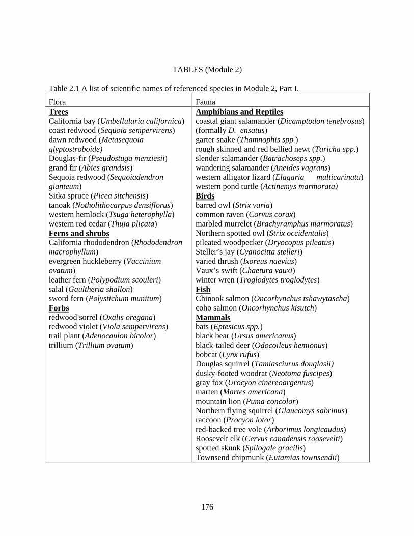
TABLES (Module 2) Table 2.1 A list of scientific names of referenced species in Module 2, Part I.

Flora Fauna Trees California bay (Umbellularia californica) coast redwood (Sequoia sempervirens) dawn redwood (Metasequoia glyptostroboide) Douglas-fir (Pseudostuga menziesii) grand fir (Abies grandsis) Sequoia redwood (Sequoiadendron gianteum) Sitka spruce (Picea sitchensis) tanoak (Notholithocarpus densiflorus) western hemlock (Tsuga heterophylla) western red cedar (Thuja plicata) Ferns and shrubs California rhododendron (Rhododendron macrophyllum) evergreen huckleberry (Vaccinium ovatum) leather fern (Polypodium scouleri) salal (Gaultheria shallon) sword fern (Polystichum munitum) Forbs redwood sorrel (Oxalis oregana) redwood violet (Viola sempervirens) trail plant (Adenocaulon bicolor) trillium (Trillium ovatum)

Amphibians and Reptiles coastal giant salamander (Dicamptodon tenebrosus) (formally D. ensatus) garter snake (Thamnophis spp.) rough skinned and red bellied newt (Taricha spp.) slender salamander (Batrachoseps spp.) wandering salamander (Aneides vagrans) western alligator lizard (Elagaria multicarinata) western pond turtle (Actinemys marmorata) Birds barred owl (Strix varia) common raven (Corvus corax) marbled murrelet (Brachyramphus marmoratus) Northern spotted owl (Strix occidentalis) pileated woodpecker (Dryocopus pileatus) Steller’s jay (Cyanocitta stelleri) varied thrush (Ixoreus naevius) Vaux’s swift (Chaetura vauxi) winter wren (Troglodytes troglodytes) Fish Chinook salmon (Oncorhynchus tshawytascha) coho salmon (Oncorhynchus kisutch) Mammals bats (Eptesicus spp.) black bear (Ursus americanus) black-tailed deer (Odocoileus hemionus) bobcat (Lynx rufus) Douglas squirrel (Tamiasciurus douglasii) dusky-footed woodrat (Neotoma fuscipes) gray fox (Urocyon cinereoargentus) marten (Martes americana) mountain lion (Puma concolor) Northern flying squirrel (Glaucomys sabrinus) raccoon (Procyon lotor) red-backed tree vole (Arborimus longicaudus) Roosevelt elk (Cervus canadensis roosevelti) spotted skunk (Spilogale gracilis) Townsend chipmunk (Eutamias townsendii)

176

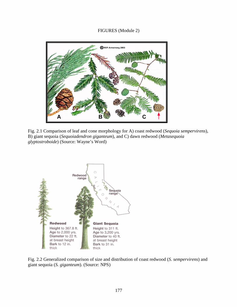
FIGURES (Module 2)

Fig. 2.1 Comparison of leaf and cone morphology for A) coast redwood (Sequoia sempervirens), B) giant sequoia (Sequoiadendron giganteum), and C) dawn redwood (Metasequoia glyptostroboide) (Source: Wayne’s Word)

Fig. 2.2 Generalized comparison of size and distribution of coast redwood (S. sempervirens) and giant sequoia (S. giganteum). (Source: NPS)

177

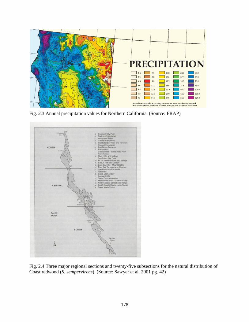
Fig. 2.3 Annual precipitation values for Northern California. (Source: FRAP)

Fig. 2.4 Three major regional sections and twenty-five subsections for the natural distribution of Coast redwood (S. sempervirens). (Source: Sawyer et al. 2001 pg. 42)

178

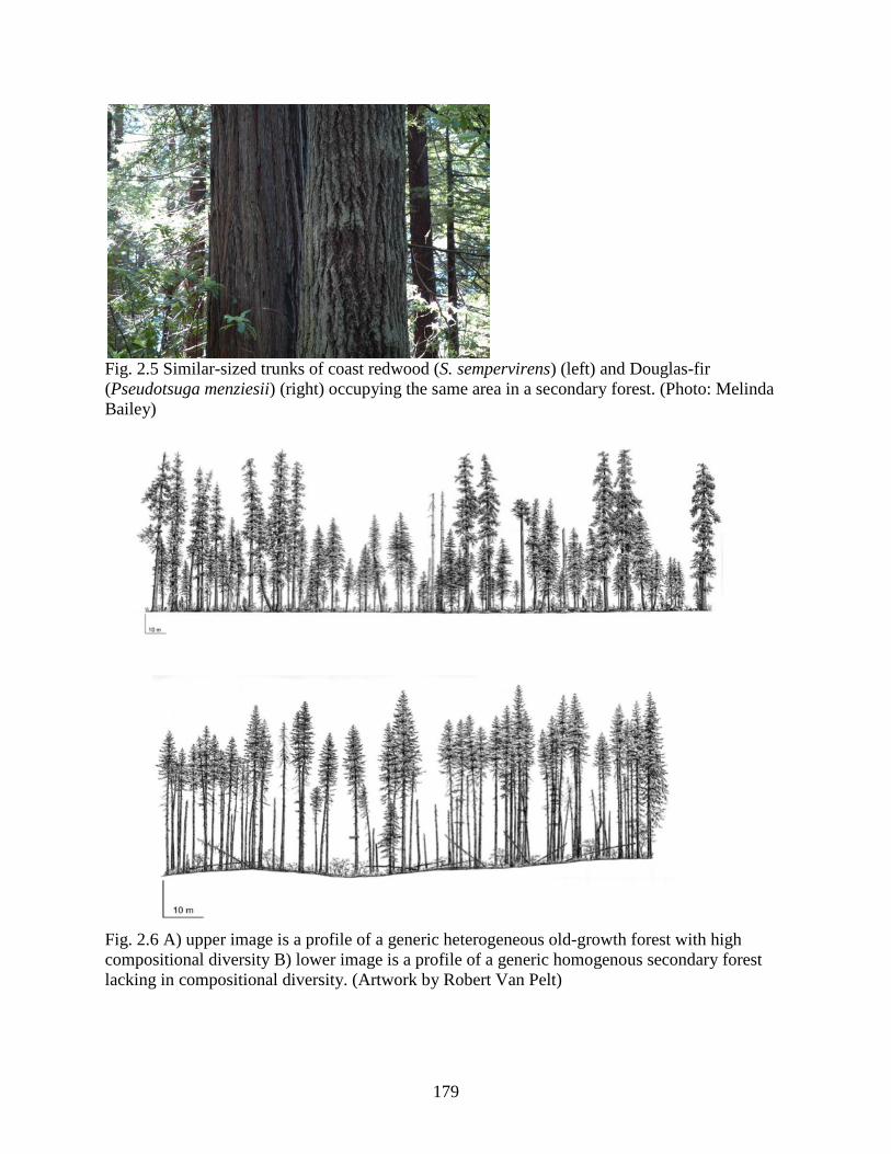
Fig. 2.5 Similar-sized trunks of coast redwood (S. sempervirens) (left) and Douglas-fir (Pseudotsuga menziesii) (right) occupying the same area in a secondary forest. (Photo: Melinda Bailey)

Fig. 2.6 A) upper image is a profile of a generic heterogeneous old-growth forest with high compositional diversity B) lower image is a profile of a generic homogenous secondary forest lacking in compositional diversity. (Artwork by Robert Van Pelt)

179

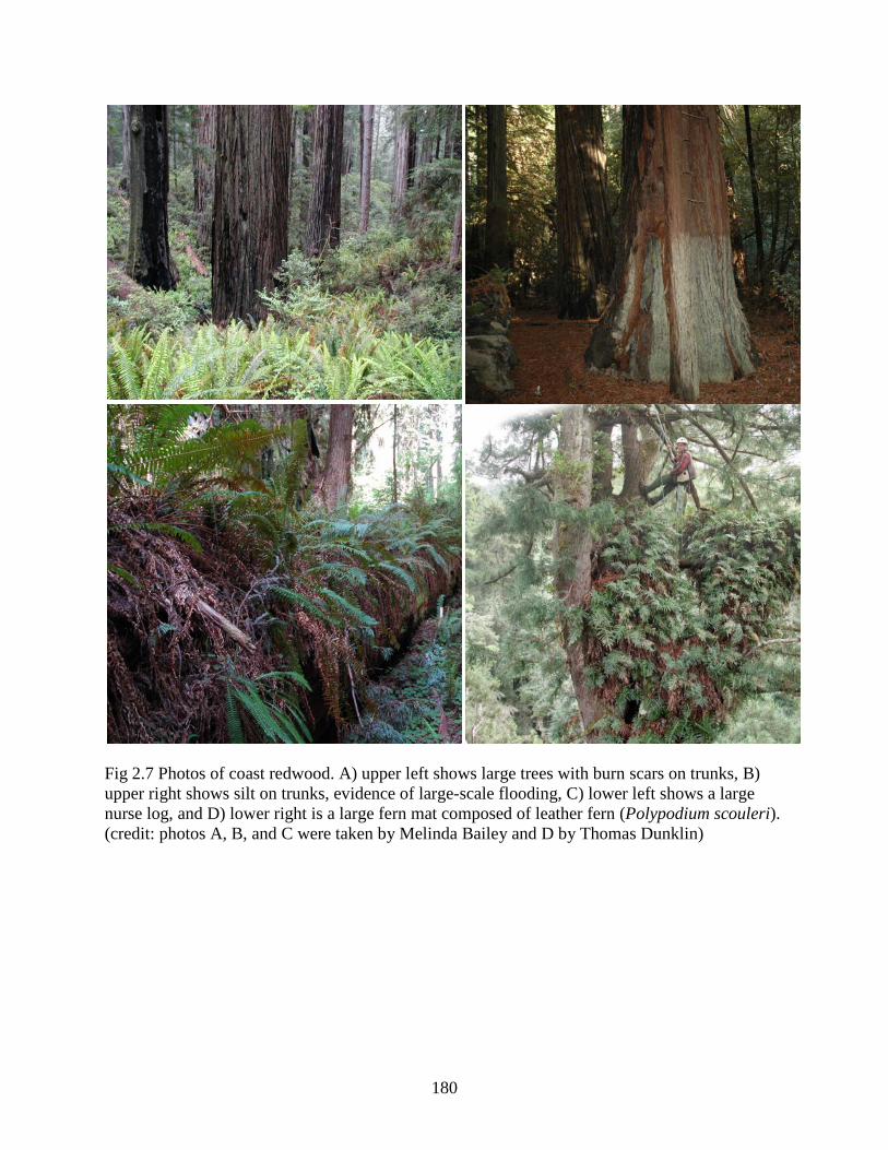
Fig 2.7 Photos of coast redwood. A) upper left shows large trees with burn scars on trunks, B) upper right shows silt on trunks, evidence of large-scale flooding, C) lower left shows a large nurse log, and D) lower right is a large fern mat composed of leather fern (Polypodium scouleri). (credit: photos A, B, and C were taken by Melinda Bailey and D by Thomas Dunklin)

180

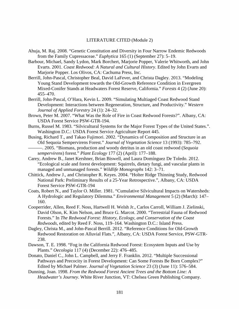
LITERATURE CITED (Module 2) Ahuja, M. Raj. 2008. “Genetic Constitution and Diversity in Four Narrow Endemic Redwoods

from the Family Cupressaceae.” Euphytica 165 (1) (September 27): 5–19. Barbour, Michael, Sandy Lydon, Mark Borchert, Marjorie Popper, Valerie Whitworth, and John

Evarts. 2001. Coast Redwood: A Natural and Cultural History. Edited by John Evarts and Marjorie Popper. Los Olivos, CA: Cachuma Press, Inc.

Berrill, John-Pascal, Christopher Beal, David LaFever, and Christa Dagley. 2013. “Modeling Young Stand Development towards the Old-Growth Reference Condition in Evergreen Mixed-Conifer Stands at Headwaters Forest Reserve, California.” Forests 4 (2) (June 20): 455–470.

Berrill, John-Pascal, O’Hara, Kevin L. 2009. “Simulating Multiaged Coast Redwood Stand Development: Interactions between Regeneration, Structure, and Productivity.” Western Journal of Applied Forestry 24 (1): 24–32.

Brown, Peter M. 2007. “What Was the Role of Fire in Coast Redwood Forests?”. Albany, CA: USDA Forest Service PSW-GTR-194.

Burns, Russel M. 1983. “Silvicultural Systems for the Major Forest Types of the United States.”. Washington D.C.: USDA Forest Service Agriculture Report 445.

Busing, Richard T., and Takao Fujimori. 2002. “Dynamics of Composition and Structure in an Old Sequoia Sempervirens Forest.” Journal of Vegetation Science 13 (1993): 785–792.

———. 2005. “Biomass, production and woody detritus in an old coast redwood (Sequoia sempervirens) forest.” Plant Ecology 177 (2) (April): 177–188.

Carey, Andrew B., Janet Kershner, Brian Biswell, and Laura Domínguez De Toledo. 2012. “Ecological scale and forest development: Squirrels, dietary fungi, and vascular plants in managed and unmanaged forests.” Wildlife Monographs 142: 3–71.

Chittick, Andrew J., and Christopher R. Keyes. 2004. “Holter Ridge Thinning Study, Redwood National Park: Preliminary Results of a 25-Year Retrospective.”, Albany, CA: USDA Forest Service PSW-GTR-194

Coats, Robert N., and Taylor O. Miller. 1981. “Cumulative Silvicultural Impacts on Watersheds: A Hydrologic and Regulatory Dilemma.” Environmental Management 5 (2) (March): 147–160.

Cooperrider, Allen, Reed F. Noss, Hartwell H. Welsh Jr., Carlos Carroll, William J. Zielinski, David Olson, K. Kim Nelson, and Bruce G. Marcot. 2000. “Terrestrial Fauna of Redwood Forests.” In The Redwood Forest: History, Ecology, and Conservation of the Coast Redwoods, edited by Reed F. Noss, 119–164. Washington D.C.: Island Press.

Dagley, Christa M., and John-Pascal Berrill. 2012. “Reference Conditions for Old-Growth Redwood Restoration on Alluvial Flats.”, Albany, CA: USDA Forest Service, PSW-GTR-238.

Dawson, T. E. 1998. “Fog in the California Redwood Forest: Ecosystem Inputs and Use by Plants.” Oecologia 117 (4) (December 22): 476–485.

Donato, Daniel C., John L. Campbell, and Jerry F. Franklin. 2012. “Multiple Successional Pathways and Precocity in Forest Development: Can Some Forests Be Born Complex?” Edited by Michael Palmer. Journal of Vegetation Science 23 (3) (June 11): 576–584.

Dunning, Joan. 1998. From the Redwood Forest Ancient Trees and the Bottom Line: A Headwater’s Journey. White River Junction, VT: Chelsea Green Publishing Company.

181

Earle, Christopher. 2013. “The Gymnosperm Database.” http://www.conifers.org. Fire Resource and Assessment Program (FRAP). 2003. “Forests and Climate Change: Forest and

Range 2003 Assessment.” In The Changing California, 1–24. FRAP. Franklin, Jerry F., Thomas A. Spies, Robert Van Pelt, Andrew B. Carey, Dale A. Thornburgh,

Dean Rae Berg, David B. Lindenmayer, et al. 2002. “Disturbances and Structural Development of Natural Forest Ecosystems with Silvicultural Implications, Using Douglas-Fir Forests as an Example.” Forest Ecology and Management 155: 399–423.

Franklin, Jerry F., Dean Rae Berg, Andrew B. Carey, and Richard A. Hardt. 2006. “Old Growth Conifer Forests.” In Restoring the Pacific Northwest: The Art and Science of Ecological Restoration in Cascadia, edited by D. Apostol and M Sinclair, 100–150. Washington D.C.: Island Press.

Fritschle, Joy A. 2009. “Pre-EuroAmerican Settlement Forests in Redwood National Park, California, USA: A Reconstruction Using Line Summaries in Historic Land Surveys.” Landscape Ecology 24 (6) (May 13): 833–847.

Fritz, Emanuel. 1940. “Problems in Dating Rings of California Coast Redwood.” Tree Ring Bulletin 6 (3): 19–22.

Galindo-Leal, Carlos, and Fred L. Bunnel. 1995. “Ecosystem Management : Implications and Opportunities of a New Paradigm.” The Forestry Chronicle 71 (5): 601–606.

Green Diamond Resource Compnay (GDRC). 2014. “California: Maintaining Essential Habitat.” https://greendiamond.com/responsible-forestry/california/

Giusti, Gregory A. 1988. “Recognizing Damage by Black Bear Damage to Second Growth Redwoods.” In Proceedings of the Thirteenth Vertebrate Pest Conference, 188–189. Lincoln, NB: UC California Cooperative Extension.

———. 2004. “Structural Characteristics of an Old-Growth Coast Redwood Stand in Mendocino.”, Albany, CA: USDA Forest Service PSW-GTR-197

———. 2012. “Management Practices Related to the Restoration of Old Forest Characteristics in Coast Redwood Forests.”, Albany, CA: USDA Forest Service PSW-GTR-238.

Gower, Stith T., Ross E. Mcmurtrie, and Danuse Murty. 1996. “Aboveground Net Primary Production Decline with Stand Age: Potential Causes.” TREE 11 (9): 378–382.

Hagar, Joan C. 2007. “Managing for Wildlife Habitat in Westside Production Forests.”, Portland, OR: USDA Forest Service PNW-GTR-695.

Hamilton, Healy. 2013. “Current and Future Trends in Coast Redwood Climate.” In Past, Present and Future of Redwoods: A Redwood Ecology and Climate Symposium, sponsored by Save-the-Redwoods League. unpublished

Hartley, Ruskin K. 2012. “Redwood Forest Conservation: Where Do We Go from Here?”, Albany, CA: USDA Forest Service PSW-GTR-238.

Ishii, Hiroaki T., Shin-ichi Tanabe, and Tsutom Hiura. 2004. “Exploring the Relationships among Canopy Structure, Stand Productivity, and Biodiversity of Temperate Forest Ecosystems.” Forest Science 50 (3): 342–355.

Johnston, Verna R. 1994. California Forests and Woodlands. Berkeley, CA: University of California Press.

Johnstone, James A., and Todd E. Dawson. 2010. “Climatic Context and Ecological Implications of Summer Fog Decline in the Coast Redwood Region.” Proceedings of the National Academy of Sciences of the United States of America. Vol. 107.

Jones, D. A., and K. L. O’Hara. 2011. “Carbon Density in Managed Coast Redwood Stands: Implications for Forest Carbon Estimation.” Forestry 85 (1) (December 6): 99–110.

182

Keppeler, Elizabeth. 2007. “Effects of Timber Harvest on Fog Drip and Streamflow, Caspar Creek Experimental Watersheds, Mendocino County, California.”, Albany, CA: USDA Forest Service PSW-GTR-194.

Kidder, Allison. 2013. “Big Trees, Big Trouble.” Berkeley Science Review. http://sciencereview.berkeley.edu.

Kruse, Bill. 2013. “Redwoods, Lasers, Optics and Bytes: Computational Remote Sensing for the RCCI from Trees to the Landscape.” In Past, Present and Future of Redwoods: A Redwood Ecology and Climate Symposium, 11–15. sponsored by Save-the-Redwoods League.

Lefsky, M. A., W. B. Cohen, S. A. Acker, G. G. Parker, T. A. Spies, and D. Harding. 1996. “Lidar Remote Sensing of the Canopy Structure and Biophysical Properties of Douglas-Fir Western Hemlock Forests”. Remote Sensing Environment (70): 339-361.

Lenihan, James M., Raymond Drapek, Dominique Bachelet, and Ronald P. Neilson. 2003. “Climate Change Effects on Vegetation Distribution, Carbon, and Fire in California.” Ecological Applications 13 (6): 1667–1681.

Limm, Emily Burns, Kevin A. Simonin, Aron G. Bothman, and Todd E. Dawson. 2009. “Foliar Water Uptake: A Common Water Acquisition Strategy for Plants of the Redwood Forest.” Oecologia 161 (3) (September): 449–59.

Lindenmayer, D.B., J.F. Franklin, and J. Fischer. 2006. “General Management Principles and a Checklist of Strategies to Guide Forest Biodiversity Conservation.” Biological Conservation 131 (3) (August): 433–445.

Lindquist, James. 2004. “The Whiskey Springs Redwood Commercial Thinning Study : A 29- Year Status Report (1970 to 1999) 305–315, Albany, CA: USDA Forest Service PSW-GTR-194.

Litman, Laurie, and Gary Nakamura. 2007. “Forest Ecology.” http://anrcatalog.ucdavis.edu. Lorimer, Craig G., Daniel J. Porter, Mary Ann Madej, John D. Stuart, Stephen D. Veirs, Steven

P. Norman, Kevin L. O’Hara, and William J. Libby. 2009. “Presettlement and Modern Disturbance Regimes in Coast Redwood Forests: Implications for the Conservation of Old-Growth Stands.” Forest Ecology and Management 258 (7) (September): 1038–1054.

Loya, David T., and Erik S. Jules. 2007. “Use of Species Richness Estimators Improves Evaluation of Understory Plant Response to Logging: A Study of Redwood Forests.” Plant Ecology 194 (2) (April 6): 179–194.

Lutz, James A., and Charles B. Halpern. 2006. “Tree Mortality during Early Forest Development: A Long-Term Study of Rates, Causes, and Consequences.” Ecological Monographs 76 (2): 257–275.

Madej, Mary Ann. 2010. “Redwoods, Restoration, and Implications for Carbon Budgets.” Geomorphology 116 (3-4) (April): 264–273.

Mazurek, M.J, and William J. Zielinski. 2004. “Individual Legacy Trees Influence Vertebrate Wildlife Diversity in Commercial Forests.” Forest Ecology and Management 193 (3) (June): 321–334.

Michels, Kristin K. Hageseth, and Will Russell. 1981. “A Chronosequence of Vegetation Change Following Timber Harvest in Naturally Recovering Coast Redwood (Sequoia sempervirens) Forests.”, Albany, CA: USDA Forest Service PSW-GTR-238.

Millar, Constance I., Nathan L. Stephenson, and Scott L. Stephens. 2007. “Climate Change and Forests of the Future: Managing in the Face of Uncertainty.” Ecological Applications : A Publication of the Ecological Society of America 17 (8) (December): 2145–51.

183

Monroe, Gary W., and Forest Reynolds. 1974. “Natural Resources of the Eel River Delta.”. Coastal Wetland Series #9. California Department of Fish and Game.

Myers, Norman. 1988. “Tropical Forests and Their Species.” In Biodiversity, edited by E.O. Wilson and Frances M. Peter, 28–35. Washington D.C.: National Academy of Sciences/Smithsonian Institution.

Noss, Reed F. 2000a. “More Than Big Trees.” In The Redwood Forest: History, Ecology, and Conservation of the Coast Redwoods, edited by Reed F. Noss. Washington D.C.: Island Press.

———. 2000b. “Lessons from the Redwoods.” In The Redwood Forest: History, Ecology, and Conservation of the Coast Redwoods, edited by Reed F. Noss, 263–268. Washington D.C.: Island Press.

O’Hara, Kevin L., and John-Pascal Berrill. 2009. “Dynamics of Coast Redwood Sprout Clump Development in Variable Light Environments.” Journal of Forest Research 15 (2) (December 25): 131–139.

O’Hara, Kevin L., Petru Tudor Stancioiu, and Mark A. Spencer. 2007. “Understory Stump Sprout Development under Variable Canopy Density and Leaf Area in Coast Redwood.” Forest Ecology and Management 244 (1-3) (June): 76–85.

Olson, David F., Douglass F. Roy, and Gerald A. Walters. 1990. “Sequoia Sempervirens (D. Don) Endl.” In Silvics of North America Vol:1 Conifers, edited by R.M. Barnes and B.H. Honkala, 541–551. USDA Forest Service.

Peattie, Donald Culross. 1981. A Natural History of Western Trees. 2nd ed. Boston, MA: Houghton Miffline Company.

Pwnet. 2013. “Comparison of Tropical and Temperate Rain Forests.” America’s Rain Forests. http://rainforests.pwnet.org.

Raphael, Martin G. 2006. “Conservation of the Marbled Murrelet under the Northwest Forest Plan.” Conservation Biology 20 (2) (April): 297–305.

Rizzo, David M., and Matteo Garbelotto. 2003. “Sudden Oak Death: Endangering California and Oregon Forest Ecosystems.” Frontiers in Ecology and the Environment 1 (5): 197–204.

Rosso, Abbey L., Bruce Mccune, and Thomas R. Rambo. 2000. “Ecology and Conservation of a Rare , Old-Growth-Associated Canopy Lichen in a Silvicultural Landscape.” The Bryologist 103 (1): 117–127.

Russell, William. 2009. “The Influence of Timber Harvest on the Structure and Composition of Riparian Forests in the Coastal Redwood Region.” Forest Ecology and Management 257 (5) (February): 1427–1433.

———. 2000. “Ecology and Management of Coast Redwood (Sequoia sempervirens).” In Conference on the Restoration and Management of Coast Redwood at Jackson Demonstration State Forest, edited by William Russell, 6–22. Fort Bragg, CA.

Ryan, Michael G., Dan Binkley, James H. Fownes, Christian P. Giardina, and Randy S. Senock. 2004. “An Experimental Test of the Causes of Forest Growth Decline with Stand Age.” Ecological Monographs 74 (3): 393–414.

Sanders, Tim, and World Forest. 2011. “Adaptive Management in Response to Climate Change: A Synthesis of Research Findings and Observations from the Pacific Northwest Forests.”

Save-the-Redwoods League (SRL). 2013. “The Most Massive Trees.” About Redwoods. http://www.savetheredwoods.org/redwoods/giant-sequoias.php.

Sawyer, John O., Jane Gray, James G. West, Dale A. Thornburg, Reed F. Noss, Joseph H. Engbeck, Bruce G. Marcot, and Roland Raymond. 2000. “History of Redwood and

184

Redwood Forests.” In The Redwood Forest: History, Ecology, and Conservation of the Coast Redwoods, edited by Reed F. Noss, 7–38. Washington D.C.: Island Press.

Sawyer, John O., Stephen C. Sillett, William J. Libby, Todd E. Dawson, James H. Popenoe, David L. Largent, Robert Van Pelt, et al. 2000. “Redwood Trees, Communities, and Ecosystems: A Closer Look.” In The Redwood Forest: History, Ecology, and Conservation of the Coast Redwoods, edited by Reed F. Noss, 81–118. Washington D.C.: Island Press.

Sawyer, John O., Stephen C. Sillett, James H. Popenoe, Dale A. Thornburg, Anthony LaBanca, Teresa Sholars, David L. Largent, Fred Euphrat, Reed F. Noss, and Robert Van Pelt. 2000. “Characteristics of Redwood Forests.” In The Redwood Forest: History, Ecology, and Conservation of the Coast Redwoods, 39–80. Washington D.C.: Island Press.

Schoenherr, Allan A. 1992. A Natural History of California, Berkeley, CA: University of California Press.

Schultz, Stewart T. 1990. The Nortwest Coast. The Northwest Coast: A Natural History. Portland, OR: Timber Press, Inc.

Sillett, Stephen C. 2013. “Separating Effects of Tree Size and Age on Trunk Growth in California Redwoods.” Abstract of report given In Past, Present and Future of Redwoods: A Redwood Ecology and Climate Symposium sponsored by Save-the-Redwoods League, unpublished data.

Sillett, Stephen C., and Matthew N. Goslin. 1999. “Distribution of Epiphytic Macrolichens in Relation to Remnant Trees in a Multiple-Age Douglas-Fir Forest.” Canadian Journal of Forest Research 29: 1204–1215.

Sillett, Stephen C., and Robert Van Pelt. 2000. “A Redwood Tree Whose Crown Is a Forest Canopy.” Northwest Science 74 (1): 34–43.

———. 2007. “Trunk Reiteration Promotes Ephiphytes and Water Storage in an Old-Growth Redwood Forest Canopy.” Ecological Monographs 77 (3): 335–359.

Sillett, Stephen C., Robert Van Pelt, George W. Koch, Anthony R. Ambrose, Allyson L. Carroll, Marie E. Antoine, and Brett M. Mifsud. 2010. “Increasing Wood Production through Old Age in Tall Trees.” Forest Ecology and Management 259 (5) (February): 976–994.

Sillett, Stephen C., Robert Van Pelt, Russell Kramer, and Allyson L. Carroll. 2013. “Annual Rates of Trunk Wood Production in Old-Growth Redwood Forest since 1750.” In Past, Present and Future of Redwoods: A Redwood Ecology and Climate Symposium. Save-the- Redwoods League. Unpublished data.

Stone, Stephanie, and Andrew Ng. 2013. “Mapping Our Future.” California Academy of Science Newsletter. http://calacademy.org/newsroom.

Swenson, Steven W. 2009. “Carbon Distribution in Managed Upland Redwood Stands Using the California Climate Registry Forest Project Protocol”. Master's Thesis. Humboldt State University.

Teraoka, Jason R., and Christopher R. Keyes. 2011. “Low Thinning as a Forest Restoration Tool and Redwood National Park.” Western Journal of Applied Forestry 26 (2): 91–93.

Thompson, Ian, Brendan Mackey, Steven McNulty, and Alex Mosseler. 2009. “Forest Resilience, Biodiversity, and Climate Change.”, Convention on Biological Diversity, UNEP

Thornburgh, Dale A., Reed F. Noss, Dean P. Angelides, Craig M. Olson, Fred Euphrat, and Hartwell H. Welsh Jr. 2000. “Managing Redwoods.” In The Redwood Forest: History, Ecology, and Conservation of the Coast Redwoods, edited by Reed F. Noss, 229–262. Washington D.C.: Island Press.

185

Valentine, Bradley E. 2012. “Size Distribution of Unharvested Redwood Forests in Mendocino County.”, Albany, CA: USDA Forest Service PSW-GTR-238.

Van Pelt, Robert. 2001. Forest Giants of the Pacific Coast, Seattle: WA: Global Forest Society and University of Washington Press.

Van Pelt, Robert, and Jerry F. Franklin. 2000. “Influence of Canopy Structure on the Understory Environment in Tall, Old-Growth, Conifer Forests.” Canadian Journal of Forest Research 30 (8) (August): 1231–1245.

Veirs Jr., Stephen D. 1996. “Ecology of the Coast Redwood”. Arcata, CA: Proceedings of the Conference for Coast Redwood.

Vose, James M., David L. Peterson, and Toral Patel-Weynand. 2012. “Effects of Climatic Variability and Change on Forest Ecosystems: A Comprehensive Science Synthesis for the U. S. Forest Sector.”, Portland, OR: USDA Forest Service PNW-GTR-870.

Waring, R. H., and J. Major. 1964. “Some Vegetation of the California Coastal Redwood Region in Relation to Gradients of Moisture, Nutrients, Light, and Temperature.” Ecological Society of America 34 (2): 167–215.

Webb, Lynn A., James L. Lindquist, Erik Wahl, and Andres Hubbs. 2011. “Whiskey Springs Long-Term Coast Redwood Density Management; Final Grown, Sprout, and Yield Results”. Albany, CA: USDA Forest Service PSW-GTR-238.

Weir, Roseanne. n.d. "Temperate Rainforest Ecosystems" Nasa Quest! quest.arc.nasa.gov/projects/jason/xv/docs/TempRain.pdf

Williams, Cameron B., and Stephen C. Sillett. 2007. “Epiphyte Communities on Redwood (Sequoia sempervirens) in Northwestern California.” The Bryologist 110 (3): 420–452.

Wolf, Edward C., Andrew P. Mitchell, and Peter K. Schoonmaker. 1995. The Rain Forests of Home: An Atlas of People and Place. Edited by Erin L. Kellogg. Ecotrust, Pacific GIS, Conservation International.

Zinke, Paul J. 1988. “The Redwood Forest and Associated North Coast Forests.” In Terrestrial Vegetation of California, edited by Michael G Barbour and Jack Major, 2nd ed., 679–698. Davis, CA: California Native Plant Society.

Zuckerman, Seth. 2000. “Arcata Community Forest: A Model for Redwood Management.” In Conference on the Restoration and Management of Coast Redwood at Jackson Demonstration State Forest, edited by William H. Russell, 35–37. Fort Bragg, CA.

186

Forest Ecology 101 Series (M2: Part II)

Module 2: Behind the Redwood Curtain

Part II

UNIT OF STUDY COVER PAGE

Grade 7 Unit Lesson 1 - Teasing Temperate Rainforests

Lesson 2 - Comparing Cousins Lesson 3 - Tree Thinning Dynamics

Lesson 4 - Measuring Up to the Tallest Trees Lesson 5 - Hidden Heights

187

M2.G7 Lesson 1: Teasing Temperate Rainforests Unit Overview: Coast Redwoods Grade 7 Key Concepts:

• Earth’s biomes • Patterns: cause and

effect • Stability and change • Gather and synthesize

information • Biodiversity and

humans Time: 50 - 80 minutes Materials for the Teacher: Student reading

M2.7.1a Student handout and

Teacher key M2.7.1b Pictures of tropical

and temperate rainforests (optional)

Connections: Geography, earth science, biogeography, biology, botany, biodiversity, forestry, carbon cycle, soils, biomass, climate change, atmosphere, human interactions, endangered species Forest Ecology Series integration: M1: Integrative Forest Ecology

Learning Objectives: Students will understand why the northernmost coastal forests of California are referred to as a temperate rainforest. They will compare factors between temperate and tropical rainforests including latitude, average rainfall, soils, canopy heights, biomass, and biodiversity in order to understand how and why these two biomes differ. Background information: Refer to the appropriate section in Part I: Teacher Companion for Module 2 and online information. Suggested procedure: Begin the lesson by asking some of the preliminary questions below to assess what students already know about rainforests and forests in general. Write down their responses. Once this short discussion is done, give a solid definition of a forest. Follow up by showing a few slides that compare various features of tropical and temperate forests. Visuals can also serve as a reinforcement and can be shown after the students have finished the reading and/or after completing the worksheet below. Have students read the passage Comparing Temperate and Tropical Rainforests (see M2.7.1a). This can be alone, in groups, or assigned as homework. Once they are done, have them complete the handout where they will fill out a comparison chart and write a summary (see M2.7.1b). Begin or end this lesson with some of the suggested extensions below. Preliminary questions:

• What is the definition of a forest? (Continue to ask for more information until you get several components of a forest such as the hydrologic cycle and several of the interconnected relationships between abiotic and biotic factors).

• What are some different forest types? • What environmental factors might limit or influence a

forest type? • What do you associate rainforests with? • (Hold up a globe or point on map) - Does anyone know

where tropical rainforests are found? • What sorts of forests do we have growing in our region? • Within what latitudinal zone do we live? • Do you think we live near a rainforest?

Critical Thinking: Some researchers predict that some areas of the tropical rainforest may change into a savannah because of human disturbance and climate change. What potential

188

changes in the environment could cause this shift? Keywords: abiotic factor, annual, biomass, biodiversity, debris, decomposition, deforestation, diameter, hectare, latitude, precipitation, rainforest NGSS alignment: MS-LS2: Ecosystems: Interactions, Energy, and Dynamics LS2.A: Interdependent Relationships in Ecosystems LS2.B: Cycle of Matter and Energy Transfer in Ecosystems LS2.C: Ecosystem Dynamics, Functioning, and Resilience LS4.D: Biodiversity and Humans ETS1:B Developing Possible Solutions Online resources: GCS Webquest: Rainforests temperate and tropical http://its.guilford.k12.nc.us/webquests/rf/rf.htm This site has information contrasting tropical and temperate forests and suggests making a Venn diagram, having students write a report, and supplies a card game. America’s Rainforests: http://rainforests.pwnet.org/4teachers/background.php Here you can find good indepth information on both types of rainforests including the role of forests, different types of tropical forests, wood products, and climate change. It also includes many good links for further exploration. Rainforest Action Network: http://ran.org/get-involved Go to this website if you want students to participate in rainforest protection. This organization has adopt-an-acre program, awareness about palm oil, and many other campaigns students can get involved with. Atlas for the temperate rainforests of North America http://www.ecotrust.org/publications/rain-forests-atlas.html This atlas gives good up-to-date information regarding the cultural and physical geography of the Pacific Northwest including colorful maps. It nicely connects the relationship between forests, rivers and the sea and explains how these forested communities were intimately connected to the first peoples. From this site you can download a free pdf of the atlas. EEI Connection: B.6.a. Biodiversity: The keystone of Life on Earth B.8.b Biological Diversity: The World’s Riches

189

M2.G7.L1 (Unit Overview continued) Answers to preliminary questions: - What is the definition of a forest? (Continue to ask for more information until you get several components of a forest such as the hydrologic cycle and several of the interconnected relationships between abiotic and biotic factors). (Answers will vary) - What are some different forest types? (Accept all answer. Forest types include redwood forests, mixed evergreen forests, tropical forests, cloud forest, etc.) - What environmental factors might limit or influence a forest type? (Accept all answers. Factors include rainfall, altitude, latitude, temperature, soil type, etc.) - What do you associate rainforests with? (answers will vary) -(Hold up a globe or point on map) Does anyone know where tropical rainforests are found? (in the tropical zone 23.5 degrees north and south of the equator) - What sorts of forests do we have growing in our region? (Most students should be able to come up with a redwood forest. Others types include dune forest, oak woodland, evergreen forest, coastal forest, Douglas fir or mixed evergreen, closed pine forest, etc.) -Within what latitudinal zone do we live? (The North Coast lies within the temperate zone 23.5 - 66.5 degrees north and south) -Do you think we live near a rainforest? (This answer varies depending on your location. The northern most redwood groves of California are considered temperate rainforests.) Suggested follow up questions:

• What are three main differences between a tropical and temperate rainforest? • How do these rainforests compare with other forest types? • Which type of forest has the greatest biodiversity? • Who knows of an endangered species that lives in a rainforest? • What is an epiphyte? What is an example of an epiphyte? • What sort of forest has the highest above ground biomass compared to all other forest

types? • How can human beings help save rainforests?

Suggested extensions:

• Have students write a short report about a threatened or endangered species living in a tropical or temperate rainforest.

• As authentic assessment, have students draw a large picture of a temperate rainforest including most of the components reviewed in this lesson.

• Using maps have students shade and label the different latitudinal zones. • Have students research different products that come from a tropical rainforest. Make a

large classroom list as they come up with answers. • Show a video about a rainforest or other forest type. • Integrate awareness about global extinction and the loss of biodiversity coincided with

other local awareness campaigns such as Earth Day or River Days. M2.7.1a Student reading M2.7.1b Student worksheet and Teacher key

190

Student reading M2.7.1a Comparing Temperate and Tropical Rainforests

Rainforests are defined by the high amounts of yearly rainfall combined with moderate temperatures. There are two main types of rainforests: tropical rainforests and temperate rainforests, which are found in different regions of the world. Tropical rainforests are found between 23.5° north and south of the equator in the tropical zone. They can be found in many places around the world including Australia, Africa, Southeast Asia, the Caribbean, Brazil, and Central America. These forests typically have two seasons: wet and dry. On average they receive over 2,500 mm (98 in) of precipitation a year and have average temperatures above 24°C (75°F). Of course this varies depending on their location and global weather conditions. Temperate rainforests are found in the temperate zone located in latitudes ranging from 23.5-66.5 degrees north and south. They typically receive over 2,000 mm (80 in) of annual rainfall. By comparison, they have four seasons with most precipitation occurring between October and March. Average temperatures range from 2-3°C (28-37°F) in January and 20-27°C (68 - 81°F) in July. What type of rainforest do you think the lush redwood forests of northern California are a part of? If you guessed a temperate rainforest - you are correct. Because these places occur along the coast, they are often called Coastal Temperate Rain Forests or CTRFs. What is a CTRF? Ecologists Paul Alaback and James Weigand note four factors these forests have compared to other temperate forests, such as a pine forest or boreal forests. CTRFs are closer to the ocean, have coastal mountains, cooler summer temperatures, and higher rainfall levels. They use to be more widespread and were found on all continents except Africa and Antarctica. Today, more than half of the remaining CTRF is located in a coastal band extending from Humboldt County north to Alaska - called the Pacific Northwest. Other examples can be found in the coastal areas of Chile, Tasmania, and New Zealand. Even though all of the CTRFs have similar rainfall amounts, the plants and animals living in them will be different just like in tropical rainforests. Most trees in a tropical rainforest are evergreen with broadleaves. They don’t live much over 150 years and the tallest trees here measure about 60 m (200 ft) high. Many trees have large buttress roots to help support their shallow root systems. Due to high amounts of rainfall and warm temperatures, the rate of decomposition in tropical regions is high. Abundant rainfall leaches the soils so they tend to be acidic and lack nutrients and therefore, are considered poor soils. Many trees in the CTRF would tower over most tropical species. These tall trees are called conifers or evergreen trees and have needle-like leaves. Some

191

conifers grow so large they hold the world’s record for being the tallest and largest trees on the planet! Some of the larger ones can grow over 80 m (262 ft) high and have diameters over 6 m (20 ft). One reason why these trees can grow so large is because they live a long time. On average old conifers can grow over 600 years and the oldest redwoods can live over 2,000 years. Over long periods of time, large amounts of leaf litter and woody debris accumulate creating fertile soils. Because temperatures here are relatively cool, the rate of decomposition is slowed. If you weighed all of the living and once living things in a forest and then took this value and compared it to the amount of area the forest covers, you could calculate its biomass. Because trees in the CTRFs are so large, they have the highest amounts of biomass compared to any other type of ecosystem. In some cases they can have ten times the biomass of tropical forests. The forest type with the highest recorded above-ground biomass are old-growth coast redwood, which can reach heights over 110 m (360 ft). Although CTRFs have higher biomass compared to other forest types, tropical rainforests have the highest biodiversity. Combined, they may contain up to 60 percent of all known species on the planet! Biodiversity is the total number of different organisms that live in an area. In some places 100-300 different tree species can be found in just one hectare (2.5 acres). On the high end, one hectare may house approximately 8,000 different animal and plant species. By comparison, CTRFs may only have a dozen different trees and may only support around 400 different plant species and 300 bird and mammal species. Maintaining high biodiversity is one reason why forests are so valuable. Both types of rainforests are threatened by land clearing or deforestation. Rainforests are disappearing the fastest because the space they occupy is being converted to things like palm oil plantations and places to graze cattle. This broad-scale clearing of the world's tropical forests is the main cause of species extinctions. Every day scientists estimate that over 150 different plant and animals species disappear or become extinct due to tropical deforestation. One of the reasons why we lose so many tropical species compared to other places is because many organisms living here are very specialized and live nowhere else. Logging and land-clearing continue to occur in CTRFs and many of the tallest and largest trees are gone. --------------------------------------------------------------------

Written by Melinda Bailey

192

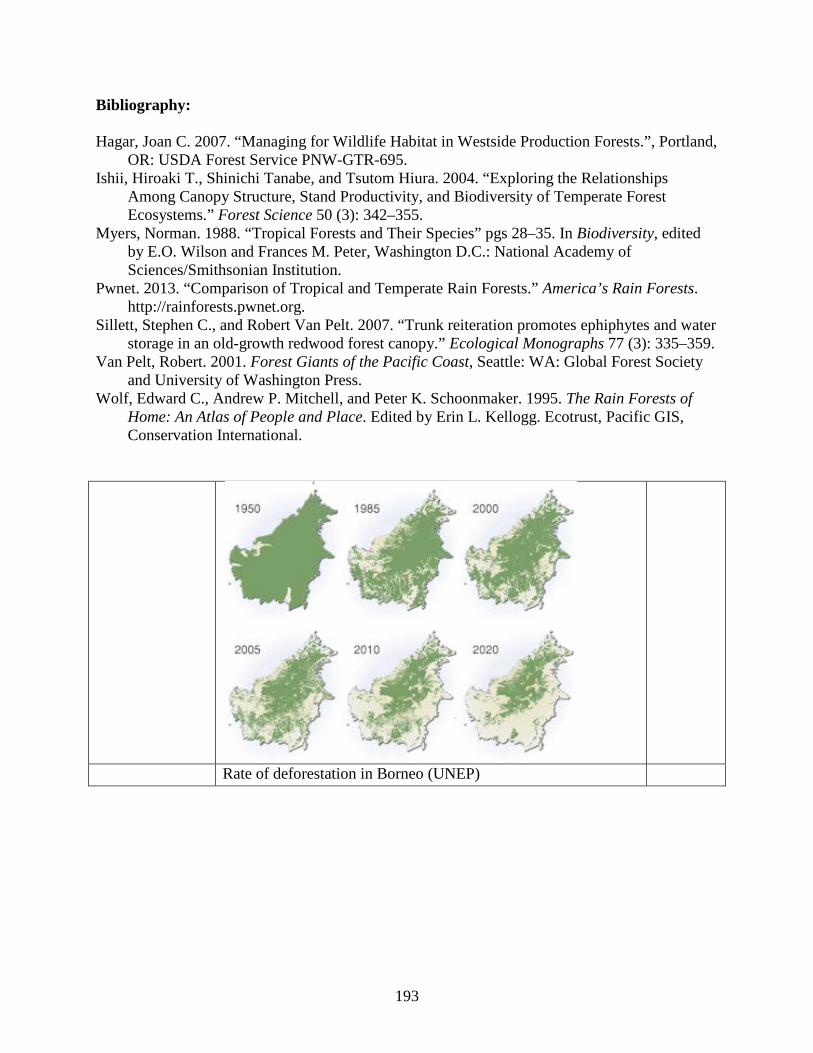
Bibliography: Hagar, Joan C. 2007. “Managing for Wildlife Habitat in Westside Production Forests.”, Portland,

OR: USDA Forest Service PNW-GTR-695. Ishii, Hiroaki T., Shinichi Tanabe, and Tsutom Hiura. 2004. “Exploring the Relationships

Among Canopy Structure, Stand Productivity, and Biodiversity of Temperate Forest Ecosystems.” Forest Science 50 (3): 342–355.

Myers, Norman. 1988. “Tropical Forests and Their Species” pgs 28–35. In Biodiversity, edited by E.O. Wilson and Frances M. Peter, Washington D.C.: National Academy of Sciences/Smithsonian Institution.

Pwnet. 2013. “Comparison of Tropical and Temperate Rain Forests.” America’s Rain Forests. http://rainforests.pwnet.org.

Sillett, Stephen C., and Robert Van Pelt. 2007. “Trunk reiteration promotes ephiphytes and water storage in an old-growth redwood forest canopy.” Ecological Monographs 77 (3): 335–359.

Van Pelt, Robert. 2001. Forest Giants of the Pacific Coast, Seattle: WA: Global Forest Society and University of Washington Press.

Wolf, Edward C., Andrew P. Mitchell, and Peter K. Schoonmaker. 1995. The Rain Forests of Home: An Atlas of People and Place. Edited by Erin L. Kellogg. Ecotrust, Pacific GIS, Conservation International.

Rate of deforestation in Borneo (UNEP)

193

Student worksheet G7.1b Name _________________________ Date ___________ Period _________ Directions: Read the passage Comparing Temperate and Tropical Rainforests. Using the information from the above reading, fill in the chart below.

Comparing temperate and tropical rainforests Feature

Temperate

Tropical

Latitude: (in degrees)

Places located:

Seasons:

Annual precipitation:

Average temperature:

Soil condition:

Biomass:

Rate of decomposition

Types of trees:

Tree height:

Longevity of trees:

Species diversity:

Other:

194

Follow Up: 1. What is the main abiotic factor that defines a rainforest? ______________________________________________________________________________

______________________________________________________________________________

______________________________________________________________________________

______________________________________________________________________________

______________________________________________________________________________

2. Why do the soils found in tropical regions tend to be poor? ______________________________________________________________________________

______________________________________________________________________________

______________________________________________________________________________

______________________________________________________________________________

______________________________________________________________________________

3. Identify three other places Coastal Temperate Rain Forests (CTRFs) occur besides northern California. ______________________________________________________________________________

______________________________________________________________________________

______________________________________________________________________________

______________________________________________________________________________

______________________________________________________________________________

4. Write three sentences about a temperate rainforest below. ______________________________________________________________________________

______________________________________________________________________________

______________________________________________________________________________

______________________________________________________________________________

______________________________________________________________________________

______________________________________________________________________________

______________________________________________________________________________

195

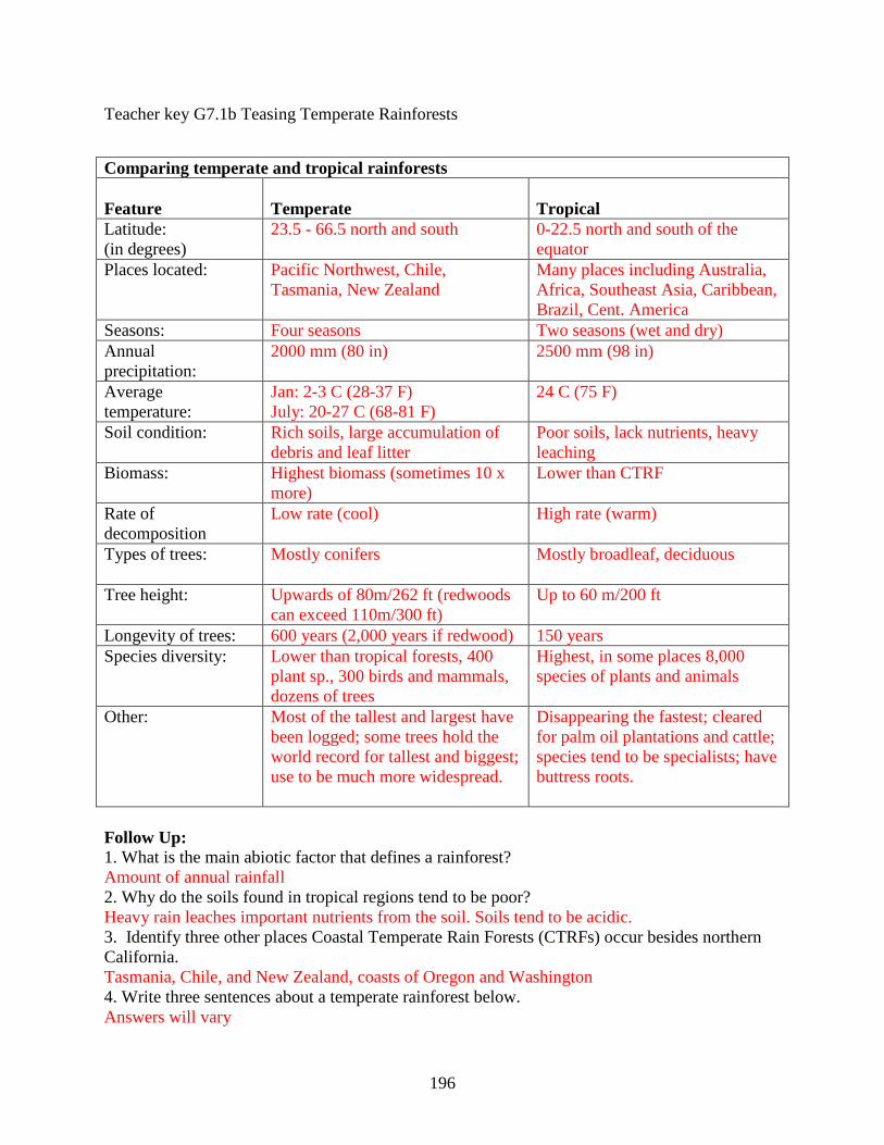
Teacher key G7.1b Teasing Temperate Rainforests

Comparing temperate and tropical rainforests Feature

Temperate

Tropical

Latitude: (in degrees)

23.5 - 66.5 north and south 0-22.5 north and south of the equator

Places located:

Pacific Northwest, Chile, Tasmania, New Zealand

Many places including Australia, Africa, Southeast Asia, Caribbean, Brazil, Cent. America

Seasons: Four seasons Two seasons (wet and dry) Annual precipitation:

2000 mm (80 in) 2500 mm (98 in)

Average temperature:

Jan: 2-3 C (28-37 F) July: 20-27 C (68-81 F)

24 C (75 F)

Soil condition:

Rich soils, large accumulation of debris and leaf litter

Poor soils, lack nutrients, heavy leaching

Biomass:

Highest biomass (sometimes 10 x more)

Lower than CTRF

Rate of decomposition

Low rate (cool) High rate (warm)

Types of trees:

Mostly conifers Mostly broadleaf, deciduous

Tree height:

Upwards of 80m/262 ft (redwoods can exceed 110m/300 ft)

Up to 60 m/200 ft

Longevity of trees: 600 years (2,000 years if redwood) 150 years Species diversity:

Lower than tropical forests, 400 plant sp., 300 birds and mammals, dozens of trees

Highest, in some places 8,000 species of plants and animals

Other:

Most of the tallest and largest have been logged; some trees hold the world record for tallest and biggest; use to be much more widespread.

Disappearing the fastest; cleared for palm oil plantations and cattle; species tend to be specialists; have buttress roots.

Follow Up: 1. What is the main abiotic factor that defines a rainforest? Amount of annual rainfall 2. Why do the soils found in tropical regions tend to be poor? Heavy rain leaches important nutrients from the soil. Soils tend to be acidic. 3. Identify three other places Coastal Temperate Rain Forests (CTRFs) occur besides northern California. Tasmania, Chile, and New Zealand, coasts of Oregon and Washington 4. Write three sentences about a temperate rainforest below. Answers will vary

196

M2.G7 Lesson 2: Comparing Cousins Unit: Coast Redwoods Grade 7 Key Concepts:

• Evidence of common ancestry

• Unity and diversity • Evolution and

adaptation • Heredity • Stability and change • Classification

Time: 40 - 60 minutes Materials for the Teacher: Pictures of different

redwood species that show leaves, bark, and general tree structure (see online resources).

Computers - one per student (optional)

Student worksheet and teacher key M2.7.2a

Connections: Geologic time, fossils, adaptation, natural selection, evolution, heredity, speciation, botany, genetics, endangered species, extinction, classification, climate change Forest Ecology Series integration: M1: Integrative Forest Ecology M3: Oak Woodlands

Learning Objectives: Students will compare and contrast similarities and differences between the three members of the redwood subfamily, in order to understand the concept of common ancestry and species diversity. Students will compare distribution, size, longevity, morphology, adaptations, and other notable features. By doing so they will understand that many organisms are classified based on shared similar traits. Background information: Refer to the appropriate section in Part I: Teacher Companion for Module 2, online information and your textbook. Suggested procedure: Begin by asking the preliminary questions below. Afterwards, explain to the student that they will be focusing on different species of redwood. Briefly explain redwoods that exist today are considered paleoendemic species because their ancestry goes back over 300 million years. Break the word apart (paleo and endemic) and see if anyone can guess what this word means. Begin by displaying one or more pictures of coast redwood (refer to online resources). Next, group the students up with a partner and have them make a quick list of words that describe the characteristics of a coast redwood tree (this works well using portable white boards). You may want to have laminated photographs available showing characteristic features. If redwoods are nearby, this can be done in the field. Tell the partners they need to organize their descriptions using different structures such as leaves, bark and trunk. After 3-5 minutes, have them share their descriptions while you make a master list. Continue explaining that the comparison of anatomical features is useful in classifying organisms. Similarities provide evidence of ancestry. Continue to explain that species adapt and change into new species through the process of natural selection (refer to your textbook). Next display a picture of a giant sequoia. Together compare the two similarly appearing trees. Have students comment on the similarities and differences they observe. Features they cannot see, such as pollen, are also used to make evolutionary relationships. For further understanding of these concepts, have students compare the three redwood cousins using student handout M2.7.2a. Begin or end with some of the suggested extensions below or proceed to the next lesson.

Critical Thinking: Different species of redwood use to be much more widespread. Climate change is one force that has altered species over time. How could climate change over the next few centuries potentially lead to a new redwood species?

197

Keywords: adaptation, ancestry, classification, species, paleoendemic, speciation Preliminary questions:

• Can anyone think of two species that are closely related? (Examples: wolves and dogs, horses and donkeys, domestic cat and wild cats, humans and chimps)

• What changes or pressures might change a species change over time? • What sorts of things would you need to study to find relationships between different

species? • If you wanted to make a family tree, what steps would you need to take? • What are some examples of extinct species? • Do you think there are extinct species of redwood trees?

NGSS alignment: MS-LS2: Ecosystems: Interactions, Energy, and Dynamics LS2: A: Interdependent Relationships in Ecosystems MS-LS4: Biological Evolution: Unity and Diversity LS4.A: Evidence of Common Ancestry and Diversity LS4.C: Adaptation Online resources: Redwood Ed: http://www.stewardsofthecoastandredwoods.org/redwooded.htm The most comprehensive redwood ecology curriculum to date is Redwood Ed. It is written for teachers instead of students and has many great ideas. It is broken up into sections for ease of uploading. For this lesson, refer to pages 8 - 13. Save the Redwoods League http://www.savetheredwoods.org/redwoods/index.php The About Redwoods link is a good place to start for comparing the redwood cousins. The information is current and the site has general descriptions of each redwood species and pictures of redwoods in their natural setting. California State Parks Port Program http://www.ports.parks.ca.gov/?page_id=25462 Refer to the redwood ecology unit on the ports page. This is a good site to use if you don’t have access to a computer lab for this lesson. To stay up-to-date, please make a correction. Their Fallen Giant lesson is out dated. The tallest coast redwood is now 379 feet tall. ARKive http://www.arkive.org/species/ This is an excellent site for students to research many different species especially those threatened and/or endangered. The current status of all redwoods on this site is classified as endangered however, some experts tend to avoid this term when describing them.

198

(Online resources continued) Institute for Redwood Ecology: http://www.humboldt.edu/redwoods/photos/ Great photos of both coast redwood and giant sequoia can be found here. This is Professor Sillett’s site - the world-renowned redwood canopy ecologist and forestry professor. He has been highlighted in two different issues of National Geographic worth showing students: October 2009 The Tallest Trees and December 2012 The World’s Largest Trees EEI Connection: 7.3.a Science: Shaping Natural Systems through Evolution 7.3.e Science: Responding to Environmental Change Answers to preliminary questions: -Can anyone think of two species that are closely related? (There are many possible answers. Examples: wolves and dogs, dolphins and whales, domestic cat and wild cats, humans and chimps, redwood and cypress trees, blackberries and raspberries) -What changes or pressures might change a species change over time? (Answers will vary. Organisms with the traits best-suited to the environment they live in have the most successful reproduction. Something like climate change may favor plants that are adapted to low water needs and produce leaves that can conserve water; for example plants with leaves that are small, thick and waxy). -What sorts of things would you need to study to find relationships between different species? (compare physical characteristics, genomes, distribution, cellular structure, reproductive parts, and other related factors) - If you wanted to make a family tree, what steps would you need to take? (Answers will vary. Taxonomists use a binomial system for naming species and group them based on degree of relatedness. Kingdom, phylum, etc.) - What are some examples of extinct species? (Answer will vary. Examples include any dinosaurs, Saber tooth tiger, giant ground sloth, trilobites, the California Grizzly Bear, seed ferns, and giant horsetails). - Do you think there are extinct species of redwood trees? (There are extinct species of redwoods. Some thought the dawn redwood (Metasequoia) was extinct. Fossils of similar looking species date back 90 million years) Suggested follow up questions:

• What anatomical feature or features (structure) were different between the three species of redwoods?

• What features are similar between the different redwood species? • Can all redwood species resprout? • What kingdom do redwoods belong to? • What family do redwoods belong to? • What is the difference between an endangered species and an extinct species?

199

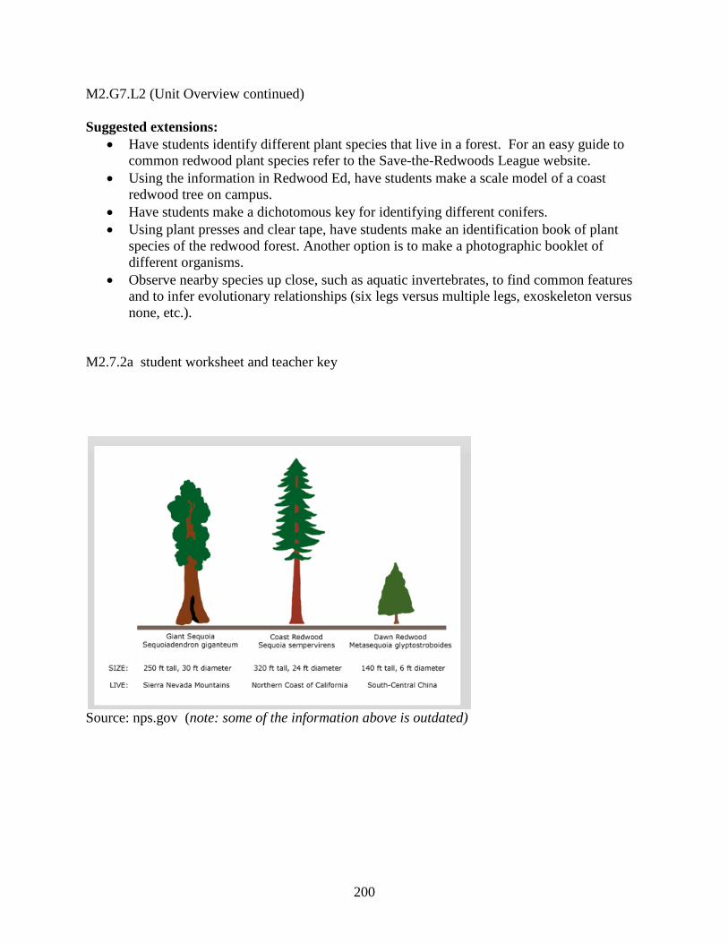
M2.G7.L2 (Unit Overview continued) Suggested extensions:

• Have students identify different plant species that live in a forest. For an easy guide to common redwood plant species refer to the Save-the-Redwoods League website.

• Using the information in Redwood Ed, have students make a scale model of a coast redwood tree on campus.

• Have students make a dichotomous key for identifying different conifers. • Using plant presses and clear tape, have students make an identification book of plant

species of the redwood forest. Another option is to make a photographic booklet of different organisms.

• Observe nearby species up close, such as aquatic invertebrates, to find common features and to infer evolutionary relationships (six legs versus multiple legs, exoskeleton versus none, etc.).

M2.7.2a student worksheet and teacher key

Source: nps.gov (note: some of the information above is outdated)

200

Student worksheet M2.7.2a Name _________________________ Date _____________ Period _______ Directions: Compare and contrast the three different species of redwood below. Refer to the reading assigned by your teacher.

Comparing the Redwood Cousins Feature Dawn Redwood Coast Redwood Giant Sequoia Scientific name Family Range/Distribution

Description

Average sizes: Diameter Height

Maximum height Oldest known Adaptations

Status

Other

201

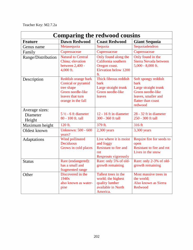
Teacher Key: M2.7.2a

Comparing the redwood cousins Feature Dawn Redwood Coast Redwood Giant Sequoia Genus name Metasequoia Sequoia Sequoiadendron Family Cupressaceae Cupressaceae Cupressaceae Range/Distribution

Natural to Central China; elevation between 2,400 - 4,000 ft.

Only found along the California southern Oregon coast. Elevation below 1200 ft.

Only found in the Sierra Nevada between 5,000 - 8,000 ft.

Description

Reddish orange bark Conical or pyramid tree shape Green needle-like leaves that turn orange in the fall

Thick fibrous reddish bark Large straight trunk Green needle-like leaves

Soft spongy reddish bark Large straight trunk Green needle-like leaves, smaller and flatter than coast redwood

Average sizes: Diameter Height

5 ½ - 6 ft diameter 80 - 100 ft. tall

12 - 16 ft in diameter 300 - 360 ft tall

28 - 32 ft in diameter 250 - 300 ft tall

Maximum height 120 ft. 379 ft. 316 ft Oldest known Unknown: 500 - 600

years? 2,300 years 3,300 years

Adaptations

Wind pollinated Deciduous Grows in cold places

Live where it is moist and foggy Resistant to fire and rot Resprouts vigorously

Require fire for seeds to open Resistant to fire and rot Lives in the snow

Status

Rare (endangered): has a small and fragmented range

Rare: only 5% of old-growth remaining

Rare: only 2-3% of old-growth remaining

Other

Discovered in the 1940s also known as water-pine

Tallest trees in the world; the highest quality lumber available in North America.

Most massive trees in the world; Also known as Sierra Redwood

202

M2.G7 Lesson 3: Tree-Thinning Dynamics Unit Overview: Coast Redwoods Grade 7 Key Concepts:

• Patterns: cause and effect

• Interdependent relationships in ecosystems

• Biodiversity and humans

• Earth’s ecosystems Time: 45 - 90 minutes (depending on ability to use a graphing program) Materials for the Teacher: Computer lab with a

graphing program similar to Excel

Student directions (data set) M2.7.3a

Student worksheet and teacher key M2.7.3b

Examples of other graphs and charts (optional)

Connections: STEM, mathematics, botany, forestry, carbon cycle, soils, biomass, climate change, atmosphere, human impact, Social Studies Forest Ecology Series integration: M1: Integrative Forest Ecology M3: Oak Woodlands

Learning Objectives: Students will analyze and graphically represent data from a tree-thinning project using a graphing program to see how young redwood trees respond to various levels of thinning. They will understand that ecosystems are dynamic and different management strategies produce different results. Following their data analysis, they will briefly summarize the results of the study in a short written paragraph. Background information: Refer to the appropriate sections in Part I: Teacher Companion for Module 2 and Part 1: Teacher Companion for Module 1. The data used for this lesson comes from US Forest Service general technical report GTR-PSW-238 regarding silviculture and restoration that you can find online (Webb et al. 2012). (See online resources.) Suggested procedure: Begin this lesson by asking some of the preliminary questions below. Students should understand that scientists often gather data in the field to help them understand the dynamics of a changing ecosystem. Review how trees grow and discuss some of the limiting factors regarding tree growth (refer to Module 1). If possible, show them a tree “cookie”, either a projected one or a real one to review tree circumference, diameter, and how they can become suppressed. Ask them to predict how a tree’s diameter and growth rate might change if other trees around it are removed. Before you begin, assess their skill level regarding the graphing program you intend to use. Instruct them appropriately. If you have a limited number of computers have them work in pairs to produce their graphs together. If you want to use Excel and are new to it, refer to the tutorial below (online resources). Inform them how you want them to graph (see teacher key M2.7.3a). You might want to show them a few examples to get them started. To begin, have students make a line-graph showing the results of four different treatments over 39 years (refer to M2.7.3a). After students have produced a clear graph, have them interpret the data by answering the questions on student worksheet M2.7.3b. Be sure to stress that the study was done in a clearcut that was 40 years old. If using computers is not an option, students can use graph paper. There is an optional extension available that has students compare how trees respond to different tree densities. Begin or end with some of the suggested extensions or proceed to the next lesson.

Critical Thinking: Besides increased light and space (competition) identify some other factors that may influence tree growth.

203

Keywords: analyze, abiotic factor, control group, density, diameter, dbh (diameter breast height), limiting factor, mortality, stand Suggested preliminary questions: • What types of abiotic factors influence tree growth? • How might younger trees respond if older larger trees were cut out next to them? • Do you think all trees will react the same if trees around them are cut? • How does the density of a stand relate to competition? • Do you think a land manager wanting to produce timber would want to thin his forest? Why/Why not? • What are some different reasons for managing a forest? NGSS alignment: MS-LS2: Ecosystems: Interactions, Energy, and Dynamics LS2.A: Interdependent Relationships in an Ecosystem LS2.C: Ecosystem Dynamics, Functioning, and Resilience LS2.D: Biodiversity and Humans Online resources: Original study pdf [The Whiskey Springs Redwood Commercial Thinning Study: A 29-year status report (1970-1999)] http://www.fs.fed.us/psw/publications/documents/psw_gtr194/psw_gtr194_47.pdf The full study highlighted in this lesson can be easily downloaded from this website for your review. Teach-nology: http://www.teach-nology.com/tutorials/excel/ This website explores the pros and cons of using Excel in the classroom. It gives other helpful links about using Excel as well. For Excel Tutorial: http://www.youtube.com/watch?v=8L1OVkw2ZQ8 There are many tutorials out there on The Web. This one is short and incorporates all of the components needed for entering simple data sets similar to the ones in this lesson. EEI Connection: B.6.a. Biodiversity: The keystone of Life on Earth B.8.b Biological Diversity: The World’s Riches

204

Answers to preliminary questions: - What types of abiotic factors influence tree growth? (the amount of space, light, water, and nutrients are the main limiting factors affecting tree growth) - How might younger trees respond if older larger trees were cut out next to them? (younger trees would probably grow a lot faster unless they require dense shade) - Do you think all trees will react the same if trees around them are cut? (Answer will vary. How trees react will differ, however, overall increased light usually means faster growth) (answer to preliminary questions continued) - How does the density of a stand relate to competition? (the denser the stand the more competition between trees exists) - Do you think a land manager wanting to produce timber would want to thin his forest? Why/Why not? (Most land managers wanting to produce timber will want to thin the forest to reduce competition and encourage growth. Many different management techniques are used including clear cutting and selective cutting) - What are some different reasons for managing a forest? (there are many reasons for managing forests differently. Some reasons are restoration, timber production, reducing stream sediment, and habitat enhancement) Suggested follow up questions:

• Why were all of the trees in this study the same age before thinning began? • Would thinning be necessary in an old-growth redwood forests? Why/why not? • What negative consequences might occur if trees grow close together?

Suggested extensions:

• Find density dependent factors for other populations such as planted carrots or flowers. • Using tree height and diameter, find the volume of simplified tree models. Conifers can

be considered cones since they often have pointed tops. • Design a controlled experiment that isolates a certain limiting factor, such as water

availability, and study its effects on plant growth. • Show slides or a video about logging in the redwood forest or another forest type. • Study different tree cookies to learn about tree growth patterns (see Module 1 Lesson

M1.G7.L3 and L4). • Research champion trees around the world or those in the Pacific Northwest.

M2.7.3a Student directions M2.7.3b Student worksheet M2.7.3a and 3b Teacher keys

205

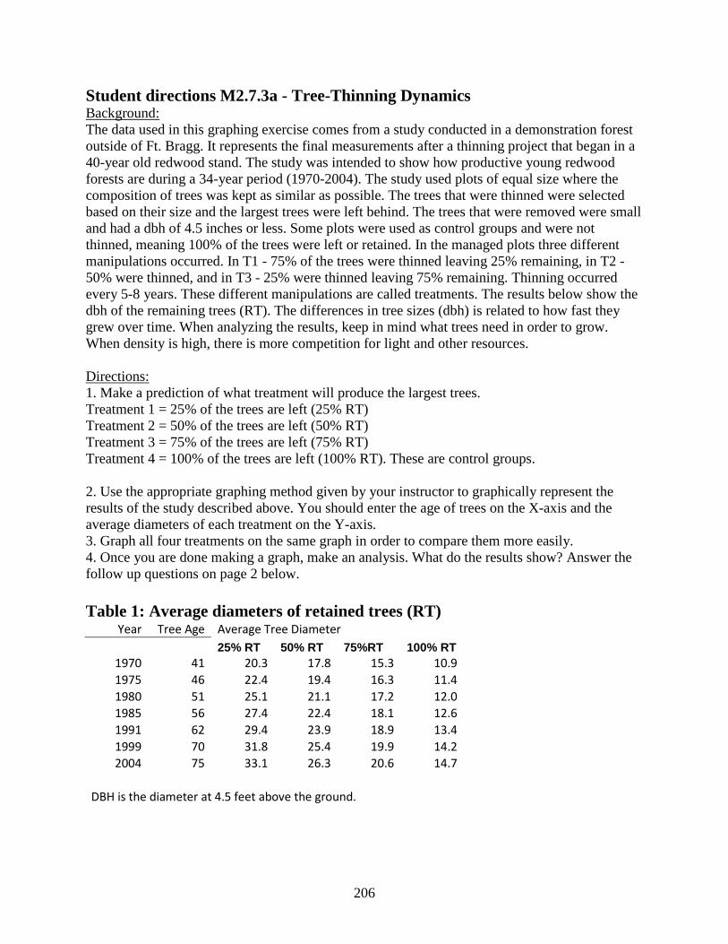
Student directions M2.7.3a - Tree-Thinning Dynamics Background: The data used in this graphing exercise comes from a study conducted in a demonstration forest outside of Ft. Bragg. It represents the final measurements after a thinning project that began in a 40-year old redwood stand. The study was intended to show how productive young redwood forests are during a 34-year period (1970-2004). The study used plots of equal size where the composition of trees was kept as similar as possible. The trees that were thinned were selected based on their size and the largest trees were left behind. The trees that were removed were small and had a dbh of 4.5 inches or less. Some plots were used as control groups and were not thinned, meaning 100% of the trees were left or retained. In the managed plots three different manipulations occurred. In T1 - 75% of the trees were thinned leaving 25% remaining, in T2 - 50% were thinned, and in T3 - 25% were thinned leaving 75% remaining. Thinning occurred every 5-8 years. These different manipulations are called treatments. The results below show the dbh of the remaining trees (RT). The differences in tree sizes (dbh) is related to how fast they grew over time. When analyzing the results, keep in mind what trees need in order to grow. When density is high, there is more competition for light and other resources. Directions: 1. Make a prediction of what treatment will produce the largest trees. Treatment 1 = 25% of the trees are left (25% RT) Treatment 2 = 50% of the trees are left (50% RT) Treatment 3 = 75% of the trees are left (75% RT) Treatment 4 = 100% of the trees are left (100% RT). These are control groups. 2. Use the appropriate graphing method given by your instructor to graphically represent the results of the study described above. You should enter the age of trees on the X-axis and the average diameters of each treatment on the Y-axis. 3. Graph all four treatments on the same graph in order to compare them more easily. 4. Once you are done making a graph, make an analysis. What do the results show? Answer the follow up questions on page 2 below. Table 1: Average diameters of retained trees (RT)

Year Tree Age Average Tree Diameter 25% RT 50% RT 75%RT 100% RT

1970 41 20.3 17.8 15.3 10.9 1975 46 22.4 19.4 16.3 11.4 1980 51 25.1 21.1 17.2 12.0 1985 56 27.4 22.4 18.1 12.6 1991 62 29.4 23.9 18.9 13.4 1999 70 31.8 25.4 19.9 14.2 2004 75 33.1 26.3 20.6 14.7

DBH is the diameter at 4.5 feet above the ground.

206

Student worksheet G7.3b Name _________________________ Date ___________ Period _________ Follow Up Activity (Tree-Thinning) Analysis: After making a graph of the above data, compare the results of each level of treatment. Did the trees in the plots with the heaviest thinning (25% retained) grow faster or slower? How do you know? What factors are directly related? 1. What treatment had the smallest trees on average over the 39-year study period? 2. What percent of trees were removed to cause the trees to grow the fastest on average? 3. Identify two limiting factors that control for tree size according to this study. 4. Write a concluding paragraph explaining how the trees responded to the different degrees of thinning in this study. ______________________________________________________________________________

______________________________________________________________________________

______________________________________________________________________________

______________________________________________________________________________

______________________________________________________________________________

______________________________________________________________________________

______________________________________________________________________________

______________________________________________________________________________

5. Explain how the density of trees in a stand relates to competition and tree mortality. ______________________________________________________________________________

______________________________________________________________________________

______________________________________________________________________________

page 1

207

______________________________________________________________________________

______________________________________________________________________________

______________________________________________________________________________

______________________________________________________________________________

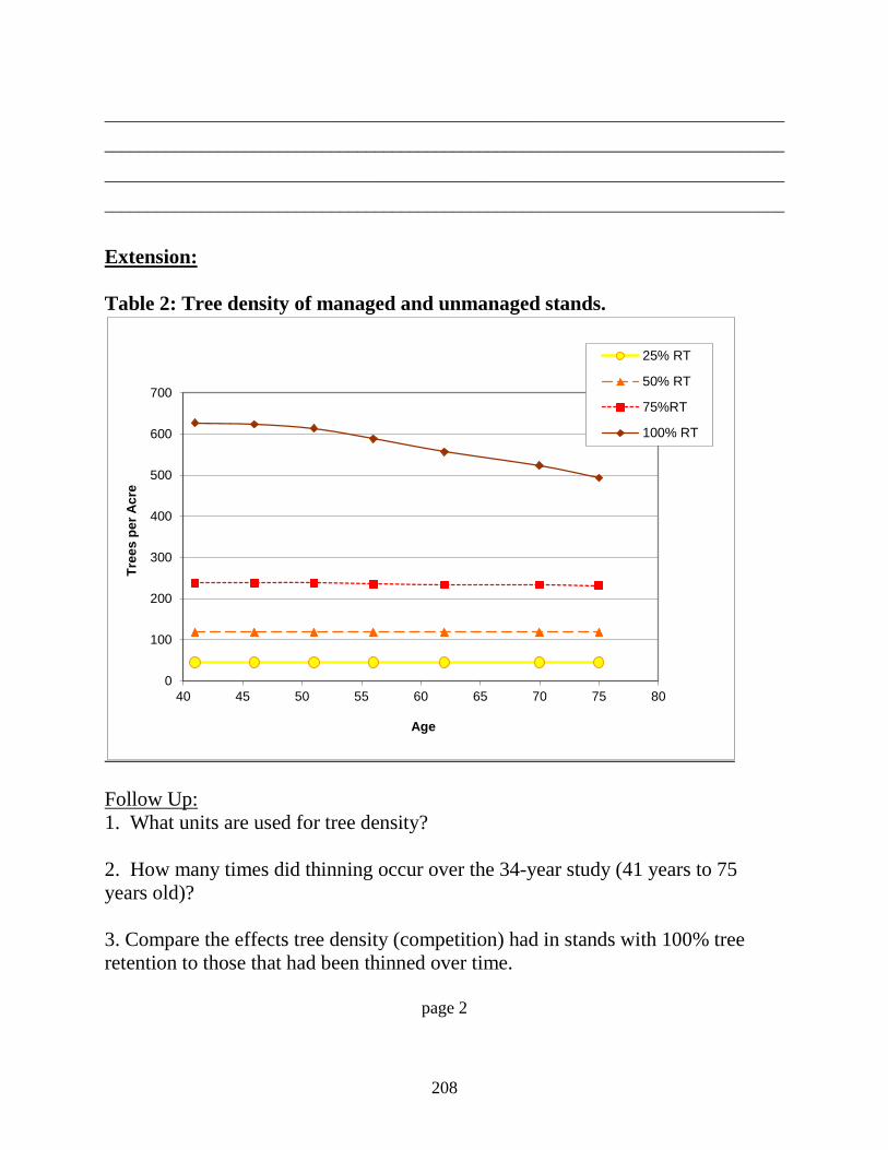
Extension: Table 2: Tree density of managed and unmanaged stands.

Follow Up: 1. What units are used for tree density? 2. How many times did thinning occur over the 34-year study (41 years to 75 years old)? 3. Compare the effects tree density (competition) had in stands with 100% tree retention to those that had been thinned over time.

page 2

0

100

200

300

400

500

600

700

40 45 50 55 60 65 70 75 80

Tree

s pe

r Acr

e

Age

25% RT

50% RT

75%RT

100% RT

208

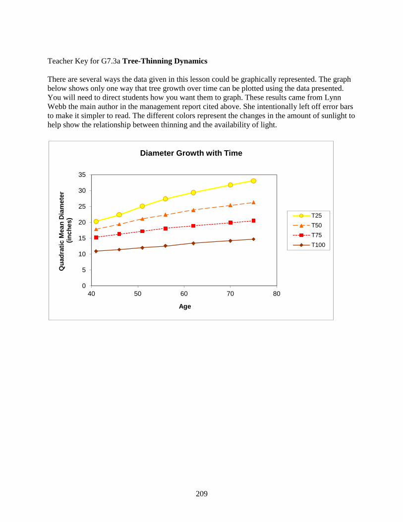
Teacher Key for G7.3a Tree-Thinning Dynamics There are several ways the data given in this lesson could be graphically represented. The graph below shows only one way that tree growth over time can be plotted using the data presented. You will need to direct students how you want them to graph. These results came from Lynn Webb the main author in the management report cited above. She intentionally left off error bars to make it simpler to read. The different colors represent the changes in the amount of sunlight to help show the relationship between thinning and the availability of light.

0

5

10

15

20

25

30

35

40 50 60 70 80

Qua

drat

ic M

ean

Dia

met

er

(inc

hes)

Age

Diameter Growth with Time

T25T50T75T100

209

Teacher key G7.3b Follow Up Activity (Tree Thinning) Analysis: Refers to Table 1: After making a graph of the above data, compare the results of each level of treatment. Did the trees in the plots with the heaviest thinning (25% retained) grow faster or slower? How do you know? What factors are directly related? 1. What treatment had the smallest trees on average over the 39-year study period? Treatment 4 - 100% retention 2. What percent of trees removed resulted in the fastest growing trees on average? Treatment 1 - 25% retention (75% thinned) 3. Identify two limiting factors that control for tree size according to this study. Answers will vary. The main factors are space and light. 4. Write a concluding paragraph explaining how the trees responded to the different degrees of thinning in this study. Answer will vary. There was a direct relationship between the amount of thinning and tree size. As trees were thinned more light was available. This allowed the stand of trees with the most thinning to grow the fastest. Stands with no thinning had the slowest growth resulting in the smallest trees. Without thinning there was a higher degree of competition for light, space, and other resources. 5. Explain how the density of trees in a stand relates to competition and tree mortality. When tree density is higher competition is increased and over time trees begin to die. Extension: Refers to Table 2 Follow Up: 1. What units are used for tree density? Trees per acre 2. How many times did thinning occur over the 34-year study (41 years to 75 years old)? Seven times 3. Compare the effects tree density (competition) had in stands with 100% tree retention to those that had been thinned over time. Trees in the control group or with 100% retention began to die after about 15 years, whereas managed or thinned stands kept the same amount of trees per acre.

210

M2.G7 Lesson 4: Measuring Up to the Tallest Trees Unit Overview: Coast Redwoods Grade 7 Key Concepts:

• Growth and development of organisms

• Inheritance of traits • Developing and using

models • Energy and matter • Using quantitative data

to increase understanding

Time: 70 - 100 minutes Materials for the Teacher: Measuring tapes or

meter sticks Student reading

M2.7.4a Student worksheet

M2.7.4b Connections: STEM, math, photosynthesis, carbon cycle, carbon sequestration, genetics, botany, forestry, soils, biomass, atmosphere, architecture, engineering Forest Ecology Series integration: M1: Integrative Forest Ecology M3: Oak woodlands

Learning Objectives: After reading about the world’s tallest trees, students will conduct a short series of athletic challenges to find various lengths. They will use these base measurements to calculate equivalences compared to the height of some of the tallest trees. Optionally, students will write out their calculations using algebraic expression. Background information: Refer to the appropriate sections in Part I: Teacher Companion for Module 2 and the Student Reading The Largest Living Things below. You can also find information on tree growth and structure and the wonders of wood in Part I: Teacher Companion for Module 1. Suggested procedure: Begin this lesson by asking students if they have ever compared how far they could jump or how tall they were to other objects. Making comparisons allows us to become familiar with something, which can help us gain a clearer perspective. It is very difficult to see the top of a tall building in a city center or the tops of tall redwood trees in an old-growth forest. How tall is 379 feet? How many pencils end to end would it take to stretch this distance? In this lesson, students will compare their height (along with other distances they measure) to the height of the tallest coast redwood, Douglas-fir, and eucalyptus through athletic challenges. These species are the tallest living things on the planet! It is assumed that students already have some prior knowledge about redwoods, if not you will need to give them a review of the distribution and ecology of this quintessential forest type of Northern California. This lesson can be easily modified to include other notable large things such as the Eiffel Tower or blue whale. Begin by assigning student reading M2.7.4a The Tallest Living Things. This can be done as homework. The length of time this activity will take depends on how many and what type of athletic challenges you assign. Alternatively, instead of using athletic challenges to find distances, students can use the heights and lengths of objects they measure around their schoolyard, such as the height of their classroom ceiling or the length of a hallway. You will need to decide what challenges they should perform and set rules for safety. Follow this lesson with an extension activity or continue to the next lesson in the forest ecology series.

Critical Thinking: What are some factors that allow certain tree species to grow exceptionally tall or live an extremely long time compared to others that don’t? Key words: cambium, canopy, conifer, crown, dominate, heartwood, vascular tissue

211

M2.G10.L4 (Unit Overview continued) NGSS alignment: MS-LS1: From Molecules to Organisms: Structures and Processes LS1:B Growth and Development of Organisms LS1:C Organization for Matter and Energy Flow in Organisms MS-LS3: Heredity: Inheritance and Variations of Traits LS3:A Inheritance of Traits Online resources: Redwood Ed: Chapter 4 from the Stewards of the Coast and Redwoods website http://www.stewardscr.org/cms/images/red_ed18_lessons_activities_pgs329to376.pdf This curriculum guide is full of great lessons regarding the coast redwoods. Chapter 4 in particular has several activities relating to tree size, fog, microhabitats, and the capillary action of water good to use as extension activities. American Forest Foundation: A Journey through Champion Trees http://www.americanforests.org/magazine/article/journey-through-champion-trees/ Good pictures and descriptions of champion trees found in America can be found here. The selection of trees may be limited, for instance it omits the tallest coast redwoods in the introductory sequence. It has many other useful links such as the National Registry of Big Trees which is organized by year. California Academy of Sciences Hotspots: Redwood Forests (California on the Edge) http://www.calacademy.org/exhibits/california_hotspot/habitat_redwoods.htm#explore A good overview of the types of things that define a coast redwood forest can be found in this simple and straight forward website including a short slide show. Conifer Country: page on conifers http://www.conifercountry.com/conifers.html If you want good information on the conifer species found throughout the Klamath/North Coast area - this is a great resource. It has range maps, pictures, and key identifying features. EEI Connections: B.8.a. Differential Survival of Organisms E.7.b The Life and Times of Carbon 7.6.3 Managing Nature’s Bounty: Feudalism in Medieval Europe (History-Social Science connection)

212

M2.G7.L4 (Lesson Overview continued) Suggested extensions:

• Germinate seeds of trees and measure their growth rates. • Have students make posters on the “bio” of champion trees. Information on champion

trees can be found on many online sources. • Calculate how many board feet there are in different sized trees then figure out how many

average houses could be built from one large redwood tree. • Connect large trees to the carbon cycle. New research finds that the largest trees absorb

the most carbon dioxide. • Connect tall trees to the physics of water such as negative pressure, capillary action, and

evapotranspiration. • Make a scale model of a redwood tree on campus (see Redwood Ed above). • Explore the microclimates and microhabitats of a tall redwood tree. The leaves on top of

a large redwood tree for instance are very different from the leaves that grow in the shade towards the bottom.

M2.7.4a Student reading M2.7.4b Student worksheet

213

Student reading M2.7.4a The Tallest Living Things

Many evergreen trees or conifers grow for a very long time making them

among the tallest living things on Earth. Generally they shoot for the sky and are

cone-shaped with narrow crowns. In the Pacific Northwest, individual trees can

live over 1,000 years and can surpass 20 feet (6 m) in diameter. The tallest trees

living today are old-growth coast redwoods (Sequoia sempervirens). The tallest on

record is 379 feet (116 m) and is still growing. It was discovered in 2006, well

after most other giants had been recorded.

One of the reasons redwoods can grow so big and tall is they spend a lot of

energy making rot resistant and fire-resistant heartwood. Researchers recently

discovered the oldest redwood on record, which is at least 2,510 years old. The

tallest redwood grove is located in Humboldt Redwood State Park. It contains a

few dozen trees over 300 feet (90 m). No other tree species can normally grow to

this height. Another type of redwood tree, the giant sequoia, is the largest living

thing on land. They don’t grow as tall but they stay wide most of the way up their

trunk and into their crown. This species can live more than 1,000 years longer than

coast redwood. The largest giant sequoia has a volume over 56,000 cubic feet,

which is equal to over fifteen adult blue whales!

There are some trees that at one time may have been taller than the tallest

redwood living today. Before the days of logging, some Douglas-fir trees

(Pseudotsuga menziesii) may well have grown over 400 ft (122 m) tall. It is a

common conifer found in the Pacific Northwest and is the tree most commonly

used for building houses. The tallest ones today live among the redwoods with the

tallest found so far measuring 318 feet high (97 m). This species is more prone to

insect and fungal attack and can host many more harmful insects, such as bark

beetles, which is one of the reasons why they do not live as long as redwoods. In

214

the Southern Hemisphere, the tallest trees are not conifers - they are eucalyptus

trees. One species of eucalyptus, the Australian mountain ash (Eucalyptus regnans)

holds the record for the fastest growing tree. The tallest of them all lives in

Tasmania and is 327 feet (100 m) tall. This makes it the tallest flowering plant in

the world! Even though this species grows very fast and tall it is not long-lived.

Trees are woody vascular plants. Like all vascular plants, trees have roots,

leaves, and stems. The trunk of a tree supports the crown and holds most of the

cambium. Cambium is the living part of a tree, usually only a few cells thick. It

can be thought of as a “highway” because it contains the transportation network or

the vascular system that is found throughout a tree’s trunk, branches, and roots.

Vascular plants have two types of tissues used in transport: xylem, which

transports water and nutrients upwards to the leaves and phloem, which transports

sugars downwards and outwards. As trees age older xylem cells lose their ability to

transport water and turn into dense heartwood.

A mature tree is complex and is shaped by physical factors. These include

amount of light and water available, as well as biological factors, such as its genes.

A tree can be divided into three main parts: a trunk, roots, and a crown. The trunk

supports the crown and contains the majority of the wood. Leaves make up the

majority of a tree’s crown, which is the top of a tree. Special organelles within

leaves produce food by converting sunlight and carbon dioxide into sugars, which

enable plants to reproduce, grow, and repair when needed. Roots absorb water

from the ground, which is transported up the trunk and throughout the branches.

They provide a tree an anchor aiding in support. The combined tops of trees in a

forest make up the forest canopy. When certain trees dominate they cast shade,

which can slow the growth of other plants, decreasing competition. In some places,

Douglas-fir and coast redwood are considered co-dominant because both have

their crowns at the top of the canopy where the amount of light is greatest.

215

Written By Melinda Bailey

--------------------------------------------------------------------------

Bibliography:

Armstrong, W. (2013). The Taxodium family: Taxodiaceae. Wayne’s Word. http://waynesworld.palomar.edu

Sillett, S. C. (2013). Separating effects of tree size and age on trunk growth in California redwoods. In Past, present and future of redwoods: a redwood ecology and climate symposium. Save the Redwoods League. Unpublished data.

Van Pelt, Robert. 2001. Forest Giants of the Pacific Coast, Seattle, WA: Global Forest Society and University of Washington Press.

Wolf, E. C., A.P. Mitchell and P.K. Schoonmaker (1995). The rain forests of home: an atlas of people and place. (E. L. Kellogg, Ed.) (pp. 1–31). Ecotrust, Pacific GIS, Conservation International.

216

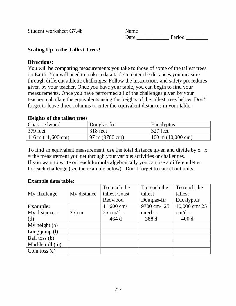
Student worksheet G7.4b Name ________________________ Date ____________ Period ________ Scaling Up to the Tallest Trees! Directions: You will be comparing measurements you take to those of some of the tallest trees on Earth. You will need to make a data table to enter the distances you measure through different athletic challenges. Follow the instructions and safety procedures given by your teacher. Once you have your table, you can begin to find your measurements. Once you have performed all of the challenges given by your teacher, calculate the equivalents using the heights of the tallest trees below. Don’t forget to leave three columns to enter the equivalent distances in your table. Heights of the tallest trees Coast redwood Douglas-fir Eucalyptus 379 feet 318 feet 327 feet 116 m (11,600 cm) 97 m (9700 cm) 100 m (10,000 cm) To find an equivalent measurement, use the total distance given and divide by x. x = the measurement you get through your various activities or challenges. If you want to write out each formula algebraically you can use a different letter for each challenge (see the example below). Don’t forget to cancel out units. Example data table: My challenge

My distance

To reach the tallest Coast Redwood

To reach the tallest Douglas-fir

To reach the tallest Eucalyptus

Example: My distance = (d)

25 cm

11,600 cm/ 25 cm/d = 464 d

9700 cm/ 25 cm/d = 388 d

10,000 cm/ 25 cm/d = 400 d

My height (h) Long jump (l) Ball toss (b) Marble roll (m) Coin toss (c)

217

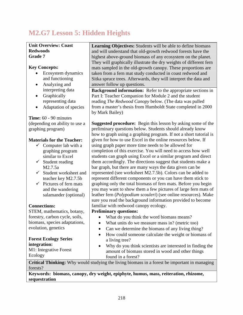
M2.G7 Lesson 5: Hidden Heights Unit Overview: Coast Redwoods Grade 7 Key Concepts:

• Ecosystem dynamics and functioning

• Analyzing and interpreting data

• Graphically representing data

• Adaptation of species Time: 60 - 90 minutes (depending on ability to use a graphing program) Materials for the Teacher: Computer lab with a

graphing program similar to Excel

Student reading M2.7.5a

Student worksheet and teacher key M2.7.5b

Pictures of fern mats and the wandering salamander (optional)

Connections: STEM, mathematics, botany, forestry, carbon cycle, soils, biomass, species adaptations, evolution, genetics Forest Ecology Series integration: M1: Integrative Forest Ecology

Learning Objectives: Students will be able to define biomass and will understand that old-growth redwood forests have the highest above-ground biomass of any ecosystem on the planet. They will graphically illustrate the dry weights of different fern mats sampled in the old-growth canopy. These proportions are taken from a fern mat study conducted in coast redwood and Sitka spruce trees. Afterwards, they will interpret the data and answer follow up questions. Background information: Refer to the appropriate sections in Part I: Teacher Companion for Module 2 and the student reading The Redwood Canopy below. (The data was pulled from a master’s thesis from Humboldt State completed in 2000 by Mark Bailey) Suggested procedure: Begin this lesson by asking some of the preliminary questions below. Students should already know how to graph using a graphing program. If not a short tutorial is given for how to use Excel in the online resources below. If using graph paper more time needs to be allowed for completion of this exercise. You will need to access how well students can graph using Excel or a similar program and direct them accordingly. The directions suggest that students make a bar graph, but there are many ways the data given can be represented (see worksheet M2.7.5b). Colors can be added to represent different components or you can have them stick to graphing only the total biomass of fern mats. Before you begin you may want to show them a few pictures of large fern mats of leather fern (Polypodium scouleri) (see online resources). Make sure you read the background information provided to become familiar with redwood canopy ecology. Preliminary questions:

• What do you think the word biomass means? • What units do we measure mass in? (metric too) • Can we determine the biomass of any living thing? • How could someone calculate the weight or biomass of

a living tree? • Why do you think scientists are interested in finding the

amount of biomass stored in wood and other things found in a forest?

Critical Thinking: Why would studying the living biomass in a forest be important in managing forests? Keywords: biomass, canopy, dry weight, epiphyte, humus, mass, reiteration, rhizome, sequestration

218

(M2.G7.L5 Unit Overview Continued) NGSS alignment: MS-LS2: Ecosystems: Interactions, Energy, and Dynamics LS2: Analyzing and interpreting data (Science and Engineering) LS2.B: Cycle of Matter and Energy Transfer in Ecosystems Online resources: Ecology of the Coast Redwood http://www.ecology.info/redwood.htm This site is a good overview of what some of the latest scientific studies reveal about coast redwoods. It sites scientific papers including the ones used in this lesson. Institute for Redwood Ecology: Advancing the world’s understanding of Redwood Forest Ecology by Professor Sillett http://www.humboldt.edu/redwoods/ Good pictures of fern mats can be found here. Also links to research papers are given revealing some of latest findings regarding the largest trees in the world. GLOBE - Biomass Units: Calculating Classroom Biomass http://globecarboncycle.unh.edu/DownloadActivities/Field/FieldMeasurements-LearningActivities/BiomassUnits/BiomassUnits_TeacherGuide.pdf: This website gives several lessons relating to biomass. It includes a short description of biomass and how it is calculated. For Excel Tutorial: http://www.youtube.com/watch?v=8L1OVkw2ZQ8 There are many tutorials out there on The Web. This one is short and incorporates all of the components needed for entering simple data sets similar to the ones in this lesson. EEI Connection: E.7.b The Life and Times of Carbon B.8.b Biological Diversity: The World’s Riches B.8.d The Isolation of Species

219

M2.G7.L5 (Unit overview continued) Answers to preliminary questions: - What do you think the word biomass means? (Biomass is the total mass of living material measured over a particular area) - What units do we measure mass in? (metric too) (Biomass is typically measured in grams g/m2 or kilograms kg/m2, but other answers such as pounds are acceptable) - Can we determine the biomass of any living thing? (Answers will vary. It depends. Sometimes it is very difficult to get accurate measurements of living things without killing them. Measuring trees requires complex calculations) - How could someone calculate the weight or biomass of a living tree? (The biomass of a living tree can only be estimated. Allometric equations are used after finding complex measurements. Sometimes samples are used to find standards, but this kills the trees) - Why do you think scientists are interested in finding the amount of biomass stored in wood and other things found in a forest? (Answers will vary. Living things are made of carbon. Excess carbon is contributing to a warming planet. Trees absorb carbon and therefore help reduce the impact of global warming. If we can calculate the carbon stored in a tree, we can get an idea of the carbon stored over a sample site. This helps in understanding climate). Suggested extensions:

• Find the biomass of all the students in your classroom or some other group of people • Identify local fern species using a fern finder or the information in Redwood Ed. • Observe soil samples up close and have students separate the things they find into various

abiotic and biotic components. • Walk in a redwood forest looking for signs of disturbance. • Study the lifecycle of ferns, lichens, and or mosses. • Use Landsat images of different regions to compare differences in vegetative cover

between different areas (i.e. forest, chaparral, desert). • Collect weeds or other plant material that doesn’t impact a natural area. Have the students

dry it and weigh it to find biomass. • Find the masses of equal sized pieces of wood to observe differences in density. • Show a video on recent discoveries in the redwoods.

M2.7.5a Student reading M2.7.5b Student worksheet and Teacher key

220

Student reading M2.7.5a The Redwood Canopy

Large redwood trees are some of the most structurally complex on Earth.

Part of this complexity is because they can grow for a very long time. Old trees are

shaped by natural disturbances such as fire, lightning, wind, and disease.

Sometimes you can often see the effects of ground fires as blackened bark or

burned out cavities called “goose pens”. Coast redwoods are unique because they

have the ability to resprout from any part including their trunks and roots. If a

branch breaks off, usually a new sprout will emerge. Sprouts that take the form of a

tree are called reiterations. Over time a redwood’s crown can become a maze of

reiterations.

Large complex reiterated trunks and branches make bench-like platforms.

Fallen leaves and duff collect on these platforms, beginning the formation of

canopy soil. One particular plant, the leather fern (Polypodium scouleri) often

takes advantage of these thin soils. It can live high-up on tree- top ledges in places

where moisture collects. As leather ferns grow they add depth to the canopy soil

and slowly spread forming fern mats. Over time these fern mats can become as

large as a truck! Big mats store moisture and act as hiding places for a variety of

species including mites, spiders, beetles, and voles (a squirrel-like animal).

Another animal recently discovered living in these fern mats is the

wandering salamander (Aneides vagrans). Salamanders are amphibians and need

moist places to survive. This salamander is able to get everything it needs high up

in the moist fern mats - and some have even been discovered more than 200 feet

up! They also live on the ground, in moist crevices, and in downed wood. This

particular species is native to northern California.

Over 250 species of lichens and mosses have been found growing in the

redwood canopy. They avoid competition by living on top of others things such as

221

rocks, wood, and bark. When a plant or lichen lives atop another plant without

causing harming, it is called an epiphyte. Sometimes accidental epiphytes exist in

redwoods, including trees living atop other trees! Epiphytes are also common in

tropical rainforests, such as orchids and bromeliads. Epiphytes, especially large

ones, can add a lot of weight to tree’s crown.

When fern mats are dissected most of the material is dead roots and

rhizomes. In order to find the relative proportions of the different parts, the

biomass of each kind is measured. Biomass is the amount of living material found

within a specific area. One way to calculate biomass is to find dry weight. Dry

weight is an accurate measurement because all water is removed from the sample.

This can be done by drying samples in an oven. The data in the following study

comes from different dissected fern mats that have been dried and weighed.

Finding the biomass of things living can be important for wildlife

management, forestry, and scientific studies. Because redwoods grow old and get

extremely large, redwood forests have the most above-ground biomass compared

to any other ecosystem in the world. Some of the biomass is held in large logs and

snags. Typically 50% of dry mass is pure carbon. The more mass a tree, log, or

fern mat has, the more carbon it stores. The ability to store carbon is important and

is referred to as carbon absorption or sequestration. The sequestration of carbon is

offset by decomposition because during this process carbon is released. The

absorption and release of carbon over time is referred to as the carbon cycle. Written by Melinda Bailey

222

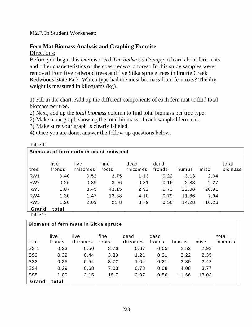
M2.7.5b Student Worksheet: Fern Mat Biomass Analysis and Graphing Exercise Directions: Before you begin this exercise read The Redwood Canopy to learn about fern mats and other characteristics of the coast redwood forest. In this study samples were removed from five redwood trees and five Sitka spruce trees in Prairie Creek Redwoods State Park. Which type had the most biomass from fernmats? The dry weight is measured in kilograms (kg). 1) Fill in the chart. Add up the different components of each fern mat to find total biomass per tree. 2) Next, add up the total biomass column to find total biomass per tree type. 2) Make a bar graph showing the total biomass of each sampled fern mat. 3) Make sure your graph is clearly labeled. 4) Once you are done, answer the follow up questions below. Table 1: Biomass of fern mats in coast redwood

tree live fronds

live rhizomes

fine roots

dead rhizomes

dead fronds humus misc

total biomass

RW1 0.40 0.52 2.75 1.13 0.22 3.13 2.34 RW2 0.26 0.39 3.96 0.81 0.16 2.88 2.27 RW3 1.07 3.45 43.15 2.92 0.73 22.08 20.91 RW4 1.30 1.47 13.38 4.10 0.79 11.86 7.94 RW5 1.20 2.09 21.8 3.79 0.56 14.28 10.26 Grand total Table 2:

Biomass of fern mats in Sitka spruce

tree live fronds

live rhizomes

fine roots

dead rhizomes

dead fronds humus misc

total biomass

SS 1 0.23 0.50 3.76 0.67 0.05 2.52 2.93 SS2 0.39 0.44 3.30 1.21 0.21 3.22 2.35 SS3 0.25 0.54 3.72 1.04 0.21 3.39 2.42 SS4 0.29 0.68 7.03 0.78 0.08 4.08 3.77 SS5 1.09 2.15 15.7 3.07 0.56 11.66 13.03 Grand total

223

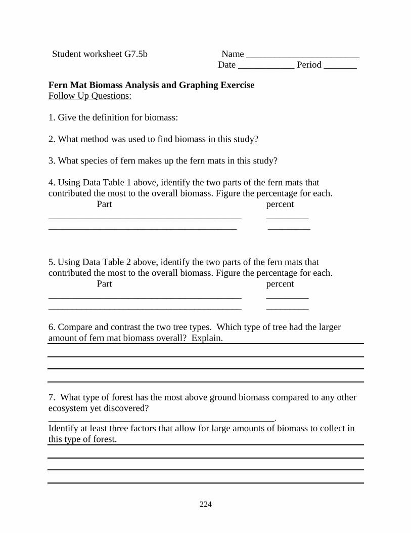
Student worksheet G7.5b Name ________________________ Date ____________ Period _______ Fern Mat Biomass Analysis and Graphing Exercise Follow Up Questions: 1. Give the definition for biomass: 2. What method was used to find biomass in this study? 3. What species of fern makes up the fern mats in this study? 4. Using Data Table 1 above, identify the two parts of the fern mats that contributed the most to the overall biomass. Figure the percentage for each. Part percent _________________________________________ _________ ________________________________________ _________

5. Using Data Table 2 above, identify the two parts of the fern mats that contributed the most to the overall biomass. Figure the percentage for each. Part percent _________________________________________ _________ _________________________________________ _________ 6. Compare and contrast the two tree types. Which type of tree had the larger amount of fern mat biomass overall? Explain. 7. What type of forest has the most above ground biomass compared to any other ecosystem yet discovered? ________________________________________________________. Identify at least three factors that allow for large amounts of biomass to collect in this type of forest.

224

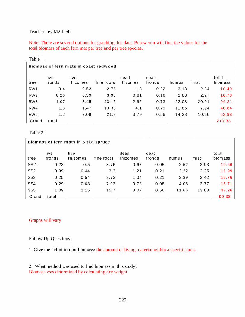
Teacher key M2.L.5b Note: There are several options for graphing this data. Below you will find the values for the total biomass of each fern mat per tree and per tree species. Table 1: Biomass of fern mats in coast redwood

tree live fronds

live rhizomes fine roots

dead rhizomes

dead fronds humus misc

total biomass

RW1 0.4 0.52 2.75 1.13 0.22 3.13 2.34 10.49 RW2 0.26 0.39 3.96 0.81 0.16 2.88 2.27 10.73 RW3 1.07 3.45 43.15 2.92 0.73 22.08 20.91 94.31 RW4 1.3 1.47 13.38 4.1 0.79 11.86 7.94 40.84 RW5 1.2 2.09 21.8 3.79 0.56 14.28 10.26 53.98 Grand total 210.33 Table 2:

Graphs will vary Follow Up Questions: 1. Give the definition for biomass: the amount of living material within a specific area. 2. What method was used to find biomass in this study? Biomass was determined by calculating dry weight

Biomass of fern mats in Sitka spruce

tree live fronds

live rhizomes fine roots

dead rhizomes

dead fronds humus misc

total biomass

SS 1 0.23 0.5 3.76 0.67 0.05 2.52 2.93 10.66 SS2 0.39 0.44 3.3 1.21 0.21 3.22 2.35 11.99 SS3 0.25 0.54 3.72 1.04 0.21 3.39 2.42 12.76 SS4 0.29 0.68 7.03 0.78 0.08 4.08 3.77 16.71 SS5 1.09 2.15 15.7 3.07 0.56 11.66 13.03 47.26 Grand total 99.38

225

3. What species of fern makes up the fern mats in this study? Leather fern (P. scouleri) 3. Using Data Table 1 above, identify the two parts of the fern mats that contributed the most to the overall biomass. Figure the percentage for each. Part percent ______________fine roots________________ ____41%_ ______________humus__________________ ____26%_ 4. Using Data Table 2 above, identify the two parts of the fern mats that contributed the most to the overall biomass. Figure the percentage for each. Part percent ______________fine roots_______________ ___34%__ ______________humus_________________ ___25.0% Note a close third place is misc. at 24.7%. If students estimate this is valid. Misc. includes debris, lichens, and bryophtes. 5. Compare and contrast the two tree types. Which type of tree had the larger amount of fern mat biomass overall? Explain. The larger biomass was found in coast redwood trees. Totals for RW were 210.33 kg and for SS 99.38 kg. The largest fern mat was found in RW 3 at a weight of 94.3 kg. 6. What type of forest has the most above ground biomass compared to any other ecosystem yet discovered? Old-growth coast redwood forest. Identify at least three factors that allow for large amounts of biomass to collect in this type of forest. -They live a long time -They get very large -The canopy can become very complex by the ability to resprout. Here complex reiterated branching occurs making large flat limbs or platforms where debris can accumulate. -Large epiphytes can grow in the crowns including fern mats the size of a truck.

226

Forest Ecology 101 Series (M2: Part II)

Module 2: Behind the Redwood Curtain

Part II

UNIT OF STUDY COVER PAGE

10th Grade Unit Lesson 1 - Biggest Trees on the Block

Lesson 2 - Shaking Up the Giants Lesson 3 - Life and Loss: Race to the Sky

Lesson 4 - Scaling the Tallest Trees Lesson 5 - A Canopy Conundrum

227

M2.G10 Lesson 1: Biggest Trees on the Block Unit Overview: Coast Redwoods Grade 10 Key Concepts:

• Life history strategies • Ecosystem dynamics • Energy and matter • Biomass and carbon • Developing and using

models to show relationships

Time: 80 - 120 minutes Materials for the Teacher: Student reading

M2.10.1a Student worksheet

M2.10.1b Teacher instructions

and key M2.10.1T Bathroom scales Calculators Measuring tapes Pictures or a video of

redwoods (optional) Graphing (optional)

Connections: STEM, carbon cycle, atmosphere, photosynthesis, forestry, mathematics, forest function and structure, conservation, earth science, social studies, economics Forest Ecology Series integration: M1: Integrative Forest Ecology

Learning Objectives: Students will review the concept of biomass. They will identify the life history strategies of the coast redwood that allows them to live 2,000 years and grow over 320 feet tall. They will understand that through the process of photosynthesis, water and carbon dioxide are converted into carbohydrates such as cellulose. Students will estimate the biomass of their classroom using the estimated dry weight of themselves and will compare their estimate to the biomass of some of largest redwood trees. Background information: Refer to the appropriate section in Part I: Teacher Companion for Module 2 and pgs. 6 and 7 from the Globe Carbon Cycle (see online resources below). Important Reference: The largest above ground biomass (AGB) calculations for redwood forests thus far are 3,500-5,000 Mg-1 ha (metric tons per hectare). Suggested procedure: Begin by asking some of the preliminary questions below to assess what students already know about photosynthesis and the carbon cycle. Next, define biomass and write the definition on the board. You may want to review the common units used for mass, volume, and area. Explain that the largest above-ground biomass (AGB) values that exist anywhere in the world occur in old-growth redwood forests. More than 2 to 3 times what you would find in a tropical rainforest. It may be appropriate at this time to show pictures or a video of large redwood trees in their natural setting. After initial questioning, have students read M2.10.1a The Life History of the Coast Redwood and complete student worksheet M2.10.1b. This could be assigned as homework or they can work on it using a partner in class. Once they learn about coast redwoods, proceed to the student activity explained in M2.10.1T. During this activity they will need to find their body weight and then calculate their dry weight by removing the portion that is water. Before proceeding, please read Biomass Units - Calculating Classroom Biomass (see online resources). If you want to have them calculate the biomass within a given area, you will need to measure the appropriate area. Once they calculate the biomass of “their classroom” they will compare it to the AGB values referenced above for redwoods. It is optional to have students graphically represent the comparative values. If you choose this option, you will need to allow for more time. Follow up this lesson with checking for understanding below.

228

Preliminary questions: • What process converts sunlight and CO2 into carbohydrates? • What does the term biomass mean? • What types of places are likely to have a lot of above ground biomass (AGB)? • How could we calculate the biomass of your body? • How could we calculate the biomass of a tree; of a grove of trees? • Do you think tree circumference has a direct relationship with the tree’s biomass? Why?

Why not? • What unit of measurement would we then use (refers to the previous question) for the

biomass of a tree in a 1 m square plot; in a 1 ha plot? Critical Thinking: Trees grow at different rates. How does the rate at which a tree grows influence the amount of carbon that is sequestered? Keywords: above-ground biomass (AGB), biomass, clonal, tree crown, dry weight, hectare, paleoendemic, photosynthesis, reiteration, sequester, volume NGSS alignment: HS-LS2.B: Ecosystem Interactions, Energy, and Dynamics LS2.A: Interdependent Relationships in Ecosystems LS2.B: Cycles of Matter and Energy Transfer in Ecosystems HS-LS2: Use mathematical representations to support and revise explanations based on evidence about factors affecting biodiversity and populations in ecosystems of different scales. Online resources: GLOBE Carbon Cycle Introduction to biomass: http://www.naturfagsenteret.no/binfil/download2.php?tid=1823763 Refer to this site for some of the necessary components of the activity in this lesson. There is excellent information presented here regarding how scientists measure trees and calculate biomass. The information comes from the University of New Hampshire which has many other lessons and activities regarding carbon and the carbon cycle. Save the Redwoods League: Redwoods and Climate: http://www.savetheredwoods.org/what-we-do/study/detail.php?id=438 This website is constantly updated and posts some of the latest research findings regarding coast redwood and climate change. The Learning Center page gives lesson options and many links to other information on redwoods including the complete Redwood Ed curriculum. U.S. Forest Service: Carbon Sequestration http://www.fs.fed.us/ecosystemservices/carbon.shtml. This site lists many links regarding forestry and carbon sequestration including sustainable forestry practices and ecosystem services. VIDEO: Climbing redwood giants http://channel.nationalgeographic.com/channel/explorer/videos/climbing-redwood-giants/ This is an excellent video showing researchers climbing the giant sequoia and coast redwood. It shows researchers in the canopy and is a good way to depict how large redwood trees actually are and how scientists are finding out more about them by studying the canopy.

229

EEI Connection: B.6.a. Biodiversity: The keystone of Life on Earth E.7.b. The Life and Times of Carbon B.8.b Biological Diversity: The World’s Riches Answers to preliminary questions: -What process converts sunlight and CO2 into carbohydrates? (photosynthesis) -What does the term biomass mean? (biomass is the total living material measured over a particular area) - What types of places are likely to have a lot of above ground biomass (AGB)? (students should be able to make the connection that any area with a lot of vegetation will have a lot of biomass. Places include all types of forests especially those with large trees) -How could we calculate the biomass of your body? (weigh yourself, convert to dry weight, and divide by a given area) -How could we calculate the biomass of a tree; of a grove of trees? (Obviously we can’t cut down whole trees and weigh them. Scientists therefore take tree measurements including dbh, height, volume, and density to calculate biomass and usually convert to dry weight by drying samples in an oven)(for more information refer to the GLOBE: Carbon Cycle link above) -Do you think tree circumference has a direct relationship to a tree’s biomass? Why or why not? (Why - usually trees with larger diameters have greater mass. Why not? - You could have a large diameter tree that is not very tall or vice versa. Finding accurate measurements can be difficult. You also need to consider the height of the tree, the density of the wood, and the size of the tree crown or total volume of a tree to find biomass) -What unit of measurement would we then use for the biomass of a tree in a 1 m square plot; in a 1 ha plot (Scientists typically use the metric system and measure mass in grams, kilograms, or metric tons. The standard unit for area is m2 or a hectare (10,000 m2). An example of a unit for biomass therefore is g/m2 or Mg/ha2. You could also use lbs/acre or lbs/ft2) Checking for understanding:

• How did the actual data compare with your predictions? • How accurate is the data we collected? What factors are unaccounted for? • Assume two trees have the same height and circumference, but different biomasses.

What factors might account for this difference? • How does the carbon stored in trees relate to climate (greenhouse effect)? • What different parts of a forest are considered “pools of carbon”? • Is the storing of carbon in living trees a long-term or short-term component of the carbon

cycle?

230

M2.G10.L1 (Unit Overview continued) Suggested extensions:

• Show a video about coast redwoods. Two films are recommended: Nat’l Geographic: Climbing the World’s largest trees and California Legacy Project: Changing Places: The Redwoods found at calegacy.org.

• Using online resources and other information, have students take tree measurements in the field such as circumference, height, and basal area (see lesson M1.G10.L4).

• Have students read about managing our forests for carbon sequestration. Refer to the online resources for more information.

• Have students find their carbon footprint using one of the many carbon calculators available online or as an app.

• Review the greenhouse effect by connecting the carbon stored in trees to the carbon stored in fossil fuels such as coal and oil.

• Begin a tree-planting project. • Visit a redwood state park or another redwood sanctuary such as Headwaters Forest

Reserve to look for the objects that contribute substantial biomass. Student reading M2.10.L1a Student worksheet M2.10.L1b Teacher instructions and key M2.10.1T

231

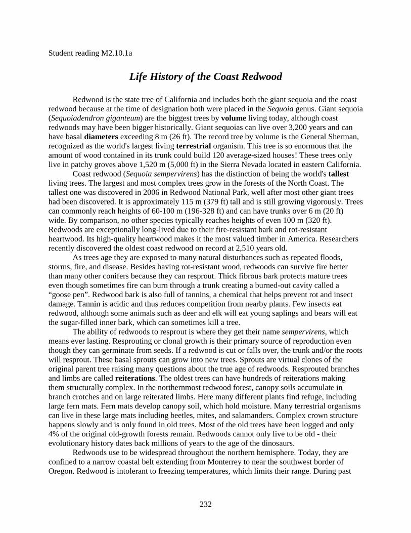
Student reading M2.10.1a

Life History of the Coast Redwood Redwood is the state tree of California and includes both the giant sequoia and the coast redwood because at the time of designation both were placed in the Sequoia genus. Giant sequoia (Sequoiadendron giganteum) are the biggest trees by volume living today, although coast redwoods may have been bigger historically. Giant sequoias can live over 3,200 years and can have basal diameters exceeding 8 m (26 ft). The record tree by volume is the General Sherman, recognized as the world's largest living terrestrial organism. This tree is so enormous that the amount of wood contained in its trunk could build 120 average-sized houses! These trees only live in patchy groves above 1,520 m (5,000 ft) in the Sierra Nevada located in eastern California. Coast redwood (Sequoia sempervirens) has the distinction of being the world's tallest living trees. The largest and most complex trees grow in the forests of the North Coast. The tallest one was discovered in 2006 in Redwood National Park, well after most other giant trees had been discovered. It is approximately 115 m (379 ft) tall and is still growing vigorously. Trees can commonly reach heights of 60-100 m (196-328 ft) and can have trunks over 6 m (20 ft) wide. By comparison, no other species typically reaches heights of even 100 m (320 ft). Redwoods are exceptionally long-lived due to their fire-resistant bark and rot-resistant heartwood. Its high-quality heartwood makes it the most valued timber in America. Researchers recently discovered the oldest coast redwood on record at 2,510 years old. As trees age they are exposed to many natural disturbances such as repeated floods, storms, fire, and disease. Besides having rot-resistant wood, redwoods can survive fire better than many other conifers because they can resprout. Thick fibrous bark protects mature trees even though sometimes fire can burn through a trunk creating a burned-out cavity called a “goose pen”. Redwood bark is also full of tannins, a chemical that helps prevent rot and insect damage. Tannin is acidic and thus reduces competition from nearby plants. Few insects eat redwood, although some animals such as deer and elk will eat young saplings and bears will eat the sugar-filled inner bark, which can sometimes kill a tree. The ability of redwoods to resprout is where they get their name sempervirens, which means ever lasting. Resprouting or clonal growth is their primary source of reproduction even though they can germinate from seeds. If a redwood is cut or falls over, the trunk and/or the roots will resprout. These basal sprouts can grow into new trees. Sprouts are virtual clones of the original parent tree raising many questions about the true age of redwoods. Resprouted branches and limbs are called reiterations. The oldest trees can have hundreds of reiterations making them structurally complex. In the northernmost redwood forest, canopy soils accumulate in branch crotches and on large reiterated limbs. Here many different plants find refuge, including large fern mats. Fern mats develop canopy soil, which hold moisture. Many terrestrial organisms can live in these large mats including beetles, mites, and salamanders. Complex crown structure happens slowly and is only found in old trees. Most of the old trees have been logged and only 4% of the original old-growth forests remain. Redwoods cannot only live to be old - their evolutionary history dates back millions of years to the age of the dinosaurs. Redwoods use to be widespread throughout the northern hemisphere. Today, they are confined to a narrow coastal belt extending from Monterrey to near the southwest border of Oregon. Redwood is intolerant to freezing temperatures, which limits their range. During past

232

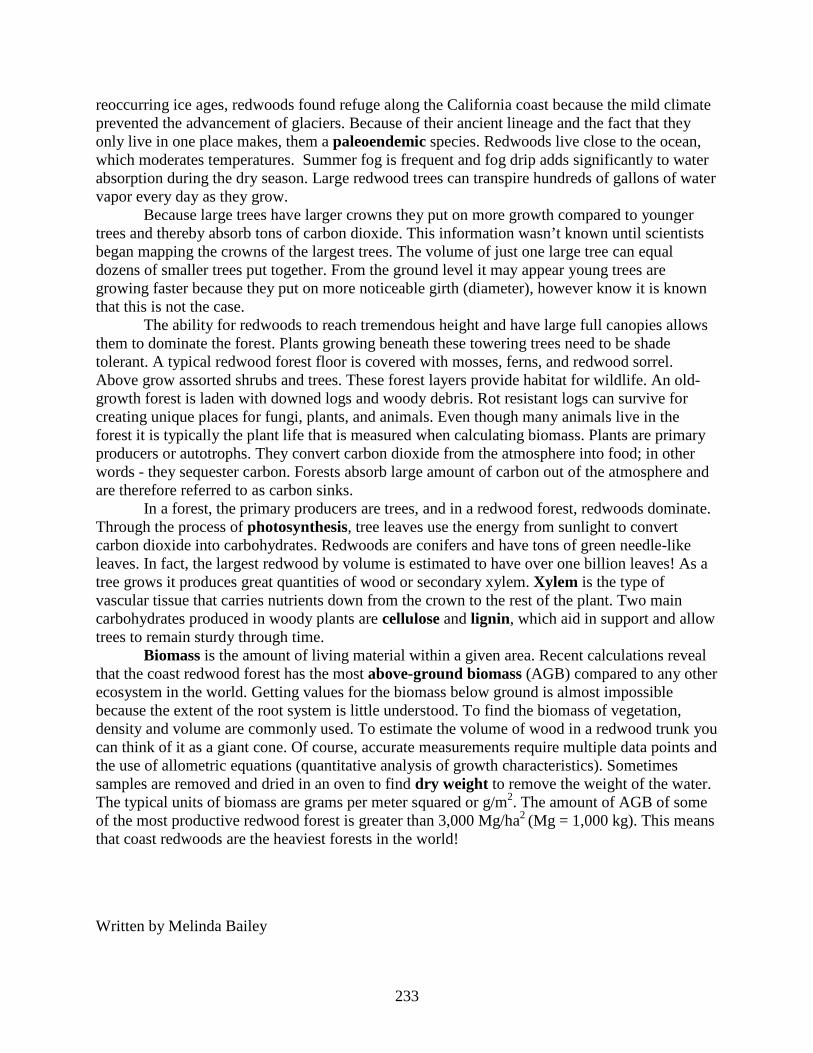
reoccurring ice ages, redwoods found refuge along the California coast because the mild climate prevented the advancement of glaciers. Because of their ancient lineage and the fact that they only live in one place makes, them a paleoendemic species. Redwoods live close to the ocean, which moderates temperatures. Summer fog is frequent and fog drip adds significantly to water absorption during the dry season. Large redwood trees can transpire hundreds of gallons of water vapor every day as they grow. Because large trees have larger crowns they put on more growth compared to younger trees and thereby absorb tons of carbon dioxide. This information wasn’t known until scientists began mapping the crowns of the largest trees. The volume of just one large tree can equal dozens of smaller trees put together. From the ground level it may appear young trees are growing faster because they put on more noticeable girth (diameter), however know it is known that this is not the case. The ability for redwoods to reach tremendous height and have large full canopies allows them to dominate the forest. Plants growing beneath these towering trees need to be shade tolerant. A typical redwood forest floor is covered with mosses, ferns, and redwood sorrel. Above grow assorted shrubs and trees. These forest layers provide habitat for wildlife. An old-growth forest is laden with downed logs and woody debris. Rot resistant logs can survive for creating unique places for fungi, plants, and animals. Even though many animals live in the forest it is typically the plant life that is measured when calculating biomass. Plants are primary producers or autotrophs. They convert carbon dioxide from the atmosphere into food; in other words - they sequester carbon. Forests absorb large amount of carbon out of the atmosphere and are therefore referred to as carbon sinks. In a forest, the primary producers are trees, and in a redwood forest, redwoods dominate. Through the process of photosynthesis, tree leaves use the energy from sunlight to convert carbon dioxide into carbohydrates. Redwoods are conifers and have tons of green needle-like leaves. In fact, the largest redwood by volume is estimated to have over one billion leaves! As a tree grows it produces great quantities of wood or secondary xylem. Xylem is the type of vascular tissue that carries nutrients down from the crown to the rest of the plant. Two main carbohydrates produced in woody plants are cellulose and lignin, which aid in support and allow trees to remain sturdy through time. Biomass is the amount of living material within a given area. Recent calculations reveal that the coast redwood forest has the most above-ground biomass (AGB) compared to any other ecosystem in the world. Getting values for the biomass below ground is almost impossible because the extent of the root system is little understood. To find the biomass of vegetation, density and volume are commonly used. To estimate the volume of wood in a redwood trunk you can think of it as a giant cone. Of course, accurate measurements require multiple data points and the use of allometric equations (quantitative analysis of growth characteristics). Sometimes samples are removed and dried in an oven to find dry weight to remove the weight of the water. The typical units of biomass are grams per meter squared or g/m2. The amount of AGB of some of the most productive redwood forest is greater than 3,000 Mg/ha2 (Mg = 1,000 kg). This means that coast redwoods are the heaviest forests in the world!

Written by Melinda Bailey

233

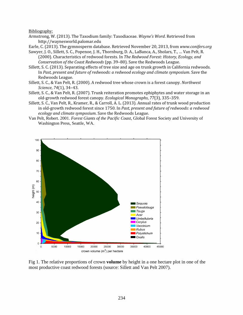
Bibliography: Armstrong, W. (2013). The Taxodium family: Taxodiaceae. Wayne’s Word. Retrieved from

http://waynesworld.palomar.edu Earle, C. (2013). The gymnosperm database. Retrieved November 20, 2013, from www.conifers.org Sawyer, J. O., Sillett, S. C., Popenoe, J. H., Thornburg, D. A., LaBanca, A., Sholars, T., … Van Pelt, R.

(2000). Characteristics of redwood forests. In The Redwood Forest: History, Ecology, and Conservation of the Coast Redwoods (pp. 39–80). Save the Redwoods League.

Sillett, S. C. (2013). Separating effects of tree size and age on trunk growth in California redwoods. In Past, present and future of redwoods: a redwood ecology and climate symposium. Save the Redwoods League.

Sillett, S. C., & Van Pelt, R. (2000). A redwood tree whose crown is a forest canopy. Northwest Science, 74(1), 34–43.

Sillett, S. C., & Van Pelt, R. (2007). Trunk reiteration promotes ephiphytes and water storage in an old-growth redwood forest canopy. Ecological Monographs, 77(3), 335–359.

Sillett, S. C., Van Pelt, R., Kramer, R., & Carroll, A. L. (2013). Annual rates of trunk wood production in old-growth redwood forest since 1750. In Past, present and future of redwoods: a redwood ecology and climate symposium. Save the Redwoods League.

Van Pelt, Robert. 2001. Forest Giants of the Pacific Coast, Global Forest Society and University of Washington Press, Seattle, WA.

Fig 1. The relative proportions of crown volume by height in a one hectare plot in one of the most productive coast redwood forests (source: Sillett and Van Pelt 2007).

234

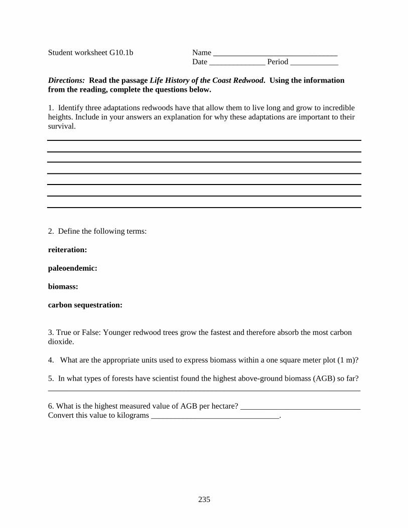
Student worksheet G10.1b Name _______________________________ Date ______________ Period ____________ Directions: Read the passage Life History of the Coast Redwood. Using the information from the reading, complete the questions below. 1. Identify three adaptations redwoods have that allow them to live long and grow to incredible heights. Include in your answers an explanation for why these adaptations are important to their survival. 2. Define the following terms: reiteration: paleoendemic: biomass: carbon sequestration: 3. True or False: Younger redwood trees grow the fastest and therefore absorb the most carbon dioxide. 4. What are the appropriate units used to express biomass within a one square meter plot (1 m)? 5. In what types of forests have scientist found the highest above-ground biomass (AGB) so far? ______________________________________________________________________________ 6. What is the highest measured value of AGB per hectare? ______________________________ Convert this value to kilograms ________________________________.

235

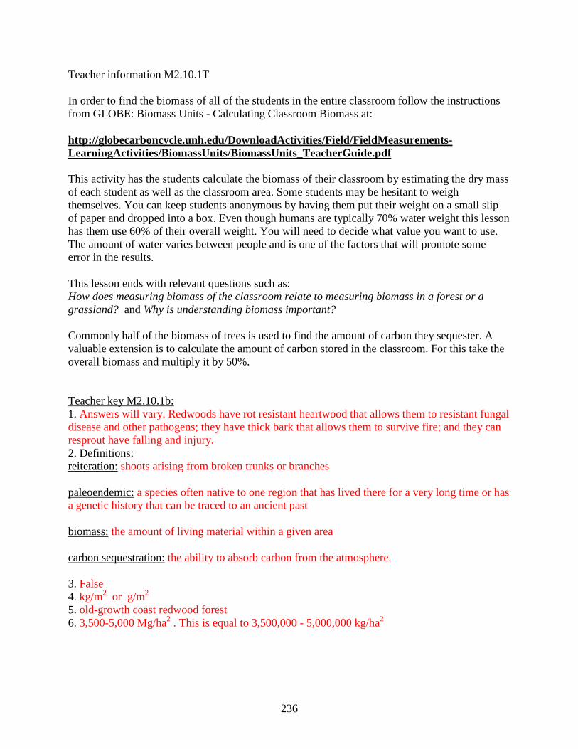
Teacher information M2.10.1T In order to find the biomass of all of the students in the entire classroom follow the instructions from GLOBE: Biomass Units - Calculating Classroom Biomass at: http://globecarboncycle.unh.edu/DownloadActivities/Field/FieldMeasurements-LearningActivities/BiomassUnits/BiomassUnits_TeacherGuide.pdf This activity has the students calculate the biomass of their classroom by estimating the dry mass of each student as well as the classroom area. Some students may be hesitant to weigh themselves. You can keep students anonymous by having them put their weight on a small slip of paper and dropped into a box. Even though humans are typically 70% water weight this lesson has them use 60% of their overall weight. You will need to decide what value you want to use. The amount of water varies between people and is one of the factors that will promote some error in the results. This lesson ends with relevant questions such as: How does measuring biomass of the classroom relate to measuring biomass in a forest or a grassland? and Why is understanding biomass important? Commonly half of the biomass of trees is used to find the amount of carbon they sequester. A valuable extension is to calculate the amount of carbon stored in the classroom. For this take the overall biomass and multiply it by 50%. Teacher key M2.10.1b: 1. Answers will vary. Redwoods have rot resistant heartwood that allows them to resistant fungal disease and other pathogens; they have thick bark that allows them to survive fire; and they can resprout have falling and injury. 2. Definitions: reiteration: shoots arising from broken trunks or branches paleoendemic: a species often native to one region that has lived there for a very long time or has a genetic history that can be traced to an ancient past biomass: the amount of living material within a given area carbon sequestration: the ability to absorb carbon from the atmosphere. 3. False 4. kg/m2 or g/m2 5. old-growth coast redwood forest 6. 3,500-5,000 Mg/ha2 . This is equal to 3,500,000 - 5,000,000 kg/ha2

236

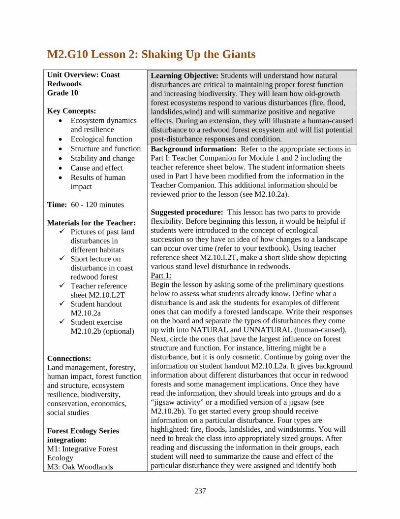
M2.G10 Lesson 2: Shaking Up the Giants Unit Overview: Coast Redwoods Grade 10 Key Concepts:

• Ecosystem dynamics and resilience

• Ecological function • Structure and function • Stability and change • Cause and effect • Results of human

impact Time: 60 - 120 minutes Materials for the Teacher: Pictures of past land

disturbances in different habitats

Short lecture on disturbance in coast redwood forest

Teacher reference sheet M2.10.L2T

Student handout M2.10.2a

Student exercise M2.10.2b (optional)

Connections: Land management, forestry, human impact, forest function and structure, ecosystem resilience, biodiversity, conservation, economics, social studies Forest Ecology Series integration: M1: Integrative Forest Ecology M3: Oak Woodlands

Learning Objective: Students will understand how natural disturbances are critical to maintaining proper forest function and increasing biodiversity. They will learn how old-growth forest ecosystems respond to various disturbances (fire, flood, landslides,wind) and will summarize positive and negative effects. During an extension, they will illustrate a human-caused disturbance to a redwood forest ecosystem and will list potential post-disturbance responses and condition. Background information: Refer to the appropriate sections in Part I: Teacher Companion for Module 1 and 2 including the teacher reference sheet below. The student information sheets used in Part I have been modified from the information in the Teacher Companion. This additional information should be reviewed prior to the lesson (see M2.10.2a). Suggested procedure: This lesson has two parts to provide flexibility. Before beginning this lesson, it would be helpful if students were introduced to the concept of ecological succession so they have an idea of how changes to a landscape can occur over time (refer to your textbook). Using teacher reference sheet M2.10.L2T, make a short slide show depicting various stand level disturbance in redwoods. Part 1: Begin the lesson by asking some of the preliminary questions below to assess what students already know. Define what a disturbance is and ask the students for examples of different ones that can modify a forested landscape. Write their responses on the board and separate the types of disturbances they come up with into NATURAL and UNNATURAL (human-caused). Next, circle the ones that have the largest influence on forest structure and function. For instance, littering might be a disturbance, but it is only cosmetic. Continue by going over the information on student handout M2.10.L2a. It gives background information about different disturbances that occur in redwood forests and some management implications. Once they have read the information, they should break into groups and do a “jigsaw activity” or a modified version of a jigsaw (see M2.10.2b). To get started every group should receive information on a particular disturbance. Four types are highlighted: fire, floods, landslides, and windstorms. You will need to break the class into appropriately sized groups. After reading and discussing the information in their groups, each student will need to summarize the cause and effect of the particular disturbance they were assigned and identify both

237

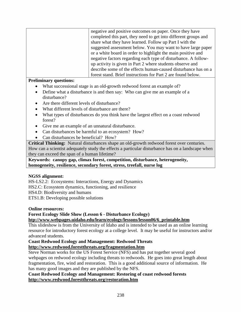
negative and positive outcomes on paper. Once they have completed this part, they need to get into different groups and share what they have learned. Follow up Part I with the suggested assessment below. You may want to have large paper or a white board in order to highlight the main positive and negative factors regarding each type of disturbance. A follow-up activity is given in Part 2 where students observe and describe some of the effects human-caused disturbance has on a forest stand. Brief instructions for Part 2 are found below.

Preliminary questions: • What successional stage is an old-growth redwood forest an example of? • Define what a disturbance is and then say: Who can give me an example of a

disturbance? • Are there different levels of disturbance? • What different levels of disturbance are there? • What types of disturbances do you think have the largest effect on a coast redwood

forest? • Give me an example of an unnatural disturbance. • Can disturbances be harmful to an ecosystem? How? • Can disturbances be beneficial? How?

Critical Thinking: Natural disturbances shape an old-growth redwood forest over centuries. How can a scientist adequately study the effects a particular disturbance has on a landscape when they can exceed the span of a human lifetime? Keywords: canopy gap, climax forest, competition, disturbance, heterogeneity, homogeneity, resilience, secondary forest, stress, treefall, nurse log NGSS alignment: HS-LS2.2: Ecosystems: Interactions, Energy and Dynamics HS2.C: Ecosystem dynamics, functioning, and resilience HS4.D: Biodiversity and humans ETS1.B: Developing possible solutions Online resources: Forest Ecology Slide Show (Lesson 6 - Disturbance Ecology) htp://www.webpages.uidaho.edu/learn/ecology/lessons/lesson06/6_printable.htm This slideshow is from the University of Idaho and is intended to be used as an online learning resource for introductory forest ecology at a college level. It may be useful for instructors and/or advanced students. Coast Redwood Ecology and Management: Redwood Threats http://www.redwood.forestthreats.org/fragmentation.htm Steve Norman works for the US Forest Service (NFS) and has put together several good webpages on redwood ecology including threats to redwoods. He goes into great length about fragmentation, fire, wind and restoration. This is a good additional source of information. He has many good images and they are published by the NFS. Coast Redwood Ecology and Management: Restoring of coast redwood forests http://www.redwood.forestthreats.org/restoration.htm

238

(Online Resources continued) This is a good reference for Part 2. Again, Steve Norman has a good overview of restoration efforts in secondary forests stands. He presents the history, past land management practices, and new efforts being used to promote heterogenous redwood forest stands. Answers to preliminary questions (Part 1): -What successional stage is an old-growth redwood forest an example of? (An old-growth redwood forest is a classic example of a stable climax forest. It is very resilient and able to withstand low level disturbance) -Define what a disturbance is and then say: Who can give me an example of a disturbance? (accept all answers and write them in the appropriate section) -Are there different levels of disturbance? (YES. Having students understand that there are different degrees or scales of disturbances is important. For instance, intense fires act very differently on a landscape than low intensity fires. Also large scale disturbances such as a flood, have a much broader effect than small scale disturbances such as a treefall) -What different levels of disturbance are there? (This applies to the question above: large scale and small scale disturbance. Also natural versus unnatural disturbance regimes may be brought up here. For instance clear cuts have a much higher level of disturbance compared to a few trees being cut to make a cabin or something like that). -What types of disturbances do you think have the largest effect on a coast redwood forest? (fire has a large effect. The degree by which fire is necessary in redwood forests in unclear. Wind is probably the most common natural occurrence and is responsible for most of the woody debris found on the forest floor) -Give me an example of an unnatural disturbance (Answers will vary. Refer to the teacher reference sheet). -Can disturbances be harmful to an ecosystem? How? (Yes. Answers will vary. Refer to the teacher reference sheet) -Can disturbances be beneficial? How? (Yes. Answers will vary. Refer to the teacher reference sheet) Suggested follow up questions and assessment (Part 1):

• What type of disturbance promotes resprouts? Why? • What type of disturbance promotes seed regeneration? How? • What type of disturbance enhances wildlife habitat? How? • What type of disturbance creates habitat coast redwood prefers? • What type of disturbance increases woody debris?

Lead into the next part - discuss impacts of land changes and how each affects the forest differently. Sometimes a forest can respond quickly and other times it may never recover.

239

Part 2: Human-caused disturbance First have students compare the two images given below (see M2.10.L2b). Figure A shows a profile of an old-growth heterogenous forest that includes multi-aged trees, forest gaps, and downed wood. Figure B shows a profile of a modified secondary homogeneous forest. Here virtually all of the trees are the same age, little understory vegetation exists, and the trees are more tightly spaced with no gaps. Have students identify the different features that are present and absent. This can be done together or as a group. An optional extension is to have them draw a picture of a human-caused disturbance and identify potential post-disturbance responses and conditions that occur. Suggested extensions:

• Explore how different ecosystems respond to different disturbance regimes such as drier upland forests and grasslands. (Certain forests are being heavily impacted by bark beetles, which redwoods are apparently immune to and other conifers don’t resprout in response to fire like redwood do.)

• Conduct an experiment using plants grown in soil with different amounts of ash or other nutrients, which can represent the replenishment of soil after certain disturbances (fire and flood).

• Begin a poster campaign on threatened and endangered species of the North Coast. Part of this campaign can connect old-growth characteristics to habitats necessary for local threatened species such as the marbled murrelet, spotted owl, coho salmon, different amphibian species, and others.

• Have students role-play the different approaches land owners and environmental activists might take regarding how to manage a redwood forest.

• During a field trip have the students make a photographic journal. In this journal they can document the different disturbances they observe first hand.

Teacher reference sheet M2.10.L2T Student handout M2.10.L2a Part 1 Student handout M2.10.L2a Part 2 Student exercise M2.10.L2b

240

Teacher reference sheet M2.10.L2T Disturbances are ecosystem processes that affect the composition, structure, and function of an ecosystem. (adapted from www.uidaho.edu) Background Information: Ecological processes are controlled by a set of factors including disturbance regimes. Sometimes disturbance are considered a negative influence on the landscape because they can lead to death and destruction, however disturbances are an expected influence on the landscape and have ecological value. The size, severity, and timing of disturbances differ and are often unpredictable. In many circumstances human alterations to the landscape have shifted the severity of disturbances beyond a natural state, which can upset the equilibrium necessary for ecosystems to rebound. Climax communities, such as an old-growth forest, are more resilient than logged forests and are able to maintain equilibrium throughout disturbance regimes. Unnatural disturbances usually leave the landscape worst off than the pristine condition. Here one needs to considered ecological and economical tradeoffs. Today, many altered landscapes require additional management to restore and enhance their ecological integrity. Foresters often use natural disturbances to assist in developing forest management (silviculture) models. Current vegetative patterns and ecological integrity are a reflection of landownership. One unnatural large-scale disturbance that negatively affects the healthy and resilience of coniferous forests is the practice of clear cutting. Soon after a clear-cut (initiation stage), biodiversity can be reduced and stand level dynamics can be altered (refer to Module 1 for more information) depending on methods used. Older practices were much more destructive that modern day practices. Today many secondary forests are 50-80 years old and are managed as tree farms with even-aged stands. These cut over regions are being studied to assess how land managers can integrate adaptive management techniques that regard the ecosystem as a whole. The challenge is to develop approaches that can lead to ecological complexity while still logging the land. One way to manage for complexity is to leave large amounts of woody debris and hardwood species. Another is to leave biological legacies such as old trees and snags. Future efforts may include the manual manipulation of tree crowns to imitate some of the complexity found in older trees in order to encourage more suitable habitat for threatened species. ----------------------------------- In this exercise students will learn about one type of disturbance and how it can shape a redwood forest over time. Once they have written down a summary, they should get into groups in order to share information. Once they are done reading, writing, and sharing, assess their knowledge by having them answer the suggested follow up questions. You may want to put these into a matching format. For an overview of disturbance regimes and post-disturbance responses, refer to Table 1 below.

241

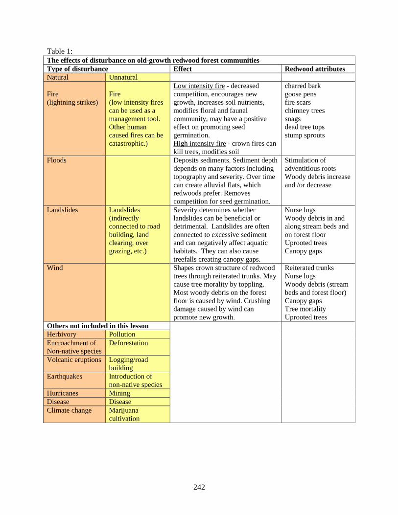
Table 1: The effects of disturbance on old-growth redwood forest communities Type of disturbance Effect Redwood attributes Natural Unnatural Fire (lightning strikes)

Fire (low intensity fires can be used as a management tool. Other human caused fires can be catastrophic.)

Low intensity fire - decreased competition, encourages new growth, increases soil nutrients, modifies floral and faunal community, may have a positive effect on promoting seed germination. High intensity fire - crown fires can kill trees, modifies soil

charred bark goose pens fire scars chimney trees snags dead tree tops stump sprouts

Floods Deposits sediments. Sediment depth depends on many factors including topography and severity. Over time can create alluvial flats, which redwoods prefer. Removes competition for seed germination.

Stimulation of adventitious roots Woody debris increase and /or decrease

Landslides Landslides (indirectly connected to road building, land clearing, over grazing, etc.)

Severity determines whether landslides can be beneficial or detrimental. Landslides are often connected to excessive sediment and can negatively affect aquatic habitats. They can also cause treefalls creating canopy gaps.

Nurse logs Woody debris in and along stream beds and on forest floor Uprooted trees Canopy gaps

Wind Shapes crown structure of redwood trees through reiterated trunks. May cause tree morality by toppling. Most woody debris on the forest floor is caused by wind. Crushing damage caused by wind can promote new growth.

Reiterated trunks Nurse logs Woody debris (stream beds and forest floor) Canopy gaps Tree mortality Uprooted trees

Others not included in this lesson

Herbivory Pollution Encroachment of Non-native species

Deforestation

Volcanic eruptions Logging/road building

Earthquakes Introduction of non-native species

Hurricanes Mining Disease Disease Climate change Marijuana

cultivation

242

Student handout M2.10.L2a

Shaking Up the Giants Part I. Background Information: A mature coast redwood forest is structurally complex and diverse and is shaped by many forces that can occur over centuries. Disturbances are a critical factor in stand-level dynamics in most forest ecosystems. Low-levels of disturbance tend to increase biodiversity by breaking up dominance and providing new opportunities for the establishment of other species. Disturbances can also have beneficial effects on nutrient cycling, modification of fuel loads, formation of tree cavities, and the promotion of complex crown structures. In addition, long-lasting woody debris that can come from wind throw or dead trees creates important habitat. Human-caused disturbances, such as those associated with Euro-American settlement, can upset the equilibrium of a mature forest and some forests may never fully recover afterwards. When we think of a disturbance to a landscape we sometimes think of it as destructive or something negative. All ecosystems experience some level of disturbance, however, and they are a natural process. When we think of disturbances we must consider their degree or scale. Large-scale disturbances can affect thousands of acres: examples are fire, hurricane, or flood. A small-scale disturbance can be something minor, which only affects a small area: examples are a tree falling down or a landslide. Additionally, disturbances are ecosystem-specific meaning they will affect specific ecosystems differently. For instance, some forest types depend on fire to promote reproduction and growth, while others are severely harmed from a fire. Maintaining ecosystems for various disturbances is a challenge in many management settings because some are considered dangerous or undesirable. Understanding the role of historical disturbances in redwood forests has been difficult to study and has been debated over many years. Some raise the question whether coast redwood need periodic flooding and/or fire to encourage reproduction. Small-scale disturbances, such as canopy gaps can promote a larger diversity of plants because more light is available these places compared to the interior of a forest. Coast redwoods have many life history strategies that allow them to recover from a host of different disturbances. Four types of disturbances are highlighted below: fire, floods, landslides, and windstorms. There are several others not discussed here, such as encroachment by non-native species and herbivory (consumption by herbivores). In this exercise, your will become familiar about the negative and positive effects of one type of disturbance. Once you learn about it, you should summarize what you have learned below. In your summary, please identify the different scenarios that might cause the particular disturbance. After writing your summary you will be instructed to get into a new group in order to share what you have learned and become informed about other types of disturbances. Directions: Write your summary on a separate piece of paper.

243

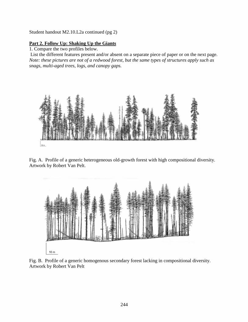
Student handout M2.10.L2a continued (pg 2) Part 2. Follow Up: Shaking Up the Giants 1. Compare the two profiles below. List the different features present and/or absent on a separate piece of paper or on the next page. Note: these pictures are not of a redwood forest, but the same types of structures apply such as snags, multi-aged trees, logs, and canopy gaps.

Fig. A. Profile of a generic heterogeneous old-growth forest with high compositional diversity. Artwork by Robert Van Pelt.

Fig. B. Profile of a generic homogenous secondary forest lacking in compositional diversity. Artwork by Robert Van Pelt

244

Student handout M2.10.L2a continued (pg 3) 2. Follow up this exercise by drawing a picture of a human caused disturbance to a redwood forest. It could be a direct disturbance, such as large scale clearing or an indirect disturbance, such as a landslide caused by a road built on a steep hillside. Discuss how your particular disturbance might alter the original forest and the organisms that live there.

page 2

245

Student Exercise M2.10.2b (Part I) Trees shaped by time: Natural disturbances of Coast Redwood Forest Group 1: Fire Fire Fire has certainly shaped the redwood forest ecosystem for millennia, Understanding exactly how this phenomenon affects the forest system has proven difficult. The fact that coasts redwoods grow in humid and foggy places makes regular or widespread fires in the wettest forests unlikely. Some redwood groves are fragmented and the effects fires may have on forest composition can vary widely depending on location. A growing body of evidence from analyzing fire scars, documents that frequent, periodic low intensity fires were a common in many coast redwood forests. Most fires, prior to 1850 were probably ignited by Native Americans since lightning rarely occurs along the coast. Observations done in old-growth redwood canopies note dead treetops that are most likely caused by crown fires leading to a more complex structure. Many redwood stands, especially those inside parks, have not experienced fire since the early 1930s. Regular fires would deter the establishment of fire-intolerant species that can compete with redwood, such as grand fir, Douglas-fir, and western hemlock. In addition, the density of shrubs, forest duff, and woody debris would have been reduced under low intensity fire, and as a consequence the forest composition and structure may have been quite different in the past. It is likely that the loss of surface fires has occurred mostly in response to the loss of Native American ignition sources, active fire suppression, and other changes brought about by Euro-American settlement and land use. When fire does occur, the thick fibrous bark protects mature trees, and many large trees can survive moderate to intense ground fires. Even a casual observer can see signs of past fires by the charred bark on lower trunk surfaces and large burned out cavities, called "goose pens". Along the lower trunks fire cavities or goose pens can serve as nesting sites for some bird and bat species. Intensive fires and crown fires can kill trees, especially young trees.

246

Trees shaped by time: Natural disturbances of Coast Redwood Forest Group 2: Floods Floods Flooding occurs in many areas across the North Coast and particularly affects stands of redwoods along alluvial flats. One study conducted in the Bull Creek area revealed nearly 15 major floods have occurred there over the last 1,000 years. Along Redwood Creek, the Tall Trees grove has experienced at least seven different floods over 810 years, depositing over a meter of silt and sand. In this same area, 12 floods have deposited over 3 meters of sediment over the last 3,250 years. The post-flood response by redwood trees varies. Sometimes so much sediment is deposited that root systems suffocate from inadequate oxygen supply and redwood trees die. Other times adventitious roots are sent towards the surface, which the tree temporarily depends on, while a more permanent multi-layered root system develops. Overall, redwoods seem to adapt well to flooding events and floods can have a positive effect on both the health and reestablishment of redwoods. In some places, new sediment deposits set up ideal conditions for successful seed germination and survival. The timing of seed fall relative to deposition of alluvial sediments may be an important factor to stand level dynamics. Flooding also brings many rich nutrients to soils increasing their fertilization. Along rivers and streams flooding can often undercut stream banks causing trees to fall. These large downed logs create important habitat for young salmon and other aquatic organisms. Two severe floods happened in the last century causing much damage to certain forests. In some cases dozens of trees were killed and massive waves of debris washed out bridges, culverts, and roads. Certain areas of the Eel River gained so much sediment that towns were buried and all trees along riparian zones were lost. The coarse gravels and lack of soil have made it difficult for trees to regenerate. Clumps of river silt deposited during the severe 1964 flood can still be clearly seen caked onto the trunks of many trees, sometimes 6 m (20 ft) or more high, in several groves located in Humboldt Redwood State Park.

247

Trees shaped by time: Natural disturbances of Coast Redwood Forest Group 3: Landslides Landslides Coast redwoods commonly live in loosely structured soils and in a highly active tectonic zone. The intensity of landslides is dependent upon many factors including the geology and topography of an area. These factors combined with high rainfall result in some of the highest erosion rates in the continental United States. Erosion is further accelerated through the removal of topsoil and forest duff associated with logging, grazing, and development. Certain redwood stands are exceptionally vulnerable to landsliding, especially those in narrow stream channels or on steep inner hillsides adjacent to large streams. Historically, erosion and deposition have helped create some of the preferred landforms coast redwoods grow on, such as broad, upraised alluvial flats that can build up over time by repeated flooding events and stream deposition. The largest densest stands of coast redwood tend to occupy alluvial flats including the tallest grove of redwoods in the world. Landslides can also cause tree toppling. When a tree falls it adds to the amount of deadwood on the forest floor and along rivers. Large woody debris is an essential component in healthy aquatic systems. Logs offer hiding places for fish and can slow water down creating necessary pools. Other times landslides can have negative effects on watersheds by the overloading of sediment. Foresters constantly have to monitor how much sediment gets into streams so they don’t log in the wrong areas. Because of the high value of rivers and streams no logging equipment is allowed with 200 feet of a waterway. Roads can also be a source of sedimentation. Too much fine silt and sediment will fill in gaps between coarse gravel where salmon eggs are deposited. Eggs need to have oxygen around them or they will suffocate and die.

248

Trees shaped by time: Natural disturbances of Coast Redwood Forest Group 4: Windstorms Windstorms The North Coast can experience severe windstorms. Winds are responsible for shaping trees and can damage crowns of redwoods. Large branches or parts of a tree trunk can calve off leaving entry points for fungus and disease. Wind is one of the primary causes of coarse woody debris found resting on the forest floor. The crushing damage caused by falling debris can reduce potential suppression and stimulate succession in some forests. When a tree falls a canopy gap is created. Canopy gaps allow higher light levels to penetrate to the forest floor, encouraging new plant growth and establishment, thereby producing a more diverse plant community. Redwood trees do not have a taproot and their shallow root systems become disadvantageous when the ground is saturated and the winds are high, especially for trees that lean. Many heavy and tall mature redwood trees, unable to withstand this strong force, have toppled over in winter storms. In fact, wind is the leading natural cause of death for large decadent trees. Wind-caused tree casualties are abundant in many local redwood groves and can be easily observed. One of the more famous examples is the Dyerville Giant, which fell in 1991, located in Founders Grove in Humboldt Redwoods State Park, north of Weott. This tree, taller than the Statue of Liberty, crashed with such force that it registered on a nearby seismograph. When a large tree is lost during a windstorm, the large downed tree becomes a valuable forest commodity. Once on the forest floor, a huge log may take centuries to decompose. In the process, it produces shade, traps moisture, and provides habitat for moisture-loving plants and animals. Large downed logs are often called nurse logs because they support a wide diversity of living things and are an important addition to the forest ecosystem.

249

M2.G10 Lesson 3: Race to the Sky Unit Overview: Coast Redwoods Grade 10 Key Concepts:

• Ecosystem dynamics • Analyzing density

dependent factors • Graphically

interpreting data • The movement of

systems to stable state. Time: 80 - 100 minutes Materials for the Teacher: Access to computers

and a graphing program similar to Excel.

Teacher key M2.10.3T Student Worksheet

M2.10.3a Reference sheet

M2.10.3R Pictures and/or a short

lecture about managing in coast redwood (optional)

Connections: STEM, photosynthesis, competition, carrying capacity, genetics, forestry, mathematics, conservation, soil science, social studies, economics Forest Ecology Series integration: M1: Integrative Forest Ecology

Learning Objectives: Students will graphically illustrate the results of a tree-thinning project conducted in Redwood National Park that reduced Douglas-fir and other competitive species in order to restore and enhance redwood dominance. Students will use their graphs to assist with an analysis to evaluate whether two different thinning regimes support current management objectives 35 years since the stand was clearcut. Background information: Refer to the appropriate section in Part I: Teacher Companion for Module 2 and the attached paper Seeing the Forest for the Trees: Thinning the Whiskey 40. For further background regarding the study used in this lesson, refer to the online resources below. Suggested procedure: This lesson has students analyze data from a thinning project conducted in Redwood National Park. The park thins trees for restoration purposes to encourage redwood dominance - a more original forest composition. Please become familiar with the history of the Whiskey 40 stand before proceeding with this lesson. It was clearcut, burned, and reseeded. Attached is good overview of the study for an optional student reading assignment. It is suggested that students have some background information about redwood ecology before they begin looking at the data (see reference sheet M2.10.3R). Another alternative is to put together a short lecture on coast redwood, especially those residing in the Redwood National and State Parks near Orick, California. Once students have some background information, assess their ability to make a graduated column graph using a graphing program. A tutorial for how to do this using Excel is given in the online resources below. Many other modeling exist and you will need to instruct the students how they should make their graph and what components of the study you would like them to include (see teacher key M2.10.3T). The amount of time for this lesson is dependent upon the experience and ability of the students. It is recommended that the students graph all three parameters and the responses of the three primary tree species over the entire study. For additional information regarding the original paper, refer to the online resources below. Conclude the lesson by adding one of the extension activities or continuing to the next lesson where students will create scale models of some of the largest redwood trees on the planet.

250

Preliminary questions: • What is carrying capacity? • How can we graph the normal curve for carrying capacity? • What are some density-dependent factors regarding tree survivorship? • What are a few ways trees can get stressed? • How might a tree respond to stress? • What are some visual indicators of a healthy forest? • How might one manage a forest stand to increase biodiversity?

Critical Thinking: Assume three different trees species are planted in equal numbers in a forest stand. Over the next twenty years, species A becomes the most dominant and most of species C dies. Over the next 100 years, species B becomes the dominant species, all of C has apparently died, and A is reduced in number but actively growing. What hypothetical conditions or factors might have caused this scenario? Keywords: basal area, carrying capacity, density-dependent factor, hectare, mean diameter, tree density NGSS alignment: HS-LS2.B: Ecosystem Interactions, Energy, and Dynamics LS2.A: Interdependent Relationships in Ecosystems - carrying capacity LS2.C: Ecosystem Dynamics, Functioning, and Resilience LS4.D: Biodiversity and Humans HS-LS1: Use mathematical representations to support explanation of factors that affect carrying capacity of ecosystems at different scales. Online resources: US Forest Service link to a symposium on redwood in 2007 http://www.fs.fed.us/psw/publications/documents/psw_gtr194/ Look for Session 7: Silviculture. The report by Chittick, A.J. and C.R. Keyes. 2007. Holter Ridge Thinning Study, Redwood National Park: preliminary results of a 25-year retrospective. Pp 271-280 in Proceedings of the Redwood Science Symposium: What Does The Future Hold? USDA Forest Service General Technical Report PSW-GTR-194. US Forest Service link to a symposium on redwood in 2012 http://www.fs.fed.us/psw/publications/documents/psw_gtr238/ Look for: Teraoka, J.R. 2012. Forest Restoration at Redwood National Park: A Case Study of an Emerging Program. In Proceedings of the 2010 Redwood Science Symposium, Santa Cruz, California 21-23 June 2011. USDA Forest Service Proceedings A graphing tutorial using Excel by https://www.youtube.com/watch?v=HcB0TL-ooCA This is an 11 minute video tutorial showing how to make a stacked column chart using Excel. There are many other videos available to choose from on You Tube depending on your needs and graphing program.

251

M2.G10.L3 (Unit Overview continued) EEI Connection: B.8.a Differential Survival of Organisms B.8.b Biological Diversity: The World’s Riches 11.4.7 Mass Production, Marketing, and Consumption in the Roaring Twenties 12.2.2 and 12.2.7 Sustaining Economies and the Earth’s Resources 12.2.2 and 12.2.4 This Land is Our Land Answers to preliminary questions: - What is carrying capacity? (the maximum population size of a certain species that the environment can sustain indefinitely) - How can we graph the normal curve for carrying capacity? (it depends on the species, however it usually reaches a point of equilibrium such as an S curve of a J curve) - What are some density-dependent factors regarding tree survivorship? (Examples include limited resources, competition, disease, predation, emigration, etc.) - What are a few ways trees can get stressed? (several environmental factors can stress trees including drought, disease, lack of nutrients, and competition) - How might a tree respond to stress? (answers will vary. A stressed tree will usually show some sign such as yellowing leaves, wilting, slowed growth, fungal growth, dead top, etc.) - What are some visual indicators of a healthy forest? (the health of a forest is difficult to measure because many variables are involved and some are hard to quantify, however a high level of diversity is commonly used) - How might one manage a forest stand to increase biodiversity? (answers will vary) Suggested extensions:

• Have students identify the different tree species in their area. • Using online resources and other information, have students take tree measurements in

the field such as circumference, height, and basal area (see lesson M1.10.L4). • Draw the four main successional stages of a forest from an initiation stage to a climax

forest or late seral stage to show change over time. • Invite a guest forester or other land manager to talk about different management goals,

methods, and outcomes. • Make a photographic journal of the different species found in a redwood forest. • Measure the effects of a density dependent factor such as competition by performing a

growth experiment using easy to grow plant such as radishes. • Visit a redwood state park or another redwood sanctuary such as Headwaters Forest

Reserve to observe competition between trees and forest health issues. Student worksheet M2.10.3a Teacher key M2.10.3T Reference sheet M2.10.3R

252

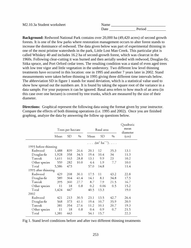
M2.10.3a Student worksheet Name _____________________________ Date ______________ Period __________ Background: Redwood National Park contains over 20,000 ha (49,420 acres) of second growth forests. It is one of the few parks where restoration management occurs to alter forest stands to increase the dominance of redwood. The data given below was part of experimental thinning in one of the most pristine watersheds in the park, Little Lost Man Creek. This particular plot is called Whiskey 40 and includes 16.2 ha of second-growth forest, which was clearcut in the 1960s. Following clear-cutting it was burned and then aerially seeded with redwood, Douglas-fir, Sitka spruce, and Port Orford cedar trees. The resulting condition was a stand of even aged trees with low tree vigor and little vegetation in the understory. Two different low level thinning treatments have occurred in this location: one in 1995 and another 7 years later in 2002. Stand measurements were taken before thinning in 1995 giving three different time intervals below. The abbreviation SD in figure 1 stands for stand deviation, which is a statistical value used to show how spread out the numbers are. It is found by taking the square root of the variance in a data sample. For your purposes it can be ignored. Basal area refers to how much of an area (in this case over one hectare) is covered by tree trunks, which are measured by the size of their diameter. Directions: Graphical represent the following data using the format given by your instructor. Compare the effects of both thinning operations (i.e. 1995 and 2002). Once you are finished graphing, analyze the data by answering the follow up questions below.

Fig 1. Stand level conditions before and after two different thinning treatments

253

Analysis Follow up questions: 1. Compare the tree density of the three dominant tree species. Place each tree species in order from greatest to least for each time interval.

2. After 2002, which tree species is the most abundant? 3. After 2002, which tree species covers the most area? 4. After 2002, which tree species has the greatest average diameter? 5. Do the results in 2002 support the management goals of the park? Why/Why not? 6. What type of tree is the most shade tolerant and would likely be the most dominant if it wasn’t for human interference? 7. Give two different scenarios below describing how the stand could change over time.

page 2

254

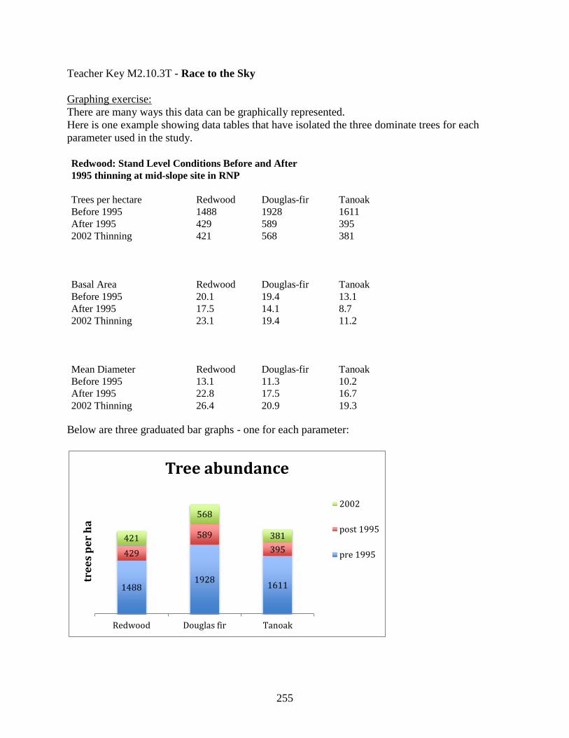
Teacher Key M2.10.3T - Race to the Sky Graphing exercise: There are many ways this data can be graphically represented. Here is one example showing data tables that have isolated the three dominate trees for each parameter used in the study. Redwood: Stand Level Conditions Before and After 1995 thinning at mid-slope site in RNP Trees per hectare Redwood Douglas-fir Tanoak Before 1995 1488 1928 1611 After 1995 429 589 395 2002 Thinning 421 568 381 Basal Area Redwood Douglas-fir Tanoak Before 1995 20.1 19.4 13.1 After 1995 17.5 14.1 8.7 2002 Thinning 23.1 19.4 11.2 Mean Diameter Redwood Douglas-fir Tanoak Before 1995 13.1 11.3 10.2 After 1995 22.8 17.5 16.7 2002 Thinning 26.4 20.9 19.3

Below are three graduated bar graphs - one for each parameter:

1488 1928 1611

429

589 395

421

568

381

Redwood Douglas fir Tanoak

tree

s pe

r ha

Tree abundance

2002

post 1995

pre 1995

255

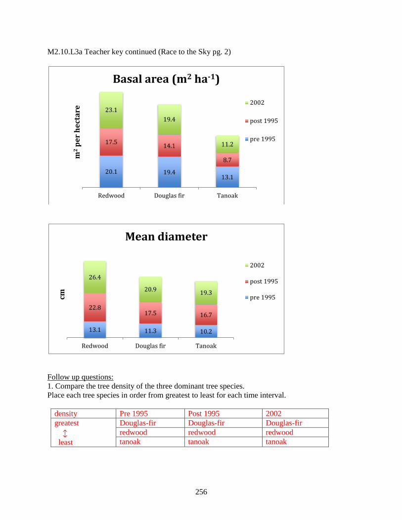
M2.10.L3a Teacher key continued (Race to the Sky pg. 2)

Follow up questions: 1. Compare the tree density of the three dominant tree species. Place each tree species in order from greatest to least for each time interval.

density Pre 1995 Post 1995 2002 greatest least

Douglas-fir Douglas-fir Douglas-fir redwood redwood redwood tanoak tanoak tanoak

20.1 19.4 13.1

17.5 14.1

8.7

23.1 19.4

11.2

Redwood Douglas fir Tanoak

m2 p

er h

ecta

re

Basal area (m2 ha-1)

2002

post 1995

pre 1995

13.1 11.3 10.2

22.8 17.5 16.7

26.4

20.9 19.3

Redwood Douglas fir Tanoak

cm

Mean diameter

2002

post 1995

pre 1995

256

M2.10.L3a Teacher key continued (Race to the Sky pg. 3) 2. After 2002, which tree species is the most abundant? Douglas-fir - 568 trees / ha 3. After 2002, which tree species covers the most area? Coast redwood - 23.1 m2/ha 4. After 2002, which tree species has the greatest average diameter? Coast redwood - 26.4 cm 5. Do the results in 2002 support the management goals of the park? Why/Why not? Answers will vary. The results support management goals because redwood has increased in area and diameter. However, Douglas fir still remains the most numerous so the future fate of this stand is unclear. 6. What type of tree is the most shade tolerant and would likely be the most dominant if it wasn’t for human interference? Coast redwood 7. Give two different scenarios below describing how the stand could change over time. Answers will vary.

257

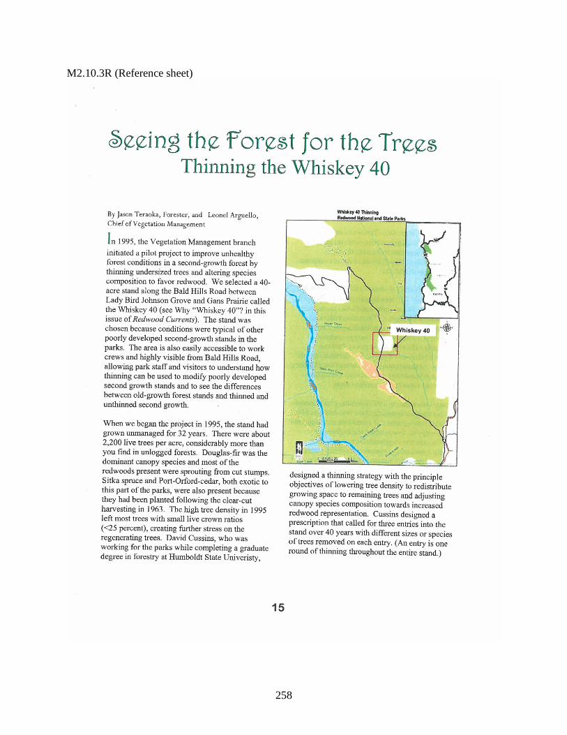
M2.10.3R (Reference sheet)

258

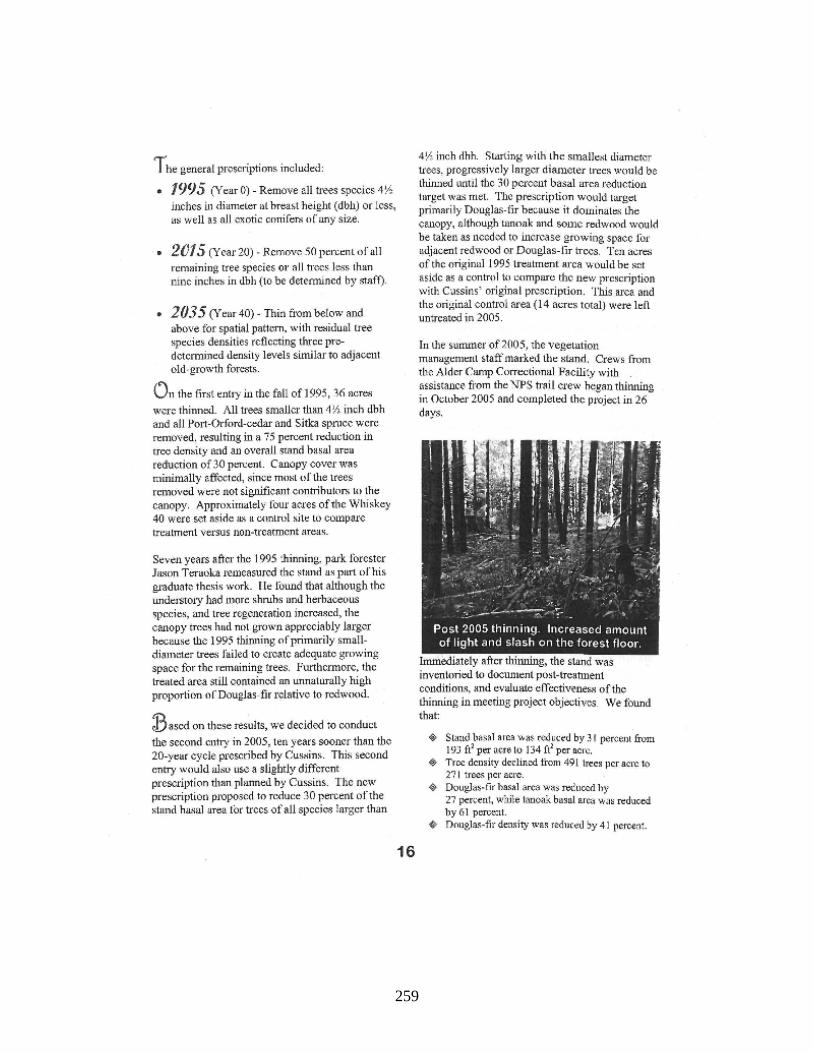
259

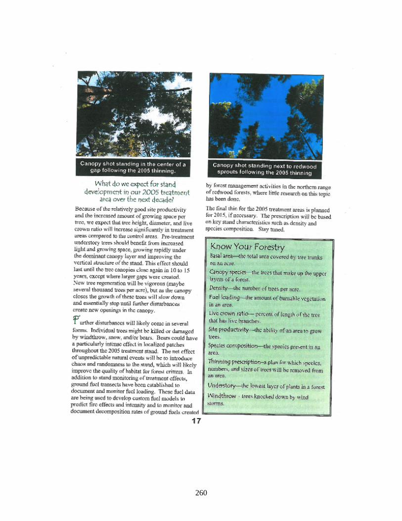
260

M2.G10 Lesson 4: Scaling the Tallest Trees Unit Overview: Coast Redwoods Grade 10 Key Concepts:

• Forest structure and function

• Developing and using scale models to show relationships

• Biomass and carbon • Photosynthesis and

tree height Time: 90 - 120 minutes Materials for the Teacher: Assess to computers

and a graphing program similar to Excel (optional)

Teacher instructions M2.10.4T

large paper (optional) Pictures of the canopy

of an old-growth redwood forest (optional)

Connections: Mathematics, STEM, photosynthesis, forestry, engineering, forest function and structure, plant science, genetics, conservation, biogeography, earth science, environmental science, art Forest Ecology Series integration: M1: Integrative Forest Ecology

Learning Objectives: Students will create one or more scale models of some of the largest redwood trees using selected data collected from a one-hectare plot located in Prairie Creek State Park. Measurements include tree height, trunk volume, and diameter breast height (dbh) of some of the largest and most complex trees known. Background information: Refer to the appropriate section in Part I: Teacher Companion for Module 2 and online information. For the original paper refer to: Sillett, S. and R.Van Pelt. 2007. Trunk reiteration promotes epiphytes and water storage in an old-growth redwood forest canopy, Ecological Monographs 77(3): 335-359 Suggested procedure: There are many ways students can make a scale model of the giant redwood trees referenced in this lesson. The given data set includes many unnecessary metrics that are included but are not intended to be used for practical application (refer to M2.10.4T). The data comes from the largest trees measured in a one-hectare plot located in Prairie Creek State Park. Data is given for 14 trees with a dbh greater than 400 cm. The amount of data students integrate will dictate the amount of time needed to complete this lesson. It is at your discretion whether you want students to model only certain trees, have students select their own tree, or assign trees at random. They should be introduced to the distribution of redwoods and the fact that not all trees reach these gargantuan proportions. There are several good movies showing some of the research that is done in redwood forests and could be used as an appropriate introduction (see online resources). The teacher instructions give the actual scale models developed from this data set. These trees were originally named, however, in this lesson they are numbered. These models are sophisticated and should not be considered realistic models for students to achieve. The students should build a model that at the minimum integrates dbh and height. They can add other metrics such as trunk volume, crown spread, and number of reiterations in the margin of their paper. It is also optional to add another reference to scale, such as the Statue of Liberty, which is 46.9 m or 154 ft high or the height of an average sized person. Once you have decided what trees and accompanied data you want them to include in their design, give clear instructions of what they should do and show an example. Students can work in groups or alone. An appropriate scale to use is 1 cm = 1 m or 100 cm. This means a height of 100 m will

261

equal 1 m and a diameter of 400 cm will equal 4 cm. If these scales are used you will need paper over 1 m long. If scaling is done on a computer then smaller units could be used. Once they have completed their models, give an opportunity to share them with the rest of the class. This lesson easily leads into the next lesson in the series where students interpret what structural features and habitat characteristics are found in this same set of trees.

Preliminary questions: • What are the tallest trees on Earth? • Where do coast redwoods live? • How does the climate vary between the northern and southern extent of the coasts

redwood range (show a precipitation map)? • What limitations are there to tree height? • How does water move through a tree? • What types of organisms might be found in an old-growth forest compared to a stand that

is less than 100 years old? Critical Thinking: How and why might the leaves at the top of a tree’s crown differ from the leaves at the bottom of the crown where less light is available? Key Words: canopy, crown, limb, mass, reiteration, volume NGSS alignment: HS-LS1.B: From Molecules to Organisms: Structures and Processes LS1.B: Growth and Development of Organisms HS-LS2.B: Ecosystem Interactions, Energy, and Dynamics LS2.B: Cycles of Matter and Energy Transfer in Ecosystems HS-LS2: Use mathematical representations to support and revise explanations based on evidence about factors affecting biodiversity and populations in ecosystems of different scales. Online resources: Monumental Trees - The Tallest Trees in the World: http://www.monumentaltrees.com/en/trees/coastredwood/tallest_tree_in_the_world/ This site gives a good overview the tallest trees in the world. It reviews the history of finding the tallest redwoods and provides information on the varying leaf morphology found in coast redwood (answer to the Critical Thinking question above). Save the Redwoods League: Redwoods and Climate: http://www.savetheredwoods.org/what-we-do/study/detail.php?id=438 This website is constantly updated and posts some of the latest research regarding all redwood species. The Learning Center page gives lesson options and many links to other information on redwoods including the complete Redwood Ed curriculum. VIDEO: Climbing redwood giants http://channel.nationalgeographic.com/channel/explorer/videos/climbing-redwood-giants/ This is an excellent video showing researchers climbing the giant sequoia and coast redwood. It shows researchers in the canopy and is a good way to grasp how large redwood trees actually are and how scientists are finding out more about them by studying the canopy.

262

Online resources (continued) Redwood Visitor Center Film http://www.calegacy.org/ This brand new visitor center film for the Redwood National and State Park in Humboldt County has some of latest information regarding research in the redwoods. Note: At the time of this printing (2014) several new films about redwoods are being developed including an IMAX film. EEI Connection: B.6.a. Biodiversity: The Keystone of Life on Earth E.7.b. The Life and Times of Carbon B.8.b Biological Diversity: The World’s Riches Answers to preliminary questions: - What are the tallest trees on Earth? (Coast redwoods are currently the tallest with the champion so far at 379.7 ft or 116 m) - Where do coast redwoods live? (along a narrow 65 mile wide strip along the California coast and into the southernmost region of Oregon) - How does the climate vary between the northern and southern extent of the coasts redwood range (show a precipitation map)? (much more precipitation occurs further north. In the northern most range redwoods live in a true temperate rainforest) - What limitations are there to tree height? (answers will vary. This is an ongoing question. There may not be a physiological limit if a tree is given necessary resources. For discussion purposes you may want to talk about the need to transport water up to the crown of a tree; in this case over 100 m) - How does water move through a tree? (water is transported through xylem - a vascular tissue. It is drawn up through the roots and into the leaves during photosynthesis. As water exits leaves through transpiration, cohesion pulls water upwards). - What types of organisms might be found in an old-growth forest compared to a stand that is less than 100 years old? (Older trees will typically house more epiphytes and will have deadwood and crevices that support more animal and plant species. There may be less biodiversity on the forest floor, however, some plants and animals are sensitive to disturbances and are considered old-growth dependent. Some animals include the marbled murrelet, and the marten and fisher - two members of the weasel family)

263

M2.G10.L4 (Unit Overview continued) Suggested extensions:

• Show a video about coast redwoods. Two films are recommended: Nat’l Geographic: Climbing the World’s largest trees and California Legacy Project: Changing Places - The Redwoods.

• Have students take tree measurements in the field such as circumference, height, and basal area (see lesson M1.10.L4).

• Make a scale model of a redwood tree somewhere on campus. • Perform a plant growth experiment by applying different treatments such as the amount

of water, light, and/or nutrients. • Discuss the amazing physics necessary for tall trees to pull water up their trunks during

photosynthesis. • Study dendrochronology and apply it to tree growth, climate change, and/or historical

references. • Figure out how much paper or linear feet of timber can come from the wood volume

found in one of these amazing trees. • Have students go stand underneath a towering redwood tree and write about the

experience. Teacher instructions M2.10.4T

264

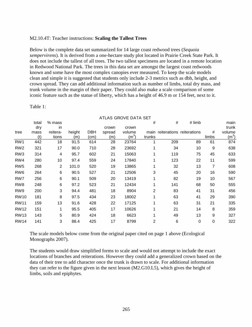
M2.10.4T: Teacher instructions: Scaling the Tallest Trees Below is the complete data set summarized for 14 large coast redwood trees (Sequoia sempervirens). It is derived from a one-hectare study plot located in Prairie Creek State Park. It does not include the tallest of all trees. The two tallest specimens are located in a remote location in Redwood National Park. The trees in this data set are amongst the largest coast redwoods known and some have the most complex canopies ever measured. To keep the scale models clean and simple it is suggested that students only include 2-3 metrics such as dbh, height, and crown spread. They can add additional information such as number of limbs, total dry mass, and trunk volume in the margin of their paper. They could also make a scale comparison of some iconic feature such as the statue of liberty, which has a height of 46.9 m or 154 feet, next to it. Table 1:

ATLAS GROVE DATA SET

total dry

% mass in

reitera-tions

crown

spread (m)

crown

volume (m3)

# # # limb main trunk

tree mass (t)

height (m)

DBH (cm)

main trunks

reiterations reiterations # limbs

volume (m3)

RW1 442 18 91.5 614 28 23764 1 209 89 61 874 RW2 321 17 90.0 710 28 23692 1 34 10 9 638 RW3 314 4 95.7 602 21 15063 1 119 75 45 633 RW4 280 10 97.4 559 24 17840 1 123 22 11 599 RW5 268 2 101.0 520 19 13865 1 32 13 7 608 RW6 264 6 90.5 527 21 12506 3 45 20 16 590 RW7 256 6 90.1 509 20 13419 1 82 19 10 567 RW8 248 6 97.2 523 21 12434 1 141 68 50 555 RW9 200 3 94.4 481 18 8904 2 83 41 31 456 RW10 181 8 97.5 434 23 18002 1 63 41 29 390 RW11 159 13 91.6 428 22 17125 1 63 31 21 335 RW12 151 1 95.5 405 17 10626 1 21 14 8 359 RW13 143 5 80.9 424 18 6623 1 49 13 9 327 RW14 141 3 88.4 425 17 8799 2 6 0 0 322

The scale models below come from the original paper cited on page 1 above (Ecological Monographs 2007). The students would draw simplified forms to scale and would not attempt to include the exact locations of branches and reiterations. However they could add a generalized crown based on the data of their tree to add character once the trunk is drawn to scale. For additional information they can refer to the figure given in the next lesson (M2.G10.L5), which gives the height of limbs, soils and epiphytes.

265

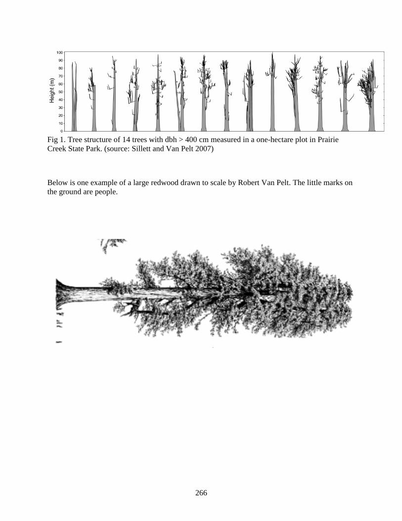
Fig 1. Tree structure of 14 trees with dbh > 400 cm measured in a one-hectare plot in Prairie Creek State Park. (source: Sillett and Van Pelt 2007)

Below is one example of a large redwood drawn to scale by Robert Van Pelt. The little marks on the ground are people.

266

M2.G10 Lesson 5: A Canopy Conundrum Unit Overview: Coast Redwoods Grade 10 Key Concepts:

• Interpreting data • Biomass and carbon • Biodiversity of life • Energy and Matter

Time: 40 - 60 minutes Materials for the Teacher: Student worksheet and

teacher key M2.10.5a Pictures showing

features of the old-growth redwood forest canopy and/or large redwood trees(optional)

Connections: Photosynthesis, biomass, biodiversity, carbon cycle, forest conservation, plant science, genetics, soils, earth science, environmental science Forest Ecology Series integration: M1: Integrative Forest Ecology

Learning Objectives: Students will interpret a figure showing summarized data from one of the most complex forest canopies of the world. They will write summaries about what the data attempts to reveal and will show their understanding through questioning. Background information: Refer to the appropriate section in Part I: Teacher Companion for Module 2 and online information. For the original paper refer to: Sillett, S., and R. Van Pelt. 2007. Trunk reiteration promotes epiphytes and water storage in an old-growth redwood forest canopy, Ecological Monographs 77(3):335-359 Suggested procedure: This lesson is a nice follow up from the previous lesson. It can be applied to photosynthesis, carbon sequestration, biomass, and other factors regarding the carbon cycle. In this lesson students interpret a figure showing summarized data of canopy structures and habitat characteristics in 14 trees over 400 cm dbh measured within a one hectare plot in Prairie Creek State Park. These are some of the largest redwoods on the planet. The data includes different metrics based on a vertical scale such as trunk volume, amount of biomass, volume of epiphytes and canopy soils (see student worksheet M2.10.5a). You may want to show a similar figure and ask some preliminary questions before you begin, to make sure students have critical background information. Some definitions are given. It is optional to show pictures of the redwood canopy (see online resources) and or other forest canopies such as those found in certain rainforests. As a follow-up or preceding lesson, students can graph the biomass of fern mats that live in the redwood canopy (refer to G7.L5) Even though this lesson is found in the 7th grade unit it is applicable and challenging enough for high school students.

Preliminary questions: • What are the different parts of a tree? • What parts go through photosynthesis? • Where is most of the biomass contained within a redwood tree? • How could you measure the biomass of a living thing? • How might the crowns of old redwood trees differ from those of younger trees? • How can a complex redwood canopy with reiterations and deadwood add to the biodiversity of a forest? Critical Thinking: Why does a small volume of soil dry out faster than a large volume of soil? Keywords: basal area, biomass, epiphyte, limb, substrate, reiteration

267

(M2.G10.L5 Unit Overview Continued) NGSS alignment: HS-LS1.B: From Molecules to Organisms: Structures and Processes LS1.B: Growth and Development of Organisms HS-LS2.B: Ecosystem Interactions, Energy, and Dynamics LS2.B: Cycles of Matter and Energy Transfer in Ecosystems LS2.C: Ecosystem Dynamics, Functioning and Resilience Online resources: Forest Ecology by UC Cooperative Extension (A forest stewardship series) http://anrcatalog.ucdavis.edu/pdf/8233.pdf This publication is a good overview of forest ecology. It gives clear explanations of forest types and physical factors that influence a forest. Photo Tour of Redwood, HSU Institute for Redwood Ecology http://www.humboldt.edu/redwoods/photos/redwood.php Some of the best pictures available of the redwood canopy can be viewed here. Research in the big trees continues and this website is updated periodically. Save the Redwoods League: Redwoods and Climate: http://www.savetheredwoods.org/what-we-do/study/detail.php?id=438 This website is constantly updated and posts some of the latest research regarding all redwood species. The Learning Center page gives lesson options and many links including the Redwood Ed curriculum guide. EEI Connection: B.6.a. Biodiversity: The Keystone of Life on Earth E.7.b. The Life and Times of Carbon B.8.b Biological Diversity: The World’s Riches Answers to preliminary questions: - What are the different parts of a tree? (a tree has roots, a trunk, and a crown. Roots have root hairs, the trunk has bark, and the crown has branches and leaves) - What parts go through photosynthesis? (in most trees it is the leaves that contain chlorophyll and therefore is the place photosynthesis occurs) - Where is most of the biomass contained within a redwood tree? (if you look at total volume the trunk of a tree has the most biomass. In large trees the many reiterations and branches contribute substantially) - How could you measure the biomass of a living thing? (biomass is often measured using dry weight or equations that have been derived from in depth studies) - How might the crowns of old redwood trees differ from those of younger trees? (the crowns of older trees will be much larger and more complex. Overtime they might have a dead top, multiple reiterations, and large branches. At a glance older trees will have flattened tops and lose the classic architectural model of a pointed top)

268

(answer to preliminary questions continued) - How can a complex redwood canopy with reiterations and deadwood add to the biodiversity of a forest?(complexity adds to biodiversity in general. Older trees in general are bigger and provide places for lichens and mosses to grow. Deadwood and crevices are places animals can hide and where the roots of epiphytic plants can take hold. Where redwoods receive lots of rain, large fern mats grow. Lots of invertebrates have been found in canopy soils including the wandering salamander where it can find adequate moisture. Large branches are potential nesting sites for endangered birds such as the marbled murrelet and spotted owl) Suggested extensions:

• Graph the different components found in fern mats that live in the redwood canopy (see lesson M2.G7.L5)

• Have high school students teach younger students about selected topics in redwood forest ecology

• Learn about the epiphytes that live in tropical rainforests and the high degree of biodiversity that lives there.

• Measure the biodiversity of different plants and animals that live on a nearby forest floor by sampling randomly picked m2 plots along a transect line.

• Sample nearby soils and test for their pH, texture, and nutrient content. • Discuss the different uses of wood and how forestry can become sustainable. • Learn about John Muir and his race to save the giant sequoia trees. • Visit a park and learn about the coast redwood trees firsthand.

M2.10. 5a student worksheet and teacher key

269

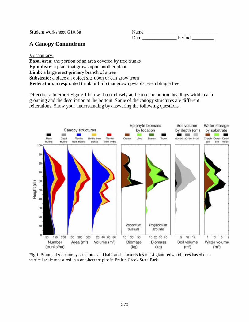
Student worksheet G10.5a Name _____________________________ Date ______________ Period _________ A Canopy Conundrum Vocabulary: Basal area: the portion of an area covered by tree trunks Ephiphyte: a plant that grows upon another plant Limb: a large erect primary branch of a tree Substrate: a place an object sits upon or can grow from Reiteration: a resprouted trunk or limb that grow upwards resembling a tree Directions: Interpret Figure 1 below. Look closely at the top and bottom headings within each grouping and the description at the bottom. Some of the canopy structures are different reiterations. Show your understanding by answering the following questions:

Fig 1. Summarized canopy structures and habitat characteristics of 14 giant redwood trees based on a vertical scale measured in a one-hectare plot in Prairie Creek State Park.

270

Questions: 1. At what height is most of the biomass above the ground found (volume of the canopy, mass of epiphytes, and volume of soil)? Don’t include the tree trunks. 2. Do trunks of redwoods taper off as they grow (the measurement used here is basal area - trunks/ha)? Explain. 3. In the canopy, identify the kind of reiteration (see the definition above) that contributes the most to overall volume. 4. What two species make up large portions of epiphyte biomass? 5. a. At what location do most Polypodium scouleri mats grow? b. give the range of height for these epiphytic mats. 6. At what location do most epiphytic huckleberries (Vaccinium ovatum) grow? 7. Explain the type of relationship that exists between soil volume and water storage or water volume. 8. In two to three sentences summarize the measurements used to produce the results found in Figure 1 above. How would people be able to obtain these measurements?

page 2

271

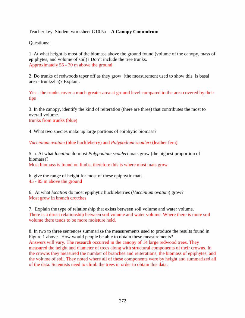
Teacher key: Student worksheet G10.5a - A Canopy Conundrum Questions: 1. At what height is most of the biomass above the ground found (volume of the canopy, mass of epiphytes, and volume of soil)? Don’t include the tree trunks. Approximately 55 - 70 m above the ground 2. Do trunks of redwoods taper off as they grow (the measurement used to show this is basal area - trunks/ha)? Explain. Yes - the trunks cover a much greater area at ground level compared to the area covered by their tips 3. In the canopy, identify the kind of reiteration (there are three) that contributes the most to overall volume. trunks from trunks (blue) 4. What two species make up large portions of epiphytic biomass? Vaccinium ovatum (blue huckleberry) and Polypodium scouleri (leather fern) 5. a. At what location do most Polypodium scouleri mats grow (the highest proportion of biomass)? Most biomass is found on limbs, therefore this is where most mats grow b. give the range of height for most of these epiphytic mats. 45 - 85 m above the ground 6. At what location do most epiphytic huckleberries (Vaccinium ovatum) grow? Most grow in branch crotches 7. Explain the type of relationship that exists between soil volume and water volume. There is a direct relationship between soil volume and water volume. Where there is more soil volume there tends to be more moisture held. 8. In two to three sentences summarize the measurements used to produce the results found in Figure 1 above. How would people be able to obtain these measurements? Answers will vary. The research occurred in the canopy of 14 large redwood trees. They measured the height and diameter of trees along with structural components of their crowns. In the crowns they measured the number of branches and reiterations, the biomass of epiphytes, and the volume of soil. They noted where all of these components were by height and summarized all of the data. Scientists need to climb the trees in order to obtain this data.

272

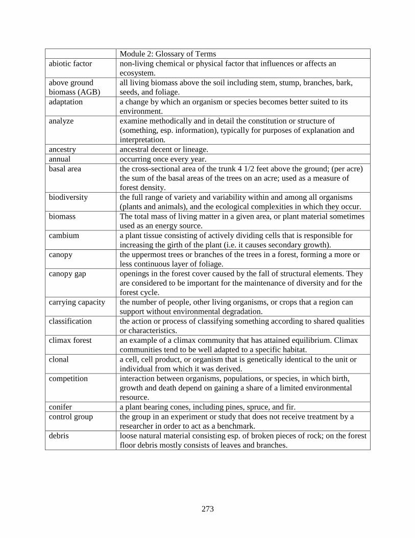
Module 2: Glossary of Terms abiotic factor non-living chemical or physical factor that influences or affects an

ecosystem. above ground biomass (AGB)

all living biomass above the soil including stem, stump, branches, bark, seeds, and foliage.

adaptation a change by which an organism or species becomes better suited to its environment.

analyze examine methodically and in detail the constitution or structure of (something, esp. information), typically for purposes of explanation and interpretation.

ancestry ancestral decent or lineage. annual occurring once every year. basal area the cross-sectional area of the trunk 4 1/2 feet above the ground; (per acre)

the sum of the basal areas of the trees on an acre; used as a measure of forest density.

biodiversity the full range of variety and variability within and among all organisms (plants and animals), and the ecological complexities in which they occur.

biomass The total mass of living matter in a given area, or plant material sometimes used as an energy source.

cambium a plant tissue consisting of actively dividing cells that is responsible for increasing the girth of the plant (i.e. it causes secondary growth).

canopy the uppermost trees or branches of the trees in a forest, forming a more or less continuous layer of foliage.

canopy gap openings in the forest cover caused by the fall of structural elements. They are considered to be important for the maintenance of diversity and for the forest cycle.

carrying capacity the number of people, other living organisms, or crops that a region can support without environmental degradation.

classification the action or process of classifying something according to shared qualities or characteristics.

climax forest an example of a climax community that has attained equilibrium. Climax communities tend to be well adapted to a specific habitat.

clonal a cell, cell product, or organism that is genetically identical to the unit or individual from which it was derived.

competition interaction between organisms, populations, or species, in which birth, growth and death depend on gaining a share of a limited environmental resource.

conifer a plant bearing cones, including pines, spruce, and fir. control group the group in an experiment or study that does not receive treatment by a

researcher in order to act as a benchmark. debris loose natural material consisting esp. of broken pieces of rock; on the forest

floor debris mostly consists of leaves and branches.

273

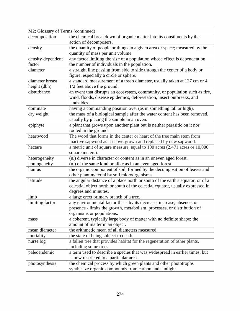
M2: Glossary of Terms (continued) decomposition the chemical breakdown of organic matter into its constituents by the

action of decomposers. density the quantity of people or things in a given area or space; measured by the

quantity of mass per unit volume. density-dependent factor

any factor limiting the size of a population whose effect is dependent on the number of individuals in the population.

diameter a straight line passing from side to side through the center of a body or figure, especially a circle or sphere.

diameter breast height (dbh)

a standard measurement of a tree's diameter, usually taken at 137 cm or 4 1/2 feet above the ground.

disturbance an event that disrupts an ecosystem, community, or population such as fire, wind, floods, disease epidemics, deforestation, insect outbreaks, and landslides.

dominate having a commanding position over (as in something tall or high). dry weight the mass of a biological sample after the water content has been removed,

usually by placing the sample in an oven. epiphyte a plant that grows upon another plant but is neither parasitic on it nor

rooted in the ground. heartwood The wood that forms in the center or heart of the tree main stem from

inactive sapwood as it is overgrown and replaced by new sapwood. hectare a metric unit of square measure, equal to 100 acres (2.471 acres or 10,000

square meters). heterogeneity (n.) diverse in character or content as in an uneven aged forest. homogeneity (n.) of the same kind or alike as in an even aged forest. humus the organic component of soil, formed by the decomposition of leaves and

other plant material by soil microorganisms. latitude the angular distance of a place north or south of the earth's equator, or of a

celestial object north or south of the celestial equator, usually expressed in degrees and minutes.

limb a large erect primary branch of a tree. limiting factor any environmental factor that - by its decrease, increase, absence, or

presence - limits the growth, metabolism, processes, or distribution of organisms or populations.

mass a coherent, typically large body of matter with no definite shape; the amount of matter in an object.

mean diameter the arithmetic mean of all diameters measured. mortality the state of being subject to death. nurse log a fallen tree that provides habitat for the regeneration of other plants,

including some trees. paleoendemic a term used to describe a species that was widespread in earlier times, but

is now restricted to a particular area. photosynthesis the chemical process by which green plants and other phototrophs

synthesize organic compounds from carbon and sunlight.

274

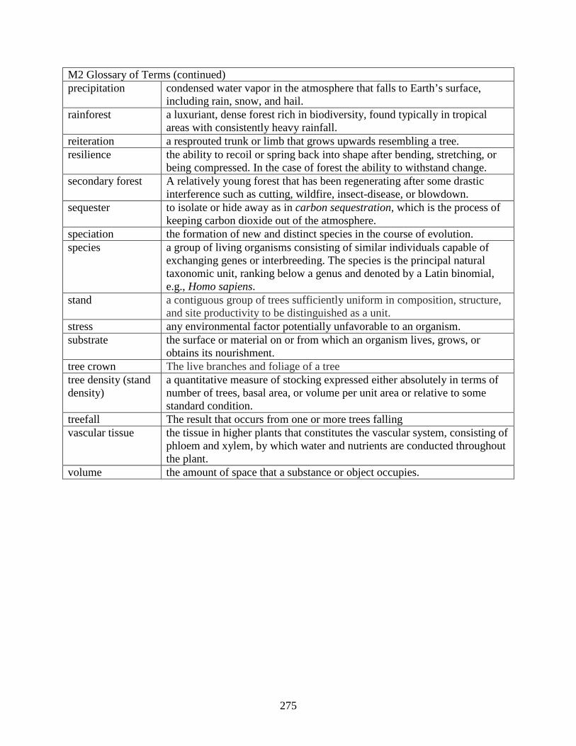
M2 Glossary of Terms (continued) precipitation condensed water vapor in the atmosphere that falls to Earth’s surface,

including rain, snow, and hail. rainforest a luxuriant, dense forest rich in biodiversity, found typically in tropical

areas with consistently heavy rainfall. reiteration a resprouted trunk or limb that grows upwards resembling a tree. resilience the ability to recoil or spring back into shape after bending, stretching, or

being compressed. In the case of forest the ability to withstand change. secondary forest A relatively young forest that has been regenerating after some drastic

interference such as cutting, wildfire, insect-disease, or blowdown. sequester to isolate or hide away as in carbon sequestration, which is the process of

keeping carbon dioxide out of the atmosphere. speciation the formation of new and distinct species in the course of evolution. species a group of living organisms consisting of similar individuals capable of

exchanging genes or interbreeding. The species is the principal natural taxonomic unit, ranking below a genus and denoted by a Latin binomial, e.g., Homo sapiens.

stand a contiguous group of trees sufficiently uniform in composition, structure, and site productivity to be distinguished as a unit.

stress any environmental factor potentially unfavorable to an organism. substrate the surface or material on or from which an organism lives, grows, or

obtains its nourishment. tree crown The live branches and foliage of a tree tree density (stand density)

a quantitative measure of stocking expressed either absolutely in terms of number of trees, basal area, or volume per unit area or relative to some standard condition.

treefall The result that occurs from one or more trees falling vascular tissue the tissue in higher plants that constitutes the vascular system, consisting of

phloem and xylem, by which water and nutrients are conducted throughout the plant.

volume the amount of space that a substance or object occupies.

275

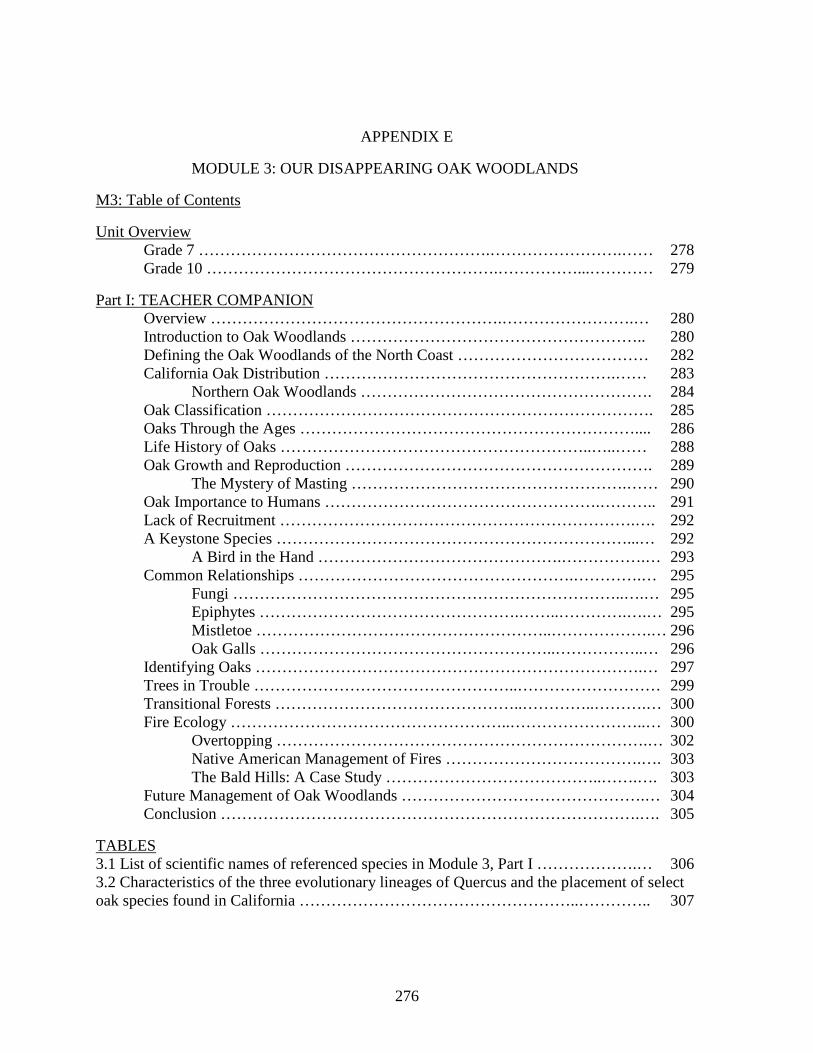
APPENDIX E

MODULE 3: OUR DISAPPEARING OAK WOODLANDS M3: Table of Contents

Unit Overview Grade 7 ……………………………………………….…………………….…… 278 Grade 10 ……………………………………………….……………...………… 279

Part I: TEACHER COMPANION Overview ……………………………………………….…………………….… 280

Introduction to Oak Woodlands ……………………………………………….. 280 Defining the Oak Woodlands of the North Coast ……………………………… 282

California Oak Distribution ……………………………………………….…… 283 Northern Oak Woodlands ………………………………………………. 284 Oak Classification ………………………………………………………………. 285 Oaks Through the Ages ……………………………………………………….... 286 Life History of Oaks …………………………………………………..…..…… 288 Oak Growth and Reproduction …………………………………………………. 289 The Mystery of Masting …………………………………………….…… 290 Oak Importance to Humans …………………………………………….……….. 291 Lack of Recruitment ………………………………………………………….…. 292 A Keystone Species …………………………………………………………...… 292 A Bird in the Hand ……………………………………….…………….… 293 Common Relationships …………………………………………….………….… 295 Fungi ………………………………………………………………..….… 295 Epiphytes ………………………………………….……..………….….… 295 Mistletoe ………………………………………………..……………….… 296 Oak Galls ………………………………………………..……………..… 296 Identifying Oaks ……………………………………………………………….… 297 Trees in Trouble …………………………………………..……………………… 299 Transitional Forests ………………………………………..…………..……….… 300 Fire Ecology ……………………………………………..……………………..… 300 Overtopping …………………………………………………………….… 302 Native American Management of Fires ……………………………….…. 303 The Bald Hills: A Case Study …………………………………..…….…. 303

Future Management of Oak Woodlands ……………………………………….… 304 Conclusion …………………………………………………………………….…. 305

TABLES 3.1 List of scientific names of referenced species in Module 3, Part I ……………….… 306 3.2 Characteristics of the three evolutionary lineages of Quercus and the placement of select oak species found in California ……………………………………………..………….. 307

276

FIGURES 3.1 The Hooker Oak (sp. Quercus lobata) located in Bidwell Park, Chico CA. (1957). This tree was claimed to be the largest oak tree in the world up until the time it fell in 1977. Measurements: ht=31 m or 101 ft, c=2.4 m or 8 ft (2.4 m above ground). It was found to be two trees both 325 years old that had merged together …………………………………. 308 3.2 Variable oak communities in Mendocino County ……….………………………..… 308 3.3 Current distribution of oak woodland in North Coast California …………………… 309 3.4 Inventory and distribution by oak forest type in California ……………………..….. 309 3.5 Geologic timescale for the Cenozoic era including periods and epochs …………...... 310 3.6 Morphology of leaves, flower, and fruit of an oak tree (Quercus robur) ………….... 310 3.7 Two birds heavily dependent upon acorns as a food source. A) acorn woodpecker (Melanerpes formicivorus) B) western scrub jay (Apenlocoma californica) ……….…... 311 3.8 Acorn woodpecker granary ……………………………………….………………… 311 3.9 Generic representation of linear secondary succession leading to an oak forest climax community ………………………………………………………………………….……. 312 3.10 Overtopping by Douglas-fir (Pseudotsuga menziesii) in a Oregon white oak woodland (location Kneeland, CA)……………………….…………………………………….…… 312

LITERATURE CITED ………………………………………………………………….. 313

Part II: M3: UNITS OF STUDY Grade 7 (Middle School) Unit of Study Cover Page ………………………….… 317 Lesson 1 - Oak Detectives ……………………………………………..… 318 Lesson 2 - Identifying Oaks ……………………………………………… 324 Lesson 3 - Let There Be Light! ……………………………………..….… 333 Lesson 4 - Keystone of Diversity ………………………………………… 344 Lesson 5 - Trees in Trouble ………………………………………………. 352 Grade 10 (High School) Unit of Study Cover Page ……………………………… 361 Lesson 1 - Oaks Through the Ages ………………………………………. 362 Lesson 2 - The Mystery of Masting ……………………………………… 372 Lesson 3 - A Bird in the Hand …………………………………………… 384 Lesson 4 - King Conifers ……………………………………………..…. 392 Lesson 5 - Friendly Fire ……………………………………………….… 405 Module 3 Glossary ………………………………………………………………. 420

277

Forest Ecology 101 Series (M3: Part I)

MODULE 3: OUR DISAPPEARING OAK WOODLANDS

Unit Overview Grade 7 Days 1-3 Lesson 1 - Oak Detectives Learning Objectives: Students will practice journaling through periodic observations of a nearby oak and its surroundings. They will take basic tree measurements, conduct a soil analysis, and learn about species utilization in order to study both abiotic and biotic factors influencing their tree. They will learn that observation is one of the key steps to the scientific process. Days 4-5 Lesson 2 - Identifying Oaks Learning Objectives: Students will use a dichotomous key to identify up to 12 different hardwood species found in the North Coast. As an extension activity, they will press leaves or use cut-out drawings to make an identification booklet useful in the field or future identification needs. Day 6 Lesson 3 - Let There be Light! Learning Objectives: Students will interpret data regarding how oak seedlings respond to various levels of light. In doing so they will learn about life history tradeoffs, competitive advantages, and potential reasons for poor oak regeneration. They will compare results of shoot and root mass and overall biomass of seedlings from three different oak species after exposure to three different light levels. Days 7-8 Lesson 4 - Keystone of Diversity Learning Objectives: Students will be able to define what a keystone species is and will identify interconnected ecological relationships relative to an oak woodland. They will reveal and apply their knowledge by developing a food web that highlights oaks as the dominant producer after filling out a graphic organizer. Days 9-10 Lesson 5 - Trees in Trouble Learning Objectives: Through an online investigation students will learn about Sudden Oak Death (SOD) and will be able to identify the pathogen, symptoms, and vectors of this disease. They will also be able to describe some of the precautions people can take to limit the spread of this oak tree disease.

278

Forest Ecology 101 Series (M3: Part I)

Unit Overview Grade 10 Days 1-2 Lesson 1 - Oaks Through the Ages Learning Objectives: Using written clues students will sequence some of the major climatic and geological events that have influenced the distribution pattern of the oaks in California over the last 20,000 years. They will be able to identify and describe some of the adaptations oaks have developed to live in a Mediterranean climate. Days 3-4 - The Mystery of Masting Learning Objective: Students will read about acorn masting and will identify some of the main theories attempting to explain this phenomenon. They will interpret several figures from a scientific study attempting to find significant contributing factors for yearly acorn productivity across varying scales. Comparisons include yearly acorn abundance per species, versus average monthly temperature, and between individual trees within the same species. Days 5-6 Lesson 3 - Bird in the Hand Learning Objectives: Students will research and compare the interdependent relationships between two bird species (acorn woodpecker and western scrub jay) and oak trees. Both species rely heavily on acorns and have different methods of caching them for winter food. Students will apply systems thinking by designing a model that shows an outcome related to these animal-plant interactions. Days 7-8 Lesson 4 - King Conifers Learning Objectives: Students will identify the cause and effects of fire suppression particularly overtopping by Douglas-fir in Oregon white oak habitat. They will analyze data from a thinning project and will determine how oaks respond to different treatment levels. In this study, changes in acorn productivity, dbh, and epicormic sprouting were measured over five years. Days 9-10 Lesson 5 - Friendly Fire Learning Objectives: Students will compare past and present land management practices in the Bald Hills of Redwood National Park. The will read a scientific paper in groups and will describe structural and compositional changes in vegetation caused by the use and suppression of fire. They will be able to explain the advantages of using fire as a tool for restoration.

279

APPENDIX E

MODULE 3: TEACHER COMPANION

OUR DISAPPEARING OAK WOODLANDS

“As the oaks live, so do the people; as the oaks go, so go the people”

Greg Sarris quoting Southern Pomo and Coast Miwok elders

Overview The following information is intended to provide interesting and relevant content for science educators and resource specialists regarding the oak woodlands of North Coast California. This companion guide is designed to accompany the lessons in Part II. The synthesis of information has been sourced from a variety of resources, including U.S. Forest Service reports, land manager guides, and peer-reviewed scientific papers. Every lesson is aligned to the Next Generation Science Standards (NGSS) and apply to the interdisciplinary approach set forth by the Common Core Skills and Standards (CCSS). Core concepts include species interactions, unity and diversity, adaptation, and stability and change. Information relevant to the 21st century is presented, including past and future land management practices, fire ecology, and the critical ecological services oak woodlands provide in protecting biodiversity. Information is presented from a wide variety of spatial and temporal scales. Students will explore how these ecosystems have changed over time and why continued management is vital to their survival. They will learn why oaks are considered keystone species and how regular fire regimes help sustain these disappearing habitats. Many lessons integrate scientific data and adhere to the principles of STEM (science, technology, engineering, and mathematics). Students will analyze data from acorn mast observations and wildlife interactions regarding oaks and their distribution. Throughout this companion guide, you will find useful background information, field study ideas, and potential field trip locations to encourage a deeper understanding about the world of our disappearing oak woodlands.

Introduction to Oak Woodlands Culturally and ecologically oak woodlands play prominent roles in the Californian landscape. Oaks produce an important food source for people and wildlife. During Euro-American settlement, oak woodlands were recognized as a connection to the European homeland. Throughout history large, iconic oak trees have been symbols of strength, beauty, courage, and power. Some can live over 500 years, have crown spreads greater than 40 m (130 ft), and diameters exceeding 3 m (10 ft) (Pavlik et al. 1991) (Fig. 3.1). Many species are endemic to California and share ancestry with other oak species of North America, Eurasia, and Japan. During the Miocene (~5-24 mya), western oaks were much more widespread, with fossils found in Oregon, Nevada, and Washington. California oaks are similar to other Mediterranean plants

280

and over millennia they have adapted to a warm and arid climate lacking summer precipitation (Mensing 2005). Because oak woodlands are critical to a vast array of species, oaks are considered keystone species and are essential to California's biological diversity. Over 300 vertebrate species (mostly birds), 5,000 invertebrates, and 2,000 plant species occupy oak-associated habitats making them the most biologically diverse and productive ecosystems in the entire state (Bernhardt and Swiecki 2001; CalPIF 2002). The abundance of certain bird species, such as the acorn woodpecker (Melanerpes formicivorus), can be directly linked to oak diversity. Part of their productivity comes from their leaves, sap, and a nutritious seed: the acorn. For thousands of years indigenous peoples have depended on acorns as a major food source. The three most culturally important oak species in northern California are tanoak (Notholithocarpus densiflorus), black oak (Quercus kelloggii), and Oregon white oak (Quercus garryana) (Hosten et al. 2006). In order to maximize the health and productivity of these ecosystems, Native Americans historically managed these landscapes using fire and other tools to promote acorn production, improve wildlife habitat, and encourage the growth of certain plants used for medicine and basketry. The production of acorns is variable and fluctuates from year to year and between species. The leaves, buds, flowers, and acorns continue to provide sustenance for dozens of vertebrates, including bears, deer, rodents, and birds as well as hundreds of invertebrates. As recently as 50 years ago very little was known about the important role California oaks play from an ecological standpoint. Since Euro-American settlement, oak-dominated landscapes across California have been negatively affected from multiple factors, most of them caused by conversion to agricultural lands and urban development. Other contributing factors include water diversion, overgrazing, and introduction of non-native species (McCreary 2009). Many oak habitats are associated with grasslands and are considered non-timberland. These communities have been managed primarily for livestock grazing. Approximately 80% of California's oak woodlands are privately owned (Gaman and Firman 2008). Between 1945 and 1975 the annual rate of clearing averaged 12,950 ha (32,000 ac) in order to increase rangeland (Christensen et al. 2008). Today the rate has decreased, however approximately 303,515 ha (750,000 ac) are estimated to be at risk from further development by the year 2040. About 50% of California’s oak woodlands are concentrated in the Sacramento and San Joaquin Valleys, where the most immediate threat resides (Gaman and Firman 2008). These factors, combined with fire suppression and the onslaught of Sudden Oak Death (SOD), have not only decreased the total area of oak woodland habitat, but also may have diminished the resiliency of these systems. Research remains to be done in order to gain a deeper understanding of the complexity of factors affecting acorn masting, competition, and wildlife diversity. Today the survival of oaks may be in peril and the successful maintenance of oak woodland is a growing concern for land managers, ecologists, and preservationists. Many oak species have low recruitment, and in some places, little to no regeneration has occurred for over 60 years (Holland 2005). In 1986, growing awareness and concern about low recruitment instigated a statewide effort, called the Integrated Hardwood Management Plan, to encourage oak conservation and to assist with making correct land management practices. Since implementation, regular oak symposia are held where studies and perspectives are shared. As a result of these efforts and many others, information and resources have become available to landowners on how to encourage oak regeneration. Although some scientists are getting closer to understanding the complex issues surrounding low recruitment, many other questions remain,

281

especially regarding what effects past management practices have had on these systems and how future development will alter these ecosystems (McCreary 2009). In some places oak stands may depend largely on regular low-intensity fire, especially those in wetter areas such as the North Coast and the Pacific Northwest (Purcell and Stephens 2006). A well-documented threat that commonly occurs in northern oak woodlands is overtopping or shading out by faster growing conifers. Regular fire would have naturally thinned young conifer species that are less fire resistant than oaks, such as Douglas-fir (Pseudotsuga menziesii) and Ponderosa pine (Pinus ponderosa). Over time, oaks have evolved adaptations allowing them to survive fire, including thick bark and the ability to resprout. Today, federal and state land managers and other agencies are reintroducing low-intensity fire regimes and conifer removal in some places in order to save these precious resources. Both practices have been used in Redwood National Park (hereafter RNP) for over 20 years to maintain nearly 1,400 ha (4,000 ac) of Oregon white oak savanna (Underwood et al. 2003). Throughout California public and private land managers continue to work together to study, preserve, and enhance these disappearing habitats.

Defining the Oak Woodlands of the North Coast The oak woodlands of the North Coast are a minor component of the overall landscape compared to the vast timberlands that dominate the area (Green and Magnuson 2011). The maze of mountain ranges and complicated river systems that occur in Humboldt and Mendocino Counties create many localized climates, some well-suited for the establishment of oaks, including river valleys, low ridgetops, and south facing slopes (Fig 3.2). These areas are loosely classified and can be difficult to place into distinct groups (discussed further below). Some of the difficulty arises from the vast array of soil types found (Sawyer et al. 1988). Furthermore, almost all oak woodlands have been modified to some degree and are often transitional zones between nearby vegetative types. Oak woodlands frequently form a multi-layered mosaic shaped by surrounding environments, such as grassland, shrubland, and montane forest (George and Alonso 2006). To further complicate matters, one of the more prolific oak species living in the North Coast is tanoak (Notholithocarpus densiflora), which produces acorns but is not considered a true oak. It is a North American member of the tanbark oaks and is more closely related to chestnut trees. When explaining this discrepancy to students, you may want to point out the name tanoak is one word because it is not a true oak. In many local forests, tanoak can be a dominant species and is often heavily mixed with California bay (Umbellularia californica), madrone (Arbutus menziesii), and Douglas-fir. It typically belongs to the mixed evergreen forest community and can be a major understory component of coast redwood forest in drier central and upland forest stands (Sawyer et al. 1988). Because tanoak is common, produces acorns, and provides a similar ecological role to the true oaks, it is included in this module. In lesson G7.L5, students will take a closer look at how tanoak is being impacted by SOD, to be discussed in greater detail. One of the many challenges in characterizing oak woodlands and forests is their alteration caused by past human activities. As earlier mentioned, these habitats have been heavily modified by grazing, development, and fire suppression. Disturbances such as these can make assessment of a particular oak-infused habitat type difficult, especially for the amateur naturalist or science teacher. Uncertainty may occur over whether a particular habitat qualifies as oak woodland, an oak forest, or a transitional zone. Furthermore, many oak species can occupy riparian habitats along with other hardwood species, such as alder, maple, and cottonwood.

282

Overall these concerns are unwarranted since much of the information in this module applies to many oak-dominated ecosystems. Instead of relying too heavily on the definition of oak woodland, hopefully the information herein can be utilized to increase one’s understanding and appreciation of these often overlooked and underappreciated places.

California Oak Distribution Unlike the modern distribution of the coast redwood (covered in Module 2), which has maintained much of its original range, the range and distribution of oak woodland have been drastically reduced over the last two centuries over parts of its range. Woodlands dominated by oaks preferentially occupying valley floors and foothills have been the most adversely affected. For instance, if you could step back in time to the relatively recent past (<300 years ago), one particular oak, called valley oak (Quercus lobata), would have dominated some of the fertile floodplains of the Great Central Valley. Endemic to California it is the largest and tallest of all North American oaks. Today these open park-like oak covered savannas are virtually gone (Griffin 1988). The fertile soil of the Great Central Valley has been tilled, regular flooding has been curtailed, and much of the oak savanna has been transformed into one of the most productive agricultural regions of the world. Current estimates predict it oak woodland only occupies 1% of its former range! Its preference for level fertile sites in prime agricultural areas has placed it in direct competition with human expansion. During development, these stately trees were considered little more than an obstacle to a plow's path and most were cut down for firewood and charcoal production. Their open park-like structure described in historical references was probably maintained by regular fire and natural herbivory (Bartolome 1987). In the North Coast region, heritage valley oaks can be found throughout meandering streams and moist valleys in Sonoma, Napa, and Mendocino Counties, as well as elsewhere. One of the last remaining monarchs is located on Fetzer property in Round Valley in Mendocino County. This landmark tree is sometimes referred to as the Fetzer Oak or the Henley Oak. It stands over 49.7 m (163 ft) tall and has a diameter at breast height (dbh) of 2.8 m (9 ft) (Stuart and Sawyer 2001a). One can also witness some of the last vestiges standing in vineyards, decorating residential and commercial areas, and occasionally occupying parkland (Dawson 2006). The best remaining representative valley oak savannas are found in the Santa Lucia Range near Monterey (Griffin 1988). This oak species and others commonly found in the North Coast are discussed further in the oak identification section below. The longevity of oaks, coupled with lack of reliable data, makes piecing together the components of their historical distribution an arduous task. Reconstructing long-term historical land use and associated ecological implications is essential to understanding current ecological patterns and processes (Whipple et al. 2011). A missing piece to the puzzle is the lack of tall perennial grassland. The original California grassland was a mix of perennial bunchgrasses and annuals. Large herds of elk and other megafauna would have been present, including the California grizzly bear (Ursus arctos californicus). The once-expansive native grasslands were replaced by non-native annual species as early as the mid-1800s. Many of these invaders originally came from Europe and were already well adapted to a Mediterranean climate so established themselves quickly. How these original grasses and other factors modify the oak woodland environments is complex and requires perspectives from different temporal and spatial scales (Bartolome 1989). Some evidence reveals that annual grasses compete directly with oak seedling establishment (McLaughlin and Zavaleta 2013).

283

Historically, prairies and oak savannas have been the dominant vegetation of the interior valleys along the Pacific Coast from central California to southern British Columbia (Bachelet et al. 2011). In California, oak woodlands are typically distributed along a north-south axis, with the majority forming a ring around the Central Valley in the foothill regions (Griffin and Critchfield 1976) (Fig 3.3). They primarily occupy semi-arid zones in low to mid elevations, ending at the timberline. Geographically they sit between the coastal mixed evergreen forests and the valley grasslands, occupying a variety of habitats. They are often associated with other hardwood species, such as California bay, madrone, and buckeye, and can form mixed riparian habitats (Griffin 1988) (for scientific names, refer to Table 3.1). Many factors affect the distribution of woodlands, including soil type, elevation, aspect, and the amount of annual precipitation (Pavlik et al. 1991). The availability of water influences oak density. In drier sites trees are spaced further apart (Holland 2005). In this companion guide, oak woodland is generally defined as a place dominated by oak trees covering greater than 30% of the forested landscape, with an associated understory of grasses and forbs. In a well-defined oak woodland habitat, the canopies of trees will sometimes touch, but rarely do they overlap (Pavlik et al. 1991). Existing major oak woodland habitats are commonly divided into three separate units: southern oak woodland, foothill woodland, and northern oak woodland. Generally, each regional unit has a dominant member from the white oak group (discussed further below): Engelmann oak (Quercus engelmannii) in the southern oak woodland, blue oak (Quercus douglasii) in the foothill woodland, and Oregon white oak (Quercus garryana) in the northern oak woodland (Griffin 1988). Southern oak woodland spreads from Santa Barbara south and will not be discussed here. Foothill woodland is an exclusive California plant community. Some even think it would be a good choice for the state vegetative type, if there was one selected (Barbour et al. 1993). It expands much further than the name implies and can reach elevations of 1,830 m (6,000 ft). It is the most widely distributed oak forest type and covers nearly 1.2 million ha (3 million ac) or one-third of the state’s oak woodlands (Gaman and Firman 2008). Most are dominated by blue oak, which inhabits some of the hottest and driest places (excluding deserts) in California. On dry foothill slopes it is frequently associated with gray pine (Pinus sabiniana) (previously known as digger pine) (Griffin 1988). Northern oak woodland, as the name suggests, is the distinctive type occupying the North Coast.

Northern Oak Woodlands The North Coast has over 400,000 ha (1 million ac) of northern oak woodland and 600,000 ha (1.5 million ac) of oak forest (Gaman and Firman 2008). They are typically found between 150 m and 760 m (500 and 2,500 ft) however, some exist as high as 2,750 m (9,000 ft) (Pavlik et al. 1991). This regional unit represents an extensive rangeland community extending from roughly Mendocino County northward (Holmes 1990). In some places, this vegetative type might be considered an extension of the foothill woodland found further south and east, with Oregon white oak replacing blue oak. Oregon white oak can form nearly pure extensive stands surrounded by grasslands loosely referred to as “balds.” Soil type often defines the locations of these “balds” or “opens” and one of the largest and most accessible is located in RNP. Learning about the natural and cultural aspects of the Bald Hills in RNP and what land management practices are being applied today is the focus of lesson G10.L5. A reconstruction of the history here reveals that at least two Native American tribes, the Chilula and the Yurok, have been using fire for centuries to encourage native plant and animal populations. Ecologically based studies support the reinstitution of fire to restore this area to help transition back to the ethnographic

284

landscape (Underwood et al. 2003). More in-depth information about this case study is given below. Balds and their associated oak woodlands range from Napa to northern Humboldt and Trinity counties. In the North Coast well-developed balds occur on ridgetops up to 1550 m (5,000 ft) (Griffin 1988). The diversity of oak woodland in the region features several species. Aside from Oregon white oak, dominant species include black oak and tanoak. By far, tanoak is the most abundant oak species occupying areas in Humboldt and Mendocino Counties, although it is not a true oak. It occupies mixed habitats in elevations below 2,500 m (6,000 ft), mostly in moist places (Stuart and Sawyer 2001b). Black oak is the most widespread oak of the Californian oaks, extending from Baja to southern Oregon. It is the most abundant oak in the montane belt and rarely occurs alone (Sawyer 2006). Another abundant species is canyon live oak (Quercus chrysolepis). It occupies a wide variety of habitats and is the most widely distributed of all oaks within California (Fig 3.4). It can be found on dry rocky slopes, in mixed forest edges, and can contribute to Oregon white oak woodland. Where rainfall and soil conditions are favorable, trunks can reach 1.2 m (4 ft) across and can have many large spreading branches radiating outwards creating large crowns (Pavlik et al. 1991). Tanoak, black oak, and canyon live oak make up 80% of the northern oak woodland (Gaman and Firman 2008). Identifying local hardwoods is the main objective in lesson G7.L2. In that lesson, students will observe leaf samples and other features using a dichotomous key to identify trees to species. As previously mentioned, the distribution of different oak species tends to coincide with changes in moisture, elevation, and soil type. In Oak Detectives (lesson G7.L1) students will make observations regarding various abiotic and biotic factors surrounding a particular oak tree they find in the field. During this investigation, they will take tree measurements and soil samples and will note any epiphytes, galls, or other interesting biotic features they find (discussed further below). If oak trees are not close to your site, travel may be required to perform field studies. Even though much oak woodland is privately owned, several publicly accessible places are relatively nearby. Southeast of Ukiah at the town of Hopland is the Hopland Research Center (Hastings Reserve) open for workshops and field trips. In northern Mendocino County, a pristine oak woodland and mixed evergreen forest community can be found outside of Laytonville at the Angelo State Reserve. This reserve is affiliated with UC Berkeley and welcomes school groups. Just off Highway 101 near Garberville is the Southern Humboldt Community Park, which has over 160 ha (400 ac) of grassland, woodland, and mixed evergreen forest. Northward, about 32 km (20 mi) east of Arcata along Highway 299, smaller, accessible groves can be found at Lacks Creek, an area managed by the Bureau of Land Management (BLM). Further north along the Hwy 101 corridor in the upper elevations of RNP, more than 1,800 ha (4,000 ac) of Oregon white oak savanna can be found (Pavlik et al. 1991; Underwood et al. 2003). As earlier mentioned, this location is covered in more detail later because of its relevance to fire ecology and recent management strategies aimed at protecting and restoring these valuable habitats. Other less expensive options may be available as well, such as gaining access onto private land near your site, including those with land conservation easements. For more information about planning a field trip, refer to Appendix F, Going Further at the end of this forest ecology series.

Oak Classification One thing all true oak woodlands have in common is they are dominated by the genus Quercus. Quercus means oak in Latin and comes from two Celtic words: quer, meaning fine, and

285

cuez, meaning tree. This genus belongs to the beech or oak family (Fagacae) along with eight other genera. Other members include beeches, chinquapins, chestnuts, and tanbark oaks. Two species of chinquapin exist in the North Coast: giant chinquapin (Chrysolepis chrysophylla) and bush chinquapin (Chrysolepis sempervirens). Horse chestnut or California buckeye (Aesculus californica), a species that inhabits dry slopes and canyons, does not belong to the oak family, despite its reference to chestnuts. It belongs to the buckeye family or Hippocastanaceae. Likewise, poison oak (Toxicodendron diversilobum) is not related to oaks either; however, its leaves can appear similar to some oak species. A clear phylogeny of the Fagacae is lacking and more research is required to reach a consensus. Many species in China and elsewhere have not been thoroughly examined and some phylogenetic studies suggest multiple origins. One of the most important features used in classifying members of this group is the relationship of the cupule (the acorn cap) to the fruit or pistillate flower (Manos et al. 2001). This family is monoecious, referring to the fact that female and male flowers are found on the same plant. Quercus is a relative newcomer among tree genera. It is a monophyletic group that evolved approximately 30 million years ago. It includes over 400-600 extant species, placing it squarely at the forefront of tree prominence and diversity. Some researchers conclude the overwhelming diversity is most likely linked to its relatively recent arrival. Within this major genus about 60 species are native to the United States, most of them associated with the broad-leaved hardwood forests that now extend across the east coast of the United States. Mexico has the highest diversity, with over 150 native species, 81 of which are endemic. Hundreds more species inhabit parts of Asia, Europe, and North Africa (Nixon 2002). The successful radiation of Quercus can be partially attributed to a transition from animal to wind pollination and seed dispersal aided by animals. Oak structure can vary from low prostrate shrubs to tall stately trees. Although most oaks are deciduous, some are evergreen, including several species of live oak that can be found in the North Coast region. The most relevant shared phenotypic trait is the formation of a fruit in the form of a nut enclosed within a capsule bearing a cupule or cap, otherwise known as an acorn (Manos et al. 2001). Tanoak is a transitional species between true oaks and chestnuts. Its flowers and pollen are similar to chestnuts and its seed is similar to true oaks (Keator 1998) True oaks fall into three evolutionary lineages: the white oaks, black oaks (also referred to as red oaks), and intermediate oaks (also referred to as golden oaks). These three subgenera have differences in wood structure, bark characteristics, leaf morphology, and acorn physiology (McCreary 2009) (Table 3.2). White oaks (subgenus Lepidobalanus) are all deciduous. They tend to have rounded leaf lobes, scaly or rough bark, and acorns that ripen within one year. They need little dormancy and their seeds (acorns) germinate almost immediately. Black or red oaks (subgenus Erythrobalanus) can be deciduous or evergreen and have acorns that take two years to ripen. They usually have unlobed leaves or leaves with pointed lobes and relatively smooth dark bark. Usually species in this group require some embryo dormancy to stimulate germination. Oaks within the intermediate group (subgenus Protobalanus) have characteristics of both the white and black oak groups. They tend to have unlobed leaves with smooth or serrated margins and acorns that mature in the second year (Pavlik et al. 1991). All intermediate oaks are true evergreen oaks. More descriptive information regarding oak identification is found below.

286

Oaks Through the Ages Oaks live in many habitats. They can dominate temperate and subtropical regions and can be significant in chaparral and scrub vegetation (Nixon 2002). Climatic changes lead to environmental changes that can upset genetic equilibrium resulting in adaptive divergence or speciation (Gugger et al. 2013). The evolutionary development of Quercus has been primarily influenced by climatic conditions and adaption to fire and periodic drought (Plumb and McDonald 1981). The ancient distribution pattern of Fagaceae suggests a radiation event that most likely occurred before the ancient landmass of Laurasia broke up completely. Most evidence suggests the most distant ancestry of oaks most likely originated in Southeast Asia, where some extant species remain. These more primitive species belong to the Nothofagus genus or southern beeches, which are now grouped into their own family, Nothofagaceae. Today, the majority of oak species inhabit the Northern Hemisphere. Most lie below 40°N with the highest diversity between 15-30°N latitude, although some extend to 50°N (Alexrod 1983) and one species is found in Colombia (Nixon 2002). In North America, the earliest oaks can be traced back nearly 30 million years to the Oligocene (Fig. 3.5). These hardwood communities probably thrived in a wetter year-around climate compared to the Mediterranean climate we experience today. During this time, oaks existed in the West, but were more commonly associated with large broadleaf deciduous forests of the East Coast, including maple, beech, walnut, cherry, and sassafras (Alexrod 1983). Some ancestral evidence of the red oak lineage along with other hardwoods, such as big leaf maple (Acer macrophyllum), can be traced to the Arcto-Tertiary geoflora, which was a botanical group consisting mostly of conifers and broadleaved plants that extended across North America and Eurasia. This group was adapted to a cold temperate climate, whereas the white oak lineage and the sclerophyllous (woody plants with leathery green leaves) evergreen oaks can trace their origins to subtropical habitats associated with the Madro-Tertiary group (Rundel 1987). Paleobotanists have traced the oaks of California with confidence to the Miocene epoch (12-26 mya) (Mensing 2005). During this time, much of California may have been a temperate rainforest along the shore of a semi-tropical sea (Bartolome 1989). In lesson G10.L1, students will learn about the past distribution patterns of western oaks by sequencing some of the significant events that have occurred over the last 20 million years using cut-out written clues. In the past, extant species now confined to California were once much more widespread, with fossils being found in Nevada, Idaho, Oregon, and Washington. In fact, the majority lived outside of California during much of the Miocene. Fossil ancestors of black oak, valley oak, and live oak dating back as far as 16 million years have been found in Oregon (Mensing 2005). The ancestors of the live oaks or the intermediate group appeared a little later. Correlative pollen studies allow for greater accuracy of species richness and confirm that Quercus once extended well beyond today’s political borders. Fossil evidence supports cohabitation with exotic species such as elm, sassafras, and avocado well into the Pliocene (2-5 mya). By 10 million years ago, the Coast Range and Cascade Mountains were uplifted to near present height, causing the climate to become cooler and wetter along the coast. This cooler and wetter climate was favored by gymnosperms or conifers and the range of hardwoods in the western region shrank. During the early Pliocene epoch (~5 mya), a large inland sea occupied the Central Valley. Its existence would have modified temperature and precipitation patterns, creating a barrier to dispersal. Roughly 3 million years ago, a mixed forest community similar to today’s was apparent in Sonoma and Napa Counties, including live oak, blue oak, valley oak, redwood, tanoak, and Douglas-fir (Mensing 2005). By 1.5 million years ago the large coniferous

287

forests associated with the Pacific Northwest became similar to what we see today (Schultz 1990). During the Pleistocene (~2.6 million-10,000 years ago), several glacial and interglacial oscillations occurred. The distribution of oaks apparently expanded during the relatively short interglacial periods and became much reduced during glacial maxima. As oaks became constricted, their diversity may have decreased (Rundel 1987). As regions dried up, those requiring summer moisture became locally extinct. Most species adapted to drier climates found refuge west of the Sierra Nevada (Mensing 2005). Following the last glaciation event about 11,000 years ago, the Mediterranean climate associated with much of modern California began to take shape. This is the approximate time that Native Americans began to arrive in parts of California. The North Coast Range experienced three major climatic periods at the end of the Pleistocene. A cool continental climate moved in for a short stretch between 10,000 and 8,500 BP (before present), with open pine forest and sparse shrubs dominating. Between 8,500 and 3,000 B.P. pollen records reveal that the climate became warmer and drier, allowing the current cohort of oak species to increase. Over the last 3,000 years a moist cool climate that we now associate with the North Coast developed and populations of true firs, tanoak, and Douglas-fir increased (Stuart and Stephens 2006). Unraveling the past is never an easy task; more research is required to fully understand the paleoecology of oaks and other hardwood species. Most researchers suggest today's native oak species were pre-adapted to summer drought, allowing them to persist as the succeeding climate became harsher and drier (Mensing 2005). The arrival of indigenous people may have assisted the establishment and success of many oak habitats by preferentially managing for them at the expense of montane forests. No matter what forces and biological influences have shaped the oak-studded landscapes of California, they are a natural fixture and have a profound ecological importance. As previously mentioned, presently 20 oak species are recognized in California (not counting hybrids), 15 of which are endemic (Pavlik et al. 1991). Only one species extends well into the Pacific Northwest beyond California's northern border: the Oregon white oak (Quercus garryana). Its common name can be easily confused with the eastern white oak (Quercus alba) or valley oak because it too is called white oak. Both belong to the white oak lineage.

Life History of Oaks The persistence of oaks can be attributed to their high adaptability (Plumb and McDonald 1981). In lesson G7.L3, students will learn about some of the tradeoffs and adaptations oaks have evolved over time. They will analyze results from a study that attempts to measure comparative responses of seedlings to shade for three different oak species. Most oaks are shade intolerant and lovers of the sun. Their deep taproot is efficient at pulling water out of the soil. Their vast root system can run deep, is widely branched, and provides a good anchor. Oaks tend to grow outward instead of upward. Their broad canopy shades the understory reducing competition and evaporative loss. Branches twist and turn providing all angles of light to the leaves. Bluish-green leaves deflect the hottest most energetic rays of the sun, resulting in cooling. Many leaves have waxy cuticles and hairs on the underside or are small and leathery to minimize evaporation. The broad canopy with abundant leaves, along with an extensive root system, provides the energy required for substantial food storage. Deciduous oaks draw upon their reserves during long winters for maintenance of basic cellular processes. Large quantities of seed production or acorns makes them attractive to foraging rodents and birds (Keator 1998), a topic covered in greater detail below.

288

Similar to most organisms, hormones help orchestrate the growth and development of oaks. As trees age they lace themselves with chemicals to retard attack from fungi and insects. Many parts of an oak are high in tannins, including leaves, acorns, and bark. Tannins are a broad group of bitter tasting chemicals. Their ecological purpose is still somewhat of a mystery, although it is generally accepted that they evolved as a plant defense mechanism (Koenig and Heck 1988). Tanoak, also called tanbark oak, is named for its high amounts of tannins, which in the early 20th century were used for tanning hides. Because of the high tannin content in acorns, they need to be leached before they are ready for human consumption. Livestock only eat acorns when other food is not available. Certain animals have adaptive ways to circumvent the set of chemicals intended for defense. One moth in particular is closely associated with oaks: the oak moth (Phryganidia californica). When conditions are favorable, their caterpillars (the larval stage) can strip oaks of their leaves, especially in spring when the leaves are young (Keator 1998). These moths are generally active from April to November and can have multiple broods in places with mild climates. They have never been known to be fatal to oaks, however. Oaks can be victimized by a suite of other organisms, including mildew, gall wasps, mistletoe, and myriad arthropods. Two insects that voraciously consume acorns are filbertworm (a moth larva) and filbertweevil (a beetle larva) (Pavlik et al. 1991). An acorn is packed with carbohydrates, fats, and proteins. All acorns are high in fat; however some contain roughly twice as much fat as others. Generally acorns of the black oak group have the most fat and higher tannin levels compared to the white oak lineage. Acorn proteins are not readily available to most acorn eaters because they are bound to bitter tannins (Koenig and Heck 1988). Bitter acorns were oilier, thus tastier and stored better. The preference of acorns by Native Americans varied from tribe to tribe. If you have access to acorns, students can easily assess which ones are good to eat by placing them in water; the ones that float have been compromised and should be discarded. Small holes where insects have entered can be seen upon closer inspection. Planting acorns can be integrated into oak woodland restoration and is a valuable conservation project.

Oak Growth and Reproduction Germination varies widely according to differences in rainfall and temperature. Once an acorn germinates it grows into a young seedling and from there, a young sapling. Seedlings begin life by investing in a substantial taproot. The taproot probes for hidden moisture. Seedlings may have less success at survival during drought years (Adams et al. 1992). Once established, saplings need to reach a height of approximately 2-3 m (6-9 ft) to improve their chances of survival from elk and deer browse (Engber, pers. conversation). Over the last 50 years, some studies indicate a consistent trend in fewer intermediate sized trees or saplings. This is commonly referred to as lack of recruitment and will be discussed in greater detail below. Although no lessons look specifically at oak flowers, they are a critical link to successful reproduction in oak trees, especially the availability of pollen (Koenig and Ashley 2003). Oaks are true flowering plants (angiosperms) and belong to the Tracheophyta division and the Anthophyta phylum. All oaks, including tanoak, are wind pollinated so successful germination is largely dependent on weather. A new cycle of reproduction begins in the spring when pollen is produced. As aforementioned, oaks are monoecious and have separate male and female flowers on the same plant (Fig. 3.6). The male flower forms slender catkins, which are long reaching flowers that lack petals. These flowers are more conspicuous than the female

289

flowers, which are very small. They sit at the axil of a leaf and twig. To avoid self-pollination, individual trees are genetically programmed to open their female flowers at a different times from when their pollen is released. Once a pollen grain reaches a female stigma successful fertilization can begin. An acorn is the product of a fertilized embryo and is a true nut. It comes from the old English for oak, ac and cern, meaning grain or kernel in Greek, and can be loosely translated as “fruit of the field.” It houses all of the parts that a young seedling needs to survive, including the two cotyledons that will become the first set of leaves. The shell has multiple layers of variable strengths for protection and a waxy shell that helps repel water and prevent rot. Once in the ground acorns grow rapidly provided they have the proper nutrients (Keator 1998). For simplicity’s sake the intricacy of oak flowers, the complexity of fertilization, and the structure of the embryonic plant are not covered here. However, having students examine flowers can be a worthwhile lesson when discussing evolution, reproduction, and/or adaptation. The morphological characteristics of leaves, flowers, and their pollen are particularly interesting under a microscope or through a hand lens (pers. observation). In lesson G7.L3, students are encouraged to observe cut-open acorns to identify their embryonic components.

The Mystery of Masting The production of acorns is of fundamental importance to the understanding of oak regeneration problems and to the diverse assemblage of wildlife dependent on acorns as food (Koenig et al 1991). Many oaks have years of bumper acorn crops followed by years nearly devoid of fruit. The years of high productivity are called acorn masts deriving from the old English word mete, which means meat. The production of acorns varies in time and space and between different sites and species. In lesson G10.L2, students will learn about different hypotheses attempting to explain masting events and will analyze data comparing mean annual acorn productivity between species over 15 consecutive years. It has been known for centuries that certain species of oaks can synchronize their masts. Several hypotheses have been developed to explain this phenomenon. One is a chemical response to environmental clues. Chemical signals may somehow be passed through the mycelia of fungi encircling roots or might be transmitted through the air. Another is that oaks across a region respond to similar environmental stimuli. An example would be large-scale weather events brought on by wetter-than-normal periods or drought. Lastly, some of the latest research studying the occurrence of masting in many other wind-pollinated trees has discovered that pollen coupling or the limitation of pollen may be responsible for synchronicity (Koenig and Knops 2013; Koenig and Ashley 2003). Oaks most likely have mast years to conserve resources. By producing the occasional large seed crop they can increase the probability that in certain years not all acorns will be eaten by a vast array of potential consumers, thereby improving reproductive success. A large seed crop takes a lot of resources. During periods of low productivity, trees can shift those resources into growth and repair. Certain abiotic factors (e.g., temperature, precipitation) have been found to have weak correlation with acorn productivity. For instance warm and dry conditions during the month of April correlate with a high yield in valley oak, blue oak, and the eastern white oak. When the most optimal conditions occur across species and regions depends on differences in environmental conditions such as slope, elevation, and vegetative structure. Again, in lesson G10.L2, students will interpret several figures from a 15-year study attempting to find significant factors contributing to acorn masting. This multi-layered investigation took place in the Hastings Reserve in the Santa Lucia Mountains along the Central Coast. Results included comparative

290

mean annual acorn productivity for five different oak species, finding high variation among species. Similar masting events were found only in species belonging to the white oak group and few other correlations were discovered. To estimate quantities of acorns in trees, visual surveying was done using two observers viewing for 15 seconds. It also compared the variation in mean seed production within the same species and found acorn yield differed substantially between individual trees during the same year. Even though there was high variation in productivity, the pattern remains very similar from year to year. Reasons for variability are still being investigated; however, for blue oak and valley oak measured differences are most likely linked to the amount of available groundwater (Koenig et al. 1991; Koenig and Knops 2000). In good years, acorns may be among the most underutilized, widespread natural food source in the state. Some estimate, that in good years, oaks can produce a ton of acorns per acre. If you multiply this over the 7.6 million acres of oak woodland in California, the net result is 7.6 million tons of acorns per year. For comparison, a bumper walnut crop in 1993 produced 260,000 tons statewide. This potential acorn bounty has been exploited across many regions worldwide, but few groups have had the degree of cultural integration as the Native Californians. Historically, acorns furnished over 50% of the yearly diet for some tribes (Koenig and Knops 1995). It is estimated that some tribes collected 225-900 kg (500-2000 lbs) per year (Anderson 2002). Collecting and preparing acorns to eat can be a fun class project and can ultimately connect students to the place they live. Socially, economically, and spiritually, oaks continue to play a central role in the lives of Californians.

Oak Importance to Humans In California, Native Americans favored oak savannas and woodlands over mixed conifer forests. Many tribes had - and still have - cultural practices and rituals honoring and protecting oak trees and their surrounding areas (Hosten et al. 2006). Their philosophy linked the quality of a place to the quality of the food it could produce. Particular oak trees were so valued that they were among the few things considered private property. The management of these habitats varied. The Yurok tribe in the Klamath Mountains maintained the edges of coniferous forest near oak trees with fire and manual cleared these places to encourage desirable shrubs used in basketry and medicine (Huntsinger and McCaffrey 1995). Prized places were managed for better hunting and to reduce rot and acorn-boring insects (Hosten et al. 2006). The indigenous people of California were not the only groups that admired and utilized oaks. Oaks are widespread and have attracted people the world over. Written accounts by early Spanish and Euro-American settlers refer to the majestic oaks. Their admiration is clearly marked by the many towns and landmarks associated with the word oak or robles, which is the Spanish word for oak. In Europe, stately oaks occupy beautiful gardens and open grasslands, some with interesting historical references. Many older cultures, including the ancient Greeks and the Druids, have long worshipped oaks. In North America and elsewhere, the wood of oak has been valued for centuries. It produces a high-quality, fine-grained hardwood that has been used hundreds of different ways. English oak was used widely for ship masts. Oak wood is durable and has been central in furniture making, cabinetry, and hardwood flooring. The wine industry has long been dependent on oaks for making casks used in wine making and cork for wine bottles. In the past huge quantities of oak and other hardwoods were burned for firewood to heat living spaces (Pavlik et al. 1991). In 1984 alone, Californians burned over 35,000 cords of hardwood for heating purposes (Bolsinger 1988). The ecological benefit oaks have to biodiversity, watershed quality,

291

and aesthetics, combined with their cultural significance is surpassed by few species. In California, oaks truly play a key role in the natural history and culture of the state.

Lack of Recruitment Recruitment levels vary widely among oak species and from place to place. Four members of the white oak group are experiencing inadequate regeneration. Three occur in northern California (Q. lobata, Q. douglasii, Q. garryana) and the fourth is confined to southern California (Q. engelmannii) (Barbour et al. 2006). Valley oak and blue oak survival have been of primary concern in the foothills of the Sacramento and San Joaquin Valleys. In the Pacific Northwest, few successional stands of Oregon white oak are evident, especially where fire suppression and grazing occurs. No one factor has been linked to this lack of regeneration and several possible causes have been proposed, among them: competition between annual forbs and grasses; browsing by livestock, deer, and rodents; absence of surface fires; soil compaction; and insufficient shade for seedling survival (Barbour et al. 2006; McCreary 2009) . Evidence shows a lack of recruitment comes from seedling and sapling mortality, not from inadequate germination (Adams et al. 1992). Success of seedlings depends on a host of factors such as water availability, effects of competing vegetation, and degree of herbivory (McLaughlin and Zavaleta 2013). A seedling’s success may be influenced by direct competition. Oak seedlings and grasses complete for soil moisture and annuals tend to deplete soil moisture at a faster rate than perennials (Zavaleta et al. 2007). Once a seedling is established, browsing becomes a major factor and the reduction of oaks can coincide with heavy grazing. Oak seedlings can also be trampled by cattle and deer, which increases soil compaction and reduces levels of organic matter (Dahlgren et al. 1997). In some places where cattle have been removed, lack of regeneration still occurs, although other study sites attempting to grow oak seedlings found growth improved where cattle were prohibited (McCreary 2009). Rodents pose another problem and gophers are known to damage oak roots and stems (McCreary et al. 2011). A switch from perennial to annual grasses has changed the types of seeds present. The seeds from annual grasses may be a contributing factor to increased rodent populations. Another disturbance is the introduction of wild pigs into oak woodland habitat. Their introduction has been devastating in some areas of Sonoma and Mendocino Counties and elsewhere. Pigs don't overburden oak in the Old World where pigs and oaks evolved together. In California, however, the story is much different. Pigs damage oaks directly by eating acorns and young seedlings and indirectly through major disturbance as they plow up the ground rooting for forage (Sweitzer and Van Vuren 2006). If lack of regeneration continues, there is concern that oak woodlands will slowly convert to grasslands or brushfields in some places (McCreary 2009) and coniferous forest in others (Hunter and Barbour 2001).

A Keystone Species Many ecologists refer to oaks as keystone species. This implies that without such species, the vast web of interrelated plant and animal life in the ecosystem would soon unravel. As the keystone species disappears, so do others that depend on it. The leaves, buds, and seeds of oaks have become the target of many opportunistic prospectors and their predators. Leaves are irresistible morsels of food to many insects, which in turn are consumed by larger organisms, especially birds. Over 300 vertebrate species (mostly birds), 5,000 invertebrates, and 2,000 plant species occupy oak-associated habitats making them the most biologically diverse and most

292

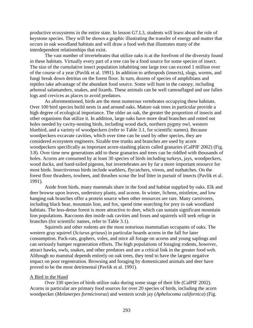
productive ecosystems in the entire state. In lesson G7.L3, students will learn about the role of keystone species. They will be shown a graphic illustrating the transfer of energy and matter that occurs in oak woodland habitats and will draw a food web that illustrates many of the interdependent relationships that exist. The vast number of invertebrates that utilize oaks is at the forefront of the diversity found in these habitats. Virtually every part of a tree can be a food source for some species of insect. The size of the cumulative insect population inhabiting one large tree can exceed 1 million over of the course of a year (Pavlik et al. 1991). In addition to arthropods (insects), slugs, worms, and fungi break down detritus on the forest floor. In turn, dozens of species of amphibians and reptiles take advantage of the abundant food source. Some will hunt in the canopy, including arboreal salamanders, snakes, and lizards. These animals can be well camouflaged and use fallen logs and crevices as places to avoid predators. As aforementioned, birds are the most numerous vertebrates occupying these habitats. Over 100 bird species build nests in and around oaks. Mature oak trees in particular provide a high degree of ecological importance. The older an oak, the greater the proportion of insects and other organisms that utilize it. In addition, large oaks have more dead branches and rotted out holes needed by cavity-nesting birds, including wood duck, northern pygmy owl, western bluebird, and a variety of woodpeckers (refer to Table 3.1, for scientific names). Because woodpeckers excavate cavities, which over time can be used by other species, they are considered ecosystem engineers. Sizable tree trunks and branches are used by acorn woodpeckers specifically as important acorn-stashing places called granaries (CalPIF 2002) (Fig. 3.8). Over time new generations add to these granaries and trees can be riddled with thousands of holes. Acorns are consumed by at least 30 species of birds including turkeys, jays, woodpeckers, wood ducks, and band-tailed pigeons, but invertebrates are by far a more important resource for most birds. Insectivorous birds include warblers, flycatchers, vireos, and nuthatches. On the forest floor thrashers, towhees, and thrushes scour the leaf litter in pursuit of insects (Pavlik et al. 1991). Aside from birds, many mammals share in the food and habitat supplied by oaks. Elk and deer browse upon leaves, understory plants, and acorns. In winter, lichens, mistletoe, and low hanging oak branches offer a protein source when other resources are rare. Many carnivores, including black bear, mountain lion, and fox, spend time searching for prey in oak woodland habitats. The less-dense forest is more attractive to deer, which can sustain significant mountain lion populations. Raccoons den inside oak cavities and foxes and squirrels will seek refuge in branches (for scientific names, refer to Table 3.1). Squirrels and other rodents are the most notorious mammalian occupants of oaks. The western gray squirrel (Sciurus griseus) in particular hoards acorns in the fall for later consumption. Pack-rats, gophers, voles, and mice all forage on acorns and young saplings and can seriously hamper regeneration efforts. The high populations of foraging rodents, however, attract hawks, owls, snakes, and other predators and are a critical link in the greater food web. Although no mammal depends entirely on oak trees, they tend to have the largest negative impact on poor regeneration. Browsing and foraging by domesticated animals and deer have proved to be the most detrimental (Pavlik et al. 1991).

A Bird in the Hand Over 330 species of birds utilize oaks during some stage of their life (CalPIF 2002). Acorns in particular are primary food sources for over 20 species of birds, including the acorn woodpecker (Melanerpes formicivorus) and western scrub jay (Aphelocoma californica) (Fig.

293

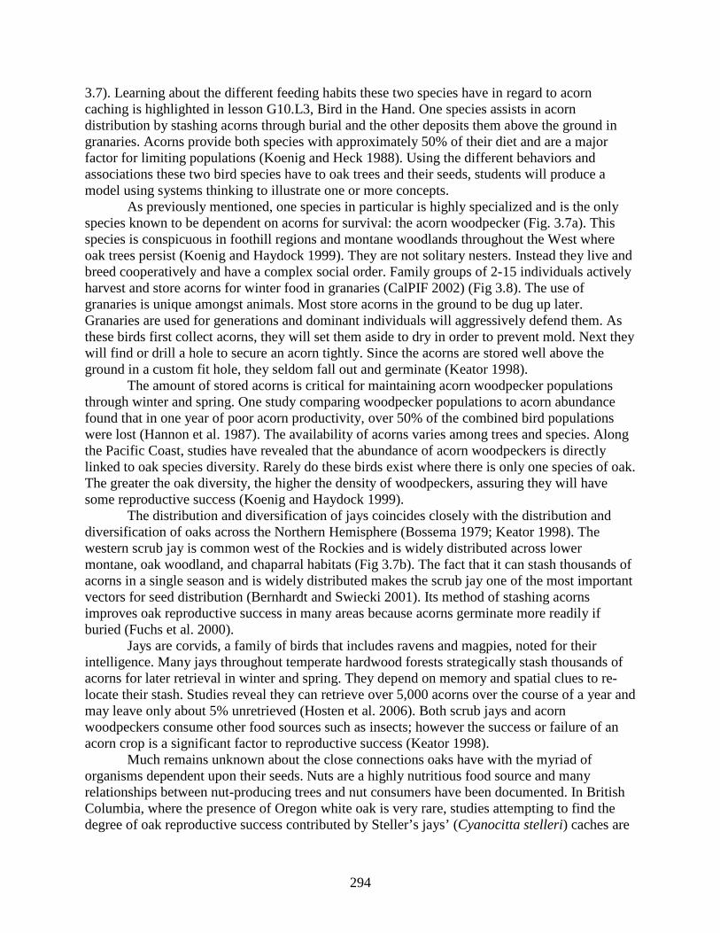
3.7). Learning about the different feeding habits these two species have in regard to acorn caching is highlighted in lesson G10.L3, Bird in the Hand. One species assists in acorn distribution by stashing acorns through burial and the other deposits them above the ground in granaries. Acorns provide both species with approximately 50% of their diet and are a major factor for limiting populations (Koenig and Heck 1988). Using the different behaviors and associations these two bird species have to oak trees and their seeds, students will produce a model using systems thinking to illustrate one or more concepts. As previously mentioned, one species in particular is highly specialized and is the only species known to be dependent on acorns for survival: the acorn woodpecker (Fig. 3.7a). This species is conspicuous in foothill regions and montane woodlands throughout the West where oak trees persist (Koenig and Haydock 1999). They are not solitary nesters. Instead they live and breed cooperatively and have a complex social order. Family groups of 2-15 individuals actively harvest and store acorns for winter food in granaries (CalPIF 2002) (Fig 3.8). The use of granaries is unique amongst animals. Most store acorns in the ground to be dug up later. Granaries are used for generations and dominant individuals will aggressively defend them. As these birds first collect acorns, they will set them aside to dry in order to prevent mold. Next they will find or drill a hole to secure an acorn tightly. Since the acorns are stored well above the ground in a custom fit hole, they seldom fall out and germinate (Keator 1998). The amount of stored acorns is critical for maintaining acorn woodpecker populations through winter and spring. One study comparing woodpecker populations to acorn abundance found that in one year of poor acorn productivity, over 50% of the combined bird populations were lost (Hannon et al. 1987). The availability of acorns varies among trees and species. Along the Pacific Coast, studies have revealed that the abundance of acorn woodpeckers is directly linked to oak species diversity. Rarely do these birds exist where there is only one species of oak. The greater the oak diversity, the higher the density of woodpeckers, assuring they will have some reproductive success (Koenig and Haydock 1999). The distribution and diversification of jays coincides closely with the distribution and diversification of oaks across the Northern Hemisphere (Bossema 1979; Keator 1998). The western scrub jay is common west of the Rockies and is widely distributed across lower montane, oak woodland, and chaparral habitats (Fig 3.7b). The fact that it can stash thousands of acorns in a single season and is widely distributed makes the scrub jay one of the most important vectors for seed distribution (Bernhardt and Swiecki 2001). Its method of stashing acorns improves oak reproductive success in many areas because acorns germinate more readily if buried (Fuchs et al. 2000). Jays are corvids, a family of birds that includes ravens and magpies, noted for their intelligence. Many jays throughout temperate hardwood forests strategically stash thousands of acorns for later retrieval in winter and spring. They depend on memory and spatial clues to re-locate their stash. Studies reveal they can retrieve over 5,000 acorns over the course of a year and may leave only about 5% unretrieved (Hosten et al. 2006). Both scrub jays and acorn woodpeckers consume other food sources such as insects; however the success or failure of an acorn crop is a significant factor to reproductive success (Keator 1998). Much remains unknown about the close connections oaks have with the myriad of organisms dependent upon their seeds. Nuts are a highly nutritious food source and many relationships between nut-producing trees and nut consumers have been documented. In British Columbia, where the presence of Oregon white oak is very rare, studies attempting to find the degree of oak reproductive success contributed by Steller’s jays’ (Cyanocitta stelleri) caches are

294

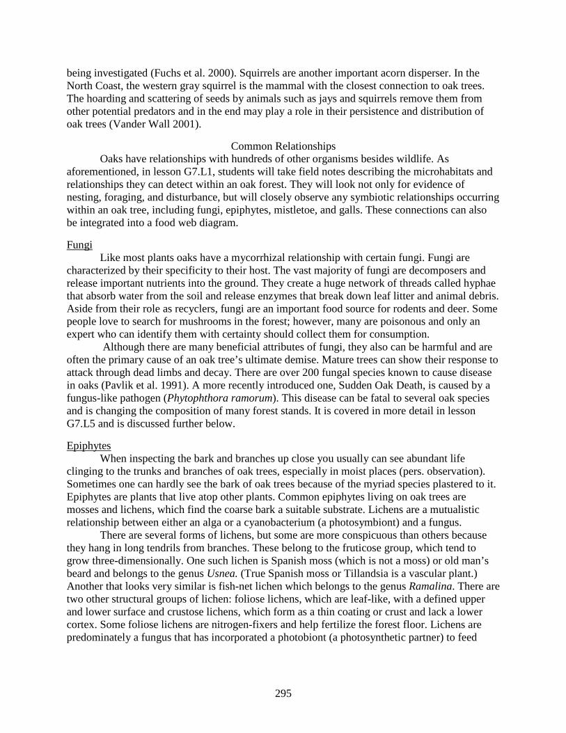
being investigated (Fuchs et al. 2000). Squirrels are another important acorn disperser. In the North Coast, the western gray squirrel is the mammal with the closest connection to oak trees. The hoarding and scattering of seeds by animals such as jays and squirrels remove them from other potential predators and in the end may play a role in their persistence and distribution of oak trees (Vander Wall 2001).

Common Relationships Oaks have relationships with hundreds of other organisms besides wildlife. As aforementioned, in lesson G7.L1, students will take field notes describing the microhabitats and relationships they can detect within an oak forest. They will look not only for evidence of nesting, foraging, and disturbance, but will closely observe any symbiotic relationships occurring within an oak tree, including fungi, epiphytes, mistletoe, and galls. These connections can also be integrated into a food web diagram.

Fungi Like most plants oaks have a mycorrhizal relationship with certain fungi. Fungi are characterized by their specificity to their host. The vast majority of fungi are decomposers and release important nutrients into the ground. They create a huge network of threads called hyphae that absorb water from the soil and release enzymes that break down leaf litter and animal debris. Aside from their role as recyclers, fungi are an important food source for rodents and deer. Some people love to search for mushrooms in the forest; however, many are poisonous and only an expert who can identify them with certainty should collect them for consumption. Although there are many beneficial attributes of fungi, they also can be harmful and are often the primary cause of an oak tree’s ultimate demise. Mature trees can show their response to attack through dead limbs and decay. There are over 200 fungal species known to cause disease in oaks (Pavlik et al. 1991). A more recently introduced one, Sudden Oak Death, is caused by a fungus-like pathogen (Phytophthora ramorum). This disease can be fatal to several oak species and is changing the composition of many forest stands. It is covered in more detail in lesson G7.L5 and is discussed further below.

Epiphytes When inspecting the bark and branches up close you usually can see abundant life clinging to the trunks and branches of oak trees, especially in moist places (pers. observation). Sometimes one can hardly see the bark of oak trees because of the myriad species plastered to it. Epiphytes are plants that live atop other plants. Common epiphytes living on oak trees are mosses and lichens, which find the coarse bark a suitable substrate. Lichens are a mutualistic relationship between either an alga or a cyanobacterium (a photosymbiont) and a fungus. There are several forms of lichens, but some are more conspicuous than others because they hang in long tendrils from branches. These belong to the fruticose group, which tend to grow three-dimensionally. One such lichen is Spanish moss (which is not a moss) or old man’s beard and belongs to the genus Usnea. (True Spanish moss or Tillandsia is a vascular plant.) Another that looks very similar is fish-net lichen which belongs to the genus Ramalina. There are two other structural groups of lichen: foliose lichens, which are leaf-like, with a defined upper and lower surface and crustose lichens, which form as a thin coating or crust and lack a lower cortex. Some foliose lichens are nitrogen-fixers and help fertilize the forest floor. Lichens are predominately a fungus that has incorporated a photobiont (a photosynthetic partner) to feed

295

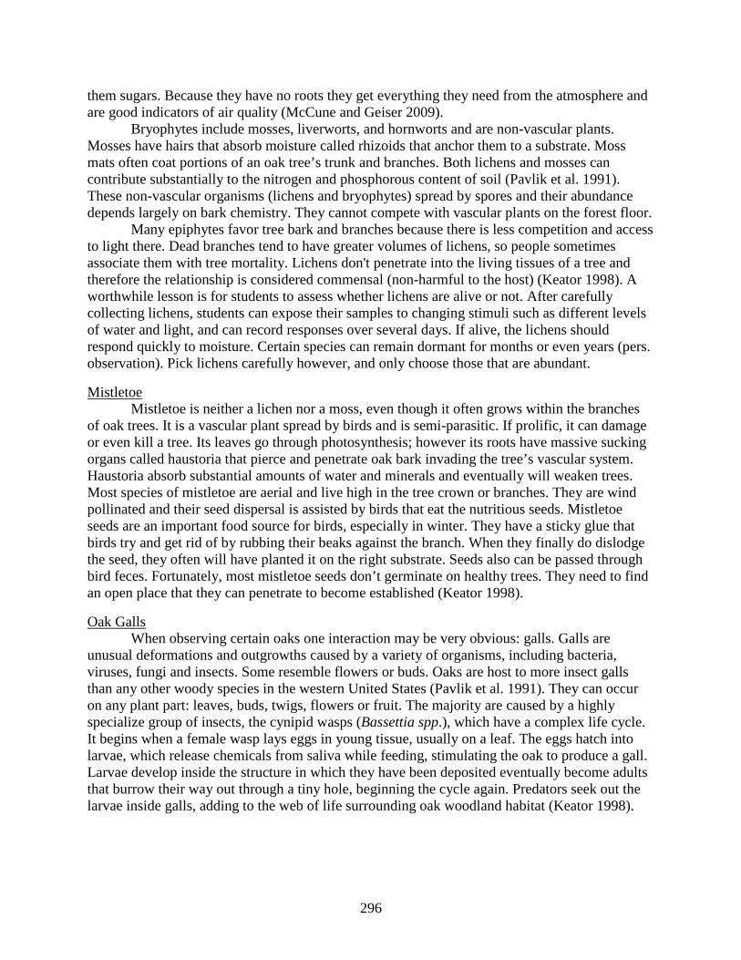
them sugars. Because they have no roots they get everything they need from the atmosphere and are good indicators of air quality (McCune and Geiser 2009). Bryophytes include mosses, liverworts, and hornworts and are non-vascular plants. Mosses have hairs that absorb moisture called rhizoids that anchor them to a substrate. Moss mats often coat portions of an oak tree’s trunk and branches. Both lichens and mosses can contribute substantially to the nitrogen and phosphorous content of soil (Pavlik et al. 1991). These non-vascular organisms (lichens and bryophytes) spread by spores and their abundance depends largely on bark chemistry. They cannot compete with vascular plants on the forest floor. Many epiphytes favor tree bark and branches because there is less competition and access to light there. Dead branches tend to have greater volumes of lichens, so people sometimes associate them with tree mortality. Lichens don't penetrate into the living tissues of a tree and therefore the relationship is considered commensal (non-harmful to the host) (Keator 1998). A worthwhile lesson is for students to assess whether lichens are alive or not. After carefully collecting lichens, students can expose their samples to changing stimuli such as different levels of water and light, and can record responses over several days. If alive, the lichens should respond quickly to moisture. Certain species can remain dormant for months or even years (pers. observation). Pick lichens carefully however, and only choose those that are abundant.

Mistletoe Mistletoe is neither a lichen nor a moss, even though it often grows within the branches of oak trees. It is a vascular plant spread by birds and is semi-parasitic. If prolific, it can damage or even kill a tree. Its leaves go through photosynthesis; however its roots have massive sucking organs called haustoria that pierce and penetrate oak bark invading the tree’s vascular system. Haustoria absorb substantial amounts of water and minerals and eventually will weaken trees. Most species of mistletoe are aerial and live high in the tree crown or branches. They are wind pollinated and their seed dispersal is assisted by birds that eat the nutritious seeds. Mistletoe seeds are an important food source for birds, especially in winter. They have a sticky glue that birds try and get rid of by rubbing their beaks against the branch. When they finally do dislodge the seed, they often will have planted it on the right substrate. Seeds also can be passed through bird feces. Fortunately, most mistletoe seeds don’t germinate on healthy trees. They need to find an open place that they can penetrate to become established (Keator 1998).

Oak Galls When observing certain oaks one interaction may be very obvious: galls. Galls are unusual deformations and outgrowths caused by a variety of organisms, including bacteria, viruses, fungi and insects. Some resemble flowers or buds. Oaks are host to more insect galls than any other woody species in the western United States (Pavlik et al. 1991). They can occur on any plant part: leaves, buds, twigs, flowers or fruit. The majority are caused by a highly specialize group of insects, the cynipid wasps (Bassettia spp.), which have a complex life cycle. It begins when a female wasp lays eggs in young tissue, usually on a leaf. The eggs hatch into larvae, which release chemicals from saliva while feeding, stimulating the oak to produce a gall. Larvae develop inside the structure in which they have been deposited eventually become adults that burrow their way out through a tiny hole, beginning the cycle again. Predators seek out the larvae inside galls, adding to the web of life surrounding oak woodland habitat (Keator 1998).

296

Identifying Oaks Oaks are variable in appearance and often occupy similar habitats as other hardwood species. Species that are tree-like are emphasized here, although others can be shrub-like. Several shrub-like forms are found in the North Coast Range, including Sadler oak (Quercus sadleriana), huckleberry oak (Q. vaccinifolia), and leather oak (Q. durata var. durata). Sadler oak is endemic to the Klamath-Siskiyou region and prefers higher elevations. It can hybridize with a shrub-like variation of Oregon white oak (Q. garryana var. breweri). Huckleberry oak can be found in many parts of the Coast Range and can be associated with serpentine soils. A form of leather oak (Q. durata var. durata) is restricted to serpentine soils. Another variety found in southern California lives on granitic soils (Q. durata var. garbrielensis) (Nixon 2002). Many features are useful when identifying oaks, including the arrangement of male catkins, stigmas, and female ovaries. For the sake of brevity and simplification, students will mostly identify oaks using the shape, color, and size of both leaves and acorns, including the acorn cap or cupule. The margins of oak leaves can be smooth, serrated, or toothed. Leaf shape can range from elliptical to deeply lobed. A closer look at leaf veins can reveal a complex, featherlike pattern or a pinnate vein arrangement that can be readily seen when making leaf rubbings. Using these key features is usually adequate for successful identification. However, depending on where leaves are collected it is possible to find oak hybrids. This fact should be considered for more advanced identification purposes (Hickman 1993). One of the first defining features for oak identification is whether an oak is evergreen or deciduous. In northwestern California, there are three evergreen species: coast live oak (Q. agrifolia), interior live oak (Q. wislizenii), and canyon live oak (Q. chrysolepis). Southern Mendocino marks the northern tip of the range for coast live oak, which extends down into northern Baja. It is characteristically found along coastal plains, valleys, and foothills. The other two common species of evergreen oaks - interior live oak and canyon live oak - are discussed further below. Distinguishing these three evergreen species from each other can be aided with range maps. The rest of the highlighted species are winter deciduous, although some will lose their leaves early in drought conditions. Below is an alphabetical listing giving brief descriptions for the most common oaks found on the North Coast. (For further information, refer to an identification book or an online resource.) Black oak (Q. kelloggii) is one of the more widely distributed oak trees in California, extending from Baja California to western Oregon. It is a deciduous tree reaching heights between 18-20 m (60-90 ft) that produces fine, strong wood that can be used in cabinetry and furniture. This species rarely occurs in pure stands and is commonly part of a matrix of mixed hardwoods and conifers, including the montane Douglas-fir forest. In fall it can add vibrant seasonal color and its acorns are considered some of the best for eating (Pavlik et al. 1991). It is relatively shade intolerant and a vigorous sprouter. Fire is the primary mode of stand replacement (Garrison et al. 2002). It ranges from 20-2,660 m (200-8,700 ft) in elevation, occurring mostly in higher elevations except in the North Coast Range (Nixon 2002). It hybridizes with interior live oak and belongs to the black oak group, which is susceptible to SOD. Distinguishing features include: dark grayish bark, fairly large leaves with pointed leaf lobes that end with a fine bristle, and acorns about 2.5 cm (1 in) long with a scaly cap (de Mayolo 2000; Hickman 1993; Pavlik et al. 1991) Blue oak (Q. douglasii) is a sun loving deciduous species sometimes forming pure stands, which can include foothill or gray pine (Pinus sabiniana). It can be mixed with other hardwood species such as interior live oak and valley oak. Blue oak savanna is common on the

297

eastern side of the North Coast Range and is well adapted to xeric sites. It is much more common in eastern Mendocino County than Humboldt County and has remarkable drought tolerance. It usually stands 6-18 m (20-60 ft) tall and is a long-lived species. It has bluish-green leaves due to a waxy coating, as the common name implies (Pavlik et al. 1991). Seedlings are intolerant to shade. Overgrazing and other factors have negatively impacted young trees. It can vigorously resprout after low-intensity grass fires but not hotter blazes (Bartolome et al. 2002). Distinguishing features include light gray to whitish bark; medium sized bluish-gray leaves that are smooth to slightly lobed; and acorns with a warty cap (de Mayolo 2000). Canyon live oak or goldcup oak (Q. chrysolepis) is found on variable sites, including mixed conifer, chaparral, and woodlands. As the name implies, this species commonly occupies steep canyons and sheltered north slopes. It is evergreen and shade tolerant. Mature trees can be over 300 years old and can have branches extending over 30 m (100 ft), forming wide crowns. It can form a large majestic tree or be shrub-like where conditions are less favorable. Mature trees can have wide trunks up to 1.5 m (4 ft) across. The largest known tree is 22 m (72 ft) tall with a trunk 3 m (10 ft) wide. Extremely adaptable, it can live between 200-2,600 m (650-8,500 ft) in elevation. Despite its many forms, the leaves and acorns are distinctive. Distinguishing characteristics include gray to whitish bark sometimes composed of smooth shallow strips; dark green elliptical leaves 2.5-5 cm long (1-2 in) long with hairs on the underside; and a thick saucer-shaped acorn cap (Pavlik et al. 1991). Interior live oak (Q. wislizenii) is another evergreen species occupying varied sites. The advantage of holding onto leaves all year is to generate a large supply of food for growth and reproduction. It does not tolerate frost well; thus, at higher elevations where snow and ice are common, it can be replaced by black oak. It can dominate dry sites and only occurs in the southeast corner of Humboldt County. It typically forms a broad compact shape with dense branches and is a vigorous resprouter. The leaves are flat, stiff, and shiny. Leaf margins are variable and can be smooth, toothed, or spiny. It can be confused with coast live oak (Q. agrifolia). Distinguishing features include flat, thick, leathery leaves, dark green on top and yellowish below, and narrow acorns up to 3.8 cm (1.5 in) long that sit deep in their cup (Pavlik et al. 1991). Oregon white oak (Q. garryana) can form pure stands, which can stand out in autumn against the evergreen hills of the inner North Coast and Klamath Ranges. It inhabits a variety of sites from 300-1,200 m (1,000-4,000 ft) in elevation and can mix with black oak and other hardwoods. It is also referred to as Oregon oak. Because the heartwood resists rot when in contact with soil, it is suitable for fence posts and has been referred to as “post oak.” The largest stands occur in the deep bottomlands of the Columbia River and within the Willamette Valley of northwestern Oregon, where trunks can easily reach 1 m (3 ft) across (Thilenius 2012). The record tree in California is 2.4 m (8 ft) in diameter and 37.2 m (122 ft) tall (Stuart and Sawyer 2001c). Relatively straight upright trunks with few branches can give this species a distinctive profile. After fire or logging, multiple resprouts will occur that thin over time. It can tolerate damp places and is much more common in Humboldt County than Mendocino County. Pure stands were maintained by regular fire. Today fire suppression has favored faster growing conifers throughout their range. This oak is deciduous and can be distinguished from black oak by its leaves and bark coloration. Distinguishing characteristics include light-colored wood; large, broad, lobed leaves with smooth margins; and rounded acorns with shallow warty caps (de Mayolo 2000; Pavlik et al. 1991).

298

Tanoak (Notholithocarpus densiflora) is not a true oak. It typically forms an erect tree 15-27 m (50-90 ft) tall with a main stem; however, on poor sites, it can have a shrub-like character (Stuart and Sawyer 2001b). Also called tanbark oak, during the 1900s, its inner bark was used for tanning hides because of the presence of tannic acid. It is a relic species endemic to California and southern Oregon and distributed among moist varied sites. It is often an understory component of coast redwood and is associated with many forest types, including Port-Orford cedar (Chamaecyparis lawsoniana), knobcone pine (Pinus attenuata) and mixed evergreen forest where Douglas-fir is dominant. It is associated with many hardwood species, including, true oaks, madrone, and California bay and is found in woodlands and chaparral. Although it grows best in full sunlight, it can be very shade tolerant. It can vigorously resprout and become the dominant tree post-harvest. Like true oaks its flowers are unisexual. The male flowers, bearing pollen, form long, upright catkins that are much more conspicuous than other oak flowers. Acorns mature in their second year and were the most prized for eating by many Native American tribes living within the species range (Barbour et al. 2001). Distinguishing characteristics include a very bristly cap atop an egg-shaped acorn and leathery, elliptical leaves with serrated or entire margins. The tops of leaves are darkish green and the underside is lighter in color and coated with dense hairs (Stuart and Sawyer 2001b) Valley Oak (Q. lobata) is the largest North American oak and can live 400-600 years. It can easily reach heights over 30 m (100 ft) with massive trunks exceeding 1.5 m (5 ft) in diameter. Its distribution is largely regulated by the availability and depth of water (Griffin 1988). In Sonoma Valley, they achieve their grandest size where the water table is 3-6 m (10-20 ft) below the surface (Dawson 2006) and at elevations below 600 m (2,000 ft) (Pavlik et al. 1991). This species is deciduous and can be confused with Oregon white oak where ranges overlap. Its grandeur reminded the early settlers of the majestic white oaks of Europe and is commonly referred to as the Roble oak. Although much of its former range consisted of large, expansive savannas, it now mostly occupies riparian zones, mixed forests, and woodlands. Several historically significant trees exist in the North Coast, including the current largest one found in Round Valley near Covelo. Distinguishing characteristics include its size; light gray bark that can form a checkerboard pattern on mature trees; deeply lobed leaves with soft hairs; and large acorns reaching 5 cm (2 in) with warty knobs on their caps (de Mayolo 2000; Pavlik et al. 1991).

Trees in Trouble Sudden Oak Death (hereafter SOD) is a relatively new disease that has killed over one million oak trees in California and Oregon. Although tanoaks are most affected, California black oak, coast live oak, and canyon oak are also susceptible. The pathogen has been confirmed in 14 coastal counties extending from Monterrey to Humboldt (McCreary et al. 2011). In lesson G7.L5, students will read about SOD and will learn how to recognize signs of this disease and what precautions can be taken to help prevent the spread of its infection. As aforementioned, the cause of SOD is an invasive fungus-like organism, Phytophythora ramorum, that prefers cool, wet climates. The lifecycle of this pathogen is complex and won’t be discussed here. SOD is a forest disease that was accidentally introduced into California from Europe in the 1990s through nursery plants. It can be fatal to oak trees and causes twig and foliar diseases in dozens of other plants, including rhododendrons, Douglas-fir, redwood, and California bay. California bay can give an advanced warning since it often becomes infected first. More spores develop on the smooth leaves of this tree than anywhere

299

else. In some places bay is being removed to reduce infection. Because this pathogen prefers moisture, it often begins in riparian areas and spreads outwards. There are many steps people can take to help prevent this disease once they are aware of it. People travelling to known infected areas should thoroughly wash their shoes, tires, vehicles, tools, and pets before returning home (Lee et al. 2011). SOD poses an ecological threat because it is changing species composition and increasing fuel loads in some places. Changes in composition will affect food sources for wildlife, watershed quality, and fire frequency and intensity. Changes in species diversity are likely to alter ecosystem functions and are difficult to predict, especially those factors compounded by global climate change. Extensive research and monitoring is taking place across the Coast Ranges and excellent online resources are available. The Oak Mortality Task Force coordinates the extensive research and has an excellent website (COMTF 2014).

Transitional Forests The life histories and life history traits of different oak species and woodland vegetation greatly influence the course of succession. Traditional theories of plant succession tend to show a linear model of change leading to a stable or climax state (Fig 3.9). This model does not adequately describe the vegetation dynamics of some oak woodland communities. In these communities, multiple successional pathways and stable endpoints can occur. Oak woodlands are in dynamic equilibrium with other plant associations and, depending on their locations and exposure to different disturbance regimes, they can be converted into grasslands, coastal sage scrub, or chaparral (George and Alonso 2006). Disturbances may occur suddenly from fire or flood or slowly from repeated stresses such as grazing or drought. Transitions are often triggered by natural or human caused disturbances. Disturbances change the structure and function of ecosystems by changing the composition and evenness of communities. The degree of disturbance modifies nutrient cycling and, with changes in species composition, alters linkages in the food web (Dale et al. 2013). Every species responds to disturbances based on physiological and genetic variances. Trees and understory plants have different ranges of survival, tolerance to stresses, degree of shade tolerance, and other factors that can lead to different community structure over time. It can take over 80 years for the development of large trees and most coastal oak woodlands are at least this old (Holland 2005). The rate at which succession occurs depends on the degree of disturbances. Some of the largest changes to oak woodlands have come from human disturbances. In some places, the mechanical removal of trees and use of chemical controls have permanently converted woodlands to grasslands. Between 1945 and 1974, almost 810,000 ha (2 million ac) of hardwoods and chaparral were cleared for rangeland improvement. Millions of trees have been removed for firewood and most ranchers today continue to value conifers over oaks (Koski 2012). Fire has been another important activity that has shaped oak woodland succession and is discussed in greater detail below.

Fire Ecology Fire is a normal disturbance in California's oak woodlands and certain oak-dominated landscapes require fire for sustainability. Some estimate that major fires would have normally occurred every 30 to 50 years in savannas, oak woodlands, and chaparral communities (Pavlik et

300

al. 1991). Investigations in Annadel State Park located in Sonoma County, an area largely covered by oak woodlands and mixed conifer forest, found evidence of mean fire intervals every 6 to 21 years (Hastings et al. 1997). Lack of fire has created compositional and structural changes throughout forest and woodlands of the western United States. Where fire has been suppressed, advancement of the forest boundary and woody vegetation has occurred, shifting the understory vegetation towards shade-tolerant species. Overall, forested communities have become denser, causing forests to burn uncharacteristically hot. How a species responds to fire depends on its life history traits and the environmental conditions of the site. Following a fire, an oak woodland community is characterized by standing trees relatively intact, with much of the shrub and herbaceous layer reduced (George and Alonso 2006). Mature trees can have adaptations that allow them to survive moderate fire, such as thick bark or dormant buds well insulated below ground in root crowns. After fire, young shoots utilize the stored carbohydrates in the surviving roots and also take advantage of increased light (Carle 2008). Many herbaceous shrubs such as manzanita and ceanothus (see Table 3.1 for scientific names) have seed banks that survive after fire. Sprouting from the root crown is the most important survival adaption of most oak species (Plumb and McDonald 1981), although many can also resprout from their bole or crown. Not all oak species respond to fire in the same way. Sprouting from evergreen oaks tends to be more vigorous than deciduous species. Tanoak is one of the least resistant to fires despite its ability to resprout. Even mature tanoaks are susceptible to burning (Anderson 2002). Most oaks are fire-resistant; however, even the most fire-resistant species cannot survive intense fires. Under natural conditions, fire is necessary for the perpetuation of oak woodlands, especially on sites where oaks compete with faster growing conifers. Douglas-fir becomes increasingly fire-resistant as it ages, developing thicker bark and a taller crown. Similar to most conifers it cannot resprout after fire. Coast redwood is an exception to this resprouting ability. In many places, black oak, Oregon white oak, and other hardwoods are being increasingly encroached upon by conifers which is discussed further below. As we become better at controlling fires, the wildfire problem becomes worse. Cessation of cultural burning began around 1910 and since the 1930s fire suppression became one of the primary objectives of the U.S. Forest Service. Most experts agree that the compositional shift in vegetation witnessed today is a product of fire suppression. Fire intensity and behavior changes with moisture, fuel mass, and bulk density, along with other factors (Engber et al. 2011). With lack of regular fire, those that do occur may become more intense because brush and young trees accumulate in the understory. These and other herbaceous shrubs would normally die in a fire. Most people still view fires as a negative disturbance and a decrease in air quality is problematic. The outlook is slowly changing within certain populations and fire is now viewed as an essential link to effective management. Understanding historical patterns on a particular landscape, as a result of human impacts, is critical in correctly interpreting the ecological bases for vegetation distribution and management - in this case, the role of fire. Many fires in oak woodland were initiated by Native Americans and sustained by Euro-American settlers (Keeley 2002). The degree to which anthropogenic fire regimes have altered oak woodland and savannas is continually investigated and debated. It is well known that in portions of the Pacific Northwest, low-intensity burning by Native Americans limited the extent of coniferous forest, favoring fire-tolerant oak stands (Devine and Harrington 2006). Through frequent burning, indigenous peoples modified the landscape for desired outcomes such as: improved browsing for deer, favored plant-growth

301

forms used in basketry, and decreased disease and insect infestations of acorns to improve the harvest. For information about how Native Americans shaped the landscape of California, refer to the prelude in the Forest Ecology 101 series.

Overtopping In the absence of fire, encroachment by conifers can change the vegetative structure of oak woodlands and surrounding grasslands. In northern California, many oak species are associated with mixed evergreen forests, which can quickly become over-crowded by faster growing conifers. Conifers tend to be more shade-tolerant than most oaks. On the North Coast, the main coniferous invader is Douglas-fir. Young trees have pointed crowns and grow quicker and taller than the surrounding hardwoods. As they grow, they can penetrate the spaces between the more open, rounded crowns of oak trees and other hardwoods. Without natural or anthropogenic periodic clearing, hardwoods eventually will experience crown die-back, leading to eventual mortality. This phenomenon is referred to as overtopping (Hunter et al. 2001) (Fig. 3.10). Past fire regimes would have reduced the numbers of conifers. Normally oaks resprout after fire and live to be much older than conifers. Douglas-fir cannot resprout after fire, but it has a prolific seed bank and therefore can be an aggressive colonizer of open or moderately shady sites (Huntsinger and McCaffrey 1995). Under the right conditions, once established, seedlings can easily grow a meter per year and can quickly overtop surrounding oak trees. Studies done in the Eel River Basin report a 30% decline in oak woodland and a 35% increase in Douglas-fir forest from 1865 to 1985 (Sawyer 2006). Frequent burning that does not kill the oaks can halt the progression of conifers by killing saplings, thereby maintaining openings and clearings. Conifer encroachment into oak woodland habitat is a major management concern (Agee and Skinner 2005; Engber et al. 2011). Investigating this phenomenon and analyzing oak response to conifer thinning is the main objective in lesson G10.L4, King Conifer. In this lesson, students will learn about and interpret results from a thinning project that removed different proportions of Douglas-fir in a woodland where Oregon white oak exists. Oregon white oak is shade-intolerant and its range has been altered due to fire suppression. A major problem is overtopping and enroachment by conifers, namely, Douglas-fir. The results in this study show oak responses to various treatments using changes in diameter breast height (dbh), epicormic sprouting (sprouts that occur from buds), and acorn productivity over five years (Devine and Harrington 2007). Consideration of fire at a landscape level is essential to facilitating ecological restoration efforts intended to bring stands back to historical condition. Low-intensity prescribed fire and manual removal of conifers are now being practiced more readily as a management tool in establishing and restoring oak stands. Periodic burning reduces fuel accumulations that support high-intensity wildfires, which often kill or severely damage tree trunks and crowns. In the North Coast and the Klamath region, the maintenance of Oregon white oak and black oak in particular benefit from oak release. Oak release refers to the removal of overcrowding conifers. Oaks that initially develop with little competition will form rounded crowns, which will end up sparse or dead if overtopped. Observing the crown of a tree can be a good way to assess whether an oak tree can benefit from thinning. Having students observe overcrowding is a good way to introduce them to some of the competitive dynamics between different tree species and to discuss tradeoffs regarding growth strategies. At a suitable site, students can help prevent overtopping by manually pulling conifer seedlings and saplings that would normally die during fires.

302

Understanding forest dynamics can allow better assessment of which management techniques are required to enhance or restore a site.

Native American Management of Fires A combination of wildfires and Native American burning have maintained oak woodland and surrounding grasslands for millennia by preventing succession to woodland or forest (Bachelet et al 2011). As aforementioned, some contend that the indigenous use of fire has had dramatic and widespread impacts on our landscape. Many of these anthropogenic patterns are still evident in the distribution of vegetation types. Potential patterns of Native American burning are evaluated based upon historical documents, ethnographic accounts, archaeological records, and consideration of current land management practices. Knowing the full scale of the fire history and the impact it has had on stand structure and landscape patterns is difficult to determine with confidence. In the Coast Ranges, the frequency of natural fire frequency has not been high enough to maintain the present landscape configurations. Most researchers agree that grasslands and oak woodlands in many parts of the Coast Range had high Native American occupancy and regular low frequency burning. However, the high diversity of languages found throughout the Coast Ranges, combined with rugged and steep terrain, suggest some wilderness patches must have existed between tribal areas (Keeley 2002). In the Klamath National Forest, similar to many mixed forest communities on the North Coast, the pre-settlement landscape was probably patchy. Modifying a Douglas-fir forest to encourage an open canopy dominated by hardwood species was regularly practiced. Studies have revealed two phenomena associated with anthropogenic burning: fire yards and fire corridors. Fire yards were openings within a forest maintained by burning while fire corridors were maintained along linear features such as ridges, trails, and forest edges (Underwood et al. 2003). Open patches support a considerably higher diversity of plant and animals species than a dense, closed canopy forest (Huntsinger and McCaffrey 1995). Federal land managers and others are beginning to understand the ecological need for regular fire regimes in these mixed forest habitats and are working with several indigenous tribes to remedy the situation. More collaboration between the U.S. Forest Service and Native American tribes is occurring. Ecological research is beginning to confirm some of the historical records and traditional knowledge claims, which have supported changes in vegetation dynamics due to indigenous practices (Leskiw 2006). One thing is certain: built-up fuel loads have created unfavorable conditions for regenerative success of oaks and lack of fire is taking its toll on the integrity of these ecosystems (McCreary 2009). To understand the complex vegetation dynamics and the role past and future fire regimes have on the oak-dominated landscapes require a great deal more study.

The Bald Hills: A Case Study One place receiving attention is Redwood National Park (RNP). The traditional philosophy of the National Park Service has favored keeping each park pristine or as close as possible to its natural condition. This idea has been increasingly contradictory (in some cases), because many places located in our parks have been managed by Native Americans for centuries and later by white settlers. This is the case in the Bald Hills. The Bald Hills is an area over 1,700 ha (4,000 ac) covered by Oregon white oak savanna and coastal grassland (formerly called prairies). It is located on the east side of RNP and includes elevations from 76 to 945 m (250 ft to 3,100 ft).

303

It is difficult to reconstruct the past vegetative distribution here, although park managers believe that the natural balds existed before 5,000 years ago. This is roughly the same amount of time it has been used and managed by Native American inhabitants, including the Chilula and Yurok tribes. For thousands of years fire was used to keep the oak woodlands open. Once the Gold Rush hit the area, Native Americans were pushed out. By the 1870s, permanent Euro-American settlements were made. The largest homestead was the Lyons Ranch, portions of which still exist today. The family regularly practiced sheep and cattle ranching, which facilitated the spread of exotic grasses. Managing with fire presumably continued until it was banned in the early 1900s. Today, fire exclusion has resulted in a structural and compositional shift to a forest dominated by conifers. It is estimated that by 1990, one quarter of the Bald Hill’s vegetation was already converted to coniferous forest and another half was being threatened (Underwood et al. 2003). The elimination of regular fire regimes has altered the fuelbed composition and vegetative structure, changing the way fire behaves. With lack of fire a characteristically open terrain is now cluttered by heavy, herbaceous mass increasing flammability and fire intensity (Engber et al. 2011). In lesson G10.L5, students will read about some of the past and current land management practices used in the Bald Hills. They will learn how human interferences have altered the landscape and will explain why fire is currently used as a restoration tool. In the late 1970s, park managers began ecological investigations that have since revealed several threats to the area, including invasion by exotic species, encroachment by conifers, and increased erosion from roads. A multifaceted management plan was quickly established and approved. Goals include the promotion of native plant diversity, the protection of pre-European fauna, and repairing or eliminating roads. The park has begun reinstituting prehistoric fire regimes. Grasslands are burned every 3 to 5 years in some places. Conifers occupying over 810 ha (2,000 ac) have been removed (Underwood et al. 2003). In hard to reach places conifers are girdled and smaller ones are manually cut or pulled. Girdling a tree is a method where the bark and cambium is removed 360 degrees around a section of the tree. This stops the flow of water and nutrients and the tree eventually dies, leaving a snag. The Bald Hills are accessible by bus and field trips there are encouraged.

Future Management of Oak Woodlands California is rapidly losing its oak woodlands to increased urbanization. The large valley oak savannas of the Central Valley are virtually gone and many others have been reduced. The current population of California is estimated at 38 million and is expected to increase by another 10 million people by 2050. Oak woodlands in the Central Valley and Sierra foothills currently face the greatest risk. A quick comparison showing human population densities superimposed over oak woodland’s range in the state of California would show a direct correlation. People are drawn to the same places many oaks prefer. Currently, more than 1 million acres of California's oak woodlands have been developed and before 2040 another 750,000 are at risk of development. In the greater North Coast region, 84% of oak woodland habitat is privately owned. Sonoma County has already developed over 20% of its oak woodlands and another 10% are at risk. Mendocino County has developed 5% and risks losing an additional 5% in the next 25 years (Gaman and Firman 2008). Although the oak woodlands of Humboldt County are relatively immune to reduction due to urbanization, they are still at risk from improper management strategies, lack of funding, and fire suppression. Approximately 6% of Humboldt County is

304

occupied by oak woodland, which is currently threatened by conifer encroachment and the subsequent succession to mixed coniferous forest (Green and Magnuson 2011). Interest in ecology, management, and perpetuation of oak woodlands has increased dramatically in the last three decades (McCreary 2009). Managers and researchers have come a long way in understanding how best to grow and plant native oaks useful in oak improvement projects. Research has addressed a wide array of factors with the hope of improving manual oak regeneration, including acorn collection, storage, and handling. Even though the demographics of land ownership have not changed significantly over the last 20 years, some of the attitudes of people might be evolving. According to surveys of oak woodland managers, more are recognizing the value of their oak trees and making efforts to replant and protect them (Huntsinger et al. 2006). Future oak management holds many challenges. There is still a great deal unknown about the vegetation dynamics of oak woodlands. Management objectives vary between agencies and departments. Oak woodlands continue to provide quality agricultural sites and grazing land and the majority of these habitats will continue to be managed by private landholders. Even without fully knowing causes of poor oak recruitment, it is important for owners and managers to evaluate their oak stands and assess whether adequate regeneration is occurring. Saving heritage oak woodlands requires restoration and active monitoring. Much work needs to be done to initiate and maintain long-term studies of vegetation change in California oak woodlands and associated communities to assure their long-term survival (George and Alonso 2006).

Conclusion Oak woodlands and forests are a key natural feature of California. These diverse ecosystems have been shaped by climate change and fire over millennia and fire seems to be central to maintaining them. Oak woodlands are some of the most biologically diverse ecosystems and oaks are considered a keystone species. Their productivity and importance connect them to many ecological concepts, adding value to any secondary curriculum. Hundreds of different species utilize oaks, supplying endless examples of plant and animal interactions and interdependencies. Acorns were a primary food source for Native Americans and remain culturally significant. Oak woodlands are still maintained on tribal lands through fire and clearing to encourage certain plants and animals. Today, oak woodlands remain vulnerable to urbanization and agricultural development. Few intermediate to young stands are observed, and lack of recruitment is a concern to both private and public land managers. Urbanization continues to be one of the greatest threats as the population of California continues to grow faster than most states. Urbanization is not as great a threat to the oak woodlands of the North Coast; however, oak inhabited zones are variable and can be shaded out quickly by faster and larger growing conifers. Because of their variability, placing oak-dominated zones into a broader regional context is necessary in order to truly understand, enhance, and protect these vital forests. By learning about these important systems, students can gain a deeper understanding into the world of our disappearing oak woodlands.

305

TABLES (Module 3): Table 3.1. List of scientific names of referenced species in Module 3, Part I. FLORA FAUNA Trees big leaf maple (Acer macrophyllum) black oak (Quercus kelloggii) blue oak (Quercus douglasii) bush chinquapin (Chrysolepis sempervirens) California bay (Umbellularia californica) canyon live oak or goldcup oak (Quercus chrysolepis) coast live oak (Quercus agrifolia) coast redwood (Sequoia sempervirens) Douglas-fir (Pseudostuga menziesii) eastern white oak (Quercus alba) Engelmann-oak (Quercus engelmannii) giant chinquapin (Chrysolepis chrysophylla) gray or ghost pine (Pinus sabiniana) interior live oak (Quercus wislizenii) knobcone pine (Pinus attenuata)ponderosa pine (Pinus ponderosa madrone (Arbutus menseizii) Oregon white oak (Quercus garryana) Port-Orford cedar (Chamaecyparis lawsoniana) tanoak (Notholithocarpus densiflorus) valley oak (Quercus lobata) Shrubs California buckeye (Aesculus californica) ceanothus (Ceanothus spp.) huckleberry oak (Quercus vaccinifolia) leather oak (Quercus durata var. durata) manzanita (Arctostaphylos spp.) poison oak (Toxicodendron diversilobum) Sadler oak (Quercus sadleriana) Mosses and Lichens fish-net lichen (Ramalina spp.) old man’s beard (Usnea spp.) Fungi Phytophythora ramorum

Invertebrates cynipid wasp (Bassettia spp.) filbertweevil (Curculio occidentis) filbertworm (Melissopus latiferreanus) oak moth (Phryganidia californica) Birds acorn woodpecker (Melanerpes formicivorus) Northern pygmy owl (Glaucidium gnoma) Steller’s jay (Cyanocitta stelleri) Western bluebird (Sialia Mexicana) Western scrub jay (Aphelocoma californica) wood duck (Aix sponsa) Mammals black bear (Ursus americanus) black-tailed deer (Odocoileus hemionus) California grizzly bear (Ursus arctos californicus) gray fox (Urocyon cinereoargentus) mountain lion or cougar (Puma concolor) raccoon (Procyon lotor) Western gray squirrel (Sciurus griseus) wild pig (Sus scrofa)

306

Table 3.2 Characteristics of the three evolutionary lineages of Quercus and the placement of select oak species found in California (source Pavlik et al. 1991).

Characteristics of the Three Evolutionary Lineages of Quercus (Pavlik et al. 1991) Lineage white oaks

(Lepidobalanus) red oaks

(Erythrobalanus) golden oaks

(Protobalanus) Leaves

lobes lobed or unlobed lobed or unlobed unlobed lobe shape round pointed margins smooth or with blunt,

green teeth or spines tawny bristles and spines

smooth or with green teeth or spines

Acorns inner shell smooth densely hairy smooth or hairy cup scales thick and knobby thin and flat thick, often knobby matures in 1 year 2 years 2 years Bark (mature trees) light gray or brown,

scaly or rough dark gray, blackish or brown, smooth

light gray or brown, scaly or rough

California oaks (selected species)

valley, blue, Englelmann, Oregon white, scrub, leather

black, coast live, interior live

canyon live, huckleberry

307

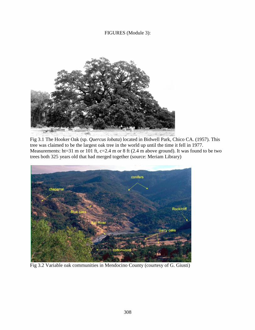
FIGURES (Module 3):

Fig 3.1 The Hooker Oak (sp. Quercus lobata) located in Bidwell Park, Chico CA. (1957). This tree was claimed to be the largest oak tree in the world up until the time it fell in 1977. Measurements: ht=31 m or 101 ft, c=2.4 m or 8 ft (2.4 m above ground). It was found to be two trees both 325 years old that had merged together (source: Meriam Library)

Fig 3.2 Variable oak communities in Mendocino County (courtesy of G. Giusti)

308

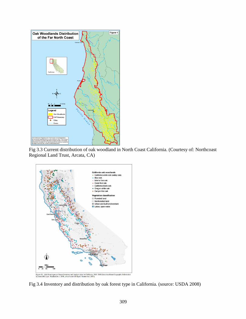
Fig 3.3 Current distribution of oak woodland in North Coast California. (Courtesy of: Northcoast Regional Land Trust, Arcata, CA)

Fig 3.4 Inventory and distribution by oak forest type in California. (source: USDA 2008)

309

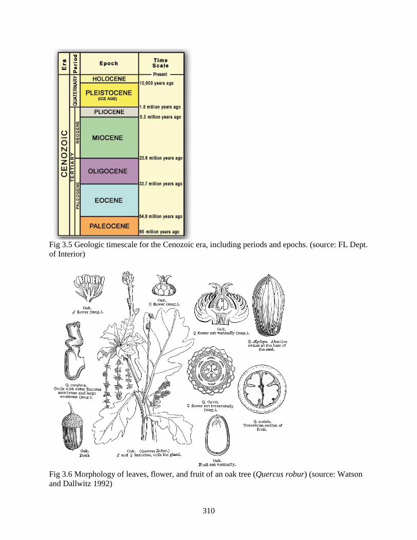
Fig 3.5 Geologic timescale for the Cenozoic era, including periods and epochs. (source: FL Dept. of Interior)

Fig 3.6 Morphology of leaves, flower, and fruit of an oak tree (Quercus robur) (source: Watson and Dallwitz 1992)

310

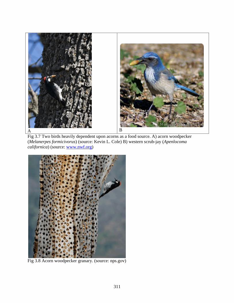
A

B

Fig 3.7 Two birds heavily dependent upon acorns as a food source. A) acorn woodpecker (Melanerpes formicivorus) (source: Kevin L. Cole) B) western scrub-jay (Apenlocoma californica) (source: www.nwf.org)

Fig 3.8 Acorn woodpecker granary. (source: nps.gov)

311

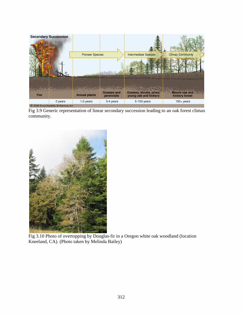
Fig 3.9 Generic representation of linear secondary succession leading to an oak forest climax community.

Fig 3.10 Photo of overtopping by Douglas-fir in a Oregon white oak woodland (location Kneeland, CA). (Photo taken by Melinda Bailey)

312

LITERATURE CITED (Module 3): Adams, Theodore E., Peter B. Sands, William H. Weitkamp, K. Neil, and Neil K. McDougald.

1992. “Oak Seedling Establishment on California Rangelands.” Journal of Range Management 45 (1): 93–98.

Agee, James K., and Carl N. Skinner. 2005. “Basic Principles of Forest Fuel Reduction Treatments.” Forest Ecology and Management 211 (1-2) (June): 83–96.

Alexrod, Daniel L. 1983. “Biogeography of Oaks in the Arcto-Tertiary Province.” Annals of the Missouri Botantical Garden 70 (4): 629–657.

Anderson, Kat M. 2002. “USDA Plant Guide: Tanoak”. Davis, CA. http://plants.usda.gov. Barbour, Michael G., Stephen Barnhart, Emin Ugurlu, and Daniel Sanchez Mata. 2006. “Species

Characteristics and Stand Structure of Quercus garryana and Q . pyrenaica woodlands in the Mediterranean Regions of California and Spain.”

Barbour, Michael, Bruce Pavlik, Frank Drysdale, and Susan Lindstrom. 1993. California’s Changing Landscapes. Edited by Phyllis Faber. 2nd ed. Sacramento, CA: California Native Plant Society.

Barbour, Michael, Sandy Lydon, Mark Borchert, Marjorie Popper, Valerie Whitworth, and John Evarts. 2001. Coast Redwood: A Natural and Cultural History. Edited by John Evarts and Marjorie Popper. Los Olivos, CA: Cachuma Press, Inc.

Bartolome, James W. 1987. “California Annual Grassland and Oak Savannah.” Rangelands 9 (3): 122–125.

———. 1989. “Ecological History of the California Mediterraean-Type Landscape.”. Berkeley, CA: Department of Forestry and Resource Management.

Bartolome, James W., Mitchel P. Mcclaran, Barbara H. Allen-Diaz, Jim Dunne, Lawrence D. Ford, Richard B. Standiford, Neil K. Mcdougald, and Larry C. Forero. 2002. “Effects of Fire and Browsing on Regeneration of Blue Oak.”Albany, CA: USDA Forest Service PSW-GTR-184.

Bernhardt, Elizabeth A., and Tedmund J. Swiecki. 2001. “Restoring Oak Woodlands in California: Theory and Practice.” Phytosphere Research.

Bolsinger, Charles L. 1988. “The Hardwoods of California’s Timberlands, Woodlands, and Savannas”. Portland, OR. USDA Forest Service PSW-RB-148.

Bossema, I. 1979. “Jays and Oaks: An Eco-Ethological Study of a Symbiosis.” Behaviour 70 (1): 1–117.

CalPIF. 2002. The Oak Woodland Bird Conservation Plan. Edited by Steve Zack. The Oak Woodland Bird Conservation Plan: A Strategy for Protecting and Managing Oak Woodland Habitats and Associated Birds in California. Stinson Beach, CA: Pt Reyes Bird Observatory.

Carle, David. 2008. Introduction to Fire in California. Edited by Phyllis M. Faber and Bruce M. Pavlik. Berkeley, CA: University of California Press.

Christensen, Glenn A., Sally J. Campbell, Jeremy S. Fried, and Technical Editors. 2008. “California’s Forest Resources, 2001 – 2005 Five-Year Forest Inventory and Analysis Report.”, Portland, OR: USDA Forest Service PNW-GTR-763.

COMTF. 2014. “Sudden Oak Death Overview.” California Oak Mortality Task Force. http://www.suddenoakdeath.org/about-sudden-oak-death/history-background/.

313

Dahlgren, R.A., M.J. Singer, and X. Huang. 1997. “Oak Tree and Grazing Impacts on Soil Properties and Nutrients in a California Oak Woodland.” Biogeochemistry 39 (1): 45–64.

Dale, V.H., S. Brown, R.A. Haeuber, N.T. Hobbs, N. Huntly, R.J. Naiman, W.E. Riebsame, M.G. Turner, and T.J. Valone. 2013. “Ecological Principles and Guidelines for Managing the Use of Land.” Ecological Applications, ESA Report 10 (3): 639–670.

Dawson, Arthur. 2006. “Oaks through Time: Reconstructing Historical Change in Oak Landscapes.”. Albany, CA: USDA Forest Service PSW-GTR-217.

De Mayolo, Kay. 2000. Investigating the Oak Community: A Curriculum Guide for Grades 4-8. Edited by Leslie Comnes. Oakland, CA: California Oak Foundation.

Devine, Warren D., and Constance a. Harrington. 2006. “Changes in Oregon White Oak (Quercus garryana Dougl. Ex Hook.) Following Release from Overtopping Conifers.” Trees 20 (6) (October 11): 747–756.

———. 2007. “Release of Oregon White Oak from Overtopping Douglas-Fir: Effects on Soil Water and Microclimate.” Northwest Science 81 (2) (March): 112–124.

Engber, Eamon A., J. Morgan Varner III, Leonel A. Arguello, and Neil G. Sugihara. 2011. “The Effects of Conifer Encroachment and Overstory Structure on Fuels and Fire in an Oak Woodland Landscape.” Fire Ecology 7 (2) (August): 32–50.

Fuchs, Marilyn A., Pam G. Krannitz, and Alton Harestad. 2000. “Dispersal of Garry Oak Acorns by Steller’s Jay”. Vancouver, BC. University of B.C., Forest Sciences Centre.

Gaman, Tom, and Jeffrey Firman. 2008. “Oaks 2040: The Status and Future of Oaks in California.”. Oakland, CA: California Oaks Foundation.

Garrison, Barrett A., Christopher D. Otahal, and L. Matthew. 2002. “Age Structure and Growth of California Black Oak (Quercus Kelloggii) in the Central Sierra Nevada, California”. Vol. 95023. Albany, CA: USDA Forest Service PSW-Gtr-184.

George, Melvin R., and Maximo F. Alonso. 2006. “Oak Woodland Vegetation Dynamics: A State and Transition Approach.”. Albany, CA: USDA Forest Service PSW-GTR-217.

Green, Shayne, and Lindsay Magnuson. 2011. “Oak Woodlands of Humboldt County: A Report on Their Use, Distribution, Diversity, Ownership, and Conservation.” Arcata, CA: Prepared by North Coast Regional Land Trust.

Griffin, James R. 1988. “Oak Woodland.” In Terrestrial Vegetation of California, edited by Michael G Barbour and Jack Major, 2nd ed., 383–415. California Native Plant Society.

Griffin, James R., and William B. Critchfield. 1976. “The Distribution of Forest Trees in California”. Vol. 1972.

Gugger, Paul F., Makihiko Ikegami, and Victoria L Sork. 2013. “Influence of Late Quaternary Climate Change on Present Patterns of Genetic Variation in Valley Oak, Quercus Lobata Née.” Molecular Ecology 22 (13) (July): 3598–612.

Hannon, Susan J., Ronald L. Mumme, Walter D. Koenig, Sandy Spon, and Frank A. Pitelka. 1987. “Poor Acorn Crop, Dominance, and Decline in Numbers of Acorn Woodpeckers.” Journal of Animal Ecology 56 (1): 197–207.

Hastings, Marla S., Steve Barnhart, and Joe R. McBride. 1997. “Restoration Management of Northern Oak Woodlands.” Albany, CA: USDA Forest Service PSW-GTR-160.

Hickman, James C. (ed). 1993. The Jepson Manual: Higher Plants of California. University of California Press.

Holland, V.L. 2005. “Coastal Oak Woodland.” U.S. Department of Fish and Game and the Interagency Wildlife Task Group.

314

Holmes, Tyson H. 1990. “Botanical Trends in Northern California Oak Woodland.” Rangelands 12 (1): 3–7.

Hosten, Paul E., O.E. Hickman, F.L. Lake, F.A. Lang, and D. Vesley. 2006. “Oak Woodlands and Savannas.” In Restoring the Pacific Northwest: The Art and Science of Ecological Restoration in Cascadia, 63–96. Covelo, CA: Island Press.

Hunter, John C., Michael G. Barbour, C. John, and G. Michael. 2001. “Through-Growth by Pseudotsuga menziesii: A Mechanism for Change in Forest Composition without Canopy Gaps.” Journal of Vegetation Science 12 (4): 445–452.

Huntsinger, Lynn, Martin Johnson, and Monica Stafford. 2006. “A Resurvey of Oak Woodland Landowners: 1984, 1992, and 2004.” Albany, CA: USDA Forest Service PSW-GTR-217

Huntsinger, Lynn, and Sarah McCaffrey. 1995. “A Forest for the Trees: Forest Management and the Yurok Environment, 1850 to 1994.” American Indian Culture and Research 19 (4): 155–192.

Keator, Glenn. 1998. The Life of an Oak: An Intimate Portrait. Oakland, CA: Heyday Books and California Oak Foundation.

Keeley, Jon E. 2002. “Native American Impacts on Fire Regimes of the California Coastal Ranges.” Journal of Biogeography 29: 303–320.

Koenig, Walter D., and Mary V. Ashley. 2003. “Is Pollen Limited? The Answer Is Blowin’ in the Wind.” Trends in Ecology & Evolution 18 (4): 157–159.

Koenig, Walter D., William J. Carmen, Mark T. Stanback, and Ronald L. Mumme. 1991. “Determinants of Acorn Productivity among Five Species of Oaks in Central Coastal California.” Albany, CA: USDA Forest Service PSW-GTR-126.

Koenig, Walter D., and Joseph Haydock. 1999. “Oaks, Acorns, and the Geographical Ecology of Acorn Woodpeckers.” Journal of Biogeography 26 (1): 159–165.

Koenig, Walter D., and M. Katy Heck. 1988. “Ability of Two Species of Oak Woodland Birds to Subsist on Acorns.” The Condor 90 (3): 705–708.

Koenig, Walter D., and Jean Knops. 1995. “Why Do Oaks Produce Boom-and-Bust Seed Crops?” California Agriculture 49 (5): 7–12.

Koenig, Walter D., and Johannes M. H. Knops. 2013. “The Mystery of Masting in Trees Some Trees Reproduce Synchronously over Large Areas, with Widespread Ecological Effects, but How and Why?” American Scientist 93 (4): 340–347.

———. 2000. “Patterns of Annual Seed Production by Northern Hemisphere Trees: A Global Perspective.” The American Naturalist 155 (1) (January): 59–69.

Koski, Iris E. 2012. “Landscape in Transition: Private Lands Oak Woodland Management in the Klamath-Siskiyou Bioregion”. Master's Thesis Humboldt State University, CA.

Lee, Chris, Yana Valachovic, and Matteo Garbelotto. 2011. “Protecting Trees from Sudden Oak Death before Infection.” ANR Catalog (8426): 1–14.

Leskiw, Tom. 2006. “Following the Smoke, Fire: Demon or Ally?” Watersheds 1 (3): 17–22. Manos, Paul S., Zhe-Kun Zhou, and Charles H. Cannon. 2001. “Systematics of Fagaceae:

Phylogenetic Tests of Reproductive Trait Evolution.” International Journal of Plant Sciences 162 (6) (November): 1361–1379.

McCreary, Douglas D., William D. Tietje, Sabrina L Drill, Gregory A Giusti, and Laurence R Costello. 2011. “Living among the Oaks: A Management Guide for Woodland Owners and Managers.” UC ANR Publication 21538.

McCreary, Douglas D. 2009. “Regenerating Rangeland Oaks in California Regenerating Rangeland Oaks in California.” UC ANR Publications 21601e.

315

McCune, Bruce, and Linda Geiser. 2009. Macrolichens of the Pacific Northwest. 2nd ed. Corvallis, OR: Oregon State University Press.

McLaughlin, Blair C., and Erika S. Zavaleta. 2013. “Regional and Temporal Patterns of Natural Recruitment in a California Endemic Oak and a Possible ‘research Reserve Effect.’” Edited by Bethany Bradley. Diversity and Distributions 19 (11) (November 17): 1440–1449.

Mensing, Scott. 2005. “The History of Oak Woodlands in California, Part I: The Paleoecologic Record.” The California Geographer 45 (Millar): 1–38.

Nixon, Kevin C. 2002. “The Oak (Quercus) Biodiversity of California and Adjacent Regions.” Pavlik, Bruce M., Pamela C. Muick, Sharon G. Johnson, and Marjorie Popper. 1991. Oaks of

California. Edited by John Evarts. Oaks of California. 3rd ed. Oakland, CA: Cachuma Press, Inc. and California Oaks Foundation.

Plumb, Timothy R., and Philip M. McDonald. 1981. “Oak Management in California.” Berkeley, CA: USDA Forest Service GTR-PSW-54.

Purcell, Kathryn L., and Scott L. Stephens. 2006. “Changing Fire Regimes and the Avifauna of California Oak Woodlands.” Studies in Avian Biology 30: 33–45.

Rundel, Philip W. 1987. “Origins and Adaptations of California Hardwoods.” Albany, CA: USDA Forest Service PSW-GTR-100

Sawyer, John. 2006. Northwest California: A Natural History. Berkeley, CA: University of California Press.

Sawyer, John O., Dale A. Thornburgh, and James Griffin. 1988. “Mixed Evergreen Forests.” In Terrestrial Vegetation of California, edited by Michael G Barbour and Jack Major, 2nd ed., 359–381. California Native Plant Society.

Schultz, Stewart T. 1990. The Northwest Coast: A Natural History, Portland, OR: Timber Press, Inc.

Stuart, John D., and John O. Sawyer. 2001a. Trees and Shrubs of California, Berkeley, CA: University of California Press.

Stuart, John, and Scott L. Stephens. 2006. “North Coast Bioregion.” In Fire in California’s Ecosystems, 147–169. University of California Press.

Sweitzer, Rick A., and Dirk H. Van Vuren. 2006. “Effects of Wild Pigs on Seedling Survival in California Oak Woodlands.” Albany, CA: USDA Forest Service PSW-GTR-217.

Thilenius, John F. 2012. “The Quercus Garryana Forests of the Willamette Valley.” Ecological Society of America 49 (6): 1124–1133.

Underwood, Stephen, Leonel Arguello, and Bald Hills. 2003. “Restoring Ethnographic Landscapes and Natural Elements in Redwood National Park.” Ecological Restoration: Case Study 21 (4): 278–283.

Vander Wall, Stephen B. 2001. “The Evolutionary Ecology of Nut Dispersal.” The Botantical Review 67 (1): 74–117.

Whipple, Alison A., Robin M. Grossinger, and Frank W. Davis. 2011. “Shifting Baselines in a California Oak Savanna: Nineteenth Century Data to Inform Restoration Scenarios.” Restoration Ecology 19 (101) (January 12): 88–101.

Zavaleta, Erika S., Kristin B. Hulvey, and Brian Fulfrost. 2007. “Regional Patterns of Recruitment Success and Failure in Two Endemic California Oaks.” Diversity and Distributions 13 (6) (July 26): 735–745.

316

Forest Ecology 101 Series (M3: Part II)

Module 3: Our Disappearing Oak Woodlands

Part II

UNIT OF STUDY COVER PAGE

Grade 7 Unit Lesson 1 - Oak Detectives Lesson 2 - Identifying Oaks

Lesson 3 - Let There be Light! Lesson 4 - Keystone of Diversity

Lesson 5 - Trees in Trouble

317

M3.G7 Lesson 1: Oak Detectives Unit Overview: Oak Woodlands Grade 7 Key Concepts:

• Earth’s ecosystems • Patterns can be used to

identify cause and effect

• Interdependent relationships in ecosystems

• Biodiversity and humans

Time: 90 - 120 minutes Materials for the Teacher: Soil test kits Magnifying glasses Measuring tapes or

string Students journals Teacher reference

M3.7.1T Student investigation

M3.7.1a Binoculars (optional)

Connections: Growth and reproduction, scientific method, biodiversity, botany, plant/animal interactions, entomology, biodiversity, microbiology, soils, carbon cycle, biomass, climate change, forest conservation, wood-working, careers

Learning Objectives: Students will practice journaling through periodic observations of a nearby oak and its surroundings. They will take basic tree measurements, conduct a soil analysis, and learn about species utilization in order to study both abiotic and biotic factors influencing their tree. They will learn that observation is one of the key steps to the scientific process. Background information: Refer to the appropriate section in Part I: Teacher Companion for Module 3 and online resources. Suggested procedure: Begin this lesson by asking some of the preliminary questions below to assess what students already know about oak trees. It is optional to show pictures of oak trees and some of the animals and plants that live in oak woodlands (see preliminary questions below). This lesson assumes that there is access to native oak trees nearby, if not it can be modified for any nearby trees. Much of the information has been adapted from an oak curriculum guide for grades 4-8 written by Kay Antúnez de Mayolo (see online resources below). Before taking students outside, it is recommended that you visit the site first. Look for any safety issues such as poison oak, wasp nests, and barbed wire. This lesson assumes students have experience with using a science journal already. To get started begin by taking the group out for 15-20 minutes. If you have another adult to assist you, break the class up into two large groups and do a practice observation under a tree for 5-10 minutes. After everyone has had an opportunity to write and draw quietly in their journal, give them a chance to share their observations in a respectful manner. Remind them most wildlife is timid and will flee the moment they hear a person coming. Explain to them that keen observation takes practice and patience. The more you look the more you find. Point out some of the things they may have missed upon closer observation. Remind them that it is important for field biologists to be observant. Observations are usually the first step to a scientific investigation where a question is asked, ultimately leading to experimentation or data collection. Ideally, students should visit the site as much as possible for several months. If they can return after several months they will be able to notice seasonal changes. Depending on the suitability of your site, more than one student can share the same tree. It is optional for them to use digital cameras to record some of their observations, however, pictures should not replace written observations and drawings. The estimated time given in this lesson only considers the preliminary investigation, which includes

318

Forest Ecology 101 integration: M1: Integrative Forest Ecology M2: Coast Redwood

journaling, tree measurement, and a soil analysis (see teacher instruction sheet M3.7.1T). Depending on what you want to accomplish and how much time you have, you may need to schedule more time. Begin or end with some of the suggested extensions below or continue to the next lesson.

Preliminary questions: • What do people use oak trees for? • How does wildlife use oaks? • Why do you think so many animals are drawn to oak trees compared to other trees like

pines or redwoods? • Do any plants live in oak trees? Which ones? • Are oak woodland habitats important to conserve? Why? • If you were to look into an old tree compared to a young tree, what sorts of things might

you find there? • If you were to find a lichen on a tree - is it harming it? (picture optional) • If you were to find an oak gall on a tree - is it harming it? (picture optional) • If you were to find mistletoe in a tree - is it harming it? (picture optional)

Critical Thinking: You notice that an oak tree looks like it has been damaged from some sort of insect. What steps could you take to step up an investigation to find out? Keywords: crown, epiphyte, oak gall, host, lichen, mistletoe, moss, parasite NGSS alignment: MS-LS2: Ecosystems: Interactions, Energy, and Dynamics LS2.A Independent Relationships in Ecosystems LS2.B Cycle of Matter and Energy Transfer in Ecosystems LS2.C Ecosystem Dynamics, Functioning, and Resilience LS4.D Biodiversity and Humans Online resources: Investigating the Oak Community: A curriculum guide for grades 4-8 http://www.californiaoaks.org/ExtAssets/investigating_the_oak_community.pdf This curriculum guide was published by the California Oak Foundation and written by Kay Antúnez de Mayolo. It has great ideas that can be integrated into any lesson about oaks. California Oaks Foundation, reference page http://www.californiaoaks.org/html/reference.html There are great links on this page that can be integrated into this lesson or other lessons including a comprehensive list of species dependent on oaks for food and shelter, role of fire in oak woodlands, and an oak slide show. Agricultural and Natural Resources UC extension: Harwood Rangeland Habitats http://ucanr.edu/sites/oak_range/Californias_Rangeland_Oak_Species/Habitats_Descritpions/ This is a great resource for finding a particular type of habitat regarding a nearby oak woodland. Each major oak woodland type is described using vegetation composition and structure, ecological processes, and locational characteristics.

319

(online resources continued) National Resource Conservation Service (NRCS) http://www.nrcs.usda.gov/wps/portal/nrcs/detail/soils/ref/?cid=nrcs142p2_054184 This link takes you to an online guide on how to collect and analyze soil samples in the field. Ecoliteracy Activity on Oak Woodlands http://www.ecoliteracy.org/sites/default/files/uploads/shared_files/CEL_Oak_Woodland_Activity.pdf This is a great activity to incorporate into this lesson especially if students begin to become bored with their field observations. Students look at one section of a large oak woodland mural to observe and understand some of the abiotic and biotic relationships that occur within an oak woodland. EEI Connection: B.6.a. Biodiversity: The Keystone of Life on Earth B.6.b. Ecosystem Change in California B.8.a Differential Survival of Organisms Answers to preliminary questions: - What do people use oak trees for? (people have used oaks for thousands of years. In the old days oaks were used to build ships, barrels, and furniture. Today oaks are still used in barrel making and furniture. Their high quality wood also makes good flooring. Cork comes from the cork oak. The Native Americans harvested acorns as a main food source. Many oaks are cut down for firewood. Oaks also provide recreation and are beautiful to look at. They provide shade and privacy) - How does wildlife use oaks? (oak woodlands are some of the most biologically diverse places. Animals use oak trees as protection, food, and nesting. All parts of an oak tree are eaten by animals especially insects, including the leaves, flowers, and acorns. The vast of array of insects and other invertebrates that utilize oaks provide food for larger animals. Wildlife that commonly eats acorns includes birds, such as turkey, woodpeckers, and jays; deer and elk, wild pigs, and squirrels) - Why do you think so many animals are drawn to oak trees compared to other trees like pines or redwoods? (answers will vary. Guesses may include that leaves are nutritious or tasty; branches are numerous adding protection; and that bark is rough supplying a lot of hiding places) - Do any plants live in oak trees? Which ones? (some students may be familiar with mistletoe and/or moss and lichens. Moss is a true plant and lichen is a mutualistic relationship with fungi and either an alga or a cyanobacterium) - Are oak woodland habitats important to conserve? Why? (Yes - because oaks supply a lot of food and habitat for animals and other organisms, they are very important and are considered keystone species) - If you were to look into an old tree compared to a young tree, what sorts of things might you find there? (answers will vary. A large oak tree in particular often has cavities used by different animals and tends to have more things living in it such as lichen and mistletoe because it is larger and has been established longer)

320

(Answers to preliminary questions continued) - If you were to find a lichen on a tree - is it harming it? (No. Lichens have a commensal relationship to trees. They often live on deadwood and don’t penetrate the bark) - If you were to find an oak gall on a tree - is it harming it? (Usually not. Galls do not spread enough to cause tree death) - If you were to find mistletoe in a tree - is it harming it? (Yes. Mistletoe is a parasite. It usually will not kill a tree but it adds stress and weakens a tree) Suggested extensions:

• Use the ecoliteracy learning activity on an oak woodland ecosystem given in the online resources above.

• Compare tree measurements that students take with some of the record giant oaks of the world.

• Formulate and test hypotheses regarding wildlife populations and their carrying capacities.

• Read from books on the importance of oaks including Oaks of California, Early Uses of California Plants, and California’s Changing Landscapes.

• Investigate various niches that take place within an oak tree or an oak woodland. For instance, different birds have different adaptations that allow them to glean insects from different parts of a tree.

• Dissect owl pellets and estimate the owl’s energy consumption by counting how many rodents and/or birds it ate in one day.

• Be a part of an oak woodland restoration project by collecting and planting acorns. • Have students identify, describe, and evaluate the positive and negative effects of fire in

oak woodlands. • Discuss some of the issues regarding loss of oak woodland habitat such as human

population growth, demand for vineyards, and the need for firewood. M3.7.1T teacher reference sheet M3.7.1a student investigation sheet

321

Teacher instruction sheet M3.7.1T Oak Detectives Planning for Outdoor Observations: Taking students outside can sometimes be a little hectic, but it is usually worth the additional planning and effort. Taking students out into the field broadens their awareness and understanding of nature and is often a rewarding experience. They can often make deeper connections to classroom concepts by adding relevancy. Some evidence shows students are more apt to become part of the democratic process when they have a sense of ownership. Here are a few considerations to make the experience more enjoyable. Be sure you have permission to visit the location Visit the site ahead of time Look for hazards such as poison oak, garbage, and downed barbed-wire

fences. Know your audience. Are your students okay with sitting on the ground or

will they need to bring newspaper to sit on? Will they begin to climb the trees? Use their cell phones?

Remember safety first - set clear boundaries and rules Read through the student investigation sheet and decide what sorts of

observations you want them to make. The soil analysis can be kept simple or can include a chemical analysis. A simple soil analysis will require some background information and some handouts, such as a texture table. It is useful for students to have access to water in order to wet the soil and test it for graininess and elasticity. Another simple test is pH. This can be done with a pH monitor, pH paper, or a kit.

Be sure to have required materials ahead of time. If time and resources allow, have students use binoculars, hand lenses, and

shovels to observe birds in the canopy, lichens and mosses, and other organisms.

Be sure to give plenty of time to return to class and clean up or to continue with further investigations.

Having a whistle can be handy to give the signal that time is up. Encourage students to use respect when visiting the site. No living materials should be collected from the site unless there is an

abundance of it. Be sure students wash their hands following the investigation.

322

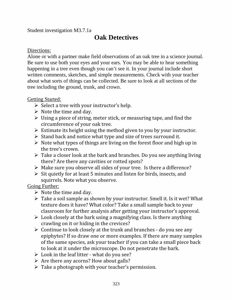
Student investigation M3.7.1a Oak Detectives

Directions: Alone or with a partner make field observations of an oak tree in a science journal. Be sure to use both your eyes and your ears. You may be able to hear something happening in a tree even though you can’t see it. In your journal include short written comments, sketches, and simple measurements. Check with your teacher about what sorts of things can be collected. Be sure to look at all sections of the tree including the ground, trunk, and crown. Getting Started: Select a tree with your instructor’s help. Note the time and day. Using a piece of string, meter stick, or measuring tape, and find the

circumference of your oak tree. Estimate its height using the method given to you by your instructor. Stand back and notice what type and size of trees surround it. Note what types of things are living on the forest floor and high up in

the tree’s crown. Take a closer look at the bark and branches. Do you see anything living

there? Are there any cavities or rotted spots? Make sure you observe all sides of your tree. Is there a difference? Sit quietly for at least 5 minutes and listen for birds, insects, and

squirrels. Note what you observe. Going Further: Note the time and day. Take a soil sample as shown by your instructor. Smell it. Is it wet? What

texture does it have? What color? Take a small sample back to your classroom for further analysis after getting your instructor’s approval.

Look closely at the bark using a magnifying class. Is there anything crawling on it or hiding in the crevices?

Continue to look closely at the trunk and branches - do you see any epiphytes? If so draw one or more examples. If there are many samples of the same species, ask your teacher if you can take a small piece back to look at it under the microscope. Do not penetrate the bark.

Look in the leaf litter - what do you see? Are there any acorns? How about galls? Take a photograph with your teacher’s permission.

323

M3.G7 Lesson 2: The Key to Hardwoods Unit Overview: Oak Woodlands Grade 7 Key Concepts:

• Unity and diversity • Growth and

development • Adaptation • Structure and function • Classification

Time: 40 - 80 minutes Materials for the Teacher: Hardwood leaf

samples for identification

Teacher reference sheet M3.7.2T

Student handout M3.7.1a

Pictures of local tree species

Colored paper or index cards for booklets (optional)

Packaging tape (optional)

Permanent pens (optional)

Connections: STEM, biodiversity, genetics, taxonomy, adaptations, botany, natural selection, photosynthesis, chemistry, population dynamics, forestry, zoology, art

Learning Objectives: Students will use a dichotomous key to identify up to 12 different hardwood species found in the North Coast. As an extension activity, they will press leaves or use cut out drawings to make an identification booklet useful in the field or for future identification needs. Background information: Refer to the appropriate section in Part II: Teacher Companion for Module 3 and plant identification books. Suggested procedure: This lesson requires you to collect leaf samples from native hardwood trees ahead of time for use in identification. How much you need to collect depends on your class size and whether students will make an identification booklet. To preserve samples longer than one day, cut branches instead of only picking leaves and place them in water. You can also press leaves or put them in a plastic bag and place them in a refrigerator. Some leaves turn color if you refrigerate them when wet. If you don’t have a site where collection is possible, then it is recommended that students identify trees using botanically accurate line drawings (see teacher reference sheet M3.7.2T). This lesson is best to do in late spring or early fall when leaves of deciduous species are fully developed and still green. Begin the lesson by asking some of the preliminary questions below to assess what students already know about local trees especially hardwoods. If you are following the forest series, students will already be familiar with local conifer identification. If not, then this lesson can be a great introduction to local tree identification. If students have no prior experience using a dichotomous key, then it is recommended that they work with a partner or within a group and that the class practices identifying one or two species together before independent practice begins. Once they are ready and you have explained some of the terminology used in identification (see key terms below), ask them what they think the word dichotomous means. They should be able to narrow it down to meaning something split in two. When using a dichotomous key they will always have two choices. They need to choose one that is the best fit and then go on to the next prompt. Once they have identified the samples you have supplied them, it is optional for them to make a booklet. An easy way to do this is to have them place leaves on pre-cut construction paper and then cover each with clear packaging tape. Once they have their leaves laid flat and covered with tape, they should write down the common and scientific name and any key characteristic(s)

324

Forest Ecology 101 integration: M1: Integrative Forest Ecology

useful in identification. Booklets can be held together with metal rings, clips, or string. Some recommended identification books to use for additional information are:

• Trees and Shrubs of California. 2001. by John Stuart and John Sawyer, illustrated by Andrea Pickart.

• Plants of the Pacific Northwest.1994. By Jim Pojar and Andry MacKinnon.

Preliminary questions: • What are some of the names of our local trees (keep asking this until you have a list of at

least 4). (If they don’t know any, try and prompt them by giving clues. During this question you may want to separate the different tree species that the group comes up with into hardwoods and softwoods.)

• Which ones (from the list) are hardwoods and which ones are softwoods or conifers? • What do scientists look for in order to tell different species apart? • Are similar characteristics evidence of a common ancestry? • Has anyone used the characteristics of leaves to identify a tree or another plant before? • How can the leaves of plants differ from one another? (hold up examples or show

examples on the screen. While doing so introduce some key terminology) • Can people make inferences about adaptations based on leaf design (morphology)? • What sorts of leaves would a tree have if it lived in a hot and dry environment? • How can knowing how to identify different tree species be useful?

Critical Thinking: What may cause a tree or shrub to have the combined characteristics of two different well known species living nearby? In other words, unknown specimen C has characteristics of known species A and known species B. Keywords: acorn, deciduous, elliptical, entire leaf margin, leaf margin, lobed leaf, serrated leaf margin, simple leaf, variable, taxonomy NGSS alignment: MS-LS2: From Molecules to Organisms LS1.A: Structure and Function LS1.B: Growth and Development of Organisms MS-LS4: Biological Evolution: Unity and Diversity LS4.A: Evidence of Common Ancestry and Diversity Online resources: Investigation the Oak Community: A curriculum guide for grades 4-8 http://www.californiaoaks.org/ExtAssets/investigating_the_oak_community.pdf This curriculum guide has a section on identifying oaks. It is published by the California Oak Foundation and is written by Kay Antúnez de Mayolo. Other great lesson ideas are presented including a reading assignment where kids read about how Native Americans influenced and used oaks.

325

(Online Resources continued) California Oaks Foundation, reference page http://www.californiaoaks.org/html/reference.html There are great links on this page to other reference material on the oaks of California. In 2012 this organization became the Oak Wildlife Foundation. They produce a poster for oaks of California and a great mini-poster depicting an oak woodland community poster, which can be purchased online. Fish and Wildlife, index to trees http://www.fs.fed.us/database/feis/plants/tree/ This site is great for more in-depth information about local tree species for purposes of student reports or expanding your existing knowledge. It is organized by the first three letters of the scientific name and includes information about distribution, ecology, and management considerations, as well as taxonomy and introductory information. EEI Connection: B.6.a. Biodiversity: The keystone of Life on Earth B.8.a. Differential Survival of Organisms B.8.b Biological Diversity: The World’s Riches B.8.d. The Isolation of Species Answers to preliminary questions: - What are some of the names of our local trees (keep asking this until you have a list of at least 4) (answers will vary - see teacher reference sheet) - Which ones (from the list) are hardwoods and which ones are softwoods or conifers? (answers will vary - you will need to organize this) - What do scientists look for in order to tell different species apart? (features unique to a particular group are often used in identification. It can be something difficult to see such as fine hairs on the underside of a leaf or something easier to see such as the shape of the leaves and the color of the bark. Today more and more genetic analyzes are used) - Are similar characteristics evidence of a common ancestry? (Similar characteristics are supportive but not conclusive evidence. Sometimes species that look similar might have a distant relationship caused by parallel evolution. Species are shaped by the environment in which they live. If two species on separate continents live in a similar habitat, they will often appear similar) - Has anyone used the characteristics of leaves to identify a tree or another plant before? (answer will vary) - How can the leaves of plants differ from one another? (hold up examples or show examples on the screen. While doing so introduce some key terminology) (answers will vary. Some characteristics include the leaf shape, color, size, and arrangement) - Can people make inferences about adaptations based on leaf design (morphology)? (Yes. Tropical trees tend to have large leaves that can collect a lot of sunlight in a shady environment. Plants in dry environments tend to have small leaves with a protective coat) - What sorts of leaves would a tree have if it lived in a hot and dry environment? (leaves tend to be reduced in size and have a waxy cuticle to reduce evaporative loss). - How can knowing how to identify different tree species be useful? (answers will vary. Plant identification is useful in gardening, forestry, health, and wildlife conservation)

326

M3.G7.L2 Unit Overview (continued) Suggested extensions:

• Have students write a short report or make a poster about a local tree species. • Use a dichotomous key to identify a different set of organisms such as butterflies, ants, or

mammalian skulls. • Have students separate leaf pigments using coffee filters and isopropyl alcohol. • Using leaves or other plant materials, have students draw what they see. • Under a microscope have students view the chloroplasts of Elodea, a common freshwater

aquarium plant. • During spring collect flowers and have students dissect them and identify the different

parts. • Visit a riparian zone. Identify the hardwoods and discuss the importance trees have to

maintaining water quality. • Have students design a tree given adaptations to a certain environment.

M3.7.2T Teacher reference sheet M3.7.2a Student handout

327

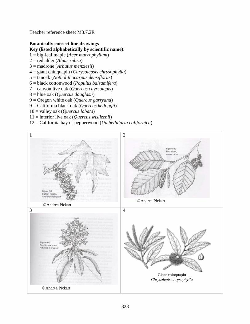
Teacher reference sheet M3.7.2R Botanically correct line drawings Key (listed alphabetically by scientific name): 1 = big-leaf maple (Acer macrophyllum) 2 = red alder (Alnus rubra) 3 = madrone (Arbutus menziesii) 4 = giant chinquapin (Chrysolepsis chrysophylla) 5 = tanoak (Notholithocarpus densiflorus) 6 = black cottonwood (Populus balsamifera) 7 = canyon live oak (Quercus chyrsolepis) 8 = blue oak (Quercus douglasii) 9 = Oregon white oak (Quercus garryana) 9 = California black oak (Quercus kelloggii) 10 = valley oak (Quercus lobata) 11 = interior live oak (Quercus wislizenii) 12 = California bay or pepperwood (Umbellularia californica) 1

Andrea Pickart

2

Andrea Pickart

3

Andrea Pickart

4

Giant chinquapin

Chrysolepis chrysophylla

328

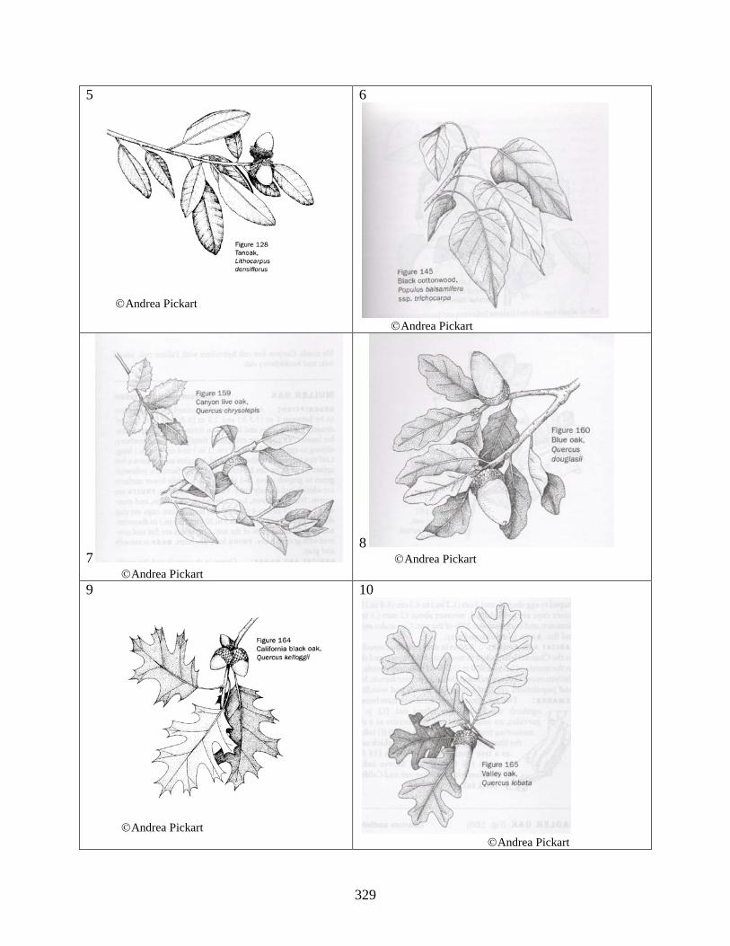
5

Andrea Pickart

6

Andrea Pickart

7 Andrea Pickart

8 Andrea Pickart

9

Andrea Pickart

10

Andrea Pickart

329

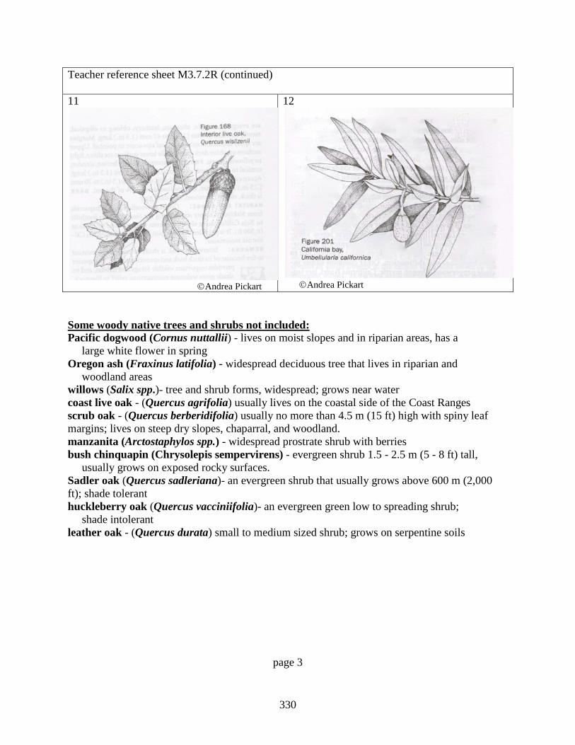
Teacher reference sheet M3.7.2R (continued) 11

Andrea Pickart

12

Andrea Pickart

Some woody native trees and shrubs not included: Pacific dogwood (Cornus nuttallii) - lives on moist slopes and in riparian areas, has a large white flower in spring Oregon ash (Fraxinus latifolia) - widespread deciduous tree that lives in riparian and woodland areas willows (Salix spp.)- tree and shrub forms, widespread; grows near water coast live oak - (Quercus agrifolia) usually lives on the coastal side of the Coast Ranges scrub oak - (Quercus berberidifolia) usually no more than 4.5 m (15 ft) high with spiny leaf margins; lives on steep dry slopes, chaparral, and woodland. manzanita (Arctostaphylos spp.) - widespread prostrate shrub with berries bush chinquapin (Chrysolepis sempervirens) - evergreen shrub 1.5 - 2.5 m (5 - 8 ft) tall, usually grows on exposed rocky surfaces. Sadler oak (Quercus sadleriana)- an evergreen shrub that usually grows above 600 m (2,000 ft); shade tolerant huckleberry oak (Quercus vacciniifolia)- an evergreen green low to spreading shrub; shade intolerant leather oak - (Quercus durata) small to medium sized shrub; grows on serpentine soils

page 3

330

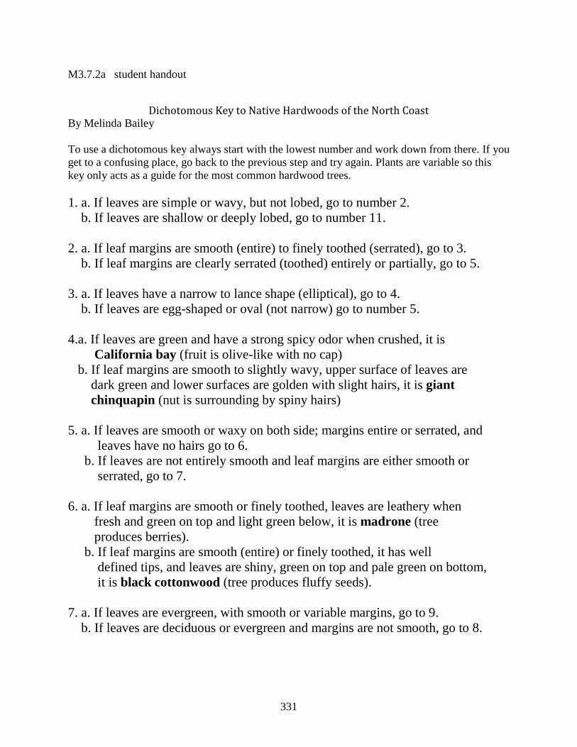
M3.7.2a student handout

Dichotomous Key to Native Hardwoods of the North Coast By Melinda Bailey To use a dichotomous key always start with the lowest number and work down from there. If you get to a confusing place, go back to the previous step and try again. Plants are variable so this key only acts as a guide for the most common hardwood trees. 1. a. If leaves are simple or wavy, but not lobed, go to number 2. b. If leaves are shallow or deeply lobed, go to number 11. 2. a. If leaf margins are smooth (entire) to finely toothed (serrated), go to 3. b. If leaf margins are clearly serrated (toothed) entirely or partially, go to 5. 3. a. If leaves have a narrow to lance shape (elliptical), go to 4. b. If leaves are egg-shaped or oval (not narrow) go to number 5. 4.a. If leaves are green and have a strong spicy odor when crushed, it is California bay (fruit is olive-like with no cap) b. If leaf margins are smooth to slightly wavy, upper surface of leaves are dark green and lower surfaces are golden with slight hairs, it is giant chinquapin (nut is surrounding by spiny hairs) 5. a. If leaves are smooth or waxy on both side; margins entire or serrated, and leaves have no hairs go to 6. b. If leaves are not entirely smooth and leaf margins are either smooth or serrated, go to 7. 6. a. If leaf margins are smooth or finely toothed, leaves are leathery when fresh and green on top and light green below, it is madrone (tree produces berries). b. If leaf margins are smooth (entire) or finely toothed, it has well defined tips, and leaves are shiny, green on top and pale green on bottom, it is black cottonwood (tree produces fluffy seeds). 7. a. If leaves are evergreen, with smooth or variable margins, go to 9. b. If leaves are deciduous or evergreen and margins are not smooth, go to 8.

331

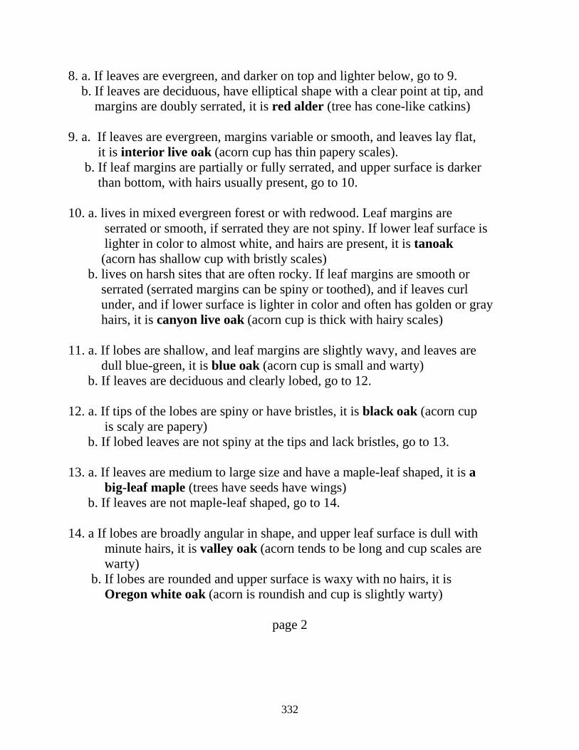
8. a. If leaves are evergreen, and darker on top and lighter below, go to 9. b. If leaves are deciduous, have elliptical shape with a clear point at tip, and margins are doubly serrated, it is red alder (tree has cone-like catkins) 9. a. If leaves are evergreen, margins variable or smooth, and leaves lay flat, it is interior live oak (acorn cup has thin papery scales). b. If leaf margins are partially or fully serrated, and upper surface is darker than bottom, with hairs usually present, go to 10. 10. a. lives in mixed evergreen forest or with redwood. Leaf margins are serrated or smooth, if serrated they are not spiny. If lower leaf surface is lighter in color to almost white, and hairs are present, it is tanoak (acorn has shallow cup with bristly scales) b. lives on harsh sites that are often rocky. If leaf margins are smooth or serrated (serrated margins can be spiny or toothed), and if leaves curl under, and if lower surface is lighter in color and often has golden or gray hairs, it is canyon live oak (acorn cup is thick with hairy scales) 11. a. If lobes are shallow, and leaf margins are slightly wavy, and leaves are dull blue-green, it is blue oak (acorn cup is small and warty) b. If leaves are deciduous and clearly lobed, go to 12. 12. a. If tips of the lobes are spiny or have bristles, it is black oak (acorn cup is scaly are papery) b. If lobed leaves are not spiny at the tips and lack bristles, go to 13. 13. a. If leaves are medium to large size and have a maple-leaf shaped, it is a big-leaf maple (trees have seeds have wings) b. If leaves are not maple-leaf shaped, go to 14. 14. a If lobes are broadly angular in shape, and upper leaf surface is dull with minute hairs, it is valley oak (acorn tends to be long and cup scales are warty) b. If lobes are rounded and upper surface is waxy with no hairs, it is Oregon white oak (acorn is roundish and cup is slightly warty)

page 2

332

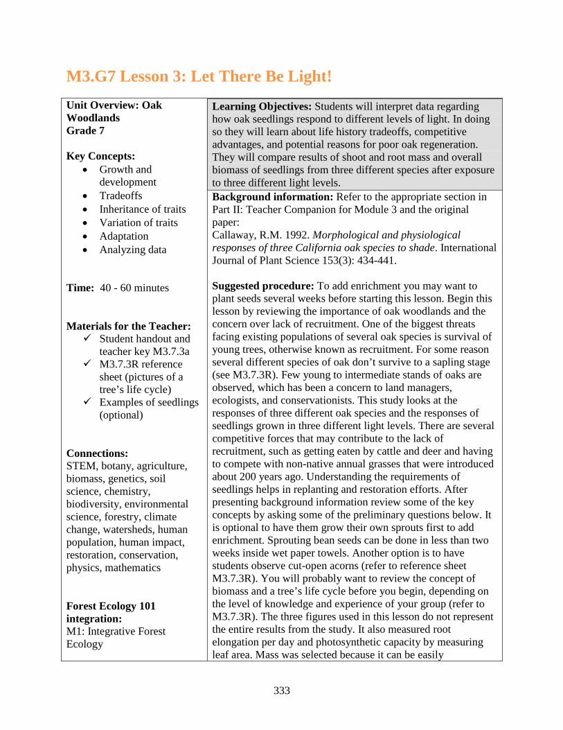
M3.G7 Lesson 3: Let There Be Light! Unit Overview: Oak Woodlands Grade 7 Key Concepts:

• Growth and development

• Tradeoffs • Inheritance of traits • Variation of traits • Adaptation • Analyzing data

Time: 40 - 60 minutes Materials for the Teacher: Student handout and

teacher key M3.7.3a M3.7.3R reference

sheet (pictures of a tree’s life cycle)

Examples of seedlings (optional)

Connections: STEM, botany, agriculture, biomass, genetics, soil science, chemistry, biodiversity, environmental science, forestry, climate change, watersheds, human population, human impact, restoration, conservation, physics, mathematics Forest Ecology 101 integration: M1: Integrative Forest Ecology

Learning Objectives: Students will interpret data regarding how oak seedlings respond to different levels of light. In doing so they will learn about life history tradeoffs, competitive advantages, and potential reasons for poor oak regeneration. They will compare results of shoot and root mass and overall biomass of seedlings from three different species after exposure to three different light levels. Background information: Refer to the appropriate section in Part II: Teacher Companion for Module 3 and the original paper: Callaway, R.M. 1992. Morphological and physiological responses of three California oak species to shade. International Journal of Plant Science 153(3): 434-441. Suggested procedure: To add enrichment you may want to plant seeds several weeks before starting this lesson. Begin this lesson by reviewing the importance of oak woodlands and the concern over lack of recruitment. One of the biggest threats facing existing populations of several oak species is survival of young trees, otherwise known as recruitment. For some reason several different species of oak don’t survive to a sapling stage (see M3.7.3R). Few young to intermediate stands of oaks are observed, which has been a concern to land managers, ecologists, and conservationists. This study looks at the responses of three different oak species and the responses of seedlings grown in three different light levels. There are several competitive forces that may contribute to the lack of recruitment, such as getting eaten by cattle and deer and having to compete with non-native annual grasses that were introduced about 200 years ago. Understanding the requirements of seedlings helps in replanting and restoration efforts. After presenting background information review some of the key concepts by asking some of the preliminary questions below. It is optional to have them grow their own sprouts first to add enrichment. Sprouting bean seeds can be done in less than two weeks inside wet paper towels. Another option is to have students observe cut-open acorns (refer to reference sheet M3.7.3R). You will probably want to review the concept of biomass and a tree’s life cycle before you begin, depending on the level of knowledge and experience of your group (refer to M3.7.3R). The three figures used in this lesson do not represent the entire results from the study. It also measured root elongation per day and photosynthetic capacity by measuring leaf area. Mass was selected because it can be easily

333

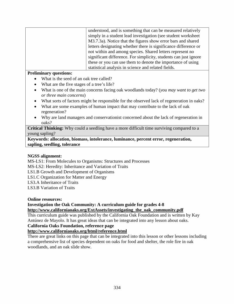
understood, and is something that can be measured relatively simply in a student lead investigation (see student worksheet M3.7.3a). Notice that the figures show error bars and shared letters designating whether there is significance difference or not within and among species. Shared letters represent no significant difference. For simplicity, students can just ignore these or you can use them to denote the importance of using statistical analysis in science and related fields.

Preliminary questions: • What is the seed of an oak tree called? • What are the five stages of a tree’s life? • What is one of the main concerns facing oak woodlands today? (you may want to get two

or three main concerns) • What sorts of factors might be responsible for the observed lack of regeneration in oaks? • What are some examples of human impact that may contribute to the lack of oak

regeneration? • Why are land managers and conservationist concerned about the lack of regeneration in

oaks? Critical Thinking: Why could a seedling have a more difficult time surviving compared to a young sapling? Keywords: allocation, biomass, intolerance, luminance, percent error, regeneration, sapling, seedling, tolerance NGSS alignment: MS-LS1: From Molecules to Organisms: Structures and Processes MS-LS2: Heredity: Inheritance and Variation of Traits LS1.B Growth and Development of Organisms LS1.C Organization for Matter and Energy LS3.A Inheritance of Traits LS3.B Variation of Traits Online resources: Investigation the Oak Community: A curriculum guide for grades 4-8 http://www.californiaoaks.org/ExtAssets/investigating_the_oak_community.pdf This curriculum guide was published by the California Oak Foundation and is written by Kay Antúnez de Mayolo. It has great ideas that can be integrated into any lesson about oaks. California Oaks Foundation, reference page http://www.californiaoaks.org/html/reference.html There are great links on this page that can be integrated into this lesson or other lessons including a comprehensive list of species dependent on oaks for food and shelter, the role fire in oak woodlands, and an oak slide show.

334

(online resources continued) UC ANR publication 21538: Living Among the Oaks: A Management Guide for Landowners and Managers. http://anrcatalog.ucdavis.edu/items/21538.aspx At this site you can download a free pdf about living among oak trees written by Douglas McCreary. It reviews the importance of oaks and how to enhance wildlife in oak habitats. In addition it gives a short overview of 10 oak species living in California. UC ANR publication 21601: Regenerating Rangeland Oaks of California http://ucanr.edu/sites/oak_range/files/59453.pdf This is a great guide to use if you want to plant acorns or oak seedlings. It explains how to best collect, store, and plant acorns and reviews some of the problems with poor regeneration in some oak species. EEI Connection: B.6.a. Biodiversity: The keystone of Life on Earth B.6.b. Ecosystem Change in California B.8.b Biological Diversity: The World’s Riches Answers to preliminary questions: - What is the seed of an oak tree called? (the seed is called an acorn) - What are the five stages of a tree’s life? (acorn - sprout or seedling- sapling - tree - snag. You can add a 6th stage - a log) - What is one of the main concerns facing oak woodlands today? (1 - there is poor regeneration in young oaks, often referred to as lack of recruitment 2 - oaks live where there are a lot of people and more areas are at risk of development 3 - S.O.D. is killing tanoaks, live oaks, and black oaks. This is a relatively new disease and is spreading.) - What sorts of factors might be responsible for the observed lack of regeneration in oaks? (possible causes for lack of recruitment include competition with annual grasses and forbs, browsing by livestock, deer, and rodents, absence of surface fires, and soil compaction) - What are some examples of human impact that may contribute to the lack of oak regeneration? (with the introduction of livestock came non-native grasses that compete with seedlings. Also livestock eat young saplings in winter when food is scarce. The biggest threat today is continued human expansion and development. California remains the fastest growing state in the union) - Why are land managers and conservationist concerned about the lack of regeneration in oaks? (oaks have a disproportionate amount of species that utilize them and are considered keystone species. They provide food, shelter, and shade for plants and animals. They protect watersheds and prevent soil erosion. Oaks provide fuel and food for people as well as recreational opportunities. They are also beautiful and increase property values)

335

M3.G7.L3 Unit Overview (continued) Suggested extensions:

• Have students perform a similar investigation by growing seedlings and then separating them into up roots, stems, and leaves and taking the dry weight of each.

• Learn about plant reproduction by having students cut open large seeds, such as acorns or lima beans, and identify the different features such as the cotyledons, epicotyl, radicle, and the seed coat.

• Plant seeds in different soils and measure their growth rate. • Compare transpiration rates between plants in the shade and plants in the sun by

collecting moisture inside plastic bags and measuring it. • Show a video about the growth of trees and/or of a deciduous forest ecosystem. • Get a classroom pet and have students record changes in its growth and development

throughout the year. • Collect, leach, and prepare acorns for eating during the fall. • Visit a local farm to observe the assortment of plants grown there.

M3.7.3a Student worksheet M3.7.3T Teacher key M3.7.3R Reference sheet

336

Student worksheet M3.7.3a Name _________________________ Date __________ Period __________

Let There Be Light!

Background: Many studies have attempted to understand the limiting factors responsible for why several different oak species are not regenerating well. Most agree that it is not just one factor responsible for this problem, but is probably a combination of factors that are involved. The inability for young trees to survive can be due to competition with grasses and other plants, being eaten by cattle and other animals, and not enough water, light, and nutrients. Human impacts and the lack of fire can also be part of the problem. Oak trees sprouts from an acorn that grows into a seedling and then into a sapling before becoming a tree. Oaks grow slowly and many can live to be over 300 years old. When they are young they are the most vulnerable. Understanding the seedling stage of an oak tree’s lifecycle, can help us understand why some aren’t surviving very well and can potentially help us find solutions to the problem. Certain species of oaks live along the coast while others live inland where it is much drier. Which ones have more tolerance for shade? Are any able to tap into more water because of a longer root? Oak trees are considered keystone species, and without them, the survival of many species could be in jeopardy. Quercus lobata or Valley Oak - this species loses its leaves in winter and is in leaf between late March and November. Acorns germinate in the fall and seedlings usually keep their leaves for at least the first year. Seedlings tend to be shade intolerant and seedlings rarely survive under shrubs. This species is the largest of all oak trees in North America. Quercus douglasii or Blue Oak - Similar to Valley Oak, this species is also deciduous and is in leaf from March until November. Seedlings are relatively shade tolerant, however the adult trees don’t like shade. Seedlings are frequently found growing in shrubs, which act as a sort of nursery. This species is drought tolerant and is known to grow in very hot and dry places. Quercus agrifolia or Coast Live Oak - this species lives along the coast of California and is evergreen. It can grow in chaparral, which receives a lot of sun and in mixed forest, which are relatively shady. When young it is probably shade

337

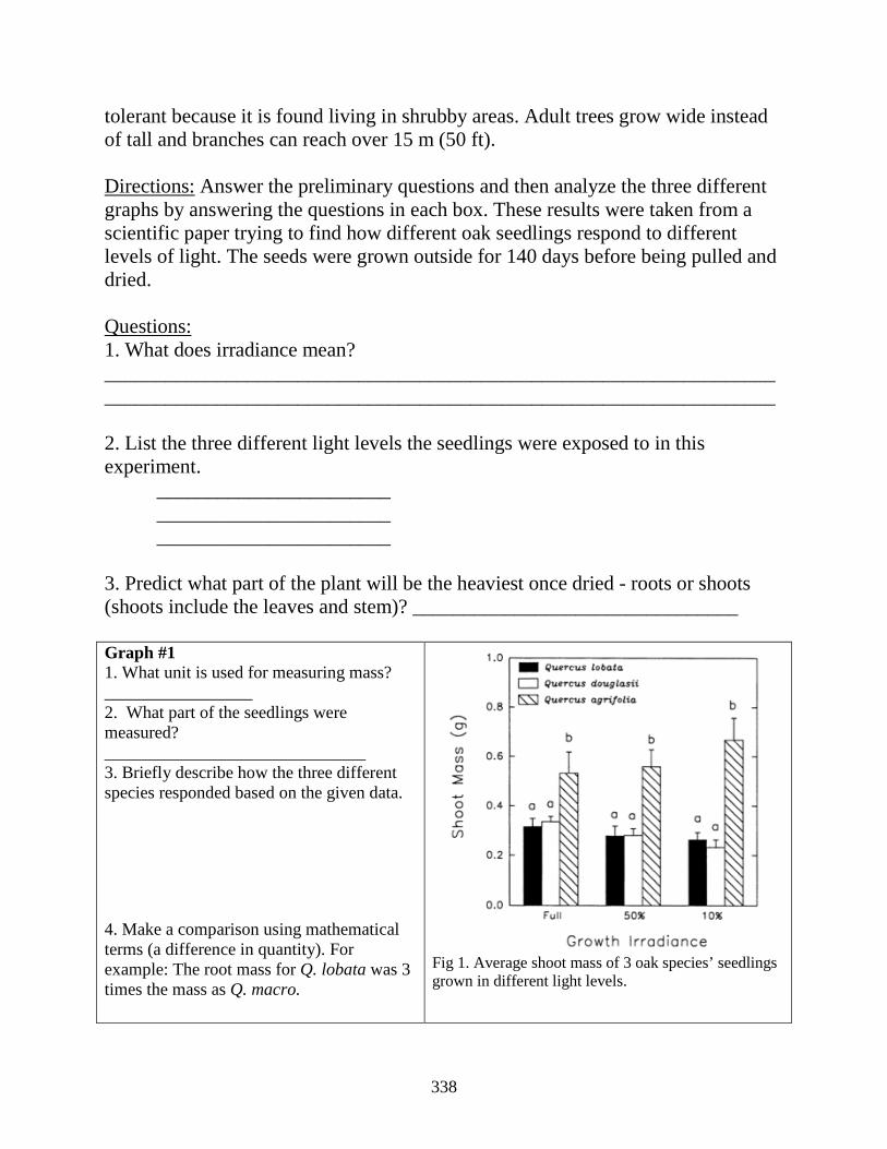
tolerant because it is found living in shrubby areas. Adult trees grow wide instead of tall and branches can reach over 15 m (50 ft). Directions: Answer the preliminary questions and then analyze the three different graphs by answering the questions in each box. These results were taken from a scientific paper trying to find how different oak seedlings respond to different levels of light. The seeds were grown outside for 140 days before being pulled and dried. Questions: 1. What does irradiance mean? __________________________________________________________________ __________________________________________________________________ 2. List the three different light levels the seedlings were exposed to in this experiment. _______________________ _______________________ _______________________ 3. Predict what part of the plant will be the heaviest once dried - roots or shoots (shoots include the leaves and stem)? ________________________________ Graph #1 1. What unit is used for measuring mass? _________________ 2. What part of the seedlings were measured? ______________________________ 3. Briefly describe how the three different species responded based on the given data. 4. Make a comparison using mathematical terms (a difference in quantity). For example: The root mass for Q. lobata was 3 times the mass as Q. macro.

Fig 1. Average shoot mass of 3 oak species’ seedlings grown in different light levels.

338

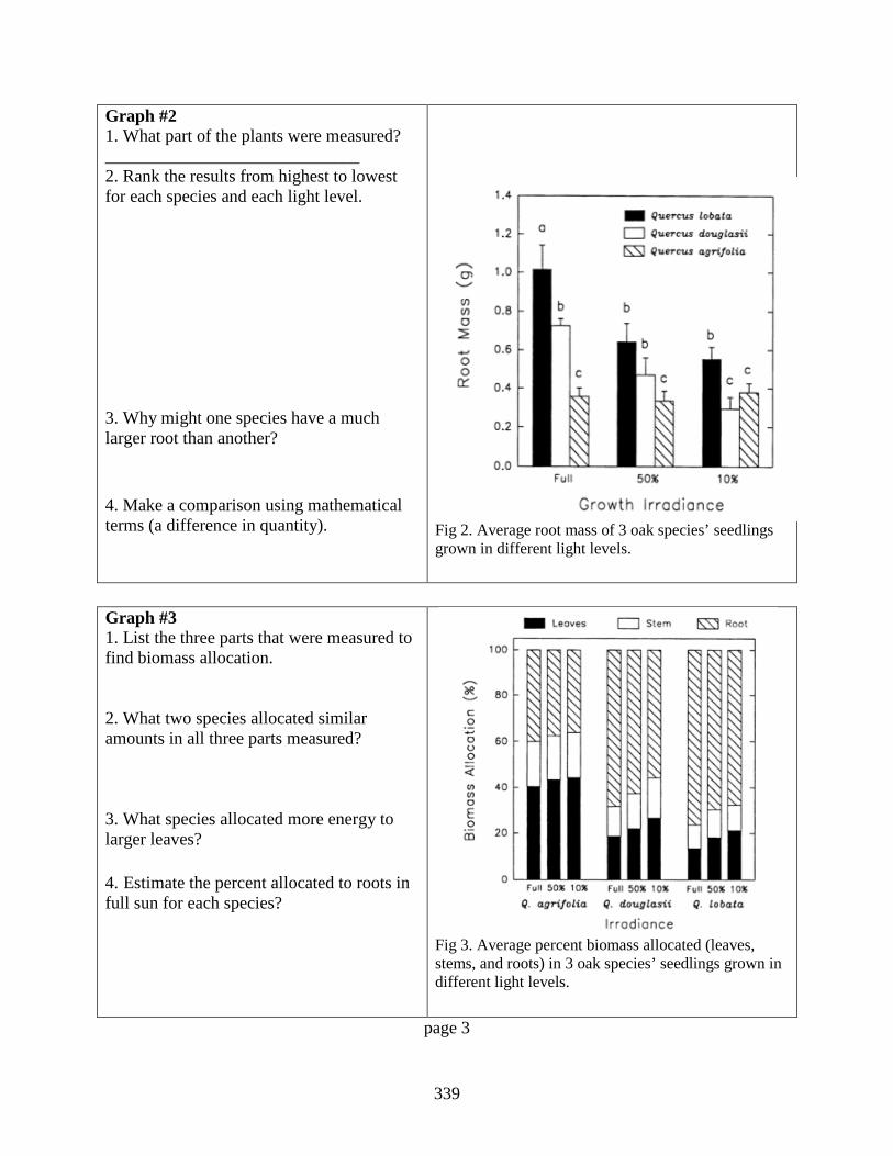
Graph #2 1. What part of the plants were measured? _____________________________ 2. Rank the results from highest to lowest for each species and each light level. 3. Why might one species have a much larger root than another? 4. Make a comparison using mathematical terms (a difference in quantity).

Fig 2. Average root mass of 3 oak species’ seedlings grown in different light levels.

Graph #3 1. List the three parts that were measured to find biomass allocation. 2. What two species allocated similar amounts in all three parts measured? 3. What species allocated more energy to larger leaves? 4. Estimate the percent allocated to roots in full sun for each species?

Fig 3. Average percent biomass allocated (leaves, stems, and roots) in 3 oak species’ seedlings grown in different light levels.

page 3

339

Conclusion: 1. Write a conclusion for each species. Include quantitative data regarding roots and shoots. ____________________________________________________________________________________________________________________________________ 2. What advantage does a species have that allocates a high amount of energy to a well-developed taproot? 3. What advantage does a species have that allocates a high amount of energy to large leaves? 4. Besides environmental factors, what governs how a plant will grow within a particular habitat?

page 4

340

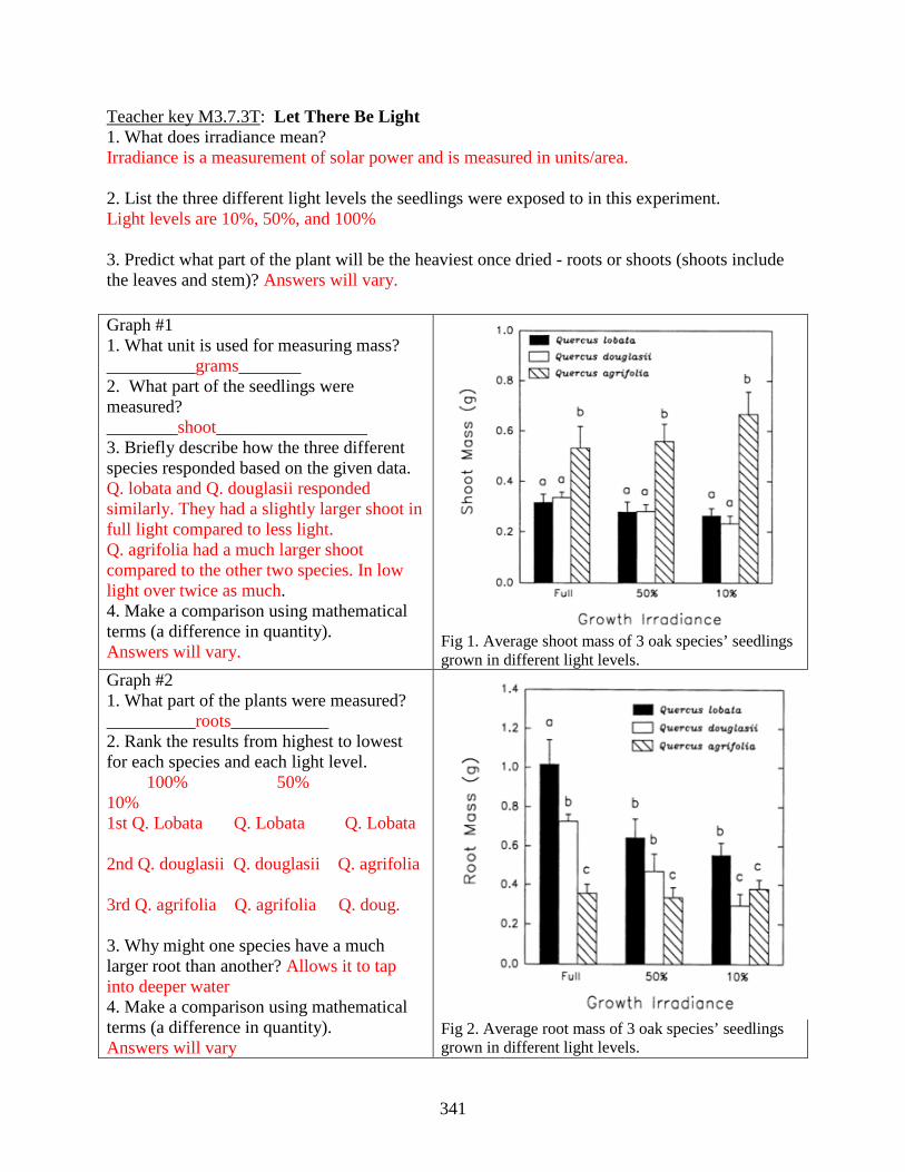
Teacher key M3.7.3T: Let There Be Light 1. What does irradiance mean? Irradiance is a measurement of solar power and is measured in units/area. 2. List the three different light levels the seedlings were exposed to in this experiment. Light levels are 10%, 50%, and 100% 3. Predict what part of the plant will be the heaviest once dried - roots or shoots (shoots include the leaves and stem)? Answers will vary. Graph #1 1. What unit is used for measuring mass? __________grams_______ 2. What part of the seedlings were measured? ________shoot_________________ 3. Briefly describe how the three different species responded based on the given data. Q. lobata and Q. douglasii responded similarly. They had a slightly larger shoot in full light compared to less light. Q. agrifolia had a much larger shoot compared to the other two species. In low light over twice as much. 4. Make a comparison using mathematical terms (a difference in quantity). Answers will vary.

Fig 1. Average shoot mass of 3 oak species’ seedlings grown in different light levels.

Graph #2 1. What part of the plants were measured? __________roots___________ 2. Rank the results from highest to lowest for each species and each light level. 100% 50% 10% 1st Q. Lobata Q. Lobata Q. Lobata 2nd Q. douglasii Q. douglasii Q. agrifolia 3rd Q. agrifolia Q. agrifolia Q. doug. 3. Why might one species have a much larger root than another? Allows it to tap into deeper water 4. Make a comparison using mathematical terms (a difference in quantity). Answers will vary

Fig 2. Average root mass of 3 oak species’ seedlings grown in different light levels.

341

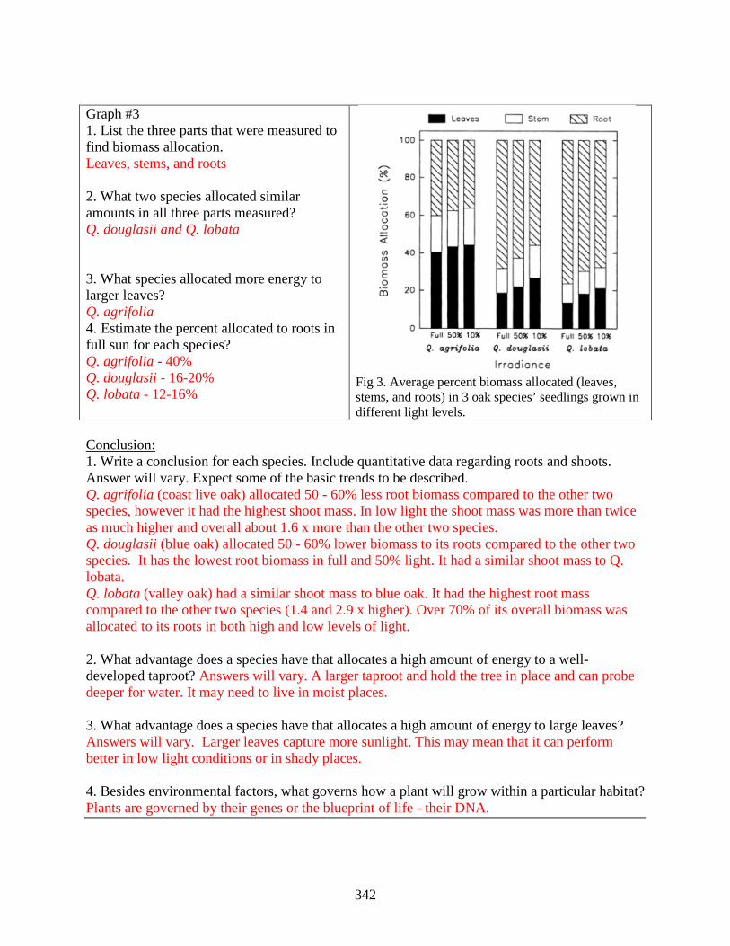
Graph #3 1. List the three parts that were measured to find biomass allocation. Leaves, stems, and roots 2. What two species allocated similar amounts in all three parts measured? Q. douglasii and Q. lobata 3. What species allocated more energy to larger leaves? Q. agrifolia 4. Estimate the percent allocated to roots in full sun for each species? Q. agrifolia - 40% Q. douglasii - 16-20% Q. lobata - 12-16%

Fig 3. Average percent biomass allocated (leaves, stems, and roots) in 3 oak species’ seedlings grown in different light levels.

Conclusion: 1. Write a conclusion for each species. Include quantitative data regarding roots and shoots. Answer will vary. Expect some of the basic trends to be described. Q. agrifolia (coast live oak) allocated 50 - 60% less root biomass compared to the other two species, however it had the highest shoot mass. In low light the shoot mass was more than twice as much higher and overall about 1.6 x more than the other two species. Q. douglasii (blue oak) allocated 50 - 60% lower biomass to its roots compared to the other two species. It has the lowest root biomass in full and 50% light. It had a similar shoot mass to Q. lobata. Q. lobata (valley oak) had a similar shoot mass to blue oak. It had the highest root mass compared to the other two species (1.4 and 2.9 x higher). Over 70% of its overall biomass was allocated to its roots in both high and low levels of light. 2. What advantage does a species have that allocates a high amount of energy to a well-developed taproot? Answers will vary. A larger taproot and hold the tree in place and can probe deeper for water. It may need to live in moist places. 3. What advantage does a species have that allocates a high amount of energy to large leaves? Answers will vary. Larger leaves capture more sunlight. This may mean that it can perform better in low light conditions or in shady places. 4. Besides environmental factors, what governs how a plant will grow within a particular habitat? Plants are governed by their genes or the blueprint of life - their DNA.

342

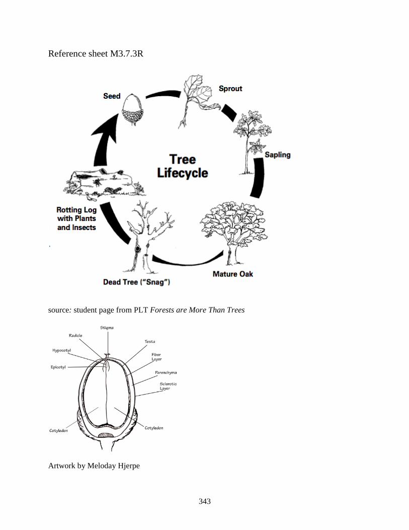
Reference sheet M3.7.3R

source: student page from PLT Forests are More Than Trees

Artwork by Meloday Hjerpe

343

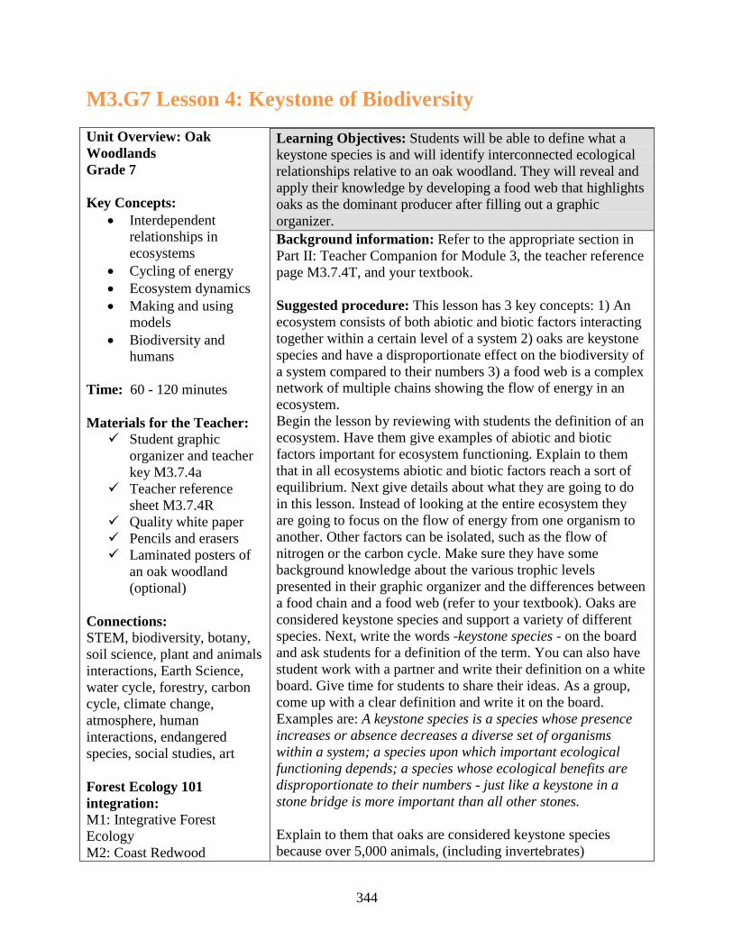
M3.G7 Lesson 4: Keystone of Biodiversity Unit Overview: Oak Woodlands Grade 7 Key Concepts:

• Interdependent relationships in ecosystems

• Cycling of energy • Ecosystem dynamics • Making and using

models • Biodiversity and

humans Time: 60 - 120 minutes Materials for the Teacher: Student graphic

organizer and teacher key M3.7.4a

Teacher reference sheet M3.7.4R

Quality white paper Pencils and erasers Laminated posters of

an oak woodland (optional)

Connections: STEM, biodiversity, botany, soil science, plant and animals interactions, Earth Science, water cycle, forestry, carbon cycle, climate change, atmosphere, human interactions, endangered species, social studies, art Forest Ecology 101 integration: M1: Integrative Forest Ecology M2: Coast Redwood

Learning Objectives: Students will be able to define what a keystone species is and will identify interconnected ecological relationships relative to an oak woodland. They will reveal and apply their knowledge by developing a food web that highlights oaks as the dominant producer after filling out a graphic organizer. Background information: Refer to the appropriate section in Part II: Teacher Companion for Module 3, the teacher reference page M3.7.4T, and your textbook. Suggested procedure: This lesson has 3 key concepts: 1) An ecosystem consists of both abiotic and biotic factors interacting together within a certain level of a system 2) oaks are keystone species and have a disproportionate effect on the biodiversity of a system compared to their numbers 3) a food web is a complex network of multiple chains showing the flow of energy in an ecosystem. Begin the lesson by reviewing with students the definition of an ecosystem. Have them give examples of abiotic and biotic factors important for ecosystem functioning. Explain to them that in all ecosystems abiotic and biotic factors reach a sort of equilibrium. Next give details about what they are going to do in this lesson. Instead of looking at the entire ecosystem they are going to focus on the flow of energy from one organism to another. Other factors can be isolated, such as the flow of nitrogen or the carbon cycle. Make sure they have some background knowledge about the various trophic levels presented in their graphic organizer and the differences between a food chain and a food web (refer to your textbook). Oaks are considered keystone species and support a variety of different species. Next, write the words -keystone species - on the board and ask students for a definition of the term. You can also have student work with a partner and write their definition on a white board. Give time for students to share their ideas. As a group, come up with a clear definition and write it on the board. Examples are: A keystone species is a species whose presence increases or absence decreases a diverse set of organisms within a system; a species upon which important ecological functioning depends; a species whose ecological benefits are disproportionate to their numbers - just like a keystone in a stone bridge is more important than all other stones. Explain to them that oaks are considered keystone species because over 5,000 animals, (including invertebrates)

344

M3.G7.L4 Unit Overview (continued) depend on oak habitats - not counting non-animal life such as mosses, lichens, protists, and fungi. The primary purpose of this lesson is for students to be familiar enough with an oak woodland that they can draw a food web that incorporates organisms at different trophic levels using oaks as the primary producer. Depending on their present level of knowledge you may want to show examples of organisms (see teacher reference sheet M3.7.4T). If you show your own collection of organisms, be sure to include beetles, ants, moths, and other insects because they are primary food for many of the more familiar animals we associate oaks with, such as birds, raccoons and deer. Once students have enough background information, have them fill out the graphic organizer (see M3.7.4a). Once they are done, have them draw a high-quality, well-organized food web on good paper. Several options are given in the teacher reference sheet. Arrows depict the flow of energy and point towards the organism at the higher trophic level (see M3.7.4T). This activity can be simplified several ways. Students can draw a food chain instead of a food web or if necessary, they can omit the tertiary level. Food webs are much more complex than food chains. Critical Thinking: Oak trees often live in urban areas. What sorts of problems might exist for oak trees living in an urban area compared to a rural area? Keywords: abiotic, biotic, consumer, decomposer, ecosystem, food web, keystone species, predator, producer, trophic level NGSS alignment: MS-LS2: Ecosystems: Interactions, Energy, and Dynamics LS2.A Interdependent Relationships in Ecosystems LS2.B Cycle of Matter and Energy Transfer in Ecosystems LS2.C Ecosystem Dynamics, Functioning, and Resilience LS4.D Biodiversity and Humans Online resources: Oak Woodland Wildlife, UCANR website http://ucanr.edu/sites/oak_range/Woodland_Wildlife/ This site has several links to available resources including lists of wildlife species living in oak woodlands. For more in-depth information regarding the future of oaks in California seek out the link to the Oaks 2040 publication available here. Exploring Nature: Deciduous Forest Food Web Activity http://www.exploringnature.org/db/detail.php?dbID=2&detID=3456 If your students need an introductory level activity this is a good one. This link provides a student worksheet that can also be used as an assessment tool. Oak Woodlands: Who’s Eating Whom? By Vera Strader http://ucanr.org/sites/Tuolumne_County_Master_Gardeners/files/137482.pdf This is a well-written and passionate two-page essay about the importance of oak woodlands in the foothills of the Sierra Nevada. It can be read to the class as an introduction to this lesson. Crash Course on Ecosystems: Links in the Chain, Episode #7 (video) https://www.youtube.com/watch?v=v6ubvEJ3KGM A fast moving video that reviews what an ecosystem is and how energy and materials move through it. It introduces similar vocabulary used on the student graphic organizer.

345

EEI Connection: B.6.a. Biodiversity: The Keystone of Life on Earth B.6.b. Ecosystem Change in California B.8.b Biological Diversity: The World’s Riches Suggested extensions:

• Haves students investigate another example of a keystone species such as the role sea otters have along the California coast.

• Use the size of selected oak trees to estimate carbon storage. • Show the Planet Earth episode (video) on deciduous forests of the world. • Dissect owl pellets and estimate the energy accumulation of an owl for a day, a week, and

a year. • Have students keep records of their daily food intake to find out how many calories they

consume. Easy to use calorie counters are available online. • Discuss the issues surrounding introduced species and how they can alter ecosystem

dynamics. • Learn about focal bird species important to the oak woodlands of California. Great

information is available through California Partners in Flight (CalPIF). • Visit an oak woodland and conduct certain field studies or have students write in nature

journals. M3.7.4a Student graphic organizer M3.7.4T Teacher key M3.7.4R Teacher reference sheet

346

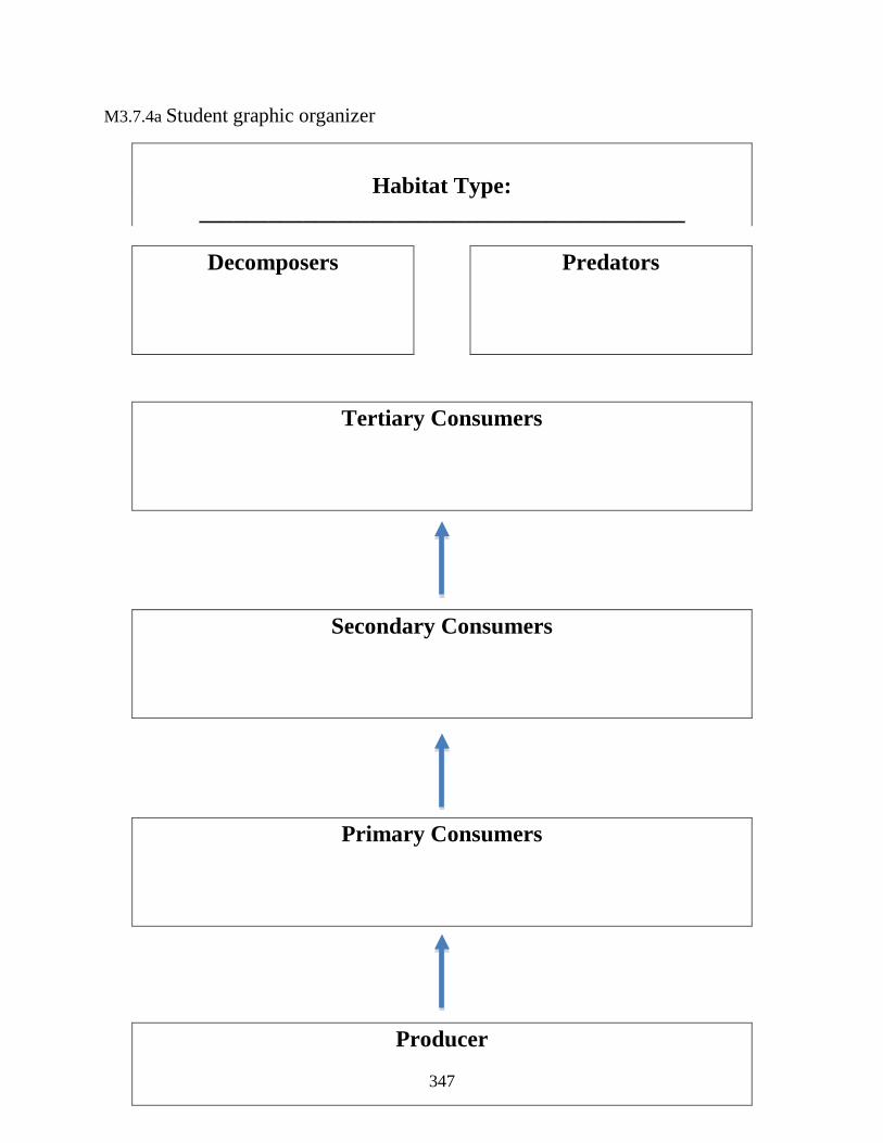
M3.7.4a Student graphic organizer

Habitat Type:

__________________________________________

Secondary Consumers

Tertiary Consumers

Predators Decomposers

Primary Consumers

Producer

347

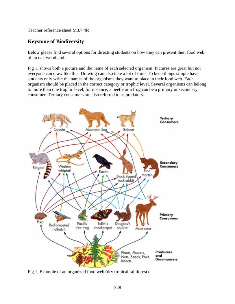
Teacher reference sheet M3.7.4R Keystone of Biodiversity Below please find several options for directing students on how they can present their food web of an oak woodland. Fig 1. shows both a picture and the name of each selected organism. Pictures are great but not everyone can draw like this. Drawing can also take a lot of time. To keep things simple have students only write the names of the organisms they want to place in their food web. Each organism should be placed in the correct category or trophic level. Several organisms can belong to more than one trophic level, for instance, a beetle or a frog can be a primary or secondary consumer. Tertiary consumers are also referred to as predators.

Fig 1. Example of an organized food web (dry tropical rainforest).

348

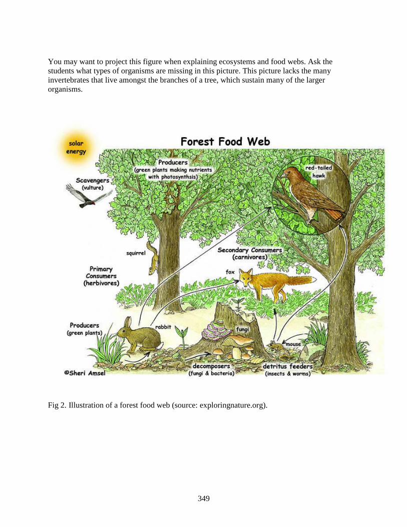
You may want to project this figure when explaining ecosystems and food webs. Ask the students what types of organisms are missing in this picture. This picture lacks the many invertebrates that live amongst the branches of a tree, which sustain many of the larger organisms.

Fig 2. Illustration of a forest food web (source: exploringnature.org).

349

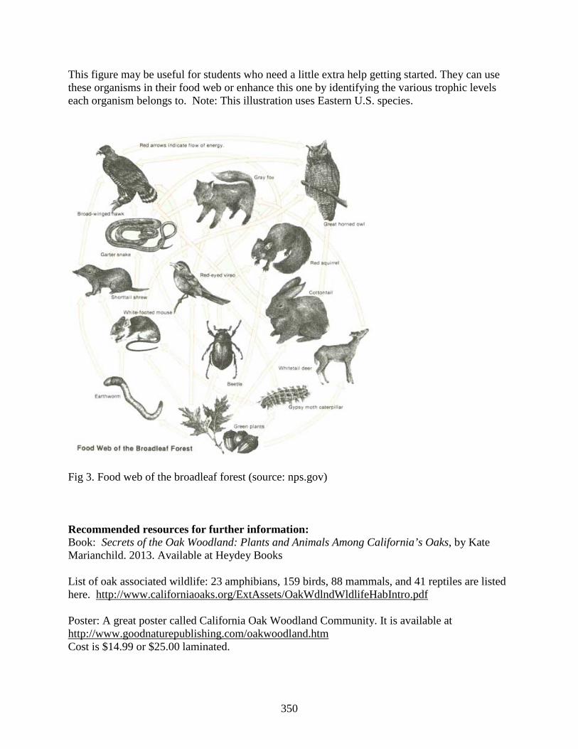
This figure may be useful for students who need a little extra help getting started. They can use these organisms in their food web or enhance this one by identifying the various trophic levels each organism belongs to. Note: This illustration uses Eastern U.S. species.

Fig 3. Food web of the broadleaf forest (source: nps.gov) Recommended resources for further information: Book: Secrets of the Oak Woodland: Plants and Animals Among California’s Oaks, by Kate Marianchild. 2013. Available at Heydey Books List of oak associated wildlife: 23 amphibians, 159 birds, 88 mammals, and 41 reptiles are listed here. http://www.californiaoaks.org/ExtAssets/OakWdlndWldlifeHabIntro.pdf Poster: A great poster called California Oak Woodland Community. It is available at http://www.goodnaturepublishing.com/oakwoodland.htm Cost is $14.99 or $25.00 laminated.

350

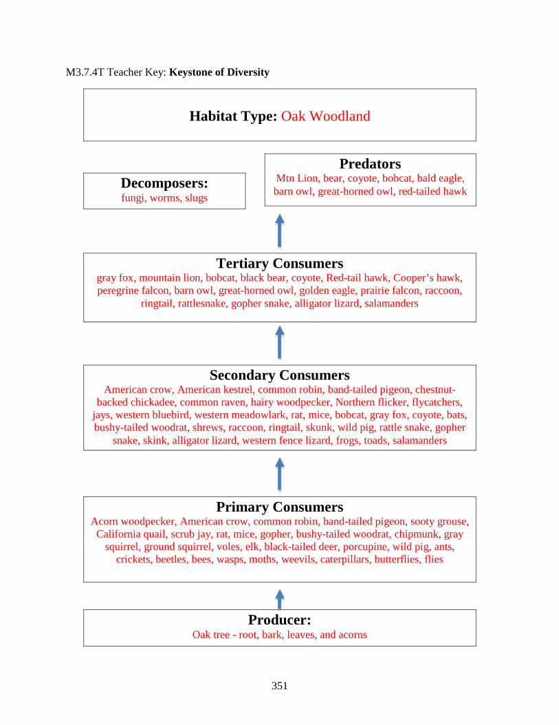
M3.7.4T Teacher Key: Keystone of Diversity

Habitat Type: Oak Woodland

Primary Consumers Acorn woodpecker, American crow, common robin, band-tailed pigeon, sooty grouse,

California quail, scrub jay, rat, mice, gopher, bushy-tailed woodrat, chipmunk, gray squirrel, ground squirrel, voles, elk, black-tailed deer, porcupine, wild pig, ants,

crickets, beetles, bees, wasps, moths, weevils, caterpillars, butterflies, flies

Producer: Oak tree - root, bark, leaves, and acorns

Secondary Consumers American crow, American kestrel, common robin, band-tailed pigeon, chestnut-

backed chickadee, common raven, hairy woodpecker, Northern flicker, flycatchers, jays, western bluebird, western meadowlark, rat, mice, bobcat, gray fox, coyote, bats, bushy-tailed woodrat, shrews, raccoon, ringtail, skunk, wild pig, rattle snake, gopher

snake, skink, alligator lizard, western fence lizard, frogs, toads, salamanders

Tertiary Consumers gray fox, mountain lion, bobcat, black bear, coyote, Red-tail hawk, Cooper’s hawk, peregrine falcon, barn owl, great-horned owl, golden eagle, prairie falcon, raccoon,

ringtail, rattlesnake, gopher snake, alligator lizard, salamanders

Decomposers: fungi, worms, slugs

Predators Mtn Lion, bear, coyote, bobcat, bald eagle, barn owl, great-horned owl, red-tailed hawk

351

M3.G7 Lesson 5: Trees in Trouble Unit Overview: Oak Woodlands Grade 7 Key Concepts:

• Stability and change • Cause and effect • Transmission of

pathogens • Natural selection • Adaptation • Independent

relationships within an ecosystem

Time: 60 - 120 minutes Materials for the Teacher: Student worksheet

M3.7.5a Teacher key M3.7.5T Access to computers Colored pencils Pictures of infected

trees (optional) Connections: STEM, health, microbiology, forest health, non-native species, agriculture, geography, botany, fire ecology, forestry, carbon cycle, biomass, climate change, soils, human impact, social studies, careers Forest Ecology 101 integration: M1: Integrative Forest Ecology M3: Coast Redwood

Learning Objectives: After an online investigation students will learn about Sudden Oak Death (SOD) and will be able to identify the pathogen, symptoms, and vectors of this disease. They will also be able to describe some of the precautions people can take to limit the spread of this oak tree disease. Background information: Refer to the appropriate section in Part II: Teacher Companion for Module 3 and online information. Suggested procedure: By now students should be familiar with oak trees and a woodland habitat. In this lesson they will research the cause and effects of Sudden Oak Death (SOD) and steps that can be taken to decrease its spread. It is thought to have been accidently brought into northern California through the shipment of rhododendrons from Europe, a common nursery plant. Since its first discovery in 1995 in Marin County, it has spread to over fourteen other counties including Sonoma, Mendocino, and Humboldt. It causes foliar damage to over one hundred native plants and can be fatal to five different oak species. One of the largest vectors of this disease is California bay and it is most fatal to tanoak. In places with the largest infestations it is changing the forest community structure and building up fuel loads. Begin this lesson by asking some of the preliminary questions below to prepare students for their short research project. You may want to begin by introducing the name of the disease and the name of the pathogen Phytophthora ramorum. Write it on the board and have them all say it together. It is pronounced - Fi-TOFF-thor-ra ra-MOR-um. During online research they should fill out student worksheet M3.7.5a. Before they begin you will need to give them clear instructions about how to conduct their research and whether research will be done at school or at home. Once they have filled out the questions and colored in the map, collect or check the worksheet and make sure they are filling in the answers correctly. You may need to steer them to certain links to save time. The best website to use is www.suddenoakdeath.org (see online resources). Once they are through, check for their understanding by asking them how the disease is spread and what symptoms to look for (see suggested follow-up questions). The entire disease cycle in still not fully understood and there is no known cure at this time.

352

Preliminary questions: • Has anyone heard of Sudden Oak Death (SOD)? • Are all oak trees susceptible to this disease? • How is this disease spread? • Where did it come from? • What is a person who studies diseases called?

Use these preliminary questions as a pathway into preparing them for their research. Their quest is to find the answers to these questions and more. When checking for understanding you may want to address natural selection and how some trees are apt to have a stronger resistance to the disease. Critical Thinking: Are some diseases harder to control than others? If so, which ones would be the most difficult to control? Keywords: canker, fatal, foliar, host, pathogen, pathologist, symptom, water mold NGSS alignment: MS-LS2: Ecosystems: Interactions, Energy, and Dynamics LS2.C Ecosystem Dynamics, Functioning, and Resilience ETS1.B Developing Possible Solutions MS-LS4: Biological Functioning: Unity and Diversity LS4.B Natural Selection LS4.C Adaptation Online resources: The official site of Sudden Oak Death (SOD) http://www.suddenoakdeath.org/ This website is probably the best to use for student research. It has many links to information that can get technical so it would be best for you to navigate through the site first in order to steer students to the correct places. Good general information is present on the FAQ page and information for a homeowner. You can also go to Oak Mapper for information regarding where it resides. A guide to SOD is available here in Spanish as well. Sudden Oak Death and Related Diseases http://www.plantmanagementnetwork.org/php/shared/sod/ The information here is too complex for most students, however it shows great pictures of the cankers and gives in-depth information useful for further research. UC Extension: SOD Environmental Program Lesson Plan http://cemarin.ucdavis.edu/files/56664.pdf This link takes you directly to a series of activities entitled Can My Tree Catch the Flu? It cleverly informs students how certain diseases can be transmitted and encourages the use of visuals such as a video of a person sneezing. Many different activities are presented including one where they use glow in the dark lotion to show how easily infections can be spread and the use of fresh and salt water spray on black paper.

353

(Online Resources continued) Sudden Oak Death Activity Guide: http://www.suddenoakdeath.org/pdf/KidsActivityGuide.pdf Simple word searches and other activities are given here to educate kids about SOD. It is a little out of date and may be more appropriate to use for more remedial classes or younger grades. EEI Connection: B.8.a Differential Survival of Organisms Answers to preliminary questions: - Has anyone heard of Sudden Oak Death (SOD)? (answers will vary) - Are all oak trees susceptible to this disease? (No - those in the red oak or black oak family are the most susceptible. Other trees can also become infected but it is rarely fatal) - How is this disease spread? (Tell them this is for them to find out - refer to teacher key) - Where did it come from? (Tell them this is for them to find out - refer to teacher key) - What is a person who studies diseases called? (a pathologist) Suggested follow-up questions:

• Does SOD infect all oak trees? • Is SOD in our area? • What oak tree is the most at risk? • What tree is a predictor for the disease? • What symptoms do trees get? • Can SOD be cured? • Do some trees have a higher resistance to SOD? • How can people help reduce the spread of SOD? • What ecological problems might this disease cause?

Suggested extensions:

• Learn about other introduced fatal plant diseases and infections such as Port-Orford-Root disease and Dutch elm disease.

• Introduce students to living with the fire and the fire triangle and discuss which one SOD is changing.

• Be Tree-tectives and assess the health of trees on campus or leaves from trees you have collected (see PLT lesson Trees in Trouble).

• Have students research the cause and effect of a human disease. • Explore the different ways seeds and/or spores can travel. • Observe plant spores under the microscope. • Remove invasive plants such as English ivy or broom from a natural area.

M3.7.5a Student worksheet M3.7.5aT Teacher key

354

Student worksheet M3.7.5a Name ________________________ Date ___________ Period ________

Trees in Trouble While researching Sudden Oak Death (SOD), answer the questions below. Go to the website: suddenoakdeath.org WHAT IS SOD? 1. Name of the pathogen ________________________________________ 2. What group of pathogens does this species belong to? ____________________ 3. Briefly describe SOD. WHERE DID IT COME FROM? 4. Is SOD a native or introduced disease? 5. Where and when did the disease begin to impact the west coast of the United States? HOW IS IT SPREAD? 6. How is the disease spread? 7. The complete life cycle of P. ramorum is unknown. Watch the short video on a sporangia releasing zoospores and either describe what happens or draw a picture. Label your picture. 8. During what time of year do the spores spread? _____________________________

355

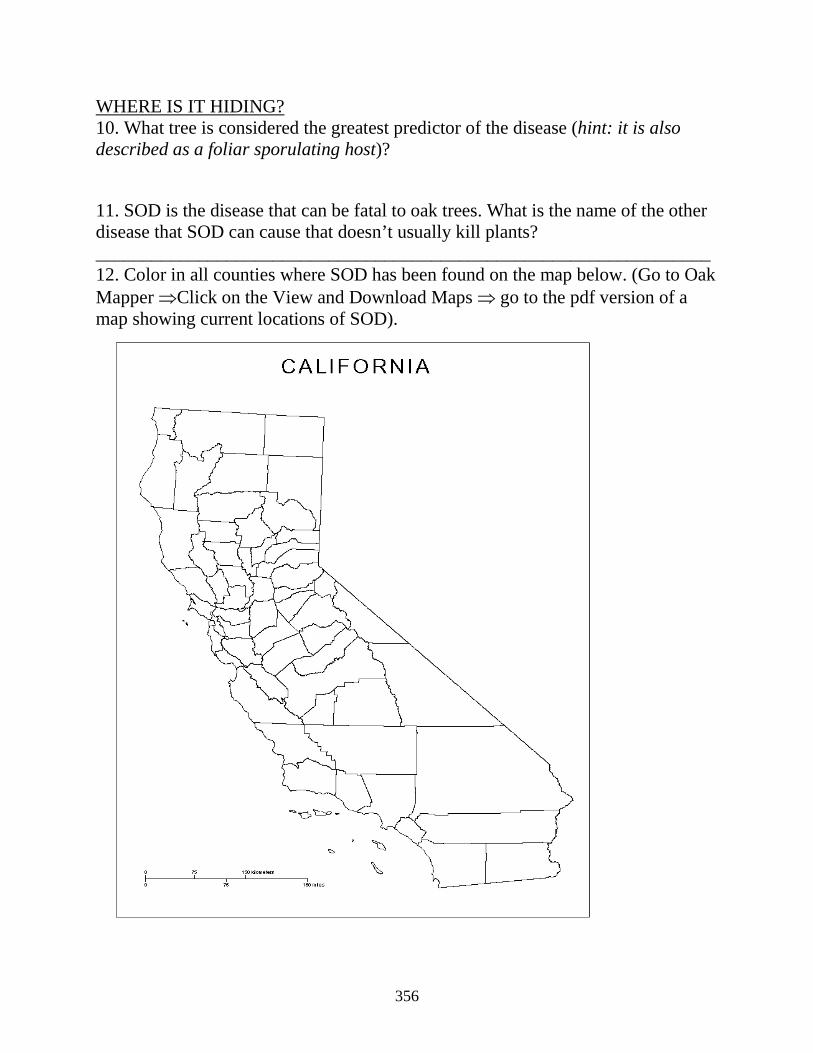
WHERE IS IT HIDING? 10. What tree is considered the greatest predictor of the disease (hint: it is also described as a foliar sporulating host)? 11. SOD is the disease that can be fatal to oak trees. What is the name of the other disease that SOD can cause that doesn’t usually kill plants? __________________________________________________________________ 12. Color in all counties where SOD has been found on the map below. (Go to Oak Mapper ⇒Click on the View and Download Maps ⇒ go to the pdf version of a map showing current locations of SOD).

356

IS SOD FATAL? 13. Can SOD kill trees? 14. List 5 tree species (oaks) threatened by SOD. WHAT ARE THE SYMPTOMS? 15. What are some common symptoms of this disease? 16. List steps to diagnosis whether a tree has the disease or not. IS YOUR TREE SICK? 17. List three things that increase the chances (probability) that your tree is infected. HOW CAN WE REDUCE THE SPREAD? 18. List at least three ways people can help reduce the spread of SOD.

page 3

357

Teacher Key: G7.5T: Trees in Trouble Note: The answers to these questions are sourced from suddenoakdeath.org and the links found there. WHAT IS SOD? 1. Name of the pathogen - Phytophthora ramorum pronounced - Fi-TOFF-thor-ra ra-MOR-um 2. What group of pathogens does this species belong to? Water molds (link: About the pathogen) 3. Briefly describe SOD. SOD is a forest disease caused by the pathogen P. ramorum. It infects susceptible trees such as tanoak and can cause foliar/twig disease in other plants. WHERE DID IT COME FROM? 4. Is SOD a native or introduced disease? Introduced 5. Where and when did the disease begin to impact the west coast of the United States? It was discovered in 2001 but did not begin to impact the nursery business until 2004. It was discovered in Marin County. HOW IS IT SPREAD? 6. How is the disease spread? (About the Pathogen) The pathogen releases spores in moist humid conditions. The inoculum can be spread through wind-driven rain, water, plant material, and human activities such as driving, hiking, and pets. 7. The complete life cycle of P. ramorum is unknown. Watch a short video on a sporangia releasing zoospores and either describe what happens or draw a picture. Label your picture. (link: About the Pathogen) A sporangia which looks like a little capsule, releases round zoospores in water. 8. During what time of year do the spores spread? In the wet season - spring WHERE IS IT HIDING? 9. Give the name of five host plants (not oaks). Note: there are over 100. The most commonly referred to ones are: California bay, Douglas fir, coast redwood, rhododendron, and madrone. 10. What tree is considered the greatest predictor of the disease (hint: it is also described as a foliar sporulating host)? California bay or laurel 11. SOD is the disease that can be fatal to oak trees. What is the name of the other disease that SOD can cause that doesn’t usually kill plants? Ramorum blight or Foliar/twig disease

358

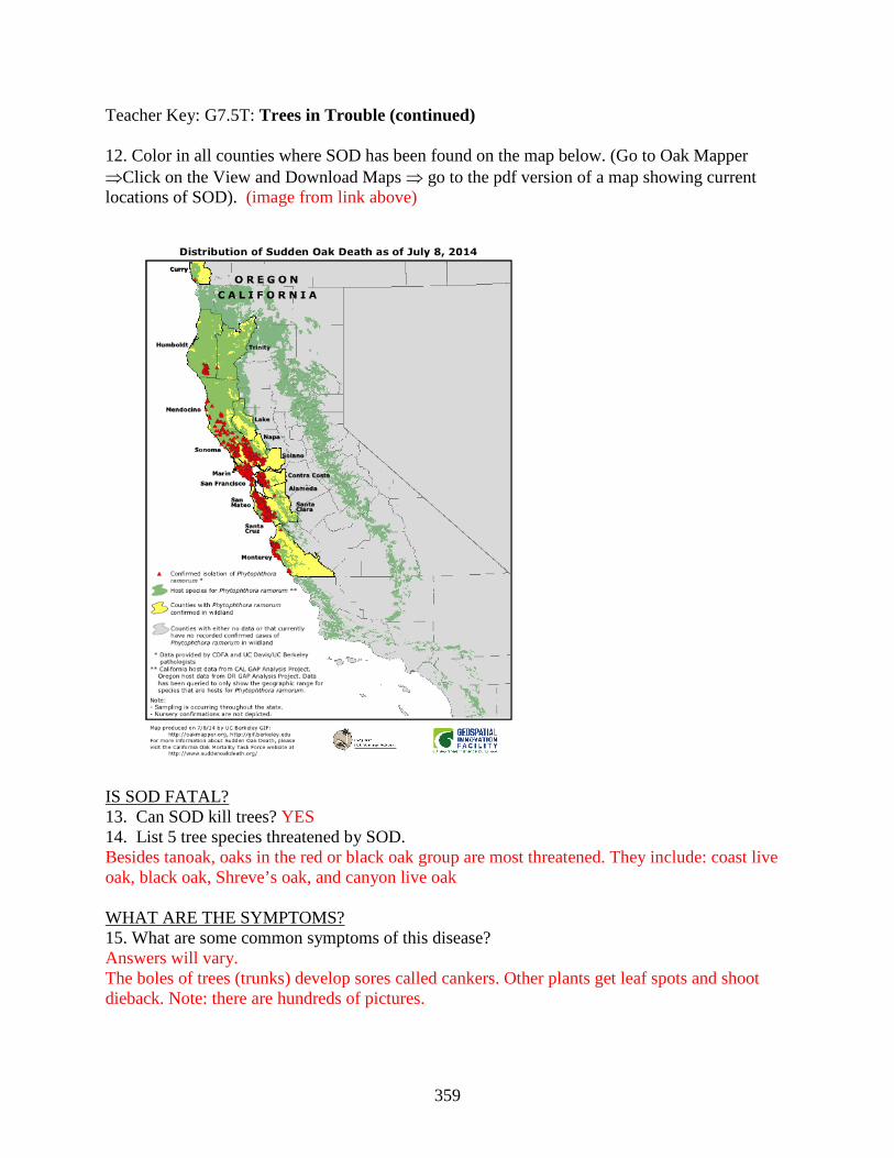
Teacher Key: G7.5T: Trees in Trouble (continued) 12. Color in all counties where SOD has been found on the map below. (Go to Oak Mapper ⇒Click on the View and Download Maps ⇒ go to the pdf version of a map showing current locations of SOD). (image from link above)

IS SOD FATAL? 13. Can SOD kill trees? YES 14. List 5 tree species threatened by SOD. Besides tanoak, oaks in the red or black oak group are most threatened. They include: coast live oak, black oak, Shreve’s oak, and canyon live oak WHAT ARE THE SYMPTOMS? 15. What are some common symptoms of this disease? Answers will vary. The boles of trees (trunks) develop sores called cankers. Other plants get leaf spots and shoot dieback. Note: there are hundreds of pictures.

359

Teacher Key: G7.5T Trees in Trouble (continued) 16. List steps to diagnosis whether a tree has the disease or not. (Go to: Homeowner’s Guide to SOD) Answers will vary. The only way to confirm the disease is to have tissue samples laboratory-tested. The steps are: 1) determine if your tree is susceptible 2) determine if you are in a susceptible area 3) Compare the symptoms to your tree to infected oaks IS YOUR TREE SICK? 16. List three things that increase the chances (probability) that your tree is infected. (found in A Homeowner’s Guide to SOD) The probability that your tree is infected with Phytophthora ramorum will be greater if your tree is a susceptible species, exhibits typical symptoms, and is located in an infested area where other trees and plants are showing symptoms HOW CAN WE REDUCE THE SPREAD? 17. List at least three ways people can help reduce the spread of SOD. (link: Sanitation and Reducing Spread) -Stay out of infested areas -Don’t collect or transport host plant material from an infested or quarantined area -Avoid entering infested areas during the wet season -Stay out of areas of wet soil and mud -If you do enter an area - remove mud, soil, and organic material before leaving the area -Reduce contamination by having clean shoes, bikes, vehicles, pets, etc. before leaving the area

360

Forest Ecology 101 Series (M3: Part II)

Module 3: Our Disappearing Oak Woodlands

Part II

UNIT OF STUDY COVER PAGE

Grade 10 Unit Lesson 1 - Oaks Through the Ages Lesson 2 - The Mystery of Masting

Lesson 3 - A Bird in the Hand Lesson 4 - King Conifers Lesson 5 - Friendly Fire

361

M3.G10 Lesson 1: Oaks Through the Ages Unit Overview: Oak Woodlands Grade 10 Key Concepts:

• Patterns and influence of climate change

• Adaptation • Biogeology and

feedbacks between the biosphere and Earth’s systems

• Natural selection Time: 50- 80 minutes Materials for the Teacher: Reference sheet

M3.10.1R (optional) Activity sheet

M3.10.1a Student worksheet

M3.10.1b Teacher key

M3.10.1aT Plant fossil specimens

(optional) Short presentation on

oak morphology and current distribution

Connections: STEM, Earth Science, climate change, agents of change, adaptation, evolution, maps, genetics, paleobotany, plant biology, biodiversity, biogeography, careers

Learning Objectives: Using written clues students will sequence some of the major climatic and geological events that have influenced the distribution pattern of the oaks of California over the last 20,000 years. They will be able to identify and describe some of the adaptations oaks have developed to live in a Mediterranean climate. Background information: Refer to the appropriate section in Part II: Teacher Companion for Module 3 and your textbook. Suggested procedure: Some preparation is necessary to prepare for this activity. You will need to cut up the passage the students will sequence (see M3.10.1a). Laminating the pages (text strips) is recommended if you plan on doing this activity repeatedly. You will want to have students refer to a geological time scale for the Cenozoic period to use as a reference (see M3.10.1R). Begin the lesson by explaining to the students that they are beginning a unit on oak woodlands. To begin they will at look at climatic and geologic forces that have shaped the past and current distribution of oaks found in the western U.S. over the last 20 million years. Oaks are angiosperms and appeared much more recently compared to conifers. They probably evolved from a more primitive oak still found in Southeast Asia. Climate and mountain building have been the primary driving forces of change. Briefly define paleontology, paleoecology, and palynology. To put together the past the evidence is always incomplete. Sequencing allows them to use logic and critical thinking skills. Tell them or review with them how species adapt to their environment through natural selection (refer to your textbook). If they have previous knowledge about oak trees, ask them what sort of environment oaks are probably best suited for (see preliminary questions). You may want to review the geologic timescale, fossil evidence for life, and the general morphology of oaks before getting started. A short presentation showing oaks and their current distribution is recommended. Some oaks are evergreen and others are deciduous. The oaks of California are well adapted to a Mediterranean climate with dry summers. This is a different sort of climate compared to the more extensive deciduous forests found across the eastern U.S. where summer rain is normal. See how much they know about oaks by asking some of the preliminary questions below. Next have them practice sequencing if they are inexperienced at it by passing out the practice passage (refer M3.10.1R). They should work in groups

362

Forest Ecology 101 integration: M1: Integrative Forest Ecology

of 2-3 for both the practice run and the full activity. If they tried the practice run go over the answer before beginning the group independent practice. Once they are done, they can compare answers with other groups to model how scientists learn from each other by sharing their work. Check their progress and give credit for participation before you let them share however. They will need to list the correct numerical sequence on their follow-up worksheet (see M3.10.1b). This worksheet has them identify and describe some of the adaptations oaks living in California have to a Mediterranean climate as well as being able to define paleoecology and palynology. After completing this lesson continue learning about oaks by proceeding to the next lesson in the series.

Preliminary questions: • How many oak species are there living in this area? (name them) • What kind of environment are California oaks adapted to? • What sorts of adaptations do oak trees have that allow them to survive in a Mediterranean

climate (wet winters and dry summers)? • What sorts of pressures exist in nature that force species to adapt or perish?

Critical Thinking: Besides using pollen studies, how else can a paleoecologist piece together the past morphology and distribution of a species? Keywords: distribution, morphology, natural selection, paleoecology, palynology NGSS alignment: HS-LS4: Biological Evolution: Unity and Diversity LS4.A Evidence of Common Ancestry and Diversity LS4.B Natural Selection LS4.C Adaptation HS-ESS2: Earth’s Systems ES2.E Biogeology Online resources: Paleogeography and Geologic Evolution of North America http://www2.nau.edu/rcb7/nam.html A great visual interactive tool to find out the paleogeography of any location in North America during different geologic periods. Labels of features can be added or deleted. California Oaks Foundation, reference page http://www.californiaoaks.org/html/reference.html There are great links on this page that can be integrated into lessons about the oaks of California including an oak slide show. This organization is now called California Wildlife Foundation, which no longer maintains this site.

363

(Online Resources continued) Paleoportal: Famous Flora and Fauna http://www.paleoportal.org/index.php?globalnav=flora_fauna&sectionnav=map This site has links to a map gallery full of information about ancient earth and pictures and locations of famous fossils found in the United States throughout geologic time. It includes an interactive geologic time scale for any state, links to educational resources, and information on careers in paleontology. Sonoma State University, California’s Coastal Prairies http://www.sonoma.edu/preserves/prairie/resources/ If you want to explore prairies and grasslands of California in more detail, this is an excellent resource. It has links to curriculum guides, grass identification, and games and puzzles. EEI Connection: B.6.b. Ecosystem Change in California B.8.a. Differential Survival of Organisms Answers to preliminary questions: - How many oak species are there living in this area? (answers will vary) - What kind of environment are California oaks adapted to? (for the most part the oaks of California are adapted to a Mediterranean climate although some are found along the coast which has a maritime influence. The center of oak diversity is found in Mexico which largely has a continental climate) - What sorts of adaptations do oak trees have that allow them to survive in a Mediterranean climate (wet winters and dry summers)? (answers will vary. Oaks are variable by nature. Some lose their leaves and others retain them. All of them have ways of conserving moisture through the dry season including a deep taproot and tough leaves. They are adapted to fire and can resprout after low to moderate intensity wildfire). - What sorts of pressures exist in nature that force species to adapt or perish? (answers will vary. Forces include climate change, competition, facilitation, and chemical warfare). Suggested extensions:

• Haves students explore the fascinating world of paleontology by going to one of the interactive websites given above in the online resources section.

• Show the video Walking With Prehistoric Beasts produced by the BBC. It shows the bazaar animals that arose after the extinction of the dinosaurs to the last ice age.

• Haves students look at different leaves, skulls, or another assorted collection to compare different morphological features and how they are adapted to certain niches or habitats.

• Compare the different adaptations plants have for living in or near freshwater versus brackish habitats.

• Using different DNA sequences, have students compare the degree of ancestry in two or more closely related species such as dogs and wolves or humans, chimpanzees, and gorillas.

• Have students key out the grasses inhabiting their area (see online resources) • Watch the film Becoming California; a 2 hour PBS film produced by the California

Environmental Legacy Project. It has great graphics depicting how plate tectonics have shaped the topography and influenced the biota of California.

364

M3.10.1R reference sheet M3.10.1a activity sheet M3.10.1b student worksheet M3.10.1aT and M3.10.1bT teacher keys

365

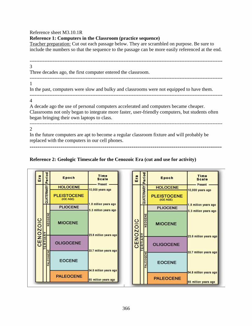
Reference sheet M3.10.1R Reference 1: Computers in the Classroom (practice sequence) Teacher preparation: Cut out each passage below. They are scrambled on purpose. Be sure to include the numbers so that the sequence to the passage can be more easily referenced at the end. --------------------------------------------------------------------------------------------------------------------- 3 Three decades ago, the first computer entered the classroom. --------------------------------------------------------------------------------------------------------------------- 1 In the past, computers were slow and bulky and classrooms were not equipped to have them. --------------------------------------------------------------------------------------------------------------------- 4 A decade ago the use of personal computers accelerated and computers became cheaper. Classrooms not only began to integrate more faster, user-friendly computers, but students often began bringing their own laptops to class. --------------------------------------------------------------------------------------------------------------------- 2 In the future computers are apt to become a regular classroom fixture and will probably be replaced with the computers in our cell phones. ---------------------------------------------------------------------------------------------------- Reference 2: Geologic Timescale for the Cenozoic Era (cut and use for activity)

366

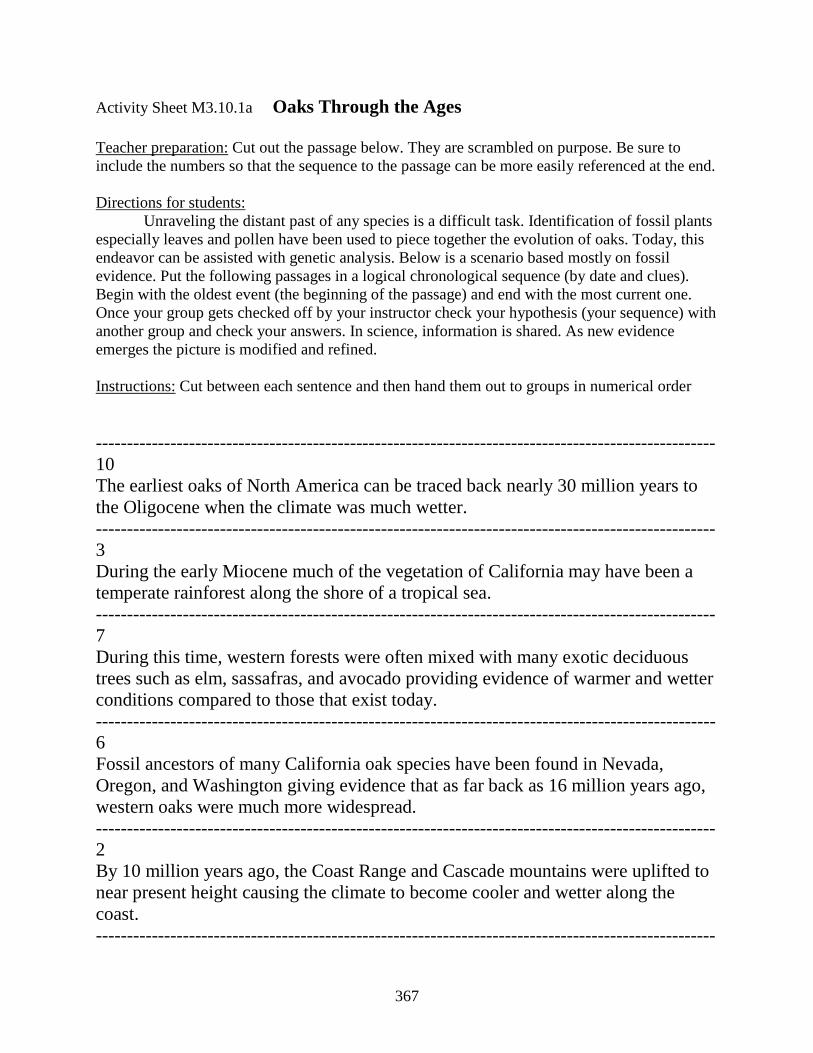
Activity Sheet M3.10.1a Oaks Through the Ages Teacher preparation: Cut out the passage below. They are scrambled on purpose. Be sure to include the numbers so that the sequence to the passage can be more easily referenced at the end. Directions for students: Unraveling the distant past of any species is a difficult task. Identification of fossil plants especially leaves and pollen have been used to piece together the evolution of oaks. Today, this endeavor can be assisted with genetic analysis. Below is a scenario based mostly on fossil evidence. Put the following passages in a logical chronological sequence (by date and clues). Begin with the oldest event (the beginning of the passage) and end with the most current one. Once your group gets checked off by your instructor check your hypothesis (your sequence) with another group and check your answers. In science, information is shared. As new evidence emerges the picture is modified and refined. Instructions: Cut between each sentence and then hand them out to groups in numerical order ---------------------------------------------------------------------------------------------------- 10 The earliest oaks of North America can be traced back nearly 30 million years to the Oligocene when the climate was much wetter. ---------------------------------------------------------------------------------------------------- 3 During the early Miocene much of the vegetation of California may have been a temperate rainforest along the shore of a tropical sea. ---------------------------------------------------------------------------------------------------- 7 During this time, western forests were often mixed with many exotic deciduous trees such as elm, sassafras, and avocado providing evidence of warmer and wetter conditions compared to those that exist today. ---------------------------------------------------------------------------------------------------- 6 Fossil ancestors of many California oak species have been found in Nevada, Oregon, and Washington giving evidence that as far back as 16 million years ago, western oaks were much more widespread. ---------------------------------------------------------------------------------------------------- 2 By 10 million years ago, the Coast Range and Cascade mountains were uplifted to near present height causing the climate to become cooler and wetter along the coast. ----------------------------------------------------------------------------------------------------

367

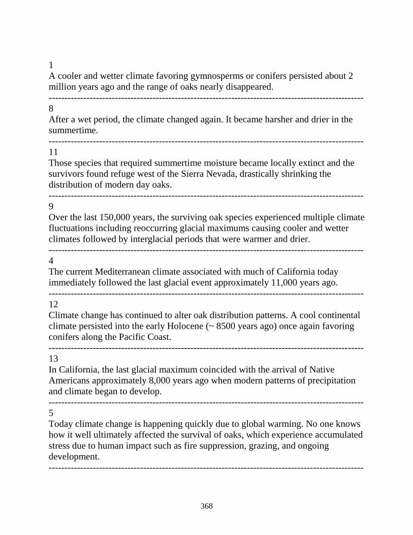
1 A cooler and wetter climate favoring gymnosperms or conifers persisted about 2 million years ago and the range of oaks nearly disappeared. ---------------------------------------------------------------------------------------------------- 8 After a wet period, the climate changed again. It became harsher and drier in the summertime. ---------------------------------------------------------------------------------------------------- 11 Those species that required summertime moisture became locally extinct and the survivors found refuge west of the Sierra Nevada, drastically shrinking the distribution of modern day oaks. ---------------------------------------------------------------------------------------------------- 9 Over the last 150,000 years, the surviving oak species experienced multiple climate fluctuations including reoccurring glacial maximums causing cooler and wetter climates followed by interglacial periods that were warmer and drier. ---------------------------------------------------------------------------------------------------- 4 The current Mediterranean climate associated with much of California today immediately followed the last glacial event approximately 11,000 years ago. ---------------------------------------------------------------------------------------------------- 12 Climate change has continued to alter oak distribution patterns. A cool continental climate persisted into the early Holocene (~ 8500 years ago) once again favoring conifers along the Pacific Coast. ---------------------------------------------------------------------------------------------------- 13 In California, the last glacial maximum coincided with the arrival of Native Americans approximately 8,000 years ago when modern patterns of precipitation and climate began to develop. ---------------------------------------------------------------------------------------------------- 5 Today climate change is happening quickly due to global warming. No one knows how it well ultimately affected the survival of oaks, which experience accumulated stress due to human impact such as fire suppression, grazing, and ongoing development. ----------------------------------------------------------------------------------------------------

368

Student worksheet M3.10.1b Name ______________________________ Date ______________ Period ___________

Oaks Through the Ages

Instructions: After learning about the oaks of California and sequencing the passage Oak Through the Ages, answer the review questions below: Define: 1. palynology: 2. paleoecology: True or False?: ________3. Millions of years ago the place we call California today was moist and tropical. ________4. Many trees oaks use to be associated with, such as sassafras and elm, are now extinct. _______5. Several oak species less suited to dry conditions either retreated to wetter places or became extinct when the climate began to get drier and warmer. Short answer: 6. Give two examples of large-scale phenomenon that pressure species to change over time. 7. What sort of climate is favored by conifers or gymnosperms and not by oaks? 8. Identify three adaptations oak trees have to live in a Mediterranean climate.

369

Teacher Key M3.10.1aT: Oaks Through the Ages Teacher key: Practice Run Sequence: 3,1,4,2 3 Three decades ago, the first computer entered the classroom. 1 In the past, computers were slow and bulky and classrooms were not equipped to have them. 4 A decade ago the use of personal computers accelerated and computers became cheaper. Classrooms not only began to integrate more faster, user-friendly computers, but students often began bringing their own laptops to class. 2 Teacher key: Student activity (M3.10.1a): Oaks Through the Ages In the future computers are apt to become a regular classroom fixture and will probably be replaced with the computers in our cell phones. It is not essential that the students get the sequence exactly right. Getting the sequence slightly off could actually be a more accurate portrayal of paleontology. As more evidence emerges, hypotheses change. Sequence: 10,3,7,6,2,1,8,11,9,4,12,13,5 10 The earliest oaks of North America can be traced back nearly 30 million years to the Oligocene when the climate was much wetter. 3 During the early Miocene much of the vegetation of California may have been a temperate rainforest along the shore of a tropical sea. 7 During this time, western forests were often mixed with many exotic deciduous trees such as elm, sassafras, and avocado providing evidence of warmer and wetter conditions compared to those that exist today. 6 Fossil ancestors of many California oak species have been found in Nevada, Oregon, and Washington giving evidence that as far back as 16 million years ago, western oaks were much more widespread. 2 By 10 million years ago, the Coast Range and Cascade mountains were uplifted to near present height causing the climate to become cooler and wetter along the coast.

370

1 A cooler and wetter climate favoring gymnosperms or conifers persisted about 2 million years ago and the range of oaks nearly disappeared. 8 After a wet period, the climate changed again. It became harsher and drier in the summertime. 11 Those species that required summertime moisture became locally extinct and the survivors found refugee west of the Sierra Nevada, drastically shrinking the distribution of oaks. 9 Over the last 150,000 years, the surviving oak species experienced multiple climate fluctuations including reoccurring glacial maximums causing cooler and wetter climates followed by interglacial periods that were warmer and drier. 4 The current Mediterranean climate associated with much of California today immediately followed the last glacial event approximately 11,000 years ago. 12 Climate change has continued to alter oak distribution patterns. A cool continental climate persisted into the early Holocene (~ 8500 years ago) once again favoring conifers. 13 In California, the last glacial maximum coincided with the arrival of Native Americans approximately 8,000 years ago when modern patterns of precipitation and climate began to develop. 5 Today not only climate change continues to impact oak survival, but human impact such as fire suppression, grazing, and ongoing development are adding stress on the oaks inhabiting California. ---------------------------------- Teacher key M3.10.3bT Define: 1. palynology - the study of spores and other grains, especially those found in archeological or geological deposits 2. paleoecology - the ecology of fossil plants and animals 3. T 4. F 5. T 6. Mountain building, climate change 7. A climate that is wetter and colder 8. Adaptations include the ability to resprout after fire, leaves that are drought tolerant and that can minimize water loss, a taproot to search for water, deciduous leaves, they are highly variable or adaptable, often hybridize, and live in assorted habitats.

371

M3.G10 Lesson 2: The Mystery of Masting Unit Overview: Oak Woodlands Grade 10 Key Concepts:

• Plant reproduction • Plant responses • Patterns of cause and

effect • Interdependent

relationships in ecosystems

• Interpreting data Time: 50 - 80 minutes Materials for the Teacher: Student reading

M3.10.2a Student worksheet

M3.10.2b and teacher key.

Images of acorns, oak sprouts, granaries, and oak woodlands and savannas

The life cycle of an oak tree

Connections: STEM, growth and development, botany, pollination, sexual reproduction, agriculture, mathematics, human impact, stability and change, biodiversity, soils, biomass, economics, climate change, forest conservation, careers

Learning Objectives: Students will read about acorn masting and will identify some of the main theories attempting to explain this phenomenon. They will interpret several figures from a scientific study attempting to find significant contributing factors for yearly acorn productivity across varying scales. Comparisons include yearly acorn abundance per species, versus average monthly temperature, and between individual trees within the same species. Background information: Refer to the appropriate section in Part II: Teacher Companion for Module 3 and the original paper below: Koenig W.D., and J.D. Knops. 2005. The mystery of masting in trees: some trees reproduce synchronously over large areas, with widespread ecological effects, but how and why? American Scientist 93(4): 340-347. Suggested procedure: Begin this lesson by briefly reviewing an oak tree’s life cycle and the steps necessary for pollination by asking some of the preliminary questions found below. Next give a brief overview of the importance of oaks and the concern over lack of successful regeneration occurring in some species. Ecologically oaks are a keystone species because they support a profound number of organisms. For the last fifty years an observed lack of recruitment has stimulated concern over the persistence of some species. Oaks are widespread, variable by nature, and are grouped into three lineages. Finding the main reasons for poor regeneration has been difficult. Different oak species have distinct reproductive strategies. Some take one year for acorns to mature and others take two. One reproductive strategy in most oaks is acorn masting. A mast year is a higher than normal seed year. Patterns in productivity can be synchronized over large areas. The advantages for masting are unknown. Some evidence supports the “predator-satiation” hypothesis where in mast years a higher degree of seeds escape predation. High production years require a lot of energy and are difficult to maintain. Linking masting events to particular abiotic and biotic factors has proved challenging. Anecdotal evidence points to high rainfall as a stimulus, although this tends to be unsupported scientifically. One factor found to have a high degree of correlation for valley oak and blue oak is warm weather in April. This is the time of year when these trees are in flower. These issues and others should be integrated into a short discussion before students begin analyzing the data presented in this lesson. During the preliminary discussion you may want to

372

Forest Ecology 101 integration: M1: Integrative Forest Ecology

assess their knowledge and interest by having them fill out a K-W-L chart (Know-Want to know-Learned). They should begin by reading The Mystery of Masting (see M3.10.2a). Next they should complete worksheet M3.102b. Here they will need to identify the comparative scale used in each analysis and interpret the relationships they observe in each figure. The worksheet can be completed alone or by collaborating with a partner. If students run out of time on the first day, you may want to assign the remainder as homework. It is recommended that you read the entire paper first (cited above) in order to gain a deeper understanding about this comprehensive study (see online resources). You should also be well acquainted with the figures and questions asked on their worksheet. For instance, students are asked what N stands for. N refers to the number sampled. Understanding factors responsible for acorn masting could be useful in wildlife management and may facilitate efforts towards oak woodland conservation and restoration among other things. Once students have finished this lesson they may have a deeper insight into some of the potential relationships presented in the next lesson, which delves deeper into animal and plant interactions.

Preliminary questions: • What happens during pollination? • Why do people refer to the birds and the bees when discussing sex? • What advantages do wind-pollinated plants have compared to those pollinated by

animals? • Do you think the amount of pollen would need to be higher or lower for wind-pollinated

plants opposed to those pollinated by animals? Why? • What variables could be responsible for high and low seed production? • What factors could be connected to an observed lack of young trees? • Why are oaks considered a keystone species?

Critical Thinking: Over a ten-year study dozens of individual trees have been compared. Some regularly reproduce a high volume of seeds and others never do. What factors could be responsible for this observed discrepancy? Keywords: acorn, acorn mast, hybridize, keystone species, pollen, pollination, productivity, synchronized NGSS alignment: HS-LS1: From Molecules to Organisms: Structures and Processes LS1.A Structure and Function LS1.B Growth and Development of Organisms S and E: Developing and Using Models HS-LS2: Ecosystems: Interactions, Energy, and Dynamics LS2.C Ecosystem Dynamics, Functioning, and Resilience

373

M3.G10.L2 Unit Overview (continued) Online Resources: Hasting Reserve: An Introduction to Oak Woodlands http://www.hastingsreserve.org/OakStory/OakIntro.html Over 500 scientific studies have been conducted on this reserve. This page of their website focuses on oak woodland in particular. A link to a pdf version of the study used in this lesson can be found here along with good information and pictures on oak flowers and acorns. California Oaks http://www.californiaoaks.org/html/2040.html For a good overview of the status and future of California oaks go to this site. A pdf is available for Oaks 2040 - a short report designed to give land managers valuable information for the advancement of oak conservation. California Oaks Foundation, reference page http://www.californiaoaks.org/html/reference.html There are several links to information regarding the oaks of California on this site including an oak slide show and links to student activities. From here you can navigate to a host of other sites including information on eating acorns, oak restoration, and fire in oak woodlands. Rangeland Watershed Laboratory http://rangelandwatersheds.ucdavis.edu/main/transition_models.htm If you want to learn about the vegetation dynamics between disturbed and undisturbed sites in a grassland/oak woodland ecosystem this is a great site. It has information about past land management and gives preliminary results for nitrogen and carbon content in soil, soil surface bulk density, and biodiversity between study sites. EEI Connection: B.6.b. Ecosystem Change in California B.8.a Differential Survival of Organisms Answers to preliminary questions: - What happens during pollination? (during pollination pollen from a male stamen lands on the stigma of a flower. During fertilization egg unites with sperm) - Why do people refer to the birds and the bees when discussing sex? (often birds and bees are the essential pollinators for plants. They inadvertently pass the pollen from flower to flower. The main purpose of a flower is to attract pollinators.) - What advantages do wind-pollinated plants have compared to those pollinated by animals? (wind-pollinated plants do not need to rely on the presence of animals. The arrival of animals needs to be in sync with the opening of flowers for pollination to be successful. This relates to phenology - the study of plant and animal events.) - Do you think the quantity of pollen would need to be higher or lower for wind-pollinated plants opposed to those pollinated by animals? Why? (answers will vary. Wind-pollinated plants produce more pollen to assure that it gets broadcasted over a long distance. Allergy sufferers can usually relate to this.)

374

(Answers to preliminary questions continued) - What variables could be responsible for high and low seed production? (answers will vary. Poor weather, lack of pollinators, lack of essential nutrients, disease, stress, predation, and genetics could all contribute to varying seed production) - What factors could be connected to an observed lack of young trees? (answers will vary. If seeds are germinating, but young trees are not present, the shortage could be contributed to trampling, herbivory, disease, drying out, soil compaction, lack of nutrients, etc.) - Why are oaks considered a keystone species? (oaks have a disproportionate value to the ecosystem compared to the overall number of plants. Oak woodlands are identified as the most biologically rich terrestrial ecosystem in California. Over 300 vertebrate and 5,000 invertebrates are known to utilize oak-dominated landscapes.) Suggested extensions:

• Collect various seeds and have students learn how they are adapted for dispersal. • Show a video on plant pollination and fertilization. • Begin an investigation on seed germination and compare success to a factor that may

contribute to the lack of recruitment in oaks such as soil compaction or competition. • Learn about important pollinators such as bees and bats and the environmental issues

facing their decline. • Have students view, draw, and label the reproductive parts of flowers using dissecting

microscopes or magnifying glasses. • Have students learn about past land management practices in oak woodland habitats and

suggest new ways to help conserve oaks. • Be a part of an oak woodland restoration project by collecting and planting acorns. • Identify the local hardwoods in your area. A key is available in lesson M3.G7.L2.

M3.10.2a Student reading M3.10.2b Student worksheet M3.10.2bT Teacher key

375

Student Reading M3.10.2a

The Mystery of Masting Oaks are true flowering plants or angiosperms. Because they are wind-pollinated

successful germination is largely dependent on weather. A new cycle of reproduction begins in

the spring when large quantities of pollen are produced. Pollination occurs when a pollen grain

originating from a male stamen reaches a female stigma. Successful fertilization doesn’t occur

until a sperm unites with an egg inside the ovary of a flower. Other plants rely on animals for

pollination such as birds, bees, and bats.

In oak trees a fertilized embryo develops into an acorn, which is a true nut. It comes from

the old English word for oak, ac and cern, which means grain or kernel in Greek. It can be

loosely translated as “fruit of the field.” An acorn (the fruit of an oak) houses all of the parts that

a young seedling needs to survive. Once in the ground, acorns grow rapidly forming a sprout or a

seedling provided they have the proper nutrients and conditions. Over the last 60 years, a lack of

young trees (referred to as recruitment) has been observed across the California landscape in

many oak species including valley oak, blue oak, and Oregon white oak. Many factors have been

linked to this shortage, including grazing by livestock and increased competition with non-native

annual grasses; however, much remains unknown. For instance, Oregon white oak may need

regular fire regimes to reduce competition by faster growing conifers.

The production of acorns is of fundamental importance to the understanding of problems

associated with oak regeneration and to the diverse assemblage of wildlife dependent on acorns

for food. Oaks are considered keystone species because they support a high diversity of

organisms. The reproductive success of some species are directly linked to the availability of

acorns. Many oaks have years of bumper acorn crops followed by years nearly devoid of fruit.

The years of high productivity are called acorn masts. The word mast comes from the old

English word mete, which means meat. Acorns have been a primary food source for people for

thousands of years.

The pattern of acorn masts varies in time and space and between different sites and

species. Native Americans favored the acorns of certain oak species. In the North Coast, black

oak and tanoak were - and still are - highly prized for their acorns. In order to have a dependable

376

supply of acorns Native Americans would build storage structures called granaries to keep

wildlife away and to prevent rot.

It has been known for centuries that certain oak species can synchronize their masts. How

and why this happens remains a mystery. Several hypotheses have been developed to explain this

phenomenon. One is a chemical response to environmental clues. Somehow chemical signals

may be transmitted from tree to tree. Another is that oaks across a large region may respond

similarly to environmental stimuli such as wetter-than-normal periods or drought. The most

common explanation is called the predator-satiation hypothesis. Satiation refers to an animal

being satisfied and having enough to eat. In bumper years a higher release of acorns will increase

the odds that some seeds can escape predation by the large array of organisms ready to feast

upon them. Squirrels and birds are avid collectors of acorns. They will collect and hide them

away in caches to eat later. Lastly, synchronized masting may be related to the limitation of

pollen. It is possible that only in certain years enough pollen can reach all of the flowers

necessary for large-scale pollination. Whatever reason oaks have for masting they have most

likely evolved this reproductive strategy to conserve resources. A large seed crop takes a lot of

energy and during periods of low acorn production, they can shift their resources towards growth

and repair.

Oaks are variable by nature and can live hundreds of years making the study of them

challenging. Different oak species belong to different lineages. Some oaks take two years for

acorns to mature while others only need one year. Some species are more shade or drought-

tolerant than others. Oaks can be deciduous or remain evergreen. They can be shrubs or trees and

can readily hybridize. What factors are responsible for their synchronized masting? What sorts of

investigations can occur to pinpoint the factors responsible for bumper acorn years?

Understanding the patterns of acorn masting can be useful in wildlife management and can aid in

efforts towards oak conservation and restoration.

Written by Melinda Bailey

377

Student worksheet G10.2b Name ______________________________ Date_______________ Period __________ The Mystery of Masting Background: Many investigations have attempted to identify the factors that significantly play a role in the variation of acorn productivity from year to year and between species. Below you will find the results of a fifteen-year study that attempted to find factors responsible for acorn masting between species and within species. Results came from studying over 150 trees in Central California. Review Questions: 1. Briefly explain the four main hypotheses presented in the student reading above to explain acorn mast events. 2. Why can understanding the patterns of acorn masting be important for future management efforts? Instructions: Look at each figure below and see if you can find either a significant relationship between factors or recognize a pattern. It may be that to truly understand the variable nature of oaks and the mystery behind masting, longer duration studies are required. At the beginning of each figure you will be asked to identify the scale. Scale: This study used three comparative scales: year to year, tree to tree, and site to site. For each of the figures choose one of these. FIGURE A - Comparing yearly acorn productivity between five species. Is there a pattern showing acorn mast events across species? How about related species? (Refer to Table 1) 1. Scale? ____________________________________________________________ (year to year, tree to tree, or site to site) 2. What relationship do you observe between the different species over time? Are there any similar trends? Be specific.

378

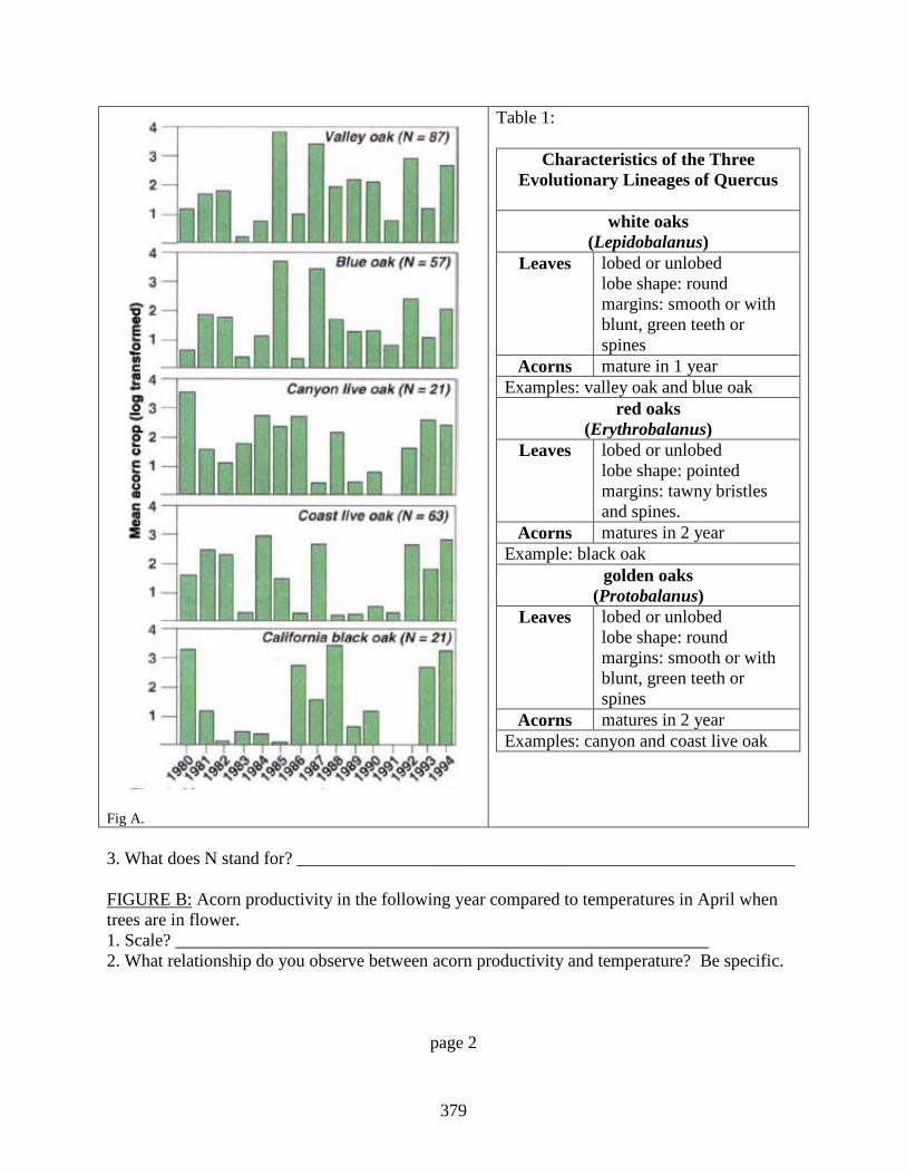
Fig A.

Table 1:

Characteristics of the Three Evolutionary Lineages of Quercus

white oaks

(Lepidobalanus) Leaves lobed or unlobed

lobe shape: round margins: smooth or with blunt, green teeth or spines

Acorns mature in 1 year Examples: valley oak and blue oak

red oaks (Erythrobalanus)

Leaves lobed or unlobed lobe shape: pointed margins: tawny bristles and spines.

Acorns matures in 2 year Example: black oak

golden oaks (Protobalanus)

Leaves lobed or unlobed lobe shape: round margins: smooth or with blunt, green teeth or spines

Acorns matures in 2 year Examples: canyon and coast live oak

3. What does N stand for? ________________________________________________________ FIGURE B: Acorn productivity in the following year compared to temperatures in April when trees are in flower. 1. Scale? ____________________________________________________________ 2. What relationship do you observe between acorn productivity and temperature? Be specific.

page 2

379

Fig B. 3. What other abiotic factor might be linked to the amount of acorns produced annually for different oak species? FIGURE C: Mean acorn crop in coast live oak compared across three different regions. 1. Scale? ____________________________________________________________ 2. What relationship in acorn productivity do you observe between the three sites?

Fig. C 3. What was the duration of this study? _____________________________________________

page 3

380

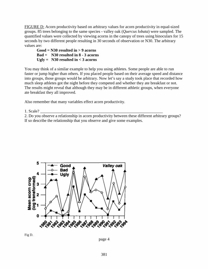
FIGURE D: Acorn productivity based on arbitrary values for acorn productivity in equal-sized groups. 85 trees belonging to the same species - valley oak (Quercus lobata) were sampled. The quantified values were collected by viewing acorns in the canopy of trees using binoculars for 15 seconds by two different people resulting in 30 seconds of observation or N30. The arbitrary values are: Good = N30 resulted in > 9 acorns Bad = N30 resulted in 8 - 3 acorns Ugly = N30 resulted in < 3 acorns You may think of a similar example to help you using athletes. Some people are able to run faster or jump higher than others. If you placed people based on their average speed and distance into groups, those groups would be arbitrary. Now let’s say a study took place that recorded how much sleep athletes got the night before they competed and whether they ate breakfast or not. The results might reveal that although they may be in different athletic groups, when everyone ate breakfast they all improved. Also remember that many variables effect acorn productivity. 1. Scale? ____________________________________________________________ 2. Do you observe a relationship in acorn productivity between these different arbitrary groups? If so describe the relationship that you observe and give some examples.

Fig D.

page 4

381

Teacher key: M3.10.2bT: Mystery of Masting Review Questions: 1. Briefly explain the four main hypotheses presented in the student reading above to explain acorn mast events. Chemical response - trees respond to chemical responses based on environmental clues Response to environmental stimuli Predator-satiation hypothesis - bumper acorn crops increase the chance of successful germination because predators have more than enough to eat and leave some beind. Pollen limitation - only during large-scale pollination events can mast years occur. 2. Why can understanding the patterns of acorn masting be important for future management efforts? Answers will vary. By knowing the cause and effects of acorn mast events, land managers will be better equipped to predict when they might occur and how this may affect wildlife. FIGURE A - Comparing yearly acorn productivity between five species. Is there a pattern showing acorn mast events across species? How about related species? No apparent patter exists across species. Blue oak and valley oak have similar trends and belong to the white oak lineage. 1. Scale? _______________year to year_________________ (year to year, tree to tree, or site to site) 2. What relationship do you observe between the different species over time? Are there any similar trends? Be specific. Answers will vary. All species had a lower than average acorn crop in year 1983 except Coast live oak. Both valley oak and blue oak had bumper years in 1985 and 1987 which was a very low year for canyon live oak. Coast live oak seems to have the lowest correlation with other species. 3. What does N stand for? _________sample number (population) ____ FIGURE B: Acorn productivity in the following year compared to temperatures in April when trees are in flower. 1. Scale? _________tree to tree _______ 2. What relationship do you observe between acorn productivity and temperature? Be specific. The higher the temperature in April the higher the mean annual acorn crop (direct relationship or linear) 3. What other abiotic factor might be linked to the amount of acorns produced annually for different oak species? Answers will vary. A good example = amount of moisture or wind strength

382

Teacher key: M3.10.2bT: Mystery of Masting (continued) FIGURE C: Mean acorn crop in coast live oak compared across three different regions. 1. Scale? _______site to site _____________ 2. What relationship in acorn productivity do you observe between the three sites? Answers will vary. Low acorn productivity happened in all three sites from 1989 - 1991 especially in 1991. The highest acorn productivity happened in all three sites during 1992 3. What was the duration of this study? 6 years (1989 - 1993) FIGURE D: 1. Scale? ___________year to year______ 2. Do you observe a relationship in acorn productivity between these different arbitrary groups? If so describe the relationship that you observe and give some examples. Answers will vary. Yes - all arbitrary groups followed a similar pattern whether they were good or poor producers of acorns. 1993 was a low producing year across all categories and years 1985, 1987, 1992, and 1994 had relatively high production in all categories.

383

M3.G10 Lesson 3: A Bird in the Hand Unit Overview: Oak Woodlands Grade 10 Key Concepts:

• Interdependent relationships

• Developing models • Understanding

positive and negative feedbacks within a system

• Ecosystem interactions Time: 80 - 140 minutes Materials for the Teacher: Access to computers Teacher reference

M3.10.3R Student online

investigation M3.10.3a Example of models or

illustrations (optional) Poster paper (optional)

Connections: STEM, ornithology, wildlife management, resource partitioning, carrying capacity, reproduction, biodiversity, cycling of matter and energy, phenology, CAD, engineering, careers, social studies Forest Ecology 101 integration: M1: Integrative Forest Ecology

Learning Objectives: Students will research and compare the interdependent relationships between two bird species (acorn woodpecker and western scrub-jay) and oak trees. Both species rely heavily on acorns and have different methods of caching them for winter food. Students will apply systems thinking by designing a model that shows an outcome related to these animal-plant interactions. Background information: Refer to the appropriate section in Part II: Teacher Companion for Module 3 and online resources. Suggested procedure: This lesson will require you to be familiar with systems thinking. A great online resource is available at the Pacific Education Institute (see online resources). Information on how to get started is given in the teacher reference sheet (see M3.10.3R). Begin this lesson by explaining some of the interesting plant and animal interactions that exist in nature (refer to your textbook). Show how these relationships can be illustrated using models such as a concept map or a causal loop diagram. Next review some of the common interactions that occur within an ecological community (i.e. predation, herbivory, parasitism, mutualism, and commensalism). Many relationships are mutually dependent, however few are altruistic in nature. Some mutualistic relationships can influence the abundance of organisms such as in the case of scrub jays and oak trees. This relationship has a positive influence on both organisms. Other relationships can have a negative influence such as parasitism. The relationship between acorn woodpeckers and oaks is considered commensal. The oak trees provide food and a place for the birds to live so they are positively impacted and the oak tree is not harmed. In addition, you may want to explain to them that all species have a particular niche or role within an ecosystem and some partition resources. For instance, bees are important pollinators for plants and can be prey for birds and mammals. In this lesson students need to know the relationship of the two bird species (acorn woodpecker and western scrub jay) well enough to be able to illustrate relationships using diagrams. You will need to assign how they will conduct their research and what specific objectives need to be met while designing their model. Making a model may be challenging for them so having some examples to show them ahead time could be helpful. To get started they should fill out the student online investigation sheet (M3.10.3a) where they will compare the two bird species. An option is to have students work with a partner or even within groups.

384

Preliminary questions: • What sorts of interactions exist between species in an ecosystem? (ask for several

examples) • What kind of interaction is a coyote catching and eating a rabbit? • What kind of interaction is a bee pollinating a flower? • What are some other examples of plant and animal interactions? • What sort of interaction can you think of that might occur in an oak woodland? • If a squirrel stashes acorns for later use is this an interaction? • If a squirrel stashes acorns for later use but doesn’t dig all of them up is this an

interaction? • How could we illustrate some of these examples using systems thinking?

Critical Thinking: In a good acorn crop year the population of acorn woodpeckers increases and in poor production years the population is reduced. How can you show this dynamic interaction in a variable time graph? Keywords: biodiversity, cache, commensalism, competition, facilitate, granary, herbivory, interaction, mutualism, predation NGSS alignment: HS-LS2: Ecosystems: Interactions, Energy, and Dynamics LS2.A Interdependent Relationships in Ecosystems LS2.C Ecosystem Dynamics, Functioning, and Resilience LS2.D Social Interactions and Group Behavior S and E: Developing and Using Models Online resources: Pacific Education Institute: Sustainable Tomorrow http://www.pacificeducationinstitute.org/workspace/resources/systems-thinking.pdf This informative booklet includes many things you need to know to get started with systems thinking in your class. It is titled: Sustainable Tomorrow: A Teacher’s Guidebook for Applying Systems Thinking to Environmental Education Curricula in Grades 9-12. UCANR: Oak Woodland Wildlife http://ucanr.edu/sites/oak_range/Oak_Articles_On_Line/Oak_Woodland_Wildlife/ This is the site suggested on student worksheet (M3.10.L3a) where they should begin their research concerning the interactions of acorn woodpeckers and western scrub jays. One article is titled: Oaks, Acorns, and Acorn Woodpeckers and the other Jays Plant Acorns. Several other articles and links to information about wildlife is available here. Papers discuss a range of issues including the dependency of birds on oaks woodlands, the affects feral pigs have on oak woodlands, and the nesting habitats of many birds in oak trees including owls and hawks. Hastings Reserve: Oak Woodlands and Introduction and Overview http://www.hastingsreserve.org/OakStory/OakIntro.html Hastings Reserve is one of the centers for scientific research in oak woodland and grassland habitats in Central California. This page has several links to good information about natural planting of acorns by jays, oak reproduction, and best methods to use of oak restoration.

385

(Online Resources continued) eBird: Bird Quest http://www.birdsleuth.org/citizen-science-bird-quest/ If you want to have students collect data on the local birds of your area this might be a great place to start. Here you can download Bird Quest for free. It has places for students to find information about birds and methods for downloading data for citizen science projects. EEI Connection: B.6.b. Ecosystem Change in California B.8.a Differential Survival of Organisms Answers to preliminary questions: - What sorts of interactions exist between species in an ecosystem? (ask for several examples) (answers will vary. Examples could include a mountain lion eating a deer, a grasshopper eating grass, a tick on a mouse, a sponge on a rock, etc.) - What kind of interaction is a coyote catching and eating a rabbit? (predation) - What kind of interaction is a bee pollinating a flower? (mutualistic) - What are some other examples of plant and animal interactions? (answers will vary) - What sort of interaction can you think of that might occur in an oak woodland? (answers will vary. Hopefully they will mention squirrels or birds eat acorns, which would be forms of herbivory.) - If a squirrel stashes acorns for later use is this an interaction? (yes. This is a type of herbivory) - If a squirrel stashes acorns for later use but doesn’t dig all of them up is this an interaction? (yes - indirectly the squirrel is facilitating the germination of seeds. Acorns germinate better if buried. Squirrels and jays help in the distribution of oaks because they carry seeds farther compared to where they would naturally fall) - How could we illustrate some of these examples using systems thinking? (answers will vary. See teacher reference sheet) Suggested extensions:

• Assign a student research project about a particular species found within an oak woodland.

• Begin an ongoing student investigation in the field of phenology where over several years, similar data is collected and compared such as the flowering times of certain plants on campus.

• Gather quantitative data about past land management practices on rangelands in your county. Data can include values about acreage, ownership, conversion, wood production and livestock.

• Have students draw a model of secondary succession in an oak woodland beginning with fire or clearing and ending with a mature stand.

• Discuss how woodpeckers are keystone species because they are ecosystem engineers. They make cavities while searching for food, which are used as important hiding places and nesting sites for many other species.

• Learn about the social interactions of acorn woodpeckers. They are one of the only local communal bird species that live and cooperate together.

386

(Suggested extensions continued) • Visit an oak woodland and have students note what sorts of relationships they can

observe there. • Go out and birdwatch! eBird has Bird Quest for students available online.

M3.10.3T Teacher reference sheet M3.10.3a Student online investigation sheet

387

Teacher reference sheet M3.10.3T

A Bird in the Hand An Introduction to Systems Thinking Having students develop models is important in science and engineering. Models can illustrate relationships between components within a system such as population dynamics, nutrient load, and interdependent relationships. For instance, positive and negative relationships can be illustrated using + and - signs respectively next to a word or concept. Arrows show the time lapse, movement of materials, or the next sequence in a series. Most students are familiar with concept mapping, which is one way to simplify and reinforce an idea or concept. Systems thinking organizes a story or a concept objectively at a broad level. Systems thinking is characterized by the fact that most problems to solutions are not linear but need to be evaluated in the context of a whole system. They are often applied to environmental science and sustainability. In this lesson we are referring to an oak woodland ecosystem. In this scenario key ideas should be drawn from the main text after students research the two bird species. For instance scrub jays cache acorns for food in the ground, leave some behind, and in the process encourage oak reproduction. Their relationship with oaks is mutualistic. Conversely, acorn woodpeckers cache acorns in granaries, pack them in tight above the ground where they don’t fall out, and therefore don’t assist in oak reproduction. They have a commensal relationship with oaks and don’t pose a significant negative impact on oak reproduction. They rarely depend on one species. To get students started on this project you may want them to divide a piece of poster paper in half and have them illustrate the relationships they have isolated for species A on one side and species B on the other with an oak tree in the middle (see the example below). How creative you want them to be is up to you! Below are some ways of getting students started with systems thinking. The first set of information comes directly from the Pacific Education Institute’s website. You can find the link to the full text in the online resources in the lesson overview. Structure: Structure is the way in which the parts of a system are organized and relate to each other. Sometimes the structure of a system can be seen and sometimes it cannot be seen. How desks in a classroom are arranged is an example of a structure we can see. The rules and laws that are in place in our schools and communities are examples of structures that we cannot see. The structure of a system drives its behavior. A systems thinker asks: What structures are in place in this system that may be determining the behaviors we see? Leverage Point: A place in a system where making a small change can result in a large improvement in the whole system. A systems thinker asks: Where in this system could we make small shifts that would make a big difference?

388

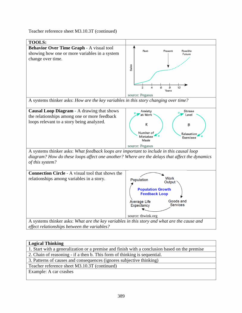
Teacher reference sheet M3.10.3T (continued) TOOLS: Behavior Over Time Graph - A visual tool showing how one or more variables in a system change over time.

source: Pegasus

A systems thinker asks: How are the key variables in this story changing over time?

Causal Loop Diagram - A drawing that shows the relationships among one or more feedback loops relevant to a story being analyzed.

source: Pegasus

A systems thinker asks: What feedback loops are important to include in this causal loop diagram? How do these loops affect one another? Where are the delays that affect the dynamics of this system? Connection Circle - A visual tool that shows the relationships among variables in a story.

source: thwink.org

A systems thinker asks: What are the key variables in this story and what are the cause and effect relationships between the variables? Logical Thinking 1. Start with a generalization or a premise and finish with a conclusion based on the premise 2. Chain of reasoning - if a then b. This form of thinking is sequential. 3. Patterns of causes and consequences (ignores subjective thinking) Teacher reference sheet M3.10.3T (continued) Example: A car crashes

389

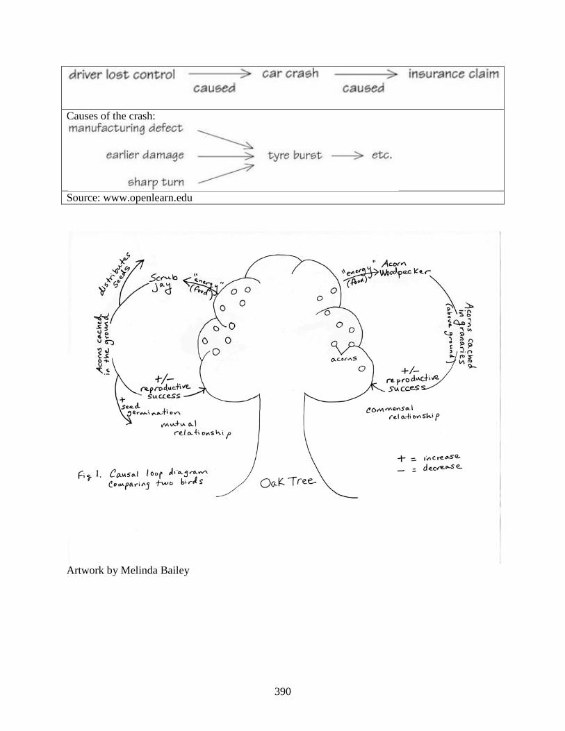
Causes of the crash:

Source: www.openlearn.edu

Artwork by Melinda Bailey

390

Student online investigation M3.10.L3a Name ______________________________ Date __________________ Period________ A Bird in the Hand Instructions: Investigate how acorn woodpeckers and western scrub jays differ in their interactions with oak trees, particularly through the behavior they use to harvest acorns. A good place to start your online research is at the University of California Extension on Oak Woodland Management website (http://ucanr.edu/sites/oak_range/). The main purpose of this investigation is to use systems thinking to illustrate the relationship each bird has to an oak woodland ecosystem by designing a model. The specific objectives of your model, and the steps you should take to complete it, should be given to you by your instructor. A: Research: Use the table below to take notes on both bird species. Be sure to include each species name, their behavior (how do they store acorns?), their relationship with oaks, and any population dynamics, reinforcement principles (do behaviors affect oak trees?), and/or future concerns that come up in your research.

Use the back of this page for more notes

391

M3.G10 Lesson 4: King Conifers Unit Overview: Oak Woodlands Grade 10 Key Concepts:

• Ecosystem dynamics • Inter-species

competition in an ecosystem

• Secondary succession • Human interaction

(fire suppression) • Analyzing data • Adaptation

Time: 80 - 100 minutes Materials for the Teacher: Teacher reference

M3.10.4R Student worksheet and

teacher key M3.10.4a Highlighters (optional)

Connections: STEM, scientific method, math, forestry, fire ecology, biodiversity, adaptation, photosynthesis, carbon cycle, human interactions, economics, social studies, Native American studies, biomass, climate change, forest conservation, careers Forest Ecology Series integration: M1: Integrative Forest Ecology M2: Coast Redwood

Learning Objectives: Students will identify the cause and effects of fire suppression particularly overtopping by Douglas-fir in Oregon white oak habitat. They will analyze data from a thinning project and will determine how oaks respond to increased resources at different treatment levels. In this study changes in acorn productivity, dbh, and epicormic sprouting were measured over five years. Background information: Refer to the appropriate section in Part II: Teacher Companion for Module 3 and the original paper sited below: Devine W.D., and C.A. Harrington. 2006. Changes in Oregon white oak (Quercus garryana) following release from overtopping conifers. Trees 20: 747-756 Suggested procedure: A problem facing the forests of northern California and elsewhere is a change in ecosystem structure, function, and resilience due to fire suppression. Fire suppression campaigns using the well-known mascot, Smokey the Bear, have proven successful across the West. Elimination of fire has increased fuel loads and has promoted other structural changes, some of which are just beginning to be understood. Problems and solutions concerning the effects of fire need to be addressed differently from site to site. In some oak woodlands overtopping of faster-growing, taller conifers (specifically Douglas-fir) is a problem, ultimately leading to oak mortality. Young conifers are ill equipped to survive fire and under historical fire regimes would be killed. Oaks are better adapted for surviving fire because of thick bark and the ability to resprout. Native Americans and early settlers intentionally set fires to increase grazing areas and to encourage select plant and animal species. After fire, many pests that can ruin an acorn crop were decreased or removed. In this lesson, students will identify some of the problems associated with fire suppression, particularly overtopping. Most of their information will come from the study cited above. After reading the introduction, they should be able to identify the problem and the methods used to study the responses of oaks to suppression and release. Some of the concepts and features discussed in the paper will need to be reviewed ahead of time such as the meaning of encroachment, overtopping, epicormic sprouting, and oak release (see M3.10.4R). Students need to be reminded that many variables effect acorn masting. Year 5 in the data set has a poor year in all treatments possibly caused by a drought year. To begin this lesson, ask some of the preliminary questions below to assess

392

what students already know about competition for resources and the benefits of fire. Next, working with an elbow partner (a nearby student) have students predict what some of the consequences of fire suppression are after decades of fire suppression. Share their predictions. Once they are ready, explain the main objectives of this lesson and show them some pictures of overtopping and release (see M3.10.4R and online resources). While filling out the worksheet they will need to highlight some of the main ideas and analyze the selected data (see M3.10.4a). Assist as needed. The following lesson in this series has students read about a case study in Redwood National Park regarding fire suppression and why fire has become a management restoration tool for promoting biodiversity and for maintaining Native American cultural values. Once they are finished with this lesson they can proceed to the next one.

Preliminary questions: • Do trees compete directly for resources? • What are the limiting factors to tree growth and survival? • What are some of the differences between conifers and hardwoods? • What are some of the native trees inhabiting this area? Which ones tend to be dominant? • What ecological services do trees provide? • What role does fire have in a forest?

Ask the next set of questions after they have made their predicted outcomes for fire suppression with the help of a partner.

• What predicted outcomes of suppression did you come up with? (give time to share) • How can fire be detrimental? Beneficial?

Critical Thinking: What sorts of variables could be isolated, measured, and/or compared by a researcher attempting to quantify some of the affects fire suppression has had in a forested ecosystem? Keywords: crown, dbh, dieback, encroachment, epicormic sprouting, mortality, release, overtopping, suppression, treatment NGSS alignment: HS-LS2: Ecosystems: Interactions, Energy, and Dynamics LS2.A Interdependent Relationships in Ecosystems LS2.C Ecosystem Dynamics, Functioning, and Resilience LS4.D Biodiversity and Humans HS-LS-6: Evaluate claims, evidence, and reasoning that the complex interactions in ecosystems maintain relatively consistent numbers and types of organisms in stable conditions, but changing conditions may result in a new ecosystem

393

M3.G10.L4 Unit Overview (continued) Online resources: California Oaks Foundation: Fire in California’s Oak Woodlands http://www.californiaoaks.org/ExtAssets/FireByMcCreary.pdf The first couple of pages of this document, written by Douglas McCreary, gives a great overview of how fire is changing oak woodland communities. It is well written, brief and very relevant to the issues presented in this lesson. USFS Land and Watershed Management: Can Oaks Respond to Release from Overtopping Conifers? by Devine and Harrington http://www.fs.fed.us/pnw/olympia/silv/oak-studies/oak-releasing.shtmlCalifornia This page reviews the work by Devine and Harrington (the authors of this study) and shows pictures of the different treatments highlighted in this lesson. It can prove useful in reviewing terms and concepts before you begin this lesson. California Fire Science Consortium: Northern California http://www.cafiresci.org/northern-ca/#2 This is a great site to learn more about fire science. Links to fuel and fire in Oregon white oak forests and the wildfire trends in Northern California are just some of the topics found here. Restoring Oak Woodlands in California: Theory and Practice http://phytosphere.com/restoringoakwoodlands/oakrestoration.htm Although this paper dates back to 2001, the information is still relevant. It gives great information on the ecological importance of oaks, the loss of oak woodlands, and constraints affecting poor recruitment including lack of fire in northern oak woodlands. EEI Connection: B.6.b. Ecosystem Change in California B.8.a. Differential Survival of Organisms B.8.b. Biological Diversity: The World’s Riches 11.11.4 Many Voices, Many Visions; Analyzing Contemporary Environmental Issues 12.1.4 Private Property and Resource Conservation (Social Studies) Answers to preliminary questions: - Do trees compete directly for resources? (yes) - What are the limiting factors to tree growth and survival? (trees similar to other plants need light, water, soil nutrients, and space) - What are some of the differences between conifers and hardwoods? (answers will vary. Conifers are evergreen, have leaves that are needle-like, tend to be taller, and produce cones. Hardwoods have a broader crown, have broad leaves, tend to have more things living on them, and produce seeds such as acorns) - What are some of the native trees inhabiting this area? Which ones tend to be dominant? (answers will vary) - What ecological services do trees provide? (trees stabilize soil, maintain healthy watersheds, provide habitat and food for wildlife, and add to the beauty of the landscape)

394

(Answers to preliminary questions continued) - What role does fire have in a forest? (answers will vary. Fire replenishes nutrients, reduces disease outbreaks, creates openings which reduces competition, stimulates the germination and spouting of some species, improves the odds of seedling success, and creates fire scars in trees that become habitat for wildlife) - What predicted outcomes of suppression did you come up with? (answers will vary) - How can fire be detrimental? Beneficial? (answers will vary. Benefits are given above. Intense fires kill trees, shrubs, and the microbiota living in soil. Lack of trees reduces shade and makes it difficult for a new cohort of species to survive. Denuded hillsides increase erosion and the abundance of snags can attract insects) Suggested extensions:

• Use range maps showing the distribution of different oak species and have students learn about the various factors are that influence the observed patterns.

• Estimate the area of change in vegetation (overtopping by conifers) by comparing aerial historical and contemporary photographs.

• Investigate various niches that take place within an oak tree or an oak woodland. For instance, different birds have different adaptations that allow them to glean insects from different parts of a tree.

• Have students model how ecological succession takes place when encroachment from conifers takes place in an oak woodland.

• Have students assess the quality of a site. Useful information is available in the online resources or in the Project Learning Tree curriculum guide.

• Discuss some of the issues regarding loss of oak woodland habitat such as human population growth, demand for vineyards, and the need for firewood.

M3.10.4R Teacher reference sheet M3.10.4a Student worksheet M3.10.4aT Teacher key

395

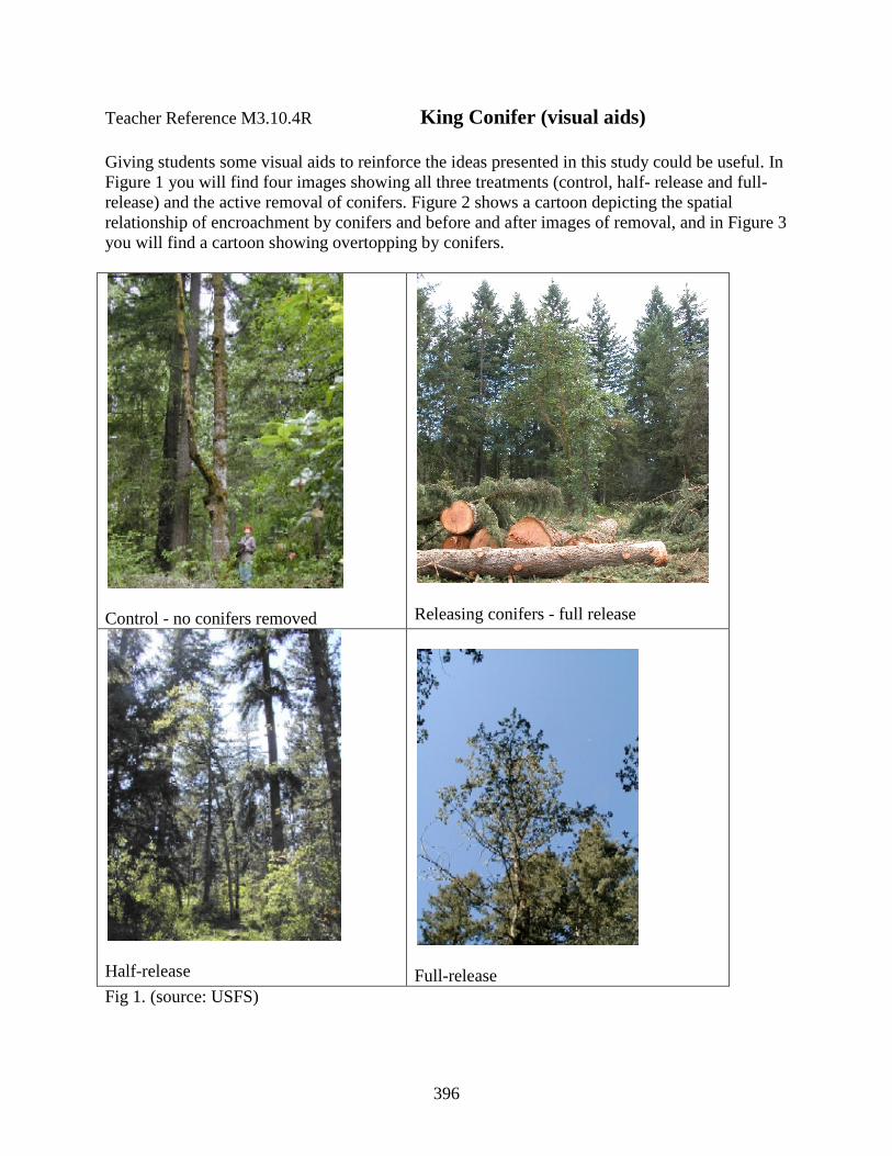
Teacher Reference M3.10.4R King Conifer (visual aids) Giving students some visual aids to reinforce the ideas presented in this study could be useful. In Figure 1 you will find four images showing all three treatments (control, half- release and full-release) and the active removal of conifers. Figure 2 shows a cartoon depicting the spatial relationship of encroachment by conifers and before and after images of removal, and in Figure 3 you will find a cartoon showing overtopping by conifers.

Control - no conifers removed

Releasing conifers - full release

Half-release

Full-release

Fig 1. (source: USFS)

396

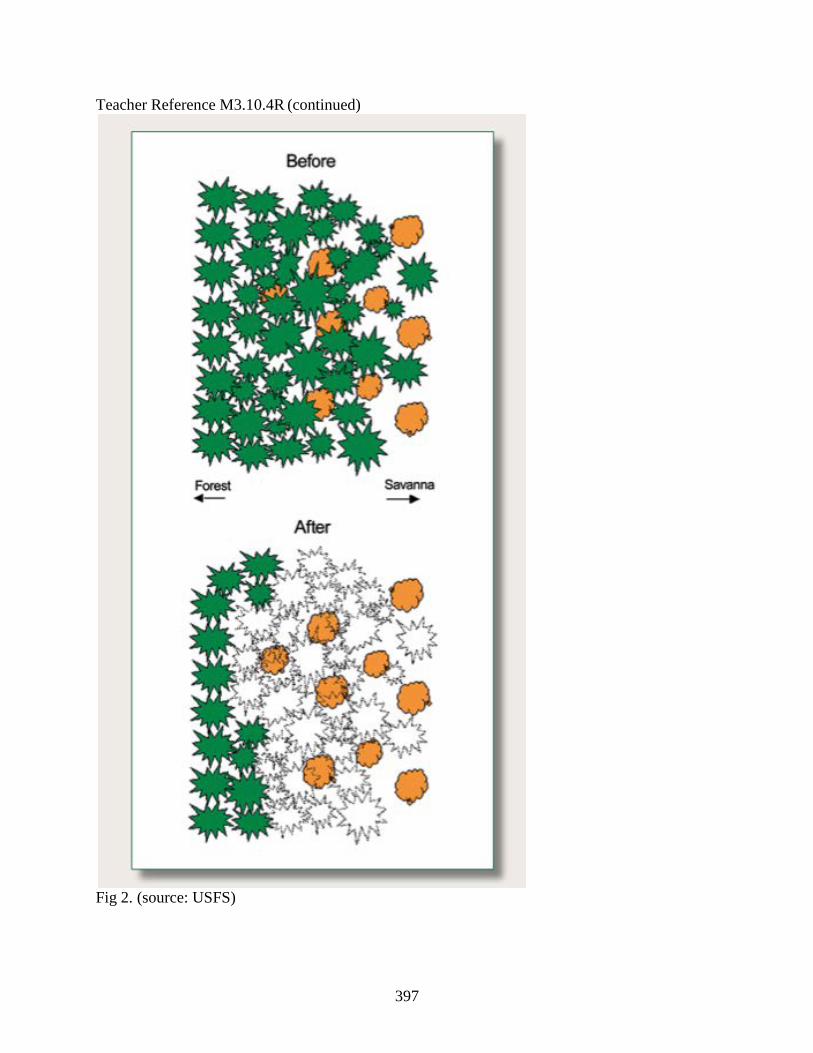
Teacher Reference M3.10.4R (continued)

Fig 2. (source: USFS)

397

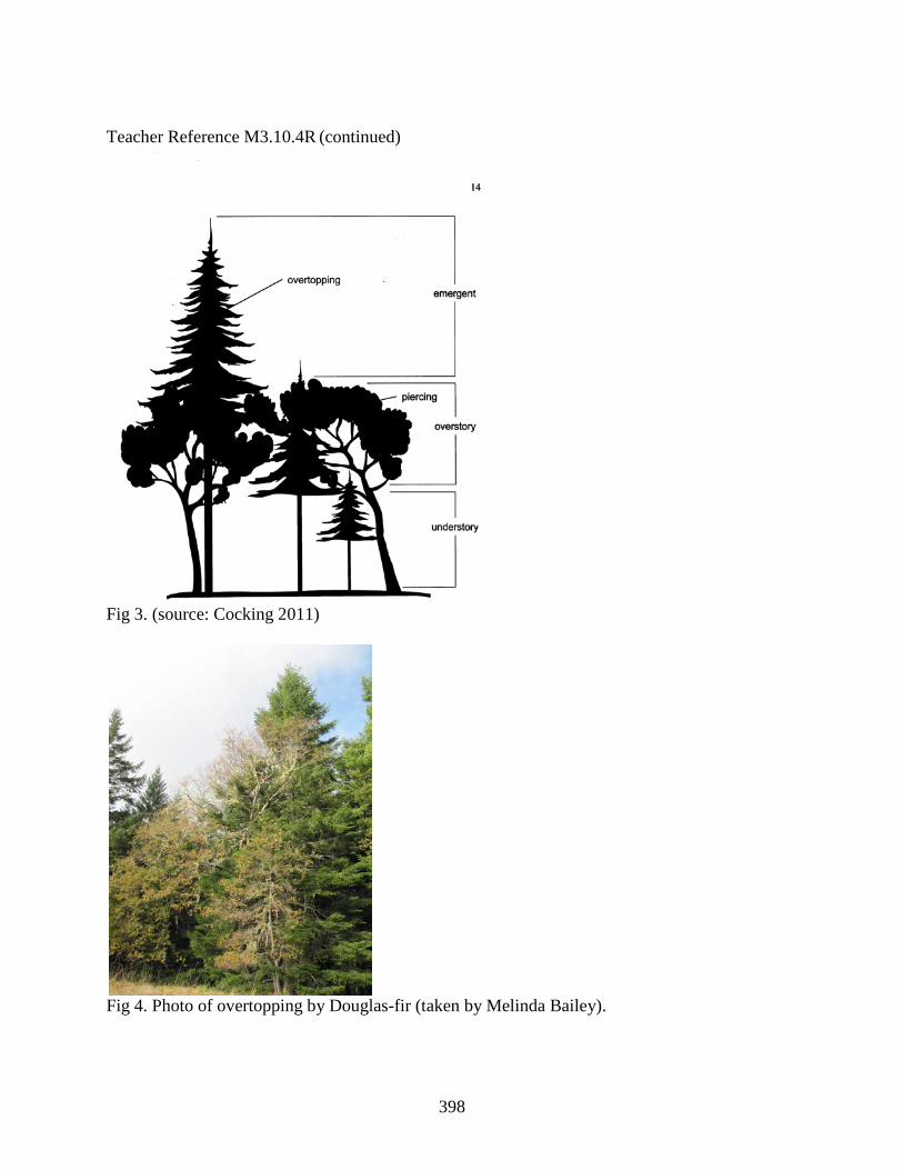
Teacher Reference M3.10.4R (continued)

Fig 3. (source: Cocking 2011)

Fig 4. Photo of overtopping by Douglas-fir (taken by Melinda Bailey).

398

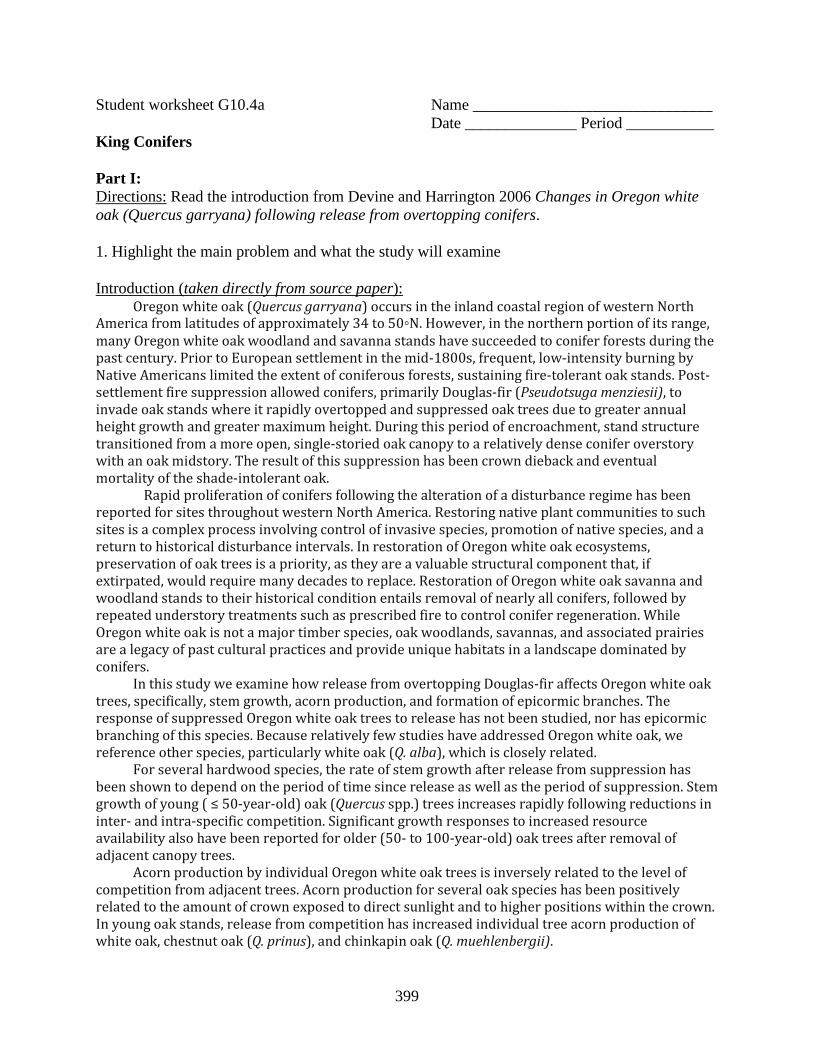
Student worksheet G10.4a Name ______________________________ Date ______________ Period ___________ King Conifers Part I: Directions: Read the introduction from Devine and Harrington 2006 Changes in Oregon white oak (Quercus garryana) following release from overtopping conifers. 1. Highlight the main problem and what the study will examine Introduction (taken directly from source paper): Oregon white oak (Quercus garryana) occurs in the inland coastal region of western North America from latitudes of approximately 34 to 50◦N. However, in the northern portion of its range, many Oregon white oak woodland and savanna stands have succeeded to conifer forests during the past century. Prior to European settlement in the mid-1800s, frequent, low-intensity burning by Native Americans limited the extent of coniferous forests, sustaining fire-tolerant oak stands. Post-settlement fire suppression allowed conifers, primarily Douglas-fir (Pseudotsuga menziesii), to invade oak stands where it rapidly overtopped and suppressed oak trees due to greater annual height growth and greater maximum height. During this period of encroachment, stand structure transitioned from a more open, single-storied oak canopy to a relatively dense conifer overstory with an oak midstory. The result of this suppression has been crown dieback and eventual mortality of the shade-intolerant oak. Rapid proliferation of conifers following the alteration of a disturbance regime has been reported for sites throughout western North America. Restoring native plant communities to such sites is a complex process involving control of invasive species, promotion of native species, and a return to historical disturbance intervals. In restoration of Oregon white oak ecosystems, preservation of oak trees is a priority, as they are a valuable structural component that, if extirpated, would require many decades to replace. Restoration of Oregon white oak savanna and woodland stands to their historical condition entails removal of nearly all conifers, followed by repeated understory treatments such as prescribed fire to control conifer regeneration. While Oregon white oak is not a major timber species, oak woodlands, savannas, and associated prairies are a legacy of past cultural practices and provide unique habitats in a landscape dominated by conifers. In this study we examine how release from overtopping Douglas-fir affects Oregon white oak trees, specifically, stem growth, acorn production, and formation of epicormic branches. The response of suppressed Oregon white oak trees to release has not been studied, nor has epicormic branching of this species. Because relatively few studies have addressed Oregon white oak, we reference other species, particularly white oak (Q. alba), which is closely related. For several hardwood species, the rate of stem growth after release from suppression has been shown to depend on the period of time since release as well as the period of suppression. Stem growth of young ( ≤ 50-year-old) oak (Quercus spp.) trees increases rapidly following reductions in inter- and intra-specific competition. Significant growth responses to increased resource availability also have been reported for older (50- to 100-year-old) oak trees after removal of adjacent canopy trees. Acorn production by individual Oregon white oak trees is inversely related to the level of competition from adjacent trees. Acorn production for several oak species has been positively related to the amount of crown exposed to direct sunlight and to higher positions within the crown. In young oak stands, release from competition has increased individual tree acorn production of white oak, chestnut oak (Q. prinus), and chinkapin oak (Q. muehlenbergii).

399

Epicormic branches are formed following the release of dormant buds, which may be either proventitious (i.e., formed from original buds) or adventitious, such as buds formed in response to injury. Epicormic branch formation has been linked to numerous variables related to suppression and crown dieback and to increased light availability. Epicormic branches can be an important mechanism for increasing total leaf area and photosynthetic capacity, particularly following crown loss due to dieback or damage. Our objectives were to quantify the response of Oregon white oak trees to release from long-term conifer suppression. This analysis contains results from the first 5 years post-treatment. After reading the introduction above answer the following questions: 2. What is the main objective of this study? 3. Identify the main problem and describe the changes in forest structure it has caused. 4. What allowed conifers to invade oak woodland stands? 5. Why is the restoration of Oregon white oak woodland important? 6. What was the duration of this study? Part 2: Directions: Read about the methods used in this study and analyze the three figures by answering the related questions. Methods: All sites were chosen because they had oaks overtopped by conifers. The Douglas-fir trees were removed around each study tree that differed in age and height. The first treatment was a control group where no conifers were removed. The second treatment removed conifers within an area equivalent to half of the radius of the study tree’s height (half-release). The last treatment released all of the conifers within the radius equal to the height of each study tree (full-release). By removing conifers, oaks had access to more light, water, and nutrients. All values represent the averages taken from over 72 overtopped oaks trees in the state of Washington.

page 2

400

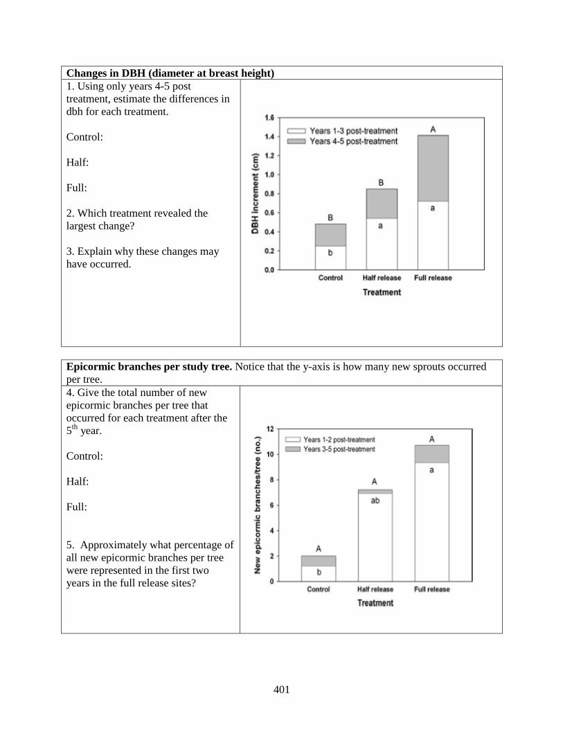
Changes in DBH (diameter at breast height) 1. Using only years 4-5 post treatment, estimate the differences in dbh for each treatment. Control: Half: Full: 2. Which treatment revealed the largest change? 3. Explain why these changes may have occurred.

Epicormic branches per study tree. Notice that the y-axis is how many new sprouts occurred per tree. 4. Give the total number of new epicormic branches per tree that occurred for each treatment after the 5th year. Control: Half: Full: 5. Approximately what percentage of all new epicormic branches per tree were represented in the first two years in the full release sites?

401

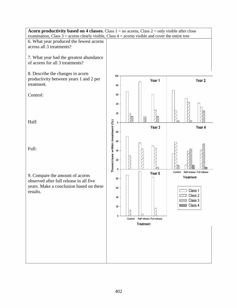
Acorn productivity based on 4 classes. Class 1 = no acorns, Class 2 = only visible after close examination, Class 3 = acorns clearly visible, Class 4 = acorns visible and cover the entire tree 6. What year produced the fewest acorns across all 3 treatments? 7. What year had the greatest abundance of acorns for all 3 treatments? 8. Describe the changes in acorn productivity between years 1 and 2 per treatment. Control: Half: Full: 9. Compare the amount of acorns observed after full release in all five years. Make a conclusion based on these results.

402

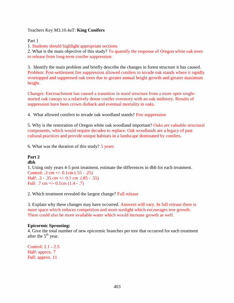
Teachers Key M3.10.4aT: King Conifers Part 1 1. Students should highlight appropriate sections. 2. What is the main objective of this study? To quantify the response of Oregon white oak trees to release from long-term conifer suppression. 3. Identify the main problem and briefly describe the changes in forest structure it has caused. Problem: Post-settlement fire suppression allowed conifers to invade oak stands where it rapidly overtopped and suppressed oak trees due to greater annual height growth and greater maximum height. Changes: Encroachment has caused a transition in stand structure from a more open single-storied oak canopy to a relatively dense conifer overstory with an oak midstory. Results of suppression have been crown dieback and eventual mortality in oaks. 4. What allowed conifers to invade oak woodland stands? Fire suppression 5. Why is the restoration of Oregon white oak woodland important? Oaks are valuable structural components, which would require decades to replace. Oak woodlands are a legacy of past cultural practices and provide unique habitats in a landscape dominated by conifers. 6. What was the duration of this study? 5 years Part 2 dbh 1. Using only years 4-5 post treatment, estimate the differences in dbh for each treatment. Control: .3 cm +/- 0.1cm (.55 - .25) Half: .3 - .35 cm +/- 0.1 cm (.85 - .55) Full: .7 cm +/- 0.1cm (1.4 - .7) 2. Which treatment revealed the largest change? Full release 3. Explain why these changes may have occurred. Answers will vary. In full release there is more space which reduces competition and more sunlight which encourages tree growth. There could also be more available water which would increase growth as well. Epicormic Sprouting: 4. Give the total number of new epicormic branches per tree that occurred for each treatment after the 5th year. Control: 2.1 - 2.5 Half: approx. 7 Full: approx. 11

403

Teachers Key M3.10.4a (continued) 5. Approximately what percentage of all new epicormic branches per tree were represented in the first two years in the full release sites? 80% (approx. 9 out of 11 therefore 9/11 = 80%) Note: Out of all branches the first two years contributed to 92% Acorn Productivity 6. What year produced the fewest acorns across all 3 treatments? Year 5 7. What year had the greatest abundance of acorns for all 3 treatments? Year 4 8. Describe the changes in acorn productivity between years 1 and 2 per treatment. Control: Differences not severe. Greatest difference in Class 3, which showed a 50% increase in the 2nd year. Half: Class 1 decreased from 90 to 60% in year 2, Large change in Class 2. No trees observed in year 1 and 50% of trees fell into this category in year 2. Class 3 - a decrease occurred in year 2 from approx. 10 to 5%. Full: Class 1 - small decrease in the 2nd year 60 - 40%, Class 2 increased 2nd year from 30 - 45% or so, Class 3 approx. 50 % increase observed. Changed from 15 to 30% in year 2. 9. Compare the amount of acorns observed after full release in all five years. Make a conclusion based on these results. Answers will vary. Students should be able to see that the full release produced more acorns over all since more trees feel into classes 3 and 4 in the first 4 years and in the low production year (year 5) full release had the largest % of trees in Class 2.

404

M3.G10 Lesson 5: Friendly Fire Unit Overview: Oak Woodlands Grade 10 Key Concepts:

• Stability and change • Review evidence of

how changing conditions may result in a new ecosystem

• Interdependent relationships in ecosystems

• Biodiversity and human activities

Time: 60 - 90 minutes Materials for the Teacher: Student worksheet and

teacher key M3.10.5a M3.10.5R, Case Study

of the Bald Hills Dictionaries for

student use (optional) Pictures of the Bald

Hills (optional) Connections: Park management, recreation, fire ecology, biodiversity, forest health, agriculture, forest management, climate change, air quality, forest conservation, Native American studies, environmental stewardship, careers, community planning

Learning Objectives: Students will compare past and present land management practices in the Bald Hills of Redwood National Park. They will read a scientific paper in groups and will describe structural and compositional changes in vegetation caused from the use and suppression of fire. They will be able to explain the advantages of using fire as a tool for restoration. Background information: Refer to the appropriate section in Part II: Teacher Companion for Module 3 and the attached paper (M3.10.5R). Underwood, S., and L. Arguello, N. Sieflki. 2003. Restoring Ethnographic Landscapes and Natural Elements in Redwood National Park, Ecological Restoration 21(4): 278-283. Suggested procedure: Begin this lesson by explaining the main objectives above. Students should have some background knowledge about the affects of overtopping from conifers and the benefits of fire in grasslands and oak woodlands (see previous lesson). You may want to show pictures of the Bald Hills area and give a brief background before students read the attached paper (see online resources). In this lesson, students will read about a case study that discusses the past and present land management practices in Redwood National Park. This area has been managed using fire for a thousand years until the early 1900s when fire was halted. Pollen studies show oak woodland habitat existed at least five thousand years ago. Today fire has been reintroduced as a restoration tool to encourage biodiversity and to support Native American cultural practices. The area covers more than 4,000 acres and much of it is periodically burned to reduce conifer encroachment. In other places, conifers are manually thinned or girdled. To begin students should read the paper cited above alone or in groups (see M3.10.5R). Inform them that they may find the reading challenging because it comes from a scientific journal and is written at a college level. (Perhaps they can treat it as a challenge.) Give a few examples from the article and see if they can comprehend their meaning. For instance what does post-burn mean? What does harvesting ungulates imply? Encourage them to use a dictionary to help understand some of the issues if necessary. As they read the article they should answer the questions on the student worksheet (see M3.10.5a). While doing so they will describe the historical and ecological setting of the Bald Hills; compare changes in vegetative structure and composition over time; and explain why fire is being used as a restoration tool. Once they have completed the worksheet,

405

Forest Ecology Series integration: M1: Integrative Forest Ecology M2: Coast Redwood

check for understanding by asking some of the follow-up questions below. Have them discuss future implications and possible conflicts that could arise if the existing management plan were to continue the way they are or change. If possible end this series with a field trip to the Bald Hills where students can meet the park managers and see firsthand the effects of using fire as a management tool.

Follow-up questions • Where does this case study take place? • Who maintained the oak woodland savannah here before the 1900s? • Why do Native Americans use fire as a management tool? • How have fire suppression and other human activities change the composition and

structure of the vegetation? • Do you think fire is more difficult to use today because of these changes? • What plan has been implemented in the park to improve biodiversity? • Is the park considering traditional use of the Bald Hills in their plan? Explain. • Is the park’s management plan working? • What sorts of conflict might result in the current management strategy? • What would happen if the park stopped using fire to manage the bald hills? • If you were a land manager in charge of the Bald Hills, how would you handle the

situation? Critical Thinking: What considerations does a park manager need to include when making a park management plan? Assume that the park is known for its beauty, wildlife, and recreational values that need to be maintained into perpetuity. Keywords: biodiversity, conifer, coniferous, encroachment, ethnographic, exotic, mortality, overtopping, restoration, understory, ungulate, vascular plants NGSS alignment: HS-LS2: Ecosystems: Interactions, Energy, and Dynamics LS2.A Interdependent Relationships in Ecosystems LS2.C Ecosystem Dynamics, Functioning, and Resilience LS4.D Biodiversity and Humans HS-LS-6: Evaluate claims, evidence, and reasoning that the complex interactions in ecosystems maintain relatively consistent numbers and types of organisms in stable conditions, but changing conditions may result in a new ecosystem Online resources: USFS: Coast Redwood Ecology and Management http://www.redwood.forestthreats.org/baldhillsfire.htm Good pictures and general information about the Bald Hills and the use of fire as a management tool is available on this site. It is managed by Steve Norman an ecologist for US Forest Service and also includes links to the redwood forest ecology.

406

(online resources continued) California Fire Science Consortium: Northern California http://www.cafiresci.org/northern-ca/#2 This is a great site to learn more about fire science. Links to fuel and fire in Oregon white oak forests and the wildfire trends in Northern California are just some of the topics found here. RNSP: Plan Your Visit http://www.nps.gov/redw/planyourvisit/index.htm This site is the official place to plan a visit to Redwood National and State Park. It includes links to current weather conditions, gives camping information, assorted maps, and contact information. EEI Connection: B.6.a. Biodiversity: The keystone of Life on Earth B.6.b. Ecosystem Change in California B.8.a Differential Survival of Organisms Answers to follow-up questions: - Where does this case study take place? (RNP Bald Hills) - Who maintained the oak woodland savanna here before the 1900s? (Native Americans; specifically the Chilula and Yurok tribes) - Why do Native Americans use fire as a management tool? (they use fire to enhance the quality or abundance of desirable plant and animals species used for food, basketry, medicine, and ceremony) - How have fire suppression and other human activities change the composition and structure of the vegetation? (Coniferous forests have replaced oak woodlands, grazing brought in non-native grass species, and logging increase erosion) - Do you think fire is more difficult to use today because of these changes? (answers will vary. Most students will probably make the connection that conifers burn hotter and that understory builds up creating more fuels making the use of fire in some places near impossible. They may also bring up the fact that fire is still considered bad, dangerous and ugly to most visitors. There are health issues such as poor air quality and asthma. ) - What plan has been implemented in the park to improve biodiversity? (Manual removal of unwanted conifers and prescribed burning. The name of the plan is the Bald Hills Management Plan and was instituted in 1992) - Is the park considering traditional use of the Bald Hills in their plan? Explain. (Yes - they have identified the Bald Hills as an archeological district and have identified parts as a cultural and ethnographic landscape. They did extensive research to learn about the traditional uses of the Bald Hills and they try use pre-settlement disturbance as a reference point for restoration. Currently, Native Americans have the opportunity to participate in the plan) - Is the park’s management plan working? (So far the plan has increased native species diversity, reduced fuel loads, and has reduced some key exotic species. The plan is described as successful and the fire program has treated 500 acres of oak woodland and 2,000 acres of prairie)

407

(answers to follow-up questions continued) -What sorts of conflict might result in the current management strategy? (answers will vary. There could be a gender issue. Management decisions tend to permit female pursuits such as collecting material for basketry, however male activities such as hunting are prohibited. Other conflicts could arise from the reintroduction of elk, which like to eat young hazelnut. Also, visitors may be resistant to the ideas of fires in the landscape. Black hills and snags are not very beautiful to look at) - What would happen if the park stopped using fire to manage the bald hills? (answers will vary. It would mostly likely revert to coniferous forest in many places. Also a decease in overall biodiversity would likely occur) - If you were a land manager in charge of the Bald Hills, how would you handle the situation? (answers will vary) Suggested extensions:

• Identify different ways forests are used for human and environmental needs. • Assign different roles that exist between different interest groups pertaining to a

hypothetical land-management debate and have students support their position. • Invite a forest or fire ecologists into your classroom to discuss the pros and cons of using

fire in forest management. • Show a wildlife video of a grassland ecosystem depicting the abundant wildlife that

depends on these open places. • Integrate physics and chemistry into the intensity and behavior of fire. Certain fuels burn

hotter, more oxygen fans flames, and all matter and energy is converted into different forms.

• Have students learn the common grasses that inhabit coastal and inland prairies. • Discuss some of the issues regarding loss of oak woodland habitat such as human

population growth, demand for vineyards, and the need for firewood. • Learn about the effects of wildland fires in other national parks, such as Yellowstone and

Yosemite. • Take a field trip to the Bald Hills area or another oak woodland/prairie ecosystem.

M3.10.5a Student worksheet M3.10.5aT Teacher key M3.10.5R copy of cited paper (Case Study)

408

Student worksheet M3.10.5a Name ______________________________ Date________________ Period _________ Friendly Fire Instructions: Read the journal article below Restoring Ethnographic Landscapes in Natural Elements in Redwood National Park. Learn how past and present land management practices have changed the vegetative structure and about the importance fire has at maintaining biodiversity and cultural practices associated with this particular landscape. 1. Describe the setting of the Balds Hills. Include the location, acreage, elevation, and the vegetative types found here. 2. What is the traditional view or philosophy for how to manage a National Park? 3. Give a sequential overview of past human interactions and disturbances that have taken place in the Bald Hills. Include the approximate dates beginning with about one thousand years ago and ending with the purchase of the park. 4. Identify three environmental changes that have occurred since the suppression of fire in the early 1900s due to human activities. Give both the cause and the effect.

409

5. What was the probable vegetative composition of the Bald Hills 5,000 years ago? What studies provide clues to past vegetation? 6. What types of trees were likely the most common here thousands of years ago? 7. Why did Native Americans use fire to manage this area? 8. Give an example of a plant that is managed for basketry. 9. Give an example of a plant that is managed for food. 10. What evidence is there that the Native Americans used burning as a management tool? 11. When did the park staff and researchers begin ecological studies of the Bald Hills? 12. What threats did they observe? 13. What were the main objectives of the Bald Hills Management Plan? 14. Three main efforts were implemented after the plan was established, what were they?

page 2

410

15. What was the main tool used for restoring oak woodlands and prairies? 16. Why has fire been used a restoration tool? 17. How many hectares/acres have been treated? Include the first year and active treatments. 18. How does the General Management Plan (in place after the implementation of fire and erosion control) make provisions for Native American values and practices? 19. What conflicts could arise in the future regarding the current management plan or the park’s mission? 20. An ungulate is a four-legged animal with hooves such as a cows and deer. What large ungulate inhabits the prairies? 21. If burning were to stop, predict how the vegetation would change along the prairie edges. Use some of the vocabulary words given in this lesson. 22. Do you think the park’s plan has been successful? Support your reasoning.

page 3

411

Teacher key M3.10.5aT: Friendly Fire 1. Describe the setting of the Balds Hills. Include the location, acreage, elevation, and the vegetative types found here. The Bald Hills lie between the Klamath River and Redwood Creek in NW California. The area covers approx. 1700 ha (4200 ac) at an elevation of 76 - 945 m (250 - 3100 ft). Most of the ridge tops are covered by coastal grasslands (prairies) and oak woodlands. 2. What is the traditional view or philosophy for how to manage a National Park? That parks be maintained in their natural condition. No comprehensive definition of natural has been determined however. 3. Give a sequential overview of past human interactions and disturbances that have taken place in the Bald Hills. Include the approximate dates beginning with about one thousand years ago and ending with the purchase of the park. Answers should approximate the following: Approx 1,000 yrs ago - Yuroks arrived into the region and most likely began managing the land. They collected grass seeds, basketry material, acorns and hunted game. About 700 yrs ago - the Chilula and Hupa tribes occupied areas and utilized resources here. late 1800s - discovery of gold. 1850s - Miners made a supply line through the Bald Hills. Led to bloody skirmishes and displacement of the Chilula peoples. 1860s - permanent Euro-American settlement. Arrival of the Lyons family who ran sheep and cattle. They burned to improve forage, to prevent conifer encroachment. Intense grazing probably influenced the establishment of exotic grasses. 1930s to 1970s - Commercial logging of conifers. Increased road building. 4. Identify three environmental changes that have occurred since the suppression of fire in the early 1900s due to human activities. Give both the cause and the effect. Cause: lack of fire Effect: one-quarter of the original extent of the bald hills changed to coniferous forest and another half of the area was threatened. Cause: grazing/ranching Effect: introduction of exotic species Cause: logging Effect: increased erosion 5. What was the probable vegetative composition of the Bald Hills 5,000 years ago? What studies provide clues to past vegetation? Prairies (balds) and oak woodlands. Pollen studies are used. 6. What types of trees were likely the most common here thousands of years ago? The main trees were likely Oregon white oak, California black oak, California bay, big-leaf maple, and tanbark oak. 7. Why did Native Americans use fire to manage this area? Native American management helped to create and maintain oak woodlands, they intentionally burned to make fire yards and fire corridors. 8. Give an example of a plant that is managed for basketry. Hazelnut (hazel trees) 9. Give an example of a plant that is managed for food. Oaks (acorns), grasses 10. What evidence is there that the Native Americans used burning as a management tool?

412

Teacher key M3.10.5a (continued) Answers will vary. They helped maintain tanoak groves. The evidence is even-aged tanoak stands that can still be found. Tanoaks are not fire resistant. 11. When did the park staff and researchers begin ecological studies of the Bald Hills? They began in 1978 12. What threats did they observe? Conifer encroachment, exotic species invasion, increased erosion from logging/ranching roads. 13. What were the main objectives of the Bald Hills Management Plan? The dominant management strategy was to reverse or minimize the immediate effects of post-settlement impacts and to maintain the highest diversity of pre-European plants and animals possible. 14. Three main efforts were implemented after the plan was established, what were they? The restoration of prehistoric fire regimes Control of invasive exotics Control of encroachment of conifers within the prairies and oak woodlands 15. What was the main tool used for restoring oak woodlands and prairies? Fire. They also manually removed conifers. 16. Why has fire been used a restoration tool? Post-burn fire effects have increased native species diversity, reduced fuel loads, has caused conifer seedling mortality, and helped reduce key exotic plant species. 17. How many hectares/acres have been treated? Include the first year and active treatments. About 607 ha (1500 ac) were treated in the first year. 202 - 809 (500 - 2000 ac) are actively treated 18. How does the General Management Plan (in place after the implementation of fire and erosion control) make provisions for Native American values and practices? The plan provides contemporary Native Americans the opportunity to participate in the identification, designation, and management of cultural and enthnographic landscapes within the park. Prescribed burning can be used to promote the desired quantity and quality of natural materials valued by Native Americans. 19. What conflicts could arise in the future regarding the current management plan or the park’s mission? Answers will vary. Native Americans have expressed an interest in hunting elk (harvesting ungulates), which is not currently allowed. The park tends to favor or allow female pursuits such as basketry and not male activities such as hunting and fishing. 20. An ungulate is a four-legged animal with hooves such as a cows and deer. What large ungulate inhabits the prairies? Roosevelt elk (there are also deer) 21. If burning were to stop, predict how the vegetation would change along the prairie edges. Use some of the vocabulary words given in this lesson. Answers will vary. They should be able to note there would be a lack of biodiversity and an increase in coniferous forest. 22. Do you think the park’s plan has been successful? Support your reasoning. Accept all reasonable responses.

413

M3.10.5R

414

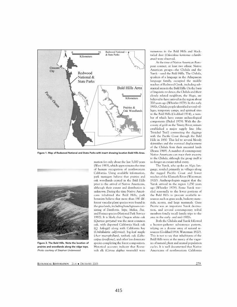
415

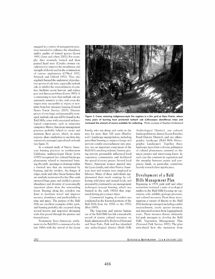
416

417

418

419

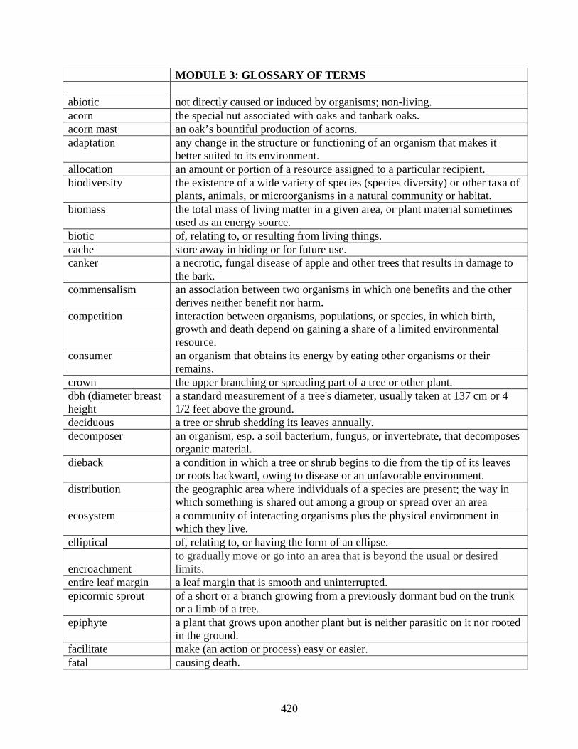
MODULE 3: GLOSSARY OF TERMS abiotic not directly caused or induced by organisms; non-living. acorn the special nut associated with oaks and tanbark oaks. acorn mast an oak’s bountiful production of acorns. adaptation

any change in the structure or functioning of an organism that makes it better suited to its environment.

allocation an amount or portion of a resource assigned to a particular recipient. biodiversity

the existence of a wide variety of species (species diversity) or other taxa of plants, animals, or microorganisms in a natural community or habitat.

biomass

the total mass of living matter in a given area, or plant material sometimes used as an energy source.

biotic of, relating to, or resulting from living things. cache store away in hiding or for future use. canker

a necrotic, fungal disease of apple and other trees that results in damage to the bark.

commensalism

an association between two organisms in which one benefits and the other derives neither benefit nor harm.

competition

interaction between organisms, populations, or species, in which birth, growth and death depend on gaining a share of a limited environmental resource.

consumer

an organism that obtains its energy by eating other organisms or their remains.

crown the upper branching or spreading part of a tree or other plant. dbh (diameter breast height

a standard measurement of a tree's diameter, usually taken at 137 cm or 4 1/2 feet above the ground.

deciduous a tree or shrub shedding its leaves annually. decomposer

an organism, esp. a soil bacterium, fungus, or invertebrate, that decomposes organic material.

dieback

a condition in which a tree or shrub begins to die from the tip of its leaves or roots backward, owing to disease or an unfavorable environment.

distribution

the geographic area where individuals of a species are present; the way in which something is shared out among a group or spread over an area

ecosystem

a community of interacting organisms plus the physical environment in which they live.

elliptical of, relating to, or having the form of an ellipse.

encroachment to gradually move or go into an area that is beyond the usual or desired limits.

entire leaf margin a leaf margin that is smooth and uninterrupted. epicormic sprout

of a short or a branch growing from a previously dormant bud on the trunk or a limb of a tree.

epiphyte

a plant that grows upon another plant but is neither parasitic on it nor rooted in the ground.

facilitate make (an action or process) easy or easier. fatal causing death.

420

M3: Glossary of Terms (continued) foliar of or relating to leaves. food web A system of interlocking and interdependent food chains granary

a storehouse for threshed grain or in the case of acorns a store house of seeds.

herbivory the eating of plants, especially ones that are still living. host an organism on or within which a parasite or commensal organism lives. hybridize

(of an animal or plant) breed with an individual of another species or variety.

interaction reciprocal action or influence. intolerance (of a plant or animal) unable to survive exposure to (physical influence). keystone species

a species on which other species in an ecosystem largely depend, such that if it were removed the ecosystem would change drastically.

leaf margin the structure of the leaf edge. lichen

a plant-like organism that typically forms a low crustlike, leaflike, or branching growth on rocks, walls, and trees. It is a mutualistic relationship between a fungus and either a cyanobacterium or an alga.

lobed leaf a leaf having deeply indented margins as in a maple leaf. luminance

the intensity of light emitted from a surface per unit area in a given direction.

mistletoe

a leathery-leaved parasitic plant that grows on apple, oak, and other broadleaf trees and bears white glutinous berries in winter.

morphology

the branch of biology that deals with the form of living organisms, and with relationships between their structures.

mortality the state of being subject to death. moss

a small flowerless green plant that lacks true roots, growing in low carpets or rounded cushions in damp habitats and reproducing by means of spores released from stalked capsules.

mutualism symbiosis that is beneficial to both organisms involved (a +/+ relationship). natural selection

the process whereby organisms better adapted to their environment tend to survive and produce more offspring.

oak gall

a tumor-like growth that is made after an egg laid in plant tissues hatches and promotes plant tissues to grow around it.

overtopping exceed in height. paleoecology the ecology of fossil animals and plants. palynology

the study of pollen grains and other spores, esp. as found in archaeological or geological deposits.

parasite

an organism that lives in or on another organism (its host) and benefits by deriving nutrients at the host's expense.

pathogen a parasite (bacterium, virus, or other microorganism) that causes a disease. pathologist the science of the causes and effects of diseases. percent error

the approximation error in some data is the discrepancy between an exact value and some approximation to it.

421

M3: Glossary of Terms (continued) pollination

convey pollen to or deposit pollen on (a stigma, ovule, flower, or plant) and so allow fertilization.

predation the preying of one animal on others. predator an animal that naturally preys on others. producer

An organism that can produce its own food by photosynthesis or chemosynthesis; also called a primary producer.

productivity

the rate of production of new biomass by an individual, population, or community; the fertility or capacity of a given habitat or area.

regeneration

the action or process of regenerating or being regenerated, in particular the formation of new animal or plant tissue.

release allow or enable to escape from confinement; set free. sapling a young tree, esp. one with a slender trunk. seedling a young plant, esp. one raised from seed and not from a cutting. serrated leaf margin a leaf margin that is coarsely or finely toothed. simple leaf leaves that are not compound - only one leaflet occurs. succession

the change in species composition over time as a result of abiotic and biotic agents of change.

suppression

the failure to develop of some part or organ of a plant; in trees the inability to grow due to lack of light because the crowns are generally below the level of the canopy.

symptom

a physical or mental feature that is regarded as indicating a condition of disease.

synchronized cause to occur or operate at the same time or rate. taxonomy

the branch of science concerned with classification, esp. of organisms; systematics.

tolerance the capacity to survive stressful environmental conditions, without adverse reaction.

treatment

The experimental variable that is manipulated by the researcher and evaluated by its measurable effect on the dependent variable or variables in an experiment or study.

trophic level

each of several hierarchical levels in an ecosystem, comprising organisms that share the same function in the food chain and the same nutritional relationship to the primary sources of energy.

variable an element, feature, or factor that is liable to vary or change. water mold

any of a group of fungi-like organisms that live in water or soil, many of which are parasitic on plants.

422

APPENDIX F

GOING FURTHER Planning an Outdoor Field Trip: Here are a few things to consider when planning an outdoor field trip: What is the educational goal of the field trip? How can you integrate the trip into your curriculum? Does your district have a field trip policy? What is a realistic and/or necessary ratio of chaperones to students? Will you use parent vehicles or pay for a school bus? Do you need special permission slips? What items will be necessary to bring? Are you stopping at any places where students need money? How can students best prepare for their outdoor experience? Are docents available to greet you at your site? Have you stimulated their interest for the trip? What expectations do you have during their adventure? Do you or the bus driver have a first aid kit? Is there a risk of encountering poison oak, ticks, or bees? What problems might exist that you can prepare for?

Before you leave: Prepare a packing list that you send home a few days ahead of time. Check that students have proper attire including good walking shoes. Have copies of permission slips, a student roster, and an accurate head count. Pack all necessary equipment in an organized fashion. Review with the students your expectations including proper outdoor etiquette. Set clear boundaries once you arrive at your site. Remind students to treat natural areas and wildlife with respect. Discuss the role of your chaperones with them ahead of time. Have a list of contact information in case you are running late or have an emergency. Exchange cell phone numbers with all drivers.

Some outdoor etiquette: Students should use low voices and stay relatively quiet and still. Stay on designated trails unless permission is given otherwise. Be aware that trampling can cause damage to tree roots. Keep numbers small. Do not collect any plant, animal, or rocks unless it is specific to your study. Do not feed the wildlife. Do not litter or vandalize. Leave the place better than how you found it. Take pictures instead of objects.

423

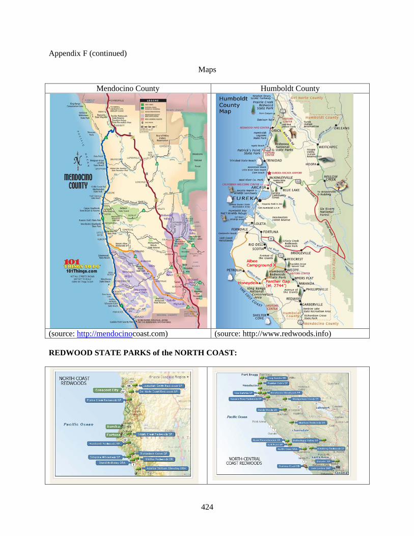
Appendix F (continued)

Maps

Mendocino County Humboldt County

(source: http://mendocinocoast.com) (source: http://www.redwoods.info) REDWOOD STATE PARKS of the NORTH COAST:

424

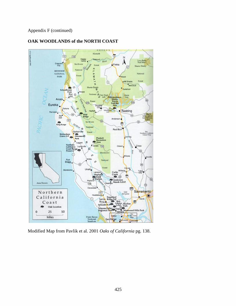
Appendix F (continued) OAK WOODLANDS of the NORTH COAST

Modified Map from Pavlik et al. 2001 Oaks of California pg. 138.

425

Appendix F (continued)

Useful Links

General Information Berkeley Natural History Museums http://bnhm.berkeley.edu/ Humboldt State Natural History Museum http://www.humboldt.edu/natmus/ Mendocino National Forest http://www.fs.usda.gov/mendocino/ PORTS (Parks Online Resources for Teachers and Students http://www.ports.parks.ca.gov/?page_id=22922 Six Rivers National Forest http://www.fs.usda.gov/srnf/ University of California: Forest Research and Outreach http://ucanr.edu/sites/forestry/California_forests/

Redwoods Arcata City Forest http://www.cityofarcata.org/departments/environmental-services/city-forests Benbow Lake State Recreation Area http://www.parks.ca.gov/?page_id=426 California’s Redwood Coast: http://redwoods.info/index.asp Grizzly Creek Redwood State Park http://www.parks.ca.gov/?page_id=421 Headwaters Forest Reserve (BLM) http://www.blm.gov/ca/st/en/fo/arcata/headwaters.html Humboldt Redwoods State Park http://humboldtredwoods.org/ McKay Tract Community Forest http://www.humtrails.org/mckay.html Montgomery Woods State Natural Reserve http://www.parks.ca.gov/?page_id=434 Redwood Adventures http://www.redwood-edventures.org/teachers-fieldtrips.php Redwood Ed - A guide to the Coast Redwoods for Teachers and Learners http://www.parks.ca.gov/?page_id=25395 Redwood National and State Park Teacher page http://redwood.areaparks.com/parkinfo.html?pid=24778 Richardson Grove State Park http://www.parks.ca.gov/?page_id=422 Save the Redwoods League - Redwoods Learning Center http://education.savetheredwoods.org/kit/index.php Smithe Redwoods State Natural Reserve http://www.parks.ca.gov/?page_id=427 Standish-Hickey State Recreation Area http://www.parks.ca.gov/?page_id=423

426

Appendix F (continued)

Useful Links

Oak Woodlands Angelo Coast Range Reserve http://nrs.ucop.edu/reserves/angelo/angelo.htm Hastings Reserve http://www.hastingsreserve.org/ King Range National Conservation Area (BLM) http://www.blm.gov/pgdata/content/ca/en/fo/arcata/kingrange/index.html Lack’s Creek Recreational Area (BLM) http://www.blm.gov/ca/st/en/fo/arcata/lacks_creek.html North Coast Regional Land Trust (contact Shayne Green) http://ncrlt.org/ Redwood National and State Parks (The Bald Hills) http://www.nps.gov/redw/planyourvisit/index.htm Southern Humboldt Community Park http://www.sohumpark.org/

427