An Improved Lower Bound for Depth Four Arithmetic Circuits A THESIS SUBMITTED FOR THE DEGREE OF Master of Science (Engineering) IN THE Faculty of Engineering BY Abhijat Sharma Computer Science and Automation Indian Institute of Science Bangalore – 560 012 (INDIA) July, 2017

Welcome message from author
This document is posted to help you gain knowledge. Please leave a comment to let me know what you think about it! Share it to your friends and learn new things together.
Transcript

An Improved Lower Bound for Depth Four Arithmetic
Circuits
A THESIS
SUBMITTED FOR THE DEGREE OF
Master of Science (Engineering)
IN THE
Faculty of Engineering
BY
Abhijat Sharma
Computer Science and Automation
Indian Institute of Science
Bangalore – 560 012 (INDIA)
July, 2017

Declaration of Originality
I, Abhijat Sharma, with SR No. 04-04-00-10-21-14-1-11590 hereby declare that the ma-
terial presented in the thesis titled
An Improved Lower Bound for Depth Four Arithmetic Circuits
represents original work carried out by me in the Department of Computer Science and
Automation at Indian Institute of Science during the years 2014-2017.
With my signature, I certify that:
• I have not manipulated any of the data or results.
• I have not committed any plagiarism of intellectual property. I have clearly indicated and
referenced the contributions of others.
• I have explicitly acknowledged all collaborative research and discusions.
• I have understood that any false claim will result in severe disciplinary action.
• I have understood that the work may be screened for any form of academic misconduct.
Date: Student Signature
In my capacity as supervisor of the above-mentioned work, I certify that the above statements
are true to the best of my knowledge, and I have carried out due diligence to ensure the
originality of the report.
Advisor Name: Advisor Signature
1


c© Abhijat Sharma
July, 2017
All rights reserved


DEDICATED TO
My beloved family
who taught me to endure and always follow my heart.

Acknowledgements
I’d like to thank my advisor Chandan Saha for his continuous help and support during my entire
stay at IISc. His precious advice and suggestions have shaped my thesis work significantly. He
has been instrumental in providing direction to my research, and getting me back on track in
times when I got distracted. My colleagues at the Complexity Theory Lab have always been an
immense help. The countless group-discussions and presentations provided valuable contribu-
tion to my work. Especially, I can never thank Vineet enough for showing great patience and
consideration while revising my final submission. Sumant has been my neighbour in the lab,
and I have always drawn inspiration and motivation from seeing him work hard.
I have been very fortunate to have a large group of friends at IISc, some at CSA and some at
my hostel, who made my stay memorable and supported me through the thick and thin. My
fellow ‘theoreticians’ Mayank, Datta, Giri and Indranil, and other CSA mates Akhil, Saravanan,
Aritra, Shyam and Sneha, have all been great company as we strived towards our respective
life goals. I must also mention the valuable philosophical discussions with Rupam, Abhishek
and Gulshan, carrying me through sleepless nights in the hostel. Bangalore is a lovely city and
I spent some good times here with my friends from IIIT-H, Utsav, Mudit and Kartik, who were
there whenever I needed a little break from work.
I would like to thank my professor from IIIT-H, Kannan Srinathan, who was my first inspiration
to pursue research in mathematics and theoretical computer science, and has been a guiding
light ever since. Finally and most importantly, I convey my regards and gratitude to all the
members of my family who have been my supreme source of confidence. I was always inspired
to pursue a career in academics, by my Dadaji and Nanaji, who have been elite professors of
science. The vast amount of faith and blessings that I receive from Dadi, Nani and all my elders,
always lifts my spirits up and keeps me working hard to make them proud. My salutations to
my parents, my pillars of support who always believed in me, and my little sister Anu for those
chirpy little phone calls that worked as instant stress-relief.
i

Abstract
We study the problem of proving lower bounds for depth four arithmetic circuits. Depth four
circuits have been receiving much attraction when it comes to recent circuit lower bound results,
as a result of the series of results culminating in the fact that strong enough lower bounds for
depth four circuits will imply super-polynomial lower bounds for general arithmetic circuits,
and hence solve one of the most central open problems in algebraic complexity i.e a separation
between the VP and VNP classes. However despite several efforts, even for general arithmetic
circuits, the best known lower bound is Ω(N logN) by [BS83], where N is the number of input
variables. In the case of arithmetic formulas, [Kal85] proved a lower bound that is quadratic in
the number of input variables, which has not seen any improvement since then. The situation
for depth three arithmetic circuits was also similar for many years, until a recent result by
[KST16] achieved an almost cubic lower bound that improved over the previous best quadratic
bound by [SW99].
As the main contribution of this thesis, we prove an Ω(N1.5) lower bound on the size of a depth
four circuit, for an explicit multilinear N -variate polynomial in VNP with degree d = Θ(√N).
Our approach offers a potential route to proving a super-quadratic lower bound for depth four
circuits. Taking cue from the numerous successful results recently, we use the technique of the
shifted partial derivatives measure to achieve the said lower bound. Particularly, we use the
Dimension of Projected Shifted Partials (DPSP) measure which has been previously used in
[KLSS14] and [KS15]. Coming to the choice of the hard polynomial, we again follow the status
quo and use a variant of the Nisan-Wigderson (NW) polynomial family that has proved to be
very helpful over the past few years in arithmetic circuit complexity.
Finally, we do a careful analysis of [SS97] and [Raz10] and compare their techniques to ours.
We conclude that our result can potentially be used as a starting point, and techniques similar
to [KST16] can likely be used to strengthen our lower bound to Ω(N2.5), for general depth
four arithmetic circuits. However, unlike depth three circuits, proving a super-quadratic lower
ii

Abstract
bound for depth four circuits remains a prevalent open problem for many years. Previous work
like [SS97] and [Raz10] implied super-linear lower bounds. To the best of our knowledge, the
previous best known lower bound for general depth four circuits is Ω(N1.33).
iii

Contents
Acknowledgements i
Abstract ii
Contents iv
List of Figures vi
1 Introduction 1
1.1 Background . . . . . . . . . . . . . . . . . . . . . . . . . . . . . . . . . . . . . . 1
1.2 Constant Depth Circuits and Motivation . . . . . . . . . . . . . . . . . . . . . . 2
1.3 Previous Work . . . . . . . . . . . . . . . . . . . . . . . . . . . . . . . . . . . . 4
1.4 Our Contribution . . . . . . . . . . . . . . . . . . . . . . . . . . . . . . . . . . . 5
1.5 Organisation . . . . . . . . . . . . . . . . . . . . . . . . . . . . . . . . . . . . . . 6
2 Preliminaries 7
2.1 Basic Definitions and Notations . . . . . . . . . . . . . . . . . . . . . . . . . . . 7
2.2 Random Restrictions . . . . . . . . . . . . . . . . . . . . . . . . . . . . . . . . . 9
2.3 Complexity Measure: Projected Shifted Partials . . . . . . . . . . . . . . . . . . 10
2.4 Nisan-Wigderson polynomials . . . . . . . . . . . . . . . . . . . . . . . . . . . . 11
2.5 Approximations and Numerical Estimates . . . . . . . . . . . . . . . . . . . . . 12
2.6 Proof of Preliminaries . . . . . . . . . . . . . . . . . . . . . . . . . . . . . . . . 13
2.6.1 Proof of Lemma 2.10 . . . . . . . . . . . . . . . . . . . . . . . . . . . . . 13
2.6.2 Proof of Lemma 2.8 . . . . . . . . . . . . . . . . . . . . . . . . . . . . . . 13
3 Analysis of the ΣΠΣΠ Circuit Model 14
3.1 Upper Bound Statement and Proof Outline . . . . . . . . . . . . . . . . . . . . . 14
3.2 Using Random Restriction and Projection . . . . . . . . . . . . . . . . . . . . . 15
iv
CONTENTS
3.3 Estimating DPSP(C) for the restricted circuit . . . . . . . . . . . . . . . . . . . 17
4 Explicit polynomial of high measure: Proof of Theorem 1 22
4.1 The Hard polynomial family f . . . . . . . . . . . . . . . . . . . . . . . . . . . . 22
4.2 Proof of Lemma 4.1 . . . . . . . . . . . . . . . . . . . . . . . . . . . . . . . . . . 24
4.3 Lower bounding SurRank(B) . . . . . . . . . . . . . . . . . . . . . . . . . . . . 26
4.3.1 Estimating a lower bound on Tr(B) . . . . . . . . . . . . . . . . . . . . . 26
4.3.2 Estimating an upper bound on Tr(B2) . . . . . . . . . . . . . . . . . . . 28
4.3.3 Putting it together: Proof of lemma 4.1 . . . . . . . . . . . . . . . . . . . 36
4.4 Completing the proof of Theorem 1 . . . . . . . . . . . . . . . . . . . . . . . . . 37
4.5 Future Work: Possible directions . . . . . . . . . . . . . . . . . . . . . . . . . . 39
5 Previous Lower Bounds for Depth Four Circuits 41
5.1 Shoup-Smolensky: Polynomial Evaluation . . . . . . . . . . . . . . . . . . . . . 41
5.2 Ran Raz: Elusive Polynomial Functions . . . . . . . . . . . . . . . . . . . . . . . 46
5.2.1 Description of Ψ . . . . . . . . . . . . . . . . . . . . . . . . . . . . . . . 50
5.2.2 Explicit Elusive Mapping f . . . . . . . . . . . . . . . . . . . . . . . . . 51
5.2.3 The hard polynomial f . . . . . . . . . . . . . . . . . . . . . . . . . . . . 52
5.2.4 Putting it together: Proof of Theorem 3 . . . . . . . . . . . . . . . . . . 53
5.3 Comparison with our result . . . . . . . . . . . . . . . . . . . . . . . . . . . . . 54
Bibliography 55
v
List of Figures
2.1 Depth four ΣΠΣΠ Circuit . . . . . . . . . . . . . . . . . . . . . . . . . . . . . . 8
5.1 Depth-d Linear Circuit . . . . . . . . . . . . . . . . . . . . . . . . . . . . . . . . 43
vi

Chapter 1
Introduction
1.1 Background
Proving lower bounds for various interesting computational models is one of the most impor-
tant aspect of computational complexity theory. The famous P versus NP problem (introduced
formally in [Coo71]) can be seen as an instance of a lower bound proving problem. Viewing com-
putation on Turing machines as Boolean circuits, it becomes sufficient to prove super-polynomial
lower bound for boolean circuits computing an NP-function, in order to show P 6= NP. With
boolean circuits came the notions of circuit-size and circuit-depth complexity, and the corre-
sponding complexity classes AC0,AC,NC etc.
Arithmetic circuits ([Val79],[Val82]) are arithmetic analogues of boolean circuits, and the area
which studies this model is known as arithmetic circuit complexity. Like Boolean circuits,
arithmetic circuits form a non-uniform model of computation and they are structurally very
similar to boolean circuits. Arithmetic circuits are acyclic directed graphs just like their boolean
counterparts, only the OR and AND gates are replaced by sum (+) and product (×) gates re-
spectively. The leaves are still labelled by one of the input variables x = x1, x2, . . . , xN or a
constant from the underlying field F. The edges are also sometimes labelled by field constants
so the + gate eventually computes a weighted sum of its children, and similarly the × gate
computes the weighted product of its children. Thus it can be realised that an arithmetic circuit
basically captures the step-by-step computation of a multivariate polynomial in F[x], and so it
is also called a straight-line program. Similar to boolean circuits, there are two measures asso-
ciated with an arithmetic circuit: the size which is defined as the total number of edges, and
the depth which is the length of the longest directed path in the circuit. The formal description
of an arithmetic circuit and associated parameters are discussed in Section 2.1.
1
Valiant ([Val79], [Val82]) defined two complexity classes (for the arithmetic world) analogous
to the P and NP complexity classes, called as VP and VNP. VP is defined as the class of
polynomial families that can be computed by polynomial-sized arithmetic circuits. VNP can be
defined analogous to the “polynomial-time verifiable” definition of NP, as the class of polynomial
families that given any monomial can determine its coefficient in polynomial time. As VP
and VNP were defined in close similarity to their analogs P and NP, naturally it gave rise to
the corresponding important open question in algebraic complexity, is VP 6= VNP? Just like
P ⊆ NP, the containment VP ⊆ VNP holds here, and the question is only whether it is a
proper containment. These complexity classes are also more precisely described in Section 2.1.
Hereafter in the thesis, by circuit(s) we shall mean arithmetic circuit(s).
1.2 Constant Depth Circuits and Motivation
The depth of a circuit corresponds to the amount of parallel time spent to compute a polyno-
mial using the circuit. So, lower the depth of circuits computing a polynomial, the faster it is
to compute the polynomial in parallel. In a breakthrough result on depth reduction by Valiant
et. al. ([VSBR83]) proved that if a polynomial f having total degree d can be computed by
an arithmetic circuit of size s, then f can also be computed by a circuit of depth O(log d) with
size only polynomial in s and d. This was followed by a series of improvements ([AV08],[Koi12],
[Tav13]) that utilized the O(log d) depth circuit to construct a depth four circuit computing the
same polynomial f while keeping the size still sub-exponential. The structure of the reduced
arithmetic circuit is such that the sum and the product gates are arranged in alternating layers
as follows: the output gate is a sum gate, with all its children being product gates and so
on. Therefore, these depth four circuits are commonly represented as ΣΠΣΠ circuits, Σ and Π
denoting layers of sum gates and product gates respectively. The depth four circuits resulting
from depth reduction are also homogeneous, meaning all gates in the circuit compute homoge-
neous polynomials. Eventually, the series of research ([AV08],[Koi12], [Tav13]) concluded that
any N -variate d-degree polynomial f ∈ VP can be computed by a homogeneous ΣΠΣΠ circuit
of size NO(√d) and bottom fan-in O(
√d). Here, the bottom fan-in refers to the maximum fan-in
of the gates in the layer closest to the input variables. Thus, it can be concluded that a Nω(√d)
lower bound on the size of any homogeneous ΣΠΣΠ circuit (in-fact a low-bottom fan-in ho-
mogeneous depth four circuit) computing a polynomial in VNP, would imply that VP 6= VNP.
Interestingly, this direction has seen significant progress over the recent years through the re-
sults of [Kay12], [GKKS13b], [KSS14], [FLMS14], [KLSS14] and [KS14] which finally proved a
NΩ(√d) lower bound for depth four homogeneous circuits (without any bottom fan-in restric-
2
tion), computing the iterated matrix multiplication (IMM) polynomial.
In a surprising result, the ΣΠΣΠ circuit from [AV08] was further reduced to a depth three
(ΣΠΣ) circuit in [GKKS13a]. Unlike depth four, the reduction to depth three circuit does not
preserve homogeneity, but still has bottom fan-in bounded by O(√d). Like depth four, it can be
concluded that an Nω(√d) lower bound for depth three circuits with low bottom fan-in implies
general circuit lower bound. Building on the work of [KLSS14], [KS15] showed an NΩ(sqrtd)
lower bound for depth three circuits with low bottom fan-in computing a polynomial in VNP
(which was improved to a polynomial in VP, namely IMM, in [BC15]).
The lower bounds for homogeneous depth four and of depth three circuit with low bottom
fan-in have reached a threshold crossing which would imply VP 6= VNP. It is natural to ask if
the current techniques can be used to at first prove super-polynomial lower bounds for general
depth three and depth four circuits. Proving super-polynomial lower bounds for depth three
circuits has been posed as an open problem (among many other places) in [Wig06], in terms of
the determinant polynomial as Open Problem 7.5. For quite some time the best known lower
bound at depth three (for circuits as well as formulas) was quadratic ([SW99]). Attempting
to prove super-quadratic lower bound even at depth three or four is interesting as the best
known lower bound for general formulas is quadratic ([Kal85]). So, these low depth models
(with no other restriction like homogeneity or low bottom fan-in) serve as interesting testbed
to strengthen our techniques to achieve super-quadratic bounds. Recently, there has been some
progress for general depth three circuits/formulas in the form of a modest (almost) cubic lower
bound ([KST16], [BLS16], [Yau16]). Can we achieve a similar super-quadratic lower bound for
general depth four circuits/formulas? This has also been mentioned in [SY10], (Section 1.4.2,
page 8). This question serves as the main motivation behind our work.
Most of the recent depth four lower bound results are based on the concept of partial deriva-
tive measures. Nisan and Wigderson ([NW97]) introduced the use of partial derivatives in the
arithmetic circuit lower bound literature, to prove an exponential lower bound for homoge-
neous depth three circuits. Kayal ([Kay12]) then came up with an augmentation of the partial
derivatives measure, called the shifted partials dimension, followed by by multiple extensions
and alterations of the measure to achieve more lower bound results. In our proof, we employ
one such variation of the measure, known as dimension of the projected shifted partial deriva-
tives (DPSP) that was also first used in [KLSS14]. Partial derivatives based techniques have
been an essential part of analyzing arithmetic circuits, and the interested reader can explore
3
the extensive use of partial derivatives in the survey [CKW11].
1.3 Previous Work
As mentioned before, we have seen a lot of progress in lower bounds for homogeneous depth four
circuits, multilinear depth four circuits, depth four circuits with restricted bottom fan-in etc.
But when it comes to general ΣΠΣΠ circuits without any restrictions, there has not been much
progress in recent times. We record some relevant results in this regard. Baur and Strassen
([Str73],[BS83]) obtained a Ω(N log d) lower bound on the size of a circuit of any depth, where
d is the degree of the polynomial being computed. There are known super-linear bounds for
constant-degree multilinear polynomials (for instance, a polynomial derived from a product of
two symbolic matrices). First such bounds were proved by [Pud94] and later [RS03], which are
asymptotically super-linear. For depth-∆ circuits, these bounds are of the form Ω(N.λ∆(N)),
where λ∆(N) are extremely slowly growing functions (λ∆(N) logN).
An improvement over this was the polynomial interpolation lower bound by Shoup and Smolen-
sky ([SS97]). They proved a lower bound of Ω(∆.N1+1/∆) for depth-∆ circuits computing an
explicit polynomial of degree O(N). Later, Raz proved an N1+Ω(1/∆) lower bound on the size
of any depth-∆ arithmetic circuit computing an explicit polynomial of degree O(∆) in O(n∆)
variables. The motivation for considering explicit polynomials of constant degree comes from
the fact that super-quadratic lower bound for constant depth circuits computing an explicit
polynomial of constant degree will imply super-linear lower bound for general (depth unre-
stricted) circuits [Raz10].
The above mentioned results [SS97] and [Raz10] imply super-linear lower bounds for depth four
circuits. We discuss both the above works in more detail, and analyse their techniques as com-
pared to our Ω(N1.5) lower bound for depth four circuits computing an explicit Θ(√N) degree
polynomial, in Chapter 5. However, the question of proving a super-quadratic lower bound for
depth four circuits (over fields of characteristic other than two) remains open (mentioned in the
survey [SY10]). Nevertheless, as stated before, our approach does have the promise of leading
to a super-quadratic lower bound.
4

1.4 Our Contribution
The structure and computation process of a general ΣΠΣΠ circuit C can be formally described
as follows:
C = T1 + . . .+ Ts and Ti =
s1∏j=1
Pij (1.1)
where s is the top fan-in of the ΣΠΣΠ circuit, every Ti (i ∈ [s]) is a ΠΣΠ circuit (s1 being the
maximum of the top fan-ins of all the T1, . . . , Ts), and Pij’s are polynomials with sparsity (total
number of monomials) bounded by s2 (say). In the rest of this thesis, we shall assume that the
underlying field has characteristic zero. The main lower bound result for ΣΠΣΠ circuits proved
in this work, is as follows.
Theorem 1 There exists an explicit family of N-variate degree d polynomials, fN ∈ VNP,
such that any ΣΠΣΠ circuit, over any field of characteristic zero, computing fN must have size
Ω( Ndlog5N
) for any d ≤√N
log4N.
In the process of proving Theorem 1, we first enforce the constraint,
s1, s2 ≤(
Nd
log5N
),
otherwise the target lower bound as in Theorem 1 would be proved already. Hence, the theorem
can be restated more precisely as the following lemma.
Lemma 1.1 There exists a family of N-variate, degree d polynomials fN in VNP such that
for any ΣΠΣΠ circuit C that computes f , if s1, s2 ≤ ( Ndlog5N
) (where s1, s2 are the fan-in bounds
on the level 3 product gates and level 2 sum gates respectively), then the top fan-in of C,
s = Ω( Ndlog5N
).
We give more explicit details about the hard polynomial family fN in later chapters, but
here we substitute the degree of the polynomial fN , d =√N
log4Nto achieve our main result as a
corollary of Theorem 1.
Corollary 1.2 There exists a family of N-variate, degree d =√N
log4Npolynomials fN in VNP
such that any ΣΠΣΠ circuit, over any field of characteristic zero, computing fN must have size
Ω(N1.5) = Ω( N1.5
poly(logN)).
We will proceed to prove Lemma 1.1 in two steps (closely following the recent literature),
5
• proving an upper bound on the measure Dimension of Projected Shifted Partials (DPSPk,`)
for a general depth four circuit C (under a random restriction), for a certain choice of the
parameters k, `,
• proving a lower bound on the same measure used above for the hard polynomial family
fN, for the same parameters k, `.
We use random restrictions on the circuit C to restrict the degree of all monomials in C, by
a fixed bound. This makes the restricted circuit simpler and easier to analyse, and obtain the
required upper bound on the measure.
The explicit polynomial is an instance of the Nisan-Wigderson (NW) polynomial family. The
lower bound is obtained by closely following the arguments in [KLSS14] and [KS15]. We define
a matrix M , such that the rank of M is exactly equal to the required measure. Then, the
problem of lower bounding rank(M) is simplified by constructing another matrix B such that
rank(M) ≥ Rank(B) and rank(B) is easier to lower bound through the concept of Surrogate
Rank ([Alo09], and just as in [KLSS14]), which we discuss in detail later.
1.5 Organisation
We start by introducing some basic notations and definitions in Chapter 2, necessary to get
acquainted with the commonly used terminology related to arithmetic circuits, formulas, poly-
nomials being computed, the complexity measure etc. In chapter 3, we prove the upper bound
on the complexity measure DPSPk,` for a general depth four circuit C. Chapter 4 introduces
the explicit hard polynomial f , followed by proof of the lower bound DPSPk,`(f) and ultimately
completing the proof of Theorem 1. We also discuss possible future directions and improvement
of our result. Finally, in Chapter 5, we discuss two previous lower bound results for general
depth four circuits and how our result stands in their perspective.
6

Chapter 2
Preliminaries
In this chapter, we introduce some preliminary notations and definitions that we would be using
hereafter, in the subsequent chapters.
2.1 Basic Definitions and Notations
Throughout the article, N and d denote the total number of variables and the degree of the
polynomial (or the circuit depending upon context) respectively. Some other notations used in
the text are:
• The set 1, 2, 3, . . . , a is denoted simply as [a], for any a ∈ N.
• The combinatorial notation(
[a]b
)refers to the set of all subsets of [a] of size b, for any
a, b ∈ N.
The main model of computation and related terms are formally defined below.
Definition 2.1 (Arithmetic Circuit) An arithmetic circuit, defined over a set of input vari-
ables x = x1, x2, . . . , xN and an underlying field F, is a directed acyclic graph where each
vertex (called a gate) is labelled by either an input variable, a field element, or by one of the
two symbols + (sum gate) and × (product gate). The incoming edges into a sum gate are also
labelled with field elements, so that it computes a linear combination of its inputs. The vertex
with no outgoing edges is known as the output gate as that computes the final output of the
circuit, the polynomial f ∈ F[x].
An arithmetic circuit in which every gate has at most one outgoing edge is called a arithmetic
formula. For every circuit or a formula, two parameters are defined, namely the size and the
depth. The size of an arithmetic circuit (or formula) is defined as the number of edges in the
7
circuit. The depth of a circuit (or formula) is defined as the length of the longest path from a
leaf node (labelled by an input variable or a field element) to the output gate. For our calcu-
lations, we will be primarily concerned with depth four arithmetic circuits.
As discussed briefly in Chapter 1, Valiant defined two classes in arithmetic circuit complexity:
Definition 2.2 (Class VP) A family of multivariate polynomials fN, is said to be in VP, if
there exists some polynomial t : N 7→ N and an arithmetic circuit C computing fN such that
for every N , the number of variables in fN , the degree of fN and the size of C, are all bounded
by t(N). These are also called p-computable families. Thus, VP consists of all p-computable
families of polynomials.
Definition 2.3 (Class VNP) A family of multivariate polynomials fN, is said to be in VNP,
if there exist two polynomially bounded functions t, k : N 7→ N and a family gN ∈ VP, such
that for every N ,
fN(x1, x2, . . . , xk(N)) =∑
w∈0,1t(N)
gt(N)(x1, . . . , xk(N), w1, . . . , wt(N)) (2.1)
These are also called p-definable families. Thus, VNP consists of all p-definable families of
polynomials.
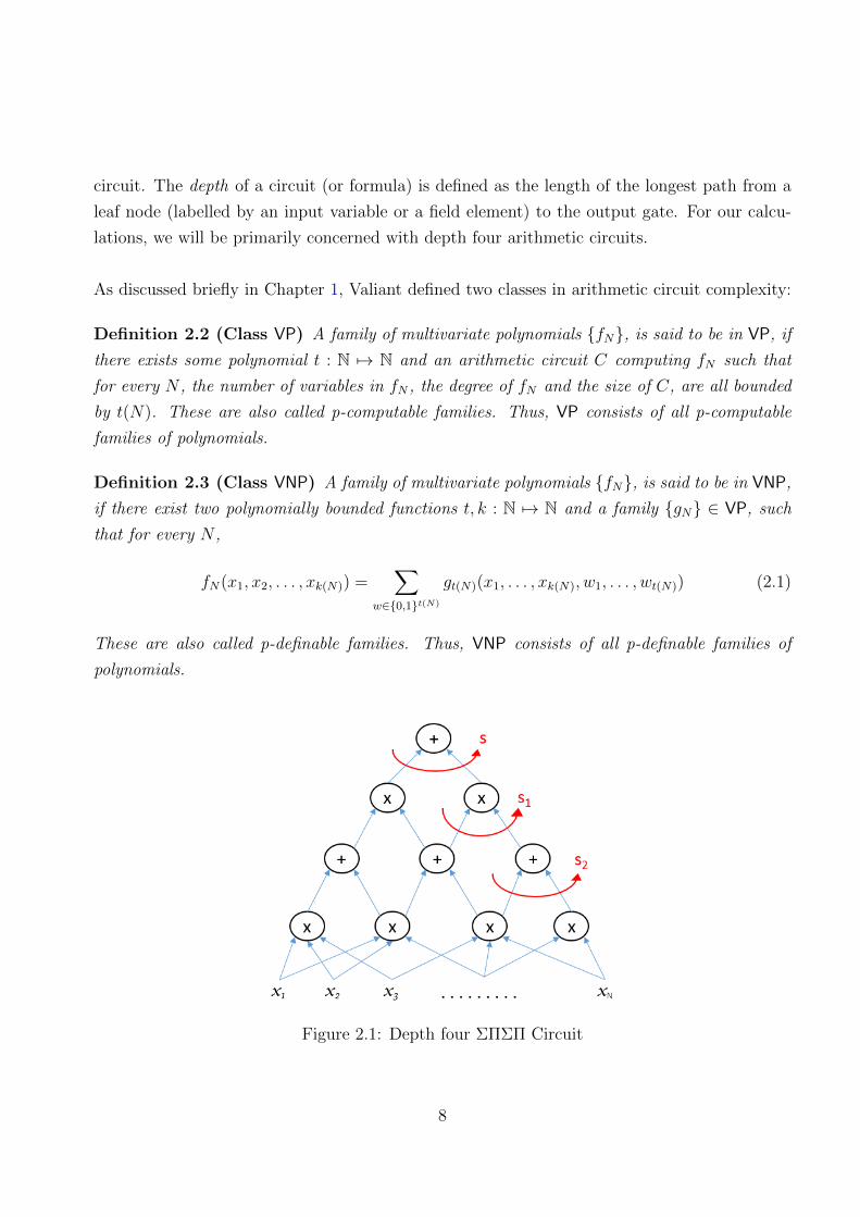
Figure 2.1: Depth four ΣΠΣΠ Circuit
8

Constant Depth Circuits: In this article, we work with arithmetic circuits having constant
depth i.e independent of N and d. In particular, our result is a lower bound on the size of a
depth four circuit, the model as depicted in Figure 2.1 above. We shall also use the term levels
to refer to all nodes at a particular depth. The leaf nodes would be taken as level zero, the mono-
mials being computed at level 1 product gates, and similarly the output gate would be at level 4.
In addition to the above, we shall also use the term support in two different contexts, defined
as follows:
Definition 2.4 (Support of a monomial) For any monomial m ∈ F[x] we define the sup-
port of m, denoted as Supp(m), as the minimal set of variables that are required to be non-zero
for m to be non-zero.
Supp(m) := xi : m |xi=0 = 0
In case of multilinear monomials, if S = Supp(m), then the monomial m is sometimes denoted
using its support set as xS.
Definition 2.5 (Support of a polynomial) The support of a polynomial f , denoted simply
as Support(f), is just the number of monomials in the polynomial with non-zero coefficients.
2.2 Random Restrictions
Given a set S ⊆ [N ] that refers to a subset of variables from x1, x2, . . . , xN, we define a
substitution map σS : x 7→ F ∪ x such that:
σS(xi) :=
0 if i ∈ S,
xi otherwise.
This substitution map can be extended naturally to polynomials and sets of polynomials. Thus,
for any polynomial f ∈ F[x] and any set of polynomials A ⊆ F[x],
σS(f) := f |xi=0 ∀ i∈S,
σS(A) := f |xi=0 ∀ i∈S : f ∈ A.
In our proof later, we will choose the set S randomly and use the restriction σS to eliminate
higher degree terms from the circuit. This operation is called as random restriction.
9
Definition 2.6 (Random Restriction) A random restriction σR is a substitution map cor-
responding to a subset of variables R ⊆ [N ], which is obtained by picking each variable inde-
pendently at random with probability (1− p) and setting it to zero (every variable survives with
probability p). The set R consists of all the variables that are set to zero.
2.3 Complexity Measure: Projected Shifted Partials
We use the following complexity measure in our proof: Dimension of the Projected Shifted Par-
tial Derivatives. We now proceed to describe the measure taking one term at a time.
Dimension: We shall use the notation dim(A), for any set of polynomials A ⊆ F[x], to denote
the linear dimension of the F-linear span of the polynomials in A. It might also sometimes be
referred simply as the F-linear dimension of A.
Projection: Define a map π : F[x] 7→ F[x] such that for any polynomial f , π(f) retains
only and exactly the multilinear monomials of f . The definition can be extended to any set of
polynomials A ⊆ F[x],
π(A) := π(f) : f ∈ A.
Observation 2.7 For any set of polynomials A ⊆ F[x], dim(π(A)) ≤ dim(A).
Proof: Let p = dim(A) and a1, a2, . . . , ap be a basis of A (ai ∈ A). Then we can observe that
the polynomials π(a1), π(a2), . . . , π(ap) form a spanning set for π(A). The above can also be
inferred from the fact that π(a + b) = π(a) + π(b) for any two polynomialss a and b. Hence,
dim(π(A)) ≤ p. 2
Shift: Let x=` denote the set of all multilinear monomials in x1, . . . , xN of degree exactly `.
When this set is multiplied to any fixed polynomial f of degree d, we get a set of polynomials
x=`.f , all of degree d+ ` and we say that f is shifted by `.
Partial Derivatives: Now, we define the notion of partial derivative of a polynomial f with
respect to a monomial m, which is also referred to as a k-th order partial derivative where k
is the degree of the monomial m. First we define first order partial derivative of f , that is ∂f∂xi
10
where xi is an input variable. It is defined as follows:
∂f
∂xi=
∑m∈Support(f)
∂m
∂xi, (2.2)
where
∂m
∂xi=
mxi
if m = xi.g for some polynomial g ∈ F[x],
0 otherwise.(2.3)
The k-th order partial derivatives are obtained by applying the above first order derivative, to
an already computed (k − 1)-th order partial derivative, as follows:
∂f
∂m=
∂f
∂(xi.m′)=
∂
∂xi
(∂f
∂m′
),
where m and m′ are monomials of degrees k and k − 1 respectively. In our work, we consider
derivatives with respect to multilinear monomials. We shall use ∂=kf to refer to the set of all
multilinear k-th order partial derivatives of f ∈ F[x].
Also, x=`.∂=kf denotes the set of all polynomials of the form m.g where m ∈ x=` and g ∈ ∂=kf .
Then, for any polynomial f , the measure DPSPk,` is defined as:
DPSPk,`(f) := dim(π(x=`.∂=kf)) (2.4)
Lemma 2.8 (Sub-additivity) DPSP is a sub-additive measure, i.e for any fixed k, ` and any
two polynomials f, g:
DPSPk,`(f + g) ≤ DPSPk,`(f) + DPSPk,`(g)
2.4 Nisan-Wigderson polynomials
To achieve the required lower bound, we define a polynomial f , such that DPSPk,`(f) is as high
as possible. One possible candidate is the Nisan-Wigderson (NW) polynomial, first introduced
in [KSS14] and has been useful in proving lower bounds for certain constant depth, in particular
depth three and depth four, circuits in the past few years. It is a degree-d set-multilinear
polynomial on N = d.q variables, where q is power of a prime. The explicit form of the NW
11

polynomial is given below, where r is an associated parameter.
NWr(x1,1, x1,2, . . . , xd,q) :=∑
h(z)∈Fq [z]deg(h)≤r
∏i∈[d]
xi,h(i). (2.5)
Observe that when q = dα, N = dα+1 where α is any constant. We will be using an appropriate
version of the above NW polynomial in proving our depth four lower bound result. To get an
estimate of the ‘hardness’ of NW polynomial, we state the following result from [KLSS14] as a
fact (without proof) below.
Fact 2.9 Let q = d2, r = d/3, k = o(d), ` = N2.(1− k log d
d). Then,
DPSPk,`(NWr) ≥1
dO(1).min
((N
`+ d− k
),
(d
k
)2
.dk.k!.
(N
`
)). (2.6)
2.5 Approximations and Numerical Estimates
Stirling’s Formula Stirling’s formula is the following approximation:
ln(n!) = n lnn− n+O(lnn) (2.7)
The above is used to obtain the following estimates (proved in Section 2.6)
Lemma 2.10 Let a(n), f(n), g(n) : Z>0 7→ Z be integer valued functions such that f+g = o(a).
Then,
ln(a+ f)!
(a− g)!= (f + g) ln a±O
(f 2 + g2
a
). (2.8)
Combinatorial Approximation The following is an approximation of the binomial coeffi-
cient that we can use either as an upper or a lower bound depending on the requirements. For
any m ≥ n ≥ 0, (mn
)n≤(m
n
)≤(men
)n. (2.9)
12
2.6 Proof of Preliminaries
2.6.1 Proof of Lemma 2.10
Proof:
(a+ f)!
(a− g)!= (a+ f)(a+ f − 1) . . . (a− g + 1) (2.10)
=⇒ af+g(
1− g
a
)f+g
≤ (a+ f)!
(a− g)!≤ af+g
(1 +
f
a
)f+g
(2.11)
Taking logarithms on all sides,
=⇒ (f + g) ln(
1− g
a
)≤ ln
(a+ f)!
(a− g)!− (f + g) ln a ≤ (f + g) ln
(1 +
f
a
). (2.12)
Using the fact that x1+x≤ ln(1 + x) ≤ x for x > −1, we can bound both L.H.S and R.H.S by
O(f2+g2
a
). 2
2.6.2 Proof of Lemma 2.8
Proof: Recall from the definition of DPSP:
DPSPk,`(f + g) := dim(π(x=`.∂=k(f + g))) (2.13)
For any monomial m of degree k, ∂(f + g)/∂m = ∂f/∂m + ∂g/∂m. Further, for any 2 poly-
nomials f and g, π(f + g) = π(f) + π(g). The above two properties reduce Equation 2.13 to:
DPSPk,`(f + g) = dim(π(x=`.∂=k(f)) + π(x=`.∂=k(g))) (2.14)
This implies that every polynomial in the set π(x=`.∂=k(f + g)) is a sum of two polynomials,
one each from the sets π(x=`.∂=k(f)) and π(x=`.∂=k(g)) respectively. We know that the former
is generated by a basis of size DPSPk,`(f) and the latter by a basis of size DPSPk,`(g). Also, for
any two sets A and B, dim(A+B) ≤ dim(A) + dim(B). Hence, Equation 2.14 reduces to:
DPSPk,`(f + g) ≤ dim(π(x=`.∂=k(f))) + dim(π(x=`.∂=k(g))),
= DPSPk,`(f) + DPSPk,`(g).
2
13

Chapter 3
Analysis of the ΣΠΣΠ Circuit Model
3.1 Upper Bound Statement and Proof Outline
As mentioned in Lemma 1.1, we will assume that the parameters s1 and s2 are upper bounded
by Ndlog5N
, and the degree parameter d =√N
log4Nin the rest of this chapter. For the sake of
simplicity, we shall ignore all ceil and floor notations hereafter.
Let C be a depth four circuit and let DPSPk,`(C) denote the Dimension of Projected Shifted
Partial Derivatives measure of the polynomial computed by C. We prove the following upper
bound on the measure DPSPk,`(C).
Lemma 3.1 Let C be any depth four circuit computing an N-variate polynomial of degree d,
with top fan-in s ≤ N2. Let τ = 20 logN and t = dlog3N
be specific parameters. Then, for all
k, ` satisfying ` < N2− 2kt, a random restriction R satisfies the following with high probability:
DPSPk,`(σR(C)) ≤ s ·(
1 + τ.Ndlog5N.t
k
)·(
N
`+ 2kt
).
The rest of this chapter is dedicated to proving the above lemma. The main steps involved in
the proof are as follows:
• First, we decompose the original circuit C, represented as C =∑
i
∏j Pij, into two
separate depth four circuits, say C1 and C2. This is done by splitting every polynomial
Pij into two groups of monomials based on some degree criteria (discussed in detail later),
and combining all the ‘high’ degree monomials into the new circuit C2 by exhaustive
multiplication (elaborated later). The circuit C1 then contains only the remaining ‘low’
degree monomials.
14

• Then on the decomposed circuit, we apply the random restriction, derivative, shift and
projection operations in that order to evaluate DPSPk,`(C). The degree criteria for the
decomposition is chosen in such a manner that in the process of evaluating DPSPk,`(C), the
projection and derivative operations together effectively eliminate C2 from the calculations
and allows us to focus on just the restricted degree depth four circuit C1.
• The circuit C1 is constructed such that the degree of all the polynomials computed at
level 2 sum gates is bounded by a fixed parameter τ (which will be equal to Θ(logN)).
We start by combining these polynomials together into factors of degree at least t (which
will be equal to dlog3N
), which simplifies the estimation of an upper bound on DPSPk,l(C1),
and hence on DPSPk,l(C).
The choice of all the parameters used, k, `, t, τ has been reasoned in the final calculations
leading to the desired Ω(N1.5) lower bound.
3.2 Using Random Restriction and Projection
Decomposing the circuit. Recall from Equation (1.1), the representation of the circuit C as
a sum of products of sparse polynomials.
C = T1 + . . .+ Ts ,
Ti =
s1∏j=1
Pij ∀i ∈ [s],
where Support(Pij) for all i, j is bounded by s2. We split the polynomials Pij’s into two parts,
the first one (say P ′ij) containing all those monomials where each variable has individual degree
at most two, and the second (say P ′′ij) comprising of the remaining monomials (i.e at least one
of the variables in these monomials has degree at least 3).
Random restriction. Let σR be the substitution map that every variable independently
survives with probability p = N−β = 1/2, i.e. for β = 1/ logN . Here, R ⊆ [N ] refers to the set
of variables set to zero. Then under the random restriction σR, Equation (1.1) reduces to
σR(C(x)) =s∑i=1
s1∏j=1
σR(P ′ij(x)) + σR(P ′′ij(x)). (3.1)
After the decomposition, we multiply out all the factors in a term, and split the resulting
summands into two groups, one group contributing to the depth four circuit C1 with all low-
15

individual-degree terms, and the other group adding into another circuit C2. More precisely,
the term Ti = Πs1j=1Pij is replaced by 2s1 terms, only one of which (the
s1∏j=1
P ′ij term) belongs to
C1, and the rest belong to C2 as follows:
Ti = (P ′i1 + P ′′i1)(P ′i2 + P ′′i2) . . . (P ′is1 + P ′′is1)
=
s1∏j=1
P ′ij + (other terms having at least one P ′′ij factor)
Similarly manipulating every term Ti of C for i ∈ [s], from Equation (3.1) we get
σR(C(x)) = σR(C1(x) + σR(C2(x)), (3.2)
where as explained before, C1(x) =s∑i=1
s1∏j=1
P ′ij(x).
Observation 3.2 DPSPk,`(C2(x)) = 0.
Proof: When the partial derivative operation ∂=k (by a multilinear monomial of degree k)
is applied on the entire circuit C, the monomials in C2(x) which have at least one variable
with degree three or more, do not reduce to multilinear monomials. Hence, they do not sur-
vive after the multilinear projection π. More precisely, π(∂=k(C2(x))) = 0, and therefore
π(x=`.∂=k(C2(x)) = 0. 2
As a result of Observation 3.2, C2 does not contribute to the final DPSP calculation, despite
having a much larger size than C1. Hence we observe that proving a lower bound on the circuit
size of C1 implies a lower bound on the size of the circuit C, since the size of C1 is at most the
size of C. Thus, we focus on lower bounding C1(x) =s∑i=1
s1∏j=1
P ′ij(x).
Observation 3.3 If σR is a random restriction chosen as above, then with high probability
σR(P ′ij) consists of monomials of support at most τ ′ = 10 logN for every i ∈ [s], j ∈ [s1].
Proof: Consider the random restriction σR described earlier, where every variable indepen-
dently survives with probability p = N−β , and R ⊆ [N ] refers to the set of variables that are
set to zero. Under σR, a monomial having support at least τ ′ will survive with probability at
most pτ′. The size of Support(Pij) for every polynomial P ′ij computed at a level 2 sum gate
(Figure 2.1) is bounded by s2 ≤ Ndlog5N
, and there are total s.s1 ≤ s.(
Ndlog5N
)such polynomials,
so by union bound the bad probability that a monomial having support at least τ ′ survives in
16

any of the P ′ij’s is at most s.(
Ndlog5N
)2
pτ′.
As mentioned earlier in Section 1.4, the hard polynomial f has degree d =√N
log4N. Substituting
d and p = N−β in the expression for bad probability, we get s.(
N3
poly logN
).N−βτ
′. Moreover, as
we are trying to achieve a Ω(N1.5) lower bound on s, it is safe to assume s ≤ N2 and therefore
it suffices that the product β.τ ′ be a large enough constant (> 5) for the bad probability to be
ultimately negligible. In our proof, we choose the values of the parameters as τ ′ = 10 logN and
β = 1logN
(p = 1/2) to enforce the above argument and keep the bad probability low. Thus, for
the above setting of parameters β and τ ′
s.
(N3
poly logN
).N−βτ
′=
1
N5poly logN
Hence, with probability at least 1−O(N−5), R ⊆ [N ] is such that σR(P ′ij) consists of monomials
of support at most τ ′ for all i, j. 2
Since the individual degrees of each variable in P ′ij is at most 2, from Observation 3.3, the
degree of all the monomials in σR(P ′ij) is bounded by 2τ ′ = 20 logN = τ (say). Hereafter, it
suffices to account for these bounded degree P ′ij’s while estimating DPSPk,`(C). Therefore, we
slightly abuse the notation and refer to C1 as C and P ′ij’s simply as Pij’s, and assume all Pij’s
to have degree bounded by τ = 20 logN .
3.3 Estimating DPSP(C) for the restricted circuit
Applying the sub-additivity of the DPSP measure (Lemma 2.8) on Equation (1.1), we get:
DPSPk,`(C) ≤ s.DPSPk,`(T ) (3.3)
where T is the representative term with maximum DPSP value out of T1, . . . , Ts. So, to upper
bound DPSPk,`(C), it is sufficient to focus on DPSPk,`(T ), where T is of the form T = Πs1j=1Pj.
Inspired from the techniques used in [KST16], we group the Pj’s into disjoint subsets, such that
the degree of the product of Pj’s in every set is at least t and at most 2t (where t = dlog3N
,
so t τ) , except perhaps one remaining Pj factor that could not be grouped with any other
factor. Hence,
T = Q1 . . . Qm (3.4)
17
where every Qi for all i ∈ [m] is a product of one or more Pj’s, and all except one have degree
in [t, 2t]. As the Pj’s (after random restriction) are all restricted to degree at most τ , we have
(m− 1).t ≤ τ.s1
m ≤ 1 + τ.s1/t.
From the definition of the DPSP measure, we know that
DPSPk,`(T ) = dim(π(x=`.∂=k(Q1 . . . Qm)). (3.5)
Let us first analyse ∂=k(Q1 . . . Qm). The k-th order derivative of the product Q1 . . . Qm is
obtained by applying the chain rule of derivatives. It is a sum of many terms, each term having
at most k of the Qi’s touched (i.e affected) by the derivative (k ≤ m). For example, consider
the case of k = 1 i.e derivative with respect to a variable:
∂(Q1 . . . Qm)
∂xi=∑i∈[m]
∂Qi
∂xi·∏
j∈[m]\i
Qj
As k increases, the number of summands increase but every summand has at least m − k of
the Qi’s unaffected by the derivative. Fixing this unaffected set of Qi’s, for every summand in
∂=k(Q1 . . . Qm), we denote the remaining set of Qi’s as touched by the derivative, and identified
by the set A ⊆ [m] of size |A| = k. For any such set A, we define
dA :=∑i∈A
deg(Qi),
VA := spanF(x≤(`+dA−k).Πi/∈A Qi),
where x≤(`+dA−k) refers to the set of monomials of degree at most ` + dA − k. Since the total
degrees of the factors Qi are bounded by 2t, dA ≤ 2kt for all A ∈(
[m]k
). We now make the
following observation that is critical to upper bound DPSPk,`(C), which is later used to obtain
the final upper bound on DPSPk,`(C).
Observation 3.4 x=`.∂=k(T ) ⊆ spanFVA : A ∈(
[m]k
).
Proof: As discussed earlier, ∂=k(T ) can be split into(mk
)terms based on the subset A touched
by the derivative. Then, all these polynomials are multiplied by the shift x=` as follows:
∂=k(T ) ⊆ spanF(∂=k(Πi∈A Qi))(Πi/∈A Qi) : A ∈(
[m]
k
),
18

x=`.∂=k(T ) ⊆ spanF(x=`.∂=k(Πi∈A Qi))(Πi/∈A Qi) : A ∈(
[m]
k
).
As the degree of ∂=k(Πi∈A Qi) is at most dA − k,
x=`.∂=k(T ) ⊆ spanF(x≤(`+dA−k).Πi/∈A Qi) : A ∈(
[m]
k
).
Thus, from the definition of the set VA, the proposition is proved. 2
Applying the above proposition, along with the sub-additivity of DPSP (Lemma 2.8) and Ob-
servation 2.7, Equation (3.5) can be written as
DPSPk,`(T ) ≤∑
A∈([m]k )
dim(π(VA)). (3.6)
Suppose dim(π(VA)) ≤ u, where u ∈ N. Since m ≤ 1 + τ.s1/t, Equation 3.3 reduces to the
following:
DPSPk,`(C) ≤ s.
(1 + τ.s1/t
k
).u (3.7)
Observation 3.5 dim(π(VA)) ≤(
N`+2kt
)for every A ∈
([m]k
).
Proof: Consider any representative VA for some A ∈(
[m]k
). The generators of VA would consist
of polynomials of the form g(x) = m(x).(Πi/∈AQi), where m(x) ∈ F[x] is a monomial of degree
at most `+ dA− k, and without loss of generality we can assume that it is a multilinear mono-
mial (otherwise it would be eliminated by π). So, let us denote m(x) by xS, where S is the set
of variables (S ⊆ [N ]), such that S = Supp(m(x)).
The number of ways of choosing S such that xS is a monomial of degree `+ dA− k is given by(N
`+dA−k
). Also, notice that once the set S is fixed, it would also fix the variables that cannot
occur in the (Πi/∈AQi) part of the polynomial g(x), in order to maintain the multilinear property
of the projected polynomial π(g(x)). Hence, to sum up:
π(VA) ⊆ spanF (xS.π(σS(Πi/∈AQi)) : S ⊆ [N ], |S| = `+ dA − k)
⇒ dim(π(VA)) ≤(
N
`+ dA − k
)(3.8)
19
using dA ≤ 2kt and `+ 2kt < N/2 (proved below),
dim(π(VA)) ≤(
N
`+ 2kt
). (3.9)
2
Plugging this upper bound u =(
N`+2kt
)from Observation 3.5 in Equation (3.7), we get
DPSPk,`(C) ≤ s ·(
1 + τ.s1t
k
)·(
N
`+ 2kt
),
where C is restricted by the random restriction σR and τ = 20 logN and s1 ≤ Ndlog5N
. This
completes the proof of Lemma 3.1.
Choice of `. In Lemma 3.1, we state the result under the constraint that ` + 2kt < N/2,
which was essential to the upper bound in Equation 3.9. We show that this is indeed true for
our choice of parameters which is as follows:
d =
√N
log4N
t =d
log3N
k =δ.d
t
δ =1
logN
` =N
2.
(1− N δ/t − 1
N δ/t + 1
)=
N
N δ/t + 1
Claim 3.6 for the above choice of parameters, ` < N/2− 2kt.
Proof: We prove that the following ratio is greater than 1.
N2− 2kt
`=
(N2− 2δd).(N δ/t + 1)
N
=
(1
2− 2δd
N
).(N δ/t + 1)
20

Thus, we have to prove the following:
112− 2δd
N
< N δ/t + 1
⇒ 112− 2δd
N
− 1 < N δ/t
⇒1 + 4δd
N
1− 4δdN
< 21/t
As 4δdN 1 and ex ≈ 1 + x for x 1,
e8δdN < 21/t
e8δdtN < 2
The above is true if c0δdtN
< 1 for some constant c0.
c0δdt
N=
c0.d2
N log4N=
c0
poly logN
2
21

Chapter 4
Explicit polynomial of high measure:
Proof of Theorem 1
The analysis in the chapter closely follows the analysis in [KLSS14] and [KS15], but we repro-
duce some of the arguments and calculations here as our choices of parameters (in particular,
`, k, t, d, β) are slightly different and suited to our purpose.
4.1 The Hard polynomial family f
As mentioned earlier in Chapter 1, the hard polynomial family is a variant of the Nisan-
Wigderson polynomial family (Equation 2.5). The N -th member of this family has degree d
and N = dq variables, is parametrized by a number r (fixed later in the analysis), and is defined
as follows:
NWr(x1,1, x1,2, . . . , xd,q) :=∑
h(z)∈Fq [z]deg(h)≤r
∏i∈[d]
xi,h(i) (4.1)
where q is chosen as the smallest prime number greater than d1+α, where α < 1 is a parameter
fixed later to achieve the required result. Hence the number of input variables N is such that
d2+α ≤ N ≤ 2d2+α.
As part of our proof, we focus on the polynomial f obtained by applying the random restriction
described in Chapter 3. Hence, f = σR(NWr) is the hard polynomial for which we prove the
lower bound as in Lemma 4.1, borrowing the main ideas from [KS15], but with a slightly
different polynomial family fN, and an updated setting of the basic parameters. In the
following lemma, β = 1logN
, α is as described above, and t = dlog3N
, p = N−β are as chosen in
the circuit upper bound in Chapter 3.
22

Lemma 4.1 Let k = δ.dt
where 0 < δ < 1 is a small constant, r be some fixed function
dependent on α, β, d, and ` = NNδ/t+1
. Then with probability at least 1− 1dO(1) ,
DPSPk,`(f) ≥ 1
d3.min
(pk
4k.
(N
k
).
(N
`
),
(N
`+ d− k
)).
The parameters: The DPSP measure was first used in [KLSS14], where the result was ob-
tained by setting the parameters as ` = N2.(1− k log d
d) and k = δ.d
t, where t was set to be O(
√d)
and d = N1/3. The parameters in our proof are set as follows:
` =N
N δ/t + 1
d =
√N
log4N
k = δ.d
t
t = d/ log3N
δ =1
logN
r =(α + β)
2· d− 1
Also, from the inequality d2+α ≤ N ≤ 2d2+α and d =√N
log4N, we find α = Θ( log logN
logN). It must be
noted that we make use of few results from [KLSS14] and [KS15], where the choice of param-
eters were different, but we have verified that those results hold under our choice of parameters.
We approach the proof of Lemma 4.1 in three steps. First, we equate the measure DPSPk,`(f)
to the rank of a coefficient matrix M , that exactly captures the effect of shift and derivative
operations on the NWr polynomial. Second, we construct a square matrix B = MT ·M and
recall the notion of Surrogate Rank (denoted SurRank) from [KS15] and hence, further reduce
our lower bound candidate from rank(M) to SurRank(B). Thus, as a consequence of the first
two steps:
DPSPk,`(f) = rank(M) ≥ SurRank(B).
In the final step, we prove a lower bound on SurRank(B).
An important aspect of our proof, is the choice of parameters k, `, α, β that constitute the
primary difference in our work from [KS15]. Both [KLSS14] and [KS15] use members of the
23

Nisan-Wigderson family as their choice of hard polynomials, but operate on different underlying
arithmetic circuit models. [KLSS14] proves lower bounds for homogeneous ΣΠΣΠ circuits,
where as [KS15] operates on ΣΠΣ circuits with bottom fan-in restricted by τ . As described
in Chapter 3, we too have applied the appropriate random restriction, such that it suffices
to assume that all polynomials computed at level 2 gates in our ΣΠΣΠ circuit are degree-
bounded by τ = Θ(logN). Therefore, the parameter τ used to bound the degree (or support)
of intermediate polynomials, forms a common node of importance in [KLSS14],[KS15], and in
our proof.
4.2 Proof of Lemma 4.1
The set of multilinear N -variate d-degree monomials is in 1-1 correspondence with(
[N ]d
)=(
[d]×[q]d
). Hence in the arguments below, we naturally associate elements of
([N ]d
)with N -variate
d-degree monomials. A monomial in Support(f) corresponds to a univariate polynomial h ∈Fq[z] of degree at most r. As any two different univariate r-degree polynomials over Fq (r < q)
can have at most r roots over any field, we make the following observation.
Observation 4.2 For two distinct sets D1, D2 ∈(
[d]×[q]d
), corresponding to monomials in
Support(f), the following holds:
|D1 ∩D2| ≤ r.
Applying the DPSP measure to the polynomial in Equation (4.1) gives us
DPSPk,`(f) = dim
(xA.σA(∂Cf) : A ∈
([N ]
`
), C ∈
([N ]
k
)), (4.2)
where A and C are the subsets corresponding to the shift and the derivative monomials re-
spectively and ∂C(f) denotes the partial derivative of f with respect to the monomial xC . We
show that DPSPk,`(f) is equal to the rank of the matrix M(f) as constructed below. In the
arguments below, d′ = d− k.
Construction of the matrix M(f): Define the matrix M(f) as follows:
• The rows of M(f) are labelled by pairs of subsets (A,C) ∈(
[N ]`
)×(
[N ]k
), and
• The columns of M(f) are labelled by subsets S ∈(
[N ]`+d′
).
24
Each row corresponds to the polynomial f(A,C) := xA.σA(∂Cf), and the S-th entry of that row
is the coefficient of the monomial xS in the polynomial f(A,C). Then it is easy to observe the
following.
Observation 4.3 DPSPk,`(f) = rank(M(f)).
Hereafter in the arguments, we will refer to M(f) simply as the matrix M . We wish to lower
bound rank(M). First we make the following observation.
Observation 4.4 M is a 0-1 valued matrix.
Let A,C, S be subsets of [N ], such that A ⊆ S and (S \A)∩C = φ. Taking cue from the above
discussion, we label the ((A,C), S)-th entry with the set D ∈(
[N ]d
)computed as D = (S\A)]C.
We call D a valid set if the monomial xD ∈ Support(f), else we call it an invalid set. Instead,
if A * S or (S \ A) ∩ C 6= φ, we simply call the label not defined. Observe that an entry in
M is non-zero if and only if it is labelled by a valid set. We lower bound the rank of M by
calculating a lower bound on the surrogate rank of M defined as follows.
Definition 4.5 (Surrogate Rank) For any matrix M ∈ ∪m,n∈NMm,n(R) where Mm,n(R) de-
notes the set of real valued m× n matrices, we define the real symmetric matrix B := MT ·M .
From the definition of B, it is easy to show that
rank(M) ≥ rank(B)
where the equality holds over the field of real numbers R. Further, by an application of Cauchy-
Schwartz on the non-zero eigenvalues of B, [Alo09] obtained the following bound over R:
rank(B) ≥ Tr(B)2
Tr(B2). (4.3)
The above ratio is called the surrogate rank of B, denoted SurRank(B).
The notion of SurRank has been previously used in [KLSS14] and [KS15] to prove lower bounds.
The idea is to exploit the structure of the matrix M , to compute a lower bound on the surrogate
rank of B where B = MT ·M . Observe that M is a relatively sparse 0-1 matrix. Hence, it
becomes simpler to estimate Tr(B) and Tr(B2). The rest of the proof shall be devoted to
finding a tight lower bound on SurRank(B) which would (from Observation 4.3 and Equation
4.3) imply the DPSPk,`(f) lower bound as claimed in Lemma 4.1.
25

4.3 Lower bounding SurRank(B)
To compute a lower bound on SurRank(B), we lower bound (Tr(B))2, and upper bound Tr(B2).
Equation 4.3 thus enables us to lower bound SurRank(B). In the following proof calculations, we
use an upper bound on the quantity Hr(d, w) that denotes the number of univariate polynomials
in Fq[z] of degree at most r, having exactly w distinct roots , where w ∈ [d].
An upper bound on Hr(d, w): A polynomial h(z) ∈ Fq[z] of degree at most r, with exactly
w distinct roots in [d] must be of the form:
h(z) = (z − α1).(z − α2) . . . (z − αw).h(z)
where αi ∈ [d] for i ∈ [w] and h(z) ∈ Fq[z] is of degree at most (r − w). Thus, we have
Hr(d, w) ≤ qr−w+1 ·(d
w
)≤ qr+1 ·
(d
q
)w· 1
w!. (4.4)
4.3.1 Estimating a lower bound on Tr(B)
Since M is a 0-1 valued matrix (Observation 4.4), Tr(B) = Tr(MT ·M) is equal to the num-
ber of non-zero entries in the matrix M . Hence, Tr(B) is equal to the number of cells labelled
by a valid set. Recall that a set D ∈(
[N ]d
)labelling a cell in M , is a valid set if xD ∈ Support(f).
To estimate the number of cells in M labelled by a valid set, we first count all possible valid sets
i.e the size of the Support(f), and then multiply this to the number of possible entries in M
that can be labelled by a particular fixed valid set. Firstly, it is easy to observe the following:
Observation 4.6 A set D ∈(
[N ]d
)labels at least
(dk
).(N−d`
)entries of M .
Proof: A set D ∈(
[N ]d
)labels the ((A,C), S)-th entry of M if and only if the monomial xS
is obtained by removing the variables of xC and adding the variables of xA to the variables in
xD. Hence the number of entries in M labelled by D equals the number of ways we can choose
C and A. We can choose the set C in exactly(dk
)ways, and choose the set A in at least
(N−d`
)ways. Thus, a set D ∈
([N ]d
)labels at least
(dk
).(N−d`
)entries of M . 2
The size of Support(f) is equal to the number of monomials in NWr that survive after the
26
random restriction R. More precisely,
f = σR(NWr) =∑
D∈Supp(NWr)
eD.xD,
where eD is an indicator random variable which equals 1 if and only if σR(xD) 6= 0, i.e the
monomial xD has no variable in common with the random restriction set R. Let µ(f) be a
random variable that denotes the number of monomials in f , equal to the size of Support(f).
We make the following observation:
Observation 4.7 E[µ(f)] = pd.qr+1.
Proof: We know that the number of monomials that survive after random restriction R, is
equal to
µ(f) =∑
D∈Supp(NWr)
eD
⇒ E[µ(f)] =∑
D∈Supp(NWr)
E[eD].
Since there are qr+1 monomials in NWr all of degree d,
E[µ(f)] = pd.qr+1.
2
Let γ := pd.qr+1. Hence, from Observations 4.6 and 4.7,
E[Tr(B)] ≥ γ.
(d
k
).
(N − d`
).
The following result has been proved in [KS15] using variance calculation and Chebyshev’s
inequalities.
Proposition 4.8 ([KS15]) Pr[Tr(B)] ≤ 12.γ.(dk
).(N−d`
)] ≤ 10
pdα.
27

4.3.2 Estimating an upper bound on Tr(B2)
From the definition of B, we have B2 = (MT ·M)(MT ·M). Hence,
Tr(B2) =∑
(A1,C1),(A2,C2)∈((N` )×(Nk))2
∑S1,S2∈(( N
`+d′))2
M(A1,C1),S1 ·M(A1,C1),S2 ·M(A2,C2),S1 ·M(A2,C2),S2
(4.5)
Since M is a 0-1 matrix (Observation 4.4), Tr(B2) is exactly equal to the number of 4-tuples
(A1, C1), (A2, C2), S1, S2 such that the four corresponding matrix entries (from the above
equation (4.5)) are non-zero. More formally, for any pair of row indices (A1, C1), (A2, C2) and
any pair of column indices S1, S2, we define the box b consisting of the corresponding entries
from the matrix M .
b : = box((A1, C1), (A2, C2), S1, S2)
= (M(A1,C1),S1 ,M(A1,C1),S2 ,M(A2,C2),S1 ,M(A2,C2),S2)
Therefore, from equation (4.5), Tr(B2) is equal to the number of boxes b with all four cell-
entries non-zero. In other words, it is equal to the number of boxes b with all four cell entries
labelled by valid sets. We formally make a note of this in the following observation.
Observation 4.9 Tr(B2) is equal to the number of boxes b = box((A1, C1), (A2, C2), S1, S2),
such that all four entries in b are labelled by valid sets. We call such boxes as valid boxes.
Let b be a valid box, and D1, D2, D3, D4 be the labels of the corresponding entries of M ,
M(A1,C1),S1 ,M(A1,C1),S2 ,M(A2,C2),S1 ,M(A2,C2),S2 respectively. To compute an upper bound on the
number of such valid boxes, we analyse the structure of the sets D1, D2, D3, D4 corresponding
to the valid boxes. We introduce the following operations on sets, which would bring clarity to
the subsequent calculations. For any 2 sets A and B,
• Subset difference: A B equals A \B if B ⊆ A, else the operation outputs not defined.
• Disjoint set union: A ] B equals A ∪ B if B ∩ A = φ else the operation outputs not
defined.
Thus the label of the ((A,C), S)-th cell in M is (S A) ]C. Here, (S A) ]C is not defined,
if either S A is not defined or (S A)∩C 6= φ. Similarly, if any entry in the (A,C)-th row is
labelled by a set D ∈(
[N ]d
), then it corresponds to the column identified by S = (D C) ] A.
28

For any box b = box((A1, C1), (A2, C2), S1, S2), we define the following sets, as subsets of the
sets D1, D2, D3, D4 labelling the corresponding entries of b:
E1 := A1 \ (A1 ∩ A2) E2 := A2 \ (A1 ∩ A2)
E3 := C1 E4 := C2
E5 := D1 \ (E2 ] E3) = D3 \ (E1 ] E4) E6 := D2 \ (E2 ] E3) = D4 \ (E1 ] E4)
Observation 4.10 Based on the sets defined above we make the following observations:
1. The set E2 ] E3 is a subset of both D1 and D2.
2. The set E1 ] E4 is a subset of both D3 and D4.
3. D1 \ (E2 ] E3) = D3 \ (E1 ] E4).
4. D2 \ (E2 ] E3) = D4 \ (E1 ] E4).
Proof: Since D1, D2, D3, D4 are all valid sets, A1, A2 ⊆ S1 and A1, A2 ⊆ S2. Further, C1 ∩(S1 \A1) = C1∩ (S2 \A1) = φ. Hence E2∩E3 = φ, and E2]E3 ⊆ D1. Similarly, E2 ⊆ (S2 A1)
implies E2]E3 ⊆ D2. This proves the first observation, and the second can be proved similarly.
To prove the third observation, we show that D1 \ (E2 ]E3) = S1 \ (A1 ∪A2) = D3 \ (E1 ]E4).
Since D1 = (S1 A1)]C1 and E3 = C2, the set D1 \ (E2 ]E3) = (S1 \A1) \E2. Thus it is easy
to see that D1 \ (E2 ] E3) ⊆ S1 \ (A1 ∪ A2). Moreover, as C1 ∩ (S1 \ A1) = φ, it implies that
S1 \ (A1 ∪A2) ⊆ D1 \ (E2 ]E3). Similarly, we can prove that D3 \ (E1 ]E4) = S1 \ (A1 ∪A2).
The fourth observation can be proved similarly. 2
Finally, it can be verified that the sets D1, D2, D3, D4 can be expressed as decompositions of
the sets E1, E2, E3, E4, E5, E6 as stated in the following observation.
Observation 4.11 The decomposition expressions are as follows:
1. D1 = E2 ] E3 ] E5,
2. D2 = E2 ] E3 ] E6,
3. D3 = E1 ] E4 ] E5,
4. D4 = E1 ] E4 ] E6.
29
Let |A1 ∩ A2| = v, then
|E1| = |E2| = `− v (4.6)
|E3| = |E4| = k (4.7)
|E5| = |E6| = d− (`− v + k) (4.8)
Proposition 4.12 Among the sets D1, D2, D3, D4, only the following scenarios are possible:
• D1 = D2 = D3 = D4,
• Di \Dj 6= φ for all i 6= j (i.e all four sets D1, D2, D3, D4 are distinct),
• D1 = D2 and D3 = D4,
• D1 = D3 and D2 = D4.
Further, if D1, D2, D3 are all distinct then `− v + k ≤ r and d− (`− v + k) ≤ r.
Proof: We prove this by considering different possible cases:
• Case 1: If D1 = D2, from Observation 4.11, E5 = E6 and thus, D3 = D4.
• Case 2: If D1 = D3, then E2 ] E3 = E1 ] E4, which implies that D2 = D4.
• Case 3: If D1 = D4, then from Observation 4.11 , E6 ⊆ D1 which implies D2 ⊆ D1.
Since |D1| = |D2| = d, D1 = D2. Hence D1 = D2 = D3 = D4.
Thus, if D1 equals any of D2, D3, D4, the proposition holds true. The arguments for the other
cases are similar. Suppose D1, D2, D3 are distinct sets. Then, |D1∩D2| ≥ |E2]E3| = `−v+k.
But, from Observation 4.2, if D1 6= D2 then |D1 ∩ D2| ≤ r. Hence, ` − v + k ≤ r. Similarly,
since |D1 ∩D3| ≥ |E5| = d− (`− v + k), it follows that d− (`− v + k) ≤ r. 2
We classify the valid boxes based on the four possible scenarios mentioned in Proposition 4.12,
and count each of these cases separately. Let D1, D2, D3, D4 ∈(
[N ]d
)be the labels of a valid box
b as stated earlier. Then b belongs to one of the sets as defined below:
B0(D1) := box b : all four labels equal to D1,
B1(D1, D2) := box b : D1 = D3, D2 = D4,
B2(D1, D3) := box b : D1 = D2, D3 = D4,
B3(D1, D2, D3, D4) := box b : all labels are distinct.
30
We further define random variables T0, T1, T2, T3 as follows, where as previously, eD is an indi-
cator variable, and equals 1 if xD survives after the random restriction else 0.
T0 :=∑
D1∈Support(NWr)
eD1 .|B0(D1)|, (4.9)
T1 :=∑
D1 6=D2∈Support(NWr)
eD1 .eD2 .|B1(D1, D2)|, (4.10)
T2 :=∑
D1 6=D3∈Support(NWr)
eD1 .eD3 .|B2(D1, D3)|, (4.11)
T3 :=∑
D1 6=D2 6=D3 6=D4∈Support(NWr)
eD1 .eD2 .eD3 .eD4 .|B3(D1, D2, D3, D4)|. (4.12)
Hence, from Observation 4.9 and the above arguments, it is easy to observe the following.
Observation 4.13 Tr(B2) = T0 + T1 + T2 + T3.
Thus in the arguments that follow, we find suitable upper bounds on T0, T1, T2, T3.
4.3.2.1 Upper bound for E[T3]
T3 corresponds to the number of valid boxes b where D1, D2, D3, D4 are all distinct valid sets. As
a result of Proposition 4.12, for a valid box if D1, D2, D3 are distinct, D4 is also distinct. Hence,
we approximate T3 by first counting the number of possible valid boxes for a particular choice of
D1, D2, D3, and then multiplying it to the number of ways of choosing D1, D2, D3 ∈ Support(f).
Let D1, D2, D3 be distinct valid sets. The following observation shows that a valid box with first
three labels D1, D2, D3 can be uniquely determined by fixing the sets E2, E3, E4 and A1 ∩ A2.
Observation 4.14 For any fixed distinct valid sets D1, D2, D3, the sets A1, C1, A2, C2 can be
uniquely determined, by fixing the sets E2, E3, E4 and A1 ∩ A2.
Proof: Suppose we fix the set A1 ∩A2, fixing E2 = A2 \ (A1 ∩A2) will determine A2. Further,
the sets C1 and C2 are directly determined by E3 and E4 respectively. From Observation 4.10,
E2, E3, E4 determine E1 and therefore A1. 2
We count the number of unique ways to pick E2, E3, E4 and A1 ∩ A2 for a given D1, D2, D3.
The choice of E3 and E4 are made in(dk
)ways each, from (Equation ??). Further, E2 can be
chosen in at most(d−k`−v
)ways, as E2 ]E3 ⊆ D1 from Observation 4.10. Finally, the set A1 ∩A2
31

is chosen in at most(N−d+2k
v
)ways, as A1 ∩ A2 is disjoint from (D1 ∪D3) \ (C1 ∪ C2). Hence,
the total number of unique choices are at most(d
k
).
(d
k
).
(d− k`− v
).
(N − d+ 2k
v
). (4.13)
As(d−k`−v
)≤ 2d−k and v ≤ l < N−d
2from proposition 4.12, the number of unique ways to pick
E2, E3, E4 and A1 ∩ A2 for a given D1, D2, D3 are at most
2d−k.
(d
k
)2
.
(N − d+ 2k
`
). (4.14)
Let ρ = 2d−k.(dk
)2.(N−d+2k
`
). Then,
T3 ≤ ρ.∑
D1 6=D2 6=D3∈Support(NWr)
eD1 .eD2 .eD3 . (4.15)
Let η =∑
D1 6=D2 6=D3∈Support(NWr)eD1 .eD2 .eD3 . We upper bound the expected value of η and
therefore T3 in the following proposition, the proof of which is similar to that in [KS15].
Proposition 4.15 Let γ be as defined in proposition 4.8. Then
E[η] ≤ 4 · γ2 · qr+1 ·(d
q
)d.
Substituting in Equation 4.15, we get
E[T3] ≤ 4
2k·(
2
d(α−β)/2
)d· γ2 ·
(d
k
)2
·(N − d+ 2k
`
).
Proof: The upper bound on E[η] has been proved in [KS15], and hence omitted. We now
achieve the claimed upper bound on E[T3], using the above estimate. From Equation 4.15,
E[T3] ≤ ρ.E[η]
From equation 4.14,
E[T3] ≤ 2d−k ·(d
k
)2
·(N − d+ 2k
`
)· 4 · γ2 · qr+1 ·
(d
q
)d
32

Since r + 1 = α+β2(1+α)
.d and q ≥ d1+α,
E[T3] ≤ 4
2k·(
2
d(α−β)/2
)d· γ2 ·
(d
k
)2
·(N − d+ 2k
`
).
2
Eventually, E[T3] is found to be negligible in comparison to E[T0 + T1 + T2] and hence does not
contribute to the final expected value of Tr(B2).
4.3.2.2 Upper bound for E[T0]
The following observation is used to upper-bound T0, T1, T2 in the subsequent arguments.
Observation 4.16 For any set D1 ∈(
[N ]d
)and any row (A,C) of the matrix M , there can be
at most one cell in that row with the label D1.
Proof: Suppose there are two cells in the row (A,C) labelled by a set D1, corresponding to
the columns S1 and S2 respectively. Then, D1 = (S1 A1)]C1 = (S2 A1)]C1. This implies
S1 = S2, as S1 \ A1 = S2 \ A1. 2
From Observation 4.16, for all the boxes in B0(D1) or B2(D1, D2), the columns S1 and S2 must
be the same. Keeping the above in mind, we make another important observation about the
boxes in B0(D1).
Observation 4.17 For every box b ∈ B0(D1) defined as b = box((A1, C1), (A2, C2), S1, S2),
A1 = A2 and C1 = C2.
Proof: Given a box b ∈ B0(D1), we know that all four cells of b are labelled by a valid set,
say D1. Comparing the entries in the column corresponding to S1,
D1 = D3 (4.16)
⇒ (S1 A1) ] C1 = (S1 A2) ] C2. (4.17)
From Observation 4.11, E1 ⊆ D3 = D1 and E1 ⊆ A1. But D1 and A1 are disjoint sets, hence
E1 must be an empty set. Similarly, E2 ⊆ D1 = D3, E2 ⊆ A2 and D3 ∩ A2 = φ together
imply that E2 is an empty set. Substituting E1, E2 as empty sets in the expressions for D1 and
D3 (Observation 4.11), and again using the fact that D1 = D3, we get E3 = E4 i.e C1 = C2.
33
Plugging in C1 = C2 in Equation 4.17 also proves that A1 = A2. 2
From Observations 4.16 and 4.17, we prove the following upper bound on E[T0]:
Proposition 4.18
|B0(D1)| ≤(N − d+ k
`
).
(d
k
), and hence
E[T0] ≤ γ.
(N − d+ k
`
).
(d
k
).
Proof: For any fixed set D1 of size d, we can pick the set C1 ⊆ D1 in(dk
)ways and the set
A1 (disjoint with D1 \ C1) in(N−d+k
`
)ways. The expression for E[T0] follows straight from
definition of T0, where γ is as defined in Proposition 4.8. 2
4.3.2.3 Upper bound for E[T1]
Let D1, D2 ∈(
[N ]d
)be distinct sets, such that xD1 ,xD2 ∈ Support(f). A valid box b =
box((A1, C1), (A2, C2), S1, S2) is in B1(D1, D2) if the labels satisfy the following: D1 = D3
and D2 = D4. Recall that the proof of Observation 4.17 was also based on the premise that
D1 = D3. Hence from the arguments in the proof of Observation 4.17, A1 = A2 = A and
C1 = C2 = C. In Proposition 4.19, w = |D1 ∩D2|.
Proposition 4.19
|B1(D1, D2)| =(N − 2d+ w + k
`
).
(w
k
), and hence
E[T1] ≤ d.γ2
d(α−3β)k.k!.
(N − 2d+ 2k
`
).
Proof: We fix two sets D1, D2 ∈(
[N ]d
)and count the number of rows (A,C), such that D1 and
D2 are the first two labels of the box b = box((A,C), (A,C), S1, S2). Since C ⊂ D1 ∩D2 and
|D1 ∩D2| = w, we can pick C in(wk
)ways. And for every choice of C, we can pick the set A
which is disjoint from (D1∪D2)\C, in(N−2d+w+k
`
)ways (|(D1∪D2)\C| = 2d−w−k). Hence,
|B1(D1, D2)| =(N − 2d+ w + k
`
).
(w
k
)
34
From Equation 4.10,
T1 =∑
D1∈Support(NWr)
∑w≥k
∑D2∈Support(NWr)D2 6=D1,|D1∩D2|=w
eD1 .eD2 .|B1(D1, D2)|
⇒ E[T1] =∑
D1∈Support(NWr)
∑w≥k
∑D2∈Support(NWr)D2 6=D1,|D1∩D2|=w
pd.pd−w.
(N − 2d+ w + k
`
).
(w
k
)
≤ p2d.∑
D1∈Support(NWr)
∑w≥k
Hr(d, w).p−w.
(N − 2d+ w + k
`
).
(w
k
).
From equation (4.4):
≤ p2d.∑
D1∈Support(NWr)
∑w≥k
qr+1.
(d
pq
)w.
1
w!.
(N − 2d+ w + k
`
).
(w
k
).
Recall that N = d.q ≥ d2+α where α < 1, and p = N−β, then
E[T1] ≤ p2d.qr+1.∑
D1∈Support(NWr)
∑w≥k
(1
dα−3β
)w.
1
w!.
(N − 2d+ w + k
`
).
(w
k
)
The term(
1dα−3β
)w. 1w!.(N−2d+w+k
`
).(wk
)attains its maximised value at w = k as β = 1/ logN
α = Θ(log logN/ logN). Hence,
E[T1] ≤ d.γ2
d(α−3β)k.k!.
(N − 2d+ 2k
`
).
This completes the proof of the proposition. 2
4.3.2.4 Upper bound for E[T2]
From Observation 4.16, any box b = box((A1, C1), (A2, C2), S1, S2) in B2(D1, D3) has S1 =
S2 = S. Moreover, D1 = D2 = (S A1)]C1 and D3 = D4 = (S A2)]C2. Let u := |C1 ∩C2|and w as defined in Proposition 4.19, then
Proposition 4.20
|B2(D1, D2)| =∑
0≤u≤k
(N − 2d+ w + k
`− d+ k + w − u
).
(d− wk − u
)2
.
(w
u
), and hence
35

E[T2] ≤ dk.γ2.
(N − 2d+ k
`− d+ k
).
(d
k
)2
.
The proof of this proposition is very similar to the proof of Proposition 4.19, hence omitted.
Here, the maxima of the relevant expression is achieved at w = u = 0.
4.3.3 Putting it together: Proof of lemma 4.1
From Observation 4.13, we know that Tr(B2) = T0 + T1 + T2 + T3. We recall the upper bounds
from Propositions 4.18, 4.19, 4.20 and 4.15.
E[T3] ≤ 4
2k·(
2
d(α−β)/2
)d· γ2 ·
(d
k
)2
·(N − d+ 2k
`
)E[T0] ≤ γ.
(N − d+ k
`
).
(d
k
)E[T1] ≤ d.
γ2
d(α−3β)k.k!.
(N − 2d+ 2k
`
)E[T2] ≤ dk.γ2.
(N − 2d+ k
`− d+ k
).
(d
k
)2
Comparing the above equations, it can be observed that the upper bound on E[T2] dominates
upper bounds on E[T0] and E[T3]. Hence, we assume T0, T3 ≤ T2 which implies Tr(B2) ≤T1 + 3T2. Thus, we get the following result.
Proposition 4.21 Using Markov’s inequality, with probability at least 1− 1d,
Tr(B2) ≤ d2 · γ2
d(α−3β)k · k!·(N − 2d+ 2k
`
)+ 3d2 · k · γ2 ·
(N − 2d+ k
`− d+ k
)·(d
k
)2
.
Proof: From Markov’s inequality, PrT1 > d.E[T1] < 1d
and PrT2 > d.E[T2] < 1d. Con-
sidering the complimentary event of both, with probability at least (1 − 1d), T1 ≤ d.E[T1]
and T2 ≤ d.E[T2]. Plugging in the bounds from Propositions 4.19 and 4.20 into the equation
Tr(B2) ≤ T1 + 3T2, we get the claimed upper bound. 2
From Proposition 4.8, PrTr(B) > 12· γ ·
(dk
)·(N−d`
) is at least 1− 10
pdα. Combining this with
Proposition 4.21, with probability at least 1− 1dO(1) ,
36
SurRank(B) ≥ (Tr(B))2
Tr(B2)
≥14· γ2 ·
(dk
)2 ·(N−d`
)2
d2 · γ2
d(α−3β)k·k!·(N−2d+2k
`
)+ 3d2 · k · γ2 ·
(N−2d+k`−d+k
)·(dk
)2 .
We split the denominator based on one summand dominating another,
≥ min
(14· γ2 ·
(dk
)2 ·(N−d`
)2
2d2 · γ2
d(α−3β)k·k!·(N−2d+2k
`
) , 14· γ2 ·
(dk
)2 ·(N−d`
)2
6d2 · k · γ2 ·(N−2d+k`−d+k
)·(dk
)2
).
The first ratio can be split into two factors and separately lower bounded as follows:
dαk · k! ·(d
k
)2
≥ 1
2k·(N
k
), and(
N−d`
)2(N−2d+2k
`
) ≥ 1
2k.d3·(N
`
).
The second ratio is lower bounded as follows:(N−d`
)2(N−2d+k`−d+k
) ≥ 1
d3·(
N
`+ d− k
).
Hence, the final lower bound expression reduces to
SurRank(B) ≥ 1
d3.min
(pk
4k.
(N
k
).
(N
`
),
(N
`+ d− k
)).
where p = N−β as chosen earlier. This completes the proof of Lemma 4.1.
4.4 Completing the proof of Theorem 1
Now, we prove the final lower bound result by combining Lemma 4.1 with Lemma 3.1. Thus,
DPSPk,`(σR(C)) = DPSPk,`(f) where f = σR(NWr). The random restriction σR is guaranteed
to exist with high probability from Observation 3.3. Also taking union of the probabilities from
Observation 3.3 and Lemma 4.1, the following lower bound is also under the high probability
of 1− 1NO(1) .
37

s ≥ DPSPk,`(NWr)(1+
τ.s1t
k
)·(
N`+2kt
) (4.18)
≥ 1
d3·min
( (p4
)k · (Nk
)·(N`
)(1+
τ.s1t
k
)·(
N`+2kt
) , (N
`+d−k
)(1+
τ.s1t
k
)·(
N`+2kt
)) (4.19)
Recall the choice of the parameters (Paragraph 4.1) t = dlog3N
, k = δ dt, δ = 1/ logN and
` = NNδ/t+1
. Using Lemma 2.10, and substituting ` = NNδ/t+1
,(N`
)(N
`+2kt
) =(`+ 2kt)(`+ 2kt− 1) . . . (`+ 1)
(N − `)(N − `− 1) . . . (N − `− 2kt)
≈(N
`− 1
)−2kt
= (N δ/t)−2kt
= N−2δ.k.
Similarly, the second term of the minima is approximated using ` (d− k) and k t,
(N
`+d−k
)(N
`+2kt
) ≈ (N`− 1
)d−k−2kt
= (N δ/t)d−k−2kt
≈ N δ/t.(1−2δ).d
= N (1−2δ).k.
Substituting in the final lower bound, and approximating(
1+τ.s1t
k
)by( τ.s1
tk
):
s ≥ 1
d3·min
((p4
)k·(Nk
)( τ.s1tk
) ·N−2δ.k,N (1−2δ).k( τ.s1
tk
) )≥ min(L1, L2),
where L1 =( p4)
k·(Nk)·N−2δ.k
d3·(τ.s1tk )
and L2 = N(1−2δ).k
d3·(τ.s1tk )
. Observe that L1 =( p4)
k·(Nk)
Nk · L2, i.e L1 ≤ L2 for
all values of N . Therefore, we compute a lower bound on L1, that will imply the required lower
38
bound on s.
L1 =1
d3.N2δ.k·(p
4
)k·(Nk
)( τ.s1tk
) (4.20)
Using p = N−β, s1 ≤ Ndlog5N
and the estimate from Equation 2.9,
≥ 1
d3·
(Nk
4.Nβ+2δ. eτNdkt log5N
)k
(4.21)
≥ 1
d3·(
t. log5N
4.Nβ+2δ.e.τ.d
)k(4.22)
Recall that β = δ = 1/ logN , τ = 20 logN . t = dlog3N
and k = δ.dt, for which the above
equation equals
=1
d3· Ω (logN)k (4.23)
= ω
(Nd
log5N
)(4.24)
This completes the proof of Theorem 1.
4.5 Future Work: Possible directions
Following the recent breakthrough result by [KST16], a lot of interest has been generated
regarding improved lower bounds for constant depth arithmetic circuits. The proof of an “al-
most cubic lower bound” for general depth three circuits involves a major step, where ‘heavy’
product gates are eliminated from the target circuit, i.e gates with total degree higher than a
fixed threshold, by considering the circuit modulo a particular set of linear polynomials. This
restricts the circuit to an affine subspace, wherein they achieve stronger lower bounds. This
technique is inspired from the previous quadratic lower bound result by [SW99].
We too employ a similar technique for depth four circuits, wherein we remove gates with high
in-degree and isolate the remaining low-degree gates in the circuit, to achieve stronger lower
bound on the total size of ΣΠΣΠ circuits. Particularly, in order to achieve a similar situation
as in [KST16], we need to consider the field of polynomials taken modulo higher degree (more
than 1) polynomials. This might result in a more complex algebraic structure as compared to
39

affine subspaces in [KST16], and therefore needs to be analysed carefully.
Another direction to build on our result, is to manipulate the choice of `. The current choice
is made with the purpose to maximize the value of the minimum of the two numerators in
Equation 4.19,((Nk
)·(N`
))and
(N
`+2kt
), by choosing a ` for which both quantities are as close
as possible. However, it is conceivable that a different choice of `, that gives an inferior lower
bound expression than Equation 4.23, but could result in a stronger depth four lower bound
result by allowing a larger choice for d. That would imply a different choice of the hard NWr
polynomial family. Here, we are forced to restrict d to at most√N to enforce the constraint
proved in Claim 3.6, that also dictates the choice of parameters k and t. But, it is worth
analysing whether this constraint is a hard necessity, and if we can achieve close to a quadratic
lower bound (for depth four circuits computing multilinear polynomials) in its absence.
40

Chapter 5
Previous Lower Bounds for Depth Four
Circuits
In this section, we analyse two previous results for general depth four circuits, and compare our
techniques with those results in detail. Both the results have related approaches (but different
from ours) to arithmetic circuit lower bounds, and both of them deal with general circuits
having constant depth. In the rest of this chapter we discuss these results, the main techniques
and ideas involved, and their implications to the model of our interest, depth four arithmetic
circuits.
5.1 Shoup-Smolensky: Polynomial Evaluation
The first breakthrough result for constant depth arithmetic circuits was achieved by Shoup
and Smolensky in 1997. They employed arithmetic circuits to solve the well-known problem
of multi-point evaluation of a univariate polynomial. The goal is to evaluate a given univari-
ate n-degree polynomial f , with coefficients in C, on a fixed set of points p1, p2, . . . , pn ∈ C.
Therefore the arithmetic circuit C designed for the above computation, takes as input the set
of coefficients ai ∈ C (i ∈ [n]) of the polynomial f = a1 + a2x + . . . + anxn−1, and outputs
the evaluations f(p1), f(p2), . . . , f(pn). Hereafter in the analysis, circuits of the above type are
referred to as polynomial evaluation circuits.
The problem of multi-point polynomial evaluation has been well-studied over the decades for its
implications connected to algebraic complexity. In the special case when the points p1, . . . , pn
are n-th roots of unity, the problem is known as Discrete Fourier Transform (DFT), which has
an arithmetic circuit of size O(n log n) and depth O(log n), where n is a power of 2. [SS97]
41

proved the existence of a set of points p1, . . . , pn such that any arithmetic circuit for polynomial
evaluation at these points must have at least superlinear size.
It can be observed that the polynomial evaluation circuit C described above, essentially com-
putes a linear transformation of the coefficients a1, . . . , an ∈ C, into the multi-point evaluations
f(p1), f(p2), . . . , f(pn) ∈ C. The transformation can be represented by the Vandermonde ma-
trix V where the (i, j)-th entry is given by vij = pj−1i for all i, j ∈ [n]. Since all the intermediate
polynomials computed in C are linear forms (total degree one) in the variables a1, a2, . . . , an,
we focus on a restricted class of arithmetic circuits called as linear circuits defined as follows.
Definition 5.1 (Linear Circuits) A linear circuit over a field F is an arithmetic circuit,
where every gate is either an input gate (leaf node) or an addition gate, i.e there are no multi-
plication gates. Further, the addition gates have unbounded fan-in and every incoming edge is
labelled with a field element. The size and depth of a linear circuit are defined in the same way
as for general arithmetic circuits.
Thus, a linear circuit C with n input nodes and m output nodes, computes a linear trans-
formation T : Fn 7→ Fm defined by the m × n matrix AC . The entries of AC = aij are
computed as follows: The weight of a path is the product of the weights of all its edges, and
aij is the sum of weights of all paths from the j-th input gate (j ∈ [n]) to the i-th output
gate (i ∈ [m]). For infinite fields, [Str73] showed that if a linear transformation T is computed
by an arithmetic circuit C ′, then there is also a linear circuit C computing T , with size and
depth of C within constant factor of the size and depth of C ′. Precisely, if the linear circuit
C has size s and depth d, the equivalent general arithmetic circuit has size at most 16s and
depth at most d. Therefore, the lower bound proved by [SS97] on size of a depth-d linear cir-
cuit, implies the same asymptotic lower bound on the size of general depth-d arithmetic circuits.
Let C be a linear circuit. Let the linear transformation computed by C be defined by the
square matrix A ∈ Cn×n, with entries aij ∈ C for all i, j ∈ [n]. Let LA(n) denote the set of all
monomials of degree m in aij, and let DA(n) be the dimension of the Q-linear space spanned
by the monomials in LA(n). Then, we have the following result.
Lemma 5.2 ([SS97]) Let C be a linear circuit of size s and depth d, computing a linear
transformation T over Cn. Let A = AC be the associated matrix. Then for r = ds/de,
DA(n) ≤(n+ r
n
)d.
42

Figure 5.1: Depth-d Linear Circuit
Proof: For this proof, let L and D denote LA(n) and DA(n) respectively. Consider the graph
of the circuit as depicted in the figure 5.1, with the level of each gate as defined for general
arithmetic circuits. For 1 ≤ i ≤ d, let si denote the number of outgoing edges from gates at
level i. Hence, the size of the circuit C is equal to s =∑
i∈[d] si, i.e the total number of edges.
Also define Wi as the set of edge weights of the outgoing edges from level i gates. Hence,
|Wi| ≤ si depending on number of distinct edge weights.
Each entry aij in A can be expressed as a sum of products of the form (α1 . . . αd) where
αi ∈ Wi ∪ 1 for all i ∈ [d], as each product corresponds to a path from xj to yi. The value
1 for some αi’s takes care of the paths where some levels are skipped. For example if there
exists an edge from a level 2 gate to level e (e > 3) gate, α2 is equal to the weight of that edge,
and α3 = α4 = . . . = αe−1 = 1. Further, each element in L is an n-degree monomial in aij.Suppose m = ai1j1ai2j2 . . . ainjn is a monomial in L, where aikjk is a sum of products of the form
(α(k)1 . . . α
(k)d ). Then, m is expressed as a sum of products of the form:
(α(1)1 . . . α
(n)1 ) . . . (α
(1)d . . . α
(n)d ) (5.1)
43

where α(k)i ∈ Wi ∪ 1 for all i ∈ [d], k ∈ [n]. Let Γ be the set of all such products (Equation
5.1), then each element in L belongs to the set spanZ(Γ). Hence D, which is the dimension of
the span of L over Q, is at most the cardinality of the set Γ, i.e D ≤ |Γ|.
To calculate the size of the set Γ, we first count the number of products of the form (α(1)i . . . α
(n)i ).
As αi ∈ Wi, it can be chosen in at most si ways. So, the number of products of the form
(α(1)i . . . α
(n)i ) are exactly equal to the number of monomials of degree at most n (few of the α
(k)i
can be 1) in si variables, i.e(n+sin
). Thus, counting for all i ∈ [d], we get
D ≤d∏i=1
(n+ sin
)
=d∏i=1
n∏j=1
n+ si − j + 1
j
=n∏j=1
j−dd∏i=1
(n+ si − j + 1).
From arithmetic-geometric mean inequality,
d∏i=1
(n+ si − j + 1) ≤ (n+s
d+ 1− j + 1)d.
Therefore, substituting r = d sde,
D ≤n∏j=1
(n+ r − j + 1)d
jd=
(n+ r
n
)d.
2
The above lemma forms the foundation of the main lower bound result from [SS97]. The
set of points p1, . . . , pn considered by [SS97] are algebraically independent over Q, i.e they do
not satisfy any non-trivial polynomial equation over Q. In other words, for every polynomial
f(x1, . . . , xn) ∈ Q[x1, . . . , xn] that is not identically zero, f(p1, . . . , pn) 6= 0.
Theorem 2 ([SS97]) Let p1, p2, . . . , pn be complex numbers, algebraically independent over Q,
with n > 1. Any depth d linear circuit for polynomial evaluation at these points, must have size
s > K.dn1+1/d
44

where K is an absolute constant and d ≤ log n/ log 3.
Proof: Consider the linear circuit C for polynomial evaluation at the fixed set of points
p1, p2, . . . , pn ∈ C. Let oi = f(pi) be the evaluations of the polynomial f = a1+a2x+. . .+anxn−1
at these points. Thus, the evaluation can be represented as the following transformation by the
Vandermonde matrix V = vijn×n.o1
...
on
=
v11 · · · v1n
.... . .
...
vn1 · · · vnn
a1
...
an
The linear circuit C computes the linear transformation defined by the matrix V . Consider the
product of n elements in V , taking one from each row. They are precisely sets of products of
the form (pe11 . . . penn ) where ei ∈ [0, n− 1]. Hence, there are nn possible products of the above
kind.
Observation 5.3 All nn products described above are linearly independent over Q.
Proof: Note that the pi’s are algebraically independent over Q. This implies that the set
pe11 . . . penn : ei ∈ [0, n− 1] for all i ∈ [n] is linearly independent over Q, otherwise the depen-
dence relation would form a non-trivial polynomial equation satisfied p1, . . . , pn which contra-
dicts the algebraic independence assumption. 2
Thus, from the above observation and Lemma 5.2,(n+ r
n
)d≥ DV (n) ≥ nn.
Taking logarithm on both sides and applying Stirling’s approximation (Equation 2.7) on the
left, we get
n log(
1 +r
n
)+ r log
(1 +
n
r
)≥ n log n
d+O(1)
45

For all x > 0, we have log(1 + x) ≤ x. So, r log(1 + n
r
)≤ n,
⇒ n log(
1 +r
n
)+ n ≥ n log n
d+O(1)
log(
1 +r
n
)≥ log n
d− 1 +O(1/n)
r
n≥ n1/d.e−1+O(1/n) − 1
Assuming sufficiently large n such that d ≤ log3 n i.e n1/d ≥ 3,
r
n= Ω(n1/d)
s = Ω(dn1+1/d)
This completes the proof of the theorem. 2
When we substitute d = 4 in the above result, for depth-4 circuits, we get the lower bound of
Ω(n5/4), where the input is the set of coefficients a1, a2, . . . , an i.e input length is N = n log n.
Hence, this provides an Ω(N5/4) lower bound for depth-4 arithmetic circuits. But it appears to
us that some careful analysis of the above calculations can lead to an ≈ Ω(N4/3) lower bound,
which is the current best for general depth four circuits to our knowledge.
5.2 Ran Raz: Elusive Polynomial Functions
The next result we discuss is Ran Raz’s “Elusive functions and Lower Bounds for Arithmetic
Circuits” from 2010. It approaches circuit lower bounds by introducing the notion of elusive
polynomial mappings. They show that providing examples of explicit polynomial functions,
whose image is not contained in some predefined set, can imply significant arithmetic circuit
lower bounds, for instance the superpolynomial lower bounds on the size of arithmetic circuits
computing the permanent polynomial. The main lower bound result in [Raz10] is as stated
below.
Theorem 3 ([Raz10]) Let n be a prime number and 1 ≤ d ≤ (log2 n)/100 be an integer.
There exists an N-variate polynomial f : FN 7→ F of degree (5d+2) where N = n.(5d+2), such
that any depth-bd/3c arithmetic circuit computing f , over any field F, is of size Ω(n1+1/(2d)).
We present a closer analysis of Raz’s proof for the special case of depth four circuits. We observe
that the result in Theorem 3 for depth four circuits, has d ≥ 8 and number of input variables
46
N = n.(5d+ 2) = O(n). Therefore, the lower bound implied for depth four circuits, is Ω(N9/8).
First, we restate a few definitions and terminology, borrowed from the original work by Raz,
essential to their analysis.
Definition 5.4 (Polynomial Mappings) Let F be any field, a polynomial mapping f : Fn 7→Fm of degree r is the map defined by the m-tuple f = (f1, f2, . . . , fm), where for all i ∈ [m],
fi ∈ F[x1, x2, . . . , xn] are n-variate polynomials of degree at most r.
A mapping f is said to be a multilinear mapping, if all the polynomials f1, f2, . . . , fn are multi-
linear polynomials (i.e. degree with respect to every variable is at most 1). A mapping f is said
to be a homogeneous mapping of degree r, if all the polynomials f1, f2, . . . , fn are homogeneous
polynomials of total degree r.
We also define the set Image(f) ⊆ Fm as follows:
Image(f) := (f1(a), f2(a), . . . , fm(a)) | a ∈ Fn.
Note that for fi ∈ F[x1, x2, . . . , xn] for all i ∈ [m], f = (f1, f2, . . . , fm) can also be thought
as a mapping f : Kn 7→ Km where K ⊃ F is a field extension, as F [x1, x2, . . . , xn] ⊆K[x1, x2, . . . , xn]. Based on the above definition of polynomial mappings and their Image sets,
we define the notion of elusive polynomial mappings.
Definition 5.5 (Elusive Mappings) We say that a mapping f : Fn 7→ Fm “eludes” another
mapping Ψ : Fs 7→ Fm, if Image(f) * Image(Ψ). If f eludes every mapping Ψ : Fs 7→ Fm of
degree at most r, we say f is (s, r)-elusive.
The principle idea behind Raz’s result is to find explicit constructions of polynomial mappings
that elude all polynomial mappings Ψ : Fs 7→ Fm of degree r. Here, the notion of explicit
polynomial mappings is closely derived from explicit polynomial functions. A polynomial f ∈F[x1, x2, . . . , xN ] is said to be explicitly defined if it belongs to the class VNP. Recall the precise
definition of VNP, where a polynomial f ∈ VNP if and only if there exists a polynomial g ∈ VP
in (n+ w) variables, such that
f(x1, x2, . . . , xn) =∑
e1,...,ew∈0,1
g(x1, . . . , xn, e1, . . . , ew)
where w = poly(n). Following the above definition closely, we define the notion of poly(n)-
definability for polynomial mappings f : Fn 7→ Fm.
47

Definition 5.6 (poly(n)-Definable Mappings) We say that a polynomial mapping is poly(n)-
definable, if there exists w = poly(n), k = dlog2me, and a polynomial g ∈ VP in (n + w + k)
variables, such that for every i ∈ [m],
fi(x1, x2, . . . , xn) =∑
e1,...,ew∈0,1
g(x1, . . . , xn, e1 . . . , ew, i1, . . . , ik) (5.2)
where (ik, . . . , i1) is the binary representation of i− 1.
Hereafter in the arguments, if we mention an explicit polynomial mapping, it would refer to
a poly(n)-definable mapping. Also, similar to polynomial families in VNP, the mapping f is
poly(n)-definable if there exists a deterministic polynomial time Turing machine that computes
the coefficient of the monomial xγ11 . . . xγnn in fi, when γ1, . . . , γn, i are given as inputs.
We define a structure called circuit graphs, associated with arithmetic circuits. For every
arithmetic circuit C, the circuit graph GC is the directed graph consisting of gates and edges
from C, but excluding the labels (weights) on the edges. Thus, size of GC is equal to the size
of the circuit C, that is the number of edges in C. The depth of GC is also similarly defined as
for C. We associate the notion of syntactic degree with a circuit graph. The syntactic degree
of a node in a circuit graph is inductively defined as follows:
• For a leaf node, the syntactic degree is 1 if it is labelled by an input variable, else it is 0.
• For a sum gate, it is the maximum of the syntactic degrees of its children.
• For a product gate, it is the sum of the syntactic degrees of its children.
The syntactic degree of the node corresponding to the output gate of the circuit, is called the
syntactic degree of the circuit graph GC . The notion of circuit graphs enables us to construct
a single circuit to capture computation of all n-variate homogeneous polynomials of degree r,
known as the Universal Arithmetic Circuit.
Definition 5.7 A circuit Φ is called universal for all circuits with n inputs and n outputs, of
size s and computing homogeneous polynomials of degree r, if the following holds: for every
n-tuple of homogeneous r degree polynomials f1(x1, . . . , xn), . . . , fn(x1, . . . , xn) that can be com-
puted simultaneously by a size s circuit, there exist another circuit C of size s and arbitrary
depth, computing f1, . . . , fn such that the circuit graph GC = GΦ.
The existence of a universal circuit, for any n, r, s ∈ N, was shown by [Raz10], which we use in
the proof strategy for Theorem 3 below.
48
Proof Overview: Let m =(n+r−1
r
)be the number of monomials in n variables of degree
exactly r. Then, every n-variate degree r polynomial p ∈ F[x1, x2, . . . , xn] can be represented
as a vector in Fm, where every index corresponds to the coefficient of a r degree monomial in n
variables. Hereafter, when we say a polynomial p ∈ Fm, we refer to the homogeneous n-variate
degree r polynomial represented by the vector p in Fm as explained above. Consider a universal
arithmetic circuit U with inputs x1, . . . , xn, for computing all possible homogeneous n-variate
degree r polynomials, and let s be the size of the circuit U , i.e the number of edges in U . If we
consider the labels of the edges in U as formal variables y1, . . . , ys, then from the definition of
universal arithmetic circuit it follows that the output of U is a polynomial p ∈ Fm, where every
entry of the vector is a polynomial in y1, . . . , ys variables. This computation is represented
as a polynomial mapping Ψ : Fs 7→ Fm. The proof of Theorem 3 involves three major steps:
• First, we prove the following: Let a polynomial g ∈ Fm be computed by an arithmetic
circuit of size s′, then for every n, r, s′, there exists a polynomial mapping Ψ : Fs 7→ Fm
(where s = poly(s′, n, r)) such that g ∈ Image(Ψ). Raz proves the existence of the mapping
Ψ, of degree O(r) and that it can be constructed in time poly(sr). In a way, Ψ captures
the computation of all polynomials of ‘low’ complexity (complexity of size s′), and hence
the task at hand is to find a set of polynomials in Fm not contained in Image(Ψ), or in
other words another polynomial mapping that eludes Ψ.
• Then the proof proceeds by showing an explicit (poly(n)-definable) description of a poly-
nomial mapping f that is (s, d)-elusive for appropriate s, d, and hence elusive of the
mapping Ψ.
• Finally, Raz gives a ‘hard’ polynomial family f derived from the elusive functions in
mapping f , such that f being (s, d)-elusive implies that any arithmetic circuit computing
f must have large size.
Similar to [SS97], the lower bound proof by Raz focusses on a special form of arithmetic circuits,
known as the Normal Linear Form of arithmetic circuits, that compute homogeneous linear
polynomials (total degree one) also called linear forms.
Definition 5.8 (Normal Linear Form) An arithmetic circuit is said to be in normal linear
form if every intermediate gate is a sum gate, and all the leaf nodes are labelled by input
variables (no field constants). Further, if we construct the circuit graph for an arithmetic
circuit in normal linear form, the syntactic degree of every node is exactly one.
It is also easy to observe the following result that implies equivalence of general arithmetic
circuits computing linear forms, and arithmetic circuits in normal linear form.
49
Proposition 5.9 Over any field F, if C is an arithmetic circuit of size s and depth d computing
n linear forms f1, f2, . . . fn, then there exists a circuit C ′ in normal linear form of size s and
depth d, that also computes the polynomials f1, f2, . . . , fn.
We describe the three steps that prove Theorem 3 below.
5.2.1 Description of Ψ
Let F be a field, n, r be integers such that 1 ≤ r ≤ n and n is a power of 2. Let x =
x1, x2, . . . , xn be the set of input variables, and M be the set of monomials in x of de-
gree exactly r. Thus, |M | =(n+r−1
r
)= m′. Let Γ be the set of all homogeneous r degree
polynomials in F[x], thus Γ is identified as the set Fm′ as every polynomial in Γ is repre-
sented as a coefficient vector of dimension m′. Assume the following precedence among the
x-variables:x1 > x2 > . . . > xn. Naturally using this ordering among the variables, we can
lexicographically order the monomials in M . This allows us to identify the set M with the set
[m′] where i ∈ [m′] corresponds to the i-th monomial in the above lexicographical ordering.
Further, consider the set Γn, of n-tuples (g1, g2, . . . , gn) where every gi ∈ Γ for all i ∈ [n]. Every
member of the set Γn can be represented as a vector of dimension m = m′.n = n ·(n+r−1
r
),
concatenating the coefficient vectors of the n polynomials. Thus, every tuple in Γn can be
identified by a vector in Fm. This generates a homomorphism H from the set Γn to the set
Fm, which is used hereafter in the proof, to denote the n-tuples of homogeneous polynomials
of degree r in F[x]. In other words, for every (g1, g2, . . . , gn) ∈ Γn, H((g1, g2, . . . , gn)) ∈ Fm.
Consider the set Gn,r of circuit graphs that have n input gates labelled x1, . . . , xn, and n output
gates, all of syntactic degree r. Let s ≥ n be the size of every graph G ∈ Gn,r. Let C be
an arithmetic circuit over F, with corresponding circuit graph GC ∈ Gn,r. Let the s edges of
GC be labelled by the variables y1, y2, . . . , ys. Then, C computes n homogeneous polynomials
in F[x], of degree exactly r, such that the coefficients of these polynomials are functions of
y1, y2, . . . , ys. This gives us the polynomial mapping ΨG : Fs 7→ Fm, where ΨG(y1, . . . , ys) is the
m-tuple of polynomials (Ψ1, . . . ,Ψm) in F[y1, . . . , ys] representing the coefficient of monomials
in the n output polynomials of C. It is worth noting that the polynomials Ψ1, . . . ,Ψm are only
dependent on the characteristic of the field F, not on the field F. (As the coefficients are only
sums of products of 0, 1-values that are contained in the minimal subfield of F.) We make the
following simple observation.
Proposition 5.10 Let G ∈ Gn,r be a circuit graph. For every g = (g1, g2, . . . , gn) ∈ Γn,
H(g) ∈ Image(ΨG) if and only if g1, g2, . . . , gn are computed by an arithmetic circuit C over F
50

such that GC = G.
Proof: If H(g) ∈ Image(ΨG), then by the definition of ΨG, there exists an arithmetic circuit
C over F, with GC = G that computes the polynomials g1, g2, . . . , gn as outputs. For the other
direction, let C be the arithmetic circuit over F, computing the n polynomials g1, g2, . . . , gn
such that GC = G. Since the circuit graph of GC has s edges, the size of circuit C is s
and suppose these s edges are labelled by α1, α2, . . . , αs ∈ F. Then, by definition of ΨG,
ΨG(α1, . . . , αn) = H(g). 2
Proposition 5.11 ([Raz10]) Let r = 1, and hence m = n2. If GC ∈ Gn,r is the circuit graph
of a circuit C in normal linear form, then ΨG : Fs 7→ Fm is a polynomial mapping of degree
equal to the depth of the circuit C.
Proof: Let C be the arithmetic circuit with circuit graph GC = G and its s edges be labelled
by the variables Y = y1, . . . , ys. Let v be a gate in C, and let gv ∈ F[x] be the intermediate
polynomial computed at v. If v is a leaf, all the coefficients of gv are independent of the vari-
ables y1, . . . , ys. Using this as the base case, we use induction to prove that if v is at a distance
dv from the farthest leaf node, then every coefficient of the polynomial gv is of degree at most
dv. The inductive proof is as follows: All children of the gate v are at distance dv − 1 from
their farthest leaves, and hence for every child u of v, the coefficients of the polynomial gu are
of degree at most dv − 1 in the variables y1, . . . , ys. Since v is an addition gate (normal linear
form) and there is a single edge labelled by a Y -variable between v and any of its children, the
degree of the coefficients of the polynomial gv is at most dv. When v is the output gate, the
degree d is equal to the depth of the circuit C. 2
It has been shown in [Raz10] that given n, r, s′ (s′ ≥ n) as inputs, the universal arithmetic circuit
on n inputs, computing n homogeneous polynomials of degree r, can be constructed in time
poly(s, r) and has size O(s′r4). Further, [Raz10] also proves that we can conclude that given the
graph G corresponding to the universal circuit, there exists a Turing machine that computes
the polynomial mapping ΨG : Fs 7→ Fm of degree O(r), where s = O((s′)2r8). Further, from
Propositions 5.10 and 5.11, this mapping ΨG captures computation of polynomials with ‘low’
complexity, as required.
5.2.2 Explicit Elusive Mapping f
Let n be a prime, m = n2. Then, the set [m] can be identified as [n] × [n] (in lexicographic
ordering). Let 1 ≤ d ≤ (log2 n)/100 be an integer. Then the set of input variables for the
51

polynomial mapping f is the set X = xi,ji∈[5d],j∈[n]. Hence, there are n.(5d) input variables.
For every (a, b) ∈ [n]× [n] = [m], define the polynomial
f(a,b)(x1,1, . . . , x5d,n) :=∏i∈[5d]
xi,a+i.b
where the sum a+ i.b is calculated modulo n. Thus, f = (f(1,1), . . . , f(n,n)) is the m-tuple that
defines the polynomial mapping f : Kn.(5d) 7→ Km over any field K. The proof of the following
lemma is omitted here and the interested reader may refer to [Raz10].
Lemma 5.12 ([Raz10]) Let n be a prime. Let m = n2 and 1 ≤ d ≤ (log2 n)/100 be integers.
Let K be a field of size at least m. Then, the polynomial mapping f : Kn.(5d) 7→ Km is (s, d)-
elusive, where s = dn1+1/(2d)e.
It is also easy to prove, as has been shown in [Raz10], that f is a poly(n)-definable mapping as
required.
5.2.3 The hard polynomial f
Let z = z1, . . . , zn be an additional set of input variables. Then, define the following set of
polynomials derived from the polynomial mapping f defined above. For every i ∈ [n],
fi(x1,1, . . . , x5d,n, z1, . . . , zn) :=∑j∈[n]
zj · f(i,j).
For every a ∈ Fn.(5d), we can substitute a for variables in X, and get f1|a, . . . , fn|a ∈ F[z]. The
following result has ben proved in [Raz10].
Proposition 5.13 ∀a ∈ Fn.(5d), we have (f1|a, . . . , fn|a) ∈ Γn and H((f1|a, . . . , fn|a)) = f(a).
In view of the above definitions, we prove the main result that connects the elusive mapping f
to depth d arithmetic circuit size, and helps achieve the claimed lower bound.
Proposition 5.14 ([Raz10]) Let m,n, d, s be integers such that n, d ≤ s and m = n2. Let
f : Fn 7→ Fm be a polynomial mapping. If there exists a field extension K ⊇ F such that f
is (s,d)-elusive over K, then any depth-d arithmetic circuit over F computing the polynomials
f1, f2, . . . , fn : F(5d+1).n 7→ F must have size at least s.
Proof: First, we prove the above result for K = F. Let F(X) be the set of rational functions
in the variables x1,1, . . . , x5d,n over F. By definition of f1, f2, . . . , fn ∈ F[X, z] have z-degree
52

1 and therefore total degree at most one more than the degree of f . Thus, the polynomials
f1, f2, . . . , fn are members of the polynomial ring F(X)[z1, . . . , zn], in fact they are all linear
polynomials in z variables with coefficients in F(X).
Suppose there exists an arithmetic circuit C, over F, computing the polynomials f1, f2, . . . , fn ∈F(X)[z], of size s and depth d. The circuit C is computing linear polynomials in the variables
z1, . . . , zn, and hence we can assume it is in normal linear form (by Proposition 5.9). Fur-
ther, as the proof of Proposition 5.9 involves elimination of the division operation, the labels
of the edges in the normal linear form circuit, can be assumed to be in F[X] rather than
F(X) (without loss of generality). Let G = GC be the circuit graph of the circuit C, in nor-
mal linear form. By Proposition 5.11, the mapping ΨG is a polynomial mapping of degree d.
Since f is (s, d)-elusive, Image(f) * Image(ΨG) and there exists a point a ∈ Fn.(5d) such that
f(a) /∈ Image(ΨG). Substituting x1,1 = a1,1, . . . , x5d,n = a5d,n in the circuit C gives us another
circuit of size s and depth d (with circuit graph G), over F, that computes the n polynomials
f1|a, . . . , fn|a ∈ F[z]. By Proposition 5.13, H((f1|a, . . . , fn)) = f(a), and by the definition of
ΨG (Proposition 5.10), H((f1|a, . . . , fn)) ∈ Image(ΨG). This contradicts the assumption that
f(a) /∈ Image(ΨG). Hence, the proposition is proved for K = F.
For any general field extension K ⊆ F, we assume that f is (s, d)-elusive over K. We proved
above that any depth d circuit over K (where K = F) for the polynomials (f)1, . . . , fn must
have size at least s. But, an arithmetic circuit over F is also an arithmetic circuit over K.
Hence, any depth d circuit over F for the polynomials (f)1, . . . , fn must have size at least s. 2
5.2.4 Putting it together: Proof of Theorem 3
From Proposition 5.14 and Lemma 5.12 proved above, the following result is a direct implication.
Corollary 5.15 ([Raz10]) Let n be a prime and 1 ≤ d ≤ (log2 n)/100 be an integer. Any
depth d arithmetic circuit, over any field F that computes the n polynomials f1, f2, . . . , fn :
Fn.(5d+1) 7→ F (defined above), must have size at least n1+1/(2d).
In order to define the single output polynomial for the result in Theorem 3, consider another
additional set of variables w1, . . . , wn. Now, define the polynomial f of degree (5d+ 2) from
the n polynomials fi’s (i ∈ [n]) described above.
f =∑k∈[n]
wk · fk.
53

Observe that we get the polynomials f1, f2, . . . , fn : Fn.(5d+1) 7→ F as the set of first order partial
derivatives of f with respect to wk variables (k ∈ [n]). Applying the result by [BS83] on the
polynomial f , if f is computed by a circuit of size s′ and depth d, its n partial derivative
polynomials are computed by an arithmetic circuit of size 5s′ and depth 3d′. Therefore, we get
the result in Theorem 3. Substituting d = 4, the result is equal to a Ω(N9/8) lower bound for
depth four arithmetic circuits.
5.3 Comparison with our result
As described in the earlier sections, we improve upon the implicit lower bounds for depth four
circuits from the above two results. However, the two results are more closely related than they
appear to be. On careful observation, [SS97] can be visualised as a special case of [Raz10]’s
result, as the circuit provided for polynomial evaluation is essentially computing a polynomial
mapping Fn 7→ Fn2of degree O(n), that is (s, r)-elusive for s = n1+Ω(1/r). Hence, Raz gen-
eralizes the result in [SS97] for other kinds of polynomial functions. Further, the points for
evaluation are not considered part of the input in [SS97], which is a significant variation from
lower bound techniques used today.
On the other hand, we make use of recently successful techniques of partial derivative measures
and Nisan-Wigderson Polynomials, to achieve an asymptotically stronger result of Ω(N3/2) as
compared to Ω(N9/8) and Ω(N5/4) (rather ≈ Ω(N4/3)) by [Raz10] and [SS97] respectively. We
provide an explicit polynomial family in VNP, and our circuit model is strictly ΣΠΣΠ which is
not restricted to linear circuits as in the above discussed results. Further, the hard polynomial
used in [SS97] is a linear polynomial (total x-degree is one), and the polynomial ised in [Raz10]
has constant degree (= 5d + 2, for depth-dd/3e circuits), where as the degree is a function of
N in our NW polynomial. This relation plays a major role in shaping our proof.
54

Bibliography
[Alo09] Noga Alon. Perturbed Identity Matrices Have High Rank: Proof and Applications.
Combinatorics, Probability & Computing, 18(1-2):3–15, 2009. 6, 25
[AV08] Manindra Agrawal and V. Vinay. Arithmetic circuits: A chasm at depth four. In
FOCS, pages 67–75, 2008. 2, 3
[BC15] Suman K. Bera and Amit Chakrabarti. A depth-five lower bound for iterated
matrix multiplication. In 30th Conference on Computational Complexity, CCC
2015, June 17-19, 2015, Portland, Oregon, USA, pages 183–197, 2015. 3
[BLS16] Nikhil Balaji, Nutan Limaye, and Srikanth Srinivasan. An almost cubic lower
bound for ΣΠΣ circuits computing a polynomial in VP. Electronic Colloquium on
Computational Complexity (ECCC), 23:143, 2016. 3
[BS83] W. Baur and V. Strassen. The complexity of partial derivatives. Theoretical
Computer Science, 22(3):317–330, 1983. ii, 4, 54
[CKW11] Xi Chen, Neeraj Kayal, and Avi Wigderson. Partial Derivatives in Arithmetic
Complexity and Beyond. Foundations and Trends in Theoretical Computer Sci-
ence, 6(1-2):1–138, 2011. 4
[Coo71] Stephen A. Cook. The complexity of theorem-proving procedures. In Proceedings
of the Third Annual ACM Symposium on Theory of Computing, STOC ’71, pages
151–158, New York, NY, USA, 1971. ACM. 1
[FLMS14] Herve Fournier, Nutan Limaye, Guillaume Malod, and Srikanth Srinivasan. Lower
bounds for depth 4 formulas computing iterated matrix multiplication. In STOC,
pages 128–135, 2014. 2
55
BIBLIOGRAPHY
[GKKS13a] Ankit Gupta, Pritish Kamath, Neeraj Kayal, and Ramprasad Saptharishi. Arith-
metic circuits: A chasm at depth three. In Foundations of Computer Science
(FOCS), pages 578–587, 2013. 3
[GKKS13b] Ankit Gupta, Neeraj Kayal, Pritish Kamath, and Ramprasad Saptharishi. Ap-
proaching the chasm at depth four. In Conference on Computational Complexity
(CCC), 2013. 2
[Kal85] K. A. Kalorkoti. A lower bound for the formula size of rational functions. SIAM
Journal on Computing, 14(3):678–687, 8 1985. ii, 3
[Kay12] Neeraj Kayal. An exponential lower bound for the sum of powers of bounded degree
polynomials. Electronic Colloquium on Computational Complexity (ECCC), 19:81,
2012. 2, 3
[KLSS14] Neeraj Kayal, Nutan Limaye, Chandan Saha, and Srikanth Srinivasan. An expo-
nential lower bound for homogeneous depth four arithmetic formulas. In 55th IEEE
Annual Symposium on Foundations of Computer Science, FOCS 2014, Philadel-
phia, PA, USA, October 18-21, 2014, 2014. ii, 2, 3, 6, 12, 22, 23, 24, 25
[Koi12] Pascal Koiran. Arithmetic circuits: The chasm at depth four gets wider. Theor.
Comput. Sci., 448:56–65, 2012. 2
[KS14] Mrinal Kumar and Shubhangi Saraf. On the power of homogeneous depth 4 arith-
metic circuits. 55th IEEE Annual Symposium on Foundations of Computer Sci-
ence, FOCS 2014, Philadelphia, PA, USA, October 18-21, 2014, 2014. 2
[KS15] Neeraj Kayal and Chandan Saha. Lower bounds for depth three arithmetic circuits
with small bottom fanin. In 30th Conference on Computational Complexity, CCC
2015, June 17-19, 2015, Portland, Oregon, USA, pages 158–208, 2015. ii, 3, 6, 22,
23, 24, 25, 27, 32
[KSS14] Neeraj Kayal, Chandan Saha, and Ramprasad Saptharishi. A super-polynomial
lower bound for regular arithmetic formulas. In STOC, pages 146–153, 2014. 2, 11
[KST16] Neeraj Kayal, Chandan Saha, and Sebastien Tavenas. An almost cubic lower bound
for depth three arithmetic circuits. In 43rd International Colloquium on Automata,
Languages, and Programming (ICALP), 2016. ii, 3, 17, 39, 40
56
BIBLIOGRAPHY
[NW97] Noam Nisan and Avi Wigderson. Lower bounds on arithmetic circuits via partial
derivatives. Computational Complexity, 6(3):217–234, 1997. 3
[Pud94] P. Pudlak. Communication in bounded depth circuits. Combinatorica, 14(2):203–
216, Jun 1994. 4
[Raz10] Ran Raz. Elusive functions and lower bounds for arithmetic circuits. Theory of
Computing, 6(1):135–177, 2010. ii, iii, 4, 46, 48, 51, 52, 53, 54
[RS03] Ran Raz and Amir Shpilka. Lower bounds for matrix product in bounded depth
circuits with arbitrary gates. SIAM Journal on Computing, 32(2):488–513, 2003.
4
[SS97] Victor Shoup and Roman Smolensky. Lower bounds for polynomial evaluation and
interpolation problems. Computational Complexity, 6(4):301–311, 1997. ii, iii, 4,
41, 42, 44, 49, 54
[Str73] Volker Strassen. Vermeidung von divisionen. Journal fr die reine und angewandte
Mathematik, 264:184–202, 1973. 4, 42
[SW99] Amir Shpilka and Avi Wigderson. Depth-3 arithmetic formulae over fields of char-
acteristic zero. In IEEE Conference on Computational Complexity, 1999. ii, 3,
39
[SY10] Amir Shpilka and Amir Yehudayoff. Arithmetic circuits: A survey of recent results
and open questions. Foundations and Trends in Theoretical Computer Science,
5:207–388, March 2010. 3, 4
[Tav13] Sebastien Tavenas. Improved bounds for reduction to depth 4 and depth 3. In
MFCS, pages 813–824, 2013. 2
[Val79] L. G. Valiant. Completeness Classes in Algebra. In STOC ’79: Proceedings of the
eleventh annual ACM symposium on Theory of computing, pages 249–261, New
York, NY, USA, 1979. ACM Press. 1, 2
[Val82] L. G. Valiant. Reducibility by Algebraic Projections. In Logic and Algorithmic:
an International Symposium held in honor of Ernst Specker, volume 30 of Mono-
graphies de l’Enseignement Mathemathique, pages 365–380, 1982. 1, 2
57

BIBLIOGRAPHY
[VSBR83] L.G. Valiant, S. Skyum, S. Berkowitz, and C. Rackoff. Fast parallel computation
of polynomials using few processors. SIAM Journal on Computing, 12(4):641–644,
1983. 2
[Wig06] Avi Wigderson. P, np and mathematics - a computational complexity perspective.
In Proceedings of the ICM 06 (Madrid), 2006. 3
[Yau16] Morris Yau. Almost cubic bound for depth three circuits in VP. Electronic Collo-
quium on Computational Complexity (ECCC), 2016. 3
58
Related Documents