An FX Software Correlator for the Karoo Array Telescope Project Undergraduate Thesis Andrew Woods 4th Year Electrical and Computer Engineer University of Cape Town Supervisor: Prof. Mike Inggs October 23, 2006

Welcome message from author
This document is posted to help you gain knowledge. Please leave a comment to let me know what you think about it! Share it to your friends and learn new things together.
Transcript

An FX Software Correlator for theKaroo Array Telescope Project
Undergraduate Thesis
Andrew Woods4th Year Electrical and Computer Engineer
University of Cape Town
Supervisor:
Prof. Mike Inggs
October 23, 2006

Declaration
I declare that this report is my own, unaided work. It is beingsubmitted to the Electrical
Engineering Department at the University of Cape Town for the degee of Bachelor of
Science in Electrical Engineering. It has not been submitted before for any degree or
examination in any other university.
Signature of Author . . . . . . . . . . . . . . . . . . . . . . . . . . . . . . . . . .. . . . . . . . . . . . . . . . . . . . . . . . . . . .
Cape Town
23 October 2006
i

Abstract
This report describes the relevant electrical engineeringissues involved with designing
and implementing a software correlator, more specifically an FX correlator, in software.
A correlator is a hardware or software device that combines sampled voltage time series
from one or more antennas to produce sets of complex visibilities. At all times it was
kept in mind that this correlator must be designed with the knowledge that it needs to be
implemented in hardware.
Certain radio astronomy and the DSP concepts required to construct a software correlator
are discussed and the reasons for needing a correlated made clear.
The output of the correlator and its uses are briefly described. DSP concepts used to
design and implement a working correlator are discussed. Basic digital filter concepts
and characteristics are reviewed and the ideas behind polyphase filter decomposition are
introduced. Other concepts such as analytic signal representation and cross-correlation
are briefly touched on.
The requirements of the correlator are reviewed and each stage of the correlator and its
operations presented. The sequential mathematical transformations are shown from real
time voltage signal input, through to the complex visibilities output. These mathematical
operations were simulated in python and the results presented. The python simulations
not only aid in the understanding of the correlator’s operations. They were developed to
test the mathematical operations that needed to be performed. These simulations were
all run on a finite set of ideal input data, from only one source. There were no invalid
inputs and the operations were not distributed over different computational devices. The
problems created by less ideal input that the correlator receives in reality and the actions
taken to produce the desired output is described.
The design of the KAT API provided for the software correlator and modifications to be
done to it to fully support the less than ideal input are discussed. The channel abstraction
from the KAT data frame is presented and its purpose described.
Various tests performed on sets of input data is shown. The results of this project are
discussed and conclusions are drawn.
ii

Acknowledgements
I would like to thank my supervisor, Prof. Mike Inggs for his advice and guidance
throughout this thesis. Thanks also to Dr. Alan Langman and everyone at the KAT office
for accommodating me and providing constant encouragementand input. Finally I would
like to extend my gratitude to my sister, who helped me translate some of my nonsensical
language back into English.
iii
Contents
Declaration i
Abstract ii
Acknowledgements iii
List of Figures vi
List of Symbols ix
Glossary x
1 Introduction 1
1.1 Subject of this Project . . . . . . . . . . . . . . . . . . . . . . . . . . . .1
1.2 Project Background . . . . . . . . . . . . . . . . . . . . . . . . . . . . . 1
1.3 Overview of the KAT Project . . . . . . . . . . . . . . . . . . . . . . . . 2
1.3.1 KAT Correlator Requirements . . . . . . . . . . . . . . . . . . . 2
1.4 Objectives of this Project . . . . . . . . . . . . . . . . . . . . . . . . .. 2
1.4.1 Provided Recourses . . . . . . . . . . . . . . . . . . . . . . . . . 2
1.4.2 Methodology Followed . . . . . . . . . . . . . . . . . . . . . . . 3
1.4.3 Deliverables . . . . . . . . . . . . . . . . . . . . . . . . . . . . 3
1.4.4 Testing . . . . . . . . . . . . . . . . . . . . . . . . . . . . . . . 3
1.5 Scope and Limitations . . . . . . . . . . . . . . . . . . . . . . . . . . . 4
1.5.1 Project Scope . . . . . . . . . . . . . . . . . . . . . . . . . . . . 4
1.6 Document Outline . . . . . . . . . . . . . . . . . . . . . . . . . . . . . . 4
2 Concept Review 7
2.1 Radio Astronomy Concepts . . . . . . . . . . . . . . . . . . . . . . . . . 7
2.1.1 Electromagnetic Waves . . . . . . . . . . . . . . . . . . . . . . . 7
2.1.2 Background to Radio Astronomy . . . . . . . . . . . . . . . . . 7
2.1.3 Interferometry . . . . . . . . . . . . . . . . . . . . . . . . . . . 8
iv

2.1.4 Correlation . . . . . . . . . . . . . . . . . . . . . . . . . . . . . 10
2.1.5 Analytic Signal Representation . . . . . . . . . . . . . . . . . .. 10
2.1.6 Complex Visibilities . . . . . . . . . . . . . . . . . . . . . . . . 13
2.1.7 Coherency vector and Stokes Visibilities . . . . . . . . . .. . . . 13
2.2 Spectral Line Correlators . . . . . . . . . . . . . . . . . . . . . . . . .. 14
2.2.1 FX and XF Correlators . . . . . . . . . . . . . . . . . . . . . . . 14
2.3 DSP Concepts . . . . . . . . . . . . . . . . . . . . . . . . . . . . . . . . 15
2.3.1 Conventional DSP Concepts . . . . . . . . . . . . . . . . . . . . 15
2.3.2 Polyphase Filtering Concept . . . . . . . . . . . . . . . . . . . . 16
2.4 Concept Review Conclusion . . . . . . . . . . . . . . . . . . . . . . . . 19
3 Design 20
3.1 Software Correlator Requirements Review . . . . . . . . . . . .. . . . . 20
3.1.1 KAT Correlator Requirements . . . . . . . . . . . . . . . . . . . 20
3.2 Correlator Design . . . . . . . . . . . . . . . . . . . . . . . . . . . . . . 21
3.2.1 The Analogue to Digital Converter (ADC) . . . . . . . . . . . .. 22
3.2.2 The Time Delay Compensation . . . . . . . . . . . . . . . . . . 22
3.2.3 Digital Down Conversion (DDC) with Fringe Stopping . .. . . . 23
3.2.4 Channelisation . . . . . . . . . . . . . . . . . . . . . . . . . . . 25
3.2.5 Phase Correction . . . . . . . . . . . . . . . . . . . . . . . . . . 28
3.2.6 Correlation . . . . . . . . . . . . . . . . . . . . . . . . . . . . . 29
3.3 Design Conclusion . . . . . . . . . . . . . . . . . . . . . . . . . . . . . 30
4 Implementation 32
4.1 Software Correlator Infrastructure . . . . . . . . . . . . . . . .. . . . . 32
4.2 Adaptation to Support Realistic Input . . . . . . . . . . . . . . .. . . . 32
4.2.1 The KAT API . . . . . . . . . . . . . . . . . . . . . . . . . . . . 33
4.2.2 Additions to API . . . . . . . . . . . . . . . . . . . . . . . . . . 34
4.3 Complex Input . . . . . . . . . . . . . . . . . . . . . . . . . . . . . . . 39
4.4 Convolution . . . . . . . . . . . . . . . . . . . . . . . . . . . . . . . . . 39
4.5 Implementation Conclusion . . . . . . . . . . . . . . . . . . . . . . . .. 40
5 Testing 41
5.1 Testing Methods . . . . . . . . . . . . . . . . . . . . . . . . . . . . . . . 41
5.2 Testing Tools . . . . . . . . . . . . . . . . . . . . . . . . . . . . . . . . 41
5.2.1 Simulated Input (Signal Generator) . . . . . . . . . . . . . . .. 41
5.2.2 Creating Visualisation Tool (Probe) . . . . . . . . . . . . . .. . 42
v

5.2.3 Framing Tool . . . . . . . . . . . . . . . . . . . . . . . . . . . . 42
5.3 Correlator Executable (Simulator) . . . . . . . . . . . . . . . . .. . . . 43
5.4 Tests . . . . . . . . . . . . . . . . . . . . . . . . . . . . . . . . . . . . . 44
5.4.1 KAT API . . . . . . . . . . . . . . . . . . . . . . . . . . . . . . 44
5.4.2 Software Correlator Testing . . . . . . . . . . . . . . . . . . . . 47
6 Conclusions/Results 53
Appendix A 54
Appendix B 55
Appendix C 56
Appendix D 57
Bibliography 60
vi

List of Figures
1.1 Flow Diagram of the FX Correlator, by Dr. van der Merwe andDr. Lord.
[19] . . . . . . . . . . . . . . . . . . . . . . . . . . . . . . . . . . . . . 6
2.1 Wavelength, adapted from [7] . . . . . . . . . . . . . . . . . . . . . . .. 8
2.2 Phase Difference, adapted from [18]. . . . . . . . . . . . . . . . .. . . . 9
2.3 Adding out of phase signals . . . . . . . . . . . . . . . . . . . . . . . . .9
2.4 Analytic Signal . . . . . . . . . . . . . . . . . . . . . . . . . . . . . . . 11
2.5 The following represent signals at a particular time instance. . . . . . . . 12
2.6 FIR Filter Block Diagram . . . . . . . . . . . . . . . . . . . . . . . . . . 15
2.7 Channeliser . . . . . . . . . . . . . . . . . . . . . . . . . . . . . . . . . 16
2.8 Two-branch polyphase decomposition . . . . . . . . . . . . . . . .. . . 17
2.9 FIR Filter with decimator . . . . . . . . . . . . . . . . . . . . . . . . . .17
2.10 Polyphase Filter Decimation . . . . . . . . . . . . . . . . . . . . . .. . 18
2.11 Channelk with polyphase representation andequivalency theorem. . . . 18
2.12 Polyphase Filter Bank . . . . . . . . . . . . . . . . . . . . . . . . . . . .19
3.1 Delay compensator operation, whereτg 6= Tn. . . . . . . . . . . . . . . . 23
3.2 Input and output of analytic signal construction stage .. . . . . . . . . . 24
3.3 Down Sampled signal alias back to baseband . . . . . . . . . . . .. . . 25
3.4 Coarse channelisation demonstration . . . . . . . . . . . . . . .. . . . . 26
3.5 Bandwidth Reduction demonstration . . . . . . . . . . . . . . . . .. . . 27
3.6 Fine channelisation demonstration . . . . . . . . . . . . . . . . .. . . . 28
3.7 Phase Correction . . . . . . . . . . . . . . . . . . . . . . . . . . . . . . 29
3.8 Correlation in Detail, by Dr. van der Merwe and Dr. Lord.[19] . . . . . . 31
4.1 Original header for the KAT data frame [20] . . . . . . . . . . . .. . . . 33
4.2 KAT network protocol stack . . . . . . . . . . . . . . . . . . . . . . . . 34
4.3 Effect of bad input and low resolution identification . . .. . . . . . . . . 35
4.4 Interleaved Channels . . . . . . . . . . . . . . . . . . . . . . . . . . . . 36
4.5 Interleaved channels with only one bad input range . . . . .. . . . . . . 36
vii

4.6 Final Modified KAT data frame . . . . . . . . . . . . . . . . . . . . . . . 37
4.7 Channel Abstraction . . . . . . . . . . . . . . . . . . . . . . . . . . . . 38
4.8 KAT protocol stack with added channel abstraction . . . . .. . . . . . . 38
4.9 Simplified overview of the software correlator infrastructure . . . . . . . 39
4.10 FIR architecture . . . . . . . . . . . . . . . . . . . . . . . . . . . . . . . 39
5.1 Flow Diagram of Signal Generator . . . . . . . . . . . . . . . . . . . .. 42
5.2 Flow Diagram of the Framing Tool . . . . . . . . . . . . . . . . . . . . .43
5.3 Flow Diagram of the Correlator Executable . . . . . . . . . . . .. . . . 44
5.4 20 Channels separated . . . . . . . . . . . . . . . . . . . . . . . . . . . 45
5.5 1 000 000 channels tested . . . . . . . . . . . . . . . . . . . . . . . . . . 45
5.6 The Effect of Invalid Input with Poor Resolution. . . . . . .. . . . . . . 46
5.7 Quantization Noise and Magnitude Out of Range . . . . . . . . .. . . . 47
5.8 The time variation in the input to the correlator are corrected by the delay
compensator. (KAT API) . . . . . . . . . . . . . . . . . . . . . . . . . . 48
5.9 Filter test with noise. (KAT API) . . . . . . . . . . . . . . . . . . . .. . 49
5.10 Analytic Signal Construction and Down Sampling (KAT API) . . . . . . 50
5.11 Polyphase Filter (python simulation) . . . . . . . . . . . . . .. . . . . . 51
5.12 Polyphase Filtering Results compared with Channeliser Results (python
simulation) . . . . . . . . . . . . . . . . . . . . . . . . . . . . . . . . . 52
6.1 Analytic Representation ofcos(ωt) . . . . . . . . . . . . . . . . . . . . . 57
6.2 Example of block convolution . . . . . . . . . . . . . . . . . . . . . . .59
viii

List of Symbols
b — Baseline vector
B — Transmitted RF bandwidth
c — Speed of light
D — Diameter of aperture
s — Direction vector of antenna
λ — Wavelength of Electromagnetic Waves
ix

Glossary
DSP— Digital Signal Processing (DSP) is an electrical engineering field concerned with
the analyses, modification and extraction of information from digital represtations of sig-
nals.
Correlator — A correlator is a hardware or software device that combinessampled volt-
age time series from one or more antennas to produce sets of complex visibilities [15].
Angular Resolution— The minimum angular distance required between two objectssuch
that they can be differentiatedλD
[7].
Linear System — If the relationship between the input and the output of the system
satisfies the scaling and superposition properties, the system is linear.
Time-Invariant System — The system is time-invariant if when there is a time shift or
delay in the input to the system, then there is a corresponding time shift in the output. ie.
in a time invariant system, wherey[n] is the output to the inputx[n], theny[n− t]will be
the output tox[n− t] [14].
Linear Time-Invariant System (LTI) — Where a system is both linear and time-invariant.
Interferometry — Interferometry is the science of combining two or more waves, which
interfere with each other.[21]
Radio Astonomy —The study of celestial phenomena through measurement of thechar-
acteristics of radio waves emitted by physical processes occurring in space. [21]
Multirate Systems — Are systems that operate with one or more sample rate change
embedded in the signal processing acrchitecture.[11]
ANSI C — This is the C programming language which conforms to the American Na-
tional Standards Intitute (ANSI) standards, if followed, helps to create portable code.
ANSI C was used in this project to implement the final softwarecorrelator.
Base Line pair —An imaginary line between two anntenna.
Electromagnetic Wave —The radiated energy emitted by warm object can be clasiffied
as massless packets of energy call photons or quanta. These photons are radiated as trans-
verse waves with a frequency in proportion to the temperature of the radiating source.
These waves exibit a electric and magnetic field and thus are called electromagnetic
waves. [9]
Transverse Wave — “A transverse wave is a wave that causes a disturbance in the
medium perpendicular to the direction it advances.“ [21]
x

Chapter 1
Introduction
1.1 Subject of this Project
This project describes the relevant electrical engineering issues involved with designing
and implementing a correlator, more specifically an FX correlator, in software for the
Karoo Array Telescope. A correlator is a device used in radioastronomy that combines
sampled voltage time series from one or more antennas to produce sets of complex visi-
bilities [15].
1.2 Project Background
At the time of writing, South Africa is a potential candidateto host the Square Kilometre
Array (SKA). The SKA, on completion, will be the largest radio telescope in theworld.
To strengthen South Africa’s bid and to demonstrate its commitment to the SKA project,
the Karoo Array Telescope (KAT) is being constructed. The KAT is being built as a testing
ground for technologies that could potentially be implemented in the SKA. Although the
KAT will be about 0.5% of the size of the SKA, it will still be a powerful radio telescope.
[2]
The KAT will consist of 20 antenna stations, each of which have 7 beams with dual
polarisation. Each of these 280 points of reception will independently receive radio wave
emissions from astronomical objects. The radio waves from each antenna will be digitised
at a high sampling rate, producing massive streams of incoming data. This flood of data
needs to be combined and manipulated by acorrelator to produce useful information
which is used to create images of our Universe. To cope with this vast quantity of input,
the correlator needs to operate efficiently and quickly.
A correlator, in the radio astronomy world, is a hardware or software device that combines
sampled voltage time series data from one or more antennas toproduce sets of complex
visibilities. Many astronomy processes such as imaging, spectroscopy/polarimetry and
astrometry rely heavily on the validity of the correlator’soutput. Because of this reliance
1

on the output, the accuracy of the correlator is of great importance. [15]
1.3 Overview of the KAT Project
The KAT project currently requires a correlator for the new telescope they are building.
The correlator is a vital part of a radio astronomy telescopeas it helps convert other-
wise meaningless voltages received by the antennas into useful output which is used for
imaging, spectroscopy/polarimetry and astrometry.
At the beginning of this project the KAT team had already decided on the following re-
quirements of the correlator:
1.3.1 KAT Correlator Requirements
The 280 analogue inputs to the correlator are the signals received by the antennas. These
inputs will be sampled and digitised at the first stage of the correlator. The remaining
operations will be performed on these digital signals.
The correlator will need to be able to operate on a wide variety of incoming data. The
functions of the correlator will differ greatly depending on the input, therefore the corre-
lator needs to be versatile in order to adapt to variable types of inputs.
The correlator will first be designed and simulated in software, to ensure correct func-
tioning, then later ported to hardware for speed. Software is an ideal testing environment,
as it is easy to manipulate the design. The software simulation is vital as it serves as a
powerful tool to implement and test core concepts that will be used in the final hardware
design.
1.4 Objectives of this Project
The objective of this project was to investigate and implement a software correlator, keep-
ing in mind the requirements set by the KAT team. The softwarecorrelator performs the
same functions to the same degree of accuracy as the final hardware implementation, just
at a slower speed. This will allow the hardware correlator tobe tested against the software
correlator to ensure the hardware is functioning correctly.
Once the software implementation is complete one will have afunctional correlator. Since
hardware and software modules are interchangeable, as modules are implemented in hard-
ware they will replace the software modules, improving the performance of the correlator.
1.4.1 Provided Recourses
The following work and recourses had been provided to me:
2
• The skeleton of the correlator had been designed by Dr. Rudolph van der Merwe
and Dr. Richard Lord. (Fig 1.1 and Fig 3.8)
• Dr. Marc Welz had created the required application programming interface (API)
for the data to be passed between modules.
The API defines the structure of input and output data for eachstage of the correlator.
1.4.2 Methodology Followed
The following steps were followed throughout the development of the correlator:
• Review the mathematical description of the stages of the correlator.
• Run the mathematical operations in Python, an interpretiveprogramming language,
to ensure correctness.
• Update the API when necessary to perform additional functionality.
• Implement the correlator in ANSI C, using the provided API.
The modules were first implemented independently in Python,which is a higher level
language than ANSI C. This was done so that the focus was on thealgorithms, rather than
on the code and the integration of the separate modules.
1.4.3 Deliverables
The final deliverables of this project were:
• This report, explaining the related issues with designing and implementing a soft-
ware correlator to fulfill the KAT requirements.
• Python Simulations demonstrating some of the functions performed by the software
correlator. (Provided on accompanying CD)
• The working software correlator to the KAT requirements written in ANSI C with
the provided API. (Provided on accompanying CD)
1.4.4 Testing
The correctness and validity of the correlator is vital for the later hardware implementa-
tion. Several test cases will be created to test all facets ofeach stage of the correlator.
These test cases will be first introduced in the design section to validate the design of the
algorithms. These same tests are then run on the final software implementation.
3
1.5 Scope and Limitations
1.5.1 Project Scope
This project approaches the design problem of the correlator from a DSP perspective.
Digital Signal Processing (DSP) is an electrical engineering field that is concerned with
the digital representation of signals and the manipulationof these signals with digital
processors.
The project ran for a duration of 12 weeks. This time factor limited the depth of investi-
gation that could take place into the various sections.
1.6 Document Outline
Chapter 2 provides a more detailed explanation of radio astronomy and the DSP concepts
required to construct the software correlator. This chapter begins with a brief introduction
of the history and advantages of radio astronomy. It will explain the quest for angular
resolution which will lead into the need for interferometry. Interferometry is one of the
vital functions which the correlator performs to produce its output. The output is briefly
explained and its uses described. Once the reason for the correlator has been made clear,
the chapter briefly discusses two possible implementationsof a correlator, FX and XF.
The reason for KAT’s choice of an FX correlator is discussed.The chapter continues with
an overview of the DSP concepts required to design and implement a working FX cor-
relator. Basic FIR filter characteristics are reviewed which will lead into the idea behind
polyphase filter decomposition, a key concept which is used extensively in FX corre-
lators. Other concepts such as analytic signal representation and cross-correlation are
briefly touched on.
Chapter 3 presents each stage of the correlator and its operations. This chapter begins by
providing a more detailed review of the requirements and specification of the software
correlator. The flow of operations presented in figure 1.1 areeach addressed individually
and their operations are discussed in detail. The mathematical transformations are shown
from real time voltage signal at the input of the correlator through to the complex visi-
bilities at the output. These mathematical operations weresimulated in python and the
results presented. The python simulations not only aid in the understanding of the cor-
relators operations but also provide a useful reference to algorithms and results for later
chapters.
Chapter 4 discusses the implementation and integration of the functions discussed in chap-
ter 3 into the KAT ANSI C API. The desired behaviour of the finalsoftware correlator
is reviewed and the adaptation to the API to support this behaviour is investigated. The
4
problems with not having separate input streams for each channel, but rather interleaved
packetised data are addressed and possible solutions presented. The coded correlator
functions, which were presented in chapter 3, are briefly reviewed while concentrating on
the issues which arose with the final implementation.
Chapter 5 is involved with various sets of input data to test particular aspects of the soft-
ware correlator.
Chapter 6 discussed the results and draws conclusions.
5

Figure 1.1: Flow Diagram of the FX Correlator, by Dr. van der Merwe and Dr. Lord. [19]
6
Chapter 2
Concept Review
This chapter provides a more detailed explanation of radio astronomy and the DSP con-
cepts required to construct the software correlator. This chapter begins with a brief intro-
duction, discussing the history and advantages of radio astronomy. This will explain the
quest for angular resolution, which is the reason interferometry is needed. Interferometry
is one of the vital functions which the correlator performs to produce its output. The out-
put is briefly explained and its uses described. Once the reason for the correlator has been
made clear the chapter will continue with an overview of the DSP concepts used to de-
sign and implement a working correlator. Basic digital filter concepts and characteristics
are reviewed and the ideas behind polyphase filter decomposition are introduced. Other
concepts such as analytic signal representation and cross-correlation are briefly touched
on.
2.1 Radio Astronomy Concepts
2.1.1 Electromagnetic Waves
The radiated energy emitted by warm objects can be classifiedas massless packets of
energy called photons or quanta. These photons are radiatedas transverse waves with a
frequency in proportion to the temperature of the radiatingsource. These waves exhibit
an electric and magnetic field and thus are called electromagnetic waves which can be
measured. [9] Observational astronomy is the study of the electromagnetic waves radiated
by celestial bodies.
2.1.2 Background to Radio Astronomy
For centuries astronomers have observed the night sky in search of objects emitting opti-
cal waves. However optical waves are only a small fraction ofthe electromagnetic spec-
trum produced by astronomical objects. All warm objects give off electromagnetic waves.
These waves are divided into sections depending on their wavelength, as shown in Figure
7
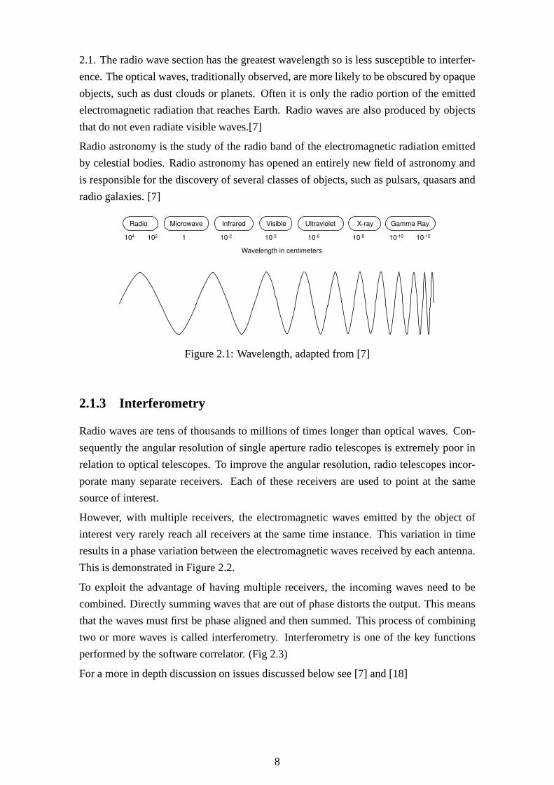
2.1. The radio wave section has the greatest wavelength so isless susceptible to interfer-
ence. The optical waves, traditionally observed, are more likely to be obscured by opaque
objects, such as dust clouds or planets. Often it is only the radio portion of the emitted
electromagnetic radiation that reaches Earth. Radio wavesare also produced by objects
that do not even radiate visible waves.[7]
Radio astronomy is the study of the radio band of the electromagnetic radiation emitted
by celestial bodies. Radio astronomy has opened an entirelynew field of astronomy and
is responsible for the discovery of several classes of objects, such as pulsars, quasars and
radio galaxies. [7]
Radio Microwave Infrared Visible Ultraviolet X-ray Gamma Ray
104 102 1 10-2 10-5 10-6 10-8 10-10 10-12
Wavelength in centimeters
Figure 2.1: Wavelength, adapted from [7]
2.1.3 Interferometry
Radio waves are tens of thousands to millions of times longerthan optical waves. Con-
sequently the angular resolution of single aperture radio telescopes is extremely poor in
relation to optical telescopes. To improve the angular resolution, radio telescopes incor-
porate many separate receivers. Each of these receivers areused to point at the same
source of interest.
However, with multiple receivers, the electromagnetic waves emitted by the object of
interest very rarely reach all receivers at the same time instance. This variation in time
results in a phase variation between the electromagnetic waves received by each antenna.
This is demonstrated in Figure 2.2.
To exploit the advantage of having multiple receivers, the incoming waves need to be
combined. Directly summing waves that are out of phase distorts the output. This means
that the waves must first be phase aligned and then summed. This process of combining
two or more waves is called interferometry. Interferometryis one of the key functions
performed by the software correlator. (Fig 2.3)
For a more in depth discussion on issues discussed below see [7] and [18]
8
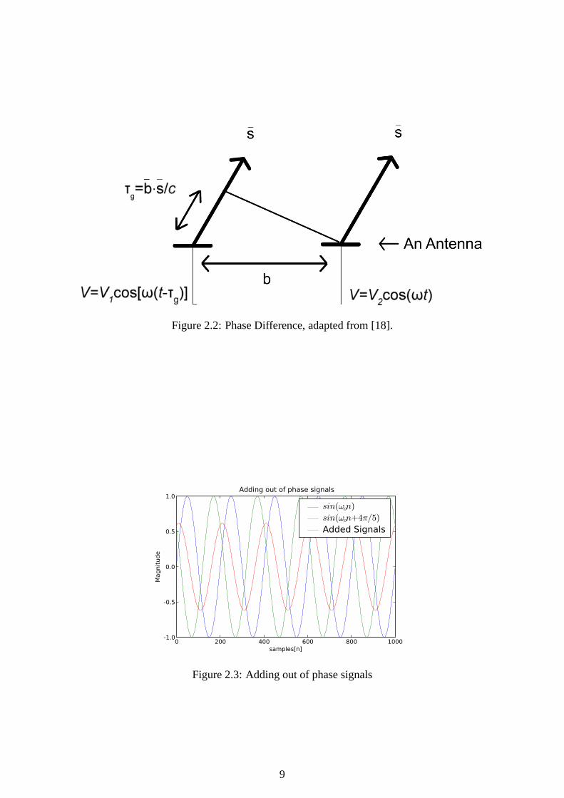
Figure 2.2: Phase Difference, adapted from [18].
0 200 400 600 800 1000
samples[n]
-1.0
-0.5
0.0
0.5
1.0
Magnit
ude
Adding out of phase signals
o )nω(nis
o )5/π4+nω(nis
Added Signals
Figure 2.3: Adding out of phase signals
9

2.1.4 Correlation
The correlation of two signals tell us how similar the signals are. It can be used to identify
the phase variation between two signals, among other things.
Suppose we have two sampled voltage signals,f(t) andg(t), the correlation function,
Rfg(τ) is defined as[17]:
Rfg(τ) = limT→∞
1
T
∫ T
0
f ∗(t)g(t + τ)dt, (2.1)
which can be written as,
Rfg(τ) = 〈f(t)∗g(t + τ)〉τ (2.2)
The magnitude of the correlation output ,|Rfg(τ)|, will depend on the two signals’ simi-
larity.
Two identical antennas pointing in the same direction will both receive the same signal,
however, they will receive it at different times. Thus the variation in the correlation output
is due to a phase difference between the signals. This phase differences can be identified
through the correlation of the two signals. This is needed toperform interferometry.
Correlation is a key operation used to compute complex visibilities, the final output of the
software correlator.
2.1.5 Analytic Signal Representation
All real time signals have a two sided frequency response which is symmetrical about the
origin. Since both sides of the frequency response are identical, all the spectral informa-
tion of the real time signal can be represented by one side. The analytical representation
of a signal is twice the positive side of its spectrum with thenegative frequency compo-
nents set to zero. Since we take twice the positive spectral components, the same power
in the signal is retained.[14]
If f(t) is a real time signal then the analytical representationE(t) can be constructed as
follows :
E(t) = f + jH{f(t)} (2.3)
where,
H{f(t)} =1
π
∫ ∞
∞
f(τ)
t− τdτ (2.4)
H [f(t)] represents the Hilbert transform of signalf(t). The Hilbert transform effectively
rotates the negative frequency components of voltage signal f(t) by 90o and the positive
spectral components by−90o. Multiplying the Hilbert transform byj further rotates all
the phase components by90o. When summed with the original signal,f(t), results in the
10
analytic signalE(t). The construction of an analytic signal using the Hilbert transform is
demonstrated in Figure 2.5.
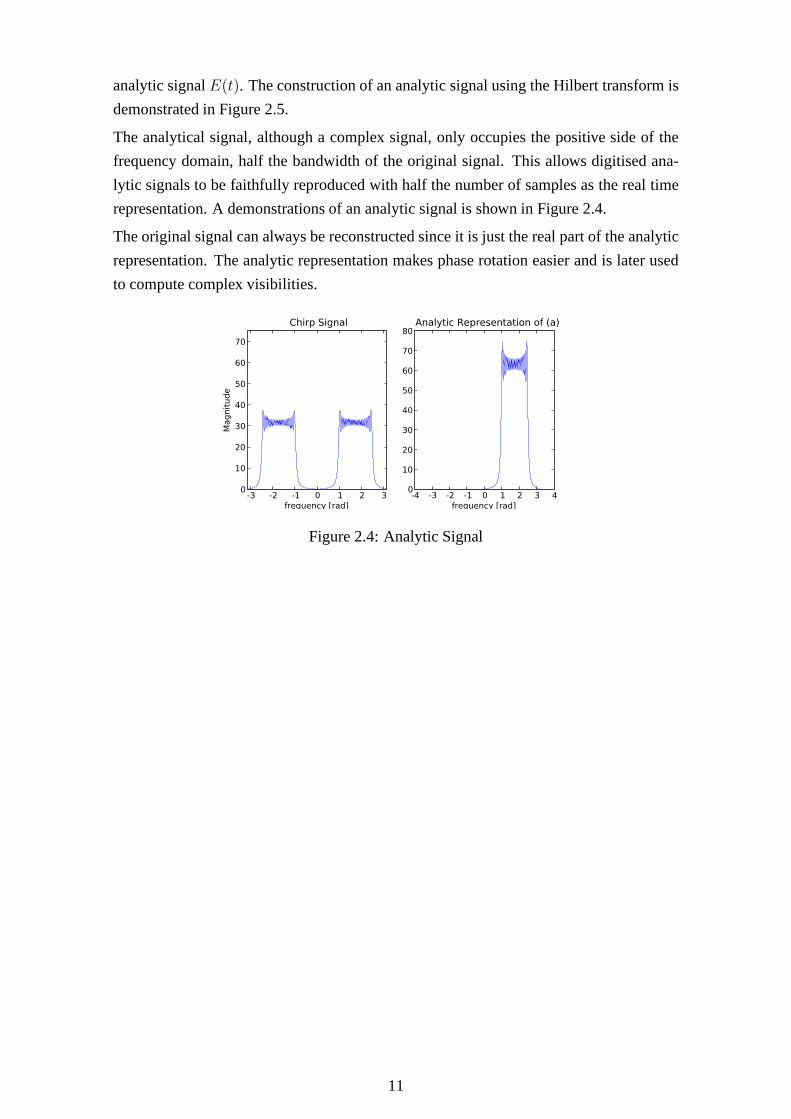
The analytical signal, although a complex signal, only occupies the positive side of the
frequency domain, half the bandwidth of the original signal. This allows digitised ana-
lytic signals to be faithfully reproduced with half the number of samples as the real time
representation. A demonstrations of an analytic signal is shown in Figure 2.4.
The original signal can always be reconstructed since it is just the real part of the analytic
representation. The analytic representation makes phase rotation easier and is later used
to compute complex visibilities.
-3 -2 -1 0 1 2 3
frequency [rad]
0
10
20
30
40
50
60
70
Magnit
ude
Chirp Signal
-4 -3 -2 -1 0 1 2 3 4
frequency [rad]
0
10
20
30
40
50
60
70
80Analytic Representation of (a)
Figure 2.4: Analytic Signal
11
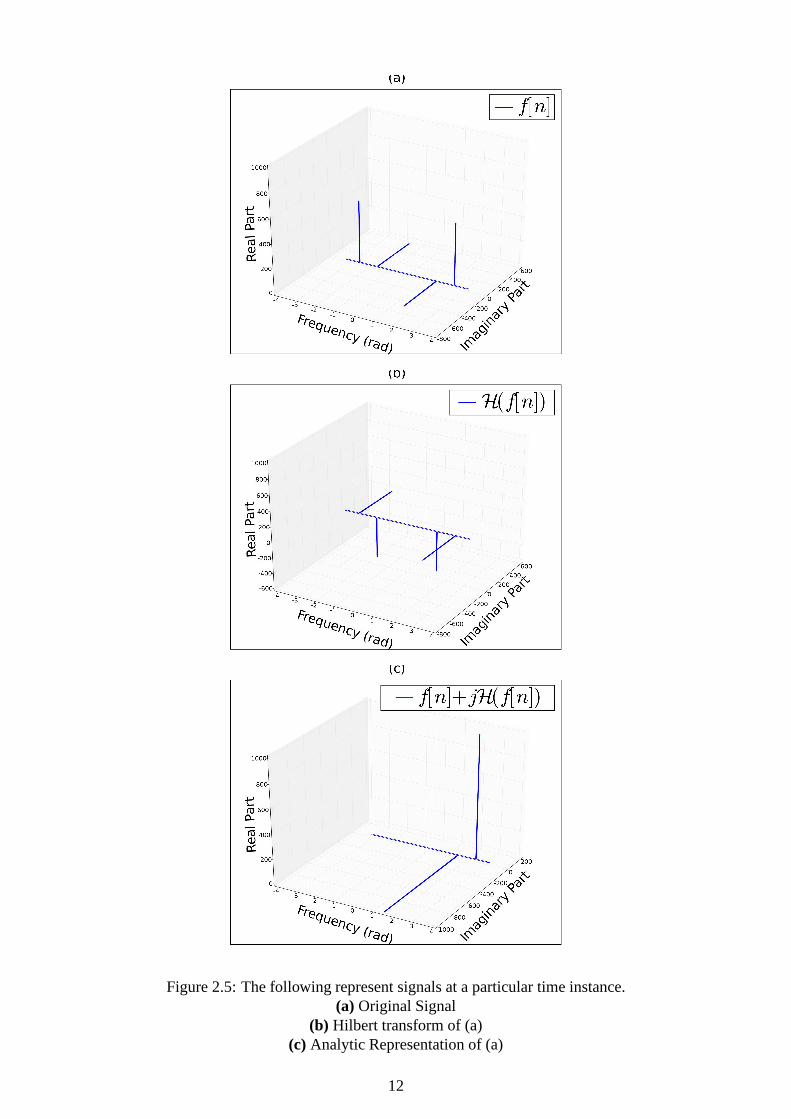
Figure 2.5: The following represent signals at a particulartime instance.(a) Original Signal
(b) Hilbert transform of (a)(c) Analytic Representation of (a)
12

2.1.6 Complex Visibilities
The complex visibilities, the final output of the software correlator, are what astronomers
are really interested in. Complex visibilities are used to find the difference in intensity
between the fringes which are used for imaging, spectroscopy/polarimetry and astrometry
[4].
The complex visibility of two signals,f(t) andg(t) , can be defined as follows:
Vf g(τ) =< f(t)g(t + τ) > +j < H{f(t)} g(t + τ) > (2.5)
So in words, the complex visibility of two signals,f(t) andg(t), is the summation of the
correlation off(t) andg(t) and the Hilbert transform off(t) correlated withg(t).
The phase difference between the two signalsf(t)andg(t)can now be extracted from the
visibility:
φ = arctan
(
ℑ{Vfg(τ)}
ℜ {Vfg(τ)}
)
(2.6)
This phase information can then be fed back to the software correlator so that the neces-
sary interferometry can be performed. However, the complexvisibilities are used in later
operations to perform imaging, spectroscopy/polarimetryand astrometry. These all fall
out of the scope of this project, but for a more comprehensivediscussion on these topics
refer to [15].
2.1.7 Coherency vector and Stokes Visibilities
Electromagnetic waves are transverse in nature and have twoaxes of oscillation(polarisation),
usually represented byx andy, and one axis of propagation, usually represented by the
z axis. Because of this polarisation it is customary to represent a radio wave as a set of
stokes parameters. Stokes parameters are a set of values used to describe the polarisation
state of a electromagnetic wave [10].
A polarised wave is usually represented by vectore =
(
ex
ey
)
, whereex andey are com-
plex vectors of the polarisation state in the x and y axis respectively. With two polarised
vectors,eA andeB, received from antennaA andB respectively it is useful to represent a
coherency vector which can be defined from the two vectors as follows:
e+ =
⟨
eAxe∗Bx
eAxe∗By
eAye∗Bx
eAye∗By
⟩
(2.7)
From this coherence vector we can form the Stokes Visibilities,I Q U V , which are the
actual outputs of the software correlator and are created bythe following relationship:
13
I
Q
U
V
= Te+ (2.8)
where:
T =
1 0 0 1
1 0 0 −1
0 1 1 0
0 −i i 0
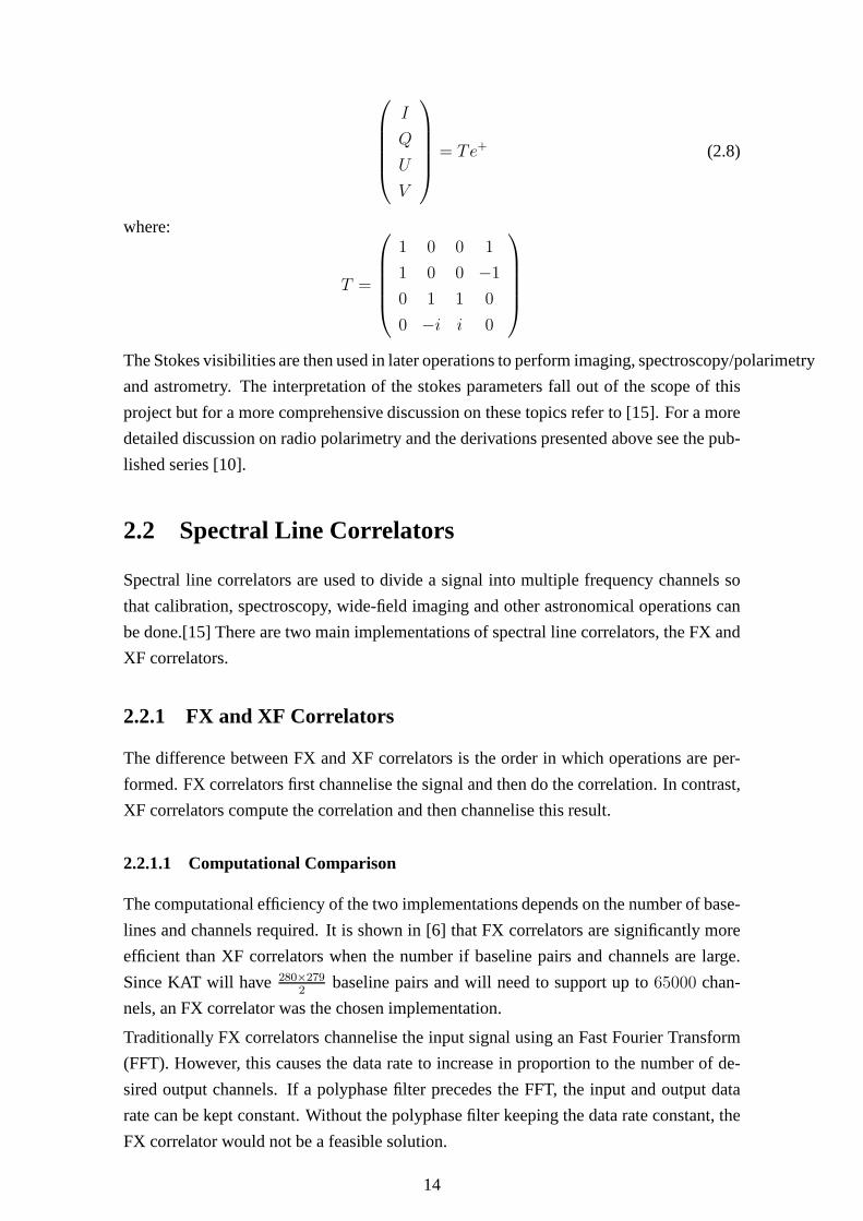
The Stokes visibilities are then used in later operations toperform imaging, spectroscopy/polarimetry
and astrometry. The interpretation of the stokes parameters fall out of the scope of this
project but for a more comprehensive discussion on these topics refer to [15]. For a more
detailed discussion on radio polarimetry and the derivations presented above see the pub-
lished series [10].
2.2 Spectral Line Correlators
Spectral line correlators are used to divide a signal into multiple frequency channels so
that calibration, spectroscopy, wide-field imaging and other astronomical operations can
be done.[15] There are two main implementations of spectralline correlators, the FX and
XF correlators.
2.2.1 FX and XF Correlators
The difference between FX and XF correlators is the order in which operations are per-
formed. FX correlators first channelise the signal and then do the correlation. In contrast,
XF correlators compute the correlation and then channelisethis result.
2.2.1.1 Computational Comparison
The computational efficiency of the two implementations depends on the number of base-
lines and channels required. It is shown in [6] that FX correlators are significantly more
efficient than XF correlators when the number if baseline pairs and channels are large.
Since KAT will have 280×2792
baseline pairs and will need to support up to65000 chan-
nels, an FX correlator was the chosen implementation.
Traditionally FX correlators channelise the input signal using an Fast Fourier Transform
(FFT). However, this causes the data rate to increase in proportion to the number of de-
sired output channels. If a polyphase filter precedes the FFT, the input and output data
rate can be kept constant. Without the polyphase filter keeping the data rate constant, the
FX correlator would not be a feasible solution.
14

For a more in depth review of the performance issues relatingto FX correlators see [6],
by John Bunton, or one of his many other published articles.
2.3 DSP Concepts
A channeliser is needed for the software correlator to breakup the received radio waves
into various frequency channels. Once channelised, the individual components can be
analyzed and correlated. However, a conventional channeliser offers poor performance.
This section will briefly review the conventional channeliser, introduce the ideas behind
polyphase decomposition and explain why a polyphase channeliser architecture was used
for the software correlator.
2.3.1 Conventional DSP Concepts
2.3.1.1 Finite Impulse Response (FIR) Filters
A filter is a system used to remove a range of unwanted frequency components from a
signal, while preserving other frequencies. Filters are characterised by their magnitude
response and phase response.
Digital FIR filters are linear time-invariant (LTI) systemswhich are represented by a finite
length sequence,h[n]. Given the sequence,x[n], an input to an LTI system, the output,
y[n] can be computed by convolving the input withh[n]:
y[n] =
N−1∑
r=0
x[r]h[n− r] (2.9)
Equation 2.9 can be represented by the following block diagram:
Figure 2.6: FIR Filter Block Diagram
2.3.1.2 Channelising
A channeliser is a system that decomposes an input signal into its various frequency com-
ponents.
Channelisers traditionally make use of FIR filters, in combination with decimators and
complex oscillators, to extract the desired bandwidth out of a signal. A typical channeliser
has the form[11]:
15
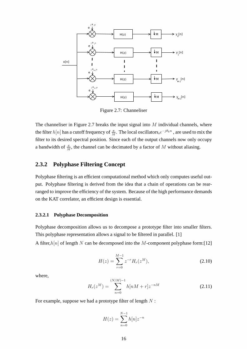
Figure 2.7: Channeliser
The channeliser in Figure 2.7 breaks the input signal intoM individual channels, where
the filterh[n] has a cutoff frequency ofπM
. The local oscillators,e−jθkn , are used to mix the
filter to its desired spectral position. Since each of the output channels now only occupy
a bandwidth ofπM
, the channel can be decimated by a factor ofM without aliasing.
2.3.2 Polyphase Filtering Concept
Polyphase filtering is an efficient computational method which only computes useful out-
put. Polyphase filtering is derived from the idea that a chainof operations can be rear-
ranged to improve the efficiency of the system. Because of thehigh performance demands
on the KAT correlator, an efficient design is essential.
2.3.2.1 Polyphase Decomposition
Polyphase decomposition allows us to decompose a prototypefilter into smaller filters.
This polyphase representation allows a signal to be filteredin parallel. [1]
A filter,h[n] of lengthN can be decomposed into theM-component polyphase form:[12]
H(z) =M−1∑
r=0
z−rHr(zM), (2.10)
where,
Hr(zM ) =
(N/M)−1∑
n=0
h[nM + r]z−nM (2.11)
For example, suppose we had a prototype filter of lengthN :
H(z) =N−1∑
n=0
h[n]z−n
16

Traditionally we would compute the output of LTI systemh[n] as shown in Figure 2.6.
However, if we were to decompose the prototype filter into twotermsH0(z2) andH1(z
2),
we could compute the same prototype filter by:
H(z) = H0(z2) + z−1H1(z
2)
and represent the same transfer function as in Figure 2.6 by the figure below.
Figure 2.8: Two-branch polyphase decomposition
In the above diagram, for every execution period, two coefficients can be calculated. This
idea can be extended to multi-branch decomposition, usually with 2n branches1.
2.3.2.2 Polyphase Filtering with Re-sampling
Computing the output of LTI systems involves a large number of multiplication and addi-
tion operations. However when a FIR filter is superseded by a decimator,M − 1 of every
M of these results are discarded as shown in Figure 2.9. It is inefficient to calculate all
these results when only a small proportion is kept.
Figure 2.9: FIR Filter with decimator
However if the filter is represented inM-component polyphase form, as shown in Figure
2.10, the decimation can be performed before the filtering while still achieving the same
result [11]2. In this polyphase equivalent form, the input data rate is1M
th of what is was
in Figure 2.9. This greatly reduces the workload of a filter, increasing the efficiency.
2.3.2.3 Polyphase Filter as a Channeliser
Each channel of a traditional channeliser is composed of a complex mixer, a low pass
filter and a decimator. However, because of theequivalency theoremit can be shown that
1The reason for the2n restriction is due to the fact that the polyphase filter is often used in conjunctionwith an FFT
2For a detailed derivation of the decimator rearrangement see [11] chapter 2
17
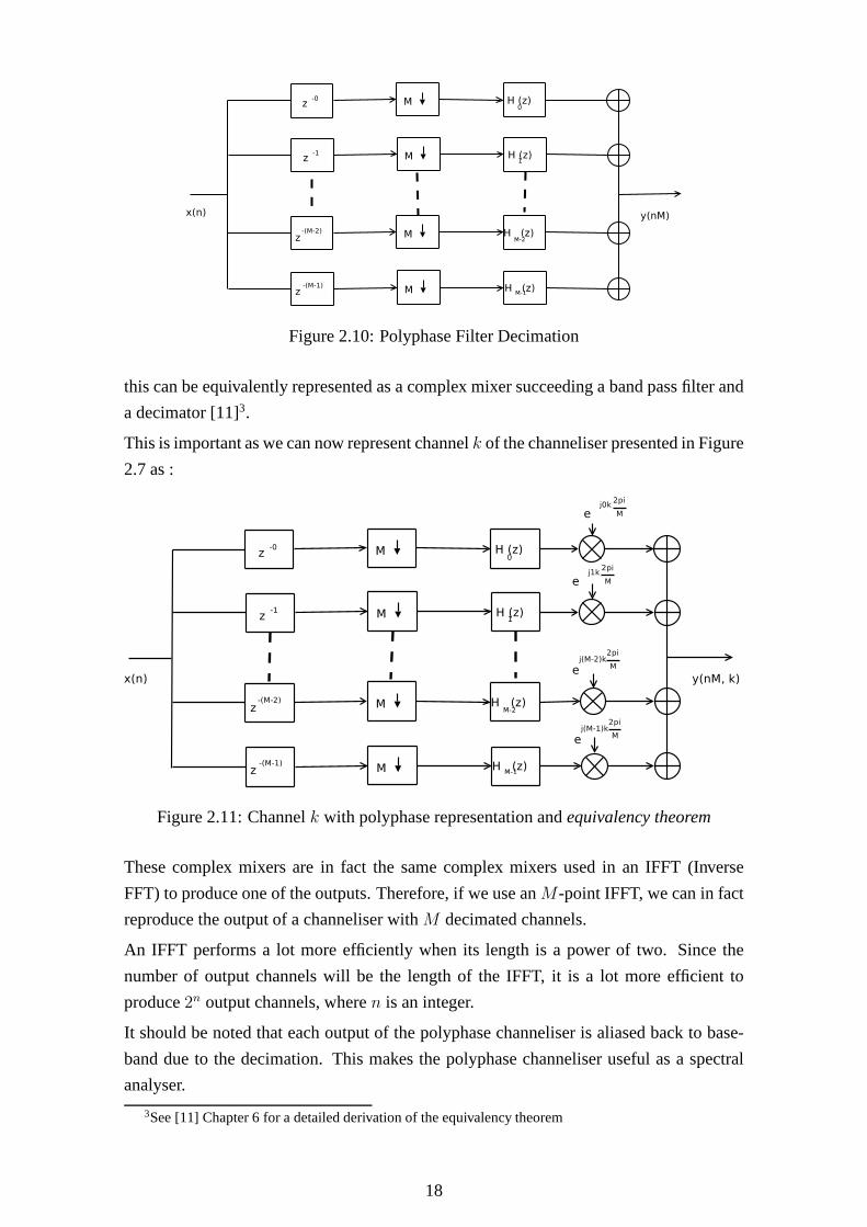
Figure 2.10: Polyphase Filter Decimation
this can be equivalently represented as a complex mixer succeeding a band pass filter and
a decimator [11]3.
This is important as we can now represent channelk of the channeliser presented in Figure
2.7 as :
Figure 2.11: Channelk with polyphase representation andequivalency theorem
These complex mixers are in fact the same complex mixers usedin an IFFT (Inverse
FFT) to produce one of the outputs. Therefore, if we use anM-point IFFT, we can in fact
reproduce the output of a channeliser withM decimated channels.
An IFFT performs a lot more efficiently when its length is a power of two. Since the
number of output channels will be the length of the IFFT, it isa lot more efficient to
produce2n output channels, wheren is an integer.
It should be noted that each output of the polyphase channeliser is aliased back to base-
band due to the decimation. This makes the polyphase channeliser useful as a spectral
analyser.
3See [11] Chapter 6 for a detailed derivation of the equivalency theorem
18

Figure 2.12: Polyphase Filter Bank
2.4 Concept Review Conclusion
The above concepts lay the foundation of the design and implementation to follow. These
concepts are vital to the development and testing of the system. Once these concepts are
understood, a clear picture of the outcomes of the software correlator can be created.
19

Chapter 3
Design
Chapter 3 presents each stage of the correlator and its operations. This chapter begins by
providing a more detailed requirements review of the software correlator. Each operation
presented in Figure 1.1 is addressed individually and discussed in detail. The sequential
mathematical transformations are shown from real time voltage signal input, through to
the complex visibilities output. These mathematical operations were simulated in python
and the results presented. The python simulations not only aid in the understanding of
the correlator’s operations but also provide a useful reference for algorithms and results
discussed in later chapters.
3.1 Software Correlator Requirements Review
3.1.1 KAT Correlator Requirements
A total of 280 incoming streams of data will be sampled at 1.2GHz with 8 bits per sample.
This is a total of almost 2.7 Terabits that need to be processed every second. Each of these
280 input streams will need to be channelised into65000 different channels.
Each of these 280 incoming channels need to have a number of operations performed on
their data. These operations are outlined in Figures 1.1 and3.8.
The correlator will need to be able to operate on a wide variety of incoming data. The
functions of the correlator will differ greatly depending on the input, therefore the oper-
ations the correlator performs need to be versatile in orderto adapt to variable types of
inputs.
Because of these demanding requirements, the KAT team decided to implement the cor-
relator in hardware. Each input to the correlator is largelyindependent of other inputs and
each input has the same operations performed on it. These repetitive independent tasks al-
low the correlator to be constructed in a highly paralisablemanner. These attributes make
the correlator ideally suited to being implemented in hardware. Each of the operations
shown in Figure 1.1 is independent of other operations and can be treated as a separate
system.
20

On the downside, hardware development is a slow and difficult. It would be difficult
to test a hardware implementation until it is fully completed. The development time of
hardware can be greatly reduced if there is a system against which to test its output.
The objective of this project was to investigate each of the operations in the correlator
chain and implement them in software. Software is an ideal testing environment, as it
is easy to manipulate. A software simulation is vital as it serves as a powerful tool to
implement and test core concepts that will be used in the finalhardware design. The
software implementation developed in this project was designed to be modular so that
each operation could be interchanged with the hardware equivalent. As future hardware
development is completed, the correlator will become a hybrid of software and hardware
components and eventually purely hardware.
Since the software is interchangeable with hardware components, the software followed
much of the constraints set on the hardware. More detail on the implementation of the
correlator is discussed in Chapter 4.
This chapter will continue by describing the correlator operations provided by Dr. Rudolph
van der Merwe and Dr. Richard Lord and running simulations ofthem.
The objectives of this project can be summarised as:
• Investigate the operations of the correlator in detail and provide an architectural
design.
• Build onto the API provided by Dr. Marc Welz to support the operations the corre-
lator needs to perform.
• Implement the correlator in ANSI C, using the modified API.
• Ensure flexibility in design.
3.2 Correlator Design
The electromagnetic waves detected by the antennas have various modifications per-
formed on them by the radio frequency(RF) front end. These modified electromagnetic
waves are the input to the correlator. The correlator performs various computations on
this input to produce the output, the complex visibilities.
Since the correlator is operating at a tremendously high data rate, signals are down-
sampled and unwanted channels are discarded whenever not needed.
The correlator is very modular in design, allowing each of the computations to be im-
plemented and tested independently. The basic design of thecorrelator is divided into
stages, with each one feeding its output into the next module. Each of these stages will be
discussed in the order it appears in Figure 1.1.
21

3.2.1 The Analogue to Digital Converter (ADC)
The ADC is responsible for converting the voltage time series signal into a digitalized
sampled signal. The ADC has a sampling rate of 1.2GHz ,(Fs), with 8bits per sample
and a 550MHz input bandwidth.1 The input,vi,j,p(t), (wherei is the voltage of the dish,
j the beam andp the polarity) is sampled at time periodT to produce the sampled signal
vi,j,p[k] of lengthM .
vi,j,p[k] = vi,j,p(t)
M−1∑
k=0
δ(t− kT ) (3.1)
=M−1∑
k=0
vi,j,p(kT ).δ(t− kT ) (3.2)
3.2.2 The Time Delay Compensation
Each time signal will be received at different time instances by different antennas, re-
sulting in a phase difference. These signals need to be phasealigned to perform inter-
ferometry. See Interferometry Section 2.1.3.The phase alignment of the input waves will
take place in two sections, the time delay compensation and then the phase correction
operation.
The delay compensation is used for coarse alignment of out ofphase signals. The input
to the delay compensatorvi,j,p[k], is delayed by an integer,n, of the sampling period,T ,
to produce the output,ui,j,p[k]. Where:
ui,j,p[k] = vi,j,p[k − n] (3.3)
vi,j,p[k] z←→Vi,j,p(z)
vi,j,p[k − nT ] z←→z−nVi,j,p(z)
The time delay,τg, experienced by the incoming signal can only perfectly align by the
time delay compensation stage if the time delay,τg = Tn for some integer value ofn.
This is often not the case as in Figure 3.1:
The remaining phase difference needs to be adjusted in the phase correction operation.
The finer phase correction is discussed in Section 3.2.5.
1This1.2GHz band will not be taken from baseband so aliasing will take place. This was not consideredduring this project but must be considered in the final implementation.
22

Figure 3.1: Delay compensator operation, whereτg 6= Tn.
3.2.3 Digital Down Conversion (DDC) with Fringe Stopping
This stage performs three separate operations; analytic signal representation, digital down
conversion and fringe stopping.
3.2.3.1 Fringe Stopping
The delay compensation in the previous section is calculated as a function of the baseline
distance and direction vector of the source, assuming stationary receivers. Since the Earth
is rotating, the effective time taken for a signal to reach a receiver is either increased or
decreased depending on the position of the receiver. This causes a Doppler shift, which
will effect both the phase and frequency of the signal, and ifnot corrected will produce an
incorrect correlation value. Little investigation has been done in Fringe Stopping for this
report, but the usual solution is to correct the error by adjusting the phase and frequency
in the local oscillator used to create the analytic signal representation.[3]
3.2.3.2 Analytic Signal Construction2
An analytic signal, as discussed in Section 2.1.5, can be constructed from any real signal
by preserving only the positive side of the spectrum and nulling the negative side. This
2See Appendix D for more detailed derivation.
23

representation is useful as it simplifies phase correction and is also used in computing the
complex visibilities.
Since the input signal,ui,j,p[k], is real, the spectral components will be symmetrical and
therefore can be represented as an analytical signal. In this implementation a baseband
representation of the analytic signals is constructed by using oscillators to mix the signal
to be centered at eitherπrad/sec or0rad/sec. The last statement may sound contradictory but
since a decimation factor of23 is used, the signal mixed toπ will alias back to baseband as
shown in Figure 3.3. We define the analytical baseband representation of the input signal
ui,j,p[k] as:
u[k]a = u,I [k] + j.uQ[k] (3.4)
where:
uI [k] = [2u[k]. cos(2πf0t)]LPF (3.5)
uQ[k] = [2u[k]. sin(2πf0t)]LPF (3.6)
and:
uQ[k] = H{uI [k]} = [2u[k]. cos(2πf0t−π
2)]LPF
An example of input and output to the analytic signal construction stage is shown below
in Figure3.2.
-3 -2 -1 0 1 2 3
frequency [rad]
0
20
40
60
80
100
Magnit
ude
Analytic Construction Input
Delay Compenator Output
-3 -2 -1 0 1 2 3
frequency [rad]
0
20
40
60
80
100
120
Analytic Construction Output
Analytic signal Constuction output
Figure 3.2: Input and output of analytic signal construction stage
3.2.3.3 Down Conversion
The analytical signal, although now a complex signal, only occupies the positive side of
the frequency domain, half the length of the original signal. The analytical signal can now
3Decimator will also work for all even decimation factors
24

be down sampled to reduce the sample rate fromFs to Fs2
. This is done by taking every
2nd sample fromu[k]a, an example of this is shown in Figure 3.3. Thus we can define the
output of the DDC section as,u[k], where:
˜u[k] = u[2k]
-3 -2 -1 0 1 2 3
frequency [rad]
0
20
40
60
80
100
120
Magnit
ude
Down Sampler Input
Analytic Construction Output
-3 -2 -1 0 1 2 3
frequency [rad]
0
20
40
60
80
100
Down Sampler Output
Down Sampler Output
Figure 3.3: Down Sampled signal alias back to baseband
3.2.4 Channelisation
Channelisation separates incoming signals into a number offrequency channels. It is
an important part of the correlator as it allows individual components to be analysed
and correlated. Because this is an FX correlator, the channelisation takes place before
the correlation. If the channeliser can decompose the inputsignal into channels with a
small enough bandwidth, the output from each channel can be treated as a monochromatic
signal. This is important as it allows the correlator to effectively phase adjust and analyse
each frequency component of the input signal separately.
Channelising is performed in three separate stages; coarsechannelisation, bandwidth re-
duction and fine channelisation. Both coarse and fine channelisation are done by polyphase
channelisers. This dual stage filterisation offers a computational advantage, as discussed
below.
3.2.4.1 Coarse Channelisation
The first polyphase channeliser is used to divide the input signal band into coarse chan-
nels. This is done so that channels not containing useful spectral information can be
discarded before more processing takes place.
The number of output channels of the polyphase channeliser is the same length as the
input to the IFFT used in the polyphase channeliser. The number of computations of a
standardN point FFT isN log2N , whereN is the number of output channels,M. Since
25

a number of these channels will be discarded in the BandwidthReduction stage 3.2.4.2,
it would be computationally wasteful to decompose the entire input bandwidth into fine
channels before bandwidth reduction.
The input analytical signalui,j,p[k] will pass through the polyphase filter to produceNc1
separate channels of centre frequencyvc1m . The outputui,j,p,vc1′
mwill then be passed to the
bandwidth reduction stage.
Continuing with the previous example, Figure 3.4 shows the input divided into five coarse
channels. Each channel will have an independent output and will be aliased back to
baseband.
-3 -2 -1 0 1 2 3
frequency [rad]
0
20
40
60
80
100
magnit
ude
Coarse Channeliser Input
DDC stage output
Output Channel 0
Output Channel 1
Output Channel 2
Output Channel 3
Output Channel 4
Figure 3.4: Coarse channelisation demonstration
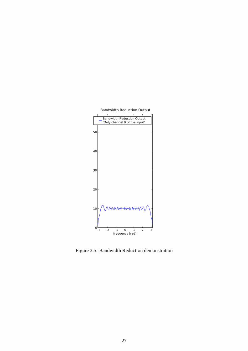
3.2.4.2 Bandwidth Reduction
The bandwidth reduction stage will discard channels created by the coarse channeliser,
that are not required. The bandwidth preserved needs to be specified as it will vary de-
pending on the astronomical process.
The number of channels will be reduced fromNc1to N ′c1whereN ′
c1≤Nc1.
Continuing from the example presented in Figure 3.4, if it isknown that channel 0 was the
only band of interest in a hypothetical astronomical operation, then the other 4 channels
could be discarded, reducing the data rate by a factor of 5. The remaining channel is
decimated by a factor of five as consequence of the polyphase filtering. This causes
aliasing back to baseband and a reduction in amplitude, as shown in Figure 3.5.
3.2.4.3 Fine Channelisation
The fine channeliser is responsible for the further decomposition of the remaining chan-
nels, using a polyphase filter bank.
It is now important to note the following. As the number of output channels of the
polyphase channeliser tends to infinity, each channel tendstowards zero bandwidth and
26
-3 -2 -1 0 1 2 3
frequency [rad]
0
10
20
30
40
50
Bandwidth Reduction Output
Bandwidth Reduction Output
’Only channel 0 of the input’
Figure 3.5: Bandwidth Reduction demonstration
27

is aliased to baseband, creating a DC signal. Each channel output can be represented by
|vωijpC|ejφωijpC , whereφ is the phase and|v| the magnitude of the spectral component of
the input to the correlator, atωc . The output no longer has any frequency component and
therefore is represented by a constant DC value. It is usefulto view the polyphase chan-
neliser with infinite output channels as the Fourier transform, since it effectively gives the
magnitude and phase response for each spectral component,ωc [11].
It is impossible to have infinite output channels, thereforewe decompose the input to the
fine channeliser into up to65000 separate channels. This decreases the spectral resolution
to a point where each output channel can be assumed to have almost zero bandwidth. The
phase of the individual components can now be aligned with the corresponding channel
of other antennas. This is done in the next section, Phase Correction.
The input,ui,j,p,vc1′m
will pass through the polyphase filter to produceNc2 separate channels
of centre frequencyvc2m . The output,ui,j,p,vc2′
mwill then be passed to the phase correction
stage.
Continuing with the example, the expected output of the fine channeliser is presented
in Figure 3.6. The channel in the example is only decomposed into 40 separate output
channels. However, the KAT FX software correlator can decompose the input channel
into up to65000 separate channels.
-3 -2 -1 0 1 2 3
frequency [rad]
0
5
10
15
20
magnit
ude
Fine Channeliser Input
Output Channel from Bandwidth Reduction
Output channels of Fine Channeliser
Figure 3.6: Fine channelisation demonstration
3.2.5 Phase Correction
In the phase correction stage we continue the phase alignment of signals from each an-
tenna that began in the delay compensation stage. Since the input to the correlator,vi,j,p[k]
, has bandwidth, the phase shift experienced will not be uniform across the band and will
depend on each frequency component. The phase correction stage does the fine align-
ments not able to be performed in the delay compensation stage and is used to complete
the phase alignment used for interferometry.
The input received from the channeliser have effectively nobandwidth, allowing the phase
28

correction stage to treat each channel as a monochromatic baseband signal4. The corre-
sponding channels from each antenna are phase aligned by a complex multiplier.
The phase correction stage performs corrections needing a change of less than one sam-
pling periodT . The inputui,j,p,vc2′m
will be multiplied bye−jφ
i,j,p,vc2′m , whereφ is the fre-
quency value that the input will be adjusted by.
vi,j,p,vc2′m
= ui,j,p,vc2′m× e
−jφi,j,p,vc2′
m (3.7)
The previous example is continued, showing the phase alignment between two channels,
ui anduj. This is shown in Figure 3.7.
Figure 3.7: Phase Correction
3.2.6 Correlation
In this final stage of the correlator the separate signals from the various antennas are
combined. This process is performed in two subsections, first correlation is performed
and then the Stokes Visibilities are computed.5
3.2.6.1 Correlation Functions
Each channel is multiplied by each polarity of the corresponding channels of each of the
20 antennas, including its own antenna (See Fig 3.8). This is represented by the following
correlation function[19]:
cxy∗ ,v(n) = ˜vx,p(n)v∗y,p(n) (correlation) (3.8)
4In reality the channels will have small bandwidth5The interpretation of these results fall outside the scope of this project.
29

Because the input channels are not purely DC signals and contain some frequency com-
ponent, time averaging is used to smooth out this variation in phase. This produces the
power spectral density,Sxy∗,v(k). This function is shown below:
Sxy∗,v(k) =1
N
k∑
n=k−N
cxy∗ ,v(n) (time average) (3.9)
When a particular polarity of a particular channel is correlated with itself, the correlation
is referred to as auto-correlation. This is one of the outputs of the correlator that is used
in the succeeding astronomical processes.
When correlated with anything else, this cross correlationproduces coherency vectors.
These coherency vectors are used to compute the Stokes Visibilities and determine the
phase variation between two signals.
3.2.6.2 The Complex Stokes Visibilities
The four coherency vectors for each channel pair are used to calculate the Stokes Visibili-
ties as shown in Equation 3.10. These Stokes Visibilities are used to describe the complex
visibility in terms of the polarisation state. This is the other output of the correlator that
is be used in the succeeding astronomical processes[19].
V obsI,i1,i2,vm
(k)
V obsQ,i1,i2,vm
(k)
V obsU,i1,i2,vm
(k)
V obsV,i1,i2,vm
(k)
=
1 0 0 1
1 0 0 −1
0 1 1 0
0 −i i 0
Sxi1x∗
i2,vm(k)
Sxi1y∗
i2,vm(k)
Syi1x∗
i2,vm(k)
Syi1y∗
i2,vm(k)
(3.10)
3.3 Design Conclusion
The python simulations used to generate the above diagrams,helped in understand the
FX correlator operations. These simulations supplied the coded algorithms that formed
the basis of the final software correlator implementation. With these foundations covered
in this design chapter, the issues relating to the final correlator implementation can be
addressed.
30

Figure 3.8: Correlation in Detail, by Dr. van der Merwe and Dr. Lord.[19]
31
Chapter 4
Implementation
The python simulations mentioned in Chapter 3 were developed to test the mathematical
operations that needed to be performed. These simulations were all run on a finite set of
input data, from only one source. There were no invalid inputs and the operations were
not distributed over different computational devices. However, the environment in which
the actual correlator operates receives a continuous stream of input data, from multiple
sources (antennas). There could be invalid inputs and the operations will be distributed
over different computational devices. This chapter discusses the problems created by
less ideal input that the correlator receives in reality andthe actions taken to produce the
desired output as presented in Chapter 3.
This chapter begins by reviewing the design of the KAT API provided for the software
correlator. This chapter continues to describe the modifications to the KAT API to fully
support the specifications of the input data stream. The channel abstraction from the KAT
data frame is presented and its purpose described.
4.1 Software Correlator Infrastructure
The final hardware will be implemented over a distributed system and will use a 10 gigabit
Ethernet architecture as the connection infrastructure. Since the software is interchange-
able with hardware components, this same distributed specification applies to the software
correlator.1
4.2 Adaptation to Support Realistic Input
The changes needed to support realistic data flow between thestages in the software
correlator are discussed below and shown in Table 4.1.1The other possibility for the networking architecture was InfiniBand
32

Ideal Input Realistic InputFinite Input Streaming Input
No Distributed System Distributed SystemNo Invalid Input Invalid InputOne Input Source Multiple Input Sources
Table 4.1: Ideal vs. Realistic data input.
4.2.1 The KAT API
The KAT API provides a description of the methods and messagestructure used to com-
municate between the correlator stages. Dr. Marc Welz, a member of KAT team, provided
the following design outline in the following subsections,which was a very useful starting
point and aided the software correlator implementation. The implementation was done in
the ANSI C programming language, as this is an efficient programming language and
simpler to port to hardware.
4.2.1.1 Packetising input stream
The output from the ADC, the input to the section of the correlator focused on in the
project, is an endless stream of data. This needs to be packetised so that it can be passed
to the next stage of the correlator. These packets need headers to describe the data, the
payload of the packet, so that the stream can be reconstructed at each reception point.
This message structure will be referred to as a KAT data frameand the original structure
is presented in Figure 4.1. Output data from each correlatoroperation is first packetised
into a KAT data frame before being passed down the network protocol stack. The protocol
stack for the software correlator is described in Figure 4.2. The KAT API holds one input
frame and one output frame at any particular instant. Any buffering must be done by the
correlator operations.
Figure 4.1: Original header for the KAT data frame [20]
4.2.1.2 Dealing with bad input
The ADC will produce9.6Gbps data for each antenna input, which is near the maximum
operating rate of 10 gigabit Ethernet (10Gbps). Therefore, using transport protocols to
retransmit KAT packets dropped by the network architecturewould not be a reasonable
33

Figure 4.2: KAT network protocol stack
solution, as it would be unable to cope with a data rate increase. This would cause un-
wanted delays to the output and possible buffer overflows.
If a KAT data frame is dropped or corrupted, the correlator will instead create dummy
samples to retain the constant data rate flow. This constant data rate helps to maintain
predictability of the system.
The invalid data needs to be flagged so that the next stage of the correlator can identify it
as invalid and can handle it correctly. It was decided that out of band signalling would be
used to describe this invalid input. Out of band signaling has the advantage that it does
not effect the word size of the sampled data (eg in the case of using a dirty bit). However,
this means there will be more overhead to describe the KAT data frame.
It is not reasonable to describe to the validity of every input, as this will cause extensive
overhead. The bad samples of the payload are rather described by a range, byf_bad_first
andf_bad_sizeas shown in Figure 4.1.
This allows the state of the payload to be described by only two integers, however there is
a tradeoff with poor bad input identification resolution. This range describes only the first
and last bad sample, treating any valid samples in between asinvalid. Fortunately, bad
data should not be a regular occurrence and usually occur in clusters, so this is appropriate.
4.2.2 Additions to API
The section documents the evolution of the KAT API during this project.2
4.2.2.1 Dealing with multiple input channels
The software correlator will have many independent inputs that need to be transported
across the network infrastructure. The number of independent inputs increase dramati-
cally after the polyphase channelisation stage. See chapter 3.2.4. Therefore, often many
independent inputs will need to be serviced by only one router or switching device.
These inputs need to remain differentiable from each other and is a responsibility that falls
on the KAT API. Interleaving the input samples into a KAT dataframe was the chosen
2The adaptations were made with consulting Dr. Marc Welz.
34
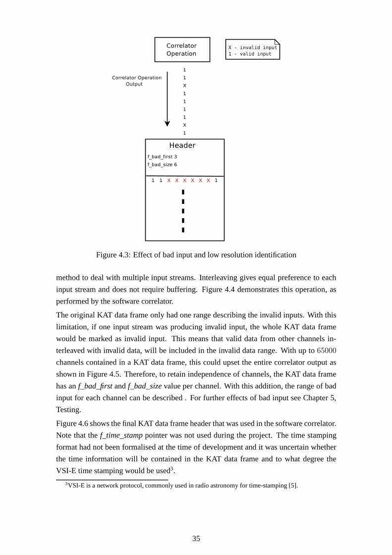
Figure 4.3: Effect of bad input and low resolution identification
method to deal with multiple input streams. Interleaving gives equal preference to each
input stream and does not require buffering. Figure 4.4 demonstrates this operation, as
performed by the software correlator.
The original KAT data frame only had one range describing theinvalid inputs. With this
limitation, if one input stream was producing invalid input, the whole KAT data frame
would be marked as invalid input. This means that valid data from other channels in-
terleaved with invalid data, will be included in the invaliddata range. With up to65000
channels contained in a KAT data frame, this could upset the entire correlator output as
shown in Figure 4.5. Therefore, to retain independence of channels, the KAT data frame
has anf_bad_firstandf_bad_sizevalue per channel. With this addition, the range of bad
input for each channel can be described . For further effectsof bad input see Chapter 5,
Testing.
Figure 4.6 shows the final KAT data frame header that was used in the software correlator.
Note that thef_time_stamppointer was not used during the project. The time stamping
format had not been formalised at the time of development andit was uncertain whether
the time information will be contained in the KAT data frame and to what degree the
VSI-E time stamping would be used3.
3VSI-E is a network protocol, commonly used in radio astronomy for time-stamping [5].
35

Figure 4.4: Interleaved Channels
Figure 4.5: Interleaved channels with only one bad input range
36

Figure 4.6: Final Modified KAT data frame
4.2.2.2 Dealing with variable sample size
Being a experimental platform, one of the main requirementsof the KAT API is flexibility.
The KAT correlator is a multi-rate system and accepts variable bit size data samples.
However, ANSI C uses32 bit integer as the data type, and so the correlator operations use
32 bit integers. Bit-masking is used to allow variable sample size, making it possible to
include samples of2n bits, where5 ≥ n ≥ 1, in the fixed ANSI C32 bit integer.
4.2.2.3 KAT Date Frame Size
In the original design of the KAT API, the KAT data frame was the same size as a Ethernet
packet. This is either 1500 bytes, standard Ethernet packet, or 9000 bytes, jumbo gigabit
Ethernet packet. Keeping these sizes helps add transparency to the KAT API.
However, the original KAT data frame only catered for one input channel and therefore
could assume constant header size. With multiple input channels the size of the KAT
data frame will depend on the number of channel inputs. With up to 65000 channels,
the header size required to describe the payload becomes much larger than the largest
Ethernet packet. Therefore it would be impossible to use standard Ethernet packet sizes.
Since the size of the final KAT data frame is not yet finalised, data frame size is an input
parameter to the software correlator.
4.2.2.4 Channel Abstraction
The network infrastructure sends KAT data frames between stages. However, the cor-
relator stages perform operations on channels, not packets. To retrieve the data for the
particular channel, the interleaved KAT data frame payloadneeds to be reassembled.
This tedious task of extraction and re-assembly of each KAT data frame was hidden
from the software correlator’s processing operations by a channel abstraction function,
as shown in Figure 4.7. This allows the correlator operations to perform functions on a
specific channel stream, hiding all detail of KAT data frame assembly, extraction, trans-
mission and receiving. This greatly simplified the complexity of coding the correlator
37

Correlator Operation
Channel
Correlator Operation
Channel
Correlator Operation
Channel
KAT Data Frame KAT Data Frame
Input Frame Output Frame
1
2
3
1
2
3
1
2
3
10
11
12
10
11
12
Input Output
1 1 1 2 2 2 3 3
3
12 12 12 11 11 11 10 10
10
10
11
12
Key
Figure 4.7: Channel Abstraction
operations. We can see this channel abstraction as another layer on the protocol stack as
shown in Figure 4.8.
Figure 4.8: KAT protocol stack with added channel abstraction
4.2.2.5 Final KAT API
The final KAT API provided the additional support of buffering of frames. This allowed
the correlator operations to request a large set of data which spans across multiple frames.
The final design of the KAT API infrastructure that was used inthe implementation of the
software correlator is presented in Figure 4.9.
38

Frame"The packet(a struct) that is passed inthe network, containing some header
variables and the payload"
Channel’An abstraction of a channel from the
KAT data frame’
FX Correlator Operation’Performs correlator operations on
channels’
Main ’The controlling function’
Frame Buffer’Gets/Sets channel sample from KAT data
frame buffer’
Get/Set sample
Get/Set sample
[Return control]
Send/Recieve Frame
Network Achitechture
Get/Send Frame
Figure 4.9: Simplified overview of the software correlator infrastructure
4.3 Complex Input
Support for complex data was not implemented into the KAT API. Therefore two samples
were used to represent a complex sample.
4.4 Convolution
Equation 2.9 shows the time domain convolution ofx[n] andh[n]. Input, x[n], passes
through a LTI system,h[n], with output,y[n], as a result. The architecture of the convo-
lution function is shown below.
Figure 4.10: FIR architecture
Convolution is heavily used in the correlator, as it is used to do filtering. Convolution is a
computationally expensive operation, as it requires that asample input,x[n], be multiplied
by every filter coefficient ofh[n], and these results be added together. Ifh[n] has length
39

N , thenN multiplications andN − 1 additions need to be performed per output sample,
y[n].
However, equation 2.9 has an equivalent z-domain representation, which is the multipli-
cationX(z) andH(z), whereX(z) ⇋ x[n] andH(z) ⇌ h[n]:
Y (z) = H(z)X(z) (4.1)
This requires only one multiplication operation per out. However, this requires both an
FFT and an inverse FFT to be performed.
It can be shown, as in [16], that if the filter has more than 64 coefficients, then it is faster
to perform FFT multiplication than time domain correlation.
Since the polyphase filter, used in convolution, has the effect of decomposing a proto-
type filter into smaller kernels, it is not viable to perform FFT multiplications. However,
the filtering when calculating the analytic signal representation is not restricted to using
polyphase filtering. There is a section of this filtering which could possibly utilise FFT
multiplication, but for this project all convolution was performed in the time domain.
4.5 Implementation Conclusion
With the implementation completed, the final stage of the project is to test and visually
represent the results.
40

Chapter 5
Testing
This chapter is involved with various sets of input data to test particular aspects of the
software correlator.
5.1 Testing Methods
A network infrastructure was not used for testing. The network was simulated with the
use of text streams.
5.2 Testing Tools
The following tools will not be used in the final software correlator, but were created to
emulate components outside the scope of the project and to aid in the development.
5.2.1 Simulated Input (Signal Generator)
In reality, the input stream to the correlator will originate from the ADC. During testing, a
simulated ADC was created with the ability to create a numberof different input signals.
The flow diagram of the signal generator is shown in Figure 5.1.
41

Begin Signal_creator
Get Input Arguments
Create output signal ofraw data from the the
Arguments specification
Send off Frame viaNetwork
Usage: ./sig_gen [options]...
Signal generator
-h Display this help.
-c Set of channels
-f Set the signals inverse frequency 2pi/[f]
-d DC offset
-a Amplitude of signal. Note if too small the
quantisation noise will be large
-s Signal generated
[0] sinusoidal [1] delayed sinusoidal [2] strange
[3] two sinusoidals [4] three sinusoidals [5] counter
[6] amplified noise [7] chirp signal
Current Function: Output the signal of choice
Figure 5.1: Flow Diagram of Signal Generator
5.2.2 Creating Visualisation Tool (Probe)
The raw data output of each stage is difficult to interpret. Therefore a visualization tool
was used to help with debugging and development of the software correlator.
5.2.3 Framing Tool
The input stream data created by the signal generator has no KAT data frame structure.
The Correlator Executable is a generic programme that operates on KAT data frames.
Therefore, the framing tool is used to create this KAT data frame. The flow diagram of
the framing tool is shown in Figure 5.2.
42

Begin frame_creator
Get Input Arguments
Create input frame from raw input datafrom network
Send off Frame viaNetwork
Raw stream sampled input data from network (signal_generation)
Usage: ./create_frame [options]...
-h Display this help.
-f Set the frame size
-s Set the sample size
-c Set of channels
-o Set the output mode.
0:the output displayed as is.
1:the output grouped in channels.
Figure 5.2: Flow Diagram of the Framing Tool .
5.3 Correlator Executable (Simulator)
The correlator exucutable is a programme that performs the FX correlator operations on
a KAT data frame. This has various methods that implement thecorrelator stages. The
flow diagram of the correlator executable is shown in Figure 5.3.
43

Begin Simulator
Get Input Arguments
Create input frame from raw input datafrom network
Send off Frame viaNetwork
Perform SimulationOperation
Input Frame from previous operation
Usage: ./test-simulator [options]...
-h Display this help.
-p Specify input parameters [number parameters] [parameters]
-c Number of channels [input] [output]
-f Specify Output frame size. [output size]
-t Specify the type of operation. 1-8
[1]:delay [2]:analytic signal
[3]:polyphase filter [4]:bandwidth reduction
[5]:phase correction [6]:correlation
[7]:test [8]:FIR filter
[9]:DDC
-d Specify the DC_offset of the incomming signal.
-x Set input mode to hex.
-o Set the output mode.
0:the output displayed as is.
1:the output grouped in channels.
2:Header and output printed
Function: Runs operations on kat data frames
Figure 5.3: Flow Diagram of the Correlator Executable
5.4 Tests
The testing of the correlator was done in two stages: testingthe KAT API and testing the
various modules’ output against that of the Python simulations.
5.4.1 KAT API
5.4.1.1 Channel separation
In Figure 5.4 20 identical channels streams are produced andran for a period of time.
This is to ensure that the timing and independence of each channel in maintained.
5.4.1.2 Coping with large number of channels
The correlated needs to be able to support a large number of inputs. To test this, 1 million
inputs were transported across the KAT API infrastructure.It is unreasonable to use the
visualisation to plot each of these outputs, therefore the terminal output is shown in Figure
5.5.
44

Figure 5.4: 20 Channels separated
Figure 5.5: 1 000 000 channels tested
Another test was run with 20 million channels. This failed torun, due to lack of memory
on executing computer.
45

5.4.1.3 Invalid Input Propagation Through System
The effect of having low resolution to the bad inputs is demonstrated below in Figure 5.6.
Invalid input can be dealt with in various ways, depending onuser specification. In this
instance, invalid inputs were set to zero. The frame size here was set to 20 samples.
Figure 5.6: The Effect of Invalid Input with Poor Resolution.(Top) Input data containing invalid inputs(Bottom) The output showing lost sectors
5.4.1.4 Effect of Word Size
The effect of word size of the output of the correlator is demonstrated in Figure 5.7. In
this case, 4 bit sampling was used. We can see two of the effects of using a word size that
is too small to represent the data, the jagged edges caused byquanitisation noise and the
distortion of the spectral peaks. The distortion is due to the magnitude being too large for
the word size.
46

Figure 5.7: Quantization Noise and Magnitude Out of Range
5.4.2 Software Correlator Testing
In this stage the correlator operations are tested. Due to the time limitations, a correctly
functioning version of the polyphase filtering stage could not be implemented in the KAT
API. However, all other stages presented here were implemented in the KAT API.
47

Figure 5.8: The time variation in the input to the correlatorare corrected by the delaycompensator. (KAT API)
48
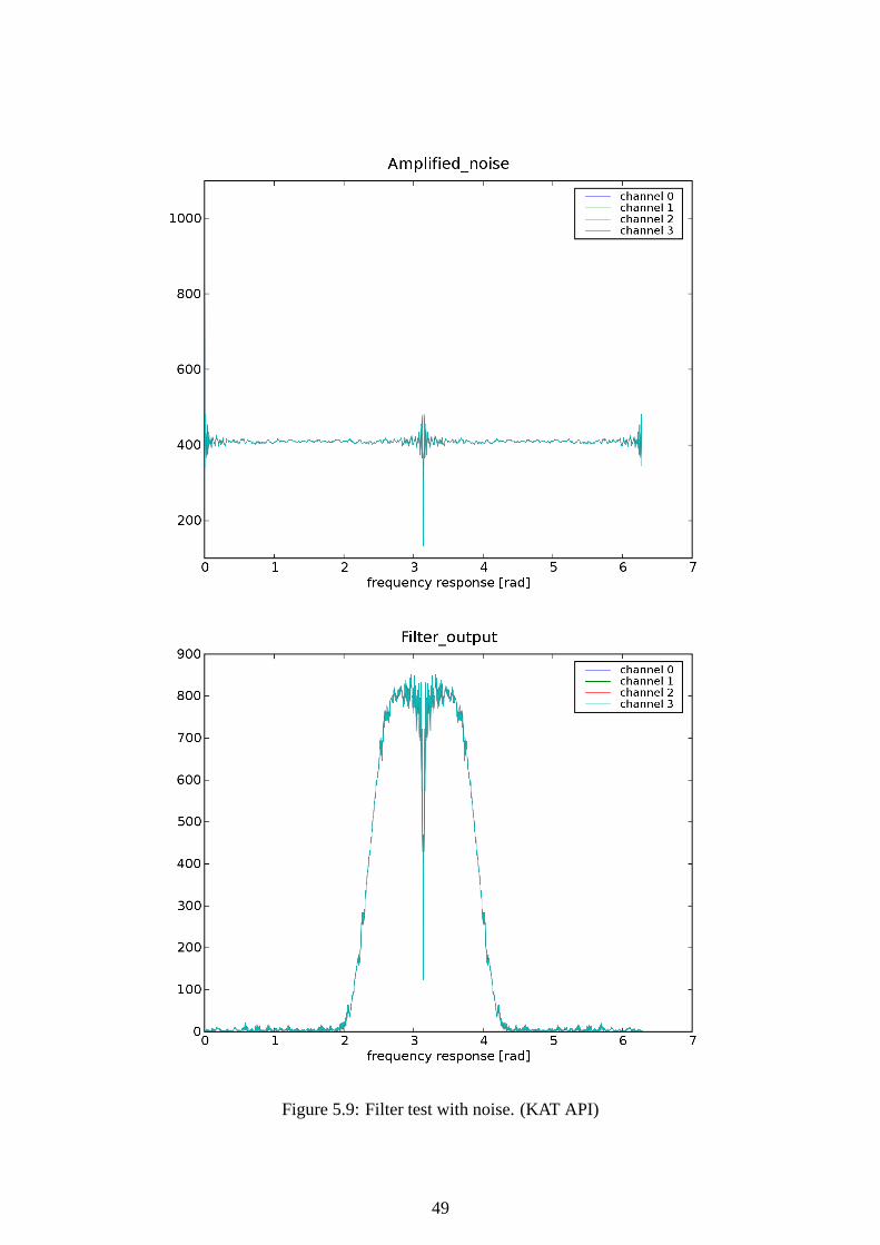
Figure 5.9: Filter test with noise. (KAT API)
49
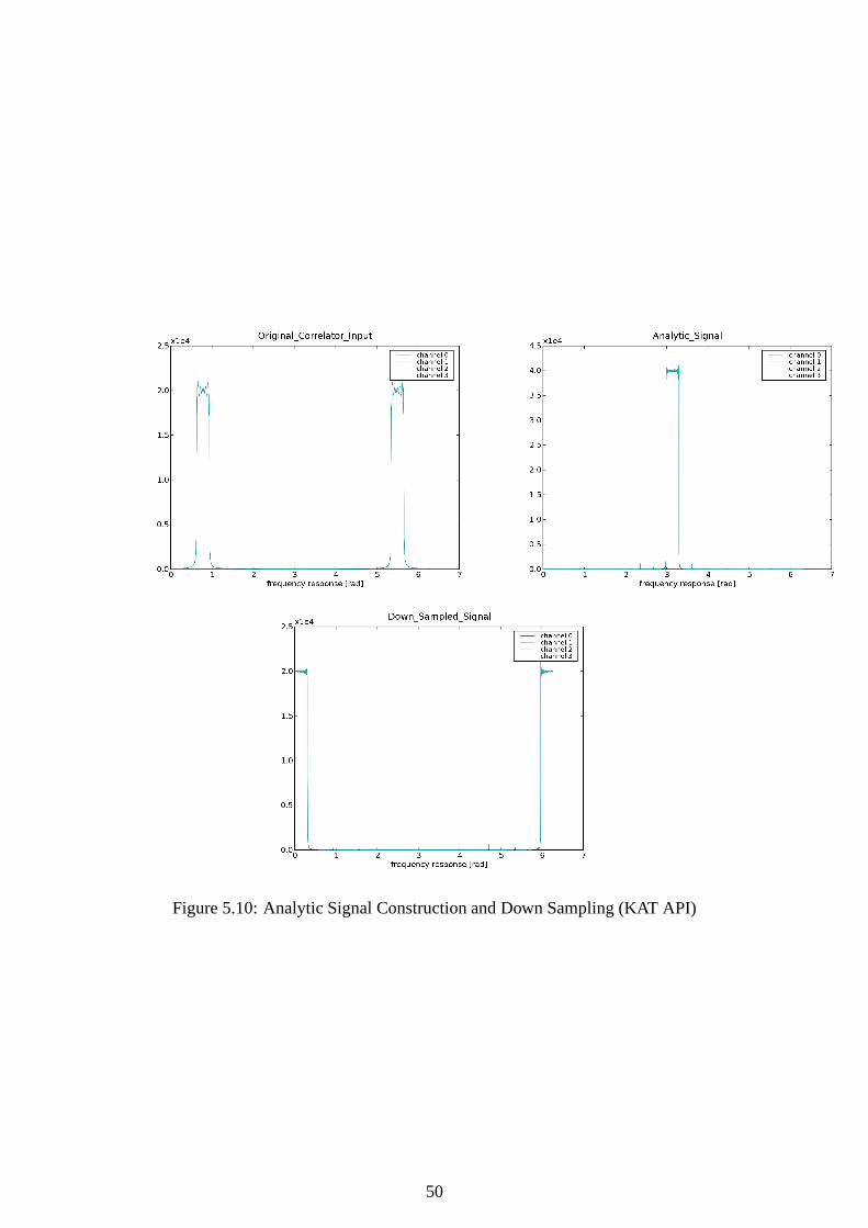
Figure 5.10: Analytic Signal Construction and Down Sampling (KAT API)
50

Figure 5.11: Polyphase Filter (python simulation)
51

Figure 5.12: Polyphase Filtering Results compared with Channeliser Results (python sim-ulation)
52

Chapter 6
Conclusions/Results
The requirements of this project as originally stated in chapter 3, are listed below:
• Investigate the operations of the correlator in detail and provide an architectural
design.
• Build onto the API provided by Dr. Marc Welz to support the operations the corre-
lator needs to perform.
• Implement the correlator in ANSI C, using the modified API.
• Ensure flexibility in design.
The software correlator has been investigated in detail. The API provided by Dr. Marc
Welz was modified to support of the desired operations of the FX software correlator.
Although the entire implementation was not completed, the stages that have been com-
pleted, demonstrate that the KAT API developed and the Python simulations investigated,
perform to the desired standard. The KAT API has much flexibility in its design and will
be well suited to be used to continue the development and complete the remaining stages
of the correlator.
53
Appendix A: Open Source Tools
The following definitions all came from Wikipedia, http://www.wikipedia.com
Ipython
“An enhanced Python shell designed for efficient interactive work. It includes many en-
hancements over the default Python shell, including the ability for controlling interac-
tively all major GUI toolkits in a non-blocking manner.”
Numarray
Numarray is a mathematical Python Library.
Matplotlib
“Matplotlib is a plotting library for Python which uses syntax similar to MATLAB. “
Mplot3D
This is an extension of Mplotlib, created by John Porter, to support 3D modelling.
GCC
“The GNU Compiler Collection (usually shortened to GCC) is aset of programming
language compilers produced by the GNU Project.” Was used tocompile ANSI C code.
Make
“Make is a utility for automatically building large applications. ”
Octave
“GNU Octave, in computing, a program for performing numerical analysis, similar to
MATLAB”
DIA
“Dia is an free software/open-source general-purpose diagramming software, developed
as part of the GNOME project.”
FFTW3 library
“FFTW is a C subroutine library for computing the discrete Fourier transform (DFT) in
one or more dimensions, of arbitrary input size, and of both real and complex data .”
LYX
“LYX is a document processor in which the user only has to care about the structure
and content of the text, while the formatting is done by LATEX, an advanced typesetting
system.“
54

Appendix B: Source Code
Source Code is on accomponing CD
55

Appendix C: Additional Acknowledgements
David George’s undergrad thesis for an exellent reference[8].
Marc Welz for providing a very useful programme demonstrating his KAT API [20].
56

Appendix D: Additional Diagrams and DefinitionsAnalytic Signal (Another look)
Analytic signals provide one with the very useful ability ofrepresenting a real time signal
as a complex phaser. The classical example is representing asignalcos(ωt) in its analytic
form, E(t), see Figure 6.1.
E(t) = cos(ωt) + jH{cos(ωt)}
E(t) = cos(ωt) + j cos(ωt−π
2)
E(t) = cos(ωt) + j sin(ωt)
E(t) = ejωt (Eurler′s formula)
Figure 6.1: Analytic Representation ofcos(ωt)
Constructing an Analytical Signal (in more detail)
Any real time signal can be represented in its analytical form. The analytical form of a
signal is just the positive side of its spectrum.[14] Let,x(t)be a real time signal where
x(t) ⇋ X(F ) then the analytical signalv(t)can be constructed as follows :
57

v(t) = I(t) + jQ(t) (6.1)
where,
f0 = desiredPosition− centerF
I(t) = [2x(t). cos(2πf0t)]LPF ⇋
I(F ) = [2X(F )⊗ [δ(F − f0) + δ(F + f0)
2]LPF
I(F ) = [X(F − f0) + X(F + f0)]LPF (6.2)
= X+(F + f0) + X−(F − f0)
X+(F ) = {X(F ) F≥00 F≤0 , X−(F ) = { 0 F≥0
F0 F≤0
and,
Q(t) = [2x(t). sin(2πf0t)]LPF ⇋
Q(F ) = [2X(F )⊗ [−jδ(F − f0) + jδ(F + f0)
2]LPF
Q(F ) = −jX+(F + f0) + jX−(F − f0) (6.3)
Therefore,
v(t) = I(t) + jQ(t) ⇋ V (F ) = 2X+(F + f0) (6.4)
Over-lap Add Convolution
In this project, the finite length filter,h[n], needs to be convolved with the infinitely long
input signal,x[n]. It is impossible to have an infinite length buffer, and therefore the input
signal was truncated into a number of equal lengthed blocks with lengthL. The inputx[n]
can be decomposed as follows[14]:
x[n] =
∞∑
r=0
xr[n− rL] (6.5)
where,
58

xr[n] =
{
x[n + rL] 0 ≤ n ≤ L− 1
0 otherwise
Figure 6.2: Example of block convolution
To avoid the consequences of circular convolution, each block,xr[n], is zero padded with
P zeros, whereP is the length of filterh[n]. Each of these blocks are convolved indepen-
dently and summed to reconstruct a signal which is equivilant to the linear convolution of
x[n] as shown in Equation 2.9. This process is known as over-lap add convolution.
59
Bibliography
[1] DSP: Digital Signal Processing. Online-Publication. http://www.dsprelated.com/.
[2] The Karoo Array Telescope (KAT) Website. http://www.ska.ac.za/kat/index.html.
[3] National Radio Astronomy Observatory. Online-Publication. http://www.nrao.edu/.
[4] The European Southern Observatory Homepage. www.eso.org.
[5] Draft Proposal for VSI-E - Rev 2.7.Experimental Astronomy, January 2004. Mas-
sachusetts Institute of Technology(MIT) Haystack Observatory, author not stated.
[6] J. D. Bunton. A SAR Correlation Algorithm which Accommodates Large-Range
Migration. Experimental Astronomy, 17:251–259, 2004.
[7] B. F. Burke and F. Graham-Smith.An Introduction to Radio Astronomy. Cambridge
University Press, second edition, 2002.
[8] D. George.A Firmware-Based Polyphase Filter Design Tool. October 2005. Uni-
versity of Cape Town.
[9] D. Halliday, R. Resnick, and J. Walker.Fundamentals of Physics. John Wiley and
Sons, Inc, 6th edition, 2001.
[10] J. Hamaker1, J. Bregman1, and R. Sault. Understanding radio polarimetry.Astron-
omy and Astrophysics.
[11] F. Harris. Multirate Signal Processing for Communication Systems. Prentice Hall
PTR.
[12] F. Harris, C. Dick, and M. Rice. Digital Receivers and Transmitters Using Polyphase
Filter Banks for Wireless Communications.IEEE Transactions on Microwave The-
ory and Techniques, 51, 2002.
[13] J. F. Kurose and K. W. Rose.Computer Networking, A Top-Down Approach. Addi-
son Wesley, 3rd edition, 2005.
[14] F. Nicolls and A. Wilkinson.Digital Signal Processing Course Notes. 2006. Uni-
versity of Cape Town.
60

[15] R. Perley and W. Brosken. 10th Sythesis Imaging Summer School, June 2006. Uni-
versity of New Mexico.
[16] S. W. Smith. The Scientist and Engineer’s Guide to Digital Signal Processing.
Online-Publication. www.dspguide.com.
[17] F. G. Stremler. Introduction to Communication Systems. Addison-Wesley, third
edition, 1992.
[18] A. Thompson, J.Moran, and G.Swenson.Interferometry and Synthesis in Radio
Astronomy. Wiley-VCH, 2nd edition, 2004.
[19] R. van der Merwe and R. Lord. Correlator Flow Diagram. Members of KAT Com-
puting Team, PineLands, Cape Town.
[20] M. Welz. KAT Frame API. Member of KAT DSP Team, PineLands, Cape Town.
[21] Wikipedia. The Free Encyclopedia. www.wikipedia.com.
[22] C. Y. Correlators for interferometry - today and tomorrw. Astronomical Society of
the Pacific Conferene Series, 19, 1991.
61
Related Documents