An evaluation exercise of a multizone air flow model

Ž .Energy and Buildings 30 1999 35–51

An evaluation exercise of a multizone air flow model

Romano Borchiellini a,), Jean-Marie Furbringer b¨a Dipartimento di Energetica, Politecnico di Torino, I-10129 Turin, Italy

b Laboratoire d’Energie Solaire et de Physique du Batiment, Ecole Polytechnique Federale, CH-1015 Lausanne, Switzerlandˆ ´ ´

Abstract

In the IEA-ECBCS Annex 23 ‘Multizone Air Flow Modelling,’ a sensitivity analysis procedure, that included both the Monte Carloand Fractional Factorial analyses, was defined to evaluate COMVEN, a multizone air flow code. This procedure is here applied toevaluate COMVEN, when the simulation of the ventilation of a detached house is performed for the case of ventilation driven mainly bystack effect. The simulated values are compared to the measured values using the uncertainty range for each value; the confidence intervalfor the simulated values are obtained using the Monte Carlo method while the fractional factorial analysis has been used to identify therelative effects of the input parameters on the output accuracy. It is an interesting case which makes it possible to demonstrate theapplication of both sensitivity techniques. q 1999 Elsevier Science S.A. All rights reserved.

Keywords: Building simulation; Experimental comparison; Monte-Carlo method; Factorial design; Sensitivity analysis; Tracer gas measurements

1. Introduction

The use of numerical models to simulate physical phe-nomena is continuously increasing. These models are usu-ally run on computers using programs with a core numeri-cal model and pre- and post-processors to manipulate theinputs and outputs.

The current problem for the user is therefore not only toperform the simulation but to correctly interpret the resultsand their accuracy. As many acceptable values can be usedas input for the same parameters, the knowledge of thespread of the results, due to different input values, be-comes one of the most important topics for the user.Furthermore, the assessment of this spread, that is, theconfidence intervals of output data, is required when thecomparison between simulated values and measured valuesis performed for validation purposes.

The sensitivity analysis is used to relate the inputvariation to the subsequent output variation. This techniqueconsists of performing a set of code runs in order toexplore the input data space. The number of runs that mustbe performed depends on the chosen method and on thekind of information required; this number can be min-imised by optimally designing these runs.

In the IEA-ECBCS Annex 23 ‘Multizone Air Floww x Ž w x .Modelling’ 6 see also Refs. 8,9 in the present issue , an

) Corresponding author. Tel.: q39-011-5644489; Fax: q39-011-5644499.

extensive work was planned to evaluate COMVEN aw xmultizone air flow code 3 and a sensitivity analysis

procedure, including both the Monte Carlo and Fractionalw xFactorial analyses, were defined 4,8,9 ; the validation

example presented here belongs to this framework.This article aims to show a detailed example of the

application of this sensitivity analysis procedure. Thisinvolves describing:Ø the chosen input parameters and their uncertainty ranges;Ø the strategy used to define the number of runs;Ø the analysis of the simulation results and their uncer-

tainties;Ø the method used to compare the measured with the

simulated values.Both the Monte Carlo and fractional factorial analyses

have been used to investigate the effects of the inputvariations and obtain information on the role played by theparameters on the model.

A comparison between the measured and simulatedvalues is also presented for a detached laboratory house;the uncertainty of the simulated values has been obtainedusing the Monte Carlo method.

2. Measurements

All the measurements here illustrated were carried outusing the tracer gas decay technique in a detached two

0378-7788r99r$ - see front matter q 1999 Elsevier Science S.A. All rights reserved.Ž .PII: S0378-7788 98 00045-0

( )R. Borchiellini, J.-M. FurbringerrEnergy and Buildings 30 1999 35–51¨36

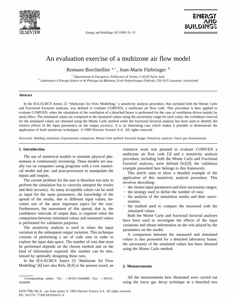
Fig. 1. Plant view of the detached house.

w xstorey laboratory house 1,6 the underground floor hoststhe centralised service equipment and the data acquisition

Žand processing system; the ground floor in which the tests. 2were performed has a floor area of 114 m , and is made

up of two bedrooms, a living room, a bathroom and akitchen. The attic space above the ground floor can beheated, so that the test floor may also reproduce thethermal conditions of an apartment in a multi-storey build-ing. A plan view of the test area is shown in Fig. 1.

The experimental apparatus used for the tracer gasmeasurements has been developed at the Dipartimento di

w xEnergetica of the Politecnico di Torino 2 .The tracer gas measurements, here analysed, have been

carried out over two different periods: October 1992 andJanuary 1994. The main characteristics of the measure-ments are summarised in Table 1.

Ž .During the tests in October 1992 see Table 1 the airchange rate in the dwellings with a small gas-fire individ-ual unit for space heating and service hot water productionwas measured in order to investigate the influence of

Žpurpose-provided ventilation openings sized according to.the national UNI-CIG 7129-72 standard on the air changes

Ž .and the IAQ. During these tests, the air supply area ASAof the purpose-provided opening was set respectively to

Ž .0%, 50% and 100%; the chimney cross-section CCS wasvaried from 25% to 100%.

The experimental measurements were carried out withŽ .one or two tracer gases N O and or SF . When two2 6

tracers were used the concentration data was analysed withŽa two-zone model whereas in the other test only one

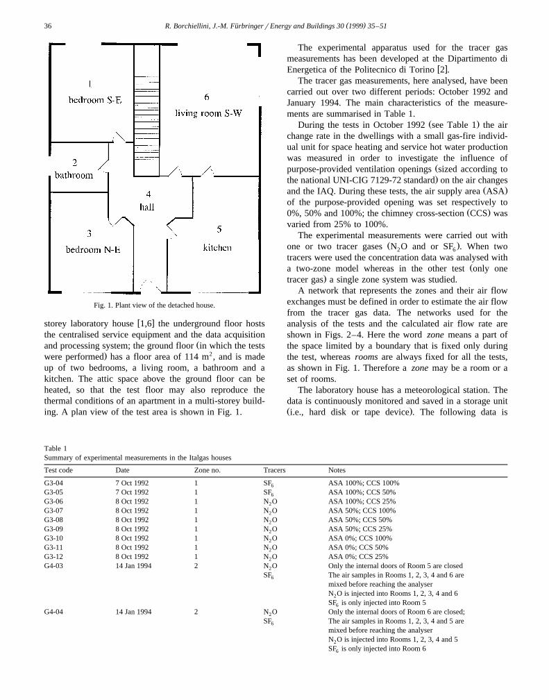
.tracer gas a single zone system was studied.A network that represents the zones and their air flow

exchanges must be defined in order to estimate the air flowfrom the tracer gas data. The networks used for theanalysis of the tests and the calculated air flow rate areshown in Figs. 2–4. Here the word zone means a part ofthe space limited by a boundary that is fixed only duringthe test, whereas rooms are always fixed for all the tests,as shown in Fig. 1. Therefore a zone may be a room or aset of rooms.

The laboratory house has a meteorological station. Thedata is continuously monitored and saved in a storage unitŽ .i.e., hard disk or tape device . The following data is

Table 1Summary of experimental measurements in the Italgas houses

Test code Date Zone no. Tracers Notes

G3-04 7 Oct 1992 1 SF ASA 100%; CCS 100%6

G3-05 7 Oct 1992 1 SF ASA 100%; CCS 50%6

G3-06 8 Oct 1992 1 N O ASA 100%; CCS 25%2

G3-07 8 Oct 1992 1 N O ASA 50%; CCS 100%2

G3-08 8 Oct 1992 1 N O ASA 50%; CCS 50%2

G3-09 8 Oct 1992 1 N O ASA 50%; CCS 25%2

G3-10 8 Oct 1992 1 N O ASA 0%; CCS 100%2

G3-11 8 Oct 1992 1 N O ASA 0%; CCS 50%2

G3-12 8 Oct 1992 1 N O ASA 0%; CCS 25%2

G4-03 14 Jan 1994 2 N O Only the internal doors of Room 5 are closed2

SF The air samples in Rooms 1, 2, 3, 4 and 6 are6

mixed before reaching the analyserN O is injected into Rooms 1, 2, 3, 4 and 62

SF is only injected into Room 56

G4-04 14 Jan 1994 2 N O Only the internal doors of Room 6 are closed;2

SF The air samples in Rooms 1, 2, 3, 4 and 5 are6

mixed before reaching the analyserN O is injected into Rooms 1, 2, 3, 4 and 52

SF is only injected into Room 66

( )R. Borchiellini, J.-M. FurbringerrEnergy and Buildings 30 1999 35–51¨ 37

Fig. 2. Experimental network for the single zone tests from G3-04 to G3-12.

Fig. 3. Experimental network for the two-zone test G4-03.

Fig. 4. Experimental network for the two-zone test G4-04.

( )R. Borchiellini, J.-M. FurbringerrEnergy and Buildings 30 1999 35–51¨38

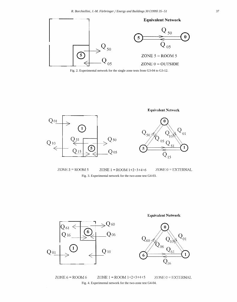
Fig. 5. COMVEN networks for tests from G3-04 to G3-12.

Ž .recorded for each time step: external temperature 8C ,Ž . Ž .absolute barometer pressure hPa , relative humidity % ,

Ž 2 . Ž .solar radiation Wrm , wind velocity mrs , wind direc-Ž . Ž . Ž .tion degrees , rain mm , time s . The meteorological

data were available only each 15 min for the measurementŽof October 1992 while for the last measurements January

.1994 the meteorological data were recorded each minuteto improve the COMVEN comparison.

3. COMVEN air flow simulation

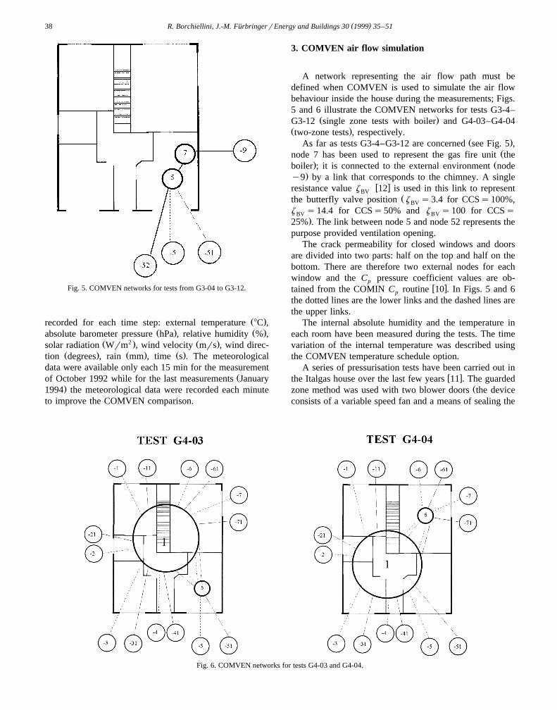
A network representing the air flow path must bedefined when COMVEN is used to simulate the air flowbehaviour inside the house during the measurements; Figs.5 and 6 illustrate the COMVEN networks for tests G3-4–

Ž .G3-12 single zone tests with boiler and G4-03–G4-04Ž .two-zone tests , respectively.

Ž .As far as tests G3-4–G3-12 are concerned see Fig. 5 ,Žnode 7 has been used to represent the gas fire unit the

. Žboiler ; it is connected to the external environment node.y9 by a link that corresponds to the chimney. A single

w xresistance value z 12 is used in this link to representBVŽthe butterfly valve position z s3.4 for CCSs100%,BV

z s14.4 for CCSs50% and z s100 for CCSsBV BV.25% . The link between node 5 and node 52 represents the

purpose provided ventilation opening.The crack permeability for closed windows and doors

are divided into two parts: half on the top and half on thebottom. There are therefore two external nodes for eachwindow and the C pressure coefficient values are ob-p

w xtained from the COMIN C routine 10 . In Figs. 5 and 6p

the dotted lines are the lower links and the dashed lines arethe upper links.

The internal absolute humidity and the temperature ineach room have been measured during the tests. The timevariation of the internal temperature was described usingthe COMVEN temperature schedule option.

A series of pressurisation tests have been carried out inw xthe Italgas house over the last few years 11 . The guarded

Žzone method was used with two blower doors the deviceconsists of a variable speed fan and a means of sealing the

Fig. 6. COMVEN networks for tests G4-03 and G4-04.

( )R. Borchiellini, J.-M. FurbringerrEnergy and Buildings 30 1999 35–51¨ 39

.fan into the doorway . These tests were performed mainlyto define the wall permeability, that is, the characteristic ofthe cracks between the inside and outside. The values ofthe AIVC data base have been used for the crack coeffi-

w xcients of the internal doors 15 .

4. Monte Carlo and fractional factorial analysis

4.1. Monte Carlo Analysis

A complete sensitivity analysis of the COMVEN resultsof each test has been performed using the Monte-Carlo

Žmethod with the help of MISA Multirun Interface for. w xSensitivity Analysis 4,7 .

The range used for the Monte-Carlo analysis is given inTable 2 for each class of parameters. This range, for themeasured parameters, has been established on the basis ofthe measurement error, while for the parameters obtained

Ž .from the literature i.e., pressure coefficient it has beendefined in order to represent the variation that exists inbibliographic data.

As the parameter set must be defined for each teststarting from the classes defined in Table 2, it is impossi-ble to provide here a detailed description of all the parame-ters adopted for the eleven tests. Therefore only the num-ber of parameters and the number of simulations used foreach test is given in Table 3. Three hundred simulationsfor each analysis were considered to be sufficient to obtainaccurate mean and standard deviation values, even though

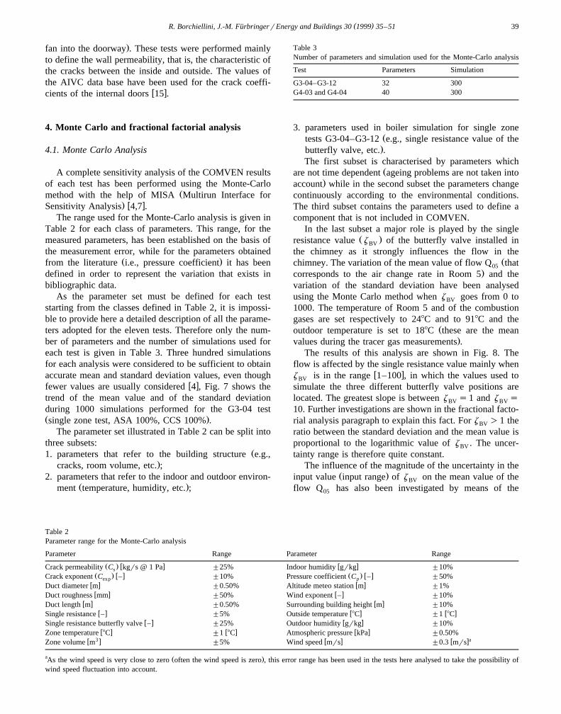
w xfewer values are usually considered 4 , Fig. 7 shows thetrend of the mean value and of the standard deviationduring 1000 simulations performed for the G3-04 testŽ .single zone test, ASA 100%, CCS 100% .

The parameter set illustrated in Table 2 can be split intothree subsets:

Ž1. parameters that refer to the building structure e.g.,.cracks, room volume, etc. ;

2. parameters that refer to the indoor and outdoor environ-Ž .ment temperature, humidity, etc. ;

Table 3Number of parameters and simulation used for the Monte-Carlo analysis

Test Parameters Simulation

G3-04–G3-12 32 300G4-03 and G4-04 40 300

3. parameters used in boiler simulation for single zoneŽtests G3-04–G3-12 e.g., single resistance value of the.butterfly valve, etc. .

The first subset is characterised by parameters whichŽare not time dependent ageing problems are not taken into

.account while in the second subset the parameters changecontinuously according to the environmental conditions.The third subset contains the parameters used to define acomponent that is not included in COMVEN.

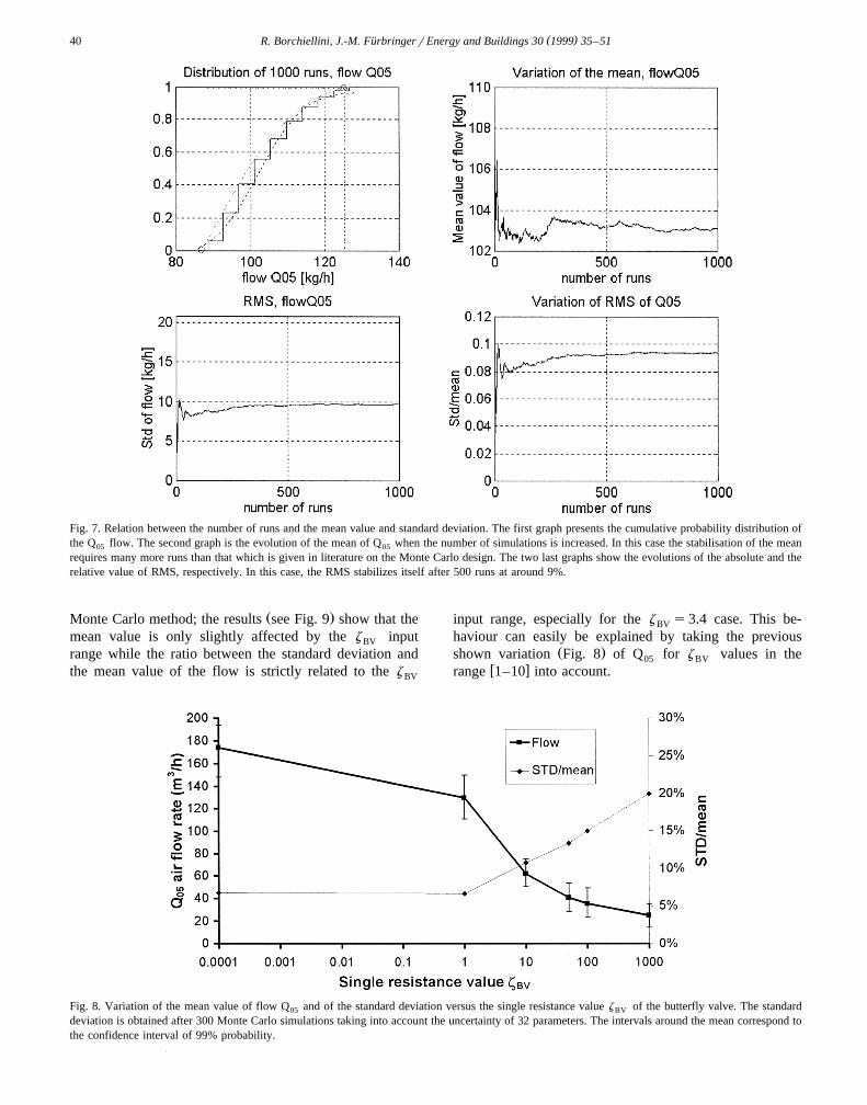
In the last subset a major role is played by the singleŽ .resistance value z of the butterfly valve installed inBV

the chimney as it strongly influences the flow in theŽchimney. The variation of the mean value of flow Q that05

.corresponds to the air change rate in Room 5 and thevariation of the standard deviation have been analysedusing the Monte Carlo method when z goes from 0 toBV

1000. The temperature of Room 5 and of the combustiongases are set respectively to 248C and to 918C and the

Žoutdoor temperature is set to 188C these are the mean.values during the tracer gas measurements .

The results of this analysis are shown in Fig. 8. Theflow is affected by the single resistance value mainly when

w xz is in the range 1–100 , in which the values used toBV

simulate the three different butterfly valve positions arelocated. The greatest slope is between z s1 and z sBV BV

10. Further investigations are shown in the fractional facto-rial analysis paragraph to explain this fact. For z )1 theBV

ratio between the standard deviation and the mean value isproportional to the logarithmic value of z . The uncer-BV

tainty range is therefore quite constant.The influence of the magnitude of the uncertainty in the

Ž .input value input range of z on the mean value of theBV

flow Q has also been investigated by means of the05

Table 2Parameter range for the Monte-Carlo analysis

Parameter Range Parameter Range

Ž . w x w xCrack permeability C kgrs @ 1 Pa "25% Indoor humidity grkg "10%sŽ . w x Ž . w xCrack exponent C – "10% Pressure coefficient C – "50%exp p

w x w xDuct diameter m "0.50% Altitude meteo station m "1%w x w xDuct roughness mm "50% Wind exponent – "10%

w x w xDuct length m "0.50% Surrounding building height m "10%w x w x w xSingle resistance – "5% Outside temperature 8C "1 8C

w x w xSingle resistance butterfly valve – "25% Outdoor humidity grkg "10%w x w x w xZone temperature 8C "1 8C Atmospheric pressure kPa "0.50%

3 aw x w x w xZone volume m "5% Wind speed mrs "0.3 mrs

a Ž .As the wind speed is very close to zero often the wind speed is zero , this error range has been used in the tests here analysed to take the possibility ofwind speed fluctuation into account.

( )R. Borchiellini, J.-M. FurbringerrEnergy and Buildings 30 1999 35–51¨40

Fig. 7. Relation between the number of runs and the mean value and standard deviation. The first graph presents the cumulative probability distribution ofthe Q flow. The second graph is the evolution of the mean of Q when the number of simulations is increased. In this case the stabilisation of the mean05 05

requires many more runs than that which is given in literature on the Monte Carlo design. The two last graphs show the evolutions of the absolute and therelative value of RMS, respectively. In this case, the RMS stabilizes itself after 500 runs at around 9%.

Ž .Monte Carlo method; the results see Fig. 9 show that themean value is only slightly affected by the z inputBV

range while the ratio between the standard deviation andthe mean value of the flow is strictly related to the zBV

input range, especially for the z s3.4 case. This be-BV

haviour can easily be explained by taking the previousŽ .shown variation Fig. 8 of Q for z values in the05 BV

w xrange 1–10 into account.

Fig. 8. Variation of the mean value of flow Q and of the standard deviation versus the single resistance value z of the butterfly valve. The standard05 BV

deviation is obtained after 300 Monte Carlo simulations taking into account the uncertainty of 32 parameters. The intervals around the mean correspond tothe confidence interval of 99% probability.

( )R. Borchiellini, J.-M. FurbringerrEnergy and Buildings 30 1999 35–51¨ 41

Fig. 9. Variation of the mean value of flow Q with an increase of the input variation amplitude.05

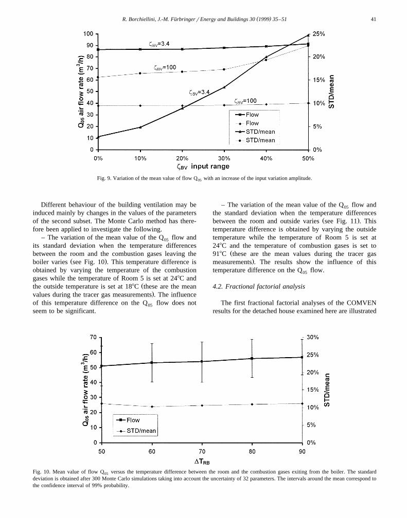
Different behaviour of the building ventilation may beinduced mainly by changes in the values of the parametersof the second subset. The Monte Carlo method has there-fore been applied to investigate the following.

– The variation of the mean value of the Q flow and05

its standard deviation when the temperature differencesbetween the room and the combustion gases leaving the

Ž .boiler varies see Fig. 10 . This temperature difference isobtained by varying the temperature of the combustiongases while the temperature of Room 5 is set at 248C and

Žthe outside temperature is set at 188C these are the mean.values during the tracer gas measurements . The influence

of this temperature difference on the Q flow does not05

seem to be significant.

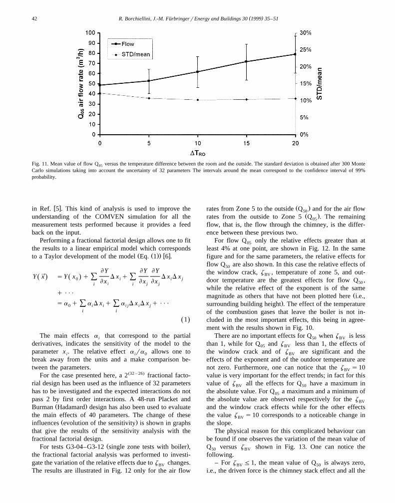
– The variation of the mean value of the Q flow and05

the standard deviation when the temperature differencesŽ .between the room and outside varies see Fig. 11 . This

temperature difference is obtained by varying the outsidetemperature while the temperature of Room 5 is set at248C and the temperature of combustion gases is set to

Ž918C these are the mean values during the tracer gas.measurements . The results show the influence of this

temperature difference on the Q flow.05

4.2. Fractional factorial analysis

The first fractional factorial analyses of the COMVENresults for the detached house examined here are illustrated

Fig. 10. Mean value of flow Q versus the temperature difference between the room and the combustion gases exiting from the boiler. The standard05

deviation is obtained after 300 Monte Carlo simulations taking into account the uncertainty of 32 parameters. The intervals around the mean correspond tothe confidence interval of 99% probability.

( )R. Borchiellini, J.-M. FurbringerrEnergy and Buildings 30 1999 35–51¨42

Fig. 11. Mean value of flow Q versus the temperature difference between the room and the outside. The standard deviation is obtained after 300 Monte05

Carlo simulations taking into account the uncertainty of 32 parameters The intervals around the mean correspond to the confidence interval of 99%probability.

w xin Ref. 5 . This kind of analysis is used to improve theunderstanding of the COMVEN simulation for all themeasurement tests performed because it provides a feedback on the input.

Performing a fractional factorial design allows one to fitthe results to a linear empirical model which corresponds

Ž Ž .. w xto a Taylor development of the model Eq. 1 6 .

E Y E Y E Y™Y x sY x q D x q D x D xŽ . Ž . Ý Ý0 i i jE x E x E xi j ji i

q PPP

sa q a D x q a D x D x q PPPÝ Ý0 i i i j i ji i

1Ž .

The main effects a that correspond to the partiali

derivatives, indicates the sensitivity of the model to theparameter x . The relative effect a ra allows one toi i 0

break away from the units and a make comparison be-tween the parameters.

For the case presented here, a 2Ž32 – 26. fractional facto-rial design has been used as the influence of 32 parametershas to be investigated and the expected interactions do notpass 2 by first order interactions. A 48-run Placket and

Ž .Burman Hadamard design has also been used to evaluatethe main effects of 40 parameters. The change of these

Ž .influences evolution of the sensitivity is shown in graphsthat give the results of the sensitivity analysis with thefractional factorial design.

Ž .For tests G3-04–G3-12 single zone tests with boiler ,the fractional factorial analysis was performed to investi-gate the variation of the relative effects due to z changes.BV

The results are illustrated in Fig. 12 only for the air flow

Ž .rates from Zone 5 to the outside Q and for the air flow50Ž .rates from the outside to Zone 5 Q . The remaining05

flow, that is, the flow through the chimney, is the differ-ence between these previous two.

For flow Q only the relative effects greater than at05

least 4% at one point, are shown in Fig. 12. In the samefigure and for the same parameters, the relative effects forflow Q are also shown. In this case the relative effects of50

the window crack, z , temperature of zone 5, and out-BV

door temperature are the greatest effects for flow Q ,50

while the relative effect of the exponent is of the sameŽmagnitude as others that have not been plotted here i.e.,

.surrounding building height . The effect of the temperatureof the combustion gases that leave the boiler is not in-cluded in the most important effects, this being in agree-ment with the results shown in Fig. 10.

There are no important effects for Q when z is less50 BV

than 1, while for Q and z less than 1, the effects of05 BV

the window crack and of z are significant and theBV

effects of the exponent and of the outdoor temperature arenot zero. Furthermore, one can notice that the z s10BV

value is very important for the effect trends; in fact for thisvalue of z all the effects for Q have a maximum inBV 50

the absolute value. For Q a maximum and a minimum of05

the absolute value are observed respectively for the zBV

and the window crack effects while for the other effectsthe value z s10 corresponds to a noticeable change inBV

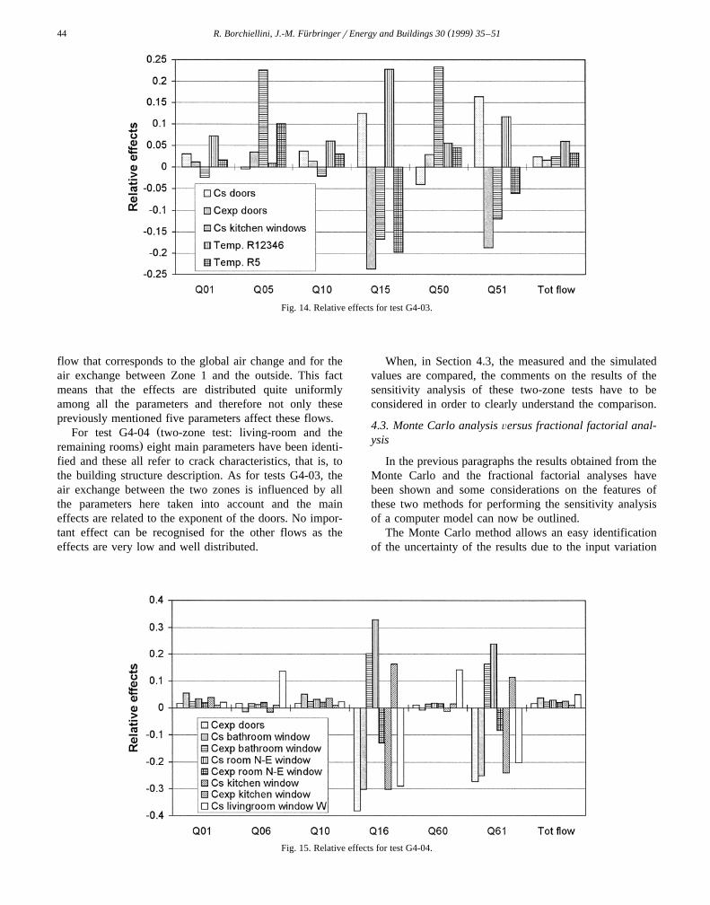
the slope.The physical reason for this complicated behaviour can

be found if one observes the variation of the mean value ofQ versus z shown in Fig. 13. One can notice the50 BV

following.– For z F1, the mean value of Q is always zero,BV 50

i.e., the driven force is the chimney stack effect and all the

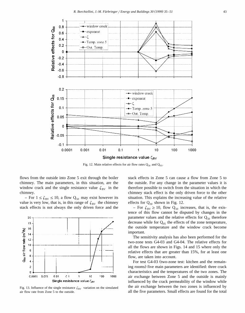
( )R. Borchiellini, J.-M. FurbringerrEnergy and Buildings 30 1999 35–51¨ 43

Fig. 12. Main relative effects for air flow rates Q and Q .50 05

flows from the outside into Zone 5 exit through the boilerchimney. The main parameters, in this situation, are thewindow crack and the single resistance value z in theBV

chimney.– For 1Fz F10, a flow Q may exist however itsBV 50

value is very low, that is, in this range of z the chimneyBV

stack effects is not always the only driven force and the

Fig. 13. Influence of the single resistance z variation on the simulatedBV

air flow rate from Zone 5 to the outside.

stack effects in Zone 5 can cause a flow from Zone 5 tothe outside. For any change in the parameter values it istherefore possible to switch from the situation in which thechimney stack effect is the only driven force to the othersituation. This explains the increasing value of the relativeeffects for Q shown in Fig. 12.50

– For z G10, flow Q increases, that is, the exis-BV 50

tence of this flow cannot be disputed by changes in theparameter values and the relative effects for Q therefore50

decrease while for Q the effects of the zone temperature,05

the outside temperature and the window crack becomeimportant.

The sensitivity analysis has also been performed for thetwo-zone tests G4-03 and G4-04. The relative effects forall the flows are shown in Figs. 14 and 15 where only therelative effects that are greater than 15%, for at least oneflow, are taken into account.

ŽFor test G4-03 two-zone test: kitchen and the remain-.ing rooms five main parameters are identified: three crack

characteristics and the temperatures of the two zones. Theair exchange between Zone 5 and the outside is mainlyinfluenced by the crack permeability of the window whilethe air exchange between the two zones is influenced byall the five parameters. Small effects are found for the total

( )R. Borchiellini, J.-M. FurbringerrEnergy and Buildings 30 1999 35–51¨44

Fig. 14. Relative effects for test G4-03.

flow that corresponds to the global air change and for theair exchange between Zone 1 and the outside. This factmeans that the effects are distributed quite uniformlyamong all the parameters and therefore not only thesepreviously mentioned five parameters affect these flows.

ŽFor test G4-04 two-zone test: living-room and the.remaining rooms eight main parameters have been identi-

fied and these all refer to crack characteristics, that is, tothe building structure description. As for tests G4-03, theair exchange between the two zones is influenced by allthe parameters here taken into account and the maineffects are related to the exponent of the doors. No impor-tant effect can be recognised for the other flows as theeffects are very low and well distributed.

When, in Section 4.3, the measured and the simulatedvalues are compared, the comments on the results of thesensitivity analysis of these two-zone tests have to beconsidered in order to clearly understand the comparison.

4.3. Monte Carlo analysis Õersus fractional factorial anal-ysis

In the previous paragraphs the results obtained from theMonte Carlo and the fractional factorial analyses havebeen shown and some considerations on the features ofthese two methods for performing the sensitivity analysisof a computer model can now be outlined.

The Monte Carlo method allows an easy identificationof the uncertainty of the results due to the input variation

Fig. 15. Relative effects for test G4-04.

( )R. Borchiellini, J.-M. FurbringerrEnergy and Buildings 30 1999 35–51¨ 45

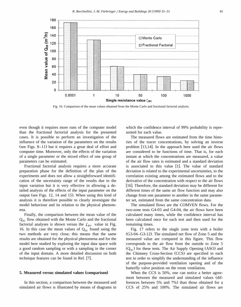
Fig. 16. Comparison of the mean values obtained from the Monte Carlo and fractional factorial analysis.

even though it requires more runs of the computer modelthan the fractional factorial analysis for the presentedcases. It is possible to perform an investigation of theinfluence of the variation of the parameters on the resultsŽ .see Figs. 8–11 but it requires a great deal of effort andcomputer time. Moreover, only the effects of the variationof a single parameter or the mixed effect of one group ofparameters can be estimated.

Fractional factorial analysis requires a more accuratepreparation phase for the definition of the plan of theexperiments and does not allow a straightforward identifi-cation of the uncertainty range of the results due to theinput variation but it is very effective in allowing a de-tailed analysis of the effects of the input parameter on the

Ž .output see Figs. 12, 14 and 15 . When using this kind ofanalysis it is therefore possible to clearly investigate themodel behaviour and its relation to the physical phenom-ena.

Finally, the comparison between the mean value of theQ flow obtained with the Monte Carlo and the fractional05

factorial analyses is shown versus the z value in Fig.BV

16. In this case the mean values of Q found using the05

two methods are very close; this means that the sameresults are obtained for the physical phenomena and for themodel here studied by exploring the input data space witha good random sampling or with a sampling in the cornerof the input domain. A more detailed discussion on both

w xtechnique features can be found in Ref. 7 .

( )5. Measured versus simulated values comparison

In this section, a comparison between the measured andsimulated air flows is illustrated by means of diagrams in

which the confidence interval of 99% probability is repre-sented for each value.

The measured flows are estimated from the time histo-ries of the tracer concentrations, by solving an inverse

w xproblem 13,14 . In the approach here used the air flowsare considered to be functions of time. That is, for eachinstant at which the concentrations are measured, a valueof the air flow rates is estimated and a standard deviation

w xis associated to this value 1 . The value of standarddeviation is related to the experimental uncertainties, to thecorrelation existing among the estimated flows and to thederivative of the concentration with respect to the air flowsw x16 . Therefore, the standard deviation may be different fordifferent times of the same air flow function and may alsochange from one parameter to another in the same parame-ter set, estimated from the same concentration data.

The simulated flows are the COMVEN flows. For thetwo-zone tests G4-03 and G4-04, the air flows have beencalculated many times, while the confidence interval hasbeen calculated once for each test and then used for theremaining times.

Fig. 17 refers to the single zone tests with a boilerŽ .G3-04–G3-12 . The simulated net flow of Zone 5 and themeasured value are compared in this figure. This flowcorresponds to the air flow from the outside to Zone 5Ž . Ž .Q for these tests. The Air Supply Opening ASO and05

Ž .the Chimney Cross-Section CCS are specified in eachtest in order to simplify the understanding of the influenceof the purpose-provided ventilation opening and of thebutterfly valve position on the room ventilation.

When the CCS is 50%, one can notice a better agree-Žment between the measured and simulated values dif-

.ferences between 5% and 7% than those obtained for aCCS of 25% and 100%. The simulated air flows are

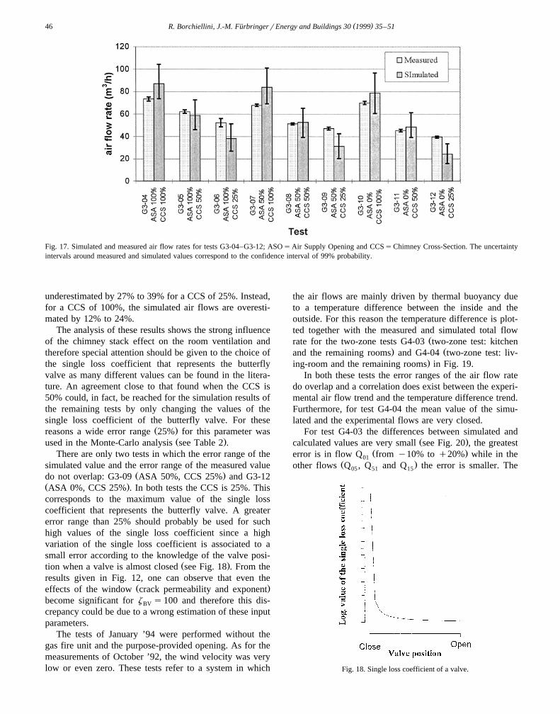
( )R. Borchiellini, J.-M. FurbringerrEnergy and Buildings 30 1999 35–51¨46

Fig. 17. Simulated and measured air flow rates for tests G3-04–G3-12; ASOsAir Supply Opening and CCSsChimney Cross-Section. The uncertaintyintervals around measured and simulated values correspond to the confidence interval of 99% probability.

underestimated by 27% to 39% for a CCS of 25%. Instead,for a CCS of 100%, the simulated air flows are overesti-mated by 12% to 24%.

The analysis of these results shows the strong influenceof the chimney stack effect on the room ventilation andtherefore special attention should be given to the choice ofthe single loss coefficient that represents the butterflyvalve as many different values can be found in the litera-ture. An agreement close to that found when the CCS is50% could, in fact, be reached for the simulation results ofthe remaining tests by only changing the values of thesingle loss coefficient of the butterfly valve. For these

Ž .reasons a wide error range 25% for this parameter wasŽ .used in the Monte-Carlo analysis see Table 2 .

There are only two tests in which the error range of thesimulated value and the error range of the measured value

Ž .do not overlap: G3-09 ASA 50%, CCS 25% and G3-12Ž .ASA 0%, CCS 25% . In both tests the CCS is 25%. Thiscorresponds to the maximum value of the single losscoefficient that represents the butterfly valve. A greatererror range than 25% should probably be used for suchhigh values of the single loss coefficient since a highvariation of the single loss coefficient is associated to asmall error according to the knowledge of the valve posi-

Ž .tion when a valve is almost closed see Fig. 18 . From theresults given in Fig. 12, one can observe that even the

Ž .effects of the window crack permeability and exponentbecome significant for z s100 and therefore this dis-BV

crepancy could be due to a wrong estimation of these inputparameters.

The tests of January ’94 were performed without thegas fire unit and the purpose-provided opening. As for themeasurements of October ’92, the wind velocity was verylow or even zero. These tests refer to a system in which

the air flows are mainly driven by thermal buoyancy dueto a temperature difference between the inside and theoutside. For this reason the temperature difference is plot-ted together with the measured and simulated total flow

Žrate for the two-zone tests G4-03 two-zone test: kitchen. Žand the remaining rooms and G4-04 two-zone test: liv-

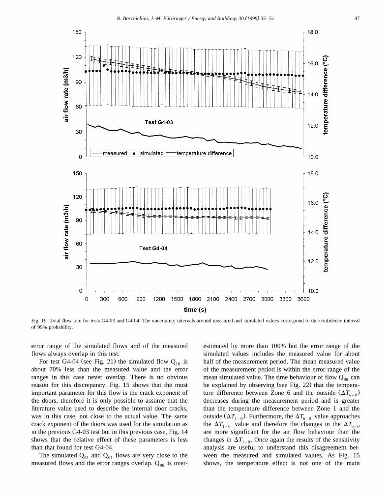
.ing-room and the remaining rooms in Fig. 19.In both these tests the error ranges of the air flow rate

do overlap and a correlation does exist between the experi-mental air flow trend and the temperature difference trend.Furthermore, for test G4-04 the mean value of the simu-lated and the experimental flows are very closed.

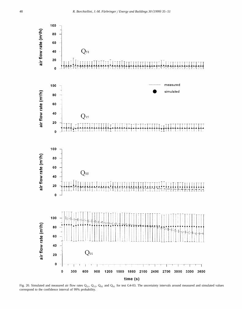
For test G4-03 the differences between simulated andŽ .calculated values are very small see Fig. 20 , the greatest

Ž .error is in flow Q from y10% to q20% while in the01Ž .other flows Q , Q and Q the error is smaller. The05 51 15

Fig. 18. Single loss coefficient of a valve.

( )R. Borchiellini, J.-M. FurbringerrEnergy and Buildings 30 1999 35–51¨ 47

Fig. 19. Total flow rate for tests G4-03 and G4-04. The uncertainty intervals around measured and simulated values correspond to the confidence intervalof 99% probability.

error range of the simulated flows and of the measuredflows always overlap in this test.

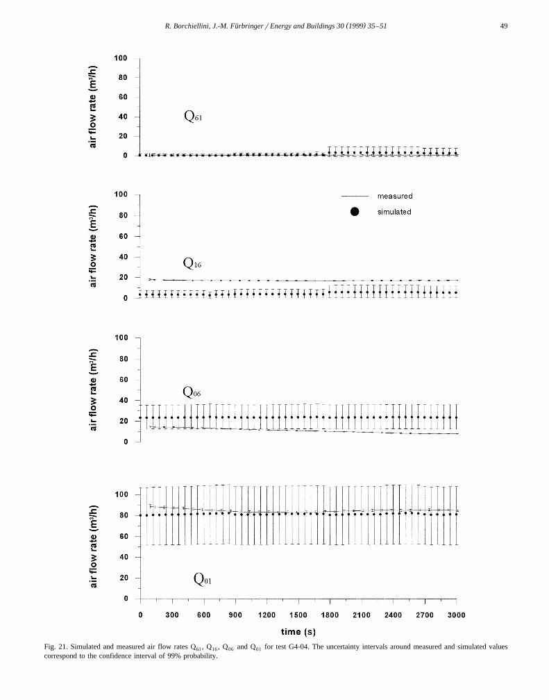
Ž .For test G4-04 see Fig. 21 the simulated flow Q is16

about 70% less than the measured value and the errorranges in this case never overlap. There is no obviousreason for this discrepancy. Fig. 15 shows that the mostimportant parameter for this flow is the crack exponent ofthe doors, therefore it is only possible to assume that theliterature value used to describe the internal door cracks,was in this case, not close to the actual value. The samecrack exponent of the doors was used for the simulation asin the previous G4-03 test but in this previous case, Fig. 14shows that the relative effect of these parameters is lessthan that found for test G4-04.

The simulated Q and Q flows are very close to the61 01

measured flows and the error ranges overlap. Q is over-06

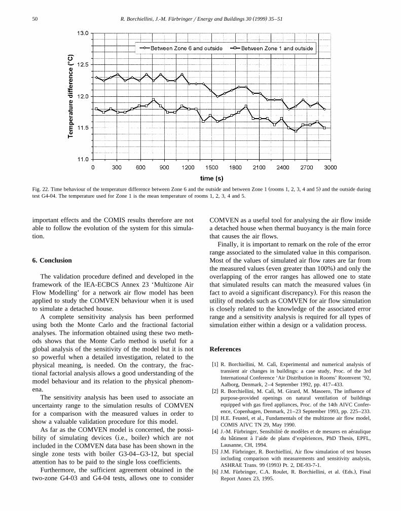
estimated by more than 100% but the error range of thesimulated values includes the measured value for abouthalf of the measurement period. The mean measured valueof the measurement period is within the error range of themean simulated value. The time behaviour of flow Q can06

Ž .be explained by observing see Fig. 22 that the tempera-Ž .ture difference between Zone 6 and the outside DT6 – 0

decreases during the measurement period and is greaterthan the temperature difference between Zone 1 and the

Ž .outside DT . Furthermore, the DT value approaches1 – 0 6 – 0

the DT value and therefore the changes in the DT1 – 0 6 – 0

are more significant for the air flow behaviour than thechanges in DT . Once again the results of the sensitivity1 – 0

analysis are useful to understand this disagreement bet-ween the measured and simulated values. As Fig. 15shows, the temperature effect is not one of the main

( )R. Borchiellini, J.-M. FurbringerrEnergy and Buildings 30 1999 35–51¨48

Fig. 20. Simulated and measured air flow rates Q , Q , Q and Q for test G4-03. The uncertainty intervals around measured and simulated values51 15 05 01

correspond to the confidence interval of 99% probability.

( )R. Borchiellini, J.-M. FurbringerrEnergy and Buildings 30 1999 35–51¨ 49

Fig. 21. Simulated and measured air flow rates Q , Q , Q and Q for test G4-04. The uncertainty intervals around measured and simulated values61 16 06 01

correspond to the confidence interval of 99% probability.

( )R. Borchiellini, J.-M. FurbringerrEnergy and Buildings 30 1999 35–51¨50

Ž .Fig. 22. Time behaviour of the temperature difference between Zone 6 and the outside and between Zone 1 rooms 1, 2, 3, 4 and 5 and the outside duringtest G4-04. The temperature used for Zone 1 is the mean temperature of rooms 1, 2, 3, 4 and 5.

important effects and the COMIS results therefore are notable to follow the evolution of the system for this simula-tion.

6. Conclusion

The validation procedure defined and developed in theframework of the IEA-ECBCS Annex 23 ‘Multizone AirFlow Modelling’ for a network air flow model has beenapplied to study the COMVEN behaviour when it is usedto simulate a detached house.

A complete sensitivity analysis has been performedusing both the Monte Carlo and the fractional factorialanalyses. The information obtained using these two meth-ods shows that the Monte Carlo method is useful for aglobal analysis of the sensitivity of the model but it is notso powerful when a detailed investigation, related to thephysical meaning, is needed. On the contrary, the frac-tional factorial analysis allows a good understanding of themodel behaviour and its relation to the physical phenom-ena.

The sensitivity analysis has been used to associate anuncertainty range to the simulation results of COMVENfor a comparison with the measured values in order toshow a valuable validation procedure for this model.

As far as the COMVEN model is concerned, the possi-Ž .bility of simulating devices i.e., boiler which are not

included in the COMVEN data base has been shown in thesingle zone tests with boiler G3-04–G3-12, but specialattention has to be paid to the single loss coefficients.

Furthermore, the sufficient agreement obtained in thetwo-zone G4-03 and G4-04 tests, allows one to consider

COMVEN as a useful tool for analysing the air flow insidea detached house when thermal buoyancy is the main forcethat causes the air flows.

Finally, it is important to remark on the role of the errorrange associated to the simulated value in this comparison.Most of the values of simulated air flow rates are far from

Ž .the measured values even greater than 100% and only theoverlapping of the error ranges has allowed one to state

Žthat simulated results can match the measured values in.fact to avoid a significant discrepancy . For this reason the

utility of models such as COMVEN for air flow simulationis closely related to the knowledge of the associated errorrange and a sensitivity analysis is required for all types ofsimulation either within a design or a validation process.

References

w x1 R. Borchiellini, M. Calı, Experimental and numerical analysis of`transient air changes in buildings: a case study, Proc. of the 3rdInternational Conference ‘Air Distribution in Rooms’ Roomvent ’92,Aalborg, Denmark, 2–4 September 1992, pp. 417–433.

w x2 R. Borchiellini, M. Calı, M. Girard, M. Masoero, The influence of`purpose-provided openings on natural ventilation of buildingsequipped with gas fired appliances, Proc. of the 14th AIVC Confer-ence, Copenhagen, Denmark, 21–23 September 1993, pp. 225–233.

w x3 H.E. Feustel, et al., Fundamentals of the multizone air flow model,COMIS AIVC TN 29, May 1990.

w x4 J.-M. Furbringer, Sensibilite de modeles et de mesures en aeraulique¨ ´ ` ´du batiment a l’aide de plans d’experiences, PhD Thesis, EPFL,ˆ ` ´Lausanne, CH, 1994.

w x5 J.M. Furbringer, R. Borchiellini, Air flow simulation of test houses¨including comparison with measurements and sensitivity analysis,

Ž .ASHRAE Trans. 99 1993 Pt. 2, DE-93-7-1.w x Ž .6 J.M. Furbringer, C.A. Roulet, R. Borchiellini, et al. Eds. , Final¨

Report Annex 23, 1995.

( )R. Borchiellini, J.-M. FurbringerrEnergy and Buildings 30 1999 35–51¨ 51

w x7 J.M. Furbringer, C.A. Roulet, Comparison and combination of Monte¨Ž . Ž .Carlo and factorial design, Building and Environment 30 4 1995

505–519.w x8 J.M. Furbringer, C.A. Roulet, Confidence of simulation results: put a¨

SAM in your MODEL, same Special Issue on the COMIS program,1996.

w x9 J.M. Furbringer, C.A. Roulet, R. Borchiellini, An overview on the¨evaluation activities of IEA ECB Annex 23, same Special Issue onthe COMIS program, 1996.

w x10 M. Grosso, Wind pressure distribution around buildings: a paramet-Ž . Ž .rical model, Energy and Buildings 18 2 1992 101–131.

w x11 M. Masoero, G.V. Fracastoro, D. Vercelli, Analisi della permeabilitadell’aria degli edifici tramite prove di pressurizzazione, Contratto Di

Ricerca: Analisi Di Sicurezza, Efficienza Energetica e QualitaDell’Aria Nell’Utilizzazione Delle Apparecchiature a Gas, Torino,Italy, Settembre, 1991.

w x Ž12 D.S. Miller, Internal Flow System, BHRA British Hydromechanics.Research Association , Fluid Engineering, 1978.

w x13 C.A. Roulet, R. Compagnon, Multizone tracer gaz infiltration mea-surements—interpretation algorithm for non-isothermal cases, Build-

Ž .ing and Environment 24 1989 221–227.w x14 C.A. Roulet, L. Vandaele, Airflow pattern within buildings—mea-

surement technique, AIVC TN 34, 1991.w x15 A. Wilson, AIVC Numerical Database—Component and Whole

Building Leakage Database User Guide, AIVC, 1992.w x16 Sherman, 1989.