AN ASSESSMENT OF TRANSPORTATION CONTROL …an assessment of transportation control measures, transportation technologies, and pricing/regulatory policies texas transportation efficiency

--- - ---~---- -------- -- -"

AN ASSESSMENT OF TRANSPORTATION CONTROL MEASURES, TRANSPORTATION TECHNOLOGIES, AND PRICING/REGULATORY POLICIES

TEXAS TRANSPORTATION EFFICIENCY STUDY

,- Project for the Texas Sustainable Energy Development Council

CTR SEDC-1 JUNE 1995

CENTER FOR TRANSPORTATION RESEARCH BUREAU OF ENGINEERING RESEARCH

THE UNIVERSITY OF TEXAS AT AUSTIN

THE TELL.US INSTITUTE Boston MA

CENTER FOR TRANSPORTATION RESEARCH LIBRARY

111111111111111111111111111111111111111111111 L006394

AN ASSESSMENT OF TRANSPORTATION CONTROL

MEASURES, TRANSPORTATION TECHNOLOGIES, AND

PRICING/REGULATORY POLICIES

CTR Mark A. Euritt Angela Weissmann Robert Harrison Mike Martello Jiefeng Qin Sreedhar R. V arada

TELLUS INSTITUTE Stephen Bemow John M. Decicco, ACEEE Mark Fulmer Jeffrey Hall Irene Peters

TEXAS TRANSPORTATION EFFICIENCY STUDY

conducted for the

Sustainable Energy Development Council

by the

CENTER FOR TRANSPORTATION RESEARCH Bureau of Engineering Research

THE UNIVERSITY OF TEXAS AT AUSTIN

and

THE TELLUS INSTITUTE BostonMA

JUNE 1995

ACKNOWLEDGMENT

We wish to acknowledge the technical guidance, support, and review by Harvey

Sachs, SEDC Technical consultant. His insight and expertise have been particularly

helpful.

The research work of CTR was also facilitated by the contributions of many

persons including Bridget Dickerson, Bonnie Malek, Judy McCullough, Balaji

Mohanarangan, Jan Slack, and Karen Smith. Each of these individuals contributed in

different ways to enhance the overall quality of the research effort.

Finally, we are grateful to SEDC for their outlook and interest in a sustainable

transportation future. Judith Carroll and Charlotte Banks were instrumental in assisting our

research team during the challenging administrative phases of the research work.

DISCLAIMER

The contents of this report reflect the views of the authors who are responsible for

the facts and accuracy of the data presented herein. The contents do not necessarily reflect

the official views or policies of the Sustainable Energy Development Council, University

of Texas at Austin or the Center for Transportation Research.

ii

ABSTRACT

The energy intensiveness of the transportation sector has created significant

sustainability problems, as well as air quality concerns. The Texas transportation system is

auto-highway dependent. Efforts to address future mobility needs, must manage this

dependence in relation to energy sustainabililty and environmental quality issues. Various

measures have been identified for reducing the number of passenger miles of travel, as well

as improve the efficiency of the transportation technologies. Transportation control

measures (TCM) have been proposed to curb the growth vehicle traffic. These TCM

measures include both transportation demand management (TDM) and supply

(transportation infrastructure) management strategies. The impact of these measures on

energy use are not well documented. Rather, the focus of these efforts has been on

improved air quality. The various TCMs used around the country are evaluated from an

energy efficiency perspective. Most transportation energy efficiency evaluation has

occurred in the technology area. This technology includes vehicle engine and drivetrain,

aerodynamics, rolling resistance, as well as alternative fuels including electric vehicles and

fuel cell-powered vehicles. Numerous policy strategies -- feebates, accelerated vehicle

retirement, distance taxes, congestion charges, pay-as-you-drive-insurance -- are available

to promote consumer purchases of new technologies, as well as encourage changes in

travel behavior. These various TCM and technology options are evaluated in order to

construct future scenarios for a more energy efficient and environmentally friendly

transportation system.

iii

TABLE OF CONTENTS

CHAPTER 1 •• INTRODUCTION ..................................................... 1 BACKGROUND ..................................................................................... 1

The Texas Transportation System ......................................................... 2 The Texas Transportation Challenge ...................................................... 3

REPORT OBJECTIVE ............................................................................... 3 REPORT ORGANIZATION ........................................................................ 4

CHAPTER 2 •• OPTIONS FOR ENERGY EFFICIENCY AND EMISSIONS REDUCTION IN TRANSPORTATION ............................ 5

BACKGROUND ..................................................................................... 5 TRANSPORTATION SYSTEM MANAGEMENT (TSM) ..................................... 5

Definition, Objectives and Typology ...................................................... 6 Transportation Supply Management ....................................................... 7 Transportation Demand Management ...................................................... ?

LAND USE MANAGEMENT ...................................................................... 8 Land Use and Transportation Demand .................................................... 9 Concentrated Demand Management ..................................................... 10

Definition .......................................................................... 10 Description ......................................................................... 11 Current Status ..................................................................... 11

TECirnOLOGY OPTIONS ....................................................................... 13 TRANSPORTATION POLICIES AND PRICING STRATEGIES .......................... 14

Problem Definition ......................................................................... 14 Transportation Policies and Technology Improvements .............................. 15

TCM PROGRAMS FOR TEXAS NON-ATTAINMENT AREAS ........................... 16 Background ................................................................................. 18 Current Non-Attainment Status .......................................................... 19 State Plan for Ozone Control ............................................................. 20

Objectives .......................................................................... 20 Methodology ...................................................................... 20 Implementation Mechanisms .................................................... 21 Texas' SIP Programs for Reducing Ozone Pollution ......................... 22

SUNfiVfAR Y ......................................................................................... 23 CHAPTER 3 •• AN ASSESSMENT OF TRANSPORTATION CONTROL

MEASURES ....................................................................... 2 4 BACKGROUND ................................................................................... 24 THE STATE-OF-THE-ART IN TCM ASSESSMENT ........................................ 24 TCM ASSESSMENT APPROACH .............................................................. 25

Objectives ................................................................................... 25 Factors Influencing TCM Impacts ....................................................... 25

Baseline for Relative TCM Impacts ............................................. 25 Projections of TCM Effects ...................................................... 26 Duration of TCM Impacts ........................................................ 26 Interaction Among TCMs ........................................................ 26 Demand Elasticities and TCM Implementation ................................ 27 Baseline Traffic for TCM Evaluation ........................................... 27

Major Case Studies ........................................................................ 27 Delaware Valley Regional Planning Commission ............................. 27 Houston-Galveston Area Council.. ............................................. 28 National Association of Regional Councils .................................... 29 Regulation XV (Los Angeles, California) ..................................... 29

iv

TABLE OF CONTENTS, CONTINUED

Maricopa County, Arizona ....................................................... 31 Denver, Colorado ................................................................. 32 El Paso, Texas .................................................................... 33 National Overview of Individual Employers .................................. 33 US WEST ......................................................................... 35 UCLA .............................................................................. 36 Nuclear Regulatory Commission (NRC) ...................................... 37 Program Costs .................................................................... 38

Discussion .................................................................................. 38 Recommendations ......................................................................... 39

COST ASSESSMENT ............................................................................. 40 The State-of-The-Art in TCM Cost Analysis ........................................... 40 Approach for TCM Cost Assessment ................................................... 40

SUMMARY, CONCLUSIONS, AND RECOMMENDATIONS ............................ 42 CHAPTER 4 •• TRANSPORTATION SUPPLY MANAGEMENT ................. 4 3

INTRODUCTION .................................................................................. 43 DESCRIPTION OF MEASURES ................................................................ 43

Traffic Signalization ....................................................................... 43 Traffic Operations .......................................................................... 44 Traffic Management ....................................................................... 44 Intelligent Transportation Systems (ITS) ............................................... 45 Conclusions and Observations ........................................................... 47

ENERGY EFFICIENCY AND EMISSIONS REDUCTION POTENTIAL ................ 47 Traffic Signalization ....................................................................... 47

Case Studies ....................................................................... 48 /,., Summary and Conclusions ...................................................... 49

Traffic Operations .......................................................................... 49 Case Studies ....................................................................... 50 Summary and Conclusions ...................................................... 51

Traffic Management Systems ............................................................. 52 Ramp Metering .................................................................... 53 Incident Management Systems .................................................. 53

Intelligent Transportation Systems ....................................................... 54 Simulation Modeling - ATIS .................................................... 55 Field Results - ATMS ........................................................... 56

CONCLUSIONS AND OBSERVATIONS ..................................................... 57 CHAPTER 5 - TRANSPORTATION DEMAND MANAGEMENT ................ 59

INTRODUCTION .................................................................................. 59 TRIP ELIMINATION PROGRAMS ............................................................. 59

Employer-Based Trip Reduction Programs ............................................. 59 Telecommuting ............................................................................. 60 Work Schedule Changes .................................................................. 60 Non-Motorized Transport ................................................................. 61 Current Status .............................................................................. 62

INCREASED VEIDCLE OCCUPANCY ....................................................... 63 Improved Public Transit .................................................................. 63

System/Service Expansion ....................................................... 63

v


System/Service Operational Improvements .................................... 63 Demand/Market Strategies ....................................................... 64

Rides hare, Carpools and V anpools ...................................................... 64 HOV Facilities .............................................................................. 66 Parking Management ...................................................................... 66 Current Status .............................................................................. 68

Public Transit. ..................................................................... 68 HOV Facilities ..................................................................... 69 Parking Management ............................................................. 71

ASSESSMENT OF TRIP ELil\t1INATION PROGRAMS .................................... 71 Employer-based Trip Reduction Programs ............................................. 71 National Telecommuting Studies ......................................................... 72

U.S. Department of Transportation National Study .......................... 72 Arthur D. Little Study ............................................................ 76

Regional Telecommuting Studies ........................................................ 77 Delaware Valley Regional Planning Commission (DVRPC) ................ 77 National Association of Regional Councils (NARC) ......................... 77 Houston-Galveston Area Council.. ............................................. 78 Summary of Regional Telecommuting Studies ................................ 78

WORK SCHEDULE CHANGES ....................................................... 79 Delaware Valley Regional Planning Commission ............................. 79 Houston-Galveston Area Council.. ............................................. 80 Texas Transportation Institute ................................................... 80 National Association of Regional Councils .................................... 80 Summary of Work Schedule Changes ......................................... 81

NON-MOTORIZED TRANSPORT ..................................................... 81 Delaware Valley Regional Planning Commission ............................. 82 Summary of Non-Motorized Transport ........................................ 83

ASSESSMENT OF INCREASED VEIDCLE OCCUPANCY ACTIVITIES .............. 84 IMPROVED PUBLIC TRANSIT ....................................................... 84

North-Central Texas Council of Governments ................................ 84 Delaware Valley Regional Planning Commission ............................. 85 Houston-Galveston Area Council .............................................. 85 National Association of Regional Councils .................................... 87 Texas Transportation Institute ................................................... 87 Summary of Improved Public Transit. .................. _. ...................... 88

HOVFACILITIES ........................................................................ 88 North Central Texas Council of Governments ................................ 88 Houston-Galveston Area Council .............................................. 88

PARKING MANAGEMENT ............................................................ 92 North-Central Texas Council of Governments ................................ 92 Delaware Valley Regional Planning Commission ............................. 92 Texas Transportation Institute ................................................... 93 Houston-Galveston Area Council.. ............................................. 93 Summary of Parking Management Strategies ................................. 93

CONCLUSIONS ................................................................................... 94 CHAPTER 6 - TECHNOLOGY OPTIONS ......................................... 9 6

APPROACH TO ASSESS TECHNOLOGY OPTIONS ...................................... 96 General Approach .......................................................................... 96 Valuing Air Emissions .................................................................... 97

vi


CONVENTIONAL FUEL- LIGHT VEHICLES ............................................. 101 The Gasoline Consumption Process .................................................... 101

Efficiency Gains From Decreased Engine Losses ........................... 1 02 Efficiency Gains From Decreased Aerodynamic Drag ...................... 1 03 Efficiency Gains From Decreased Rolling Friction .......................... 1 03 Efficiency Gain in Acceleration (Weight Reduction) ........................ 103 Emissions Savings ............................................................... 104

Current Status ............................................................................. 104 Engine/Drivetrain Improvements ............................................... 105 Aerodynamic Drag Reduction .................................................. 1 05 Rolling Resistance Reduction .................................................. 1 05 Weight Reduction ................................................................ 1 06

Technical Feasibility ...................................................................... 106 Economic Feasibility ..................................................................... 106 Institutional Context Barriers ............................................................ 1 09

CONVENTIONAL FUEL-HEAVY VEHICLES ............................................ 109 Description ................................................................................. 109

Efficiency Improvements In Heavy Truck Engines .......................... 110 Aerodynamics Improvements .................................................. 110 Rolling Resistance Reduction .................................................. 111 Emissions Impacts ............................................................... 111

Current Status ............................................................................. 111 Technical Feasibility ...................................................................... 112 Economic Feasibility ..................................................................... 112

AIRCRAFT EFFICIENCY IMPROVEMENT ................................................. 115 Improvements in Engine Technology .................................................. 115 Improvements in Airframe ............................................................... 115 Airport Operations ........................................................................ 115 Current Status ............................................................................. 116 Technical and Economic Feasibility .................................................... 116

ALTERNATIVE FUELS- NATURAL GAS VEHICLES (NGV) .......................... l17 Fuel Characteristics ........................................................................ 117 Emissions .............................................................. : ................... 118 Natural Gas in Heavy Vehicles and Transit Buses .................................... 118 Current Status ............................................................................. 119 Technical Feasibility ...................................................................... 120 Economic Feasibility ..................................................................... 120

ALTERNATIVE FUELS- LIQUID PETROLEUM GAS (LPG) VEHICLES ............ 123 Fuel Characteristics ....................................................................... 123 Emissions .................................................................................. 123 Current Status ............................................................................. 124 Technical Feasibility ...................................................................... 124 Economic Feasibility ....................... · .............................................. 125

ALTERNATIVE FUELS- ETHANOL AND BIOFUELS ................................... 127 BioFuel Characteristics and Emissions ................................................. 127

Ethanol ............................................................................ 127 Methanol .......................................................................... 128

Current Status ............................................................................. 129 Assessment of Methanol Produced from Natural Gas ................................ 129

Technical Feasibility ............................................................. 129 Economic Feasibility ............................................................ 129

vii


Assessment of Ethanol and Biofuels ................................................... 131 Technical Feasibility ............................................................. 131 Economic Feasibility ............................................................ 132

ALTERNATIVE FUELS- ELECTRIC /BATTERY POWERED VEHICLES ........... 134 Characteristics ............................................................................. 134 Emissions .................................................................................. 135 Current Status ............................................................................. 135 Technical Feasibility ...................................................................... 136 Economic Feasibility ..................................................................... 137

ALTERNATIVE FUELS -- HYBRID AND FUEL CELL (HYDROGEN) VEHICLES ................................................................................... 139

Characteristics and Emissions ........................................................... 139 Current Status ............................................................................. 140 Technical Feasibility ...................................................................... 141

Fuel Cells ......................................................................... 141 Fuel Storage ...................................................................... 142 System Integration ............................................................... 142 Refueling Infrastructure ......................................................... 142

Economic Feasibility ..................................................................... 143 HIGH SPEED RAIL INTERCITY TRIP OPTION ........................................... 144

Characteristics ............................................................................. 144 Current Status ............................................................................. 145

SUM:MARY, CONCLUSIONS AND OBSERVATIONS ................................... 146 CHAPTER 7 - TRANSPORTATION POLICIES ................................. 148

INTRODUCTION ................................................................................. 148 FEEB A TES ......................................................................................... 148

Description ................................................................................. 149 Current Status ............................................................................. 149 Practical Feasibility ....................................................................... 150 Economic Feasibility ..................................................................... 150 Equity and Institutional Issues .......................................................... 152

INSPECTION AND MAINTENANCE (liM) PROGRAMS ................................ 154 Current status .............................................................................. 154

ACCELERATED RETIREMENT OF VEHICLES ............................................ 155 Description ................................................................................. 155 Current Status ............................................................................. 156 Practical Feasibility ....................................................................... 156 Economic Feasibility ..................................................................... 157 Equity and Implementation Issues ...................................................... 160

LOW EMISSION VEHICLES (LEV), ZERO EMISSION VEHICLES (ZEV), AND ALTERNATIVE FUELS ................................................... 161

Description of Policy Options ........................................................... 161 Regulation and Subsidies ....................................................... 161 Government Procurement ....................................................... 162

Current Status ............................................................................. 163 Texas Initiatives ........................................................................... 164

FUEL TAXES ..................................................................................... 166 Description ................................................................................. 167 Current Status ............................................................................. 167 Practical Feasibility ....................................................................... 168 Economic Feasibility ..................................................................... 168

Estimating the Response Of Gasoline Consumption to

viii


Changing Prices ............................................................ 169 Recent Estimates of the Price Elasticity of Demand

for Gasoline Consumption ................................................ 170 Implementation and Equity Issues ...................................................... 171

Direct Distributional Effects of Fuel Taxes ................................... 171 Indirect Macro-Economic Effects of Fuel Taxes ............................. 172 The Public's Perception of Equity ............................................. 172

VMT AND CONGESTION CHARGES ....................................................... 173 Description ................................................................................. 173 Current Status ............................................................................. 175 Practical Feasibility ....................................................................... 17 5 Economic Feasibility ..................................................................... 177 Equity and Implementation Issues ...................................................... 179

PAY-AS-YOU-ORNE-INSURANCE (PAYDI) .............................................. 180 Description ................................................................................. 181

Pay-at-the-Pump ................................................................. 181 Pay-by-Mile ...................................................................... 183

Current status .............................................................................. 183 Practical Feasibility ....................................................................... 184 Economic Feasibility ..................................................................... 184 Implementation Issues .................................................................... 185

CONCLUSIONS AND RECO.MNIENDATIONS ............................................. 185 Induced Travel, Fixed Costs, and Variable Costs .................................... 186 Interaction Between Different Policy Goals and Targets ............................. 186 Equity and Implementation Considerations ............................................ 188 Conclusion ................................................................................. 189

CHAPTER 8- SUMMARY, CONCLUSIONS, AND RECOMMENDATIONS ..• 191 S~Y ........................................................................................ 191 CONCLUSIONS AND RECO.MNIENDATIONS ............................................. 192

Transportation Control Measures ....................................................... 192 Technology and pricing .................................................................. 193

REFERENCES 195

ix

LIST OF TABLES

Table 2.1 Transportation Supply Management Strategies ................................................ 8 Table 2.2 Transportation Demand Management Strategies ............................................... 9 Table 2.3 Technology Options for Energy Efficient Transportation ................................... 13 Table 2.4 Clean Air Act Standards for Major Transportation-Related Pollutants .................... 17 Table 2.5 Provisions for ISTEA and CAAA that Encourage the Use ofTCMs .................... 18 Table 2.6 Texas Non-Attainment Areas as of 1992 ..................................................... 19 Table 2.7 Regional Planning Programs in Texas Non-Attainment Areas ............................ 22 Table 3.1 DVRPC Baseline Travel Activity .............................................................. 28 Table 3.2 HGAC Baseline Travel Characteristics ....................................................... 29 Table 3.3 Regulation XV Frequency of Incentives by Types .......................................... 30 Table 3.4 Regulation XV Costs ........................................................................... 31 Table 3.5 Regulation XV Change in Average Vehicle Ridership by Average

Vehicle Ridership Target .................................................................... 31 Table 3.6 Regulation XV Mode Shares .................................................................. 31 Table 3.7 DRCOG Assumed Levels of Application ofVMT Reduction Measures ................. 34 Table 3.8 Individual Employer TRP -- Impacts ......................................................... 35 Table 3.8 Individual Employer TRP -- Impacts (Cont.) ................................................ 36 Table 3.9 US WEST Employee Mode Split (June 1988) .............................................. 37 Table 3.10 ETRP Case Studies-- Costs ................................................................. 38 Table 3.11 ETRP Case Studies -- Impacts ............................................................... 3 8 Table 3.12 Summary of Cost and Benefit Categories for Some TCMs .............................. 41 Table 4.1 Current Status in ITS ........................................................................... 47 Table 4.2 Costs of Traffic Signalization Improvements ................................................ 50 Table 4.3 Impacts of Traffic Signalization Improvements ............................................. 50 Table 4.4 Costs of Traffic Operation Improvements .................................................... 52 Table 4.5 Impacts of Traffic Operations Improvements ................................................ 52 Table 4.6 Costs of Ramp Metering ....................................................................... 53 Table 4.7 Impacts of Ramp Metering ..................................................................... 53 Table 4.8 Costs of CIMS Improvements ................................................................. 54 Table 4.9 Impacts of CIMS Improvements .............................................................. 55 Table 5.1 EPA Categories for Employer-Promoted TCMs ............................................ 60 Table 5.2 Areawide Employer-Based Trip Reduction Programs -- Costs ............................ 73 Table 5.3 Areawide Employer-Based Trip Reduction Programs-- Impacts .......................... 74 Table 5.4 Areawide Employer Based Trip Reduction Programs-- Impacts ......................... 74 Table 5.5 Nationwide Telecommuting Survey Results ................................................. 75 Table 5.6 Nationwide Telecommuting Projections ...................................................... 75 Table 5.7 Nationwide Telecommuting Impacts -- Assumptions ....................................... 76 Table 5.8 Nationwide Telecommuting Impacts .......................................................... 77 Table 5.9 Telecommuting Costs-- Houston/Galveston Area .......................................... 78 Table 5.10 Telecommuting Costs Per Employee -- Houston/Galveston Area ....................... 78 Table 5.11 Telecommuting -- Regional Studies --Impacts ............................................ 79 Table 5.12 Work Schedule Changes -- Costs ........................................................... 81 Table 5.13 Work Schedule Changes-- Impacts ......................................................... 81 Table 5.13 (cont.) Work Schedule Changes-- Impacts ................................................. 82 Table 5.14 Non-Motorized Transport-- Costs .......................................................... 83 Table 5.15 Non-Motorized Transport -- Impacts ........................................................ 84 Table 5.15 (cont.) Non-Motorized Transport -- Impacts ................................................ 84 Table 5.16 Improved Public Transit-- Impacts ......................................................... 89 Table 5.16 (cont.) Improved Public Transit- Impacts ................................................... 90 Table 5.17 Houston HOV Lane System-- Impacts ...................................................... 91

X

LIST OF TABLES, CONTINUED

Table 5.18 HOV Lanes Houston/Galveston Area-- Impacts .......................................... 91 Table 5.18 (cont) HOV Lanes Houston/Galveston Area-- Impacts .................................. 92 Table 5.19 HOV Lanes Houston/Galveston Area -- Costs ............................................. 92 Table 5.19 (cont) HOV Lanes Houston/Galveston Area-- Costs ..................................... 92 Table 5.20 Parking Management Strategies- Costs ..................................................... 94 Table 5.21 Parking Management Strategies- Impacts .................................................. 95 Table 6.1 Summary of Alternative Vehicles Assumptions ............................................. 98 Table 6.2 Air Emissions Externality Values Adopted I Proposed in Various U.S. States .......... 99 Table 6.3 Source and Notes for Table 6.2 ............................................................... 100 Table 6.4 Air Emissions Externality Values for Texas ................................................ 101 Table 6.5 Engine and Transmission Technology Penetration in the 1990 Fleet .................... 105 Table 6.6 Automobile Efficiency Improving Technologies, Associated

Fuel Economy Improvements, and Costs ................................................ 1 08 Table 6. 7 Class 8 Trucks Fuel Economy ................................................................ 111 Table 6.8 Heavy Truck Efficiency Improving Technologies, Associated

Fuel Economy Improvements, And Costs ............................................... 114 Table 6.9 Basic Assumptions and Results of the NGV Economic Screening Analysis ........... 121 Table 6.10 Basic Assumptions and Results of the LPG Vehicle Economic Screening

Analysis ...................................................................................... 125 Table 6.11 Basic Assumptions and Results of the MV from Natural Gas Economic

Screening Analysis .......................................................................... 130 Table 6.12 Basic Assumptions and Results of the Biomass - MV Economic Screening

Analysis ...................................................................................... 133 Table 6.13 Selected EV Battery Technologies and Key Performance Criteria ...................... 136 Table 6.14 Basic Assumptions and Results of the EV Economic Screening Analysis ............. 138 Table 6.15 Basic Assumptions and Results of the FCV Economic Screening Analysis ........... 143 Table 6.16 Energy use per Seat-Mile of Various Intercity Transportation Modes .................. 145 Table 7.1 Estimated Emissions Reductions (tons) ..................................................... 160 Table 7.2 SB 740 Conversion Schedule (Texas) ....................................................... 164 Table 7.3 SB 769 Conversion Schedule for Local Government and Private Fleets

in Texas ...................................................................................... 165 Table 7.4 SB 7 Conversion Schedule for Texas School District Fleets ............................. 166 Table 7.5 Motor Fuel Tax Rates .......................................................................... 168

XI

LIST OF FIGURES

Figure 3.1 Maricopa County TRP Results ...................................................... 32 Figure 5.1 National Public Transit PMT Mode Split .......................................... 70 Figure 5.2 Improved Public Transit Measures-- Cost-Effectiveness ........................ 85 Figure 6.1 Energy Consumption By Gasoline Powered Vehicles (average of

highway and urban driving cycles) ................................................ 102 Figure 6.2 Cost of Saved Energy for Automobile Fuel Efficiency

Programs Societal Perspective ................................................. 107 Figure 6.3 Cost of Saved Energy for Automobile Fuel Efficiency

Programs- Private Perspective ................................................. 107 Figure 6.4 Cost of Saved Energy for Heavy Truck Fuel Efficiency

Programs Societal Perspective ................................................. 113 Figure 6.5 Cost of Saved Energy for Heavy Truck Fuel Efficiency

Programs Private Perspective .................................................. 113 Figure 6.6 NGV Cost per mile-- Societal and Private Perspectives ........................ 122 Figure 6.7 LPG Vehicle Cost per Mile-- Societal and Private Perspectives ............... 126 Figure 6.8 Methanol Vehicle from Natural Gas Cost per Mile-- Societal

and Private Perspectives ............................................................ 131 Figure 6.9 Methanol from Biomass Vehicle Cost per Mile -- Societal

and Private Perspectives ............................................................ 133 Figure 6.10 EV Cost per Mile-- Societal and Private Perspectives ......................... 138 Figure 6.11 Fuel Cell Vehicle Cost per Mile - Societal and Private

Perspectives .......................................................................... 144

xii

CHAPTER 1 --INTRODUCTION

The automobile-dominated transportation observed in the U.S. started in first decade of

the 20th Century when Henry Ford industrialized the automobile. By 1913, the U.S. had 80% of

the world automobile production. As automobile production and usage increased, urban mass

transit became less and less competitive, and by 1950 automobiles assumed a dominant role in

U.S. transportation. Only cities with public mass transit subsidies, such as New York, Boston

and Philadelphia, retained strong mass transit systems. For intercity travel, implementation of

the interstate highway system coupled with the growth in the air transport sector relegated

railroads to their current role as freight carrier (Ref. 1).

The initial focus of the typical U.S. automobile was passenger comfort. This vehicle was

large, caused significant pollution, and was not energy efficient. The oil embargo of the 1970s

changed this situation, albeit more slowly than many critics desired. At the same time, air

pollution and automobile safety became concerns. Together, these events have led to the

enactment of various laws and policies aimed at improving vehicle safety, decreasing pollution,

and lessening U.S. dependence on foreign oil.

BACKGROUND

Interestingly, current efforts to address transportation demand are being driven primarily

by air quality issues, coupled with concerns about dependence on foreign oil. The Clean Air

Amendments of 1990 (CAAA) and the Intermodal Surface Transportation Efficiency Act of

1991 (ISTEA) were strongly influenced by the recognition that mobile sources, i.e.

transportation, are important contributors to air quality problems, and that the constant increase

in vehicle miles of travel (VMT) was reducing the effectiveness of technological advances

lessening tailpipe emissions. These two initiatives, CAAA and ISTEA, especially its Congestion

Mitigation and Air Quality Improvement Program (CMAQ), are designed to promote more

efficient utilization of the transportation system. Accordingly, they tackle the issues of energy

conservation, better air quality, and, to some extent, dependence on foreign oil in two major

ways: technological innovations and transportation management.

Technology has been responsive to the needs and concerns of the 1990s. Alternative fuel

vehicles, more fuel efficient vehicles, and less pollutants in tailpipe emissions are all

technological achievements. However, the continuing growth of VMT is still offsetting the

benefits derived from these innovations, and it is imperative that transportation be analyzed both

in terms of demand and supply.

THE TEXAS TRANSPORTATION SYSTEM

In Texas, a vast transportation network has developed to address mobility and

accessibility needs. This transportation system is dominated by 294,152 miles of public roads,

74% more than any other state in the country. The system also includes the largest rail network

in the U.S. with 11,370 miles of rail line. In the aviation sector, 90% of the Texas population is

within one-hour of the state's 26 primary commercial airports. In addition to these primary

facilities, there are 369 reliever and utility airport facilities serving general aviation traffic. In

1975, the Texas Legislature approved the Texas Coastal Waterway Act, authorizing the state to

serve as the nonfederal sponsor of the Texas Intracoastal Waterway. This human-made canal

parallels the gulf coastline from Brownsville, Texas to St. Marks, Florida. Finally, the state

transportation system includes 172,000 miles of pipeline carrying crude oil and refined

petroleum products, and 196,000 miles of natural gas pipeline.

A majority (55%) of the passenger miles are for local travel. Nearly 71% of the total

local travel occurs in the Texas cities with populations over 200,000 people. Most of the local

travel is by private vehicle. It is estimated that about 1% of all local travel is by public

transportation. Of some interest is the finding that only 23% of all local trips are work-related.

This has important implications for transportation policies aimed at reducing employee trips.

\Intercity trips account for 45% of the state's 301.8 billion passenger miles of travel (PMT).

Nearly 60% of this traffic is by private vehicle, 39% by airline, and the remaining 1% by

commercial bus and rail::)

The largest percentage (43%) of freight ton-miles are moved across Texas highways by

truck. Next come the railroads (26%) and pipelines (25%). The Texas Intracoastal Waterway

accounts for 5% of total ton-miles. Over 50% of the commodities moved along this waterway

consist of petroleum and coal products. The importance of the waterway is illustrated in a recent

impact study reporting that its closure would require an additional 574,185 railroad cars or 2.3

million truck loads if moved by rail or highway (Ref. 2). Air transportation accounts for less

than 1% of the freight ton-miles. However, airlines generally move most of the freight that is

time or value sensitive.

Unlike passenger transportation, most freight transportation is intercity. In 1994, it is

estimated that 83% of the states ton-miles are intercity in nature, 13% of the ton-miles will be in

cities of more than 200,000 persons, and the remaining 4% in cities under 200,000 persons.

Within the intercity transportation network, truck, rail, and pipeline share nearly an equal

percentage of freight ton-miles.

2

THE TEXAS TRANSPORTATION CHALLENGE

Without question, Texas depends on its network of public roads to move people and

commodities. This dependence, however, is not without significant costs. The Federal Highway

Administration (FHW A) reports that 25% of the Texas urban interstate highways exceed 95% of

their capacity and 43% are operating at over 80% of their carrying capacity. The resulting

congestion is estimated to cost Texas motorists an additional $3.9 billion in delay and fuel costs

each year. At the same time the capacity of the system is being stretched to its limits, the quality

of the road pavements are rapidly deteriorating.. FHW A reports that nearly 75% of the state

highway system is in fair or worse condition. Poorly maintained roads mean higher operating

costs for the Texas consumer. The Congressional Budget Office (CBO) estimates that consumer

variable vehicle operating costs increase from 11% to 29% on roads in poor condition.

In addition to higher costs to the motoring public, dependence on highways has also led

to worsening air quality, greater dependence on imported petroleum, and more rapid depletion of

non-renewable resources. These are major social concerns and the impetus behind this study's

effort to explore future scenarios aimed at promoting greater efficiency in the transportation

sector.

REPORT OBJECTIVE

Recognizing that energy efficiency measures and renewable energy sources have

significant potential for meeting Texas' long-term energy needs, the Sustainable Energy

Development Council (SEDC) was created by Executive Order in March 1993. With almost

one-fourth of the energy consumed by Texans each year used to transport passengers and freight,

the transportation sector is an essential element in any strategic plan for increasing energy

efficiency. To assess the potential for improved efficiency in the transportation sector, the

SEDC contracted with The University of Texas' Center for Transportation Research and the

Tellus Institute to conduct a comprehensive study of transportation in Texas. The research team

was asked to define the current Texas transportation system and to identify and evaluate

measures to reduce energy consumption and associated pollutant emissions. The study began

with a careful and thorough assessment of current options for transportation energy savings,

which is documented in this report. A second report outlines the analytical model and scenarios

for estimating the impact of future transportation alternatives on energy consumption and air

pollution.

This report presents a comprehensive discussion and a thorough assessment of the major

alternatives to increase energy efficiency in the transportation sector, namely transportation

system management (TSM) and technological improvements. Importantly, new technological

options will not supersede the traditional gasoline-powered automobile, and TSM measures will

3

not become widely used, unless policies specifically designed to promote and encourage

transportation alternatives are implemented. Therefore, in many cases policies and options are

intertwined. This report discusses alternatives as well as implementation policies where

appropriate.

The objective of this report is twofold. First, it describes and discusses each measure

conducive to energy efficiency and emissions reduction in transportation. Next, it presents a

critical review of each one of these measures, in terms of their potential, their observed

performance, and their economic feasibility. Since much of the current efforts to improve

transportation are motivated by environmental concerns, this report also presents a review of the

Texas State Implementation Plan (SIP) and a discussion of measures implemented and

considered for Texas' non-attainment areas.

This report is based on a literature review complemented by interviews with persons

familiar with practical implementation of such transportation management options. The material

in this report provides the background information for subsequent phases of this study, which

consisted of the development and analysis of scenarios for more energy efficient transportation

in Texas. This report consists of an assessment of transportation measures for dealing with

energy and environmental issues in the transportation sector, as well as with transportation

control measures, alternative fuels, and transportation policies in general.

REPORT ORGANIZATION

This report is divided into eight chapters. The first chapter is introductory, and describes

the report objectives and scope. Chapter 2 of this report discusses the options for energy savings

in the transportation sector, namely transportation supply and demand management, technology

options, and pricing and pricing-related strategies. The chapter includes a brief discussion of the

programs and strategies for state compliance of National Ambient Air Quality Standards

(NAAQS) in Texas non-attainment areas.

Chapter 3 discusses the incipient state-of-the-art in TSM evaluation, and describes a

methodology used in this study to assess the effectiveness of TSM in providing an energy

efficient and environmentally friendly transportation system. The options are defined, discussed

and evaluated in Chapters 4, 5, 6 and 7. These chapters contain, respectively, the transportation

supply management options, the transportation demand management options, the technological

options, and the policy and pricing options. Chapters 4, 5, 6 and 7 are organized in an analogous

way. They begin with a description of each particular option or measure, then present an

assessment of its potential effectiveness in terms of energy efficiency and emissions reduction,

as well as a cost assessment based on observed cases. The report closes with a summary and

conclusions in Chapter 8.

4

CHAPTER 2 -- OPTIONS FOR ENERGY EFFICIENCY AND El\1ISSIONS

REDUCTION IN TRANSPORTATION

BACKGROUND

To date, energy policy has been driven by a need to reduce dependence on foreign oil. In

the transportation sector, this has been accomplished primarily through improvements in vehicle

fuel economy according to the federal mandated corporate average fuel economy (CAFE)

standards. The impact of these standards has been dramatic for new car sales-nominal fuel

economy has doubled since 1974. These advances, however, have been rendered less effective

by the net impact of increases in vehicle trips, vehicle ownership, sales of light trucks, and the

resulting growth in vehicle miles traveled (VMT) (Ref. 3, 4, 5). The latter two have grown at

higher rates than the population: VMT, for example, increased by 41% between 1983 and 1990.

Making matters worse, the percentage of travelers driving alone has increased nationwide, from

64.4% in 1983 to 73.3% in 1990, and the shortfall between nominal (EPA-test) fuel economy

and real fuel economy is growing (Ref. 4).

More recent energy policy initiatives have focused on fuel selection, i.e., alternatives to

petroleum-based fuels. The success of these efforts has been limited. Moreover, greater

utilization of alternative fuels does not necessarily lead to reductions in energy consumption,

only a shift away from petroleum-based fuels. Future efforts to improve energy efficiency must

include demand-related strategies. A sustainable transportation system must equally address

demand and supply issues.

An energy efficient, environmentally friendly transportation system can be achieved

through a more rigorous application of transportation management, technological improvements,

pricing policies, and land use changes. Rather than independent, these options are

complementary and sometimes intertwined. For example, a measure such as parking

management can be considered either a transportation control measure (TCM) or a pricing

policy. Use of alternative fuels may require mandates or pricing incentives. Nevertheless, the

various options are classified according to nomenclature presently used by the Environmental

Protection Agency (EPA) and the transportation community, in order to present the material in a

more organized way (Ref. 3). This chapter presents an overview of the options examined in this

study, as well as a description of the present application of TCMs in Texas.

TRANSPORTATION SYSTEM MANAGEMENT (TSM)

Transportation system management is a broad term that includes any measure to promote

more efficient use of the transportation infrastructure. The definitions and typology are

5

somewhat inconsistent at this point, therefore the measures are classified in a way that is

conducive to a meaningful discussion of their potential to promote energy efficiency, while at the

same time maintaining the official EPA typology where appropriate.

DEFINITION, OBJECTIVES AND TYPOLOGY

TSM promotes better utilization of the existing transportation infrastructure both from

supply and demand perspectives. Supply management strategies focus on low cost techniques

that optimize system capacity and include projects that optimize traffic signalization, incident

management systems, and ramp metering. Demand management, generally termed

"transportation demand management" (TDM), focuses on low cost strategies to reduce travel

demand on the system by eliminating actual trips, by moving trips to non-peak periods, or by

increasing vehicle occupancy.

Another term, transportation control measure (TCM), is often used interchangeably with

TSM. However, from a technical perspective, TCMs are designed to reduce vehicle trips for air

quality purposes and include demand, supply, and some technology alternatives. TCMs are

defined in the Clean Air Act Amendments of 1990 (CAAA) and specifically include the

following (Ref. 3):

(1) Trip reduction ordinances (TROs) (2) Employer-based transportation management programs (3) Work schedule changes (4) Rideshare incentives (5) Improved public transit (6) High occupancy vehicle (HOV) lanes (7) Traffic flow improvements (8) Parking management (9) Park-and-ride/fringe parking

(10) Bicycle and pedestrian measures (11) Special event (traffic and parking management) (12) Vehicle use limitations/restrictions (13) Accelerated retirement of vehicles (14) Activity centers (15) (Reduction) in extended vehicle idling (16) (A voiding) extreme low-temperature cold starts

This typology was developed as guidance to municipal, state, and other agencies

interested in or required to implement TCMs. From a transportation evaluation perspective,

however, it is not a practical typology for examining TSM alternatives. The typology does not

distinguish between a policy (or strategy) and implementation mechanisms. For example,

bicycle and pedestrian measures (category 10) are policies aimed at decreasing VMT. These

programs can be implemented through a myriad of ways, which include, but are not restricted to,

6

TROs (category 1), employer-sponsored programs (category 2), and vehicle use limitations/

restrictions (category 12).

TRANSPORTATION SUPPLY MANAGEMENT

Transportation supply management is concerned primarily with improving traffic flow.

These improvements represent those actions that can be implemented to enhance the person

carrying capability of the roadway system, without adding significantly to the width of the

roadway. An important reason to implement transportation supply management measures is

related to the need for alleviating traffic congestion and related problems such as air pollution.

Other factors include financial difficulties in supporting new major transportation projects, and

the environmental and physical constraints associated with new infrastructure construction.

Transportation supply management actions can be applied to all functional levels of the road

system, i.e. freeway, arterials, collectors, and local streets.

Most supply management strategies are implemented with the objective of improving the

peak period traffic flows, even though non-peak period trips account for 75% of trips

nationwide. The applicability of such strategies could be expanded to include traffic conditions

throughout the day, but implementation of supply management strategies can result in induced

demand and shifts from transit to cars, leading to a net decrease in system efficiency. Therefore,

providing additional capacity for private vehicles must be carefully weighed against the need for

greater priority for other modes, particularly in the light of the bias towards private vehicles

already prevalent in the system. Examples of such trade-offs are right turn on red versus

pedestrian safety, and delayed greens to allow pedestrian crossings versus more continuous car

flow.

Supply management actions include a range of strategies, summarized in Table 2.1 (Ref.

6). Intelligent Transportation System (ITS) technology is also considered a traffic flow

improvement strategy, and as such is included in this discussion (Ref. 7).

TRANSPORTATION DEMAND MANAGEMENT

The basic objective of TDM is to reduce congestion by decreasing the overall number of

trips, especially during peak hours. This reduction can be achieved in two different, but

sometimes complementary ways: trip elimination and increased vehicle occupancy. In trip

elimination strategies, the number of trips is reduced through various programs such as

telecommuting, in which both legs of the work trip are eliminated by encouraging the employee

to work either at home or at a satellite office close to horne. Trip elimination strategies result in

a decrease in both VMT and person-miles traveled (PMT).

7

Table 2.1 Transportation Supply Management Strategies (Ref. 6)

(1) Traffic Signalization • Equipment or software updating • Timing plan improvements • Signal coordination and interconnection • Signal removal

(2) Traffic Operations • Converting two-way streets to one-way operation • Two-way street left tum restrictions • Continuous median strip for left tum lanes • Channelized roadway and intersections • Roadway and intersection widening and reconstruction

(3) Enforcement and Management • Enforcement for all of the actions described in this table • Incident Management Systems • Ramp metering

(4) Intelligent Transportation Systems (ITS) • Advanced Traffic Management System (ATMS) • Advanced Traveler Information System (ATIS) • Commercial Vehicle Operation (CVO) • Advanced Vehicle Control System (AVCS)

Increased vehicle occupancy, on the other hand, promotes a reduction in the number of

vehicle trips by pooling several persons that would otherwise drive alone. Strategies to decrease

the number of trips through increased vehicle occupancy include mass transit, carpooling, and

other forms of ridesharing. Increased vehicle occupancy strategies result in a decrease in VMT

w]file PMT remains the same.

For the benefit of a technical discussion, TDM strategies can be classified according to

the two categories discussed above: "trip elimination" and "increased occupancy." Each of these

two categories can be further divided into sub-categories that depend on public investments,

implementation strategy, employer cooperation, and marketing strategies. A typology conducive

to a succinct, self-contained discussion of each sub-category is not possible because of the

overlap inherent in many of the sub-categories. The outline shown in Table 2.2 provides a

convenient framework for the understanding of TDM strategies.

LAND USE :MANAGEMENT

The type of urban development typically found in the U.S. and particularly in Texas is

highly dependent on individual transport. Zoning ordinances usually result in low density

suburban residential areas where winding streets and cui-de-sacs are common and transit and

pedestrian facilities are rare or non-existent. In addition, two-thirds of all new jobs are located in

suburban areas, leading to an amount of suburban-to-suburban movement that is twice the

8

suburban-to-central business district (CBD) movement (Ref. 1). Land use and development

management measures such as jobs/housing balance and new zoning ordinances will be required

to solve urban and regional transportation problems.

Table 2.2 Transportation Demand 1\tlanagement Strategies

(1) Trip Elimination (or change to non-peak period) • Telecommuting • Work schedule changes

-Flex time - Compressed work week -Staggered work week

• Non-motorized transport

(2) Increased Vehicle Occupancy • Public transportation

- System/service expansion (including transit-ways, park-and-ride) - Operational improvements -Marketing

• Private HOVs - Ridesharing, carpool and vanpool programs - Parking management - Road pricing - HOV facilities - Auto restrictions

LAND USE AND TRANSPORTATION DEMAND

Land use and development policies affect transportation demand, and several studies as

well as practical observations support the ad-hoc wisdom that higher population density and

multi-purpose land development are more conducive to energy-efficient mobility. According to

Gordon, the following factors can increase transit use and encourage non-motorized transport

(Ref. 1):

(1) High residential density. Studies indicate that residential density should exceed 2,400 persons per square mile to encourage non-motorized transport and transit use.

(2) High employment density. There should be at least 50 employees per acre of business development in areas with 10,000 or more jobs to encourage 6% to 11% of employees to ride transit.

(3) Land development in close proximity to transit. Younger people can be expected to walk up to 1,000 feet to transit stops, while senior citizens can be expected to walk 750 feet.

9

(4) Mixed land development. In addition to energy efficient transportation, balanced residential and commercial/industrial land use also results in reduced parking requirements, more open spaces, enhanced retail activity, reduced auto traffic, and increased safety during evening hours.

(5) Transit-oriented development design. Street layout design should include transit routes and be designed to support heavy buses. Sidewalks must be provided, as well as a gridded street layout, which is conducive to non-motorized transport.

Cervero notes that states like California have a considerable sunk investment in rail

systems, and yet most urban development focuses on freeway-served suburban corridors. He

suggests that growth should focus around rail stops, capitalizing on public transit investments

and producing other social benefits, such as increased regional accessibility, reduced traffic

congestion, a more sustainable urban development, and increased mobility for transportation

disadvantaged groups (Ref. 1).

CONCENTRATED DEMAND MANAGE1l1ENT

Another issue that is related to land use and development is the management of traffic in

areas of highly concentrated demand. The U.S. Environmental Protection Agency (EPA) defines

"special events" and "activity centers" as TCMs. Both relate to managing situations of high

concentrated demand, the former in a one-time only or infrequent basis, the latter on a routine

basis. They are not individual TDM tools and/or strategies; rather, they require a combination of

several of the TDMs discussed above, and as such they provide interesting examples of TDM

applications.

Definition

EPA defines special events as "any plan to manage travel demand in effect during special

events, which are defined as destinations for a large number of vehicle trips which occur on a

one-time, infrequent, or scheduled basis." Special events include, but are not restricted to (Ref.

3):

(1) Parades (2) Festivals and fairs (3) Fireworks (4) Conventions and expositions (5) Holiday travel (6) Vacation, recreational and tourist (7) Regularly scheduled athletic events (8) Concerts and theater (9) Olympics, world fairs, and other infrequent, large events

(10) Roadway construction and maintenance

10

The special events category varies from very occasional, very large events to almost

regularly scheduled weekly activities such as baseball games. A special event can be oriented to

a single destination, such as a theater or a stadium, and thus affect limited areas and routes, or it

can be spread over a larger area, such as recreational traffic leading to major vacation areas.

An EPA term activity center refers to a relatively large concentration of development,

usually containing a high percentage of commercial, institutional, and/or recreational

development (Ref. 3). Typical examples of activity centers are CBDs, universities and medical

centers. By design the centers discourage automobile travel and promote non-motorized

movements. Activity centers can include one or more of the following characteristics (Ref. 8):

(1) More jobs than residents (2) Major amounts of retail (3) Integrated planning ( 4) Mixed commercial uses (5) Higher development density than surrounding areas

Description

Special events attract large volumes of traffic, but patrons' willingness to utilize

alternative transportation services and systems management measures are rather unpredictable

(Ref. 3). Issues that are managed through a special event plan include parking, mitigation of

congestion and other adverse effects on adjacent and/or affected areas, as well as minimization

of transportation conflicts with the routine peak hour congestion in the metropolitan area.

Impacts of special events are usually anticipated by those traveling to the event, but are usually

unexpected by travelers not associated with the event. People develop travel patterns in response

to routine situations, and effective communication is needed to reach all travelers to or through

the event area.

TDMs related to activity centers include policies, design guidelines, and ordinances to

encourage more efficient use of transportation facilities, such as improvement of transit and

other HOV usage, parking management, and mixed-use development ordinances and zones.

Nearly all cities have some kind of land-development plan and related ordinances, but

preoccupation with transportation efficiency is fairly recent. Several cities throughout the nation

are modifying their development concepts to provide layouts that encourage pedestrian traffic

and reinforce the use of public transportation.

Current Status

Special events and activity centers are rather frequent in major metropolitan areas, and

planners have developed sets of policies and techniques to deal with congestion and air quality

problems associated with them. These policies and techniques are similar to those developed for

ll

other forms of congestion, since the same issues are at stake and analogous solutions apply. The

scale of effort may be different, but the basic activities required are very similar.

A major special event recently observed in Texas was the 1994 World Cup games held in

Dallas' Cotton Bowl (Ref. 9). These games attracted over 350,000 spectators, and a significant

amount of the organizing effort was directed towards machining the security and traffic

management requirements. The successful management of such a large event is a good example

of the applications of TDM strategies.

The Cotton Bowl periodically houses important events, and the City has prepared plans

and procedures to deal with them. Nevertheless, due to the large number of international

attendees, planners expected the following major differences from other special events:

(1) Larger percentage of taxicabs and tour buses. (2) Higher demand for transit services. (3) Need for specific signs and directions on all major routes to the Cotton Bowl area. (4) Security-related need to separate the locations where each team would arrive and

depart the Cotton Bowl, before and after the game.

Signing on all major routes to the Cotton Bowl included a soccer ball insignia. These

routes were planned in order to minimize traffic congestion, and were different than those

normally used to reach the Cotton Bowl area. The facility has a parking lot for 9,000 vehicles of

which 7,000 are available for fans. This was complemented by additional parking spaces along

the rail tracks utilized by private companies during special events, and neighboring residents

renting parking spaces on their property. In addition, there were nine park-and-ride lots served

by convenient shuttle service; however, these services had about half the expected demand,

possibly because their price was almost the same as that of a taxicab, and attendees preferred the

latter.

In addition to the park-and-ride shuttle, there were two other major types of bus service:

local and tour. Each type of bus used a separate route that merged at a designated parking lot at

the Cotton Bowl. The City of Dallas initially planned to rent an additional 600 buses, but the

actual demand was below 300, possibly due to the pricing policy discussed above. Taxicabs

were directed to specific areas around the Cotton Bowl. Planners held meetings with all taxicab

providers to explain the routes and reserved spaces. Taxicab demand was greater than expected

at only one game.

Overall, these measures were very successful, and the City is considering the use of some

of the plan developed for this event in subsequent Cotton Bowl events. Dallas' Planning

agencies that participated in this experience were contacted by the City of Atlanta in preparation

for the Olympic games.

12

TECHNOLOGY OPTIONS

Technological options for improving energy efficiency and reducing emissions are

divided into two general categories: improving the fuel economy of individual vehicles and

switching to an alternative fuel. Technology options addressing fuel economy improvements

were prepared for light highway vehicles (autos and light trucks), U.S. Department of

Transportation (DOT) Class 8 tractor-trailer combination trucks, and passenger aircraft. High

speed rail options are also discussed as an alternative to intercity air and auto traffic. Table 2.3

depicts a summary of technology options examined in this report.

Table 2.3 Technology Options for Energy Efficient Transportation

(1) Conventional Fuel

• Light vehicles • Heavy vehicles

(2) Aircraft Efficiency Improvement

(3) Alternative Fuels

• Natural gas vehicles (NGVs) • Liquid petroleum gas (LPG) Vehicles • Ethanol and biofuel powered vehicles • Electric/battery powered vehicles • Hybrid and fuel cell (hydrogen) powered vehicles

(4) Intercity ffigh Speed Rail

A review of the literature indicates that fuel economy in each of these alternatives can be

significantly increased using existing and near-term technologies. Most of the fuel economy

improvements result from improvements in the engine-transmission system, with lesser

contributions coming from aerodynamic improvements, reductions in tire friction, and vehicle

weight reduction.

Natural gas (both compressed and liquefied), LPG, methanol, ethanol and other biofuels

(mainly methanol from wood), electricity, and fuel cells (including hybrids) are the alternative

fuels technology options examined in this report. Since air quality is a driving force behind

alternative fuels policy, the air emissions benefits (or penalties) associated with each alternative

fuel are discussed. In general, electric, hybrid, and fuel-cell vehicles offer the greatest potential

for reducing emissions, followed by natural gas, LPG, and the alcohol fuels.

Most of the alternative fuels also offer potential energy efficiency gains relative to

gasoline. Because they are not constrained by the low efficiency of the combustion engine, fuel

13

cell vehicles have the greatest potential for fuel efficiency gains. Electric vehicles also offer

significant efficiency gains even when their energy is measured at the power plant and not the

vehicle. Because of their increased octane rating, natural gas, LPG, and the alcohol fuels all

offer potential efficiency improvements relative to gasoline. However, these improvements are

generally dependent upon the vehicle's engine being optimized to operate on the particular

alternative fuel. Vehicles which contain two different fuel systems, one for gasoline and one for

another fuel, do not experience any net efficiency gains relative to gasoline alone, and often are

slightly less efficient.

Of the alternative fuels considered, LPG was by far the most common, with 30,000 LPG

vehicles in Texas and 350,000 in the entire U.S. Natural gas was the second most common

alternative fuel, with approximately 4,000 NGVs in Texas and 23,600 in the entire U.S. Other

alternative fuels are not significant in Texas.

Interest in natural gas as a vehicle fuel is particularly high in Texas. The public transit

agencies in Houston, Dallas, Fort Worth, Austin and El Paso have all made a significant

commitment to use natural gas in their transit fleets, and major natural gas vehicle conversion

and service centers have been set up in Houston, Dallas, Fort Worth and Austin.

TRANSPORTATION POLICIES AND PRICING STRATEGIES

PROBLEM DEFINITION

Ultimately, fuel consumption in transportation is driven by travel technology and travel

demand. Travel demand, in tum, is driven by patterns of land use, work and production, and by

people's lifestyles and preferences. Ideally, public policies aimed at containing fuel consumption

should target all of these variables. But given that it took decades, if not centuries, for the

structure of the economy to evolve, these patterns are reversible only in the long-term. Policies

that are to be effective in the short-term have to focus on transportation technologies and

behavior.

In this section we offer some thoughts on the variables which individual policies are

directed to and how they might interact. In later sections, issues that are important to the

formulation of transportation policies are added to the discussion.

Equation 1 illustrates the targets of passenger travel policies; analogous arguments apply

to freight travel.

Fuel Consumption = Fuel Consumption * VMT * PMT VMT PMT Person Tasks* Person Tasks (1)

14

All factors in equation 1 are influenced by technology, behavior, and institutional

aspects. They involve decisions at various levels: federal, state, and local governments;

manufacturers and employers; and workers and consumers. These factors also interact with one

another.

The first factor, fuel consumption!VMT, represents fuel economy and is specific to an

individual transportation mode. For a given mode, such as car travel, it is mainly influenced by

technology. However, driver behavior and the organization of traffic can play a role too.

Drivers can improve mileage by regular maintenance of their car, thoughtful driving, and by

choosing travel times and routes that avoid congestion (congestion results in greater fuel

consumption per mile). Congestion can also be addressed by traffic management. For example,

coordinating traffic lights in urban traffic helps reduce idling times.

The second factor, VMT/PMT, is a measure of capacity utilization. Improved capacity

utilization can be achieved by increasing vehicle occupancy in some way, such as ridesharing,

and transit., but adequate land use is of utmost importance for long-term success of these

measures.

The third factor, PMT/Person Task, is affected by the way in which people organize their

lives. Technology can play an important role here, too. Telecommuting, teleconferencing, and

teleshopping are three areas in which technology can help to reduce travel significantly. Another

less technology intensive way to influence the PMT/Person Task factor is trip chaining, that is,

organizing trips such that they can take care of several tasks. Finally, the choice of residence in

relation to the work place, the choice of where to shop, and destination for vacations are choices

that are determined by personal preferences as well as by land use.

Transportation policies can target all of these factors. Some policies will be very specific

to a single target, such as the mandate on employers of a certain size to induce their workers to

rideshare. Other policies, such as a motor fuel tax, are likely to affect many variables at once.

TRANSPORTATION POUCIES AND TECHNOLOGY IMPROVEMENTS

This section discusses a number of transportation policies aimed at reducing energy

consumption in car and light duty vehicle travel. It distinguishes two types of policies: first,

those that reduce energy consumption through vehicle fuel efficiency improvements, and second,

those that reduce energy consumption through increasing the cost of vehicle use and thus

providing a disincentive to driving through fuel taxes, distance taxes, or other fees, for example.

If the increased cost of vehicle use is linked to fuel consumption, then the second type of policy

is likely to affect fuel efficiency also. Specifically, the first class of policies includes measures

to:

15

(1) Increase the fuel efficiency of new vehicles, primarily "feebates" -- sliding automobile sales taxes or registration fees tailored to the fuel efficiency of the vehicle.

(2) Increase the fuel efficiency of existing vehicles through tighter inspection and maintenance programs.

(3) Decrease the share of old (typically fuel intensive) vehicles from the fleet, through tax incentives, buy-backs, and other such measures.

(4) Increase the share of low emission vehicles (LEVs) and zero emission vehicles (ZEVs) in the vehicle fleet, be it through procurement, tax incentives, or regulation of manufacturers.

The second class of policies includes:

(5) Motor fuel taxes (6) VMT charges (7) Pay-As-You-Drive-Insurance

The main issue addressed via pricing policies is elimination of the hidden costs of

transportation or full cost pricing. For example, the revenues generated by fuel taxes and other

user fees are insufficient to finance the full cost of street and highway infrastructure, and

additional funds from non-transportation related taxes are required. There is considerable

controversy as to whether or not heavy trucks are charged enough for their consumption of

pavement. In Texas, large trucks pay for only half of their road consumption costs on the state

highway network (Ref. 10). Development of public awareness of actual transportation costs and

a cost allocation and taxation program in which each user pays for their fair share of the

transportation infrastructure would be more conducive to an energy efficient and

environmentally friendly system.

TCM PROGRAMS FOR TEXAS NON-ATTAINMENT AREAS

CAAA authorized the EPA to designate areas failing to meet the National Ambient Air

Quality Standards (NAAQS) and to classify them according to the level they exceed the

standards (Ref. 11). Table 2.4 shows levels of pollution severity and compares them to the

acceptable standard levels for ozone (03) and carbon monoxide (CO).

Particulate matter (PMlO) and nitrogen dioxide are classified differently. PM10

concentrations reflect a 24-hour average with conditions categorized as follows:

Good 0 to 50 Jlglm 3

Moderate 50 to 150 J.lg/m 3

Hazardous 150 to 350 J.lg/m 3

16

Table 2.4 Clean Air Act Standards for Major Transportation-Related Pollutants

Classification

Attainment

Non-Attainment

0 0 ppm = parts per nulhon NA =not applicable

EPA Designation

Accentable Level Marginal

Moderate

Serious

Severe

Extreme

03 (ppm) CO(ppm)

0012 9 Oo121 -00138 NA

(<15%) Oo138- Oo160 9ol- 16.4 (15%-33%) (<82%)

00160 - 00180 ~1605 ppm (33%-50%) (>83%) Oo180- Oo28 NA (50%-133%)

~00280 NA (~133%)

Nitrogen dioxide is measured in hourly averages: 006 - 1.2 ppm is rated "very

unhealthy," and 1.2- 2.0 ppm is considered "hazardous."

Pollution comes from three primary sources: stationary, area (such as dry-clean

establishments), and mobile. Mobile source emissions can be significant; in urban areas, they

are responsible for 40% to 50% of hydrocarbons (HC), 50% of nitrogen oxides (NOx), and 80%

to 90% of CO (Ref. 4). As a result, federal transportation clean air policies have sought to

reduce traffic congestion and resulting emissions through technological improvements in the

vehicles and TCM programs to decrease VMT in affected areas.

Section 108F(3) of the Clean Air Act requires the U.S. Secretary of Transportation and

EPA to submit to Congress every three years a report that reviews and analyzes existing state

and local air quality related transportation programs (Ref. 11). This report is also required to

evaluate the adequacy of funding and to make recommendations regarding meeting the Act's

requirements (Ref. 5). The new CAAA and ISTEA requirements are based on the recognition

that motor vehicles contribute substantially to high levels of 03 and CO (Ref. 4). These

requirements significantly changed the relationship between transportation and air quality

agencies, since failure to attain air pollution standards can result in federal enforcement that will

bring new transportation projects to a halt.

CAAA and ISTEA emphasize the roles of TCMs in state and local efforts to reduce

emissions from transportation sources, and allow considerable flexibility in the use of TCMs.

ISTEA reinforces the Clean Air Act mandates by limiting the use of federal transportation funds

in non-attainment areas. Table 2.5 summarizes the provisions of ISTEA and the Clean Air Act

that encourage the use of TCMs.

17

Table 2.5 Provisions for IS TEA and CAAA that Encourage the Use of TCMs

Legislative provision %* Possible impact on TCM implementation ISTEA Congestion Mitigation and Air Quality 96 Program provides $6 billion through 1997 for projects Improvement Program likely to contribute to attainment ofNAAQS. ISTEA Flexible Use of Surface Transportation 77 States may transfer up to 100% of highway funds to Program Funds support mass transit. ISTEA-Mandated Congestion Management 74 Management system may encourage implementation of System TCMs CAAA Sanctions 86 State may lose federal highway funds unless it

implements TCMs in its SIP. CAAA Transportation Conformity 88 CAAA requires state transportation plans to agree with Requirements state air quality plans and requires expeditious

implementation of TCMs . . . . . . . * Percentage of metropolitan planning orgamzauons cmng proviSion as posiUve factor . Source: Ref. 4.

Under these new mandates and regulations, non-attainment areas must reduce emissions

that either directly cause pollution, such as CO, or react with sunlight in the atmosphere to form

03 (smog), such as HC. As a result, states and metropolitan planning organizations (MPOs) are

including more TCM programs in their transportation and clean air plans.

The implementation of these Clean Air Act and ISTEA TCM requirements is usually

accomplished through the State Implementation Plan (SIP) for pollution control, which sets forth

a control strategy for emission reductions necessary for attainment and maintenance of NAAQS

(Ref. 12). These implementation plans were required by the 1977 amendments to the Federal

Clean Air Act (Refs. 11, 12).

BACKGROUND

In Texas, the revisions of the SIP submitted in 1979 included only strategies for

controlling total levels of ozone, suspended particles, and CO. Other pollutants, such as sulfur

dioxide and nitrogen oxides, did not exceed the NAAQS anywhere in Texas. On October 5,

1978, EPA promulgated a lead (Pb) ambient air quality standard, and a SIP revision for Pb was

submitted in March of 1981. Previous EPA revisions (April, November 2, and November 21,

1979) that incorporated the requirements had also been submitted, and by May 1982 most

revisions had either been fully approved or were addressed in a Federal Register as proposed for

final approval (Ref. 12).

Although the control strategies approved by EPA in the 1979 SIP revisions were

implemented in accordance with the provisions of the plan, several areas in Texas did not attain

the NAAQS, and in 1983 EPA called for supplemental revisions that would lead to attainment

status by the end of 1987. However, the revisions for Dallas and Tarrant Counties were still

unsuccessful in attaining the 0 3 standard, and additional revisions were requested.

18

CURRENT NON-ATTAINMENT STATUS

Currently, four regions are identified as non-attainment in Texas. The situation is

summarized in Table 2.6 along with proposed attainment dates. In addition, three Texas cities

(San Antonio, Austin, and Corpus Christi) are marginally below the NAAQS for 03.

CAAA requires a SIP revision to be submitted for all 03 non-attainment areas. The SIP

must describe in part how the areas intend to decrease VOC emissions by 15% by November 15,

1996. CAAA also required all areas classified as serious or above for other pollutants to submit

a revision to the SIP that explains how the areas intend to achieve volatile organic compound

(VOC) and/or NOx reductions of 3% per year (averaged over three years) (Ref. 12). According

to the most recent amendments, Texas will submit rules to meet the rate-of-progress reduction in

two phases. The first phase will consist of a core set of rules comprising at least 70% of the

required reductions, to be submitted by November 15, 1993. Plans for the remaining 15% net

growth reductions, as well as contingency measures to obtain an additional 3% reduction are part

of phase 2 that was due in November 1994.

The classifications shown in Table 2.6 are based on the "design value" for the area,

which is calculated from data collected at monitoring stations in the non-attainment area.

Attainment deadlines are based primarily on the severity of the problem.

Table 2.6 Texas Non-Attainment Areas as of 1992

Area Pollutant Severity Attainment Population Deadline

Beaumont/ Port Arthur ~ Serious 11/15/99 361,000 Dallas/Fort Worth ~ Moderate 11/15/96 3.561,000

Pb El Paso ~ Serious 11/15/99 592,000

co Serious PMlO

Houston/Galveston ~ Severe 11115/05 3.731,000 Sources: Refs. 12, 13.

Since 1990, non-attainment areas include both rural and urban contributions to the 03

problem. Accordingly, the counties affected in the Houston/Galveston area are Harris, Brazoria,

Chambers, Fort Bend, Galveston, Liberty, Montgomery, and Waller. TheEl Paso area includes

only El Paso county. The Beaumont/Port Arthur area includes the counties of Jefferson, Hardin,

and Orange. The Dallas/Fort Worth area includes the counties of Dallas, Collin, Denton, and

Tarrant, as well as Ellis, Johnson, Kaufman, Parker and Rockwall counties which chose to

participate in the TCM plan.

19

STATE PLAN FOR OZONE CONTROL

Objectives

The primary purpose of SIP is to accomplish the VOC emission reductions required by

the Clean Air Act avoiding the sanctions and penalties prescribed by §§ 110 (a) (2) (I), 176, and

316. Reductions in accordance with technical guidance are expected to lower 03 concentrations

sufficiently to achieve the standard (Ref. 12).

Substantial quantities of VOCs are emitted by businesses, industries, and motor vehicles.

The plan identifies the contributions from known sources and sets forth a program of control

measures required to demonstrate a 15% reduction, net of growth, of VOC levels in the non

attainment areas. This report, however, will discuss only the measures related to motor vehicle

emissions.

Methodology

In order to determine the 03 air quality in relation to the NAAQS in each non-attainment

area, CAAA requires each Governor to submit a list designating non-attainment areas. CAAA

also requires the design values for each area to be based on three-year data collected according to

CAAA guidelines for measuring emissions levels, calculating baseline air quality, determining

the amount of emission reductions required, and demonstrating attainment of the NAAQS. For

the initial non-attainment classification, data was used from 1987, 1988, and 1989.

Emission reduction requirements for each non-attainment area are related to the degree

by which baseline air quality exceeds the NAAQS for ozone. Reduction requirements are

calculated by the use of algorithms or models that rely on measured data as well as certain

assumed values.

Because 03 is photochemically produced in the atmosphere when VOCs react with NOx

and CO in the presence of sunlight, it is important that the planning agency compile information

on the important sources of these precursor pollutants. The emissions inventory identifies the

sources present in an area, the amount of each pollutant emitted and the types of processes and

control devices employed at each plant or source category. The emissions inventory provides

data for a variety of air quality planning tasks, including establishing baseline emission levels,

calculating the 15% reduction target, developing a control strategy for achieving the required

emissions reductions, obtaining inputs for air quality simulation models, and tracking actual

emissions reductions against the established emissions growth and control budget. The total

inventory of emissions for VOC, NOx, and CO are summarized into five general categories for

each area (Ref. 12):

(1) Point Sources (2) Minor Area Sources

20

(3) On-Road Mobile Sources (4) Non-Road Mobile Sources (5) Biogenics

Point sources, minor area sources, and biogenic sources are not related to transportation.

Non-road mobile sources include military, commercial and general aircraft, marine vessels,

recreational boats, railroad locomotives, and a very broad category that includes everything from

the engines on construction equipment and tractors to lawn mowers and chain saws.

On-road mobile sources are the leading emitter of CO in the U.S. In 1993, highway

vehicles emitted nearly 60 million short tons of CO, or 62% of the total U.S. CO emissions.

Highway vehicles are responsible for one-third of the nation's NOx emissions, and one-fourth of

the nation's VOC emissions. In both of the latter cases, highway vehicles are the second highest

emitter (Ref. 13).

The basic methodology to estimate emissions from on-road mobile sources is as follows.

Combustion-related emissions are estimated for vehicle engine exhaust, and evaporative

emissions are estimated for the fuel tank and other evaporative mechanisms on the vehicle using

the most current version of EPA's mobile emissions factor model, MOBILE 5a. Various inputs

are provided to the model to simulate the vehicle fleet operating characteristics in each particular

non-attainment area. These inputs include vehicle speeds by roadway type, vehicle registration

by vehicle type and age, percentage of vehicles in cold-start mode, percentage of miles traveled

by vehicle type, type of inspection and maintenance (IIM) program, and gasoline vapor pressure.

All of these inputs have an impact on the emission factor calculated by the MOBILE program,

and every effort is made to input parameters reflecting local conditions. To complete the

emissions estimate, the emission factors calculated by MOBILE must be multiplied by the level

of vehicle activity, i.e., VMT. The latter parameter is developed from travel demand models run

by the Texas Department of Transportation (TxDOT) or the responsible MPO. The travel

demand models have been validated against actual ground counts of traffic passing over counters

placed in various locations throughout each county. Estimates of VMT have been provided for

some areas based on data from the Highway Performance Monitoring System (HPMS), which is

a model built around vehicle count data from a number of specially located traffic counters (Ref.

12).

Implementation Mechanisms

The Texas Clean Air Act established the Texas Air Control Board (TACB) as the official

air pollution control agency for the State of Texas. Senate Bill 2, passed in 1991, merged the

TACB and the Texas Water Commission (TWC) into the Texas Natural Resources Conservation

Commission (TNRCC) effective September 1, 1993.

21

The regional planning agencies located within the Texas non-attainment areas assist the

TNRCC with the development of the SIP to produce the most effective and affordable solutions

to the regions' air pollution problems. Much of the responsibility for planning and implementing

certain control programs, especially TCMs, has been delegated to the appropriate regional

agency or MPO. In the Houston and Dallas/Fort Worth non-attainment areas, the MPOs are

responsible for compiling their own data and performing computer modeling to evaluate various

measures. In El Paso and BeaumonUPort Arthur, TNRCC performs the modeling function, but

the regional organizations play a role in the planning and implementation process. The MPOs

for each of the Texas non-attainment areas are listed in Table 2. 7.

Texas' SIP Programs for Reducing Ozone Pollution

Regarding 03 pollution due to mobile sources, the Texas SIP comprises four distinct, but

interrelated programs:

(1) Program for tailpipe emissions reduction. (2) Program for controlling gasoline volatility. (3) Vehicles inspection and maintenance program. ( 4) Transportation planning program.

Table 2.7 Regional Planning Programs in Texas Non-Attainment Areas

Location A!!encv Address

Dallas I Fort Worth North Central Texas Council of 616 Six Flags Drive Governments Arlington. TX 76005-5888

Houston I Galveston Houston-Galveston Area Council of P.O. Box 22777 Governments Houston. TX 77227-2777

Beaumont I Port Arthur South-East Texas Regional 3501 Turtle Creek Planning Commission Port Arthur, TX 77642 409n27-2384

El Paso City of El Paso 2 Civic Center Plaza El Paso. TX 79901-1196

The latter consists of TCMs with most of the implementation responsibility delegated to MPOs.

There are a variety of TCMs being considered in each of the non-attainment areas, including

(Ref. 12):

(1) Employee Trip Reduction Program (ETRP). This program requires employers in non-attainment areas to implement programs to reduce work-related vehicle trips and miles traveled by employees, including those who commute from attainment areas into non-attainment areas.

(2) Restriction of certain roads or lanes to passenger buses or HOV s, and programs for the provision of all forms of high-occupancy, shared-ride services.

(3) TROs.

22

(4) Traffic flow improvement programs that reduce emissions. Signal timing improvements and computer controlled signal coordination/progression permit vehicles traveling in the direction of the major traffic flow to receive a green light whenever possible, reducing idling time. Intersections can also be improved and emissions reduced by adding turning lanes, channelization, and geometric improvements.

(5) Programs to limit or restrict vehicle use in the downtown area or other areas of high emission concentration, particularly during peak periods.

(6) Programs to limit portions of road surfaces or certain sections of the metropolitan area to bicycle or pedestrian use, and to construct new roads or paths for this purpose. Programs for secure bicycle storage facilities and other facilities, including bicycle lanes, for the protection and convenience of bicyclists, in both public and private areas.

(7) Programs to control extended idling of vehicles.

(8) Programs to reduce motor vehicle emissions caused by extreme cold start conditions.

(9) Programs and ordinances to facilitate non-automobile travel, to encourage provision and utilization of mass transit, and to generally reduce the need for single-occupant vehicle travel, including programs and ordinances applicable to new shopping centers, special events, and other centers of vehicle activity. Programs for improved public transit routes, service, frequency, and route modifications are also included. Other programs include reduced transit fare, and municipal carpoollvanpool programs.

(10) Programs to encourage the voluntary removal of pre-1980 light duty vehicles and trucks.

In more severe non-attainment areas, some of these programs are required. In the

Houston/Galveston area, an ETR program is required due to their "Severe-17" classification for

03 levels. The Dallas/Fort Worth and El Paso non-attainment areas are considering ETRPs as a

part of their committal/contingency rules package.

SUMMARY

This chapter starts by presenting definitions and a simple typology of the four basic types

of measures conducive to an energy efficient and environmentally friendly transportation system.

These are: transportation system management, land use management, technology options, and

pricing and pricing-related policies. The end of the Chapter is devoted to the current status of

implementation of TCM programs in Texas. These measures provide a basis for developing

strategies to implement a more efficient transportation system. The following chapter will assess

the potential impact of these TCMs based on reported case studies and experiences.

23

CHAPTER 3 --AN ASSESSMENT OF TRANSPORTATION CONTROL MEASURES

BACKGROUND

Transportation control measure (TCM) refers to a set of policies and actions for

improving personal mobility within congested urban areas. As discussed in Chapter 2, the Clean

Air Act Amendments (CAAA) of 1990 and the Intermodal Surface Transportation Efficiency

Act (ISTEA) of 1991 place considerable importance on the implementation of TCM, especially

in metropolitan areas that do not meet National Ambient Air Quality Standards (NAAQS).

Policy-makers must coordinate efforts in transportation, and air quality so optimal strategies may

be implemented.

This new focus of transportation developed over the last 25 years in the wake of the

auto/highway system expansion era and in the rise of environmental legislation, specifically the

Clean Air Act. ISTEA provided funding for TCM through its Congestion Management and Air

Quality (CMAQ) program. ISTEA's focus is not just on expansion of the auto/highway system

but on maximizing passenger movement efficiency through promotion of HOVs and the VMT

reduction strategies. TCMs are one way to attain these objectives.

TCM, using the EPA terminology, can be categorized into two main groups:

transportation supply management and transportation demand management (TDM). Generally,

the former consists of measures to increase the capacity and/or improve the traffic flow of the

existing system, while the latter addresses ways to decrease or modify existing demand for the

system.

THE STATE-OF-THE-ART IN TCM ASSESSMENT

CAAA and ISTEA require that State Implementation Plans (SIPs) as well as other plans

or projects provide for timely implementation of TCMs, reduce localized carbon monoxide (CO)

concentrations, and not create additional pollution. TCMs can promote energy-efficient

transportation and improve air quality in two ways: traffic flow improvements and reduced use

of single-occupant vehicles (SOVs).

There is no standard procedure to assess the potential impacts of TCMs on air quality and

energy consumption, and many non-attainment areas are rather burdened with their efforts to

plan and implement strategies which promote more efficient use of the existing transportation

facilities. Moreover, air quality impacts have not routinely been part of the transportation

planning process, and the traditional outputs of transportation planning models are inadequate

inputs for modeling mobile source emissions and energy consumption. Furthermore, models that

predict pollutant concentration in the air resulting from emissions sources are also rather

24

incipient, as well as the relationship between emissions and energy consumption. Currently,

each agency has its own methodology for evaluating TCM impacts on air quality and congestion.

To date, reported methodologies are not concerned with energy consumption and sustainability.

There is a pressing need for a standard methodology to adequately address and strengthen

planning endeavors in all areas, while at the same time being cost effective.

TCM ASSESSl\1ENT APPROACH

The primary objective of this study is to develop scenarios for reducing the growth in

transportation energy consumption (including associated costs). Air quality impacts are a

secondary study objective, although a primary focus of TCM implementation nationwide.

Therefore, it is necessary to develop an approach to evaluate potential and/or observed TCM

impacts on energy consumption.

OBJECTIVES

The scenarios developed by this study necessarily include a number of TCMs, selected

on base of their potential in reducing energy consumption, and the order of magnitude of their

costs. Given the current state-of-the-art, the best assessment methodology to attain our

objectives is based on a comprehensive review of the existing TCM documentation nationwide,

focusing on the cost of the measure, and its effectiveness in reducing the number of trips taken

and the number of vehicle-miles traveled (VMT).

FACTORS INFLUENCING TOM IMPACTS

The efficacy of TCM measures should be measured by their effects on VMT, passenger

miles of travel (PMT), energy use, and emissions over a specified planning period. Doing so

will help to ensure that accurate TCM policy impacts-both costs and benefits-are estimated.

Accordingly, the development of this TCM assessment included a thorough examination the

factors affecting TCM potential to reduce energy consumption and emissions.

Baseline for Relative TCM Impacts

The literature reports TCM impacts in terms of relative (or percent) reductions of the

desired variable, which usually is some measure of pollutant emissions. Some documents are

rather limited in scope, and the reported percent reduction may refer to a rather small part of the

transportation demand. Other documents are more comprehensive and may report TCM impacts

on a larger scale.

An important issue to be aware of when assessing the travel impacts of TCMs in terms of

percent reductions is to know the relative baseline for calculating the impact. Some references

report large (i.e., two digit) percent reductions in vehicle trips or VMT. However, the percent

calculation may be based either on an individual employer's baseline travel characteristics, or on

25

drivers affected by the TCM, rather than the total VMT or total number of trips in the entire

metropolitan planning organization (MPO) area.

Projections of TCM Effects

Another important issue when comparing different documents reporting TCM impacts is

the baseline year for VMT on number of trips used in the calculation. In the TCM assessment

literature, percent reductions might be calculated in future years relative to a baseline at the

beginning year just before the control measure is implemented. A second option for calculating

future year percent reductions might be to project into the future the amount of VMT and

number of trips that would have occurred if the TCMs had not been implemented, and then use

these future amounts as individual baselines for projected percent reductions. It is not always

possible to determine which method is employed in the various TCM literature.

Duration of TCM Impacts

Questions concerning the duration of the TCM impacts are generally not addressed in the

literature. Do the impacts (i.e., percent reductions) accumulate year after year, and if so, for how

long? Do costs accumulate as well? There is some yearly impact trend data in the references on

Employer Trip Reduction Programs (ETRPs) which indicates that without significant price

incentives, there is a limited market of drivers who are willing to participate in an ETRP.

Interaction Among TCMs

With the exception of ETRPs, which encompass several individual TCMs, the literature

evaluates TCMs individually, rather than as a package of combined measures. The impacts of

measures that are independent of one another are presumably additive, while the impacts of those

that are not independent can vary from partially additive to contradictory.

Mode choice reflects travel behavior, and much has been written with respect to the many

uncertainties in the modeling of human behavior in general, and travel behavior in particular.

Research in travel behavior indicates that users' responses to increases in travel time (or

congestion) is fairly consistent, and include chaining or foregoing trips, changing modes,

selecting alternative routes, and other actions that have an overall impact of reducing VMT, and

a long-term impact of reducing vehicle ownership. The response to decreases in travel time (or

congestion) causes an increase in VMT, since people's behavior will be almost exactly the

opposite: foregone trips will be taken, chained trips will be moved to other times, and so on.

When analyzing TCMs, it is important to take into account the interaction of these

contradictory responses: a successful TCM program will reduce congestion, and this in tum may

steer users back to SOVs. In addition, while some TCMs, such as high occupancy vehicles

(HOVs), reduce congestion through a reduction in VMT, TCMs that improve traffic flow are

likely to cause an increase in VMT due to user response to less congestion.

26

Demand Elasticities and TCM Implementation

One common measure of TCM impact is the demand elasticity with respect to some

factor of interest. For example, a TCM impact study conducted for the Houston-Galveston Area

Council (HGAC) estimates the elasticity of transit use with respect to service to be 0.60 (Ref.

14). That is to say a 1% increase in transit service will result in a 0.6% increase in transit use.

Numbers such as those reported for HGAC are very controversial, and vary widely from

one reference to another. In addition, the reported elasticities are usually calculated without

taking into account the impacts of other TCMs also in place. Going back to the transit use

example above, service improvement alone can encourage transit use by a certain factor;

however, implementation of another TCM such as parking management can also encourage

transit use by itself. The combined elasticity is not straightforward to estimate, and would be

needed for a rigorous assessment of TCM impacts.

Baseline Traffic for TCM Evaluation

TCM impacts are normally reported with respect to weekday traffic due to the fact that

most TCMs are designed for weekday work trips. However, the objectives of this study are

broader looking at all types of traffic.

Weekday impacts such as VMT decreases (~VMT) can be converted to annual impacts

by assuming 250 working weekdays per year and multiplying the weekday impact by this

number. However, estimating the percent annual change in total VMT would require the total

annual VMT in the particular metropolitan area, and this information is generally not provided.

Annual urban VMT and trips are estimated in this study by first multiplying the average

weekday amount by a weekly factor of 6.75 and then multiplying by 52 weeks per year. (The

weekly factor used to convert the average weekday is from the Institute of Transportation

Engineers, Transportation Planning Handbook, Ref. 8.)

MAJOR CASE STUDIES

For each measure, a TCM assessment is made based on various reported case studies.

The descriptive discussion of each case study reveals the diversity and variation among TCMs

from one location to the next. In all case studies, the objective of TCM implementation was

related to air quality issues, and most evaluations are in terms of emissions. The major case

studies reviewed during the course of this study are discussed in this section.

Delaware Valley Regional Planning Commission

The Delaware Valley Regional Planners Commission (DVRPC) hired COMSIS to

analyze TCMs for the Pennsylvania portion of the DVRPC (Ref. 15). This is one of the most

comprehensive case studies reported in the literature. Thirty-seven TCM measures were

27

evaluated along with impact projections. Although the analysis focuses primarily on emissions

reductions, it documents other results (such as VMT reductions) that are applicable for energy

use studies.

Most TCM impacts were evaluated with respect to the average summer weekday for a

five-county Pennsylvania region. The typical weekday used in the analysis is described in terms

of VMT, number of trips, and resulting volatile organic compound (VOC), carbon monoxide

(CO) and nitrogen oxide (NOx) emissions. This average weekday data was converted to annual

estimates based on the approach described in the previous section. For some TCMs, the percent

reported impact was based on daily activity within the Philadelphia central business district

(CBD) only. The daily transportation activity in terms of VMT and resulting emissions for the

Philadelphia CBD is not given in the report and, therefore, assumptions were made in order to

annualize the data. Table 3.1 shows the baseline travel activity.

Table 3.1 DVRPC Baseline Travel Activity

Characteristic Philadelphia CBD Five-Countv Region Annual Estimate Average Weekday Annual Estimate

VMT 14.672 million 71.7 million 25.167 billion Vehicle trips - 10.092 million 3.542 billion

Some of the measures are assessed with respect to other baseline data that are not

specified in the report. For instance, two of three improved public transit measures (non-metro

service area transit and fixed commuter rail) appear to have been evaluated on another baseline,

perhaps a corridor-specific baseline rather than the entire MPO area.

Houston-Galveston Area Council

In February 1994, HGAC published a study of the potential impacts of TCMs for

expeditious attainment of ozone levels required by CAAA. This study contains estimates of

potential costs and benefits of 30 TCMs and is based on actual traffic, trips and VMT data

furnished by the HGAC (Ref. 14).

Although the main objective of the HGAC study was to evaluate the TCMs in terms of

their potential to reduce ozone (03 ) emissions, the report is very comprehensive and contains

thorough documentation of the expected changes in speed and VMT, as well as costs. Table 3.2

shows the baseline travel characteristics for the study.

28

Table 3.2 HGAC Baseline Travel Characteristics

Characteristic HGACArea Average Weekday Annual Estimate

VMT 103.2 million 36.355 billion Vehicle trips 11.638 million 4.124 billion

National Association of Regional Councils

The National Association of Regional Councils (NARC), the Federal Highway

Administration (FHW A), Federal Transit Administration (FT A), and the Environmental

Protection Agency (EPA), sponsored a nation-wide study of TCM impacts for the Clean Air

Project (Ref. 16). The report presents quantitative estimates of the ranges of effectiveness and

cost-effectiveness of various classes of TCMs, based on a review of available, relevant work,

both through a review of the literature and through discussion with current practitioners.

The document is under revision by practitioners, consultants, and academics, and 15-20

observers. The proceedings and a revised "White Paper", which will include recommendations

for other actions and research, will be published and widely distributed, principally to local and

state officials involved in applying TCMs.

This reference is a summary of a national literature search on TCM impacts. Baseline

conditions are not given. It is assumed that the daily percent reductions given are based upon

total transport activity within an MPO's area.

Regulation XV (Los Angeles, California)

Regulation XV is probably the most well known area-wide ETRP in the country. The

South Coast Air Quality Management District (SCAQMD) is the regional agency responsible for

developing and implementing the Air Quality Management Plan for the Los Angeles

metropolitan area. Implementation of Regulation XV began July 1, 1988 and it requires public

and private employers with 100 or more employees at any work site to complete and file a plan

for that site describing how they intend to increase the average vehicle ridership to a specified

level.

The target average vehicle ridership specification varies by land use density and transit

availability (1.75 for the CBD, 1.5 for developed urban and suburban areas, and 1.3 for outlying,

low density areas). As of June 1, 1992, nearly 6,200 employment sites had filed initial or

updated existing Regulation XV plans, representing an estimated 40% of the District's

workforce.

Alternative transportation being utilized by employees and being fostered by employer

incentives in order to meet average vehicle ridership goals include carpooling, vanpooling,

29

telecommuting, compressed work week, and public transit. Table 3.3 lists the incentives used by

employers and their frequency of use. Table 3.4 through 3.6 display the first year impacts and

costs of Regulation XV.

Table 3.3 Regulation XV Frequency of Incentives by Types

Incentive Percent of Employment Percent of Employment Sites Sites

COMMUTE-RELATED SITE SERVICES INITIAL PLAN FIRST UPDATE PLAN • preferential parking area 66.9 71.5 • guaranteed ride home** 47.3 74.5 • bike racks 42.5 44.6 • outside computerized ride matching service 36.5 41.9 • employer-based rider matching 26.0 29.6 • showers and lockers 21.5 25.7 • facility improvement others** 3.2 5.0 • passenger loading area 1.7 1.8

MODE-SPECIFIC MONEY INCENTIVES • financial incentives for transit areas** 49.0 67.8 • financial incentives for carpoolers** 29.0 41.1 • financial incentives for walkers** 18.6 31.7 • financial incentives for bikers** 17.7 30.0 • financial incentives for vanpool users** 13.9 22.9 • other financial subsidies 8.0 13.6 • introductory transit subsidies 5.5 11.0 • subsidized vanpool seats 3.6 5.9

EMPLOYEE BENEFIT • prize drawings** 47.7 64.8 • other employee benefits** 23.4 36.4 • company owned/leased vanpools 15.8 13.8 • auto services 13.6 20.2 • recognition in company newsletter* 12.8 16.1 • additional time off with pav** 7.0 10.1

SITE SERVICE • transit information, booths/bike racks 31.5 25.1 • cafeteria, A TM's, postal, fitness center 19.0 23.0 • other on-site services 16.0 19.9 • child care services 1.2 1.7

ALTERNATIVE WORKHOURS • flexible work hours 31.4 33.3 • compressed work week 21.4 30.8 • telecommuting 8.8 13.1

~ORMATION&~TING • commuter information center 26.8 28.7 • new hire orientation 25.5 30.7 • other marketing elements 24.4 34.0 • special interest group 12.7 11.5 • commuter fairs 11.5 16.1

P ARIGNG STRATEGIES • parking price increase 3.0 3.1 • subsidized parking for ridesharers 2.4 4.5 • other parking management strategies 2.1 4.6 • transportation allowance 0.5 1.1

* Presence of incentive stgmficantly related to greater mcrease m average vehicle ndersh1p, at p<.05 ** Presence of incentive significantly related to greater increase in average vehicle ridership, at p<.O 1

30

Table 3.4 Regulation XV Costs

Cost Category Annual Cost % of Total Costs Annual Cost per Empiovee

ETC Training $922.547 3.0% $3.15 Plan Preparation $3.693.738 12.0% $12.61 Plan Implementation $25.773.270 83.8% $87.95 Other $366.847 1.2% $1.25

TOTAL $30.756,402 100% $104.96

Table 3.5 Regulation XV Change in Average Vehicle Ridership by Average Vehicle Ridership Target

Target Ridership* Mean Baseline Mean Ridership Percent Change in Sample Size Ridership After One Year Ridership

1.75 1.421 1.481 +4.2% 41 1.50 1.201 1.232 +2.6% 102 1.30 1.155 1.190 +3.0% 28

* Average Vehicle Ridership.

Table 3.6 Regulation XV Mode Shares

Mode Baseline Year One Percent Change

Drive Alone 75.7% 70.9% -6.3% Carpool 13.8% 18.4% +33.3% Vanpool 2.1% 2.4% +14.2% Bus 3.2% 3.2% 0.0% WalkiBike 2.9% 2.8% -3.4% Telecommuting 0.6% 0.5% +16.7% Compressed Work Week 1.6% 1.9% +18.8%

Maricopa County, Arizona

In 1988, the countywide Travel Reduction Program (TRP) was mandated in Maricopa

County. Employers participating in the TRP must comply with the guidelines and requirements

of the program as stated in Arizona's 1988 Omnibus Clean Air Act. Originally, the TRP applied

to employers with 100 or more employees at a given site. In 1993, a Trip Reduction Ordinance

(TRO) was enacted in Maricopa County which lowered the requirements for program

implementation to 75 employees per worksite. This increases the number of worksites involved

in the program from 500 sites to 800 sites. Figure 3.1 shows a four year trend in the use of

SOVs for home-based work trips at employer sites that completed the fourth year trip survey.

31

Figure 3.1 Maricopa County TRP Results

90.0%

(IJ 80.0% CD u ~ 70.0% CD > 'E 60.0% 01 a. ::s (,) (,) 50.0% 0 CD

~ 40.0% u; 0 30.0% CD (IJ

:::1 20.0% 'E CD (J

10.0% ... CD

11.

0.0%

BASEUNE YEAR SE<X:NJYEAR THIRD YEAR FOURTH YEAR

SOVMT = single occupant vehicle miles of travel

The program's mode split data indicates that carpooling, telecommuting, compressed

work weeks, and vanpooling are the four major alternatives being utilized to reduce SOV work

trips. Cost data indicates that parking management and transit subsidies, as well as subsidies for

ridesharing, carpooling, and vanpooling, are also being utilized in the TRP.

Denver, Colorado

The Denver Regional Council of Governments (DRCOG) analyzed TCMs via Denver's

regional travel demand model (Ref. 17). VMT reductions are based upon a 1995 base level of

38.5 million VMT. Individual measures were evaluated as well as packages of measures.

The flrst package is a program to promote carpooling and vanpooling. This includes a

continuation of DRCOG's RideArrangers matching service. This service is designed to facilitate

carpooling and vanpooling by managing a data base that can be used to connect individuals

according to their proximate work locations, home locations, and work hours. DRCOG also will

continue to encourage employer promotion of HOVs for their employees' journey to work by

hosting workplace meetings, providing information on alternative modes, posting maps with

employee home locations, and distributing RideArranger application forms. This flrst package

includes an expanded carpool program that offers "same day" matching to individuals who call

in; provides follow-up service to assist applicants in forming carpools; and encourages

32

employers to offer flexible work hours, preferential parking, or other incentives to ridersharers.

The package also includes vanpool subsidies and a guaranteed ride horne for carpoolers.

Other packages include a parking management program that increases parking rates and

reduces the number of parking spaces; higher vehicle operating costs via fuel taxes, registration

fees based on VMT and/or emissions, and tolls; a TRP operated by a new transportation

management association (TMA); compressed work weeks and telecommuting for government

agencies; no-drive days; and reductions in transit fares.

Table 3.7 summarizes the assumed levels of application of the various packages and

individual measures.

El Paso, Texas

The El Paso study involves a critique of various sketch-planning tools used for TCM

evaluation as well as a case study of El Paso (Ref. 18). Projections of TCM impacts are made,

including a hypothetical rideshare program. The level of participation in the rideshare program

is given by two sets of variables depending on which TCM model was used. No other project or

cost information is presented. In one model, the input data is given as 6,500 participants

carpooling three days per week. In the other model, the participation level is given as follows:

(1) Percent increase in non-drive alone modes= 25.9% (2) Percentage of maximum VMT reduction realized due to circuity of ridesharing or

access to transit = 80% · (3) Percentage of new carpool riders that still make a trip, not including the carpool

driver= 33.9% (4) Percentage of employees affected= 63.0%

National Overview of Individual Employers

ETRPs are discussed in the literature both on an individual employer location basis and

on an aggregated areawide basis. Table 3.8 summarizes a sample of ETRPs at individual

employment sites nationwide. Although not reported, the sample of 22 employers is probably

not a random sample of programs being implemented at individual employer sites but rather the

sample probably represents ETRP best practices.

EPA discusses in detail three individual employer case studies included in the nationwide

summary table. The employer case study sites are US West, UCLA, and the Nuclear Regulatory

Commission (NRC). The following descriptions of these three case studies are excerpts from the

EPA report (Ref. 3).

33

Table 3.7 DRCOG Assumed Levels of Application ofVMT Reduction Measures

Measure Level of Application Model Representation Ge01rraphic Temporal Intensitv or Analvsis Techniaue

1. frQWQl~ C!!lllQQling: and Vant!QQiing a. Continue area-wide Region Peaks Continue existing Ride- Current effectiveness of

carpool location ser- Arrangers Program. Ride-Arrangers program vice and employer Sporadic and limited and employer program promotions effort by employees built into modeled 1995

attainment check case b. Expand carpool Region Peaks 1) On-line matching By analysis of similar

program 2) Follow-up service programs elsewhere 3) EmQlover promotions

c. Develop vanpool Boulder, Longmont, Peaks Employer/ Agency subsidy Estimate size of program Castle Rock to potential market

Denver and large employer zones

d. Expand Mobility Peaks Mandatory program for all Discuss effectiveness by Pass/Guaranteed employees extrapolations from Ride Home Pro- existing programs gram

2. far!Qng: Management a. Parking Cost All employers with All day $1 and $5 per vehicle per Estimate effectiveness

Increase more than 50 trip surcharge for work by use of mode split emplovees trio; $1.50 for non-work model sensitivitv

b. Parking Supply 1) Denver Allday 1) Current level of spaces 1) Estimate effect of Ceiling 2) Other trip 2) 80% of currently re- limiting space while

generators commended in new/ CBD grows existing developments 2) Discuss effect of

limiting new and existing spaces

3. In~~e AutQ Ot~erating Cost a. Fuel Tax Recion All dav $0.50 and $2.00 per gallon Mode solit sensitivities b. Mileage Tax Recion All dav $0.01 and $0.10 per mile Mode split sensitivities c. Toll Program Freeways All day $1.00 entry fee Discussion of potential

im_Q_act 4. Tri12 ReductiQn Progrnm

Region Peak Governor's Task Force Dependent upon Task recommendations Force recommendations

5. WgrkDav a. 4 day work week Region Peak Mandatory program made Effectiveness of federal

available to 24% of em- program ployees

b. Work-at-home Region Peak Mandatory program made Effectiveness of pro-available to 23% of grams elsewhere employees

6. M;mgatQO::: No-.Qrive Q~~ Region All day 20% of all cars banned Eliminate VMT

associated triJ) purQoses 7. Reduce Tr;m~it Fares

Recion All day Free fare Mode split sensitivities Source: Ref. 17.

34

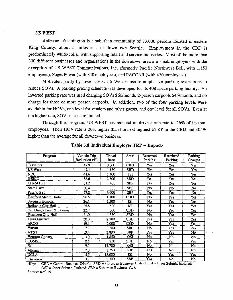
US WEST

Bellevue, Washington is a suburban community of 83,000 persons located in eastern

King County, about 5 miles east of downtown Seattle. Employment in the CBD is

predominately white-collar with supporting retail and service industries. Most of the more than

300 different businesses and organizations in the downtown area are small employers with the

exception of US WEST Communications, Inc. (formerly Pacific Northwest Bell, with 1,150

employees), Puget Power (with 840 employees), and PACCAR (with 450 employees).

Motivated partly by lower costs, US West chose to emphasize parking restrictions to

reduce SOVs. A parking pricing schedule was developed for its 408 space parking facility. An

inverted parking rate was used charging SOV s $60/month, 2-person carpools $45/month, and no

charge for three or more person carpools. In addition, two of the four parking levels were

available for HOVs, one level for vendors and other guests, and one level for all SOVs. Even at

the higher rate, SOV spaces are limited.

Through this program, US WEST has reduced its drive alone rate to 26% of its total

employees. Their HOV rate is 30% higher than the next highest ETRP in the CBD and 405%

higher than the average for all downtown business.

Table 3.8 Individual Employer TRP -- Impacts

Program Vehicle Trip Travel Area1 Reserved Restricted Parking Reduction (%) Base Parkin!! Parking Charges

Travelers 47.9 10.000 CBD Yes Yes Yes US West 47.1 1.150 SBD Yes Yes Yes NRC 41.6 1.400 lSI Yes Yes Yes GEICO 38.6 2.500 SBD Yes Yes Yes Cli2MHil1 31.2 400 SBP No Yes Yes State Fann 30.4 980 SBP No No No Pacific Bell 27.8 6,900 SBP Yes Yes No Hartford Steam Boiler 26.5 1,100 CBD No Yes Yes Swedish Hospital 26.1 2,500 lSI No Yes Yes Bellevue Citv Hall 25.8 600 lSI Yes Yes Yes San Die!!O Trust & Savings 22.7 500 CBD No Yes Yes Pasadena Citv Hall 21.0 350 SBD No Yes Yes TransAmerica 20.0 2.700 CBD Yes Yes Yes ARCO 19.1 2.000 CBD No Yes Yes Varian 17.7 3.200 SBP No Yes No AT&T 13.4 3,890 SBP Yes Yes No Ventura Countv 13.0 1,850 OSI No No No COMSIS 10.5 250 SBD No Yes Yes 3M 9.7 12.700 OSI No No No Allergan 7.0 1.250 SBP Yes No No UCLA 5.5 18.000 lSI No Yes Yes Cheveron 3.7 2.300 SBP Yes No No I Key: CBD =Central Bus mess District; SBD =Suburban Busmess Dtstnct; lSI = Inner Suburb, Isolated;

OSI =Outer Suburb, Isolated; SBP = Suburban Business Park. Source: Ref. 19.

35

Table 3.8 Individual Employer TRP --Impacts (Cont.)

Program Employer Support Levels

Travelers Transit US West High NRC Low GEICO Medium OI2MHill High

State Farm High Pacific Bell None Hartford Steam Boiler High Swedish Hospital High Bellevue Ci!Y Hall Medium San Diego Trust & Savings High Pasadena City Hall High TransAmerica Medium ARCO Medium Varian Medium AT&T Low Ventura County Medium COMSIS Medium 3M Low All erg an Medium UCLA High Cheveron High 2Key: May not sum to 100% Source: Ref. 19.

Carpool VanQ_ool High High High None

Medium None High High High None High Medium High Medium High High

Medium Medium High Medium

Medium None High High

Medium High High High Low Low

Medium Medium Medium None

Low None Medium High

Low High Medium High

Legally Emplovee Modal Split (% )2 Required sov Transit Carpool Vanpool

No 33 36 19 8 Yes 26 13 60 -Yes 42 28 27 -Yes 40 31 20 8 Yes 54 17 12 -Yes 66 - 31 2 Yes 63 2 22 11 No 40 36 21 1 Yes 33 44 23 -No 52 7 29 4 Yes 44 37 14 -Yes 58 7 27 2 Yes 45 14 21 19 Yes 46 20 20 14 Yes 62 8 21 3 Yes 71 2 22 3 Yes 69 2 23 -Yes 54 18 25 -No 83 2 14 8 Yes 76 1 14 7 Yes 74 6 10 5 Yes 82 1 11 5

The practical impact of the ETRP for US WEST is more limited, however. Many

employees who carpool with co-workers drive to meet their carpools at a park-n-ride lot within a

short distance of downtown (about 1 mile). If carpooling is a major contributor to the high HOV

rate (see Table 3.9), then the scenario described above significantly affects estimations of VMT

savings, number of trips, and increased speeds. This in tum affects calculations of air pollution

emissions and energy use reductions. This characteristic portrays the potential effect that a

commuter's response to demand management strategies can have which potentially lessens the

planned or estimated benefits in air pollution emissions or energy use.

UClA

The University of California, Los Angeles (UCLA) campus is located immediately

adjacent to Westwood Village, a densely developed urban area in West Los Angeles

approximately 10 miles west of downtown Los Angeles. Westwood's population is

approximately 37,000. UCLA has some 34,000 students and over 18,000 faculty and staff. This

case study focuses on the faculty and staff and not on the students.

36

Table 3.9 US WEST Employee Mode Split (June 1988)

Mode Percent

SOY 25.7% Transit 12.8% Carpool 44.7% Vanpool 1.8% Multi-Modal 13.0% Other 2.0%

Daytime parking is limited but faculty and staff are virtually guaranteed a space.

Students compete for a limited number of spaces on a need-based point system. Students who

carpool (3 or more per vehicle) are assigned student parking first. Employees and students pay

$30 per month or $4 per day, well below the market rate in Westwood of $80-$120 per month or

$6-$10 per day.

The Commuter Assistance Ridesharing Office promotes or subsidizes the following as

part of its TRP:

( 1) V anpools (2) Carpools (3) Buspools and Transit services (4) Motorcycles, Mopeds and Bicycles (5) Shuttle Service ( 6) Guaranteed Ride Home

Implementation of the plan began in 1984. The results of the program for university employees

show that mode shifting occurred between transit, carpooling, and vanpooling, with the overall

trip rate (trips per 100 employees) fluctuating some, but by 1988 returning to the 1980 trip rate

of 79 trips per 100 employees.

Nuclear Regulatory Commission (NRC)

The NRC is a federal agency that was relocated to North Bethesda, Maryland. The site is

located near highway and public transit facilities (bus and rail). There are 2,450 total employees

at the NRC. An existing TRO in the area required the NRC to develop a trip reduction plan

before being allowed to move to the new site.

In 1988, a transportation management plan (TMP) was developed by the NRC and the

Montgomery County Department of Transportation. The plan contained the following elements:

(1) Parking Management including • Fee parking at the NRC garage for employees • Guaranteed parking space in the building garage for carpoolers • Nearby parking restrictions

(2) Transit Discounts for NRC employees

37

(3) Transit shuttle to park-n-ride lot (4) Carpool matching service (5) Flextime

Program Costs

The cost impacts of the three case studies are shown in Table 3.10. The reported costs

vary between the three studies, partly due to size of employer and different reported costs. Not

withstanding, the major cost differences seem to be related to the nature of the ETRP itself.

Programs that subsidize HOVs and/or transit passes tend to be more expensive than programs

that contribute staff time and marketing dollars (Ref. 3).

Table 3.10 ETRP Case Studies -- Costs

Annual Costs Employer Annual Costs Annual Cost Cost per Trip Annual Savings* Net Cost per Trip

per Emplovee Reduced Reduced

US West $27.625 $24.02 $0.24 $113.044 -$0.75 UCLA $2.428.689 $134.93 $11.24 $1.349.640 $4.99 NRC $35.506 $25.36 $0.25 $772.200 -$5.28

* Annual employer savmgs are attnbutable to savmgs m parking costs and any recouped vanpool fares.

Table 3.11 summarizes the travel impacts of the three case studies. The percent

reductions are relative to that individual employer's baseline amount of travel and not relative to

the entire urban area.

Table 3.11 ETRP Case Studies -- Impacts

Dailv & Annual Impacts Employer Vehicle Trips Vehicle Daily Vehicle DailyVMT Annual VMT % Reduction of

Without Trips With Trips Reduced Reduced Reduced Trips& VMT Program Pro!!I'am

US West 994 520 474 18.012 4.683.120 47% UCLA 15.048 14,220 828 26.496 6.888.960 5% NRC 1.334 752 582 12.571 3.268.512 43%

DISCUSSION

The case studies discussed above were selected based on two criteria: similarity with

Texas conditions, and/or usefulness of the assessment in terms of energy use evaluation. They

served as a guide for developing the scenarios analyzed in second phase of this study and

reported in Strategies for Reducing Energy Consumption in the Texas Transportation Sector.

A significant advantage of this case-study approach is that it captures what has been

possible to accomplish so far with TCM policies. In most cases, the potential TCM impacts are

38

based either on the accomplishments in various metropolitan areas, or on what has been

predicted by MPO planning staffs and their transportation consultants.

It is important to bear in mind that the TCM impacts discussed in this report are based

upon an entire MPO area or at most a county-wide region. When considering the travel

characteristics of an entire state as the baseline, the percent reductions in VMT and number of

trips taken due to TCM will be considerably smaller than the numbers discussed in this

document. An additional caveat: some reported impacts are based assumptions and estimates

that are not clearly defined or documented. Other results do not include cumulative impacts of

combined TCMs. (The exception is DRCOG who reports estimates of cumulative TCM impacts

but without explanation.)

RECOMMENDATIONS

TCM effectiveness in reducing energy consumption should ideally be based on three

measures of effectiveness that can be directly converted into changes in energy use and air

pollution emissions. They are:

(1) Change in speed (Mipeed). The primary issue concerned with reported change in speeds is determining what percentage of the annual VMT the change in speed applies to. In addition, the relationship between a change in speed and a change in energy use will have to be developed.

(2) Change in the number of SOV trips taken (~Trips). Several issues arise when searching the literature for this measure. First, vehicle trips presumably refer to total auto trips of various occupancies, not just SOV s. The studies found in the literature take this into consideration by applying an occupancy factor. Second, the references may or may not be assuming that transit users and carpoolers take an intermediate trip in a SOV in order to get to the transit station or to meet the other carpoolers. Third, it is difficult to determine from the references whether the number of trips reported are one-way or two-way trips. Presumably they are twoway trips. However, this is irrelevant when considering the reported percent change in trips.

(3) Change in the vehicle miles traveled (~ VMT). The changes in VMT are presumed to be auto VMT only.

Ideal case studies report the applicable measures of effectiveness listed above, and

preferably are located in an analogous area appropriate to Texas for the particular TCM.

However, the main thrust behind TCM implementation is attainment of pollution standards, and

most reported measures of effectiveness are defined in terms of modal split changes and changes

in air emissions. In addition, this limits the scope of the literature to locations that have been in

non-attainment for a sufficient time to allow for the development of TCM plans and their

39

subsequent implementation and evaluation. Nevertheless, a sufficient number of case studies

were found to derive a range of estimates.

COST ASSESSMENT

The development of analysis scenarios used in the subsequent phase of this study

required selection of TCMs that have the potential to reduce energy consumption and emissions

in a cost-effective manner. This section summarizes the relevant findings in the literature survey

conducted for this study and defines an approach to arrive at useful cost estimates.

THE STATE-OF-THE-ART IN TCM COST ANALYSIS

The effectiveness of TCMs can be measured economically through benefit-cost or cost

minimization analysis. Ideally, the costs should include traditional expenses for new facilities or

improvements, e.g., HOV lanes, improved transit operations, and traffic signal improvements, as

well as vehicle operating, delay, accident, and environmental costs. The expected benefits are

the cost reductions associated with various alternatives. Some of these costs and benefits are

difficult to monetize.

In assessing the cost-effectiveness of transportation management strategies for the

purpose of policy making, both costs and benefits can be evaluated from a societal perspective;

this includes both economic resource costs (incremental costs) and social costs (externalities). A

social cost analysis would also choose an appropriate discount rate, ignoring transfer payments.

Of course, it is equally important to reckon costs and benefits from the market price and cost

perspective, as these are the costs "seen" by consumers, businesses and government agencies.

Some of these costs and benefits categories for different TCMs are summarized in Table 3.12.

Recent studies assessing the full cost of transportation monetize some of these

transportation externalities. Air quality is among those externalities that are most frequently

monetized; however few of the TCM reports reviewed in our study included these externalities

in their cost analysis.

Other studies assessing the full cost of transportation so far have produced some national

averages, and they are generally preoccupied with the costs of current practices, which include

few TCMs and are almost entirely dependent on SOV s. There are no estimations of the benefits

of emission reduction that are location specific, and the benefits of TCMs must be identified in

relation to their costs.

APPROACH FOR TCM COST ASSESSlVIENT

The scenarios developed in this study (see Strategies for Reducing Energy Consumption

in the Texas Transportation Sector) include a number ofTCMs, which were selected based on an

assessment of their potential to reduce energy consumption in a cost-effective manner. Given

40

the controversial and somewhat incipient state-of-the-art in TCM cost assessment, our cost

assessment approach consisted of analyzing observed and/or estimated TCM costs in order to

arrive at an acceptable cost magnitude to use in the scenario analysis phase of this study.

Table 3.12 Summary of Cost and Benefit Categories for Some TCMs

Costs Benefits

Improved public transit • % Operation • % Fuel consumption reduction • % Additional initial investment • % Emissions reduction

Traffic flow improvement •% Construction (HOY lanes) • % Fuel consumption reduction for some users • % O~ation and enforcement • % Travel time saving for some users

Work schedule changes • % Construction and operation of work satellite centers • % Fuel consumption reduction

for telecommuting • % Emissions reduction • % Building energy consumption • % Office space savings and reduced parking • % Telecommunication and computer use requirements • % Congestion near satellite centers

Park and ride and fringe parking • % Facility construction • % Fuel consumption reduction for some users • % Traffic congestion near facilities • % Emissions reduction in CBD • % Emissions near facilities

Road pricing • % Travel costs for users • % Emissions reduction for overall systems • % Emissions reduction

TCM costs reported in the literature are usually based on traditional cost analysis

consisting of initial capital costs, annualized operation, maintenance and administration costs,

and periodic capital costs. Ideally, when comparing costs reported by different references, they

should be converted to a consistent annual cost with only one discount rate. However, the TCM

related literature usually reports annualized costs based on an assumed life cycle and discount

rate for the particular capital purchase being considered. The discount rates may or may not be

documented, and it is safe to assume that they vary from one study to another. Additional data

required to back-calculate the initial costs and/or the discount rate is not always documented, and

the thoroughness and consistency of the cost data varies from case study to case study.

In addition, transferring cost data from one location to another is precarious. Specific

cost data are not readily available for most TCMs, and one study may consider certain

components of costs that are not considered in another study. Therefore, the approach of the

assessment is to show a range of TCM cost-effectiveness across the country through case study

reviews. This range provides an upper and lower boundary for the potenti_al cost of proposed

analysis scenarios.

41

SUMMARY, CONCLUSIONS, AND RECOMMENDATIONS

The objective of our approach for assessing TCM impacts is to develop a "snapshot" of

the observed and predicted impacts and costs of TCMs. Literature on TCMs is almost

exclusively motivated by air quality concerns, and little information is available on TCM

relationships to an energy-efficient transportation system. TCM cost components are also

controversial, and a significant research effort is needed to arrive at consistent quantification of

TCM impacts and costs. Nevertheless, the approach used in this study provides a good

understanding of TCM impacts and cost-effectiveness, and provides guidance not only to the

energy scenario phase of the study, but also serves as a launching point for much needed

additional research on TCMs.

42

CHAPTER 4-- TRANSPORTATION SUPPLY MANAGE:MENT

INTRODUCTION

The objective of transportation supply management strategies is to enhance the person

carrying capability of the roadway system without adding significantly to the existing roadway

infrastructure. While most management strategies focus on improving peak period traffic flows,

non-peak-period trips account for 75% of trips nationwide. Therefore, system optimization for

private vehicles must be carefully weighed against the need for greater priority for other modes,

particularly in light of the strong preference for private vehicles. Classic trade-offs are right turn

on red versus pedestrian safety and delayed greens to allow pedestrian crossings versus more

continuous car flow. Implementation of system management strategies can result in induced

demand, and shifts from transit to cars, leading to a net decrease in system efficiency. Little

substantive research has been done in this area.

DESCRIPTION OF l\IIEASURES *

As discussed in Chapter 2, traffic flow improvement actions include a range of strategies

that can be broadly classified into traffic signalization, traffic operations, traffic management,

and intelligent transportation systems (ITS). As with other transportation control measures

(TCMs) these categories are not self contained, and some measures apply to more than one

category. Nevertheless, the classification presented here is conducive for organizing the

discussion of these measures.

TRAFFIC SIGNAUZATION

Traffic signal control technology, including such applications as computer-based control

systems, has become very sophisticated. The benefits of improved signalization are well

documented. Despite this reduction in delay and improved travel times, it is estimated that of the

240,000 urban signalized intersections in the country, about 178,000 need equipment and/or

timing upgrades (Ref. 3). In states, such as California, that have instituted aggressive programs

to improve signal timing, the results show clear and tangible overall system reductions in vehicle

delays, stops and travel times (Ref. 3). Traffic signal improvements include traffic signal

equipment upgrades, signal timing plan improvements, signal coordination and interconnection,

and signal removal.

* The description of the following measures are taken primarily from the Environmental Protection Agency's Transportation Control Measures Infonnatjon Documents (Ref. 3).

43

TRAFFIC OPERATIONS

Traffic operations is an umbrella term for several types of roadway improvement projects

that require little or no investments in additional infrastructure, typically, involving signing and

pavement markings. They are relatively inexpensive and quick to implement, especially in

locations where the feasibility and cost of widening a roadway or intersection is largely

dependent on right-of-way (ROW) cost and availability. Generally, these improvements are

directed to a specific traffic problem like an intersection bottleneck, in a relatively small or local

area. According to the EPA (Ref. 3), traffic operation improvements can be classified into the

following categories:

(1) Conversion of two-way streets into one-way streets. (2) Restriction of two-way street left turn movements. (3) Provision of continuous turn lanes. (4) Provision of channelized roadway and intersections. (5) Roadway and intersection widenings and reconstruction.

TRAFFIC MANAGEMENT

Traffic management systems consist of a series of measures to efficiently manage heavy

traffic and/or optimize traffic flow, especially during peak periods and roadway reconstruction.

The two most common management systems are for congestion and incidents. Congestion

management systems are mandated under the Intermodal Surface Transportation Efficiency Act

of 1991 (ISTEA). In addition ISTEA has set aside funds for congestion mitigation in non

attainment areas through the Congestion Mitigation and Air Quality (CMAQ) program. One

component often considered in congestion management plans is ramp metering. Incident

management systems are designed to mitigate negative impacts associated with non-recurring

congestion conditions that develop when accidents occur. Actions and measures of traffic

management systems often require equipment and other initial investments (capital costs), as

well as maintenance and operating costs. Most elements of a traffic management system can be

implemented alone or in combination with measures classified under other categories.

Advanced Traffic Management System (ATMS) technology, a component of ITS,

utilizes a roadway information system in order to optimize traffic signal networks and provide

some limited information to drivers. It usually consists of one or more of the following

measures:

(1) Ramp metering (2) Incident detection (3) Variable message signs (4) Radio traffic broadcasts (5) Cellular phones

44

Radio traffic broadcasts and cellular car telephones are familiar examples of a simple

traveler information system. "A complete traveler information system would improve on these

simpler systems by allowing for much more data to be provided to the traveler, by giving the

traveler control over what information to access and when, and by integrating current traffic data

directly into a vehicle's on-board navigation system" (Ref. 20). This type of information system

is known as Advanced Traveler Information System ATIS, which is also a component of ITS.

INTELliGENT TRANSPORTATION SYSTEMS (ITS)

"ITS utilizes computer and communications technology to provide information to

travelers about road and transit travel conditions and to monitor, guide, or control the operation

of vehicles." (Ref. 20). Thus, ITS technologies today, or as envisioned for the future, serve a

spectrum of traffic operation and demand management functions.

Both the private and public sectors are involved with ITS technology development. This

cooperation has led to a more focused response resources evaluation. The ITS research and

implementation agenda is categorized into five basic areas:

(1) Advanced Vehicle Control Systems (AVCS). AVCS focuses on systems that automate driving, either by enhancing information available to the driver through, for example, radar detection of obstacles in a car's "blind spot," or by replacing driver control with automated control, at least for selected portions of a trip (Ref. 7).

(2) Commercial Vehicle Operations (CVO). Efforts in the CVO area focus on improving the management of commercial fleets by enhanced vehicle identification and tracking. (Ref. 7).

(3) Automatic Vehicle Identification (A VI). A VI is a system whereby a vehicle carries a small identification device that allows unique, automated identification by roadside mechanisms. In the highway domain, A VI has been used to identify properly equipped vehicles as they cross certain points on the highway, without requiring action by an observer or the driver. A VI technologies can be used for many transportation applications, including electronic toll collection (ETC) and vehicle monitoring (Ref. 7).

(4) Advanced Traveler Information System (ATIS). This system provides travelers with information on the auto and transit systems' current status at the trip origin before the journey begins and also while in route. A TIS could induce temporal shifts, mode shifts, and route choice shifts in the trip planning decision process. ATIS technology has implications for transportation demand management (TDM) as well as transportation system management, such as work schedule changes, improved public transit, ridesharing, parking management, and special events. Transit applications of ATIS are sometimes referred to as Advanced Public Transportation Systems (APTS). ATIS requires more technology than traditional traffic management system measures, and is generally regarded as a form of ITS (Ref. 7).

(5) ATMS. See earlier discussion on Traffic Management Systems.

45

Significant activity is currently ongoing in the ITS area. These activities can be classified

as research and development, operational tests, and deployment. The U.S. Department of

Transportation's (DOT) summary of ITS projects categorizes the different ITS technologies as

follows:

(1) Travel and Traffic Management. This category is primarily composed of ATMS and ATIS services and technologies such as pre-trip travel information, en-route driver information, route guidance, ride matching and reservation, traveler services information, traffic control, incident management, and travel demand management policy support (Ref. 21).

(2) Public Transportation Management. This category is composed of APTS services and technologies such as en-route transit information, public transportation management, and personalized public transit (Ref. 21).

(3) Electronic Payment. This technology utilizes the "smart card" as a common electronic payment medium for all transportation modes and functions, including tolls, transit fares, and parking. This is not the same technology as A VI, where vehicles are automatically identified and the owners are later billed. Rather, smart cards are usually purchased in advance (Ref. 21).

(4) Commercial Vehicle Operations. CVO technologies include commercial vehicle electronic clearance, automated roadside safety inspection, commercial vehicle administrative processes, on-board safety monitoring, commercial fleet management, and hazardous material incident notification (Ref. 21).

(5) Emergency Management. This involves ATMS and ATIS technologies specifically applied to emergency vehicle management, emergency notification, and personal security (Ref. 21).

(6) Advanced Vehicle Control Systems. This technology involves collision avoidance (longitudinal, lateral, and intersection), vision enhancement for crash avoidance, safety readiness, pre-crash restraint deployment, and automated vehicle operations(Ref. 21).

Over $400 million has been or will be spent on ITS operations testing, 80% of which is

targeted to travel and traffic management. Table 4.1 presents the level of ongoing activity in

each of these categories for projects that are at least partially federally funded. Examples of

other activities are ITS Priority Corridors (including one in Houston), National Compatibility

Planning for technology standards, and Deployment Planning Studies (which includes locations

in Austin and Dallas).

46

Table 4.1 Current Status in ITS

R&D Operation Tests Deplovment (Number Estimated Anticipated Estimated Anticipated

of Total Project Federal Share Total Project Federal Share Projects) Costs of Costs Costs of Costs

Travel and Traffic USA 38 $316,079.814 56% $60,134,609 8% Management Texas - $18.298,466 - -0- -Public Transp. USA 4 $47,655,500 73% -0- -Management Texas - $10.000,000 80% -0- -Electronic USA 2 $133.750 86% -0- -Pavment Texas - -0- - -0- -Commercial Vehicle USA 4 $35.278,974 43% -0- -Operations Texas - * - -0- -Emergency USA -0- (1 Proj.) - -0- -Management Texas -0- - - -0- -Advanced Vehicle USA 32 $7,650.000 20% -0- -Safety Svstem Texas - -0- - -0- -* Texas IS part of the $22 mtlhon Multi-State Heavy Vehicle Electronic Ltcense Plate Program (HELP/ CRESCENT), an integrated heavy vehicle monitoring system. Source: Ref. 21.

CONCLUSIONS AND OBSERVATIONS

Better management of the transportation network has the potential to reduce traffic

congestion and thus reduce energy consumption, and mobile source emissions. Concerning ITS,

an individual driver's reactions to receiving real-time traffic information, either before his/her

journey begins or during the journey, will not only affect his/her travel time, emissions, and

energy consumption, but also that of other persons using the transportation network depending

on specific traffic conditions. Thus, while individual benefits are potentially significant, system

wide impacts of implementing ITS are difficult to predict.

ENERGY EFFICIENCY AND E:MISSIONS REDUCTION POTENTIAL

This section discusses the results and major findings regarding the potential of

transportation supply management practices as measures to promote energy efficiency and

reduce emissions. As discussed in Chapter 3, this assessment is based primarily on a thorough

review of the literature.

TRAFFIC SIGNAliZATION

More efficient traffic signalization can reduce stops and delays at signalized

intersections, and thus optimize vehicle output on the existing roadway system. It is usually

accepted that reduced intersection stops and delays for conventional motor vehicles results in

higher fuel efficiency (less energy consumption per mile) and cleaner engine operation (less air

47

pollution emitted per mile). Impacts of traffic signalization are thus evaluated in terms of speed

improvements (~Speed).

Other impacts of traffic signalization are more controversial. Some references assume

that the number of trips (~Trips) or vehicle miles traveled (~VMT), are unaffected by traffic

signalization. Even more important, others acknowledge that every measure that improves

traffic flow has the potential to induce additional demand. Decreases in ~ VMT and/or ~trips

due to traffic signalization improvements can be safely assumed to occur only in cases where this

measure is oriented specifically towards optimizing the output of high occupancy vehicles

(HOVs), or if route shifting occurs due to improved speeds (Ref. 15).

Case Studies

Traffic signalization usually is not treated as a TCM in the literature; instead, it is

reported in the broader context of traffic management systems implementation. Nevertheless,

four case studies discussing traffic signalization were found that evaluate this measure in terms

of its effectiveness as a TCM.

North Central Texas Council of Governments

The North Central Texas Council of Governments (NCTCOG) has documented their

latest efforts to control mobile source emissions in the Dallas-Fort Worth ozone (03)

nonattainment area. This documentation includes a list of TCMs for the State Implementation

Plan (SIP) that are designed to help the region meet U.S. Environmental Protection Agency

(EPA) 03 standards. Their list of TCMs includes traffic signalization improvements currently

implemented in 261 locations, with 1,000 planned for future years (Ref. 22).

The main concern of the Dallas-Fort Worth metropolitan planning organization (MPO) is

attainment of acceptable 0 3 levels defined by the Clean Air Act, and as such the evaluation of

effectiveness focuses on emissions of hydrocarbons (HCs) and nitrogen oxides (NOx). Project

description and cost data were not included in the documentation. The reported reduction of 03

is about 4.58 lb/weekday for each location.


In the Delaware Valley Regional Planning Commission (DVRPC) study, this particular

TCM was used to improve flow on the fifty most congested miles of 4-lane arterials in the

region, as well as in the Philadelphia central business district (CBD) (Ref. 15). A detailed

description of the projects was not provided.

Effectiveness was assessed and reported both for the regional arterials and CBD in terms

of annual VMT reduction (due to route shifting), average speed increase, average capacity

increase, and reductions in pollutant emissions. Likewise, costs are reported separately for the

regional arterials and CBD.

48


The Houston-Galveston Area Council (HGAC) study examined the benefits and costs of

improving traffic signal timing. The analysis does not include hardware improvements; rather, it

estimates costs and benefits which could be derived by efficient utilization of existing hardware.

Cost estimates consist of the initial expense of optimizing the signal timing throughout the

region, and the maintenance expense to ensure continuity. The study reported a potential 5%

increase in speed associated with this measure but did not report any impact on~ VMT.


The National Association of Regional Councils (NARC) estimates for signal timing

improvements are based on work done in the San Francisco/Oakland Bay area for the

Metropolitan Transportation Commission (MTC) (Ref. 16). Improved traffic flow is estimated

to generate some additional travel, but will still result in an overall reduction in emissions.

Texas Transportation Institute CTID. Texas A&M University

The TTI study on urban congestion provides a comprehensive assessment of various

strategies for alleviating urban traffic congestion. Traffic signalization improvements are

included in this assessment. The cost and impact data are based upon the installation of an

advanced computer-based master control system, including interconnection and optimization.

The estimate for vehicle speed increase assumes the existence of a signal system made up of

non-interconnected signals with traffic-actuated controllers.

Summary and Conclusions

The cost of the traffic signalization improvements for each of the case studies is shown in

Table 4.2. Costs are reported in terms of ~ VMT, emissions reduction, and per intersection.

Differences in costs can be attributed to local variations and to differences in cost assessment

methodology which could not be detected through a review of the literature. Benefits are

summarized in Table 4.3, and are somewhat controversial. One reference reports some VMT

reduction, while others assume them to be zero. Route shifting is not an easy variable to

measure or estimate, and it is safer to assume that traffic signal optimization measures will not

lead to VMT reductions. Speed increases varied from 5% to 16%. This is the range utilized in

the next phase of this study to estimate reductions in energy use.

TRAFFIC OPERATIONS

Traffic operation measures are responsible for improving vehicle efficiency by providing

better and more uniform speeds. As such, the effectiveness of traffic operation improvements is

evaluated in terms of ~Speed. Generally, the number of trips or VMT are not reduced by traffic

operations measures. Improved traffic flows may encourage additional trips (or VMT), and the

49

consequent increase in energy consumption may offset any reductions gained from

improvements in traffic flow.

Table 4.2 Costs of Traffic Signalization Improvements

Annual Costs Case Studv _ p_er VMT reduced per ton of emissions reduced per intersection

NCTCOG NR NR NR DVRPC - PhiladelQ_hia CBD $1.07* $125.000 NR DVRPC - Regional Arterials $0.09* $21.600 $8,340 HGAC dVMT=O $1.216 NR NARC NR $23.000 NR TTI** NR NR $3.200- $6.600 .. * VMT reducuon due to assumed route shtfung

** TTI reported costs are in 1980 dollars. Values shown have been converted to 1994 dollars using a 4% annual inflation rate. NR = not reported

Table 4.3 Impacts of Traffic Signalization Improvements

Annual Impacts dVMT dSpeed dEmissions

Case Study Annual Percent Percent %Annual Annual Percent Change Amount Change Change VMT Applied Amount (kg)

NCTCOG NR NR NR NR NR NR DVRPC- -1,834,000 -0.04% +6.5% NR -8,000VOC 0.04%VOC Philadelphia -56,750 co 0.04%CO CBD -6,250NOx 0.04%NOx DVRPC- -17 ,636,000* -0.07% +10% NR -33,750 voc -0.14% voc Regional -136,250 co -0.07% co Arterials -36.250NOx -0.07%NO,

HGAC NR NR +5% NR -367,750 voc -0.71% -415.500 NOx -0.52%

NARC NR -0.04% NR NR NR -0.30% HC TIT NR NR +16% NR NR NR .. * VMT reducuon due to assumed route shifung VOC =Volatile Organic Compounds; CO= Carbon Monoxide; NO,.;= Nitrogen Oxides; HC =Hydrocarbons. NR = not reported

Case Studies

Three case studies were found that report measures to optimize traffic operations. As the

norm, these operations improvements are part of the efforts to control emissions, and the results

are reported primarily in terms of emissions reductions.


NCTCOG reports three types of traffic operations measures, which currently are being

implemented or/are funded for future years, as a part of an overall plan to attain 03 emission

standards. These measures are: intersection improvements, grade separations. and arterial street

50

widenings. They are reported to have an emissions reduction potential of 5.2 pounds per

weekday per location, 8 pounds per weekday per location, and 4.8 to 8.1 pounds per weekday

per lane-mile, respectively. Additional impacts and costs are not reported.


HGAC reports that improvements will be made to "increase roadway capacity" but few

details are provided. The benefits for capacity increases are based on the roadway construction

projects programmed into the 1993 Transportation Improvement Program (TIP), to reduce

emissions by increasing average vehicle speeds. Potentially, however, there could be additional

trips induced due to the increased capacity of the roadway, but the information was insufficient

to estimate such induced travel.

The following data are reported as inputs to the HGAC model:

(1) 418 lane miles of freeway to be constructed (2) 2,242 lane miles of arterial to be constructed (3) 15.3% average change in peak speed (4) 2.3% average percent change in off-peak speed (5) $285,000 per lane mile capital cost of arterials (6) $2,933 per lane mile annual operations/maintenance cost of arterials (7) $3,300 per lane mile operations and maintenance cost of freeway

Due to the lack of pertinent data, no increase in the number of vehicle trips (i.e. induced

trips), is assumed for this measure. As there is no reduction in vehicle trips or VMT, there are no

cost savings or avoided costs associated with this measure.

Delaware V allev Regional Planning Commission

Emissions are sensitive to speed, and vehicles exceeding 55 miles per hour (mph) are

generating more emissions than those traveling at the 55 mph speed limit. The D VRPC

implemented a program to enforce the 55 mph speed limit on 192 directional miles of freeway

(Pennsylvania Turnpike). The objective of this program was to attain 85% adherence to the

speed limit on the turnpike (Ref. 15). The report documents an evaluation of the program's costs

and impacts.

Summary and Conclusions

These case studies reported the costs shown in Table 4.4 and the benefits shown in Table

4.5. Differences in costs can be attributed to local variations, and to a certain extent to

differences in cost assessment methodology that could not be detected in the review of the

documented reports. Speed increases varied from 2% to 15% while one measure (55 mph

enforcement) decreased speeds in order to reduce emissions. This points out the non-linear

relationship between speed and emissions and the need to be aware of how and where (e.g.

freeway, arterial) speed changes are estimated.

51

Table 4.4 Costs of Traffic Operation Improvements

Case Study

DVRPC (55 mob Enforcement) NCTCOG HGAC

VOC = Volatile Orgamc Compound. NA = not applicable NR = not reported

perVMT reduced

NA

NR NR

Annual Costs per ton of per intersection emissions reduced

$11,166 NA

NR NR $44,000VOC NR

Table 4.5 Impacts of Traffic Operations Improvements

Annual Impacts

per mile

NR

NR NR

.!lVMT LlSQ_eed 6. Emissions Case Study Annual Percent Percent %Annual Annual

Amount Change Change VMT Amount (ton) Applied

DVRPC NA NA -14% NR -40VOC (55 mph -1,307 co Enforcement) -142NOx NCTCOG NA NA NR NR -37to-171 Intersection voc Improvements NCTCOG Grade NA NA NR NR -2.75VOC Separations NCTCOG NA NA NR NR -180 to -491 Arterial Street voc Widening_s HGAC 0 0 + 15.3% (Peak) NR -1,208 VOC

+2.3% (Off-peak) (1,823) NOx VOC =Volatile Orgamc Compounds; CO= Carbon MonoXIde; NOx = Nttrogen Oxtdes. NR = not reported NA = not applicable

TRAFFIC MANAGEMENT SYSTEMS

Percent Change

-0.14%VOC -0.71%CO -0.36%NOx

NR

NR

NR

-2.31% VOC (2.28%) NO~

Traffic management systems are designed to improve traffic flow by using technological

advances such as incident detection, dynamic signal optimization, and network-wide

communication between traffic control devices across facility types.

The effectiveness of traffic management systems is usually evaluated in terms of speed

improvements (~Speed). However, as discussed before, the number of trips and/or VMT could

increase due to induced demand. They could also decrease as a result of route changes due to the

speed changes, or if these measures were to specifically target HOVs (Ref. 15). The

effectiveness of each individual traffic management measure is discussed below.

52

Ramp Metering

DVRPC was the only case study found that reports costs and impacts of ramp metering.

They document metering at 17 ramp locations to improve flow on major limited access facilities.

The reported capital costs of ramp metering are $50,000 per metered ramp. An additional $1

million is needed for enhancement of the existing centralized control system, as well as

$1,500/ramp for operations and maintenance. The annual costs for DVRPC's ramp metering are

shown in Table 4.6 (capital costs are annualized over 10 years at 8%).

The reported effectiveness of ramp metering is summarized in Table 4.7. Speeds before

ramp metering were not reported and are needed to calculate the percent increase. However,

assuming that ramp metering allows the traffic to flow at the 55 mph speed limit on freeways,

and considering that rigid enforcement of speed limits in the same region yielded 85%

adherence, the ~Speed should be around 11%.

Table 4.6 Costs of Ramp Metering

Annual Costs Case Study perVMT per ton of per intersection per mile

reduced emissions reduced

DVRPC $0.03 $2.700 NA NA NA = not applicable

Table 4.7 Impacts of Ramp Metering

Annual Impacts 6.VMT 6.Speed 6. Emissions

Case Study Annual Percent Percent %Annual Annual Amount Change Change VMT Amount (ton)

Applied

DVRPC -10,800,000 -0.1% NR NR -122 voc andNOx

VOC = Volaule Orgamc Compounds; CO= Carbon MonoXIde; NOx =Nitrogen Oxides. NR = not reported

Incident Management Systems

Percent Change

-0.5%VOC -0.6%CO

<-0.1%NOx

Incident management systems are directed at major traffic stoppages caused by accidents

or breakdowns. An incident management system attempts to rapidly identify and quickly resolve

these incidents through a high state of readiness. As part of the incident response management,

routing alternatives are communicated through traveler information systems. Energy

consumption impacts are obtained through an overall increase in speed due to more uniform

traffic flow.

53

The case studies reporting installment of incident management systems are discussed

below, and the reported costs and impacts are presented in Table 4.8 and Table 4.9, respectively.


The equipment projected to be in place over 115 miles of interstate highways in

Pennsylvania includes 361 detectors and 27 closed circuit television (CCTV) cameras, 7

changeable message signs, and 1 control center. Ramp meters are considered separately, as

another measure, and were described in the previous section.


The HGAC study assesses two measures that pertain to congestion and incident

management systems. One measure is a motorist information system informing motorists of

traffic conditions so that they can avoid badly congested areas (Ref. 14). The second measure is

an advanced traffic management system and is discussed under the next section on ITS.


NCTCOG lists motorist assistance, incident detection and response, and freeway

surveillance as one specific TCM category to be funded to help achieve air quality goals. Project

details and costs are not provided. Combined benefits for funded projects are listed as 261 lbs of

VOC reduction per weekday for two corridors.


This case study reports costs and benefits of incident management based on a projected

surveillance and response program in the San Francisco/Oakland Bay area (Ref. 16).

Table 4.8 Costs of CIMS Improvements

Case Studv per VMT reduced

DVRPC NCTCOG HGAC NARC

*Per ton VOC and NOx combmed VOC =Volatile Organic Compound; HC =Hydrocarbon. NA = not applicable NR = not reported

NA NA NA NA

INTELLIGENT TRANSPORTATION SYSTEMS

Annual Cost per ton of emissions reduced

$200,452* NR

$8,100 NOC) $83.000 (HC)

The U.S. General Accounting Office (GAO) report presents an interesting evaluation of

38 nationwide reports addressing potential impacts of ITS technologies on congestion, economy,

safety, fuel efficiency, and the environment (Ref. 24). This evaluation is based on a literature

54

review of reported results or potential benefits of ITS technologies, including traffic management

system technologies.

Table 4.9 Impacts of CIMS Improvements

Annual Impacts 6.VMT LlSQeed Ll Emissions

Case Study Annual Percent Percent %Annual Annual Percent Change Amount Change Change VMT Amount (ton)

AQplied

DVRPC +3,118,000 +0.07% NR -37VOC -0.14% voc -l60CO -0.07% co +1.5 NO>t O.O%NO>t

NCTCOG NR NR NR 30VOC NR HGAC NR NR + 1.21% (Peak) -223 VOC -0.43% voc

+ 1.21 (off-peak) +211 NO>t +0.26%NO>t NARC NR +0.1% NR NR -0.6%HC VOC = Volaule Orgamc Compounds; CO= Carbon MonoXIde; NO>t =Nitrogen Ox1des; HC =Hydrocarbon. NR = not reported

Impacts of ITS technologies on congestion are measured in terms of speed improvements

(~Speed) and fuel efficiency. These impacts are of primary concern for this project due to their

influence on energy consumption. The summary presented in this section discusses ITS

technologies (A TIS and ATMS) under two categories of studies, simulation modeling reports

(projections), and operational test reports.

The simulation modeling results are based on traffic flow operation computer models that

simulate a freeway or a surface street with intersection control devices. The operational test

reports present actual "before and after" results of ITS systems implemented in metropolitan

areas such as Los Angeles and Chicago.

Simulation Modeling • ATIS

Benefits of ATIS technology can be simulated by various methods. The most realistic

method is to assume that a certain number of vehicles receive information as to the shortest path

for their given origin and destination, while the remaining traffic utilizes the routes they

normally take. This method is conducted under simulated incident conditions as well as

recurring congestion conditions. Several ATIS simulation modeling case studies are

summarized by the GAO and are presented below (Ref. 24). Cost estimates are not given.

Two reports were found that document simulation studies of ITS implementation in Los

Angeles. The first is a 1989 report entitled "The Smart Corridor for the City of Los Angeles:

Demonstration Project Conceptual Design Study" that discusses the benefits of ATIS

technology. This study reports the following corridor effects:

55

(1) Travel time is reduced by 3.8 to 5.2 million vehicle-hours per year (11 o/o-15%). (2) Fuel consumption is decreased by 1.3 million gallons per year (2.5%). (3) Annual HC emissions are reduced by 8%. (4) Intersection delay is reduced nearly 2 million vehicle-hours per year (20%). (5) Annual savings amount to $24-32.5 million.

In addition the following effects are reported for individual drivers:

(1) Increased average freeway speeds from 15-35 mph to 40-50 mph. (2) 12% decrease in the duration of the average freeway trip. (3) Increased average surface street speeds during peak commute periods from 20-22

mph (11 %). (4) 13% decrease in the duration of the average surface street trip.

The second ATIS simulation study summarized by GAO in Los Angeles is a 1988 report

entitled "Potential Benefits of In-vehicle Information Systems: Demand and Incident Sensitivity

Analysis." It reports a range of travel time savings from 0-14 minutes (0-47%) for a 30-minute

average trip under different congestion scenarios (recurring and non-recurring). Results of other

case studies summarized by the GAO include:

• "Some Theoretical Aspects of the Benefits of En-Route Vehicle Guidance (ERVG)." A 1989 report that presents a theoretical assessment of A TIS technology implementation, and concludes that it can lead to travel time savings typically of 3% to 4%.

• "Effectiveness of Motorist Information Systems in Reducing Traffic Congestion." A 1989 report estimating benefits of modest reductions in travel times up to 4.4%. (Assumed to be either ATMS or ATIS technology.)

• "Study to Show the Benefits of AUTOGUIDE in London." A 1989 study that reports travel time savings of 8%- 11%. (Assumed to be ATIS technology.)

• "Some Possible Effects of AUTOGUIDE on Traffic in London." A 1989 study that reports travel time savings of 2.2% for unequipped vehicles to 6.9% for equipped vehicles (10% of vehicles equipped). (Assumed to be ATIS technology.)

Field Results - ATMS

The following case studies reporting field observations of ATMS are briefly summarized

by the GAO (Ref. 24):

• "Automated Traffic Surveillance and Control." This ongoing operation utilizes ATMS technology for computer control of traffic signals. The system included 188 signals and 396 detectors and reported the following benefits and annualized costs:

Benefits (1) 13% reduction in travel time (2) 35% reduction in vehicle stops (3) 14% increase in average speed (4) 20% decrease in intersection delay (5) 12.5% reduction in fuel consumption

56

•

Annualized Costs (1) $654,200 for construction and engineering (2) $148,400 for operation and maintenance (3) $6,800 per intersection (average)

"Chicago Area Expressway Surveillance and Control Project." A project utilizing A TMS technology for a large-scale freeway surveillance and control system. The reported ( 1979) before and after benefits of ~Speed and fuel consumption are not given. Other impacts that are given include:

(1) 30% reduction in peak period congestion (2) 18% reduction in accidents

• "USA Signal Timing Optimization Project (11 cities nationwide)." This 1982 project conducted field tests as well as utilized TRANSYT -7F traffic signal optimization computer model in order to simulate A TMS technology for improving traffic signal timing plans on local streets. Travel time improvements of 8.5% are reported along with a cost of $456/intersection.

• "Fuel Efficient Traffic Signal Management (FETSIM)." This 1986 study based on a simulation model and field test of ATMS technology for improving traffic signal timing plans for 61 cities and 1 county in California reported the following impacts.

(1) 15% reduction in vehicle delays (2) 16% reduction in vehicle stops (3) 7% reduction in travel time (4) 8.6% reduction in fuel use

The report also estimated the 3-year program cost at about $4 million based on the retiming of 3,172 signals at a cost of $980/signal.

CONCLUSIONS AND OBSERVATIONS

Transportation supply management measures are developed to improve traffic flows by

orienting traffic operations below capacity. They target the supply side of the transportation

system and include no effort to control demand. Rather, the main thrust is the provision of

adequate facilities to serve an increasing demand.

The potential of transportation supply management strategies to decrease energy

consumption through speed improvement is controversial. For each individual vehicle using the

system, better traffic flows result in higher fuel efficiency (less energy consumption per mile)

and cleaner burning engines (less air pollution emitted per mile). However, these individual

benefits cannot be directly extrapolated to the entire fleet and VMT as a whole. Increases in

VMT have been repeatedly reported, since better traffic conditions encourage additional travel.

These increases in VMT can offset any gains due to improvements in the efficiency of individual

vehicles. On the other hand, decreases in VMT are due to route shifting and thus very localized,

resulting in little or no overall energy savings.

57

A 1988 paper by Newman and Lyons, which analyzed the potential impacts of free

flowing traffic in energy consumption and emissions in 32 cities worldwide, found that

unimpeded traffic does not lead to significant savings in fuel consumption, time, or overall

emissions in a city as whole. This insignificance is especially evident when compared to the

effects of fundamental changes in transport modes and land use. The significance of

transportation supply management measures is restricted to specific and very localized air

quality and congestion problems. Transportation supply management effects on overall

efficiency and mobility are either negligible or negative, the latter due to the fact that any

measure to improve traffic flows has a potential to induce additional demand.

Transportation supply management designed specifically to improve traffic flow for

HOVs are the best type to encourage energy savings in the transportation system. However,

additional capacity improvements and traffic flow improvements lose their effectiveness over

time as traffic volumes increase.

Measures that strive to control the demand for individual transportation seem to have

more potential to improve the statewide energy consumption standards. These include

employer-based measures such as telecommuting, public sponsored measures such as improved

public transit, and measures that comprise a combination of private and public efforts such as

parking pricing policies supplemented by employer encouragement of carpooling and transit

ridership.

58

CHAPTER 5-TRANSPORTATION DEMAND MANAGE:MENT

INTRODUCTION

The objective of transportation demand management (TDM) strategies and policies is to

optimize the overall mobility by decreasing demand for single occupancy vehicles (SOVs),

encouraging non-motorized transport and other trip elimination measures, and/or shifting trips to

off-peak hours. When effectively implemented, TDMs can reduce energy consumption, either

by reducing both vehicle miles of travel (VMT) and passenger miles of travel (PMT) (trip

elimination programs), or by reducing VMT while PMT is kept unchanged (increased vehicle

occupancy).

TRIP ELIMINATION PROGRAMS

Trip elimination programs can be classified into telecommuting (or teletravel in general),

work schedule changes, and non-motorized transport. Implementation of such programs can be

achieved through a variety of strategies; however, the main motivation of most trip elimination

programs currently implemented and/or planned is to reduce emissions and travel time during

peak periods. Consequently, most trip elimination programs planned or implemented in the U.S.

focus on work-related trips.

EMPLOYER-BASED TRIP REDUCTION PROGRAMS

A widely used "combination package" of TDMs are the employer-based trip reduction

programs (ETRPs). These programs feature assistance and incentives for employee use of

commute modes other than the single occupancy vehicle (SOV). The U.S. Environmental

Protection Agency (EPA) recognizes two separate categories of employer-promoted

transportation control measures (TCMs): employer-based transportation management programs

and work schedule changes. Table 5.1 shows the official EPA definitions of these two

categories.

The first category, employer-based transportation management programs, includes a wide

range of alternatives, such as high occupancy vehicles (HOVs) in general, non-motorized

transport, and related incentives and disincentives. Each of these categories consists of a

separate TDM tool discussed in this document, while incentives and disincentives are discussed

with other implementation strategies. The second category, work schedule changes, includes

telecommuting and alternative work schedules. These can be considered separate TDM

categories, and as such are discussed in detail in the upcoming sections.

59

Table 5.1 EPA Categories for Employer-Promoted TCMs

Category EPA Definition

Employer-based transportation Various programs implemented by employers to manage the commute management programs and travel behavior of the employees, with the objective of reducing the

number of single occupant automobiles used for commuting. Work schedule changes Changes in work schedules to provide flexibility in work schedule and

reduce volume of commute travel during peak periods, such as telecommuting, flextime, compressed work weeks, and staggered work hours.

Source: Ref. 3.

TELECOMMUTING

Telecommuting is seen as the most drastic employer program to reduce VMT,

congestion, and their effects. It consists of a change in the location where the work takes place:

work duties are performed either at home or at a satellite work center near the home, one or more

days a week. This either eliminates or drastically reduces the length and/or number of work

trips, reducing both VMT and PMT.

Telecommuting has been made possible with the advent of telecommunications

equipment that allows fast and convenient interaction with the central office. It is an interesting

arrangement to employers due to resulting decreases in fixed costs to provide office space, and

better competitiveness in hiring and in bidding (the latter due to a decrease in the overhead

proportional to the decrease in office space). The advantages to employees are its potential to

drastically cut expenses as well as time lost to commuting.

Telecommuting was not devised as a TDM tool. Rather, it has been utilized because of

the advantages discussed above, mainly for activities that do not require face-to-face interaction.

These include, but are not restricted to, sales, consulting, report writing and editing, computer

programming, accounting, and many others.

WORK SCHEDULE CHANGES Flexible hour programs change the specific times when individuals must be at the

workplace and includes: flextime, compressed work week, and staggered work week. These

programs are implemented with employer assistance, or by employer initiative. In some non

attainment areas, they are implemented by mandate. They basically consist of either changing

work trips to non-peak periods or eliminating trips altogether.

Flextime allows the employee to select his/her own start time, while continuing to work a

regular 8-hour day. As a result, the employee can commute outside peak periods and more

effectively manage his/her time. Pilot programs in cities such as San Francisco indicate

flextime has the potential to decrease congestion at peak periods, increase speeds, decrease fuel

consumption, and improve air quality (Ref. 3).

60

A compressed work week consists of concentrating the weekly workload into longer

days, while working fewer days per week. This arrangement transfers at least one end of the

work trip to a non-peak period as well as two fewer trips for a 4-day work week. Denver

participated in a compressed work week experiment and reported impacts similar to those

observed with flextime in San Francisco (Ref. 3).

Staggered work weeks are based on the standard 8-hour day, 5-day work week. The

arrival times are staggered so each group of employees arrives at work at different times. It is

important to note, unlike flextime, telecommuting, and compressed work weeks, staggered work

weeks have no impact in the number of trips, PMT or VMT. Staggering may reduce congestion

and its environmental consequences, but its rigid schemes may discourage carpooling and other

ridesharing arrangements that actually reduce overall VMT (Ref. 3).

NON-MOTORIZED TRANSPORT

Non-motorized transport does not actually eliminate a trip, individuals still reach their

destinations; it does, however, eliminate a vehicle trip. The idea of bicycling or walking as

viable alternatives to automobile use is not widely recognized, mostly because it is not

compatible with the common U.S. metropolitan layout based on suburban residential and

downtown employment areas. Practical feasibility of non-motorized transport requires public

education about these options, as well as safe and convenient facilities.

EPA defines bicycle and pedestrian programs as "measures to encourage bicycle and

pedestrian travel as viable alternative transportation modes to the private automobile" (Ref. 3).

In this case, the TDM tool and its implementation strategies overlap, and a brief discussion of the

latter is necessary to discuss bicycle and pedestrian programs.

The most fundamental element of a bicycle program is the development of a safe system

of roadways, which are typically routes, lanes, and/or paths. On bicycle routes, the cyclists share

the appropriately marked roadway with other vehicles, and ride in the right lane adjacent to the

curb. Bicycle lanes are clearly striped lanes, located in the roadway also utilized by motorized

vehicles (Ref. 25). Bicycle lanes can be shared with buses and parked cars, but no through auto

traffic is allowed. Bicycle paths are facilities built exclusively for bicycles and other non

motorized vehicles and pedestrians, frequently for recreational purposes. They can

accommodate two-way traffic and are usually provided either adjacent to a roadway or as a part

of an independent right-of-way (ROW).

Convenient storage facilities to protect cyclists from vandalism and theft are an essential

component of a successful bicycling program. Bicycle lockers, racks, posts and ribbons are

provided by many employers, stores, schools, and government agencies. Racks and posts are the

most common types of storage facility, but since they provide a structure to lock the bicycles, the

61

bicycles are still exposed to vandalism and the weather. Lockers are by far the most secure

facility, since they are enclosed. Not surprisingly, they are also the most expensive and least

commonly used facility.

Additional facilities that encourage bicycle utilization for the commute to work are

showers and personal lockers in the workplace. Also, bicycle usage for long trips can be

enhanced by integration with transit. This requires secure bicycle storage at transit stations or

outfitting transit vehicles with bicycle storage racks.

Education and marketing campaigns are paramount for successful implementation of a

bicycle program. The objective of education programs is to instruct and train cyclists and

motorists on bicycle safety issues. Some cities have developed programs to educate engineers

about the needs of the cyclist. Marketing campaigns are necessary to make both cyclists and

motorists aware of the bicycle program, and attract potential users to the bicycle system. In

addition, stability of funding and effective enforcement are paramount to achieve effective

bicycle utilization.

As in the case of the bicycle programs, safe pedestrian facilities are fundamental for

successful mode shift. It is not unusual for U.S. suburban and residential areas to be constructed

without sidewalks, forcing the pedestrian to either use the car or share the street with motorized

vehicles. Crosswalks that are well marked and provided with walk signals long enough to allow

pedestrians to safely cross the streets are also important for promoting walking. Median strips in

wide boulevards and busy intersections provide a safe space where pedestrians can wait for the

next walk signal. Adequate lighting and elimination of objects that can be used as hiding places

enhance night safety for pedestrians. While unimportant in terms of safety, a pleasant

environment is an important measure to promote walking (Ref. 3).

CURRENT STATUS

Interest in telecommuting and work schedule changes as TDM tools is relatively recent,

and so far these TDMs are mainly in the pilot study phase. A 1992 survey of telecommuting

practices, obtained via an annual random survey of commercial telephones indicated that 1.6% of

the total labor force or about 2.8% of the number of "information" workers in the labor force

were telecommuting in 1992. This amounts to 2 million telecommuters nationwide (Ref. 26).

Large scale implementation is still dependent on a number of issues. Some unions have

expressed concerns about increases in work-related accidents due to longer work days.

Prospective telecommuting employees have concerns about professional isolation, lack of

support and clerical services, and increased home utility costs (Ref. 3).

Until the 1970s, bicycling was considered a recreational activity in the U.S. The oil

embargo caused bicycling to be received as a viable commute alternative. University

62

communities led the way in developing bicycle facilities, because the student population was and

still is a good target market for this alternative. Later, the emphasis on fitness that started in the

1980s further fostered consideration of bicycles as a transportation alternative.

Walking as a transportation alternative is viewed basically in the context of short trips or

in combination with transit alternatives. In many metropolitan areas around the world,

commutes based on the combination of walking and mass transit are faster and more reliable

than their auto equivalents, especially during peak hours. Facilities for bicycle and pedestrian

circulation are increasingly being incorporated into the development plans for new activity

centers (Ref. 3).

INCREASED VEIDCLE OCCUPANCY

The trip elimination strategies discussed in the previous section strive to reduce VMT by

actually targeting PMT. Substantial reductions in VMT, however, can also be achieved using

strategies to decrease the number of vehicles while the number of travelers remains the same.

These strategies can be grouped into the increased vehicle occupancy category, which in tum can

be divided into strategies based on public transport and strategies based on private vehicles, such

as carpool, vanpool and other variations of ridesharing.

IMPROVED PUBUC TRANSIT

Improved Public Transit encompasses a wide range of activities. As defined by the EPA

(Ref. 3), transit improvements are classified into three major types as outlined below.

System/Service Expansion

Systernlservice expansion implies that new riders will be using new services, a portion of

whom will presumably be substituting transit for previously used automobiles. Transit systems

and services can be expanded using different expansion strategies, including fixed guideway

transit, express bus services, circumferential and local bus services, and paratransit programs.

System/Service Operational Improvements

"Improvements in systems and service operations have as their major objective

increasing the productivity and cost effectiveness of transit lines. These improvements can focus

on the characteristics of the transit service itself, such as geographic coverage and scheduling, or

on the conditions that make transit a more attractive option." (Ref. 3). These improvements are

delineated by the EPA as follows:

63

• Service Feeder Bus Service Express Bus Service Bus Route and Schedule Modifications Improved Transfers Subscription Bus Service

• Management Schedule Coordination Operations Monitoring Maintenance Improvements

• Infrastructure Bus Traffic Signal Preemption Road Operational Changes Park and Ride Service

Demand/Market Strategies

These factors focus on efforts to encourage travelers to select public transit as the

preferred mode. This requires promotion of transit as a lower cost, safer, comfortable, and more

reliable alternative. EPA identifies a number of strategies to help change public perception of

transit: (Ref. 3)

• Employer Offered Incentives • Reduced Fares • Peak/Off-peak Transit Fares • Monthly Passes • Marketing and Information Programs • Simplified Fare Collection • Uniticket Programs • Passenger Amenities • Joint Development Activities

RIDESHARE, CARPOOLS AND V ANPOOLS

Matching commuters to share rides is one of the oldest TDM strategies used to mitigate

congestion and air pollution caused by vehicle emissions (Ref. 29). Rideshare, carpool and

vanpool are all strategies to increase vehicle occupancy, especially during peak traffic hours, and

as a result obtain a net decrease in area VMT. This particular TDM consists of finding ways to

encourage commuters to ride together rather than individually, and as such the TDM tool and its

implementation strategies overlap.

EPA defines ridesharing incentives as "the promotion and assistance through state, local

and regional efforts to encourage commuters to use alternatives to driving alone to work, and

encouraging employers to provide in-house programs to promote ridesharing and mode shift

among employees" (Ref. 3).

64

There are basically three broad categories of ridesharing programs (Ref. 3). All

categories provide services such as computerized carpool matching, vanpool matching,

provisional vanpool vehicle, marketing of ridesharing, technical assistance to employers, tax

credit and financial subsidies. They are:

(1) Area-wide commute management organizations or third party associations (2) TMAs (3) State and local tax incentives- and subsidy programs

Area-wide commute management organizations or third party associations promote

ridesharing among the general public and assist employers in developing their own programs to

match the supply of commuter services (empty car, van, transit seats) with those desiring an

alternative to driving alone. TMAs, sometimes referred to in the literature as Transportation

Management Organizations (TMOs), are a relatively recent institutional response in areas with

growing traffic and air quality problems. A general definition of TMAs is as follows:

A Ti\1/A is a proactive organization formed so that employers, developers, building owners, local government representatives, and others can work together and collectively establish policies, programs and services to address local transportation problems (Ref. 3).

TMAs are as diverse as the areas and members they represent. Some are independent

associations, organized as non-profit corporations and others involve existing business

organizations assuming transportation management functions as part of their overall mission.

State, regional and local governments can also provide incentives to employers and

commuters by offering tax incentives and subsidies for participating in a ridesharing program.

For example, they can provide tax exemptions for shared ride arrangements, or subsidize

programs to facilitate new vanpools, transit usage, and carpooling. They can also promote

ridesharing by enacting trip reduction ordinances (TROs), promoting "no drive days,"

constructing park-and-ride and fringe parking facilities, as well as other public information

programs about ridesharing.

Finally, it should be stressed that TMAs, subsidies and incentives are not transportation

management techniques in and of themselves. They are actually implementation mechanisms

intended to create more effective individual programs, and as such are thoroughly addressed in

the sections of this chapter that discuss TDM implementation However, in this case TDM tools

and TDM implementation are interrelated, and a clear description of the particular TDM requires

a brief discussion of possible implementation alternatives.

65

HOV FACIUTIES

Another important incentive for carpooling, vanpooling and ridesharing in general are the

HOY lanes, including some transitways. HOY lanes consist of a system of priority lanes for

HOY on urban freeways. They provide two important incentives for people to travel by HOY:

travel time savings and trip time reliability.

The EPA defines HOY lanes as a separate TDM tool. Freeway HOY facilities can be in

separate exclusive right-of-way (ROW), barrier or buffer-separated, concurrent-flow, no physical

separation, contra-flow, or queue bypass. Arterial HOY facilities are generally concurrent-flow

or contra-flow, but can also be used in a median (Ref. 3).

An HOY lane is typically open to buses and other vehicles with at least 2 or 3 persons.

Some HOY lanes are exclusive to buses, such as those in New York City. HOY lanes can

contribute to reductions in vehicle trips and VMT in two ways:

(1) Mode shift: HOY lanes have been shown to significantly increase transit use for the journey to work. (Ref. 3).

(2) Higher vehicle occupancy: availability of HOY lanes encourages carpooling, vanpooling and ridesharing to take advantage of better traffic conditions.

On the other hand, in terms of energy efficiency, HOY lanes can actually contribute to

induced travel and increase YMT. Since 75% of trips are non-work commute, adding a new lane

that is HOY only during peak hours can induce further off-peak travel.

PARKING MANAGEl~lENT

Two of the TCMs identified in the Clean Air Act Amendments of 1990 (CAAA) involve

managing an area's parking facility so as to encourage certain kinds of travel and discourage

others (Ref. 11). These programs are geared towards limiting or restricting vehicle use in areas

of high emission concentration, and/or to facilitate non-auto travel (Ref. 3).

EPA defines parking management as: 'The management of parking supply and demand,

including public and private parking facilities, and both on- and off-street parking, through

pricing, zoning, and usage" (Ref. 3). An example is preferential parking for HOYs.

Park-and-ride and fringe (or peripheral) parking are defined as a separate TCM category

by EPA as follows: "Parking facilities designed to facilitate transfer to transit services,

carpooling and vanpooling. " Examples are automobile and bicycle parking at transit commute

stations, or remote fringe parking facilities at highway interchanges or busy corridors (Ref. 3).

Park-and-ride usually refers to parking facilities that serve as a modal transfer station

(usually from individual to HOY). Fringe parking, also termed peripheral parking, refers to any

parking facility located outside a business district, usually a park-and-ride lot served by public

shuttle. Conceptually, park-and-ride facilities are designed to maximize HOY usage and thus

66

minimize total VMT, while fringe parking programs are aimed towards reducing parking

demand and traffic volumes within CBDs. Park-and-ride and fringe parking facilities are

designed to serve a variety of purposes, depending on location and types of services they

support. They can consist of dedicated lots on public property or joint use lots on privately

owned property not oriented to mode transfer (e.g., shopping malls), and they can accommodate

bicycles and pedestrian access. Additional services usually provided in connection with these

parking facilities are: information, signing, and marketing to promote lot usage.

Parking policies, especially those related to pricing, can have a dramatic effect on short

and long-term parking. In general, parking management strategies are most effective when

implemented in dense and busy CBDs that have little available parking. If there is excess

parking available, motorists will simply select alternative parking locations, and the measures

will have no effect on mode choice or vehicle occupancy.

EPA recognizes four parking management strategies (Ref. 3):

(1) Preferential parking policies for HOVs (2) Public sector pricing policies (3) Parking requirements in zoning codes (4) Control of parking supply

The first category includes policies that are designed to directly encourage the formation

of carpools and vanpools. These programs reserve convenient spaces and/or offer lower parking

fees for HOVs, and they can reduce pollutant emissions, traffic congestion, and demand for long

term parking. These policies are effective in situations where there is either a shortage of easily

accessible and convenient parking, or the walking distance between the parked car and the

workplace is time consuming, and/or the commuter parking rates are high (Ref. 3). It should be

noted that these policies may encourage former transit users to form carpools and vanpools; in

such cases, VMT is increased rather than reduced.

The second category (public sector pricing policies) consists of pricing policies enforced

by cities, counties and parking districts that discourage parking in peak periods, and offset

advantages of employer-provided free parking. There are some basic strategies to implement

pricing policies. Public garages, lots and curbside parking can be priced at a sliding scale fee

that is higher for peak hours, long term parking, and low occupancy vehicles. Priced parking

permits may be imposed at busy and congested zones, for both public and private parking.

Taxing the receipt of free employer-provided parking removes an incentive to drive alone, and

workers have a more balanced choice between auto, transit and ridesharing (Ref. 3).

Locations where pricing policies can effectively reduce emissions and congestion have

the following characteristics: the least through traffic; the highest proportion of parking under

67

public control and the least amount of employer subsidized parking; the best transit and

ridesharing services; and the least supply of uncontrolled parking available (Ref. 3).

The third category, parking requirements in zoning codes, controls the number of

available parking spaces in new developments to discourage traffic. Localities can set low

standards for parking spaces, in order to ensure that demand is greater than supply. They can

also offer developers a reduction in minimum standards in return for supporting utilization of

HOVs and other modes. This strategy is effective in localities where parking codes have

resulted in idle parking spaces; when employer subsidies for parking can be curtailed or cashed

out; where nearby parking options are well utilized; when the costs of providing parking are high

compared to traffic mitigation alternatives; when transit capacity is not saturated; and when

uncontrolled parking supplies are minimal (Ref. 3).

Suburban communities are good candidates for low parking requirements. Surveys in

California and Texas indicate that suburban office parking supplies exceed demand by 1.2 to 3.8

spaces per 1,000 square feet of office floor (Ref. 3). Urban communities are also good

candidates, due to the high cost of land.

The fourth and most strict initiative is the direct control of parking supply. Most cities

have requirements on minimum number of parking spaces in new developments, but no

requirements on the maximum (Ref. 3). These policies can be revised to decrease the parking

spaces, and hence discourage auto trips. Some developers are skeptical about chances of leasing

a building that does not provide adequate parking, and this strategy can be perceived as a factor

to limit future development. In addition, area merchants may feel that a decrease in available

parking spaces may lead customers away to suburban shopping malls (Ref. 3). Implementation

of a "parking freeze" policy is more likely to be accepted and successful in densely developed

areas with high land values, which are subject to high levels of congestion and severe parking

problems. However, it should be noted that such conditions, per se, already promote

disincentives to use land just for parking, and developers are likely to favor a policy that can be

perceived as a good opportunity to avoid "wasting" expensive real estate with parking (Ref. 3).

Any measure to curtail available parking has the potential to draw public criticism.

Collateral actions such as increased carpool and transit services, and preferential parking for

residents of the affected area may help offset perceived disadvantages and ease criticism.

CURRENT STATUS

Public Transit

In 1990 there were about 42 billion passenger-miles provided by the nations' local transit

system for motor bus, heavy rail, commuter rail, light rail, demand response, ferryboat, trolley

bus and other local transit modes (Ref. 30). This is low in comparison to the 1,053 billion total

68

passenger miles operating in the nations urban areas (Ref. 31). * Amongst local transit modes,

the motor bus carries about 50% of the passenger-mile market, as depicted in Figure 5.1.

With recent legislation such as the CAAA and the 1991 Interm.odal Surface

Transportation and Efficiency Act (ISTEA), Surface Transportation Program (STP) funding has

been made more flexible and is available for transportation projects that promote alternatives to

driving alone (Ref. 5). However, during the first year of funding authorization, only about 0.5%

of the total STP funds were actually utilized for transit projects (Ref. 5). In addition, Congress

has failed to appropriate the funding levels authorized under ISTEA for Title I programs as well

as for Title ill programs (Federal Transit Act funding under ISTEA).

ISTEA also created specific funding authorization of $6 billion over 6 years for the

Congestion Management and Air Quality (CMAQ) Program. CMAQ funding is primarily

targeted to nonattainment areas under CAAA with about 58% of 1992 CMAQ funding spent on

transit projects nationwide. However, the ability of individual states to obligate the available

CMAQ funds made available in FY 1992 by Congress was only 42% (Ref. 5).

HOV Facilities

Commute management efforts were largely a result of the 1973-197 4 and 1979 energy

crises. These programs emphasize marketing of rideshare options to the general public via

roadside view-boards and mass media campaigns. The need to target employers was quickly

observed and those programs usually fostered employers efforts to promote ridesharing for their

employees.

Many examples of rideshare incentives and promotional programs exist on a national

scale. Promotion in computerized matching is often provided by commuter management

organizations. Examples include Sacramento Rideshare (CALTRANS), Montgomery County

(Maryland) Rideshare, Caravan for Commuters (Boston). Subsidy of vanpool participation

and/or vehicle costs have been in effect in various locations nationally. State level measures can

include tax incentives between employers and employees who participate in rideshare programs.

At the regional and local level, TMAs have been established throughout the country and are

effectively implementing ridesharing programs (Ref. 3).

A review of current literature indicates that the subsidy mechanism is far more popular

than tax incentives. Some of the reasons include the unpredictable nature of tax incentive

revenue impacts and the flexibility inherent in subsidy programs. In addition, local and regional

governments have less taxing powers over employers and commuters than the state or federal

government. It should be stated, however, that except for rideshare vehicle exemption

* With 957.4 billion VMT of personal passenger vehicle travel in urban areas in 1990 and an assumed vehicle occupancy of 1.1, this translates to an estimated 1990 PMT of 1,053 billion.

69

legislation, very few tax incentive or subsidy programs exist nation-wide. It is far more common

for state and local governments to support public sector programs, like commute management

organization, or implement HOY lanes. However, when area-wide programs are implemented,

employers usually get involved (Ref. 3).

60

50

40

%

30

20

10

0 Motor Bus

Figure 5.1 National Public Transit PMT Mode Split

Heavy Rail

Commuter Rail

Light Rail

Demand Response

Ferry Boat

Trolley Bus

Other

According to the EPA, the most recent TMA survey was conducted in 1989, and it

revealed a total of 72 associations throughout the U.S. (Ref. 3). Twelve were classified as fully

operational, 22 in start-up mode, and the remaining 38 as planned. By 1991, TMAs existed in 16

states, with the majority of them found in California and the Washington, D.C. area.

HOY facilities have been implemented throughout the U.S., and in 1989 there were 38

freeway HOY facilities operating in 18 metropolitan areas. Many planned and existing HOY

lanes serve major downtown cores of metropolitan areas, and primarily serve the downtown

work trip. They are usually open during morning and afternoon peak hours and are situated

along major radial corridors (Ref. 3).

More recently, the scope of HOY facilities has been expanded to address regional

problems of suburban mobility, congestion, and air quality. In Portland, Seattle and San

Francisco, analyses suggest that other transportation management measures such as park-and-

70

ride lots, employer-based transportation (vanpool and carpool) programs and commuter parking

subsidies can have an important role in supporting the level of HOV lane usage.

Houston began experimenting with HOV lanes in the late 1970s, with a 9-mile contra

flow lane on the North Freeway (IH-45). It was concluded that there was significant latent

demand for high-speed transit in some Houston corridors. As a result, the Houston area has seen

continuous development of HOV facilities. By 1990, Houston had over 45 miles of HOV

facilities at a cost of approximately $276 million (Ref. 33).

Successful HOV programs depend on availability of additional measures to facilitate the

commute. One of the most important measures is park-and-ride programs, considered important

enough to warrant a special category in the CAAAIEPA typology (Ref. 3). Park-and-ride is

discussed in the next section, as a part of parking management strategies in general.

Parking Management

Park-and-ride facilities are paramount to successful implementation of HOV programs,

since they are collecting points for individuals transferring from a private vehicle to the HOV.

Nearly all major metropolitan areas in the country have implemented some form of park-and

ride. Two important examples are the San Francisco Bay area and Chicago Metropolitan area.

In the San Francisco Bay area, over 3,150 park-and-ride facilities are provided, covering

every county in this area. In California, park-and-ride lots are an important component of

CAL TRANS' Traffic Mitigation Plans for construction projects (Ref. 3).

ASSESSMENT OF TRIP ELTh'IINATION PROGRAMS

The main motivation of most trip elimination programs is reduction of peak-hour

congestion and pollutant concentrations. Consequently, most programs implemented in the U.S.

focus on work-related trips. Assessments and evaluations of TDM programs are usually reported

as "packages," such as employer-based programs and include a combination of trip elimination

and increased occupancy measures.

This type of combined assessment is useful, since combined effects of individual

measures are not easy to disaggregate, and, conversely, individual effects are not easily

aggregated into an overall impact. The impacts of these measures are discussed in this section as

found in the literature.

EMPLOYER-BASED TRIP REDUCTION PROGRAMS

The assessment of ETRPs is based upon several case studies described in Chapter 3. The

case studies include individual employer programs and area-wide metropolitan planning

organization (MPO) programs. The results of the ETRPs are either based upon projections or

observed results. Table 5.2 summarizes the annual cost estimates of four area-wide ETRP case

71

studies found in the literature. In some instances, the reported costs were converted to annual

equivalents.

The preceding table of ETRP costs demonstrates how much these costs can vary

depending on the assumptions made in the cost estimation. And to further compound this

problem background information concerning the cost estimates is limited. Some studies include

the public costs of providing additional public transit (capital and operating) while other do not

consider these costs. Some studies report the change in an individual's vehicle operating

expenses due to the control measure while other studies do not consider these costs. Table 5.3

summarizes the annual impacts of ETRPs for the case studies. In some cases, reported impacts

are converted to equivalent annual amounts. Impacts for Maricopa County, Arizona and

SCAQMD are shown in Table 5.4.

NATIONAL TELECOMMUTING STUDIES

U.S. Department of Transportation National Study

A 1993 report by the U.S. Department of Transportation (DOT) discusses an estimate of

1992 telecommuting practices, obtained via an annual random survey of commercial telephones.

The number of workers involved in the information sector of the economy (about 56% of the

entire labor force) were considered to be the potential pool from which actual telecommuters

come from, and such the survey included only these types of workers. Based on the survey

results, about 2.8% of this potential pool of telecommuters were telecommuting in 1992, which

represents 1.6% of the total work force, or 2 million telecommuters (Ref. 26).

The survey disaggregated telecommuters into five categories, based on the number of

days per week telecommuting (less than 5 days is part-time telecommuting) and the location of

the telecommuter-- at home or at a telecommuting regional center. The disaggregated survey

results are presented in Table 5.5.

This study also presents national projections for future telecommuting based on a

potential pool of information workers and the following assumptions and considerations (Ref.

26):

(1) The suitability of a job to function at a remote location.

(2) The employee capability of working with little or no direct supervision.

(3) The supervisor or manager of the employee must accept the concept and practice of telecommuting, and be able to effectively manage and coordinate telecommuters.

(4) The employing firm must accept telecommuting as a legitimate and desirable activity, provide necessary support, and must have appropriate information technology applications.

72

Table 5.2 Areawide Employer-Based Trip Reduction Programs -- Costs

Case Study

Delaware Valley Region

Philadelphia TransitChek Subsidy

Trip Reduction Ordinance

Employer Based Ridesharing

Employee Paid Parking

Employee Transit/Van pool

Subsidy

Total Annualized Cost - Public/

Private/ lndividuaU Combined

1 .· .. · .. rn H $32,785,419

($69,356,085)

$853,505

$3,747,659 $4,621,792

$109,8 $5,148,325

($15,260,285) 10.001.730)

($147,491,390) ($269 ,303 ,205)

$21,415,280 .378

($13,705, $15,156,260

($101,878,800)

"Costs" in parentheses are revenues

$1.21 $1.50

$0.04 $1.90

($5.63) 3.69)

($2.28) ($4.15) $0.33

$0.18 $0.22

Total $ Per Ton dEmissions

Public/Private lndividuaU

$1 $57,656 $71,104

($86,699) voc $9,650VOC

($158,434) voc

2 The DVRPC study did not report "individual" costs as a separate category. Some "individual" costs may be reported with "private" costs in the DVRPC study. 3 Government (public) costs only; assumes costs of individual measures are additive 4 The Houston report presented "gross" costs and "net" costs. Houston's "gross" costs (costs minus revenues) is equivalent to "net" costs presented in other studies. Therefore, "gross" costs are presenced in this table for Houston.

73

Table 5.3 Areawide Employer-Based Trip Reduction Programs -- Impacts

LlliMISSIONS

Case Study Annual Percent Annual Percent Change Amount Change Change

-40,309 -1.14% -305,606 -1.21% -406VOC -1.42% voc -2,603 co -1.42%CO -499N0x -1.28% NOx

Delaware Valley -6,036 -0.14% -46,064 -0.21% -68 voc -0.21% voc Region -350CO -0.21%CO

-74N0x -0.21% NOx

Philadelphia -3,087 -0.07% -21,198 -0.07% -0.07%VOC TransitChek -0.07%CO

-0.07%NOx

HGAC -1.40%

-2,709 -0.06% -30,119 -0.09%

-16,601 -0.41% -230,752 -0.63%

TTl

1 See description of Denver TCM packages in Chapter 3 .. 2 Package #4 includes pricing strategies that are not considered to be a part of an ETRP in the other case studies.

Table 5.4 Areawide Employer Based Trip Reduction Programs -- Impacts

ANNUAL IMPACTS MVO ~sov at Worksites

Case Study Percent Change Percent Change

Maricopa County, AZ NR -5.7% (YR 1) -4.4% (YR 2) -10.1% (Total)

REGULATION XV, +3.3% -6.3% (YR 1) SCAQMD (YR I)

1 Calculation based upon methodology presented in Appendix ill of Ref. 16, p. ill-2. AVO = average vehicle occupancy

74

Eouivalent MPO ~Tripsl Percent Change

-0.6 % (Total) -0.3%

Table 5.5 Nationwide Telecommuting Survey Results

Telecommute Office location location

Home CBD Regional center CBD Home/Regional Center NA Home NA Regional Center NA

* Survey mcluded only workers at the mformauon sector NA = not applicable

Days/week in Thousands of telecommute workers*

2 1.700 2 1.2

1/4 7.5 5 303 5 11.5

Percent of work force

2.354% 0.002% 0.010% 0.420% 0.016%

(5) The employee must feel comfortable with telecommuting in terms of its suitability to his or her personal work habits and style, its reduction of social interaction, and its relationship to advancement and career.

(6) The employee must have a workplace free of distractions.

(7) Available technology, particularly telecommunications services, must be adequate and cost-effective for the work to be performed at home.

The DOT report (Ref. 26) utilizes projections made by Niles. Niles estimates the number

of telecommuters to increase from 2 million (1.6% of the total work force) in year 1992 to 15

million (10.4% of the total work force) in year 2002. This represents an average annual growth

rate of22%.

Given the uncertainties involved in projections of telecommuting, the DOT report uses

Niles' projections as an upper bound and assumes half of the upper bound at year 2002 for a

lower bound projection. Due to the non-linear nature of Niles' projection, the lower bound

projection at year 1997 is about three-fourths of the upper bound projection while the lower

bound projection at year 2002 is half of the upper bound. Table 5.6 summarizes these

projections.

Table 5.6 Nationwide Telecommuting Projections

Projected Future Telecommuting 1992 1997 2002

Number of Telecommuters (millions) 2.0 4.8-6.2 7.5-15.0 Percent of Total Labor Force 1.6% 3.5%-4.6% 5.2%-10.4% Percent of Information Workers 2.8% 6.1%-7.9% 8.8%-17.5% (The potential telecommuting pool) Percent of Telecommuters @ Home 99.0% 74.3% 49.7% Percent of Telecommuters @ Center 1.0% 25.7% 50.3% Average Davs _Q_er Week 1-2 2-3 3-4

In order to calculate the net transportation impacts of telecommuting, the assumptions

listed in Table 5.7 were made in the DOT study.

75

Table 5.7 Nationwide Telecommuting Impacts-- Assumptions

Assumption Value Commute Distance (1-wav, Home-based) 10.7 miles Commute Distance (1-wav, Center-based) 4.5 miles Commute Time (1-way, Home-based) 22.4 minutes Commute Time (1-wav. Center-based) 11.2 minutes Commute Speed (urban) 19.6mph Commute Speed (rural) 45mph Fuel Efficiency 20.9mpg Fuel Cost $1.14/gallon State Gasoline Excise Tax $0.158 Annual Highwav Fatalitv Rate 0.0232 per million miles Urban/Rural Mileage Splits 75.2%/24.8%

Telecommuting costs are a controversial issue. In general, specific cost data are not

reported in the literature. Telecommuting costs depend on the scope of the telecommuting

technology, such as fax machines, dedicated phone lines, and computers, which may or may not

be offset by savings in office space, parking subsidies, and other costs related to the traditional

workplace location.

In order to put the potential national impacts of telecommuting into perspective, the

following statistics are presented:

(1) 1,515,370 million (1.515xl012) vehicle miles were traveled by passenger cars in 1990 (Ref. 34)

(2) 32% of the total VMT were commuting miles (Ref. 30)

(3) 26% of total trips were commute trips (Ref. 30)

Assuming that the average vehicle occupancy for the commute trip is not much greater

than one, and considering that about 56% of workers have the potential to telecommute, a

maximum of approximately 2x10ll to 2.5x10ll VMT can be saved yearly if telecommuting at

horne becomes the preferred option.

The increase in VMT averaged 3.7% annually between 1988 and 1990 and this growth

rate was used in this analysis to calculate projected VMT for the 1992-2002 period. The

projected net impacts on VMT and trips taken are summarized in Table 5.8.

Arthur D. Little Study

This 1991 study estimates the impacts of telecommunication technologies beyond the

work-trip to include teleconferencing, teleshopping and electronic transportation of information

(i.e. e-mail, FAX).

76

Table 5.8 Nationwide Telecommuting Impacts

1992 1997 2002 Nation-wide estimated benefits Lower Upper Lower Upper Lower Upper

VMT VMT saved (in billions) 3.7 3.7 10.0 12.9 17.6 35.1 % of total auto VMT 0.23 0.23 0.49 0.63 0.7 1.4 % of total commuting auto VMT 0.70 0.70 1.6 2.0 2.3 4.5

Trips trios avoided (in millions) 238 238 679 882 1300 2500 % potential commuting auto trips 0.17 0.17 0.45 0.59 0.77 1.54

Teleconferencing can help eliminate both plane and vehicle business trips. Five types of

business trips are delineated for each mode along with estimated teleconferencing substitution

rates. The substitution rates for business trips to teleconferencing ranges from 0% to 23%. The

average business round-trip distance by plane is estimated to be 2,000 miles. For every plane

load of business travelers that switch to teleconferencing, 2,000 vehicle-miles of air travel are

saved. For business trips by motor vehicle, the estimated round trip distance is 840 miles.

Teleshopping is proposed as an option to reduce personal shopping trips. An 11-mile

round trip shopping distance is estimated along with a teleshopping substitution rate of 20%.

Transportation of information data involves paper information handling by truck and air

carriers. Twenty percent of the truck and air carrier cargo trips involved in paper information

handling are assumed to be substituted by e-mail, voice mail or FAX technology.

REGIONAL TELECOMMUTING STUDIES

Delaware Valley Regional Planning Commission (DVRPC)

The DVRPC study estimated telecommuting potential in its regional employment base

and estimated associated travel changes. The base employment (or potential pool) for

telecommuting was estimated at 15.6% of the regional employment base. Thirty-two percent of

this 15.6%, which equates to 5% of the regional employment base, was projected to actually

partake in telecommuting an average of 1.8 days per week in the year 1996.

The DVRPC study estimates a $350 cost per telecommuting employee for computer

equipment and accessories and a $3/day revenue per telecommuting employee for parking saved.

This yields a total cost of $0.05 per VMT reduced or $14,272 per ton of emissions (VOC &

NOx) reduced (Ref. 15).

National Association of Regional Councils (NARC)

It is estimated by Apogee that 10% of the workforce can shift to telecommuting and that

32% of the total VMT are work trips. For these estimates, they assume a person telecommutes

two days a week and that non-work related trips induced by telecommuting amount to a 14%

reduction in telecommuting benefits. Based on these assumptions, the weekday impacts of

77

telecommuting are estimated to be a 1.1% reduction in VMT, a 1.0% reduction in the number of

trips, and a 1.0% reduction in HC emissions.


HGAC assumes that each telecommuting employee works at home, thus eliminating two

commuter trips. Non-commute trips may be affected, but existing information is conflicting and

the effect is difficult to quantify. Based on information provided by Houston METRO and

HGAC's technical consultants, the following data were used to develop the inputs to the

transportation and cost effectiveness modules:

• work force participation rate, 4% (equivalent to 83,999 employees in 1996) • average percent of workdays that participants telecommute, 36% • capital cost of telecommuting computer system, $2,000 • annual private cost of administering program, $20 per employee • average subsidy per telecommuting employee, $0.58 • number of employees receiving subsidy, 83,999

There is no public cost associated with this measure. Private costs are significant,

resulting from program administration costs and assumed computer costs. Overall projected cost

savings are shown in Table 5.9 and per employee in Table 5.10.

Table 5.9 Telecommuting Costs -- Houston/Galveston Area

Estimated Annual Gross and Net Costs (millions) Cost Categorv Public Cost Private Cost Individual Cost Total Cost

Gross $0 $48.138 (78.544) (30.406) Net ($0.810)* $39.146 (78.544) (40.208) * "Costs" m parentheses are revenues

Table 5.10 Telecommuting Costs Per Employee -- Houston/Galveston Area

Estimated Annual Gross And Net Costs Per Emplovee Cost Categorv Public Cost Private Cost Individual Cost Total Cost

Gross $0 $573 ($935) ($362) Net ($9.64)* $466 ($935) ($479) * "Costs" m parentheses are revenues

Summary of Regional Telecommuting Studies

The transportation and emissions impacts for all the regional telecommuting studies are

highlighted in Table 5.11.

78

Table 5.11 Telecommuting -- Regional Studies -- Impacts

ANNUAL IMPACTS ilTRIPS ilVMT LlEMISSIONS (Vehicle)

Case Study Annual Percent Annual Percent Annual Percent Amount Change Amount Change Amount (kg) Change

DVRPC -12,076,500 -0.36% -97,092,000 -0.36% -133,000 voc -0.5%VOC -751,250 co -0.43% co

-154,750 NOx -0.43% NOx NARC NR -0.75% NR -0.83% NR -0.75% HC HGAC -7,637,7500 -0.19% -106.166,250 -0.29% -181.500 voc -0.35% voc

-170,250 NO X -0.21% NOx

NR = not reported

WORK SCHEDULE CHANGES

Work schedule changes refer to compressed work weeks and flextime. The "9/80" and

"4/40" plans are the most common form used. Both plans are designed to reduce the number of

home-base work trips and VMT. The '9/80' plan allows employees to complete 80 hours of

work, normally done over 10 working days, in 9 working days. The '4/40' plan is similar to the

'9/80' but results in one day less commuting each week rather than one day every two weeks as in

the '9/80' plan.

Flextime is not designed to reduce number of trips or VMT but is designed to spread the

peak traffic flows over a longer period of time, sometimes referred to as "peak spreading."

Flextime gives employees the flexibility for arrival and departure. This temporal effect of

flextime is supposed to have a damping effect on the system's "peaking" problem (demand

exceeding capacity only at certain times) which will then theoretically result in increased speeds

for all drivers.


The DVRPC study utilizes a TCM model to project the effects (Ref. 15) of a 9/80

compressed work week for the Pennsylvania portion of their planning area. The analysis begins

with an assessment of employer support for compressed work weeks. The study estimates the

effective potential base for the compressed work week covers 9.7% of the regional employment

base in Pennsylvania.

The impacts of the program are measured against their 1996 regional no-build scenario.

Apparently, potential impacts on non-work trips were not considered. Cost impacts (savings)

reflect assumed reductions in transit operating costs and subsidies due to a reduction in transit

ridership as a result of this measure.

79


Flexible work hours:

The percentage of program participants for the Houston-Galveston area are based on

findings from the Bay Area Metropolitan Transportation Commission in California. Houston

METRO and HGAC's technical consultants estimated that 180,195 employees out of the total

1996 employment base of 2,099,970, or 0.17% will participate in a flexible work hour program.

Accordingly, for 1996, 3,600 trips and 50,000 miles were transferred from the peak period to the

off-peak period. The costs associated with a flexible work hour program are for private

administration of the program, only. No employee subsidies to promote work hour shifts were

considered in this measure.

Compressed work week:

The Houston METRO and HGAC technical consultants provided the following estimates

related to the compressed work week:

• work force participation rate, 0.14% • average number of days per week employees participate, 4.25 • annual private cost of administering program, $20 per employee • number of employees working flexible hours, 2,883 • average number of induced non-commute trips on employee's day off, 4.6

Cost impacts reflect reduced private vehicle operating expenses and the private

administration costs of this measure.

Texas Transportation Institute

Potential transportation benefits of several TCMs in the El Paso metropolitan area were

projected by TTI as part of an evaluation of tools used to evaluate TCM impacts (Ref. 18).

Concerning work schedule changes, a projection for the benefits of flextime implementation in

the E1 Paso MPO area was made. The projection assumes 5% of peak commute trips participate

in flextime. The flextime strategy does not alter the number of days per week that a worker must

commute but rather it allows the worker to commute in an off-peak period. The study does not

include cost estimates. The projected benefits from the flextime program are relative to the base

1990 period.


As with telecommuting, the potential impact of compressed work weeks depends on the

assumed number of commuters that participate in the program. As part of the NARC effort,

Apogee analyzed various compressed work week estimates (Ref. 16). Accordingly, based on a

10% workforce participation rate, a 4/40 work week will result in a 9% reduction in trips per

person.

80

Summary of Work Schedule Changes

Table 5.12 summarizes the costs that were reported in the case studies. Table 5.13

summarizes annual impacts for trips, VMT, speed, and emissions.

Table 5.12 Work Schedule Changes ··Costs

Case Studv

DVRPC Compressed Work Week TTl (Flextime onlv) HGAC Flextime HGAC Compressed Work Week NARC ComQ_ressed Work Week *Per ton VOC and NOx combmed * "Costs" in parentheses are revenues NR = not reported NA = not applicable

ANNUAL COSTS

IJer VMT reduced per ton of emissions reduced

($0.03) ($11,226)*

NR NR NA $4,100 VOC

($0.59) voc ($280,000 to $310,000) VOC CNOx same as VOC)

NR NR

Table 5.13 Work Schedule Changes •• Impacts

ANNUAL IMP ACTS ~TRIPS (Vehicle) ~VMT ~PEED

Case Study Annual Percent Annual Percent Percent Amount Change Amount Change Change

DVRPC Compressed Work Week -5.360,000 -0.14% -40.572.000 -0.14% NR TTl (Flextime only) 0 0 0 0 +0.2% (Peak) HGAC Flextime 0 0 0 0 +0.15% (Peak) HGAC Compressed Work Week -289.500 <-0.01% -6.211.500 -0.01% +0.05% (Peak) NARC Compressed Work Week NR -0.53% NR -0.6% NR NR = not reported

NON-MOTORIZED TRANSPORT

Three of the case studies discuss the potential effects of non-motorized transport. Of

these three, only DVRPC details the impacts of their program. As noted by Apogee, "bicycle

and pedestrian facilities have been discussed widely, but few analyses contain usable numbers on

travel impact" (Ref. 16).

81

Table 5.13 (cont.) Work Schedule Changes-- Impacts

ANNUAL IMP ACTS LlEMISSIONS

Case Studv Annual Amount (kg) Percent Change DVRPC Compressed Work Week -46,500VOC -0.14%VOC

-291,250 co -0.14% co -61.250 NOx -0.14% NOx

TTI (Flextime only) -1,250 HC NR -10,250CO +250NOx

HGAC (Flextime) -16,000 voc 0.03% voc +11.250 NOx 0.01% NOx

HGAC (Compressed Work Week) -11,250 voc 0.02% voc -11.250 NOx O.Ol%NOx

NARC Compressed Work Week NR -0.53% HC NR = not reported


DVRPC assesses the impacts of three comprehensive bicycle improvement scenarios.

Basic assumptions for constructing the first scenario are:

(1) Current share of work trips by bicycle are based on the 1990 National Personal Transportation Survey data. For urbanized areas with a population of 1 million or more and with rail transit, the percentage of regional home based work trips made by bicycle is 0.27%.

(2) 36% of all regional home based work person trips are 5 miles or less.

(3) The target bicycle rate was set equal to the average bicycle use rate of 2.2% for six metropolitan areas (Tucson, Palo Alto, Seattle, Phoenix, Minneapolis, and San Diego) that have active bicycle programs. This equates to 5.8% of trips under 5 miles in the DVRPC region.

(4) Finally, the measure is designed to increase bicycle trips less than or equal to 5 miles to 5.8%, less the existing rate of 0.75%, for a net increase of 5%, or 79,185 daily bike trips.

It is assumed that commuters will use biking as an alternative mode for only four months

of a year. Both public and private costs are estimated. The annualized (20 year life, 8% discount

rate) public costs include the engineering and construction costs of the facilities. In addition, the

reported costs appear to include system wide transit fare reductions.

A negative cost implies a savings. The DVRPC does not elaborate on this item so it is

assumed that this public cost savings results from less roadway maintenance expenditures due to

less auto traffic. A negative revenue implies a reduction in revenue. Again, the report does not

82

elaborate on this item. It is assumed that this decrease in revenue reflects reductions in transit

ridership.

The cost of bike lockers at the employment site are estimated to be $1,000 each.

Amortizing these costs over 10 years at 8% means the 79,185 new bicycle trips will cost about

$11 million. Cost savings from reduced auto trips do not seem to be included in the analysis.

A second cycling scenario consists of comprehensive bicycle improvements region-wide

that capture 5% of access trips within 5 miles for work purposes to 14 selected rail stations. The

existing average bicycle access rate to these stations is estimated at 1%. The same costs

described in the first scenario are used except that the cost of lockers are a public cost and

included in the cost of a rail station. No private sector costs are assumed in the second scenario.

The third cycling scenario involves making bicycle improvements region-wide in order

to capture 5% of non-work trips with a length of 5 miles or less. This equates to an increase of

1.93% for non-work bicycle trips. Of the 13 million non-work person trips in the region, it is

estimated that bicycling infrastructure improvements would shift about 260,000 of these non

work trips to cycling. The methodology for estimating costs and benefits is similar to the

previous scenarios except that the bike lockers are privately funded and used four times per day

instead of once a day. Also, non-peak transit headways and service are not adjusted to reflect a

reduction in ridership since headways are policy driven and not capacity driven. However,

transit revenue is reduced to reflect a drop in ridership (Ref. 15).

Summary of Non-Motorized Transport

Table 5.14 summarizes the public and private costs of the three scenarios. Impacts on

trips, VMT, speed, and emissions are reported in Table 5.15.

Table 5.14 Non-Motorized Transport -- Costs

Case Study

DVRPC SCENARIO 1

Public Private

SCENARI02 Public Private

SCENARI03 Public Private

HGAC NARC-(Year 1997) * "Costs" in parentheses are revenues NR = not reported

per VMT reduced

($0.02) $0.23

$0.22 $0

$0.03 $0.06

($0.49) NR

83

ANNUAL COSTS* per ton of emissions

reduced

($5,212) VOC & NOx $53,730 VOC & NOx

$65,513 VOC & NOx $0

$7,500 VOC & NOx $14,163 VOC & NOx

($319.000) voc $376.000 HC

per mile per LlTrip

NR NR NR NR

NR NR NR NR

NR NR NR NR

NR $10.60

Table 5.15 Non-Motorized Transport -- Impacts

ANNUAL IMPACTS .!lTRIPS .!lVMT LlSPEED

(Vehicle) Case Study Annual Percent Change Annual Percent Change Percent

Amount Amount Change

DVRPC Scenario 1 -15.496.250 -0.43% -23.146.000 -0.07% NR Scenario 2 -162.750 <-0.1% -330.000 <-0.1% NR Scenario 3 -28.178.000 -0.78% -40.084.000 -0.14% NR

HGAC -2.546.000 -0.06% -88.471.750 -0.24% +0.42% (Peak) NARC NR <-0.1% NR <-0.1% NR NR = not reported

Table 5.15 (cont.) Non-Motorized Transport-- Impacts

ANNUAL IMPACTS .!lEMISSIONS

Case Studv Annual Amount (kg) Percent Change

NCTCOG 1.125 NR DVRPC i??i::Cii c'

Scenario 1 -47,750VOC -0.14% -232,750 co -0.14% -40,750 NOx -0.07%

Scenario 2 -500VOC <-0.1% -2.750 co <-0.1% -500NOx <-0.1%

Scenario 3 -75,250 voc -0.28% -397,000CO -0.21% -77,750 NOx -0.21%

HGAC -122,500 voc -0.24%VOC -159,000NOx -0.20% NOx

NARC NR <-0.1% (HC)

NR = not reported

ASSESSMENT OF INCREASED VEIDCLE OCCUPANCY ACTIVITIES

IMPROVED PUBUC TRANSIT

North-Central Texas Council of Governments

As part of their efforts to improve their non-attainment status for ozone, NCTCOG has

assessed the potential benefits of several TCMs, including Commuter Rail and Light Rail

projects. Project description and cost data were not presented.

84


Eleven improved public transit measures are assessed by DVRPC. Six of these measures

are chosen for their general applicability to urban areas and include:

~ :> 2: "-l 0 z :s 0 >it

< ::l z z <

( 1) Systemwide fare reductions of 10% (2) Systemwide fare reductions of 20% (3) Systemwide fare reductions of 50% ( 4) Improve suburban bus service (5) Signal priority system for transit (6) Improve City Transit Division service

The cost effectiveness of these DVRPC transit measures are illustrated in Figure 5.2.

0.40%

0.35%

0.30%

0.25%

0.20%

0.15%

0.10%

0.05%

0.00%

Figure 5.2 Improved Public Transit Measures •• Cost-Effectiveness

.,...-----------------------------"7" 1,800 0.36%

DVRP- DVRP- DVRP- DVRP-10% Fare 20% Fare 50% Fare Improved Reduction Reduction Reduction Suburban

Bus

-•-ANNUAL PUBUC COST PER PERCDIT &VMT (MIU.IONS)

~ 1------,f---=r 1.600 :>

2: "-l

1,400 ~

0 1.200 ~ ;;

1,000 ~ ~

~ 3_ 800 lt !;;6

600 8 S:l aS

400 2 ~

~~m-----:1.. 200 ~

DVRP- DVRP- HGAC-

Signal Improved Transit

Priority City Service

System Transit Increases

HGAC-

Non· Metro

Service

HGAC-

Fixed

Commuter

Rail

0

z <


HGAC identified 3 programs --transit service increases, non-Metro service area transit,

and fixed commuter rail-- for their program to improve public transit (Ref. 14).

Transit Service Increases

This measure includes projected improvements to the existing diesel-powered transit bus

service in the Houston area. In estimating the emission benefits, no attempt is made to link

increased transit service with other measures ( e.g. the mandatory ETR program ) that could

85

potentially lead to more transit ridership. Rather, transit service was assumed to be a voluntary

strategy. The following factors were used to assess costs and impacts.

•

•

• • • • • • • •

25,259 increase in daily transit vehicle miles= (16% increase over the period 1990-1996) 31% average fare decrease (constant fare that loses value because of cost of living increases) Capital cost of facilities to be constructed, $202,502,000 Capital cost of diesel transit bus, $192,000 Capital cost of diesel mini-bus, $175,000 426 buses added 241 mini-buses added 31,339 added local and express daily revenue miles Operations I maintenance cost of buses, $2.99 per revenue mile Transit revenue, $ 1.13 per revenue mile

Non-Metro Service Area Transit

This measure includes projected improvements to existing transit service in the

Houston/Galveston region outside the METRO transit area. The non-metro service increases

modeled in this measure require substantially smaller capital investments than previously shown

for METRO, with a total estimated initial cost of $3 million. The following factors are used in

estimating the programs' costs and impacts.

• 1,200 passenger base line transit ridership • 115% increase in daily transit vehicle miles • Capital cost of facilities to be constructed, $228,000 • Capital cost of a transit bus, $200,000 • Capital cost of a mini bus, $40,000 • Capital cost of a transit van, $19,000 • 8 buses added • 15 mini bused added • 22 vans added • 2,768 added daily revenue miles • Operations I maintenance cost of transit vehicles, $ 1.10 per mile • Transit revenue, $0.42 per mile

Fixed Commuter Rail

This final measure includes the proposed Missouri City and Compaq Line commuter rail

lines. For this analysis, it is assumed that rail service begins in 1995. The following data were

used to develop the inputs to the transportation and cost-effectiveness models:

• 2,784 decrease in daily transit bus miles • 4,067 daily fixed rail passengers • No bus fare increase • Capital cost of facilities to be constructed, $23,226,000 • Capital cost of railway improvements, $57,000,000 • Capital cost of rolling stock, $18,300,000 • Capital cost of transfer bus, $192,000

86

• • • • • •

16 transfer buses added 21,254 added daily rail passengers miles 379 less daily bus revenue miles Operations I maintenance cost of buses, $2.99 per revenue mile Transit revenue, $1.13 per revenue mile Fixed rail fare, $2.88 per passenger

The cost effectiveness of the HGAC improved public transportation programs are also

illustrated in Figure 5.2.


Apogee estimates improved public transit to lead to a 1% reduction in VMT, a 0.8%

reduction in (vehicle) trips, and a 0.9% reduction in HC. These estimates are based on "actual

outcomes of transit improvements across the country as well as on Apogee's own analysis of

DOT-published transit project impact data" (Ref. 16). We are particularly interested in the rail

system portion of these improvements.

Capital and operating costs are reported for major rail transit improvements. The brief

description of costs includes a statement which implies that operating costs are not the full cost

but rather the difference between the full operating cost and the revenue collected. Implicitly

this makes some allowance for the travel benefit of the improvement. Thus, to some degree

private vehicle operating savings are considered. Costs are estimated at $8 to $13 per vehicle

round-trip avoided (VRT A) (Ref. 16). However, the authors also state that recently built rail

systems cost nearly double this amount ($20 per VRTA). In addition, the cost per ton of HC

removed is estimated at $220,000 in 1990, $272,000 in 1994, and $353,000 in 1997.


Two hypothetical improved public transit measures were assessed in El Paso as part of

the TTl assessment (Ref. 18).

Transit Fare Decrease

The first measure assessed is a transit fare decrease. The two TCM models used in the

report require different inputs. The first model (SAl) requires input of the number of individuals

experiencing the transit fare decrease and the percent change in fare. The study specified that

19,950 individuals experienced a reduced fare of 25%. The second TCM model (SANDAG)

requires input of the percent transit ridership that equals the trip reduction as well as the percent

fare reduction. Inputs of 74.1% and 25% are used, respectively.

87

Transit Service Increase

The second improved public transit measure assessed in the report is transit service

increase. The basic model inputs consisted of:

• 6,500 new patrons • 7,145 increase in transit vehicle miles • 7 4.1% of transit ridership that equals the trip reduction

Summary of Improved Public Transit

Table 5.16 summarizes the annual metropolitan-wide impacts of improved public transit

on vehicle trips, miles traveled, vehicle speeds, and emissions. A wide range of trip reduction

potential is reported, from less than 0.01 to 0.6%. Similarly, the potential impacts on VMT

range from 0.01% to 0.8% and emission impacts range from a 0.01% reduction to 0.7%

reduction.

HOV FACILITIES


NCTCOG sent information concerning their latest efforts to control mobile source

emissions in the Dallas-Fort Worth ozone nonattainment area (Ref. 22). This included a list of

TCMs for the State Implementation Plan (SIP) designed to help the region meet the EPA

standards. The TCMs are currently being implemented or are being funded for future years.

Eight HOV lane facilities covering 46.8 lane-miles are to be built. Project description and cost

data were not included in the information sent.


At the end of 1990 Houston had 46.5 miles of barrier-separated HOV facilities in

operation in four corridors (Ref. 32). Over 67,000 daily person trips are served by these HOV

lanes; 60% in carpools and vanpools and 40% served by transit buses. The cost of the HOV lane

system is summarized as follows (in 1990 dollars):

Capital Cost per Mile ($1990) • HOV Lane Plus Ramp, $4 million (Excluding ROW) • Support Facilities, $2 million (park-n-ride lots, bus transfer centers) • Surveillance, Communication and Control, $300,000 • Additional Buses, not Included in Houston HOV study.

Operations $660,000

Enforcement $400,000

Bus Operating Subsidv $3.00 per passenger or $18 million annually

88

Table 5.16 Improved Public Transit ·· Impacts

ANNUAL IMPACTS

ct~; ilVMT ilSPEED

Case Study Annual Percent Annual Percent Percent %Annual VMT Amount Amount Applied Change Change Change

(.A ~~""led)

DVRPC ·X.·.·.,·,,,;• •:··::.: p;:.• :.;.~"'''''' ;·'\'i'j :•.:;;:::.<: .. ::·.::.)-::t•:;:,• .,, 10% Fare -2,374,250 -0.07% -18,372,000 -0.07% NR NR Reduction 20% Fare -4,190,500 -0.14% -36,004,000 -0.14% NR NR Reduction 50% Fare -10,517,750 -0.28% -90,608.000 -0.36% NR NR Reduction

Improved Suburban -1,812.000 -0.07% -13,500,000 -0.07% NR NR Bus Service

Signal Priority -669,250 -0.01% -2.316.000 -0.01% NR NR Svstem for Transit

Improved City -2.374,250 -0.07% -13,128,000 -0.07% NR NR Transit Service

HGAC , .. , ..•. , .. , .. ,., .• ... , .. :.•:.

Transit Service -5,573,250 -0.14% -49,145,750 -0.14% ~;a1~ NR Increases

Non-Metro Service -124,250 <-0.01% ~1;095,250 -0.03% ~~~~~ NR Area

Fixed Commuter -239,500 -0.02% -1,322.750 -0.01% = NR Rail

Til ... ;.····.·~·· d . . l . . . . . .

Transit Service 2.357,000 NR -13,941,000 NR +0.4% NR In~.-... = ..

Transit Fare 9,000,250 NR -5,455,500 NR +0.2% NR D

NARC -New Rail NR -0.6 NR -0.8% NR NR co.

~~L<:;Hl"'

It is difficult to fully assess the impact of Houston HOV program. The following

observation raises some important questions:

It has been demonstrated previously that HOV facilities, to be successful, must offer a significant travel time savings. As such, they are congestion-dependent improvements; that is, severe congestion must exist on the freeway mainlines in order for the HOV lane to be able to offer a significant travel time savings. Available data suggest that the implementation of high-occupancy vehicle lanes ... does not greatly affect the operation of the freeway general-purpose lanes, in spite of the fact that the transitways are moving several thousand persons in the peak hour. Current per lane volumes on mainline freeway lanes (for two HOV corridors in Houston) are within 10% of what they were prior to HOV lane implementation ... while speeds on some freeways have actually increased since transitway implementation, this is largely attributable to factors other than the transitway implementation (emphasis added). (Ref. 32).

89

Table 5.16 (cont.) Improved Public Transit- Impacts

ANNUAL IMPACTS L\EMISSIONS

Case Studv Annual Amount (kg) Percent Change

DVRPC = >·: .. ·.•:•: .... , ...... :.::·:·:·:··:: ... :·

10% Fare Reduction -21,000 voc -0.07%VOC -126,500 co -0.07% co -29.500NOx -0.07% NOx

20% Fare Reduction -44,500VOC -0.14% voc -244,250CO -0.14% co -59.500NOx -0.14% NOx

50% Fare Reduction -106,250 voc -0.36%VOC -615,000 co -0.36% co

-155.500 NOx -0.43% NOx Improved Suburban Bus Service -15,250 voc -0.07%VOC

-98,250 co -0.07% co -23.000 NOx -0.07% NOx

Signal Priority System for Transit -4,500 voc -0.01% voc -18,500 co -0.01% co -3.500 NOx -0.01% NOx

Improved City Transit Service -21,000 voc -0.07%VOC -126,500 co -0.07% co -29.500NOx -0.07%NOx

HGAC . ·.:;,·..,., ··'.'>::,::::./:;:. ,,,,,.,, .. Transit Service Increases -88,500 voc -0.17% VOC

-86.260 NOx -0.11% NOx Non-Metro Service Area -4.500VOC -0.01% voc

Fixed Commuter Rail -4.500VOC -0.01%VOC NARC - New Rail Svstems NR -0.7% HC

The above statement makes two very important points. One, latent demand returns the

freeway traffic volume back to its pre-HOV levels. And two, the change in mainline speed as

reported for these particular corridors in Houston is not attributable to the HOV lane but rather to

other factors (probably added capacity on the mainline). The impact assessment should consist

of before and after traffic operation simulation studies, taking into account the growth in traffic

volume from latent demand. In this manner, a change in speed could be calculated that would be

attributable to the HOV lane. Table 5.17 summarizes the reported impacts.

An estimate is made for converting the change in average vehicle occupancy (+24%) into

~Trips. The result is a 0.02% decrease in annual vehicle trips for the Katy HOV facility alone.

Assuming that this percent reduction applies to all four HOV facilities in Houston, the

cumulative annual impact is 0.08%.

90

Table 5.17 Houston HOV Lane System-- Impacts

HOV Facilitv/Corridor !MEASURE OF EFFECTIVENESS Katv North !Average Vehicle Occupancy HOV & Mainline Combined (persons per vehicle)

Before HOV Facility 1.26 1.28 After HOV Facilitv 1.56 1.59

Percent Change +23.8% +24.2%

Mainline Speed Percent Change* +43% +65% A.M. peak-hour. peak-direction)

* Change in speed on the mamhne IS not attnbutable to the HOV lane (Ref. #32, p.67)

Another assessment of the HOV lanes in Houston investigated adding new lanes to

existing freeways that would be restricted to hours (Ref. 14). The analysis focuses exclusively on

the benefits achieved during peak traffic periods. The following data were used to develop the

inputs to the transportation and cost effectiveness models:

• • • • • • • • • •

44.6 miles of affected freeway Average of 1.0 HOV lane added per freeway Average mode shift from drive-alone per mile ofHOV lane per hour, 98vh/l-mi 5 peak period hours 5 existing freeway lanes 8.4% of affected freeway 48 lane miles of HOV lanes to be constructed Capital cost of HOV lane per lane-mile, $6,757,000 Operations and maintenance cost ofHOV lane per lane mile, $12,215 Due to lack of available data, no increase in the number vehicle trips (i.e, induced trips ) is assumed.

Table 5.18 summarizes the reported impacts of HOV lanes on vehicle trips, miles

traveled, speed, and emissions. Table 5.19 summarizes the reported costs.

Table 5.18 HOV Lanes Houston/Galveston Area -- Impacts

ESTIMATED ANNUAL TRAVEL IMPACTS PERron TRIP REDUCTION VMT REDUCTION SPEED INCREASE

Peak NA NA +3.17% Off-peak NA NA 0 Daily -21,798 (-0.14%) -204,977 (-0.16%) NA

91

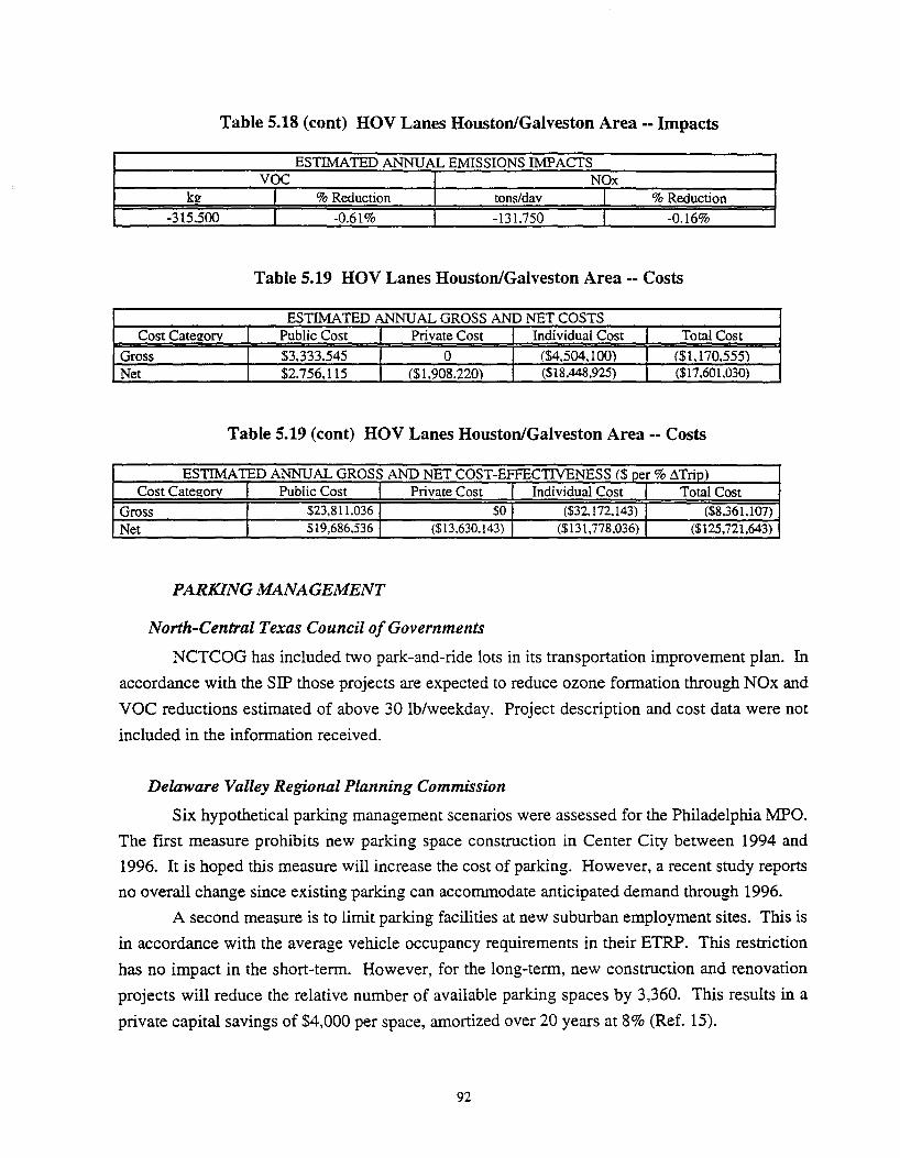
Table 5.18 (cont) HOV Lanes Houston/Galveston Area-- Impacts

ESTIMATED ANNUAL EMISSIONS IMP ACTS VOC NOx

kg I %Reduction tons/dav I %Reduction

-315.500 I -0.61% -131.750 I -0.16%

Table 5.19 HOV Lanes Houston/Galveston Area -- Costs

ESTIMATED ANNUAL GROSS AND NET COSTS Cost Categorv Public Cost Private Cost Individual Cost Total Cost

Gross $3,333.545 0 ($4,504. 1 00) ($1, 170,555) Net $2,756.115 ($1,908.220) ($18,448,925) ($17 ,60 1,030)

Table 5.19 (cont) HOV Lanes Houston/Galveston Area-- Costs

ESTIMATED ANNUAL GROSS AND NET COST-EFFECTIVENESS($ per% ~Trip) Cost Categorv Public Cost Private Cost Individual Cost Total Cost

Gross $23,811,036 $0 ($32,172.143) ($8,361,107) Net $19,686.536 ($13.630.143) ($131,778,036) ($125,721,643)

PARKING MANAGE1l1ENT

North-Central Texas Council of Governments

NCTCOG has included two park-and-ride lots in its transportation improvement plan. In

accordance with the SIP those projects are expected to reduce ozone formation through NOx and

VOC reductions estimated of above 30 lb/weekday. Project description and cost data were not

included in the information received.


Six hypothetical parking management scenarios were assessed for the Philadelphia .MPO.

The first measure prohibits new parking space construction in Center City between 1994 and

1996. It is hoped this measure will increase the cost of parking. However, a recent study reports

no overall change since existing parking can accommodate anticipated demand through 1996.

A second measure is to limit parking facilities at new suburban employment sites. This is

in accordance with the average vehicle occupancy requirements in their ETRP. This restriction

has no impact in the short-term. However, for the long-term, new construction and renovation

projects will reduce the relative number of available parking spaces by 3,360. This results in a

private capital savings of $4,000 per space, amortized over 20 years at 8% (Ref. 15).

92

A third activity in their parking management program is a regional parking charge on all

free or subsidized employee parking. A $3 surcharge is to be paid by all regional employees

arriving in private vehicles. The public cost of this program includes capital and operating cost

for additional transit riders and administrative costs of $500,000. The private sector will collect

the parking surcharge at a cost of $42 per space per year.

The fourth measure is identical to the previous one except that it is targeted to employees

in the Philadelphia CBD. The public administration cost of this activity is $250,000.

The ETRP calls for the construction of 22 new park-n-ride lots throughout the region.

These lots will accommodate 7,500 vehicles available for carpooling or bus commuting.

Construction costs of $4,000 per space are estimated, excluding land costs, and amortized over a

20 year period at 8%. The operating cost per space was assumed to be $0.50 per day. The

parking is free, and therefore, there are no private costs (Ref .. 15).

Finally, parking will be expanded at rail stations throughout the region. For all locations,

there will be 6,400 new parking spaces.


For parking management, TTI projected the benefits of increasing the price of 500

parking spaces in El Paso by 50 percent. Cost estimates are not made. The projected benefits

from the parking surcharge program are relative to the base year 1990.


The elimination of free employee parking is simulated by HGAC by assuming the

average parking fee is equal to the market rate for parking in the Houston-Galveston area. "The

percent of employees affected by this program is assumed to be equal to the fraction that work

for companies that employ 100 or more employees (43.2%)." (Ref. 14). This measure is similar

to their TRO program except the TRO is based on both parking subsidies and parking fees while

this measure is based on parking fees alone. The key inputs for this assessment are as follows:

• Monthly parking space lease rate, $33.60 (equivalent to $1.61 per day); • 43.2% of employees affected • Annual public program administrative cost, $160,000 (based on Regulation XV in

southern California)

Summary of Parking Management Strategies

Table 5.20 summarizes the costs associated with the parking management case studies.

Table 5.21 summarizes the reported impacts in terms of vehicle trips, miles traveled and

emissions.

93

Table 5.20 Parking Management Strategies - Costs

Case Study Public Sector Total$ per L\VMT

($1,368,894) ($0.12) ($33,728)

$61,999,680 (541.421,418) ($1.40) ($435,912)

$21,741,360 ($34,942,632) ($0.13) ($43,909)

$4,899,392 $0 $0.39 $139,991

$8,411,977 $0 $0.32 $112,640

($147,491,390) ($269,303.205) $21,415,280 ($0.55)

*"Costs" in parentheses are revenues

CONCLUSIONS

TDM strategies are designed from the perspective of reducing the use of SOVs, either

through mode shifts to HOV s such as carpools and public transit or through the elimination of

trips altogether. These strategies are being recommended primarily in major urban areas of the

country where air pollution emissions from mobile sources have become a significant problem.

However, for most locations in the U.S the single occupant auto is the predominant transport

mode of choice for personal travel in what is mostly low density metropolitan land use.

Voluntary changes in personal travel characteristics of individuals has been limited.

94

Table 5.21 Parking Management Strategies - Impacts

Case Study Annual Amount

-44,481

-11,261

Ride Lots

Expand Parking At Rail 0 Stations

Parkin!!

* Impacts are given in peak and reductions not reported.

dEmissions

% Annual % Annual Percent Change Amount Change Amount (kg) Change

)

-0.07% -11,903 -0.07%

-1.3% -343,398 -1.4% -1.6% -1.5%

-0.3% -98,084 -0.4%

-1 -74,750CO

-19.500 NOx 0 -26,540 -0.07% -25,250VOC

-148,250CO NOx

-1.6%

~VMT

periods. A daily total is derived by summing the two periods. Percent

95

CHAPTER 6- TECHNOLOGY OPTIONS

One way to save energy and reduce emissions in the transportation sector is through the

implementation of transportation system management (TSM), discussed in Chapters 4 and 5.

These strategies strive to optimize the transportation system through more efficient use of

conventional vehicles and technologies.

Another way to preserve energy and/or provide a sustainable and environmentally

friendly transportation system is based on the development of new technology options. These

two options for efficient transportation (TSM and technological) are by no means mutually

exclusive; rather, they should ideally be implemented after a critical analysis of interactive

effects on the overall mobility process.

The technology options can be designed either to improve efficiency of conventional

vehicles, or to utilize an alternative fuel. This chapter discusses and evaluates the following

technology options: conventional fuels (light and heavy vehicles), aircraft efficiency

improvements, and several alternative fuels.

APPROACH TO ASSESS TECHNOLOGY OPTIONS

This section addresses the approach used to discuss the technical and economic barriers

to improve energy efficiency and switch to alternative fuels in existing road vehicles. The

approach is based on a review of the literature. The cost assessment strives to take into account

both the societal and private perspectives.

GENERAL APPROACH

Technology options addressing conventional fuel economy improvements were prepared

for light highway vehicles (autos and light trucks), U.S. Department of Transportation (DOT)

Class 8 tractor-trailer type trucks, and passenger aircraft. Our examination of alternative fuels

concentrates on those applicable to light-duty vehicles, although heavy vehicle applications are

addressed where appropriate. The most important assumption made in the fuel-economy

analysis is that the performance (e.g., acceleration) of the vehicle is held constant. In other

words, technological improvements would be implemented to increase fuel economy rather than

performance or power, which is the current automakers perspective.

For alternative fuels technology options, compressed natural gas (CNG), liquid petroleum

gas (LPG), methanol, ethanol and other biofuels (mainly methanol from wood), electricity, and

fuel cell vehicles are examined. In all cases, the costs assume that the alternative fuel vehicle is

mass produced, and that production economies of scale have been achieved.

96

The economic feasibility of the alternative fueled vehicles are detennined by calculating

the life-cycle cost of each alternatively fueled vehicle (along with gasoline) under a set of

plausible cost and operating assumptions. The analysis is conducted from two perspectives: a

societal perspective and a private perspective. The societal perspective utilizes the resource cost

of the fuels (rather than the retail price). Resource cost includes environmental externalities

associated with the air pollution generated by a vehicle and excludes vehicle taxes and fees, and

any other transfers. A social discount rate of 3% (real) issues in all discounting and levelizing

calculations.

For the private perspective, the full retail price of the fuels is used. Additionally, a

private discount rate of 10% (real) is used to annualize future costs. Table 6.1 summarizes all

the assumptions used for gasoline and alternative fueled vehicles. These assumptions are used to

develop the economic feasibility analysis discussed later in this chapter.

In almost all cases, the life-cycle cost of the alternative fueled vehicle and the gasoline

were very close, often within 2% of each other. This occurs because the alternative-fueled

vehicle generally experiences higher vehicle purchase costs than gasoline, that were either

partially or completely offset by the alternative fuel vehicle's lower operating and fuel costs.

Under our baseline assumptions, electric vehicles (EV) are the least costly from both the societal

and private perspectives. However, because of the particularly high uncertainty levels in many

of the critical EV cost parameters, this result is not robust.

VALUING AIR EMISSIONS

In analyzing the benefits of avoided emissions, air pollutant emissions are valued in

dollar terms. There is much controversy about this practice and the pitfalls are obvious. It is

virtually impossible to arrive at economic values that reflect the actual cost of air pollutant

emissions to society. Damages from air pollution are diffuse, varied, affect a great number of

people, and often impact objects that are invaluable in monetary terms. Nevertheless, the

advantage of explicitly monetizing pollutant damages is that they establish consistent decision

protocols. Whether one likes it or not, monetary valuation of pollution damages is implied

whenever decisions are made about resource uses. Abating a certain amount of emissions

implies that the benefits from abating it are perceived as at least as great as the cost of abatement.

Likewise, not abating an emission implies that the damage it causes is valued less than the cost

of the cheapest abatement option.

In the ideal case, the cost of pollution damage would be assessed by a thorough study of

air pollutant exposure to and impacts on people, plants, and animals. Some of these impacts,

such as losses to agricultural crops and corrosion of materials, can be valued at least in principle.

For other types of damages, such as health impacts, lower bound estimates can be established in

97

the form of the expenditures undertaken to mitigate the effects. For impacts on objects that do

not have a market value, such as many environmental resources, so-called "willingness-to-pay"

surveys can be used that attempt to elicit consumers' valuation of the resource. These surveys

are based on neoclassical economic models of individual decision making; they attempt to

simulate situations in which individuals would actually make a choice about resource use.

Table 6.1 Summary of Alternative Vehicles Assumptions

Vehicle Costs t Base (1992) At cost-effective mp)!

Vehicle Life (in vears) 2

Levelized Maint. Cost3 Levelized Insurance Cost4 Vehicle Base 1992 mpg Efficiency s Societal cost-

effective m~g Notes and Sources for Table 6.1 (1) (a) Base 1992 mpg (Ref. 35)

Gasoline

(a)

$17,784 $18,560

12 $436 $468 27.8 46

Societal cost-effective mpg (Ref. 35)

Natural Methanol Gas (b) (c)

$18,784 $17.784 $19,560 $18,560

12 12 $353 $436 $471 $468

- -51 53

(b) Incremental natural gas vehicle (NGV) costs (Refs. 36, 37) (c) Incremental methanol costs (Refs. 36, 38, 39) (d) Incremental electric vehicle fuel costs (Ref. 40) (e) Incremental LPG vehicle costs (Ref. 41) (t) Incremental fuel-cell vehicle costs (Ref. 42)

(2) (a) (Ref. 42)

Battery LPG Hydrogen electric Fuel Cell

(d) (e) (f)

$20.584 $18.284 -$21,360 $19,060 $23,183

15 12 15 $291 $436 $354 $443 $468 $468

- - -133 46 74

Methanol Fuel Cell

(f)

-$24,810

15 $370 $468

-63

(b) Natural gas vehicle life assumed to be 1 year longer in the longer-term (8.3% longer). The longer life of NGVs is due to reduced engine wear during cold-starts (Refs. 37, 42)

(c) Assumes same life as gasoline vehicle (d) EV is estimated to have a 33% longer life than standard gasoline vehicles (mileage basis), (Ref. 40) (e) Assumes same life as gasoline vehicle (t) FCV is estimated to have a 33% longer life than standard gasoline vehicles (mileage basis), (Ref. 40)

(3) (a) Levelized over life of vehicle, (Refs. 40, 41) (b) In longer term. assumes maintenance at 80% of that of gasoline vehicle (Ref. 37) (c) Assumes the same as gasoline vehicles (t) EV is estimated to have a 33% longer life than standard gasoline vehicles (mileage basis), (Ref. 40) (e) Assumes the same as gasoline vehicles (t) (Ref. 40)

(4) (a) Assumes collision damage insurance is carried for first 5 years (Ref. 40) (b) Assumes that the vehicle carries collision damage insurance for first 6 years (Ref. 40) (c) Assumes the same as gasoline vehicles (d) Assumes that the vehicle carries collision damage insurance for first 6.5 years (Ref. 40) (c) Assumes the same as gasoline vehicles (c) Assumes the same as annual average as gasoline vehicles

(5) (a) (Ref. 35) (b) (Ref. 36) (c) (Ref. 37) (d) (Ref. 40) (e) Assumed to be the same as gasoline (t) (Ref. 40)

98

In most cases, conducting such a study is well beyond the means of the decision maker,

or even of the agency that regulates resource decisions. A procedure to arrive at values in the

interim is to take the cost of the most expensive mandated abatement technology as the value

that society ascribes to pollutant emissions. This "marginal" control cost is the cost that society,

represented by the regulator, is willing to pay to avoid the last pollutant emission.

A number of state regulatory bodies have adopted dollar values for air pollutant

emissions and mandate their use in energy resource decisions as shown in Table 6.2. Some of

these values are based on the marginal control cost approach mentioned above (Massachusetts),

while others rely on damage cost estimates (see Table 6.3). Note that the highest values are used

by the California Energy Commission, for the South Coast Air Quality Management District, the

region with the most critical air pollution problems in the nation.

Table 6.2 Air Emissions Externality Values Adopted I Proposed in Various U.S. States

Pollutants-- Emissions cost. 1993 S!fon State NOx SOx TSP* co

MassDPU $7.410 $1.710 $4.560 $992 Nevada PUC $7.454 $1.710 $4.582 $1.009 Cal PUC (SCAQMD) $31.268 $23.356 $6.765 -Cal PUC (PG&E) $9.068 $4.451 $2.609 -Cal PUC (Attainment Areas) $7.454 $1.710 $4.582 -Cal CEC. ER 92. SCAQMD $16.866 $9.694 $53.205 $3 Cal CEC, ER 92, other district $7,761 $4,446 $24,107 $1 maximums Cal CEC, ER 92, other district $92 $1,717 $117 $0 minimums Cal CEC, ER 92, out-of-state $870 $1,717 $1,488 -Southwest Cal CEC, ER 92, out-of-state $836 $1,717 $1,465 -Northwest NY State Energy Office $4.608 $941 - -NY State Energy Office $1.064 $206 - -NYPSC $2.029 $935 $365 -WIPSC - - - -Oregon PUC Low $2.192 - $2.192 -Oregon PUC High $5.481 - $4.385 -Bonneville BPA, west of $969 $1,644 $1,688 -Cascades*** Bonneville BPA, east of $76 $1,644 $183 -Cascades*** * TSP values for CA and Bonneville PA represent values for PMlO ** VOC values for CA represent values for reactive organic gases (ROGs) *** Endorsed by the Washington State Energy Office

99

VOC**

$6.042 $1.294

$22.334 $4.212 $1.294 $7.911 $5,405

$32

$6

$0

-------

-

C02 OI4 $25 $251 $24 $241

$9 -$9 -$9 -$9 -$9 -$9 -

$9 -$9 -

$81 -$6 -

$1.3 -$15 $154 $11 -$44 -- -

- -

Table 6.3 Source and Notes for Table 6.2

State Notes Sources MassDPU Control Cost (a) Nevada PUC Control Cost (b)

Cal PUC (SCAOMD) Control Cost: SCE & SDG&E Areas (assumed level) (c) Cal PUC (PG&E) Control Cost: PG&E Area (NO>t is 29% of SCiQMD). (c) Cal PUC (Attainment Areas) Control Cost- directed to use "Nevada" numbers (c) Cal CEC. ER 92. SCAQMD Damage Cost (d) Cal CEC. ER 92. other district maximums Damage Cost (e)

Cal CEC. ER 92. other district minimums - (t)

Cal CEC. ER 92. out-of-state Southwest Damage Cost. levelized (t)

Cal CEC. ER 92. out-of-state Northwest - (t)

NY State Energy Office Mixture of Damage and Control Cost (General Revenue (g) Tax)

NY State Energy Office Mixture of Damage and Control Cost (Trust Fund Tax) (g)

NYPSC Control Cost (h)

WIPSC $3,845/ton for N 20; mixture of Damage and Control Cost (i)

Oregon PUC Low Control Cost (i)

Oregon PUC High - (j)

Bonneville BPA, west of Cascades*** Damage Cost (NOx, TSP)--estimated allowance market (k) value for so2

Bonneville BPA. east of Cascades*** - (k)

Sources: (a) MA DPU Order 91-131, November 10, 1992. (b) Nevada PSC Order 89-752, January 22, 1991. (c) CA PUC Decision 91-06-022, June 5, 1991. (d) California Energy Commission Docket No. 90-ER-92S. Order Adopting. Actual values taken from ER 92,

Appendix F, Air Quality, January, 1993. (e) The maximum and minimum values shown are those across all districts. (t) ER 92, Appendix F, Air Quality, January 1993. (g) NY State Energy Office, Draft New York State Energy Plan: 1991 Biennial (h) State of New York PSC Case 88-E-241, Order issuing final environmental, agency comments. Issued and

effective March 24, 1989. (i) WI PSC, Docket 05-EP-6, September, 18, 1992. (j) Range of values given in Oregon PUC Order no. 93-695. (k) Documentation: Environmental Cost Adjustments, BPA's Competitive Acquisition of Firm Energy

Resources, 1991.

For the Texas scenarios, a set of air emission dollar values that lie within the range of the

values operative in the U.S. are used (see Table 6.4). The ozone precursors, nitrogen oxide

(NOx) and volatile organic compounds (VOC), are differentiated between the urban and the rural

regions of Texas. For the urban regions (basically the Texas triangle), separate values are

applied to Houston and the rest of the Texas triangle resulting in population weighted averages

for the two pollutants. For Houston, the midpoint between the values adopted by California's

South Coast Air Quality Management District and the Massachusetts values are used. The

Massachusetts values are applied to the remainder of the triangle. For the rural region, one half

of the Massachusetts values are used. The rationale for this procedure is that the occurrence of

ozone and the impacts it causes are tied to local conditions. Obviously, ozone is more of a

100

problem in cities than in rural areas; and cities differ in their air quality. Houston was singled

out because it is in non-attainment status and because it has a large industrial base, specifically, a

number of petrochemical facilities, which are important contributors to ozone precursor

emissions.

Table 6.4 Air Emissions Externality Values for Texas

Pollutants. Emissions cost. 1993 $/Ton Regions of Texas NOx SOx TSP co voc C02

Urban (Texas Triangle) $9.070 $300 $4.560 $992 $6.371 $25 Rural (remainder of state) $3.705 $300 $4.560 $992 $3.021 $25

For the other air pollutants, there is no differentiation between the rural and urban

regions. The values used for particulates (TSP), carbon monoxide (CO), and carbon dioxide

(C02) adopted by Massachusetts are used throughout the state. The price for tradable emission

allowances is used for sulfur oxides (SOx). This is a conservative estimate of the externality

costs of that pollutant.

CONVENTIONAL FUEL -LIGHT VEIDCLES *

This section discusses the current and near-term options to provide a cleaner, more

energy-efficient gasoline automobile. These options are conceptually based on finding ways to

reduce exhaust gases and frictional losses.

THE GASOLINE CONSUMPTION PROCESS

In order to understand where potential efficiency gains in light vehicles could come from,

it is useful to discuss where exactly all the energy being poured into the gas tank is going. When

a car is driven, part of the fuel's chemical potential energy ends up warming the air and road

through the exhaust stream. Additionally, there are frictional losses in the engine, brakes, tires,

and from aerodynamic drag. Energy losses depend on both vehicle characteristics and the type

of driving. For example, fuel economy is worse in congested conditions.

Figure 6.1 illustrates on average where the energy from burning gasoline in a typical light

vehicles goes. The vast majority of the energy is lost as heat in the engine system. Much of this

heat is spewed out the tailpipe as exhaust, out of the radiator, or radiates from the engine itself.

Another fraction of the heat is generated as friction in the moving parts of the engine.

Of the remaining 18% of the fuel's energy that moves the vehicle engine, about one-third

is used to overcome aerodynamic drag, another one-third is used to overcome rolling friction

(friction between the tires and the road), and the remaining one-third goes toward powering

*Unless otherwise noted, information provided in this is from (Ref. 35).

101

accelerations (part of which is eventually lost as heat in the brakes). Each of these sources of

energy loss, from heat loss in the engine to overcoming drag, is a source of potential

improvement in vehicle fuel economy. Areas where energy is used for non-useful purposes,

such as heating up the radiator, can be prime targets for investigation of efficiency

improvements.

Figure 6.1 Energy Consumption By Gasoline Powered Vehicles (average of highway and urban driving cycles)

I FUEL ENERGY INTO ENGINE (100%) l

Mechanical energy out of motor Heat lost in engine system (18%) (82%)

Overcoming Overcoming Power Heat lost Heat rejected aerodynamic rolling acceleration; as internal out radiator,

drag drag ends up as friction tailpipe, etc. heat in the

brakes

Efficiency Gains From Decreased Engine Losses

The laws of thermodynamics make most of the heat losses unavoidable. Nevertheless,

significant improvements can be made in the engine system to reduce friction losses and allow

the engine to operate at its peak efficiency. Some improvements that are either being developed

or have recently been developed are discussed below:

(1) Valve Improvements. Four or more valves per cylinder reduce pumping losses and improve efficiency by moving fuel and air into and out the of the cylinder more quickly and easily. Variable valve timing also allows the valves to be more optimally positioned, reducing pumping losses and increasing low-end torque and fuel economy. This technology is already implemented in some new vehicles.

(2) Improved Controls. Multi-port fuel injection is a fairly recent development that improves not only fuel economy but also performance, reliability, and emissions. A more exotic, yet technically feasible control improvement is having the engine automatically tum itself off during prolonged idle periods when no power is demanded.

(3) Engine friction reduction involves a number of incremental improvements which can substantially improve fuel economy. Examples of friction reduction include low friction piston/ring design, roller can followers, overhead camshaft designs, and improved lubricants.

102

(4) Non-standard engine designs such as diesel engines and two-stroke engines can improve fuel economy by 11% - 28% and 35% - 40%, respectively, over standard gasoline engines. Turbo- or super-charging a smaller engine allows it to achieve the same peak power as a larger, non-boosted engine. SRI notes that "optimal redesigns of downsized gas engines with forced induction systems can demonstrate potential (fuel economy) gains of up to 8%." Most gasoline engines utilize a fuel to air ratio just sufficient to completely burn all of the fuel. Lean-bum engines operate with significantly more air than is strictly required to completely bum all of the fuel. Diesel engines are inherently lean-burn. Although 2-stroke engines have higher emissions than 4-stroke engines, with improvements in aerodynamics, controls and emission controls, some advocates see them as a realistic possibility.

(5) Automatic transmission improvements can allow the engine to operate a larger fraction of the time at its most efficient speed and torque.

Efficiency Gains From Decreased Aerodynamic Drag

The energy needed to overcome the force of air drag on a car (or any moving object) is a

function of its size and shape, expressed as a function of the coefficient of drag C 0 and the

square of the speed. Thus, the energy needed to overcome drag in any vehicle at 70 miles per

hour is four times than needed at 35 miles per hour. Based on the EPA composite highway/city

driving cycle, each 10% reduction in C0 increases fuel economy by 1.57%. For autos with

higher highway use than is assumed in the Environmental Protection Act (EPA) composite

driving cycle, the impact of drag reduction in fuel economy would be greater.

Efficiency Gains From Decreased Rolling Friction

Because the weight of a vehicle tends to deform the tires slightly against the road, energy

must be used to move the deformation around the circumference of the tire as it rolls along. This

is known as rolling friction or rolling resistance. Rolling resistance, C R• is generally expressed

as a percentage. A rolling resistance of 1% means that a one pound force is needed to roll 100

pounds of tire load.

Efficiency Gain in Acceleration (Weight Reduction)

Reducing vehicle mass can be an effective approach to fuel economy improvement. This

is particularly true for urban driving, where the energy spent accelerating up to speed in the first

half of a block is wasted to the brakes stopping for the next light. If a vehicle's mass were

reduced by 1% and engine power is maintained, a 0.3% improvement in fuel economy would

occur, along with an increase in performance (acceleration). If, instead, the car's performance is

held constant and the engine power reduced, a 1% decrease in mass yields a 0.66% increase in

fuel economy.

There are numerous places on automobiles where mass can be reduced. The most

obvious option is to simply downsize the vehicle. However, the large variation in curb weight

seen within a vehicle class indicates that this is not necessarily the only, or even the best option.

103

Within any given EPA size class, the curb weight of the heaviest vehicle is roughly twice that of

the lightest one. Other options for reducing vehicle mass include:

(1) Switching from rear-wheel drive to front-wheel drive (2) Replacing steel components with aluminum or composite materials (3) Improving manufacturing techniques using existing materials (4) Improving designs which can maintain vehicle safety with less materials

Emissions Savings

Emissions from gasoline engines (and all other forms of combustion) are a function of

the make-up of the fuel, the way in which the fuel is burned, and the emissions control

equipment. One class of emissions, which includes C02 and SOx, is strictly a function of the

composition of the fuel. For practical purposes, all of the carbon in the fuel can end up as carbon

dioxide, and all of the sulfur can be emitted as SOx· For these constituents, there is a direct

relationship between emissions and efficiency. The less fuel that is burned, the less these

pollutants are formed and emitted.

The second class of emissions from combustion are those which are formed as a result of

the combustion process. CO and hydrocarbon (HC) emissions result from incomplete

combustion, and are not a function of vehicle efficiency generally, the reduced efficiency

associated with incomplete combustion is negligible.

The vast majority of oxides of NOx are formed from the natural nitrogen and oxygen in

the air when temperatures become greater than approximately 1,800° F. Emissions of these

pollutants are dramatically reduced through the use of a catalytic converter, provided the

operating systems are operating properly.

Efficiency improvements can impact the upstream fuel-cycle emissions of these

pollutants. When a vehicle is refueled less frequently, less volatile HC are emitted into the air

during refueling. Also, all emissions associated with extracting, shipping, and refining crude oil

are reduced proportionally.

CURRENT STATUS

Since 1974, average nominal fuel economy for the new automobile fleet has doubled,

from 14 miles per gallon (mpg) up to 27.8 mpg in 1992 (Ref. 44, 45). Average fuel economy for

new cars actually peaked in 1988 at 28.8 mpg, and has been slowly decreasing since. Since

1985, the average fuel economy of the U.S. manufacturers fleet has been one to two miles per

gallons less than the fleet as a whole, while the average fuel economy for imported cars has been

from 1.5 to 3.5 mpg higher (Ref. 45)

104

Engine/Drivetrain Improvements

Many of the options described above have been routinely used over the past few years (as

shown in Table 6.5), but not to increase fuel economy. Most of the changes shown in the table

and others, such as Hondas' variable valve timing VTEC engine, serve to increase the engine's

power. Efficiency is gained when the engine is downside, while holding the power output

constant. However, though average engine sizes have been decreased, automakers have not

downside engines to take full advantage of the efficiency improvement potential. Rather,

average overall power has continued to increase.

Table 6.5 Engine and Transmission Technology Penetration in the 1990 Fleet

Improved Technology Reference Technology Penetration in the 1990 New Car Fleet (in%)

ENGINE Sub. Como. Mid. Large Avg. Roller cam followers Flat Followers 29.2 42.5 31.0 100.0 44.9 10% friction reduction 1987 Base 12.3 10.3 34.1 37.3 21.2 4 valves/cvlinder 2 valves/cvl. 36.3 38.5 9.0 0.4 24.3 Overhead Camshaft Pushrod 43.7 17.6 14.9 0.0 20.2 Throttle Body Fuel Iniection Carburetor 34.8 31.7 14.4 0.0 22.9 Multi-Point Fuel Injection Carburetor 58.0 68.3 84.7 97.3 74.7

TRANSMISSION Sub. Comp. Mid. Large Avg. Lock-up converter Ojlen converter 45.5 71.3 96.1 99.4 76.2 4 speed 1ock-up 3 speed lock-up 14.8 18.6 54.5 0.0 25.1 5 speed manual 3 speed lock-up 42.5 16.0 3.1 0.1 16.3

Aerodynamic Drag Reduction

In 1990, the estimated average C0 of new automobiles was 0.352 (±0.037). At least 13

models with C0 of 0.33 or less have been in mass production since 1987. Current research

vehicles have achieved a Co as low as 0.14.

Rolling Resistance Reduction

The increase in fuel economy associated with a decrease in rolling resistance is a function

of vehicle characteristics and driving cycle. Estimates for this relationship suggest that every

percentage point decrease in rolling resistance increases fuel economy by 0.15%- 0.25%. Tires

on 1991 automobiles were reported to have a CR. of about 1.1 %. Tire manufacturers have

recently announced models with 20% - 35% less rolling resistance than their standard models

(the CR. of neither the new tires nor the baseline models were reported). Special high-pressure

tires designed for the GM electric Impact tires have a CR. of 0.5%, but the overall applicability

of these tires is not known. It is estimated that improving rolling resistance from a CR of 1.1%

to a CR of 0.85% increases fuel economy 3.4%, and decreasing rolling resistance to 0.65%

increases fuel economy by 6.1 %.

105

Weight Reduction

From 1975 to 1991, the curb weight of the average automobile dropped by 21%. A

portion of this drop is attributable to the general downsizing of the typical automobile, but other

factors also contributed. Major weight reductions were achieved in the 1980s though conversion

from rear-wheel drive to front-wheel drive. One study estimates that a 10% total fuel economy

benefit resulted from this switch to front wheel drive. Future weight reductions will come from

increased use of plastics, composites, high-strength aluminum and magnesium (Ref. 46).

TECHNICAL FEASIBILITY

Most, if not all, of the basic technologies discussed above are technically feasible today,

and in fact are in use in one or more existing models. The only technical feasibility constraint

faced is the engineering design and manufacturing adjustments needed to implement the

changes.

ECONOMIC FEASIBiliTY*

Figures 6.2 and 6.3 show "conservation supply curves" for currently available measures

to increase automobile fuel economy. Figure 6.2 corresponds to a societal perspective and

Figure 6.3 corresponds to a private perspective.

The horizontal axis of each figure represents the average fuel economy for a standard

domestic automobile (such as the Ford Taurus). The vertical axis represents the incremental cost

of increasing fuel economy, expressed as the levelized cost per gallon saved. The bottom left

hand end of the cost of saved energy line represents the current status: the fuel economy is 27.8

mpg, and no incremental investment in energy efficiency has been made. Each "stair-step"

beyond this end-point in the cost of saved energy line represents the cost and savings associated

with a discrete technology. For example, the first visible step in the curve corresponds to

lubrication improvements, which increases fuel economy by 0.2 mpg at an average cost of about

10¢ per gallon saved. The measures and savings shown in both figures are summarized in Table

6.6.

The dashed lines in each figure correspond to various benchmark costs of gasoline. In

the societal perspective figure, the lowest line is the estimated wholesale cost of gasoline,

levelized over the period 1995 to 2010. Based on this benchmark, any fuel economy

improvements which can be implemented at a cost less than 78¢/gallon (1992 dollars) are cost

effective, i.e., the cost to save gasoline is less than the cost to acquire it. Based on this

benchmark, the fuel economy of a mid-sized domestic car could cost-effectively be increased to

about 41 mpg.

* Throught this chapter the wholesale cost of petrolem excluding any taxes is used as a proxy for the resource cost or avoided cost of the product

106

Figure 6.2 Cost of Saved Energy for Automobile Fuel Efficiency Programs -- Societal Perspective

3.0

2.5 "CC ~-;;-(13 ""'

2.0 "' (13 == 1.5 Q Q :"0

.::::::::::::::::::::::::::~:::::::::::::::::::::::: ::::::::::: e'3M Cllc:. 1.0 r..c:. ~-c.'-'

0.5 ~

0

25 30 35 40

miles per gallon

---- Cost of Saved Energy ----!---A voided Cost* with ----<>---Triangle Externalities

----x---

* 1995 - 2010 levelized costs

45

A voided Cost* with Rural Externalities

A voided Cost*, No Externalities

50

Figure 6.3 Cost of Saved Energy for Automobile Fuel Efficiency Programs - Private Perspective

"CC

4.5

4.0

3.5

~ 'E 3.0 "' = ; ~ 2.5 :"0

~~ 2.0 r..c:. ~- 5 ~-- 1. ::::::::::::::::::::::::::~:::::::::::·:: _____ ::::::::::::::::

1.0

0.5

0+-~~~~~~~~-r~~~~r-~~-r~-,-r-~~-r~~~~

25 30 35 40 45 50

miles per gallon

--- Cost of Saved Energy - -o-- Retail Rate in 2010 - "*-- Levelized Retail Rate (1995 - 20 10)

107

Table 6.6 Automobile* Efficiency Improving Technologies, Associated Fuel Economy Improvements, and Costs

Measure Increased Fuel Cost per gallon of gasoline saved Economv (mpg) Societal Private

Compression Ratio Increase 0.3 $0.00 $0.00 Lubrication Improvements 0.2 $0.10 $0.14 Lower tire rolling resistance 1.4 $0.11 $0.16 Continuously Variable Transmission 0.8 $0.13 $0.20 Optimized manual transmission 0.7 $0.16 $0.23 Optimized transmission control 1.9 $0.21 $0.31 Accessorv improvements 0.6 $0.27 $0.39 Variable Valve Control 3.0 $0.41 $0.60 Variable Displacement 0.6 $0.54 $0.79 Overhead Cam 0.6 $0.57 $0.83 Weight Reduction 2.9 $0.70 $1.03 Friction Reduction 1.5 $0.86 $1.26 Four valve per cylinder 1.5 $0.92 $1.34 TorQue converter lock-up 0.1 $1.04 $1.52 5-speed automatic 0.6 $1.26 $1.85 Aerodvnamic improvements 1.3 $1.42 $2.07 Multi-I>Qint fuel injection 0.3 $1.54 $2.25 Super-/turbo charging 1.1 $2.02 $2.95 Idle-off l.O $2.84 $4.15

* Basehne: Domesuc sedan, 27.8 mpg

Two other benchmarks are also shown in the societal perspective figure. The middle line

represents the levelized resource cost of gasoline plus the estimated environmental externality

cost of the air pollutants emitted into a rural setting. At this level, the fuel economy of the

typical U.S. mid-sized car can cost-effectively increase to about 45.5 mpg. The highest dashed

line corresponds to the levelized resource cost of gasoline plus the estimated environmental

externality cost of the air pollution emitted into an urban environment, particularly one in ozone

(03) non-attainment. Including these additional externality costs the cost-effective automobile

fuel economy increases an additional 0.5 mpg, up to about 46 mpg. This small increase is due to

the shape of the cost of saved energy curve, which is very steep at this point, and to the fact that

at the assumed emissions characteristics (California low emission vehicle standards) and

externality costs, the dominant pollutant is C02.

The two dashed lines in the private perspective curve correspond to the levelized retail

price of gasoline from 1995 to 2010 (1992 dollars), and the estimated price of gasoline in 2010

(1992 dollars). Using these benchmarks, the fuel economy of the typical mid-sized sedan can be

cost-effectively increased to about 41 or 44 mpg, respectively. It is a convenient coincidence

that the cost-effective level of fuel economy improvement from the private perspective is about

the same as it is from the societal perspective, 40-45 mpg.

108

INSTITUTIONAL CONTEXT BARRIERS

The question that often troubles energy-efficiency analysts is: if these measures are cost

effective, even at 78¢/gallon, why aren't they being implemented? One part of the answer to this

question is that the measures are being implemented, but to increase performance rather than fuel

economy. The assumption made in this fuel-economy analysis is that the performance (e.g.,

acceleration) of the vehicle is held constant. The efficiency measures increase the power

available from a given engine, allowing the engine to be downsized to a more efficient size while

maintaining the same power. In practice, the converse generally occurs: the engine size (and

roughly fuel economy) is held constant while the power and performance of the vehicle

increases. Fuel-injection, variable valve timing, and four valves per cylinder are all being used

today, but generally to the benefit of power rather than fuel economy.

A second reason that fuel economy is not given a high priority by manufacturers or

consumers is that non-cost factors, such as reliability, performance, aesthetics, and safety play

more important roles in the consumers automobile purchasing decision. Also, fuel costs

represent only about 10% to 12% of the total cost of owning and operating a car-- not enough to

grab the attention of the typical auto-buyer.

CONVENTIONAL FUEL ·HEAVY VEHICLES*

This section examines the technical opportunities to increase the average efficiency of

"heavy" (class 8, tractor-trailer or tractor-semi-trailer) trucks. Class 8 trucks travel 65% of the

annual truck miles and consume 71% of the fuel consumed by Class 3 or higher trucks (Ref. 47).

DESCRIPTION

Like light vehicles, improvements in the engine/transmission system, reductions in

aerodynamic drag, and reductions in rolling resistance offer opportunities to increase the fuel

economy of heavy trucks. Unlike light vehicles, weight reduction is not a feasible option; the

cargo load of heavy trucks is large relative to the gross weight of the vehicle. A reduction in the

weight of an empty vehicle is more likely to be compensated with additional loading rather than

lead to improvements in fuel economy (Ref. 48). Because of shifts in the U.S. economy to more

finished goods, which are less dense and require more packaging than raw materials, truck loads

are increasingly becoming volume-limited ("cube-out") rather than weight limited ("weight

out"). Therefore, truck weight reductions can still contribute, in some cases, to fuel economy

improvements.

Additionally, fuel economy improvements in these vehicles are difficult to measure.

Unlike light vehicles, there are no standard EPA tests to establish a fuel economy baseline for

*Unless otherwise noted, infonnation provided in this section is from (Ref. 47).

109

heavy trucks. Some tests can be performed in the laboratory, such as dynamometer testing of

engine and wind-tunnel testing of aerodynamics, but how these results translate to improvements

in the fleet is less clear. It is also important to note that many of the savings estimates are not

additive; a 15% increase in engine efficiency coupled with a 10% savings from reduced drag will

result in a net savings of something less than 25%.

Efficiency Improvements In Heavy Truck Engines

The basic power plant in a heavy truck, a turbo-charged diesel engine, is significantly

more efficient than the gasoline engines found in light vehicles. A gasoline engine typically

operates at 18% efficiency. Nonetheless, some of the measures that could increase large truck

fuel economy include:

(1) High-torque, low rpm engines can increase fuel efficiency by 10%-12%.

(2) Electronic engine controls are presently being used to meet emissions regulations but can also increase fuel economy by 4%. These control packages regulate engine fuel intake, maximum rpm, maximum road speed, power output, and other parameters.

(3) Temperature controlled fan clutches improve fuel economy by 6%-8%, and are standard on nearly all new trucks.

(4) Advanced technologies are currently being investigated and offer promise of significantly improving the efficiency of heavy truck engines. Low heat rejection (adiabatic) diesel engines might improve fuel economy up to 20%. Various strategies for recovering energy from engine exhaust are projected to be able to increase fuel economy by 10%-15%.

(5) Drivetrain/transmission and differential lubrication improvements increase fuel economy by 1%-1.5%, optimized gearing improves fuel economy by 3%-5%, and using a non-driven "tag" axle improves fuel economy by 2%-3%. Taken together, these drivetrain improvements can increase fuel economy by 5%-7%.

Aerodynamics Improvements

At highway speeds, 50% of the engine power of a heavy truck is needed to overcome

aerodynamic drag. A 10% reduction in drag translates into a fuel economy improvement of

about 3.6%. Aerodynamic improvements on the tractor include air dams, which redirect air from

beneath the truck, roof fairings, which smoothly direct air over the top of the trailer, and gap

seals, which smooth the transition from tractor to trailer. A full aerodynamic tractor package can

increase fuel economy by up to 14%.

Improved trailer aerodynamics, such as trailer skirting and underbody air defectors, can

improve fuel economy by 5%. However, the critical issue for trailer aerodynamics is merging

the tractor-trailer into a single unit. This is particularly difficult in that there are many different

kinds of both tractors and trailers, varying by maker, vintage and application. The savings

110

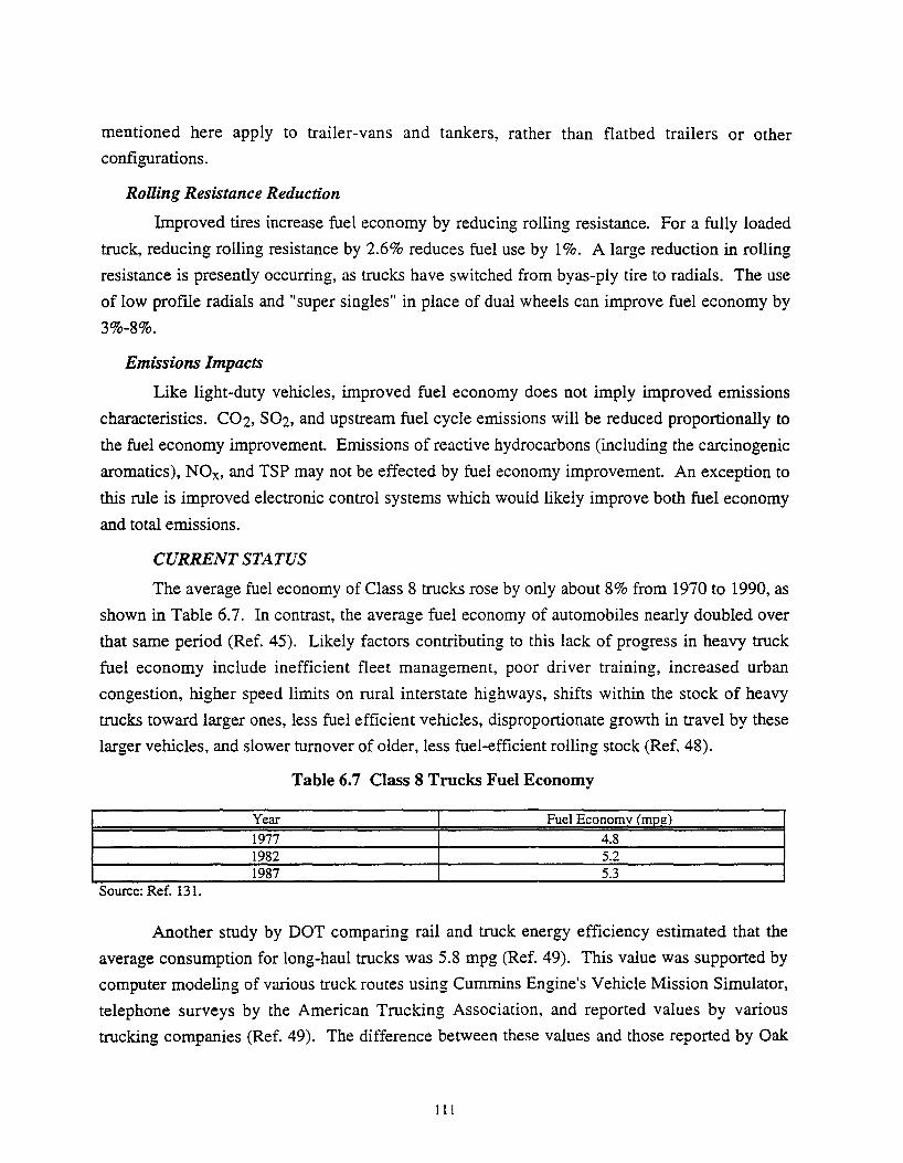
mentioned here apply to trailer-vans and tankers, rather than flatbed trailers or other

configurations.

Rolling Resistance Reduction

Improved tires increase fuel economy by reducing rolling resistance. For a fully loaded

truck, reducing rolling resistance by 2.6% reduces fuel use by 1%. A large reduction in rolling

resistance is presently occurring, as trucks have switched from byas-ply tire to radials. The use

of low profile radials and "super singles" in place of dual wheels can improve fuel economy by

3%-8%.

Emissions Impacts

Like light-duty vehicles, improved fuel economy does not imply improved emissions

characteristics. C02, S02, and upstream fuel cycle emissions will be reduced proportionally to

the fuel economy improvement. Emissions of reactive hydrocarbons (including the carcinogenic

aromatics), NOx, and TSP may not be effected by fuel economy improvement. An exception to

this rule is improved electronic control systems which would likely improve both fuel economy

and total emissions.

CURRENT STATUS

The average fuel economy of Class 8 trucks rose by only about 8% from 1970 to 1990, as

shown in Table 6.7. In contrast, the average fuel economy of automobiles nearly doubled over

that same period (Ref. 45). Likely factors contributing to this lack of progress in heavy truck

fuel economy include inefficient fleet management, poor driver training, increased urban

congestion, higher speed limits on rural interstate highways, shifts within the stock of heavy

trucks toward larger ones, less fuel efficient vehicles, disproportionate growth in travel by these

larger vehicles, and slower turnover of older, less fuel-efficient rolling stock (Ref. 48).

Table 6. 7 Class 8 Trucks Fuel Economy

Year Fuel Economv (mpg)

1977 4.8 1982 5.2 1987 5.3

Source: Ref. 131.

Another study by DOT comparing rail and truck energy efficiency estimated that the

average consumption for long-haul trucks was 5.8 mpg (Ref. 49). This value was supported by

computer modeling of various truck routes using Cummins Engine's Vehicle Mission Simulator,

telephone surveys by the American Trucking Association, and reported values by various

trucking companies (Ref. 49). The difference between these values and those reported by Oak

Ill

Ridge National Laboratories (Ref. 45) might be due to the fact that the earlier study focused on

routes that were competing with rail (e.g., long-haul). Long-haul trucks tend to be newer and

hence more efficient than short-haul trucks, and the national average statistics also include a

larger fraction of less energy efficient urban driving.

According to the 1987 Truck Inventory and User Survey (TIUS), 20% of all class 8

trucks were equipped with aerodynamic devices, 13% had engines with fuel economy

improvements (unspecified), and 6% had radial tires (Ref. 48). Compared to the base fleet,

trucks fitted with fuel economizing features achieved a 15% increase in fuel economy. This

lackluster improvement indicates that other factors, such as driver training and fleet

management, are as important as, if not more important than technological improvements.

TECHNICAL FEASIBiliTY

Many of the technologies discussed above are feasible today, and in fact, are in use in

one or more existing models: cabs are becoming more aerodynamic while electronic engine

controls, albeit currently used for emission control, are improving fuel economy of heavy trucks.

Other technologies (e.g., advanced diesel and turbine engines) have been technically

demonstrated, either on the road or in the laboratory, but are not yet commercially available.

Both levels of technologies are included in the economic feasibility screening below.

ECONOMIC FEASIBILITY

Figures 6.4 and 6.5 show "conservation supply curves" for currently available measures

to increase the fuel economy of heavy trucks. Figure 6.4 corresponds to a societal perspective.

Figure 6.5 corresponds to a private perspective. The horizontal axis of each figure represents the

average fuel economy for a baseline Class 8 tractor trailer; the vertical axis represents the

incremental cost of increasing fuel economy, expressed as the levelized cost per gallon saved.

The bottom left-hand end of the cost of saved energy line represents the current status: the fuel

economy is 5.2 mpg, and no incremental investment in energy efficiency has been made. Each

"stair-step" beyond this end-point in the cost of saved energy line represents the cost and savings

associated with a discrete technology. For example, the first visible step in the curve corresponds

to lubrication improvements, which increases fuel economy by 0.36 mpg at an incremental cost

of about 0¢ per gallon saved. The measures and savings shown in both figures are provided in

Table 6.8.

112

Figure 6.4 Cost of Saved Energy for Heavy Truck Fuel Efficiency Programs •• Societal Perspective

4.5

4.0

1l 3.5

~ ~ 3.0 = == ~ ~ 2.5 ~~ 2.0 loo~

~-c..._ 1.5 ~

1.0

------------ ·---·-~------------·-0 -·------______ ,_ ______ ..... ------I

----- .. --- ... ------ ---------·- ------ ----- ·- ---- ·-.- -----

··- -----------------------·X-------------------- --------------------0~~~~~~~~~~~~~~~~~~~~~

5 6 7 8 9

miles per ~on

----Cost of Saved Energy

A voided Cost* with - --~--- Triangle Externalities

* 1995 - 2010 levelized costs

-------- Avoided Cost* with Rural Externalities

__ --X- __ Avoided Cost*, No Externalities

10

Figure 6.5 Cost of Saved Energy for Heavy Truck Fuel Efficiency Programs -- Private Perspective

-=

4.0

3.5

~ ~ 3.0

~ ~ 2.5 Q Q

=-= ~~ 2.0 "'~ ! ::::, 1.5 - : : : : : : : : : : : : : : : : : : : : : : : : : =i : : : : : : : : : : : - 1.0

--------------------------

0.5

o~~~~~~~r+-r~~~~OT.-~rT.-~~.-~~

4 5 6 7 8 9 10 miles per gallon

--- Cost of Saved _ -¢ __ Retail Rate - "* --Levelized Retail Rate Energy in 2010 (1995- 2010)

113

Table 6.8 Heavy Truck* Efficiency Improving Technologies, Associated Fuel Economy Improvements, And Costs

Measure

Drive train Other available engine technologies Aerodynamics. tractor Engine control technologies Aerodvnamics. trailer Tires Engines in development Weight reduction Speed reduction *Baseline: Tractor-Trailer, 5.2 mpg Source: Ref. 35.

Increased Fuel Economv (mpg)

0.36 0.78 0.73 0.83 0.26 0.42 0.52 0.05 0.78

Cost per gallon of gasoline saved Societal Private $0.00 $0.00 $0.14 $0.21 $0.23 $0.34 $0.28 $0.40 $0.39 $0.57 $0.59 $0.86 $1.03 $1.51 $2.85 $4.16 $4.41 $6.44

The dashed lines in each figure correspond to various benchmark costs of diesel. In

Figure 6.5 the societal perspective, the lowest line is the estimated wholesale cost of diesel,

levelized over the period 1995 to 2010. Based on this benchmark, any fuel economy

improvements which can be implemented at a cost less than 70¢/gallon (1992 dollars), are cost

effective; the cost to save diesel is less than the cost to acquire it. Based on this benchmark, the

fuel economy of a Class 8 tractor trailer can cost-effectively be increased to about 8.6 mpg.

Two other benchmarks are also shown in the societal perspective figure. The middle line

represents the levelized resource cost of diesel plus the estimated environmental externality cost

of the air pollutants, both at the tailpipe and upstream in the fuel cycle, emitted into a rural

setting. At this level, the fuel economy of the heavy truck can cost-effectively increase to about

9.1 mpg. The highest dashed lines corresponds to the levelized resource cost of diesel plus the

estimated environmental externality cost of the air pollution emitted into an urban environment,

particularly in an 03 non-attainment area. Including these additional externality costs increases

the cost-effective fuel economy an additional 0.1 mpg, up to about 9.2 mpg. The small size of

this incremental increase in fuel economy is due primarily to the steepness of the cost of saved

energy curve at this point.

The two dashed lines in the private perspective curve (Figure 6.5) correspond to the

levelized retail price of diesel from 1995 to 2010 (1992 dollars), and to the estimated price of

diesel in 2010 (1992 dollars). Using these benchmarks, the fuel economy of the baseline heavy

truck can be cost-effectively increased to about 8.6 mpg.

114

AIRCRAFT EFFICIENCY IMPROVEMENT*

This Technology Option discusses the opportunities for efficiency improvement in two

engine, narrow-body jet aircraft, typified by the Boeing 737 (the only plane used by Southwest

Airlines). Substantial energy efficiency gains are possible through technological improvements

to aircraft engines, airframes and controls.

IMPROVEMENTS IN ENGINE TECHNOLOGY

Aircraft engine efficiency improvements come from two primary sources: increasing the

thermodynamic efficiency of the engine and increasing the propulsion efficiency of the engine

through the use of higher bypass ratios.

Improvements in the thermodynamic efficiency of the core turbine engine depend

directly upon the development of high-temperature materials. The practical limiting parameter

in turbine engine efficiency is the allowable temperature of the turbine blades closest to the

combustors. Advanced ceramic and composite materials allow turbine inlet temperatures to rise,

and hence increase engine efficiency.

In a turbofan engine, the engine core drives a fan, which accelerates air passing through

the nacelle (engine pod) of the aircraft, which in tum propels the aircraft. The bypass ratio is the

ratio of the amount of air which is accelerated by the fan to the amount of air which passes

through the engine core. Propulsion efficiency (thrust per pound of fuel burned) can be

increased by increasing the bypass ratio of the engine. Ultra-high bypass ratio engines increase

the bypass ratio from 6 to 7 up to 15 to 20, increasing efficiency by 10%-20%. Propfan engines

increase the bypass ratio even further and offer potential efficiency improvements of 40%-50%.

In practice, unducted turbofan engines deliver 30% greater fuel economy.

IMPROVEMENTS IN AIRFRAME

Efficiency improvements associated with the airframe result from improved

aerodynamics and reduced structural weight. Most of these improvements will come from the

increased use of lightweight composite materials. Present commercial aircraft are 97% metallic;

some analysts suggest that aircraft could eventually be 80% composite materials, reducing

weight by 30%. Since for smaller commercial aircraft, such as the Boeing 737, every percentage

point drop in aircraft weight reduces fuel consumption by about 0.25%, this 30% weight

reduction corresponds to a fuel economy improvement of about 7%.

AIRPORT OPERATIONS

Particularly for the short inter-Texas flights considered in this study, fuel consumed

during taxi and idle times can be 7%-10% of total fuel consumption (Ref. 50). Improved ground

*Unless otherwise noted, the information provided in this section is from (Ref. 23).

115

traffic management should at least keep delays at their current level as air traffic continues to

increase.

Airport congestion will also result in the use of larger planes. Since larger aircraft are

generally more efficient in terms of seat-miles per gallon of fuel, this trend alone should increase

fuel economy of inter-Texas flights. For example, a Boeing 757-200 (200 seats) flying between

Dallas and Houston is 23% more fuel efficient on a seat-mile basis than a Boeing 737-300 (120

seats) on the same route (Ref. 50).

CURRENT STATUS

Large improvements in aircraft energy efficiency have occurred over the past 20 years.

Older narrow body aircraft such as the Boeing 727 or the Fokker F-28 achieve around 35-45

seat-miles per gallon jet fuel, while newer Boeing 737-500s and McDonnell Douglas MD-80s

achieve around 55 seat-miles per gallon.

A critical limiting factor is the rate at which old aircraft are retired. Aircraft lifetimes are

typically 25-30 years. Therefore, a new generation of aircraft using a greater amount of

composite materials and improved engine design will not likely be introduced for at least 10

years.

TECHNICAL AND ECONOMIC FEASIBiliTY

Unlike the fuel efficiency improvements in automobiles and heavy trucks, the fuel

economy improvements discussed above are generally not currently available. The exception to

the is a ducted ultra-high bypass engine, which is beginning to be introduced on a few newer

large aircraft. Most of the improvements discussed above are projected to be technically feasible

by the tum of the century, but their introduction into the fleet will depend upon a number of

factors, including the rate of research and development, economic growth, demand for new

aircraft, and the price of jet fuel.

The most easily attained and most likely improvements in intra-state air travel will occur

through the retirement of older, less efficient aircraft and their replacement with newer, more

efficient ones. To a lesser degree, the replacement of small (737) aircraft with slightly larger

ones (757) may also contribute to intra-state aircraft fuel economy improvements. Insufficient

data are available to construct a cost of saved energy curve analogous to those in the automotive

and heavy truck fuel economy sections.

116

ALTERNATIVE FUELS· NATURAL GAS VEIDCLES (NGV)

FUEL CHARACTERISTICS

Natural gas can be used in both light-duty vehicles (autos, light trucks and vans) and

heavy vehicles. This technology option considers natural gas in both light vehicles and in heavy

vehicles (primarily transit buses).

Because natural gas has a very low density, it must either be compressed to a very high

pressure, often around 3,000 pounds per square inch (psi), or cryogenically cooled into liquefied

natural gas (LNG) to be stored on a vehicle. Because of the added complexity of dealing with a

cryogenic liquid, compressed natural gas (CNG) is the preferred form. However, LNG is used in

applications where vehicle range between refueling stops is critical because significantly more

energy can be stored in an equal space with LNG than CNG.

Because CNG at 3,000 psi has only one-fourth of the energy density of gasoline for

equivalent fuel tank space, a NGV can travel only about one-fourth of the distance of a gasoline

vehicle between refills. This means that either trunk or cargo space must be sacrificed in order

to accommodate a large fuel cylinder or that one must stop to refuel four times as often. At the

same time, the gaseous fuel can provide distinct benefits. Because the fuel is in a gaseous state,

natural gas does not need to be vaporized prior to combustion, and, thus, does not experience the

cold start problems of gasoline, diesel, or alcohol-fueled engines (Ref. 43).

In gasoline and other liquid fueled engines, significant engine wear occurs during the first

few minutes of operation, when the fuel-air mixture entering the cylinders must be enriched

("choked"). The gasoline enters the cylinder in a partially liquid state and in essence washes the

lubrication off of the cylinder walls (Ref. 43). Thus, most engine wear occurs during the first

few minutes of engine operation, before the components are hot enough to ensure the gasoline is

fully vaporized when it enters the engine. Since natural gas is not a liquid and does not require

enrichment, much of this cold-start wear does not occur. In addition, methane (the primary gas

in natural gas) does not mix with lubricating oil, and consequently does not foul the combustion

chamber, spark plug or engine oil as much as gasoline does (Ref. 51).

Because natural gas's octane rating is much higher than gasoline's (120-130, versus 87-93

for gasoline), higher compression ratios can be used in the vehicles' engines, thereby increasing

efficiency. In vehicles designed to operate solely on natural gas ("dedicated vehicles"),

theoretical efficiency improvements are as high as 25% (Ref. 52). In practice, dedicated light

NGVs are expected to have approximately a 10% efficiency advantage over an equivalent

gasoline vehicle. Most NGVs on the road today, however, are retrofits of existing gasoline

vehicles. They can operate on either gasoline or natural gas and are equipped with both a

gasoline tank and CNG cylinder. Because the engine must be able to operate on either fuel and

117

because of the added weight of the CNG cylinder, these dual-fuel NGVs can actually be slightly

less fuel efficient than conventional vehicles (Ref. 38).

EMISSIONS

The primary HC emitted from NGVs is methane (CH 4), which is virtually non-reactive.

NGVs have the potential for significant reductions in CO, NOx, and reactive hydrocarbons

(RHCs).* Methane is not reactive and thus does not contribute to ozone formation. Retrofit dual

fuel NGVs can significantly reduce RHC emissions relative to gasoline and often meet the EPA

standard of 3.4 gram/mile of CO without a catalytic converter. Also, because of methane's non

reactivity, "evaporative" emissions and fuel leaks from NGVs and NGV refueling infrastructure

will not contribute to urban ozone formation. Dedicated NGV s also have the potential of

reducing NOx emissions, whereas only minimal improvement in NO x emissions is experienced

in retrofit, dual fuel NGVs. However, given the RHC reduction potential ofNGVs, one should

realize that reduction in RHC emissions does not necessarily imply a reduction in urban ozone

formation. The ambient ratio of RHCs to NO x in a particular city is critical to the ozone

reducing potential of emissions reductions. In cities with high RHC-to-NOx ratios, such as

Houston (Ref. 39, 53), reductions in RHCs will have little effect on ozone concentrations.

Therefore, dedicated NGVs are necessary in order to fully achieve the urban ozone benefits

possible with NGV s.

Substantial reductions in CO 2 emissions would be realized in switching from gasoline to

natural gas, owing to the relative carbon to energy ratios of these fuels. However, because

methane, while not reactive, is a potent greenhouse gas, the latter effect is still a concern. In terms of global warming potential, one pound of methane is equivalent to 10-60 pounds of C02.

The most thorough study to date on greenhouse gas emissions from vehicles estimates that

NGVs offer a net 23% improvement in effective greenhouse gas emissions relative to gasoline.

(Ref. 51).

NATURAL GAS IN HEAVY VEHICLES AND TRANSIT BUSES.

The use of natural gas in heavy vehicles presents a number of benefits and challenges not

found in light vehicles. First, natural gas cannot be directly used in a diesel engine. A small

amount of diesel fuel must be co-burned with the natural gas, and additional ignition sources

(e.g., glow plugs) must be added. Alternatively, the heavy vehicle can use a heavy-duty spark

ignited engine. In applications where a vehicle's range between refueling stops is critical, LNG

is preferred over CNG.

*Reactive hydrocarbons, reactive organic gases (ROGs), and non-methane hydrocarbons (NMHC) all refer to the non-methane component of the organic emissions.

118

Particularly relative to vehicles with diesel engines, heavy duty NGV s offer significant

emissions improvements. Emissions from diesel engines differ significantly from those of

gasoline engines. First, diesel engines emit considerable quantities of fine particulate matter

(soot). EPA certification data shows that the most common natural gas engine (Cummins L10)

emits one-tenth the particulates as the most common diesel engine without a particulate trap, and

one-half the amount emitted by a diesel engine with a particulate trap (Ref. 54). The same

engine also emits half the amount of NO x as typical diesel engines, and one-fourth the CO. On

an absolute basis, heavy duty natural gas engines emit more HC than diesel engines, but since

the natural gas HC emissions are dominated by relatively non-reactive methane, the net ozone

forming potential of the hydrocarbon emissions is less than that of diesel exhaust (Ref. 54).

Additionally, natural gas engines do not emit the toxic and carcinogenic aromatic hydrocarbon

compounds associated with diesel exhaust.

CURRENT STATUS

The Energy Information Administration (EIA) estimated that in 1993 there were

approximately 23,600 NGVs in the U.S. More were found in Texas (4,000) than any other state.

California, Colorado, Florida, Indiana, New York, Ohio, and Oklahoma were reported to have

NGV fleets of 1,000 or more. EIA also reports that there were 497 NGV refueling sites in the

U.S. Colorado has the greatest number (41), while 10 others states had 20 or more sites,

including Texas with 26. It should be noted, however, that the EIA does not differentiate

between publicly accessible refueling sites and private fleet refueling sites.

Natural gas use for buses, both transit and school, is increasing rapidly. As recently as

1990, federal government assessments of natural gas use in heavy vehicles reported "very few

test results regarding the operational characteristics of vehicles using natural gas ... " (Ref. 38).

Also, a 1990 EPA report showed fewer than 300 natural gas school buses and less than 10

natural gas transit buses on the road in 1990. In December 1992 a Texas General Land Office

Report identified over 200 CNG or dual gasoline- or diesel-CNG school buses in Texas alone.

Texas State Senate Bill 763 requires the use of CNG, or other alternatives fuels that

reduce emissions, to be used in rapid transit buses in Clean Air Act non-attainment areas. In

Texas, these areas are Dallas-Ft. Worth, Houston-Galveston-Brazoria, Beaumont-Port Arthur,

and El Paso (Ref. 55). Austin, Dallas, Fort Worth, and Houston have all committed to fully

converting their diesel bus fleet to natural gas (Ref. 54). The Texas Land Office estimated that

there were some 475 natural gas transit buses in Texas. Conversations with local utilities

revealed that approximately 86 were in the Dallas-Fort Worth area, another 96 in the Austin area,

and the bulk of the remainder serving Houston. In Austin, 80 were small "para-transit" buses,

while 16 were full40-foot buses.

119

In addition to the transit buses, the General Land Office and local gas utilities estimate

that there are some 3,500 light NGV s in the state. Of these, approximately 500 are fleet vehicles

for Lone Star and Southern Union Gas, while another 1,500 are State fleet vehicles. There are

presently 9 NGV refueling stations in the Lone Star Gas service area (primarily Dallas-Ft.

Worth), three in Austin, two each in Galveston and El Paso, one in Yoakum, and approximately

12 in Houston. Special centers to service NGVs and convert gasoline vehicles to natural gas

have been built in Houston, Dallas, Fort Worth, and Austin (Ref. 51).

Recent events have focused attention on safety issues for NGVs. Following the rupture

of CNG cylinders on two dedicated NG pickup trucks, GM recalled all of its 1992 and 1993

dedicated NG trucks and halted production on its 1994 models (Ref. 56). The problem was

traced to acid corrosion stress fractures of the fiberglass portion of the cylinders on the trucks

(Ref. 57). In one case, the source of the acid was identified as coming from batteries which the

vehicle had been hauling. In the other case the source was not identified. In either case, the

source was not road-salt corrosion.

These failures are somewhat of an a aberration from NGVs historical safety record. In

Italy, where NGVs have been used extensively since the second World War, there have been no

reported collision-related cylinder failures. DOT requires that the cylinders be capable of

withstanding gunfire without fragmenting, a bonfire without exploding, and several pressure

cycling and thermal cycling tests (Ref. 37).

In the event of leakage or rupture natural gas should not prove to be as dangerous as

gasoline. Methane has very narrow flammability limits (the fuel-to-air ratios at which methane

will bum are very limited), a high ignition energy requirement, and is lighter than air (it floats

away in the event of a leak) (Ref. 43).


Although many technical details still require attention for NGVs and the infrastructure

needed to service them, there are no major technical barriers to the use of natural gas as a

transportation fuel. On the vehicle itself, fuel storage remains the biggest issue. CNG storage

tanks are still relatively bulky, heavy, and expensive. On the supply side, the existing natural gas

pipeline system in Texas allows natural gas to be available in all major population centers.

Additional research, however, is needed to refine the design and bring down the costs of NGV

refueling stations.


The economic feasibility of automobiles fueled with compressed natural gas (CNG) was

assessed by comparing the life-cycle cost of an NGV to that of a gasoline vehicle. The base-case

NGV assumes mature, fully developed vehicle technology. The fuel economy of the baseline

120

gasoline vehicle assumes the societal cost-effective level of fuel economy (46 mpg). Because of

natural gas's higher octane rating, the fuel economy of the NOV is assumed to be 10% higher

than that of the gasoline vehicle.

Three sensitivity cases were run. This first case assumes that the NOV achieves the same

life as a gasoline vehicle, 12 years, rather than the 13 year life assumed in the NOV baseline.*

The second sensitivity case assumes that the incremental cost of the NOV is $2,500 rather than

$1,000. The third sensitivity case assumes that the cost of natural gas vehicles will be 20% less

than that assumed in the base case. The basic assumptions and results are summarized in Table

6.9. Other assumptions were provided in Table 6.1.

Table 6.9 Basic Assumptions and Results of the NGV Economic Screening Analysis

Baseline Base Case Gasoline

Base vehicle cost $18.560 $19.560 Vehicle life 12 vears 13 vears Moe:. aasoline equiv. 46 51 Maint., Insurance, etc. $904 $824 Fuel Cost Resource Cost $7.18/GJ $8.07/GJ Retail Price $10.37/GJ 8.61/GJ Levelized Cost oer mile Societal* 31.2rt 29.9rt Private I 40.2rt 39.lrt * Includes urban Texas triangle externality costs. **These analyses were not screened from the private perspective. GJ stands for GIGA Joule. 1 GJ = 947,800 Btu.

Natural Gas Vehicles Shorter Life Higher Cost Low Fuel

Cost

$19.560 $21.062 $19,560 12 years 13 years 13 years

51 51 51 $824 $824 $824

$8.07/GJ $8.07/GJ $6.46/GJ NA** NA NA

3l.lrt 31.3rt 29.4rt NA** NA NA

Figure 6.6 summarizes the results of the analysis from both a societal and a private

perspective. From a societal perspective, the totallevelized cost of the baseline NGV was about

4.4% lower than the baseline gasoline vehicle. This difference results from the NOV's lower

maintenance, levelized vehicle, and environmental externality costs. (Although on an absolute

basis, the baseline NOV is assumed to cost $1,000 more than its gasoline equivalent, because the

costs are amortized over 13 years rather than 12, the levelized annual costs is slightly less for the

NOV.) Because the full cost of the refueling infrastructure is included in the resource cost of

natural gas, while it is considered sunk for gasoline, NOV's actually experience slightly higher

fuel costs from the societal perspective. It should also be noted that the U.S. Department of

Energy (DOE) price forecast for natural gas as a transportation fuel escalates much more quickly

than the natural gas wellhead price or the price to any other end user. This occurs because the

* Using natural gas should reduce engine wear by minimizing the condensation of fuel on the cylinder walls during cold-start. In the base case we have assumed that this reduction in engine wear will allow NGVs to be used on average one year longer than their gasoline counterparts.

121

DOE assumes that as natural gas becomes more common as a vehicle fuel, market forces will

push its price closer towards that of gasoline. Because the resource price of natural gas was

calculated by subtracting the natural gas fuel tax from the DOE forecast retail price, and since we

assume fuel taxes escalate only with inflation, the resource cost of natural gas may be overstated.

Figure 6.6 NGV Cost per mile-- Societal and Private Perspectives

$0.50

$0.45 1 Private

------------------------------------------1----Pe~pective ___ _ I

$0.40 ~

$0.35 ! $0.30 M

------------------------------------------1-.-------. Societal Perspective 1

-----------------------------------------i-I

T"Pli.I.U.IIoi.I.Lf----------------------------------- ~-=" =" - $0.25 "C

~l:g_l

~

• .!::! $0.20 Q:i ~ ~ $0.15 ..J

$0.10

$0.05

$0.00 0 > ..2

_.. ~ 0 > c "' c

0 0 ;J 0 d: 0 0 z u z "' 0 ~ "' <:1 0 ..c <:1 0 0 "' E eJl 0 0 "' <:1 <:1 ;.;::: ..J <:1

Q:l Cl) ...... Q:l

~ Vehicle Cost 1:§§1 Maintenance, Insurance, etc. 0 Fuel Cost m Externality Cost

When the NGV is assumed to have the same operating life as the gasoline vehicle, its

life-cycle cost advantage drops to only 0.3%. When the incremental cost of the NGV vehicle

increases to $2,500, NGVs become slightly more expensive (0.2%) than gasoline vehicles.

Finally, lowering the cost of natural gas by 20% further decreases the life-cycle cost of NGVs to

about 5.7% less than that of gasoline vehicles.

From the private perspective, the difference between the baseline gasoline vehicle and the

baseline NGV is less pronounced, with the baseline NGV costing about 2.9% less per mile than

the gasoline vehicle. The smaller cost differential from the private perspective relative to the

societal one is primarily due to the $1,000 incremental cost of the NGV, and the higher private

discount rate. Additionally, the NGV environmental externality advantage is not counted from

the private perspective.

From the private perspective, the annual fuel use of a vehicle can be an important factor.

Because the tax rate on natural gas is much lower than that on gasoline, the retail price of natural

122

gas is lower. (The tax rate used in the private perspective analysis is the sum of the present

federal and Texas state fuel taxes. For gasoline, this was 20¢/gallon federal, 18.4¢ state. For

natural gas, the tax rates were 4.3¢/gallon equivalent state and 0¢/gallon federal.) This fuel price

differential means that, all other factors being equal, the more fuel a vehicle uses the greater the

levelized cost advantage of natural gas. This sensitivity to fuel usage helps account for natural

gas's popularity in such high-use applications such as light- and medium-duty trucks and buses.

ALTERNATIVE FUELS- LIQUID PETROLEUM GAS (LPG) VEIDCLES

FUEL CHARACTERISTICS

Liquid petroleum gas (LPG) is primarily a mixture of propane, butane, and other light

hydrocarbons. While it is a gas at room temperature and pressure, it can be liquefied at modest

pressures (100-300 psi). Seventy percent of the present LPG supply comes as a by-product of

natural gas production, while 30% comes as a by-product or crude oil refining. Approximately

40% of the present LPG consumption in the U.S. is used as a feedstock and fuel in chemical

manufacturing; 35% as a fuel for space heating; 17% as a fuel in agricultural and industrial

processes; 2.8% as an automotive fuel; 1.7% as a fuel for non-automotive engines; and the

remaining 2% in other uses.

LPG has a volumetric energy density about 75% to 80% of that of gasoline. This means

for an equivalent amount of tank space, an LPG vehicle can travel 80% as far as a gasoline

powered one. Because the fuel is gaseous when introduced into the engine, LPG does not need

to be vaporized prior to combustion and thus, does not experience the cold start problems of

gasoline, diesel, or alcohol-fueled engines (Ref. 43). Also because of the fuel's gaseous state,

engine maintenance is expected to be reduced, and engine life extended.

Because propane's octane rating is higher than gasoline's (104, versus 87-93 for gasoline),

higher compression ratios can be used in the vehicles' engines, thereby theoretically increasing

efficiency. In practice, however, LPG vehicles achieve about the same or slightly worse fuel

economy than equivalent gasoline vehicles (Ref. 58).

EMISSIONS

LPG is classified as a "clean fuel" by EPA. LPG vehicles have the potential for

reductions in CO, NOx, and RHCs, although, in general, this potential is not as great as that for

natural gas. Emissions testing reported by the Colorado Department of Public Health found that

in practice, LPG vehicles experience significant reductions in CO emissions, moderate

reductions in HC emissions, but no improvement in NOx emissions relative to gasoline (Ref. 41).

Because of pressure-regulating venting, the use of LPG vehicles and refueling infrastructure will

result in some RHC evaporative emissions, but they should be less than that of gasoline.

123

LPG as a vehicle fuel should be no more dangerous than gasoline, although the risks

differ. LPG is non-toxic and as a gas will evaporate and diffuse away from a leak or spill more

quickly. Its on-vehicle storage cylinders are sturdier than gasoline and other liquid fuel tanks.

CURRENT STATUS

EIA estimates that in 1993 there were at least 87,000 propane vehicles in the U.S.,

whereas the National Propane Gas Association (NPGA) reports 350,000 LPG vehicles in the

U.S. Of the states listed in the EIA estimate, 30,000 LPG vehicles were located in Texas, second

only to California with 40,000. EIA also reported that there are 3,330 LPG refueling sites in the

U.S. The NPGA reported over 10,000 publicly accessible LPG refueling sites.

The EIA acknowledges that its count of LPG vehicles is incomplete, and does not include

LPG vehicles in more than half of the states (Ref. 45). On the other hand, the NPGA vehicle

count may also include off-road vehicles (farm equipment, fork-lifts) in its count. The First

Interim Report of the Federal Fleet Conversion Task Force identified at least 27 LPG refueling

sites in Houston, and 18 in Dallas/Fort Worth. This document provided a sampling of alternative

fuel refueling sites in cities throughout the U.S., and reported that its count was not

comprehensive. LPG is being used for the full range of vehicle types: personal and fleet, auto,

light truck, heavy truck and school buses (Ref. 59).

Most of the propane vehicles on the road today are conversions of gasoline vehicles, with

85% equipped to run on LPG exclusively and 15% maintaining a dual-fuel capability. General

Motors offers special engines for light-duty and medium-duty trucks and vans, while Ford offers

new medium-duty trucks that run exclusively on LPG.

TECHNICAL FEASIBIUTY

LPG is the most common alternative vehicle fuel and hence, does not face many of the

technical challenges confronting many of the other alternative vehicle fuels. Propane tanks are

relatively expensive and improvements in tank design and cost reductions are needed. While a

relatively wide refueling network is already in place, it would have to be expanded if LPG

vehicle are to capture more than a small fraction of the vehicle fuel market.

With LPG as a by-product of natural gas processing and petroleum refining, its supply is

as much a function of the demand for natural gas and petroleum products as it is a function of the

demand for LPG itself. Therefore, maintaining sufficient LPG supplies if large numbers of

vehicles switched to LPG is seen as an important issue. The DOE projects some 2.5 quadrillion

BTUs (quads) of LPG will be consumed in 2000, of which 3.2%, or 0.8 quads is projected for

transportation (Ref. 60). For comparison, the DOE forecasts motor gasoline consumption at 15

quads in the year 2000, over 6 times the total LPG demand in all sectors (Ref. 61). Therefore,

nationwide, LPG cannot replace more than a small fraction of the motor gasoline usage without

124

significant changes in its production, importation, and its use in other sectors. Nonetheless, LPG

as a transportation fuel could probably increase over time by a factor of 10 without serious issues

concerning its supply.


The economic feasibility of LPG vehicles was assessed by comparing the life-cycle cost

of an LPG vehicle to that of a gasoline vehicle. The base-case LPG vehicle assumes mature,

fully developed vehicle technology.

Two sensitivity cases were run. First, the LPG vehicle's maintenance cost and lifespan

are assumed to equal that assumed for NGVs (19% lower maintenance cost and 1 year longer

life on average than gasoline vehicles). Second, the cost of LPG is 20% lower than is assumed

in the base case. The first case is chosen because LPG vehicles are similar to NGVs in that the

gaseous nature of the fuel reduces engine wear. The basic assumptions and results are

summarized in Table 6.10. Other assumptions were provided in Table 6.1

Table 6.10 Basic Assumptions and Results of the LPG Vehicle Economic Screening Analysis


Base vehicle cost $18.560 $19,060 Vehicle life 12 vears 12 vears Mpg, gasoline equivalent 46 46 Maintenance. Insurance. etc. $904 $904 Fuel Cost Resource Cost: $7.18/GJ $6.00/GJ Retail Price: $10.37/GJ $7.88/GJ Levelized Cost per mile Societal* 31.2<t 30.7<t Private 40.2<t 40.1<t * Includes urban Texas tnangle externality costs. **These analyses were not screened from the private perspective. GJ stands for GIGA Joule. 1 GJ = 947,800 Btu. O&M is operation and maintenance.

LPG Vehicles LowO&M, Low Fuel Cost Longer Life

$19.060 $19.060 13 years 12 years

46 46 $821 $904

$6.00/GJ $5.10/GJ NA** NA

28.7<t 30.5<t NA NA

Figure 6.7 summarizes the results of the analysis, both from a societal and a private

perspective. From a societal perspective, the totallevelized cost of the baseline LPG vehicle was

about 1.6% lower than that of the baseline gasoline vehicle. This slight difference between the

baseline gasoline and LPG vehicles results from the lower fuel and environmental externality

costs of the LPG vehicle, counterbalanced somewhat by its higher initial cost. Decreasing the

LPG vehicle's maintenance cost and increasing its life by one year increases its position relative

to gasoline, making the LPG vehicle's levelized cost about 8% less than that of the gasoline

125

vehicle. Also, assuming a 20% reduction in LPG fuel costs resulted in the LPG vehicle being

less expensive by about 2.5% on a levelized basis.

Figure 6. 7 LPG Vehicle Cost per Mile -- Societal and Private Perspectives

~ ·e -~ N

=--=---"= QJ .!::! ~ > QJ

,..;:

$0.50

$0.45

$0.40

$0.35

$0.30

$0.25

$0.20

$0.15

$0.10

$0.05

$0.00

Private -----------------------------------------Perspective __ _

Societal Perspective

oU 0 :2~ c Q... ·- ~ 0 ...J -:a "' oU ~

0 "' oU ~ ~ ~0 a:l o...J

...J

d) ::l

!:.I. ~ 0

...J

oU c

0 "' ~ 0

~Vehicle Cost ~Maintenance, Insurance, etc. 0Fuel Cost m Externality Cost


baseline LPG vehicle is somewhat less pronounced, with the baseline LPG vehicle costing about

0.3% less per mile than the gasoline vehicle. The LPG vehicle advantage is narrower from this

perspective primarily due to the incremental cost of the LPG vehicle and the higher private

discount rate. Additionally, the LPG vehicle's environmental externality advantage is not

counted from the private perspective.

Like NGVs, the amount of fuel used annually is a critical factor for LPG vehicles. The

base case analysis presented here assumes a vehicle achieving 46 mpg (gasoline). If the assumed

fuel use was doubled, the levelized cost of LPG vehicles would be 2.5% less than that of

gasoline from the societal perspective and nearly 2% less from the private perspective. (This

doubling could result from reducing the fuel economy to 23 miles per gallon, doubling the

annual distance traveled, or some combination of fuel economy decrease and mileage increase.)

If doubled again-corresponding to a medium-duty truck at 11.5 mpg-the LPG vehicle would

have a clear levelized cost advantage over the gasoline one. This sensitivity to fuel usage

126

explains LPG's popularity in such high-use applications as light- and medium-duty trucks and

school buses.

Also, it should be noted that the price differential assumed between LPG and gasoline is

projected to narrow with time. Therefore, the annual fuel demand for LPG to be cost effective is

projected to increase with time.

ALTERNATIVE FUELS- ETHANOL AND BIOFUELS

BIOFUEL CHARACTERISTICS AND EMISSIONS

The term biofuel refers to any fuel that is created from living matter, generally plants, or

in some parts of the world, animal waste. In the context of transportation fuels, biofuels

generally mean ethanol, methanol or "biodiesel" derived form plant sources.

Ethanol

Ethanol has a number of properties that make it a good fuel for motor vehicles. First, it

can be stored and transported at atmospheric pressures. It is both less flammable and less toxic

than gasoline and can be mixed with gasoline, up to about 20%, without modification to a

vehicle's engine. On the other hand, ethanol contains about two-thirds the energy per gallon as

gasoline, and thus requires a larger fuel tank or more frequent refuelings. Because of ethanol's

low vapor pressure, ethanol vehicles (EthVs) burning pure ethanol experience difficulty in cold

starting. The most widely used cold start system for Eth V s consists of a small auxiliary tank of

gasoline or propane for starting. In Brazil, where over 50% of the automobile fleet bums pure

ethanol, all Eth V s have this auxiliary gasoline tank.

Because ethanol has a much higher octane rating than gasoline ( 111 versus 87 for regular

gasoline) and other differing combustion characteristics, an engine optimized to bum ethanol

should theoretically experience a 15% increase in efficiency relative to gasoline (Ref. 62). If the

engine is not optimized for burning ethanol, the efficiency gain is closer to 7% (Ref. 62).

Estimating the emissions benefits of EthVs relative to gasoline is not straightforward.

Direct emissions of CO and NOx from EthVs are similar to that of gasoline, however, 03

formation is a function of the concentration of RHCs and NOx in the air along with atmospheric

variables. RHCs emitted by burning ethanol are different than that of a gasoline vehicle. A

large fraction of Eth V RHC emissions is unburned ethanol, which is much less reactive than the

hydrocarbon emissions from a gasoline vehicle and hence, less likely to form 03. Additionally,

evaporative emissions from EthVs and refueling infrastructure would be less, due to ethanol's

lower vapor pressure. Therefore, there is the potential for modest 03 benefit from EthVs,

depending upon the local atmospheric chemistry. However, the Reid Vapor Pressure of gasohol

127

mixtures is actually higher than that of gasoline alone, and the use of ethanol as a blending agent

may actually increase RHC emissions.

Technically, ethanol can be produced from virtually any biomass source. However, the

closer the biomass source is to fermentable sugars, the easier the conversion process. In the

U.S., com is the primary feedstock while elsewhere, most notably Brazil, sugar cane is used.

DOE and others are investigating techniques to convert herbaceous (grassy) and woody biomass

resources to ethanol.

The amount of energy and emissions associated with the conversion of biomass to

ethanol, particularly C02, is a critical and contentious issue. In theory, ethanol, along with all

biofuels, should be able to be produced with minimal or no net C02 emissions. If managed in a

sustainable manner, the C02 emitted during combustion comes from C02 taken from the air in

the first place during photosynthesis. However, harvesting and processing the ethanol can, and

often does, require fossil fuels. Including agricultural production, feedstock processing, fuel

transportation, and tailpipe emissions when com is used as a feedstock for ethanol production,

the gross C02 emissions is estimated to be between 20% lower than that of gasoline to 20%

greater than that of gasoline (Ref. 51, 63, 64). Net C02 impact of ethanol from com is a function

of local agricultural practices, energy efficiency of the ethanol production facilities (newer

facilities are much more energy efficient than older ones), and assumptions on how the

agricultural emissions are allocated among the various products and by-products of com

production (Ref. 64).

Ethanol production from other crops is generally less energy intensive than from com. In

theory, all of the agricultural and processing energy needed to produce ethanol from sugar can be

met with the residues from sugarcane cultivation (Ref. 66). In Texas, switchgrass or short

rotation siviculture using hybrid poplar, willow or aspen could be effectively used for ethanol

production. Ethanol from these woody sources can potentially reduce net C02 emissions by

75% to 80%, based on the full fuel-cycle for both ethanol and gasoline (Ref. 51).

The emission of CO, NOx and RHCs in the cultivation and transformation of biomass

crops into ethanol (or other biofuels) is not nearly as critical as the emissions of these pollutants

at the tailpipe in urban settings. In the rural setting, in which biofuel cultivation and processing

occurs, ground level ozone (from NOx and RHCs) and CO concentrations tend to be well below

EPA clean air standards.

Methanol

Unlike ethanol, methanol is not fermented from the sugars and starches in the biomass.

Instead, the woody biomass is first gasified and the process gas reacted with steam to form

methanol and C02. When methanol is produced from woody biomass, methanol vehicles total

128

C02 emissions are about 40% less that of gasoline vehicles, assuming the full fuel-cycle for both

methanol and gasoline. If biomass were used as the fuel source for methanol production, then

the savings could be even greater. Ethanol and methanol from woody or herbaceous crops is still

in the laboratory and pilot stages and is being investigated by the DOE and others. Methanol's

use as a fuel and its emissions characteristics are discussed later in the assessment section.

CURRENT STATUS

In the U.S., over one billion gallons of ethanol is produced annually, almost exclusively

from com (Ref. 45). This ethanol is blended with gasoline in a 1:9 ratio to form gasohol.

Approximately 0.8% of the U.S. gasoline sales are gasohol. The EIA reports that there are 192

vehicles using "E85," a mixture of 85% ethanol and 15% gasoline. Nearly half of these are

located in Iowa and lllinois, with the remainder scattered about eight other states. There are also

a total of seven E85 refueling sites, with three of the seven located in Illinois.

There were no reported E85 vehicles or refueling sites in Texas. However, between 244

and 362 million gallons of gasohol were consumed in Texas from 1986 through 1992. This

represents approximately 2.5% to 5% of the gasoline consumed in the U.S.

ASSESSllt!ENT OF METHANOL PRODUCED FROM NATURAL GAS

Technical Feasibility

The technical difficulties of using methanol as an automotive fuel derive from its

physical and chemical properties. The' fuel systems of methanol vehicles (MVs) must be adapted

to account for its higher corrosiveness, replacing many components with stainless steel and high

fluorine content plastics. The catalytic converter must be adapted to reflect the different

emissions characteristics, while the electronic engine controls must be modified to optimally

bum the different fuel.

On the supply side, large scale methanol production and distribution systems would need

to be established. Production facilities would have to be constructed, either in the U.S. or abroad

at sites where low-cost natural gas is available. Existing petroleum marine terminals would have

to be adapted to off-load the imported methanol. Methanol distribution would be analogous to

that for gasoline, with the exceptions that account for methanol's corrosiveness and methanol's

lower energy density (BTUs/gallon) which would require somewhat different and larger storage,

pipeline, and trucking facilities than those of gasoline.

Economic Feasibility

The economic feasibility of automobiles fueled with methanol was assessed by

comparing the life-cycle cost of an MV to a gasoline vehicle. The base-case MV assumes

mature, fully developed vehicle technology with methanol being produced from domestic natural

129

gas. The fuel economy of the baseline gasoline vehicle assumes the societal cost-effective level

of fuel economy (46 mpg). Because of methanol's higher octane rating, the MV is assumed to

achieve 15% higher fuel economy.

In addition to the base case, two sensitivity cases were run, one in which the fuel cost of

methanol is 20% lower than that in the base case and one in which the MV is assumed to cost

$1,000 more than the gasoline vehicle (the base-case assumes no cost difference). The basic

assumptions and results are summarized in Table 6.11 with other assumptions previously

provided in Table 6.1.

Table 6.11 Basic Assumptions and Results of the MV from Natural Gas Economic Screening Analysis


Base vehicle cost $18.560 $18.560 Vehicle life 12 vears 12 vears Mpg, gasoline equivalent 46 53 Maintenance. Insurance. etc. $904 $904 Fuel Cost Resource Cost $7.18/GJ $10.60/GJ Retail Price $10.37/GJ $13.71/GJ Levelized Cost per mile Societal* 31.2ct 32.3ct Private 40.2ct 40.7ct *Includes urban Texas triangle externality costs. ** These options were not screened from the private perspective. GJ stands for GIGA Joule. 1 GJ = 947,800 Btu.

Methanol Vehicles Low Fuel Cost Incremental

Vehicle Cost $18.560 $19,560 12 vears 12 years

53 53 $904 $904

$8.48/GJ $10.60/GJ NA** NA

31.7ct 33.3ct NA** NA

Figure 6.8 summarizes the methanol to gasoline comparison, both from a societal and a

private perspective. From a societal perspective, the totallevelized cost of a MV is about 3%

higher than the baseline gasoline vehicle. The difference between the baseline gasoline vehicle

and the MV s results from the higher fuel costs of the MV s, plus somewhat higher environmental

externality costs. The higher externality cost for the MV s is attributable to its higher C02

emissions. Decreasing the cost of methanol by 20% could not make up this difference, with the

MV still having a levelized cost 1% higher than that of the gasoline vehicle. Likewise,

introducing an incremental vehicle cost widened the life-cycle cost gap between the gasoline and

methanol vehicles.


MVs is somewhat less pronounced, with the baseline MV costing about 1% more per mile than

the gasoline vehicle. This decreased differential is attributable to the omission of environmental

externality costs. Also, unlike most of the other alternative vehicles considered, incremental

vehicle price is not a factor from either perspective. Nor is the position of MVs improved with

130

an increase in fuel usage. This latter effect results from the methanol costs, both resource and

retail, being higher than that of gasoline.

Figure 6.8 Methanol Vehicle from Natural Gas Cost per Mile -- Societal and Private Perspectives

$0.50 $0.45

~ $0.40 ·e $0.35 -~ N $0.30 C'l C'l $0.25 -"'0 $0.20 ~

.t! $0.15 ~ ... $0.10 ~

,..;: $0.05 $0.00

' .... ~ "' ,_ 0 gu --oS 8 ~ _:e: '-'7

~ c 0 "' <=

0

~ Vehicle Cost ~ Maintenance, Insurance, etc. D Fuel Cost m Externality Cost

ASSESSMENT OF ETHANOL AND BIOFUELS

Technical Feasibility

Vehicles burning ethanol and methanol are a commercially demonstrated technology, and

therefore pose only minimal technical challenges. For biomass based ethanol and methanol, the

bigger technical challenges lay in the cost-effective and sustainable production of the biomass

feedstock and the transformation of the feedstock into the liquid fuel.

Corn Ethanol. As mentioned above, ethanol is already being commercially produced

from com in the U.S. However, the cost of this ethanol is relatively high and is competitive only

with the aid of significant federal subsidies. While there is some prospect of lowering

production cost though innovative processing techniques and production economies of scale,

because of the high feedstock cost (driven by the food value of the com), the cost of com-based

ethanol is not projected to be competitive with gasoline in the time frame of this study.

Woody and Herbaceous Methanol and Ethanol. Because of the value of com as a food

crop, one interesting line of research being pursued at the National Renewable Energy

131

Laboratory, Oak Ridge National Laboratory, and elsewhere is using woody and herbaceous

crops and crop residues as a feedstock for ethanol and methanol production. Producing ethanol

from these biomass crops requires the hydrolysis of the cellulose and hemicellulose into sugars.

which are then fermented into ethanol. Methanol, on the other hand, is produced by gasifying

the biomass and treating the resulting process gas in the presence of a catalyst to form methanol.

Both production methods have been demonstrated at the laboratory level but lack any

commercial scale demonstrations.

The second technical challenge facing methanol or ethanol is the cost-effective

production of the biomass feedstock. While agricultural and wood residues can supply some

fuel, dedicated energy crops are required if biofuels are to reach any kind of scale economy.

Ongoing research is being conducted into the cost-effective and sustainable production of these

energy crops.

Economic Feasibility

The economic feasibility of automobiles fueled with biomass-derived methanol was

assessed by comparing the life-cycle cost of bio-methanol MV s to a gasoline vehicle on a

levelized per mile basis. (Under optimistic assumptions, ethanol could be produced from either

corn or biomass at approximately the same rate as methanol from biomass. Corn is not

considered as an option in this analysis because of the complex interactions large scale corn

ethanol would have with agricultural policy and food-based corn prices.) Two bio-methanol

costs were used in the analysis. The higher value corresponds to a smaller biomass to methanol

conversion plant based on near term technologies. The lower bio-methanol cost corresponds to a

large biomass to methanol conversion plant and more advanced technologies. Both costs are

based on data from Larson and Katofsky 1992 (Ref. 66) and a biomass feedstock price of

$3.00/GJ. The methanol vehicle itself assumes mature, fully developed vehicle technology. The

basic assumptions are summarized in Table 6.12. Detailed assumptions are provided in Table

6.1.

Figure 6.9 summarizes the bio-rnethanol to gasoline comparison, both from a societal and

a private perspective. From a societal perspective, the totallevelized cost of a MV with low cost

bio-methanol was only about 0.25% higher than the baseline gasoline vehicle, whereas the MV

using the higher cost fuel was about 5% higher than the baseline gasoline vehicle. The

difference between the baseline gasoline vehicle and the MV s results from the higher fuel costs

of the MVs, counteracted somewhat by their higher efficiency and lower environmental

externality costs.

132

Table 6.12 Basic Assumptions and Results of the Biomass - MV Economic Screening Analysis

Baseline Methanol Vehicle Gasoline Higher Fuel Cost I Lower Fuel Cost

Base vehicle cost $18,560 $18,560 Vehicle life 12 vears 12 vears Mpg gasoline equiv. 46 53 Maintenance, Insurance, etc. $904 $904 Resource Cost $7.18/GJ $16.72/GJ I $11.03/GJ Retail Price $10.37/GJ $20.43/GJ I $14.70/GJ Levelized Cost per mile Societal* 31.2¢ 32.7¢ I 31.3¢ Private 40.2¢ 42.4¢ I 40.9¢ * Includes Texas tnangle externality costs. GJ stands for GIGA Joule. 1 GJ = 947,800 Btu.

Figure 6.9 Methanol from Biomass Vehicle Cost per Mile -- Societal and Private Perspectives

$0.45..,..--------------~~~~~-.....

$0.40 - - - - - - - - - - - - - - - - - - - - - - - - - - - - - ..----Societal Perspective

$0.30

$0.25

$0.20

$0.15

$0.10

$0.05

$0.00 II) c :a "' ~ 0

~Vehicle Cost ~Maintenance, Insurance, etc. D Fuel Cost m Externality Cost


MVs is somewhat more pronounced, with the MVs costing from 1.75% to 5.75% more per mile

than the gasoline vehicle. This increased differential is attributable to the omission of

environmental externality benefits of bio-methanol. Unlike most of the other alternative vehicles

considered, incremental vehicle price is not a factor from either perspective.

133

ALTERNATIVE FUELS- ELECTRIC I BATTERY POWERED VEIDCLES

CHARACTERISTICS

EVs use a combination of an electric motor and storage system (along with all the

necessary electronic controls) to replace the fuel-engine system found in a standard gasoline

powered vehicle. Electric vehicles will be recharged predominantly from the local utility grid,

with a few locations using local photovoltaics for recharging.

EV performance varies significantly among the different prototype and retrofit EV s

presently being investigated. Some have significantly limited acceleration and top speed, while

others, such as the Solectria Force, have acceleration and top speeds comparable to gasoline

vehicles. Still others, such as the prototype GM Impacts, have sports car acceleration.

Currently, battery-powered EVs have a very limited range. Present retrofit EVs and

prototypes all have a maximum range of 60 to 120 miles between charges. Even with optimistic

advances in battery technology, EV s are likely to have a shorter range than comparably sized

gasoline vehicles. Other storage methods such as flywheel systems and "ultra-capacitors" are

also being investigated. Because these other technologies have different and complementary

characteristics to batteries, it is conceivable that a single vehicle might have multiple energy

storage systems, as discussed in the section on Hybrid Vehicles and Fuel Cell Vehicles. While

these other storage technologies can permit additional performance improvements, EVs will still

have range restrictions relative to comparable gasoline vehicles. Such restrictions are likely to

be more severe in cold weather, when using air conditioning, when carrying heavy loads, or

during sustained high speed driving. Thus, EVs that derive their power from the electrical grid

(as opposed to hybrid vehicles) cannot be considered as replacements for all private vehicles,

even though they may find important applications in commuting or other short-range, low-load

uses.

The energy conversion efficiency of an EV is two to four times greater than a gasoline

vehicle. This advantage comes primarily from the high efficiency of an electric motor relative to

an internal combustion engine. Electric motors can convert 90% or more of the electric energy

into mechanical energy, while gasoline engines convert about 15%-20% the chemical energy in

the fuel to mechanical energy.

When the efficiency of the power plants generating the electricity are taken into account,

the comparison is not quite so lopsided. Modem, baseload fossil-fueled power plants (coal-fired

or natural gas combined-cycle) operate at 35%-45% efficiency. Therefore, even taking into

account the losses in delivering the electricity to the vehicle and the losses in charging and

discharging the battery, EVs still have a significant (25%-40%) energy conversion efficiency

advantage (Ref. 67).

134

A second large efficiency advantage of the EV is the vehicle's "regenerative brakes."

When an EV slows down, the electric motors driving the wheels can act as generators and

recover some of the kinetic energy of the vehicle. In combustion engine based vehicles, all of

this energy is lost to the brakes. In congested urban driving these savings can be significant.

In order to improve the range of electric vehicles (about 100 miles or less between

charges), other efficiency measures are more likely to be found on EVs than on standard gasoline

vehicles. These efficiency increases include more aerodynamic styling, reduced vehicle weight,

and low-friction tires, as discussed in the Light Vehicle Efficiency Technology Options section.

EMISSIONS

Since EVs emit no tailpipe emissions, they are often and somewhat erroneously, referred

to as. zero emissions vehicles (ZEVs). EVs do emit pollutants, but indirectly at the power plants

supplying them rather than at the vehicle itself. However, on the whole, they are likely to emit

much less than gasoline vehicles. How much less is a strong function of the power plants

supplying the EVs as well as their actual end-use fuel efficiency. In general, power plants emit

virtually no CO or reactive hydrocarbons, two of the biggest offending pollutants associated with

vehicles. Effective NOx emissions can be reduced, but the amount depends upon the emissions

controls at the power plants, the location of the power plant, and the vintage of the gasoline

vehicle. If the power plant supplying EV s is located in an urban airshed, and as Clean Air Act

and California Low Emissions Vehicle standards begin to take effect, the NOx savings

advantages of EV s will tend to be nullified. On the other hand, if the power plant is located

away from any areas with ground level ozone problems, EV s will maintain a strong emissions

advantage.

Because of the energy efficiency advantage of EVs, effective C02 emissions from EVs

will be significantly less than that of gasoline vehicles. This conclusion could also be reversed if

the electricity for the EVs is being supplied by coal-fired power plants and/or if significant

efficiency gains are made in gasoline vehicles.

CURRENT STATUS

Battery-powered EVs are not new. The first prototype EV was built in 1887. In the

1890s and 1900s, battery-powered EVs held a significant market share-38% of the new car

market in 1892. Steam powered automobiles (presumably fueled by coal) captured 40% of the

market while gasoline powered autos captured the remaining 22% (Ref. 68). By 1912, 34,000

EVs were on the road. However, after World War I the invention of the electric starter

(replacing the hand-crank), the increased number of gasoline filling stations, and the increased

range of gasoline vehicles allowed gasoline to emerge as the fuel of choice. EV's, however, did

135

not completely die out; in 1977, 13,000 EVs were in use in Japan and 30,000 are in use in Great

Britain, primarily as urban delivery vehicles (Ref. 68).

Recent interest and research in EV s is primarily a result of California LEV regulations,

which mandate the sale of ZEVs beginning in 1998. All major U.S., Japanese, and European

manufacturers are gearing up to meet this mandate. For U.S. automakers, most of these

prototype vehicles are electric versions of their already popular minivans. Ford is investigating

an electric version of its European light-duty Escort Van ("Ecostar") and its Aerostar minivan

(ETX-m. Chrysler is producing electric prototypes of its popular Dodge Caravan. GM has

produced the highest profile EV, the "Impact," a two seat sports car.


The commercialization of a competitive electric vehicle for general light-duty use faces

numerous challenges. The largest challenge is finding batteries that can meet the power and

energy storage (range) demands of a vehicle while at the same time not being prohibitively

heavy, bulky or expensive. Table 6.13 lists a selection of the battery technologies being given

serious consideration for EV applications and how each battery technology performs under a

number of key criteria.

Table 6.13 Selected EV Battery Technologies and Key Performance Criteria

Specific Power Energy Density Specific Energy Ultimate cost (W/kg) (Wh/Iiter) (Wh/kg) ($/kWh)

US ABC Lon_g-Term Goal 400 300 200 <$150 USABC Mid-Term Goal 150 135 80 <$100 Present Status Lead-Acid 67- 138 50-82 18-56 $70-$100 Nickel-iron 70- 132 60- 115 39-70 $160-$300 Sodium Sulfur 90- 130 76- 120 80- 140 $100+ Lithium Po1vmer 100 100- 120 150 $50-$500 Source: Ref. 68.

Specific power refers to the amount of energy that can be drawn from the battery in a

short time. Some of the battery technologies are approaching the United States Advanced

Battery Coalition's (USABC) mid-term goal but still fall significantly short of its long-term goal.

Energy density is a reflection of how much energy can be stored per unit volume. All of the

battery technologies are approaching the USABC mid-term goal. Specific energy refers to the

amount of energy that can be stored per unit weight. Here, some of the batteries have surpassed

the mid-term goal and are approaching the long-term goal. The last criterion listed is cost per

unit of energy stored. Some of the battery technologies are approaching the USABC's long-term

goal. However, even at the long-term goal, the battery pack for an EV with an range of 200 miles

would cost over $3,000.

136

Other technical challenges facing EV s include recharging systems, control electronics,

and reducing energy use by auxiliary systems (A heater consumes about 5 kW, while an air

conditioner 3.5 kW.)


The economic feasibility of EV s was assessed by comparing the life-cycle cost of an EV

to a gasoline vehicle. The base-case EV assumes mature, fully developed vehicle technology,

with the USABC long-term goals being met.

Because of the great uncertainty surrounding a number of critical EV parameters, four

sensitivity cases were run in addition to the base case economic analysis. This first case assumes

that the EV's life is only one year more than that of a gasoline vehicle, rather than 5 years longer,

as assumed in the EV baseline. (Because electric motors last much longer than combustion

engines, EVs are generally assumed to have significantly longer lives than gasoline vehicles.)

The second sensitivity case assumes that the EV has sufficient battery storage to travel 250 miles

between charges, rather than the 100 miles assumed in the base case. Extending the range

greatly increases the vehicle cost and slightly decreases its fuel economy (due to the added

weight). The third sensitivity case assumes that the batteries must be replaced once during the

life of the EV at a cost of $2,000. The fourth sensitivity case assumes that the source of the EV's

power is a coal-steam power plant. The other cases assume that the electricity is supplied by a

natural gas combined cycle power plant. The basic assumptions and results are summarized in

Table 6.14. Figure 6.10 summarizes the results of the analysis from both a societal and a private

perspective.

The economic ramifications of not attaining some of the usable battery goals are

illustrated in the first and third cases. In the first case, where the EV's life is assumed to be only

slightly longer than that of the gasoline vehicle, the EV's life-cycle cost advantage is reduced to

2%. In the third case, where the battery must be replaced once during the life of the vehicle, the

life-cycle cost advantage of the EV is reduced to 8%. The largest impact results from fitting the

EV with sufficient batteries to travel250 miles. In this case, the EV is 6% more expensive from

a societal perspective than the gasoline vehicle.

The last EV sensitivity case examined the implications of charging the EVs with

electricity derived from coal rather than natural gas. Using coal rather than natural gas has two

implications. First, due to coal's low cost relative to natural gas, it reduces the cost of electricity

production. Second, it greatly increases the air emissions and hence environmental externality

costs. When gas is used, the environmental externality costs of the EV are about 113 that of the

gasoline vehicle. When coal is used to charge EV s, the environmental externality cost increases

by a factor of 2.6. Even so, the environmental externality cost of an EV charged by coal is still

137

only 80% that of gasoline's. However, the net effect of using coal rather than gas to generate the

electricity is negligible-the life-cycle cost of EV s are still about 11% less than that of gasoline

vehicles.

Figure 6.10 EV Cost per Mile •• Societal and Private Perspectives

$0.50 $0.45

...!! $0.40 ·e $0.35 -~ M $0.30 ="' ="' $0.25 --::: $0.20 ~

.!:::! $0.15 "Z

> ~ $0.10 - $0.05

$0.00

Private ----------------------------------~-l'erspecnve· ----------------------------------r ----------:~~~~!::-:P:~~~~---------L

0 > ~ 0 0 >. u 0 > c ;.J

01) u ,_ ·;:::: .5 0

~ c ~ 0 u 0 0 0 ,_ <:':! c.= 0 z "' "' 0 0:: 0 ~ "' <:':! ~ t:: o::a:l m <:':! 0

0 a:l 01) 0 "' 0 c "a <:':! ..c 0 0 a:l Cl) ...J u

~ Vehicle Cost ~ Maintenance, Insurance, etc. 0 Fuel Cost liD Externality Cost

Table 6.14 Basic Assumptions and Results of the EV Economic Screening Analysis

Baseline Base Shorter Gasoline Case Life

Base vehicle cost $18,560 $21.360 $28.560 Vehicle life 12 years 15 vears 13 vears Mog, gasoline eauiv. 46 133 133 Maint.. Insurance. etc. $904 $759 $759 Fuel Cost Resource Cost $7.18/GJ $14.04/GJ $14.04/GJ Retail Price $10.37/GJ $33.07/GJ NA** Levelized Cost per mile Societal* 31.2rt 27.1rt 29.3rt Private 40.2rt 39.1rt NA** * Includes urban Texas triangle externality costs. ** These analyses were not screened from the private perspective. GJ stands for GIGA Joule. 1 GJ = 947,800 Btu.

Electric Vehicles Longer Replace Coal Ran_ge Batteries ElectricitY

$21.360 $21.360 $21.360 15 years 15 vears 15 years

124 133 133 $759 $927 $759

$14.04/GJ $14.04/GJ $11.08/GJ NA NA NA

33.2rt 28.7rt 27.7rt NA NA NA

From the private perspective, the difference between the baseline gasoline vehicle and

EV is less pronounced, with the baseline EV costing about 2.0% less per mile than the gasoline

vehicle. The smaller cost differential from the private perspective relative to the societal one is

138

primarily due to the use of the higher private discount rate and the omission of the environmental

externality cost. Also, the assumed cost of electricity in the private perspective analysis was

three times that used in the societal perspective analysis. This is due to the fact that in the

societal analysis, only the power plant marginal operating costs were included, whereas in the

private perspective, fully loaded rates were used.

Although not shown in the Figure 6.1 0, the life-cycle cost of the EV is greater than that

of the gasoline vehicle under the first three sensitivity cases (the fact that coal rather than natural

gas is used to generate the electricity is irrelevant from a user's perspective).

ALTERNATIVE FUELS·· HYBRID AND FUEL CELL (HYDROGEN) VEIDCLES

CHARACTERISTICS AND EMISSIONS

Hybrid and fuel cell vehicles are both variations of electric vehicles. In the case of the

hybrid vehicle (HV), a small combustion engine is added in order to supplement the EV's power

and range. In some hybrid vehicles, the engine can be directly linked to the drivetrain and aid or

replace the electric motor in providing power to the wheels. In other configurations, the engine

is connected to a generator that can either charge the on-board battery pack or provide electric

current to the motor.

HVs provide two major opportunities for efficiency improvements relative to gasoline

vehicles. First, the engine can operate close to steady state at the torque-RPM combination

which affords the highest efficiency, and be shut off completely when not needed. Second,

because of the electric drive system on the vehicle, regenerative braking can be used. In other

words the electric motors driving the wheels can act as generators and recover some of the

vehicle's kinetic energy.

Because of the many possible strategies of merging engine and electric drive systems, it

is difficult to quantify the emissions characteristics of hybrid vehicles. At one extreme, a hybrid

could be operated exclusively on battery power, using the engine only to extend the range when

needed. Such a strategy would result in emissions characteristics similar to EVs. At the other

end of the spectrum, the engine might be used as an integral part of the propulsion system,

operating nearly full-time. Even in this case, emissions of all major pollutants should be reduced

because the engine is downsized and operated in a more optimal manner than straight

combustion engine autos and has regenerative brakes and off-system battery charging.

A fuel cell vehicle (FCV) is an electric drive vehicle that uses a fuel cell plus fuel-storage

in place of rechargeable batteries. Fuel cells convert fuel energy directly into electricity using

electrochemistry, without combustion or moving parts. Hydrogen flows along one side of an

electrolyte, with air flowing down the other side. After a platinum catalyst breaks down the

hydrogen molecule (H2) into hydrogen atoms, the protons of the hydrogen nuclei cross the

139

electrolyte to join with the oxygen atoms in the air to form water. The electrons released during

the reaction produce the flow of current to power the vehicle.

The fuel cell must use hydrogen as the fuel source but hydrogen itself need not be stored

on the vehicle. A hydrogen-rich fuel such as natural gas (methane, CH4) or methanol (CH 3-0H)

can act as a source of hydrogen for the fuel cell. A number of different types of fuel cells are

being investigated for FCV use. Fuel cells are customarily identified by the electrolyte used in

the cell and the most promising are the phosphoric acid, alkaline, solid oxide (ceramic), and

proton-exchange membrane (PEM).

The fuel cell provides electricity to an electric drive-train, which consists of a motor,

electronics controls, and a transmission. A complete fuel cell system consists of:

(1) The fuel cell "stack"; an assemble of individual cells which produce electricity directly from a hydrogen rich fuel.

(2) Fuel storage; for either hydrogen or a hydrogen-rich fuel such as methane or methanol.

(3) Auxiliary systems; which keep the cell cool, supply the air for the cell, etc.

(4) Hydrogen Reformer; to "reform" methane or methanol into hydrogen (H2), with carbon dioxide (C02), a by-product.

(5) Peak-power device; additional electric storage devices, such as batteries or flywheels to provide extra power for accelerations, hill climbing, or any other peak power needs.

Hydrogen-oxygen fuel cells have a theoretical maximum efficiency of 83%, but in

practice H2-02 fuel cells operate at 50%-65% efficiency, which is still three to four times more

efficient than gasoline powered engines.

By removing the intermediate step of combustion, fuel cells would virtually eliminate

automotive air pollution. If hydrogen is used, then the only by-products are heat and pure water

vapor. If the hydrogen is provided by methane or methanol, then C02, along with small amounts

of oxides of nitrogen (NOx), will also be emitted in the fuel reformer. In either case, the

emissions of particulates and hydrocarbons would be negligible.

CURRENT STATUS

Hybrid vehicles are still in the design and prototype stages. While all of the individual

components necessary to hybrid vehicles are commercially available, the difficult task in

designing a hybrid vehicle is integrating the components and the control electronics.

Fuel cells are not a new technology; the first fuel cell was built in England in 1839. In

the 1960's NASA used fuel cells to power the Gemini spacecraft and today fuel cells are used on

the Space Shuttle.

140

There are several FCV demonstration projects in North America and Europe. Energy

Partners in Florida is designing and building a hydrogen-powered FCV with a 20kW PEM fuel

cell, a 20kW peaking battery and a compressed hydrogen storage system. Ballard Power

Systems of Canada is operating a 30-foot transit bus powered by a PEM fuel cell with

compressed hydrogen storage. DOE is supporting two FCV demonstration projects: the

Georgetown Bus Project (using reformed methanol, a phosphoric acid fuel cell, and a peak

power battery) and a project with General Motors, slated for delivery in 1996. There are also

FCV activities in Japan and Europe. There are no FCV activities in Texas.

Hybrid vehicles are a leading contender for major research and development efforts by

the U.S. auto industry under the Partnership for a New Generation of Vehicles (PNGV),

announced by the Clinton administration and Detroit firms in 1993. Auto makers have identified

hybrid designs capable of meeting the PNGV goal of tripled fuel economy. Even higher fuel

economy potentials for hybrids utilizing advanced weight reduction designs have been identified

(Ref. 46). Because hybrid vehicle research and development was relatively neglected until

recently, it is difficult to say when vehicles of this design might begin to enter mass production.

Nevertheless, a hybrid vehicle, perhaps fueled by renewably produced alcohol, is a leading

contender for a longer term vehicle design solution that can provide substantially lower

emissions and energy use without trade-offs in consumer amenities and without the need for

major developmental breakthroughs.

TECHNICAL FEASIBiliTY

The basic concept and operation of fuel cells, even in transportation applications, has

been demonstrated. The greater technical challenges surround making the technology meet the

range and power needs of the typical motorist and bringing the costs down to a competitive

level.

The technical challenges facing FCVs can be divided into four major components: The

fuel cell, fuel storage, systems integration, and fueling infrastructure.

Fuel Cells

Four types of fuel cells are being investigated for automotive use: phosphoric acid,

alkaline, PEM and solid oxide. The phosphoric acid fuel cell is commercially available but is

generally regarded as too bulky and heavy to be practical in all but heavy vehicles. Alkaline fuel

cells are also commercially available and perform well but require pure oxygen to operate and

are highly intolerant of C02. Solid oxide fuel cells will require significant research and

development before becoming commercially available and require relatively high operating

temperatures. PEM fuel cells are in the laboratory and demonstration stage, and are generally

seen as the most realistic technology for vehicle applications (Ref. 40).

141

Fuel Storage

Fuel cells need a source of hydrogen. A number of methods of storing hydrogen are

being investigated by a number of private companies and governments. Some of the possibilities

include:

Compressed Hydrogen: Storing hydrogen in a high-pressure tank (3,000- 10,000 psi) is conceptually simple. CNG is presently being storing in vehicles at 3,000-3,600 psi. But because of hydrogen's poor energy density, higher pressure cylinders need to be developed. These high pressure hydrogen tanks will likely be expensive and still not hold enough hydrogen to operate at ranges comparable to present gasoline vehicles.

Liquefied Hydrogen: Like natural gas, hydrogen can be liquefied for more spaceefficient storage. However, the liquefaction temperature of hydrogen is very low (less than -400"F) creating significant handling and safety issues. Also, liquefying the hydrogen requires added energy inputs equivalent to about 113 of the energy content of the fuel (i.e., liquefying 1 BTU of hydrogen requires 0.3 BTUs of energy).

Metal hydrides: Certain materials absorb hydrogen at moderate pressures and temperatures, forming unstable metal hydrides. Absorbed hydrogen is released form the metals when the metal hydrides are heated and pressure is reduced. Metal hydride storage systems can store as much hydrogen as the liquefied systems (volume basis) but require complicated temperature and pressure management systems.

Oxidized Iron: Hydrogen can be generated from the oxidation of iron with steam. In such a system, a tank of iron powder would be treated with steam (perhaps from the fuel cell) which would release hydrogen atoms while oxidizing (rusting) the iron. When all of the iron is completely oxidized, it is simply replaced with fresh iron. Such a fuel storage system eliminates the need for a hydrogen pipeline/refueling infrastructure but is relatively heavy.

Reformed methanol: As a liquid fuel of moderate heat content, methanol (CH30H) can be used as a carrier for hydrogen. In this case, methanol is reacted with steam to form C0 2 and hydrogen which is then used in the fuel cell. Using methanol as a hydrogen carrier allows for greater on-board energy storage and eliminates the need for a hydrogen pipeline/refueling infrastructure. However, it adds the extra on-board complexity of reforming the methanol into usable hydrogen.

System Integration

A FCV would consist of a set of complex subsystems which would all have to work

together smoothly: fuel storage, the fuel cell itself, peak power devise such as a battery or

flywheel, and a regenerative braking system, to name a few. Efficiently controlling and

integrating these subsystems presents significant, but not insurmountable, technical challenges.

Refueling Infrastructure

No matter how the FCV stores hydrogen, a significant new refueling infrastructure will

have to be developed to serve FCVs. One of the simplest possibilities would be if methanol is

used as a hydrogen carrier. Although adapting gasoline infrastructure to serve methanol requires

142

retrofits and adaptations, it is technically feasible. Alternatively, if FCV hydrogen comes from

oxidizing iron, no new "fuel" infrastructure would have to be developed. At the other end of the

spectrum, if hydrogen is stored as a compressed gas, as a cryogenic liquid or in metal hydrides, a

significant new refueling infrastructure would have to be developed.

ECONOMIC FEASIBiliTY

The economic feasibility of FCV s is assessed by comparing the life-cycle cost, levelized

per mile traveled, of two types of FCVs to a gasoline vehicle. The first fuel cell vehicle

considered was one with a PEM fuel cell, fueled with renewably produced hydrogen (155 mile

range). The second was one with a PEM fuel cell, fueled by reformed methanol (250 mile

range). The methanol was assumed to be produced from natural gas. The cost data for the fuel

cell vehicles was based on Deluchi 1992 (Ref. 40). The baseline gasoline vehicle assumed the

societal cost-effective level of fuel economy (46 mpg). The basic assumptions are summarized

in Table 6.15.

Table 6.15 Basic Assumptions and Results of the FCV Economic Screening Analysis

Baseline FCV FCV Gasoline Hvdrogen Methanol

Base vehicle cost $18.560 $23.183 $24.810 Vehicle life 12 vears 15 vears 15 vears Mpg,_gasoline eg_uiv. 46 74 63 Maintenance. Insurance. etc. $904 $822 $838 Fuel Cost Resource Cost $7.18/GJ $22.53/GJ $10.60/GJ Retail Price $10.37/GJ $22.85/GJ $13.68/GJ GJ stands for GIGA Joule. I GJ = 947,800 Btu.

Figure 6.11 summarizes the comparison, both from a societal perspective and a private

perspective. From a societal perspective, the total levelized cost of a hydrogen powered FCV

was less than 0.30% higher than the baseline gasoline vehicle, while the methanol-powered FCV

was only 3.4% higher than the baseline gasoline vehicle. Given the large degree of uncertainty

surrounding the basic assumptions going into the analysis, these differences are trivial. On one

hand, the FCV assumptions are "optimistic, but plausible" (Ref. 40), indicating that FCV costs

could easily be greater than those shown. On the other hand, the assumed gasoline vehicle fuel

economy is rather high and given the time frame likely for FCV, the gasoline price relatively

low.

The difference between the costs of the FCV s and the gasoline vehicle are much more

pronounced from the private perspective. From this perspective, the FCVs are about 10% more

expensive per mile than the gasoline vehicle. The bulk of the cost differential between the FCV

143

and the gasoline vehicle is the high incremental cost of the FCV-$4,700 to $6,300-and the

higher private discount rate used.

Figure 6.11 Fuel Cell Vehicle Cost per Mile - Societal and Private Perspectives

$0.50

:S $0.45 $0.40

..e $0.35 -":1 $0.30 4.1

.!::! $0.25 ~ ;... $0.20 ~ - $0.15 N

<:'\ $0.10 <:'\ - $0.05 $0.00

~ ..!. c ' 0 ~ ..!. c ' 0 c ~ ~ ~

c ~ ~ ~ 0 OJ) c

0 OJ) c u 0 u c: u e u c:

"' ..... .c "' .c c: ~ "'0 ~ 0 c: ~ "'0 ~ 0 0 ::: >. ::: ~ 0 ::: >. ~ ll. ::c ll. ll. ::c ~

E§:1 Vehicle Cost ~ Maintenance, Insurance, etc. 0 Fuel Cost [II Externality Cost

IDGH SPEED RAIL INTERCITY TRIP OPTION

CHARACTERISTICS

Modem high-speed rail (HSR) involves trains that achieve sustained high speeds -- a

minimum of 125 miler per hour-- between cities that are typically between 100 and 500 miles

apart. High speed rail can be divided into two basic technologies: Steel-wheel-on-rails (TGV for

the French system, "Train a Grande Vitesse") and magnetic levitation (maglev). TGV systems

are, for practical purposes, optimized standard electric rail technology systems and typically

cruise at a speed of 167 to 187 miles per hour (Ref. 69). Maglev systems are significantly

different. Magnetic attraction or repulsion is used to levitate the vehicle above, keep it on, and

propel it along a guideway. Test maglev vehicles in Germany have attained speeds of 270 miles

per hour while experimental Japanese maglev vehicles have achieved 321 miles per hour (Ref.

69).

As shown in Table 6.16, HSR offers potential energy savings relative to air and auto

travel. On a seat-mile basis, HSR can be three times more efficient than air travel, even after the

efficiency of the power plant has been included. It is important to note, however, that the values

144

shown here are per seat-mile. Therefore, ridership and mode capacity factor can be an important

factor in evaluating the relative energy impacts of HSR versus air or auto.

Because all forms of HSR are electric, the pollution savings relative to air or auto travel

are partially a factor of the emissions of the power stations supplying the power plant.

Nevertheless, because of the better emissions monitoring and control at power plants relative to

engines on individual vehicles, and because of HSR systems' higher efficiency, significant

pollutant savings are likely.

Table 6.16 Energy use per Seat-Mile of Various Intercity Transportation Modes

Mode

Boeing 7371 Maglev 1·2.3

TGV 1·2.3

AMTRAK Metro liner 1.3

Automobile 4 (2 passengers) Automobile (4 passengers)

1 assumes a 200 mile tnp (Ref. 69) 2 (Ref. 71)

BTU/Seat-Mile

3.500 1.500-1.900 900-1.200

600 2,100

1.050

3. Energy use by electric rail technologies is gross energy consumption measured at the power plant. 4 assumes 30 mpg, 125,000 BTU/Gallon

CURRENT STATUS

Modem high speed rail began thirty years ago (1964) when the Japanese opened the

Tokaido Shinkansen between Tokyo and Osaka. In 1981, France opened its Train a Grande

Vitesse between Paris and Lyon. In 1991, the French opened a second line, the Atlantique,

between Paris and the Atlantic coast which regularly achieves speeds of 187 mph. In 1993, a

third line connecting Paris and the English Channel coast was opened. Other European countries

such as Germany, Sweden, Britain, Spain, and Italy also have steel-wheel technology high speed

rail lines (Ref. 70). No high-speed rail systems exist in the U.S.

Maglev technology is not presently used in commercial operations, but is being

investigated in Japan, Germany and the U.S. A small demonstration maglev system has

transported passengers at several Expos in Japan and the 1989 Canada Transportation Expo in

Vancouver (Ref. 69). In Japan, a $2 billion test line is presently under construction, while in

Germany a 20 mile maglev test track is already operating (Ref. 69). In the U.S., maglev lines

have been proposed in Florida, connecting Orlando Airport and the Disney W odd entertainment

complex, and in Pennsylvania, connecting downtown Pittsburgh and the airport (Ref. 69). Both

of the U.S. projects are based on the German maglev technology.

In 1990, the Texas High Speed Rail Authority (THSRA) was created by the Texas High

Speed Rail Act. The THSRA was authorized to grant franchise rights to a private applicant to

145

build and operate a high-speed rail system in Texas. The legislation creating THSRA also

stipulated that no state tax money could be used for the development of a HSR system.

However, it did not preclude the use of federal of local tax money (Ref. 72).

In 1991, the Texas TGV Corporation (previously the Texas High-Speed Rail

Corporation) was granted the franchise to design, build and operate a high speed rail system in

Texas. The proposed TGV-type system would form a triangle between Dallas/Fort Worth

(including access to DFW airport), Houston, and San Antonio/Austin. The first proposed leg

would be between Dallas and Houston, followed by the Dallas to San Antonio leg, followed by

the Houston to San Antonio leg. The franchise was recently revoked when the consortium was

unable to raise the necessary capital to finance the system. Currently, there are no plans to

proceed with HSR in Texas.

SUMMARY, CONCLUSIONS AND OBSERVATIONS

For light passenger vehicles, we found that using proven technologies, the fuel economy

of a typical US sedan could be cost-effectively increased to 40-45 mpg gasoline (from about 28

mpg). The fuel economy of heavy vehicles could also be nearly doubled using technologies

presently available or those that could become available within the next 10 years.

Somewhat more modest fuel economy gains can be attained in aircraft, primarily through

the use of larger aircraft that are more efficient on a seat-mile basis, and through the introduction

of advanced engines.

The technical and economic feasibility of alternative fuels varied widely among the

different options. For example, LPG is commercially proven with hundreds of thousands of

LPG vehicles in the road today.

Because of state government support and the large domestic natural gas resource, NGVs

are gaining momentum in Texas. For instance, Texas State Senate Bill 763 requires the use of

CNG or other alternatives fuels to be used in rapid transit buses in Clean Air Act non-attainment

areas.

EIA reported no methanol or ethanol vehicles refueling sites in Texas. Because the fuels

must be processed from either biomass or natural gas, they tend to be more expensive than

gasoline, natural gas, or LPG. However, because they can be produced from biomass, they offer

the possibility of being produced renewably, emitting no net greenhouse gases.

The largest challenge facing the commercialization of electric vehicles is finding batteries

that can meet the power and energy storage (range) demands of a vehicle while at the same time

not being prohibitively heavy, bulky or expensive. However, because of their high efficiency,

low maintenance costs and long lives, battery electric vehicles have the possibility of having

lower overall life-cycle costs than any vehicle using any other fuel. Furthermore, if the batteries

146

are charged by solar or wind generated electricity, EV s have the possibility of emitting no net air

emissions.

Although the basic operation of fuel cells in transportation applications has been

demonstrated, the primary technical challenge facing fuel cell vehicles is cost-effectively making

the technology meet the range and power needs of the typical motorist. Also, like battery

electric vehicles, fuel cells powered by methanol from biomass or renewably produced hydrogen

offer the possibility of running on renewable fuels and emitting no net greenhouse gases.

147

CHAPTER 7- TRANSPORTATION POLICIES

INTRODUCTION

In the past, consumer mobility demands have been addressed through expanded road

systems without regard to the total social costs of this investment decision. Responding to the

transportation challenge is inherently complex and requires a comprehensive approach that

includes multimodal analysis, public/private partnerships, demand management, and the impact

of transportation investment on other state and national priorities, i.e., energy conservation and

security, clean air, and economic growth.

Multimodal system development has suffered because of the highway focus of

transportation policy. Transportation problems are not viewed from a multimodal perspective

and U.S. passenger travel is dependent on highway infrastructure serving private vehicle needs.

This differs from most European countries, where reliance on highway private vehicle transport

is less significant.

In order to change this highway emphasis and develop an effective multimodal

transportation system, a multi-dimensional framework must be developed to evaluate the

economic consequences of various transportation alternatives. A systems perspective for

addressing mobility problems focuses on the total social costs of transportation decisions,

including infrastructure and related support costs, modal ownership and operating costs, and the

costs of externalities. Investment of public dollars for transportation can maximize public gain

only if overall system costs are minimized.

If a sustainable energy policy is to be developed for the State, then its transportation

system must be examined from a multimodal framework where the social costs are addressed.

This becomes even more apparent when examining the relationship between transportation

policies and energy. This chapter will focus on the discussion of a set of policies with the

potential to encourage a more energy-efficient transportation system.

FEEBATES

Feebates-a contraction of the words "fee" and "rebate"-are a system of sales taxes and

rebates on new vehicle purchases. Vehicles with a low fuel efficiency (relative to a defined

reference level), or "gas guzzlers," are levied with a sales tax and vehicles with a relatively high

fuel efficiency, or "gas sippers," receive a rebate. All vehicles would fall on a continuum of fuel

efficiency between the best and the worst and, accordingly, would be levied an appropriate tax.

Current feebate proposals are designed to be revenue neutral, although this is not a necessary

feature.

148

DESCRIPTION

Two critical elements of a feebate system are the reference level for fuel efficiency and a

formula which computes the tax or rebate on a vehicle based on its deviation from this reference

level. The most straightforward system would define the average fuel efficiency of the entire

vehicle fleet as the reference level and compute the tax or rebate proportional to the deviation of

the vehicle's efficiency from the reference level. Possible variations are a system with a neutral

range around the reference level; feebates that increase more or less than linearly with the

deviation of the vehicle's fuel efficiency from the reference level, and so on. A dynamic feebate

system would adjust the reference level upwards as fuel efficiency of manufactured vehicles

rises.

For a system to be revenue neutral, the reference level has to be the average of the fleet

(weighted by sales). In order for the feebate system to generate tax revenues, the reference level

- above which a vehicle qualifies for a rebate - would be set higher than the fleet average. The

case for designing a system as revenue neutral is that it is likely to be politically more acceptable

and easier to implement than a policy that would impose an additional tax burden or require

funding.

Feebates target the one variable that probably has the greatest potential for gasoline

savings, namely fuel efficiency. One estimate states that the fuel savings potential of improved

fuel efficiency in the U.S. is three times as great as that of a reduction in miles traveled (Ref. 35,

73). At the same time, consumers don't have much of an incentive to purchase fuel efficient

vehicles. With current gasoline prices, fuel cost averages 12% of total vehicle cost, including

fixed costs such as insurance, excise tax, registration fee, and variable costs for operation and

maintenance (Ref. 74). Feebates provide consumers with an incentive to buy vehicles. with a

higher fuel efficiency than they would choose otherwise. Changed consumer demand, in tum,

provides an incentive for manufacturers to increase the fuel efficiency of their fleets.

Encouraging the purchase of fuel efficient vehicles. could prove to be a very effective energy

conservation policy given that the price incentives are big enough to alter manufacturer and

consumer choices noticeably.

CURRENT STATUS

No feebate system is operative yet in the United States, but there is some experience with

the gas guzzler tax. This tax, enacted in 1978, levies taxes on automobiles with a fuel efficiency

of less than 22.5 miles per gallon (mpg); a level which has not been altered since the inception

of the law. The tax is graduated according to fuel efficiency. In 1990, the tax rates were $1,000

on vehicles falling short of the minimum by 1 mpg, $1,300 for vehicles falling short 2 mpg, all

the way through $7,700 on vehicles with a fuel efficiency falling less than 12.5 mpg (Ref. 75).

149

Light trucks are exempt. Nowadays, very few new vehicles have such a low fuel efficiency. But

during the 1980s, the tax contributed to improving fuel efficiency at the low end of the vehicle

fleet (Ref. 75).

Several feebate systems have been proposed to the federal legislature, but none have been

actively considered. At the state level, there is quite a lot of interest in feebate systems. In 1990,

the California legislature passed a program called DRIVE+ ("Demand-Based Reductions in

Vehicle Emissions, Plus Improvements in Fuel Economy"), a revenue-neutral feebate system

based on a number of vehicle emissions, including carbon dioxide (C02). Since C02 emissions

are proportional to fuel use, this feebate system addresses fuel efficiency as well as air pollution.

DRIVE+ was vetoed by the governor, but has since been introduced again and legislative action

is now pending (Ref. 73). Maryland enacted a revenue-raising feebate system in 1992, but it is

still pending due to a conflict that arose over displaying fuel economy information on the

vehicle, identifying the base for the feebate, as discussed in the previous section.

The province of Ontario introduced a gas guzzler tax in 1989, to which a rebate

component for fuel efficient vehicles was added in 1991. The program is designed to be revenue

raising, with generated funds earmarked for the development of alternative transportation

options. A proposed expansion of the program (additional coverage of light trucks and increase

of rebates) was defeated in 1992 (Ref. 73).

PRACTICAL FEASIBiliTY

A feebate system would be easy to establish. Both at federal and at the state levels,

mechanisms to assess and collect the tax are already in place. At the federal level, a rudimentary

feebate system already exists in the form of the gas guzzler tax. At the state level, the sales tax

on automobiles could be the transformed into a feebate system. For example, vehicles with the

reference fuel efficiency could be taxed at the current rate; vehicles qualifying for a rebate

would be levied a decreased sales tax, and vehicles subject to fees would be levied an increased

sales tax. As to the basis for the tax, the fuel efficiency of new vehicles is already routinely

determined as part of enforcement of the federal corporate average fuel economy (CAFE)

standards.


To assess whether a tax/subsidy policy such as the feebate system would be a cost

effective means to reduce fuel consumption, cost and benefits have to be compared. The

additional cost of administering and enforcing a feebate system would likely be small because

tax assessment and collection mechanisms already exist.

In order to assess the potential benefits of a feebate system, one has to ask how much fuel

savings could be achieved with a feebate system. The experience with the gas guzzler tax is

150

encouraging, but its applicability is limited. Only a very small portion of the fleet is or ever was

affected by this tax (Ref. 73), but during the 1980s, the tax seems to have contributed to

improving efficiency of the vehicles at the lower end of the efficiency range.

An estimate by Gordon, based on the database supporting a study of DRIVE+, suggests

that a nationwide feebate of $300 for each mpg could improve the average efficiency of the

whole fleet by 1 mpg (Ref. 76). This is an estimate of consumer response alone. Whether such

an improvement could be achieved depends on a number of factors.

First, when a vehicle becomes more fuel efficient, the operating cost decreases, all other

things equal, and this could result in additional travel by drivers. This effect is called the

"rebound" effect (Ref. 77, 78). (The same phenomenon is known in the electric appliance and

building insulation market; there, it is often called the "take-back" effect. Consumers are not

demanding energy per se, but energy services; increasing energy efficiency makes the energy

service cheaper, which usually makes consumers buy more of it.)

Second, if rebates are large and reduce the price of vehicles sufficiently, it is possible that

people who hitherto did not buy a vehicle now do so. Alternatively, people who would have

bought a used vehicle could buy a new vehicle, thus increasing the demand for new vehicles and

eventually the supply of used vehicles. The ensuing increase in vehicle production would likely

generate more driving. At the same time, demand for fuel inefficient vehicles should decrease.

However, it is possible that consumers who buy fuel inefficient vehicles are not as sensitive to

price as those who buy fuel efficient vehicles. There is no way of knowing the net effect, but

with a feebate system that is re-assessed periodically, negative effects could easily be eliminated.

A somewhat complex model for the national economy that reflects manufacturers' and

consumers' choice has been developed (Ref. 79). This model is used to simulate a variety of

fee bates, based on fuel consumption and fuel efficiency, with and without separate treatment of

cars and light trucks. The results are summarized below.

According to the simulations, relatively modest feebates could achieve big increases in

fuel efficiency, with most of this change coming from improved vehicle design rather than from

consumer choice. Of course, this result is an outcome of how vehicle manufacturer and

consumer behavior is modeled. Manufacturers will adopt fuel efficient technologies when they

are cost-effective. Consumers, on the other hand, choose vehicles based on a variety of

characteristics. This suggests that feebate systems at the state level would not bring about

significant fuel efficiency improvements, but that only national programs would be effective by

virtue of exerting an influence over manufacturers.

The model was used to first simulate a revenue neutral consumption based feebate of

$50,000 for each gallon per mile (or $100 for each mpg improvement). Under this system, a

vehicle with a fuel efficiency of 25 mpg (which corresponds to 0.04 gpm) would receive a $500

151

credit vis-a-vis a vehicle with a fuel efficiency of 20 mpg (equivalent to 0.05 gpm). For a

vehicle with 100,000 life-time miles, this corresponds to a gasoline tax of $0.50/gallon. Given

the current fleet composition, the highest fee levied on a vehicle would be $480, and the highest

rebate would be $760. The numbers for light trucks are $720 and $920, respectively. Over the

model period (1990 to 2010), this feebate would yield a 15% improvement in new vehicle fuel

economy and a 12% improvement in new light truck fuel economy. For the whole vehicle fleet,

average fuel economy would increase by 13%, and for the truck fleet, by 8% in the year 2010.

The overwhelming part of this development is due to manufacturers adopting new technologies,

not consumers choosing different vehicles.

The take-back effect would amount to 25%; that is, fuel savings are predicted to be 25%

lower than they would be if people did the same amount of driving with the more fuel efficient

vehicles than they would have done in the absence of fee bates.

Doubling the feebate to $100,000 for each gpm does not improve fuel efficiencies greatly

(18% improvement in new vehicle fuel efficiency and 13% improvement in new truck

efficiency). This is because most technically feasible efficiency measures are already cost

effective with the lower fee. Feebate systems based on fuel efficiency (mpg) produce similar

results.

EQUITY AND INSTITUTIONAL ISSUES

In this section, we first touch on the legal problems that have arisen so far with a feebate

system on the state level. Then we briefly discuss some concerns about feebates that are

perceived as equity issues: the potential discrimination against domestic manufacturers and

against consumers with preferences for big vehicles.

A federal law preempts states from passing any "law or regulation relating to fuel

economy standards" (Motor Vehicle Information and Cost Savings Act, 15 U.S.C. & 2009(a))

(Ref. 73). This law could determine the fate of feebate systems at the state level. In 1992, the

U.S. Department of Transportation's National Highway Traffic Safety Administration (NHTSA)

pronounced the feebate system passed by the Maryland legislature in violation with this law.

The federal agency's objection was twofold: first, it objected to the state's alleged attempt to

tamper with fuel efficiency regulation; the second objection pertained to the display of

information about the vehicle's fuel efficiency. The Maryland program implied that vehicle

dealers displayed labels with fuel economy ratings on their vehicles, which were the basis for the

feebate system which is in violation of federal provisions surrounding the CAFE standards.

They specify that only the EPA fuel efficiency ratings, and no additional information relating to

fuel efficiency, be displayed on the vehicle. The intent of this provision is laudable; it is to

prevent fraudulent manufacturers' claims.

152

The Maryland Attorney General in a 1992 opinion acknowledged the validity of the

second objection but not of the first one (Ref. 80). Interpreting the federal law so broadly as to

preempt a state feebate system implies that existing state taxes and regulations are also in

violation of the law. That would apply, for example, to state fuel taxes and weight-based

registration fees (Ref. 81). As of now, the case is still undecided.*

Concerning foreign trade, a simple feebate system, based on a single average for the

whole fleet, is likely to favor foreign manufacturers (especially Asians) over domestic ones.

Domestic vehicles tend to be bigger and less fuel efficient than foreign vehicles; hence, a feebate

system based on a single average fuel efficiency might cause sales of domestic vehicles to fall

and imports to rise. If environmental considerations are the only concern, this shift to a larger

share of imported vehicles could indeed be desirable. But job impacts are high on the political

agenda, and a feebate system that takes them into account might prove more acceptable to

legislators and the public at large.

Others suggest adjusting the feebate system for vehicle size to address the issue of

foreign import competition (Ref. 73). Vehicles would be grouped in size classes which are

treated separately. Each size class would have its own reference level and sliding fee scale. This

would avoid discrimination against manufacturers with specific fleet characteristics. However,

the model simulations discussed previously suggest that basing feebates on a size-adjusted

measure of efficiency effectively halves the fuel efficiency improvements achievable with an

unadulterated feebate system (Ref. 79).

Adjusting feebates for vehicle size reduces the effectiveness of the feebate system

because it does not give an incentive for people to shift from larger to smaller vehicles.

Incidentally, the choice of a big over a small vehicle is cause for concern about equity between

consumers. People who live in rural areas, it is argued, need trucks to conduct their daily

business. Trucks make up a large part of the private vehicle fleet and have a very low fuel

efficiency. Subjecting these vehicles to fees allegedly discriminates against the rural population;

and equity considerations require that vehicle classes are treated separately. It is possible to

interpret the concept of equity in a different manner. One could argue that it is equitable to let

each person pay for the damage they cause, and that his/her choice of residence and lifestyle is

not sacrosanct when it affects other people.

Feebate systems could be implemented on the national as well as on the state level. (The

state feebate system would have to base its definition of the reference level on state data). A

state feebate system would be less effective than a nationwide one. A single state accounts only

*Personal communication with Frank Muller, Center for Global Change, 1994.

153

for a share of national vehicle sales, and manufacturers would feel less pressure to increase the

fuel efficiency of their vehicles. Obviously, this effect would vary with the size of the state.

INSPECTION AND MAINTENANCE (11M) PROGRAMS

I/M programs are mandated by the Clean Air Act Amendments for areas that do not

attain air quality standards (non-attainment areas). While the motivation of liM programs is air

quality, in particular the reduction of hydrocarbon (HC) and nitrogen oxide (NOx) emissions,

liM can also significantly contribute to fuel savings. liM programs lead to an increased

detection of vehicle defects and facilitate their repair. Many defects that cause unallowable air

pollutant emissions also impair fuel efficiency. 11M programs also give drivers an incentive to

take better care of their vehicles, knowing that they have to pass inspection. Keeping a vehicle

well tuned improves fuel efficiency.

There are reasonably stable estimates for the fuel efficiency improvements in vehicles

that are repaired following a failure to pass inspection tests. However, little is known about the

condition of the vehicles on the road. Therefore, estimates about the impact of 11M programs on

aggregate fuel consumption differ widely.

In Massachusetts, the introduction of an enhanced 11M program is estimated to reduce

volatile organic compounds (VOC) emissions by 28%- the biggest VOC emission reduction by

any single program that is part of the State Implementation Plan (SIP). The added benefit of this

program is an estimated 1.5% savings in statewide highway fuel consumption, due to improved

fuel efficiency (Ref. 82). An enhanced 11M program for New York City is estimated to improve

average fuel efficiency by as much as 10% to 15% (Ref. 83). In Ontario, which did not have an

inspection program prior to 1991, the anticipated fuel savings for the passenger and light truck

fleet amount to 5% (Ref. 84).

CURRENT STATUS

Two types of 11M programs are mandated, based on the severity of the nonattainment:

basic 11M and enhanced 1/M. Metropolitan statistical areas with a population of 100,000 or more

and located in the ozone transport region (basically the district of Columbia, north Atlantic

seaboard states, and New England states) have to implement enhanced I/M programs regardless

of their attainment status (Ref. 85).

States determine IIM program requirements, under guidance from the U.S.

Environmental Protection Agency (EPA). Based on EPA's model program, states have to

demonstrate that they can meet or surpass the estimates for vehicle emissions. The EPA model

programs (one for basic and one for enhanced liM) specify emission standards and inspection

procedures. Its effects on air emissions reduction are based on assumptions about compliance,

failure, and waiver rates (Ref. 85).

154

ACCELERATED RETIREMENT OF VEIDCLES*

EPA defines this strategy to reduce fuel consumption and pollutant emissions as a

transportation control measure, rather than as a policy to achieve fuel economy. This agency

defines accelerated retirement of vehicles as "an offer to purchase older vehicles having high

emissions rates in order to remove these vehicles from the active vehicle fleet" (Ref. 86).

DESCRIPTION

Programs to accelerate the retirement of old vehicles, or scrappage programs, induce

owners of very old vehicles to give them up for a cash payment or another incentive. The

vehicles are then scrapped. Such programs could be carried out by the public as well as by the

private sector.

The rationale for scrapping old vehicles is clear. Since fuel efficiency in new vehicles

has been constantly rising until the late 1980s, old vehicles use a disproportionate share of fuel.

The same applies to emissions which are not directly proportional to fuel use- VOC, NOx and

carbon monoxide (CO) emissions. In fact, the share of these emissions contributed by old

vehicles may be even greater than their share of fuel consumption. EPA has estimated that

vehicles of 1971 or older vintage contribute 1.7% of all vehicle miles driven, but 7.5% of total

HC emissions, 7.6% of CO emissions, and 4.7% of NOx emissions. Not surprisingly, the interest

in this policy originated from concerns about air quality, but it is obvious that it has a great

potential for energy savings, provided there is continuous improvement in the energy efficiency

of new stock.

Federal and state governments could get involved in vehicle retirement programs; but

they could also stimulate such programs in the private sector, for example by granting emission

reduction credits. The U.S. Senate discussed scrappage programs that would allow vehicle

dealers to earn credits toward CAFE requirements. This might well prove counterproductive.

The carmakers could apply the credits towards fuel efficiency in new vehicles, which would

slow down the commercialization of new technologies. A more tangible possible effect is that

dealers could receive CAFE credits for vehicles they would have scrapped anyway. The net

effect cannot be predicted.

Another possibility is to let stationary emission sources earn emission credits from

scrappage programs. Scrapping old vehicles seems to be a cheap option to reduce emissions and

should be encouraged in the comprehensive effort to achieve emissions reductions at least cost.

However, allowing emission credits to be earned with accelerated vehicle retirement (AVR)

programs requires that the amount of emissions reductions that an A VR program contributes be

* This discussion borrows extensively from (Ref. 87) unless referenced otherwise.

155

known, or at least can be estimated with some confidence. This is no easy feat. Both the amount

of driving that would have been done with the scrapped vehicle and the amount that will be done

with the replacement vehicle, if any, are highly uncertain. The same goes for emissions, both of

the scrapped and of the replacement vehicle.

CURRENT STATUS

The 1990 Clean Air Act Amendments (CAAA) instruct EPA to give guidance to the

states on old vehicle retirement programs. EPA promulgated these guidelines in the spring of

1993. They allow the states to apply credits from scrappage programs towards emission

reduction requirements. California does already allow the private sector to do that. The South

Coast Air Quality Management District (SCAQMD) has published a protocol for calculating the

credits earned with A VR programs. The Environmental Defense Fund (EDF), in collaboration

with General Motors, has developed guidelines for an ongoing, comprehensive A VR program

(Ref. 88).

Individual states have become very interested in A VR as a means to achieve air quality

requirements because these programs seem to be rather cost-effective. For the same reason,

industry has participated in the effort to advance A VR programs, promoting them as a means to

earn relatively cheap emission reduction credits. In 1990, Unocal of Los Angeles carried out the

first AVR program of the nation, called SCRAP ("South Coast Retirement of Automobiles

Program") (Ref. 89). Unocal has conducted two other A VR programs, SCRAP II and SCRAP

III, one for research and one to earn emission reduction credits. Chevron, too, has conducted an

A VR program.*

Some states plan to let private companies execute these programs and earn emission

reduction credits, other states intend to carry out such programs themselves. California has

enacted a surcharge on vehicle registrations, the revenue from which goes towards policy

measures to reduce pollution from vehicles. Kern County in California carried out an A VR

program in 1992, targeted at pre-1975 vehicles. In the same year, Illinois and Delaware have

conducted pilot scrapping programs to investigate their potential for reducing air emissions.

These were targeted at pre-1980 vehicles (Ref. 86).


Unocal's first SCRAP program demonstrated the technical feasibility of AVR. Some

conditions have to be met for the program to be successful in reducing some emissions. First,

vehicles should not be imported out of the region. To ensure this, drivers have to show that the

vehicle was registered in the region and owned for a minimum length of time, for example, six

* Personal communication with Mark Riehle, UNOCAL, 1994.

156

months prior to the announcement of the program. Second, vehicles brought in for scrapping

should actually be used by the owner. Since this is difficult to ascertain, at the least it should be

ensured that traded-in vehicles are in driving condition. Requiring trade-in vehicles to be driven

to the collection site should fulfill this purpose.

ECONOMIC FEASIBIUTY

An economic feasibility analysis compares costs and benefits. The benefits are the

reduction in energy use and vehicle emissions. The costs of the program are the money

disbursed for the trade-ins, plus the administrative cost and the cost of testing the traded vehicles

for emissions. Arguably, one could include part of the disposal cost. Some disposal cost would

have arisen anyway, but the fact that disposal is being accelerated for some vehicles creates an

extra cost. The money paid for trade-ins is a private cost; from a societal point of view, it

constitutes a transfer and is welfare neutral. The cost of administration, of vehicle testing, and of

advanced disposal are true societal costs. It is estimated that the administration and the

emissions testing component cost of A VR programs amounts to about $100 per vehicle (Ref.

86).

Defining costs and benefits more broadly, one could include the loss in consumer surplus

for vehicle purchasers that experience higher prices in the second-hand vehicle market, as well as

gains for those owners that brought in their vehicle for scrappage and had a lower reservation

price than the one offered by the program. However, these magnitudes are less tangible and are

not pursued in this analysis.

To arrive at the benefits, one has to compute the avoided emissions achieved through an

AVR program, more specifically, the net avoided emissions. At least some portion of the

owners who have their vehicle scrapped will replace it with another one and the energy use and

emissions of the replacement vehicle should be netted from the scrapped vehicle.

The avoided emissions and energy use depends on a number of factors that are highly

uncertain. The first set of factors relates to the emissions and the energy use that would have

occurred had the vehicle not been scrapped:

(1) The remaining lifetime of the scrapped vehicle.

(2) The amount of driving that would have been done with the scrapped vehicle.

(3) The emission profile and fuel efficiency of the scrapped vehicle (possibly, deteriorating with age).

The second set of factors pertains to the emissions and energy use that is caused through

replacement of the scrapped vehicle:

157

(1) The nature of the replacement vehicle-fuel efficiency and emission profile.

(2) The amount of driving done with the replacement vehicle-if it is more fuel efficient and in better shape, it is reasonable to assume that it would be driven more than the vehicle it replaces. This effect is a version of the "rebound effect" (Ref. 77).

Naively approaching these questions, one could assume that both the scrapped and the

replacement vehicle simply reflect the average characteristics of the fleet of the same vintage.

For scrapped vehicles, that is certainly a wrong assumption. Since owners bring in their vehicles

voluntarily, some amount of self-selection is bound to occur. That implies that trade-in vehicles

systematically differ from the total pool of vehicles of the same vintage. Presumably, the trade-in

vehicles are in worse condition than the average because owners want to get rid of them.

Vehicles that are in better shape than the fleet average would likely not be brought in by the

owners since they are too valuable.

A VR programs conducted so far have attempted to account for this problem. For

example, Unocal's first scrap program assumed that the hypothetical remaining life of scrapped

vehicles was half that of the surviving fleet of the same vintage. The EPA guidelines suggest a

number of three years for remaining life of vehicles (Ref. 86). These are arbitrary assumptions

and the question is how to obtain somewhat more realistic estimates. The AVR program in

Delaware was designed as a research program to shed light on this and other questions (Ref. 86).

In order to address the self-selection problem, the researchers for the Delaware A VR

program made an effort to sample the whole population of old vehicle owners, those that did

trade in their vehicles and those that chose not to (Ref. 86). Through this effort it was possible to

determine the nature and extent of the differences of the scrapped vehicles vis-a-vis the fleet

average. Estimates of vehicle condition, remaining life, and vehicle use did not entirely rely on

self-reported estimates of the owners, but were supplemented with objective observations such as

the odometer readings at the time of scrappage compared to the last registration, and follow up

surveys and odometer readings (Ref. 86).

In terms of physical condition, the trade-in vehicles were in much worse shape than those

kept (in terms of repair costs and emissions that would have been incurred). The scrapped

vehicles were anticipated to have much shorter remaining lives (by their owners and by

independent assessments) than the non-scrapped ones. Surprisingly, the scrapped vehicles

would have been driven as much, if not more, than the non-scrapped ones (Ref. 86). The A VR

program carried out by the Delaware EPA produced similar results (Ref. 86). This is a positive

finding: it means that A VR programs would indeed manage to reduce high emission and high

fuel cost driving, rather than eliminate vehicles that would not have been driven anyway.

158

Finally, the Delaware research program elicited reservation prices from vehicle owners -

the prices at which they would have traded in their vehicle. This is a crucial part of the

economics of A VR programs. Offering a higher trade-in price obviously would attract more

vehicles and bring about a greater emission reduction. Not only did the researchers estimate a

supply curve of vehicles offered at different trade-in prices, they even attempted to relate vehicle

characteristics to trade-in prices. This, in effect, established a supply curve of emission

reductions that would be "sold" by the owner at different trade-in prices. It was possible to

establish this relationship as a function of the remaining life of the vehicle but not as a function

of vehicle miles traveled (VMT) (Ref. 86).

The estimated vehicle supply curve (for vehicles of pre-1980 vintage) is very elastic: at

$300, less than 1% of the pre-1980 vehicle population would have been traded in; at $500,

around 4% were traded in ($500 was the actual offer price, which attracted 125 vehicles). At

$700, 13% of the targeted vehicle population would have been scrapped, and at $1,000, 30%

(Ref. 86).

What to assume about the replacement vehicle and its use? A standard assumption is that

the replacement vehicle is the average vehicle in the fleet, with an average emissions profile, and

is driven the same amount of miles that the scrapped vehicle would have been driven. As to the

latter assumption, there is concern about a significant "rebound" effect (people driving the

replacement vehicle more because it is cheaper to drive and more reliable) which could reduce

the fuel savings by about 10% (Ref. 87). But given the Delaware, the illinois, and the Unocal

findings, it seems reasonable to assume that travel with the replacement vehicle will be the same

as travel which would have been done with the scrapped vehicle (Ref. 86).

Assuming the replacement vehicle reflects the entire fleet average, however, might be

less justified. It is possible people would want to improve the quality of their vehicle somewhat.

If they use the money received for the trade-in towards the purchase of the replacement vehicle,

then they might very well obtain a vehicle which is better than the fleet average. The estimate of

emission reductions is quite sensitive to this assumption (Ref. 86). For example, under the

assumption that the Delaware scrappage participants had bought replacement vehicles of vintage 1986, the emission reductions in HC, CO, and NOx would have been twice as much compared to

the standard assumption they bought an average vehicle (Ref. 86).

Air emissions savings from the Delaware scrap program are reported, but not fuel

economy savings. Given the estimate of remaining life for scrapped vehicles of 1.7 years and

assuming the replacement vehicles reflect the entire fleet average, air emissions over the 1.7 year

period would have been reduced as shown in Table 7 .1.

159

Table 7.1 Estimated Emissions Reductions (tons)

HC co NOx Gross reduction (from scrapped autos) -18.5 -101.7 -3.8 Emissions from replacement autos 3.7 32.9 2.7 Net -14.8 -68.8 -1.1

With 125 vehicles scrapped, $500 offered per vehicle, and $100 administration and

testing cost, the total program cost was $ 75,000 (Ref. 86). Compare this to the results of

Unocal's first SCRAP program. SCRAP paid $700 per vehicle of pre-1971 vintage. The

program attracted some 8,400 vehicles which had an average fuel efficiency of 12.1 mpg for city

driving (Ref. 87).

The fuel and emissions savings which can be achieved with A VR programs are likely to

differ for regions of the country. Vehicles in the South are kept longer because climatic

conditions are more favorable. Therefore, the fleets in Southern regions will have a greater share

of very old vehicles and A VR programs there could achieve higher emission and fuel savings.

EQUITY AND IMPLEiW:ENTATION ISSUES

Vehicle retirement programs have distributional consequences. Removing a big enough

part of the vehicle fleet would impact the secondary, if not the primary, vehicle market. At least

some of the people who give up their vehicles would replace them with another vehicle, used or

new. The demand for vehicles of all vintages would rise and with it, their price. Assuming

people who traded in their old vehicle buy a used rather than a new replacement vehicle, prices

of second-hand vehicles would rise in greater proportion than prices of new vehicles. This

would impact low-income households disproportionately because they tend to buy more second

hand vehicles. Removing the cheapest vehicles from the fleet of available vehicles could mean

some lower income groups can no longer afford a vehicle. They might simply be priced out of

the market and depending on where they reside, severely restrict their mobility.

The same reason may lead to a low response to vehicle retirement programs. People who

drive old vehicles and cannot afford new ones might not be willing to give up their vehicle

unless the incentive payment is big enough. Thus, scrappage programs may attract vehicles from

better-off households. It may be true most low income groups own old vehicles, but most old

vehicles are not necessarily owned by low income groups.

It is difficult to estimate the implications of vehicle retirement programs for fuel savings

and emission reductions. The key parameters that influence the outcome of these programs are

subject to great uncertainty such as the number and fuel efficiency of vehicles captured by the

program, their expected remaining life, and the method of replacing the lost miles from the old

vehicle.

160

In this context, Unocal's experience is interesting. As state previously, Unocal paid $700

per vehicle of pre-1971 vintage, attracting some 8,400 vehicles with an average fuel efficiency of

12.1 mpg for city driving (compared with the 23.4 mpg 1990 average for new vehicle city

driving). A follow-up survey found that 46% of the owners who had traded in their vehicles had

bought new ones, 6% still meant to do so. Thirty-six percent drove a second vehicle that was in

the household. This indicates that a substantial share of traded vehicles come from better-off

households. Only 12% shifted to transit, bus, and carpooling, or reduced their traveling (Ref.

87).

There is a "takeback" effect when fuel efficiency improves. With improved fuel

efficiency, driving becomes cheaper and people are likely to react by driving more. Plotkin

estimates early retirement of a pre-1975 vehicle would save some 866 gallons of gasoline, under

certain assumptions about fuel economy of the old and the replacement vehicle, and the

remaining life of the old vehicle. However, Plotkin also estimates that the takeback effect might

reduce the fuel savings by about 10% (Ref. 87).

LOW EMISSION VEHICLES (LEV), ZERO EMISSION VEHICLES (ZEV), AND

ALTERNATIVE FUELS

DESCRIPTION OF POUCY OPTIONS

LEV s and ZEV s are vehicles that meet strict emission standards, be it through advanced

emission control technologies, or the use of alternative fuels such as natural gas, methanol,

ethanol, or oxygenated gasoline. Federal and state governments differ in how they accelerate the

phase-in of these vehicles. There are basically three options: regulation, in which states are

severely restricted; preferential tax treatment and other subsidies for LEV s and ZEV s; and

government procurement policies. These three policy options are not mutually exclusive.

Before these options are discussed, a caveat: The original motivation for phasing in

alternative fuel vehicles was the concern about air quality, rather than energy use. Alternative

fuel vehicles are not inherently more energy efficient than traditional fuel vehicles, especially if

the whole fuel cycle is taken into account. However, alternative fuel vehicles have the potential

to be energy efficient as well as clean.

Regulation and Subsidies

States are severely restricted in their authority to regulate emission and fuel economy

standards. The Federal Clean Air Act Amendments of 1970 preempted all states but California

from regulating automobile emissions, granting the federal government the sole authority over

this matter. California was exempted because at the time, its emission standards were already

more stringent than the federal ones. This preemption provision was later altered, allowing

individual states to adopt the California policy program.

161

The 1990 CAAA set goals for emission standards, tightening the 1977 specifications.

Also in 1990, California advanced its own air emission standards and enacted a policy package

to meet them, the LEV program. The other states now have the option to adopt this policy

package or remain with the federal regime.

The California LEV program defines four levels of tailpipe emissions standards. In order

of increasing stringency, these are: Transitional Low Emission Vehicles (TLEVs), Low

Emission Vehicles (LEVs), Ultra-Low Emission Vehicles (ULEVs), and Zero-Emission

Vehicles (ZEVs). As of now, only electric vehicles qualify for ZEVs. In addition, the California

policy package mandates an increasing share of manufacturer fleets be made up of ZEV s. In

1998, 1999, and 2000,2% of new sales must be ZEV; in 2001 and 2002, 5%; and by 2003, 10%

of new vehicle sales must be ZEV. California also allows an emissions credits trading program.

Credits can be banked over four years, but are discounted at increasing rates the longer they are

kept. (Ref. 85).

The California LEV program leaves it up to manufacturers to develop affordable

alternative fuel vehicles and to get them to the people. States could help this process by granting

preferential tax treatment to alternative fuel vehicles and their fuels. Creating a price differential

between traditional and alternative fuels would encourage consumers to overcome the

reservations they might have against new fuels.

It is important not to confuse performance-based standards with alternative fuels

promotion. In particular, it would be better to link preferential tax treatment to achievement of

strict environmental standards than to the use of a particular fuel, despite the fact that some

emissions standards are easier to meet with the use of some alternative fuels. For example,

natural gas almost completely eliminates reactive HC emissions and neat alcohols reduce such

emissions substantially compared to gasoline.

Government Procurement Government procurement policies are another channel by which cleaner and more

efficient fuels can be introduced. Federal legislation does indeed mandate some amount of

government procurement. The Energy Policy Act (EP ACT) of 1992 mandates centrally fueled

federal and state government fleets, as well as private fleets of a certain size, to have specified

shares of alternative fuel vehicles (Ref. 90). States can over fulfill the EPACT requirements

(Ref. 83) and purchase alternative single fuel vehicles rather than the dual fuel vehicles that

EP ACT allows.

States could have an important role in the one proposed strategic procurement program

that would be based on stringent energy efficiency and environmental performance criteria.

Termed a II green machine challenge, II this program would link procurement programs of federal,

state, and local governments with voluntary private sector commitments in order to help

162

establish sufficient demand for auto makers to invest in production facilities or advanced vehicle

designs.

The benefits of state procurement go beyond the immediate contribution to emission

reduction. It could help create a dynamic which allows alternative fuel vehicles to become

competitive. Products need to reach a critical market share before they are securely established

in the market. Precisely for this reason, policies that benefit one vehicle type or fuel over

another should only be pursued after careful consideration of all the costs, direct and indirect,

associated with each. Indirect costs which arise upstream with the fuel production can be quite

high. There are also costs associated with the infrastructure necessary to operate alternative fuel

vehicles. Government interventions today will influence the transportation sector in the future.

The U.S. energy sector as well as the transportation sector bear witness to the fact that selective

government interventions in the market help create structures that are not easy to alter.

CURRENT STATUS

As of February 1993, two states- Massachusetts and New York- had decided to adopt

the California LEV program. Beginning in 1993, New York State's decision was ruled to be in

violation of the Clean Air Act. But this ruling was successfully appealed. Most of the remaining

Northeastern States intend to adopt the California LEV program. Texas is still deliberating

whether to do so.

A number of federal and state laws encourage or mandate the purchase of low emission

vehicles. Among federal acts, there is the Alternative Motor Fuels Act of 1988. It allows

manufacturers to earn CAFE credits on alcohol and natural gas fueled vehicles. It also sets

procurement goals for the federal government (Ref. 1, 91).

The Clean Fuels Program of the CAAA mandates that all centrally fueled fleets of 10

vehicles or more begin to purchase or retrofit vehicles that can use clean fuels (clean fuels are

those that meet a specified lower emission standard than the federal standard applicable to the

general vehicle fleet).

Washington state has committed to an ambitious procurement policy. The Clean Air

Washington Act of 1991 states "at least 30% of all new vehicles purchased through a state

contract be clean fuel vehicles ... " and that the share of those vehicles in the fleet increase at a

rate of 5% per year thereafter (Ref. 41).

Federal and state tax codes contain many provisions concerning alternative fuels. The

federal tax code concentrates its subsidies mostly on ethanol, which received a federal tax

subsidy of $505 million in 1989. The tax subsidy was a combination of an income tax credit for

production and an exemption from the federal motor fuel excise tax (Ref. 92). Ethanol receives

further subsidies in the form of crop insurance and price support for the feedstock com (Ref. 92).

163

A number of states also provide tax incentives for ethanol and methanol. A few states

exempt gasohol (gasoline blended with at least 10% alcohol fuels) from the motor fuels tax or

impose a reduced rate (Ref. 92). Other states grant income tax credits for production. (Idaho's

income tax credit expired in 1992, Kansas' is still active (Ref. 92)). Texas does not treat alcohol

fuels preferentially (Ref. 92). Electric vehicles have received subsidies in the form of federal

research and development expenditures and direct payments by states like California (Ref. 1).

Texas initiatives are discussed in the section below.

TEXAS INITIATIVES

Alternative fuels in Texas currently include natural gas, propane, methanol, ethanol, and

electricity, and their use is encouraged primarily by Senate Bill 740. SB 740 is "an act relating

to the purchasing, lease or conversion of motor vehicles by state agencies, school districts, and

local transit authorities and districts to assure use of compressed natural gas or other alternative

fuels" (Ref. 93). The law became effective September 1, 1991, for:

(1) School districts with more than 50 vehicles used for transporting children

(2) State agencies with more than 15 vehicles, excluding law enforcement and emergency vehicles

(3) All metropolitan transit authorities

(4) All city transit departments

The law requires all new vehicles purchased for the above groups to be capable of

operating on an alternative fuel. In addition, these organizations must meet the alternative fuel

conversion requirements shown in Table 7.2. The conversion to 90% is contingent on a ruling

by the Texas Air Control Board (TACB), now the Texas Natural Resources Conservation

Commission (TNRCC), that the program has been effective in reducing total annual emissions.

Compliance may be accomplished through the purchase of new vehicles, the conversion of

existing vehicles, or by leasing the necessary vehicles (Ref. 94).

Table 7.2 SB 740 Conversion Schedule (Texas)

Date Percent of Fleet

9/1/94 30% 911/96 50% 911/98 90%

An important component in the development and adoption of this legislation was the

argument that utilization of alternative fuels would produce cost savings to state agencies.

164

Accordingly, the legislation allows for a waiver if the affected agency can demonstrate any of

the following:

1. The effort for operating the alternate-fueled fleet is more expensive than a gasoline or diesel fleet over its useful life.

2. Alternative fuels are not available in sufficient supply.

3. The agency is unable to acquire alternative fuel vehicles or equipment necessary for their conversion

To date, no waivers have been granted by the Texas General Services Commission, although

several studies have demonstrated that alternative fuel vehicles are not cost-effective for some

public fleets (Ref. 95, 96).

Senate Bill 769 amends the Texas Clean Air Act with certain regulations to encourage

and require the use of natural gas and other alternative fuels in designated federal non-attainment

regions, which currently include the Houston, Dallas-Fort Worth, Beaumont-Port Arthur, and El

Paso areas (Ref. 93). The organizations affected by this bill include metropolitan and regional

transit/ transportation authorities, city transportation departments, local governments with 16 or

more vehicles (excluding law enforcement and emergency vehicles), and private fleets with 26

or more vehicles (excluding law enforcement and emergency vehicles). The implementation

schedule and requirements for the first two groups are the same as SB 740 illustrated in Table

7 .2. If the TNRCC determines that the alternative fuels program has been effective in reducing

emissions, then groups 3 and 4 above will be required to convert to alternative fuels according to

the schedule shown in Table 7.3. SB 769 became effective September 1, 1991.

Table 7.3 SB 769 Conversion Schedule for Local Government and Private Fleets in Texas

Date Percent of Fleet

9/1/98 30% 9/1100 50% 9/1/02 90%

Senate Bill 737 is an act relating to fuels and creation of an alternative fuels council and

an alternative fuels loan program. SB 737 authorizes the creation of the Alternative Fuels

Council (AFC) to oversee the Alternative Fuels Conversion Fund and promote the use of

environmentally beneficial alternative fuels. The council consists of the General Land Office

Commissioner, the three Railroad Commissioners, the Chairperson of the General Services

Commission, and the Chairperson of the TNRCC, or designated representatives from these

agencies.

The Alternative Fuels Conversion Fund is commissioned to make loans or grants for

activities supporting or encouraging the use of alternative fuels. The fund is supported by

165

designated oil overcharge funds, gifts, grants, payments made on fund loans, interest earned on

the fund, and other government-approved money. The fund targets historically underutilized

businesses, individuals with low incomes, institutions of higher learning, and health care

facilities. In addition, government agencies, school districts, and transit authorities are

automatically eligible. The loans can be for vehicle purchases, conversions, and construction of

public refueling facilities (Ref. 97).

Finally, SB 737 authorizes the Texas Public Finance Authority to issue bonds up to $50

million for:

(1) Conversion of state vehicles to alternative fuels (2) Construction of alternative fuel vehicle refueling stations (3) Conversion of school buses (4) Conversion of transit authority vehicles (5) Public-private joint ventures to develop alternative fuel infrastructure

Bond issuance is contingent on the proposed project demonstrating energy and cost savings (Ref.

97).

Senate Bill 7 amends the requirements of SB 740 pertaining to school districts with more

than 50 buses. SB 7 amends the implementation requirements according to the schedule shown

in Table 7.4. Unlike SB 740, the 90% requirement in 2001 is not contingent on the TNRCC

ruling. School districts are encouraged to meet the 30% requirement by 1994, although not

required. As an incentive, SB 7 gives priority to appropriated funds to conversion for school

districts meeting the 30% mix by 1994 (Ref. 94).

Table 7.4 SB 7 Conversion Schedule for Texas School District Fleets

Date Percent of Aeet

9/1/97 50% 9/1101 90%

SB 7 also provides for more lax waiver requirements. The burden of demonstrating

economic feasibility shifts from the school district to the bidder.

FUEL TAXES

Fuel taxes are levied on the gallon or cubic meter of fuel. They could be levied as an

excise tax (a nominal fee per unit of fuel), or an ad valorem tax (a percentage of the price). The

fuel excise tax could be anchored in a given year and indexed to a measure of inflation. Current

federal and state motor fuel taxes are predominantly non-indexed excise taxes.

166

DESCRIPTION

Fuel taxes are an extremely versatile policy measure. They can address many of the

different costs of transportation at once. Fuel taxes can contribute to fuel savings and associated

reductions in air pollution. They act on travel technology and behavior. Fuel taxes present an

incentive for manufacturers to increase the fuel efficiency of their fleets because consumers

would value fuel efficiency more highly. By raising the cost of driving, fuel taxes discourage

vehicle use and with it energy consumption. Similarly, fuel taxes that are graduated according to

the pollution associated with different fuels would also encourage manufacturers and consumers

to shift to environmentally less costly fuels.

Since fuel taxes raise the cost of driving, they address the infrastructure and land use

costs associated with driving. People might choose to drive less in response to a fuel tax, to

switch to public transport, and possibly to locate closer to their place of work, at least in the

long-run. Fuel taxes even address congestion because the fuel use per mile traveled is higher in

congested than in free flowing traffic. Thus, fuel taxes raise the price of traveling in congested

traffic more, in relative terms, than the price of traveling on an uncongested road. But since the

value of time and stress caused by congestion are likely to outweigh the fuel cost, fuel taxes

would not be the policy instrument of choice to address congestion in particular.

CURRENT STATUS

Motor fuel taxes have been in effect for a long time, both at the state and federal level.

They were explicitly introduced as user fees for road service. Historically, a large share of the

tax revenue was devoted to road construction and maintenance. For example, the

Reauthorization of the Federal Highway Administration Act of 1956 established the Federal

Highway Trust Fund and earmarked the largest share of the federal motor fuel tax revenues for

this fund. The remainder of the revenues went partly to mass transit programs, and partly to the

Leaking Underground Storage Tank Trust Fund. This picture has changed some with the

passage of the Intermodal Surface Transportation Efficiency Act of 1991 (ISTEA) which in

principle has freed gasoline tax revenues to be used for other transportation purposes.

Table 7.5 lists current U.S. tax rates on motor fuels. The federal gasoline tax rate is

18.4¢/gallon and the Texas rate is 20¢/gallon. Currently, state gasoline taxes range from

7.5¢/gal1on in Georgia to 29¢/gallon in Connecticut. The average state gasoline tax rate is

15.8¢/gallon (Ref. 98). On the federal level and in most states, alternative fuels are taxed at

lower rates than gasoline and diesel.

The U.S. has one of the lowest motor fuel taxes countries in the world. Among the

Organization for Economic Cooperation and Development (OECD) countries, Italy has the

highest gas tax. In 1989, it was about 10 times the tax of the U.S. (in terms of absolute amount

167

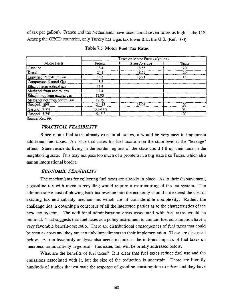
of tax per gallon). France and the Netherlands have taxes about seven times as high as the U.S.

Among the OECD countries, only Turkey has a gas tax lower than the U.S. (Ref. 100).

Table 7.5 Motor Fuel Tax Rates

Taxes on Motor Fuels (¢/gallon) Motor Fuels Federal State Average Texas

Gasoline 18.4 18.55 20 Diesel 24.4 18.59 20 Liquefied Petroleum Gas 18.3 15.21 15 Com_pressed Natural Gas 18.3 Ethanol from natural gas 11.4 Methanol from natural gas 11.4 Ethanol not from natural gas 12.95 Methanol not from natural gas 12.35 Gasohol. 10% 12.4-13 18.06 20 Gasohol. 7.7% 13.8-14.2 20 Gasohol. 5.7% 15-15.3 20 Source: Ref. 99.


Since motor fuel taxes already exist in all states, it would be very easy to implement

additional fuel taxes. An issue that arises for fuel taxation on the state level is the "leakage"

effect. State residents living in the border regions of the state could fill up their tank in the

neighboring state. This may not pose too much of a problem in a big state like Texas, which also

has an international border.


The mechanisms for collecting fuel taxes are already in place. As to their disbursement,

a gasoline tax with revenue recycling would require a restructuring of the tax system. The

administrative cost of plowing back tax revenue into the economy should not exceed the cost of

existing tax and subsidy mechanisms which are of considerable complexity. Rather, the

challenge lies in obtaining a consensus of all the interested parties as to the characteristics of the

new tax system. The additional administration costs associated with fuel taxes would be

minimal. That suggests that fuel taxes as a policy instrument to contain fuel consumption have a

very favorable benefit-cost ratio. There are distributional consequences of fuel taxes that could

be seen as costs and they are certainly impediments to their implementation. These are discussed

below. A true feasibility analysis also needs to look at the indirect impacts of fuel taxes on

macroeconomic activity in general. This issue, too, will be briefly addressed below.

What are the benefits of fuel taxes? It is clear that fuel taxes reduce fuel use and the

emissions associated with it, but the size of the reduction is uncertain. There are literally

hundreds of studies that estimate the response of gasoline consumption to prices and they have

168

produced a wide range of results. Before recent estimates are presented, some background

information is in order.

Estimating The Response Of Gasoline Consumption To Changing Prices

The response of gasoline consumption to a change in price is measured with the price

elasticity of demand. This measure expresses the percentage change in gasoline consumption

that is caused by a 1 o/o change in the price. For example, if a price increase of 10% leads to a

decrease in purchases of 5%, then the price elasticity of demand is -5%/10% = -0.5. A higher

elasticity (in terms of absolute value) implies a more sensitive response to price changes. (In the

following, references to the size of an elasticity are in terms of absolute value).

Demand elasticities can be estimated from historical data. However, the results of these

estimations depend crucially on the type of model used, on the time period studied, and on the

units of observation - individual households, or aggregate sales data. For example, as a rule of

thumb, cross-sectional data yield higher elasticity estimates than time-series data, and data on the

household level higher estimates than aggregate data. We comment on a number of issues that

are germane to price elasticity estimates produced over the years. This discussion is by no

means exhaustive, and does not touch on the technical issues of model specification. However,

it may provide a flavor of the complexities involved in estimating the relationship between

gasoline demand and prices.

First, it is important to distinguish between the short-run and the long-run. The short-run

is defined as the period for which the vehicle stock is fixed, that is, people can respond to a

change in price only by changing driving behavior. In the long-run, as the vehicle stock turns

over, people have the opportunity to choose vehicle efficiency. This suggests that long-run price

elasticities of demand are higher than short-run elasticities, a pattern which indeed is verified

empirically. (Short-run estimates are produced with different data and different model

specifications. Typically, in estimation of long-run elasticities the vehicle stock is represented

endogenously, i.e. the demand for vehicle characteristics are modeled explicitly.

Second, it is important to recognize that some price responses are irreversible. In the

past, high gasoline prices have forced fuel efficiency of new vehicles to improve. This technical

progress will not be reversed. People may buy bigger and more powerful vehicles when prices

fall, but the fuel efficiency of a given vehicle type is not going to deteriorate. (For a discussion

and estimation of this effect, see Ref. 78, 101, and 102). Thus, demand does not behave

symmetrically. A steep price increase may have led to reduced fuel consumption, but a

comparable price decline will not make gasoline demand return to earlier levels. This

asymmetry of demand behavior implies that high estimates of the price elasticity of demand,

obtained from periods of steep price increases, cannot be applied to declining prices.

169

Third, there has been a historical shift in gasoline demand, paralleling demographic

developments and an increased saturation with vehicles. Not only did the baby boom generation

come of age, but more people of driving age were licensed as well. In 1960, 75% of all adults

had driving licenses and by 1990 this number rose to 90% (Ref. 101). Women entering the labor

force accounted for a large share of this increase. At the same time, per-capita ownership of

vehicles increased tremendously. In 1966, there were about 0.85 vehicles per driver, compared

to 1.1 vehicles per driver in 1990 (Ref. 101). This means that the U.S. has moved towards a state

of affairs where the demand for driving is no longer constrained by the vehicle stock. Most

people that want to drive have a license and access to a vehicle and many people have access to

more than one vehicle. Vehicle ownership has moved close to saturation. This will make

gasoline demand more elastic, in the short-term as well as the long-term, all other things being

equal.

Fourth, the responsiveness to fuel prices varies not only with time but also with place.

The extent to which drivers can shift away from the automobile depends on land use patterns and

infrastructure. In the densely populated countries of Western Europe that have a well developed

public transportation system, price elasticities of demand for gasoline have been estimated to be

much higher than for the U.S. Within the U.S., there is a fair amount of regional variation. Not

surprisingly, people in Western states drive more than in the Northeast and one-vehicle driving

tends to be less elastic. However, driving by households with more than one vehicle seems to be

more elastic than in other parts of the country (Ref. 103).

Recent Estimates Of The Price Elasticity Of Demand For Gasoline Consumption

The most comprehensive survey of gasoline demand elasticities to date is Dahl and

Sterner (Ref. 104, 105). They surveyed more than one-hundred studies and found the following:

For the U.S., short-run elasticity estimates vary from -0.12 to -0.41 and for the long-run vary

from -0.23 to -1.05 (Ref. 104). Supplemental analysis of the effects of a tax on gasoline for a

number of OECD countries and, after careful deliberations of the various estimates, resulted in

an adjusted value of -0.18 for the short-run and -1.0 for the long-run price elasticity of demand

for gasoline in the U.S. (Ref. 100).

Recently, efforts have focused on the use of household data from the 1990 National

Personal Transportation Survey to find short-run price elasticities of demand for gasoline (Ref.

103, 106). This research effort differentiates between households with one, two, and three or

more vehicles, explicitly allowing for substitution of travel by different vehicles within a

household. This is a novel model specification. The rationale for this distinction is that

households with several vehicles make different choices than one-vehicle households. In recent

years, multi-vehicle households have increased to the extent that they now account for a large

170

share of all car travel. A third of all vehicle miles of travel (VMT) is done by households with

three or more vehicles (Ref. 103). With more substitution possibilities (from fuel inefficient to

efficient cars), these households should have a more elastic gasoline demand. This is indeed

borne out by the data. The authors estimate an elasticity of -0.78 for three-or-more vehicle

households, an elasticity of -0.41 for two-vehicle households, and an elasticity of -0.29 for one

vehicle households. Weighted by VMT of the different household types, the average is -0.51.

The households reported in the National Personal Transportation Survey are also

differentiated by income class, region of the country, and location (urban, suburban, and rural).

Price elasticities of demand differ by region and by location. Elasticity estimates for the South

and West are higher than for the Northeast and the North Central region.

The same researchers also estimated the impact of the 4.3¢/gallon increase in the gasoline

tax instituted in 1993. It is estimated that gasoline consumption dropped by 1.9 billion, or

1.89%, and VMT slightly less, due to a small amount of substitution between VMT across

vehicles (Ref. 106). This suggests that the high price elasticity of gasoline demand for three-or

more-vehicle households is due more to VMT reduction than to substitution between cars.

Presumably, these households do a greater amount of discretionary driving.

IMPLEMENTATION AND EQUITY ISSUES

As already mentioned, the one feature of motor fuel taxes that might be most important to

their implementation are their distributional consequences, perceived or real. Rising gasoline

prices will affect consumers since they increase the cost of driving. This is a direct effect. Since

gasoline is an important input for many businesses, product prices will rise, too. Insofar as

gasoline supplies are affected, supply prices might rise. Since consumers experience a real

decrease in their disposable income when gasoline and other product prices rise, macroeconomic

activity will be dampened eventually. To discuss these indirect effects and present detailed data

from the literature is beyond the scope of this report, hence, the focus is on the direct

distributional impacts, and macroeconomic implications will be discussed briefly.

Direct Distributional Effects Of Fuel Taxes

Fuel taxes are clearly regressive. In other words, low income households have to give up

a larger share of their budget in additional taxes than high-income households. For one, this

comes about simply because high-income households have more money to spend. But there are

also more specific travel-related reasons for this regressivity: 1) the amount of driving done by

low-income versus high-income household, and 2) the fuel efficiency of their vehicles.

Beginning with the latter, low-income households tend to have older vehicles which are less fuel

efficient. While high-income households also own a great number of old vehicles, low income

households tend to have mostly old vehicles.

171

The evidence on the driving issue is mixed. In some areas of the country, low income

households drive less, in other parts they drive as much or even more than high income

households. This is a function of land use patterns. In the Northeast, many low income persons

tend to live in urban centers, while higher income households live in the suburban areas and

commute longer distances. In California, however, the picture is more mixed. There are many

self-sufficient urban centers that cater to the better off. At the same time, many economically

disadvantaged persons live in communities that do not have access to a range of services and

they have to drive longer distances (Ref. 107). * The situation in Texas might be more similar to

California than to the Northeast.

Indirect Macro-Economic Effects Of Fuel Taxes

Here again, the type of model and their assumptions are crucial to the outcome of the

analysis. Of particular importance is the treatment of the tax revenue. Most of the studies in the

1980s assumed that fuel tax revenues would be used for deficit reduction, the benefits of which

are not felt in the short- or even intermediate-term. Thus, for all practical purposes, the tax

revenue was siphoned off the economy. Studies in the later 1980s and 1990s began to explicitly

model the use of the tax revenue, i.e. its reintroduction in the economy.

Results of the early modeling efforts all point in one direction: seen in isolation, a

gasoline tax would decrease social welfare (output and consumption) more than it raises taxes.

As to its distributional impacts, if indirect macroeconomic effects are included, regressivity

diminishes (Ref. 108). Another study from this same period concludes that" ... the results of

recent studies, comparing the macro-economic impacts of gasoline taxes with other tax options,

suggest that near-term income losses from a gasoline tax would be roughly comparable with

those from other tax options" (Ref. 76).

The Public's Perception Of Equity

Gasoline taxes are perceived as inequitable, more so than other policies that impact

people in comparable ways. A recent Gallup survey found that people felt a 25¢/gallon gasoline

tax was inequitable, while they did not perceive gasoline rationing as such, although the latter

imposed a much greater cost (Ref. 109). In general, protectionist schemes raise prices of

consumer goods, for example textiles and clothing. These policies impact lower income groups

more than other groups since these goods constitute a larger share of the lower income group's

budget. Thus, while it is true that a gasoline tax is regressive, the same is true for many other

policies, but these tend not to generate the same amount of public opposition. A possible

* Personal communication with Bob Huddy, Southern California Association of Governments, 1994.

172

explanation is that these policies benefit small interest groups significantly, while a gasoline tax

does not (Ref. 109).

VMT AND CONGESTION CHARGES

The motivation for VMT charges is that distance traveled is a fair basis to allocate the

cost of road construction and maintenance, especially if it is graduated by vehicle type. Because

of different fuel economies, current fuel taxes do not adequately measure level of system use.

All vehicles are taxed at the same rate, although most vehicles consume fuel at a different rate.

Even more important, the fuel consumption of a motor vehicle is an insufficient indicator for

road maintenance and rehabilitation needs; the axle weights of the vehicle plays a more crucial

role. This is why most states tax heavy trucks according to some measure of weight. Some

states also levy weight-distance charges (Ref. 110).

DESCRIPTION

VMT charges and congestion charges are not equivalent, but are often treated alike.

VMT charges are taxes on vehicle mileage. They can be assessed on odometer readings and

graduated according to vehicle type. Congestion charges are levied on the use of specific road

space at specific times. The basis for assessment is more complicated than for VMT charges,

since vehicle time and place has to be identified.

VMT taxes as a source of revenue for road construction and maintenance will become

more attractive as the motor fuel tax base shrinks. This is of special relevance in California,

where policies to introduce alternative fuel vehicles are most advanced. Another factor which

will make road builders more seriously consider VMT taxes is that ISTEA gives more room for

gasoline tax revenues to be used for purposes other than road construction and maintenance.

VMT charges are not only of interest to road builders; they can be used to address

various costs associated with transportation. If they are graduated according to fuel efficiency,

they would be almost equivalent to fuel taxes (the basis of the tax assessment would differ);

ungraduated VMT taxes would be a basis to charge for the cost of land use. By raising the cost

of driving, they would encourage high occupancy vehicle (HOY) and non-motorized transport

use. Theoretically, VMT charges could be levied on all kinds of individual travel - issues of

measurement and assessment aside. Arguably, other kinds of travel have a cost, too, but these

pale in comparison to the cost of car travel. The motivation of VMT charges is to induce people

to utilize transportation modes other than the single occupant car.

Congestion charges target congested roads. Congestion is costly to people, businesses,

and the environment. Apart from stress and inconvenience, congestion imposes great time costs

on drivers and businesses which can readily be translated into monetary terms. Vehicles in

173

traffic jams also use more fuel and emit far more air pollutants per mile than when freely

moving.

While public support for congestion pricing is tentative at best, the technology to assess

the basis for the charge exists and is already in use. Cities abroad, notably Singapore, have

demonstrated experience with congestion pricing.

VMT charges and congestion charges should not be viewed as mutually exclusive

alternatives. They address different costs and could be levied at the same time. Congestion fees

are an effective means to relieve congestion, which has environmental and social cost

implications; while a comprehensive, basic VMT charge could be levied to discourage general

automobile travel. If set at appropriate levels, both charges together can decrease congestion as

well as overall travel. However, it is important to recognize that a public body which levies

these charges might not have a maximum reduction of congestion and overall travel in mind;

rather, the charges may also fulfill the purpose of generating funds. If congestion or VMT fees

are implemented as revenue-raisers, it is unlikely that they would be set at levels which minimize

congestion or VMT.

As with any policy that raises revenues, the use of the generated funds is critical to the

acceptability of the policy. A policy package, in order to be successful, needs to earmark

revenues for the purposes of improving transportation and mitigating potentially adverse

distributional impacts. Specifically, revenue from congestion charges could be used for policy

measures and investments specifically targeted at reducing congestion, and revenue from VMT

charges for the maintenance of roads and other road-related infrastructure.

Uniform VMT charges levied on all vehicle VMT would decrease travel, and hence

energy use and emissions. The impact of congestion fees on total VMT, and therefore on energy

use, is not clear. While congestion fees would discourage driving at the peak traffic hours, they

might simply shift driving from peak periods to off-peak periods. Congestion charges also

generate new travel by attracting drivers with a higher marginal value of time. These drivers

would have stayed off the road because of congestion, but are willing to travel by automobile if

it takes less time. Finally, congestion charges could generate additional VMT by pushing drivers

onto other roads, causing them to drive longer distances. If the opportunity exists, drivers with a

lower value of time might opt to take a detour to get to their destination.

A properly constructed program of VMT and congestion charges would lead to a more

efficient transportation system. Simulations of a transportation model used by the California Air

Resources Board (CRAB) suggest that the total amount of VMT would decrease under both

VMT charges and congestion charges. This result applies for the four largest metropolitan areas

174

in California and depends on the congestion fees input in the model.* A simulation study for

Southern California predicts the same (Ref. 111).

CURRENT STATUS

Many other countries, and the U.S. to a lesser extent, have extensive networks of toll

roads. However, toll roads are not equivalent to a regime of VMT or congestion charges. While

drivers on a toll road are charged according to the mileage driven, this charge is not

comprehensive. Drivers can avoid the charge by using a toll-free road. Likewise, toll roads do

not graduate the charge according to time of day.

A rudimentary form of VMT charges exist in some U.S. states, as weight-distance fees

levied on commercial trucks. The rationale for this type of charge is the amount of VMT,

especially if graduated by vehicle type, is a fair basis to allocate the cost of road maintenance

and rehabilitation. The axle weights of a vehicle are critical factor in pavement consumption.

This is why most states tax heavy trucks according to some measure of weight; but only a few

states (8 in 1990) levy a charge on distance as well (Ref. 110).

The interest in congestion pricing has grown steadily, with the recognition that expanding

the existing infrastructure does not alleviate the congestion problem. New road space attracts

new cars. ISTEA lists congestion pricing as one of the policy measures to address traffic

problems and has promoted the development of pilot projects (Ref. 112, 113). DOT has begun

to study congestion pricing, and no doubt it will soon be instituted in some locations.

Several foreign countries have experimented with congestion pricing. Singapore was the

first to introduce a form of congestion pricing, as early as 1975. The initial system was very

simple - it restricted access to the inner city zone by requiring vehicles to display a special

license. This approach is called an area-licensing scheme. Later, electronic road pricing was

introduced. This policy succeeded in decongesting the inner city area. People shifted to buses

and to driving during off-peak hours. However, congestion in the surrounding region increased

(Ref. 114). Other cities that have experimented with congestion charges are Hong Kong, Oslo

and Bergen in Norway and Cambridge in England (Ref. 75, 113).

PRACTICAL FEASIBILITY*

Assessing VMT charges annually or semiannually, based on odometer readings, should

be easy. In locations where there are mandatory inspection programs, odometer readings could

be recorded as part of the annual inspection.

*Personal communication with Jeff Weir, California Air Resources Board. 1994. *The discussion in this section draws heavily on (Ref. 112, 113).

175

Assessment of congestion charges is more complicated. Individual vehicles have to be

identified by location and time of day. New technological developments for automated toll

collection, however, should assist in future efforts to implement congestion charging schemes ..

Electronic toll collection systems (ETC) operate with an antenna installed either

overhead, at the side of the road, or buried in the pavement. The first generation of ETC systems

consisted of very simple tags and complex readers. The tags would only transmit vehicle

information data ("read-only" or "passive" tags); the reading device on the road would feed the

observation into a computer which maintained an account for each vehicle. Readings from

different locations were then transmitted to a central facility. Technical progress has shifted the

computation of the fee liability to the vehicle tag ("active" tags, or "smart-cards"); information

processing can now be done on board, with the antenna emitting only very simple signals. These

battery powered active tags also eliminate a potential health hazard: they do not need to draw

energy from the antenna, thus allowing for a much weaker radio signal.

Early concerns over privacy violation were obviated with the smart card system. A

simple, "passive tag" ETC system would store data on individual travel behavior; if the

accounting is done on board, this should not be a concern. The smart card does not store data on

individual trips but can compute the toll charge liability directly. But even simpler systems

using passive tags can be organized in such a way as to insure privacy is maintained. For

example, drivers could sign up for numbered anonymous accounts that require prepayment.

Anecdotal evidence in California and Texas suggests that drivers are not too concerned about

privacy. The Dallas North Tollway offers numbered anonymous accounts, but few drivers have

selected this option.* A survey in California showed similar results. An ETC system in Hong

Kong, however, failed because of the privacy issue (Ref. 112). It is clear issues of privacy need

to be taken into account.

One alternative solution to the privacy concern is a "read/erase" tag which banks a certain

amount of credit points. This system would work like phone cards which are available in some

European countries, or like the farecards of the Washington, D.C. metro. Drivers could buy a

tag, worth a certain amount of dollars of congestion charges. The devices in the road would emit

signals carrying information about the price of driving at that time; charges would be deducted

from the tag as the car passes the emitting devices in the road.

Over the last five years, ETC facilities have been built in a number of places in the U.S.:

two bridges in New Orleans, LA; several highways in Oklahoma; and two toll road systems in

Texas (the Dallas North Tollway operated by the Texas Turnpike Authority, and a system of

highways in Houston operated by the Harris County Toll Authority).* A number of additional

* Personal communication with Bob Poole, The Reason Foundation, 1994. *Personal communication with John Carrera, Goodman Corporation, 1994.

176

facilities are proposed for the Dulles Toll Road connecting Dulles Airport to the D.C. urban area,

and for the tri-state region of New York, New Jersey, and Pennsylvania (Ref. 113). Abroad,

ETC is practiced in Norway, Spain, Italy, France, and Mexico.

ECONOMIC FEASIBIUTY

Whether VMT and congestion pricing are economically feasible depends on the relation

of benefits to cost and the methods to recover these costs. From the operating authority's point

of view, fee collections have to be greater than system costs; from a societal point of view,

societal benefits must exceed societal costs. A full-scale societal cost-benefit analysis includes a

number of costs: the cost of constructing and operating the system and the losses in social

welfare (if any). On the benefit side, there are the savings in automobile operating costs, the

savings in road maintenance costs, the social welfare changes resulting from the use of the

revenues and, foremost, the time savings from decreases in congestion. In this section, attention

is given to the real resource cost and to the anticipated energy savings of VMT and congestion

pricing. Potential welfare and distributional effects are discussed in the section on

implementation.

There are few estimates of administrative costs in the VMT pricing literature. An

estimate of about $100 million has been made for a VMT fee in Southern California (Ref. 111).

With 7.26 million cars operating in the region, that would amount to $14 per vehicle. VMT

charges should be cheaper to implement and administer than congestion charges; hence, in this

section, the focus is on cost estimates for congestion pricing. The cost components of

congestion pricing include installation, maintenance and operating costs both for the reading

devices and the vehicle tags.

Hong Kong has some experience with an electronic pricing scheme that uses passive

vehicle tags. This system was operative from 1983 to 1985. Total system capital cost was U.S.

$31 million (all cost estimates for this case study are in 1985 U.S. dollars), of which a little less

than half was accounted for by the vehicle tags. About 210,000 vehicles were equipped with

tags at a cost of $59, plus a 10% installation cost. The annual operating cost was about $ 2.5

million. Assuming a capital recovery factor of 0.125, the annualized capital cost accounted for

three-fifths and the annual operating cost for two-fifths of system expenditure. Assuming 260

operating days and 550,000 trips made on each of those days, the cost per transaction amounted

to 6.6¢ (Ref. 113). Today, this estimate would be far lower because electronics have become so

much cheaper. In 1992, the price of vehicle tags had fallen by two-thirds (Ref. 113).

Another example is the ETC facility proposed for the Dulles Toll Road in Virginia. The

capital cost of this project is anticipated to be $16.5 million, and the operating cost $5 million in

1990 (most of the operating cost is caused by operation of the in-ground antenna). Anticipated

177

daily traffic is 70,000 vehicles, yielding 250,000 transactions. The cost per transaction is

estimated at 7.7¢ in 1990 (Ref. 113).

A smart card system proposed for the Randstad Area in the Netherlands (comprising

Amsterdam, Den Haag, Rotterdam, and Utrecht) was found to cost about 12¢ per transaction (in

1990 U.S. dollars) (Ref. 113).

Finally, it is estimated that collection costs for a congestion fee scheme in Southern

California would amount to some 4.4% of revenues (Ref. 115). Given these costs, it is clear that

congestion pricing is economically feasible. Even for modest fees, system costs are a small part

of fee revenues (less than 10%). As stated before, the administrative costs of VMT fees are

likely to be much smaller.

The administrative and operating costs of congestion and VMT charges must be

compared to the energy and emissions benefits. An assessment of these benefits has to rely on

estimates of the reduction in VMT. Presumably, VMT charges would lead to a greater reduction

in travel than congestion charges. An estimate for a reduction in VMT from VMT charges

constitutes an upper bound for an estimate in the reduction in VMT due to congestion charges

(provided the charge levels are comparable). This is because, as discussed previously,

congestion charges simply shift some travel from peak to off-peak times and could generate

additional VMT for some drivers.

Estimates for gasoline price elasticities could be useful in assessing the impacts of VMT

charges. For an individual vehicle, with a given fuel efficiency, VMT charges can be translated

into a charge per gallon of fuel. This can be done in an aggregate fashion for the entire fleet, but

this method is likely to produce inaccurate results because it does not account for the fact that

individual drivers are charged at different rates.

An alternative is to look at the results of a specific model simulation and infer aggregate

responses. A 1994 study by Cameron investigates the effect of a VMT charge and a congestion

charge on personal automobile travel in Southern California (Ref. 111). The study utilizes the

TRIPS travel demand model. TRIPS expresses the demand for personal travel by mode as a

function of travel cost, income, and other socio-economic characteristics of households (Ref.

116). Travel demand is modeled separately for each income quintile.

First, the model is simulated for a $0.05 per mile VMT charge. A fee of this size would

raise roughly the same amount of revenue as all current transportation fees and taxes combined

(Ref. 111). For a vehicle with an average fuel efficiency of 25 mpg, this fee would translate into

a $1.25 per gallon fuel tax. The average cost of owning and operating a vehicle in Southern

California amounted to $0.37/mile in 1991 (the year for which this study was done); with the

operating cost accounting for 27% of the total or $0.10/mile (Ref. 111). Thus, a VMT charge of

$0.05 per mile would raise the operating cost by 50%.

178

Simulating the imposition of a $0.05 per mile VMT charge for the year, total personal

automobile VMT would decrease by 11%, from 101.5 billion vehicle miles to 90.3 billion (Ref.

111 ). This reduction in car travel is partly replaced with an increased demand for public transit,

which increases by 50%, from 2.2 billion passenger miles to 3.3 billion (Ref. 111). The 11%

reduction in auto VMT implies an average price elasticity of demand of -0.22 for car VMT (-

11%/50% = -0.22).

The study also looks at the external air pollution cost caused by car travel and the cost of

congestion. Drawing on a study of health impacts of air pollutants 03 is valued at $3,256 per ton

and particulate matter (PM10) at $87,173 per ton (Ref. 111). Given these values, a $0.05 VMT

fee would reduce air pollution costs by 40% from $3.7 billion to $2.2 billion (Ref. 111 ).

Congestion costs are measured as the time loss incurred by individuals, valued at their time

price. This price ranges from $2 per hour for the lowest income quintile to $15 per hour for the

highest quintile (Ref. 111). A $0.05 VMT fee would reduce congestion costs by around 26%, or

$5.7 billion to $7.7 billion (Ref. 111).

A congestion fee that would raise the same amount of revenue as the VMT charge is also

estimated. A simple pricing regime with one peak-time price ($0.17) and a zero off-peak price is

used. It is assumed that 30% of all vehicle travel occurs at peak times when a charge is in effect

(Ref. 111 ). Simulating this fee with the TRIPS model yields a smaller reduction in VMT than

the VMT charge of $0.05 per mile. This is because some vehicle trips are shifted to off-peak

hours. The congestion fee does lead to a larger reduction in congestion costs than the VMT

charge (congestion cost is measured in hours lost multiplied by individuals' value of time). This

is because the people who benefit from the decrease in congestion and still chose to drive in peak

hours and pay the fee, have a high value of time.

It appears that the model does not consider induced travel, or latent demand - that is, it

does not account for people who are induced to driving because of less congested conditions

(Ref. 111).

EQUITY AND IMPLEMENTATION ISSUES

It is interesting to note that less than ten years ago, congestion charges and the associated

technologies of ETC and automatic vehicle identification (A VI) were thought to be futuristic.

The following quote reflects the opinion of the time: "The DOT study suggests that such

programs are decades away from full-scale implementation, even if they survive public opinion"

(Ref. 76, 117). Today, it is clear that VMT pricing and congestion pricing are both technically

and economically feasible-the revenues from effective charges (charges that would noticeably

impact congestion levels) would far exceed the costs of installation, maintenance, and

administration. Congestion pricing is generating a great amount of interest. The National

179

Research Council has just completed a comprehensive study on implementation issues. The

challenge for implementing VMT and congestion charges lies in the political and institutional

arenas.

A key obstacle to implementing VMT and congestion charges are the perceived

distributional effects. Congestion charges have more pronounced distributional consequences

than VMT charges. Congestion charges are an attractive policy for drivers from the upper-end

of the income scale. They benefit because the time savings they gain outweigh the toll charges.

The higher the time price of these drivers, the higher the charge they are willing to pay. Low

income drivers will lose since to them, the gains in time will not match the charges they have to

pay. If there is no cap on congestion charges (and in order to relieve congestion, they should be

allowed to be set at a level that deters a sufficient number of drivers), they could prove

prohibitively high for lower income classes. This would be severely inequitable if no

transportation alternative is available.

To see how people from different income brackets differ in their response to road pricing,

recall the California discussion. The simulation of the TRIPS model yielded a -0.22 aggregate

price elasticity for VMT. But these elasticities greatly differ for drivers with different incomes.

For the lowest income quintile, the price elasticity of VMT demand is -0.59; for the middle

quintile, it is -0.33; and for the highest quintile, it is -0.06. Since high income households drive

more often and barely react to VMT charges, they also shoulder most of the burden. They would

incur $570 per year per capita, while the lowest income quintile would incur $110 per capita

(Ref. 111).

A VMT and congestion fee policy package will be more successful if it addresses these

distributional impacts. Analysts point out that a number of corrective measures aimed at

different groups could be attached to a congestion fee policy package to ensure that every person

impacted by the policy is covered (Ref. 115). Corrective measures include commuting

allowances for employees, cash-out parking, improved transit, and reduced property and road

user fees and taxes.

PAY -AS-YOU-DRIVE-INSURANCE (PA YDI)

Pay-as-you-drive-insurance (P A YDI) is an automobile insurance system that shifts

premium payments from the flat fee to fees levied on driving activity. There are two basic

variants: Pay-at-the-Pump (insurance fees are levied on gasoline) and Pay-by-mile (fees are

assessed based on odometer readings). Each system would complement the variable fee with a

flat fee, covering insurance against risk that is not related to driving distance. This insurance

system would not involve any public funds, except for a small amount to cover administrative

costs that might arise with the Pay-at-the-pump version.

180

DESCRIPTION

P A YDI was conceived as a scheme to deal with the inequities and the excessive legal and

administrative costs that characterize the American motor vehicle insurance system. Both

PA YDI proposals are "no-fault" systems which should lower insurance premiums significantly.

However, this option is not a necessary element of the underlying concept of transforming a flat

premium payment into a variable one. Although PA YDI did not originate out of a concern for

energy consumption or air pollution, it obviously has important implications for these issues.

The Pay-at-the-pump version would act like a gasoline tax, and the Pay-by-mile version

like a VMT charge. P A YDI would not address congestion costs (recall that only a small share of

congestion costs are due to decreased fuel efficiency). In addition, it would only address those

pollutants which are proportional to fuel use, C02 and S02. The Pay-at-the-pump version would

address these pollutants directly; the Pay-by-mile version less so, because of differing fuel

efficiencies. The net impact of PA YDI on VMT is not clear. By raising the cost of operating a

vehicle, it provides an incentive to drive less. By lowering the fixed cost of owning a car, it

could increase vehicle sales.

Pay-at-the-Pump

The Pay-at-the-pump version has strong advocates in California, where it recently was

proposed to the legislature. It is known as PPN ("Private Pay-at-the-pump No-fault insurance").

PPN consists of two kinds of premium payments that complement each other: a fixed fee, paid

when the vehicle is registered, and a fee on gasoline. The fees would be collected by a state

agency and disbursed to private insurance companies. Two variants have been suggested. The

first would let insurance companies serve individual customers, as is presently the case. The

state agency would simply administer the premium payments, that is, collect them and pay them

out to the insurance companies according to the policies they have sold. The second variant

would form pools of drivers which private companies could compete to cover. A state insurance

commissioner would act as an auctioneer. The no-fault feature would reduce the share of the

premiums that are in effect legal fees that at present are 19% of the premium revenues (Ref.

118). Centralized collection, it is argued, would reduce overhead costs by 23% of the insurance

premium (Ref. 118)). Linking insurance premiums to the amount of driving is equitable and

efficient because those who drive more have higher probabilities of being involved in an

accident. Finally, this system would insure the uninsured, further reducing premiums through

spreading risk over a greater pool of drivers. Under the status quo, people spend great amounts

to insure themselves against damage from uninsured motorists. A side benefit of reducing the

number of uninsured drivers would be savings in legal enforcement and monitoring costs.

The variable fee is a uniform amount per gallon of gasoline. It is to account for all the

risk incurred with driving. The version proposed in California would include optional coverage

181

against driving-related risk, such as collision and medical insurance. Drivers choosing not to

elect this coverage could receive a refund, based on some evidence of the amount of miles

driven. The flat fee is to account for administration costs, coverage of risk that is not related to

driving (theft and fire) and to adjust for different risk classes and vehicle types with different fuel

efficiencies. This feature is problematic in two ways, one relating to the efficiency of insurance

and the other relating to the aspect of energy savings.

Levying the premium at the pump means no distinction can be made between drivers

belonging to different risk groups. Rather, the incremental fee is based on an average driver

profile; more specifically, the anticipated average annual insurance premium per vehicle divided

by an estimate of the average statewide amount of miles driven per vehicle. This lack of

differentiation constitutes an inefficiency from the insurance point of view - one of the very

concerns that generated the interest in P A YDI. Two variables determine the efficient amount of

insurance coverage: classification - the risk group that the insured belongs to - and exposure.

The cost of exposure differs according to the risk group to which an individual belongs. The

California proposal takes account of different risk classes and vehicle types by adjusting the flat

fee. People with a lower risk classification would receive a discount, since they cause less cost

to the system than higher risk groups, but the proposal does not link the risk to exposure

(distance driven).

From the perspective of energy consumption, the lack of differentiation between driver

and vehicle types does not matter. People should be charged according to the fuel they consume

(presumably, emissions are roughly proportionate to fuel consumption). Fuel efficient vehicles

should be charged less than fuel intensive ones. The California proposal, however, would adjust

the flat fee for fuel efficiency. This is an attempt to account for the fact that exposure is not

equivalent to the gallons of gas consumed, but to mileage driven. People who drive relatively

inefficient cars would receive a rebate, because they use more gas and hence pay a higher rate

per vehicle mile driven. Unless people kept a record of their gas purchases or had their odometer

read, the rebate would not capture the amount of over- or underpayment. If rebates would be

assessed correctly (i.e., computed from the fuel efficiency of the car and the miles driven), then

this would obviate the incentive to drive fuel efficient cars.

Clearly, the goal of making insurance payments more efficient and equitable (in the sense

that people should be charged according to the risk they cause) is in conflict with the goal of

furthering fuel efficiency. The rebate that is supposed to compensate drivers of cars that use a

lot of fuel is equitable from the point of view of paying for insurance, but it is at odds with the

goal to further fuel efficiency. It seems awkward to adjust the variable fee payments by a fixed

amount in order to compensate for differing fuel efficiencies. This mechanism allocates neither

182

insurance costs nor the external costs of fuel use in an efficient way. The attempt to address both

conflicting objectives at once compromises each of them individually.

Pay-by-Mile

The alternative scheme, the Pay-by-mile proposal, is advocated by the National

Organization of Women.* Their motivation is the concern for discrimination against women and

low-income drivers. People belonging to these groups tend to drive far less than the rest of the

population, causing less cost to the pool of drivers. Yet, they pay the same amount of insurance.

Under the Pay-by-mile system, insurance premiums would be split into a flat fee, covering risks

related to ownership and a variable fee covering risk related to driving distance.

The crucial difference from Pay-at-the-pump insurance is the rate per VMT can be

tailored to the individual driver. The issue of different fuel efficiencies does not even arise

because the basis for the charge is VMT, which is the variable that drives insurance cost. For

each driver class, insurance would be formulated as a rate per mile. Drivers would purchase

insurance once or twice a year, based on the miles they anticipate to drive. Should they drive

more than anticipated, they could buy additional insurance. Should they drive less, then they

could apply the credit at the next annual or semiannual payment date. Pay-by-mile would not

require any third party involvement. The mileage would be verified through an odometer audit

that would be the responsibility of the insurance company, who could arrange this audit to be

performed through a state agency, if it should prove more cost-effective.

From an insurance point of view, the pay-at-the-pump scheme is superior. It accounts

accurately for the risk that individual drivers cause. Also, it would imply a small change of the

existing insurance system and would be less of an administrative burden. However, it would

provide a weaker incentive for energy conservation, since the link between driving and fuel

consumption is weaker. It is also possible people are more sensitive to costs they incur in the

present than to those costs they incur in the future. Pay-at-the-pump, one could argue, makes the

cost of driving more visible than annual or semi-annual payments. Pay-by-mile also would not

automatically capture uninsured drivers.

CURRENT STATUS

In California, PPN was proposed to the legislature as Senate Bill 684. The bill proposed

a $100 payment at vehicle registration and a $0.35 charge on a gallon of gasoline. The bill failed

to leave the Senate Judiciary Committee. A new initiative is proposed for the California ballot,

with a slightly altered fee structure that involves a higher flat fee of $141 and a lower gas

*Personal communication with Pat Butler, National Organization of Worrnen, 1994.

183

surcharge of $0.25 per gallon (Ref. 118). The Pay-by-mile version ofPAYDI was introduced to

the Pennsylvania legislature, as Senate Bill 775, but it was not brought to the floor either.*

PRACTICAL FEASIBILITY

No PA YDI is in effect as yet, but proposals for both versions of PA YDI are detailed and

specific. The Pay-by-mile version implies a minimal change in existing regulations; it would

simply require a restructuring of insurance payments. The burden of assessing motorists'

mileage would fall on insurance companies who could use third party auditing. For example, the

state could cooperate by reading mileage at mandatory inspections, but this is not essential. No

additional public agency needs to be involved in automobile insurance. Clearly, this seems

feasible from a technical point of view.

Pay-at-the-pump would require a more complex system. Money paid at the pump needs

to be transferred to a state agency which acts as an intermediary to the insurance companies; a

model explored in the course of the current discussion of national health care reform. Some of

the mechanisms for assessing rebates seem cumbersome. Requiring people to produce proof of

gasoline purchases over the course of a year is impractical. The most recent PPN proposal in

California has done away with this feature.


Again, there are no estimates of the administration costs associated with these insurance

systems. Given the technical features previously described, one can speculate that the

administration cost of Pay-by-mile is minimal. There will be a cost to the insurance business to

restructure fees and meter mileage. The Pay-at-the-pump version would cause a greater

administrative burden than the Pay-by-mile version, but it seems fair to assume these costs

would be outweighed by the benefits of a P A YDI system.

Some of the benefits have already been noted. For one, the no-fault option might reduce

premiums by more than 19% (Ref. 118). Centralized collection could reduce overhead costs

which at present account for 23% of premium payments. Uninsured motorists, which constitute

some 20% to 30% of all drivers in California, costs each insured California driver $150 (Ref.

119). To the extent that insurance payments are linked to driving, the system makes for

horizontal equity.

In terms of its effect on fuel consumption, PA YDI should act as a fuel tax (in the Pay-at

the-pump version) or a VMT charge (in the Pay-by-mile version). Recall that gasoline demand

elasticities are estimated to be between -0.18 and -0.51 for the short-run and -1.0 for the long

run. A surcharge of $0.25 per gallon of gasoline would constitute a price increase of about 20%.

*Personal communication with Pat Butler, National Organization ofWonnen, 1994.

184

If the high short-run elasticity of -0.5 holds, gasoline consumption would decrease by 10%, all

other things being equal. The Pay-by-mile version is equivalent to a VMT charge, but aggregate

VMT demand elasticities are not applicable because individual drivers face different rates.

Recall however that PA YDI, by virtue of lowering insurance cost, might attract some marginal

vehicle buyers to the market.

The times of collection may play a role in the way motorists respond to variable

insurance charges. A great deal of evidence exists which shows people are more sensitive to the

costs they incur in the present than to the costs they incur in the future. For example, people

tend to have very high discount rates when it comes to taking measures which increase energy

efficiency. One reason is people tend to have a positive time preference (preferring consumption

now to consumption later), but evidence also exists which shows the cost associated with

monitoring expenditures and transforming future costs and benefits into present values is very

high. In this context, one could argue that Pay-by-mile insurance, which is paid annually or

semiannually, might not be as effective in making the cost of driving visible to people as Pay-at

the-pump insurance.

IMPLEMENTATION ISSUES

Clearly, both PA YDI systems would enhance equity as well as economic efficiency

because they would link insurance payments more closely to the activities and individuals that

cause it. For individuals that drive infrequently, this means a decrease in insurance payments. A

no-fault option would reduce premium payments significantly because legal fees in litigation

cases constitute a large share of insurance costs. Furthermore, the Pay-at-the-pump version of

P A YDI would cover uninsured motorists. For all of these reasons, P A YDI should be politically

appealing.

CONCLUSIONS AND RECOl\IIMENDATIONS

There is no doubt increasing vehicle fuel efficiency is critical to reducing energy

consumption in transportation (Ref. 35). A straightforward method to increase vehicle fuel

efficiency is to mandate it by imposing standards on manufacturers. This has been the policy of

preference in the U.S., in the form of CAFE standards. Alternative policy proposals suggest

giving manufacturers incentives to improve vehicle fuel efficiency through a system of taxes and

rebates which affect the sale price. In this way, consumers have an incentive to buy more fuel

efficient cars, and manufacturers are free to react to consumer needs as they see fit. But

targeting vehicle fuel efficiency alone does not address the problem of induced demand for

travel. If fuel efficiency increases, the cost of driving decreases, which could lead to more VMT.

185

INDUCED TRAVEL, FIXED COSTS, AND VARIABLE COSTS

The problem of induced travel does not only pertain to fuel efficiency. It looms large

over all transportation planning efforts and applies a fortiori to the provision of alternative travel

modes as well. In other words, travel can be induced by improved traffic flows and better access

to travel technology. There is evidence indicating people budget their time such that the share

devoted to travel stays roughly constant. They will cover greater distances as transportation

access and travel speed increases (Ref. 120). This applies to recreational as well as to commuter

travel. Experience in Germany has shown the introduction of high speed rail is accompanied by

a significant increase in VMT.

Thus, addressing vehicle fuel efficiency either through standards or incentives to

manufacturers is an important policy; but if the intent of the policy is to contain the social costs

of transportation (related to fuel consumption, pollution, and land use), increases in fuel

efficiency need to be complemented with policies which address the amount of travel itself.

Increasing the variable cost of traveling to the traveler, rather than its fixed cost, is a step towards

this goal.

Policies which increase the variable price of travel, and car travel in particular, are fuel

taxes, taxes on VMT, parking fees, pay-as-you-drive-insurance, and so on. Fuel taxes have the

advantage that they not only address the activity of traveling, but influence technology as well.

They provide an incentive to drivers to reduce their travel, and an incentive to manufacturers to

increase the fuel efficiency of their vehicles. (Should the latter outpace the former, then the cost

of travel might still decrease.)

It is also important to increase public awareness of transportation costs by unbundling

travel costs and making them more apparent to the taxpayer. Transportation projects funded

from road bond issues which are paid by property andfor sales taxes, rather than directly by

drivers is an example. Change in these tax practices is crucial for realistic policy-making. A

fundamental shift is needed in the taxation and charging policies so as to make hidden costs less

transparent to users.

INTERACTION BETWEEN DIFFERENT POUCY GOALS AND TARGETS

The list of social impacts and costs of transportation is too large to enumerate in this

report; this has been done elsewhere (Ref. 51, 121, 122, 123, 124). However, it is important to

note different transportation policies target different social impacts and costs, and they are

interactive.

Take for example charges aimed at relieving congestion. Congestion results in a cost to

people and businesses due to time loss. Congestion is also responsible for a significant amount

of air emissions which would be less in free-flowing traffic. Another cost of congestion is the

186

increased fuel consumption per mile traveled. Congestion fees thus would impact air quality as

well as address congestion itself and the associated time loss. However, such fees might attract

some people to the road who would not have traveled by car otherwise. Since people with a high

value of time tend to be high wage earners, they would not be deterred by congestion fees. For

these people, driving becomes more attractive with decreasing levels of congestion. Thus,

congestion fees could in effect increase fuel use. This has been observed in a simulation study

with the STEP transportation model for the four metropolitan areas of California. The study has

shown congestion fees do generate new travel in the higher income classes. *

Another example of the interaction between policies and the conflict of goals are

pollutant emissions from fuel combustion. Some pollutant emissions are strictly proportional to

fuel use (SOx and C02), other emissions depend on the number of cold starts and vehicle speed

(NOx, HC, and CO). While improving fuel efficiency would reduce SOx and C02 emissions, it

would not reduce HC emissions significantly. Technologies to reduce HC emissions are

independent of the fuel efficiency of a vehicle. Thus, a tightening of emission standards on

vehicles does not imply a proportionate improvement in fuel efficiency, or vice versa. In fact,

the control technology for these pollutants is not at all related to technologies for improving fuel

efficiency (Ref. 73).

Important transportation policies such as the introduction of LEV s, ZEV s, and other

alternative fueled vehicles, are motivated by the concern for air quality, particularly in congested

urban areas and in the 03 transport corridor. Of course, these vehicles would reduce gasoline

consumption by virtue of the fact they do not run on gasoline, but their impact on overall energy

use is less clear. It cannot be said these types of vehicles are energy saving (in terms of

BTU/mile), especially if energy use over the whole fuel cycle is taken into account. For

example, ethanol and methanol fuels give rise to upstream energy consumption because they

depend on feedstocks which are grown with the use of fertilizers. The production of fertilizer is

in itself quite energy intensive.

The introduction of LEV s and ZEV s, apart from their impact on energy use in

transportation, will have important effects on other transportation policies. Their introduction

will reduce gasoline consumption and thus decrease tax revenues from fuel; LEV s and ZEV s are

tax exempt in some states (California, for example). This exemption will increase the need for

another source of revenue for funding the transportation system infrastructure. A universal fuel

tax, graduated according to emissions and energy embodied in the individual fuel, would address

all of the issues raised above.

*Personal communication with Jeff Weir, California Air Resources Board, 1994.

187

EQUITY AND IMPLEMENTATION CONSIDERATIONS

Each of the policies discussed in this chapter have distributional consequences. They

will impact some segments of the population more than others which has important political

implications.

For example, retirement of old vehicles might cause economically disadvantaged persons

to lose access to transportation, by affecting the secondary and tertiary vehicle markets in such a

way that the low income groups are priced out of the market. Another example is congestion

fees. If they are set high enough to be effective, then they may be unaffordable for some

economically disadvantaged people, thus constraining their mobility. Similarly higher fuel taxes

will affect the production and refining of oil, which is of special relevance in Texas.

In the economic theory of policy analysis, the allocation and distribution effects of a

policy are strictly divorced from each other. Economic efficiency is enhanced by a pricing

policy which accounts for the full cost of resources. This ensures that resources are used where

they produce the greatest value for all. Negative distributional consequences can theoretically be

mitigated by policies to effect transfers.

In practice, this mitigation is not easy to accomplish. Governments cannot freely dispose

of large amount of funds. Special provisions for economically disadvantaged consumers may be

a necessary feature for new policies. This may make an otherwise easy policy administratively

expensive. Direct offsets might need to be considered for higher taxes on vehicles and fuels such

as targeted income tax reductions, transit vouchers, or other means-tested aid for lower income

classes whose access to employment and other necessities could be harmed by transportation

pricing policies.

A related issue is that taxes and fees earmarked for specific purposes may be more

palatable to the public than those that go into a general revenue fund. Additional taxes are

unpopular, for one, because people perceive that they are burdened enough, and second, because

they are critical of the governments' involvement in the economy in general, and doubt its

efficacy. Therefore, any policy which is anticipated to raise funds must be formulated with a

provision clarifying how the funds are to be used. Hence, the attraction of revenue-neutral

incentives, such as feebates and pay-as-you-drive insurance.

It is important to recognize that policies such as feebates and pay-as-you-drive insurance

have distributional implications, too, but they are not as visible and direct as, say, fuel taxes. For

example, a feebate scheme would adversely impact people who prefer more fuel intensive cars.

From an environmental perspective, it is clear people who use more fuel should pay more, since

they impose a greater cost on society. However, this feature of the feebate system-and any

schemes that discourage fuel intensive cars-are seen as unfair to those people who prefer bigger

cars, be it for reasons of safety, family size, or geographic location. Which of these reasons are

188

"legitimate" for people to be allowed to drive fuel intensive cars and not pay for it; and which

reasons are not legitimate? Take, for example, family size. An argument can be made that

family size is a matter of choice and people should pay for that choice. On the other hand. it

may be argued people who decide to have children are subsidizing the adults of today (because

they are raising the social security payers of tomorrow). Even if this is so, the question is should

these deliberations enter into pricing of vehicles? Economic theory suggests costs (benefits)

should be paid (accrued) for where they arise. Political reality, however, does not conform to

economic theory.

CONCLUSION

It is important to recognize that all fees and charges which are levied on driving, be they

fuel taxes, VMT charges, congestion charges, or Pay-as-you-drive insurance, will impact

gasoline use negatively, and with it the oil producers. For Texas, this distributional effect might

be the most important one. While the production of crude oil in Texas has steeply declined over

the last one and a half decades, the service and process sectors associated with oil are still an

important part of the state economy. The state is now sustained by oil imports. These sectors

and their jobs would be negatively affected by a decrease in gasoline use. Although this impacts

a relatively small share of the population, it could well be the most important obstacle in the way

of raising fuel taxes. Impacts which affect only a few people noticeably prove more important in

the political system than the impacts which affect a large constituency only a little. This is true

even if the aggregate effect of the former is smaller than that of the latter.

The answer to these concerns is to combine fuel taxes with measures which mitigate the

distributional impacts. There is extensive literature on the benefits of offsetting labor and capital

taxes (so-called distortion taxes) with pollution tax revenues (Ref. 125, 126, 127, 128, 129, 130).

There is ample opportunity for using gasoline tax revenues, not only to soften the impact on low

income groups, but to improve the efficiency of the tax system. The European Union, and

several individual member countries, notably Germany, are seriously considering adopting a

carbon tax and using the generated revenues to offset income and payroll taxes (Ref. 129). Such

a policy package is also feasible at the state level. While states are not at liberty to reduce

federal taxes, there is still room to improve state tax systems.

The impact of policies which restrict gasoline consumption on the local economy may

prove to be the hardest to compensate. A certain restructuring of economic sectors must take

place, if the U.S. is to be weaned off the high energy intensity of its economic activity. Also, it

is important to recognize most fees and charges which are levied on driving, be they fuel taxes,

VMT charges, or congestion charges have distributional consequences. The only possible

exceptions are feebates and Pay~As-You-Drive-Insurance which are designed to be revenue-

189

neutral. In addition, the administrative costs of a policy are an important feature which may very

well decide its fate. If a policy can be incorporated into the existing administrative mechanism,

it might have a better chance of succeeding.

190

CHAPTER 8-SUl\1MARY, CONCLUSIONS, AND RECOMMENDATIONS

Prior to the industrial revolution, sunshine, wind, and plant and animal growth were the

only forms of energy in use. After the 19th century, however, modem civilization became

increasingly dependent on fossil fuels, principally coal and oil. The oil embargo of the 1970s

was perhaps the turning point in terms of energy policies; it forced governments to face the fact

that fossil fuels cannot be taken for granted, and that alternative, renewable, and domestic energy

sources are necessary for consistent economic development.

The need for energy sources that are renewable, efficient, and environmentally friendly

cuts across all economic sectors. This study is dedicated to the critical examination of energy

policy for the transportation sector. The study is organized in two phases. First, the near-term

options for energy efficient transportation are identified and assessed. This is the subject of this

report. Based on this assessment, five transportation scenarios are constructed and their

associated energy consumption and air pollution emissions are estimated. This is the subject of

the second report, Strategies for Reducing Energy Consumption in the Texas Transportation

Sector.

SlJI\IIMARY

This report discussed and assessed near-term options for the transportation sector that are

renewable, efficient, and/or environmentally friendly. These options are classified into the

following categories:

(1) Transportation system management

(2) Technology

(3) Land use management

(3) Transportation pricing policies

Transportation system management, often termed transportation control measures

(TCMs), are strategies and policies to manage the demand and supply of transportation

infrastructure, with the primary objective of the latter to improve traffic flows without significant

new investment for infrastructure expansion. TCM implementation has been motivated

primarily by air quality concerns, but there is considerable potential for TCMs to impact energy

efficiency as well.

The technology options consist of vehicle improvements and switching to alternative

fuels that are renewable and cleaner. Motivation for technological improvements has been

primarily air quality and consumer satisfaction. Improvements in vehicle efficiency have been

oriented towards improving performance while maintaining the same basic fuel economy (to

191

meet consumer desires). A focus on energy efficiency requires the opposite mentality: constant

performance and higher fuel efficiency.

Fuel consumption in transportation is a function of travel technology, travel demand, and

travel behavior. Travel demand and behavior, in turn, are driven by patterns of land use, work

and production, and by people's lifestyles and preferences. Given that it took decades, if not

centuries, for the structure of the economy to evolve, these patterns are reversible only in the

long-term. Policies that are to be effective in the near-term must focus on transportation

technologies and behavior. Accordingly, this report also discusses the potential impacts of

pricing policies and land use changes designed to restrict transportation demand and change

travel behavior.

CONCLUSIONS AND RECO.MMENDATIONS

Most energy conservation options that are feasible in the near-term for the transportation

sector are developed, implemented, analyzed, and reported in the literature in terms of air quality

impacts. Without question, energy-efficient transportation needs to be implemented in Texas, as

well as other states, to address growing mobility and environmental needs. The main hurdles to

an energy-efficient transportation system are both political and technical. The political are

related to the necessary changes in travel behavior, while the technical difficulties come

primarily from the fact that existing models and methodologies to assess TCMs, as well as most

technologies for vehicle improvements, were developed to address air quality problems. In this

chapter, we discuss our main findings and recommendations regarding the current status of the

TCMs, technology options, and pricing policies.

TRANSPORTATION CONTROL MEASURES

The Clean Air Act Amendments of 1990 (CAAA) and the Intermodal Surface

Transportation Efficiency Act of 1991 (ISTEA) place considerable importance on the

implementation of TCMs, especially in nonattainment areas. Policy-makers must coordinate

transportation improvement programs with air quality plans.

The traditional transportation planning comprises four sequential steps: trip generation,

trip distribution, mode choice, and network assignment. TCMs simultaneously affect trip

generation and distribution, as well as route and mode choice, and these interactions are not

adequately simulated in the traditional sequential process, especially when TCMs are

implemented in groups. Air quality and energy consumption impacts have routinely not been

part of the transportation planning process, and the traditional outputs of transportation planning

models are inadequate inputs for modeling mobile source emissions and energy consumption.

Much energy has been devoted to TCM implementation as well as to estimate their

potential and observed impacts on air quality. On the other hand, little attention is given to the

192

impact of TCMs on energy use. This report documents a comprehensive review of the TCM

literature, focusing on energy efficiency as well as air quality impacts. The major findings of

this review can be summarized as follows:

(1) Effectiveness in emissions reductions does not always correspond to costeffectiveness (measured in dollars per ton of emissions reduced). Only TCMs that make use of pricing strategies to encourage higher occupancy vehicles (HOVs) have the potential to significantly reduce emissions.

(2) The state-of-the-art in TCM analysis is restricted to individual TCMs, while they are usually implemented in groups and their combined effects may vary from additive to contradictory.

(3) Most methods of TCM evaluation are geared towards estimating emissions, while the requirements of the CAAA are expressed in terms of pollutant concentrations in the air.

(4) Prediction of travel behavior (such as mode shifts) with respect to TCM implementation is somewhat incipient and uncertain.

(5) The impact of TCMs over time is difficult to estimate, especially when TCMs are considered in groups rather than individually.

(6) Prediction of TCM impacts on energy consumption is also rather incipient, and this study is pioneering in this regard.

(7) The reported elasticities of vehicle-miles traveled (VMT) or traffic demand in general with respect to specific TCMs are very inconsistent.

This current state-of-the-art calls for the development of a framework for TCM

evaluation that can adequately resolve the controversial and uncertain issues, and provide

metropolitan planning organizations (MPOs) and other interested parties with a reliable tool to

develop their transportation plans. The second report in this study (Strategies for Reducing

Energy Consumption in the Texas Transportation Sector) provides a framework to estimate the

energy intensity of various transportation system alternatives.

TECHNOLOGY AND PRICING

An important element of a sustainable and environmentally friendly transportation

system is the technology used. Technology options are designed either to improve the efficiency

of transportation vehicles or to use an alternative fuel. For the near-term, significant gains can

be achieved in both areas. For the typical internal combustion engine, 82% of the energy is lost

as heat in the engine, leaving only 18% for mechanical energy to move the vehicle. Significant

improvements in the engine/drivetrain, aerodynamics, rolling resistance, and vehicle weight can

be achieved, both technically and economically. In the near-term, the typical U.S. mid-sized

193

automobile can cost-effectively increase its fuel economy to 45.5 miles per gallon, significantly

higher than current fleet fuel economy levels.

Alternative fuels are also promising near-term options. While liquid petroleum gas,

natural gas, and bio-fuels are attractive and currently available, the future lies with electric and

fuel cell vehicles. The electric vehicle converts nearly 90% of its energy to mechanical uses.

Even when accounting for the power plant supplying the electricity to recharge the batteries, the

electric vehicle is more efficient than the internal combustion engine. Fuel cells can offset the

limited range of battery-powered electric vehicles by providing an on-board energy converter.

Fuel cell vehicles operate at much higher levels of efficiency than do gasoline-powered vehicles.

The primary challenges to large-scale fuel cell application are cost-effectiveness and consumer

preferences for vehicle power and range. Alternative fuels will become serious alternatives for

consumers, when they are forced to address the social cost of their transportation decision.

A number of pricing and regulatory policies have been proposed to promote more

efficient use of the transportation system (demand management) as well as selection of more

efficient transportation technologies. These policies include feebates, accelerated retirement of

vehicles, inspection and maintenance requirements, low emission vehicle and zero emission

vehicle mandates, fuel taxes, VMT taxes and congestion charges, and pay as you drive

insurance. The focus of these policy alternatives is to encourage more rational transportation

choices by consumers. While numerous political, institutional, and equity obstacles stand in the

way of wide-spread implementation of these policies, they must be given serious consideration if

a sustainable energy future is to be attained.

This report provides the basis for developing and evaluating the impact of various

transportation strategies. The second report (Strategies for Reducing Energy Consumption in the

Texas Transportation Sector) focuses on the development of scenarios that includes various

transportation systems management, technology, and pricing policies. These scenarios provide a

basis for evaluating strategies and policies necessary for the development of an energy efficient

and environmentally friendly transportation system that meets the growing mobility and

accessibility needs of people.

194

REFERENCES

1. Gordon, D. Steering a New Course: Transportation. Energy. and the Environment. Union of Concerned Scientists, Island Press, Washington, D.C., 1991.

2. Roop, S. S., D. U. Wang, R. W. Dickinson, and G. M. Clarke. Closure of the GIWW and its Impact on the Texas Highway Transportation System: Final Report - Volume II. Research Report 1283-2F, Texas Transportation Institute, Texas A&M University, September 1993.

3. U.S. Environmental Protection Agency (EPA), Office of Air and Radiation. Transportation Control Measure Information Documents. Washington, D.C., March 1992.

4. General Accounting Office. Urban Transportation -Reducing Vehicle Emissions With Transportation Control Measures. GAO/RCED-93-169, Washington, D.C., August 1993.

5. U.S. Department of Transportation and U.S. Environmental Protection Agency, Clean Air Through Transportation: Challenges in Meeting National Air Quality Standards. Washington, D.C., August 1993.

6. Institute of Transportation Engineers. Strategies to Alleviate Traffic Congestion. Proceedings of ITE's 1987 National Conference.

7. Gifford, J. L. Standards for Intelligent Vehicle-Highway System Technologies. Transportation Research Record 1358. Washington, D.C.

8. Institute of Transportation Engineers. Transportation Planning Handbook. Prentiss-Hall, New Jersey, 1992.

9. Arturo Serna, City of Dallas, phone interview, Fall1994.

10. Euritt, M.A., C. M. Walton, Z. A. Goff, and D. Burke. Texas Highway Cost Allocation Analysis and Estimates. 1993-1995. Research Report 1919-3F/1910/4F, Center for Transportation Research, University of Texas at Austin, and Texas Transportation Institute, Texas A&M University, 1994.

11. Clean Air Act Amendments of 1990. 42 USC §7401 et seq., P.L. 101-549, 104 Stat. 2399.

12. Texas Air Control Board. Revisions to the State Implementation Plan CSIP) for the Control of Ozone Air Pollution, 1993 Rate of Progress SIP for Dallas/Fort Worth, El Paso, Beaumont/Port Arthur, and Houston/Galveston Ozone Non-Attainment Areas, July 16, 1993.

13. National Air Quality and Emissions Trends Report, Environmental Protection Agency, 1992.

14. SR Consultants, Inc., and Sierra Research, Inc. Analysis of Potential Transportation Control Measures in the Houston-Galveston Area. Prepared for the Houston-Galveston Area Council, February 17, 1994.

195

15. An Analvsis of Potential Transportation Control Measures for Implementation in the Pennsylvania Portion of the DVRPC Region. Delaware Valley Regional Planning Commission, 1994.

16. Apogee Research, Inc. Cost and Effectiveness of Transportation Control Measures CTCMs): A Review and Analysis of the Literature. National Association of Regional Councils, 1994.

17. Transportation Measures to Reduce Vehicular Travel. Denver Regional Council of Governments (DRCG), 1991.

18. A Critical Analysis of Sketch-Planning Tools for Evaluating the Emission Benefits of Transportation Control Measures. Research Report 1279-5, Texas Transportation Institute, September 1991-August 1993.

19. U.S. Department of Transportation. Overview of Travel Demand Management Measures. Washington, D.C., 1994.

20. Advanced Vehicle and Highwav Technologies. Special Report 232, Transportation Research Board, 1991.

21. U.S. Department of Transportation. Intelligent Vehicle Highwav Svstems Projects. Washington, D.C. March 1994.

22. North Central Texas Council of Governments, distributed materials.

23. Greene, D.L. Energy Efficiencv Improvement Potential of Commercial Aircraft to 2010. ORNL-6622, Oak Ridge National Laboratory, Oak Ridge, Tenn., 1990.

24. Smart Highwavs -- An Assessment of Their Potential to Improve Travel. Report GAO/PEM0-91-18, General Accounting Office, May 1991.

25. American Association of State Highway and Transportation Officials. Guide for Development of New Bicycle Facilities. Washington, D.C., 1981.

26. U.S. Department of Transportation. Transportation Implication of Telecommuting. Washington, D.C., April1993.

27. Austin Metropolitan Area Transportation Plan. Austin Transportation Study, Austin, Texas, 1994.

28. Applied Science Associations, Inc. Florida Pedestrian Svstem Plan. Florida Department of Transportation, 1989.

29. Beroldo, S. Ride matching System Effectiveness: A Coast-to-Coast Perspective. Transportation Research Record 1321. Washington, D.C.

30. National Transportation Statistics. Annual Report. DOT-VNTSC-RSPA-92-1, June 1992.

31. Highwav Statistics. FHW A, U.S. Government Printing Office, Washington, D.C., 1992.

32. U.S. Department of Transportation. An Evaluation of the Houston High-Occupancv Vehicle Lane Svstem. Washington, D.C., June 1991.

196

33. A. D. Little, Inc. Can Telecommunications Help Solve America's Transportation Problems? February 1991.

34. U.S. Department of Transportation. MVMA: Motor Vehicle Facts & Figures 1992. Washington, D.C., 1992.

35. DeCicco, J., and M. Ross. An Updated Assessment of the Near-Term Potential of Improving Automotive Fuel Economy. American Council for an Energy Efficient Economy, Washington, D.C., 1993.

36. Analysis of the Economic and Environmental Effect of Compressed Natural Gas as a Vehicle Fuel. Volume I. Passenger Cars and Light Trucks. Special Report, Office of Mobile Source Emissions, EPA, Ann Arbor, Michigan, 1990.

37. DeLuchi, M.A., R. A. Johnston, and D. Sperling. Methanol vs. Natural Gas Vehicles: A Comparison of Resource Supply. Performance. Emissions. Fuel Storage. Safety. Costs. and Transitions. SAE Technical Paper Series 881656, Society of Automotive Engineers, Warrendale, Penn., 1988.

38. U.S. Department of Energy, Policy, Planning and Analysis Resource Management, Department of Energy. Assessment of Costs and Benefits of Flexible and Alternative Fuel Use in the US Transportation Sector. Technical Report Four: Vehicle and Fuel Distribution Requirements. DOE/PE/0095P, Washington, D.C., 1990.

39. Krupnick, A. J., M. A. Wells, and M. A. Toman. The Cost-Effectiveness and Energy Security Benefits of Methanol Vehicles. Discussion Paper QE90-25, Resources for the Future, Washington D.C., 1990.

40. DeLuchi, M. Hydrogen Fuel-Cell Vehicles. Research Report UCD-ITS-RR-92-14, Institute of Transportation Studies, University of California at Davis, 1992.

41. McCoy, G. A., J. K. Lyons, and G. Ware. A Low Emission Vehicle Procurement Approach for Washington State. WSEO 92-071, Washington State Energy Office, Olympia, Wash., 1992.

42. Alliance to Save Energy, American Council of ran Energy-Efficient Economy, Natural Resources Defense Council, Union of Concerned Scientists. America's Energy Choices; Investing in a Strong Economy and a Clean Environment. Technical Appendices. Union of Concerned Scientists, Cambridge, Mass., 1992.

43. Durbin, E. J. Understanding Emission Levels from Vehicles Engines Fueled with Gaseous Fuels. Princeton University Department of Mechanical and Aerospace Engineering, Princeton, N.J., 1989.

44. Hanchey, C. M., and M. C. Holocomb. Transportation Energy Data Book: Edition 8. ORNL-6205, Oak Ridge National Laboratory, Oak Ridge, Tenn., 1985.

45. Davis, S. C., and S. G. Strang. Transportation Energy Data Book: Edition 13. ORNL-6743, Oak Ridge National Laboratory, Oak Ridge, Tenn., 1993.

46. Lovins, A. B., J. W. Barnett, and L. H. Lovins 1993. Supercars: The Coming LightVehicle Revolution. The Energy Efficiency Challenge for Europe. Proceedings of the 1993 ECEEE Summer Study. European Council for an Energy Efficient Economy, Oslo, Norway.

197

47. Sachs, H. M., J. DeCicco, M. Ledbetter, and U. Mengelberg. Heavy Truck Fuel Economy: A Review of Technologies and the Potential of Improvement. American Council for an Energy Efficient Economy, Washington, D.C., 1992.

48. Mintz, M. M., and A. D. Vyas. Why Is Energy Use Rising in the Freight Sector? Transportation and Global Change . American Council for an Energy Efficient Economy, Washington D.C., 1993, Chapter 9.

49. Abacus Technology Corp. Rail vs. Truck Fuel Efficiency: The Relative Fuel Efficiency of Truck Competitive Rail Freight and Truck Operations Compared in Range of Corridors. DOT/FRAIRRP-91/2, U.S. Department of Transportation, Federal Railroad Administration, Washington, D.C., 1991.

50. Archer, L. J. Aircraft Emissions and the Environment: COx. SOx. HOx. and NOx. Oxford Institute for Energy Studies, Parchment Press, Oxford, United Kingdom, 1993.

51. DeLuchi, M. Emissions of Greenhouse Gases from the Use of Transportation Fuels and Electricity. Volume 2: Appendices A-S. ANL/ESD/T-22, Center for Transportation Research, Argonne National Laboratory, Argonne, ill., 1993.

52. McArdle, P. An Analysis of the Economic and Environmental Effects of Natural Gas as an Alternative Fuel Gas Energy Review. American Gas Association, Vol. 18, No. 3, March 1990.

53. Chang, T. Y., and S. J. Rudy. Urban Air Quality Impact of Methanol-Fueled Vehicles Compared to Gasoline-Fueled Vehicles. Methanol as an Alternative Fuel Choice: An Assessment. John Hopkins Foreign Policy Institute, Washington, D.C., 1989.

54. Skelton, R., and R. A. Kassel. End of the Line for Dirty Diesels: Why New York City Needs Natural Gas Buses. Natural Resources Defense Council, New York, 1993.

55. Analysis of the Economic and Environmental Effect of Compressed Natural Gas as a Vehicle Fuel. Volume II. Heavv Dutv Vehicles. Special Report, Environmental Protection Agency, Office of Mobile Source Emissions, EPA, Ann Arbor, Mich., 1990.

56. Problem with Gas-Powered GM Trucks Doesn't Seem to Dampen NGV Industry Spirit. Gas Utility Report. McGraw-Hill, New York, 1994.

57. Speedy Fix for Failed Cylinders Suggested by GRI, Research Group. Inside F.E.R.C.'s Gas Market Report. McGraw-Hill, New York, 1994.

58. U.S. Environmental Protection Agency Office of Mobile Sources Emission Control Technology Division. Environmental and Economic Studv of Alternative Motor Fuels Use. Report to Congress, Vol. 2: Appendices. Ann Arbor, Mich., 1991.

59. Villareal, G. Alternative Fuels and Texas School Districts, A Report of the Texas General Land Office. General Land Office, Austin, Texas, 1992.

60. U.S. Department of Energy. Final Report of the Interagencv Commission on Alternative Motor Fuels. DOE/EP-0002P, Washington, D.C., 1992.

61. U.S. Department of Energy, Energy Information Administration. Annual Energy Outlook 1994. Washington, D.C., 1994.

198

62. Tyson, K. S., C. J. Riley, and K. K. Humphreys. Fuel Cycle Evaluations of Biomass:: Ethanol and Reformulated Gasoline. Volume I. NRELITP-463-4950, National Renewable Energy Laboratory, Golden, Colorado, 1993.

63. U.S. Environmental Protection Agency. Analysis of the Economic and Environmental Effects of Ethanol as an Automotive Fuel. Office of Mobile Sources, Ann Arbor, Mich., 1990.

64. Marland, G., and A. Turhollow. C02 Emissions for Production and Combustion of Fuel Ethanol for Corn. ORNLITM-11180, Oak Ridge National Laboratory, Oak Ridge, Tenn., 1990.

65. Fulmer, Mark. The Co-Production of Electricity and Ethanol from Sugar Cane: A Technical and Economic Assessment. Master's Thesis and Center for Energy and Environmental Studies Report, Princeton University, Princeton, New Jersey, 1991.

66. Larson, E. D., and R. E. Katofsky. Production of Methanol and Hydrogen from Biomass. PU/CEES Report 271, Center for Energy and Environmental Studies, Princeton University, Princeton, New Jersey, 1992.

67. Pratt, G. A. EVs: On the Road Again. Technology Review. MIT, Cambridge, Mass., August/September 1992.

68. MacKenzie, J. J. The Kevs to the Car. Electric Vehicles and Hydrogen Vehicles for the 21st Century. World Resources Institute, Washington, D.C., 1994.

69. National Maglev Initiative. Final Report on the National Maglev Initiative. DOT/FRA/NMI-93/03, U.S. Department of Transportation, Washington, D.C., 1993.

70. Hall, Peter. Time Again for Rail? Access, No. 4. University of California, Berkeley, Cal., 1994.

71. Lynch, T. MagLev and High Speed Rail System Environmental. Energy and Economic Benefit Evaluation in Florida: A Comparative Analysis. SAE Technical Paper Series 901477, Society of Automotive Engineers, Warrendale, Penn., 1990.

72. Woodward-Clyde Consultants. Environmental Impact Statement. Proposed Texas High.:. Speed Rail Project. Scoping Report. Austin, Texas, 1993.

73. DeCicco, J., H. S. Geller, and J. H. Morrill. Feebates for Fuel Economy: Market Incentives for Encouraging Production and Sales of Efficient Vehicles. American Council for an Energy Efficient Economy, 1993.

74. Ledbetter, M., and M. Ross. Light Vehicles: Policies for Reducing Their Energy Use and Environmental Impacts. Energy and Environment: the Policv Challenge. Volume 6 ofEnergy Policy Studies. University of Delaware, 1991.

75. Keuchel, S. Internationale Erfahrungen mit Strassenbenutzungsgebuehren im Stadtverkehr. Internationales Verkehrswesen. Vol. 44, No. 10., 1992.

76. French, M. Efficiency and Equity of a Gasoline Tax Increase. Energy Systems and Policv. Vol. 13, 1989.

199

77. Greene, D. L. Vehicle Use and Fuel Economy: How Big is the Rebound Effect? The Energy Journal. Vol. 13, No. 1., 1992. -

78. Jones, C. T. Another Look at U.S. Passenger Vehicle Use and the 'Rebound' Effect from Improved Fuel Efficiency. The Energy Journal, 1993.

79. Davis, W. B., M.D. Levine, and K. Train, in association with K. G. Duleep. Feebates: Estimated Impacts on Vehicle Fuel Economy. Fuel Consumption. C02 Emissions. and Consumer Surplus. Draft, LBL-34408, Lawrence Berkeley Laboratory, 1993.

80. Opinions of the Attorney General. Opinion No. 92-020, Office of the Attorney General, Baltimore, Maryland, June 1992.

81. News Update: State Taxes Potentially Preempted by the NHTSA Interpretation of the Motor Vehicle Information and Cost Saving Act. Center for Global Change, Maryland, 1992.

82. The Massachusetts Energy Plan. Massachusetts Division of Energy Resources, Boston, Mass., 1993.

83. New York State Energy Plan. Draft, New York State Energy Office, Albany, New York, 1994.

84. VHB Research and Consulting, McCormick Rankin, and Pilorusso Research Associates. Reduction of Energy Use in Ontario's Transportation Sector. Prepared for the Ontario Ministry of Energy, Toronto, Ontario, 1991.

85. E. H. Pechan and Associates and M.P. Walsh. Adopting the California Low Emission Vehicle Program in Texas. Prepared for the Texas Air Control Board, 1993.

86. Alberini, A., D. Edelstein, W. Harrington, and V. McConnell. "Reducing Emissions from Old Cars: The Economics of the Delaware Vehicle Retirement Program," Discussion Paper 94-27, Resources for the Future, Washington, D.C., 1994.

87. Office of Technology Assessment, U.S. Congress. Retiring Old Cars. Programs to Save Gasoline and Reduce Emissions. U.S. Government Printing Office, Washington, D.C., 1992.

88. Mobile Emissions Reduction Crediting: A Clean Air Act Economic Incentive Policv Proposal for Retiring High-Emitting Vehicles. General Motors and Environmental Defense Fund.

89. Tatsutani, M. UNOCAL Corporation's SCRAP: An Experiment in Corporate Environmental Initiative. Energy and Resources Group, University of California at Berkeley, 1991.

90. NESCAUM ILEV Fleet Initiative. Northeast States for Coordinated Air Use Management, Boston, Mass.

91. Wang, Q. The Use of a Marketable Permit Svstem for Light-Dutv Vehicle Emission Control. Institute of Transportation Studies, University of California at Davis, 1992.

92. Koplow, D. N., and the Alliance to Save Energy. Federal Energv Subsidies: Energy. Environmental and Fiscal Impacts. Washington, D.C., 1993.

200

93. Hitchcock. D. Texas Alternative Fuels Legislation-- SB 740 and SB 769. Alternative Fuels Transportation Briefs. No. 1-1. Houston Advanced Research Center. 1991.

94. Euritt, M. A. Cost Effectiveness Analysis of CNG Urban Taxi Operations. Research Report 502XXF3003, Center for Transportation Research. University of Texas at Austin, 1993.

95. Euritt, M. A., D. B. Taylor, and H. S. Mahmassani. Cost Effectiveness Analysis of TxDOT CNG Fleet Conversion: Volume I. Research Report 983-2/1, Center for Transportation Research, University of Texas at Austin, 1992.

96. Euritt, M. A., D. B. Taylor, and H. S. Mahmassani. Cost Effectiveness Analysis of TxDOT LPG Fleet Conversion: Volume I. Research Report 983-4/1, Center for Transportation Research, University of Texas at Austin, 1992.

97. Hitchcock, D. 1993 Texas Alternative Fuels Legislation: Senate Bills 737 and Senate Bill 7. Alternative Fuels Transportation Briefs. No. 1-5. Houston Advanced Research Center, 1993.

98. Loper. J. State and Local Taxation: Energy Policy by Accident. The Alliance to Save Energy, Washington, D.C., 1994.

99. U.S. Department of Transportation. Highwav Taxes and Fees -- How They are Collected and Distributed. FHW A-PL-93-018, Washington, D.C., 1993.

100. Dahl, C. A., M. Franzen, and T. Sterner. Gasoline Tax Policy, Carbon Emissions, and the Global Environment. Journal of Transport Economics and Policv, May 1992.

101. Gately, D. Imperfect Price-Reversibility of U.S. Gasoline Demand: Asymmetric Responses to Price Increases and Declines. The Energy Journal, Vol. 13, No.4, 1992.

102. Walker, I. 0., and F. Wirl. Irreversible Price-Induced Efficiency Improvements: Theory and Empirical Application to Road Transportation. The Energy Journal, Vol. 14, No.4, 1993.

103. Hood, H. C., A. J. Krupnick, and M.A. Walls. Estimating the Demand for Vehicle.: Miles-Traveled Using Household Survey Data: Results from the 1990 Nationwide Personal Transportation Survev. ENR93-25, Resources for the Future, Washington, D.C., 1993.

104. Dahl, C. A., and T. Sterner. Analyzing Gasoline Demand Elasticities: A Survey. Energv Economics, Vol. 13, 1991.

105. Dahl, C. A.. and T. Sterner. A Survey of Econometric Gasoline Demand Elasticities. International Journal of Energy Svstems, Vol. 11, No.2. 1991.

106. Hood, H. C., A. J. Krupnick, and M. A. Walls. The Distributional and Environmental Implications of an Increase in the Federal Gasoline Tax. ENR93-24, Resources for the Future, Washington, D.C., 1993.

107. Bresnock, A. E., and R. H. Huddy. "Mobile Source Market Incentives for Southern California: Revenue and Equity Assessment of Emission/Use-Based Fees," Paper presented at the Western Economic Association International Conference, Vancouver, Canada, 1994.

201

108. Boyd, R., and N. D. Uri. The Potential Benefits and Costs of an Increase in U.S. Gasoline Tax. Energy Policy, Vol. 17, No.4, 1989.

109. Nivola, P. Deja Vu All Over Again: Revisiting the Politics of Gasoline Taxation. The Brookings Review, 1990.

110. Sinha, K. C., and A. Varma. On User Charges for Highway Financing Transportation Research, Vol. 24A, No.4, 1990.

111. Cameron, M. Efficiency and Fairness on the Road. Strategies for Unsnarling Traffic in Southern California. Environmental Defense Fund, 1994.

112. Halloran, J. V., III. Standardizing Electronic Toll Collection. Congestion Pricing for Southern California. Using Market Pricing to Reduce Congestion and Emissions. The Reason Foundation, Los Angeles, Cal., 1992.

113. Hau, T. Congestion Charging Mechanisms for Roads. Paper No. WPS 1071, World Bank, Washington, D.C., 1992.

114. Field, B. G. Road Pricing in Practice. Transportation Journal, Vol. 32, No. 19, 1992.

115. Small, K. Using the Revenues from Congestion Pricing: A Southern California Case Study. Congestion Pricing for Southern California. Using Market Pricing to Reduce Congestion and Emissions. The Reason Foundation, Los Angeles, 1992.

116. Harvey, G. Methodology for Incorporating Transportation Svstem Effects into Regional Transportation Energy Demand Forecasts. Prepared for the California Energy Commission, Contract No. 400-82-023, 1983.

117. The Future National Highway Program 1991 and Beyond, Working Paper No. 10: Urban and Suburban Highway Congestion. U.S. Department of Transportation, 1987.

118. Segal, D. Crash Cow: Two Ideas that Would Fix America's Spectacularly Wasteful, Hopelessly Litigious System of Compensating Auto Accident Victims. The Washington Monthly, 1993.

119. Allen, J., R. Hwang, and J. Kelly. An Equity Analysis of 'Pay-As-You-Drive' Automobile Insurance in California. Draft Report, Union of Concerned Scientists, Berkeley, 1993.

120. Pfleiderer, R., and L. Braun. Der Einfluss von Geschwindigkeitsanderungen auf den Treibstoffverbrauch des Pkw-Verkehrs. Internationales Verkehrswesen. Vol. 45, No. 7/8, 1993.

121. Apogee Research, Inc. The Cost of Transportation: Final Report. Prepared for Conservation Law Foundation, 1994.

122. Hanson, M. E. Results of Literature Survey and Summary of Findings: The Nature and Magnitude of Social Costs of Urban Roadway Use. Prepared for the U.S. Department of Transportation, Federal Highway Administration, 1992.

123. MacKenzie, J. J., R. C. Dower, and D. D. T. Chen. The Going Rate: What It Reallv Costs to Drive. Would Resources Institute, Washington, D.C., 1992.

202

124. Moffet, J. The Price ofMobilitv. Draft, Natural Resources Defense Council, New York, 1994.

125. Brinner, R. E., A. Cristofaro, L. Goulder, D. Jorgenson, R. Shackleton, M. Shelby, P. Pauly, P. Wilcoxen, and J. M. Yanchar. The Efficiencv Value of Carbon Tax Revenues. Draft, EPA, 1992.

126. Brinner, R. E., A. Cristofaro, M. Novak, M. Shelby, and J. M. Yanchar. Carbon Tax Recvcling: Converting Costs into Benefits. U.S. Environmental Protection Agency and Data Resources, Inc., 1992.

127. Brinner, R. E., A. Cristofaro, M. Shelby, and J. M. Yanchar. Optimizing Tax Strategies to Reduce Greenhouse Gases Without Curtailing Growth. The Energy Journal. Vol. 12, No.4, 1991.

128. Brinner, R. E., M. Shelby, R. Shackleton, and J. M. Yanchar. Balanced Policies to Address Global Warming. EPA, 1992.

129. Oekosteuer -- Sackgasse oder Koenigsweg? Wirtschaftliche Auswirkungen einer oekologischen Steuerreform. Deutsches Institut fuer Wertschaftsforschung, Berlin, Germany, 1994.

130. Dower, R. C., J. Geoghegan, R. Jenkins, and R. Repetto. Green Fees: How a Tax Shift Can Work for the Environment and the Economy. World Resources Institute, Washington, D.C., 1992.

131. International Energy Agency. Taxing Energy. Whv and How. Organization for Economic Cooperation and Development, 1993.

203