INTERNATIONAL JOURNAL OF CLIMATOLOGY Int. J. Climatol. 29: 1560–1573 (2009) Published online 10 December 2008 in Wiley InterScience (www.interscience.wiley.com) DOI: 10.1002/joc.1813 An analysis of the seasonal precipitation forecasts in South America using wavelets Luciano Ponzi Pezzi* and Mary Toshie Kayano Center for Weather Forecast and Climate Studies (CPTEC), National Institute for Space Research (INPE), Cachoeira Paulista, SP, Brazil ABSTRACT: A post-processing technique was applied to statistically correct the seasonal rainfall forecasts over South America (SA). The aim of this work was to reduce errors in the seasonal climate simulations obtained from the Centro de Previs˜ ao de Tempo e Estudos Clim´ aticos (CPTEC) atmospheric general circulation model (AGCM) which was run with different deep cumulus convection parameterizations. One of the main contributions of this study is the discussion of the super-ensemble approach to reduce errors in the seasonal rainfall prediction for SA. A novel aspect here is the use of the wavelet technique to compare forecast and observed time series by investigating their time-frequency structures. This methodology has not yet been applied to super-ensemble model validations. The statistical algorithm used in the super- ensemble technique was based on the linear multiple regression method. The time series of the super-ensemble forecast (FCT), arithmetic averaged forecast (MEM) and individual model forecasts and the observed (OBS) ones for selected areas of SA were compared by calculating the root mean square errors (RMSEs) and by applying the wavelet technique on these time series. In general, for the analysed areas we obtained a super-ensemble skill superior to that for the MEM. The wavelet analysis proved to be very useful to compare forecast and observed time series. In fact, differences and similarities among the time series such as the dominant scale of variability and the time location of the largest variances in the time series were detected with the wavelet analyses. Copyright 2008 Royal Meteorological Society KEY WORDS seasonal forecast; ensemble forecast; South America precipitation; wavelet analysis Received 24 April 2008; Revised 6 October 2008; Accepted 17 October 2008 1. Introduction The seasonal to interannual climate forecasts have become essential for policy makers and risk managers in the planning of several activities, including those related to the agribusiness, hydropower management and many others which directly or indirectly affect society. So, a great effort has been devoted to the development of post-processing techniques of the numerical forecasts aimed at their improvement. In this context, Krishna- murti et al. (2000a,b, 2001) demonstrated the potential of the ensemble techniques to improve seasonal climate and global weather forecasts. This method statistically combines forecasts obtained from different model inte- grations and objectively extracts the best information from each member of the ensemble forecast to contribute to the final simulation or forecast. It is becoming popular and is known as the multi-model super-ensemble (MMS) method (Krishnamurti et al., 2000a,b, 2001). These stud- ies have shown that the MMS method has a skill superior to the traditional forecast scheme in global weather and hurricane intensity and track forecasts, and in seasonal climate simulations. The 10 years (1979–1988) of sea- sonal climate simulations used by Krishnamurti et al. * Correspondence to: Luciano Ponzi Pezzi, Center for Weather Fore- cast and Climate Studies (CPTEC/INPE), Rodovia Presidente Dutra Km 40, Cachoeira Paulista, SP, 12630-000, Brazil. E-mail: [email protected] (2000a) were derived from the Atmospheric Model Inter- comparison Project (Gates et al., 1999) and consisted of an arbitrary choice of eight different low-resolution models of different international centres used for climate simulations and weather forecasts. The numerical weather forecasting models used have higher resolution than the climate simulation models. Chaves et al. (2005a,b) used the MMS approach to correct both the climate simulations and the weather forecasts for South America (SA). The ensembles used in these studies are also obtained from a variety of international centre models, including four versions of the Florida State University (FSU) coupled ocean- atmosphere model, and seven models from the Develop- ment of a European Multi-model Ensemble System for Seasonal to Interannual Prediction (DEMETER) project (Palmer et al., 2004). The main model used by Chaves et al. (2005a), the FSU model, consists of an atmospheric global spectral model with 14 vertical levels and 63 waves in the horizontal; and the oceanic primitive equa- tion global model with a variable meridional resolution (0.5 ° near equator, decreasing to 5 ° near the northern and southern boundaries) and a constant zonal resolution of 5 ° . Their main results suggest that the MMS is able to simulate the seasonal cycle and the interannual variability of rainfall over SA. It reproduces quite well the summer rainfall anomalies of 1997/1998 and with less accuracy, those of the 2001/2002 summer. Copyright 2008 Royal Meteorological Society

Welcome message from author
This document is posted to help you gain knowledge. Please leave a comment to let me know what you think about it! Share it to your friends and learn new things together.
Transcript
INTERNATIONAL JOURNAL OF CLIMATOLOGYInt. J. Climatol. 29: 1560–1573 (2009)Published online 10 December 2008 in Wiley InterScience(www.interscience.wiley.com) DOI: 10.1002/joc.1813
An analysis of the seasonal precipitation forecasts in SouthAmerica using wavelets
Luciano Ponzi Pezzi* and Mary Toshie KayanoCenter for Weather Forecast and Climate Studies (CPTEC), National Institute for Space Research (INPE), Cachoeira Paulista, SP, Brazil
ABSTRACT: A post-processing technique was applied to statistically correct the seasonal rainfall forecasts over SouthAmerica (SA). The aim of this work was to reduce errors in the seasonal climate simulations obtained from the Centro dePrevisao de Tempo e Estudos Climaticos (CPTEC) atmospheric general circulation model (AGCM) which was run withdifferent deep cumulus convection parameterizations. One of the main contributions of this study is the discussion of thesuper-ensemble approach to reduce errors in the seasonal rainfall prediction for SA. A novel aspect here is the use ofthe wavelet technique to compare forecast and observed time series by investigating their time-frequency structures. Thismethodology has not yet been applied to super-ensemble model validations. The statistical algorithm used in the super-ensemble technique was based on the linear multiple regression method. The time series of the super-ensemble forecast(FCT), arithmetic averaged forecast (MEM) and individual model forecasts and the observed (OBS) ones for selected areasof SA were compared by calculating the root mean square errors (RMSEs) and by applying the wavelet technique onthese time series. In general, for the analysed areas we obtained a super-ensemble skill superior to that for the MEM. Thewavelet analysis proved to be very useful to compare forecast and observed time series. In fact, differences and similaritiesamong the time series such as the dominant scale of variability and the time location of the largest variances in the timeseries were detected with the wavelet analyses. Copyright 2008 Royal Meteorological Society
KEY WORDS seasonal forecast; ensemble forecast; South America precipitation; wavelet analysis
Received 24 April 2008; Revised 6 October 2008; Accepted 17 October 2008
1. Introduction
The seasonal to interannual climate forecasts havebecome essential for policy makers and risk managersin the planning of several activities, including thoserelated to the agribusiness, hydropower management andmany others which directly or indirectly affect society.So, a great effort has been devoted to the developmentof post-processing techniques of the numerical forecastsaimed at their improvement. In this context, Krishna-murti et al. (2000a,b, 2001) demonstrated the potentialof the ensemble techniques to improve seasonal climateand global weather forecasts. This method statisticallycombines forecasts obtained from different model inte-grations and objectively extracts the best informationfrom each member of the ensemble forecast to contributeto the final simulation or forecast. It is becoming popularand is known as the multi-model super-ensemble (MMS)method (Krishnamurti et al., 2000a,b, 2001). These stud-ies have shown that the MMS method has a skill superiorto the traditional forecast scheme in global weather andhurricane intensity and track forecasts, and in seasonalclimate simulations. The 10 years (1979–1988) of sea-sonal climate simulations used by Krishnamurti et al.
* Correspondence to: Luciano Ponzi Pezzi, Center for Weather Fore-cast and Climate Studies (CPTEC/INPE), Rodovia Presidente DutraKm 40, Cachoeira Paulista, SP, 12630-000, Brazil.E-mail: [email protected]
(2000a) were derived from the Atmospheric Model Inter-comparison Project (Gates et al., 1999) and consistedof an arbitrary choice of eight different low-resolutionmodels of different international centres used for climatesimulations and weather forecasts. The numerical weatherforecasting models used have higher resolution than theclimate simulation models.
Chaves et al. (2005a,b) used the MMS approach tocorrect both the climate simulations and the weatherforecasts for South America (SA). The ensembles usedin these studies are also obtained from a variety ofinternational centre models, including four versionsof the Florida State University (FSU) coupled ocean-atmosphere model, and seven models from the Develop-ment of a European Multi-model Ensemble System forSeasonal to Interannual Prediction (DEMETER) project(Palmer et al., 2004). The main model used by Chaveset al. (2005a), the FSU model, consists of an atmosphericglobal spectral model with 14 vertical levels and 63waves in the horizontal; and the oceanic primitive equa-tion global model with a variable meridional resolution(0.5° near equator, decreasing to 5° near the northern andsouthern boundaries) and a constant zonal resolution of5°. Their main results suggest that the MMS is able tosimulate the seasonal cycle and the interannual variabilityof rainfall over SA. It reproduces quite well the summerrainfall anomalies of 1997/1998 and with less accuracy,those of the 2001/2002 summer.
Copyright 2008 Royal Meteorological Society
SEASONAL PRECIPITATION FORECASTS IN SA 1561
The Bayesian approach is another technique used tocombine numerical forecasts with the historical observeddata (Coelho et al., 2004, 2006). This method, based onstatistical probability theory, combines dynamical fore-cast with historical observations and produces categoricaland probabilistic forecasts. Coelho et al. (2006) com-bined rainfall forecasts for SA obtained from an empiricalmodel based on the Atlantic and Pacific sea-surface tem-perature (SST) anomalies and a multi-model system withthree European coupled ocean-atmosphere models. Theyfound comparable skill levels for the empirical modeland the multi-model system. A more skillful forecast wasfound when these models were combined and calibratedwith the forecast assimilation. They also argued that theforecast skill over SA is modest, and that the skill isimproved when either the positive or negative phase of ElNino/Southern Oscillation (ENSO) occurs. Consistently,they have found skill improvements in areas where theENSO has strong impacts, as the northern and southeast-ern SA.
Overall, the forecasts generated by the MMS tech-nique (Krishnamurti et al., 2000a,b, 2001; Chaves et al.,2005a,b) or Bayesian approach (Coelho et al., 2004,2006) to combine and correct forecast have shown bet-ter skills than the forecast generated either by individualmodels or the arithmetic average of the ensembles (eachwith weight 1). This latter approach has been largely usedto produce seasonal forecasts in many operational centres,including the Centro de Previsao de Tempo e EstudosClimaticos (CPTEC).
This centre has performed long-term simulations withan Atmospheric General Circulation Model (AGCM)using different parameterization schemes of the deepcumulus convection. Concerning the climatologicalresponse of this model for precipitation over SA, Pezziet al. (2008) examined the convection scheme pro-posed by Kuo (1965) (KUO) and the relaxed Arakawa–Schubert (RAS) deep convection scheme (Arakawa andSchubert, 1974; Moorthi and Suarez, 1992). They foundbetter results with the RAS scheme over the tropicalAtlantic and Pacific oceans, Uruguay and part of east-ern Argentina, and with the KUO scheme over most ofthe land areas. They also found small errors with the RASscheme in the southern area of the South Atlantic Con-vergence Zone (SACZ), where the KUO scheme showedthe largest errors. The SACZ is a quasi-stationary north-west–southeast oriented cloud band over SA that appearsduring the austral spring and summer seasons (Kodama,1992, 1993). Finally they showed that a combination ofboth schemes might improve the precipitation simula-tion over northern northeast Brazil, northwestern Amazon(NWSA) and in the southern part of the SACZ.
Several of the aspects related to the performance ofthe CPTEC AGCM in climate simulations have beenanalysed. Cavalcanti et al. (2002) showed that this modelreproduces the interannual variability of the rainfallover northeastern Brazil. However, a post-processingtechnique that combines different climate simulationsavailable at the CPTEC has not been analysed yet.
So, based on the idea behind the MMS technique, analternative approach is used here to post-process thenumerical outputs and to compose a super-ensemblewhich is indeed the set of runs of the CPTEC AGCM.Hereinafter, the term super-ensemble is used in thiscontext.
Monthly rainfall simulations over SA are verified forits tropical sector and small sub-areas within this largerarea, and considering the super-ensemble technique. Thesub-areas include those where the ENSO and/or the trop-ical Atlantic SST anomalies have strong impacts, suchas the northwestern and northeastern SA regions andsouthern Brazil (SB). In fact, several diagnostic stud-ies have associated the dry (wet) conditions over north-eastern SA and the opposite conditions over SB to theoccurrence of warm (cold) ENSO phase (Kousky et al.,1984; Rao et al., 1986; Ropelewski and Halpert, 1987,1989; Kayano et al., 1988; Kousky and Ropelewski,1989). In addition, observational studies have shownthat the Atlantic SST anomalies influence the anoma-lous rainfall distribution over northeastern SA (Mouraand Shukla, 1981; Kayano and Andreoli, 2006) and theAmazon region (Souza et al., 2000). Pezzi and Caval-canti (2001) have shown through modelling results thatboth the ENSO and tropical SST Atlantic dipole influ-ence the rainfall over northeastern SA, when they occursimultaneously. Because of the strong linkages of therainfall variations over northeastern Brazil and the SSTanomalies in the tropical Pacific and Atlantic, the rain-fall in this region has a high degree of predictabilitywith AGCMs (Graham, 1994; Sperber and Palmer, 1996;Marengo et al., 2003).
In addition, other areas where the ENSO signal is notstrong are also examined. One of them is in southeasternBrazil (SEB), where it is difficult to correctly predictthe rainfall (Cavalcanti et al., 2002; Marengo et al.,2003). These authors argued that the precipitation and theseasonal forecasts in this region show a chaotic behaviourduring the rainy season. This region is affected by frontalsystems during the whole year and by the SACZ in springand summer.
Furthermore, the potential of the wavelet technique tocompare the forecast and observed time series is alsoexamined. To our knowledge, this technique has notyet been applied on super-ensemble model validations.The advantage of this technique is that it allows us toevaluate if the forecast reproduces the dominant scalesof the observed modes and how these modes vary intime. So, this work will be based on the ContinuousWavelet Transform which is an appropriate technique forthis purpose.
The remaining of the paper is organized as follows:The method used to combine forecasts, forecast skillevaluations, the CPTEC AGCM configurations and thedeep convection parameterizations used for each indi-vidual ensemble experiment, and the observed data usedhere are described in Section 2. The results includingthe potential in the use of wavelet analysis to verify thesuper-ensemble skill are presented in Section 3. A brief
Copyright 2008 Royal Meteorological Society Int. J. Climatol. 29: 1560–1573 (2009)DOI: 10.1002/joc
1562 L. P. PEZZI AND M. T. KAYANO
summary, conclusions and final remarks are presented inthe last section.
2. Data and methodology
2.1. The model
The model used for the seasonal forecasts is the CPTECversion of the Center for Ocean, Land and AtmosphericStudies (COLA) AGCM, which is derived from theNational Centers for Environmental Prediction (NCEP)model (DeWitt, 1996; Kinter et al., 1997; Pezzi and Cav-alcanti, 2001; Cavalcanti et al., 2002; Marengo et al.,2003). It is a global spectral model with horizontal reso-lution of approximately 1.88°. The T62L28 version usedhere represents a triangular truncation of 62 waves inthe horizontal and 28 levels in the vertical sigma coor-dinate (21 in the troposphere and 7 in the stratosphere)(Cavalcanti et al., 2002). In this model, three options fordeep (Cumulus) convection parameterization schemes areavailable: the one proposed by Kuo (1965); the relaxedArakawa-Schubert deep convection scheme (Arakawaand Schubert, 1974; Moorthi and Suarez, 1992); andthe third one proposed by Grell and Devenyi (2002)(GRE). These schemes are used to compose the super-ensemble set. Details of these schemes can be found inthe mentioned references. These different parameteriza-tion schemes are referred to as KUO, RAS and GREmodels, respectively.
The climate simulations are performed in an ensem-ble mode, integrating the model with nine different ini-tial conditions obtained from the European Centre forMedium-range Weather Forecasts (ECMWF) daily anal-yses for 9 consecutive days. Spectral data of tempera-ture, zonal and meridional wind components, and rela-tive humidity are transformed into spectral coefficients ofvirtual temperature, divergence, vorticity, specific humid-ity, and logarithm of pressure, which are the initialconditions for each day. Surface pressure is calculatedfrom the geopotential height, temperature, and topogra-phy. All runs use the same observed time with varyingmonthly SST as the lower boundary condition. This datais obtained from the NCEP/Climate Prediction Centeroptimum interpolated SST dataset (Reynolds and Smith,1994). Since the integration periods of the experimentsare distinct, only the common period among them thatgoes from January 1982 to December 2001 is consideredto construct the super-ensemble.
2.2. Observations
The observed monthly precipitation data over SA usedfor model calibration and validation is obtained fromthe Global Precipitation Climatology Project (GPCP)version-2 dataset. The GPCP version-2 precipitation datacombines precipitation estimated from low-orbit satellitemicrowave data, geosynchronous-orbit satellite infrareddata, and surface rain gauge observations. The globalgridded GPCP version 2-monthly precipitation data has ahorizontal resolution of 2.5° in latitude and longitude, and
covers the period from 1979 up to the present. A moredetailed description and evaluation of this dataset canbe found in Adler et al. (2003). One advantage of thisdataset is that it provides satellite-derived precipitationinformation over regions where no in situ observationis available. In the GPCP-based precipitation dataset,the seasonal monsoonal variations, the climatologicalprecipitation in the intertropical convergence zone (ITCZ)and in the convergence zones of the subtropics (SouthPacific, Atlantic, Africa) are quite well reproduced. Thismerged precipitation dataset has been widely used inmodel validation and calibration and in climate studiesas well (Cavalcanti et al., 2002; Krishnamurti et al.,2000a,b; Chaves et al., 2005a; Pezzi et al., 2008). Onthe other hand, a disadvantage of this dataset is that theprecipitation is underestimated over mountainous regions(Nijssen et al., 2001; Adler et al., 2003). In order to avoidthis, the analysis here does not include highland areas ofthe Andes Cordillera.
Because of the different horizontal resolutions of themodel simulations (1.8° in latitude by 1.8° in longitude)and the observed data (2.5° in latitude by 2.5° inlongitude) used for verification, the ensemble data areinterpolated into the GPCP grid. So, for this grid, monthlyprecipitation anomalies are also calculated in each gridpoint of the SA region. These anomalies are relative tothe monthly climatologies of the 1982–2001 period.
2.3. The combined forecast method
The method used to combine and correct the super-ensemble of forecasts is deterministic, based on the mul-tiple linear regression (MLR) analysis, and consists oftwo distinct stages: the training and the forecast peri-ods (Wilks, 1995). In the training period, the statisticalweights are calculated for each distinct climatic simula-tions based on the best estimations of the observations.The weights are calculated for each grid point. At thesecond stage, the superensemble forecast (FCT) is pro-duced using the weights. This approach is similar to theMMS previously used with success (Krishnamurti et al.,2000a,b).
In order to minimize or avoid artificial skill, thecross-validation technique is used here. This approachconsists in leaving 1 year out, each time the MLRcalibration equations are constructed (Wilks, 1995). Thus,the training period has nt-1 length, where nt is thetime series length. The excluded observation is used tovalidate the forecast made with the weights found withthe corresponding nt-1 realization. So, nt realizations aremade to find the model weights and then nt forecastsare made. This approach, besides avoiding artificial skill,maximizes the series length because the original timeseries does not need to be split into a training period anda verification period, as in a traditional model validation.
2.4. The standard forecast skill evaluations
The areas selected for the skill evaluations are: trop-ical SA, NWSA, Brazilian Amazon (AMZ), northern
Copyright 2008 Royal Meteorological Society Int. J. Climatol. 29: 1560–1573 (2009)DOI: 10.1002/joc
SEASONAL PRECIPITATION FORECASTS IN SA 1563
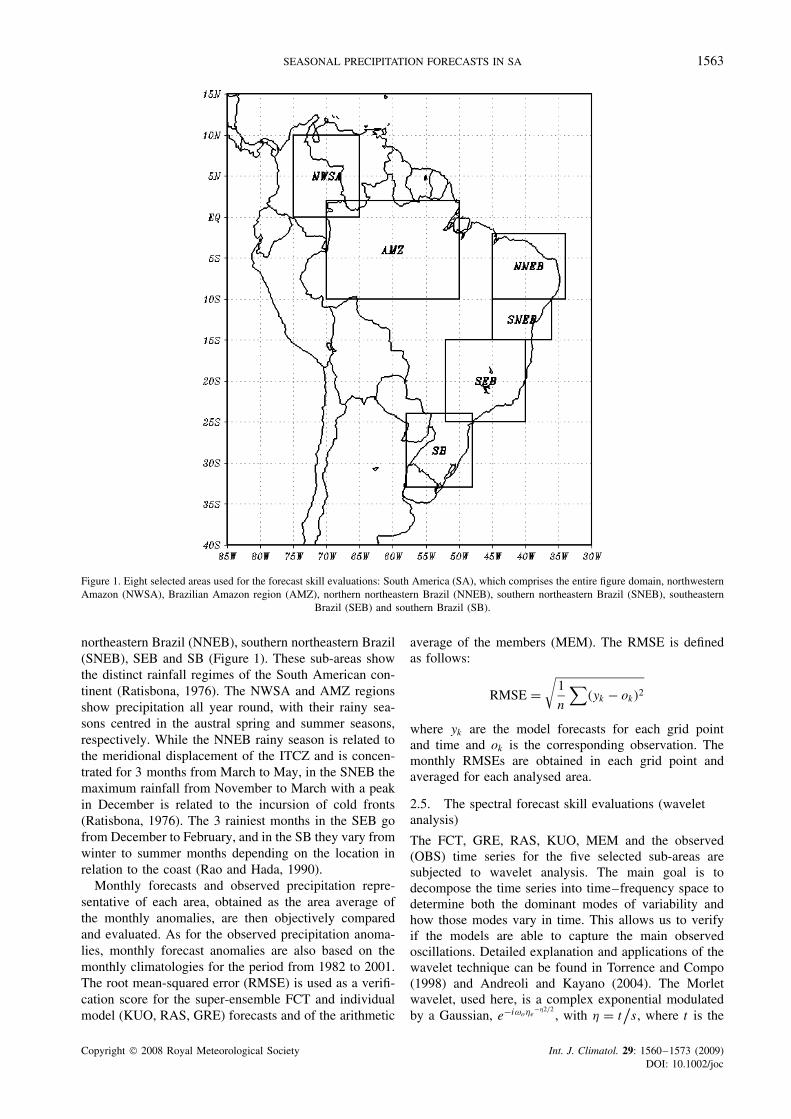
Figure 1. Eight selected areas used for the forecast skill evaluations: South America (SA), which comprises the entire figure domain, northwesternAmazon (NWSA), Brazilian Amazon region (AMZ), northern northeastern Brazil (NNEB), southern northeastern Brazil (SNEB), southeastern
Brazil (SEB) and southern Brazil (SB).
northeastern Brazil (NNEB), southern northeastern Brazil(SNEB), SEB and SB (Figure 1). These sub-areas showthe distinct rainfall regimes of the South American con-tinent (Ratisbona, 1976). The NWSA and AMZ regionsshow precipitation all year round, with their rainy sea-sons centred in the austral spring and summer seasons,respectively. While the NNEB rainy season is related tothe meridional displacement of the ITCZ and is concen-trated for 3 months from March to May, in the SNEB themaximum rainfall from November to March with a peakin December is related to the incursion of cold fronts(Ratisbona, 1976). The 3 rainiest months in the SEB gofrom December to February, and in the SB they vary fromwinter to summer months depending on the location inrelation to the coast (Rao and Hada, 1990).
Monthly forecasts and observed precipitation repre-sentative of each area, obtained as the area average ofthe monthly anomalies, are then objectively comparedand evaluated. As for the observed precipitation anoma-lies, monthly forecast anomalies are also based on themonthly climatologies for the period from 1982 to 2001.The root mean-squared error (RMSE) is used as a verifi-cation score for the super-ensemble FCT and individualmodel (KUO, RAS, GRE) forecasts and of the arithmetic
average of the members (MEM). The RMSE is definedas follows:
RMSE =√
1
n
∑(yk − ok)2
where yk are the model forecasts for each grid pointand time and ok is the corresponding observation. Themonthly RMSEs are obtained in each grid point andaveraged for each analysed area.
2.5. The spectral forecast skill evaluations (waveletanalysis)
The FCT, GRE, RAS, KUO, MEM and the observed(OBS) time series for the five selected sub-areas aresubjected to wavelet analysis. The main goal is todecompose the time series into time–frequency space todetermine both the dominant modes of variability andhow those modes vary in time. This allows us to verifyif the models are able to capture the main observedoscillations. Detailed explanation and applications of thewavelet technique can be found in Torrence and Compo(1998) and Andreoli and Kayano (2004). The Morletwavelet, used here, is a complex exponential modulatedby a Gaussian, e−iωoηe
−η2/2, with η = t
/s, where t is the
Copyright 2008 Royal Meteorological Society Int. J. Climatol. 29: 1560–1573 (2009)DOI: 10.1002/joc
1564 L. P. PEZZI AND M. T. KAYANO
time; s is the wavelet scale; and ωo is a non-dimensionalfrequency. The computational procedure of the waveletanalysis described by Torrence and Compo (1998) isused. It is worth mentioning that the wavelet function ateach scale s is normalized by s−1/2 to have unit energy,which ensures that the wavelet transform at each scale s
is comparable to each other and to the transform of othertime series (Torrence and Compo, 1998). This analysisprovides the local wavelet power spectrum (LWPS) givenby the square of the wavelet coefficients and the globalwavelet spectrum (GWS), which is the averaged spectrumover all the time periods.
3. Results
3.1. Annual climatological error analysis
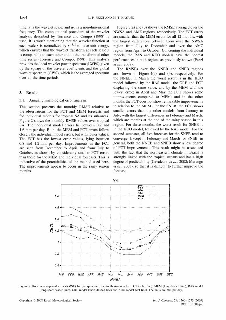
This section presents the monthly RMSE relative tothe observations for the FCT and MEM forecasts andfor individual models for tropical SA and its sub-areas.Figure 2 shows the monthly RMSE values over tropicalSA. The individual model errors lie between 0.9 and1.6 mm per day. Both, the MEM and FCT errors followclosely the individual model errors, but with lower values.The FCT has the lowest error values, lying between0.8 and 1.2 mm per day. Improvements in the FCTare seen from December to April and from July toOctober, as shown by considerably smaller FCT errorsthan those for the MEM and individual forecasts. This isindicative of the potentialities of the method used here.The improvements appear to occur in the rainy seasonmonths.
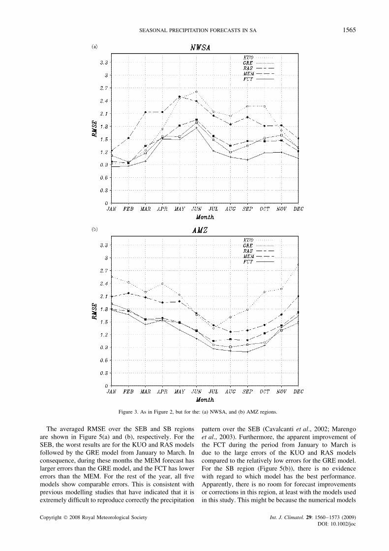
Figure 3(a) and (b) shows the RMSE averaged over theNWSA and AMZ regions, respectively. The FCT errorsare smaller than the MEM errors for all 12 months, withthe largest differences between them over the NWSAregion from July to December and over the AMZregion from April to October. Concerning the individualmodels, the RAS and KUO models have the poorestperformances in both regions as previously shown (Pezziet al., 2008).
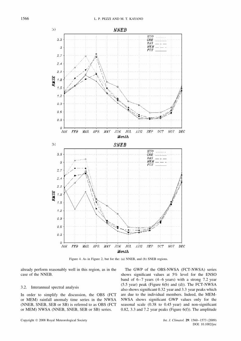
The RMSEs over the NNEB and SNEB regionsare shown in Figure 4(a) and (b), respectively. Forthe NNEB, in March the worst result is in the KUOmodel followed by the RAS model, the GRE and FCTdisplaying the same value, and by the MEM with thelowest error; in April and May the FCT shows someimprovements compared to MEM; and in the othermonths the FCT does not show remarkable improvementsin relation to the MEM. For the SNEB, the FCT showssmaller errors than the other models from January toJuly, with the largest differences in February and March,which are months at the end of the rainy season in thisregion. For these months, the worst result for SNEB isin the KUO model, followed by the RAS model. For thesecond semester, all five forecasts for the SNEB tend toconverge. Except in February and March for SNEB, ingeneral, both the NNEB and SNEB show a low degreeof FCT improvements. This result might be associatedwith the fact that the northeastern climate in Brazil isstrongly linked with the tropical oceans and has a highdegree of predictability (Cavalcanti et al., 2002; Marengoet al., 2003), so that it is difficult to further improve theforecast.
Figure 2. Root mean-squared error (RMSE) for precipitation over South America for: FCT (solid line), MEM (long dashed line), RAS model(long-short dashed line), GRE model (short dashed line) and KUO model (dot line). The units are mm per day.
Copyright 2008 Royal Meteorological Society Int. J. Climatol. 29: 1560–1573 (2009)DOI: 10.1002/joc
SEASONAL PRECIPITATION FORECASTS IN SA 1565
Figure 3. As in Figure 2, but for the: (a) NWSA, and (b) AMZ regions.
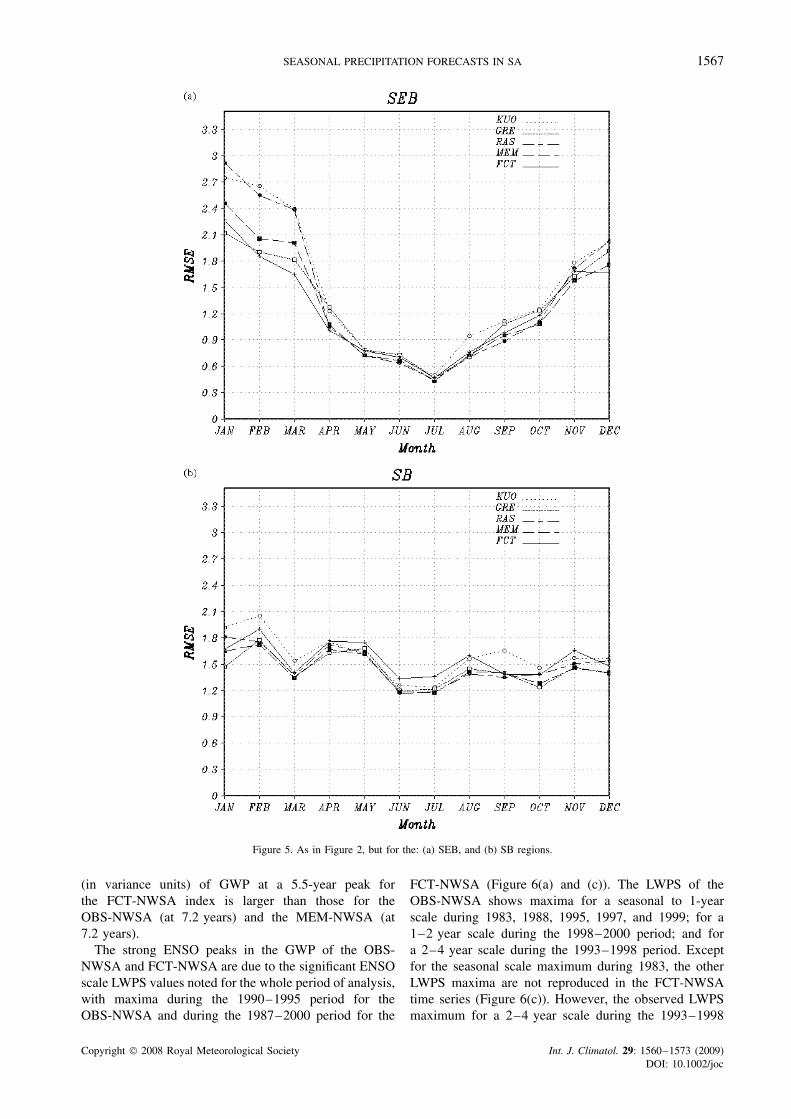
The averaged RMSE over the SEB and SB regionsare shown in Figure 5(a) and (b), respectively. For theSEB, the worst results are for the KUO and RAS modelsfollowed by the GRE model from January to March. Inconsequence, during these months the MEM forecast haslarger errors than the GRE model, and the FCT has lowererrors than the MEM. For the rest of the year, all fivemodels show comparable errors. This is consistent withprevious modelling studies that have indicated that it isextremely difficult to reproduce correctly the precipitation
pattern over the SEB (Cavalcanti et al., 2002; Marengoet al., 2003). Furthermore, the apparent improvement ofthe FCT during the period from January to March isdue to the large errors of the KUO and RAS modelscompared to the relatively low errors for the GRE model.For the SB region (Figure 5(b)), there is no evidencewith regard to which model has the best performance.Apparently, there is no room for forecast improvementsor corrections in this region, at least with the models usedin this study. This might be because the numerical models
Copyright 2008 Royal Meteorological Society Int. J. Climatol. 29: 1560–1573 (2009)DOI: 10.1002/joc
1566 L. P. PEZZI AND M. T. KAYANO
Figure 4. As in Figure 2, but for the: (a) NNEB, and (b) SNEB regions.
already perform reasonably well in this region, as in thecase of the NNEB.
3.2. Interannual spectral analysis
In order to simplify the discussion, the OBS (FCTor MEM) rainfall anomaly time series in the NWSA(NNEB, SNEB, SEB or SB) is referred to as OBS (FCTor MEM) NWSA (NNEB, SNEB, SEB or SB) series.
The GWP of the OBS-NWSA (FCT-NWSA) seriesshows significant values at 5% level for the ENSOband of 6–7 years (4–6 years) with a strong 7.2 year(5.5 year) peak (Figure 6(b) and (d)). The FCT-NWSAalso shows significant 0.32 year and 3.3 year peaks whichare due to the individual members. Indeed, the MEM-NWSA shows significant GWP values only for theseasonal scale (0.38 to 0.45 year) and non-significant0.82, 3.3 and 7.2 year peaks (Figure 6(f)). The amplitude
Copyright 2008 Royal Meteorological Society Int. J. Climatol. 29: 1560–1573 (2009)DOI: 10.1002/joc
SEASONAL PRECIPITATION FORECASTS IN SA 1567
Figure 5. As in Figure 2, but for the: (a) SEB, and (b) SB regions.
(in variance units) of GWP at a 5.5-year peak forthe FCT-NWSA index is larger than those for theOBS-NWSA (at 7.2 years) and the MEM-NWSA (at7.2 years).
The strong ENSO peaks in the GWP of the OBS-NWSA and FCT-NWSA are due to the significant ENSOscale LWPS values noted for the whole period of analysis,with maxima during the 1990–1995 period for theOBS-NWSA and during the 1987–2000 period for the
FCT-NWSA (Figure 6(a) and (c)). The LWPS of theOBS-NWSA shows maxima for a seasonal to 1-yearscale during 1983, 1988, 1995, 1997, and 1999; for a1–2 year scale during the 1998–2000 period; and fora 2–4 year scale during the 1993–1998 period. Exceptfor the seasonal scale maximum during 1983, the otherLWPS maxima are not reproduced in the FCT-NWSAtime series (Figure 6(c)). However, the observed LWPSmaximum for a 2–4 year scale during the 1993–1998
Copyright 2008 Royal Meteorological Society Int. J. Climatol. 29: 1560–1573 (2009)DOI: 10.1002/joc
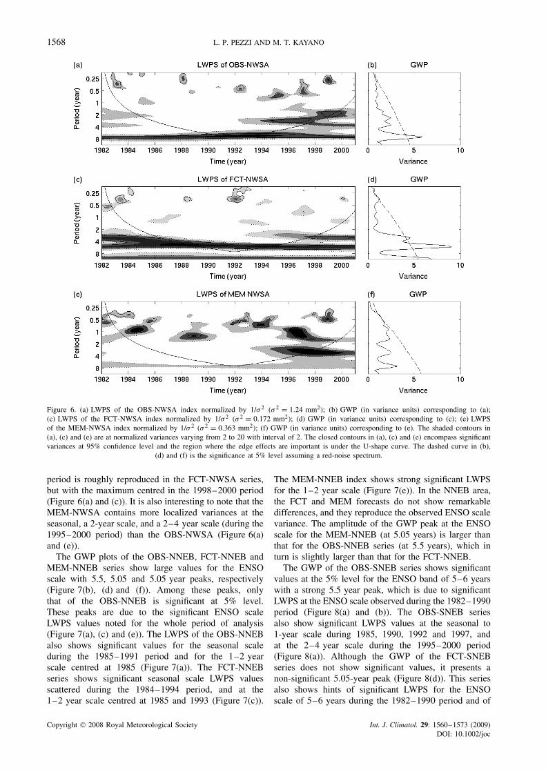
1568 L. P. PEZZI AND M. T. KAYANO
Figure 6. (a) LWPS of the OBS-NWSA index normalized by 1/σ 2 (σ 2 = 1.24 mm2); (b) GWP (in variance units) corresponding to (a);(c) LWPS of the FCT-NWSA index normalized by 1/σ 2 (σ 2 = 0.172 mm2); (d) GWP (in variance units) corresponding to (c); (e) LWPSof the MEM-NWSA index normalized by 1/σ 2 (σ 2 = 0.363 mm2); (f) GWP (in variance units) corresponding to (e). The shaded contours in(a), (c) and (e) are at normalized variances varying from 2 to 20 with interval of 2. The closed contours in (a), (c) and (e) encompass significantvariances at 95% confidence level and the region where the edge effects are important is under the U-shape curve. The dashed curve in (b),
(d) and (f) is the significance at 5% level assuming a red-noise spectrum.
period is roughly reproduced in the FCT-NWSA series,but with the maximum centred in the 1998–2000 period(Figure 6(a) and (c)). It is also interesting to note that theMEM-NWSA contains more localized variances at theseasonal, a 2-year scale, and a 2–4 year scale (during the1995–2000 period) than the OBS-NWSA (Figure 6(a)and (e)).
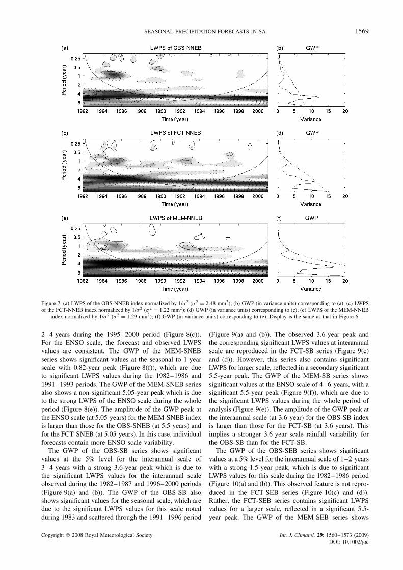
The GWP plots of the OBS-NNEB, FCT-NNEB andMEM-NNEB series show large values for the ENSOscale with 5.5, 5.05 and 5.05 year peaks, respectively(Figure 7(b), (d) and (f)). Among these peaks, onlythat of the OBS-NNEB is significant at 5% level.These peaks are due to the significant ENSO scaleLWPS values noted for the whole period of analysis(Figure 7(a), (c) and (e)). The LWPS of the OBS-NNEBalso shows significant values for the seasonal scaleduring the 1985–1991 period and for the 1–2 yearscale centred at 1985 (Figure 7(a)). The FCT-NNEBseries shows significant seasonal scale LWPS valuesscattered during the 1984–1994 period, and at the1–2 year scale centred at 1985 and 1993 (Figure 7(c)).
The MEM-NNEB index shows strong significant LWPSfor the 1–2 year scale (Figure 7(e)). In the NNEB area,the FCT and MEM forecasts do not show remarkabledifferences, and they reproduce the observed ENSO scalevariance. The amplitude of the GWP peak at the ENSOscale for the MEM-NNEB (at 5.05 years) is larger thanthat for the OBS-NNEB series (at 5.5 years), which inturn is slightly larger than that for the FCT-NNEB.
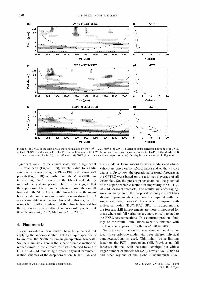
The GWP of the OBS-SNEB series shows significantvalues at the 5% level for the ENSO band of 5–6 yearswith a strong 5.5 year peak, which is due to significantLWPS at the ENSO scale observed during the 1982–1990period (Figure 8(a) and (b)). The OBS-SNEB seriesalso show significant LWPS values at the seasonal to1-year scale during 1985, 1990, 1992 and 1997, andat the 2–4 year scale during the 1995–2000 period(Figure 8(a)). Although the GWP of the FCT-SNEBseries does not show significant values, it presents anon-significant 5.05-year peak (Figure 8(d)). This seriesalso shows hints of significant LWPS for the ENSOscale of 5–6 years during the 1982–1990 period and of
Copyright 2008 Royal Meteorological Society Int. J. Climatol. 29: 1560–1573 (2009)DOI: 10.1002/joc
SEASONAL PRECIPITATION FORECASTS IN SA 1569
Figure 7. (a) LWPS of the OBS-NNEB index normalized by 1/σ 2 (σ 2 = 2.48 mm2); (b) GWP (in variance units) corresponding to (a); (c) LWPSof the FCT-NNEB index normalized by 1/σ 2 (σ 2 = 1.22 mm2); (d) GWP (in variance units) corresponding to (c); (e) LWPS of the MEM-NNEB
index normalized by 1/σ 2 (σ 2 = 1.29 mm2); (f) GWP (in variance units) corresponding to (e). Display is the same as that in Figure 6.
2–4 years during the 1995–2000 period (Figure 8(c)).For the ENSO scale, the forecast and observed LWPSvalues are consistent. The GWP of the MEM-SNEBseries shows significant values at the seasonal to 1-yearscale with 0.82-year peak (Figure 8(f)), which are dueto significant LWPS values during the 1982–1986 and1991–1993 periods. The GWP of the MEM-SNEB seriesalso shows a non-significant 5.05-year peak which is dueto the strong LWPS of the ENSO scale during the wholeperiod (Figure 8(e)). The amplitude of the GWP peak atthe ENSO scale (at 5.05 years) for the MEM-SNEB indexis larger than those for the OBS-SNEB (at 5.5 years) andfor the FCT-SNEB (at 5.05 years). In this case, individualforecasts contain more ENSO scale variability.
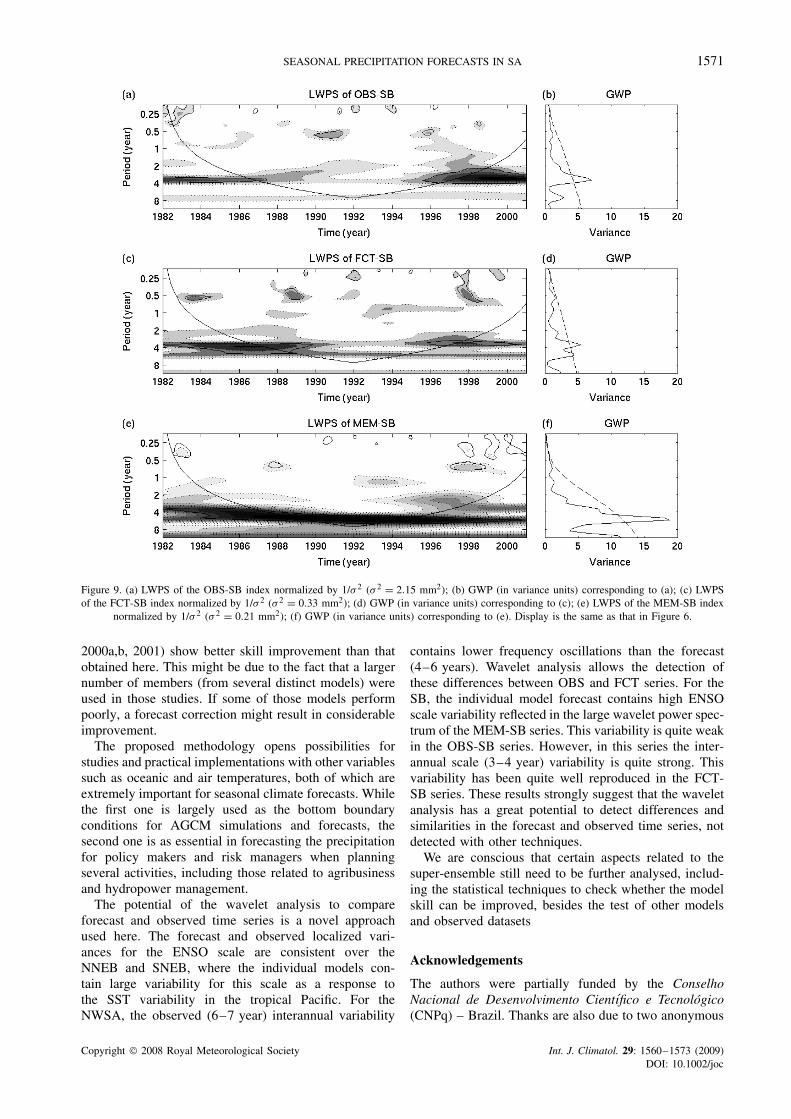
The GWP of the OBS-SB series shows significantvalues at the 5% level for the interannual scale of3–4 years with a strong 3.6-year peak which is due tothe significant LWPS values for the interannual scaleobserved during the 1982–1987 and 1996–2000 periods(Figure 9(a) and (b)). The GWP of the OBS-SB alsoshows significant values for the seasonal scale, which aredue to the significant LWPS values for this scale notedduring 1983 and scattered through the 1991–1996 period
(Figure 9(a) and (b)). The observed 3.6-year peak andthe corresponding significant LWPS values at interannualscale are reproduced in the FCT-SB series (Figure 9(c)and (d)). However, this series also contains significantLWPS for larger scale, reflected in a secondary significant5.5-year peak. The GWP of the MEM-SB series showssignificant values at the ENSO scale of 4–6 years, with asignificant 5.5-year peak (Figure 9(f)), which are due tothe significant LWPS values during the whole period ofanalysis (Figure 9(e)). The amplitude of the GWP peak atthe interannual scale (at 3.6 year) for the OBS-SB indexis larger than those for the FCT-SB (at 3.6 years). Thisimplies a stronger 3.6-year scale rainfall variability forthe OBS-SB than for the FCT-SB.
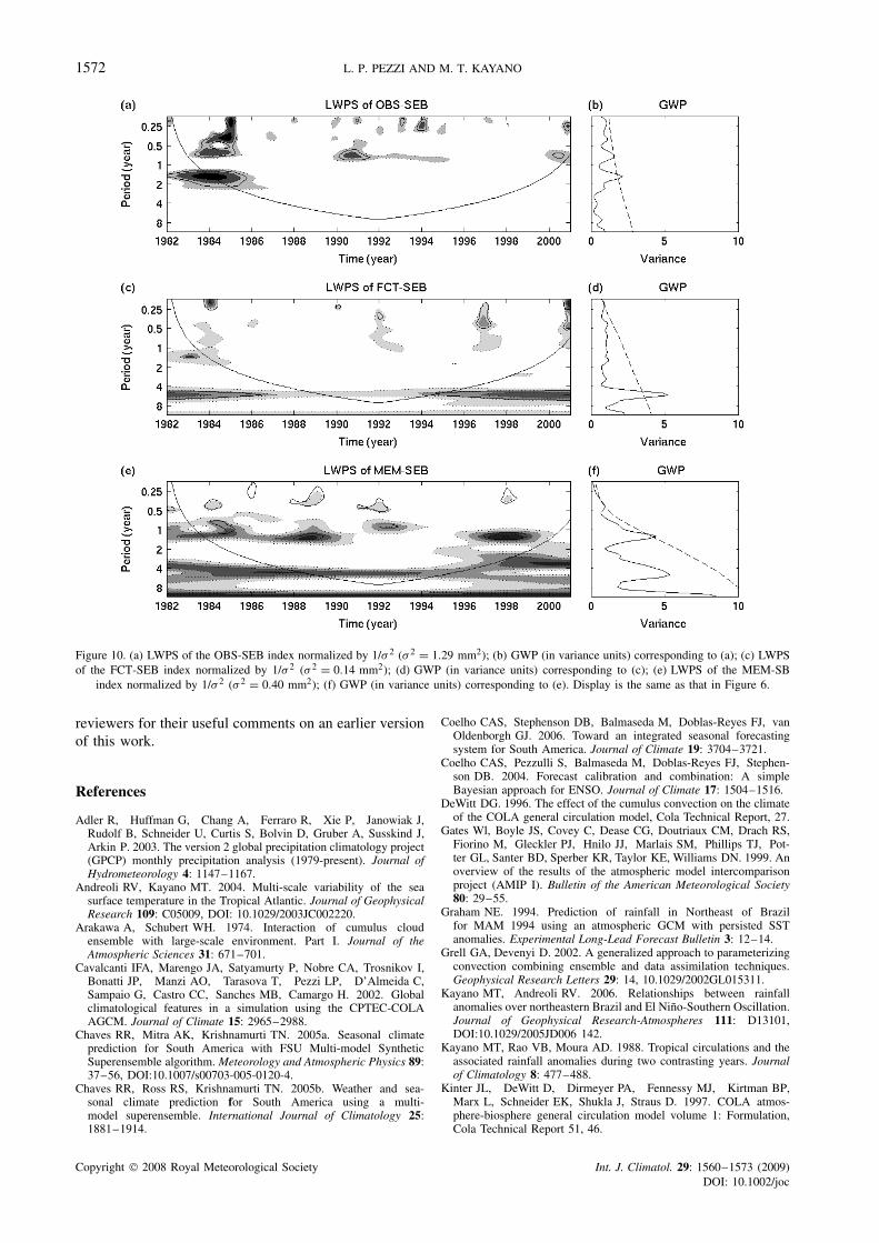
The GWP of the OBS-SEB series shows significantvalues at a 5% level for the interannual scale of 1–2 yearswith a strong 1.5-year peak, which is due to significantLWPS values for this scale during the 1982–1986 period(Figure 10(a) and (b)). This observed feature is not repro-duced in the FCT-SEB series (Figure 10(c) and (d)).Rather, the FCT-SEB series contains significant LWPSvalues for a larger scale, reflected in a significant 5.5-year peak. The GWP of the MEM-SEB series shows
Copyright 2008 Royal Meteorological Society Int. J. Climatol. 29: 1560–1573 (2009)DOI: 10.1002/joc
1570 L. P. PEZZI AND M. T. KAYANO
Figure 8. (a) LWPS of the OBS-SNEB index normalized by 1/σ 2 (σ 2 = 2.21 mm2); (b) GWP (in variance units) corresponding to (a); (c) LWPSof the FCT-SNEB index normalized by 1/σ 2 (σ 2 = 0.37 mm2); (d) GWP (in variance units) corresponding to (c); (e) LWPS of the MEM-SNEB
index normalized by 1/σ 2 (σ 2 = 1.67 mm2); (f) GWP (in variance units) corresponding to (e). Display is the same as that in Figure 6.
significant values at the annual scale, with a significant1.3- year peak (Figure 10(f)), which is due to signifi-cant LWPS values during the 1982–1990 and 1996–1999periods (Figure 10(e)). Furthermore, the MEM-SEB con-tains strong LWPS values for the ENSO scale duringmost of the analysis period. These results suggest thatthe super-ensemble technique fails to improve the rainfallforecast in the SEB. Apparently, this is because the mem-bers included in the super-ensemble contain strong ENSOscale variability which is not observed in this region. Theresults here further confirm that the climate forecast forthe SEB is extremely difficult as previously pointed out(Cavalcanti et al., 2002; Marengo et al., 2003).
4. Final remarks
To our knowledge, few studies have been carried outapplying the super-ensemble FCT technique specificallyto improve the South American precipitation forecasts.So, the main issue here is the super-ensemble method toreduce errors in the climate forecasts obtained from theCPTEC AGCM runs using different physical parameter-ization schemes of the deep convection (KUO, RAS and
GRE models). Comparisons between models and obser-vations are based on the RMSE values and on the waveletanalysis. Up to now, the operational seasonal forecasts atthe CPTEC were based on the arithmetic average of allensembles. So, the present paper examines the potentialof the super-ensemble method in improving the CPTECAGCM seasonal forecasts. The results are encouraging,since in many areas the proposed technique (FCT) hasshown improvements either when compared with thesingle arithmetic mean (MEM) or when compared withindividual models (KUO, RAS, GRE). It is apparent thatthe forecast skill improvements are more pronounced forareas where rainfall variations are more closely related tothe ENSO teleconnections. This confirms previous find-ings on the rainfall simulations over SA obtained withthe Bayesian approach (Coelho et al., 2004, 2006).
We are aware that our super-ensemble model is notideal, since only one model with three different physicalparameterizations is used. This might be a limitingfactor on the FCT improvement skill. Previous rainfallforecasts obtained with the same technique but with alarger number of models for SA (Chaves et al., 2005a,b)and other regions of the globe (Krishnamurti et al.,
Copyright 2008 Royal Meteorological Society Int. J. Climatol. 29: 1560–1573 (2009)DOI: 10.1002/joc
SEASONAL PRECIPITATION FORECASTS IN SA 1571
Figure 9. (a) LWPS of the OBS-SB index normalized by 1/σ 2 (σ 2 = 2.15 mm2); (b) GWP (in variance units) corresponding to (a); (c) LWPSof the FCT-SB index normalized by 1/σ 2 (σ 2 = 0.33 mm2); (d) GWP (in variance units) corresponding to (c); (e) LWPS of the MEM-SB index
normalized by 1/σ 2 (σ 2 = 0.21 mm2); (f) GWP (in variance units) corresponding to (e). Display is the same as that in Figure 6.
2000a,b, 2001) show better skill improvement than thatobtained here. This might be due to the fact that a largernumber of members (from several distinct models) wereused in those studies. If some of those models performpoorly, a forecast correction might result in considerableimprovement.
The proposed methodology opens possibilities forstudies and practical implementations with other variablessuch as oceanic and air temperatures, both of which areextremely important for seasonal climate forecasts. Whilethe first one is largely used as the bottom boundaryconditions for AGCM simulations and forecasts, thesecond one is as essential in forecasting the precipitationfor policy makers and risk managers when planningseveral activities, including those related to agribusinessand hydropower management.
The potential of the wavelet analysis to compareforecast and observed time series is a novel approachused here. The forecast and observed localized vari-ances for the ENSO scale are consistent over theNNEB and SNEB, where the individual models con-tain large variability for this scale as a response tothe SST variability in the tropical Pacific. For theNWSA, the observed (6–7 year) interannual variability
contains lower frequency oscillations than the forecast(4–6 years). Wavelet analysis allows the detection ofthese differences between OBS and FCT series. For theSB, the individual model forecast contains high ENSOscale variability reflected in the large wavelet power spec-trum of the MEM-SB series. This variability is quite weakin the OBS-SB series. However, in this series the inter-annual scale (3–4 year) variability is quite strong. Thisvariability has been quite well reproduced in the FCT-SB series. These results strongly suggest that the waveletanalysis has a great potential to detect differences andsimilarities in the forecast and observed time series, notdetected with other techniques.
We are conscious that certain aspects related to thesuper-ensemble still need to be further analysed, includ-ing the statistical techniques to check whether the modelskill can be improved, besides the test of other modelsand observed datasets
Acknowledgements
The authors were partially funded by the ConselhoNacional de Desenvolvimento Cientıfico e Tecnologico(CNPq) – Brazil. Thanks are also due to two anonymous
Copyright 2008 Royal Meteorological Society Int. J. Climatol. 29: 1560–1573 (2009)DOI: 10.1002/joc
1572 L. P. PEZZI AND M. T. KAYANO
Figure 10. (a) LWPS of the OBS-SEB index normalized by 1/σ 2 (σ 2 = 1.29 mm2); (b) GWP (in variance units) corresponding to (a); (c) LWPSof the FCT-SEB index normalized by 1/σ 2 (σ 2 = 0.14 mm2); (d) GWP (in variance units) corresponding to (c); (e) LWPS of the MEM-SB
index normalized by 1/σ 2 (σ 2 = 0.40 mm2); (f) GWP (in variance units) corresponding to (e). Display is the same as that in Figure 6.
reviewers for their useful comments on an earlier versionof this work.
References
Adler R, Huffman G, Chang A, Ferraro R, Xie P, Janowiak J,Rudolf B, Schneider U, Curtis S, Bolvin D, Gruber A, Susskind J,Arkin P. 2003. The version 2 global precipitation climatology project(GPCP) monthly precipitation analysis (1979-present). Journal ofHydrometeorology 4: 1147–1167.
Andreoli RV, Kayano MT. 2004. Multi-scale variability of the seasurface temperature in the Tropical Atlantic. Journal of GeophysicalResearch 109: C05009, DOI: 10.1029/2003JC002220.
Arakawa A, Schubert WH. 1974. Interaction of cumulus cloudensemble with large-scale environment. Part I. Journal of theAtmospheric Sciences 31: 671–701.
Cavalcanti IFA, Marengo JA, Satyamurty P, Nobre CA, Trosnikov I,Bonatti JP, Manzi AO, Tarasova T, Pezzi LP, D’Almeida C,Sampaio G, Castro CC, Sanches MB, Camargo H. 2002. Globalclimatological features in a simulation using the CPTEC-COLAAGCM. Journal of Climate 15: 2965–2988.
Chaves RR, Mitra AK, Krishnamurti TN. 2005a. Seasonal climateprediction for South America with FSU Multi-model SyntheticSuperensemble algorithm. Meteorology and Atmospheric Physics 89:37–56, DOI:10.1007/s00703-005-0120-4.
Chaves RR, Ross RS, Krishnamurti TN. 2005b. Weather and sea-sonal climate prediction for South America using a multi-model superensemble. International Journal of Climatology 25:1881–1914.
Coelho CAS, Stephenson DB, Balmaseda M, Doblas-Reyes FJ, vanOldenborgh GJ. 2006. Toward an integrated seasonal forecastingsystem for South America. Journal of Climate 19: 3704–3721.
Coelho CAS, Pezzulli S, Balmaseda M, Doblas-Reyes FJ, Stephen-son DB. 2004. Forecast calibration and combination: A simpleBayesian approach for ENSO. Journal of Climate 17: 1504–1516.
DeWitt DG. 1996. The effect of the cumulus convection on the climateof the COLA general circulation model, Cola Technical Report, 27.
Gates Wl, Boyle JS, Covey C, Dease CG, Doutriaux CM, Drach RS,Fiorino M, Gleckler PJ, Hnilo JJ, Marlais SM, Phillips TJ, Pot-ter GL, Santer BD, Sperber KR, Taylor KE, Williams DN. 1999. Anoverview of the results of the atmospheric model intercomparisonproject (AMIP I). Bulletin of the American Meteorological Society80: 29–55.
Graham NE. 1994. Prediction of rainfall in Northeast of Brazilfor MAM 1994 using an atmospheric GCM with persisted SSTanomalies. Experimental Long-Lead Forecast Bulletin 3: 12–14.
Grell GA, Devenyi D. 2002. A generalized approach to parameterizingconvection combining ensemble and data assimilation techniques.Geophysical Research Letters 29: 14, 10.1029/2002GL015311.
Kayano MT, Andreoli RV. 2006. Relationships between rainfallanomalies over northeastern Brazil and El Nino-Southern Oscillation.Journal of Geophysical Research-Atmospheres 111: D13101,DOI:10.1029/2005JD006 142.
Kayano MT, Rao VB, Moura AD. 1988. Tropical circulations and theassociated rainfall anomalies during two contrasting years. Journalof Climatology 8: 477–488.
Kinter JL, DeWitt D, Dirmeyer PA, Fennessy MJ, Kirtman BP,Marx L, Schneider EK, Shukla J, Straus D. 1997. COLA atmos-phere-biosphere general circulation model volume 1: Formulation,Cola Technical Report 51, 46.
Copyright 2008 Royal Meteorological Society Int. J. Climatol. 29: 1560–1573 (2009)DOI: 10.1002/joc

SEASONAL PRECIPITATION FORECASTS IN SA 1573
Kodama YM. 1992. Large-scale common features of subtropicalprecipitation zones (the Baiu frontal zone, the SPCZ, and the SACZ).Part I: Characteristics of subtropical frontal zones. Journal of theMeteorological Society of Japan 70: 813–836.
Kodama YM. 1993. Large-scale common features of subtropicalconvergence zones (the Baiu frontal zone, the SPCZ, and the SACZ).Part II: Conditions of the circulations for generating the STCZs.Journal of the Meteorological Society of Japan 71: 581–610.
Kousky VE, Kayano MT, Cavalcanti IFA. 1984. A Review of theSouthern Oscillation: Oceanic-atmospheric circulation changes andrelated rainfall anomalies. Tellus 36A: 490–504.
Kousky VE, Ropelewski CF. 1989. Extremes in the SouthernOscillation and their relationship to precipitation anomalies withemphasis on the South American region. Brazilian Journal ofMeteorology 4: 351–363.
Krishnamurti TN, Kishtawal CM, Shin DW, Williford E. 2000a.Improving tropical precipitation forecasts from multianalysissuperensemble. Journal of Climate 13: 4217–4227.
Krishnamurti TN, Kishtawal CM, Zhang Z, LaRow T, Bachiochi D,Williford E. 2000b. Multimodel ensemble forecasts for weather andseasonal climate. Journal of Climate 13: 4196–4216.
Krishnamurti TN, Surendran S, Shin DW, Correa-Torres RJ, VijayaKumar TSV, Williford E, Kummerow C, Adler RF, Simpson J,Kakar R, Olson WS, Turk FJ. 2001. Realtime multianalysis-multimodel superensemble forecasts of precipitation using TRMMand SSM/I products. Monthly Weather Review 129: 2861–2883.
Kuo HL. 1965. On the formation and intensification of tropicalcyclones through latent heat release by cumulus convection. Journalof the Atmospheric Sciences 22: 40–63.
Marengo JA, Cavalcanti IFA, Satyamurty P, Trosnikov I, Nobre CA,Bonatti JP, Camargo H, Sampaio G, Sanches MB, Manzi AO,Castro CAC, D’Almeida C, Pezzi LP, Candido L. 2003. Assessmentof regional seasonal rainfall predictability using the CPTEC/COLAatmospheric GCM. Climate Dynamics 21: 459–475, DOI:10.1007/s00382-003-0346-0.
Moorthi S, Suarez MJ. 1992. Relaxed Arakawa-Shubert: A parameter-ization of moist convection for general circulation models. MonthlyWeather Review 120: 978–1002.
Moura AD, Shukla J. 1981. On the dynamics of droughts in northeastof Brazil: Observations, theory and numerical experiments withgeneral circulation model. Journal of the Atmospheric Sciences 38:2653–2675.
Nijssen B, O’Donnell GM, Lettenmaier DP, Lohmann D, Wood EF.2001. Predicting the discharge of global rivers. Journal of Climate14: 3307–3323.
Palmer TN, Alessandri A, Andersen U, Cantelaube P, Davey M,Delecluse P, Deque M, Dıez E, Doblas-Reyes FJ, Feddersen H,Graham R, Gualdi S, Gueremy JF, Hagedorn R, Hoshen M, Keenly-side N, Latif M, Lazar A, Maisonnave E, Marletto V, Morse AP,Orfila B, Rogel P, Terres J-M, Thomson MC. 2004. Development ofa European multimodel ensemble system for seasonal to interannualprediction (DEMETER). Bulletin of the American MeteorologicalSociety 85: 853–872.
Pezzi LP, Cavalcanti IFA. 2001. The relative importance of ENSOand tropical Atlantic sea surface temperature anomalies for seasonalprecipitation over South America: A numerical study. ClimateDynamics 17: 205–212.
Pezzi LP, Cavalcanti IFA, Mendonca MA. 2008. A sensitivity studyusing two different convection schemes over South America.Brazilian Journal of Meteorology 23: 170–190.
Rao VB, Hada K. 1990. Characteristics of rainfall over Brazil: annualand variations and connections with the Southern Oscillation.Theoretical and Applied Climatology 42: 81–91.
Rao VB, Satyamurti P, Brito JIB. 1986. On the 1983 drought innortheast Brazil. International Journal of Climatology 6: 43–51.
Ratisbona LR. 1976. The climate of Brazil: Climate of centraland South America. In World Survey of Climatology, vol.12, Schwerdtfeger W, Landsberg HE (eds). Elsevier: Amsterdam;219–293, Chap 5.
Reynolds RW, Smith TM. 1994. Improved global sea surfacetemperature analysis using optimum interpolation. Journal of Climate7: 929–948.
Ropelewski CF, Halpert MS. 1987. Global and regional scaleprecipitation patterns associated with the El Nino/SouthernOscillation. Monthly Weather Review 115: 1606–1626.
Ropelewski CF, Halpert MS. 1989. Precipitation patterns associatedwith high index phase of the Southern Oscillation. Journal of Climate2: 268–284.
Souza E, Kayano MT, Tota J, Pezzi L, Fisch G, Nobre C. 2000. Onthe influences of the El Nino, La Nina and Atlantic dipole patternon the Amazonian rainfall during 1960–1998. Acta Amazonica 30:305–318.
Sperber K, Palmer T. 1996. Interannual tropical rainfall variabilityin general circulation model simulations associated with theatmospheric model intercomparison project. Journal of Climate 9:2727–2750.
Torrence C, Compo GP. 1998. A practical guide to wavelet analysis.Bulletin of the American Meteorological Society 79: 61–78.
Wilks D. 1995. Statistical Methods in the Atmospheric Sciences: AnIntroduction, Academic Press: San Diego, USA, 59; 464.
Copyright 2008 Royal Meteorological Society Int. J. Climatol. 29: 1560–1573 (2009)DOI: 10.1002/joc
Related Documents