An Analysis between Implied and Realised Volatility in the Greek Derivative Market

1

An analysis between implied and realized volatility in the

Greek Derivative market

George Filis

University of Portsmouth,

Portsmouth Business School,

Department of Economics, UK.

e-mail: [email protected]., tel: 0044 (0) 2392844828.

Abstract

In this article, we examine the relationship between implied and realised volatility in the

Greek derivative market. We examine the differences between realised volatility and

implied volatility of call and put options for at-the-money index options with a two-

month expiration period. The findings provide evidence that implied volatility is not an

efficient estimate of realised volatility. Implied volatility creates overpricing, for both call

and put options, in the Greek market. This is an indication of inefficiency for the market.

In addition, we find evidence that realised volatility ‘Granger causes’ implied volatility

for call options, and implied volatility of call options ‘Granger causes’, the implied

volatility of put options.

JEL: C22, C32, G10

Keywords: Implied volatility, realised volatility, Athens derivatives exchange, Granger

causality

2

1. Introduction

In this study, we examine the relationship between implied volatility and realised

volatility. There are several criticisms of implied volatility derived from the Black-

Scholes Option Pricing Model (BSOPM). The most important criticisms concern the

ability of implied volatility to predict realised volatility accurately (Jackwerth and

Rubinstein, 1996). The mis-estimation of realised volatility can cause mis-pricing in the

option market. Through this study, we add to the existing literature by using implied

volatility for both call and put options, whereas most of previous studies have

concentrated on call option implied volatility. The Greek derivative market is a new

market with only 5 years of life. Any evidence of mis-pricing in the option contracts can

cause serious problems to the underlying market and the option market. In addition any

mis-estimation of the realised volatility could provide evidence that the market is not

efficient. According to the BSOPM, if the market is efficient, then implied volatility

should be an unbiased and efficient predictor of realised volatility. In this study we use

implied volatility for the at-the-money call and put index options of the Greek derivative

market (i.e. the Athens Derivatives Exchange – ADEX) and we test it against realised

volatility.

2. Background of study

Many researchers (Cox et al, 1976, Hull and White, 1987, Kon, 1984, Rubinstein,

1985, Bodurtha and Courtadon, 1984, Heston, 1993b, Madan et al, 1998, Jiang and Van

Der Sluis, 2000, Heston and Nandi, 2000), since the appearance of the BSOPM, have

tried to relax some of the model’s assumptions. One of these assumptions is constant

3

volatility. These researchers have tried to show that stochastic volatility is independent of

the stock price and so should be valued independently. In the case where the volatility is

truly uncorrelated with the stock price, then BSOPM provides wrong estimates for the at-

the-money options (overvaluation) and additionally for the deep out-of-the-money and in-

the-money options (undervaluation).

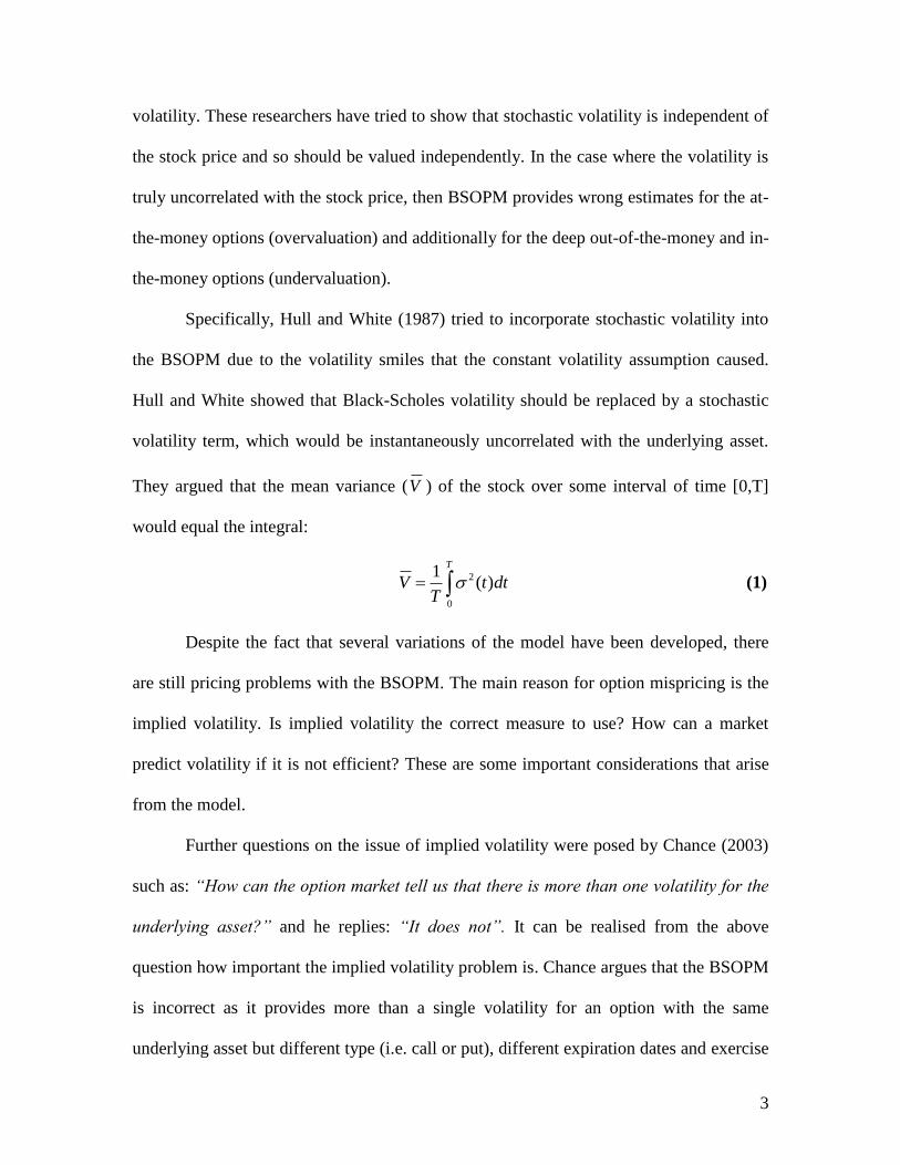
Specifically, Hull and White (1987) tried to incorporate stochastic volatility into

the BSOPM due to the volatility smiles that the constant volatility assumption caused.

Hull and White showed that Black-Scholes volatility should be replaced by a stochastic

volatility term, which would be instantaneously uncorrelated with the underlying asset.

They argued that the mean variance (V ) of the stock over some interval of time [0,T]

would equal the integral:

2

0

1( )

T

V t dtT

(1)

Despite the fact that several variations of the model have been developed, there

are still pricing problems with the BSOPM. The main reason for option mispricing is the

implied volatility. Is implied volatility the correct measure to use? How can a market

predict volatility if it is not efficient? These are some important considerations that arise

from the model.

Further questions on the issue of implied volatility were posed by Chance (2003)

such as: “How can the option market tell us that there is more than one volatility for the

underlying asset?” and he replies: “It does not”. It can be realised from the above

question how important the implied volatility problem is. Chance argues that the BSOPM

is incorrect as it provides more than a single volatility for an option with the same

underlying asset but different type (i.e. call or put), different expiration dates and exercise

4

prices. To give an example of the implied volatility problem, assume that we know the

volatility but not the option price. In this case, we would estimate the implied option price

from the volatility. However, we would get more than one option price. How can an asset

have more than one price at a specific time? Simply, it cannot (Chance, 2003).

Furthermore, according to Jackwerth and Rubinstein (1996), the BSOPM exhibits

bias in the at-the-money option prices. Two reasons can explain such bias. The first one is

that the implied volatility of the at-the-money option rarely equals the historic volatility.

The second reason is the one we have mentioned before, i.e. the different implied

volatilities for the same underlying asset in options with different strike prices and

expiration dates (Rubinstein, 1994, Jackwerth and Rubinstein, 1996, Chance, 2003).

The gap between implied and realised volatility could also be considered as

market inefficiency. If the market is efficient, then it should be able to predict the realised

volatility, thus there should not be any significant difference between the implied and

realised volatilities.

In addition, several other studies have also found evidence that implied volatility

is a biased and inefficient predictor of realised volatility (Christensen and Prabhala, 1998,

Neely, 2002, Doran and Ronn, 2004, Becker et al, 2006). The same conclusion was

reached by Szakmary et al (2003), who studied 35 stock markets for the information

content of implied volatility. Their findings are very significant due to the number of

stock markets under examination. Overall, they concluded that there is no significant

information incorporated in implied volatility.

5

Finally Koopman et al (2005) using the S&P 100 index from October 2001 until

November 2003, found evidence that the realised volatility model performs significantly

better than the implied volatility model, with regard to volatility forecasts.

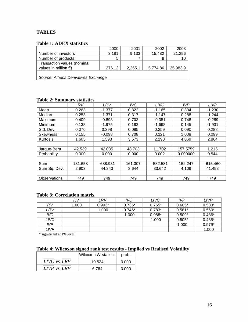
3. The Athens Derivatives Exchange

The Athens Derivatives Exchange (ADEX) began to trade option contract on the

high capitalization index (FTSE/ATHEX 20) of the Athens Stock Exchange (ATHEX) in

September 2000.

[Table 1 HERE]

Table 1 shows that the market has significantly increased its operations from one

year to the next. There is a huge increase in the transaction values of the market and in

the number of investors. Since 2000, there ha been an increase of 6.7 times in the number

of investors that trade in derivatives and the transaction values have increased by 94

times.

However, it is clear that the market is very new as it only trades 10 derivative

products and the number of investors and the transaction values are very small compared

to the traditional derivative exchanges such as CBOE and LIFFE.

Furthermore, by the time ADEX started to trade options in 2000, the ATHEX was

still an emerging market. The ATHEX became a mature market in 2001. So, it is clear

that there could be important implications in the underlying and the derivative market, if

there is evidence of volatility mis-estimation.

6

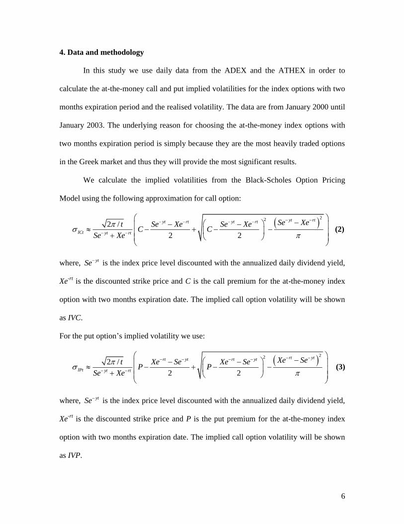
4. Data and methodology

In this study we use daily data from the ADEX and the ATHEX in order to

calculate the at-the-money call and put implied volatilities for the index options with two

months expiration period and the realised volatility. The data are from January 2000 until

January 2003. The underlying reason for choosing the at-the-money index options with

two months expiration period is simply because they are the most heavily traded options

in the Greek market and thus they will provide the most significant results.

We calculate the implied volatilities from the Black-Scholes Option Pricing

Model using the following approximation for call option:

22

2 /

2 2

yt rtyt rt yt rt

ICt yt rt

Se Xet Se Xe Se XeC C

Se Xe

(2)

where, ytSe is the index price level discounted with the annualized daily dividend yield,

Xe-rt

is the discounted strike price and C is the call premium for the at-the-money index

option with two months expiration date. The implied call option volatility will be shown

as IVC.

For the put option’s implied volatility we use:

22

2 /

2 2

rt ytrt yt rt yt

IPt yt rt

Xe Set Xe Se Xe SeP P

Se Xe

(3)

where, ytSe is the index price level discounted with the annualized daily dividend yield,

Xe-rt

is the discounted strike price and P is the put premium for the at-the-money index

option with two months expiration date. The implied call option volatility will be shown

as IVP.

7

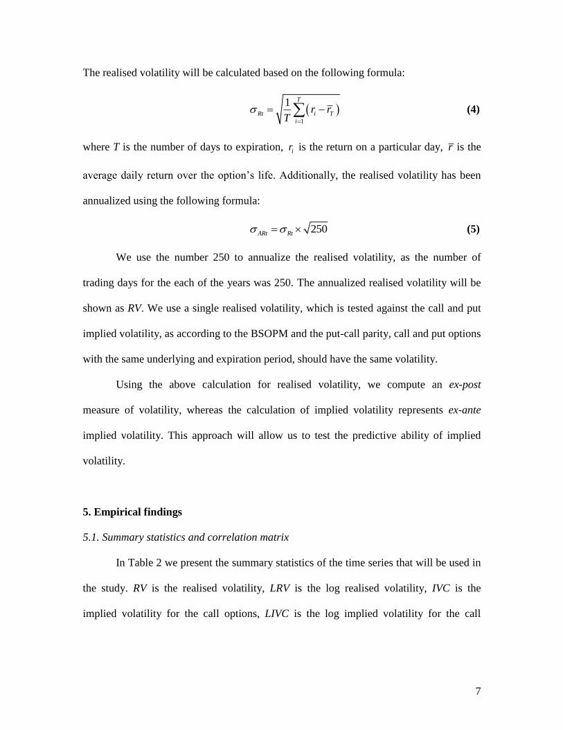
The realised volatility will be calculated based on the following formula:

1

1 T

Rt i T

i

r rT

(4)

where T is the number of days to expiration, ir is the return on a particular day, r is the

average daily return over the option’s life. Additionally, the realised volatility has been

annualized using the following formula:

250ARt Rt (5)

We use the number 250 to annualize the realised volatility, as the number of

trading days for the each of the years was 250. The annualized realised volatility will be

shown as RV. We use a single realised volatility, which is tested against the call and put

implied volatility, as according to the BSOPM and the put-call parity, call and put options

with the same underlying and expiration period, should have the same volatility.

Using the above calculation for realised volatility, we compute an ex-post

measure of volatility, whereas the calculation of implied volatility represents ex-ante

implied volatility. This approach will allow us to test the predictive ability of implied

volatility.

5. Empirical findings

5.1. Summary statistics and correlation matrix

In Table 2 we present the summary statistics of the time series that will be used in

the study. RV is the realised volatility, LRV is the log realised volatility, IVC is the

implied volatility for the call options, LIVC is the log implied volatility for the call

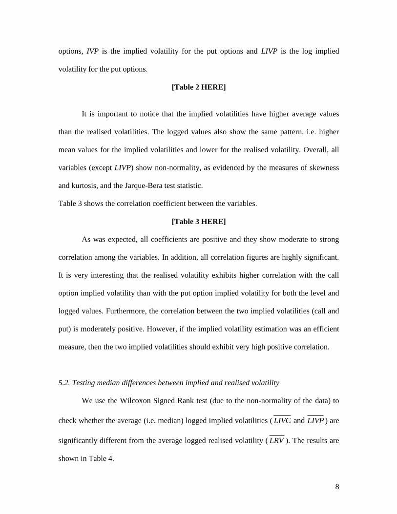
8

options, IVP is the implied volatility for the put options and LIVP is the log implied

volatility for the put options.

[Table 2 HERE]

It is important to notice that the implied volatilities have higher average values

than the realised volatilities. The logged values also show the same pattern, i.e. higher

mean values for the implied volatilities and lower for the realised volatility. Overall, all

variables (except LIVP) show non-normality, as evidenced by the measures of skewness

and kurtosis, and the Jarque-Bera test statistic.

Table 3 shows the correlation coefficient between the variables.

[Table 3 HERE]

As was expected, all coefficients are positive and they show moderate to strong

correlation among the variables. In addition, all correlation figures are highly significant.

It is very interesting that the realised volatility exhibits higher correlation with the call

option implied volatility than with the put option implied volatility for both the level and

logged values. Furthermore, the correlation between the two implied volatilities (call and

put) is moderately positive. However, if the implied volatility estimation was an efficient

measure, then the two implied volatilities should exhibit very high positive correlation.

5.2. Testing median differences between implied and realised volatility

We use the Wilcoxon Signed Rank test (due to the non-normality of the data) to

check whether the average (i.e. median) logged implied volatilities ( and LIVC LIVP ) are

significantly different from the average logged realised volatility ( LRV ). The results are

shown in Table 4.

9

[Table 4 HERE]

As we can observe, the W-statistics for both pairs of data are highly significant at

the 1% level. So, we are able to say that there is a significant difference between the

realised and implied volatilities for both call and put options. A reason for this result

could be that the implied volatility is not an efficient predictor of the realised one.

However, it could also be an indication of inefficiency in the Greek market. In addition,

such a significant difference between implied and realised volatilities is an indication of

mis-pricing with respect to realised volatility.

5.3. Testing implied volatility for bias and inefficiency

The information content of implied volatility can be assessed by estimating a

regression equation using realised volatility as the dependent variable and implied

volatility as the independent variable (Christensen and Prabhala, 1998). So, we estimate

the following regression equations:

0 1 1t t tLRV a a LIVC e (6)

0 1 2t t tLRV b b LIVP e (7)

Based on these equations, we are able to examine the following hypotheses. The

first concerns the information content of implied volatility. If implied volatility contains

information about future volatility, then we should have 1 10 and 0a b . In addition, we

should find that 1 11 and 1a b if implied volatility is an unbiased estimator of realised

volatility and the constants should not be significantly different from zero

(i.e. 0 00 and 0a b ). Finally, if implied volatility is an efficient estimator, then the

error terms should be white noise, i.e. they should have a mean of zero and they should

10

be uncorrelated. However, we will perform an ADF unit root test prior the regression

estimation. The ADF-test results for unit root in the variables are shown in Table 5.

[Table 5 HERE]

From the ADF unit root test, we are able to find strong evidence that the implied

and realised volatilities for put and call options are stationary.

Following the ADF unit root test, we perform the regression analysis. Based on

the observation from 1/2000 until 1/2003, the regression results indicate that the

estimated coefficients of LIVC and LIVP are significantly different from zero, which

suggests that they do contain some information regarding future volatility.

[Table 6 HERE]

However as the variables are significantly different from one and the constants are

significant different from zero, we can argue that the implied volatilities are biased

predictors. Furthermore, the constant term is negative for both regressions. This finding

implies that when the implied volatility (either for the call or put options) is low, the

realised volatility is higher and vice versa.

The R-squared is higher for the call implied volatility equation compared to the

put implied volatility equation. This is an indication that the predictive power of the call

options is higher than the predictive ability of the put options. If the market was able to

predict volatility correctly, then there should not be any difference in the predictive

abilities between call and put implied volatilities. In addition, if implied volatility was an

unbiased predictor of realised volatility, then again there should not be any difference in

the R-squared of the two regressions.

11

The two implied volatilities are inefficient predictors as well. The error terms for

both regressions exhibit positive autocorrelation (Durbin Watson statistic is 0.32 and 0.07

respectively), i.e. they are not white noise.

From the regression results, we argue that implied volatility is not a good and

efficient predictor of realised volatility. This mis-estimation of realised volatility could

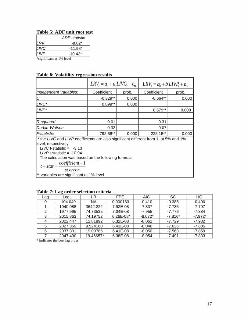
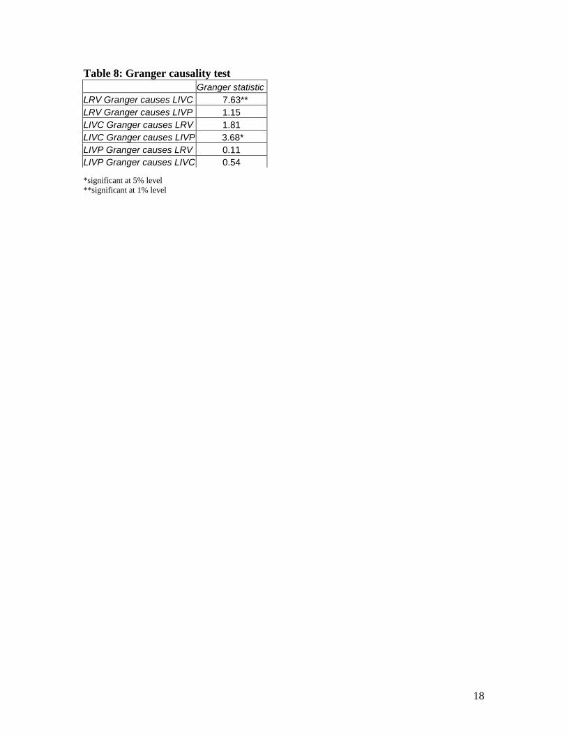
create mispricing problems to the options. Figures I and II show this effect.

[Figure 1 HERE]

[Figure 2 HERE]

The above figures indicate the both call and put options are mainly overpriced

with respect to the implied volatility. Based on the above scatter diagrams, we can

specifically notice there are some days where the mis-pricing seems to be very

significant. This is another indication that the implied volatility causes problem to the

option pricing and that the market may be inefficient.

5.4. Granger Causality results

Correlation does not necessarily imply causation. In Table 2 we observed that

there was a positive correlation among the LRV, LIVC and LIVP. However, we need to

identify any causality among them. So, in this part we perform a Granger causality test.

In order to run the test we need first to estimate the optimum number of lags.

From the VAR lag order selection criteria we find that the optimum number of lags is

three. Table 7 reports the lag order selection criteria.

12

[Table 7 HERE]

If implied volatility can predict future volatility then we expect to find that LIVC

and LIVP “Granger cause” LRV. Further, we expect to find that there is a multi-

directional causality between the LIVC and LIVP, according to the literature.

[Table 8 HERE]

Table 8 reports the F-statistic of the Granger causality test. Our findings are far

from expected. From the above results it is clear that LRV “Granger causes” LIVC, and

LIVC “Granger causes” LIVP. These results indicate that implied volatility cannot cause

realised volatility. Furthermore, the uni-directional causality that is observed from LIVC

to LIVP shows that implied volatility is not an efficient predictor, as there should be a

multi-directional causality due to the fact that the implied volatility for both call and put

options with the same expiration date and underlying asset, should be the same and due to

the put-call parity that should hold.

6. Conclusion

Overall the results indicate that implied volatility is a biased and inefficient

predictor of the realised volatility. These results support the empirical findings of the past

literature. Yet the significance of the evidence is also important due to two reasons.

Firstly, in this study we use both the call and put option implied volatilities and we test

them against the realised volatility, the first such study for an emerging market, such as

the Greek derivative market. During the period of the study, the Greek market was an

13

emerging market and thus option mis-pricing due to implied volatility could create

serious problems for the market. Furthermore, the bias and the inefficiency that the

implied volatility exhibits could also be interpreted as a market anomaly or inefficiency.

Additional tests should be performed in the Greek market, using additional data, in order

to assess whether the current mis-estimation of realised volatility is due to implied

volatility weaknesses or due to the emerging status of the market.

References

Becker, R., E. A. Clements and I. S. White. 2006. ‘On the informational efficiency of

S&P500 implied volatility.’ North American Journal of Economics and Finance,

forthcoming (in press).

Bodurtha, J. N. and G. Courtadon. 1984. ‘Empirical tests of the Philadelphia stock

exchange foreign currency options markets.’ Working Paper WPS 84-69, Ohio State

University.

Chance, D. 2003. ‘Rethinking implied volatility.’ Financial Engineering News,

January/February issue no.29.

http://www.fenews.com/fen29/one_time_articles/chance_implied_vol.html

Christensen, J. B. and R. N. Prabhala. 1998. ‘The relation between implied and realised

volatility.’ Journal of Financial Economics, 50:125-150.

14

Cox, J. C. and S. A. Ross. 1976. ‘The valuation of options for alternative stochastic

processes.’ Journal of Financial Economics, 3:145-166.

Doran, S. J. and I. E. Ronn. 2004. ‘The Bias in Black-Scholes/Black Implied Volatility.’

http://papers.ssrn.com/sol3/papers.cfm?abstract_id=628722, Working Paper, Florida

State University, Department of Finance.

Heston, S. L. 1993b. ‘A closed-form solution for options with stochastic volatility with

applications to bond and currency options.’ Review of Financial Studies, 6:327-343.

Heston, S. L. and S. Nandi. 2000. ‘A closed-form GARCH option valuation model.’

Review of Financial Studies, 13:85-625.

Hull, J. and A. White. 1987. ‘The pricing of options on assets with stochastic volatilities.’

The Journal of Finance, 42:281-300.

Jackwerth, J. C. and M. Rubinstein. 1996. ‘Recovering probability distribution from

option prices.’ Journal of Financial Economics, 3:1611-1631.

Jiang, G. J. and P. Van der Sluis. 2000. ‘Index option pricing models with stochastic

volatility and stochastic interest rates.’ Working Paper, Centre for Economic Research.

15

Kon, S. J. 1984. ‘Models of stock returns - a comparison.’ Journal of Finance, 39:147-

166.

Koopman, S. J., B. Jungbacker and E. Hol. 2005. ‘Forecasting daily variability of the

S&P 100 stock index using historical, realised and implied volatility measurements.’

Journal of Empirical Finance, 12:445-475.

Madan, D. B., P. Carr and E. C. Chang. 1998. ‘The variance gamma process and option

pricing.’ European Finance Review, 2:79-105.

Neely, J. C. 2004. ‘Forecasting Foreign Exchange Volatility: Why Is Implied Volatility

Biased and Inefficient? And Does It Matter?’ Working Paper, 2002-017D, Federal

Reserve Bank of St. Louis.

Rubinstein, M. 1985. ‘Nonparametric tests of the alternative option pricing models using

all reported trades and quotes on the 30 most active CBOE option classes from August

23, 1976 through August 31.’ Journal of Finance, 40:445-480.

Rubinstein, M.1994. ‘Implied binomial tree.’ Journal of Finance, 49:771-818.

Szakmary, A., E. Ors, K. J. Kyoung and W. N. Davidson. 2003. ‘The predictive power of

implied volatility: Evidence from 35 futures markets.’ Journal of Banking & Finance,

27:2151-2175.

16

TABLES

Table 1: ADEX statistics 2000 2001 2002 2003

Number of investors 3,181 9,133 15,482 21,256

Number of products 5 7 8 10

Transaction values (nominal values in million €) 276.12 2,255.1 5,774.86 25,983.9

Source: Athens Derivatives Exchange

Table 2: Summary statistics RV LRV IVC LIVC IVP LIVP

Mean 0.263 -1.377 0.322 -1.165 0.304 -1.230

Median 0.253 -1.371 0.317 -1.147 0.288 -1.244

Maximum 0.409 -0.893 0.703 -0.351 0.748 -0.289

Minimum 0.138 -1.975 0.182 -1.698 0.145 -1.931

Std. Dev. 0.076 0.298 0.085 0.259 0.090 0.288

Skewness 0.155 -0.098 0.708 0.121 1.008 0.099

Kurtosis 1.605 1.593 3.573 2.290 4.869 2.864

Jarque-Bera 42.539 42.035 48.703 11.702 157.5759 1.215

Probability 0.000 0.000 0.000 0.002 0.000000 0.544

Sum 131.658 -688.931 161.307 -582.581 152.247 -615.460

Sum Sq. Dev. 2.903 44.343 3.644 33.642 4.109 41.453

Observations 749 749 749 749 749 749

Table 3: Correlation matrix RV LRV IVC LIVC IVP LIVP

RV 1.000 0.993* 0.736* 0.765* 0.605* 0.583*

LRV 1.000 0.746* 0.783* 0.581* 0.560*

IVC 1.000 0.988* 0.509* 0.486*

LIVC 1.000 0.505* 0.485*

IVP 1.000 0.979*

LIVP 1.000 * significant at 1% level

Table 4: Wilcoxon signed rank test results - Implied vs Realised Volatility

Wilcoxon W-statistic prob.

LIVC vs LRV 10.524 0.000

LIVP vs LRV 6.784 0.000

17

Table 5: ADF unit root test

ADF-statistic

LRV -8.02*

LIVC -11.98*

LIVP -10.42* *significant at 1% level

Table 6: Volatility regression results

0 1 1t t tLRV a a LIVC e 0 1 2t t tLRV b b LIVP e

Independent Variables: Coefficient prob. Coefficient prob.

C -0.329** 0.000 -0.664** 0.000

LIVC* 0.899** 0.000

LIVP* 0.579** 0.000

R-squared 0.61 0.31

Durbin-Watson 0.32 0.07

F-statistic 792.88** 0.000 228.18** 0.000

* the LIVC and LIVP coefficients are also significant different from 1, at 5% and 1% level, respectively: LIVC t-statistic = -3.13 LIVP t-statistic = -10.94 The calculation was based on the following formula:

1

.

coefficientt stat

st error

** variables are significant at 1% level

Table 7: Lag order selection criteria Lag LogL LR FPE AIC SC HQ

0 104.049 NA 0.000133 -0.410 -0.385 -0.400

1 1940.088 3642.222 7.92E-08 -7.837 -7.735 -7.797

2 1977.995 74.73535 7.04E-08 -7.955 -7.776 -7.884

3 2015.863 74.19752 6.26E-08* -8.072* -7.816* -7.972*

4 2022.447 12.81892 6.32E-08 -8.062 -7.729 -7.932

5 2027.369 9.524160 6.43E-08 -8.046 -7.636 -7.885

6 2037.301 19.09786 6.41E-08 -8.050 -7.563 -7.859

7 2047.490 19.46657* 6.38E-08 -8.054 -7.491 -7.833 * indicates the best lag order

18

Table 8: Granger causality test

*significant at 5% level

**significant at 1% level

Granger statistic

LRV Granger causes LIVC 7.63**

LRV Granger causes LIVP 1.15

LIVC Granger causes LRV 1.81

LIVC Granger causes LIVP 3.68*

LIVP Granger causes LRV 0.11

LIVP Granger causes LIVC 0.54

19

FIGURES

Figure 1: Call option mispricing

20

Figure 2: Put option mispricing