Innovative Cost Engineering Approaches, Analyses and Methods Applied to SpaceLiner – an Advanced, Hypersonic, Suborbital Spaceplane Case-Study by Olga Trivailo BEng (Hons), BCom A Thesis submitted for the Degree of Doctor of Philosophy Monash University, Electrical and Computer Systems Engineering Department (ECSE), Melbourne, Australia Space Launcher Systems Analysis Department (SART), Deutsches Zentrum für Luft- und Raumfahrt, DLR - German Aerospace Center, Bremen, Germany March, 2015

Welcome message from author
This document is posted to help you gain knowledge. Please leave a comment to let me know what you think about it! Share it to your friends and learn new things together.
Transcript
Innovative Cost Engineering Approaches, Analyses and Methods Applied to
SpaceLiner – an Advanced, Hypersonic, Suborbital Spaceplane Case-Study
by
Olga Trivailo BEng (Hons), BCom
A Thesis submitted for the Degree of
Doctor of Philosophy
Monash University, Electrical and Computer Systems Engineering Department (ECSE), Melbourne, Australia
Space Launcher Systems Analysis Department (SART), Deutsches Zentrum für Luft- und Raumfahrt, DLR - German Aerospace Center, Bremen,
Germany
March, 2015

i
COPYRIGHT NOTICES
Notice 1
© The author. Under the Copyright Act 1968, this thesis may not be reproduced in any form
without the written permission of the author. This Thesis must be used only under the normal
conditions of scholarly fair dealing. In particular, not results or conclusions should be extracted
from it, nor should it be copied or closely paraphrased in whole or in part without the written
consent of the author. Proper written acknowledgement should be made for any assistance
obtained from this Thesis.
Notice 2
I certify that I have made all reasonable efforts to secure copyright permissions for third-party
content included in this thesis and have not knowingly added copyright content to my work
without the owner’s permission.

ii
iii
ABSTRACT
Olga Trivailo
PhD Candidate, Monash University, Melbourne, Australia. Deutsches Zentrum für Luft- und Raumfahrt, DLR, Bremen, Germany.
Dr. Y. Ahmet Şekercioğlu
Supervisor, Monash University, Melbourne, Australia
Dr. Martin Sippel Co-Supervisor, German Aerospace Center, DLR, Bremen, Germany
When commencing a new program within the space sector, the question of expected
program costs has emerged as a most critical criterion to be considered, especially within the
context of large and highly complex international programs where multiple domains and
disciplines are directly interfaced. Given added technical, economic, and political complexities,
the real challenge is to representatively estimate costs during the early program phases where
physical, technical, performance and programmatic parameters, requirements and specifications
might be scarce, unavailable, or still evolving. Here, the disciplines of systems and cost
engineering, as well as program management converge to support the costing function.
Cost estimation is a subset of the cost engineering domain, and a plethora of cost
estimation methods (CEMs), models, tools and resources applicable to various space sector
applications, exist. However, due to the unique nature and specificity of each mission, project
and respectively, program, the available arsenal of costing means can often be too general.
A new class of vehicle has also recently established itself as one of prevalent interest –
launcher vehicles with a focus on reusability to render them economically viable, while
concurrently offering cost-effective access to space for both cargo and humans. For such
manned, reusable launchers (RLVs), a lack of historical data implies that classically assuming a
single cost estimate based on a single heuristic parametric or analogy cost estimation alone is, by
definition, limited. Thus new ways are needed to address cost estimation for complex,
iv
unprecedented programs in the early program phase where system specifications are limited, but
the available research budget needs to be defined. The hypersonic, suborbital, passenger
spaceplane SpaceLiner currently being studied at the German Space Center, DLR, is one such
vehicle and is selected as a current RLV case-study to model and apply the advanced cost
engineering approaches and innovative techniques developed and described in this work.
Within the context of the case-study, the development of necessary processes and
application of advanced and modified cost estimation approaches and programmatic principles is
demonstrated. After a thorough literature review of current estimating practices in industry, the
parametric method is justified as the prime CEM for optimal use during the early program phase.
The TransCost statistical-analytical model for cost estimation and economical optimisation of
launch vehicles, as well as two cost models, 4cost aces and the PRICE software, all of which are
parametric, are selected. The transparent TransCost model is then extensively tested against
realised development programs with an RLV focus, and consequently calibrated.
Prior to the three models being input with high-level, technical SpaceLiner data, some
essential programmatic analyses are performed. The SpaceLiner program is considered from a
top level as a global whole, and a detailed work breakdown structure of the required components
to be developed and produced, is derived. In conjunction, and in accordance with European
Cooperation for Space Standardization standards, a baseline program schedule is also established
in order to represent the possible timeframe of the global project, to identify major milestones,
and to support model inputs for the costing process.
Based on the WBS, program schedule and selected three models, independent
development cost estimates are prepared, and an Amalgamation Approach of the multiple sets of
results is then assumed. A final baseline development cost range is ultimately determined for the
SpaceLiner, being maximally reflective of all currently available inputs. The cost of production
is also considered using parametrics, while the operational scenario is qualitatively outlined,
completing the SpaceLiner cost- and economics baseline.
v
DECLARATION
In accordance with Monash University Doctorate Regulation 17.2: Doctor of Philosophy and
Research Master’s Regulations, the following declarations are made:
In hereby declare that this Thesis contains no material which has been accepted for the award of
any other degree or diploma at any university or equivalent institution and that, to the best of my
knowledge and belief, this thesis contains no material previously published or written by another
person, except where due reference is made in the text of the Thesis.
The core theme of the Thesis is a new cost estimation methodology and approach within the
systems engineering framework, focusing on estimating development and production costs for
large, complex space systems during the early program phase. The ideas, development and
writing up of all work contained in the Thesis were the principal responsibility of myself, the
candidate, from the Department of Electrical and Computer Systems Engineering (ECSE) under
the supervision of Dr. Y. Ahmet Şekercioğlu, and in cooperation with the co-supervisor, Dr.
Martin Sippel, head of the department of Space Launcher Systems Analysis (SART) at the
German Aerospace Center, Deutsches Zentrum für Luft- und Raumfahrt (DLR), in Bremen,
Germany.
Olga Trivailo
March, 2015

vi
vii
ACKNOWLEDGEMENTS
Retrospectively, the PhD journey is one of oscillating sinusoids. Distinguished by peaks of
excitement, exhilaration and an ultimate feeling of achievement, the sinusoid is consistently
punctuated and skewed by troughs of challenges, exhaustion, despair and infuriating frustration.
However, like our oscillating sinusoid paradigm, when combined, the standalone peaks and
single troughs somehow synergise into a melodious and unique little sound-wave – albeit a
seemingly insignificant one in the grand scheme of things. But what is beautiful music made of
other than from a collection of those same sound-waves, big and little? Contributing but a peep
to the symphony of knowledge is most certainly worth traversing that aforementioned journey.
During this PhD phase the peaks were greatly enhanced and the troughs gently dampened by
the involvement of some exceptional people. Firstly, I would like to thank my two most
outstanding Supervisors, Dr. Martin Sippel and Dr. Y. Ahmet Şekercioğlu, for their unwavering
and ongoing support, always wise advice, calming counsel, careful guidance and continued
understanding and unwavering encouragement, especially during the challenging times.
Furthermore, my sincerest gratitude extends to my distinguished advisor and mentor, Prof. Dr.
Bernd Madauss, as well as Mr. Joachim Schöffer, Mr. Herbert Spix, Dr. Fabian Eilingsfeld and
Dr. Dietrich E. Koelle for their invaluable input and for so generously sharing their time,
expertise and wealth of experience and knowledge to enrich my own understanding. A heartfelt
thanks must also be expressed to all my wonderful friends, peers and colleagues, whose staunch
support, patience and unconditional understanding were both an incredible motivational driver
and an absolutely crucial contributing factor to the ultimate completion of this PhD – I trust that
you all know well who you awesome people are.
And finally, to my tiny yet very precious little family circle which so devastatingly diminished
during the years that it took to complete this Thesis - even though you may not be with me
because of a distance, geographical and divine, I carry you in my heart wherever I may be,
always, forever and indelibly so. This particular PhD Thesis and work is, in every way, for you.

viii
ix
TABLE OF CONTENTS
List of Tables xv
List of Figures xxi
Nomenclature xxv
Superscripts and Subscripts xxxi
1 INTRODUCTION 1
1.1 Focus of Thesis 3
1.2 Research motivation 3
1.3 Problem Definition 5
1.4 Organisation of Thesis 5
1.5 Contribution of Dissertation 7
1.6 Publications 9
2 COST ESTIMATION IN THE SPACE DOMAIN 10
2.1 Cost versus Price 19
2.2 Space Sector Cost Engineering & Estimation 20
2.2.1 Cost Estimation in a Cost Engineering Framework 20
2.3 Cost Risk Assessment & Uncertainties 23
2.3.1 Cost Estimation Diversity within the Space Sector 25
2.3.2 Cost Engineering Oriented Organisations 26
2.4 Cost Estimation Methods 28
2.4.1 Parametric Cost Estimation 29
2.4.2 Engineering Build-Up 31
2.4.3 Estimation by Analogy 32
2.4.4 Estimation by Expert Judgement 33
2.4.5 Rough Order of Magnitude Estimation 34

x
2.5 Cost Estimation Methodology Selection 35
2.5.1 Cost Estimation Handbooks, Reports, Manuals & Sources 35
2.6 The Amalgamation Approach to Cost Estimation 38
2.6.1 Multiple CEMs, Models & for Cost Estimation 38
2.6.2 Amalgamation Approach Definition & Application 39
2.6.2.1 Sub-element AA Cost Estimation 41
2.6.2.2 Prime, Independent AA Cost Estimation 43
2.6.2.3 Validating AA Cost Estimation 48
2.6.3 AA Key Requirements 48
2.6.4 AA Advantages 50
2.6.5 AA Drawbacks 51
2.6.5.1 Increased Resource Requirements 51
2.6.5.2 Variability of Model Mechanics & Model Experts 52
2.6.6 Amalgamation Approach Summary & Conclusions 54
3 SPACELINER - AN INDUSTRY CASE-STUDY 56
3.1 SpaceLiner Configuration Development & Launch Sequence 58
3.2 Mission Definition 62
3.3 SpaceLiner 7 63
3.4 SpaceLiner Considerations & Challenges 65
4 SPACELINER CASE-STUDY COST ESTIMATION 68
4.1 The SpaceLiner Cost Philosophy 69
4.1.1 SpaceLiner WBS Definition & Development 70
4.1.2 SpaceLiner Program Schedule & Milestones 76
4.1.3 SpaceLiner Development & Prototype Modeling 80
4.1.4 The Development & Production Industry Analogue 87
4.1.5 The Main Engine Development 87
4.1.6 Cost Estimation for Software Effort 88
4.1.7 SpaceLiner Production Quantity 89
4.1.8 SpaceLiner Reusability Impact on Production 90
xi
4.1.9 SpaceLiner Cabin / Rescue Capsule 91
4.1.10 SpaceLiner Operations & Ground Costs 92
4.1.11 SpaceLiner Cost Risk Analysis 93
4.2 Case-Study Cost Estimation Approach 98
4.3 Cost Estimation Methodology Identification 99
4.4 AAMAC Cost Estimation Model & Tool Selection 100
4.4.1 TransCost Model 100
4.4.2 TransCost Selection Criteria 104
4.4.3 PRICE Systems PRICE-H 106
4.4.4 aces by 4cost 108
4.5 TransCost Model Testing, Calibration & Validation 109
4.5.1 Understanding TransCost Development Cost Estimation 110
4.5.2 TransCost Development Cost Structure 111
4.5.3 TransCost Production Cost Structure 114
4.5.4 TransCost Model Excel Tool 116
4.5.5 TransCost Development Cost Test & Calibration 119
4.6 TransCost Testing, Calibration & Validation for RLVs 120
4.6.1 Liquid Fly-back Booster 121
4.6.1.1 LFBB Configuration 122
4.6.1.2 LFBB Excel Component Break-down Structure 122
4.6.1.3 LFBB Calculation Assumptions 122
4.6.1.4 TransCost LFBB Result and Literature Comparison 127
4.7 CER Development for Reusable Booster Stages 130
4.7.1 CER Establishment Process 131
4.8 Costing the SpaceLiner Case-Study 140
4.8.1 Methodology 140
4.8.2 Amalgamation Approach to SpaceLiner 144
4.9 Development Cost Analysis 145
4.9.1 TransCost SpaceLiner Development Costs 145
xii
4.9.1.1 TransCost SpaceLiner Development Assumptions 146
4.9.1.2 TransCost Development Results 152
4.9.1.3 TransCost Sensitivities & Development Cost Range 153
4.9.2 Commercial Cost Models & Development Costs 155
4.9.3 aces by 4cost 157
4.9.4 PRICE 162
4.9.5 Optimal Development Timeframe 167
4.9.6 Development Project Management Office Cost Estimation 168
4.9.6.1 PMO Cost Assumptions 173
4.9.7 Development Amalgamation Approach Results 175
4.9.7.1 An AAMAC Iteration Example 176
4.9.7.2 AAMAC Final Development Results 178
4.9.8 Discussion of AAMAC Development Costs 183
4.9.8.1 SLME Development Cost Difference 186
4.9.8.2 SPC Development Cost Difference 186
4.9.8.3 Variability of Model Mechanics 187
4.9.8.4 Variability in Model Users & EJ Bias 187
4.9.8.5 Software Considerations 188
4.9.9 Development Cost Sensitivities 190
4.9.9.1 Prototype Quantity 190
4.9.9.2 Team Experience 191
4.9.9.3 Development Sensitivity Discussion & Summary 191
4.9.10 Development Cost Calculation Conclusions 192
4.10 Production Cost Analysis 193
4.10.1 Learning Curve Determination 193
4.10.2 TransCost Production Cost Calculation 198
4.10.3 4cost aces Production Cost Calculation 210
4.10.4 PRICE Production Cost Calculation 213
4.10.5 Optimal Production Timeframe 215
4.10.6 Production Project Management Office Cost Estimation 216
4.10.7 Production Amalgamation Approach Results 218
xiii
4.10.8 Discussion of Production Amalgamation Approach Costs 225
4.10.8.1 TransCost Production Cost Deviation 227
4.10.8.1.1 TransCost Non-Applicability to SLO & SLB 228
4.10.8.1.2 TransCost Model ‘Classical Space Production’ 229
4.10.8.1.3 TransCost Orbital Vehicle Focus 231
4.10.8.2 Learning Curve Assumption 232
4.10.8.3 Other Production Cost Fluctuations 235
4.10.9 Production Cost Sensitivities 235
4.10.9.1 Learning Curve Variation 236
4.10.9.2 Production Quantity 239
4.10.9.3 Engine Reusability 241
4.10.9.4 Production Sensitivity Summary 242
4.10.10 Production Cost Calculation Conclusions 243
4.11 Operations and Ground Costs Analysis 245
4.12 Representativeness & Reliability of Presented Cost Estimation 250
4.12.1 Estimating Conditions 255
4.12.2 Nature of the Item 255
4.12.3 Item Description 256
4.12.4 Cost Methods & Data 256
4.12.5 Estimator Experience & Competence 257
4.12.6 Cost Estimate Confidence Conclusion 258
5 THESIS FINAL CONCLUSIONS 261
5.1.1 Summary of Results 263
5.1.1.1 Case-study Development Costs Summary 263
5.1.1.2 Case-Study Production Costs Summary 264
5.1.1.3 Case-study Sensitivity Analysis Summary 265
5.1.1.4 Case-study Operations & Ground Costs Summary 266
5.1.2 Future work 267
5.1.2.1 Amalgamation Approach 268
5.1.2.2 SpaceLiner Development & Production Cost Estimation 268
xiv
5.1.2.3 Software Costs 269
5.1.2.4 SpaceLiner Operation & Ground Costs 270
5.1.2.5 Sensitivity Analyses 270
5.1.2.6 WBS & Program Schedule Iterations 272
5.1.2.7 Financing 273
5.1.2.8 Budget, Resource Planning 274
5.1.2.9 Risk Assessment & Planning 275
APPENDICES 277
Appendix A – SpaceLiner WBS Breakdown 277
Appendix B – SpaceLiner Model Matrices 284
Appendix C – TransCost Work Year Costs [102] 287
Appendix D – TransCost 8.2 Complexity Factors 289
Appendix E – RLV TransCost Development Cost Calculations 301
Appendix F – SpaceLiner Mass Data 344
Appendix G – 4cost aces Engineering Difficulty (ENGDIF) Values 349
Appendix H – 4cost aces Tool Key Inputs & Outputs 350
Appendix I – PRICE Tool Key Inputs & Outputs 359
Appendix J – Preliminary Case-Study Operations Concept 377
xv
LIST OF TABLES
Table 1: Key parameters of SpaceLiner 7 booster stage 64
Table 2: Key parameters of SpaceLiner 7 orbiter stage 64
Table 4: Mass data for SpaceLiner 7 orbiter stage 65
Table 5: Mass data for SpaceLiner 7 launch configuration 65
Table 6: ESA Standard prototype counting values for various prototype-models 84
Table 7: Numerical values derived for SpaceLiner five-model prototype philosophy 85
Table 8: SLO Model Matrix quantitatively showing model philosophy components 86
Table 9: TransCost Complexity Factors defined for three TransCost versions 103
Table 10: Space programs used as inputs for extensive TransCost testing process 119
Table 11: TransCost CER for Vulcain 3 engine 123
Table 12: TransCost CER for main cryogenic stage EPC-H185 123
Table 13: TransCost CER for LFBB 124
Table 14: Updated CER for LFBB development cost (described later in Chapter 4.7) 124
Table 15: Industry estimated total LFBB development costs [158] 127
Table 16: Industry LFBB figures (L) compared with TransCost (TC) estimated values 128
Table 17: Comparison of LFBB TransCost 7.3 and industry development cost 129
Table 18: CER complexity factor values assigned to stated cost data for normalisation 134
Table 19: SpaceLiner complexity factors for each component 146
Table 20: TransCost CER for SpaceLiner Orbiter (SLO) development 149
Table 21: TransCost CER for SpaceLiner Main Engine (SLME) development 149
Table 22: Newly established CER for SpaceLiner Booster (SLB) development 150
Table 23: TransCost CER for SpaceLiner Cabin/Capsule (SPC) development 150
Table 24: Revised TransCost CER for SPC with f10 and f11 complexity factors 152
Table 25: TransCost SpaceLiner development costs without programmatic factors 153
Table 26: TransCost complexities sensitivity variations (S) for development cost range 154
xvi
Table 27: SpaceLiner development costs for lower and upper limits 155
Table 28: 4cost aces table for the scope of mechanical and electronic design novelty [1] 161
Table 29: PRICE engineering complexity (ECMPLX) values matrix [53, 154] 165
Table 30: Qualitative break-down into constituents of the PMO function with an EJ estimate
for average number of personnel required per function [119, 147] 172
Table 31: Estimated PMO costs for 7 year development phase 174
Table 32: Example of an essential iteration in the AAMAC process 177
Table 33: Example of an essential iteration in the AAMAC process 178
Table 34: AAInT spreadsheet for SpaceLiner PMO development costs 180
Table 35: AAInT spreadsheet for SLO case-study development costs 180
Table 36: AAInT spreadsheet for SLB case-study development costs 181
Table 37: AAInT spreadsheet for SPC case-study development costs 181
Table 38: Total SpaceLiner case-study development program costs, with margin 182
Table 39: Comparative summary of AAMAC total program development costs per element
with 20% margin, including all programmatic factors 185
Table 40: 4cost aces prototype quantity sensitivities for development costs 191
Table 41: 4cost aces TEAM complexity sensitivities for development costs 191
Table 42: Summary of learning curves for high-speed and large aviation programs polled
from various literature sources 197
Table 43: TransCost CER for SpaceLiner main engine (SLME) TFU production 203
Table 44: TransCost CER for Orbiter (SLOAvio) TFU ‘best case’ production 203
Table 45: TransCost CER for Orbiter (SLOSpace) TFU ‘worst case’ production 204
Table 46: TransCost CER for Booster (SLBAvio) TFU ‘best case’ production 204
Table 47: TransCost CER for Booster (SLBSpace) TFU ‘worst case’ production 205
Table 48: TransCost CER for Passenger Cabin (SPC) TFU production 205
xvii
Table 49: TransCost ‘worst case’ TFU production cost calculation per element using the
TransCost ‘Space’ CER 206
Table 50: TransCost ‘best case’ TFU production cost calculation per element using the
TransCost Aviation ‘Avio’ CER 206
Table 51: TransCost ‘average case’ TFU production cost calculation per element assuming
an average of the ‘Space’ and ‘Avio’ TransCost CER results 206
Table 52: TransCost 85%LC calculation of production cost for eleven SLME engines 207
Table 53: Calculation of production cost for all components for the SpaceLiner TFU 208
Table 54: Total TransCost production costs for a batch of 500 SpaceLiner vehicles with a
global 85% production learning curve 210
Table 55: Derived qualitative break-down of the PMO function with an EJ estimate for
average number of personnel required per function [119, 147] 217
Table 56: AAInT spreadsheet interface for overall SpaceLiner production PMO costs 220
Table 57: AAInT spreadsheet interface for SLO total case-study production costs 220
Table 58: AAInT spreadsheet interface for SLB total case-study production costs 221
Table 59: AAInT spreadsheet interface for SPC total case-study production costs 221
Table 60: AAInT spreadsheet for SLO average unit case-study production costs 222
Table 61: AAInT spreadsheet for SLB average unit case-study production costs 223
Table 62: AAInT spreadsheet for SPC average unit case-study production costs 223
Table 63: Total SpaceLiner case-study production program costs, with margin 224
Table 64: SpaceLiner case-study average unit production costs, with margin 224
Table 65: Comparative summary of total program production costs per case-study vehicle
element using AAMAC 226
Table 66: Summary of individual TransCost ‘best-case’ (aviation) and ‘worst-case’ (space)
assumed CER results prior to obtaining their equal average 229
Table 67: Crawford learning rates (ʎc) observed in the aircraft industry [64] 233
xviii
Table 68: Summary of typical learning curves within the aviation industry [51] 234
Table 69: 4cost aces LC sensitivity summary for average production costs 237
Table 70: 4cost aces LC sensitivity for T1(TFU) production costs 238
Table 71: 4cost aces production quantity sensitivity for average production costs 240
Table 72: 4cost aces production quantity sensitivity for T1 (TFU) production costs 240
Table 73: 4cost aces engine reusability sensitivity for average production costs 241
Table 74: 4cost aces engine reusability sensitivity for T1 (TFU) production costs 241
Table 75: Summary table of identified geographical locations for SpaceLiner L/L sites 248
Table 76. AACE cost estimate classification matrix for process industries [32] 252
Table 77: Summary of AA development and production results 263
Table 78: Potentially interesting sensitivity analyses for the SpaceLiner case-study 271
Table 79: Established WBS for the SpaceLiner PMO element 1000 277
Table 80: Established WBS for the SpaceLiner SLO element 2000 278
Table 81: Established WBS for the SpaceLiner SLB element 3000 279
Table 82: Established WBS for the SpaceLiner SPC element 4000 280
Table 83: Established WBS for the SpaceLiner software and AIT element 5000 281
Table 84: Established WBS for the SpaceLiner ground segment element 6000 281
Table 85: Established WBS for the SpaceLiner operations/flight support element 7000 283
Table 86: SLB Model Matrix qualitatively showing case-study prototype philosophy
described in Chapter 4.1.3 284
Table 87: SPC Model Matrix qualitatively showing case-study prototype philosophy 285
Table 88: Development standard factor classification for f1 289
Table 89: Team experience factor classification for f3 291
Table 90: TransCost formulas for empirical learning factor (LF) for rocket engines 293
Table 91: Most common values for f7 297
Table 92: The 1980-1999 regional productivity model defining complexity factor f8 298
xix
Table 93: TransCost CER for the SSME 303
Table 94: TransCost CER for the AJ10-190 OMS Aerojet Engine 303
Table 95: TransCost CER for the Orbiter Columbia 303
Table 96: TransCost CER for the light-weight version External Tank 304
Table 97: TransCost CER for the RCS-OMS Propulsion Module 304
Table 98: TransCost CER for the SRM Boosters 304
Table 99: Space Shuttle Columbia development cost breakdown per element 307
Table 100: Space Shuttle Columbia development cost breakdown for respective stages and
components updated for ET* lesson learnt 310
Table 101: Development costs of the Space Shuttle as calculated using TransCost 7.3 311
Table 102: TransCost CER for 17D11Buran OMS/RCS propulsion 316
Table 103: TransCost CER for Energia rocket (core) Stage 2, Block B (LH2/LOX) 316
Table 104: TransCost CER for Buran orbital vehicle 317
Table 105: TransCost CER for Energia rocket Stage 1, Block A, 11s25 (Kerosene/LOX) 317
Table 106: TransCost CER for 17D12 engine OMS Buran orbital propulsion system 318
Table 107: TransCost CER for 11D122 Energia core engine RD-0120 318
Table 108: TransCost CER for RD-180, booster stage engine 318
Table 109: Development WYr effort summary Energia-Buran system components 321
Table 110: Revised calculation of tank-like components 324
Table 111: Summary of development WYr effort and associated costs for Energia-buran
system components, modified by application of STSR 324
Table 112: Cosmonaut and astronaut salaries for Russia, US and Europe 326
Table 113: TransCost 7.3 development costs for Buran-Energia System under Russian
conditions 328
Table 114: Functionality-based groupings of Space Shuttle development effort & costs 331
Table 115: Functionality-based groupings of Buran-Energia development effort & costs 332
xx
Table 116: Purely technical comparison of TransCost calculated work effort for Shuttle and
Buran-Energia, ignoring programmatic factors f6 and f8 333
Table 117: TransCost CER for Vinci (upper stage HUS-24) engine 336
Table 118: TransCost CER for upper stage (HUS-24) 336
Table 119: TransCost CER for Vulcain 3R (main stage) engine 337
Table 120: TransCost CER for ASTRA Hopper (reusable) stage 337
Table 121: TransCost summary of calculated ASTRA Hopper development work effort and
costs, with imposition of f8 340
Table 122: Industry estimated ASTRA Hopper development costs [158] 341
Table 123: TransCost (TC) & industry (L) estimate ASTRA Hopper Figures 342
Table 124: Development costs of the ASTRA Hopper system as calculated using TransCost
7.3 and as identified in an independent industry cost estimate 342
Table 125: 4cost aces key hardware inputs for both development and production cost
calculation as discussed in Chapters 4.9.3 and 4.10.3 350
Table 126: 4cost aces hardware key outputs for both development and production cost
calculation, as discussed in Chapters 4.9.3 and 4.10.3 354
Table 127: PRICE key hardware inputs for development cost calculation as discussed in
Chapter 4.9.4 359
Table 128: PRICE key hardware outputs for development cost calculation as discussed in
Chapter 4.9.4 363
Table 129: PRICE key hardware inputs for production cost calculation as discussed in
Chapter 4.10.4 368
Table 130: PRICE key hardware outputs for production cost calculation as discussed in
Chapter 4.10.4 372
Table 131: Assumptions underlying calculation of preliminary operations scenario [111] 377
Table 132: Preliminary breakdown and estimate of DOC & IOC categories [111] 378
xxi
LIST OF FIGURES
Figure 1: Artist’s interpretation of SpaceLiner 7 [82] 13
Figure 2: Qualitative traditional PLC curve for potential applicable to the industry of
civilian access to space [149] [151] 15
Figure 3: Key elements essential for a representative, robust and justifiable cost estimate
[128] 22
Figure 4: Cone of uncertainty illustrating estimate uncertainty associated with baseline cost
estimates as it is iterated throughout the program phases [212] 24
Figure 5: Qualitative application of CEMs according to project phase [109] 36
Figure 6: Example of AAMIC application within context of the parametric SSCM cost
estimation, where the analogy CEM is used to replace the initial cost
estimation model output [7] 43
Figure 7: Graphical representation of AAMAC showing key inputs, logic and processes 47
Figure 8: The SpaceLiner vision of an ultra-fast, rocket-propelled intercontinental, point-to-
point passenger transportation spaceplane [82] 57
Figure 9: Evolution of the SpaceLiner concept [186] 61
Figure 10: Visual representation of the latest SpaceLiner 7 launch configuration with
passenger stage (top) and booster stage (bottom) with stage attachment [183] 63
Figure 11: Latest SpaceLiner 7 orbiter shape (left) and CAD drawing of the reusable
SpaceLiner 7 passenger stage (right) showing configuration of cabin,
propellant tanks and landing gear [22, 182]Table 3: Mass data of SpaceLiner 7
booster stage 64
Figure 12: SpaceLiner WBS for development Phase C showing three levels of detail 75
Figure 13: Preliminary SpaceLiner case-study program schedule 77
Figure 14: Review life cycle showing various program reviews within context of the V-
Model structure [57] 79
xxii
Figure 15: SpaceLiner Orbiter (left) and Booster (right) engines with different nozzle
extensions [225] 88
Figure 16: SpaceLiner SPC passenger cabin and emergency escape capsule [22] 92
Figure 17: Interrelation of program elements which introduce risk and uncertainty [116] 94
Figure 18: Four step process to risk assessment and mitigation [69, 115, 116, 133] 95
Figure 19: Framework for SpaceLiner development costs estimation processes 98
Figure 20: TransCost Model category structure for CERs and costs 104
Figure 21: Illustration of TransCost model testing regime 110
Figure 22: Screenshot of programmed TransCost tool in Excel showing the development
cost interface 117
Figure 23: ASSC2-Y9 concept of a semi-reusable launch vehicle with A5 core stage and
two attached, reusable fly-back boosters [46] 121
Figure 24: TransCost CER for fly-back boosters based on four reference projects [100] 131
Figure 25: An example of a basic TransCost graph and associated CER with numerous
reference data points for rocket engines [100] 132
Figure 26: ASSC-2 Y-9 [46] 134
Figure 27: STS configuration (left) and schematic (right) showing Orbiter, External Tank
and dual LFBBs in its ascent configuration [26] 135
Figure 28: FESTIP FSS-16SR (top) [108] 136
Figure 29: Newly established CER for reusable LFBBs 137
Figure 30: Comparison of newly established LFBB CER (power regression) with the
existing TransCost CER 139
Figure 31: Screenshot of developed AAMAC Excel AAInT tool adjusted for application to
the SpaceLiner case-study, shown for development costs 142
Figure 32: Developed AAMAC Excel AAInT tool screenshot with expanded L3WBS elements
to show a further SpaceLiner L4WBS level of detail 143
xxiii
Figure 33: Typical 4cost ENVIRD/ENVIRP factor values for various applications [1] 159
Figure 34: The constituent costs and their typical qualitative variations incurred by each
program phase [25, 118] 170
Figure 35: Visual comparative representation of AAMAC development costs per element
only, without programmatic factors, but including 20% margin 185
Figure 36: Some examples of learning curves across various industries [201] 195
Figure 37: LC slopes of typical activities at a higher overall-industry level [201] 196
Figure 38: Visual comparative representation of total program production costs per case-
study vehicle element only using AAMAC 225
Figure 39: Major operational criteria and their interrelation for RLVs [102] 246
Figure 40: Kansai International Airport in Osaka Bay, Japan [86] 247
Figure 41: Proposed layout of the on-shore configuration spaceport [110] 249
Figure 42: Sketch of proposed terminal layout [110] 249
Figure 43: Air Force Systems Command Manual, AFSCM 173-1, “Cost Estimating
Procedures” [8, 113] 254
Figure 44: Cost estimate review checklist from RAND Project AIR FORCE Guidelines and
Metrics for Accessing Space System Cost Estimates report [65] 259
Figure 45: Example of best practices criteria used to qualitatively assess the confidence of
NASA’s JWST by GAO [213] 260
Figure 46: Graphical representation and comparison of Wright vs Crawford curves [202] 292
Figure 47: Empirical learning factor model chart for rocket engines with the learning factor
(p) plotted against unit size (mass) and annual production rate [102] 294
Figure 48: Refurbishment Cost Elements [102] 295
Figure 49: f6 factor for cost growth by deviation from the optimum schedule [102] 296
Figure 50: Management Cost Impact of Sub-contractorship 299
Figure 51: Cost Increase by Sub-contractors’ Profit 299
xxiv
Figure 52: Space Shuttle Columbia STS1 detailed drawing [195] 301
Figure 53: Visual representation of development cost distribution for the various Shuttle
systems and components based on the TransCost calculation 310
Figure 54: A techno-graphics, 3D rendered layout of the Buran Orbiter [131] 314
Figure 55: Hopper, the sub-orbital, single stage concept [17] 334
Figure 56: Typical 4cost relation and values between Team and Task functions 349
xxv
NOMENCLATURE
A/B air-breathing
AA Amalgamation Approach
AACE Association for the Advancement of Cost Engineering through Total Cost
Management International
AAInT Amalgamation Approach Interface Tool
ACE Advocacy Cost Estimate
ACEIT Automated Cost Estimating Integrated Tools
aces Advanced Cost Estimating System
ADCS attitude determination and control subsystem
AIT assembly, integration and testing
AMCM Advanced Missions Cost Model
APR Annual Production Review
AR Acquisition Review
ASPE American Society of Professional Estimators
ATLO assembly, test and launch operations
CBS cost break-down structure
CDR Critical Design Review
CE cost estimation
C&DH command & data handling
CECM Cost Estimating Cost Model
CEH Cost Estimating Handbook
CEM cost estimation methodology
CER cost estimation relationship
CHATT Cryogenic Hypersonic Advanced Tank Technologies
COCOMO Constructive Cost Model
COSYSMO Constructive Systems Engineering Cost Model
COTS commercial off the shelf
c/o cut-off
xxvi
CSM capsule solid motors
DDT&E design, development, test & evaluation
DLR German Aerospace Center (Deutsches Zentrum für Luft- und Raumfahrt)
DOC Direct Operating Costs
EADS European Aeronautic Defence and Space Company
EASA European Aviation Safety Agency
EBU engineering build-up (engineering bottom-up)
e.c. economic conditions
EDC-D Effective Date of Contract Development
EDC-P Effective Date of Contract Production
ELV expendable launch vehicle
EPC End of Production Contract
ESA European Space Agency
FAA Federal Aviation Administration
FAR Federal Acquisition Regulation
FAST 20XX Future High-Altitude High-Speed Transport 20XX
FTR Flight Test Review
GAO General Accounting Office
GLO gross lift-off
GOTS government off the shelf
HIKARI High Speed Key Technologies for Future Air Transport Research & Innovation
Cooperation Scheme
HLLV heavy lift launch vehicle
HST high speed transport
HQ headquarters
ICE independent cost estimate
ICEC International Cost Engineering Council
IOC indirect operating costs
ISPA International Society of Parametric Analysts
ISU International Space University
xxvii
JPL Jet Propulsion Laboratory
LC learning curve
LCC life cycle costs
LF learning factor
LH2 liquid hydrogen
L/L launch and landing
LOOS launch and orbital operations support
LOX liquid oxygen
LPA launch per annum
LVCM Launch Vehicle Cost Model
MDR Mission Definition Review
MECO main engine cut-off
MESSOC Model for Estimating Space Station Operation Costs
MICM Multi-Variable Instrument Cost Model
MRR Mission Requirements Review
MSFC Marshall Space Flight Center
MUPE Minimum Unbiased Percentage Error
NAFCOM NASA/Air Force Cost Model
NASA National Aeronautics and Space Administration
NASCOM NASA Cost Model
NE North East
NICM launch and orbital operations support
NMF Net Mass Fraction
NOx mono-nitrogen oxides (NO and NO2)
NORP number of reference points (TransCost handbook)
NRC non-recurring costs
NW North West
O&G operations and ground
OHB Orbitale Hochtechnologie Bremen
ORR Operational Readiness Review
xxviii
PAF Project AIR FORCE
PAX passengers
PBS Product Breakdown Structure
PCEH Parametric Cost Estimating Handbook
PDR Preliminary Design Review
PEI Parametric Estimating Initiative
PF TransCost programmatic factors (f6, f7, f8)
PFM Prototype Flight Model
PLC product life cycle
PM program/project management
PMO Project Management Office
PPP Public-Private Partnership
PRICE Parametric Review of Information for Costing and Evaluation
PRR Preliminary Requirements Review
QR Qualification Review
RAND Research and Development
RC recurring costs
REDSTAR Resource Data Storage and Retrieval Library
Res. residual
RLV reusable launch vehicle
ROM rough order of magnitude
SAIC Science Applications International Corporation
SART Space Launcher Systems Analysis Department
SCEA Society of Cost Estimating and Analysis
SE systems engineering
SEER Systems Evaluation and Estimation of Resources
SLB SpaceLiner booster stage
SLO SpaceLiner orbiter stage
SOC Space Operations Center
SOCM Space Operations Cost Model
xxix
SSCAG Space Systems Cost Analysis Group
SPC SpaceLiner passenger cabin / rescue capsule element
SPO System Project Office
SRR System Requirements Review
STSO single stage to orbit
SVLCM Spacecraft/Vehicle Level Cost Model
S/W software
TC TransCost
TFU theoretical first unit
TLC technological life cycle
TPS thermal protection system
TransCost Model for Space Transportation Systems Cost Estimation and Economic
Optimization
TSTO two stage to orbit
TT&C telemetry, tracking and command
USCM Unmanned Space Vehicle Cost Model
VQ Vendor Quote
WBS work break-down structure
WYr work year

xxx
xxxi
SUPERSCRIPTS AND SUBSCRIPTS
AAMAC Amalgamation Approach (macro-mode)
AAMIC Amalgamation Approach (micro-mode)
AAVAL Amalgamation Approach (validation-mode)
CD TransCost development costs
CP TransCost production costs
fx TransCost complexity factors
f0 system engineering / integration factor
f1 development standard factor
f2 technical quality factor
f3 team experience factor
f4 cost reduction for series production factor
f5 refurbishment costs factor
f6 cost growth by deviation from optimum schedule factor
f7 program organisation (parallel contractor organisation cost growth) factor
f8 regional productivity factor
f9 cost impact of sub-contractorship factor
f10 cost reduction by past experience factor
f11 cost reduction through government-free development factor
f12 newly established delta development complexity factor
Mx component mass with exponent x (TransCost)
SDX development sensitivity
SPX production sensitivity
TM maximum mission design lifetime
T0 Time 0 (reference)
WE electronic component weight (4cost aces software)
WM mechanical component weight (4cost aces software)
WS structural component weight (PRICE software)
WT total component weight (PRICE software)

xxxii
1
1 INTRODUCTION
“Going into the unknown is how you expand what is known” – Julien Smith
When commencing a new program within any sector or industry, the question of expected
program costs has emerged as a most critical criterion to be considered. Within the space sector,
this is also true, being particularly relevant within the context of large and highly complex
international programs where multiple domains and disciplines are directly interfaced and where
a large budget is usually required. Given the technical, economic, and political complexities, the
real challenge is to representatively estimate costs during the early program phases where
physical, technical, performance and programmatic parameters, requirements and specifications
might be scarce, unavailable, or still evolving. Here, the disciplines of systems and cost
engineering, as well as program management all converge to support the costing function.
Cost estimation is a subset of the cost engineering domain, and a plethora of cost
estimation methods (CEMs), models, tools and resources applicable to various space sector
applications, exist. However, due to the unique nature and specificity of each mission, project and
respectively program, the available arsenal of costing means can often be too general.
A new class of vehicle has also emerged and established itself as one of currently
prevalent interest – launcher vehicles with a reusability focus to render them economically viable,
while concurrently offering cost-effective access to space for both cargo and humans. For such
manned, reusable vehicles (RLVs), a lack of historical data implies that using purely the classic
heuristic approaches such as parametric cost estimation alone, or analogy, is, by definition,
limited. Thus new ways are needed to address cost estimation for complex, unprecedented
programs during very early program phase where system specifications are limited, but the
necessary budget requires definition. The hypersonic, suborbital, passenger spaceplane
SpaceLiner currently under development at the German Space Center (DLR), is an example of a
2
current industry RLV under research, which has been chosen to model and apply the advanced
cost engineering approaches and innovative techniques developed and described in this work.
Within the context of the current SpaceLiner case-study, the development of necessary
processes and application of advanced and modified cost estimation approaches and
programmatic principles is demonstrated. After a thorough literature review of current estimating
practices in industry, the parametric CEM is justified as the prime method for optimal use during
the early program phase. The TransCost statistical-analytical model for cost estimation and
economical optimisation of launch vehicles [100-102], as well as two commercial models, aces
by 4cost GmbH [2-4] and the PRICE tool and software [152-154], all of which hinge on the
parametric method, are selected. The transparent TransCost model is then extensively tested
against realised development programs with an RLV focus, and consequently calibrated.
Prior to the three models being input with high-level, technical SpaceLiner data, some
essential programmatic analyses are performed. The SpaceLiner program is considered from a
top level as a global whole, and a detailed work breakdown structure (WBS) of the required
components to be developed and produced, is derived. In conjunction, and in accordance with
European Cooperation for Space Standardization (ECSS) standards, a baseline program schedule
in also established in order to represent the possible timeframe of the global project, to identify
critical milestones, and to support model inputs for the costing process.
Through combination of the WBS, development program schedule and selected three
models within context of the Amalgamation Approach (AA), multiple independent development
and production cost estimates are calculated, and an amalgamation of the multiple sets of results
is then assumed based on stringent analyses and consequent iterations, if necessary. A software
interface and tool, AAInT, is especially developed and designed to support the AA function. A
final baseline development and production cost range is ultimately determined for the SpaceLiner
case-study, being maximally reflective of all currently available program and mission inputs at an
3
early program phase. The operational scenario is qualitatively outlined, completing the cost- and
economics baseline for the large, complex industry case-study concept.
1.1 FOCUS OF THESIS
From a historical perspective, attaining maximum performance has been the dominating
design criteria for space missions. This ideology, however, has now been rendered outdated with
cost becoming the new design criteria of dominance [99]. Limited resources and stringent
mission budgets constitute a real, monetary barrier for access to space, meaning that cost must be
a major and stringent consideration within the scope of mission planning and management. Here,
a particular focus of the work is placed on launch vehicles, the sole means of access to space. The
ability to develop, assemble and launch a cost effective, reliable and safe launch vehicle is a key
measure of organisational space sophistication and capabilities [191]. For such programs, results
of a cost estimate performed during the early program phases represent a determining factor for
mission realisation. Hence the need for increasingly accurate cost models, methods and tools
within the space sector is key, a difficult task given the highly variable nature, scope as well as
scientific and technical requirements applicable to each mission.
1.2 RESEARCH MOTIVATION
For all new programs, the estimation of costs during the early study phases, and into
design, development, testing and integration phases, is an extremely challenging albeit necessary
activity.
The research conducted within this thesis is motivated by the need to develop modified
and innovative cost engineering practices and cost estimating approaches, methods and analyses
for large, complex, multidisciplinary programs during the early phases. There is a need to
4
synchronise the current cost engineering and estimation arsenals in line with the multitude of
changes influencing the space industry in recent years.
One main reason is the space industry evolution influencing shift in space mission
applications. Recent evolution of the space industry has seen the scope and purpose of space
missions deviating from purely scientific goals, in the direction of cost-effective and economical
access to space for a commercial advantage. Furthermore, coupled with rapid advancements and
improved capabilities and affordability of space technologies, has given rise to a realistic advent
of concepts such as that for hypersonic intercontinental passenger travel and also the realisation
of an embryonic space tourism segment. Application of space technologies for manned
applications forms a breakaway to traditional space access, meaning that previously applied
analyses methods are not as representative.
Another key influence on the space sector has been the effect of recent political and
economic conditions on the space industry influencing vehicle design towards a focus on
reusability capability. Access to space has lately found a strengthened source of funding from
private investors instead of government agencies. This has resulted in the increasing emergence
of private, commercial space companies, such as Space Exploration Technologies (SpaceX)
[198], Virgin Galactic [218] and Reaction Engines Limited [157], amongst others. Consequently,
there has been an influx of new developments for innovative and cost-efficient vehicle concepts,
including launcher vehicles, advanced stages, capsules and spaceplanes intended not only for
transport of cargo, but for civilian applications. As previously mentioned, reusability of these
systems is key for supporting economic success. But while the technology is advancing, analyses
methodologies, and specifically, cost estimation methods find themselves lacking, especially for
such a new class of vehicles where little precedence exists.
5
1.3 PROBLEM DEFINITION
There are several problems at hand to be overcome when costing an unprecedented,
reusable vehicle for manned applications like the SpaceLiner case-study. Firstly, the concept is
still in a preliminary design phase with system and indeed subsystem specifications still being
designed, calculated and deduced. Hence any cost estimation method or model would either have
to assume a specific subsystem configuration scenario, or alternatively be at a broad system level
rather than at a specific sub-system one. Secondly, there is a distinct lack of applicable precedent
missions and therefore little relevant historical data can be obtained. So application of existing
CERs from the parametric approach contained within TransCost might yield non-representative
results.
Furthermore, the cost estimation would have to fit within context of current economics
and trends of the space market, another challenging task given that the current political, social,
financial and economic environment has changed drastically over the past decade. The dynamic
emergence of companies pushing the boundaries of space access with a civilian focus, have
emerged, inciting considerable competition for access to space. This competition has
consequently underpinned considerable technological progress and therefore both higher
anticipated launch rates and logically, consequently lower launcher prices. In turn the lower
launch prices feed back into industry competitiveness and the cycle is reiterated.
1.4 ORGANISATION OF THESIS
This Thesis commences with an introduction to the domains of system engineering, cost
engineering, cost estimation, with Chapter 2 defining their context, utility and importance within
space applications - namely within complex, large scale international programs. A brief historical
overview of cost estimation methods (CEMs), models, tools and general and current industry
practices is provided. The latter is complemented with an in-depth literature review specifically
6
addressing cost estimation early in space program phases for launcher systems, with a hardware
focus. Based on the review, the proposed Amalgamation Approach (AA) for reducing increasing
cost estimation confidence, while reducing uncertainty of early program cost estimates is also
introduced and explained. This employs the relatively simple concept of result redundancy to
arrive at a final consensus, as opposed to the traditional approach of accepting a single source or
single value cost estimate.
Expanding on the presentation and discussion of theory, Chapter 3 then outlines the
background and progress of a hypersonic, suborbital space plane being studied at the Bremen
Institute of Space Systems of the German Aerospace Center, DLR, for ultra-fast point to point
passenger transportation. Dubbed the SpaceLiner, this project is introduced and discussed as
being a highly relevant and current industry example of a large-scale international program which
is largely unprecedented in nature. Knowledge and process shortcomings and gaps for cost
estimation of such an unprecedented vehicle are also highlighted, and linked to theory presented
in the earlier chapters.
Linking the cost theory and the selected case-study example, Chapter 4 describes the
SpaceLiner philosophy in terms of data, factors and technologies which are identified to
influence program costs, in particular, development and production program Phases C and D.
Accordingly, an in-depth and multi-level work breakdown structure (WBS) for the case-study is
developed, and preliminary program schedules devised. Drawing key points from the literature
review, Chapter 4 highlights the TransCost parametric model to be used as a focal starting point
for further dissemination of the various difficulties associated with costing a vehicle with limited
similar precedent. A dedicated TransCost tool is programmed in an Excel interface to support
extensive TransCost model testing. Development data from large and complex space launcher
programs is entered into the TransCost tool, with a focus on those programs with reusability
capabilities. Two prominent examples are the heritage Space Shuttle and the Soviet Buran
7
vehicle development efforts. Through this exhaustive TransCost testing and validation process, a
modified model is developed in view of application to the SpaceLiner case-study vehicle.
Additionally, in line with AAMAC theory, the PRICE and 4cost aces software models are
selected as suitable candidates for incorporation into the AA cost estimation framework.
Finally, synthesizing theory, TransCost model testing outcomes and lessons and the
newly developed AA and AAInT tool, a development and production cost estimation is
performed on the fully reusable, suborbital hypersonic SpaceLiner industry example. Numerical
results are derived implementing the highly analytical and stringent AAMAC mode, and respective
cost ranges for production and development are established. A qualitative confidence level for the
latter is also discussed and established. Operations and grounds costs addressed qualitatively
given the still evolving nature of the SpaceLiner program, with a preliminary breakdown of
required resources and infrastructure, also proposed.
The key results, findings and outcomes are analytically discussed and associated
conclusions drawn, documented, with ramifications and contribution of the research and work
presented within this Thesis extended to other future large, complex, multi-disciplinary programs.
1.5 CONTRIBUTION OF DISSERTATION
Within forward looking industries such as the aerospace industry, large scale, complex,
international projects must pass certain preliminary research phases to reach maturity and
actualisation. Inseparable and mandatory for every new program proposal, is always an estimate
of the expected costs including all foreseen lifecycle costs spanning development through to
production and ultimately, program execution and operations. A representative cost estimate is
critical to secure a suitable, justifiable program budget, which is consequently key to
underpinning program success. Particularly challenging is establishing an estimate very early on,
8
when program details, requirements and specifications are not crystallised, and when changes to
technical design, mission requirements and other cost-critical aspects are still occurring.
This Thesis addresses exactly this challenge through a step-wise process, outlining the
background in theory and research to the approach and required preparation of a cost estimate
and business plan for large, complex, interdisciplinary programs. The acquisition of necessary
information and its dissemination is described, after which key activities for program cost
assessment are outlined and performed on a suitable case-study, the SpaceLiner. The Thesis
introduces, describes and discusses the amalgamation approach (AA) which is used as a tool to
ascertain and analyse the resulting cost estimate accuracy and representativeness of the program
at an early state through cost estimation result redundancy. Effectively, the Thesis therefore
builds upon existing cost estimation practices, and then further explores, defines, explains and
extrapolates on this baseline to establishes a new set of processes and necessary steps for
producing a first, representative cost estimate early during a program, based on limited, still
evolving information. With respect to the case-study selected, this Thesis establishes an
unambiguous path for the future application of the cost estimation processes described and
developed within, also facilitating for incorporation of new information into an existing and clear
cost estimation structure and business planning framework, as it becomes available.
Ultimately, and in line with the contribution of this work and document, the goal of the
Thesis is to address the current gaps outlined in Chapter 1.3, and to establish a preliminary but
justifiable and defensible development and production cost estimate with a high level of
confidence for the chosen case-study, the unprecedented, early-phase, large, complex and
international SpaceLiner concept.
9
1.6 PUBLICATIONS
During the compilation of this document, several publications were made through
independent peer-review, as well as through conference papers which were written and presented
based on the work contained within this Thesis. These are listed below. Later publications with
final results of this work could not be made, since cost results obtained using the PRICE Systems
and 4cost aces tools were performed under an agreement for limited and exclusive use and
dissemination within context of this Thesis only.
Peer-Reviewed Journal Publication
Trivailo O., Sippel M., Sekercioglu Y. A., Review of hardware cost estimation methods,
models and tools applied to early phases of space mission planning, Progress in
Aerospace Sciences, Vol. 53, pp. 1-17, August (2012).
Conference Paper Submissions, Presentations and Contributions
Trivailo, O., Sippel, M., Sekercioglu, Y. A., Review of Cost Estimation Methods, models
and Tools Applied to Space Mission Planning Now and in the Future, 60. Deutscher Luft-
und Raumfahrt Congress by Deutsches Gesellschaft für Luft- und Raumfahrt (DGLR),
Bremen, 27-29 September, 2011 (main author and presenter of peer reviewed paper).
Sippel M., Schwanekamp T., Trivailo, O., Progress of SpaceLiner Rocket-Powered High-
Speed Concept, 64th International Astronautical Congress (IAC), Beijing, 23-27
September, 2013 (co-author of paper).
Trivailo, O., Lentsch, A., Sippel, M., Sekercioglu, Y. A., Cost Modeling Considerations
& Challenges of the SpaceLiner – An Advanced Hypersonic, Suborbital Spaceplane,
American Institute of Aeronautics and Astronautics (AIAA) SPACE2013 Congress and
Expo, San Diego, October 10-12th, 2013 (main author and presenter of paper).
10
2 COST ESTIMATION IN THE SPACE DOMAIN
“Cost estimating is the translation of technical, programmatic and management specifications into cost.” – Joe Hamaker, Cost Analysis Division, NASA HQ, Washington [75]
Historically attaining maximum performance has dominated design criteria for space
programs and missions with maximising performance mistakenly once seen as being
synonymous with minimising weight. This ideology, however, has now been rendered outdated
with cost becoming the new design criteria of dominance. In today’s competitive environment,
limited resources and stringent mission budgets constitute a real monetary barrier for access to
space, meaning that cost must be a major consideration within the scope of mission planning and
for all management decisions and processes. Therefore cost engineering, the new paradigm for
space launch vehicle design [99] is an essential component during the preliminary stages of any
space program, as well as consistently and progressively throughout the entire project execution.
Cost estimation CE and cost modeling are the two elements focal to this Thesis, with the topics
being of current, significant interest within industry as seen by the rapid advancements and
evolution of the process [72]. The two components have been classified as being key constituent
functions within the overall cost engineering and cost control frameworks [107, 203]. In fact
conclusions from a cost estimate performed during the early Phase 0/A are often a determining
factor for program realisation. Within a research context, and given that research drives progress,
a preliminary cost estimate performed at a pre-phase 0 stage can dictate if a developing program
is achievable or not within a stipulated, available budget. An initial cost over-estimate can result
in a project not being funded, or non-selection within a competitive bidding context. Conversely,
significant cost under-estimation increases the risk of financial loss and program failure by
influencing the decision making process associated with budget allocation [56, 72]. Hence the
need for representative and adequate cost estimation during the very early program research,
establishment and development phase is obvious. Here it is important to note that a cost estimate
11
(CE) is a dynamic value rather than a fixed, static one, and as such, should be reassessed
regularly so as to absorb and reflect any new information which becomes available. Early in
program planning, available specifications may be limited and the resulting CE would therefore
have a higher uncertainty than one made later on during the program life cycle. However at this
early stage, a representative CE reflective of all available information and data at the given time
can optimally support the project funding and underpin allocation of an adequate initial budget.
Most recently, global, social, economic and political circumstances and events have seen
the aerospace industry as a whole evolve significantly, and in part, space access has deviated
from its fundamentally scientifically oriented and largely government funded origins. As pointed
out by Maryniak (2005), governments have been ousted and replaced by markets as the principal
engines of technological change [124]. Such political variability and an uncertain financial
market have both heralded significant changes and restructure within many international space
agencies including America’s National Aeronautics and Space Administration (NASA), arguably
the most prolific body in the world’s organisation and funding of space [67]. Coupled with rapid
advancements and improved capabilities and affordability of space technologies, these events
have all given rise to the plausibility, design and preliminary implementation of novel concepts
such as super- and hypersonic intercontinental passenger travel. Concurrently, space tourism in
the form of sub-orbital civilian is becoming an attainable reality and the promise of orbital flights
for civilians is also developing strongly from its embryonic phases.
Diverse papers, articles and reports have addressed and explored the topic of space
tourism, its advent, current progress and future potential of the industry [5, 23, 35, 38, 66, 67,
104, 106, 125, 146, 150, 197, 200]. Additionally, well summarised by Crouch (2001), numerous
surveys and studies to gauge interest and plausibility of a space tourism market have been
conducted predominantly in the 1990s across Japan [33, 34], the USA [35, 36, 143], Germany
[5], Canada [35], the United Kingdom [19] and even Australia [39]. More currently, several
studies are also being undertaken by various institutions addressing the evolving public
12
propensity and openness to space tourism and space transportation for civilians [23, 38, 70, 125,
146, 149, 167, 200]. Generally speaking, findings suggested that conceptually, a significant
proportion of respondents were positively inclined towards the prospect of space travel. While
such survey results are more speculative than they are conclusive, the common trends observed
were relatively consistent and positive, and are well reflected in the conclusions drawn from a
key NASA and Space Transportation Association (STA) General Public Space Travel and
Tourism study, which states that “serious national attention should now be given to activities that
would enable the expansion of today's terrestrial space tourism businesses…in time, it should
become a very important part of…[the] overall commercial and civil space business-program
structure” [143].
In recognising and adapting to latter trends, an increasing number of private entities
prominent companies, entrepreneurs, space transport technologists and other proponents have
emerged over the past decade targeting the anticipated space market from a commercial
perspective [150]. Prolific examples include Sir Richard Branson’s Virgin Galactic [20, 218], a
highly successful synergy of the Virgin Group and Paul Allen and Burt Rutan’s Mojave
Aerospace Adventures [61, 218], renowned for its prize-winning suborbital SpaceShipOne
spaceplane, Sir Richard Branson’s, has had a significant impact on the technological progress of
space technologies as well as on media exposure and public awareness of space access. Other
companies actively proving and enhancing the existence of a commercial space market include
Space Adventures [77], Armadillo Aerospace [14], and Elon Musk’s SpaceX, whose key
organisational goal is “enabling humanity to become a space-faring civilization” [198]. The latter
are all major contributors to recalibrating the interest levels in manned spaceflight through
heightening exposure and public awareness, as well as pushing barriers of technology and
feasibility through competition, while seeking to cost-effectively and rapidly progress manned
space travel in the long term, while concurrently capitalising on these activities. Until now, much
of the activities have focused on sub-orbital flights, while more recently focus has also turned to
13
orbital civilian ventures [104]. In fact Eilingsfeld (2006) suggests that growth is limited for
suborbital space tourism due to very short times to experience space despite relatively high ticket
prices [52] compared to the aviation segment. So in order to enhance the business case, he
identifies and proposes three options to prolonged the space experience, which are an orbital
cruiser, a space hotel or a suborbital spaceplane.
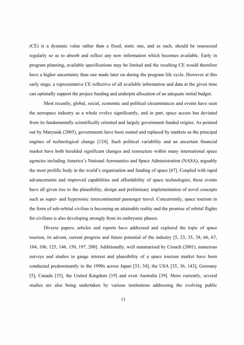
One such particular spaceplane which deviates from a purely space tourism objective, is
the SpaceLiner [168, 182, 183, 185, 186], shown below in Figure 1.
Figure 1: Artist’s interpretation of SpaceLiner 7 [82]
This hypersonic, suborbital vehicle, shown below in Figure 1, is currently under
preliminary design within the Space Launcher Systems Analysis (SART) department at the
German Aerospace Center, DLR. The concept recently received substantial funding within
context of the European FAST20XX framework [172], and aims to revolutionise the space
14
market by marrying an ultra-fast means of transportation with the allure of thrill seeking [185].
The SpaceLiner concept aims to transport passengers from Australia to Europe in 90 minutes, an
unprecedented speed compared to current civilian aviation sector capabilities.
Directly relevant to the SpaceLiner, in their paper on reusable hypersonic architectures,
Kothari and Webber (2008) derive a $500,000 figure for potential orbital space tourism [104].
More generally, however, initial forecasts made by the Futron group [23, 66] indicate that the
initial customer cluster will be prepared to pay up to $200,000 for a first ticket to space, while
more recent circulating predictions suggest that by as early as 2014, a ticket for suborbital flight
is likely to cost between $50,000 and $100,000 [192]. This initially apparent discrepancy can be
attributed to lower prices incited by anticipated market competition, and given this phenomenon
it is therefore reasonable to expect a growing emergence of public companies competing to make
access to space simpler and more affordable in the coming decades [205]. Furthermore
fundamental marketing theory of a product life cycle (PLC) can be constructively applied to the
case of space access in the form of tourism. PLC describes the expected phases for a given
product or service, from its inception, design and development, through to maturity and in some
cases, obsolescence [98]. In accordance with fundamental PLC principles, Klepper (1997)
describes that a general trend can be observed for the evolution of a particular industry,
irrespective of the industry itself. Klepper proposes that any interdisciplinary product life cycle
can be segmented into three fundamental phases being an early exploratory stage, which can be
further split into development and introduction, followed by an intermediate growth and
development stage, and finally by product maturity [149]. A PLC is then represented visually as a
relation of volume of sales and profits with respect to time during the associated phases. While
differences and deviations to a traditional PLC and its phases are recognised and classified in
wider literature to reflect the varying nature of a product [98], Peeters (2010) suggests that the
traditional PLC curve, shown qualitatively in Figure 2, can be applied directly to the potential
civilian space access and tourism industries [149].
15
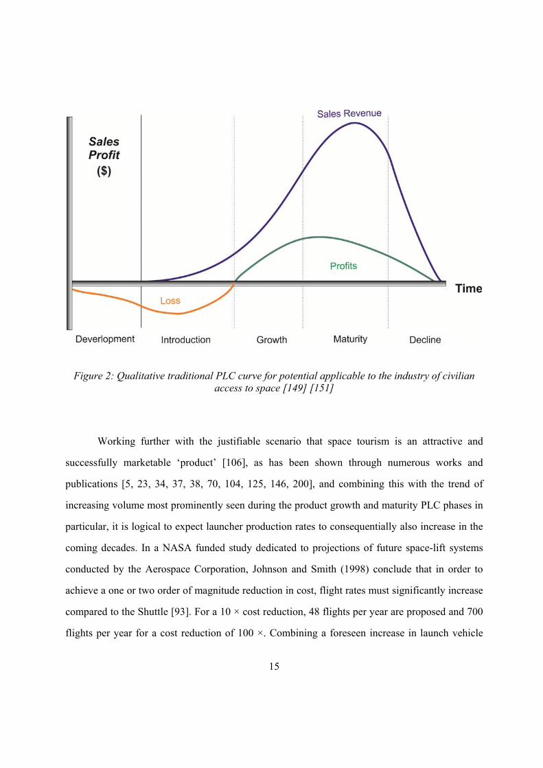
Figure 2: Qualitative traditional PLC curve for potential applicable to the industry of civilian access to space [149] [151]
Working further with the justifiable scenario that space tourism is an attractive and
successfully marketable ‘product’ [106], as has been shown through numerous works and
publications [5, 23, 34, 37, 38, 70, 104, 125, 146, 200], and combining this with the trend of
increasing volume most prominently seen during the product growth and maturity PLC phases in
particular, it is logical to expect launcher production rates to consequentially also increase in the
coming decades. In a NASA funded study dedicated to projections of future space-lift systems
conducted by the Aerospace Corporation, Johnson and Smith (1998) conclude that in order to
achieve a one or two order of magnitude reduction in cost, flight rates must significantly increase
compared to the Shuttle [93]. For a 10 × cost reduction, 48 flights per year are proposed and 700
flights per year for a cost reduction of 100 ×. Combining a foreseen increase in launch vehicle
16
demand with an increase in flights, should incite technological enhancements in spacecraft
hardware reusability, which at present is fairly limited, in particular for launcher vehicles with
manned capabilities. At present, the only projects comparable for this category of space vehicles
are the Space Shuttle fleet, which was only semi-reusable , and the Russian Buran orbital vehicle,
which performed just one unmanned flight before the program was cancelled due to a mix of
political influences and lack of funding [80]. Consequently, higher launch rates should drive
launch costs and overall space access costs down, requiring existing cost models to be
recalibrated to facilitate the change. As an example, recent suggestions have implied that the
SpaceX fleet of Falcon 9 vehicles “break the NASA/Air Force Cost Model NAFCOM” [193]. So
with the recently transpired and justifiably foreseen advancements to space access through the
advent of commercial space travel spurred on by current space access and space tourism
initiatives, it is essential for cost estimators and experts to keep abreast of the technological
changes and have the capability to obtain indicative, relevant and justifiable estimates despite
implementation of novel, unprecedented technologies.
Returning back from the costs of applications to the costs of the space vehicles and
launchers themselves, to foster and accommodate for such progressive trends within the space
sector, stringent and consistently applied cost engineering principles and practices are key to
ensuring that estimated costs for new, unprecedented programs are representative, justifiable or at
the least indicative of expected costs while being reflective of all available inputs and information
at the time. As mentioned previously, a CE is a dynamic, constantly varying figure. So while it is
impossible to predict exact program costs, consistently applying certain principles, practices and
methods, like revising CEs at regular interval throughout the program life cycle to incorporate
any changes and reflect new information, supports budgeting decisions and maximally assists in
avoiding significant unexpected budget blow-outs [72]. Or if exceeded, helps to ensure that the
discrepancy between the existing dynamic estimate, the available allocated budget and the actual
cost is minimised. Furthermore, at various program phases the amount of defined information
17
increases as program specifications and requirements crystallise. Here, it is important to identify
the most appropriate cost estimation approach at each phase from a diverse selection of cost
estimation methods, models and techniques as defined and reviewed within this Thesis.
Numerous excellent resources exist, which list and describe general and specific cost
estimation methods, models and tools applicable to the space sector. Actually many of the most
extensive documents have been lengthy government funded projects and studies, a fact which
only emphasises the importance of the topic within industry. In 1977 The RAND Corporation
released a comprehensive study under Project AIR FORCE aimed at listing and assessing the
validity of parametric spacecraft cost estimation methods for current and future applications with
a decreased focus on system mass, while stressing the importance of concurrent utility of human
logic and reasoning during cost model use and application [47]. Consequently, another two in-
depth RAND studies into shortcomings of cost estimation methods were released in 2008 [65,
227]. In the RAND document which addresses cost estimation of space systems within the Air
Force Space and Missile Systems Centre (SMC), Younossi et al. incorporated past lessons learnt,
while providing future recommendations for improving the processes, methods, tools and
resources based on the study’s findings [227]. The second, document by Fox et al. is a dedicated
handbook reference describing guidelines and metrics needed to review costs associated with
space acquisition programs [65]. Both documents list and contain descriptions of some key cost
estimation models, such as the Unmanned Space Vehicle Cost Model [214], (USCM), the
NASA/Airforce Cost Model (NAFCOM) [170, 171, 188] and Small Satellite Cost Model [7].
More specifically, Meisl (1988) described the cost estimating techniques especially for early
program phases [128], while more recently, Curran et. al (2004) provides an in-depth look on
aerospace engineering cost modeling [40]. Other documents, such as NASA’s Cost Estimating
Handbook [135-137] and the online DoD Parametric Cost Estimating Handbook [42] also offer
their own lists of various industry-relevant cost estimation tools and methods. Depending on the
source, the scope of these lists is typically broad, covering many specific estimation methods for
18
mission hardware and software, development, operations, management and risk analysis amongst
others, but usually with limited, brief descriptions per entry. Alternatively, the literature will
focus on a very narrow range of select models and methods, while omitting key others.
The remainder of this chapter presents the critical first steps, basic theory and material
necessary for logical progression of the rest of this Thesis. It does so through offering a niche,
robust summary for the main cost estimation methods, approaches and resources applied within
the space sector for space hardware, with key existing commercial off the shelf (COTS) and
government off the shelf (GOTS) tools and software products also discussed. Many of the
commercially available products feature classified databases and have associated annual license
fees. They are therefore not deemed focal to very early program phases where research into
program development is still ongoing, specifications are not yet clearly defined, but a CE for the
anticipated program is nevertheless required to proceed further. For completeness sake, these
models are, however, included and briefly discussed within the review. Manuals, handbooks and
reports directly applicable to space sector cost estimation with a specific complete system level
are also outlined, since they are seen as valuable resources for advanced methodology
development for reusable launch vehicles. Furthermore, the Thesis features a hardware focus, and
while it is clear that software and associated development, implementation and operations costs
are essential for the realisation of every mission, the software-specific cost models are not
included within the scope of this Thesis, since this is considered a sub-system component of an
overall system. This Thesis approaches cost estimation at early program phase, and therefore
from a top system level.
Firstly the relevant cost estimation methodologies applicable to the space sector are
outlined and discussed. Consequently, their implementations in key existing models, tools and
resources are provided, with each the associated features, factors, benefits, drawbacks and
applications detailed and discussed.
19
2.1 COST VERSUS PRICE
At the commencement of this Thesis work, it is essential to define the accounting terms of
cost and price, briefly outline the significant distinction between their meanings, and consequent
use of terms both throughout this Thesis, as well as within context of the cost estimation domain.
Cost and price are directly related, although frequently the two are used interchangeably
depending on their context, which are not always correct to the definition. Cost is the amount
considered from the side of the program organisation, and relates to the total amount paid or
payable for the acquisition of all materials, property (goods) and services calculated for the
project on the basis of an estimate of required effort, and other direct costs for all additional
resources, such as manpower, equipment, real facilities, material, supplies, as well as travel and
bought out items [202]. The term ‘cost’ is then frequently combined with an adjective, for
example ‘program development cost’. In contrast, price is what the consumer is expected to pay
for the product, or the dollar value that a company will sell its product for or commit to a
contract, meaning usually the total monetary value of the total project cost, with a calculated
profit or fee additionally imposed [202]. In this respect, ‘cost’ is a sub-set of the term, ‘price’.
Very often, the terms price and cost are used interchangeably. And while recognising the
difference in the technical definition, in this Thesis, the term ‘cost’ (or ‘costs’, both of which are
also used interchangeably), is predominantly used to describe how much monetary resources are
required to fund the various phases of space programs in the early phases. This is because the
perspective of this Thesis is from the producer’s position. At the end of most cost estimations and
calculations, the profit is also finally built in, thus technically making that value a ‘price’ value.
However, whenever a profit margin is included in a presented figure, this point is always clearly
identified and stated. Therefore, in recognising the technical difference between price and cost,
the term ‘cost’ is adhered to throughout this work, since the area of research is cost engineering,
and cost estimation, and the bulk of the resulting figures which are calculated, manipulated and
analysed, are indeed costs, unless otherwise indicated.
20
2.2 SPACE SECTOR COST ENGINEERING & ESTIMATION
2.2.1 Cost Estimation in a Cost Engineering Framework
Cost estimation features prominently, essentially and diversely across all industries and
domains in today’s competitive and profit-driven environment. From small-scale, private,
commercial initiatives such as how much a holiday or the purchase of a house might cost, right
through to multi-billion dollar project bids within the construction, building and infrastructure
industries – the question of cost firmly dominates and dictates business activity, initiatives and
undertakings, and ultimately progress.
Within the aerospace industry, this is no exception. From cost figures simply being made
up, like in the initial instance for the Concorde program [221], to labour hours and materials
being tediously tallied to obtain crude cost estimates during World War II to advanced models
and tools which have been developed and applied today, cost estimation is an integral element of
program planning, management, overall system design and the cost engineering framework.
While cost estimation and cost engineering are distinct and separate disciplines, the two
are intimately related. Cost engineering itself is a multi-faceted discipline and science which
addresses cost estimation and control, business planning and management, profitability analyses
and scheduling of major and complex engineering projects through the application of engineering
principles [40, 84, 161]. By applying this definition, cost estimation is therefore a constituent
component or subset of the larger cost engineering framework [107, 203], and is defined as the
process of prediction of forecasting of product or output costs, resulting in an estimate [162]. A
CE in itself, however, is not a static or deterministic value. On the contrary, it is a living variable
which must be progressively updated, revised and readjusted throughout the program life cycle. It
is true that an estimate will almost always vary from the final program cost due to unforeseen
factors and events which cannot be factored in during formulation of the estimate. Nevertheless
careful, realistic budgeting is a crucial first step to underpin future program success, the basis for
21
which is derived from a preliminary program CE. Hence it is logical to state that a justifiable,
competent, informed CE reflective of all the data which is available during the early program
planning is a solid foundation for an adequate and supportable program budget [212]. In turn this
increases chances for a program’s timely and efficient execution and ultimately realisation. An
initially excessively high estimate may result in a lost contract award, while an underestimated
figure would lead to cost overruns during project implementation [132]. So while there may be
preliminary, limited, or insufficient information available regarding configuration, mission or
environmental parameters of a mission early during a program, a pronounced need still exists for
reasonable, justifiable estimates to be achieved. During such estimates, analyses performed assist
in identification of key cost drivers which may be specific to each mission. In 1988, Meisl
proposed that a heuristic approach is optimal for application during early program phases where
many program parameters, such as configuration, mission and environment, were undefined and
unclear. This approach draws upon past experience and knowledge while adjusting for
differences between the new and historical data [128]. And within the space industry even today,
such a heuristic approach still forms the fundamental backbone of most cost estimation methods
and models [72].
Here, during early mission phases, effective schedule management also directly integrates
into the cost estimation framework, since the two are directly interdependent. It is clear that time
delays result in increased costs not factored for in an initial CE, and therefore in cost overruns.
With supporting processes and practices in place aiming to optimise available resources,
facilities, funds and materials, careful and strategic schedule definition and management, both
essential elements within cost engineering, determine the success of a program [56]. The ultimate
objective is to meet project deadlines and thus cost targets while attaining required technical
performance.
Overall, however, essentially three key elements can be identified to accommodate for
effective cost estimation practice [128], as shown graphically in Figure 3. The most challenging
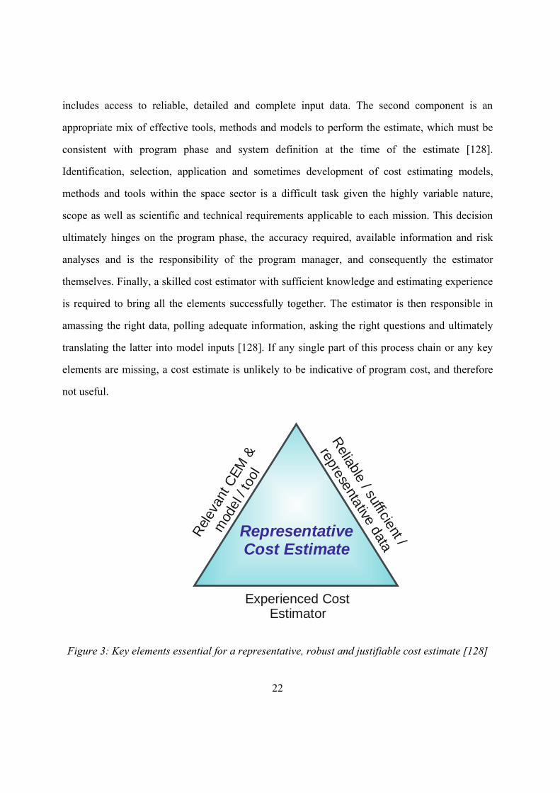
22
includes access to reliable, detailed and complete input data. The second component is an
appropriate mix of effective tools, methods and models to perform the estimate, which must be
consistent with program phase and system definition at the time of the estimate [128].
Identification, selection, application and sometimes development of cost estimating models,
methods and tools within the space sector is a difficult task given the highly variable nature,
scope as well as scientific and technical requirements applicable to each mission. This decision
ultimately hinges on the program phase, the accuracy required, available information and risk
analyses and is the responsibility of the program manager, and consequently the estimator
themselves. Finally, a skilled cost estimator with sufficient knowledge and estimating experience
is required to bring all the elements successfully together. The estimator is then responsible in
amassing the right data, polling adequate information, asking the right questions and ultimately
translating the latter into model inputs [128]. If any single part of this process chain or any key
elements are missing, a cost estimate is unlikely to be indicative of program cost, and therefore
not useful.
Experienced Cost Estimator
Reliable / sufficient /
representative data
Rel
evan
t CEM
&
mod
el /
tool
Representative Cost Estimate
Figure 3: Key elements essential for a representative, robust and justifiable cost estimate [128]
23
2.3 COST RISK ASSESSMENT & UNCERTAINTIES
In addition to careful scheduling, to minimise the likelihood of cost overruns and
scheduling delays, the effects of unexpected events must be considered during initialisation of a
program. This process is particularly important during formulation of a program’s initial CE,
when a detailed understanding and assessment of potential cost risks is essential. Here it is
important to define the meaning of ‘risk’ and differentiate this from ‘uncertainty’. Risk addresses
the probability of a certain event occurring and its consequent impact on a project, and therefore
risk can be in part preempted for and factored in within an estimate. Uncertainty, however, relates
to an unforeseen, unexpected event which becomes known only after it has occurred [173]. So
while potential risks for a project can be identified, analysed, planned for and managed, the
uncertainty element for unexpected costs during project lifetime is impossible to fully address
during the early program phase. Furthermore, risk and uncertainty are not mutually exclusive,
with the modeling of uncertainty directly translating into risk [42]. Therefore any given project
can never be entirely risk-free, although various cost risk quantification analysis methodologies,
strategies and approaches exist to address this aspect. So while cost risk estimation is an
extremely important element within the cost estimation process and cost engineering framework,
it is not delved into in great detail within the scope of this work. Interested readers may refer to
the following references for further details on cost risk assessment and management [13, 42, 65,
137, 175, 212].
Another type of uncertainty not directly associated with unexpected events arising during
a program relates to a formulated CE itself. This uncertainty is associated with the development
or implementation and thus usefulness of any cost model underlying the estimate, and includes
factors like omission of a key cost driver, data inconsistencies, and model limitations and
simplifications due to lack of data [42]. Additionally, this uncertainty also encompasses an
estimate’s accuracy based on available program data, and also the correlation with a program’s
phases. Normally, early in a program only few specific mission details are available based on
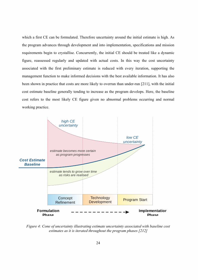
24
which a first CE can be formulated. Therefore uncertainty around the initial estimate is high. As
the program advances through development and into implementation, specifications and mission
requirements begin to crystallise. Concurrently, the initial CE should be treated like a dynamic
figure, reassessed regularly and updated with actual costs. In this way the cost uncertainty
associated with the first preliminary estimate is reduced with every iteration, supporting the
management function to make informed decisions with the best available information. It has also
been shown in practice that costs are more likely to overrun than under-run [211], with the initial
cost estimate baseline generally tending to increase as the program develops. Here, the baseline
cost refers to the most likely CE figure given no abnormal problems occurring and normal
working practice.
Figure 4: Cone of uncertainty illustrating estimate uncertainty associated with baseline cost
estimates as it is iterated throughout the program phases [212]
Concept Refinement
Technology Development
Program Start
Cost Estimate Baseline
ImplementationPhase
Formulation Phase
high CEuncertainty
low CEuncertainty
estimate becomes more certain as program progresses
estimate tends to grow over time as risks are realised
25
The latter processes and principles are graphically illustrated below in Figure 4 in what is
referred to as the cone of uncertainty [211], where the horizontal axis represents project
milestones and phases, while the vertical axis indicates estimation uncertainty and variability. It
can be seen that underrun of costs during early program phase is significantly less likely than a
cost overrun.
2.3.1 Cost Estimation Diversity within the Space Sector
Cost estimation within the space sector must be able to encompass a diverse scope of
missions ranging from simple satellites to reusable launch vehicles and manned spacecraft. Each
project is then further broken down into its technical system and sub-system deliverable elements
as well as organisational components. Therefore at various stages of a program, separate cost
estimates are required to address program development and manufacture of both hardware and
software, operation costs, life cycle costs (LCC), management and organisation costs. Other cost
assessments, such as advocacy and independent cost estimates (ACE and ICEs) are also required,
which are separate, although associated with or embedded within the context of an existing LCC
estimate [136]. To facilitate for all these cases, proper selection of appropriate estimation
methods and tools is vital, since this positively impacts overall project costs. Many variables and
considerations dictate this choice, including available technical definition detail and program
phase, the scope of the effort to be costed, availability of historical cost data and program
maturity coupled with the cost estimator competency and experience [135]. While it is important
to recognise these differences, the methods and processes themselves remain fairly consistent.
To address the diversity for cost estimation purposes, numerous proprietary, dedicated
models exist to estimate various aspects of mission costs for both software and hardware. These
include cost models for subsystems and space instruments (SICM, NICM, MICM) [65, 74, 135],
systems engineering processes (COSYSMO) [29], operations and processing (SOCM, MESSOC)
26
[134, 174, 194], as well as ground development and risk assessments (ACEIT, Crystal Ball,
@Risk) [136]. Even a model for determining the cost of performing a cost estimate has been
addressed [47, 159]. This Thesis, however, specifically focuses on commercial off-the-shelf
(COTS) cost estimation approaches applicable on a more global system level for an overall space
flight project with a hardware focus. The methods of focus here are normally best suited and
particularly necessary and applicable during the initial phases of program development and
mission planning.
2.3.2 Cost Engineering Oriented Organisations
The importance of effective, efficient and accurate cost engineering practices, as
underpinned by effective cost estimation throughout a program life cycle, is unquestioned. Yet
despite this fact, cost estimation methods and practices within industry remain largely undefined,
with a lack of understanding stemming from limited education, training and support available to
the cost engineering community. It is logical that an ability to control costs directly hinges on
closely adhering to set guidelines and learning from previous projects while simultaneously
reacting to current circumstances efficiently and effectively [123]. Yet prevailing organisational
inconsistencies concerning the absence of formal structure, documentation and processes for cost
estimation methods and practices [161] combined with ineffective retention of past experience,
knowledge and ‘lessons learned’ continuously results in inefficient outcomes. And with deadlines
and competitive bidding for projects adding time pressure to the mix, unstructured, hasty cost
estimations result in repeated significant budget overruns, particularly within larger organisations
and agencies like the US DoD [226], ESA [43, 44], and NASA [210].
These issues and inconsistencies have underpinned the emergence of numerous
professional, industry and Government cost estimation groups and organisations whose core
fundamental philosophy and aims are to promote the standardisation of cost engineering
27
principles within industry. This is done through encouraging effective knowledge management
and retention, and pooling available resources to establish and maintain a common basis and
standards for cost engineering practice. Amongst others these include the International Society of
Parametric Analysts (ISPA) [90] and the Society of Cost Estimating and Analysis (SCEA) [189]
(both of which merged together in November 2012 to form the International Cost Estimating and
Analysis Association (ICEAA)[88]), the Space Systems Cost Analysis Group (SSCAG) [196],
the Association for the Advancement of Cost Engineering through Total Cost Management
(AACE) International [16], American Society of Professional Estimators (ASPE) [11],
Association of Cost Engineers (ACostE) [204] and the International Cost Engineering Council
(ICEC) [87]. While having a slightly different focus, fundamentally all of these organisations
share the common goal of cooperating and promoting better, more consistent cost engineering
principles and cost estimation practices and standards.
28
2.4 COST ESTIMATION METHODS
Predominantly, four main, commonly accepted and staple cost estimation methods
(CEMs) form the backbone of tools applied for cost estimation within the space sector being:
Engineering Build-Up
Analogy
Parametrics
Expert Judgement
The detailed engineering build-up (also known as bottom-up) estimation approach
encompasses the synonymous techniques of engineering build-up, grassroots or detailed cost
estimations. Analogy and parametric cost estimations are then part of the top-down methods or
statistical approaches and can be classed as gross estimation methods. The Rough Order of
Magnitude (ROM) approach is also outlined in the NASA Handbooks as a commonly utilised
method. Finally, expert judgment (EJ), arguably, is another method commonly relied upon to
generate cost estimates, although there does not appear to be a clear consensus on whether or not
it constitutes an official method [83].
Several of the techniques can also be strategically combined to formulate a hybrid
estimate. Alternatively, if this is possible, an existing tool or model can be taken and potentially
‘tailored’ to a particular mission’s specifications through manual input or calibration. Given
recent radical advancements to space access and technologies with the political environment
encouraging commercial space access coupled with the advent of space tourism, it is more
important than ever to have the capability to obtain representative cost estimates. Currently,
given the promising advent of commercial launches [58, 205], ultrafast space transportation [52,
104, 167, 183, 191, 208] as well as the potential for space tourism [5, 23, 37, 70, 71, 106, 143,
146, 149, 167, 197, 200], this applies particularly to launch vehicles with manned capabilities.
29
Yet a lack of precedent and consequently very limited data exists for this category of spacecraft,
limiting the suitability and application of the most commonly implemented CEMs within the
space sector.
The key CEMs, including the core three, as well as the supplement ones currently
recognised and utilised within the space sector are concisely summarised below, and their
respective attributes, strengths and shortcomings also provided.
2.4.1 Parametric Cost Estimation
Parametric cost estimation is applied prolifically within academic, research, industry and
government applications, offering a means to economically approach proposals, negotiations or
basic program cost assessments which hinge on cost or price data and estimation. More
specifically, the parametric approach is extensively applies in advanced planning studies,
contractor proposal validation, as well as commonly being used within planning and budgeting
during acquisition processes [42] with the CEM having official acceptance by the Federal
Acquisition Regulation (FAR) for proposal preparation [59]. It is also the foundation of
numerous key models and software used for early phase cost estimation of space programs, such
as the TransCost Model [100-102], the USCM [214] and NAFCOM [171, 188]. A particular
distinction of this approach is that it can be used when little is known about the design to be
costed, or when a readily applied validation or consistency check of an existing estimate is
required.
Best applied within early program phases, a top-down approach is assumed since only
basic requirements are usually available, while more detailed system and subsystem criteria are
not yet established. Only basic inputs which can be easily projected before concrete of final
design and specification information is available, and which logically relate to cost, are required.
Such often preliminary inputs are then sufficient to provide adequately representative cost results
30
[81]. A series of mathematical relationships called cost estimating relationships (CERs) are then
determined based on historical data. CERs seek to relate cost to physical, technical and
performance parameters that are known to strongly correlate with program costs. Complexity
factors, or specific manually defined user inputs can then be applied to address deviations from
underlying CER parameters and a particular mission of interest.
However while it is commonly believed that early mission costing cannot be done
effectively in any other way, a difficult aspect of parametric cost estimation is the actual CER
formulation itself. A cost model is only as robust and reliable as its underlying database of
projects, so database quality and size impose limitations on CER credibility [60]. Significant
amounts of time and resourced are devoted to the collection of quality raw data, which then
usually needs to be adjusted for consistency, or normalised, to make it comparable and
compatible with other relative data. The challenge lies in obtaining sufficient, representative
quantities of cost data, yet alone in finding accurate, relevant and sufficiently detailed numbers
and figures. The DoD Parametric Cost Estimating Handbook [42] identifies nine main data
sources which include basic accounting records, contracts, cost reports and proposals, historical
and technical databases, other information systems and organisations, and functional specialists.
Here, a key difficulty concerning access to data arises due to the classified nature of most projects
within context of a competitive space industry. In fact the data collection process is often the
most time-consuming, strenuous and costly aspect in cost estimation and for accurate CER
formulation [137]. Even extracting data retrospectively from projects poses challenges relating to
contractual and administrative complexity [100]. Furthermore, all developed CER credibility
must be verified through comparison and sufficient correlation to existing projects. The interested
reader is directed to consult references [42, 89, 212] for more detailed information and discussion
about quality data collection, adjustments and normalisation for CER development.
In addition to the challenges of CER formulation, the CERs, once developed, may not be
relevant when new technologies or requirements beyond normal boundaries of the underlying
31
CERs are introduced [109]. In this respect, assumptions must be made that historical data are
representative of future conditions, rendering CERs only effectively applicable to projects similar
in nature as the CER data itself. A solution here is to employ an alternative estimation method
which can be used as a sanity check, or to combine several approaches if it is possible to segment
the cost estimate into constituents which can be each addressed by various approaches.
2.4.2 Engineering Build-Up
Known synonymously as engineering build-up (EBU), bottom-up, grassroots or detailed
cost estimation, this very specific analytical approach is generally applied to a mission when all
parameters at system and sub-system levels are known and clearly defined. Cost estimations are
then performed at the lowest level of detail, and require a breakdown of the overall project into
smaller work packages, taking the form of a Work Breakdown Structure (WBS), which also
provides the reference for the Cost Breakdown Structure (CBS). The low level cost estimates
usually come directly from the engineers and experts performing the designated work, the sum of
which then constitutes the overall cost estimate for the program. It is common for labour
requirements and non-labour factors, such as material quantities, to be identified and estimated
separately, with any additional overhead costs, such as administrative expenses, being
concurrently factored in to obtain the total estimate [135, 136]. Therefore EBU is inherently an
extremely resource-intensive approach with significant associated costs, time and effort.
Extremely careful attention must be paid to the organisation of the WBS to avoid duplications
and omissions of tasks, which would then reflect directly on costs [173].
Inability to quickly adapt to scenario changes or specifications, requirement and design
alterations, which are frequently made during early planning phases, is a weakness of this CEM.
Given any modifications, new estimates must then be built up again. So ideally, detailed and
advanced low level specifications are necessary for application of EBU. These are usually not
32
available during the beginning stages for mission planning, which renders the approach
unsuitable for application during early project phases.
However if applied during later project phases (i.e. Phases A – D) when sufficient details
are available, the resulting cost estimate can be extremely accurate since it is unique to the
specific industry and application [212]. Credibility is established since the total cost can be
broken down into constituent cost elements, providing clear insight into major cost contributors,
making elements of the estimate reusable within individual project budgets, and making the cost
estimate defensible [135]. Insight is also gained into major drivers and contributors to overall
cost, which can be useful for program review and analysis.
2.4.3 Estimation by Analogy
Analogy cost estimation relies on an extrapolation based comparison between different
precedent or existing efforts which are deemed to be similar or ‘analogous’ with the item being
costed [137]. Intensive analyst judgment is required regarding the similarity of two projects,
followed by adjustments made for any differences, such as project size, complexity, team
experience or technologies, between them. Although necessary, such judgment is often
considered subjective [212]. Application of the method is also limited since identifying a suitable
analog or adequately detailed technical, program and cost data are often an extremely difficult
task. If successfully identified, reliance for the comparison is then based on a single data point
only. Therefore sufficiently detailed data of the ‘compared’ system as well as the ‘new’ system
under consideration is essential. The method then hinges on the past experience, knowledge and
judgment of the expert regarding consequent adjustments or extrapolations. Strengths of the
analogy CEM include its quick and effective application at any time throughout various program
phases at minimum cost, since analogy can be applied even before specific program
33
specifications are known. And if a close suitable analog is found, the resulting estimate is then
based on sound factual historical data and is defensible.
Analogy can be further broken down into Loose Analogy (LA) and Close Analogy (CA).
LA requires only few ‘loosely similar’ data points not closely related to new project, and adjusts
relevant past broad experience for moderate changes in complexity. CA requires very similar data
points from either another program or through technical development studies, and calls upon
direct past experience with adjustments made for only minor changes in complexity [109].
2.4.4 Estimation by Expert Judgement
Expert judgment (EJ), or expert opinion, is a commonly applied approach despite being
subjective in nature of the assumptions and assessments which are formulated by the estimator
based on their own experience and knowledge. According to ESA’s Engineering Costing
Techniques specifications, EJ is classed as an cost estimation method [72], contradictorily as both
the backbone and limitation of the analogy approach [60], as knowledge based cognition [130]
and simply guessing [97] in other literature. A widespread feeling exists that the EJ approach is
particularly intuitive and as such, consequently liable to personal knowledge bias and sensitive to
political pressures [83]. Yet while frequently criticised and often misunderstood by those outside
the cost estimating community [161], EJ is consistently and extensively applied in the generation
of cost estimates [72, 163]. Applicable during all project phases, EJ can be beneficial when
historical data are scarce or unavailable. While gathering a group of experts may require some
resources, once achieved, EJ requires comparatively minimal effort, time and cost and is often
used as a sanity check for CER results where implemented data are significantly beyond the CER
data ranges [212]. In fact various more advanced techniques have been designed with EJ at their
core. One example, the Delphi method, relies solely on group engineering EJ obtained from
several professionals, to provide the cost estimator with latitude in their cost prediction [135].
34
Another useful approach is the Analytic Hierarchy Process (AHP) developed by Dr. Thomas
Saaty [164, 165]. AHP decomposes a problem into a hierarchy of specific criteria and
alternatives. Expert judgment is then employed to determine and assign specific rankings, or
priority scales through pairwise comparisons to the established criteria [73, 95, 165], and after
some normalisation of the rankings, an overall relative score can be deduced per option. An
advantage of AHP is its capability to significantly reduce complex, multi-faceted decisions to a
series of simple pairwise comparisons, in this way capturing and reflecting the subjective and
objective aspects of a decision [164]. Another strength is the method’s applicability to a decision
process despite the absence of quantitative ratings, since assessors and experts are always capable
of determining which criteria dominate over other criteria within a pairwise comparison context
[95]. A recognised weakness pertains, however, directly to the same weakness as that of the EJ
element itself, namely the fact that the EJ involved can be inconsistent or prone to knowledge or
experience bias. Ways to gauge any inconsistency and improve the EJ element of AHP are
challenging [95]. Despite this, AHP constitutes a powerful tool for comparisons of alternative
design concepts based on qualitative and quantitative criteria.
2.4.5 Rough Order of Magnitude Estimation
The NASA Cost Estimating Handbooks [135-137] define the rough order of magnitude
(ROM) estimation as one of ‘four generally accepted estimating methodological approaches’
[137]. Also referred to as a vendor quote (VQ), this ‘first order’ methodology is useful early in
mission planning phases to estimate costs via ‘rules of thumb’ that are either already known from
past experience, or readily available based on polling of current industry-wide data [109].
Applications of the ROM method for cost estimation include hardware, facilities and services,
usually when a project has not been started and when requirements are not explicitly specified.
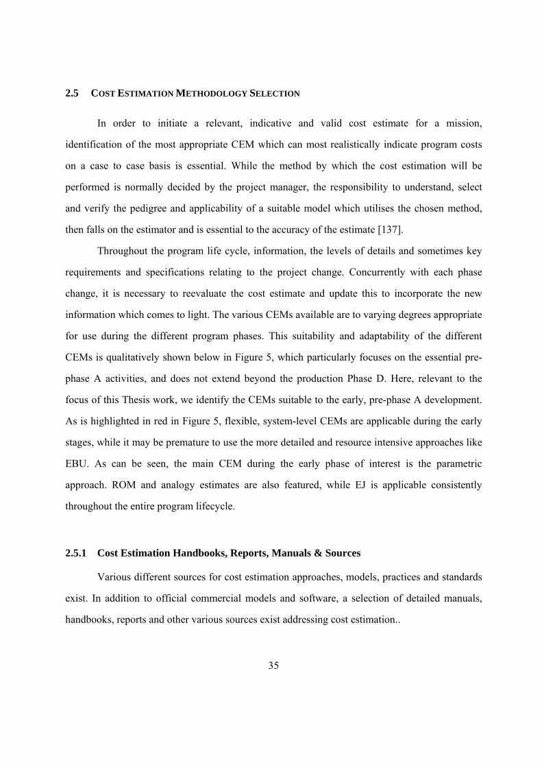
35
2.5 COST ESTIMATION METHODOLOGY SELECTION
In order to initiate a relevant, indicative and valid cost estimate for a mission,
identification of the most appropriate CEM which can most realistically indicate program costs
on a case to case basis is essential. While the method by which the cost estimation will be
performed is normally decided by the project manager, the responsibility to understand, select
and verify the pedigree and applicability of a suitable model which utilises the chosen method,
then falls on the estimator and is essential to the accuracy of the estimate [137].
Throughout the program life cycle, information, the levels of details and sometimes key
requirements and specifications relating to the project change. Concurrently with each phase
change, it is necessary to reevaluate the cost estimate and update this to incorporate the new
information which comes to light. The various CEMs available are to varying degrees appropriate
for use during the different program phases. This suitability and adaptability of the different
CEMs is qualitatively shown below in Figure 5, which particularly focuses on the essential pre-
phase A activities, and does not extend beyond the production Phase D. Here, relevant to the
focus of this Thesis work, we identify the CEMs suitable to the early, pre-phase A development.
As is highlighted in red in Figure 5, flexible, system-level CEMs are applicable during the early
stages, while it may be premature to use the more detailed and resource intensive approaches like
EBU. As can be seen, the main CEM during the early phase of interest is the parametric
approach. ROM and analogy estimates are also featured, while EJ is applicable consistently
throughout the entire program lifecycle.
2.5.1 Cost Estimation Handbooks, Reports, Manuals & Sources
Various different sources for cost estimation approaches, models, practices and standards
exist. In addition to official commercial models and software, a selection of detailed manuals,
handbooks, reports and other various sources exist addressing cost estimation..
36
Figure 5: Qualitative application of CEMs according to project phase [109]
Prominent handbooks include the NASA Cost Estimating Handbook versions [135-137]
the SSCAG Space Systems Cost Risk Handbook [137], the FAA Life Cycle Cost Estimating
Handbook [60], the ISPA Parametric Estimating Handbook [89], the DoD Parametric Cost
Estimation Handbook [42], the RAND Project AIR FORCE Reports [47, 65, 227], and the GAO
Cost Estimating Assessment Guides [210-212], amongst others. These numerous sources,
however, generally tend to focus on particular elements of cost, such as cost risk or life cycle, or
a particular approach, as relevant to their most common application.
Feas
ibility
Pre-P
hase
APha
se A
Phase
B
Phase
C/D
Archit
ectu
re
LooseAnalogy
CloseAnalogy
EngineeringBuild-Up
Parametric Modeling
Rough Order of Magnitude
(ROM)
Expert Judgement (EJ)
Top-DownCost Estimation
Bottom-UpCost Estimation
Produ
ction
37
As a part of this Thesis, a comprehensive literature review of relevant literature was
conducted and published to determine CEMs and consequently tools, models and resources
which utilise them. This review can be found in ref. [209] for the interested reader, and allowed
the identification and selection of methods, as well as tools, models and resources for application
to large scale, complex programs during the early program phases. Extracting information from
this research, relevant models and tools were identified for effective practical application to the
SpaceLiner industry case-study.
38
2.6 THE AMALGAMATION APPROACH TO COST ESTIMATION
The wide scope of available cost estimation resources means that cost estimators must
select the most suitable cost assessment means for a given project during a specific program
phase. Such choice is subject to constraints including laws and regulations, as well as license and
subscription fees for most software packages. The cost estimator must be capable to justify their
choice of cost model, as dictated by project purpose and level of design details available [135].
Here, two important things should be emphasised. The first being a distinction between a
cost estimation methodology (CEM) and a cost estimation tool or model. CEMs refer to an
underlying approach or principle of performing a cost estimate, like the parametric or analogy
approaches. In turn, tools like PRICE-H or 4cost, or the various available models like TransCost,
refer to commercial or government products which are based around a specific underlying CEM.
It is essential to again stress that while a suitable method, model or tool is key for an estimation,
the science of cost estimation also incorporates the elements of good data, as well as an
experienced, knowledgeable estimator. Together, the three elements combine to produce a robust,
justifiable estimate to support a representative, realistic project budget, as previously shown in
Figure 3. Within this chapter, the development, logic, structure and application of the new
Amalgamation Approach, as developed through the work conducted within this Thesis, is
introduced and explained.
2.6.1 Multiple CEMs, Models & for Cost Estimation
In order to obtain an overall system level cost estimate for a program, the mission
elements must be costed with respect to their development, production and operations phases
including launch and ground operations and support. Any associated profit margins should then
also be incorporated to obtain the price (see Chapter 2.1). The CEMs and range of available
models, tools and resources available are more suitable in varying degrees for use in particular
39
circumstances and for specific applications during different project phases, as has been
demonstrated in Chapter 2.5. It is therefore common for estimators to loosely combine multiple
different CEMs and also tools to obtain cost estimate for an overall system. It is known that this
approach can maximally support the various associated engineering tasks involved for large
projects, while also allowing for the comparison of cost models [203]. For example, in their paper
which compares ESA and NASA cost estimation approaches and end results for a human mission
to Mars, Hunt and van Pelt (2004) list the CEMs of parametric CERs, PRICE-H, SEER-H,
historical analogies and vendor quotes as the chosen methodologies to arrive at a preliminary
estimate [85]. However, although applied and described in select research papers, until now, such
a combination approach has remained predominantly, highly intuitive, with no formal structure
being outlined nor defined for its application.
2.6.2 Amalgamation Approach Definition & Application
Many of the significant cost estimations, in particular for large scale complex projects like
those undertaken within the space sector, rely on one main cost estimation source, model, tool or
CEM, with perhaps a loose sanity check from another estimating source [60], and sometimes also
numerous models and tools. The AA definition hinges on a cost estimate, whether at a macro- or
micro level, being derived through a formalised cross-check with multiple other means, whether
through a different CEM or tool and model. In any case, a minimum of three cost estimate results
are required and contrasted amongst each other. In this way, multiple points can be used by the
estimator as reference, with strategic analyses then employed to justify selection of a most
representative cost estimate or range. In this instance, simply a pairwise comparison would be no
different to a sanity check, and given a significant cost estimate delta, might make it challenging
to determine which out of two estimate holds the most uncertainty. Three estimate results which
40
are thoroughly and strategically executed, however, should allow for the cost estimator to make
an easier identification of where any inconsistencies or issues might originate from.
This Thesis therefore proposes a formalised standard, the AA, for such an approach,
which harnesses a strategic combination of multiple, justifiably selected CEMs and consequently
models or tools to increase the reliability and representativeness of the cost estimate. Through
AA, an added redundancy is incorporated into the cost estimate through multiple results which
can then be analysed and contrasted. Such a seemingly basic comparison process increases the
cost estimation fidelity through elimination of factors such as human error, while concurrently
reducing uncertainty and cost risk, which might arise when a previously applied method has
specific limitations known by the estimator, which undermines credibility of the resulting cost
estimate. In essence, AA can be paralleled to life critical engineering systems within a
mechanical and hardware sense, or, for example, avionics networks on manned space craft, which
must always feature system redundancy. A similar concept and redundancy configuration, albeit
relevant within a financial context to the budget of a space program rather than human life, is
therefore proposed for cost the estimation function, through utility of AA.
Furthermore, AA is designed specifically for application during early program phase
when uncertainty of the estimate is inherently very high in accordance with the cone of
uncertainty principles already presented in Figure 4. At this stage, also, the relevant CEMs, as
well as models and tools are also relatively fast to implement, thus accommodating for relatively
quick and simple changes of parameters since inputs are generally higher-level ones.
Here, it is assumed that given the respectively large budgets associated with international,
complex programs in the space industry, due to the large scale of investment and ramifications of
failure, that sufficient resources are available to adequately support a solid cost engineering team
and its cost estimation experts, with funding allocated for necessary resources. Core requirements
are a sufficient quantity of staff to effectively execute the cost estimation function, as well as
resources for acquisition of any necessary cost estimation tools or models (license fees).
41
The proposed AA technique can ideally be utilised for three different although
complimentary purposes, at three different ‘modes’ of function. These are introduced below:
AA contribution within the formulation of cost estimate on a micro-scale, internal
to that estimate (AAMIC)
Formulation of an independent, stand-alone, ‘prime’ cost estimate at a macro-level
based on AA (AAMAC)
AA application to an existing cost estimate to serve as a sanity check or validation
for that existing estimate (AAVAL)
For each different purpose and mode of application, however, slightly different standards,
rules and requirements apply, as defined and outlined in more detail in the following sub-chapters
below.
2.6.2.1 Sub-element AA Cost Estimation
The first application of AA, AAMIC, would be a sub-function within context of
formulation of a single cost estimate which is already based on a certain CEM, and deals with the
unique requirements and specification for a particular project. In this case, internal to that
estimate, different CEMs might be able to better address the individual and various project
elements, components or processes to be costed. An example of this is where a system model,
such as the Small Satellite Cost Model (SSCM), a parametric-based tool, is applied, but where
the resulting cost estimate is expressed as a sum of constituent sub-system cost estimates at lower
levels. Here, the estimator may opt to take out particular sub-system estimate components and
42
replace them with, for example an analogy or bottoms-up estimate if more in-depth details are
available for that particular sub-system, or if past experience can offer a more representative cost
for that segment. This is an example of AA application on a micro-scale (AAMIC), contributing to
a more reliable estimate in a manner internal to that estimate. This principle is illustrated
graphically in Figure 6. A typical SSCM output is shown, but where selected cost elements (in
this instance, the propulsion sub-system) estimate as calculated by the initial SSCM parametric
model based on inputs, is replaced by costs (in this instance, cost) obtained through other CEM or
tool known to be more representative. In this example, the analogy CEM is applied, where the
propulsion engineer might know of a similar propulsion module which already exists and costs
$18.5M, based on firmly known data. The SSCM model-calculated cost element is thus removed,
and replaced by the AA-deduced value. All consequently affected values, shown crossed out in
red in Figure 6, are then revised and adjusted. While the example shows only one element being
affected by AAMIC, more elements can be influenced and revised, and more than one CEM or
even tool, can be used.
For the AAMIC the sub-system nature of the initial cost estimate to which AAMIC is
internally applied to, might imply that this initial estimate must be a bottom-up estimate, and
therefore only possible to be formulated later on during a program phase. However, even with the
case of the high-level system TransCost parametric model which can be applied even during very
early phases, a basic component breakdown to at least a secondary level of detail (i.e. engine,
rocket stage, booster etc.) AAMIC can still be applied when one of the component costs produced
by the baseline cost model is known or shown to be different through application of another CEM
or tool or model.
As the program develops through into the later program phases, the AAMIC method is
rendered less applicable. As the WBS breakdown becomes more detailed, encompassing lower
system levels, and the EBU CEM increases in relevance, by its definition, each sub-item is then
costed independently in line with the definition of this CEM.
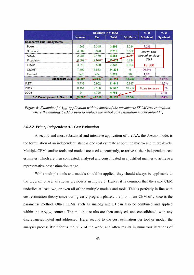
43
Figure 6: Example of AAMIC application within context of the parametric SSCM cost estimation,
where the analogy CEM is used to replace the initial cost estimation model output [7]
2.6.2.2 Prime, Independent AA Cost Estimation
A second and most substantial and intensive application of the AA, the AAMAC mode, is
the formulation of an independent, stand-alone cost estimate at both the macro- and micro-levels.
Multiple CEMs and/or tools and models are used concurrently, to arrive at their independent cost
estimates, which are then contrasted, analysed and consolidated in a justified manner to achieve a
representative cost estimation range.
While multiple tools and models should be applied, they should always be applicable to
the program phase, as shown previously in Figure 5. Hence, it is common that the same CEM
underlies at least two, or even all of the multiple models and tools. This is perfectly in line with
cost estimation theory since during early program phases, the prominent CEM of choice is the
parametric method. Other CEMs, such as analogy and EJ can also be combined and applied
within the AAMAC context. The multiple results are then analysed, and consolidated, with any
discrepancies noted and addressed. Here, second to the cost estimation per tool or model, the
analysis process itself forms the bulk of the work, and often results in numerous iterations of
Known cost through analogy
CEM
18.500
Value to revise
44
calculations before a reasonable consensus and firmly justified synthesised cost range is
achieved. The skill, knowledge and expertise of the cost estimator are essential during this
process. The cost consolidation and result synthesis process should comprise of a concise and
thorough description of analyses conducted, assumptions made and respective, detailed
justification for the final cost range selected. Being an early phase CE also indicates that a point
figure is inappropriately precise at such an early stage.
In order for AAMAC to be effective, (unlike AAMIC which has no minimum number of cost
results for effective application of the method), a minimum of three separate CEs are required to
address the case where significant discrepancies exist between cost estimation results. In the case
of only two results, while redundancy is implemented, it would be very difficult to identify the
source of uncertainty given only a pair-wise comparison. However, with three values for
comparison and analyses, yet another added degree of redundancy is achieved between three
independently derived results, making it easier to analytically identify the source of any
discrepancies or significantly large variations. Besides, significant variations or discrepancies
between results would indicate a higher uncertainty of the final CE, which is an important finding
and outcome in itself. Such discrepancies indicate to the estimator to seek and identify reasons
behind the non-consensus, focusing on where and why they night arise. And if results differ
dramatically, then the further analysis which is elicited leads to a synergy of multiple results
based on analyses of the cost engineer. This higher level of analyses and more solid justification
are enforced through AAMAC than would result from a single-source estimate value. If a clear
consensus and consolidation of the multiple AAMAC cost results reflected through a reasonable
cost range are still difficult to attain, either a larger CE range might be appropriate, or a higher
uncertainty interval associated with a more narrow cost range, might be assigned. Both outcomes
would nevertheless provide vital, transparent information to program management about the
accuracy and reliability of the final estimate. This element is usually missing, or not as explicitly
and clearly reflected in standard, single, stand-alone CEs. Alternatively, a greater uncertainty, or
45
larger cost range might incite an increased urgency to re-valuate and reassess the results as soon
as new, more specific information about the project becomes available.
For efficient use of AAMAC, a WBS of the program is required to allow for a cost
breakdown to be established at a high program level, but also at a lower WBS level, if needed.
Here, it is also necessary to establish an AAMAC interface which supports the AA function. As
such, a simple yet highly effective Excel-based tool, the Amalgamation Approach Interface Tool
(AAInT), was designed and developed within the scope of this Thesis to address the need for a
clear, simple and specialised interface which facilitates for entry and quick analysis and
dissemination of at least three sets of results in line with the AAMAC. This interface is able to
show the multiple cost results in a convenient and clear way that allows the cost estimator to
make a convenient and fast comparison and consequent analysis of multiple figures. AAInT is
also flexible and can be customised by the user to incorporate WBS structures of various depths
depending on the scale of the program. Furthermore, and more essentially, the AAinT supports
importation of cost data directly from the source into dedicated spreadsheets at the discretion of
the user, to avoid the potential for human and other transcription errors. Caution must
nevertheless be exercised when linking the input cells on the main calculations sheet to the
various cost figures in other sheets. A more detailed description of a customised AAInT example
is provided later in this Thesis in Chapter 4.8.1 with respect to the chosen case-study.
A drawback of AAMAC is that the derivation of three values using three different methods
or models is of course more resource consuming, especially if more than three values are derived
through application of different CEMs, models and tools and the costs compared and analysed.
However this is then a question of trade-off between the increase of resources and expected
increase in CE certainty, and should be decided on a case-to-case basis, with consideration to
given available resources for the cost estimation function.
The AAMAC process and the associated steps for a minimum of three tools are shown in
Figure 7. All key AA elements which are new to standard cost estimating practice are highlighted
46
in purple. At the highest AAMAC level, and reiterating theory presented previously in Figure 3, the
three elements required for a justified CE are shown, being reliable, representative and sufficient
program data, suitable models or tools to support estimate execution, and a competent cost
estimator. The data then supports the estimator in creating a program breakdown of elements to
be costed (usually in a WBS format) at the necessary level of detail. Cost calculations are
performed using multiple models, and results entered into an AA interface, AAInT, after which
they are contrasted, compared and any significant cost deltas analysed to determine the reason. If
the analyses determine an inconsistency or error, this is corrected and another cost run done via a
crucial iterative process. Thus, when the final result it reached, any inconsistencies or errors are
maximally eliminated. Not all cost deltas necessarily indicate an error as they could result from
different model mechanics. All cost estimator conclusions, reasoning, logic and justifications
should be fully documented and explained. The final step is then consolidation of multiple results
into a cost range based on the analyses performed and on the latter reasoning, justifications and
conclusions to reach the ultimate AAMAC result.

47
Figure 7: Graphical representation of AAMAC showing key inputs, logic and processes
Element
Structure
(WBS)
AAMAC
Result
cost calculations(model/tool expert user input)
Result 1 Result 2 Result 3
iteration
contrast & compare identi fy significant cost deltas in‐depth analysis
consolidation & synthesisof multiple results
full documentation
Estimator competent experienced thorough
Engineering Data current/reliable representative sufficient
>3 CEMs / models / tools
program‐phase relevant justifiable
inconsistency / error / discrepancyjustification of results
CEM/model/tool 1 input
CEM/model/tool 2 input
CEM/model/tool 3 input
AA supporting interface toolMAC (AAInT)
48
2.6.2.3 Validating AA Cost Estimation
Alternatively AA can be implemented as a sanity check or validation (AAVAL) to an
already existing estimate which might need to be validated or confirmed. The assumption here is
that such an existing estimate was compiled through use of the standard single CEM, method or
tool. Here, uncertainty may arise when the previously applied method has specific limitations
known by the estimator, which undermines credibility of the resulting CE.
As previously described, in line with the AAVAL process, other CEMs, methods or tools
are then applied to existing, identical inputs used during formulation of the initial CE, and the
result of the second cost estimate, compared and analysed alongside the already existing figure.
Here AA acts as a staunch sanity check for order of magnitude of the original estimate, to support
it, or if the difference is significant, may indicate that an alternative CEM or tool should be
applied, or that the original estimate should be questioned or reconsidered if the two are
drastically divergent. Although here, it is important to be aware that the divergence could lie in
the sanity check method itself, in which case this distinction lies to be made by the estimator
based on available data as well as their expertise and experience, two of the identified elements
for a representative cost estimate.
2.6.3 AA Key Requirements
For the AAMIC and AAVAL modes of AA there are no specific requirements or limitations,
other than first the selection of an appropriate CEM, followed by choosing a relevant model or
tool, if necessary. For the standalone AAMAC approach, however, and as already outlined in
Chapter 2.6.2.2 above, a minimum number of three models or tools must be identified and
acquired to allow concurrent estimation of program costs. Out of the three AA modes, AAMAC is
the most structured, formalised and resource intensive mode. After this, the individual costs and
model results are contrasted, compared and analysed in what is essentially a cost estimate
redundancy process. With a high level of analytical activity necessary once the first multiple set
49
of results is obtained, AAMAC can evolve into a highly iterative process where initial analysis
uncovers any inconsistencies. Inconsistencies identified may be related to human error, EJ bias,
the inaccurate translation of technical details into model/tool parameters, among others, and need
to be rectified. At each iterative loop, however, the cost result uncertainty is reduced, and the
final results honed in upon.
Since numerous CEMs exist, many combinations of different methodologies are possible,
in addition with various combinations of the available tools and models based on them. Decision
of which particular methods to combine and apply, remains the responsibility of the project
manager in close coordination with the cost estimator themselves. Here, the experience and
knowledge of the estimator is of crucial importance [128]. Such a decision hinges on a number of
determining factors which include the available information with respect to program definition,
specification and requirements, expected level of cost estimate detail, and availability of
resources such as costing tools or models, available data, finances, personnel and time. In any
case, it is essential that any decision must be fully justifiable and defensible in scope of the latter
constraints and overall project. In addition, close attention must be paid that each method or tool
is implemented by a professional and experienced estimator who intricately understands the
capabilities of their method or tool. After all, using a multitude of models does not translate into a
more accurate estimate if the methods applied are not suitable for the program, or in accordance
to program phase, or are wielded by an inexperienced estimator.
Furthermore, as already described in Chapter 2.6.2.2 an essential requirement and element
of the AAMAC framework is a simple, effective and flexible AA interface which can be tailored
for the unique nature of each program being costed with AA. In addition, a WBS is also usually
required. Depending on the nature of the program being costed, as well as the depth of cost
estimation, this usually delves into at least three if not four levels of WBS elements, which
should be achievable albeit only at a preliminary level even during the early program phases.
50
2.6.4 AA Advantages
Regardless of the mode, there are multiple benefits associated with the amalgamation
approach. All these points have already been mentioned respectively per individual AA mode in
the preceding chapters. Since each of the advantages is linked or feeds into the other advantages
due to their close relation and logical effect, the points are shown in a succinct point form below.
Cost estimate redundancy check / validation
Immediate identification of significant cost variances between methods
Assists quick and effective identification of human error data input
Increases fidelity of data accuracy for model input
Increased final cost estimate robustness, representativeness and reliability
Reduced cost estimate uncertainty and thus associated risk
Clear indication through result discrepancies, if a cost estimate needs to be reassessed or
revised
AA framework supports and elicits further analyses and clear, detailed justification of any assumptions made during cost estimation formulation
Overall, AA offers a powerful, effective and efficient redundancy check, validation or
consolidation of an existing cost estimate within context of a formalised procedural program
management framework. It helps to reduce cost estimation uncertainty and consequently financial
risk, while increasing the estimate’s representativeness, robustness and accuracy. In addition, if a
significant deviation between multiple results is observed, this outcome already indicates the
level of uncertainty, which the cost estimator can then seek to address through further, deeper
analyses to determine the underlying reasons. If discrepancies are considerable (order of
magnitude delta), then often, several iterations and revisions of cost calculations may be
necessary to arrive at a final, logical and justifiable consensus.

51
2.6.5 AA Drawbacks
Several drawbacks of AA can be identified, and are dependent on the AA mode being
used. These are:
Increased resource requirements (i.e. time, work effort, cost) associated with:
o cost estimate calculation using multiple models/tools
o analyses of multiple cost estimates, at top, and lower project WBS levels
o performing multiple cost estimate iterations if necessary, in case of significant
result variations to justify the reason
o tool/model acquisition (licensing fees and processes) and professional model/tool
user recruitment / involvement
variability of models/tool and consequently internal model/tool mechanics (additional
requirement for cost estimator to have a basic understanding of each AA tool’s key model
mechanics)
The following sub-chapters offer a more in-depth explanation of the drawbacks, and how
these should be addressed and minimised.
2.6.5.1 Increased Resource Requirements
The main drawback of AA is that the derivation of multiple values using numerous
different methods or models is of course more resource consuming, requiring more time, effort
amount and consequently resulting in increased costs for compilation of a cost estimate. Of
course more than three values can always be derived through application of different CEMs,
models and tools. However whether this approach is taken is then a trade-off question between

52
the increase of resources (and costs) and expected increase in cost estimate certainty and
reliability. This should be decided on a case-to-case basis.
In addition, in the common case of considerable cost discrepancies, various cost
estimation iterations might be required, once again being costly in terms of the time dimension.
However, it is exactly through these iterations, that sound justifications for any contradictory
figures, and thus an increased cost certainty are also achieved.
Additionally, costs for any licensing fees of commercial tools and models which are
required, might also be incurred. In addition, if multiple models and tools are utilised, and, as is
common, if these are specific, complex, multi-dimensional models, the involvement of a
professional model/tool user might be required to enter all associated inputs and ensure all data
are effectively translated into the model-specific parameters. After all, cost estimate reliability is
a direct function of the experience and model familiarity and proficiency of the user, and their
ability to translate mission specifications into specific model or tool inputs. However, compared
to the enhancement of the resulting cost estimate in terms of representativeness and reliability,
and given the very high order of magnitude costs associated with the aerospace industry
programs which the cost estimation process relates to, the increase in resources at the critical
stage of cost estimation compilation is seen as proportionate. After all, establishing a sound,
realistic and sufficient initial program budget is essential to underpin future successful program
progression and execution.
2.6.5.2 Variability of Model Mechanics & Model Experts
The AA stipulates that several models or tools, as well as possibly CEMs need to be
applied. If multiple models and tools are used, then careful attention needs to be paid with respect
to maintaining a consistent input of the same program data between different models/tools to
ensure comparability of results.
53
Another complication here is that most commercial tools, such as the PRICE and 4cost
aces models require an experienced user to conduct the proper input of data and translation of
technical parameters into model- or tool-specific inputs due to their specificity and definitions
and complexity of structure. The decision whether to involve a professional model/tool user
remains up to the prime cost engineer, relating also to the available early-phase program budget.
Here, if an expert user needs to be employed, then another consideration is the potential scope for
personal knowledge and expert judgement bias with respect to translation and interpretation of
technical program inputs into model/tool numerical values. The expert interpreting and entering
ultimate data into a cost tool/model should have knowledge of the space domain, and work
closely with the cost estimator. Here, the expert judgement and subjectivity of interpretation of
program data which is then translated into complexity factors, directly influence cost results. But
while it is important to note this drawback, the issue of subjective judgement is fairly prolific
within the cost estimation domain. After all, the EJ CEM shares the same problem, but is still
nevertheless widely applied and accepted within the aerospace industry. It is therefore extremely
important for the cost engineer to clearly and consistently communicate with the model/tool
expert throughout the entire process of data entry. It is also essential to clearly record and
document in detail all assumptions and logic behind inputs, the subjectivity of which may
potentially result in a respective reflection on final results. In this way, a clear logic-log and
transparent record must be kept of all decision making processes.
Even if expert model/tool user is involved, the prime cost estimator must nevertheless be
sufficiently familiar with the mechanics and workings of the selected cost estimation
models/tools, their mechanics and basic input and output variable definitions to ensure either
their own effective input or alternatively clear communication of technical, program and mission
specifications and to the expert user into the model/tool inputs. This is essential to facilitate for
commonality of model/tool calibration (if applicable), and transferring technical details into
representative complexity definitions relevant to whichever tool/model being used. In addition, a
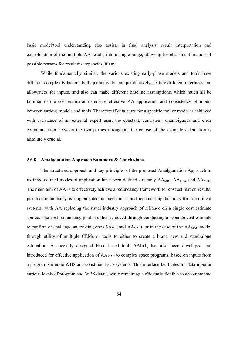
54
basic model/tool understanding also assists in final analysis, result interpretation and
consolidation of the multiple AA results into a single range, allowing for clear identification of
possible reasons for result discrepancies, if any.
While fundamentally similar, the various existing early-phase models and tools have
different complexity factors, both qualitatively and quantitatively, feature different interfaces and
allowances for inputs, and also can make different baseline assumptions, which much all be
familiar to the cost estimator to ensure effective AA application and consistency of inputs
between various models and tools. Therefore if data entry for a specific tool or model is achieved
with assistance of an external expert user, the constant, consistent, unambiguous and clear
communication between the two parties throughout the course of the estimate calculation is
absolutely crucial.
2.6.6 Amalgamation Approach Summary & Conclusions
The structured approach and key principles of the proposed Amalgamation Approach in
its three defined modes of application have been defined - namely AAMIC, AAMAC and AAVAL.
The main aim of AA is to effectively achieve a redundancy framework for cost estimation results,
just like redundancy is implemented in mechanical and technical applications for life-critical
systems, with AA replacing the usual industry approach of reliance on a single cost estimate
source. The cost redundancy goal is either achieved through conducting a separate cost estimate
to confirm or challenge an existing one (AAMIC and AAVAL), or in the case of the AAMAC mode,
through utility of multiple CEMs or tools to either to create a brand new and stand-alone
estimation. A specially designed Excel-based tool, AAInT, has also been developed and
introduced for effective application of AAMAC to complex space programs, based on inputs from
a program’s unique WBS and constituent sub-systems. This interface facilitates for data input at
various levels of program and WBS detail, while remaining sufficiently flexible to accommodate
55
the various specificities inherent to each program, particularly of a complex and international
nature.
Overall, AA constitutes an effective method to reduce uncertainty associated with an
initial, single cost estimate, and is ideally suited for application during early phases when cost
risk associated with an estimate is high. While AA (especially AAMAC) to a cost estimate is more
resource intensive, the reduced uncertainty and increased justification and representativeness
through result redundancy may often warrant the latter given the large scale of space programs.

56
3 SPACELINER - AN INDUSTRY CASE-STUDY
“Nothing ever built arose to touch the skies unless some man dreamed that it should,
some man believed that it could, and some man willed that it must.” – Charles Kettering
In 2005, a strategic, innovative and visionary concept was proposed by the German
Aerospace Center (DLR), with the potential to not only enable sustainable low-cost space
transportation to orbit [176, 179, 180], but also to revolutionse the status of currently viable
passenger point-to-point transportation. Based on statistics extracted directly from the aviation
industry, it is clear that ultra-long haul travel between the world’s key locations and business
centers is a substantial and mature market. Since the termination of Concorde’s operation in
2003, intercontinental travel has been restricted to low-speed, subsonic and long-duration flights.
An interesting and attractive alternative, therefore, to conventional air-breathing hypersonic
passenger airliners in the context of designing and developing intercontinental passenger HST
vehicles of the future, would be a rocket propelled suborbital craft. Such a concept, dubbed the
SpaceLiner [168, 182, 183], has been proposed, and is currently under investigation by the DLR
Space Launcher Systems Analysis (SART) group at the Institute of Space Systems in Bremen,
Germany. This two stage RLV would be capable of traveling ultra long-haul distances such as
Europe – Australia in 90 minutes, while other intercontinental routes between business centers
located in East Asia, Europe and the East and West coast of North America, could be reduced to
flight times of slightly more than one hour [168].
A perfect hybrid between the space and aviation industries, the SpaceLiner design is
based on using well established rocket technologies in order to benefit from the existing safety
standards established within the space industry, rather than having to establish a track-record for
completely new and untried technologies.
57
Figure 8: The SpaceLiner vision of an ultra-fast, rocket-propelled intercontinental, point-to-point
passenger transportation spaceplane [82]
Here, repeated studied have shown that estimates for developmental projects containing
only “modest technical advances” have a tendency to be more accurate than projects which
incorporate totally novel ideas and concepts, thus pushing the development threshold
substantially [31]. And with the vehicle reaching speeds of up to Mach 25 during flight, safety is
of the utmost priority to the concept and the potential for its future commercial success. The
SpaceLiner’s main purpose would be to service the point-to-point, intercontinental passenger
transportation segment, which, as previously touched upon, is foreseen to be considerable. With
the new space age depending on the combination of reusability and high traffic levels civilian
space access is the new market most likely to demand these high traffic levels [15].
This utility overlaps neatly with the latest deviation of space access into the space tourism
and ultra-fast long distance passenger transportation domains, giving SpaceLiner the potential to
revolutionise the launcher market with both high production and launch rates per year, and
consequently significantly lower costs.
An important distinction which needs to be made within context of the SpaceLiner, is that
this vehicle, in terms of technology and application, is new in the sense that it is a hybrid between
58
the aviation and space domains. Basically, a space technology has been proposed for application
to a standard civilian application and function of passenger transport. This characteristic
influences the development and production processes and approaches for such a vehicle, as well
as the associated costs. Development would be more in line with space industry standards, while
the high number of serial production foreseen for the vehicle would resemble more the aviation
industry. This is further elaborated upon in more detail, later on in the Thesis.
3.1 SPACELINER CONFIGURATION DEVELOPMENT & LAUNCH SEQUENCE
First proposed in 2005 [179], the SpaceLiner concept has been and continues to be under
constant development as technical requirements crystallise. Numerous papers detailing progress
of the iterative design process have been regularly and consistently published and presented to
the wider aerospace community [169, 180, 182-184, 187, 208].
The SpaceLiner baseline design concept consists of a fully reusable booster and passenger
stage, both of which are arranged in a piggy back configuration, as seen in Figure 8. The vertical
launch system is powered by rather conventional LOX/LH2 staged combustion engines, all of
which should be functioning from lift-off until main engine cut-off (MECO). The booster stage is
predominantly the cryogenic propellants vessel with its own engines. The passenger stage,
referred to synonymously as the orbiter, encapsulates and carries the passengers in a cabin
configuration. Passengers embark horizontally, as they would a standard aircraft, after which the
capsule is integrated into the orbiter for a vertical system start. This passenger cabin element of
the SpaceLiner vehicle is a highly complex sub-system in its own right. Furthermore equipped
with a solid propellant propulsion system, the cabin is also designed to functions as the passenger
escape capsule in the unlikely event of an emergency [21].
A fundamental characteristic of the concept is its full reusability, which should allow for
low turnaround times between flights of each vehicle. Both the booster and orbiter, including
59
engines, are designed to be fully reusable and equipped with wings for a gliding return flight.
After the launch, the vehicle climbs to an altitude of approximately 73 km, at which point the
booster separation occurs. During the entirety of the ascent phase, a propellant cross-feed from
the booster to the orbiter is foreseen right up until separation between the stages to reduce overall
size of the orbiter. After separation, the booster makes a controlled re-entry and is transferred
back to the launch base by a patented ‘in-air capturing’ method. This has been investigated at the
DLR through simulations in the past, and has been proven feasible in principle [177, 178], while
further research and future work pertaining to the topic is also planned.
Meanwhile, the orbiter continues to accelerate to a velocity of 6.7 km/s and an altitude of
80 km using its own propulsion system. After the passenger stage main engine cut-off (MECO),
the powerless gliding flight phase begins. Initially, the SpaceLiner was designed to use a so-
called skipping trajectory which was believed to maximise the range and thus reduce propellant
and mass. However, it was also found that this trajectory leads to comparatively high heat loads,
and increases the mass of the thermal protection system. Most recent trajectory optimisations
have obtained a smooth trajectory devoid of any skipping, while greatly improving passenger
comfort and reducing heat loads [187]. Here, a small increase in propellant mass for the new
trajectory profile is more than balanced by a lower TPS mass. In addition to the trajectory
improvements, the vehicle shape has also changed.
Since the first design, different configurations in terms of propellant combinations,
staging, aerodynamic shapes, and structural architectures have been analyzed. A subsequent and
respective configuration numbering scheme has also been established for all investigation phases.
60
The genealogy of the different SpaceLiner versions is shown in
Figure 9. The configuration trade-offs within the FAST20XX studies performed in recent years
support the definition of the latest and most current reference configuration, SpaceLiner 7, which,
up to date, has advanced through to the version SpaceLiner 7-3.
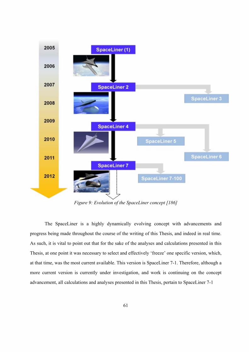
61
Figure 9: Evolution of the SpaceLiner concept [186]
The SpaceLiner is a highly dynamically evolving concept with advancements and
progress being made throughout the course of the writing of this Thesis, and indeed in real time.
As such, it is vital to point out that for the sake of the analyses and calculations presented in this
Thesis, at one point it was necessary to select and effectively ‘freeze’ one specific version, which,
at that time, was the most current available. This version is SpaceLiner 7-1. Therefore, although a
more current version is currently under investigation, and work is continuing on the concept
advancement, all calculations and analyses presented in this Thesis, pertain to SpaceLiner 7-1
62
3.2 MISSION DEFINITION
Since investigations on the SpaceLiner began, the ambitious westbound Australia –
Europe route has been defined as the reference case. Using the mission range as a fundamental
criteria, the connection between Australia (Sydney) and Western Europe, has been calculated to
be the longest at roughly 17,000km [186, 216]. The effect of the surface rotation of the Earth
influences the chosen direction of travel, with a positive effect observed for all trajectories flying
towards the East. As a result of the selection process, the westbound Sydney to West Europe
route is identified as being the most demanding, and thus has always been taken as the
SpaceLiner design reference mission. It is therefore the reference trajectory that has been most
extensively studied to date. It is proposed that this flight distance will be traversed on a daily
basis in each direction by a spaceplane, carrying 50 passengers (PAX) onboard. Several other,
shorter intercontinental missions have also been defined, which have the potential to generate a
larger market demand. For this reason, a SpaceLiner derivative configuration with the capability
of transporting up to 100 PAX over the shorter intercontinental distance has also been studied
[169]. In order to keep the number of different stage configurations at the lowest possible level, the
potential flight destinations of interest have been divided into three classes, and could be flexibly
serviced by a suitable combination of four vehicles (50 PAX orbiter stage, 100 PAX orbiter
stage, nominal booster, shortened booster), all with a high commonality of fundamental
components and sub-systems, such as engines and avionics, despite differences in size.
Class 1: Reference mission (up to 17,000 km) Australia – Europe with 50 PAX
orbiter and large reference booster
Class 2: Mission (up to 12,500 km) e.g. Dubai – Denver with increased 100 PAX
orbiter and large reference booster
Class 3: Mission (up to 9,200 km) e.g. Trans-Pacific with increased 100 PAX
passenger orbiter and reduced size booster
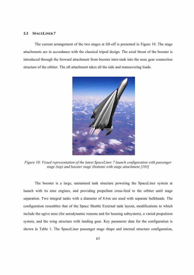
63
3.3 SPACELINER 7
The current arrangement of the two stages at lift-off is presented in Figure 10. The stage
attachments are in accordance with the classical tripod design. The axial thrust of the booster is
introduced through the forward attachment from booster inter-tank into the nose gear connection
structure of the orbiter. The aft attachment takes all the side and maneuvering loads.
Figure 10: Visual representation of the latest SpaceLiner 7 launch configuration with passenger stage (top) and booster stage (bottom) with stage attachment [183]
The booster is a large, unmanned tank structure powering the SpaceLiner system at
launch with its nine engines, and providing propellant cross-feed to the orbiter until stage
separation. Two integral tanks with a diameter of 8.6 m are used with separate bulkheads. The
configuration resembles that of the Space Shuttle External tank layout, modifications to which
include the ogive nose (for aerodynamic reasons and for housing subsystem), a varied propulsion
system, and the wing structure with landing gear. Key parameter data for the configuration is
shown in Table 1. The SpaceLiner passenger stage shape and internal structure configuration,

64
including two engines and the passenger cabin/rescue capsule, are graphically shown in Figure
11. Some key parameter data are also given in Table 2 for the SpaceLiner 7 passenger stage.
Table 1: Key parameters of SpaceLiner 7 booster stage
Length [m]
Span [m]
Height [m]
Fuselage Diameter
[m]
Wing Leading Edge Angle
[deg]
Wing Pitch Angle [deg]
Wing Dihedral Angle [deg]
83.5 36.0 8.7 8.6 82/61/43 3.5 0
Table 2: Key parameters of SpaceLiner 7 orbiter stage
Length [m]
Span [m]
Height [m]
Fuselage Diameter
[m]
Wing Leading Edge Angle
[deg]
Wing Pitch Angle [deg]
Wing Dihedral Angle [deg]
65.6 33.0 12.1 6.4 70 0.4 2.65
As the structural pre-design is not yet finished, all dry mass data are still based on
empirical estimation relationships derived from launch vehicles or hypersonic transport studies.
These data are shown in Table 3. System margins of 14% (and 12% for propulsion) are added to
the estimated mass data. Based on available subsystem sizing and empirical mass estimation
relationships, the orbiter mass is derived as listed in Table 4. The total fluid and propellant mass
includes all ascent, residual and RCS propellants and the water needed for the active leading edge
cooling. The stages’ MECO mass is approximately 161.8 Mg.
Figure 11: Latest SpaceLiner 7 orbiter shape (left) and CAD drawing of the reusable SpaceLiner 7 passenger stage (right) showing configuration of cabin, propellant tanks and landing gear [22,
182]
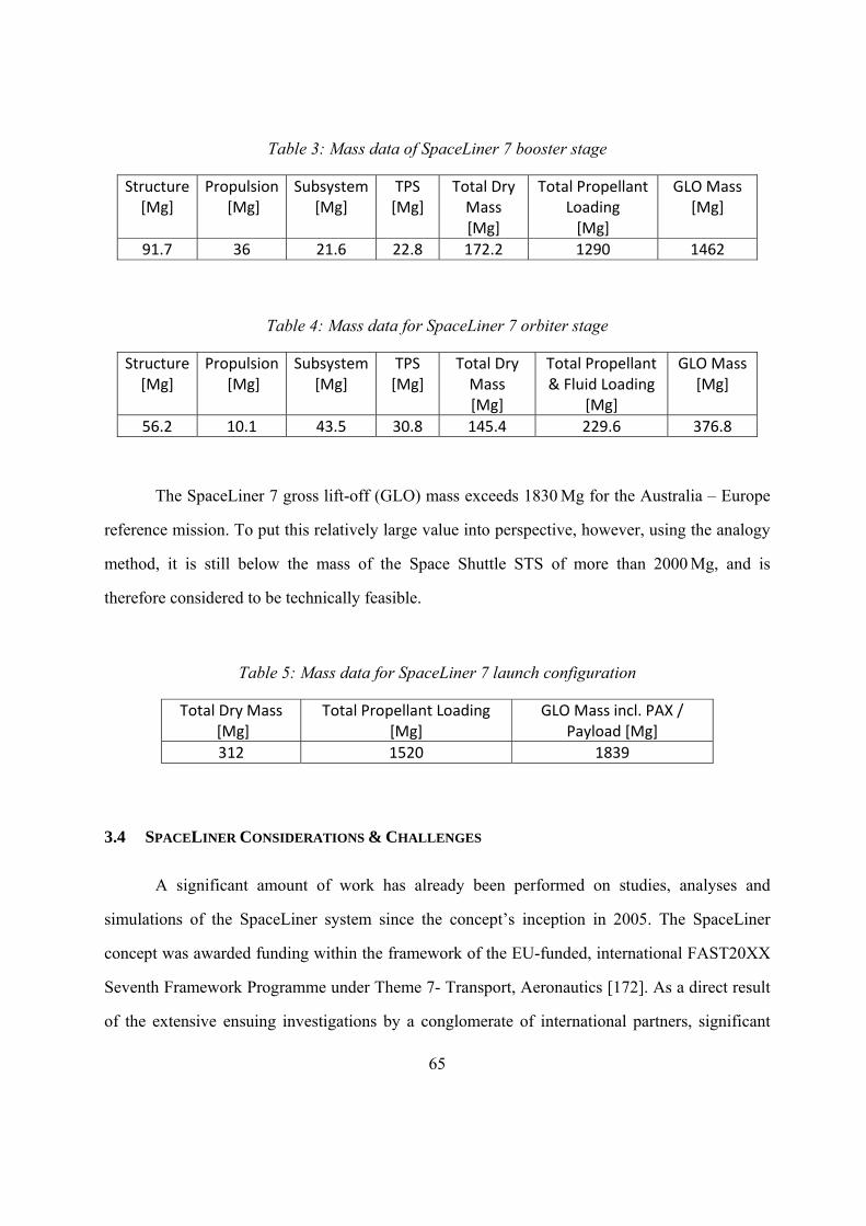
65
Table 3: Mass data of SpaceLiner 7 booster stage
Structure [Mg]
Propulsion [Mg]
Subsystem[Mg]
TPS [Mg]
Total Dry Mass [Mg]
Total Propellant Loading [Mg]
GLO Mass [Mg]
91.7 36 21.6 22.8 172.2 1290 1462
Table 4: Mass data for SpaceLiner 7 orbiter stage
Structure [Mg]
Propulsion [Mg]
Subsystem[Mg]
TPS[Mg]
Total Dry Mass [Mg]
Total Propellant & Fluid Loading
[Mg]
GLO Mass[Mg]
56.2 10.1 43.5 30.8 145.4 229.6 376.8
The SpaceLiner 7 gross lift-off (GLO) mass exceeds 1830 Mg for the Australia – Europe
reference mission. To put this relatively large value into perspective, however, using the analogy
method, it is still below the mass of the Space Shuttle STS of more than 2000 Mg, and is
therefore considered to be technically feasible.
Table 5: Mass data for SpaceLiner 7 launch configuration
Total Dry Mass [Mg]
Total Propellant Loading [Mg]
GLO Mass incl. PAX / Payload [Mg]
312 1520 1839
3.4 SPACELINER CONSIDERATIONS & CHALLENGES
A significant amount of work has already been performed on studies, analyses and
simulations of the SpaceLiner system since the concept’s inception in 2005. The SpaceLiner
concept was awarded funding within the framework of the EU-funded, international FAST20XX
Seventh Framework Programme under Theme 7- Transport, Aeronautics [172]. As a direct result
of the extensive ensuing investigations by a conglomerate of international partners, significant

66
progress of the concept status was made. Concurrently, during the detailed preliminary
investigations, various challenges spanning across the technical, logistical, commercial, socio-
political as well as economic domains have been encountered, identified and explicitly defined.
Key points are listed below:
Acoustic noise and sonic boom
Launch and landing site selection
Routes, destination and city-pairs
Trajectories and TPS
Environmental impact
Operational considerations
Door-to-door passenger transport network
Reusability
Reliability and safety
Business case considerations
The latter key issues and challenges as per the present status of research and have been
categorically outlined in separate works belonging to the course and progression of this Thesis
work [208]. The challenges arising for the SpaceLiner program are directly and irrevocably
linked and interrelated in a complex network of technical, logistical and programmatic
dependencies. Many outputs from various disciplines directly provide inputs and influencing
other categories. Nevertheless, ref. [208] describes each aspect and issue separately. It is beyond
the scope of this Thesis to define explicit solutions, but rather to hone in on the particular area of
interest, being the cost considerations and cost modeling of large, complex space systems in an
international context.

67
Consideration and estimation of life cycle costs (LCC) of any new and proposed program,
and in this case, the SpaceLiner case-study, is an extremely important task. More specifically, the
aspect of performing a cost estimation during the early program phase for an unprecedented,
large and complex program is indeed the kernel of this Thesis. The classical LCC categories of
the non-recurring development and the recursive production costs are addressed, while operations
and the associated recurring costs are discussed in a more qualitative manner in line with the
early case-study program status. This will be elaborated upon in greater detail in subsequent
chapters.
In terms of the cost of the service to passengers themselves, immediately it is clear that
tickets for such a journey will considerably exceed that paid for standard airline tickets of today.
This cost increase is reflective of an entirely new level of technological application, and is the
premium assigned to the time savings of SpaceLiner’s ultra-fast mode of travel. Such logic
automatically narrows the potential target market for SpaceLiner, honing in on the current
aviation segment’s 63 million business class and first class travelers who flew in 2012, and
generated more than €72 billion ($95 billion USD in revenues) [166]. Congruent with this
definition of the initial target market niche, the underlying assumption is the increased propensity
of the consumer to travel and also enhanced ability and willingness to expend money for an
enhanced travel experience, making them ideal consumers of the service which SpaceLiner
encompasses.
The consequent Chapter 4 is dedicated to the development and discussion of effective and
novel cost estimation approaches and processes (AAMAC mode), resulting in a preliminary cost
range for SpaceLiner development and production. More importantly, a structured cost
estimation framework is established to allow for future refinement of the initial cost estimations
as more information and technical details of the program become available.
68
4 SPACELINER CASE-STUDY COST ESTIMATION
“Man must rise above the Earth- to the top of the atmosphere and beyond – for only thus
will he fully understand the World in which he lives.” – Socrates
In this chapter, the challenge of formulating a representative early phase cost estimate for
an unprecedented vehicle is considered directly through a practical application of cost
engineering principles and cost estimation approaches on a selected case-study - the SpaceLiner.
Using the cost engineering and estimation theory which has already been introduced, developed
and discussed in earlier chapters as a baseline, the following chapters outline in detail the tailored
and strategic approach undertaken to produce a cost estimate for a large, complex and
unprecedented vehicle concept which is in an early pre-phase A stage. A pivotal tool to this
approach is implementation of AA, in particular, the AAMAC mode, as discussed in Chapter
2.6.2.2. From now, any mention of AA can be assumed to be with reference to the AAMAC mode.
During the early phases of the program, an initial cost estimation is necessary to
determine the various life cycle cost (LCC) elements, establish a funding scheme and to
formulate a desirable and representative business case. The latter three elements are not mutually
exclusive, but in fact, heavily related. The final program cost is almost always guaranteed to vary
from the initial estimate due to dynamic program evolution, as well as unforeseen events which
cannot be factored in for during formulation of that estimate. Here, adequate and representative
risk and uncertainty, between which a clear distinction should be made [209], play a very
important role and should also be assessed at program commencement. This topic, however, is
not a focus of this Thesis, as it constitutes an own extensive field of study and research. Still,
realistic budgeting, the basis of which is derived from a preliminary program cost estimate of
development, production and operation costs, is a crucial first step to underpin future program
success. A justifiable, competent, informed cost estimate reflective of all the data which is
69
available during the early program planning forms a solid foundation for an adequate and
supportable program budget [212]. Synergised implementation with strong project and schedule
management functions further increases chances for a program’s timely and efficient execution
and ultimately realisation. So despite preliminary, limited or incomplete information regarding
configuration, mission or environmental parameters, as is the case for the still evolving
SpaceLiner case-study, a pronounced need still exists for reasonable, justifiable and
representative cost range to be achieved, early in the program.
4.1 THE SPACELINER COST PHILOSOPHY
Although SpaceLiner does not use any fundamentally new or exotic technologies, the
integration and adaptation of these heritage elements is within a new context, and results in
revised requirements such as reusability, and stringent standards for a civilian application. Thus
the concept is unprecedented and novel in nature, making application of only existing cost
estimation models and methods based on data derived from historical programs, a challenge.
From purely a technical perspective, SpaceLiner is very much a launch vehicle, so one
must therefore look at historical projects in the launch vehicle segment. The only realised
projects to date which are comparable for this specific category of space vehicles are the Space
Shuttle Fleet, which was only semi-reusable [93], and the Russian Buran orbital vehicle, which
performed just one unmanned flight before the program was cancelled due to a mix of political
influences and insufficient funding [76]. In terms of the recent launcher markets, current launch
rates have continued to steadily increase, arguably due to increased competition and changes to
newly emerging commercial companies. And the higher launch rates influence launch costs,
generally driving the costs of space access down, and requiring that existing cost models to be
recalibrated. As an example, recent suggestions have implied that the SpaceX fleet of Falcon 9
vehicles “break the NASA/Air Force Cost Model NAFCOM” [193], a cost estimation tool
70
commonly used in the space industry. So in order to keep up with the deviating space economy
trends and space market changes, it is essential that future cost estimations have the capability to
obtain indicative, relevant and justifiable estimates despite implementation of novel and
unprecedented concepts, furthermore integrated within new company structures [209].
4.1.1 SpaceLiner WBS Definition & Development
For all systems, and in particular for large, complex ones, like the SpaceLiner case-study,
the principle of successive refinement given the divide-and-conquer strategy is an essential
component of effective program planning at project commencement. During this decomposition
process, complex systems are successively and strategically segmented into modular, less
complex pieces, until they are simple enough to be conquered [175]. From this, generally two
structures emerge, namely for describing the product system itself, as well as a structure to
describe the system which produced the product system. This is the prime goal of a work
breakdown structure (WBS), which is a necessity for logically, categorically and systematically
addressing all project phases, and in particular the development and production Phases C and D.
A WBS and the work package definitions provide the reference for a detailed bottom-up cost
estimation and budget formulation, since the cost breakdown structure (CBS) is then directly
linked to the content of the WBS [115, 175]. After all, costing smaller, more tangible units is
significantly more achievable and traceable, allowing for more stringent control and increased
transparency than when the cost of a whole agglomerated system comprising of already very
complex sub-systems is considered at an overall top level. In addition, the project is immunised
with improved visibility of management data such as schedule, cost, and technical performance,
amongst others [112].
Therefore, the first critical step to the logical commencement and progression of cost
analysis for any large-scale, international complex space program is the establishment of an
71
adequate and representative WBS. The development of such a WBS, incorporating the model
philosophy (see Chapter 4.1.3, Table 8 and Appendix A) is an iterative top-down process
defining lower level elements until the work package level has been reached. This WBS then
forms the backbone for not only program organisation and execution, but indeed also for cost
estimation and control of actual costs and schedule throughout all project phase [112, 115, 202].
As such, upon consultation with topic-specific literature, a specific and detailed WBS for the
SpaceLiner case-study Phases C and D was developed, as shown in Figure 12, and to a deeper
WBS level in Appendix A. Establishment of the WBS was a very intense, dynamic, iterative and
time-consuming process requiring many loops, changes, modifications and rearrangements of
elements between groupings before the final breakdown, as it is shown in Appendix A, was
achieved. Here, the interaction, communication and open dialog between project management
experts and case-study engineers and specialists in their respective SpaceLiner domains was
essential to establish an efficient break-down of the overall complex program into its logical
substituent units strategically. The author wishes to acknowledge Professor Bernd Madauss from
ISU for his invaluable guidance and sharing his knowledge and expertise for the compilation of
the case-study WBS.
Firstly, the SpaceLiner concept, as a whole, was segmented into logical sub-level
constituent modules which conformed to the group of non-recurring development and the
recursive production costs.
SpaceLiner fly-back Booster (SLB)
SpaceLiner orbiter passenger stage (SLO)
SpaceLiner main engine (SLME)
Passenger cabin / passenger rescue capsule (SPC)
72
While the engine SLME belongs to the lower-level of SLO and SLB components, it was
identified separately as a key element, and the ‘heart’ of the SpaceLiner vehicle which would
incur development costs, as well as consequently, production costs.
A WBS was consequently derived for the multi-element SpaceLiner case-study to provide
a logical outline and vocabulary that describes the entire project and integrates all available
information in a strategic, transparent and consistent way [175]. The sub-system inputs and
categories were based on existing SART in-house Space Transportation Systems Mass (STSM)
software package [45] inputs and outputs for both constituent system elements and the respective
element masses. The latter were consequently strategically segmented into appropriate
SpaceLiner categories of SLO, SLB and SPC in line with WBS requirements and standards.
In line with theory for successful WBS development, multiple iterations were then
required, and will continue to be required throughout project advancement. This is because the
full extent of the work and tasks is often not evident at commencement, but rather evolves during
the WBS formulation and consequent project execution phases [175].
While quantitatively, the derived SpaceLiner case-study WBS ideally describes the top-
level system components, which were necessary for application of the AA, attention was also
paid to extrapolating the systems into accurate descriptions of their constituent sub-elements and
components. This was challenging since many sub-system elements are still works in progress
and being dynamically defined prior to their ultimate crystallisation. Nevertheless, sub-system
SpaceLiner components were defined qualitatively, thereby providing an essential and thorough
structure and framework for more detailed, bottom-up estimation of the concept to occur as it
matures in the future.
The SpaceLiner is a two-stage launch vehicle system comprising of the main fly-back
booster stage (SLB) and the passenger orbiter stage (SLO). Furthermore, unlike any vehicles
which are used as reference projects within the TransCost manual, the SLO stage features an
integrated passenger capsule which has a hybrid function, and also doubles as a passenger rescue
73
capsule (SPC) in case of emergencies. Its prime goal is to eject from the SLO body, and
autonomously and safely return the passengers back to the ground. In this regard, the SPC
features its own solid propulsion system which requires a minimum of development effort since
all the technology already exists.
In terms of the SpaceLiner propulsion, while based on standard cryogenic propulsion
technology, the SpaceLiner main engine (SLME) would need to be newly developed in view of
the passenger-transportation context, with the key challenge here being the required reusability
component. SpaceLiner assumes engine reusability of 25-50 times, as is explained later in
Chapter 4.1.5. For the sake of the cost estimation, it is also assumed that the SLB and SLO use
the same cryogenic engine. Mechanically, the engines are identical, although having different
size nozzles. Being a traditional, heritage LOX/LH cryogenic engine technology, assuming an
100% new development effort for a single engine is sufficient to address the development of both
SLO and SLB propulsion. This important assumption has already been defined and outlined in
detail also in the Chapter 4.1.5.
To reflect all technical information, the resulting WBS has seven top-level WBS elements
from 1000 through to 7000, which are further expanded overall to three levels of detail. The top
three levels are shown in Figure 12, while the full four levels of detail can be found in full in
Appendix A.
The kernel of this Thesis predominantly focuses on development and application of novel
and innovative new cost estimation approaches and strategies aimed at calculating development
and production costs of physical hardware elements of complex space systems during the early
pre-phase A phase. The chosen complex and unprecedented SpaceLiner case-study constitutes an
ideal candidate for application of the new cost estimation models, approaches and theory
developed within this Thesis work, as it is clearly still in the targeted early pre-phase A stage. As
such, however, assessing and estimating costs for the WBS ground and operations elements in
detail is still deemed too premature as the requirements and key, necessary details are not yet
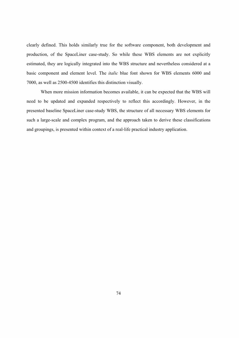
74
clearly defined. This holds similarly true for the software component, both development and
production, of the SpaceLiner case-study. So while these WBS elements are not explicitly
estimated, they are logically integrated into the WBS structure and nevertheless considered at a
basic component and element level. The italic blue font shown for WBS elements 6000 and
7000, as well as 2500-4500 identifies this distinction visually.
When more mission information becomes available, it can be expected that the WBS will
need to be updated and expanded respectively to reflect this accordingly. However, in the
presented baseline SpaceLiner case-study WBS, the structure of all necessary WBS elements for
such a large-scale and complex program, and the approach taken to derive these classifications
and groupings, is presented within context of a real-life practical industry application.
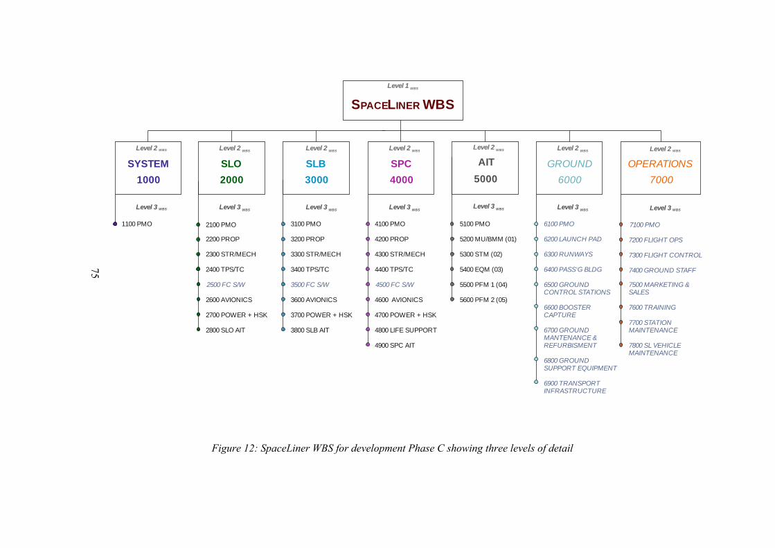
75
Figure 12: SpaceLiner WBS for development Phase C showing three levels of detail
S L WBSPACE INER
SYSTEM
1000
OPERATIONS
7000
GROUND
6000
AIT
5000
SPC
4000
SLB
3000
SLO
2000
1100 PMO 2100 PMO
2200 PROP
2300 STR/MECH
2400 TPS/TC
2500 FC S/W
2600 AVIONICS
2700 POWER + HSK
2800 SLO AIT
3100 PMO
3200 PROP
3300 STR/MECH
3400 TPS/TC
3500 FC S/W
3600 AVIONICS
3700 POWER + HSK
3800 SLB AIT
4100 PMO
4200 PROP
4300 STR/MECH
4400 TPS/TC
4500 FC S/W
4600 AVIONICS
4700 POWER + HSK
4800 LIFE SUPPORT
4900 SPC AIT
5100 PMO
5200 MU/BMM (01)
5300 STM (02)
5400 EQM (03)
5500 PFM 1 (04)
5600 PFM 2 (05)
6100 PMO
6200 LAUNCH PAD
6300 RUNWAYS
6400 PASS‘G BLDG
6500 GROUND CONTROL STATIONS
6600 BOOSTER CAPTURE
6700 GROUND MANTENANCE & REFURBISMENT
6800 GROUND SUPPORT EQUIPMENT
6900 TRANSPORT INFRASTRUCTURE
7100 PMO
7200 FLIGHT OPS
7300 FLIGHT CONTROL
7400 GROUND STAFF
7500 MARKETING & SALES
7600 TRAINING
7700 STATION MAINTENANCE
7800 SL VEHICLE MAINTENANCE
Level 1 WBS
Level 2 WBS Level 2 WBS Level 2 WBS Level 2 WBS Level 2 WBS Level 2 WBS Level 2 WBS
Level 3 WBS Level 3 WBS Level 3 WBS Level 3 WBS Level 3 WBS Level 3 WBS Level 3 WBS
76
4.1.2 SpaceLiner Program Schedule & Milestones
Despite the early phase of the program, and to complement the developed WBS, it was
important to establish a preliminary and realistically executable, expected program schedule to
determine and define key dates, some necessary milestones and the distribution of program
phases with respect to time. While slightly different systems and terminology can be adopted
between international space agencies, the European Cooperation for Space Standardization
(ECSS) standard for project planning and implementation [57] was relied upon as a baseline for
this work. This Standard outlines seven distinct program phases, as shown below:
• Phase 0 – Mission Requirements
• Phase A – Concept & Feasibility
• Phase B – System Definition
• Phase C – Design, Development & Verification
• Phase D –Production
• Phase E –Utilisation
• Phase F – Disposal
The last two Phases E and F, shown in italics, are not addressed in this Thesis, since the
development and production phases are the key focal elements of this work. Analogy and the EJ
methods were then employed to estimate and predict the expected, realistic duration of each
program phase drawing on previous large-scale space program examples. Consolidated
information and expert opinion was extracted from direct discussions with top experts from both
academia and industry specialising in the program management function of the space domain to
determine ROM representative timeframes for the various scheduling phases, keeping in mind
the considerable scale, scope and high complexity of the SpaceLiner concept. With the mission
analysis of Phase 0 presently underway, Phase A could commence already in 2015, which, given
that the Mission Definition Review (MDR) is executed during 2015 or 2016, presents a realistic
77
and current scenario. Phase B, the preliminary program definition which precedes final definition
may be estimated to then take approximately eight years. The design and development of Phase C
could then commence in 2025, realistically lasting up to ten years. The consequent production
Phase D is preliminarily assumed extend over 15 years.
The resulting preliminary schedule, which assumes T0 to indicate the time reference for
program commencement, is shown qualitatively (not to scale) in Figure 13 below. The logical
sequence and progression for each milestone, activity and review as well as preliminary phase
durations assumed for the SpaceLiner case-study, are also included in italics with reference to T0.
Figure 13: Preliminary SpaceLiner case-study program schedule
Additionally, and in close consultation with the European Cooperation for Space
Standardisation (ECSS) guidelines [57], the aim of which is to be applied for the management,
engineering and product assurance in space projects and applications, the following milestones
associated with the various program phases have been identified as necessary for effective and
thorough execution of the SpaceLiner program:
78
Pre-Phase A – Mission Requirements
Mission Definition Review (MDR)
Phase A – Concept & Feasibility
Preliminary Requirements Review (PRR)
Phase B – System Definition
System Requirement Review (SRR)
Preliminary Design Review (PDR)
Phase C – Design & Development
Effective Date of Contract Development (EDC-D)
Critical Design Review (CDR)
E/QM Qualification Review (QR)
PFM1/2 Flight Test Reviews (FTR1/FTR2)
Phase D – Production
Effective Date of Contract Production (EDC-P)
Annual Production Reviews (APR1 to APR15)
Operational Readiness Review (ORR)
End of Production Contract (EPC)
While the ECSS standard stipulates that the QR and FTR (also interchangeable with the
acceptance review, AR) milestones are associated with Phase D, in line with the SpaceLiner
philosophy presented in Chapter 4.1.3, it is deemed that any prototype activities belong firmly
within the Phase C development phase, and as such, both the QR and FTR case-study reviews are
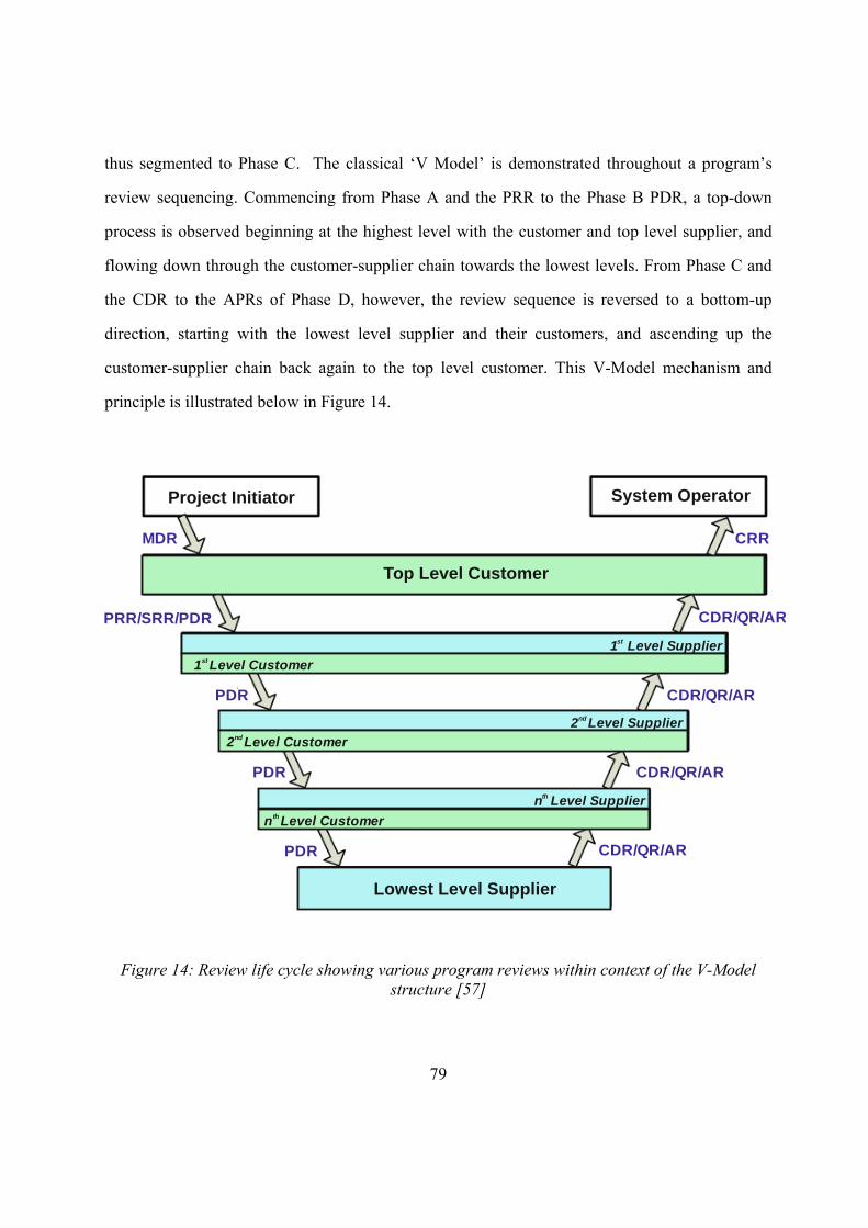
79
thus segmented to Phase C. The classical ‘V Model’ is demonstrated throughout a program’s
review sequencing. Commencing from Phase A and the PRR to the Phase B PDR, a top-down
process is observed beginning at the highest level with the customer and top level supplier, and
flowing down through the customer-supplier chain towards the lowest levels. From Phase C and
the CDR to the APRs of Phase D, however, the review sequence is reversed to a bottom-up
direction, starting with the lowest level supplier and their customers, and ascending up the
customer-supplier chain back again to the top level customer. This V-Model mechanism and
principle is illustrated below in Figure 14.
Project Initiator System Operator
MDR
PRR/SRR/PDR
PDR
PDR
PDR CDR/QR/AR
CDR/QR/AR
CDR/QR/AR
CDR/QR/AR
CRR
Lowest Level Supplier
nth Level Supplier
nth Level Customer
2 Level Suppliernd
2nd Level Customer
1 Level Supplierst
1st Level Customer
Top Level Customer
Figure 14: Review life cycle showing various program reviews within context of the V-Model structure [57]
80
It must also be pointed out that despite the template of milestones and project reviews
outlined above, the program management must remain flexible to incorporate additional reviews
into the project planning schedule to address the specific and unique project needs of every
program [57]. With context for the SpaceLiner case-study, it should be noted that due to the
safety-critical nature of the vehicle, in line with stringent safety requirements, additional reviews
and audits may well be incorporated into the preliminary schedule structure presented within this
Thesis.
Here, it is not the aim of this work to describe the specific features, key objectives,
structure, logistics and requirements for each of the above milestones and reviews, although full
information, detailing aims and goals of each review, can be found in the ECSS Standard in ref.
[57], on pages 21-28.
4.1.3 SpaceLiner Development & Prototype Modeling
Space is undeniably a risky business. Therefore building development models and prototypes to
verify the design and proper function through test in flight in the development phase, is of the
highest priority to establish a strong safety and solid reliability baseline. This is particularly
crucial for unprecedented vehicles like the SpaceLiner case-study. In fact, the risk for such a
vehicle increases due to the high number and untrained nature of its civilian passengers for a
spacecraft. Implementing a stringent testing campaign, as well as increasing the number of
SpaceLiner prototypes flown, as well as test-flight hours prior to commercial implementation
should therefore increase and establish a particular reliability standard, and reduce risk. At this
stage it is ambiguous to attempt to numerically capture and quantify this risk, however it is clear
that the more development models and prototypes which are built and successfully, respectively
tested, the better the safety record, and the lower the perceived risk. The SpaceLiner technology
is from the space domain, while its application resembles an aviation scenario. Classic space
81
components have fewer prototype units than those within the aviation industry, with many of
those being on a sub-system level rather than at a full system level. However, given the safety-
critical nature of the SpaceLiner program, the aviation industry analogous prototype quantity
philosophy was largely adopted for definition of the development phase prototype philosophy
applied to the SpaceLiner case-study example. Research was conducted to ascertain both the
aviation and space industry approaches for prototype and testing standards and regimes.
Within the aviation domain, a focus was placed on large, current aircraft programs from
the leading aircraft manufacturers like Airbus and Boeing, and existing literature was extensively
consulted. While detailed internal program information is usually difficult to locate as it is rarely
made public due to confidentiality constraints, several reliable sources were nevertheless
identified and referred to [10, 62, 63]. The Airbus A380 program had five fully operational
prototypes which clocked a total of 2,500 hours of flight tests to achieve certification with both
the European and US airworthiness authorities, the European Aviation Safety Agency (EASA)
and the Federal Aviation Administration (FAA), respectively. Similarly, the recent A-350
program also incorporates five prototypes, MSN001-MSN005 with another 2,500 flight-test
hours. The sequence of flights is designed to use the flight-test aircraft exactly like a potential
airliner would, training the associated processes accordingly and assessing general handling
qualities, operational performance airfield noise emissions, and systems operation in nominal
mode.
Within the space industry, prototype philosophy differs given that flight duration of most
launchers is significantly shorter, and as such, flight hours are not as important a parameters, as
the number of successful launches and landings, where appropriate. Similarly, the flight and
mission dynamics of a program like SpaceLiner would be rather different, operationally, to
standard civil aircraft. Long haul carrier airplanes frequently fly long routes lasting up to 16
hours, and as such, a test regime which incorporates extenuating durations of flight hours holds
relevant. The SpaceLiner vehicle would only fly a maximum duration of 90 minutes in
82
accordance with its reference mission requirements. Therefore here, at a top system level, a much
more relevant and representative statistic for SpaceLiner prototype units would be with the
number of successful launches and landings, especially with the vehicle being fully reusable. On
a sub-system level, the number of engine test-firings would be a solid statistic for the prototype
and testing regime.
However, prior to having fully functional flight prototypes, numerous preceding
mockups, test and engineering models must be constructed and tested. Furthermore, various
standards exist for the various sub-systems, which define different requirements and goals per
sub-system. For example, a recent 2014 NASA standard for ^the critical structural design and test
factors (NASA-STD-5001B [140]), stipulates that “The standard accepted practice for
verification of launch vehicles and human-rated spaceflight hardware is the prototype approach
in which a separate, dedicated test structure, identical to the flight structure, is tested to ultimate
loads to demonstrate that the design meets both yield and ultimate factor-of-safety requirements.
An acceptable alternative for verification of spacecraft and science payloads is the protoflight
approach, wherein the flight structure is tested to levels above limit load but below yield strength
to verify workmanship and demonstrate structural integrity of the flight hardware .” Here, we
see that from a structural perspective, the space industry stipulates a low number of components
to achieve verification of a system through the prototypes. It can also be seen that the prototype
approach incorporates an extra level of test hardware prior to flight. However the protoflight
verification approach is advantageous in that it does not require a dedicated test unit, since
qualification testing can be performed directly on the flight hardware, although here, a margin
over flight limit loads must also be demonstrated be test [140]. Choice of which method is
applied depends on the available budget, which, if insufficient, might force the program to adhere
to the protoflight method [120]. It must also be noted that electronics and software for such a
large system adhere to a completely different testing standards, requirements and processes.
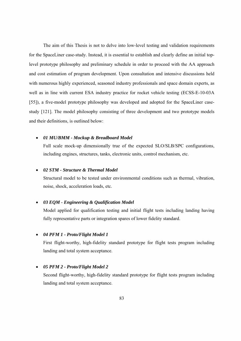
83
The aim of this Thesis is not to delve into low-level testing and validation requirements
for the SpaceLiner case-study. Instead, it is essential to establish and clearly define an initial top-
level prototype philosophy and preliminary schedule in order to proceed with the AA approach
and cost estimation of program development. Upon consultation and intensive discussions held
with numerous highly experienced, seasoned industry professionals and space domain experts, as
well as in line with current ESA industry practice for rocket vehicle testing (ECSS-E-10-03A
[55]), a five-model prototype philosophy was developed and adopted for the SpaceLiner case-
study [121]. The model philosophy consisting of three development and two prototype models
and their definitions, is outlined below:
01 MU/BMM - Mockup & Breadboard Model
Full scale mock-up dimensionally true of the expected SLO/SLB/SPC configurations,
including engines, structures, tanks, electronic units, control mechanism, etc.
02 STM - Structure & Thermal Model
Structural model to be tested under environmental conditions such as thermal, vibration,
noise, shock, acceleration loads, etc.
03 EQM - Engineering & Qualification Model
Model applied for qualification testing and initial flight tests including landing having
fully representative parts or integration spares of lower fidelity standard.
04 PFM 1 - Proto/Flight Model 1
First flight-worthy, high-fidelity standard prototype for flight tests program including
landing and total system acceptance.
05 PFM 2 - Proto/Flight Model 2
Second flight-worthy, high-fidelity standard prototype for flight tests program including
landing and total system acceptance.
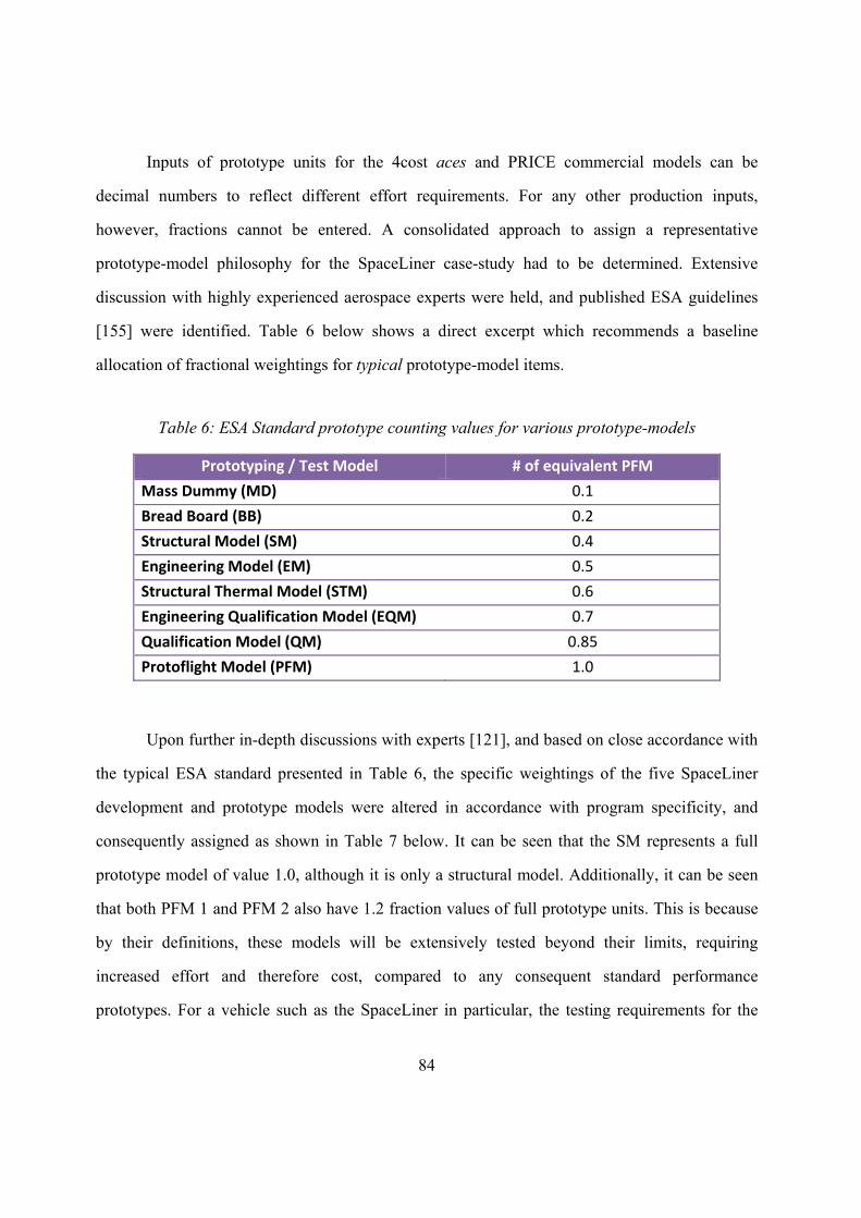
84
Inputs of prototype units for the 4cost aces and PRICE commercial models can be
decimal numbers to reflect different effort requirements. For any other production inputs,
however, fractions cannot be entered. A consolidated approach to assign a representative
prototype-model philosophy for the SpaceLiner case-study had to be determined. Extensive
discussion with highly experienced aerospace experts were held, and published ESA guidelines
[155] were identified. Table 6 below shows a direct excerpt which recommends a baseline
allocation of fractional weightings for typical prototype-model items.
Table 6: ESA Standard prototype counting values for various prototype-models
Prototyping / Test Model # of equivalent PFM
Mass Dummy (MD) 0.1
Bread Board (BB) 0.2
Structural Model (SM) 0.4
Engineering Model (EM) 0.5
Structural Thermal Model (STM) 0.6
Engineering Qualification Model (EQM) 0.7
Qualification Model (QM) 0.85
Protoflight Model (PFM) 1.0
Upon further in-depth discussions with experts [121], and based on close accordance with
the typical ESA standard presented in Table 6, the specific weightings of the five SpaceLiner
development and prototype models were altered in accordance with program specificity, and
consequently assigned as shown in Table 7 below. It can be seen that the SM represents a full
prototype model of value 1.0, although it is only a structural model. Additionally, it can be seen
that both PFM 1 and PFM 2 also have 1.2 fraction values of full prototype units. This is because
by their definitions, these models will be extensively tested beyond their limits, requiring
increased effort and therefore cost, compared to any consequent standard performance
prototypes. For a vehicle such as the SpaceLiner in particular, the testing requirements for the
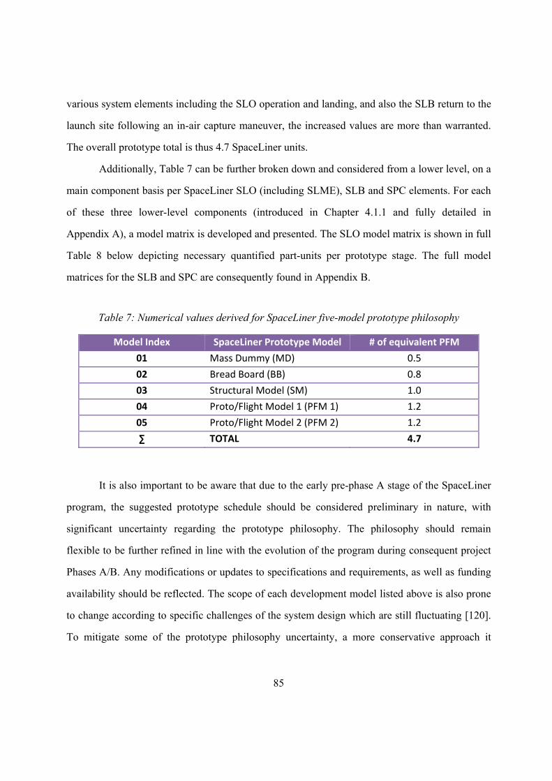
85
various system elements including the SLO operation and landing, and also the SLB return to the
launch site following an in-air capture maneuver, the increased values are more than warranted.
The overall prototype total is thus 4.7 SpaceLiner units.
Additionally, Table 7 can be further broken down and considered from a lower level, on a
main component basis per SpaceLiner SLO (including SLME), SLB and SPC elements. For each
of these three lower-level components (introduced in Chapter 4.1.1 and fully detailed in
Appendix A), a model matrix is developed and presented. The SLO model matrix is shown in full
Table 8 below depicting necessary quantified part-units per prototype stage. The full model
matrices for the SLB and SPC are consequently found in Appendix B.
Table 7: Numerical values derived for SpaceLiner five-model prototype philosophy
Model Index SpaceLiner Prototype Model # of equivalent PFM
01 Mass Dummy (MD) 0.5
02 Bread Board (BB) 0.8
03 Structural Model (SM) 1.0
04 Proto/Flight Model 1 (PFM 1) 1.2
05 Proto/Flight Model 2 (PFM 2) 1.2
∑ TOTAL 4.7
It is also important to be aware that due to the early pre-phase A stage of the SpaceLiner
program, the suggested prototype schedule should be considered preliminary in nature, with
significant uncertainty regarding the prototype philosophy. The philosophy should remain
flexible to be further refined in line with the evolution of the program during consequent project
Phases A/B. Any modifications or updates to specifications and requirements, as well as funding
availability should be reflected. The scope of each development model listed above is also prone
to change according to specific challenges of the system design which are still fluctuating [120].
To mitigate some of the prototype philosophy uncertainty, a more conservative approach it
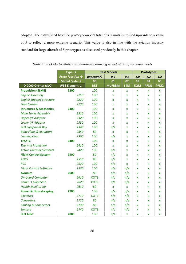
86
adopted. The established baseline prototype-model total of 4.7 units is revised upwards to a value
of 5 to reflect a more extreme scenario. This value is also in line with the aviation industry
standard for large aircraft of 5 prototypes as discussed previously in this chapter
Table 8: SLO Model Matrix quantitatively showing model philosophy components
Type → Test Models Prototypes
Proto Fraction → paperwork 0.5 0.8 1.0 1.2 1.2
Model Code → 00 01 02 03 04 05
D‐2000 Orbiter (SLO) WBS Element ↓ DES MU/BBM STM EQM PFM1 PFM2
Propulsion (SLME) 2200 100 x x x x x
Engine Assembly 2210 100 x x x x x
Engine Support Structure 2220 100 x x x x x
Feed System 2230 100 x x x x x
Structures & Mechanics 2300 100 x x x x x
Main Tanks Assembly 2310 100 x x x x x
Upper I/F Adaptor 2320 100 x x x x x
Lower I/F Adaptor 2330 100 x x x x x
SLO Equipment Bay 2340 100 n/a x x x x
Body Flaps & Actuators 2350 80 x x x x x
Landing Gear 2360 100 n/a x x x x
TPS/TC 2400 100 x x x x x
Thermal Protection 2410 100 x x x x x
Active Thermal Elements 2420 100 n/a x x x x
Flight Control System 2500 80 n/a x x x x
ADCS 2510 80 n/a x x x x
RCS 2520 100 n/a x x x x
Flight Control Software 2530 100 n/a n/a x x x
Avionics 2600 80 n/a n/a x x x
On‐board Computer 2610 COTS n/a n/a x x x
Comm. Equipment 2620 COTS n/a n/a x x x
Health Monitoring 2630 80 x x x x x
Power & Housekeeping 2700 100 n/a n/a x x x
Batteries 2710 COTS n/a n/a x x x
Converters 2720 80 n/a n/a x x x
Cabling & Connectors 2730 80 n/a n/a x x x
Sensors 2740 COTS n/a n/a x x x
SLO AI&T 2800 100 n/a x x x x
87
4.1.4 The Development & Production Industry Analogue
For the SpaceLiner, two of the three classical key components of the overall program
cost, being the non-recurring development and the recursive production costs. It was deemed to
preliminary to calculate operation costs due to the early phase of the program, and no clear
operations scheme having being determined as yet. Here, given the hybrid nature of the vehicle, it
is the philosophy that the development effort lies in the space-realm, since all technologies to be
designed and tested are space-based. After the initial flight test units, production then resembles
production processes of the aviation industry. The high quantities of the SpaceLiner vehicles
expected to be produced is analogous to the rates of modern production of large airlines, like the
Airbus A380 [9], or Boeing’s B777 Dreamliner [30]. The cost of consequent units of production
is thus considered based on assessment and analyses of the aviation industry to determine the
potential production learning curve for SpaceLiner. These latter assumptions translate themselves
into associated numerical complexities when calculating development and production costs for
the SpaceLiner case-study.
4.1.5 The Main Engine Development
SpaceLiner features two cryogenic engines – a Booster (SLB) stage engine (nine engines
per SLB stage), and a second engine for the passenger “orbiter” (SLO) stage (two engines per
SLO stage). Here, it is vital to note that the SLO and SLB engines, mechanically, are the same,
except for the nozzle extensions, as shown in Figure 15. As such, the SLO net engine mass is
larger than for the SLB engine, having a larger nozzle. To attribute specific percentiles of novelty
to two separate engines of the same technology, but of different scaling, would also be
unreasonably precise at this early stage. Being identical mechanically, it is therefore assumed
that only one development cost is incurred for the heavier SLO engine, thus providing a most
extreme, ‘worst case’ cost, but which is then considered to also cover the development cost of the
smaller SLB engine.
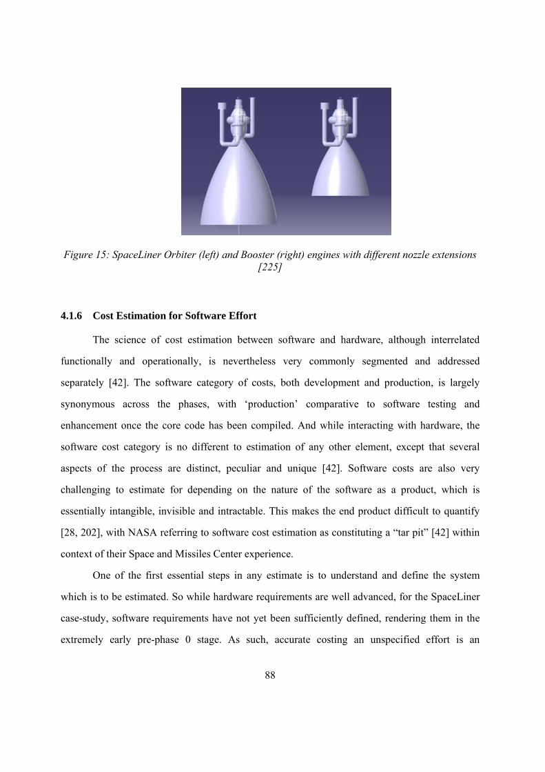
88
Figure 15: SpaceLiner Orbiter (left) and Booster (right) engines with different nozzle extensions [225]
4.1.6 Cost Estimation for Software Effort
The science of cost estimation between software and hardware, although interrelated
functionally and operationally, is nevertheless very commonly segmented and addressed
separately [42]. The software category of costs, both development and production, is largely
synonymous across the phases, with ‘production’ comparative to software testing and
enhancement once the core code has been compiled. And while interacting with hardware, the
software cost category is no different to estimation of any other element, except that several
aspects of the process are distinct, peculiar and unique [42]. Software costs are also very
challenging to estimate for depending on the nature of the software as a product, which is
essentially intangible, invisible and intractable. This makes the end product difficult to quantify
[28, 202], with NASA referring to software cost estimation as constituting a “tar pit” [42] within
context of their Space and Missiles Center experience.
One of the first essential steps in any estimate is to understand and define the system
which is to be estimated. So while hardware requirements are well advanced, for the SpaceLiner
case-study, software requirements have not yet been sufficiently defined, rendering them in the
extremely early pre-phase 0 stage. As such, accurate costing an unspecified effort is an
89
impossible task. After all, premature estimates are one of the contributors to inaccurate software
development costs [202]. As such, software costs were not considered for the SpaceLiner concept
at this stage.
4.1.7 SpaceLiner Production Quantity
For calculation of the SpaceLiner production costs, an interesting figure is the theoretical
first unit (TFU) cost produced. Particularly for the TransCost model, the TFU cost is then used as
the basis for calculation of all serial production costs for a batch of items to be produced. By
definition, the TFU is the first unit in the serial production of multiple vehicles and as such,
should incur the highest production cost out of the batch to be produced. Usually, production
quantity is directly dependent on a clearly defined business case. In turn, the latter incorporates
not only a clear, overall program schedule, but also flights rates, which inherently assumes the
clear defined launch/landing (L/L) sites and consequently determines the total revenue from
expected flights to be sufficiently profitable resulting in financial gain, and a sufficient return on
investment (ROI) for its investors. For the SpaceLiner case-study, such a business case has not
been yet established, since the technical details, as well as key programmatic data are not yet
finalised. As such, a basic assumption had to be made.
Taking the established SpaceLiner program schedule already introduced in Chapter 4.1.2,
we see that the operational timeframe has been assumed and set as being 20 years. Although
some L/L sites have been proposed, with the reference mission established being Australia to
Europe, it can be assumed in a conservative approach that L/L pairs may be located in China and
the USA as well (see also Chapter 4.11 for a more detailed discussion). Assuming that between
these L/L pairs, four routes are established, those would be flown daily, in each direction,
equating to eight SpaceLiner flights per day. Daily flights would need to be ensured to allow
passengers the freedom and flexibility of travel to tailor their travel needs and short travel times.
90
With eight flights per day, this equates to 2920 flights per annum. And with SpaceLiner baseline
core vehicle element reusability (excluding engines) of 150 times, this results in a required
SpaceLiner production rate of 20 vehicles per year. Adding an additional 5 vehicles as a margin
to this amount (one additional SpaceLiner per L/L pairing, with one further additional safety-
margin vehicle) results in a required production rate (with margin) of 25 vehicles. Consequently,
over the 20 year proposed production phase, this results in a total of 500 SpaceLiner vehicles
produced.
4.1.8 SpaceLiner Reusability Impact on Production
Being designed as a fully reusable vehicle means that a single SpaceLiner vehicle can be
flown multiple times, a capability which is strongly aligned with cost effective space access. This
reusability has a technical limit, which is specific as being 150 flight cycles for the SLO (and
SPC) and SLB elements. For the eleven SLMEs per SpaceLiner vehicles, it is assumed that a
baseline engine reusability will be 25 times given technical restraints and the current capability of
existing rocket engines. Despite being known to be a technical challenge for rocket engines, the
relatively high reusability rate is, however, not deemed impossible. For example, the Russian
Kuznetsov NK-33 engine, currently utilised in the first stage of Orbital Sciences Corporation’s
Antares launchers, albeit in a modified version, are rumoured to have been successfully fired on a
test-bench well above 30 times [54, 141]. In view of this, a further interesting and plausible
sensitivity analysis for 50 times SLME reusability would be relevant, and is indeed considered
later in this Thesis in Chapter 4.10.9.3, although realising this goal this will depend on technical
capabilities and limits, which can only be determined through prototyping and extensive testing.
With an SLME/(SLO/SPC/SLB) reusability ration, it is also clear that the varying rates of
reusability for parts in a single, common vehicle also directly influence production rates, since
engines would have to be replaced during vehicle maintenance six times during the lifetime of a
91
single SpaceLiner vehicle. This consequently influences production rate of SLMEs as well as the
overall production costs during the program lifecycle. For production, 500 SpaceLiner units are
considered. Each vehicle requires eleven engines, which must then be replaced six times.
Therefore 66 SLMEs need to be supplied per SpaceLiner vehicle to match the reusability lifetime
of each key component.
4.1.9 SpaceLiner Cabin / Rescue Capsule
The SpaceLiner passenger cabin and rescue capsule life-critical system (SPC) is the sub-
system which constitutes the most novel and unprecedented and therefore challenging of
technologies within the SpaceLiner case-study. Initially the structure is separated, allowing
passengers to embark in a normal horizontal configuration. It is then integrated into the SLO
main structure on the launch pad prior to launch. In case of emergencies during the flight, the
cabin functions as a rescue capsule, capable of returning the passengers safely to Earth in an
autonomous manner. The SPC and its integration within the SpaceLiner stage are shown in
Figure 16.
While some loosely analogous rescue capsule systems based on a similar premise do
exist, these are mainly observed within the aviation industry, including the B-58 Hustler, the XB-
70 Valkyrie, the high-speed F-111 aircraft (2 crew), and the early prototypes of the Rockwell B-1
Lancer aircraft (4 crew). However for all of those aircraft, the scale and crew-carrying capacity of
these capsule structures deviates extremely to the SPC requirement of being able to transport 50
passengers. Looking into the space domain, historically, the Gemini (2 crew), and Apollo (3
crew) capsules from the mid-1960s, as well as the Mercury program, and the more recently
proposed Orion capsule (4 crew) once again transport only a very limited number of crew
compared to SpaceLiner case-study requirements. Therefore, directly using any aviation and
space analogues forms a weak basis for a representative comparison of technologies, and
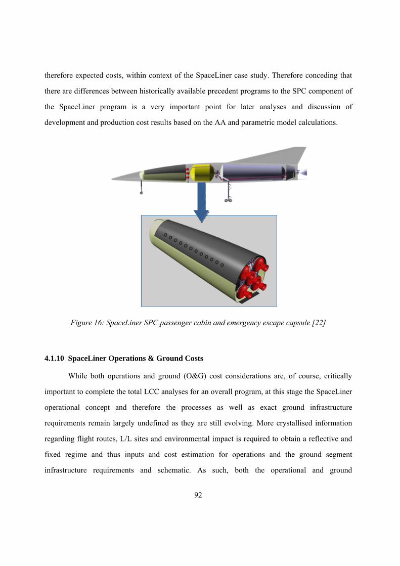
92
therefore expected costs, within context of the SpaceLiner case study. Therefore conceding that
there are differences between historically available precedent programs to the SPC component of
the SpaceLiner program is a very important point for later analyses and discussion of
development and production cost results based on the AA and parametric model calculations.
Figure 16: SpaceLiner SPC passenger cabin and emergency escape capsule [22]
4.1.10 SpaceLiner Operations & Ground Costs
While both operations and ground (O&G) cost considerations are, of course, critically
important to complete the total LCC analyses for an overall program, at this stage the SpaceLiner
operational concept and therefore the processes as well as exact ground infrastructure
requirements remain largely undefined as they are still evolving. More crystallised information
regarding flight routes, L/L sites and environmental impact is required to obtain a reflective and
fixed regime and thus inputs and cost estimation for operations and the ground segment
infrastructure requirements and schematic. As such, both the operational and ground
93
infrastructure scenarios are described quantitatively only, in Chapter 4.11, with some numerical
estimates and assumptions provided. However, these LCC components specific to the
SpaceLiner case-study and application will need to be investigated further in particular as the
technical and mission specifications and requirements of the concept continue to emerge to a
maturity and into fruition.
4.1.11 SpaceLiner Cost Risk Analysis
In addition to the importance of representative scheduling, which seeks to minimise the
likelihood of cost overruns and scheduling delays, the effects of potential risks must be
considered during initialisation of a program through risk analysis. While this topic has already
been briefly introduced theoretically in Chapter 2.3, it is discussed in greater depth, albeit at a
qualitative manner, in the consequent chapter.
In his classic 1982 book entitled Augustine’s Laws, Norman R. Augustine famously stated
that “two types of uncertainty plague most efforts to introduce major new products: known-
unknowns, and unknown unknowns” [18]. This is particularly relevant to the chosen SpaceLiner
case-study. Given the magnitude and expanse of the SpaceLiner program, here, close assessment
of the known unknowns, the cost risk assessment element, is especially crucial. Risk bears a
negative connotation, implying a detrimental effect of an unforeseen or unexpected event on the
program execution, scheduling and therefore, cost. It is therefore very important to conduct
various risk analyses and assessments prior to program commencement, to try and address,
capture and identify possible risk factors and elements which may impact a program, and seek to
quantify the cost ramifications.
Risk is defined as the uncertainty of successfully achieving any of the technical,
programmatic and/or cost targets of a project [116]. Within this definition, and with reference to
the SpaceLiner case-study, technical, scheduling, programmatic, financial (cost) and operational
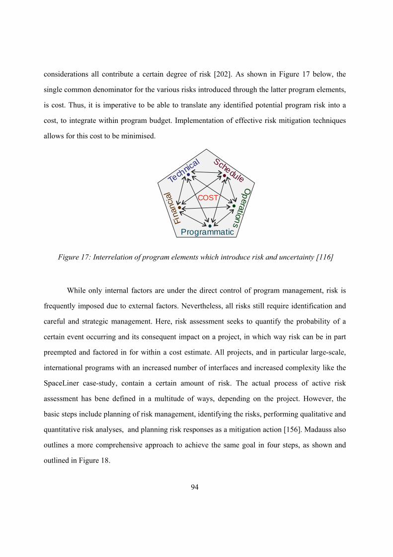
94
considerations all contribute a certain degree of risk [202]. As shown in Figure 17 below, the
single common denominator for the various risks introduced through the latter program elements,
is cost. Thus, it is imperative to be able to translate any identified potential program risk into a
cost, to integrate within program budget. Implementation of effective risk mitigation techniques
allows for this cost to be minimised.
Tech
nical Schedule
Programmatic
Op
erationsFi
nanc
ial
COST
Figure 17: Interrelation of program elements which introduce risk and uncertainty [116]
While only internal factors are under the direct control of program management, risk is
frequently imposed due to external factors. Nevertheless, all risks still require identification and
careful and strategic management. Here, risk assessment seeks to quantify the probability of a
certain event occurring and its consequent impact on a project, in which way risk can be in part
preempted and factored in for within a cost estimate. All projects, and in particular large-scale,
international programs with an increased number of interfaces and increased complexity like the
SpaceLiner case-study, contain a certain amount of risk. The actual process of active risk
assessment has bene defined in a multitude of ways, depending on the project. However, the
basic steps include planning of risk management, identifying the risks, performing qualitative and
quantitative risk analyses, and planning risk responses as a mitigation action [156]. Madauss also
outlines a more comprehensive approach to achieve the same goal in four steps, as shown and
outlined in Figure 18.
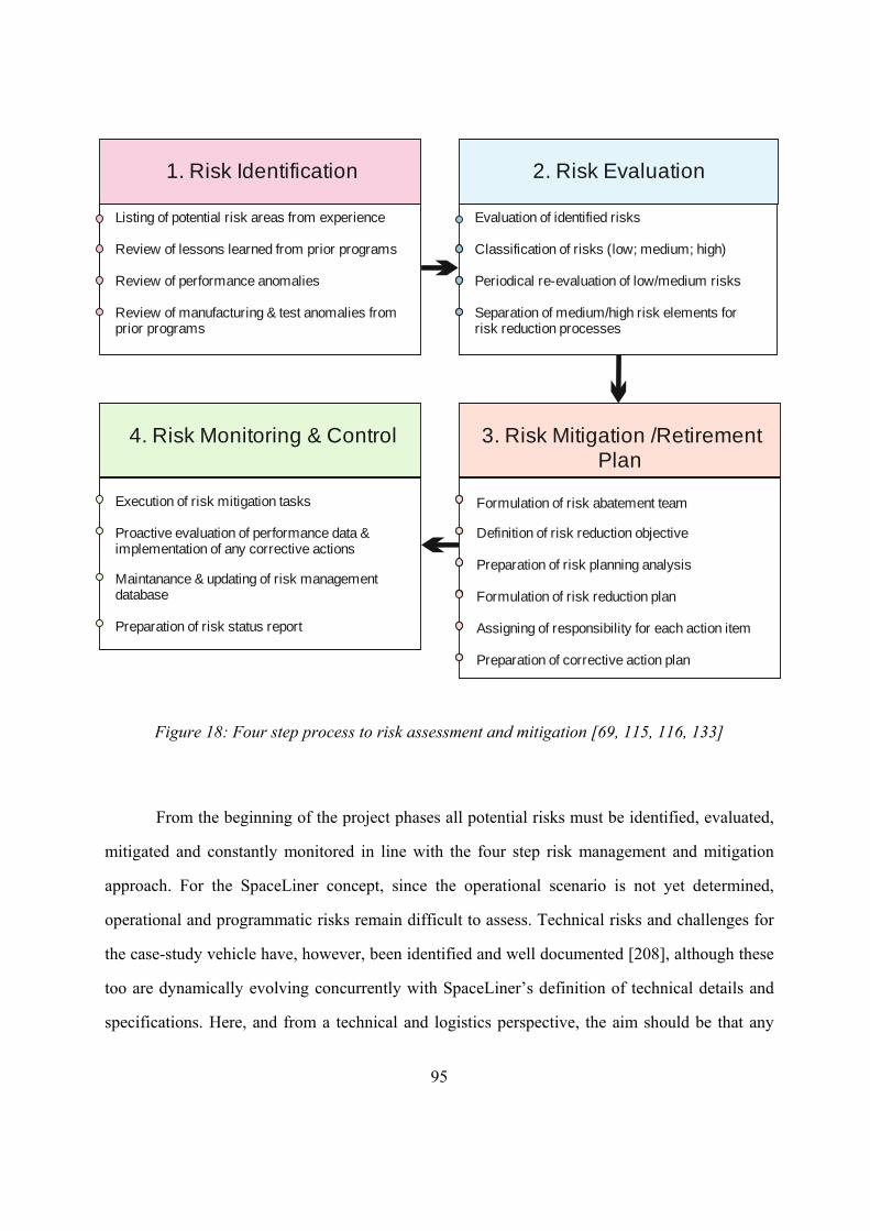
95
Figure 18: Four step process to risk assessment and mitigation [69, 115, 116, 133]
From the beginning of the project phases all potential risks must be identified, evaluated,
mitigated and constantly monitored in line with the four step risk management and mitigation
approach. For the SpaceLiner concept, since the operational scenario is not yet determined,
operational and programmatic risks remain difficult to assess. Technical risks and challenges for
the case-study vehicle have, however, been identified and well documented [208], although these
too are dynamically evolving concurrently with SpaceLiner’s definition of technical details and
specifications. Here, and from a technical and logistics perspective, the aim should be that any
Listing of potential risk areas from experience
Review of lessons learned from prior programs
Review of performance anomalies
Review of manufacturing & test anomalies from prior programs
2. Risk Evaluation
Evaluation of identified risks
Classification of risks (low; medium; high)
Periodical re-evaluation of low/medium risks
Separation of medium/high risk elements for risk reduction processes
4. Risk Monitoring & Control
Execution of risk mitigation tasks
Proactive evaluation of performance data & implementation of any corrective actions
Maintanance & updating of risk management database
Preparation of risk status report
3. Risk Mitigation /Retirement Plan
Formulation of risk abatement team
Definition of risk reduction objective
Preparation of risk planning analysis
Formulation of risk reduction plan
Assigning of responsibility for each action item
Preparation of corrective action plan
1. Risk Identification
96
remaining technical risks will be minimised to a level which is acceptable for successful
integration into the commercial passenger transportation niche, being comparable with standards
enforced within the aviation industry. To address this, a key philosophy of the SpaceLiner design
concept is to base the design on state-of-the-art technologies in order to keep the potential
technical risks as low as possible. In addition, a passenger rescue capsule has also been integrated
into the design with the aim of improving the significantly lower safety factor of the space
domain.
Here, a critical engineering challenge for all passenger transportation vehicles is to reach
a high reliability status through low technical and operating risks (see Figure 17). In this respect,
the rocket SLB, SLO (SPC) elements should be man-rated to achieve a much higher reliability
and a well proven safety record of close to 100 percent, similar to the aviation industry. This,
however, cannot occur until the elements have been fully developed, and performed regular,
successive, intensive and successful flights to prove the reliability of the technologies involved.
When a firm reliability record is established, it can be expected that passenger demand based on
the feeling of security, as well as funding sources, are likely to increase [6]. More information of
SpaceLiner case-study technological, logistical and operational risks can be found in detail in ref.
[208]. Here, key SpaceLiner case-study challenges are identified to be the safety and reliability of
the system, acoustic noise and sonic boom, launch and landing (L/L) site as well as routes,
destinations and city pair selection, a door-to-door passenger transportation network, trajectory
optimisation and thermal protection system (TPS) ramifications, environmental impact, as well as
operational considerations [208]. Each aspect would require a risk assessment, to translate into a
cost equivalent. At this stage, this has been achieved through a global margin imposed for costs
for all models applied within the AA context.
A baseline SpaceLiner case-study schedule and timeline has also been proposed in
Chapter 4.1.2, although this is also of a preliminary nature, hinging on future elements such as
production quantities, which in turn depend on flight location pairings, and a business case which
97
considers flight frequency and how many vehicles should be in concurrent operation. To achieve
such a preliminary schedule, various assumptions had to be relied upon, all of which have also
been fully documented to support justification. When concrete information becomes available, in
line with the four step risk assessment plan, assumption should be replaced with fixed program
data.
In terms of the financial risks for a complex system as the SpaceLiner concept,
assessment and quantification is a challenging task given the multitude of influencing factors.
However it is well known that estimating confidence hinges directly on the detail and status of
program definition, which makes early program phase cost estimation such a challenge. It is
therefore of great importance to develop and crystallise realistic and clear technical specifications
and requirements as a solid basis and prerequisite of a reliable cost estimation.
In summary, risk assessment must be implemented across all major WBS element
categories. The introduction of risk assessment actions and the attempt to eliminate all risks
related to cost estimation is the primary formal means for risk control, at this early stage of the
SpaceLiner case-study, the assessment of risks was performed at a very top system level through
a judgement of the overall estimating confidence, as will be discussed in Chapter 4.12. The
hardware cost estimation for the development and production phases of the SpaceLiner case-
study which are performed and discussed in this Thesis are optimally based on all currently
available preliminary technical definitions, a systematic baseline project structure demonstrated
in consolidation of a WBS, as well as establishment of a preliminary project schedule.
For more information on the diverse field of risk assessment, the interested readers may
refer to the following references for further details on risk and uncertainty assessment and
management across the various program aspects [13, 31, 42, 65, 94, 115, 133, 137, 156, 212].
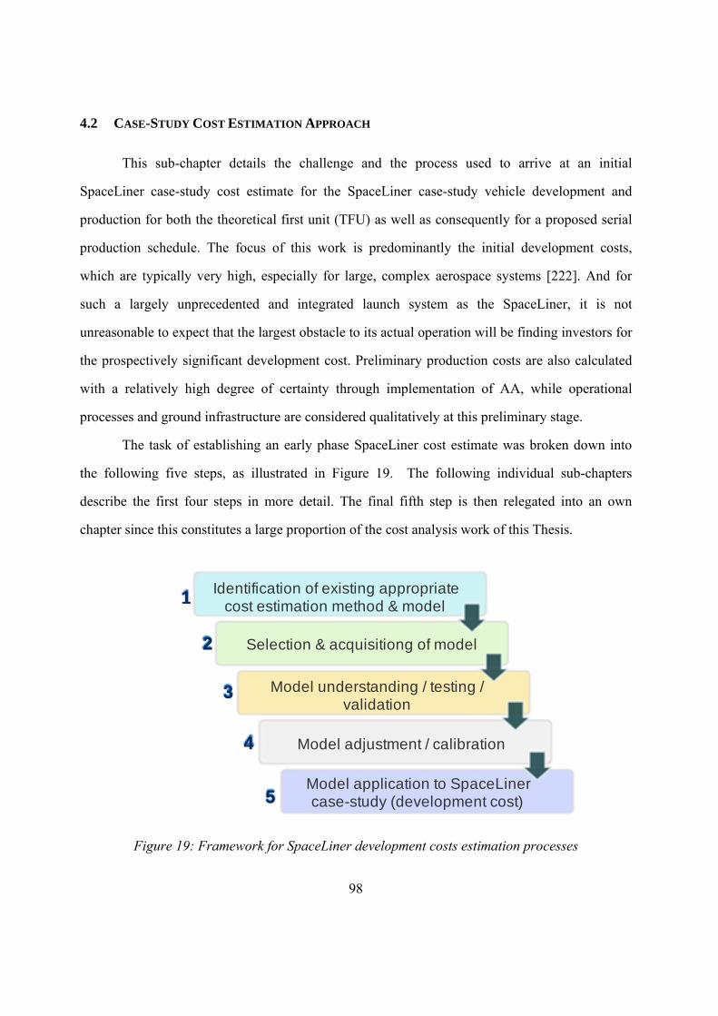
98
4.2 CASE-STUDY COST ESTIMATION APPROACH
This sub-chapter details the challenge and the process used to arrive at an initial
SpaceLiner case-study cost estimate for the SpaceLiner case-study vehicle development and
production for both the theoretical first unit (TFU) as well as consequently for a proposed serial
production schedule. The focus of this work is predominantly the initial development costs,
which are typically very high, especially for large, complex aerospace systems [222]. And for
such a largely unprecedented and integrated launch system as the SpaceLiner, it is not
unreasonable to expect that the largest obstacle to its actual operation will be finding investors for
the prospectively significant development cost. Preliminary production costs are also calculated
with a relatively high degree of certainty through implementation of AA, while operational
processes and ground infrastructure are considered qualitatively at this preliminary stage.
The task of establishing an early phase SpaceLiner cost estimate was broken down into
the following five steps, as illustrated in Figure 19. The following individual sub-chapters
describe the first four steps in more detail. The final fifth step is then relegated into an own
chapter since this constitutes a large proportion of the cost analysis work of this Thesis.
Identification of existing appropriate cost estimation method & model
Selection & acquisitiong of model
Model understanding / testing / validation
Model adjustment / calibration
Model application to SpaceLiner case-study (development cost)
2
3
5
1
4
Figure 19: Framework for SpaceLiner development costs estimation processes
99
4.3 COST ESTIMATION METHODOLOGY IDENTIFICATION
As introduced and described in Chapter 2.6.2, the Amalgamation Approach will be
implemented and demonstrated within this Thesis within application of a current and actual
industry case-study, the SpaceLiner concept.
Furthermore, as previously established and detailed in Chapter 2, various key cost
estimation methods (CEMs) exist for application within the space industry. Suitability of each
CEM is strongly dependent on program phase. With every advancement and change to any aspect
of a program, it is essential to re-evaluate and update the latest cost estimate to incorporate
changes and reflect new information as it becomes available. In this way cost estimation is a
dynamic process ongoing throughout the entire program lifetime.
SpaceLiner is in the early development phases, and more specifically, currently classed
within the pre-phase A stages. As such, reflective of the active research and concept advancement
and incorporation of technological progresses within context of the program, the concept is
dynamically evolving. Flexible, system level CEMs are applicable to this early stage, while more
detailed and resource intensive approaches, like EBU, are inefficient and thus inappropriate.
Consequently, the firm theoretical cost engineering baseline established through the
intensive literature review found in ref. [209] could be applied to a current and real industry
example of a large, complex and international space program in its early phase – the SpaceLiner
concept. Through application of key findings from analyses already presented in Chapter 2 and
through dissemination of cost estimating principles presented in Figure 5, the parametric
approach was selected for predominant utility and application to the SpaceLiner. Analogy as well
as the EJ and ROM CEMs were also identified as being relevant during this phase.
In line with the AAMAC structure requirements and theory, three tools and models were
identified for application to the case-study example chosen within the context of this Thesis. As
already introduced in Chapter 4.4, two space-industry prominent and highly utilised commercial
off-the-shelf models and tools were chosen, being PRICE and the 4cost aces parametric and data-
100
empty models. In addition, the high-level, dedicated launcher systems parametric TransCost
handbook and model was also selected. The TransCost Model is available for ready purchase in
the form of a textbook. The PRICE and 4cost aces models, however, all require varying annual
license fees.
For the purpose of this work, the 4cost aces software was used under an agreement to
support the aims and goals outlined in this Thesis with the unwavering and excellent support of
Mr. Joachim Schöffer and Mr. Herbert Spix. The PRICE software was utilised under an academic
license from the International Space University (ISU) in Strasbourg under the guidance of the
distinguished Professor Bernd Madauss, with outstanding assistance offered by Mr. Fabian
Eilingsfeld.
All three models of TransCost, 4cost aces and PRICE selected for AAMAC mode
utilisation in this Thesis are outlined in greater detail in the consequent chapters.
4.4 AAMAC COST ESTIMATION MODEL & TOOL SELECTION
CEMs form the backbone of various existing cost estimation tools and commercial
models relevant to the space sector which exist. These were also identified and listed in the
literature review [209]. Three such parametric tools and models were identified and chosen and in
line with AA principles and based on their suitability to the SpaceLiner case-study. These
comprise of the dedicated TransCost model for launch vehicles, as well as the commercial 4cost
aces, and PRICE tools. These are briefly introduced and outlined below.
4.4.1 TransCost Model
The parametric TransCost Model for Space Transportation Systems Cost Estimation and
Economic Optimisation was chosen as one of three models within the AA framework for the
SpaceLiner case-study. TransCost is a dedicated launch vehicle system model encompassing cost
101
categories of expendable (ELV) and reusable (RLV) launch vehicles. It is therefore of interest
within the context of this review. The model itself is integrated into the Handbook of Cost
Engineering for Space Transportation Systems. Conceived initially as a cost engineering tool,
TransCost uses the parametric CEM with underlying CERs derived from a vehicle and engine
database of cost data of European and US space vehicle and engine projects within the 1960-
2009 timeframe. As such, TransCost is referred to as a ‘data-full’ model to reflect its inclusion of
project-related data for space programs.
TransCost breaks down the costs of a program into three clear categories, being
development costs, production costs (incorporating the learning factor, f4) and operations costs.
This latter group of costs is more generally defined categorically, since operations costs are
mission-specific, making universal formulae difficult to establish. In this sense, TransCost sets
out categories, areas and classes of costs for individual consideration and determination on a case
to case basis.
Designed specifically to be applied in the initial conceptual mission design phases,
TransCost was an extension of the 1971 dissertation work of D. E. Koelle and is now a very
commonly used space transportation cost model within industry, perhaps due to its low cost and
ready availability, simple handling, and transparent cost estimation relationships (CERs) and data
which underlie the model. Data from historically recorded missions is used to derive a regression
line of best fit. Such a regression line is then represented mathematically, in the form of a CER. It
is then assumed that any future missions of similar characteristics can be modeled by this trend
line. TransCost features dedicated CERs for various vehicle categories, with any differences
between underlying CER data and the mission being estimated (i.e. complexities, technology
novelty and other deviations), adjusted for by specially defined complexity factors. TransCost
effectively features twelve complexity factors (fx), from f0 to f11, which can be applied to the
existing basic CERs to adjust for variations between the underlying CER and the program which
is being costed. These factors are defined and summarised in Table 9 below, while a full list of all
102
the complexity factors, their definitions and values are also included in Appendix D for
completeness and the self-contained autonomy of this Thesis as a stand-alone document.
Being a dynamic model, both the database and CERs are continuously updated, and the
latest model available since October 2010 is TransCost Version 8.1. Minor variations in CERs
exit between the modified TransCost versions, the latest three of which are comparatively shown
below in Table 9. While some minor variations of TransCost value ranges can be observed
between the three TransCost versions, this shows the dynamic and evolving nature of the
Handbook and cost estimation model which seeks to keep up to date with current trends and
developments within the space launch vehicle sector.
The model itself addresses three areas of the launch vehicle life cycle costs, being
development, production and operations costs. Each category is further broken down into sub-
categories, each with its own unique respective CERs, which address distinctly identified
categories of ELVs, RLVs and craft, and include solid propellant boosters, liquid propellant,
pressure-fed as well as turbo- and ramjet engines, and crewed capsules and space systems.
Different factors underpin each CER, and focus on vehicle mass, number of launcher stages,
number of units produced and the expected launch rate.
Furthermore, a range of twelve additional complexity factors exist, to be assigned in
accordance with what is being costed. These factors, collectively denoted as fx, address the
impacts of varying technological advancements and quality level, team experience, regional
productivity, series production, effects from increased number of participating contractor
organisations, subcontractor-ship or Government involvement, optimum schedule deviations and
past technical experience, as well as, more recently, the commercial element to development and
production. A visual representation of the TransCost Model structure breakdown is presented in
Figure 20.
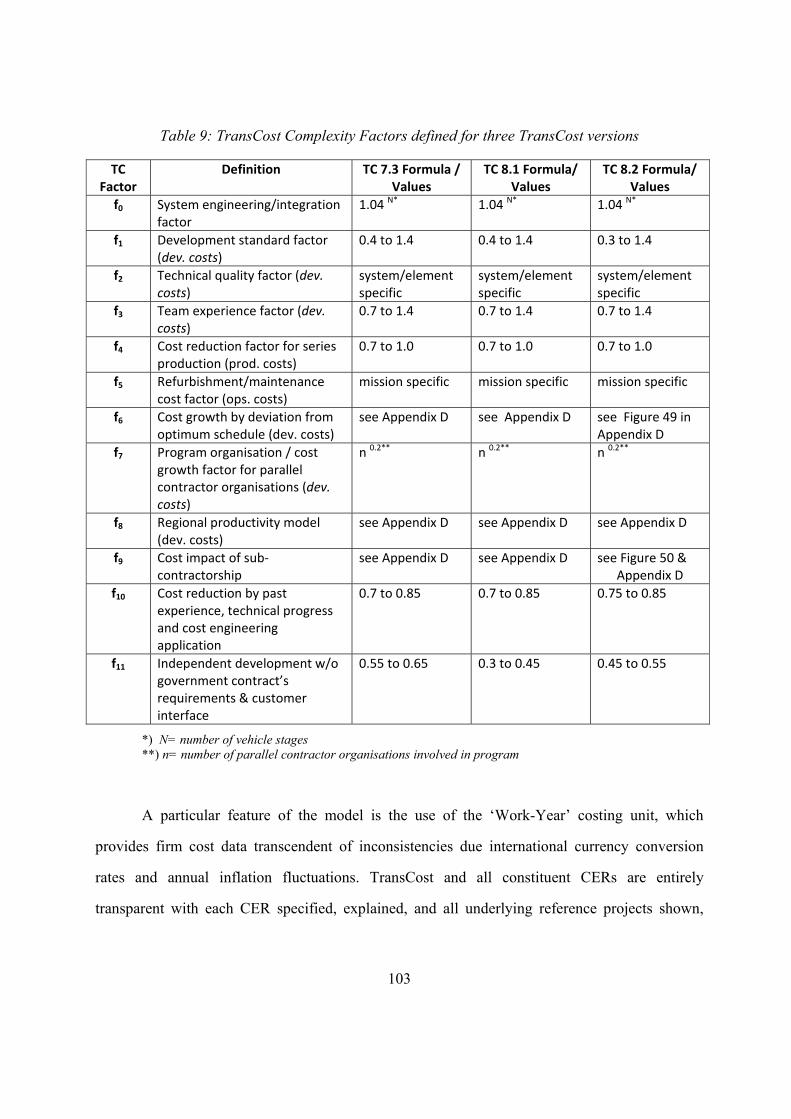
103
Table 9: TransCost Complexity Factors defined for three TransCost versions
TC Factor
Definition TC 7.3 Formula / Values
TC 8.1 Formula/ Values
TC 8.2 Formula/ Values
f0 System engineering/integration factor
1.04 N* 1.04 N* 1.04 N*
f1 Development standard factor (dev. costs)
0.4 to 1.4 0.4 to 1.4 0.3 to 1.4
f2 Technical quality factor (dev. costs)
system/element specific
system/element specific
system/element specific
f3 Team experience factor (dev. costs)
0.7 to 1.4 0.7 to 1.4 0.7 to 1.4
f4 Cost reduction factor for series production (prod. costs)
0.7 to 1.0 0.7 to 1.0 0.7 to 1.0
f5 Refurbishment/maintenance cost factor (ops. costs)
mission specific mission specific mission specific
f6 Cost growth by deviation from optimum schedule (dev. costs)
see Appendix D see Appendix D see Figure 49 in Appendix D
f7 Program organisation / cost growth factor for parallel contractor organisations (dev. costs)
n 0.2** n 0.2** n 0.2**
f8 Regional productivity model (dev. costs)
see Appendix D see Appendix D see Appendix D
f9 Cost impact of sub‐contractorship
see Appendix D see Appendix D see Figure 50 & Appendix D
f10 Cost reduction by past experience, technical progress and cost engineering application
0.7 to 0.85
0.7 to 0.85 0.75 to 0.85
f11 Independent development w/o government contract’s requirements & customer interface
0.55 to 0.65 0.3 to 0.45 0.45 to 0.55
*) N= number of vehicle stages **) n= number of parallel contractor organisations involved in program
A particular feature of the model is the use of the ‘Work-Year’ costing unit, which
provides firm cost data transcendent of inconsistencies due international currency conversion
rates and annual inflation fluctuations. TransCost and all constituent CERs are entirely
transparent with each CER specified, explained, and all underlying reference projects shown,
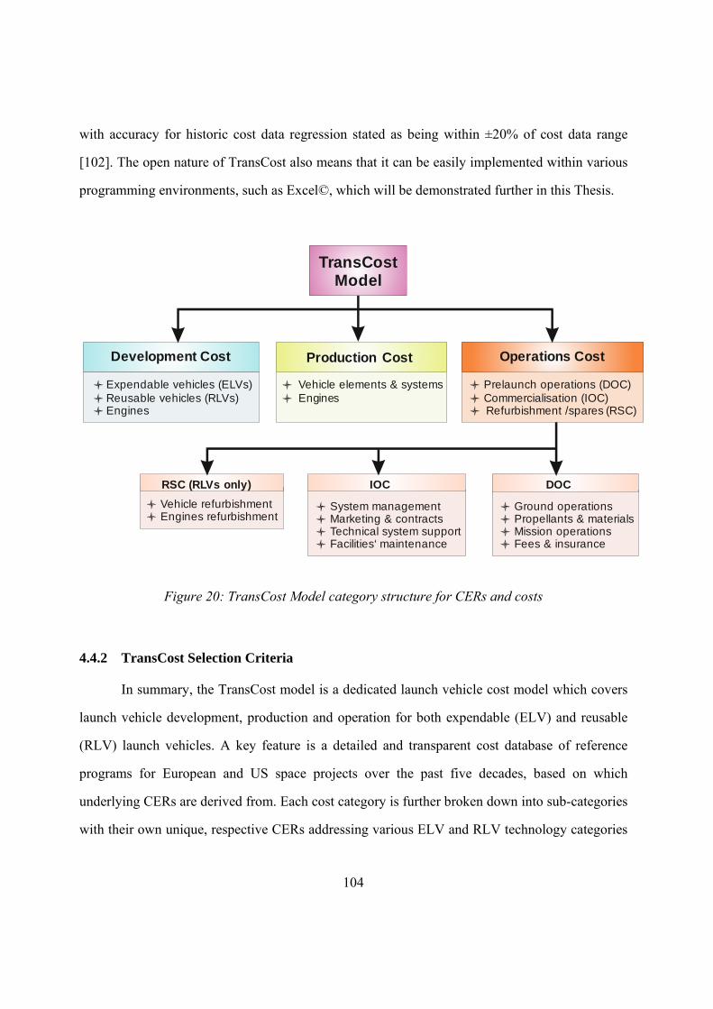
104
with accuracy for historic cost data regression stated as being within ±20% of cost data range
[102]. The open nature of TransCost also means that it can be easily implemented within various
programming environments, such as Excel©, which will be demonstrated further in this Thesis.
TransCost Model
Development Cost
Expendable vehicles (ELVs)Reusable vehicles (RLVs)
Engines
Production Cost
Vehicle elements & systems ineEng s
Operations Cost
Prelaunch operations (DOC) Commercialisation (IOC)
s (RSC) Refurbishment / pares
IOC
System management Marketing & contracts Technical system support
Facilities‘ maintenance
RSC (RLVs only)
Vehicle refurbishment Engines refurbishment
DOC
Ground operations Propellants & materials Mission operations Fees & insurance
Figure 20: TransCost Model category structure for CERs and costs
4.4.2 TransCost Selection Criteria
In summary, the TransCost model is a dedicated launch vehicle cost model which covers
launch vehicle development, production and operation for both expendable (ELV) and reusable
(RLV) launch vehicles. A key feature is a detailed and transparent cost database of reference
programs for European and US space projects over the past five decades, based on which
underlying CERs are derived from. Each cost category is further broken down into sub-categories
with their own unique, respective CERs addressing various ELV and RLV technology categories
105
of stages, solid and liquid propellant boosters, pressure-fed and turbo- and ramjet engines, and
crewed capsules and space systems. Different complexity factors underpin each CER, and
address system-level parameters including mass, number of launcher stages, number of units to
be produced, and expected launch rates. Complexity factors are then further assigned as
necessary to factor for aspects like technological level, team experience, regional productivity,
series production, and program funding structure. A particular feature of the model is also the use
of the ‘Work-Year’ (WYr) costing unit, which provides firm cost data transcendent of
inconsistencies due to international currency conversion rates and annual inflation fluctuations.
The effort figure can then be converted to any currency, for any year’s economic conditions
(e.c.).
Therefore the TransCost model applicability and selection for the SpaceLiner project was
justified for the following main reasons:
Dedicated cost model for launcher vehicles (ELVs and RLVs).
Updated database from 52 years of program history for Europe, USA, and Japan.
Transparent, open CERs with identifiable and visible reference missions behind each
formula shown in a graphical display of reference points.
Ideal applicability at high, total system level
High suitability for use during early, conceptual inception and design phase while
technical and mission details are still emerging
Uses of effort “WYr” unit to quantify cost, which overcomes possible exchange rates,
currency, inflation and timeframe conversion fluctuations and inconsistencies
High relevance also to advanced, reusable space transportation concepts
106
Therefore the TransCost model was selected as the basic, kernel model and tool for the
baseline SpaceLiner LCC calculations of development and production. In particular, dedicated
CERs applicable to these two cost categories were targeted for utility. Operations costs (WBS
element 7000) could be disseminated largely in a qualitative only, with some numerical figures
provided, although backed mainly by analog or EJ CEMs. In addition, ground infrastructure
(WBS element 6000) was also loosely estimated based on the EBU, analogy and EJ approaches.
due to the still early program phase of the SpaceLiner concept, the final version of these two LCC
aspects will need to be reconsidered at a later stage when final program details and requirements
are concrete. Therefore, the non-recursive development costs, and the recurring production costs
were focal to this study.
Based on theory, other supporting CEMs including analogy, EJ and the ROM approach
were also deemed relevant, concurrently employed, and often relied upon as sanity checks during
the costing process.
The overall cost estimation ranges for SpaceLiner development and production are
therefore a result of the CEM amalgamation approach (AA) which has been strategically
established, developed within this Thesis, and applied to a current actual space program in line
with efficient cost engineering principles and practices.
4.4.3 PRICE Systems PRICE-H
The PRICE-H cost estimation model was developed by Frank Freiman in Moorestown,
New Jersey, with its origins in military space applications. Based on his studies of statistical
quality control, in 1969 he invented parametric cost modeling for hardware systems development
and acquisition [12, 152]. The PRICE-H Model was then established commercially by Mark H.
Burmeister at the former RCA-Astro organisation, now Lockheed Martin in 1975 [152]. Being
developed to assist with bidding on payloads for military systems to DoD on intelligence
satellites, the PRICE Systems Solutions now constitutes a market leading software distributed by
107
PRICE (Parametric Review of Information for Costing and Evaluation) Systems internationally.
A subscription for the software is required.
The PRICE® Systems Solutions is based on the parametric CEM, and consists of two sets
of models, being the legacy PRICE Estimating Suite (PRICE-H and PRICE-S) and the new
generation TruePlanner (True-H and True-S) [137]. Both PRICE models contain hundreds of
CERs derived from extensive research and statistical analysis of data from over eleven thousand
completed projects with defined product characteristics and known schedules, with most of the
data points themselves sanitised. The CERs are proprietary and the database therefore
confidential. As such, PRICE-H is what is referred to as a ‘data-empty model’, also meaning that
the model must be calibrated prior to its application for a specific project. The PRICE Estimating
Suite is not a dedicated space systems or launcher model, so applications extend across multi-
disciplinary estimates. The model is however very frequently applied to the space sector for
hardware, software and scheduling estimations and project planning, particularly at the product
concept stages [42]. Clients of the PRICE products include organisations like the DLR and
NASA, which hold agency wide licenses on the software [135].
Since this Thesis has a hardware focus, only hardware models will be mentioned herein.
To complement PRICE-H, the PRICE suite also includes the PRICE-HL (Hardware Lifecycle)
and PRICE-M (Electronic Module and Microcircuit) models. PRICE-H has the capability to
estimate most manufactured items and assemblies, and requires key inputs such as weight,
manufacturing complexity, quantities, schedule information, development costs and production
costs [60]. The model must first be calibrated for each individual project by the user, which
consequently allows for extraction of benchmark data for future use and reuse. This calibration is
achieved through application of multiplication factors including the main Platform and
Complexity parameters, the latter are deemed to be the core of the PRICE hardware cost model,
being the universal metric for normalised cost density in a hardware item. A basic Platform Value
108
allows for conversion of historical data to more modern applications by transcending different
disciplines, and effectively considers different operational environments in terms of commercial,
military ground, airborne, manned and unmanned space. Complexity factors must be calibrated
respective of product family, with the Engineering Complexity Factor addressing design standard
and team experience in combination with a Manufacturing Complexity Factor. While the model
facilitates for manual entry of parameter values, default Complexity values are also available.
The complementary PRICE-HL model generates operations and support cost outputs
across all phases of hardware life cycle. Additionally, the PRICE-M estimates electronic module
and applications specific integrated circuits (ASICs) development and production costs.
4.4.4 aces by 4cost
The Advanced Cost Estimating System, aces, is a parametrics-based module of the 4cost
suite, constituting cost estimating software for gauging plausibility of projects during the early
stages. Released by the German company 4cost, this ‘most innovative parametric model
available’ [2] was developed by a group of software, hardware and cost engineers under the
leadership of Herbert Spix, and has been on the market since 1992. An annual license fee
depending on the license type is applicable.
The 4cost aces model is a general all-purpose model applicable to compile cost estimates
for mechanical and electronic hardware assemblies and systems as well as software programs [4].
Again, being a data-empty model, 4cost aces must be calibrated prior to project application and
in line with respective historical company data. A built-in model for life cycle costs allows aces
to derive costs from acquisition stages, to preliminary design and development through to
production and LCC analysis. Optional user calibration allows the model to function like a
specific tool. Within the space industry aces has been used by companies and research
institutions including OHB, DLR and the former EADS Astrium, now known as Airbus Defence
and Space.
109
The model is differentiated by the fact that it does not have an underlying database of past
missions. Instead mathematical functions and algorithms (CERs) based on multi-disciplinary data
collected and analysed over many years, form the basis of all cost estimates. As a deviation from
the traditional processes, inputs like material lists and labour hours are therefore not needed.
Instead, inputs pertain to economic conditions, manufacturing processes and development
strategies [2], based on which only relevant inputs associated with an appropriate mode are
highlighted for the user. Programmed using Visual Studio and C++, aces facilitates for common
import and export interfaces in various formats including, amongst others, Excel© as well as text
files [3].
The resulting output estimate provides an initial ‘feasibility check’ for a preliminary
design, and cost information for hardware development, production and LCC trends. The output
also reflects costs including those associated with design engineering, drafting, project
management, documentation, system engineering, special tooling and test equipment, material,
labour and any overheads. The model also provides estimates for subsystem integration and
assembly costs and system testing [2].
4.5 TRANSCOST MODEL TESTING, CALIBRATION & VALIDATION
The process of understanding, testing and validation was only possible and therefore only
relevant and applicable for the TransCost model. This is the only transparent, and data-open
model which facilitates for a testing and calibration regime to be implemented. The 4cost aces
and the PRICE tools, being commercial tools, are both data-closed and confidential models with
non-transparent databases and thus, model mechanics. Both models, however, are widely utilised
within the space sector within formulation of cost estimates for a wide range of missions and
applications, and also during various program phases.
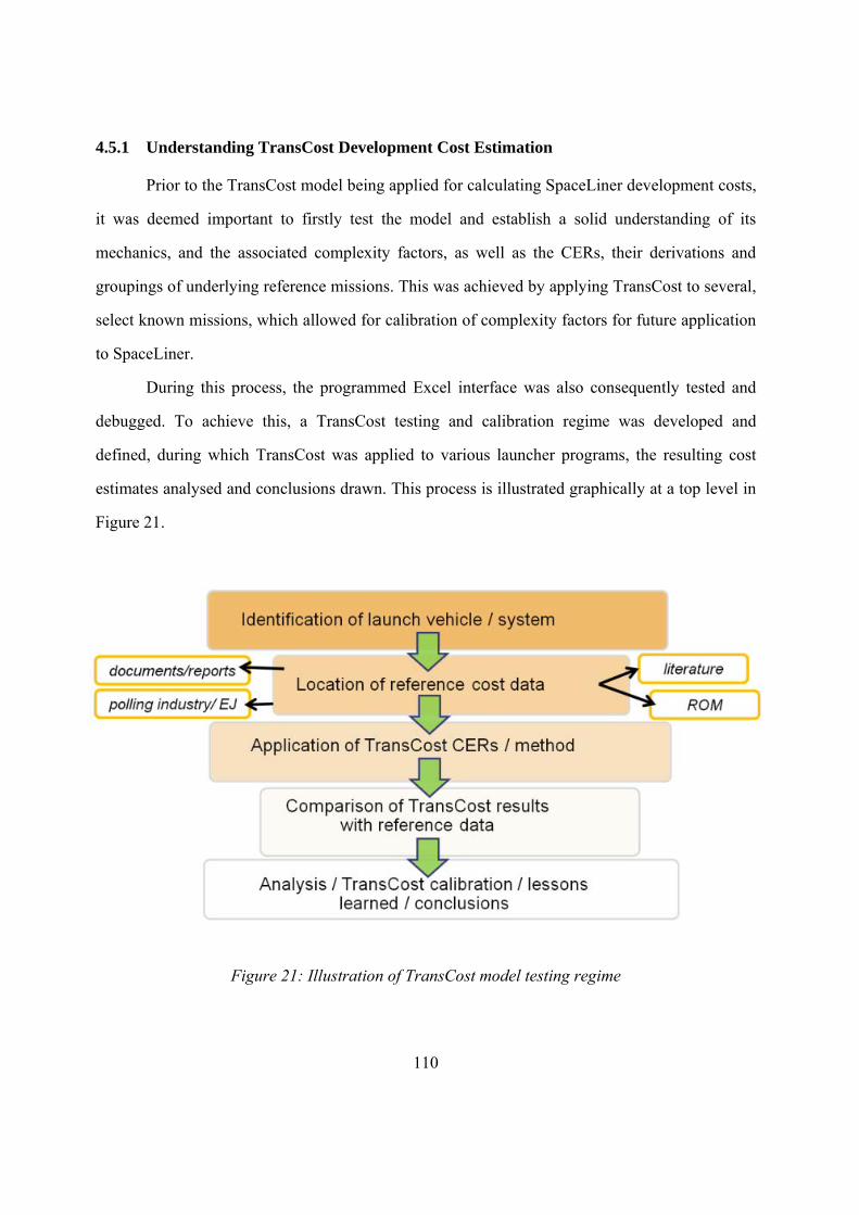
110
4.5.1 Understanding TransCost Development Cost Estimation
Prior to the TransCost model being applied for calculating SpaceLiner development costs,
it was deemed important to firstly test the model and establish a solid understanding of its
mechanics, and the associated complexity factors, as well as the CERs, their derivations and
groupings of underlying reference missions. This was achieved by applying TransCost to several,
select known missions, which allowed for calibration of complexity factors for future application
to SpaceLiner.
During this process, the programmed Excel interface was also consequently tested and
debugged. To achieve this, a TransCost testing and calibration regime was developed and
defined, during which TransCost was applied to various launcher programs, the resulting cost
estimates analysed and conclusions drawn. This process is illustrated graphically at a top level in
Figure 21.
Figure 21: Illustration of TransCost model testing regime
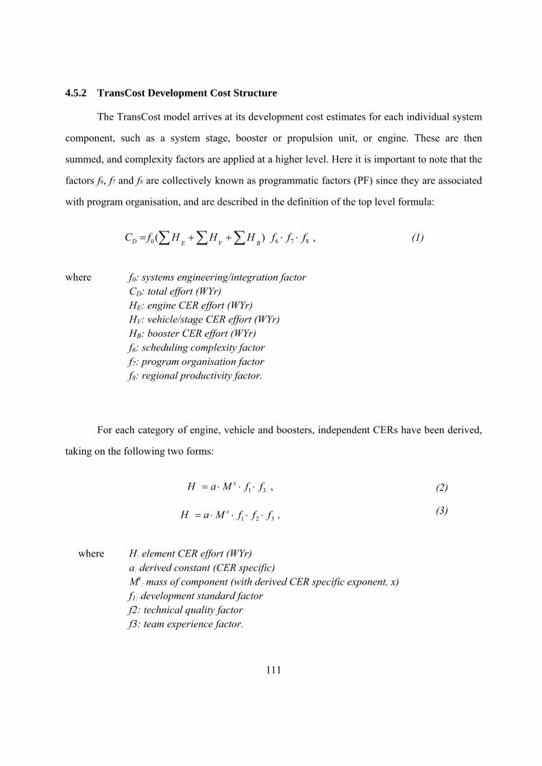
111
4.5.2 TransCost Development Cost Structure
The TransCost model arrives at its development cost estimates for each individual system
component, such as a system stage, booster or propulsion unit, or engine. These are then
summed, and complexity factors are applied at a higher level. Here it is important to note that the
factors f6, f7 and f8 are collectively known as programmatic factors (PF) since they are associated
with program organisation, and are described in the definition of the top level formula:
8760 )( fffHHHfCBVED , (1)
where f0: systems engineering/integration factor
CD: total effort (WYr) HE: engine CER effort (WYr) HV: vehicle/stage CER effort (WYr) HB: booster CER effort (WYr) f6: scheduling complexity factor f7: program organisation factor f8: regional productivity factor.
For each category of engine, vehicle and boosters, independent CERs have been derived,
taking on the following two forms:
31 ffMaH x , (2)
321 fffMaH x , (3)
where H: element CER effort (WYr) a: derived constant (CER specific) Mx
: mass of component (with derived CER specific exponent, x) f1: development standard factor f2: technical quality factor f3: team experience factor.
112
Therefore, each program or vehicle must be segmented into its constituents, which are
then costed respectively at a system level. The launcher system elements covered by the
TransCost model are split into two categories of Propulsion/Engine Development CERs and
Vehicle Systems Development CERs, the constituent elements of which are shown below.
Propulsion/Engine Development CERs
o Solid-Propellant Rocket Motors
o Liquid Propellant Rocket Engines with Turbopumps
o Pressure-fed Rocket Engines
o Air-breathing Turbo- and Ramjet Engines
Vehicle Systems Development CERs
o Solid-Propellant Strap-on Boosters and Stage Systems Rocket Motors
o Liquid Propellant Propulsion Systems/Modules
o Expendable Ballistic Stages and Transfer Vehicles (ELVs)
o Reusable Ballistic Stages and Transfer Vehicles (RLVs)
o Winged Orbital Rocket Vehicles
o HTO First Stage Vehicles, Advanced Aircraft and Aerospace Planes
o VTO First Stage Fly-Back Rocket Vehicles
o Crewed Ballistic Re-Entry Capsules
o Crewed Space Systems
After this, the appropriate TransCost defined complexity factors are applied, and all
individual costs tallied to arrive at a final total system-level cost. The only sub-system
information required by TransCost is that for engines (namely the mass and a technology factor,
f2, which is specific on a case to case basis). Inherently, the TransCost model does not adequately
113
facilitate for a reduction in costs due to existing heritage from previous, similar programs. A team
experience factor addresses the familiarity of a team with a proposed project. A technology
specific factor, f2, is then applied based on each specific system or element type.
Furthermore, it is important to note and highlight the specific ‘development costs’
definition which TransCost adopts. Five types of development costs can be identified and
classified. These are:
1) Effective Cost to Completion (CTC) – Total cost after completion of the program, including inflation
2) Most Probable / Realistic Development Cost – Including a margin for unforeseen
technical problems and delays which cannot be established at commencement of a program 3) Ideal / Theoretical Development Cost – assumes everything goes according to
plan with no technical or schedule problems (this is the standard industrial proposal basis) 4) Minimum Credible Development Cost – unrealistic cost estimate under
competitive situation in order to win a bid or contract (some cost items neglected) 5) Unrealistic Development Cost – Cost figures based on “believing” with no cost
studies nor analyses and a lack of experience in order to sell a concept
Here, the development cost type which is calculated by the TransCost CER algorithms is
Type 2 - Most probable / Realistic Development Cost since the underlying CERs are based on
actual post-program completion system development costs. To put this in a rough numerical
context, such a ‘most probable’ cost is a ROM 15-20% higher than the ‘ideal cost’ shown above
in example 3, and also calculated using the EBU CEM which tallies independent cost estimates at
a micro, sub-systems. Here, since TransCost CERs are based on actual costs, including therefore
the costs for unforeseen technical problems and delays, TransCost therefore claims to “represent
the ‘most probable’ or ‘realistic cost’”[102].
114
4.5.3 TransCost Production Cost Structure
Similarly to the development costs, TransCost arrives at its production cost estimates for
each individual system component, such as a system stage, booster or propulsion unit, or engine.
Furthermore, the cost for production of n number of units can be calculated, as well as for the nth
number of units. The top level formula is described in in Eq. 4 below:
811
0 )( fFFfCn
V
n
EF , (4)
where f0: systems management/vehicle integration & checkout factor CF: total effort (WYr) n: number of units to be produced FE: engine CER effort (WYr) FV: vehicle/stage CER effort (WYr) f8: regional productivity factor.
If we assume that n=1, then we can calculate the production cost for the theoretical first
unit (TFU), which is always the most expensive unit of the production chain, since afterwards the
learning effect is observed.
Going one level deeper, for each category of engines and vehicles, independent CERs
have been derived for production costs, which take on the following form:
4fManF x , (5)
where F: element CER effort (WYr)
n: number of units to be built a: derived constant (CER specific) Mx: mass of component (with derived CER specific exponent, x) f4: learning factor.
115
Once again each program or vehicle must be segmented into its constituents, for which
production costs are then calculated. For production, again, the components are split into two
categories of Engine Production CERs and Launch Vehicle Systems Production CERs, as shown
below.
Engine Production CERs (First Unit Cost)
o Solid-Propellant Rocket Motor, Strap-on Boosters and Stage Systems
o Liquid Propellant Rocket Engines
o Air-breathing Turbojet Engines
Launch Vehicle Systems’ Development CERs
o Propulsion Modules
o Ballistic Vehicles/Stages (Expendable and Reusable)
o High Speed Aircraft / Winged First Stage Vehicles
o Winged Orbital Rocket Vehicles
o Crewed Space Systems
A key consideration within the TransCost production cost category is the learning factor
calculation. This hinges on empirical charts featured in the handbook, for engines and stages
respectively, and is underpinned by the unit mass (per engine/stage) and the expected annual
production rate. In fact, the number of units to be produced plays an important role, since the
production cost can be expressed as a sum of a batch of n units, or alternatively, as the cost to
produce the nth unit in a batch.
As in any industry, consecutive units manufactured in succession to the TFU will be
subject to the learning effects of production. Consequently, associated costs are expected to fall.
This process can be described mathematically, with various learning effects mathematically noted
across different industries. The TransCost model addresses the issue of the learning effect
116
through a production cost reduction factor, f4 on a component level, as seen in Eq. 5. This f4 factor
is based on the learning factor, p. Originally proposed by Theodore Paul Wright in the traditional
average unit value approach denotes that a learning factor of 0.8 results in a cost reduction of
80% through the doubling of production for a single unit [100-102].
For space systems, the learning curve value has been found to lie generally between 0.80
and 1.0. Concurrently, for the aerospace industry, NASA has established this learning factor to be
0.85 [136, 137]. The specific value, of course, is quite logically dependent on unit size (mass)
and the frequency of production (i.e. annual production rate). The basic underlying presumption
is that the higher the production rate, the more pronounced the learning phenomenon, and hence
the lower the overall production costs.
The number of parallel contractors, or in other words, a collaborative multi-organisational
effort for production, also incurs a significant cost increase. For example, in the case of the
Concorde, it was rumoured that the development cost increased by 30% due to the collaborative
nature of the project, with two production lines required, one in Bristol, and one in Toulouse
[145].
While this is an interesting production cost-driver to identify, as the production
framework for the SpaceLiner case-study remains to be defined at this early phase, this factor is
not incorporated into the calculations. As this becomes known, the cost estimate should be
amended and revised, in line with cost engineering principles.
4.5.4 TransCost Model Excel Tool
The TransCost 7.3 model was taken as the baseline and programmed into a dedicated in-
house Excel® spread-sheet interface and this tool was used to arrive at development and
production cost estimate ranges using information. A screenshot of a development cost
spreadsheet is shown in Figure 22 below.
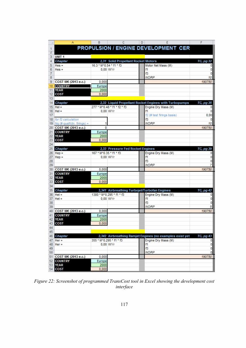
117
Figure 22: Screenshot of programmed TransCost tool in Excel showing the development cost interface
118
The initial TransCost 7.3 cost estimation model and the associated CERs and complexity
factors were programmed in Microsoft Excel in three dedicated spreadsheets for Development,
Production and Operations. Supporting worksheets were also made for key complexity factors,
including f4, learning factor, f8, country productivity, as well as the vital TransCost WYr model.
This spreadsheet tool was used as the basis for conducting cost estimation calculations for
existing programs, and therefore analyses of the TransCost model and its mechanics.
More recently, the latest versions of TransCost 8.1 and 8.2 were obtained and studied
closely to identify the changes which have been implemented since the previous TransCost 7.3
version. The existing Excel spreadsheets were consequently reprogrammed to implement
TransCost 8.2 and new results calculated and compared to existing cost estimation results. The
outcome of this exercise was to ascertain whether the new version was more representative of
actual costs. The main changes observed were small variations in factor-defined value ranges,
and are shown comparatively in Table 9 from Chapter 4.4.1 above.
A key difference with TransCost 8.1 and 8.2 is that the f8 country productivity factor is
applied on an individual CER basis internally within each of the development, production and
operation (DP&O) sub-groups. Previously, however, f8 was applied to the sum of the latter, at a
higher level, when the sum of each CER was individually tallied. From a logic perspective, f8
represents country productivity. In this sense, it is logical for this factor to apply at a lower level,
since within a single project, difference components are frequently manufactured in various
countries and are subject to different productivity conditions, which also influences costs. For
most of the above development programs, work was performed in Europe and the European
productivity factor (0.86) was therefore overall applied to the sum of the development,
production and operations rather than on an overall ∑CD basis. In any case, this minor difference
has no significant effect on costs calculated within this Thesis. Nevertheless, a future work to this
existing TransCost validation regime could be a re-calculation using the updated and latest
TransCost version, which ever this may be at the time of this proposed future re-work.
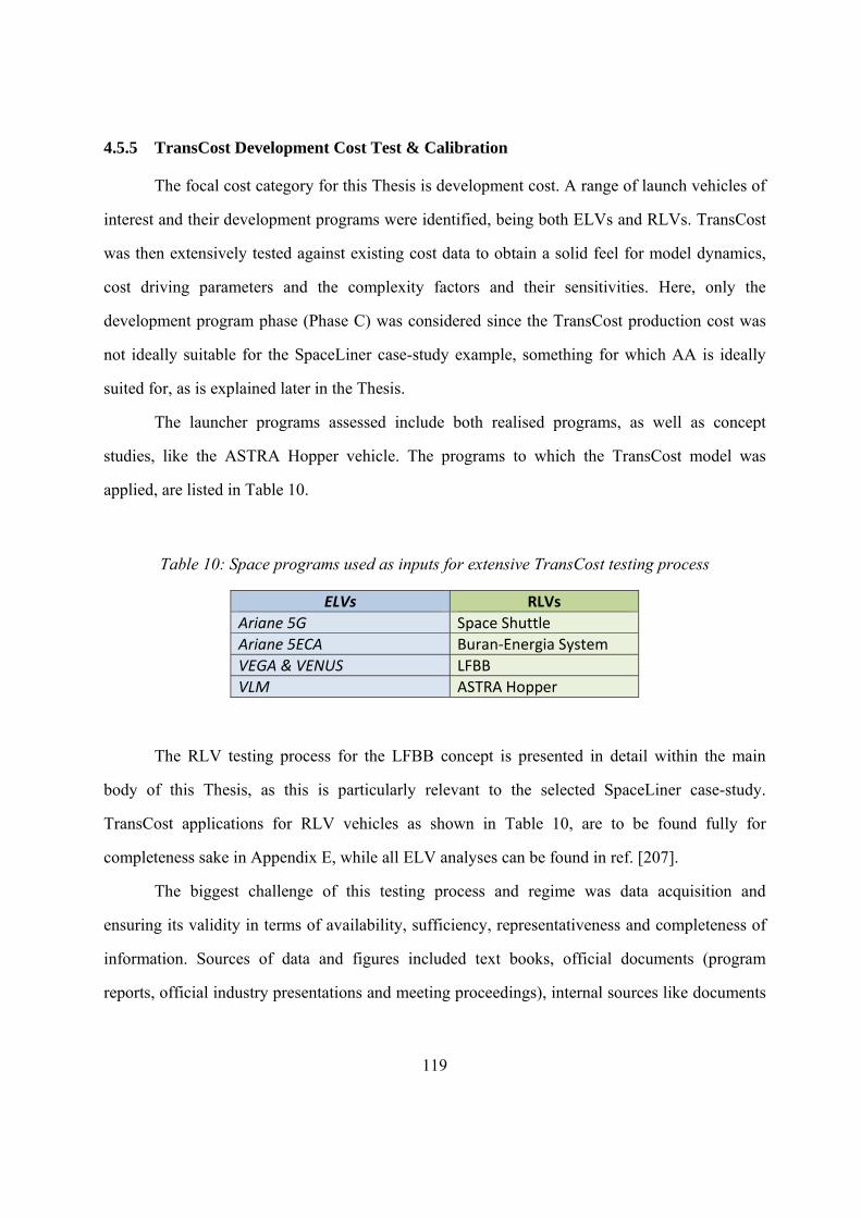
119
4.5.5 TransCost Development Cost Test & Calibration
The focal cost category for this Thesis is development cost. A range of launch vehicles of
interest and their development programs were identified, being both ELVs and RLVs. TransCost
was then extensively tested against existing cost data to obtain a solid feel for model dynamics,
cost driving parameters and the complexity factors and their sensitivities. Here, only the
development program phase (Phase C) was considered since the TransCost production cost was
not ideally suitable for the SpaceLiner case-study example, something for which AA is ideally
suited for, as is explained later in the Thesis.
The launcher programs assessed include both realised programs, as well as concept
studies, like the ASTRA Hopper vehicle. The programs to which the TransCost model was
applied, are listed in Table 10.
Table 10: Space programs used as inputs for extensive TransCost testing process
ELVs RLVs
Ariane 5G Space Shuttle
Ariane 5ECA Buran‐Energia System
VEGA & VENUS LFBB
VLM ASTRA Hopper
The RLV testing process for the LFBB concept is presented in detail within the main
body of this Thesis, as this is particularly relevant to the selected SpaceLiner case-study.
TransCost applications for RLV vehicles as shown in Table 10, are to be found fully for
completeness sake in Appendix E, while all ELV analyses can be found in ref. [207].
The biggest challenge of this testing process and regime was data acquisition and
ensuring its validity in terms of availability, sufficiency, representativeness and completeness of
information. Sources of data and figures included text books, official documents (program
reports, official industry presentations and meeting proceedings), internal sources like documents

120
and technical notes, and complimented by information obtained from the polling of experts. In
particular, vehicle program cost data was required, as well as background information and
technical parameters, including masses. In many cases, existing data had to be carefully analysed,
disseminated and processed to identify respective development and production costs proportion
of overall stated program costs which were often expressed as bulk, combined figures.
In addition to the baseline parametric TransCost model and Excel tool, other CEMs which
were used concurrently and include the analogy, EJ and the ROM approach. These were
necessary and applied during selection of the TransCost complexity factors (fx), as well as for
‘sanity checks’ to the resulting costs calculated.
4.6 TRANSCOST TESTING, CALIBRATION & VALIDATION FOR RLVS
Extensive work and analyses were conducted for the purpose of applying and therefore
testing, calibrating and validating the TransCost model. Such a strenuous testing regime also
allowed to ascertain whether the programmed TransCost model Excel tool (see Chapter 4.5.4)
was representative, facilitating for the debugging of any potential programming errors. The
created Excel Tool was therefore used to perform all the cost estimations for validation purposes.
In addition, in order to be able to calibrate the model in the future for application to other
purposes, such as the SpaceLiner case-study, different exampled had to be taken where some
available cost data could be found, so as to compare, be it only loosely, the results TransCost
costs with some existing stated cost data.
TransCost was applied to the Russian Energia-Buran launcher system, as well as the
American Space Shuttle to determine the program development costs (see Appendices 0 and 0).
These two programs are of distinct interest since they are the only existing space systems which
can be considered as “reusable” (although technically, only partly so) which have flown to date.
Due to numerous similarities between the Buran and Shuttle programs, a direct comparison
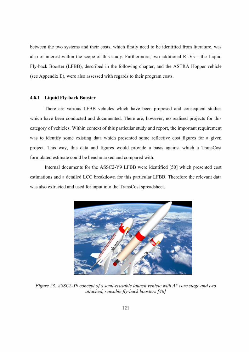
121
between the two systems and their costs, which firstly need to be identified from literature, was
also of interest within the scope of this study. Furthermore, two additional RLVs – the Liquid
Fly-back Booster (LFBB), described in the following chapter, and the ASTRA Hopper vehicle
(see Appendix E), were also assessed with regards to their program costs.
4.6.1 Liquid Fly-back Booster
There are various LFBB vehicles which have been proposed and consequent studies
which have been conducted and documented. There are, however, no realised projects for this
category of vehicles. Within context of this particular study and report, the important requirement
was to identify some existing data which presented some reflective cost figures for a given
project. This way, this data and figures would provide a basis against which a TransCost
formulated estimate could be benchmarked and compared with.
Internal documents for the ASSC2-Y9 LFBB were identified [50] which presented cost
estimations and a detailed LCC breakdown for this particular LFBB. Therefore the relevant data
was also extracted and used for input into the TransCost spreadsheet.
Figure 23: ASSC2-Y9 concept of a semi-reusable launch vehicle with A5 core stage and two attached, reusable fly-back boosters [46]
122
4.6.1.1 LFBB Configuration
The LFBB (ASSC2-Y9) launch vehicle comprises of the following elements, for which
the development costs are applicable:
Main cryogenic stage EPC-H185 (expendable)
Vulcain 3 main engine (reusable)
LFBB (reusable)
Here, the focal element for cost estimation is of course the reusable LFBB stage. Of
course this has no bearing on the effort amount, since this is merely a measure of effort, and as
such is irrelevant for which year this work effort is converted into a monetary amount. The final
costs, however, are all given in 2011 e.c. values to assist for a relevant comparison to be made.
4.6.1.2 LFBB Excel Component Break-down Structure
The component breakdown structure and the Excel TransCost spreadsheet screenshots
with all relevant inputs and complexity factors for ASSC2-Y9 are presented in Table 11 through
to Table 13 below.
4.6.1.3 LFBB Calculation Assumptions
Some key assumptions also had to be made within the scope of the LFBB cost estimation
with regards to numerous inputs and some complexity factors. The key assumptions are outlined
below, and are also annotated in red with association to the fields which the assumptions affect
in the tables above.
Furthermore, for the LFBB, significant heritage exists for various components, and
therefore, the newly developed and introduced TransCost f12 factor for delta developments, is
applied. This is found in Appendix E, where the derivation process is also fully described.
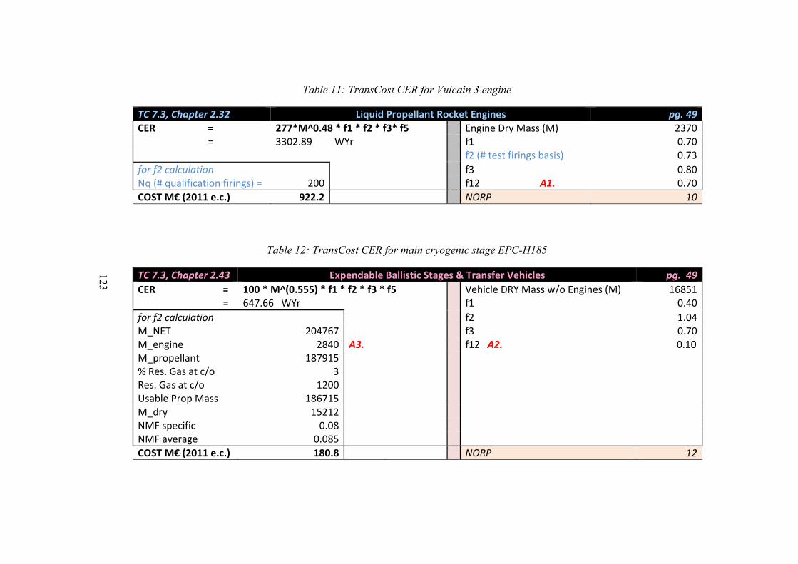
123
Table 11: TransCost CER for Vulcain 3 engine
TC 7.3, Chapter 2.32 Liquid Propellant Rocket Engines pg. 49
CER = 277*M^0.48 * f1 * f2 * f3* f5 Engine Dry Mass (M) 2370 = 3302.89 WYr f1 0.70 f2 (# test firings basis) 0.73
for f2 calculation f3 0.80Nq (# qualification firings) = 200 f12 A1. 0.70
COST M€ (2011 e.c.) 922.2 NORP 10
Table 12: TransCost CER for main cryogenic stage EPC-H185
TC 7.3, Chapter 2.43 Expendable Ballistic Stages & Transfer Vehicles pg. 49
CER = 100 * M^(0.555) * f1 * f2 * f3 * f5 Vehicle DRY Mass w/o Engines (M) 16851 = 647.66 WYr f1 0.40
for f2 calculation f2 1.04M_NET 204767 f3 0.70M_engine 2840 A3. f12 A2. 0.10 M_propellant 187915 % Res. Gas at c/o 3 Res. Gas at c/o 1200 Usable Prop Mass 186715 M_dry 15212 NMF specific 0.08 NMF average 0.085
COST M€ (2011 e.c.) 180.8 NORP 12
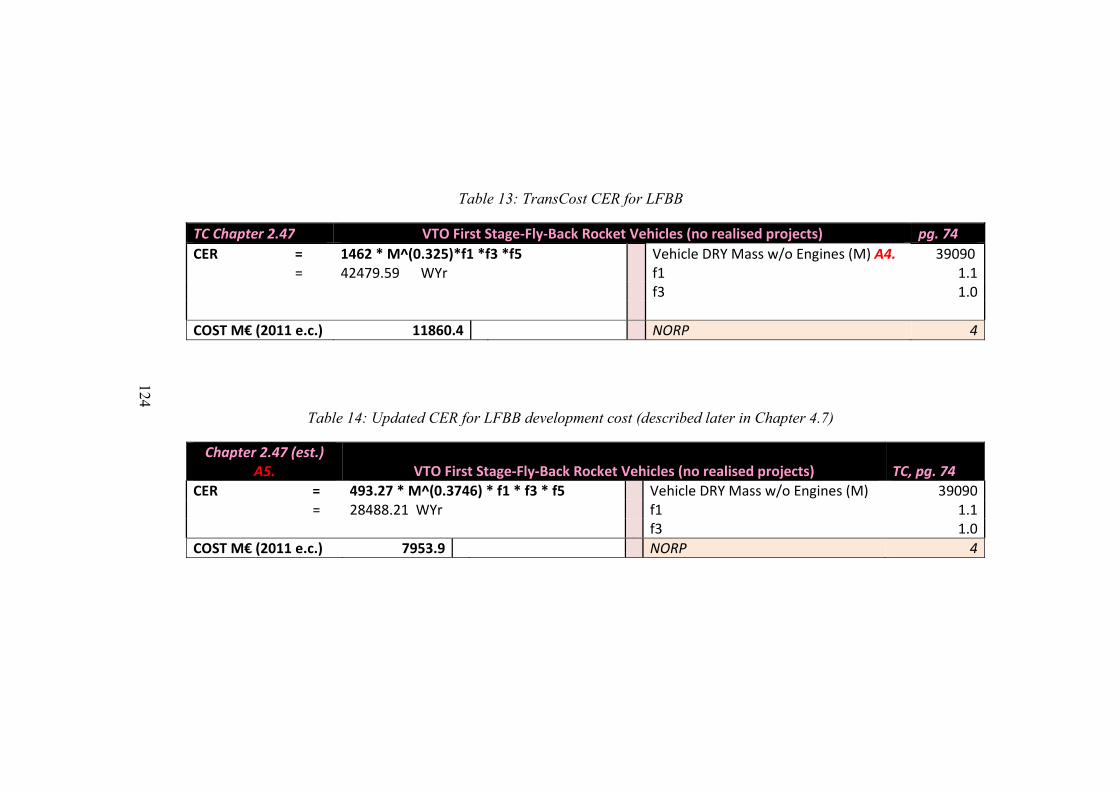
124
Table 13: TransCost CER for LFBB
TC Chapter 2.47 VTO First Stage‐Fly‐Back Rocket Vehicles (no realised projects) pg. 74
CER = 1462 * M^(0.325)*f1 *f3 *f5 Vehicle DRY Mass w/o Engines (M) A4. 39090 = 42479.59 WYr f1 1.1 f3 1.0
COST M€ (2011 e.c.) 11860.4 NORP 4
Table 14: Updated CER for LFBB development cost (described later in Chapter 4.7)
Chapter 2.47 (est.) A5. VTO First Stage‐Fly‐Back Rocket Vehicles (no realised projects) TC, pg. 74
CER = 493.27 * M^(0.3746) * f1 * f3 * f5 Vehicle DRY Mass w/o Engines (M) 39090 = 28488.21 WYr f1 1.1 f3 1.0
COST M€ (2011 e.c.) 7953.9 NORP 4
125
A1. The Vulcain 3R engine and the associated technology already exist. However for the
ASSC2-Y9 vehicle, the engine must be reusable. To factor in for this, the f12 factor is taken to be
0.7.
A2. For the main EPC stage development, the newly developed f12 delta development
factor was applied. Based on calibration performed for ELVs (ref. [207]). the value was assumed
to be 0.1 since the stage already exists, and only minor delta developments are necessary.
A3. The mass for the engine was extracted from documents pertaining to a previously
conducted ASTRA study [199], and was taken to be 2840kg. This mass is seemingly different to
the mass entry for actual development of the Vulcain 3R in Table 11. This is explained by the
fact that the mass difference between the two is due to a nozzle-extension used for the EPC than
for the boosters, despite an identical engine. For the Vulcain 3R engine calculation, this is taken
to be the lighter mass, since mechanical tests are independent of the nozzle configuration. For the
f2 calculation of the EPC, the heavier engine/nozzle mass is taken, representative of the actual
stage configuration.
A4. The LFBB dry mass w/o engines was calculated using data from [181] with the three
Vulcain 3R engines (3 x 2370kg) subtracted from the LFBB gross weight of 46200kg.
A5. A new, modified CER was established (est.) to rectify a shortcoming of the
TransCost model. This process is described in a dedicated Chapter 4.7 to be found later on in this
Thesis. The new CER applies directly to the LFBB category of vehicles, and is essentially an
augmented and modified version of CER 2.47. Here, it is interesting to apply this new, more
representative and justifiable CER to the ASSC2-Y9, for the LFBB stage. This recalculation and
the new results are shown in Table 14 above.
126
After calculating all independent components which needed to be developed within the
scope of the program, the usual top-level TransCost formula stated in Eq. 4 is applied.
Here, it is important to note that results incorporate the WYr value calculated by the
updated and new CER derived for LFBBs (which is shown above in Table 13 and is outlined in
assumption on the previous page A5), and whose development is fully explained in Chapter 4.7.
In this case, the additional TransCost factors which are then imposed on the sum of the
constituent elements for ASSC2-Y9 system, are all outlined below, and their chosen values
stated:
• f0 = 1.08
(f0 = 1.04 number of stages, in the case of the ASSC2-Y9, 2)
• f6 = 1.0
(here, assume no deviation from optimum schedule)
• f7 = 1.00
(f7 = n 0.2; with n being the number of parallel contractor organisations, in this case
assumed to be 1)
• f8 = 0.86
(TransCost stated country productivity factor for ESA)
The final development effort of the ASSC2-Y9 system, as calculated using the TransCost
7.3 model, was found to be a little over 30,000 WYr (30,174 WYr), equating to 8.6 B€ at 2013
economic conditions.
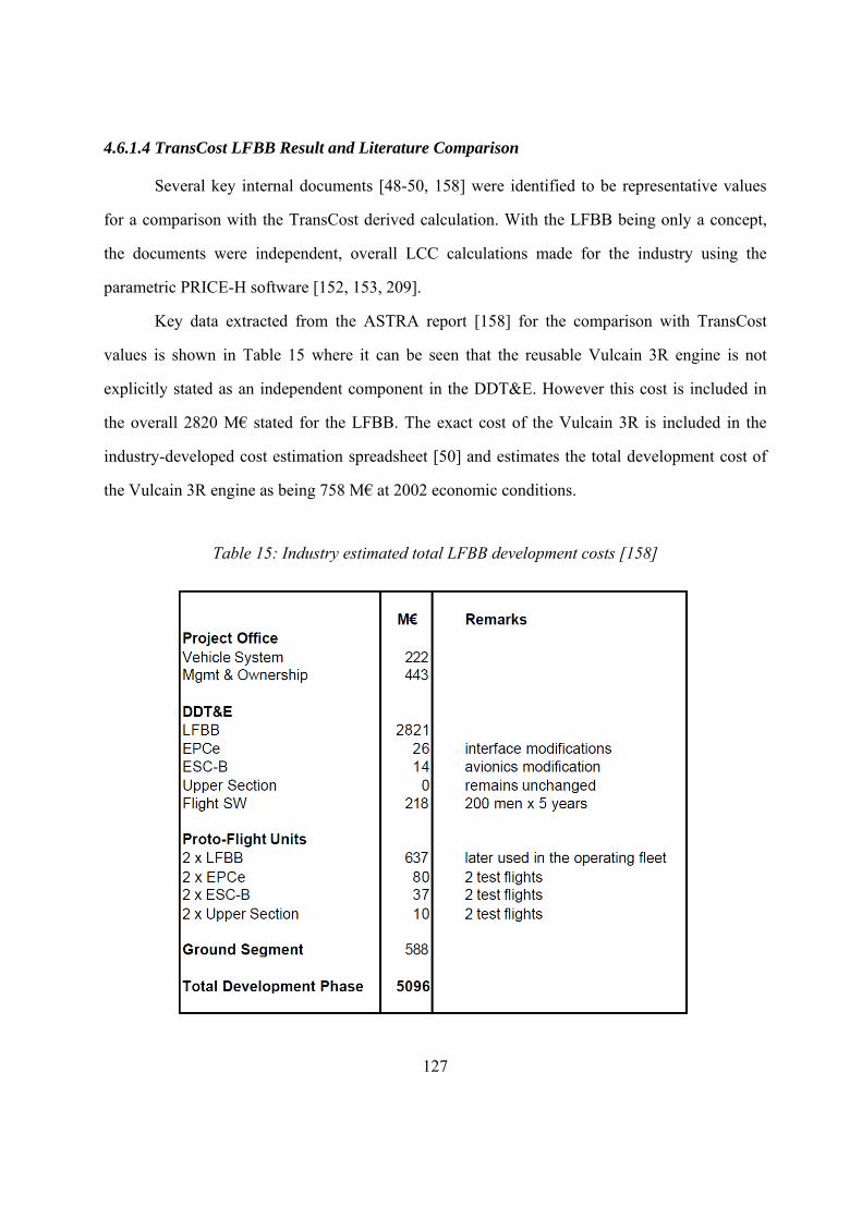
127
4.6.1.4 TransCost LFBB Result and Literature Comparison
Several key internal documents [48-50, 158] were identified to be representative values
for a comparison with the TransCost derived calculation. With the LFBB being only a concept,
the documents were independent, overall LCC calculations made for the industry using the
parametric PRICE-H software [152, 153, 209].
Key data extracted from the ASTRA report [158] for the comparison with TransCost
values is shown in Table 15 where it can be seen that the reusable Vulcain 3R engine is not
explicitly stated as an independent component in the DDT&E. However this cost is included in
the overall 2820 M€ stated for the LFBB. The exact cost of the Vulcain 3R is included in the
industry-developed cost estimation spreadsheet [50] and estimates the total development cost of
the Vulcain 3R engine as being 758 M€ at 2002 economic conditions.
Table 15: Industry estimated total LFBB development costs [158]
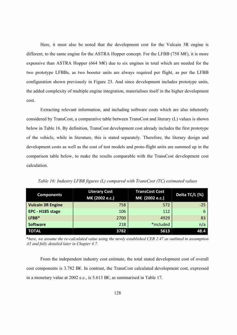
128
Here, it must also be noted that the development cost for the Vulcain 3R engine is
different, to the same engine for the ASTRA Hopper concept. For the LFBB (758 M€), it is more
expensive than ASTRA Hopper (664 M€) due to six engines in total which are needed for the
two prototype LFBBs, as two booster units are always required per flight, as per the LFBB
configuration shown previously in Figure 23. And since development includes prototype units,
the added complexity of multiple engine integration, materialises itself in the higher development
cost.
Extracting relevant information, and including software costs which are also inherently
considered by TransCost, a comparative table between TransCost and literary (L) values is shown
below in Table 16. By definition, TransCost development cost already includes the first prototype
of the vehicle, while in literature, this is stated separately. Therefore, the literary design and
development costs as well as the cost of test models and proto-flight units are summed up in the
comparison table below, to make the results comparable with the TransCost development cost
calculation.
Table 16: Industry LFBB figures (L) compared with TransCost (TC) estimated values
Components Literary Cost
M€ (2002 e.c.)
TransCost Cost
M€ (2002 e.c.) Delta TC/L (%)
Vulcain 3R Engine 758 572 ‐25
EPC ‐ H185 stage 106 112 6
LFBB* 2700 4929 83
Software 218 *included n/a
TOTAL 3782 5613 48.4
*here, we assume the re-calculated value using the newly established CER 2.47 as outlined in assumption A5 and fully detailed later in Chapter 4.7.
From the independent industry cost estimate, the total stated development cost of overall
cost components is 3.782 B€. In contrast, the TransCost calculated development cost, expressed
in a monetary value at 2002 e.c., is 5.613 B€, as summarised in Table 17.
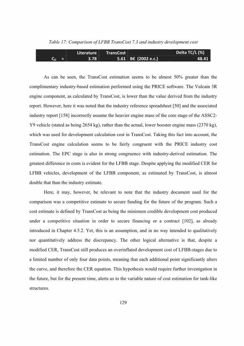
129
Table 17: Comparison of LFBB TransCost 7.3 and industry development cost
Literature TransCost Delta TC/L (%)
CD = 3.78 5.61 B€ (2002 e.c.) 48.41
As can be seen, the TransCost estimation seems to be almost 50% greater than the
complimentary industry-based estimation performed using the PRICE software. The Vulcain 3R
engine component, as calculated by TransCost, is lower than the value derived from the industry
report. However, here it was noted that the industry reference spreadsheet [50] and the associated
industry report [158] incorrectly assume the heavier engine mass of the core stage of the ASSC2-
Y9 vehicle (stated as being 2654 kg), rather than the actual, lower booster engine mass (2370 kg),
which was used for development calculation cost in TransCost. Taking this fact into account, the
TransCost engine calculation seems to be fairly congruent with the PRICE industry cost
estimation. The EPC stage is also in strong congruence with industry-derived estimation. The
greatest difference in costs is evident for the LFBB stage. Despite applying the modified CER for
LFBB vehicles, development of the LFBB component, as estimated by TransCost, is almost
double that than the industry estimate.
Here, it may, however, be relevant to note that the industry document used for the
comparison was a competitive estimate to secure funding for the future of the program. Such a
cost estimate is defined by TransCost as being the minimum credible development cost produced
under a competitive situation in order to secure financing or a contract [102], as already
introduced in Chapter 4.5.2. Yet, this is an assumption, and in no way intended to qualitatively
nor quantitatively address the discrepancy. The other logical alternative is that, despite a
modified CER, TransCost still produces an overinflated development cost of LFBB-stages due to
a limited number of only four data points, meaning that each additional point significantly alters
the curve, and therefore the CER equation. This hypothesis would require further investigation in
the future, but for the present time, alerts us to the variable nature of cost estimation for tank-like
structures.
130
4.7 CER DEVELOPMENT FOR REUSABLE BOOSTER STAGES
Throughout the entire process of using the TransCost model to come up with a cost
estimate, the utmost care was taken to ensure that every CER and its underlying data have been
understood. In fact, this philosophy is what underpins the logic for this part of this very work. So,
at every stage of that TransCost application process, wherever possible, own data has been
identified and compared with data points that feature in the TransCost model.
In view of this approach, the TransCost model’s Chapter 2.47 CER for VTO First Stage
Fly-back Rocket Vehicles, based on 4 reference points, triggered some doubt for the data point of
the ASSC-2, shown circled in red. This doubt arose during comparison of internal SART data
obtained from in-house documents, with the data implied by a reference point on the TransCost
CER curve. The CER graph in question is shown in Figure 24, as it appears in the TransCost
handbook.
Being one of only 4 data points (one of four reference projects) underpinning the CER
and thus the resulting development costs estimation, it was decided to establish a new CER using
relevant, available data to promote transparency and comprehension of the underlying database
and therefore the resulting development cost estimation figure. The data sets used for the CER
formulation were extracted directly from internal DLR and other available documents, and
included the following vehicles:
• ASSC2 V-4
• Space Shuttle LFBB
• ASSC2 Y-9
• FSSC-16 SR
Reliable and transparent data was readily available and therefore facilitated for
dissemination and analysis within context of the CER formulation process.
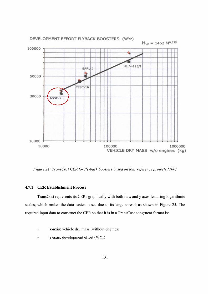
131
Figure 24: TransCost CER for fly-back boosters based on four reference projects [100]
4.7.1 CER Establishment Process
TransCost represents its CERs graphically with both its x and y axes featuring logarithmic
scales, which makes the data easier to see due to its large spread, as shown in Figure 25. The
required input data to construct the CER so that it is in a TransCost congruent format is:
• x-axis: vehicle dry mass (without engines)
• y-axis: development effort (WYr)
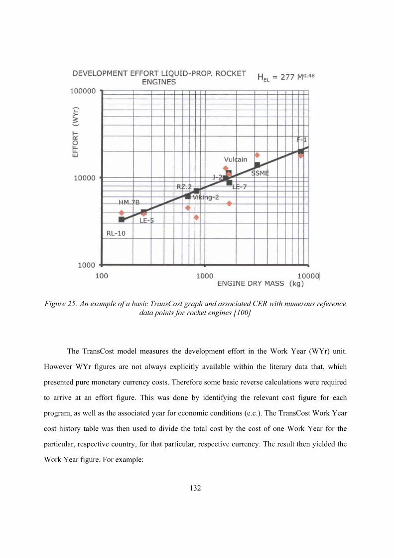
132
Figure 25: An example of a basic TransCost graph and associated CER with numerous reference data points for rocket engines [100]
The TransCost model measures the development effort in the Work Year (WYr) unit.
However WYr figures are not always explicitly available within the literary data that, which
presented pure monetary currency costs. Therefore some basic reverse calculations were required
to arrive at an effort figure. This was done by identifying the relevant cost figure for each
program, as well as the associated year for economic conditions (e.c.). The TransCost Work Year
cost history table was then used to divide the total cost by the cost of one Work Year for the
particular, respective country, for that particular, respective currency. The result then yielded the
Work Year figure. For example:
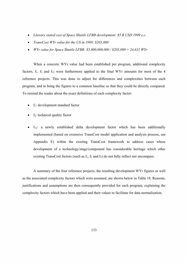
133
Literary stated cost of Space Shuttle LFBB development: $5 B USD 1999 e.c.
TransCost WYr value for the US in 1999: $203,000
WYr value for Space Shuttle LFBB: $5,000,000,000 / $203,000 = 24,631 WYr
When a concrete WYr value had been established per program, additional complexity
factors, f1, f3 and f12 were furthermore applied to the final WYr amounts for most of the 4
reference projects. This was done to adjust for differences and complexities between each
program, and to bring the figures to a common baseline so that they could be directly compared.
To remind the reader about the exact definitions of each complexity factor:
f1: development standard factor
f3: technical quality factor
f12: a newly established delta development factor which has been additionally
implemented (based on extensive TransCost model application and analysis process, see
Appendix E) within the existing TransCost framework to address cases where
development of a technology/stage/component has considerable heritage which other
existing TransCost factors (such as f1, f2 and f3) do not fully reflect nor encompass.
A summary of the four reference projects, the resulting development WYr figures as well
as the associated complexity factors which were assumed, are shown below in Table 18. Reasons,
justifications and assumptions are then consequently provided for each program, explaining the
complexity factors which have been applied and their values to facilitate for data normalisation.
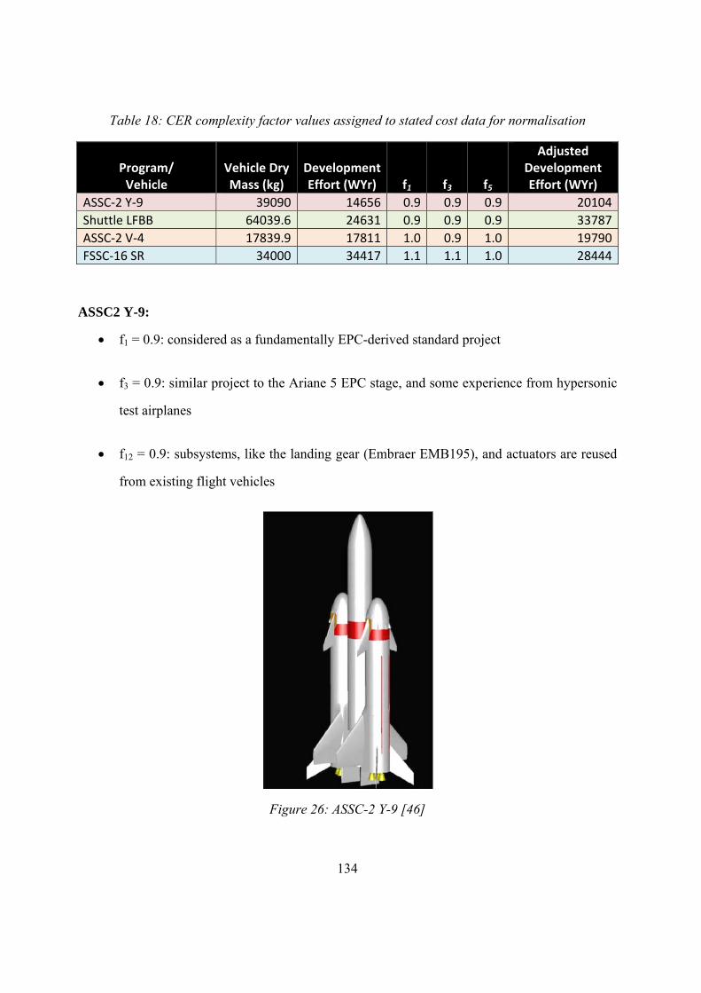
134
Table 18: CER complexity factor values assigned to stated cost data for normalisation
Program/ Vehicle
Vehicle Dry Mass (kg)
Development Effort (WYr) f1 f3 f5
Adjusted Development Effort (WYr)
ASSC‐2 Y‐9 39090 14656 0.9 0.9 0.9 20104
Shuttle LFBB 64039.6 24631 0.9 0.9 0.9 33787
ASSC‐2 V‐4 17839.9 17811 1.0 0.9 1.0 19790
FSSC‐16 SR 34000 34417 1.1 1.1 1.0 28444
ASSC2 Y-9:
f1 = 0.9: considered as a fundamentally EPC-derived standard project
f3 = 0.9: similar project to the Ariane 5 EPC stage, and some experience from hypersonic
test airplanes
f12 = 0.9: subsystems, like the landing gear (Embraer EMB195), and actuators are reused
from existing flight vehicles
Figure 26: ASSC-2 Y-9 [46]
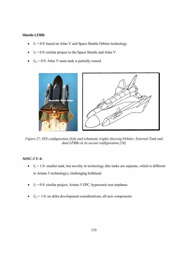
135
Shuttle LFBB:
f1 = 0.9: based on Atlas V and Space Shuttle Orbiter technology
f3 = 0.9: similar project to the Space Shuttle and Atlas V
f12 = 0.9: Atlas V main tank is partially reused
Figure 27: STS configuration (left) and schematic (right) showing Orbiter, External Tank and dual LFBBs in its ascent configuration [26]
ASSC-2 V-4:
f1 = 1.0: smaller tank, but novelty in technology (the tanks are separate, which is different
to Ariane 5 technology), challenging bulkhead
f3 = 0.9: similar project, Ariane 5 EPC, hypersonic test airplanes
f12 = 1.0: no delta development considerations, all new components
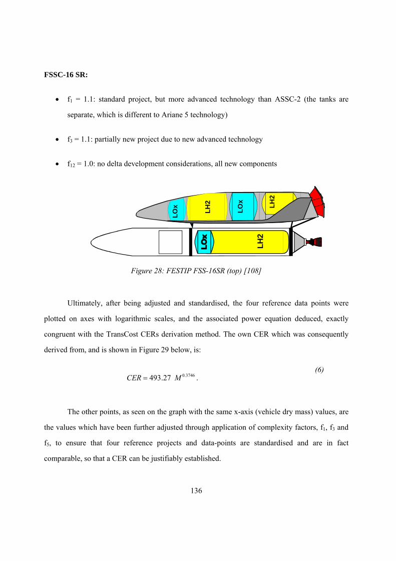
136
FSSC-16 SR:
f1 = 1.1: standard project, but more advanced technology than ASSC-2 (the tanks are
separate, which is different to Ariane 5 technology)
f3 = 1.1: partially new project due to new advanced technology
f12 = 1.0: no delta development considerations, all new components
LH
2
LO
x
LO
x
LH
2
LH
2
Figure 28: FESTIP FSS-16SR (top) [108]
Ultimately, after being adjusted and standardised, the four reference data points were
plotted on axes with logarithmic scales, and the associated power equation deduced, exactly
congruent with the TransCost CERs derivation method. The own CER which was consequently
derived from, and is shown in Figure 29 below, is:
3746.027.493 MCER . (6)
The other points, as seen on the graph with the same x-axis (vehicle dry mass) values, are
the values which have been further adjusted through application of complexity factors, f1, f3 and
f5, to ensure that four reference projects and data-points are standardised and are in fact
comparable, so that a CER can be justifiably established.
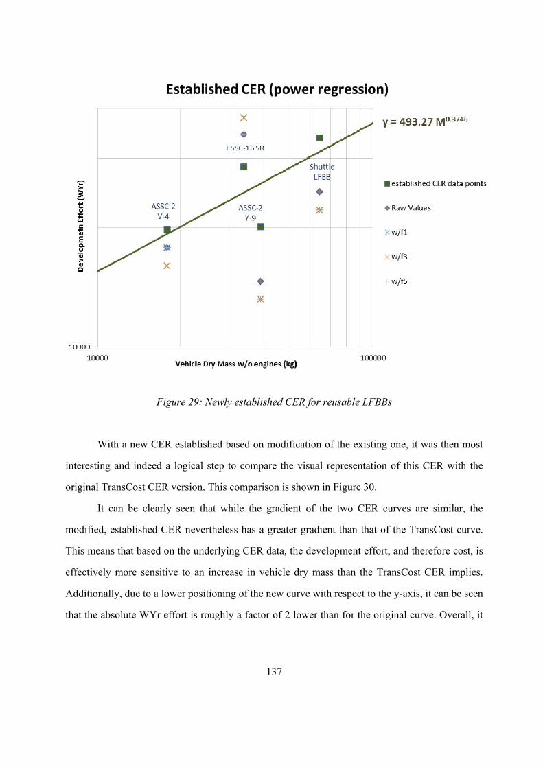
137
Figure 29: Newly established CER for reusable LFBBs
With a new CER established based on modification of the existing one, it was then most
interesting and indeed a logical step to compare the visual representation of this CER with the
original TransCost CER version. This comparison is shown in Figure 30.
It can be clearly seen that while the gradient of the two CER curves are similar, the
modified, established CER nevertheless has a greater gradient than that of the TransCost curve.
This means that based on the underlying CER data, the development effort, and therefore cost, is
effectively more sensitive to an increase in vehicle dry mass than the TransCost CER implies.
Additionally, due to a lower positioning of the new curve with respect to the y-axis, it can be seen
that the absolute WYr effort is roughly a factor of 2 lower than for the original curve. Overall, it
138
is considered that with this modification, a more accurate representative CER has been
established for reusable stages.
In addition, and given the newly established LFBB CER, the calculation already
conducted for the Liquid Fly-back Booster earlier in Chapter 4.6.1 was also revisited, and a
revised development cost for the LFBB stage, calculated. This is outlined in Assumption 5 (A5)
of Chapter 4.6.1.3 on page 119 of this Thesis, with final results shown in the previous Table 14.
As expected, a significant cost reduction of over 30% in this instance is observed between the
original TransCost LFBB CER result, and the result of the newly established CER shown in Eq. 6
above and visually contrasted with the TransCost CER below in Figure 30.
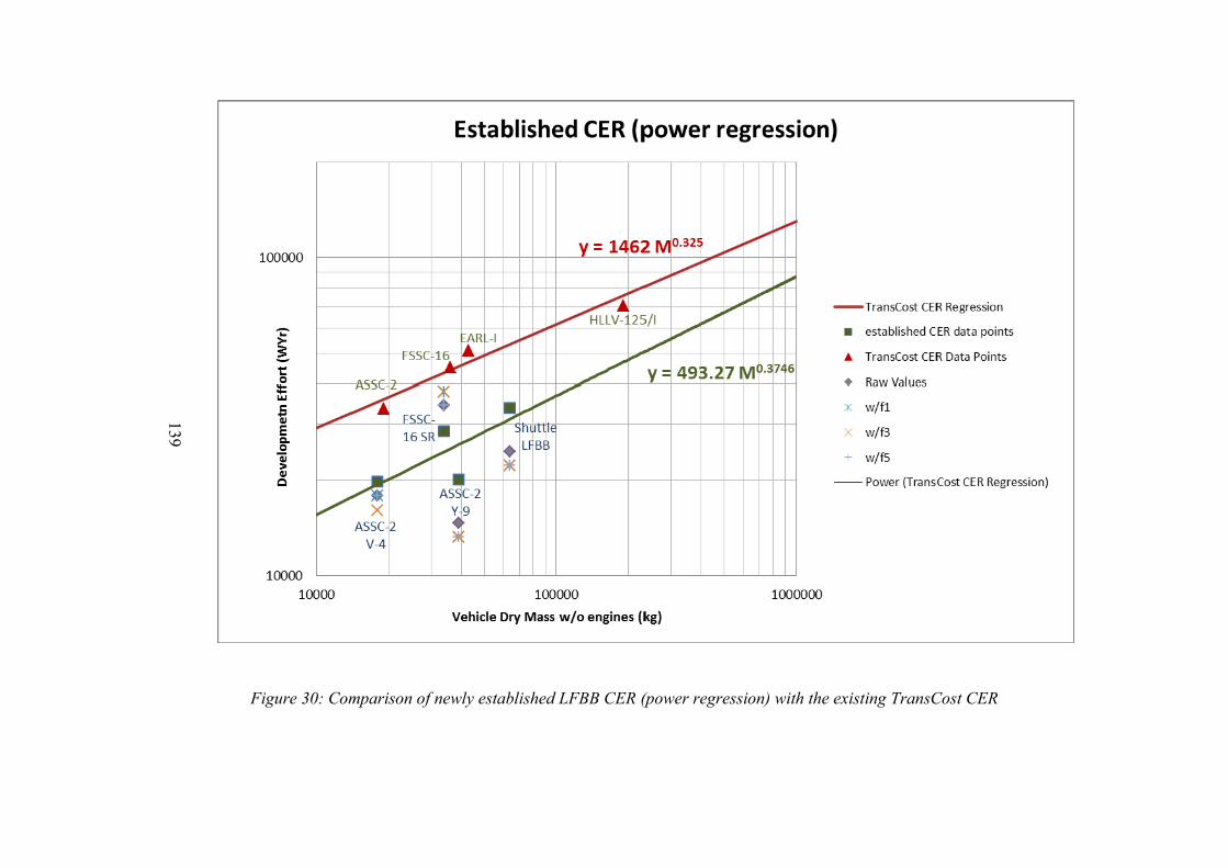
139
Figure 30: Comparison of newly established LFBB CER (power regression) with the existing TransCost CER
140
4.8 COSTING THE SPACELINER CASE-STUDY
4.8.1 Methodology
Early phase cost estimation poses a significant challenge given still evolving, limited
program information. CEMs, models and tools do exist to deal with very top-level estimates even
during early phases. However, most are parametric, meaning historical references are used to
model and predict future costs, adjusting for any minor modifications with complexity factors.
Yet if the program to be costed is significantly new or state-of-the-art compared with historical
projects which form the basis of a CER, then results of a single parametric model may provide a
non-indicative result of realistic costs. SpaceLiner is both in the early development phase, and
also a largely unprecedented vehicle, so both challenges hold true. As such, the associated risk
and uncertainty of the cost estimate, while already being inherently high during early program
phase (see Figure 4) is furthermore compounded.
At the top WBS level, as already presented in Chapter 4.1.1, the four key SpaceLiner
components of SLB, SLO, SLME and SPC are foreseen to incur non-recurring development
costs. Their masses for the SpaceLiner version 7.2 were obtained (see Appendix F) and used as
inputs for all models and tools.
The SLO, SLB and SPC form the top hardware categories of the overall developed WBS
for the SpaceLiner concept, from WBS element 2000 through to 4000. In the WBS the main
engine, SLME, is a subset of level two SLO and SLB elements found under 2200 and 3200 for
Propulsion. Here, it should be reminded that only one development cost for the two SLO and
SLB engines is incurred, since both engines are mechanically identical, with the only difference
being the nozzle extension. Here, to attribute specific percentiles of novelty to two separate
engines of the same technology, but of different scaling, would also be unreasonably precise at
this early stage. Therefore, with the inherent margin for technology heritage of the engines in
mind, it was assumed and deemed sufficient that development cost of one 100% new engine
(taken to be the larger mass and dimension) would be calculated, and would adequate to address
141
the engine development effort and cost for both SLO and SLB, as has been discussed in Chapter
4.1.
All cost estimates resulting from multiple modes were entered into the specially
developed AA Excel spreadsheet, AAInT, which is specifically designed and developed to
ideally support the AA function, as already introduced in Chapter 2.6.2.2. AAInT was then
adapted for the unique nature and particular WBS of the chosen case-study. The key objective
and function of AAInT is to contain all WBS as well as multi-modal cost data in one spreadsheet.
As such, the main summary AAInT cost sheet derives its values directly from the source cost
files, thus eliminating the chance of transcription errors and minimising the potential for human
error. The summary sheet, as tailored to the SpaceLiner case-study, a snapshot of which is shown
below in Figure 31, then allows for direct comparison of costs at WBS level 2 (L2WBS) and L3WBS
between the different costing modes. Functionally, AAInT is designed to display up to as many
levels of a WBS. Each of the WBS elements are categorically listed on the left, with their
associated WBS index, and various columns allow for direct entry of resulting costs per WBS
element in a common row, facilitating for easy contrast and comparison, as well as efficient
analysis across the various levels. Lower-level costs are also tallied and shown in higher level
WBS figures. Both a development and production spreadsheet was programmed.
At the end of the cost estimation per SpaceLiner system element, a cost estimation using
the analog and EJ CEMs was also performed for the Project Management Office (PMO)
component. This critical management function is an essential one, and should not be omitted in
the cost estimation.
The WBS level 3 can be further expanded to show the lower SpaceLiner case-study
constituent level 4 components also. Such an expansion is shown for the SpaceLiner case-study
AAInT tool below in Figure 32. Due to the relatively early program phase and therefore inherent
cost uncertainty incurred by still evolving technical input parameters, all cost analyses were
performed at L3WBS and L2WBS, and as such, the level 4 expansion seen in Figure 32 shows no

142
cost values. While the commercial PRICE and 4cost aces tools provided all costs at a constant
L3WBS, the high level TransCost model (in accordance with its definition) produced only costs at
L2 WBS, except for the engine, SLME, which was calculated at L3WBS.
Figure 31: Screenshot of developed AAMAC Excel AAInT tool adjusted for application to the SpaceLiner case-study, shown for development costs
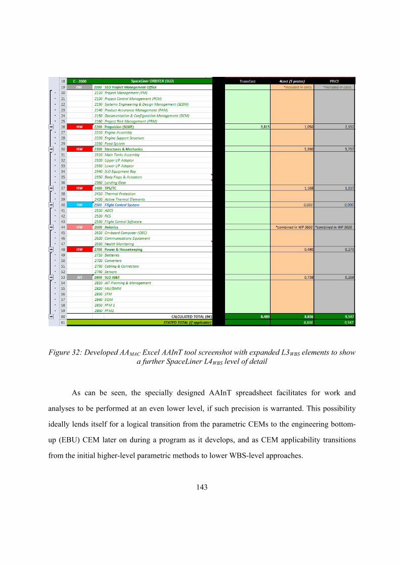
143
Figure 32: Developed AAMAC Excel AAInT tool screenshot with expanded L3WBS elements to show a further SpaceLiner L4WBS level of detail
As can be seen, the specially designed AAInT spreadsheet facilitates for work and
analyses to be performed at an even lower level, if such precision is warranted. This possibility
ideally lends itself for a logical transition from the parametric CEMs to the engineering bottom-
up (EBU) CEM later on during a program as it develops, and as CEM applicability transitions
from the initial higher-level parametric methods to lower WBS-level approaches.
144
4.8.2 Amalgamation Approach to SpaceLiner
The SpaceLiner program is both in the very early development phase, and also a largely
unprecedented vehicle. To address this and the associated challenges this poses to derivation of a
representative cost estimate range, the amalgamation approach (AA) proposed in ref. [209] and
also introduced in Chapter 2.6, is assumed. AA employs multiple selected, relevant models or
tools to obtain several cost estimates of the same program, independently. The results for each
model or tool are then analysed individually, before being compared and analysed in reference to
each other. During this process, several iterations might be necessary to eliminate discrepancies.
Ultimately, the multiple cost values are then synthesised to obtain a representative cost range
given certain assumptions and justifications based on analogy or expert judgement. While being
more resource intensive to application of a single tool and CEM, when applied at early program
phase where uncertainty of the cost estimate is already high, the benefits are significant. AA
approach provides an added level of redundancy for an otherwise single cost estimate, which is
considered to raise the confidence and representativeness of the single range or figure obtained
from application of one method and model alone. In addition, attention is focused on elements
where cost discrepancies between multiple modes of cost estimation might arise, indicating
variances in cost uncertainty. For the SpaceLiner case-study application, the AAMAC mode
(Chapter 2.6.2.2) is assumed and used.
145
4.9 DEVELOPMENT COST ANALYSIS
“Development cost estimation is one of the most difficult costing areas since a lot of
subjective influence can be found in the definition of a development program.”
-Dr. Dietrich E. Koelle [102]
The first classical category of program costs are the non-recurring development costs.
Basic SpaceLiner information and technical data was assembled and provided for input into the
three AAMAC models of 4cost aces, the PRICE-H model from PRICE Systems, and the TransCost
model. Close attention was paid to ensuring that input data was kept as consistent as possible
between all three models to allow for maximally comparable results.
For TransCost, only basic, top-level mass and complexity factor information was needed.
For both commercial tools, a higher degree of information was required and included details like
masses and complexities for mechanical and electronic components, team experiences, and
technical complexities. These latter values were either extracted from existing SpaceLiner data
files, or were estimated based on close consultation with relevant experts and professional users
for each tool. The resulting costs are all expressed with an economic base of 2013 and in a Euro
currency. Basic schedule information for inputs such as the anticipated start of the development
Phase C is derived from the overall program schedule introduced in Chapter 4.1.2 and shown in
Figure 13.
4.9.1 TransCost SpaceLiner Development Costs
Having analysed and tested the TransCost model to identify its validity, relevance,
applicability, and indeed its shortcomings and drawbacks, and after its calibration, it was now
suitable to apply the model and its CERs to the SpaceLiner concept to calculate a development
effort and cost. The most recently available TransCost 8.2 version was taken.

146
For the TransCost model structure and for CER application, the top-level SpaceLiner
stages, as already presented in Chapters 4.1.1 and 4.8.1, were taken. These are the SLO, SLME,
SLB and SPC components. Relevant complexity factors, based on the TransCost model testing
and calibration procedure described in Chapter 4.5, also had to be determined and defined. These
are summarised in Table 19 below.
Table 19: SpaceLiner complexity factors for each component
Element f1 f2 f3 f8
SLO 1.1 0.44 1.0 0.86
SLME 1.1 1.31 0.8 0.86
SLB 1.1 n/a 0.9 0.86
SPC 1.3 1.19 1.0 0.86
For this calculation, it was assumed that there was no deviation from the optimum
schedule (f6=1.0), that cost increase due to multiple parallel contractor organisations is ignored
(f7=1.0) and that the country productivity factor (f8) is assumed to be that for ESA, defined in
TransCost as being 0.86. In additional, for calculation of the SLB, the modified TransCost CER,
as described in Chapter 4.7, was applied to determine the development cost.
All inputs were entered into the programmed TransCost interface described in Chapter
4.5.4, with all relevant inputs and complexity factors for the SpaceLiner case-study. All inputs
and complexity factors and resulting effort amounts and costs and are shown in detail below, with
respective assumptions shown in the tables in red, justified.
4.9.1.1 TransCost SpaceLiner Development Assumptions
Key assumptions had to be made for the SpaceLiner cost estimation addressing
complexity factors, since physical data about mass was taken directly from latest sources. The
assumptions for complexity factor value selection are summarised below and their choice,
147
justified. All assumptions made for each calculation are also annotated in red next to the relevant
fields in Table 20 to Table 23, are outlined below:
A1. A complexity of 1.1 was chosen for the SLO development standard factor, f1. The
SLO is the SpaceLiner stage into which the passenger stage is integrated into. Due to this
proposed integration, the stage is largely unprecedented in nature, structure and application. To
address this, the development standard factor is set to indicate a new design with some new
technical and/or operational features, as per the TransCost definition of values.
A2. A complexity of 1.0 was chosen for the SLO team experience factor, f3. Here, while
the technical complexity is already addressed with a high f1 factor (1.1) for the element, the
industry team for the SLO development has been assumed to be one which has some related
experience to the nature of the project.
A3. For all elements throughout the entirety of the SpaceLiner case-study, the TransCost
defined value of 0.86 was assumed for the f8 country productivity factor. This complexity factor
seeks to describe the ESA productivity level with comparison to the baseline value of 1.0 for the
US. This assumption is in line with the anticipation that the SpaceLiner program would be led by
the European companies, making the current ESA productivity factor the most appropriate value
available.
A4. A complexity of 1.1 was chosen for the SLME development standard factor, f1. The
SpaceLiner engine employs standard, heritage cryogenic propulsion and as such, uses no novel
technologies. However, a main difference is engine reusability (25 times), which is challenging
and unprecedented in the rocket propulsion domain of today. This point is already in part
addressed by the increased number of test firings which influence the complexity factor f2.
148
However, the development standard factor f1 is selected to be higher than the norm, indicating a
new design with some new technical and operational features. Here, it is also assumed that the
development cost of the SLME here also covers the development cost of the engine for the
booster, which is mechanically identical, although it has a different nozzle extension.
A5. The number of qualification firings for development of an engine is a key cost driving
parameter. For the development of the SLME, 1200 test firings were assumed. This number is
extrapolated from a known reference number of 730 test firings for the similarly manned Space
Shuttle main engine, or the 800 test firings conducted for the RD-0120 rocket, both of which also
have a similar engine mass (3200 kg and 3180 kg for the RD-0120 and SSME respectively).
Since the SpaceLiner will be a manned system, although for civilian passengers, carrying a
significantly higher number of people on board, the safety and reliability requirements are much
higher. As such, the engine would require more test firings than that conducted for the Space
Shuttle. The assumed 1200 test firings roughly constitute a 165% increase on both the SSME and
the RD-0120.
A6. A complexity of 0.0 was chosen for the SLME team experience factor, f3. Here, it is
assumed that due to significant heritage of the classical liquid propulsion engines in Europe, the
development team would have performed development of similar projects (i.e. the ESA Vinci
engine).
A7. A complexity of 1.1 was chosen for the SLB development standard factor, f1. The
SpaceLiner booster element is somewhat new in its reusability functionality. In addition, the fly-
back capability is also unprecedented by today’s space industry standards. As such, the f1 factor
represents this novelty of new design with some new technical and operational features.
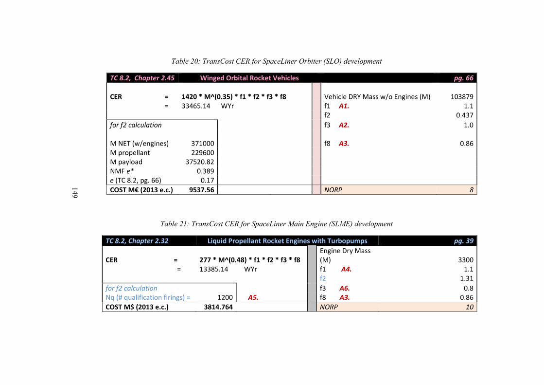
149
Table 20: TransCost CER for SpaceLiner Orbiter (SLO) development
TC 8.2, Chapter 2.45 Winged Orbital Rocket Vehicles pg. 66
CER = 1420 * M^(0.35) * f1 * f2 * f3 * f8 Vehicle DRY Mass w/o Engines (M) 103879 = 33465.14 WYr f1 A1. 1.1
f2 0.437
for f2 calculation f3 A2. 1.0
M NET (w/engines) 371000 f8 A3.
0 0.86M propellant 229600 M payload 37520.82 NMF e* 0.389 e (TC 8.2, pg. 66) 0.17
COST M€ (2013 e.c.) 9537.56 NORP 8
Table 21: TransCost CER for SpaceLiner Main Engine (SLME) development
TC 8.2, Chapter 2.32 Liquid Propellant Rocket Engines with Turbopumps pg. 39
CER = 277 * M^(0.48) * f1 * f2 * f3 * f8 Engine Dry Mass (M) 3300
= 13385.14 WYr f1 A4. 1.1 f2 1.31
for f2 calculation f3 A6. 0.8Nq (# qualification firings) = 1200 A5. f8 A3. 0.86
COST M$ (2013 e.c.) 3814.764 NORP 10
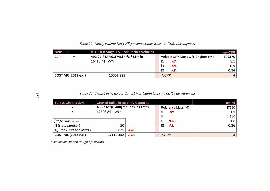
150
Table 22: Newly established CER for SpaceLiner Booster (SLB) development
New CER VTO First Stage‐Fly‐Back Rocket Vehicles new CER
CER = 493.27 * M^(0.3746) * f1 * f3 * f8 Vehicle DRY Mass w/o Engines (M) 135379 = 16416.44 WYr f1 A7. 1.1
f3 A8. 0.9 f8 A3. 0.86
COST M€ (2013 e.c.) 10007.885 NORP 4
Table 23: TransCost CER for SpaceLiner Cabin/Capsule (SPC) development
TC 8.2, Chapter 2.48 Crewed Ballistic Re-entry Capsules pg. 76
CER = 436 * M^(0.408) * f1 * f2 * f3 * f8 Reference Mass (M) 37520 = 42506.85 WYr f1 A9. 1.3
f2 1.186
for f2 calculation f3 A11. 1.0N (crew number) = 50 f8 A3. 0.86TM (max. mission life*) = 0.0625 A10.
COST M€ (2013 e.c.) 12114.452 A12. NORP 4
* maximum mission design life in days
151
A8. A complexity of 0.9 was chosen for the SLB team experience factor, f3 to signify an
experienced team which has performed similar projects in the past, to reflect knowledge and
experience gained from manufacture of the Space Shuttle external tank.
A9. A complexity of 1.3 was chosen for the SPC development standard factor, f1.
Although this is the smallest element of the overall SpaceLiner vehicle, the function duality of
the passenger cabin which also doubles up as a rescue capsule capable of safely returning all
passengers to Earth in case of an emergency, presents an increased technical complexity. As
such, the high f1 factor is chosen to reflect a first generation system and new concept approach
involving new techniques and new technologies.
A10. To calculate the f2 factor for the SPC, the TransCost formula requires input of the
number of crew (50, for the SpaceLiner baseline case) and the nominal mission time in days
(being 0.0625 for a 90 minute SpaceLiner flight).
A11 A complexity of 1.0 was chosen for the SPC team experience factor, f3. Although the
SPC is a challenging technical element, the team is selected to have some related experience,
since the cabin would take significant heritage from the aviation sector. In addition, for such a
life-critical system, the team members would have to be selected with significant experience to
address the task at hand.
A12. It can be seen that based on the final results, the SPC is by far the most expensive
component of the four SpaceLiner elements, at over 12 B€. Here, it must also be noted that the
data underlying the CER is considerably old data based on only four data points. These are the
Gemini and Apollo capsules from the mid-1960s, as well as the Mercury program, and the more
recent Orion capsule proposal values for 2006 [102]. As such, it can be argued that for a
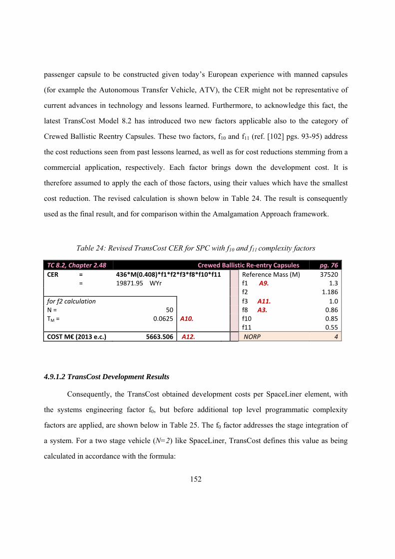
152
passenger capsule to be constructed given today’s European experience with manned capsules
(for example the Autonomous Transfer Vehicle, ATV), the CER might not be representative of
current advances in technology and lessons learned. Furthermore, to acknowledge this fact, the
latest TransCost Model 8.2 has introduced two new factors applicable also to the category of
Crewed Ballistic Reentry Capsules. These two factors, f10 and f11 (ref. [102] pgs. 93-95) address
the cost reductions seen from past lessons learned, as well as for cost reductions stemming from a
commercial application, respectively. Each factor brings down the development cost. It is
therefore assumed to apply the each of those factors, using their values which have the smallest
cost reduction. The revised calculation is shown below in Table 24. The result is consequently
used as the final result, and for comparison within the Amalgamation Approach framework.
Table 24: Revised TransCost CER for SPC with f10 and f11 complexity factors
TC 8.2, Chapter 2.48 Crewed Ballistic Re‐entry Capsules pg. 76
CER = 436*M(0.408)*f1*f2*f3*f8*f10*f11 Reference Mass (M) 37520 = 19871.95 WYr f1 A9. 1.3
f2 1.186
for f2 calculation f3 A11. 1.0N = 50 f8 A3. 0.86TM = 0.0625 A10. f10 0.85 f11 0.55
COST M€ (2013 e.c.) 5663.506 A12. NORP 4
4.9.1.2 TransCost Development Results
Consequently, the TransCost obtained development costs per SpaceLiner element, with
the systems engineering factor f0, but before additional top level programmatic complexity
factors are applied, are shown below in Table 25. The f0 factor addresses the stage integration of
a system. For a two stage vehicle (N=2) like SpaceLiner, TransCost defines this value as being
calculated in accordance with the formula:
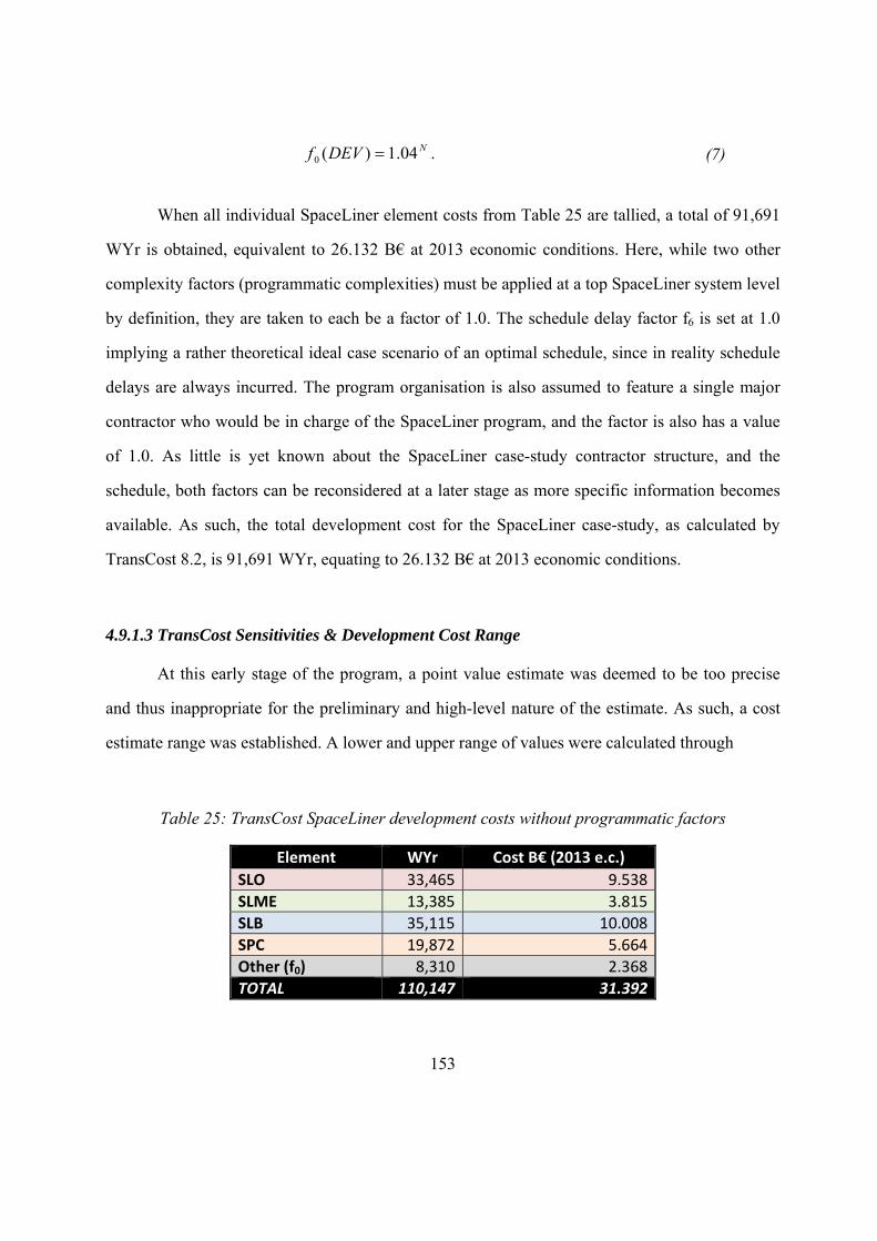
153
NDEVf 04.1)(0 . (7)
When all individual SpaceLiner element costs from Table 25 are tallied, a total of 91,691
WYr is obtained, equivalent to 26.132 B€ at 2013 economic conditions. Here, while two other
complexity factors (programmatic complexities) must be applied at a top SpaceLiner system level
by definition, they are taken to each be a factor of 1.0. The schedule delay factor f6 is set at 1.0
implying a rather theoretical ideal case scenario of an optimal schedule, since in reality schedule
delays are always incurred. The program organisation is also assumed to feature a single major
contractor who would be in charge of the SpaceLiner program, and the factor is also has a value
of 1.0. As little is yet known about the SpaceLiner case-study contractor structure, and the
schedule, both factors can be reconsidered at a later stage as more specific information becomes
available. As such, the total development cost for the SpaceLiner case-study, as calculated by
TransCost 8.2, is 91,691 WYr, equating to 26.132 B€ at 2013 economic conditions.
4.9.1.3 TransCost Sensitivities & Development Cost Range
At this early stage of the program, a point value estimate was deemed to be too precise
and thus inappropriate for the preliminary and high-level nature of the estimate. As such, a cost
estimate range was established. A lower and upper range of values were calculated through
Table 25: TransCost SpaceLiner development costs without programmatic factors
Element WYr Cost B€ (2013 e.c.)
SLO 33,465 9.538
SLME 13,385 3.815
SLB 35,115 10.008
SPC 19,872 5.664
Other (f0) 8,310 2.368
TOTAL 110,147 31.392
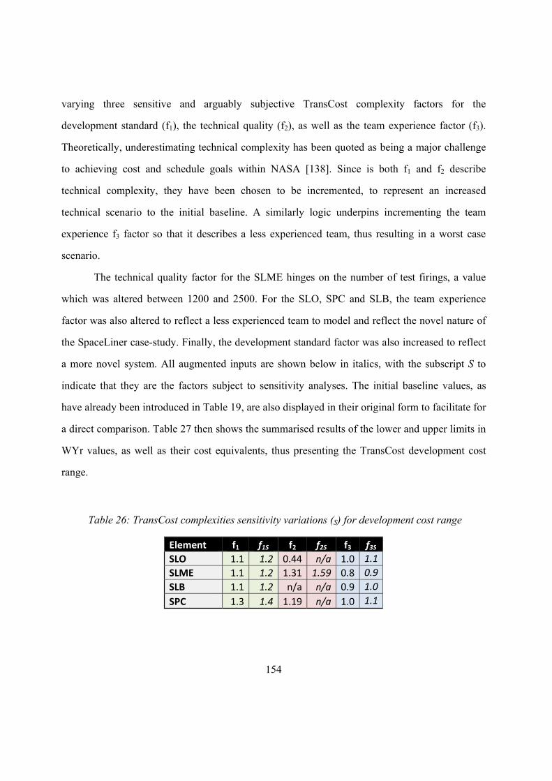
154
varying three sensitive and arguably subjective TransCost complexity factors for the
development standard (f1), the technical quality (f2), as well as the team experience factor (f3).
Theoretically, underestimating technical complexity has been quoted as being a major challenge
to achieving cost and schedule goals within NASA [138]. Since is both f1 and f2 describe
technical complexity, they have been chosen to be incremented, to represent an increased
technical scenario to the initial baseline. A similarly logic underpins incrementing the team
experience f3 factor so that it describes a less experienced team, thus resulting in a worst case
scenario.
The technical quality factor for the SLME hinges on the number of test firings, a value
which was altered between 1200 and 2500. For the SLO, SPC and SLB, the team experience
factor was also altered to reflect a less experienced team to model and reflect the novel nature of
the SpaceLiner case-study. Finally, the development standard factor was also increased to reflect
a more novel system. All augmented inputs are shown below in italics, with the subscript S to
indicate that they are the factors subject to sensitivity analyses. The initial baseline values, as
have already been introduced in Table 19, are also displayed in their original form to facilitate for
a direct comparison. Table 27 then shows the summarised results of the lower and upper limits in
WYr values, as well as their cost equivalents, thus presenting the TransCost development cost
range.
Table 26: TransCost complexities sensitivity variations (S) for development cost range
Element f1 f1S f2 f2S f3 f3S
SLO 1.1 1.2 0.44 n/a 1.0 1.1
SLME 1.1 1.2 1.31 1.59 0.8 0.9
SLB 1.1 1.2 n/a n/a 0.9 1.0
SPC 1.3 1.4 1.19 n/a 1.0 1.1
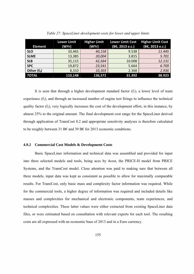
155
Table 27: SpaceLiner development costs for lower and upper limits
Element Lower Limit
(WYr) Higher Limit
(WYr) Lower Limit Cost (B€, 2013 e.c.)
Higher Limit Cost (B€, 2013 e.c.)
SLO 33,465 40,158 9.538 11.445
SLME 13,385 20,004 3.815 5.701
SLB 35,115 42,564 10.008 12.131
SPC 19,872 23,541 5.664 6.709
Other (f0) 8,310 10,303 2.368 2.936
TOTAL 110,148 136,571 31.392 38.923
It is seen that through a higher development standard factor (f1), a lower level of team
experience (f3), and through an increased number of engine test firings to influence the technical
quality factor (f2), very logically increases the cost of the development effort, in this instance, by
almost 25% to the original amount. The final development cost range for the SpaceLiner derived
through application of TransCost 8.2 and appropriate sensitivity analyses is therefore calculated
to be roughly between 31 B€ and 39 B€ for 2013 economic conditions.
4.9.2 Commercial Cost Models & Development Costs
Basic SpaceLiner information and technical data was assembled and provided for input
into three selected models and tools, being aces by 4cost, the PRICE-H model from PRICE
Systems, and the TransCost model. Close attention was paid to making sure that between all
three models, input data was kept as consistent as possible to allow for maximally comparable
results. For TransCost, only basic mass and complexity factor information was required. While
for the commercial tools, a higher degree of information was required and included details like
masses and complexities for mechanical and electronic components, team experiences, and
technical complexities. These latter values were either extracted from existing SpaceLiner data
files, or were estimated based on consultation with relevant experts for each tool. The resulting
costs are all expressed with an economic base of 2013 and in a Euro currency.
156
The process of compiling a cost estimate using the 4cost aces commercial tool was done
in parallel with the cost estimate using the PRICE model. Calculations using each model were
made with the assistance of trained, highly qualified experts for each tool. The numerical cost
estimation results were then entered directly into the specially designed and programmed AA
Excel tool, alongside the TransCost values, allowing for the critical analysis step. In line with the
AA, several iterations had to be made, with re-calculations of costs from all models, based on
analysis of results after they had been committed to the AAInT spreadsheet. The final AA results
are therefore shown in this Thesis work as ultimate result from the AA cost estimation process.
Close attention was directed to ensuring inputs were as congruent and comparative
between the two models and tools used, to ensure maximum and unilateral comparability of end
results. Here, it must be noted that regardless of the fact that an identical data set was provided
for input into both software packages. Ultimately, aces and PRICE are very different models with
different mathematics behind them. Thus, typically, and not surprisingly, same input values will
result in different numbers. Variations can be attributed to inherent program algorithms and
internally generated factors and complexities for elements, as well as interpretations and
assumptions made by the expert cost estimators themselves while entering the data.
While calibration is normally performed for each model in view of the program to be
estimated, for the early stage of the SpaceLiner program, and thus the high level overview of sub-
systems, this step was unnecessary.
In both cases, the closest of attention was paid to ensure that inputs provided for both
models were reflective of the current status of the SpaceLiner technical specifications at the time
of model utility. Certain assumptions also had to be made to adjust for the various input formats
(i.e. complexity values and their classifications) between each model. Once again, some were
dependent on expert and program user interpretation. Additionally, a fixed SpaceLiner “baseline”
case had to be established in terms of not only technical data, but also programmatic information.
This was provided in a fixed format to both experts. Key criteria and assumptions for the
157
SpaceLiner “baseline” case have been carefully kept in line with the detailed SpaceLiner
philosophy outlined previously in Chapter 4.1.
After all individual results were obtained from the three cost estimation tools and models,
in line with the Amalgamation Approach, these were entered into the specially designed AA
Excel interface, to allow for the final and most critical step of the process – the result analysis,
dissemination and appraisal.
The only cost element missing, as seen on the SpaceLiner case-study developed WBS, is
therefore the overall Project Management Office component described by WBS element 1100.
An additional element 1200 for travel costs is also considered, since by definition of the 4cost
model, travel costs for a program, which are in fact not entirely insignificant, are not calculated
by the model in the cost estimate, and need to be added additionally.
4.9.3 aces by 4cost
The parametric aces tool from 4cost GmbH was input with SpaceLiner data and necessary
additional factors which were derived upon consultation with an aces software expert. SpaceLiner
data was input, with the following aces parameters of focus:
• Structure and Electronics Element Mass (WE/WM)
• Development Environment (ENVIRD)
• Engineering Difficulty (ENGDIF)
• Technology Electronics/Mechanical Index (INDEXE/M)
• Amount of New Design (NEWREPE/M)
• Year of Technology (TECHYEAR)
• Number of Prototypes (PROTO)
• Economic Currency Base (ECBASE)
• Development phase commencement
158
Based on these inputs, an optimal development time was then synthesised by the aces
software, as well as the associated development and production costs. A basic outline of the key
aces parameters and defined parameters, and the associated justifications of values, are listed and
explained below:
• WM /WE
The element masses for SpaceLiner were entered from DLR internal documents and
calculations, into the WBS structure established in the 4cost aces interface. The WM entry refers
to the weight of mechanical items, while WE refers to electronic item weight.
• ENVIRD
The ENVIR value addresses the environment, with ENVIRD describing the environment
for the development effort. Four categories of defined complexities are defined classed into the
stationary, mobile, aircraft and space environment categories. ENVIRD describes criteria for
environmental conditions, manufacturing formalities, deployment conditions and quality
assurances. For the SpaceLiner case-study, the categories of aircraft (ENVIRD values 1.9 – 2.1)
and space (ENVIRD values 1.9 – 2.2) are relevant. An ENVIRD value of 2.0 was consequently
chosen, which encompasses both the higher bracket of the aircraft category for military projects,
and the lower bracket of the space segment for unmanned typical satellite missions. The 4cost
table is shown in Figure 33, with the selected values, highlighted in green. Selecting a value
which overlaps both domains is representative of the SpaceLiner concept and the associated
philosophy of the hybrid nature of the vehicle. Despite being a new vehicle in context, the lower
end of the space segment classification is considered to reflect the significant amount of heritage
technology of the concept and, although manned, in effect, constitutes an advanced airplane
concept.
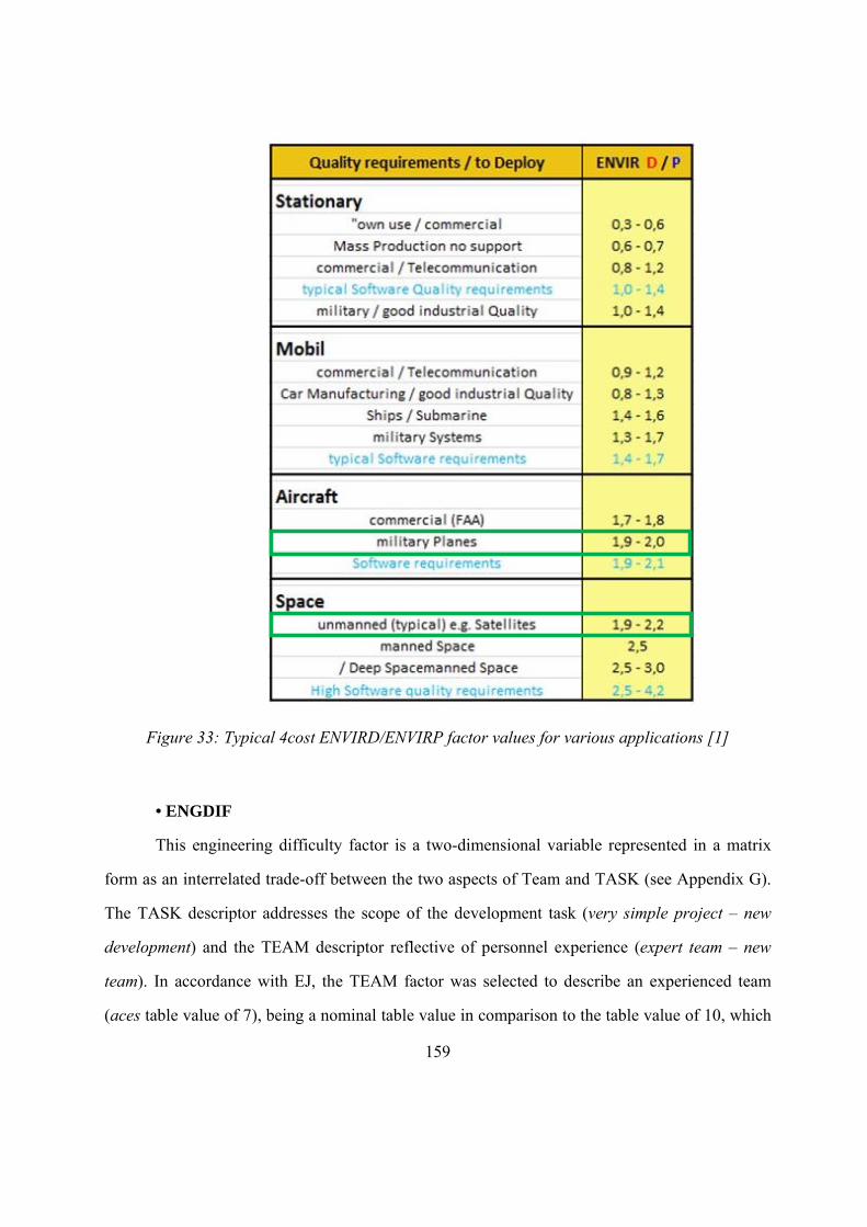
159
Figure 33: Typical 4cost ENVIRD/ENVIRP factor values for various applications [1]
• ENGDIF
This engineering difficulty factor is a two-dimensional variable represented in a matrix
form as an interrelated trade-off between the two aspects of Team and TASK (see Appendix G).
The TASK descriptor addresses the scope of the development task (very simple project – new
development) and the TEAM descriptor reflective of personnel experience (expert team – new
team). In accordance with EJ, the TEAM factor was selected to describe an experienced team
(aces table value of 7), being a nominal table value in comparison to the table value of 10, which
160
describes the ‘ideal’ and therefore unachievable team status. The 7 table value is entered into the
software as a ‘0’ numerical input. An experienced team is a reasonable assumption to make, since
for a project such as the manned SpaceLiner based on largely existing technology, an experienced
team would be required for component and hardware realisation. And for a program as
expansive, complex and international as the SpaceLiner, an inexperienced, a new, inexperienced
team would be inadequate and insufficient.
The TASK parameter was then automatically generated by an assistant function based on
other inputs including ENVIRD, TECHYEAR (described below) and mass.
• INDEXE/M
The INDEXE/M is the technology index for electronics (INDEXE) and mechanics
(INDEXM). Both are usually empirically derived values representing product producibility while
also qualifying the development effort. The numerical input values are available from dedicated
INDEX tables incorporated within the 4cost software, and for the SpaceLiner case-study were
determined automatically.
INDEXM is a function of physical characteristics, such as material type, finished product
density and fabrication method. INDEXE is a function of componentry, packaging density, easy
of manufacture, degree of testing and power dissipation. Both parameters depend, in this
instance, on the ENVIRD (development environment) inputs, always increasing alongside an
increase in ENVIRD. These inputs are also required for the production effort.
• Amount of New Design (NEWREPE/M)
The NEWREPE/M variables are used to quantify the amount of new design and drafting
effort required to manufacture electronic and mechanical hardware for non-repetitive assemblies.
All NEWREPE/M values to quantify the amount of new design and drafting effort required to
manufacture mechanical and electronic hardware were generated either through EJ based on an
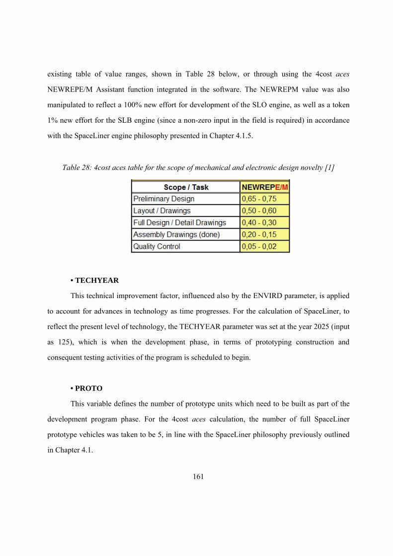
161
existing table of value ranges, shown in Table 28 below, or through using the 4cost aces
NEWREPE/M Assistant function integrated in the software. The NEWREPM value was also
manipulated to reflect a 100% new effort for development of the SLO engine, as well as a token
1% new effort for the SLB engine (since a non-zero input in the field is required) in accordance
with the SpaceLiner engine philosophy presented in Chapter 4.1.5.
Table 28: 4cost aces table for the scope of mechanical and electronic design novelty [1]
• TECHYEAR
This technical improvement factor, influenced also by the ENVIRD parameter, is applied
to account for advances in technology as time progresses. For the calculation of SpaceLiner, to
reflect the present level of technology, the TECHYEAR parameter was set at the year 2025 (input
as 125), which is when the development phase, in terms of prototyping construction and
consequent testing activities of the program is scheduled to begin.
• PROTO
This variable defines the number of prototype units which need to be built as part of the
development program phase. For the 4cost aces calculation, the number of full SpaceLiner
prototype vehicles was taken to be 5, in line with the SpaceLiner philosophy previously outlined
in Chapter 4.1.
162
• ECBASE
The economic base (ECBASE), as the name implies, defines the economic base of the
output costs, and was set to the year 2013.
• Development ECBASE
The development commencement was also entered as being the year 2025, which is in
line with the proposed SpaceLiner schedule presented in Chapter 4.1.1.
A full list of the relevant, key 4cost aces software inputs as well as the resulting outputs
can be found in Appendix H.
4.9.4 PRICE
PRICE-H Suite was used as the interface for this calculation. The model facilitates for a
large number of control parameters used for primary calibration of the model to a specific
environment. However, in view of the preliminary nature of the SpaceLiner program, given the
top-level nature of the estimate and the high-level inputs, for this exercise, the model was used in
its un-calibrated mode, meaning all control parameters and PRICE-H Global values and
multipliers were set at their nominal, unadjusted values. Required complexities were then either
generated from look-up tables, or were entered manually by an experienced and expert tool user,
to translate technical requirements into representative model parameters. Key model inputs
included:
• Individual element mass (WS/WT)
• Platform value (PLTFM)
• Engineering complexity (ECMPLX)
• Manufacturing complexity (MCPLXS/E)
163
• Number of prototypes (PROTOS)
• Design heritage (NEWST/NEWEL)
• Year of technology (YRTECH)
• Development start date (DSTART)
• Economic conditions (YECON)
While all detailed definitions can be found in the official PRICE manual [154], a basic
outline of the key parameters listed above, their selected values for the SpaceLiner case-study,
and the respective justifications for each decision are provided below.
• WS/WT
The element masses were entered into the WBS established in the PRICE-H software.
The WS entry refers to structure weight, while WT refers to total weight per element. As such, the
electronic weight is never input directly, but is derived by calculating the difference between the
total and structural weights (WT – WS). Because of this, the two values are very commonly
identical if there are no electronic parts present. Differences do exist between the two values for
electronic components in the WBS elements such as Power and ECS (WBS elements 2400, 3400
and 4400) or Cabin Avionics (element 4600) for example.
• PLTFM
The empirically derived platform (PLTFM) value influences development engineering
costs, and addresses the specification and testing level, the operating environment and reliability
requirements associated with the element to be designed. Very loosely (but not identically)
comparable to the ENVIRD value featured in the 4cost aces tool, the PLTFM value is also
divided into the four categories of ground, mobile, airborne and space. For the SpaceLiner case-
study calculation, a value of 2.0 was selected, being reflective of the quality assurance level for
164
parts and inspections for a typical unmanned space mission. This may seem to be contradictive to
the manned nature of the SpaceLiner vehicle by its definition. However, if the PLTFM value of
2.5 for traditional, heritage manned space applications was taken, this would result in an over-
inflated cost for the program, as it would not take into account the existing significant heritage
for the SpaceLiner technology, nor the commercial nature and context of the program. Since
SpaceLiner aims to exploit lessons learned from advanced aviation products, economies of scale,
and more mature processes, a lower PLTFM value to strictly and purely space technologies is
reflective and representative of this.
• ECMPLX
The engineering complexity (ECMPLX) value is a measure of the complicating factors of
the design effort as they relate to the level of technology, and the skills of the development team.
More specifically, this factor addresses the influence and experience of the design team within
the scope of the development effort, with respect to the TRL of the technology. A typical value of
1.0 describes a new design, within state of the art, and performed by an experienced team familiar
with similar work. For the SpaceLiner, based on extensive PRICE expert user consultation, the
ECMPLX value was set to be 1.5 to reflect a team experienced with similar familiar, but not
identical technology, with the scope of the design effort having a new design, with unfamiliar
technology. The value is highlighted in green in Table 29. Although the SpaceLiner case-study
project would be based on significant technical heritage, the context of elements within a new
application imposes an added level of complexity, especially given the manned nature of the
system. The value of 1.5 therefore takes a more cautious approach, with the aim of not being too
optimistic, and to avoid resulting in understatement of development effort and costs. This
ECMPLX factor is only relevant to the development effort as it describes the design phase,
addressing drawing complexity which is then translated into an effort mount, and therefore does
not influence production.
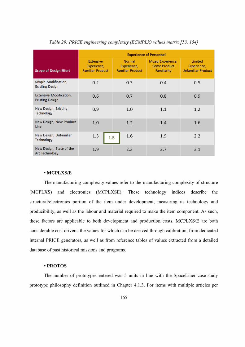
165
Table 29: PRICE engineering complexity (ECMPLX) values matrix [53, 154]
• MCPLXS/E
The manufacturing complexity values refer to the manufacturing complexity of structure
(MCPLXS) and electronics (MCPLXSE). These technology indices describe the
structural/electronics portion of the item under development, measuring its technology and
producibility, as well as the labour and material required to make the item component. As such,
these factors are applicable to both development and production costs. MCPLXS/E are both
considerable cost drivers, the values for which can be derived through calibration, from dedicated
internal PRICE generators, as well as from reference tables of values extracted from a detailed
database of past historical missions and programs.
• PROTOS
The number of prototypes entered was 5 units in line with the SpaceLiner case-study
prototype philosophy definition outlined in Chapter 4.1.3. For items with multiple articles per
1.5
166
SpaceLiner unit (i.e. engines, with 9 SLB and 2 SLO engines per vehicle), the number of
prototypes was increased to provide a complete set of hardware for each higher level assembly.
As such, the cost for 45 SLB and 10 SLO engines were calculated within framework of the
prototype units for the SpaceLiner development phase. For development of the SLME component
(element 2200), the PRICE model does not take into account the test firings for the development
effort. As such, a global multiplier was imposed to factor in for the stipulated number of 1200 of
test firings, which, at this early stage, was deemed by PRICE experts as a representative
amendment to address the qualitatively known cost gap. At a later program phase, however, it
would be appropriate to address this model shortcoming by conducting an independent bottom-up
analysis of the expected test-firing campaign costs. These should then be added on as a separate
element to the PRICE cost estimation structure. Here, it would be necessary to consider the non-
recursive costs for test-rig procurement and installation, and then the recursive fixed direct
operating costs (DOC) for the test facility as well as staff required for the campaign.
• NEWST/NEWEL
The new structure (NEWST) and new electronics (NEWEL) inputs define the amount of
the new structure/design effort required, where 100% equates to an input of 1.0. This was only
deviated from a 1.0 input to 0.01 for the propulsion component of the booster engine in WBS
element 3200, since development of this was assumed to be fully covered in the development of
the SLME for element 2200 (see Chapter 4.1.5).
• YRTECH
The year of technology defines the technological state for the development phase
timeframe. In case of the SpaceLiner program, YRTECH was set to the commencement of the
Design and Development (Phase C) of the program identified already in the program schedule
described in Chapter 4.1.2, and is determined as 2025, also in line with the 4cost aces tool input.
167
• DSTART
The date of production start (PSTART) is given to be January, 2025 (input as 125), in line
with the YRTECH input shown above, and also reflective of the SpaceLiner baseline program
schedule introduced in Chapter 4.1.2.
• YECON
The year of economics (YECON) defines the economic base of the output costs, and was
set to 2013.
Based on all above key inputs, development costs per element were calculated. In
addition, an optimal development time was also synthesised by the PRICE software assuming an
ideal scenario with no schedule delays. A list of key PRICE software inputs which are discussed
above, as well as resulting outputs can be found in Appendix I.
4.9.5 Optimal Development Timeframe
The TransCost model is not dedicated to generating scheduling information, although
both the commercial software models, 4cost aces and PRICE generated baseline development
timeframes given an internal synthesis of all available inputs. Both tools rely on internal
algorithms to propose an optimal development phase which results in no cost penalties under
ideal, optimised scheduling conditions.
Duration of the development phase is a parameter which is automatically calculated by
the PRICE-H model. This is influenced by other model inputs and factors, including equipment
complexity, PLTFM and ECMPLX values, and results in an optimised cost, thus avoiding
penalties by enforcing an artificial timeframe. For the SpaceLiner case-study, this was found to
be 81 months, commencing in January, 2025 and continuing through until the end of September,
2031. The 4cost aces software similarly relies on inputs such as the environment descriptor
168
ENVIRD, the engineering difficulty ENGDIF and the mechanical index INDEXM as key inputs,
and resulted in a development timeframe of 59 months, from January, 2025, until November,
2029.
It must be noted that both software tools produce idyllic and rather uncertain scenarios of
a development phase assuming no scheduling delays and no unexpected events. In reality, for a
program as large and complex as the SpaceLiner case-study would be, the timeframe is dictated
not only by technical capabilities, but also by a myriad of other aspects including politics,
economics, financing, as well as unforeseen occurrences. Here, the risk and uncertainty
assessment outlined qualitatively in Chapter 4.1.11 would constitute an essential input. As such,
taking the longer PRICE tool optimal development phase of 83 months, it can be almost certainly
assumed that the development phase would take longer than this.
The baseline results obtained from both commercial tools can be used to build upon as
more SpaceLiner program information comes to light. And with an initial program schedule
having already and freshly been established translating the still evolving technical details into a
timeframe, it is not too unreasonable to assume a simplified and optimised schedule at this stage.
Certainly, however, a greater level of scheduling risk analysis will also need to be integrated into
the cost estimate at a later program stage alongside revision of the currently proposed program
schedule as more precise information becomes available.
4.9.6 Development Project Management Office Cost Estimation
In this section, in accordance with the distinction made between the terms of ‘price’ and
‘cost’ in Chapter 2.1, ultimately the overall figures estimated in for the PMO function are in fact
prices, since the profit margin is always incorporated. Nevertheless, to comply with the cost
estimation goal of this Thesis, and to avoid confusion, while recognising the difference between
‘cost’ and ‘price’, the term ‘cost’ is nevertheless adhered to.
169
The PMO functions at the total, top system level (L1WBS) and at a major program element
level (L2WBS), are represented in WBS elements 1000 as well as 2100, 3100, 4100, 5100, 6100
and 7100, respectively. While the independent component PMO function costs for development
of the SpaceLiner SLO, SLB and SPC (elements 2100, 3100, 4100 respectively) are already
inherently included in all three models used for the AA, the overall, top-level PMO function of
WBS element 1000 needs to be estimated. Here, EJ is once again employed to determine a
representative and defensible figure.
In addition, and as previously defined, elements 6000 (Ground) is only qualitatively
considered within this Thesis, and for the PMO function, it is possible to do a ROM cost estimate
using EJ in close consultation with experienced project management experts. For element 7000
(Operations), PMO costs are not considered since, being a recurring cost, they do not apply for
the non-recursive elements of the development phase.
For this section of calculations, both literature [114, 147] and high-level space industry
management and programmatic experts and professionals were consulted with respect to their
knowledge of the project office costs [118, 119], since here, real-industry practical experience is
essential for application due to the unique and unprecedented nature of the SpaceLiner case-
study. Expert judgement was also relied upon to assist in formulation of the PMO function
component breakdown, as well as to estimate preliminary numbers of staff and consequently the
costs for this vital function within the overall program framework.
Overall program costs vary significantly during a project as a whole, and more
specifically, within each program phase, as illustrated in Figure 34 below. PMO effort and costs
are not linear or proportionate with these movements, although it has been observed that the
highest levels of PMO and program management activities occur during the early program
phases, in the lead-up to production [223]. Such a trend is logically attributed to significant time
investment and initiatives for establishing and developing a project plan, which sees an effort
increase and therefore a higher utility, need, application and consequently cost of the PMO
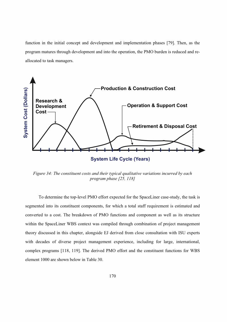
170
function in the initial concept and development and implementation phases [79]. Then, as the
program matures through development and into the operation, the PMO burden is reduced and re-
allocated to task managers.
Figure 34: The constituent costs and their typical qualitative variations incurred by each program phase [25, 118]
To determine the top-level PMO effort expected for the SpaceLiner case-study, the task is
segmented into its constituent components, for which a total staff requirement is estimated and
converted to a cost. The breakdown of PMO functions and component as well as its structure
within the SpaceLiner WBS context was compiled through combination of project management
theory discussed in this chapter, alongside EJ derived from close consultation with ISU experts
with decades of diverse project management experience, including for large, international,
complex programs [118, 119]. The derived PMO effort and the constituent functions for WBS
element 1000 are shown below in Table 30.
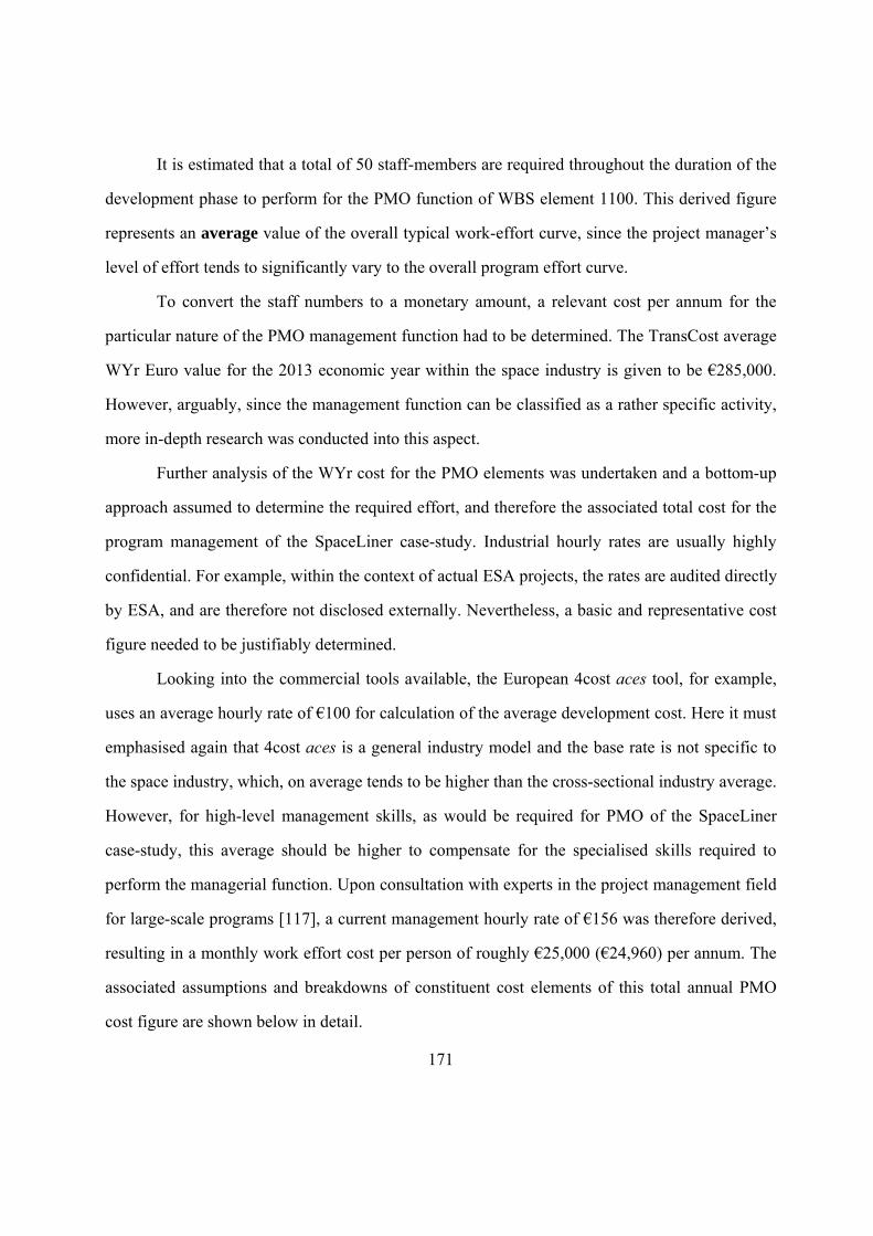
171
It is estimated that a total of 50 staff-members are required throughout the duration of the
development phase to perform for the PMO function of WBS element 1100. This derived figure
represents an average value of the overall typical work-effort curve, since the project manager’s
level of effort tends to significantly vary to the overall program effort curve.
To convert the staff numbers to a monetary amount, a relevant cost per annum for the
particular nature of the PMO management function had to be determined. The TransCost average
WYr Euro value for the 2013 economic year within the space industry is given to be €285,000.
However, arguably, since the management function can be classified as a rather specific activity,
more in-depth research was conducted into this aspect.
Further analysis of the WYr cost for the PMO elements was undertaken and a bottom-up
approach assumed to determine the required effort, and therefore the associated total cost for the
program management of the SpaceLiner case-study. Industrial hourly rates are usually highly
confidential. For example, within the context of actual ESA projects, the rates are audited directly
by ESA, and are therefore not disclosed externally. Nevertheless, a basic and representative cost
figure needed to be justifiably determined.
Looking into the commercial tools available, the European 4cost aces tool, for example,
uses an average hourly rate of €100 for calculation of the average development cost. Here it must
emphasised again that 4cost aces is a general industry model and the base rate is not specific to
the space industry, which, on average tends to be higher than the cross-sectional industry average.
However, for high-level management skills, as would be required for PMO of the SpaceLiner
case-study, this average should be higher to compensate for the specialised skills required to
perform the managerial function. Upon consultation with experts in the project management field
for large-scale programs [117], a current management hourly rate of €156 was therefore derived,
resulting in a monthly work effort cost per person of roughly €25,000 (€24,960) per annum. The
associated assumptions and breakdowns of constituent cost elements of this total annual PMO
cost figure are shown below in detail.
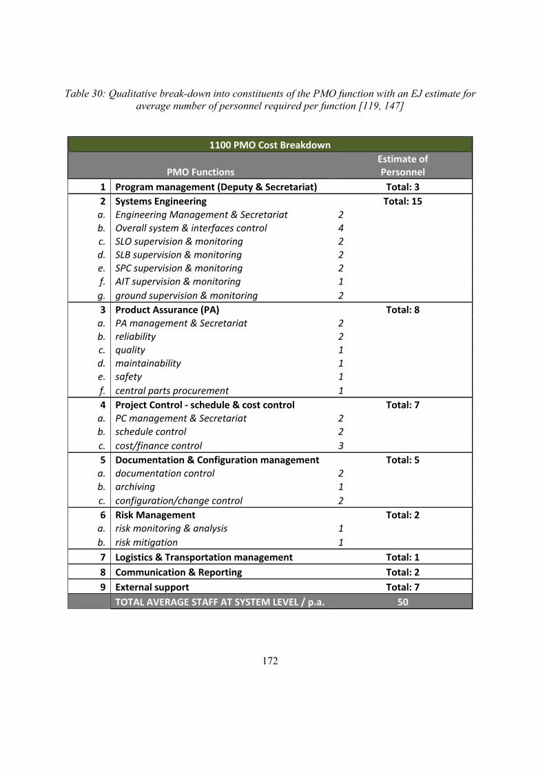
172
Table 30: Qualitative break-down into constituents of the PMO function with an EJ estimate for average number of personnel required per function [119, 147]
1100 PMO Cost Breakdown
PMO Functions Estimate of Personnel
1 Program management (Deputy & Secretariat) Total: 3
2 Systems Engineering Total: 15 a. Engineering Management & Secretariat 2
b. Overall system & interfaces control 4 c. SLO supervision & monitoring 2 d. SLB supervision & monitoring 2 e. SPC supervision & monitoring 2 f. AIT supervision & monitoring 1
g. ground supervision & monitoring 2
3 Product Assurance (PA) Total: 8 a. PA management & Secretariat 2 b. reliability 2 c. quality 1 d. maintainability 1 e. safety 1
f. central parts procurement 1
4 Project Control ‐ schedule & cost control Total: 7 a. PC management & Secretariat 2 b. schedule control 2
c. cost/finance control 3
5 Documentation & Configuration management Total: 5 a. documentation control 2
b. archiving 1
c. configuration/change control 2
6 Risk Management Total: 2 a. risk monitoring & analysis 1
b. risk mitigation 1
7 Logistics & Transportation management Total: 1
8 Communication & Reporting Total: 2
9 External support Total: 7
TOTAL AVERAGE STAFF AT SYSTEM LEVEL / p.a. 50
173
4.9.6.1 PMO Cost Assumptions
€120/hour base: average hourly industrial gross rate for PMO functions, catering for
management, highly qualified engineering personnel and necessary support staff.
plus 20% other direct costs (€24/hour): allowance and provision for extra costs such as
for transportation, travel and lodging, communication, rental of special purpose
equipment, small value item purchases, social events etc. (updated total €144/hr)
plus 8% profit (€12/hour): the standard industry ESA profit margin (updated total
€156/hr)
140 hours per month: hours required per management function based on the following
assumptions:
o 4 weeks per month o 5 work days per week o 7 hours per day
The German office of Statistics [68] stipulates that on average, in 2012, individuals in
Europe worked 37.5 hours per week, which is roughly 156 hours per month. In addition,
TransCost states that in Europe (ESA) an average of 1583 effective hours are worked per year,
translating to an equivalent of 132 hours per month and 33 hours per week. Therefore, the value
of 160 hours per month, as estimated for the SpaceLiner PMO function, is well in line with both
the general and the industry-specific averages. The slightly higher 160 hour per month estimate is
revised up from both averages to correspond with a schedule of respectively higher intensity in
line with the large scope and very complex nature of the SpaceLiner program, requiring increased
management efforts. Combining and summarising the analyses, the resulting figure for the
estimated PMO function is therefore €156 per hour, with 160 accountable hours per month.
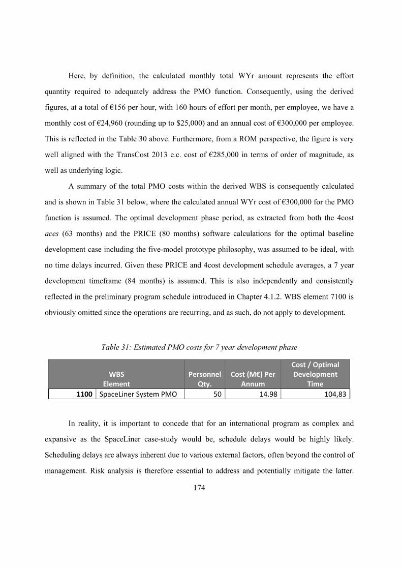
174
Here, by definition, the calculated monthly total WYr amount represents the effort
quantity required to adequately address the PMO function. Consequently, using the derived
figures, at a total of €156 per hour, with 160 hours of effort per month, per employee, we have a
monthly cost of €24,960 (rounding up to $25,000) and an annual cost of €300,000 per employee.
This is reflected in the Table 30 above. Furthermore, from a ROM perspective, the figure is very
well aligned with the TransCost 2013 e.c. cost of €285,000 in terms of order of magnitude, as
well as underlying logic.
A summary of the total PMO costs within the derived WBS is consequently calculated
and is shown in Table 31 below, where the calculated annual WYr cost of €300,000 for the PMO
function is assumed. The optimal development phase period, as extracted from both the 4cost
aces (63 months) and the PRICE (80 months) software calculations for the optimal baseline
development case including the five-model prototype philosophy, was assumed to be ideal, with
no time delays incurred. Given these PRICE and 4cost development schedule averages, a 7 year
development timeframe (84 months) is assumed. This is also independently and consistently
reflected in the preliminary program schedule introduced in Chapter 4.1.2. WBS element 7100 is
obviously omitted since the operations are recurring, and as such, do not apply to development.
Table 31: Estimated PMO costs for 7 year development phase
WBS Element
Personnel Qty.
Cost (M€) Per Annum
Cost / Optimal Development
Time
1100 SpaceLiner System PMO 50 14.98 104,83
In reality, it is important to concede that for an international program as complex and
expansive as the SpaceLiner case-study would be, schedule delays would be highly likely.
Scheduling delays are always inherent due to various external factors, often beyond the control of
management. Risk analysis is therefore essential to address and potentially mitigate the latter.
175
Any schedule delays would consequently incur time and therefore cost penalties. For the PMO
category, any penalty costs can be simply derived from the calculated figures presented in Table
31 above. For every month of delay to the development phase, global program PMO costs for all
WBS elements incurred would have to cover employment of the full program PMO staff, being
250 personnel, and costing 6.24 M€.
Another factor to consider here is that due to the magnitude and scope of the program, the
size of the teams to be managed by one manager, might be comparatively large. Management
studies have shown that the span of control of a supervisor over a complex activity should not
exceed 12 workers. For simple activities, the ratio of supervisors to employees can go down. But
the 1:12 ratio (8.3%) will usually yield best results. Project Management for a complex project
can add an additional 10 to 14% [202]. This fact should also be considered within context of any
further and more in-depth studies of the PMO function and cost within such a large, complex,
international program as the SpaceLiner case-study.
4.9.7 Development Amalgamation Approach Results
With all cost element fields being complete, results amongst the three AAMAC models
could be analysed. Before the final development costs can be presented, however, a cheeky sub-
chapter is absolutely essential to visually show and practically explain the intensively iterative
nature of the AAMAC process. Such an example of just one iteration of many which happen prior
to the final cost-range figures being achieved, shows both the power and effectiveness of the
AAMAC method, especially when applied in conjunction with the specifically designed and
developed AAInT.

176
4.9.7.1 An AAMAC Iteration Example
Before AAMAC final results are achieved, which will be presented shortly, the AAMAC can
lend itself to many numerous iterations for each model if this is necessary before the final cost
range is reached. The aim of these iterations is to identify potential inaccuracies in results
whether due to model input, because of human error or incorrect logic, or perhaps translation of
technical data into model inputs. It can also be that sometimes a particular model is not capable to
effectively estimate the cost of a particular element, and may thus be inappropriate for the
application. Whatever the reason, the logical structure of the AAMAC maximally ensures that any
inconsistencies can be identified.
Thus, upon completion of a cost-estimate run for each of the three respective models and
tools and entry of all into AAInT, a critical analysis must then made between the estimates. As
shown previously in Figure 7, if significant differences are identified in costs for a common
element between models, this is immediately an indication to the cost estimator that further
analyses should be performed to determine the reason and justify the significant delta. The
conclusion of these analyses could yield explanations such as the non-applicability of a particular
tool or model to the current element (or even project) being costed, an inaccurate translation of a
variable could be discovered, or even human error could be noted, amongst others. Identification
of any issues or problems allows for them to be corrected before the next cost iteration is made.
As such, every single iteration serves to eliminate error in the final result, thus also reducing the
uncertainty through a staunch and justifiable result. An example of one such iteration is outlined
briefly here.
Upon completion of an almost-final development cost run across all three models, the
following results were observed of the SLO component, per model, as shown in the simplified
table extracted from the AAInT tool below in Table 32.
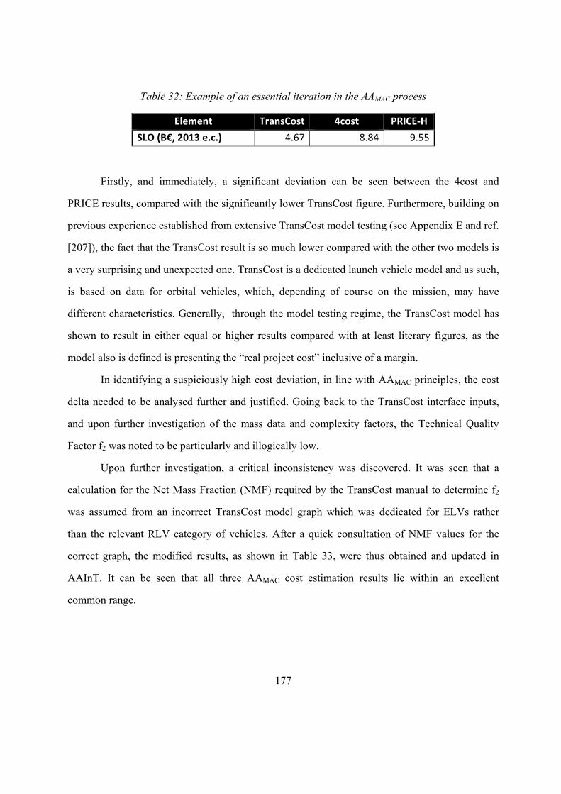
177
Table 32: Example of an essential iteration in the AAMAC process
Element TransCost 4cost PRICE‐H
SLO (B€, 2013 e.c.) 4.67 8.84 9.55
Firstly, and immediately, a significant deviation can be seen between the 4cost and
PRICE results, compared with the significantly lower TransCost figure. Furthermore, building on
previous experience established from extensive TransCost model testing (see Appendix E and ref.
[207]), the fact that the TransCost result is so much lower compared with the other two models is
a very surprising and unexpected one. TransCost is a dedicated launch vehicle model and as such,
is based on data for orbital vehicles, which, depending of course on the mission, may have
different characteristics. Generally, through the model testing regime, the TransCost model has
shown to result in either equal or higher results compared with at least literary figures, as the
model also is defined is presenting the “real project cost” inclusive of a margin.
In identifying a suspiciously high cost deviation, in line with AAMAC principles, the cost
delta needed to be analysed further and justified. Going back to the TransCost interface inputs,
and upon further investigation of the mass data and complexity factors, the Technical Quality
Factor f2 was noted to be particularly and illogically low.
Upon further investigation, a critical inconsistency was discovered. It was seen that a
calculation for the Net Mass Fraction (NMF) required by the TransCost manual to determine f2
was assumed from an incorrect TransCost model graph which was dedicated for ELVs rather
than the relevant RLV category of vehicles. After a quick consultation of NMF values for the
correct graph, the modified results, as shown in Table 33, were thus obtained and updated in
AAInT. It can be seen that all three AAMAC cost estimation results lie within an excellent
common range.
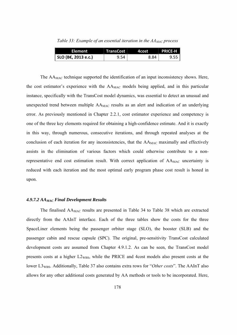
178
Table 33: Example of an essential iteration in the AAMAC process
Element TransCost 4cost PRICE‐H
SLO (B€, 2013 e.c.) 9.54 8.84 9.55
The AAMAC technique supported the identification of an input inconsistency shows. Here,
the cost estimator’s experience with the AAMAC models being applied, and in this particular
instance, specifically with the TransCost model dynamics, was essential to detect an unusual and
unexpected trend between multiple AAMAC results as an alert and indication of an underlying
error. As previously mentioned in Chapter 2.2.1, cost estimator experience and competency is
one of the three key elements required for obtaining a high-confidence estimate. And it is exactly
in this way, through numerous, consecutive iterations, and through repeated analyses at the
conclusion of each iteration for any inconsistencies, that the AAMAC maximally and effectively
assists in the elimination of various factors which could otherwise contribute to a non-
representative end cost estimation result. With correct application of AAMAC uncertainty is
reduced with each iteration and the most optimal early program phase cost result is honed in
upon.
4.9.7.2 AAMAC Final Development Results
The finalised AAMAC results are presented in Table 34 to Table 38 which are extracted
directly from the AAInT interface. Each of the three tables show the costs for the three
SpaceLiner elements being the passenger orbiter stage (SLO), the booster (SLB) and the
passenger cabin and rescue capsule (SPC). The original, pre-sensitivity TransCost calculated
development costs are assumed from Chapter 4.9.1.2. As can be seen, the TransCost model
presents costs at a higher L2WBS, while the PRICE and 4cost models also present costs at the
lower L3WBS. Additionally, Table 37 also contains extra rows for “Other costs”. The AAInT also
allows for any other additional costs generated by AA methods or tools to be incorporated. Here,
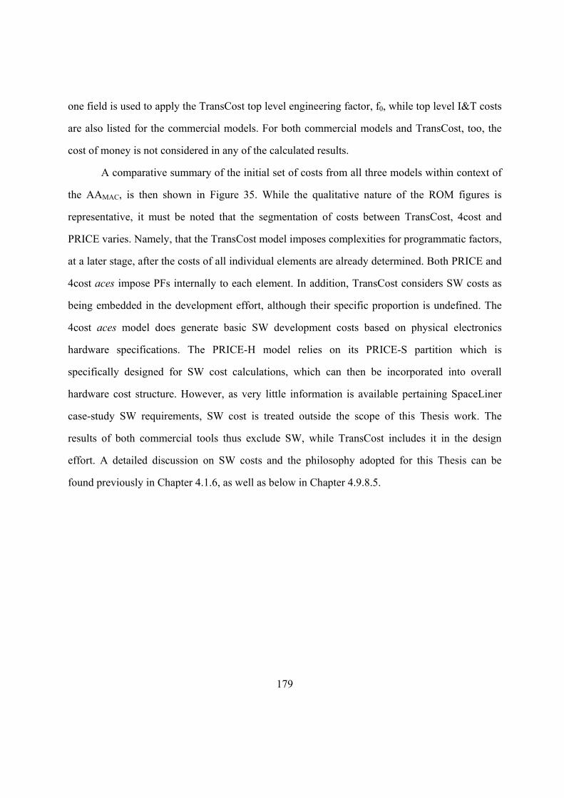
179
one field is used to apply the TransCost top level engineering factor, f0, while top level I&T costs
are also listed for the commercial models. For both commercial models and TransCost, too, the
cost of money is not considered in any of the calculated results.
A comparative summary of the initial set of costs from all three models within context of
the AAMAC, is then shown in Figure 35. While the qualitative nature of the ROM figures is
representative, it must be noted that the segmentation of costs between TransCost, 4cost and
PRICE varies. Namely, that the TransCost model imposes complexities for programmatic factors,
at a later stage, after the costs of all individual elements are already determined. Both PRICE and
4cost aces impose PFs internally to each element. In addition, TransCost considers SW costs as
being embedded in the development effort, although their specific proportion is undefined. The
4cost aces model does generate basic SW development costs based on physical electronics
hardware specifications. The PRICE-H model relies on its PRICE-S partition which is
specifically designed for SW cost calculations, which can then be incorporated into overall
hardware cost structure. However, as very little information is available pertaining SpaceLiner
case-study SW requirements, SW cost is treated outside the scope of this Thesis work. The
results of both commercial tools thus exclude SW, while TransCost includes it in the design
effort. A detailed discussion on SW costs and the philosophy adopted for this Thesis can be
found previously in Chapter 4.1.6, as well as below in Chapter 4.9.8.5.
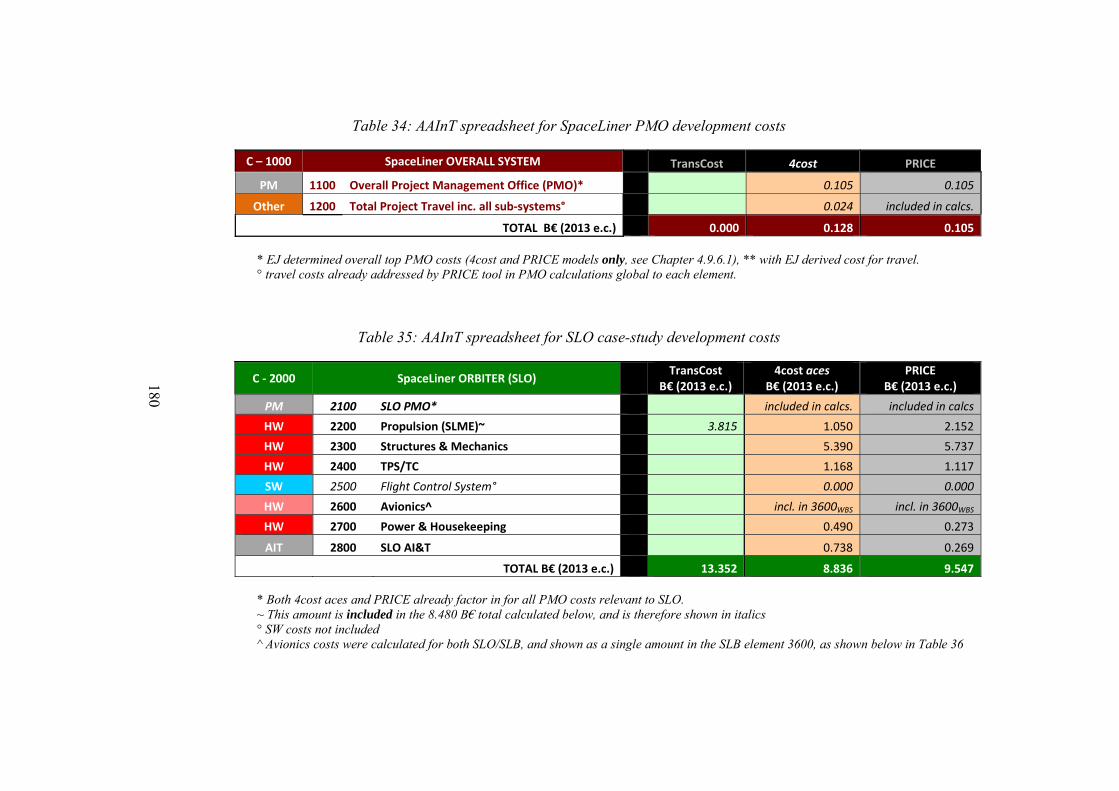
180
Table 34: AAInT spreadsheet for SpaceLiner PMO development costs
C – 1000 SpaceLiner OVERALL SYSTEM TransCost 4cost PRICE
PM 1100 Overall Project Management Office (PMO)* 0.105 0.105
Other 1200 Total Project Travel inc. all sub‐systems° 0.024 included in calcs.
TOTAL B€ (2013 e.c.) 0.000 0.128 0.105
* EJ determined overall top PMO costs (4cost and PRICE models only, see Chapter 4.9.6.1), ** with EJ derived cost for travel. ° travel costs already addressed by PRICE tool in PMO calculations global to each element.
Table 35: AAInT spreadsheet for SLO case-study development costs
C ‐ 2000 SpaceLiner ORBITER (SLO)
TransCostB€ (2013 e.c.)
4cost acesB€ (2013 e.c.)
PRICEB€ (2013 e.c.)
PM 2100 SLO PMO* included in calcs. included in calcs
HW 2200 Propulsion (SLME)~ 3.815 1.050 2.152
HW 2300 Structures & Mechanics 5.390 5.737
HW 2400 TPS/TC 1.168 1.117
SW 2500 Flight Control System° 0.000 0.000
HW 2600 Avionics^ incl. in 3600WBS incl. in 3600WBS
HW 2700 Power & Housekeeping 0.490 0.273
AIT 2800 SLO AI&T 0.738 0.269
TOTAL B€ (2013 e.c.) 13.352 8.836 9.547
* Both 4cost aces and PRICE already factor in for all PMO costs relevant to SLO. ~ This amount is included in the 8.480 B€ total calculated below, and is therefore shown in italics ° SW costs not included ^ Avionics costs were calculated for both SLO/SLB, and shown as a single amount in the SLB element 3600, as shown below in Table 36
181
Table 36: AAInT spreadsheet for SLB case-study development costs
C ‐ 3000 SpaceLiner BOOSTER (SLB)
TransCostB€ (2013 e.c.)
4cost acesB€ (2013 e.c.)
PRICEB€ (2013 e.c.)
PM 3100 SLB PMO* included in calcs. Included in calcs.
HW 3200 Propulsion 0.714 0.850
HW 3300 Structures & Mechanics 6.612 7.267
HW 3400 TPS/TC 1.496 1.212
SW 3500 Flight Control System° 0.000 0.000
HW 3600 Avionics^ 0.348 0.145
HW 3700 Power & Housekeeping 0.903 0.576
AIT 3800 SLB AI&T 0.955 0.417
TOTAL (B€, 2013 e.c.) 10.008 11.029 10.467
*Both 4cost aces and PRICE already factor in for all PMO costs relevant to SLB. ° SW costs not included ^ Costs shown here represent avionics costs for both SLO/SLB.
Table 37: AAInT spreadsheet for SPC case-study development costs
C ‐ 4000 SpaceLiner PASSENGER CABIN /
RESCUE CAPSULE (SPC) TransCost
B€ (2013 e.c.) 4cost aces
B€ (2013 e.c.) PRICE
B€ (2013 e.c.)
PM 4100 SPC PMO* included in calc. included in calc.
HW 4200 Propulsion (CSM capsule solid motors) 0.051 0.086
HW 4300 Structures & Mechanics 0.351 0.364
HW 4400 TPS/TC 0.257 0.380
SW 4500 Flight Control System° 0.000 0.000
HW 4600 Avionics 0.186 0.072
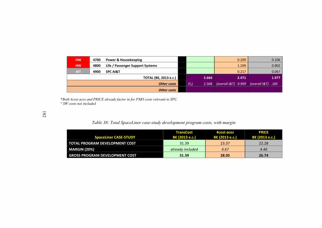
182
HW 4700 Power & Housekeeping 0.209 0.106
HW 4800 Life / Passenger Support Systems 1.209 0.902
AIT 4900 SPC AI&T 0.217 0.067
TOTAL (B€, 2013 e.c.) 5.664 2.471 1.977
Other costs (f0) 2.368 (overall I&T) 0.909 (overall I&T) .185
Other costs
*Both 4cost aces and PRICE already factor in for PMO costs relevant to SPC. ° SW costs not included
Table 38: Total SpaceLiner case-study development program costs, with margin
SpaceLiner CASE‐STUDY TransCost
B€ (2013 e.c.) 4cost aces
B€ (2013 e.c.) PRICE
B€ (2013 e.c.)
TOTAL PROGRAM DEVELOPMENT COST 31.39 23.37 22.28
MARGIN (20%) already included 4.67 4.46
GROSS PROGRAM DEVELOPMENT COST 31.39 28.05 26.74
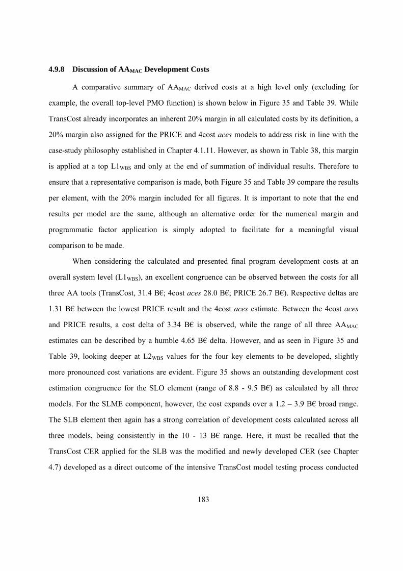
183
4.9.8 Discussion of AAMAC Development Costs
A comparative summary of AAMAC derived costs at a high level only (excluding for
example, the overall top-level PMO function) is shown below in Figure 35 and Table 39. While
TransCost already incorporates an inherent 20% margin in all calculated costs by its definition, a
20% margin also assigned for the PRICE and 4cost aces models to address risk in line with the
case-study philosophy established in Chapter 4.1.11. However, as shown in Table 38, this margin
is applied at a top L1WBS and only at the end of summation of individual results. Therefore to
ensure that a representative comparison is made, both Figure 35 and Table 39 compare the results
per element, with the 20% margin included for all figures. It is important to note that the end
results per model are the same, although an alternative order for the numerical margin and
programmatic factor application is simply adopted to facilitate for a meaningful visual
comparison to be made.
When considering the calculated and presented final program development costs at an
overall system level (L1WBS), an excellent congruence can be observed between the costs for all
three AA tools (TransCost, 31.4 B€; 4cost aces 28.0 B€; PRICE 26.7 B€). Respective deltas are
1.31 B€ between the lowest PRICE result and the 4cost aces estimate. Between the 4cost aces
and PRICE results, a cost delta of 3.34 B€ is observed, while the range of all three AAMAC
estimates can be described by a humble 4.65 B€ delta. However, and as seen in Figure 35 and
Table 39, looking deeper at L2WBS values for the four key elements to be developed, slightly
more pronounced cost variations are evident. Figure 35 shows an outstanding development cost
estimation congruence for the SLO element (range of 8.8 - 9.5 B€) as calculated by all three
models. For the SLME component, however, the cost expands over a 1.2 – 3.9 B€ broad range.
The SLB element then again has a strong correlation of development costs calculated across all
three models, being consistently in the 10 - 13 B€ range. Here, it must be recalled that the
TransCost CER applied for the SLB was the modified and newly developed CER (see Chapter
4.7) developed as a direct outcome of the intensive TransCost model testing process conducted
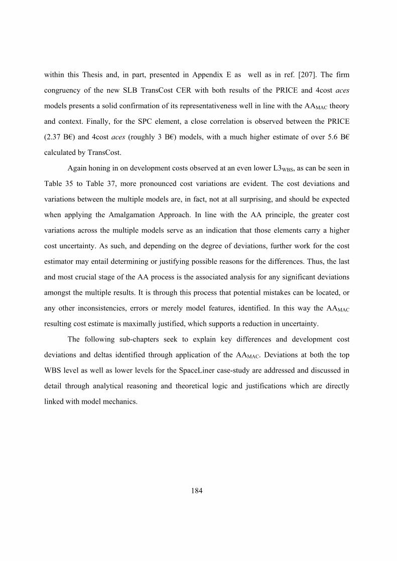
184
within this Thesis and, in part, presented in Appendix E as well as in ref. [207]. The firm
congruency of the new SLB TransCost CER with both results of the PRICE and 4cost aces
models presents a solid confirmation of its representativeness well in line with the AAMAC theory
and context. Finally, for the SPC element, a close correlation is observed between the PRICE
(2.37 B€) and 4cost aces (roughly 3 B€) models, with a much higher estimate of over 5.6 B€
calculated by TransCost.
Again honing in on development costs observed at an even lower L3WBS, as can be seen in
Table 35 to Table 37, more pronounced cost variations are evident. The cost deviations and
variations between the multiple models are, in fact, not at all surprising, and should be expected
when applying the Amalgamation Approach. In line with the AA principle, the greater cost
variations across the multiple models serve as an indication that those elements carry a higher
cost uncertainty. As such, and depending on the degree of deviations, further work for the cost
estimator may entail determining or justifying possible reasons for the differences. Thus, the last
and most crucial stage of the AA process is the associated analysis for any significant deviations
amongst the multiple results. It is through this process that potential mistakes can be located, or
any other inconsistencies, errors or merely model features, identified. In this way the AAMAC
resulting cost estimate is maximally justified, which supports a reduction in uncertainty.
The following sub-chapters seek to explain key differences and development cost
deviations and deltas identified through application of the AAMAC. Deviations at both the top
WBS level as well as lower levels for the SpaceLiner case-study are addressed and discussed in
detail through analytical reasoning and theoretical logic and justifications which are directly
linked with model mechanics.
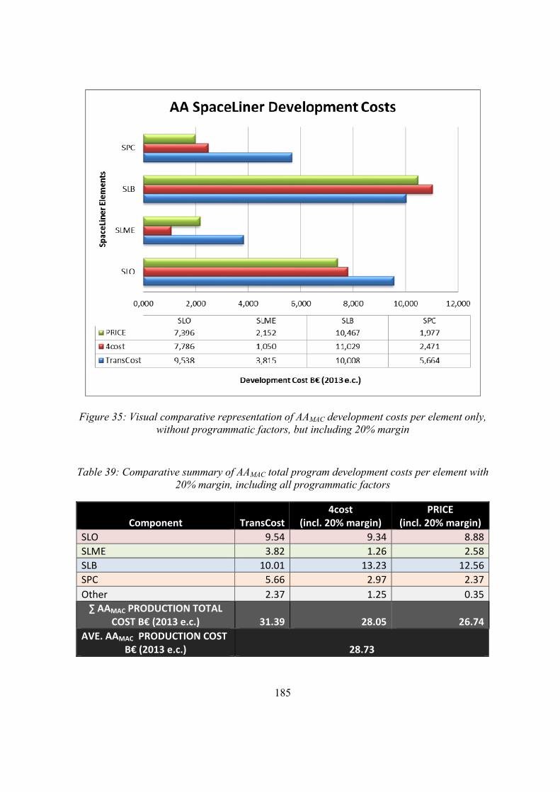
185
Figure 35: Visual comparative representation of AAMAC development costs per element only, without programmatic factors, but including 20% margin
Table 39: Comparative summary of AAMAC total program development costs per element with 20% margin, including all programmatic factors
Component TransCost4cost
(incl. 20% margin) PRICE
(incl. 20% margin)
SLO 9.54 9.34 8.88
SLME 3.82 1.26 2.58
SLB 10.01 13.23 12.56
SPC 5.66 2.97 2.37
Other 2.37 1.25 0.35
∑ AAMAC PRODUCTION TOTAL COST B€ (2013 e.c.) 31.39 28.05 26.74
AVE. AAMAC PRODUCTION COST B€ (2013 e.c.) 28.73

186
4.9.8.1 SLME Development Cost Difference
A key distinction between the 4cost aces and PRICE models relevant to development
effort of engines was that both commercial tools do not take into account the number of test
firings, which is a key cost driver in the simple, top-level TransCost calculation. However, the
models deal with this aspect through other factors, like complexity and environmental
parameters. As such, a direct comparison of factors and their values is impossible. With the
chosen number of test firings entered into the TransCost model (being 1200, based on Space
Shuttle main engine firings of 800 times), the f2 factor is increased to 1.31, resulting in a
respective linear increase to the engine development cost by 31%. For the commercial tools,
however, the increase in required test firings is reflected through complexity values (PLTFM,
MCPLXS and ECMPLX variables for PRICE and ENVIRD, ENGDIF HW and INDEXM for
4cost aces).
4.9.8.2 SPC Development Cost Difference
Once again a significant cost difference exists between TransCost and the highly
congruent PRICE and 4cost aces models for SPC development. This distinction has largely been
described in Chapter 4.1.9, in that TransCost CER data-points refer to capsules like Mercury and
Gemini, which significantly differ to the SpaceLiner SPC, both in purpose, PAX capacity and
lifetime. It is important to note that the TransCost model development cost-driving parameters
includes the number of crew, and the mission lifetime, which is given in days (as seen in Table
23). Needless to say cost variances and the dynamics of the development effort would be
significantly different for a capsule with a 4-6 PAX capacity over several days, to a 50 PAX
cabin over a 90-minute duration. Through extrapolation of a relationship based on description of
the latter, it is not surprising that the SpaceLiner case-study SPC is ultimately over-estimated.
187
4.9.8.3 Variability of Model Mechanics
In addition to specific reasons for cot variation, each cost estimation tool and model has
an own unique structure of cost segmentation, as well as internal model mechanics and inputs and
outputs structure (also see Chapter 2.6.5.2). As such, variability of model mechanics, in part,
would contribute to differences between element costs, especially as observed at the lower WBS
levels. The TransCost model, for example, calculates costs using basic element CERs, after
which the sum of all individual CERs is calculated, and as a last step, programmatic factors
applied. These programmatic complexities address overall system integration, schedule delays,
hierarchy of participating companies within a program with respect to the structure of prime and
sub-prime contractors, as well as the commercial nature of a program. The other two AA
employed tools, PRICE and 4cost, do not necessarily segment their costs in this manner, but
incorporate them in other groupings, and with a different roll-up order and structure across cost
categories. As such, when comparing costs at a very low level of detail, particularly within an
early program phase, variations in costs between different models and tools must always be
expected. It is only when these variations are significant (namely a multiple order of magnitude
inconsistency) that further work and analyses should be conducted to determine why in line with
the AA philosophy introduced previously and outlined in Chapter 2.6.2.
4.9.8.4 Variability in Model Users & EJ Bias
All three 4cost aces, PRICE and TransCost models required utility of EJ at various stages
of the calculating process to arrive at a cost.
The commercial tools, 4cost aces and PRICE, required inputs of various factors and
complexities either generated internally by the software, or as deemed appropriate by the expert
users. For each decision, EJ is relied upon and employed by the model user. Multiple separate,
independent users entered and calibrated data for their respective cost estimation models
throughout the course of the calculations described within this Thesis. As such, it cannot be
188
expected that all users consistently generated identical complexity factors, potentially resulting in
various degrees of EJ bias already described in Chapter 2.4.4. The subjective nature of the EJ
method constitutes a well-known and identified weakness of the EJ approach. In addition, minor
errors and/or fluctuations in EJ concerning determination and assignment of complexity factors,
coupled with case-study system inputs which are themselves estimates, and not fully crystallised,
would also contribute to discrepancies and fluctuations between the two commercial cost models
on a micro-, subsystem and component level.
4.9.8.5 Software Considerations
In the calculations for the SpaceLiner case-study, in line with the SpaceLiner philosophy,
it was decided to exclude software (SW) costs due to an immature specification status within the
program context (see Chapter 4.1.6). This decision, however, has ramifications on the
development and in part, later on production costs. In view of the SpaceLiner case-study being in
the early program phase and approaching maturity in terms of SW considerations in the future,
the SW WBS elements are still included in the WBS to facilitate for future incorporation of costs
once these can be calculated. As such, in the AA representation, the largely software element
2500, 3500 and 4500 fields are shown in italics, also with a zero cost.
Here, it must also be recalled that SW costs were addressed differently by the two
commercial 4cost aces and PRICE tools used for the AA framework. The PRICE-H module of
the PES software did not explicitly calculate SpaceLiner case-study SW costs. If software costs
are required with the PRICE Estimating Suite, the dedicated PRICE-S module is used. Still, this
module requires basic inputs, which, for the SpaceLiner case-study, are unavailable. The 4cost
aces model, however, does calculate basic, global SW development and production costs based
purely on electrical hardware component inputs for the WBS. The aces tool then derives a very
basic, top level, un-calibrated baseline SW estimate in line with the hardware components which
189
require software. Yet although estimated loosely by the 4cost aces tool, the software costs were
excluded as they were seen as being extremely preliminary in nature, and therefore potentially
misrepresentative of true SW costs, and thus introducing uncertainty.
The top system-level TransCost model inherently does incorporate SW costs in its CERs
although at a global level. The segmentation of these SW costs amongst the respective elements,
as well as between development and production cost categories, is embedded within total CER
results, and could not be determined individually.
In recognising that all three models treat SW costs differently, it was necessary to decide
on a logical, defensible and consistent approach to ensure the models were most optimally
comparable. Since SW costs could not be generated accurately and justifiably enough due to
insufficient specification data, it was decided to eliminate the existing SW costs from the 4cost
aces calculation. In this way, both commercial models would then exclude any SW costs,
especially since the resulting numbers would have been speculative and unfounded in any case.
Nevertheless, in view of the SpaceLiner case-study coming to a maturity in terms of SW
considerations in the future, the software elements of the WBS were still factored in for to
facilitate future incorporation of these costs once they can be calculated. As such, in the AA
representation shown in Chapter 4.9.7, the software elements 2500, 3500 and 4500 fields are
shown in italics, and with a zero cost.
Since TransCost SW costs are globally addressed, their segmentation within overall
development and production costs, as already mentioned, could not be determined. Therefore,
although being impossible to quantify, this important distinction must be identified as a
contributing factor to why TransCost may yield higher development (and in fact partially
production costs) than the two commercial models, 4cots aces and PRICE.
190
4.9.9 Development Cost Sensitivities
In extension to the AA utility, and in addition to the sensitivity study already presented
during the process to ascertain a TransCost range in Chapter 4.9.1.3, it was interesting to perform
some sensitivity studies to the baseline case-study configuration. Since the development costs
showed a strong congruence between the two commercial tools, the 4cost aces tool was chosen as
the backbone to initiate some first sensitivity analyses. It was interesting to see overall costs may
be affected through changes to select criteria known to influence development. Two such
variables are the number of prototypes as well as the level of the development team experience.
Both values were augmented to represent a worse-case scenario compared with the baseline, also
congruent with a more conservative approach which is prudent during early program cost
analyses to assist in factoring in for risk and uncertainty.
4.9.9.1 Prototype Quantity
The baseline 5 prototype-model philosophy (Chapter 4.1.3) was subjected to sensitivity
analyses. It is known that during development, one of the most cost-consuming activities is the
number of proto-models produced, which also includes the associated testing and validation of
technology processes. The proto-model quantity was increased to 8 and 10 models. Within a
large, complex aerospace program context, while increasing the number of test model units
would increase the development costs, in the long run, the full-scale and high-fidelity prototypes
could potentially be sold at a discount rate to interested parties after undergoing and passing
necessary certification. So, within a full program LCC context, some monies expended for more
prototype units could be recovered through their consequent sales. Results of the sensitivity are
shown below in Table 40. Quite clearly, an increase in prototype units results in a noticeable cost
increase for the development effort. A 34% increase was observed for a 3-unit increase to the
baseline, with a 56% increase on the baseline for a doubling of prototype units. The results firmly
prove that the prototype quantity is a strong cost driver for the development phase.
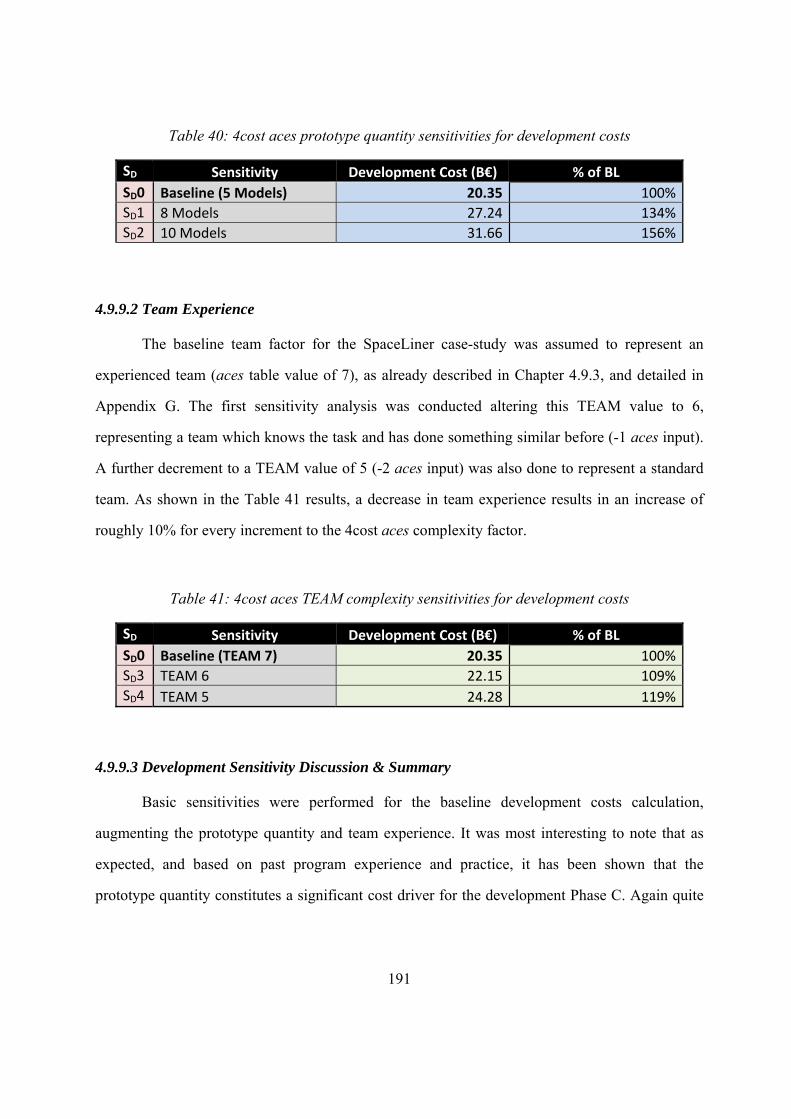
191
Table 40: 4cost aces prototype quantity sensitivities for development costs
SD Sensitivity Development Cost (B€) % of BL
SD0 Baseline (5 Models) 20.35 100%
SD1 8 Models 27.24 134%
SD2 10 Models 31.66 156%
4.9.9.2 Team Experience
The baseline team factor for the SpaceLiner case-study was assumed to represent an
experienced team (aces table value of 7), as already described in Chapter 4.9.3, and detailed in
Appendix G. The first sensitivity analysis was conducted altering this TEAM value to 6,
representing a team which knows the task and has done something similar before (-1 aces input).
A further decrement to a TEAM value of 5 (-2 aces input) was also done to represent a standard
team. As shown in the Table 41 results, a decrease in team experience results in an increase of
roughly 10% for every increment to the 4cost aces complexity factor.
Table 41: 4cost aces TEAM complexity sensitivities for development costs
SD Sensitivity Development Cost (B€) % of BL
SD0 Baseline (TEAM 7) 20.35 100%
SD3 TEAM 6 22.15 109%
SD4 TEAM 5 24.28 119%
4.9.9.3 Development Sensitivity Discussion & Summary
Basic sensitivities were performed for the baseline development costs calculation,
augmenting the prototype quantity and team experience. It was most interesting to note that as
expected, and based on past program experience and practice, it has been shown that the
prototype quantity constitutes a significant cost driver for the development Phase C. Again quite
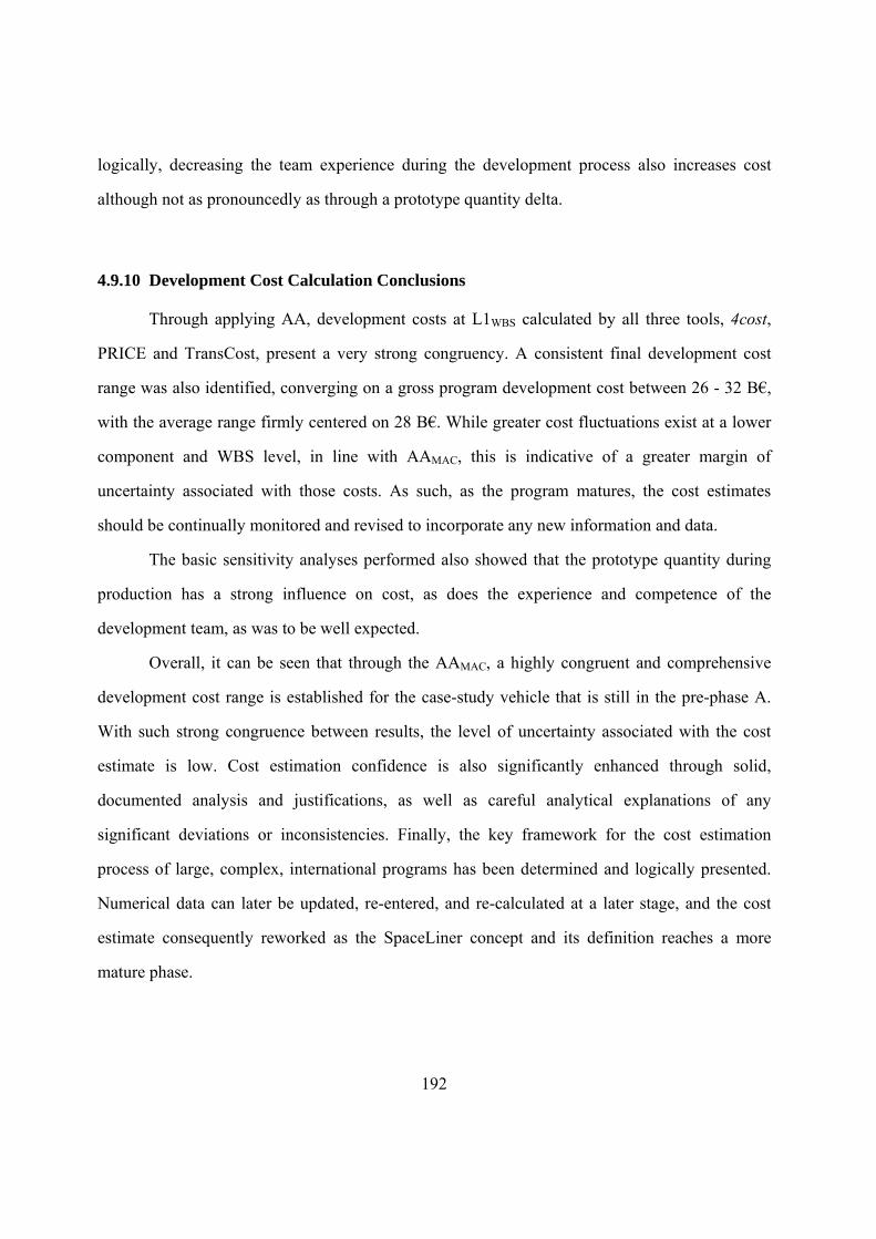
192
logically, decreasing the team experience during the development process also increases cost
although not as pronouncedly as through a prototype quantity delta.
4.9.10 Development Cost Calculation Conclusions
Through applying AA, development costs at L1WBS calculated by all three tools, 4cost,
PRICE and TransCost, present a very strong congruency. A consistent final development cost
range was also identified, converging on a gross program development cost between 26 - 32 B€,
with the average range firmly centered on 28 B€. While greater cost fluctuations exist at a lower
component and WBS level, in line with AAMAC, this is indicative of a greater margin of
uncertainty associated with those costs. As such, as the program matures, the cost estimates
should be continually monitored and revised to incorporate any new information and data.
The basic sensitivity analyses performed also showed that the prototype quantity during
production has a strong influence on cost, as does the experience and competence of the
development team, as was to be well expected.
Overall, it can be seen that through the AAMAC, a highly congruent and comprehensive
development cost range is established for the case-study vehicle that is still in the pre-phase A.
With such strong congruence between results, the level of uncertainty associated with the cost
estimate is low. Cost estimation confidence is also significantly enhanced through solid,
documented analysis and justifications, as well as careful analytical explanations of any
significant deviations or inconsistencies. Finally, the key framework for the cost estimation
process of large, complex, international programs has been determined and logically presented.
Numerical data can later be updated, re-entered, and re-calculated at a later stage, and the cost
estimate consequently reworked as the SpaceLiner concept and its definition reaches a more
mature phase.
193
4.10 PRODUCTION COST ANALYSIS
The process to ascertain the recurring production costs for the SpaceLiner case-study,
featured a similar conformity to the process for development costs. In line with the AA approach,
multiple models were used, being the same three models as for development. Here, the
SpaceLiner philosophy about the qualitative development schedule (see Chapter 4.1.2), the
prototype model logic (Chapter 4.1.3 ) and the element reusability philosophy (Chapter 4.1.8)
were drawn upon and integrated into the calculations in a practical, consistent, numeric and
logical manner.
For the program production Phase D, the cost figure of interest is the cost of the
theoretical first unit (TFU). Furthermore to the TFU cost, it is also interesting to know the total
cost of the overall production batch which, for the SpaceLiner concept was chosen to be a
baseline of 500 units (see Chapter 4.1.7). For such batch production, the learning factor (LC) is a
critical value to model and reflect cost reduction observed from learning in application of
processes during production, as described and quantified in Chapter 4.10.1 below.
4.10.1 Learning Curve Determination
The concept of LCs is applied for uninterrupted manufacturing and assembly tasks to
describe learning for highly repetitive and labour intensive processes [137]. LCs seek to describe
and quantify the typical phenomenon of human performance improvement when activities are
done on a repetitive basis. Here, the time required to perform a task is seen to decrease with
increasing repetitions [201, 202]. From an organisational perspective in particular, and
irrespective of industry, determining the predictability of the learning effect is essential to
underpin estimation of costs during the production phase. Some examples of various LCs in the
engineering industry are shown in Figure 36. If such a learning relationship is identified and
194
plotted on a log-log scale, the result is a straight line reflective of a certain learning percentage,
thus forming the basis of LC estimates, as furthermore shown in Figure 37 [201].
As previously mentioned, in line with the SpaceLiner case-study philosophy established
in Chapter 4.1.2, the production scheme of the SpaceLiner has been assumed to bear a close
resemblance to the aviation sector. As such it is essential to study the production practices of this
particular industry and determine how this correlates with commonly accepted and frequently
assumed space sector LC values.
In literature, it has been proposed that the manufacturer production cost for each series of
aircraft depends on several key considerations including production quantities and the technology
risk [217], with the learning effect of production also being crucial to the recursive production
costs.
Aircraft production size of a fleet has been shown to be directly linked to market research
which determines the break-even point to ensure financial gain for the aircraft or vehicle from a
particular fleet [217]. Here, the assumption of a total production of 500 SpaceLiner units is a
baseline albeit preliminary one, and prone to change in the future as a clearer operational scenario
is established. However, the initial TFU cost range calculated at this stage through application of
AA can be considered to constitute a solid baseline for future incorporation of new information to
reflect program modifications.
The technology risk refers to a cost increase observed at higher Mach numbers [102]. As
such, more expensive materials are required, with the known result that more expensive systems
constitute a larger fraction of empty weight, and consequently increase the airframe cost per unit
weight [217].
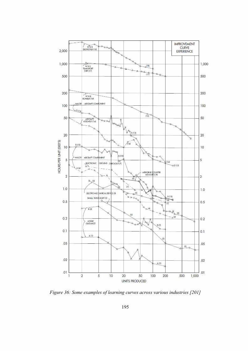
195
Figure 36: Some examples of learning curves across various industries [201]
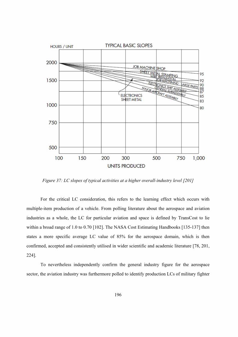
196
Figure 37: LC slopes of typical activities at a higher overall-industry level [201]
For the critical LC consideration, this refers to the learning effect which occurs with
multiple-item production of a vehicle. From polling literature about the aerospace and aviation
industries as a whole, the LC for particular aviation and space is defined by TransCost to lie
within a broad range of 1.0 to 0.70 [102]. The NASA Cost Estimating Handbooks [135-137] then
states a more specific average LC value of 85% for the aerospace domain, which is then
confirmed, accepted and consistently utilised in wider scientific and academic literature [78, 201,
224].
To nevertheless independently confirm the general industry figure for the aerospace
sector, the aviation industry was furthermore polled to identify production LCs of military fighter
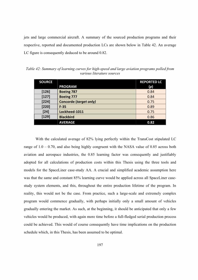
197
jets and large commercial aircraft. A summary of the sourced production programs and their
respective, reported and documented production LCs are shown below in Table 42. An average
LC figure is consequently deduced to be around 0.82.
Table 42: Summary of learning curves for high-speed and large aviation programs polled from various literature sources
SOURCE PROGRAM
REPORTED LC (p)
[126] Boeing 787 0.84
[127] Boeing 777 0.84
[224] Concorde (target only) 0.75
[220] F‐35 0.89
[24] Lockheed‐1011 0.75
[129] Blackbird 0.86
AVERAGE 0.82
With the calculated average of 82% lying perfectly within the TransCost stipulated LC
range of 1.0 – 0.70, and also being highly congruent with the NASA value of 0.85 across both
aviation and aerospace industries, the 0.85 learning factor was consequently and justifiably
adopted for all calculations of production costs within this Thesis using the three tools and
models for the SpaceLiner case-study AA. A crucial and simplified academic assumption here
was that the same and constant 85% learning curve would be applied across all SpaceLiner case-
study system elements, and this, throughout the entire production lifetime of the program. In
reality, this would not be the case. From practice, such a large-scale and extremely complex
program would commence gradually, with perhaps initially only a small amount of vehicles
gradually entering the market. As such, at the beginning, it should be anticipated that only a few
vehicles would be produced, with again more time before a full-fledged serial production process
could be achieved. This would of course consequently have time implications on the production
schedule which, in this Thesis, has been assumed to be optimal.
198
Returning back to the LC value, this is indeed a dynamic figure and, as already seen from
Figure 36 and Figure 37, would vary not only depending on production quantity, but also on the
component or element being produced.
While at this early stage a common and consistent LC of 85% is a sufficient albeit
simplified, academic assumption for the respective level of detail, at a later stage, this would have
to be reassessed and honed in for different elements at lower levels.
4.10.2 TransCost Production Cost Calculation
For the TransCost model structure and for CER application, the top-level SpaceLiner
components, as already presented in Chapter 4.1.1, and as assumed also for production cost
calculation, were taken, being the SLO, SLME, SLB and SPC. Yet, a critical difference between
the development costs and the production costs lies in the fact that while the TransCost model
was an ideal tool suitable for calculating the development costs of the SpaceLiner, for the
production cost group of calculations, no TransCost CERs exist to ideally address all four
SpaceLiner system elements. While suitable CERs exist for the SLME (Liquid Propellant Rocket
Engines CERSpace) and SPC (Crewed Space Systems CERSpace), no dedicated CERs could be
identified for the SLO nor the SLB system elements. The two most relevant CERs were for these
elements were the Winged Orbital Rocket Vehicles and High Speed Aircraft / Winged First Stage
Vehicles CER (CERsAvio), which are clearly more relevant to the aviation segment. An indirect
approach to determine the TFU production cost range was therefore undertaken in order to arrive
at a preliminary yet justifiable cost figure.
The preliminary approach which was undertaken fairly firmly ensures that the resulting
production cost of the SpaceLiner case-study would be within the range of combining a ‘worst-
case’ TransCost scenario which assumes the space-applicable TransCost CERs, as well as a
‘best-case’ scenario, which takes the aviation TransCost CERs. Given the hybrid nature of the
199
SpaceLiner vehicle, the fleet would operate in a regime more congruent with the airline industry
due to the high production quantities and high expected frequency of flights, albeit through utility
of space standard technologies, therefore reducing cost for space access. So given a lack of direct
CERs to describe production for the SLO and SLB, it was rationalised that if both the space and
aviation CERs were applied to SpaceLiner data, the range of values would be an indicative ROM
indication of the expected SLO and SLB production costs. Then, combining and contrasting this
result with the other two results expected from the 4cost aces and PRICE models would further
allow to verify the validity of the figure, or alternatively challenge it.
It is clear that a lower production cost can be expected from the application of the aircraft
CER (CERAvio) while the higher production cost would be derived from the Rocket Vehicle CER
(CERSpace) due to a difference in technical levels and complexity, as well as echelon of
technological standards. The resulting two calculations were taken to be the lower and higher cost
limits, accordingly, for production cost scenarios, and to establish a production cost range.
For the SpaceLiner case-study production cost calculation, the required inputs were:
number of units to be built (1 for TFU; 500 for total program production)
component mass
The TransCost complexity factors which are then applicable to production cost calculation,
included:
f4: learning effect factor
f8: country productivity
f10: cost reduction by past experience
f11: cost reduction through government-free development factor
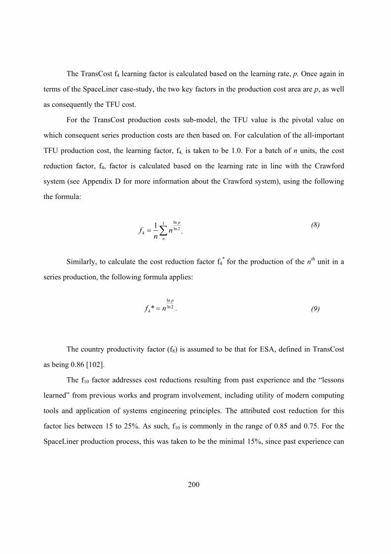
200
.
The TransCost f4 learning factor is calculated based on the learning rate, p. Once again in
terms of the SpaceLiner case-study, the two key factors in the production cost area are p, as well
as consequently the TFU cost.
For the TransCost production costs sub-model, the TFU value is the pivotal value on
which consequent series production costs are then based on. For calculation of the all-important
TFU production cost, the learning factor, f4, is taken to be 1.0. For a batch of n units, the cost
reduction factor, f4, factor is calculated based on the learning rate in line with the Crawford
system (see Appendix D for more information about the Crawford system), using the following
the formula:
1
2ln
ln
4
1
n
p
nn
f (8)
Similarly, to calculate the cost reduction factor f4* for the production of the nth unit in a
series production, the following formula applies:
2ln
ln
4*p
nf . (9)
The country productivity factor (f8) is assumed to be that for ESA, defined in TransCost
as being 0.86 [102].
The f10 factor addresses cost reductions resulting from past experience and the “lessons
learned” from previous works and program involvement, including utility of modern computing
tools and application of systems engineering principles. The attributed cost reduction for this
factor lies between 15 to 25%. As such, f10 is commonly in the range of 0.85 and 0.75. For the
SpaceLiner production process, this was taken to be the minimal 15%, since past experience can
201
be based on the example set from vehicle series production of aircraft from the commercial and
military aviation sector.
The f11 factor applies only to commercial, non-governmental projects which have no
government contracts’ requirements and no customer interference, significantly reducing the high
costs involved with government requirements, procedures requirements and the associated
personnel. TransCost stipulates that without governmental specifications, requirements,
procedures and reporting, a significant saving of 45 – 55% is achievable. The resulting
commercial development cost correction factor f11 is therefore 0.45 – 0.55. For the SpaceLiner
case-study production costs calculation, this value was taken to be the minimal 0.55 to reflect that
the program would be a commercial initiative, and would, therefore, fully maximise the expected
cost benefits associated with such a financing structure.
Here, it must be emphasised, that at this stage, the SpaceLiner case-study is foreseen to be
a commercial venture. However, depending on the actual financing scheme, which may change
from being purely commercial to perhaps a public-private-partnership (PPP) arrangement if this
is more beneficial, the f11 factor may be equally subject to change. As such, it should be revised
in line with any new programmatic developments.
Again, all inputs were entered into the programmed TransCost interface described in
Chapter 4.5.4, with all masses and relevant inputs and complexity factors for the SpaceLiner
case-study which have already been outlined. All entries for production cost of the all-important
TFU to be produced are shown below in Table 43 - Table 48.
By taking the calculation for the worst-case (CERSpace) and best-case (CERAvio) scenarios,
it was possible to find an average case of the two. While it may be argued that certain strategic
weightings may be applied to each of the high-speed aviation and space CERs, at this stage, since
the production CERs are not ideally tailored for the SpaceLiner case-study, the simple,
unweighted and equal average of the two values is deemed a sufficient ROM indicator of the
expected range of production costs. Here, it must be heavily highlighted that due to the latter
202
assumption, the uncertainty associated with the equal 50/50 average approach for two elements
out of four being costed, is therefore transferred into the resulting production cost not only for
each element, but also at the highest and top WBS level.
Consequently, Table 49 - Table 51 present a summary of the three resulting TransCost
scenarios showing the total cost of the TFU for each case, upon which the serial production
reflective of the selected learning curve can be further modeled with a TransCost defined
Crawford learning curve of 85%.
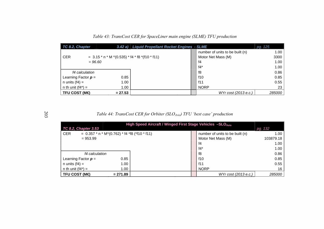
203
Table 43: TransCost CER for SpaceLiner main engine (SLME) TFU production
TC 8.2, Chapter 3.42 a) Liquid Propellant Rocket Engines - SLME pg. 125
number of units to be built (n) 1.00CER = 3.15 * n * M ^(0.535) * f4 * f8 *(f10 * f11) Motor Net Mass (M) 3300 = 96.60 f4 1.00 f4* 1.00
f4 calculation f8 0.86Learning Factor p = 0.85 f10 0.85n units (f4) = 1.00 f11 0.55n th unit (f4*) = 1.00 NORP 23
TFU COST (M€) = 27.53 WYr cost (2013 e.c.) 285000
Table 44: TransCost CER for Orbiter (SLOAvio) TFU ‘best case’ production
TC 8.2, Chapter 3.53 High Speed Aircraft / Winged First Stage Vehicles –SLOAvio
pg. 132 CER = 0.357 * n * M^(0.762) * f4 *f8 (*f10 * f11) number of units to be built (n) 1.00 = 953.99 Motor Net Mass (M) 103879.18 f4 1.00 f4* 1.00
f4 calculation f8 0.86Learning Factor p = 0.85 f10 0.85n units (f4) = 1.00 f11 0.55n th unit (f4*) = 1.00 NORP 16
TFU COST (M€) = 271.89 WYr cost (2013 e.c.) 285000
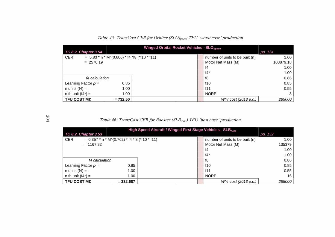
204
Table 45: TransCost CER for Orbiter (SLOSpace) TFU ‘worst case’ production
TC 8.2, Chapter 3.54 Winged Orbital Rocket Vehicles –SLOSpace
pg. 134 CER = 5.83 * n * M^(0.606) * f4 *f8 (*f10 * f11) number of units to be built (n) 1.00 = 2570.19 Motor Net Mass (M) 103879.18 f4 1.00 f4* 1.00
f4 calculation f8 0.86Learning Factor p = 0.85 f10 0.85n units (f4) = 1.00 f11 0.55n th unit (f4*) = 1.00 NORP 3
TFU COST M€ = 732.50 WYr cost (2013 e.c.) 285000
Table 46: TransCost CER for Booster (SLBAvio) TFU ‘best case’ production
TC 8.2, Chapter 3.53 High Speed Aircraft / Winged First Stage Vehicles - SLBAvio
pg. 132 CER = 0.357 * n * M^(0.762) * f4 *f8 (*f10 * f11) number of units to be built (n) 1.00 = 1167.32 Motor Net Mass (M) 135379 f4 1.00 f4* 1.00
f4 calculation f8 0.86Learning Factor p = 0.85 f10 0.85n units (f4) = 1.00 f11 0.55n th unit (f4*) = 1.00 NORP 16
TFU COST M€ = 332.687 WYr cost (2013 e.c.) 285000
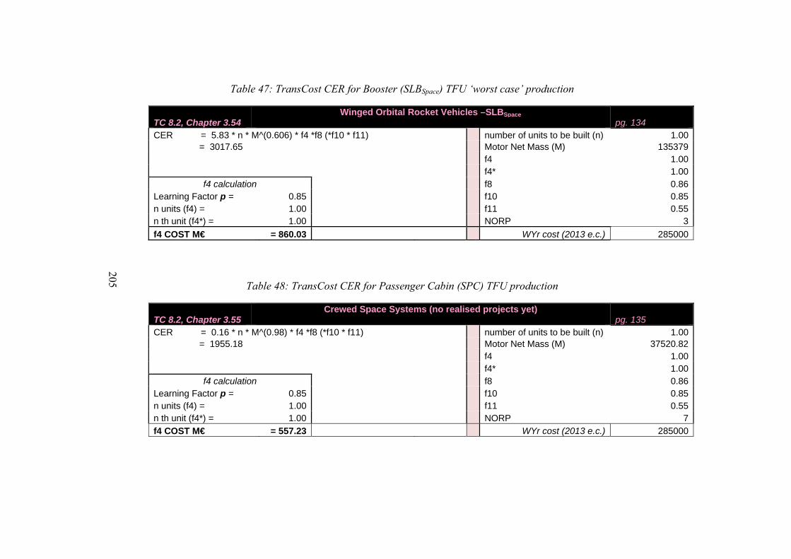
205
Table 47: TransCost CER for Booster (SLBSpace) TFU ‘worst case’ production
TC 8.2, Chapter 3.54 Winged Orbital Rocket Vehicles –SLBSpace
pg. 134 CER = 5.83 * n * M^(0.606) * f4 *f8 (*f10 * f11) number of units to be built (n) 1.00 = 3017.65 Motor Net Mass (M) 135379
f4 1.00 f4* 1.00
f4 calculation f8 0.86Learning Factor p = 0.85 f10 0.85n units (f4) = 1.00 f11 0.55n th unit (f4*) = 1.00 NORP 3
f4 COST M€ = 860.03 WYr cost (2013 e.c.) 285000
Table 48: TransCost CER for Passenger Cabin (SPC) TFU production
TC 8.2, Chapter 3.55 Crewed Space Systems (no realised projects yet)
pg. 135 CER = 0.16 * n * M^(0.98) * f4 *f8 (*f10 * f11) number of units to be built (n) 1.00 = 1955.18 Motor Net Mass (M) 37520.82
f4 1.00 f4* 1.00
f4 calculation f8 0.86Learning Factor p = 0.85 f10 0.85n units (f4) = 1.00 f11 0.55n th unit (f4*) = 1.00 NORP 7
f4 COST M€ = 557.23 WYr cost (2013 e.c.) 285000
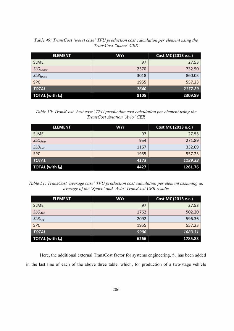
206
Table 49: TransCost ‘worst case’ TFU production cost calculation per element using the TransCost ‘Space’ CER
ELEMENT WYr Cost M€ (2013 e.c.)
SLME 97 27.53
SLOSpace 2570 732.50
SLBSpace 3018 860.03
SPC 1955 557.23
TOTAL 7640 2177.29
TOTAL (with f0) 8105 2309.89
Table 50: TransCost ‘best case’ TFU production cost calculation per element using the TransCost Aviation ‘Avio’ CER
ELEMENT WYr Cost M€ (2013 e.c.)
SLME 97 27.53
SLOAvio 954 271.89
SLBAvio 1167 332.69
SPC 1955 557.23
TOTAL 4173 1189.33
TOTAL (with f0) 4427 1261.76
Table 51: TransCost ‘average case’ TFU production cost calculation per element assuming an average of the ‘Space’ and ‘Avio’ TransCost CER results
ELEMENT WYr Cost M€ (2013 e.c.)
SLME 97 27.53
SLOAve 1762 502.20
SLBAve 2092 596.36
SPC 1955 557.23
TOTAL 5906 1683.31
TOTAL (with f0) 6266 1785.83
Here, the additional external TransCost factor for systems engineering, f0, has been added
in the last line of each of the above three table, which, for production of a two-stage vehicle
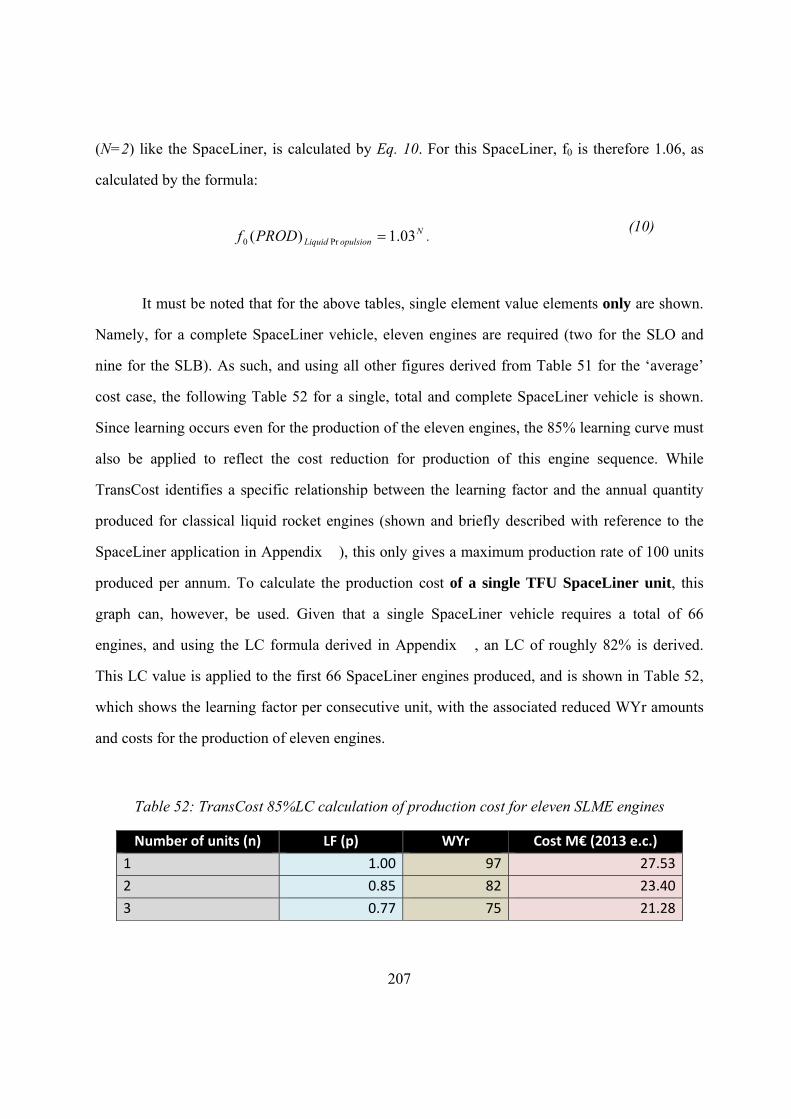
207
(N=2) like the SpaceLiner, is calculated by Eq. 10. For this SpaceLiner, f0 is therefore 1.06, as
calculated by the formula:
NopulsionLiquidPRODf 03.1)( Pr0 .
(10)
It must be noted that for the above tables, single element value elements only are shown.
Namely, for a complete SpaceLiner vehicle, eleven engines are required (two for the SLO and
nine for the SLB). As such, and using all other figures derived from Table 51 for the ‘average’
cost case, the following Table 52 for a single, total and complete SpaceLiner vehicle is shown.
Since learning occurs even for the production of the eleven engines, the 85% learning curve must
also be applied to reflect the cost reduction for production of this engine sequence. While
TransCost identifies a specific relationship between the learning factor and the annual quantity
produced for classical liquid rocket engines (shown and briefly described with reference to the
SpaceLiner application in Appendix �), this only gives a maximum production rate of 100 units
produced per annum. To calculate the production cost of a single TFU SpaceLiner unit, this
graph can, however, be used. Given that a single SpaceLiner vehicle requires a total of 66
engines, and using the LC formula derived in Appendix �, an LC of roughly 82% is derived.
This LC value is applied to the first 66 SpaceLiner engines produced, and is shown in Table 52,
which shows the learning factor per consecutive unit, with the associated reduced WYr amounts
and costs for the production of eleven engines.
Table 52: TransCost 85%LC calculation of production cost for eleven SLME engines
Number of units (n) LF (p) WYr Cost M€ (2013 e.c.)
1 1.00 97 27.53
2 0.85 82 23.40
3 0.77 75 21.28
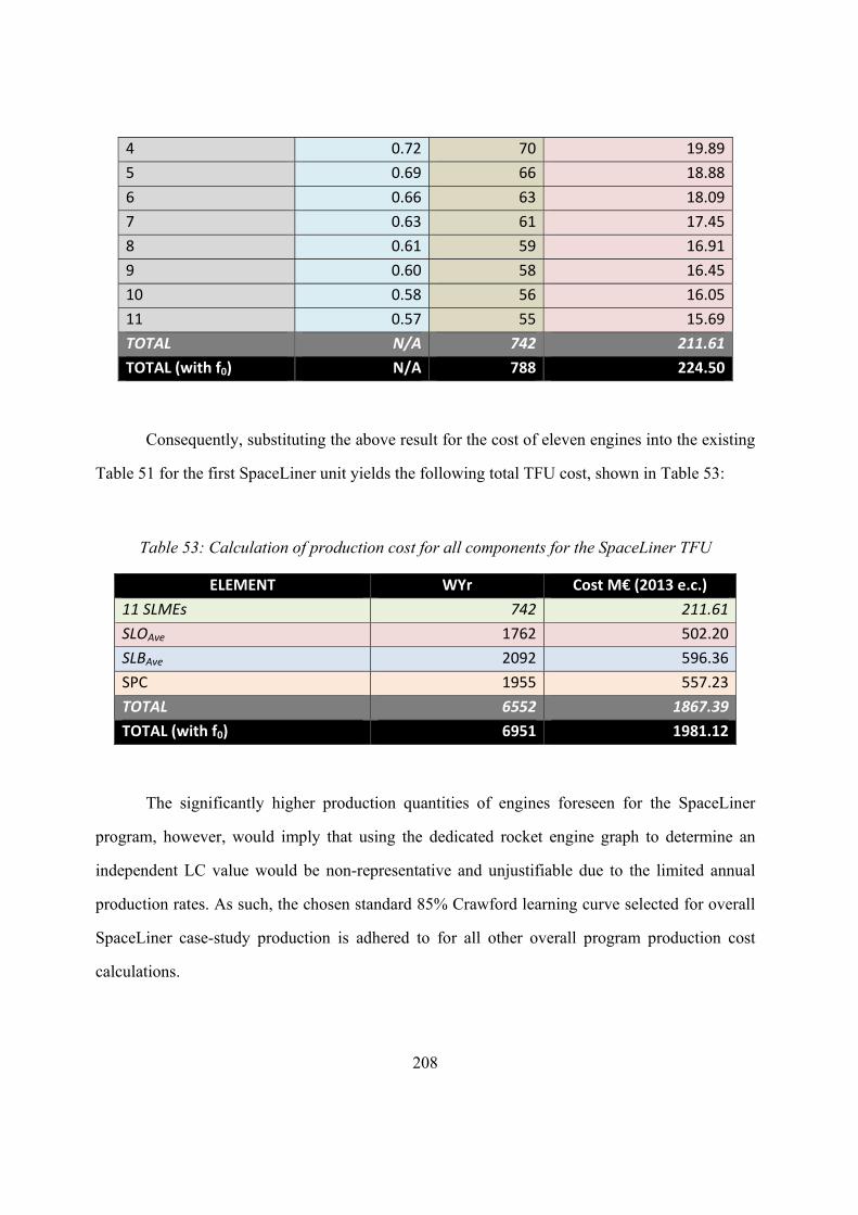
208
4 0.72 70 19.89
5 0.69 66 18.88
6 0.66 63 18.09
7 0.63 61 17.45
8 0.61 59 16.91
9 0.60 58 16.45
10 0.58 56 16.05
11 0.57 55 15.69
TOTAL N/A 742 211.61
TOTAL (with f0) N/A 788 224.50
Consequently, substituting the above result for the cost of eleven engines into the existing
Table 51 for the first SpaceLiner unit yields the following total TFU cost, shown in Table 53:
Table 53: Calculation of production cost for all components for the SpaceLiner TFU
ELEMENT WYr Cost M€ (2013 e.c.)
11 SLMEs 742 211.61
SLOAve 1762 502.20
SLBAve 2092 596.36
SPC 1955 557.23
TOTAL 6552 1867.39
TOTAL (with f0) 6951 1981.12
The significantly higher production quantities of engines foreseen for the SpaceLiner
program, however, would imply that using the dedicated rocket engine graph to determine an
independent LC value would be non-representative and unjustifiable due to the limited annual
production rates. As such, the chosen standard 85% Crawford learning curve selected for overall
SpaceLiner case-study production is adhered to for all other overall program production cost
calculations.
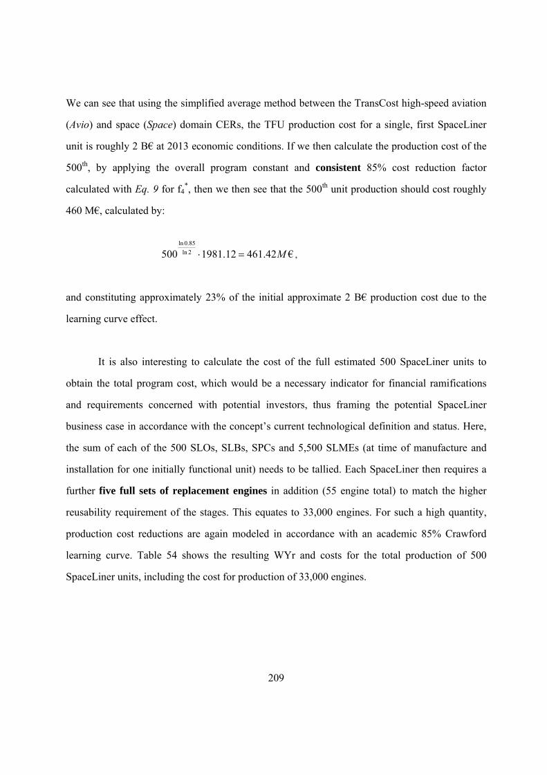
209
We can see that using the simplified average method between the TransCost high-speed aviation
(Avio) and space (Space) domain CERs, the TFU production cost for a single, first SpaceLiner
unit is roughly 2 B€ at 2013 economic conditions. If we then calculate the production cost of the
500th, by applying the overall program constant and consistent 85% cost reduction factor
calculated with Eq. 9 for f4*, then we then see that the 500th unit production should cost roughly
460 M€, calculated by:
€42.46112.1981500 2ln
85.0ln
M ,
and constituting approximately 23% of the initial approximate 2 B€ production cost due to the
learning curve effect.
It is also interesting to calculate the cost of the full estimated 500 SpaceLiner units to
obtain the total program cost, which would be a necessary indicator for financial ramifications
and requirements concerned with potential investors, thus framing the potential SpaceLiner
business case in accordance with the concept’s current technological definition and status. Here,
the sum of each of the 500 SLOs, SLBs, SPCs and 5,500 SLMEs (at time of manufacture and
installation for one initially functional unit) needs to be tallied. Each SpaceLiner then requires a
further five full sets of replacement engines in addition (55 engine total) to match the higher
reusability requirement of the stages. This equates to 33,000 engines. For such a high quantity,
production cost reductions are again modeled in accordance with an academic 85% Crawford
learning curve. Table 54 shows the resulting WYr and costs for the total production of 500
SpaceLiner units, including the cost for production of 33,000 engines.
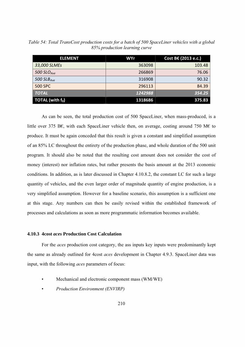
210
Table 54: Total TransCost production costs for a batch of 500 SpaceLiner vehicles with a global 85% production learning curve
ELEMENT WYr Cost B€ (2013 e.c.)
33,000 SLMEs 363098 103.48
500 SLOAve 266869 76.06
500 SLBAve 316908 90.32
500 SPC 296113 84.39
TOTAL 1242988 354.25
TOTAL (with f0) 1318686 375.83
As can be seen, the total production cost of 500 SpaceLiner, when mass-produced, is a
little over 375 B€, with each SpaceLiner vehicle then, on average, costing around 750 M€ to
produce. It must be again conceded that this result is given a constant and simplified assumption
of an 85% LC throughout the entirety of the production phase, and whole duration of the 500 unit
program. It should also be noted that the resulting cost amount does not consider the cost of
money (interest) nor inflation rates, but rather presents the basis amount at the 2013 economic
conditions. In addition, as is later discussed in Chapter 4.10.8.2, the constant LC for such a large
quantity of vehicles, and the even larger order of magnitude quantity of engine production, is a
very simplified assumption. However for a baseline scenario, this assumption is a sufficient one
at this stage. Any numbers can then be easily revised within the established framework of
processes and calculations as soon as more programmatic information becomes available.
4.10.3 4cost aces Production Cost Calculation
For the aces production cost category, the ass inputs key inputs were predominantly kept
the same as already outlined for 4cost aces development in Chapter 4.9.3. SpaceLiner data was
input, with the following aces parameters of focus:
• Mechanical and electronic component mass (WM/WE)
• Production Environment (ENVIRP)
211
• Electronics/Mechanical index (INDEXE/M)
• Production quantity (QTY)
• Production Start (STARTPD)
Inputs which were new or different to those already described for the 4cost aces
development cost calculations, are shown in italics. The aces model computes production costs
using the INDEXE/M values weight, and the environment (ENVIRP) as main inputs. The
INDEXE/M parameters are already introduced in the development Chapter 4.9.3, and their values
remain the same, although a reiteration of the input function within context of the production
effort is highlighted. Of course other inputs such as production quantity (500 SpaceLiner units,
33,000 SLMEs), and the learning curve value, which was fixed at 0.85 for all AA processes. The
ideal production starting date was also an input, although this was generated by the 4cost aces
software based on the output of the development schedule. The key parameters which are unique
or different from inputs already detailed for the development cost calculation, are described and
quantified below:
• Production Environment (ENVIRP)
Upon discussion with experts, ENVIRP was chosen to be 1.8 (see Figure 33). This is a
lower value than that for development, since production of the SpaceLiner fleet is anticipated to
follow an aviation model due to large production quantities. This factor value is therefore
exclusive to the “Aircraft” section, under “commercial” projects. A higher sensitivity analyses
limit was defined as being 2.5, to see how this would affect the overall calculated cost.
• Electronics/Mechanical Index (INDEXE/M)
As previously introduced for development, INDEXE/M is the technology index for
electronics (INDEXE) and mechanics (INDEXM). Both inputs are used to calculate element TFU
212
costs for production, and reflect the cost of more stringent reliability requirements associated
with most extreme operating environments. Values were generated from internal INDEXE/M
tables.
• Production Quantity (QTY)
The production quantity, in line with the SpaceLiner case-study philosophy outlined in
Chapter 4.1.7, was SpaceLiner 500 units, and therefore also 33,000 SLMEs. Production cost was
assumed to be for acquisition of a SpaceLiner unit, as well as the required replacement engines to
ensure a common life-time for all SpaceLiner vehicle components. Since the lifetime of the
engines is expected to be shorter than that for the SpaceLiner stages and passenger cabin/rescue
capsule, more engine units are therefore required.
• Start of Production (STARTPD)
This STARTPD input determines when the production effort begins, in months and years.
This input can be manually entered, or can be generated by the 4cost aces software to formulate
an optimal schedule, the latter being the case for the SpaceLiner case-study application, and was
given as commencing in December, 2029.
The production costs as calculated by the 4cost aces tool (found in the ModAmuc3
column in Table 126 in Appendix H) represent the basis production cost of the full batch of 500
SpaceLiner vehicles, including 25% for general and administrative (G&A) costs and a further
10% fee and profit allowance. While by definition ModAmuc3 also contains a SW production
component, in line with the SW philosophy adopted for this Thesis and outlined in Chapter 4.1.6,
this SW element was subtracted out of the costs. The TFU cost, while not being focal for the
purposes of this study, is nevertheless shown in the column T1ModT1 of Appendix H for data
completeness.
213
4.10.4 PRICE Production Cost Calculation
For the PRICE tool production cost calculation, the required key inputs for production
cost calculations are shown below:
• Structural and electronic component mass (WS/WT)
• Platform Value (PLTFM)
• Manufacturing Complexity (MCPLXS/E)
• Learning Curve (Materials / Labour)
• Year of technology (YRTECH)
• Production quantity (QTY)
• Production start (PSTART)
The mass inputs were kept the same as already presented for PRICE development
estimation in Chapter 4.9.4, while inputs in italics highlight new parameters or information
specific to production, and are therefore briefly described below:
• PLTFM
For the SpaceLiner case study, this value was chosen to be 1.8, in line with the
philosophy that the SpaceLiner production resembles more that of the aviation industry. The only
exception here was made for production of the engines, which are, nevertheless, rocket engines,
where, upon extensive consultation with space programmatic experts as well as PRICE user
experts, the PLTFM was set at a higher value of 2.0.
• MCPLXS/E
The MCPLXS/E values for all components were adjusted in accordance with Peter
Korda’s formula for manufacturing complexity, which stipulates that the PLTFM value is a
214
defining parameter [53]. Here, when the PLTFM value is arbitrarily set, then the MCPLX values
should also be adjusted accordingly (for the case of the SpaceLiner case-study, the values were
lowered). Hence, this was done manually for all elements affected. The engine complexity,
however, was kept the same to address the stringent reusability and operational safety
requirements, resulting in a higher level of complexity.
• Learning Curve
The learning curve was set at 85%, in line with the LC philosophy developed and
described in Chapter 4.10.1.
• Production Start
The PRICE software calculated the optimal starting time for production, based on
optimal development timeframe which had already been calculated. The production start date was
given as being January, 2032.
The production costs resulting from the PRICE software also show the total production
cost for 500 SpaceLiner units (also including similar 25% G&A and 10% additional fees and
profit margins, in line with the same values input for the 4cost tool), in the column entitled
MANUFACTURING_PROD_Total found in Table 130 of Appendix I. The Unit Production Cost
(UPC) column the shows the calculated average production cost per unit, which can be derived
by dividing the total cost by the total number of production units. Consequently, the
AMORTIZED_UNIT_COST column is then calculated to show the average cost per unit, while
also including costs for production engineering, production manufacturing, and production
tooling and test for the component being modelled. Another column called
AMORTIZED_UNIT_COST_TOT* has also been included. The definition of the values here are
identical to the values of AMORTIZED_UNIT_COST, except that a significant cost increase can
215
be seen for WBS elements 2200 and 3200, to account for not only the original eleven engines per
vehicle, but also the consequent additional 55 engines to ensure that all SpaceLiner vehicle
components have a common 150 times reusability capability.
The TFU costs are then shown in the column T1_COST, is influenced by the PRICE Unit
Learning Curve (ULC), selected and set to be a fixed 85%, and the Development Cost Multiplier
(DMULT) which is used to include markups for G&A, for example. Again, however, unlike for
the TransCost calculation, the commercial PRICE model TFU value is not interesting for the
purposes of this study, as will be further outlined later in Chapter 4.10.7. The TFU values are
nevertheless included rather for the sake of data completeness.
In addition, Table 130 of Appendix I also includes the separate and segmented cost
components calculated by the PRICE tool for manufacturing, program management and
engineering efforts during the production phase.
4.10.5 Optimal Production Timeframe
For both commercial 4cost aces and PRICE software tools, an optimal production
timeframe was calculated on the basis that an optimal schedule of activities and task execution
were assumed. TransCost yielded no scheduling results as per its definition of a top level cost
estimation model only.
The optimal duration of the PRICE tool production phase is a parameter which was
automatically calculated by the PRICE-H model. This is influenced by other model inputs and
factors, including equipment complexity, PLTFM and ECMPLX values, and results in an
optimised cost, thus avoiding penalties by enforcing an artificial timeframe. For the SpaceLiner
case-study, this was found to be 127 months, commencing in January, 2032 and continuing
through until the end of July, 2042. This logic is repeated in the 4cost aces optimal production
216
duration, which his heavily influenced by key factors including the electrical and mechanical
complexities (INDEXE/M) and the environment ENVIRP factor, amongst others, and resulted in
a production timeframe of 116 months, beginning in December 2029, and finishing in July of
2039. Both software tools are highly congruent in their estimation, of roughly 10 years for
production.
For both models, the optimal production timeframe assumes no delays, resulting in a very
optimistic and rather idyllic scenario of a development phase with no delays. In reality, for a
program as large and complex as the SpaceLiner case-study would be, the timeframe would also
be dictated not only by technical capabilities, but also by other aspects including politics,
economics and financing not under program management influence, as has already been
discussed in Chapter 4.9.6.1 for program development. Similarly for production, program delays
would almost certainly be evident during program execution especially for an undertaking of
such complexity and expanse as the SpaceLiner. This would be a point for further analysis and
dissemination as more program information crystallises and becomes available. However, it can
be assumed with a high degree of certainty that the production process, being even longer than
the development phase, would also extend well beyond the more extreme 127 months as
calculated by the PRICE software. Applying a margin of 50% at this early program stage, and in
consultation with project management experts, based on calculation, a baseline preliminary
timeframe of 15 years for the production effort was therefore assumed.
4.10.6 Production Project Management Office Cost Estimation
Similarly as for the development cost estimation, while all three AA models already
factor in for PMO cost on an element level, the top WBS element 1100 PMO cost for production
had to be estimated separately for both the commercial 4cost aces and PRICE models as it was
not taken into account.
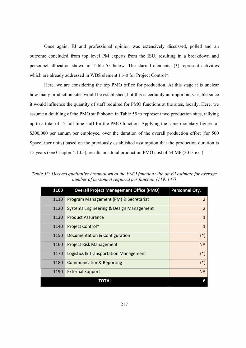
217
Once again, EJ and professional opinion was extensively discussed, polled and an
outcome concluded from top level PM experts from the ISU, resulting in a breakdown and
personnel allocation shown in Table 55 below. The starred elements, (*) represent activities
which are already addressed in WBS element 1140 for Project Control*.
Here, we are considering the top PMO office for production. At this stage it is unclear
how many production sites would be established, but this is certainly an important variable since
it would influence the quantity of staff required for PMO functions at the sites, locally. Here, we
assume a doubling of the PMO staff shown in Table 55 to represent two production sites, tallying
up to a total of 12 full-time staff for the PMO function. Applying the same monetary figures of
$300,000 per annum per employee, over the duration of the overall production effort (for 500
SpaceLiner units) based on the previously established assumption that the production duration is
15 years (see Chapter 4.10.5), results in a total production PMO cost of 54 M€ (2013 e.c.).
Table 55: Derived qualitative break-down of the PMO function with an EJ estimate for average number of personnel required per function [119, 147]
1100 Overall Project Management Office (PMO) Personnel Qty.
1110 Program Management (PM) & Secretariat 2
1120 Systems Engineering & Design Management 2
1130 Product Assurance 1
1140 Project Control* 1
1150 Documentation & Configuration (*)
1160 Project Risk Management NA
1170 Logistics & Transportation Management (*)
1180 Communication& Reporting (*)
1190 External Support NA
TOTAL 6
218
4.10.7 Production Amalgamation Approach Results
With all production cost element fields being complete, the cost results for the overall
program costs as well as the average costs per unit value were determined. Once again using the
powerful AA interface, the results could be contrasted with each other in line with the AA
philosophy. While for TransCost model the TFU value was very important on which to base the
cost of all consequent production units from, for both commercial tools, due to the imposed and
fixed LC value high production quantities for a complex space sector program, the TFU values,
which are highly dependent on both the chosen LC value (which in this instance, was
synthetically and externally imposed) were non-focal. For both PRICE and 4cost aces advanced
internal software mechanics, the TFU (T1) value is treated, quite logically, as a direct function of
the manufacturing process, hinging also on the proposed LC and production quantity. The
TransCost model assumes a mire simplified approach here, where any differences in the
manufacturing process having no influence on the TFU value. Arguably, this may not be
representative of reality, as has been demonstrated in learning curve theory and shown in practice
[1, 154]. As such, the T1 values were deemed unimportant and largely irrelevant within the
context of this cost analyses. Instead, here the two key figures of interest were the total program
production cost, as well as the average unit cost for production of 500 SpaceLiner case-study
vehicles as calculated by each AA model and tool. Summarised tables of results are directly from
the AAInT Excel interface already described in Chapters 2.6.2.2 and 4.8.1. The first PMO Table
56 is applicable to the entire production phase, assumed to be 15 years, as already presented in
Chapter 4.10.6. All further tables then show the costs for the three SpaceLiner elements (SLO,
SLB, SPC). As previously noted for development costs, once again the top-level TransCost
model presents production costs at a top L2WBS, while the PRICE and 4cost models present their
costs at the lower sub-system and component levels 3 and 4.
Additionally, and similar to the development AAInT spreadsheet, Table 88 contains an
extra row for “Other costs” used to apply the TransCost top level engineering factor, f0,
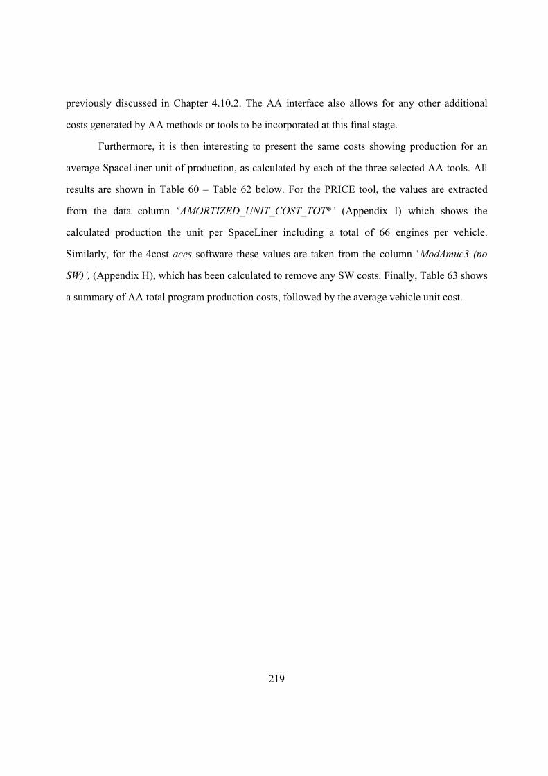
219
previously discussed in Chapter 4.10.2. The AA interface also allows for any other additional
costs generated by AA methods or tools to be incorporated at this final stage.
Furthermore, it is then interesting to present the same costs showing production for an
average SpaceLiner unit of production, as calculated by each of the three selected AA tools. All
results are shown in Table 60 – Table 62 below. For the PRICE tool, the values are extracted
from the data column ‘AMORTIZED_UNIT_COST_TOT*’ (Appendix I) which shows the
calculated production the unit per SpaceLiner including a total of 66 engines per vehicle.
Similarly, for the 4cost aces software these values are taken from the column ‘ModAmuc3 (no
SW)’, (Appendix H), which has been calculated to remove any SW costs. Finally, Table 63 shows
a summary of AA total program production costs, followed by the average vehicle unit cost.
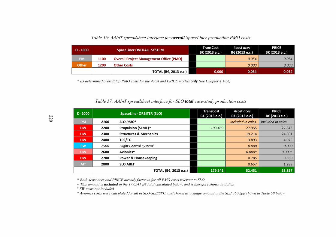
220
Table 56: AAInT spreadsheet interface for overall SpaceLiner production PMO costs
D ‐ 1000 SpaceLiner OVERALL SYSTEM
TransCostB€ (2013 e.c.)
4cost acesB€ (2013 e.c.)
PRICEB€ (2013 e.c.)
PM 1100 Overall Project Management Office (PMO) 0.054 0.054
Other 1200 Other Costs 0.000 0.000
TOTAL (B€, 2013 e.c.) 0,000 0.054 0.054
* EJ determined overall top PMO costs for the 4cost and PRICE models only (see Chapter 4.10.6)
Table 57: AAInT spreadsheet interface for SLO total case-study production costs
D‐ 2000 SpaceLiner ORBITER (SLO) TransCost
B€ (2013 e.c.) 4cost aces
B€ (2013 e.c.) PRICE
B€ (2013 e.c.)
PM 2100 SLO PMO* included in calcs. included in calcs.
HW 2200 Propulsion (SLME)~ 103.483 27.955 22.843
HW 2300 Structures & Mechanics 19.214 24.801
HW 2400 TPS/TC 3.893 4.075
SW 2500 Flight Control System° 0.000 0.000
HW 2600 Avionics^ 0.000^ 0.000^
HW 2700 Power & Housekeeping 0.785 0.850
AIT 2800 SLO AI&T 0.657 1.289
TOTAL (B€, 2013 e.c.) 179.541 52.451 53.857
* Both 4cost aces and PRICE already factor in for all PMO costs relevant to SLO. ~ This amount is included in the 179.541 B€ total calculated below, and is therefore shown in italics ° SW costs not included ^ Avionics costs were calculated for all of SLO/SLB/SPC, and shown as a single amount in the SLB 3600WBS shown in Table 58 below
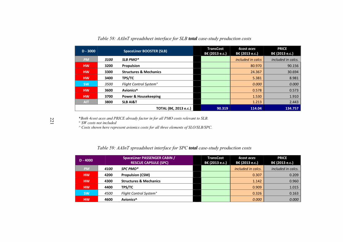
221
Table 58: AAInT spreadsheet interface for SLB total case-study production costs
D ‐ 3000 SpaceLiner BOOSTER (SLB) TransCost
B€ (2013 e.c.) 4cost aces
B€ (2013 e.c.) PRICE
B€ (2013 e.c.)
PM 3100 SLB PMO* included in calcs included in calcs.
HW 3200 Propulsion 80.970 90.156
HW 3300 Structures & Mechanics 24.367 30.694
HW 3400 TPS/TC 5.381 8.981
SW 3500 Flight Control System° 0.000 0.000
HW 3600 Avionics^ 0.578 0.573
HW 3700 Power & Housekeeping 1.530 1.910
AIT 3800 SLB AI&T 1.213 2.443
TOTAL (B€, 2013 e.c.) 90.319 114.04 134.757
*Both 4cost aces and PRICE already factor in for all PMO costs relevant to SLB. ° SW costs not included ^ Costs shown here represent avionics costs for all three elements of SLO/SLB/SPC.
Table 59: AAInT spreadsheet interface for SPC total case-study production costs
D ‐ 4000 SpaceLiner PASSENGER CABIN /
RESCUE CAPSULE (SPC) TransCost
B€ (2013 e.c.) 4cost aces
B€ (2013 e.c.) PRICE
B€ (2013 e.c.)
PM 4100 SPC PMO* included in calcs. included in calcs.
HW 4200 Propulsion (CSM) 0.307 0.209
HW 4300 Structures & Mechanics 1.142 0.960
HW 4400 TPS/TC 0.909 1.015
SW 4500 Flight Control System° 0.326 0.163
HW 4600 Avionics^ 0.000 0.000
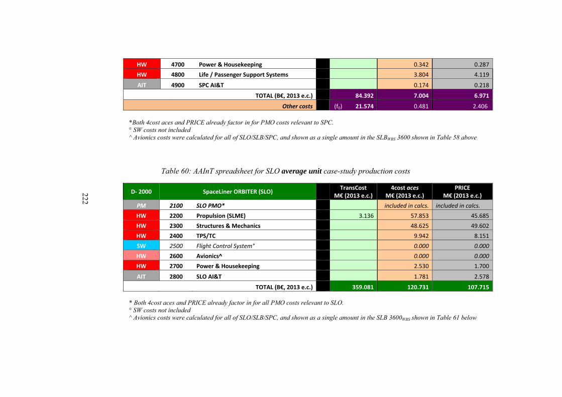
222
HW 4700 Power & Housekeeping 0.342 0.287
HW 4800 Life / Passenger Support Systems 3.804 4.119
AIT 4900 SPC AI&T 0.174 0.218
TOTAL (B€, 2013 e.c.) 84.392 7.004 6.971
Other costs (f0) 21.574 0.481 2.406
*Both 4cost aces and PRICE already factor in for PMO costs relevant to SPC. ° SW costs not included ^ Avionics costs were calculated for all of SLO/SLB/SPC, and shown as a single amount in the SLBWBS 3600 shown in Table 58 above
Table 60: AAInT spreadsheet for SLO average unit case-study production costs
D‐ 2000 SpaceLiner ORBITER (SLO) TransCost
M€ (2013 e.c.) 4cost aces
M€ (2013 e.c.) PRICE
M€ (2013 e.c.)
PM 2100 SLO PMO* included in calcs. included in calcs.
HW 2200 Propulsion (SLME) 3.136 57.853 45.685
HW 2300 Structures & Mechanics 48.625 49.602
HW 2400 TPS/TC 9.942 8.151
SW 2500 Flight Control System° 0.000 0.000
HW 2600 Avionics^ 0.000 0.000
HW 2700 Power & Housekeeping 2.530 1.700
AIT 2800 SLO AI&T 1.781 2.578
TOTAL (B€, 2013 e.c.) 359.081 120.731 107.715
* Both 4cost aces and PRICE already factor in for all PMO costs relevant to SLO. ° SW costs not included ^ Avionics costs were calculated for all of SLO/SLB/SPC, and shown as a single amount in the SLB 3600WBS shown in Table 61 below
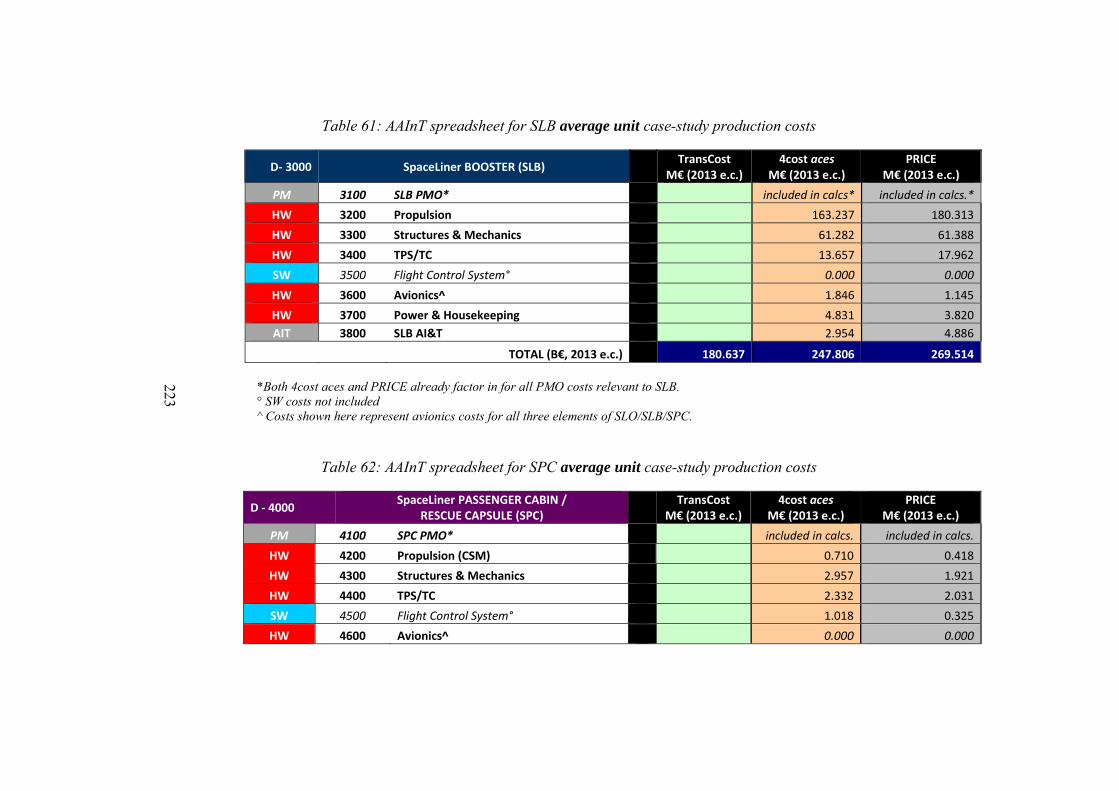
223
Table 61: AAInT spreadsheet for SLB average unit case-study production costs
D‐ 3000 SpaceLiner BOOSTER (SLB) TransCost
M€ (2013 e.c.) 4cost aces
M€ (2013 e.c.) PRICE
M€ (2013 e.c.)
PM 3100 SLB PMO* included in calcs* included in calcs.*
HW 3200 Propulsion 163.237 180.313
HW 3300 Structures & Mechanics 61.282 61.388
HW 3400 TPS/TC 13.657 17.962
SW 3500 Flight Control System° 0.000 0.000
HW 3600 Avionics^ 1.846 1.145
HW 3700 Power & Housekeeping 4.831 3.820
AIT 3800 SLB AI&T 2.954 4.886
TOTAL (B€, 2013 e.c.) 180.637 247.806 269.514
*Both 4cost aces and PRICE already factor in for all PMO costs relevant to SLB. ° SW costs not included ^ Costs shown here represent avionics costs for all three elements of SLO/SLB/SPC.
Table 62: AAInT spreadsheet for SPC average unit case-study production costs
D ‐ 4000 SpaceLiner PASSENGER CABIN /
RESCUE CAPSULE (SPC) TransCost
M€ (2013 e.c.) 4cost aces
M€ (2013 e.c.) PRICE
M€ (2013 e.c.)
PM 4100 SPC PMO* included in calcs. included in calcs.
HW 4200 Propulsion (CSM) 0.710 0.418
HW 4300 Structures & Mechanics 2.957 1.921
HW 4400 TPS/TC 2.332 2.031
SW 4500 Flight Control System° 1.018 0.325
HW 4600 Avionics^ 0.000 0.000
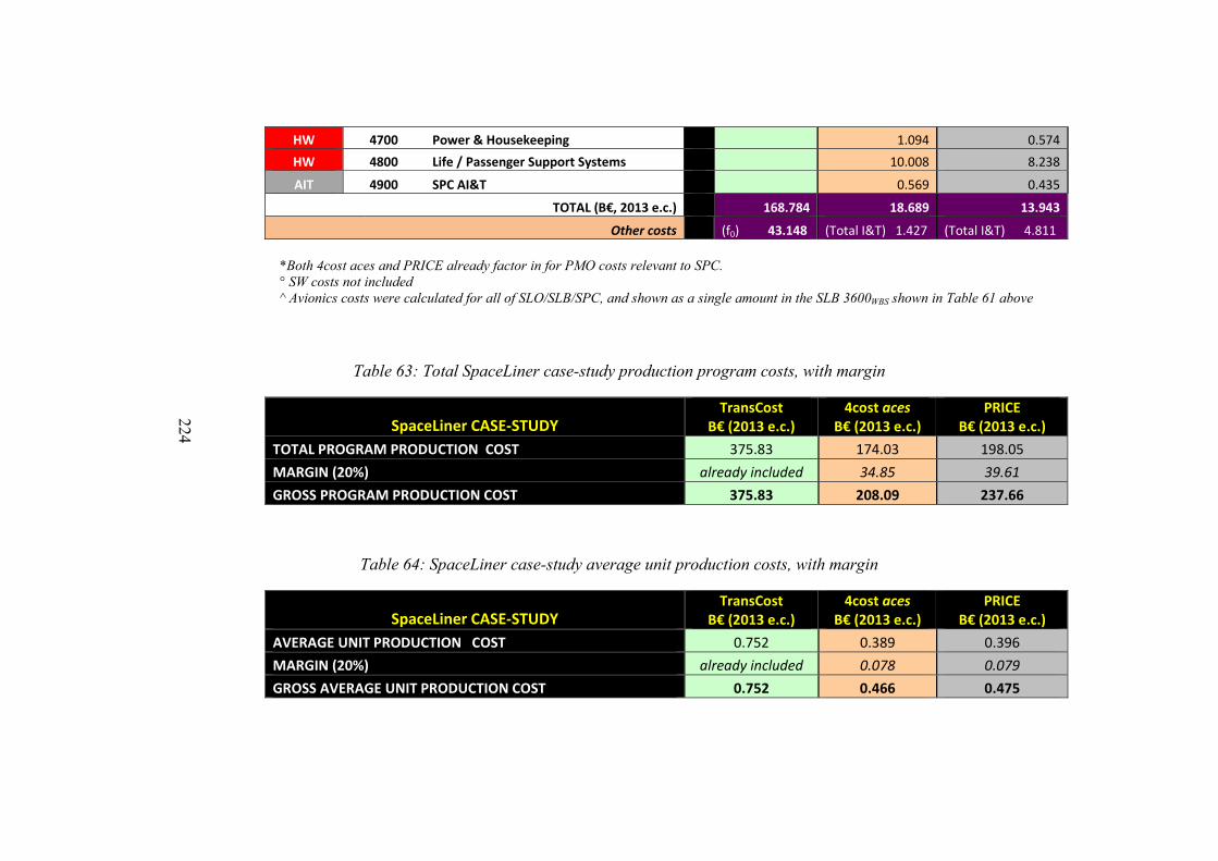
224
HW 4700 Power & Housekeeping 1.094 0.574
HW 4800 Life / Passenger Support Systems 10.008 8.238
AIT 4900 SPC AI&T 0.569 0.435
TOTAL (B€, 2013 e.c.) 168.784 18.689 13.943
Other costs (f0) 43.148 (Total I&T) 1.427 (Total I&T) 4.811
*Both 4cost aces and PRICE already factor in for PMO costs relevant to SPC. ° SW costs not included ^ Avionics costs were calculated for all of SLO/SLB/SPC, and shown as a single amount in the SLB 3600WBS shown in Table 61 above
Table 63: Total SpaceLiner case-study production program costs, with margin
Table 64: SpaceLiner case-study average unit production costs, with margin
SpaceLiner CASE‐STUDY TransCost
B€ (2013 e.c.)4cost aces
B€ (2013 e.c.)PRICE
B€ (2013 e.c.)
AVERAGE UNIT PRODUCTION COST 0.752 0.389 0.396
MARGIN (20%) already included 0.078 0.079
GROSS AVERAGE UNIT PRODUCTION COST 0.752 0.466 0.475
SpaceLiner CASE‐STUDY TransCost
B€ (2013 e.c.) 4cost aces
B€ (2013 e.c.) PRICE
B€ (2013 e.c.)
TOTAL PROGRAM PRODUCTION COST 375.83 174.03 198.05
MARGIN (20%) already included 34.85 39.61
GROSS PROGRAM PRODUCTION COST 375.83 208.09 237.66
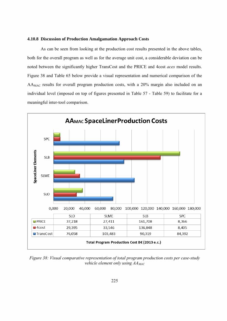
225
4.10.8 Discussion of Production Amalgamation Approach Costs
As can be seen from looking at the production cost results presented in the above tables,
both for the overall program as well as for the average unit cost, a considerable deviation can be
noted between the significantly higher TransCost and the PRICE and 4cost aces model results.
Figure 38 and Table 65 below provide a visual representation and numerical comparison of the
AAMAC results for overall program production costs, with a 20% margin also included on an
individual level (imposed on top of figures presented in Table 57 - Table 59) to facilitate for a
meaningful inter-tool comparison.
Figure 38: Visual comparative representation of total program production costs per case-study vehicle element only using AAMAC
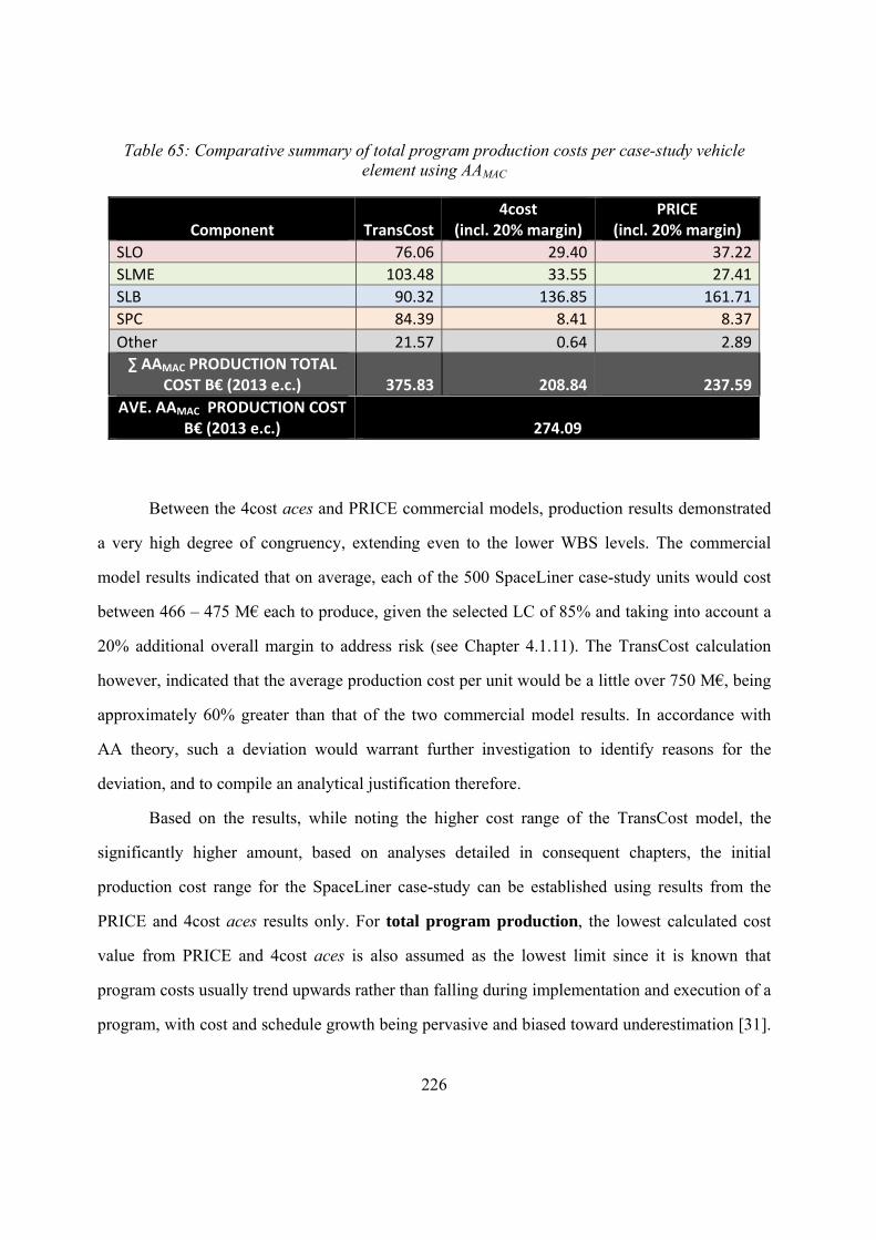
226
Table 65: Comparative summary of total program production costs per case-study vehicle element using AAMAC
Component TransCost4cost
(incl. 20% margin) PRICE
(incl. 20% margin)
SLO 76.06 29.40 37.22
SLME 103.48 33.55 27.41
SLB 90.32 136.85 161.71
SPC 84.39 8.41 8.37
Other 21.57 0.64 2.89
∑ AAMAC PRODUCTION TOTAL COST B€ (2013 e.c.) 375.83 208.84 237.59
AVE. AAMAC PRODUCTION COST B€ (2013 e.c.) 274.09
Between the 4cost aces and PRICE commercial models, production results demonstrated
a very high degree of congruency, extending even to the lower WBS levels. The commercial
model results indicated that on average, each of the 500 SpaceLiner case-study units would cost
between 466 – 475 M€ each to produce, given the selected LC of 85% and taking into account a
20% additional overall margin to address risk (see Chapter 4.1.11). The TransCost calculation
however, indicated that the average production cost per unit would be a little over 750 M€, being
approximately 60% greater than that of the two commercial model results. In accordance with
AA theory, such a deviation would warrant further investigation to identify reasons for the
deviation, and to compile an analytical justification therefore.
Based on the results, while noting the higher cost range of the TransCost model, the
significantly higher amount, based on analyses detailed in consequent chapters, the initial
production cost range for the SpaceLiner case-study can be established using results from the
PRICE and 4cost aces results only. For total program production, the lowest calculated cost
value from PRICE and 4cost aces is also assumed as the lowest limit since it is known that
program costs usually trend upwards rather than falling during implementation and execution of a
program, with cost and schedule growth being pervasive and biased toward underestimation [31].
227
The cost delta between AA results is then taken between the PRICE result (238 B€) and the 4cost
aces (210 B€), being approximately 28 B€. This delta is then multiplied by a cost risk factor of
1.5 (42 B€), and added to the higher PRICE cost estimate, to obtain the higher production cost
estimate limit of 280 B€.
The same process is applied to the average unit production cost, where the PRICE-4cost
aces delta is 9 B€ (475 – 466 M€), is multiplied by the same 1.5 cost risk factor (roughly 15 B€)
which, added to the highest PRICE average unit production cost of 475 M€ produces a total of
€490 M€, which is assumed to be the highest production range boundary cost.
4.10.8.1 TransCost Production Cost Deviation
As can be seen from AAMAC results, there is a considerable deviation in the TransCost
overall program production costs as well as the average unit costs as compared to results from the
PRICE and 4cost aces models. Looking at the values presented in Table 65 above, for example,
not only is the cost delta significant, but also the production cost distribution between elements is
also different. TransCost results in highest cost for SLME production, followed by SLB, then
SPC with the SLO component being the cheapest to produce. The commercial tools, however,
both indicate that by far the most expensive element to produce is the SLB, followed by the SLO,
SLME and finally, the cabin/capsule SLB element. In any case, in line with AAMAC theory, it is
important to analyse and ascertain where and why such a difference would have arisen. Upon
further analysis, three main contributing factors for the incongruence between TransCost and the
PRICE and 4cost aces models can be identified. These are listed and explained in the following
sub-chapters.
228
4.10.8.1.1 TRANSCOST NON-APPLICABILITY TO SLO & SLB
As already outlined in Chapter 4.10.2, TransCost does not appear to be an ideally suited
model to reflect production costs for a novel vehicle with high production rates and with a
passenger transport application such as the SpaceLiner case-study, which is addressed in this
Thesis. The existing TransCost CERs could be identified to adequately represent two of the four
main components of the SpaceLiner vehicle, being the SLO and SLB components. As such, and
to conform to the SpaceLiner philosophy which has been described in Chapter 4.1.4, the
production cost estimation conducted using the TransCost model was based on the rather gross
assumption that for the SLO and SLB, an average cost was assumed between the aviation and
space domain CER groups (also see Chapter 4.10.2). For the SLO, the average result of the two
CERs for Winged Orbital Rocket Vehicles (space domain), and High Speed Aircraft / Winged
First Stage Vehicles (aviation domain) were assumed. Similarly, for the SLB, the same two CER
results were again averaged to arrive at a production cost range. An equal 50/50 split was taken
between each CER, since at this stage to assign particular fractions seeking to represent a
different weighting between the space and aviation domains would have been premature,
unjustified and thus, non-constructive. A summary table of the TFU results for the SLB and SLO
elements is shown below in Table 66. As can be seen, the production cost delta is significant
between the space and aviation domain CERs, resulting in a percentile difference of roughly 260
– 270%. Therefore, because of the necessary although highly simplistic assumption to assume an
average production cost between the aviation and space representative CERs, it must be conceded
that a significant amount of uncertainty, especially pertaining to the SLO and SLB components,
is associated with the cost figures. As such, although unlike the development costs discussed in
Chapter 4.9.1, the TransCost production costs should be interpreted tentatively.
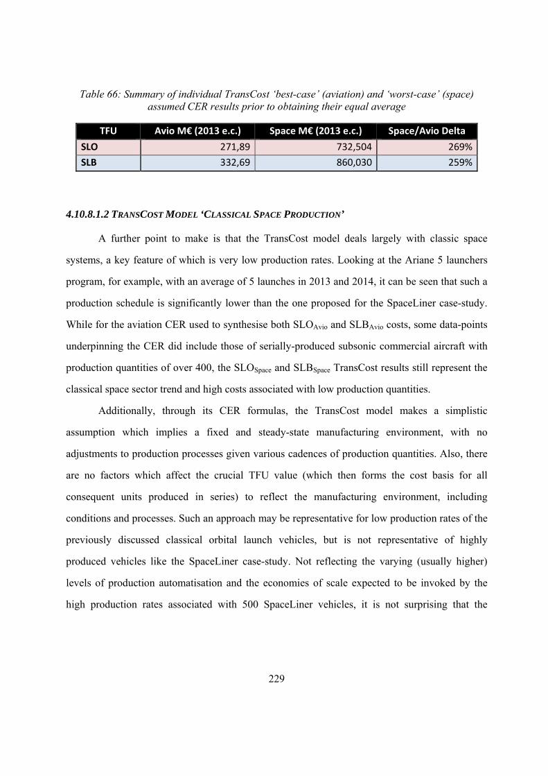
229
Table 66: Summary of individual TransCost ‘best-case’ (aviation) and ‘worst-case’ (space) assumed CER results prior to obtaining their equal average
TFU Avio M€ (2013 e.c.) Space M€ (2013 e.c.) Space/Avio Delta
SLO 271,89 732,504 269%
SLB 332,69 860,030 259%
4.10.8.1.2 TRANSCOST MODEL ‘CLASSICAL SPACE PRODUCTION’
A further point to make is that the TransCost model deals largely with classic space
systems, a key feature of which is very low production rates. Looking at the Ariane 5 launchers
program, for example, with an average of 5 launches in 2013 and 2014, it can be seen that such a
production schedule is significantly lower than the one proposed for the SpaceLiner case-study.
While for the aviation CER used to synthesise both SLOAvio and SLBAvio costs, some data-points
underpinning the CER did include those of serially-produced subsonic commercial aircraft with
production quantities of over 400, the SLOSpace and SLBSpace TransCost results still represent the
classical space sector trend and high costs associated with low production quantities.
Additionally, through its CER formulas, the TransCost model makes a simplistic
assumption which implies a fixed and steady-state manufacturing environment, with no
adjustments to production processes given various cadences of production quantities. Also, there
are no factors which affect the crucial TFU value (which then forms the cost basis for all
consequent units produced in series) to reflect the manufacturing environment, including
conditions and processes. Such an approach may be representative for low production rates of the
previously discussed classical orbital launch vehicles, but is not representative of highly
produced vehicles like the SpaceLiner case-study. Not reflecting the varying (usually higher)
levels of production automatisation and the economies of scale expected to be invoked by the
high production rates associated with 500 SpaceLiner vehicles, it is not surprising that the
230
TransCost model results in costs double those of the commercial models. The LC distinction is
discussed in more depth in the following Chapter 4.10.8.2.
Here, the significant cost deviation seen for the TransCost calculated SPC element
compared with PRICE and 4cost aces results must also be briefly mentioned. The TransCost
CER applied for calculation of SPC production costs was for Crewed Space Systems and is based
on reference points for a wide range of vehicles, ranging from crewed re-entry capsules, which
include the Mercury and Gemini capsules, lunar transfer and landing vehicles (Lunar Lander),
and even the Shuttle Orbiter, although without engines. The TransCost manual openly states that
this category of vehicles also incurs the highest production cost, due to the need for complex life-
support systems, power supply and electronic/communications equipment necessary for crewed
space systems [102]. However, the context of the SPC within this selection of vehicles, and also
within its SpaceLiner vehicle case-study application, is arguably misplaced, as has already been
presented in Chapter 4.1.9 which outlines and establishes details of the baseline SpaceLiner case-
study philosophy.
The SPC differs greatly from the function and technical requirements for a lunar-lander,
or Space Shuttle Orbiter vehicle. The SPC bears more resembles to a plane cockpit, and in this
respect, many COTS elements could easily be used during the production process. While it is true
that the cabin must also function as an escape capsule, this is foreseen to be in the unlikely case
of an emergency, after which the SPC will not be re-used. As such, the functionality, operational
lifetime under space conditions and hence technical requirements of the SPC can be considered to
significantly differ to those of, for example, the Space Shuttle. And with the highest costing CER,
in this context it is not surprising that the TransCost model results in a production cost of more
than 84 B€ for the SPC element compared to the roughly 7 B€ as calculated by both PRICE and
4cost aces. Given this analysis within the AAMAC framework, it can be concluded that the
TransCost model, in this instance, results in unrepresentatively high production costs of the SPC
element, and as such, in line with AA theory, is not considered further.
231
4.10.8.1.3 TRANSCOST ORBITAL VEHICLE FOCUS
While the TransCost model is a dedicated tool for launch vehicle cost determination, the
data points which underpin its CERs mainly consider programs which are orbital missions (i.e.
Shuttle Orbiter). And while the case-study vehicle assumed for analysis in this Thesis relies on
traditional launch technologies, it is only a sub-orbital vehicle with a significantly shorter overall
mission duration, and a sub-orbital trajectory. This of course has an associated bearing on the
production costs. It is important to highlight that this distinction between vehicle types would be
relatively insignificant and therefore would have little bearing on the development effort, since
the development processes, sequence, prototypes, and testing would be similar for orbital and
sub-orbital vehicles. The largest influence for development, in fact, would be other aspects such
as for example whether a vehicle is designed for manned applications, in which case whether
orbital or sub-orbital, testing would be equally as extensive. Such a requirement this would
dictate an increased number of prototype models to be built and tested, which, as has already
been shown in this Thesis (see Chapter 4.9.9.1), is a key cost driver for the development effort.
During the production effort, however, a much greater cost delta would be evident due to
more extreme operating environments, different expected lengths of operation and requirements
for a vehicle like the case-study SpaceLiner, and the Space Shuttle Orbiter. This then translates
directly into technical and mechanical aspects to reflect the nature of the mission and the different
mission lifetime, all of which then transfers into a higher cost for production. This observation
and critical distinction for orbital and suborbital vehicles dependent on the nature of the mission
has already been made and documented in the ISU study assessing the potential for suborbital
transportation [6]. A modified version of the TransCost model is then very briefly mentioned in
the ISU report, referred to as ‘SUBORB-TransCost’, although its mechanics and what changes
have been implemented to the original TransCost, remain undefined and undisclosed. In any case,
due to the SpaceLiner case-study being a sub-orbital vehicle, costed using parametrics based on
232
mainly orbital programs underpinning the CER data-points, would be a contributing factor to a
higher cost than may be expected for a vehicle such as the SpaceLiner case-study.
4.10.8.2 Learning Curve Assumption
For all three models taken for the Amalgamation Approach, a pure, singular and
consistent learning curve of 85% has been assumed for all 500 SpaceLiner units and components.
However, studies and literature also show that pure models like Crawford, often do not exactly fit
with actual observation [64], since actual learning phenomena are more complex than the pure
models describe. For example, as task complexity increases, less learning is to be expected due to
different learning types for simple and complex tasks. Also, the more automatisation there is in a
task, the less the learning which can be expected. Finally, and more specifically applicable to the
SpaceLiner case-study, with a higher production rate, the lower the learning rate can be. In this
instance, with no limitation to the learning curve, for very large quantities of production, the unit
cost becomes very small – which is actually in contradiction with experience, since learning has
hard limits [64]. As a practical and directly relevant example, it can be noted that for larger
production quantities within the aircraft industry, the increase in quantity results in a variation of
the LC (denoted as ʎc), which changes for various production quantity ranges (ranks), as shown
in Table 67. Furthermore, Table 68 shows another example of in-depth learning curves within the
aviation industry as outlined by the Defense Contract Audit Agency (DCAA) [51].
With relevance to the SpaceLiner, a very high production rate of engines is required,
which is significantly greater than historical and current space industry programs. Each
SpaceLiner vehicle requires 11 engines to be produced, which, at a 25 time reusability would
then warrant an additional 55 replacement units per vehicle to service the intended 150 flight
lifetime of the SLO, SLB and SPC elements. For a fleet of 500 SpaceLiner vehicles, this equals a
considerable total of 33,000 engines to be produced. If engine lifetime is increased to 50 flights,
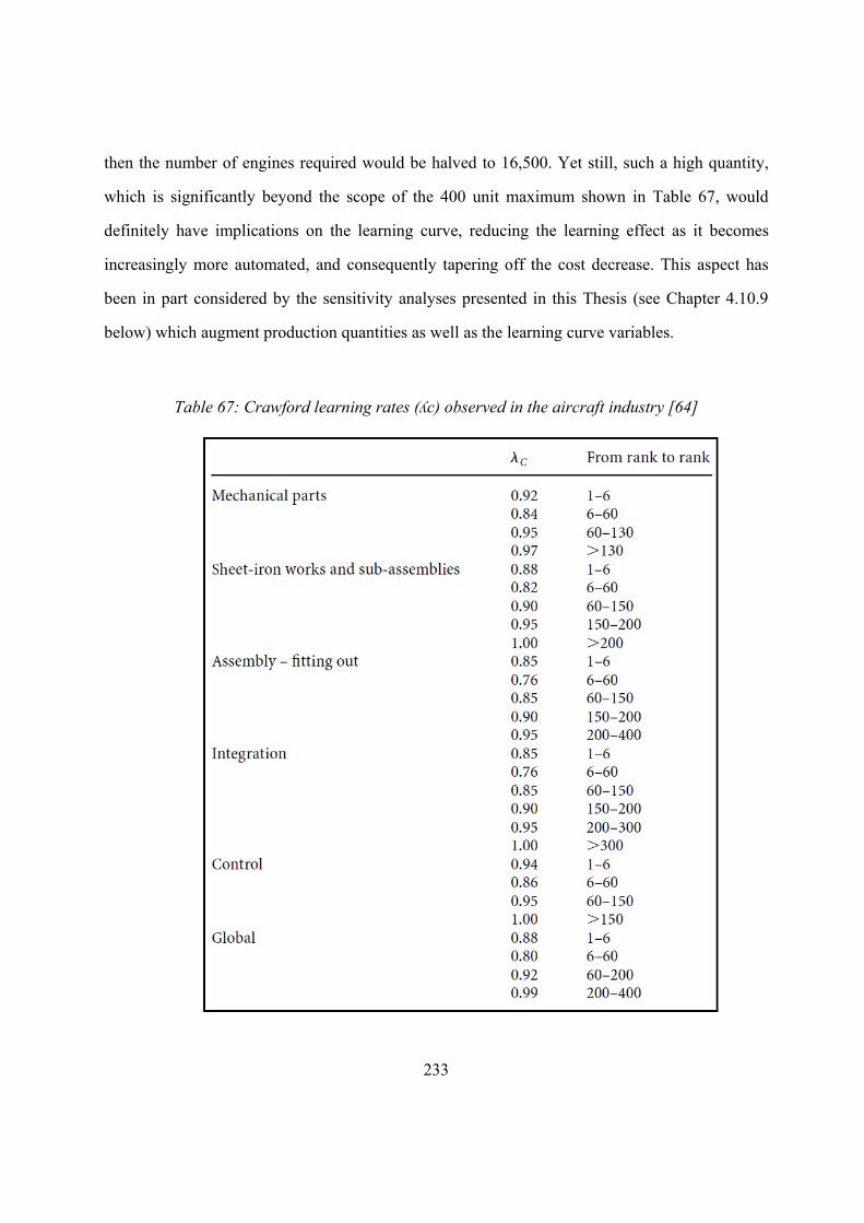
233
then the number of engines required would be halved to 16,500. Yet still, such a high quantity,
which is significantly beyond the scope of the 400 unit maximum shown in Table 67, would
definitely have implications on the learning curve, reducing the learning effect as it becomes
increasingly more automated, and consequently tapering off the cost decrease. This aspect has
been in part considered by the sensitivity analyses presented in this Thesis (see Chapter 4.10.9
below) which augment production quantities as well as the learning curve variables.
Table 67: Crawford learning rates (ʎc) observed in the aircraft industry [64]
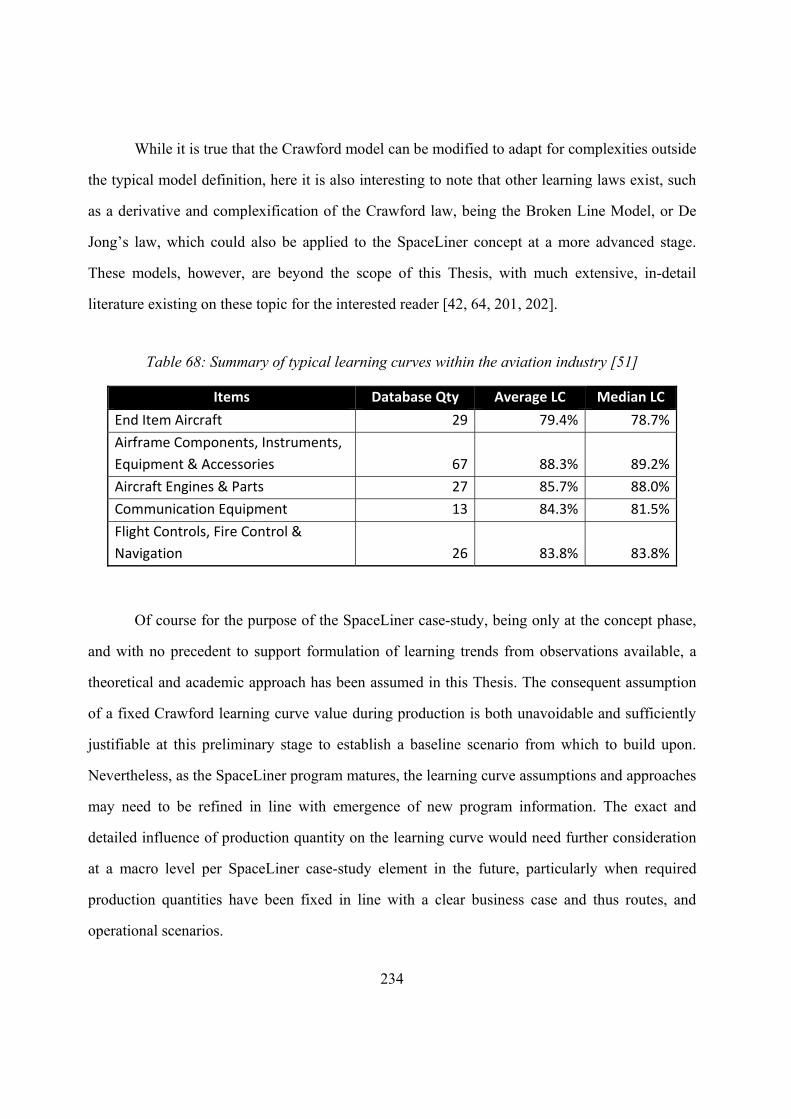
234
While it is true that the Crawford model can be modified to adapt for complexities outside
the typical model definition, here it is also interesting to note that other learning laws exist, such
as a derivative and complexification of the Crawford law, being the Broken Line Model, or De
Jong’s law, which could also be applied to the SpaceLiner concept at a more advanced stage.
These models, however, are beyond the scope of this Thesis, with much extensive, in-detail
literature existing on these topic for the interested reader [42, 64, 201, 202].
Table 68: Summary of typical learning curves within the aviation industry [51]
Items Database Qty Average LC Median LC
End Item Aircraft 29 79.4% 78.7%
Airframe Components, Instruments,
Equipment & Accessories 67 88.3% 89.2%
Aircraft Engines & Parts 27 85.7% 88.0%
Communication Equipment 13 84.3% 81.5%
Flight Controls, Fire Control &
Navigation 26 83.8% 83.8%
Of course for the purpose of the SpaceLiner case-study, being only at the concept phase,
and with no precedent to support formulation of learning trends from observations available, a
theoretical and academic approach has been assumed in this Thesis. The consequent assumption
of a fixed Crawford learning curve value during production is both unavoidable and sufficiently
justifiable at this preliminary stage to establish a baseline scenario from which to build upon.
Nevertheless, as the SpaceLiner program matures, the learning curve assumptions and approaches
may need to be refined in line with emergence of new program information. The exact and
detailed influence of production quantity on the learning curve would need further consideration
at a macro level per SpaceLiner case-study element in the future, particularly when required
production quantities have been fixed in line with a clear business case and thus routes, and
operational scenarios.
235
4.10.8.3 Other Production Cost Fluctuations
To explain the minor cost fluctuations observed between the two commercial 4cost aces
and PRICE tools, similar justifications as already discussed within context of development costs,
can also be applied here. The variability in internal model mechanics and algorithms already
discussed at length in Chapter 4.9.8.3 would contribute to fluctuations. Additionally, any changes
of the model user throughout the process and the potential for introduction of personal bias
through exercising EJ during translation of caste-study data into model-specific parameters
would be another contributing factor to cost deviations and fluctuations, as already outlined in
Chapter 4.9.8.4. While human error may also be a contributing factor, the nature of the AAMAC
approach, as supported by the AAInT spreadsheet, considerably minimises any significantly
influential errors, as has been already explained and detailed in Chapter 4.9.7.1. For production
costs, as well, as has already been discussed in Chapter 4.9.8.5, the fact that both PRICE and
4cost aces in this instance do not consider software costs, would also, to a very minor extent
explain that the TransCost results are higher, since TransCost inherently addresses SW in its
CERs.
4.10.9 Production Cost Sensitivities
To complement the sensitivities conducted for the development cost calculations, it was
also interesting to perform some basic sensitivity analyses for the baseline case-study production
phase. Since the TransCost model yields a greater uncertainty in its production cost results (see
Chapter 4.10.8.1), it was logical to use one of the commercial tools. To keep congruent with the
development cost sensitivity process, the 4cost aces tool was once again applied to implement the
chosen sensitivity deltas. Three variables, the influence of whose deltas are interesting to examine
with respect to production costs, were identified. These are variations in learning curve (LC), the
production quantity, as well as the reusability capability of the engines, resulting in a different
quantity of engines to be produced. The variables were not necessarily chosen to reflect a worst-
236
case scenario, but most commonly straddled the baseline value, as will be outlined below, for
each sensitivity-case. The 4cost aces model data used to extract the three key values of interest
from the sensitivities datasets, were total production cost (PrdTotal), the 4cost aces model
calculated average unit cost (ModAmuc3), and the cost of the TFU first unit produced
(T1ModT1), referred to as T1 by 4cost aces vocabulary. Here, it is important to note that the
4cost aces model calculated output for the average cost per unit produced was not the simple
total production cost (PrdTotal) divided by the production quantity. Through the internal
mechanics of the model, the ModAmuc3 value which represents the average unit cost of
production, also includes the overheads and profit margins assigned by the modes, assigned to be
10% (see final paragraph of Chapter 4.10.3), as well as a basic software component, which,
although eliminated for the total production case, was left in for the sensitivity analyses. Its
impact is almost negligible in the context of costs.
Furthermore, while it was inefficient to include the countless datasheets for each of the
nine sensitivities, the baseline datasets of inputs (Table 125) and more particularly the outputs
(Table 126) included in Appendix H can be consulted to see the structure and source of the
respective 4cost aces tool data required and used also for the sensitivities.
4.10.9.1 Learning Curve Variation
The LC for production using the 4cost aces tool was varied from 80% (sensitivity study
baseline LC value) to 85% and ultimately 90%. Here, it was interesting to see how the LC delta
would influence overall production costs given the internal mechanics of the model. The results
for total production cost as well as the resulting average unit production costs are shown in Table
69 while Table 70 shows the resulting costs for the TFU (referred to as T1 within 4cost aces tool
terminology, so to be used interchangeably and synonymously with the term TFU) for every LC
variation.
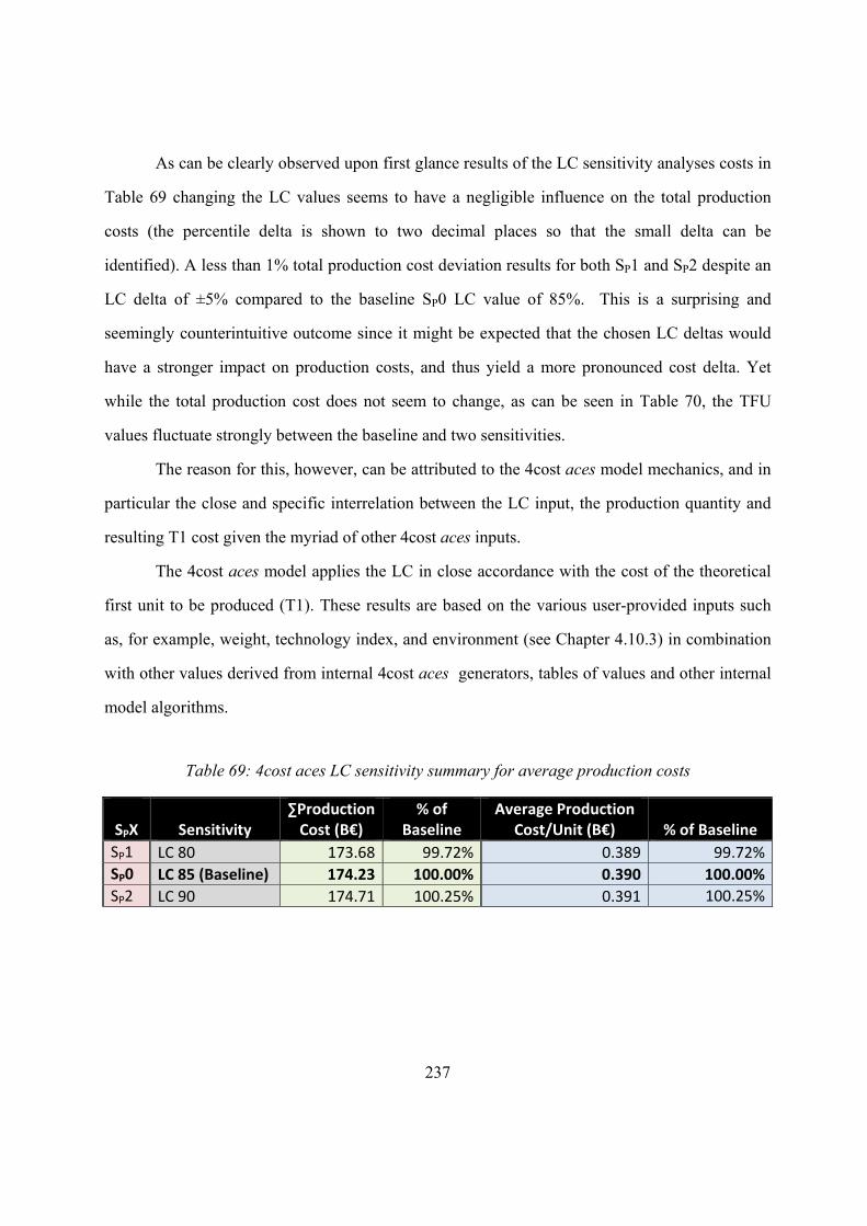
237
As can be clearly observed upon first glance results of the LC sensitivity analyses costs in
Table 69 changing the LC values seems to have a negligible influence on the total production
costs (the percentile delta is shown to two decimal places so that the small delta can be
identified). A less than 1% total production cost deviation results for both SP1 and SP2 despite an
LC delta of ±5% compared to the baseline SP0 LC value of 85%. This is a surprising and
seemingly counterintuitive outcome since it might be expected that the chosen LC deltas would
have a stronger impact on production costs, and thus yield a more pronounced cost delta. Yet
while the total production cost does not seem to change, as can be seen in Table 70, the TFU
values fluctuate strongly between the baseline and two sensitivities.
The reason for this, however, can be attributed to the 4cost aces model mechanics, and in
particular the close and specific interrelation between the LC input, the production quantity and
resulting T1 cost given the myriad of other 4cost aces inputs.
The 4cost aces model applies the LC in close accordance with the cost of the theoretical
first unit to be produced (T1). These results are based on the various user-provided inputs such
as, for example, weight, technology index, and environment (see Chapter 4.10.3) in combination
with other values derived from internal 4cost aces generators, tables of values and other internal
model algorithms.
Table 69: 4cost aces LC sensitivity summary for average production costs
SPX Sensitivity
∑Production Cost (B€)
% of Baseline
Average Production Cost/Unit (B€) % of Baseline
SP1 LC 80 173.68 99.72% 0.389 99.72%
SP0 LC 85 (Baseline) 174.23 100.00% 0.390 100.00%
SP2 LC 90 174.71 100.25% 0.391 100.25%
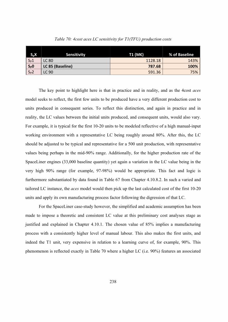
238
Table 70: 4cost aces LC sensitivity for T1(TFU) production costs
SpX Sensitivity T1 (M€) % of Baseline
SP1 LC 80 1128.18 143%
SP0 LC 85 (Baseline) 787.68 100%
SP2 LC 90 591.36 75%
The key point to highlight here is that in practice and in reality, and as the 4cost aces
model seeks to reflect, the first few units to be produced have a very different production cost to
units produced in consequent series. To reflect this distinction, and again in practice and in
reality, the LC values between the initial units produced, and consequent units, would also vary.
For example, it is typical for the first 10-20 units to be modeled reflective of a high manual-input
working environment with a representative LC being roughly around 80%. After this, the LC
should be adjusted to be typical and representative for a 500 unit production, with representative
values being perhaps in the mid-90% range. Additionally, for the higher production rate of the
SpaceLiner engines (33,000 baseline quantity) yet again a variation in the LC value being in the
very high 90% range (for example, 97-98%) would be appropriate. This fact and logic is
furthermore substantiated by data found in Table 67 from Chapter 4.10.8.2. In such a varied and
tailored LC instance, the aces model would then pick up the last calculated cost of the first 10-20
units and apply its own manufacturing process factor following the digression of that LC.
For the SpaceLiner case-study however, the simplified and academic assumption has been
made to impose a theoretic and consistent LC value at this preliminary cost analyses stage as
justified and explained in Chapter 4.10.1. The chosen value of 85% implies a manufacturing
process with a consistently higher level of manual labour. This also makes the first units, and
indeed the T1 unit, very expensive in relation to a learning curve of, for example, 90%. This
phenomenon is reflected exactly in Table 70 where a higher LC (i.e. 90%) features an associated
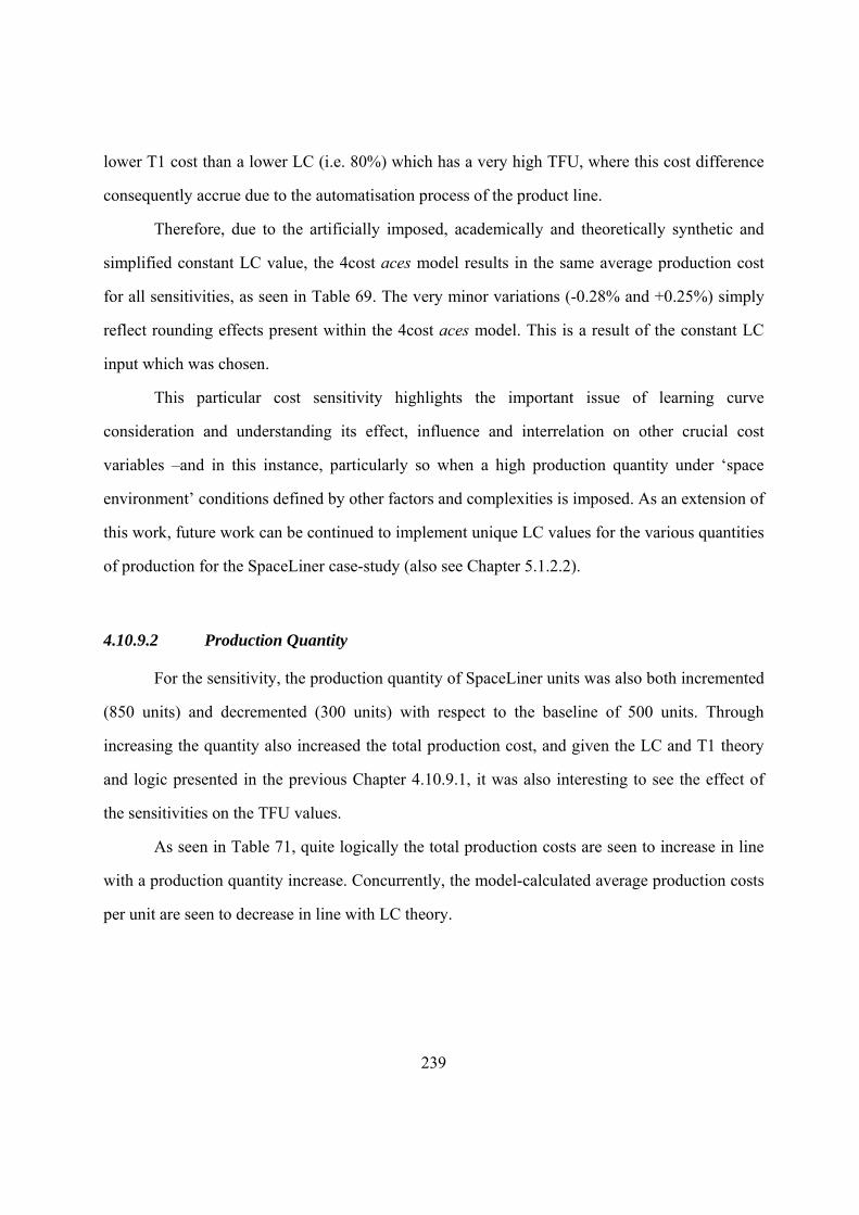
239
lower T1 cost than a lower LC (i.e. 80%) which has a very high TFU, where this cost difference
consequently accrue due to the automatisation process of the product line.
Therefore, due to the artificially imposed, academically and theoretically synthetic and
simplified constant LC value, the 4cost aces model results in the same average production cost
for all sensitivities, as seen in Table 69. The very minor variations (-0.28% and +0.25%) simply
reflect rounding effects present within the 4cost aces model. This is a result of the constant LC
input which was chosen.
This particular cost sensitivity highlights the important issue of learning curve
consideration and understanding its effect, influence and interrelation on other crucial cost
variables –and in this instance, particularly so when a high production quantity under ‘space
environment’ conditions defined by other factors and complexities is imposed. As an extension of
this work, future work can be continued to implement unique LC values for the various quantities
of production for the SpaceLiner case-study (also see Chapter 5.1.2.2).
4.10.9.2 Production Quantity
For the sensitivity, the production quantity of SpaceLiner units was also both incremented
(850 units) and decremented (300 units) with respect to the baseline of 500 units. Through
increasing the quantity also increased the total production cost, and given the LC and T1 theory
and logic presented in the previous Chapter 4.10.9.1, it was also interesting to see the effect of
the sensitivities on the TFU values.
As seen in Table 71, quite logically the total production costs are seen to increase in line
with a production quantity increase. Concurrently, the model-calculated average production costs
per unit are seen to decrease in line with LC theory.
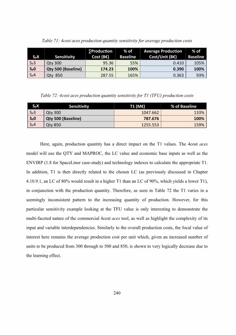
240
Table 71: 4cost aces production quantity sensitivity for average production costs
SPX Sensitivity
∑Produc on Cost (B€)
% of Baseline
Average Production Cost/Unit (B€)
% of Baseline
SP3 Qty 300 95.36 55% 0.410 105%
SP0 Qty 500 (Baseline) 174.23 100% 0.390 100%
SP4 Qty 850 287.55 165% 0.363 93%
Table 72: 4cost aces production quantity sensitivity for T1 (TFU) production costs
SPX Sensitivity T1 (M€) % of Baseline
SP3 Qty 300 1047.662 133%
SP0 Qty 500 (Baseline) 787.676 100%
SP4 Qty 850 1255.553 159%
Here, again, production quantity has a direct impact on the T1 values. The 4cost aces
model will use the QTY and MAPROC, the LC value and economic base inputs as well as the
ENVIRP (1.8 for SpaceLiner case-study) and technology indexes to calculate the appropriate T1.
In addition, T1 is then directly related to the chosen LC (as previously discussed in Chapter
4.10.9.1, an LC of 80% would result in a higher T1 than an LC of 90%, which yields a lower T1),
in conjunction with the production quantity. Therefore, as seen in Table 72 the T1 varies in a
seemingly inconsistent pattern to the increasing quantity of production. However, for this
particular sensitivity example looking at the TFU value is only interesting to demonstrate the
multi-faceted nature of the commercial 4cost aces tool, as well as highlight the complexity of its
input and variable interdependencies. Similarly to the overall production costs, the focal value of
interest here remains the average production cost per unit which, given an increased number of
units to be produced from 300 through to 500 and 850, is shown to very logically decrease due to
the learning effect.
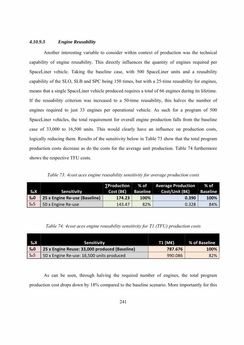
241
4.10.9.3 Engine Reusability
Another interesting variable to consider within context of production was the technical
capability of engine reusability. This directly influences the quantity of engines required per
SpaceLiner vehicle. Taking the baseline case, with 500 SpaceLiner units and a reusability
capability of the SLO, SLB and SPC being 150 times, but with a 25-time reusability for engines,
means that a single SpaceLiner vehicle produced requires a total of 66 engines during its lifetime.
If the reusability criterion was increased to a 50-time reusability, this halves the number of
engines required to just 33 engines per operational vehicle. As such for a program of 500
SpaceLiner vehicles, the total requirement for overall engine production falls from the baseline
case of 33,000 to 16,500 units. This would clearly have an influence on production costs,
logically reducing them. Results of the sensitivity below in Table 73 show that the total program
production costs decrease as do the costs for the average unit production. Table 74 furthermore
shows the respective TFU costs.
Table 73: 4cost aces engine reusability sensitivity for average production costs
SPX Sensitivity
∑Produc on Cost (B€)
% of Baseline
Average Production Cost/Unit (B€)
% of Baseline
SP0 25 x Engine Re‐use (Baseline) 174.23 100% 0.390 100%
SP5 50 x Engine Re‐use 143.47 82% 0.328 84%
Table 74: 4cost aces engine reusability sensitivity for T1 (TFU) production costs
SPX Sensitivity T1 (M€) % of Baseline
SP0 25 x Engine Reuse: 33,000 produced (Baseline) 787.676 100%
SP5 50 x Engine Re‐use: 16,500 units produced 990.086 82%
As can be seen, through halving the required number of engines, the total program
production cost drops down by 18% compared to the baseline scenario. More importantly for this
242
sensitivity study, it is shown that through enhanced engine reusability, the production of each
SpaceLiner vehicle, on average, decreases from 390 M€ to 328 M€, which constitutes a 16% cost
drop per unit. This confirms the fact that the engine is a very important cost-driving parameter of
the overall SpaceLiner system. Concerning the TFU values which are included for interest only,
the smaller quantity of engines produced implies a less significant automatisation process, and as
such, in line with previously established theory, increases the TFU, as seen in Table 74.
4.10.9.4 Production Sensitivity Summary
The sensitivity study presented in the latter chapters determined the cost effect for
production using the 4cost aces tool, through varying three key production process variables; the
LC values, the production quantity, and the engine reusability (which reflects on the production
quantity of the case-study propulsion unit). Total program production costs and consequent
average unit costs were calculated, as well as TFU values shown, with percentile differences
between the sensitivities and values of interest also calculated to facilitate of more tangible
comprehension of sensitivity impact on costs. While LC sensitivity results were surprising, a
deeper analysis into the 4cost aces model mechanics revealed the complex albeit very logical
interrelations and influence of key quantity, LC and TFU cost parameters on one another. The LC
sensitivity analysis also highlighted that LC theory would need to be considered at a deeper level
for the SpaceLiner vehicle case-study in the future, considering not only a fixed LC value
throughout the production process, but a varying one, depending on production quantities.
Variance of production quantities logically revealed a cost increase to an increased
production amount, and a decrease, with a decreased quantity produced. Finally, enhanced engine
reusability also impacted the total program costs in a positive way, as was to be logically
expected.
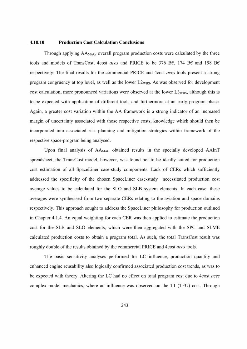
243
4.10.10 Production Cost Calculation Conclusions
Through applying AAMAC, overall program production costs were calculated by the three
tools and models of TransCost, 4cost aces and PRICE to be 376 B€, 174 B€ and 198 B€
respectively. The final results for the commercial PRICE and 4cost aces tools present a strong
program congruency at top level, as well as the lower L2WBS. As was observed for development
cost calculation, more pronounced variations were observed at the lower L3WBS, although this is
to be expected with application of different tools and furthermore at an early program phase.
Again, a greater cost variation within the AA framework is a strong indicator of an increased
margin of uncertainty associated with those respective costs, knowledge which should then be
incorporated into associated risk planning and mitigation strategies within framework of the
respective space-program being analysed.
Upon final analysis of AAMAC obtained results in the specially developed AAInT
spreadsheet, the TransCost model, however, was found not to be ideally suited for production
cost estimation of all SpaceLiner case-study components. Lack of CERs which sufficiently
addressed the specificity of the chosen SpaceLiner case-study necessitated production cost
average values to be calculated for the SLO and SLB system elements. In each case, these
averages were synthesised from two separate CERs relating to the aviation and space domains
respectively. This approach sought to address the SpaceLiner philosophy for production outlined
in Chapter 4.1.4. An equal weighting for each CER was then applied to estimate the production
cost for the SLB and SLO elements, which were then aggregated with the SPC and SLME
calculated production costs to obtain a program total. As such, the total TransCost result was
roughly double of the results obtained by the commercial PRICE and 4cost aces tools.
The basic sensitivity analyses performed for LC influence, production quantity and
enhanced engine reusability also logically confirmed associated production cost trends, as was to
be expected with theory. Altering the LC had no effect on total program cost due to 4cost aces
complex model mechanics, where an influence was observed on the T1 (TFU) cost. Through

244
analyses of the surprising LC sensitivity results, the complex nature and application of LC theory
became apparent. As such, it can be recommended that future work focus on expanding the
simplified assumption of a basic and constant LC value across all elements of production. The
LC value strongly hinges on the quantity of units to be produced, and should be adjusted in
accordance with various production quantity cadences to reflect changes in automatisation and
manual labour.
Concerning the production quantity sensitivity, a greater overall program production cost
was achieved with an increase in units produced. Concurrently, the average unit production cost
fell due to the LC effect. Through enhancing engine reusability, a production cost reduction was
observed on both overall program level, as well as at average unit cost of production.
Overall, through application of AAMAC and through consequent analyses of results using
the AAInT spreadsheet, a production cost range has been established. Although one set of results
from TransCost resulted in considerable variances to the PRICE and 4cost aces models,
nevertheless a strong level of confidence is associated with the established cost range. As the
program matures, the production cost estimates should be continually monitored and revised to
incorporate any new information, mission and technical data.
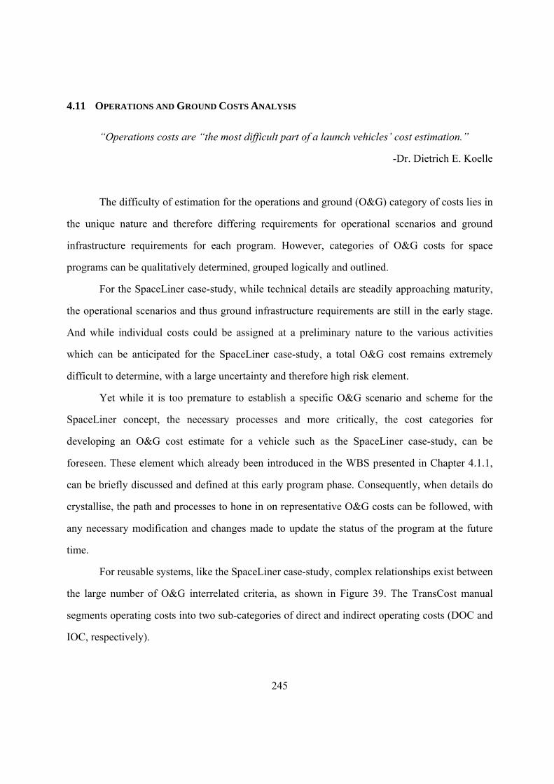
245
4.11 OPERATIONS AND GROUND COSTS ANALYSIS
“Operations costs are “the most difficult part of a launch vehicles’ cost estimation.”
-Dr. Dietrich E. Koelle
The difficulty of estimation for the operations and ground (O&G) category of costs lies in
the unique nature and therefore differing requirements for operational scenarios and ground
infrastructure requirements for each program. However, categories of O&G costs for space
programs can be qualitatively determined, grouped logically and outlined.
For the SpaceLiner case-study, while technical details are steadily approaching maturity,
the operational scenarios and thus ground infrastructure requirements are still in the early stage.
And while individual costs could be assigned at a preliminary nature to the various activities
which can be anticipated for the SpaceLiner case-study, a total O&G cost remains extremely
difficult to determine, with a large uncertainty and therefore high risk element.
Yet while it is too premature to establish a specific O&G scenario and scheme for the
SpaceLiner concept, the necessary processes and more critically, the cost categories for
developing an O&G cost estimate for a vehicle such as the SpaceLiner case-study, can be
foreseen. These element which already been introduced in the WBS presented in Chapter 4.1.1,
can be briefly discussed and defined at this early program phase. Consequently, when details do
crystallise, the path and processes to hone in on representative O&G costs can be followed, with
any necessary modification and changes made to update the status of the program at the future
time.
For reusable systems, like the SpaceLiner case-study, complex relationships exist between
the large number of O&G interrelated criteria, as shown in Figure 39. The TransCost manual
segments operating costs into two sub-categories of direct and indirect operating costs (DOC and
IOC, respectively).
246
Figure 39: Major operational criteria and their interrelation for RLVs [102]
Operations costs can be roughly grouped into ground stations and associated costs, and
personnel costs. Ground stations encompass any operating facilities, such as control centers and
communication stations. Equipment such as antennas and computers, for example, form a large
component of this. Software is also a considerable cost driver, and is commonly the most difficult
and expensive component [132] of the ground cost infrastructure. The personnel category then
encompasses maintenance costs, and any contract and government labor.
For the SpaceLiner case-study, given the fact that the purpose of the vehicle is passenger
transport, it can be foreseen that the operational scenario would be a complex one. Some
operational details for the concept are, in fact, emerging. Preliminary work has already been done
to study and propose both potential spaceport configurations and locations for the SpaceLiner
case-study, as well as preliminary operational requirements and activities [110]. Three possible
247
spaceport configurations were also suggested for landing and launch (L/L) sites, being on-shore
(inland), artificial island (off-shore), and an off-shore launch site with an on-shore landing
capability. The concept of the artificial island is has already been well demonstrated by
construction of the Kansai International Airport, shown in Figure 40, which has been operational
since 1994 [86].
Figure 40: Kansai International Airport in Osaka Bay, Japan [86]
Given the three construction options, the study [110] also then identified various possible
geographical locations optimising site remoteness requirements to address sonic boom issues,
with nevertheless considering sufficient proximity to highly populated city-hubs for travel. The
possible locations are summarised below in Table 75.
Looking at the spaceport itself, it is clear that the operational protocol would combine the
processes standards from the commercial aviation industry of boarding and de-boarding of the
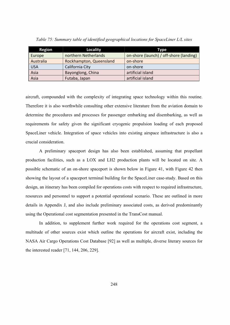
248
Table 75: Summary table of identified geographical locations for SpaceLiner L/L sites
Region Locality Type
Europe northern Netherlands on‐shore (launch) / off‐shore (landing)
Australia Rockhampton, Queensland on‐shore
USA California City on‐shore
Asia Bayonglong, China artificial island
Asia Futaba, Japan artificial island
aircraft, compounded with the complexity of integrating space technology within this routine.
Therefore it is also worthwhile consulting other extensive literature from the aviation domain to
determine the procedures and processes for passenger embarking and disembarking, as well as
requirements for safety given the significant cryogenic propulsion loading of each proposed
SpaceLiner vehicle. Integration of space vehicles into existing airspace infrastructure is also a
crucial consideration.
A preliminary spaceport design has also been established, assuming that propellant
production facilities, such as a LOX and LH2 production plants will be located on site. A
possible schematic of an on-shore spaceport is shown below in Figure 41, with Figure 42 then
showing the layout of a spaceport terminal building for the SpaceLiner case-study. Based on this
design, an itinerary has been compiled for operations costs with respect to required infrastructure,
resources and personnel to support a potential operational scenario. These are outlined in more
details in Appendix J, and also include preliminary associated costs, as derived predominantly
using the Operational cost segmentation presented in the TransCost manual.
In addition, to supplement further work required for the operations cost segment, a
multitude of other sources exist which outline the operations for aircraft exist, including the
NASA Air Cargo Operations Cost Database [92] as well as multiple, diverse literary sources for
the interested reader [71, 144, 206, 229].
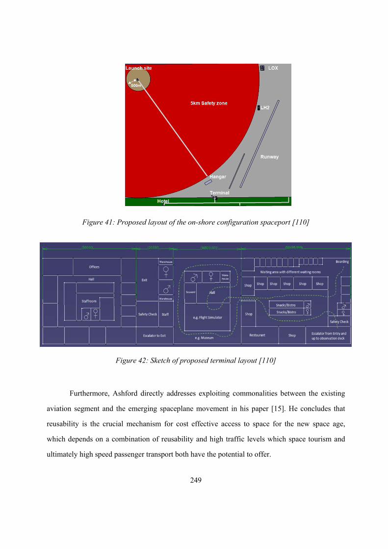
249
Figure 41: Proposed layout of the on-shore configuration spaceport [110]
Figure 42: Sketch of proposed terminal layout [110]
Furthermore, Ashford directly addresses exploiting commonalities between the existing
aviation segment and the emerging spaceplane movement in his paper [15]. He concludes that
reusability is the crucial mechanism for cost effective access to space for the new space age,
which depends on a combination of reusability and high traffic levels which space tourism and
ultimately high speed passenger transport both have the potential to offer.
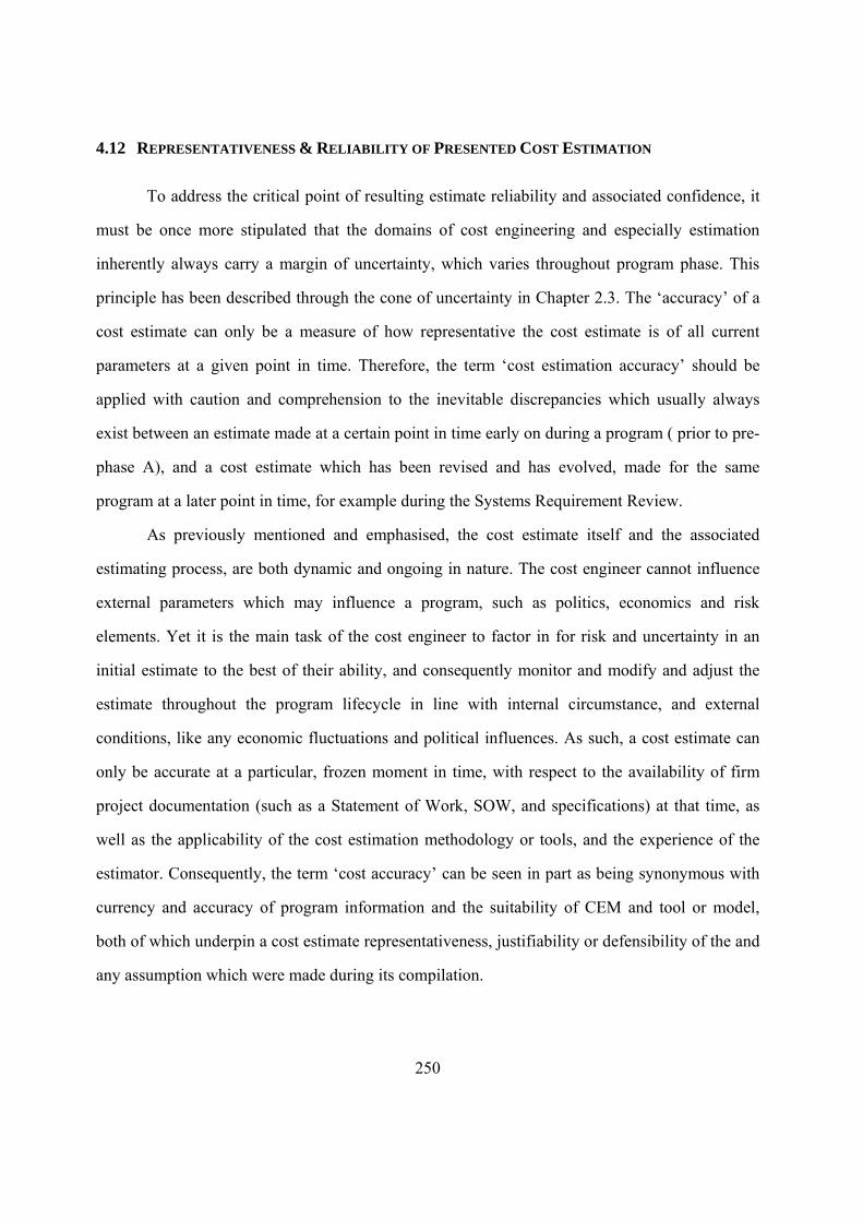
250
4.12 REPRESENTATIVENESS & RELIABILITY OF PRESENTED COST ESTIMATION
To address the critical point of resulting estimate reliability and associated confidence, it
must be once more stipulated that the domains of cost engineering and especially estimation
inherently always carry a margin of uncertainty, which varies throughout program phase. This
principle has been described through the cone of uncertainty in Chapter 2.3. The ‘accuracy’ of a
cost estimate can only be a measure of how representative the cost estimate is of all current
parameters at a given point in time. Therefore, the term ‘cost estimation accuracy’ should be
applied with caution and comprehension to the inevitable discrepancies which usually always
exist between an estimate made at a certain point in time early on during a program ( prior to pre-
phase A), and a cost estimate which has been revised and has evolved, made for the same
program at a later point in time, for example during the Systems Requirement Review.
As previously mentioned and emphasised, the cost estimate itself and the associated
estimating process, are both dynamic and ongoing in nature. The cost engineer cannot influence
external parameters which may influence a program, such as politics, economics and risk
elements. Yet it is the main task of the cost engineer to factor in for risk and uncertainty in an
initial estimate to the best of their ability, and consequently monitor and modify and adjust the
estimate throughout the program lifecycle in line with internal circumstance, and external
conditions, like any economic fluctuations and political influences. As such, a cost estimate can
only be accurate at a particular, frozen moment in time, with respect to the availability of firm
project documentation (such as a Statement of Work, SOW, and specifications) at that time, as
well as the applicability of the cost estimation methodology or tools, and the experience of the
estimator. Consequently, the term ‘cost accuracy’ can be seen in part as being synonymous with
currency and accuracy of program information and the suitability of CEM and tool or model,
both of which underpin a cost estimate representativeness, justifiability or defensibility of the and
any assumption which were made during its compilation.
251
Two prominent and real industry examples are the Space Shuttle [91, 102] and the
Concorde program, whose final development cost is quoted as being between six to ten times as
high as initially predicted [31, 145, 160]. On a more global scale, a GAO report from 1993 to the
US Congress showed that from 29 NASA programs surveyed, only 14% have been at or below
the original cost estimate, 53% exceeded cost estimations by up to 100% while 33% showed cost
growth of over 100% [102]. Furthermore, a more recent 2004 Congressional Budget Office study
compared initial and revised NASA budgets for 72 programs between 1977 and 2000, finding
that on average, a 61% increase on costs was incurred. It has been proposed that a prevalent and
considerable problem in a competitive market environment where funds are obtained based on
proposal victory, is that classical cost estimating standards are often compromised due to the
originators of project proposals being afraid to present very realistic cost estimates which might
risk proposal rejection [102].
The cost estimation task for the SpaceLiner case-study conducted within this Thesis is
based on the currently available project documentation and the use of sophisticated cost models.
The framework and processes described, set out, enhanced and applied for complex, early phase,
unprecedented space program cost estimation presented in this Thesis is intended to increase
reliability of cost estimation based on current standards. In line with industry best practice, high
quality estimates should be credible, well documented, accurate and comprehensive. This Thesis
strives to meet all the latter four criteria, with the introduction and development of the
Amalgamation Approach for cost estimate redundancy. Nevertheless, a means is necessary to
assess and class the reliability of the resulting estimate in terms of confidence.
Select approaches and measures exist in wider industry to classify cost estimation
representativeness, commonly taking on the form of confidence classification matrices. A
suitable example can be taken from the process industry, where a cost estimate classification
matrix has been established and recently published by the prominent AACE organisation in
November of 2011. The cost matrix is shown Table 76 below.
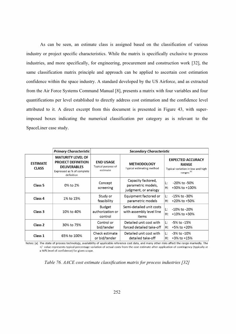
252
As can be seen, an estimate class is assigned based on the classification of various
industry or project specific characteristics. While the matrix is specifically exclusive to process
industries, and more specifically, for engineering, procurement and construction work [32], the
same classification matrix principle and approach can be applied to ascertain cost estimation
confidence within the space industry. A standard developed by the US Airforce, and as extracted
from the Air Force Systems Command Manual [8], presents a matrix with four variables and four
quantifications per level established to directly address cost estimation and the confidence level
attributed to it. A direct excerpt from this document is presented in Figure 43, with super-
imposed boxes indicating the numerical classification per category as is relevant to the
SpaceLiner case study.
Table 76. AACE cost estimate classification matrix for process industries [32]
253
As already theoretically introduced in Chapter 2.2.1 and as illustrated in Figure 3 at the
commencement of this Thesis, the estimated costs and the related confidence level, which
inherently also defines risks, is strongly dependent on the three criteria of input data, the tools,
models and methods applied, as well as experience and background of the estimator. From the
break-down of criteria from the AFSCM matrix seen in Figure 43, it can be seen that confidence
of an estimate is in this instance distinguished between four categories of estimating conditions,
the nature of the item being costed and item description, and finally cost methods and data.
Essentially, however, this is simply but a slight rearrangement on the key three criteria already
established above, although the AFSCM matrix combines the two criteria of cost methods
together with data, and also does not include the crucial facet of estimator experience. This fifth
element is a most crucial dimension to consider, and should not be ignored, as will be discussed
further in consequent Chapter 4.12.5.
The cost estimation for the hardware development and production phases of the
SpaceLiner case-study which have been performed and detailed in this Thesis are optimally based
on all currently available preliminary technical definitions, a systematic baseline project structure
demonstrated in consolidation of a WBS, as well as establishment of a preliminary development
schedule. In order to assure that the cost estimation prepared for the SpaceLiner project reaches a
sufficiently high confidence level, which of courses reduces the financial risks, the above criteria
have been stringently taken into account and are briefly discussed below. Additionally,
classification of the resulting production and development cost estimates can be analogously
compared to the confidence levels of Figure 43, although no numerical confidence interval is
specifically defined. The confidence influencing criteria from theory as well as the AFSCM
matrix are discussed individually within context of the SpaceLiner case-study, below.
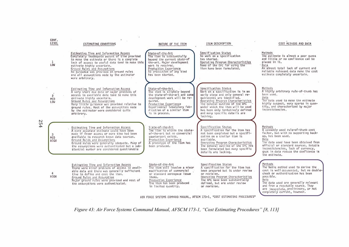
254
Figure 43: Air Force Systems Command Manual, AFSCM 173-1, “Cost Estimating Procedures” [8, 113]
255
4.12.1 Estimating Conditions
As can be seen, for the SpaceLiner case-study, the estimating conditions decisively fall
within the medium-high (confidence 3) range. Estimating time for the task was sufficient. Also,
the chosen case-study concept is currently at a very early stage. However, the technical reference
documentation which has been established as the baseline is sufficiently precise, and thus suitable
for a reasonable and representative cost estimation to be performed to reflect the current technical
status. Where insufficient data was found, strategic assumptions based on analogy or discussion
with experts and professionals (EJ) concerning scheduling, programmatic and operational
aspects, as well as some technical aspects, were made and documented. The estimating
confidence therefore lies in the medium-high category, with conditions expected to progressively
improve during consequent progression into Phases A and B, also reducing the estimating risk.
For the time being, any remaining uncertainty has been compensated by an appropriate cost
margins
4.12.2 Nature of the Item
The nature of the item can then be categorised between the low (confidence 1) and
medium-low (confidence 2) categories to reflect the considerable development effort still
required for the project, as well as the state-of-the-art being status between ‘slightly’ and
‘substantially’ beyond existing technologies, as per definition in Figure 43. Here, while the
philosophy of the concept centers on using no novel technologies, relying on existing state-of-the
art technologies wherever possible, nevertheless the system design, integration of elements and
utilisation of the SpaceLiner for passenger transport, is indeed novel and inherently carriers a
certain amount of potential risk which has a reflection on the cost estimating confidence. In
addition, the production status of the project is also addressed in the current classification, to
indicate that no current SpaceLiner case-study units have been produced.
256
4.12.3 Item Description
The item description is between the medium-low and medium-high categories with a
confidence level between 2 and 3. This indicates that specification work for the SpaceLiner case-
study is in the early stages with general requirements firmly identified. Similar concepts, such as
the Space Shuttle or the Buran vehicle, both of which are the only spacecraft of similar
magnitude which have actually flown, as well as new innovative movements such as the Florida
Space Port, can provide some existing and relevant specifications relevant for the case-study.
Additionally, the Operating Program Characteristics have been roughly defined, with technical
considerations presenting the biggest challenge.
4.12.4 Cost Methods & Data
Finally, in addition to data, at the heart of this Thesis are the cost methods. A high
confidence of 4 can therefore be decisively assumed for this category.
Basic and well established CEMs were assumed for cost estimation formulation.
Sophisticated and well renowned tools and models within the space sector which are both
recognised and utilised worldwide by government agencies like NASA, ESA and DLR as well as
industry have been independently applied for the SpaceLiner cost estimation with the
Amalgamation Approach (AAMAC) context. This novel approach was proposed, developed and
implemented as an innovative cost estimation strategy within this Thesis as an additional measure
to reduce the cost risk associated with early phase estimates. AAMAC makes a strong and most
notable contribution to boosting the confidence for this criterion through obtaining redundancy
and thus a more structured and justified final cost estimate or range. Therefore here, it can in fact
be deemed that the highest definition for the Level 4 - high certainty provided in the AFSCM
matrix is in fact below the actual cost estimate status attained and presented in this Thesis work.
The estimated results generated by the three cost models and tools are not identical but in a good
sound order of magnitude of each other, with the top-level results for phases C and D providing a
257
trustworthy, consistent, justifiable and reliable cost baseline with a high confidence rank.
Furthermore, all methods, processes and underlying assumptions for development and production
cost estimates have been clearly outlined and thoroughly documented for future reference.
It is also evident that the quality of technical data is crucial for qualitative cost estimation
and its related confidence. As previously mentioned, while the chosen case-study concept is in an
early program stage, the technical reference documentation which forms the technical baseline is
sufficiently precise, and thus suitable for deriving a reasonable and representative cost estimate.
4.12.5 Estimator Experience & Competence
While there is no confidence level defined in the AFSCM matrix for this essential
dimension, the background and the related experience of the estimator is an important
prerequisite for a professional and qualitatively high cost estimation standard, and does indeed
play a crucial role in cost estimate confidence. In fact this may be the most important
contribution to achieve a high estimating confidence and consequently a reduced risk level.
Throughout the compilation of this Thesis, a multitude of the highest level professional model
users and direct industry and software professionals and experts were always closely consulted
with, in regards to all matters associated with the three divers AAMAC tools, data input and output
interpretations, as well as theory and practical matters. All results have been consistently
discussed and respectively reviewed in great detail and through countless iterations (see Chapter
4.9.7.1) in line with AA principles, thorough a dynamic dialog between the latter professionals
and experts within the space domain, and across project management, scheduling and various
engineering fields. Consequently the confidence level of the resulting cost estimate with respect
to estimator experience and competence is considered to be very high, and the associated risk
with this aspect, low. Further improvements in line with more crystallised program information
are deemed necessary in the future, which is a task to be addressed in the consequent program
phases.
258
4.12.6 Cost Estimate Confidence Conclusion
Synthesising just the four confidence figures presented in Figure 43, (estimating
conditions 3; nature of the item 1.5; item description 2.5; cost methods and data 4;) yields an
average confidence interval of the overall estimate of 2.75, lying between medium-low and
medium high confidence. When adding the fifth essential dimension of cost estimator
competency, as discussed in Chapter 4.12.5, this confidence average would be raised to 3,
indicative of a firm medium-high cost estimate confidence level. This is the result of a
systematic cost estimating approach based on a clear and detailed preliminary WBS, project
schedule and consolidated with the innovative redundancy-infusing Amalgamation Approach to
support the cost estimation for development and production costs.
It should be noted that the AFSCM matrix presented in Figure 43 adopts a qualitative
rather than quantitative classification of the cost estimate confidence levels. A qualitative average
definition for the SpaceLiner case study is achieved, that the cost estimation results derived
within this Thesis bear medium-high confidence level at this early program phase. Given the
diverse nature, scope and complexity of the various space programs, assigning specific
quantitative values to such a matrix would be too general and therefore, non-constructive.
To assist the qualitative confidence level of the cost estimation, additionally, a cost
estimate review checklist as outlined by a RAND Project AIR FORCE report, proposes some key
points to be addressed by the cost estimator upon conclusion of the estimation procedure. This is
shown below in Figure 44. Another complimentary diagram shows a similar ‘best practices’
criteria list for the James Webb Space Telescope (JWST), again with all qualitative measure of
achievement for each category formulated based on the GAO assessment of NASA data.
At early program phase, it is difficult to specifically quantify confidence in a cost
estimate. At a later program stage, for example a clear Phase A, when a cost estimate is based on
data which is defined and frozen, quantification is possible. In 2009, NASA introduced a joint
confidence level (JCL) analysis standard, which is an integrated quantitative probability
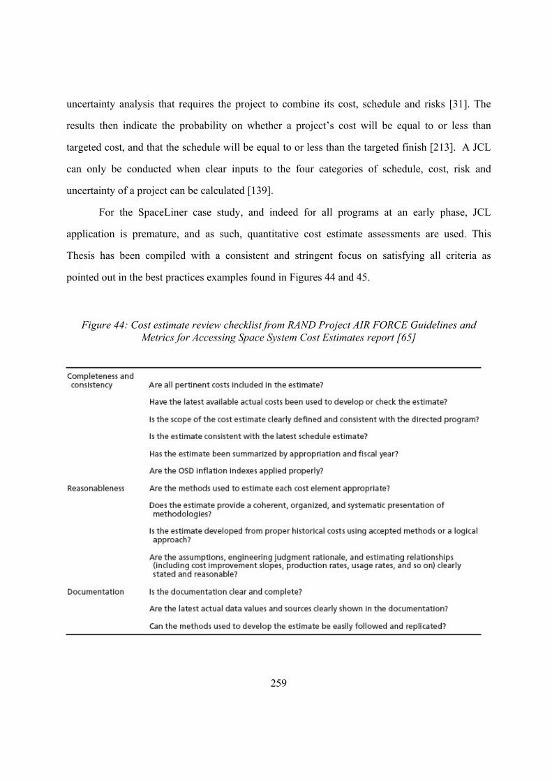
259
uncertainty analysis that requires the project to combine its cost, schedule and risks [31]. The
results then indicate the probability on whether a project’s cost will be equal to or less than
targeted cost, and that the schedule will be equal to or less than the targeted finish [213]. A JCL
can only be conducted when clear inputs to the four categories of schedule, cost, risk and
uncertainty of a project can be calculated [139].
For the SpaceLiner case study, and indeed for all programs at an early phase, JCL
application is premature, and as such, quantitative cost estimate assessments are used. This
Thesis has been compiled with a consistent and stringent focus on satisfying all criteria as
pointed out in the best practices examples found in Figures 44 and 45.
Figure 44: Cost estimate review checklist from RAND Project AIR FORCE Guidelines and Metrics for Accessing Space System Cost Estimates report [65]
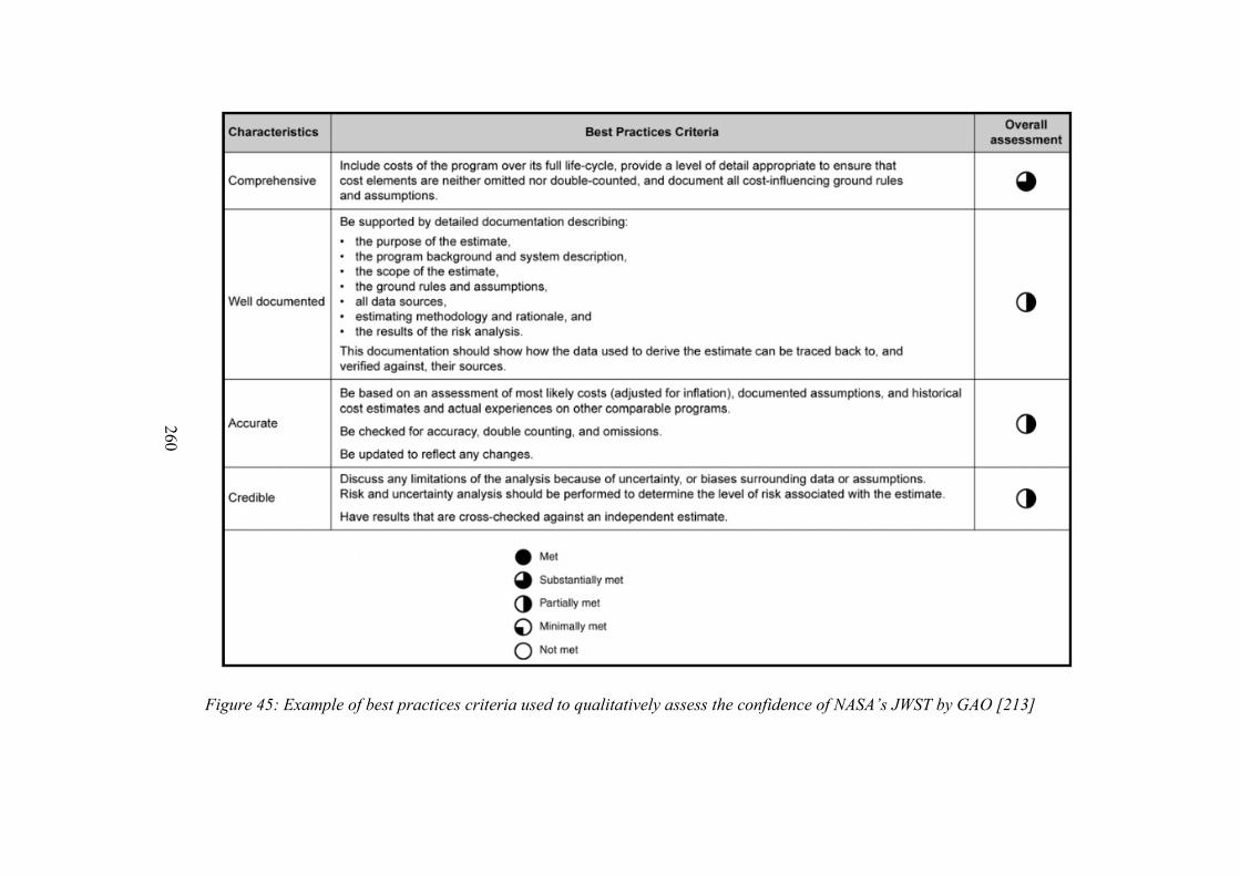
260
Figure 45: Example of best practices criteria used to qualitatively assess the confidence of NASA’s JWST by GAO [213]
261
5 THESIS FINAL CONCLUSIONS
“To most people, the sky is the limit. To those who love aviation, the sky is home.” – Anonymous
In summary, this Thesis outlined extensive cost engineering theory addressing the
challenge of justifiable and representative cost estimation for a large scale, complex, international
and unprecedented space program during the early program phase. During the process, CEMs
suitable for early phase application were determined, and current models and tools were then
reviewed, and outlined for specific program phases. The parametric approach was identified as
being most suitable for early phase application.
The Amalgamation Approach was proposed and described, drawing from the crucial
redundancy aspect usually inherent to mechanical hardware, and especially important for life-
critical systems. Since cost is a criterion with the potential to make or break a new program, then
cost can also considered here as a ‘life critical system’ within context of the program’s life – in
which case cost estimation should also incorporate a redundancy aspect from the start of cost
estimation formulation. Hence, the redundancy concept was transferred and applied to the cost
estimation domain through the AAMAC formulation of multiple (three) independent cost estimates
in an iterative process, with the resulting cost estimates produced as a synthesis of three results.
The aim here was to determine the program development (Phase C) and production (Phase D)
cost ranges for the chosen case-study vehicle.
Three models and tools were selected to implement within the AAMAC framework. These
were the parametric TransCost, and the prominent 4cost aces and PRICE-H commercial models.
A relevant and current industry case-study, the SpaceLiner, was then selected to demonstrate the
innovative AAMAC cost estimation method.
Two of the three classical program cost categories were the main target of this Thesis –
the non-recurring development and the recursive production cost, with software efforts for both
262
phases being omitted at this early stage of the case-study development, due to insufficiently
defined specifications and a lack of SW requirements. Operations were also considered mainly at
a qualitative level, although a very preliminary case-study operational scenario was also
discussed.
In order to facilitate for the cost estimate, essential programmatic considerations were
actualised in context of the SpaceLiner case-study. A detailed WBS was established, along with a
baseline program schedule, both of which were consequently used as the essential backbone for
the cost estimation.
Two key tools were programmed within the context of this Thesis work. The latest
available TransCost 82. Model (Revision 4) was programmed into a dedicated TransCost Excel
interface to allow for model testing and application. In addition, the Amalgamation Approach
Interface (AAInT) tool was also created to support the AAMAC theory and its application to the
chosen SpaceLiner case-study. Through the development and application of AA, baseline cost
estimates for the classical two categories of development and production program costs for a
selected, real-life and current case-study, were calculated.
The proposed AAMAC improves the confidence level associated with the final cost
estimation range as it provides a comparative baseline form several costs, allowing the cost
expert to identify and inconsistencies, and maximally justify and defend the final cost estimation
result. Through use of the innovative and advanced AAMAC, cost results were deemed to be in the
medium-high confidence interval.
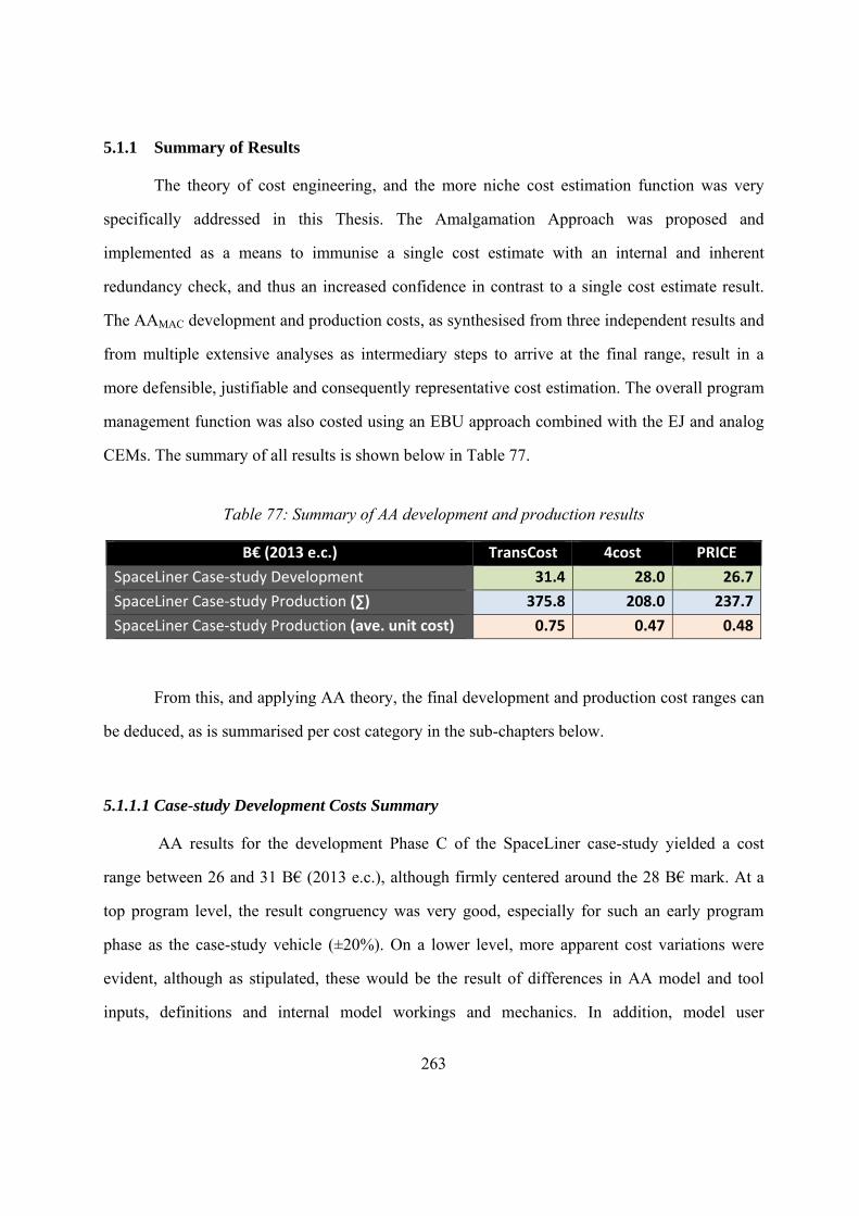
263
5.1.1 Summary of Results
The theory of cost engineering, and the more niche cost estimation function was very
specifically addressed in this Thesis. The Amalgamation Approach was proposed and
implemented as a means to immunise a single cost estimate with an internal and inherent
redundancy check, and thus an increased confidence in contrast to a single cost estimate result.
The AAMAC development and production costs, as synthesised from three independent results and
from multiple extensive analyses as intermediary steps to arrive at the final range, result in a
more defensible, justifiable and consequently representative cost estimation. The overall program
management function was also costed using an EBU approach combined with the EJ and analog
CEMs. The summary of all results is shown below in Table 77.
Table 77: Summary of AA development and production results
B€ (2013 e.c.) TransCost 4cost PRICE
SpaceLiner Case‐study Development 31.4 28.0 26.7
SpaceLiner Case‐study Production (∑) 375.8 208.0 237.7
SpaceLiner Case‐study Production (ave. unit cost) 0.75 0.47 0.48
From this, and applying AA theory, the final development and production cost ranges can
be deduced, as is summarised per cost category in the sub-chapters below.
5.1.1.1 Case-study Development Costs Summary
AA results for the development Phase C of the SpaceLiner case-study yielded a cost
range between 26 and 31 B€ (2013 e.c.), although firmly centered around the 28 B€ mark. At a
top program level, the result congruency was very good, especially for such an early program
phase as the case-study vehicle (±20%). On a lower level, more apparent cost variations were
evident, although as stipulated, these would be the result of differences in AA model and tool
inputs, definitions and internal model workings and mechanics. In addition, model user
264
specificity and EJ bias would have contributed to variations. The higher cost of the TransCost
model can also be attributed to the fact that the model is dedicated to orbital vehicles, while the
case-study vehicle is a suborbital craft. Additionally, TransCost inherently also addresses
software costs, which were not considered by the 4cost aces and PRICE tool calculations. A
medium-high confidence range could be assigned to the development cost estimate.
5.1.1.2 Case-Study Production Costs Summary
The production costs, also using the AA theory and AAMAC mode varied within the range
from the highest TransCost figure of 376 B€, through to 238 B€ (PRICE) and 4cost aces 209 B€
(2013 e.c.) for total SpaceLiner case-study program costs. Complementing the total production
costs were the average unit costs, calculated to be 752 M€ (TransCost), 475 M€ (PRICE) and 466
M€ (4cost), including an additional 20% margin for the commercial tools to allow for a relative
comparison with TransCost, which already incorporates this margin.
Here, while an excellent congruence of results was observed between the two commercial
models of PRICE and 4cost aces, the consistently (approximately 60%) higher TransCost model
results indicated an increased level of uncertainty given the significant delta to both AA-
employed models, as well as based on the theoretical and analytical justification for the
considerable deviations. The cause of this uncertainty was primarily stemmed from the need to
make necessary (and fully documented) assumptions to allow for the TransCost production cost
estimate to be compiled in the first place. These assumptions were necessary to address that no
TransCost CERs could be identified to sufficiently describe two of the four case-study elements
to be produced - the SLO and SLB. As such, an equal and un-weighted average values were
derived from two other CERs in each instance, forming a hybrid production cost estimate for the
SLO and SLB components. Given that one of the two CERs results in highest production costs of
all CERs contained in the TransCost manual, would also explain the considerably greater
265
TransCost production cost estimation results, indicative that they are not sufficiently
representative of expected SpaceLiner production costs.
Total program production of 500 units was therefore calculated to lie within the 210 – 280
B€ range, while the average unit cost range was found to be between 465 M€ and 490 M€ at
2013 economic conditions. Furthermore, as was discussed and demonstrated theoretically in
Chapter 4.12, the qualitative medium-high confidence range could be justifiably attributed to the
above cost estimation figures and derived cost ranges.
5.1.1.3 Case-study Sensitivity Analysis Summary
Sensitivity analyses were conducted within the scope of both development and production
cost estimations across all three AAMAC models.
For the TransCost model, development cost sensitivities were performed between the
complexity factors for the development standard (f1), technical quality (f2), as well as the team
experience (f3), as shown in Chapter 4.9.1.3. The purpose of the sensitivities was predominantly
to establish a development cost range internal to the TransCost model estimation itself, with a
development cost range between 31 and 39 B€ (at 2013 e.c.) deduced. Additionally, it was seen
that increasing the technology development factor and reducing team experience, while
increasing the number of engine test firings, increased the overall development cost by roughly
25% given the particular combination of complexity increments. For production costs, during the
course of the estimation process, the uncertainty associated with the TransCost model was
deemed too high due to assumptions which needed to be made. As such, the commercial tools
were relied upon to derive a more certain production cost range.
For the commercial tools, given that results were highly congruent between the PRICE
and 4cost aces tools, sensitivity analyses were performed using the 4cost aces tool only for both
development and production costs. Development sensitivities were performed for the initial 4cost
266
aces baseline costs, increasing prototype quantity and reducing team experience. As expected, it
was shown that the prototype quantity constitutes a significant cost driver for the development
Phase C, with a 36% and 56% delta to the 5-prototype model baseline for a prototype increase of
8 and 10 models respectively. A decrease in team experience during the development process by
one logical model unit also increased the baseline cost by roughly 10% at each iteration, although
this was not as pronounced as for the prototype quantity increase.
For the production cost sensitivities, the 4cost aces model was once again used to vary
three key production process variables in Chapter 4.10.9; the LC values, the production quantity,
and the engine reusability. Total program production costs and consequent average unit costs, as
well as TFU values were calculated and contrasted with baseline values. While LC sensitivity
results were surprising, a deeper analysis into the 4cost aces model mechanics revealed the
complex albeit very logical interrelations and influence of key quantity, LC and TFU cost
parameters on one another. The LC sensitivity analysis also highlighted that LC theory would
need to be considered at a deeper level for the SpaceLiner vehicle case-study in the future,
considering not only a fixed LC value throughout the production process, but a varying one,
depending on production quantities.
Variance of production quantities logically revealed a cost increase to an increased
production amount, and a decrease, with a decreased quantity produced. Finally, enhanced engine
reusability also impacted the total production costs in a positive way, reducing them by 15%
through a doubling of engine lifetime.
5.1.1.4 Case-study Operations & Ground Costs Summary
Within this Thesis, the operations and grounds (O&G) costs are presented and outlined in
a theoretical way. With respect to the SpaceLiner case-study vehicle, operational and ground cost
categories, like basic infrastructure, potential configuration and geographical locations of launch
267
and landing sites based on the anticipated vehicle requirements are outlined in a qualitative and
categorical way. Finally, a basic framework of operational activities is established and a
preliminary breakdown of costs which encompass the O&G segment as tailored to the
SpaceLiner case-study, are furthermore presented in Appendix J. The importance of expanding
the current status of knowledge, definitions, and mission requirements as future work in order to
mature this essential category of processes, requirements and associated costs, is also highlighted.
5.1.2 Future work
Much room for future work and development of the cost engineering and estimation
domains lies in the years ahead. Given the constantly evolving and dynamically changing space
industry and its environment, the function of a cost engineer within a project, and within the
wider space industry, never ceases.
This Thesis establishes the fundamental baseline for cost estimation practices for
unprecedented, large-scale and complex space programs in the early development phase. The
theory is then demonstrated within the context of an actual industry case-study, the SpaceLiner.
For this vehicle, which bridges the aviation and space industries, a parametric TransCost Excel
tool was programmed, and the model itself extensively tested. A WBS was also established,
based on which the newly proposed AA was applied to derive a baseline cost estimate for the
hardware elements and components through the phases of development and production. As such,
a strong and justified baseline of the cost estimation framework was established. Future work is
therefore required both within the cost estimation domain, as well as, more specifically, for the
SpaceLiner case-study example. Some key points are outlined below.
268
5.1.2.1 Amalgamation Approach
With respect to the proposed innovative Amalgamation Approach (including three modes
of application) as a tool to maximise cost estimate representativeness and reduce uncertainty, it
would be interesting to implement this approach alongside the classical, predominantly single-
means cost estimate approach. Towards the end of the program, the results for both approaches
should be confirmed and analysed, to determine whether AA results in an increased
representativeness of the results, and to quantify this. Furthermore, it would then be relevant to
implement this comparison across several large programs, and again, obtain quantitative
measures of the AA method and any benefits thereof. Such a comparison, however, was beyond
the scope of this Thesis work in terms of scale, and time. The duration of just the development
phase of the complex, large and multi-faceted programs such as those addressed within this
Thesis, already spans frequently over decades, and as such, is well beyond the scope of a single
PhD work.
5.1.2.2 SpaceLiner Development & Production Cost Estimation
A strong baseline cost range has been established, supported by the amalgamation
approach. Nevertheless, as the SpaceLiner case-study progresses through to a maturity where
technical specifications are finalised and frozen, the cost estimate will need to be modified, and
updated to reflect all the new information. In addition, in line with advancing program phases, the
CEMs for the models and tools being used to compile the estimates, will also need to be updated
appropriately. For example, the EBU CEM would be more applicable at a later stage, with a
significant reduction of risk associated with the estimate itself if it is performed correctly, and in
line with cost engineering principles.
Additionally, for the production costs in particular, as a clearer and more defined program
schedule evolves, the production costs would need to be reassessed to reflect the timing element
in terms of batch production. In addition, and as already thoroughly discussed in Chapters 4.10.1,
269
4.10.8.2 and 4.10.9.1, LC theory should then be fine-tuned, with respect to distinguishing
between unique LCs for the initial batch of units produced, and consequently for those units
produced in a set serial context. Here, a distinction should be made between elements with a
production quantity of 500 (SLO, SLB and SPC) and those with a production quantity in the high
thousands (SLME). The SLME with its significantly higher rate of production, would exhibit
significantly less learning than the simplified and constantly assumed 85% due to higher
quantities produced and thus higher level of automatisation.
5.1.2.3 Software Costs
In this Thesis, space hardware development and production costs were the focus. As such,
software costs were excluded due to the specific nature of the cost calculation themselves,
coupled with currently incomplete SW specifications and requirements for the SpaceLiner case-
study. It is fully conceded that for a full program, software costs constitute an essential part of the
function and are therefore critically important, and as such, the established WBS incorporates
elements to address and later include these costs at a later stage. However in this Thesis the
dedicated subset of software costs could not be calculated given the current early status of the
SpaceLiner case-study. Furthermore, space hardware cost assessment is such an own, specific
and extensive topic, and in excluding software costs in this Thesis, the integrity of the existing
cost estimate is maintained.
For future assessment of software development and production costs, various separate and
dedicated methods are available for application. These are as diverse and varied as the different
CEMs for hardware, honing in on space hardware, and, in accordance with Boehm’s compilation
of models [27] include COCOMO, Putnam, Doty and Jensen models [202]. A software module
from PRICE Systems, PRICE-S, is also available, as well as a software estimation ability from
270
4cost aces. However, all the latter require basic software inputs to reflect requirements, function
and complexity of software.
5.1.2.4 SpaceLiner Operation & Ground Costs
Within this Thesis, the operations and ground costs (WBS elements 6000 and 7000) were
discussed within a more qualitative context, although a preliminary consideration of some ground
infrastructure and resources has also been considered [111]. As the SpaceLiner concept matures,
and a clearer idea of trajectories evolves, then a more specific and dedicated analysis of these two
WBS elements will need to be performed. Based on the results, a cost estimate of the proposed
infrastructure for ground, as well as the operations procedures and regime, can also be compiled.
5.1.2.5 Sensitivity Analyses
Although some basic sensitivity analyses were presented in this Thesis, it would be
interesting to conduct further sensitivities and trades to determine the most desirable cost
scenario given various tradeoffs. In addition, the 4cost aces tool was used to conduct sensitivity
analyses. It would be furthermore relevant to pursue sensitivity analyses using the other AAMAC
models and tools, allowing for contrasting of sensitivity results amongst them, too.
A proposed matrix of interesting trades is shown below in Table 78 Other than the
baselines, the values shown in bold have already been addressed in this Thesis using the 4cost
aces tool. In the table, the *ind superscript refers to the AA commercial tool respective indices.
For example, in the context of the applied 4cost aces tool, the Production Environment sensitivity
refers to the 4cost aces specific variable ENVIRD input which describes the context and industry
of the development effort (see Figure 33). The baseline value, as outlined in Chapter 4.9.3, was
taken to be 2.0, with reasonable increments for this value being defined by the 4cost aces model
as being 0.1. Therefore the table-indicated sensitivity suggestions of +1ind; -1 ind; -2ind thus refer to
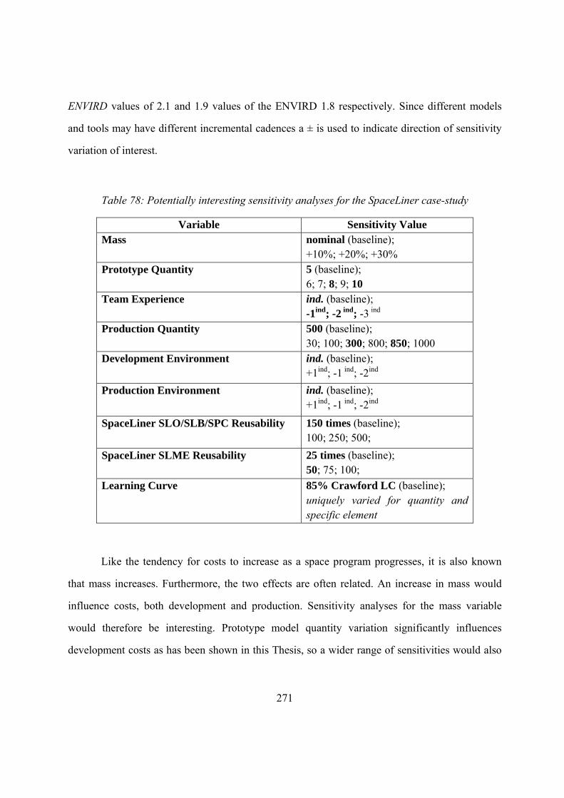
271
ENVIRD values of 2.1 and 1.9 values of the ENVIRD 1.8 respectively. Since different models
and tools may have different incremental cadences a ± is used to indicate direction of sensitivity
variation of interest.
Table 78: Potentially interesting sensitivity analyses for the SpaceLiner case-study
Variable Sensitivity Value Mass nominal (baseline);
+10%; +20%; +30% Prototype Quantity 5 (baseline);
6; 7; 8; 9; 10 Team Experience ind. (baseline);
-1ind; -2 ind; -3 ind Production Quantity 500 (baseline);
30; 100; 300; 800; 850; 1000 Development Environment ind. (baseline);
+1ind; -1 ind; -2ind
Production Environment ind. (baseline); +1ind; -1 ind; -2ind
SpaceLiner SLO/SLB/SPC Reusability 150 times (baseline); 100; 250; 500;
SpaceLiner SLME Reusability 25 times (baseline); 50; 75; 100;
Learning Curve 85% Crawford LC (baseline); uniquely varied for quantity and specific element
Like the tendency for costs to increase as a space program progresses, it is also known
that mass increases. Furthermore, the two effects are often related. An increase in mass would
influence costs, both development and production. Sensitivity analyses for the mass variable
would therefore be interesting. Prototype model quantity variation significantly influences
development costs as has been shown in this Thesis, so a wider range of sensitivities would also
272
be beneficial. Team experience and the environments for development and production are also
influential parameters on cost and should be studied further.
Finally the production quantity delta, including variances in the reusability capability of
components, directly drives the recurring production cost. Linked closely with learning curve
theory for production, as already discussed in Chapter 5.1.2.2, uniquely developing and
implementing varying LC values for various production quantities and specific elements, would
also be interesting.
In addition, modeling production quantities which integrate the production schedule in
terms of batch numbers, frequency of production as well as different reusability capabilities for
the SLO, SLB, and SPC should be attempted in the future. This step, however, would hinge on an
unambiguous and clearly defined production schedule.
5.1.2.6 WBS & Program Schedule Iterations
A baseline program schedule in conjunction with a detailed four level WBS were derived
and presented in this Thesis (Chapters 4.1.1 and 4.1.2). The WBS elements are the outcome of
activities that take time to complete. As such, it is important to respect the underlying
relationships of time precedence among them [175], highlighting the high level of
interdependency between a WBS and a program schedule. In their baseline formulation, many
assumptions were made to bridge any gaps inherent to a highly complex concept still in an early
program phase, which is still developing and constantly changing. However, as any project
matures, and more information becomes available, both the WBS and schedule can and should
undergo respective iterations and modifications to be reflective of changes and progress. Such
changes are especially pronounced and can be significant during the early program phases, as
they also occur at a lower cost. The importance of developing a program schedule consistently
with the project’s objectives, working at the lowest available WBS level, is outlined by Shishko,
273
through six steps to achieve congruency and concord between the WBS and a network schedule
which illustrates activities, their interdependencies and duration, as well as key product
milestones. Such a detailed network schedule should also be compiled for the SpaceLiner case-
study as the concept matures.
5.1.2.7 Financing
Within context of cost engineering and financial considerations for the case-study, as is
indeed the case for any large-scale, complex program, the financing element is a highly
interesting and crucial consideration. For government programs, the funding comes from the
federal sources. However for entities who operate independently of government funding,
investment must be sought elsewhere. In the space industry, it is well known and documented
that many cost overruns are the direct result of complex governmental structures and cost-
consuming interfaces. The recent emergence and flurry of the establishment of privately funded
spin-off or independent companies, however, offers attestation to the fact that the smaller, leaner
and more efficient internal company structures lend themselves to more efficient processes and
operations. The most prominent example of such a company would arguably be SpaceX, who are
reportedly achieving unprecedented cost-savings across their development, production and
operational activities [193] would be the prime and most current example of such an
organisation.
While it is beyond the scope of this work to delve into possible financing sources , it is
nevertheless very important to mention the various potential financing sources and schemes
relevant to a concept such as the SpaceLiner case-study. Of course the type of financing source
and arrangement hinges on the nature of the space program. Sources of finances for the non-
recursive research and development Phases A to C as well as the recursive production and
operational Phase D might come from the venture capital market, or from shareholder
investment, private equity funds through inclusion in risk capital, or bank loans. For the
274
development phase, financial support could also be sought from R&D agencies [122]. An
interesting financing structure to explore here would also be the Public-Private Partnership (PPP)
structure where a strategically phased mix of public and private funds are combined. Public funds
support early investment while still involving the private sector in design and development
activities. The resulting operational product is then carried further by private investors [148].
5.1.2.8 Budget, Resource Planning
Within this Thesis, costs were considered at a very top level, using parametric cost
estimation, which also assumes an average WYr cost for personnel within the aerospace industry
provided in the TransCost manual [102]. As the program matures, the EBU CEM also becomes
increasingly more appropriate for cost estimation in the later program phases, and costs must be
further broken down and looked at a lower level from a budgeting and resource planning context.
This is also reflective of a sufficiently detailed and advanced program definition and status. Such
a baseline budget is developed from the WBS and program schedule and should be addressed
systematically. Specifically, the project’s work force and other resource needs should be
combined with the appropriate workforce rates and other financial and programmatic factors to
obtain cost element estimates, which, as outlined by Shishko [175], include:
Direct labour costs
Overhead costs
Other direct costs (travel, data processing etc.)
Subcontract costs
Material costs
General and Admin costs
Cost of money (interest payments, if applicable)
Fee (if applicable)
Contingency
275
After costs have been baselined, it is then important to impose measures of cost control,
including project cost and schedule status reporting. Another vital aspect here is then cost and
schedule risk planning, and a function of high project level budgeting and resource planning
should incorporate for allowance of adequate contingency funds to cover any unforeseen events.
5.1.2.9 Risk Assessment & Planning
The risk assessment presented and discussed in this Thesis (Chapters 4.1.11 and 4.12) was
incorporated at a very basic and qualitative level due to the early program phase, as well as still
crystallising program details for the chosen SpaceLiner case-study. At this early stage mitigation
of financial risks of the SpaceLiner project has been achieved through a proposed cost margin of
20 percent. As with any maturing program, and in line with the four step risk assessment and
mitigation process described in Chapter 4.1.11 and shown in Figure 18, risk assessment and
consequent mitigation strategy would require a more detailed, in-depth and systematic approach
when the technical and programmatic assumptions underpinning this work and case-study
addressed in this Thesis are replaced with mature, fixed data, and when specifications and
requirements are clearly decided upon and set. Risk avoidance and work around strategies should
then be developed, alongside with a translation of the risk into more precise cost terms, which
should be factored into the budget and resource planning component of the program as explained
in Chapter 5.1.2.8. Since the areas of schedule, cost and risk assessment are all linked and
interdependent, at a more mature stage, a method such as the joint confidence level (JCL)
analysis standard adopted by NASA and briefly discussed in Chapter 4.12, could be
implemented.

276
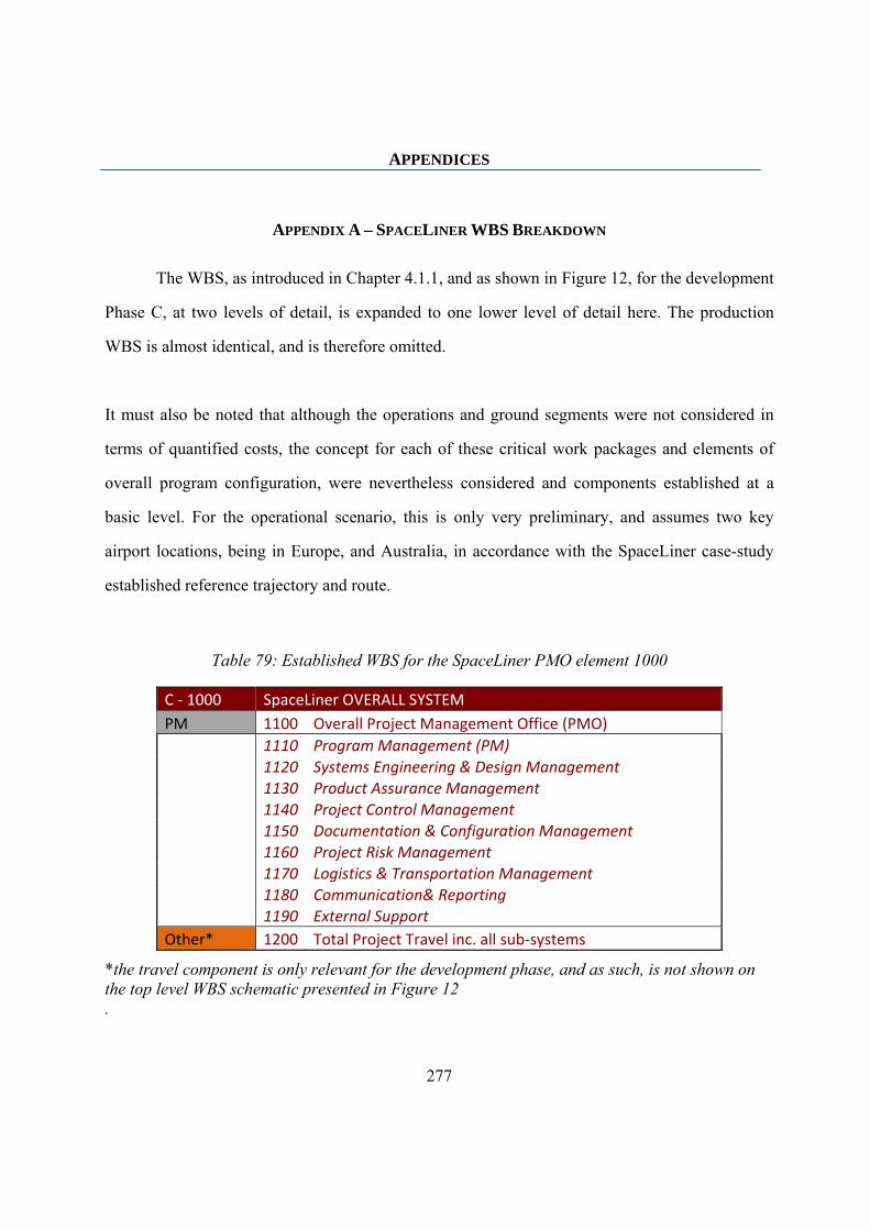
277
APPENDICES
APPENDIX A – SPACELINER WBS BREAKDOWN
The WBS, as introduced in Chapter 4.1.1, and as shown in Figure 12, for the development
Phase C, at two levels of detail, is expanded to one lower level of detail here. The production
WBS is almost identical, and is therefore omitted.
It must also be noted that although the operations and ground segments were not considered in
terms of quantified costs, the concept for each of these critical work packages and elements of
overall program configuration, were nevertheless considered and components established at a
basic level. For the operational scenario, this is only very preliminary, and assumes two key
airport locations, being in Europe, and Australia, in accordance with the SpaceLiner case-study
established reference trajectory and route.
Table 79: Established WBS for the SpaceLiner PMO element 1000
C ‐ 1000 SpaceLiner OVERALL SYSTEM
PM 1100 Overall Project Management Office (PMO)
1110 Program Management (PM)
1120 Systems Engineering & Design Management 1130 Product Assurance Management 1140 Project Control Management 1150 Documentation & Configuration Management 1160 Project Risk Management 1170 Logistics & Transportation Management 1180 Communication& Reporting 1190 External Support
Other* 1200 Total Project Travel inc. all sub‐systems
*the travel component is only relevant for the development phase, and as such, is not shown on the top level WBS schematic presented in Figure 12 .
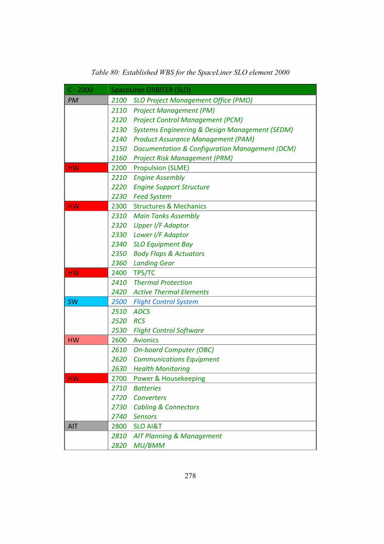
278
Table 80: Established WBS for the SpaceLiner SLO element 2000
C ‐ 2000 SpaceLiner ORBITER (SLO)
PM 2100 SLO Project Management Office (PMO)
2110 Project Management (PM) 2120 Project Control Management (PCM)
2130 Systems Engineering & Design Management (SEDM) 2140 Product Assurance Management (PAM)
2150 Documentation & Configuration Management (DCM) 2160 Project Risk Management (PRM)
HW 2200 Propulsion (SLME)
2210 Engine Assembly
2220 Engine Support Structure 2230 Feed System
HW 2300 Structures & Mechanics
2310 Main Tanks Assembly
2320 Upper I/F Adaptor 2330 Lower I/F Adaptor 2340 SLO Equipment Bay 2350 Body Flaps & Actuators 2360 Landing Gear
HW 2400 TPS/TC
2410 Thermal Protection 2420 Active Thermal Elements
SW 2500 Flight Control System
2510 ADCS 2520 RCS 2530 Flight Control Software
HW 2600 Avionics
2610 On‐board Computer (OBC) 2620 Communications Equipment 2630 Health Monitoring
HW 2700 Power & Housekeeping
2710 Batteries 2720 Converters 2730 Cabling & Connectors 2740 Sensors
AIT 2800 SLO AI&T
2810 AIT Planning & Management 2820 MU/BMM
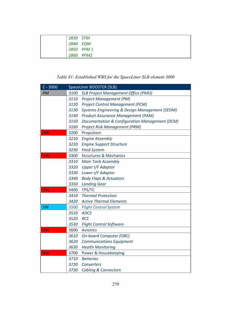
279
2830 STM
2840 EQM 2850 PFM 1
2860 PFM2
Table 81: Established WBS for the SpaceLiner SLB element 3000
C ‐ 3000 SpaceLiner BOOSTER (SLB)
PM 3100 SLB Project Management Office (PMO)
3110 Project Management (PM) 3120 Project Control Management (PCM) 3130 Systems Engineering & Design Management (SEDM) 3140 Product Assurance Management (PAM) 3150 Documentation & Configuration Management (DCM) 3160 Project Risk Management (PRM)
HW 3200 Propulsion
3210 Engine Assembly 3220 Engine Support Structure 3230 Feed System
HW 3300 Structures & Mechanics
3310 Main Tank Assembly 3320 Upper I/F Adaptor 3330 Lower I/F Adaptor 3340 Body Flaps & Actuators 3350 Landing Gear
HW 3400 TPS/TC
3410 Thermal Protection 3420 Active Thermal Elements
SW 3500 Flight Control System
3510 ADCS 3520 RCS 3530 Flight Control Software
HW 3600 Avionics
3610 On‐board Computer (OBC) 3620 Communications Equipment 3630 Health Monitoring
HW 3700 Power & Housekeeping
3710 Batteries 3720 Converters 3730 Cabling & Connectors
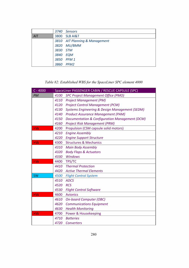
280
3740 Sensors
AIT 3800 SLB AI&T
3810 AIT Planning & Management
3820 MU/BMM 3830 STM 3840 EQM 3850 PFM 1
3860 PFM2
Table 82: Established WBS for the SpaceLiner SPC element 4000
C ‐ 4000 SpaceLiner PASSENGER CABIN / RESCUE CAPSULE (SPC)
PM 4100 SPC Project Management Office (PMO)
4110 Project Management (PM) 4120 Project Control Management (PCM) 4130 Systems Engineering & Design Management (SEDM) 4140 Product Assurance Management (PAM) 4150 Documentation & Configuration Management (DCM) 4160 Project Risk Management (PRM)
HW 4200 Propulsion (CSM capsule solid motors)
4210 Engine Assembly 4220 Engine Support Structure
HW 4300 Structures & Mechanics
4310 Main Body Assembly 4320 Body Flaps & Actuators 4330 Windows
HW 4400 TPS/TC
4410 Thermal Protection 4420 Active Thermal Elements
SW 4500 Flight Control System
4510 ADCS 4520 RCS 4530 Flight Control Software
HW 4600 Avionics
4610 On‐board Computer (OBC) 4620 Communications Equipment 4630 Health Monitoring
HW 4700 Power & Housekeeping
4710 Batteries 4720 Converters
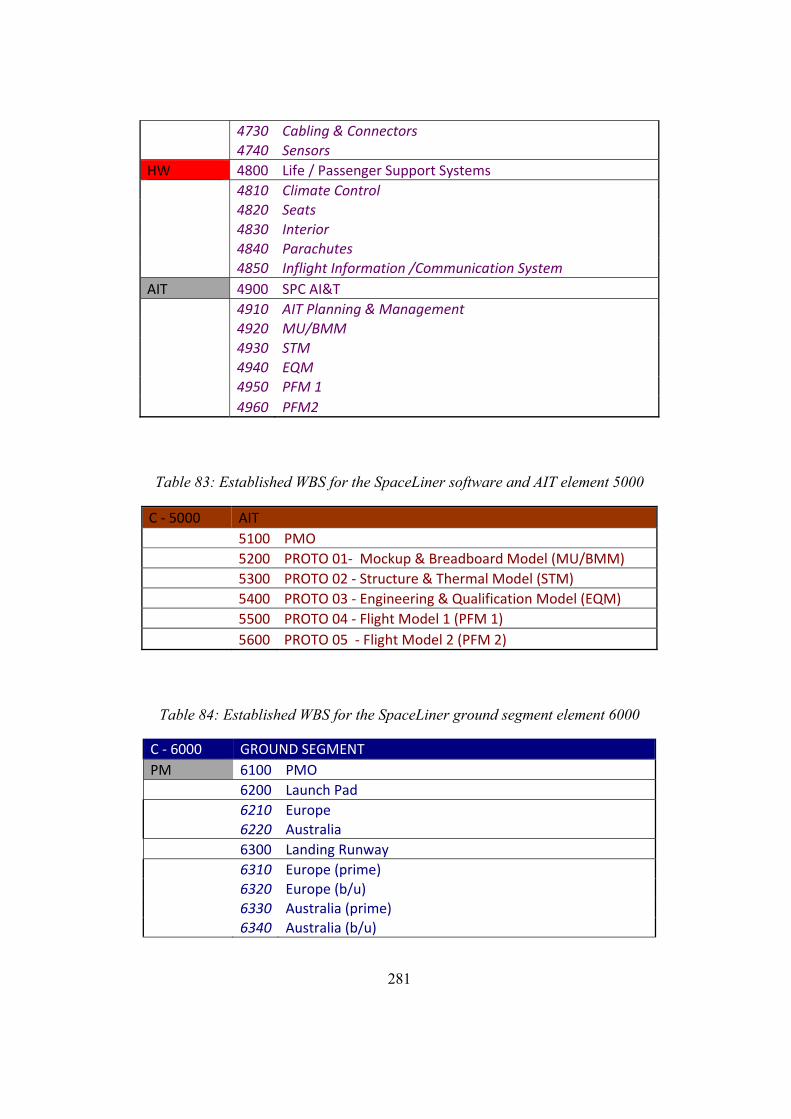
281
4730 Cabling & Connectors
4740 Sensors
HW 4800 Life / Passenger Support Systems
4810 Climate Control 4820 Seats
4830 Interior 4840 Parachutes 4850 Inflight Information /Communication System
AIT 4900 SPC AI&T
4910 AIT Planning & Management 4920 MU/BMM
4930 STM 4940 EQM 4950 PFM 1
4960 PFM2
Table 83: Established WBS for the SpaceLiner software and AIT element 5000
C ‐ 5000 AIT
5100 PMO
5200 PROTO 01‐ Mockup & Breadboard Model (MU/BMM)
5300 PROTO 02 ‐ Structure & Thermal Model (STM)
5400 PROTO 03 ‐ Engineering & Qualification Model (EQM)
5500 PROTO 04 ‐ Flight Model 1 (PFM 1)
5600 PROTO 05 ‐ Flight Model 2 (PFM 2)
Table 84: Established WBS for the SpaceLiner ground segment element 6000
C ‐ 6000 GROUND SEGMENT
PM 6100 PMO
6200 Launch Pad
6210 Europe 6220 Australia
6300 Landing Runway
6310 Europe (prime) 6320 Europe (b/u) 6330 Australia (prime) 6340 Australia (b/u)
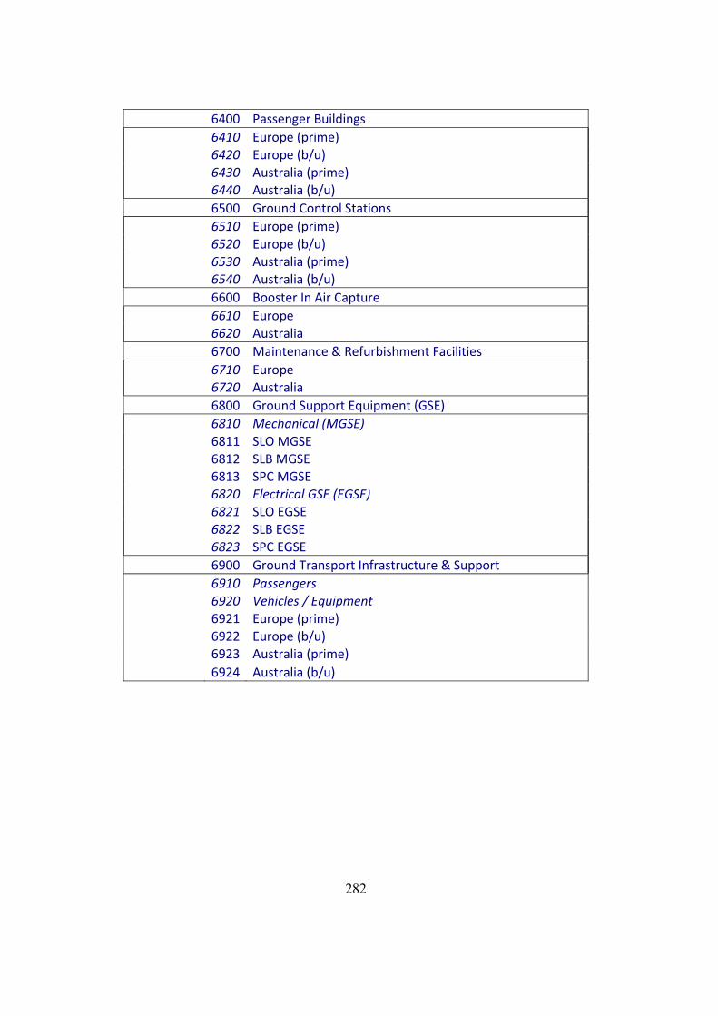
282
6400 Passenger Buildings
6410 Europe (prime) 6420 Europe (b/u)
6430 Australia (prime) 6440 Australia (b/u)
6500 Ground Control Stations
6510 Europe (prime)
6520 Europe (b/u) 6530 Australia (prime) 6540 Australia (b/u)
6600 Booster In Air Capture
6610 Europe 6620 Australia
6700 Maintenance & Refurbishment Facilities
6710 Europe 6720 Australia
6800 Ground Support Equipment (GSE)
6810 Mechanical (MGSE)
6811 SLO MGSE 6812 SLB MGSE 6813 SPC MGSE 6820 Electrical GSE (EGSE) 6821 SLO EGSE 6822 SLB EGSE 6823 SPC EGSE
6900 Ground Transport Infrastructure & Support
6910 Passengers 6920 Vehicles / Equipment 6921 Europe (prime)
6922 Europe (b/u) 6923 Australia (prime)
6924 Australia (b/u)
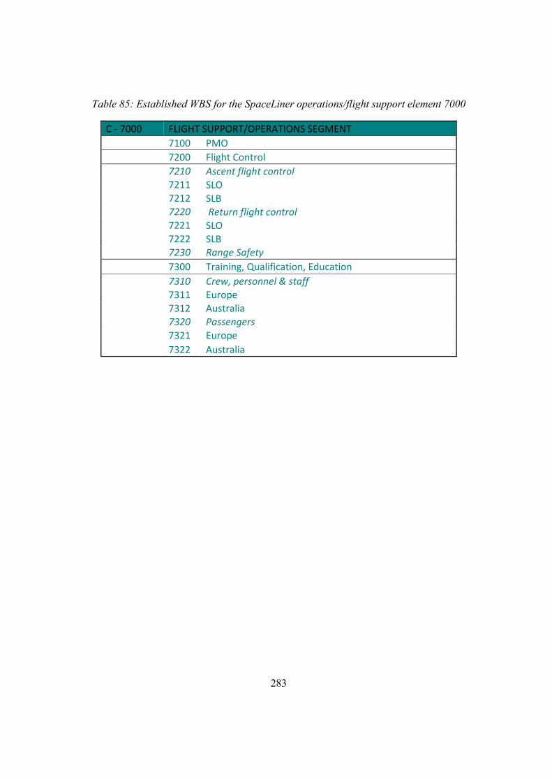
283
Table 85: Established WBS for the SpaceLiner operations/flight support element 7000
C ‐ 7000 FLIGHT SUPPORT/OPERATIONS SEGMENT
7100 PMO
7200 Flight Control
7210 Ascent flight control 7211 SLO 7212 SLB 7220 Return flight control 7221 SLO 7222 SLB
7230 Range Safety
7300 Training, Qualification, Education
7310 Crew, personnel & staff 7311 Europe 7312 Australia 7320 Passengers
7321 Europe
7322 Australia
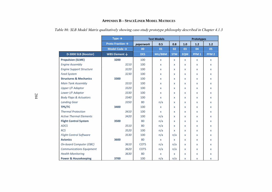
284
APPENDIX B – SPACELINER MODEL MATRICES
Table 86: SLB Model Matrix qualitatively showing case-study prototype philosophy described in Chapter 4.1.3
Type → Test Models Prototypes
Proto Fraction → paperwork 0.5 0.8 1.0 1.2 1.2
Model Code → 00 01 02 03 04 05
D‐3000 SLB (Booster) WBS Element ↓ DES MU/BBM STM EQM PFM 1 PFM 2
Propulsion (SLME) 3200 100 x x x x x
Engine Assembly 3210 100 x x x x x
Engine Support Structure 3220 100 x x x x x
Feed System 3230 100 x x x x x
Structures & Mechanics 3300 100 x x x x x
Main Tank Assembly 3310 100 x x x x x
Upper I/F Adaptor 3320 100 x x x x x
Lower I/F Adaptor 3330 100 x x x x x
Body Flaps & Actuators 3340 100 x x x x x
Landing Gear 3350 80 n/a x x x x
TPS/TC 3400 100 x x x x x
Thermal Protection 3410 100 x x x x x
Active Thermal Elements 3420 100 n/a x x x x
Flight Control System 3500 80 n/a x x x x
ADCS 3510 80 n/a x x x x
RCS 3520 100 n/a x x x x
Flight Control Software 3530 100 n/a n/a x x x
Avionics 3600 80 x x x x x
On‐board Computer (OBC) 3610 COTS n/a n/a x x x
Communications Equipment 3620 COTS n/a n/a x x x
Health Monitoring 3630 80 x x x x x
Power & Housekeeping 3700 100 n/a n/a x x x
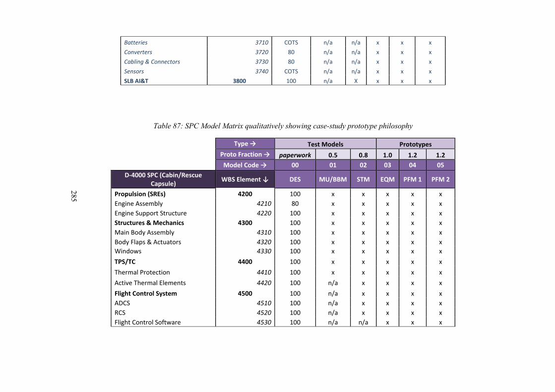
285
Batteries 3710 COTS n/a n/a x x x
Converters 3720 80 n/a n/a x x x
Cabling & Connectors 3730 80 n/a n/a x x x
Sensors 3740 COTS n/a n/a x x x
SLB AI&T 3800 100 n/a X x x x
Table 87: SPC Model Matrix qualitatively showing case-study prototype philosophy
Type → Test Models Prototypes
Proto Fraction → paperwork 0.5 0.8 1.0 1.2 1.2
Model Code → 00 01 02 03 04 05
D‐4000 SPC (Cabin/Rescue Capsule)
WBS Element ↓ DES MU/BBM STM EQM PFM 1 PFM 2
Propulsion (SREs) 4200 100 x x x x x
Engine Assembly 4210 80 x x x x x
Engine Support Structure 4220 100 x x x x x
Structures & Mechanics 4300 100 x x x x x
Main Body Assembly 4310 100 x x x x x
Body Flaps & Actuators 4320 100 x x x x x
Windows 4330 100 x x x x x
TPS/TC 4400 100 x x x x x
Thermal Protection 4410 100 x x x x x
Active Thermal Elements 4420 100 n/a x x x x
Flight Control System 4500 100 n/a x x x x
ADCS 4510 100 n/a x x x x
RCS 4520 100 n/a x x x x
Flight Control Software 4530 100 n/a n/a x x x
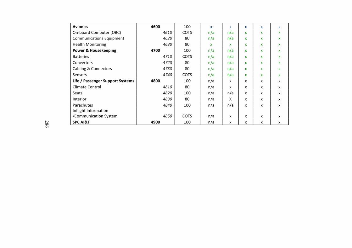
286
Avionics 4600 100 x x x x x
On‐board Computer (OBC) 4610 COTS n/a n/a x x x
Communications Equipment 4620 80 n/a n/a x x x
Health Monitoring 4630 80 x x x x x
Power & Housekeeping 4700 100 n/a n/a x x x
Batteries 4710 COTS n/a n/a x x x
Converters 4720 80 n/a n/a x x x
Cabling & Connectors 4730 80 n/a n/a x x x
Sensors 4740 COTS n/a n/a x x x
Life / Passenger Support Systems 4800 100 n/a x x x x
Climate Control 4810 80 n/a x x x x
Seats 4820 100 n/a n/a x x x
Interior 4830 80 n/a X x x x
Parachutes 4840 100 n/a n/a x x xInflight Information /Communication System 4850 COTS n/a x x x x
SPC AI&T 4900 100 n/a x x x x
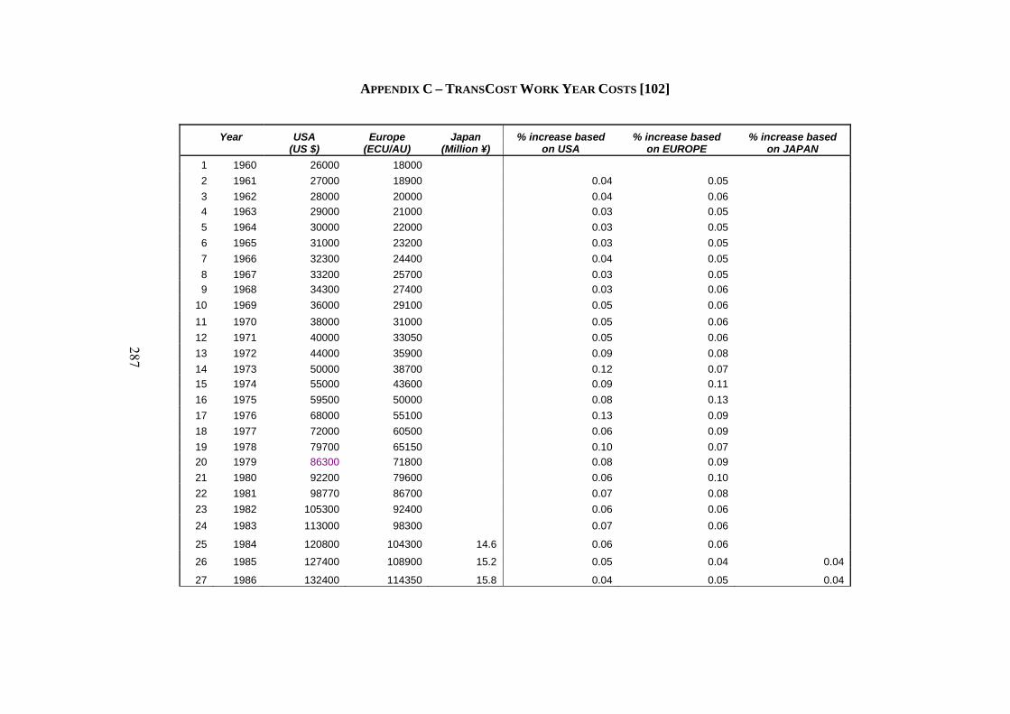
287
APPENDIX C – TRANSCOST WORK YEAR COSTS [102]
Year USA Europe Japan % increase based % increase based % increase based (US $) (ECU/AU) (Million ¥) on USA on EUROPE on JAPAN
1 1960 26000 18000
2 1961 27000 18900 0.04 0.05
3 1962 28000 20000 0.04 0.06
4 1963 29000 21000 0.03 0.05
5 1964 30000 22000 0.03 0.05
6 1965 31000 23200 0.03 0.05
7 1966 32300 24400 0.04 0.05
8 1967 33200 25700 0.03 0.05
9 1968 34300 27400 0.03 0.06
10 1969 36000 29100 0.05 0.06
11 1970 38000 31000 0.05 0.06
12 1971 40000 33050 0.05 0.06
13 1972 44000 35900 0.09 0.08
14 1973 50000 38700 0.12 0.07
15 1974 55000 43600 0.09 0.11
16 1975 59500 50000 0.08 0.13
17 1976 68000 55100 0.13 0.09
18 1977 72000 60500 0.06 0.09
19 1978 79700 65150 0.10 0.07
20 1979 86300 71800 0.08 0.09
21 1980 92200 79600 0.06 0.10
22 1981 98770 86700 0.07 0.08
23 1982 105300 92400 0.06 0.06
24 1983 113000 98300 0.07 0.06
25 1984 120800 104300 14.6 0.06 0.06
26 1985 127400 108900 15.2 0.05 0.04 0.04
27 1986 132400 114350 15.8 0.04 0.05 0.04
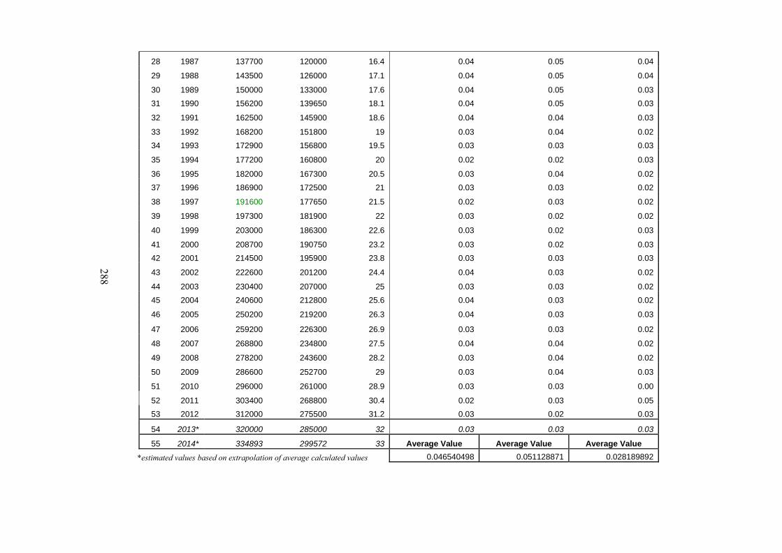
288
28 1987 137700 120000 16.4 0.04 0.05 0.04
29 1988 143500 126000 17.1 0.04 0.05 0.04
30 1989 150000 133000 17.6 0.04 0.05 0.03
31 1990 156200 139650 18.1 0.04 0.05 0.03
32 1991 162500 145900 18.6 0.04 0.04 0.03
33 1992 168200 151800 19 0.03 0.04 0.02
34 1993 172900 156800 19.5 0.03 0.03 0.03
35 1994 177200 160800 20 0.02 0.02 0.03
36 1995 182000 167300 20.5 0.03 0.04 0.02
37 1996 186900 172500 21 0.03 0.03 0.02
38 1997 191600 177650 21.5 0.02 0.03 0.02
39 1998 197300 181900 22 0.03 0.02 0.02
40 1999 203000 186300 22.6 0.03 0.02 0.03
41 2000 208700 190750 23.2 0.03 0.02 0.03
42 2001 214500 195900 23.8 0.03 0.03 0.03
43 2002 222600 201200 24.4 0.04 0.03 0.02
44 2003 230400 207000 25 0.03 0.03 0.02
45 2004 240600 212800 25.6 0.04 0.03 0.02
46 2005 250200 219200 26.3 0.04 0.03 0.03
47 2006 259200 226300 26.9 0.03 0.03 0.02
48 2007 268800 234800 27.5 0.04 0.04 0.02
49 2008 278200 243600 28.2 0.03 0.04 0.02
50 2009 286600 252700 29 0.03 0.04 0.03
51 2010 296000 261000 28.9 0.03 0.03 0.00
52 2011 303400 268800 30.4 0.02 0.03 0.05
53 2012 312000 275500 31.2 0.03 0.02 0.03
54 2013* 320000 285000 32 0.03 0.03 0.03
55 2014* 334893 299572 33 Average Value Average Value Average Value
0.046540498 0.051128871 0.028189892*estimated values based on extrapolation of average calculated values
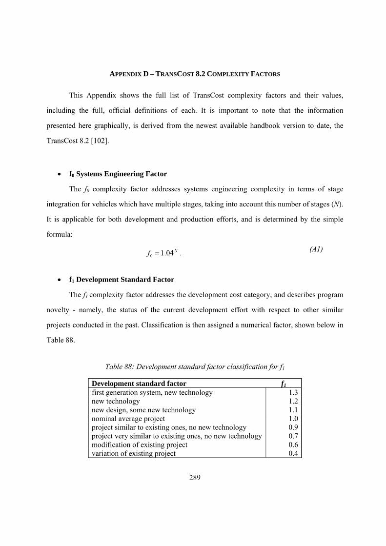
289
APPENDIX D – TRANSCOST 8.2 COMPLEXITY FACTORS
This Appendix shows the full list of TransCost complexity factors and their values,
including the full, official definitions of each. It is important to note that the information
presented here graphically, is derived from the newest available handbook version to date, the
TransCost 8.2 [102].
f0 Systems Engineering Factor
The f0 complexity factor addresses systems engineering complexity in terms of stage
integration for vehicles which have multiple stages, taking into account this number of stages (N).
It is applicable for both development and production efforts, and is determined by the simple
formula:
Nf 04.10 . (A1)
f1 Development Standard Factor
The f1 complexity factor addresses the development cost category, and describes program
novelty - namely, the status of the current development effort with respect to other similar
projects conducted in the past. Classification is then assigned a numerical factor, shown below in
Table 88.
Table 88: Development standard factor classification for f1
Development standard factor f1 first generation system, new technology 1.3 new technology 1.2 new design, some new technology 1.1 nominal average project 1.0 project similar to existing ones, no new technology 0.9 project very similar to existing ones, no new technology 0.7 modification of existing project 0.6 variation of existing project 0.4
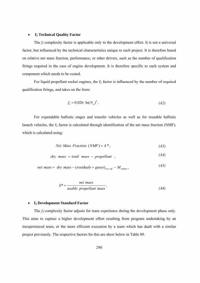
290
f2 Technical Quality Factor
The f2 complexity factor is applicable only to the development effort. It is not a universal
factor, but influenced by the technical characteristics unique to each project. It is therefore based
on relative net mass fraction, performance, or other drivers, such as the number of qualification
firings required in the case of engine development. It is therefore specific to each system and
component which needs to be costed.
For liquid propellant rocket engines, the f2 factor is influenced by the number of required
qualification firings, and takes on the form:
2
2 )ln(026.0 qNf . (A2)
For expendable ballistic stages and transfer vehicles as well as for reusable ballistic
launch vehicles, the f2 factor is calculated through identification of the net mass fraction (NMF),
which is calculated using:
*)( kNMFFractionMassNet , (A3)
propellantmasstotalmassdry , (A4)
engineoffcut Mgasesresidualsmassdrymassnet )( , (A5)
masspropellantusable
massnetk * .
(A6)
f3 Development Standard Factor
The f3 complexity factor adjusts for team experience during the development phase only.
This aims to capture a higher development effort resulting from program undertaking by an
inexperienced team, or the more efficient execution by a team which has dealt with a similar
project previously. The respective factors for this are show below in Table 89.
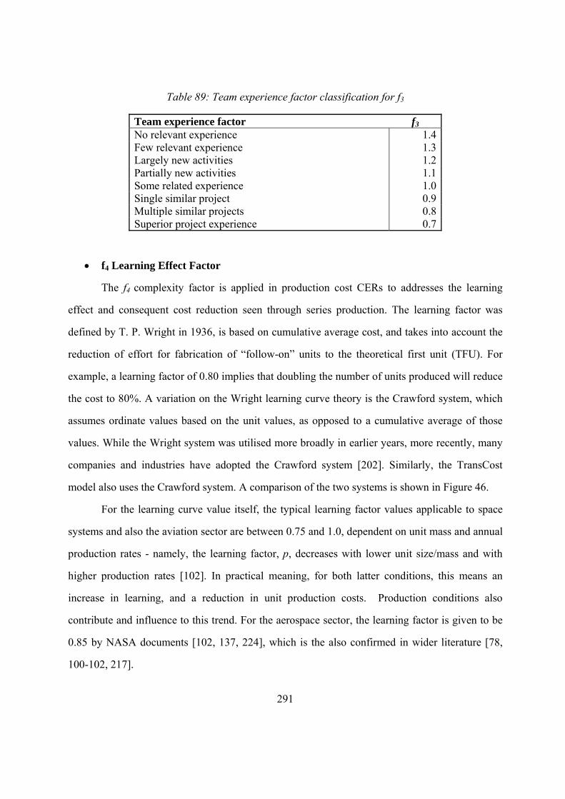
291
Table 89: Team experience factor classification for f3
Team experience factor f3 No relevant experience 1.4 Few relevant experience 1.3 Largely new activities 1.2 Partially new activities 1.1 Some related experience 1.0 Single similar project 0.9 Multiple similar projects 0.8 Superior project experience 0.7
f4 Learning Effect Factor
The f4 complexity factor is applied in production cost CERs to addresses the learning
effect and consequent cost reduction seen through series production. The learning factor was
defined by T. P. Wright in 1936, is based on cumulative average cost, and takes into account the
reduction of effort for fabrication of “follow-on” units to the theoretical first unit (TFU). For
example, a learning factor of 0.80 implies that doubling the number of units produced will reduce
the cost to 80%. A variation on the Wright learning curve theory is the Crawford system, which
assumes ordinate values based on the unit values, as opposed to a cumulative average of those
values. While the Wright system was utilised more broadly in earlier years, more recently, many
companies and industries have adopted the Crawford system [202]. Similarly, the TransCost
model also uses the Crawford system. A comparison of the two systems is shown in Figure 46.
For the learning curve value itself, the typical learning factor values applicable to space
systems and also the aviation sector are between 0.75 and 1.0, dependent on unit mass and annual
production rates - namely, the learning factor, p, decreases with lower unit size/mass and with
higher production rates [102]. In practical meaning, for both latter conditions, this means an
increase in learning, and a reduction in unit production costs. Production conditions also
contribute and influence to this trend. For the aerospace sector, the learning factor is given to be
0.85 by NASA documents [102, 137, 224], which is the also confirmed in wider literature [78,
100-102, 217].
292
Figure 46: Graphical representation and comparison of Wright vs Crawford curves [202]
Here, it must also be noted that TransCost provides a different Learning Factor Model for
liquid propulsion rocket engines to highlight the greater impact of engine size (mass) and
production rates on the effective learning factor, p. The numerous relationships are shown below
in Figure 47, which has been derived from visual analysis of the relevant TransCost data points
depicting the curves. Being an empirical model, the specific organisational conditions and
unique technical and commercial circumstances of the manufacturer as well as production
scenario and organisation may influence these trends. Furthermore, the underlying assumption is
that the learning effects are only observed for production of identical units without technical
changes nor modifications.
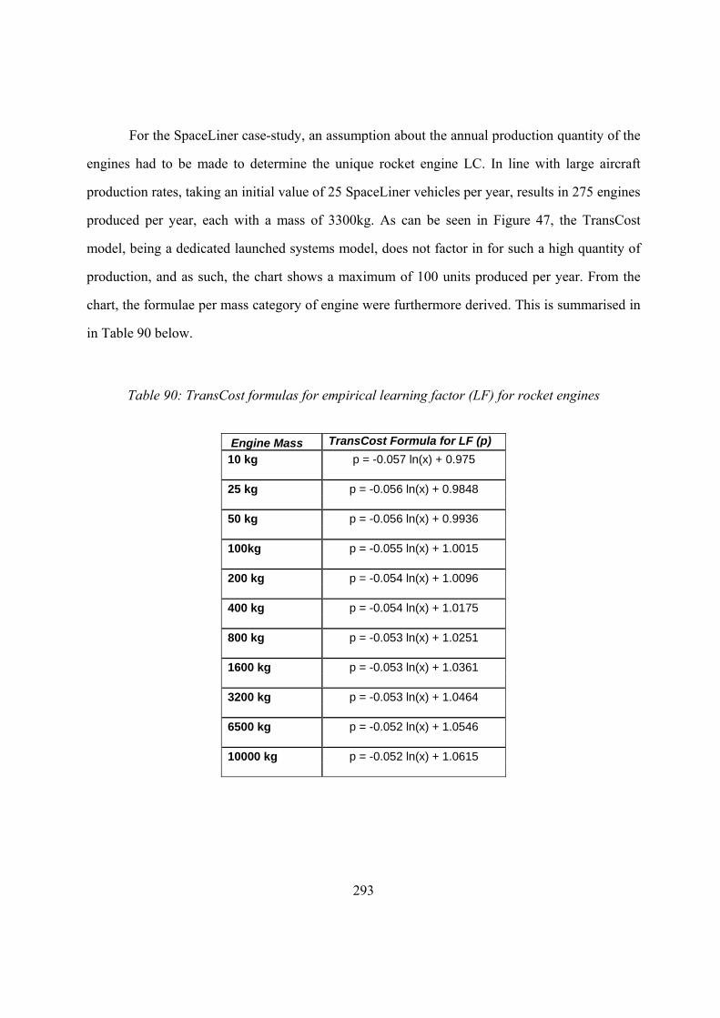
293
For the SpaceLiner case-study, an assumption about the annual production quantity of the
engines had to be made to determine the unique rocket engine LC. In line with large aircraft
production rates, taking an initial value of 25 SpaceLiner vehicles per year, results in 275 engines
produced per year, each with a mass of 3300kg. As can be seen in Figure 47, the TransCost
model, being a dedicated launched systems model, does not factor in for such a high quantity of
production, and as such, the chart shows a maximum of 100 units produced per year. From the
chart, the formulae per mass category of engine were furthermore derived. This is summarised in
in Table 90 below.
Table 90: TransCost formulas for empirical learning factor (LF) for rocket engines
Engine Mass TransCost Formula for LF (p)
10 kg p = -0.057 ln(x) + 0.975 25 kg p = -0.056 ln(x) + 0.9848 50 kg p = -0.056 ln(x) + 0.9936 100kg p = -0.055 ln(x) + 1.0015 200 kg p = -0.054 ln(x) + 1.0096 400 kg p = -0.054 ln(x) + 1.0175 800 kg p = -0.053 ln(x) + 1.0251 1600 kg p = -0.053 ln(x) + 1.0361 3200 kg p = -0.053 ln(x) + 1.0464 6500 kg p = -0.052 ln(x) + 1.0546 10000 kg p = -0.052 ln(x) + 1.0615
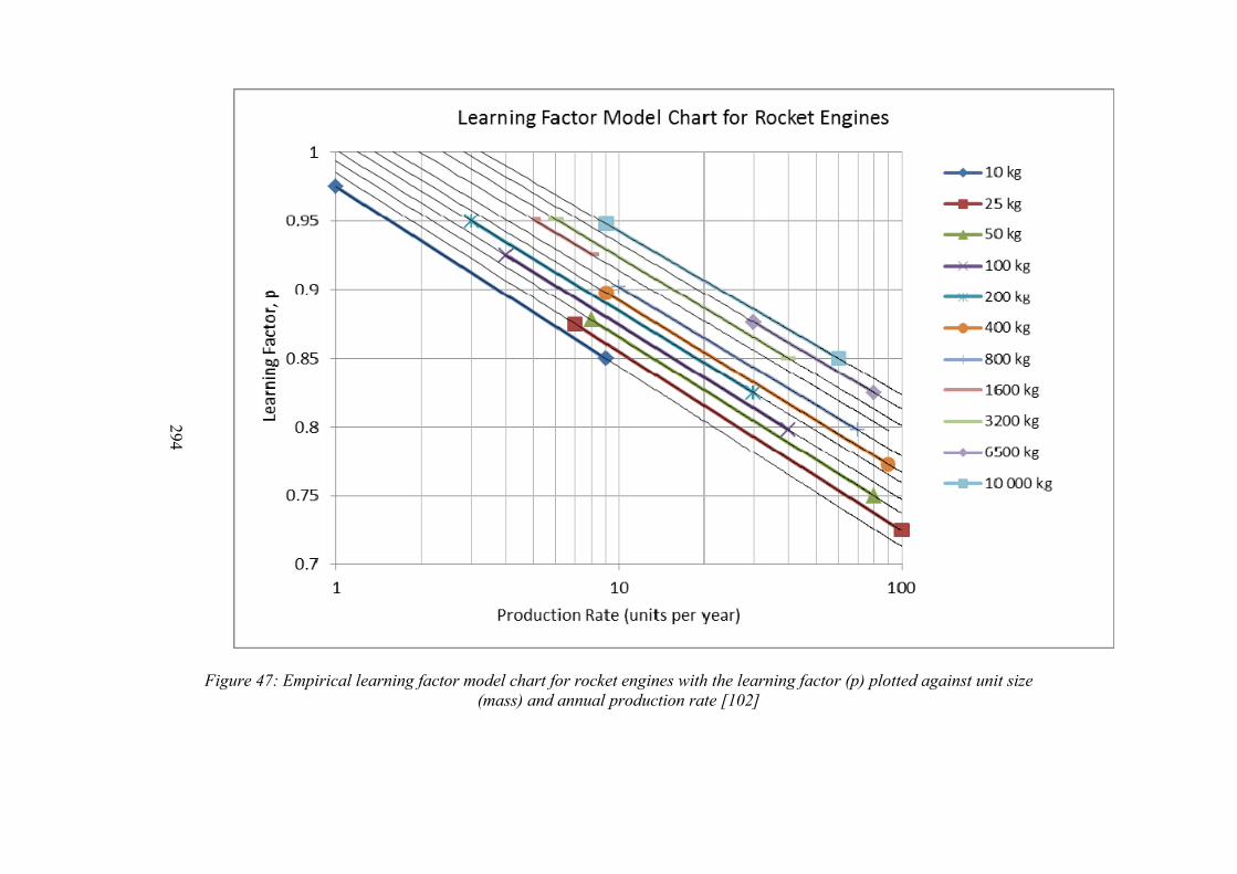
294
Figure 47: Empirical learning factor model chart for rocket engines with the learning factor (p) plotted against unit size (mass) and annual production rate [102]
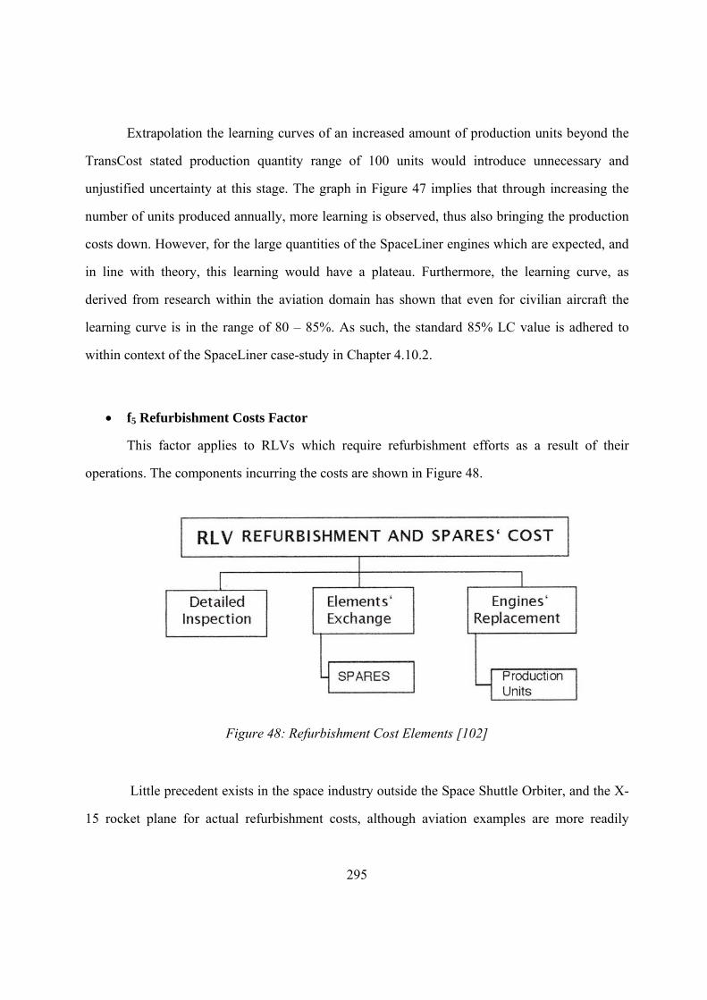
295
Extrapolation the learning curves of an increased amount of production units beyond the
TransCost stated production quantity range of 100 units would introduce unnecessary and
unjustified uncertainty at this stage. The graph in Figure 47 implies that through increasing the
number of units produced annually, more learning is observed, thus also bringing the production
costs down. However, for the large quantities of the SpaceLiner engines which are expected, and
in line with theory, this learning would have a plateau. Furthermore, the learning curve, as
derived from research within the aviation domain has shown that even for civilian aircraft the
learning curve is in the range of 80 – 85%. As such, the standard 85% LC value is adhered to
within context of the SpaceLiner case-study in Chapter 4.10.2.
f5 Refurbishment Costs Factor
This factor applies to RLVs which require refurbishment efforts as a result of their
operations. The components incurring the costs are shown in Figure 48.
Figure 48: Refurbishment Cost Elements [102]
Little precedent exists in the space industry outside the Space Shuttle Orbiter, and the X-
15 rocket plane for actual refurbishment costs, although aviation examples are more readily
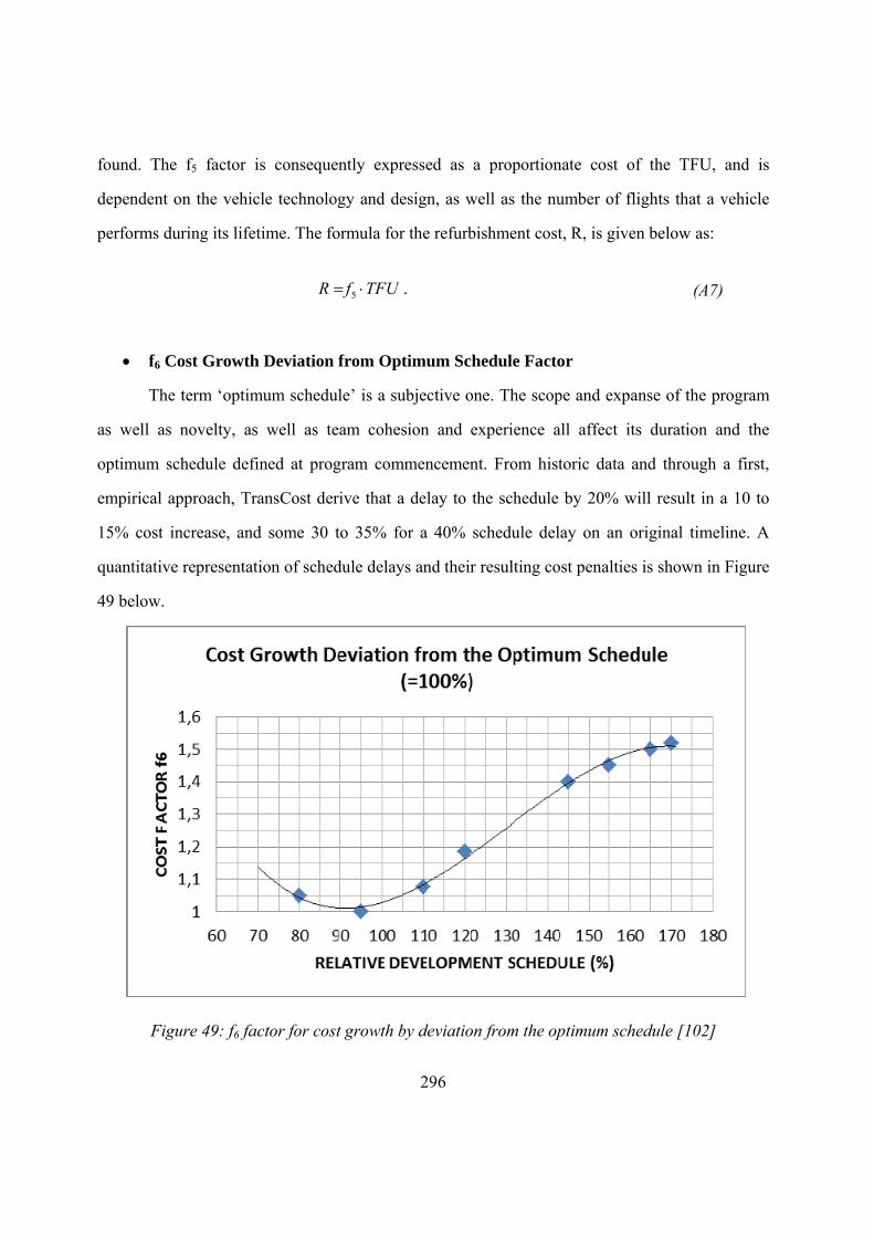
296
found. The f5 factor is consequently expressed as a proportionate cost of the TFU, and is
dependent on the vehicle technology and design, as well as the number of flights that a vehicle
performs during its lifetime. The formula for the refurbishment cost, R, is given below as:
TFUfR 5 . (A7)
f6 Cost Growth Deviation from Optimum Schedule Factor
The term ‘optimum schedule’ is a subjective one. The scope and expanse of the program
as well as novelty, as well as team cohesion and experience all affect its duration and the
optimum schedule defined at program commencement. From historic data and through a first,
empirical approach, TransCost derive that a delay to the schedule by 20% will result in a 10 to
15% cost increase, and some 30 to 35% for a 40% schedule delay on an original timeline. A
quantitative representation of schedule delays and their resulting cost penalties is shown in Figure
49 below.
Figure 49: f6 factor for cost growth by deviation from the optimum schedule [102]
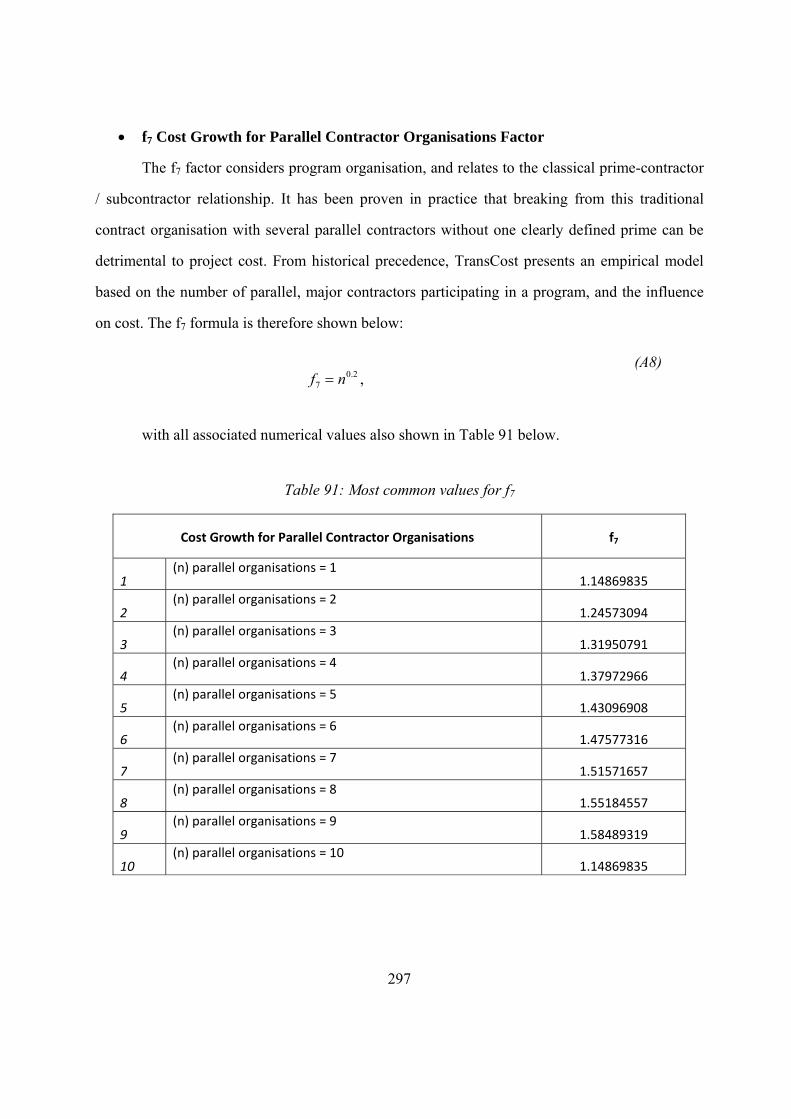
297
f7 Cost Growth for Parallel Contractor Organisations Factor
The f7 factor considers program organisation, and relates to the classical prime-contractor
/ subcontractor relationship. It has been proven in practice that breaking from this traditional
contract organisation with several parallel contractors without one clearly defined prime can be
detrimental to project cost. From historical precedence, TransCost presents an empirical model
based on the number of parallel, major contractors participating in a program, and the influence
on cost. The f7 formula is therefore shown below:
2.07 nf ,
(A8)
with all associated numerical values also shown in Table 91 below.
Table 91: Most common values for f7
Cost Growth for Parallel Contractor Organisations f7
1 (n) parallel organisations = 1
1.14869835
2 (n) parallel organisations = 2
1.24573094
3 (n) parallel organisations = 3
1.31950791
4 (n) parallel organisations = 4
1.37972966
5 (n) parallel organisations = 5
1.43096908
6 (n) parallel organisations = 6
1.47577316
7 (n) parallel organisations = 7
1.51571657
8 (n) parallel organisations = 8
1.55184557
9 (n) parallel organisations = 9
1.58489319
10 (n) parallel organisations = 10
1.14869835
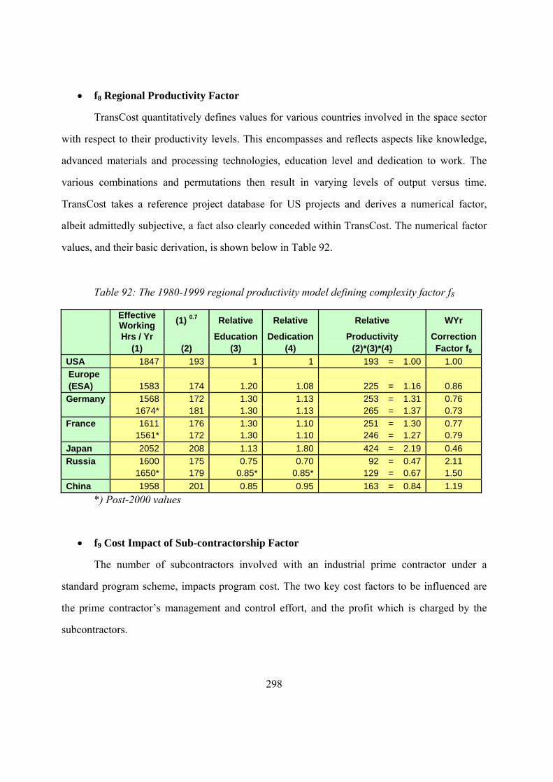
298
f8 Regional Productivity Factor
TransCost quantitatively defines values for various countries involved in the space sector
with respect to their productivity levels. This encompasses and reflects aspects like knowledge,
advanced materials and processing technologies, education level and dedication to work. The
various combinations and permutations then result in varying levels of output versus time.
TransCost takes a reference project database for US projects and derives a numerical factor,
albeit admittedly subjective, a fact also clearly conceded within TransCost. The numerical factor
values, and their basic derivation, is shown below in Table 92.
Table 92: The 1980-1999 regional productivity model defining complexity factor f8
Effective Working
(1) 0.7 Relative Relative Relative WYr
Hrs / Yr Education Dedication Productivity Correction (1) (2) (3) (4) (2)*(3)*(4) Factor f8
USA 1847 193 1 1 193 = 1.00 1.00
Europe (ESA) 1583 174 1.20 1.08 225 = 1.16 0.86
Germany 1568 172 1.30 1.13 253 = 1.31 0.76 1674* 181 1.30 1.13 265 = 1.37 0.73
France 1611 176 1.30 1.10 251 = 1.30 0.77 1561* 172 1.30 1.10 246 = 1.27 0.79
Japan 2052 208 1.13 1.80 424 = 2.19 0.46
Russia 1600 175 0.75 0.70 92 = 0.47 2.11 1650* 179 0.85* 0.85* 129 = 0.67 1.50
China 1958 201 0.85 0.95 163 = 0.84 1.19
*) Post-2000 values
f9 Cost Impact of Sub-contractorship Factor
The number of subcontractors involved with an industrial prime contractor under a
standard program scheme, impacts program cost. The two key cost factors to be influenced are
the prime contractor’s management and control effort, and the profit which is charged by the
subcontractors.
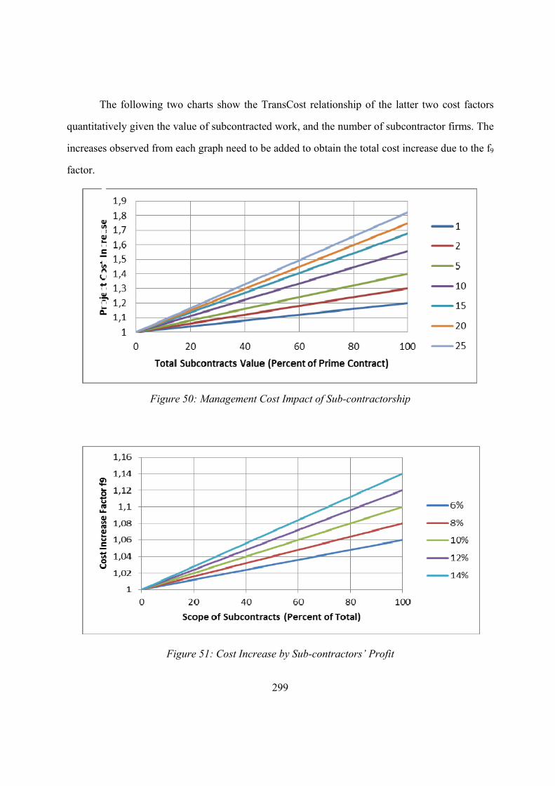
299
The following two charts show the TransCost relationship of the latter two cost factors
quantitatively given the value of subcontracted work, and the number of subcontractor firms. The
increases observed from each graph need to be added to obtain the total cost increase due to the f9
factor.
Figure 50: Management Cost Impact of Sub-contractorship
Figure 51: Cost Increase by Sub-contractors’ Profit

300
f10 Cost Reduction by Past Experience Factor
This factor addresses cost reductions resulting from past experience, the “lessons learned”
and data collected from previous works and program involvement. This includes utility of
modern computing tools and application of systems engineering principles. The attributed cost
reduction for this factor lies between 15 to 25%. As such, f10 is commonly in the range of 0.85
and 0.75.
f11 Non-Governmental Development Cost Reduction Factor
This impact factor applies only to commercial, non-governmental projects which have no
government contracts’ requirements and no customer interference. As a result, the high costs
involved with government requirements, procedures requirements and the associated personnel
(i.e. lawyers, administrative staff) are significantly reduced. From heuristic experience, it has
been shown that purely from a commercial basis, without governmental specifications,
requirements, procedures and reporting, a significant saving of 45 – 55% is achievable. The
resulting commercial development cost correction factor f11 is therefore 0.45 – 0.55.
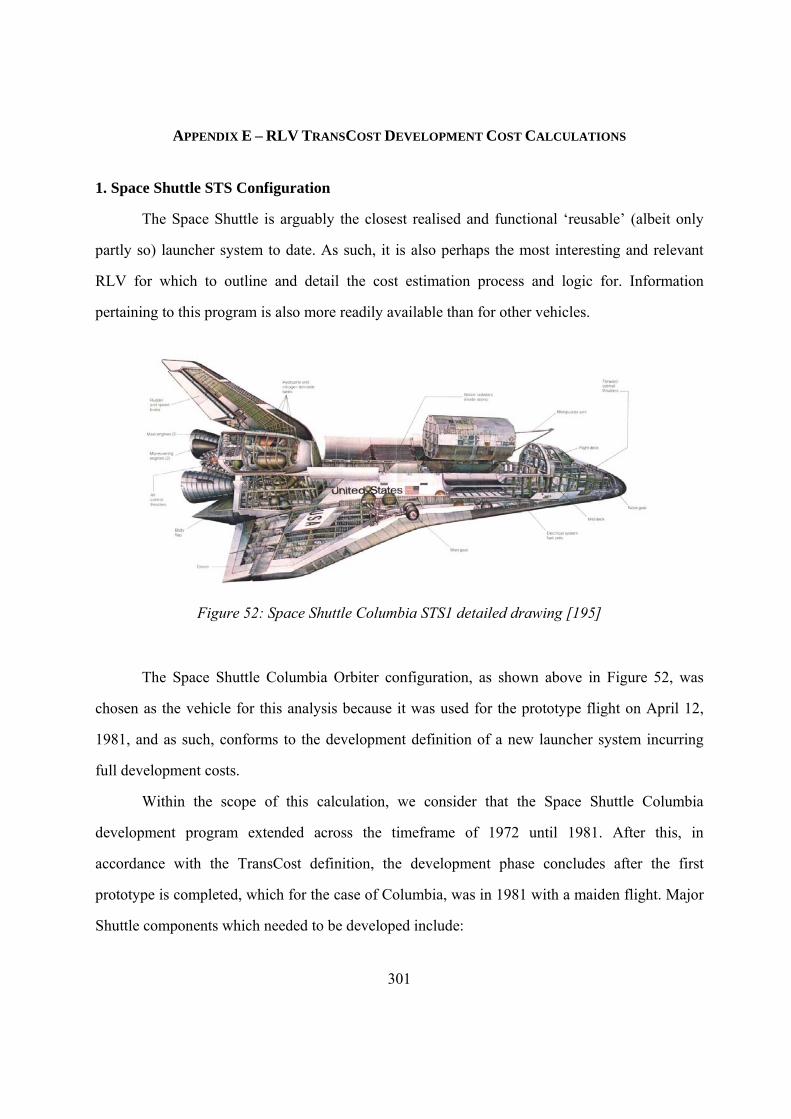
301
APPENDIX E – RLV TRANSCOST DEVELOPMENT COST CALCULATIONS
1. Space Shuttle STS Configuration
The Space Shuttle is arguably the closest realised and functional ‘reusable’ (albeit only
partly so) launcher system to date. As such, it is also perhaps the most interesting and relevant
RLV for which to outline and detail the cost estimation process and logic for. Information
pertaining to this program is also more readily available than for other vehicles.
Figure 52: Space Shuttle Columbia STS1 detailed drawing [195]
The Space Shuttle Columbia Orbiter configuration, as shown above in Figure 52, was
chosen as the vehicle for this analysis because it was used for the prototype flight on April 12,
1981, and as such, conforms to the development definition of a new launcher system incurring
full development costs.
Within the scope of this calculation, we consider that the Space Shuttle Columbia
development program extended across the timeframe of 1972 until 1981. After this, in
accordance with the TransCost definition, the development phase concludes after the first
prototype is completed, which for the case of Columbia, was in 1981 with a maiden flight. Major
Shuttle components which needed to be developed include:
302
Orbiter (Columbia)
o SSME
o RCS/OMS Module (AJ10-190 Engine)
Solid Rocket Boosters (SRBs)
Shuttle External Tank
1.1 Space Shuttle Component Break-down Structure
The component breakdown structure and the Excel TransCost spreadsheet screenshots
with all relevant inputs and complexity factors are presented below. Here, all mass data was
extracted from predominantly two sources, [96] and [91].
Table 93 through to Table 98 below present the details of all calculations performed for
each Space Shuttle system and component, with all applied complexity factors, shown.
1.2 Space Shuttle Calculation Assumptions
Some key assumptions also had to be made within the scope of the cost estimation with
regards to numerous inputs, complexity factors, as well as currency conversions. The key
assumptions are outlined below, and are also annotated in red with association to the fields which
the assumptions affect in the tables above:
A1. For the SSME, f1 and f3 complexity factors were taken to be 1.3 and 0.85
respectively. In addition, the value for the number of test firings (730 firings) was also assumed.
The latter values were taken directly from the TransCost Handbook. They were assumed for the
Excel model too in an attempt to understand the sensitivity of the factors within the context of the
project and as calculated by the TransCost model.
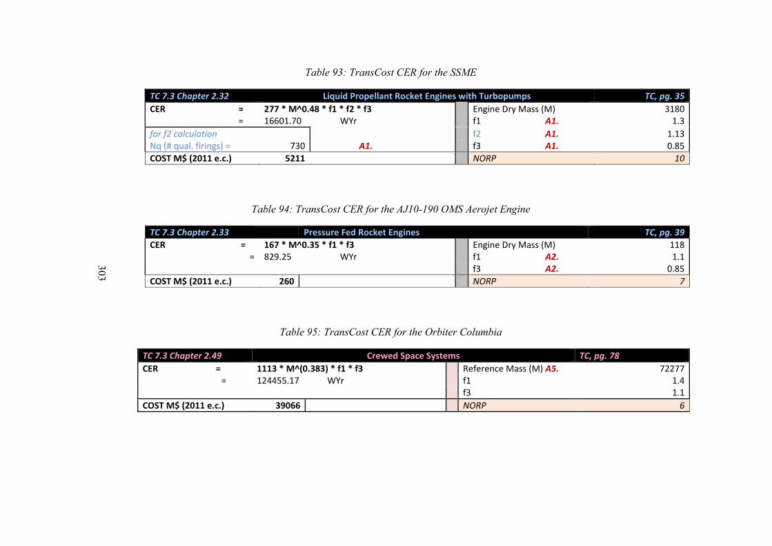
303
Table 93: TransCost CER for the SSME
TC 7.3 Chapter 2.32 Liquid Propellant Rocket Engines with Turbopumps TC, pg. 35
CER = 277 * M^0.48 * f1 * f2 * f3 Engine Dry Mass (M) 3180 = 16601.70 WYr f1 A1. 1.3
for f2 calculation f2 A1. 1.13 Nq (# qual. firings) = 730 A1. f3 A1. 0.85
COST M$ (2011 e.c.) 5211 NORP 10
Table 94: TransCost CER for the AJ10-190 OMS Aerojet Engine
TC 7.3 Chapter 2.33 Pressure Fed Rocket Engines TC, pg. 39
CER = 167 * M^0.35 * f1 * f3 Engine Dry Mass (M) 118 = 829.25 WYr f1 A2. 1.1
f3 A2. 0.85
COST M$ (2011 e.c.) 260 NORP 7
Table 95: TransCost CER for the Orbiter Columbia
TC 7.3 Chapter 2.49 Crewed Space Systems TC, pg. 78
CER = 1113 * M^(0.383) * f1 * f3 Reference Mass (M) A5. 72277 = 124455.17 WYr f1 1.4
f3 1.1
COST M$ (2011 e.c.) 39066 NORP 6
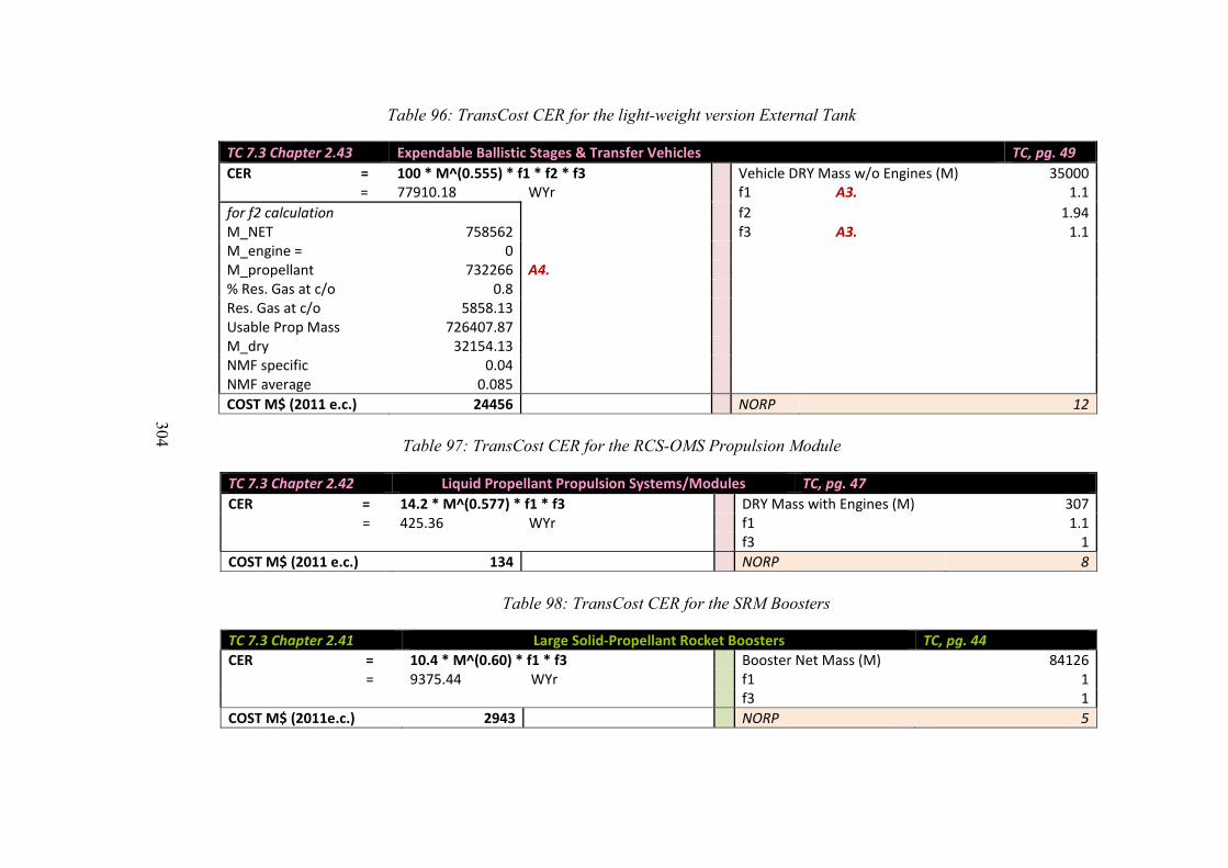
304
Table 96: TransCost CER for the light-weight version External Tank
TC 7.3 Chapter 2.43 Expendable Ballistic Stages & Transfer Vehicles TC, pg. 49
CER = 100 * M^(0.555) * f1 * f2 * f3 Vehicle DRY Mass w/o Engines (M) 35000 = 77910.18 WYr f1 A3. 1.1
for f2 calculation f2 1.94 M_NET 758562 f3 A3. 1.1 M_engine = 0 M_propellant 732266 A4. % Res. Gas at c/o 0.8 Res. Gas at c/o 5858.13 Usable Prop Mass 726407.87M_dry 32154.13 NMF specific 0.04 NMF average 0.085
COST M$ (2011 e.c.) 24456 NORP 12
Table 97: TransCost CER for the RCS-OMS Propulsion Module
TC 7.3 Chapter 2.42 Liquid Propellant Propulsion Systems/Modules TC, pg. 47
CER = 14.2 * M^(0.577) * f1 * f3 DRY Mass with Engines (M) 307 = 425.36 WYr f1 1.1
f3 1
COST M$ (2011 e.c.) 134 NORP 8
Table 98: TransCost CER for the SRM Boosters
TC 7.3 Chapter 2.41 Large Solid‐Propellant Rocket Boosters TC, pg. 44
CER = 10.4 * M^(0.60) * f1 * f3 Booster Net Mass (M) 84126 = 9375.44 WYr f1 1 f3 1
COST M$ (2011e.c.) 2943 NORP 5
305
A2. For the AJ10-190 development costs, the complexity factors f1 and f3 were defined as
being 1.1 and 0.85 respectively. The f1 value was taken as 1.1 to reflect the reusability element of
the engine, while the 0.85 f3 value was consistent and in line with the TransCost SSME f3
definition and logic.
A3. For the External Tank development cost calculations, the f1 factor was chosen to be
1.1 to reflect similarity between the Saturn V SII stage. Furthermore, the f3 factor was taken to be
1.1 to reflect the team experience existing also from the Saturn V program.
A4. For the f7 complexity factor, which is the factor that reflects cost increase associated
with an increased number of contractor organisations, this number was assumed to be 5.
Arguably, and upon consultation with the opinion of Dr. E. Koelle [103], only three main
contractors were involved in the Shuttle design phase, being Rocketdyne, North American
Rockwell and ATK-Thiokol. Dr. E. Koelle maintains that companies like United Space Boosters
and Michoud Facility came only later for the production and operations phase. However, the
entire organisation of contractors is rather difficult to assess, including the role of NASA-MSFC
and the changes versus time.
However, existing literature suggests and identifies 4 main contractors for the
development phase of the Space Shuttle [54]. Being a worst-case scenario to the previously
suggested 3 contractors, the more extreme option is taken for the sake of this document.
Therefore, for the f7 complexity factor, which is the factor that reflects cost increase
associated with an increased number of contractor organisations, this number was assumed to be
4. These were taken to be four key known companies listed below [54]:
306
1) Rocketdyne
• Shuttle SSME Contract (1972 April 21) - Rocketdyne receives the contact for
development of the shuttle main engine. By the end of the century the total value will have
exceeded $5.6 billion
2) North American Rockwell
• Shuttle orbiter contract (1972 July 7)- North American Rockwell received NASA
contract NAS9-14000, valued at $2.6 billion, for development of the space shuttle orbiter.
Included are two flight articles, the STA Structural Test Article, and the MPTA Main Propulsion
Test Article. Later production of two additional orbiters will be added, bringing the final contract
value to $ 5.815 billion by 1996.
3) ATK- Thiokol
• Shuttle solid rocket booster contract (1973 August 16) - United Space Boosters
and Thiokol receive the contract.
4) Boeing Michoud
• Shuttle external tank contract (1973 August 16) - Boeing Michoud received the
production contract, using facilities already built for Saturn V first stage construction. By 1996
the contract will have totaled $6.7 billion and covered the production of 120 external tanks.
A5. The mass for the Orbiter, Columbia, was taken from reference [91] for OV-102,
found on pg. 440.
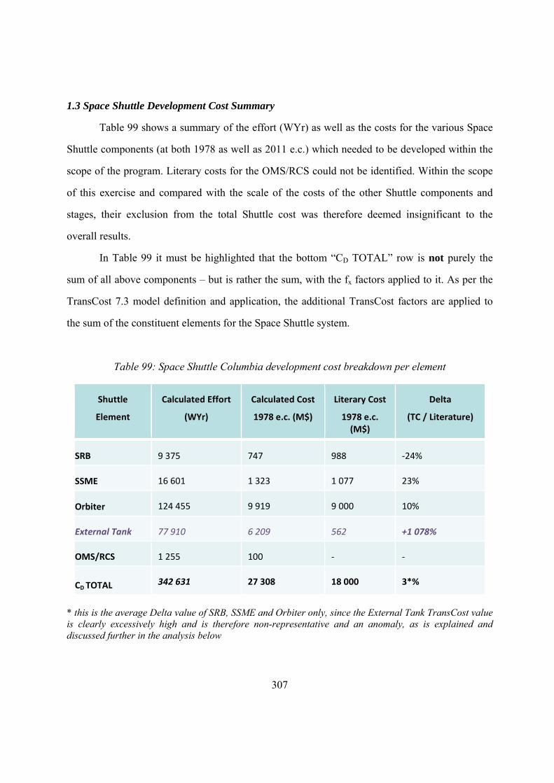
307
1.3 Space Shuttle Development Cost Summary
Table 99 shows a summary of the effort (WYr) as well as the costs for the various Space
Shuttle components (at both 1978 as well as 2011 e.c.) which needed to be developed within the
scope of the program. Literary costs for the OMS/RCS could not be identified. Within the scope
of this exercise and compared with the scale of the costs of the other Shuttle components and
stages, their exclusion from the total Shuttle cost was therefore deemed insignificant to the
overall results.
In Table 99 it must be highlighted that the bottom “CD TOTAL” row is not purely the
sum of all above components – but is rather the sum, with the fx factors applied to it. As per the
TransCost 7.3 model definition and application, the additional TransCost factors are applied to
the sum of the constituent elements for the Space Shuttle system.
Table 99: Space Shuttle Columbia development cost breakdown per element
Shuttle
Element
Calculated Effort
(WYr)
Calculated Cost
1978 e.c. (M$)
Literary Cost
1978 e.c. (M$)
Delta
(TC / Literature)
SRB 9 375 747 988 ‐24%
SSME 16 601 1 323 1 077 23%
Orbiter 124 455 9 919 9 000 10%
External Tank 77 910 6 209 562 +1 078%
OMS/RCS 1 255 100 ‐ ‐
CD TOTAL 342 631 27 308 18 000 3*%
* this is the average Delta value of SRB, SSME and Orbiter only, since the External Tank TransCost value is clearly excessively high and is therefore non-representative and an anomaly, as is explained and discussed further in the analysis below
308
These factors, fx, are outlined below, and their chosen values stated:
• f0 = 1.08 (f0 = 1.04 number of stages, in the case of the Space Shuttle, 2)
• f6 = 1.0 (assume no deviation from optimum schedule)
• f7 = 1.32 (f7 = n 0.2; with n being the number of parallel contractor organisations, in this case taken to be 4)
• f8 = 1.0 (TransCost stated country productivity factor for the US)
Upon analysis of the resulting costs as well as the respective cost deltas observed between
TransCost results and literary values, it can be seen that the TransCost model provides a good
correlation and ROM outcomes to the various Shuttle stages and components. This is because it
is generally considered that for cost estimation, being a dynamic discipline, a rough range of
±20% deviation is a reasonable value [100], particularly early on in a program phase. Therefore
the only significant and notable deviation which can be observed here is that for the Shuttle
External Tank (ET), highlighted in italics in Table 99. Purely from logic, the delta between
literary values and the TransCost calculated ET development cost of 1178% appears to be
excessive, and requires a deeper analysis and understanding to justify this discrepancy. Within
the context of this work, the author of TransCost handbook, Dr. Dietrich E. Koelle, was contacted
directly and the discrepancy outlined. The response received outlined the fact that the Shuttle ET,
although a separate component in its own right, is not, however, classed as a stage within context
of the TransCost model. It is rather defined as a sub-system, and as such, applying the system-
based CERs is inappropriate. TransCost, by its definition, is purely a higher-level, system based
309
model which therefore can results in grossly over- or under-exaggerated estimates for any sub-
systems (depending on the technology associated), as was exactly the case with the Shuttle ET.
This highlights the importance of knowing the mechanics and features of a given cost model, and
to be able to identify any shortcomings or gaps, and address these accordingly. In this instance,
another estimation methodology would therefore be required to formulate a more justifiable,
defensible development cost estimate for the Space Shuttle ET than purely the TransCost CER.
For the sake of consistency within the context of this study, an available literary figure for ET
development was taken based on the official NASA annual budget figures, which stated that the
total ET development costs between 1974 and 1982 were $562M, or an equivalent of 7030 WYr
[103]. Here, loosely calculating a ratio figure between the TransCost calculated amount and
literature, we get the Shuttle Tank Structure Ratio (STSR):
0.11562
6209STSR . (A9)
Table 100 below presents the modified values for each Space Shuttle system and
component. Since the Shuttle ET is not a suitable element to be calculated by TransCost, the
identified literary values were simply assumed and entered into this table for completeness and to
allow for a cost to be attained for the overall system. These appear written in brackets within the
table. Total WYr and total cost amounts are therefore derived. Furthermore, Figure 53 provides a
visual representation of the costs on a component and stage basis.
Consequently, the top-level TransCost formula for the overall Space Shuttle cost is:
8760 )( fffCERsfCD . (A10)
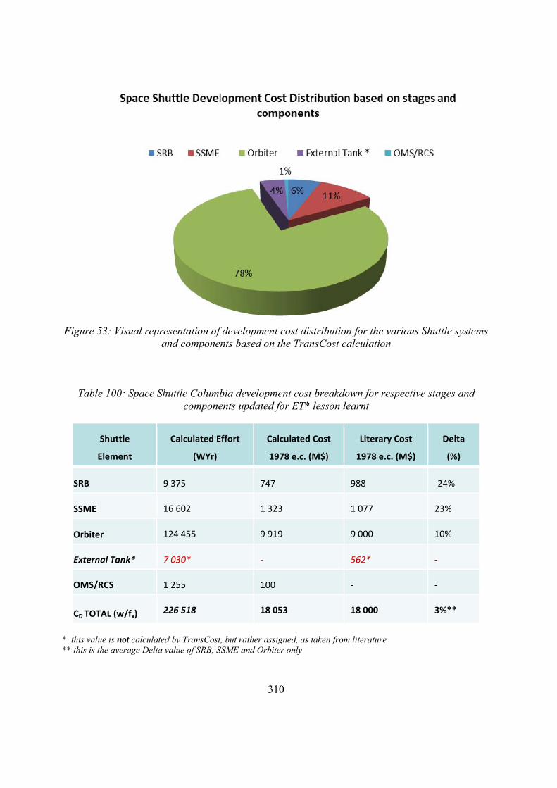
310
Figure 53: Visual representation of development cost distribution for the various Shuttle systems and components based on the TransCost calculation
Table 100: Space Shuttle Columbia development cost breakdown for respective stages and components updated for ET* lesson learnt
Shuttle
Element
Calculated Effort
(WYr)
Calculated Cost
1978 e.c. (M$)
Literary Cost
1978 e.c. (M$)
Delta
(%)
SRB 9 375 747 988 ‐24%
SSME 16 602 1 323 1 077 23%
Orbiter 124 455 9 919 9 000 10%
External Tank* 7 030* ‐ 562* ‐
OMS/RCS 1 255 100 ‐ ‐
CD TOTAL (w/fx) 226 518 18 053 18 000 3%**
* this value is not calculated by TransCost, but rather assigned, as taken from literature ** this is the average Delta value of SRB, SSME and Orbiter only
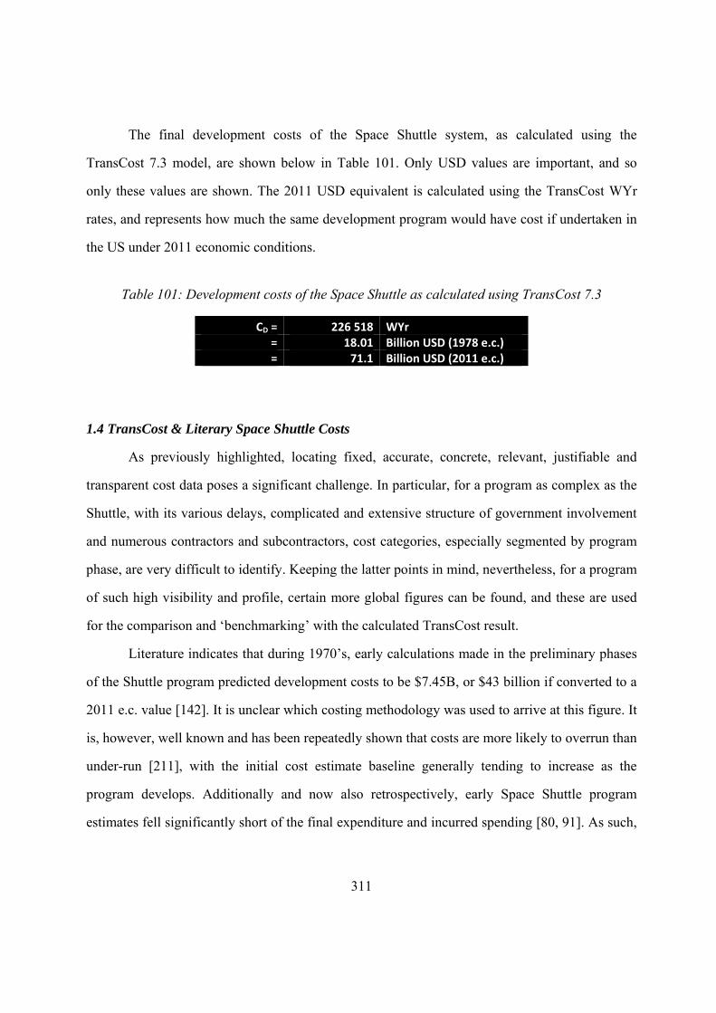
311
The final development costs of the Space Shuttle system, as calculated using the
TransCost 7.3 model, are shown below in Table 101. Only USD values are important, and so
only these values are shown. The 2011 USD equivalent is calculated using the TransCost WYr
rates, and represents how much the same development program would have cost if undertaken in
the US under 2011 economic conditions.
Table 101: Development costs of the Space Shuttle as calculated using TransCost 7.3
CD = 226 518 WYr = 18.01 Billion USD (1978 e.c.) = 71.1 Billion USD (2011 e.c.)
1.4 TransCost & Literary Space Shuttle Costs
As previously highlighted, locating fixed, accurate, concrete, relevant, justifiable and
transparent cost data poses a significant challenge. In particular, for a program as complex as the
Shuttle, with its various delays, complicated and extensive structure of government involvement
and numerous contractors and subcontractors, cost categories, especially segmented by program
phase, are very difficult to identify. Keeping the latter points in mind, nevertheless, for a program
of such high visibility and profile, certain more global figures can be found, and these are used
for the comparison and ‘benchmarking’ with the calculated TransCost result.
Literature indicates that during 1970’s, early calculations made in the preliminary phases
of the Shuttle program predicted development costs to be $7.45B, or $43 billion if converted to a
2011 e.c. value [142]. It is unclear which costing methodology was used to arrive at this figure. It
is, however, well known and has been repeatedly shown that costs are more likely to overrun than
under-run [211], with the initial cost estimate baseline generally tending to increase as the
program develops. Additionally and now also retrospectively, early Space Shuttle program
estimates fell significantly short of the final expenditure and incurred spending [80, 91]. As such,

312
it is more desirable to find a more recent cost estimate. At a slightly later date, at 1981 e.c., a
revised development cost figure exists, being $18B [91]. Taking this more recent $18B figure,
and once again converting it to a 2011 value results in an amount of roughly $57B for Shuttle
development at 2011 economic conditions. This figure is therefore extracted and taken as the
reference literary value for the comparison with TransCost values.
Reverse engineering the $18B at 1981 e.c., and applying respective TransCost US WYr
cost for 2981 ($98,770 per WYr), we obtain the implied literary value of 182, 240WYr.
Comparing this to the TransCost calculated development effort of 226,518 WYr as shown
in Table 101 it can be seen that the TransCost figure constitutes an increase of 24% over the
literary development cost. However, this margin is perfectly reasonable, since be its own
definition, the TransCost model does take into account on average a +20% margin for expected
development costs. This is an important lesson to be taken away from this particular example.
Additionally, it is highly logical to assume that this initial $57B literary figure, which was
technically a pre-program estimate in itself, would have been exceeded in reality. So, the
resulting TransCost development effort cost of $71.1B (with the logical adjustment for ET),
being more than the initial literary cost estimate, but less than the overall program cost, is highly
logical and congruent with reality.
Furthermore, from a retrospective stance, furthermore, the ultimate overall Shuttle
program budget is now being quoted as being a total of $196 billion at 2011 e.c. [91]. Here it
must be emphasised that this $196B amount represents the overall total Space Shuttle program
cost, including production and operations, as well as most probably ground infrastructure, and
vehicle maintenance and refurbishment, all of which bore significant expenditures. It is therefore
not dedicated to solely the development cost. A segmented breakdown of the separate
development, production and operations component is not explicitly available.
Given that a separate development component, which is the figure of interest within the
scope of this report, is unavailable, it is interesting from a cost analysis perspective to calculate
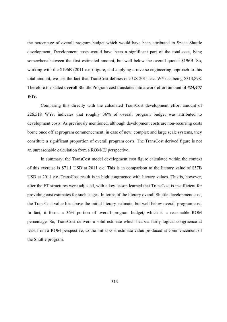
313
the percentage of overall program budget which would have been attributed to Space Shuttle
development. Development costs would have been a significant part of the total cost, lying
somewhere between the first estimated amount, but well below the overall quoted $196B. So,
working with the $196B (2011 e.c.) figure, and applying a reverse engineering approach to this
total amount, we use the fact that TransCost defines one US 2011 e.c. WYr as being $313,898.
Therefore the stated overall Shuttle Program cost translates into a work effort amount of 624,407
WYr.
Comparing this directly with the calculated TransCost development effort amount of
226,518 WYr, indicates that roughly 36% of overall program budget was attributed to
development costs. As previously mentioned, although development costs are non-recurring costs
borne once off at program commencement, in case of new, complex and large scale systems, they
constitute a significant proportion of overall program costs. The TransCost derived figure is not
an unreasonable calculation from a ROM/EJ perspective.
In summary, the TransCost model development cost figure calculated within the context
of this exercise is $71.1 USD at 2011 e.c. This is in comparison to the literary value of $57B
USD at 2011 e.c. TransCost result is in high congruence with literary values. This is, however,
after the ET structures were adjusted, with a key lesson learned that TransCost is insufficient for
providing cost estimates for such stages. In terms of the literary overall Shuttle development cost,
the TransCost value lies above the initial literary estimate, but well below overall program cost.
In fact, it forms a 36% portion of overall program budget, which is a reasonable ROM
percentage. So, TransCost delivers a solid estimate which bears a fairly logical congruence at
least from a ROM perspective, to the initial cost estimate value produced at commencement of
the Shuttle program.
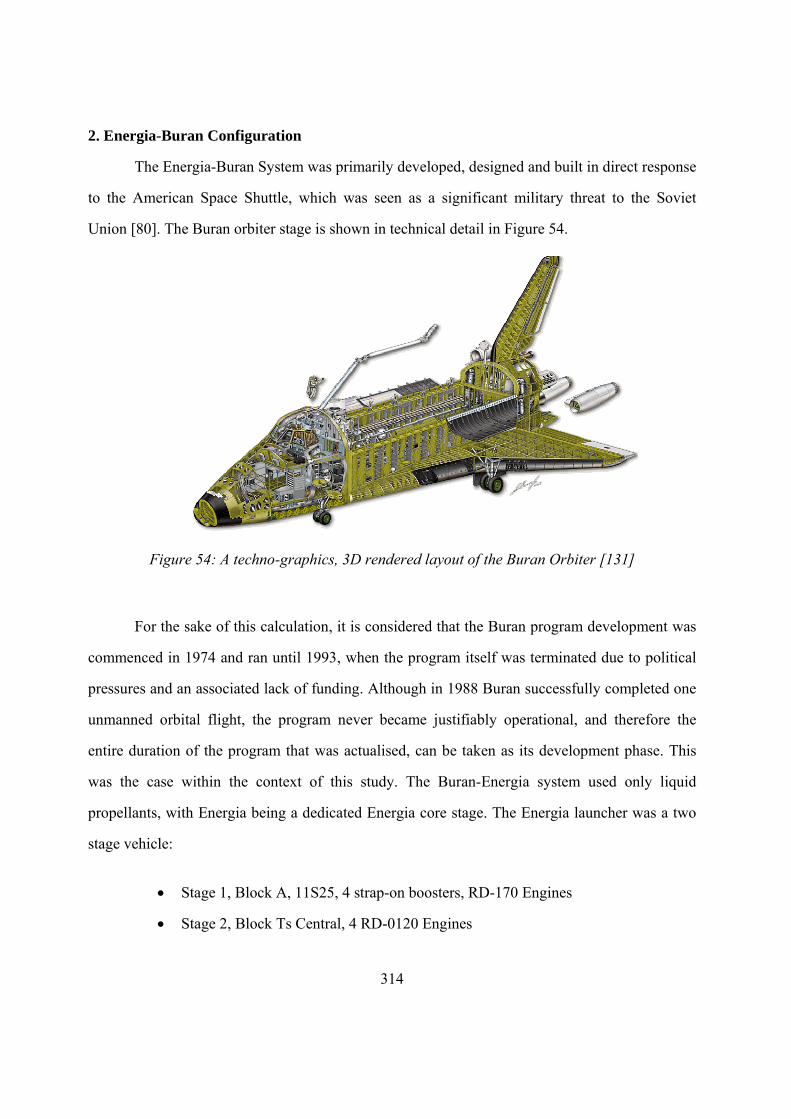
314
2. Energia-Buran Configuration
The Energia-Buran System was primarily developed, designed and built in direct response
to the American Space Shuttle, which was seen as a significant military threat to the Soviet
Union [80]. The Buran orbiter stage is shown in technical detail in Figure 54.
Figure 54: A techno-graphics, 3D rendered layout of the Buran Orbiter [131]
For the sake of this calculation, it is considered that the Buran program development was
commenced in 1974 and ran until 1993, when the program itself was terminated due to political
pressures and an associated lack of funding. Although in 1988 Buran successfully completed one
unmanned orbital flight, the program never became justifiably operational, and therefore the
entire duration of the program that was actualised, can be taken as its development phase. This
was the case within the context of this study. The Buran-Energia system used only liquid
propellants, with Energia being a dedicated Energia core stage. The Energia launcher was a two
stage vehicle:
Stage 1, Block A, 11S25, 4 strap-on boosters, RD-170 Engines
Stage 2, Block Ts Central, 4 RD-0120 Engines
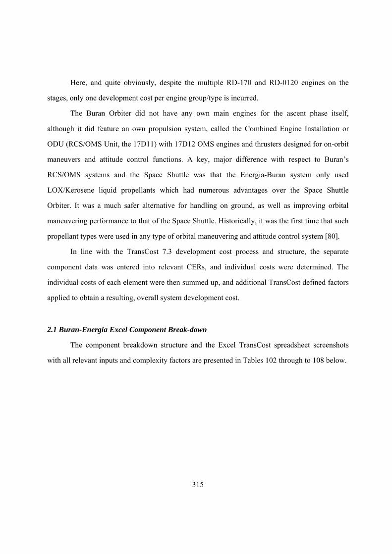
315
Here, and quite obviously, despite the multiple RD-170 and RD-0120 engines on the
stages, only one development cost per engine group/type is incurred.
The Buran Orbiter did not have any own main engines for the ascent phase itself,
although it did feature an own propulsion system, called the Combined Engine Installation or
ODU (RCS/OMS Unit, the 17D11) with 17D12 OMS engines and thrusters designed for on-orbit
maneuvers and attitude control functions. A key, major difference with respect to Buran’s
RCS/OMS systems and the Space Shuttle was that the Energia-Buran system only used
LOX/Kerosene liquid propellants which had numerous advantages over the Space Shuttle
Orbiter. It was a much safer alternative for handling on ground, as well as improving orbital
maneuvering performance to that of the Space Shuttle. Historically, it was the first time that such
propellant types were used in any type of orbital maneuvering and attitude control system [80].
In line with the TransCost 7.3 development cost process and structure, the separate
component data was entered into relevant CERs, and individual costs were determined. The
individual costs of each element were then summed up, and additional TransCost defined factors
applied to obtain a resulting, overall system development cost.
2.1 Buran-Energia Excel Component Break-down
The component breakdown structure and the Excel TransCost spreadsheet screenshots
with all relevant inputs and complexity factors are presented in Tables 102 through to 108 below.
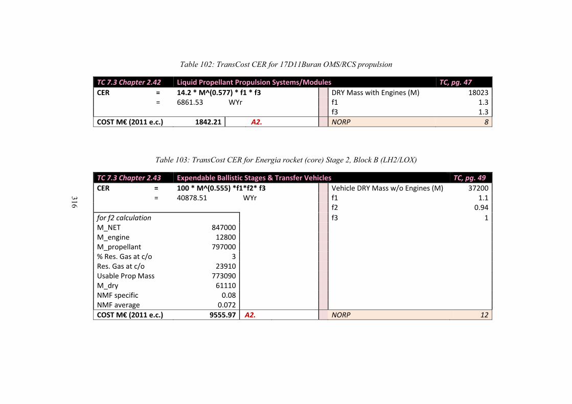
316
Table 102: TransCost CER for 17D11Buran OMS/RCS propulsion
TC 7.3 Chapter 2.42 Liquid Propellant Propulsion Systems/Modules TC, pg. 47
CER = 14.2 * M^(0.577) * f1 * f3 DRY Mass with Engines (M) 18023 = 6861.53 WYr f1 1.3 f3 1.3
COST M€ (2011 e.c.) 1842.21 A2. NORP 8
Table 103: TransCost CER for Energia rocket (core) Stage 2, Block B (LH2/LOX)
TC 7.3 Chapter 2.43 Expendable Ballistic Stages & Transfer Vehicles TC, pg. 49
CER = 100 * M^(0.555) *f1*f2* f3 Vehicle DRY Mass w/o Engines (M) 37200 = 40878.51 WYr f1 1.1
f2 0.94
for f2 calculation f3 1M_NET 847000 M_engine 12800 M_propellant 797000 % Res. Gas at c/o 3 Res. Gas at c/o 23910 Usable Prop Mass 773090 M_dry 61110 NMF specific 0.08 NMF average 0.072
COST M€ (2011 e.c.) 9555.97 A2. NORP 12
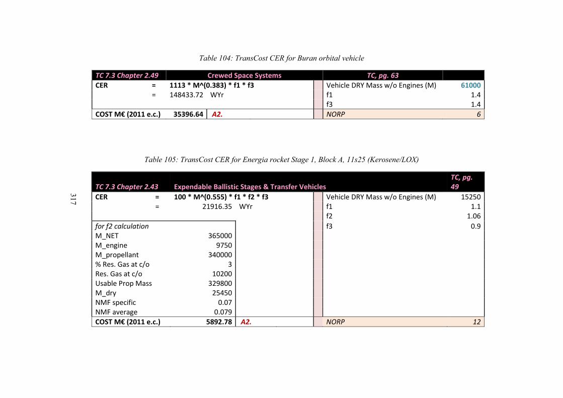
317
Table 104: TransCost CER for Buran orbital vehicle
TC 7.3 Chapter 2.49 Crewed Space Systems TC, pg. 63
CER = 1113 * M^(0.383) * f1 * f3 Vehicle DRY Mass w/o Engines (M) 61000 = 148433.72 WYr f1 1.4 f3 1.4
COST M€ (2011 e.c.) 35396.64 A2. NORP 6
Table 105: TransCost CER for Energia rocket Stage 1, Block A, 11s25 (Kerosene/LOX)
TC 7.3 Chapter 2.43 Expendable Ballistic Stages & Transfer Vehicles TC, pg. 49
CER = 100 * M^(0.555) * f1 * f2 * f3 Vehicle DRY Mass w/o Engines (M) 15250 = 21916.35 WYr f1 1.1 f2 1.06
for f2 calculation f3 0.9M_NET 365000 M_engine 9750 M_propellant 340000 % Res. Gas at c/o 3 Res. Gas at c/o 10200 Usable Prop Mass 329800 M_dry 25450 NMF specific 0.07 NMF average 0.079
COST M€ (2011 e.c.) 5892.78 A2. NORP 12

318
Table 106: TransCost CER for 17D12 engine OMS Buran orbital propulsion system
TC 7.3 Chapter 2.32 Liquid Propellant Rocket Engines with Turbopumps TC, pg. 35
CER = 277 * M^0.48 * f1 * f2 * f3 Engine Dry Mass (M) 230 = 1329.70 WYr f1 0.8
for f2 calculation f2 (# test firings basis) 0.55Nq (# qualification firings) 100 A1. f3 0.8
COST M€ (2011 e.c.) 357.53 A2. NORP 10
Table 107: TransCost CER for 11D122 Energia core engine RD-0120
TC 7.3 Chapter 2.32 Liquid Propellant Rocket Engines with
Turbopumps TC, pg. 35
CER = 277 * M^0.48 * f1 * f2 * f3 Engine Dry Mass (M) 3200 = 22306.94 WYr f1 1.2
for f2 calculation f2 (# test firings basis) 1.16Nq (# qualification firings) 800 f3 1.2
COST M€ (2011 e.c.) 5997.80 A2. NORP 10
Table 108: TransCost CER for RD-180, booster stage engine
TC 7.3 Chapter 2.32 Liquid Propellant Rocket Engines with Turbopumps TC, pg. 35
CER = 277 * M^0.48 * f1 * f2 * f3 Engine Dry Mass (M) 9750 = 38079.41 WYr f1 1.2
for f2 calculation f2 (# test firings basis) 1.16Nq (# qualification firings) 800 A3. f3 1.2
COST M€ (2011 e.c.) 10238.64 A2. NORP 10
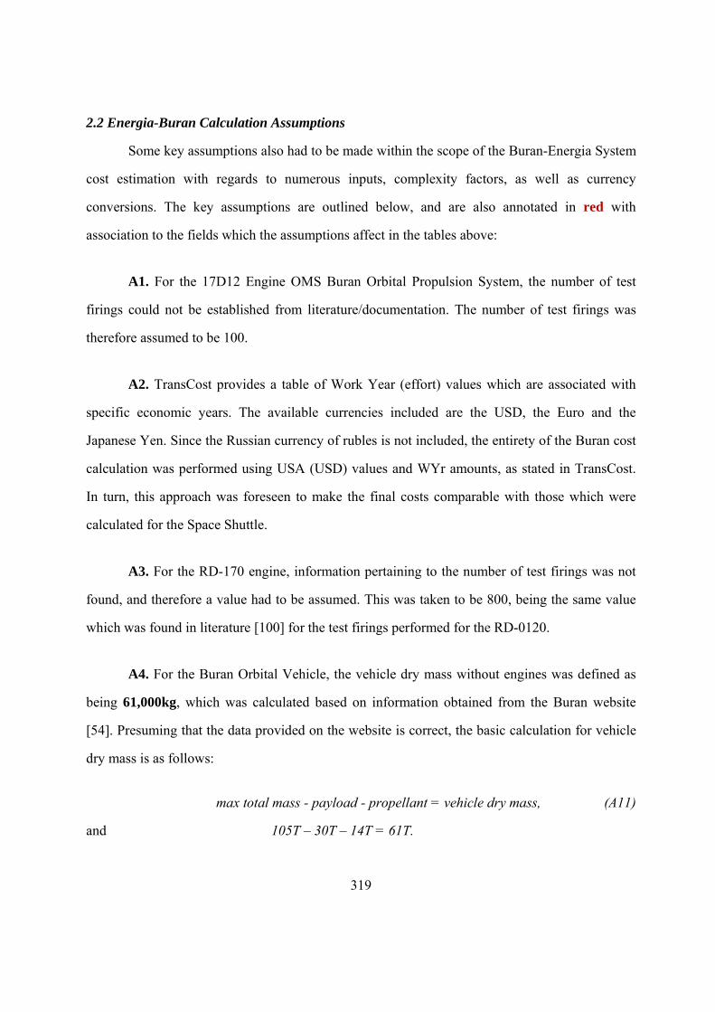
319
2.2 Energia-Buran Calculation Assumptions
Some key assumptions also had to be made within the scope of the Buran-Energia System
cost estimation with regards to numerous inputs, complexity factors, as well as currency
conversions. The key assumptions are outlined below, and are also annotated in red with
association to the fields which the assumptions affect in the tables above:
A1. For the 17D12 Engine OMS Buran Orbital Propulsion System, the number of test
firings could not be established from literature/documentation. The number of test firings was
therefore assumed to be 100.
A2. TransCost provides a table of Work Year (effort) values which are associated with
specific economic years. The available currencies included are the USD, the Euro and the
Japanese Yen. Since the Russian currency of rubles is not included, the entirety of the Buran cost
calculation was performed using USA (USD) values and WYr amounts, as stated in TransCost.
In turn, this approach was foreseen to make the final costs comparable with those which were
calculated for the Space Shuttle.
A3. For the RD-170 engine, information pertaining to the number of test firings was not
found, and therefore a value had to be assumed. This was taken to be 800, being the same value
which was found in literature [100] for the test firings performed for the RD-0120.
A4. For the Buran Orbital Vehicle, the vehicle dry mass without engines was defined as
being 61,000kg, which was calculated based on information obtained from the Buran website
[54]. Presuming that the data provided on the website is correct, the basic calculation for vehicle
dry mass is as follows:
max total mass - payload - propellant = vehicle dry mass, (A11)
and 105T – 30T – 14T = 61T.
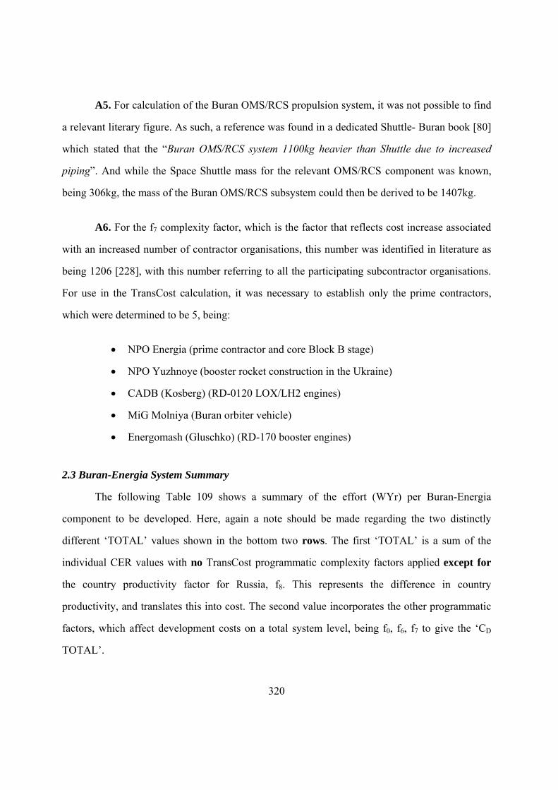
320
A5. For calculation of the Buran OMS/RCS propulsion system, it was not possible to find
a relevant literary figure. As such, a reference was found in a dedicated Shuttle- Buran book [80]
which stated that the “Buran OMS/RCS system 1100kg heavier than Shuttle due to increased
piping”. And while the Space Shuttle mass for the relevant OMS/RCS component was known,
being 306kg, the mass of the Buran OMS/RCS subsystem could then be derived to be 1407kg.
A6. For the f7 complexity factor, which is the factor that reflects cost increase associated
with an increased number of contractor organisations, this number was identified in literature as
being 1206 [228], with this number referring to all the participating subcontractor organisations.
For use in the TransCost calculation, it was necessary to establish only the prime contractors,
which were determined to be 5, being:
NPO Energia (prime contractor and core Block B stage)
NPO Yuzhnoye (booster rocket construction in the Ukraine)
CADB (Kosberg) (RD-0120 LOX/LH2 engines)
MiG Molniya (Buran orbiter vehicle)
Energomash (Gluschko) (RD-170 booster engines)
2.3 Buran-Energia System Summary
The following Table 109 shows a summary of the effort (WYr) per Buran-Energia
component to be developed. Here, again a note should be made regarding the two distinctly
different ‘TOTAL’ values shown in the bottom two rows. The first ‘TOTAL’ is a sum of the
individual CER values with no TransCost programmatic complexity factors applied except for
the country productivity factor for Russia, f8. This represents the difference in country
productivity, and translates this into cost. The second value incorporates the other programmatic
factors, which affect development costs on a total system level, being f0, f6, f7 to give the ‘CD
TOTAL’.
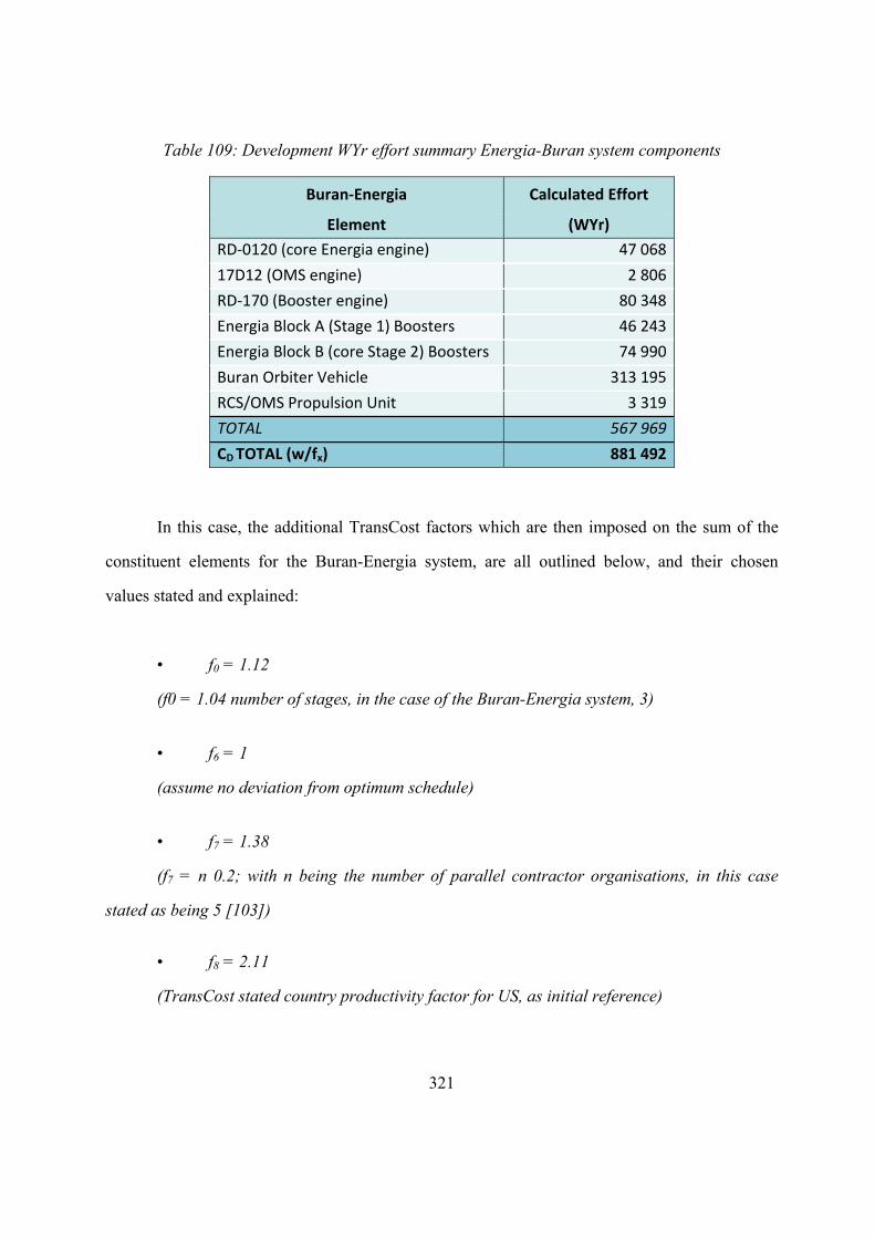
321
Table 109: Development WYr effort summary Energia-Buran system components
Buran‐Energia Calculated Effort
Element (WYr)
RD‐0120 (core Energia engine) 47 068
17D12 (OMS engine) 2 806
RD‐170 (Booster engine) 80 348
Energia Block A (Stage 1) Boosters 46 243
Energia Block B (core Stage 2) Boosters 74 990
Buran Orbiter Vehicle 313 195
RCS/OMS Propulsion Unit 3 319
TOTAL 567 969
CD TOTAL (w/fx) 881 492
In this case, the additional TransCost factors which are then imposed on the sum of the
constituent elements for the Buran-Energia system, are all outlined below, and their chosen
values stated and explained:
• f0 = 1.12
(f0 = 1.04 number of stages, in the case of the Buran-Energia system, 3)
• f6 = 1
(assume no deviation from optimum schedule)
• f7 = 1.38
(f7 = n 0.2; with n being the number of parallel contractor organisations, in this case
stated as being 5 [103])
• f8 = 2.11
(TransCost stated country productivity factor for US, as initial reference)
322
There is a significant increase on the individual WYr amounts, and the CD value, as can
be seen in Table 109. The f8 country productivity factor for Russia (stated as being 2.11 for pre-
year 2000) is quite high compared to Europe’s 0.86 and 1.00 (reference) for the US, and is the
key factor to influence the top-level system WYr total for the case of Russia. However, the WYr
amount must not be looked at as an individual, standalone variable, but rather as a combination
between the WYr amount, country productivity and the relevant WYr cost for that respective
country.
Nevertheless, the total WYr amount for Buran is still very high if compared with the
previously calculated Space Shuttle WYr effort of 226,518WYr. One obvious reason is explained
by the past lessons learned based on the Shuttle example described in Chapter 0, namely that
TransCost is not ideally suited for cost estimation of tank-like structures. Therefore, before
proceeding to comparisons between the TransCost derived figures and literary values, we need to
do a quick re-calculation for the tank-like structures of the Buran-Energia system.
2.4 Shuttle Lessons Learned Applied to Buran-Energia
A critical analysis point derived from this study pertains to the TransCost CER for
Expendable Ballistic Stages and Transfer Vehicles. Looking back to the Space Shuttle
development cost calculation described in Chapter 0, a key lesson learned was the limitation of
CER 2.43 for Expendable Ballistic Stages and Transfer Vehicles, and its non-suitability for
calculating development costs of tank-like structures [103]. This CER is relevant and was used to
calculated costs of the Energia Block A, Stage 1 liquid boosters, as well as the Block B core
stage.
As was identified and discussed in Chapter 0, a problem which arises with use of CER
2.43, is the resulting gross over-estimation for a simpler tank structure. In other words, and a
critical lesson learned, is that CER 2.43 is intended to describe a full stage, reflecting the
associated complexity of avionics, electrical components, and integration, rather than a simple
323
tank structure. As such, and while a result is calculated using TransCost, upon further analysis, it
is evident that this CER is inapplicable for the either of the Energia stages. The result of the
existing Energia stage TransCost calculation is therefore an over-inflated development cost which
exceeds realistic and literary stated development values. Prior to continuing with analyses of the
Buran-Energia system, we seek to amend this inconsistency in the existing calculation to allow
for effective comparisons of the system.
Recalling that having a literary development cost for the Space Shuttle External ET, as
well as a calculated TransCost value using the CER 2.43 (resulting in an as-anticipated over-
estimation), the STSR ratio was calculated. Recalling, for the Shuttle example, the calculated
value for the ET was 77 910 WYr, costing roughly $6,209 M at 1978 e.c., while the literary
figure was actually $562 M. If we once again calculate a loose ROM ratio of discrepancy
between the CER calculated result, and the literary figure, we obtain an STSR value of 11.05.
We assume this ratio to be a ROM figure with which TransCost overestimates tank
structure values (despite this being just one data point). If we then we can also seek to apply the
STSR to the Buran-Energia system calculation, we can now quickly recalculate the total Buran
vehicle development costs to remove the over-estimated tank-like structures, and obtain a more
representative cost estimate. Here, we must also recall that the Buran-Energia system also had
two elements which were classed as external tank structures, but had been calculated with CER
2.43. Therefore, we can now apply the STSR to the two Buran tank structure elements of:
• Energia Block A (Stage 1, Kerosene/LOX) Boosters
• Energia Block B (core Stage 2, LH2/LOX) Boosters
Taking the STSR ratio and applying it to the Buran example for both the Stage 1 and
Stage 2 boosters, yields quite different values to the original system elements, and of course the
overall development cost calculation, as shown below in Table 110.
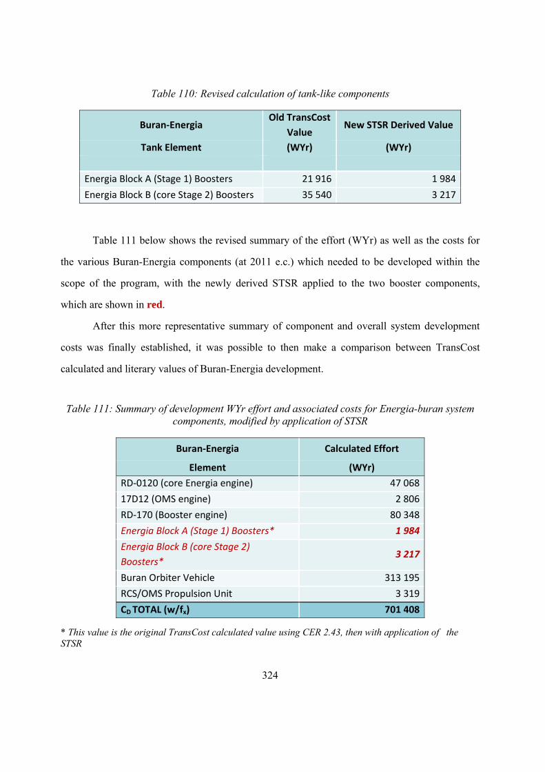
324
Table 110: Revised calculation of tank-like components
Buran‐Energia Old TransCost
Value New STSR Derived Value
Tank Element (WYr) (WYr)
Energia Block A (Stage 1) Boosters 21 916 1 984
Energia Block B (core Stage 2) Boosters 35 540 3 217
Table 111 below shows the revised summary of the effort (WYr) as well as the costs for
the various Buran-Energia components (at 2011 e.c.) which needed to be developed within the
scope of the program, with the newly derived STSR applied to the two booster components,
which are shown in red.
After this more representative summary of component and overall system development
costs was finally established, it was possible to then make a comparison between TransCost
calculated and literary values of Buran-Energia development.
Table 111: Summary of development WYr effort and associated costs for Energia-buran system components, modified by application of STSR
Buran‐Energia Calculated Effort
Element (WYr)
RD‐0120 (core Energia engine) 47 068
17D12 (OMS engine) 2 806
RD‐170 (Booster engine) 80 348
Energia Block A (Stage 1) Boosters* 1 984
Energia Block B (core Stage 2)
Boosters* 3 217
Buran Orbiter Vehicle 313 195
RCS/OMS Propulsion Unit 3 319
CD TOTAL (w/fx) 701 408
* This value is the original TransCost calculated value using CER 2.43, then with application of the STSR
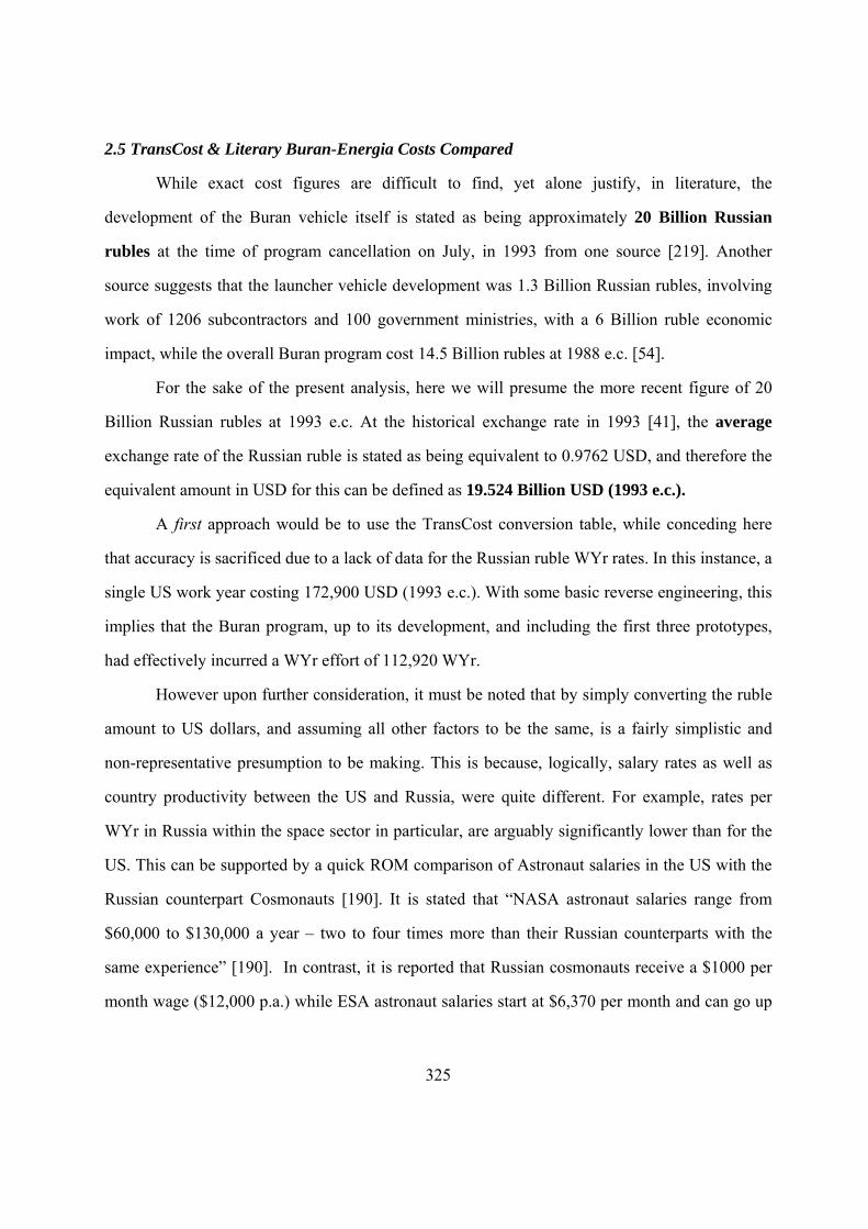
325
2.5 TransCost & Literary Buran-Energia Costs Compared
While exact cost figures are difficult to find, yet alone justify, in literature, the
development of the Buran vehicle itself is stated as being approximately 20 Billion Russian
rubles at the time of program cancellation on July, in 1993 from one source [219]. Another
source suggests that the launcher vehicle development was 1.3 Billion Russian rubles, involving
work of 1206 subcontractors and 100 government ministries, with a 6 Billion ruble economic
impact, while the overall Buran program cost 14.5 Billion rubles at 1988 e.c. [54].
For the sake of the present analysis, here we will presume the more recent figure of 20
Billion Russian rubles at 1993 e.c. At the historical exchange rate in 1993 [41], the average
exchange rate of the Russian ruble is stated as being equivalent to 0.9762 USD, and therefore the
equivalent amount in USD for this can be defined as 19.524 Billion USD (1993 e.c.).
A first approach would be to use the TransCost conversion table, while conceding here
that accuracy is sacrificed due to a lack of data for the Russian ruble WYr rates. In this instance, a
single US work year costing 172,900 USD (1993 e.c.). With some basic reverse engineering, this
implies that the Buran program, up to its development, and including the first three prototypes,
had effectively incurred a WYr effort of 112,920 WYr.
However upon further consideration, it must be noted that by simply converting the ruble
amount to US dollars, and assuming all other factors to be the same, is a fairly simplistic and
non-representative presumption to be making. This is because, logically, salary rates as well as
country productivity between the US and Russia, were quite different. For example, rates per
WYr in Russia within the space sector in particular, are arguably significantly lower than for the
US. This can be supported by a quick ROM comparison of Astronaut salaries in the US with the
Russian counterpart Cosmonauts [190]. It is stated that “NASA astronaut salaries range from
$60,000 to $130,000 a year – two to four times more than their Russian counterparts with the
same experience” [190]. In contrast, it is reported that Russian cosmonauts receive a $1000 per
month wage ($12,000 p.a.) while ESA astronaut salaries start at $6,370 per month and can go up
326
to $10,480 per month. Assuming that this comparison is accurate and representative, doing a
simple calculation to obtain a representative salary ratio between the US, Europe and Russia
yields:
Table 112: Cosmonaut and astronaut salaries for Russia, US and Europe
COUNTRY SALARY (p.a.)
Russia $12,000
US (NASA) $95,000 (mean)
Europe (ESA) $101,000 (mean)
The resulting Salary ratios are therefore established:
• Ratio EU = Europe / US: 1.063
• Ratio ER = Europe / Russia: 8.417
• Ratio UR = US / Russia: 7.917
It is interesting to compare the salary ratios, in a simple ROM analysis to determine
whether this ratio loosely holds and is in congruence with the ratios between WYr values, as
stated in the TransCost handbook. If so, then the ratios can be used as a guide, to determine
values for the Russian WYr cost. This approach is seen to be most suitable to address the lack of
stated WYr values which are relevant for Russia.
The TransCost WYr values provided for Europe and the US for 1993 are:
• USA WYr – $172,900
• Europe (ESA) WYr – €156,800
When converted at the exchange rate from 1993 (€/USD 1.1243 [105]) this equates to:
327
• USA WYr – $172,900
• Europe (ESA) WYr – $176,290
Once again, calculating the resulting TransCost WYr cost ratio for Europe/US for 1993, we
obtain:
(0196.1)(900,172$
)(290,176$
CostWYrUSA
CostWYrEurope1.02)
The calculated ratio value of 1.02 is very close to the ratio obtained for Europe/US space
sector salaries, and therefore firmly confirms the Europe/US Ratio EU value of 1.06 previously
obtained. Hence it is not unreasonable to extrapolate the salary ratio and therefore obtain a WYr
amount for Russia which can then be used within the Buran calculation. After obtaining a
positive confirmation of salary ratios being indicative of WYr cost ratios for TransCost, we can
therefore derive values for the Russian WYr.
As previously calculated, the Europe / Russia salary ratio (Ratio ER) is 8.417. We will
assume this ratio to correspond, or at least be reflective of the different costs of labour between
Russia and Europe. By extrapolating this ratio to a similar correspondence of WYr costs provided
in TransCost, we can derive the Russia WYr value. Then, for 1993, taking the European WYr
cost as being $176,290 in TransCost, and applying our salary ratio, implies that a Russian WYr
amount costs an equivalent of:
$20,945 – calculated Russian WYr EUR/RUS cost (1993 e.c.)
Alternatively, taking the US WYr cost as being $172,900, and applying the US/Russia
(Ratio UR) of 7.917, implies that a Russian WYr amount costs an equivalent of:
$21,840 – calculated Russian WYr US/RUS cost (1993 e.c.)
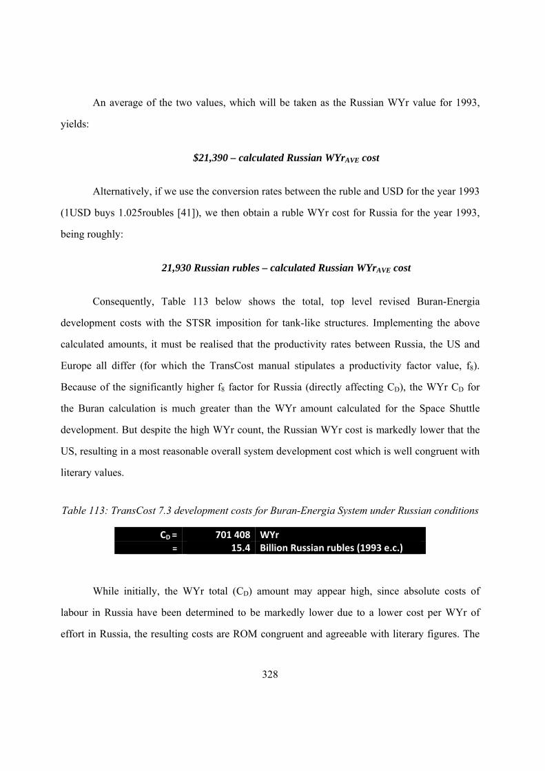
328
An average of the two values, which will be taken as the Russian WYr value for 1993,
yields:
$21,390 – calculated Russian WYrAVE cost
Alternatively, if we use the conversion rates between the ruble and USD for the year 1993
(1USD buys 1.025roubles [41]), we then obtain a ruble WYr cost for Russia for the year 1993,
being roughly:
21,930 Russian rubles – calculated Russian WYrAVE cost
Consequently, Table 113 below shows the total, top level revised Buran-Energia
development costs with the STSR imposition for tank-like structures. Implementing the above
calculated amounts, it must be realised that the productivity rates between Russia, the US and
Europe all differ (for which the TransCost manual stipulates a productivity factor value, f8).
Because of the significantly higher f8 factor for Russia (directly affecting CD), the WYr CD for
the Buran calculation is much greater than the WYr amount calculated for the Space Shuttle
development. But despite the high WYr count, the Russian WYr cost is markedly lower that the
US, resulting in a most reasonable overall system development cost which is well congruent with
literary values.
Table 113: TransCost 7.3 development costs for Buran-Energia System under Russian conditions
CD = 701 408 WYr = 15.4 Billion Russian rubles (1993 e.c.)
While initially, the WYr total (CD) amount may appear high, since absolute costs of
labour in Russia have been determined to be markedly lower due to a lower cost per WYr of
effort in Russia, the resulting costs are ROM congruent and agreeable with literary figures. The
329
overall cost is presented in rubles only to allow for a logical comparison to be made with ruble
values of the Buran-Energia program which were found in literature and previously already
discussed in this chapter.
This TransCost Buran calculation is reasonably congruent with the literary figures
assumed to be the comparative benchmark for the development cost of the Buran program of 20B
rubles at 1993 e.c. at the time of program cancellation. Admittedly, with the Buran examples, it
must be conceded that exact program figures are very challenging to obtain. In addition, the
financial situation in Russia makes conversion rates between years, and also the calculation of the
cost of Russian WYr very difficult.
The newly determined development WYr values for the Buran-Energia system using the
STSR, as described in this Chapter, are consequently used for the comparison between the Space
Shuttle system in the following chapter.
2.6 Space Shuttle & Buran-Energia Development Comparison
Now that the development costs for the two shuttle systems were calculated, it was an
interesting exercise to compare the two results. While some elements of the Shuttle and Buran are
indeed directly comparable, others are fairly different so to make a comparison is a little more
challenging. Therefore some data processing and manipulation was required to achieve this
purpose.
2.6.1 Generic Shuttle-Buran Comparison
To facilitate for a comparison to be made, it was necessary to establish and then group the
individually standing and separately costed components into clear general categories which, after
being summed, would then be tangibly comparable. This was achieved by grouping elements
based on their functionality within each of the Shuttle and Buran launcher systems. The groups
330
themselves were in fact similar to the CER groupings established in TransCost model. The
launcher system functionality groups identified were:
Engines
Boosters
Orbiter
External Tank
RCS/OMS Units
After this was achieved, all the components for the Buran-Energia, and the Shuttle had to
then, fairly logically, be assigned to each category. The respective WYr effort figures and costs
derived from TransCost, were filled in for each category and the amounts tallied to arrive at an
overall category WYr effort figure and therefore cost.
The two key numerical results which are of importance within context of this analysis, are
the WYr effort amounts, and their respective costs, in the home currency of the development
effort, for the chosen year. In this respect, the logical pairing of the information pairs had to be
strictly maintained in order to result in a meaningful result. In order to be representative, the f8
country productivity complexity factor also had to be taken into account for each the US
developed Shuttle system, and the Russian Buran. This is because the overall program cost
comprises of a pairing of inputs between the WYr amount (a unit-less amount of effort) as well as
then the WYr rate for that respective country, in that country’s respective currency.
It is also important to point out that the Shuttle development phase was considered to be
concluded in 1981. The development phase of the program began in 1972, and therefore a middle
value year of 1978 was chosen, to represent the peak of development initiatives. As such, the
USD costs are calculated using data for 1978 economic conditions (as seen in Table 114). For
Buran, as seen in Table 115, the costs are calculated for 1993 economic conditions, since this was
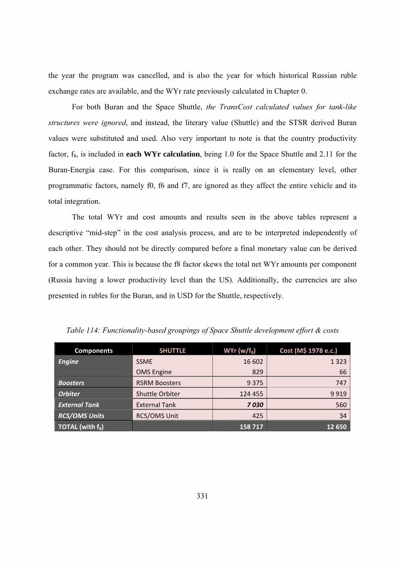
331
the year the program was cancelled, and is also the year for which historical Russian ruble
exchange rates are available, and the WYr rate previously calculated in Chapter 0.
For both Buran and the Space Shuttle, the TransCost calculated values for tank-like
structures were ignored, and instead, the literary value (Shuttle) and the STSR derived Buran
values were substituted and used. Also very important to note is that the country productivity
factor, f8, is included in each WYr calculation, being 1.0 for the Space Shuttle and 2.11 for the
Buran-Energia case. For this comparison, since it is really on an elementary level, other
programmatic factors, namely f0, f6 and f7, are ignored as they affect the entire vehicle and its
total integration.
The total WYr and cost amounts and results seen in the above tables represent a
descriptive “mid-step” in the cost analysis process, and are to be interpreted independently of
each other. They should not be directly compared before a final monetary value can be derived
for a common year. This is because the f8 factor skews the total net WYr amounts per component
(Russia having a lower productivity level than the US). Additionally, the currencies are also
presented in rubles for the Buran, and in USD for the Shuttle, respectively.
Table 114: Functionality-based groupings of Space Shuttle development effort & costs
Components SHUTTLE WYr (w/f8) Cost (M$ 1978 e.c.)
Engine SSME 16 602 1 323
OMS Engine 829 66
Boosters RSRM Boosters 9 375 747
Orbiter Shuttle Orbiter 124 455 9 919
External Tank External Tank 7 030 560
RCS/OMS Units RCS/OMS Unit 425 34
TOTAL (with f8) 158 717 12 650
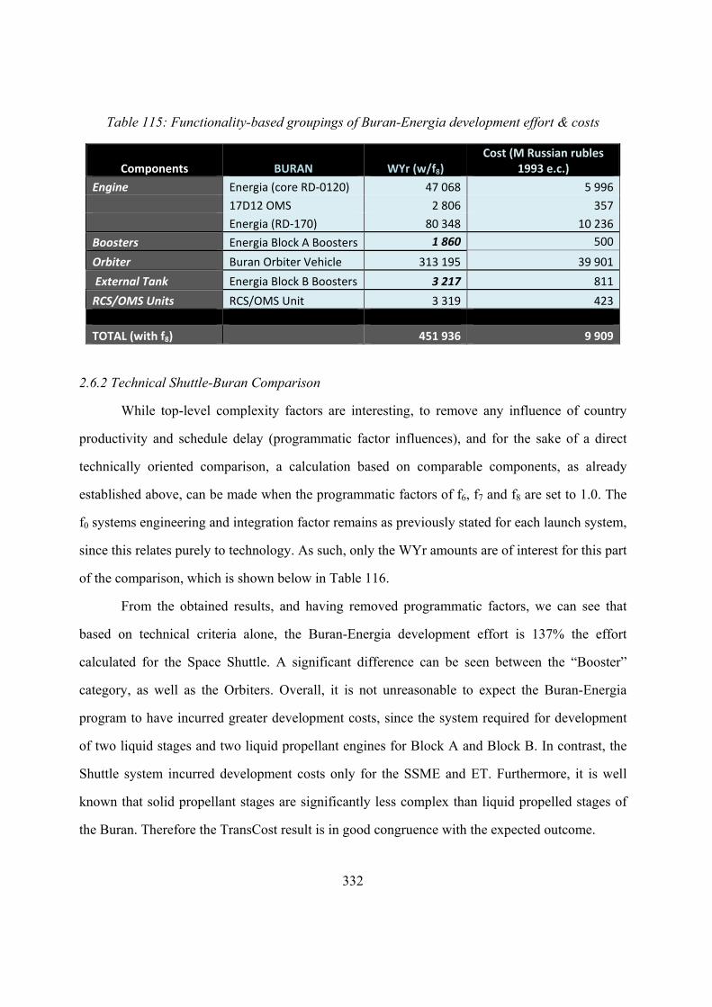
332
Table 115: Functionality-based groupings of Buran-Energia development effort & costs
Components BURAN WYr (w/f8) Cost (M Russian rubles
1993 e.c.)
Engine Energia (core RD‐0120) 47 068 5 996
17D12 OMS 2 806 357
Energia (RD‐170) 80 348 10 236
Boosters Energia Block A Boosters 1 860 500
Orbiter Buran Orbiter Vehicle 313 195 39 901
External Tank Energia Block B Boosters 3 217 811
RCS/OMS Units RCS/OMS Unit 3 319 423
TOTAL (with f8) 451 936 9 909
2.6.2 Technical Shuttle-Buran Comparison
While top-level complexity factors are interesting, to remove any influence of country
productivity and schedule delay (programmatic factor influences), and for the sake of a direct
technically oriented comparison, a calculation based on comparable components, as already
established above, can be made when the programmatic factors of f6, f7 and f8 are set to 1.0. The
f0 systems engineering and integration factor remains as previously stated for each launch system,
since this relates purely to technology. As such, only the WYr amounts are of interest for this part
of the comparison, which is shown below in Table 116.
From the obtained results, and having removed programmatic factors, we can see that
based on technical criteria alone, the Buran-Energia development effort is 137% the effort
calculated for the Space Shuttle. A significant difference can be seen between the “Booster”
category, as well as the Orbiters. Overall, it is not unreasonable to expect the Buran-Energia
program to have incurred greater development costs, since the system required for development
of two liquid stages and two liquid propellant engines for Block A and Block B. In contrast, the
Shuttle system incurred development costs only for the SSME and ET. Furthermore, it is well
known that solid propellant stages are significantly less complex than liquid propelled stages of
the Buran. Therefore the TransCost result is in good congruence with the expected outcome.
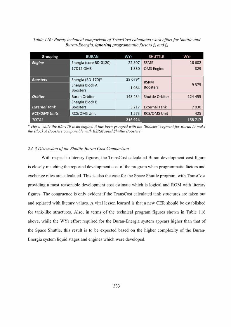
333
Table 116: Purely technical comparison of TransCost calculated work effort for Shuttle and Buran-Energia, ignoring programmatic factors f6 and f8
Grouping BURAN WYr SHUTTLE WYr
Engine Energia (core RD‐0120) 22 307 SSME 16 602
17D12 OMS 1 330 OMS Engine 829
Boosters Energia (RD‐170)* 38 079*RSRM Boosters
9 375
Energia Block A Boosters
1 984
Orbiter Buran Orbiter 148 434 Shuttle Orbiter 124 455
External Tank Energia Block B Boosters 3 217 External Tank 7 030
RCS/OMS Units RCS/OMS Unit 1 573 RCS/OMS Unit 425
TOTAL 216 924 158 717
* Here, while the RD-170 is an engine, it has been grouped with the ‘Booster’ segment for Buran to make the Block A Boosters comparable with RSRM solid Shuttle Boosters.
2.6.3 Discussion of the Shuttle-Buran Cost Comparison
With respect to literary figures, the TransCost calculated Buran development cost figure
is closely matching the reported development cost of the program when programmatic factors and
exchange rates are calculated. This is also the case for the Space Shuttle program, with TransCost
providing a most reasonable development cost estimate which is logical and ROM with literary
figures. The congruence is only evident if the TransCost calculated tank structures are taken out
and replaced with literary values. A vital lesson learned is that a new CER should be established
for tank-like structures. Also, in terms of the technical program figures shown in Table 116
above, while the WYr effort required for the Buran-Energia system appears higher than that of
the Space Shuttle, this result is to be expected based on the higher complexity of the Buran-
Energia system liquid stages and engines which were developed.
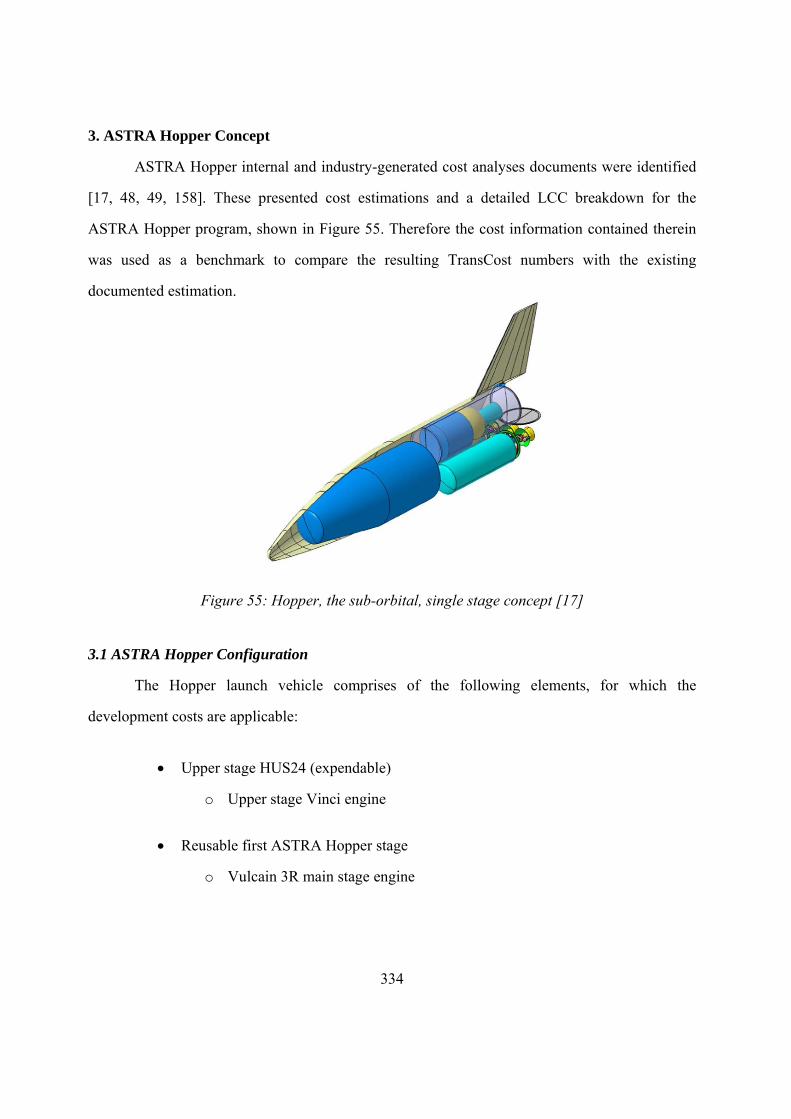
334
3. ASTRA Hopper Concept
ASTRA Hopper internal and industry-generated cost analyses documents were identified
[17, 48, 49, 158]. These presented cost estimations and a detailed LCC breakdown for the
ASTRA Hopper program, shown in Figure 55. Therefore the cost information contained therein
was used as a benchmark to compare the resulting TransCost numbers with the existing
documented estimation.
Figure 55: Hopper, the sub-orbital, single stage concept [17]
3.1 ASTRA Hopper Configuration
The Hopper launch vehicle comprises of the following elements, for which the
development costs are applicable:
Upper stage HUS24 (expendable)
o Upper stage Vinci engine
Reusable first ASTRA Hopper stage
o Vulcain 3R main stage engine
335
Although the Vinci engine already exists, the development effort which is meant in the
context of the ASTRA Hopper configuration is the development cost which would be incurred
for a horizontal launch of the vehicle. Also, here, as with the LFBB stage from the ASSC2-Y9
program, the focal element for cost estimation is of course the reusable ASTRA stage.
Furthermore, the development costs are calculated predominantly in 2002 e.c. since this was
considered to be the timeframe of the Hopper development period. Of course this has no bearing
on the effort amount, since this is merely a measure of effort, and as such is irrelevant for which
year this work effort is converted into a monetary amount. The final costs, however, are all given
in 2011 e.c. values to assist for a relevant comparison to be made.
3.2 ASTRA Hopper Excel Component Break-down
The component breakdown structure and the Excel TransCost spreadsheet screenshots
with all relevant inputs and complexity factors for Hopper are presented below in Table 117
through to Table 120.
3.3 ASTRA Hopper Calculation Assumptions
Some key assumptions also had to be made within the scope of the Hopper and ASTRA
cost estimation with regards to numerous inputs, complexity factors, as well as currency
conversions. The key assumptions are outlined below, and are also annotated in red with
association to the fields which the assumptions affect in the tables below.
A1. For the Vinci engine development cost estimation, an f12 delta development factor
was assumed to account for the fact that the engine is merely a modification to previous engine
developments. The prominent delta here is the fact that the vehicle is a horizontally starting one.
Arguably, this f12 value was taken to be 0.1.
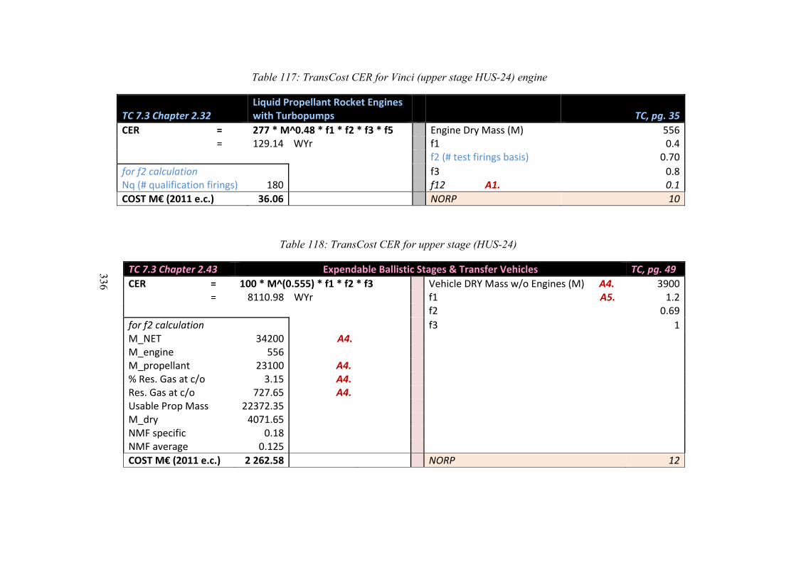
336
Table 117: TransCost CER for Vinci (upper stage HUS-24) engine
TC 7.3 Chapter 2.32 Liquid Propellant Rocket Engines with Turbopumps TC, pg. 35
CER = 277 * M^0.48 * f1 * f2 * f3 * f5 Engine Dry Mass (M) 556 = 129.14 WYr f1 0.4 f2 (# test firings basis) 0.70
for f2 calculation f3 0.8Nq (# qualification firings) 180 f12 A1. 0.1
COST M€ (2011 e.c.) 36.06 NORP 10
Table 118: TransCost CER for upper stage (HUS-24)
TC 7.3 Chapter 2.43 Expendable Ballistic Stages & Transfer Vehicles TC, pg. 49
CER = 100 * M^(0.555) * f1 * f2 * f3 Vehicle DRY Mass w/o Engines (M) A4. 3900 = 8110.98 WYr f1 A5. 1.2 f2 0.69
for f2 calculation f3 1M_NET 34200 A4. M_engine 556 M_propellant 23100 A4.% Res. Gas at c/o 3.15 A4. Res. Gas at c/o 727.65 A4. Usable Prop Mass 22372.35 M_dry 4071.65NMF specific 0.18 NMF average 0.125
COST M€ (2011 e.c.) 2 262.58 NORP 12
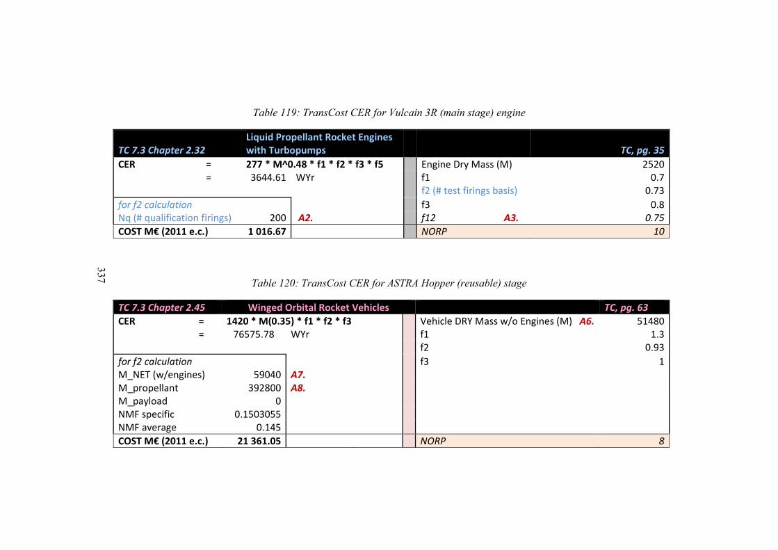
337
Table 119: TransCost CER for Vulcain 3R (main stage) engine
TC 7.3 Chapter 2.32 Liquid Propellant Rocket Engines with Turbopumps TC, pg. 35
CER = 277 * M^0.48 * f1 * f2 * f3 * f5 Engine Dry Mass (M) 2520 = 3644.61 WYr f1 0.7 f2 (# test firings basis) 0.73
for f2 calculation f3 0.8Nq (# qualification firings) 200 A2. f12 A3. 0.75
COST M€ (2011 e.c.) 1 016.67 NORP 10
Table 120: TransCost CER for ASTRA Hopper (reusable) stage
TC 7.3 Chapter 2.45 Winged Orbital Rocket Vehicles TC, pg. 63
CER = 1420 * M(0.35) * f1 * f2 * f3 Vehicle DRY Mass w/o Engines (M) A6. 51480 = 76575.78 WYr f1 1.3 f2 0.93
for f2 calculation f3 1M_NET (w/engines) 59040 A7.M_propellant 392800 A8. M_payload 0 NMF specific 0.1503055 NMF average 0.145
COST M€ (2011 e.c.) 21 361.05 NORP 8
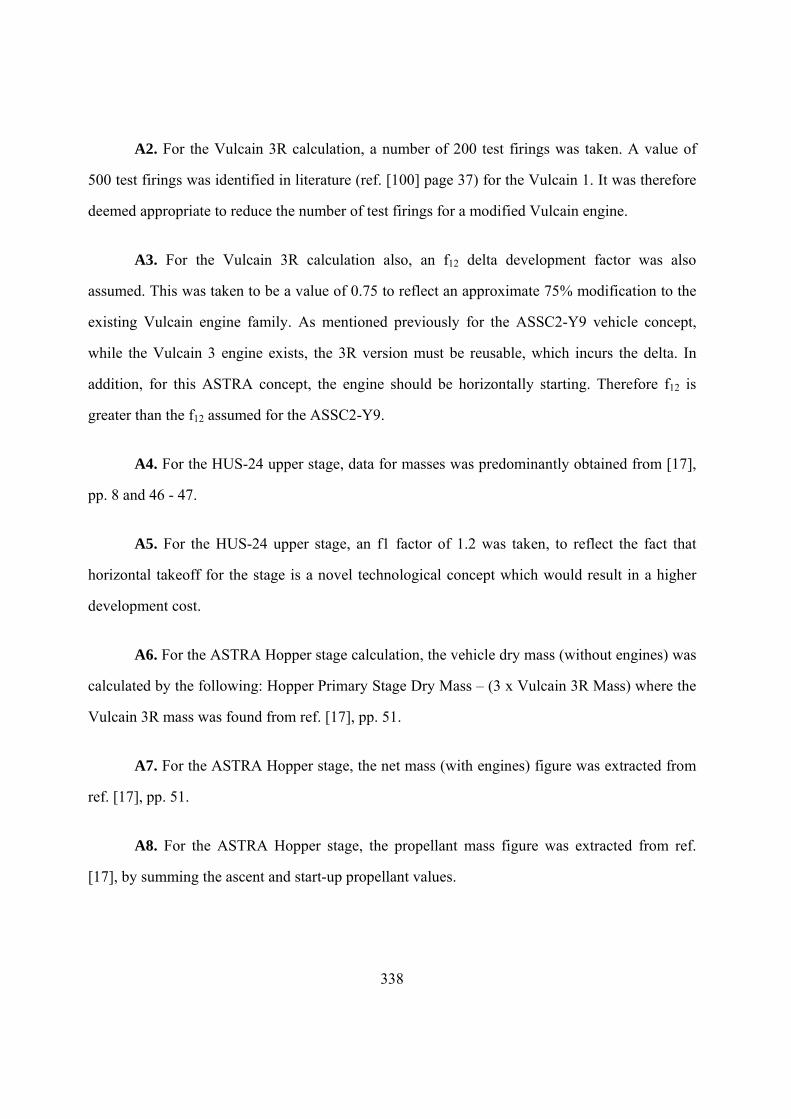
338
A2. For the Vulcain 3R calculation, a number of 200 test firings was taken. A value of
500 test firings was identified in literature (ref. [100] page 37) for the Vulcain 1. It was therefore
deemed appropriate to reduce the number of test firings for a modified Vulcain engine.
A3. For the Vulcain 3R calculation also, an f12 delta development factor was also
assumed. This was taken to be a value of 0.75 to reflect an approximate 75% modification to the
existing Vulcain engine family. As mentioned previously for the ASSC2-Y9 vehicle concept,
while the Vulcain 3 engine exists, the 3R version must be reusable, which incurs the delta. In
addition, for this ASTRA concept, the engine should be horizontally starting. Therefore f12 is
greater than the f12 assumed for the ASSC2-Y9.
A4. For the HUS-24 upper stage, data for masses was predominantly obtained from [17],
pp. 8 and 46 - 47.
A5. For the HUS-24 upper stage, an f1 factor of 1.2 was taken, to reflect the fact that
horizontal takeoff for the stage is a novel technological concept which would result in a higher
development cost.
A6. For the ASTRA Hopper stage calculation, the vehicle dry mass (without engines) was
calculated by the following: Hopper Primary Stage Dry Mass – (3 x Vulcain 3R Mass) where the
Vulcain 3R mass was found from ref. [17], pp. 51.
A7. For the ASTRA Hopper stage, the net mass (with engines) figure was extracted from
ref. [17], pp. 51.
A8. For the ASTRA Hopper stage, the propellant mass figure was extracted from ref.
[17], by summing the ascent and start-up propellant values.
339
A9. For the ASTRA Hopper stage, the payload technically is the main stage, and as such,
the mass for the payload within the calculation was given as zero.
In addition, it is interesting to note that the mass of the Vulcain 3R engines for the LFBB
(Table 11) and Hopper (
Table 119), as entered into the TransCost CERs, is different (2370 kg and 2520 kg for
LFBB and Hopper respectively). Although the mechanics of the engine itself are the same, the
difference arises due to a difference in the nozzle extension.
3.4 ASTRA Hopper Summary
Following the breakdown of individual components on a technical level, the additional
TransCost programmatic factors which are then imposed on the sum of the constituent elements
for the Hopper system, are all outlined below, and their chosen values stated:
• f0 = 1.08
(f0 = 1.04 number of stages, in the case of the Hopper, 2)
• f6 = 1
(here, assume no deviation from optimum schedule)
• f7 = 1.00
(f7 = n 0.2; with n being the number of parallel contractor organisations, in this case
assumed to be 1)
• f8 = 0.86
(TransCost stated country productivity factor for ESA)
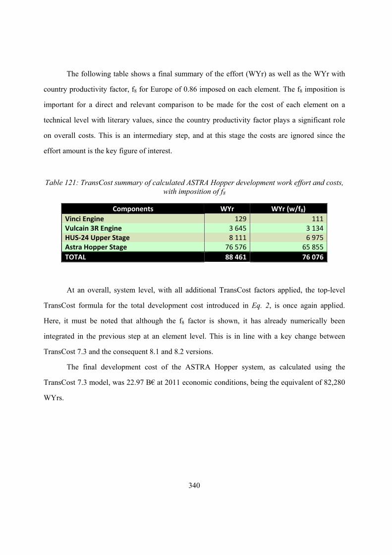
340
The following table shows a final summary of the effort (WYr) as well as the WYr with
country productivity factor, f8 for Europe of 0.86 imposed on each element. The f8 imposition is
important for a direct and relevant comparison to be made for the cost of each element on a
technical level with literary values, since the country productivity factor plays a significant role
on overall costs. This is an intermediary step, and at this stage the costs are ignored since the
effort amount is the key figure of interest.
Table 121: TransCost summary of calculated ASTRA Hopper development work effort and costs, with imposition of f8
Components WYr WYr (w/f8)
Vinci Engine 129 111 Vulcain 3R Engine 3 645 3 134 HUS‐24 Upper Stage 8 111 6 975 Astra Hopper Stage 76 576 65 855
TOTAL 88 461 76 076
At an overall, system level, with all additional TransCost factors applied, the top-level
TransCost formula for the total development cost introduced in Eq. 2, is once again applied.
Here, it must be noted that although the f8 factor is shown, it has already numerically been
integrated in the previous step at an element level. This is in line with a key change between
TransCost 7.3 and the consequent 8.1 and 8.2 versions.
The final development cost of the ASTRA Hopper system, as calculated using the
TransCost 7.3 model, was 22.97 B€ at 2011 economic conditions, being the equivalent of 82,280
WYrs.
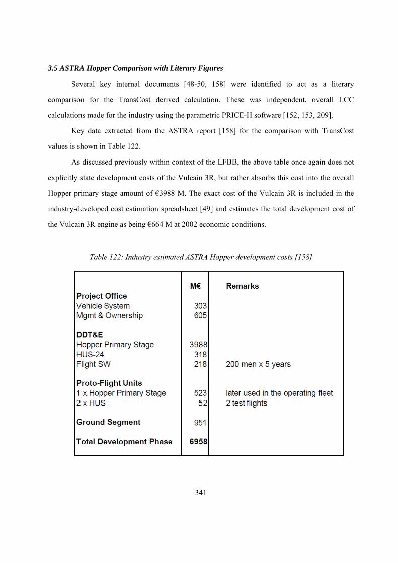
341
3.5 ASTRA Hopper Comparison with Literary Figures
Several key internal documents [48-50, 158] were identified to act as a literary
comparison for the TransCost derived calculation. These was independent, overall LCC
calculations made for the industry using the parametric PRICE-H software [152, 153, 209].
Key data extracted from the ASTRA report [158] for the comparison with TransCost
values is shown in Table 122.
As discussed previously within context of the LFBB, the above table once again does not
explicitly state development costs of the Vulcain 3R, but rather absorbs this cost into the overall
Hopper primary stage amount of €3988 M. The exact cost of the Vulcain 3R is included in the
industry-developed cost estimation spreadsheet [49] and estimates the total development cost of
the Vulcain 3R engine as being €664 M at 2002 economic conditions.
Table 122: Industry estimated ASTRA Hopper development costs [158]
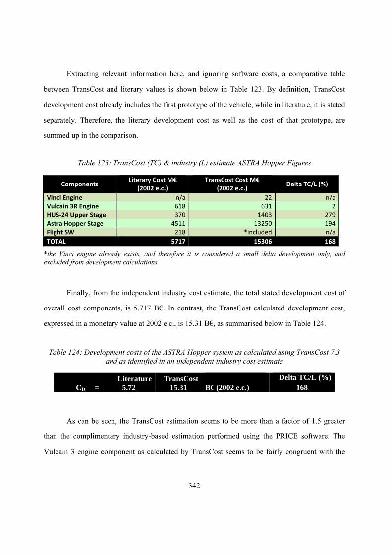
342
Extracting relevant information here, and ignoring software costs, a comparative table
between TransCost and literary values is shown below in Table 123. By definition, TransCost
development cost already includes the first prototype of the vehicle, while in literature, it is stated
separately. Therefore, the literary development cost as well as the cost of that prototype, are
summed up in the comparison.
Table 123: TransCost (TC) & industry (L) estimate ASTRA Hopper Figures
Components Literary Cost M€
(2002 e.c.) TransCost Cost M€
(2002 e.c.) Delta TC/L (%)
Vinci Engine n/a 22 n/aVulcain 3R Engine 618 631 2HUS‐24 Upper Stage 370 1403 279Astra Hopper Stage 4511 13250 194Flight SW 218 *included n/a
TOTAL 5717 15306 168
*the Vinci engine already exists, and therefore it is considered a small delta development only, and excluded from development calculations.
Finally, from the independent industry cost estimate, the total stated development cost of
overall cost components, is 5.717 B€. In contrast, the TransCost calculated development cost,
expressed in a monetary value at 2002 e.c., is 15.31 B€, as summarised below in Table 124.
Table 124: Development costs of the ASTRA Hopper system as calculated using TransCost 7.3 and as identified in an independent industry cost estimate
Literature TransCost Delta TC/L (%)CD = 5.72 15.31 B€ (2002 e.c.) 168
As can be seen, the TransCost estimation seems to be more than a factor of 1.5 greater
than the complimentary industry-based estimation performed using the PRICE software. The
Vulcain 3 engine component as calculated by TransCost seems to be fairly congruent with the
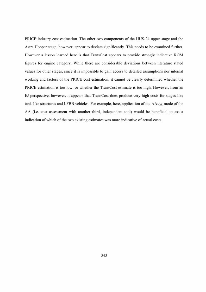
343
PRICE industry cost estimation. The other two components of the HUS-24 upper stage and the
Astra Hopper stage, however, appear to deviate significantly. This needs to be examined further.
However a lesson learned here is that TransCost appears to provide strongly indicative ROM
figures for engine category. While there are considerable deviations between literature stated
values for other stages, since it is impossible to gain access to detailed assumptions nor internal
working and factors of the PRICE cost estimation, it cannot be clearly determined whether the
PRICE estimation is too low, or whether the TransCost estimate is too high. However, from an
EJ perspective, however, it appears that TransCost does produce very high costs for stages like
tank-like structures and LFBB vehicles. For example, here, application of the AAVAL mode of the
AA (i.e. cost assessment with another third, independent tool) would be beneficial to assist
indication of which of the two existing estimates was more indicative of actual costs.
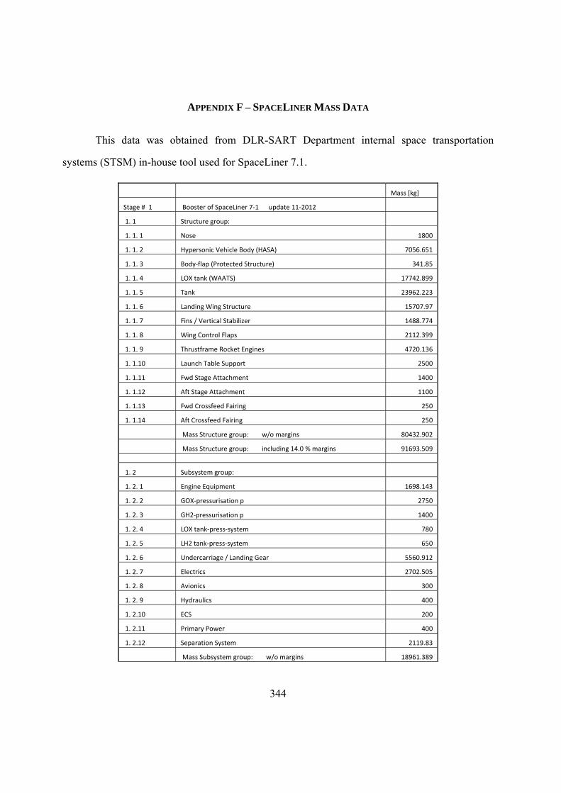
344
APPENDIX F – SPACELINER MASS DATA
This data was obtained from DLR-SART Department internal space transportation
systems (STSM) in-house tool used for SpaceLiner 7.1.
Mass [kg]
Stage # 1 Booster of SpaceLiner 7‐1 update 11‐2012
1. 1 Structure group:
1. 1. 1 Nose 1800
1. 1. 2 Hypersonic Vehicle Body (HASA) 7056.651
1. 1. 3 Body‐flap (Protected Structure) 341.85
1. 1. 4 LOX tank (WAATS) 17742.899
1. 1. 5 Tank 23962.223
1. 1. 6 Landing Wing Structure 15707.97
1. 1. 7 Fins / Vertical Stabilizer 1488.774
1. 1. 8 Wing Control Flaps 2112.399
1. 1. 9 Thrustframe Rocket Engines 4720.136
1. 1.10 Launch Table Support 2500
1. 1.11 Fwd Stage Attachment 1400
1. 1.12 Aft Stage Attachment 1100
1. 1.13 Fwd Crossfeed Fairing 250
1. 1.14 Aft Crossfeed Fairing 250
Mass Structure group: w/o margins 80432.902
Mass Structure group: including 14.0 % margins 91693.509
1. 2 Subsystem group:
1. 2. 1 Engine Equipment 1698.143
1. 2. 2 GOX‐pressurisation p 2750
1. 2. 3 GH2‐pressurisation p 1400
1. 2. 4 LOX tank‐press‐system 780
1. 2. 5 LH2 tank‐press‐system 650
1. 2. 6 Undercarriage / Landing Gear 5560.912
1. 2. 7 Electrics 2702.505
1. 2. 8 Avionics 300
1. 2. 9 Hydraulics 400
1. 2.10 ECS 200
1. 2.11 Primary Power 400
1. 2.12 Separation System 2119.83
Mass Subsystem group: w/o margins 18961.389
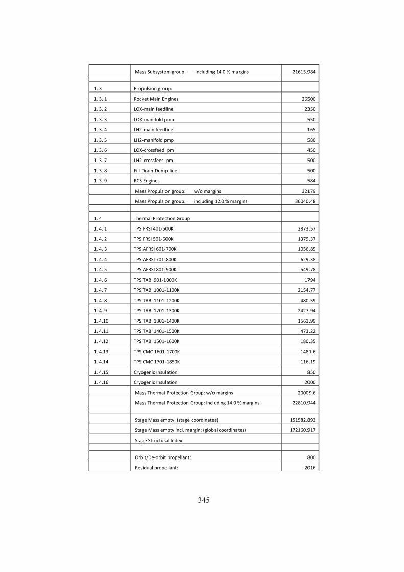
345
Mass Subsystem group: including 14.0 % margins 21615.984
1. 3 Propulsion group:
1. 3. 1 Rocket Main Engines 26500
1. 3. 2 LOX‐main feedline 2350
1. 3. 3 LOX‐manifold pmp 550
1. 3. 4 LH2‐main feedline 165
1. 3. 5 LH2‐manifold pmp 580
1. 3. 6 LOX‐crossfeed pm 450
1. 3. 7 LH2‐crossfees pm 500
1. 3. 8 Fill‐Drain‐Dump‐line 500
1. 3. 9 RCS Engines 584
Mass Propulsion group: w/o margins 32179
Mass Propulsion group: including 12.0 % margins 36040.48
1. 4 Thermal Protection Group:
1. 4. 1 TPS FRSI 401‐500K 2873.57
1. 4. 2 TPS FRSI 501‐600K 1379.37
1. 4. 3 TPS AFRSI 601‐700K 1056.85
1. 4. 4 TPS AFRSI 701‐800K 629.38
1. 4. 5 TPS AFRSI 801‐900K 549.78
1. 4. 6 TPS TABI 901‐1000K 1794
1. 4. 7 TPS TABI 1001‐1100K 2154.77
1. 4. 8 TPS TABI 1101‐1200K 480.59
1. 4. 9 TPS TABI 1201‐1300K 2427.94
1. 4.10 TPS TABI 1301‐1400K 1561.99
1. 4.11 TPS TABI 1401‐1500K 473.22
1. 4.12 TPS TABI 1501‐1600K 180.35
1. 4.13 TPS CMC 1601‐1700K 1481.6
1. 4.14 TPS CMC 1701‐1850K 116.19
1. 4.15 Cryogenic Insulation 850
1. 4.16 Cryogenic Insulation 2000
Mass Thermal Protection Group: w/o margins 20009.6
Mass Thermal Protection Group: including 14.0 % margins 22810.944
Stage Mass empty: (stage coordinates) 151582.892
Stage Mass empty incl. margin: (global coordinates) 172160.917
Stage Structural Index:
Orbit/De‐orbit propellant: 800
Residual propellant: 2016
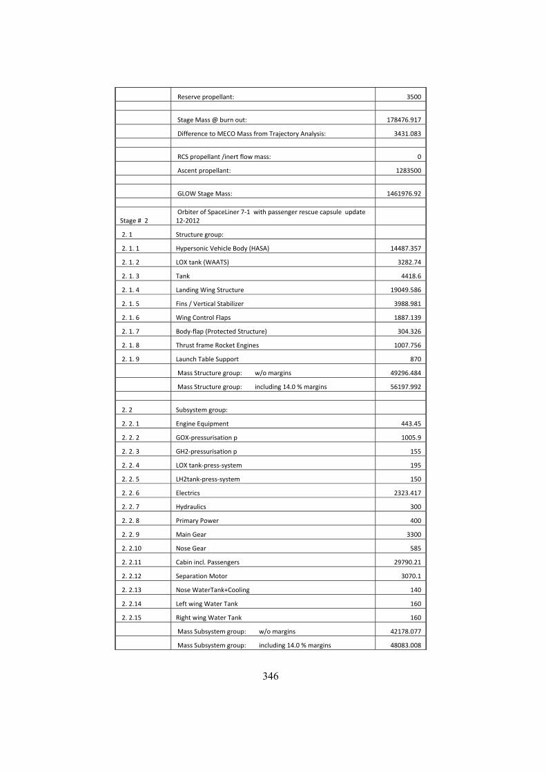
346
Reserve propellant: 3500
Stage Mass @ burn out: 178476.917
Difference to MECO Mass from Trajectory Analysis: 3431.083
RCS propellant /inert flow mass: 0
Ascent propellant: 1283500
GLOW Stage Mass: 1461976.92
Stage # 2 Orbiter of SpaceLiner 7‐1 with passenger rescue capsule update 12‐2012
2. 1 Structure group:
2. 1. 1 Hypersonic Vehicle Body (HASA) 14487.357
2. 1. 2 LOX tank (WAATS) 3282.74
2. 1. 3 Tank 4418.6
2. 1. 4 Landing Wing Structure 19049.586
2. 1. 5 Fins / Vertical Stabilizer 3988.981
2. 1. 6 Wing Control Flaps 1887.139
2. 1. 7 Body‐flap (Protected Structure) 304.326
2. 1. 8 Thrust frame Rocket Engines 1007.756
2. 1. 9 Launch Table Support 870
Mass Structure group: w/o margins 49296.484
Mass Structure group: including 14.0 % margins 56197.992
2. 2 Subsystem group:
2. 2. 1 Engine Equipment 443.45
2. 2. 2 GOX‐pressurisation p 1005.9
2. 2. 3 GH2‐pressurisation p 155
2. 2. 4 LOX tank‐press‐system 195
2. 2. 5 LH2tank‐press‐system 150
2. 2. 6 Electrics 2323.417
2. 2. 7 Hydraulics 300
2. 2. 8 Primary Power 400
2. 2. 9 Main Gear 3300
2. 2.10 Nose Gear 585
2. 2.11 Cabin incl. Passengers 29790.21
2. 2.12 Separation Motor 3070.1
2. 2.13 Nose WaterTank+Cooling 140
2. 2.14 Left wing Water Tank 160
2. 2.15 Right wing Water Tank 160
Mass Subsystem group: w/o margins 42178.077
Mass Subsystem group: including 14.0 % margins 48083.008
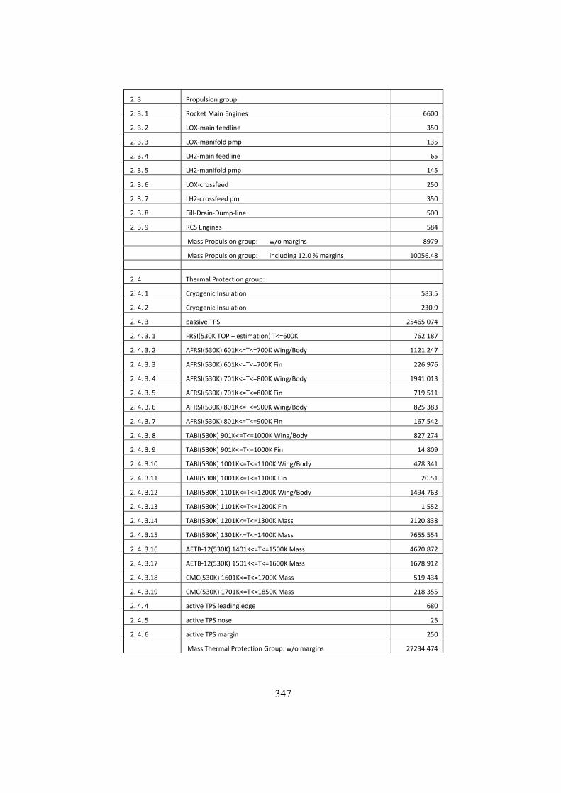
347
2. 3 Propulsion group:
2. 3. 1 Rocket Main Engines 6600
2. 3. 2 LOX‐main feedline 350
2. 3. 3 LOX‐manifold pmp 135
2. 3. 4 LH2‐main feedline 65
2. 3. 5 LH2‐manifold pmp 145
2. 3. 6 LOX‐crossfeed 250
2. 3. 7 LH2‐crossfeed pm 350
2. 3. 8 Fill‐Drain‐Dump‐line 500
2. 3. 9 RCS Engines 584
Mass Propulsion group: w/o margins 8979
Mass Propulsion group: including 12.0 % margins 10056.48
2. 4 Thermal Protection group:
2. 4. 1 Cryogenic Insulation 583.5
2. 4. 2 Cryogenic Insulation 230.9
2. 4. 3 passive TPS 25465.074
2. 4. 3. 1 FRSI(530K TOP + estimation) T<=600K 762.187
2. 4. 3. 2 AFRSI(530K) 601K<=T<=700K Wing/Body 1121.247
2. 4. 3. 3 AFRSI(530K) 601K<=T<=700K Fin 226.976
2. 4. 3. 4 AFRSI(530K) 701K<=T<=800K Wing/Body 1941.013
2. 4. 3. 5 AFRSI(530K) 701K<=T<=800K Fin 719.511
2. 4. 3. 6 AFRSI(530K) 801K<=T<=900K Wing/Body 825.383
2. 4. 3. 7 AFRSI(530K) 801K<=T<=900K Fin 167.542
2. 4. 3. 8 TABI(530K) 901K<=T<=1000K Wing/Body 827.274
2. 4. 3. 9 TABI(530K) 901K<=T<=1000K Fin 14.809
2. 4. 3.10 TABI(530K) 1001K<=T<=1100K Wing/Body 478.341
2. 4. 3.11 TABI(530K) 1001K<=T<=1100K Fin 20.51
2. 4. 3.12 TABI(530K) 1101K<=T<=1200K Wing/Body 1494.763
2. 4. 3.13 TABI(530K) 1101K<=T<=1200K Fin 1.552
2. 4. 3.14 TABI(530K) 1201K<=T<=1300K Mass 2120.838
2. 4. 3.15 TABI(530K) 1301K<=T<=1400K Mass 7655.554
2. 4. 3.16 AETB‐12(530K) 1401K<=T<=1500K Mass 4670.872
2. 4. 3.17 AETB‐12(530K) 1501K<=T<=1600K Mass 1678.912
2. 4. 3.18 CMC(530K) 1601K<=T<=1700K Mass 519.434
2. 4. 3.19 CMC(530K) 1701K<=T<=1850K Mass 218.355
2. 4. 4 active TPS leading edge 680
2. 4. 5 active TPS nose 25
2. 4. 6 active TPS margin 250
Mass Thermal Protection Group: w/o margins 27234.474
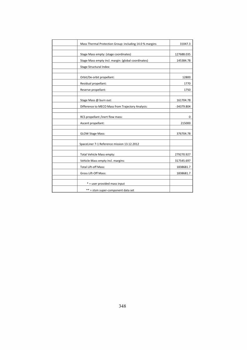
348
Mass Thermal Protection Group: including 14.0 % margins 31047.3
Stage Mass empty: (stage coordinates) 127688.035
Stage Mass empty incl. margin: (global coordinates) 145384.78
Stage Structural Index:
Orbit/De‐orbit propellant: 12800
Residual propellant: 1770
Reserve propellant: 1750
Stage Mass @ burn out: 161704.78
Difference to MECO Mass from Trajectory Analysis: ‐34379.804
RCS propellant /inert flow mass: 0
Ascent propellant: 215000
GLOW Stage Mass: 376704.78
SpaceLiner 7‐1 Reference mission 13.12.2012
Total Vehicle Mass empty: 279270.927
Vehicle Mass empty incl. margins: 317545.697
Total Lift‐off Mass: 1838681.7
Gross Lift‐Off Mass: 1838681.7
* = user provided mass input
** = stsm super‐component data set
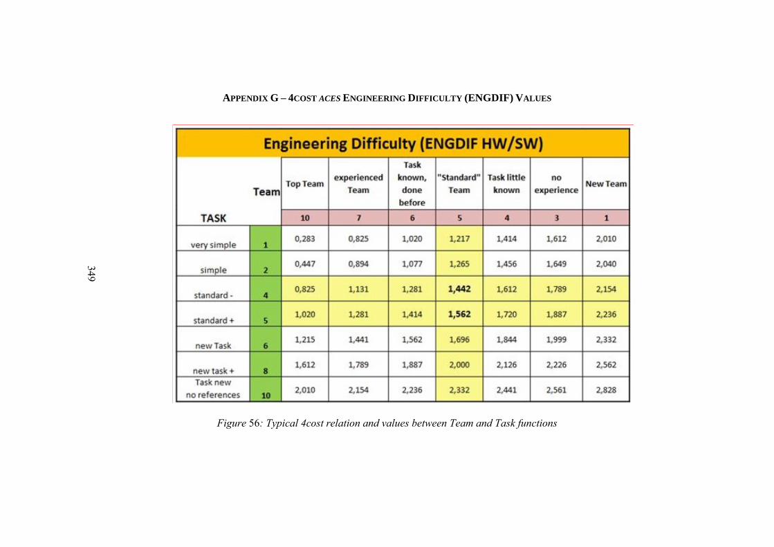
349
APPENDIX G – 4COST ACES ENGINEERING DIFFICULTY (ENGDIF) VALUES
Figure 56: Typical 4cost relation and values between Team and Task functions
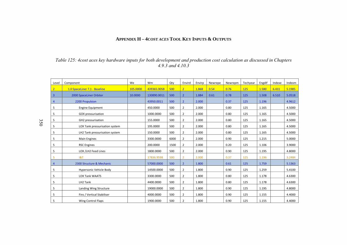
350
APPENDIX H – 4COST ACES TOOL KEY INPUTS & OUTPUTS
Table 125: 4cost aces key hardware inputs for both development and production cost calculation as discussed in Chapters 4.9.3 and 4.10.3
Level Component We Wm Qty Envird Envirp Newrepe Newrepm Techyear Engdif Indexe Indexm
2 1.0 SpaceLiner 7.1 ‐ Baseline 105.0000 439365.0058 500 2 1.868 0.54 0.76 125 1.580 6.431 5.1985
3 2000 SpaceLiner Orbiter 10.0000 130890.0011 500 2 1.884 0.61 0.78 125 1.508 6.510 5.0518
4 2200 Propulsion 43950.0011 500 2 2.000 0.37 125 1.196 4.9612
5 Engine Equipment 450.0000 500 2 2.000 0.80 125 1.165 4.5000
5 GOX pressurisation 1000.0000 500 2 2.000 0.80 125 1.165 4.5000
5 GH2 pressurisation 155.0000 500 2 2.000 0.80 125 1.165 4.5000
5 LOX Tank pressurisation system 195.0000 500 2 2.000 0.80 125 1.165 4.5000
5 LH2 Tank pressurisation system 150.0000 500 2 2.000 0.80 125 1.165 4.5000
5 Main Engines 3300.0000 6000 2 2.000 0.90 125 1.215 5.0000
5 RSC Engines 200.0000 1500 2 2.000 0.20 125 1.106 3.9000
5 LOX /LH2 Feed Lines 1800.0000 500 2 2.000 0.90 125 1.195 4.8000
5 I&T 17836.9598 500 2 2.000 0.37 125 1.196 3.2484
4 2300 Structure & Mechanic 57000.0000 500 2 1.800 0.61 125 1.759 5.1363
5 Hypersonic Vehicle Body 14500.0000 500 2 1.800 0.90 125 1.259 5.4100
5 LOX Tank WAATS 3300.0000 500 2 1.800 0.80 125 1.178 4.6300
5 LH2 Tank 4400.0000 500 2 1.800 0.80 125 1.178 4.6300
5 Landing Wing Structure 19000.0000 500 2 1.800 0.90 125 1.195 4.8000
5 Fins / Vertical Stabiliser 4000.0000 500 2 1.800 0.90 125 1.155 4.4000
5 Wing Control Flaps 1900.0000 500 2 1.800 0.90 125 1.155 4.4000
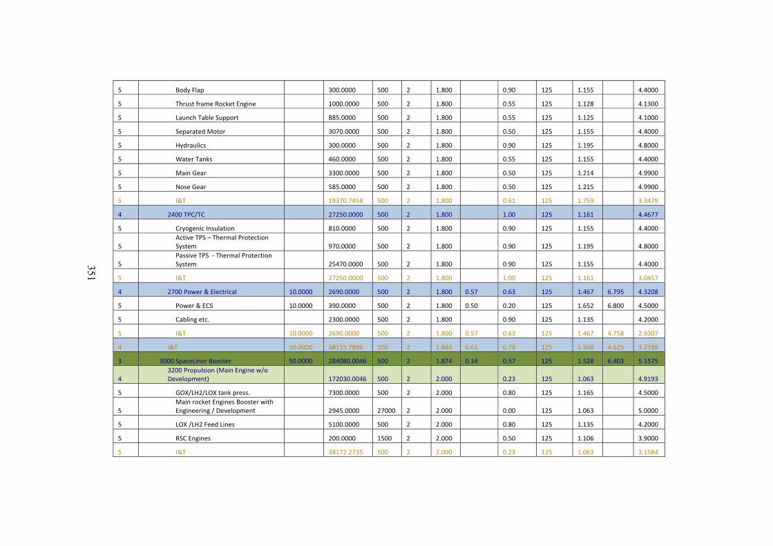
351
5 Body Flap 300.0000 500 2 1.800 0.90 125 1.155 4.4000
5 Thrust frame Rocket Engine 1000.0000 500 2 1.800 0.55 125 1.128 4.1300
5 Launch Table Support 885.0000 500 2 1.800 0.55 125 1.125 4.1000
5 Separated Motor 3070.0000 500 2 1.800 0.50 125 1.155 4.4000
5 Hydraulics 300.0000 500 2 1.800 0.90 125 1.195 4.8000
5 Water Tanks 460.0000 500 2 1.800 0.55 125 1.155 4.4000
5 Main Gear 3300.0000 500 2 1.800 0.50 125 1.214 4.9900
5 Nose Gear 585.0000 500 2 1.800 0.50 125 1.215 4.9900
5 I&T 19370.7458 500 2 1.800 0.61 125 1.759 3.3479
4 2400 TPC/TC 27250.0000 500 2 1.800 1.00 125 1.161 4.4677
5 Cryogenic Insulation 810.0000 500 2 1.800 0.90 125 1.155 4.4000
5 Active TPS – Thermal Protection System 970.0000 500 2 1.800 0.90 125 1.195 4.8000
5 Passive TPS ‐ Thermal Protection System 25470.0000 500 2 1.800 0.90 125 1.155 4.4000
5 I&T 27250.0000 500 2 1.800 1.00 125 1.161 3.0457
4 2700 Power & Electrical 10.0000 2690.0000 500 2 1.800 0.57 0.63 125 1.467 6.795 4.3208
5 Power & ECS 10.0000 390.0000 500 2 1.800 0.50 0.20 125 1.652 6.800 4.5000
5 Cabling etc. 2300.0000 500 2 1.800 0.90 125 1.135 4.2000
5 I&T 10.0000 2690.0000 500 2 1.800 0.57 0.63 125 1.467 4.758 2.9307
4 I&T 10.0000 38115.7896 500 2 1.884 0.61 0.78 125 1.508 4.625 3.2798
3 3000 SpaceLiner Booster 50.0000 284080.0046 500 2 1.874 0.34 0.57 125 1.528 6.403 5.1575
4 3200 Propulsion (Main Engine w/o Development) 172030.0046 500 2 2.000 0.23 125 1.063 4.9193
5 GOX/LH2/LOX tank press. 7300.0000 500 2 2.000 0.80 125 1.165 4.5000
5 Main rocket Engines Booster with Engineering / Development 2945.0000 27000 2 2.000 0.00 125 1.063 5.0000
5 LOX /LH2 Feed Lines 5100.0000 500 2 2.000 0.80 125 1.135 4.2000
5 RSC Engines 200.0000 1500 2 2.000 0.50 125 1.106 3.9000
5 I&T 38172.2735 500 2 2.000 0.23 125 1.063 3.1584
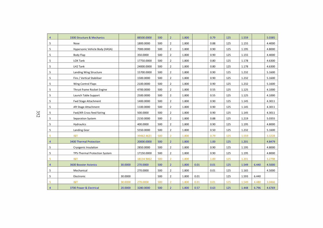
352
4 3300 Structure & Mechanics 88500.0000 500 2 1.800 0.79 125 1.559 5.0385
5 Nose 1800.0000 500 2 1.800 0.88 125 1.155 4.4000
5 Hypersonic Vehicle Body (HASA) 7000.0000 500 2 1.800 0.90 125 1.195 4.8000
5 Body Flap 350.0000 500 2 1.800 0.90 125 1.155 4.4000
5 LOX Tank 17750.0000 500 2 1.800 0.80 125 1.178 4.6300
5 LH2 Tank 24000.0000 500 2 1.800 0.80 125 1.178 4.6300
5 Landing Wing Structure 15700.0000 500 2 1.800 0.90 125 1.232 5.1600
5 Fins / Vertical Stabiliser 1500.0000 500 2 1.800 0.90 125 1.232 5.1600
5 Wing Control Flaps 2100.0000 500 2 1.800 0.90 125 1.232 5.1600
5 Thrust frame Rocket Engine 4700.0000 500 2 1.800 0.55 125 1.125 4.1000
5 Launch Table Support 2500.0000 500 2 1.800 0.55 125 1.125 4.1000
5 Fwd Stage Attachment 1400.0000 500 2 1.800 0.90 125 1.145 4.3011
5 Aft Stage Attachment 1100.0000 500 2 1.800 0.90 125 1.145 4.3011
5 Fwd/Aft Cross feed fairing 500.0000 500 2 1.800 0.90 125 1.145 4.3011
5 Separation System 2150.0000 500 2 1.800 0.88 125 1.219 5.0355
5 Hydraulics 400.0000 500 2 1.800 0.90 125 1.195 4.8000
5 Landing Gear 5550.0000 500 2 1.800 0.50 125 1.232 5.1600
5 I&T 39462.4621 500 2 1.800 0.79 125 1.559 3.3228
4 3400 Thermal Protection 20000.0000 500 2 1.800 1.00 125 1.201 4.8479
5 Cryogenic Insulation 2850.0000 500 2 1.800 0.90 125 1.195 4.8000
5 TPS‐Thermal Protection System 17150.0000 500 2 1.800 0.90 125 1.195 4.8000
5 I&T 18134.9062 500 2 1.800 1.00 125 1.201 3.2798
4 3600 Booster Avionics 30.0000 270.0000 500 2 1.800 0.01 0.01 125 1.549 6.440 4.5000
5 Mechanical 270.0000 500 2 1.800 0.01 125 1.165 4.5000
5 Electronic 30.0000 500 2 1.800 0.01 125 1.593 6.440
5 I&T 30.0000 270.0000 500 2 1.800 0.01 0.01 125 1.549 4.480 3.0466
4 3700 Power & Electrical 20.0000 3280.0000 500 2 1.800 0.57 0.63 125 1.448 6.796 4.6769
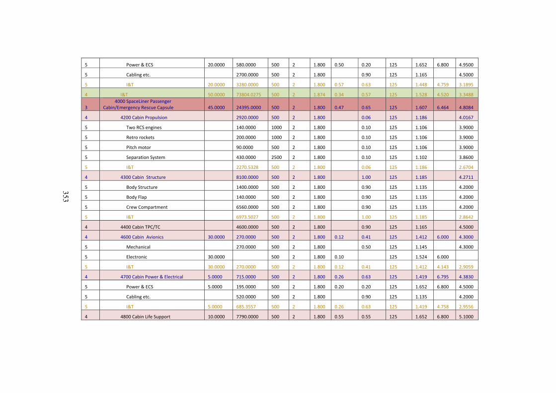
353
5 Power & ECS 20.0000 580.0000 500 2 1.800 0.50 0.20 125 1.652 6.800 4.9500
5 Cabling etc. 2700.0000 500 2 1.800 0.90 125 1.165 4.5000
5 I&T 20.0000 3280.0000 500 2 1.800 0.57 0.63 125 1.448 4.759 3.1895
4 I&T 50.0000 73804.0275 500 2 1.874 0.34 0.57 125 1.528 4.520 3.3488
3 4000 SpaceLiner Passenger Cabin/Emergency Rescue Capsule 45.0000 24395.0000 500 2 1.800 0.47 0.65 125 1.607 6.464 4.8084
4 4200 Cabin Propulsion 2920.0000 500 2 1.800 0.06 125 1.186 4.0167
5 Two RCS engines 140.0000 1000 2 1.800 0.10 125 1.106 3.9000
5 Retro rockets 200.0000 1000 2 1.800 0.10 125 1.106 3.9000
5 Pitch motor 90.0000 500 2 1.800 0.10 125 1.106 3.9000
5 Separation System 430.0000 2500 2 1.800 0.10 125 1.102 3.8600
5 I&T 2270.5328 500 2 1.800 0.06 125 1.186 2.6704
4 4300 Cabin Structure 8100.0000 500 2 1.800 1.00 125 1.185 4.2711
5 Body Structure 1400.0000 500 2 1.800 0.90 125 1.135 4.2000
5 Body Flap 140.0000 500 2 1.800 0.90 125 1.135 4.2000
5 Crew Compartment 6560.0000 500 2 1.800 0.90 125 1.135 4.2000
5 I&T 6973.5027 500 2 1.800 1.00 125 1.185 2.8642
4 4400 Cabin TPC/TC 4600.0000 500 2 1.800 0.90 125 1.165 4.5000
4 4600 Cabin Avionics 30.0000 270.0000 500 2 1.800 0.12 0.41 125 1.412 6.000 4.3000
5 Mechanical 270.0000 500 2 1.800 0.50 125 1.145 4.3000
5 Electronic 30.0000 500 2 1.800 0.10 125 1.524 6.000
5 I&T 30.0000 270.0000 500 2 1.800 0.12 0.41 125 1.412 4.143 2.9059
4 4700 Cabin Power & Electrical 5.0000 715.0000 500 2 1.800 0.26 0.63 125 1.419 6.795 4.3830
5 Power & ECS 5.0000 195.0000 500 2 1.800 0.20 0.20 125 1.652 6.800 4.5000
5 Cabling etc. 520.0000 500 2 1.800 0.90 125 1.135 4.2000
5 I&T 5.0000 685.3557 500 2 1.800 0.26 0.63 125 1.419 4.758 2.9556
4 4800 Cabin Life Support 10.0000 7790.0000 500 2 1.800 0.55 0.55 125 1.652 6.800 5.1000
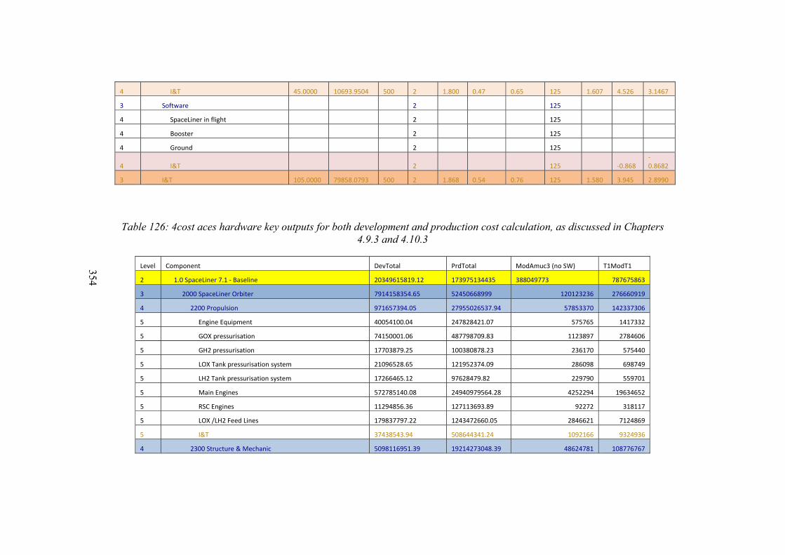
354
4 I&T 45.0000 10693.9504 500 2 1.800 0.47 0.65 125 1.607 4.526 3.1467
3 Software 2 125
4 SpaceLiner in flight 2 125
4 Booster 2 125
4 Ground 2 125
4 I&T 2 125 ‐0.868 ‐0.8682
3 I&T 105.0000 79858.0793 500 2 1.868 0.54 0.76 125 1.580 3.945 2.8990
Table 126: 4cost aces hardware key outputs for both development and production cost calculation, as discussed in Chapters 4.9.3 and 4.10.3
Level Component DevTotal PrdTotal ModAmuc3 (no SW) T1ModT1
2 1.0 SpaceLiner 7.1 ‐ Baseline 20349615819.12 173975134435 388049773 787675863
3 2000 SpaceLiner Orbiter 7914158354.65 52450668999 120123236 276660919
4 2200 Propulsion 971657394.05 27955026537.94 57853370 142337306
5 Engine Equipment 40054100.04 247828421.07 575765 1417332
5 GOX pressurisation 74150001.06 487798709.83 1123897 2784606
5 GH2 pressurisation 17703879.25 100380878.23 236170 575440
5 LOX Tank pressurisation system 21096528.65 121952374.09 286098 698749
5 LH2 Tank pressurisation system 17266465.12 97628479.82 229790 559701
5 Main Engines 572785140.08 24940979564.28 4252294 19634652
5 RSC Engines 11294856.36 127113693.89 92272 318117
5 LOX /LH2 Feed Lines 179837797.22 1243472660.05 2846621 7124869
5 I&T 37438543.94 508644341.24 1092166 9324936
4 2300 Structure & Mechanic 5098116951.39 19214273048.39 48624781 108776767
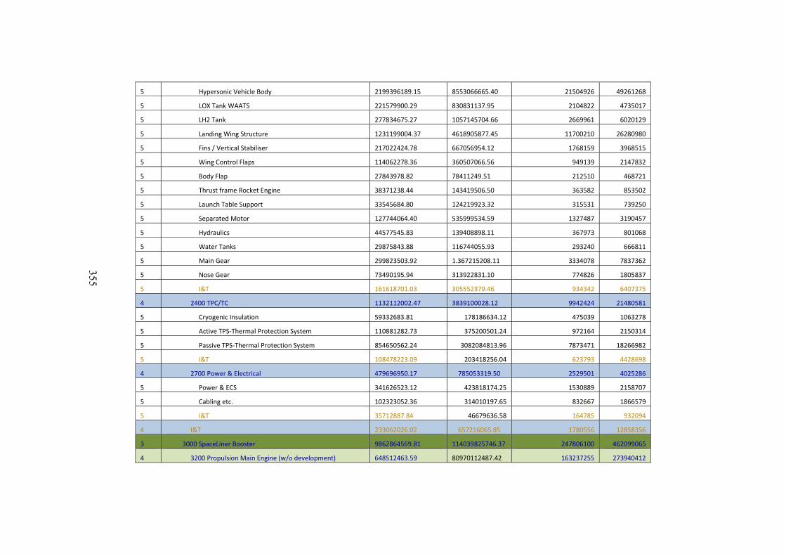
355
5 Hypersonic Vehicle Body 2199396189.15 8553066665.40 21504926 49261268
5 LOX Tank WAATS 221579900.29 830831137.95 2104822 4735017
5 LH2 Tank 277834675.27 1057145704.66 2669961 6020129
5 Landing Wing Structure 1231199004.37 4618905877.45 11700210 26280980
5 Fins / Vertical Stabiliser 217022424.78 667056954.12 1768159 3968515
5 Wing Control Flaps 114062278.36 360507066.56 949139 2147832
5 Body Flap 27843978.82 78411249.51 212510 468721
5 Thrust frame Rocket Engine 38371238.44 143419506.50 363582 853502
5 Launch Table Support 33545684.80 124219923.32 315531 739250
5 Separated Motor 127744064.40 535999534.59 1327487 3190457
5 Hydraulics 44577545.83 139408898.11 367973 801068
5 Water Tanks 29875843.88 116744055.93 293240 666811
5 Main Gear 299823503.92 1.367215208.11 3334078 7837362
5 Nose Gear 73490195.94 313922831.10 774826 1805837
5 I&T 161618701.03 305552379.46 934342 6407375
4 2400 TPC/TC 1132112002.47 3839100028.12 9942424 21480581
5 Cryogenic Insulation 59332683.81 178186634.12 475039 1063278
5 Active TPS‐Thermal Protection System 110881282.73 375200501.24 972164 2150314
5 Passive TPS‐Thermal Protection System 854650562.24 3082084813.96 7873471 18266982
5 I&T 108478223.09 203418256.04 623793 4428698
4 2700 Power & Electrical 479696950.17 785053319.50 2529501 4025286
5 Power & ECS 341626523.12 423818174.25 1530889 2158707
5 Cabling etc. 102323052.36 314010197.65 832667 1866579
5 I&T 35712887.84 46679636.58 164785 932094
4 I&T 233062026.02 657216065.85 1780556 12858356
3 3000 SpaceLiner Booster 9862864569.81 114039825746.37 247806100 462099065
4 3200 Propulsion Main Engine (w/o development) 648512463.59 80970112487.42 163237255 273940412
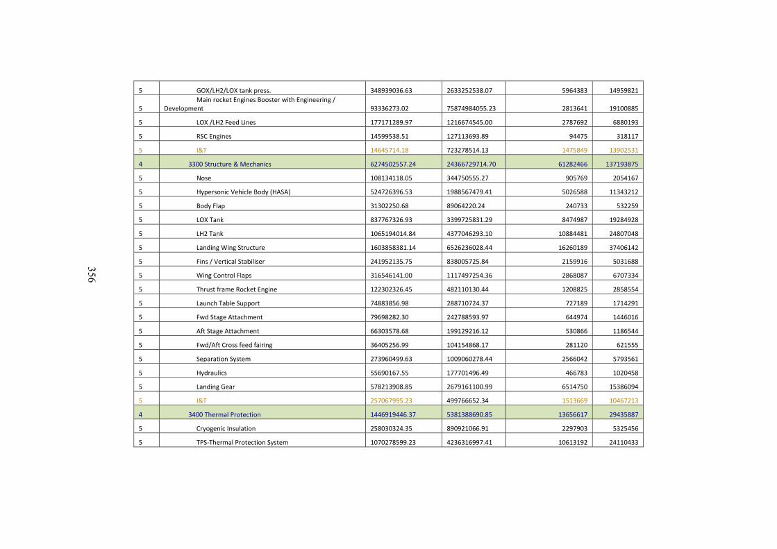
356
5 GOX/LH2/LOX tank press. 348939036.63 2633252538.07 5964383 14959821
5 Main rocket Engines Booster with Engineering / Development 93336273.02 75874984055.23 2813641 19100885
5 LOX /LH2 Feed Lines 177171289.97 1216674545.00 2787692 6880193
5 RSC Engines 14599538.51 127113693.89 94475 318117
5 I&T 14645714.18 723278514.13 1475849 13902531
4 3300 Structure & Mechanics 6274502557.24 24366729714.70 61282466 137193875
5 Nose 108134118.05 344750555.27 905769 2054167
5 Hypersonic Vehicle Body (HASA) 524726396.53 1988567479.41 5026588 11343212
5 Body Flap 31302250.68 89064220.24 240733 532259
5 LOX Tank 837767326.93 3399725831.29 8474987 19284928
5 LH2 Tank 1065194014.84 4377046293.10 10884481 24807048
5 Landing Wing Structure 1603858381.14 6526236028.44 16260189 37406142
5 Fins / Vertical Stabiliser 241952135.75 838005725.84 2159916 5031688
5 Wing Control Flaps 316546141.00 1117497254.36 2868087 6707334
5 Thrust frame Rocket Engine 122302326.45 482110130.44 1208825 2858554
5 Launch Table Support 74883856.98 288710724.37 727189 1714291
5 Fwd Stage Attachment 79698282.30 242788593.97 644974 1446016
5 Aft Stage Attachment 66303578.68 199129216.12 530866 1186544
5 Fwd/Aft Cross feed fairing 36405256.99 104154868.17 281120 621555
5 Separation System 273960499.63 1009060278.44 2566042 5793561
5 Hydraulics 55690167.55 177701496.49 466783 1020458
5 Landing Gear 578213908.85 2679161100.99 6514750 15386094
5 I&T 257067995.23 499766652.34 1513669 10467213
4 3400 Thermal Protection 1446919446.37 5381388690.85 13656617 29435887
5 Cryogenic Insulation 258030324.35 890921066.91 2297903 5325456
5 TPS‐Thermal Protection System 1070278599.23 4236316997.41 10613192 24110433
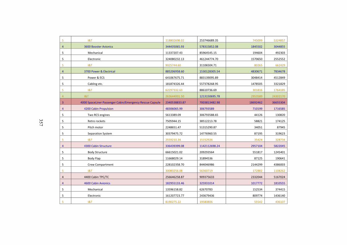
357
5 I&T 118802698.02 253746689.35 745099 5324857
4 3600 Booster Avionics 344435065.93 578315852.08 1845502 3044855
5 Mechanical 11337207.43 85964545.15 194604 492303
5 Electronic 324080232.13 461244774.70 1570650 2552552
5 I&T 9025744.60 31106504.71 80265 662429
4 3700 Power & Electrical 885206958.60 1530128305.54 4830671 7834678
5 Power & ECS 641067675.71 883139095.89 3048414 4512849
5 Cabling etc. 181874326.44 557378268.95 1478505 3321829
5 I&T 62297332.63 88610736.69 301816 1764185
4 I&T 263644001.50 1213150695.78 2953589 24302170
3 4000 SpaceLiner Passenger Cabin/Emergency Rescue Capsule 2340538833.87 7003813482.98 18692462 36655304
4 4200 Cabin Propulsion 48306065.99 306793589 710199 1716585
5 Two RCS engines 5613389.09 306793588.65 44126 130820
5 Retro rockets 7505944.15 38512213.78 58821 174125
5 Pitch motor 2248651.47 51315290.87 34051 87945
5 Separation System 30379475.72 14776960.55 87195 319623
5 I&T 2559210.34 15152926 35424 328734
4 4300 Cabin Structure 336439399.08 1142112698.24 2957104 5822045
5 Body Structure 66615021.02 209293564 551817 1245401
5 Body Flap 11668029.14 31894536 87125 190641
5 Crew Compartment 228102358.70 844046986 2144299 4386003
5 I&T 30080256.08 56360719 172882 1108262
4 4400 Cabin TPC/TC 256646258.87 909375633 2332044 5167024
4 4600 Cabin Avionics 182955133.46 325931014 1017772 1810555
5 Mechanical 13596158.82 62670783 152534 374415
5 Electronic 161207723.77 243679436 809774 1436140
5 I&T 8190275.22 19580806 55542 436107

358
4 4700 Cabin Power & Electrical 205227037.96 341718758 1093892 1722009
5 Power & ECS 159577848.47 227838758 774833 1166471
5 Cabling etc. 33114572.81 93174191 252578 555539
5 I&T 12529492.03 20509392 66078 409196
4 4800 Cabin Life Support 1200015350.36 3804109869 10008251 20417144
4 I&T 110924922.38 173771922 569394 3516675
3 Software
4 SpaceLiner in flight
4 Booster
4 Ground
4 I&T
3 I&T 233161083.78 480826206 1427975 9697110
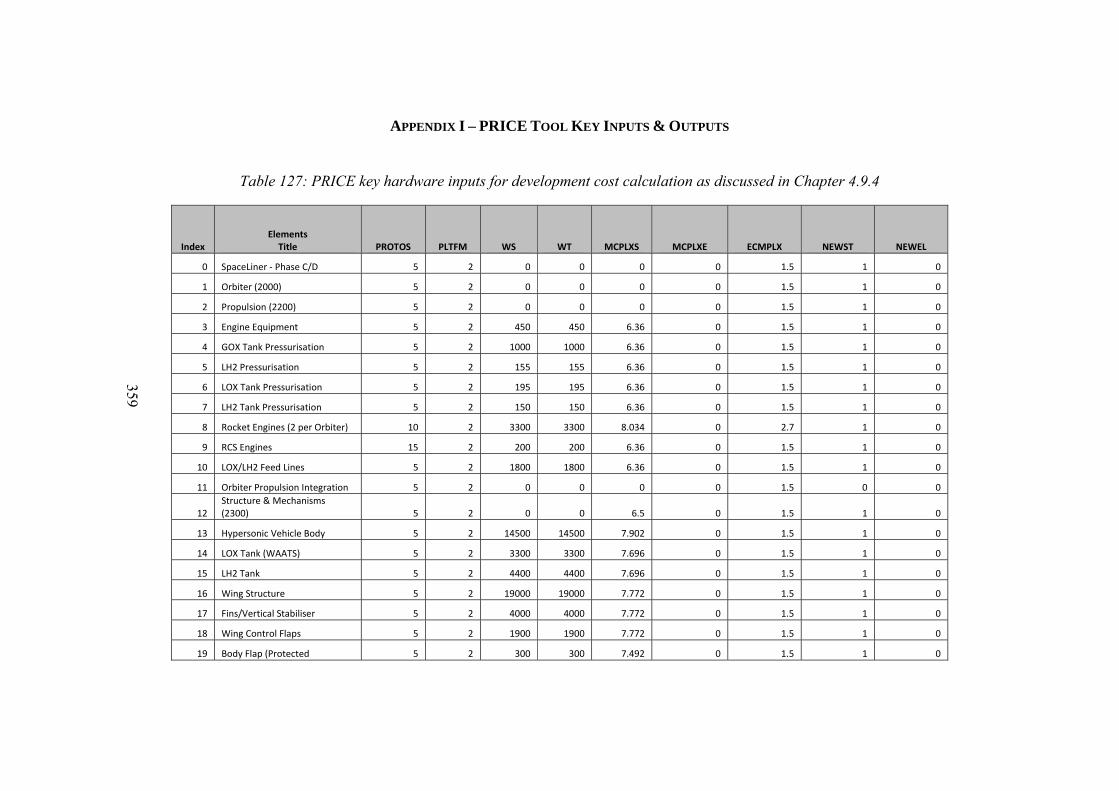
359
APPENDIX I – PRICE TOOL KEY INPUTS & OUTPUTS
Table 127: PRICE key hardware inputs for development cost calculation as discussed in Chapter 4.9.4
Index Elements Title PROTOS PLTFM WS WT MCPLXS MCPLXE ECMPLX NEWST NEWEL
0 SpaceLiner ‐ Phase C/D 5 2 0 0 0 0 1.5 1 0
1 Orbiter (2000) 5 2 0 0 0 0 1.5 1 0
2 Propulsion (2200) 5 2 0 0 0 0 1.5 1 0
3 Engine Equipment 5 2 450 450 6.36 0 1.5 1 0
4 GOX Tank Pressurisation 5 2 1000 1000 6.36 0 1.5 1 0
5 LH2 Pressurisation 5 2 155 155 6.36 0 1.5 1 0
6 LOX Tank Pressurisation 5 2 195 195 6.36 0 1.5 1 0
7 LH2 Tank Pressurisation 5 2 150 150 6.36 0 1.5 1 0
8 Rocket Engines (2 per Orbiter) 10 2 3300 3300 8.034 0 2.7 1 0
9 RCS Engines 15 2 200 200 6.36 0 1.5 1 0
10 LOX/LH2 Feed Lines 5 2 1800 1800 6.36 0 1.5 1 0
11 Orbiter Propulsion Integration 5 2 0 0 0 0 1.5 0 0
12 Structure & Mechanisms (2300) 5 2 0 0 6.5 0 1.5 1 0
13 Hypersonic Vehicle Body 5 2 14500 14500 7.902 0 1.5 1 0
14 LOX Tank (WAATS) 5 2 3300 3300 7.696 0 1.5 1 0
15 LH2 Tank 5 2 4400 4400 7.696 0 1.5 1 0
16 Wing Structure 5 2 19000 19000 7.772 0 1.5 1 0
17 Fins/Vertical Stabiliser 5 2 4000 4000 7.772 0 1.5 1 0
18 Wing Control Flaps 5 2 1900 1900 7.772 0 1.5 1 0
19 Body Flap (Protected 5 2 300 300 7.492 0 1.5 1 0
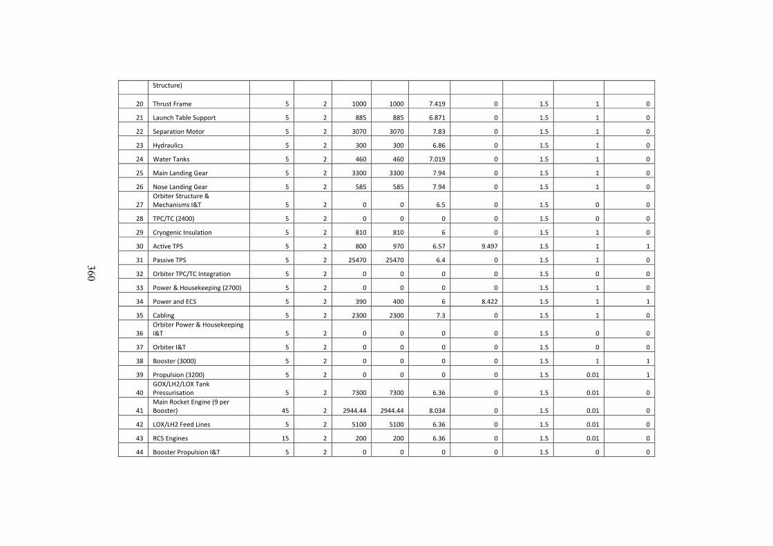
360
Structure)
20 Thrust Frame 5 2 1000 1000 7.419 0 1.5 1 0
21 Launch Table Support 5 2 885 885 6.871 0 1.5 1 0
22 Separation Motor 5 2 3070 3070 7.83 0 1.5 1 0
23 Hydraulics 5 2 300 300 6.86 0 1.5 1 0
24 Water Tanks 5 2 460 460 7.019 0 1.5 1 0
25 Main Landing Gear 5 2 3300 3300 7.94 0 1.5 1 0
26 Nose Landing Gear 5 2 585 585 7.94 0 1.5 1 0
27 Orbiter Structure & Mechanisms I&T 5 2 0 0 6.5 0 1.5 0 0
28 TPC/TC (2400) 5 2 0 0 0 0 1.5 0 0
29 Cryogenic Insulation 5 2 810 810 6 0 1.5 1 0
30 Active TPS 5 2 800 970 6.57 9.497 1.5 1 1
31 Passive TPS 5 2 25470 25470 6.4 0 1.5 1 0
32 Orbiter TPC/TC Integration 5 2 0 0 0 0 1.5 0 0
33 Power & Housekeeping (2700) 5 2 0 0 0 0 1.5 1 0
34 Power and ECS 5 2 390 400 6 8.422 1.5 1 1
35 Cabling 5 2 2300 2300 7.3 0 1.5 1 0
36 Orbiter Power & Housekeeping I&T 5 2 0 0 0 0 1.5 0 0
37 Orbiter I&T 5 2 0 0 0 0 1.5 0 0
38 Booster (3000) 5 2 0 0 0 0 1.5 1 1
39 Propulsion (3200) 5 2 0 0 0 0 1.5 0.01 1
40 GOX/LH2/LOX Tank Pressurisation 5 2 7300 7300 6.36 0 1.5 0.01 0
41 Main Rocket Engine (9 per Booster) 45 2 2944.44 2944.44 8.034 0 1.5 0.01 0
42 LOX/LH2 Feed Lines 5 2 5100 5100 6.36 0 1.5 0.01 0
43 RCS Engines 15 2 200 200 6.36 0 1.5 0.01 0
44 Booster Propulsion I&T 5 2 0 0 0 0 1.5 0 0
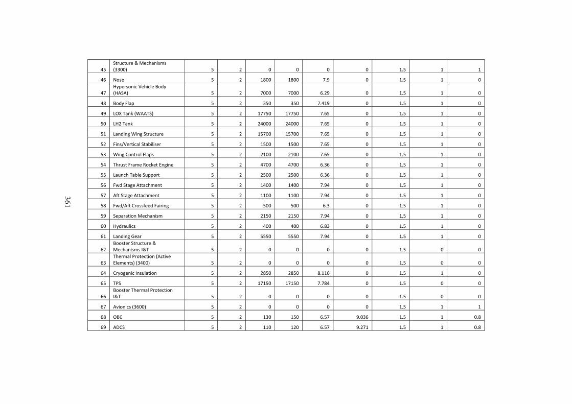
361
45 Structure & Mechanisms (3300) 5 2 0 0 0 0 1.5 1 1
46 Nose 5 2 1800 1800 7.9 0 1.5 1 0
47 Hypersonic Vehicle Body (HASA) 5 2 7000 7000 6.29 0 1.5 1 0
48 Body Flap 5 2 350 350 7.419 0 1.5 1 0
49 LOX Tank (WAATS) 5 2 17750 17750 7.65 0 1.5 1 0
50 LH2 Tank 5 2 24000 24000 7.65 0 1.5 1 0
51 Landing Wing Structure 5 2 15700 15700 7.65 0 1.5 1 0
52 Fins/Vertical Stabiliser 5 2 1500 1500 7.65 0 1.5 1 0
53 Wing Control Flaps 5 2 2100 2100 7.65 0 1.5 1 0
54 Thrust Frame Rocket Engine 5 2 4700 4700 6.36 0 1.5 1 0
55 Launch Table Support 5 2 2500 2500 6.36 0 1.5 1 0
56 Fwd Stage Attachment 5 2 1400 1400 7.94 0 1.5 1 0
57 Aft Stage Attachment 5 2 1100 1100 7.94 0 1.5 1 0
58 Fwd/Aft Crossfeed Fairing 5 2 500 500 6.3 0 1.5 1 0
59 Separation Mechanism 5 2 2150 2150 7.94 0 1.5 1 0
60 Hydraulics 5 2 400 400 6.83 0 1.5 1 0
61 Landing Gear 5 2 5550 5550 7.94 0 1.5 1 0
62 Booster Structure & Mechanisms I&T 5 2 0 0 0 0 1.5 0 0
63 Thermal Protection (Active Elements) (3400) 5 2 0 0 0 0 1.5 0 0
64 Cryogenic Insulation 5 2 2850 2850 8.116 0 1.5 1 0
65 TPS 5 2 17150 17150 7.784 0 1.5 0 0
66 Booster Thermal Protection I&T 5 2 0 0 0 0 1.5 0 0
67 Avionics (3600) 5 2 0 0 0 0 1.5 1 1
68 OBC 5 2 130 150 6.57 9.036 1.5 1 0.8
69 ADCS 5 2 110 120 6.57 9.271 1.5 1 0.8
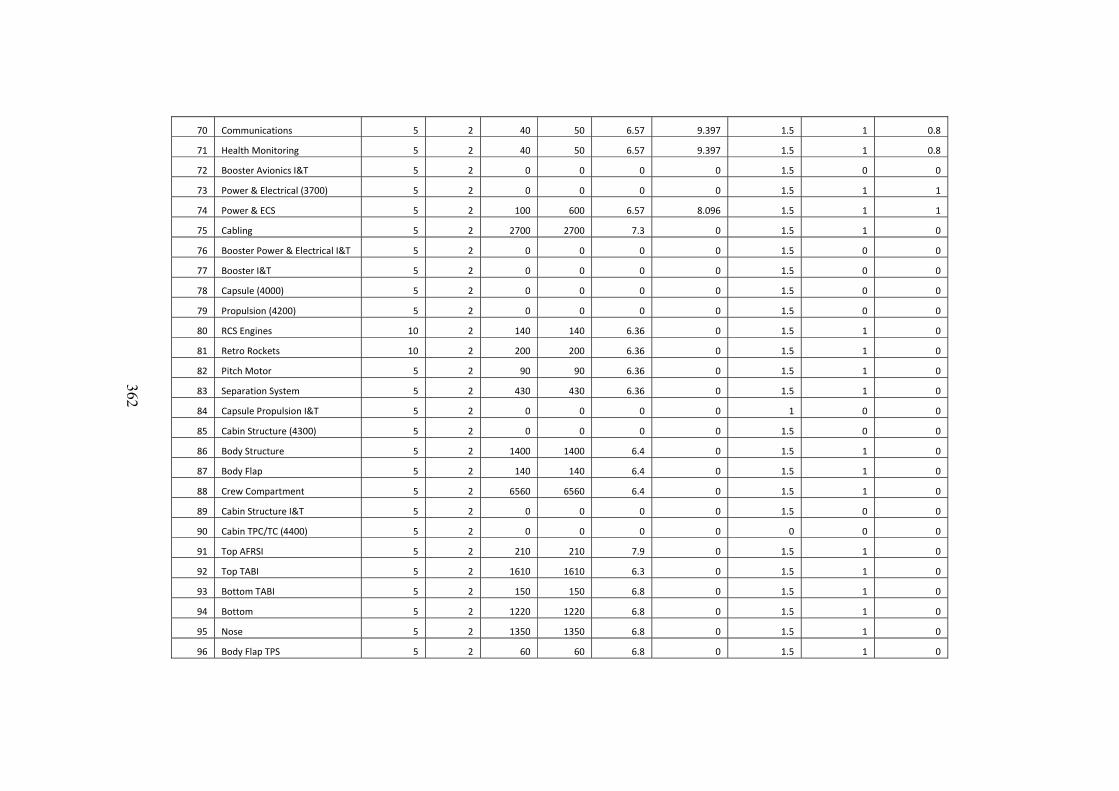
362
70 Communications 5 2 40 50 6.57 9.397 1.5 1 0.8
71 Health Monitoring 5 2 40 50 6.57 9.397 1.5 1 0.8
72 Booster Avionics I&T 5 2 0 0 0 0 1.5 0 0
73 Power & Electrical (3700) 5 2 0 0 0 0 1.5 1 1
74 Power & ECS 5 2 100 600 6.57 8.096 1.5 1 1
75 Cabling 5 2 2700 2700 7.3 0 1.5 1 0
76 Booster Power & Electrical I&T 5 2 0 0 0 0 1.5 0 0
77 Booster I&T 5 2 0 0 0 0 1.5 0 0
78 Capsule (4000) 5 2 0 0 0 0 1.5 0 0
79 Propulsion (4200) 5 2 0 0 0 0 1.5 0 0
80 RCS Engines 10 2 140 140 6.36 0 1.5 1 0
81 Retro Rockets 10 2 200 200 6.36 0 1.5 1 0
82 Pitch Motor 5 2 90 90 6.36 0 1.5 1 0
83 Separation System 5 2 430 430 6.36 0 1.5 1 0
84 Capsule Propulsion I&T 5 2 0 0 0 0 1 0 0
85 Cabin Structure (4300) 5 2 0 0 0 0 1.5 0 0
86 Body Structure 5 2 1400 1400 6.4 0 1.5 1 0
87 Body Flap 5 2 140 140 6.4 0 1.5 1 0
88 Crew Compartment 5 2 6560 6560 6.4 0 1.5 1 0
89 Cabin Structure I&T 5 2 0 0 0 0 1.5 0 0
90 Cabin TPC/TC (4400) 5 2 0 0 0 0 0 0 0
91 Top AFRSI 5 2 210 210 7.9 0 1.5 1 0
92 Top TABI 5 2 1610 1610 6.3 0 1.5 1 0
93 Bottom TABI 5 2 150 150 6.8 0 1.5 1 0
94 Bottom 5 2 1220 1220 6.8 0 1.5 1 0
95 Nose 5 2 1350 1350 6.8 0 1.5 1 0
96 Body Flap TPS 5 2 60 60 6.8 0 1.5 1 0
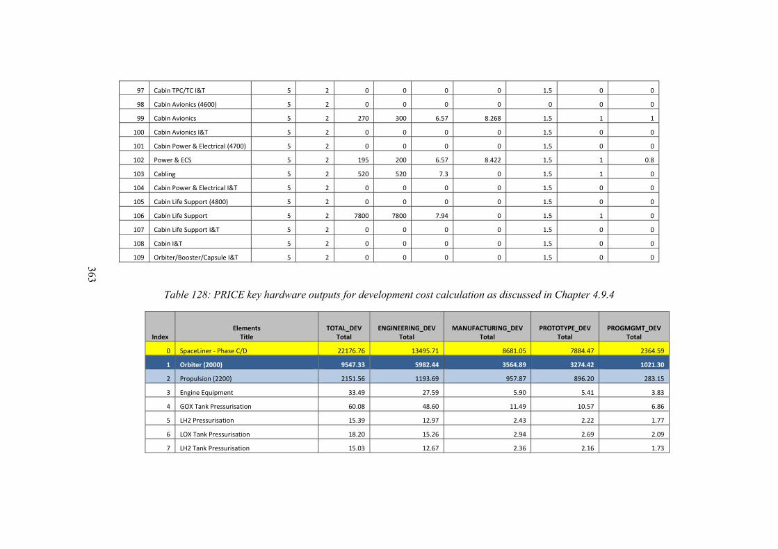
363
97 Cabin TPC/TC I&T 5 2 0 0 0 0 1.5 0 0
98 Cabin Avionics (4600) 5 2 0 0 0 0 0 0 0
99 Cabin Avionics 5 2 270 300 6.57 8.268 1.5 1 1
100 Cabin Avionics I&T 5 2 0 0 0 0 1.5 0 0
101 Cabin Power & Electrical (4700) 5 2 0 0 0 0 1.5 0 0
102 Power & ECS 5 2 195 200 6.57 8.422 1.5 1 0.8
103 Cabling 5 2 520 520 7.3 0 1.5 1 0
104 Cabin Power & Electrical I&T 5 2 0 0 0 0 1.5 0 0
105 Cabin Life Support (4800) 5 2 0 0 0 0 1.5 0 0
106 Cabin Life Support 5 2 7800 7800 7.94 0 1.5 1 0
107 Cabin Life Support I&T 5 2 0 0 0 0 1.5 0 0
108 Cabin I&T 5 2 0 0 0 0 1.5 0 0
109 Orbiter/Booster/Capsule I&T 5 2 0 0 0 0 1.5 0 0
Table 128: PRICE key hardware outputs for development cost calculation as discussed in Chapter 4.9.4
Index Elements Title
TOTAL_DEV Total
ENGINEERING_DEV Total
MANUFACTURING_DEV Total
PROTOTYPE_DEV Total
PROGMGMT_DEV Total
0 SpaceLiner ‐ Phase C/D 22176.76 13495.71 8681.05 7884.47 2364.59
1 Orbiter (2000) 9547.33 5982.44 3564.89 3274.42 1021.30
2 Propulsion (2200) 2151.56 1193.69 957.87 896.20 283.15
3 Engine Equipment 33.49 27.59 5.90 5.41 3.83
4 GOX Tank Pressurisation 60.08 48.60 11.49 10.57 6.86
5 LH2 Pressurisation 15.39 12.97 2.43 2.22 1.77
6 LOX Tank Pressurisation 18.20 15.26 2.94 2.69 2.09
7 LH2 Tank Pressurisation 15.03 12.67 2.36 2.16 1.73
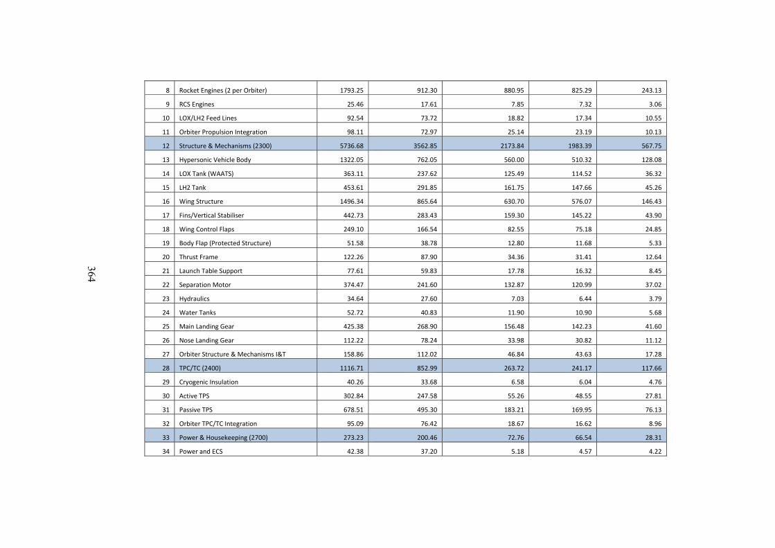
364
8 Rocket Engines (2 per Orbiter) 1793.25 912.30 880.95 825.29 243.13
9 RCS Engines 25.46 17.61 7.85 7.32 3.06
10 LOX/LH2 Feed Lines 92.54 73.72 18.82 17.34 10.55
11 Orbiter Propulsion Integration 98.11 72.97 25.14 23.19 10.13
12 Structure & Mechanisms (2300) 5736.68 3562.85 2173.84 1983.39 567.75
13 Hypersonic Vehicle Body 1322.05 762.05 560.00 510.32 128.08
14 LOX Tank (WAATS) 363.11 237.62 125.49 114.52 36.32
15 LH2 Tank 453.61 291.85 161.75 147.66 45.26
16 Wing Structure 1496.34 865.64 630.70 576.07 146.43
17 Fins/Vertical Stabiliser 442.73 283.43 159.30 145.22 43.90
18 Wing Control Flaps 249.10 166.54 82.55 75.18 24.85
19 Body Flap (Protected Structure) 51.58 38.78 12.80 11.68 5.33
20 Thrust Frame 122.26 87.90 34.36 31.41 12.64
21 Launch Table Support 77.61 59.83 17.78 16.32 8.45
22 Separation Motor 374.47 241.60 132.87 120.99 37.02
23 Hydraulics 34.64 27.60 7.03 6.44 3.79
24 Water Tanks 52.72 40.83 11.90 10.90 5.68
25 Main Landing Gear 425.38 268.90 156.48 142.23 41.60
26 Nose Landing Gear 112.22 78.24 33.98 30.82 11.12
27 Orbiter Structure & Mechanisms I&T 158.86 112.02 46.84 43.63 17.28
28 TPC/TC (2400) 1116.71 852.99 263.72 241.17 117.66
29 Cryogenic Insulation 40.26 33.68 6.58 6.04 4.76
30 Active TPS 302.84 247.58 55.26 48.55 27.81
31 Passive TPS 678.51 495.30 183.21 169.95 76.13
32 Orbiter TPC/TC Integration 95.09 76.42 18.67 16.62 8.96
33 Power & Housekeeping (2700) 273.23 200.46 72.76 66.54 28.31
34 Power and ECS 42.38 37.20 5.18 4.57 4.22
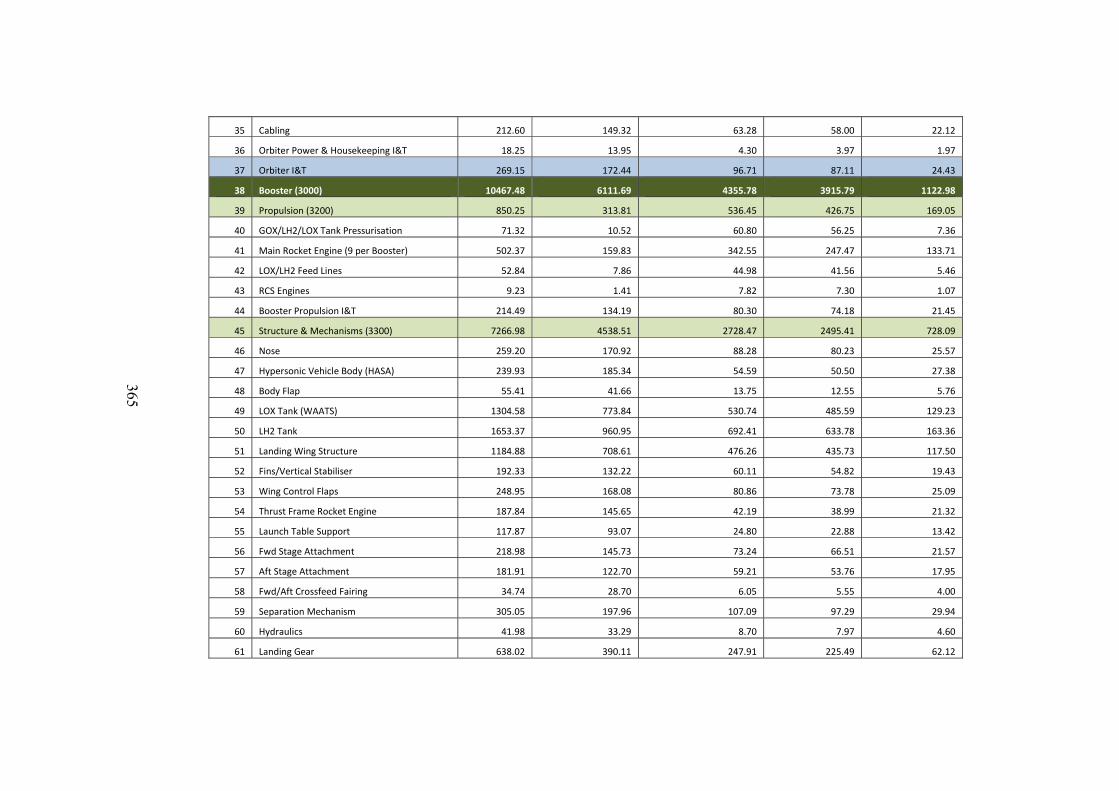
365
35 Cabling 212.60 149.32 63.28 58.00 22.12
36 Orbiter Power & Housekeeping I&T 18.25 13.95 4.30 3.97 1.97
37 Orbiter I&T 269.15 172.44 96.71 87.11 24.43
38 Booster (3000) 10467.48 6111.69 4355.78 3915.79 1122.98
39 Propulsion (3200) 850.25 313.81 536.45 426.75 169.05
40 GOX/LH2/LOX Tank Pressurisation 71.32 10.52 60.80 56.25 7.36
41 Main Rocket Engine (9 per Booster) 502.37 159.83 342.55 247.47 133.71
42 LOX/LH2 Feed Lines 52.84 7.86 44.98 41.56 5.46
43 RCS Engines 9.23 1.41 7.82 7.30 1.07
44 Booster Propulsion I&T 214.49 134.19 80.30 74.18 21.45
45 Structure & Mechanisms (3300) 7266.98 4538.51 2728.47 2495.41 728.09
46 Nose 259.20 170.92 88.28 80.23 25.57
47 Hypersonic Vehicle Body (HASA) 239.93 185.34 54.59 50.50 27.38
48 Body Flap 55.41 41.66 13.75 12.55 5.76
49 LOX Tank (WAATS) 1304.58 773.84 530.74 485.59 129.23
50 LH2 Tank 1653.37 960.95 692.41 633.78 163.36
51 Landing Wing Structure 1184.88 708.61 476.26 435.73 117.50
52 Fins/Vertical Stabiliser 192.33 132.22 60.11 54.82 19.43
53 Wing Control Flaps 248.95 168.08 80.86 73.78 25.09
54 Thrust Frame Rocket Engine 187.84 145.65 42.19 38.99 21.32
55 Launch Table Support 117.87 93.07 24.80 22.88 13.42
56 Fwd Stage Attachment 218.98 145.73 73.24 66.51 21.57
57 Aft Stage Attachment 181.91 122.70 59.21 53.76 17.95
58 Fwd/Aft Crossfeed Fairing 34.74 28.70 6.05 5.55 4.00
59 Separation Mechanism 305.05 197.96 107.09 97.29 29.94
60 Hydraulics 41.98 33.29 8.70 7.97 4.60
61 Landing Gear 638.02 390.11 247.91 225.49 62.12
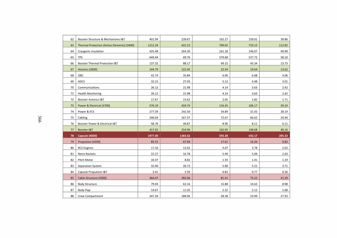
366
62 Booster Structure & Mechanisms I&T 401.94 239.67 162.27 150.01 39.86
63 Thermal Protection (Active Elements) (3400) 1212.24 422.22 790.02 719.13 112.82
64 Cryogenic Insulation 425.48 264.30 161.18 146.07 40.99
65 TPS 649.44 69.76 579.68 527.72 58.10
66 Booster Thermal Protection I&T 137.32 88.17 49.15 45.34 13.73
67 Avionics (3600) 144.79 122.45 22.34 19.64 13.62
68 OBC 42.74 35.84 6.90 6.08 4.06
69 ADCS 32.15 27.03 5.12 4.48 3.01
70 Communications 26.12 21.98 4.14 3.63 2.42
71 Health Monitoring 26.12 21.98 4.14 3.63 2.42
72 Booster Avionics I&T 17.67 15.62 2.05 1.82 1.71
73 Power & Electrical (3700) 576.19 459.74 116.45 106.17 59.24
74 Power & ECS 277.39 242.50 34.89 31.43 28.19
75 Cabling 240.04 167.37 72.67 66.62 24.94
76 Booster Power & Electrical I&T 58.76 49.87 8.90 8.11 6.11
77 Booster I&T 417.02 254.96 162.05 148.68 40.16
78 Capsule (4000) 1977.00 1383.62 593.38 542.17 205.33
79 Propulsion (4200) 85.55 67.94 17.61 16.26 9.82
80 RCS Engines 17.10 13.02 4.07 3.78 2.02
81 Retro Rockets 22.27 16.78 5.49 5.09 2.63
82 Pitch Motor 10.37 8.82 1.55 1.41 1.19
83 Separation System 32.40 26.72 5.68 5.21 3.71
84 Capsule Propulsion I&T 3.41 2.59 0.82 0.77 0.26
85 Cabin Structure (4300) 364.47 283.06 81.41 75.22 41.29
86 Body Structure 79.04 63.16 15.88 14.63 8.98
87 Body Flap 14.67 12.35 2.32 2.12 1.68
88 Crew Compartment 247.34 188.96 58.38 53.99 27.93
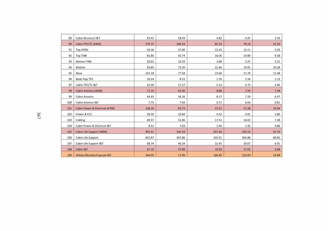
367
89 Cabin Structure I&T 23.41 18.59 4.82 4.47 2.70
90 Cabin TPC/TC (4400) 379.73 294.54 85.19 78.19 41.56
91 Top AFRSI 50.36 37.00 13.35 12.11 5.03
92 Top TABI 81.80 65.74 16.06 14.80 9.38
93 Bottom TABI 20.01 16.33 3.68 3.37 2.21
94 Bottom 93.85 72.20 21.66 19.91 10.28
95 Nose 101.18 77.58 23.60 21.70 11.08
96 Body Flap TPS 10.24 8.53 1.70 1.56 1.13
97 Cabin TPC/TC I&T 22.30 17.17 5.13 4.75 2.46
98 Cabin Avionics (4600) 72.19 63.30 8.88 7.93 7.28
99 Cabin Avionics 64.43 56.26 8.17 7.29 6.47
100 Cabin Avionics I&T 7.75 7.04 0.71 0.64 0.81
101 Cabin Power & Electrical (4700) 106.26 82.73 23.52 21.38 10.94
102 Power & ECS 28.36 23.84 4.52 4.01 2.80
103 Cabling 69.37 51.86 17.51 16.02 7.28
104 Cabin Power & Electrical I&T 8.52 7.03 1.49 1.35 0.86
105 Cabin Life Support (4800) 901.61 544.16 357.46 325.55 87.76
106 Cabin Life Support 832.87 497.86 335.01 304.88 80.85
107 Cabin Life Support I&T 68.74 46.29 22.45 20.67 6.91
108 Cabin I&T 67.19 47.89 19.30 17.65 6.68
109 Orbiter/Booster/Capsule I&T 184.95 17.96 166.99 152.09 14.98
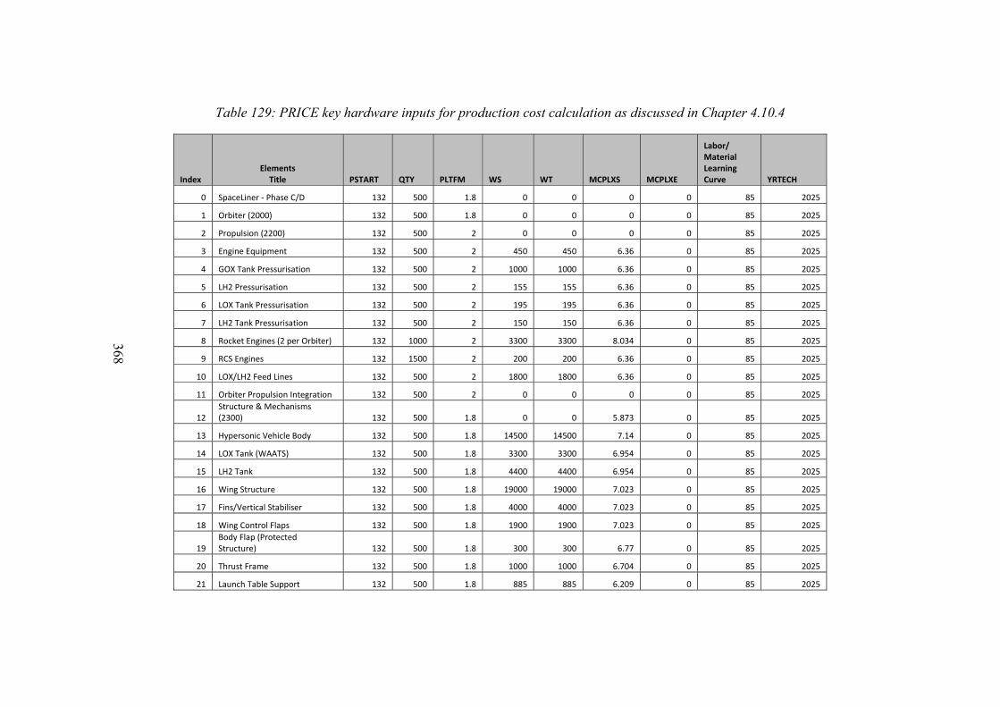
368
Table 129: PRICE key hardware inputs for production cost calculation as discussed in Chapter 4.10.4
Index Elements Title PSTART
QTY PLTFM WS WT MCPLXS MCPLXE
Labor/ Material Learning Curve YRTECH
0 SpaceLiner ‐ Phase C/D 132 500 1.8 0 0 0 0 85 2025
1 Orbiter (2000) 132 500 1.8 0 0 0 0 85 2025
2 Propulsion (2200) 132 500 2 0 0 0 0 85 2025
3 Engine Equipment 132 500 2 450 450 6.36 0 85 2025
4 GOX Tank Pressurisation 132 500 2 1000 1000 6.36 0 85 2025
5 LH2 Pressurisation 132 500 2 155 155 6.36 0 85 2025
6 LOX Tank Pressurisation 132 500 2 195 195 6.36 0 85 2025
7 LH2 Tank Pressurisation 132 500 2 150 150 6.36 0 85 2025
8 Rocket Engines (2 per Orbiter) 132 1000 2 3300 3300 8.034 0 85 2025
9 RCS Engines 132 1500 2 200 200 6.36 0 85 2025
10 LOX/LH2 Feed Lines 132 500 2 1800 1800 6.36 0 85 2025
11 Orbiter Propulsion Integration 132 500 2 0 0 0 0 85 2025
12 Structure & Mechanisms (2300) 132 500 1.8 0 0 5.873 0 85 2025
13 Hypersonic Vehicle Body 132 500 1.8 14500 14500 7.14 0 85 2025
14 LOX Tank (WAATS) 132 500 1.8 3300 3300 6.954 0 85 2025
15 LH2 Tank 132 500 1.8 4400 4400 6.954 0 85 2025
16 Wing Structure 132 500 1.8 19000 19000 7.023 0 85 2025
17 Fins/Vertical Stabiliser 132 500 1.8 4000 4000 7.023 0 85 2025
18 Wing Control Flaps 132 500 1.8 1900 1900 7.023 0 85 2025
19 Body Flap (Protected Structure) 132 500 1.8 300 300 6.77 0 85 2025
20 Thrust Frame 132 500 1.8 1000 1000 6.704 0 85 2025
21 Launch Table Support 132 500 1.8 885 885 6.209 0 85 2025
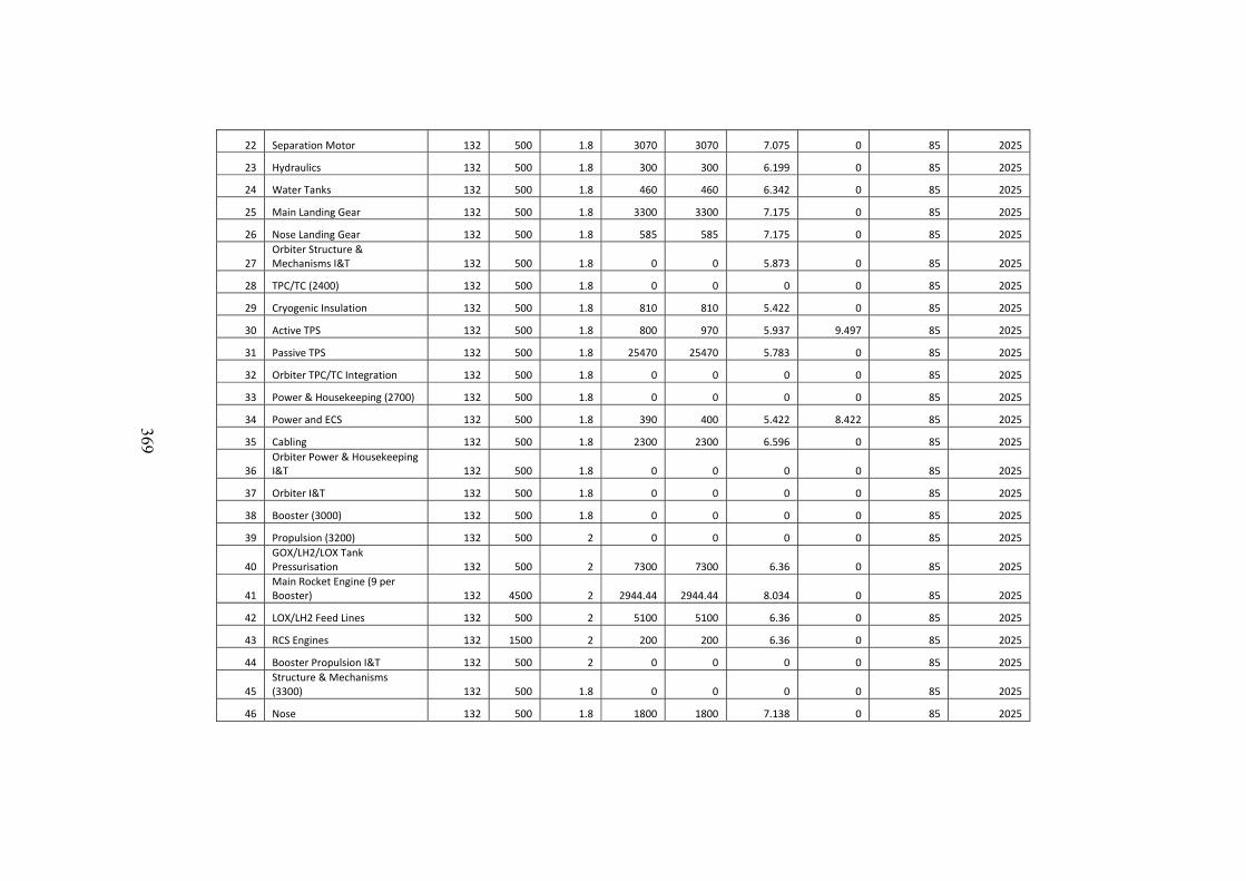
369
22 Separation Motor 132 500 1.8 3070 3070 7.075 0 85 2025
23 Hydraulics 132 500 1.8 300 300 6.199 0 85 2025
24 Water Tanks 132 500 1.8 460 460 6.342 0 85 2025
25 Main Landing Gear 132 500 1.8 3300 3300 7.175 0 85 2025
26 Nose Landing Gear 132 500 1.8 585 585 7.175 0 85 2025
27 Orbiter Structure & Mechanisms I&T 132 500 1.8 0 0 5.873 0 85 2025
28 TPC/TC (2400) 132 500 1.8 0 0 0 0 85 2025
29 Cryogenic Insulation 132 500 1.8 810 810 5.422 0 85 2025
30 Active TPS 132 500 1.8 800 970 5.937 9.497 85 2025
31 Passive TPS 132 500 1.8 25470 25470 5.783 0 85 2025
32 Orbiter TPC/TC Integration 132 500 1.8 0 0 0 0 85 2025
33 Power & Housekeeping (2700) 132 500 1.8 0 0 0 0 85 2025
34 Power and ECS 132 500 1.8 390 400 5.422 8.422 85 2025
35 Cabling 132 500 1.8 2300 2300 6.596 0 85 2025
36 Orbiter Power & Housekeeping I&T 132 500 1.8 0 0 0 0 85 2025
37 Orbiter I&T 132 500 1.8 0 0 0 0 85 2025
38 Booster (3000) 132 500 1.8 0 0 0 0 85 2025
39 Propulsion (3200) 132 500 2 0 0 0 0 85 2025
40 GOX/LH2/LOX Tank Pressurisation 132 500 2 7300 7300 6.36 0 85 2025
41 Main Rocket Engine (9 per Booster) 132 4500 2 2944.44 2944.44 8.034 0 85 2025
42 LOX/LH2 Feed Lines 132 500 2 5100 5100 6.36 0 85 2025
43 RCS Engines 132 1500 2 200 200 6.36 0 85 2025
44 Booster Propulsion I&T 132 500 2 0 0 0 0 85 2025
45 Structure & Mechanisms (3300) 132 500 1.8 0 0 0 0 85 2025
46 Nose 132 500 1.8 1800 1800 7.138 0 85 2025
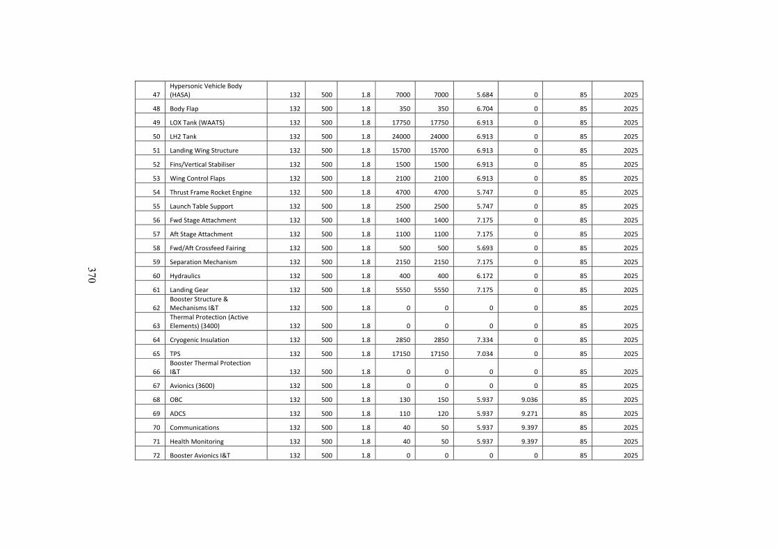
370
47 Hypersonic Vehicle Body (HASA) 132 500 1.8 7000 7000 5.684 0 85 2025
48 Body Flap 132 500 1.8 350 350 6.704 0 85 2025
49 LOX Tank (WAATS) 132 500 1.8 17750 17750 6.913 0 85 2025
50 LH2 Tank 132 500 1.8 24000 24000 6.913 0 85 2025
51 Landing Wing Structure 132 500 1.8 15700 15700 6.913 0 85 2025
52 Fins/Vertical Stabiliser 132 500 1.8 1500 1500 6.913 0 85 2025
53 Wing Control Flaps 132 500 1.8 2100 2100 6.913 0 85 2025
54 Thrust Frame Rocket Engine 132 500 1.8 4700 4700 5.747 0 85 2025
55 Launch Table Support 132 500 1.8 2500 2500 5.747 0 85 2025
56 Fwd Stage Attachment 132 500 1.8 1400 1400 7.175 0 85 2025
57 Aft Stage Attachment 132 500 1.8 1100 1100 7.175 0 85 2025
58 Fwd/Aft Crossfeed Fairing 132 500 1.8 500 500 5.693 0 85 2025
59 Separation Mechanism 132 500 1.8 2150 2150 7.175 0 85 2025
60 Hydraulics 132 500 1.8 400 400 6.172 0 85 2025
61 Landing Gear 132 500 1.8 5550 5550 7.175 0 85 2025
62 Booster Structure & Mechanisms I&T 132 500 1.8 0 0 0 0 85 2025
63 Thermal Protection (Active Elements) (3400) 132 500 1.8 0 0 0 0 85 2025
64 Cryogenic Insulation 132 500 1.8 2850 2850 7.334 0 85 2025
65 TPS 132 500 1.8 17150 17150 7.034 0 85 2025
66 Booster Thermal Protection I&T 132 500 1.8 0 0 0 0 85 2025
67 Avionics (3600) 132 500 1.8 0 0 0 0 85 2025
68 OBC 132 500 1.8 130 150 5.937 9.036 85 2025
69 ADCS 132 500 1.8 110 120 5.937 9.271 85 2025
70 Communications 132 500 1.8 40 50 5.937 9.397 85 2025
71 Health Monitoring 132 500 1.8 40 50 5.937 9.397 85 2025
72 Booster Avionics I&T 132 500 1.8 0 0 0 0 85 2025
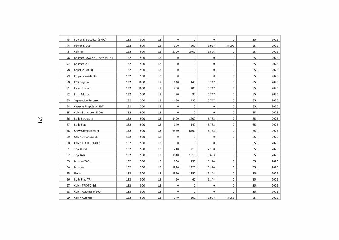
371
73 Power & Electrical (3700) 132 500 1.8 0 0 0 0 85 2025
74 Power & ECS 132 500 1.8 100 600 5.937 8.096 85 2025
75 Cabling 132 500 1.8 2700 2700 6.596 0 85 2025
76 Booster Power & Electrical I&T 132 500 1.8 0 0 0 0 85 2025
77 Booster I&T 132 500 1.8 0 0 0 0 85 2025
78 Capsule (4000) 132 500 1.8 0 0 0 0 85 2025
79 Propulsion (4200) 132 500 1.8 0 0 0 0 85 2025
80 RCS Engines 132 1000 1.8 140 140 5.747 0 85 2025
81 Retro Rockets 132 1000 1.8 200 200 5.747 0 85 2025
82 Pitch Motor 132 500 1.8 90 90 5.747 0 85 2025
83 Separation System 132 500 1.8 430 430 5.747 0 85 2025
84 Capsule Propulsion I&T 132 500 1.8 0 0 0 0 85 2025
85 Cabin Structure (4300) 132 500 1.8 0 0 0 0 85 2025
86 Body Structure 132 500 1.8 1400 1400 5.783 0 85 2025
87 Body Flap 132 500 1.8 140 140 5.783 0 85 2025
88 Crew Compartment 132 500 1.8 6560 6560 5.783 0 85 2025
89 Cabin Structure I&T 132 500 1.8 0 0 0 0 85 2025
90 Cabin TPC/TC (4400) 132 500 1.8 0 0 0 0 85 2025
91 Top AFRSI 132 500 1.8 210 210 7.138 0 85 2025
92 Top TABI 132 500 1.8 1610 1610 5.693 0 85 2025
93 Bottom TABI 132 500 1.8 150 150 6.144 0 85 2025
94 Bottom 132 500 1.8 1220 1220 6.144 0 85 2025
95 Nose 132 500 1.8 1350 1350 6.144 0 85 2025
96 Body Flap TPS 132 500 1.8 60 60 6.144 0 85 2025
97 Cabin TPC/TC I&T 132 500 1.8 0 0 0 0 85 2025
98 Cabin Avionics (4600) 132 500 1.8 0 0 0 0 85 2025
99 Cabin Avionics 132 500 1.8 270 300 5.937 8.268 85 2025
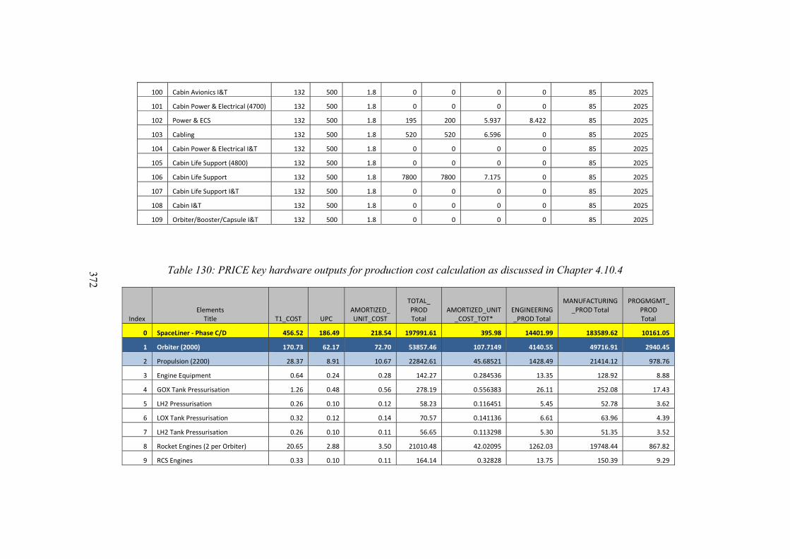
372
100 Cabin Avionics I&T 132 500 1.8 0 0 0 0 85 2025
101 Cabin Power & Electrical (4700) 132 500 1.8 0 0 0 0 85 2025
102 Power & ECS 132 500 1.8 195 200 5.937 8.422 85 2025
103 Cabling 132 500 1.8 520 520 6.596 0 85 2025
104 Cabin Power & Electrical I&T 132 500 1.8 0 0 0 0 85 2025
105 Cabin Life Support (4800) 132 500 1.8 0 0 0 0 85 2025
106 Cabin Life Support 132 500 1.8 7800 7800 7.175 0 85 2025
107 Cabin Life Support I&T 132 500 1.8 0 0 0 0 85 2025
108 Cabin I&T 132 500 1.8 0 0 0 0 85 2025
109 Orbiter/Booster/Capsule I&T 132 500 1.8 0 0 0 0 85 2025
Table 130: PRICE key hardware outputs for production cost calculation as discussed in Chapter 4.10.4
Index Elements Title T1_COST UPC
AMORTIZED_UNIT_COST
TOTAL_ PROD Total
AMORTIZED_UNIT
_COST_TOT* ENGINEERING_PROD Total
MANUFACTURING_PROD Total
PROGMGMT_PROD Total
0 SpaceLiner ‐ Phase C/D 456.52 186.49 218.54 197991.61 395.98 14401.99 183589.62 10161.05
1 Orbiter (2000) 170.73 62.17 72.70 53857.46 107.7149 4140.55 49716.91 2940.45
2 Propulsion (2200) 28.37 8.91 10.67 22842.61 45.68521 1428.49 21414.12 978.76
3 Engine Equipment 0.64 0.24 0.28 142.27 0.284536 13.35 128.92 8.88
4 GOX Tank Pressurisation 1.26 0.48 0.56 278.19 0.556383 26.11 252.08 17.43
5 LH2 Pressurisation 0.26 0.10 0.12 58.23 0.116451 5.45 52.78 3.62
6 LOX Tank Pressurisation 0.32 0.12 0.14 70.57 0.141136 6.61 63.96 4.39
7 LH2 Tank Pressurisation 0.26 0.10 0.11 56.65 0.113298 5.30 51.35 3.52
8 Rocket Engines (2 per Orbiter) 20.65 2.88 3.50 21010.48 42.02095 1262.03 19748.44 867.82
9 RCS Engines 0.33 0.10 0.11 164.14 0.32828 13.75 150.39 9.29
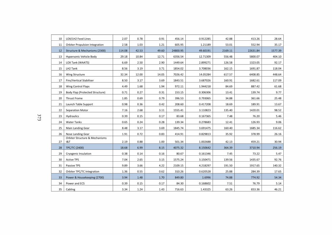
373
10 LOX/LH2 Feed Lines 2.07 0.78 0.91 456.14 0.912285 42.88 413.26 28.64
11 Orbiter Propulsion Integration 2.58 1.03 1.21 605.95 1.21189 53.01 552.94 35.17
12 Structure & Mechanisms (2300) 114.08 42.53 49.60 24800.95 49.60191 2169.11 22631.84 1577.39
13 Hypersonic Vehicle Body 29.18 10.84 12.71 6356.54 12.71309 556.48 5800.07 404.10
14 LOX Tank (WAATS) 6.69 2.50 2.90 1449.64 2.899271 126.58 1323.05 92.17
15 LH2 Tank 8.56 3.19 3.71 1854.02 3.708036 162.15 1691.87 118.04
16 Wing Structure 32.34 12.00 14.05 7026.42 14.05284 617.57 6408.85 448.64
17 Fins/Vertical Stabiliser 8.50 3.17 3.69 1843.51 3.687026 160.91 1682.61 117.09
18 Wing Control Flaps 4.49 1.68 1.94 972.11 1.944218 84.69 887.42 61.68
19 Body Flap (Protected Structure) 0.71 0.27 0.31 153.15 0.306306 13.41 139.74 9.77
20 Thrust Frame 1.85 0.69 0.79 396.53 0.793065 34.88 361.66 25.48
21 Launch Table Support 0.98 0.36 0.42 208.60 0.417208 18.69 189.91 13.67
22 Separation Motor 7.16 2.68 3.11 1555.41 3.110823 135.40 1420.01 98.52
23 Hydraulics 0.39 0.15 0.17 83.68 0.167365 7.48 76.20 5.46
24 Water Tanks 0.65 0.24 0.28 139.34 0.278683 12.41 126.93 9.06
25 Main Landing Gear 8.48 3.17 3.69 1845.74 3.691475 160.40 1685.34 116.62
26 Nose Landing Gear 1.91 0.72 0.83 414.91 0.829813 35.92 378.99 26.16
27 Orbiter Structure & Mechanisms I&T 2.19 0.88 1.00 501.34 1.002688 42.13 459.21 30.94
28 TPC/TC (2400) 18.68 6.99 8.15 4075.32 8.150642 364.39 3710.94 256.19
29 Cryogenic Insulation 0.38 0.14 0.16 80.67 0.161346 7.45 73.22 5.47
30 Active TPS 7.04 2.65 3.15 1575.24 3.150471 139.56 1435.67 92.76
31 Passive TPS 9.89 3.66 4.22 2109.15 4.218297 191.50 1917.65 140.32
32 Orbiter TPC/TC Integration 1.36 0.55 0.62 310.26 0.620528 25.88 284.39 17.65
33 Power & Housekeeping (2700) 3.94 1.48 1.70 849.80 1.6996 74.88 774.92 54.34
34 Power and ECS 0.39 0.15 0.17 84.30 0.168602 7.51 76.79 5.14
35 Cabling 3.34 1.24 1.43 716.63 1.43325 63.26 653.36 46.21
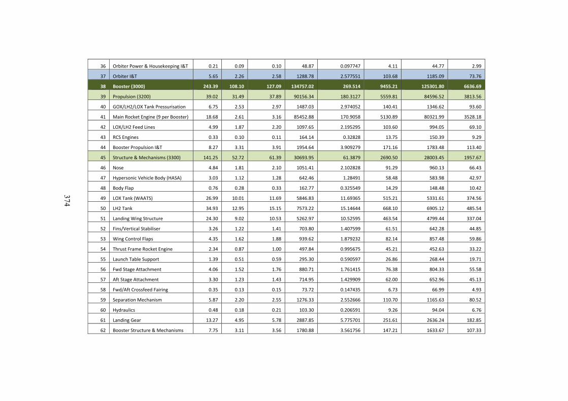
374
36 Orbiter Power & Housekeeping I&T 0.21 0.09 0.10 48.87 0.097747 4.11 44.77 2.99
37 Orbiter I&T 5.65 2.26 2.58 1288.78 2.577551 103.68 1185.09 73.76
38 Booster (3000) 243.39 108.10 127.09 134757.02 269.514 9455.21 125301.80 6636.69
39 Propulsion (3200) 39.02 31.49 37.89 90156.34 180.3127 5559.81 84596.52 3813.56
40 GOX/LH2/LOX Tank Pressurisation 6.75 2.53 2.97 1487.03 2.974052 140.41 1346.62 93.60
41 Main Rocket Engine (9 per Booster) 18.68 2.61 3.16 85452.88 170.9058 5130.89 80321.99 3528.18
42 LOX/LH2 Feed Lines 4.99 1.87 2.20 1097.65 2.195295 103.60 994.05 69.10
43 RCS Engines 0.33 0.10 0.11 164.14 0.32828 13.75 150.39 9.29
44 Booster Propulsion I&T 8.27 3.31 3.91 1954.64 3.909279 171.16 1783.48 113.40
45 Structure & Mechanisms (3300) 141.25 52.72 61.39 30693.95 61.3879 2690.50 28003.45 1957.67
46 Nose 4.84 1.81 2.10 1051.41 2.102828 91.29 960.13 66.43
47 Hypersonic Vehicle Body (HASA) 3.03 1.12 1.28 642.46 1.28491 58.48 583.98 42.97
48 Body Flap 0.76 0.28 0.33 162.77 0.325549 14.29 148.48 10.42
49 LOX Tank (WAATS) 26.99 10.01 11.69 5846.83 11.69365 515.21 5331.61 374.56
50 LH2 Tank 34.93 12.95 15.15 7573.22 15.14644 668.10 6905.12 485.54
51 Landing Wing Structure 24.30 9.02 10.53 5262.97 10.52595 463.54 4799.44 337.04
52 Fins/Vertical Stabiliser 3.26 1.22 1.41 703.80 1.407599 61.51 642.28 44.85
53 Wing Control Flaps 4.35 1.62 1.88 939.62 1.879232 82.14 857.48 59.86
54 Thrust Frame Rocket Engine 2.34 0.87 1.00 497.84 0.995675 45.21 452.63 33.22
55 Launch Table Support 1.39 0.51 0.59 295.30 0.590597 26.86 268.44 19.71
56 Fwd Stage Attachment 4.06 1.52 1.76 880.71 1.761415 76.38 804.33 55.58
57 Aft Stage Attachment 3.30 1.23 1.43 714.95 1.429909 62.00 652.96 45.13
58 Fwd/Aft Crossfeed Fairing 0.35 0.13 0.15 73.72 0.147435 6.73 66.99 4.93
59 Separation Mechanism 5.87 2.20 2.55 1276.33 2.552666 110.70 1165.63 80.52
60 Hydraulics 0.48 0.18 0.21 103.30 0.206591 9.26 94.04 6.76
61 Landing Gear 13.27 4.95 5.78 2887.85 5.775701 251.61 2636.24 182.85
62 Booster Structure & Mechanisms 7.75 3.11 3.56 1780.88 3.561756 147.21 1633.67 107.33
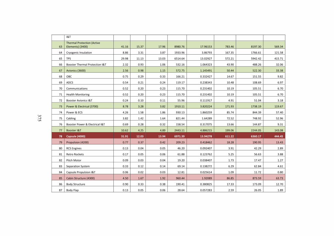
375
I&T
63 Thermal Protection (Active Elements) (3400) 41.16 15.37 17.96 8980.76 17.96153 783.46 8197.30 569.34
64 Cryogenic Insulation 8.86 3.31 3.87 1933.96 3.86793 167.35 1766.61 121.58
65 TPS 29.98 11.13 13.03 6514.64 13.02927 572.21 5942.42 415.71
66 Booster Thermal Protection I&T 2.32 0.93 1.06 532.16 1.064323 43.90 488.26 32.06
67 Avionics (3600) 2.56 0.98 1.15 572.75 1.145491 50.44 522.30 33.38
68 OBC 0.75 0.29 0.33 166.21 0.332427 14.67 151.55 9.82
69 ADCS 0.54 0.21 0.24 119.17 0.238343 10.48 108.69 6.97
70 Communications 0.52 0.20 0.23 115.70 0.231402 10.19 105.51 6.70
71 Health Monitoring 0.52 0.20 0.23 115.70 0.231402 10.19 105.51 6.70
72 Booster Avionics I&T 0.24 0.10 0.11 55.96 0.111917 4.91 51.04 3.18
73 Power & Electrical (3700) 8.78 3.28 3.82 1910.11 3.820224 171.93 1738.19 119.67
74 Power & ECS 4.26 1.58 1.86 930.13 1.860259 85.74 844.39 57.40
75 Cabling 3.82 1.42 1.64 821.44 1.64289 72.52 748.92 52.96
76 Booster Power & Electrical I&T 0.69 0.28 0.32 158.54 0.317075 13.66 144.87 9.31
77 Booster I&T 10.62 4.25 4.89 2443.11 4.886215 199.06 2244.05 143.08
78 Capsule (4000) 31.91 12.03 13.94 6971.39 13.94278 611.22 6360.17 444.45
79 Propulsion (4200) 0.77 0.37 0.42 209.23 0.418462 18.28 190.95 13.43
80 RCS Engines 0.13 0.04 0.05 46.20 0.092407 3.91 42.29 2.89
81 Retro Rockets 0.17 0.05 0.06 61.88 0.123762 5.25 56.63 3.88
82 Pitch Motor 0.09 0.03 0.04 19.20 0.038407 1.73 17.47 1.27
83 Separation System 0.33 0.12 0.14 69.14 0.138272 6.29 62.84 4.61
84 Capsule Propulsion I&T 0.06 0.02 0.03 12.81 0.025614 1.09 11.72 0.80
85 Cabin Structure (4300) 4.50 1.67 1.92 960.44 1.92089 86.85 873.59 63.73
86 Body Structure 0.90 0.33 0.38 190.41 0.380825 17.33 173.09 12.70
87 Body Flap 0.13 0.05 0.06 28.64 0.057283 2.59 26.05 1.89
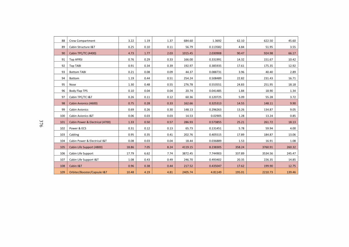
376
88 Crew Compartment 3.22 1.19 1.37 684.60 1.3692 62.10 622.50 45.60
89 Cabin Structure I&T 0.25 0.10 0.11 56.79 0.113582 4.84 51.95 3.55
90 Cabin TPC/TC (4400) 4.73 1.77 2.03 1015.45 2.030908 90.47 924.98 66.17
91 Top AFRSI 0.76 0.29 0.33 166.00 0.331991 14.32 151.67 10.42
92 Top TABI 0.91 0.34 0.39 192.97 0.385935 17.61 175.35 12.92
93 Bottom TABI 0.21 0.08 0.09 44.37 0.088731 3.96 40.40 2.89
94 Bottom 1.19 0.44 0.51 254.24 0.508489 22.82 231.43 16.71
95 Nose 1.30 0.48 0.55 276.78 0.553551 24.83 251.95 18.18
96 Body Flap TPS 0.10 0.04 0.04 20.74 0.041485 1.84 18.90 1.34
97 Cabin TPC/TC I&T 0.26 0.11 0.12 60.36 0.120725 5.09 55.28 3.72
98 Cabin Avionics (4600) 0.75 0.28 0.33 162.66 0.325313 14.55 148.11 9.90
99 Cabin Avionics 0.69 0.26 0.30 148.13 0.296263 13.26 134.87 9.05
100 Cabin Avionics I&T 0.06 0.03 0.03 14.53 0.02905 1.28 13.24 0.85
101 Cabin Power & Electrical (4700) 1.33 0.50 0.57 286.93 0.573855 25.21 261.72 18.13
102 Power & ECS 0.31 0.12 0.13 65.73 0.131451 5.78 59.94 4.00
103 Cabling 0.95 0.35 0.41 202.76 0.405515 17.89 184.87 13.06
104 Cabin Power & Electrical I&T 0.08 0.03 0.04 18.44 0.036889 1.53 16.91 1.08
105 Cabin Life Support (4800) 18.86 7.05 8.24 4119.15 8.238305 358.24 3760.91 260.32
106 Cabin Life Support 17.79 6.62 7.74 3872.45 7.744903 337.89 3534.56 245.47
107 Cabin Life Support I&T 1.08 0.43 0.49 246.70 0.493402 20.35 226.35 14.85
108 Cabin I&T 0.96 0.38 0.44 217.52 0.435047 17.62 199.90 12.75
109 Orbiter/Booster/Capsule I&T 10.48 4.19 4.81 2405.74 4.81149 195.01 2210.73 139.46
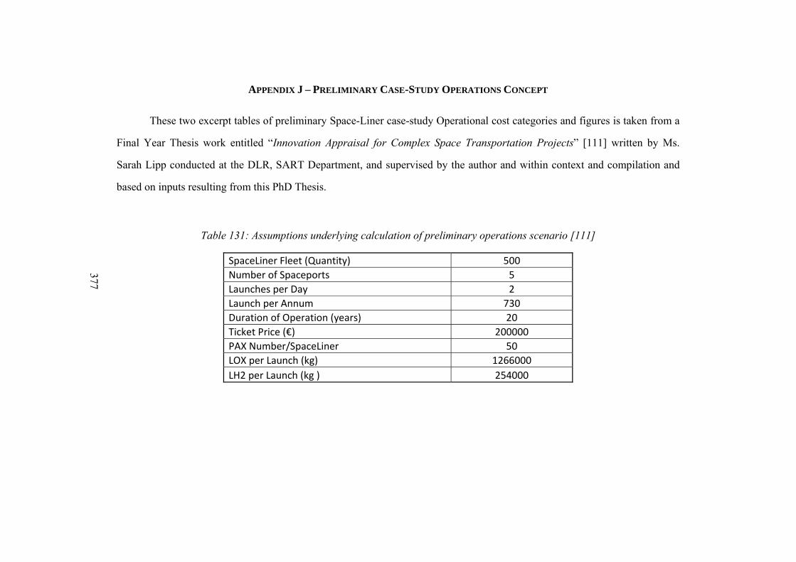
377
APPENDIX J – PRELIMINARY CASE-STUDY OPERATIONS CONCEPT
These two excerpt tables of preliminary Space-Liner case-study Operational cost categories and figures is taken from a
Final Year Thesis work entitled “Innovation Appraisal for Complex Space Transportation Projects” [111] written by Ms.
Sarah Lipp conducted at the DLR, SART Department, and supervised by the author and within context and compilation and
based on inputs resulting from this PhD Thesis.
Table 131: Assumptions underlying calculation of preliminary operations scenario [111]
SpaceLiner Fleet (Quantity) 500
Number of Spaceports 5
Launches per Day 2
Launch per Annum 730
Duration of Operation (years) 20
Ticket Price (€) 200000
PAX Number/SpaceLiner 50
LOX per Launch (kg) 1266000
LH2 per Launch (kg ) 254000
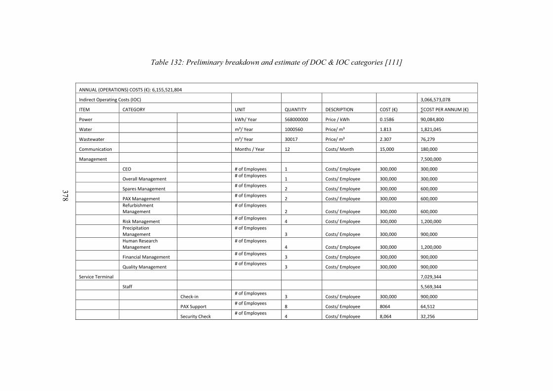
378
Table 132: Preliminary breakdown and estimate of DOC & IOC categories [111]
ANNUAL (OPERATIONS) COSTS (€): 6,155,521,804
Indirect Operating Costs (IOC) 3,066,573,078
ITEM CATEGORY UNIT QUANTITY DESCRIPTION COST (€) ∑COST PER ANNUM (€)
Power kWh/ Year 568000000 Price / kWh 0.1586 90,084,800
Water m³/ Year 1000560 Price/ m³ 1.813 1,821,045
Wastewater m³/ Year 30017 Price/ m³ 2.307 76,279
Communication Months / Year 12 Costs/ Month 15,000 180,000
Management 7,500,000
CEO # of Employees 1 Costs/ Employee 300,000 300,000
Overall Management # of Employees
1 Costs/ Employee 300,000 300,000
Spares Management # of Employees
2 Costs/ Employee 300,000 600,000
PAX Management # of Employees
2 Costs/ Employee 300,000 600,000
Refurbishment Management
# of Employees 2 Costs/ Employee 300,000 600,000
Risk Management # of Employees
4 Costs/ Employee 300,000 1,200,000
Precipitation Management
# of Employees3 Costs/ Employee 300,000 900,000
Human Research Management
# of Employees4 Costs/ Employee 300,000 1,200,000
Financial Management # of Employees
3 Costs/ Employee 300,000 900,000
Quality Management # of Employees
3 Costs/ Employee 300,000 900,000
Service Terminal 7,029,344
Staff 5,569,344
Check‐in # of Employees
3 Costs/ Employee 300,000 900,000
PAX Support # of Employees
8 Costs/ Employee 8064 64,512
Security Check # of Employees
4 Costs/ Employee 8,064 32,256
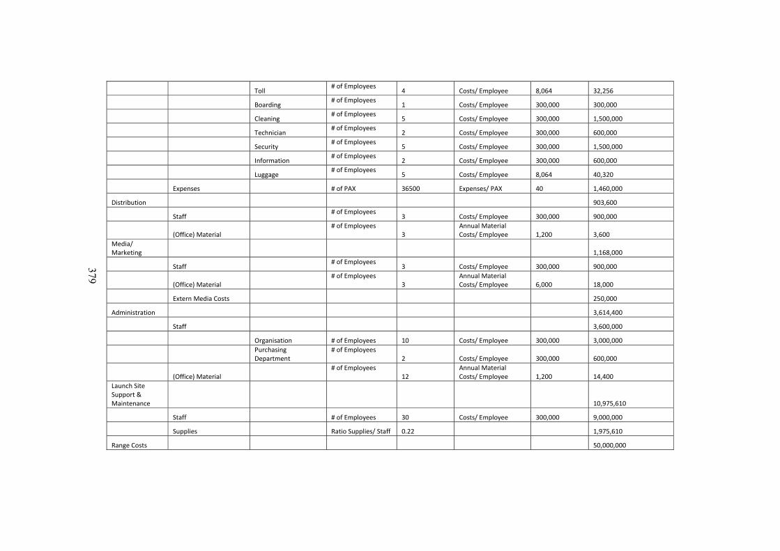
379
Toll # of Employees
4 Costs/ Employee 8,064 32,256
Boarding # of Employees
1 Costs/ Employee 300,000 300,000
Cleaning # of Employees
5 Costs/ Employee 300,000 1,500,000
Technician # of Employees
2 Costs/ Employee 300,000 600,000
Security # of Employees
5 Costs/ Employee 300,000 1,500,000
Information # of Employees
2 Costs/ Employee 300,000 600,000
Luggage # of Employees
5 Costs/ Employee 8,064 40,320
Expenses # of PAX 36500 Expenses/ PAX 40 1,460,000
Distribution 903,600
Staff # of Employees
3 Costs/ Employee 300,000 900,000
(Office) Material # of Employees
3 Annual Material Costs/ Employee 1,200 3,600
Media/ Marketing 1,168,000
Staff # of Employees
3 Costs/ Employee 300,000 900,000
(Office) Material # of Employees
3 Annual Material Costs/ Employee 6,000 18,000
Extern Media Costs 250,000
Administration 3,614,400
Staff 3,600,000
Organisation # of Employees 10 Costs/ Employee 300,000 3,000,000
Purchasing Department
# of Employees 2 Costs/ Employee 300,000 600,000
(Office) Material # of Employees
12 Annual Material Costs/ Employee 1,200 14,400
Launch Site Support & Maintenance 10,975,610
Staff # of Employees 30 Costs/ Employee 300,000 9,000,000
Supplies Ratio Supplies/ Staff 0.22 1,975,610
Range Costs 50,000,000
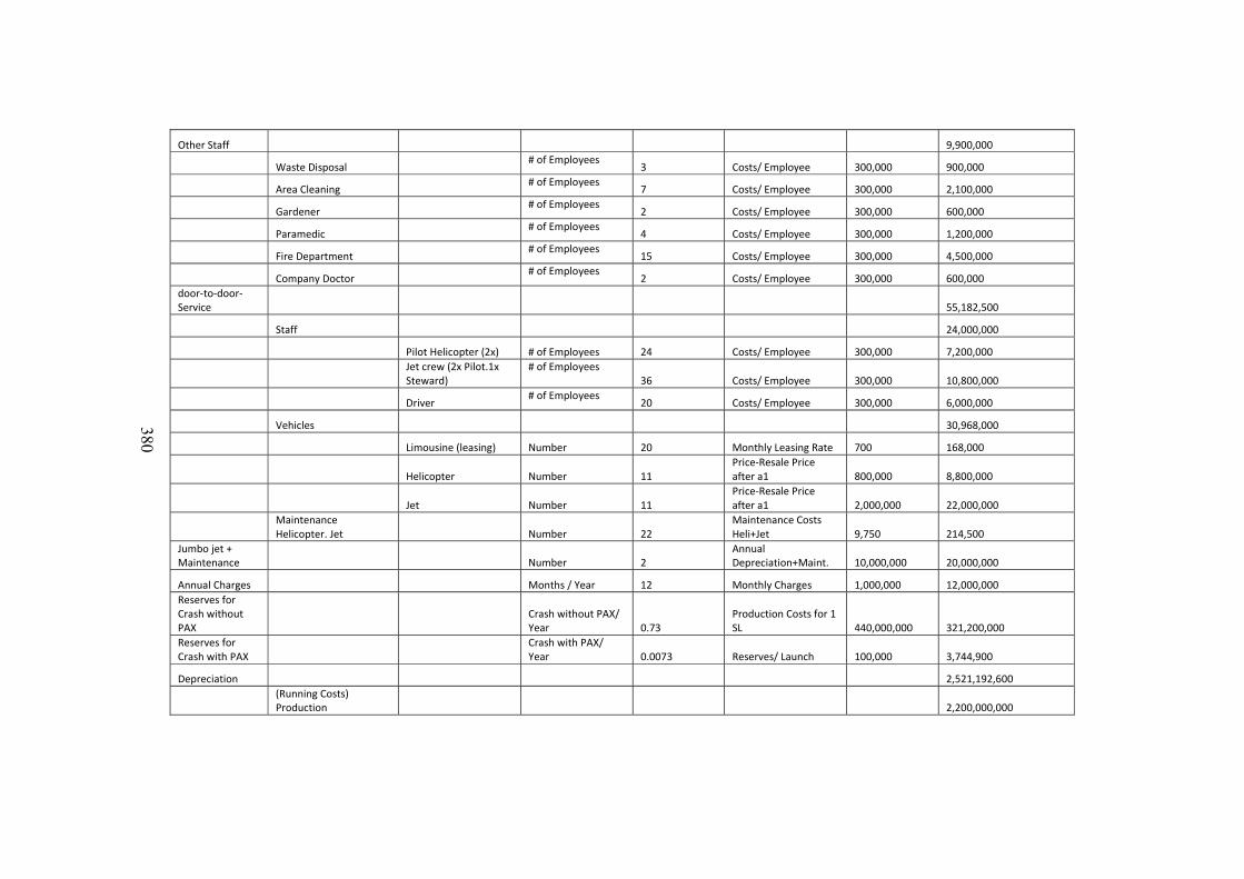
380
Other Staff 9,900,000
Waste Disposal # of Employees
3 Costs/ Employee 300,000 900,000
Area Cleaning # of Employees
7 Costs/ Employee 300,000 2,100,000
Gardener # of Employees
2 Costs/ Employee 300,000 600,000
Paramedic # of Employees
4 Costs/ Employee 300,000 1,200,000
Fire Department # of Employees
15 Costs/ Employee 300,000 4,500,000
Company Doctor # of Employees
2 Costs/ Employee 300,000 600,000
door‐to‐door‐Service 55,182,500
Staff 24,000,000
Pilot Helicopter (2x) # of Employees 24 Costs/ Employee 300,000 7,200,000
Jet crew (2x Pilot.1x Steward)
# of Employees 36 Costs/ Employee 300,000 10,800,000
Driver # of Employees
20 Costs/ Employee 300,000 6,000,000
Vehicles 30,968,000
Limousine (leasing) Number 20 Monthly Leasing Rate 700 168,000
Helicopter Number 11 Price‐Resale Price after a1 800,000 8,800,000
Jet Number 11 Price‐Resale Price after a1 2,000,000 22,000,000
Maintenance Helicopter. Jet Number 22
Maintenance Costs Heli+Jet 9,750 214,500
Jumbo jet + Maintenance Number 2
Annual Depreciation+Maint. 10,000,000 20,000,000
Annual Charges Months / Year 12 Monthly Charges 1,000,000 12,000,000
Reserves for Crash without PAX
Crash without PAX/ Year 0.73
Production Costs for 1 SL 440,000,000 321,200,000
Reserves for Crash with PAX
Crash with PAX/ Year 0.0073 Reserves/ Launch 100,000 3,744,900
Depreciation 2,521,192,600
(Running Costs) Production 2,200,000,000
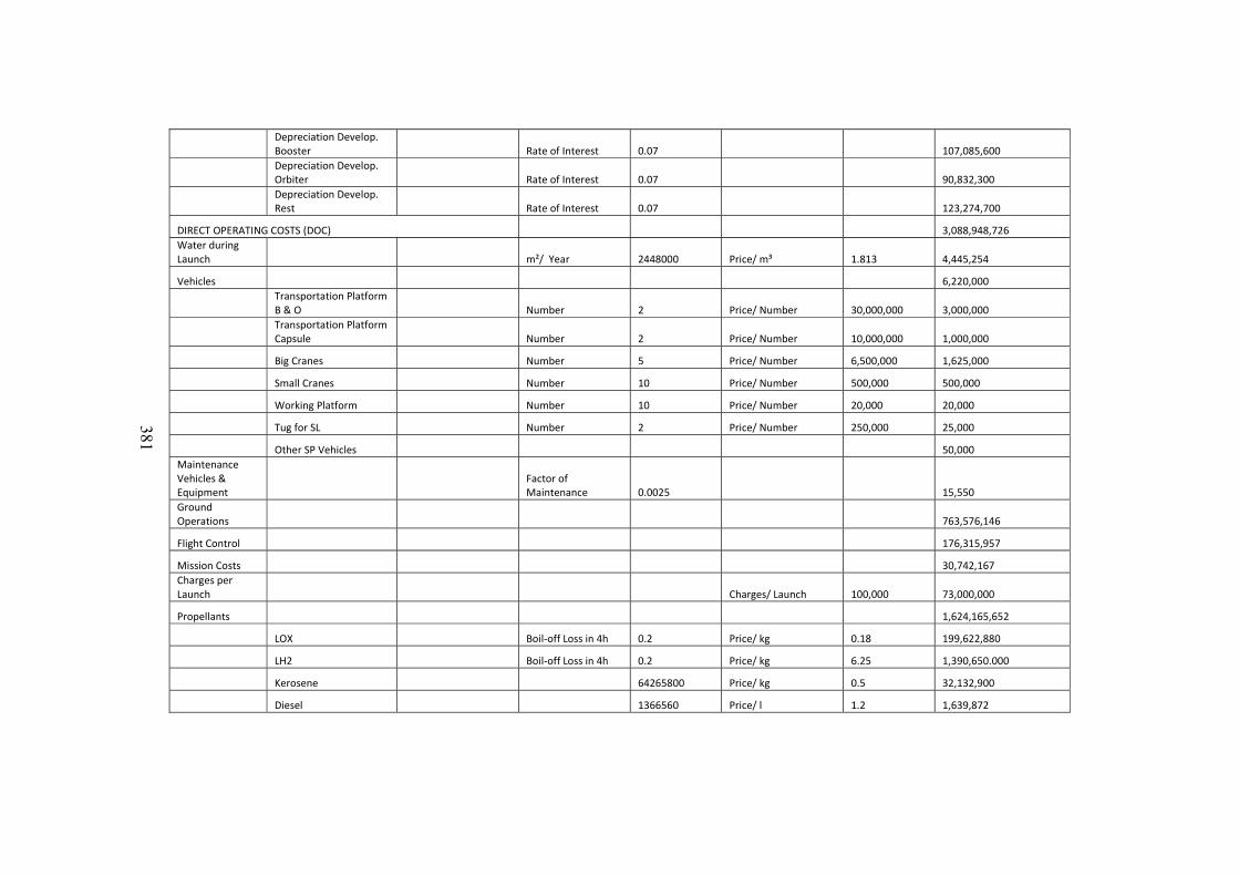
381
Depreciation Develop. Booster Rate of Interest 0.07 107,085,600
Depreciation Develop. Orbiter Rate of Interest 0.07 90,832,300
Depreciation Develop. Rest Rate of Interest 0.07 123,274,700
DIRECT OPERATING COSTS (DOC) 3,088,948,726
Water during Launch m²/ Year 2448000 Price/ m³ 1.813 4,445,254
Vehicles 6,220,000
Transportation Platform B & O Number 2 Price/ Number 30,000,000 3,000,000
Transportation Platform Capsule Number 2 Price/ Number 10,000,000 1,000,000
Big Cranes Number 5 Price/ Number 6,500,000 1,625,000
Small Cranes Number 10 Price/ Number 500,000 500,000
Working Platform Number 10 Price/ Number 20,000 20,000
Tug for SL Number 2 Price/ Number 250,000 25,000
Other SP Vehicles 50,000
Maintenance Vehicles & Equipment
Factor of Maintenance 0.0025 15,550
Ground Operations 763,576,146
Flight Control 176,315,957
Mission Costs 30,742,167
Charges per Launch Charges/ Launch 100,000 73,000,000
Propellants 1,624,165,652
LOX Boil‐off Loss in 4h 0.2 Price/ kg 0.18 199,622,880
LH2 Boil‐off Loss in 4h 0.2 Price/ kg 6.25 1,390,650.000
Kerosene 64265800 Price/ kg 0.5 32,132,900
Diesel 1366560 Price/ l 1.2 1,639,872
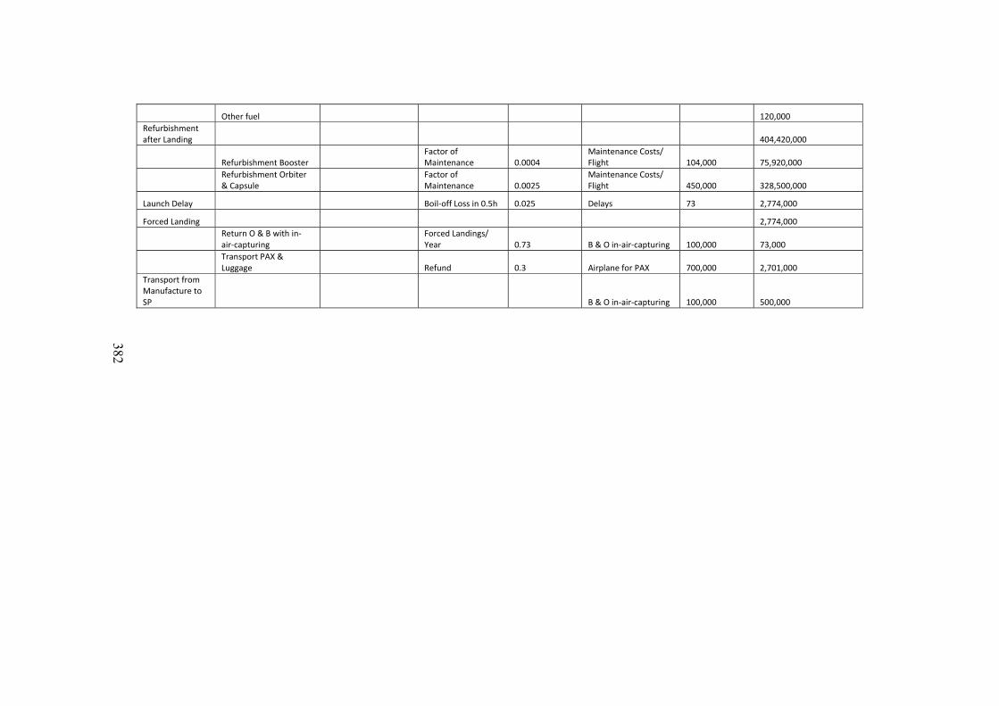
382
Other fuel 120,000
Refurbishment after Landing 404,420,000
Refurbishment Booster Factor of Maintenance 0.0004
Maintenance Costs/ Flight 104,000 75,920,000
Refurbishment Orbiter & Capsule
Factor of Maintenance 0.0025
Maintenance Costs/ Flight 450,000 328,500,000
Launch Delay Boil‐off Loss in 0.5h 0.025 Delays 73 2,774,000
Forced Landing 2,774,000
Return O & B with in‐air‐capturing
Forced Landings/ Year 0.73 B & O in‐air‐capturing 100,000 73,000
Transport PAX & Luggage Refund 0.3 Airplane for PAX 700,000 2,701,000
Transport from Manufacture to SP B & O in‐air‐capturing 100,000 500,000

383
384
REFERENCES
[1] 4cost GmbH, "4cost-suite V3 Help Manual," instructional manual computer file.
[2] 4cost GmbH. (Accessed 14 September, 2010). 4cost GmbH website. Available:
http://www.4cost.de
[3] 4cost GmbH, "4cost=Interactive and Integrated Management Method for Software and
Product Costing," Berlin, Germany.
[4] 4cost GmbH, "General Overview of the aces Cost Estimation Model, Advanced Cost
Estimating System," 4cost GmbH, Berlin, Germany, 2011.
[5] Abitzsch, S., "Prospects of Space Tourism," presented at the 9th European Aerospace
Congress - Visions and Limits of Long-term Aerospace Developments, Berlin, Germany,
1996.
[6] Adebola, S., Antifaev, J., Curran, C., Desportes, C., Rovira, O. G., Kelly, C., et al., "Great
Expectations: An Assessment of the Potential for Suborbital Transportation," Masters,
International Space University (ISU), Illkirch-Graffenstaden, France, 2008.
[7] Aerospace Corporation. (Accessed 7 December, 2010). Small Satellite Cost Model
(SSCM) website. Available: http://www.aero.org/capabilities/sscm/index.html
[8] Air Force Systems, "Cost Estimating Procedures," Headquarters Air Force System
Command, USA, AFSCM-173-1, 1972.
[9] AIRBUS S.A.S. (Accessed 12 December, 2014). A380. Available: www.airbus.com
[10] AIRBUS website. (Accessed 19 August, 2014). How is an aircraft built? Test
Programme and Certification. Available: http://www.airbus.com/company/aircraft-
manufacture/how-is-an-aircraft-built/test-programme-and-certification/
[11] American Society of Professional Estimators (ASPE). (Accessed 1 October, 2010). ASPE
website. Available: http://www.aspenational.org/
[12] Apgar, H., "A Tribute to Frank Frieman," presented at the ISPA Parametric World, A
Newsletter to the International Society of Parametric Estimators, 2010.
385
[13] Arena, M. V., Younossi, O., Galway, L. A., Fox, B., Graser, J. C., Sollinger, J. M., et al.,
"Impossible Certainty - Cost Risk Analysis for Air Force Systems," RAND Corporation,
2006.
[14] Armadillo Aerospace website. (Accessed 21 March, 2011). Available:
http://www.armadilloaerospace.com
[15] Ashford, D., "An aviation approach to space transportation (A strategy for increasing
space exploration within existing budget streams)," The Aeronautical Journal vol. 113,
pp. 499-514, August, 2009.
[16] Association for the Advancement of Cost Engineering through Total Cost Management
International (AACE). (Accessed 1 October, 2010). AACE website. Available:
http://aacei.org/
[17] "Astra Hopper - System Concept Data Book," EADS Space Transportation, 27 June,
2003.
[18] Augustine, N. R., Augustine's Laws and Major System Development Programs. New
York: American Institute of Aeronautics and Astronautics, 1980.
[19] Barrett, O. ([1999], Accessed 4 February, 2014). An evaluation of the potential demand
for space tourism within the United Kingdom. Available:
http://www.spacefuture.com/archive/an_evaluation_of_the_potential_demand_for_space_
tourism_within_the_united_kingdom.shtml
[20] Batey, A. (23 April, 2014). Your flight is now departing from space terminal 1: the
amazing story behind Branson's Virgin Galactic project Available:
https://markosun.wordpress.com/2010/06/08/your-flight-is-now-departing-from-space-
terminal-1-the-amazing-story-behind-bransons-virgin-galactic-project/
[21] Bauer, C., Garbers, N., Johannsson, M., and Lentsch, A., "Investigations of the
SpaceLiner Passenger Capsule and Various Abort Scenarios," presented at the Deutscher
Luft- und Raumfahrtkongress (DGLR), Berlin, Germany, 2012.
386
[22] Bauer, C., Garbers, N., and Sippel, M., "The SpaceLiner7 - Vehicle and Rescue Capsule,"
presented at the 29th International Symposium on Space Technology and Science (ISTS),
Nagoya, Japan, 2013.
[23] Beard, S. S., Starzyk, J., "Space Tourism Market Study - orbital space travel &
destinations with suborbital space travel," Futron Corporation, 2002.
[24] Benkard, C. L., "Learning and Forgetting: The Dynamics of Aircraft Production,"
American Economic Review, vol. 90, pp. 1034-1054, 4 September, 2000.
[25] Blanchard, B. S., Design and Manage to Life Cycle Cost. USA: M/A Press, 1978.
[26] Blum, C., Jones, P., and Meinders, B., "Dual Liquid Flyback Booster for the Space
Shuttle," Lockheed Martin Michoud Space Systems, New Orleans, LA, 1998.
[27] Boehm, B. W., "Software Engineering Economics," IEEE Transactions on Software
Engineering, vol. SE-10, pp. 4-21, 1984.
[28] Boehm, B. W., "Understanding and Controlling Software Costs " Journal of Parametrics,
vol. 8, 1988.
[29] Boehm, B. W., Reifer, J. D., and Valerdi, R., "COSYSMO: A Systems Engineering Cost
Model," University of Southern California, USA.
[30] Boeing. (Accessed 12 December, 2014). 777 Family - Orders and Deliveries. Available:
http://active.boeing.com/commercial/orders/index.cfm
[31] Butts, G., Linton, K., "The Joint Confidence Level Paradox: A History of Denial,"
National Aeronautics and Space Administration, 28 April, 2009.
[32] Christensen, P., Dysert, L. R., "Cost Estimate Classification System - As Applied in
Engineering, Procurement, and Construction for the Process Industries," AACE
International - the Authority for Total Cost Management, 29 November, 2011.
[33] Collins, P., Isozaki, K., "The Japanese Rocket Society's Space Tourism Research,"
presented at the International Symposium of Space Tourism, Bremen, 1997.
387
[34] Collins, P., Iwasaki, Y., Kanayama, H., and Ohnuki, M., "Commercial implications of
market research on space tourism," Journal of Space Technology and Science: Special
Issue on Space Tourism, part 2, vol. 10, No. 2, pp. 3-11, 1994.
[35] Collins, P., Stockmans, R., and Maita, M., "Demand for space tourism in America and
Japan, and its implications for future space activities," Advances in Astronautical
Sciences, vol. 91, pp. 601-610, 1995.
[36] Commercial Space Transportation Study. ([1997], Accessed 24 June, 2011). Available:
http://www.hq.nasa.gov/webaccess/CommSpaceTrans/
[37] Crouch, G. I., "Researching the Space Tourism Market," in Annual Conference of the
Travel and Tourism Research Association, 2001.
[38] Crouch, G. I., Devinney, T. M., Louviere, J. J., and Towhidul, I., "Modelling consumer
choice behaviour in space tourism," Tourism Management, vol. 30, pp. 441-454, 2009.
[39] Crouch, G. I., Laing, J. H., "Australian public interest in space tourism and a cross-
cultural comparison," The Journal of Tourism Studies, vol. 15, December, 2004.
[40] Curran, R., Raghunathan, S., and Price, M., "Review of aerospace engineering cost
modeling: the genetic causal approach," Progress in Aerospace Sciences, vol. 40, pp. 487-
534, 2004.
[41] Currency Converter (Accessed 13 June, 2014). Available: http://fxtop.com/
[42] Department of Defense (DoD). ([1995], Accessed 13 September, 2010). DoD Parametric
Cost Estimating Handbook (2nd ed.). Available: http://www.cost.jsc.nasa.gov/pceh.htm
[43] deSelding, P. B. (4 December, 2009) ESA Determined to Learn from the Mistakes of
BepiColombo. Space News International.
[44] deSelding, P. B. (20 October, 2003) Europe's ATV Program Facing Launch Delay, Cost
Overruns. Space News International.
[45] DLR-SART, "Space Transportation Systems Manual (STSM)," DLR - SART, Volume
1.2, Bremen, Germany, 2014.
388
[46] DLR Institute für Raumfahrtsysteme. (Accessed 13 September, 2011). Astra Concept:
semi-reusable launch vehicle with Ariane 5 cost stage and two attached reusable fly-back
boosters (LFBB) Available: http://www.dlr.de/irs/DesktopDefault.aspx/tabid-
7629/12934_read-32489/gallery-1/gallery_read-Image.46.20496/
[47] Dryden, J. A., Large, J. P., "A Critique of Spacecraft Models, R-2196-1-AF," 1977.
[48] EADS Astrium, "ASSC 1 Life Cycle Cost - Issue 3," Excel spreadsheet, 22 March, 2001.
[49] EADS Astrium, "ASSC 1 Life Cycle Cost - Issue 6," Excel spreadsheet, 12 January,
2004.
[50] EADS Astrium, "ASSC 2Y Life Cycle Cost Calculation- Issue 4," Excel spreadsheet, 13
January, 2004.
[51] Eilingsfeld, F., "Technical Appendix - Parametrics," International Space University
(ISU), 27 October, 2010.
[52] Eilingsfeld, F., "Estimating the Development Cost of an Orbital Passenger Spaceplane -
Case Study for the International Space University," PRICE Systems Deutschland
Ruesselsheim, Germany, 2006.
[53] Eilingsfeld, F., "Hardware Cost Modeling," International Space University (ISU),
Illkirch-Graffenstaden, Lecture Series, 2014.
[54] Encyclopedia Astronautica. (Accessed 16 November, 2011). Available:
www.astronautix.com
[55] ESA Requirements and Standards Division (ESTEC), "Space engineering - Testing " The
Netherlands, European Cooperation for Space Standardization ECSS-E-10-03A, 15
February, 2002.
[56] ESA Requirements and Standards Division (ESTEC), "Space project management - Cost
and schedule management," The Netherlands, European Cooperation for Space
Standardization ECSS-M-ST-60C, 31 July, 2008.
389
[57] ESA Requirements and Standards Division (ESTEC), "Space project management -
Project planning and implementation," European Cooperation for Space Standardization,
The Netherlands ECSS-M-ST-10C Revision 1, 6 March, 2009.
[58] Evans, A., Bond, A., "The Commercial Case (2010) for the SKYLON Spaceplane
Satellite Launcher," Reaction Engines Ltd., Abingdon, UK, July, 2010.
[59] Federal Acquisition Regulation website. (Accessed 22 October, 2010). Available:
http://www.acquisition.gov/Far/
[60] Federal Aviation Administration (FAA), "FAA Life Cycle Cost Estimating Handbook:
Parametric, Analogy, Engineering Estimation Risk Analysis Modeling and Simulation,
Version 2.0," FAA Investment Cost Analysis Branch ASD-410, June, 2002.
[61] Floreani, D., Wood, L., "Internet to Orbit - Exploring the Potential of IP Networking
Technologies in Space," 2005.
[62] Flottau, J. (10 June, 2013) Readying for Take Off. Aviation Week & Space Technology.
[63] Flottau, J. (17 June, 2013) Testing Times. Aviation Week & Space Technology
[64] Foussier, P., From Product Descrpition to Cost: A Practical Approach vol. 1: The
Parametric Approach. France: Springer Publishing, 2006.
[65] Fox, B., Brancato, K., and Alkire, B., "Guidelines and Metrics for Assessing Space
System Cost Estimates," The RAND Corporation, 2008.
[66] Futron Corporation, "Suborbital Space Tourism Demand Revisited," Bethesda, Maryland,
August, 2006.
[67] Futron Corporation, "Innovative Strategies for Space Competitiveness," Bethesda,
Maryland, 1 February, 2011.
[68] German Bureau of Statistics. (Accessed 20 October, 2014). Weekly Hours Worked.
Available:
https://www.destatis.de/EN/FactsFigures/Indicators/QualityEmployment/Dimension3/3_1
_WeeklyHoursWorked.html
390
[69] Gerosa, S., Nasini, F., "Project Financing and Risk Management: a new challenge for
program manahement in the space industry of the third millennium," presented at the
Fourth European Project Management Conference (PMI), London, UK, 2001.
[70] Giacalone, J. A., "The evolving private spaceflight industry: space tourism and cargo
transport," in ASBBS Annual Conference, Las Vegas, USA, 2013.
[71] Goehlich, R. A., Rücker, U., "Low-cost management aspects for developing, producing
and operating future space transportation systems," Acta Astronautica, vol. 56, pp. 337-
346, 2005.
[72] Greves, D., Schreiber, B. ([1995], Accessed 12 September, 2011). Engineering Costing
Techniques in ESA. Available: http://www.esa.int/esapub/bulletin/bullet81/greve81.htm
[73] Haas, R., Maixner, O., "An Illustrated Guide to the Analytic Hierarchy Process," Institute
of Natural Resource and Applied Life Sciences, Vienna, presentation slides.
[74] Habib-Agahi, H., Kwan, E., "NASA Instrument Cost Model (NICM) Presented to the
NASA Cost Symposium " 13 April, 2005.
[75] Hamaker, J., "NASA Cost Estimating with emphasis on the Exploration Systems
Architecture Study," in NIA/SACD Distinguished Lecture Series in Systems Analysis,
NASA Headquarters, Washington D.C., 2006.
[76] Hammond, W. E., Space Transportation: A Systems Approach to Analysis and Design
Virginia, USA: American Institute of Aeronautics and Astronautics Inc., 1999.
[77] Hart, K. ([2007], Accessed 21 March, 2011). Travel Agency launches tourists on out-of-
this-world adventures. Available:
http://seattletimes.nwsource.com/html/businesstechnology/
[78] Hartley, K., "The Learning Curve and its Application to the Aircraft Industry," Journal of
Industrial Economics, vol. 13, pp. 122-128, 1965.
[79] Havranek, T. J., Modern Project Management Techniques for the Environmental
Remediation Industry. Florida, USA: CRC Press LCC, 1999.
391
[80] Hendrickx, v. B., Vis, B., Energiya-Buran: The Soviet Space Shuttle Checheser, UK:
Praxis Publishing Ltd., 2007.
[81] Hess, R. W., Romanoff, H. P., "Aircraft Airframe Cost Estimating Relationships - Study
Approach and Conclusions," Santa Monica, USA R-3255-AF, December, 1987.
[82] Hochschule für Angewandte Wissenschaften Hamburg (HAW), IDS Hamburg GmbH,
"Vision of the SpaceLiner concept in gliding flight," Graphic.
[83] Hughes, R. T., "Expert judgement as an estimating method," Information & Software
Technology, vol. 38, pp. 67-75, 1996.
[84] Humphreys, K., Wellman, P., "Basic Cost Engineering," New York, USA, 1996.
[85] Hunt, C. D., van Pelt, M. O., "Comparing NASA and ESA Cost Estimating Methods for
Human Missions to Mars," NASA MSFC, Huntsville, USA, ESA-ESTEC, Noordwijk,
The Netherlands, March, 2004.
[86] Interesting Engineering. (Accessed 27 November, 2014). Kansai International Airport.
Available: http://interestingengineering.com/kansai-international-airport/
[87] International Cost Engineering Council (ICOSTE). (Accessed 5 October, 2010). ICOSTE
website. Available: http://www.icoste.org/
[88] International Cost Estimating and Analysis Association (ICEAA). (Accessed 2 December,
2014). ICEAA website Available: http://www.iceaaonline.com/
[89] International Society of Parametric Analysts (ISPA), Society of Cost Estimating and
Analysis (SCEA), "ISPA and SCEA Parametric Estimating Handbook," 4th Edition,
Vienna, VA.
[90] International Society of Parametric Analysts (ISPA). (Accessed 1 October, 2010). ISPA
website. Available: http://www.ispa-cost.org/
[91] Jenkins, D. R., Space Shuttle - The History of the National Space Transportation System,
The First 100 Missions: Elsevier Publishing, 2010.
[92] Johnson, J. P., Gaier, E. M., "Air Cargo Operations Cost Database," NASA, Virginia,
USA, April, 1998.
392
[93] Johnson, R. F., Smith, P. L., "Future spacelift projections," Space Policy, vol. 14, pp. 145-
151, 1998.
[94] Jonas, V., "Five steps to Enterprise Risk Management " Risk Decisions Group, January,
2011.
[95] Kasperczyk, N., Knickel, K. ([2006], 16 March, 2011). The Analytic Hierarchy Process
(AHP) Available: www.ivm.vu.nl/en/Images/MCA3_tcm53-161529.pdf
[96] Keiderling, D., "SART TN-002/2010: Aufstiegssimulation des Space Transportation
Systems," DLR Systemanalyse Raumtransport (SART), Bremen, 2010.
[97] Kitchenham, B., Making Process Predictions. New York Chapman & Hall, 1997.
[98] Klepper, S., "Industry Life Cycles," Industrial and Corporate Change, vol. 6, 1997.
[99] Koelle, D. E., "Cost Engineering, the new paradigm for space launch vehicle design,"
Journal of Reducing Space Mission Cost, vol. 1, pp. 73-86, 1998.
[100] Koelle, D. E., "Handbook of Cost Engineering for Space Transportation Systems
including TransCost 7.3, Revision 3," TransCostSystems, 2010.
[101] Koelle, D. E., "Handbook of Cost Engineering for Space Transportation Systems
including TransCost 8.1, Revision 3a," TransCostSystems, 2010.
[102] Koelle, D. E., "Handbook of Cost Engineering for Space Transportation Systems
including TransCost 8.2, Revision 4," TransCostSystems, 2012.
[103] Koelle, D. E., "Two TransCost Questions re. Shuttle ET & WYr," E-mail communication,
27 November, 2012.
[104] Kothari, A. P., Webber, D., "Potential Demand for Orbital Space Tourism Opportunities
Made Available via Reusable Rocket and Hypersonic Architectures " presented at the
AIAA SPACE 2010 Conference & Exposition, Anaheim, California, USA, 2010.
[105] Kurshistorie EUR/USD Currency Converter. (Accessed 9 November, 2013 ). Available:
http://www.boerse.de/historische-kurse/Euro-Dollar/EU0009652759
393
[106] Laing, J., Crouch, G. I., Chapter 2: Vacationing in Space: Tourism Seeks "New Skies".
Oxfordshire, UK: CABI Publishing, 2004.
[107] Liebers, A., "An architecture for cost control, the use of cost information in order-related
decisions," Ph.D. Thesis, University of Twente, 1998.
[108] "Life Cycle Cost Estimations for FESTIP Concepts - FESTIP CONFIDENTIAL, FSS-
SCT-RP-0060 Report," Germany.
[109] Lillie, C. F., Thompson, B. E., "Parametric cost estimation for space science missions,"
presented at the International Society for Optical Engineering (SPIE), Congress of
Advanced Optical and Mechanical Technologies in Telescopes and Instrumentation,
Marseille, France, 2008.
[110] Lipp, S., "Spaceport Concepts and Locations for the SpaceLiner," Deustsches Zentrum für
Luft- und Raumfahrt, Bremen, Germany, November, 2014.
[111] Lipp, S., "Innovationsbewertung bei komplexen Raumtransportprojekten,"
Wirtschaftsingenieurwesen Produktionstechnik, Schwerpunkt Luft- und Raumfahrt
Bachelor Thesis, Universität Bremen, Germany, 2015.
[112] Madauss, B., "Management Advantages of the Standard Work Breakdown Structure
Proposed by the European Space Agency for Space Satelitte Projects," Pacific States
University, Los Angeles, USA, 1980.
[113] Madauss, B., Planung und Überwaching von Forschungs- und Entwicklungsprojekten -
mit Beiträgen aus der Raumfahrttechnik (Planning and Monitoring of Research and
Development projects - with contributions from Space Technology). Ottobrunn: AIB
Fachliteratur, 1982.
[114] Madauss, B., Handbuch Projektmanagement (Project Management Handbook). Stuttgart:
5th Edition, Schäffer-Poeschel, 1994.
[115] Madauss, B., Handbuch Projektmanagement (Project Management Handbook). Stuttgart:
6th Edition, Schäffer-Poeschel, 2000.
394
[116] Madauss, B., "Training for Satelitte Engineering and Management - XIII.6 Risk
Evaluation and Mitigation Plan," International Space University (ISU), Illkirchen-
Graffenstanden, France, Lecture Series, 2010.
[117] Madauss, B., "Hourly Rates for SPO," E-mail communication, 20 October, 2014.
[118] Madauss, B., "SpaceLiner - Additional SPO Information," International Space University
(ISU), Illkirch-Graffenstaden, France, official ISU letter, 28 November, 2014.
[119] Madauss, B., "SpaceLiner - SPO Information," International Space University (ISU),
Illkirch-Graffenstaden, France, official ISU letter, 18 October, 2014.
[120] Madauss, B., "SpaceLiner - Model Philosophy," International Space University (ISU),
Illkirch-Graffenstaden, France, official ISU letter, 5 January, 2015.
[121] Madauss, B., "SpaceLiner - Model Philosophy (revised)," International Space University
(ISU), Illkirch-Graffenstaden, France, official ISU letter, 12 January, 2015.
[122] Madauss, B., Trivailo, O., "Important Programmatic Aspects," in SpaceLiner Workshop,
power point presentation slides, Bremen, Germany, 2013.
[123] Make or Break: Why Accurate Cost Estimation Is Key. ([2008], Accessed 9 November,
2012). Available: http://www.projectsmart.co.uk/make-or-break-why-accurate-cost-
estimation-is-key.html
[124] Maryniak, G. E., "When will we see a golden age of spaceflight?," Space Policy, vol. 21,
pp. 111-119, 2005.
[125] Mealey, A. (Accessed 8 June, 2011). Space Tourism Survey. Available:
http://www.spacetourismnow.com/blog/index.php/space-tourism/space-tourism-survey/
[126] Mediavilla, J. I. ([2011], Accessed 20 November, 2014). Learning Curves: Boeing 787
case in 2013. Available: http://theblogbyjavier.com/2014/03/05/learning-curves-boeing-
787-case-in-2013/
[127] Mediavilla, J. I. ([2011], Accessed 20 November, 2014). Will Boeing 787 ever break-
even? Available: http://theblogbyjavier.com/2011/10/28/will-boeing-787-ever-break-
even/
395
[128] Meisl, C. J., "Techniques for cost estimating in early program phases," Engineering Costs
and Production Economics, vol. 14, pp. 95-106, 1988.
[129] Merlin, P. W., Design and Development of the Blackbird. California, USA: American
Institute of Aeronautics and Astronautics, Inc., 2008.
[130] Meyer, M. A., Booker, J. M., Eliciting and Analyzing Expert Judgement - A Practical
Guide London: Academic Press Ltd., 2001.
[131] Mikheev, A., Lukashevich, V. ([2000], Accessed 19 August, 2013). Buran Schematic.
Available: http://airwingmedia.com/news/2013/buran-soviet-space-shuttle/
[132] Miller, D. W., Keesee, K., and Jilla, C., "Space System Cost Modeling," MIT Aeronautics
and Astronautics Course, 2003.
[133] Möller, T., Projekte erfolgreich managen. Köln, Germany: TÜV Media, 2014.
[134] NASA/Jet Propulsion Laboratories Cost Estimation website. (Accessed 13 September,
2010). Available: http://cost.jsc.nasa.gov/
[135] National Aeronautics and Space Administration, 2002 NASA Cost Estimating Handbook.
Washington D.C., 2002.
[136] National Aeronautics and Space Administration, 2004 NASA Cost Estimating Handbook.
Washington D.C., 2004.
[137] National Aeronautics and Space Administration, 2008 NASA Cost Estimating Handbook.
Washington D.C., 2008.
[138] National Aeronautics and Space Administration, "NASA's Challenges to Meeting Cost,
Schedule, and Performance Goals," National Aeronautics and Space Administration, IG-
12-021, 27 September, 2012.
[139] National Aeronautics and Space Administration, "Understanding Joint Confidence Level
(JCL) at NASA," Office of Evaluation, Cost Analysis Division, JCL Analysis Primer,
2012.
[140] National Aeronautics and Space Administration, "Structural Design and Test Factors of
Safety for Spaceflight Hardware," Washington D.C. NASA-STD-5001B, 6 August, 2014.
396
[141] National Research Council of the National Academies, Reusable Booster System: Review
and Assessment. Washington, DC: The National Academies Press, 2012.
[142] O'Leary, B., "The Space Shuttle - NASA's White Elephant in the Sky " Science and
Public Affairs - Bulletin of the Atomic Scientists, vol. XXIX, pp. 36-43, February, 1973.
[143] O'Neil, D., Bekey, I., Mankins, J., Rogers, T. F., and Stallmen, E. W., "General Public
Space Travel and Tourism," March, 1998.
[144] Operating and Support Cost-Estimating Guide. ([1992], Accessed 25 April, 2014).
Available: http://www.dtic.mil/pae/
[145] Orlebar, C., The Concorde Story: 6th Edition, Osprey Publishing Ltd., 2004.
[146] Papathanassis, A., Klemm, G., and Markkanen, S., "Space tourism: The Long Tail of
Tourism - Holiday Niches and their Impact on Mainstream Tourism," Germany, 2011.
[147] Pataki, G. E., Dillon, J. T., and McCormack, M., "Project Management Lifecycle," New
York State Office for Technology, 2003.
[148] Peeters, W., Space Marketing. El Segundo, USA and Dordrechts, The Netherlands:
Microcosm Inc. and Kluwer Publishers, 2000.
[149] Peeters, W., "From suborbital space tourism to commercial personal spaceflight," Acta
Astronautica, vol. 66, pp. 1625-1632, 2010.
[150] Penn, J. P., Lindley, C. A., "Requirements and approach for a space tourism launch
system," Acta Astronautica vol. 52, pp. 49-75, 2003.
[151] Perrault, J. W. D., Cannon, J., and McArthy, E. J., Essentials of Marketing: 12th Edition,
McGraw-Hill, 2009.
[152] PRICE Systems. (Accessed 11 October, 2011). PRICE Systems website. Available:
http://www.pricesystems.com
[153] PRICE Systems, "PRICE H - Hardware Model for Estimation of Acquisition Costs,"
PRICE information pamphlet, Mt. Laurel, New Jersey, USA, 2005.

397
[154] PRICE Systems, "PRICE H User Manual - Estimating Cost and Schedule of Hardware
Development and Production," PRICE Systems, Mt. Laurel, New Jersey, USA, 2005.
[155] PRICE Systems, "Guidelines for ESA cost estimating projects," Rüsselsheim, Germany,
iternal report, 2012.
[156] Project Management Institute Inc., "A Guide to the Project Management Body of
Knowledge (PMBOK Guide)," Project Management Institute Inc., 4th Edition,
Pennsylvania, USA, 2008.
[157] Reaction Engines Limited website (Accessed 15 May, 2014). Available:
http://www.reactionengines.co.uk/
[158] Reinbold, G., "Life Cycle Cost Assessments - ASTRA System Study Slice 2," EADS
Astrium, technical note, 2004.
[159] Remer, D. S., Buchanan, H. R., "A Model for the Cost of Doing a Cost Estimate, TDA
Progress Report 42-110," Jet Propulsion Laboratory, Pasadena, California, 15 August,
1992.
[160] Roxburgh, G. (Accessed 7 August, 2013). Concorde History, Early History- The End of
the Beginning Available: http://www.concordesst.com/history/eh5.html#n
[161] Roy, R., "Cost Engineering: Why, What and How?," Cranfield University, UK, July,
2008.
[162] Roy, R., Kelvesjo, S., Forsberg, S., and Rush, C., "Quantitative and qualitative cost
estimating for engineering design," Journal of Engineering Design, vol. 12, 1 June, 2001.
[163] Rush, C., Roy, R., "Analysis of cost estimating processes used within a concurrent
engineering environment throuhgout a product life cycle," in Concurrent Engineering
2000 (CE2) Conference, Lyon, France, 2000.
[164] Saaty, T. L., The Analytic Hierarchy Process: Planning, Priority Setting, Resource
Allocation. New York: McGraw-Hill, 1980.
[165] Saaty, T. L., "Decision making with the analytical hierarchy process," International
Journal of Services Science, vol. 1, pp. 83-89, 2008.

398
[166] Sabre Airline Solutions. Airport Data Intelligence (ADI) Database [Online]. Available:
http://www.sabreairlinesolutions.com/home/software_solutions/airports
[167] Savino, R., Russo, G., Carandente, V., and D'oriano, V., "Hyplane: Challenges for Space
Tourism and Business Transportation," Journal of Aeronautics & Aerospace Engineering,
vol. 2, 2013.
[168] Schwanekamp, T., Bauer, C., and Kopp, A., "The Development of the SpaceLiner
Concept and its Latest Progress," presented at the 4th CSA-IAA Conference on Advanced
Space Technology, Shanghai, China, 2011.
[169] Schwanekamp, T., Bütünley, J., and Sippel, M., "Preliminary Multidisciplinary Design
Studies on an Upgraded 100 Passenger SpaceLiner Derivative," presented at the 18th
AIAA/3AF International Space Planes and Hypersonic Systems and Technologies
Conference, Tours, France, 2012.
[170] Science Applications International Corporation (SAIC), "Recent NAFCOM Extensions
and Improvements, powerpoint presentation," 14 April, 2005.
[171] Science Applications International Corporation (SAIC), "NASA/Air Force Cost Model
NAFCOM," powerpoint presentation, 15 May, 2002.
[172] Seventh Framework Programme Theme 7, "FAST20XX/233816 Seventh Framework
Programme Theme 7 Transport Aeronautics - Annex 1," January, 2009.
[173] Shermon, D., Systems Cost Engineering - Program Affordability, Management and Cost
Control. UK Gower Publising Ltd., 2009.
[174] Shishko, R., "Model for Estimating Space Station Operations Costs (MESSOC),"
presentation slides, Jet Propulsion Laboratory, National Aeronautics and Space
Administration, Pasadena, California, February, 2004.
[175] Shishko, R., Chamberlain, R. G., Bilardo, V., Forsberg, K., Mooz, H., Polaski, L., et al.,
"Management Issues in Systems Engineering," 1993.
[176] Sippel, M., "Introducing the SpaceLiner Vision," presented at the 7th International
Symposium on Launcher technologies, Barcelona, Spain, 2007.
399
[177] Sippel, M., Klevanski, J., "Progress in Simulating the Advanced In-Air-Capturing
Method," presented at the 5th International Conference on Launcher Technology, Madrid,
Spain, 2003.
[178] Sippel, M., Klevanski, J., and Kauffmann, J., "Innovative Method for Return to the
Launch Site of Reusable Winged Stages," presented at the 52nd International
Astronautical Congress, Toulouse, France, 2001.
[179] Sippel, M., Klevanski, J., and Steelant, J., "Comparative Study on Options for High-
Speed Intercontinental Passenger Transports: Air-Breathing- vs Rocket Propelled,"
presented at the 56th International Astronautical Congress, Fukuoka, Japan, 2005.
[180] Sippel, M., Klevanski, J., and Van Foreest, A., "The SpaceLiner Concept and its
Aerothermodynamic Challenges," presented at the 1st ARA-Days, Arachon, France,
2006.
[181] Sippel, M., Manfletti, C., Burkhardt, H., and Eggers, T., "Technical Development
Perspective of Reusable Booster Stages," presented at the 12th International Space Planes
and Hypersonic Systems and Technologies, , Norfolk, Virginia, 2003.
[182] Sippel, M., Schwanekamp, T., Bauer, C., Garbers, N., van Foreest, A., Tengzelius, U., et
al., "Technical Maturation of the SpaceLiner Concept," presented at the 18th AIAA
International Space Planes and Hypersonic Systems and Technologies Conference, Tours,
France, 2012.
[183] Sippel, M., Schwanekamp, T., Trivailo, O., and Lentsch, A., "Progress of SpaceLiner
Rocket-Powered High-Speed Concept," presented at the 64th International Astronautical
Congress (IAC), Beijing, China, 2013.
[184] Sippel, M., van Foreest, A., "Latest Progress in Research on the SpaceLiner High-Speed
Passenger Transportation Concept," presented at the 58th International Astronautical
Congress, India, 2007.
[185] Sippel, M., van Foreest, A., "SpaceLiner Rocket-Powered High-Speed Passenger
Transportation Concept Evolving in FAST20XX," presented at the 61st International
Astronautical Congress (IAC) Prague, Czech Republic, 2010.
400
[186] Sippel, M., van Foreest, A., and Bauer, C., "System Investigations of the SpaceLiner
Concept in FAST20XX," presented at the 17th AIAA International Space Planes and
Hypersonic Systems and Technologies Conference, San Francisco, USA, 2011.
[187] Sippel, M., van Foreest, A., Dietlein, I., Schwanekamp, T., Kopp, A., and Neeb, D.,
"System Analyses Driving Improved Aerothermodynamic Lay-out of the SpaceLiner
Configuration," presented at the 1st ESA Aerothermodynamic Conference, Brugge,
Belgium, 2011.
[188] Smith, K., "NASA/Air Force Cost Model NAFCOM," in 2002 SCEA National
Conference, Scottsdale, Arizona, 2002.
[189] Society of Cost Estimating and Analysis (SCEA). (Accessed 4 October, 2010). SCEA
website. Available: http://sceaonline.org/
[190] Soyuz spaceship makes harmonious docking with ISS. ([2012], Accessed 16 November,
2013). Available: http://rt.com/news/soyuz-iss-docking-space-salaries-585/
[191] Space Foundation, "The Space Report - The Authoritative Guide to Global Space
Activity," Colorado Springs, USA, 2012.
[192] Space News International, "Suborbital Price Drop Foreseen by 2014," 23 July, 2003.
[193] Space News International, "Old Model Doesn't Apply to SpaceX's Expenditure," letter to
the editor, 7 February, 2011.
[194] "Space Operations Cost Model, SOCM, Final Report for Option 2 Contract Year," SAIC
December, 2007.
[195] Space Shuttle graphics. ([2007], Accessed 24 October, 2014). Available:
http://www.columbiassacrifice.com/&0_shttlovrvw.htm
[196] Space Systems Cost Analysis Group (SSCAG). (Accessed 1 October, 2010). SSCAG
website. Available: http://sscag.saic.com/
[197] SPACECAST2020. ([1994], Accessed August 8, 2013). SPACECAST2020, The World of
2020 and Alternative Futures Available:
http://www.fas.org/spp/military/docops/usaf/2020/alt-futr.htm
401
[198] SpaceX website. (Accessed 21 February, 2011). Available: http://www.spacex.com
[199] Spies, J., "ASTRA System Requirements, Design Standards, and Technology
Assumptions," 2000.
[200] Srivastava, M., Srivastava, S., "Space Tourism: The Future Tourism," Management
Insight, vol. 6, 2010.
[201] Stevenson, W., Hojati, M., "Supplement to Chapter 7: Learning Curves," McGraw-Hill
Higher Education, 2004.
[202] Stewart, R. D., Wyskida, R. M., and Johannes, J. D., "Cost Estimator's Reference
Manual," 2nd Edition, Wiley-Interscience, 1995.
[203] tenBrinke, E., "Costing support and cost control in manufacturing - a cost estimation tool
applied to the sheet metal domain," Ph.D. Thesis, University of Twente, Enschede, The
Netherlands, 2002.
[204] The Association of Cost Engineers (ACOSTE). (Accessed 4 October, 2010). ACOSTE
website. Available: http://www.acoste.org.uk/
[205] The White House Office of the Press Secretary, "Remarks by the President of Space
Exploration in the 21st Century," John F. Kennedy Space Center, Merrit Island, Florida,
2010.
[206] The World Bank's International Trade Department, "Air Freight: A Market Study with
Implications for Landlocked Countries, TP-26," Chapter 4, The World Bank Group,
Washington D.C.August, 2009.
[207] Trivailo, O., "Calibration of TransCost for Launcher Development Cost Calculations,
SART TN-001/2012," Deutsches Zentrum für Luft- und Raumfahrt, Bremen, Germany,
December, 2012.
[208] Trivailo, O., Sippel, M., Lentsch, A., and Sekercioglu, A., "Cost Modeling Considerations
& Challenges of the SpaceLiner - An Advanced Hypersonic, Suborbital Spaceplane,"
presented at the AIAA SPACE 2013 Conference & Exposition, San Diego, USA, 2013.
402
[209] Trivailo, O., Sippel, M., and Sekercioglu, A., "Review of hardware cost estimation
methods, models and tools applied to early phases of space mission planning," Progress
in Aerospace Sciences, vol. 53, pp. 1-17, August, 2012.
[210] United States Governement Accountability Office (GAO), "NASA Lack of Disciplined
Cost-Estimating Processes Hinders Effective Program Management," GAO, Virginia,
May, 2004.
[211] United States Governement Accountability Office (GAO), "GAO Cost Assessment Guide
- Best Practices for Estimating and Managing Program Costs," GAO-07-1134SP, GAO,
Virginia, July, 2007.
[212] United States Governement Accountability Office (GAO), "GAO Cost Estimating and
Assessment Guide - Best Practices for Developing and Managing Capital Program Costs,"
GAO-09-3SP, GAO, Virginia, March, 2009.
[213] United States Government Accountability Office (GAO), "James Webb Space Telescope
- Actions Needed to Improve Cost Esimtate and Oversight of Test and Integration " GAO-
13-4, GAODecember, 2012.
[214] "Unmanned Space Vehicle Cost Model (USCM)," software tool, 8th Edition, California,
USA, 2002.
[215] van Foreest, A., Bauer, C., and Sippel, M., "The Development of the SpaceLiner in the
FAST20XX Program," presented at the 2nd International IAA Conference on Private
Human Access to Space, Arachon, France, 2011.
[216] van Foreest, A., Sippel, M., "The Logistical Challenges of the SpaceLiner," presented at
the 1st International Academy of Astronautics Symposium on Private Human Access to
Space, Arachon, France, 2008.
[217] Velden, A. V. d., New Design Concepts for High Speet Air Transport. New York:
Springer Wien, 1997.
[218] Virgin Galactic website (Accessed 29 August, 2011). Available: www.virgingalactic.com
[219] Wade, M. ([1993], Accessed 19 November, 2012). Yeltsin cancels Buran Project.
Available: http://www.astronautix.com/details/yelt5401.htm
403
[220] Washington, A. B., "Clashing Calculations - Cost per flying hour proves a thorny subject
for F-35 overseers," Aviation Week & Space Technology, 6 May, 2013.
[221] Watkins, T. (Accessed 21 March, 2013). The Concorde Supersonic Transport. Available:
http://www.applet-magic.com/concorde.htm
[222] Wertz, J. R., Larson, W. J., Reducing Space Mission Cost. California, USA: Microcosm
Press and Kluwer Academic Publishers, 1996.
[223] Wideman, R. M., Havranek, T. J., Modern Project Management Techniques for the
Environmental Remediation Industry, General Project Management Concepts, Chapter 3:
A Framework for Project and Program Management Integration, 1999.
[224] Woolley, P. K., "A Cost-Benefit Analysis of the Concorde Project," Journal of Transport
Economics and Policy, vol. 6, pp. 225-239, 1972.
[225] Yamashiro, R., Sippel, M., "Preliminary Design Study of Staged Combustion Cycle
Rocket Engine for SpaceLiner High-Speed Passenger Transport Concept," presented at
the 63rd International Astronautical Congress (IAC) Naples, Italy, 2012.
[226] Young, M., Markley, T., "A Better Cost-Estimating Tool: The Key to Not Going Over
Budget," Defense AT&L, pp. 23-26, July, 2008.
[227] Younossi, O., Lorell, M. A., Brancato, K., Cook, C. R., Eisman, M., Fox, B., et al.,
"Improving the Cost Estimation of Space Systems," The RAND Corporation, 2008.
[228] Zak, A. (Accessed 13 June, 2014). Spacecraft Manned: Buran. Available:
http://www.russianspaceweb.com/buran.html
[229] Zapata, E., "Air Force Reusable Booster System A Quick-look, Design Focused Modeling
and Cost Analysis Study," NASA, Kennedy Space Center, Florida, 2011.
Related Documents