An Adaptive Algorithm for Finding the Optimal Base-Stock

An Adaptive Algorithm for Finding the Optimal Base-Stock Policy

in Lost Sales Inventory Systems with Censored Demand

Woonghee Tim Huh∗, Ganesh Janakiraman†, John A. Muckstadt‡, Paat Rusmevichientong§

February 8, 2007

Abstract

We consider a periodic-review single-location single-product inventory system with lost sales

and positive replenishment lead times. It is well known that the optimal policy does not possess

a simple structure. Motivated by recent results showing that base-stock policies perform well

in these systems, we study the problem of finding the best base-stock policy in such a system.

In contrast to the classical inventory literature, we assume that the manager does not know

the demand distribution a priori, but must make the replenishment decision in each period

based only on the past sales (censored demand) data. We develop a nonparametric adaptive

algorithm that generates a sequence of order-up-to levels whose T -period running average of

the inventory holding and lost sales penalty cost converges to the cost of the optimal base-stock

policy at the rate of O(1/T 1/3). Our analysis is based on recent advances in stochastic online

convex optimization and on the uniform ergodicity of Markov chains associated with bases-stock

policies.

∗Department of Industrial Engineering and Operations Research, Columbia University, New York, NY 10027,USA. E-mail: [email protected].

†IOMS-OM Group, Stern School of Business, New York University, 44 W. 4th Street, Room 8-71, New York, NY10012-1126. E-mail: [email protected]

‡School of Operations Research and Industrial Engineering, Cornell University, Ithaca, NY 14853, USA. E-mail:[email protected]

§School of Operations Research and Industrial Engineering, Cornell University, Ithaca, NY 14853, USA. E-mail:[email protected]

1

1. Introduction

We study the problem of managing a periodically reviewed inventory system with the following

features. Inventory is replenished from a supplier with ample supply, where the replenishment lead

time is deterministic and is an integer multiple of the review period. Any demand that cannot be

satisfied immediately with the on-hand inventory leads to lost sales while any excess inventory at

the end of a period is carried over to the next period. At the end of each period, either inventory

holding cost of lost sales cost is incurred, and is proportional to the amount of lost sales or on-hand

carry-over inventory. The manager wants to minimize the long-run average cost per period.

Assume demands in different periods are independently and identically distributed. However,

contrary to the classical inventory literature, the common distribution of demand is not known to

the manager a priori. In each period, only sales are known, but not demand. Since sales are strictly

smaller than demand if demand exceeds the available supply, the demand information is censored.

Even when the demand distribution is known, it is well known that the optimal policy for this

problem does not possess any simple structure (Karlin and Scarf (1958)), and is difficult to compute

when the lead time is long. For this problem, the class of base-stock policies, though not optimal,

are known to perform well, especially when the ratio of the lost sales cost parameter to the holding

cost parameter is high (Huh et al. (2006)). We use as a benchmark the long-run average cost of the

best base-stock policy, which could be computed if the demand distribution were known. In this

paper, we provide an algorithm for computing a base-stock level in each period under the condition

of the unknown demand distribution and censored demand information, and show that the average

cost of using this algorithm over T periods converges to the benchmark at the rate of 1/ 3√

T .

1.1 Connections to the Literature

We first discuss papers that study the lost sales inventory problem under the assumption that the

demand distribution is known. Morton (1969) and Karlin and Scarf (1958) study the dynamic

program and establishes that the optimal ordering quantity is a decreasing function of the on-

hand and on-order inventory vector with the rate of decrease at most 1. Zipkin (2006b) presents

a new derivation of this result and extends it to more general settings, for example, allowing

capacity restrictions. While it is possible to determine the optimal replenishment policy via dynamic

programming, the size of the state space increases exponentially with the lead time, making the

2

approach intractable even for problems with reasonably short lead times. As a result, various

heuristics have been proposed; however, it is unclear which algorithm, if any, performs better

than the others in general. A recent paper by Zipkin (2006a) contains a numerical comparison of

several inventory policies, such as the myopic policy (Morton (1971)), the base-stock policy, the

dual-balancing policy (Levi et al. (2006)), the constant-order policy (Reiman (2004)), and their

variants.

Recently, Huh et al. (2006) show the asymptotic optimality of the base-stock policies. As

the ratio of the unit penalty cost to the unit holding cost increases to infinity, they prove, under

mild technical conditions, that the ratio of the cost of the best base-stock policy to the optimal

cost converges to 1. Since the penalty cost is typically much larger than the holding cost (with

the ratio exceeding 200 in many applications), it is reasonable to expect that the best base-stock

policy performs well compared to the optimal policy. This hypothesis is confirmed by computational

results by Huh et al. (2006) and Zipkin (2006a). In fact, when the ratio between the ratio of the lost

sales penalty and the holding cost is 100, the cost of the best base-stock policy is typically within

1.5% of the optimal cost. Although base-stock policies have been shown to perform reasonably

well in lost sales systems, finding the best base-stock policy, in general, cannot be accomplished

analytically, and involves simulation optimization techniques.

Whereas the demand distribution is assumed to be known to the manager a priori in the

classical lost sales inventory literature, in many applications, however, the manager does not know

the underlying demand distribution, and must make the ordering decision in each period based

on the historical data. Since unsatisfied demand is immediately lost, the data available to the

manager often consists of historical sales data, corresponding to the smaller of the beginning on-

hand inventory level and the demand realization for that period. The demand data is thus censored.

The first contribution of our paper is to develop an adaptive algorithm with a provable perfor-

mance guarantee. It generates a sequence of order-up-to levels {St : t ≥ 1} such that the order-up-to

level St in period t depends only on the sales data observed in the previous t − 1 periods. The

T -period running average expected cost under this algorithm converges to the cost of the best

base-stock policy. We also establish the rate of convergence, showing that the average expected

cost after T periods differs from the cost of the best base-stock policy by at most O(1/T 1/3

).

There exist a number of adaptive methods for the lost sales system with censored demand, but all

of them address only the case of zero replenishment lead-time. Burnetas and Smith (2000) propose

3

a stochastic approximation method for estimating the newsvendor quantile. Godfrey and Powell

(2001) and Powell et al. (2004) develop a method of iteratively approximating the convex objective

function with piece-wise linear functions. Huh and Rusmevichientong (2006b) apply stochastic

online convex optimization to this problem; in their setting, the adaptive control problem is much

easier because the Markov chain is independent of the starting state, and one can obtain an unbiased

derivative estimator in each period.

While the above adaptive methods are nonparametric, Nahmias (1994) and Agrawal and Smith

(1996) consider Bayesian settings, and use censored historical data to estimate the parameters of

the normal and negative binomial distributions, respectively. All of the papers mentioned here

only consider the case of zero lead time. When replenishment is instantaneous, the lost sales model

turns out to be analytically equivalent to the backorder system, and the best base-stock level is

the newsvendor quantile of the demand distribution. When lead times are positive, however, the

problem is much more difficult and there is no explicit formula that describes the optimal base-stock

level. To the best of our knowledge, our result represents the first adaptive algorithm for finding

the best base-stock policy in lost sales inventory systems with positive replenishment lead times.

The second contribution of our paper is the analysis of the long-run average cost under a

base-stock policy. It is well known that the stochastic process that tracks the on-hand and on-

order inventories under any base-stock policy forms a Markov chain. The Markov chain, however,

may not be ergodic, that is, it may not have a stationary distribution. We provide a sufficient

condition on the base-stock level that ensures that the distribution of the on-hand inventory under

the base-stock policy converges to a stationary distribution, and establish the rate of convergence.

This result simplifies the expression for the long-run average cost, leads to new insights about the

structure of the cost functions under base-stock policy, and provides a foundation for our adaptive

algorithm. We believe the sufficient condition for the ergodicity represents the first such results

for Markov chains associated with order-up-to policies in a stochastic inventory system despite the

extensive literature in this area. Our analysis is based on the uniform ergodicity of Markov chains.

We expect a similar analysis to be applicable to other inventory systems.

The third contribution of the paper is to provide a framework for applying an adaptive algorithm

to a stochastic system where the performance measure depends on its stationary distribution. In

these systems, it is often not possible to obtain the gradient of the objective function or its unbiased

estimate. The bias of the estimate often depends on how long the system has been running. As a

4

result, an adaptive algorithm needs to balance the benefit of smaller bias by continuing to implement

the current decision, and the benefit of switching quickly to a potentially better decision. We believe

that the adaptive method developed in this paper can be useful in other stochastic systems provided

that the convergence rate to the stationary distribution can be established uniformly for any choice

of decision variables.

1.2 Organization

The remainder of the paper is organized as follows. In Section 2, we formally describe the inventory

control problem with lost sales and positive lead times. In Section 3, we consider the long-run

average cost under any base-stock policy and establish a sufficient condition that guarantees the

distribution of the on-hand inventory converges to its stationary distribution. We also establish

the rate of convergence. Then, in Section 4, we consider the problem of estimating the long-run

average cost and its derivative using censored demand samples. We establish bounds on the bias

of the sample-based estimates for the objective function and its derivative. Based on the findings

in Sections 3 and 4, we present the main result of the paper in Section 5, where we develop an

adaptive algorithm and establish a provable performance bound for the algorithm.

2. Problem Formulation and Model Description

Let t ∈ {1, 2, . . .} represent the time period, which is indexed forward. The demand in period t

is denoted by Dt, and we assume that the demands over time {D1, D2, . . .} are independent and

identically distributed random variables. We will denote by D the generic demand random variable

having the same distribution as Dt. We assume that D is nonnegative satisfying E[D] > 0. Let

µ = E[D]. Let F denote the cumulative distribution function of D. Throughout the paper, we

will assume that D is a continuous random variable. Let τ ≥ 1 denote the replenishment lead

time. Given a replenishment policy π, we denote by Qt(π) the quantity ordered in period t, which

arrives at the beginning of period t + τ . Let Q−τ+1(π), Q−τ+2(π), . . . , Q0(π) be the amounts of

delivery scheduled to arrive in periods 1, 2, . . . , τ , respectively. Furthermore, let It(π) denote the

after-delivery on-hand inventory level in period t under the replenishment policy π.

For any replenishment policy π, we assume that events in period t ≥ 1 occur in the following or-

der. At the beginning of each period, the delivery of Qt−τ (π) units arrives, which were ordered in pe-

5

riod t−τ . The manager observes the outstanding procurement orders (Qt−1(π), Qt−2(π), . . . , Qt−τ+1(π))

and the on-hand inventory It(π). Let

Xt(π) = (Qt−1(π), Qt−2(π), . . . , Qt−τ+1(π), It(π))

be the inventory vector associated with policy π. Note that each Xt(π) is a τ -dimensional vector.

In particular, we call X1(π) = (Q0(π), Q−1(π), . . . , Q−τ+2(π), I1(π)) is the initial inventory vector,

which is independent of π. The manager places an order of Qt(π) ≥ 0 units. Then, demand Dt

is realized. The manager does not observe the realized demand, but observes the sales quantity

min{Dt, It(π)} only.

At the end of each period, the holding cost of $h per unit is charged on excess inventory, and

the lost sales penalty cost of $b per unit is charged on excess demand. Given the on-hand inventory

It(π), the expected cost in period t is given by C (It(π)), where

C (y) = h · E [y −Dt]+ + b · E [Dt − y]+ , (1)

where the expectation is taken with respect to both the demand Dt and the on-hand inventory It(π)

in period t under the replenishment policy π. (The manager does not observe the total lost sales

penalty cost, but this cost has nonetheless been incurred.) The on-hand inventory level in the next

period, It+1(π), is the sum of the carry-over inventory and the delivery due that period; thus, it is

given by the following recursion:

It+1(π) = [It(π)−Dt]+ + Qt−τ+1(π) .

We wish to find the replenishment policy that minimizes the total long-run average expected holding

cost and lost sales penalty, that is,

infπ

{lim supT→∞

1T

T∑t=1

C (It(π))

}.

As indicated in the introduction, we will restrict our attention to the class of base-stock policies.

Let S ≥ 0. Under the order-up-to-S policy, if the inventory position (inventory on hand plus on

order) in each period is less than S, we place an order to bring the inventory position to S. If the

inventory position exceeds S, however, we do not place any order. Let Xt(S), It(S), and Qt(S)

denote the inventory vector, the on-hand inventory, and the order quantity in period t under the

order-up-to-S policy, respectively. Thus,

Qt(S) = [S −Xt(S) · 1τ ]+ ,

6

where 1τ = (1, 1, . . . , 1) denotes a vector of length τ .

The adaptive algorithm that we propose in this paper is a period-dependent base-stock policy.

It generates a sequence of order-up-to levels φ = {St : t ≥ 1} such that the order-up-to level St

in period t depends only on the sales data observed in the previous t − 1 periods. The T -period

average expected cost under the constructed policy φ converges to the cost of the best base-stock

policy, i.e.,

lim supT→∞

1T

T∑t=1

C (It(φ)) = infS

{lim supT→∞

1T

T∑t=1

C (It(S))

}.

3. Long-Run Average Costs Under a Base-Stock Policy

In this section, we study properties of the Markov chain associated with a base-stock policy, and

provide a characterization of the long-run average cost. Instead of working with the Markov chain

{Xt(S) : t ≥ 1} associated with the inventory vectors under order-up-to-S policy, it is more con-

venient to augment the Markov chain such that the state in each period also includes the sample

derivatives of the inventory vector with respect to S. In Section 3.1, we study the derivatives of

both the on-hand inventory level It(S) and the order quantity Qt(S) with respect to the order-up-

to level S, and develop recursive formulae that define the stochastic processes {I ′t(S) : t ≥ 1} and

{Q′t(S) : t ≥ 1}.

In Section 3.2, we establish a sufficient condition on the order-up-to level S that guarantees that

the augmented Markov chain associated with order-up-to-S policy is ergodic. When this condition

is satisfied, the augmented Markov chain converges to a stationary random vector. We also establish

an upper bound on the rate of convergence (Theorem 3), and provide an example when ergodicity

fails. The proof of Theorem 3 appears in Section 3.3.

Based on the ergodicity of the augmented Markov chain associated with order-up-to policies,

Theorem 7 in Section 3.4 characterizes the long-run average cost for any base-stock level, regardless

of whether the condition for ergodicity holds. This characterization becomes useful for developing

our adaptive algorithm in Section 5.

We remark that in Sections 3 and 4, we study the Markov chain stochastic process associated

with the lost-sales inventory system under a fixed base-stock policy. The results in these sections

7

stand alone (without any reference to the adaptive algorithm), and are of interest in their own

right.

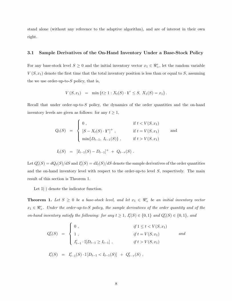
3.1 Sample Derivatives of the On-Hand Inventory Under a Base-Stock Policy

For any base-stock level S ≥ 0 and the initial inventory vector x1 ∈ <τ+, let the random variable

V (S, x1) denote the first time that the total inventory position is less than or equal to S, assuming

the we use order-up-to-S policy, that is,

V (S, x1) = min {t≥ 1 : Xt(S) · 1τ ≤ S, X1(S) = x1} .

Recall that under order-up-to-S policy, the dynamics of the order quantities and the on-hand

inventory levels are given as follows: for any t ≥ 1,

Qt(S) =

0 , if t < V (S, x1)

[S −Xt(S) · 1τ ]+ , if t = V (S, x1)

min{Dt−1, It−1(S)} , if t > V (S, x1)

and

It(S) = [It−1(S)−Dt−1]+ + Qt−τ (S) .

Let Q′t(S) = dQt(S)/dS and I ′t(S) = dIt(S)/dS denote the sample derivatives of the order quantities

and the on-hand inventory level with respect to the order-up-to level S, respectively. The main

result of this section is Theorem 1.

Let I(·) denote the indicator function.

Theorem 1. Let S ≥ 0 be a base-stock level, and let x1 ∈ <τ+ be an initial inventory vector

x1 ∈ <τ+. Under the order-up-to-S policy, the sample derivatives of the order quantity and of the

on-hand inventory satisfy the following: for any t ≥ 1, I ′t(S) ∈ {0, 1} and Q′t(S) ∈ {0, 1}, and

Q′t(S) =

0 , if 1 ≤ t < V (S, x1)

1 , if t = V (S, x1)

I ′t−1 · I[Dt−1 ≥ It−1] , if t > V (S, x1)

and

I ′t(S) = I ′t−1(S) · I [Dt−1 < It−1(S)] + Q′t−τ (S) ,

8

where we define I ′0(S) = 0 and Q′t(S) = 0 for all t ≤ 0. Moreover, for any t ≥ 1, with probability

one,

I ′t(S) +t∑

`=t−τ+1

Q′`(S) = 1.

Proof. The fact that Q′t(S) ∈ {0, 1} and I ′t(S) ∈ {0, 1} follows from Lemma 1 in Janakiraman

and Roundy (2004). The formulae for the derivatives Q′t(S) and I ′t(S) follow immediately from

the dynamics of the order quantities and the on-hand inventory under an order-up-to-S policy.

Moreover, it follows from Janakiraman and Roundy (2004) that for any t ≥ V (S, x1), It(S) =

S −∑t−1

`=t−τ min {I`(S), D`}. This implies

I ′t(S) = 1−t−1∑

`=t−τ

I ′`(S) · I [D` ≥ I`(S)] = 1−t∑

`=t−τ+1

Q′`(S),

where the last equality follows from the fact that Q′`(S) = I ′`−1(S) · I [D`−1 ≥ I`−1(S)] for ` ≥

V (S, x1) and Q′`(S) = 0 for ` < V (S, x1). This proves the desired result for t ≥ V (S, x1). For

t < V (S, x1), the result follows from the fact that I ′t(S) = 1 and Q′`(S) = 0 for all ` < V (S, x1).

Let N τ = {x ∈ {0, 1}τ :∑τ

i=1 xi ≤ 1} be the set of τ -dimensional binary vectors such that at

most one component is 1. Theorem 1 implies X ′t(S) =

(Q′

t−1(S), . . . , Q′t−τ+1(S), I ′t(S)

)∈ N τ .

3.2 A Sufficient Condition for Ergodicity of the Markov Chain Associated with

a Base-Stock Policy

In this section, we identify a sufficient condition for the Markov chain associated with a base-stock

policy to be ergodic. Under this condition, we establish the convergence rate for the Markov chain to

its stationary distribution. We introduce an augmented Markov chain X(S) = {(Xt(S), X ′t(S)) : t ≥ 1}

associated with an order-up-to-S policy and establish a sufficient condition for its ergodicity. We

let X(S) keep track of the inventory vector in each period as well as the sample derivatives of the

order quantities and the on-hand inventory. Define, for any t ≥ 1,

(Xt(S), X ′

t(S))

=(Qt−1(S), . . . , Qt−τ+1(S), It(S), Q′

t−1(S), . . . , Q′t−τ+1(S), I ′t(S)

).

Lemma 2. The stochastic process X(S) = {(Xt(S), X ′t(S)) : t ≥ 1} forms a Markov chain.

9

Proof. We first note that Xt+1(S) = (Qt(S), . . . , Qt−τ+2(S), It+1(S)) depends only on Xt(S) =

(Qt−1(S), . . . , Qt−τ+1(S), It(S)) and Dt. Moreover, it follows from Theorem 1 that

Q′t(S) = 1− I ′t(S)−

t−1∑`=t−τ+1

Q′`(S) and

I ′t+1(S) = 1−Q′t+1(S)−Q′

t(S)−t−1∑

`=t−τ+2

Q′`(S) ,

where Q′t+1(S) = I ′t(S) · I [Dt ≥ It]. This shows that X ′

t+1(S) depends only on Xt(S), X ′t(S), and

Dt, giving the desired result.

We will identify a sufficient condition for the ergodicity of the Markov chain X(S). Before we

proceed, we recall the definition of ergodicity (see Chapter 13 of Meyn and Tweedie (1993) for more

details). The Markov chain X(S) ={(Xt(S), Xt(S)) ∈ <τ

+ ×N τ : t ≥}

is ergodic if there exists a

random variable (X∞(S), X ′∞(S)) such that for any initial state (x1, x

′1) ∈ <τ

+ ×N τ ,

limt→∞

δt

(S, x1, x

′1

)= 0,

where, for any t ≥ 1,

δt

(S, x1, x

′1

)= sup

{∣∣∣P [(Xt(S), X ′t(S)

)∈ B |

(X1(S), X ′

1(S))

= (x1, x′1)]− P

[(X∞(S), X ′

∞(S))∈ B

] ∣∣∣ :

measurable set B ⊆ <τ+ ×N τ

}.

In such case, we say (X∞(S), X ′∞(S)) is the steady-state vector of X(S).

The main result of this section is stated in the following theorem that provides a sufficient

condition for the ergodicity of the Markov chain X(S). Furthermore, it shows that the convergence

rate is exponentially decreasing in t. The proof of this result appears in Section 3.3. For any S ≥ 0,

define

γ(S) = P [D ≤ S/(τ + 1)] .

Theorem 3. Let S ≥ 0 be a base-stock level. If γ(S) > 0, then the Markov chain X(S) =

{(Xt(S), X ′t(S)) : t ≥ 1} associated with an order-up-to-S policy is ergodic with a steady-state ran-

dom variable (X∞(S), X ′∞(S)). Furthermore, for any initial inventory vector (x1, x

′1) ∈ <τ

+ ×N τ ,

10

and t ≥ 4τ + 1,

δt+1

(S, x1, x

′1

)≤

(1− γ(S)2τ

)t/(4τ) + F (η)t2−τ , if D has an infinite support(

1− γ(S)2τ)t/(4τ) + exp(4η/D − 2µ2( t

2 − τ)/D2), if D ≤ D with probability one,

where F (·) denotes the distribution function of D with µ = E[D], and η = x1 · 1τ − S denotes the

difference between the initial inventory position x1 · 1τ and the order-up-to level S.

An Example of Non-Ergodicity

We now show that the Markov chain X(S) = {(Xt(S), X ′t(S)) : t = 1, 2, . . .} may not be ergodic if

the condition of Theorem 3 fails, that is, if γ(S) = 0. The key idea behind this example is that

if S is too small, then a stockout occurs in every period, which causes the after-delivery on-hand

inventory in each period t to be exactly the amount ordered in period t − τ . Thus, the inventory

vector Xt(S) follows a cyclic pattern.

Consider a base-stock level S such that there exists sufficiently small ε such that 0 < ε < τS

and γ(S + ε) = P [D ≤ (S + ε)/(τ + 1)] = 0. Suppose that the initial inventory vector X1(S) =

(Q0(S), Q−1(S), . . . , Q−τ+2(S), I1(S)) is given by

I1(S) =S

τ + 1+

ε

τ + 1and Qt(S) =

S

τ + 1− ε/τ

τ + 1for each t = −τ + 2, . . . , 1, 0 .

Then, the quantity ordered in period 1 is given by

Q1(S) = S − (Q0(S) + Q1(S) + · · ·+ Q−τ+2(S) + I1(S))

= S −(

(τ − 1) ·(

S

τ + 1− ε/τ

τ + 1

)+(

S

τ + 1+

ε

τ + 1

))= S −

(τ · S

τ + 1+

ε/τ

τ + 1

)=

S

τ + 1− ε/τ

τ + 1,

which is strictly positive since ε < Sτ . Since γ(S + ε) = 0, it follows that the event

D >S

τ + 1+

ε

τ + 1

occurs with probability 1, that is, D is greater than Q1(S) and each component of X1(S) with

probability 1. Thus, the process of inventory vectors {Xt(S) : t = 1, 2, . . .} follows a cyclic process

where at most one of the components of each inventory vector Xt(S) is S/(τ + 1) + ε/(τ + 1) and

all the other components are S/(τ + 1)− (ε/τ)/(τ + 1). Similarly, we can show that {X ′t(S) : t =

1, 2, . . .} is also cyclic.

11

3.3 Proof of Theorem 3

In this section, we prove Theorem 3. We first show this result for the case where the starting

inventory position at the beginning of period 1 is at most S (Lemma 4 in Case I), and then extend

the result to a general setting (Case II).

Case I: Initial Inventory Position is at Most S

The main idea used in this section is that all the sample paths couple after a certain pattern or

sequence of demands occurs. An example of such a demand pattern is the τ consecutive periods

of zero demands, which results in the on-hand inventory of S units with no outstanding order

regardless of the inventory vector before the pattern occurs. Yet, this particular example of zero

demands may never occur depending on the distribution of demand. Another example of demand

pattern, as we shall see, is as follows: the 2τ consecutive periods in each of which demand is at

most S/(τ + 1). This pattern of demands is used in the proof of Lemma 4.

Lemma 4. If γ(S) = P [D ≤ S/(τ + 1)] > 0, then the Markov chain X(S) = {(Xt(S), X ′t(S)) : t ≥ 1}

associated with the order-up-to-S policy is ergodic with a steady-state random vector (X∞(S), X ′∞(S)).

Moreover, for any t ≥ 2τ + 1, any initial inventory vector x1 ∈ <τ+ satisfying x1 · 1τ ≤ S, and any

x′1 ∈ N τ ,

δt+1

(S, x1, x

′1

)≤

(1− γ(S)2τ

)t/(2τ).

Proof. We make use of the following result on the uniform ergodicity of Markov chains (see Meyn

and Tweedie (1993) for more details). We say a measurable set U ⊆ <τ+ ×N τ is a small set with

respect to a nontrivial measure ν provided that there exists t∗ > 0 such that for any (x1, x′1) ∈ U

and any measurable set B ×N ⊆ <τ+ ×N τ ,

P[(

Xt∗(S), X ′t∗(S)

)∈ B ×N

∣∣∣ (X1(S), X ′1(S)

)= (x1, x

′1)]

≥ ν (B ×N) .

The following result appears in Theorem 16.0.2 in Meyn and Tweedie (1993). If U is a small set

with respect to ν, then there exists stationary random variable (X∞(S), X ′∞(S)) such that for any

(x1, x′1) ∈ U and t ≥ t∗,

δt+1

(S, x1, x

′1

)≤

(1− ν

(<τ

+ ×N τ))t/(t∗−1)

.

12

To apply the above result, we let U = {x ∈ <τ+ | x · 1τ ≤ S} × N τ . We define a nontrivial

measure ν such that U is a small set with respect to this measure ν with t∗ = 2τ + 1, and

ν(<τ

+ ×N τ)≥ γ(S)2τ . Let the measure ν be defined on <τ

+×N τ as follows. For any 0 ≤ ` ≤ τ−1,

let B` ⊆ <+ be any measurable set and let

B =

{(q−1, q−2, . . . , q−τ+1, i0) ∈ <τ

+

∣∣∣ q−` ∈ B` for 1 ≤ ` ≤ τ − 1, and S − i0 −τ−1∑`=1

q−` ∈ B0

}.

(Note that S − i0 −∑τ−1

`=1 q−` represents the order quantity associated with the state.) For any

subset N ⊆ N τ , define ν (B ×N) by

ν(B ×N) = γ(S)τ ·τ−1∏i=0

P[D ∈ Bi ∩

[0,

S

τ + 1

]]· I [(0, 0, . . . , 0, 1) ∈ N ] .

From the above definition of ν, it is straightforward to verify that ν(<τ

+ ×N τ)

= γ(S)2τ > 0.

Thus, to complete the proof, it remains to show that U is a small set with respect to ν where

t∗ = 2τ + 1. For any 1 ≤ i ≤ τ − 1, let Bi = Bi ∩ [0, S/(τ + 1)], and let B be defined similarly to

B, except that Bi’s are replaced by Bi’s. It follows that

P[(

X2τ+1(S), X ′2τ+1(S)

)∈ B ×N

∣∣∣ (X1(S), X ′1(S)

)=(x1, x

′1

)]≥ P

[(X2τ+1(S), X ′

2τ+1(S))∈ B ×N

∣∣∣ (X1(S), X ′1(S)

)=(x1, x

′1

)]From the definition of ν, it follows that ν (B ×N) = ν

(B ×N

). Thus, it suffices to show that

P[(

X2τ+1(S), X ′2τ+1(S)

)∈ B ×N

∣∣∣ (X1(S), X ′1(S)

)=(x1, x

′1

)]≥ ν

(B ×N

).

To prove the above inequality, we can assume without loss of generality that (0, . . . , 0, 1) ∈ N ;

otherwise, the definition of ν implies ν(B ×N

)= 0, and the result is trivially true. We consider

the following demand pattern of length 2τ , where the demand in each of the first τ periods is at most

S/(τ + 1) and the demands in the next τ periods satisfy D2τ−` ∈ Bi for each ` = 0, 1, . . . , τ − 1. It

is straightforward to verify that the probability of this event occurring is γ(S)τ ·∏τ−1

i=0 P[D ∈ Bi

].

We claim that the above demand pattern implies that

X2τ+1(S) = (Q2τ (S), . . . , Qτ+2(S), I2τ+1(S)) =

(D2τ−1, . . . , Dτ+1, S −

2τ∑`=τ+1

D`

),

X ′2τ+1(S) =

(Q′

2τ (S), . . . , Q′τ+2(S), I ′2τ+1(S)

)= (0, 0, . . . , 0, 1) .

To prove this claim, note that since the initial inventory position x1 · 1τ is less than or equal to

S, we have that Q1(S) = S − X1(S) · 1τ for the first period, and Qt+1(S) = min{Dt, It(S)} for

13

all t≥ 1. This implies that for 1 ≤ t ≤ 2τ , Qt+1(S) ≤ Dt ≤ S/(τ + 1). We will now show that

Qt+1(S) = Dt for τ + 1 ≤ t ≤ 2τ . Note that

Dt−1 ≥ Qt(S) = S −Xt(S) · 1τ = S − (Qt−τ+1(S) + Qt−τ+2(S) + · · ·+ Qt−1(S) + It(S)) .

By rearranging the above inequality and using the fact that Qt(S) ≤ S/(τ + 1) for all t, we obtain

It(S) ≥ S − (Qt−τ+1(S) + Qt−τ+2(S) + · · ·+ Qt−1(S))−Dt−1

≥ S − S(τ − 1)τ + 1

− S

τ + 1=

S

τ + 1,

and therefore Dt ≤ S/(τ + 1) ≤ It(S). This implies that Qt+1(S) = min{Dt, It(S)} = Dt for

τ+1 ≤ t ≤ 2τ . Thus, in particular, (Q2τ (S), Q2τ−1(S), . . . , Qτ+2(S)) = (D2τ−1, D2τ−2, . . . , Dτ+1).

Note that

I2τ+1(S) = X2τ+1(S) · 1τ −2τ∑

`=τ+2

Q`(S) = X2τ+1(S) · 1τ −2τ−1∑

`=τ+1

D`

= S −Q2τ+1(S)−2τ−1∑

`=τ+1

D` = S −D2τ −2τ−1∑

`=τ+1

D`,

where the third equality follows from the fact that Q2τ+1(S) = S − X2τ+1(S) · 1τ . The final

equality follows from the fact that Q2τ+1(S) = min{D2τ , I2τ (S)} = D2τ . Moreover, since Dt ≤ It

for τ + 1 ≤ t ≤ 2τ , it follows from Theorem 1 that

Q′τ+2(S) = Q′

τ+3(S) = · · · = Q′2τ+1(S) = 0,

which implies (by Theorem 1) that I ′2τ+1(S) = 1−∑2τ+1

`=τ+2 Q′`(S) = 1, completing the proof of the

claim.

Now, it follows from the claim that for 1 ≤ ` ≤ τ − 1, Q2τ+1−`(S) = D2τ−` ∈ B`, and

S−X2τ+1(S)·1τ = D2τ ∈ B0. Thus, X2τ+1(S) ∈ B and X ′2τ+1(S) ∈ N . Since the particular demand

pattern used in our proof has the probability of occurring of at least γ(S)τ ·∏τ−1

i=0 P[D ∈ Bi

], it

follows that

P[(

X2τ+1(S), X ′2τ+1(S)

)∈ B ×N

∣∣∣ (X1(S), X ′1(S)

)=(x1, x

′1

)]≥ γ(S)τ ·

τ−1∏i=0

P[D ∈ Bi

]= ν

(B ×N

),

which is the desired result.

14

The pattern of demand used in the proof of Lemma 4 has been carefully selected. In the first

τ periods, demands are small such that sufficiently large quantities of inventory become available

on-hand (as opposed to on-order) during the the second τ periods. The demands from period τ +1

to 2τ are small enough that they do not cause any stock out, in order to ensure that the vector

of outstanding orders in period 2τ + 1 are defined in terms of these demands without censoring.

The proof of Lemma 4 is based on recognizing a set of demand patterns such that if such a pattern

occurs, then all the sample paths will meet regardless of the state of the inventory vector before

the demand pattern occurs. Such a demand pattern is called the “coalescing pattern”, and has

been used by Cooper and Tweedie (2002) in the context of simulating an inventory system with

age-dependent perishability.

We examine the bound given in the statement of Lemma 4. If S is so small such that γ(S) =

P [D ∈ [0, S/(τ + 1)]] = 0, then this bound is equal to 1, and it is not meaningful. Otherwise, it

converges to 0 exponentially with respect to t, and the convergence rate improves as γ(S) increases,

i.e., the base-stock S increases.

Case II: Initial Inventory Position Exceeds S

We now extend the convergence result to the case where the initial inventory position may exceed

S. We need the following lemma. Recall that F (·) denote the distribution function of D and

µ = E [D].

Lemma 5. For any η ∈ < and t ≥ 1,

P

[t∑

`=1

D` ≤ η

]≤

F (η)t, if D has an infinite support

e4η/D · e−2tµ2/D2

, if D ≤ D with probability one.

Proof. It suffices to consider η ≥ 0. If the demand has an infinite support, then

P

[t∑

`=1

D` ≤ η

]≤ P [D` ≤ η for each 1 ≤ ` ≤ t] ≤ F (η)t.

If the demand is bounded above by D, then it follows from Chernoff-Hoeffding’s Inequality (Ho-

effding (1963)) that

P

[t∑

`=1

D` ≤ η

]= P

[t∑

`=1

(D` − µ) ≤ η − tµ

]≤ exp

{−2 (η − tµ)2

tD2

}.

15

Since exp(·) is an increasing function, and

−2 (η − tµ)2

tD2 =

−2η2 + 4ηtµ− 2t2µ2

tD2 ≤ 4ηµ/D

2 − 2tµ2/D2 ≤ 4η/D − 2tµ2/D

2,

we obtain the required result.

If the starting inventory position exceeds S, then under the order-up-to-S policy, the manager

does not place any order until the inventory position falls below S, and the Markov chain states

are transient. This result is shown in the following lemma. Recall µ = E [D].

Lemma 6. Consider an order-up-to-S policy, where S ≥ 0. For any starting inventory vector

x1 ∈ <τ+ and t ≥ τ ,

P [Xt(S) · 1τ > S | X1(S) = x1]

≤

F (x1 · 1τ − S)t−τ , if D has an infinite support

e4(x1·1τ−S)/D · e−2µ2(t−τ)/D2

, if D ≤ D with probability one.

Proof. Note that if the starting inventory position x1 · 1τ is at most S, then Xt(S) · 1τ ≤ S

with probability one for all t ≥ 1. Thus, the required result holds. We proceed by assuming

otherwise, that is, x1 · 1τ > S. By the description of the base-stock policy, max{Xt(S) · 1τ , S} ≤

max{X1(S) · 1τ , S} holds for any t ≥ 1. Thus,

P[D1 + D2 + · · ·+ Dt−τ < X1(S) · 1τ − S]

= P[Dτ + Dτ+1 + · · ·+ Dt−1 < X1(S) · 1τ − S]

≥ P[Dτ + Dτ+1 + · · ·+ Dt−1 < Xτ (S) · 1τ − S] ,

where the equality follows since demand distributions are independent and identically distributed.

Also, for t ≥ τ , observe that

Xt(S) · 1τ > S if and only if Xτ (S) · 1τ − (Dτ + Dτ+1 + · · ·+ Dt−1) > S.

Therefore, combining the above results,

P[Xt(S) · 1τ > S

∣∣∣ X1(S) = x1

]≤ P[D1 + D2 + · · ·+ Dt−τ < x1 · 1τ − S] .

The desired result then follows immediately from Lemma 5.

We are now ready to prove Theorem 3. The proof of Theorem 3 combines Lemmas 4 and 6.

16

Proof. We will prove the result when the demand D has an infinite support. An analogous argument

is applicable when D is bounded. If x1 · 1τ ≤ S, the result follows directly from Lemma 4. Thus,

we proceed by assuming that x1 · 1τ > S.

To facilitate our exposition, we fix the initial state (x1, x′1), and denote by E(x1,x′1) [·] and

P(x1,x′1) [·] expectation and probability that are conditioned on the event that (X1(S), X ′1(S)) =

(x1, x′1). By conditioning on the value of Xdt/2e(S) and X ′

dt/2e(S) and applying the Markov property,

it follows that, for any measurable set B ⊆ <τ+ ×N τ ,

P(x1,x′1)

[(Xt+1(S), X ′

t+1(S))∈ B

]= E(x1,x′1)

[P(x1,x′1)

[(Xt+1(S), X ′

t+1(S))∈ B

∣∣∣ Xdt/2e(S), X ′dt/2e(S)

]]= E(x1,x′1)

[I[Xdt/2e(S) · 1τ ≤ S

]· P[(

Xt+1(S), X ′t+1(S)

)∈ B

∣∣∣ Xdt/2e(S), X ′dt/2e(S)

] ]+E(x1,x′1)

[I[Xdt/2e(S) · 1τ > S

]· P[(

Xt+1(S), X ′t+1(S)

)∈ B

∣∣∣ Xdt/2e(S), X ′dt/2e(S)

] ].

Therefore, for any measurable set B ⊆ <τ+ ×N τ , we have

P(x1,x′1)

[(Xt+1(S), X ′

t+1(S))∈ B

]− P

[(X∞(S), X ′

∞(S))∈ B

]= E(x1,x′1)

[I[Xdt/2e(S) · 1τ ≤ S

]·∆(B)

]+ E(x1,x′1)

[I[Xdt/2e(S) · 1τ > S

]·∆(B)

],

where

∆(B) = P[(

Xt+1(S), X ′t+1(S)

)∈ B

∣∣∣ Xdt/2e(S), X ′dt/2e(S)

]− P

[(X∞(S), X ′

∞(S))∈ B

].

The random variable |∆(B)|, however, is bounded above almost surely by δt−dt/2e+2

(S, Xdt/2e(S), X ′

dt/2e(S))

by the definition of δt−dt/2e+2(·), and is also bounded above by 1. Therefore, we obtain∣∣∣P(x1,x′1)

[(Xt+1(S), X ′

t+1(S))∈ B

]− P

[(X∞(S), X ′

∞(S))∈ B

]∣∣∣≤ E(x1,x′1)

[I[Xdt/2e(S) · 1τ ≤ S

]· δt−dt/2e+2

(S, Xdt/2e(S), X ′

dt/2e(S))]

+ P(x1,x′1)

[Xdt/2e(S) · 1τ > S

].

We provide an upper bound on each term of the right-hand side of the above inequality. By Lemma

4, the first term satisfies

E(x1,x′1)

[I[Xdt/2e(S) · 1τ ≤ S

]· δt−dt/2e+2

(S, Xdt/2e(S), X ′

dt/2e(S))]

≤ P(x1,x′1)

[Xdt/2e(S) · 1τ ≤ S

]·(1− γ(S)2τ

)(t−dt/2e+1)/(2τ)

≤(1− γ(S)2τ

)(t−dt/2e+1)/(2τ)

≤(1− γ(S)2τ

)t/(4τ),

17

where the last inequality follows from the fact that t/(4τ) ≤ (t− dt/2e+ 1)/(2τ). Furthermore, by

Lemma 6, the second term satisfies

P(x1,x′1)

[Xdt/2e(S) · 1τ > S

]≤ F (x1 · 1τ − S)dt/2e−τ ≤ F (x1 · 1τ − S)

t2−τ .

Therefore, we obtain the required result from the definition of δt+1(S, x1, x′1).

3.4 Structure of the Cost Function and the Optimal Base-Stock Level

We now provide a characterization of the long-run average holding cost and lost sales penalty under

any order-up-to policy. The main result of this section is stated in the following theorem. Recall

γ(S) = P [D ≤ S/(τ + 1)]. To simplify our exposition, we use the expressions C (It(S)) to denote

the expected holding cost and lost sales penalty in period t under the order-up-to-S policy, that is,

C (It(S)) = h · E [It(S)−Dt]+ + b · E [It(S)−Dt]

+ ,

where the expectation is taken with respect to both the random variables Dt and It(S). Similarly,

we use C (I∞(S)) to denote the long-run average expected cost under the order-up-to-S policy.

Theorem 7. For any S ≥ 0, the long-run average holding cost and lost sales penalty under an order-

up-to-S policy always exists, is independent of the initial starting inventory vector, and satisfies

C (I∞(S)) := limT→∞

1T

T∑t=1

C (It(S)) =

b ·(E [D]− S

τ+1

), if γ(S) = 0,

b · E [D − I∞(S)]+ + h · E [I∞(S)−D]+ , if γ(S) > 0.

Moreover, the function C (I∞(S)) is convex and differentiable in S, and has a minimizer S∗ satis-

fying γ (S∗) > 0.

Proof. If γ(S) > 0, we know from Theorem 3 that the Markov chain X(S) = {(Xt(S), X ′t(S)) : t ≥ 1}

converges to the stationary random vector (X∞(S), X ′∞(S)), and the stated expression for the long-

run average cost follows from Markov chain theory. When γ(S) = 0, the existence of the long-run

average cost and its formula follow from Huh et al. (2006). It is easy to verify that C (I∞(S))

is continuous in S. The differentiability of C (I∞(·)) follows from the above formula since D is a

continuous random variable. Moreover, let S = sup {x : γ(x) = 0}. Using the analysis in Huh et al.

(2006), it is easy to verify that the left and the right derivatives of C (I∞(S)) at S are −b/(τ + 1),

i.e.,

limS↑S

d

dSC (I∞(S)) = lim

S↓S

d

dSC (I∞(S)) =

−b

τ + 1.

18

Thus, there exists a minimizing S∗ such that γ(S∗) > 0. For S > S, the convexity of C (I∞(S))

follows from Theorem 12 in Janakiraman and Roundy (2004). Since the function is linear for S < S

and the left and right derivatives at S coincide at S, the convexity of C (I∞(S)) follows for all S.

4. Sample-Based Estimation of the Cost and Its Derivative

To estimate the cost function C (I∞(S)) and its derivative with respect to S, one can run the

system for a long time, and obtain appropriate sample-based estimates. However, for any finite

t ≥ 1, the distribution of the state in period t is not in general exactly the same as the stationary

random vector, resulting in a bias in the above estimates. In this section, we establish error bounds

associated with sample-based estimates of the cost function C (I∞(S)) and its derivative. The main

result of this section is stated in the following theorem.

Theorem 8. Let S ≥ 0 be a base-stock level such that γ(S) = P [D ≤ S/(τ + 1)] > 0. Let

(x1, x′1) ∈ <τ

+×N τ . If we apply the order-up-to-S policy with the initial inventory vector X1(S) = x1

and X ′1(S) = x′1, then, for any t ≥ 1,

|C (I∞(S))− C (It(S))| ≤ (b + h) ·max {S, x1 · 1τ} · δt

(S, x1, x

′1

).

Moreover, ∣∣∣∣ d

dSC (I∞(S))− d

dSC (It(S))

∣∣∣∣ ≤ (b + h) · δt

(S, x1, x

′1

).

We first establish the following lemma before we prove Theorem 8.

Lemma 9. Under the conditions of Theorem 8,

(i)∣∣E [It(S)− d]+ − E [I∞(S)− d]+

∣∣ ≤ max {S, x1 · 1τ} · δt (S, x1, x′1), for any d.

(i)∣∣d− E [It(S)]+ − E [d− I∞(S)]+

∣∣ ≤ max {S, x1 · 1τ} · δt (S, x1, x′1), for any d.

(iii) |E [I [D < It(S)] · I ′t(S)]− E [I [D < I∞(S)] · I ′∞(S)]| ≤ δt (S, x1, x′1) .

(iv) |E [I [D ≥ It(S)] · I ′t(S)]− E [I [D ≥ I∞(S)] · I ′∞(S)]| ≤ δt (S, x1, x′1) .

Proof. To prove part (i), note that by definition of order-up-to-S policy, both random variables It(S)

and I∞(S) are bounded above by max {S, x1 · 1τ} with probability one. Since they are nonnegative

19

random variables, it follows that, for any d ≥ 0,

∣∣E [It(S)− d]+ − E [I∞(S)− d]+∣∣ =

∣∣∣∣∣∫ max{S,x1·1τ}

0{P [It(S)− d > z]− P [I∞(S)− d > z]} dz

∣∣∣∣∣≤

∫ max{S,x1·1τ}

0|P [It(S) > z + d]− P [I∞(S) > z + d]| dz

≤∫ max{S,x1·1τ}

0δt

(S, x1, x

′1

)dz

= max {S, x1 · 1τ} · δt

(S, x1, x

′1

),

where the second inequality follows from the definition of δ(S, x1, x′1), establishing (i). Similarly,

(ii) holds.

Now, we prove (iii). By Theorem 1, I ′t(S) is binary. It follows that I ′∞(S) is also binary with

probability one. (To see this, suppose there exists a measurable set B ⊆ <+ \ {0, 1} such that

P[I ′∞(S) ∈ B] > 0. Then, let B ={(

q−1, . . . , q−τ+1, i0, q′−1, . . . , q′−τ+1, i

′0

)∈ <τ

+ ×N τ∣∣ i′0 ∈ B

}.

Thus, P [(X∞(S), X ′∞(S)) ∈ B] > 0, but P [(Xt(S), X ′

t(S)) ∈ B] = 0 for each t ≥ 1. Therefore,

δt (S, x1, x′1) does not converge to 0 as t →∞, contradicting Theorem 3.)

For any value of D = d, let

B(d) ={(

q−1, . . . , q−τ+1, i0, q′−1, . . . , q′−τ+1, i

′0

)∈ <τ

+ ×N τ∣∣ i0 > d, i′0 = 1

}.

Thus, for any fixed value of D = d,

E[I [d < It(S)] · I ′t(S)

]− E

[I [d < I∞(S)] · I ′∞(S)

]= E

[I[d < It(S), I ′t(S) = 1

]]− E

[I[d < I∞(S), I ′∞(S) = 1

]]= P

[d < It(S), I ′t(S) = 1

]− P

[d < I∞(S), I ′∞(S) = 1

]= P

[(Xt(S), X ′

t(S))∈ B(d)

]− P

[(X∞(S), X ′

∞(S))∈ B(d)

].

The absolute value of the above expression is bounded above by δt (S, x1, x′1). By taking the

expectation with respect to D, we establish (iii). Similarly, (iv) holds.

Let us now prove Theorem 8.

Proof. Note that by definition of C(·),

C (It(S)) = h · E[(It(S)−D)+

]+ b · E

[(D − It(S))+

]C (I∞(S)) = h · E

[(I∞(S)−D)+

]+ b · E

[(D − I∞(S))+

].

20

It follows from Lemma 9 (i) and (ii) that

|C (It(S))− C (I∞(S))|

≤ h ·∣∣∣E [It(S)−D]+ − E [I∞(S)−D]+

∣∣∣+ b ·∣∣∣E [(D − It(S))+

]− E

[(D − I∞(S))+

] ∣∣∣≤ (h + b) ·max {S, x1 · 1τ} · δt

(S, x1, x

′1

)which proves the first inequality.

Now, from Section 3.4, recall

d

dSC (It(S)) = h · E

[I [D < It(S)] · I ′t(S)

]− b · E

[I [D ≥ It(S)] · I ′t(S)

], and

d

dSC (I∞(S)) = h · E

[I [D < I∞(S)] · I ′∞(S)

]− b · E

[I [D ≥ I∞(S)] · I ′∞(S)

].

Thus, ∣∣∣∣ d

dSC (It(S))− d

dSC (I∞(S))

∣∣∣∣≤ h ·

∣∣E [I [D < It(S)] · I ′t(S)]− E

[I [D < I∞(S)] · I ′∞(S)

]∣∣+ b ·

∣∣E [I [D ≥ It(S)] · I ′t(S)]− E

[I [D ≥ I∞(S)] · I ′∞(S)

]∣∣≤ (h + b) · δt

(S, x1, x

′1

).

where the first inequality above follows from Lemma 9 (iii) and (iv).

5. An Adaptive Algorithm

Building upon the results of the previous two sections, we propose an adaptive algorithm that

determines the base-stock level for each period, where the decision in each period depends only on

the observed sales data in the past. We also establish the convergence rate of our algorithm. As a

benchmark, we compare the running average holding cost and lost sales penalty of our algorithm

to the cost of the optimal base-stock policy. Let S∗ be the optimal base-stock level. We make the

following assumption throughout Section 5.

Assumption 1. The manager has an a priori knowledge of a lower bound M ≥ 0 and an upper

bound M ≥ 0 on S∗, i.e., M ≤ S∗ ≤ M , and γ (M) = P[D ≤ M/(τ + 1)] > 0.

We note for any demand distribution with positive probability at zero, the choice of M = 0

satisfies the condition of Assumption 1. Throughout the remainder of this section, we will also

21

assume without loss of generality that the demand random variable has an infinite support. We

emphasize that this assumption is taken primarily to simplify our exposition and the formula for

the error bounds. When the demand is bounded almost surely, exactly the same argument applies.

(See the error bounds given in Theorem 3.)

5.1 Description of the Algorithm

Leveraging the convexity of C (I∞(S)) as a function of the order-up-to level S, we extend the

existing result from the online convex optimization literature, which requires an unbiased estimate

of the gradient dC (I∞(S)) /dS of the cost function. However, in our case, it is difficult to obtain

an unbiased sample of the cost and its derivative because they depend on the steady-state on-hand

inventory level I∞(S).

To address this problem, we divide time into a sequence of cycles. We maintain the same

base-stock level within a cycle. Base-stock levels may be adjusted from one cycle to another.

Let Sk denote the order-up-to level for the kth cycle. We will use the sample derivative of the

cost function evaluated in the last period of the cycle as a proxy for dC (I∞(Sk)) /dS, which will

be discussed subsequently. If the length of the kth cycle is sufficiently long, the ergodicity of the

Markov chain {(Xt(Sk), X ′t(Sk)) : t ≥ 1} should ensure that our estimate has a small bias compared

to dC (I∞(Sk)) /dS.

Our adaptive algorithm, which we refer to as Adaptive(α, β), is parameterized by two param-

eters α, β ∈ (0, 1). The first parameter α controls the adjustment of the order-up-to level between

two successive cycles while the second parameter β controls the length of each cycle. We use k to

index cycles and j to index periods within a given cycle. Let (k, j) denote the jth period in the kth

cycle. We now describe the algorithm in details.

Algorithm Adaptive(α, β)

Initialization: For the first cycle, set the order-up-to level S1 to any number in[M,M

], and set

the initial inventory vector X(1,1) ∈ <τ+ such that X(1,1) · 1τ ≤ M .

Algorithm Definition: For each cycle k = 1, 2, . . . ,

• The length of cycle k, denoted by Tk, is defined by Tk :=⌈kβ⌉, and cycle k begins at period∑k−1

k′=1 Tk′ + 1 and ends at∑k

k′=1 Tk′ (inclusive).

22

• Let Sk denote the base-stock level for this cycle. The initial inventory vector in cycle k is given

by X(k,1). We will use the order-up-to-Sk policy for every period in cycle k. Let X(k,j) and

I(k,j)(Sk;X(k,1)) denote the inventory vector and the on-hand inventory level, respectively, in

the jth period of the kth cycle.

• For each period 1 ≤ j ≤ Tk in cycle k, compute an estimate of the sample-path derivative of

the on-hand inventory I ′(k,j)

(Sk;X(k,1)

)using the following recursion from Theorem 1:

I ′(k,j)

(Sk;X(k,1)

)= 1−

j−1∑`=j−τ

I ′(k,`)

(Sk;X(k,1)

)· I[I(k,`)

(Sk;X(k,1)

)≤ D(k,`)

],

where D(k,`) is the realized demand in the `th period of the kth cycle. Note that we define

I ′(k,j)

(Sk;X(k,1)

)= 0 if j ≤ 0. Thus, to compute the sample-based derivative in each period,

we only need to keep the derivative values from at most the τ previous periods. Moreover,

note that the event I[I(k,`)

(Sk;X(k,1)

)≤ D(k,`)

]can be computed based on the sales data in

the `th period of the jth cycle. We simply need to check whether or not we have a stockout.

• At the end of the kth cycle (period Tk of the kth cycle), update the base-stock level as follows.

Let

εk =(M −M)

max{b, h} · kα,

and let Hk(Sk) be defined by

Hk(Sk) =

h, if I ′(k,Tk)(Sk;X(k,1)) = 1 and I(k,Tk) > D(k,Tk),

−b, if I ′(k,Tk)(Sk;X(k,1)) = 1 and I(k,Tk) ≤ D(k,Tk),

0, if I ′(k,Tk)(Sk;X(k,1)) = 0.

The base-stock level for the cycle k + 1 is then given by

Sk+1 = P[M,M ](Sk − εk ·Hk(Sk)) ,

where P[M,M ](z) = max{M, min{z,M)} is the projection operator.

• The initial inventory vector X(k+1,1) for cycle k + 1 will correspond to the inventory vector

after ordering at the end of the last period of cycle k (period Tk).

For any L ≥ 1, let N(L) =∑L

k=1 Tk denote the total number of time periods after L cycles.

We define the L-cycle regret Λ(L) as follows:

Λ(L) = E

L∑k=1

Tk∑j=1

C(I(k,j)(Sk;X(k,1)))

− E [C(I∞(S∗))] ·N(L) ,

23

where S∗ is the optimal base-stock level. The main result of this section is that the L-cycle

per-period average regret, the expression Λ(L) divided by N(L), converges to zero at the rate of

O(N(L)−1/3

)if the α and β parameters are chosen carefully. This result is stated in Theorem 10,

whose proof is given in Section 5.3.

Theorem 10. Under Assumption 1, let ν = max{1− γ(M)2τ , F (M), 1/e

}. Then, for any α, β ∈

(0, 1), the L-cycle per-period average regret under the algorithm Adaptive(α, β) satisfies

Λ(L)N(L)

≤ (b + h) ·(M −M

)·

{C1 (α, β)

N(L)1−α1+β

+C2 (α, β)

N(L)α

1+β

+C3 (α, β)

N(L)1

1+β

+C4 (α, β)

N(L)β

1+β

},

where the constants are given by:

C1 (α, β) = 4,

C2 (α, β) =4

1− α,

C3 (α, β) =12 (4τ)1/β Γ (1/β) (1/β)

(ln (1/ν))1/β,

C4 (α, β) =24τ

ln (1/ν),

and Γ(·) denotes the Gamma function. If we set α = β = 1/2, then Λ(L)/N(L) = O(N(L)−1/3

).

5.2 Preliminary Results

Online convex optimization is the minimization of a convex function, for which little is known a

priori except the convexity of the objective function. At each iteration, we choose a point in the

feasible region and incur the cost associated with this point; however, we obtain some information

about the function at this point, such as the gradient or its stochastic estimator. The objective is to

minimize the average cost over time. The following theorem appears in Huh and Rusmevichientong

(2006a). Note that for any compact set S, PS(·) denotes the projection operator on S.

Theorem 11. Let Φ : S → R be a convex function and let z∗ = arg minz∈S Φ(z) be its minimizer.

For any z ∈ S, let Ht(z) be an n-dimensional random vector defined on S, and suppose that there

exists B > 0 such that E[‖Ht(z)‖2

]≤ B

2 holds for all z ∈ S. Let the sequence (Zt : t ≥ 1) be

defined by

Zt+1 = PS (Zt − εt ·Ht(Zt)) , where εt =ζ diam(S)

B· 1tα

24

for some ζ > 0 and α ∈ (0, 1), where Z1 is any point in S. Let ηA(z) = E [Ht(z) | z]−5Φ(z) .

Then, for all T ≥ 1,

T∑t=1

E [Φ(Zt)− Φ(z∗)] ≤ diam(S)

{B ·[Tα

2ζ+

ζ T 1−α

2(1− α)

]+

T∑t=1

E∣∣ηA(Zt)

∣∣} .

The next two lemmas are used in the analysis of Section 5.3 and their proofs appear in Appendix

A. Let Γ(·) represent the gamma function, which is defined by Γ(z) =∫∞0 wz−1e−wdw for any real

number z > 0.

Lemma 12. For any ρ ∈ (0, 1), β ∈ (0, 1), and L ≥ 1,

L∑k=1

ρdkβe ≤

L∑k=1

ρkβ ≤ Γ (1/β) (1/β)

(ln (1/ρ))1/β.

From the description the algorithm described in Section 5.1, Tk = dkβe is the length of the kth

cycle, and N(k) =∑k

k′=1 Tk′ denote the total length of the first k cycles. The following lemma

establishes the relationship among k, dkβe and N(k).

Lemma 13. Let β ∈ (0, 1). For k ≥ 1, let N(k) =∑k

k′=1dk′βe. Then,

(i) k ≤ [(β + 1) ·N(k)]1/(β+1).

(ii) k · dkβe ≤ 2(β + 1) ·N(k).

(iii) dkβe ≤ 2 [(β + 1) ·N(k)]β/(β+1).

(iv) dkβeα ≤ 2 [(β + 1) ·N(k)]αβ/(β+1) for any α ∈ (0, 1).

5.3 Proof of Theorem 10

We express the L-cycle total regret Λ(L) as a sum of the following two expressions:

Λ1(L) =L∑

k=1

Tk · {E [C(I∞(Sk))]− E [C(I∞(S∗))]} , and

Λ2(L) = E

L∑k=1

Tk∑j=1

{C(I(k,j)(Sk;X(k,1)))− C(I∞(Sk))

} .

The first expression Λ1(L) corresponds to the regret due to the deviation of Sk from S∗, and the

second expression Λ2(L) reflects how much the on-hand inventory levels {I(k,j) | j = 1, 2, . . . Tk}

25

differ from the stationary on-hand inventory level. We provide an upper bound for each term in

Lemma 14 and 15.

Let ν = max{1− γ(M)2τ , F (M), 1/e

}.

Lemma 14. Suppose Assumption 1 holds and D has an infinite support. Then, for any α, β ∈

(0, 1), the algorithm Adaptive(α, β) satisfies

Λ1(L) ≤(M −M

)· (b + h) · TL ·

{Lα

2+

L1−α

2(1− α)+

3 (4τ)1/β Γ (1/β) (1/β)

(ln (1/ν))1/β

}.

Proof. From the definition of Λ1(L) and the fact that T1 ≤ · · · ≤ TL, we have

Λ1(L)TL

≤L∑

k=1

{E [C(I∞(Sk))]− E [C(I∞(S∗))]} .

From Theorem 7, E [C(I∞(S))] is a convex function of the base-stock level S. Moreover, the

dynamics of Sk defined in the algorithm Adaptive(α, β) are exactly the same as the gradient

descent method defined in Theorem 11, with S =[M,M

], ζ = 1, and B = max{b, h}. Thus, we

obtain

L∑k=1

{E [C(I∞(Sk))]− E [C(I∞(S∗))]}

≤(M −M

)·

{max{b, h} ·

[Lα

2+

L1−α

2(1− α)

]+

L∑k=1

E∣∣ηA(Sk)

∣∣} ,

where

ηA(S) =d

dSE[C(I(k,Tk)(S;X(k,1)))

]− d

dSE [C(I∞(S))] . (2)

Note max{b, h} ≤ b + h.

We will now establish an upper bound for∑L

k=1 E∣∣ηA(Sk)

∣∣. There are two cases to consider:

dkβe ≤ 4τ and dkβe ≥ 4τ+1. Suppose that dkβe ≤ 4τ . The definition of C(·) implies C ′(·) ∈ [−b, h].

From I ′(k,Tk)(S;X(k,1)) ∈ {0, 1} for all k, it follows that∣∣ηA(Sk)

∣∣ ≤ b + h. Note that the condition

dkβe ≤ 4τ is equivalent to k ≤ (4τ)1/β , which implies that

L∑k=1

∣∣ηA(Sk)∣∣ · I[dkβe ≤ 4τ ] ≤ (b + h) · (4τ)1/β .

26

Suppose that dkβe ≥ 4τ + 1. Let ηk = X(k,1) · 1τ −Sk. Theorem 3, Theorem 8 and Assumption

1 imply that

∣∣ηA(Sk)∣∣ ≤ (b + h) ·

[(1− γ(Sk)2τ

)dkβe/(4τ) + F (ηk)dkβe/2−τ

]≤ (b + h) ·

[(1− γ(M)2τ

)dkβe/(4τ) + F (M)dkβe/2−τ

]≤ 2(b + h) ·max

{(1− γ(M)2τ

), F (M)

}dkβe/(4τ)

≤ 2(b + h) · νdkβe/(4τ),

where the second inequality follows from the fact that γ(·) and F (·) are nondecreasing functions.

The third inequality follows from the fact that⌈kβ⌉≥ 4τ + 1 and τ ≥ 1, which implies that

dkβe/(4τ) ≤ dkβe/2− τ . It thus follows from Lemma 12 that

L∑k=1

∣∣ηA(Sk)∣∣ · I[dkβe ≥ 4τ + 1] ≤ 2(b + h) · Γ (1/β) (1/β)(

ln(1/ν1/(4τ)

))1/β

= 2(b + h) · (4τ)1/β · Γ (1/β) (1/β)

(ln (1/ν))1/β.

Combining the two cases, we see that

L∑k=1

∣∣ηA(Sk)∣∣ ≤ (4τ)1/β ·

((b + h) +

2(b + h) · Γ (1/β) (1/β)

(ln (1/ν))1/β

)

≤ 3(b + h) · (4τ)1/β Γ (1/β) (1/β)

(ln (1/ν))1/β,

where the last inequality follows from the fact that 0 ≤ ln(1/ν) ≤ 1 and 1 ≤ Γ(1/β)(1/β), and we

obtain the required result.

Lemma 15. Suppose Assumption 1 holds and D has an infinite support. Then, for any α, β ∈

(0, 1), the algorithm Adaptive(α, β) satisfies

Λ2(L) ≤ (b + h) · (M −M) · L · 12τ

ln (1/ν).

Proof. Recall that

Λ2(L) = E

L∑k=1

Tk∑j=1

{C(I(k,j)(Sk;X(k,1)))− C(I∞(Sk))

} .

Consider the summand C(I(k,j)(Sk;X(k,1))) − C(I∞(Sk)) for 1 ≤ j ≤ Tk. There are two cases to

consider: j ≤ 4τ and j ≥ 4τ + 1. Suppose j ≤ 4τ . By the convexity of the cost function C (·),

27

∣∣E [C(I(k,j)(Sk;X(k,1)))]− E [C(I∞(Sk))]

∣∣ is bounded above by (M −M) ·max{b, h}. Therefore,

Tk∑j=1

∣∣E [C(I(k,j)(Sk;X(k,1)))]− E [C(I∞(Sk))]

∣∣ · I[j ≤ 4τ ] ≤ 4 · τ · (M −M) ·max{b, h} .

Now, suppose j ≥ 4τ + 1. By Theorem 8,

∣∣E [C(I(k,j)(Sk;X(k,1)))]− E [C(I∞(Sk))]

∣∣≤ (b + h) · (M −M) ·

[(1− γ(M)2τ

)j/(4τ) + F (M)j/2−τ]

.

Therefore,

Tk∑j=1

∣∣E [C(I(k,j)(Sk;X(k,1)))]− E [C(I∞(Sk))]

∣∣ · I[j ≥ 4τ + 1]

≤ (b + h) · (M −M) ·Tk∑j=1

[(1− γ(M)2τ

)j/(4τ) + F (M)j/2−τ]

≤ 2(b + h) · (M −M) ·Tk∑j=1

max{1− γ(M)2τ , F (M)

}j/(4τ)

≤ 2(b + h) · (M −M) ·∫ ∞

0νz/(4τ)dz

= 2(b + h) · (M −M) · 4τ

ln (1/ν),

where the second inequality follows from the fact that j ≥ 4τ + 1, which implies that j/(4τ) ≤

j/2− τ . The last inequality follows from max{1− γ(M)2τ , F (M)

}≤ ν < 1.

Combining the two cases, it follows that

Tk∑j=1

∣∣E [C(I(k,j)(Sk;X(k,1)))]− E [C(I∞(Sk))]

∣∣≤ 4 · τ · (M −M) ·

(max{b, h}+

2(b + h)ln (1/ν)

)≤ (b + h) · (M −M) · 12τ

ln (1/ν),

where we use the fact that 0 ≤ ln(1/ν) ≤ 1 for the second inequality. Summing the above inequality

over all possible values of k = 1, . . . , L gives the required result.

We will now prove Theorem 10.

28

Proof. From Lemma 14, we have

Λ1(L) ≤(M −M

)· (b + h) · TL ·

{Lα

2+

L1−α

2(1− α)+

3 (4τ)1/β Γ (1/β) (1/β)

(ln (1/ν))1/β

}Λ2(L) ≤

(M −M

)· (b + h) · L · 12τ

ln (1/ν).

It follows from Lemma 13 and TL = dLβe that

TL · Lα =(L ·⌈Lβ⌉)α

·⌈Lβ⌉1−α

≤ (2 · (β + 1) ·N(L))α · 2 · ((β + 1) ·N(L))(1−α)β/(β+1)

= 21+α(β + 1)α+(1−α)β/(β+1) ·N(L)α+(1−α)β/(β+1)

≤ 8 ·N(L)(α+β)/(1+β).

A similar argument shows that TL · L1−α ≤ 8 ·N(L)(1−α+β)/(1+β). Also, by Lemma 13,

TL = dLβe ≤ 2 ((β + 1) ·N(L))β/(β+1) ≤ 4N(L)β/(1+β) .

Thus, we obtain

Λ1(L)N(L)

≤(M −M

)· (b + h) ·

{4

N(L)(1−α)/(1+β)+

4/(1− α)N(L)α/(1+β)

+12 (4τ)1/β Γ (1/β) (1/β)

(ln (1/ν))1/β ·N(L)1/(1+β)

}.

Since L ≤ ((β + 1)N(L))1/(1+β) ≤ 2 ·N(L)1/(1+β) by Lemma 13,

Λ2(L)N(L)

≤(M −M

)· (b + h) · 24τ

ln (1/ν) ·N(L)β/(1+β).

Combining the above two inequalities gives the desired result.

5.4 Remarks

Theorem 10 shows that the T -period expected running-average is O(T−1/3

). The proof of Theorem

10 can easily be modified for other stochastic systems where the gradient depends on the steady-

state distribution. We require, as in most papers in the online convex optimization literature, that

the objective is convex with respect to the decision vector, the feasible set is a convex compact set,

and the gradient of the objective function is bounded. Furthermore, the Markov chain obtained by

fixing the decision vector displays the property that both the sample costs and the sample derivatives

converge to their steady-state distributions, and that their convergence rates are exponential and

independent of the decision vector (analogous to Theorem 8). Then the arguments in the proof of

Theorem 10 also become applicable.

29

We explain the above generalization in more detail. Suppose S is a control parameter that we

want to optimize. Let Xt(S) denote the state vector of the system in period t, and let X ′t(S) denote

the sample derivative of Xt(S) with respect to S. Let X(S) = {(Xt(S), X ′t(S) : t ≥ 1)}. Suppose

that the following conditions are satisfied. (i) The feasible set S of S is convex and compact. (ii) For

any S ∈ S, X(S) is a Markov chain, and its state space belongs to a bounded set M independent

of S. (iii) For any S ∈ S, X(S) is ergodic, and the rate of convergence δt can be uniformly bounded

by an exponentially decreasing function, regardless of S and the initial state (analogous to Lemma

4 and 5). (iv) The average-cost criterion, denoted by C(X∞(S)), is convex with respect to S. (v)

In period t, the manager can obtain the estimates for both the cost and the derivatives having

biases whose magnitudes are no more than a multiple of δt (analogous to Theorem 8).

Conditions (i) and (iv) above ensure that the problem is a convex minimization problem over

a compact set, a requirement for applying Theorem 11. This theorem, together with the bound

on the bias of the derivative estimators in Condition (v), implies a result similar to Lemma 14.

Meanwhile, Conditions (ii) and (iii) ensure that the stationary process exists for any choice of the

control, and the convergence rate (mixing time) can be uniformly bounded for each cycle. These

conditions, along with the bound on the bias of the cost estimators in Condition (v), imply a result

similar to Lemma 15. Therefore, we establish a result analogous to Theorem 10, and show that the

algorithm Adaptive(α, β) can be easily adapted to result in the time-average regret of O(T−1/3).

6. Conclusion

In this paper, we have considered an adaptive control of replenishment quantities in a periodic-

review inventory system with lost sales and a positive lead time. Contrary to the classical inventory

literature, the manager does not know the demand distribution a priori, and only observes the

sales data in each period. Under the long-run average-cost criterion, we have proposed an adaptive

method such that its T -period average cost converges to the cost of the optimal base-stock policy,

and we have shown the convergence rate of O(1/T 1/3). We achieve this by characterizing the

ergodicity and the mixing time of the inventory system under a fixed base-stock policy. We believe

that our adaptive method is applicable to other settings where the objective function is convex

with respect to the control variable, and depends on the steady-state distribution of a system

under consideration.

30

References

Agrawal, N., and S. A. Smith. 1996. Estimating Negative Binomial Demand for Retail Inventory

Management with Unobservable Lost Sales. Naval Research Logistics 43:839–861.

Burnetas, A. N., and C. E. Smith. 2000. Adaptive Ordering and Pricing For Perishable Products.

Operations Research 48 (3): 436–443.

Cooper, W. L., and R. L. Tweedie. 2002. Perfect Simulation of an Inventory Model for Perishable

Products. Stochastic Models 18.

Godfrey, G. A., and W. B. Powell. 2001. An Adaptive, Distribution-Free Algorithm for the Newsven-

dor Problem with Censored Demands, with Applications to Inventory and Distribution. Man-

agement Science 47:1101–1112.

Hoeffding, W. 1963. Probability inequalities for sums of bounded random variables. Journal of the

American Statistical Association 58:13–30.

Huh, W. T., G. Janakiraman, J. Muckstadt, and P. Rusmevichientong. 2006. Asymptotic Opti-

mality of Order-up-to Policies in Lost Sales Inventory Systems. Working Paper .

Huh, W. T., and P. Rusmevichientong. 2006a. Adaptive Capacity Allocation with Censored De-

mand Data: Application of Concave Umbrella Functions. Working Paper .

Huh, W. T., and P. Rusmevichientong. 2006b. An Asymptotic Analysis of Inventory Planning with

Censored Demand. Working Paper .

Janakiraman, G., and R. Roundy. 2004. Lost-Sales Problems with Stochastic Lead Times: Con-

vexity Results for Base-Stock Policies. Operations Research 52:795–803.

Karlin, S., and H. Scarf. 1958. Inventory Models of the Arrow-Harris-Marschak Type with Time Leg.

In Studies in the Mathematical Theorey of Inventory and Production, ed. K. Arrow, S. Karlin,

and H. Scarf.

Levi, R., G. Janakiraman, and M. Nagarajan. 2006. Provably Near-Optimal Balancing Policies for

Stochastic Inventory Control Models with Lost Sales. Working Paper .

Meyn, S. P., and R. L. Tweedie. 1993. Markov Chains and Stochastic Stability. Springer-Verlag.

31

Morton, T. 1971. The Near-Myopic Nature of the Lagged-Proportional-Cost Inventory Problem

with Lost Sales. Operations Research 19.

Morton, T. E. 1969. Bounds on the Solution of the Lagged Optimal Inventory Equation with no

Demand Backlogging and Proportional Costs. SIAM Review 11 (4): 572–596.

Nahmias, S. 1994. Demand Estimation in Lost Sales Inventory Systems. Naval Research Logis-

tics 41:739–757.

Powell, W., A. Ruszczynski, and H. Topaloglu. 2004. Learning Algorithms for Separable Approxi-

mations of Discrete Stochastic Optimization Problems. Mathematics of Operations Research 29

(4): 814–836.

Reiman, M. 2004. A New and Simple Policy for the Continuous Review Lost Sales Inventory Model.

Working Paper .

Zipkin, P. 2006a. Old and New Methods for Lost-Sales Inventory Systems. Working Paper .

Zipkin, P. 2006b. On the Structure of Lost-Sales Inventory Models. Working Paper, Duke Univer-

sity.

A. Proof of Lemma 12 and 13

We now prove Lemma 12.

Proof. The first inequality follows easily from ρ ∈ (0, 1) and dkβe ≥ kβ. For the second inequality,

observe∑L

k=1 ρkβ ≤∫ Lu=0 ρuβ

du. Using the substitution y = uβ , obtain∫ L

u=0ρuβ

du =1β

∫ Lβ

y=0y−(β−1)/βρydy

=1β

∫ Lβ

y=0y1/β−1 exp

(−y

−1/ ln ρ

)dy

=Γ(1/β) · (−1/ln ρ)1/β

β·∫ Lβ

y=0

(−1/ln ρ)−1/β

Γ(1/β)· y1/β−1 exp

(−y

−1/ ln ρ

)dy .

Here, the integral corresponds to the cumulative distribution of a gamma distribution at Lβ ,

where the gamma distribution has the shape parameter 1/β and the scale parameter −1/ ln ρ.

32

Since the cumulative density is at most 1, it follows that the above expression is at most β−1 ·

Γ(1/β) · (−1/ln ρ)1/β .

We now prove Lemma 13.

Proof. Observe that

N(k) =k∑

k′=1

dk′βe ≥k∑

k′=1

k′β ≥

∫ k

u=0uβdu =

uβ+1

β + 1

∣∣∣∣∣k

0

=kβ+1

β + 1.

Therefore, N(k) ≥ kβ+1/(β + 1), which implyies part (i). From above, we also obtain

N(k) ≥ kβ+1

β + 1=

k · kβ

β + 1≥ k · (dkβe − 1)

β + 1,

which implies that k · dkβe ≤ (β + 1)N(k) + k. Thus, from part (i), we obtain k · dkβe ≤ (β + 1) ·

N(k) + [(β + 1) ·N(k)]1/(β+1), which in turn implies part (ii).

For (iii), observe that dkβe ≤ kβ + 1. From part (i), it follows

dkβe ≤ 1 + kβ ≤ 1 + [(β + 1) ·N(k)]β/(β+1) . (3)

Since N(k) ≥ 1, we obtain part (iii). To prove part (iv), consider f(u) = uα where α ∈ (0, 1). Since

f is a concave function,

(1 + u)α = f(1 + u) ≤ f(u) + 1 · f ′(u) = uα + α · uα−1 ≤ uα + 1

for u ≥ 1. Apply the above inequality to u = [(β + 1) ·N(k)]β/(β+1) ≥ 1, to obtain

(1 + [(β + 1) ·N(k)]β/(β+1))α ≤ [(β + 1) ·N(k)]αβ/(β+1) + 1 .

Then, (3) implies dkβeα ≤ 1 + [(β + 1) ·N(k)]αβ/(β+1), from which we obtain part (iv).

33