Robust Optimal Adaptive Control Method with Large Adaptive Gain

Robust Optimal Adaptive Control Method with Large AdaptiveGain

Nhan T. Nguyen∗

NASA Ames Research Center, Moffett Field, CA 94035

In the presence of large uncertainties, a control system needs to be able to adapt rapidly to regain per-formance. Fast adaptation is referred to the implementation of adaptive control with a large adaptive gain toreduce the tracking error rapidly. However, a large adaptive gain can lead to high-frequency oscillations whichcan adversely affect robustness of an adaptive control law.A new adaptive control modification is presentedthat can achieve robust adaptation with a large adaptive gain without incurring high-frequency oscillations aswith the standard model-reference adaptive control. The modification is based on the minimization of theL2norm of the tracking error, which is formulated as an optimal control problem. The optimality condition isused to derive the modification using the gradient method. The optimal control modification results in a stableadaptation and allows a large adaptive gain to be used for better tracking while providing sufficient stabilityrobustness. Simulations were conducted for a damaged generic transport aircraft with both standard adaptivecontrol and the adaptive optimal control modification technique. The results demonstrate the effectiveness ofthe proposed modification in tracking a reference model while maintaining a sufficient time delay margin.

I. Introduction

Adaptive control is a potentially promising technology that can improve performance and stability of a conven-tional fixed-gain controller. In recent years, adaptive control has been receiving a significant amount of attention. Inaerospace applications, adaptive control has been demonstrated in a number of flight vehicles. For example, NASAhas recently conducted a flight test of a neural net intelligent flight control system on board a modified F-15 testaircraft.1 The U.S. Air Force and Boeing have successfully developed and completed numerous flight tests of directadaptive control on Joint Direct Attack Munitions (JDAM).2 The ability to accommodate system uncertainties and toimprove fault tolerance of a control system is a major selling point of adaptive control since traditional gain-schedulingor fixed-gain control methods are viewed as being less capable of handling off-nominal operating conditions outsideof a normal operating envelope. Nonetheless, these traditional control methods tend to be robust to disturbances andunmodeled dynamics when operated as intended.

In spite of the advances made in the field of adaptive control,there are several challenges related to the imple-mentation of adaptive control technology in aerospace systems. These challenges include but are not limited to: 1)robustness in the presence of unmodeled dynamics3 and exogenous disturbances; 2) stability metrics of adaptive con-trol as related to adaptive gain and input signals; 3) adaptation in the presence of actuator dynamic constraints; 4)on-line reconfiguration and control reallocation using non-traditional control effectors; and 5) time-scale separation inactuator systems with different time latency.

The absence of the verification and validation methods of adaptive control systems remain a major hurdle to theimplementation of adaptive control in safety-critical systems.4,5 This hurdle can be traced to the lack of performanceand stability metrics for adaptive control which poses a major challenge that prevents adaptive control from beingimplemented in safety critical systems. The development ofverifiable metrics for adaptive control will be important inorder to mature adaptive control technology for use in operational safety-critical systems. Of these, stability metrics ofadaptive control are an important consideration for assessing system robustness to unmodeled dynamics and exogenousdisturbances. In one aspect of verification and validation,a control system is usually certified by demonstrating that itmeets an acceptable set of requirements or specifications for stability margins, among other things. Herein lies a majorchallenge for verification and validation as there is no existing standard tool for stability margin analysis of nonlinearadaptive control. The lack of stability metrics for adaptive control is viewed as a technology barrier to developingcertifiable adaptive control for safety-critical systems.4,5

∗Research Scientist, Intelligent Systems Division, Mail Stop 269-1, AIAA Associate Fellow

1 of 20

American Institute of Aeronautics and Astronautics

Over the past several years, various model-reference adaptive control (MRAC) methods have been investigated.6–15

The majority of MRAC methods may be classified as direct, indirect, or a combination thereof. Indirect adaptivecontrol methods are based on identification of unknown plantparameters and certainty-equivalence control schemesderived from the parameter estimates which are assumed to betheir true values.16 Parameter identification techniquessuch as recursive least-squares and neural networks have been used in indirect adaptive control methods.7 In con-trast, direct adaptive control methods directly adjust control parameters to account for system uncertainties withoutidentifying unknown plant parameters explicitly. MRAC methods based on neural networks have been a topic of greatresearch interest.8–10 Feedforward neural networks are capable of approximating ageneric class of nonlinear functionson a compact domain within arbitrary tolerance,17 thus making them suitable for adaptive control applications. In par-ticular, Rysdyk and Calise described a neural net direct adaptive control method for improving tracking performancebased on a model inversion control architecture.8 This method is the basis for the intelligent flight control system thathas been developed for the F-15 test aircraft by NASA. Johnson et al. introduced a pseudo-control hedging approachfor dealing with control input characteristics such as actuator saturation, rate limit, and linear input dynamics.10 Ho-vakimyan et al. developed an output feedback adaptive control to address issues with parametric uncertainties andunmodeled dynamics.12 Cao and Hovakimyan developed anL1 adaptive control method to address high-gain con-trol.13 Nguyen et al. developed a hybrid direct-indirect adaptive control to also deal with high-gain control issuesduring adaptation.

While adaptive control has been used with success in a numberof applications, the possibility of high-gain controldue to fast adaptation can be an issue. In certain applications, fast adaptation is needed in order to improve trackingperformance when a system is subject to a large source of uncertainties such as structural damage to an aircraft thatcould cause large changes in system dynamics. In these situations, a large adaptive gains can be used in the adaptationin order to reduce the tracking error rapidly. However, there typically exists a balance between stability and adaptation.It is well known that high-gain control or fast adaptation can result in high-frequency oscillations which can exciteunmodeled dynamics that could adversely affect the stability of an MRAC law.16 Recognizing this, some recentadaptive control methods have begun to address high-gain control, such as theL1 adaptive control13 and the hybriddirect-indirect adaptive control.14 In the former approach, the use of a low-pass filter effectively prevents any highfrequency oscillation that may occur due to fast adaptation. In so doing, the reference model is no longer preserved andinstead must be reconstructed using a predictor model. In the latter approach, direct and indirect adaptive control areblended together within the same control architecture. Theindirect adaptive law is based on a recursive least-squaresparameter estimation that is used to adjust parameters of a nominal controller to reduce the modeling error, and anyremaining tracking error signal could then be handled by a direct adaptive law with a smaller adaptive gain.

Various modifications were developed to increase robustness of MRAC by adding damping to the adaptive law.Two well-known modifications in adaptive control are theσ -modification16 andε1- modification.18 These modifica-tions have been used extensively in adaptive control. This paper introduces a new adaptive law based on an optimalcontrol formulation to minimize theL2 norm of the tracking error. The optimality condition results in a dampingterm proportional to the persistent excitation. The analysis shows that the adaptive optimal control modification canallow fast adaptation with a large adaptive gain without causing high-frequency oscillations and can provide improvedstability robustness while preserving the tracking performance.

This paper is organized in two major sections. The first section is devoted entirely to the theoretical developmentof the new adaptive optimal control law which includes a Lyapunov stability proof and a derivation of an upper boundof the tracking error. The second section demonstrates a practical implementation of the optimal control modificationin a neural net adaptive flight control architecture for a damaged generic transport aircraft. Simulation results arepresented to demonstrate potential benefits of the new adaptive control law.

2 of 20


II. Theory of Optimal Control Modification

Fig. 1 - Direct MRAC

A direct MRAC problem is posed as follows:Given a nonlinear plant as

x = Ax + B [u + f (x)] (1)

wherex(t) : [0,∞) → Rn is a state vector,u(t) : [0,∞) → R

p is a control vector,A ∈ Rn×n andB ∈ R

n×p are knownsuch that the pair(A,B) is controllable, andf (x) : R

n → Rp is a bounded unstructured uncertainty.

Assumption 1: The uncertaintyf (x) can be approximated using a feedforward neural network in the form

f (x) =n

∑i=1

θ ∗i φi (x)+ ε (x) = Θ∗>Φ(x)+ ε (x) (2)

whereΘ∗ ∈ Rm×p is an unknown constant weight matrix that represents a parametric uncertainty,Φ(x) : R

n → Rm is

a vector of known bounded basis functions with Lipschitz nonlinearity, andε (x) : Rn → R

p is an approximation error.SinceΦ(x) is Lipschitz, then

‖Φ(x)−Φ(x0)‖ ≤C‖x− x0‖ (3)

for some constantC > 0, which implies a bounded partial derivative∥

∥

∥

∥

∂Φ(x)∂x

∥

∥

∥

∥

≤ L (4)

for some constantL > 0.The set of basis functionsΦ(x) is chosen such that the approximation errorε (x) becomes small on a compact

domainx ∈ Rn. The universal approximation theorem for sigmoidal neuralnetworks by Cybenko can be used for

selecting a good set of basis functionsΦ(x).17 Alternatively, the Micchelli’s theorem provides theoretical basis for aneural net design ofΘ>Φ(x) using radial basis functions to keep the approximation error ε (x) small.19

Assumption 2: The set of basis functionsΦ(x) satisfies the persistent excitation (PE) condition for someα0,α1,T0 ≥0

α1I ≥ 1T0

ˆ t+T0

tΦ(x(τ))Φ> (x(τ))dτ ≥ α0I, ∀t > 0 (5)

whereI is an identity matrix.The objective is to design a controller that enables the plant to follow a reference model

xm = Amxm + Bmr (6)

whereAm ∈ Rn×n is Hurwitz and known,Bm ∈ R

n×p is also known, andr (t) : [0,∞)→ Rp ∈L∞ is a command vector

with r ∈ L∞.Defining the tracking error ase = xm − x, then the controlleru(t) is specified by

u = Kxx + Krr−uad (7)

3 of 20


whereKx ∈ Rp×n andKr ∈ R

p×p are known nominal gain matrices, anduad ∈ Rp is a direct adaptive signal.

Then, the tracking error equation becomes

e = xm − x = Ame +(Am −A−BKx)x +(Bm −BKr)r + B[

uad −Θ∗>Φ(x)− ε (x)]

(8)

We choose the gain matricesKx andKr to satisfy the model matching conditionsA + BKx = Am andBKr = Bm.The adaptive signaluad is an estimator of the parametric uncertainty in the plant such that

uad = Θ>Φ(x) (9)

whereΘ ∈ Rm×p is an estimate of the parametric uncertaintyΘ∗.

Let Θ = Θ−Θ∗ be an estimation error of the parametric uncertainty. Then the tracking error equation can beexpressed as

e = Ame + B(

Θ>Φ− ε)

(10)

Proposition 1: The following adaptive law provides an update law that minimizes‖e‖L2

Θ = −ΓΦ(

e>P−νΦ>ΘB>PA−1m

)

B (11)

whereΓ = Γ> > 0 ∈ Rm×m is an adaptive gain matrix,ν > 0∈ R is a weighting constant, andP = P> > 0 ∈ R

n×n

solvesPAm + A>

mP = −Q (12)

whereQ = Q> > 0∈ Rn×n.

Proof: The adaptive law seeks to minimize the cost function

J =12

ˆ t f

0(e−∆)> Q(e−∆)dt (13)

subject to Eq. (10) where∆ represents the tracking error att = t f .J is convex and represents the distance measured from the normal surface of a ballBr with a radius∆.

Fig. 2 - Tracking Error Bound

This optimal control problem can be formulated by the Pontryagin’s Minimum Principle. Defining a Hamiltonian

H(

e,Θ)

=12

(e−∆)> Q(e−∆)+ p>(

Ame + BΘ>Φ−Bε)

(14)

wherep(t) : [0,∞) → Rn is an adjoint variable, then the necessary condition gives

p = −∇H>e = −Q(e−∆)−A>

m p (15)

with the transversality conditionp(

t f)

= 0 sincee(0) is known. The optimality condition is obtained by

∇HΘ> = Φ∇HΘ>Φ = Φp>B (16)

4 of 20


The adaptive law is formulated by the gradient method as

˙Θ = −Γ∇HΘ> = −ΓΦp>B (17)

The solution ofp can be obtained using a “sweeping” method20 by letting p = Pe + SΘ>Φ. Then

Pe + P(

Ame + BΘ>Φ−BΘ∗>Φ−Bε)

+ SΘ>Φ+ Sd

(

Θ>Φ)

dt= −Q(e−∆)−A>

m

(

Pe + SΘ>Φ)

(18)

which yields the following equationsP+ PAm + A>

mP+ Q = 0 (19)

S+ PB + A>mS = 0 (20)

Q∆−Sd

(

Θ>Φ)

dt+ PB

(

Θ∗>Φ+ ε)

= 0 (21)

subject to the transversality conditionsP(

t f)

= 0 andS(

t f)

= 0.The existence and uniqueness of the solution of the Lyapunovdifferential equation (19) is well-established. It

follows that Eq. (20) also has a stable, unique solution in time-to-goτ = t f − t.Since ˙r ∈ L∞, Φ is bounded and Lipschitz, andp

(

t f)

= 0 from the transversality condition, then ast f → ∞,limt f →∞

∣

∣d(

Θ>Φ)

/dt∣

∣ exists, where

limt f →∞

∣

∣

∣

∣

∣

d(

Θ>Φ)

dt

∣

∣

∣

∣

∣

= limt f →∞

∣

∣

∣

∣

−B>p(

t f)

Φ>ΓΦ+ Θ>∂Φ∂x

[

xm −B(

Θ>Φ− ε)]

∣

∣

∣

∣

≤ limt f →∞

∣

∣

∣Θ>LI

[

−A−1m Bmr−B

(

Θ>Φ− ε)]∣

∣

∣= σt (22)

for some constant vectorσt > 0∈ Rn, andI ∈ R

m×n is a matrix whose elements are all equal to one.Consider an infinite time-horizon problem ast f → ∞, thenP(t) → P(0) andS (t) → S (0). The constant solutions

of P andS are determined by their steady state values from Eqs. (19) and (20) that give

PAm + A>mP = −Q (23)

S = −A−>m PB (24)

The adjointp is then obtained asp = Pe−νA−>

m PBΘ>Φ (25)

whereν is introduced as a weighting constant to allow for adjustments of the second term in the adaptive law. SinceΘ∗ is constant, then the adaptive law (11) is obtained from Eqs.(75) and (25).

Definingδε = supt |ε| andϕ = supt

∣

∣Θ∗>Φ∣

∣, then forν = 1 the unknown tracking error∆ at t = t f → ∞ is boundedby

‖∆‖ ≤ λmax (P)‖B‖λmin (Q)

[

‖ϕ‖+‖δε‖+‖σt‖

σmin (Am)

]

(26)

whereλ andσ denote the eigenvalue and singular value, respectively.

�

Theorem 1: The adaptive law (11) results in stable and uniformly bounded tracking error outside a compact set

W =

{

e,Θ>Φ ∈ Rn : λmin (Q)

[

(‖e‖−∆1)2−∆2

1

]

+ νλmin

(

B>A−>m QA−1

m B)

[

(∥

∥

∥Θ>Φ

∥

∥

∥−∆2

)2−∆2

2

]

≤ 0

}

(27)

where

∆1 =λmax (P)‖B‖‖δε‖

λmin (Q)(28)

∆2 =σmax

(

B>PA−1m B

)

‖ϕ‖λmin

(

B>A−>m QA−1

m B) (29)

5 of 20


Proof: Choose a Lyapunov candidate function

V = e>Pe + trace(

Θ>Γ−1Θ)

(30)

EvaluatingV yields

V = e> (AmP+ PAm)e +2e>PB(

Θ>Φ− ε)

−2trace[

Θ>Φ(

e>PB−νΦ>ΘB>PA−1m B

)]

(31)

Using the trace identity trace(

A>B)

= BA>, V can be written as

V = −e>Qe +2e>PB(

Θ>Φ− ε)

−2e>PBΘ>Φ+2νΦ>ΘB>PA−1m BΘ>Φ (32)

The sign-definiteness of the termPA−1m is now considered. We recall that a general real matrixG is positive

(negative) definite if and only if its symmetric partG = 12

(

G+ G>)

is also positive (negative) definite. Then, by pre-and post-multiplication of Eq. (12) byA−>

m andA−1m , respectively,PA−1

m can be decomposed into a symmetric partMand anti-symmetric partN as

PA−1m = M + N (33)

where

M =12

(

A−>m P+ PA−1

m

)

= −12

A−>m QA−1

m (34)

N =12

(

PA−1m −A−>

m P)

. (35)

Since the symmetric partM < 0, we conclude thatPA−1m < 0. Then,V becomes

V = −e>Qe−2e>PBε −νΦ>ΘB>A−>m QA−1

m BΘ>Φ+2νΦ>ΘB>NBΘ>Φ+2νΦ>Θ∗B>PA−1m BΘ>Φ (36)

Lettingy = BΘ>Φ and using the propertyy>Ny = 0 for an anti-symmetric matrixN, V is reduced to

V = −e>Qe−2e>PBε −νΦ>ΘB>A−>m QA−1

m BΘ>Φ+2νΦ>Θ∗B>PA−1m BΘ>Φ (37)

which is bounded by

V ≤−λmin (Q)‖e‖2 +2‖e‖λmax (P)‖B‖‖δε‖−νλmin

(

B>A−>m QA−1

m B)∥

∥

∥Θ>Φ

∥

∥

∥

2

+2νσmax

(

B>PA−1m B

)∥

∥

∥Θ∗>Φ

∥

∥

∥

∥

∥

∥Θ>Φ

∥

∥

∥(38)

By completing the squares, an upper bound ofV is obtained as

V ≤−λmin (Q)[

(‖e‖−∆1)2−∆2

1

]

−νλmin

(

B>A−>m QA−1

m B)

[

(∥

∥

∥Θ>Φ

∥

∥

∥−∆2

)2−∆2

2

]

(39)

If W is a compact set defined in Eq. (27), then the time rate of change of the Lyapunov candidate function isstrictly semi-negative in the complementary setW

c and positive in the compact setW . Thus, the Lyapunov candidatefunctionV decreases everywhere in the complementary setW c, but increases in the compact setW which containsthe origin ate = 0 andΘ = 0. Any trajectory ofe andΘ starting inW will remain in W for all t. Therefore, thecompact setW is an invariant set.16 Then, any trajectorye andΘ starting in the complementary setW c will approachthe largest invariant setW ast → ∞.21 It follows by the LaSalle’s Invariance Principle thate andΘ are ultimatelyuniformly bounded. Thus, the adaptive optimal control modification is stable.

�

Remark: The effect of the optimal control modification is to add damping to the weight update law so as to reducehigh-frequency oscillations in the weights. The damping term depends on the persistent excitation (PE) condition.With persistent excitation, the weightΘ is exponentially stable and bounded. This scheme is contrasted to the well-knownσ -16 andε1-18 modification methods and other variances which also add damping terms to prevent parameterdrift in the absence of the persistent excitation.18 These adaptive laws are compared as follows:

6 of 20


Modification Adaptive Law

σ - Θ = −Γ(

Φe>PB + σΘ)

, σ > 0

ε1- Θ = −Γ(

Φe>PB + µ∥

∥e>PB∥

∥Θ)

, µ > 0

Optimal Θ = −Γ(

Φe>PB−νΦΦ>ΘB>PA−1m B

)

, ν > 0

Table 1 - Modifications to MRAC Law

Theorem 2: In the presence of fast adaptation, i.e.,λmin (Γ) � 1, the adaptive law (11) is robustly stable forν = 1with all closed-loop poles having negative real values.

Proof: The adaptive law (11) can be written as

Φ>ΘΦ>ΓΦ

= −(

e>P−νΦ>ΘB>PA−1m

)

B (40)

If Γ � 1 is large and the input is PE, then in the limit asΦ>ΓΦ → ∞

BΘ>Φ → 1ν

P−1A>mPe (41)

Hence, the closed-loop tracking error equation becomes

e = −P−1[(

1+ ν2ν

)

Q−(

1−ν2ν

)

S

]

e−B(

Θ∗>Φ+ ε)

(42)

whereS = A>mP−PAm.

For ν = 1, the closed-loop poles are all real, negative values with Re[s] = −λ(

P−1Q)

. The system transfer

function matrixH (s) =(

sI + P−1Q)−1

is strictly positive real (SPR) sinceH ( jω) + H> (− jω) > 0, and thus thesystem is minimum phase and dissipative.22 The Nyquist plot of a strictly stable transfer function for aSISO systemis strictly in the right half plane with a phase shift less than or equal toπ

2 ,22 corresponding to a phase margin of at leastπ2 . For a MIMO system, the diagonal elements of the system transfer function matrix exhibit a similar behavior.

�

Lemma 1: The equilibrium statey = 0 of the differential equation

y = −Φ> (t)ΓΦ(t)y (43)

wherey(t) : [0,∞) → R, Φ(t) ∈ L2 : [0,∞)→ Rn is a piecewise continuous and bounded function, andΓ > 0∈ R

n×n,is uniformly asymptotically stable, if there exists a constantγ > 0 such that

1T0

ˆ t+T0

tΦ> (τ)ΓΦ(τ)dτ ≥ γ (44)

which implies thaty is locally bounded by the solution of a linear differential equation

z = −γz (45)

for t ∈ [ti,ti + T0], whereti = ti−1 + T0 andi = 1,2, . . . ,n → ∞.Proof: Choose a Lyapunov candidate function and evaluate its time derivative

V =12

y2 (46)

V = −Φ> (t)ΓΦ(t)y2 = −2Φ> (t)ΓΦ(t)V (47)

Then, there existsγ > 0 for whichV is uniformly asymptotically stable since

V (t + To) = V (t)exp

(

−2ˆ t+T0

tΦ> (τ)ΓΦ(τ)dτ

)

≤V (t)e−2γT0 (48)

7 of 20


This implies that

exp

(

−2ˆ t+T0

tΦ> (τ)ΓΦ(τ)dτ

)

≤ e−2γT0 (49)

Thus, the equilibriumy = 0 is uniformly asymptotically stable if

1T0

ˆ t+T0

tΦ> (τ)ΓΦ(τ)dτ ≥ γ (50)

providedΦ(t) ∈ L2 is bounded.Theny(t) ∈ L2∩L∞ since

V (t → ∞)−V (0) ≤−2γˆ ∞

0y2 (t)dt ⇒ 2γ

ˆ ∞

0y2 (t)dt ≤V (0)−V (t → ∞) < ∞ (51)

It follows thatV ≤−2γV ⇒ yy ≤−γy2 (52)

which implies that the solution of Eq. (43) is bounded from above if y≥ 0 and from below ify≤ 0 by the local solutionof

z = −γz (53)

for t ∈ [ti,ti + T0], wheret0 = 0, ti = ti−1 + T0, andi = 1,2, . . . ,n → ∞.Now, suppose thatΦ = Φ(y), Eq. (53) still applies. The conditionΦ(y(t)) ∈ L2 is identically satisfied since

y ∈ L2∩L∞. To show this, we first evaluateV as

V = −Φ> (y)ΓΦ(y)y2 = −2Φ> (y)ΓΦ(y)V (54)

ExpressingV (t) asV (y) yields

V = ydVdy

= −Φ> (y)ΓΦ(y)ydVdy

= −2Φ> (y)ΓΦ(y)V (55)

ThusdVV

= 2dyy

(56)

Suppose we can findγ such thatdyy

≤−γdt (57)

Then multiplying both sides of Eq.(57) by y2 and dividing bydt result in the same equation as Eq. (52). Thus,Vis uniformly asymptotically stable andy is bounded by the same equation as Eq. (53). Therefore,γ given by Eq. (44)satisfies Eq. (57).

Lemma 1 is a version of the well-known Comparison Lemma.21 A different version of the proof is also providedby Nadrenda and Annaswamy.23

�

Lemma 2: The solution of a linear differential equation

y = Ay + g(t) (58)

wherey(t) : [0,∞) → Rn, A ∈ R

n×n is a Hurwitz matrix, andg(t) : [0,∞) → Rn ∈ L∞ is a piecewise continuous,

bounded function, is asymptotically stable and semi-globally bounded from above by the solution of a differentialequation

z = A(

z−α∣

∣A−1c∣

∣

)

(59)

whereα ≥ 1∈ R andc = supt |g(t)|.Proof: For matching initial conditionsy(0) = z(0), the solutions ofy andz are

y = eAty(0)+

ˆ t

0eA(t−τ)g(τ)dτ (60)

8 of 20


z = eAty(0)−ˆ t

0eA(t−τ)αA

∣

∣A−1c∣

∣dτ (61)

If A−1c > 0, then

y = z+

ˆ t

0eA(t−τ)αcdτ +

ˆ t

0eA(t−τ)g(τ)dτ = z+

ˆ t

0eA(t−τ)A

[

αA−1c + A−1g(τ)]

dτ (62)

α ≥ 1 can be made large enough forαA−1c + A−1g(τ) > 0 becauseA−1c > 0 andg is bounded, and since´ t

0 eA(t−τ)Adτ ≤ 0, thenˆ t

0eA(t−τ)A

[

αA−1c + A−1g(τ)]

dτ ≤ 0 (63)

Therefore,y ≤ z.If A−1c < 0, then

y = z−ˆ t

0eA(t−τ)αcdτ +

ˆ t

0eA(t−τ)g(τ)dτ = z−

ˆ t

0eA(t−τ)A

[

αA−1c−A−1g(τ)]

dτ (64)

α can be made large enough forαA−1c−A−1g(τ) < 0 becauseA−1c < 0 andg is bounded, thereforey ≤ z. Thus,y ≤ z for all t ∈ [0,∞) and someα ≥ 1.

�

Theorem 3: The steady state tracking error is bounded by

limt→∞

supt‖e‖ =

λmax (P)‖B‖σmin (A>

mP+ νPAm)

[

ν ‖ϕ‖+ ν ‖Am‖∥

∥A−1m

∥

∥‖δε‖+1γ

∥

∥

∥

∥

(

B>A−>m PB

)−1∥

∥

∥

∥

‖β‖]

(65)

if there exists a constantγ > 0 such thatγ = inft

(

1T0

´ t+T0t Φ>ΓΦdτ

)

> 0∈R and a constant vectorβ > 0∈ Rn where

β = supt

∣

∣Θ>Φ∣

∣.Proof: SinceΘ is bounded by the adaptive law (11) and limt f →∞

∣

∣d(

Θ>Φ)

/dt∣

∣< σt exists which impliesd(

Θ>Φ)

/dt

is bounded, thenβ = supt

∣

∣Θ>Φ∣

∣ ∈ L∞ is bounded.Sincee ∈ L2, x ∈ L2, and soΦ(x) ∈ L2, then using Lemma 1, the adaptive law (11) can be written as

ddt

(

Θ>Φ)

= ˙Θ>Φ+ Θ>Φ ≤−γB>Pe + γνB>A−>m PB

(

Θ>Φ−ϕ −∣

∣

∣

∣

(

γνB>A−>m PB

)−1β

∣

∣

∣

∣

)

(66)

for t ∈ [ti,ti + T0], whereti = ti−1 + T0 andi = 1,2, . . . ,n → ∞.Using Lemma 2 withα = 1 for simplicity, we write

e ≤ Am(

e−∣

∣A−1m Bδε

∣

∣

)

+ BΘ>Φ (67)

Differentiating Eq. (67) and upon substitution yields

e−(

Am + γνBB>A−>m P

)

e +(

γBB>P+ γνBB>A−>m PAm

)

e ≤−γνBB>A−>m PB

[

ϕ +

∣

∣

∣

∣

(

γνB>A−>m PB

)−1β

∣

∣

∣

∣

]

+ γνBB>A−>m PAm

∣

∣A−1m Bδε

∣

∣ (68)

whose steady state solution is

(

A>mP + νPAm

)

limt→∞

e ≤−νPB

[

ϕ +

∣

∣

∣

∣

(

γνB>A−>m PB

)−1β

∣

∣

∣

∣

]

+ νPAm∣

∣A−1m Bδε

∣

∣ (69)

which leads to Eq. (65).The steady state upper bound on the norm ofΘ>Φ is also obtained as

limt→∞

supt

∥

∥

∥Θ>Φ

∥

∥

∥=

λmax (P)‖Am‖σmin (A>

mP+ νPAm)

[

ν ‖ϕ‖+‖Am‖∥

∥A−1m

∥

∥‖δε‖+1γ

∥

∥

∥

∥

(

B>A−>m PB

)−1∥

∥

∥

∥

‖β‖]

(70)

9 of 20


Thus forγ → ∞, the last term on the RHS of Eq. (65) goes to zero, and‖e‖ is only dependent onν. If, in addition,ν → 0, then‖e‖ → 0, but if ν → ∞, e ∈ L∞ is finite and does not tend to zero. Thus,ν has to be selected smallenough to provide a desired tracking performance, but largeenough to provide sufficient robustness against time delayor unmodeled dynamics. Withν = 1 as the optimal value, further increase the value ofν beyond the optimal value willactually reduce robustness as well as tracking performance. Thus, a practical bound forν is 0< ν < 1. Both Theorems2 and 3 provide a guidance in a trade-off design process for selecting a suitable value ofν to meet performance androbustness requirements.

�

III. Application to Neural Net Adaptive Flight Control

Fig. 3 - Direct Neural Network Adaptive Flight Control

Consider the following inner loop adaptive flight control architecture as shown in Fig. 3. The control architecturecomprises: 1) a reference model that translates rate commands into desired acceleration commands, 2) a proportional-integral (PI) feedback control for rate stabilization and tracking, 3) a dynamic inversion controller that computesactuator commands using desired acceleration commands, and 4) a neural net direct MRAC with the optimal controlmodification.

Damage adaptive flight control can be used to provide consistent handling qualities and restore stability of aircraftunder off-nominal flight conditions such as those due to failures or damage. The linearized equations of motion areexpressed as

x = A11x + A12z+ B1u + f1(x,z) (71)

z = A21x + A22z+ B2u + f2(x,z) (72)

whereAi j and Bi, i = 1,2, j = 1,2 are known,x =[

p q r]>

is a vector of roll, pitch, and yaw rates;z =[

∆φ ∆α ∆β ∆V ∆h ∆θ]>

is a vector of perturbation in the bank angle∆φ , angle of attack∆α, sideslip

angle∆β , airspeed∆V , altitude∆h, and pitch angle∆θ ; u =[

∆δa ∆δe ∆δr

]>is a vector of additional aileron,

elevator, and rudder deflections; andfi (x,z), i = 1,2 is an uncertainty due to damage which can be approximated as

fi (x,z) = Θ>i Φ(x,z)+ ε (73)

Φ(x,z) is a basis function for a sigma-pi neural network withCi, i = 1, . . . ,4, as inputs consisting of controlcommands, sensor feedback, and bias terms; defined as follows:

C1 =12

ρ (h)V 2[

x> αx> β x>]

(74)

C2 =12

ρ (h)V 2[

1 φ θ α β α2 β 2 αβ]

(75)

C3 =12

ρ (h)V 2[

u(x,z)> αu(x,z)> β u(x,z)>]

(76)

C4 =12

ρ (h)V 2[

px> qx> rx>]

(77)

10 of 20


whereφ = φ + ∆φ , α = α + ∆α, β = β + ∆β , V = V + ∆V , h = h + ∆h, andθ = θ + ∆θ ; and the overbar symboldenotes a trim state.

These inputs are designed to model the unknown nonlinearitythat exists in the damaged aircraft plant dynamics.For example, the aerodynamic force in thex-axis for an aircraft is given by

Fx = T +12

qS

(

CL0 +CLα α +CLβ β +CLp

pb2V

+CLq

qc2V

+CLr

rb2V

+CLδaδa +CLδe

δe +CLδrδr

)

α

− 12

qS

(

CD0 +CDα α +CDp

pb2V

+CDq

qc2V

+CDr

rb2V

+CDδaδa +CDδe

δe +CDδrδr

)

(78)

Thus,C1, C2, andC3 are designed to model the product terms ofx, z, andu in the aerodynamic forces and momentsequations; andC4 models the gyroscopic cross-coupling terms ofx in the moment equations.

The inner loop rate feedback control is designed to improve aircraft rate response characteristics such as the shortperiod mode and the dutch roll mode. A second-order reference model is specified to provide desired handling qualitieswith good damping and natural frequency characteristics asfollows:

(

s2 +2ζpωps+ ω2p

)

φm = gpδlat (79)

(

s2 +2ζqωqs+ ω2q

)

θm = gqδlon (80)(

s2 +2ζrωrs+ ω2r

)

rm = grδrud (81)

whereφm, θm, andψm are reference bank, pitch, and heading angles;ωp, ωq, andωr are the natural frequencies fordesired handling qualities in the roll, pitch, and yaw axes;ζp, ζq, andζr are the desired damping ratios;δlat , δlon, andδrud are the lateral stick input, longitudinal stick input, and rudder pedal input; andgp, gq, andgr are input gains.

Let pm = φm, qm = θm, andrm = ψm be the reference roll, pitch, and yaw rates. Then the reference model can berepresented as

xm = −Kpxm −Ki

ˆ t

0xmdτ + Gr (82)

wherexm =[

pm qm rm

]>, Kp = diag(2ζpωp,2ζqωq,2ζrωr), Ki = diag

(

ω2p,ω2

q ,ω2r

)

, G = diag(gp,gq,gr), and

r =[

δlat δlon δrud

]>.

Assuming the pair(A11,B1) is controllable andz is stabilizable, an angular rate feedback dynamic inversion con-troller is computed as

uc = B−11

[

−(

Kp +Ki

s

)

x + Gr−A11x−A12z−Θ>1 Φ

]

(83)

whereuc is a control surface deflection command vector as an input to aflight control actuator system which can bemodeled as a first-order system

u = −Λ(u−uc) (84)

whereΛ = diag(λa,λe,λr) > 0 is a vector of actuator rates for aileron, elevator, and rudder.When the actuator dynamics are fast relative to the reference model, i.e.,λmin (Λ) � σmin (Am), then the actuator

output follows the input closely so thatu ≈ uc.

Let e =[

´ t0 (xm − x)dτ xm − x

]>be the tracking error, then the tracking error equation is given by

e = Ame + B(

Θ>1 Φ− f1

)

(85)

where

Am =

[

0 I

−Ki −Kp

]

(86)

B =

[

0

I

]

(87)

11 of 20


Let Q = 2I, then the solution of Eq. (12) yields

P =

[

K−1i Kp + K−1

p (Ki + I) K−1i

K−1i K−1

p

(

I + K−1i

)

]

> 0 (88)

A−1m is computed to be

A−1m =

[

−K−1i Kp −K−1

i

I 0

]

(89)

Evaluating the termB>PA−1m B yields

B>PA−1m B = −K−2

i < 0 (90)

Applying the adaptive optimal control modification (11), the weight update law is then given by

Θ1 = −ΓΦ(

e>PB + νΦ>Θ1K−2i

)

(91)

IV. Simulation Results

To evaluate the adaptive optimal control modification, a simulation was conducted using a generic transport model(GTM) which represents a notational twin-engine transportaircraft as shown in Fig. 4.24 An aerodynamic model ofthe damaged aircraft is created using a vortex lattice method to estimate aerodynamic coefficients, and stability andcontrol derivatives. For the simulation, a damage configuration is modeled corresponding to a 28% loss of the leftwing. The damage causes an estimated C.G. shift mostly alongthe pitch axis with∆y = 0.0388c and an estimatedmass loss of 1.2%. The principal moment of inertia about the roll axis is reduced by 12%, while changes in the inertiavalues in the other two axes are not as significant. Since the damaged aircraft is asymmetric, the inertia tensor hasall six non-zero elements. This means that all the three roll, pitch, and yaw axes are coupled together throughout theflight regime.

Fig. 4 - Left Wing Damaged Generic Transport Model

A level flight condition of Mach 0.6 at 15,000 ft is selected. Upon damage, the aircraft is re-trimmed withT =13,951 lb, α = 5.86o, φ = −3.16o, δa = 27.32o, δe = −0.53o, δr = −1.26o. The remaining right aileron is theonly roll control effector available. In practice, some aircraft can control a roll motion with spoilers, which are notmodeled in this study. The reference model is specified byωp = 2.0 rad/sec,ωq = 1.5 rad/sec,ωr = 1.0 rad/sec, andζp = ζq = ζr = 1/

√2.

12 of 20


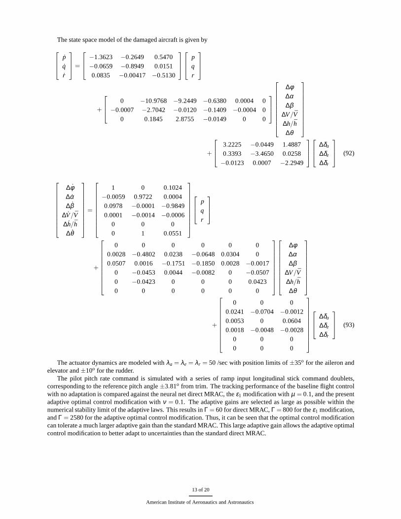
The state space model of the damaged aircraft is given by

p

q

r

=

−1.3623 −0.2649 0.5470

−0.0659 −0.8949 0.0151

0.0835 −0.00417 −0.5130

p

q

r

+

0 −10.9768 −9.2449 −0.6380 0.0004 0

−0.0007 −2.7042 −0.0120 −0.1409 −0.0004 0

0 0.1845 2.8755 −0.0149 0 0

∆φ∆α∆β

∆V/V

∆h/h

∆θ

+

3.2225 −0.0449 1.4887

0.3393 −3.4650 0.0258

−0.0123 0.0007 −2.2949

∆δa

∆δe

∆δr

(92)

∆φ∆α∆β

∆V/V

∆h/h

∆θ

=

1 0 0.1024

−0.0059 0.9722 0.0004

0.0978 −0.0001 −0.9849

0.0001 −0.0014 −0.0006

0 0 0

0 1 0.0551

p

q

r

+

0 0 0 0 0 0

0.0028 −0.4802 0.0238 −0.0648 0.0304 0

0.0507 0.0016 −0.1751 −0.1850 0.0028 −0.0017

0 −0.0453 0.0044 −0.0082 0 −0.0507

0 −0.0423 0 0 0 0.0423

0 0 0 0 0 0

∆φ∆α∆β

∆V/V

∆h/h

∆θ

+

0 0 0

0.0241 −0.0704 −0.0012

0.0053 0 0.0604

0.0018 −0.0048 −0.0028

0 0 0

0 0 0

∆δa

∆δe

∆δr

(93)

The actuator dynamics are modeled withλa = λe = λr = 50 /sec with position limits of±35o for the aileron andelevator and±10o for the rudder.

The pilot pitch rate command is simulated with a series of ramp input longitudinal stick command doublets,corresponding to the reference pitch angle±3.81o from trim. The tracking performance of the baseline flight controlwith no adaptation is compared against the neural net directMRAC, theε1 modification withµ = 0.1, and the presentadaptive optimal control modification withν = 0.1. The adaptive gains are selected as large as possible within thenumerical stability limit of the adaptive laws. This results inΓ = 60 for direct MRAC,Γ = 800 for theε1 modification,andΓ = 2580 for the adaptive optimal control modification. Thus, itcan be seen that the optimal control modificationcan tolerate a much larger adaptive gain than the standard MRAC. This large adaptive gain allows the adaptive optimalcontrol modification to better adapt to uncertainties than the standard direct MRAC.

13 of 20


0 10 20 30 40−4

−2

0

2

4

t, secq,

deg

/sec

0 10 20 30 40−4

−2

0

2

4

t, sec

q, d

eg/s

ec

0 10 20 30 40−4

−2

0

2

4

t, sec

q, d

eg/s

ec

0 10 20 30 40−4

−2

0

2

4

t, sec

q, d

eg/s

ec

No AdaptationReference Model

MRACReference Model

ε1−Mod., µ=0.1

Reference ModelOptimal, ν=0.1Reference Model

Fig. 5 - Pitch Rate

The aircraft angular rate responses are shown in Figs. 5 to 8.Figure 5 illustrates the pitch rate response due to thefour controllers. With no adaptation, the baseline flight control system cannot follow the reference pitch rate very wellas there is a significant overshoot. Both the direct MRAC and theε1 modification improves the tracking by about thesame amount. However, the adaptive optimal control modification appears to provide better tracking than the MRACand theε1 modification.

Since the damage occurs to one of the wings, the roll axis is most affected. With no adaptation, there is a significantroll rate as high as 20o/sec as shown in Fig. 6. Both the direct MRAC andε1 modification reduce to maximumamplitude of the roll rate to about 10o/sec. The adaptive optimal control modification further reduces the roll rate to amaximum value of about 4o/sec.

0 10 20 30 40−20

−10

0

10

20

t, sec

p, d

eg/s

ec

0 10 20 30 40−20

−10

0

10

20

t, sec

p, d

eg/s

ec

0 10 20 30 40−20

−10

0

10

20

t, sec

p, d

eg/s

ec


0 10 20 30 40−20

−10

0

10

20

t, sec

p, d

eg/s

ec

MRACReference Model

Optimal, ν=0.1Reference Model

ε1−Mod., µ=0.1

Reference Model

Fig. 6 - Roll Rate

Figure 7 is the yaw rate response of the damaged aircraft. Allthe three adaptive controllers significantly reduce theroll rate to a reasonably low level. Theε1 modification performs slightly better than the MRAC and adaptive optimalcontrol modification.

14 of 20


0 10 20 30 40−0.4

−0.2

0

0.2

0.4

0.6

t, secr,

deg

/sec

0 10 20 30 40−0.4

−0.2

0

0.2

0.4

0.6

t, sec

r, d

eg/s

ec

0 10 20 30 40−0.4

−0.2

0

0.2

0.4

0.6

t, sec

r, d

eg/s

ec

0 10 20 30 40−0.4

−0.2

0

0.2

0.4

0.6

t, sec

r, d

eg/s

ec


MRACReference Model

ε1−Mod., µ=0.1

Reference Model


Fig. 7 - Yaw Rate

Figure 8 is the plot of the tracking errorL2 norm for all the three aircraft angular rates that compares the overallperformance of the four controllers collectively in the three axes. When there is no adaptation, the tracking error normappears to grow considerably in the first 10 sec. Theε1 modification actually results in higher tracking error thanthe direct MRAC. This could be explained by the fact that theε1 modification trades performance for robustness, sothe tracking performance is expected to be worse. The adaptive optimal control modification results in the smallesttracking error norm as compared to the MRAC andε1 modification. Thus, overall, the adaptive optimal controlmodification performs significantly better than the MRAC andε1 modification.

0 10 20 30 400

5

10

15

20

t, sec

||xm

−x|

| 2, deg

/sec

0 10 20 30 400

5

10

15

20

t, sec

||xm

−x|

| 2, deg

/sec

0 10 20 30 400

5

10

15

20

t, sec

||xm

−x|

| 2, deg

/sec

0 10 20 30 400

5

10

15

20

t, sec

||xm

−x|

| 2, deg

/sec

No Adaptation MRAC

ε1−Mod., µ=0.1 Optimal, ν=0.1

Fig. 8 - Tracking Error Norm

The attitude responses of the damaged aircraft are shown in Figs. 9 to 12. When there is no adaptation, the pitchattitude could not be followed accurately as seen in Fig. 9. With adaptation on, the tracking is much improved and theadaptive optimal control modification follows the pitch command better than the direct MRAC and theε1 modification.

15 of 20


0 10 20 30 400

5

10

15

t, secθ,

deg

0 10 20 30 400

5

10

15

t, sec

θ, d

eg

0 10 20 30 400

5

10

15

t, sec

θ, d

eg

0 10 20 30 400

5

10

15

t, sec

θ, d

eg


ε1−Mod., µ=0.1

Reference Model

MRACReference Model


Fig. 9 - Pitch Angle

Figure 10 is the plot of the bank angle. Without adaptation, the damaged aircraft exhibits a rather severe rollbehavior with the bank angle ranging from−30o to 20o. Both the direct MRAC andε1 modification improve thesituation significantly. The adaptive optimal control shows a drastic improvement in the arrest of the roll motion withthe bank angle maintained closed to the trim value.

0 10 20 30 40−30

−20

−10

0

10

20

t, sec

φ, d

eg

0 10 20 30 40−30

−20

−10

0

10

20

t, sec

φ, d

eg

0 10 20 30 40−30

−20

−10

0

10

20

t, sec

φ, d

eg

0 10 20 30 40−30

−20

−10

0

10

20

t, sec

φ, d

eg

No Adaptation MRAC


Fig. 10 - Bank Angle

Figure 11 is a plot of the angle of attack. All the adaptive controllers produce similar angle of attack responses.

16 of 20


0 10 20 30 400

2

4

6

8

10

t, secα,

deg

0 10 20 30 400

2

4

6

8

10

t, sec

α, d

eg

0 10 20 30 400

2

4

6

8

10

t, sec

α, d

eg

0 10 20 30 400

2

4

6

8

10

t, sec

α, d

eg

No Adaptation MRAC


Fig. 11 - Angle of Attack

Figure 12 shows a plot of the sideslip angle. In general, flying with sideslip angle is not a common practicesince a large sideslip angle can cause an increase in drag andmore importantly a decrease in the yaw damping. Withthe adaptive optimal control modification, the sideslip angle is reduced to near zero, while the direct MRAC andε1

modification still show some sideslip angle responses.

0 10 20 30 40−4

−2

0

2

4

t, sec

β, d

eg

0 10 20 30 40−4

−2

0

2

4

t, sec

β, d

eg

0 10 20 30 40−4

−2

0

2

4

t, sec

β, d

eg

0 10 20 30 40−4

−2

0

2

4

t, sec

β, d

eg

No Adaptation MRAC


Fig. 12 - Sideslip Angle

The control surface deflections are plotted in Figs. 10 to 12.Because of the wing damage, the damaged aircraft hasto be trimmed with a rather large aileron deflection. This causes the roll control authority to severely decrease. Anypitch maneuver can potentially run into a control saturation in the roll axis due to the pitch-roll coupling that exists ina wing damage scenario. With the maximum aileron deflection at 35o, it can be seen clearly from Fig. 13 that a rollcontrol saturation is present in all cases. The range of aileron deflection when there is no adaptation is quite large. Asthe aileron deflection hits the maximum position limit, it tends to over-compensate in the down swing because of thelarge pitch rate error produced by the control saturation.

17 of 20


0 10 20 30 4010

20

30

40

t, secδ a, d

eg

0 10 20 30 4010

20

30

40

t, sec

δ a, deg

0 10 20 30 4010

20

30

40

t, sec

δ a, deg

0 10 20 30 4010

20

30

40

t, sec

δ a, deg

Fig. 13 - Aileron Deflection

Figure 14 is a plot of the elevator deflection which is shown tobe within a range of few degrees for all the fourcontrollers and well within the control authority of the elevator. This implies that the roll control contributes mostly tothe overall response of the wing-damaged aircraft.

0 10 20 30 40−4

−2

0

2

t, sec

δ e, deg

0 10 20 30 40−4

−2

0

2

t, sec

δ e, deg

0 10 20 30 40−4

−2

0

2

t, sec

δ e, deg

0 10 20 30 40−4

−2

0

2

t, sec

δ e, deg

No Adaptation MRAC


Fig. 14 - Elevator Deflection

The rudder deflection is shown in Fig. 15. With no adaptation,the rudder deflection is quite active, going fromalmost−7o to 2o. While this appears small, it should be compared relative tothe rudder position limit, which isusually reduced as the airspeed and altitude increase. The absolute rudder position limit is±10o but in practice theactual rudder position limit may be less. Therefore, it is usually desired to keep the rudder deflection as small aspossible. Both the direct MRAC andε1 modification improve the situation somewhat, but the adaptive optimal controlis able to keep the rudder deflection quite small and virtually almost at trim.

18 of 20


0 10 20 30 40−6

−4

−2

0

2

t, secδ r, d

eg

0 10 20 30 40−6

−4

−2

0

2

t, sec

δ r, deg

0 10 20 30 40−6

−4

−2

0

2

t, sec

δ r, deg

0 10 20 30 40−6

−4

−2

0

2

t, sec

δ r, deg

No Adaptation MRAC


Fig. 15 - Rudder Deflection

To demonstrate stability robustness of the adaptive optimal control modification, the time delay margin (TDM)is computed numerically in the simulations as a function of the parameterν. A time delay is introduced betweenthe actuators and the damaged aircraft plant model and is adjusted until the adaptive optimal control modificationalgorithm is on the verge of instability. The results are plotted in Fig. 16 for an adaptive gainΓ = 60. Asν increases,the time delay margin also increases. This results in a more robust controller that can tolerate a larger time delay whichacts as a destabilizing disturbance to the controller. However, for the same adaptive gain, increasingν tends to degradethe tracking performance. Therefore, in general,ν is selected to balance the competing requirements for performanceand stability robustness that usually exist in a control design.

0 0.2 0.4 0.6 0.8 1

0.2

0.25

0.3

0.35

0.4

0.45

0.5

0.55

ν

TD

M, s

ec

Γ=60

Fig. 16 - Estimated Time Delay Margin

V. Conclusions

This study presents a new modification to the standard model-reference adaptive control based on an optimalcontrol formulation of minimizing theL2 norm of the tracking error. The adaptive optimal control modification adds

19 of 20


a damping term to the adaptive law that is proportional to thepersistent excitation. The modification enables fastadaptation without sacrificing robustness. The modification can be tuned using a parameterν to provide a trade-offbetween tracking performance and stability robustness. Increasingν results in better stability margins but reducedtracking performance. Whenν approaches unity, the system is robustly stable with all closed-loop poles havingnegative real values. Simulations of a damaged generic transport aircraft were conducted. The results demonstrate theeffectiveness of the adaptive optimal modification, which shows that tracking performance can be achieved at a muchlarger adaptive gain than the standard direct model-reference adaptive control. As a result, significant improvementsin performance can be attained with the adaptive optimal control modification.

References1Bosworth, J. and Williams-Hayes, P.S., “Flight Test Results from the NF-15B IFCS Project with Adaptation to a SimulatedStabilator

Failure”, AIAA Infotech@Aerospace Conference, AIAA-2007-2818, 2007.2Sharma, M., Lavretsky, E., and Wise, K., “Application and Flight Testing of an Adaptive Autopilot On Precision Guided Munitions”, AIAA

Guidance, Navigation, and Control Conference, AIAA-2006-6568, 2006.3Rohrs, C.E., Valavani, L., Athans, M., and Stein, G., “Robustness of Continuous-Time Adaptive Control Algorithms in the Presence of

Unmodeled Dynamics”, IEEE Transactions on Automatic Control, Vol AC-30, No. 9, pp. 881-889, 1985.4Nguyen, N., and Jacklin, S., “Neural Net Adaptive Flight Control Stability, Verification and Validation Challenges, and Future Research”,

Workshop on “Applications of Neural Networks in High Assurance Systems”, International Joint Conference on Neural Networks, 2007.5Jacklin, S. A., Schumann, J. M., Gupta, P. P., Richard, R., Guenther, K., and Soares, F., “Development of Advanced Verification and

Validation Procedures and Tools for the Certification of Learning Systems in Aerospace Applications”, AIAA Infotech@Aerospace Conference,AIAA-2005-6912, 2005.

6Steinberg, M. L., “A Comparison of Intelligent, Adaptive, and Nonlinear Flight Control Laws”, AIAA Guidance, Navigation, and ControlConference, AIAA-1999-4044, 1999.

7Eberhart, R. L. and Ward, D. G., “Indirect Adaptive Flight Control System Interactions”, International Journal of Robust and NonlinearControl, Vol. 9, pp. 1013-1031, 1999.

8Rysdyk, R. T. and Calise, A. J., “Fault Tolerant Flight Control via Adaptive Neural Network Augmentation”, AIAA Guidance, Navigation,and Control Conference, AIAA-1998-4483, 1998.

9Kim, B. S. and Calise, A. J., “Nonlinear Flight Control UsingNeural Networks”, Journal of Guidance, Control, and Dynamics, Vol. 20, No.1, pp. 26-33, 1997.

10Johnson, E. N., Calise, A. J., El-Shirbiny, H. A., and Rysdyk, R. T., “Feedback Linearization with Neural Network Augmentation Appliedto X-33 Attitude Control”, AIAA Guidance, Navigation, and Control Conference, AIAA-2000-4157, 2000.

11Idan, M., Johnson, M. D., and Calise, A. J., "A Hierarchical Approach to Adaptive Control for Improved Flight Safety", AIAA Journal ofGuidance, Control and Dynamics, Vol. 25, No. 6, pp. 1012-1020, 2002.

12Hovakimyan, N., Kim, N., Calise, A. J., Prasad, J. V. R., and Corban, E. J., “Adaptive Output Feedback for High-BandwidthControl of anUnmanned Helicopter”, AIAA Guidance, Navigation and Control Conference, AIAA-2001-4181, 2001.

13Cao, C. and Hovakimyan, N., “Design and Analysis of a Novel L1Adaptive Control Architecture with Guaranteed Transient Performance”,IEEE Transactions on Automatic Control, Vol. 53, No. 2, pp. 586-591, 2008.

14N. Nguyen, K. Krishnakumar, J. Kaneshige, and P. Nespeca, “Flight Dynamics and Hybrid Adaptive Control of Damaged Aircraft”, AIAAJournal of Guidance, Control, and Dynamics, Vol. 31, No. 3, pp. :751-764, 2008.

15Nguyen, N., Krishnakumar, K., and Boskovic, J., ”An OptimalControl Modification to Model-Reference Adaptive Control for Fast Adapta-tion”, AIAA Guidance, Navigation, and Control Conference,AIAA 2008-7283, 2008.

16Ioannu, P.A. and Sun, J.,Robust Adaptive Control, Prentice-Hall, 1996.17Cybenko, G., “Approximation by Superpositions of a Sigmoidal Function”, Mathematics of Control Signals Systems, Vol.2, pp. 303-314,

1989.18Narendra, K. S. and Annaswamy, A. M., “A New Adaptive Law for Robust Adaptation Without Persistent Excitation”, IEEE Transactions

on Automatic Control, Vol. AC-32, No. 2, pp. 134-145, 1987.19Micchelli, C. A., “Interpolation of Scattered Data: Distance Matrices and Conditionally Positive Definite Functions”, Constructive Approx-

imation, Vol.2, pp. 11-12, 1986.20Bryson, A.E. and Ho, Y.C.,Applied Optimal Control: Optimization, Estimation, and Control, John Wiley & Sons Inc., 1979.21Khalil, H. K., Nonlinear Systems, Prentice-Hall, 2002.22Slotine, J.-J. and Li, W.,Applied Nonlinear Control, Prentice-Hall, 1991.23Narendra, K.S. and Annaswamy, A.M.,Stable Adaptive Systems, Dover Publications, 2005.24Bailey, R. M, Hostetler, R. W., Barnes, K. N., Belcastro, C. M. and Belcastro, C. M., “Experimental Validation: SubscaleAircraft Ground

Facilities and Integrated Test Capability”, AIAA Guidance, Navigation, and Control Conference, AIAA-2005-6433, 2005.

20 of 20


Robust Optimal Adaptive Control Method with Large Adaptive Gain

Documents