ammonia emissions and dry deposition from broiler barns in the

AMMONIA EMISSIONS AND DRY DEPOSITION FROM BROILER BARNS IN THE

FRASER VALLEY OF BRITISH COLUMBIA

by

DANIEL EDWARD SEETON

B.Sc., The University of British Columbia, 2010

A THESIS SUMITTED IN PARTIAL FULFILLMENT OF

THE REQUIREMENTS FOR THE DEGREE OF

MASTER OF SCIENCE

in

THE FACULTY OF GRADUATE AND POSTDOCTORAL STUDIES

(Soil Science)

THE UNIVERSITY OF BRITISH COLUMBIA

(Vancouver)

April 2016

© Daniel Edward Seeton, 2016

ii

Abstract Ammonia emissions from commercial broiler operations have been noted as one of the potential contributors to the nitrate contamination of the Abbotsford-Sumas aquifer in southwestern British Columbia (BC). The localized dry deposition of this emitted ammonia was of special interest and had not been measured in any comparable climate. Three barns, on two farms, located on the aquifer were assessed from July 2011 to June 2012. Ventilation, emission, and deposition samples were taken weekly throughout the seasons to accurately characterize the impact on the local environment. Ventilation was measured using a Fan Assessment Numeration System and timers that recorded individual fan activity. Acid impinger traps were used to measure the ammonia emitted by the sidewall fans. A methodology for measuring dry deposition by exposing air-dried soil was modified to use small Petri dishes and a 24-hr exposure time. The modified dry deposition method was found to be robust and effective for the requirements of this study. Dishes of soil were placed 2.1 and 3.6 m in front of and between each fan, as well as around the barns and farm properties. Ventilation rates for the barns were significantly and positively correlated with bird age and exterior temperature. Ammonia emissions were correlated with bird age and the emission factors for the three barns ranged from 0.19-0.37 g NH3 bird-1 day-1with annual ammonia emissions for each barn reaching 600 to 815 kg NH3. Dry deposition levels on the two farms exceeded 50 kg NH3 annually although this accounted for less than 10% of the ammonia emitted. The deposition levels were highest near the barns and were concentrated directly under the sidewall fan hoods. These levels of ammonia show significant potential to cause nitrate to leach into the groundwater and further contaminate the aquifer but future work and upscaling of data collection are needed.

iii

Preface This research project was designed by the author. The field work, sampling, and lab analysis was completed by the author with some assistance from members of the Agriculture and Agri-Food Canada Agassiz Station Forage Lab when multiple people were required. The analysis of the research data was undertaken by the author.

iv

Table of Contents

Abstract .............................................................................................................................. ii Preface ............................................................................................................................... iii Table of Contents ............................................................................................................. iv

List of Tables ..................................................................................................................... vi List of Figures .................................................................................................................. vii Acknowledgements ........................................................................................................... x

1 INTRODUCTION AND LITERATURE REVIEW ............................................................... 1

1.1 Introduction ............................................................................................................ 1

1.2 Chemical Processes Involved in the Nitrogen Cycle ........................................... 1 1.2.1 Ammonia Production ........................................................................................ 2

1.2.2 Ammonia Volatilization .................................................................................... 3

1.2.3 Ammonia Deposition ........................................................................................ 4

1.2.4 Nitrification of Ammonia .................................................................................. 6

1.3 Industrial Broiler Production ............................................................................... 7 1.3.1 Barn Design and Management .......................................................................... 7

1.3.2 Feed Management ............................................................................................11

1.3.3 Litter Management ...........................................................................................11

1.3.4 Measuring Barn Emissions ............................................................................. 13

1.3.5 Emission Factors ............................................................................................. 15

1.4 Geographical Context .......................................................................................... 17 1.4.1 Agricultural Practices in the Lower Fraser Valley .......................................... 17

1.4.2 Air Quality in the Lower Fraser Valley ........................................................... 18

1.4.3 Water Quality in the Abbotsford-Sumas Aquifer ............................................ 19

1.5 Study Objectives ................................................................................................... 20

2 ASSESSMENT OF MODIFIED METHODOLOGY FOR MEASURING DRY AMMONIA

DEPOSITION USING SOIL AS AN AMMONIA SORPTION MEDIUM ......................................... 21

2.1 Introduction .......................................................................................................... 21

2.2 Materials and Methods ........................................................................................ 22 2.2.1 Study Sites ...................................................................................................... 22

2.2.2 Sample Preparation, Extraction, and Analyses ............................................... 23

2.2.3 Statistical Analysis .......................................................................................... 24

2.3 Results and Discussion ......................................................................................... 24 2.3.1 Sample Mass ................................................................................................... 25

v

2.3.2 Sample Volume Measurement ........................................................................ 25 2.3.3 Exposure Duration .......................................................................................... 26 2.3.4 Soil Water Content .......................................................................................... 26 2.3.5 Soil pH ............................................................................................................ 27 2.3.6 Soil Texture ..................................................................................................... 28 2.3.7 Rain Cover ...................................................................................................... 28 2.3.8 Proposed Sampling Protocol ........................................................................... 29

2.4 Conclusions ........................................................................................................... 29

3 ANNUAL AMMONIA EMISSION AND DEPOSITION LEVELS FOR TWO BROILER FARM

VENTILATION SYSTEMS IN THE LOWER FRASER VALLEY OF BRITISH COLUMBIA ......... 34

3.1 Introduction .......................................................................................................... 34

3.2 Materials and Methods ........................................................................................ 37 3.2.1 Study Sites ...................................................................................................... 37 3.2.2 Sampling and Laboratory Analyses ................................................................ 39 3.2.3 Statistical Analysis .......................................................................................... 41 3.2.4 Calculation of Ammonia Emissions................................................................ 41 3.2.5 Calculation of Ammonia Deposition .............................................................. 42 3.2.6 Estimation of End of Cycle Ammonia Emission and Deposition ................... 44

3.3 Results and Discussion ......................................................................................... 45 3.3.1 Barn Ventilation Rates .................................................................................... 45 3.3.2 Ammonia Emissions from the Barns .............................................................. 48 3.3.3 Emission Factors ............................................................................................. 49 3.3.4 Dry Deposition of Ammonia ........................................................................... 52

3.4 Conclusions ........................................................................................................... 56

4 GENERAL CONCLUSIONS ......................................................................................... 85

4.2 Conclusions and Recommendations ................................................................... 85 4.2.1 Future Research ............................................................................................... 86

4.2 Evaluation of Study Methods and Recommendations for Future Modifications ............................................................................................................... 87

References ........................................................................................................................ 90

APPENDIX I: Historic and study period weather data for Abbotsford, BC. ........... 97

APPENDIX II: Description of treatments and samples sizes for each of the methodology trials. .......................................................................................................... 98

APPENDIX III: Fan Assessment Numeration System (FANS) .................................. 99

APPENDIX IV: Gas Impinger Acid Trap System and sidewall fan hoods. ............. 101

APPENDIX V: Dry deposition sample rain cover detail. .......................................... 103

APPENDIX VI: Average flow rate for sidewall fans at each ventilation stage. ...... 104

vi

List of Tables

Table 2.1 NH4-N deposition (μg cm-2) in sample size and rain cover trials .................................32

Table 2. 2 ANOVA table for the soil moisture and soil texture trials ...........................................32

Table 3.1 Summary of multiple linear regressions ........................................................................79

Table 3.2 Summary of emission factors and literature values ......................................................80

Table 3.3 Average flow rate for each fan across all stages ...........................................................81

Table 3.4 Average flow rate for each fan for each ventilation stage and total flow rate for each stage at the Farm No.1 in Chilliwack, BC. ............................................................................82

Table 3.5 Average flow rate for each fan for each ventilation stage and total flow rate for each stage at the Farm No.2 in Aldergrove, BC.............................................................................83

Table 3.6 Total emitted ammonia for each flock for each barn at Farm No.1 in Chilliwack, BC and for Farm No.2 in Aldergrove, BC. ....................................................................................84

Table 3.7 Total deposited ammonia for each flock for each barn at Farm No.1 in Chilliwack, BC and for Farm No.2 in Aldergrove, BC. ................................................................84

Table A.1 Description of treatments and samples sizes for each of the methodology trials. .........98

Table A.2 Average flow rate of fans at each stage for Farm No. 1 .............................................104

Table A.3 Average flow rate of fans at each stage for Farm No. 2 .............................................105

vii

List of Figures

Figure 2.1 Increase in dry deposited NH4-N over exposure times ranging from 1 to 144 hours. Soil samples were located 1.5 m from poultry barn ventilation fan ...................................33

Figure 3.1 Map of lower Fraser Valley of British Columbia and locations of Farm No.1 in Chilliwack, BC and Farm No. 2 in Aldergrove, BC. .....................................................................59

Figure 3.2 Map of Farm No.1 located in Chilliwack, BC showing locations of dry deposition sampling sites and gas impinger traps ..........................................................................60

Figure 3.3 Map of Farm No.2 in Aldergrove, BC showing locations of dry deposition sampling sites and gas impinger traps ...........................................................................................61

Figure 3.4 An isoconcentration plot of the average high density ammonia deposition samples obtained at Farm No. 1 located in Chilliwack, BC. .........................................................62

Figure 3.5 Changes at Farm No.1 during the four stages of ventilation and at farm No.2 during the seven stages of ventilation in (a) air pressure deficit within the barns and (b) sum total ventilation flow rates ......................................................................................................63

Figure 3.6 Percentage of time that (a) any fans were active in the barns of Farm No.1 and No.2 during sample times and (b) that ventilation stages 3 or higher were active. .......................64

Figure 3.7 Ammonia in ventilated air within the barns on Farm No. 1. Determined during the summer and winter periods. .....................................................................................................65

Figure 3.8 Barn ventilation rates for each flock and weather station air temperature during the year-long period of measurement.............................................................................................66

Figure 3.9 Barn exhaust NH3 concentration for each flock and weather station air temperature during the year-long period of measurement. ............................................................66

Figure 3.10 Barn NH3 emissions for each flock and weather station air temperature during the year-long period of measurement. ................................................................................67

Figure 3.11 Emission factors for each flock and weather station air temperature during the year-long period of measurement.............................................................................................67

Figure 3.12 Total Farm NH3 deposition for each flock and weather station air temperature during the year-long period of measurement. ................................................................................68

viii

Figure 3.13 Flock A-105 from Farm No.1’s (a) ammonia emission curve in actual units, (b) after being normalized, (c) plotted alongside normalized growth curve (weight vs age), (d) with the estimated harvest date emission using the growth curve’s slope, and (e) the ammonia emission curve converted back into actual units along with the new final point. ..........70

Figure 3.14 High density deposition samples from 1 m to 3.6 m away from the side of the barn at Farm No.1 at positions (a) in front of a 36” fan, (b) halfway between a 36” and a 24” fan (5 m apart), (c) in front of a 24” fan, and (d) halfway between two widely spaced 24” fans (10 m apart) .....................................................................................................................72

Figure 3.15 Average high density ammonia deposition sample points along the corridor (parallel to barn) at 2.1 m and 3.6 m from the barn and fans at Farm No.1. .................................73

Figure 3.16 Comparison of the non-MLR calculated and the MLR NH3 deposited in the corridor between the barns at Farm No.1 for flock A110. .............................................................73

Figure 3.17 Comparison of the non-MLR calculated and the MLR NH3 deposited in the corridor between the barns at Farm No.2 for flock A111. .............................................................74

Figure 3.18 Deposition of ammonia at 2.1 m from each barn and 3.6 m, between the barns, at Farm No.1 averaged for all sample dates with birds over 20 days old. ..........................74

Figure 3.19 Isoconcentration of ammonia deposition on the entire Farm No.1 for flocks (a) A105 (36 days old), (b) A106 (29 days old), (c) A107 (32 days old), (d) A108 (22 days old), (e) A109 (34 days old), and (f) A110 (34 days old). .............................................................75

Figure 3.20 Isoconcentration of ammonia deposition for the field in front of Farm No.2 for flocks (a) A109 (24 days old), (b) A110 (35 days old), and (c) A111 (32 days old). ...............76

Figure 3.21 Deposition of ammonia at 2.1 m and 3.6 m from the fans in line with the barn at Farm No.2 averaged for all sample dates with birds over 20 days old. .....................................77

Figure 3.22 Deposition of ammonia in line with active hooded fans at Farm No.2 averaged for all sample dates with birds over 20 days old. ...........................................................77

Figure 3.23 Isoconcentration of ammonia re-deposition on the entire Farm No.1 between flocks A105 and A106 ....................................................................................................................78

Figure 3.24 Isoconcentration of ammonia re-deposition for the field in front of Farm No.2 after flock A111 ..............................................................................................................................78

ix

Figure A.1 Comparison of historic monthly data (1981-2010) in comparison with the July 2011 to June 2012 for (a) total precipitation and (b) average temperature for Abbotsford, BC, Canada (Environment Canada 2015). .....................................................................................97

Figure A.2 Fan Assessment Numeration System (FANS) measurements of a 24” ventilation fan at Farm No.2 located in Aldergrove, BC ...............................................................99

Figure A.3 Contour plot of air flow (m s-1) through the FANS while measuring a 36” ventilation fan ..............................................................................................................................100

Figure A.4 Gas Impinger Acid Trap System (with four separate sample streams) outside the barn at Farm No.2 located in Aldergrove, BC .......................................................................101

Figure A.5 Air filters used for the gas impinger traps. Shown is the ambient sampling point. ............................................................................................................................................101

Figure A.6 Dust clogged air filter beneath a fan hood. ................................................................102

Figure A.7 Corridor at Farm No.1 with hooded 24” (0.61 m) sidewall fans and non-hooded 36” (0.91 m) fans.............................................................................................................102

Figure A.8 Rain cover for soil filled Petri dish dry deposition sample on (a) grass and (b) dusty soil beneath a fan hood. ......................................................................................................103

x

Acknowledgements

I am eternally grateful to my supervisors Dr. Maja Krzic and Dr. Shabtai Bittman,

without whose guidance I would never have come this far. I also want to thank my

committee members Dr. Andy Black and Dr. Andreas Christen, who provided me with

such helpful advice and encouragement, often exceeding their obligations. The endless

reassurance and editing advice of Dr. Les Lavkulich, statistical aid of Dr. Tony Kozak,

and the technical expertise provided by Zoran Nesic were all critical to my success. A

special thanks to my fellow LFS Soils and “Pro-Soils” Forestry grad students who helped

me through endless classes and assignments. The wonderful soils professors were

contagious with their passion and love for the study of soils.

This research would not have been possible without the wonderful people at the

Agriculture and Agri-food Canada (AAFC) Agassiz Forage Lab: Derek Hunt, Maureen

Schaber, Anthony Friesen, Connie Pietrafesa, Pierre Groenenboom, and many nameless

Co-op students that lent a hand when I needed one. Shawn Loo, who provided academic

debate and inspiration over many, many late night meals. I would also like to thank Kevin

and Lindsay Chipperfield of the Sustainable Poultry Farmers Group who participated in

some of the most arduous days of field sampling. I recognize that this research would not

have been possible without the financial assistance of Sustainable Agriculture

Environmental Systems (SAGES) and AAFC Agassiz and I express my gratitude to those

agencies.

Last, but not the least, I would like to thank my family: Dad, Ma, Pa, and Girl. You

put up with my lengthy student life, patiently listened to me ramble for hours on end, and

helped me put it all together at the end.

xi

Dedication

To my Grandpa, Grandma, and Nana, who helped to raise me in their gardens: dirt under

my fingernails, sharing in their love and awe for the natural world, just not those weeds.

1

1 INTRODUCTION AND LITERATURE REVIEW

1.1 Introduction

There are numerous sources of ammonia emissions in areas with intensive

agricultural production, but confined livestock operations, like broiler poultry farms in

the lower Fraser Valley of British Columbia (BC), are potentially one of the greatest

contributors (Hao et al. 2005). The emission and deposition of ammonia are challenging

to accurately characterize. Understanding these processes is of great significance as

ammonia pollution is considered a “hazardous gas” and has serious environmental

impacts and raises health concerns (Jacobson et al. 2011). In areas of high ammonia

emissions and deposition, the critical load of the local environment can often be exceeded

and result in a change in local species composition, acidification of poorly buffered soils,

and the contamination of ground water sources such as the Abbotsford-Sumas aquifer

(Pitcairn et al. 1998; Van der Eerden 1982). Locally derived estimates of emissions and

deposition of ammonia do not currently exist. These are critical to determine the negative

effect of the entire broiler industry on the local environment, with respect to air, soil, and

ground water quality.

1.2 Chemical Processes Involved in the Nitrogen Cycle

Ammonia, NH3, is the most prevalent basic gas and the most significant reactive

form of nitrogen in the atmosphere (Arogo et al. 2006; Van der Eerden 1982). It readily

adheres to acidic, vegetative, and moist surfaces, but it also combines with acid gases;

forming fine particulate matter (Arogo et al. 2006). Ammonia is naturally produced by

2

the enzymatic decomposition of urea or uric acid found in animal manure (Arogo et al.

2006). The chemical processes of ammonia production and volatilization are well

understood and follow a regular pathway. There are a number of factors that can affect

these processes, but the end product is the same.

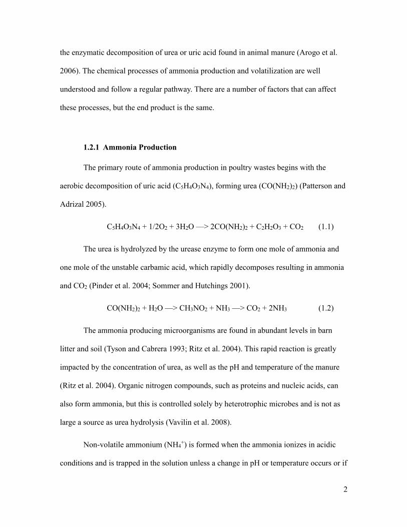
1.2.1 Ammonia Production

The primary route of ammonia production in poultry wastes begins with the

aerobic decomposition of uric acid (C5H4O3N4), forming urea (CO(NH2)2) (Patterson and

Adrizal 2005).

C5H4O3N4 + 1/2O2 + 3H2O ––> 2CO(NH2)2 + C2H2O3 + CO2 (1.1)

The urea is hydrolyzed by the urease enzyme to form one mole of ammonia and

one mole of the unstable carbamic acid, which rapidly decomposes resulting in ammonia

and CO2 (Pinder et al. 2004; Sommer and Hutchings 2001).

CO(NH2)2 + H2O ––> CH3NO2 + NH3 ––> CO2 + 2NH3 (1.2)

The ammonia producing microorganisms are found in abundant levels in barn

litter and soil (Tyson and Cabrera 1993; Ritz et al. 2004). This rapid reaction is greatly

impacted by the concentration of urea, as well as the pH and temperature of the manure

(Ritz et al. 2004). Organic nitrogen compounds, such as proteins and nucleic acids, can

also form ammonia, but this is controlled solely by heterotrophic microbes and is not as

large a source as urea hydrolysis (Vavilin et al. 2008).

Non-volatile ammonium (NH4+) is formed when the ammonia ionizes in acidic

conditions and is trapped in the solution unless a change in pH or temperature occurs or if

3

ammonia is lost, in accordance with the dissociation equilibrium constant, Ka (Pinder et

al. 2004; Monteny and Erisman 1998).

NH3 + H2O <–––> NH4+ + OH- (1.3)

The sum of these two forms, NH3 and NH4+, is commonly referred to as the total

ammonia nitrogen (TAN) as measurements techniques often combine these two forms

(Monteny and Erisman 1998; Sommer and Hutchings 2001).The form that the TAN takes

is highly dependent on pH, so much so that at a pH below 6 almost all of the TAN is in

the ammonium form, but at pH 8.6 up to 50% of the TAN is in the ammonia form

(Monteny and Erisman 1998; Elzing and Monteny 1997). Poultry litter is typically at pH

9 to 10, ideal for the breakdown of uric acid by uricase, so the TAN is predominantly in

ammonia form (Blake and Hess 2001). Ammonia levels are also much lower at low

temperatures, which is another variable that can markedly affect subsequent

transformations (Fenn and Kissel 1973).

1.2.2 Ammonia Volatilization

Once ammonia is in solution (aqueous phase) it may enter the gas phase,

following Henry’s Law (Pinder et al. 2004).

NH3 (aq) <––> NH3 (gas, boundary) <––> NH3 (gas, air) (1.4)

The transition into the gas phase is positively correlated and strictly controlled by

temperature (Monteny and Erisman 1998). Once in the gas phase the ammonia is still

largely held near the surface (boundary layer). Any mass flow of air such as horizontal

advection or vertical turbulent diffusion will cause ammonia gas to move away from the

emitting surface, creating a gradient and driving the equilibrium above toward the right

(Monteny and Erisman 1998). Other meteorological conditions can also have an impact

4

on the emission of ammonia, for example heavy rains can decrease emissions to near zero

(Sommer and Hutchings 2001).

Once in the gas phase, the very basic ammonia is prone to forming particulate

matter (within 0.5 hours to 5 days) by reacting with acid gases such as nitric acid (HNO3)

or sulphur dioxide (SO2), largely produced by the combustion of fossil fuels (Arogo et al.

2006; Stelson and Seinfeld 2007; Fowler et al. 1998; Harris, Shores, and Jones 2001;

Vayenas et al. 2005). In the case of HNO3 the reaction is

NH3 (g) + HNO3 (g) <–––> NH4NO3 (s) (1.5)

The salt particles that this reaction causes are extremely small, a diameter of less

than 2.5 μm, and are included in the collective designation of particulate matter 2.5

(PM2.5) (Vayenas et al. 2005). The movement and destination of these particles can be

quite different from gaseous ammonia and is an active area of research, especially

because of the implications to air quality and respiratory health (Vayenas et al. 2005). The

characteristics and movement of the ammonia salts can also be affected by relative

humidity, potentially leading to more rapid deposition (Stelson and Seinfeld 1982).

1.2.3 Ammonia Deposition

1.2.4.1 Dry Deposition

Dry deposition of ammonia requires ammonia or PM2.5 to be transported to the

laminar boundary layer of a surface by turbulent diffusion of particles and within the

laminar boundary layer by diffusion (Fick’s law) and usually occurs within a few days

(Loubet et al. 2009; Ritz, Fairchild, and Lacy 2004). Once at a surface the gaseous

ammonia is deposited by adsorption and PM2.5 is deposited by impaction (Loubet et al.

2009). This can involve a great deal of complexity when encountering reactive surfaces

5

such as soil and highly variable surfaces such as plant tissue with stomata and hair-like

projections (Loubet et al. 2009). Variations in surface roughness and canopy structure

create complex boundary layers and become far more difficult to measure than a prepared

surface used in laboratory assays (Loubet et al. 2006; Theobald et al. 2001). Current

models often use a number of different resistances that try and describe the complex

processes occurring at surfaces such as the cuticle and stomata of leaves (Loubet et al.

2009; Pearson and Stewart 1993). Stomata in particular, are very difficult to model as

they are only open during active photosynthesis, making the internal air space available

for the diffusion of gaseous ammonia, though PM2.5 are not transported through the

stomata (Loubet et al. 2009).

1.2.4.2 Wet Deposition

Wet deposition is the result of ammonia or ammonia salts being deposited by rain

drops. Unlike dry deposition, which is often highly localized around the emission source

(2-60% within 1 km of source), wet deposition is spatially much less variable as ambient

atmospheric ammonia concentrations are the primary controlling factor (Loubet et al.

2009).

Dry deposition is also prevalent when wet surfaces are present, such as during a

period of rainfall, so isolating wet deposition from the additional dry deposition to a wet

surface can become rather problematic. Separating the gaseous ammonia dissolved in rain

drops from the ammonium from deliquesced PM2.5 is trivial since both are chemically

similar sources of wet deposited ammonia. The difficulty of properly segregating wet

deposition from supplementary dry deposition is circumvented as they are usually

reported in combination (Poor et al. 2001). This is not a serious problem when looking at

6

local deposition levels as usually less than 5% of ammonia is recaptured by wet

deposition within 1 km of the source (Loubet et al. 2009).

1.2.4 Nitrification of Ammonia

In a natural system, ammonia deposited on a moist surface will acidify the

solution and transition into ammonium. The pH of this solution is important as an

alkaline shift to greater than pH 8.5 can cause the formation of ammonia and possible

volatilization (Buss et al. 2004). This soluble ammonium is typically transported to soil

and enters the soil solution. The ammonium is readily oxidized by different

microorganisms (nitrosomonas and nitrobacter) in two-stages to produce energy, nitrite

(NO2-), and nitrate (NO3

-) (Buss et al. 2004). These two reactions follow one another

quickly and the level of nitrite at any time is quite low.

NH4+ + 1.5O2 ––> NO2

- + H2O + 2H+ (6)

NO2- + 0.5O2 ––> NO3

- (7)

Nitrification can also occur under anaerobic conditions with oxidants such as

nitrogen oxides (Schmidt et al. 2002), but nitrification is much more active in the

presence of oxygen (Buss et al. 2004). Temperature is also a factor in nitrification as this

process is biologically driven (Buss et al. 2004).

1.2.5 Leaching of Nitrate

Once nitrate is in the soil solution it is available for biological uptake by plants

and other soil organisms. As nitrate is an anion it is prone to leaching through the soil and

into the groundwater and is the most dominant form of nitrogen contributing to water

contamination (Di and Cameron 2002). Large concentrations of leached nitrate usually

7

coincide with localized areas like urine patches or manure storage drainage points (Silva

et al. 1999). Though nitrate leaching may be elevated, the production of nitrate has been

shown to limit the leaching of ammonium into groundwater (Christensen et al. 2001).

Soil and climate conditions also have a large impact on nitrate leaching: fine-

textured soils, high proportions of soil macropores, lower water table, lower precipitation

rates, and higher evapotranspiration rates are all associated with reduced nitrate leaching

(Silva et al. 2000; Di and Cameron 2002). The most effective control is ensuring that the

application rate does not exceed the requirements by the plants both in magnitude and

timing (Di and Cameron 2002).

1.3 Industrial Broiler Production

Broilers are chickens grown solely for meat production. They are bread at a

hatchery and then the chicks are placed into a large single room barn with industrial

feeding and watering system and grown until they reach harvest age, typically 5-7 weeks.

The entire production cycle occurs indoors and the barns are densely spaced on small

plots of land.

1.3.1 Barn Design and Management

Broiler barn design concerns both external and internal factors including: site

location, windbreaks, filters, ventilation, and watering systems (Patterson and Adrizal

2005). The impact of the barn on the local area is the main concern of the external design

aspects, while the internal systems are focused on maintaining bird health. Both the

ammonia gas and particulate matter produced from poultry operations can have negative

impacts on human health and activity. Inside poorly ventilated barns; however, high

8

levels of ammonia (>50 ppm) can result in severe irritation of eyes, pulmonary and

respiratory systems, and numerous other tissues that result in poor weight gain and

production characteristics of livestock (Colina et al. 2000). Safe exposure standards for

livestock are in the range of 25 ppm, but research indicates that levels greater than 10

ppm can have negative effects on animals and humans (Colina et al. 2000).

1.3.1.1 External Considerations

Site location and barn orientation are impacted by prevailing wind direction and

setback from nearby forests, fields, or residences as barn emissions are often considered a

pollutant (Malone and Van Wicklen 2002). Windbreaks outside of barn ventilation

systems are often used to manage dust and odor from barns, but also impact the allocation

of ammonia. Hedges and fences are common forms of windbreaks, though the non-

uniform surface, porosity and thickness of hedges can be much more effective (Malone

and Van Wicklen 2002; Adderley and Christen 2014). By increasing the potential plant

surface contact that the highest velocity PM2.5 will impact, a great deal of small

particulate ammonia can be captured locally (Patterson and Adrizal 2005). The dry

deposition of molecular ammonia is also affected, but this has been seen indirectly where

the deposition levels behind the hedge is lower than if unimpeded (Patterson and Adrizal

2005). The hedges do this by causing a greater up flow of the ventilated air and resulting

in greater non-localized wet and dry deposition (Patterson and Adrizal 2005). Fences

have been found to be effective when they are placed 3.0-6.1 m away from the ventilation

fans, where the dust and ammonia deposits nearby the barn at low ventilation speeds, but

is directed up over the fence and mixes in the air at high speeds (Malone and Van

Wicklen 2002). Water filters are located directly outside a fan and are exclusively used to

9

capture particulate and molecular emissions by passing the ventilated air through a

scrubbing media (Snell and Schwarz 2003).

Watering systems in barns have the greatest potential impact on the moisture level

of the litter in the barns, and thereby are critical to controlling ammonia volatilization

(Fairchild and Ritz 2009). Broiler barns have almost universally switched to a nipple

watering system, but improper nipple height or water pressure can cause birds to spill

more water as they drink (May and Lott 2000). Drinker spill trays can be used to keep the

litter from getting excessively wet when barn temperatures are high, as panting broilers

have difficulty coordinating drinking and breathing (May and Lott 2000).

1.3.1.2 Internal Considerations

The two main types of mechanical ventilation are positive pressure and negative

pressure systems, which use either sidewall or tunnel fans (Vest and Tyson 1991).

Positive pressure systems force air into the barn, which mixes and then exits through

louvers. Negative pressure systems, the much more common type, use an adjustable

intake louver to limit air flow and cause internal air mixing via turbulent flow (Vest and

Tyson 1991). Sidewall barns have numerous fans down the side of the barn that turn on in

stages, additional fan(s) activating to increase ventilation. These systems have a wide

dispersal pattern, which makes them poor candidates for using windbreaks or water filters

for ammonia capture or reduction (Patterson and Adrizal 2005). Tunnel barns use a wall

of fans on one end of the barn with intake points distributed in various patterns along the

other three sides of the barn (Lacy and Czarick 1992). Tunnel ventilation systems are

more expensive to operate than sidewall, but they have a lower mortality rate during

periods of high temperature and are increasing in popularity (Lacy and Czarick 1992).

10

The highly concentrated tunnel exhaust systems create a very different emission scenario

and systems such as water filters have been shown to be highly effective at decreasing

ammonia levels (Arogo et al. 2006).

The balance of air temperature and air quality is an important variable for

ammonia emissions. Management that focuses on maintaining the high ambient

temperature (26-29°C) the birds prefer must also try to reduce the ammonia and

particulate level in the air to maintain quality of life (Cheng et al. 1997). Production costs

are higher in cold climates or seasons as the barns also need to be heated (Jacobson et al.

2011). These ventilation systems are typically automated and controlled by indoor

temperature, along with humidity and/or air pressure (Jacobson et al. 2011). Emission

concentrations tend to be much higher in the winter, as ventilation rates are lower, the

opposite is true in the summer and this balances out, resulting in fairly steady emission

rates, though summer is typically higher (Wheeler et al. 2006). Overall emissions may be

increased by excessive levels of ventilation.

Poultry barns also show a considerable diurnal variation of ammonia emission

levels, especially during cooler weather when the ventilation rates are lowered to retain

ideal air temperature inside (Jacobson et al. 2011). These daily maximums and minimums

vary throughout the seasons and ages, typically being greater when ventilation activity is

more extreme, as in early in the growth cycle and during the summer (Harper et al. 2010).

Higher daytime summer ventilation rates also compound the problem by temporarily

drying the soiled litter, reducing the emission of ammonia (Harper et al. 2010). Moist

winter air could also have a similar effect, thereby decreasing the seasonal differences in

barn emissions (Harper et al. 2010).

11

1.3.2 Feed Management

Outside of growing facilities, the main cost of broiler production is related to feed,

often accounting for 60-80% of the total production cost (Oluyemi and Roberts 2000;

Folorunso et al. 2014)(Folorunso, Adesua, and Onibi 2014). Growth rate and meat quality

are affected by various nutrients, different levels of which are required for each stage of

growth and are often detailed in nutritional texts (Chiba 2014; Folorunso et al. 2014).

Throughout the broiler industry the principle focus of diet, with respect to ammonia, is on

crude protein levels, which are positively correlated with nitrogen in the litter and

subsequently ammonia emissions (Cheng et al. 1997). Feed efficiency and cost of feeding

are always a focus for a producer who is trying to maximize growth for the minimum

level of feed protein (Folorunso et al. 2014). For the broiler industry, feed and water

consumption increase with bird age and thus show a steady increase in ammonia

emissions through their growth cycle (Arogo et al. 2006). Non-nutritional additions to

broiler feed has been explored in recent years and has shown to have an positive effect on

ammonia emissions and bird health (Karamanlis et al. 2008). Regardless of feed or

additives, the nitrogen waste products in manure are typically very consistent (Sommer

and Hutchings 2001).

1.3.3 Litter Management

Broiler barns use littered floor systems where sawdust, grain hulls, or other

agricultural waste is spread on the open barn floor (Jacobson et al. 2011). The bedding is

either reused (built-up litter) or cleaned out between every flock (Jacobson et al. 2011).

Built-up litter systems use machinery to remove the caked litter (packed layers of manure

and bedding) between flocks and may add fresh bedding as a replacement (top-dressing),

12

cleaning the entire barn out once a year (Jacobson et al. 2011). Even during the de-caking

cleaning of the barn ammonia emissions can be very high, amounting to 11-20% of the

total emissions of the flock (Harper et al. 2010). The European and Canadian farms

usually use new saw dust litter for every flock and have ammonia emissions of 27-47%

that of built-up systems (Gates et al. 2008; Pescatore et al. 2005). Ammonia emission

from litter is highly dependent on moisture level, with 40-60% being ideal for ammonia

production, though at least 30% moisture is needed for dust reduction (Koerkamp et al.

1994; Patterson and Adrizal 2005). The pH of litter is very important as well, with almost

no emissions below pH 7 and at a maximum at pH 8 (Reece et al. 1985). The ground

floors of barns are almost exclusively made of concrete, which is quite alkaline, making

adequate litter coverage even more important for decreasing ammonia emissions. Various

litter treatments that acidify the litter, contain absorbents, modify microbial populations,

or control enzyme activity have been studied, some are successful, but they often only

work temporarily or even have the opposite intended effect of increasing the emission of

ammonia (Karamanlis et al. 2008; Carey et al. 2004; Patterson and Adrizal 2005).

Soiled litter is stored at most broiler operations and the duration of that storage

can last from a few days to years (Jacobson et al. 2011). Much like barn design, broiler

manure storage systems can vary widely, from a pile in a field to a concrete base with

three sides and a tight fitting cover, which can drastically decrease ammonia emissions

and leaching (Kelleher et al. 2002). Ammonia emission levels tend to depending on the

surface area of the exposed manure with uncovered storage having a cumulative loss of

10% of total nitrogen compared to 7% when covered (Rodhe and Karlsson 2002; Hristov

et al. 2011). The complications arise because the attributes of the manure being stored

13

changes depends on the litter substrate, climate, any pre-storage treatments, as well as

how much ammonia has been lost before this point (Hristov et al. 2011). An increase in

manure ammonia emissions has been observed with increases in storage temperature

(Pratt et al. 2002). Using ammonia suppressing additives have also been shown to

effectively reduce emissions during storage (Li et al. 2006).

1.3.4 Measuring Barn Emissions

Ammonia emissions of livestock operations are measured in numerous ways and

the sampling strategies determine the method used. Low-frequency sampling (e.g.,

weekly or monthly) allows spatial patterns along with seasonal or even longer term trends

to be resolved (Loubet et al. 2009). These types of sampling are often done using low-

cost methods such as passive diffusion samplers, acid-coated denuders, filter packs and

acid traps (Loubet et al. 2009). To complement the low-frequency strategy, high-

frequency measurements (e.g., hourly) can be taken continuously using real-time

methods (Loubet et al. 2009). This allows the diurnal patterns to be seen, but often

requires expensive equipment, limiting the number of replications. Teflon-lined tubing,

filters, and surfaces are commonly used when measuring ammonia, since ammonia gas

has an innate tendency to adsorb readily to almost any surface and intermittently release

thus altering any downstream measurements thereafter (Aneja et al. 2000).

Passive samplers use a dry acid impregnated surface that captures ammonia in the

air. Ammonia is then washed off the surface and analyzed to determine the amount

adsorbed during to the exposure time (Hristov et al. 2011). Determining the volume of air

sampled is difficult as wind ventilation and diffusion are responsible for the adsorption

(Hristov et al. 2011). Annular denuders are another class of chemical adsorption samplers

14

that also use acidic or basic surfaces inside a glass tube, but rely on a laminar flow of air

(Hristov et al. 2011). Due to their low cost and lack of moving parts, the use of passive

samplers and denuders remain a popular methodology (Hristov et al. 2011). This method

is well suited to low-frequency sampling, but can be prone to saturation and must be

protected from rain (Hansen et al. 1998). A limitation of this method is that the minimum

detection limit is around 50-100 mg m-3 (Hristov et al. 2011).

Passive filter packs use acid coated cellulose fibers to trap ammonia similar to

denuders, but require wind speeds greater than 1 m s-1 for the complex surface to be

sufficiently exposed (Sutton et al.1993; Rabaud et al. 2001). They are inexpensive, robust

and do not need pumps or a power source, but determining the volume of air sampled

requires reference samplers to determine and “effective sampling rate”(Rabaud et al.

2001). The difficulty with that method is separating out what was gaseous ammonia and

what was in fact already an ammonium salt so the sum (total inorganic ammonium) is

often used (Loubet et al. 2009). Because of the additional ammonium salts this method

can give quite different measurements from some of the methods that measure ammonia

gas specifically (Sutton et al. 1993).

Acid traps rely on the solubility of ammonia and its rapid change to ammonium at

low pH. An air sample is drawn into a tube, often through a filter, and is passed through

an impinger, a container where incoming air is bubbled through a liquid before exiting

(Todd et al. 2008). Photospectroscopy via flow injection analysis is commonly used to

determine the concentration of ammonia in the acid (Todd et al. 2008). The minimum

detection limit of this method is around 5 mg m-3, a magnitude lower than the denuders

(Hristov et al. 2011; Todd et al. 2008).

15

High-frequency sampling strategies include optical analysis and

chemiluminescence. Optical measurement instruments rely on the adsorption of both

infrared and near-infrared wavelengths of light by ammonia to determine its

concentration (Hristov et al. 2011). This method uses an open-path laser, is non-invasive,

and sensitive enough to measure concentrations seen at most livestock facilities, but dust

can dramatically weaken its signal (Harper et al. 2010; Hristov et al. 2011). The

popularity of this method is limited primarily by its cost, but it also demands careful

maintenance and calibration (Hristov et al. 2011). Through the chemical transformation

of ammonia, concentrations can also be determined by chemiluminescence. Using a

thermal catalyst converter ammonia can react with NOx to form NO, which is reacted

with ozone to form NO2 radiation proportional to the amount of NO is emitted, from

which the ammonia concentration can be calculated (Koerkamp et al. 1998; Hristov et al.

2011). This method allows continuous and accurate measurement of ammonia

concentrations, but requires electricity and a suitable operating environment along with

frequent on-site calibration (Hristov et al. 2011).

1.3.5 Emission Factors

Emission factors are the most common term that relates emissions of ammonia, or

other pollutants, to a source and duration. These values allow comparisons between

different flocks or barns, but are often reported in a variety of units and require altering.

Ammonia is typically given in a mass, either as ammonia (NH3), ammonium (NH4+), or

as nitrogen that originated from a reactive chemical species (NH3-N or NH4-N), so units

often need to be adjusted. The source of the ammonia (i.e., broilers) is listed on an animal

or animal unit basis, which again requires conversion before comparison. Animal

16

description, type and age, must be specified for the per head unit to be useful (De

Visscher et al. 2002). Another vital piece of information concerns how the measurement

of emissions is done, depending on how the emission factor is reported. Emissions are

typically measured from a group of animals and then averaged by the unit used, but

reporting an emission factor of one chicken may cause confusion without some

background (Arogo et al. 2006). The third part of an emission factor is time. This is most

often reported in minutes, days, or years, but lifecycles are sometimes used so production

specifics should be clearly stated or well-known (Arogo et al. 2006).

The techniques and even some of the assumptions used to determine emission

factors are critical in synthesizing for using the information. Data collected over a short

period of time is typically not representative of longer periods that are the intended use

and so large errors in estimations of annual emissions are a constant problem (Arogo et al.

2006). This is even more apparent when a single emission factor is made and all the

variations in even a single industry are averaged out, such as the United States

Environmental Protection Agency (USEPA) has done, instead of providing a range,

which would allow a much better understanding of ammonia emissions from the

livestock industry (Hristov et al. 2011). Without adequate background the comparison of

these values is tenuous at best and should be considered individual pieces that add to the

greater picture of ammonia emissions. Values from Europe are difficult to compare with

those from North America, especially the USA, because of the differences in

management scenarios (Arogo et al. 2006). The variability in measurement practices can

also create biases, especially when some methodologies dominate in specific areas and

very different regional emission characteristics are reported. This problem is improving

17

as more research is being conducted with newer technology, leading to a better

understanding of nitrogen mass balances (Arogo et al. 2006). This sort of holistic

understanding is fast becoming the most important thing to improve our understanding of

agriculture.

1.4 Geographical Context

1.4.1 Agricultural Practices in the Lower Fraser Valley

The Lower Fraser Valley is a fertile and flat corridor created by alluvial deposits

from the Fraser River. It spans 150 km in length and provides over 85,000 hectares of

farmed land, over 80% of which is in pasture and crop production (Belzer et al. 1997).

With its mild winter and ample precipitation, 1,100 to 1,600 mm annually, the growing

conditions allow for a wide variety of crops can be grown (Environment Canada 2015).

The Lower Fraser Valley is the most financially productive agricultural land in the

province, despite being less than 2% of the agricultural land reserve, as it produces

primarily high value crops (Fraser Valley Regional District 2011). The primary industries

in this area include berry crops, grapes, numerous greenhouse vegetables, dairy products,

and poultry.

The berry and poultry operations are primarily located above the Abbotsford-

Sumas aquifer due to the excellent growing conditions and ready access to supply chains,

labour, and consumers. The intensive nature of dairy and poultry farming has led to an

increase in emission issues including odor, dust, and potentially harmful gases, of which

ammonia is one (Bittman et al. 2014). In addition to emissions, these poultry operations

produce a considerable amount of manure on relatively small plots of land and so it must

18

be used elsewhere. It is often considered that the application of poultry manure and

fertilizer to berry fields is a major contributor to the leaching of NO3 through the sandy

soils and into the aquifer (Mitchell et al. 2003; Wassenaar 1995). Though it is generally

acknowledged that N management of berries has improved over the past 10 years, recent

sampling of test wells has not detected noticeable reductions in nitrate concentrations and

levels remain above the Canadian drinking water guideline (Chesnaux et al. 2007). The

wet climate also causes a potential risk of nitrate leaching in the colder months as the

rainfall is frequent, but the poultry industry continues to produce and store manure, while

also exhausting ammonia.

1.4.2 Air Quality in the Lower Fraser Valley

In the Lower Fraser Valley extensive air quality measurements are made to

monitor trends and communicate pertinent information to the public. The focus of the

measurements are on visual air quality and various pollutants, which allow an Air Quality

Health Index to be calculated (Metro Vancouver 2015). Ammonia is not a significant

pollutant on its own as it is readily dispersed and quickly forms PM2.5. Visual air quality

is an assessment of particulate matter that causes haze and impaired visibility. The Lower

Fraser Valley has a relatively constrained weather system, which can have stagnant

conditions during high pressure systems that lead to periods of highly degraded air

quality (Metro Vancouver 2015; Belzer et al. 1997). The fossil fuel combustion in urban

areas leads to the formation of brownish PM2.5, while in the agrarian areas a white

coloured PM2.5 forms due to the prevalence of ammonia in the atmosphere (Metro

Vancouver 2015). The difference in the types of PM2.5 is important, but the primary

concern is the serious health effects associated with these particles that are easily inhaled

19

deeply into the lungs and can lead to respiratory and cardiovascular issues (Metro

Vancouver 2015). In the last ten years, the Canadian Ambient Air Quality Standard values

have only been exceeded on ten or fewer days annually, typically during extended

summertime heatwaves or when smoke from forest fires enters the valley (Metro

Vancouver 2015). The annual average daily concentration of PM2.5 across the Lower

Fraser Valley has been around 5 μg m-3 since 1999, which is far below the Canadian

standard of 28 μg m-3 (Metro Vancouver 2015).

1.4.3 Water Quality in the Abbotsford-Sumas Aquifer

Atop the shallow unconfined Abbotsford-Sumas aquifer there is an extremely high

prevalence of broiler production operations and berry fields that are often associated with

the application of poultry manure for fertilizer. The high levels of rainfall and the

excessive levels of mineral nitrogen in soil create ideal conditions for nitrate leaching

resulting in water contamination issues (Zebarth et al. 1998). Measurements of the

groundwater consistently show nitrate levels that exceed the USEPA 10 ppm drinking

water guideline (Mitchell et al. 2003). Despite large and widespread improvement in the

implementation of best management practices in the Abbotsford-Sumas area this aquifer

contamination has continued (Mitchell et al. 2003). The aquifer flows south and crosses

the international boundary between southwestern BC, Canada and northwestern

Washington, USA and supplies drinking water to rural residences on both sides. With the

centralization of animal production around the world, the occurrences of groundwater

contamination are ever increasing and have spurred a great deal of research in an effort to

protect water quality (Zebarth et al. 1998).

20

1.5 Study Objectives

Although numerous studies have assessed the ammonia levels and deposition rates

in the Lower Fraser Valley (Belzer et al. 1997), there have been few studies on individual

poultry barns and localized dry deposition of ammonia. This research project includes the

following two objectives:

1. To modify and evaluate several modifications of the existing methodology

used to determine dry ammonia deposition outside of poultry barn ventilation

systems.

2. To evaluate total ammonia emissions from three broiler barns on the

Abbotsford-Sumas Aquifer during a period of one year and the amount of

ammonia that is dry deposited on the farm areas. In addition, annual ammonia

emission factors representative for the Fraser Valley poultry industry were also

determined.

21

2 ASSESSMENT OF MODIFIED METHODOLOGY FOR MEASURING DRY

AMMONIA DEPOSITION USING SOIL AS AN AMMONIA SORPTION MEDIUM

2.1 Introduction

Ammonia from the atmosphere can follow several paths of deposition, including

dry and wet deposition and deposition as particulate matter 2.5 (PM2.5). Dry deposition of

ammonia is a complex physical/chemical process that is highly dependent of surface

chemistry and equilibriums (Loubet et al. 2009). Many resistance models have been

developed in an attempt to estimate deposition rates, but the highly variable conditions in

which deposition occurs often demand direct measurement (Loubet et al. 2009; Pearson

and Stewart 1993). Generally, ammonia is readily deposited on complex surfaces such as

soil and plants (Loubet et al. 2009). Soils are an excellent medium to measure deposition

as they are a natural deposition surface and are relatively inert compared to plants. In

addition, the preparation of soil is simple, cost efficient, and procedures for the extraction

of ammonia are well established (McGinn et al. 2003).

Dry soil has been used in an existing methodology to measure dry deposition of

ammonia up to 200 m downwind of a beef feedlot (McGinn et al. 2003; Hao et al. 2005).

The rationale for this method is that soil (as a common surface for natural deposition) is a

better surface to measure deposition level than a synthetic surface, which would only

show potential deposition. A low carbon and nitrogen soil is used for the measurements

after it has been air-dried and ground sufficiently to pass through a 2-mm sieve, removing

any larger soil particles or plant material and mixing it thoroughly (X. Hao et al. 2005).

Exposure of the soil has varied; e.g., 20 g of soil in a Petri dish on the ground for 7-14

22

days(McGinn et al. 2003) and 5 g of soil in a 4.3-cm-diameter straight-sided vial (8.8 cm

high) placed 1 m above the ground for 5-9 days (Hao et al. 2005). Both of these methods

also used rain covers and were found to give similar ammonia deposition values that were

highly correlated with ambient ammonia concentration (McGinn et al. 2003; Hao et al.

2005).

Determination of the dry deposition levels outside of poultry barn ventilation fans

required a modification of the existing methodology due to several issues specific to the

poultry barns. First, the poultry ventilation systems are characterized by having fans that

blow ammonia-rich exhaust toward the ground next to the barn. The method of

measurement must therefore be able to handle strong airflow. Second, the poultry

industry is based on short flock growth cycles, which require frequent sampling events.

Third, humid climate with abundance of rainfall during fall and winter months bring the

need to protect samples (or measuring spots) from precipitation.

The objective of this study was to evaluate several modifications of the existing

methodology used to determine ammonia deposition outside poultry barn ventilation

systems.

2.2 Materials and Methods

2.2.1 Study Sites

The study was carried out from May to August 2011 at a broiler (meat bird)

poultry farm in Chilliwack, British Columbia (BC) (4916’N 12191’W). This time of

year has monthly precipitation less than 100 mm and average daily temperatures from 13

to18°C (Fig. A.1a, b). The soils in this region are gravelly silt loam to silt loam Orthic

23

Humo-Ferric Podzols.

The farm had two parallel barns with sidewall fans that exhausted into the

corridor between them (Fig A.7). The dry deposition samples were placed between 1 to 3

m in front of one 24” (0.61 m) fan that had a hood that directed the airflow downwards.

The flow rate of this sized fan can reach or 2 m3 s-1 with ammonia concentrations

exceeding 30 ppm. The soil and vegetation outside the barns was highly variable and

included barren patches of soil with no plants, located directly below the fan hoods and

grass growing in between the fans (Fig A.7).

2.2.2 Sample Preparation, Extraction, and Analyses

The soil used as an sorption medium was a silt loam collected from the A horizon

of a field at the AAFC Pacific Agricultural Research Center located in Agassiz, BC

(Kelley and Spilsbury 1939). The field had not had nitrogen fertilizer applied in over 20

years, resulting in relatively low residual nitrogen content, as was recommended in the

original methodology upon which this procedure was based (X. Hao et al. 2005; Xi. Hao

et al. 2006). The soil was air dried, ground, sieved to 2 mm, and mixed in large plastic

bags in order to homogenize it (X. Hao et al. 2005).

The preparation of the soil samples included the following: the pH was adjusted

from 5.5 to 4.5 by adding 0.05 M H3PO4 and deionized (DI) water, and 5 texture types

ranged from 100% silt loam soil to 100% sharp quarry sand (Table A.1). Rain covers

used to protect sampling positions were constructed from an inverted disposable

polystyrene laboratory weigh boat (14 cm x 14 cm) with 18-cm-long wire legs that fit

into a 14 cm x 14 cm piece of ¾” (1.9 cm) thick plywood.

24

The soil samples were placed in plastic Petri dishes (55 mm in diameter) during

the varied exposure time, and after removal were kept in the closed dishes, inside two

plastic bags, sealed with twist ties and refrigerated, until analysis. Subsamples of 5.00 +/-

0.01 g, from the typically 12.0 +/- 0.01 g soil samples, were extracted with 50 ml of 2 M

KCl, shaken on a shaker table (Lab-Line Orbital, Tripunithura, India) at 200 rpm for 1

hour. A ~15 ml subsample was collected in a small test tube while the extractant was

filtered through a Fisherbrand Q5 Medium filter paper. The subsamples were sealed with

ParaFilm and refrigerated until they were analyzed on a FIAstar 5000 Analyzer (FOSS,

Hillerod, Denmark) for ammonia and nitrate. The nitrate contents were negligible and

were not included in any calculations.

2.2.3 Statistical Analysis

A general linear model procedure was performed using the SAS package, version

9.3 (SAS Institute Inc., 2007). When multiple treatments were compared the least

significant difference (LSD) of means were compared. Samples were placed randomly in

grids and these locations were compared with the model residuals to ensure independence.

Results were considered significant at P < 0.05.

2.3 Results and Discussion

Evaluations of modifications of the existing methodology used to determine

ammonia deposition (Hao et al. 2005; Hao et al. 2006) focused on the following: (1)

sample mass, (2) sample volume, (3) exposure duration, (4) soil water content, (5) soil

pH, (6) soil texture, and (7) addition of a rain cover. These modifications were selected as

they reflect various soil conditions found in the study area of the Fraser Valley in BC. The

25

exposed surface area of all the samples was kept constant as the same sized Petri dishes

were used.

2.3.1 Sample Mass

Different masses of soil, placed in the same sized Petri dishes, were exposed to

ammonia to determine if there is a significant effect on dry deposition. As mentioned

above, existing methodologies have used soil masses of 5 g and 20 g (McGinn et al. 2003;

Hao et al. 2005). The masses of the exposed samples were 8.0, 12.0, and 16.0 g, which

ranged from approximately 4 mm of soil depth to 8 mm, or 1/3 to 2/3 the capacity of the

small Petri dish. The samples were all placed at a location 20 m away from the barn and

at another location 1.5 m from an active fan for 6 hours. Unexposed samples (double

bagged and left onsite) were used as a control and the average ammonia content of the

controls were subtracted from the exposed samples in order to calculate the net increase

in ammonia (i.e., the true value of deposition).

The mean ammonia depositions on the soil samples of different masses were not

found to be significantly different (Table 2.1). This suggests that an 8.0-g soil sample,

which provided full coverage of the entire surface of the Petri dish had the same reactive

surface as the other samples.

2.3.2 Sample Volume Measurement

Instead of weighing each sample, which is very time consuming, the possibility of

using a volume measurement for preparing soil samples for ammonia dry deposition was

investigated. A short plastic test tube (7 ml) was used to scoop up soil, the soil was then

given a light tap to eliminate any air spaces, soil was then added to overfill the test tube,

26

and the soil was leveled off to the top edge.

The resultant soil mass was 7.83 g with a standard deviation of 0.22 g (n = 66).

This variability was smaller than that of the return masses of the rain cover trial samples:

12.39 g 1.86 g (n = 64), all of which started out at 12.0 0.01 g. The dust and moisture

(humidity or precipitation) additions and soil lost as a result of the high air speed created

by the barn ventilation system appeared to cause a greater sample error than the volume

measurements. Lower variability in mass accompanied with shorter sample preparation

time favor the volume measurement method for the soil sample.

2.3.3 Exposure Duration

The potential saturation of the soil sample with ammonia was measured over

various exposure times ranging from 1 to 144 hours (Table A.1). The existing

methodology was exposed for 1-2 weeks downwind from a beer feedlot (McGinn et al.

2003; Hao et al. 2005), but the ammonia outside a poultry barn are much more variable

and so shorter exposure times are required. The length of sample exposure was strongly

correlated with the deposition of ammonia (r2 = 0.98) and was approaching saturation in

the samples with the highest exposure duration (Fig. 2.1).

2.3.4 Soil Water Content

The existing methodology used air dried soil (X. Hao et al. 2005), as in this study,

but water content is an important issue due to the high levels of precipitation at the study

site. Knowing the effect of water content on the samples would possibly allow wet

samples to be used as viable data. Three different volumes of DI water (2, 4 and, 6 ml)

were added to Petri dishes containing 12 g of air dried soil and then laid out in front of an

27

active fan for 1.5 hours (Table A.1). This short exposure did not reveal any trends of

increasing deposition with increasing water content. Only the 4 ml treatment was

significantly different from the 2 and 6 ml (Table A.1). When dry samples were compared

with all of the wet samples, no significant difference was found (Table 2.2).

The greatest complication with moist samples was the risk of under-sampling

when weighing out 5 g of damp soil to be extracted and compared with 5 g of the dry

samples. In addition, the added water serves to slightly dilute the extracted ammonia. If

there was enough water to puddle in the dishes, there may be a considerable measurement

error. In light of this, heavily wetted soils should not be analyzed, which emphasizes the

requirement for rain protection. Additionally, subsampling 5 g from the total 12 g appears

to be an overcomplicated lab process and source of sampling error. Extracting the entire

sample would remedy this by allowing analysis of the entire surface of the exposed soil.

2.3.5 Soil pH

The effect of a change in soil sample pH was also of interest as acidic surfaces are

often highly susceptible to ammonia dry deposition and the transformation of ammonia to

ammonium causes a lowering of pH (Van Herk 1999; Wesely and Hicks 2000). All soil

samples received 0 ml, 0.5 ml, 1 ml, or 4 ml of 0.05 M H3PO4 and enough DI water to

make a total of 4 ml (Table A.1). These additions represented an approximate decrease in

the soil pH of 0, 0.2, 0.3, and 1.0, respectively. Only the addition of 4 ml 0.05 M H3PO4

had significantly higher deposition from the control treatment with only 4 ml of DI water

addition (Table A.1).

28

2.3.6 Soil Texture

The impact of soil texture on ammonia dry deposition rate was examined by

mixing in various proportions of clean sharp sand with the silt loam soil. The existing

methodology used soil similar to that found on the study site (X. Hao et al. 2005). Since

the soils in the study area range from silt loam into gravelly silt loam, additions of sand

were made to approximate and extend this range of textures. The percentages of the

sample that was sand in this trial were: 0%, 25%, 50%, 75%, and 100%, even though the

range that would be found in the field is between 0% and 50% (Kelley and Spilsbury

1939).

The ammonia deposition levels significantly decreased (P <0.0001) as sand

content in soil samples increased above 50% (Table 2.2) as would be expected since the

reactive surface of the soil is inversely related to sand content. There were no significant

differences in ammonia deposition among 0%, 25%, and 50% of sand (Table A.2),

implying that variability in soil texture found the study area does not affect the dry

deposition of ammonia.

2.3.7 Rain Cover

The effect of the proposed 18 cm rain covers on ammonia deposition was tested at

1.5, 3.0, and 20 m (ambient) distances from an active fan. No detailed information on the

rain covers of the existing methodology was available so small rain covers were a new

variable to test. The presence of the rain cover relative to no cover did not result in a

significantly different dry deposition of ammonia (P = 0.498) (Table 2.1). Any water

content that the soil samples gained during exposure to the humid fan exhaust has been

discussed above and removed as a possible source of variation.

29

2.3.8 Proposed Sampling Protocol

In light of these findings, a modified sampling protocol is proposed. In regards to

the soil sample size and the potential error of subsampling 5.0 g from the 12.0 g exposure

samples, it is proposed that an ~8 g sample is used and that the entire sample is extracted.

This relatively small increase from 5.0 g to ~8 g in the soil sample used for the extraction,

is still large enough to effectively cover the entire surface area of the Petri dish, where 5.0

g would be insufficient.

Rather than weighing each sample, which is tedious and time consuming, an

approximate sample mass is to be made by using a simple and quick volume

measurement. The 24-hour soil sample exposure time appears to fall well below the

ammonia saturation level and will also remove potential diurnal variations in the

ammonia deposition rates. The emission rates of poultry barns change rapidly as the birds

age; hence, the improved time resolution of a 24-hour exposure should provide a greater

level of detail over the existing week-long exposure. The lack of effect of low levels of

water content on the deposition of ammonia is reassuring, but rain covers will be

employed to avoid excessive wetting and subsequent dilution effects that could

complicate the extraction procedure. The silt loam soil also is to be used without textural

modification since sand additions did not result in any difference in ammonia dry

deposition. This may not be the case for all soils and should be reexamined if this

methodology was to be used again.

2.4 Conclusions

As part of an investigation of the dry deposition of ammonia resulting from

30

poultry barn ventilations systems, a methodology using soil as a sorption medium was

modified and tested. Varying the amount of soil exposed in a standardized container did

not significantly impact the dry deposition of ammonia. Surface area was deemed to be

the important factor, but not the mass of the soil, which implies that depth of soil was not

important. The standard deviation of soil sample mass was compared between the return

mass of 12.0 g of exposed soil and a 7 ml volume measure of soil and the volume

measure appears to be sufficiently accurate. This method worked well for this specific

soil, but should be reassessed if a different texture was used. The dry deposition of

ammonia on soil samples was monitored over 144 hours to determine whether the

proposed exposure time of 24 hours would suffer from any saturation effects, potentially

underestimating the deposition of ammonia. The large capacity for ammonia deposition

in the soil samples was sufficient to quell any concerns with the proposed 24-hour

exposure. Three different volumes of DI water were added to soil samples prior to

ammonia exposure and no significant differences in deposition were observed. Additions

of acid were also investigated to evaluate the effect of differing soil pH on ammonia

deposition. Only the treatment with a decrease of 1.0 in pH had a significantly greater

ammonia deposition relative to the control, but this pH was well beyond what is expected

under the field conditions in this region. Various mixtures of the sample soil and sand

were exposed to ammonia and the deposition levels significantly decreased as sand

content in soil samples increased especially in 75 and 100% sand samples. That range of

sand content, however, is not typically found in the study area and so the dry deposition

sample texture does not need to be modified to better represent the soil in-situ. Even

though the water content trial did not show significant issues with low levels of water

31

content in the soil samples, very wet samples are still of a great concern in this region

with high fall and winter precipitation. Consequently, use of rain covers was investigated

at various distances from an ammonia source but was shown not to have any significant

effect on dry ammonia deposition.

These findings support the modification of the sample volume, exposure duration,

soil texture, and rain cover of the existing methodology for use in determining ammonia

dry deposition from poultry barn ventilation systems. These modifications will enhance

the ease of this method allowing for a greater number of samples to be processed in a

relatively short time. In turn, sampling of ammonia deposition on the entire farm could be

undertaken allowing a larger scale assessment of this complex process.

32

Table 2.1 NH4-N deposition (μg cm-2) in sample mass and rain cover trials Trial Treatment N Ammonia

deposition (μg cm-2)

Sample Mass

8 g 8 151.4a*

12 g 8 144.8a 16 g 8 174.2a

5% LSD 57.3 Rain Cover Cover 24 266.3a

No Cover 24 228.5a 5% LSD 95.1 * Means followed by the same letter are not significantly different within the same trial (P > 0.05). Table 2.2 ANOVA table for the soil water content and soil texture trials

Trial Source of Variation df Sum of Squares

Mean Square

F-Value Pr > F*

oil Water Content

Model 1 6.17 6.17 1.40 0.2539 Error 16 70.44 4.40 Corrected Total 17 76.60 Soil Texture Model 4 7276.90 1819.23 17.86 <.0001 Error 15 1527.68 101.85

Corrected Total 19 8804.58 Soil Texture** Model 2 362.22 181.11 1.12 0.3681 Error 9 1456.49 161.83 Corrected Total 11 1818.71 * Trials with Pr > 0.05 do not have significant differences between the treatments. ** Limited to 0-50% sand content

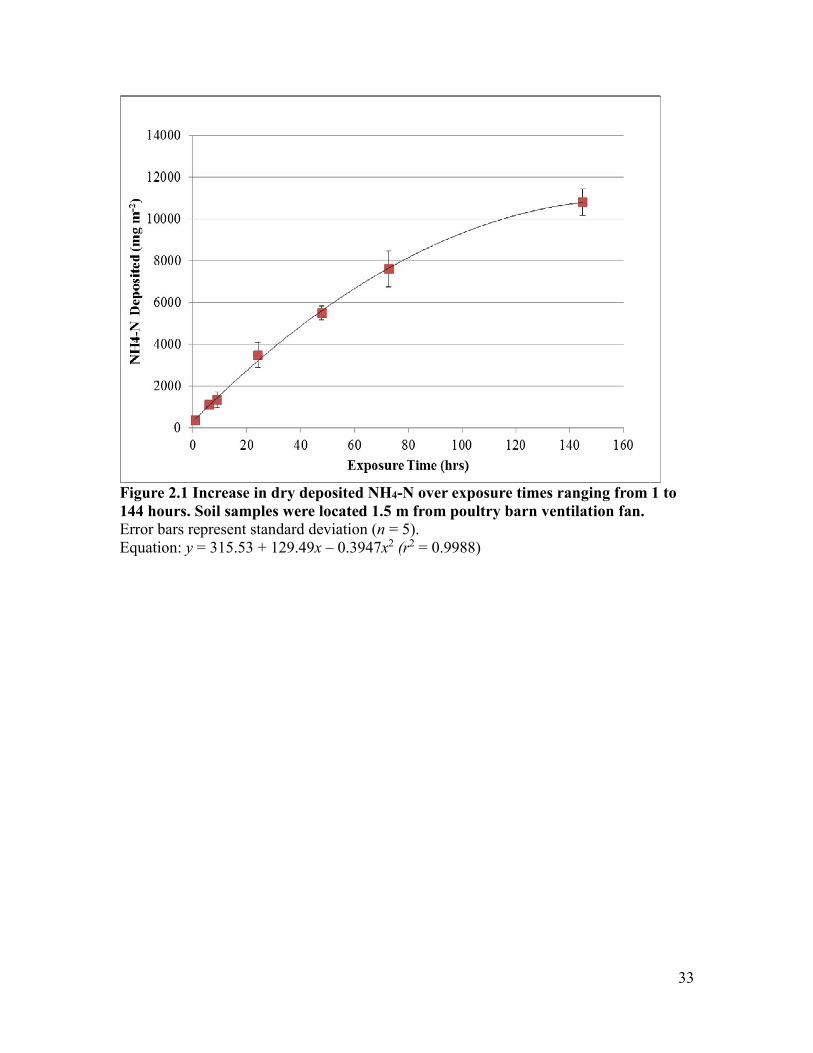
33

Figure 2.1 Increase in dry deposited NH4-N over exposure times ranging from 1 to 144 hours. Soil samples were located 1.5 m from poultry barn ventilation fan. Error bars represent standard deviation (n = 5). Equation: y = 315.53 + 129.49x – 0.3947x2 (r2 = 0.9988)

34

3 ANNUAL AMMONIA EMISSION AND DEPOSITION LEVELS FOR TWO

BROILER FARM VENTILATION SYSTEMS IN THE LOWER FRASER VALLEY OF

BRITISH COLUMBIA

3.1 Introduction

Ammonia emissions from agriculture are a significant contributing factor to air

pollution and imbalances in the global nitrogen cycle. Confined livestock operations such

as poultry barns are important sources of ammonia emissions especially if they are

concentrated spatially, due to the need for access to market, feed and labour (X. Hao et al.

2005). Local nitrogen deposition in areas with a high concentration of confined livestock

operations may contribute to overloading of nitrogen in soils and waterways by

exceeding the area’s loading capacity (Harper et al. 2010).

The Lower Fraser Valley in British Columbia (BC) is an example of an

agricultural area with a large number of confined poultry operations. These are

concentrated in a few areas within the valley, reaching almost 40 barns over a 16 km2

area, with the largest concentration in the municipality of Abbotsford (Bittman, S.

personal communication). Though poultry production, in particular broiler chickens (bred

and raised specifically for meat production), is one of the largest agricultural industries in

the area the extent of its impact on the nitrogen cycle is still poorly understood. The need

for a better understanding of nitrogen fluxes stems from the concern about nitrate

contamination of the shallow surficial Abbotsford-Sumas aquifer, which is located in the

Abbotsford, Sumas, and Lynden areas of BC and Washington State (Almasri and

Kaluarachchi 2004). Intensive dairy and berry farming operations have been investigated

35

as potential causes of the aquifer pollution, but broiler barns have not been assessed for

their potential emission of ammonia and subsequent deposition (Almasri and

Kaluarachchi 2004; Zebarth et al. 1998). The Abbotsford-Sumas aquifer has had a

historic problem with nitrate contamination that frequently surpasses the 10 mg N L-1

Canadian water quality health standard (Mitchell et al. 2003). The aquifer supplies

drinking water to 100,000 people in BC, and the water quality is worse in Washington

state where nearly 10,000 people rely on the aquifer for potable water (Chesnaux et al.

2007).

Broiler bird production is a highly regimented process and the management

scenario of the birds is unique to each area. In the lower Fraser Valley the birds are placed

in a freshly cleaned barn with sawdust litter that is replaced between each flock. The

birds are grown indoors for 35-39 days, removed for processing, and the next flock is

placed into the barn one month later. In contrast, some barns in the U.S. are empty for

only 10 days before a new flock is placed in them (Harper et al. 2010). The length of the

growth cycle can also vary substantially with U.S. barns often aiming for a market age of

approximately 50 days (Table 3.2). This range in management scenarios of bird

production cycles requires that local studies be performed to assess the local ammonia

emissions, deposition and their impact.

The deposition of ammonia emitted from broiler barns follows two pathways: wet

deposition and dry deposition. The majority of deposition occurs via wet deposition;

when ammonia or ammonia salts are scavenged from the atmosphere by water particles

in clouds, fog, or rain (Belzer et al. 1997; Fowler et al. 1998; Hao et al. 2006) and

eventually, this ammonia is brought to the ground by rainfall. The location of this wet

36

deposition is typically within the weather system of the emission source and thus the

exact source is difficult to determine (Loubet et al. 2009). In this study the weather

system of concern is limited to the Lower Fraser Valley (Fig. 3.1) (Belzer et al. 1997).

Dry deposition can occur due to the simple adsorption of molecular ammonia to

an inert surface as dictated by Fick’s law, but more often can involve the complex

surfaces of soil and plant tissues such as leaves that have complex laminar boundary

layers (Loubet et al. 2009). High air speed and turbulence can increase dry deposition of

ammonia due to amplified impaction velocities (Theobald et al. 2001). Ammonia

deposited on leaves is typically transported to the soil by rain. The ammonia can also be

re-released from the soil into the air. The level of dry deposition, as compared to the total

emission of ammonia is quite low, often less than 5% within 1 km of the source (Xi. Hao

et al. 2006; Loubet et al. 2009). The impact of high concentrations of poultry operations

within a small area and the dry deposition that occurs nearby is not well understood,

especially in the Fraser Valley of BC.

The objectives of this study were to (a) evaluate ammonia emissions of three

broiler barns (two barns were located on the same farm, while the third barn was on a

different farm) typical for the Fraser Valley poultry industry during a period of one year,

(b) calculate ammonia emission factors for each barn, and (c) determine the dry

deposition of emitted ammonia over the entire area of each farm during a period of one

year.

37

3.2 Materials and Methods

3.2.1 Study Sites

This study was carried out from July 2011 to June 2012 on two broiler farms

located in the lower Fraser Valley of BC (Fig. 3.1). The area is characterized by a humid

maritime climate with wet winters and short dry summers. The monthly precipitation

during the fall of 2011 was slightly below the historical averages, though the spring of

2012 was slightly above (Fig. A.1a). Total precipitation during the study period was

1,379 mm, which was somewhat lower than the 1981-2010 average (1,538 mm)

(Environment Canada 2015). The average monthly temperatures during the study were

very close to the historic (1981-2010) averages (Fig. A.1b).

Broiler Farm No.1 was located in Chilliwack, BC (4916’N 12191’W). This farm

has two parallel barns with ventilation fans that exhaust into the corridor between the

barns (Fig. 3.2). The stocking rate of the west and east barns are 11,000 and 12,000 birds,

respectively. Prior to the construction of the barns, this low lying parcel of land had been

raised with the addition of a large amount of gravel to provide quick drainage. There is,

as a result, very little topsoil in the area around the barns.

Broiler Farm No.2 was located in Aldergrove, BC (4903’N 12252’W) and has

three barns, with the northern most barn exhausting into a small grass field, away from

the other barns (Fig. 3.1 and 3.3). Only the north barn at Farm No.2 was included in this

study and had a stocking rate of 18,000 birds. The soil in the field adjacent to the farm

ranged in texture from silt loam to sand, was formed on gravelly glacial outwash and is

classified as Orthic Humo-Ferric Podzol.

38

The barns of Farm No. 1 and 2 had numerous 24”-52” (0.61-1.32 m) diameter (so-

called sidewall) fans mounted on one side of each barn (Fig. 3.2 and 3.3). All of the fans

had shutters to prevent passive air flow through them and the smaller fans also had hoods

that directed the airflow downwards (Fig. A.6). The fan activity of each barn was

controlled by an automated system that monitored indoor air temperature and relative

humidity and turned sets of fans on or off until the ideal temperature for bird growth and

comfort was achieved (Turnbull and Huffman 1987). The barns were kept at a lower

indoor pressure allowing the incoming air to enter the barn with a rapid turbulent flow,

which led to better mixing. This meant that the thermal shock of cool incoming air was

not felt by the delicate young poultry (Vest and Tyson 1991). Indoor barn temperature has

a large impact on the mortality rates of birds in the first week of growth cycles and can

impact body weight after the third week (May and Lott 2000). Incoming air is controlled

by a louver that runs the length of the barn on the opposite side from the fans. Farm No.1

had a manually adjusted louver that had the same opening for each of the ventilation

stages. Farm No.2 had a static pressure control machine that adjusted the louver opening

for each of the ventilation stages, allowing for constant indoor to outdoor pressure

differential. The fans were activated in a series of ventilation stages and each stage

included a set of 2-4 fans, depending on the size of the fans and their location on the barn.

During this study there were four ventilation stages at Farm No.1 and seven at Farm No.2.

Ambient air temperature, precipitation and wind speed measurements were

obtained at a weather station located in Abbotsford, BC about 28 km and 21 km from the

Farm No.1 and No.2, respectively. Average daily environmental values were calculated

using the day the sampling started and the day the sampling ended.

39

3.2.2 Sampling and Laboratory Analyses

At Farm No.1, both emission and deposition measurements were taken from July

2011 to May 2012, covering six bird production cycles. At Farm No.2, emission and

deposition measurements were taken from February 2012 to June 2012, covering three

bird production cycles. Emission and deposition measurements were made

simultaneously for a 24-hour period each week when the barns were occupied and at least

once when the barns were empty.

Ventilation rates of the barn fans were measured using a Fan Assessment

Numeration System (FANS) (Richard et al. 2004). The FANS consisted of a frame with

five propeller anemometers that transverse the area of the fan, while also measuring the

air pressure difference between the inside and outside of the barn (Fig. A.2). The FANS

software determined the flow rate of each fan using approximately 1,400 sample points

generated by each anemometer (Fig. A.3). Two measurements were taken for each fan

and averaged for each stage of ventilation. In July 2010, all nine of the fans on the west

barn and the ten functioning fans on the east barn were measured at Farm No.1 (Table

3.3). In August 2010, seven of the eleven fans were measured at Farm No.2 (Table 3.4).

Due to the size of the FANS frame and the internal framing of the barn at Farm No.2, the

flow rates of fans 8 and 10 could not be measured. An assumption was made that the

average flow rates of the other fans of the same size (fans 2 and 4) at the same ventilation

stage could be used to estimate fans 8 and 10 (Table 3.5).

The active times of each fan at Farm No.1 were measured using LH2H Panasonic

Hour Meter timers that counted the duration of time that the fan was in operation during

the sampling period. The active times of each fan at Farm No.2 were monitored using

40

CR9321-PNP current switches feeding to a CR1000 Campbell Scientific data logger that

recorded how many minutes each fan was active during a 24-hour period. This data was

stored on a CompactFlash card and downloaded after every bird production cycle.

Concentrations of ammonia emissions were measured using a gas impinger acid

trap system (Fig. A.4) (Ndegwa et al. 2005). Exhausted air from the ventilation fans was

sampled through an automotive air filter to remove particulates and bubbled through a

series of two cylinders with 0.01 M H3PO4 solution to ensure all ammonia was collected

(Fig. A.5). The air exited through a gas meter and a diaphragm pump. Emitted ammonia

measurements were taken for 24 hours and then the acid samples were collected, diluted

to 0.005 M, to correct for any evaporation during sampling, and refrigerated until they

could be analyzed for ammonia on a FIAstar 5000 Analyzer (FOSS, Hillerod, Denmark).

Dry deposition of ammonia was measured using 55-mm plastic Petri dishes filled

with air-dried soil as a sorption medium (McGinn et al. 2003). These collection dishes

were placed in front and between each fan at distance of 2.1 m and 3.6 m perpendicular

from the barn, as well as around the perimeter of the barns and the farm property (Fig.

3.2-3.3). The distances used allowed for sampling at the center of the corridor at Farm

No.1 and just beyond the most wind-blown ground in front of the fan hoods (Fig. A.7).

The same distances were used at Farm No.2 to give comparable data. Four high density

(HD) dry deposition samplings were also carried out at Farm No.1. The same 2.1 m and

3.6 m sampling distances were maintained, but the number of sampling points in a 26 m2

area increased from 8 to 54 (Fig. 3.4). Rain covers were installed 16 cm above collection

dishes used to avoid wet deposition and the confounding effects of wet samples during

analysis (Fig. A.8a, b). The collection dishes were sealed inside two plastic bags, each

41

sealed with twist ties, prior to and after exposure at the barn. After exposure the dishes

were kept in a refrigerator until extraction could be carried out to prevent any potential

transformation of nitrogen species. The collection dishes were extracted with 2 M KCl

and analyzed for NH4-N and NO3-N on a FIAstar 5000 Analyzer (FOSS, Hillerød,

Denmark).

3.2.3 Statistical Analysis

The statistical analysis of environmental, ventilation, emission, and deposition

data was done using a backward selection multiple linear regression (MLR) with an α

value of 0.05 (SAS Institute Inc., 2011). The high density (HD) deposition ratios were

constructed with the same MLR, but used transformations of distance from the barn and

down the corridor to create a series of limited spatial models.

3.2.4 Calculation of Ammonia Emissions

Ammonia emission values (E) were calculated using the barn ventilation rate (Q)

at each ventilation stage, the amount of time each stage was functioning, and ammonia

concentration sampled outside the fans and at the edge of the farm property. The barn

ventilation rate for each stage was calculated as follows:

1-11 Qstage1 = Σ Qfan n (3.1) n=1

where Q is in liters.

The ammonia in the barn exhaust emitted by the birds was calculated using the

following relationship. The concentration of ammonia collected by outside ([NH3]o) of

the intermittently running ventilation fan of the barn over one sample period (24 hrs) is

42

equal to the sum of the ambient ammonia concentration ([NH3]a) when the fan is off (toff)

and the exhausted ammonia concentration ([NH3]e) when the fan is on (ton). The outside

ammonia concentration was measured directly with the impinger acid trap by collecting

air outside a fan, while the ambient ammonia concentration was determined by collecting

air at the edge of the farms away from the barns. The mass of ammonia collected was

divided by the volume of air sampled by the impinger acid trap (μg NH3 L-1).

[NH3]o * 24 hrs = ([NH3]e + [NH3]a )* ton + [NH3]a * toff (3.2)

where ton and toff are in hours.

It was assumed that the concentration of ammonia leaving each of the fans

was the same throughout the 24-hour sampling period as high frequency sampling of the

concentration of ammonia leaving the fans and the fan activity was not feasible. This is

not absolutely accurate as diurnal variability in interior ammonia concentration can be

quite high, but since all sampling periods were 24 hours in duration, this approximation

allows for comparative values for every sampling period (Jacobson et al. 2011). The total

barn emissions of ammonia (g NH3 hr-1) were calculated using the exhausted ammonia

concentration and the total barn ventilation for all of the stages during the 24 hr sampling

period.

1-4 E = (Σ [NH3]e * Qstage n) / 24 hrs (3.3) n=1

3.2.5 Calculation of Ammonia Deposition

Dry deposition totals were calculated by transforming the net increase in ammonia

content for each collection soil dish into an “ammonia deposited over area” value. The

43

assumption of these collection dishes was that they were consistent sinks for ammonia

and were effective representations of the soil in situ (Fowler et al. 1998). Another

assumption was that all ammonia collected was from the barn ventilation and not re-

emitted from the immediate surrounding area (Grunhage et al. 1993). The areas external

to the corridor or beyond 3.6 m from the barns were estimated by using the deposition

value of each point as the center of its own block (Fig. 3.2). These blocks were summed

and added to the corridor total to determine the total deposition on the farm.

The corridor between the barns, or area nearer than 3.6 m from the barns, are

areas of high deposition with large spatial gradients. The HD sampling of deposition was

used to develop a series of Multiple Linear Regression (MLR) models for each standard

measurement point, located in front of and between each of the fans (2.1 m and 3.6 m

away) (Fig. 3.4); thus avoiding a gross underestimate or overestimate that using simple

blocks for each sampling point could result in. The 54 HD sample points were divided

into 8 unequal groups delineated by the thick grid lines as seen in Fig 3.4. These groups

were drawn so that 8 models could be constructed to modify the 8 standard sampling

points (Fig. 3.4).

Each group was made up of multiple small blocks and the total deposited

ammonia was calculated for each block using the average deposition of the 4 corners

applied to the area between them. The blocks in the group were summed to give a total

and it was this deposition value that the MLR model was applied to. Each group

deposition total had a model constructed using a backward selection regression of the

positional coordinates of the standard measurement point (i.e., the distance down the

corridor and away from the fan). The resulting model was used to estimate the total

44

deposition of the group area and this total was divided by the average of the standard

sampling point deposition value to form a coefficient. This resulting coefficient, when

multiplied with a standard sampling point produced an estimate of the deposition of the

entire area of the group (i.e., the ammonia deposited in Group B is estimated by

multiplying this coefficient by the standard sampling point B) (Fig. 3.4). If the ammonia

deposited in Group B was calculated by using it as the center of its own block the

extremely high deposition peak directly below the 24” fan could be missed and result in a

poor estimation. The 8 group coefficients were used to convert the corridor standard

sampling points for every deposition sample set, improving the estimate, while keeping

the sample size manageable.

3.2.6 Estimation of End of Cycle Ammonia Emission and Deposition

The measurement methods used only collected dry ammonia deposition; therefore,

sampling during rainy conditions was avoided. Due to frequent inclement weather and

the variable length of bird production cycles, the entirety of the cycle was rarely captured

in the sample set (i.e., though the last week of the bird cycles were sampled, the harvest

date was often missed). This resulted in measurements that did not span the entire growth

cycle, which was required for the best estimate of the total emission and deposition of

ammonia. Since broiler growth was very consistent, a bird growth curve was used to

estimate the emission and deposition from the last sampling date to the harvest date. The

measured values and the bird growth curve were normalized and then the final emission

(or deposition) value was estimated using the slope of the normalized growth curve

between the last sample age and the age of interest (Fig. 3.13a-d). The measured values

were transformed back into their original form, along with the estimated final value (Fig.

45

3.13e). This estimated value is subject to variability depending on the magnitude of the

last measured value, but since the emission and deposition curves both followed the

growth rate curve shape, an assumption was made that this uncertainty was acceptable in

order to achieve total flock estimation. Once final flock estimations were determined, an

emission factor (EF) was calculated by dividing the total flock emissions (E) by the

number of birds in the barn at the harvest date (B) and divided by the number of days in

that the cycle (D).

EF = E / B / D (3.4)

The resultant emission factor units were g NH3 bird-1 day-1. These emission

factors were combined for each barn and a standard deviation was calculated so that they

could be compared with literature values.

3.3 Results and Discussion

3.3.1 Barn Ventilation Rates

The individual fan ventilation data collected by the FANS were very consistent.

The average flow rates that were calculated for each fan at each stage (n = 2) had a

relative standard deviation of less than 1.3% at Farm No.1 (Table A.2) and 1.6% at Farm

No.2 (Table A.3). When examining the average flow rate of fans of a similar size,

regardless of stage, there was a relative standard deviation of less than 7.2% for Farm

No.1 and 5.3% for Farm No.2 (Table 3.3). This increase in standard deviation was likely

due to the decreasing performance of the fans as the ventilation stages increase, which

results in more fans turning on and struggling against the restricted turbulent inflow. The

west and east barns at Farm No.1 had an average decrease in performance from the

46

lowest active stage to the highest stage of 15±4% and 6±1%, respectively, which is

consistent with the west barn having an increasing pressure differential over the different

ventilation stages, as compared to the east barn (Fig. 3.5a) (Tables 3.4 and 3.5). Further

evidence that the east barn had a more effective ventilation system is that the total

ventilation was greater than in the west barn (Fig. 3.5b). The increasing air pressure

difference at Farm No.1 as the ventilation stages increased was quite different from Farm

No.2, where the air pressure difference remained unchanged across the ventilation stages

due to the static pressure control system that governed the louver opening (Fig. 3.5a). A

common value for required pressure difference allowing minimum adequate mixing of

incoming air is 25 N m-2 (Czarick and Fairchild 2013)(Turnbull and Huffman 1987). It is

apparent that Farm No.1 had difficulty in achieving this level at the lower ventilation

stages, which is common, but Farm No.2 easily exceeded this at all stages.

The accurate characterization of the ventilation rate and fan activity is very

important as it is used in the calculation of the emission data, which influences the

deposition data. A limited subset of fans was used for emissions measurements and had

any of these fans had unusual performance the barn emission estimates would be

inaccurate. The deposition measurements were collected in front of every fan and any

unusual data points may be explained with the fan activity data. There were occasions

when timer data and observations showed that individual fans were under repair and not

function, thereby had to be omitted from the whole barn ventilation and emission

estimates. Notification of this was passed onto the farmers so that repairs could be made.

At Farm No.1, fan 6 was not running for 3 of the 6 flocks and so the emission data from

that fan was not used and the total ventilation for the entire barn had to reflect the actual

47

number of fans functioning (Table 3.4). Of the 35 sampling dates at Farm No.1, there

were 3 instances that a random fan was found to be nonfunctional, but these occurrences

did not impact any emissions testing and total barn ventilation rate was, again, adjusted.

The timer data or fan activity were found to be positively related to bird age (r2 =

0.712) (Fig. 3.6a and Table 3.1). Along with increasing the amount of time that the

ventilation system was on, the time that a ventilation stage 3 or higher was running also

increased with bird age (Fig. 3.6b), which led to the much higher total ventilation rates

just prior to harvest date (Table 3.4-3.5).

The calculated ventilation rates of the barns at Farm No.1 were significantly

correlated (r2 = 0.825) with both exterior daily mean temperature and bird age (Table 3.1).

The summer bird production cycles showed a much larger increase in ventilation rate

than the winter cycles as the birds progressed through 5 weeks of growth (Fig. 3.7). A

comparison of the ventilation levels from each study site over the year showed a striking

trend with exterior daily mean temperature (Fig. 3.8). Farm No.2, had less data than Farm

No.1, but it unexpectedly showed a significant correlation (r2 = 0.925) between

ventilation rates and both exterior mean temperature and bird age (Table 3.1). Although

fan activity is directly controlled by interior temperature, the positive correlation between

ventilation rate and exterior temperature was expected because during the summer, the air

coming into the barn is much warmer than during rest of the year and less effective at

cooling. Bird age also had a substantial impact on interior barn temperature. The

metabolic rate of adult birds is much greater than that of chicks; hence, older birds

require significantly more ventilation to keep cool. In cool weather barn cooling is not

needed and ventilation is used to improve air quality in the barn by exhausting ammonia,

48

but this is minimized to save on heating costs.

3.3.2 Ammonia Emissions from the Barns

The ammonia collected by the gas impinger traps from different fans on the same

barn was not consistent, while the internal replicate impinger traps (paired on a same fan)

were much more reliable. The relative standard deviation of ammonia concentrations for

the fans with replicated impinger traps at Farm No.2 (fan 10) was only 5%, while Farm

No.1 (fan 7) was 6% (data not shown). When looking at all the gas impinger traps

sampling at Farm No.1, the relative standard deviation of ammonia concentration was

24% and 25%, for the west and east barns respectively, while Farm No.2’s was 35%. This

level of consistency is a complication with this methodology, though equipment issues

and environmental sensitivity were also a difficulty, such as dust clogged air filters (Fig.

3.15). A possible explanation of this large relative standard deviation is that when the

birds are small they do not spread out in the barns evenly, and often move around the

barn in large groups, which could give higher ammonia concentrations at apparently

random fans. When the birds are mature, however, there is less free space and they cannot

clump to the same extent. When only the week prior to harvest date is examined, the

relative standard deviation of the ammonia concentrations drops to 14%, 16%, and 26%

for Farm No.1 west barn, east barn, and Farm No.2, respectively. The previously

mentioned assumption that the ammonia leaving each fan would have the same

concentration appears more appropriate as the birds mature and the emissions become

more substantial.

Similar to ventilation rates, the concentration of emitted ammonia followed an

inverse trend with exterior mean temperature, with high concentrations of ammonia in the

49

winter when the temperature was the lowest (Fig. 3.9). The emission of ammonia from

the barns at Farm No.1 showed a significant correlation (r2 = 0.765) with bird age and

exterior temperature (Table 3.1 and Fig 3.10), while at Farm No.2 emission rate was only

correlated (r2 = 0.775) with bird age (Table 3.1). When emission rates for Farm No.1 were

correlated to bird age and exterior temperature individually the resultant P values were

<0.0001 and 0.534, respectively (Table 3.1). This suggests that emission rate, unlike the

ventilation rate, is less impacted by the exterior temperature. The increase of ammonia

emissions with bird age is expected as manure excretion increases substantially with bird

age (Amon et al. 1997). One possible reason that exterior temperature would affect the

emission level is that this is actually an effect of the relative humidity inside the barns,

which has been shown to be higher during the winter months due to the low ventilation

rate that decreases the drying of the litter (Harper et al. 2010). Larger amounts of

ammonia would then volatilize from the wet broiler manure as volatilization is highly

dependent on surface moisture of the source (Sommer et al. 1991).

3.3.3 Emission Factors

Calculating representative emission factors required the use of complete ammonia

emissions for the entire duration of the flock growth, from stocking date to harvest date.

This was only possible if the emissions at harvest date could be estimated as various

circumstances prevented measurements from being taken on all nine of those dates. The

relationship between bird age and ammonia emissions mentioned above made it plausible

to use a broiler growth curve to estimate emissions during periods where no emission

measurements were taken (Amon et al. 1997; Harper et al. 2010). Using this estimated

value, emission factors for the each of the entire growth cycles could be calculated (Fig.

50

3.10). The west and east barns of Farm No.1 had emission factors of 0.30±0.08 and

0.37±0.10 g NH3 bird-1 day-1, respectively, and Farm No.2 was lower at 0.19±0.06 g NH3

bird-1 day-1 (Table 3.2). Without using the estimated final value, the emission factors for

the west and east barns of Farm No.1 and for Farm No.2 were 86%, 82%, and 88%,

respectively, of the above value and caused two of the reported literature emission factors

to fall outside the range of those from this study’s (Table 3.2).

When comparing the study sites, only the emission factor of the east barn of Farm

No.1 was significantly different from Farm No.2 (Table 3.2). Though only three flocks at

Farm No.2 were sampled and they did not span the whole year, the emission factor

measured in Denmark fell within the standard deviation of Farm No.2’s emission factor

(Koerkamp et al. 1998). The standard deviation of the emission factors for Farm No.1

encompassed those in six other studies (Table 3.2). These literature values were mostly

from studies in Europe, but those that were carried out in the U.S. followed a fresh-litter

management scenario more similar to the European and Canadian poultry industry.

Typically in the U.S. the birds are kept longer (market age) and the litter in the barn is de-

caked between flocks and used for an entire year, occasionally top-dressed with fresh

litter (Wheeler et al. 2006). This results in higher emission factors than in Europe and

Canada where new litter is used for every flock (Table 3.2).

The emission factors were not significantly correlated with temperature,

precipitation, or time of year (Fig. 3.11), which agrees with data collected in California

(Harper et al. 2010). The only significant correlation (r2 = 0.324 ) was with stocking

density, which is interesting as the emission factors are scaled to a per bird unit and the

other reported emission factors do not appear to follow a distinct trend with respect to

51

stocking density (Table 3.1).

The usefulness of emission factors are two fold, first they are estimates of annual

ammonia production of a poultry barn, and second they are a commonly reported derived

value that describes how a specific environmental or management scenario determines

the atmospheric impact of a poultry barn. For management scenarios the impact of new

litter versus de-caked litter can be seen in emission factors, as mentioned previously, as

can different ventilation scenarios, market ages, feed regimes, etc. (Wheeler et al. 2006).

As to annual ammonia production, the emission factors can easily be multiplied by the

number of flocks in a year and by the average stocking rates used in a specific facility to

give an informative estimate. For all of the study sites used, the maximum number of

flocks in a year is 6 as usually a 20 day rest period is used between flocks to ensure a

thorough cleaning and sanitation of the barns. This gives an estimated annual ammonia

emission of 639 kg and 815 kg from the west and east barns at Farm No.1, respectively,

and 600 kg for Farm No.2. These values are for barns of different size and population,

which must be addressed for larger-scale estimates. Flock quotas are also typically

reported in units of 20,000 birds; hence, converting the average ammonia emissions per

cycle to this quota would give an annual production of 1,188 kg of NH3 per flock.

Considering the lower emission factors observed at the study sites, this value is

comparable to the annual broiler flock ammonia production of 3,786 kg in Kentucky

where the emission factor is 0.65 g NH3 b-1 d-1, more than twice that of this study (Gates

et al. 2008). Broilers are expected by the quota system in BC to be 2.0-2.2 kg live weight

and by using the 2014 BC Chicken Marketing Board report on Lower Mainland quota

holdings there were nearly 75,000,000 birds produced annually in BC (BC Chicken

52

Marketing Board 2014). The product of the average emission factor (EF) of all the barns,

the average days per cycle (d = 37), and the reported total broilers grown in BC results in

an estimate that 794,000 kg of ammonia is released annually from broiler barn ventilation

systems.

3.3.4 Dry Deposition of Ammonia

The HD deposition measurements made at Farm No.1 were highly informative of

the spatial distribution of ammonia deposition outside of the fan hoods (Fig. 3.4).

Directly in front of a highly active hooded 24” fan the deposition rates decrease rapidly

with distance from the fan (Fig. 3.14c). The samples that fall halfway between the 24”

and 36” fan and the 24” fan and the next 24” fan are much less drastic in slope and

magnitude, but there is still a decrease in deposition of ammonia from over 400 µg cm-2

at 1 m to almost 350 µg cm-2 at 2.1 m to less than 100 µg cm-2 at 3.6 m away from the

barn (Fig. 3.14b, c, d). The larger 36” fan is much less active and so the deposition levels

are relatively low (<150 μg cm-2), but as it does not have a hood it exhibits a slight

increase in deposition as the samples move further from the fan (Fig. 3.14a). These plots

also show the variability between three sample sets, which demonstrates the importance

of replication when measuring dry deposition of ammonia in such a harsh and active

environment. When moving down the corridor (parallel to the barn) the positions directly

in front of the active 24” fan (5 m along corridor distance) show a deposition level much

greater than those only 1.25 m away from the fan (3.75 m and 6.25 m along corridor),

though the standard deviation is quite large (Fig. 3.15). This sample data was very

informative in determining that using the 8 standard sampling points (the filled points at

2.1 m and 3.6 m from the barn) would not be sufficient as the representative deposition

53

value applied to the area centered on that sample point. For example, the 2.1 m and 3.6 m

samples in front of the 24” fan would underestimate the deposition for their respective

areas (0 m to 2.85 m and 2.85 m to 3.6 m from the fan) (Fig. 3.14c). This underestimation

can be seen in a larger scale when the total deposition in the corridor between the barns at

Farm No.1 was determined using the simple block method (non-MLR) and the using

MLR model coefficients , the latter of which had a 50% larger deposition estimate (Fig.

3.16).

The same MLR model system was also used for estimating the deposition out to

3.6 m from the barn at Farm No.2, but with some modifications. The different spacing of

fans resulted in slightly different groups of the HD samples being used to create the new

coefficients. The result of using the MLR models at Farm No.2 was a 25% lower

ammonia deposition total that the simple block method (Fig. 3.17). It is suspected that

this occurred because the larger block size (due to the wider fan spacing) would over

emphasize the high deposition levels found directly in front of the fans.

The highly localized large deposition levels of ammonia were also apparent when

examining the regular data sets for individual sampling dates. The locations of the active

fans at Farm No.1 were readily apparent as the large peaks surrounded by relatively low

deposition levels (Fig. 3.18). There was noticeable deposition directly north of the west

barn, where manure was being stored (Fig. 3.18). This area is also completely paved and

a more uniform deposition pattern was observed compared to the grassy corridor with the

multiple point sources of ammonia. The manure pile deposition points were not included

in further estimates of deposition. Two of the sample periods also showed a dispersed

deposition west of the barns, where a field had been recently fertilized with poultry

54

manure (Fig. 3.19e-f).

The field in front of the barn at Farm No.2 also demonstrated localized ammonia

deposition outside of the fans, especially at the 2.1 and 3.6 m distances from the fans (Fig.

3.20). The peak at 58 m is due to a moderate amount of activity from one of the large 52”

fans that were not hooded (Fig. 3.21). Unlike Farm No.1, the size of the field at Farm

No.2 allowed for a longer transect along the exhaust plume, which again demonstrates

the high spatial dependency of dry deposition. Within the first 8 m, 98.8% of the total

deposition on these transects had occurred (Fig. 3.22). In the field at Farm No.2 there are

two groups of trees that were tested as a wind break to capture dust from the ventilation

systems (Fig. 3.3). Two of the long transects used passed through these and a few sample

dates at in the first two weeks of growth showed a slight, but not significant, increase in

ammonia deposition within these trees (data not shown).

Another interesting process was observed from the deposition samples collected

between two flocks residing in the barns. After the barns were cleaned out and the fans

were turned off, deposition of ammonia was observed at the manure pile, as expected,

and in the corridor (Fig. 3.23). Though the levels of ammonia were quite low the same

pattern of the ventilation system can be seen. Ammonia is known to deposit at high levels

when a highly concentrated source is present, but when that source is removed the

deposition surface can release some of the previously deposited ammonia, becoming a

new source due to the shift in concentration equilibrium (Fowler et al. 1998). As with

Farm No.1, a familiar deposition pattern was observed at Farm No.2 on the ground close

to the fans (Fig. 3.24). The barns were empty and no fan activity was recorded, though

the barns had not yet had the litter cleaned out. Because of this internal concentration

55

some of the deposition may be explained by loosely closing fan shutters, especially in the

case of the large 52” fan located 58 m down the barn. The other traces of deposition at

Farm No.2 were 60 μg NH3 cm-2 or less, only slightly higher than those found at Farm

No.1.

The deposition rates over that year showed some seasonality at Farm No.1 when

plotted alongside ambient air temperature (Fig. 3.12). This is in contrast to the emission

of ammonia, but is very similar to ventilation rates (Fig. 3.8, 3.10). Since ammonia

deposition is known to be highly dependent on impaction velocities, higher levels of

ventilation should result in higher levels of deposition. This importance of air velocity

helps to explain why deposition is so spatially dependent and why less than 10% of the

total deposited ammonia is recorded further than 3.6 m from the ventilation fans, even

though the area beyond 3.6 m makes up 86% and 83% of the total farm area at Farm No.1

and No.2, respectively (Table 3.7).

The dry deposition of ammonia at both Farm No.1 and No.2 were significantly

correlated (r2= 0.885 and 0.903, respectively) with bird age (Table 3.1). This is similar to

the findings of the ammonia emissions. For the barn at Farm No.1 exterior temperature

was also included in a backward selected regression, but the improvement in fit was

minor (r2 = 0.896). Again this strong relationship with deposition and bird age was used

to support using a broiler growth curve to estimate the final deposition value on the

harvest date. The ammonia deposition rates were also significantly correlated with the

calculated ammonia emissions in barns at both Farm No.1 and No.2 (r2= 0.786 and 0.836,

respectively) (Table 3.1). Considering the deposition of ammonia after emission can be

dependent on numerous environmental factors and the difference in measurement

56

techniques, this relationship is quite encouraging.

Similar to emissions, the deposition totals calculated can be scaled to an annual

value by averaging to find a “per flock” deposition and assuming a 6 flock year (BC

Chicken Marketing Board 2014). The total annual deposition of ammonia would be 50.03

kg and 52.52 kg at Farm No.1 and No.2, respectively. The deposition on the farm

property only accounts for 3.4% and 8.8% of the total emission at Farms No.1 and No.2,

respectively. The values cited in the literature often describe ammonia dry deposition

levels around 3-10% of emission within 300 m of the emission source and this study did

not have samples further than 25 m from the emission source (Fowler et al. 1998). The

large difference in deposition percentage of the two study sites is quite different from the

relatively similar emission levels. This is likely due to the different orientation of the

barns and may show that corridor ventilated barns have less deposition than barns that

simply exhaust to a field. Having a more turbulent area in the corridor could result in

more upward flow of emissions and cause a plume effect, drastically decreasing the

localized deposition of the ammonia and increasing the atmospheric impact. Because of

the differences between the barns, a large-scale estimate would have an extremely large

error.

3.4 Conclusions

The ventilation systems at both study sites were effectively characterized with the

combination of fan activity timers and FANS measurement. A significant relationship

between ventilation rate and both bird age and exterior temperature was found at both

sites, though fan activity was only correlated with bird age. The emission methodology,

impinger gas traps, demonstrated some substantial variability between sample points on

57

the barns, though the replicate samples on the same fan were promisingly consistent. The

distribution of birds inside the barns were suspected of causing this variability as it

appeared to decrease once the birds were large enough that uneven distribution in the

barn was no longer possible. The emission of ammonia from the barns was significantly

related to bird age (0.765 and 0.775 for Farm No.1 and 2 respectively) and a slight

relationship was seen to exterior temperature at Farm No.1. The emission factors

calculated for each barn were consistent with numerous literature values, especially those

obtained under similar management scenarios. End of cycle estimations using a poultry

growth curve provided larger emission factor estimates than the data not including a

harvest date sampling and appeared to be an appropriate method. Emission factors

appeared to be unaffected by seasonal variability as has been seen in the literature, but a

weakly significant relationship with stocking density was also found. The ammonia

emissions factors calculated for the three broiler barns ranged from 0.19-0.37 g NH3 bird-

1 day-1with total ammonia emissions from 600 to 815 kg annually.

Measurements of ammonia deposition were highly successful in demonstrating the

spatial variability nearby ventilation fans and the high density samplings revealed

extremely high rates. The methodology used proved very effective and inexpensive to use

on a large scale, though there were issues with measuring dry deposition in an area with

large amounts of precipitation. The methodology was sensitive enough to measure re-

volatilization and deposition of ammonia from the ground after the barns were emptied

and the primary source of ammonia was removed. The most significant factor affecting

deposition levels appeared to be bird age and the percentage of emissions deposited

locally supported previous findings in the literature. The annual deposition of ammonia

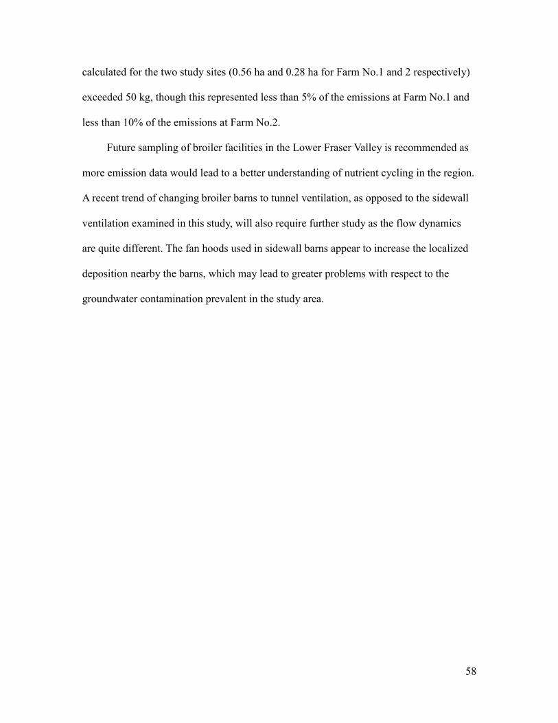
58

calculated for the two study sites (0.56 ha and 0.28 ha for Farm No.1 and 2 respectively)

exceeded 50 kg, though this represented less than 5% of the emissions at Farm No.1 and

less than 10% of the emissions at Farm No.2.

Future sampling of broiler facilities in the Lower Fraser Valley is recommended as

more emission data would lead to a better understanding of nutrient cycling in the region.

A recent trend of changing broiler barns to tunnel ventilation, as opposed to the sidewall

ventilation examined in this study, will also require further study as the flow dynamics

are quite different. The fan hoods used in sidewall barns appear to increase the localized

deposition nearby the barns, which may lead to greater problems with respect to the

groundwater contamination prevalent in the study area.

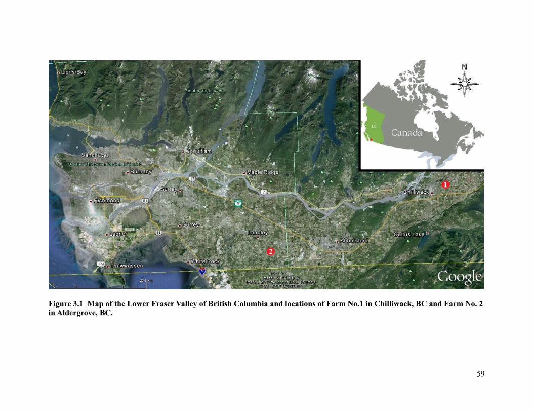
59

Figure 3.1 Map of the Lower Fraser Valley of British Columbia and locations of Farm No.1 in Chilliwack, BC and Farm No. 2 in Aldergrove, BC.

60

Figure 3.2 Map of Farm No.1 located in Chilliwack, BC showing locations of dry deposition sampling sites and gas impinger traps. The dry deposition sites are indicated by the red dots and the fans being sampled by gas impinger traps are indicated by the blue boxes. The green box in the corridor indicates where the high density (HD) deposition samples were taken. The light blue boxes on the east side of the barns show the area that the deposition samples were applied to when estimating for the entire property.

61

Figure 3.3 Map of Farm No.2 in Aldergrove, BC showing locations of dry deposition sampling sites and gas impinger traps. The dry deposition sites are indicated by the red dots and the fans being sampled by gas impinger traps are indicated by the blue boxes. The hash marked barns were not studied

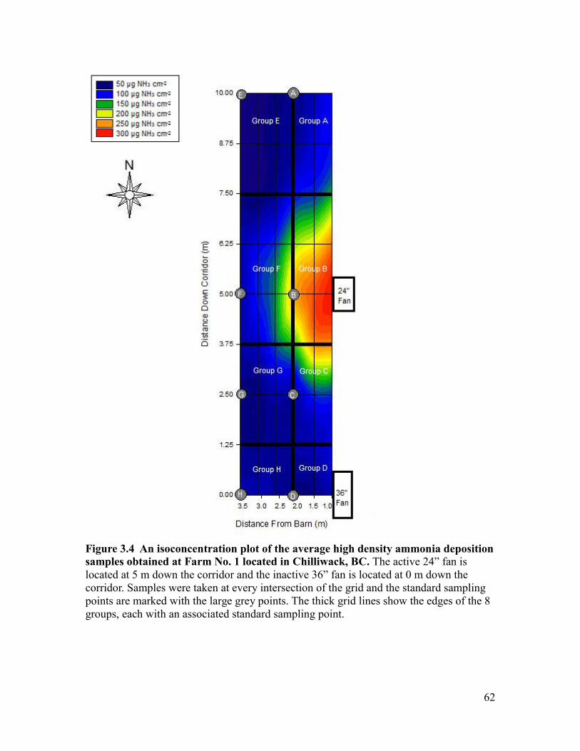
62

Figure 3.4 An isoconcentration plot of the average high density ammonia deposition samples obtained at Farm No. 1 located in Chilliwack, BC. The active 24” fan is located at 5 m down the corridor and the inactive 36” fan is located at 0 m down the corridor. Samples were taken at every intersection of the grid and the standard sampling points are marked with the large grey points. The thick grid lines show the edges of the 8 groups, each with an associated standard sampling point.

63

(a)

(b)

Figure 3.5 Changes at Farm No.1 during the four stages of ventilation and at farm No.2 during the seven stages of ventilation in (a) air pressure deficit within the barns and (b) sum total ventilation flow rates

64

(a)

(b) Figure 3.6 Percentage of time that (a) any fans were active in the barns of Farm No.1 and No.2 during sample times and (b) ventilation stages 3 or higher were active.

65

Figure 3.7 Ammonia in ventilated air within the barns on Farm No. 1. determined during the summer and winter periods.

66

Figure 3.8 Barn ventilation rates for each flock and weather station air temperature during the year-long period of measurement.

Figure 3.9 Barn exhaust NH3 concentration for each flock and weather station air temperature during the year-long period of measurement.

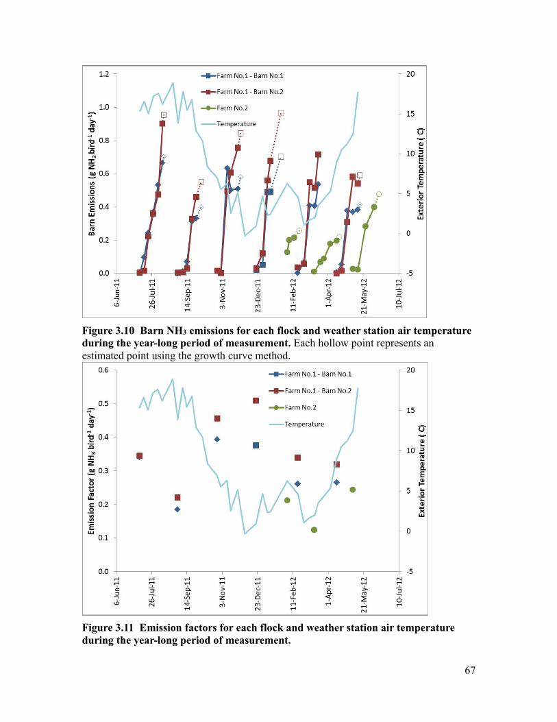
67

Figure 3.10 Barn NH3 emissions for each flock and weather station air temperature during the year-long period of measurement. Each hollow point represents an estimated point using the growth curve method.

Figure 3.11 Emission factors for each flock and weather station air temperature during the year-long period of measurement.

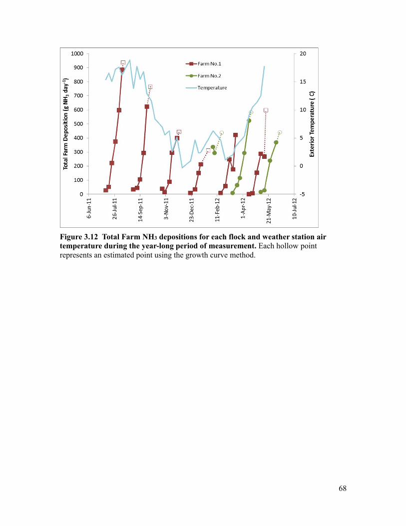
68

Figure 3.12 Total Farm NH3 depositions for each flock and weather station air temperature during the year-long period of measurement. Each hollow point represents an estimated point using the growth curve method.

69

(a) (b)

(c) (d)

70

(e) Figure 3.13 Flock A-105 from Farm No.1’s (a) ammonia emission curve in emission factor units, (b) after being normalized, (c) plotted alongside normalized growth curve (weight vs age), (d) with the estimated harvest date emission using the growth curve’s slope, and (e) the ammonia emission curve converted back into actual units along with the new final point.

71

(a)

(b)

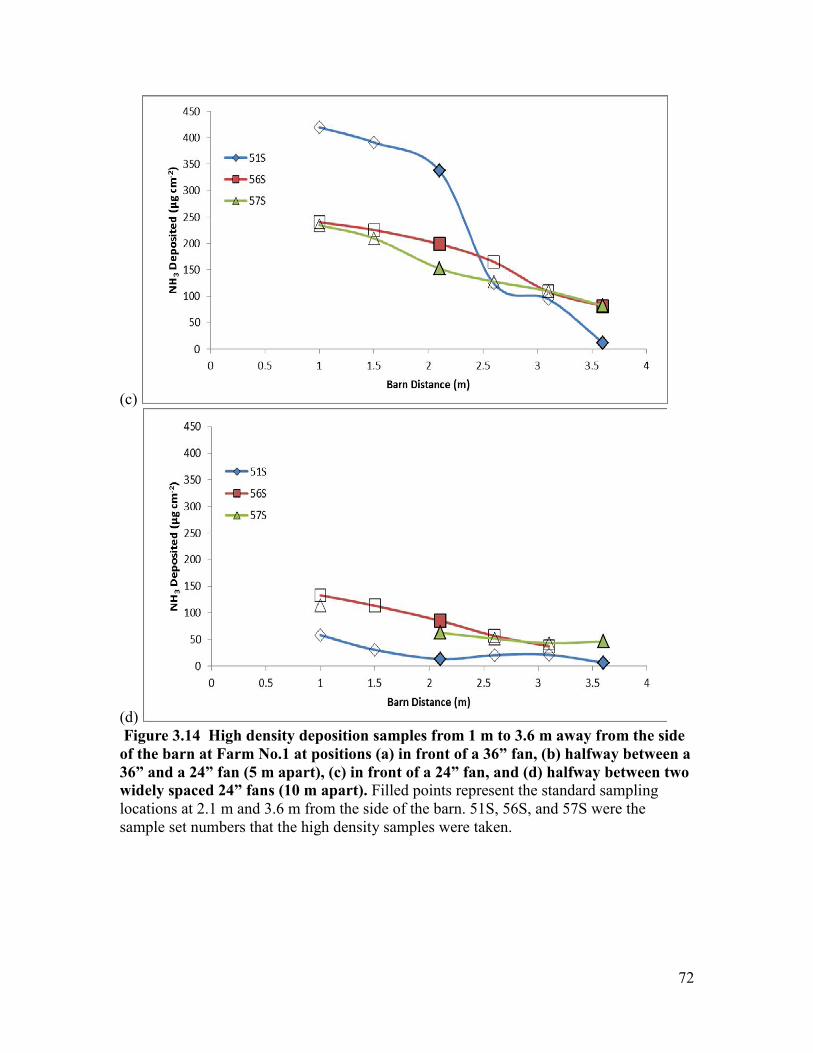
72

(c)

(d) Figure 3.14 High density deposition samples from 1 m to 3.6 m away from the side of the barn at Farm No.1 at positions (a) in front of a 36” fan, (b) halfway between a 36” and a 24” fan (5 m apart), (c) in front of a 24” fan, and (d) halfway between two widely spaced 24” fans (10 m apart). Filled points represent the standard sampling locations at 2.1 m and 3.6 m from the side of the barn. 51S, 56S, and 57S were the sample set numbers that the high density samples were taken.

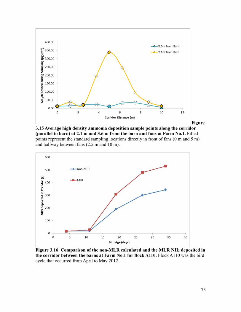
73

Figure 3.15 Average high density ammonia deposition sample points along the corridor (parallel to barn) at 2.1 m and 3.6 m from the barn and fans at Farm No.1. Filled points represent the standard sampling locations directly in front of fans (0 m and 5 m) and halfway between fans (2.5 m and 10 m).

Figure 3.16 Comparison of the non-MLR calculated and the MLR NH3 deposited in the corridor between the barns at Farm No.1 for flock A110. Flock A110 was the bird cycle that occurred from April to May 2012.

74

Figure 3.17 Comparison of the non-MLR calculated and the MLR NH3 deposited in the corridor between the barns at Farm No.2 for flock A111. Flock A111 was the bird cycle that occurred from May to June 2012.

Figure 3.18 Deposition of ammonia at 2.1 m from each barn and 3.6 m, between the barns, at Farm No.1 averaged for all sample dates with birds over 20 days old.

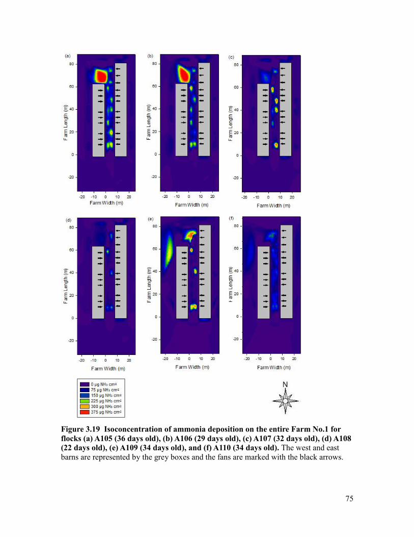
75

Figure 3.19 Isoconcentration of ammonia deposition on the entire Farm No.1 for flocks (a) A105 (36 days old), (b) A106 (29 days old), (c) A107 (32 days old), (d) A108 (22 days old), (e) A109 (34 days old), and (f) A110 (34 days old). The west and east barns are represented by the grey boxes and the fans are marked with the black arrows.

76

Figure 3.20 Isoconcentration of ammonia deposition for the field in front of Farm No.2 for flocks (a) A109 (24 days old), (b) A110 (35 days old), and (c) A111 (32 days old). The barn is represented by the grey box and the fans are marked with the black arrows.

77

Figure 3.21 Deposition of ammonia at 2.1 m and 3.6 m from the fans in line with the barn at Farm No.2 averaged for all sample dates with birds over 20 days old.

Figure 3.22 Deposition of ammonia in line with active hooded fans at Farm No.2 averaged for all sample dates with birds over 20 days old.

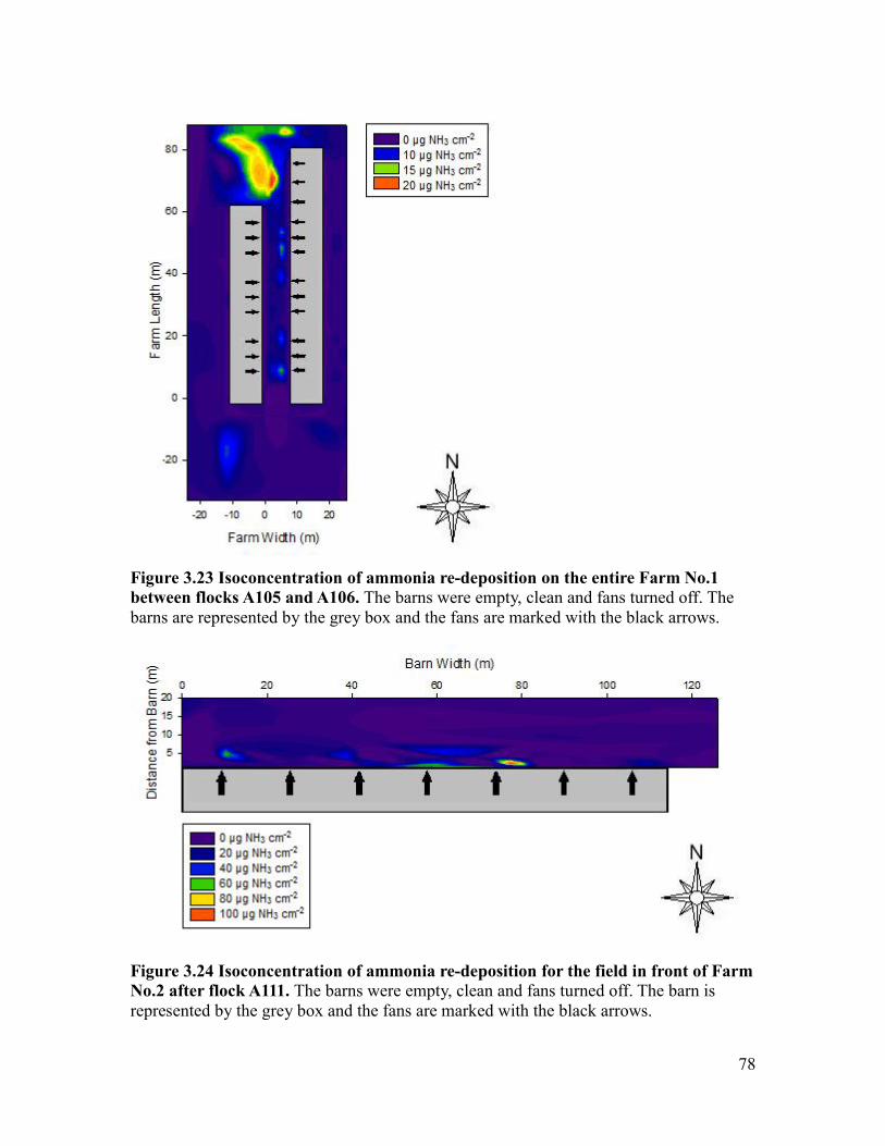
78

Figure 3.23 Isoconcentration of ammonia re-deposition on the entire Farm No.1 between flocks A105 and A106. The barns were empty, clean and fans turned off. The barns are represented by the grey box and the fans are marked with the black arrows.

Figure 3.24 Isoconcentration of ammonia re-deposition for the field in front of Farm No.2 after flock A111. The barns were empty, clean and fans turned off. The barn is represented by the grey box and the fans are marked with the black arrows.

79

Table 3.1 Summary of Multiple Linear Regressions

Factor Variable* r2

Site

Ventilation Farm No.1 BA + ET 0.825 Farm No.2 BA + ET 0.925 Fan Activity

Farm No.1 and No.2 BA 0.712 Emissions Farm No.1 BA + ET 0.765 BA (P <0.0001) ** ET (P = 0.534)** Farm No.2 BA 0.775 Emission Factor Farm No.1 and No.2 SD 0.324 Deposition Farm No.1 BA 0.885 BA + ET 0.896 Farm No.2 BA 0.903 Deposition Farm No.1 BA + E 0.786 Farm No.2 BA + E 0.836 *Variable: BA = bird age, E = emissions, EF = emission factor, ET = exterior temperature, SD = stocking density, V = ventilation **Values of P when individually correlated with emissions

80

Table 3.2 Summary of emission factors and literature values

Study Location (Reference) Market Age (days)

Stocking Density (b

m-2)

Litter Management*

Monitoring Method**

Number of

Flocks

Emission Factor (g NH3 b-1 d-1)

BC, Canada (this study) Farm No.1 - West Barn 36.4 12.34 N S-CF 6 0.30 ± 0.08 Farm No.1 - East Barn 36.4 10.97 N S-CF 6 0.37 ± 0.10 Farm No.2 - North Barn 38.7 12.10 N S-CF 3 0.19 ± 0.06 Europe (Koerkamp et al. 1998) England - - N C-CL 4 0.48

Netherlands - - N C-CL 4 0.27 Denmark - - N C-CL 4 0.21 Germany - - N C-CL 4 0.44

U.S. (Harper et al. 2010) CA (summer) 47 10.6 P C-OPL 16 0.34 CA (winter) 47 10.6 P C-OPL 16 0.30 U.S. (Wheeler et al. 2003) PA and KY 42 14.7 N C-EC 10 0.47

PA and KY 42 14.7 D C-EC 12 0.65 PA and KY 49 13.4 D C-EC 24 0.76 PA and KY 63 10.8 D C-EC 20 0.98 U.S. (Lacey et al. 2003) TX 49 13.5 D S-CM 12 0.63 U.K. (Wathes et al. 1997) England 32 9.4 N C-CL 4 0.26 *Litter Management: N = new, P = partial (new every three flocks), D = de-caked **Monitoring method: C = continuous, S = sample (discrete), CF = colorimetric flow injection analysis, CL = chemiluminescence extraction, CM = colorimetric tube, EC = electrochemical extraction, OPL = open-path laser, and PS = photoacoustic extraction

81

Table 3.3 Average flow rate for each fan across all stages

Farm Fan Diameter (in)

Average Flow Rate (m3 hr-1)

Standard Deviation

Relative Standard Deviation (%)

No.1 24 6405.8 459.4 7.17 36 12388.7 858.0 6.93

No.2 24 6979.7 195.5 2.80 36 10440.4 550.6 5.27 52 36446.8 848.7 2.33

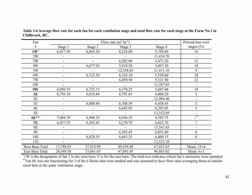
82

Table 3.4 Average flow rate for each fan for each ventilation stage and total flow rate for each stage at the Farm No.1 in Chilliwack, BC.

Fan #

Flow rate (m3 hr-1) Percent loss over stages (%) Stage 1 Stage 2 Stage 3 Stage 4

1W* 6,837.50 6,865.20 6,218.80 5,750.60 16 2W - - - 11,434.70 - 3W - - 6,202.60 5,473.20 12 4W - 6,677.05 5,918.50 5,497.30 18 5W - - 12,558.65 11,411.10 9 6W - 6,723.50 6,103.10 5,539.60 18 7W - - 6,059.50 5,321.90 12 8W - - - 11,387.85 - 9W 6,950.55 6,753.15 6,378.25 5,607.40 19 1E 6,793.10 6,610.40 6,791.65 6,460.20 5 2E - - - 12,900.40 - 3E - 6,800.40 6,768.50 6,438.45 5 4E - - 6,642.95 6,293.05 5 5E - - - 13,352.05 -

6E** 7,004.70 6,988.25 6,956.35 6,585.75 -**

7E 6,457.55 6,303.45 6,270.70 6,022.70 7 8E - - - 13,541.85 - 9E - - 6,585.45 6,031.80 8 10E - 6,828.35 6,663.25 6,400.15 6 11E - - - 12,523.10 -

West Barn Total 13,788.05 27,018.90 49,439.40 67,423.65 Mean: 15±4 East Barn Total 20,549.58 33,861.43 47,081.05 96,883.02 Mean: 6±1

*1W is the designation of fan 1 in the west barn. E is for the east barn. The bold text indicates which fan’s emissions were sampled. **Fan 6E was not functioning for 3 of the 6 flocks that were studied and was assumed to have flow rates averaging those of similar sized fans at the same ventilation stage.

83

Table 3.5 Average flow rate for each fan for each ventilation stage and total flow rate for each stage at the Farm No.2 in Aldergrove, BC.

Fan # Flow rate (m3 hr-1) Percent loss over stages (%) Stage 1 Stage 2 Stage 3 Stage 4 Stage 5 Stage 6 Stage 7

1 - - - 11,517.30 11,071.00 11,320.40 11,406.40 1 2 - 7,078.35 7,088.95 6,941.05 6,917.65 6,795.10 6,638.95 6 3 - - - - - 37,023.35 37,023.35 - 4 7,393.75 7,073.65 7,081.90 6,993.20 6,930.10 6,922.30 6,881.65 7 5 - - - - 10,275.60 10,374.15 10,164.35 1 6 - - 10,571.50 10,516.90 10,472.35 10,331.70 10,104.40 4 7 - - - - 10,423.80 10,443.10 9,995.95 4 8 7,393.75 7,076.00 7,085.43 6,967.13 6,923.88 6,858.70 6,760.30 9 9 - - - - - - 35,691.85 - 10 - 7,076.00 7,085.43 6,967.13 6,923.88 6,858.70 6,760.30 4 11 - - - 9,844.20 9,892.65 9,856.05 9,785.90 1

Total 14,787.50 28,304.00 38,913.20 59,746.90 79,830.90 116,783.55 151,213.40 Mean: 4±3

84

Table 3.6 Total emitted ammonia for each flock for each barn at Farm No.1 in Chilliwack, BC and for Farm No.2 in Aldergrove, BC.

Flock Farm - Barn Population Total Emitted NH3 (kg NH3 cycle-1)

A105 No.1 - West 9,502 110.1 No.1 - East 11,261 132.1

A106 No.1 - West 9,493 126.9 No.1 - East 11,283 82.4

A107 No.1 - West 9,555 124.0 No.1 - East 11,306 170.2

A108 No.1 - West 8,464 111.2 No.1 - East 10,487 187.0

A109 No.1 - West 10,125 79.2 No.1 - East 11,545 117.7 No.2 17082 61.5

A110 No.1 - West 10,059 87.9 No.1 - East 11,906 125.7 No.2 17472 78.1

A111 No.2 17720 160.3

Average 117.0±36.0

Sums No.1 - West 639.4* No.1 - East 815.0* No.2 599.9*

*Annual sums are in kg NH3 year-1

Table 3.7 Total deposited ammonia for each flock for each barn at Farm No.1 in Chilliwack, BC and for Farm No.2 in Aldergrove, BC.

Flock Farm Corridor Deposition

(kg NH3 cycle-1) Farm Deposition (kg NH3 cycle-1)

Total deposition in-side Corridor (%)

A105 1 11.51 12.87 89 A106 1 8.82 9.79 90 A107 1 6.25 6.77 92 A108 1 4.91 5.51 89 A109 1 4.43 4.74 93 A109 2 9.80 10.35 95 A110 1 8.85 9.60 92 A110 2 7.65 8.53 90 A111 2 7.25 8.12 89

Average 7.72±2.30 8.48±2.54

Sum 1 45.72* 50.03* 91 Sum 2 47.49* 52.52* 90

*Annual sums are in kg NH3 year-1

85

4 GENERAL CONCLUSIONS

Confined livestock operations in the Lower Fraser Valley of BC are known to

produce large amounts of ammonia. Broiler barns in this area have not been well

researched with respect to quantifying the ammonia that the ventilation systems exhausts

and how much of that is locally dry deposited, potentially contributing to groundwater

contamination. As management scenarios greatly impact ammonia emissions and

depositions from barns, a locally focused research project was required to determine the

potential environmental impacts. This chapter will outline the conclusions from the

research and then evaluate the strength and weaknesses of the methods used.

4.2 Conclusions and Recommendations

The ammonia emissions measurements at three broiler barns over the period of

one year allowed for a comparison among the barns typical for this region. Emission

factors reported in the literature were found to be similar to those from this study. This

supported the comparison of Canadian broiler operations with those found in Europe and

the USA with similar management styles, primarily litter management. The relatively

modest emission factors of the local barns are encouraging as the best management

practices appear to be reducing excessive nutrient loss. Though the emission factors are

low, the total ammonia emissions from this industry is substantial as the poultry industry

in this region is quite large. The emissions that are dispersed into the atmosphere are a

concern for non-localized deposition of ammonia and PM2.5, but the highly localized dry

deposition of ammonia above Abbotsford-Sumas aquifer is a probable source of nitrate

contamination. Current air quality measurements in the Lower Fraser Valley have not

86

recorded excessive levels of PM2.5 or ammonia, but the indiscriminate deposition of those

nitrogen species is a potential issue (Metro Vancouver 2015).

The highest levels of deposited ammonia exceeded 400 μg cm-2 over a 24-hour

exposure, which is equivalent to 40 kg ha-1. The area with this level of deposition is

limited to less than 2 m2 directly under the fan hood. Over the entire farm area the

deposition level is under 10% of the ammonia emissions measured and would be

expected to be far below the saturation point of the soil. These high values are only found

when the flock is in its last week of growth before harvest, but there are six flocks every

year and the timing of this deposition is critical to the leaching potential (i.e., when plant

uptake is very low and/or when precipitation is high). This study provides localized and

crucial emission factors and information on spatial distribution of deposition that can in

future studies be used to assess the poultry barns’ contribution to the nitrate pollution of

the Sumas-Abbotsford aquifer.

4.2.1 Future Research

Complete assessment of ammonia emissions and leaching from deposition

requires more research. It is highly probably that nitrogen leaching is taking place

considering the levels of ammonia that are being deposited. What needs to be determined

is how significant these “hot spot” sources of nitrate are compared to the typical culprits

of nitrate leaching (e.g., excessive field fertilization, improper manure storage facilities).

To investigate this localized leaching the research must venture below the surface of the

soil. Analyzing soil cores or suction lysimeter samples of the soil solution will not give a

full picture of the magnitude of this problem, though they can confirm that the suspected

leaching is taking place.

87

Various types of lysimeters have been used extensively on the Abbotsford-Sumas

aquifer to assess leaching from raspberry fields, in the effort to design new best

management practices (Malekani 2012). The installation of this type of equipment is

expensive and difficult, but is likely the only way that quantitative data on the

contaminating nitrate could be obtained. Once the initial set of data is collected the use of

modelling to estimate the total impact on the aquifer will be needed.

Although the conventional sidewall ventilation barns are the norm in the Lower

Fraser Valley there are a few different barn designs, including two-story sidewall barns

and tunnel ventilated barns, which some producers are beginning to use. These different

barn types will have a very different emission and dry deposition pattern and possibly a

lesser impact if dispersion of the ammonia is encouraged. Ammonia collection systems

are also better suited to tunnel style ventilation systems so the emission problem could be

remedied in an entirely different way. These new barn designs will need to have emission

and deposition measurements made in a manner similar to this study so that their impact

may also be assessed.

4.2 Evaluation of Study Methods and Recommendations for Future

Modifications

This study involved numerous measurements and methods of varying complexity.

The characterization of the barn ventilation systems was a critical part of this research as

the emission estimates were highly dependent on this being accurate. Measuring the flow

patterns of fans is a complicated task and using equipment designed for that purpose

made it far easier. The FANS unit is highly recommended since it measures the air flow

88

of the fan in addition to recording the pressure differential that is critical to understanding

the efficacy of the ventilation system as a whole.

The acid impinger system that collected the ammonia in the exhausted air was

another effective, though temperamental system. The numerous Teflon tubes, glass

containers, fragile fritted glass bubblers, and diaphragm pumps create a delicate system

often in need of repair. The sensitivity of the system was comparable to the levels of

ammonia it was required to measure. High-frequency measurements would require a

much more expensive system and investigation of the diurnal emission patterns were not

of concern in this study. In the future, protecting the impinger system from the seasonal

temperature fluctuations would be recommended as they resulted in a great number of

repairs. Another limitation of the ammonia measurements concerned the replication and

number of fans that could be sampled. The impinger system is complex enough that

sampling all of the fans of a barn at once requires a great deal of effort and time.

The dust in the fan exhaust was a variable that has been investigated to a limited

extent in other studies. Consisting mainly of dander and fecal particulate the potential for

it to contaminate both impinger samples and dry deposition samples deserves more

research. The level of dust would make optical ammonia measurements at the barns

unreliable and the contamination of dry deposition measurements would be considerable,

except possibly in the case of measuring deposition with biological systems such as grass.

The dry deposition sampling methodology was very successful in this study. The

modification of the existing method demonstrated the flexibility of using soil as a

collection medium. The extremely low cost of the method was offset by the time

consuming process of extracting and analyzing the large number of samples. Using a

89

naturally occurring medium allowed for a logical transferal of measured deposition in the

sample which would occur in situ. The soil was surprisingly stable in the high air speed

environment below the fan hoods, though some loss of soil was inevitable. The elevated

humidity of the fan exhaust likely dampened the soil and increased its stability. The high

levels and rate of deposition in that environment allowed any newly exposed soil to retain

sufficient ammonia to still yield an appropriate sample.

The high density samples and the MLR model used to modify the standard

deposition measurement points of the other sampling dates is one aspect of this study that

could use expanded complexity. The MLR model was effective in preventing the over-

and under-estimations of deposition in the large sample blocks, but it is rather crude.

Spatial statistical methods could certainly be used to improve this method of estimation

in future studies.

Overall, the methods used in this study effectively characterized and quantified

the emissions and localized dry deposition of ammonia. The calculated emission factors

demonstrated that the broiler operations in the Lower Fraser Valley are similar to those in

Europe and the USA. The dry deposition levels on the three farms included in this study

were similar to those reported in the literature, accounting for less than 10% of the total

emissions. The extremely high levels of ammonia deposition found directly below the fan

hoods is a new information that requires further study to determine the associated nitrate

leaching potential. An assessment of the overall contribution of the broiler industry to the

contamination of the Abbotsford-Sumas aquifer will be made possible by addition of

estimates of nitrogen leaching from individual farms.

90

References

Adderley, C., and A. Christen. 2014. “Evaluation of the Performance of Vegetative Buffers for Emission Reduction of Particulate Matter from Poultry Facilities.” https://open.library.ubc.ca/cIRcle/collections/facultyresearchandpublications/42387/items/1.0103596. (Accessed April 2016).

Almasri, M.N., and J.J. Kaluarachchi. 2004. “Assessment and Management of Long-Term Nitrate Pollution of Ground Water in Agriculture-Dominated Watersheds.” Journal of Hydrology 295 (1-4): 225–45.

Amon, M., M. Dobeic, R.W. Sneath, V.R. Phillips, T.H. Misselbrook, and B.F. Pain. 1997. “A Farm-Scale Study on the Use of Clinoptilolite Zeolite and De-Odorase® for Reducing Odour and Ammonia Emissions from Broiler Houses.” Bioresource Technology 61 (3): 229–37.

Aneja, V.P., J.P. Chauhan, and J.T. Walker. 2000. “Characterization of Atmospheric Ammonia Emissions from Swine Waste Storage and Treatment Lagoons.” Journal of Geophysical Research 105 (May 2000): 11,535–11,545.

Arogo, J., P.W. Westerman, A.J. Heber, W.P. Robarge, and J.J. Classen. 2006. “Ammonia Emissions From Animal Feeding Operations.” Animal Agriculture and the Environment: National Center for Manure and Animal Watse Management White Papers, no. 913: 41–88.

BC Chicken Marketing Board. 2014. “2014 Annual Report.” www.bcchicken.ca/BCChickenAnnualReport2014.pdf. (Accessed April 2016).

Belzer, W., C. Evans, and A. Poon. 1997. “Atmospheric Nitrogen Concentrations in the Lower Fraser Valley.” Environment Canada, Aquatic and Atmospheric Science Division, Vancouver, BC DOE FRAP, 1997.

Bittman, S., D.I. Massé, E. Pattey, M. Cournoyer, G. Qiu, A. Narjoux, S.C. Sheppard, and A. Van der Zaag. 2014. “Effects of Agriculture on Air Quality in Canada.” In Air Quality Management: Canadian Perspectives on a Global Issue, edited by Eric Taylor and Ann McMillan, 237–59. Springer Science & Business Media.

Blake, J.P., and J.B. Hess. 2001. “Litter Treatments for Poultry.” Alabama Cooperative Extension System.

Buss, S.R., A.W. Herbert, P. Morgan, S.F. Thornton, and J.W.N. Smith. 2004. “A Review of Ammonium Attenuation in Soil and Groundwater.” Quarterly Journal of Engineering Geology and Hydrogeology 37 (4): 347–59.

Carey, J.B., R.E. Lacey, and S. Mukhtar. 2004. “A Review of Literature Concerning Odors, Ammonia, and Dust from Broiler Production Facilities: 2. Flock and House Management Factors.” The Journal of Applied Poultry Research 13 (3): 509–13.

Cheng, T.K., M.L. Hamre, and C.N. Coon. 1997. “Effect of Environmental Temperature, Dietary Protein, and Energy Levels on Broiler Performance.” The Journal of Applied Poultry Research 6 (1): 1–17.

Chesnaux, R., D.M. Allen, and G. Graham. 2007. “Assessment of the Impact of Nutrient

91

Management Practices on Nitrate Contamination in the Abbotsford-Sumas Aquifer.” Environmental Science & Technology 41 (21): 7229–34.

Chiba, L. 2014. “Poultry Nutrition and Feeding.” In Animal Nutrition Handbook, 3rd ed., 410–25. http://www.ag.auburn.edu/~chibale/animalnutrition.html. (Accessed April 2016).

Christensen, T.H., P. Kjeldsen, P.L. Bjerg, D.L. Jensen, J.B. Christensen, A. Baun, H. Albrechtsen, and G. Heron. 2001. “Biogeochemistry of Landfill Leachate Plumes.” Applied Geochemistry 16 (7): 659–718.

Colina, J., A. Lewis, and P.S. Miller. 2000. “A Review of the Ammonia Issue and Pork Production.” Nebraska Swine Reports. University of Nebraska. Animal Science Department.

Czarick, M., and B.D. Fairchild. 2013. “What Is the Optimal Static Pressure When Using Air Inlets?” Poultry Housing Tips. http://www.thepoultrysite.com/articles/2786/what-is-the-optimal-static-pressure-when-using-air-inlets/. (Accessed April 2016).

De Visscher, A., L.A. Harper, P.W. Westerman, Z. Liang, J. Arogo, R.R. Sharpe, and O. Van Cleemput. 2002. “Ammonia Emissions from Anaerobic Swine Lagoons : Model Development.” Journal of Applied Meteorology 41: 426–33.

Di, H.J., and K.C. Cameron. 2002. “Nitrate Leaching in Temperate Agroecosystems: Sources, Factors and Mitigating Strategies.” Nutrient Cycling in Agroecosystems 64 (3): 237–56.

Elzing, A., and G.J. Monteny. 1997. “Modeling and Experimental Determination of Ammonia Emissions Rates from a Scale Model Dairy-Cow House.” Transactions of the ASAE 40 (3). American Society of Agricultural and Biological Engineers: 721–26.

Environment Canada. 2015. “Environment Canada, National Climate Data and Information Archive.” Downsview, Ontario. http://climate.weather.gc.ca/. (Accessed April 2016).

Fairchild, B.D., and C.W. Ritz. 2009. “Poultry Drinking Water Primer.” University of Georgia. http://www.thepoultrysite.cn/articles/686/poultry-drinking-water-primer/. (Accessed April 2016).

Fenn, L.B., and D.E. Kissel. 1973. “Ammonia Volatilization from Surface Applications of Ammonium Compounds on Calcareous Soils: I. General Theory.” Soil Science Society of America Journal 37 (6). Soil Science Society of America: 855–59.

Folorunso, O.R., A.A. Adesua, and G.E. Onibi. 2014. “Response of Broiler Chickens to Diets of Varying Protein Contents under Ad Libitum and Skip-a-Day Feeding Regimes.” African Journal of Agricultural Research 9 (1). Academic Journals: 113–18.

Fowler, D., C.E.R. Pitcairn, M.A. Sutton, C. Flechard, B. Loubet, M. Coyle, and R.C. Munro. 1998. “The Mass Budget of Atmospheric Ammonia in Woodland within 1 Km of Livestock Buildings.” Environmental Pollution 102 (1): 343–48.

Fraser Valley Regional District. 2011. “Agricultural Economy in the Fraser Valley

92

Regional District; Regional Snapshot Series,” 16. http://www.fvrd.ca/assets/Government/Documents/AgricultureSnapshot.pdf. (Accessed April 2016).

Gates, R.S., K.D. Casey, E.F. Wheeler, H. Xin, and a.J. Pescatore. 2008. “U.S. Broiler Housing Ammonia Emissions Inventory.” Atmospheric Environment 42 (14): 3342–50.

Gates, R.S., K.D. Casey, H. Xin, E.F. Wheeler, and J.D. Simmons. 2004. “Fan Assessment Numeration System (FANS) Design and Calibration Specifications.” Transactions of the ASABE 47 (5): 1709–15.

Grunhage, L., U. Dammgen, U. Hertstein, and H.J. Jager. 1993. “Response of Grassland Ecosystem to Air Pollutants: I-Experimental Concept and Site of the Braunschweig Grassland Investigation Program.” Environmental Pollution (Barking, Essex : 1987) 81 (2). England: 163–71.

Hansen, Bi., P. Nørnberg, and K.R. Rasmussen. 1998. “Atmospheric Ammonia Exchange on a Heathland in Denmark.” Atmospheric Environment 32 (3): 461–64.

Hao, X., C. Chang, H.H. Janzen, B.R. Hill, and T. Ormann. 2005. “Potential Nitrogen Enrichment of Soil and Surface Water by Atmospheric Ammonia Sorption in Intensive Livestock Production Areas.” Agriculture, Ecosystems & Environment 110 (3-4): 185–94.

Hao, Xi., C. Chang, H.H. Janzen, G. Clayton, and B.R. Hill. 2006. “Sorption of Atmospheric Ammonia by Soil and Perennial Grass Downwind from Two Large Cattle Feedlots.” Journal of Environmental Quality 35 (5): 1960–65.

Harper, L.A., T.K. Flesch, and J.D. Wilson. 2010. “Ammonia Emissions from Broiler Production in the San Joaquin Valley.” Poultry Science 89 (9): 1802–14.

Harris, D.B., R.C. Shores, and L.G. Jones. 2001. “Ammonia Emission Factors from Swine Finishing Operations.” In EPA Emissions Inventory Conference, 6.

Hristov, A.N., M. Hanigan, A. Cole, R. Todd, T.A. McAllister, P.M. Ndegwa, and A. Rotz. 2011. “Review: Ammonia Emissions from Dairy Farms and Beef Feedlots 1.” Canadian Journal of Animal Science 91 (1): 1–35.

Jacobson, L.D., B.W. Auvermann, R. Massey, F.M. Mitloehner, A.L. Sutton, and H. Xin. 2011. “Air Issues Associated with Animal Agriculture : A North American Perspective.” Council for Agricultural Science and Technology (CAST), 47.

Karamanlis, X., P. Fortomaris, G. Arsenos, I. Dosis, D. Papaioannou, C. Batzios, and A. Kamarianos. 2008. “The Effect of a Natural Zeolite (clinoptilolite) on the Performance of Broiler Chickens and the Quality of Their Litter.” Asian-Aust J Anim Sci 21: 1642–50.

Kelleher, B.P., J.J. Leahy, A.M. Henihan, T.F. O’dwyer, D. Sutton, and M.J. Leahy. 2002. “Advances in Poultry Litter Disposal Technology–a Review.” Bioresource Technology 83 (1). Elsevier: 27–36.

Kelley, C.C., and R.H. Spilsbury. 1939. “Soil Survey of the Lower Fraser Valley.” Department of Agriculture. http://sis.agr.gc.ca/cansis/publications/surveys/bc/bc1/bc1_report.pdf. (Accessed

93

April 2016).

Koerkamp, P.W.G.G. 1994. “Review on Emissions of Ammonia from Housing Systems for Laying Hens in Relation to Sources, Processes, Building Design and Manure Handling.” Journal of Agricultural Engineering Research 59 (2): 73–87.

Koerkamp, P.W.G.G., J.H.M. Metz, G.H. Uenk, V.R. Phillips, M.R. Holden, R.W. Sneath, J.L. Short, et al. 1998. “Concentrations and Emissions of Ammonia in Livestock Buildings in Northern Europe.” Journal of Agricultural Engineering Research 70 (1): 79–95.

Lacey, R.E., J.S. Redwine, and C.B. Parnell. 2003. “Particulate Matter and Ammonia Emission Factors.” Transactions of the ASABE 46 (4): 1203–14.

Lacy, M.P., and M. Czarick. 1992. “Tunnel-Ventilated Broiler Houses: Broiler Performance and Operating Costs.” The Journal of Applied Poultry Research 1 (1): 104–9.

Li, H., H. Xin, and R.T. Burns. 2006. “Reduction of Ammonia Emission from Stored Poultry Manure Using Additives: Zeolite, Al+ Clear, Ferix-3 and PLT.” In 2006 ASAE Annual Meeting, 1. American Society of Agricultural and Biological Engineers.

Loubet, B., W.A.H. Asman, M. Theobald, O. Hertel, S.Y. Tang, P. Robin, M. Hassouna, et al. 2009. “Ammonia Deposition near Hot Spots: Processes, Models and Monitoring Methods.” Atmospheric Ammonia 4 (December): 1–59.

Malekani, Farzin. 2012. “A New Approach to Estimate Monthly Groundwater Nitrate Loading from an Individual Agricultural Field.” University of Calgary.

Malone, G., and G. Van Wicklen. 2002. “Trees as a Vegetative Filter around Poultry Farms.” In InProc. Natl. Poult. Waste Management Symp.(CD), National Poultry Waste Management Symposium, edited by P. H. Patterson and J. P. Blake, 271–72. Birmingham, Alabama.

May, J.D., and B.D. Lott. 2000. “The Effect of Environmental Temperature on Growth and Feed Conversion of Broilers to 21 Days of Age.” Poultry Science 79 (no. 5): 669–71.

McGinn, S.M., H.H. Janzen, and T.W. Coates. 2003. “Atmospheric Pollutants and Trace Gases Atmospheric Ammonia , Volatile Fatty Acids , and Other Odorants near Beef Feedlots.” Journal of Environmental Quality 32: 1173–82.

Metro Vancouver. 2015. “2014 Lower Fraser Valley Air Quality Monitoring Report.” http://www.metrovancouver.org/services/air-quality/AirQualityPublications/2014_LFV_AQ_Monitoring_Report.pdf. (Accessed April 2016).

Mitchell, R.J., R.S. Babcock, S. Gelinas, L. Nanus, and D.E. Stasney. 2003. “Nitrate Distributions and Source Identification in the Abbotsford–Sumas Aquifer, Northwestern Washington State.” Journal of Environmental Quality 32: 789–800.

Monteny, G.J., and J.W. Erisman. 1998. “Ammonia Emission from Dairy Cow Buildings : A Review of Measurement Techniques , Influencing Factors.” Netherlands Journal of Agricultural Science 46: 225–47.

94

Ndegwa, P.M., V.K. Vaddella, A.N. Hristov, and H.S. Joo. 2005. “Measuring Concentrations of Ammonia in Ambient Air or Exhaust Air Stream Using Acid Traps.” Journal of Environmental Quality 38 (2): 647–53.

Oluyemi, J.A., and F.A. Roberts. 2000. Poultry Production in Warm Wet Climates. 2nd ed. Ibadan, Oyo State, Nigeria: Spectrum Books Limited.

Patterson, P. H., and T. Adrizal. 2005. “Management Strategies to Reduce Air Emissions: Emphasis—Dust and Ammonia.” The Journal of Applied Poultry Research 14 (3). Oxford University Press: 638–50.

Pearson, B.Y.J., and G.R. Stewart. 1993. “Tansley Review No . 56 The Deposition of Atmospheric Ammonia and Its Effects on Plants.” New Phytol. 125: 283–305.

Pescatore, A.J., K.D. Casey, and R.S. Gates. 2005. “Ammonia Emissions from Broiler Houses.” Journal of Applied Meteorology 14: 635–37.

Pinder, R.W., N.J. Pekney, C.I. Davidson, and P.J. Adams. 2004. “A Process-Based Model of Ammonia Emissions from Dairy Cows: Improved Temporal and Spatial Resolution.” Atmospheric Environment 38 (9): 1357–65.

Pitcairn, C.E.R., I.D. Leith, L.J. Sheppard, M.A. Sutton, D. Fowler, R.C. Munro, S. Tang, and D. Wilson. 1998. “The Relationship between Nitrogen Deposition, Species Composition and Foliar Nitrogen Concentrations in Woodland Flora in the Vicinity of Livestock Farms.” Environmental Pollution 102 (1): 41–48.

Poor, N., R. Pribble, and H. Greening. 2001. “Direct Wet and Dry Deposition of Ammonia, Nitric Acid, Ammonium and Nitrate to the Tampa Bay Estuary, FL, USA.” Atmospheric Environment 35 (23). Elsevier: 3947–55.

Pratt, E.V., S.P. Rose, and A.A. Keeling. 2002. “Effect of Ambient Temperature on Losses of Volatile Nitrogen Compounds from Stored Laying Hen Manure.” Bioresource Technology 84 (2). Elsevier: 203–5.

Rabaud, N.E., T.A. James, L.L. Ashbaugh, and R.G. Flocchini. 2001. “A Passive Sampler for the Determination of Airborne Ammonia Concentrations near Large-Scale Animal Facilities.” Environmental Science & Technology 35 (6): 1190–96.

Reece, F.N., B.D. Lott, and B.J. Bates. 1985. “The Performance of a Computerized System for Control of Broiler-House Environment.” Poultry Science 64 (2): 261–65.

Ritz, C.W., B.D. Fairchild, and M.P. Lacy. 2004. “Implications of Ammonia Production and Emissions from Commercial Poultry Facilities: A Review.” The Journal of Applied Poultry Research 13 (4): 684–92.

Rodhe, L., and S. Karlsson. 2002. “SE—Structures and Environment: Ammonia Emissions from Broiler Manure—Influence of Storage and Spreading Method.” Biosystems Engineering 82 (4). Elsevier: 455–62.

Schmidt, I., O. Sliekers, M. Schmid, I. Cirpus, M. Strous, E. Bock, J.G. Kuenen, and M.S.M. Jetten. 2002. “Aerobic and Anaerobic Ammonia Oxidizing Bacteria--Competitors or Natural Partners?” FEMS Microbiology Ecology 39 (3). England: 175–81.

Silva, R.G., K.C. Cameron, H.J. Di, and T. Hendry. 1999. “A Lysimeter Study of the

95

Impact of Cow Urine, Dairy Shed Effluent, and Nitrogen Fertiliser on Nitrate Leaching.” Australian Journal of Soil Research 37 (2). CSIRO Publishing: 357–58.

Silva, R.G., K.C. Cameron, H.J. Di, N.P. Smith, and G.D. Buchan. 2000. “Effect of Macropore Flow on the Transport of Surface-Applied Cow Urine through a Soil Profile.” Soil Research 38 (1): 13–24.

Snell, H.G.J., and A. Schwarz. 2003. “Development of an Efficient Bioscrubber System for the Reduction of Emissions.” In 2003 ASAE Annual Meeting, 1. American Society of Agricultural and Biological Engineers.

Sommer, S.G., and N.J. Hutchings. 2001. “Ammonia Emission from Field Applied Manure and Its Reduction—invited Paper.” European Journal of Agronomy 15 (1): 1–15.

Sommer, S.G., J.E. Olesen, and B.T. Christensen. 1991. “Effects of Temperature, Wind Speed and Air Humidity on Ammonia Volatilization from Surface Applied Cattle Slurry.” The Journal of Agricultural Science 117 (01): 91–100.

Stelson, A.W., and J.H. Seinfeld. 2007. “Relative Humidity and Temperature Dependence of the Ammonium Nitrate Dissociation Constant.” Atmospheric Environment 41. Elsevier: 126–35.

Sutton, M.A., D. Fowler, and J.B. Moncriefe. 1993. “The Exchange of Atmospheric Ammonia with Vegetated Surfaces. I: Unfertilized Vegetation.” Quarterly Journal of the Royal Meteorological Society 119 (513). Wiley Online Library: 1023–45.

Theobald, M.R., C. Milford, K.J. Hargreaves, L.J. Sheppard, E. Nemitz, Y.S. Tang, V.R. Phillips, et al. 2001. “Potential for Ammonia Recapture by Farm Woodlands: Design and Application of a New Experimental Facility.” TheScientificWorldJournal 1 Suppl 2 (November): 791–801.

Todd, R.W., N.A. Cole, R.N. Clark, T.K. Flesch, L.A. Harper, and B.H. Baek. 2008. “Ammonia Emissions from a Beef Cattle Feedyard on the Southern High Plains.” Atmospheric Environment 42 (28): 6797–6805.

Turnbull, J.E., and H.E. Huffman. 1987. “Fan Ventilation Principles and Rates.” Ottawa, ON: Agiculture Canada.

Tyson, S.C., and M.L. Cabrera. 1993. “Nitrogen Mineralization in Soils Amended with Composted and Uncomposted Poultry Litter.” Communications in Soil Science and Plant Analysis 24 (17-18). Taylor & Francis: 2361–74.

Van der Eerden, L.J.M. 1982. “Toxicity of Ammonia to Plants.” Agriculture and Environment 7 (3-4). Elsevier: 223–35.

Van Herk, C. 1999. “Mapping of Ammonia Pollution With Epiphytic Lichens in the Netherlands.” The Lichenologist 31 (1): 9–20.

Vavilin, V.A., B. Fernandez, J. Palatsi, and X. Flotats. 2008. “Hydrolysis Kinetics in Anaerobic Degradation of Particulate Organic Material: An Overview.” Waste Management 28 (6). Elsevier: 939–51.

Vayenas, D.V., S. Takahama, C.I. Davidson, and S.N. Pandis. 2005. “Simulation of the Thermodynamics and Removal Processes in the Sulfate‐ammonia‐nitric Acid

96

System during Winter: Implications for PM2. 5 Control Strategies.” Journal of Geophysical Research: Atmospheres 110 (D7). Wiley Online Library.

Vest, L., and B.L. Tyson. 1991. “Key Factors for Poultry House Ventilation.” Bulletin-Cooperative Extension Service, University of Georgia, College of Agriculture (USA). http://www.thepoultrysite.com/articles/2321/key-factors-for-poultry-house-ventilation/. (Accessed April 2016).

Wassenaar, L.I. 1995. “Evaluation of the Origin and Fate of Nitrate in the Abbotsford Aquifer Using the Isotopes of 15 N and 18 O in NO 3−.” Applied Geochemistry 10 (4). Elsevier: 391–405.

Wathes, C.M., M.R. Holden, R.W. Sneath, R.P. White, and V.R. Phillips. 1997. “Concentrations and Emission Rates of Aerial Ammonia, Nitrous Oxide, Methane, Carbon Dioxide, Dust and Endotoxin in UK Broiler and Layer Houses.” British Poultry Science 38 (1): 14–28.

Wesely, M.L., and B.B. Hicks. 2000. “A Review of the Current Status of Knowledge on Dry Deposition.” Atmospheric Environment 34: 2261–82.

Wheeler, E.F., K.D. Casey, R.S. Gates, H. Xin, J.L. Zajaczkowski, P.A. Topper, Y. Liang, and A.J. Pescatore. 2006. “Ammonia Emissions From Twelve U.S. Broiler Chicken Houses.” Transactions of the ASABE 49 (5): 1495–1512.

Wheeler, E.F., J.S. Zajaczkowski, P.A. Topper, R.S. Gates, H. Xin, K.D. Casey, and Y. Liang. 2003. “Ammonia Emissions from Broiler Houses in Pennsylvania During Cold Weather.” In International Symposiun on Gaseous and Odour Emissions from Animal Production Facilities, 1–8.

Zebarth, B.J., B. Hii, H. Liebscher, K. Chipperfield, J.W. Paul, G. Grove, and S.Y. Szeto. 1998. “Agricultural Land Use Practices and Nitrate Contamination in the Abbotsford Aquifer, British Columbia, Canada.” Agriculture, Ecosystems & Environment 69 (2): 99–112.

97

APPENDIX I: Historic and study period weather data for Abbotsford, BC.

(a)

(b)

Figure A.1 Comparison of historic monthly data (1981-2010) in comparison with the July 2011 to June 2012 for (a) total precipitation and (b) average temperature for Abbotsford, BC, Canada (Environment Canada 2015). The Abbotsford weather station was located 12 km from the Aldergrove study site and 40 km from the Chilliwack study site.

98

APPENDIX II: Description of treatments and samples sizes for each of the methodology trials. Table A.1 Description of treatments and samples sizes for each of the methodology trials.

Trial Treatment n Mass (g)* Location Exposure Time (h)

NH4-N Deposited (mg m-2)**

Sample - 8 8.00 1.5 m & 20 m*** 6.8 1521.15 a****

Mass - 8 12.00 1.5 m & 20 m 6.8 1462.50 a

- 8 16.00 1.5 m & 20 m 6.8 1753.68 a

Saturation - 10 12.00 1.5 m 1.0 365.27 a

- 5 12.00 1.5 m 6.0 1108.14 b

- 5 12.00 1.5 m 9.5 1354.78 b

- 5 12.00 1.5 m 24.1 3488.52 c

- 5 12.00 1.5 m 47.8 5503.49 d

- 5 12.00 1.5 m 72.8 7610.37 e

- 5 12.00 1.5 m 144.8 10804.52 f

Moisture Dry 6 12.00 1.5 m 1.5 390.23 ab

2 ml DI 3 12.00 1.5 m 1.5 296.38 a

4 ml DI 3 12.00 1.5 m 1.5 507.85 b

6 ml DI 3 12.00 1.5 m 1.5 272.63 ab

Dry 6 12.00 1.5 m 1.5 390.23 a

Wet 9 12.00 1.5 m 1.5 390.23 a

pH 0 ml Acid 5 12.00 1.5 m 25.0 3992.34 a

0.5 ml Acid 5 12.00 1.5 m 25.0 4181.23 a

1 ml Acid 5 12.00 1.5 m 25.0 4001.42 a

4 ml Acid 5 12.00 1.5 m 25.0 4681.53 b

Texture 0% sand 4 12.00 1.5 m 23.3 3240.94 a

25% 4 12.00 1.5 m 23.3 2891.11 a

50% 4 12.00 1.5 m 23.3 2561.31 ab

75% 4 12.00 1.5 m 23.3 1909.47 b

100% 4 12.00 1.5 m 23.3 506.68 c

Rain No Cover 4 12.00 1.5 m 7.0 1650.10 a

Cover Cover 4 12.00 1.5 m 7.0 1536.03 a

No Cover 4 12.00 3 m 7.0 685.74 b

Cover 4 12.00 3 m 7.0 669.37 b

No Cover 4 12.00 20 m 7.0 16.08 c

Cover 4 12.00 20 m 7.0 7.35 c * Masses were measured to +/- 0.01 g ** NH4-N deposited is not given in a per hour unit for the Saturation trial (mg m-2) *** Ambient samples were taken at a location 20 m away from the ventilation fan **** Means followed by the same letter are not significantly different (P > 0.05) as determined by LSD mean comparison.

99

APPENDIX III: Fan Assessment Numeration System (FANS)

Figure A.2 Fan Assessment Numeration System (FANS) that allowed measurements of a 24” ventilation fan at Farm No.2 located in Aldergrove, BC

100

Figure A.3 Contour plot of air flow (m/s) through the Fan Assessment Numeration System while measuring a 36” ventilation fan at Farm No.1

101

APPENDIX IV: Gas Impinger Acid Trap System and sidewall fan hoods.

Figure A.4 Gas Impinger Acid Trap System (with four separate sample streams) outside the barn at Farm No.2 located in Aldergrove, BC

Figure A.5 Air filters used for the gas impinger traps. Shown is the ambient sampling point.

102

Figure A.6 Dust clogged air filter beneath a fan hood.

Figure A.7 Corridor at Farm No.1 with hooded 24” (0.61 m) sidewall fans and non-hooded 36” (0.91 m) fans.

103

APPENDIX V: Dry deposition sample rain cover detail.

(a)

(b) Figure A.8 Rain cover for soil filled Petri dish dry deposition sample on (a) grass and (b) dusty soil beneath a fan hood.

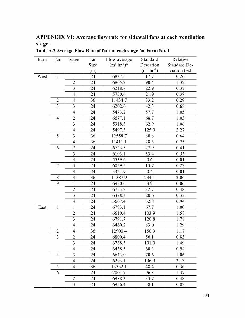
104

APPENDIX VI: Average flow rate for sidewall fans at each ventilation stage. Table A.2 Average Flow Rate of fans at each stage for Farm No. 1

Barn Fan Stage Fan Size (in)

Flow average (m3 hr-1)*

Standard Deviation (m3 hr-1)

Relative Standard De-viation (%)

West

1 1 24 6837.5 17.7 0.26 2 24 6865.2 90.4 1.32 3 24 6218.8 22.9 0.37 4 24 5750.6 21.9 0.38

2 4 36 11434.7 33.2 0.29 3 3 24 6202.6 42.3 0.68

4 24 5473.2 57.7 1.05 4 2 24 6677.1 68.7 1.03

3 24 5918.5 62.9 1.06 4 24 5497.3 125.0 2.27

5 3 36 12558.7 80.8 0.64 4 36 11411.1 28.3 0.25

6 2 24 6723.5 27.9 0.41 3 24 6103.1 33.4 0.55 4 24 5539.6 0.6 0.01

7 3 24 6059.5 13.7 0.23 4 24 5321.9 0.4 0.01

8 4 36 11387.9 234.1 2.06 9 1 24 6950.6 3.9 0.06

2 24 6753.2 32.7 0.48 3 24 6378.3 20.6 0.32 4 24 5607.4 52.8 0.94

East 1 1 24 6793.1 67.7 1.00 2 24 6610.4 103.9 1.57 3 24 6791.7 120.8 1.78 4 24 6460.2 83.0 1.29

2 4 36 12900.4 150.9 1.17 3 2 24 6800.4 56.1 0.83

3 24 6768.5 101.0 1.49 4 24 6438.5 60.3 0.94

4 3 24 6643.0 70.6 1.06 4 24 6293.1 196.9 3.13

5 4 36 13352.1 48.4 0.36 6 1 24 7004.7 96.3 1.37

2 24 6988.3 33.7 0.48 3 24 6956.4 58.1 0.83

105

Barn Fan Stage Fan Size (in)

Flow average (m3 hr-1)*

Standard Deviation (m3 hr-1)

Relative Standard De-viation (%)

East 6 4 24 6585.8 65.4 0.99 7 1 24 6457.6 127.1 1.97

2 24 6303.5 40.0 0.63 3 24 6270.7 93.8 1.50 4 24 6022.7 67.7 1.12

8 4 36 13541.9 182.2 1.35 9 3 24 6585.5 27.4 0.42

4 24 6031.8 35.4 0.59 10 2 24 6846.3 216.4 3.16

2 24 6828.4 90.2 1.32 3 24 6720.8 72.1 1.07 3 24 6663.3 95.0 1.43 4 24 6309.5 58.7 0.93 4 24 6400.2 66.0 1.03

11 4 36 12523.1 229.8 1.84

Total Averages 93.6 1.26

* Averages calculated from two consecutive measurements (n = 2).

Table A.3 Average Flow Rate of fans at each stage for Farm No. 2

Fan Stage Fan Size ("diameter)

Flow average

(m3 hr-1)*

Standard Deviation (m3 hr-1)

Relative Standard De-viation (%)

1 4 36 11517.3 287.2 2.49 5 36 11071.0 387.8 3.50 6 36 11320.4 77.9 0.69 7 36 11406.4 118.2 1.04

2 2 24 7078.4 27.1 0.38 3 24 7089.0 63.4 0.89 4 24 6941.1 22.3 0.32 5 24 6917.7 108.5 1.57 6 24 6795.1 143.1 2.11 7 24 6639.0 160.7 2.42

3 6 52 37023.4 659.5 1.78 7 52 36625.2 34.0 0.09

4 1 24 7393.8 166.5 2.25 2 24 7073.7 46.2 0.65 3 24 7081.9 167.6 2.37 4 24 6993.2 242.3 3.46

106

Fan Stage Fan Size ("diameter)

Flow average

(m3 hr-1) *

Standard Deviation (m3 hr-1)

Relative Standard De-viation (%)

4 5 24 6930.1 16.8 0.24 6 24 6922.3 51.6 0.75 7 24 6881.7 74.2 1.08

5 5 36 10275.6 86.8 0.85 6 36 10374.2 64.1 0.62 7 36 10164.4 200.7 1.98

6 3 36 10571.5 23.5 0.22 4 36 10516.9 227.5 2.16 5 36 10472.4 474.7 4.53 6 36 10331.7 174.9 1.69 7 36 10104.4 485.1 4.80

7 5 36 10423.8 89.0 0.85 6 36 10443.1 5.8 0.06 7 36 9996.0 85.6 0.86

8** 1 24 7393.8 - - 2 24 7076.0 - - 3 24 7085.4 - - 4 24 6967.1 - - 5 24 6923.9 - - 6 24 6858.7 - - 7 24 6760.3 - -

9 7 52 35691.9 1138.8 3.19 10** 4 24 6967.1 - -

5 24 6923.9 - - 6 24 6858.7 - - 7 24 6760.3 - -

11 4 36 9844.2 164.8 1.67 5 36 9892.7 34.9 0.35 6 36 9856.1 165.1 1.68 7 36 9785.9 82.3 0.84

Total Averages 181.7 1.56 * Averages calculated from two consecutive measurements (n = 2). ** Fan 8 and Fan 10, though functional, were not measured due to the internal framing of the barn not allowing the FANS to fit around the fan. The flow rates were calculated from the averages of the other fans of similar size at the same stage.